EMF due to Return STrokes at CN Tower - TSpace

RADIATED ELECTRIC AND MAGNETIC FIELDS CAUSED BY LIGHTNING RETURN STROKES TO THE

TORONTO CN TOWER

by

Ivan Krasimirov Boev

A thesis submitted in conformity with the requirements for the degree of Doctor of Philosophy

Graduate Department of Electrical and Computer Engineering University of Toronto

© Copyright by Ivan Krasimirov Boev 2010

ii

Radiated Electric and Magnetic Fields Caused by Lightning

Return Strokes to the Toronto CN Tower

Ivan Krasimirov Boev

Doctor of Philosophy

Department of Electrical and Computer Engineering of Graduate Department University of Toronto

Year 2010

Abstract

In the present PhD work, three sophisticated models based on the “Engineering” modeling

approach have been utilized to conveniently describe and thoroughly analyze details of Lightning

events at the CN Tower. Both the CN Tower and the Lightning Channel are represented by a

number of connected in series Transmission Line sections in order to account for the variations

in the shape of the tower and for plasma processes that take place within the Lightning Channel.

A sum of two Heidler functions is used to describe the “uncontaminated” Return Stroke current,

which is injected at the attachment point between the CN Tower and the Lightning Channel.

Reflections and refractions at all points of mismatched impedances are considered until their

contribution becomes less than 1% of the originally injected current wave.

In the proposed models, the problem with the current discontinuity at the Lightning Channel

front, commonly taken care of by introducing a “turn-on” term when computing radiation fields,

is uniquely treated by introducing reflected and transmitted components.

For the first time, variable speed of propagation of the Return Stroke current front has been

considered and its influence upon the predicted current distributions along the whole Lightning

Channel path and upon the radiated distant fields analyzed.

iii

Furthermore, as another novelty, computation of the electromagnetic field is accomplished in

Cartesian Coordinates. This fact permits to relax the requirement on the verticality of the

Lightning Channel, normally imposed in Cylindrical Coordinates. Therefore, it becomes possible

to study without difficulty the influence of a slanted Lightning Channel upon the surrounding

electromagnetic field.

Since the proposed sophisticated Five-Section Model has the capability to represent very closely

the structure of the CN Tower and to emulate faithfully the shape of, as well as physical

processes within the Lightning Channel, it is believed to have the potential of truthfully

reproducing observed fields.

The developed modeling approach can be easily adapted to study the anticipated radiated fields

at tall structures even before construction.

iv

Acknowledgments During the last several years in my studies at the University of Toronto I have been focusing

primarily on Lightning at tall structures, and Lightning at the CN Tower in particular. My

research interest in this field was first ignited by one of the world’s most prominent figures in the

area of Lightning, namely my supervisor Professor Emeritus Wasyl Janischewskyj. I have

learned from him a great deal not only about the fascinating natural phenomenon, but also about

conducting research as a professional activity. This PhD thesis work is greatly influenced by

Professor Janischewskyj and would not exist without his valuable guidance and supervision. I am

truly thankful to him and highly appreciate his advice and support. I am also extremely thankful

to my co-supervisor Professor Reza Iravani, who in addition to teaching me two outstanding

courses on “Static Power Converters” introduced me to technical writing.

Since 2005, I have been a member of the Lightning Studies Group, which is a highly dedicated

focus group consisting of professors, students, and industry professionals. Professor Wasyl

Janischewskyj is the Group Chair and all remaining members are mostly involved in research of

the Lightning activity at the CN Tower, but also in research of Lightning phenomena in general.

I have had the rare opportunity to learn from some of the best Lightning researchers nowadays,

who have been very kind to share their vast knowledge and experience with me. Throughout the

years, we have discussed and resolved various Lightning related issues, both theoretical and

practical, and I would like to extend my gratitude to all of them. In particular, I would like to

thank Professor Ali M. Hussein (Ryerson University, Toronto), Professor Jen-Shih Chang

(McMaster University, Hamilton), Professor Volodymyr Shostak (Kyiv Polytechnic Institute,

Ukraine), Professor Farhad Rachidi (Swiss Federal Institute of Technology), and Dr. William A.

Chisholm (Kinectrics/University of Quebec at Chicoutimi). There have been a number of former

and current students with whom I have been working on a daily basis, and I would like to

mention Dr. E. Petrache, Dr. D. Pavanello, M. Milewski, and K. Yandulska. My sincere thanks

go to all of you.

Finally, I would like to thank my wife Anna for her continuous support and encouragement

throughout my years of studies.

Thank you.

v

Table of Contents

Abstract ………………………………………………………………………………… ii

Acknowledgments ……………………………………………………………………... iv

Table of Contents ……………………………………………………………………… v

List of Tables …………………………………………………………………………... xi

List of Figures ………………………………………………………………………….. xii

List of Appendices ……………………………………………………………………... xxiv

Chapter I - Introduction to Lightning ……………………………………………….. 1

I.1 Outline ………………………………………………………………………………. 1

I.2 Preface ………………………………………………………………………………. 1

I.3 Some Summarized Facts Regarding Worldwide Lightning ………………………… 3

I.4 Global Atmospheric Electric Circuit ………………………………………………... 5

I.5 Upper Atmospheric Lightning (Megalightning) ……………………………………. 6

I.5.1 Sprites, Blue Jets, and Elves ………………………………………………………. 6

I.6 Structure and Formation of Cumulonimbus ………………………………………… 8

I.6.1 Thunderstorm Formation Requirements …………………………………………... 11

I.6.2 Thundercloud Electrification Mechanisms ………………………………………... 11

I.7 Categorization of Lightning ………………………………………………………… 15

I.7.1 Negative Cloud-to-Ground Lightning …………………………………………….. 17

I.7.2 Positive Cloud-to-Ground Lightning ……………………………………………… 19

vi

I.7.3 Tall Structures Initiated and Rocket Triggered Lightning ………………………... 20

Chapter II - Development of Expressions for Current Distribution at any Level

Along the CN Tower and the Lightning Channel ……………………………………

23

II.1 Outline ……………………………………………………………………………… 23

II.2 Modeling of Lightning (to Flat Ground and to Tall Objects) ……………………… 23

II.2.1 Gas Dynamic (Physical) Models …………………………………………………. 24

II.2.2 Electromagnetic Models ………………………………………………………….. 24

II.2.3 Distributed-circuit Models ……………………………………………………….. 24

II.2.4 “Engineering” Models ……………………………………………………………. 24

II.3 Most Used “Engineering” Models ………………………………………………… 25

II.4 Modeling of Lightning Events at the CN Tower …………………………………... 29

II.4.1 The CN Tower ……………………………………………………………………. 30

II.4.1.1 A Few Facts …………………………………………………………………….. 31

II.4.1.2 Instrumentation at the CN Tower ………………………………………………. 31

II.4.2 Three Sophisticated “Engineering” Models ……………………………………… 35

II.4.2.1 Single-Section Model …………………………………………………………... 38

II.4.2.1.1 Current Distributions for Single-Section Model ……………………………... 41

II.4.2.1.1.1 Major Components (inside the CN Tower) ………………………………… 41

II.4.2.1.1.2 Additional Components: (inside the CN Tower) …………………………... 41

II.4.2.1.1.3 Channel Base Current (Initial Current Propagating upwards in the Not-

Fully Ionized Portion of the Lightning Channel) ……………………………………….

42

vii

II.4.2.1.1.4 Internal Components “bouncing” within the Ionized Portion of the

Lightning Channel ………………………………………………………………………

42

II.4.2.1.1.5 Components Transmitted into the Not-Fully Ionized Portion of the

Lightning Channel ………………………………………………………………………

42

II.4.2.2 Three-Section Model and Five-Section Model ………………………………… 43

Chapter III - Development of Expressions for Currents Pertinent to Variable

Speed of Propagation of the Lightning Channel Front ……………………………...

45

III.1 Outline …………………………………………………………………………….. 45

III.2 Variable Lightning Return Stroke Speed at Different Height …………………….. 45

III.3 Cases Involving Parabolic Decrease in Lightning Channel Propagation Speed ….. 49

III.3.1 Relations Pertaining to First Major Reflection from Ground …………………… 49

III.3.1.1 Channel-Base Current (Initial Current Propagating upwards in the Not-Fully

Ionized Portion of the Lightning Channel) ……………………………………………...

53

III.3.1.2 Internal Components (Trapped in the Fully-Ionized Portion of the Lightning

Channel) …………………………………………………………………………………

53

III.3.1.3 Additional Components ……………………………………………………….. 54

III.3.1.4 Transmitted Components ……………………………………………………… 55

III.3.2 Relations Pertaining to Second Major Reflection from Ground ………………… 55

III.3.2.1 Channel-Base Current (Initial Current Propagating upwards in the Not-Fully


58

III.3.2.2 Internal Components (Trapped in the Fully-Ionized Portion of the Lightning

Channel) …………………………………………………………………………………

59

viii

III.3.2.3 Additional Components ……………………………………………………….. 60

III.3.2.4 Transmitted Components ……………………………………………………… 60

III.4 Graphical Solution Approach for Cases Involving Variable Lightning Channel

Propagation Speed ………………………………………………………………………

61

III.4.1 Channel-Base Current (Initial Current Propagating upwards in the Not-Fully


63

III.4.2 Internal Components (Trapped in the Fully-Ionized Portion of the Lightning

Channel) …………………………………………………………………………………

64

III.4.3 Additional Components …………………………………………………………. 64

III.4.4 Transmitted Components ………………………………………………………... 64

III.4.5 Extension of the Proposed Graphical Solution Approach to Account for

Sophisticated Representation of the CN Tower …………………………………………

64

III.5 Influence of Different Speed of Propagation of the Return Stroke upon the

Computed Current Waveforms at Different Levels ……………………………………..

65

Chapter IV - Development of Expressions for Fields at a Distance ………………... 76

IV.1 Outline …………………………………………………………………………….. 76

IV.2 Fundamental Laws – General Description ………………………………………... 76

IV.2.1 Gauss' Law ………………………………………………………………………. 76

IV.2.2 Gauss' Law for Magnetism ……………………………………………………… 78

IV.2.3 Faraday's Law of Induction ……………………………………………………... 78

IV.2.4 Ampère's Law with Maxwell's Correction ……………………………………… 79

IV.3 Maxwell’s Work …………………………………………………………………... 81

IV.4 Constitutive Relations …………………………………………………………… 83

IV.4.1 Case without Magnetic or Dielectric Materials …………………………………. 83

IV.4.2 Case of Linear Materials ……………………………………………………........ 83

IV.4.3 General Case …………………………………………………………………….. 83

IV.5 Maxwell's Equations in Terms of E and B for Linear Materials ………………….. 84

IV.5.1 Formulation in Vacuum ………………………………………………………..... 85

IV.6 Potentials ………………………………………………………………………….. 86

IV.7 Radiation Fields …………………………………………………………………… 87

IV.7.1 Currents and Charges as Sources of Fields ……………………………………... 87

IV.8 Retarded Potentials ………………………………………………………………... 88

IV.9 General Notes Regarding Radiation from a Finite Vertical Antenna ……………... 89

IV.10 Derivation Considerations ……………………………………………………….. 90

IV.10.1 Expressions for Electric and Magnetic field Components in Cylindrical

Coordinates ……………………………………………………………………………...

91

IV.10.1.1 Azimuthal Component of Magnetic Field (Hφ ) …………………………….. 91

IV.10.1.2 Vertical Component of Electric Field (Ez) …………………………………... 91

IV.10.2 Expressions for Electric and Magnetic Field Components in Cartesian

Coordinates ……………………………………………………………………………...

93

IV.10.2.1 x, y, and z Components of the Magnetic Field ……………………………….. 93

IV.10.2.2 x, y, and z Components of the Electric Field ………………………………… 93

ix

x

IV.11 Possibilities to Study the Influence of Lightning Channel Inclination Upon

Radiated Electric and Magnetic Fields ………………………………………………….

95

Chapter V - Studies, Analyses, and Experimental Results …………………………. 98

V.1 Outline ……………………………………………………………………………… 98

V.2 Computation of Current Waveforms ………………………………………………. 99

V.2.1 Channel Base Current ……………………………………………………………. 99

V.2.2 Effects of Chosen Models ………………………………………………………... 101

V.3 Computation of Electric and Magnetic Fields at a Distance ……………………….. 106

V.3.1 Base Case ………………………………………………………………………… 106

V.3.2 Sensitivity Studies ………………………………………………………………... 109

V.3.2.1 Sensitivity Study of Lightning Channel Inclination …………………………… 110

V.3.2.2 Sensitivity Study of Different Lightning Channel Front Speeds ………………. 114

V.3.3 Validation of Newly Proposed Formulae ……………………………................... 118

V.3.3.1 Comparison to Another Author’s Study Results ………………………………. 118

V.3.3.2 Comparison to a Real Event …………………………………………………… 121

V.3.4 Prospects for Computation of the Ex, Ey Components of the Electric Field and

Hy, Hz Components of the Magnetic Field ……………………………………………...

125

Chapter VI - Concluding Remarks …………………………………………………... 127

List of Tables

Table II.1 ( )'zP and v in Eq. (II.1) for Five “Engineering” Models …………... 26

Table II.2 TL based Models ……………………………………………………. 27

Table II.3 TCS based Models …………………………………………………... 28

Table IV.1 Original Maxwell’s Equations ………………………………………. 81

Table AI.1 Heidler Function – Input Parameters ………………………………... 147

Table AII.1 Surge Impedances and Lengths for Three-Section Model …………... 150

Table AIII.1 Values of Surge Impedances for Five-Section Model ………………. 166

xi

xii

List of Figures

Fig. I.1 Global Electric Circuit ……………………………………………………. 5

Fig. I.2 Upper Atmosphere Lightning Events ……………………………………... 7

Fig. I.3 Typical Thundercloud Observed in New Mexico ………………………… 9

Fig. I.4 Vertical Tri-Pole Structure of a Thundercloud …………………………… 9

Fig. I.5 Locations of Ground Flash Sources for Typical Thunderclouds for

Specific Geographical Regions ……………………………………………

10

Fig.I.6 Electric Field at Ground Level Due to a Thundercloud Having the Tri-

Pole Structure Shown in Fig. I.4 …………………………………………..

10

Fig. I.7 Precipitation Mechanism ………………………………………………….. 12

Fig. I.8 Convection Mechanism …………………………………………………… 13

Fig. I.9 Graupel-Ice Mechanism of Cloud Electrification ………………………… 14

Fig. I.10 Types of Lightning Discharge from Cumulonimbus Clouds ……………... 15

Fig. I.11 Categorization of Cloud-to-Ground Lightning …………………………… 16

Fig. I.12 A Photograph of a Negative Cloud-to-Ground Lightning Flash ………….. 17

Fig. I.13 Processes Involved in the Development of Negative Cloud-to-Ground

Lightning Flash ……………………………………………………………

18

Fig.II.1 The CN Tower in Toronto ………………………………………………… 30

Fig. II.2 CN Tower and Instrumentation Locations ………………………………... 32

Fig. II.3 Raw data and Processed Current Waveshape captured at 474m Above

Ground Level ….…………………………………………………………..

33

Fig. II.4 Recorded Ez and Hφ Waves ……………………………………………… 34

Fig. II.5 Video Frame of the August 19, 2005 event (14:11:41) …………………... 34

Fig. II.6 High Speed Camera Frame of the August 19, 2005 event (14:11:41) ……. 35

Fig. II.7 Experimental Set-Up ……………………………………………………… 36

Fig. II.8 Reduced Scale Model - Equivalent Circuit Diagram ……………………... 36

Fig. II.9 Compared Experimental to Calculated Results …………………………… 37

Fig. II.10 Single-Section Model ……………………………………………………... 38

Fig. II.11 Lattice Diagram for the Single-Section Model …………………………… 40

Fig. III.1 Speed Variation of the Progressing Upwards Lightning Channel Front

Recorded by ALPS ………………………………………………………...

46

Fig. III.2 Partial Lattice Diagram for Increase in Lightning Channel Speed ……….. 48

Fig. III.3 Detailed Lattice Diagram for Parabolic Decrease in Lightning Channel

Speed (First Major Reflection from Ground) ……………………………...

50

Fig. III.4 Detailed Lattice Diagram for Parabolic Decrease in Lightning Channel

Speed for the Second Major Reflection from Ground …………………….

56

Fig. III.5 Lattice Diagram for Increase in Lightning Channel Speed ……………….. 62

Fig. III.6 Lightning Channel Front Speed at Various Heights ……………………… 66

Fig. III.7 Lightning Channel Front Progression in Time ……………………………. 67

Fig. III.8 Computed Waveforms at 509m Above Ground Level Using the Single-

Section Model for Three Different Speeds of Propagation of the Lightning

Channel Front ……………………………………………………………...

8

xiii

6

Fig. III.9 Computed Waveforms at 509m Above Ground Level Using the Three-


Channel Front ……………………………………………………………...

Fig. III.10 Computed Waveforms at 509m Above Ground Level Using the Five-


Channel Front ……………………………………………………………...



Channel Front ……………………………………………………….……..



Channel Front ……………………………………………………………...



Channel Front ……………………………………………………………...



Channel Front ……………………………………………………………...



Channel Front ……………………………………………………………...



Channel Front ……………………………………………………………...

Fig. IV.1 Geometrical Relations Pertinent to Radiating Vertical Antenna Above

Perfectly Conducting Ground and Observation Point P …………………..

9

9

0

1

2

2

3

3

xiv

7

7

7

7

7

7

6

6

90

Fig. IV.2 Geometry of the Problem in Cartesian Coordinates ……………………… 92

Fig. IV.3 General Geometrical Relations for Inclined Lightning Channel Case …… 96

Fig. IV.4 Angle φ in the x-y Plane ………………………………………………….. 97

Fig. V.1 Heidler Current Used in Simulations ……………………………………... 100

Fig. V.2 Injected and Calculated Current Derivatives using the Single-, Three- and

Five-Section CN Tower Model for the Arbitrary Lightning Event ……….

102

Fig. V.3 Injected and Calculated Current Waveshapes using Single-, Three- and

Five-Section CN Tower Model for the Arbitrary Lightning Event ……….

103

Fig. V.4 Travel Times inside CN Tower for the Five-Section Model ……………... 104

Fig. V.5 Injected Current and Computed Current Waveforms, using Five-Section

Model of CN Tower, at Various Heights along the CN Tower and the

Lightning Channel ………….……………………………………………...

Fig. V.6 Computed Ez and Hφ at 2km away from the CN Tower (Single-Section

Model) ……………………………………………………………………..

106

Fig. V.7 Computed Ez and Hφ at 2km away from the CN Tower (Three-Section

Model) ……………………………………………………………………..

107

Fig. V.8 Computed Ez and Hφ at 2km away from the CN Tower (Five-Section

Model) …………………………………………………….……………….

108

Fig. V.9 Computed Ez and Hφ at 2km away from the CN Tower ……………….... 108

Fig. V.10 Computed Ez as a function of φ for different γ (Single-Section Model) … 110

Fig. V.11 Computed Hx as a function of φ for different γ (Single-Section Model) … 111

Fig. V.12 Computed Ez as a function of φ for different γ (Three-Section Model) … 111

105

xv

Fig. V.13 Computed Hx as a function of φ for different γ (Three-Section Model) …. 112

Fig. V.14 Computed Ez as a function of φ for different γ (Five-Section Model) …... 112

Fig. V.15 Computed Hx as a function of φ for different γ (Five-Section Model) …... 113

Fig. V.16 Peak Values of Hx as a Function of γ ……………………………………... 113

Fig. V.17 Ez Computed Using the Single-Section Model …………………………… 115

Fig. V.18 Hx Computed Using the Single-Section Model …………………………... 115

Fig. V.19 Ez Computed Using the Three-Section Model ……………………………. 116

Fig. V.20 Hx Computed Using the Three-Section Model …………………………… 116

Fig V.21 Ez Computed Using the Five-Section Model ……………………………... 117

Fig V.22 Hx Computed Using the Five-Section Model …………………………….. 117

Fig V.23 Simulated Cases of Lightning Return Stroke to the Tower with Different

Channel Inclinations ……………………………………………………….

119

Fig V.24 Computed Ez for Simulated Cases from Fig. V.23 ……………………….. 120

Fig V.25 Computed Hx for Simulated Cases from Fig. V.23 ………………………. 120

Fig V.26 Recorded and Calculated Current and Current Derivative at 474m Above

Ground ……………………………….…………………………………….

121

Fig V.27 Recorded and Calculated Current at 474m Above Ground ……………….. 122

Fig V.28 Reconstructed Lightning Channel Trajectory in 3-D Space (Visual

Record) .……………………………………………………………………

123

Fig V.29 Reconstructed Lightning Channel Trajectory in 3-D Space (Drawing

Reproduction) ……………………………………………………………..

124

xvi

xvii

Fig V.30 Recorded and Calculated Ez and Hx at 2km away from CN Tower ……… 124

Fig. AI.1 Detailed Lattice Diagram for Single-Section Model (inside the CN

Tower) ……………………………………………………………………..

142

Fig. AI.2 Detailed Lattice Diagram for Single-Section Model (inside the Lightning

Channel) …………………………………………………………………...

143

Fig. AI.3 Geometric Relations for Deriving Expressions for σ and ξ Terms ……….. 145

Fig. AI.4 Injected (“uncontaminated” by reflections) Heidler Current Derivative

and Current ………………………………………………………………...

147

Fig. AI.5 Calculated Current Derivative and Current at 474m and at 509m Above

Ground Level ……………………………………………………………...

148

Fig. AII.1 Three-Sections Model …………………………………………………….. 149

Fig. AII.2 Partial Lattice Diagram for the Three-Section Model of the CN Tower …. 150

Fig. AII.3 Current contributions i1 & i2 ……………………………………………… 151




Fig. AII.7 Current contributions i9 & i10 ……………………………………………... 152

Fig. AII.8 Current contribution i11 …………………………………………………… 153


Fig. AII.10 Current contributions i13 & i14 …………………………………………….. 153


xviii





Fig. AII.16 Current contributions i16 …………………………………………………... 155

Fig. AII.17 Current contributions i17 …………………………………………………... 156










Fig. AII.27 Current contributions ich, iT1, iT2, iT3, iT3, & iT5 ……………………………. 159





xix


Fig. AII.33 Calculated Current Derivative and Current at 474m and at 509m Above

Ground Level ……………………………………………………………...

164

Fig. AIII.1 Five-Sections Model ……………………………………………………… 165

Fig. AIII.2 Partial Lattice Diagram for the Five-Section Model of the CN Tower …… 167

Fig. AIII.3 Current contributions i1 & i2 ……………………………………………… 167




Fig. AIII.7 Current contributions i9 & i10 ……………………………………………... 169

Fig. AIII.8 Current contributions i11& i12 ……………………………………………... 169

Fig. AIII.9 Current contributions i13 & i14 …………………………………………….. 170



Fig. AIII.12 Current contributions ir1, ir2, ir3, ir4, & ir5 …………………………………. 171

Fig. AIII.13 Current contribution iA1 …………………………………………………… 172



Fig. AIII.16 Current contributions iA4, iA5, & iA6 ……………………………………….. 173


xx


Fig. AIII.19 Current contributions iA9, & iA10 …………………………………………... 174

Fig. AIII.20 Current contribution iA11 …………………………………………………... 174

Fig. AIII.21 Current contributions iA12, & iA13 …………………………………………. 174









Fig. AIII.30 Current contributions i9 & i10 ……………………………………………... 178




Fig. AIII.34 Current contributions ir1, ir2, ir3, ir4, & ir5 …………………………………. 180

Fig. AIII.35 Current contributions iA7, & iA8 …………………………………………… 181


Fig. AIII.37 Current contributions iA18, iA19, & iA19d ……………………………………. 181

xxi



Fig. AIII.40 Current contributions iA24, & iA24d ………………………………………… 183


Fig. AIII.42 Current contributions ir1, ir2, ir3, ir4, ir5 ……………………………………. 184

Fig. AIII.43 Current contributions iA3, iA3d, iA3u, iA3dd & iA3ddd ………………………….. 185


Fig. AIII.45 Current contributions i5, iA5d, iA5u, & iA5dd ………………………………… 186

Fig. AIII.46 Current contribution i6 …………………………………………………….. 186

Fig. AIII.47 Current contributions iA7, & iA7d …………………………………………... 187

Fig. AIII.48 Current contributions iA8, & iA8d …………………………………………... 187




Fig. AIII.52 Current contributions ir1 , ir2, ir3, ir4, & ir5 ………………………………. 189

Fig. AIII.53 Current contributions iA3 & iA4 ……………………………………………. 190

Fig. AIII.54 Current contributions iA9 & iA10 …………………………………………… 190

Fig. AIII.55 Current contributions iA11 & iA12 ………………………………………….. 190


Fig. AIII.57 Current contributions iA15, iA16 & iA17 ……………………………………... 191

xxii







Fig. AIII.64 Current contributions ir1 , ir2, ir3, ir4, & ir5 ………………………………. 194


Fig. AIII.66 Current contributions iA5, iA6 & iA7 ………………………………………... 195



Fig. AIII.69 Current contributions iA12, iA13, iA14, & iA15 ………………………………... 196




Fig. AIII.73 Current contributions iA22, iA23, iA24, & iA25 ………………………………... 198


Fig. AIII.75 Current contributions iz0, iz1, iz2, iz3, iz4, iz5, iz6, iz7, & iz8 …………………... 199

Fig. AIII.76 Current contributions i1, i2, i3, i4, i5, i6, i7, i8, i9, & i10 ……………………... 200

Fig. AIII.77 Current contributions i11, i12, i13, & i14 ……………………………………. 202

xxiii

Fig. AIII.78 Current contributions i15, i16, i17, & i18 ……………………………………. 203

Fig. AIII.79 Current contributions i19, i20, i21, i22, i23 & i24 ……………………………... 204

Fig. AIII.80 Current contributions i25, i26, i27, i28, i29 & i30 ……………………………... 205

Fig. AIII.81 Current contributions i31, i32, i33, i34, i35, i36, i37 & i38 ……………………... 206

Fig. AIII.82 Current contributions i39, i40, i41, i42, i43, & i44 …………………………….. 207

Fig. AIII.83 Calculated Current Derivative and Current at 474m and at 509m Above

Ground Level ……………………………………………………………...

209

Fig. AIV.1 Geometrical Relations Pertinent to Deriving Expressions in Cartesian

Coordinates ………………………………………………………………..

212

Fig. AV.1 Geometrical Relations in First Quadrant ………………………………….. 222

Fig. AV.2 Currents in First Quadrant ………………………………………………… 223

Fig. AV.3 Geometrical Relations in Second Quadrant ………………………………. 224

Fig. AV.4 Currents in Second Quadrant ……………………………………………... 224

Fig. AV.5 Geometrical Relations in Third Quadrant ………………………………… 226

Fig. AV.6 Currents in Third Quadrant ……………………………………………….. 226

Fig. AV.7 Geometrical Relations in Fourth Quadrant ……………………………….. 227

Fig. AV.8 Currents in Fourth Quadrant ……………………………………………… 227

xxiv

List of Appendices

Appendix I Current Distribution for Single-Section Model of the CN Tower …... 142

Appendix II Current Distribution for Three-Section Model of the CN Tower …… 149

Appendix III Current Distribution for Five-Section Model of the CN Tower …….. 165

Appendix IV Derivation of Expressions for Distant Electric and Magnetic Fields

in Cartesian Coordinates ……………………………………………..

210

Appendix V Geometrical Relations and Current Components Used in

Calculations Involving Inclined Lightning Channel …………………

222

1

Chapter I Introduction to Lightning

I.1 Outline In Chapter I after introducing basic historical background regarding Lightning and Lightning

studies, typical features associated with the phenomenon are reported. Discussed are also the

Global Electric Circuit and Megalightning events that have become quite popular areas of

research lately.

Particular attention is paid to the producer of Lightning – the cumulonimbus cloud, its formation

and structure. Moreover, the mechanism of electrification of the cloud is elaborated on.

Categorization of Lightning is then discussed and the processes involved in the development of a

negative cloud-to-ground flash are fully described since this is the most common of all cloud-to-

ground Lightning.

Finally, Lightning at tall structures and rocket-triggered Lightning are discussed. These

geometry-initiated Lightning processes are of great interest to researchers because they allow

collection of useful data regarding Lightning flash parameters that can be used in modeling

considerations.

I.2 Preface Lightning has always been intriguing, but also disturbing for mankind. It is present in many

religions and myths of most of the ancient and modern civilizations. People have been trying to

understand its origins and mechanisms for many years, but there is still some ambiguity and

many questions remain unanswered.

Numerous examples of Lightning striking churches were reported in the Middle Ages in Europe.

Back then, it was believed that ringing the church bells would disperse Lightning. Some

churches were destroyed by Lightning and many bell ringers were killed performing their duties.

In some cases churches were used to store gunpowder. Back in 1769, in one such particular case

(St. Nazaire in Brescia, Italy) the Lightning-initiated explosion killed 3000 people and wiped out

1/6 of the city. On the other hand a number of churches never suffered any damage due to

2

Lightning and the reason for that appeared to be their unintentionally provided Lightning

protection path consisting of metallic roofs connected to ground via metallic rain drains. Back in

these times, many wooden ships having wooden masts were also damaged or destroyed by

Lightning.

First scientific studies of Lightning date back to the second half of the eighteen century and were

carried out by Benjamin Franklin. He proved by experiment that thunderclouds contain electrical

charge and that Lightning is electrical in nature. In the experiment he performed, assisted by his

son, he observed sparks jumping from a key, which was tied to the bottom of the string of

probably the best known kite worldwide, to his knuckles. Franklin must have been lucky. There

have been others that were killed by similar experiments. He later suggested the famous

Lightning rod protection and such rods were first used for Lightning protection in 1752 in

France. Even nowadays, Franklin’s invention is still used as the primary Lightning protection of

structures.

In the late nineteenth century photography and spectroscopy were invented and were used in

Lightning research. Leader processes and individual strokes belonging to a flash were identified.

Major advances in understanding of Lightning became possible after the invention of the double-

lens streak camera by Boys in 1900.

The early days of modern Lightning research are associated with C.T.R. Wilson [1], who was

first to use Electric Field measurements in England to find the charge distribution within a

thunderstorm and the charges involved in a Lightning flash.

Recent contributions to understanding of Lightning are primarily motivated by the necessity to

provide Lightning protection from direct strikes to aircraft, spacecraft and electrical and

electronic installations vulnerable to direct Lightning strikes. Such events are relatively rare and

are well handled. What is more probable is the secondary effect due to Lightning strikes in the

vicinity of an object or installation, namely the radiated Electromagnetic Pulse. The associated

Electric and Magnetic Fields could travel hundreds of km and influence electrical and electronic

equipment in such a way as to disrupt their operation or even to destroy some sensitive electronic

devices.

3

With advancements in all technological areas, Lightning research has picked up quite

significantly in the recent years. There are a large number of experiments and publications

readily available in the technical literature from different authors from all over the world. Some

of the “hot” spots for conducting Lightning research are usually associated with regions with

high Lightning activity such as Florida (USA), Brazil, South Africa, and Japan (winter

thunderstorms), but also with particular locations where high rise towers exist including CN

Tower (Canada), Ostankino tower (Russia), Monte San Salvatore (Switzerland), Peissenberg

Tower (Germany), and Gaisberg Tower (Austria). Such tall towers are frequently struck by

Lightning and thus are very convenient means for direct measurements of the Lightning current.

Knowledge of the current would be useful if one used it in a computer model to estimate the

impact of radiated fields at a distance for example. Nowadays, computer capabilities are

becoming better every couple of months and, consequently, computer modeling is becoming

even more handy and convenient means for studying of Lightning.

In the present thesis work use is made of the contemporary “Engineering” modeling approach

and of present computing capabilities to come up with a sophisticated model adequately

describing Lightning events at the CN Tower in Toronto. The outcomes of the model are the

radiated Electric Field components as well as the Magnetic Field components at a certain

distance, provided the Lightning Return Stroke current is known. The implementation of the

model is elaborated on and the achieved results are fully analyzed. Such a model could be easily

adapted to produce results for any other tall structure.

The reader is first presented with the opportunity to go through a quick overview of a few of the

aspects regarding Lightning, its physics and its effects. Three of the very good and thorough

references on these topics, where interested readers could review in depth more information are

[2], [3], and [4].

I.3 Some Summarized Facts Regarding Worldwide Lightning Lightning could be defined as a transient, high current electric discharge over a path length in the

order of kilometres [2]. The primary producer of Lightning is the cumulonimbus thundercloud.

Globally, the Lightning flash rate is somewhere in the range of tens to a hundred per second.

There are some 16 million Lightning storms in the world every year [5]. Most of the Lightning

4

discharges are occurring between thunderclouds or inside them. The type of Lightning most

commonly occurring at Earth’s ground, and for that reason most studied is downward negative

Lightning. Positive Lightning discharges are approximately 10% of the global Lightning activity

(cloud-to ground flashes) and are somewhat less understood. This type of Lightning is observed

in the dissipating stage of a thunderstorm, during winter thunderstorms, when shallow clouds are

present, during severe thunderstorms, and over forest fires [2], [3].

The Lightning flash consists of several phases. The whole event is initiated by a corona process.

This phase then transforms into a streamer phase. Please, note that these processes take place on

different scales. The developed streamer later matures and moves the process into a leader phase.

In the leader phase, a “Stepped Leader” traverses progressively in steps of some tens of meters

lengths in general direction towards ground. At some point a connection with an upward leader

from ground might take place after which a “Final Jump” occurs. Finally the Lightning flash

process ends up with a single “Return Stroke” or possibly with several ”Subsequent Strokes”,

each of which is initiated by the “Dart Leader”. The stroke process may be repeated until the

local charge in the cloud is depleted.

The produced Electric and Magnetic Fields are transient with variations in time from ns to ms.

Typical speed of the downward dart leader is 107m/s. The average peak power output of a single

Lightning stroke is about a terawatt (1012W). The diameter of the Lightning Channel is about a

centimetre (0.4in). NASA scientists have found that the radio waves created by Lightning define

a safe zone in the radiation belt surrounding the earth. This zone, known as the Van Allen Belt

slot, can potentially be a safe haven for satellites, offering them protection from the Sun's

radiation [6],[7],[8].

Negative Lightning flashes usually contain up to five strokes but this number could be much

larger (up to twenty strokes). The duration of such a Lightning flash is some hundreds of ms and

the inter-stroke times are in the range of tens of ms (there have been observed inter-stroke times

of few ms with more sensitive equipment). The average Return Stroke current for negative

flashes characteristically exhibits a peak value of 30kA after a rise time of a few µs and decays to

half-peak value in about 50µs. The respective positive flash current is in the order of 10 times

larger as compared to the negative flash current. The associated voltage is proportional to the

length of the Lightning flash. The potential gradient inside a well-developed Return Stroke

5

channel is in the order of hundreds of volts per metre. The lowered charge to ground is in the

range of several Coulombs. The Lightning Channel temperature is near 30,000K and the channel

pressure is around 10atm or higher. This compresses the surrounding air and creates a supersonic

shock wave which decays to an acoustic wave that is heard as thunder [9].

I.4 Global Atmospheric Electric Circuit Fig. I.1 depicts one of the contemporary interpretations of the global electric circuit. The

Ionospheric potential at 60-80km height is estimated to be 250kV with respect to the Earth’s

surface. The total global current produced by thunderstorms is approximately 1250A and flows

through the fair weather part of the circuit, Earth, and closes as point discharge currents below

the thunderstorms. The fair weather regions are everywhere from the Ionosphere and

Mesosphere, down through the Stratosphere to the Troposphere (including flat or mountainous

regions) and comprise 99% of the Earth’s surface area. The remaining 1% of the Earth’s surface

area is covered with thunderstorms at all times. Values of all resistors seen in the three branches

on the right hand side of the “Equivalent Circuit” at the bottom of Fig. I.1 are 5Ω, 95Ω and 100Ω

respectively. This is the assumed distributed resistance of the fair weather circuit and essentially

most of the resistance is close to Earth’s surface. The resistor at the boundary layer above

mountains or above Antarctica is neglected.

Fig. I.1 - Global Electric Circuit (adapted from Rycroft et al., JASTP, 2000, Fig. 5)

6

Other respective values are clearly marked in Fig. I.1, which also shows an equivalent electrical

diagram. It is a well-known fact that not all types of clouds have the potential to carry large

amounts of charge and consequently to produce Lightning. Thunderclouds (especially of the

cumulonimbus type) are considered as the batteries, or the sources, in the global electric circuit.

In general, the sources driving the global atmospheric electric circuit could be categorized in 2

major classes – DC and AC sources. DC sources are the consequences of charges collected in

electrified shower clouds during thunderstorms. AC sources are caused by inter-cloud, intra-

cloud and cloud-to-ground discharges of Lightning strikes.

An experiment proving that the atmospheric electric circuit looks like the approximation shown

in Fig. I.1 has not been conducted yet. Therefore, this topic is still open and a subject of debate

as is the case with many other issues in the field of Lightning research. For example, there are a

number of Lightning related physical and chemical processes that take place during the

formation and dissipation of thunderstorms. Processes of most concern to us, and commonly

seen by the naked eye, including negative and positive cloud-to-ground Lightning flashes, will

be investigated later on in this Chapter. Particular attention will be paid to negative cloud-to

ground Lightning. Other processes occur in the upper layers of the atmosphere. They belong to

most spectacular Lightning observations and have been monitored only comparatively recently

since they often require special observation equipment. These are briefly discussed below.

I.5 Upper Atmospheric Lightning (Megalightning)

I.5.1 Sprites, Blue Jets, and Elves Lately, scientists and researchers from around the globe, working in various study areas, have

become quite interested in Lightning related events that are occurring at high altitudes in the

Stratosphere and the Ionosphere.

A chart showing in somewhat up to scale positive/negative cloud-to-ground Lightning

discharges, Blue Jets, Sprites and Elves is seen in Fig. I.2.

7

Fig. I.2 - Upper Atmosphere Lightning Events (adapted from Neubert, Science, 2 May 2003)

Each of these atmospheric phenomena is really interesting, intriguing, and has impact on various

aspects of human life. It seems that they are also directly related to each other.

Research of Megalightning events became possible in the recent years with the development of

modern video and other types of recording equipment with high resolution and zooming

capabilities. Sprites, Blue Jets, and Elves have been studied also because of concerns of their

interaction with spacecraft in particular. In fact some of the modern space shuttles carry onboard

equipment that is used to monitor and study these high altitude events.

Sprites are large scale electrical discharges which occur high above a thunderstorm cloud, giving

rise to a wide range of visual shapes. They are triggered by the more powerful cloud-to-ground

discharges, namely the positive Lightning (marked with +CG in Fig. I.2 above) [10]. Their name

stems from the mischievous sprite (air spirit) Puck in Shakespeare's Midsummer Night's Dream.

8

Sprites appear reddish-orange or greenish-blue in color and have hanging tendrils below with

arcing branches above their location. They can be preceded by a reddish halo [11]. Those

phenomena often occur in clusters, sitting at 80-145km above Earth's surface. Since they were

first photographed by scientists from the University of Minnesota on July 6, 1989, Sprites have

been observed tens of thousands of times [12].

Blue jets look like giant sparks that short-circuit the Stratosphere. They extend from the top of

the cumulonimbus (12-15km) above a thunderstorm, typically in a narrow cone, to the lowest

levels of the Mesosphere (48-50km) above Earth (see Fig. I.2). They are brighter than sprites and

are blue in colour. The first recorded blue jet dates back to October 21, 1989. A video was taken

from the space shuttle as it passed over Australia [13].

Elves often appear as dim, flattened, and expanded doughnut shaped glows that are around

400km in diameter. They last for approximately one ms [14]. Elves occur in the ionosphere 97km

above the ground over thunderstorms. Their colour is now believed to be a red hue. Elves were

first recorded off French Guiana on October 7, 1990 on a space shuttle mission. Their name

comes from the abbreviation (Emissions of Light and Very Low Frequency Perturbations from

Electromagnetic Pulse Sources) [15].

All those phenomena described above are driven by power sources, namely the thunderclouds

formed during thunderstorms.

I.6 Structure and Formation of Cumulonimbus A photograph of a typical thundercloud observed in central New Mexico is seen in Fig. I.3. The

hypothetical charge distribution is clearly marked and also the temperature values at different

heights are shown. Such a cloud has the shape of an anvil and is thought to have a tri-pole charge

separation structure with a negative screening layer at the top [3]. Fig. I.4 is depicting the

idealized gross charge structure of the typical thundercloud shown in Fig. I.3. There is a large

positive charge at the top of the cloud sitting at a height of approximately 12km, a large negative

charge at about 7km height and a small positive charge at the bottom of the cloud at about 2km

height. The approximate charges are +40C, -40C, and +3C respectively.

9

Fig. I.3 - Typical Thundercloud Observed in New Mexico (adapted from [3], Fig 3.1)

Please, note that the presented values are applicable to thunderclouds found in New Mexico,

USA and are shown for illustrative purposes. The heights vary for different regions of the world.

For example the heights of the cloud charges observed during winter storms in Japan are

consistently lower. Please, check Fig. I.5.

Fig. I.4 - Vertical Tri-Pole Structure of a Thundercloud (adapted from [3], Fig 3.2a)

10

Fig. I.5 - Locations of Ground Flash Sources for Typical Thunderclouds for Specific

Geographical Regions (adapted from [3], Fig 3.7)

The total Electric Field and contributing components that would be measured at ground level due

to major bulk charges, produced by thunderclouds represented by a tri-pole charged structure

seen in Fig. I.4, as a function of the distance from the vertical axis of the tri-pole, are shown in

Fig. I.6.

Fig. I.6 - Electric Field at Ground Level Due to a Thundercloud Having the Tri-Pole Structure

Shown in Fig. I.4 (adapted from [3], Fig 3.2c)

11

Clearly, all three charges have significant influence upon the observed total Electric Field. At far

distances the total Electric Field is practically very close to zero, at distances in the range 2.5-

10km away from the cloud the produced field is positive and at near distances (up to

approximately 2.5km away), the total Electric Field is evaluated to be negative having maximum

negative peak value directly under the vertical axis of the thundercloud. The question remains

how these major bulk charges are formed, separated, and moved to their respective locations to

form the tri-pole structure of the thundercloud.

I.6.1 Thunderstorm Formation Requirements

So far there is no available fully satisfactory theory that explains the exact mechanisms of

electrification of thunderclouds. A list of observations regarding thunderstorm formation

requirements and accompanying processes was first proposed by Mason [16] and later

augmented and extended by Moore and Vonnegut [17].

Those requirements could also be found summarized in [4]. Among some of the most important

observations with regards to formation of thunderclouds that should be mentioned is the fact that

the electrification of clouds is closely connected to processes taking place in the freezing layer

inside a thundercloud. Ice and supercooled air appear to be crucial in separating of opposite

charges within the cloud. Furthermore, strong electrification is observed whenever the cloud

exhibits strong convective activity with rapid vertical development. An agreement exists that

Lightning generally originates in the vicinity of high-precipitation regions.

In the past decades several mechanisms trying to explain the formation of thunderclouds in

agreement with the requirements mentioned above have been proposed. All of these mechanisms

explain to some extent some of the involved processes, but also lack argumentation regarding

some of the remaining observed phenomena. A brief list of the suggested mechanisms is shown

in [4] together with relevant references.

I.6.2 Thundercloud Electrification Mechanisms

Not a long time ago, there were two major vying theories trying to explain the mechanism of

electrification of clouds and those are namely the Precipitation and the Convection hypothesis.

12

They are two very different models both trying to explain the old-fashioned dipole structure of

the thundercloud. A good reference containing more details regarding this topic is [18].

Fig. I.7 - Precipitation Mechanism (adapted from [18])

The precipitation model is considering the phenomenon observed whenever a garden sprinkler is

working. The dispersed water consists of larger and smaller droplets. The heavier water droplets

are pulled down towards ground whereas the smaller size droplets (mist of water) remain in the

air and possibly are moved or blown away by the wind. Following the same principle, there are

water droplets, mist, graupel, ice crystals, and various other smaller or bigger water formations

within a thundercloud. The heavy particles are descending towards ground and the lighter ones

are suspended and free to move inside the cloud. While moving downwards, the heavy particles

(including raindrops, hailstones, ice particles, and graupel) collide with suspended supercooled

precipitation particles and it is assumed that the ice crystals transfer positive charge to the mist,

while they become negatively charged. This means that the lower part of the cloud would be

predominantly negatively charged and the upper part would be positively charged invoking the

dipole structure representing a thundercloud.

13

The convection mechanism was first proposed by Grenet [19].

Fig. I.8 - Convection Mechanism (adapted from [18])

This model is considering an analogue to the Van de Graaff generator in which charges are

sprayed onto a moving belt that later transports them to a high voltage terminal. The first

question that comes to mind now is how the charges in a cloud would be supplied and where do

they come from. In that theory, on one hand, charges are assumed to be supplied by the upper

atmosphere and by cosmic rays that impinge on the air molecules found at the top of the cloud.

Those cosmic rays ionize the air molecules and effectively separate positive and negative

charges. On the other hand, charges are supplied by corona discharge of positive ions produced

by strong Electric Fields found near grounded sharp objects. These positive charges are lifted

upwards by strong upwinds (warm air masses rising due to convection) - analogous to the

moving belt in the Van de Graaff generator. At some point these positive charges reach higher

14

altitudes inside the cloud and attract the negative charges formed at the top of the cloud by the

cosmic rays. While entering the cloud, the negative charges attach themselves to water droplets

and form the so called “screening” negative layer. There are strong downdrafts at the outskirts of

the cloud that are assumed to carry downward the negatively charged particles. This again would

result in a dipole charge separation found in the thundercloud.

Fig. I.9 - Graupel-Ice Mechanism of Cloud Electrification (adapted from [3], Fig.3.13)

In actual fact both mechanisms are observed in all thunderclouds, but the two theories are

completely different and they do not invoke each other. Furthermore, it has been found out that

the thundercloud features a tripole structure, rather than a dipole structure. Several modifications

of the precipitation model have been proposed throughout the years in order to present an

explanation for the observed lower positive charge and also for the fact that usually the rain

carries positive charges. There are many unanswered questions and the exact mechanism of

electrification of thunderclouds is still under investigation.

Among all the available theories that are trying to explain that mechanism, it seems that lately

most researchers have relative agreement in considering the “graupel-ice mechanism”, shown in

Fig. I.9.

15

Essentially, this mechanism attributes the formation of electrical particles to the collisions

between precipitation particles (graupel) and cloud particles (small ice crystals) in the presence

of water droplets. Precipitation particles are usually larger than cloud particles and are falling at a

higher speed as compared to cloud particles. The graupel particles fall through the surrounding

smaller ice crystals and supercooled water droplets. Those droplets freeze and stick to ice

surfaces as they touch them (rimming). Below certain temperature (reversal temperature), the

falling graupel particles acquire a negative charge when colliding with the ice crystals, whereas

at temperatures higher than the critical value those graupel particles become positively charged.

The temperature reversal value is found to be between -10° and -20° C. This mechanism could

explain the formation of the lower positive charge.

Besides the lack of thorough understanding of the exact mechanism of electrification of the

thundercloud, another phase of the Lightning process is of importance, namely development of

the Lightning flash, which is produced by the cumulonimbus cloud. Lightning events have been

observed, documented, and analyzed for many years. Let us first start the examination of

Lightning flashes by looking into their categorization.

I.7 Categorization of Lightning

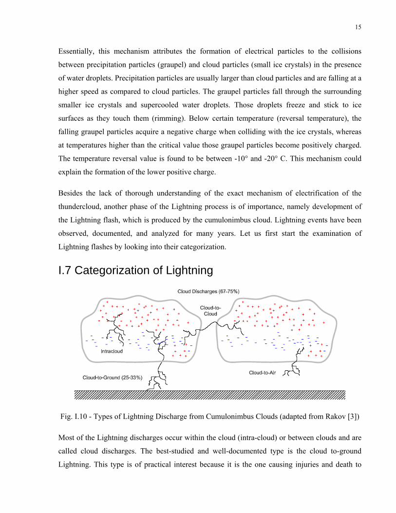
Fig. I.10 - Types of Lightning Discharge from Cumulonimbus Clouds (adapted from Rakov [3])

Most of the Lightning discharges occur within the cloud (intra-cloud) or between clouds and are

called cloud discharges. The best-studied and well-documented type is the cloud to-ground

Lightning. This type is of practical interest because it is the one causing injuries and death to

16

people and livestock, forest fires, and also destruction and disturbances in power grids and

installations and electrical and electronic equipment. In addition, there are very rare discharges

from cloud to air. Fig. I.10 depicts the associated percentage of Lightning type occurrence.

According to Berger [20] there are four types of Lightning between the cloud and earth in terms

of direction of motion (upward or downward) and positive or negative charge sign of the leader

that initiates the Lightning stroke. Those four types are presented in Fig. I.11 below.

Fig. I.11 - Categorization of Cloud-to-Ground Lightning (adapted from [2], Fig. 1.3)

I.7.a) Category 1 Lightning accounts for about 90 percent of all cloud-to-ground Lightning. It is

initiated by downwards moving negative leader and causes transfer of negative cloud charge to

the Earth.

I.7.b) Category 2 Lightning is due to positively charged moving upwards leader and causes

neutralizing of negative cloud charge.

I.7.c) Category 3 Lightning is initiated by a moving downwards but positive leader. This time the

charge being neutralized is positive. This accounts for less than 10 percent of cloud-to-ground

Lightning.

17

I.7.d) Category 4 Lightning is due to negatively charged moving upwards leader and transfers

positive cloud charge to the Earth.

Categories 2 and 4 are very rare events and are generally initiated by very tall and sharp objects

such as mountain tops or tall towers. Category 2 will be given special attention later in the thesis.

Category 4 Lightning flashes are extremely rare and usually neutralize a very large amount of

charge in one stroke only which has extremely high associated current.

I.7.1 Negative Cloud-to-Ground Lightning This is the most common type of Lightning discharge from cloud to ground and thus will be

reviewed in some more detail below. Lightning of this type is striking short or flat objects and a

photograph of such an event is seen in Fig. I.12. It is very typical for negative flashes to ground

to exhibit downward branching, clearly visible in the figure below. In some cases more than one

branch is contacting the ground at the same time (also visible in the blow-out in Fig. I.12).

Fig. I.12 - A Photograph of a Negative Cloud-to-Ground Lightning Flash

18

The processes involved in cloud-to-ground Lightning are explained using the idealized Lightning

flash time development diagram adapted from Uman [2] and shown in Fig. I.13.

The whole process is started by the stepped leader, which initiates the first stroke of a flash by

jumping in a series of discrete steps from cloud to ground. The stepped leader is initiated by a

preliminary breakdown within the cloud. This breakdown process is believed to take place in the

lower regions between the smaller positive charge and the negative charge. It preconditions the

area for the stepped leader to take place. The stepped leader steps are usually some tens of meters

long and their duration is in the order of 1µs. Stops between individual steps are in the order of

50µs and the average speed of stepped leader propagation is around 2e5m/s.

Fig. I.13 - Processes Involved in the Development of Negative Cloud-to-Ground Lightning Flash

(adapted from [2], Fig. 1.5)

19

The average stepped leader current is estimated to be in the range 100-1000A. The associated

radiated Electric and Magnetic Fields have duration of about 1µs and risetimes 0.1µs or less.

The electric potential at the bottom of the negatively charged stepped leader channel with respect

to the potential of ground is in the order of more than 107V. This high potential difference drives

the local Electric Field at ground level and near the grounded objects to rise in excess of the air

breakdown value. Consequently, one or even several upward moving discharges are created and

the attachment process begins. As soon as one of these upwards extending branches contacts the

downward moving stepped leader, at some tens of meters above ground, the final jump occurs

and the leader is effectively connected to ground. This initiates the flow of the first Return Stroke

current, which propagates upwards in the Lightning Channel path already ionized by the stepped

leader and reaches the top of the Lightning Channel in about 100µs.

A Lightning flash could contain just one stroke or several (up to 20) strokes. If the charge

lowered to ground in the first stroke depleted the available cloud charge, there might not be any

further subsequent strokes. On the other hand, if there was still additional charge available in the

cloud after the first-stroke took place, and this charge was conveniently located close to the top

of the already ionized Lightning Channel path, a dart leader might be formed that would

propagate down the residual channel without branching and initiate a subsequent stroke. The

additional charge brought to the Lightning Channel and responsible for subsequent strokes is

believed to be driven by K and J processes. The charge and current associated with dart leaders

are in the order of 1C and 1kA respectively and the duration of the Electric Field changes is

usually about 1ms. These changes are similar to first Return Stroke changes, but exhibit faster

risetimes and lower overall values.

The time between subsequent strokes belonging to a flash is several ms. This interstroke interval

is sometimes up to tenths of a second provided a continuing current is flowing after the stroke in

the channel. Such current is associated with direct charge transfer from cloud to ground and

linear Electric Field change for about 0.1s.

I.7.2 Positive Cloud-to-Ground Lightning Positive cloud-to-ground Lightning is a relatively rare event and is observed to increase in

occurrence towards the end (mature stage) of thunderstorms. This type of Lightning is believed

20

to be produced by the upper positively charged region of the cumulonimbus and occurs

whenever the negatively charged region is depleted, thus providing less shielding for the positive

charge to connect to ground. Since the positive charge is sitting at higher altitude, the associated

voltage potential and charge lowered to ground are substantially higher as compared to a regular

negative cloud-to-ground Lightning flash. The associated positive flash current may be in the

range of 200-300kA. Positive flashes usually consist of a single stroke, followed by a continuing

current. Another observation regarding positive flashes is that they predominantly occur during

winter thunderstorms and are relatively uncommon during summer thunderstorms. Positive

flashes are frequently observed and reported during winter storms in Japan. The structure of the

thunderclouds in these Japanese winter storms is somewhat different in terms of vertical

arrangement of the large positive and negative charges. Essentially, the upper positive charge is

not directly on top of the negative charge, and thus often has a clear view towards ground (see

Fig. I.5). In addition, the distance to ground is not as large and this makes it even easier for the

positive charge to find its way to ground. More relevant information could be also found in [2-4].

I.7.3 Tall Structures Initiated and Rocket Triggered Lightning It is assumed that grounded objects that are rising above 500m above ground level experience

only upward flashes, objects of 100-500m height experience both downward an upward flashes

and structures of less than 100m height experience only downward Lightning [2].

The tall structure initiated and rocket triggered Lightning are predominantly of the upward

initiated type (see Category 2 and Category 4 in Fig. I.11). The Return Stroke current neutralizes

most often negative cloud charge through several strokes. Those strokes usually resemble

subsequent strokes to flat ground since they feature fast risetimes and peak currents in the order

of only tens of kA. It is not uncommon to observe bipolar discharges occasionally and

sometimes, very rarely, only positive charge may be transferred to ground.

Lightning to tall structures is one very interesting area of research involving Category 2 and

Category 4 Lightning events (see Fig. I.11). It is a relatively new field of study, since very tall

towers started to become necessary for broadcasting of radio and TV programming some tens of

years ago. Tall structures are usually frequently struck by Lightning and can be instrumented to

directly measure Lightning current. Lightning researchers realized the convenience of such tall

objects for performing Lightning studies and started taking advantage of the situation. A few

21

telecommunication towers around the world have been equipped permanently, others temporarily

with current measuring equipment and were used to perform different studies throughout the

years. For example, a Rogowski coil was mounted on the CN Tower in Toronto soon after its

completion back in the 70’s. Currently, there are two permanently mounted Rogowski coils on

the CN Tower and Lightning current derivative is routinely captured at that site some 50-70

times per year. Very soon, after performing the very first measurements, it was noticed that

Lightning at tall structures is somewhat different from Lightning to flat ground and this is due to

the propagation processes that take place inside the structure. Tall towers have considerable

influence (enhancement) upon the recorded Lightning current and consequently upon the

radiated Electric and Magnetic Fields. Some relevant information is introduced in [21-27].

Furthermore, some of the most comprehensive and thorough studies performed by researchers at

tall towers could be reviewed in [28-40]. Essentially these studies show that Lightning current

waveforms are affected by transient processes that take place along the tall structure. Currents

measured close to the top of such structures are less influenced as opposed to those measured

close to ground level. The current amplitudes at the bottom are significantly affected and may be

much larger than the corresponding ones at the top.

Tall structures are often struck by Lightning and this is mostly because of the involved

mechanism of discharge initiation. This mechanism is quite similar to the analogous one

involved when “classical” rocket initiated Lightning is considered (described further down).

Essentially, at the tip of the tall structure the Electric Field is intensified and positive charges

may form a positively charged leader or leaders that in turn may propagate upwards some tens to

hundreds of meters. From the other end, there might be just enough negative charge, attracting

even further the developing positive leaders. That charge could be easily neutralized under the

existing favorable conditions (short distance to the grounded object and presence of upwards

propagating positive leaders). In case one of the positive leaders found its way up to the

negatively charged region of the cloud, a continuous current would start flowing and neutralizing

some of the available charge. At this time, if more charge were available a number of flashes

could take place.

The first successful tests with rocket-triggered Lightning were implemented back in 1960.

Rockets trailing thin, grounded wires were launched from a research vessel off the west coast of

22

Florida [41]. Triggered Lightning experiments and results have been considered and summarized

in [42] and [2].

Rocket triggered Lightning discharges are initiated in a very similar way to the tall objects

Lightning discharges, e.g. grounded telecommunication towers or antennas initiated discharges.

The difference between them is mainly in the fact that whenever a tall structure is considered

there is an associated static structure, which may contain reinforced concrete and metallic down-

conductors comprising the Lightning protection of the structure, whereas the rocket triggered

Lightning makes use of a grounded wire that propagates upwards at a certain speed.

Basically in a successful triggered Lightning experiment several processes take place one after

another, which are described briefly here. First, a rocket trailing a grounded wire is launched

toward a charged cloud. Then, the rocket ascending at a certain speed may trigger a positively

charged leader. That leader consequently vaporizes the wire and continues on its own to bridge

the gap between the ground and the cloud. Upon reaching the cloud charge, the leader may

become quite well branched upwards. A continuous current starts flowing in the preconditioned

channels and effectively neutralizes some negative cloud charge. After that several sequences of

dart leader Return Strokes may take place along the same discharge paths.

There is another way of triggering Lightning by launched rockets, called altitude triggering. In

this technique the metallic wire is not grounded and a bi-directional leader process is involved.

More details could be reviewed in [43] and [44].

23

Chapter II Development of Expressions for Current Distribution at any Level

along the CN Tower and the Lightning Channel

II.1 Outline In Chapter II the reader will find information pertinent to modern models used to describe

Lightning events. The existing four major classes of models are reviewed and the most used

“Engineering” models discussed in more detail.

An original contribution shown here is the different treatment of the extension of the

“Engineering” transmission based model that includes the presence of a tall structure in the

Lightning Channel path.

The CN Tower was chosen to be modeled as the struck tall object, because there are data records

including directly measured current, vertical component of the Electric and azimuthal component

of the Magnetic Field, as well as video records, and Lightning Channel front speed records that

have been accumulated by former and current researchers for more than 30 years. These data are

very useful for verifying the simulated currents and fields by various proposed modeling

approaches.

In the chapter, there are a few newly proposed solutions to some of the existing difficulties and

inconsistencies associated with modified transmission line based models. In addition to the

thorough description of the proposed modeling approach using a Single-Section Model of the

CN Tower, full details are also found in Appendix I. Appendices II and III contain all relevant

information for the Three- and Five-Section Model representation of the CN Tower respectively.

II.2 Modeling of Lightning (to Flat Ground and to Tall Objects) Four major classes of Lightning Return Stroke models are summarized and discussed in great

detail in [45]. In actual fact, most of the published readily available models could be classified

under one or in certain cases maybe two of these classes. They are briefly introduced below.

24

II.2.1 Gas Dynamic (Physical) Models These are looking into the radial evolution of a short segment of the Lightning Channel and its

associated shock wave and involve solving of three hydrodynamic equations describing

conservation of mass, momentum, and energy. These equations are coupled to two equations of

state. A known channel current as a function of time is used as an input parameter and the

outputs of such described model are the pressure, mass density, and temperature as functions of

radial coordinate and time (e.g. [46], [47], and [48]).

Such models were used to describe laboratory spark discharge in air (e.g. [46-48]), but

speculated to be applicable to Lightning Return Stroke modeling as well. According to some

recent works (e.g. [49-57]) the physical modeling approach assumes that the plasma column is

straight and cylindrically symmetrical, the algebraic sum of positive and negative charges in any

volume element is “zero”, and local thermodynamic equilibrium exists at all times.

II.2.2 Electromagnetic Models These models are usually based on a lossy, thin-wire antenna approximation of the Lightning

Channel. They involve a numerical solution of Maxwell’s equations to find the current

distribution at any point along the channel. Such current is then plugged in known relations for

different components of Electric and Magnetic Fields to evaluate them at a certain distance away

(e.g. [58-61]).

II.2.3 Distributed-circuit Models This class of models can be considered as an approximation of the Electromagnetic models.

Here, the Lightning discharge is assumed to represent a transient process on a vertical

transmission line of specific resistance, inductance, and capacitance. The distributed-circuit

models (sometimes referred to as R-L-C TL models) are used to determine the channel current as

a function of time and height and can also be used for evaluation of Electric and Magnetic Fields

at a distance (e.g. [62] and [63]).

II.2.4 “Engineering” Models

25

The distribution of the channel current (at any given point and time along the channel) is

deduced from observed Lightning Return Stroke characteristics such as the current at the channel

base, the speed of the upward-propagating Lightning Channel front, and the channel luminosity

profile. These models have just a few extra parameters that need to be adjusted and predict

reasonably well the electromagnetic field profiles computed at a distance (e.g. [64-65], and [45]).

In this thesis work three sophisticated “Engineering” models, representing the CN Tower and the

associated Lightning Channel by variable number of transmission lines, are developed and

thoroughly analyzed. The decision to use “Engineering” models was made primarily due to the

fact that there are readily available data regarding the channel-base current, the Return Stroke

velocity, radiated Electric and Magnetic Fields at a certain distance, and visual records pertinent

to the CN Tower Lightning events. In order to refresh the reader’s knowledge and also to look at

the details pertaining to the adopted modeling approach, a brief review of the different most

commonly used “Engineering” models follows.

II.3 Most Used “Engineering” Models An “Engineering” model could be defined by an equation that relates the current along the

Lightning Channel at any height ' and any time t to the current at the Lightning

Channel base [45]. The “Engineering” model could be also defined in terms of line

charge density

),'( tzI z

'( =z )0

( )tzL ,'ρ along the channel using the continuity equation [66]. Some of the

“Engineering” models could be summarized and described mathematically by the following

expression [67]:

( ) ( ) ( ) ( vztIzPvztutzI f ',0'',' −−= ) (II.1)

where:

u Heaviside function equal to unity for fvzt '≥ , and zero for fvzt '<

( )'zP height dependent current attenuation factor [68]

fv upward propagating Return Stroke speed

26

v current wave propagating speed

Values for and for five “Engineering” models are summarized in Table II.1 below. ( )'zP v

Table II.1 ( )'zP and in Eq. (II.1) for Five “Engineering” Models (Adapted from [67]) v

Model ( )'zP v Transmission Line Model (TL)

[69] 1 fv

Modified TL Model with Linear Current Decay with Height

(MTLL) [70] Hz'1− fv

Modified TL Model with Exponential Current Decay with

Height (MTLE) [71] ⎟⎟⎠

⎞⎜⎜⎝

⎛ −ψ

'z

e fv

Bruce-Golde Model (BG) [72] 1 ∞

Traveling Current Source Model (TCS) [73] 1 c−

In Table II.1:

H total channel height

ψ current decay constant (assumed to be 2000 m [71])

c speed of light

In the above shown models is usually assumed to be a constant value. fv

The most used “Engineering” models could also be divided into two groups namely the TL

(transmission line) based models and the TCS (traveling current source) based models. They are

summarized in Table II.2 and in Table II.3 below [45].

The degree of reproduction of Lightning electromagnetic field waveforms by “Engineering”

models is analyzed in [74].

27

Table II.2 TL based Models (Adapted from [45])

Model ( ) ( tztzI L ,',' )ρ ( ) ( )vztItzI ',0' −=

TL [69] ( ) ( )⎟⎠⎞

⎜⎝⎛ −

=v

vztItzL',0,'ρ

( ) ( ) ( )vztIHztzI ',0'1' −−= MTLL [70] ( ) ( ) ( ) ( )

HtzQ

vvztIHztzL

,'',0'1,' +⎟⎠⎞

⎜⎝⎛ −

−=ρ

( ) ( )vztIetzIz

',0''

−=−ψ

MTLE [71] ( ) ( ) ( )tzQe

vvztIetz

zz

L ,'',0,'

''

ψρ

ψψ

−−

+⎟⎠⎞

⎜⎝⎛ −

=

( ) ( )∫ −=t

vz

dvzItzQ'

',0' ττ ; constvv f == ; constH = ; const=ψ .

“Engineering” models have been validated by different authors primarily using two common

approaches. One way to do that is by considering a typical channel base current and propagation

speed as inputs to the chosen model, and then comparing the output of the model, namely the

computed Electric and Magnetic Fields, to typically observed ones. The other approach is

applicable whenever recorded information regarding the channel base current, propagation

speed, and recorded radiated fields are readily available. Such records exist for rocket-triggered

Lightning and at instrumented tall towers. Using those captured data, one could reproduce the

“uncontaminated” current waveform and based on that compute the respective radiated field

components. The computed fields could be then compared to the actual ones in order to validate

the modeling approach. Since the question of what exactly happens at the physical origin of

Lightning (at the end of the Lightning Channel in the cloud where the charge is located) is

usually not treated, the “Engineering” models yield satisfactory results that could be trusted to

some extent in the first tens of µs (up to usually 50µs). After that time, depending on the used

propagation speed, reflections within the Lightning Channel and possibly other influences from

the cloud charge may come into play and eventually impose additional changes in the model.

28

Table II.3 TCS based Models (Adapted from [45])

Model ( ) ( tztzI L ,',' )ρ ( ) ( tItzI ,0' )=

BG [72] ( ) ( )⎟⎟⎠

⎞⎜⎜⎝

⎛=

f

fL v

vzItz

',0,'ρ

( ) ( )cztItzI ',0' += TCS [73] ( ) ( ) ( )

*

*',0',0,'v

vzIc

cztItzL +⎟⎠⎞

⎜⎝⎛ +−=ρ

( ) ( ) ( ) Dfv

zt

evzIcztItzIτ⎟

⎟⎠

⎞⎜⎜⎝

⎛−−

−+='

*',0',0'

Diendorfer and Uman (DU) [75]

( ) ( ) ( )

( )

( ) ( )dt

vzdIvv

vzI

edt

vzdIv

vvzI

ccztItz

D

vzt

D

fL

Df

*

**

*

'*

*

*

',0',0

',0

',0',0,'

τ

τ

ρ

τ

++

+⎥⎦

⎤+

+⎢⎢⎣

⎡−

+−=

⎟⎟⎠

⎞⎜⎜⎝

⎛−−

( )cvvv ff += 1* ; ; constv f = constD =τ

The presence of a high tower in the Lightning Channel path has been found to exert a major

influence upon the Lightning Return Stroke current as well as upon the emanated Electric and

Magnetic Fields. The respective current and field waveforms recorded at tall towers are

substantially different in terms of peak and overall values as compared to the corresponding ones

in the case whenever the tall structure were not present. An elaborate study looking into

Lightning at tall structures in which two “Engineering” models were extended in order to take

into consideration the presence of a tall tower in the path of the Lightning Channel could be

found in [76]. The reader may also wish to check the more recent reference [77].

All “Engineering” models that consider extended object as a part of the Lightning Channel

feature a discontinuity at the Return Stroke front. This discontinuity stems from the fact that

propagation along the tall object is considered to take place at the speed of light and propagation

along the rest of the Lightning path (within the Lightning Channel) occurs at a different speed.

That velocity is usually more than twice less than the speed of light. Basically a current wave is

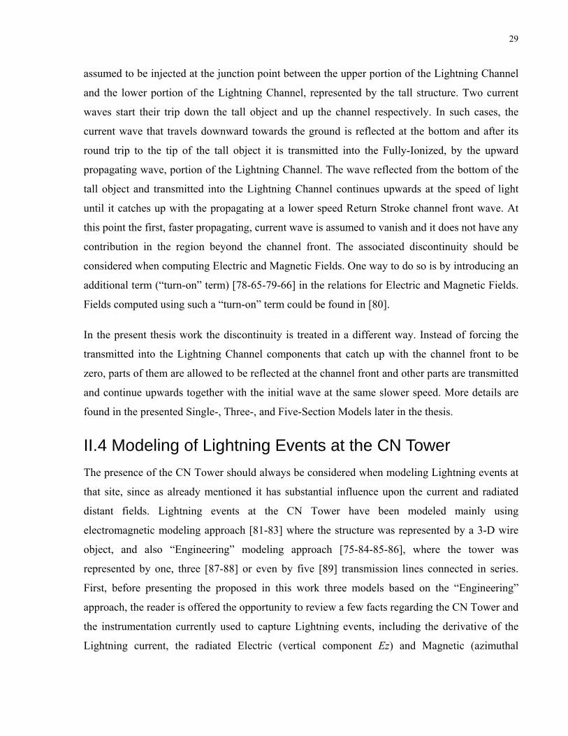
29

assumed to be injected at the junction point between the upper portion of the Lightning Channel

and the lower portion of the Lightning Channel, represented by the tall structure. Two current

waves start their trip down the tall object and up the channel respectively. In such cases, the

current wave that travels downward towards the ground is reflected at the bottom and after its

round trip to the tip of the tall object it is transmitted into the Fully-Ionized, by the upward

propagating wave, portion of the Lightning Channel. The wave reflected from the bottom of the

tall object and transmitted into the Lightning Channel continues upwards at the speed of light

until it catches up with the propagating at a lower speed Return Stroke channel front wave. At

this point the first, faster propagating, current wave is assumed to vanish and it does not have any

contribution in the region beyond the channel front. The associated discontinuity should be

considered when computing Electric and Magnetic Fields. One way to do so is by introducing an

additional term (“turn-on” term) [78-65-79-66] in the relations for Electric and Magnetic Fields.

Fields computed using such a “turn-on” term could be found in [80].

In the present thesis work the discontinuity is treated in a different way. Instead of forcing the

transmitted into the Lightning Channel components that catch up with the channel front to be

zero, parts of them are allowed to be reflected at the channel front and other parts are transmitted

and continue upwards together with the initial wave at the same slower speed. More details are

found in the presented Single-, Three-, and Five-Section Models later in the thesis.

II.4 Modeling of Lightning Events at the CN Tower The presence of the CN Tower should always be considered when modeling Lightning events at

that site, since as already mentioned it has substantial influence upon the current and radiated

distant fields. Lightning events at the CN Tower have been modeled mainly using

electromagnetic modeling approach [81-83] where the structure was represented by a 3-D wire

object, and also “Engineering” modeling approach [75-84-85-86], where the tower was

represented by one, three [87-88] or even by five [89] transmission lines connected in series.

First, before presenting the proposed in this work three models based on the “Engineering”

approach, the reader is offered the opportunity to review a few facts regarding the CN Tower and

the instrumentation currently used to capture Lightning events, including the derivative of the

Lightning current, the radiated Electric (vertical component Ez) and Magnetic (azimuthal

30

component Hφ ) fields at 2km away from the CN Tower, and visual records of the respective

Lightning events.

II.4.1 The CN Tower

Fig. II.1 - The CN Tower in Toronto

Lightning has been observed and recorded for more than 30 years at the CN Tower in Toronto.

Currently, this tower is one of the few permanently instrumented tall structures worldwide. Many

31

papers regarding the specifics of the site and observed Lightning parameters are readily available

(e.g. [90-94]).

The CN Tower in Toronto was completed in June 1976 after 40 months of construction. It is

rising 553.33m (1,815ft) and has held the title “World’s tallest free-standing building” for more

than 30 years. It is still the world’s tallest free-standing structure instrumented for Lightning

Research.

II.4.1.1 A Few Facts Although the Lightning flash density for the Toronto region is only about 2fl/year/km2, Lightning

strikes the CN Tower some 50 to 70 times per year. While visible copper Lightning protection

strips run inside the CN Tower, due to skin effect, the bulk of the Lightning current is conducted

down the tower, as designed, by the bonded concrete reinforcing steel. Both feed into the

massive grounding rods below ground level and thus ensure that each Lightning strike safely

finds its way to ground [95].

In accordance with information provided by the CN Tower publicity, the top of the CN Tower is

625.09m (2,050ft, 10in) above sea level. The Glass Floor is 113 stories high, which is 342m

(1,122ft) above ground level, the Skypod – 114 stories – 346m (1,136ft) above ground level, and

the Space Deck – 147 stories or 447m (1,465ft) above ground level. At the Skypod Level the

circumference is 109.1m (358ft), and at the base of the CN Tower the circumference is 208.7m

(684.52ft) and the radius is 33.2m (109.2ft). Total weight of the CN Tower is 117,910 metric

tonnes (130,000 tons).

II.4.1.2 Instrumentation at the CN Tower As shown in Fig. II.2, there are two permanently installed current sensing elements on the

structure at 474m and at 509m above ground level. Both elements are Rogowski coils and are

used to capture directly the derivative of the Lightning current. The captured raw data are relayed

via coaxial (lower coil) and fiber-optic (higher coil) cables to a digitizer where they are stored

onto a PC. Later on the raw data are initially treated using LabView and finally processed using a

specially developed integration routine in Matlab to produce the actual Lightning current

waveform as it is captured at the respective level.

32

Fig. II.2 - CN Tower and Instrumentation Locations

A similar routine for processing and a set-up for capturing raw data corresponding to the vertical

Electric Field (Ez) and the azimuthal component of the Magnetic Field (Hφ ) radiated during

Lightning events at the CN Tower are used at the University of Toronto (2km north of the CN

Tower). The sensing elements in this case are broadband active field sensors. Both set-ups (at the

CN Tower and at the University of Toronto) have GPS time stamping and the recorded current

strokes and respective Electric and Magnetic Fields belonging to a certain Lightning flash event

can be well correlated. Furthermore, two DVD recorders (16ms time resolution) and a High

Speed Digital Camera (2ms resolution) are used to capture the Lightning flash trajectory. The

High Speed Camera and one of the DVD recorders are operated at the University of Toronto,

while the second DVD recorder is mounted at Kinectrics (11km to the West of the CN Tower)

The High Speed Camera records bear computer clock time-stamps and the second DVD

recording set has been recently augmented with a time-inserter that is set regularly. The main

purpose of the video recording is to confirm that captured current and fields belong to a

33

Lightning flash landing on the CN Tower. The secondary purpose (accomplished mainly using

the High Speed Camera which has higher time resolution) is to help in establishing the Lightning

flash multiplicity (number of strokes in a flash). Since the two DVD recorders are now recording

the Lightning flash activity at the CN Tower from two directions that are almost perpendicular

with respect to each other, a third application is currently being investigated and this is namely

the opportunity to reproduce the 3-D trajectory of each Lightning stroke. This would be useful in

studies related to the influence of the Lightning Channel inclination and tortuosity upon the

recorded currents, fields and field-current relationships. In many cases there is a difference in the

number of recorded strokes by different equipment due to the particular device and set-up

characteristics [96].

Fig. II.3 - Raw Data and Processed Current Waveshape Captured at 474m Above Ground Level

Plots of the current derivative of the third stroke of a Lightning event captured at the 474m above

ground level and of the respective processed current waveform are shown in Fig. II.3.

The corresponding radiated Ez and Hφ for the same event form August 19, 2005 are shown in

Fig. II.4. Fig. II.5 depicts its Lightning flash trajectory and the respective High Speed Camera

record is presented in Fig. II.6.

34

Fig. II.4 - Recorded Ez and Hφ Waves

Fig. II.5 - Video Frame of the August 19, 2005 event (14:11:41)

35

Fig. II.6 - High Speed Camera Frame of the August 19, 2005 event (14:11:41)

II.4.2 Three Sophisticated “Engineering” Models Bermudez et al. [97] showed that transmission line modeling approach is quite adequate and

useful to model Lightning events at tall structures. In their experiment two scaled down models

of the CN Tower were used, the first one representing the structure by one transmission line

section only, and the second one - by three transmission line sections. It was observed that the

three section model yielded better results, since it represented the structure in greater detail. Fig.

II.7 shows the experimental setup and the three section model used. The equivalent circuit

diagram is seen in Fig. II.8, and the obtained results by the three section model in Fig. II.9.

Injected narrow pulse signals were used in the experiment. The presented plot in Fig. II.9 was

achieved using injected voltage pulse of 2ns width. Figs. II.7 to II.9 are adapted from [97].

36

Fig. II.7 - Experimental Set-Up

Fig. II.8 - Reduced Scale Model - Equivalent Circuit Diagram

37

-10 0 10 20 30 40 50 60-2

-1

0

1

2

3

4

Time [ns]

lt

[

VoageV]

Vol

tage

[V] Calculated

Measured

Time [ns]

Fig. II.9 - Compared Experimental to Calculated Results

Practically, the experiment validated the transmission line representation of an elevated strike

object that is struck by Lightning. This is part of the motivation behind developing of the Five-

Section Model presented in this thesis.

Connecting in series a number of transmission line sections representing a tall structure, such as

the CN Tower, is a convenient means to capture and reproduce in detail the tower’s structural

peculiarities. In previous studies, readily available in the Technical literature [86-89] and [98],

Single- and Three-Section “Engineering” models based on the TL modeling approach [69] were

used. At the University of Toronto, as shown in [87] and in [89], different multi-section

representations of the CN Tower were considered. In particular, the Five-Section modeling

approach was developed and explored in detail for the first time in [89]. This thesis is

contributing to the technical literature the sophisticated transmission line based “Engineering”

Single-, Three-, and Five-Section Models of the CN Tower. Multiple sections are considered in

order to represent the structure in more detail. Full derivations and considerations regarding the

Single-, Three-, and Five-Section Models could be reviewed in Appendices I, II, and III

respectively. In the main body, only highlights and some final expressions are shown. The

Single-Section model is shown almost in full details in order to introduce the modeling approach.

The models include reflections coming from the upwards-propagating Lightning Channel front

and also transmitted components beyond the channel front. Another novel assumption introduced

38

in these models is that all contributions that are less than 1% in magnitude of the original

injected current wave (Return Stroke current) are neglected.

II.4.2.1 Single-Section Model Full details regarding the Single-Section Model, including expanding of newly introduced terms

σ and ξ are shown in Appendix I.

To visualize the processes of reflections and refractions at different levels of the CN Tower and

in the Lightning Channel, a Lattice diagram is useful. To illustrate the use of the Lattice

Diagram, in view of its reduced complexity, the case of the Single-Section representation will be

discussed in detail (see Fig. II.10). However, principles described are directly applicable to the

Three- and Five-Section modeling approaches.

Fig. II.10 - Single-Section Model1

1 Note, that the Lightning Channel is shown for the general case, when both Not-Fully Ionized (dashed line) and Fully Ionized (thick line) portions of the Lightning Channel exist, while in the instance of time when the Return Stroke current is initiated only the Not-Fully Ionized part of the Lightning Channel is present.

39

Following assumptions are considered for the Single-Section Model, most of which are also

valid in case of the Three- and Five-Section Models:

- The CN Tower is represented by one transmission line section of constant surge impedance,

which was calculated using Chisholm’s formula for cone representation of a transmission

line tower [99] (Zt = 110 Ω);

- The grounding system is considered to be a simple resistance (Zg = 30 Ω);

- Reflection Coefficients:

o kb = (Zt-Zg)/(Zt+Zg);

o kt = (Zt-Zch)/(Zt+Zch);

o kc = (Zch-Ztch)/(Zch+Ztch);

- The Lightning Channel is vertical and attached to the tip of the CN Tower;

- Lightning Channel length zMAX = 8km;

- Lightning Channel is split into two sections (Initially the Lightning Channel is represented

by a single transmission line of constant surge impedance (Ztch = 495Ω) to account for the

Not-Fully Ionized portion. As soon as a current wave starts its way up the Lightning

Channel, the Lightning Channel is already consisting of two sections and that part, up to

where the current wave has already progressed, becomes Fully Ionized, thus having a

different (reduced) surge impedance (Zch = 330Ω)). Used values are 4.5xZt and 3xZt

respectively;

- Speed of propagation in the Not-Fully Ionized portion of the Lightning Channel is constant

and is assumed to be v = 1.9e8m/s;

- Constant for the exponential decay of propagation within the Not-Fully Ionized portion of

the Lightning Channel is ψ = 2000m;

- Speed of propagation in the Fully Ionized portion of the Lightning Channel as well as in the

CN Tower is constant and is c = 3e8m/s (speed of light);

40

- It is assumed there is no decay in propagation within the Fully Ionized portion of the

Lightning Channel and in the CN Tower;

- Contributions due to reflections and refractions at different locations along the structure of

the tower and in the Lightning Channel are followed and considered until they become less

than 1% in amplitude of the original injected wave;

- A sum of two Heidler functions [100] is used to approximate the injected “uncontaminated”

Lightning current.

The “uncontaminated” Lightning current is injected at the attachment point between the CN

Tower and the Lightning Channel. Two current waves having identical waveshapes, but

amplitudes inversely proportional to the surge impedances of the CN Tower and the Not-Fully

Ionized portion of the Lightning Channel start their way down the tower and up the channel

respectively. The wave going down the tower is travelling at the speed of light c, while the one

propagating upwards in the Not-Fully Ionized part of the Lightning Channel is traveling at a

reduced speed v.

(II.4)

(II.6)

(II.5a)

(II.5b)

(II.3) (II.2)

Fig. II.11 - Lattice Diagram for the Single-Section Model

41

Let’s look at the Lattice diagram in Fig. II.11 and follow first the injected current wave that goes

down the CN Tower. It reaches the bottom of the tower where it “sees” a different impedance

and consequently here a reflection takes place. The reflected wave goes back to the tower top

and is here reflected back down the tower, while a part of it is refracted into the Lightning

Channel. The reflected portion reaches once again the bottom where it is once more reflected

towards the top of the structure (where it is split again into reflected and refracted parts).

The part originally refracted into the Lightning Channel continues up the Fully Ionized portion of

the channel at the speed of light and at some point catches up with the slower propagating

Lightning Channel front. At this point a portion of the originally refracted wave is reflected back

towards the CN Tower top while a part of it is transmitted beyond and continues to flow in the

Not-Fully ionized portion of the Lightning Channel together with the initially injected current

wave and at the same lower speed v. Same fate follows all other reflections not only from the

bottom of the tower but also those reflected back into the Lightning Channel at the discontinuity

between the ionized portion of the Lightning Channel and the tower top.

II.4.2.1.1 Current Distributions for Single-Section Model

II.4.2.1.1.1 Major Components (inside the CN Tower)

∑∞

= +

⎪⎪⎭

⎪⎪⎬

⎫

⎪⎪⎩

⎪⎪⎨

⎧

⎟⎠⎞

⎜⎝⎛ −

+−+

⎟⎠⎞

⎜⎝⎛ −

−−

=0

01

0

2

2

n nt

nb

nt

nb

M

cnh

czhtikk

cnh

czhtikk

i (II.2)

II.4.2.1.1.2 Additional Components: (inside the CN Tower)2

( ) ( )

( ) ( ) ⎟⎠⎞

⎜⎝⎛ ++−−+=

⎟⎠⎞

⎜⎝⎛ −+−−+=

czhhtikkkki

czhhtikkkki

tctbA

tctbA

ξ

ξ

211

211

02

2,

01,

(II.3)

2 There are further additional components that are neglected since their amplitudes are less than 1% of the initial injected current wave.

42

where:

vcvc

vcvhz

−+

=−

=≤≤ ξσ0

II.4.2.1.1.3 Channel Base Current (Initial Current Propagating

upwards in the Not-Fully Ionized portion of the Lightning Channel)

⎟⎟⎠

⎞⎜⎜⎝

⎛ −

⎟⎠⎞

⎜⎝⎛ −−= ψ

zh

cht

tch e

vhzti

zzi 0 (II.4)

where: MAXzzh ≤≤

II.4.2.1.1.4 Internal Components “bouncing” within the Ionized

Portion of the Lightning Channel

( ) ( ) ( )

( )⎟⎠⎞

⎜⎝⎛ −

−−

−+= ∑∞

=

−−

chz

cmhti

kkkkki

n

n

nt

nct

mt

mbmI

ξ2.

1

0

0

112,

(II.5a)

( ) ( ) ( )

( )( )⎟⎟⎠

⎞⎜⎜⎝

⎛ −+−

−−

−+= ∑∞

=

+−

czmh

vcmhti

kkkkki

nn

n

nt

nct

mt

mbmI

σξξ 212.

1

0

0

112,

(II.5b)

where:

( ) ,...3,2,121 =≤+<< mzmhzh MAXnσξ

II.4.2.1.1.5 Components Transmitted into the Not-Fully Ionized

Portion of the Lightning Channel

43

( ) ( ) ( )

( ) ⎟⎟⎠

⎞⎜⎜⎝

⎛ −

∞

=

−

⎟⎟⎠

⎞⎜⎜⎝

⎛ +−−

−−

+−+= ∑

ψσξξzhn

n

cn

tnct

n

mt

mbTm

ev

mhzvc

mhti

kkkkkki

212.

11

0

0

1

(II.6)

where:

( ) ,...3,2,121 =≤<+ mzzmh MAXnσξ

In order to find the current at any specified level of the tower or of the channel, corresponding

contributions indicated for that level by the Lattice Diagram are summed up.

II.4.2.2 Three-Section Model and Five-Section Model Following the same principles and considerations applicable to the Single-Section Model, any

multi-section model of the CN Tower could be implemented. The author has considered a Three-

Section (Fig. AII.1) and a Five-Section Model (Fig. AIII.1) of the CN Tower. Basically,

individual sections of the CN Tower constituting the Three-Section or the Five-Section Model,

and the Lightning Channel, are treated in the same way as indicated above for the case of the

Single-Section Model. Table AII.1 contains the values of the lengths of different sections, their

surge impedances, and respective reflection coefficients pertaining to the Three-Section Model

and Table AIII.1 the same quantities corresponding to the Five-Section Model.

Full details regarding the Three- and Five-Section Model current contributions are not

reproduced here, but the reader may find all of them in Appendices II and III.

It should be mentioned that one of the major salient features of the CN Tower, namely the

Skypod, is considered in the Three-Section Model. It has a great influence upon the current

distribution along the tower and the Lightning Channel respectively. Representing the structure

more closely helps in computing of a closer current waveform to the recorded one. In actual fact,

the newly introduced two additional locations of mismatched impedances influence the

simulated current waveshape at 474m above ground level (one of the heights where recording is

implemented) at early times in such a way to produce the otherwise missing peak in the Single-

Section Model calculations (please check Figs. AI.5 and AII.33). This peak is normally always

observed in the actual records, but it is not reproduced by the Single-Section Model at all.

44

Furthermore, the inclusion of even more structural details, such as the Space deck in the Five-

Section Model, in particular makes the model more realistically representing the actual tower.

This in turn helps in reproducing more accurate current waveform at the respective height of

interest. The most sophisticated model (Five-Section Model) used so far yields the best results

possible using the described modeling approach. The fine details that could be reproduced are

shown in Fig. AIII.83 in Appendix III.

A partial Lattice Diagram of the Five-Section Model is shown in Fig AIII.2, which is restricted

to 2.5µs. It is seen that the complexity of such a diagram is enormous even for such a short

timeframe. This was one of the reasons why it was decided to follow and use reflections only

until their amplitudes are higher than 1% of the original injected current.

Caution should be exercised when certain contributions to the current within the Lightning

Channel are described, since the point of reflection between the Not-Fully Ionized and Fully

Ionized portions of the Lightning Channel is not static. The propagation speed of the Return

Stroke channel front v is affecting times and locations of reflection points and thus the current

distributions in the Lightning Channel and consequently currents in the CN Tower as well.

The values of the impedances used in the Three- and Five-Section Model are chosen considering

previous publications [87], [89] and based on recorded currents. They are fine tuned in order to

achieve as close as possible predicted current waveforms at 474m or at 509m above ground level.

The process of estimation of the impedances of different sections involved computation of the

ratios between distinctive peaks found in the recorded current derivatives. These ratios are

corresponding to the reflection coefficients at the borders of mismatched impedances, and thus

are used to approximate the surge impedance of distinctive sections comprising the multi-section

representation of the CN Tower. Theoretical expressions currently exist for transmission line

towers that are considered as a single transmission line section only. Developing of relations for

a multi-section representation of a transmission line tower or any high-rise structure could be a

separate area of research.

The reader may have also noticed that the reflection coefficients at ground level as well as at the

top of the CN Tower are slightly different in the three considered models. It should be kept in

mind that these models are only approximations. However the reflection coefficient values used

in the Five-Section Model arguably may be considered to be the most accurate.

45

Chapter III Development of Expressions for Currents Pertinent to Variable

Speed of Propagation of the Lightning Channel Front

III.1 Outline Chapter III contains the second original contribution, which is modification of the proposed

relations from Chapter II to include the possibility for varying the Lightning Channel front

speed. Variable Lightning Channel front speed is treated and discussed for the first time and all

developed expressions for the considered increasing and decreasing cases using the Single-

Section Model are shown. The first and second “legs” of major reflections are discussed

thoroughly, and then based on the produced relations further ones corresponding to subsequent

“legs” are written down. Moreover, in order to somewhat reduce the computation burden, a

graphical solution approach is proposed. The graphical solution approach is then extended to

account for the more sophisticated representation of the CN Tower by the Three- and Five-

Section Models.

In the end of the chapter several special cases involving variable and constant Lightning Channel

speed are simulated and produced results showing currents at particular levels analyzed.

III.2 Variable Lightning Return Stroke Speed at Different

Height

In the previous Chapter II, three sophisticated models for describing Lightning events at the CN

Tower were introduced. In all of them, the speed of propagation of the Return Stroke current (or

Lightning Channel front) into the Not-Fully Ionized portion of the Lightning Channel was

assumed to be constant and less than the speed of light. It would be interesting to look into the

possibility of using a variable instead of constant speed of propagation, which in fact would be

more realistic and closer to the actually observed phenomenon.

It is commonly perceived that the speed of propagation of the Lightning Channel front somewhat

decreases with height, which could be approximated, for instance, by a parabolic function. While

confirming that fact, Chang et. al. [101] showed that, based on their measurements at the CN

46

Tower site, the speed of propagation of the Return Stroke channel is actually increasing with

height in some cases. This is clearly seen in Fig. III.1 below.

Based on the data recorded and presented in Fig.III.1, one could choose to approximate the

increase in speed with height by a linear function or by second, third, or any nth order function.

After coming up with the appropriate representation of the variation of speed with height, it

could be incorporated into the corresponding Lattice diagram.

The study presented below considers a general case of variable front propagation speed. While

the chosen approach may be utilized for both, the decreasing and increasing front speed, the case

of increasing speed is elaborated in detail. It is utilizing the “Engineering” transmission line

models from Chapter II and a linear approximation (performed using MatLab) of the increase in

speed with height. The propagation speed increases up to a specified value and remains constant

after that.

Fig. III.1 - Speed Variation of the Progressing Upwards Lightning Channel Front Recorded by

ALPS (Adapted from [101], figure 8 – July 14, 04 at 4:33:56h)

Linear increase in speed with height corresponds to a non-linear increase of height with time.

Such behavior is observed in Fig. III.2 up to a certain instance of time, after which point, the

reached speed is assumed to remain constant and thus further increase of height in time is linear.

47

The equation for speed as a function of height as a linear approximation could be represented by

the following relation:

bazdtdz

=+ , (III.1)

where:

vdtdz

= is the speed of the Return Stroke front;

z is the height;

ba, - constants that are later evaluated based on Fig. III.1:

Eq. III.1 is an ODE and is solved below:

( )( ) ∫∫ =

′=

′

=+

dtbedtze

beze

bezaedtdze

atat

atat

atatat

at

atat

atat

Ceabz

Ceabze

keabkze

−+=

+=

+=+ 1

Finally:

( ) atCeabtz −+= (III.2)

In particular, if one considered a specific case such as the one presented in Fig. III.1, a and

could be found directly from that Fig. III.1:

b

48

2000000066000

=−=

ba

The initial condition is: 553;0 == zt

( )03.856

03.3035530 0

=+−===

CCetz

Finally:

( ) tetz 6600003.85603.303 +−=

The last measured speed of propagation of the Lightning Channel is at z = 1303m above ground

level and using the approximation (III.1) one could calculate speed v = 105998000m/s.

The corresponding time turns out to be t = 9.53µs.

The Lattice diagram showing the first three major reflections coming from ground level and

trapped in the Lightning Channel may be found below in Fig. III.2. In the Diagram critical

instances of time are indicated, at which either the Lightning Channel front or the top of the CN

Tower are reached. These times are measured geometrically directly from the diagram.

Fig. III.2 - Partial Lattice Diagram for Increase in Lightning Channel Speed

49

For the Lightning Channel front propagation, relation (III.2) is used up to t = 9.53µs, and after

that time a linear relation (III.3) is utilized, which is developed as follows.

Linear approximation for constant speed v = 105998000m/s:

8391.29253.91059980001303

=→=+=

CstCt

µ

The linear approximation then becomes:

8391.292105998000 += tz (III.3)

The approach described for the increasing front speed and shown in Fig. III.2 may be used for

any speed variation, increasing, decreasing or even one described by a curve provided as a table

of heights versus times. In what will follow the case of the decreasing front speed variation will

be considered. A parabolic change of channel height with time will be adopted. z t

III.3 Cases Involving Parabolic Decrease in Lightning

Channel Propagation Speed

In order to pursue the case of a front speed decreasing with time, a parabolic relation is used to

approximate the decrease in speed of the Return Stroke with increasing height up to the

previously discussed time (t = 9.53µs) where the speed is becoming constant and consequently

described by a linear function (shown later).

( ) qhzdt −+= 2 (III.4)

III.3.1 Relations Pertaining to First Major Reflection from Ground Derivations of heights and times associated with first major reflection from bottom of CN Tower

that penetrates into the Fully-Ionized portion of Lightning Channel are discussed below. The

corresponding detailed Lattice diagram is depicted in Fig. III.3.

The geometrical location of the initial point (where the “uncontaminated” current is injected) is

once again:

50

0, == thz (III.5)

If the initial conditions (III.5) are substituted into (III.4) it follows that:

( ) qhd −= 240 (III.6)

In order to produce a more realistic case, let us assume that 124 −= ed

tq +

z

Fig. III.3 - Detailed Lat

Then based on the cho

value q . 6−

ttzz ==

8929.4= e

Let us now examine the

the tower and in the Full

and since at ,11,

hz =1

dhz +−=

hct −=

tice Diagram for Parabolic Decrease in Lightning Channel Speed (First

Major Reflection from Ground)

sen value of , using (III.6) one can compute the corresponding d

resulting plot shown in Fig. III.3. Since it is assumed that propagation in

y Ionized portion of the Lightning Channel occurs at the speed of light

one could easily find out that at

(III.7)

51

cht 2

1 = (III.8)

Since the equation describing the first reflection from ground is

hctz −= (III.9)

its intersection with the parabola of equation (III.4) (trajectory of the Return Stroke front) occurs

at

( )cd

dqccdhz

24121 2

2++−

= (III.10)

where:

dcdqc

t 2

2

2 2411 ++

= (III.11)

Please, note that at this point ( ) the current contribution reflected at the bottom of the

tower and transmitted into the Fully Ionized portion of the Lightning Channel has caught up with

the Lightning Channel front and a Transmitted component is produced that continues

upwards the channel together with the initial injected current at the same slower speed. There

is a corresponding reflection i as well, and it starts its way down the Fully Ionized portion of

the Lightning Channel at the speed of light until it reaches the top of the tower at time t

22 , tz 1,ii

1,Ti

i

t

ch

2,i

3= and

the corresponding height is once again hz =3 . At this point another set of two current waves is

also produced. The transmitted one starts its way inside and down the tower and the reflected

one goes back into the Fully Ionized portion of the Lightning Channel heading upwards

toward the Lightning Channel front. It is found out that:

1,Ai

i 3,i

hz =3 (III.12)

czt 2

32

= (III.13)

52

The next point of interest is at time 4tt = when the internal component catches up with

and i . At this time another internal component i is produced and starts its way down towards

the top of the tower at the speed of light. A transmitted component i is also produced and

continues upwards at the slower speed of propagation of the existing components i and .

Later on the same process is repeated at different times and heights. This could be written down

in the following way:

3,ii chi

1,T 4,i

2,T

ch 1,Ti

44 , ttzz == (III.14)

Solving for and for yields: 4z 4t

( ) ( ) ( )cd

dqcdqccdhcdhz

24144141421 22

4

++++−+−= (III.15)

( ) ( )dc

dqcdqccdhdqccdht 2

222

4 24144141441283 ++++−+++−

= (III.16)

At 55 , ttzz ==

hz =5

Based on the geometrical relations seen in Fig. III.3 one could write down that:

chztt −

+= 445 (III.17)

66 , ttzz == (III.18)

Also, for convenience let

( )dqcE 241+= (III.19)

( cdhF 41−= ) (III.20)

Then it could be shown that:

53

( )cd

EEFEFEcdhz2

444484216

++++++−= (III.21)

( )dc

EEFEFEEEFEcdht 26 2

444484422165 ++++++++++−= (III.22)

Now the components that contribute to the description of the current at any level and at any time

by the Single-Section Model could be written down.

III.3.1.1 Channel-Base Current (Initial Current Propagating

upwards in the Not-Fully Ionized Portion of the Lightning Channel)

⎟⎟⎠

⎞⎜⎜⎝

⎛ −

⎟⎠⎞

⎜⎝⎛ −−= ψ

zh

tch

tch e

vhzti

zzi 0 (III.23)

The speed of propagation of the Lightning Channel front is found to be (derivative dtdz ):

tqdv

+=

21 (III.24)

so now:

( )( )( ) ⎟⎟⎠

⎞⎜⎜⎝

⎛ −

+−−= ψzh

tch

tch etqdhzti

zzi 20 (III.25)

for MAXzzh ≤≤

III.3.1.2 Internal Components (Trapped in the Fully-Ionized

Portion of the Lightning Channel)

( ) ⎟⎠⎞

⎜⎝⎛ −

−−+=c

hzttikki tbI 101, 1 (III.26)

54

( ) ⎟⎠⎞

⎜⎝⎛ −

−−+=c

zzttikkki ctbI2

202, 1 (III.27)

( ) ( ) ⎟⎠⎞

⎜⎝⎛ −

−−−+=c

hzttikkkki tctbI 303, 1 (III.28)

( ) ( ) ⎟⎠⎞

⎜⎝⎛ −

−−−+=c

zzttikkkki tctbI4

402

4, 1 (III.29)

One can also write down the general relations:

( ) ( ) ( ) ( ) ⎟⎠⎞

⎜⎝⎛ −

−−−+= −−−

− chzttikkkki n

nt

nctbnI 120

1112, 1 (III.30)

( ) ( ) ( ) ⎟⎠⎞

⎜⎝⎛ −

−−−+= −

czzttikkkki n

nn

tnctbnI

220

12, 1 (III.31)

for and , and ,...3,2,1=n ( )nzzh 2≤≤ ( ) ( 1412 −− )≤≤ nn ttt

III.3.1.3 Additional Components

( ) ( ) ⎟⎠⎞

⎜⎝⎛ −

−−−+=c

zhttikkkki tctbA 301, 11 (III.32)

( ) ( ) ⎟⎠⎞

⎜⎝⎛ +

−−−+=c

zhttikkkki tctbA 302

2, 11 (III.33)

( ) ( ) ⎟⎠⎞

⎜⎝⎛ −

−−−−+=c

zhchttikkkkki ttctbA

211 302

3, (III.34)

( ) ( ) ⎟⎠⎞

⎜⎝⎛ +

−−−−+=c

zhchttikkkkki ttctbA

211 303

4, (III.35)

or in general:

( ) ( ) ( ) ( )⎟⎠⎞

⎜⎝⎛ −

−−

−−−+= −− c

zhc

hnttikkkkki nttct

nbnA

1211 301

12, , for ( ) ( ) chttt nn +≤≤ −− 1414 (III.36)

55

( ) ( ) ( ) ( )⎟⎠⎞

⎜⎝⎛ +

−−

−−−+= −+

czh

chnttikkkkki n

ttctnbnA

1211 3011

2, , for ( ) ( ) chtt

cht nn

21414 +≤≤+ −− (III.37)

for and ,...3,2,1=n hz ≤≤0

III.3.1.4 Transmitted Components

( )( ) ( ) ⎟⎟⎠

⎞⎜⎜⎝

⎛ −

−++= ψzh

ctbT ettikkki 201, 11 (III.38)

( ) ( )( ) ( ) ⎟⎟⎠

⎞⎜⎜⎝

⎛ −

−+−+= ψzh

ctctbT ettikkkkki 402, 11 (III.39)

( ) ( ) ( ) ( ) ⎟⎟⎠

⎞⎜⎜⎝

⎛ −

−+−+= ψzh

ctctbT ettikkkkki 6022

3, 11 (III.40)

or in general:

( ) ( ) ( ) ( ) ( )( ) ⎟⎟⎠

⎞⎜⎜⎝

⎛ −−− −+−+= ψ

zh

ncn

tnctbnT ettikkkkki 20

11, 11 (III.41)

for and , and ,...3,2,1=n ( ) MAXn zzz ≤≤2 ( ) tt n ≤2

III.3.2 Relations Pertaining to Second Major Reflection from

Ground

Let us now look into the derivations of heights and times for components in the Fully Ionized

portion of the Lightning Channel due to the second major reflection from bottom of the CN

Tower as shown in Fig. III.4. The same nomenclature regarding heights and times is used, but

the values are different.

The same parabolic relation (III.4) is considered in this case:

( ) qhzdt −+= 2 (III.42)

The initial point is (similarly to III.5):

56

0, == thz (III.43)

tq +

Fig. III.4 - Detailed La

Substituting the initial

( ) qhd −= 240

Again let 124 − ⇒= ed

The same consideratio

The produced relations

11, ttzz ==

dhz +−=

hctz 3−=

ttice Diagr

Seco

conditions

8929.4= eq

ns as previ

are written

am for Parabolic Decrease in Lightning Channel Speed for the

nd Major Reflection from Ground

yields the same resultant relation as in (III.6):

(III.44)

6−

ously described when analyzing Fig. III.3 apply in this case.

down:

(III.45)

57

hz =1 (III.46)

cht 4

1 = (III.47)

22 , ttzz ==

( )cd

dqccdhcdhz

214821 2

2+++−

= (III.48)

( )dc

dqccdhcdht 2

2

2 214841 ++++

= (III.49)

33 , ttzz == (III.50)

hz =3 (III.51)

chztt −

+= 213 (III.52)

44 , ttzz == (III.53)

( ) ( ) ( ) ( )cd

dqccdhdqccdhcdhz

214844121421 22

4

+++++−+−= (III.54)

let:

dqcE 241+= (III.55)

cdhF 41−= (III.56)

cdhI 21−= (III.57)

dqcJ 241+= (III.58)

JcdhG += 8 (III.59)

58

GJIH 44 ++= (III.60)

so now:

cdJcdhJIIz

2844

4++++

= (III.61)

( )dc

JcdhJIIJcdhcdht 24 2844812 +++++++−

= (III.62)

55 , ttzz == (III.63)

hz =5 (III.64)

chztt −

+= 445 (III.65)

66 , ttzz == (III.66)

cdJcdhJIJcdhIEFIz

284448444

6+++++++++

= (III.67)

dcHGIEFHGcdhIt 26 2

444422623 +++++++−+= (III.68)

Now the considered current contributions are written down as follows.

III.3.2.1 Channel-Base Current (Initial Current Propagating

upwards in the Not-Fully Ionized Portion of the Lightning Channel)

⎟⎟⎠

⎞⎜⎜⎝

⎛ −

⎟⎠⎞

⎜⎝⎛ −−= ψ

zh

tch

tch e

vhzti

zzi 0 (III.69)

59

The speed of propagation of the Lightning Channel front is found to be (derivative dtdz ):

tqdv

+=

21 (III.70)

so now:

( )( )( ) ⎟⎟⎠

⎞⎜⎜⎝

⎛ −

+−−= ψzh

tch

tch etqdhzti

zzi 20 (III.71)

for MAXzzh ≤≤

III.3.2.2 Internal Components (Trapped in the Fully-Ionized

Portion of the Lightning Channel)

( ) ⎟⎠⎞

⎜⎝⎛ −

−−+=c

hzttikkki ttbI 102

1, 1 (III.72)

( ) ⎟⎠⎞

⎜⎝⎛ −

−−+=c

zzttikkkki cttbI2

202

2, 1 (III.73)

( ) ( ) ⎟⎠⎞

⎜⎝⎛ −

−−−+=c

hzttikkkkki tcttbI 302

3, 1 (III.74)

( ) ( ) ⎟⎠⎞

⎜⎝⎛ −

−−−+=c

zzttikkkkki tcttbI4

4022

4, 1 (III.75)

Or in general:

( ) ( ) ( ) ( ) ⎟⎠⎞

⎜⎝⎛ −

−−−+= −−−

− chzttikkkkki n

nt

ncttbnI 120

11212, 1 (III.76)

( ) ( ) ( ) ⎟⎠⎞

⎜⎝⎛ −

−−−+= −

czzttikkkkki n

nn

tncttbnI

220

122, 1 (III.77)

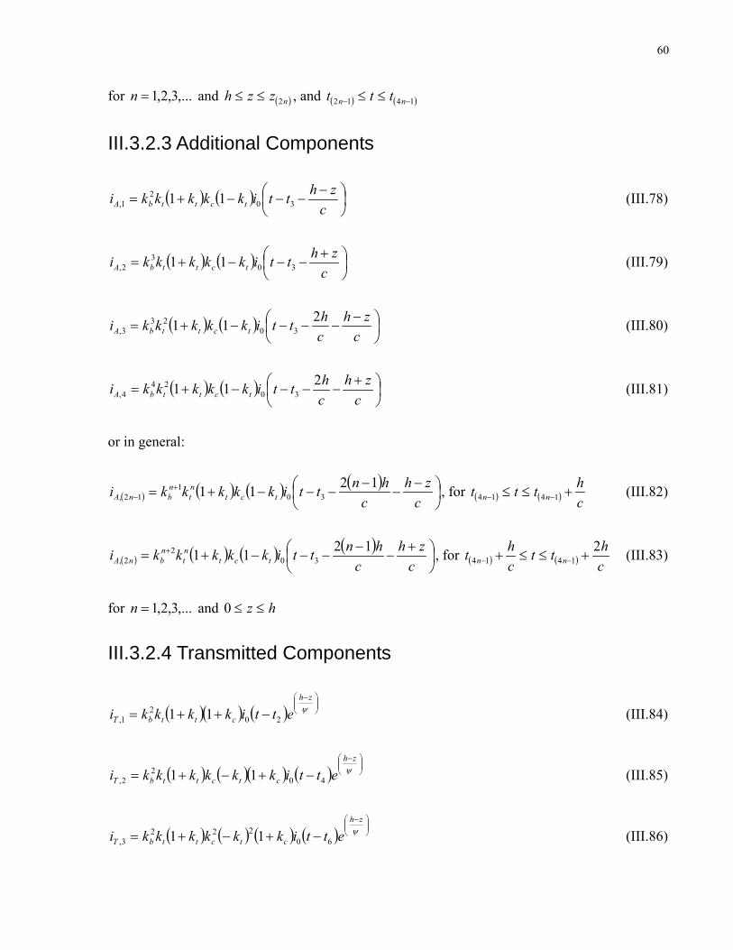
60


III.3.2.3 Additional Components

( ) ( ) ⎟⎠⎞

⎜⎝⎛ −

−−−+=c

zhttikkkkki tcttbA 302

1, 11 (III.78)

( ) ( ) ⎟⎠⎞

⎜⎝⎛ +

−−−+=c

zhttikkkkki tcttbA 303

2, 11 (III.79)

( ) ( ) ⎟⎠⎞

⎜⎝⎛ −

−−−−+=c

zhchttikkkkki tcttbA

211 3023

3, (III.80)

( ) ( ) ⎟⎠⎞

⎜⎝⎛ +

−−−−+=c

zhchttikkkkki tcttbA

211 3024

4, (III.81)

or in general:

( ) ( ) ( ) ( )⎟⎠⎞

⎜⎝⎛ −

−−

−−−+= +− c

zhc

hnttikkkkki tctnt

nbnA

1211 301

12, , for ( ) ( ) chttt nn +≤≤ −− 1414 (III.82)

( ) ( ) ( ) ( )⎟⎠⎞

⎜⎝⎛ +

−−

−−−+= +

czh

chnttikkkkki tct

nt

nbnA

1211 302

2, , for ( ) ( ) chtt

cht nn

21414 +≤≤+ −− (III.83)

for and ,...3,2,1=n hz ≤≤0

III.3.2.4 Transmitted Components

( )( ) ( ) ⎟⎟⎠

⎞⎜⎜⎝

⎛ −

−++= ψzh

cttbT ettikkkki 202

1, 11 (III.84)

( ) ( )( ) ( ) ⎟⎟⎠

⎞⎜⎜⎝

⎛ −

−+−+= ψzh

ctcttbT ettikkkkkki 402

2, 11 (III.85)

( ) ( ) ( ) ( ) ⎟⎟⎠

⎞⎜⎜⎝

⎛ −

−+−+= ψzh

ctcttbT ettikkkkkki 60222

3, 11 (III.86)

61

or in general:

( ) ( ) ( ) ( ) ( )( ) ⎟⎟⎠

⎞⎜⎜⎝

⎛ −−− −+−+= ψ

zh

ncn

tncttbnT ettikkkkkki 20

112, 11 (III.87)


Similar derivations could be produced for any subsequent major reflection inside the CN Tower.

One has to pay attention to the fact that at some point in time and height, the relation describing

the speed of propagation of the Lightning Channel front is switching from variable to constant.

At this time the components comprising the current at any height and at any time along the tower

and the Lightning Channel also have to be modified accordingly in order to produce consistent

results.

III.4 Graphical Solution Approach for Cases Involving

Variable Lightning Channel Propagation Speed

Derivations of heights and times for components in Fully Ionized portion of the Lightning

Channel due to first major reflection from bottom of CN Tower that penetrates into the Fully

Ionized portion of Lightning Channel are considered below.

Since the development of relations for and t that need to be included in the current

components, comprising the total current at any level along the Lightning Channel, requires

considerable effort and attention to the details, an alternate approach to find their numerical

values is proposed. The numerical evaluation of the values for and directly from a plot

provides the exact numbers when compared to the analytically computed ones (matching could

be shown in the parabolic cases), but is done instantly and without room for errors, provided the

drawing is precise. Another advantage is also the fact that any type of curve related to the

Lightning Channel front (Not-Fully Ionized portion of the Lightning Channel) propagation could

be treated in the same way easily. The speed of propagation of the Lightning Channel front is the

derivative

z

z t

dtdz , but it could be estimated at any point also by using numerical differentiation with

high accuracy.

62

Fig. III.5 - Lattice Diagram for Increase in Lightning Channel Speed

Proposed method:

- Prepare an exact drawing based on the Lattice diagram pertinent to the particular case (for

variable speed of propagation of the Lightning Channel front).

- Find the intersection points (their values) between the curve associated with the Lightning

Channel front propagation and the respective line representing a specific reflection leg.

- Use these values in the equations developed previously for different current components.

Let us consider now increase in speed of the Lightning Channel front as shown in [101], Fig. 8.

It is seen in Fig.III.5 that for:

hz =1 (III.88)

cht 2

1 = (III.89)

63

These values for height and time could be easily computed or taken directly from the plot.

In the proposed methodology are taken from the plot. 22 ,tz

At height and the associated time we have: 3z 3t

hz =3 (III.90)

chztt −

+= 223 (III.91)

The values at height and the associated time are retrieved from the plot again. 4z 4t

At height and the associated time we have: 5z 5t

hz =5 (III.92)

chztt −

+= 445 (III.93)

Once again, the values at height and the associated time are taken directly from the plot. 6z 6t

One could continue in the same manner until needed.

Based on the presented considerations the different components of the current described by the

Single-Section model become:

III.4.1 Channel-Base Current (Initial Current Propagating upwards

in the Not-Fully Ionized Portion of the Lightning Channel)

⎟⎟⎠

⎞⎜⎜⎝

⎛ −

⎟⎠⎞

⎜⎝⎛ −−= ψ

zh

tch

tch e

vhzti

zzi 0 (III.94)

for MAXzzh ≤≤

64

The speed of propagation of the Lightning Channel front is dtdz which is found using numerical

differentiation.

III.4.2 Internal Components (Trapped in the Fully-Ionized Portion

of the Lightning Channel)

( ) ( ) ( ) ( ) ⎟⎠⎞

⎜⎝⎛ −

−−−+= −−−

− chzttikkkki n

nt

nctbnI 120

1112, 1 (III.95)

( ) ( ) ( ) ⎟⎠⎞

⎜⎝⎛ −

−−−+= −

czzttikkkki n

nn

tnctbnI

220

12, 1 (III.96)


III.4.3 Additional Components

( ) ( ) ( ) ( )⎟⎠⎞

⎜⎝⎛ −

−−

−−−+= −− c

zhc

hnttikkkkki nttct

nbnA

1211 301

12, , for ( ) ( ) chttt nn +≤≤ −− 1414 (III.97)

( ) ( ) ( ) ( )⎟⎠⎞

⎜⎝⎛ +

−−

−−−+= −+

czh

chnttikkkkki n

ttctnbnA

1211 3011

2, , for ( ) ( ) chtt

cht nn

21414 +≤≤+ −− (III.98)

for and ,...3,2,1=n hz ≤≤0

III.4.4 Transmitted Components

( ) ( ) ( ) ( ) ( )( ) ⎟⎟⎠

⎞⎜⎜⎝

⎛ −−− −+−+= ψ

zh

ncn

tnctbnT ettikkkkki 20

11, 11 (III.99)


III.4.5 Extension of the Proposed Graphical Solution Approach to

Account for Sophisticated Representation of the CN Tower

65

The graphical solution approach proposed above could be adapted and used with the Three- and

Five Section Models as well. Basically, one should modify accordingly some of the equations

and Lattice diagram drawings seen in Appendices II and III, and measure the appropriate times

and heights of interest. A study looking into the predicted by the Single-, Three-, and Five

Section Models current waves at specific heights of interest is presented further below. In order

to come up with the required current components comprising the total current at the respective

level, Lattice drawings for Three- and Five-Section Models found in Appendices II and III are

utilized. A list of the selected considered diagrams follows.

Three-Section Model:

Current inside the CN Tower – Fig. AII.8, Fig. AII.9, Fig. AII.10, Fig. AII.15, Fig. AII.16, Fig.

AII.17, Fig. AII.24, Fig. AII.25, and Fig. AII.26.

Current inside the Lightning Channel - Fig. AII.27, Fig. AII.28, Fig. AII.29, Fig. AII.30, Fig.

AII.31, and Fig. AII.32.

Five-Section Model:

Current inside the CN Tower – Fig. AIII.12, Fig. AIII.34, Fig. AIII.42, Fig. AIII.52 and Fig.

AIII.64.

Current inside the Lightning Channel - Fig. AIII.75, Fig. AIII.76, Fig. AIII.77, Fig. AIII.78, Fig.

AIII.79, Fig. AIII.80, Fig. AIII.81, and Fig. AIII.82.

III.5 Influence of Different Speed of Propagation of the

Return Stroke upon the Computed Current Waveforms at

Different Levels

In order to appreciate and visualize the influence of the speed of the Lightning Channel front

upon the channel progression in height, Fig. III.6 and Fig.III.7 are offered.

66

An attempt to use somewhat realistic values was implemented. The speed of the Return Stroke

channel was set to 1/3 of the speed of light for the case involving constant speed of propagation

and it is presented by a thick line in Figs. III.6 and III.7.

Fig. III.6 - Lightni

The considered case with decreasing

it is based on Eq. (III.4) up to t =

constant and is set to the attained

/s, , a

the speed with height, relation descr

7.6858e=v m7 -123.1595e=d

after that the attained value of speed

is shown in dotted lines in Figs. III.6

It is anticipated that the currents a

Channel will be influenced to some

in magnitude reflected and transmitt

for the respective radiated Electric a

ng Channel Front Speed at Various Heights

speed is shown in dashed lines in the same two figures and

sµ53.9 , after which instance of time the speed becomes

at this time value. The respective constants used were

nd . Similarly, in the case involving increase in

ibed by analogous to Eq. (III.2) up to

-6

st

3.8649e=q

µ53.9=

=

is used, and

is adopted as a constant speed ( v m/s). This case

and III.7.

1.347e8

t different levels along the structure and in the Lightning

extend by the occurring at different times otherwise identical

ed components in the three different cases. This is also valid

nd Magnetic Fields at a distance, as will be shown later.

67

Fig. III.7 - Lightn

It is clearly seen in Figs. III.6 and II

propagation of the Return Stroke fro

for a certain time. For example, if on

consider other influences such as wha

(in the cloud) within the timeframe o

length was assumed to be 8000m, bu

Return Stroke is reaching to a h

Consequently, some modifications

distribution at any height and time.

Fig. III.8 is depicting the currents ca

(location of current sensing elemen

Lightning Channel front utilizing the

corresponding waveforms but calcula

The calculations are limited up to a si

reflections from top of the Lightni

propagation of the Return Stroke cha

ing Channel Front Progression in Time

I.7 that using decreasing, constant, or increasing speed of

nt affects the height to which the channel front propagates

e used the increasing speed case shown above, one should

t would happen at the upper end of the Lightning Channel

f interest. This is so, because the whole Lightning Channel

t at somewhat higher speed as is the considered case, the

igher altitude within the 60µs simulation time-frame.

must take place in the relations describing the current

lculated inside the CN Tower at 509m above ground level

t) using the three different speeds of progression of the

Single-Section Model. Figs. III.9 and III.10 show the same

ted using the Three- and Five-Section Models respectively.

mulation time-frame of 50µs in order to avoid dealing with

ng Channel for the case involving increasing speed of

nnel in the range up to 9.53µs. The plots are showing the

68

first 20µs of the simulation in order to better observe the differences in the waveforms achieved

in the three different cases. The injected current is described by a sum of two Heidler functions

[100] with input parameters seen in [22].

Fig. III.8 - Computed Waveforms at

for Three Different Speed

It could be pointed out that when the

speed of propagation of the Return S

level took place and has relatively

level. When the Three- and Five-Se

earlier times, but again it could be

although there are some observed dif

the Single-Section Model computati

speed has slightly more pronounced

increasing in the speed of propagatio

what is observed in the results yielde

509m Above Ground Level Using the Single-Section Model

s of Propagation of the Lightning Channel Front

Single-Section Model is used, the influence of the different

troke channel kicks in after the main reflection from ground

small effect upon the produced current waveshape at this

ction Models are considered some influences take place at

said that the overall waveform is not influenced greatly,

ferences mostly visible in the time-frame between 6-8µs. In

on results it is observed that the case involving decreasing

influence with comparison to the respective case involving

n of the Lightning Channel, which is exactly the opposite of

d by the other two models.

69

Fig. III.9 - Computed Waveforms at 509m Above Ground Level Using the Three-Section Model

for Three Different Speeds of Propagation of the Lightning Channel Front

Fig. III.10 - Computed Waveforms

for Three Different Spee

a

d

t 509m Above Ground Level Using the Five-Section Model

s of Propagation of the Lightning Channel Front

70

The relatively minor effects observed inside the CN Tower could be attributed to the fact that

there are stronger influences that are imposed by the current initially injected into the tower and

also the major reflections taking place inside the structure. The influence of the Lightning

Channel is somewhat diminished due to the chosen values of respective surge impedances which

translate into particular values of reflection and transmission coefficients. In the actual

computations the transmitted components into the tower are much smaller in amplitude than the

major components bouncing inside the CN Tower and thus have small effect, however their

influence is clearly seen in Figs.III.8-10.

The current inside the Lightning Channel, computed using the Single-Section Model, is shown at

two different levels in Figs. III.11 and III.12 below.

Fig. III.11 - Computed Waveform

Model for Three Different Sp

The same results calculated by the T

III.14 and in Figs.III.15-III.16 respec

s at 900m Above Ground Level Using the Single-Section

eeds of Propagation of the Lightning Channel Front

hree- and Five-Section Models are depicted in Figs. III.13-

tively.

71



In contrast to the considered cases in

chosen speed of propagation has con

representative levels where the curren

is not only noticeable in the different

but also in the reached peak values of

Those two heights (900m and 1100m

attained speed for the decreasing case

the increasing cases at 900m above

constant and to the increasing cases at

If one takes a closer look at Fig.III.1

will notice that the computed wavefo

corresponding to the constant speed

speed case waveform. If one checked

the speeds are chosen in such a way

at 1100m Above Ground Level Using the Single-Section


volving currents inside the CN Tower, the influence of the

siderable effect upon the computed waveforms at the two

t is computed inside the Lightning Channel. That influence

times of arrival of the current wave to the respective levels,

the currents.

above ground level) were deliberately chosen so that the

for example is higher as compared to the constant and to

ground level, and lower respectively as compared to the

1100m above ground level.

1, Fig.III.13, or Fig.III.15 (900m above ground level) one

rm for the decreasing speed occurs first, then the waveform

case appears and the last one to show up is the increasing

out Fig. III.6, one would notice the reason for that, namely

that the associated with the decreasing case speed is the

72

highest, the second highest is the constant speed and the slowest is the increasing case speed at

this level.

Fig. III.13 - Computed Waveforms at 900m Above Ground Level Using the Three-Section

Model for Three Different Speeds of Propagation of the Lightning Channel Front



at 1100m Above Ground Level Using the Three-Section


73

Fig. III.15 - Computed Waveforms at 900m Above Ground Level Using the Five-Section Model

for Three Different Speeds of Propagation of the Lightning Channel Front

Fig. III.16 - Computed Waveform


The maximum peak amplitudes seen

achieved when the increasing case sp

decreasing speed case is considered, a

s at 1100m Above Ground Level Using the Five-Section


in Fig.III.11 have different values. The highest value is

eed is considered, the lowest value is achieved when the

nd between them the constant speed case value is found. In

74

contrast to that, as seen in Fig. III.12, at 1100m above ground level, the lowest and highest peak

values switched places and belong to the increasing and the decreasing speed cases respectively,

while the constant speed case is again in between them.

The corresponding peaks in the waveforms computed by multi-section models of the CN Tower

show different behavior. The major difference from the waveforms computed by the Single-

Section Model at 900m above ground level is observed in the waveform computed for the case

involving increasing speed of the Lightning Channel front, which shows a noticeably lower peak

value than the other two considered speed cases. An altered difference in the peaks is observed at

1100m above ground level. The Single-Section Model is predicting a peak produced using the

decreasing speed case, which is higher than the constant and the increasing speed cases values.

The Three- and Five Section Models, however, predict variable speed (decreasing and increasing

cases) peak values that are not only lower with respect to the constant speed case peak value, but

also very close to each other in amplitude. Finally, the waveform computed by the Three-Section

Model at 1100m above ground level involving the decreasing speed of propagation features a

slightly lower peak than the corresponding one involving increasing speed of propagation, while

the respective waveforms computed by the Five-Section Model predict exactly the opposite

trend.

Based on these observations and on the fact that a multi-section model is representing in better

detail the structure of the CN Tower, one could draw a conclusion that the current waves

computed at different levels along the Lightning Channel by the Three- or by the Five-Section

Model would yield better, closer to the actual waveshapes results, than those predicted by the

Single-Section Model. This would also translate into differences in the calculated radiation fields

at a distance. To achieve the highest degree of accuracy, the most sophisticated Five-Section

Model should be used.

Furthermore it should also be mentioned that based on the Lattice diagrams presented in this

Chapter III, (e.g. that seen in Fig. III.2) and the modeling approach already described previously

in Chapter II, if one wanted to consider variable speed of propagation of the Lightning Channel

front, one should modify the relations describing the current distribution in time and along the

Lightning Channel appropriately. The process would include assigning appropriate times of

occurrence of different reflections at corresponding levels of interest. Those times may differ

75

from the analogous case involving constant speed considerably. When such modified current

expressions are plugged into the Single-, Three-, or Five-Section Model, different waveforms

would be computed at respective levels with comparison to the originally achieved ones using

constant speed of propagation of the Lightning Channel front (compare Figs. III.8-III.16).

76

Chapter IV Development of Expressions for Fields at a Distance

IV.1 Outline

Chapter IV consists of two essential parts. First, known theoretical expressions are shown.

Second, newly proposed derivations corresponding to radiated Electric and Magnetic Field

components are introduced. The chapter begins with a review of the fundamental laws of

Electromagnetic Theory. After that several derivations and considerations that are useful in

coming up with formulae pertinent to radiation fields and retarded potentials are presented. At

this point the third original contribution of the thesis is considered, development of time-domain

expressions for Electric in Magnetic fields in Cartesian Coordinates. Developed expressions for

the x, y, z components of the Electric and Magnetic Fields are written down, and the derivation

details are found in Appendix IV. Since, these expressions look like a very powerful tool to

study the impact of radiation fields due to Lightning flashes with an arbitrary shape of the

Lightning Channel upon electrical and electronic equipment, the idea for prospective studies is

discussed at the end of the chapter.

IV.2 Fundamental Laws – General Description

For convenience, a general overview including Maxwell’s equations is given below. More

information could be found in [102-108].

IV.2.1 Gauss' Law

This law describes how electric charge can create and alter Electric Fields. In particular, Electric

Fields tend to point away from positive charges, and towards negative charges. Gauss' law is the

primary explanation of why opposite charges attract, and charges of the same polarity repel. The

charges create certain Electric Fields, which other charges can then respond to by electric force.

Differential form:

77

Free Charge and Current Total Charge and Current

fD ρ=∇. 0

.ερ

=∇ E

Integral form:


∫ =S

SfQdAD ,. ∫ =S

SQdAE0

.ε

where:

.∇ The divergence operator, [/m]

D Electric Displacement Field, [C/m2]

E Electric Field [V/m]

fρ Free Charge Density, [C/m3]

ρ Total Charge Density (including both free and bound charge), [C/m3]

dA Differential vector element of surface area A, with infinitesimally small

magnitude and direction normal to surface S, [m2]

SfQ , Net unbalanced free Electric Charge enclosed by the Gaussian surface S, [C]

∫S

dAE. The flux of the Electric Field through any closed Gaussian surface S, [Jm/C]

SQ Net unbalanced Electric Charge enclosed by the Gaussian surface S (including

both free and bound charge), [C]

0ε Permittivity of free space (universal constant), [F/m]

78

IV.2.2 Gauss' Law for Magnetism

The law states that magnetism is unlike electricity in that there are no distinct "north pole" and

"south pole" particles (such particles, which exist in theory only, would be called magnetic

monopoles) that attract and repel the way positive and negative charges do. Instead, north poles

and south poles come in pairs (magnetic dipoles). In particular, unlike the Electric Field, which

tends to point away from positive charges and towards negative charges, Magnetic Field lines

always occur as closed loops (e.g. pointing away from the north pole outside of a bar magnet but

towards it inside the magnet).

Differential form:


0. =∇ B 0. =∇ B

Integral form:


∫ =S

dAB 0. ∫ =S

dAB 0.

where:

B Magnetic Field, [Wb/m2]

∫S

dAB. The flux of the Magnetic Field through any closed surface S, [Wb]

IV.2.3 Faraday's Law of Induction

It describes how a changing Magnetic Field can create an Electric Field. This is, for example, the

operating principle of many electric generators: Mechanical force (e.g. the force of water falling

through a hydroelectric dam) spins a huge magnet, and the changing Magnetic Field creates an

Electric Field which supplies consumers with electricity through the power grid.

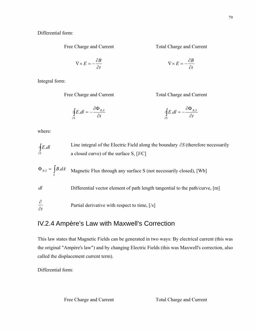
79

Differential form:


tBE∂∂

−=×∇ tBE∂∂

−=×∇

Integral form:


∫∂ ∂

Φ∂−=

S

SB

tdlE ,. ∫

∂ ∂Φ∂

−=S

SB

tdlE ,.

where:

∫∂S

dlE. Line integral of the Electric Field along the boundary (therefore necessarily

a closed curve) of the surface S, [J/C]

S∂

∫=ΦS

SB dAB., Magnetic Flux through any surface S (not necessarily closed), [Wb]

dl Differential vector element of path length tangential to the path/curve, [m]

t∂∂ Partial derivative with respect to time, [/s]

IV.2.4 Ampère's Law with Maxwell's Correction

This law states that Magnetic Fields can be generated in two ways: By electrical current (this was

the original "Ampère's law") and by changing Electric Fields (this was Maxwell's correction, also

called the displacement current term).

Differential form:


80

tDJH f ∂∂

+=×∇ tEJB∂∂

+=×∇ 000 εµµ

Integral form:


∫∂ ∂

Φ∂+=

S

SDSf t

IdlH ,,. ∫

∂ ∂Φ∂

+=S

SES t

IdlB ,000. εµµ

where:

×∇ The curl operator, [/m]

H Magnetic Field, [A/m]

0µ Permeability of free space (universal constant), [H/m]

fJ Free current density (not including bound current), [A/m2]

J Total current density (including both free and bound current), [A/m2]

∫∂S

dlB. Line integral of the Magnetic Field over the closed boundary of the surface

S, [Tm]

S∂

∫=S

fSf dAJI ., Net free electrical current passing through the surface S (not including bound

current), [A]

∫=S

S dAJI . Net electrical current passing through the surface S (including both free and

bound current), [A]

∫=ΦS

SE dAE., Electric flux through any surface S (not necessarily closed), [Jm/C]

81

∫=ΦS

SD dAD., Flux of Electric displacement Field through any surface S (not necessarily

closed), [C]

IV.3 Maxwell’s Work

Maxwell's correction to Ampère's law was very important. With the included correction, the laws

state that a changing Electric Field could produce a Magnetic Field, and vice-versa. It follows

that it is possible to have stable, self-perpetuating waves of oscillating Electric and Magnetic

Fields, with each field driving the other. (These waves are called electromagnetic radiation.) The

four Maxwell's equations describe these waves quantitatively, and moreover predict that the

waves should have a particular, universal speed, which can be simply calculated in terms of two

easily-measurable physical constants (called the electric constant and magnetic constant).

Maxwell's equations are generally applied to macroscopic averages of the fields, which deviate

considerably on a microscopic scale in the vicinity of individual atoms. The quantities

permittivity and permeability of a material are normally also defined in a macroscopic sense.

The eight original Maxwell's equations can be written in modern vector notation as follows:

Table IV.1 Original Maxwell’s Equations

No Law Equation

1. The Law of Total Currents tDJJtot ∂∂

+=

2. The Equation of Magnetic Force AH ×∇=µ

3. Ampere’s Circuital Law totJH =×∇

4.

Electromotive Force created by

Convection, Induction, and by

Static Electricity.

Φ∇−∂∂

−×=tAHvE µ

82

5. The Electric Elasticity Equation DEε1

=

6. Ohm’s Law JEσ1

=

7. Gauss’ Law ρ=∇ D.

8. Equation of Continuity t

J∂∂

−=∇ρ.

where:

H Magnetizing Field (called by Maxwell the "Magnetic Intensity”)

J Electric Current Density (with being the total current including

displacement current)

totJ

D Displacement Field (called by Maxwell the "Electric Displacement")

ρ Free Charge Density (called by Maxwell the "Quantity of Free Electricity")

A Magnetic Vector Potential (called by Maxwell the "Angular Impulse")

E "Electromotive Force" (as called by Maxwell) corresponding to Electric Field

Φ Electric Potential (called by Maxwell also the "Electric Potential")

σ Electrical Conductivity (Maxwell called the inverse of Conductivity the

"Specific Resistance”)

When Maxwell derives the electromagnetic wave equation in 1865, he uses equation 4 to cater

for electromagnetic induction rather than Faraday's law of induction, which is used in modern

textbooks. (Faraday's law itself does not appear among his equations.) However, Maxwell drops

the Hv×µ term from equation 4 when he is deriving the electromagnetic wave equation, as he

considers the situation only from the rest frame.

83

IV.4 Constitutive Relations

In order to apply Maxwell's equations (the formulation in terms of Free Charge and Current, and

and D H ), it is necessary to specify the relations between and D E , and H and B . These are

called Constitutive Relations, and correspond physically to specifying the response of bound

charge and current to the field, or equivalently, how much polarization and magnetization a

material acquires in the presence of electromagnetic fields.

IV.4.1 Case without Magnetic or Dielectric Materials

In the absence of magnetic or dielectric materials, the relations are simple:

0

0

/ µεBH

ED==

(IV.1)

where 0ε and 0µ are the two universal constants, called the permittivity of free space and

permeability of free space, respectively.

IV.4.2 Case of Linear Materials

In a "linear", isotropic, non-dispersive, uniform material, the relations become:

µε

/BHED

==

(IV.2)

where ε and µ are constants (which depend on the material), called the permittivity and

permeability, respectively, of the material.

IV.4.3 General Case

For real-world materials, the constitutive relations can usually still be written:

µε

/BHED

==

84

but ε and µ are not, usually, simple constants, but functions. For example, they can depend

upon:

- The strength of the fields;

- The direction of the fields;

- The frequency with which the fields vary;

If further there are dependencies on:

- The position inside the material;

- The history of the fields;

then the constitutive relations take a more complicated form [109]:

( ) ( ) ( )

( ) ( ) ( )

( ) ( ) ( )

( ) ( ) ( ',';',,',ˆ''1,

',';',,',ˆ'',

,,1,

,,,

3

0

30

0

0

trBBttrrdtrdtrM

trEEttrrdtrdtrP

trMtrBtrH

trPtrEtrD

magn

elec

χµ

χε

µ

)

ε

∫

∫=

=

−=

+=

(IV.3)

in which the permittivity and permeability functions are replaced by integrals over the more

general electric and magnetic susceptibilities.

IV.5 Maxwell's Equations in Terms of E and B for Linear

Materials

Using the constitutive relations from above, Maxwell's equations in a linear material (differential

form only) become:

85

tEJB

tBE

B

E

f

f

∂∂

+=×∇

∂∂

−=×∇

=∇

=∇

µεµ

ερ

0.

.

(IV.4)

These are formally identical to the general formulation in terms of E and B (given above when

formulation in terms of total charge and current is considered), except that the permittivity of

free space was replaced with the permittivity of the material, the permeability of free space was

replaced with the permeability of the material, and only free charges and currents are included.

IV.5.1 Formulation in Vacuum

Starting with the equations appropriate in the case without dielectric or magnetic materials, and

assuming that there is no current or electric charge present in the vacuum, the Maxwell equations

in free space become:

tEB

tBE

BE

∂∂

=×∇

∂∂

−=×∇

=∇=∇

00

0.0.

εµ

(IV.5)

These equations have a solution in terms of traveling sinusoidal plane waves, with the Electric

and Magnetic Field directions orthogonal to one another and the direction of travel, and with the

two fields in phase, traveling at the speed:

00

1εµ

=c (IV.6)

In fact, Maxwell's equations explain how these waves can physically propagate through space.

The changing Magnetic Field creates a changing Electric Field through Faraday's law. That

Electric Field, in turn, creates a changing Magnetic Field through Maxwell's correction to

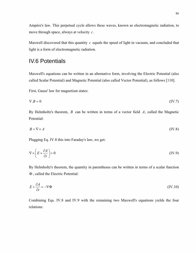
86

Ampère's law. This perpetual cycle allows these waves, known as electromagnetic radiation, to

move through space, always at velocity . c

Maxwell discovered that this quantity c equals the speed of light in vacuum, and concluded that

light is a form of electromagnetic radiation.

IV.6 Potentials

Maxwell's equations can be written in an alternative form, involving the Electric Potential (also

called Scalar Potential) and Magnetic Potential (also called Vector Potential), as follows [110].

First, Gauss' law for magnetism states:

0. =∇ B (IV.7)

By Helmholtz's theorem, B can be written in terms of a vector field , called the Magnetic

Potential:

A

AB ×∇= (IV.8)

Plugging Eq. IV.8 this into Faraday's law, we get:

0=⎟⎠⎞

⎜⎝⎛

∂∂

+×∇tAE (IV.9)

By Helmholtz's theorem, the quantity in parentheses can be written in terms of a scalar function

, called the Electric Potential: Φ

Φ−∇=∂∂

+tAE (IV.10)

Combining Eqs. IV.8 and IV.9 with the remaining two Maxwell's equations yields the four

relations:

87

( )

Jtc

AtA

cA

At

ABtAE

022

2

22

0

2

1.1

.

µ

ερ

−=⎟⎠⎞

⎜⎝⎛

∂Φ∂

+∇∇−⎟⎟⎠

⎞⎜⎜⎝

⎛∂∂

−∇

−=∇∂∂

+Φ∇

×∇=∂∂

−Φ−∇=

(IV.11)

These equations, taken together, are as powerful and complete as Maxwell's equations. In

addition, the problem has been reduced somewhat, as the Electric and Magnetic Fields each have

three components which need to be solved for (six components altogether), while the Electric

and Magnetic Potentials have only four components altogether. On the other hand, these

equations appear more complicated than Maxwell's equations using just the Electric and

Magnetic Fields.

In fact, Eqs. IV.11 can be simplified by taking advantage of the fact that there are many different

choices of and consistent with a given A Φ E and B .

IV.7 Radiation Fields

IV.7.1 Currents and Charges as Sources of Fields

Usually, the current distribution is localized in some region of space (e.g. on a wire antenna.)

Electric and Magnetic Fields are generated by such a current source and these fields can

propagate to far distances from the source location.

Normally it is more convenient to work with the Electric and Magnetic Potentials rather than

with the Electric and Magnetic Fields. Basically, using two of Maxwell’s equations these

potentials are introduced, then, making use of the other two, written in terms of these potentials,

the wave-equations are found.

The potentials and are not uniquely defined. Adding constants to them may change them.

Even more freedom is possible, known as gauge invariance of Maxwell’s equations. In actual

fact, for any scalar function

A Φ

( )trf , , the following gauge transformation leaves E and B

invariant:

88

fAAtf

∇+=∂∂

−Φ=Φ

'

' (IV.12)

When radiation problems are discussed the Lorentz condition is usually imposed.

012 =∂Φ∂

+⋅∇tc

A (IV.13)

Using the first two equations seen in (IV.11) (implied by Maxwell’s equations 0. =∇ B and

tE

∂−=×∇

B∂ ) and (IV.13) in the remaining two Maxwell equations:

tE

cJB

E

∂∂

+=×∇

=⋅∇

21µ

ερ

(IV.14)

and after a few mathematical manipulations in which also considered is the identity

, one can come up with the following relations known as the wave

equations:

( ) ( ) 2 AAA ∇−⋅∇∇=×∇×∇

JAtA

c

tc

µ

ερ

=∇−∂∂

=Φ∇−∂Φ∂

22

2

2

22

2

2

1

1

(IV.15)

As seen in Eq. (IV.15), the densities ρ and could be considered as the sources that generate

the potentials Φ and . These potentials could be then used in the first two relations of Eq.

(IV.11) to come up with the Electric and Magnetic Fields.

J

A

IV.8 Retarded Potentials

The retarded potentials have the following form:

89

( )

( ) ∫

∫

⎟⎠⎞

⎜⎝⎛ −

=

⎟⎠⎞

⎜⎝⎛ −

=Φ

'

3

'

3

'4

,',

'4

,',

V

V

rdR

cRtrJ

trA

rdR

cRtr

tr

π

µ

πε

ρ

(IV.16)

In (IV.16) 'rrR −= is the distance from the field observation point r to the source point 'r

(please, see Fig. AIV.1). Integration is performed over the volume V , in which the source

densities

'

ρ and are not zero. J

In case there is a change at the source point 'r , that change will not be felt at the observation

point r for a period of time equal to cR seconds, if propagation is assumed to take place at the

speed of light (otherwise the denominator in cR c will have a different value than ).

IV.9 General Notes Regarding Radiation from a Finite

Vertical Antenna

After this brief introduction to some of the fundamentals of Electromagnetic Theory, let us now

consider the problem involving electromagnetic radiation from Lightning Return Strokes.

Time domain solutions to the electromagnetic radiation from a finite, straight vertical antenna

above a perfectly conducting plane have been derived in Spherical Coordinates by Uman et. al

and shown in [111]. Moreover, time domain solutions to the same problem have been developed

in Cylindrical Coordinate system by Master and Uman [112]. In this thesis work the same

problem, as described above, is examined in Cartesian Coordinates. Significantly, this approach

allows to relax the requirement of the formulation in Cylindrical Coordinates for verticality of

the antenna. Now the antenna may be in an arbitrary position, including that inclined with

respect to ground. Considered are the time-dependent forms of Maxwell’s equations and their

solutions in terms of retarded Scalar and Vector Potentials. Expressions for the x, y, and z

components of the total Electric and Magnetic Fields in time are given in differential form. The

derived expression for the z component of the Electric Field is actually the well known from

Cylindrical Coordinates vertical component of the Electric Field (Ez) while derived expression

90

for the x component of the Magnetic Field is the azimuthal (Hφ ) component of Cylindrical

Coordinates respectively. Experimental data of these field components have been and continue to

be routinely captured (currently both Ez and Hφ are monitored) 2km away from the CN Tower

in Toronto, Canada. Computed fields will be compared to actually recorded ones in Chapter V,

where results of simulations will be fully analyzed and discussed as well.

IV.10 Derivation Considerations

Herewith below, geometrical considerations, derived expressions for vertical component of the

Electric Field and for azimuthal component of the Magnetic Field in Cylindrical Coordinates, as

well as derived expressions for x, y, and z components of the Electric and Magnetic Fields in

Cartesian Coordinates are shown. Details regarding deriving the newly proposed relations in

Cartesian Coordinates are presented in Appendix IV.

In Fig. IV.1, both the tall object and the Lightning Return Stroke Channel are assumed to be

vertical antennas above a perfectly conducting ground, where the observation point P lies at a

certain distance d from the bottom of the tall object. The azimuthal component of the Magnetic

Field and the vertical component of the Electric Field, due to a vertical dipole of infinitesimal

length dz’ along the z axis at height z’ observed at point P are given in Cylindrical Coordinates in

[22].

Fig. IV.1 - Geometrical Relations Pertinent to Radiating Vertical Antenna above Perfectly

Conducting Ground and Observation Point P

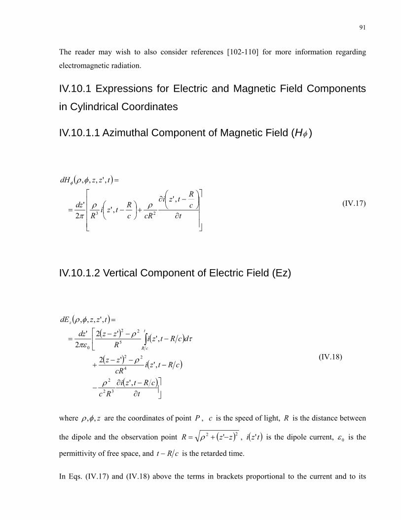
91

The reader may wish to also consider references [102-110] for more information regarding

electromagnetic radiation.

IV.10.1 Expressions for Electric and Magnetic Field Components

in Cylindrical Coordinates

IV.10.1.1 Azimuthal Component of Magnetic Field (Hφ )

( )

⎥⎥⎥⎥

⎦

⎤

⎢⎢⎢⎢

⎣

⎡

∂

⎟⎠⎞

⎜⎝⎛ −∂

+⎟⎠⎞

⎜⎝⎛ −=

=

tcRtzi

cRcRtzi

Rdz

tzzdH

,','

2'

,',,,

23ρρ

π

φρφ

(IV.17)

IV.10.1.2 Vertical Component of Electric Field (Ez)

( )( ) ( )

( ) ( )

( )⎥⎦

⎤∂−∂

−

−−−

+

−⎢⎣

⎡ −−=

=

∫

tcRtzi

Rc

cRtzicRzz

dcRtziRzzdz

tzzdEt

cR

z

,'

,''2

,''22

'

,',,,

32

2

4

22

5

22

0

ρ

ρ

τρπε

φρ

(IV.18)

where z,,φρ are the coordinates of point P , is the speed of light, c R is the distance between

the dipole and the observation point ( )22 ' zzR −+= ρ , ( )tzi ' is the dipole current, 0ε is the

permittivity of free space, and cR−t is the retarded time.

In Eqs. (IV.17) and (IV.18) above the terms in brackets proportional to the current and to its

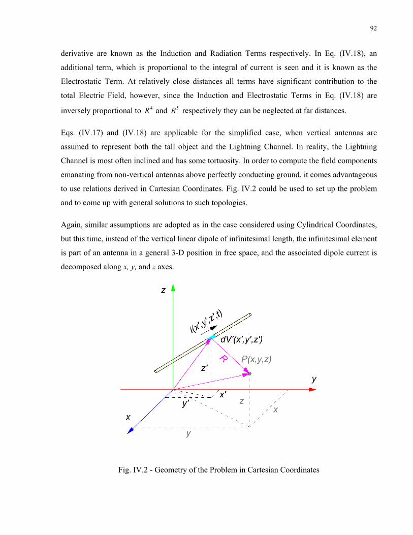
92

derivative are known as the Induction and Radiation Terms respectively. In Eq. (IV.18), an

additional term, which is proportional to the integral of current is seen and it is known as the

Electrostatic Term. At relatively close distances all terms have significant contribution to the

total Electric Field, however, since the Induction and Electrostatic Terms in Eq. (IV.18) are

inversely proportional to 4R and 5R respectively they can be neglected at far distances.

Eqs. (IV.17) and (IV.18) are applicable for the simplified case, when vertical antennas are

assumed to represent both the tall object and the Lightning Channel. In reality, the Lightning

Channel is most often inclined and has some tortuosity. In order to compute the field components

emanating from non-vertical antennas above perfectly conducting ground, it comes advantageous

to use relations derived in Cartesian Coordinates. Fig. IV.2 could be used to set up the problem

and to come up with general solutions to such topologies.

Again, similar assumptions are adopted as in the case considered using Cylindrical Coordinates,

but this time, instead of the vertical linear dipole of infinitesimal length, the infinitesimal element

is part of an antenna in a general 3-D position in free space, and the associated dipole current is

decomposed along x, y, and z axes.

Fig. IV.2 - Geometry of the Problem in Cartesian Coordinates

93

IV.10.2 Expressions for Electric and Magnetic Field Components

in Cartesian Coordinates

IV.10.2.1 x, y, and z Components of the Magnetic Field

The x, y, and z components of the Magnetic Field due to the element with associated current

at the observation point are given in Cartesian Coordinates:

'dV

),',','( tzyxi ),,( zyxP

( )

⎥⎦

⎤⎢⎣

⎡⎟⎟⎠

⎞⎜⎜⎝

⎛∂∂

+−⎟⎠⎞

⎜⎝⎛

∂∂

+=

=

ti

ci

RRZ

ti

ci

RRY

tzzyyxxdH

yy

zz

x

111141

,',,',,',

22π (IV.19)

( )

⎥⎦

⎤⎢⎣

⎡⎟⎠⎞

⎜⎝⎛

∂∂

+−⎟⎠⎞

⎜⎝⎛

∂∂

+=

=

ti

ci

RRX

ti

ci

RRZ

tzzyyxxdH

zz

xx

y

111141

,',,',,',

22π (IV.20)

( )

⎥⎦

⎤⎢⎣

⎡⎟⎠⎞

⎜⎝⎛

∂∂

+−⎟⎟⎠

⎞⎜⎜⎝

⎛∂∂

+=

=

ti

ci

RRY

ti

ci

RRX

tzzyyxxdH

xx

yy

z

111141

,',,',,',

22π (IV.21)

IV.10.2.2 x, y, and z components of the Electric Field

Using the same geometrical considerations as for the Magnetic Field components, the x, y, and z

components of the Electric Field due to the element dV with associated current at

the observation point are given in Cartesian Coordinates:

' ),',','( tzyxi

),,( zyxP

( )

⎥⎦

⎤⎟⎠⎞

⎜⎝⎛+

∂∂

⎟⎠⎞

⎜⎝⎛+⎟

⎠⎞

⎜⎝⎛+

⎟⎠⎞

⎜⎝⎛+

∂∂

⎟⎠⎞

⎜⎝⎛+⎟

⎠⎞

⎜⎝⎛+

⎟⎟⎠

⎞⎜⎜⎝

⎛−+⎢

⎣

⎡

∂∂

⎟⎟⎠

⎞⎜⎜⎝

⎛−+⎟⎟

⎠

⎞⎜⎜⎝

⎛−=

=

∫

∫

∫

t

zz

z

t

yy

y

t

xx

x

x

diRXZ

ti

RcXZi

cRXZ

diRXY

ti

RcXYi

cRXY

diRR

Xti

RcRcXi

cRcRX

tzzyyxxdE

05324

05324

035

2

232

2

24

2

0

33

33

131134

1

,',,',,',

τ

τ

τπε

(IV.22)

94

( )

⎥⎦

⎤⎟⎠⎞

⎜⎝⎛+

∂∂

⎟⎠⎞

⎜⎝⎛+⎟

⎠⎞

⎜⎝⎛+

⎟⎟⎠

⎞⎜⎜⎝

⎛−+

∂

∂⎟⎟⎠

⎞⎜⎜⎝

⎛−+⎟⎟

⎠

⎞⎜⎜⎝

⎛−+

⎢⎣

⎡⎟⎠⎞

⎜⎝⎛+

∂∂

⎟⎠⎞

⎜⎝⎛+⎟

⎠⎞

⎜⎝⎛=

=

∫

∫

∫

t

zz

z

t

yy

y

t

xx

x

y

diRYZ

ti

RcYZi

cRYZ

diRR

Yti

RcRcYi

cRcRY

diRXY

ti

RcXYi

cRXY

tzzyyxxdE

05324

035

2

232

2

24

2

05324

0

33

13113

334

1

,',,',,',

τ

τ

τπε

(IV.23)

( )

⎥⎦

⎤⎟⎟⎠

⎞⎜⎜⎝

⎛−+

∂∂

⎟⎟⎠

⎞⎜⎜⎝

⎛−+⎟⎟

⎠

⎞⎜⎜⎝

⎛−+

⎟⎠⎞

⎜⎝⎛+

∂

∂⎟⎠⎞

⎜⎝⎛+⎟

⎠⎞

⎜⎝⎛+

⎢⎣

⎡⎟⎠⎞

⎜⎝⎛+

∂∂

⎟⎠⎞

⎜⎝⎛+⎟

⎠⎞

⎜⎝⎛=

=

∫

∫

∫

t

zz

z

t

yy

y

t

xx

x

z

diRR

Zti

RcRcZi

cRcRZ

diRYZ

ti

RcYZi

cRYZ

diRXZ

ti

RcXZi

cRXZ

tzzyyxxdE

035

2

232

2

24

2

05324

05324

0

13113

33

334

1

,',,',,',

τ

τ

τπε

(IV.24)

In the relations of Eqs. (IV.19-IV.24) R is the distance from the infinitesimal element

to the point , where the field is calculated, is the speed of light, )',','(' zyxdV ),,( zyxP c

cRt − is the retarded time, ( )'xxX −= , , ( )dxcRtxii /,'x( )'yyY −= , ( )'zzZ −= −=

( )dycRt /, − zi /,'

,

, and iyiiy '= ( )dzcRtz . −=

The derived above equations for zyx ,, components of dH and of hold for the general case

when all components have contribution to the total Magnetic or Electric Field. In the case, when

Lightning current path is vertical, perfectly conducting ground is assumed, and the observation

point

dE

P lies on the y axis (see Fig. IV.1), the y and z components of the Magnetic Field, as well

as the x and y components of the Electric Field are equal to “zero” due to the absence of ix and iy

currents and some geometrical considerations. In such a case, the numerical result for Hx

(Cartesian Coordinates) coincides with Hφ (Cylindrical Coordinates) and Ez (Cartesian

Coordinates) with Ez (Cylindrical Coordinates) respectively. On the other hand, the derived

expressions for Magnetic and Electric fields in Cartesian Coordinates appear to be very useful

and powerful tools for calculating the radiated electromagnetic fields when the condition for

95

verticality of the Lightning Channel is relaxed. In fact, now the opportunity to study the

influence of the Lightning Channel arbitrarily inclined or of Lightning Channel tortuosity upon

the radiated distant fields becomes quite tractable. Please, note that for the case of the CN Tower,

when a perfectly conducting ground and an image are assumed Eqs. IV.19-IV.24 should be

multiplied by a coefficient equal to two.

IV.11 Possibilities to Study the Influence of Lightning

Channel Inclination Upon Radiated Electric and Magnetic

Fields

Although, it has been shown (e.g. Rachidi et. al [22]) that the contribution of the Lightning

Channel to the total radiated electromagnetic fields at 2km away usually is in the order of 2-3

times smaller than the contribution of the CN Tower, it is still quite considerable and has

significant influence upon magnitudes and waveshapes of the observed fields. Furthermore, as

will be shown in Chapter V of this thesis, contribution of any inclined Lightning Channel may be

considerably larger depending on the specificity of each considered case. Let us now consider an

arbitrarily inclined Lightning Channel as shown in Fig. IV.3, in order to appreciate the potential

for the influence of the Lightning Channel inclination. As an input current, a Heidler function

[100], could be used. If such current was injected at the tip of the CN Tower and provided the

current at any level along the CN Tower and the Lightning Channel at any given time was

appropriately described (e.g. Single-Section Model that is considered in [113]), one could use

Eqs. (IV.19-IV.24) to come up with the associated, radiated at a certain distance, field

components. When working in Cartesian Coordinates different components of the current

( ) are derived from the total current i using geometrical relations applicable to the

particular case study. In some convenient cases when the Lightning Channel is assumed to lie in

the y-z plane (angle

zyx ,, iii

φ equals 0°, 180°, or 360°, see Fig. IV.4) and to be inclined at a specific

angle γ with respect to the z axis (see Fig. IV.3), there are no x components contributing to the

total current i. In other special cases (angle φ equals 90° or 270°, see again Figs. IV.3 and IV.4)

there are no y components.

96

Fig. IV.3 - General Geometrical Relations for Inclined Lightning Channel Case

In general all x, y, and z current components exist and these ix, iy, and iz, together with the

geometrical relations pertinent to the case study, are precisely what we need in order to compute

different field components using the proposed relations from Eqs. (IV.19-IV.24). Appendix V

contains details regarding geometrical relations and current components needed to assess the

electromagnetic radiation due to inclined Lightning Channel.

It looks like it is important to perform a thorough analysis in order to find out whether the

Lightning Channel contribution would be significantly higher or smaller in some particular real

world cases when the Lightning Channel has some tortuosity and some inclination and the

observation point is also located at a specific arbitrary position in 3-D space. The expressions in

Cartesian Coordinates presented in this chapter provide a possibility to compute all the radiated

components of the Electric and Magnetic Fields for such geometries and eventually compare

some of them to corresponding existing records. Such a detailed study has not been performed

until this moment but could now be undertaken.

97

Fig. IV.4 - Angle φ in the x-y Plane

98

Chapter V Studies, Analyses, and Experimental Results

V.1 Outline

This chapter is devoted to analysis and examination of the developed sophisticated modeling of

Lightning events at the CN Tower. The newly introduced relations for computing radiated distant

fields due to Lightning Return Strokes to the CN Tower, together with current described using

the developed multi-section models, are taken advantage of and employed in studies presented in

this Chapter.

First, a general analysis, using a typically observed current is performed. The typical

“uncontaminated” Lightning current is used as input to the three developed in the thesis

“Engineering” models. Plots of computed current derivative and current at a specific location on

the CN Tower (where one of the current sensing elements is mounted), as well as another plot

showing the current at several different levels of CN Tower and along the Lightning Channel are

provided.

Next, radiated fields are treated. Plots of the Electric and the Magnetic Field at 2km from the

CN Tower are shown, in which the respective Induction, Radiation, and Static components are

clearly marked.

Furthermore, a full sensitivity study looking into the influence of different channel inclinations

upon the radiated Electric and Magnetic Fields is performed. Appendix V contains details

regarding the used geometries and corresponding currents. For the first time, different speeds of

propagation of the Return Stroke in the Not-Fully Ionized portion of the Lightning Channel is

studied. This includes non-linear variation in the speed of the Return Stroke front.

Later in the chapter, four discrete cases of channel inclination, considered by another author

[114], are analyzed by the techniques developed in this thesis.

Next, a recorded event from August 19, 2005 is considered and computationally modelled. It was

chosen because for that particular event, a full data set exists including captured current, vertical

component of Electric Field, azimuthal component of Magnetic Field, and video records.

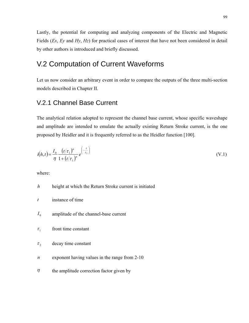
99

Lastly, the potential for computing and analyzing components of the Electric and Magnetic

Fields (Ex, Ey and Hy, Hz) for practical cases of interest that have not been considered in detail

by other authors is introduced and briefly discussed.

V.2 Computation of Current Waveforms

Let us now consider an arbitrary event in order to compare the outputs of the three multi-section

models described in Chapter II.

V.2.1 Channel Base Current

The analytical relation adopted to represent the channel base current, whose specific waveshape

and amplitude are intended to emulate the actually existing Return Stroke current, is the one

proposed by Heidler and it is frequently referred to as the Heidler function [100].

( ) ( )( )

⎟⎟⎠

⎞⎜⎜⎝

⎛−

+= 2

1

10

1, τ

ττ

η

t

n

n

et

tIthi (V.1)

where:

h height at which the Return Stroke current is initiated

t instance of time

0I amplitude of the channel-base current

1τ front time constant

2τ decay time constant

n exponent having values in the range from 2-10

η the amplitude correction factor given by

100

nn

e

1

1

2

2

1⎟⎟⎠

⎞⎜⎜⎝

⎛⎟⎟⎠

⎞⎜⎜⎝

⎛−

= ττ

ττ

η (V.2)

In studies that follow, the channel base current is represented by a sum of two Heidler functions

and it has the following analytical representation:

( ) ( )( )( )( )

⎟⎟⎠

⎞⎜⎜⎝

⎛−

⎟⎟⎠

⎞⎜⎜⎝

⎛−

++

++

=

22

2

2

21

1

1

12

12

2

02

11

11

1

010

1

1,

τ

τ

ττ

η

ττ

ηt

n

n

t

n

n

et

tI

et

tIthi

(V.3)

This equation holds for the instance of time t. The reader should bear in mind that different

current contributions, forming the total current at a respective level above ground level, have

respective time delays (e.g. see equations pertinent to Single-Section Model - Eqs. A1.1 - A1.6).

Fig. V.1 - Heidler Current Used in Simulations

The input to all considered models is a Heidler function with parameters utilized in previous

publications (e.g. [22]).

For convenience, the used values are shown below and the corresponding plot of the produced

waveform is depicted in Fig. V.1.

101

Io1 = 10.7kA; τ11 = 0.25µs; τ21 = 2.5µs; n1 = 2

Io2 = 6.5kA; τ12 = 2µs; τ22 = 230µs; n2 = 2

V.2.2 Effects of Chosen Models

Assuming v = 1.9e8 m/s as constant propagation velocity within the Not-Fully Ionized portion of

the Lightning Channel, waveforms of the Return Stroke current derivative and of the current,

both computed at the 474 m level, using a variable number of CN Tower sections, are shown in

Fig. V.2 and Fig. V.3 respectively.

As is seen in these two figures, waveforms of the current derivative and of the current itself are

more elaborately represented when a more detailed model of the CN Tower is considered.

Respective changes in the waveshapes are spaced in time according to reflection points

considered in different models. While only two reflections (from bottom and top of the CN

Tower) are seen for the Single-Section Model, additional two reflections are caused by the top

and bottom of the Skypod for the Three- and the Five-Section Models. Further two reflections,

from top and bottom of the Space Deck, are associated only with waveforms computed by the

Five-Section Model. Since these last two reflections are spaced very closely in time, they are not

easily discernable on the original timescale of Fig. V.2, and therefore an enlargement plot for the

region 0.35-0.50µs and 38-42kA/µs, showing clearly the influence of these two additional

reflections, is provided. In order to capture the effect of these reflections upon the computed

current derivative waveform, one should use a high resolution time step, because reflections are

coming from points of mismatched impedances which are only 9m apart (see Fig. AIII.1). This is

corresponding to a travel time of 60ns for the round trip of 18m. Consequently, a time step of 1ns

was needed in calculations to produce the current derivatives for the Five-Section Model shown

in Fig. V.2. The computations pertinent to Single and Three-Section Models could be carried out

using a time step of 100ns, which was found to be sufficient in terms of precision in the

produced current derivative and current waveforms.

102

Fig. V.2 - Injected and Calculate

Single-, Three- and Five-Sectio

enlargement of the area in the c

d Current Derivatives at 474m Above Ground Level using the

n CN Tower Model for the Arbitrary Lightning Event (the

ircle (t = 0.35-0.50µs and di = 38-42kA/µs) is shown on top)

103

Fig. V.3 - Injected and Calc

Single-, Three- and Five

Another aspect of the Five-S

travel up the Tower and are pa

For the Five-Section Model

Skypod for the Three-Section

of the current wave (see Fig. V

be somewhat increased by this

There are other changes in th

interactions among different

Lightning Channel. These ar

subtract to form the final wave

If one looks closely at Fig. V

computed by the Five-Section

instances of time. Since these

wave, one can associate the

reflected at discontinuities of

ulated Current Waveshapes at 474m Above Ground Level using

-Section CN Tower Model for the Arbitrary Lightning Event

ection Model concerns reflections from the Space Deck, which

rtially reflected and partially refracted into the Lightning Channel.

these occur at a much earlier time than those coming from the

Model and from the ground for the Single-Section Model. In case

.3), for the Five-Section Model, the top part of the front is seen to

First Set of Space Deck Reflections.

e computed waveforms that are due to reflections coming from

discontinuities of the CN Tower and from reflections within the

rive at the observation point at various times and either add or

shapes.

.2, presenting the current derivative at 474m above ground level

Model, one can notice distinctive peaks occurring at particular

peak values correspond to maximum steepnesses of the current

se peaks with maximum front steepnesses of the current wave

the structure. To better visualize these reflection points within the

104

CN Tower structure for the Five-Section Model, and to correlate them in time, Fig. V.4 is

offered.

Fig. V.4 - Travel Times inside the CN Tower for the Five-Section Model

In Fig. V.4 the following abbreviations are used:

Ht height of the tower

HRC height of mounting of the lower Rogowski coil with respect to ground

H4 top level of the Space deck with respect to ground

H3 bottom level of the Space deck with respect to ground

H2 top level of the Skypod with respect to ground

H1 bottom level of the Skypod with respect to ground

105

It is well worth noting that, due to the peculiarities of the CN Tower structure, some of the

considered reflections arrive from different reflection points at the 474m recording location at the

same instances of time. This is the case for example for the current waves traveling the path

HRC-H2-HRC and HRC-H3-HRC-Ht-HRC, each taking 0.72µs.

In actual fact many different contributions add up to each other or cancel off in order to produce

the final computed waveform at the respective level and time of interest. Similar considerations

are used to come up with the current distributions along the Lightning Channel as well.

While Fig. V.3 gives the waveshapes of the current at the 474m above ground level, computed

using different number of CN Tower sections, Fig. V.5 provides information about current

waveforms at different levels of the CN Tower and of the Lightning Channel, all determined

using the Five-Section representation of the CN Tower. Please, note the delay in the starting

instances of current waveshapes at different levels above ground indicating the time needed for

the incident current wave to travel down the tower at the speed of light c, and its counterpart to

progress up the Not-Fully Ionized portion of the Lightning Channel at the reduced propagation

velocity v=1.9e8m/s.

Fig. V.5 - Injected Curr

Tower, at Va

Computed peak amplitu

ent and Computed Current Waveforms, using Five-Section Model of CN

rious Heights along the CN Tower and the Lightning Channel

des are affected by the numerous reflections and refractions, making the

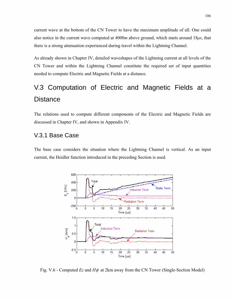
106

current wave at the bottom of the CN Tower to have the maximum amplitude of all. One could

also notice in the current wave computed at 4000m above ground, which starts around 18µs, that

there is a strong attenuation experienced during travel within the Lightning Channel.

As already shown in Chapter IV, detailed waveshapes of the Lightning current at all levels of the

CN Tower and within the Lightning Channel constitute the required set of input quantities

needed to compute Electric and Magnetic Fields at a distance.

V.3 Computation of Electric and Magnetic Fields at a

Distance

The relations used to compute different components of the Electric and Magnetic Fields are

discussed in Chapter IV, and shown in Appendix IV.

V.3.1 Base Case

The base case considers the situation where the Lightning Channel is vertical. As an input

current, the Heidler function introduced in the preceding Section is used.

Fig. V.6 - Computed Ez and Hφ at 2km away from the CN Tower (Single-Section Model)

107

Eqs. (IV.19-IV.24) are evaluated using current produced by the Single-, Three-, and Five-

Section Model and computing Electric and Magnetic Field components Ez and Hφ at a distance

2km away from the CN Tower. Resultant graphs are shown in Figs. V.6-V.8, where the

individual contribution terms are clearly marked.

It is observed in Figs. V.6-V.8 that the waveforms of both Ez and Hφ have initial peaks which

look very similar to each other. This is mainly due to the Radiation Term component which is

proportional to the derivative of the injected current. The contribution of the Induction Term,

which is proportional to the injected current, also has similar influence upon the total calculated

Ez and Hφ field components. After the peak, the Ez waveform ramps up and this is because of

the contribution of the Static Term, which is proportional to the integral of the injected current

(or the amount of transferred charge). Since there is no Static Term in the Hφ field, the tail of the

curve is not ramping up, but similar trends in the instances of appearance of distinctive “bumps”

and “dips” are observed in both calculated fields.

Fig. V.7 - Computed Ez and Hφ at 2km away from the CN Tower (Three-Section Model)

108

Fig. V.8 - Computed Ez and Hφ at 2km away from the CN Tower (Five-Section Model)

Although at first glance, the overall waveforms in the presented plots of Figs. V.6-V.8 might

look the same, under closer examination one could notice that there are some important

differences which are mainly observed in the finer waveform detail and in the peak values. In

order to better appreciate these deviations Fig. V.9 is prepared.

Fig. V.9 - Computed Ez and Hφ at 2km away from the CN Tower

109

It is clearly visible in Fig. V.9 that there is a difference in the peak values yielded by the three

employed models. The peak value is most influenced by the Radiation Term. It is apparent in

Fig. V.2 that, when the Five-Section Model is used, the first peak is reaching the highest value,

because there is a positive reflection coming from the top of the Space Deck. The Three-Section

Model does not include reflections from the Space Deck and thus yields a slightly lower first

peak. There is a considerable contribution due to the reflection coming from the Skypod, which

is considered in both the Three- and Five-Section Models and consequently these two models

predict higher peaks than the Single-Section Model as expected.

It is also observed in Fig. V.9 that the curve computed using the Single-Section Model is

smoother when compared to the corresponding ones calculated by the Three- and Five-Section

Models. In the case of the Single-Section Model only reflections at the extremities of the tower

are considered and the curve is basically influenced only by these. In the waveforms described

by the Three- and Five-Section Models reflections from the top and bottom of the additionally

introduced Skypod and Space Deck contribute to the computed waveshapes and produce a more

elaborated profile. Nevertheless, the waveforms predicted by the three models at later times

(when the reflections have been somewhat suppressed) are very close to each other and even the

simple Single-Section Model yields reasonably matching results to ones computed using the

most sophisticated Five-Section Model.

It is worth pointing out that although the first influences due to the reflections at the Space Deck

when the Five-Section Model is considered are comparably small, they have relatively high

contribution since they occur at early times both, within the Tower itself and inside the Fully

Ionized part of the Lightning Channel, where they travel only a small distance until they reach

the top of the propagating upwards Lightning Channel front. At that point parts of them are

reflected and parts of them continue beyond the Lightning Channel front together with the initial

injected wave at the slower speed of propagation v. These components influence the total

currents and in turn the radiated fields at very early times.

V.3.2 Sensitivity Studies

Relations pertinent to cases in which an inclination of the Lightning Channel is considered are

shown in Appendix V. Taking advantage of such expressions (V.A1-V.A24), one could perform

110

unlimited number of case studies, involving various inclined or tortuous channel trajectories. In

this Thesis, based on developments shown in Chapter IV, sensitivity analyses were carried out,

using the previously introduced Single-, Three-, and Five-Section Models, for straight Lightning

Channel that is inclined at different angles γ with respect to the vertical Lightning Channel, and

lies at various angles φ (please see Fig. IV.3) in the x-y plane. Moreover, a sensitivity study

looking into the influence of variable Lightning Channel front speed was also implemented.

V.3.2.1 Sensitivity Study of Lightning Channel Inclination

Plots showing computed waveforms of Ez, Hx, for straight vertical Lightning Channel (base

case) could be seen in Figs. V.6-V.8. Similar plots were prepared for a number of study case

scenarios in which the inclination angle γ was set to specific fixed angles (γ = 0°, 15°, 30°, 45°,

60°, 75°, 90°). For each fixed inclination angle γ, calculations were implemented for rotation

angles φ =0-360°. The values of the first peaks were then extracted and recorded. Corresponding

plots are shown in Figs. V.10-V.11 for the Single-Section Model, in Figs. V.12-V.13 for the

Three-Section Model, and in Figs. V.14-V.15 for the Five-Section Model.

Fig. V.10 - Computed Ez as a function of φ for different γ (Single-Section Model)

111

Fig. V.11 - Computed Hx as a function of φ for different γ (Single-Section Model)

It is observed in Figs. V.10 and V.11 that in general, for a given angle γ, peak amplitudes of both

Ez and Hx start at a maximum value for φ = 0°, reach a minimum at φ = 180° and climb back to

the maximum at φ = 360°. Furthermore, please observe that with increasing values of Lightning

Channel inclination angle γ, maximum values of the Electric as well as of the Magnetic Field do

not necessarily increase monotonically, while their minima continuously diminish with γ.

Fig. V.12 - Computed Ez as a function of φ for different γ (Three-Section Model)

112

Fig. V.13 - Computed Hx as a function of φ for different γ (Three-Section Model)

Fig. V.14 - Computed Ez as a function of φ for different γ (Five-Section Model)

113

Fig. V.15 - Computed Hx as a function of φ for different γ (Five-Section Model)

When considering the results yielded by the Five-Section Model (Figs. V.14-V.15) one could

notice that the peak values of Ez are affected by the inclined Lightning Channel from –10.95 %

(for the minima) up to +12.48 % (for the maxima). Corresponding changes for Hx are -11.01 %

and +9.66 %.

Fig. V.16 - Peak Values of Hx as a Function of γ

114

In the performed sensitivity study, it was found that the three considered models of the CN

Tower indicate similar tendencies regarding peak values of Ez and Hx. However, the more

sophisticated multi-section models predict results that are in closer agreement with each other.

This tendency is depicted for the case of the radial Magnetic Field component in Fig. V.16.

When examining Fig. V.16 in detail one can notice that the Three and Five-Section Models yield

quite similar results, which differ noticeably from the ones achieved using the Single-Section

Model. It is clearly seen that the Single-Section Model predicts in all considered cases lower Hx

peak values and this is due to the fact that major points of reflections were not considered (Space

Deck and Skypod of the CN Tower).

Use of the newly introduced Cartesian Coordinates presents the opportunity to consider different

trajectories of the Lightning Channel in computation of Ez and Hx. Each introduced more

sophisticated “Engineering” model (Single, Three and Five Sections representing the CN Tower

and two sections representing the Lightning Channel) reproduces closer and closer the Lightning

current waveshape along the CN Tower and in the Lightning Channel. Although it has been

shown [22] that the Lightning Channel has 2-3 times smaller contribution to producing the total

radiated fields than the CN Tower itself, the performed sensitivity study shows that different

channel inclinations may influence the waveforms of radiated fields by more than 10%.

V.3.2.2 Sensitivity Study of Different Lightning Channel Front

Speeds

In this study, the employed relations describing the current at any height and at any time along

the CN Tower and the Lightning Channel are presented in Chapter III. Corresponding

expressions for the vertical component of the Electric as well as the azimuthal component of the

Magnetic Field are shown in Chapter IV. Assumed is a vertical Lightning Channel and the

simulations are limited up to 60µs. However, the produced plots shown in the following Figs.

V.17-V.22 are limited up to 20µs in order to better visualize the deviations in the waveforms at

early times. Considered speeds of propagation of the Lightning Channel front are seen in Fig.

III.6.

115

Fig. V.17 - Ez Computed Using the Single-Section Model

Fig. V.18 - Hx Computed Using the Single-Section Model

116

It is observed in the waveforms shown in Figs. V.17-V.18 that, in addition to reflection details,

the peak values of Ez and of Hx computed by the use of the Single-Section Model at 2km away

from CN Tower, are also affected by the different speed of propagation of the Lightning Channel

front.

Fig. V.19 - Ez Computed Using the Three-Section Model

Fig. V.20 - Hx Computed Using the Three-Section Model

117

Fig. V.21 - Ez Computed Using the Five-Section Model

Fig. V.22 - Hx Computed Using the Five-Section Model

In addition to the observed deviations in the predicted peaks in Figs. V.19-V.22, it is also seen

that the calculated resultant radiation fields calculated with different front propagation velocities

118

feature different decay steepness after the major peaks. Moreover, the fine profile observed in

both Ez and Hx waveforms is containing some considerable deviations mostly in the region

around and after 6µs. Potentially, it may be possible that in some particular cases these

deviations may become larger in values and thus have some more pronounced influence on

affected devices susceptible to electromagnetic radiation.

In summary, it could be said that the developed formulae regarding Ez and Hx components in

Cartesian Coordinates coupled with the proposed new approach to study the influence of variable

Lightning Channel propagation speed upon the radiated fields at a particular distance present the

opportunity to conduct unlimited different scenario cases involving inclined Lightning Channel.

V.3.3 Validation of Newly Proposed Formulae

V.3.3.1 Comparison to Another Author’s Study Results

In order to validate the relations for Electric and Magnetic Fields derived in Cartesian

Coordinates (in particular Eq. IV.19 and Eq. IV.24 shown in Chapter IV), let us now consider the

same cases analyzed in [114]. In that study, the current used was represented by a Double-

exponential function:

)]))((exp())([exp()( 221

1

1 tTatTaItIo −−−=η

(V.1)

In Eq. V.1, the parameters used were:

;)(

;1264.30;6005.0;0973.0;15

2

1

2111

taatT

eaeakAI

−=

==== η

Different geometries for all considered cases in [114] are shown in Fig. V.23. This time the

computation of Ez and Hx components was carried out using the newly proposed equations in

Cartesian Coordinates (Eqs. IV.24 and IV.19). Predicted Ez and Hx waveforms at 2km away

from the CN Tower for the simulated cases seen in Fig. V.23 are presented in Fig. V.24 and in

Fig. V.25. The appearance (scales and waveforms) of these plots is matched to the corresponding

ones in [114] for easier comparison.

119

Fig. V.23 - Simulated Cases of Lightning Return Stroke to the Tower with Different Channel

Inclinations (Adapted from [114])

The details pertaining to the simulated cases are as follows:

- Case A – base case when the Lightning Channel is vertical and thus φ = 0° and γ = 0°;

- Case B1 (B2) – φ = 0° and γ = 22.5° (45°);

- Case C1 (C2) – φ = 90° and γ = 22.5° (45°);

- Case D1 (D2) – φ = 180° and γ = 22.5° (45°);

- Case E – φ = 90° and γ1 = 67.5°; γ2 = 22.5° (l1=100m, l2=2600m).

120

Fig. V.24 - Computed Ez fo

Fig. V.25 - Computed Hx fo

While there are some minor differences, th

exactly the same order as the correspondin

r Simulated Cases from Fig. V.23

r Simulated Cases from Fig. V.23

e curves shown in Figs. V.24-V.25 are stacked in

g ones in [114]. For φ = 0° (cases B1 and B2)

121

amplitudes of both Ez and Hx exceed those of the base case (φ = 0° and γ = 0°), for φ = 90°

(cases C1 and C2) they lie below the base case, finally for φ = 180° (cases D1 and D2) their

amplitudes are smallest of all. The reader should be alerted in particular to the curves

representing case E, where the change in the inclination of the Lightning Channel is clearly

reproduced at around 1.2µs. On the basis of these observations it may be stated that the used Eqs.

IV.19 and IV.24 have been successfully validated.

V.3.3.2 Comparison to a Real Event

It was already mentioned that Hφ and Ez are routinely captured at the University of Toronto.

Using Eqs. IV.19 and IV.24 one could compute, in Cartesian Coordinate system, theoretical

predictions of the waveforms of the fields. An actual event, whose current was recorded at the

474m level and respective fields at 2km away from CN Tower on August 19, 2005, shown in

Figs. II.3-II.6 will be considered for the purpose of a comparison.

In this prediction the Five-Section Model of the CN Tower was used. As the first step, the

appropriate injection current was derived through comparison of the observed and computed

current at the 474m level. Fig. V.26 shows the considered current derivative and current records

and the simulated ones after the final adjustments.

Fig. V.26 - Recorded and Calculated Current and Current Derivative at 474m Above Ground

122

It is worth noting that the speed of propagation of the Lightning Channel front also plays quite an

important role in simulating the current waveshape at concrete levels. If a different speed of

propagation were assumed, certain reflections would take place at corresponding specific

instances of time and thus influence the final waveshape in a different manner. The most

pronounced influence comes from the major reflection from the top of the Fully-Ionized

Lightning Channel.

Fig. V.27 is offered in order to appreciate the impact of the chosen speed of propagation in the

Not-Fully-Ionized part of the Lightning Channel. In Fig. V.27 several major points of reflections

are clearly marked by arrows and the recorded waveform is plotted in thick line. The calculated

wave using speed of propagation of the Lightning Channel front equal to 1.9e8m/s is shown in

dashed-dotted line and the dotted line is corresponding to speed of propagation equal to

1.0e8m/s.

Fig. V.27 - Recorded and Calculated Current at 474m Above Ground

It is clearly seen in Fig. V.27 that when the higher speed of propagation is adopted the major

reflection from the top of the Fully-Ionized Lightning Channel occurs at later time. Since the

current wave calculated by the lower speed (1.0e8m/s) is a better match to the recorded

waveform, it was selected as the appropriate one together with the following set of Heidler

123

parameters:

Io1 = 1.5kA; τ11 = 0.15µs; τ21 = 7µs; n1 = 2

Io2 = 3.5kA; τ12 = 0.25µs; τ22 = 90µs; n2 = 2

Such described current and Lightning Channel propagation speed were then plugged in the

relations for distant fields in order to carry out the computations and produce the respective plots

depicting the vertical component of the Electric Field and the azimuthal component of the

Magnetic Field for which corresponding records exist.

The calculation of radiated fields due to the CN Tower and the Lightning Channel at a distance

of 2km away from the tower included reconstruction of the Lightning Channel in 3-D space

based on the visual records from Figs II.5 and II.6. The assumed Lightning Channel trajectory is

shown in Fig V.28 and in Fig. V.29, and the corresponding heights and angles are as follows:

h1=553m; h2=587m; h3=621m; h4=689m; h5=807m;

1=45°; 2=45°; 3=45°; 4=30°; 5=30°; 6=45°; 7=45°.

Fig. V.28 - Reconstructed Lightning Channel Trajectory in 3-D Space (Visual Record)

124

Fig. V.29 - Reconstructed Lightning Channel Trajectory in 3-D Space (Drawing Reproduction)

Fig. V.30 - Recorded and Calculated Ez and Hx at 2km away from CN Tower

125

Fig V.30 shows the recorded and computed at 2km away from the CN Tower (in Pratt building of

University of Toronto) waveforms of Ez, and Hx respectively.

As is seen in Figs V.26-V.27, the observed and the computed current derivative and current were

successfully closely matched, since there was the possibility to adjust the injected current and

speed of Return Stroke front propagation. Radiated fields shown in Fig V.30, while displaying

correct shape of waveforms, do not have their amplitudes even closely matched. There are a few

reasons for that. It is shown in another study [80] that due to omission in modeling of existing

metallic frames and pipes, found in buildings sitting in the propagation path between the

radiating tall structure and the recording equipment, the predicted fields are underestimating the

actual fields and usually the deviation is more than 25%. Furthermore, there is some

enhancement due to the metallic edge of the roof where the sensors are mounted and this may be

the reason that the Electric Field is even further apart from that measured than the Magnetic

Field.

Also, please note that the Lightning Channel is reconstructed in 3-D space based on observations

in 2-D, which will bring some additional error. Currently, there is a possibility to capture the

Lightning Channel trajectory in 3-D and it is planned in future studies to develop techniques for

precise determination of the 3-D shape of the Lightning Channel to model the radiated fields. It

is well observed in Figs. V.10-V.16, and in Figs. V.23-V.25 that the Lightning Channel has some

considerable influence upon the total radiated fields and thus its contribution should be carefully

evaluated in each considered case.

V.3.4 Prospects for Computation of the Ex, Ey Components of the

Electric Field and Hy, Hz Components of the Magnetic Field

Ex, Hy, and Hz components have not been considered much in technical literature until now due

to several reasons including the lack of formulae to compute them and the fact that they have not

been routinely measured. Ex, Hy, and Hz are also not considered since they do not have any

contribution when the Lightning Channel is considered to be vertical as is assumed in most

“Engineering” models. An expression describing the radial component (Ey) of the Electric Field

in Cylindrical Coordinates is found in [112]. For observation point on the y axis and for vertical

Lightning Channel, which are commonly assumed, the Ey is also equal to zero, though.

126

Unfortunately, this component has not been monitored at the CN Tower site and no actual

records are available. However, currently observations are being performed at the Austrian

Gaisberg Tower as reported in [115-116]. The motivation behind these observations stems from

the fact that the radial (horizontal) component has some influence for the more realistic cases

when the observation point is not on the y axis, but is elevated at some height. It is reported in

[115] that at farther distances there is a difference of several orders of magnitude between the

amplitudes of the Ez and Ey components, but nevertheless the Ey component exists and has some

noticeable contribution. Furthermore, in reality the Lightning Channel is never vertical, thus all

the remaining components (Ex, Hy, and Hz) also have some contribution. It follows that in

certain cases all of the above or at least some of the considered components should not be

neglected as they might have potentially some considerable influence in the radiated Electric and

Magnetic Fields and in turn unaccounted effects upon some sensitive electronic or electrical

equipment. The newly proposed expressions (Eq. IV.19-IV.24) are now available and could be

used to estimate the impact of various Electric and Magnetic Field components if an inclined and

tortuous Lightning Channel were assumed for observation points at any height and distance.

127

Chapter VI Concluding Remarks

The objective of this work, namely to develop a sophisticated model describing Lightning events

at the CN Tower in Toronto, has been implemented successfully. In contrast to presently popular

frequency-domain approaches, computational algorithms have been developed in this thesis in

the time domain. Furthermore, the new formulae that have been derived bring new insights that

should improve the understanding of the electromagnetic radiation process associated with

Lightning at tall structures and enhance modeling of its impact upon the surroundings.

In this thesis, three transmission-line-based “Engineering” models, each representing in greater

detail the structural peculiarities of the CN Tower, have been considered. In those models, the

tower is represented by one, three, and five transmission line sections of respective lengths and

impedances. In each case, the Lightning Channel is modeled by two transmission line sections;

their respective impedances are constant, while their lengths are variable. The author has

presented to the technical literature the Five-Section Model of the CN Tower for the first time.

A novelty is introduced at the border between the two sections of the Lightning Channel. In most

other works, the authors assume that there is a discontinuity in the current components that reach

the Return Stroke front and beyond this point they cease to exist. This is physically inconsistent

and requires additional measures to rectify the situation. In the presented work this is not an

issue, since the discontinuity is fully taken into account and the effects of reflected and

transmitted current components are truthfully reproduced. The transmitted components are

joining the originally injected current wave, add up to it and propagate at the same lower speed

upwards within the Not-Fully Ionized portion of the Lightning Channel, while the reflected

components head back inside the channel’s Fully Ionized portion towards the tip of the tower at

the speed of light.

Another novelty and major contribution provides the possibility to take into account variable

speed v of Return Stroke front propagation. Until now only constant speed v has been considered

in the technical literature. At the same time observations at the CN Tower had indicated that this

speed may be either constant, or decreasing, or even increasing as the Return Stroke front

progresses up the Lightning Channel. In the thesis it is shown that the chosen speed pattern

128

exerts considerable effect upon the current waveshapes at different levels of the tower and of the

Lightning Channel as well as upon the radiated fields at a distance.

Third major contribution is the introduction of newly developed expressions describing different

components of the radiated fields in Cartesian Coordinates. These equations constitute very

powerful tools that present the opportunity to study the influence of the Lightning Channel

trajectory, which could assume any general shape in the 3-D space. It has been shown in the

thesis that, in different cases involving the inclined channel, there is considerable variation, not

only in the resultant peak values, but also in the shapes of associated waveforms as well. This

means that the theoretical predictions, in some particular cases whenever the Lightning Channel

is assumed to be vertical rather than resembling more closely its actual trajectory, will yield

estimated radiated fields that may deviate substantially from the actual ones, and one should

keep that fact in mind.

The developed theoretical expressions might be used to study the impact of field components

that have not been considered until now, namely Ex, Hy, and Hz. As already mentioned, these

components are normally neglected since for the commonly assumed vertical channel, they do

not have any contribution. However, as briefly discussed in Chapter V, these components do

exist for all cases involving inclined Lightning Channel for observation points at some height

above ground level and might have some unforeseen effects upon the radiated fields and in turn

upon the devices susceptible to electromagnetic interference. One could take advantage of the

developed theoretical expressions in this thesis work, adapt them to their own study case and

estimate the potential impact. Furthermore, sensitivity analysis involving inclined Lightning

Channel could be performed for the Ey component, as well. There is a readily available in the

technical literature expression for this component, but it is in Cylindrical Coordinates and

assumed vertical Lightning Channel only. Now the flexibility to relax the condition regarding the

verticality of the Lightning Channel exists and could be taken advantage of.

Another quantity that has been considered by some authors, but not studied extensively, is the

radial component of the Magnetic Field Hy. At the CN Tower this component has been

monitored for various periods of time, so that some records do exist in the archives. It might be a

good sub-project area to look into these records and perform some analysis using the analytical

expressions developed in this thesis.

129

A separate research area could be a study looking into the influence of the CN Tower height

upon the current waveshapes as well as upon the respective radiated fields at a distance. Along

these lines, a study may be initiated, in which analysis of the influence of the CN Tower shape

could be undertaken, i.e. to explore, what would be the impact if some of the major points of

reflections, such as the Space Deck or the Skypod were located at different heights. On a

completely general basis, adapting the proposed modeling approach, studies could be

implemented during the design stage of new tall towers to establish the impact of proposed

structural shapes upon Lightning-caused radiated fields.

130

References [1] Wilson, C. T. R. (1920). “Investigations on Lightning Discharges and the Electric Field of

Thunderstorms”. Phil. Trans. Roy. Soc. Lond., 221(A):73–115.

[2] Martin A. Uman, “The Lightning Discharge”, Academic Press, Inc., 1987.

[3] Vladimir A. Rakov and Martin A. Uman, “Lightning: Physics and Effects”, Cambridge

University Press, 2003.

[4] Vernon Cooray (edited by), “The Lightning Flash”, The Institution of Electrical Engineers,

2003.

[5] National Weather Service (2007), "Lightning Safety". National Weather Service.

http://www.lightningsafety.noaa.gov/science.htm.

[6] NASA (2005), "Flashes in the Sky: Lightning Zaps Space Radiation Surrounding Earth",

NASA http://www.nasa.gov/vision/universe/solarsystem/image_lightning.html.

[7] Robert Roy Britt (1999), "Lightning Interacts with Space, Electrons Rain Down", Space.com.

http://www.space.com/scienceastronomy/planetearth/space_lightning_991216.html.

[8] Demirkol, M. K.; Inan, Umran S.; Bell, T.F.; Kanekal, S.G.; and Wilkinson, D.C. (December

1999), "(abstract) Ionospheric Effects of Relativistic Electron Enhancement Events",

Geophysical Research Letters Vol. 26 (No. 23): 3557–3560. doi:10.1029/1999GL010686.

http://adsabs.harvard.edu/abs/1999GeoRL..26.3557D (abstract).

[9] Dr. Hugh J. Christian; Melanie A. McCook, "A Lightning Primer - Characteristics of a

Storm", NASA. http://thunder.nsstc.nasa.gov/primer/primer2.html.

[10] Boccippio, D. J., et al. (August 1995), "Sprites, ELF Transients, and Positive Ground

Strokes", Science 269: 1088–1091. doi:10.1126/science.269.5227.1088. PMID 17755531.

[11] Sterling D. Allen - Pure Energy Systems News (2005), "BLAM-O!! Power from Lightning",

Pure Energy Systems, http://pesn.com/2005/07/10/9600120_Livingstone_Lightning/.

http://www.lightningsafety.noaa.gov/science.htm

http://thunder.nsstc.nasa.gov/primer/primer2.html

131

[12] Walter A. Lyons and Michey D. Schmidt (2003), “P1.39 The Discovery of Red Sprites as an

Opportunity For Informal Science Education”, American Meteorological Society.

[13] Tom Clarke (2002), "Blue Jets Connect Earth's Electric Circuit", Nature.com.

http://www.nature.com/news/2002/020311/pf/020311-6_pf.html. Retrieved on 2007

[14] W. Wayt Gibbs for Scientific American, "Lightning's Strange Cousins Flicker Faster than

Light Itself", Scientific American. http://www-star.stanford.edu/~vlf/optical/press/elves97sciam/.

[15] William L. Boeck, Otha H. Vaughan Jr., R. J. Blakeslee, Bernard Vonnegut and Marx

Brook, 1998, “The Role of the Space Shuttle Videotapes in the Discovery of Sprites, Jets and

Elves”, Journal of Atmospheric and Solar-Terrestrial Physics, Vol. 60, Issues 7-9, p. 669-677.

[16] Mason B. J., “A Critical Examination of Theories of Charge Generation in Thunderstorms”,

Tellus, 1953, 5, pp. 446-460.

[17] Moore C.B. and Vonnegut B., “The thundercloud” in GOLDE, R. H. (Ed.), “Lightning, vol.

1:Physics of lightning”, (Academic press, San Diego, CA, 1977) pp.51-98.

[18] Earle R. Williams, “The Electrification of Thunderstorms”, Scientific American, November

1988.

[19] Grenet G., “Essai d’explication de la charge electrique des nuages d’orages”, Ann.

Geophys., 1947, 3, pp. 306-307

[20] Berger, K., “Blitzstrom-Parameter von Aufwartsblitzen”, Bull. Schweiz. Elektrotech. Ver.,

69:353-360, 1978.

[21] J.L. Bermudez , F. Rachidi, W. Janischewskyj, A.M. Hussein, M. Rubinstein, C.A. Nucci,

M. Paolone, V. Shostak, J.S. Chang, “On the Enhancement of Radiated Electric and Magnetic

Fields Associated with Lightning Return Strokes to Tall Structures”, IEEE 2001.

[22] Farhad Rachidi, Wasyl Janischewskyj, Ali M. Hussein, Carlo Alberto Nucci, Silvia

Guerrieri, Behzad Kordi, and Jen-Shih Chang, “Current and Electromagnetic Field Associated

With Lightning-Return Strokes to Tall Towers”, IEEE Transactions on Electromagnetic

Compatibility, Vol. 43, No. 3, August 2001.

http://www.nature.com/news/2002/020311/pf/020311-6_pf.html. Retrieved on 2007

132

[23] Pavanello, D., Rachidi, F., Rubinstein, M., Bermudez, J. L., Nucci, C. A., “Electromagnetic

Field Radiated by Lightning to Tall Towers: Treatment of the Discontinuity at the Return Stroke

Wave Front”, Journal of Geophysical Research, vol. 109, num. D6, 2004, p. D06114 (7 pp.).

[24] F. Rachidi, V.A. Rakov, C.A. Nucci, J.L. Bermúdez, "The Effect of Vertically-Extended

Strike Object on the Distribution ofCurrent Along the Lightning Channel", Journal of

Geophysical Research 107/D23 (2002) pp. 4699.

[25] F. Rachidi, R. Thottappillil, "Determination of Lightning Currents from Far Electromagnetic

Fields", Journal of Geophysical Research 98 (1993) 18315–18320.

[26] Y. Baba, M. Ishii, "Numerical Electromagnetic Field Analysis on Lightning Surge Response

of Tower with Shield Wire", IEEE Transactions on Power Delivery 15 (2000) 1010–1015.

[27] V.A. Rakov, "Transient Response of a Tall Object to Lightning", IEEE Transactions on

Electromagnetic Compatibility 43 (2001) 654–661.

[28] McEachron, K. B., “Lightning to the Empire State Building”, J. Franklin Inst. 227: 149-217,

1939.

[29] Berger, K., and Vogelsanger, E., “Messungen und Resultate der Blitzforschung der Jahre

1955-1963 auf dem Monte San Salvatore”, Bull. Schweiz. Electrotech. Ver. 56: 2-22, 1965.

[30] Berger, K. Anderson, R. B., and Kroninger, H., “Parameters of Lightning Flashes”, Electra

80:223-37, 1975.

[31] Gorin, B. N., and Shkilev, A. V., “Measurements of Lightning Currents at the Ostankino

Tower”, Elektrichestvo 8: 64-5, 1984.

[32] Garbagnati, E., Marinoni, F., and Lo Piparo, G. B., “Parameters of Lightning Currents.

Interpretation of the Results Obtained in Italy”, In Proc. 16th Int. Conf. On Lightning Protection,

Szeged, Hungary, paper R-1.03, 16 pp., 1981.

[33] Eriksson, A. J., “The CSIR Lightning Research Mast-Data for 1972-1982, NEERI Internal

Report no. EK/9/82, National Electrical and Engineering Research Institute”, Pretoria, South

Africa, 1982.

133

[34] Hussein, A. M., Janischewskyj, W., Chang, J-S., Shostak, V., Chisholm, W. A., Dzurevych,

P., and Kawasaki, Z.-I., “Simultaneous Measurement of Lightning Parameters for Strokes to the

Toronto Canadian National Tower”, J. Geophys. Res. 100: 8853-61, 1995.

[35] Janischewskyj, W., Shostak, V., Barratt, J. Hussein, A. M., Rusan, R., and Chang., J.-S.,

“Collection and Use of Lightning Return-Stroke Parameters Taking Into Account Characteristics

of the Struck Object”, In Proc. 23rd Int. Conf. On Lightning Protection, Florence, Italy, pp. 16-

23., 1995.

[36] Beierl, O., “Front Shape Parameters of Negative Subsequent Strokes Measured at

Peissenberg Tower”, In Proc. 21st Int. Conf. On Lightning Protection, Berlin, Germany, pp. 19-

24, 1992.

[37] Fuchs, F., Landers, E. U., Schmid, R., and Weisinger, J., “Lightning Current and Magnetic

Field Parameters Caused by Lightning Strokes to Tall Structures Relating to Interference of

Electronic Systems”, IEEE Trans. Electromagn. Compat., 40:444-51, 1998.

[38] Montandon, E., “Messung und Ortung von Blitzeinschlaegen und ihren Auswirkungen am

Fernmeldeturm “St. Chrischona” bei Basel der Schweizerischen Telecom PTT”, Elektrotechnik

und Informationstechnik 112:283-9, 1995.

[39] Lacerda, M., Pinto, O., Pinto, I. R. C. A., Diniz, J. H., and Carvalho, A. M., “Analysis of

Negative Downward Lightning Current Curves from 1985 to 1994 at Morro do Cachimbo

Research Station (Brazil)”, In Proc. 11th Int. Conf. On Atmospheric Electricity, Guntersville,

Alabama, pp. 42-5., 1999.

[40] Diendorfer, G., Mair, M., Schulz, W., and Hadrian, W., “Lightning Current Measurements

in Austria – Experimental Setup and First Results”, In Proc. 25th Int. Conf. On Lightning

Protection, Rhodes, Greece, pp.44-7, 2000.

[41] Newman, M. M., “Use of Triggered Lightning to Study the Discharge Channel”, in

Problems of Atmospheric and Space Electricity, pp.482-90, New York: Elsevier, 1965.

[42] Rakov, V. A., “Lightning Discharges Triggered Using Rocket and Wire Techniques”, In

Recent Res. Devel. Geophysics, vol. 2, pp. 141-71, Research Signpost, India, 1999.

134

[43] Uman, M. A., Rakov, V. A., Rambo, K. J., Vaught, T. W., Fernandez, M. I., Bach, J. A., Su,

Y., Eybert-Berard, A., Berlandis, J.-P., Bador, B., Lalande, P., Bonamy, A., Audran, F.,

Morillon, F., Laroche, P., Bondiou-Clergerie, A., Chauzy, S., Soula, S., Weidman, C. D.,

Rachidi, F., Rubinstein, M. Nucci, C. A., Guerrieri, S., Hoidalen, H. K., and Cooray, V., “1995

Triggered Lightning Experiment in Florida”, In Proc. 10th Int. Conf. On Atmospheric Electricity,

Osaka, Japan, pp. 647-7, 1996.

[44] Rakov, V. A., Uman, M. A., Fernandez, M. I., Thottappillil, R., Eybert-Berard, A.,

Berlanidis, J. P., Rachidi, F., Rubinstein, M., Guerrieri, S., and Nucci, C. A., 1996, “Observed

Electromagnetic Environment Close to the Lightning Channel”, In Proc. 23rd Int. Conf. On

Lightning Protection, Florence, Italy, pp. 30-5.

[45] V. A. Rakov, M. A. Uman, “Review and Evaluation of Lightning Return Stroke Models

Including Some Aspects of Their Application”, IEEE Transactions on Electromagnetic

Compatibility, Vol. 40, No. 4, pp. 403-426, November 1998.

[46] Plooster, M. N., “Shock waves from line sources. Numerical solutions and experimental

measurements”, Physics of Fluids, 13, 2665-2675, 1970.

[47] Plooster, M. N., “Numerical Model of the Return Stroke of the Lightning Discharge”,

Physics of Fluids, 14, 2124-2133, 1971.

[48] Plooster, M. N., “Numerical Simulation of Spark Discharges in Air”, Physics of Fluids, 14,

2111-2123, 1971.

[49] R. D. Hill, “Channel Heating in Return Stroke Lightning”, J. Geophys. Res., vol. 76, pp.

637–645, 1971.

[50] R. D. Hill, “Energy Dissipation in Lightning”, J. Geophys. Res., vol. 82, pp. 4967–4968,

1977.

[51] D. F. Strawe, “Non-Linear Modeling of Lightning Return Strokes”, in Proc. Fed. Aviat.

Administra./Florida Inst. Technol. Workshop Grounding Lightning Technol., Melbourne, FL,

Mar. 1979, pp. 9–15, Rep. FAARD-79-6.

135

[52] A. H. Paxton, R. L. Gardner, and L. Baker, “Lightning Return Stroke: A Numerical

Calculation of the Optical Radiation”, Phys. Fluids, vol. 29, pp. 2736–2741, 1986.

[53] A. H. Paxton, R. L. Gardner, and L. Baker, “Lightning Return stroke: A Numerical

Calculation of the Optical Radiation”, in Lightning Electromagnetics. New York: Hemisphere,

1990, pp. 47–61.

[54] A. S. Bizjaev, V. P. Larionov, and E. H. Prokhorov, “Energetic Characteristics of Lightning

Channel”, in Proc. 20th Int. Conf. Lightning Protect., Interlaken, Switzerland, Sept. 1990, pp.

1.1/1–1.1/3.

[55] E. I. Dubovoy, V. I. Pryazhinsky, and G. I. Chitanava, “Calculation of Energy Dissipation in

Lightning Channel”, Meteorologiya i Gidrologiya, no. 2, pp. 40–45, 1991.

[56] E. I. Dubovoy, V. I. Pryazhinsky, and V. E. Bondarenko, “Numerical Modeling of the

Gasodynamical Parameters of a Lightning Channel and Radio-Sounding Reflection”, Izvestiya

AN SSSR-Fizika Atmosfery i Okeana, vol. 27, pp. 194–203, 1991.

[57] E. I. Dubovoy, M. S. Mikhailov, A. L. Ogonkov, and V. I. Pryazhinsky, “Measurement and

Numerical Modeling of Radio Sounding Reflection from a Lightning Channel”, J. Geophys.

Res., vol. 100, pp. 1497–1502, 1995.

[58] Baba, Y., and M. Ishii, “Numerical Electromagnetic Field Analysis of Lightning Current in

Tall Structures”, IEEE Transactions on Power Delivery, 16, 324-328, 2001.

[59] Moini, R., B. Kordi, G. Z. Rafi, and V. A. Rakov, “A New Lightning Return Stroke Model

Based on Antenna Theory”, Journal of Geophysical Research, 105, 29693-29702, 2000.

[60] Petrache, E., F. Rachidi, D. Pavanello, W. Janischewskyj, A. M. Hussein, M. Rubinstein, V.

Shostak, W. A. Chisholm, and J. S. Chang, “Lightning Strikes to Elevated Structures: Influence

of Grounding Conditions on Currents and Electromagnetic Fields”, paper presented at IEEE

International Symposium on Electromagnetic Compatibility, Chicago, August 2005.

[61] Petrache, E., F. Rachidi, D. Pavanello, W. Janischewskyj, M. Rubinstein, W. A. Chisholm,

A. M. Hussein, V. Shostak, and J. S. Chang, “Influence of the Finite Ground Conductivity on the

Transient Response to Lightning of a Tower and its Grounding”, paper presented at 28th General

136

Assembly of International Union of Radio Science (URSI), New Delhi, India, October 23-29,

2005.

[62] Little, P. F., “Transmission Line Representation of a Lightning Return Stroke”, Journal of

Physics D, 11, 1893-1910, 1978.

[63] Price, G. H., and E. T. Pierce, “The Modeling of Channel Current in the Lightning Return

Stroke”, Radio Science, 12, 381-388,1972.

[64] Gomes, C., and V. Cooray, “Concepts of Lightning Return Stroke Models”, IEEE

Transactions on Electromagnetic Compatibility, 42, 82-96, 2000.

[65] Nucci, C. A., G. Diendorfer, M. Uman, F. Rachidi, M. Ianoz, and C. Mazzetti, “Lightning

Return Stroke Current Models with Specified Channel-Base Current: A Review and

Comparison”, Journal of Geophysical Research, 95, 20395-20408, 1990.

[66] R. Thottappillil, V. A. Rakov, and M. A. Uman, “Distribution of Charge Along the

Lightning Channel: Relation to Remote Electric and Magnetic Fields and to Return Stroke

Models”, J. Geophys. Res., vol. 102, pp. 6887–7006, 1997.

[67] V. A. Rakov, “Lightning Electromagnetic Fields: Modeling and Measurements”, in Proc.

12th Int. Zurich Symp. Electromagn. Compat., Zurich, Switzerland, pp. 59–64, Feb. 1997.

[68] V. A. Rakov and A. A. Dulzon, “A Modified Transmission Line Model for Lightning

Return Stroke Field Calculations”, in Proc. 9th Int. Zurich. Symp. Electromagn. Compat.,

Zurich, Switzerland, pp. 229–235, Mar. 1991.

[69] M. A. Uman and D. K. McLain, “Magnetic Field of the Lightning Return Stroke”, J.

Geophys. Res., vol. 74, pp. 6899–6910, 1969.

[70] V. A. Rakov and A. A. Dulzon, “Calculated Electromagnetic Fields of Lightning Return

Stroke”, Tekh. Elektrodinam., no. 1, pp. 87–89, 1987.

[71] C. A. Nucci, C. Mazzetti, F. Rachidi, and M. Ianoz, “On Lightning Return Stroke Models

for LEMP Calculations”, in Proc. 19th Int. Conf. Lightning Protection, Graz, Austria, Apr. 1988.

137

[72] C. E. R. Bruce and R. H. Golde, “The Lightning Discharge”, J. Inst. Elect. Eng.—Pt. 2, vol.

88, pp. 487–520, 1941.

[73] F. Heidler, “Traveling Current Source Model for LEMP Calculation”, in Proc. 6th Int.

Zurich Symp. Electromagn. Compat., Zurich, Switzerland, Mar. 1985, pp. 157–162.

[74] Yoshihiro Baba, Satoru Miyazaki, and Masaru Ishii, “Reproduction of Lightning

Electromagnetic Field Waveforms by Engineering Model of Return Stroke”, IEEE Transactions

on Electromagnetic Compatibility, vol. 46, no. 1, February 2004.

[75] G. Diendorfer and M. A. Uman, “An Improved Return Stroke Model with Specified

Channel-Base Current”, J. Geophys. Res., vol. 95, pp. 13,621–13,644, 1990.

[76] S. Guerrieri, F. Heidler, C.A. Nucci, F. Rachidi, and M. Rubinstein, “Extension of Two

Return Stroke Models to Consider the Influence of Elevated Strike Objects on the Lightning

Return Stroke Current and the Radiated Electric Field”, in Proc. Int. Conf. EMC, Sept. 1996.

[77] Rachidi, F., V. A. Rakov, C. A. Nucci, and J. L. Bermudez, “The Effect of Vertically-

Extended Strike Object on the Distribution of Current Along the Lightning Channel”, Journal of

Geophysical Research, 107, 4699, 2002.

[78] Le Vine, D. M., and J. C. Willett, “Comment on the Transmission Line Model for

Computing Radiation from Lightning”, Journal of Geophysical Research, 97, 2601-2610, 1992.

[79] Rubinstein, M., and M. A. Uman, “On the Radiation Field Turn-On Term Associated with

Travelling Current Discontinuities in Lightning”, Journal of Geophysical Research, 95, 3711-

3713, 1990.

[80] Davide Pavanello, , “Electromagnetic Radiation from Lightning Return Strokes to Tall

Structures”, PhD Thesis, EPFL, Lausanne, 2007.

[81] A. S. Podgorski and J. A. Landt, “Three Dimensional Time Domain Modeling of

Lightning”, IEEE Trans. Power Del., vol. PWRD-2, pp. 931–938, July 1987.

138

[82] H. Motoyama, W. Janischewskyj, A. M. Hussein, R. Rusan, W. A. Chisholm, and J.-S.

Chang, “Electromagnetic Field Radiation Model for Lightning Strokes to Tall Structures”, IEEE

Trans. Power Delivery, vol. 11, no.3, pp.1624-1632, Jul. 1996.

[83] Behzad Kordi, Rouzbeh Moini, Wasyl Janischewskyj, Ali M. Hussein,Volodymyr O.

Shostak, and Vladimir A. Rakov, “Application of the Antenna Theory Model to a Tall Tower

Struck by Lightning”, Journal of Geophysical Research, vol. 108, no. D17, 4542,

doi:10.1029/2003JD003398, 2003.

[84] S. Guerrieri, C. A. Nucci, F. Rachidi, and M. Rubinstein, “On the Influence of Elevated

Strike Objects on Directly Measured and Indirectly Estimated Lightning Currents”, IEEE

Transactions on Power Delivery, Vol. 13, No. 4, October 1998.

[85] F. Rachidi, W. Janischewskyj, A. M. Hussein, C. A. Nucci, S. Guerrieri, and J. S. Chang,

“Electromagnetic Fields Radiated by Lightning Return Strokes to High Towers”, in Proc. 24th

Int. Conf. Lightning Protection, Birmingham, U.K., Sept. 1998, pp. 23–28.

[86] V. Shostak, W. Janischewskyj, A. M. Hussein, J.-S. Chang, and B. Kordi, “Return Stroke

Current Modeling of Lightning Striking a Tall Tower Accounting for Reflections within the

Growing Channel and for Upward-Connecting Discharges”, in Proc. Int. Conf. on Atmospheric

Electricity, Gunterville, AL, 1999.

[87] Radu Rusan, “Computation of Electromagnetic Fields Radiated by Lightning Strikes to the

Toronto CN Tower”, MASC Thesis, University of Toronto, 1997.

[88] V. Shostak, W. Janischewskyj, A. M. Hussein, “Expanding the Modified Transmission Line

Model to Account for Reflections Within the Continuously Growing Lightning Return Stroke

Channel”, IEEE/PES Summer Meeting, 2589-2602, Seattle, WA, USA, July 16-20, 2000.

[89] Ivan Boev, “Development of a Five-Section Model for Computing Lightning Current in the

CN Tower”, MASC Thesis, University of Toronto, 2006.

[90] Janischewskyj, A.M. Hussein, V. Shostak, I. Rusan. J.-X. Li and I.-S. Chang, “Statistics of

Lightning Strikes to the Toronto CN Tower (1978-1995),” IEEE Trans. Power Delivery, vol. 2,

no. 3, pp. 1210-1221, July 1997.

139

[91] A.M. Hussein. W. Janischewskyj. M. Milewski, V. Shostak, J.S. Chang and W. Chisholm,

“Return-Stroke Current Waveform Parameters of Lightning to the CN Tower (1992-2001),”

Proceedings of the 26th International Conference on Lightning Protection (ICLP), pp. 161 - 166.

Cracow, Poland, Sept. 2-6.2002.

[92] W. Janischewskyj, A.M. Hussein, Wiacek and J.S. Chang, “Details of CN Tower Flashes

Utilizing a Digital High-Speed Camera.“ Proceedings, The 24th International Conference on

Lightning Protection, Birmingham, U.K., Sept 14-18. 1998. pp. 101-106.

[93] W. Janischewskyj, A.M. Hussein and V. Shostak, “Propagation of Lightning Current within

the CN Tower”, CIGRE SC 33.97, Toronto, Ontario, Canada, September 2-3, 1997.

[94] A.M. Hussein, W. Janischewskyj, M. Milewski, V. Shostak and J.S. Chang, “Waveform

Characteristics of Electric and Magnetic Fields Generated by Lightning to the CN Tower,”

International Symposium on Wireless Systems and Networks, University of Petroleum and

Minerals, Dhahran, Saudi Arabia, March 24-26, 2003, Paper #148 (pp. 1-5).

[95] T.R. McComb, H. Linck, E.A. Cherney, W. Janischewskyj, “Preliminary Measurements of

Lightning Flashes to the CN Tower in Toronto”, Canadian Electrical Engineering Journal, Vol.

5, No. 4, October 1980, pp. 3-9.

[96] W. Janischewskyj, J.S. Chang, K. Yandulska, A.M. Hussein, V. Shostak, F. Rachidi, W.A,

Chisholm, D. Pavanello, E. Petrache, I. Boev, M. Milewski, “Lightning Multiplicity at the CN

Tower in Toronto as Recorded by Six Different Instruments”, Ground 2006 and 2nd LPE,

Maceio, Brazil, November 26-29, 2006.

[97] J. L. Bermudez, F. Rachidi, W. A. Chisholm, M. Rubinstein, W. Janischewskyj, A. M.

Hussein, V. Shostak, J. S. Chang, “On the Use of Transmission Line Theory to Represent a

Nonuniform Vertically-Extended Object Struck by Lightning”, IEEE 2003.

[98] W. Janischewskyj, V. Shostak and A.M. Hussein, “Multi-Section Lightning-Current Model

of the CN Tower,” Proceedings of the 6th International Symposium on Lightning Protection (VI

SIPDA), Santos, Brazil, Nov. 19-23, 2001, pp. 281-286.

140

[99] W. A. Chisholm, Y. L. Chow, and K. D. Srivastava, “Lightning Surge Response of

Transmission Towers,” IEEE Trans. Power App. Syst., vol. PAS-102, pp. 3232–3242, Sept.

1983.

[100] F. Heidler, J. M. Cvetic, B. V. Stanic, “Calculation of Lightning Current Parameters,”

IEEE Trans. On Power Delivery, vol. 14, no. 2, pp. 399–404, Apr. 1999.

[101] Chang, Jen-Shih, Asakawa, A., Wada, S., Janischewskyj, W., Yamamoto, K., Kawasaki,

Z., Shindo, T., Hussein, A.M., Uchida, Y., Iwasaki, S., Ueno, J., Pavanello, D., Matsuura, K.,

Bermudez, J.L., Rachidi, F. and Shostak, V., “Tall Structure Lightning Return Stroke Velocity

Measurements for the CN Telecommunication Tower”, VIII International Symposium on

Lightning Protection (VIII SIPDA), San Paulo, Brazil, 21st -25th November 2005.

[102] J. A. Stratton, “Electromagnetic Theory”, McGraw-Hill, New York, 1941.

[103] J. D. Jackson, “Classical Electrodynamics”, Wiley, New York, 1962.

[104] D. S. Jones, “The Theory of Electromagnetism”, Pergamon, Oxford, 1964.

[105] R. P. Feynman, R. B. Leighton, and M. Sands, “The Feynman Lectures on Physics”,

Addison-Wesley, Reading, MA, 1964, Vol. II.

[106] W. K. H. Panofsky and M. Phillips, “Classical Electricity and Magnetism”, Addison-

Wesley, Reading, MA, 1962.

[107] J. R. Reitz and F. J. Milford, “Foundations of Electromagnetic Theory”, Addison-Wesley,

Reading, MA 1960.

[108] Stuart M. Wentworth, “Fundamentals of Electromagnetics with Engineering Applications”,

Wiley, John Wiley & Sons, Inc., 2005.

[109] Halevi, Peter (1992). Spatial Dispersion in Solids and Plasmas. Amsterdam: North-

Holland. ISBN 978-0444874054.

[110] Jackson, John David (1999). Classical Electrodynamics (3rd ed. ed.). New York: Wiley.

ISBN 0-471-30932-X.

141

[111] Martin A. Uman, D. Kenneth McLain, E. Philip Krider “The Electromagnetic Radiation

from a Finite Antenna,”AJP, Volume 43, pp. 33–38, January 1975.

[112] M. J. Master, M. A. Uman “Transient Electric and Magnetic Fields Associated with

Establishing a Finite Electrostatic Dipole,”Am. J. Phys. 51 (2), pp. 118–126, February 1983.

[113] I. Boev, W Janischewskyj, “Calculation of Electric and Magnetic Fields at the CN Tower

in Cartesian Coordinates” presented at MOCA-09 Joint Assembly on July 27, 2009, Montreal,

Canada.

[114] V. Shostak, W. Janischewskyj, A. M. Hussein, F. Rachidi, J. L. Bermudez, and B. Kordi,

“Electromagnetic Field Associated with Lightning Return Strokes to a Tall Structure: Influence

of Channel Geometry”, 2003 IEEE Bologna PowerTech Conference, June 23-26, Bologna, Italy.

[115] F. Rachidi, M. Rubinstein, A. Shoory, R. Thottappillil, “On the Measurement and

Calculation of Lightning Horizontal Electric Fields” presented at MOCA-09, Montreal, Canada

on July 27, 2009.

[116] A. Mosaddeghi, F. Rachidi, M. Rubinstein, G. Diendorfer, H. Pichler, D. Pavanello, M.

Nyffeler, “Close-Range Electromagnetic Fields Associated with Lightning Strikes to the

Austrian Gaisberg Tower” presented at IPLT-09, Montreal, Canada on July 29, 2009.

142

Appendix I

Current Distribution for Single-Section Model of the CN Tower

Fig. II.10 found in Chapter II is depicting the adopted Single-Section Model. All assumptions

pertinent to that model are listed in Chapter II as well. In this Appendix, only the developed

expressions for currents at any time and height along the structure of the tower and along the

Lightning Channel are fully shown together with more detailed respective Lattice diagrams.

Furthermore, expansion of σ and ξ terms is also included. Finally, input parameters of the

Heidler function primarily used in the thesis are listed under AI.3 at the end of this Appendix.

AI.1 Current Distributions for Single-Section Model

Fig. AI.1 - Detailed Lattice Diagram for Single-Section Model (inside the CN Tower)

AI.1.1 Major Components (inside the CN Tower)

∑∞

=

+

⎭⎬⎫

⎩⎨⎧

⎟⎠⎞

⎜⎝⎛ −

+−+⎟

⎠⎞

⎜⎝⎛ −

−−=

00

10

22n

nt

nb

nt

nbM c

nhc

zhtikkcnh

czhtikki (AI.1)

where hz ≤≤0

143

AI.1.2 Additional Contributions (inside the CN Tower)

( ) ( )

( ) ( )

( ) ( )

( ) ( ) ⎟⎠⎞

⎜⎝⎛ −+−−+=

⎟⎠⎞

⎜⎝⎛ −+−−+=

⎟⎠⎞

⎜⎝⎛ ++−−+=

⎟⎠⎞

⎜⎝⎛ −+−−+=

czhhtikkkkki

czhhtikkkkki

czhhtikkkki

czhhtikkkki

tcttbA

ttctbA

tctbA

tctbA

ξ

ξ

ξ

ξ

411

3211

211

211

02

4.

02

3.

02

2,

01,

(AI.2)

where vcvc

vcvhz

−+

=−

=≤≤ ξσ0

AI.1.3 Channel Base Current (initial current propagating upwards

in the not-fully ionized portion of the Lightning Channel)

⎟⎟⎠

⎞⎜⎜⎝

⎛ −

⎟⎠⎞

⎜⎝⎛ −−= ψ

zh

tch

tch e

vhzti

zzi 0 (AI.3)

for MAXzzh ≤≤

Fig. AI.2 - Detailed Lattice Diagram for Single-Section Model (inside the Lightning Channel)

144

Fig. AI.2 shows a Lattice diagram containing more details pertinent to the relations for Internal

and Transmitted components. Numbers 2, 4, 6, … 2m represent the corresponding “First”,

“Second”, “Third”, … and “mth” reflections from ground respectively.

AI.1.4 Internal Components “bouncing” within the Ionized Portion

of the Lightning Channel (contributions due to the “mth” reflection

coming from ground)

( ) ( ) ( ) ( )∑∞

=

−− ⎟

⎠⎞

⎜⎝⎛ −

−−−+=0

01

12,21

n

nnt

nct

mt

mbmI c

hzcmhtikkkkki ξ (AI.4a)

( ) ( ) ( ) ( )( )∑∞

=

+−⎟⎟⎠

⎞⎜⎜⎝

⎛ −+−

−−−+=

00

112,

2121n

nnn

tnct

mt

mbmI c

zmhvc

mhtikkkkki σξξ (AI.4b)

where: ( ) ,...3,2,121 =≤+<< mzmhzh MAXnσξ ,

AI.1.5 Components Transmitted into the not-fully Ionized Portion

of the Lightning Channel

The Transmitted components are shown in Fig. AI.2 by arrows (at heights h, z2, z4,… and at

times t0, t2, t4,… respectively), which are parallel to the dashed line representing the Return

Stroke wave propagating in the upward direction (to the right). Their respective initial times and

heights of occurrence are marked clearly and are found to be the following expressions:

( )

( )

( )...

221

221

221

26

26

14

14

02

02

ξσξ

ξσξ

ξσξ

vcmhtmhz

vcmhtmhz

vcmhtmhz

−=+=

−=+=

−=+=

(AI.5)

Now, one could derive a general relation for the Transmitted contributions due to the “mth”

reflection coming from ground:

145

( ) ( ) ( ) ( ) ⎟⎟⎠

⎞⎜⎜⎝

⎛ −∞

=

−⎟⎟⎠

⎞⎜⎜⎝

⎛ +−−

−−+−+=∑ ψσξξ

zhnn

cn

tnct

n

mt

mbTm e

vmhz

vcmhtikkkkkki 21211 0

0

1 (AI.6)

where

( ) ,...3,2,121 =≤<+ mzzmh MAXnσξ

AI.2 Expanding of σ and ξ terms

Fig. AI.3 - Geometric Relations for Deriving Expressions for σ and ξ Terms

First, let us consider “line A” ( Actz += )

cLt 1

12

= ; ; hz =1

at →−=→−=→=+→ 1111 2LhActhAhActt 12Lhctz −+=

Let us now look at the intersection of “line A” and hvtz +=

at ( ) 122122 22 LvcthvtLhctt =−→+=−+→

vcLt−

= 12

2 ; →−+=+= 1222 2Lhcthvtz σ12 2Lhz +=

146

)()(2

)()(24242 11111

123 vccvcL

vccvcLcL

cL

vcLttt

−+

=−

−−=−

−=−=

ξcLt 1

32

= ; hz =3

where vc

v−

=σ , and ( )( )vc

vc−+

=ξ

Now, let us consider “line B” ( Bctz += )

at →−=→−=→=+→ ξ1333 2LhBcthBhBctt ξ12Lhctz −+=

Let us look at the intersection of “line B” and hvtz +=

at ( ) ξξ 144144 22 LvcthvtLhctt =−→+=−+→

ξvc

Lt−

= 14

2 ; →−+=+= ξ1444 2Lhcthvtz σξ14 2Lhz +=

in a similar manner it could be shown that:

215

2 ξcLt = ; and hz =5

216

2 ξvc

Lt−

= ; and 216 2 σξLhz +=

or in general:

nn c

Lt ξ112

2=+ ; and hz n =+12

nn vc

Lt ξ−

=+1

222 ; and n

n Lhz σξ122 2+=+

for ,...2,1,0=n

147

AI.3 Input Parameters of the Heidler Function

The injected “uncontaminated” current wave, used as input to the model, is approximated by a

sum of two Heidler functions. All respective parameters used are presented in Table AI.1, and

the produced current derivative and current waveshapes using Eq. V.3 are depicted in Fig. AI.4.

Typical corresponding current waveforms that would be computed using the Single-Section

Model at 474m and at 509m above ground level are shown in Fig. AI.5. These particular heights

are of interest since there are permanently mounted and operating current sensing elements at

474m and at 509m above ground level levels. A large pool of recorded data exists and the

calculated resultant waveforms could be easily compared to existing captured current and current

derivative waveshapes.

Table AI.1– Heidler Function – Input Parameters

Io1 [ kA] τ11 [µs] τ21 [µs] n1 [-] Io2 [kA] τ12 [µs] τ22 [µs] n2 [-]

10.7 0.25 2.5 2 6.5 2 230 2

Fig. AI.4 - Injected (“uncontaminated” by reflections) Heidler Current Derivative and Current

148

Fig. AI.5 - Calculated Current Derivative and Current at 474m and at 509m Above Ground Level

In the timeframe up to 5µs, shown in Fig. AI.5 above, the reflection coming from the ground at

about 3.5µs (for the 509m above ground computed current and also current derivative) is clearly

seen. This reflection is positive, due to the positive reflection coefficient at ground level and adds

up to the current to produce the maximum current peak value at the respective time.

149

Appendix II

Current Distribution for Three-Section Model of the CN Tower

Fig. AII.1 - Three-Sections Model3

AII.1 Assumptions

All assumptions previously described in “Appendix I” hold, except for the impedances and

lengths of respective CN Tower sections. Let us re-emphasize that current contributions with

peak values less than 1% of the input wave peak are neglected. The values of impedances used

3 Note, that the Lightning Channel is shown for the general case, when both Not-Fully Ionized (dashed line) and Fully Ionized (thick line) portions of the Lightning Channel exist, while in the instance of time when the Return-Stroke current is initiated only the Not-Fully Ionized part of the Lightning Channel is present.

150

in the Three-Section Model are listed in Table AII.1 below. The reflection coefficients are

computed using the relations:


o kt = (Z1-Zch)/(Z1+Zch);

o k12=(Z1-Z2)/(Z1+Z2);

o k23=(Z2-Z3)/(Z2+Z3);

o kb = (Z3-Zg)/(Z3+Zg);

Table AII.1 Surge Impedances and Lengths for Three-Section Model

Section # Length [m]

Reflection coefficient

Impedance [Ω]

LC - not ionized 8000-z Ztch 495 kc -0.20 LC – fully ionized z (variable) Zch 330

kt -0.35 L1 188 Z1 160

k12 0.30 L2 30 Z2 86 k23 -0.24 L3 335 Z3 140

Zg - kb 0.65 Zg 30

AII.2 Current Distributions for Three-Section Model

Fig. AII.2 - Partial Lattice Diagram for the Three-Section Model of the CN Tower

151

Not all components seen in Fig. AII.2 above are used to come up with the respective current

waveshapes at particular heights of interest. This is so, because many of them have very little

influence upon the final computed current waveform and only slow down the computation

without changing the result much. Only those contributions due to reflections and refractions at

different locations along the structure of the tower and in the Lightning Channel that are higher

than 1% in amplitude of the original injected wave are followed. All these considered

contributions used in the Three-Section Model are shown by means of their corresponding

graphical representations and analytical expressions below:

AII.2.1 Current inside L1 ( , for ∑=

=14

1kkii mz 553365 ≤< )

Fig. AII.3 - Current contributions i1 & i2

∑∞

=⎟⎠⎞

⎜⎝⎛ −

−−=

0

10121

2n

nt

n ncL

czhtikki (AII.1)

∑∞

=

+ ⎟⎠⎞

⎜⎝⎛ −

+−−=

0

110

1122

22n

nt

n ncL

czhLtikki (AII.2)


( ) ( )∑∞

=

+++ ⎟⎠⎞

⎜⎝⎛ −

+−−−+=

0

12120

112

123

1123

2211n

nnnnt n

cL

czhLtikkkki (AII.3)

( ) ( )∑∞

=

++++ ⎟⎠⎞

⎜⎝⎛ −

−+−−+=

0

12120

112

123

112

14

2211n

nnnnt n

cL

czhLtikkkki (AII.4)

152


( ) ( ) ( ) ( )∑∞

=

+++++ ⎟⎠⎞

⎜⎝⎛ −

+−−−++=

00

112

123

1123

1125

21111n

nnnb

nnnt n

ch

czhtikkkkkki (AII.5)

( ) ( ) ( ) ( )∑∞

=

++++++ ⎟⎠⎞

⎜⎝⎛ −

−−−−++=

00

112

123

1123

112

16

231111n

nnnb

nnnt n

ch



( ) ( ) ( )∑∞

=

++ ⎟⎠⎞

⎜⎝⎛ −

+−+−+−=

0

11120122312

11127

22112n

nt

n ncL

czhLLtikkkkki (AII.7)

( ) ( ) ( )∑∞

=

++ ⎟⎠⎞

⎜⎝⎛ −

−++−+−=

0

11120122312

21128

22112n

nt

n ncL

czhLLtikkkkki (AII.8)


( )( ) ( )( ) ( )∑∞

=

++ ⎟⎠⎞

⎜⎝⎛ −

+−+−−−++=

0

11023122312

11129

2211112n

bnt

n ncL

czhLhtikkkkkkki (AII.9)

( )( ) ( )( ) ( )∑∞

=

++ ⎟⎠⎞

⎜⎝⎛ −

−++−−−++=

0

11023122312

211210

2211112n

bnt

n ncL

czhLhtikkkkkkki (AII.10)

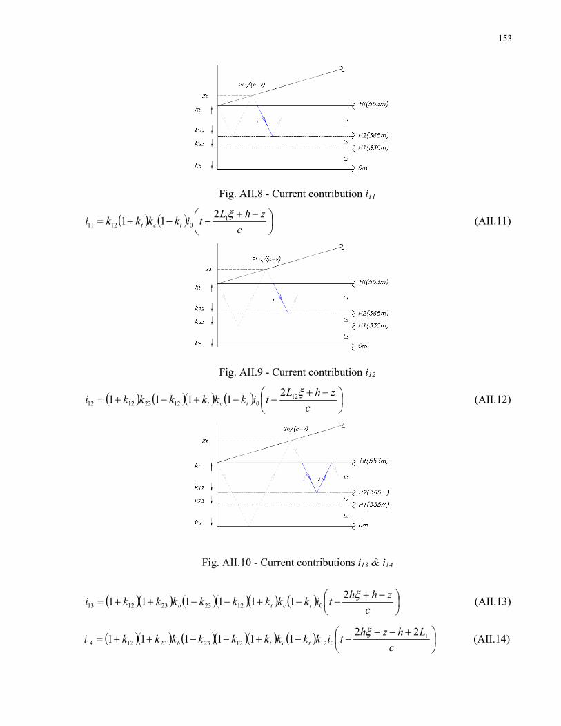
153

Fig. AII.8 - Current contribution i11

( ) ( ) ⎟⎠⎞

⎜⎝⎛ −+−−+=

czhLtikkkki tct

ξ101211

211 (AII.11)


( ) ( )( ) ( ) ⎟⎠⎞

⎜⎝⎛ −+−−+−+=

czhLtikkkkkki tct

ξ12012231212

21111 (AII.12)


( )( ) ( )( )( ) ( ) ⎟⎠⎞

⎜⎝⎛ −+−−+−−++=

czhhtikkkkkkkki tctb

ξ2111111 01223231213 (AII.13)

( )( ) ( )( )( ) ( ) ⎟⎠⎞

⎜⎝⎛ +−+−−+−−++=

cLhzhtikkkkkkkkki tctb

10121223231214

22111111 ξ (AII.14)

154

AII.2.2 Current inside L2 ( , for ) 171615

8

1iiiii

kk +++=∑

=

mz 365335 ≤<


( ) ( ) ( ) ( )∑∞

=

+ ⎟⎠⎞

⎜⎝⎛ −

−−−−++=

00122323

1121

21111n

nt

nnnb

nn nch


( ) ( ) ( ) ( )∑∞

=

++++ ⎟⎠⎞

⎜⎝⎛ −

+−−−++=

0012

123

1123

1122

21111n

nt

nnnb

nn nch



( ) ( ) ( ) ( )∑∞

=

+ ⎟⎠⎞

⎜⎝⎛ −

−+−−−++=

0

10122323

112123

221111n

nt

nnnb

nnt n

ch

czhLtikkkkkkkki (AII.17)

( ) ( ) ( ) ( )∑∞

=

++++ ⎟⎠⎞

⎜⎝⎛ −

++−−−++=

0

1012

123

1123

112124

221111n

nt

nnnb

nnt n

ch

czhLtikkkkkkkki (AII.18)


( ) ( )∑∞

=

+ ⎟⎠⎞

⎜⎝⎛ −

−+−−+=

0

23012

123125

221n

nn ncL

cLzhtikkki (AII.19)

155

( ) ( )∑∞

=

++ ⎟⎠⎞

⎜⎝⎛ −

−+−−+=

0

220

112

123126

221n

nn ncL

czLhtikkki (AII.20)


( )( ) ( )( )∑∞

=

+ ⎟⎠⎞

⎜⎝⎛ −

−+−−−++=

0

223023

1122323127

22111n

nnb n

cL

czLhtikkkkkki (AII.21)

( )( ) ( )( )∑∞

=

++ ⎟⎠⎞

⎜⎝⎛ −

++−−−++=

0

220

123

1122323128

22111n

nnb n

cL



( ) ( )( ) ⎟⎠⎞

⎜⎝⎛ −+−+−+=

czhLtikkkkki tct

ξ10121215

2111 (AII.23)

Fig. AII.16 - Current contributions i16

( ) ( )( ) ( ) ⎟⎠⎞

⎜⎝⎛ −+−−+−+=

czhLtikkkkkki tct

ξ1201223

21216

21111 (AII.24)

156

Fig. AII.17 - Current contributions i17

( ) ( ) ( )( )( ) ( ) ⎟⎠⎞

⎜⎝⎛ −+−−+−−++=


ξ2111111 01223232

1217 (AII.25)

AII.2.3 Current inside L3 ( , for ∑∑==

+=23

18

12

1 mm

kk iii mz 3350 ≤< )


( )( ) ( )∑∞

=⎟⎠⎞

⎜⎝⎛ −

−−−++=

0

302323121

211n

nnb n

cL

czhtikkkki (AII.26)

( )( ) ( )∑∞

=

+ ⎟⎠⎞

⎜⎝⎛ −

+−−++=

0

3023

123122

211n

nnb n

cL

czhtikkkki (AII.27)


( ) ( ) ( )∑∞

=

+ ⎟⎠⎞

⎜⎝⎛ −

−+−+−+=

0

32023

11223123

2211n

nb

n ncL

czLhtikkkkki (AII.28)

157

( ) ( ) ( )∑∞

=

++ ⎟⎠⎞

⎜⎝⎛ −

++−+−+=

0

320

123

11223124

2211n

nb

n ncL

czLhtikkkkki (AII.29)


( )( ) ( )∑∞

=⎟⎠⎞

⎜⎝⎛ −

−+−−++=

0

310232312125

2211n

nnbt n

cL


( )( ) ( )∑∞

=

+ ⎟⎠⎞

⎜⎝⎛ −

++−−++=

0

31023

12312126

2211n

nnbt n

cL



( ) ( ) ( ) ( )∑∞

=⎟⎠⎞

⎜⎝⎛ −

−+−−+−+=

0

312023231223

2127

22111n

nnbt n

cL

czLhtikkkkkkki (AII.32)

( ) ( ) ( ) ( )∑∞

=

+ ⎟⎠⎞

⎜⎝⎛ −

++−−+−+=

0

312023

1231223

2128

22111n

nnbt n

cL

czLhtikkkkkkki (AII.33)


( )( ) ( )∑∞

=⎟⎠⎞

⎜⎝⎛ −

−+−−++=

0

310232312

22129

2411n

nnbt n

cL


( )( ) ( )∑∞

=

+ ⎟⎠⎞

⎜⎝⎛ −

++−−++=

0

31023

12312

221210

2411n

nnbt n

cL


158


( ) ( ) ( ) ( )∑∞

=

++++++ ⎟⎠⎞

⎜⎝⎛ −

−−−−++=

00

1112

123

1223

21211

231111n

nt

nnnb

nn nch


( ) ( ) ( ) ( )∑∞

=

++++++ ⎟⎠⎞

⎜⎝⎛ −

+−−−++=

00

1112

123

2223

21212

231111n

nt

nnnb

nn nch



( ) ( )( )( ) ⎟⎠⎞

⎜⎝⎛ −+−++−+=

czhLtikkkkkki tct

ξ1023121218

21111 (AII.38)

( ) ( )( )( ) ⎟⎠⎞

⎜⎝⎛ ++−++−+=

czhLtikkkkkkki btct

ξ1023121219

21111 (AII.39)


159

( ) ( )( ) ( )( ) ⎟⎠⎞

⎜⎝⎛ −+−+−+−+=

czhLtikkkkkkki tct

ξ120231223

21220

211111 (AII.40)

( ) ( )( ) ( )( ) ⎟⎠⎞

⎜⎝⎛ ++−+−+−+=

czhLtikkkkkkkki btct

ξ120231223

21221

211111 (AII.41)


( ) ( ) ( )( )( ) ( ) ⎟⎠⎞

⎜⎝⎛ −+−−+−−++=


ξ2111111 012232

232

1222 (AII.42)

( ) ( ) ( )( )( ) ( ) ⎟⎠⎞

⎜⎝⎛ ++−−+−−++=


ξ2111111 0122322

232

1223 (AII.43)

AII.3 Derivation of Relations for the Reflections Taking

Place within the Lightning Channel

AII.3.1 Channel Base Current Propagating upwards &Transmitted

Components in the Lightning Channel

Fig. AII.27 - Current contributions ich, iT1, iT2, iT3, iT3, & iT5

160

⎟⎟⎠

⎞⎜⎜⎝

⎛ −

⎟⎠⎞

⎜⎝⎛ −−= ψ

zh

tchch e

vhzti

ZZi 0

1 (AII.44)

for m 553≥z

( ) ⎟⎟⎠

⎞⎜⎜⎝

⎛ −

⎟⎠⎞

⎜⎝⎛ +−

−−

−++= ψσzh

ctT ev

Lhzvc

Ltikkki 110121

22)1)(1( (AII.45)

for ∞<<+ zLh σ12

( ) ( )( )( ) ( ) ⎟⎟⎠

⎞⎜⎜⎝

⎛ −

⎟⎠⎞

⎜⎝⎛ +−

−−

−++−+= ψσzh

ctT ev

Lhzvc

Ltikkkkki 121201223122

221111 (AII.46)

for ∞<<+ zLh σ122

( )( ) ( )( )( )( )( ) ⎟⎟

⎠

⎞⎜⎜⎝

⎛ −

⎟⎠⎞

⎜⎝⎛ +−

−−

−

++−−++=

ψσzh

ctbT

ev

hhzvc

hti

kkkkkkki

22.

111111

0

122323123

(AII.47)

for ∞<<+ zhh σ2

( ) ( ) ( )( )( ) ( )( ) ⎟⎟

⎠

⎞⎜⎜⎝

⎛ −

⎟⎠⎞

⎜⎝⎛ ++−

−−+

−

++−+=

ψσzh

cttT

ev

LLhzvcLLti

kkkkkkki

1121120

121223124

22.

1111

(AII.48)

for ( ) ∞<<++ zLLh σ1122

( )( ) ( )( ) ( )( )( ) ( )( ) ⎟⎟

⎠

⎞⎜⎜⎝

⎛ −

⎟⎠⎞

⎜⎝⎛ ++−

−−+

−

++−−++=

ψσzh

cttbT

ev

LhhzvcLhti

kkkkkkkkki

110

12122323125

22.

1111112

(AII.49)

for ( ) ∞<<++ zLhh σ12

AII.3.2 Internal Components in the LC

161


( )( ) ( )( )( ) ( )

⎟⎠⎞

⎜⎝⎛ −

−−

−+−−++= ∑∞

=

chz

chti

kkkkkkkki

n

n

nt

nctb

ξ2.

11111

0

0122323121

(AII.50)

( )( ) ( )( )( ) ( )

( )⎟⎟⎠

⎞⎜⎜⎝

⎛ −+−

−−

−+−−++= ∑∞

=

+

czh

vchti

kkkkkkkki

nn

n

nt

nctb

σξξ 212.

11111

0

0

1122323122

(AII.51)

for ( )nhzh σξ21+<< ,


( ) ( )( ) ( )

⎟⎠⎞

⎜⎝⎛ −

−−

−+−+= ∑∞

=

chz

cLti

kkkkkki

n

n

nt

nct

ξ120

01223123

2.

111 (AII.52)

( ) ( )( ) ( )

⎟⎟⎠

⎞⎜⎜⎝

⎛ −+−

−−

−+−+= ∑∞

=

+

czLh

vcLti

kkkkkki

nn

n

nt

nct

σξξ 12120

0

11223124

22.

111 (AII.53)

162

for , nLhzh σξ122+<<


( ) ( )∑∞

=⎟⎠⎞

⎜⎝⎛ −

−−−+=0

10125

21n

nnt

nct c

hzcLtikkkki ξ (AII.54)

( ) ( )∑∞

=

+⎟⎟⎠

⎞⎜⎜⎝

⎛ −+−

−−−+=

0

110

1126

221n

nnn

tnct c

zLhvc

Ltikkkki σξξ (AII.55)

for , nLhzh σξ12+<<


( )( ) ( )( ) ( ) ( )

( )⎟⎠⎞

⎜⎝⎛ −

−+

−

−+−−++= ∑∞

=

chz

cLhti

kkkkkkkkkki

n

n

nt

ncttb

ξ10

012122323127

2.

11111 (AII.56)

163

( )( ) ( )( ) ( ) ( )

( ) ( )⎟⎟⎠

⎞⎜⎜⎝

⎛ −++−

−+

−

−+−−++= ∑∞

=

+

czLhh

vcLhti

kkkkkkkkkki

nn

n

nt

ncttb

σξξ 110

0

112122323128

22.

11111 (AII.57)

for , ( ) nLhhzh σξ12 ++<<


( ) ( ) ( ) ( )

( )⎟⎠⎞

⎜⎝⎛ −

−+

−

−+−+= ∑∞

=

chz

cLLti

kkkkkkkki

n

n

nt

nctt

ξ1120

0121223129

2.

111 (AII.58)

( ) ( ) ( ) ( )

( ) ( )⎟⎟⎠

⎞⎜⎜⎝

⎛ −++−

−+

−

−+−+= ∑∞

=

+

czLLh

vcLLti

kkkkkkkki

nn

n

nt

nctt

σξξ 1121120

0

11212231210

22.

111 (AII.59)

for , ( ) nLLhzh σξ1122 ++<<

Using the Three-Section Model and the same injection current shown in Appendix AI in Fig.

AI.4, the following resultant waveforms at respective levels of interest are calculated:

164

Fig. AII.33 - Calculated Current Derivative and Current at 474m and at 509m Above Ground

Level

It is worth noting that the waveshapes are influenced by the Skypod. In Fig. AII.33 the first most

pronounced influece is well noticed in the current derivative curve, representing the computed

signal at 474m above ground level (thick line), at 1µs. At that time, there is no change in the

corresponding curve shown in Fig. AI.5, because the presence of the Skypod in the Single-

Section Model is neglected.

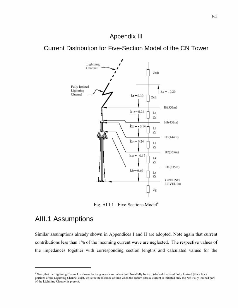
165

Appendix III

Current Distribution for Five-Section Model of the CN Tower

Fig. AIII.1 - Five-Sections Model4

AIII.1 Assumptions

Similar assumptions already shown in Appendices I and II are adopted. Note again that current

contributions less than 1% of the incoming current wave are neglected. The respective values of

the impedances together with corresponding section lengths and calculated values for the

4 Note, that the Lightning Channel is shown for the general case, when both Not-Fully Ionized (dashed line) and Fully Ionized (thick line) portions of the Lightning Channel exist, while in the instance of time when the Return-Stroke current is initiated only the Not-Fully Ionized part of the Lightning Channel is present.

166

reflection coefficients pertinent to the Five-Section Model are listed in Table AIII.1 below. The

reflection coefficients are visualized in Fig. AIII.1, where their “direction” is assigned. They are

computed using the relations:


o kt = (Z1-Zch)/(Z1+Zch);

o k12=(Z1-Z2)/(Z1+Z2);

o k23=(Z2-Z3)/(Z2+Z3);

o k34=(Z3-Z4)/(Z3+Z4);

o k45=(Z4-Z5)/(Z4+Z5);

o kb = (Z5-Zg)/(Z5+Zg);

Table AIII.1

Values of Surge Impedances for Five-Section Model

Section # Length [m]

Reflection coefficient

Impedance [Ω]

LC - not ionized 8000-z Ztch 495 kc -0.20 LC – fully ionized z (variable) Zch 330

kt -0.30 L1 100 Z1 160

k12 0.21 L2 9 Z2 105 k23 -0.14 L3 79 Z3 140 k34 0.24 L4 30 Z4 86 k45 -0.17

L5 335 Z5 120 Zg - kb 0.60 Zg 30

AIII.2 Current Distributions for Five-Section Model

Once again, in the Lattice diagram seen below all components are shown, however, in the

following figures and corresponding expressions only the ones having greater than 1% of the

originally injected current wave are considered.

167

Fig. AIII.2 - Partial Lattice Diagram for the Five-Section Model of the CN Tower

AIII.2.1 Current inside L1 ( mz 553453 ≤< )

Fig. AIII.3 - Current contributions i1 & i2

( ) ( ) ( ) ( ) ( )

( ) ( ) ( ) ⎟⎠⎞

⎜⎝⎛ −

+−−−−

−++++=

+++

∞

=

++++++∑

nch

czhtikkkk

kkkkkki

nt

nnn

n

nnb

nnnn

2111.

11111

01

121

231

34

0

145

1145

134

123

1121

(AIII.1)

( ) ( ) ( ) ( ) ( )

( ) ( ) ( ) ⎟⎠⎞

⎜⎝⎛ −

−−−−−

−++++=

++++

∞

=

++++++∑

nch

czhtikkkk

kkkkkki

nt

nnn

n

nnb

nnnn

23111.

11111

011

121

231

34

0

145

1145

134

123

1122

(AIII.2)

168


( ) ( ) ( ) ( )

( ) ( ) ⎟⎠⎞

⎜⎝⎛ −

+−−−−

−+++=

++

∞

=

+++++∑

nc

Lc

zhLtikkk

kkkkki

nt

nn

n

nnnnn

123412340

112

123

0

134

145

134

123

1123

2211.

1111 (AIII.3)

( ) ( ) ( ) ( )

( ) ( ) ⎟⎠⎞

⎜⎝⎛ −

−+−−−

−+++=

+++

∞

=

+++++∑

nc

Lc

zhLtikkk

kkkkki

nt

nn

n

nnnnn

123412340

1112

123

0

134

145

134

123

1124

2211.

1111 (AIII.4)


( ) ( ) ( )

( ) ⎟⎠⎞

⎜⎝⎛ −

+−−−

−++=

+

∞

=

++++∑

ncL

czhLtikk

kkkki

nt

n

n

nnnn

1231230

112

0

123

134

123

1125

221.

111 (AIII.5)

( ) ( ) ( )

( ) ⎟⎠⎞

⎜⎝⎛ −

−+−−

−++=

++

∞

=

++++∑

ncL

czhLtikk

kkkki

nt

n

n

nnnn

1231230

1112

0

123

134

123

1126

221.

111 (AIII.6)

169


( ) ( )∑∞

=

+++ ⎟⎠⎞

⎜⎝⎛ −

+−−−+=

0

12120

112

123

1127

2211n

nt

nnn ncL

czhLtikkkki (AIII.7)

( ) ( )∑∞

=

++++ ⎟⎠⎞

⎜⎝⎛ −

−+−−+=

0

12120

1112

123

1128

2211n

nt

nnn ncL

czhLtikkkki (AIII.8)


∑∞

=⎟⎠⎞

⎜⎝⎛ −

−−=

0

10129

2n

nt

n ncL

czhtikki (AIII.9)

∑∞

=

+ ⎟⎠⎞

⎜⎝⎛ −

+−−=

0

110

11210

22n

nt

n ncL

czhLtikki (AIII.10)

Fig. AIII.8 - Current contributions i11& i12

( )( )( )( ) ( )( )

( )( ) ( )⎟⎠⎞

⎜⎝⎛ −

+−+−−−

−−++++=

++

∞

=∑

ncL

czhLhtikkkk

kkkkkkki

nnt

nb

110

112

11223

034454534231211

2211.

1111112 (AIII.11)

170

( )( )( )( ) ( )( )

( )( ) ( )⎟⎠⎞

⎜⎝⎛ −

−++−−−

−−++++=

++

∞

=∑

ncL

czhLhtikkkk

kkkkkkki

nnt

nb

110

112

21223

034454534231212

2211.

1111112 (AIII.12)


( )( )( ) ( )( )

( ) ( )⎟⎠⎞

⎜⎝⎛ −

+−+−−

−−+++=

++

∞

=∑

ncL

czhLLtikkk

kkkkkki

nnt

n

1112340

112

112

023344534231213

221.

111112 (AIII.13)

( )( )( ) ( )( )

( ) ( )⎟⎠⎞

⎜⎝⎛ −

−++−−

−−+++=

++

∞

=∑

ncL

czhLLtikkk

kkkkkki

nnt

n

1112340

112

212

023344534231214

221.

111112 (AIII.14)


( )( ) ( )( )

( )⎟⎠⎞

⎜⎝⎛ −

+−+−

−−++= ∑∞

=

++

ncL

czhLLti

kkkkkkkin

nnt

111230

0

112

1122334231215

22.

11112 (AIII.15)

( )( ) ( )( )

( )⎟⎠⎞

⎜⎝⎛ −

−++−

−−++= ∑∞

=

++

ncL

czhLLti

kkkkkkkin

nnt

111230

0

112

2122334231216

22.

11112 (AIII.16)

171


( ) ( )

( )⎟⎠⎞

⎜⎝⎛ −

+−+−

−+= ∑∞

=

++

ncL

czhLLti

kkkkkin

nnt

11120

0

112

112231217

22.

112 (AIII.17)

( ) ( )

( )⎟⎠⎞

⎜⎝⎛ −

−++−

−+= ∑∞

=

++

ncL

czhLLti

kkkkkin

nnt

11120

0

112

212231218

22.

112 (AIII.18)

Fig. AIII.12 - Current contributions ir1, ir2, ir3, ir4, & ir5

( ) ( ) ⎟⎠⎞

⎜⎝⎛ −+−−+=

czhLtikkkki tctr

ξ10121

211 (AIII.19)

( ) ( )( ) ( ) ⎟⎠⎞

⎜⎝⎛ −+−−+−+=

czhLtikkkkkki tctr

ξ1201223122

21111 (AIII.20)

( )( ) ( )( )( ) ( )

⎟⎠⎞

⎜⎝⎛ −+−

−+−−++=

czhLti

kkkkkkkki tctr

ξ1230

12233423123

2.

111111 (AIII.21)

( )( )( ) ( )( )( )

( ) ( ) ⎟⎠⎞

⎜⎝⎛ −+−−+

−−−+++=

czhLtikkk

kkkkkkki

tct

r

ξ12340

122334453423124

211.

111111 (AIII.22)

172

( )( )( )( ) ( )( )( )

( )( ) ( ) ⎟⎠⎞

⎜⎝⎛ −+−−+−

−−−++++=

czhhtikkkk

kkkkkkkki

tct

br

ξ2111.

1111111

012

233445453423125

(AIII.23)

AIII.2.1.1 Additional Currents

Fig. AIII.13 - Current contribution iA1

( ) ( ) ( ) ( ) ⎟⎠⎞

⎜⎝⎛ +−−−−++=

czhLtikkkkkki tA

1230

212

223

234

223

2121

41111 (AIII.24)


( )( ) ( ) ( )( ) ⎟⎠⎞

⎜⎝⎛ +−+−−−−++=

czhLLtikkkkkkiA

2312301212

223

234

223122

221111 (AIII.25)


( ) ( ) ( )( ) ⎟⎠⎞

⎜⎝⎛ +−+−−−++=

czhLLtikkkkkkki tA

12123023

212233423

2123

221111 (AIII.26)

173

Fig. AIII.16 - Current contributions iA4, iA5, & iA6

( ) ( ) ( ) ( ) ( )

( ) ( )( ) ⎟⎠⎞

⎜⎝⎛ ++−−−+

+−−++=

czhLtikkkk

kkkkkkki

b

tA

1230344545

342

122

23342

232

124

2111.

11111 (AIII.27)

( ) ( ) ( ) ( ) ( )

( ) ( )( ) ⎟⎠⎞

⎜⎝⎛ −+−−−+

+−−++=

czhLtikkkkk

kkkkkkki

tb

tA

32111.

11111

1230344545

342

122

23342

232

125

(AIII.28)

( ) ( ) ( ) ( ) ( )

( ) ( ) ( ) ⎟⎠⎞

⎜⎝⎛ ++−−+−

−−+++=

czhLtikkkkk

kkkkkki

bt

A

123404545

212

223

23445

234

223

2126

2111.

11111 (AIII.29)


( )( )( )( ) ( )

( )( )( ) ( ) ⎟⎠⎞

⎜⎝⎛ ++−−−−−

−++++=

czLhtikkkkk

kkkkkki bA

201223122334

45453423127

2111.

11111 (AIII.30)


174

( )( )( )( ) ( )

( )( ) ( )( ) ⎟⎠⎞

⎜⎝⎛ ++−−−−−

−++++=

czLhtikkkkk

kkkkkki bA

301223342334

45453423128

2111.

11111 (AIII.31)

Fig. AIII.19 - Current contributions iA9, & iA10

( )( )( ) ( ) ( )

( ) ( )( )( ) ⎟⎠⎞

⎜⎝⎛ ++−−−−−

−++++=

czLhtikkkk

kkkkkki bA

3450122323

234

245

2245

23423129

2111.

11111 (AIII.32)

( )( )( ) ( ) ( )

( ) ( )( )( ) ⎟⎠⎞

⎜⎝⎛ −+−−−−−

−++++=

czLhtikkkkk

kkkkkki

t

bA

3450122323

234

245

2245

234231210

23111.

11111 (AIII.33)


( )( )( )( ) ( )( )

( )( )( ) ⎟⎠⎞

⎜⎝⎛ ++−−−−

−−++++=

czLhtikkkk

kkkkkkki bA

4012233445

34454534231211

2111.

11111 (AIII.34)


175

( )( )( )( ) ( )

( )( )( )( ) ⎟⎠⎞

⎜⎝⎛ ++−−−−−

−++++=

czLhtikkkk

kkkkkki bA

45012233434

245

224534231212

2111.

11111 (AIII.35)

( )( )( )( ) ( )

( )( )( )( ) ⎟⎠⎞

⎜⎝⎛ −+−−−−−

−++++=

czLhtikkkkk

kkkkkki

t

bA

45012233434

245

224534231213

23111.

11111 (AIII.36)


( )( )( )( ) ( )

( )( )( )( ) ⎟⎠⎞

⎜⎝⎛ ++−−−−−

−++++=

czLhtikkkk

kkkkkki bA

5012233445

452

4534231214

21111.

1111 (AIII.37)

( )( )( )( ) ( )

( )( )( )( ) ⎟⎠⎞

⎜⎝⎛ −+−−−−−

−++++=

czLhtikkkkk

kkkkkki

t

bA

5012233445

452

4534231215

231111.

1111 (AIII.38)


( )( ) ( )( ) ( )

( )( ) ( ) ( ) ⎟⎠⎞

⎜⎝⎛ ++−−−−−

−++++=

czLhtikkkkk

kkkkkki bA

230123412

22334

4545342

231216

2111.

11111 (AIII.39)

176


( )( ) ( ) ( ) ( )

( ) ( ) ( ) ( ) ⎟⎠⎞

⎜⎝⎛ ++−−−−−

−++++=

czLhtikkkkk

kkkkkki bA

2340124512

223

234

45452

342

231217

2111.

11111 (AIII.40)


( )( ) ( ) ( ) ( )

( ) ( ) ( )( ) ⎟⎠⎞

⎜⎝⎛ ++−−−−−

−++++=

czLhtikkkk

kkkkkki bA

234501212

223

234

245

2245

234

2231218

2111.

11111 (AIII.41)

( )( ) ( ) ( ) ( )

( ) ( ) ( )( ) ⎟⎠⎞

⎜⎝⎛ −+−−−−−

−++++=

czLhtikkkkk

kkkkkki

t

bA

234501212

223

234

245

2245

234

2231219

23111.

11111 (AIII.42)



177

( ) ( ) ( ) ( ) ( )

( ) ( ) ( ) ⎟⎠⎞

⎜⎝⎛ −

−−−−−

−++++= ∑∞

=

+

nch

czhtikkkk

kkkkkki

nt

nnn

n

nnb

nnnn

2111.

11111

0122334

045453423

1121

(AIII.43)

( ) ( ) ( ) ( ) ( )

( ) ( ) ( ) ⎟⎠⎞

⎜⎝⎛ −

+−−−−

−++++=

++

∞

=

++++++∑

nch

czhtikkkk

kkkkkki

nt

nnn

n

nnb

nnnn

2111.

11111

0121

231

34

0

145

1145

134

123

1122

(AIII.44)


( ) ( )∑∞

=

+ ⎟⎠⎞

⎜⎝⎛ −

−+−−+=

0

2345012

123123

221n

nn ncL

cLzhtikkki (AIII.45)

( ) ( )∑∞

=

++ ⎟⎠⎞

⎜⎝⎛ −

−+−−+=

0

220

112

123124

221n

nn ncL

czLhtikkki (AIII.46)


( )( ) ( )( )∑∞

=⎟⎠⎞

⎜⎝⎛ −

−+−−−++=

0

24502312233423125

22111n

nn ncL

cLzhtikkkkkki (AIII.47)

( )( ) ( )( )∑∞

=

+ ⎟⎠⎞

⎜⎝⎛ −

−+−−−++=

0

223023

112233423126

22111n

nn ncL

czLhtikkkkkki (AIII.48)

178


( )( )( ) ( )( )( )

⎟⎠⎞

⎜⎝⎛ −

−+−

−−−+++= ∑∞

=

ncL

cLzhti

kkkkkkkkin

nn

250

023122334453423127

22.

11111 (AIII.49)

( )( )( ) ( )( )( )

⎟⎠⎞

⎜⎝⎛ −

−+−

−−−+++= ∑∞

=

+

ncL

czLhti

kkkkkkkkin

nn

22340

023

1122334453423128

22.

11111 (AIII.50)


( )( )( )( ) ( )( )

( )( ) ⎟⎠⎞

⎜⎝⎛ −

−+−−−

−−++++=

+

∞

=∑

ncL

czLhtikkk

kkkkkkki

nn

nb

22345023

11223

03445453423129

221.

111111 (AIII.51)

( )( )( )( ) ( )( )

( )( ) ⎟⎠⎞

⎜⎝⎛ −

−+−−−

−−++++=

++

∞

=∑

ncL

cLzhtikkk

kkkkkkki

nn

nb

220

123

11223

034454534231210

221.

111111 (AIII.52)

179


( ) ( )∑∞

=

++++ ⎟⎠⎞

⎜⎝⎛ −

−+−−+=

0

12120

1112

123

21211

2211n

nt

nnn ncL

czLhtikkkki (AIII.53)

( ) ( )∑∞

=

++++ ⎟⎠⎞

⎜⎝⎛ −

−+−−+=

0

12345120

1112

223

21212

2311

n

nt

nnn ncL

cLzL

tikkkki (AIII.54)


( ) ( ) ( ) ( )

⎟⎠⎞

⎜⎝⎛ −

+−−

−−++= ∑∞

=

++++++

ncL

chzLti

kkkkkkin

nt

nnnnn

1231230

0

1112

123

134

123

21213

22.

1111 (AIII.55)

( ) ( ) ( ) ( )

⎟⎠⎞

⎜⎝⎛ −

−+−

−−++= ∑∞

=

++++++

ncL

cLzLti

kkkkkkin

nt

nnnnn

123451230

0

1112

223

234

223

21214

23.

1111 (AIII.56)


180

( ) ( ) ( ) ( ) ( )

( ) ⎟⎠⎞

⎜⎝⎛ −

+−−−

−−+++=

++

∞

=

++++++∑

nc

Lc

hzLtikk

kkkkkki

nt

n

n

nnnnnn

123412340

1112

0

123

134

145

134

123

21215

221.

11111 (AIII.57)

( ) ( ) ( ) ( ) ( )

( ) ⎟⎠⎞

⎜⎝⎛ −

−+−−

−−+++=

++

∞

=

++++++∑

nc

Lc

LzLtikk

kkkkkki

nt

n

n

nnnnnn

1234512340

1112

0

223

234

245

234

223

21216

231.

11111 (AIII.58)

Fig. AIII.34 - Current contributions ir1, ir2, ir3, ir4, & ir5

( ) ( )( ) ⎟⎠⎞

⎜⎝⎛ −+−+−+=

czhLtikkkkki tctr

ξ1012121

2111 (AIII.59)

( ) ( )( ) ( ) ⎟⎠⎞

⎜⎝⎛ −+−−+−+=

czhLtikkkkkki tctr

ξ1201223

2122

21111 (AIII.60)

( ) ( ) ( )( )( ) ( )

⎟⎠⎞

⎜⎝⎛ −+−

−+−−++=

czhLti

kkkkkkkki tctr

ξ1230

122334232

123

2.

111111 (AIII.61)

( ) ( )( ) ( )( )( )( )

( ) ⎟⎠⎞

⎜⎝⎛ −+−−

+−−−+++=

czhLtik

kkkkkkkkki

t

ctr

ξ12340

1223344534232

124

21.

1111111 (AIII.62)

( ) ( )( )( ) ( )( )

( )( )( ) ( ) ⎟⎠⎞

⎜⎝⎛ −+−−+−−

−−++++=

czhhtikkkkk

kkkkkkki

tct

br

ξ21111.

111111

01223

34454534232

125

(AIII.63)

181



( ) ⎟⎠⎞

⎜⎝⎛ +−−+=

cLzhtikkki tA

1012127

21 (AIII.64)

( ) ⎟⎠⎞

⎜⎝⎛ −++−+=

cLzLLtikkkki tA

34512102312128

21 (AIII.65)


( )( )( ) ( )( )( ) ⎟⎠⎞

⎜⎝⎛ +−−−−−+++=

cLzhtikkkkkkkiA

23401223344534231212

211111 (AIII.66)

( ) ( )( ) ( )( )( )

( ) ( ) ⎟⎠⎞

⎜⎝⎛ −++−−+

−−−+++=

cLzLLtikkk

kkkkkkkki tA

4512312340233423

1223344534232

1213

211.

111111 (AIII.67)

Fig. AIII.37 - Current contributions iA18, iA19, & iA19d

182

( )( )( )( ) ( )

( ) ( )( ) ⎟⎠⎞

⎜⎝⎛ ++−−−−

−++++=

czLhtikkkk

kkkkkki bA

4023344534

454534231218

211.

11111 (AIII.68)

( )( )( )( ) ( )

( )( )( ) ⎟⎠⎞

⎜⎝⎛ ++−−−−

−++++=

czLhtikkk

kkkkkki bA

50233445

452

4534231219

2111.

1111 (AIII.69)

( ) ( )( )( ) ( )( )

( )( ) ( ) ⎟⎠⎞

⎜⎝⎛ −+−−−−

−−++++=

czLhtikkkk

kkkkkkki

t

bdA

50122334

45452

4534232

1219

23111.

11111 (AIII.70)


( )( )( ) ( ) ( )

( ) ( )( ) ⎟⎠⎞

⎜⎝⎛ ++−−−−

−++++=

czLhtikkk

kkkkkki bA

34502323

234

245

2245

234231220

211.

11111 (AIII.71)

( )( ) ( ) ( ) ( )

( ) ( ) ( ) ⎟⎠⎞

⎜⎝⎛ ++−−−−

−++++=

czLhtikkk

kkkkkki bA

2345012

223

234

245

2245

234

2231221

211.

11111 (AIII.72)

( ) ( ) ( ) ( ) ( )

( ) ( ) ( )( ) ⎟⎠⎞

⎜⎝⎛ −+−−−−−

−++++=

czLhtikkkkk

kkkkkki

t

bdA

234501212

223

234

245

2245

234

223

21221

23111.

11111 (AIII.73)


183

( ) ( ) ( )( ) ( )

( )( ) ( ) ⎟⎠⎞

⎜⎝⎛ −++−−−−

−++++=

cLzLhtikkkkk

kkkkkki

t

bA

4512303412

22334

4545342

232

1222

2111.

11111 (AIII.74)

( ) ( ) ( )( ) ( )

( )( ) ( ) ⎟⎠⎞

⎜⎝⎛ −+−−−−

−++++=

czLhtikkkkk

kkkkkki

t

bdA

123034

2212

22334

4545342

233

1222

23111.

11111 (AIII.75)

( ) ( ) ( ) ( ) ( )

( ) ( ) ( ) ⎟⎠⎞

⎜⎝⎛ −++−−−−

−++++=

cLzLhtikkkkk

kkkkkki

t

bA

5123404512

223

234

45452

342

232

1223

2111.

11111 (AIII.76)

Fig. AIII.40 - Current contributions iA24, & iA24d

( )( )( )( ) ( )

( )( )( ) ⎟⎠⎞

⎜⎝⎛ ++−−−−

−++++=

czLhtikkk

kkkkkki bA

450233434

245

224534231224

211.

11111 (AIII.77)

( ) ( )( )( ) ( )

( )( )( )( ) ⎟⎠⎞

⎜⎝⎛ +−−−−−−

−++++=

cLzhtikkkkk

kkkkkki

t

bdA

45012233434

245

22453423

21224

23111.

11111 (AIII.78)



184

( ) ( ) ( ) ( ) ( )

( ) ( ) ( ) ⎟⎠⎞

⎜⎝⎛ −

−−−−−

−++++= ∑∞

=

++

nch

czhtikkkk

kkkkkki

nt

nnn

n

nnb

nnnn

2111.

11111

0122334

0454534

123

1121

(AIII.79)

( ) ( ) ( ) ( ) ( )

( ) ( ) ( ) ⎟⎠⎞

⎜⎝⎛ −

+−−−−

−++++=

+

∞

=

++++++∑

nch

czhtikkkk

kkkkkki

nt

nnn

n

nnb

nnnn

2111.

11111

012231

34

0

145

1145

134

123

1122

(AIII.80)

Fig. AIII.42 - Current contributions ir1, ir2, ir3, ir4, ir5

( ) ( )( )( ) ⎟⎠⎞

⎜⎝⎛ −+−++−+=

czhLtikkkkkki tctr

ξ102312121

21111 (AIII.81)

( ) ( )( ) ( )( ) ⎟⎠⎞

⎜⎝⎛ −+−+−+−+=

czhLtikkkkkkki tctr

ξ120231223

2122

211111 (AIII.82)

( ) ( ) ( )( )( ) ( )

⎟⎠⎞

⎜⎝⎛ −+−

−+−−++=

czhLti

kkkkkkkki tctr

ξ1230

1223342

232

123

2.

111111 (AIII.83)

( ) ( ) ( ) ( )( )( )

( ) ( ) ⎟⎠⎞

⎜⎝⎛ −+−−+

−−−+++=

czhLtikkk

kkkkkkki

tct

r

ξ12340

12233445342

232

124

211.

111111 (AIII.84)

( ) ( ) ( )( ) ( )( )

( )( )( ) ( ) ⎟⎠⎞

⎜⎝⎛ −+−−−+−−

−−++++=

czhhttikkkkk

kkkkkkki

tct

br

ξ21111.

111111

01223

344545342

232

125

(AIII.85)

185


Fig. AIII.43 - Current contributions iA3, iA3d, iA3u, iA3dd & iA3ddd

( )( ) ⎟⎠⎞

⎜⎝⎛ −+−++=

cLzLtikkkiA

4512303423123 11 (AIII.86)

( ) ( ) ( )( ) ⎟⎠⎞

⎜⎝⎛ −+−−−++=

czhLtikkkkkki tdA

1230122334

223

2123

21111 (AIII.87)

( ) ( ) ( )( ) ⎟⎠⎞

⎜⎝⎛ −+−−−++=

cLzLtikkkkkki tuA

4512301223

234

223

2123

31111 (AIII.88)

( ) ( ) ( )( ) ( )( )

⎟⎠⎞

⎜⎝⎛ −++−

−+−−++=

cLLzLti

kkkkkkkki tddA

541230

34341223234

223

2123

3.

111111 (AIII.89)

( ) ( ) ( )( ) ( )

( ) ( )( ) ⎟⎠⎞

⎜⎝⎛ ++−−−+

+−−++=

czhLtikkkk

kkkkkkki

b

tdddA

1230344545

341223342

232

123

2111.

11111 (AIII.90)


( )( ) ( ) ⎟⎠⎞

⎜⎝⎛ +−−−++=

cLzhtikkkkiA

30233423124

211 (AIII.91)

186

Fig. AIII.45 - Current contributions i5, iA5d, iA5u, & iA5dd

( )( )( ) ( ) ⎟⎠⎞

⎜⎝⎛ −+−−+++=

cLzLtikkkkkiA

51234034453423125 1111 (AIII.92)

( ) ( ) ( ) ( )( )( )

⎟⎠⎞

⎜⎝⎛ −+−

−−−+++=

czhLti

kkkkkkkki tdA

12340

12233445342

232

125

2.

111111 (AIII.93)

( ) ( ) ( ) ( )( )( )

⎟⎠⎞

⎜⎝⎛ −++−

−−−+++=

cLzLLti

kkkkkkkkki tuA

4512312340

3412233445342

232

125

2.

111111 (AIII.94)

( ) ( ) ( ) ( ) ( )( )

( )( )( ) ⎟⎠⎞

⎜⎝⎛ ++−−−−

−−++++=

czhLtikkkkk

kkkkkkki

t

bddA

1234012233445

3445452

342

232

125

2111.

111111 (AIII.95)

Fig. AIII.46 - Current contribution i6

( )( )( ) ( )( ) ⎟⎠⎞

⎜⎝⎛ +−−−−+++=

cLzhtikkkkkkiA

3402334453423126

21111 (AIII.96)

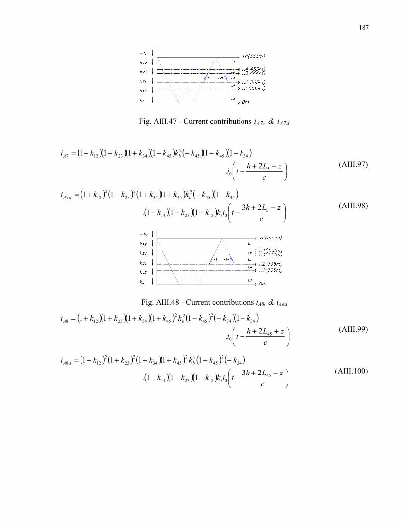
187


( )( )( )( ) ( )( )( )

⎟⎠⎞

⎜⎝⎛ ++−

−−−++++=

czLhti

kkkkkkkki bA

50

3445452

453423127

2.

111111 (AIII.97)

( ) ( ) ( )( ) ( )( )

( )( )( ) ⎟⎠⎞

⎜⎝⎛ −+−−−−

−−++++=

czLhtikkkk

kkkkkkki

t

bdA

50122334

45452

45342

232

127

23111.

11111 (AIII.98)


( )( )( )( ) ( ) ( )( )

⎟⎠⎞

⎜⎝⎛ ++−

−−−++++=

czLhti

kkkkkkkki bA

450

34342

4522

453423128

2.

111111 (AIII.99)

( ) ( ) ( )( ) ( ) ( )

( )( )( ) ⎟⎠⎞

⎜⎝⎛ −+−−−−

−−++++=

czLhtikkkk

kkkkkkki

t

bdA

450122334

342

4522

45342

232

128

23111.

11111 (AIII.100)

188



( ) ( ) ( ) ( ) ( )

( ) ( ) ( ) ⎟⎠⎞

⎜⎝⎛ −

−−−−−

−++++= ∑∞

=

+++

nch

czhtikkkk

kkkkkki

nt

nnn

n

nnb

nnnn

2111.

11111

0122334

04545

134

123

1121

(AIII.101)

( ) ( ) ( ) ( ) ( )

( ) ( ) ( ) ⎟⎠⎞

⎜⎝⎛ −

+−−−−

−++++= ∑∞

=

++++++

nch

czhtikkkk

kkkkkki

nt

nnn

n

nnb

nnnn

2111.

11111

0122334

0

145

1145

134

123

1122

(AIII.102)


( )( )( )( ) ( )( )

⎟⎠⎞

⎜⎝⎛ −

−+−

−−++++= ∑∞

=

+

ncL

czLhti

kkkkkkkkin

nnb

4450

045

13445453423125

22.

11111 (AIII.103)

( )( )( )( ) ( )( )

⎟⎠⎞

⎜⎝⎛ −

++−

−−++++= ∑∞

=

++

ncL

czLhti

kkkkkkkkin

nnb

440

0

145

13445453423126

22.

11111 (AIII.104)

189


( ) ( ) ( ) ( )

( ) ( ) ⎟⎠⎞

⎜⎝⎛ −

−+−−−

−+++=

+++

∞

=

+++++∑

nc

Lc

zhLtikkk

kkkkki

nt

nn

n

nnnnn

123412340

1112

123

0

134

145

234

223

2127

2211.

1111 (AIII.105)

( ) ( ) ( ) ( )

( ) ( ) ⎟⎠⎞

⎜⎝⎛ −

−+−−−

−+++=

+++

∞

=

+++++∑

nc

Lc

LzLtikkk

kkkkki

nt

nn

n

nnnnn

1234512340

1112

123

0

134

245

234

223

2128

2311.

1111 (AIII.106)

Fig. AIII.52 - Current contributions ir1 , ir2, ir3, ir4, & ir5

( ) ( )( )( )( ) ⎟⎠⎞

⎜⎝⎛ −+−+++−+=

czhLtikkkkkkki tctr

ξ10342312121

211111 (AIII.107)

( ) ( )( ) ( )( )( )

⎟⎠⎞

⎜⎝⎛ −+−

++−+−+=

czhLti

kkkkkkkki tctr

ξ120

342312232

122

2.

111111 (AIII.108)

( ) ( ) ( )( )( ) ( )( )

⎟⎠⎞

⎜⎝⎛ −+−

+−+−−++=

czhLti

kkkkkkkkki tctr

ξ1230

341223342

232

123

2.

1111111 (AIII.109)

( ) ( ) ( ) ( )( )( )

( ) ( ) ⎟⎠⎞

⎜⎝⎛ −+−−+

−−−+++=

czhLtikkk

kkkkkkki

tct

r

ξ12340

122334452

342

232

124

211.

111111 (AIII.110)

190

( ) ( ) ( ) ( ) ( )( )( )

( )( ) ( ) ⎟⎠⎞

⎜⎝⎛ −+−−+−

−−−++++=

czhhtikkkk

kkkkkkkki

tct

br

ξ2111.

1111111

012

233445452

342

232

125

(AIII.111)


Fig. AIII.53 - Current contributions iA3 & iA4

( )( )( ) ⎟⎠⎞

⎜⎝⎛ −+−+++=

cLzLtikkkkiA

512340453423123 111 (AIII.112)

( )( )( ) ( ) ⎟⎠⎞

⎜⎝⎛ −+−−+++=

czLhtikkkkkiA

4034453423124

2111 (AIII.113)


( )( )( )( ) ( )( ) ⎟⎠⎞

⎜⎝⎛ ++−−−++++=

czLhtikkkkkkki bA

504545

2453423129

211111 (AIII.114)

( ) ( ) ( ) ( ) ( )( )

( )( )( ) ⎟⎠⎞

⎜⎝⎛ −+−−−−

−−++++=

czLhtikkkk

kkkkkkki

t

bA

50122334

454522

452

342

232

1210

23111.

11111 (AIII.115)


191

( )( )( ) ⎟⎠⎞

⎜⎝⎛ −+−+++=

czhLtikkkkki tA

103423121211

2111 (AIII.116)

( )( )( )( ) ( ) ⎟⎠⎞

⎜⎝⎛ ++−−++++=

czLhtikkkkkkkki btA

1045453423121212

211111 (AIII.117)


( ) ( ) ( )( ) ⎟⎠⎞

⎜⎝⎛ −+−++−+=

czhLtikkkkkki tA

12034231223

21213

21111 (AIII.118)

( ) ( ) ( )( )( ) ( )

⎟⎠⎞

⎜⎝⎛ ++−

−+++−+=

czLhti

kkkkkkkkki btA

120

4545342312232

1214

2.

111111 (AIII.119)

Fig. AIII.57 - Current contributions iA15, iA16 & iA17

( ) ( ) ( )( ) ( ) ⎟⎠⎞

⎜⎝⎛ −+−+−−++=

czhLtikkkkkkki tA

123034122334

223

21215

211111 (AIII.120)

( ) ( ) ( )( ) ( )

⎟⎠⎞

⎜⎝⎛ −++−

+−−++=

cLzLLti

kkkkkkkki tA

541230

45341223342

232

1216

3.

11111 (AIII.121)

( ) ( ) ( )( ) ( )

( ) ( ) ⎟⎠⎞

⎜⎝⎛ ++−−+

+−−++=

czLhtikkk

kkkkkkki

b

tA

12304545

341223342

232

1217

211.

11111 (AIII.122)

192


( ) ( ) ( ) ( )( )

( ) ( ) ( ) ⎟⎠⎞

⎜⎝⎛ ++−−+−

−−+++=

czLLtikkkkk

kkkkkki

bt

A

512340454512

2334452

342

232

1218

3111.

11111 (AIII.123)


( )( )( ) ( )( ) ⎟⎠⎞

⎜⎝⎛ −+−−−+++=

czhLtikkkkkkiA

340233445

234231219

21111 (AIII.124)


( )( ) ( ) ( )( )( )

⎟⎠⎞

⎜⎝⎛ −+−

−−−+++=

czhLti

kkkkkkkiA

2340

122334452

342

231220

2.

11111 (AIII.125)

193


( )( )( ) ( )( ) ( )

⎟⎠⎞

⎜⎝⎛ ++−

−+−+++=

czLhti

kkkkkkkki bA

40

4545344534231221

2.

11111 (AIII.126)


( )( )( )( ) ( ) ( )

⎟⎠⎞

⎜⎝⎛ ++−

−−++++=

czLhti

kkkkkkki bA

450

342

4522

4534231222

2.

11111 (AIII.127)

AIII.2.5 Current inside L5 ( mz 335≤ )


( ) ( ) ( ) ( ) ( )

( ) ( ) ( ) ⎟⎠⎞

⎜⎝⎛ −

−−−−−

−++++= ∑∞

=

++++

nch

czhtikkkk

kkkkkki

nt

nnn

n

nnb

nnnn

2111.

11111

0122334

045

145

134

123

1121

(AIII.128)

194

( ) ( ) ( ) ( ) ( )

( ) ( ) ( ) ⎟⎠⎞

⎜⎝⎛ −

+−−−−

−++++= ∑∞

=

+++++

nch

czhtikkkk

kkkkkki

nt

nnn

n

nnb

nnnn

2111.

11111

0122334

045

1145

134

123

1122

(AIII.129)

Fig. AIII.64 - Current contributions ir1 , ir2, ir3, ir4, & ir5

( ) ( )( )( )( )( ) ⎟⎠⎞

⎜⎝⎛ −+−++++−+=

czhLtikkkkkkkki tctr

ξ1045342312121

2111111 (AIII.130)

( ) ( )( ) ( )( )( )( )

⎟⎠⎞

⎜⎝⎛ −+−

+++−+−+=

czhLti

kkkkkkkkki tctr

ξ120

45342312232

122

2.

1111111 (AIII.131)

( ) ( ) ( )( )( ) ( )

( )( ) ⎟⎠⎞

⎜⎝⎛ −+−++

−+−−++=

czhLtikk

kkkkkkkki tctr

ξ12304534

1223342

232

123

211

111111 (AIII.132)

( ) ( ) ( ) ( )( )

( )( ) ( )( ) ⎟⎠⎞

⎜⎝⎛ −+−+−+−

−−+++=

czhLtikkkkk

kkkkkki

tct

r

ξ123404512

2334452

342

232

124

21111.

11111 (AIII.133)

( ) ( ) ( ) ( ) ( )( )

( )( )( ) ( ) ⎟⎠⎞

⎜⎝⎛ −+−−+−−

−−++++=

czhhtikkkkk

kkkkkkki

tct

br

ξ21111.

111111

01223

34452

452

342

232

125

(AIII.134)



195

( )( )( )( ) ( ) ⎟⎠⎞

⎜⎝⎛ −+−−++++=

czLhtikkkkkki bA

5045453423123

21111 (AIII.135)

( )( )( )( ) ( ) ⎟⎠⎞

⎜⎝⎛ ++−−++++=

czLhtikkkkkki bA

5045

2453423124

21111 (AIII.136)

Fig. AIII.66 - Current contributions iA5, iA6 & iA7

( )( )( )( ) ( )( ) ⎟⎠⎞

⎜⎝⎛ −+−−−++++=

czLhtikkkkkkki bA

4503445

2453423125

211111 (AIII.137)

( )( )( )( ) ( )( ) ⎟⎠⎞

⎜⎝⎛ ++−−−++++=

czLhtikkkkkkki bA

4503445

22453423126

211111 (AIII.138)

( )( )( )( ) ( ) ( )

⎟⎠⎞

⎜⎝⎛ −+−

−−++++=

czLhti

kkkkkkki bA

450

234

245

23453423127

4.

11111 (AIII.139)


( )( )( ) ( ) ( )( )

( ) ⎟⎠⎞

⎜⎝⎛ −+−−

−−++++=

czLhtik

kkkkkkki bA

345023

34452

452

3423128

2.

111111 (AIII.140)

( )( )( ) ( ) ( )( )

( ) ⎟⎠⎞

⎜⎝⎛ ++−−

−−++++=

czLhtik

kkkkkkki bA

345023

344522

452

3423129

2.

111111 (AIII.141)

196


( )( ) ( ) ( ) ( )( )

( )( ) ⎟⎠⎞

⎜⎝⎛ −+−−−

−−++++=

czLhtikk

kkkkkkki bA

234501223

34452

452

342

231210

21.

111111 (AIII.142)

( )( ) ( ) ( ) ( )( )

( )( ) ⎟⎠⎞

⎜⎝⎛ ++−−−

−−++++=

czLhtikk

kkkkkkki bA

234501223

344522

452

342

231211

21.

111111 (AIII.143)

Fig. AIII.69 - Current contributions iA12, iA13, iA14, & iA15

( )( )( )( ) ⎟⎠⎞

⎜⎝⎛ −+−++++=

czhLtikkkkkki tA

10453423121212

21111 (AIII.144)

( )( )( )( ) ⎟⎠⎞

⎜⎝⎛ ++−++++=

czhLtikkkkkkki btA

10453423121213

21111 (AIII.145)

( ) ( ) ( )( )( ) ⎟⎠⎞

⎜⎝⎛ −+−+++−+=

czhLtikkkkkkki tA

1204534231223

21214

211111 (AIII.146)

( ) ( ) ( )( )( ) ⎟⎠⎞

⎜⎝⎛ ++−+++−+=

czhLtikkkkkkkki btA

1204534231223

21215

211111 (AIII.147)

197


( ) ( ) ( )( ) ( )( )

⎟⎠⎞

⎜⎝⎛ −+−

++−−++=

czhLti

kkkkkkkki tA

1230

45341223342

232

1216

2.

111111 (AIII.148)

( ) ( ) ( )( ) ( )( )

⎟⎠⎞

⎜⎝⎛ ++−

++−−++=

czhLti

kkkkkkkkki btA

1230

45341223342

232

1217

2.

111111 (AIII.149)


( ) ( ) ( ) ( )( )( )

( ) ⎟⎠⎞

⎜⎝⎛ −+−+

−−−+++=

czLLtikk

kkkkkkki

t

A

51234045

122334452

342

232

1218

31.

111111 (AIII.150)

( ) ( ) ( ) ( )( )( )

( ) ⎟⎠⎞

⎜⎝⎛ ++−+

−−−+++=

czLLtikkk

kkkkkkki

bt

A

51234045

122334452

342

232

1219

31.

111111 (AIII.151)


( )( ) ( )( )( ) ⎟⎠⎞

⎜⎝⎛ −+−++−++=

czLhtikkkkkkiA

3045342334231220

21111 (AIII.152)

198

( )( ) ( )( )( ) ⎟⎠⎞

⎜⎝⎛ ++−++−++=

czLhtikkkkkkki bA

3045342334231221

21111 (AIII.153)

Fig. AIII.73 - Current contributions iA22, iA23, iA24, & iA25

( )( ) ( ) ( )( )( )

( ) ⎟⎠⎞

⎜⎝⎛ −+−+

−−−+++=

czLhtik

kkkkkkkiA

234045

122334452

342

231222

21.

11111 (AIII.154)

( )( ) ( ) ( )( )( )( )

⎟⎠⎞

⎜⎝⎛ ++−

+−−−+++=

czLhtik

kkkkkkkki

b

A

2340

45122334452

342

231223

2.

111111 (AIII.155)

( )( ) ( )( )( )( )

⎟⎠⎞

⎜⎝⎛ −+−

++−−++=

czLhti

kkkkkkkiA

230

45341223342

231224

2.

11111 (AIII.156)

( )( ) ( )( )( )( )

⎟⎠⎞

⎜⎝⎛ ++−

++−−++=

czLhtik

kkkkkkki

b

A

230

45341223342

231225

2.

11111 (AIII.157)


( )( )( ) ( )( )( )

⎟⎠⎞

⎜⎝⎛ −+−

+−−+++=

czLhti

kkkkkkkiA

340

452334452

34231226

2.

11111 (AIII.158)

199

AIII.3 Derivation of Relations for the Processes Taking

Place within the Lightning Channel

AIII.3.1 Channel Base Current propagating upwards &Transmitted

Components in the Lightning Channel

Fig. AIII.75 - Current contributions iz0, iz1, iz2, iz3, iz4, iz5, iz6, iz7, & iz8

ψzh

tchch e

vhzti

ZZi

−

⎟⎠⎞

⎜⎝⎛ −−= 0

1 (AIII.159)

for m 553≥z

( ) ψσ zh

ctz ev

Lhzvc

Ltikkki−

⎟⎠⎞

⎜⎝⎛ +−

−−

−++= 110121

22)1)(1( (AIII.160)

for ∞<<+ zLh σ12

( ) ( )( )( ) ( ) ψσ zh

ctz ev

Lhzvc

Ltikkkkki−

⎟⎠⎞

⎜⎝⎛ +−

−−

−++−+= 121201223122

221111 (AIII.161)

for ∞<<+ zLh σ122 ( )( ) ( )( )( )( )

( ) ψσ zhctz

ev

Lhzvc

Lti

kkkkkkki−

⎟⎠⎞

⎜⎝⎛ +−

−−

−

++−−++=

1231230

12233423123

22.

111111 (AIII.162)

for ∞<<+ zLh σ1232

200

( )( )( ) ( )( )

( )( )( ) ψσ zh

ct

z

ev

Lhzvc

Ltikkk

kkkkkki−

⎟⎠⎞

⎜⎝⎛ +−

−−

−++−

−−+++=

)2(2111.

11111

12341234012

2334453423124

(AIII.163)

for ∞<<+ zLh σ12342

( )( )( )( ) ( )( )

( )( )( )( ) ( ) ψσ zh

ct

bz

ev

hhzvc

htikkkk

kkkkkkki−

⎟⎠⎞

⎜⎝⎛ +−

−−

−++−−

−−++++=

221111.

111111

01223

3445453423125

(AIII.164)

for ∞<<+ zhh σ2 ( ) ( ) ( ) ( )

( )( ) ( ) ψσ zh

ctt

z

ev

Lhzvc

Ltikkk

kkkkki−

⎟⎠⎞

⎜⎝⎛ +−

−−

−++

−−++=

1231230

212

223

234

223

2126

4411.

1111 (AIII.165)

for ∞<<+ zLh σ1234

( ) ( ) ( ) ( )( ) ( )

( )( ) ( ) ( )( ) ψσ zh

ctt

z

ev

LLhzvcLLtikkkk

kkkkkkki−

⎟⎠⎞

⎜⎝⎛ ++−

−−+

−++

−−−+++=

12312341231234034

212

223344534

223

2127

2211.

111111 (AIII.166)

for ( ) ∞<<++ zLLh σ12312342

( ) ( ) ( )( ) ( )( )( ) ( )

( )( ) ( ) ( )( ) ψσ zh

ctt

bz

ev

LhhzvcLhtikkkk

kkkkkkkkki−

⎟⎠⎞

⎜⎝⎛ ++−

−−+

−++

−−−−++++=

123123034

212

22334454534

223

2128

2211.

11111111 (AIII.167)

for ( ) ∞<<++ zLhh σ1232

AIII.3.2 Internal Components in the Lightning Channel

Fig. AIII.76 - Current contributions i1, i2, i3, i4, i5, i6, i7, i8, i9, & i10

201

( ) ( )∑∞

=⎟⎠⎞

⎜⎝⎛ −

−−−+=0

10121

21n

nnt

nct c

hzcLtikkkki ξ (AIII.168)

( ) ( ) ⎟⎟⎠

⎞⎜⎜⎝

⎛ −+−

−−−+=∑

∞

=

+

czLh

vcLtikkkki

nn

n

nt

nct

σξξ 110

0

1122

221 (AIII.169)

for nLhzh σξ12+<<

( ) ( )( ) ( ) ⎟⎠⎞

⎜⎝⎛ −

−−−+−+=∑∞

= chz

cLtikkkkkki nn

tnct

nξ12

012230

1232111 (AIII.170)

( ) ( )( ) ( )

⎟⎟⎠

⎞⎜⎜⎝

⎛ −+−

−−

−+−+= +∞

=∑

czLh

vcLti

kkkkkki

nn

nt

nct

n

σξξ 12120

11223

0124

22.

111 (AIII.171)

for nLhzh σξ122+<<

( )( ) ( )( )( ) ( )

⎟⎠⎞

⎜⎝⎛ −

−−

−+−−++= ∑∞

=

chz

cLti

kkkkkkkki nt

nct

n

ξ1230

122334230

125

2.

11111 (AIII.172)

( )( ) ( )( )( ) ( )

⎟⎟⎠

⎞⎜⎜⎝

⎛ −+−

−−

−+−−++= +∞

=∑

czLh

vcLti

kkkkkkkki

n

nt

nct

n

σξξ 1231230

112233423

0126

22.

11111 (AIII.173)


⎟⎠⎞

⎜⎝⎛ −

−−−+−

−−+++= ∑∞

=

chz

cLtikkkk

kkkkkki

nnt

nct

n

ξ1234012

02334453423127

2)()1)(1.(

)1)(1()1)(1)(1( (AIII.174)

⎟⎟⎠

⎞⎜⎜⎝

⎛ −+−

−−−+−

−−+++=

+

∞

=∑

czLh

vcLtikkkk

kkkkkki

nnn

tnct

n

σξξ 123412340

112

02334453423128

22)()1)(1.(

)1)(1()1)(1)(1( (AIII.175)


202

( ) ⎟⎠⎞

⎜⎝⎛ −

−−−+−−

−−++++= ∑∞

=

chz

chtikkkkk

kkkkkkki

nnt

nct

bn

ξ2)(1)1)(1.(

)1)(1()1)(1)(1()1(

01223

34454534230

129

(AIII.176)

⎟⎟⎠

⎞⎜⎜⎝

⎛ −+−

−−−+−−

−−++++=

+

∞

=∑

czhh

vchtikkkkk

kkkkkkki

nnn

tnct

nb

σξξ 22)()1)(1)(1.(

)1)(1()1)(1)(1)(1(

01

1223

034454534231210

(AIII.177)

for nhhzh σξ2+<<

Fig. AIII.77 - Current contributions i11, i12, i13, & i14

⎟⎠⎞

⎜⎝⎛ −

−+

−−+

−−++= ∑∞

=

chz

cLLtikkk

kkkkkkki

nnt

nct

tn

ξ)(2)()1.(

)1)(1()1()1(2

11230

12122334230

1211

(AIII.178)

⎟⎟⎠

⎞⎜⎜⎝

⎛ −++−

−+

−−+

−−++=

+

∞

=∑

czLLh

vcLLtikkk

kkkkkkki

nnn

tnct

tn

σξξ )(2)(2)()1.(

)1)(1()1()1(2

112311230

1

12122334230

1212

(AIII.179)

for nLLhzh σξ)(2 1123 ++<<

⎟⎠⎞

⎜⎝⎛ −

−+

−−

+−+= ∑∞

=

chz

cLLtik

kkkkkkki

nnt

n

nctt

ξ)(2).(

)1()1()1(2

1120

01212231213

(AIII.180)

203

⎟⎟⎠

⎞⎜⎜⎝

⎛ −++−

−+

−−

+−+= ∑∞

=

+

czLLh

vcLLtik

kkkkkkki

nnn

t

n

nctt

σξξ )(2)(2).(

)1()1()1(2

1121120

0

11212231214

(AIII.181)

for nLLhzh σξ)(2 112 ++<<

Fig. AIII.78 - Current contributions i15, i16, i17, & i18

( ) ( ) ( ) ( )∑∞

=⎟⎠⎞

⎜⎝⎛ −

−−−+−+=0

120

212

223

21215

4111n

nnt

nctt c

hzcLtikkkkkkki ξ (AIII.182)

( ) ( ) ( ) ( )

⎟⎟⎠

⎞⎜⎜⎝

⎛ −+−

−−

−+−+= ∑∞

=

+

czLh

vcLti

kkkkkkki

nn

n

nt

nctt

σξξ 12120

0

1212

223

21216

44.

111 (AIII.183)


( ) ( ) ( )( ) ( )

( ) ( )⎟⎠⎞

⎜⎝⎛ −

−+

−−

+−−++= ∑∞

=

chz

cLLtikk

kkkkkkkki

nnt

nc

ntt

ξ121230

023

212233423

21217

2.

111112 (AIII.184)

( ) ( ) ( )( ) ( )

( ) ( ) ( )⎟⎟⎠

⎞⎜⎜⎝

⎛ −++−

−+

−−

+−−++=

+

∞

=∑

czLLh

vcLLtikk

kkkkkkkki

nnn

tnc

ntt

σξξ 12123121230

1

023

212233423

21218

22.

111112 (AIII.185)

for ( ) nLLhzh σξ121232 ++<<

204

Fig. AIII.79 - Current contributions i19, i20, i21, i22, i23 & i24

( ) ( ) ( ) ( ) ( )

( ) ⎟⎠⎞

⎜⎝⎛ −

−−−

+−−++= ∑∞

=

chz

cLtikk

kkkkkkki

nnt

nc

ntt

ξ1230

0

212

223

234

223

21219

4.

11111 (AIII.186)

( ) ( ) ( ) ( ) ( )

( ) ⎟⎟⎠

⎞⎜⎜⎝

⎛ −+−

−−−

+−−++=

+

∞

=∑

czLh

vcLtikk

kkkkkkki

nnn

tnc

ntt

σξξ 1231230

1

0

212

223

234

223

21220

44.

11111 (AIII.187)


( ) ( ) ( ) ( ) ( )

( ) ( ) ( ) ⎟⎠⎞

⎜⎝⎛ −

−−−+−

−−+++= ∑∞

=

chz

cLtikkkkk

kkkkkki

nnt

nctt

n

ξ12340

212

0

223

234

245

234

223

21221

411.

11111 (AIII.188)

( ) ( ) ( ) ( ) ( ) ( )

( ) ( ) ⎟⎟⎠

⎞⎜⎜⎝

⎛ −+−

−−−+

−−−+++=

+

∞

=∑

czLh

vcLtikkkk

kkkkkkki

nnn

tnctt

n

σξξ 123412340

1

0

212

223

234

245

234

223

21222

441.

111111 (AIII.189)


( ) ( ) ( ) ( ) ( ) ( )

( ) ( ) ( ) ( ) ⎟⎠⎞

⎜⎝⎛ −

−−−+−−

−−++++= ∑∞

=

chz

chtikkkkkk

kkkkkkki

nnt

nctt

nb

ξ4111.

111111

02

122

23

0

234

245

2245

234

223

21223

(AIII.190)

205

( ) ( ) ( ) ( ) ( ) ( ) (

( ) ( ) ( )

)

⎟⎟⎠

⎞⎜⎜⎝

⎛ −+−

−−−+−

−−−++++=

+

∞

=∑

czhh

vchtikkkkk

kkkkkkkki

nnn

tnctt

nb

σξξ 4411.

1111111

012

12

0

223

234

245

2245

234

223

21224

(AIII.191)

for nhhzh σξ4+<<

Fig. AIII.80 - Current contributions i25, i26, i27, i28, i29 & i30

( )( )( )( ) ( )( )( )

( )( )( ) ( ) ( )⎟⎠⎞

⎜⎝⎛ −

−+

−−+−−

−−−++++= ∑∞

=

chz

cLhtikkkkk

kkkkkkkki

nnt

nct

nb

ξ501223

0344545

24534231225

2111.

111111 (AIII.192)

( )( )( )( ) ( )( )( )( )

( )( ) ( ) ( ) ( )⎟⎟⎠

⎞⎜⎜⎝

⎛ −++−

−+

−−+−

−−−−++++=

+

∞

=∑

czLhh

vcLhtikkkk

kkkkkkkkki

nnn

tnct

nb

σξξ 550

112

023344545

24534231226

2211.

1111111 (AIII.193)

for ( ) nLhhzh σξ52 ++<<

( )( )( )( ) ( ) ( )( )

( )( )( ) ( ) ( )⎟⎠⎞

⎜⎝⎛ −

−+

−−+−−

−−−++++= ∑∞

=

chz

cLhtikkkkk

kkkkkkkki

nnt

nct

nb

ξ4501223

03434

245

224534231227

2111.

111111 (AIII.194)

( )( )( )( ) ( ) ( )( )(

( )( ) ( ) ( )

)

( )⎟⎟⎠

⎞⎜⎜⎝

⎛ −++−

−+

−−+−

−−−−++++=

+

∞

=∑

czLhh

vcLhtikkkk

kkkkkkkkki

nnn

tnct

nb

σξξ 45450

112

230

34342

4522

4534231228

2211.

1111111 (AIII.195)


206

( )( )( )( ) ( )( )

( )( )( )( ) ( ) ( )⎟⎠⎞

⎜⎝⎛ −

−+

−−+−−−

−−++++= ∑∞

=

chz

cLhtikkkkkk

kkkkkkkki

nnt

nct

nb

ξ40122334

04534454534231229

21111.

111112 (AIII.196)

( )( )( )( ) ( )( ) ( )(

( )( ) ( ) ( )

)

( )⎟⎟⎠

⎞⎜⎜⎝

⎛ −++−

−+

−−+−

−−−−++++=

+

∞

=∑

czLhh

vcLhtikkkk

kkkkkkkkkki

nnn

tnct

nb

σξξ 440

112

23340

4534454534231230

2211.

11111112 (AIII.197)


Fig. AIII.81 - Current contributions i31, i32, i33, i34, i35, i36, i37 & i38

( )( )( )( ) ( )( )( )

( ) ( )( ) ( ) ( )⎟⎠⎞

⎜⎝⎛ −

−+

−−+−−

−−−++++= ∑∞

=

chz

cLhtikkkkkk

kkkkkkkki

nnt

nct

nb

ξ20122312

02334454534231231

211.

11111112 (AIII.198)

( )( )( )( ) ( )( )( )( )

( )( ) ( ) ( ) ( )⎟⎟⎠

⎞⎜⎜⎝

⎛ −++−

−+

−−+−

−−−−++++=

+

∞

=∑

czLhh

vcLhtikkkkk

kkkkkkkkki

nnn

tnct

nb

σξξ 220

11223

12230

34454534231232

2211.

11111112 (AIII.199)


( )( ) ( )( ) ( )( )( )

( ) ( )( ) ( ) ( )⎟⎠⎞

⎜⎝⎛ −

−+

−−+−−

−−−++++= ∑∞

=

chz

cLhtikkkkkk

kkkkkkkki

nnt

nct

nb

ξ230123412

0

22334454534

2231233

211.

11111112 (AIII.200)

( )( ) ( )( ) ( )( )( ) (

( )( ) ( ) ( )

)

( )⎟⎟⎠

⎞⎜⎜⎝

⎛ −++−

−+

−−+−

−−−−++++=

+

∞

=∑

czLhh

vcLhtikkkkk

kkkkkkkkki

nnn

tnct

nb

σξξ 23230

11234

120

22334454534

2231234

2211.

11111112 (AIII.201)

207


( )( ) ( ) ( ) ( )( ) ( )

( ) ( )( ) ( ) ( )⎟⎠⎞

⎜⎝⎛ −

−+

−−+−−

−−−++++= ∑∞

=

chz

cLhtikkkkkk

kkkkkkkki

nnt

nct

nb

ξ2340124512

0

223

2344545

234

2231235

211.

11111112 (AIII.202)

( )( ) ( ) ( ) ( )( ) ( ) (

( )( ) ( ) ( )

)

( )⎟⎟⎠

⎞⎜⎜⎝

⎛ −++−

−+

−−+−

−−−−++++=

+

∞

=∑

czLhh

vcLhtikkkkk

kkkkkkkkki

nnn

tnct

nb

σξξ 2342340

11245

120

223

2344545

234

2231236

2211.

11111112 (AIII.203)


( )( ) ( ) ( ) ( ) ( ) ( )

( )( )( ) ( ) ( )⎟⎠⎞

⎜⎝⎛ −

−+

−−+−−

−−−++++= ∑∞

=

chz

cLhtikkkkk

kkkkkkkki

nnt

nct

nb

ξ234501212

223

0

234

245

2245

234

2231237

211.

1111111 (AIII.204)

( )( ) ( ) ( ) ( ) ( ) ( ) (

( )( ) ( ) ( )

)

( )⎟⎟⎠

⎞⎜⎜⎝

⎛ −++−

−+

−−+−

−−−−++++=

+

∞

=∑

czLhh

vcLhtikkkk

kkkkkkkkki

nnn

tnct

nb

σξξ 234523450

112

122

230

234

245

2245

234

2231238

2211.

1111111 (AIII.205)


Fig. AIII.82 - Current contributions i39, i40, i41, i42, i43, & i44

( )( )( )( ) ( )( )( )

( )( )( ) ( ) ( )⎟⎠⎞

⎜⎝⎛ −

−+

−−+−−

−−−++++= ∑∞

=

chz

cLhtikkkkk

kkkkkkkkki

nnt

nct

nb

ξ301223

0342334454534231239

2111.

1111112 (AIII.206)

208

( )( )( )( ) ( )( )( ) (

( )( ) ( ) ( )

)

( )⎟⎟⎠

⎞⎜⎜⎝

⎛ −++−

−+

−−+−

−−−−++++=

+

∞

=∑

czLhh

vcLhtikkkk

kkkkkkkkkki

nnn

tnct

nb

σξξ 330

112

230

342334454534231240

2211.

11111112 (AIII.207)


( )( )( ) ( ) ( )( ) ( )

( )( )( ) ( ) ( )⎟⎠⎞

⎜⎝⎛ −

−+

−−+−−

−−−++++= ∑∞

=

chz

cLhtikkkkkk

kkkkkkkki

nnt

nct

nb

ξ340122345

023

2344545

234231241

2111.

1111112 (AIII.208)

( )( )( ) ( ) ( )( ) ( ) (

( )( ) ( ) ( )

)

( )⎟⎟⎠

⎞⎜⎜⎝

⎛ −++−

−+

−−+−

−−−−++++=

+

∞

=∑

czLhh

vcLhtikkkk

kkkkkkkkkki

nnn

tnct

nb

σξξ 34340

112

0234523

2344545

234231242

2211.

11111112 (AIII.209)


( )( )( ) ( ) ( ) ( ) ( )

( )( )( ) ( ) ( )⎟⎠⎞

⎜⎝⎛ −

−+

−−+−−

−−−++++= ∑∞

=

chz

cLhtikkkkk

kkkkkkkki

nnt

nct

nb

ξ34501223

023

234

245

2245

234231243

2111.

1111112 (AIII.210)

( )( )( ) ( ) ( ) ( ) ( )(

( )( ) ( ) ( )

)

( )⎟⎟⎠

⎞⎜⎜⎝

⎛ −++−

−+

−−+−

−−−−++++=

+

∞

=∑

czLhh

vcLhtikkkk

kkkkkkkkki

nnn

tnct

nb

σξξ 3453450

112

02323

234

245

2245

234231244

2211.

11111112 (AIII.211)


Using the Five-Section Model and the same injection current shown in Appendix AI in Fig. AI.4,

the following resultant waveforms at respective levels of interest are calculated:

209

Fig. AIII.83 - Calculated Current Derivative and Current at 474m and at 509m Above Ground

Level

This time, the waveshapes are influenced not only by the Skypod, but by the Space-deck as well.

The influence of the Space-deck is better seen when examining the current derivative computed

for the 509m level above ground. Under closer look, one will notice that there is a small “hump”

at about 0.5µs, which is precisely due to the modeling of the Space-deck. Furthermore, the

influence from the Skypod is again noticeable at 1µs (in the curve of the current derivative

computed at 474m above ground level).

210

Appendix IV Derivation of Expressions for Distant Electric and Magnetic Fields

in Cartesian Coordinates

Let us start with Ampere’s circuital law (with Maxwell’s correction):

tEJB∂∂

+=×∇ 000 εµµ (AIV.1)

where:

×∇ The curl operator

B Magnetic flux density

0µ Permeability of free space

J Total current density (including both free and bound current)

0ε Permittivity of free space

t∂∂ Partial derivative with respect to time

E Electric Field intensity

When the MAGNETIC case is considered the term tE∂∂

00εµ is equal to “zero”, (no displacement

current along medium 1 (conductor), where the CN Tower or the associated Lightning Channel

is considered as the conductor). In this case conduction and impressed current exist only.

Therefore, now Eq. (AIV.1) can be rewritten:

JB 0µ=×∇ (AIV.2)

According to the Equation of Magnetic Force:

211

AH ×∇=µ (AIV.3)

Constitutive Relation is:

BH =µ

Eq. (AIV.3) is then rewritten:

AB ×∇= (AIV.4)

Substituting Eq. (AIV.4) into Eq. (AIV.2) yields the following:

JA 0µ=×∇×∇ (AIV.5)

but ( ( ) AAA 2. ∇−∇∇=×∇×∇ ) and if we used Coulomb gauge ( 0. =∇ A ) then Eq. (AIV.5)

becomes:

JA 0

2 µ=∇− (AIV.6)

or:

zzzz

yyyy

xxxx

JzA

yA

xA

JzA

yA

xA

JzA

yA

xA

02

2

2

2

2

2

02

2

2

2

2

2

02

2

2

2

2

2

µ

µ

µ

=⎟⎟⎠

⎞⎜⎜⎝

⎛∂∂

+∂∂

+∂∂

−

=⎟⎟⎠

⎞⎜⎜⎝

⎛

∂

∂+

∂

∂+

∂

∂−

=⎟⎟⎠

⎞⎜⎜⎝

⎛∂∂

+∂∂

+∂∂

−

(AIV.6)

Each component of A obeys the Poisson equation.

In differential form Gauss’ law says that:

0

.ερ

=∇ E (AIV.7)

where:

212

ρ Total charge density (including both free and bound charge) The scalar potential “Φ” can be determined from (AIV.7):

0

2.ερ

−=Φ∇ (AIV.8)

The solution to Poisson’s equation (AIV.8) has the following form:

( ) ( ) ''

/,'4

1,'0

dVrr

cRtrtrV∫ −

−=Φ rr

rr ρ

πε (AIV.9)

Similarly, the solution to Eq. (AIV.6) is (Magnetic Vector Potential):

( ) ( )∫ −

−=

'

0 ''

/,'4

,V

dVrr

cRtrJtrA rr

rr

πµ (AIV.10)

Fig. AIV.1 - Geometrical Relations Pertinent to Deriving Expressions in

Cartesian Coordinates

213

Components “x”, “y”, and “z” of Magnetic Field

In terms of derivatives, Eq. (AIV.4) is rewritten:

zyx dAdAdAzyx

zyx

dAdB∂∂

∂∂

∂∂

=×∇=

ˆˆˆ

(AIV.11)

⎟⎟⎠

⎞⎜⎜⎝

⎛∂∂

−∂∂

+

+⎟⎠⎞

⎜⎝⎛

∂∂

−∂∂

+

+⎟⎟⎠

⎞⎜⎜⎝

⎛∂∂

−∂∂

=

ydA

xdA

z

xdA

zdAy

zdA

ydAxdB

xy

zx

yz

ˆ

ˆ

ˆ

(AIV.11)

x, y, and z components of Magnetic Vector Potential dA (Eq. (AIV.10)):

( ) dx

RcRtxidAx

/,'4

0 −=

πµ

( ) dyR

cRtyidAy/,'

40 −

=πµ

( ) dzR

cRtzidAz/,'

40 −

=πµ

Now, one could come up with the relations for Magnetic Flux Densities and respectively with the

Magnetic Field components along x, y, and z as shown hereafter.

In the following derivations some abbreviations are adopted, which are introduced below:

( )( )( )dzcRtzii

dycRtyiidxcRtxii

z

y

x

/,'

/,'/,'

−≡

−≡−≡

214

( )( )( )'

''

zzZyyYxxX

−≡−≡−≡

“x” component:

( )

⎥⎦

⎤⎢⎣

⎡∂∂

−∂∂

=∂∂

−∂∂

=

=

Ri

zRi

yzdA

ydA

tzzyyxxdB

yzyz

x

πµ4

,',,',,',

0 (AIV.12)

( )

⎥⎦

⎤⎢⎣

⎡−

∂

∂−+

∂∂

=

⎥⎦

⎤⎢⎣

⎡∂∂

−∂

∂−

∂∂

+∂∂

=

=

yy

zz

yy

zz

x

iRZ

ti

cRZi

RY

ti

cRY

Rzi

zi

RRyi

yi

R

tzzyyxxdB

32320

0

4

11114

,',,',,',

πµ

πµ (AIV.12)

( )

⎥⎦

⎤⎢⎣

⎡⎟⎟⎠

⎞⎜⎜⎝

⎛∂∂

+−⎟⎠⎞

⎜⎝⎛

∂∂

+=

=

ti

ci

RRZ

ti

ci

RRY

tzzyyxxdH

yy

zz

x

111141

,',,',,',

22π (AIV.13)

“y” component:

( )

⎥⎦⎤

⎢⎣⎡

∂∂

−∂∂

=∂∂

−∂∂

=

=

Ri

xRi

zxdA

zdA

tzzyyxxdB

zxzx

y

πµ4

,',,',,',

0 (AIV.14)

( )

⎥⎦⎤

⎢⎣⎡ −

∂∂

−+∂∂

=

⎥⎦⎤

⎢⎣⎡

∂∂

−∂∂

−∂∂

+∂∂

=

=

zz

xx

zz

xx

y

iRX

ti

cRXi

RZ

ti

cRZ

Rxi

xi

RRzi

zi

R

tzzyyxxdB

32320

0

4

11114

,',,',,',

πµπµ (AIV.14)

215

( )

⎥⎦

⎤⎢⎣

⎡⎟⎠⎞

⎜⎝⎛

∂∂

+−⎟⎠⎞

⎜⎝⎛

∂∂

+=

=

ti

ci

RRX

ti

ci

RRZ

tzzyyxxdH

zz

xx

y

111141

,',,',,',

22π (AIV.15)

“z” component:

( )

⎥⎦

⎤⎢⎣

⎡∂∂

−∂∂

=∂∂

−∂∂

=

=

Ri

yRi

xydA

xdA

tzzyyxxdB

xyxy

z

πµ4

,',,',,',

0 (AIV.16)

( )

⎥⎦

⎤⎢⎣

⎡−

∂∂

−+∂

∂=

⎥⎦

⎤⎢⎣

⎡∂∂

−∂∂

−∂∂

+∂

∂=

=

xx

yy

xx

yy

z

iRY

ti

cRYi

RX

ti

cRX

Ryi

yi

RRxi

xi

R

tzzyyxxdB

32320

0

4

11114

,',,',,',

πµ

πµ (AIV.16)

( )

⎥⎦

⎤⎢⎣

⎡⎟⎠⎞

⎜⎝⎛

∂∂

+−⎟⎟⎠

⎞⎜⎜⎝

⎛∂∂

+=

=

ti

ci

RRY

ti

ci

RRX

tzzyyxxdH

xx

yy

z

111141

,',,',,',

22π (AIV.17)

Components “x”, “y”, and “z” of Electric Field

When the ELECTRIC case is considered the term J0µ in Eq. (AIV.1) is equal to “zero” (no

conduction and impressed current flowing in medium 2 (air)). Therefore, now Eq. (AIV.1) can

be rewritten:

tEB∂∂

=×∇ 00εµ (AIV.18)

Constitutive relation is:

HB 0µ=

216

Eq. (AIV.18) is rewritten using derivatives of B (H) and E:

tdEdH∂∂

=×∇ 0ε (AIV.19)

zyx dHdHdHzyx

zyx

dH∂∂

∂∂

∂∂

=×∇

ˆˆˆ

(AIV.20)

⎟⎟⎠

⎞⎜⎜⎝

⎛∂

∂−

∂

∂+

+⎟⎠⎞

⎜⎝⎛

∂∂

−∂

∂+

+⎟⎟⎠

⎞⎜⎜⎝

⎛∂

∂−

∂∂

=×∇

ydH

xdH

z

xdH

zdHy

zdH

ydHxdH

xy

zx

yz

ˆ

ˆ

ˆ

(AIV.20)

Using Eq. (AIV.19) and Eq. (AIV.20) and also previously derived Eqs. (AIV.13, AIV.15 and

AIV.17) - Magnetic Flux Densities (derivatives) - the relations for Electric Fields (derivatives)

are derived as follows:

“x” component:

zdH

ydH

tdE yzx

∂

∂−

∂∂

=∂

∂0ε (AIV.21)

( )

⎥⎦

⎤⎟⎟⎠

⎞⎜⎜⎝

⎛∂

∂

∂∂

+∂

∂⎟⎠⎞

⎜⎝⎛

∂∂

+∂

∂+⎟

⎠⎞

⎜⎝⎛

∂∂

+

⎟⎟⎠

⎞⎜⎜⎝

⎛∂∂

∂∂

−∂∂

⎟⎠⎞

⎜⎝⎛

∂∂

−∂∂

−⎟⎠⎞

⎜⎝⎛

∂∂

−

⎟⎟⎠

⎞⎜⎜⎝

⎛

∂

∂

∂∂

−∂

∂⎟⎠

⎞⎜⎝

⎛∂∂

−∂

∂−⎟

⎠

⎞⎜⎝

⎛∂∂

−

⎟⎟⎠

⎞⎜⎜⎝

⎛∂∂

∂∂

+∂∂

⎟⎠⎞

⎜⎝⎛

∂∂

+⎢⎣

⎡∂∂

+⎟⎠⎞

⎜⎝⎛

∂∂

=

=∂

∂

ti

zcRZ

ti

cRZ

zzi

RZ

RZ

zi

ti

zcRX

ti

cRX

zzi

RX

RX

zi

t

i

ycRX

t

i

cRX

yy

i

RX

RX

yi

ti

ycRY

ti

cRY

yyi

RY

RY

yi

ttzzyyxxdE

xxxx

zzzz

yyyy

xxxx

x

2233

2233

2233

223304

1

,',,',,',

πε

(AIV.22)

217

Use the following relations in (AIV.22):

xx iR

YRRY

yi 5

22

33−

=⎟⎠⎞

⎜⎝⎛

∂∂ ;

ti

cRY

yi

RY xx

∂∂

=∂∂

4

2

3 ; ti

cRYR

ti

cRY

yxx

∂∂−

=∂∂

⎟⎠⎞

⎜⎝⎛

∂∂

4

22

24 ;

2

2

32

2

2 ti

RcY

ti

ycRY xx

∂∂

−=⎟⎠⎞

⎜⎝⎛∂∂

∂∂

⎟⎠⎞

⎜⎝⎛ .

yy iRXY

RX

yi 53

3−=⎟

⎠⎞

⎜⎝⎛

∂∂ ;

ti

cRXY

yi

RX yy

∂∂

−=∂∂

43 ; ti

cRXY

ti

cRX

yyy

∂∂

−=∂∂

⎟⎠⎞

⎜⎝⎛

∂∂

422 ;

2

2

322 ti

RcXY

ti

ycRX yy

∂∂

−=⎟⎟⎠

⎞⎜⎜⎝

⎛∂∂

∂∂

⎟⎠⎞

⎜⎝⎛ .

zz iRXZ

RX

zi 53

3−=⎟

⎠⎞

⎜⎝⎛

∂∂ ;

ti

cRXZ

zi

RX zz

∂∂

−=∂∂

43 ; ti

cRZ

ti

cRX

zzz

∂∂

−=∂∂

⎟⎠⎞

⎜⎝⎛

∂∂

4

2

2 ;

2

2

322 ti

RcXZ

ti

zcRX zz

∂∂

−=⎟⎠⎞

⎜⎝⎛∂∂

∂∂

⎟⎠⎞

⎜⎝⎛ .

xx iR

ZRRZ

zi 5

22

33−

=⎟⎠⎞

⎜⎝⎛

∂∂ ;

ti

cRZ

zi

RZ xx

∂∂

=∂∂

4

2

3 ; ti

cRZR

ti

cRZ

zxx

∂∂−

=∂∂

⎟⎠⎞

⎜⎝⎛

∂∂

4

22

24 ;

2

2

32

2

2 ti

RcZ

ti

zcRZ xx

∂∂

−=⎟⎠⎞

⎜⎝⎛∂∂

∂∂

⎟⎠⎞

⎜⎝⎛ .

To get:

( )

⎥⎦

⎤∂∂

⎟⎠⎞

⎜⎝⎛+

∂∂

⎟⎠⎞

⎜⎝⎛+⎟

⎠⎞

⎜⎝⎛+

∂

∂⎟⎠⎞

⎜⎝⎛+

∂

∂⎟⎠⎞

⎜⎝⎛+⎟

⎠⎞

⎜⎝⎛+

∂∂

⎟⎟⎠

⎞⎜⎜⎝

⎛ −−+

∂∂

⎟⎟⎠

⎞⎜⎜⎝

⎛ −++−++

⎢⎣

⎡⎟⎟⎠

⎞⎜⎜⎝

⎛ −+−=

=∂

∂

2

2

3245

2

2

3245

2

2

32

22

4

222222

5

2222

0

33

33

44

334

1

,',,',,',

ti

RcXZ

ti

cRXZi

RXZ

ti

RcXY

ti

cRXYi

RXY

ti

RcZY

ti

cRZRZYRY

iR

ZRYRt

tzzyyxxdE

zzz

yyy

x

x

x

x

πε

(AIV.23)

218

where:

⎟⎟⎠

⎞⎜⎜⎝

⎛−=⎟⎟

⎠

⎞⎜⎜⎝

⎛ +−=

=⎟⎟⎠

⎞⎜⎜⎝

⎛ +−−−=⎟⎟

⎠

⎞⎜⎜⎝

⎛ −+−

35

2

5

222

5

22222

5

2222

13332

3333233

RRX

RXRR

RXZYXR

RZRYR

⎟⎟⎠

⎞⎜⎜⎝

⎛−=⎟⎟

⎠

⎞⎜⎜⎝

⎛ +−−−=⎟⎟

⎠

⎞⎜⎜⎝

⎛ −++−+24

2

4

22222

4

222222 133333244cRcR

XcR

XZYXRcR

ZRZYRY

⎟⎟⎠

⎞⎜⎜⎝

⎛−=⎟⎟

⎠

⎞⎜⎜⎝

⎛ +−−−=⎟⎟

⎠

⎞⎜⎜⎝

⎛ −−RcRc

XRc

XZYXRc

ZY232

2

32

2222

32

22 1

So that finally after integration of Eq. (AIV.23) we can write down Eq. (IV.22).

“y” component:

xdH

zdH

tdE zxy

∂∂

−∂

∂=

∂

∂0ε (AIV.24)

( )

⎥⎦

⎤⎟⎟⎠

⎞⎜⎜⎝

⎛∂

∂

∂∂

+∂

∂⎟⎠⎞

⎜⎝⎛

∂∂

+∂

∂+⎟

⎠⎞

⎜⎝⎛

∂∂

+

+⎟⎠⎞

⎜⎝⎛∂∂

∂∂

−∂∂

⎟⎠⎞

⎜⎝⎛

∂∂

−∂∂

−⎟⎠⎞

⎜⎝⎛

∂∂

−

⎟⎠⎞

⎜⎝⎛∂∂

∂∂

−∂∂

⎟⎠⎞

⎜⎝⎛

∂∂

−∂∂

−⎟⎠⎞

⎜⎝⎛

∂∂

−

⎟⎟⎠

⎞⎜⎜⎝

⎛∂

∂

∂∂

+⎢⎣

⎡∂

∂⎟⎠⎞

⎜⎝⎛

∂∂

+∂

∂+⎟

⎠⎞

⎜⎝⎛

∂∂

=

=∂

∂

ti

xcRX

ti

cRX

xxi

RX

RX

xi

ti

xcRY

ti

cRY

xxi

RY

RY

xi

ti

zcRY

ti

cRY

zzi

RY

RY

zi

ti

zcRZ

ti

cRZ

zzi

RZ

RZ

zi

ttzzyyxxdE

yyyy

xxxx

zzzz

yyyy

y

2233

2233

2233

223304

1

,',,',,',

πε

(AIV.25)


219

yy iR

ZRRZ

zi 5

22

33−

=⎟⎠⎞

⎜⎝⎛

∂∂ ;

ti

cRZ

zi

RZ yy

∂∂

=∂∂

4

2

3 ; ti

cRZR

ti

cRZ

zyy

∂∂−

=∂∂

⎟⎠⎞

⎜⎝⎛

∂∂

4

22

24 ;

2

2

32

2

2 ti

RcZ

ti

zcRZ yy

∂∂

−=⎟⎟⎠

⎞⎜⎜⎝

⎛∂∂

∂∂

⎟⎠⎞

⎜⎝⎛ .

zz iRYZ

RY

zi 53

3−=⎟

⎠⎞

⎜⎝⎛

∂∂ ;

ti

cRYZ

zi

RY zz

∂∂

−=∂∂

43 ; ti

cRYZ

ti

cRY

zzz

∂∂

−=∂∂

⎟⎠⎞

⎜⎝⎛

∂∂

422 ;

2

2

322 ti

RcYZ

ti

zcRY zz

∂∂

−=⎟⎠⎞

⎜⎝⎛∂∂

∂∂

⎟⎠⎞

⎜⎝⎛ .

xx iRXY

RY

xi 53

3−=⎟

⎠⎞

⎜⎝⎛

∂∂ ;

ti

cRXY

xi

RY xx

∂∂

−=∂∂

43 ; ti

cRXY

ti

cRY

xxx

∂∂

−=∂∂

⎟⎠⎞

⎜⎝⎛

∂∂

422 ;

2

2

322 ti

RcXY

ti

xcRY xx

∂∂

−=⎟⎠⎞

⎜⎝⎛∂∂

∂∂

⎟⎠⎞

⎜⎝⎛ .

yy iR

XRRX

xi 5

22

33−

=⎟⎠⎞

⎜⎝⎛

∂∂ ;

ti

cRX

xi

RX yy

∂∂

=∂∂

4

2

3 ; ti

cRXR

ti

cRX

xyy

∂∂−

=∂∂

⎟⎠⎞

⎜⎝⎛

∂∂

4

22

24 ;

2

2

32

2

2 ti

RcX

ti

xcRX yy

∂∂

−=⎟⎟⎠

⎞⎜⎜⎝

⎛∂∂

∂∂

⎟⎠⎞

⎜⎝⎛ .

To get:

( )

⎥⎦

⎤∂∂

⎟⎠⎞

⎜⎝⎛+

∂∂

⎟⎠⎞

⎜⎝⎛+⎟

⎠⎞

⎜⎝⎛+

∂

∂⎟⎟⎠

⎞⎜⎜⎝

⎛ −−+

∂

∂⎟⎟⎠

⎞⎜⎜⎝

⎛ −−+⎟⎟

⎠

⎞⎜⎜⎝

⎛ −−+

∂∂

⎟⎠⎞

⎜⎝⎛+⎢

⎣

⎡∂∂

⎟⎠⎞

⎜⎝⎛+⎟

⎠⎞

⎜⎝⎛=

=∂

∂

2

2

3245

2

2

32

22

4

222

5

222

2

2

32450

33

332332

334

1

,',,',,',

ti

RcYZ

ti

cRYZi

RYZ

ti

RcXZ

ti

cRXZri

RXZr

ti

RcXY

ti

cRXYi

RXY

ttzzyyxxdE

zzz

y

yy

xxx

y

πε

(AIV.26)

where:

220

⎟⎟⎠

⎞⎜⎜⎝

⎛−=⎟⎟

⎠

⎞⎜⎜⎝

⎛ +−=

=⎟⎟⎠

⎞⎜⎜⎝

⎛ +−−−=⎟⎟

⎠

⎞⎜⎜⎝

⎛ −−

35

2

5

222

5

22222

5

222

13332

33332332

RRY

RYRR

RYZYXR

RXZR

⎟⎟⎠

⎞⎜⎜⎝

⎛−=⎟⎟

⎠

⎞⎜⎜⎝

⎛ +−−−=⎟⎟

⎠

⎞⎜⎜⎝

⎛ −−−24

2

4

22222

4

222 1333332332cRcR

YcR

YZYXRcR

XZR

⎟⎟⎠

⎞⎜⎜⎝

⎛−=⎟⎟

⎠

⎞⎜⎜⎝

⎛ +−−−=⎟⎟

⎠

⎞⎜⎜⎝

⎛ −−RcRc

YRc

YZYXRc

XZ232

2

32

2222

32

22 1

Eq. (AIV.26) is integrated in order to come up with Eq. (IV.23).

“z” component:

zdH

ydH

tdE xyz

∂∂

−∂

∂=

∂∂

0ε (AIV.27)

( )

⎥⎦

⎤⎟⎠⎞

⎜⎝⎛∂∂

∂∂

+∂∂

⎟⎠⎞

⎜⎝⎛

∂∂

+∂∂

+⎟⎠⎞

⎜⎝⎛

∂∂

+

⎟⎟⎠

⎞⎜⎜⎝

⎛∂

∂

∂∂

−∂

∂⎟⎠⎞

⎜⎝⎛

∂∂

−∂

∂−⎟

⎠⎞

⎜⎝⎛

∂∂

−

⎟⎠⎞

⎜⎝⎛∂∂

∂∂

−∂∂

⎟⎠⎞

⎜⎝⎛

∂∂

−∂∂

−⎟⎠⎞

⎜⎝⎛

∂∂

−

⎟⎠⎞

⎜⎝⎛∂∂

∂∂

+∂∂

⎟⎠⎞

⎜⎝⎛

∂∂

+⎢⎣

⎡∂∂

+⎟⎠⎞

⎜⎝⎛

∂∂

=

=∂

∂

ti

ycRY

ti

cRY

yyi

RY

RY

yi

ti

ycRZ

ti

cRZ

yyi

RZ

RZ

yi

ti

xcRZ

ti

cRZ

xxi

RZ

RZ

xi

ti

xcRX

ti

cRX

xxi

RX

RX

xi

ttzzyyxxdE

zzzz

yyyy

xxxx

zzzz

z

2233

2233

2233

223304

1

,',,',,',

πε

(AIV.28)


zz iR

XRRX

xi 5

22

33−

=⎟⎠⎞

⎜⎝⎛

∂∂ ;

ti

cRX

xi

RX zz

∂∂

=∂∂

4

2

3 ;ti

cRXR

ti

cRX

xzz

∂∂−

=∂∂

⎟⎠⎞

⎜⎝⎛

∂∂

4

22

24 ;

2

2

32

2

2 ti

RcX

ti

xcRX zz

∂∂

−=⎟⎠⎞

⎜⎝⎛∂∂

∂∂ .

533RXZi

RZ

xi xx −=⎟

⎠⎞

⎜⎝⎛

∂∂ ;

ti

cRXZ

xi

RZ xx

∂∂

−=∂∂

43 ;ti

cRXZ

ti

cRZ

xxx

∂∂

−=∂∂

⎟⎠⎞

⎜⎝⎛

∂∂

422 ;

2

2

232 ti

cRZX

ti

xcRZ xx

∂∂

−=⎟⎠⎞

⎜⎝⎛∂∂

∂∂ .

221

533RYZi

RZ

yi yy −=⎟

⎠⎞

⎜⎝⎛

∂∂ ;

ti

cRYZ

yi

RZ yy

∂∂

−=∂∂

43 ;ti

cRYZ

ti

cRZ

yyy

∂∂

−=∂∂

⎟⎠⎞

⎜⎝⎛

∂∂

422 ;

2

2

232 ti

cRZY

ti

ycRZ yy

∂∂

−=⎟⎟⎠

⎞⎜⎜⎝

⎛∂∂

∂∂ .

zz iR

YRRY

yi 5

22

33−

=⎟⎠⎞

⎜⎝⎛

∂∂ ;

ti

cRY

yi

RY zz

∂∂

=∂∂

4

2

3 ;ti

cRYR

ti

cRY

yzz

∂∂−

=∂∂

⎟⎠⎞

⎜⎝⎛

∂∂

4

22

24 ;

2

2

32

2

2 ti

RcY

ti

ycRY zz

∂∂

−=⎟⎠⎞

⎜⎝⎛∂∂

∂∂ .

To get:

( )

⎥⎦

⎤⎟⎟⎠

⎞⎜⎜⎝

⎛−

∂∂

+⎟⎟⎠

⎞⎜⎜⎝

⎛−

∂∂

+⎟⎟⎠

⎞⎜⎜⎝

⎛−+

⎟⎠⎞

⎜⎝⎛

∂

∂+⎟

⎠⎞

⎜⎝⎛

∂

∂+⎟

⎠⎞

⎜⎝⎛+

⎢⎣

⎡⎟⎠⎞

⎜⎝⎛

∂∂

+⎟⎠⎞

⎜⎝⎛

∂∂

+⎟⎠⎞

⎜⎝⎛=

=∂

∂

RcRcZ

ti

cRcRZ

ti

RRZi

cRZY

ti

cRYZ

ti

RYZi

cRZX

ti

cRXZ

ti

RXZi

ttzzyyxxdE

zzz

yyy

xxx

z

232

2

2

2

24

2

35

2

232

2

45

232

2

450

11313

33

334

1

,',,',,',

πε (AIV.29)

where:

⎟⎟⎠

⎞⎜⎜⎝

⎛−=⎟⎟

⎠

⎞⎜⎜⎝

⎛ +−=

=⎟⎟⎠

⎞⎜⎜⎝

⎛ +−−−=⎟⎟

⎠

⎞⎜⎜⎝

⎛ −+−

35

2

5

222

5

22222

5

2222

13332

3333233

RRZ

RZRR

RZZYXR

RYRXR

⎟⎟⎠

⎞⎜⎜⎝

⎛−=⎟⎟

⎠

⎞⎜⎜⎝

⎛ +−−−=⎟⎟

⎠

⎞⎜⎜⎝

⎛ −++−+24

2

4

22222

4

222222 133333244cRcR

ZcR

ZZYXRcR

YRYXRX

⎟⎟⎠

⎞⎜⎜⎝

⎛−=⎟⎟

⎠

⎞⎜⎜⎝

⎛ +−−−=⎟⎟

⎠

⎞⎜⎜⎝

⎛ −−RcRc

ZRc

ZZYXRc

YX232

2

32

2222

32

22 1

Eq. (IV.24) is produced after Integration of Eq. (AIV.29).

222

Appendix V Geometrical Relations and Current Components Used in

Calculations Involving Inclined Lightning Channel

In Fig. IV.4 of Chapter IV, angle φ varies from 0-360° in x-y plane, and angle γ varies from 0-

90° as seen in Fig. IV.3 respectively. In order to perform a sensitivity study looking into the

influence of the Lightning Channel position in 3-D space upon the radiated fields at a certain

distance, the x-y plane is subdivided into four quadrants and the corresponding geometrical

relations and current components are shown below. The total Ez or Hx field at the observation

point P is comprised of the difference of the two contributions with equal magnitudes and

opposite signs, which ultimately translates into multiplying the real solution by a factor of “two”.

Nevertheless, all pertinent relations are written down.

First Quadrant (-x, +y, +z)

Fig. AV.1 - Geometrical Relations in First Quadrant

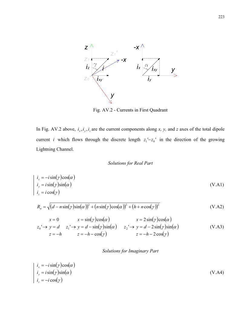
223

Fig. AV.2 - Currents in First Quadrant

In Fig. AV.2 above, are the current components along x, y, and z axes of the total dipole

current which flows through the discrete length

zyx iii ,,

i '' zz 01 − in the direction of the growing

Lightning Channel.

Solutions for Real Part

( ) ( )αγ cossiniix −=

( ) ( )αγ sinsiniiy = (V.A1) ( )γcosiiz =

( ) ( )( ) ( ) ( )( ) ( )( ) 222 coscossinsinsin γαγαγ nhnndRn +++−= (V.A2)

→'0zhz

dyx

−=== 0

→'1z( ) ( )

( ) ( )( )γ

αγαγ

cossinsin

cossin

−−=−=

=

hzdy

x →'2z

( ) ( )( ) ( )( )γ

αγαγ

cos2sinsin2

cossin2

−−=−=

=

hzdy

x (V.A3)

Solutions for Imaginary Part

( ) ( )αγ cossiniix −=

( ) ( )αγ sinsiniiy = (V.A4) ( )γcosiiz −=

224

( ) ( )( ) ( ) ( )( ) ( )( ) 222 coscossinsinsin γαγαγ nhnndRn +++−= (V.A5)

→'0zhzdy

x

=== 0

→'1z( ) ( )

( ) ( )( )γ

αγαγ

cossinsin

cossin

+=−=

=

hzdy

x →'2z

( ) ( )( ) ( )( )γ

αγαγ

cos2sinsin2

cossin2

+=−=

=

hzdy

x (V.A6)

Second Quadrant (-x, -y, +z)

Fig. AV.3 - Geometrical Relations in Second Quadrant

Fig. AV.4 - Currents in Second Quadrant

225


( ) ( )αγ cossiniix −= ( ) ( )αγ sinsiniiy −= (V.A7) ( )γcosiiz =

( ) ( )( ) ( ) ( )( ) ( )( ) 222 coscossinsinsin γαγαγ nhnndRn ++++= (V.A8)

→'0zhz

dyx

−=== 0

→'1z( ) ( )

( ) ( )( )γ

αγαγ

cossinsin

cossin

−−=+=

=

hzdy

x →'2z

( ) ( )( ) ( )( )γ

αγαγ

cos2sinsin2

cossin2

−−=+=

=

hzdy

x (V.A9)


( ) ( )αγ cossiniix −= ( ) ( )αγ sinsiniiy −= (V.A10) ( )γcosiiz −=

( ) ( )( ) ( ) ( )( ) ( )( ) 222 coscossinsinsin γαγαγ nhnndRn ++++= (V.A11)

→'0zhzdy

x

=== 0

→'1z( ) ( )

( ) ( )( )γ

αγαγ

cossinsin

cossin

+=+=

=

hzdy

x →'2z

( ) ( )( ) ( )( )γ

αγαγ

cos2sinsin2

cossin2

+=+=

=

hzdy

x (V.A12)

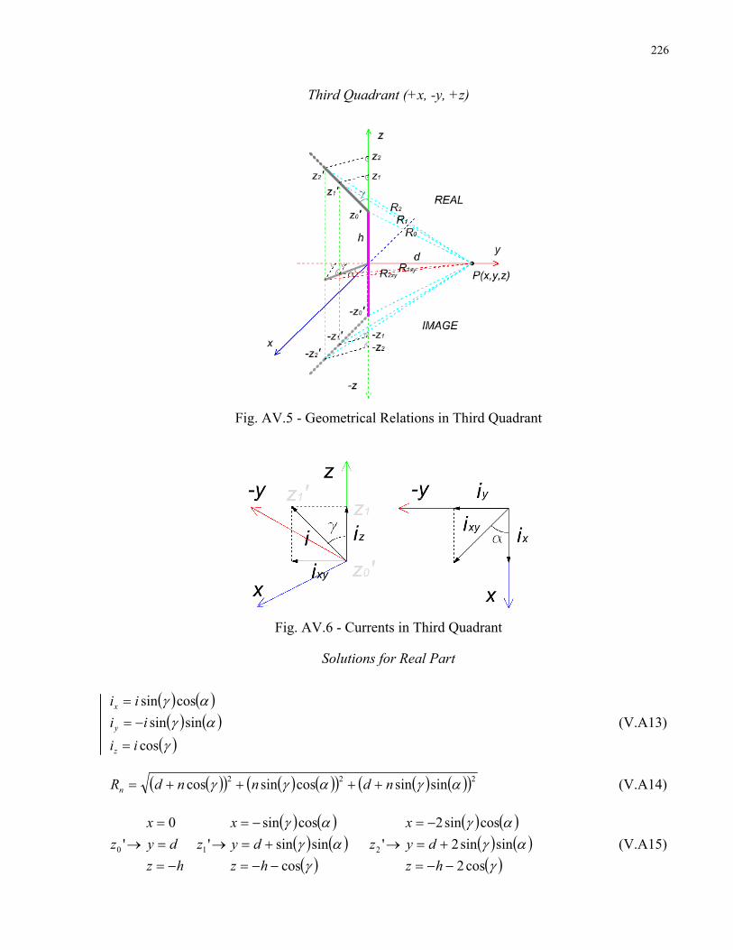
226

Third Quadrant (+x, -y, +z)

Fig. AV.5 - Geometrical Relations in Third Quadrant

Fig. AV.6 - Currents in Third Quadrant


( ) ( )αγ cossiniix = ( ) ( )αγ sinsiniiy −= (V.A13) ( )γcosiiz =

( )( ) ( ) ( )( ) ( )( ( ))222 sinsincossincos αγαγγ ndnndRn ++++= (V.A14)

→'0zhz

dyx

−=== 0

→'1z( ) ( )( ) ( )( )γ

αγαγ

cossinsin

cossin

−−=+=

−=

hzdy

x →'2z

( ) ( )( ) ( )( )γ

αγαγ

cos2sinsin2

cossin2

−−=+=

−=

hzdy

x (V.A15)

227


( ) ( )αγ cossiniix = ( ) ( )αγ sinsiniiy −= (V.A16) ( )γcosiiz −=

( )( ) ( ) ( )( ) ( )( ( ))222 sinsincossincos αγαγγ ndnndRn ++++= (V.A17)

→'0zhzdy

x

=== 0

→'1z( ) ( )( ) ( )( )γ

αγαγ

cossinsin

cossin

+=+=

−=

hzdy

x →'2z

( ) ( )( ) ( )( )γ

αγαγ

cos2sinsin2

cossin2

+=+=

−=

hzdy

x (V.A18)

Fourth Quadrant (+x, +y, +z)

Fig. AV.7 - Geometrical Relations in Fourth Quadrant

Fig. AV.8 - Currents in Fourth Quadrant

228


( ) ( )αγ cossiniix = ( ) ( )αγ sinsiniiy = (V.A19) ( )γcosiiz =

( ) ( )( ) ( ) ( )( ) ( )( ) 222 cossinsincossin γαγαγ nhndnRn ++−+= (V.A20)

→'0zhz

dyx

−=== 0

→'1z( ) ( )( ) ( )( )γ

αγαγ

cossinsin

cossin

−−=−=

−=

hzdy

x →'2z

( ) ( )( ) ( )( )γ

αγαγ

cos2sinsin2

cossin2

−−=−=

−=

hzdy

x (V.A21)


( ) ( )αγ cossiniix = ( ) ( )αγ sinsiniiy = (V.A22) ( )γcosiiz −=

( ) ( )( ) ( ) ( )( ) ( )( ) 222 cossinsincossin γαγαγ nhndnRn ++−+= (V.A23)

→'0zhzdy

x

=== 0

→'1z( ) ( )( ) ( )( )γ

αγαγ

cossinsin

cossin

+=−=

−=

hzdy

x →'2z

( ) ( )( ) ( )( )γ

αγαγ

cos2sinsin2

cossin2

+=−=

−=

hzdy

x (V.A24)

EMF due to Return STrokes at CN Tower - TSpace

Documents

Transcript of EMF due to Return STrokes at CN Tower - TSpace