Emergent behaviour in large electrical networks - University of ...

Emergent behaviour in large electricalnetworks

D. P. Almond, C. J. Budd, and N. J. McCullen

Bath Institute for Complex Systems, University of Bath, BA2 7AY, UK

Summary. Many complex systems have emergent behaviour which results fromthe way in that the components of the system interact, rather than their individualproperties. However, it is often unclear as to what this emergent bahaviour can be,or inded how large the system should be for such behaviour to arise. In this paper wewill address these problems for the specific case of an electrical network comprisinga mixture of resistive and reactive elements. Using this model we will show, usingsome spectral theory, the types of emergent behaviour that we expect and also howlarge a system we need for this to be observed.

1 Introduction and Overview

The theory of complex systems offers great potential as a way of describingand understanding many phenomena involving large numbers of interactingagents, varying from physical systems (such as the weather) to biological andsocial systems [1]. A system is complex rather than just complicated if theindividual components interact strongly and the resulting system behaviour isa product more of these interactions than of the individual components. Suchbehaviour is generally termed emergent behaviour and we can colloquiallythat the complex system is demonstrating behaviour which is more than thesum of its parts. However, such descriptions of complexity are really rathervague and leave open many scientific questions. These include: how large doesa system need to be before it is complex, what sort of interactions lead toemergent behaviour, and can the types of emergent behaviour be classified.More generally, how can we analyse a complex system? We do not believe thatthese questions can be answered in general, however, we can find answers tothem in the context of specific complex problems. This is the purpose of thispaper, which will study a complex system comprising a large binary electricalnetwork, which can be used to model certain material behaviours.

Such large binary networks comprise disordered mixtures of two different butinteracting components. These, arise both directly, in electrical circuits [2],[3],

2 D. P. Almond,C. J. Budd,N. J. McCullen

[4], or mechanical structures [5], and as models of other systems such as disor-dered materials with varying electrical [6], thermal or mechanical properties inthe micro-scale which are then coupled at a meso-scale. Many systems of con-densed matter have this form [7],[8], [9]. Significantly, such systems are oftenobserved to have macroscopic emergent properties which can have emergentpower-law behaviour over a wide range of parameter values which is differentfrom any power law behaviour of the individual elements of the network, andis a product of the way in which the responses of the components combine.As an example of such a binary disordered network, we consider a (set ofrandom realisations of a) binary network comprising a random mixture witha proportion of (1− p) resistors with frequency independent admittance 1/Rand p capacitors with complex admittance iωC directly proportional to fre-quency ω. This network when subjected to an applied alternating voltage offrequency ω has a the total admittance Y (ω). We observe that over a widerange of frequencies 0 < ω1 < ω < ω2 , the admittance displays power lawemergent characteristics, so that |Y | is proportional to ωα, for an appropriateexponent α. Significantly, α is not equal to zero or one (the power law of theresponse of the individual circuit elements) but depends upon the proportionof the capacitors in the network. For example when this proportion takes thecritical value of p = 1/2, then α = 1/2. The effects of network size, andcomponent proportion, are important in that ω1 and ω2 depend upon bothp and N . In the case of p = 1/2 this is a strong dependence and we will seethat ω1 is inversely proportional to N and ω2 directly proportional to N , asN increases to infinity. It is in this frequency range that both the resistorsand capacitors share the (many) current paths through the network, and theyinteract strongly. The emergent behaviour is a result of this interaction. For0 < ω < ω1 and ω > ω2 we see a transition in the behaviour. In these rangeseither the resistors or the capacitors act as conductors, and there are infre-quent current paths, best described by percolation theory. In these ranges theemergent power law behaviour changes and we see instead the individual com-ponent responses. Hence we see in this example of a complex system (i) anemergent region with a power law response depending on the proportion butnot the arrangement or number of the components (ii) a more random perco-lation region with a response dominated by that of individual components and(iii) a transition between these two regions at frequency values which dependson the number and proportion of components in the system. The purpose ofthis paper is to partly explain this behaviour.

The layout of the remainder of this paper is as follows. In Section 2 we willgive a series of numerical results which illustrate the various points madeabove on the nature of the network response. In Section 3 we will formulatethe matrix equations describing the network and the associated representationof the admittance function in terms of poles and zeros. In Section 4 we willdiscuss, and derive, a series of statistical results concerning the distribution ofthe poles ad zeros. In Section 5 we will use these statistical results to derive

Emergent behaviour 3

the asymptotic form of the admittance |Y (ω)| in the critical case of p =1/2. In Section 6 we compare the asymptotic predictions with the numericalcomputations. Finally in Section 7 we will draw some conclusions from thiswork.

2 Simple Network Models and Their Responses

In this section we show the basic models for composite materials and as-sociated random binary electrical networks, and present the graphs of theirresponses. In particular we will look in detail at the existence of a power lawemergent region, and will obtain empirical evidence for the effects of networksize N and capacitor proportion p, on both this region and the ’percolationbehaviour’ when CR ω � 1 and CR ω � 1.

2.1 Modelling Composites as Complex Rectangular Networks

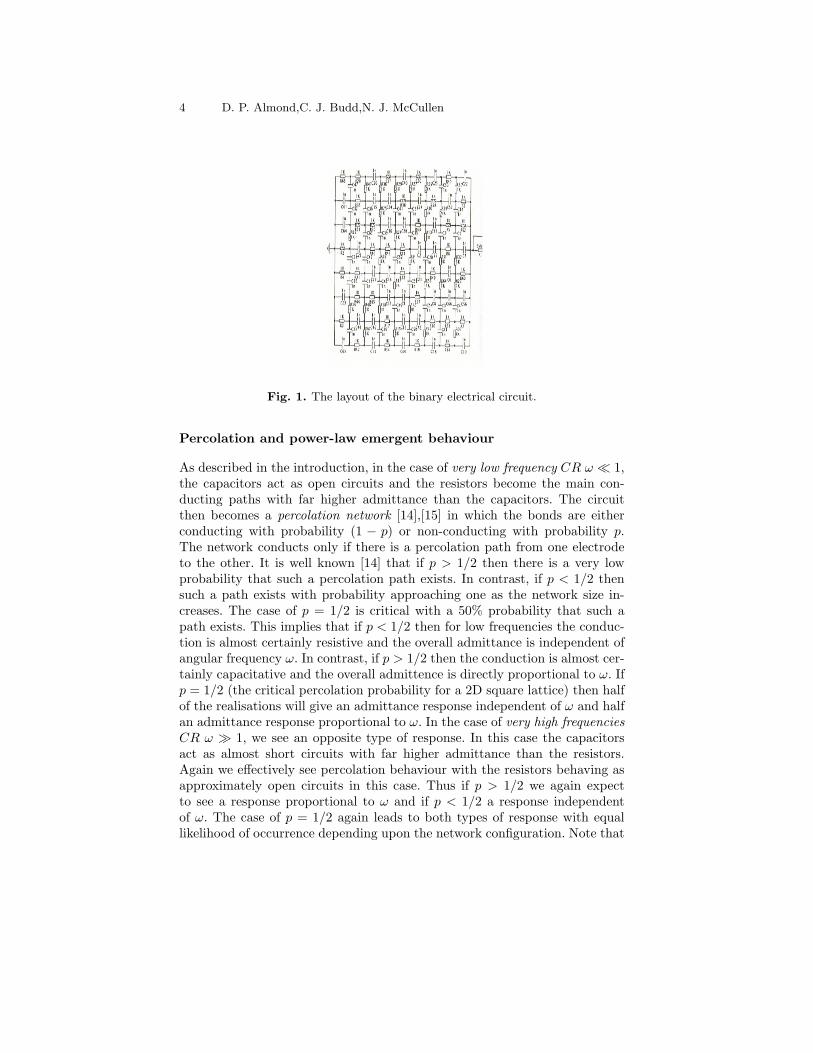
An initial motivation for studying binary networks comes from models ofcomposite materials. Disordered two-phase composite materials are found toexhibit power-law scaling in their bulk responses over several orders of magni-tude in the contrast ratio of the components [10], [3], and this effect has beenobserved [2],[11] in both physical and numerical experiments on conductor-dielectric composite materials. In the electrical experiments this was previ-ously refered to as “Universal Dielectric Response” (UDR), and it has beenobserved [7],[8] that this is an emergent property arising out of the randomnature of the mixture. A simple model of such a conductor-dielectric mixtureswith fine structure is a large electrical circuit replacing the constituent con-ducting and dielectric parts with a linear C-R network of N � 1 resistorsand capacitors, respectively as illustrated in Figure1. For a binary disorderedmixture, the different components can be assigned randomly to bonds on alattice [12]. with bonds assigned randomly as either C or R, with probabilityp, 1 − p respectively. The components are distributed in a two-dimensionallattice between two bus-bars. On of which is grounded and the other is raisedto a potential V (t) = V exp(iωt). This leads to a current I(t) = I(ω) exp(iωt)between the bus-bars, and we measure the macroscopic (complex) admittancegiven by Y (ω) = I(ω)/V. A large review of this and binary disordered net-works can be found in [13, 3].

We now present an overview of the results found for the admittance conduc-tion of the C-R network, explaining the PLER and its bounds. In particular weneed to understand the difference between percolation behaviour and powerlaw emergent behaviour. To motivate these results we consider initially thecases of very low and very large frequency.


Fig. 1. The layout of the binary electrical circuit.

Percolation and power-law emergent behaviour

As described in the introduction, in the case of very low frequency CR ω � 1,the capacitors act as open circuits and the resistors become the main con-ducting paths with far higher admittance than the capacitors. The circuitthen becomes a percolation network [14],[15] in which the bonds are eitherconducting with probability (1 − p) or non-conducting with probability p.The network conducts only if there is a percolation path from one electrodeto the other. It is well known [14] that if p > 1/2 then there is a very lowprobability that such a percolation path exists. In contrast, if p < 1/2 thensuch a path exists with probability approaching one as the network size in-creases. The case of p = 1/2 is critical with a 50% probability that such apath exists. This implies that if p < 1/2 then for low frequencies the conduc-tion is almost certainly resistive and the overall admittance is independent ofangular frequency ω. In contrast, if p > 1/2 then the conduction is almost cer-tainly capacitative and the overall admittence is directly proportional to ω. Ifp = 1/2 (the critical percolation probability for a 2D square lattice) then halfof the realisations will give an admittance response independent of ω and halfan admittance response proportional to ω. In the case of very high frequenciesCR ω � 1, we see an opposite type of response. In this case the capacitorsact as almost short circuits with far higher admittance than the resistors.Again we effectively see percolation behaviour with the resistors behaving asapproximately open circuits in this case. Thus if p > 1/2 we again expectto see a response proportional to ω and if p < 1/2 a response independentof ω. The case of p = 1/2 again leads to both types of response with equallikelihood of occurrence depending upon the network configuration. Note that


this implies that if p = 1/2 then there are four possible qualitatively differenttypes of response for any random realisation of the system.

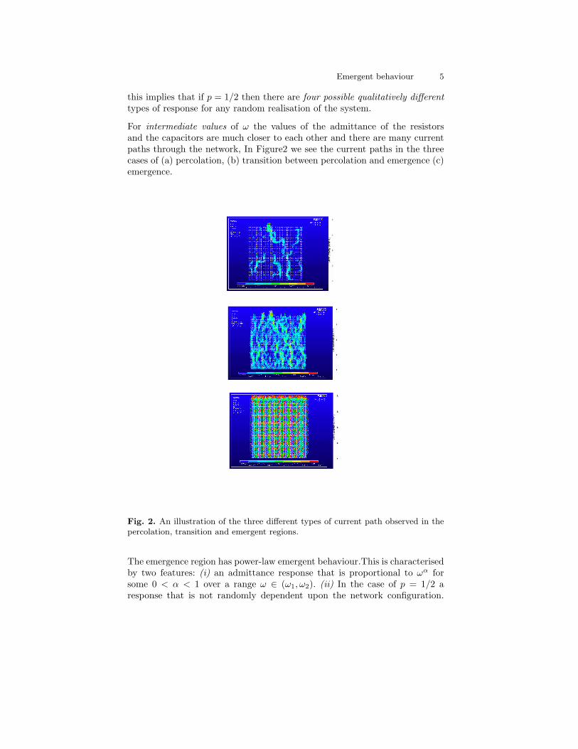
For intermediate values of ω the values of the admittance of the resistorsand the capacitors are much closer to each other and there are many currentpaths through the network, In Figure2 we see the current paths in the threecases of (a) percolation, (b) transition between percolation and emergence (c)emergence.

Fig. 2. An illustration of the three different types of current path observed in thepercolation, transition and emergent regions.

The emergence region has power-law emergent behaviour.This is characterisedby two features: (i) an admittance response that is proportional to ωα forsome 0 < α < 1 over a range ω ∈ (ω1, ω2). (ii) In the case of p = 1/2 aresponse that is not randomly dependent upon the network configuration.


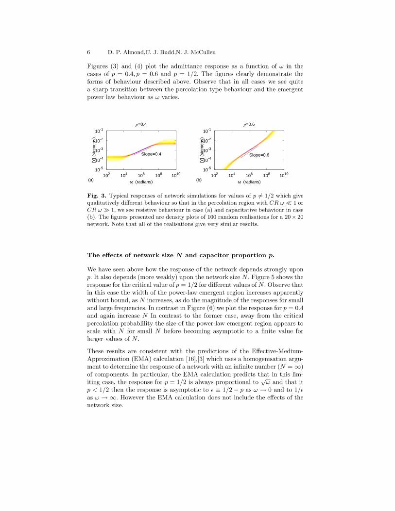
Figures (3) and (4) plot the admittance response as a function of ω in thecases of p = 0.4, p = 0.6 and p = 1/2. The figures clearly demonstrate theforms of behaviour described above. Observe that in all cases we see quitea sharp transition between the percolation type behaviour and the emergentpower law behaviour as ω varies.

p=0.4

(a)102 104 106 108 1010

ω (radians)

10-5

10-4

10-3

10-2

10-1

|Y| (

siem

ens)

Slope=0.4

p=0.6

(b)102 104 106 108 1010

ω (radians)

10-5

10-4

10-3

10-2

10-1

|Y| (

siem

ens)

Slope=0.6

Fig. 3. Typical responses of network simulations for values of p 6= 1/2 which givequalitatively different behaviour so that in the percolation region with CR ω � 1 orCR ω � 1, we see resistive behaviour in case (a) and capacitative behaviour in case(b). The figures presented are density plots of 100 random realisations for a 20× 20network. Note that all of the realisations give very similar results.

The effects of network size N and capacitor proportion p.

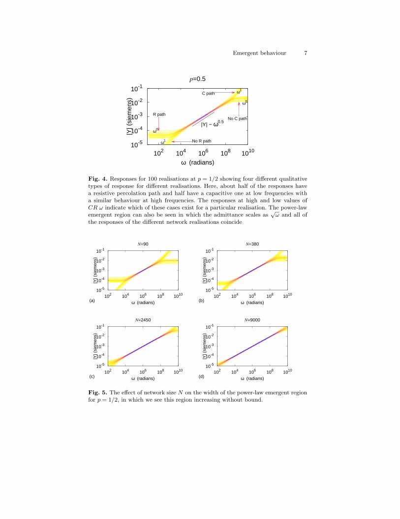
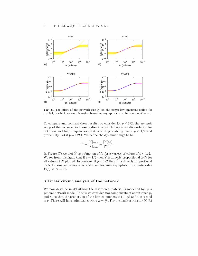
We have seen above how the response of the network depends strongly uponp. It also depends (more weakly) upon the network size N . Figure 5 shows theresponse for the critical value of p = 1/2 for different values of N . Observe thatin this case the width of the power-law emergent region increases apparentlywithout bound, as N increases, as do the magnitude of the responses for smalland large frequencies. In contrast in Figure (6) we plot the response for p = 0.4and again increase N In contrast to the former case, away from the criticalpercolation probablility the size of the power-law emergent region appears toscale with N for small N before becoming asymptotic to a finite value forlarger values of N .

These results are consistent with the predictions of the Effective-Medium-Approximation (EMA) calculation [16],[3] which uses a homogenisation argu-ment to determine the response of a network with an infinite number (N =∞)of components. In particular, the EMA calculation predicts that in this lim-iting case, the response for p = 1/2 is always proportional to

√ω and that it

p < 1/2 then the response is asymptotic to ε ≡ 1/2− p as ω → 0 and to 1/εas ω → ∞. However the EMA calculation does not include the effects of thenetwork size.


p=0.5

102 104 106 108 1010

ω (radians)

10-5

10-4

10-3

10-2

10-1

|Y| (

siem

ens)

|Y| ~ ω0.5No C path

No R path

R path

C path

ω0

ω1

ω1

ω0

Fig. 4. Responses for 100 realisations at p = 1/2 showing four different qualitativetypes of response for different realisations. Here, about half of the responses havea resistive percolation path and half have a capacitive one at low frequencies witha similar behaviour at high frequencies. The responses at high and low values ofCR ω indicate which of these cases exist for a particular realisation. The power-lawemergent region can also be seen in which the admittance scales as

√ω and all of

the responses of the different network realisations coincide

N=90

(a)102 104 106 108 1010

ω (radians)

10-5

10-4

10-3

10-2

10-1

|Y| (

siem

ens)

N=380

(b)102 104 106 108 1010

ω (radians)

10-5

10-4

10-3

10-2

10-1

|Y| (

siem

ens)

N=2450

(c)102 104 106 108 1010

ω (radians)

10-5

10-4

10-3

10-2

10-1

|Y| (

siem

ens)

N=9000

(d)102 104 106 108 1010

ω (radians)

10-5

10-4

10-3

10-2

10-1

|Y| (

siem

ens)

Fig. 5. The effect of network size N on the width of the power-law emergent regionfor p = 1/2, in which we see this region increasing without bound.


N=90

(a)102 104 106 108 1010

ω (radians)

10-5

10-4

10-3

10-2

10-1

|Y| (

siem

ens)

N=380

(b)102 104 106 108 1010

ω (radians)

10-5

10-4

10-3

10-2

10-1

|Y| (

siem

ens)

N=2450

(c)102 104 106 108 1010

ω (radians)

10-5

10-4

10-3

10-2

10-1

|Y| (

siem

ens)

N=9000

(d)102 104 106 108 1010

ω (radians)

10-5

10-4

10-3

10-2

10-1

|Y| (

siem

ens)

Fig. 6. The effect of the network size N on the power-law emergent region forp = 0.4, in which we see this region becoming asymptotic to a finite set as N →∞ .

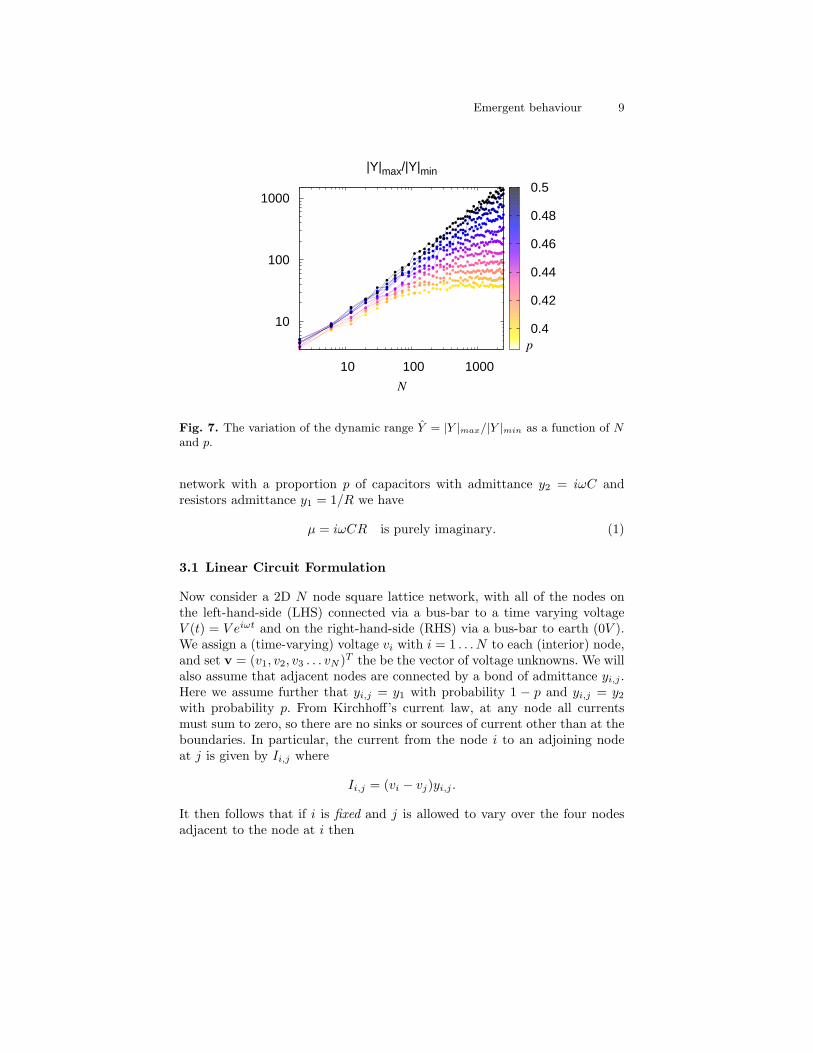
To compare and contrast these results, we consider for p ≤ 1/2, the dynamicrange of the response for those realisations which have a resistive solution forboth low and high frequencies (that is with probability one if p < 1/2 andprobability 1/4 if p = 1/2.). We define the dynamic range to be

Y =|Y |max|Y |min

=|Y (∞)||Y (0)|

.

In Figure (7) we plot Y as a function of N for a variety of values of p ≤ 1/2.We see from this figure that if p = 1/2 then Y is directly proportional to N forall values of N plotted. In contrast, if p < 1/2 then Y is directly proportionalto N for smaller values of N and then becomes asymptotic to a finite valueY (p) as N →∞.

3 Linear circuit analysis of the network

We now describe in detail how the disordered material is modelled by by ageneral network model. In this we consider two components of admittance y1and y2 so that the proportion of the first component is (1−p) and the secondis p. These will have admittance ratio µ = y2

y1. For a capacitor-resistor (C-R)


0.4

0.42

0.44

0.46

0.48

0.5

|Y|max/|Y|min

p

10 100 1000

N

10

100

1000

Fig. 7. The variation of the dynamic range Y = |Y |max/|Y |min as a function of Nand p.

network with a proportion p of capacitors with admittance y2 = iωC andresistors admittance y1 = 1/R we have

µ = iωCR is purely imaginary. (1)

3.1 Linear Circuit Formulation

Now consider a 2D N node square lattice network, with all of the nodes onthe left-hand-side (LHS) connected via a bus-bar to a time varying voltageV (t) = V eiωt and on the right-hand-side (RHS) via a bus-bar to earth (0V ).We assign a (time-varying) voltage vi with i = 1 . . . N to each (interior) node,and set v = (v1, v2, v3 . . . vN )T the be the vector of voltage unknowns. We willalso assume that adjacent nodes are connected by a bond of admittance yi,j .Here we assume further that yi,j = y1 with probability 1 − p and yi,j = y2with probability p. From Kirchhoff’s current law, at any node all currentsmust sum to zero, so there are no sinks or sources of current other than at theboundaries. In particular, the current from the node i to an adjoining nodeat j is given by Ii,j where

Ii,j = (vi − vj)yi,j .

It then follows that if i is fixed and j is allowed to vary over the four nodesadjacent to the node at i then

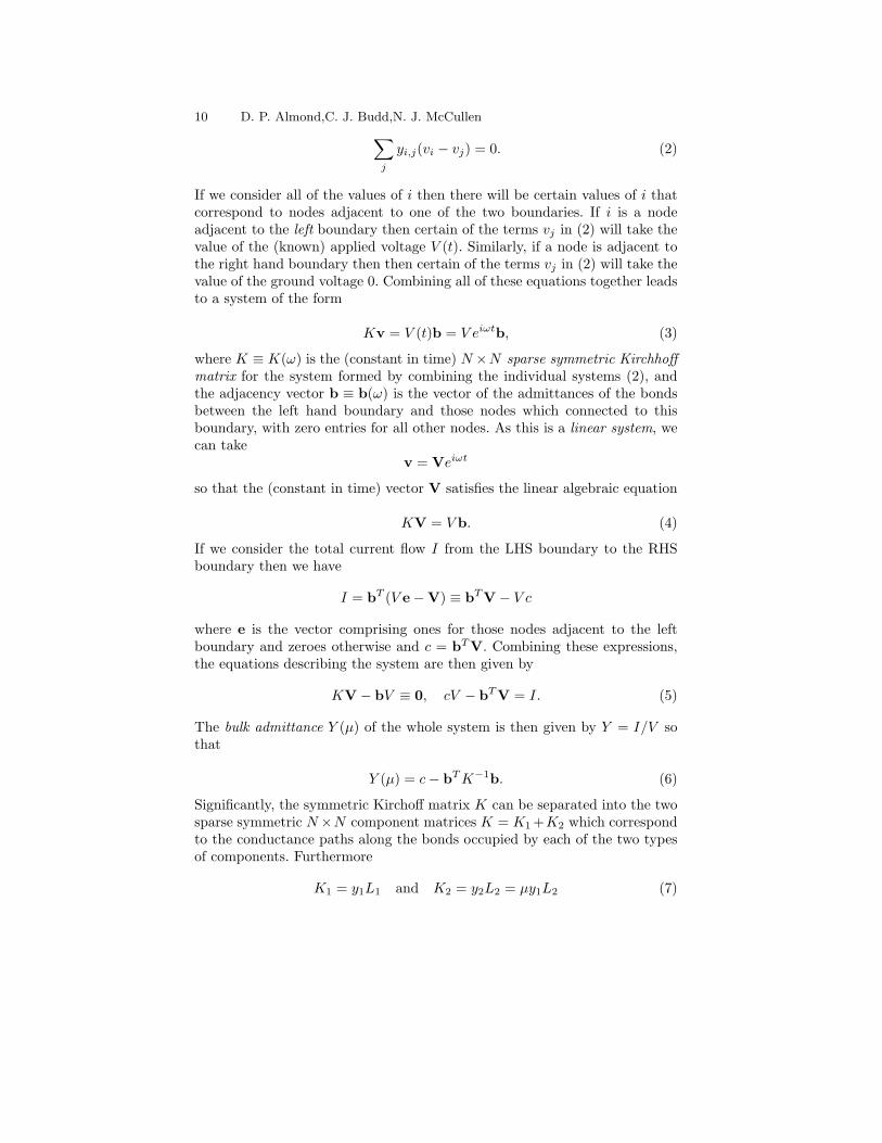
10 D. P. Almond,C. J. Budd,N. J. McCullen∑j

yi,j(vi − vj) = 0. (2)

If we consider all of the values of i then there will be certain values of i thatcorrespond to nodes adjacent to one of the two boundaries. If i is a nodeadjacent to the left boundary then certain of the terms vj in (2) will take thevalue of the (known) applied voltage V (t). Similarly, if a node is adjacent tothe right hand boundary then then certain of the terms vj in (2) will take thevalue of the ground voltage 0. Combining all of these equations together leadsto a system of the form

Kv = V (t)b = V eiωtb, (3)

where K ≡ K(ω) is the (constant in time) N ×N sparse symmetric Kirchhoffmatrix for the system formed by combining the individual systems (2), andthe adjacency vector b ≡ b(ω) is the vector of the admittances of the bondsbetween the left hand boundary and those nodes which connected to thisboundary, with zero entries for all other nodes. As this is a linear system, wecan take

v = Veiωt

so that the (constant in time) vector V satisfies the linear algebraic equation

KV = V b. (4)

If we consider the total current flow I from the LHS boundary to the RHSboundary then we have

I = bT (V e−V) ≡ bTV − V c

where e is the vector comprising ones for those nodes adjacent to the leftboundary and zeroes otherwise and c = bTV. Combining these expressions,the equations describing the system are then given by

KV − bV ≡ 0, cV − bTV = I. (5)

The bulk admittance Y (µ) of the whole system is then given by Y = I/V sothat

Y (µ) = c− bTK−1b. (6)

Significantly, the symmetric Kirchoff matrix K can be separated into the twosparse symmetric N×N component matrices K = K1 +K2 which correspondto the conductance paths along the bonds occupied by each of the two typesof components. Furthermore

K1 = y1L1 and K2 = y2L2 = µy1L2 (7)


where the terms of the sparse symmetric connectivity matrices L1 and L2 areconstant and take the values −1, 0, 1, 2, 3, 4. Note that K is a linear affinefunction of µ. Furthermore,

∆ = L1 + L2

is the discrete (negative definite symmetric) Laplacian for a 2D lattice. Simi-larly we can decompose the adjacency vector into two components b1 and b2

so thatb = b1 + b2 = y1e1 + y2e2

where e1 and e2 are orthogonal vectors comprising ones and zeros only corre-sponding to the two bond types adjacent to the LHS boundary. Observe againthat b is a linear affine function of µ. A similar decomposition can applied tothe scalar c = c1 + µc2.

3.2 Poles and Zeroes of the Admittance Function

To derive formulæ for the expected admittances in terms of the admittanceratio µ = iωCR we now examine the structure of the admittance functionY (µ). As the matrix K, the adjacency vector b and the scalar c are all affinefunctions of the parameter µ it follows immediately from Cramer’s rule appliedto (5) that the admittance of the network Y (µ) is rational function of theparameter µ, taking the form of the ratio of two complex polynomials P (µ)and Q(µ) of respective degrees r ≤ N and s ≤ N , so that

Y (µ) =Q(µ)P (µ)

=q0 + q1µ+ q2µ

2 + . . . qrµr

p0 + p1µ+ p2µ2 + . . . psµs(8)

We require that p0 6= 0 so that the response is physically realisable, withY (µ) bounded as ω and hence µ → 0. Several properties of the networkcan be immediately deduced from this formula. First consider the case of ωsmall, so that µ = iωCR is also small. From the discussions in Section 2,we predict that either there is (a) a resistive percolation path in which caseY (µ) ∼ µ0 as µ→ 0 or (b) such a path does not exist, so that the conductionis capactitative with Y (µ) ∼ µ as µ → 0. The case (a) arises when p0 6= 0and the case (b) when q0 = 0. Observe that this implies that the absence ofa resistive percolation path as µ → 0 is equivalent to the polynomial Q(µ)having a zero when µ = 0.. Next consider the case of ω and hence µ large. Inthis case

Y (µ) ∼ qrpsµr−s as µ→∞.

Again we may have (c) a resisitive percolation path at high frequency withresponse Y (µ) ∼ µ0 as µ → ∞, or a capacitative path with Y (µ) ∼ µ. Incase (c) we have s = r and pr 6= 0 and in case (d) we have s = r − 1 so thatwe can think of taking pr = 0. Accordingly, we identify four types of networkdefined in terms of there percolation paths for low and high frequencies, whichcorrespond to the cases (a),(b),(c ),(d) so that


(a) p0 6= 0(b) p0 = 0(c) pr 6= 0(d) pr = 0

The polynomials P (µ) and Q(µ) can be factorised by determining their re-spective roots µp,k,,k = 1 . . . s and µz,k,,k = 1 . . . r which are the poles andzeroes of the network. We will collectively call these zeroes and poles the res-onances of the network. It will become apparent that the emergent responseof the network is in fact a manifestation of certain regularities of the locationsof these resonances. Note that in Case (b) we have µz,1 = 0. Accordingly thenetwork admittance can be expressed as

Y (µ,N) = D(N)

r∏k=1

(µ− µz,k)

s∏k=1

(µ− µp,k). (9)

Here D(N) is a function which does not depend on µ but does depend on thecharacteristics of the network.

It is a feature of the stability of the network (bounded response), and theaffine structure of the symmetric linear equations which describe it [3], thatthe poles and zeros of Y (µ) are all negative real numbers, and interlace sothat

0 ≥ µz,1 > µp,1 > µz,2 > µp,2 . . . > µz,s > µp,s(> µz,r) (10)

Because of this, we may recast the equation (11) in terms of ω so that

|Y (µ,N)| = |D(N)|

r∏k=1

|ω − iWz,k|s∏

k=1

|ω − iWp,k|(11)

where Wz,k ≥ 0,Wp,k > 0.

4 The distribution of the resonances

The previous section has described the network response in terms of the loca-tion of the poles and the zeros. We now consider the statistical distribution ofthese values and claim that it is this distribution which leads to the observedemergent behaviour. We note that if we consider the elements of the networkto be assigned randomly (with the components taking each of the two possiblevalues with probabilities p and 1−p then we can consider the resonances to berandom variables. There are three interesting questions to ask, which becomerelevant for the calculations in the next section, namely


1. What is the statistical distribution of Wp,k if N is large.2. Given that the zeros interlace the poles, what is the statistical distribution

of the location of a zero between its two adjacent poles.3. What are the ranges of Wp,k, in particular, how do Wp,1 and Wp,N vary

with N and p.

In each case we will find good numerical evidence for strong statistical regu-larity of the poles, especially in the critical case of p = 1/2, leading to partialanswers to each of the above questions. For the remainder of this paper wewill now only consider this critical case.

4.1 Pole location

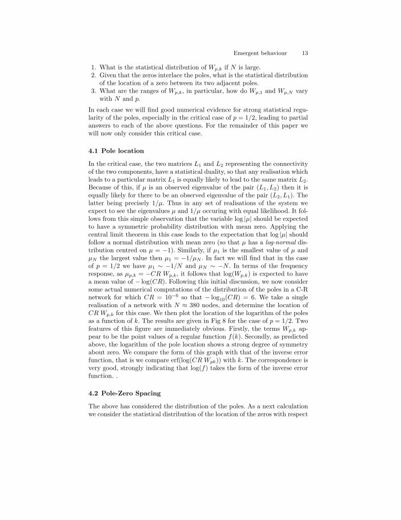
In the critical case, the two matrices L1 and L2 representing the connectivityof the two components, have a statistical duality, so that any realisation whichleads to a particular matrix L1 is equally likely to lead to the same matrix L2.Because of this, if µ is an observed eigenvalue of the pair (L1, L2) then it isequally likely for there to be an observed eigenvalue of the pair (L2, L1). Thelatter being precisely 1/µ. Thus in any set of realisations of the system weexpect to see the eigenvalues µ and 1/µ occuring with equal likelihood. It fol-lows from this simple observation that the variable log |µ| should be expectedto have a symmetric probability distribution with mean zero. Applying thecentral limit theorem in this case leads to the expectation that log |µ| shouldfollow a normal distribution with mean zero (so that µ has a log-normal dis-tribution centred on µ = −1). Similarly, if µ1 is the smallest value of µ andµN the largest value then µ1 = −1/µN . In fact we will find that in ths caseof p = 1/2 we have µ1 ∼ −1/N and µN ∼ −N . In terms of the frequencyresponse, as µp,k = −CR Wp,k, it follows that log(Wp,k) is expected to havea mean value of − log(CR). Following this initial discussion, we now considersome actual numerical computations of the distribution of the poles in a C-Rnetwork for which CR = 10−6 so that − log10(CR) = 6. We take a singlerealisation of a network with N ≈ 380 nodes, and determine the location ofCR Wp,k for this case. We then plot the location of the logarithm of the polesas a function of k. The results are given in Fig 8 for the case of p = 1/2. Twofeatures of this figure are immediately obvious. Firstly, the terms Wp,k ap-pear to be the point values of a regular function f(k). Secondly, as predictedabove, the logarithm of the pole location shows a strong degree of symmetryabout zero. We compare the form of this graph with that of the inverse errorfunction, that is we compare erf(log(CR Wpk)) with k. The correspondence isvery good, strongly indicating that log(f) takes the form of the inverse errorfunction. .

4.2 Pole-Zero Spacing

The above has considered the distribution of the poles. As a next calculationwe consider the statistical distribution of the location of the zeros with respect


-1

-0.5

0

0.5

1

-2 -1.5 -1 -0.5 0 0.5 1 1.5 22k

-1log10(Wk)/1.15(a)

erf(x)

-1

-0.5

0

0.5

1

-1 -0.5 0 0.5 1

erf(

log 1

0(W

k))

2k-1(b)

Fig. 8. The location of the logarithm of the poles as a function of k and a comparisonwith the inverse error function.

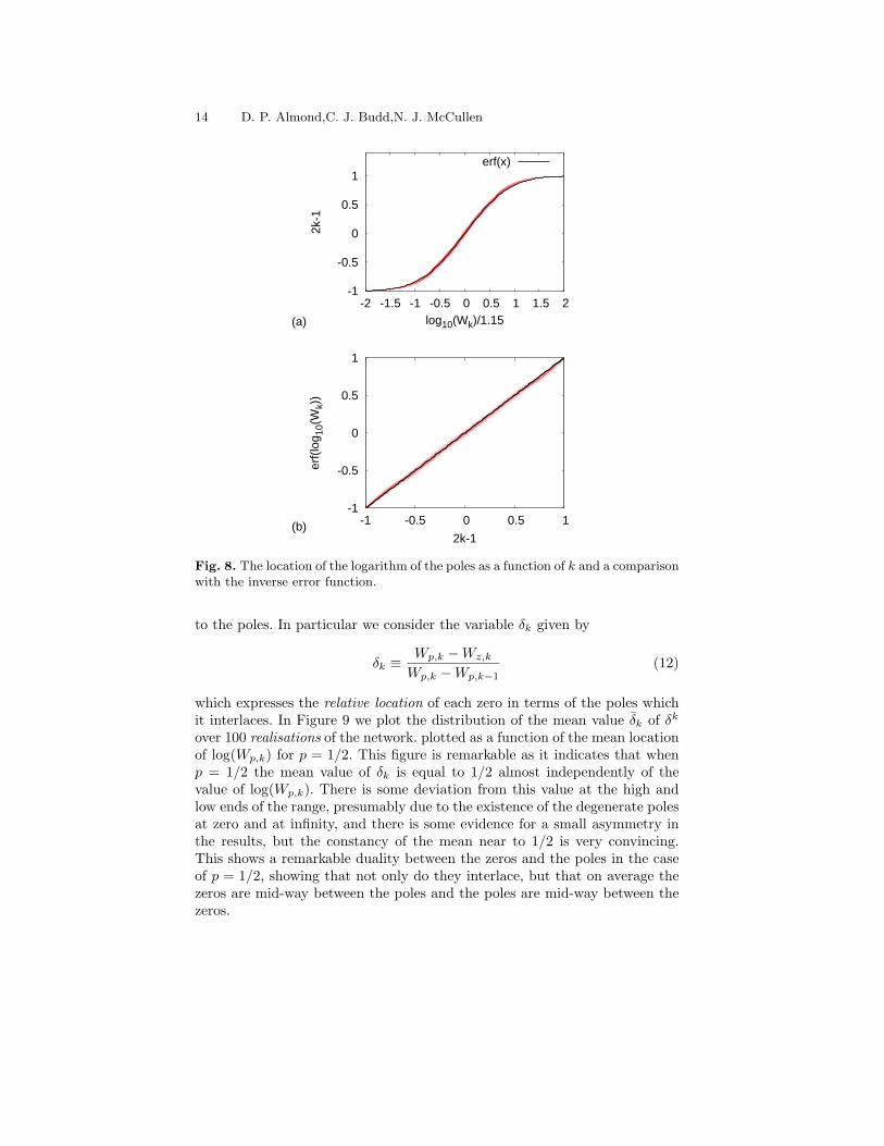
to the poles. In particular we consider the variable δk given by

δk ≡Wp,k −Wz,k

Wp,k −Wp,k−1(12)

which expresses the relative location of each zero in terms of the poles whichit interlaces. In Figure 9 we plot the distribution of the mean value δk of δk

over 100 realisations of the network. plotted as a function of the mean locationof log(Wp,k) for p = 1/2. This figure is remarkable as it indicates that whenp = 1/2 the mean value of δk is equal to 1/2 almost independently of thevalue of log(Wp,k). There is some deviation from this value at the high andlow ends of the range, presumably due to the existence of the degenerate polesat zero and at infinity, and there is some evidence for a small asymmetry inthe results, but the constancy of the mean near to 1/2 is very convincing.This shows a remarkable duality between the zeros and the poles in the caseof p = 1/2, showing that not only do they interlace, but that on average thezeros are mid-way between the poles and the poles are mid-way between thezeros.


0

0.2

0.4

0.6

0.8

1

3 4 5 6 7 8 9

δ

Wi

0.50

Fig. 9. Figure showing how the mean value δk, taken over many realisations of thecritical network, varies with the mean value of log(Wp,k).

4.3 Limiting Finite Resonances

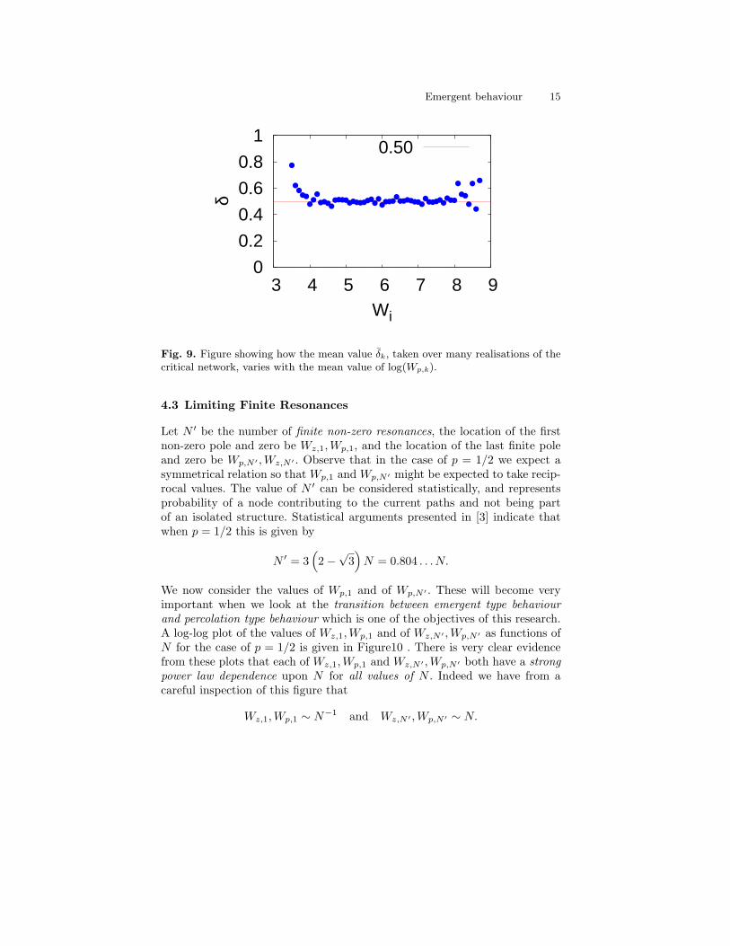
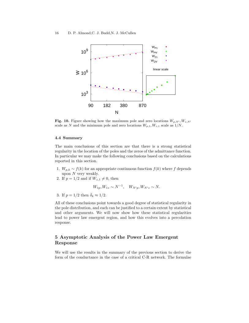
Let N ′ be the number of finite non-zero resonances, the location of the firstnon-zero pole and zero be Wz,1,Wp,1, and the location of the last finite poleand zero be Wp,N ′ ,Wz,N ′ . Observe that in the case of p = 1/2 we expect asymmetrical relation so that Wp,1 and Wp,N ′ might be expected to take recip-rocal values. The value of N ′ can be considered statistically, and representsprobability of a node contributing to the current paths and not being partof an isolated structure. Statistical arguments presented in [3] indicate thatwhen p = 1/2 this is given by

N ′ = 3(

2−√

3)N = 0.804 . . . N.

We now consider the values of Wp,1 and of Wp,N ′ . These will become veryimportant when we look at the transition between emergent type behaviourand percolation type behaviour which is one of the objectives of this research.A log-log plot of the values of Wz,1,Wp,1 and of Wz,N ′ ,Wp,N ′ as functions ofN for the case of p = 1/2 is given in Figure10 . There is very clear evidencefrom these plots that each of Wz,1,Wp,1 and Wz,N ′ ,Wp,N ′ both have a strongpower law dependence upon N for all values of N . Indeed we have from acareful inspection of this figure that

Wz,1,Wp,1 ∼ N−1 and Wz,N ′ ,Wp,N ′ ∼ N.


103

106

109

90 182 380 870

W

N

WP1

WPN’

WZ1

WZN’

linear scale

Fig. 10. Figure showing how the maximum pole and zero locations Wp,N′ ,Wz,N′

scale as N and the minimum pole and zero locations Wp,1,Wz,1 scale as 1/N .

4.4 Summary

The main conclusions of this section are that there is a strong statisticalregularity in the location of the poles and the zeros of the admittance function.In particular we may make the following conclusions based on the calculationsreported in this section.

1. Wp,k ∼ f(k) for an appropriate continuous function f(k) where f dependsupon N very weakly.

2. If p = 1/2 and if Wz,1 6= 0, then

W1p,W1z ∼ N−1, WN ′p,WN ′z ∼ N.

3. If p = 1/2 then δk ≈ 1/2.

All of these conclusions point towards a good degree of statistical regularity inthe pole distribution, and each can be justified to a certain extent by statisticaland other arguments. We will now show how these statistical regularitieslead to power law emergent region, and how this evolves into a percolationresponse.

5 Asymptotic Analysis of the Power Law EmergentResponse

We will use the results in the summary of the previous section to derive theform of the conductance in the case of a critical C-R network. The formulae


that we derive will take one of four forms, depending upon the nature of thepercolation paths for low and high frequencies.

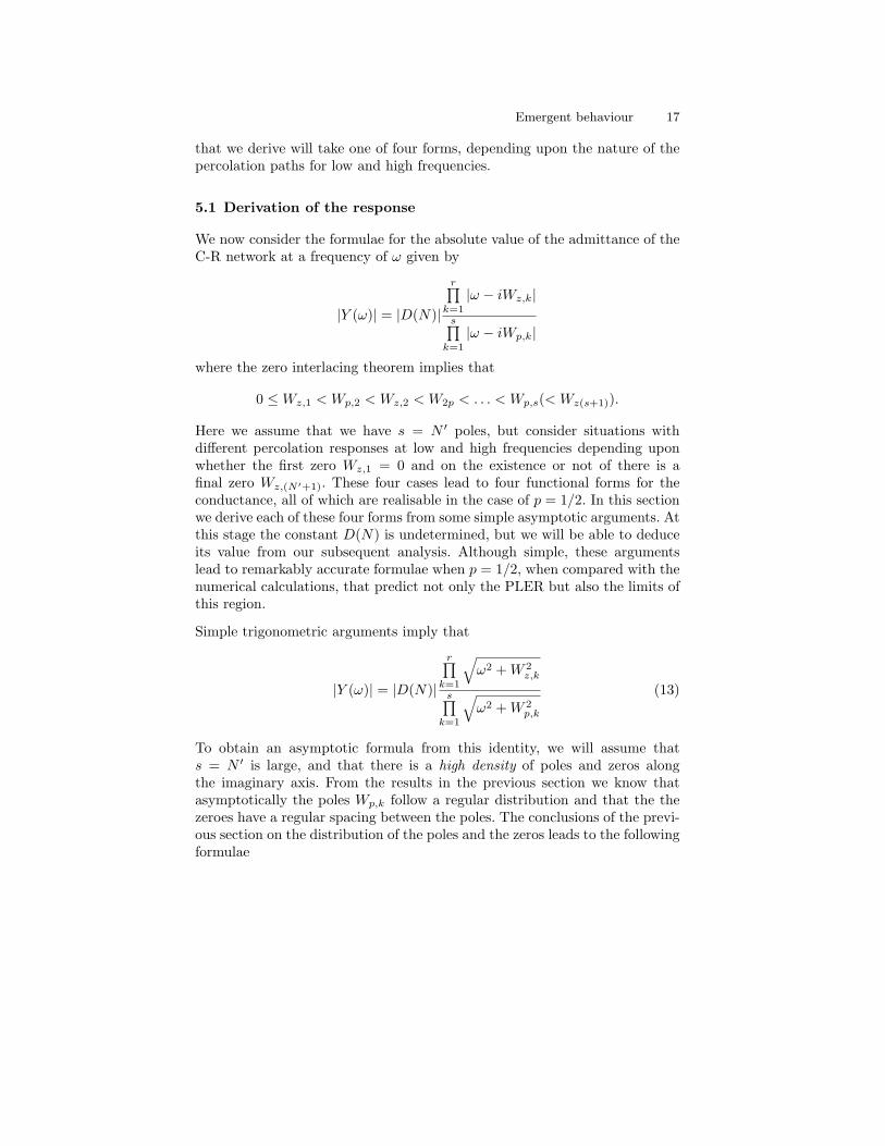
5.1 Derivation of the response

We now consider the formulae for the absolute value of the admittance of theC-R network at a frequency of ω given by

|Y (ω)| = |D(N)|

r∏k=1

|ω − iWz,k|s∏

k=1

|ω − iWp,k|

where the zero interlacing theorem implies that

0 ≤Wz,1 < Wp,2 < Wz,2 < W2p < . . . < Wp,s(< Wz(s+1)).

Here we assume that we have s = N ′ poles, but consider situations withdifferent percolation responses at low and high frequencies depending uponwhether the first zero Wz,1 = 0 and on the existence or not of there is afinal zero Wz,(N ′+1). These four cases lead to four functional forms for theconductance, all of which are realisable in the case of p = 1/2. In this sectionwe derive each of these four forms from some simple asymptotic arguments. Atthis stage the constant D(N) is undetermined, but we will be able to deduceits value from our subsequent analysis. Although simple, these argumentslead to remarkably accurate formulae when p = 1/2, when compared with thenumerical calculations, that predict not only the PLER but also the limits ofthis region.

Simple trigonometric arguments imply that

|Y (ω)| = |D(N)|

r∏k=1

√ω2 +W 2

z,k

s∏k=1

√ω2 +W 2

p,k

(13)

To obtain an asymptotic formula from this identity, we will assume thats = N ′ is large, and that there is a high density of poles and zeros alongthe imaginary axis. From the results in the previous section we know thatasymptotically the poles Wp,k follow a regular distribution and that the thezeroes have a regular spacing between the poles. The conclusions of the previ-ous section on the distribution of the poles and the zeros leads to the followingformulae


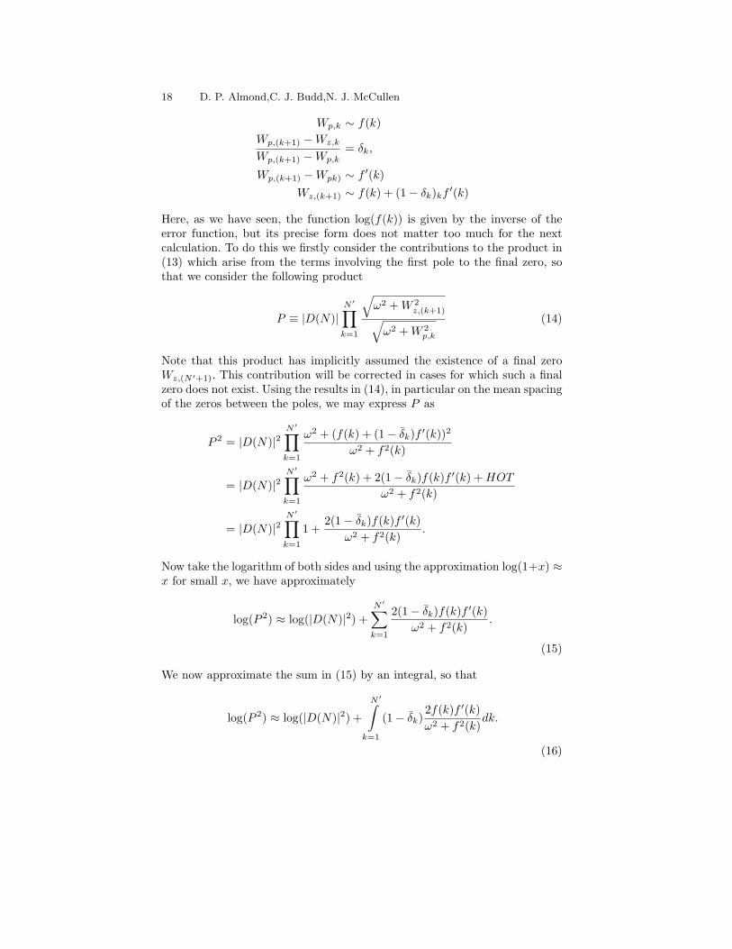
Wp,k ∼ f(k)Wp,(k+1) −Wz,k

Wp,(k+1) −Wp,k= δk,

Wp,(k+1) −Wpk) ∼ f ′(k)Wz,(k+1) ∼ f(k) + (1− δk)kf ′(k)

Here, as we have seen, the function log(f(k)) is given by the inverse of theerror function, but its precise form does not matter too much for the nextcalculation. To do this we firstly consider the contributions to the product in(13) which arise from the terms involving the first pole to the final zero, sothat we consider the following product

P ≡ |D(N)|N ′∏k=1

√ω2 +W 2

z,(k+1)√ω2 +W 2

p,k

(14)

Note that this product has implicitly assumed the existence of a final zeroWz,(N ′+1). This contribution will be corrected in cases for which such a finalzero does not exist. Using the results in (14), in particular on the mean spacingof the zeros between the poles, we may express P as

P 2 = |D(N)|2N ′∏k=1

ω2 + (f(k) + (1− δk)f ′(k))2

ω2 + f2(k)

= |D(N)|2N ′∏k=1

ω2 + f2(k) + 2(1− δk)f(k)f ′(k) +HOT

ω2 + f2(k)

= |D(N)|2N ′∏k=1

1 +2(1− δk)f(k)f ′(k)

ω2 + f2(k).

Now take the logarithm of both sides and using the approximation log(1+x) ≈x for small x, we have approximately

log(P 2) ≈ log(|D(N)|2) +N ′∑k=1

2(1− δk)f(k)f ′(k)ω2 + f2(k)

.

(15)

We now approximate the sum in (15) by an integral, so that

log(P 2) ≈ log(|D(N)|2) +

N ′∫k=1

(1− δk)2f(k)f ′(k)ω2 + f2(k)

dk.

(16)


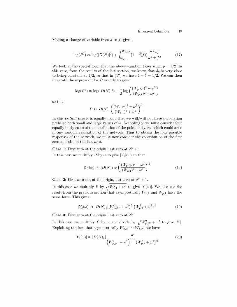
Making a change of variable from k to f , gives

log(P 2) ≈ log(|D(N)|2) +∫ Wp,N′

Wp,1

(1− δ(f))2f dfω2 + f2

(17)

We look at the special form that the above equation takes when p = 1/2. Inthis case, from the results of the last section, we know that δk is very closeto being constant at 1/2, so that in (17) we have 1 − δ = 1/2. We can thenintegrate the expression for P exactly to give

log(P 2) ≈ log(|D(N)|2) +12

log(

(Wp,N ′)2 + ω2

(Wp,1)2 + ω2

)so that

P ≈ |D(N)|(

(Wp,N ′)2 + ω2

(Wp,1)2 + ω2

) 14

.

In this critical case it is equally likely that we will/will not have percolationpaths at both small and large values of ω. Accordingly, we must consider fourequally likely cases of the distribution of the poles and zeros which could arisein any random realisation of the network. Thus to obtain the four possibleresponses of the network, we must now consider the contribution of the firstzero and also of the last zero.

Case 1: First zero at the origin, last zero at N ′ + 1

In this case we multiply P by ω to give |Y1|(ω) so that

|Y1(ω)| ≈ |D(N)1|ω(

(Wp,N ′)2 + ω2

(Wp,1)2 + ω2

) 14

(18)

Case 2: First zero not at the origin, last zero at N ′ + 1.

In this case we multiply P by√W 2z,1 + ω2 to give |Y (ω)|. We also use the

result from the previous section that asymptotically Wz,1 and Wp,1 have thesame form. This gives

|Y2(ω)| ≈ |D(N)2|(W 2p,N ′ + ω2)

14(W 2p,1 + ω2

) 14 (19)

Case 3: First zero at the origin, last zero at N ′

In this case we multiply P by ω and divide by√W 2z,N ′ + ω2 to give |Y |.

Exploiting the fact that asymptotically Wp,N ′ ∼Wz,N ′ we have

|Y3(ω)| ≈ |D(N)3|ω(

W 2p,N ′ + ω2

)1/4 (W 2p,1 + ω2

) 14

(20)


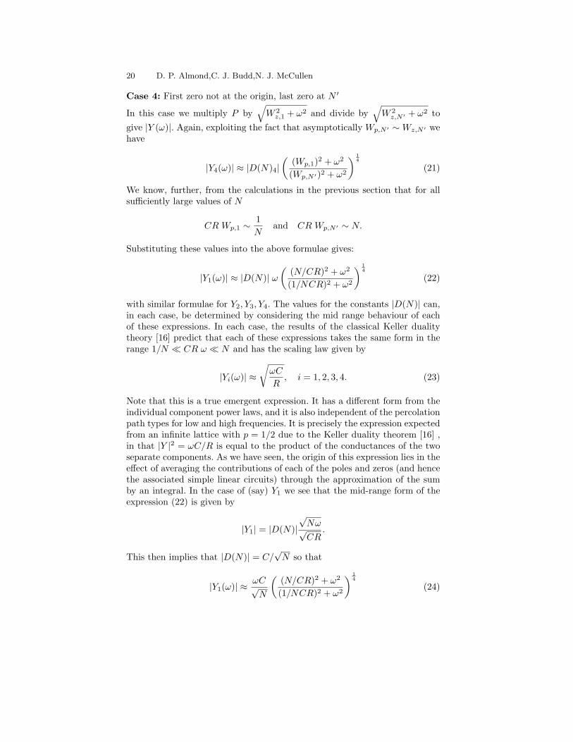
Case 4: First zero not at the origin, last zero at N ′

In this case we multiply P by√W 2z,1 + ω2 and divide by

√W 2z,N ′ + ω2 to

give |Y (ω)|. Again, exploiting the fact that asymptotically Wp,N ′ ∼Wz,N ′ wehave

|Y4(ω)| ≈ |D(N)4|(

(Wp,1)2 + ω2

(Wp,N ′)2 + ω2

) 14

(21)

We know, further, from the calculations in the previous section that for allsufficiently large values of N

CR Wp,1 ∼1N

and CR Wp,N ′ ∼ N.

Substituting these values into the above formulae gives:

|Y1(ω)| ≈ |D(N)| ω(

(N/CR)2 + ω2

(1/NCR)2 + ω2

) 14

(22)

with similar formulae for Y2, Y3, Y4. The values for the constants |D(N)| can,in each case, be determined by considering the mid range behaviour of eachof these expressions. In each case, the results of the classical Keller dualitytheory [16] predict that each of these expressions takes the same form in therange 1/N � CR ω � N and has the scaling law given by

|Yi(ω)| ≈√ωC

R, i = 1, 2, 3, 4. (23)

Note that this is a true emergent expression. It has a different form from theindividual component power laws, and it is also independent of the percolationpath types for low and high frequencies. It is precisely the expression expectedfrom an infinite lattice with p = 1/2 due to the Keller duality theorem [16] ,in that |Y |2 = ωC/R is equal to the product of the conductances of the twoseparate components. As we have seen, the origin of this expression lies in theeffect of averaging the contributions of each of the poles and zeros (and hencethe associated simple linear circuits) through the approximation of the sumby an integral. In the case of (say) Y1 we see that the mid-range form of theexpression (22) is given by

|Y1| = |D(N)|√Nω√CR

.

This then implies that |D(N)| = C/√N so that

|Y1(ω)| ≈ ωC√N

((N/CR)2 + ω2

(1/NCR)2 + ω2

) 14

(24)


Very similar arguements lead to the following expressions in the other threecases:

|Y2(ω)| ≈ C√N

((N/CR)2 + ω2)14((1/NCR)2 + ω2

) 14 (25)

|Y3(ω)| ≈√N

R

ω

((N/CR)2 + ω2)14 ((1/NCR)2 + ω2)

14

(26)

|Y4(ω)| ≈√N

R

((1/NCR)2 + ω2

(N/CR)2 + ω2

) 14

(27)

The four formulae above give a very complete asymptotic description of theresponse of the C-R network when p = 1/2. In particular they allow us tosee the transition between the power-law emergent region and the percolationregions and they also describe the form of the expressions in the percolationregions. We see a clear transition between the emergent and the percolationregions at the two frequencies

ω1 =1

NCRand ω2 =

N

CR. (28)

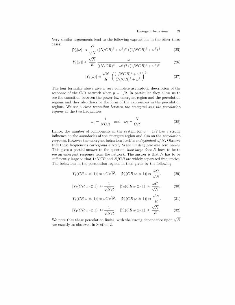
Hence, the number of components in the system for p = 1/2 has a stronginfluence on the boundaries of the emergent region and also on the percolationresponse. However the emergent behaviour itself is independent of N . Observethat these frequencies correspond directly to the limiting pole and zero values.This gives a partial answer to the question, how large does N have to be tosee an emergent response from the network. The answer is that N has to besufficiently large so that 1/NCR and N/CR are widely separated frequencies.The behaviour in the percolation regions in then given by the following

|Y1(CR ω � 1)| ≈ ωC√N, |Y1(CR ω � 1)| ≈ ωC√

N. (29)

|Y2(CR ω � 1)| ≈ 1√NR

, |Y2(CR ω � 1)| ≈ ωC√N. (30)

|Y3(CR ω � 1)| ≈ ωC√N, |Y3(CR ω � 1)| ≈

√N

R. (31)

|Y4(CR ω � 1)| ≈ 1√NR

, |Y4(CR ω � 1)| ≈√N

R. (32)

We note that these percolation limits, with the strong dependence upon√N

are exactly as observed in Section 2.


6 Comparison of the Asymptotic and Numerical Resultsfor the Critical Case

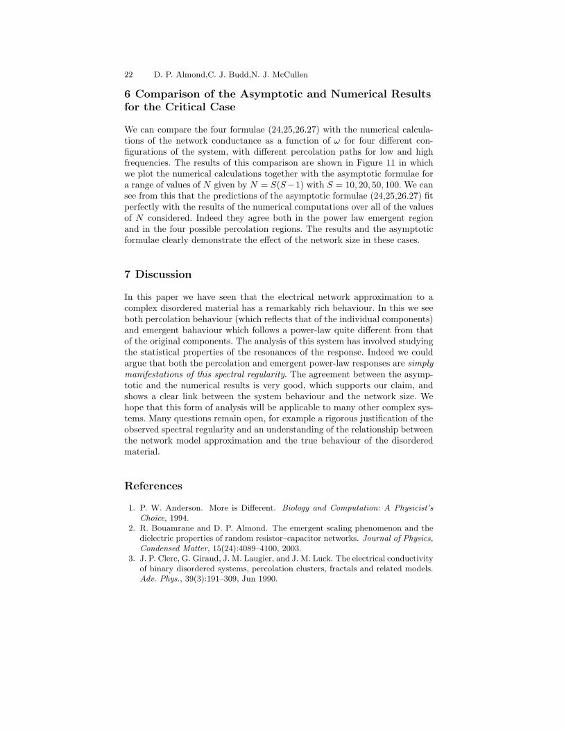
We can compare the four formulae (24,25,26.27) with the numerical calcula-tions of the network conductance as a function of ω for four different con-figurations of the system, with different percolation paths for low and highfrequencies. The results of this comparison are shown in Figure 11 in whichwe plot the numerical calculations together with the asymptotic formulae fora range of values of N given by N = S(S−1) with S = 10, 20, 50, 100. We cansee from this that the predictions of the asymptotic formulae (24,25,26.27) fitperfectly with the results of the numerical computations over all of the valuesof N considered. Indeed they agree both in the power law emergent regionand in the four possible percolation regions. The results and the asymptoticformulae clearly demonstrate the effect of the network size in these cases.

7 Discussion

In this paper we have seen that the electrical network approximation to acomplex disordered material has a remarkably rich behaviour. In this we seeboth percolation behaviour (which reflects that of the individual components)and emergent bahaviour which follows a power-law quite different from thatof the original components. The analysis of this system has involved studyingthe statistical properties of the resonances of the response. Indeed we couldargue that both the percolation and emergent power-law responses are simplymanifestations of this spectral regularity. The agreement between the asymp-totic and the numerical results is very good, which supports our claim, andshows a clear link between the system behaviour and the network size. Wehope that this form of analysis will be applicable to many other complex sys-tems. Many questions remain open, for example a rigorous justification of theobserved spectral regularity and an understanding of the relationship betweenthe network model approximation and the true behaviour of the disorderedmaterial.

References

1. P. W. Anderson. More is Different. Biology and Computation: A Physicist’sChoice, 1994.

2. R. Bouamrane and D. P. Almond. The emergent scaling phenomenon and thedielectric properties of random resistor–capacitor networks. Journal of Physics,Condensed Matter, 15(24):4089–4100, 2003.

3. J. P. Clerc, G. Giraud, J. M. Laugier, and J. M. Luck. The electrical conductivityof binary disordered systems, percolation clusters, fractals and related models.Adv. Phys., 39(3):191–309, Jun 1990.


N=90

100 104 106 108 1010

ω (radians)

10-610-510-410-310-2

0.1

1.0

|Y| (

siem

ens)

N=90

(a)

Y1(ω)Y4(ω)

N=380

100 104 106 108 1010

ω (radians)

10-610-510-410-310-2

0.1

1.0

|Y| (

siem

ens)

N=380

(b)

Y1(ω)Y4(ω)

4. B. Vainas, D. P. Almond, J. Luo, and R. Stevens. An evaluation of random RCnetworks for modelling the bulk ac electrical response of ionic conductors. SolidState Ionics, 126(1):65–80, 1999.

5. K. D. Murphy, G. W. Hunt, and D. P. Almond. Evidence of emergent scalingin mechanical systems. Philosophical Magazine, 86(21):3325–3338, 2006.

6. Jeppe C. Dyre and Thomas B. Schrøder. Universality of ac conduction in dis-ordered solids. Rev. Mod. Phys., 72(3):873–892, Jul 2000.

7. KL Ngai, CT White, and AK Jonscher. On the origin of the universal dielectricresponse in condensed matter. Nature, 277(5693):185–189, 1979.

8. A. K. Jonscher. The universal dielectric response. Nature, 267(23):673–679,1977.

9. K. Funke and R.D. Banhatti. Ionic motion in materials with disordered struc-tures. Solid State Ionics, 177(19-25):1551–1557, 2006.


N=2450

100 104 106 108 1010

ω (radians)

10-610-510-410-310-2

0.1

1.0|Y

| (si

emen

s)

N=2450

(c)

Y1(ω)Y4(ω)

N=9900

100 104 106 108 1010

ω (radians)

10-610-510-410-310-2

0.1

1.0

|Y| (

siem

ens)

N=9900

(d)

Y1(ω)Y4(ω)

Fig. 11. Comparison of the asymptotic formulae with the numerical computationsfor the C − R network over many runs, with p = 1/2 and network sizes sizes S =10, 20, 50, 100, N = S(S − 1).

10. A. K. Jonscher. Universal Relaxation Law: A Sequel to Dielectric Relaxation inSolids. Chelsea Dielectrics Press, 1996.

11. C. Brosseau. Modelling and simulation of dielectric heterostructures: a physicalsurvey from an historical perspective. J. Phys. D: Appl. Phys, 39:1277–94, 2005.

12. V.-T. Truong and J. G. Ternan. Complex Conductivity of a Conducting PolymerComposite at Microwave Frequencies. Polymer, 36(5):905–909, 1995.

13. T. Jonckheere and JM Luck. Dielectric resonances of binary random networks.J. Phys. A: Math. Gen, 31:3687–3717, 1998.


14. S. R. Broadbent and J. M. Hammersley. Percolation processes. I, II. Proc.Cambridge Philos. Soc, 53:629–641, 1953.

15. C.D. Lorenz and R.M. Ziff. Precise determination of the bond percolationthresholds and finite-size scaling corrections for the sc, fcc, and bcc lattices.Physical Review E, 57(1):230–236, 1998.

16. G. W. Milton. Bounds on the complex dielectric constant of a composite mate-rial. Applied Physics Letters, 37:300, 1980.

Emergent behaviour in large electrical networks - University of ...

Documents

Transcript of Emergent behaviour in large electrical networks - University of ...