Emergence of chemotherapy resistance

in cancer: microenvironments,

genomics, and game theory approaches

Amy Wu

A Dissertation

Presented to the Faculty

of Princeton University

in Candidacy for the Degree

of Doctor of Philosophy

Recommended for Acceptance

by the Department of

Electrical Engineering

Adviser: Professor James C Sturm

June 2015

c© Copyright by Amy Wu, 2015.

All rights reserved.

Abstract

Most cancers are still incurable because resistance to therapy is inevitable. Can-

cer cells usually acquire chemotherapy resistance due to two properties of cancer:

adaptive cellular response to a heterogeneous microenvironment, and nonlinear inter-

actions among various types of cells in a tumor community. In this thesis we construct

in vitro heterogeneous tumor microenvironments to gain physiologically relevant in-

formation of phenotypic properties of cancer, cancer genomes, and interactions among

various cells. Here we focus on metastatic breast cancer and multiple myeloma, a top

five common cancer and blood cancer, respectively.

We first design drug gradient devices to mimic a tumor microecology during

chemotherapeutic treatment, and assess multi-day spatio-temporal dynamics of breast

cancer cells. Elevated resistance to doxorubicin (a chemotherapeutic drug) of breast

cancer cells has been observed in a doxorubicin gradient based on proliferation rate,

cell morphology, and cell motility. We test the hypothesis of horizontal gene trans-

fer in breast cancer as a mechanism to diversify a population and enhance cellular

adaptability to drug.

We then investigate genomic aspects of the rapid emergence of 16-fold elevated

doxorubicin resistance in multiple myeloma (MM), which is achieved in a doxorubicin

gradient within two weeks. We analyze RNA-sequencing data of the emerged resistant

MM against non-resistant MM. Strikingly, we discover that mutational cold spots are

ancient genes, maintaining the fitness of cells and playing an important role in elevated

drug resistance. Furthermore, we probe the interacting population dynamics of MM

and bone marrow stromal cells in a doxorubicin gradient. By developing a spatial

model inspired by game theory, we successfully predict the future densities of multiple

myeloma and stromal cells in such heterogeneous environment.

Finally, we suggest that our approaches, including microfluidics experiments, next-

generation sequencing analyses, and quantitative modeling, can provide deeper in-

iii

sights on the emergence of therapy resistance in cancer and implications of novel

therapy design.

iv

Acknowledgements

First and foremost, I would like to thank James Sturm for being an excellent

Ph.D. advisor in conducting research and career development, and encouraging me

to become an independent researcher. I would like to thank Robert Austin for giving

me the opportunity to do research in his lab and leading a fantastic voyage in the

physics of cancer. This is a team with an atmosphere of innovation and exploration,

which I will definitely miss in future.

My special thanks to Guillaume Lambert and Kevin Loutherback for initially

introducing me to the equipment, microscopes and facilities in the lab after I joined

the lab. I would like to thank Qiucen Zhang and David Liao for countless discussion

that are tremendously inspiring and helpful. I am grateful to my colleagues Liyu

Liu, Bo Sun, Jonas Peterson, Julia Bob, Karen Malatesta, Jason Puchalla, Saurabh

Vyawahare, Yu Chen, Joseph D’Silva, Ke-Chih Lin, John Bestoso, Temple Douglas,

Eduardo Contijoch, Vladimir Kirilin, Jie Wang, and Brandon Comella for our random

and interesting discussions about research and lives.

Due to the Physical Science Oncology Center (PSOC) program, I have been fortu-

nate to collaborate with cancer biologists, oncologists, and theorists outside of Prince-

ton. I appreciate to work with my collaborators Kenneth Pienta at Johns Hopkins

Medical Institute, Chira Chen-Tanyolac and Thea Tlsty Laboratory at University

of California-San Francisco, John Kim and Nader Pourmand Laboratory at Univer-

sity of California-Santa Cruz, Zayar Khin and Robert Gatenby Laboratory at Moffitt

Cancer Center, Fernando Lopez-Diaz and Beverly Emerson Laboratory at Salk Insti-

tute, Atif Kahn at Cancer Institute of New Jersey, and Christopher McFarland from

Leonid Mirny Laboratory at Massachusetts Institute of Technology.

This work was performed at the Princeton Institute for the Science Technology of

Materials (PRISM) Micro/Nano Fabrication Laboratory. I appreciate the help from

clean room staffs, especially Joe Palmer and Pat Watson. The research described

v

was supported by National Cancer Institute grant U54CA143803. I am grateful for

the support from PSOCs program managers, especially Michael Espey and Larry

Nagahara.

I thank my parents for their excellent support throughout the years. Their ex-

perience as graduate students in the U. S. and as professors at Taiwan encourages

me tremendously. Finally, thanks to my husband, Yu-Cheng Tsai, for sharing all the

challenging and joyful moments since we had become Ph.D. students at Princeton.

vi

To my parents and my husband, No. 1 Yu.

vii

Contents

Abstract . . . . . . . . . . . . . . . . . . . . . . . . . . . . . . . . . . . . . iii

Acknowledgements . . . . . . . . . . . . . . . . . . . . . . . . . . . . . . . v

List of Tables . . . . . . . . . . . . . . . . . . . . . . . . . . . . . . . . . . xii

List of Figures . . . . . . . . . . . . . . . . . . . . . . . . . . . . . . . . . . xiii

1 Introduction 1

1.1 Motive . . . . . . . . . . . . . . . . . . . . . . . . . . . . . . . . . . . 1

1.2 Physical Sciences Oncology Centers (PSOCs) . . . . . . . . . . . . . . 3

1.3 Microhabitats: acceleration of evolution . . . . . . . . . . . . . . . . . 4

1.4 Bacteria versus cancer . . . . . . . . . . . . . . . . . . . . . . . . . . 5

1.5 Thesis organization . . . . . . . . . . . . . . . . . . . . . . . . . . . . 6

2 Breast Cancer: Cell Motility and Drug Gradients 8

2.1 Effects of fluid flow on cell culture . . . . . . . . . . . . . . . . . . . . 9

2.2 Long-term on-chip cell culture . . . . . . . . . . . . . . . . . . . . . . 12

2.3 Population dynamics of breast cancer cell adaptation in a microenvi-

ronment with drug gradients . . . . . . . . . . . . . . . . . . . . . . . 15

2.4 Discussion . . . . . . . . . . . . . . . . . . . . . . . . . . . . . . . . . 21

3 Horizontal Gene Transfer and Cancer Evolution 22

3.1 Horizontal gene transfer in bacteria and cancer . . . . . . . . . . . . . 22

3.2 Research plan . . . . . . . . . . . . . . . . . . . . . . . . . . . . . . . 25

viii

3.3 Results . . . . . . . . . . . . . . . . . . . . . . . . . . . . . . . . . . . 26

3.4 Discussion . . . . . . . . . . . . . . . . . . . . . . . . . . . . . . . . . 29

4 Multiple Myeloma: Accelerating the Emergence of Chemotherapy

Resistance and the Role of Ancient Mutational Cold Spots 31

4.1 Introduction . . . . . . . . . . . . . . . . . . . . . . . . . . . . . . . . 32

4.2 Rapid emergence of drug resistance in a chemotherapy gradient

metapopulation . . . . . . . . . . . . . . . . . . . . . . . . . . . . . . 34

4.3 RNA sequencing analysis of resistant cells . . . . . . . . . . . . . . . 42

4.4 Never-mutated genes and differential expression analysis . . . . . . . 49

4.5 Discussion and summary . . . . . . . . . . . . . . . . . . . . . . . . . 54

5 Friends or Foes? Game of Multiple Myeloma and Stromal Cells in

Chemotherapy Gradients 57

5.1 Introduction . . . . . . . . . . . . . . . . . . . . . . . . . . . . . . . . 58

5.1.1 Players: cancer and stroma cells . . . . . . . . . . . . . . . . . 58

5.1.2 Evolutionary game theory . . . . . . . . . . . . . . . . . . . . 58

5.1.3 Evolutionary game theory and cancer . . . . . . . . . . . . . . 59

5.2 Results . . . . . . . . . . . . . . . . . . . . . . . . . . . . . . . . . . . 62

5.2.1 Co-culture experiments . . . . . . . . . . . . . . . . . . . . . . 62

5.2.2 Temporal dynamics . . . . . . . . . . . . . . . . . . . . . . . . 64

5.2.3 Spatial and temporal dynamics . . . . . . . . . . . . . . . . . 66

5.2.4 Effect of drug gradient on fitness of MM and ST . . . . . . . . 67

5.2.5 Migration . . . . . . . . . . . . . . . . . . . . . . . . . . . . . 73

5.3 Discussion . . . . . . . . . . . . . . . . . . . . . . . . . . . . . . . . . 74

6 Technology Transfer 76

6.1 Metronomic therapy (Princeton and UCSF) . . . . . . . . . . . . . . 76

ix

6.2 Combination of Taxol and TGF-β and therapy resistance (Princeton

and Salk) . . . . . . . . . . . . . . . . . . . . . . . . . . . . . . . . . 80

6.3 The Death Galaxy chips for mammalian cells (Princeton, UCSF and

JHU) . . . . . . . . . . . . . . . . . . . . . . . . . . . . . . . . . . . . 83

6.3.1 Experiments . . . . . . . . . . . . . . . . . . . . . . . . . . . . 85

6.3.2 Preliminary results . . . . . . . . . . . . . . . . . . . . . . . . 85

7 Conclusion 90

7.1 Summary . . . . . . . . . . . . . . . . . . . . . . . . . . . . . . . . . 90

7.2 Future perspectives . . . . . . . . . . . . . . . . . . . . . . . . . . . . 93

A Instrumentation: On-Chip Live-Cell Imaging System 95

B Experiments 100

B.1 Device fabrication and flow characterization . . . . . . . . . . . . . . 100

B.2 Cell lines and cell culture protocol . . . . . . . . . . . . . . . . . . . . 102

B.3 On-chip cell culture: 2D . . . . . . . . . . . . . . . . . . . . . . . . . 103

B.4 On-chip cell culture: 3D . . . . . . . . . . . . . . . . . . . . . . . . . 104

B.5 Image acquisition and analysis . . . . . . . . . . . . . . . . . . . . . . 104

B.6 Characterization of DNA damage . . . . . . . . . . . . . . . . . . . . 104

B.7 Cell collection from the device and characterization of the dose response105

B.8 Transcriptome sequencing . . . . . . . . . . . . . . . . . . . . . . . . 106

C Data Analysis 107

C.1 Significance analysis: cell migration . . . . . . . . . . . . . . . . . . . 107

C.2 Mapping, SNVs, and expression analyses . . . . . . . . . . . . . . . . 108

C.3 Spatial pattern of transcriptome mutation and chromatin organization. 108

C.4 95% confidence intervals (CI) of per base substitution rate . . . . . . 109

C.5 Statistical analyses of significantly mutated genes. . . . . . . . . . . . 109

x

C.6 Evolutionary ages of genes . . . . . . . . . . . . . . . . . . . . . . . . 110

C.7 Gaussian and Lorentzian fit . . . . . . . . . . . . . . . . . . . . . . . 110

C.8 Analytical method for training payoffs coefficients in game theoretical

model . . . . . . . . . . . . . . . . . . . . . . . . . . . . . . . . . . . 111

C.9 Solving PDEs using finite-difference method . . . . . . . . . . . . . . 114

D Publications and Presentations 115

D.1 Refereed journal publication . . . . . . . . . . . . . . . . . . . . . . . 115

D.2 Non-refereed articles . . . . . . . . . . . . . . . . . . . . . . . . . . . 116

D.3 Oral presentations . . . . . . . . . . . . . . . . . . . . . . . . . . . . 117

D.4 Poster presentations . . . . . . . . . . . . . . . . . . . . . . . . . . . 119

Bibliography 121

xi

List of Tables

4.1 Physical parameters of cancer vs. bacteria . . . . . . . . . . . . . . . 35

4.2 Mapping statistics . . . . . . . . . . . . . . . . . . . . . . . . . . . . 42

4.3 Coverage . . . . . . . . . . . . . . . . . . . . . . . . . . . . . . . . . . 42

4.4 Number of SNVs detected and percentage (Nonsynonymous/total) . . 43

4.5 Hyper-mutated genes (exon only) . . . . . . . . . . . . . . . . . . . . 48

4.6 Zero mutation, 4X up-regulated genes and their ages (exon only) . 49

4.7 Zero mutation, 4X down-regulated genes and their ages . . . . . . 50

xii

List of Figures

1.1 Tumor microenvironment . . . . . . . . . . . . . . . . . . . . . . . . . 3

1.2 Galapagos Islands . . . . . . . . . . . . . . . . . . . . . . . . . . . . . 5

2.1 Premixer design and gradient characterization . . . . . . . . . . . . . 10

2.2 MDA-MB-231 cells at various flow speeds . . . . . . . . . . . . . . . . 11

2.3 Cross-channel diffuser design and gradient characterization . . . . . . 13

2.4 Multi-day MDA-MB-231 cell growth in cross-channel diffuser . . . . . 14

2.5 MDA-MB-231 cells exposed to various drug concentrations . . . . . . 16

2.6 MDA-MB-231 cells in drug gradients . . . . . . . . . . . . . . . . . . 18

2.7 MDA-MB-231 cell migration in drug gradients . . . . . . . . . . . . . 19

2.8 Cell proliferation rate vs. space and time . . . . . . . . . . . . . . . . 20

3.1 Bacterial horizontal gene transfer . . . . . . . . . . . . . . . . . . . . 23

3.2 Mammalian horizontal gene transfer . . . . . . . . . . . . . . . . . . . 24

3.3 Methods . . . . . . . . . . . . . . . . . . . . . . . . . . . . . . . . . . 25

3.4 Emergence of recipient cancer cell . . . . . . . . . . . . . . . . . . . . 26

3.5 Fate of recipient cancer cell . . . . . . . . . . . . . . . . . . . . . . . 27

3.6 Control experiments . . . . . . . . . . . . . . . . . . . . . . . . . . . 28

4.1 Device layout and gradient characterization . . . . . . . . . . . . . . 36

4.2 Myeloma cells in a drug gradient. . . . . . . . . . . . . . . . . . . . . 37

4.3 MM vs. drug concentration vs. time . . . . . . . . . . . . . . . . . . 38

xiii

4.4 Control experiments . . . . . . . . . . . . . . . . . . . . . . . . . . . 39

4.5 Emergence of MM resistance . . . . . . . . . . . . . . . . . . . . . . . 40

4.6 MDR assay . . . . . . . . . . . . . . . . . . . . . . . . . . . . . . . . 41

4.7 Substitution rate per gene . . . . . . . . . . . . . . . . . . . . . . . . 43

4.8 Successfully sequenced genes . . . . . . . . . . . . . . . . . . . . . . . 44

4.9 Histogram of gene length . . . . . . . . . . . . . . . . . . . . . . . . . 45

4.10 Substitution rate vs. gene length . . . . . . . . . . . . . . . . . . . . 46

4.11 Genes vs. evolutionary ages . . . . . . . . . . . . . . . . . . . . . . . 51

4.12 Histograms of differentially expressed genes . . . . . . . . . . . . . . . 52

5.1 Dose response: MM vs. ST . . . . . . . . . . . . . . . . . . . . . . . . 62

5.2 MM and ST in a microhabitat . . . . . . . . . . . . . . . . . . . . . . 63

5.3 MM and ST growth curves . . . . . . . . . . . . . . . . . . . . . . . . 64

5.4 MM and ST phase portraits . . . . . . . . . . . . . . . . . . . . . . . 65

5.5 MM-rich condition in microhabitats . . . . . . . . . . . . . . . . . . . 67

5.6 MM and ST vs. space and time (experiments) . . . . . . . . . . . . . 68

5.7 Payoffs vs. space . . . . . . . . . . . . . . . . . . . . . . . . . . . . . 69

5.8 Model prediction of ST-rich population distribution . . . . . . . . . . 70

5.9 Model prediction of MM-rich population distribution . . . . . . . . . 71

5.10 Experiments vs. model prediction . . . . . . . . . . . . . . . . . . . . 72

5.11 Mean square displacements vs. time . . . . . . . . . . . . . . . . . . . 74

6.1 The metronomic dosing chip . . . . . . . . . . . . . . . . . . . . . . . 79

6.2 MDA-MB-231 cells in the metronomic dosing chip . . . . . . . . . . . 80

6.3 MCF10A cells on a Taxol gradient chip . . . . . . . . . . . . . . . . . 81

6.4 The 2-D gradients chip . . . . . . . . . . . . . . . . . . . . . . . . . . 82

6.5 The Death Galaxy chip design . . . . . . . . . . . . . . . . . . . . . . 84

6.6 Chip packaging and cell loading process . . . . . . . . . . . . . . . . . 86

xiv

6.7 Stromal cells in the Death Galaxy . . . . . . . . . . . . . . . . . . . . 87

6.8 On-chip cell collection using nanopipette . . . . . . . . . . . . . . . . 87

6.9 Co-culture of prostate cancer in the Death Galaxy (10X) . . . . . . . 88

6.10 Co-culture of prostate cancer in the Death Galaxy . . . . . . . . . . . 89

A.1 System setup . . . . . . . . . . . . . . . . . . . . . . . . . . . . . . . 96

A.2 Multiwell plate-device adaptor . . . . . . . . . . . . . . . . . . . . . . 97

A.3 Green fluorescence imaging setup . . . . . . . . . . . . . . . . . . . . 98

A.4 Dual-color imaging setup . . . . . . . . . . . . . . . . . . . . . . . . . 99

B.1 Device fabrication . . . . . . . . . . . . . . . . . . . . . . . . . . . . . 101

C.1 Training of population dynamics equations . . . . . . . . . . . . . . . 112

xv

Chapter 1

Introduction

1.1 Motive

Although numerous “Wars on Cancer” have been declared, mortality rate of many

types of cancer has not dropped significantly for the past few decades. The major

reason of this failure is metastasis: cancer cells spread into different organs from a

primary tumor, become not operable, and usually become resistant to the original

chemotherapy used to keep the tumor in check. Therefore, a clearer knowledge of how

cancer metastasizes and how therapy resistance emerges is one of the most pressing

needs for reducing cancer mortality.

In the past, most attempts to understand cancer have been focused on the signal-

ing pathways that result in the hallmarks of cancer, for examples, how cancer cells

grow, divide, avoid death, and invade [1]. Thanks to the progress of molecular biology

and genomics, we have learned which proteins may enhance tissue invasion or which

proteins induce therapy resistance. Although we know the size of human genome is

composed of 3 billions of nucleotides, the function of most regions are still unknown;

also, novel “important” human genes that regulates the hallmarks of cancer are still

being discovered in a rapid and unlimited manner. This seems to be good news

1

for pharmaceutical companies because the list of potential “targets” for developing

cancer therapy is still expanding. However, most therapies, including chemotherapy,

radiation therapy, and targeted therapy, are found to merely extend the patients’

survival for a few months or years and eventually fail.

Why is curing cancer so challenging? There is a growing awareness that cancer ge-

nomic landscape is highly heterogeneous and unstable [2]. More specifically, genomic

landscape varies across different regions within a tumor, among different tumors in

a patient, and also varies across different patients. Cancer therapy might be able

to inhibit a subpopulation of cancer cells but not all of them. Additionally, cancer

cells change rapidly in response to stress, a threat to cell survival. Regarding the

heterogeneity, instability, and adaptability of cancer, physics becomes an alternative

perspective to tackle the cancer problem.

Since cancer is a mixture of various types of cells and keeps changing with time,

the spatial distribution and temporal dynamics of cancer are very essential for un-

derstanding the fundamental aspects of cancer. Physics, the study of matter and its

motion through space and time, becomes a promising methodology to study the dy-

namics of cancer. For example, cancer is still poorly prognostic because quantitative

information such as abundance of key molecules or various cell types, their spatial

distribution, and their rates are still unknown. This quantitative information will be

helpful for studying their non-linear interaction and potential effects on malignancy

transformation. Therefore, the approach of the physical sciences, such as quantita-

tive measurements or analytical modeling, may provide insights on understanding

the fundamental mechanisms and control of cancer initiation, progression, therapy

resistance, and metastasis.

2

1.2 Physical Sciences Oncology Centers (PSOCs)

With the aims to address some of the major questions in cancer research, the Na-

tional Cancer Institute launched 12 Physical Sciences-Oncology Centers (PS-OCs) to

support the integration of physical sciences and cancer research in 2009. Our center,

Princeton Physical Sciences-Oncology Center (Princeton PS-OC), focuses on how to

understand the evolution of cancer resistance to chemotherapy.

Blood (nutrient, drug) �ow

Stroma cell

Tumor cells

ECM More drug

Less drug

Figure 1.1: Tumor microenvironment. Blue cells, purple cells, and pink cells arecancer cells exposed to low, medium, and high levels of drugs, respectively. Greencells: stromal cells, neighboring non-cancer cells. ECM: extracellular matrices.

The emergence of cancer resistance is an evolutionary process since it is associated

with a variaty of traits, environmental selection of the fittest, and heritability of

fitness. Our hypothesis is that the tumor microenvironment provides a complex fitness

landscape for cancer cells, in which blood vessels provide rich nutrients, oxygens, and

drugs (during chemotherapy treatment) to certain part of a tumor, but in other

regions within the tumor, the tumor is poor in nutrients, oxygens, and drug (Fig.

1.1). Therefore, the drug concentration in the tumor core may be insufficient to kill all

3

cancer cells and these surviving cancer cells might propagate toward the nutrient-rich

blood vessel, then mutate, become reproducible and drug resistant. More specifically,

our approach focuses on microfabrication techniques to engineer microenvironment,

with drug gradients or glucose gradients, for exploring the origin and dynamics of

cellular adaptation to stress.

1.3 Microhabitats: acceleration of evolution

With some clues about rapid evolution, we also adopt the concept of Darwin’s living

laboratory: the Galapagos Islands, a unique set of small islands relatively close to

each other, as shown in Fig. 1.2. In the Galapagos islands, the sizes of the birds’ beaks

changed to reach food in response to drought within decades, not thousands of years.

So why could the evolution of beaks proceed so rapidly? The mathematical form of

population and evolutionary dynamics can be found in Sewell Wright’s pioneering

work [3]. Simply speaking, if a population is separated into multiple subpopulations

in microhabitats, distinct species may emerge in response to local environments and

the most fit specie can dominate in a smaller population (a process called fixation),

easier and faster than in a larger population. Furthermore, if these microhabitats are

weakly connected to each other across a fitness landscape, such as a stress gradient,

then the stress-resistant specie may migrate to neighboring microhabitats in search

of food and space, and gradually dominate the entire population.

Can we have our own Galapagos Islands for experimental validation of rapid evo-

lution? Yes. Using microfabrication techniques, we can scale down the Galapagos

Islands from kilometers to micrometers, probing the evolution of microorganisms in-

stead of birds’ beaks. Qiucen Zhang et al in Princeton PS-OC have demonstrated

a fascinating example of “engineered Galapagos Islands”, in which the resistance of

bacteria to antibiotic developed within 20 generations, with as few as 100 bacte-

4

Figure 1.2: Galapagos Islands: Darwin’s living laboratory. Image from theDistance Between Website (http://disween.com/galapagos-islands.html).

ria in the initial inoculation. Also, the resistant bacteria genome revealed that 4

novel functional mutations emerged and fixed, resulting in the antibiotic resistance

[4]. This work explores the striking role of connected microhabitats combining with

stress gradients in the acceleration of emergence of bacterial antibiotic resistance.

1.4 Bacteria versus cancer

Then, how is bacterial evolution related to oncology? First of all, human cells and

bacteria have similar DNA repair and stress response mechanisms; when these mech-

anisms are defective, human cells become more susceptible to tumorigenesis, and

bacteria increase their adaptability [5]. Also, tumor microenvironments and bacte-

ria biofilms share several components such as colony formation, heterogenous fitness

landscapes, extracellular matrices (ECM) which hinder the motion of cells, and the

emergence of mobile (metastatic) cells which break through the ECM [5, 6]. There-

5

fore, the study of rapid bacterial evolution in engineered microenvironments provides

a framework for exploring rapid evolution of cancer.

Although the bacteria model is a great tool for studying cancer, bacteria and

human cancer are very different at many physical aspects such as size, motility, and

doubling time. Such difference poses several challenges, and a detailed discussion is

presented in Chapter 2 and Section 4.2.

So, this is where we started.

1.5 Thesis organization

In this thesis, we focus on generating chemotherapy gradients to mimic tumors, and

explore how and why chemotherapy gradients and microhabitats accelerate the emer-

gence of cancer resistance.

First we study breast cancer, the second most common cancer in women in the

United States. Chapter 2 describes the rapid adaptive behaviors of cancer cells in

chemotherapy gradients, such as cell proliferation, death, and motility. In Chapter

3, we test an hypothesis of how advantageous (or drug resistant) cancer cells may

spread into a population: horizontal gene transfer.

We then study on multiple myeloma, a hematologic cancer which frequently occurs

at many sites in the bone marrow. In Chapter 4, we demonstrate the rapid emergence

of myeloma resistance in engineered microenvironments with chemotherapy gradients

and microhabitats. Then we analyze the biomolecular signatures of resistant myeloma

genome and discover the role of mutational cold spots in cancer resistance.

In order to explore environment-mediated drug resistance [7, 8], which involves

cancer cells and stromal cells, we describe the non-linear interaction of myeloma

and bone marrow stromal cells in such an engineered microenvironment, including

cooperation and competition, in Chapter 5.

6

In Chapter 6, we demonstrate the technology transfer of metronomic dosing chip,

two-dimensional gradient chip, and the Death Galaxy chip (combining metapopu-

lation and “various drug gradients”) to collaborators from University of California

at San Francisco, Salk Institute, and Johns Hopkins Medical Institute. Prelimi-

nary experiments conducted in our collaborating labs within the Princeton Physical

Sciences-Oncology Center are also demonstrated in this chapter.

We summarize these studies and discuss future directions in Chapter 7. And

finally, the instrumentation, experimental protocols and data analysis procedures are

presented in the appendices.

7

Chapter 2

Breast Cancer: Cell Motility and

Drug Gradients

Cancer cells evolve drug resistance to chemotherapy within the tumor microenvi-

ronment. Although it is widely accepted that tumor microenvironment provides a

sequential selective pressure for pre-existing mutants within the population[9, 10, 11],

an additional contribution to rapid cancer evolution is stress-induced mutagenesis,

following by the emergence of adaptive phenotypes [12, 5]. Chemotherapeutic drugs

such as doxorubicin, can cause DNA damage and generate mutations for cancer cells.

Further, mutagenic drug gradients in the tumor microenvironment lead to a spatially-

dependent fitness landscape of the cancer cells and can further accelerate the evolution

of drug resistance if the cells are motile across the gradient [13, 5].

Using a bacteria model, we recently demonstrated how a spatial gradient of antibi-

otic concentration in a metapopulation accelerated the evolution of antibiotic resis-

tance [4]. We would expect similar processes to occur in cancer cell metapopulations

as well. Because cancer cells have a much longer doubling time (∼1 day) compared to

that of bacteria (∼ 30 minutes), similar experiments with cancer cells take nearly two

order of magnitude more time (days vs hours) than those for bacteria. This presents

8

two experimental challenges: (i) the creation of a drug gradient stable for weeks, and

(ii) the creation of an environment hospitable for healthy cell growth over the course

of weeks. Once these conditions are established, it is possible to probe in an in vitro

system the complex driving forces of resistance in systems that are in vivo.

Microfluidic devices have become a versatile platform to provide precise concen-

tration gradient control for understanding various biological systems and controlling

the population size [14, 15, 16]. Gradient generating devices can be classified as: (i)

the static generators which are solely based on diffusion[17, 18], and (ii) the constant

flow generators[19, 20, 21, 22]. In this chapter, we adopt the constant-flow approach

because it is capable of creating time-independent stable gradients. However, to date

it has been challenging to grow mammalian cells in such platforms [23, 24]. Thus, the

time scale of previous studies of breast cancer chemotaxis in a gradient of epidermal

growth factors (EGF) was limited to 24 hours [25]. In this chapter we then develop

a microfluidic platform for the long-term (multi-week) culture of breast cancer cells

(MDA-MB-231) in a stable gradient.

2.1 Effects of fluid flow on cell culture

We first tested the “pre-mixer” approach [19] in which six pre-mixed streams (200

µm wide) of increasing drug concentrations flow in parallel into a 1.2-mm-wide cul-

ture chamber adjacent to one another (Fig. 2.1A). Subsequent diffusion causes the

boundaries between the streams to be blurred and create a smooth gradient in the

culture chamber (Fig. 2.1B). The concentration profiles can be maintained down

through the culture chamber if the flow speed is fast enough (i.e. v>3mm/s) (Fig.

2.1C). If the flow speed is too slow, however, (i.e. v<0.1mm/s), diffusion flattens the

concentration profiles as the liquids move along the culture chamber (Fig.2.1D) and

the gradient is lost.

9

0

(A) (B) 3 mm/s

(C)

CELL INLETSOURCE INLET

SINK INLET

CELL CULTURE REGION

OUTLETFLOW

0 200 400 600 800 1000 1200

0

20

40

60

80

100 0mm 4mm 8mm12mm

CO

NC

ENTR

ATI

ON

(%)

X (ACROSS CULTURE REGION) (μm)0 200 400 600 800 1000 1200

0

20

40

60

80

100 0mm 4mm 8mm12mm

CO

NC

ENTR

ATI

ON

(%)

X (ACROSS CULTURE REGION) (μm)

(D) X

2mm

Y

0.5mm

0.1 mm/s3mm/s

Figure 2.1: Premixer design and gradient characterization. A. Top view of pre-mixer (red, channels). Source inlet and sink inlet were supplied with drug solutionand growth medium, respectively. The two streams were repeatedly mixed and thendivided into more streams. Then six streams were introduced into a single channel(cell culture region) and mixed again. B. Fluorescein gradient with average flow speedv=3 mm/s, zoomed in from the black square in A. We characterized the concentrationgradient profile across cell culture region (X-axis) and observed its mixing along cellculture region (Y-axis). C. Fluorescence intensity in consecutive cross sections (Y=0,4, 8, 12 mm) along the chip (v=3 mm/s). D. Fluorescence intensity in consecutivecross-sections (Y=0, 4, 8, 12 mm) along the chip (v=0.1 mm/s).

The minimum flow rate requirement is significant, because we found that even

with zero drug concentration (only fresh media flowing in the culture region in all

channels) fluid flows as low as 8 µm/s in the culture region would adversely affect

the growth of MDA-MB-231 cells (supplied by Thea Tlsty Laboratory at University

of California at San Francisco, cell culture protocol is presented in Appendix B.3).

After 48 hours without flow, MDA-MB-231 cells in the culture chamber showed a

healthily elongated morphology (Fig. 2.2A, top), but under a 16 µm/s of flow (from

24 to 48 hours), the cancer cells became round and blebbing (Fig. 2.2A, bottom).

Furthermore, the population under flow decreased in 72 hours because several cells

became detached from the substrate and flushed away by the flow, even at flow speed

of only 8 µm/s (Fig. 2.2B). One reason that the cells grew poorly under a continuous

10

flow may be the loss of secreted growth factors [14], although replacing the fresh

medium with conditioned medium, used medium enriched with cell-derived factors,

did not substantially alter the results (Fig. 2.2C). More complicated mechanisms

such as flow-mediated mechanotransduction also explain the disruption of cell growth

by shear stress [26].

(A)

24 36 48 60 720

50

100

150

200

TIME (HR)

CEL

L D

ENSI

TY (c

ells

/mm

) No flow2

v=8µm/s

0 50 100 150 2000

10

20

30

40

50

60

AVERAGE FLOW SPEED IN DEVICE (µm/s)

GR

OW

TH 2

4−48

HR

(%) Fresh medium

Conditioned medium

(C)(B)

50μm

NO FLOW 16μm/s

Figure 2.2: MDA-MB-231 cells at various flow speeds in premixer devicewithout drug gradient. A. Image of cancer cell after 48 hours of cell inoculation (noflow vs. average flow speed v=16 µm/s) from 24 to 48 hours after cell inoculation. B.Population density vs time of MDA-MB-231 cells in premixer device with flow (v=8µm/s) and without flow. C. Percentage increase of population density from 24 to 48hours at various flow speeds with fresh or conditioned media.

11

2.2 Long-term on-chip cell culture

As discussed in Sec. 2.1, we found that a necessary condition for successful long-

term (16-day) MDA-MB-231 cell culture is the absence of any continuous fluid flow

above 1 µm/s in the culture region, which led us to the cross-channel diffuser device

architecture. Cross-channel diffuser gradient device can generate stable gradients

with low fluid flow rate in culture region [27, 21]. We developed a cross-channel

diffuser approach for long term cell culture using silicon microfabrication techniques

(Appendix B.1). This device separates the culture chamber (1 mm×1mm, with a

depth of 150 µm in our case) from the flow channels on opposing sides of the chamber,

one of which supplies the drug and the second of which has a flow of media free of

drug. These two channels are separated from the culture region by a linear array of

microposts, which have a narrow gap of 5 µm between them. The arrays of posts

serve as a perfusion barrier, which allows the drug to diffuse through the gaps between

the posts but do not allow a substantial fluid flow from the source and sink channels

through the gaps into the culture chamber (Fig. 2.3 A and B). To ensure there is

no flow in the culture chamber, the external connection through the left/right ends

(inlet/outlet for cell loading) are closed during cell culture (as shown in Fig. 2.3A).

Using continuous source and sink flow in the outer channels with an average flow

rate of 100 µm/s (supplied by syringe pumps), the resulting gradient profile was linear,

when tested using fluoroscein, which has a similar diffusion coefficient to doxorubicin,

drug we will use later for our experiments. By maintaining a constant flow in the

outer source and sink channels, the gradient was stable for 72 hours (Fig. 2.3 D

and E). In contrast to static gradient devices in which there is no flow to refresh the

source/sink regions outside the culture region so that gradient can be maintained up

to 24 hours [17, 18], in our devices the gradients can in principle be maintained as

long as we supply a constant flow in source and sink channels. To measure fluid flow

speeds, in one case we added fluorescent beads to the input media. In the culture

12

250μm

50μm

SOURCE

SINK

(A) (B)

(C) (D)

CULTURE CHAMBER

SOURCE

SINK

(E)

0 0.2 0.4 0.6 0.8 1

0

0.25

0.5

0.75

1

NORMALIZED FLUORESCENT INTENSITY

POSI

TIO

N (M

M)

0HR24HR48HR72HR

SOURCE

SINK

CULTURE CHAMBERCELLINLET

CELLOUTLET

CULTURECHAMBER

SOURCE

SINK250μm

Figure 2.3: Cross-channel diffuser design and gradient characterization. A.Schematic of the cross-channel device. B. Scanning electron microscopic image ofthe cross-channel device etched into silicon (depth:150 µm). The gap between themicroposts (20 µm x 40 µm) is 5 µm. The source and sink channels were 3 mmwide. C. Characterization of flow speeds using fluorescent beads (diameter: 1 µm).Exposure time: 2 s. D. Fluorescent micrograph of fluorescein gradient, with sourceand sink flow velocities of 100 µm/s. E. Gradient profile across the culture chamber.

chamber, we found the fluid flow speed was less than 1 µm/s, over 100 times lower

than in the side channels and comparable to physiologic level of interstitial flow about

0.5 µm/s (Fig. 2.3 C) [28].

In a control experiment without any drugs (flowing fresh growth media in both the

source and sink channels), the MDA-MB-231 cells grew well in the chip for more than

2 weeks (Fig. 2.4 A). The cells showed healthily elongating morphologies and became

more confluent with time. The growth curves of the cells (Fig. 2.4 B) show that the

cells grew in a log-phase for 4 days with the doubling time of 2.2 days (in chips) and

13

2 days (in tissue culture flasks), and then entered the stationary phase, where they

remained for the rest of two weeks. Creating such a hospitable environment for the

cancer cells on the microchips was an experimental challenge, the critical steps for

which are described in more detail in Appendix B.3.

DAY 1 DAY 5 DAY 11 DAY 15

100μm

(A)

(B)

0 2 4 6 8 10 12 14 16 18

200

300

400

500

600700800

TIME (DAY)CEL

L D

ENSI

TY (#

CEL

LS/M

M2 )

FLASKSCHIPS

DOUBLINGTIME

Figure 2.4: Control experiments of MDA-MB-231 cells in the cross-channeldiffxer without drug A. Micrographs of MDA-MB-231 cells in the culture chamberof the cross-channel device in time series from day 1 to day 15. B. Growth curves ofMDA-MB-231 cells in culture chamber of the cross-channel mixer vs. conventionaltissue culture flask. In the mixer, the flow rate in the source and sink channels was100 µm/s. For the flasks, the medium has been replaced every 4 days. The doublingtime in the cell culture chamber is 2.2 days and is 2 days in tissue culture flasks.Error bars represent the standard deviation of three replicates.

14

2.3 Population dynamics of breast cancer cell

adaptation in a microenvironment with drug

gradients

We use doxorubicin, a genotoxic chemotheraputic drug, as the stressor to create a drug

gradient. Unfortunately in the literature, the IC50 (drug concentration that inhibits

the viability of 50% of population in a drug-free growth medium) of doxorubicin for

MDA-MB-231 cells varies from 25 nM, 88nM to 2.7 µM [29, 30, 31]. Thus, to find

the desired dosage for our gradient experiments, we compared the effect of different

doxorubicin concentrations on our MDA-MD-231 cell line for multiple days in tissue

culture flasks (Fig. 2.5).

We found that 200nM of doxorubicin effectively inhibited the growth of MDA-

MB-231 after 24 hours and also induced morphological changes in 96 hours (Fig.

2.5 A and B), and chose this value for the concentration for the input stream for

the channel on the source side of the culture chamber. Thus, after loading the cells

into the culture chamber of our gradient device and a 24-hour attachment period, a

doxorubicin gradient was then constructed by pumping 200nM of doxorubicin at the

source channel and pumping growth medium alone at the sink channel.

That doxorubicin is a genotoxic drug which damages the chromatin of cells was

shown in cells exposed to 200nM of doxorubicin in the chip. After 72 hours, we

used a Single Cell Gel Electrophoresis assay (SCGE) and observed an average tail

moment length of 27 µm (Fig. 2.5 C). In this assay, broken DNA migrates farther

in the electric field, resulting a comet tail at single cell level (experiment protocol

presented in Appendix B.6). This shows that 72-hour exposure of 200nM doxorubicin

is adequate to induce significant DNA damage in MDA-MB-231 cells. The resulting

distribution of cells was imaged using bright field microscopy every 25 minutes over

72 hours.

15

24HR

96HR

0nM 200nM

100µm

20nM(A)

(B)

0 12 24 36 48 60 72 84 960

0.2

0.4

0.6

0.8

1

TIME (HR)CEL

L R

ATI

O (v

s. C

ON

TRO

L)

0nM (control)20nM200nM

35µm 35µm

200nM 0nM

(C) MICROFLUIDIC DEVICES

CULTURE FLASKS

CULTURE FLASKS

TAIL MOMENT LENGTH

47 CELLS 32 CELLS 29 CELLS

225 CELLS 127 CELLS 27 CELLS

Figure 2.5: MDA-MB-231 cells in various concentrations of doxorubicin. A.Micrographs of MDA-MB-231 exposed to 0 nM, 20 nM, and 200 nM of doxorubicinfor 24 hours or 96 hours in the tissue culture flasks. Under 200 nM of doxorubicin,the cell growth was effectively inhibited in 24 hours and cells became large and flat-tened significantly in 96 hours (for example, the cell circled by the dotted line). B.Population ratio to control experiment (0 nM) vs. time in the tissue culture flasks.Error bars represent the standard deviation of three replicates. 200 nM of doxorubicininhibits 50% of cells after approximately 48-hour exposure (IC50). C. DNA damage(comet assay) of the cells from the microfluidic mixer after 72-hour doxorubicin ex-posure (0 nM vs. 200 nM). Fifteen cells have been analyzed in each concentration.The tail moment length (measured from the center of the head to the center of thetail) is 0 and 27.0 ± 8.4 µm for 0 nM and 200 nM, respectively.

Fig. 2.6 A shows the image of cells in the growth chamber at 0 hour (defined as

after the 24-hour attachment period). Qualitatively, after 72 hours with the applied

gradient, the cell density increased throughout the culture chamber, under all drug

concentrations, and not surprisingly increased faster in the lower half (low drug re-

16

gion) of the culture chamber Fig. 2.6 B. To quantify the population versus space and

time, we divided the culture chamber into 5 regions of interest along the gradient

direction, with drug concentrations from top to bottom of 200-160 nM, 160-120 nM,

120-80 nM, 80-40 nM, and 40-0 nM, indicated by the dotted lines.

The cell density was uniform initially, in the 5 regions (between 260 and 300

cells/mm2), and after 24 hours the cell population increased more significantly in

the low drug region than the high drug region, forming a population gradient in

response to the drug gradient (Fig. 2.6 B). Most surprisingly, the cell population in

the high drug region (160-200nM) began to increase significantly after only 48 hours.

It is also instructional to plot the cell density in each drug concentration region vs

time (Fig. 2.6 C). One notes that in the low drug region, cells grow continuously

from the beginning of the experiment, where in regions of increasingly higher drug

concentration, there is a delay until the cell population starts growing. The delay

increases with the drug concentration. Over the range of time for which we have

data, after the delay, to first order the growth rates in all drug concentration regions

are similar.

There are three possible ways that cancer cells in a fitness landscape can show

growth at levels of a drug which should inhibit growth:

(i) Long-range random migration: If the cancer cells migrate rapidly and randomly

on a length scale as large as the culture chamber in a drug gradient, they would survive

longer in high drug region than in a uniform high drug environment since they would

only spend a short portion of their life in the high drug region.

(ii) Long-range directed motion to regions of higher stress as resistance emerges:

Conventional chemotaxis would be expected to drive the cells away from the high

drug region. However, from a fitness advantage perspective it is advantageous for a

cell to move towards regions of higher stress if resistance emerges because of reduced

competition for resources such as glucose, oxygen, or space [32].

17

0 40 80 120 160 200200

250

300

350

400

450

500

550

[DOX] (nM)

CEL

L D

ENSI

TY (#

CEL

LS/m

m2 ) 0 HR

24 HR48 HR72 HR

POSITION (μm)0 200 400 600 800 1000

(B) (C)

0 HR 72 HR(A)[DOX]=200nM

[DOX]=0nM

PERFUSIONBARRIERS

0

1000

POSI

TIO

N (μ

m)

0 12 24 36 48 60 721

1.1

1.2

1.3

1.4

1.5

1.6

1.7

1.8

TIME (HR)#CEL

L N

OR

MA

LIZE

D T

O IN

ITIA

L VA

LUE

0−40nM40−80nM80−120nM120−160nM160−200nM

[DO

X] (n

M)

0

200

100μm

Figure 2.6: MDA-MB-231 cells (0 to 72 hours) under doxorubicin gradient(200nM/mm). A. Micrographs of the cells. The rows of the posts separating theculture chamber from the source channel (top) and sink channel (bottom) have beenartificially added to the image for clarify. The source channel contains 200 nM ofdoxorubicin and the sink channel has 0 nM. The 72-hour image has schematicallyindicated 5 regions for different drug concentrations for counting cells. The cell mor-phology at the high drug region (160 to 200 nM) and the low drug region (0 to 40nM) are compared. We observed some enlarged cells at the low drug region, circledby dotted lines. B. Cell population density in 5 regions (200 µm) of the culturechamber versus time. Error bars represent standard deviation of the data within 100minutes of each time point, indicating the temporal variation due to cell migrationand division. C. Normalized growth curves in different regions of interest. Each curveis normalized by its initial value.

(iii) Local evolution of resistance to the drug without any influence of migration

of the cells. In this case the cells should show proliferation in the high drug region

during our observation. Preexisting resistant cells would be selected and proliferate

18

proliferate regardless of the drug, and emergent resistant cells should show a delayed

growth.

(B)

100µm

[DOX]=200nM

[DOX]=0nM0-24hour 24-48hour 48-72hour

Y

(A)

0 12 24 36 48 60 72−100

−75

−50

−25

0

25

50

75

100

TIME (HR)

Y PO

SITI

ON

(µm

)

Y(HIGH)Y(LOW)Y(ALL)

Figure 2.7: MDA-MB-231 cell migration in a doxorubicin gradient(200nM/mm) A. Movement of selected cancer cells in the doxorubicin gradienttracked over 3 time intervals. B. Integrated net displacement in the y direction (thedrug gradient axis) for the six cells in the upper half of the culture region (high drugconcentration) and lower half of the culture region and the net overall displacementsfor 12 individual cells.

To test these hypotheses, we first analyzed the trajectories of 12 individual cells

at different positions within the doxorubicin gradient. Fig. 2.7 A shows the local

trajectories of the individual cells over time. The information to be extracted here

is that there is no obvious bias to the motions of the cells versus position in the

gradient, and one must integrate the positions and the cells in different regions versus

time to address the 3 hypothesis that we posed above. Fig. 2.7 B shows the integrated

displacements, averaged over cells in the region, versus time. It is clear that (i) the

cells do not move from the drug, that (ii) they move only over a net distance of 50 µm

at most, for less than the total 1000-µm width of the drug gradient, and (iv) there

is a biased movement towards the higher doxorubicin drug levels. The statistical

19

significance analysis of this biased motion is described in more detail in Appendix

C.1.

In order to gain information on whether the cells acquired division capability at

high drug region, we characterized the cell divisions in each bin in the drug gradient

versus time. We count the number of cell divisions using a tracking software developed

by Danusers Laboratory at Harward [33]. Then we define the cell proliferation rate

as the accumulated number of cell divisions in each bin divided by the initial cell

population in each 12-hour time span in each bin. And then we show the deviation of

cell proliferation rate in each bin from the average proliferation rate over the entire

culture chamber (Fig. 2.8). We find that the peak of the deviation of cell proliferation

rate spreads from the low drug region to the high drug region with time. The cells in

the high drug region gradually acquired greater division capability than that of the

low drug region with time.

0 40 80 120 160 200[DOX] (nM)

−10

0

10 12HR

−10

0

10

24HR

DEV

IATI

ON

OF

PRO

LIFE

RA

TIO

N R

ATE

(%)

36HR

48HR 60HR

0 40 80 120 160 200

72HR

[DOX] (nM)0 40 80 120 160 200

[DOX] (nM)

Figure 2.8: Deviation of cell proliferation rate per 12-hour (in each bin)from cell division percentage of the entire chamber vs. time. We count thenumber of cell divisions in each bin over every 12-hour period from 0 to 72 hours.The cell proliferation rate is defined as number of cell divisions divided by the initialpopulation. Here, we show the deviation of cell proliferation rate in each bin fromthe average cell proliferation rate over the entire chamber.

20

2.4 Discussion

We have shown that stable long-term drug gradients can be engineered into a cell

culture region with microfluidic methods, and that MDA-MB-231 cells can be suc-

cessfully cultured for over two weeks in these on-chip environments without drugs.

With a strong drug gradient applied (200 nM to 0 nM over 1 mm) to the culture

chamber, the population density increases even in regions of high drug concentration

within 72 hours. This population increase was not due to the fact the cells spent only

a small fraction of their life in the high drug regions due to random motion. Instead,

the cells migrated in a biased random motion towards the drug source because of

reduced competition for resources, and successfully divided in the high drug region.

The competition for resources may be a combination of (i) space, due to contact

inhibition of adherent cells, and (ii) metabolic resources, such as glucose or oxygen.

The first one is obvious but one may ask, does the rate of resource consumption

exceed the rate of resource replenishment by constant perfusion? Although we apply

constant perfusion in cross-channel diffuser, cell-secreted growth factors may not be

rinsed away since the cells grow well in cross-channel diffuser. It is possible that each

cell becomes a local sink of metabolic resources and creates microheterogeneities in

resource concentrations that can be detected by neighboring cells. The propagation of

cell proliferation versus time from low drug to high drug region also suggests that the

growth of cells in low drug regions confers an advantage to cells in adjacent regions

with higher drug concentration. This advantage could be due to a diffusion of cell-

secreted growth hormone, or other effect. One of the other mechanism is the focus of

the next Chapter.

Chapter 4 and 5 will combine this drug gradient device with microhabitats and

3D culture, such microhabitats separate small populations and increase the fixation

of mutations [5], [4].

21

Chapter 3

Horizontal Gene Transfer and

Cancer Evolution

In Chapter 2, breast cancer cells (MDA-MB-231) develop doxorubicin resistance

within 72 hours in a gradient of 0 to 200 nM of doxorubicin in a 1mm wide culture

region [34]. However, the mechanism of how cancer cells rapidly acquired doxorubicin

resistance in such environment remains unresolved. In this chapter, we test our hy-

pothesis that cell-cell communication via transfer of genetic materials may diversify

their genome and contribute to the emergence of the drug resistance.

3.1 Horizontal gene transfer in bacteria and cancer

One rapid process for acquiring a new combination of DNA among microorganisms

is termed horizontal gene transfer. It is an effective mechanism for the exchange

of genetic information. Horizontal gene transfer allows bacteria to acquire antibiotic

resistance. Using this mechanism, bacteria do not have to wait for the right mutations

to come along if they receive resistant genes from other already resistant cells. The

process of horizontal gene transfer in bacteria is shown in Fig. 3.1. In a heterogeneous

population of bacteria, some cells might contain a plasmid with antibiotic resistant

22

DNA sequence. When these bacteria are in contact with wild type bacteria without

the resistant plasmid, a connection through pili might form and the plasmid can be

copied. Then, both bacteria will then contain the plasmid, and the wild type cell will

become resistant to antibiotics.

CHROMOSOME

PLASMID

(A) (B) (C) (D)

Figure 3.1: Horizontal gene transfer in bacteria. A. One bacterium contains aplasmid to be transferred. B. A connection (pilus) forms and the plasmid is copied.C. Both bacteria now contain the plasmid. D. The recipient may even integrate theplasmid into its chromosome.

Horizontal gene transfer between human cells within a tumor has been proposed

to induce genetic instability and genomic heterogeneity. In contrast to bacterial hor-

izontal gene transfer, it has been shown that activated oncogenes can be transferred

in fibroblast cells by engulfment of apoptotic bodies. The accumulation of genetic

changes may further lead to transformation of tumor malignancy [35]. Following

works proposed that transfer of genes in cancer could be a method of rapidly ac-

quiring chemotherapy resistance [36]. An alternative model of mammalian horizontal

gene transfer is via cell fusion following by genomic hybridization. As shown in Fig.

3.2, the emerged hybrid cells have been observed in mice and exhibit a deregulated

cell cycle and epigenomes of both parental lines [37].

Yet visualizing the dynamic process of horizontal gene transfer in cancer under

chemotherapy stress still remains challenging. A common luminescent markers to

23

MACROPHAGE MELANOMA(A) (B)

(C) (D)

MEMBRANE APPOSITIONAND FUSION

HETEROKARYON GENOMIC HYBRIDIZATION

MACROPHAGE-MELANOMA HYBRID

Figure 3.2: A model of mammalian horizontal gene transfer via fusion. A.A macrophage is attracted to a melanoma cell, which produces melanin and appearsgolden-brown in the cytoplasm. B. The macrophage and melanoma plasma mem-brane form side-by-side contact. Normally, it leads to ingestion of the melanomacell. However, in some cases the two cells fuse. C. Following fusion a heterokaryon isformed with two nuclei separate in the cytoplasma. D. Genomic hybridization occursand a mononuclear macrophage-melanoma hybrid emerges [37].

visualize the DNA, chromosomes and nuclei are DAPI or other fluorescent DNA

dyes. Unfortunately, most DNA dyes are cytotoxic so it is hard to acquire dynamic

information over an extended period (longer than 10 hours).

Direct horizontal gene transfer mediated by F pilus in bacteria has been demon-

strated using a fluorescent protein fusion (SeqA-YFP) and real-time fluorescence mi-

croscopy [38]. The successfully transferred DNA was then found to occasionally split

and segregate with different chromosomes, indicating the diversification of the genome

by foreign DNA. Thus, fluorescent protein fusion vectors is a promising real-time

marker to visualize the dynamics of horizontal gene transfer in cancer.

24

3.2 Research plan

Among various fluorescent protein fusion vectors, we chose histone-fluorescent protein

fusion vectors in our study. Histones are found in eukaryotic cell nuclei that package

and order the DNA into structural units to compose chromatin. As shown in Fig. 3.3

A, histones act as spools around which DNA winds. Since histones have high DNA

affinity, they become an ideal candidate for tracing DNA from one cell to another

cell.

(B)(A)

GFP CELL

HISTONE-RFP CELL

GFP CELL WITHRED NUCLEUS

HISTONE-RFP CELL

T

Figure 3.3: Research method. A. Complex between nucleosome core particle (hi-stone) and 146 bp long DNA fragment (Protein Data Bank). B. Co-culture of GFPcells and histone-RFP cells. After time (t), if a red nucleus emerges in GFP cells,that would indicate foreign DNA (adhering to histone-RFP) might transfer to theGFP cell.

In this project, we co-culture breast cancer cells (MDA-MB-231, a courtesy from

Beverley Emerson Laboratory at Salk Institute) expressing uniform GFP and the

same cell line with H2B-RFP lentiviral vectors (Appendix B.2) under doxorubicin

exposure (or not, as a control) for multiple days and acquire fluorescent images hourly.

We choose to co-culture two groups of cells: one has GFP uniformly expressed over the

cell body, and the other is specific in nuclei containing DNA. When a red fluorescent

compartment emerges inside a green cell, the donor DNA are transferred to recipient

cells (Fig. 3.3 B). The histones labeling vectors expressed in the donor cells may

enable us to identify potential genomic integration incidence of the transferred DNA

in the recipient cells.

25

3.3 Results

We mixed 1 × 104 metastatic breast cancer cells MDA-MB-231/GFP and 1 × 104

MDA-MB-231/H2B-RFP in each well in a 24-well plate.

49HR

48HR

50HR

GFP H2B-RFP GFP+RFP

50μm

Figure 3.4: Emergence of horizontal gene transfer in cancer under doxoru-bicin exposure. Emergence of red fluorescent donor (H2B-RFP, in nucleus) withinthe recipient green cell (GFP) was observed by time-lapse microscopy at 48, 49, 50hours of doxorubicin exposure (100nM).

In this preliminary study, we mixed two types of cells: one expressed GFP in

cytoplasm, the other expressed RFP in histones (localized in nuclei). Among a 24-

well plate, four wells (with a diameter of 15.6 mm) of cells were exposed to 100 nM of

doxorubicin, and four wells of cells were supplied with regular growth medium (10%

26

FBS in DMEM). We used an inverted fluorescence microscope (Nikon TE-2000) with

an on-stage incubator (Okolab) to take time-lapse images (Fig. A.2). Hourly green

and red fluorescent images for 20 positions in each condition were taken for 80 hours.

67HR

66HR

68HR

GFP H2B-RFP GFP+RFP

50μm

Figure 3.5: Fate of horizontal gene transfer in cancer under doxorubicin ex-posure. Red fluorescence of donor (H2B-RFP, in nucleus) within the recipient greencell (GFP) as followed by time-lapse microscopy at 66, 67, 68 hours of doxorubicinexposure (100nM). The merged cell eventually bursted in 67 hours.

In all, we observed red nuclei (H2B-RFP) emerged in 4 out of 262 GFP cells

(1.5%) under 48-hour exposure of 100nM. As we traced the movement of green cells

with red nuclei, we could exclude the scenario that two cells were overlapped (Fig.

3.4). The nuclei of GFP cells should not appear red unless they received DNA or

27

protein from H2B-RFP cells. This result shows that horizontal gene transfer occurs

if cancer cells exposed to 100 nM of doxorubicin for 48 hours.

We then followed these recipient cells (green cells with red nuclei) to find out

whether these cells become more resistant to doxorubicin. As shown in Fig. 3.5, the

nucleus of the recipient cells divided within 66 hours but these cells eventually failed

to divide and bursted within 70 hours.

48HR

GFP H2B-RFP GFP+RFP

66HR

100μm

Figure 3.6: No horizontal gene transfer in cancer without doxorubicin ex-posure. Red fluorescence of donor (H2B-RFP, in nucleus) did not emerge in any ofthe 338 recipient green cells (GFP) as we observed by time-lapse microscopy at 48and 68 hours.

Although horizontal gene transfer in cancer is a rare event, it become observ-

able after 48 hours of 100nM doxorubicin exposure. In contrast, no transfer event

was observed among 338 GFP cells traced in our control experiment without any

doxorubicin exposure, as shown in Fig. 3.6.

28

3.4 Discussion

Our preliminary result demonstrated potential horizontal gene transfer in cancer oc-

curred under doxorubicin exposure. The recipient cells (and other cells) eventually

bursted in uniform 100nM doxorubicin within 70 hours. Therefore, the role of hori-

zontal gene transfer in chemotherapy resistance is still unclear. Since mutations can

be advantageous, deleterious, or neutral, it is possible that horizontal gene transfer

might be advantageous, deleterious, or neutral as well. Then, pieces of DNA trans-

ferred to the recipient cells do not necessarily enhance the fitness of the recipient cells.

However, the role of gene transfer in the diversification process of cancer should not

be ignored.

We then ask, how did the genes actually transfer in our experiments? There are

two possible ways that cancer cells can undergo horizontal gene transfer:

(i) Cell fusion: If two cells fuse, they would form a cell with two nuclei (Fig. 3.2

C). If two nuclei fuse, genomic hybridization may occur (Fig. 3.2D). However, in our

experiments we did not observe cell fusion occurring before the emergence of a red

nucleus in green cells.

(ii) Viral infection: Viruses are an important natural cargos of transferring genes

between different species, facilitating genetic diversity and driving evolution [39]. Be-

fore our co-culture experiments, the histones of MDA-MB-231 cells were labeled using

H2B-RFP lentiviral vectors. Viral vectors are a tool commonly used by molecular

biologists to deliver genetic materials into cells, a process termed transduction. More

specifically, these MDA-MB-231/H2B-RFP cells were infected by viruses carrying

H2B-RFP sequences, so that these cells kept expressing H2B-RFP. Although usual

virus infects a cell and multiple copies of the virus are build and leave the cell, the

lentiviruses we used in our experiments are replication-defective for safety issues so

that these virus are not able to replicate by lysing their host cells. For safety concerns,

these genetic engineered lentiviral vectors (used in our experiments) are capable of

29

infecting their target cells and delivering their viral payload, but cannot continue the

typical pathway that leads to cell lysis and death. Therefore, the emergence of red

nuclei in green cells is less likely to be due to lysis of virus-infected H2B-RFP cells

and re-infection of GFP cells.

While we temporarily set aside the open question “how do genes horizontally

transfer”, we may discuss: why horizontal gene transfer in cancer became observable

if doxorubicin was supplied? Does doxorubicin make the cells more susceptible to

gene transfer? It is possible that doxorubicin, which is mutagenic, switches off some

“guardians” of the cells (such as P53) so that the cells would be more likely to accept

foreign DNA. Perhaps doxorubicin killed some H2B-RFP cells and these dead cells

released some viral vectors, or more complicated mechanisms beyond the scope of our

work may be involved in horizontal gene transfer in cancer. Future work related to

this topic is presented in the Chapter. 7.

30

Chapter 4

Multiple Myeloma: Accelerating

the Emergence of Chemotherapy

Resistance and the Role of Ancient

Mutational Cold Spots

In this chapter, we demonstrate that the presence of an in vitro drug gradient coupled

with cell motility and population fragmentation produces a strong Darwinian selective

pressure that drives forward the rapid emergence of doxorubicin resistance in multiple

myeloma (MM) cancer cells. The rapid emergence of drug resistance in MM cancer

cells based on a drug gradient and metapopulation ecology is part of a general class

of survival strategies.

RNA sequencing of the resistant cells was used to examine both (1) the emergence

and location of de novo mutations (i.e. mutational hot spots), and (2) the role played

by genes of the transcriptome which are never mutated (i.e. mutational cold spots).

The analysis of the never mutated genes revealed that they belong to an important

class of highly conserved and ancient genes essential to cellular function, while the

31

”highly mutated” regions mainly involve the regulation of chromatin organization,

cell division and cellular defense mechanisms.

We thus propose that the mutational cold spots in addition to the hot spots play

important roles in the emergence of doxorubicin resistance in MM cancer cells, and

emphasize the non-mutational aspects to cancer progression and the emergence of

resistance. Indeed, studying cold-spots could provide even more important targets in

novel treatments than the mutated areas in terms of emergence of drug resistance,

we show the cold spots contain many genes critical for cell survival. The presence

of “never-mutated” genes indicates a possible programatic aspect rather than purely

random genomic evolution.

4.1 Introduction

Multiple myeloma (MM), a hematologic cancer that develops in the bone marrow, is

usually incurable because chemotherapy resistance emerges [40]. The emergence of

resistance may be largely due to the fact that bone marrow represents a very complex

environment, due to the spatial heterogeneity of the bone marrow structure and the

non-uniform distributions of nutrient, oxygen, and drug (during chemotherapeutic

treatment) [41].

Recent studies of the bone marrow represents an ideal ecology to be reproduced

by microfluidic systems, with designed in vitro complex environments with glucose

gradient or chemotherapy gradient [42]. Gradients have been used to study the phe-

notypic progression of cancer in complex environments [32, 34]; now we add the

compartmentalization of small possibly clonal communities within the gradient. Just

as rapid fixation of drug-resistant bacterial mutants in a metapopulation can occur

in an environment with drug gradients and connected microhabitats[3, 43, 4], we now

demonstrate that an ecologically-designed microenvironment, with drug gradients and

32

connected microhabitats, can drive the rapid emergence of resistance in MM. We then

address a deeper question by transcriptome sequencing of the far more complex (than

in bacteria) genomic mutation patterns in the evolved MM cancer cells: what is the

role of both mutations and non-mutations in the evolved genomes of the resistant

cells in driving drug resistance?

In Chapter 2, we analyzed the two-dimensional motions of metastatic breast cancer

cells at the single cellular level within a drug gradient without any local population

bottlenecks [34]. These experiments lasted for 72 hours (at most 3 generations)

and there were no microhabitats within the culture region which entered the drug

gradients, nor was any genomic analysis performed. Here we designed connected

microhabitats (hexagonal arrays) in the cell culture region to mimic the porous bone

marrow structure, creating a metapopulation within the drug gradient with local

fixation possibilities and invasion of more fit mutants into higher toxicity environments

[3], and then analyzed the genomic changes that emerged in such a short time.

The conventional view of the well-known emergence of drug resistance in cancer

is that the initial stages are driven by mutations which are random and independent

events [44]. In the conventional view, once a set of mutations occurs, selective pressure

(i.e. chemotherapy for cancer) from the environment selects advantageous mutants

out of this ensemble of mutations, with a background of neutral fitness passenger

mutations carried along with the driver mutations which change fitness [45]. In the

case of cancer cells under mutagenic stress, mutations are perhaps random but the

frequency of the mutations is increased by the stress-induced mutagenesis, so that

drugs used in chemotherapy perversely can play a crucial role in the acceleration

of the evolution of drug resistance [46]. Here we chose genotoxic doxorubicin as a

mutagen, and also use a strong spatial selective pressure created by chemotherapy

gradients, and rapid fixation of mutations with the metapopulation to accelerate the

evolution of drug resistance in cancer, unlike the conventional protocol of gradually

33

increasing in time the drug concentration (temporal drug gradients [47]). Clearly

time-dependent gradients are also important in an in vivo setting, but that is beyond

the scope of this work.

A critical part of this chapter is a detailed examination of mutations and non-

mutations in the resistant cells. To be clear, we think there are two broad components

of information dynamics in cancer evolution. One involves permanent changes in

which genes are subject to gain or loss-of-function mutations. This is well established

and the main focus of cancer research. The other component is the information

in the human genome which is not mutated and even protected. The cancer cell

potentially has access to all of this and can up-regulate or down-regulate any number

of strategies used for survival and proliferation during embryogenesis, development,

and normal adaptation to environmental stresses. The concept that a mutation is

need to confer resistance is built into the Norton-Simon model which has dictated

cancer therapy practice for 5 decades [48]. Certainly mutations play a general role in

the evolution of drug resistance and so targeted therapy could require a mutational

event to provide cancer cells with a strategy around the therapy. However, we also

know that duplication of key genes is common. This is a well-known evolutionary

event that allows asexually reproducing species to maximize their adaptability and

overcome Mueller’s ratchet [49]. Gene duplication can be one of the causes of up-

regulation of proteins but is not necessary. We will examine this aspect also in this

chapter.

4.2 Rapid emergence of drug resistance in a

chemotherapy gradient metapopulation

The device, with drug gradients and microhabitats, were originally designed for bac-

teria (E. Coli.) [4, 50]. Considering the difference between cancer and bacteria, such

34

as cell size and motility (Table 4.1), we redesigned a version for cancer cells. The size

of cancer cells is about 10 µm, 10 times greater than E. Coli. Multiple myeloma cells

migrate at least 100 times slower than E. Coli. Therefore, the mammalian version

is 100 µm in depth, comparing to 10 µm deep for bacterial version. Also, we chose

the distance between neighboring microhabitats to be much shorter for mammalian

version. The mammalian version is composed of two 1 mm wide parallel channels,

continuously supplying nutrient at one side and drug plus nutrient at the other side.

Table 4.1: Physical parameters of cancer vs. bacteriaSize Motility Slits Width Chip Depth

E Coli. 1 µm 10 µm/sec[51] 100 nm 10 µmCancer 10 µm 10-100µm/hour[52] 5 µm 150 µm

Our device is composed of array of hexagons with small passageways connecting

the six sides of the hexagons with adjacent ones (fabrication method is presented in

Appendix B.1). The array is a 12mm by 2mm rectangular shape, connected with two

parallel channels maintaining the boundary concentrations of drug by array of 5 µm

slits (Fig. 2.3).

Our protocol (Appendix B.4) was to first inoculate cells into the device without a

drug gradient and incubate the cells for 24 hours to ensure that the cells were alive and

formed a uniform layer (Fig. 4.1C). Once this was achieved a drug gradient was put

across the culture chamber by turning on two syringes containing growth media alone

and growth media containing doxorubicin (Fig. 4.1D). The gradient became stable

within 30 minutes and the drug concentration decreased approximately linearly from

the high side to the zero side. While it is realistic in terms of clinical chemotherapy to

first incubate the cells and then apply the drug gradient, a more realistic microecology

would have had a distribution of gradients and time-varying gradients, but that is

also beyond the scope of this work.

The emergence of doxorubicin resistance occurred on the time scale of days in

“wild-type” parental MM with an high end doxorubicin concentration of 20 nM (x5

35

(A)

(B) (D)1mm

200µm

200µm

NUTRIENT+DOX(SOURCE INLET)

NUTRIENT (SINK INLET)

(C)

100µm

Figure 4.1: Device layout and gradient characterization. A. An overviewof the entire microfluidic device, showing the flow of the nutrient streams and thenutrient+Doxorubicin (Dox) containing streams. The nutrient stream is growthmedium, while the nutrient + Dox stream is growth medium + 20nM Dox. B. Scan-ning electron microscope (SEM) image of the area of the array outlined by the box inA. C. Image of MM cells in the device before imposing Dox gradient. D. Image of theexpected Dox concentration using the dye fluorescein as a marker. Prior work withsimilar structure to create a gradient (but without the walls to create microhabitats)gives a linear gradient [34].

the IC50 under continuous exposure [53]) maintained in the top channel (“Dox+” in

Fig. 4.2). In spite of the presence of doxorubicin, MM cells grew well and formed

colonies initially near the nutrient channel (“Dox-” in Fig. 4.2). Near the “Dox+”

channel, initially MM growth were inhibited for 3 days but resistant colonies ulti-

mately appeared in a non-uniform manner across the gradient, as shown in Fig. 4.3.

36

200µm

DAY 0 DAY 3 DAY 6DOX+ DOX+ DOX+ DOX+

DOX- DOX- DOX- DOX-

DAY 9

Figure 4.2: Emergence of doxorubicin resistance of MM cells in a doxoru-bicin gradient. Images of MM cells (8226/RFP) under a doxorubicin gradient(0-20nM/2mm) in time series. Doxorubicin diffuses from the top to the bottom. Yel-low dotted lines: MM collectively migrated in Day 6 and 7 toward the doxorubicinchannel (“Dox+” ).

The total increase in cell coverage during the experiments was only x4 (from 15%

to 60%), indicating that in the absence of cell death only two generations of cells had

passed before significant resistance had emerged. However, the increase in cell density

was greatest at the mid-point of the gradient, where the doxorubicin concentration

is still x2 the IC50, indicating the emergence of resistance across the gradient, and

cell density proceeded towards the higher doxorubicin concentrations. Note that the

overall population density only increases by a factor of x4 in within 9 days, which

indicates that only 4 cell division cycles have occurred. Thus, the evolution of drug

resistance in this experiment is relatively fast in terms of generation cycles.

37

[DOX] (nM)0 10 20

INTE

NSI

TY (A

.U.)

# 104

0.2

0.4

0.6

0.8

1

1.2

1.4

1.6

1.8

2

2.2DAY 0DAY 3DAY 6DAY 9

Figure 4.3: MM vs. doxorubicin concentration vs. time in a doxorubicingradient.The gradient region is divided into 30 region of interest (ROI) and the meanpixel intensity over each ROI is measured by ImageJ. Each fluorescence intensity datapoint is the average over 3 gradient devices and then smoothed with a span of 3.

We performed two control experiments to demonstrate the necessity of a drug

gradient for the emergence of resistant MM cells.

(1) We grew 106 cells in each tissue culture flask with 10nM of doxorubicin (re-

plenished every 4 days). After 14 days, all the cells in three tissue culture flasks lost

viability based on Trypan Blue staining, demonstrating that the emergence of drug

resistance cannot be achieved by a conventional single-step of drug selection [47].

(2) To confirm that the doxorubicin gradient instead of extracellular matrix in-

duced the doxorubicin resistance in MM in our microhabitats[54, 55], we pumped

10nM of doxorubicin at both side channels of our devices, so that the concentra-

tion of drug was uniform at 10nM throughout the microhabitat culture region, and

compared the growth curves of MM with that in the same devices with doxorubicin

gradient (0-20nM/2mm) (Fig. 4.4). The cells neither migrated nor grew after 3 days

of uniform doxorubicin exposure in the devices. After 14 days, all cells in the devices

(with or without gradients) were collected and the viability was measured by Trypan

Blue staining. The fact that all cells in the uniform doxorubicin environment lost vi-

38

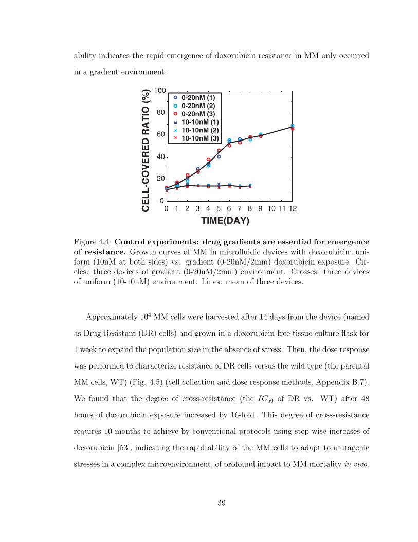
ability indicates the rapid emergence of doxorubicin resistance in MM only occurred

in a gradient environment.

0 1 2 3 4 5 6 7 8 9 10 11 120

20

40

60

80

100

TIME(DAY)

CEL

L-C

OVE

RED

RA

TIO

(%)

0-20nM (1)0-20nM (2)0-20nM (3)10-10nM (1)10-10nM (2)10-10nM (3)

Figure 4.4: Control experiments: drug gradients are essential for emergenceof resistance. Growth curves of MM in microfluidic devices with doxorubicin: uni-form (10nM at both sides) vs. gradient (0-20nM/2mm) doxorubicin exposure. Cir-cles: three devices of gradient (0-20nM/2mm) environment. Crosses: three devicesof uniform (10-10nM) environment. Lines: mean of three devices.

Approximately 104 MM cells were harvested after 14 days from the device (named

as Drug Resistant (DR) cells) and grown in a doxorubicin-free tissue culture flask for

1 week to expand the population size in the absence of stress. Then, the dose response

was performed to characterize resistance of DR cells versus the wild type (the parental

MM cells, WT) (Fig. 4.5) (cell collection and dose response methods, Appendix B.7).

We found that the degree of cross-resistance (the IC50 of DR vs. WT) after 48

hours of doxorubicin exposure increased by 16-fold. This degree of cross-resistance

requires 10 months to achieve by conventional protocols using step-wise increases of

doxorubicin [53], indicating the rapid ability of the MM cells to adapt to mutagenic

stresses in a complex microenvironment, of profound impact to MM mortality in vivo.

39

100

101

102

103

1040

20

40

60

80

100

VIAB

ILIT

Y (%

)

[DOX] (nM)

FIT (DR)DR CELLSFIT (WT)WT CELLS

Figure 4.5: Emergence of doxorubicin resistance in a doxorubicin gradient.Doxorubicin dose response (48-hour exposure). Cells from drug gradient device (0-20nM/2mm for 14 days, named as DR, red) vs. parental MM cells (WT, black).Data fitting was based on Hill equation (Materials and Methods). The inhibitoryconcentration for 50% of control population (IC50) of doxorubicin was increased by16-fold.

Sampling MM cells from different regions within the drug gradient might unveil

the degrees of resistance emerged along the gradient. Ideally, spatially resolved se-

quencing along the drug gradient would allow construction of the resistance phylogeny

trajectory. At this point, we grouped the cells from the gradient for dose response

characterization (Fig. 4.5) and for sequencing analyses so that we have to leave where

the resistance evolves along the gradient and the true role of chemotaxis as an open

question.

A common mechanism of drug resistance is via up regulation of a group of Mul-

tidrug Resistance (MDR) transporter proteins, which bind to ATP and pump drug

molecules outside of cell membrane so that intracellular concentration of drug can be

reduced. We characterized the expression level of MDR transporter of DR versus WT

cells using VybrantTM Multidrug Resistance Assay (Life Technologies), as shown in

Fig. 4.6.

The quantitative data of DR versus WT cells in MDR protein expression is shown

in Fig. 4.6C. Since DR cells are dimmer than WT cells, DR cells accumulate less

40

WT CELLS

DR CELLS

NORMAL CELL

MDR CELL

CELL

CALCEIN AM

MDR PROTEIN

CALCEIN AM

CALCEIN

CALCEIN

ESTERASE

ESTERASE

(A) (B)

25µm

0 500 1000 1500 2000 2500 3000 35000

100200300400500600700800

FLUORESCENCE (A.U.)

CO

UN

TS

WTDR

(C)

Figure 4.6: Bioluminescent MDR assay shows the MDR proteins expressionlevels. A. This assay utilizes the fluorogenic dye calcein AM as a substrate for effluxactivity of MDR pumps. Calcein AM is non fluorescent dye that can rapidly penetratethe cell membrane. Once inside the cell, ester bonds are cleaved by endogenousesterase’s, transforming calcein AM into fluorescent calcein retained in the cell. MDRcells expressing high levels of MDR proteins rapidly extrude non-fluorescent calceinAM from cell membrane, reducing accumulation of fluorescent calcein inside the cell.B. WT cells are brighter than DR cells based on MDR assay, indicating they expressedless MDR efflux pumps (qualitatively). C. Quantitative analysis of the bioluminescentMDR assay shows that the MDR proteins expression levels of most DR is higher thanWT cells.

fluorescent calcein due to more MDR efflux pumps. Using the MDR assay, we learned

that DR cells upregulated MDR efflux pumps and therefore demonstrate a resistance

phenotype. In the next section, we will study the whole transcriptome of DR versus

WT cells to explore deeper insights on the evolution of cancer resistance.

41

4.3 RNA sequencing analysis of resistant cells

We performed RNA sequencing analysis of WT and DR samples to identify the ex-

pressed mutations and differential expression levels of genes after the emergence of

resistance. We sequenced 4 samples: 2 were samples came from evolution in the

drug gradient (DR), 2 were not (WT), and each sample was composed of 104 cells

collected from 3 microfluidic devices running simultaneously under the same condi-

tion (Appendix B.8). Although there is certainly a spatial dependence to the evolved

genomes in the DR cells, in this preliminary analysis we grouped all the cells from

the chip together. Basic statistics of 4 samples are shown in Table 4.2 and Table

4.3. Mapping, SNVs, and expression analyses were based on the protocol shown in

Appendix C.2.

Table 4.2: Mapping statisticsNumber of mapped reads Sequencing 1 Sequencing 2

DR 50, 292, 847 93, 016, 838WT 62, 384, 592 111, 504, 450

Table 4.3: CoverageNumber of covered bases Sequencing 1 Sequencing 2

DR 337, 174, 818 479, 156, 993WT 422, 900, 554 646, 321, 913

Investigation of the substitutions that occurred in the evolved DR cells was done

by comparison of the mutations in the transcriptome of initial MM cells (WT) and

the evolved resistant cancer MM cells (DR) to the human reference genome (Genome

Reference Consortium GRCh37), this yielded the raw number of mutations within a

given gene in both the WT and the DR cells (Table 4.4).

42

Table 4.4: Number of SNVs detected and percentage (Nonsynonymous/total)Number of SNVs Sequencing 1 Sequencing 2

DR 1238/5231 = 24% 3129/11882 = 26%WT 2742/14333 = 19% 3107/15678 = 20%

Since the input WT cells are themselves cancer cells, there were coming into the

evolution experiment with more than 5 thousands single nucleotide variants (SNVs)

in each sample compared to GRCh37. DR SNVs which were not present in any of

WT samples are called DR de novo substitutions for the purpose of this thesis. Fig.

4.7 shows the observed substitution rates vs. sequenced exon length. The observed

mean DR de novo substitution rate, < µ >=2.0×10−4/bp may seem high, but this is

the time integrated output of cancer cells under exposure to high concentrations of

doxorubicin.

SEQUENCED LENGTH PER GENE (BP) (EXON)0 2000 4000 6000 8000 10000 12000 14000 16000 18000SU

BST

ITU

TIO

N R

ATE

10-4

10-3

10-2

MEAN RATE95% CI (BINOMIAL)

RATE PER GENE HYPERMUTATED

MEAN RATE PER BIN

0

Figure 4.7: Observed per base de novo substitution rate vs. sequenced exonlength per gene (bp). Red diamond: genes that were successfully sequenced formore than 80% of exon region. Black square: mean substitution rate within a 500bpwindow. Black line: mean substation rate < µ >=2.0×10−4/bp. Blue error bars:95% confidence intervals determined by binomial distribution (Appendix C.4). Blackdiamond with red center: hyper mutated genes determined by binomial distribution(Appendix C.5).

43

GENE (GL)

>20X SEQUENCED

EXONS (SEQL)

EXONS (EXL)

SUCCESSFULLY SEQUENCED CRITERIA: > 80%SEQLEXL

Figure 4.8: The criteria of successfully sequenced genes for mutation rate analyses:> 80% exon regions (bp) have been sequenced with a coverage depth > 20 reads.

Fig. 4.7 shows DR de novo substitution rates and mean substitution rate versus

gene length for genes that were successfully sequenced for more than 80% of exon re-

gion. We follow the flow chart shown in Fig. 4.8. to determine successfully sequenced

genes as 80% of exon regions were sequenced with 20 reads. The raw number of hits

in a given gene, that is, the numbers of SNVs per gene, is widely applied as a way to

find putative drivers of adaptation [56]. However, genes vary tremendously in length,

ranging from hundreds to millions of bases in total (intron+exon) length as shown

in Fig. 4.9, the histogram of the number of canonical human genes versus length.

Of course, if substitutions are random then longer genes will show more mutations

than shorter genes. This does not prove that they are hot spots for substitutions, but

rather that they are simply longer. The SNV density is not a function of length in

the random mutation model.

Since we did RNA sequencing rather than whole genome DNA sequencing we only

looked at mutations in genes which were transcribed into expressed proteins (exomes).

For each gene (i), we determine the “per base substitution rate” Ri as the number

44

102 104 106100

101

102

103

104

LENGTH PER GENE (BP)

NU

MB

ER O

F H

UM

AN

GEN

ES EXON LENGTHWHOLE LENGTH

Figure 4.9: Histograms of numbers of canonical human genes (downloaded from UCSCGenome Browser) vs lengths. Red: exon length per gene; black: whole gene length.

of de novo substitutions Mi divided by the length in base pairs of the successfully

sequenced exon region (covered with 20 reads) Li, as shown in Fig. 4.10A. Since

at most 3 substitutions were found in a gene, the binary nature of a substitution in

a given gene yields the nested curves shown in Fig. 4.7. We thus set the per base

gene substitution rate µ (substitutions/bp) by dividing by the length L of the gene to

correct for the smaller target size of short genes. Likewise, if we saw 2 substitutions,

then the rate is 2/L, etc. This is why you see a nested set (the substitution rates

are quantized at the gene scale) and a set of ascending curves as one approaches the

origin (because the 1/L effect). But note that as L decreases one has many more genes

which are NOT mutated. Averaging over the number of genes in a given window size,

in our case 500bp as shown in Fig. 4.7 gives a better representation of the rates of

substitution versus length. This process flattens the nested curves into a single curve,

45

but there is still a tendency for more substitutions to occur in short genes compared

to long genes, for resins discussed below.

0 0.1 0.2 0.3 0.4 0.5 0.6 0.7 0.8 0.9 110−5

10−4

10−3

10−2

10−1

100

SUB

STIT

UTI

ON

RA

TE (E

XON

)

SEQUENCED RATIO (EXON)

0 0.1 0.2 0.3 0.4 0.5 0.6 0.7 0.8 0.9 1101

102

103

104

SEQUENCED RATIO (EXON)

NU

MB

ER O

F G

ENES

GENES (0-MUTATION)

Figure 4.10: Substitution rate and number of genes vs. successfully se-quenced ratio (exon only). A. Per base substitution rate (exon only) is definedas “number of substitutions” divided by “successfully sequenced length at exonic re-gion”. Successfully sequenced ratio is defended as “number of successfully sequencedbases at exonic region” divided by “canonical exon bases”. B. Histogram of numbersof non-mutated genes vs. sequenced ratio (exon only).

Since the mean substitution density < µ > is low enough that even in the DR

cells most genes do not have mutations, and hence the substitutions per gene are

governed by Poisson statistics, we classified significantly substituted (hot) and not

46

substitute (cold) genes by calculating the mutation rate per base at the single gene

level. If substitutions arise as a random Poisson process, the per base substitution

rate averaged over of all genes should be independent of the gene length. However,

most of the sequenced genes, have a per base substitution rate within 95% confidence

intervals of < µ >, determined by using error estimate of the mean substitution

rate based on the binomial distribution (Appendix C.4). Genes with higher rates of

mutations, using the Benjamini-Hochberg method [57], we call hyper-mutated genes.

Our analysis identified 15 hyper-mutated genes in Table 4.5, such as HIST1H4H and

TUBA1A, associated with nucleosome assembly, protein folding, and cell division.

However, no clear pattern emerged in terms of function within the hyper-mutated

genes, leading us to examine the never-mutated genes.

47

Table 4.5: Hyper-mutated genes (exon only)Gene SNVs Bases Sequenced bases Mutation density Probability∗

HIST1H4H1 3 374 347 0.0086 1.1× 10−6

HIST1H2BF1 3 430 405 0.0074 2.0× 10−6

LOC101101776 3 816 816 0.0037 3.1× 10−5

PHB 4 1826 1703 0.0023 3.5× 10−5

HIST1H4B1 2 357 311 0.0064 4.3× 10−5

TUBA1A3 3 978 978 0.0031 6.1× 10−5

ARHGDIA4 3 1249 1040 0.0029 7.8× 10−5

AK022914 6 5104 4939 0.0012 1.0× 10−4

HIST1H2AM1 2 487 430 0.0047 1.1× 10−4

HIST1H2AC1 2 546 495 0.0040 1.7× 10−4

RPL36AL 2 577 503 0.0040 1.8× 10−4

PPP2CA2,4 1 96 93 0.011 1.8× 10−4

MRPS24 2 696 583 0.0034 2.7× 10−4

DPY301 2 800 650 0.0031 3.8× 10−4

CALR2,3 3 1911 1860 0.0016 7.0× 10−4

∗Probability to detect more mutations in this gene (p-value), calculation is presentedin Appendix C.5.1Biological process: chromatin organization, nucleosome assembly, telomere mainte-nance.2Biological process: DNA replication, signal transduction, cell proliferation, cellgrowth, apoptotic process, DNA biosynthetic process.3Biological process: protein folding, microtubule-based process, cell division.4Biological process: cell adhesion, apoptotic process, protein localization.

48

4.4 Never-mutated genes and differential expres-

sion analysis

We also identified 163 successfully sequenced genes without any mutations in nei-

ther DR nor WT samples, “never mutated” genes, or cold genes. Among them, 13

genes are 4X up-regulated (Table 4.6) and 21 genes are 4X down-regulated (Table

4.7) in DR samples. These are presumably important genes which cannot be mu-

tated because they play a key role in fitness of the cells. It has been suggested that

these “never mutated” genes might actually be very ancient genes which represent

a core functionality which cancer uses to maintain a basic fitness under high stress

conditions, as presumably early lifeforms must have experienced [58, 59].

Table 4.6: Zero mutation, 4X up-regulated genes and their ages (exon only)Gene Bases Sequenced bases Age (106 years) Log2(DR/WT )PRDX41 921 801 3556.3 5.9

PGK12 2733 2273 3556.3 2.0NOB1 1775 1535 2269.5 5.9

CKS1B 1015 816 2269.5 4.4TMEM167A 4721 3828 1530.3 2.7

COPZ1 2119 1727 1530.3 2.3SEC61B 562 509 1369.0 3.0

CLIC1 1251 1157 1369.0 2.1ID2 1364 1178 891.8 4.0

HIST1H2BC 438 403 891.8 2.9SHFM1 498 433 839.4 3.0

PCP4 556 451 400.1 8.5ART3 1216 1064 400.1 2.6

1Biological process: spermatogenesis, oxidation-reduction process.2Biological process: gluconeogenesis, glycolysis, phosphorylation.

It is possible to estimate roughly the age of genes by assessing the relative positions

of the genes’ homologues in a phylogenetic tree (Appendix C.6). Such an analysis is

shown in Fig. 4.11. We show there the histogram of calculated gene ages versus the

human genome containing over 19,000 genes (solid black line) and the histogram of

49

Table 4.7: Zero mutation, 4X down-regulated genes and their agesGene Bases Sequenced bases Age (106 years) Log2(DR/WT )

PSMC11 1595 1531 3556.3 −3.7ASB32 1275 1094 3556.3 −3.5RPS53 741 728 3556.3 −3.6

RPLP03 1304 1124 3556.3 −2.0NDUFAB1 667 558 2535.8 −3.4

EEF1G 1538 1379 2269.5 −2.7SUMO1 1527 1266 2269.5 −2.7PFDN2 642 554 1530.3 −3.0

POLR2H 821 672 1530.3 −2.4AHSA1 1537 1340 1530.3 −2.3RBMX 2822 2338 1381.2 −2.4OSTC 1152 1006 1369 −3.8BRK1 1176 967 1369 −3.6

FAM3C 2542 2055 937.5 −2.8XBP1 2172 1789 937.5 −2.5

COX6A1 572 517 937.5 −2.4FBXO22 448 442 891.8 −2.2

TMSB4X 629 607 839.4 −3.7COX7C 486 407 762.9 −3.9NGRN 1760 1424 742.9 −2.8CD74 1681 1443 400.1 −2.9

1Biological process: mitotic cell cycle, DNA damage response, apoptotic process.2Biological process: protein ubiquitination, intracellular signal transduction.3Biological process: translation.

“never mutated” genes from our experiment. We found that the zero-mutation genes

we detected ( 4X change in expression) are older, on average, then all human genes,

with the average age of 1.7 ± 1.0 billion years, compared to 19786 human genes with

an average age of 1.3 ± 0.9 billion years. The error bars, quite large, and are simply a

measure of the widths of the distributions and not a measure of the errors associated

with this analysis, which are difficult to quantify at this stage. However, the large

outlier of zero-mutation genes at 3.5 billion years age is statistically significant. These

cold genes are presented in Table 4.6 and Table 4.7.

These genes seem to code for essential cellular functions: up-regulated PRDX4 is

associated with spermatogenesis and oxidation-reduction process; up-regulated PGK1

50

0 1000 2000 3000 40000

500

1000

1500

2000

2500

3000

ALL GENESZERO MUTATIONS >4X CHANGE

0

2

4

6

8

10

EVOLUTIONARY AGE (MYEAR)

NU

MB

ER O

F G

ENES

Figure 4.11: Successfully sequenced genes without mutations in WT norDR samples vs. evolutionary ages. Red: histogram of numbers of genes vs. ageswith a bin size of 200 MYEAR. MYEAR: 106 years. Black: histogram of all humangenes with age information (19786 in total), shown as a control.

is associated with glycolysis and phosphorylation (Table 4.6); down-regulated PSMC1

is associated with cell cycle, DNA damage response, and apoptosis; down-regulated

ASB3 is associated with protein ubiquitination; down-regulated RPS5 and RPLP0

are associated with translation. Although these zero-mutation ancient genes shared

by DR and WT cells do not directly explain drug resistance in DR samples, they

could provide insights on protected regions of the genome during malignancy trans-

formation.

We finally address the expression levels of genes in DR vs. WT samples

based on the abundance of RNA reads (fragments per kilomegabases, FPKM)

mapped to genes (Appendix C.2). The log 2 ratio of DR to WT expression levels,

log2(FPKMDR/FPKMWT ), describes how much the expression levels changed after

exposure of doxorubicin gradient. In other words, the greater (or less) the log 2 ratio

for a given gene, the greater it is up-regulated (or down-regulated) in DR samples.

51

Histograms of numbers of all sequenced genes (with FPKM 0.1 in both WT and DR

samples) vs. log 2 ratio of expression levels is shown in Fig. 4.12.

−10 −5 0 5 100

50

100

150

200

250

300

350

400

LOG 2 EXPRESSION RATIO (DR/WT)

NU

MB

ER O

F G

ENES

GAUSSIANLORENTZIAN

DATA

Figure 4.12: Histograms of numbers of genes vs. log 2 ratio of DR to WTexpression levels. X-axis is the log2 ratio of DR expression abundance (FPKM)to WT expression abundance (FPKM). Blue: all sequenced genes with expressionlevels 0.1 in both WT and DR samples were taken into account (Dataset S2). Black:Gaussian model. Red: Lorentzian model.

The conventional way to analyze the gene expression data is to perform functional

classification of gene sets [60] in search of genes that are significantly meaningful.

For example, it is widely accepted that drug efflux pumps play an important role

in reducing intracellular drug concentration and elevation of the drug resistance if

they are up-regulated[61]. As we expected, we observed up-regulation of 3 drug efflux

pumps, including ABCA13, ABCB11, ABCC3, greater than 4-fold in DR cells vs. WT

cells (Dataset S2). Since these up-regulations are drug efflux pumps are commonly

seen, we can question if this is purely random process driven by natural selection of

a programmatic response which has been selected as part of the way that cells deal

with drug toxicity.

52

A common mistake is to assume that a normal distribution of differential expres-

sions would also yield simple Gaussian (normal) statistics. However, it has been

pointed out by Brody et al [62] that a distribution of the ratio x/y of two normally

distributed random variables is not necessarily Gaussian but rather a Lorentzian. The

histogram shown in Fig. 4.12 does indeed fit a Lorentzian distribution much better

than a Gaussian distribution. This implies that what appear to be outliers in the

distribution are not in fact outliers but artifacts of the analysis, making comments

about particular genes difficult. The mean of the distribution is however statistical

significant. Since there is a shift of the mean of the Lorentzian curve to the left of the

origin (Fig. 4.12), this may be a result of DR cancer cells suppressing some normal

cell functions, but it is difficult to proceed further.

53

4.5 Discussion and summary

We observed that in a chemotherapy gradient landscape resistance of MM cells to

doxorubicin can emerge rapidly, as we expected from previous bacterial work on an-

tibiotic resistance emergence [4]. We show that cold genes are more protected as many

evolutionary conserved genes [63]. We found that genes associated with nucleosome

assembly and protein folding tend to mutate rapidly, while ancient genes associated

with spermatogenesis, oxidation-reduction, and glycolysis are possibly protected and

abnormally up-regulated on demand of acquired drug resistance. The trade-offs may

be associated with energy and time limitation in harsh environment [64] and may be

a strategy of cancer cells to evolve rapidly.

Since longer proteins have more surface area and more connections, it has been

suggested that they encode more essential cellular functions than shorter proteins

across various species [65]. Also, ancient genes have shown to evolve more slowly, and

hence are cold, and express more “core” functional proteins compared with young

genes [65, 66]. As shown in Fig. 4.11 and Fig. 4.12, we observed the selection for

the abnormally regulated ancient genes with slow evolution rate in emerged resistant

cancer. Our sequencing result of emergence of resistant cancer address the integration

on gene length, evolutionary rates, functional essentiality, and evolutionary age; these

properties have occurred in other species for guiding the animal body plans [67].

The adaptation to chemotherapy does not necessarily involve mutations - up-

regulation of normal cellular defense mechanisms may be sufficient. The failure of a

central-limit approach to the distribution of differential expression levels lies beyond

the scope of this work. However, we can speculate that since there are thousands of

pathways associated with chemotherapy resistance, cancer cells can simply activate

selected pathways and increase expression levels of genes associated with those needed

pathways to enhance their survival. Selectivity rather than random events could lead

to failure of the central limit Gaussian distribution. Other than looking for new

54

pathways or validation of pre-existing pathways of drug resistance, we suggest that

the quantitative and physical dynamic of how cells regulate the expression levels is

equally important.

An important question that we cannot answer here is: were the de novo mutations

generated spontaneously or induced by stress? It is experimentally challenging to

prove the existence of stress-induced mutagenesis, via up-regulation of error-prone

DNA polymerases or repressing DNA repair enzymes, because de novo mutation and

selection usually come together [46]. However, we observed up-regulation of POLDIP2

of DR cells in our experiments. POLDIP2 is known to support DNA polymerase λ

in translesion synthesis (TLS), which often has low fidelity (high propensity to insert

wrong bases) on undamaged templates relative to regular polymerases and may induce

de novo mutations [46, 68]. This error-prone recovery also protects DR cells from

oxidative damage caused by doxorubicin [46, 69].

In this chapter, we have shown that in an array of interconnected microhabitats

with an applied drug gradient, MM can develop extraordinarily rapid resistance to

doxorubicin. We have shown that the mutational pattern of the resistant cells is

quite diverse, with genes that show high mutation rates and genes that show very

low, to no, mutations. It may seem strange to suggest, as we have here, that non-

mutated genes may be critical targets for chemotherapy, we argue that these non-

mutated genes may be the most fundamental ones for preservation of cancer cell

fitness. There are two broad components of information dynamics in cancer evolution.

One involves permanent changes in which genes are subject to gain or loss-of-function

mutations. This is well established and the main focus of cancer research. The

other component is the information in the human genome and preservation of that

content. The cancer cell potentially has access to all of this and can up-regulate

or down-regulate any number of strategies used for survival and proliferation during

embryogenesis, development, and normal adaptation to environmental stresses.

55

Another question is the role that cancer plays in development [67] and the tran-

sition from unicellular to multi-cellular behavior, and the role that cancer has played

as an evolutionary variable [70]. That is, since ancient genes seem to be protected

from substitution perhaps cancer represents a return to unicellularity which are rep-

resented by these crucial and ancient genes, with cancer allowing substitutions in or

abandoning higher level genes associated with multicellular cooperation [71]. Clearly,

with our limited data set in this chapter we cannot address this question in a signifi-

cant way, but we hope we can point the way to different ways of viewing how cancer

has influenced the process of development and its deep origins.

56

Chapter 5

Friends or Foes? Game of Multiple

Myeloma and Stromal Cells in

Chemotherapy Gradients

Preventing relapse after an initial treatment is the major challenge of effective therapy

in cancer. Within the tumor, stromal cells play an important role in cancer progres-

sion and emergence of drug resistance. During cancer treatment, the fitness of cancer

cells can be enhanced by stromal cells because their molecular signaling interaction

delays the drug-induced apoptosis of cancer cells. On the other hand, competition

among cancer and stromal cells for space or resources should not be ignored.

In this chapter, we explore the population dynamics of multiple myeloma versus

bone marrow stromal cells by using the same engineered micro environments as shown

in Chapter 4, with a stable drug gradient and connected micro-habitats. Since evolu-

tionary game theory is a quantitative way to capture the frequency-dependent nature

of interactive populations, we use evolutionary game theory to model the populations

in such engineered micro environments with the gradients of payoffs and successfully

57

predicts the future densities of multiple myeloma and stromal cells. We will discuss

the possible clinical use of such analysis for predicting cancer progression.

5.1 Introduction

5.1.1 Players: cancer and stroma cells

Emergence of therapy resistance is inevitable in multiple types of cancer and sig-

nificantly affects survival of cancer patients [72]. The tumor microenvironment can

influence therapy efficacy because it is not merely composed of cancer cells but also

stromal cells, a key player in cancer growth and progression [73, 55, 74]. During

initial treatment, stromal cells suppress the apoptosis signal of cancer cells and fur-

ther prolong the survival of cancer cells [75, 76]. As with many cancers, multiple

myeloma, a cancer of plasma cells in the bone marrow, acquires therapy resistance by

communicating with the stromal cells [7, 8]. The key signaling pathways in cancer-

stroma communications (i.e. interleukin 6, IL-6, and stromal cell-derived factor 1,

SDF1) have been extensively studied. However, it is challenging to extrapolate their

biomolecular network to the resulting population dynamics of cancer and stromal

cells. Therefore, we propose to use evolutionary game theory to interpret the inter-

actions between cancer and stromal cells [5].

5.1.2 Evolutionary game theory

Evolutionary game theory has been used for modeling interacting populations in

various biological networks[77]. In the evolutionary game theory, the fitness depends

on population composition of various strategies or phenotypes. For a two-player game

58

between well-mixed player α and player β, the payoff matrix is given by

α β

α A B

β C D

(5.1)

When a player α encounters a player α, it receives payoff “A”. A player α versus a

player β receives payoff “B” while the β receives payoff “C” from the α. A player β

versus a player β receives the payoff “D”. When we consider the absolute population

of each type of players (α and β), then the population rate equations can be written

as:

dα

dt= (Apα +Bpβ)α (5.2)

dβ

dt= (Cpα +Dpβ)β (5.3)

where population fractions pα = α/(α+β) and pβ = β/(α+β), fitness of each player

are fα = Apα + Bpβ and fβ = Cpα + Dpβ. If A>C and B>D, player α dominates

player β. Likewise, if A<C and B<D, player β dominates player α. This is a classic

example of frequency-dependent selection. A coordination game occurs if A>C and

B<D, then both α and β are stable. In a system with more α, it will keep being

dominated by α. If currently there are more β, there will be more β. More complex

dynamics occur if A<C and B>D, leading to a coexistence between the two players.

In this case, a population with more α will then become dominated by β, and a

population with more β will then become dominated by α (“Hawk-Dove game”[78]).

5.1.3 Evolutionary game theory and cancer

Evolutionary game theoretical models have been implemented on the interaction of

cancer and other cells in various stages of cancer progression. Dingli et al have ex-

plored an evolutionary game between multiple myeloma, osteoclasts, and osteoblasts,

59

discussing disease progression and outcome of treatment[79]. Basanta et al have used

evolutionary game to model the interaction and transformation of different stages of

glioblastoma (such as glycolysis and invasive phenotypes) and predicted the stages of

glioblastoma[80]. Flach et al have studied the role of fibroblasts in melanoma growth

and drug resistance from a game theoretical point of vie [81]. However, it is very chal-

lenging to assess cancer and non-cancer populations versus time with high temporal

resolution in clinical data. Because of the challenge of fitting experimental data,

current game theoretical approach is limited to tuning parameters and discussing

various scenarios in cancer progression. Even using in vitro co-culture experiments

in tissue culture flasks, there is no information of complex heterogeneity in tumor

microenvironment.

The tumor microenvironment highly influences the sensitivity of cancer cells to

chemotherapy treatment. In a solid tumor, the drug diffuses into tumor core from

the blood vessels. However, drug concentration drops significantly within hundreds

of microns away from the blood vessels because of (i) diffusion barriers of closely

packed cells, (ii) uptake of cells near the vessels, (iii) decreased activity of drug (such

as doxorubicin) due to hypoxia, (iv) dissociation of drug in acidic tumor core[82, 13].

The relapse usually occurs when cancer cells in the tumor core suffer less dosage of

drug, survive, and gradually form a tumor again.

On the other hand, various cells such as tumor cells, macrophages, or stromal cells

form highly interactive micro-colonies[83]. In different conditions, the stroma can

provide tumor-suppressing and tumor-promoting environments and influence cancer

development and progression[83]. Combining with non-uniform distribution of drug

within a tumor under treatment, one may ask whether the spatial drug distribution

affects the role of stromal cells on cancer survival or proliferation. Therefore, we

propose to use microfluidic technology to mimic tumor microenvironment with drug

gradient, and probe the dynamics of cancer and stromal cells.

60

Microfluidics have been used to create versatile functions for studying various

microorganisms. Microfluidics can create micro-fabricated landscapes, concentration

gradients, or dynamic switching of different chemicals[84, 32, 34, 85]. Therefore, it

is possible to reconstruct a heterogeneous microenvironment to asses the interactions

such as competition or cooperation among cells. For example, a race has been held for

prostate cancer cells to climb up micro-skyscrapers, characterizing the invasiveness

of different cells[84]. The cooperation of cancer cells has been observed while the

cells taking turns to lead the collective invasion through a glucose gradient across a

collagen matrix[32]. Since invasion through an extracellular matrix has a metabolic

cost, cancer cells intend to migrate toward a glucose abundant region with a higher

fitness and reduce the total cost via exchanging leading positions.

Likewise, a drug gradient also provides a fitness gradient for cancer cells and causes

a build up of a population gradient with time. Following by a population gradient,

local competition for space and metabolic resources such as glucose or oxygen may

drive the cancer cells to migrate toward the drug source, triggering the emergence of

drug resistance[34]. In an engineered microenvironment with a chemotherapy gradient

and microhabitats, we expect to capture the complex non-linear dynamics of multiple

myeloma (MM) and stromal (ST) cells.

61

5.2 Results

5.2.1 Co-culture experiments

In the following experiments, we work with multiple myeloma (MM) and bone mar-

row stromal cells (ST) since bone marrow cancer is incurable and the biomolecular

signaling network between MM and ST is already known[86, 7]. The MM cells (8226)

are labeled with red fluorescent protein and ST cells (HS-5) are labeled with green

fluorescent protein, a courtesy from Robert Gatenby Laboratory at Moffitt Cancer

Center (Appendix B.2). We characterized their dose response (Appendix B.7) of dox-

orubicin, a chemotherapeutic agent which intercalates DNA and produces oxidative

stress[61], prior the co-culture experiments. We found that MM is more sensitive to

doxorubicin than ST, as shown in Fig. 5.1.

10−4 10−2 100 1020

10

20

30

40

50

60

70

80

90

100

DOXORUBICIN CONCENTRATION (µM)

VIA

BIL

ITY

(%)

MMST

Figure 5.1: Doxorubicin dose response ( 24-hour exposure) of MM (red) vs.ST (blue). Error bars indicate standard deviation of 3 replicates.

We co-culture MM and ST in the microfluidic device with microhabitats and a

linear gradient of doxorubicin (Fig. 4.1) for 2 weeks. The device is described in

62

Chapter 4. Cell loading and image acquisition methods are shown in Appendix B.4

and Appendix B.5, respectively. A representative image is shown in Fig. 5.2, in which

MM and ST cells form 3D cluster near the nutrient-rich and drug-free channel within

6 days.

100µm

Figure 5.2: MM and ST in a microhabitat Image of cells in a microhabitatnear the doxorubicin-free channel after applying 6 days of doxorubicin gradient (0-2µM/2mm). Red: MM cells (8226/RFP), green: ST cells (HS-5/GFP).

First, we found that the MM grew only with the existence of ST; MM growth was

not observed in the same environment (0-200nM/2mm) without any ST cells. The

fact that MM show no growth without ST in the same strength of drug gradient is

consistent with the known mechanism of stroma-mediated drug resistance[8].

Then, we performed the same drug gradient experiments with various initial pop-

ulation ratio of MM and ST (MM:ST) including 1:3, 4:1, and 1:0. The growth curves

of both cells in the entire devices MM-rich (MM:ST=4:1) and ST-rich (MM:ST=1:3)

are shown in Fig. 5.3.

We observed the following trends by looking at the cell densities every time in

the entire devices with a drug gradient:

(1) ST cells are less sensitive to drug than MM cells.

(2) The MM do not survive for 5 days without ST cells in the same treatment.

63

(3) The initial ratio of MM versus ST affects the fate of MM cells: MM cells thrive

if initially there were more MM than ST, but outcompete by ST cells if initially

there were more ST than MM. The fact that a small population of ST cells may

desensitize MM to drug, is consistent with previous discovery of stroma-mediated

drug resistance [8] but competition between MM and ST should also be considered.

(A) ST-rich

0 2 40

200400600800

100012001400

TIME (DAY)

CEL

L D

ENSI

TY

0 5 100

200400600800

100012001400

TIME (DAY)

(B) MM-rich

ST

ST

MM MMCEL

L D

ENSI

TY

Figure 5.3: Total MM or ST population density (number of cells/4mm2) inthe entire gradient device vs. time. MM and ST are co-cultured under adoxorubicin gradient from 0 to 200nM across 2mm. A. ST-rich data with 5replicates. Green: ST, orange: MM. B. MM-rich data with 3 replicates. Dark green:ST, dark red: MM. Error bars indicate standard deviation of the replicates.

5.2.2 Temporal dynamics

An alternative way to demonstrate the growth curves of the interacting populations

of MM and ST from Fig. 5.3 is a phase portrait, in which the x-axis shows the

population densities of MM, and the y-axis shows the population densities of ST.

Then, population dynamics of the two co-culture experiments in the entire drug

gradient, can be shown in a single Fig. 5.4. Given that we observed the fitness of

64

each cell type depends on initial population ratio, evolutionary game theory is an

ideal model to describe the dynamics of this co-culture system.

0 200 400 600 800 1000 12000

200

400

600

800

1000

MM CELL DENSITY

ST C

ELL

DEN

SITY

T=0ST-RICHMM-RICH

Figure 5.4: Phase portrait of total MM and ST population density (num-ber of cells/4mm2) in the entire cell region vs. time. MM and ST areco-cultured under a doxorubicin gradient from 0 to 200nM across 2mm.Green: ST-rich data. Bold green arrow shows the average over 5 ST-rich replicateexperiments. Red: MM-rich data. Bold red arrow shows the average over 3 MM-rich replicate experiments. The gray arrows indicate the fitness determined by theexperiments (the slopes of semi-log growth curves in Figure 5.3).

We first treat the system as a well-mixed populations and seek for parameters of

a spatial-independent evolutionary game model. Here, we ignore the fact that there

is a drug gradient. Therefore, the absolute populations MM or ST can be described

by the ordinary differential equations

dMM

dt= (ApMM +BpST )MM (5.4)

65

dST

dt= (CpMM +DpST )ST (5.5)

where population fractions pMM = MM/(MM + ST ) and pST = ST/(MM + ST ).

If a MM cell encounters a MM cell, it receives a payoff A; a MM cell versus a ST

cell receives a payoff B. A ST cell versus a MM cell receives a payoff C; a ST cell

versus a ST cell receives a payoff D. From Fig. 5.4, we can see the system favors ST

and if initially MM is much greater than ST, there exists a counterclockwise motion

toward ST axis. Therefore, physical intuition tells us that A<C and B<D. By fitting

the growth curves of each cell type with various initial population fractions [87, 88],

we can find the payoffs A, B, C, and D (detailed in Appendix C.8). The quivers in

Fig. 5.4 indicate the fitness as a function of population fractions and payoff matrix

trained from our experiments (fMM = ApMM + BpST and fST = CpMM + DpST ).

Each quiver is a vector of (fMM ,fST ) determined by each position (MM ,ST ) in Fig.

5.4.

5.2.3 Spatial and temporal dynamics

We now address the spatial distribution of MM and ST in a drug gradient in time

series. An example of initial MM-rich experiment is shown in Fig. 5.5. Surprisingly,

after day 6, there were even more MM in the regions with higher drug concentration

than that with lower drug concentration (Fig. 5.5). Quantitative population land-

scapes for ST-rich and MM-rich experiments are shown in Fig. 5.6 A and B. There

are two possible mechanisms that MM cells can show survival at levels of a drug

which should inhibit growth: (1) stroma-mediated drug resistance provides protec-

tion (but not permanent) for drug-induced apoptosis [55], (2) competition between

ST and MM may be a significant factor for MM fitness. In all, the data suggests that

ST can be friends or foes of MM cells under various population compositions and

drug concentrations.

66

Dox 200nM Dox 200nM Dox 200nM

Dox 0nM Dox 0nM Dox 0nM200μm

Dox 200nM Dox 200nM

Dox 0nM Dox 0nM

D6 D8

D0 D2 D4

Figure 5.5: MM and ST co-culture (MM-rich) under a doxorubicin gradientfrom 0 to 200nM across 2mm. (Day 0 to Day 8) Red: MM cells (8226/RFP).Green: stromal cells (HS-5/GFP). Top: doxorubicin concentration is 200nM; bottom:doxorubicin concentration is 0nM.

5.2.4 Effect of drug gradient on fitness of MM and ST

Since doxorubicin causes DNA damage and inhibits cell proliferation [61], it further

affects the fitness of all cell types. A spatially-resolved game theoretical model of the

system can be achieved by assuming the payoff as a function of drug concentration.

In the device with a linear drug gradient, we can simplify the system and assume the

67

02

4

0

0.5

10

500

TIME(DAY)

MM DENSITY

[DRUG]100

200

300

400

500

02

4

0

0.5

10

1000

2000

ST DENSITY

800

1000

1200

1400

1600

05

0

0.5

10

500

1000

1500

200

400

600

800

1000

1200

05

0

0.5

10

1000

2000

200

400

600

800

1000

1200

1400

(B) (D)

(A) ST-rich (C) MM-rich

TIME(DAY)[DRUG]

TIME(DAY)[DRUG]

TIME(DAY)[DRUG]

MM DENSITY

ST DENSITY

Figure 5.6: MM and ST vs. space and time (experiments). A-B. MM vs.ST populations within the drug gradient in ST-rich condition. C-D. MM versusST populations within the drug gradient in MM-rich condition. Color bar indicatespopulation density (unit: number of cells/4mm2.)

payoff as a 1D function of space (x-direction, along the drug gradient in cell region).

Here, we also assume the payoff coefficients (A, B, C, D) at a given location are fixed

with time for simplification.

We use finite difference time domain (FDTD) analysis to solve rate equations

(Eqs. 5.4 and 5.4). The detailed numerical method is presented in Appendix C.9.

We tune the payoffs A(x), B(x), C(x), and D(x), linear functions along x-axis, using

linear-square-fit function in Matlab (LMFnlsq) until they fit both experimental data

68

(ST-rich and MM-rich). Note that the spatial mean of the payoffs are the same as

what we used to draw quivers in Fig. 5.3. The resulting payoffs as functions of space

(or drug concentration) are shown in Fig. 5.7.

−0.03

−0.02

−0.01

0

0.01

0.02

0.03

0 1POSITION(mm)

[DRUG]0 0.5 1

2

A

B

C

D

Figure 5.7: The payoff as a linear function of drug concentration in a gra-dient. a The mean and slopes are determined to match experimental results, asshown in Figure. 5.3. mean(A(x))=0.0093, mean(B(x))=-0.018, mean(C(x))=0.022,and mean(D(x))=-0.0025. The slopes of A(x), B(x), C(x), D(x), with a unit (permm) are -0.02, 0.034, -0.01, -0.018, respectively.

To explore the effect of spatial fitness function on the dynamic behavior of popu-

lation distribution, we plot the model output with an initial condition as an “uniform

distribution” across the drug gradient. Fig. 5.8 and Fig. 5.9 share the same linear

payoff functions, the only difference is initial populations of MM and ST are ST-rich

and MM-rich, respectively.

Figure 5.8 shows the ST-rich condition, in which the initial condition is set as

uniform distribution of 900 ST cells/4mm2 versus 350 MM cells/4mm2, same as the

starting point of green arrow in Fig. 5.3. The model prediction of ST-rich population

distribution within the drug gradient are shown in Fig. 5.8. The model agrees

69

(A)

0 1 20

200

400

600

800

1000

1200

1400

1600

1800

2000

2200

POSITION(mm)0 1 2

0

200

400

600

800

1000

1200

1400

1600

1800

2000

2200

POSITION(mm)

ST C

ELL

DEN

SITY

0 2 4 6 8 100

200

400

600

800

1000

1200

1400

TIME(DAY)

MM

CEL

L D

ENSI

TY

CEL

L D

ENSI

TY

DAY0

DAY1

DAY2

DAY3

DAY0DAY1DAY2DAY3

(B) (C) [DRUG]0 10.5

[DRUG]0 10.5

ST

MM

Figure 5.8: Model prediction of ST-rich population distribution within thedoxorubicin gradient. A. ST population distribution versus time (from green todark green). Initial condition is assumed as an uniform distribution of 900 cells/4mm2.B. MM population distribution versus time (from red to dark red). Initial condition:uniform distribution of 350 cells/4mm2. C. Total MM (red) and ST(green) populationversus time.

with our observations that in ST-rich condition, ST cells form population gradient in

response to drug gradient, less cells in the regions with greater concentration of drug

(Fig. 5.6A). MM cells drop monotonically with time if its initial population is much

lower than ST cells (Fig. 5.6B), but the MM distribution across the drug gradient

remains approximately flat.

For the MM-rich condition, the model prediction of population distribution within

the drug gradient are shown in Fig. 5.9, with an initial condition of uniform distri-

bution of 200 ST cells/4mm2 versus 1000 MM cells/4mm2, the starting point of red

70

0 1 20

200

400

600

800

1000

1200

1400

1600

1800

2000

2200

0 1 20

200

400

600

800

1000

1200

1400

1600

1800

2000

2200

POSITION(mm)

ST C

ELL

DEN

SITY

0 2 4 6 8 100

200

400

600

800

1000

1200

1400

TIME(DAY)POSITION(mm)

MM

CEL

L D

ENSI

TY

CEL

L D

ENSI

TY

DAY0

DAY6

DAY2

DAY4

DAY8

DAY0DAY6

DAY2

DAY4

DAY8

0 10.5 0 10.5

(A) (B) (C) [DRUG] [DRUG]

ST

MM

Figure 5.9: Model prediction of MM-rich population distribution within thedoxorubicin gradient. A. ST population distribution versus time (from green todark green). Initial condition is assumed as an uniform distribution of 200 cells/4mm2.B. MM population distribution versus time (from red to dark red). Initial condition:uniform distribution of 1000 cells/4mm2. C. Total MM (red) and ST(green) popula-tion versus time.

arrow in Fig. 5.3. The model is consistent with our experiments that in the MM-rich

condition, the total MM population increases up to day 4 and then slowly drops with

time (Fig. 5.3C and D). Interestingly, one may find the MM population gradient

is against the drug gradient (Fig. 5.9B). It seems that there exists competition in

the region with lower concentration of drug between MM and ST, different from our

expectation that stromal cells should promote cancer survival and proliferation. Note

that the population distribution after 6 days become nonlinear even with the payoff

functions are linear.

71

0500

10001500

01000

200002468

10

MM DENSITYST DENSITY

TIM

E (D

AY)

0500

10001500

01000

200002468

10

MM DENSITYST DENSITY

TIM

E (D

AY)

Fitness

[Dox]ST-RICH

MM-RICH[Dox]

(A)

(B)

Figure 5.10: Experiments versus model. Populations of regions with differ-ent doxorubicin concentrations in a gradient. A. Phase portrait of experimen-tal data (average over 3 to 5 replicates). B. Phase portrait of model with smoothedexperimental data (span=3, averaged with neighboring zones) as initial condition.Yellow to red: MM-rich condition from low to high drug concentration regions. Grassto green: ST-rich condition from low to high drug concentration regions. The grayquivers are determined by the fitness as a function of population fractions (positionsin xy-plane) and the payoffs at the center of the cell region.

The comparison of experiments and model output is summarized in three-

dimensional phase portraits shown in Fig. 5.10, in which the z-axis is time axis.

72

5.2.5 Migration

Note that so far the neighboring zones in the cell growth region are independent

because we only assign the payoffs in each zone and use the ordinary differential

equations 5.4 & 5.5. An approach for spatial coupling is to consider one dimensional

diffusive migration and fitness driven migration of the cells from each zone to another

[89].

The first input is diffusive migration, which assumes that all cells migrate

randomly following the Fick’s Law: Jk = −Dk 5 k, with Dk as the diffusion

constant, and ”k” is either the MM or ST density. The second input is fit-

ness driven migration, with the assumption that cells migrate towards a region

with better fitness[89]. Let fitness fMM(x, t) = A(x)pMM(x, t) + B(x)pST (x, t),

fST (x, t) = C(x)pMM(x, t) + D(x)pST (x, t). We obtain the partial differential equa-

tion system:

∂MM(x, t)

∂t= fMM(x, t)MM(x, t)︸ ︷︷ ︸

(i)

+DMM∂2MM(x,t)

∂x2︸ ︷︷ ︸(ii)

− βMM∂∂x

[MM(x, t) ∂∂xfMM(x, t)]︸ ︷︷ ︸

(iii)

(5.6)

∂ST (x, t)

∂t= fST (x, t)ST (x, t)︸ ︷︷ ︸

(i)

+DST∂2ST (x,t)

∂x2︸ ︷︷ ︸(ii)

− βST ∂∂x

[ST (x, t) ∂∂xfST (x, t)]︸ ︷︷ ︸

(iii)

(5.7)

where (i) fitness by interaction, (ii) DMM , DST are diffusion constants; (iii) βMM , βST

are the possibility of a cell moving along the fitness gradient flux.

By tracking both MM and ST cells in a device without any drug gradients, we

can possibly measure the diffusion coefficients of MM and ST. The mean square

displacements (MSD) versus time for MM and ST are plotted in Fig. 5.11, and

the slopes indicate the diffusion coefficients of them (MSD = Dt). Based on polyfit

function in Matlab, we found the diffusion coefficients of MM cells (DMM) and ST cells

(DST ) are 3 and 44 µm2/min, respectively. However, it is experimentally challenging

to acquire information of βMM and βST , which is beyond the scope of this work.

73

101 102101

102

103

104

TIME (min)

MSD

(μm

)2

MM

ST

Figure 5.11: Mean square displacements vs. time for MM and ST.

5.3 Discussion

From a thermodynamics point of view, cell motility and developing drug resistance

both have a cost of energy consumption. One common mechanism of drug resistance

is upregulation of membrane drug efflux protein (Pgp), which binds to ATP and

pumps the drug molecules outside of cell membrane[90]. Under drug treatment, the

environmental capacity may become smaller than without drug because each cell

requires more energy to be resistant or escape away[64]. Therefore, it is possible that

cells were competing for nutrients at a crowded region with a lower concentration of

the drug.

Conventionally, one can compare dose response of various drugs for different types

of cells in single culture. If cancer and stromal cells are independent, applying a drug

to the co-culture of cancer and stromal cells is a natural selection and should favor

the more resistant one. However, it is more complex because cancer cells become

74

less sensitive to most anticancer drugs if in a co-culture with stromal cells[8]. The

merit of evolutionary game theory provides a way to model the frequency dependent

selection of interactive populations- cancer and stromal cells. Furthermore, if the

drug concentration varies, the payoffs should vary as well because both players can

change their mind if they cannot bear the stress. Thus, we here simply assume the

payoffs as a linear gradient when a linear drug gradient is applied. We found that in

regions with higher drug concentration, stromal cells grow more slowly while the most

resistant cancer cells survive, related to previous discovery that the most aggressive

cancer cells are the least limited by environmental constraint than the others[91].

In this work, we introduce a simple spatial game model to describe the popula-

tion dynamics of multiple myeloma and stromal cells in a tumor-mimicking micro

ecology with a drug gradient. This model considers the combination of competition

and cooperation among the cells as a function of drug concentration and population

structure.

Although we have not considered the migration of cells in current model, we suc-

cessfully predict the future distributions of multiple myeloma and stromal cells in such

micro ecology (Figure 5.10). The next question is, can we apply this analytical tool

to predict cancer progression in patients? The evolutionary game theoretical model

could be validated by experimental design or by mapping clinical medical imaging

such as magnetic resonance imaging, computer tomography, and positron emission

tomography [92]. With that information, we might be able to predict some steps of

cancer progression in the short term. Integrating individual modules into systematic

level involves circulation and multiple organs. Further integration, using network

theory, may connect individual modules and become a promising tool to develop a

systematic model of metastasis [93]. We hope this work can inspire more experimen-

tal validation, and eventually provide a clinical impact on potential intervention of

cancer.

75

Chapter 6

Technology Transfer

In this chapter, we describe what we have worked to collaborate with multiple oncol-

ogy groups to share our technology. The technology transfer includes instrumentation,

chip fabrication and manipulation, and image acquisition. Early efforts include “the

metronomic dosing chip” in the Sec. 6.1 and “the two-dimensional drug gradients”

project in the Sec. 6.2. Recent efforts on “the Death Galaxy chip for mammalian

cells” are described in the Sec. 6.3. Some preliminary experiments conducted at our

collaborators’ laboratories and discussions are also presented in this chapter.

6.1 Metronomic therapy (Princeton and UCSF)

Princeton and UCSF have been interested in using microfluidic devices to mimic

metronomic therapy for controlling cancer. This work was conducted by Amy Wu

and James Sturm (the Princetonian), collaborating with David Liao, Luis Estevez-

Salmeron, Chira Chen-Tanyolac and Thea Tlsty (the San Franciscan).

Cancer is a heterogeneous and unstable population which undergoes “phenotypic

stochasticity”[94]. Within a cancer cell population, some cells become more resistant

to chemotherapy than the other cells since differences in protein levels can correspond

to differences in drug-sensitivity. Another concept of phenotypic stochasticity is that

76

reversible transitions back and forth between different states (i.e. degree of resistance)

may occur in a cancer population. For example, up-regulation of multidrug resistance

proteins (MDR), the drug efflux pumps, reduces intracellular drug concentration and

results in elevated drug resistance. Without the presence of drug molecules, MDR

expression decrease to normal levels since these proteins are not necessary in normal

(stress-green) condition.

Princeton and UCSF are interested in understanding the generation of hetero-

geneity within a cell population and the control of population composition based on

the concept of phenotypic stochasticity. In particular, we would like to study both

the ongoing emergence of drug resistance and the depletion of drug-resistant cells.

The later aim is associated with “metronomic therapy”, a proposed method to op-

timize dosing schedules. Doses greater than the maximum-tolerated dose (MTD)

would cause toxicity so that current strategy of MTD therapy kills the cancer just

before the drug kills the patient. High-frequency, low-dose therapy has been called

“metronomic therapy”, which has shown 4 times overall survival (6 years) compared

with the low-frequency, MTD control on a clinical trial of women with metastatic

breast cancer [95].

Our experimental system focuses on the interaction between (1) breast cancer

cells’ resistance to the drug methotrexate (MTX) and (2) the level of the enzyme

dihydrofolate reductase (DHFR) in individual cells. MTX binds to DHFR, preventing

the enzyme from participating DNA synthesis and further inhibiting cell growth.

However, cells exposed to MTX can still proliferate if they express high levels of

enzyme DHFR. The higher the concentration of MTX is applied, the higher level

of DHFR is required for cell survival. In this view, increasing drug/MTX-resistance

can be corresponding to increasing protein (DHFR) level. The dynamic fluctuations

of DHFR would result in interconversion between relatively drug-sensitive state and

drug-resistant state. If the MTX concentration periodically increases “faster” than

77

the accumulation of DHFR sufficient for cancer cell survival, the therapy could be

effective to inhibit cancer cell growth[96].

Optimization of dosing schedules thus provides an opportunity for effective cancer

treatment. So how to optimize the dosing schedules in the MTX-DHFR system?

To simulate metronomical conditions in a cell culture, we want to raise or lower

drug concentrations over time. Conventionally, reducing drug concentration requires

removing media with drugs and replacing it, that disturbs the cell culture. We propose

that microfluidic technology could become a solution to control temporal dynamics of

drug dosage and assess single cellular levels of DHFR. The expression levels of DHFR

in each cell can be monitored by using fluorescein methotrexate (F-MTX)[97, 98].

The quantitative binding of F-MTX (green fluorescent) to DHFR enables researchers

to measure DHFR expression levels by fluorescence microscopy.

As shown in Fig. 6.1, the system of metronomic dosing chip is composed of the

gradient chip (Section 2.2), two syringes (one continuously supplies growth medium,

the other supplies F-MTX), additionally, two three-way stopcocks valves, and two tee

connectors. At the drug ON state, F-MTX solution enters the chip, and gradually

diffuses into cell culture region. At the drug OFF state, growth medium enters the

chip, and gradually clear the residual F-MTX solution in the cell culture region. In

this system, we can probe the drug levels based on green fluorescence in the cell culture

region, and assess DHFR expression levels based on green fluorescence of individual

cells after the clearance of F-MTX solution. The more DHFR a cell expressed, the

higher fluorescent intensity a cell retained after removal of drug (F-MTX).

A preliminary data of cells in the metronomic dosing chip with two dosing cycles

is shown in Fig. 6.2. Initially, we loaded the MDA-MB-231 on the chip based on

the protocol in Appendix B.3. After 16 hours, we switched the three-way stopcocks

valves and turn the drug on. The image taken after 39 hours shows that the F-MTX

occupied the cell region. After 40 hours, we removed F-MTX. The image acquired

78

DRUG ON STATE (T=0)

WASTE

WASTE

CHIP

WASTE

WASTE

DRUG OFF STATE (T=0)

CELLS

VALVE

T

T

T

T

DRUG

DRUG ON DRUG OFF

CONNECTOR

Figure 6.1: The metronomic dosing chip system. The syringe with F-MTX(green) and the syringe with growth medium (blue) are pumped continuously. Thethree-way stopcocks (Cole Parmer) are switched back and forth to enable fluid flowin drug ON/OFF directions (black bold arrow). After the cells exposed to F-MTX,some cells expressing more DHFR would appear higher intensity of green fluorescence.

after 42 hours indicates the heterogeneous expression levels of DHFR for different

cells. After 87 hours, the F-MTX was cleared in cell culture region and some cells

still appear green fluorescent, indicating their high expression levels of DHFR. We

then repeated the dosing cycle after 88 hours and assess the cells after 113 hours.

In summary, we built a microfluidic system to assess spatio-temporal dynamics

of drug (F-MTX) dosing and cell phenotype- single cellular content of DHFR. The

microfluidic system can be upgraded by adding electronic control of the three-way

stopcocks valves. On the other hand, there are several challenges of F-MTX and

DHFR experiments. F-MTX labels DHFR but it is also a drug. Therefore, when drug

79

ADD F-MTX ADD F-MTX

LOAD CELLS ON CHIP

0 16 39 40 42 8788 112113

REMOVEF-MTX

CLEARING OF F-MTX RETENTION

TIME (HR)

50µm50µm 50µm 50µm

Figure 6.2: Exposure of MDA-MB-231 cells to F-MTX in the metronomicdosing chip.

is visible, the DHFR expression becomes invisible. The system will be improved if the

drug concentration and the live-cell DHFR expressions can be assessed independently.

We hope biologists may provide assistance to construct DHFR-RFP labeled cells for

performing the same experiments.

6.2 Combination of Taxol and TGF-β and therapy

resistance (Princeton and Salk)

Princeton and Salk Institute have been studying the effect of tumor-mimicking Taxol

gradients on premalignant breast cancer (MCF10A) cell growth. This work was

mainly conducted by John Bestoso, Amy Wu (Sturm and Austin Laboratory at

Princeton) and Fernando Lopez-Diaz (Emerson Laboratory at Salk).

Taxol is an anti-cancer chemotherapy drug which interferes with the normal break-

down of microtubules during cell division. Fig. 6.3 shows green fluorescent MCF10A

cells grown in one-dimensional gradient chip (used in Chapter 4 and Chapter 5) at Salk

Institute using the instrumentation described in Appendix A. As expected, MCF10A

cells form a population gradient in response to the Taxol gradient in 96 hours.

80

0 nM

2.5 nM

1 mm CULTURE CHAMBER WITHMICROHABITATS

TAXOL

Figure 6.3: Exposure of MCF10A cells to an Taxol on-chip gradient withmicrohabitats (Salk). Taxol treatment for 96 hours with a gradient of 2.5nM/1mm.

We are now interested in how transforming growth factor beta (TGF-β) affects

the evolution of drug resistance. TGF-β is a pleiotropic cytokine abundant in breast

tumors. Salk researchers have determined that TGF-β protects cancer cells from

chemotherapeutic drug-induced death at least partially by suppressing the P53 gene,

but how cells sense the linear gradients of chemotherapeutic drugs and TGF-β existing

in tumor tissues is still unknown [99]. Therefore, we have designed a prototype chip

to create gradients of both Taxol and TGF-β, and has begun testing and validation.

To create two-dimensional concentration gradients, we apply four boundary con-

ditions at the sides of a square-shaped culture region. The microposts at the sides of

the culture region block direct fluid flow from the side channels and allow diffusion

of drug molecules to build up the gradients. The Comsol simulation coupling the

Laminar flow model and chemical transport model is shown in Fig. 6.4A. To create

two perpendicular gradients across the culture region, we apply Taxol at the right

two sides of the culture region, buffer at the top two sids, and TGF-β at the bottom

two sides. In this design, the chip has totally 4 inlets and 4 outlets. The buffer is

continuously provided from the top-left inlet, TGF-β is pumped into the bottom-left

inlet, Taxol is pumped into the top-right inlet, and the mixture of TGF-β and Taxol

is provided from the bottom-right inlet.

The two-dimensional gradient chip is designed to be compatible with the same

apparatus used for one-dimensional chips. It features 2mm by 2mm culture chamber

81

with hexagonal microhabitats. This silicon chip is fabricated using the protocol in

Appendix B.1. As shown in Fig. 6.4B, we use green fluorescent dye (fluorescein)

and red fluorescent dye (rhodamine 6G) to visualize the 2D gradients of Taxol and

TGF-β, respectively.

BUFFER IN

BUFFER IN

BUFFERIN

TAXOLIN

TGF-ß IN

TGF-ß IN

BUFFER IN

TAXOLIN

INCREASING TAXOLIN

CR

EASI

NG

TG

F-ß

(A)

(B)

Figure 6.4: The two-dimensional gradients chip: simulation and gradientscharacterization. A. Comsol simulation. B. Gradient characterization using greenfluorescent dye (fluorescein) and red fluorescent dye (rhodamine 6G).

In this section, we have demonstrated multi-day premalignant breast cancer cell

culture on-chip, cellular response to a one-dimensional Taxol gradient, and a two-

dimensional gradient chip design. We transferred our chip technology and live-cell

imaging instrument so that the cell experiments are now able to be conducted at the

Beverly Emerson Laboratory at Salk Institute. In future, we would like to apply the

two-dimensional gradient chip to study the nonlinear effect of Taxol and TGF-β on

breast cancer cells. We hope that the two-dimensional gradient chip can be used to

82

study the synergistic effect of cocktail therapies for various types of cancer and may

provide clinical impact on personal medicine.

6.3 The Death Galaxy chips for mammalian cells

(Princeton, UCSF and JHU)

Princeton Physical Sciences-Oncology Center have been transferring the microfluidic

technology within the network. This work is the collective efforts emerged from

Robert Austin, Douglas Austin, Brandon Comella, James Sturm, and Keh-Chih Lin

(the Princetonian); Gonzalo Torga and Kenneth Pienta (the Hopkins); Chira Chen-

Tanyolac and Thea Tlsty (the San Franciscan).

The Death Galaxy chip is an evolution reactor which was first designed for bac-

teria by Zhang et al [4]. It considers two key factors of accelerating the evolution:

stress gradient and meta-population, as discussed in Sec. 1.2 and Sec. 1.3. The con-

figuration of the Death Galaxy chip is different from our cancer works described in

Chapter 4-5, which is based on a linear one-dimensional stress gradient. The Death

Galaxy chip is composed of various strengths of gradients across a large hexagonal

cell culture region (with arrays of small hexagonal microhabitats), as shown in Fig.

6.5. Thus, it creates a more complex fitness landscape and has been demonstrated to

accelerate the emergence and fixation of antibiotic-resistant bacteria.

The difference between bacteria and cancer has been introduced in Sec. 1.4. Also,

how the parameters such as growth rate, motility, and cell size influence on micro-

habitats design has been discussed in Sec. 4.2. In this section, we not only change

the chip configuration but also use a new material, Lumox membranes (Sarstedt), as

the cell culture substrate.

Lumox membranes are characterized by their ultra-thin, gas-permeable, low-

autofluorescence film base, enabling a range of applications from tissue culture

83

INLET

INLET

OUTLET

OUTLET

CELL PORT

SLITS

CELL CULTUREMICROHABITATS

0.5mm

5mm

SLITS

Figure 6.5: The top view of the Death Galaxy design for mammaliancells.The red shaded area shows the cell culture chamber and peripheral channelswhich are 60 µm tall. White hexagonal walls weakly divide the cell culture regioninto microhabitats. The green and black arrows from inlets to outlets are the flowdirections in the peripheral channels, which are separated from the cell culture mi-crohabitats by arrays of slits (yellow). The position of cell port is marked by whitedotted lines.

to fluorescence-based cell assays. However, these membranes are rarely discussed

as substrates for microfluidic cell culture devices, because Lumox does not bond

well to polydimethylsiloxane (PDMS), arguably the most widely used material in

microfluidic technology. This technical challenge can be solved by developing a

custom clamp to press PDMS-based devices against Lumox substrates, as detailed

in Sec. 6.3.1. The combination of the Death Galaxy chip and Lumox substrate dish

opens the opportunities to explore the dynamics of cell under liquid stressors (such

as chemotherapy) and gaseous stressors (such as hypoxia).

84

6.3.1 Experiments

The Death Galaxy design for mammalian cells is shown in Fig. 6.5. The PDMS chip,

with a depth of 60 µm, is fabricated based on the protocol in Appendix B.1. The

cell culture region is occupied by arrays of 250 hexagonal wells (microhabitats). Each

well has sides 500 µm long and is connected to its nearest neighbors via six micro-

channels that are 20 µm long and 20 µm wide. Slits are 5 µm wide on the sidewalls

of the peripheral wells at the edge of the array to allow nutrients and stressors (such

as drug or glucose-free growth medium) to flow into the interior of the array. The

center of the cell culture region is a cell port (white in Fig. 6.5) for loading the

cells. The stressor (drug, or other chemicals) gradient can be built up by supplying

stressor-containing growth medium at the top peripheral channel (black in Fig. 6.5)

and stressor-free growth medium at the bottom peripheral channel (green in Fig.

6.5). The slits (yellow in Fig. 6.5) enable the diffusion of stressor molecules and

create various strengths of drug gradients across the cell culture region since the two

peripheral streams are separated by different distances.

Chip packaging and cell loading process is described in Fig. 6.6.

6.3.2 Preliminary results

Here we use a compound microscope with a micro-incubator, as shown in Fig. A.1D.

This on-chip live-cell imaging system (incubator and microscope) is detailed in Ap-

pendix A. The preliminary result of bone marrow stromal cells (HS-5/GFP) in the

Death Galaxy is shown in Fig. 6.7. With a large imaging area (2” by 2”), we can

capture a high resolution image of the whole Death Galaxy chip and also zoom in to

achieve single-cell resolution.

At Thea Tlsty Laboratory at University of California- San Francisco, the breast

cancer cells (MCF10A/GFP) were introduced into the Death Galaxy chip by Chira

Chen-Tanyolac (UCSF) for 2 days. The chip was then transferred to Nader Pourmand

85

INSERT TUBING

CELLS

(-)

STERILIZATION(SHINE UV 30MIN) CELLS

(+)

CELLS

GROWTH MEDIUM

PDMS CHIPMETAL CLAMPO-RING

CLAMP THE CHIP

LUMOX DISHPETRIDISH

INSERT GAS PORT,DROP CELLS

LOAD CELLS, APPLY (-) PRESSURE

APPLY (+) PRESSURETO BRING LUMOX UP

INLET OUTLET

(A)

(B)

CELL PORT

Figure 6.6: The side view of packaging and cell loading process of the DeathGalaxy chip. A. Packaging process. 1. The Lumox dish is filled with growthmedium. 2. The PDMS chip is inserted into the Lumox dish. 3. The tubing isconnected with a syringe filled with growth medium (or stressor). 4. The metalclamp (gray) with an o-ring (black) presses the PDMS chip (ivory) against the Lumoxmembrane, which becomes concave up. At this point, there are some excess growthmedium sandwiched by the PDMS chip and the Lumox membrane. B. Cell loadingprocess. 1. Before loading cells, the chip was sterilized by UV exposure for 30minutes. 2. The gas port (purple) is a needle penetrating through the o-ring, andconnected with a gas regulator. 3. After the cell solution (a million cells per mL)is dropped on top of the cell port, a negative pressure is applied below the Lumoxmembrane by sucking air through the gas port. 4. The cells enter the culture chamber.4. During the experiment, premixed air with 5% CO2 is applied through the gas portto hold the Lumox membrane agains the PDMS chip.

Laboratory at University of California-Santa Cruz for testing on-chip cell collection

using nanopipette technology.

As shown in Fig. 6.8A, Nader Pourmand Laboratory used a micromanipulator-

controlled nanopipette to collect cells from the chip (soaked in red growth medium).

Since the Lumox membrane reseals and remains leak-proof after being penetrated

through (Fig. 6.8B-C), it provides a great potential for time-lapse cell-collection

without interruption of the ongoing experiments. With this technology, the dynamic

86

INLET

INLET

OUTLET

OUTLET

CELL PORT

0.5 mm5 mm

STROMAL CELL (HS-5/GFP)

Figure 6.7: Bone marrow stromal cells (HS-5/GFP) in the Death Galaxy.Using a compound microscope, we can achieve single-cell resolution in one snap shotcovering the whole chip.

Figure 6.8: MCF10A cells (MCF10A) collected from the Death Galaxy us-ing nanopipette. A. Micromanipulator-controlled nanopipette on top of the Lumoxmembrane. Breast cancer cells (MCF10A) were grown beneath the Lumox membrane,inside the chip. B. Micrograph of cells in the chip while the nanopipette was penetrat-ing through Lumox membrane (thus out of focus). C. Micrograph of cells in the chipafter the nanopipette was withdrawn. The Lumox membrane resealed due to mem-brane tension. Image courtesy of Nader Pourmand Lab at University of California-Santa Cruz.

cellular response to the spatial heterogeneity (created by the Death Galaxy) could be

assessed via biomolecular measurements such as qPCR or RNA-sequencing.

In collaborating with Kenneth Pienta Laboratory at Johns Hopkins Medical In-

stitute, we propose to study nonlinear interactions between various types of cells in

prostate tumor and how that would impact cancer metastasis. This project is an ex-

perimental validation of the evolutionary game theory discussed in the Chapter 5. In

87

PC3/EMT/RFPPC3/epi/GFP

100µm

Figure 6.9: Co-cuture of two types of prostate cancers (PC3/EMT-RFP andPC3/epi-RFP). This image was acquired at Princeton University using a NikonTE2000 microscope with a 10X objective.

the preliminary experiments, we co-culture prostate cancer cells PC3/epi/GFP and

PC3/EMT/RFP in the Death Galaxy chip. PC3/epi/GFP are epithelial prostate

cancer cells, and PC3/EMT/RFP are invasive prostate cancer cells which underwent

epithelial-mesenchymal-transition (EMT). The PC3/epi/GFP and PC3/EMT/RFP

cells are labeled with green and red fluorescent proteins, respectively (Fig. 6.9).

To acquire high resolution wide view image for the entire chip, we constructed a

high resolution dual-color compound microscope with a micro-incubator, detailed in

Appendix A. The preliminary result acquired at Johns Hopkins Medical Institute is

shown in Fig. 6.10.

The Death Galaxy chip for mammalian cells is an ongoing project and the tech-

nology is still evolving based on the user experience of our collaborators. We hope the

dynamic behaviors of cancer in the Death Galaxy chip, a complex fitness landscape,

would inspire novel therapy design and provide more insights on the fundamental

mechanisms of cancer progression.

88

PROSTATE CANCER (PC3/EMT-RFP)

PROSTATE CANCER (PC3/EMT-GFP)

INLET

INLET

OUTLET

OUTLET

INLET

INLET

OUTLET

OUTLET

5mm

Figure 6.10: Co-cuture of two types of prostate cancers (PC3/EMT-RFPand PC3/epi-RFP). Image courtesy of Gonzalo Torga from Kenneth Pienta Lab-oratory at Johns Hopkins Medical Institute.

89

Chapter 7

Conclusion

7.1 Summary

In summary, we have studied the evolution of drug resistance in cancer using 3 ap-

proaches: microenvironments, genomics, and game theory. By constructing a tumor-

mimicking microenvironment with a drug gradient, we could probe the population

dynamics of cancer cells (and their interaction with stromal cells), accelerate the evo-

lution of cancer drug resistance, and explore the genomic changes of cells in response

to a drug gradient landscape.

In Chapter 2, we demonstrated the rapid emergence of breast cancer cells resis-

tance to doxorubicin within three days in a microfluidic device with a drug gradient.

We characterized phenotypic behaviors of breast cancer cells in the drug gradient

environment, including cell population dynamics and migration. We surprisingly dis-

covered that resistant cells were able to divide at high levels of drug, and migrate

toward the drug source. However, we did not understand how can resistant cells

spread in a population rapidly. The open question led us to explore the horizontal

gene transfer in cancer, which was discussed in Chapter 3.

90

In Chapter 3, we tested the hypothesis that horizontal gene transfer in cancer

plays a significant role in spreading drug resistant phenotypes in a population of breast

cancer cells. We used histone-fluorescent proteins as indicators to probe the dynamics

DNA transfer among cancer cells. Preliminary result shows that the genotoxic drug,

doxorubicin, increases the rate of DNA transfer. The mechanism is still unknown and

future direction addressing this topic will be discussed in Sec. 7.2.

We incorporated the concept of microhabitats into the drug gradient environ-

ment, to explore the emergence of rapid multiple myeloma evolution in Chapter 4.

We observed a rapid emergence of myeloma resistance to doxorubicin, up to 16-fold,

within 2 weeks instead of 10 months by conventional protocol, in such microenvi-

ronment. Then we focused on the genomic analysis of these resistant myeloma cells

and their parental cells, including de novo mutations and expression levels, to unveil

biomolecular signatures of rapid resistance to drug. Strikingly, the mutational cold

spots which were abnormally regulated (4x) in the resistant cells, are more ancient (3

billions years old) compared to most human genes, indicating these “never-mutated

genes” preserve very important functions to maintain the fitness of the cells, such as

spermatogenesis, oxidation-reduction process, and apoptotic process.

In Chapter 5, we studied the myeloma resistance from an ecological perspective

instead of the biomolecular perspective as shown in Chapter 4. Here we explore the

nonlinear interaction of multiple myeloma cells and bone marrow stromal cells in

the microenvironment used in Chapter 4, with a drug gradient and microhabitats.

Although stroma-mediated drug resistance has been previously well investigated, we

found that in a drug gradient landscape, stromal cells prolong the survival of myeloma

cells in a high drug region, but outcompete myeloma cells at the low drug region. We

developed a spatial evolutionary game theoretical model to describe the dynamics of

myeloma and stromal cells, and successfully predict the progression of myeloma in

such complex landscape.

91

In Chapter 6, we transferred our microfluidic and imaging technology to our col-

laborating labs. Collaborating with UCSF, we designed the metronomic dosing chip

for the optimization of dosing schedules. Working with Salk Institute, we designed

the two-dimensional gradients chip to study the combination of Taxol and TGF-β and

therapy resistance. Furthermore, we developed the Death Galaxy chip for mammalian

cells, an evolutionary accelerator which has been demonstrated in bacteria evolution

of antibiotic resistance. Also, we explored the usage of the Lumox substrate, which

enabled the collection of cells during ongoing experiments. Preliminary data con-

ducted by our collaborating labs within Princeton Physical Sciences-Oncology Center

were also presented in this chapter.

In Appendix A, we described four live-cell on-chip imaging approaches which are

essential for data collection in this thesis. These experimental systems were also

transferred to our collaborators’ labs. All experimental protocols including device

fabrication, cell culture, image acquisition and analyses, biological characterization

(DNA damage, dose response), and transcriptome sequencing were presented in Ap-

pendix B. Statistical analysis, sequencing analyses, training and validation of models,

and finite-difference method were shown in Appendix C.

Physical sciences approaches into oncology problems provides an alternative per-

spective in probing the complexity of cancer. Furthermore, we gained a better un-

derstanding of chemotherapy resistance, with implications for novel therapy design.

For examples, non-mutated genes could be targets for prevention of cancer fitness, or

stromal cells could be utilized as “antagonists” of cancer cells. The engineered micro

environments with drug gradients, as an evolutionary accelerator, may enable rapid

drug screening for cancer patients. In all, our research has contributed to the field

of cancer evolution by focusing on reconstruction of a heterogeneous tumor microen-

vironment to study cancer genomes and interactions among various cells. We hope

92

this work can inspire further experimental validation, and eventually may provide a

clinical impact on the intervention of cancer.

7.2 Future perspectives

In this thesis, we explored the rapid evolution of chemotherapy resistance in cancer

in a landscapes with drug gradients. Although we focused on emergence of drug

resistance, applying the microfluidic approach of accelerating cancer evolution may

allow us to study the malignancy transformation of cancer. For examples, acidity and

hypoxia are constantly observed in tumors. Would these environmental cues trigger

the initiation of cancer or further induce cancer invasion, the first step of metastasis?

With excellent spatio-temporal control of fluids, microfluidics would provide a great

opportunity for probing spatio-temporal dynamics of human cells and may further

suggest how to control cancer population by optimization of dosing schedules.

Also, information transfer (via metabolite transfer, protein transfer, or gene trans-

fer) among various types of cells is clearly an important driver of cancer progression

and requests more contributions from engineers, biophysicists, and quantitative biolo-

gists. Our proposal of exploring “how cancer cells may accept DNA from neighboring

cells to construct a more heterogeneous genome” received the Young Investigator

Award by the Physical Science Oncology Center program of the National Cancer

Institute in 2013. In collaboration with molecular biologist (Fernando Lopez-Diaz,

Beverly Emerson Laboratory) from Salk Institute and theorist (Chris MacFarland,

Leonid Mirny Laboratory) from MIT, we used fluorescent protein with high DNA

affinity as a live-cell DNA marker, and quantified the frequency of DNA transfer in

various environments. Preliminary result shows that the DNA transfer event can

only be detectable for metastatic breast cancer cells under genotoxic drug exposure,

indicating the demand of creating a more heterogeneous genome under stress, as pre-

93

sented in Chapter 3. This work may provide deeper insights if we can detect the gene

fusion in the recipient cells.

Moreover, we may pursue greater clinical impacts by comparing in vitro or ex vivo

data to medical imaging database (such as Cancer Imaging Program of the National

Cancer Institute) and genomic sequencing databases (such as COSMIC). What we

learned from Chapter 4 is that ancient mutational cold spots play essential roles of

cancer cell survival in rapidly evolved multiple myeloma cells. With publicly available

sequencing data for various types of cancer, it is possible to find a deterministic and

generalized pattern of mutational landscape in cancer evolution.

The complex dynamics of interacting myeloma and stromal cells described in

Chapter 5 may have been observed by oncologists during clinical trials. Since stroma-

mediated resistance has been widely accepted by oncologists, the “stroma inhibitor”

developed by David Tuvecson Laboratory at Cold Spring Harbor Lab was once a

promising candidate for targeted therapy. However, it failed to pass the phase II

clinical trial because once the stromal cells were inhibited, cancer becomes even more

aggressive. This example demonstrated the limitation of conventional tissue culture

experiments and a great potential of microfluidic devices for addressing the complexity

of cancer. With more validations of the physiological relevance, the microfluidic

“evolution incubator” can be applied to rapid drug testing and provide significant

insights on therapy design.

94

Appendix A

Instrumentation: On-Chip

Live-Cell Imaging System

In this thesis, we study the long-term (multi-day) cancer cell dynamics in various

microfluidic chips with a drug gradient. Time-lapse imaging of cell behaviors, such as

proliferation, death, and migration, is the major source of data in our studies. The

mammalian cell culture requests an incubating environment with a temperature fixed

at 37oC, humidity (RH) as 97-100%, and the atmosphere contained with 5% CO2 for

buffering the pH of growth medium. Therefore, an imaging instrument with a cell

culture incubator which allows the manipulation of microfluidic chips is essential for

data acquisition. The illustration of four on-chip live-cell imaging systems that we

used is shown in Fig. A.1.

In Chapter 4 and 5, samples were kept in a conventional incubator (Fig. A.1 A).

A Nikon upright microscope and a Qimaging charge-coupled device camera were used

to obtain daily images of bright field, red fluorescent, and green fluorescent channels.

In Chapter 3 and 5, time-lapse red and green fluorescent images were acquired

by a Nikon inverted microscope and an EMCCD charge-coupled device camera. The

samples were in a micro-inbubator on the stage with fixed humidity and 5% CO2, and

95

CCD

LED

PUMP

4X

INCUBATORFIXED RH, CO2TEMPERATURE

SAMPLE

PUMP

INCUBATORFIXED RH, CO2TEMPERATURE

SAMPLE PUMP 4X

ENCLOSUREFIXEDTEMPERATURE

SAMPLE

INCUBATORFixed RH, CO2

(A) (B)

SLR

LEDPUMP

INCUBATORFIXED RH, CO2, TEMPERTURE

SAMPLE

(C) (D)

Figure A.1: Microfluidic device, syringe pump, incubator, and cell-imagingsystem. A. Conventional incubator. B. Cage incubator (OKOLab) on a conventionalmicroscope. C. Compound microscope in a conventional incubator. D. Compoundmicroscope with a micro-incubator. In any case the temperature is fixed at 37oC,humidity (RH) is 97-100%, and the atmosphere contains 5% CO2 for buffering thepH of growth medium.

the syringe pump was inside a large temperature-controlled enclosure, as shown in Fig.

A.1 B. To load the samples on conventional multi-well plate holder in conventional

microscopes, we designed and machined an adapter which fits our device manifold

and the multi-well plate holder (Fig.A.2). This setup was replicated at Thea Tlsty’s

Laboratory at University of California at San Francisco and some preliminary data

were demonstrated in Sec. 6.3.

In Chapter 2, the cells in the device were observed by acquiring epi-bright field

images every 5 minutes using a compound microscope (with a white LED, beam

splitter, 4X objective, and a CMOS camera from Thorlabs, Inc). The entire device,

the syringe pump to supply the growth medium and drugs (if any), and the imaging

system were placed inside a conventional incubator with 5% CO2 and 37oC (Fig.

96

SYRINGE PUMP

TEMPERATURE ENCLOSURE

MINI-ENCLOSURE (CO2, RH)

MULTIWELL PLATEDEVICE ADAPTOR

CHIPMINI-ENCLOSURE (CO2, RH)

Figure A.2: Photo of a microfluidic device in a manifold, and an OKOLabincubator on a Nikon inverted microscope. The mini-enclosure is suppliedwith humidified air with 5% CO2. Inside the mini-enclosure, a multiwell plate-deviceadaptor holds an acrylic manifold with a silicon chip, allowing tubing insertion forgrowth medium and drug delivering.

A.1 C). Similar setup for visualization of green fluorescence was built at Beverly

Emerson’s Laboratory at Salk Institute, as shown in Fig. A.3. Instead of a white

LED and a beam splitter, we used a blue LED as excitation light source and a dichroic

mirror which reflects blue excitation light and enables green fluorescence emitted by

GFP-labelled cells to pass through. Preliminary data acquired at Salk Institute was

presented in Sec. 6.2.

In Kenneth Pienta Laboratory at Johns Hopkins Medical Institute (JHMI), we

built a dual-color compound microscope with a micro-incubator, as shown in Fig.

A.4. This system was similar to the one described in Fig. A.1D. The micro-incubator

had a thermocouple and conducting tapes for feedback temperature control, and

tubing insertion for introducing humidified premixed air with 5% CO2. The dual-color

compound microscope was composed of two beam splitters, two LED illumination

systems (one blue LED for exciting green fluorescence, and one green LED for exciting

red fluorescence), two emission filters (one allows green fluorescence and the other

allows red fluorescence to pass through) on a motorized filter flip mount, and a SLR

97

SYRINGE PUMP

CAMERA

LED

CHIP

DICHROIC MIRROR

OBJECTIVE

Figure A.3: Photo of the green fluorescence imaging setup at Salk Institute.Inside a conventional incubator, we put a syringe pump for introducing liquids into thechip. The compound microscope was composed of a camera, a blue LED, a dichroicmirror, a green emission filter, and a 4X objective. The chip was placed under thecompound microscope and faced up for image acquisition.

camera (Canon) for collecting images. The two LEDs, motorized filter flip mount, and

the camera were controlled by a laptop for taking time-lapse green and red fluorescent

images of on-chip co-culture experiments. Preliminary data acquired at JHMI were

presented in Sec. 6.3.

98

INCUBATOR

THERMOCONTROLLER

GREEN LEDMIRROR

BLUE LEDSLR CAMERA

MIRROR2-COLOREMISSIONFILTERS

Figure A.4: Dual-color (red and green) fluorescent imaging setup. The bot-tom of the incubator provides a viewing window for on-chip live-cell imaging. Thegreen LED excites red fluorescent cells (dotted arrows) and then the red fluorescentimage is collected by the camera. Similarly, the blue LED excites green fluorescentcells (solid arrows) and then the green fluorescent image is collected by the camera.

99

Appendix B

Experiments

B.1 Device fabrication and flow characterization

The microfabrication process is performed in the Princeton Institute for the Science

and Technology of Materials (PRISM) Micro/Nano Fabrication Laboratory (MNFL).

The microstructure is drawn in L-Edit, and the chromium mask is written by a laser

writer (Heidelberg DWL66). We use a mask aligner (Karl Suss MA6) to expose a

silicon wafter coated with a 4 µm thick photoresist (AZ4330) and then developed by

MIF300. The silicon structure was etched by reactive ion etching (RIE800iPB, Samco

Inc, Japan).

The poly(dimethylsiloxane) (PDMS) devices (such as the pre-mixer, Sec. 2.1) were

molded from an 120-µm deep silanized silicon mold using standard soft lithography

techniques [100]. After punching the ports of the inlet and outlet by biopsy needles,

the PDMS device was permanently bonded to glass slide via oxygen plasma treatment

(Fig. B.1A).

Although PDMS soft lithography process is widely used in microfluidic technology,

we switched from PDMS to silicon devices for cross-channel diffuser (Sec. ?? and

devices in Chapter 4-5). It is because for such design, the micro posts at the sides are

100

hard to be transferred from the mold. Also, PDMS devices are permanently sealed

by oxygen plasma, in which the cells are not collectable for other biological analysis

such as RNA sequencing in Chapterch:MMEvo.

The silicon devices (150-µm deep) were made using standard photolithography

technology. Then holes were sandblasted through the substrate so that fluidics could

flow from the bottom of the substrate to the device on the top surface. We then

remove the photoresist using acetone and then perform oxygen plasma to clean the

silicon device. The top of the device was reversibly sealed by a PDMS-coated glass

slide (baked at 60oC for 2 hours), clamped by a polycarbonate manifold allowing

liquids input and output to the through holes on the back of the chips, as shown in

Fig. B.1B.

Siliconchip

Through holesPDMS

Glass

GlassPDMSSilicon

In OutOrene

ScrewMetal plate

Polycarbonate manifold

(B) SILICON DEVICE(A) PDMS DEVICE

Through holes

O2 plasma-treated glass

In Out

Bind to

PDMS

Silicon mold

Figure B.1: Microfluidic device fabrication and packaging process. A. PDMSdevice. B. Silicon device.

For all devices described in this thesis, we constructed a concentration gradient

by continuously supplying drug solution at source inlet, and drug-free solution at

101

sink inlet (Fig. 2.1A, Fig. 2.3A, Fig. 4.1A). To visualize the concentration gradient,

we pumped growth medium dissolved with sodium fluorescein (Sigma-Aldrich) at the

source inlet and growth medium alone at the sink inlet using a syringe pump (Chemyx

Inc, USA). The diffusion coefficient of sodium fluorescein (D=4.04x10−10m2/s) is

similar to that of doxorubicin (D=3.58x10−10m2/s), a common chemotherapeutic

drug. The diffusion coefficients were calculated based on their molecular weights

[101].

The flow speed in the culture chamber was measured by pumping fluorescent

polystyrene beads (with the diameter of 1 µm) into source and sink channels and then

tracking the bead trajectories from the image with the exposure time of 2 seconds.

B.2 Cell lines and cell culture protocol

The MDA-MB-231 breast cancer cells were provided by Thea Tlsty’s lab (University

of California, San Francisco) and were cultured in growth medium (DMEM supple-

mented with 10 % fetal bovine serum, 1 % penicillin-streptomycin) in an incubator

with 5 % CO2 and 37oC.

The MDA-MB-231/GFP breast cancer cells expressing green fluorescent protein

were provided by Beverly Emerson’s lab (Salk Institute).

The MDA-MB-231 cells expressing red fluorescent histones were transduced with

H2B-RFP LentiBrite vector (Millipore) by Karen Malatesta in our lab. We mixed

2 × 105 MDA-MB-231 cells (no fluorescent) with lentiviral particles at a minimum

of 4 − 4.5 × 106 infectious units (IFU). The multiplicity of infection (MOI), defined

as ratio of “number of IFU” to “number of cells being infected”, was 20-23 in our

samples. A week after the transduction, the red fluorescent cells were selected by

fluorescence-activated cell sorting (FACS) flow cytometry.

102

The RPMI-8226/RFP multiple myeloma cells and HS-5/GFP bone marrow stro-

mal cells were provided by Robert Gatenby’s lab (Moffitt Cancer Center) and were

cultured in growth medium (RPMI-1640 supplemented with 10 % fetal bovine serum,

1 % penicillin-streptomycin) in an incubator with 5 % CO2 and 37oC.

B.3 On-chip cell culture: 2D

Breast cancer cells and epithelial cells are adherent cells. In conventional cell cul-

ture, these cells are typically grown on tissue-culture polystyrenesubstrates. How-

ever, tissue-culture polystyrene can be challenging to use because it cannot bond to

PDMS and is poorly compatible with microfabrication of the substrate (limited sol-

vent resistance) [23]. Therefore, cell substrates such as glass or silicon substrates,

used in microfluidic devices, require further protein coating to enable cell adherence

and growth.

In Chapter 2, the silicon cross-channel mixer was coated with fibronectin (Sigma-

Aldrich) with a density of 6 µg/µm2 prior to cell seeding. To coat fibronectin, first we

performed oxygen plasma treatment on the silicon device. The silicon device became

hydrophilic, we then covered it with a 1-mm thick glass slide with PDMS film (about

50 µm thick), and dropped 10µL of the fibronectin solution (50µg/mL in phosphate

buffer saline) from the through holes at the backside of the device. The fibronectin

solution was then absorbed into inner channels in the device due to its hydrophilic

surface. We then kept the device faced up to let the fibronectin molecules sediment

on the cell culture region of the device for 30 minutes. We packaged the device with

a manifold as illustrated in Fig. B.1B.

The PDMS device (used in Sec. 2.1), after sealing, was coated with 0.1% gelatin by

incubation for 1 hour to promote the cell attachment onto the glass substrate. After

removing the gelatin solution, the culture chamber was filled with growth medium.

103

For both devices, the suspended breast cancer cells were then gently seeded into

the microfluidic device via the cell inlet at a density of two millions cells/ml and were

allowed to attach to the substrate by overnight incubation. After 24 hours of static

incubation, the growth medium and the drug solution was supplied continuously.

B.4 On-chip cell culture: 3D

In Chapter 4 and 5, multiple myeloma cells (8226/RFP) (and stromal cells, HS-

5/GFP) were mixed with 33% matrigel and dropped on the silicon culture chamber

previously coated by fibronectin (6 µg/(µm2)), then sealed by another PDMS-coated

glass slide. The device loaded with cells was placed in a standard incubator with 5%

CO2 and 37oC overnight before the drug gradient was turned on. A stable gradient

was established by continuously pumping growth medium (RPMI 1640 with 10% fetal

bovine serum) containing doxorubicin at the source channel (top, Dox+) and growth

medium alone at the sink channel (bottom, nutrient channel, Dox-) at a flow rate of

30 µl/hour.

B.5 Image acquisition and analysis

The cell population was determined by a threshold-based automatic counting soft-

ware (Matlab) that was calibrated with manual counting. The cell trajectories and

divisions were traced using u-track, a multiple-particle tracking Matlab software de-

veloped by Danuser Lab at Harvard University [33].

B.6 Characterization of DNA damage

The OxiSelect Comet Assay Kit (Cell Biolabs, Inc), a Single Cell Gel Electrophoresis

assay (SCGE), was used to quantify the DNA fragmentation of the cells induced

104

by doxorubicin. After 72 hours of doxorubicin exposure, the cells were collected

from the microfluidic device by scraping with a Rubber Policeman (Fisher Scientific).

The cells were then combined with agarose and then treated with a lysis buffer and

alkaline solution, which relaxes and denatures the DNA. Finally, the samples were

electrophoresed to separate the intact DNA from damaged fragments. By staining

with a DNA fluorescent dye, the migration of the damaged DNA (a ”comet tail”)

was visualized by a epifluorescence microscope. The tail moment length is measured

from the center of the head to the center of the tail.

B.7 Cell collection from the device and character-

ization of the dose response

After applying drug gradient to the cells for two weeks, the PDMS lid on the device

was removed using a razor blade. Then the cells in the device were pipetted and

transferred to a petri dish with growth medium at 37oC in a conventional incubator.

After expanding the population at drug-free medium (in tissue culture flasks for two

weeks), Cell Proliferation kit (XTT) from Roche was used to characterize doxorubicin

dose response of cells to determine its inhibition concentration of 50% of controlled

population (IC50). The assay is based on the cleavage of the yellow tetrazolium

salt XTT to form an orange formazan dye by metabolic active cells, or viable cells.

The formazan dye is soluble in aqueous solutions and is directly quantified using a

scanning multi well spectrophotometer (Chromate plate reader, Allmedtech). Dose

response curves were fitted by using Hill equation: 1−V = EEmax

= CIC50+C

+ ε, where

V: viability (%), E: drug effect, C: drug concentration, ε: constant [102].

105

B.8 Transcriptome sequencing

We collected about 100 cells from each DR sample, and then expanded them into

10000 cells for transcriptome sequencing. RNA extraction was performed using Ab-

solutely RNA Nanoprep Kit (Agilent) at Robert Austin’s Laboratory and the RNA

concentration was determined on the Agilent 2100 Bioanalyzer (Agilent) by Sophia

Li at Lewis-Sigler Institute for Integrative Genomics at Princeton University . Poly-

A-enrichment of mRNA and cDNA library construction were performed by Jimmy

Perrot from Nader Pourmand Laboratory at University of California at Santa Cruz.

The RNA samples were sequenced using the Illumina HiSeq platform at Nader Pour-

mand’s Laboratory at University of California at Santa Cruz, yielding 27-111 million

100bp paired-end high quality reads per sample.

106

Appendix C

Data Analysis

C.1 Significance analysis: cell migration

Significant test for a drift towards the high drug region: Based on the 72-hour trajec-

tories for the 12 individual cells, 9 out of 12 cells migrated toward the high drug region

(with final Y displacement is greater than 0). We design a significant test based on

a binomial distribution B(n,p) where n is the cell counts and p is the probability of

cells migrated toward the high drug region (with final Y displacement is greater than

0). If there is no significant drift toward the high or low drug region, p should be

equal to 0.5.

Null hypothesis (H0): p0=0.5. Unbiased random walk dominates the cell migration

in the doxorubicin gradient.

Alternative hypothesis (H1): p0 6=0.5. There is a bias in cell migration in the doxoru-

bicin gradient.

Let n1 be the number of cells migrated toward the high drug region, n is the total

number of tracked cells, p=n1/n=9/12=0.75. The 95% confidence interval based on

the Wald method is (p−1.96√p(1− p)/n, p+1.96

√p(1− p)/n)=(0.505,0.995). The

107

null value p0 is not in the 95% confidence interval. Thus, there is a bias of cell motion

in Y-direction toward the high drug region during the 72-hour period.

C.2 Mapping, SNVs, and expression analyses

The sequencing data analyses were performed by Amy Wu at Princeton University,

with the guidance of John Kim from Nader Pourmand’s Laboratory at University of

California at Santa Cruz. All the pipelines and bash scripts can be found at computer

cluster MHP-3 at Room 116 of Jadwin Hall, Princeton University.

FastQC was used to perform quality control of the reads. The majority of reads

from each sample (50-75%) were uniquely aligned against human reference genome

build GRCh37 (hg19) using TopHat [103]. The Genome Analysis Toolkit (GATK)

[104] was used to identify single nucleotide variants (SNVs). We filtered the SNVs

with coverage depth more than 20 reads, base quality greater than 20, and p-value

smaller than 0.01. Since we collected about 10000 cells from each DR sample for

sequencing, not all mutations may be present in every cell. To analyze mutated genes,

we annotated them using Oncotator (www.broadinstitute.org/oncotator/). We used

bedtools to find covered bases per gene. The transcript abundances (fragments per

kilobase of exon per million mapped fragments, FPKM) were compared between DR

and WT cells to asses differential expression levels using Cufflinks [105].

C.3 Spatial pattern of transcriptome mutation

and chromatin organization.

Hi-C eigenvectors at 1Mb resolution for the lymphocyte cell line GM06990 were down-

loaded from the Gene Expression Omnibus (GEO) entry. According to the original

108

paper [106], eigenvector 1 was used for all chromosomes except chromosomes 4 and 5

for which eigenvector 2 was chosen.

C.4 95% confidence intervals (CI) of per base sub-

stitution rate

Mean mutation rate (µ) is calculated by “total number of exon SNVs” divided by

“total number of successfully sequenced exon bases”. Here, x is number of exon SNVs

for a given gene. To determine the 95% CI of per base substitution rate, we need

to know “for a given exonic length, the probability to detect more then xup (or less

than xlow) mutations would be less than 5%”. Based on binomial distribution, for a

given exon length of a gene (L), the probability of detecting “more” than xup SNVs

is: P (x > xup) =∑L

xup

(Lx

)µx(1− µ)L−x.

for a given exonic length of a gene (L), the probability of detecting “less” than xlow

SNVs is: P (x < xlow) =∑xlow

0

(Lx

)µx(1− µ)L−x.

We looked for minimal integers xup and maximal integers xlow such that P (x > xup) ≤

0.025 and P (x < xlow) ≤ 0.025 for a given exonic length. Then, the upper bound of

95% CI would be xup/L and the lower bound of 95% CI would be xlow/L. Since xup

and xlow are integers, kinks are observed in 95% CI.

C.5 Statistical analyses of significantly mutated

genes.

We performed statistical tests on the observed mutations across samples to identify

genes that harbor mutations under selection during emergence of drug resistance.

We first estimate a BMR, based on total de novo mutations and then identify genes

mutated beyond this rate. Since we worked with RNA sequencing with Poly-A en-

109

richment, we preferentially selected the mature RNA to sequence. Therefore, we only

calculated the BMR using mutations and coverage at the exome. In at least one

sample, we successfully sequenced (depth >20 reads) 13714589 bases at the exome.

We detected 2617 de novo mutations at the exome in at least one sample. It turns

out that the BMR is 2.0× 10−4.

We used the standard test for each mutated genes by treating all mutations equally.

Given a uniform probability for each position in a gene, a one-tailed binomial test was

used to assess whether the observed mutation rate was significantly higher or lower

than the binomial distribution. Then, we performed multiple hypotheses tests (one

per gene) using the standard Benjamini-Hochberg procedure to look for significantly

hyper-mutated genes (Table 4.5).

C.6 Evolutionary ages of genes

The ages of 19786 human genes were a courtesy from Paul Davies’ laboratory at

Arizona State University based on the relative positions of the genes’ homologues in

a phylogenetic tree.

C.7 Gaussian and Lorentzian fit

We performed the fitting of the expression ratio histogram by using “histfit” function

and “lorentzfit” function in Matlab.

110

C.8 Analytical method for training payoffs coeffi-

cients in game theoretical model

The analytical method for training and validating population dynamics equations was

developed by David Liao from Thea Tlsty’s Laboratory at University of California at

San Francisco [87].

When we consider the absolute population of each type of players (α and β), then

the population rate equations can be written as:

dα

dt= (Apα +Bpβ)α (C.1)

dβ

dt= (Cpα +Dpβ)β (C.2)

where population fractions pα = α/(α+β) and pβ = β/(α+β), fitness of each player

are fα = Apα +Bpβ and fβ = Cpα +Dpβ.

To train the parameters in equations C.1 and C.2, we first isolate individual equa-

tion parameters by considering how population sizes (composed by cells of type α and

cells of type β) vary while one subpopulation dominates. More specifically, we need

at least two co-culture datasets with initially α− or β−rich population compositions,

as shown in Fig. C.1.

For example, one dataset is corresponding to a co-culture that is initially highly

enriched in cells of type α, with α(0) = 10000 cells and β(0) = 100 cells at initial

time t = 0 (Fig. C.1a and b). In this case, pα is nearly unity and pβ is nearly zero,

so equation C.1 becomes

dα

dt= Aα, (C.3)

111

25020015010050

α(t)

(CEL

LS)

β(t)

(CEL

LS)

0

10080

0

604020

100008000

0

600040002000

0 0.5 1.51 2TIME (DAYS)

0 0.5 1.51 2

0 0.5 1.51 2 0 0.5 1.51 2

(A) (C)

(B) (D)TIME (DAYS)

TIME (DAYS) TIME (DAYS)

15000

10000

5000

0

Figure C.1: Training of population dynamics equations for an ecology con-sisting of two populations. The number of cells of type α (A) and of type β (B)are monitored for a co-culture initially rich in cells of type α. The number of cells oftype α (C) and of type β (D) are monitored for a co-culture initially rich in cells oftype β. The slopes in (A)-(D) are used to specify the fitness in the phase diagram(Fig.5.4).

a simple proportionality between the instantaneous rate of change of population α

and the population size α itself. This implies that

1

α

δα

δt= A, (C.4)

which means that the coefficient A is approximated by the product of the reciprocal of

the population size α and the initial rate at which α changes. In Fig. C.1A, population

α increases with curvature. The slope of the line tangent to the earliest data points

covers a rise of δα = +5000 cells over the course of δt = 2 days. Substituting these

112

values along with the initial population size of 10000 cells into equation C.4, we

estimate

A =1

10000cells

+5000cells

2days= 0.25day−1. (C.5)

The equation C.4 is equivalent to stating that the rate of change of the natural

logarithm of α approximates A. Using a minimum least-square fitting of the plot of

ln(α) versus t can provide an estimation of the parameter A.

Applying the arguments analogous to those we used to obtain equations C.3 to-

C.5 allows us to use the slope of population β versus time in Fig. C.1B and equation

C.2 to estimate that

C =1

β

δβ

δt=

1

100cells

+100cells

2days= 0.5day−1. (C.6)

To estimate the remaining parameters, we consider a co-culture initially rich

in cells of type β. Setting pα nearly equal to zero and pβ nearly equal to unity in

equations C.1 and C.2 now allows us to use the plot of population α versus t in Fig.

C.1C and the plot of population β versus t in Fig. C.1D to estimate that

B =1

α

δα

δt=

1

100cells

−100cells

2days= −0.5day−1. (C.7)

and that

D =1

β

δβ

δt=

1

10000cells

−5000cells

2days= −0.25day−1. (C.8)

Now that we have determined the payoff parameter values by analyzing the dy-

namics of co-cultures with initially α− or β−rich population compositions.

113

C.9 Solving PDEs using finite-difference method

For most PDE problems, including game theoretical models, analytical solutions are

difficult to obtain. To approximate the model equations by finite differences we divide

the closed domain by a set of lines parallel to the spatial and time axes to form a

grid or a mesh. The lines are equally spaced such that the distance between crossing

points is ∆x and ∆t respectively. We seek approximations of the solution MM(xj, tn)

and ST (xj, tn) to the game theory equation at these mesh points (j∆x, n∆t);

∂MM

∂t= (A(xj)pMM +B(xj)pST )MM (C.9)

∂ST

∂t= (C(xj)pMM +D(xj)pST )ST (C.10)

where population fractions pMM=MM/(MM+ST) and pST=ST/(MM+ST).

These approximate values will be denoted

MM(xj, tn+1)−MM(xj, tn)

∆t≈ (A(xj)pMM(xj ,tn) +B(xj)pST (xj ,tn))MM(xj, tn)

(C.11)

ST (xj, tn+1)− ST (xj, tn)

∆t≈ (C(xj)pMM(xj ,tn) +D(xj)pST (xj ,tn))ST (xj, tn) (C.12)

In summary we obtain an approximation

MM(xj, tn+1) ≈MM(xj, tn) + ∆t(A(xj)pMM(xj ,tn) +B(xj)pST (xj ,tn))MM(xj, tn)

(C.13)

ST (xj, tn+1) ≈ ST (xj, tn) + ∆t(C(xj)pMM(xj ,tn) +D(xj)pST (xj ,tn))ST (xj, tn) (C.14)

Note that for a closed system, our cell culture region in the devices, we have Von

Neumann boundary condition: cellular flux across the boundary is specified as zero

(∂MM∂n

= 0 and ∂ST∂n

= 0).

114

Appendix D

Publications and Presentations

Chapter 2 is based on works published in the Proceedings of the National Academy

of Sciences [34]. Selected parts of Chapter 5 can be found in Interface Focus. As it is

the policy with most of these journals, we include in the bibliography the appropriate

copyright notices whenever we reproduce material directly from published articles.

The publications and presentations as the outcome of my Ph.D. studies are listed

below.

D.1 Refereed journal publication

1. A. Wu, D. Liao, V. Kirilin, R. A. Gatenby, T. D. Tlsty, J. C. Sturm, R. H.

Austin. Criticality and dormancy in cancer community dynamics. In prepara-

tion.

2. A. Wu, Q. Zhang, G. Lambert, Z. Khin, R. A. Gatenby, H. Kim, N. Pourmand,

K. Bussey, P. Davies, J. C. Sturm, R. H. Austin. Accelerating the emergence of

chemotherapy resistance and the role of ancient mutational cold spots. Under

review.

115

3. A. Wu, D. Liao, T. D. Tlsty, J. C. Sturm, R. H. Austin. (2014) Game theory

in the Death Galaxy: interaction of cancer and stromal cells in tumor microen-

vironment. Interface Focus, 4, 20140028, 1-6.

4. A. Wu, K. Loutherback, G. Lambert, L. Estevez-Salmeron, T. D. Tlsty, R. H.

Austin, J. C. Sturm. (2013) Cell motility and drug gradients in the emergence of

resistance to chemotherapy. Proceedings of the National Academy of Sciences,

110, 40, 16103-16108.

5. L. Liu, G. Duclos, B. Sun, J. Lee, A. Wu, Y. Kam, E. D. Sontag, H. A. Stone, J.

C. Sturm, R. A. Gatenby, R. H. Austin. (2013) Minimization of thermodynamic

costs in cancer cell invasion. Proceedings of the National Academy of Sciences,

110, 5, 1686-1691.

6. K. Loutherback, J. D’Silva, L. Liu, A. Wu, R. H. Austin, J. C. Sturm. (2012)

Deterministic separation of cancer cells from blood at 10 mL/min. AIP Ad-

vances, 2, 042107, 1-7.

D.2 Non-refereed articles

1. A. Wu, D. Liao, R. H. Austin. (2015) Game theory in cancer: a way to predict

metastatic cancer progression? Future Oncology, 11 (6), 881-883.

2. A. Wu, J. C. Sturm, R. H. Austin. (2014) Big dirty data: looking in the wrong

places for the Rosetta Stone. Institute of Physics-Biological Physics Group

Newsletter, 8, 4-7.

116

D.3 Oral presentations

1. (Invited talk) A. Wu et al. Emergence of drug resistance in cancer chemother-

apy: Galapagos Islands on a chip. National Institute of Standards and

Technology-Center for Nanoscale Science and Technology (CNST) Seminar,

Gaithersburg, MD (Jan. 2015)

2. (Invited talk) A. Wu et al. Emergence of drug resistance in cancer chemother-

apy: Galapagos Islands on a chip. Rising Stars in EECS workshop at University

of California-Berkeley, Berkeley, CA (Nov. 2014)

3. A. Wu, K. Malatesta, T. Epstein, R. H. Austin, J. C. Sturm. Tutorial of using

the Death Galaxy for cancer. Physical Sciences-Oncology Center Microhabitats

workshop at Johns Hopkins Medical Institute, Baltimore, MD (May 2014)

4. (Invited talk) A. Wu et al. Chemotherapy resistance in tumor microenvi-

ronment: from genomics to behavior modeling. IBM Computational Biology

Center Seminar, Yorktown Heights, NY (Apr. 2014)

5. A. Wu, D. Liao, T. D. Tlsty, R. A. Gatenby, R. H. Austin, J. C. Sturm. Evolu-

tionary game theory analysis of tumor progression. Physical Sciences-Oncology

Center Microhabitats workshop at University of California-San Francisco, San

Francisco, CA (Apr. 2014)

6. A. Wu, Q. Zhang, G. Lambert, Z. Khin, R. A. Gatenby, H. Kim, N. Pourmand,

K. Bussey, P. Davies, J. C. Sturm, R. H. Austin. Finding haystacks and needles

in the emergence of chemotherapy resistance. American Physical Society March

Meeting, Denver, CO (Mar. 2014)

7. (Invited talk) A. Wu et al. Probing the horizontal gene transfer in cancer.

Computational and Theoretical Biology Symposium, Rice University, Houston,

TX (Dec. 2013)

117

8. A. Wu, F. Lopez-Diaz, C. McFarland, L. Mirny, B. Emerson, R. H. Austin,

J. C. Sturm. Direct visualization of the role of horizontal gene transfer in the

evolution of drug resistance in cancer. Princeton Physical Sciences-Oncology

Center Site Visit at Salk Institute, La Jolla, CA (Sep. 2013)

9. (Invited talk) A. Wu et al. Game theory in the Death Galaxy: microhabitats,

drug gradients, and myeloma-stroma co-culture. Workshop on Game Theory

and Cancer, Johns Hopkins Medical Institute, Baltimore, MD (Aug. 2013)

10. A. Wu, K. Loutherback, G. Lambert, L. Estevez-Salmeron, T. D. Tlsty, R.

H. Austin, J. C. Sturm. Population dynamics of breast cancer cells in a drug

gradient. Material Research Society Spring Meeting, San Francisco, CA (Apr.

2013)

11. (Invited talk) A. Wu et al. Physics of evolution in cancer: the roles of mi-

croenvironmental and genetic heterogeneity. Evolution of Cancer Symposium,

Brown University, Providence, RI (May 2013)

12. (APS news highlight) A. Wu, Q. Zhang, G. Lambert, Z. Khin, R. A. Gatenby,

H. Kim, N. Pourmand, K. Bussey, P. Davies, J. C. Sturm, R. H. Austin. Rapid

evolution of drug resistance of multiple myeloma in the microenvironment with

drug gradients. American Physical Society March Meeting, Baltimore, MD

(Mar. 2013)

13. A. Wu, Q. Zhang, G. Lambert, Z. Khin, R. A. Gatenby, H. Kim, N. Pour-

mand, K. Bussey, P. Davies, J. C. Sturm, R. H. Austin. Emergence of therapy

resistance in multiple myeloma: the roles of genomic and microenvironmen-

tal heterogeneity. Princeton Physical Sciences-Oncology Center Site Visit at

Princeton, Princeton, NJ (Sep. 2012)

118

14. (Invited talk) A. Wu et al. Evolution of drug resistance of multiple myeloma

in microfluidic Death Alcatraz. Chinese Academy of Sciences and Physical

Sciences-Oncology Centers (CAS-PSOC) Cancer Biophysics Summer Work-

shop, Beijing, China (Jun. 2012)

15. A. Wu, Q. Zhang, G. Lambert, Z. Khin, R. A. Gatenby, H. Kim, N. Pourmand,

K. Bussey, P. Davies, J. C. Sturm, R. H. Austin. Evolution of drug resistance

of multiple myeloma in gradient micro environments. The 3rd Annual Physical

Sciences-Oncology Centers (PS-OCs) Network Investigators Meeting, Tampa,

FL (Apr. 2012)

16. A. Wu, D. Liao, T. D. Tlsty, R. A. Gatenby, R. H. Austin, J. C. Sturm. Cancer-

stroma evolutionary dynamics in stress-gradient micro environments. American

Physical Society March Meeting, Boston, MA (Mar. 2012)

17. A. Wu, K. Loutherback, G. Lambert, L. Estevez-Salmeron, T. D. Tlsty, R.

H. Austin, J. C. Sturm. Stable and precise stress gradient microenvironment

for study of cancer cell migration and proliferation. Material Research Society

Spring Meeting, San Francisco, CA (Apr. 2011)

18. A. Wu, K. Loutherback, G. Lambert, L. Estevez-Salmeron, T. D. Tlsty, R. H.

Austin, J. C. Sturm. Study of cancer cell behaviors in a stable stress gradi-

ent microenvironment. American Physical Society March Meeting, Dallas, TX

(Mar. 2011)

D.4 Poster presentations

1. A. Wu, D. Liao, J. C. Sturm, R. H. Austin. Evolutionary game theory analysis

of tumor progression. The Annual Retreat on Cancer Research in New Jersey,

Piscataway, NJ (May 2014)

119

2. A. Wu, F. Lopez-Diaz, C. McFarland, L. Mirny, B. Emerson, R. H. Austin, J.

C. Sturm. Direct visualization of the role of horizontal gene transfer in the evo-

lution of drug resistance in cancer. The 5th Annual Physical Sciences-Oncology

Centers (PS-OCs) Network Investigators Meeting, Bethesda, MD (2014)

3. A. Wu, D. Liao, J. C. Sturm, R. H. Austin. Evolutionary game theory analysis

of tumor progression. American Physical Society March Meeting, Denver, CO

(Mar. 2014)

4. A. Wu, Q. Zhang, G. Lambert, Z. Khin, R. A. Gatenby, H. Kim, N. Pourmand,

K. Bussey, P. Davies, J. C. Sturm, R. H. Austin. Rapid evolution of drug

resistance of multiple myeloma in the microenvironment with drug gradients.

Gordon Research Conference-Biological Mechanisms in Evolution, Easton, MA

(Jun. 2013)

5. A. Wu, K. Loutherback, G. Lambert, L. Estevez-Salmeron, T. D. Tlsty, R. H.

Austin, J. C. Sturm. Population dynamics of breast cancer cells in a drug gra-

dient. The 4th Annual Physical Sciences-Oncology Centers (PS-OCs) Network

Investigators Meeting, Scottsdale, AZ (Apr. 2013)

6. A. Wu, G. Lambert, R. H. Austin, J. C. Sturm. Cancer adaptation to drug

gradient in microfluidic microenvironment.Spring Meeting, Material Research

Society, San Francisco, CA (Apr. 2012)

7. A. Wu, K. Loutherback, G. Lambert, L. Estevez-Salmeron, T. D. Tlsty, R. H.

Austin, J. C. Sturm. Study of cancer cell migration and proliferation in a sta-

ble stress gradient microenvironment. 2nd Annual Physical Sciences-Oncology

Centers (PS-OCs) Network Investigators Meeting, La Jolla, CA (Apr. 2011)

120

Bibliography

[1] Hanahan, D & Weinberg, R. A. (2000) Cell 100, 57–70.

[2] Vogelstein, B, Papadopoulos, N, Velculescu, V. E, Zhou, S, Diaz, L. A, &Kinzler, K. W. (2013) Science 339, 1546–1558.

[3] Wright, S. (1932) Proceedings of the sixth international congress of genetics pp.356–366.

[4] Zhang, Q, Lambert, G, Liao, D, Kim, H, Robin, K, Tung, C.-k, Pourmand, N,& Austin, R. H. (2011) Science 333, 1764–1767.

[5] Lambert, G, Estvez-Salmeron, L, Oh, S, Liao, D, Emerson, B. M, Tlsty, T. D,& Austin, R. H. (2011) Nat Rev Cancer 11, 375–382.

[6] Zhang, Q & Austin, R. H. (2012) Annual Review of Condensed Matter Physics3, 363–382.

[7] Meads, M. B, Hazlehurst, L. A, & Dalton, W. S. (2008) Clinical Cancer Re-search 14, 2519–2526.

[8] McMillin, D. W, Delmore, J, Weisberg, E, Negri, J. M, Geer, D. C, Klippel,S, Mitsiades, N, Schlossman, R. L, Munshi, N. C, Kung, A. L, Griffin, J. D,Richardson, P. G, Anderson, K. C, & Mitsiades, C. S. (2010) Nature Medicine16, 483–489.

[9] Bozic, I, Antal, T, Ohtsuki, H, Carter, H, Kim, D, Chen, S, Karchin, R, Kinzler,K. W, Vogelstein, B, & Nowak, M. A. (2010) Proceedings of the NationalAcademy of Sciences 107, 18545–18550.

[10] Leder, K, Foo, J, Skaggs, B, Gorre, M, Sawyers, C. L, & Michor, F. (2011)PLoS ONE 6, e27682.

[11] Greaves, M & Maley, C. C. (2012) Nature 481, 306–313.

[12] Gillies, R. J & Gatenby, R. A. (2007) Journal of Bioenergetics and Biomem-branes 39, 251–257.

[13] Tredan, O, Galmarini, C. M, Patel, K, & Tannock, I. F. (2007) JNCI Journalof the National Cancer Institute 99, 1441–1454.

121

[14] Keenan, T. M & Folch, A. (2007) Lab Chip 8, 34–57.

[15] Walsh, C. L, Babin, B. M, Kasinskas, R. W, Foster, J. A, McGarry, M. J, &Forbes, N. S. (2009) Lab on a Chip 9, 545.

[16] Chung, B. G & Choo, J. (2010) Electrophoresis 31, 3014–3027.

[17] Abhyankar, V. V, Toepke, M. W, Cortesio, C. L, Lokuta, M. A, Huttenlocher,A, & Beebe, D. J. (2008) Lab on a Chip 8, 1507.

[18] Kim, D, Lokuta, M. A, Huttenlocher, A, & Beebe, D. J. (2009) Lab on a Chip9, 1797.

[19] Jeon, N. L, Dertinger, S. K. W, Chiu, D. T, Choi, I. S, Stroock, A. D, &Whitesides, G. M. (2000) Langmuir 16, 8311–8316.

[20] Li Jeon, N, Baskaran, H, Dertinger, S. K. W, Whitesides, G. M, Van De Water,L, & Toner, M. (2002) Nature Biotechnology.

[21] Paliwal, S, Iglesias, P. A, Campbell, K, Hilioti, Z, Groisman, A, & Levchenko,A. (2007) Nature 446, 46–51.

[22] Cimetta, E, Cannizzaro, C, James, R, Biechele, T, Moon, R. T, Elvassore, N,& Vunjak-Novakovic, G. (2010) Lab on a Chip 10, 3277.

[23] Kim, L, Toh, Y.-C, Voldman, J, & Yu, H. (2007) Lab on a Chip 7, 681–694.

[24] Regehr, K. J, Domenech, M, Koepsel, J. T, Carver, K. C, Ellison-Zelski, S. J,Murphy, W. L, Schuler, L. A, Alarid, E. T, & Beebe, D. J. (2009) Lab on achip 9, 2132–2139.

[25] Wang, S.-J, Saadi, W, Lin, F, Minh-Canh Nguyen, C, & Li Jeon, N. (2004)Experimental Cell Research 300, 180–189.

[26] Davies, P. F, Barbee, K. A, Volin, M. V, Robotewskyj, A, Chen, J, Joseph, L,Griem, M. L, Wernick, M. N, Jacobs, E, Polacek, D. C, DePaola, N, & Barakat,A. I. (1997) Annual Review of Physiology 59, 527–549.

[27] Mosadegh, B, Huang, C, Park, J. W, Shin, H. S, Chung, B. G, Hwang, S.-K, Lee,K.-H, Kim, H. J, Brody, J, & Jeon, N. L. (2007) Langmuir 23, 10910–10912.

[28] Shieh, A. C, Rozansky, H. A, Hinz, B, & Swartz, M. A. (2011) Cancer Research71, 790–800.

[29] Smith, L. (2006) Molecular Cancer Therapeutics 5, 2115–2120.

[30] Gouaz-Andersson, V, Yu, J. Y, Kreitenberg, A. J, Bielawska, A, Giuliano, A. E,& Cabot, M. C. (2007) Biochimica et Biophysica Acta (BBA) - Molecular andCell Biology of Lipids 1771, 1407–1417.

122

[31] Aroui, S, Ram, N, Appaix, F, Ronjat, M, Kenani, A, Pirollet, F, & Waard, M.(2008) Pharmaceutical Research 26, 836–845.

[32] Liu, L, Duclos, G, Sun, B, Lee, J, Wu, A, Kam, Y, Sontag, E. D, Stone, H. A,Sturm, J. C, Gatenby, R. A, & Austin, R. H. (2013) Proceedings of the NationalAcademy of Sciences 110, 1686–1691.

[33] Jaqaman, K, Loerke, D, Mettlen, M, Kuwata, H, Grinstein, S, Schmid, S. L, &Danuser, G. (2008) Nature Methods 5, 695–702.

[34] Wu, A, Loutherback, K, Lambert, G, Estevez-Salmeron, L, Tlsty, T. D, Austin,R. H, & Sturm, J. C. (2013) Proceedings of the National Academy of Sciences110, 16103–16108.

[35] Bergsmedh, A, Szeles, A, Henriksson, M, Bratt, A, Folkman, M. J, Spetz, A.-L,& Holmgren, L. (2001) Proceedings of the National Academy of Sciences 98,6407–6411.

[36] Holmgren, L. (2010) Biochemical and Biophysical Research Communications396, 147–151.

[37] Pawelek, J. M & Chakraborty, A. K. (2008) Nature Reviews Cancer 8, 377–386.

[38] Babic, A, Lindner, A. B, Vulic, M, Stewart, E. J, & Radman, M. (2008) Science319, 1533–1536.

[39] Canchaya, C, Fournous, G, Chibani-Chennoufi, S, Dillmann, M.-L, & Brssow,H. (2003) Current Opinion in Microbiology 6, 417–424.

[40] Mahindra, A, Laubach, J, Raje, N, Munshi, N, Richardson, P. G, & Anderson,K. (2012) Nature Reviews Clinical Oncology 9, 135–143.

[41] Mercier, F. E, Ragu, C, & Scadden, D. T. (2011) Nature Reviews Immunology12, 49–60.

[42] Torisawa, Y.-s, Spina, C. S, Mammoto, T, Mammoto, A, Weaver, J. C, Tat, T,Collins, J. J, & Ingber, D. E. (2014) Nature Methods 11, 663–669.

[43] Hermsen, R & Hwa, T. (2010) Physical Review Letters 105.

[44] Lawrence, M. S, Stojanov, P, Polak, P, Kryukov, G. V, Cibulskis, K, Sivachenko,A, Carter, S. L, Stewart, C, Mermel, C. H, Roberts, S. A, Kiezun, A, Hammer-man, P. S, McKenna, A, Drier, Y, Zou, L, Ramos, A. H, Pugh, T. J, Stransky,N, Helman, E, Kim, J, Sougnez, C, Ambrogio, L, Nickerson, E, Shefler, E,Corts, M. L, Auclair, D, Saksena, G, Voet, D, Noble, M, DiCara, D, Lin, P,Lichtenstein, L, Heiman, D. I, Fennell, T, Imielinski, M, Hernandez, B, Hodis,E, Baca, S, Dulak, A. M, Lohr, J, Landau, D.-A, Wu, C. J, Melendez-Zajgla, J,Hidalgo-Miranda, A, Koren, A, McCarroll, S. A, Mora, J, Lee, R. S, Crompton,B, Onofrio, R, Parkin, M, Winckler, W, Ardlie, K, Gabriel, S. B, Roberts, C.

123

W. M, Biegel, J. A, Stegmaier, K, Bass, A. J, Garraway, L. A, Meyerson, M,Golub, T. R, Gordenin, D. A, Sunyaev, S, Lander, E. S, & Getz, G. (2013)Nature 499, 214–218.

[45] Bozic, I, Antal, T, Ohtsuki, H, Carter, H, Kim, D, Chen, S, Karchin, R, Kinzler,K. W, Vogelstein, B, & Nowak, M. A. (2010) Proceedings of the NationalAcademy of Sciences 107, 18545–18550.

[46] MacLean, R. C, Torres-Barcel, C, & Moxon, R. (2013) Nature Reviews Genetics14, 221–227.

[47] Calcagno, A. M & Ambudkar, S. V. (2010) in Multi-Drug Resistance in Cancer,ed. Zhou, J. (Humana Press, Totowa, NJ) Vol. 596, pp. 77–93.

[48] Simon, R & Norton, L. (2006) Nature Clinical Practice Oncology 3, 406–407.

[49] Muller, H. J. (1932) The American Naturalist 66, 118.

[50] Zhang, Q, Robin, K, Liao, D, Lambert, G, & Austin, R. H. (2011) MolecularPharmaceutics 8, 2063–2068.

[51] Darnton, N. C, Turner, L, Rojevsky, S, & Berg, H. C. (2006) Journal of Bac-teriology 189, 1756–1764.

[52] Pathak, A & Kumar, S. (2012) Proceedings of the National Academy of Sciences109, 10334–10339.

[53] Dalton, W. S, Durle, B. G. M, Alberts, D. S, Gerlach, J. H, & Cress, A. E.(1986) Cancer Research 46, 5125–5130.

[54] Damiano, J. S, Cress, A. E, Hazlehurst, L. A, Shtil, A. A, & Dalton, W. S.(1999) Blood 93, 1658–1667.

[55] Meads, M. B, Gatenby, R. A, & Dalton, W. S. (2009) Nature Reviews Cancer9, 665–674.

[56] Lang, G. I, Rice, D. P, Hickman, M. J, Sodergren, E, Weinstock, G. M, Botstein,D, & Desai, M. M. (2013) Nature 500, 571–574.

[57] Shaffer, J. P. (1995) Annual Review of Psychology 46, 561–584.

[58] Davies, P. C. W & Lineweaver, C. H. (2011) Physical Biology 8, 015001.

[59] Davies, P. (2013) Physics World 26, 37–40.

[60] Mi, H, Muruganujan, A, Casagrande, J. T, & Thomas, P. D. (2013) NatureProtocols 8, 1551–1566.

[61] Minotti, G. (2004) Pharmacological Reviews 56, 185–229.

124

[62] Brody, J. P, Williams, B. A, Wold, B. J, & Quake, S. R. (2002) Proceedings ofthe National Academy of Sciences 99, 12975–12978.

[63] Bejerano, G. (2004) Science 304, 1321–1325.

[64] Aktipis, C. A, Boddy, A. M, Gatenby, R. A, Brown, J. S, & Maley, C. C. (2013)Nature Reviews Cancer 13, 883–892.

[65] He, J, Sun, J, & Deem, M. W. (2009) Physical Review E 79.

[66] Tan, T, Frenkel, D, Gupta, V, & Deem, M. W. (2005) Physica A: StatisticalMechanics and its Applications 350, 52–62.

[67] He, J & Deem, M. W. (2010) Developmental Biology 337, 157–161.

[68] Hurley, L. H. (2002) Nature Reviews Cancer 2, 188–200.

[69] Maga, G, Crespan, E, Markkanen, E, Imhof, R, Furrer, A, Villani, G, Hubscher,U, & van Loon, B. (2013) Proceedings of the National Academy of Sciences 110,18850–18855.

[70] SnchezAlvarado, A. (2012) Current Biology 22, R772–R778.

[71] Chen, H, Lin, F, Xing, K, & He, X. (2015) Nature Communications 6, 6367.

[72] Bardelli, A, Corso, S, Bertotti, A, Hobor, S, Valtorta, E, Siravegna, G, Sartore-Bianchi, A, Scala, E, Cassingena, A, Zecchin, D, Apicella, M, Migliardi, G,Galimi, F, Lauricella, C, Zanon, C, Perera, T, Veronese, S, Corti, G, Amatu,A, Gambacorta, M, Diaz, L. A, Sausen, M, Velculescu, V. E, Comoglio, P,Trusolino, L, Di Nicolantonio, F, Giordano, S, & Siena, S. (2013) CancerDiscovery 3, 658–673.

[73] Tlsty, T. D & Coussens, L. M. (2006) Annual Review of Pathology: Mechanismsof Disease 1, 119–150.

[74] Sun, Y, Campisi, J, Higano, C, Beer, T. M, Porter, P, Coleman, I, True, L, &Nelson, P. S. (2012) Nature Medicine 18, 1359–1368.

[75] Nefedova, Y. (2004) Blood 103, 3503–3510.

[76] Wilson, T. R, Fridlyand, J, Yan, Y, Penuel, E, Burton, L, Chan, E, Peng, J, Lin,E, Wang, Y, Sosman, J, Ribas, A, Li, J, Moffat, J, Sutherlin, D. P, Koeppen,H, Merchant, M, Neve, R, & Settleman, J. (2012) Nature 487, 505–509.

[77] Maynard Smith, J. (1982) Evolution and the theory of games. (CambridgeUniversity Press, Cambridge ; New York).

[78] Taylor, C & Nowak, M. A. (2007) Evolution 61, 2281–2292.

[79] Dingli, D, Chalub, F. A. C. C, Santos, F. C, Van Segbroeck, S, & Pacheco,J. M. (2009) British Journal of Cancer 101, 1130–1136.

125

[80] Basanta, D, Scott, J. G, Rockne, R, Swanson, K. R, & Anderson, A. R. A.(2011) Physical Biology 8, 015016.

[81] Flach, E. H, Rebecca, V. W, Herlyn, M, Smalley, K. S. M, & Anderson, A.R. A. (2011) Molecular Pharmaceutics 8, 2039–2049.

[82] Primeau, A. J. (2005) Clinical Cancer Research 11, 8782–8788.

[83] Arendt, L. M, Rudnick, J. A, Keller, P. J, & Kuperwasser, C. (2010) Seminarsin Cell & Developmental Biology 21, 11–18.

[84] Liu, L, Sun, B, Pedersen, J. N, Aw Yong, K.-M, Getzenberg, R. H, Stone, H. A,& Austin, R. H. (2011) Proceedings of the National Academy of Sciences 108,6853–6856.

[85] Melin, J & Quake, S. R. (2007) Annual Review of Biophysics and BiomolecularStructure 36, 213–231.

[86] Anderson, K. C, Alsina, M, Bensinger, W, Biermann, J. S, Chanan-Khan, A,Cohen, A. D, Devine, S, Djulbegovic, B, Faber, E. A, Gasparetto, C, Huff,C. A, Kassim, A, Medeiros, B. C, Meredith, R, Raje, N, Schriber, J, Singhal,S, Somolo, G, Stockerl-Goldstein, K, Treon, S. P, Tricot, G, Weber, D. M,Yahalom, J, & Yunus, F. (2011) Journal of the National Comprehensive CancerNetwork 9, 1146–1183.

[87] Liao, D & Tlsty, T. D. (2014) Interface Focus 4, 20140037–20140037.

[88] Liao, D & Tlsty, T. D. (2014) Interface Focus 4, 20140038–20140038.

[89] deForest, R & Belmonte, A. (2013) Physical Review E 87.

[90] Rees, D. C, Johnson, E, & Lewinson, O. (2009) Nature Reviews Molecular CellBiology 10, 218–227.

[91] Anderson, A. R, Hassanein, M, Branch, K. M, Lu, J, Lobdell, N. A, Maier,J, Basanta, D, Weidow, B, Narasanna, A, Arteaga, C. L, Reynolds, A. B,Quaranta, V, Estrada, L, & Weaver, A. M. (2009) Cancer Research 69, 8797–8806.

[92] Gatenby, R. A, Grove, O, & Gillies, R. J. (2013) Radiology 269, 8–14.

[93] Scott, J, Kuhn, P, & Anderson, A. R. A. (2012) Nature Reviews Cancer 12,445–446.

[94] Liao, D, Estvez-Salmern, L, & Tlsty, T. D. (2012) Physical Biology 9, 065005.

[95] Seidman, A. D, Berry, D, Cirrincione, C, Harris, L, Muss, H, Marcom, P. K,Gipson, G, Burstein, H, Lake, D, Shapiro, C. L, Ungaro, P, Norton, L, Winer,E, & Hudis, C. (2008) Journal of Clinical Oncology 26, 1642–1649.

126

[96] Liao, D, Estvez-Salmern, L, & Tlsty, T. D. (2012) Physical Biology 9, 065006.

[97] Johnston, R. N, Beverley, S. M, & Schimke, R. T. (1983) Proceedings of theNational Academy of Sciences of the United States of America 80, 3711–3715.

[98] Rath, H, Tlsty, T, & Schimke, R. T. (1984) Cancer Research 44, 3303–3306.

[99] Lpez-Daz, F, Gascard, P, Balakrishnan, S, Zhao, J, delRincon, S, Spruck, C,Tlsty, T, & Emerson, B. (2013) Molecular Cell 50, 552–564.

[100] Xia, Y & Whitesides, G. M. (1998) Annual Review of Materials Science 28,153–184.

[101] Krouglova, T, Vercammen, J, & Engelborghs, Y. (2004) Biophysical Journal87, 2635–2646.

[102] Goutelle, S, Maurin, M, Rougier, F, Barbaut, X, Bourguignon, L, Ducher, M,& Maire, P. (2008) Fundamental & Clinical Pharmacology 22, 633–648.

[103] Trapnell, C, Pachter, L, & Salzberg, S. L. (2009) Bioinformatics 25, 1105–1111.

[104] DePristo, M. A, Banks, E, Poplin, R, Garimella, K. V, Maguire, J. R, Hartl, C,Philippakis, A. A, del Angel, G, Rivas, M. A, Hanna, M, McKenna, A, Fennell,T. J, Kernytsky, A. M, Sivachenko, A. Y, Cibulskis, K, Gabriel, S. B, Altshuler,D, & Daly, M. J. (2011) Nature Genetics 43, 491–498.

[105] Trapnell, C, Roberts, A, Goff, L, Pertea, G, Kim, D, Kelley, D. R, Pimentel, H,Salzberg, S. L, Rinn, J. L, & Pachter, L. (2012) Nature Protocols 7, 562–578.

[106] Lieberman-Aiden, E, van Berkum, N. L, Williams, L, Imakaev, M, Ragoczy, T,Telling, A, Amit, I, Lajoie, B. R, Sabo, P. J, Dorschner, M. O, Sandstrom, R,Bernstein, B, Bender, M. A, Groudine, M, Gnirke, A, Stamatoyannopoulos, J,Mirny, L. A, Lander, E. S, & Dekker, J. (2009) Science 326, 289–293.

127