Elucidating coral reef predator trophodynamics across an ...

Elucidating coral reef predator

trophodynamics across an

oceanic atoll

Christina Skinner

School of Natural and Environmental Sciences

Newcastle University

Submitted for the degree of Doctor of Philosophy

February 2020

i

Elucidating coral reef predator trophodynamics across an oceanic atoll

Supervisors: Prof Nicholas VC Polunin, Dr Aileen C Mill, Dr Steven P Newman

Examiners: Dr Gareth J Williams and Prof John C Bythell

Abstract

Coral reef food webs are complex, vary spatially and temporally, and remain poorly

understood. Predators on reefs may play major roles linking ecosystems and maintaining

ecosystem integrity. In addition, there is increasing evidence of inter- and intra-specific

variation in marine predator resource use. Given the high biomass and diversity of

predator populations on coral reefs, sympatric predators may vary in their resource use to

facilitate coexistence. Knowledge of predator trophodynamics and resource partitioning is

important for predicting how reef communities will respond to environmental change and

fluctuations in available prey. Using a combination of underwater visual census and baited

remote underwater video survey methods, reef predator (e.g. Carangidae, Lutjanidae,

Serranidae) populations were quantified across North Malé Atoll (Maldives), which

includes outer edge forereefs as well as inner lagoonal reefs. Bulk δ13C, δ15N and δ34S

stable isotopes revealed that predators’ isotopic niches varied substantially spatially and

interspecifically, with minimal overlap in isotopic niches among species. Furthermore,

within populations, there was evidence of intraspecific variation in resource use. Bayesian

stable isotope mixing models revealed that all predators were heavily reliant on

planktonic production sources, and this planktonic reliance extended to predators inside

atoll lagoons. Compound-specific δ13C stable isotope analysis of essential amino acids

further indicated that the planktonic subsidies that played an important role in sustaining

both outer forereef and lagoonal reef grouper biomass likely originated from mesopelagic

plankton communities rather than nearshore plankton communities. Various statistical

modelling techniques (e.g. distance-based linear models and structural equation models)

highlighted the importance of live coral and reef structural complexity in driving reef

predator assemblages. Lagoonal and forereef predators are equally at risk from

anthropogenic and climate-induced changes, which may impact the energetic linkages

they construct. This highlights the need for management plans that employ a multiscale

seascape approach by integrating findings and strategies across disciplines and ecosystem

boundaries.

iii

Acknowledgements

Over the past four years and throughout my PhD, I have received substantial support and

assistance from many people, without whom this project would not have been possible. I

would like to start by thanking my supervisors Nick Polunin, Aileen Mill, and Steve Newman.

Nick has been a source of constant encouragement and enthusiasm. I am grateful that he

has always made time for discussions and has provided guidance and support whenever

needed. Aileen has helped me to love data analysis and R. Instead of dreading it, I now enjoy

it. I have also always looked forward to our meetings and chats. Steve has provided

considerable insight and support over many years. I am grateful for all the opportunities and

the experiences we have shared along the way.

A Newcastle University Faculty of Science, Agriculture & Engineering Doctoral Training

Award funded this PhD and I am grateful for being given the opportunity to carry out this

project. Fieldwork funding was provided by a collaborative agreement with Banyan Tree,

without whom this project would not have been possible. I am also grateful to the Maldives

Ministry of Fisheries and Agriculture for granting research permits which allowed this work

to proceed. Transport of fish tissue samples to the UK was made possible through a licence

granted by the Department for Environment, Food and Rural Affairs. The Natural

Environmental Research Council Life Sciences Mass Spectrometry Facility provided funding

for all stable isotope sample analysis and I thank Jason Newton and Alison Kuhl for their

patience while training me and for their continued support following analysis.

Fieldwork can be extremely challenging but thanks to Shameem Ali, Mohamed Arzan, Ali

Nasheed, Nadia Alsagoff, Nikk Mohamed and Samantha Gallimore I have many amazing

memories that I will look back on fondly. I didn’t know it was possible to laugh so much

underwater. I am also grateful to the rest of the Angsana and Banyan Tree staff for their

support and assistance during my many months in the field.

I have been lucky to have considerable support from friends both within my field and

outside of it. I thank Debbie Marino and Ronja Ringman for always listening and trying to

understand. They have been a constant source of positivity and reassurance. I thank Grace

Cooper for her unbridled optimism and interest, despite living on the other side of the

world. Finally, I also thank Celia Pundel for her friendship and support over the years.

iv

Discussions with peers are invaluable in progressing research ideas and I am grateful to

Danielle Robinson, Max Kelly, Georgina Hunt, Ellen Barrowclift, Izzy Lake, Jessica Duffill

Telsnig, Mike Zhu, and Matthew Cobain for providing clarity and assistance (and company in

the pub after work) which has helped me in times of uncertainty. I have also enjoyed

discussions with Fabrice Stephenson and Charlie Dryden, and only wish that they had been

around for the whole four years.

For as long as I can remember, I have wanted to be a marine biologist. I thank my parents

Dave and Lynda for always encouraging me to pursue a career that I am passionate about, in

a subject that I love, instead of trying to convince me to go down a more standard (more

employable?) career path. I am also grateful to my brother, Alex, for his optimistic and

unique outlook on life that helped remind me that stress is temporary and things have a way

of working themselves out. I am eternally grateful for their unwavering love and support,

and their complete and utter faith in me. I would not be where I am today without them.

Finally, I thank my partner Paul for being next to me every step of the way. Not only has he

put up with my numerous, lengthy trips away to tropical destinations, but he has been a

constant source of support, love and comfort. For that, I am always grateful and I could not

have done this without him.

v

Declaration

In addition to the supervisory team, Dr Matthew Cobain wrote the R functions for the

isotopic niche ellipsoid volume calculations in Chapter 3 and provided comments on a draft

manuscript. Dr Jason Newton provided comments on draft manuscripts of Chapters 3 and 4.

Chapter 2 is published as: Skinner, C., Mill, A. C., Newman, S. P., Alsagoff, S. N., Polunin, N. V.

C. (2020) The importance of oceanic atoll lagoons for coral reef predators. Marine Biology

167: 19. https://doi.org/10.1007/s00227-019-3634-x

Chapter 3 is published as: Skinner, C., Mill, A. C., Newman, S. P., Newton, J., Cobain, M. R. D.,

Polunin, N. V. C. (2019) Novel tri-isotope ellipsoid approach reveals dietary variation in

sympatric predators. Ecology and Evolution. 9(23): 13267-13277.

https://doi.org/10.1002/ece3.5779

Chapter 4 is published as: Skinner, C., Newman, S. P., Mill, A. C., Newton, J., Polunin, N. V. C.

(2019) Prevalence of pelagic dependence among coral reef predators across an atoll

seascape. Journal of Animal Ecology 88(10): 1564-1574. https://doi.org/10.1111/1365-

2656.13056

All published articles are appended to the thesis.

With the exception of the pelagic samples of Decapterus macarellus and Uroteuthis

duvauceli, the primary consumer compound-specific isotope data used in Chapter 5 were

processed by Dr Mike Zhu during his PhD: Zhu, Y. (2019) Studies in the stable isotope ecology

of coral reef-fish food webs. Newcastle University PhD Thesis.

All other work was done by Christina Skinner.

https://doi.org/10.1007/s00227-019-3634-x


https://doi.org/10.1111/1365-2656.13056

https://doi.org/10.1111/1365-2656.13056

vi

Contents

Abstract ............................................................................................................................... i

Acknowledgements ................................................................................................................... iii

Declaration ............................................................................................................................... v

Contents .............................................................................................................................. vi

List of Figures .............................................................................................................................. x

List of Tables ............................................................................................................................ xv

Chapter 1 General introduction ........................................................................................... 1

1.1 Ecosystem resilience ................................................................................................... 1

1.2 Connectivity ................................................................................................................. 1

1.2.1 Ecosystem connectivity ........................................................................................ 1

1.2.2 Mobile link species ............................................................................................... 2

1.3 Food web science ........................................................................................................ 4

1.3.1 Stomach content analysis (SCA) ........................................................................... 4

1.3.2 Stable isotope analysis (SIA) ................................................................................ 4

1.3.3 Compound-specific SIA (CSIA) .............................................................................. 7

1.3.4 SIA for tracing energy flow ................................................................................... 8

1.3.5 SIA data analysis ................................................................................................... 9

1.3.6 Ecosystem modelling ......................................................................................... 10

1.4 Predators ................................................................................................................... 11

1.4.1 Predator-prey relationships ............................................................................... 11

1.4.2 Resource partitioning ......................................................................................... 13

1.4.3 Predators as mobile link species ........................................................................ 14

1.5 Environmental change............................................................................................... 15

1.5.1 Climate change and anthropogenic stressors .................................................... 15

vii

1.5.2 Decline of ecosystem capacity ........................................................................... 16

1.5.3 Decline of predator populations ........................................................................ 17

1.6 Oceanic-reef systems ................................................................................................. 19

1.7 The Maldives .............................................................................................................. 21

1.7.1 Marine management in the Maldives ................................................................ 22

1.8 Thesis justification ..................................................................................................... 22

1.9 Thesis outline ............................................................................................................. 23

Chapter 2 The importance of oceanic atoll lagoons for coral reef predators .................. 25

2.1 Introduction ............................................................................................................... 25

2.2 Materials and Methods .............................................................................................. 27

2.2.1 Study site ............................................................................................................ 27

2.2.2 Underwater visual census (UVC) ........................................................................ 27

2.2.3 Baited remote underwater video (BRUV) .......................................................... 28

2.2.4 Data Analysis....................................................................................................... 30

2.3 Results ........................................................................................................................ 33

2.3.1 Spatial variation in predator populations........................................................... 33

2.3.2 Correlation with environmental variables.......................................................... 39

2.4 Discussion .................................................................................................................. 40

Chapter 3 Novel tri-isotope ellipsoid approach reveals dietary variation in sympatric

predators ............................................................................................................................ 47

3.1 Introduction ............................................................................................................... 47

3.2 Materials and Methods .............................................................................................. 49

3.2.1 Study site and sample collection ........................................................................ 49

3.2.2 Ellipsoid Metrics ................................................................................................. 50

3.2.3 Data Analysis: Application .................................................................................. 51

3.3 Results ........................................................................................................................ 53

3.4 Discussion .................................................................................................................. 55

3.4.1 Is there intraspecific variation in predator resource use? ................................. 55

3.4.2 Is there spatial variation in predator resource use? .......................................... 56

3.4.3 Do the isotopic niches of sympatric predators overlap? ................................... 62

viii

Chapter 4 Prevalence of pelagic dependence among coral reef predators across an atoll

seascape ............................................................................................................................ 64

4.1 Introduction ............................................................................................................... 64

4.2 Materials and Methods ............................................................................................. 66

4.2.1 Study site ............................................................................................................ 66

4.2.2 Predator community assessments ..................................................................... 67

4.2.3 Fish collection..................................................................................................... 67

4.2.4 Stable isotope analysis ....................................................................................... 69

4.2.5 Data analysis ...................................................................................................... 69

4.3 Results ....................................................................................................................... 71

4.4 Discussion .................................................................................................................. 74

Chapter 5 Carbon isotopes of essential amino acids highlight pelagic subsidies to

predators on oceanic coral reefs ............................................................................................ 80

5.1 Introduction ............................................................................................................... 80

5.2 Materials and Methods ............................................................................................. 82

5.2.1 Tissue sampling procedure ................................................................................ 82

5.2.2 Amino acid (AA) derivatisation and stable isotope analysis .............................. 83

5.2.3 Data analysis ...................................................................................................... 85

5.3 Results ....................................................................................................................... 87

5.4 Discussion .................................................................................................................. 94

Chapter 6 Disentangling the drivers of coral reef food webs ........................................... 99

6.1 Introduction ............................................................................................................... 99

6.2 Materials and Methods ........................................................................................... 101

6.2.1 Site selection .................................................................................................... 101

6.2.2 Underwater Visual Census (UVC) ..................................................................... 101

6.2.3 Data analysis .................................................................................................... 102

6.3 Results ..................................................................................................................... 105

6.3.1 Benthic and fish community data .................................................................... 105

6.3.2 SEM model ....................................................................................................... 106

6.3.3 Pathways .......................................................................................................... 108

6.4 Discussion ................................................................................................................ 110

ix

Chapter 7 General discussion ........................................................................................... 115

7.1 Overview .................................................................................................................. 115

7.2 Reef-pelagic connectivity and coral reef resilience ................................................. 115

7.3 Nature is complicated .............................................................................................. 118

7.4 Declining predators, increasing tourists: the Maldivian experience ....................... 120

7.5 Concluding remarks ................................................................................................. 123

Appendices

A.1 Appendix for Chapter 2…………………………………………………………………………………….…125

A.2 Appendix for Chapter 3 ............................................................................................ 129




References .......................................................................................................................... 147

x

List of Figures

Figure 1.1. Simplified model of a coral reef food web where arrows indicate the flow of

energy and predator/prey relationships. ................................................................................ 13

Figure 1.2. Global biomass trends for predatory fish over the past 100 years from 1910 to

2010, predicted from ecosystem models run by Christensen et al. (2014). Solid line: median

values, dotted lines: upper and lower 95% confidence intervals. ........................................... 18

Figure 1.3. An illustration of an atoll-reef ecosystem showing both outer edge reefs and

shallow inner lagoonal habitats. Arrows indicate water movement. Waves drive water over

reef crests and into the atoll lagoon. Lagoonal water is flushed out of deep channels. Coastal

upwelling occurs adjacent to outer reef slopes. Fish pictured on reefs are examples of coral

reef predators (Lutjanidae and Serranidae), while those in the water column are

planktivores. ............................................................................................................................. 20

Figure 2.1. Location of the underwater visual census (UVC) and baited remote underwater

video (BRUV) locations. a) Maldives location in the north Indian Ocean (3.2028° N, 73.2207°

E), b) North Malé Atoll in the central Maldives archipelago (4.4167° N, 73.5000° E), and c) the

UVC and BRUV inner and outer survey locations in North Malé Atoll. ................................... 29

Figure 2.2. A) Abundance from underwater visual census (UVC) and B) MaxN from baited

remote underwater video (BRUV) of predator families in inner and outer atoll. Individual

points are A) 250 m2 transects and B) BRUV deployments. ................................................... 34

Figure 2.3. Species accumulation curves derived from the cumulative number of UVC

transects and BRUV deployments in both inner and outer atoll. Bars represent 95%

confidence intervals derived from standard deviation. .......................................................... 35

Figure 2.4. Biomass (kg) of predator families recorded by underwater visual census (UVC).

Values are on a log10 scale. ..................................................................................................... 36

Figure 2.5. Total length (cm) of predators belonging to four families where there were

significant differences between inner and outer atoll, as indicated by ANOVA and linear

mixed effects models. Vertical bars represent the median..................................................... 38

Figure 2.6. Non-metric multidimensional scaling (nMDS) of predator abundance data from A)

underwater visual census (UVC) and B) baited remote underwater video (BRUV). Species that

are significantly correlated (p < 0.05) are overlaid. UVC (1-10) and BRUV (1-3, 11-17): 1:

xi

Aethaloperca rogaa; 2: Aprion virescens; 3: Caranx melampygus; 4: Cephalopholis spiloparea;

5: Epinephelus fasciatus; 6: Epinephelus malabaricus; 7: Epinephelus merra; 8: Gnathodentex

aureolineatu; 9: Macolor niger; 10: Pterois antennata; 11: Cephalopholis argus; 12:

Cephalopholis leopardus; 13: Cephalopholis nigripinnis; 14: Cephalopholis spp; 15:

Epinephelus spilotoceps; 16: Lutjanus bohar; 17: Nebrius ferrugineus. ................................... 39

Figure 2.7. Distance-based redundancy analysis (dbRDA) of Bray-Curtis dissimilarities

calculated from square-root transformed abundances of reef predator species vs.

environmental predictor variables. The most parsimonious model was chosen using the AICc

selection criterion and included A) complexity, depth, branching coral (BC), and massive

coral (MC) for the underwater visual census (UVC) predator data, and B) depth and

complexity for the baited remote underwater video (BRUV) predator data. ......................... 41

Figure 3.1. 75% ellipsoids corrected for small sample size generated using δ13C, δ15N and δ34S

data for predators in the inner atoll. See rotating GIF in supporting information with online

publication (https://doi.org/10.1002/ece3.5779). .................................................................. 57

Figure 3.2. 75% ellipsoids corrected for small sample size generated using δ13C, δ15N and δ34S

data for predators in the outer atoll. See rotating GIF in supporting information with online

publication (https://doi.org/10.1002/ece3.5779). .................................................................. 58

Figure 4.1. UVC sampling sites in inner lagoonal and outer edge reef areas of North Malé

atoll. .......................................................................................................................................... 66

Figure 4.2. Mean isotope values (± SE) of a) δ13C and δ15N and b) δ13C and δ34S of combined

primary consumers (triangles) sampled to represent end-members and reef predators

sampled in inner (circle) and outer (square) atoll. Predator species labelled in group order

are: CM = Caranx melampygus, LO = Lethrinus obsoletus, AF = Aphareus furca, LB = Lutjanus

bohar, LG = Lutjanus gibbus, AL = Anyperodon leucogrammicus, AR = Aethaloperca rogaa, CA

= Cephalopholis argus, CM = Cephalopholis miniata. .............................................................. 73

Figure 4.3. Results of two Bayesian mixing models with applied trophic discrimination

factors, which determined the plankton source contribution to the nine reef predators in

both inner and outer atoll. Thick bars represent credible intervals 25-75% while thin bars

represent 2.5-97.5%. Black dots represent the medians (50%). a: Model 1 had a 55%

probability of being the best model; b: model 2 had a 45% probability of being the best

model. ....................................................................................................................................... 75

xii

Figure 5.1. Principal components analysis (PCA) of the δ13CEAAn values of four groupers in

both inner and outer atoll. Arrows show the direction and magnitude of the eigenvectors for

each essential amino acid. PC1 (x-axis) and PC2 (y-axis) explain 69.2% of the variation in the

data. I = inner atoll; O = outer atoll. AeRog = Aethaloperca rogaa; AnyLeu = Anyperodon

leucogrammicus; CeAr = Cephalopholis argus; CeMi = Cephalopholis miniata. ..................... 91

Figure 5.2. Principal components analysis (PCA) of the δ13CEAAn values of A) only primary

consumers and B) primary consumers with predators (pink stars) added. Arrows show the

direction and magnitude of the eigenvectors for each essential amino acid. I: inner atoll; O:

outer atoll; CV: Caesio varilineata, variable-lined fusilier; CX: Caesio xanthonota, yellowback

fusilier. ...................................................................................................................................... 92

Figure 5.3. K-medoids cluster analysis of primary consumer species sampled to represent

food sources. Clustering was based on the normalised δ13C values of essential amino acids

Leu, Lys, Phe, Thr and Val. EAM: epilithic algal matrix. Species codes are in Table 5.1. ......... 93

Figure 5.4. Food source contributions for four grouper species in inner and outer atoll, as

determined by Bayesian isotope mixing models. Black bars represent 95% credible intervals

(2.5–97.5%), coloured bars represent interquartile ranges (25-75%) and black dots represent

the median (50%). Green = pelagic plankton, orange = reef benthic, purple = reef plankton.

.................................................................................................................................................. 94

Figure 6.1. Sites (40) on North Malé Atoll where underwater visual census (UVC) was

conducted. ............................................................................................................................. 102

Figure 6.2. Conceptual pathway model of the biotic and abiotic variables influencing reef

predator biomass. .................................................................................................................. 104

Figure 6.3. Principal components analysis (PCA) of the benthic community with eigenvectors

overlaid showing the benthic categories contributing to the PC1 and PC2 axes, which explain

46.7% of the variation in the data. ........................................................................................ 105

Figure 6.4. Mean site-level structural complexity plotted on the PC1 and PC2 coordinates for

each site. A number closer to 1 signifies a flat, low relief reef while a number closer to 0

indicates a reef of high complexity. Points are scaled to values, with larger points indicating

values closer to 1 (low relief) while smaller points indicate values closer to 0 (high relief).

Circles = inner atoll, triangle = outer atoll. ............................................................................ 106

Figure 6.5. Mean site-level predator (a) and prey (b-f) biomass (kg/150 m2) plotted on the

PC1 and PC2 coordinates for each site. Note the difference in scales on the different panels.

xiii

Points are scaled to values, with larger points indicating larger values (higher biomass) while

smaller points indicate lower values (low biomass). BenCarn = benthic carnivores. Circles =

inner atoll, triangles = outer atoll. .......................................................................................... 107

Figure 6.6. The full (null) model of path analysis results exploring the abiotic and biotic

drivers of reef predator biomass. Single arrows indicate causal paths. Thick arrows indicate

significant relationships and thin arrows denote a non-significant relationship. .................. 109

Figure 6.7. The parsimonious model of path analysis results exploring the abiotic and biotic

drivers of reef predator biomass. Single arrows indicate causal paths with standardised path

coefficients. Thick arrows indicate significant relationships with stars showing the

significance level (* = p < 0.05, *** = P < 0.001). Thin arrows indicate a non-significant

relationship and dotted arrows signify covariance. ............................................................... 111

Figure 7.1. Log transformed biomass data of fish functional groups in both inner and outer

areas of North Malé atoll, Maldives. BenCarn: benthic carnivore, EAM: epilithic algal matrix.

Note low corallivore biomass due to post-bleaching reef state. ........................................... 120

Figure A1. Non-metric multidimensional scaling (MDS) plot of UVC data with outliers of

transects 70, 126 and 127. Transect 70 had no recorded predators except five Epinephelus

merra, a rare species. Transect 126 and 127 were from the same inner atoll site that had

high abundances of C. spiloparea and C. nigripinnis compared to other transects. ............. 125

Figure A2. Non-metric multidimensional scaling (MDS) plot of BRUV data showing an outlier

of BRUV 143. This video had no recorded predators for the entirety of the video footage

except one C. falciformis, a rare species only recorded twice during all deployments. ........ 125

Figure A3. Fish tissue sampling sites in North Malé atoll, Republic of the Maldives. Fish

sampling sites were located in either the inner lagoonal reefs (inner) or along the outer edge

reefs (outer). ........................................................................................................................... 129

Figure A4. Bias estimation plots for population standard ellipsoid volume (SEV) as a function

of sample size (n, on log scale) based on 𝑆𝐸𝑉 (left hand plot), after small sample size

correction 𝑆𝐸𝑉𝐶 (middle plot), and the Bayesian estimation 𝑆𝐸𝑉𝐵 taken as the median

posterior value (right hand plot) following methods described by Jackson et al. (2011). Note

that the y-axis is restricted for clarity leaving some extreme values outside the depicted

boundaries. Grey point are the results of 10000 total simulations, with heavy black line the

median value for a given n. Thin black line shows perfect estimate of y = 0. Populations were

xiv

defined by drawing from a Wishart distribution with degrees of freedom ρ = 3 and the scale

matrix V = 200020002 using the MASS’ package in R (Venables and Ripley, 2002; R Core

Team, 2017). Bayesian posteriors were determined from 15000 iterations with a burn in of

10000 and a thinning factor of 25.......................................................................................... 130

Figure A5. Density histograms of difference in overlap volume calculated from 75% 𝑆𝐸𝑉𝐵 for

A. rogaa and A. leucogrammicus data (15000 iterations with a burn in of 10000 and a

thinning factor of 25) with increasing number of subdivisions used for mesh approximation

of ellipsoids: 1 to 2 (a); 2 to 3 (b); 3 to 4 (c); and 4 to 5 (d). Differences rapidly converge to

zero beyond 4 subdivisions. Note that both the x and y axes differ for each plot. Mesh

construction and overlap approximation done using the packages ‘rgl’ (Adler et al., 2018)

and ‘geometry’ (Habel et al., 2019) respectively in R (R Core Team, 2017), see code provided

in supplement to paper online (https://doi.org/10.1002/ece3.5779). ................................. 131

Figure A6. Mean isotope values (± SE) of a) δ13C and δ15N and b) δ13C and δ34S of all primary

consumers sampled to represent different end-members in both inner (●) and outer (▲)

atoll before they were combined a priori. Boxes show a posteriori groupings. Four species of

diurnal planktivores were sampled: CV: Caesio varilineata, CX: Caesio xanthanota, DM:

Decapterus macarellus and PP: Pterocaesio pisang. ............................................................. 139

Figure A7. The model of path analysis results exploring the abiotic and biotic variables

influencing reef predator biomass without the planktivore pathway. This model was a poorer

fit than the model presented in the results (Figure 6.7). Single arrows indicate indicate causal

paths with standardised path coefficients. Thick arrows indicate significant relationships with

stars denoting the significance level (* = p < 0.05, ** = p < 0.01, *** = P < 0.001) and dotted

arrows signify covariance. ...................................................................................................... 142

xv

List of Tables

Table 1.1. Advantages and disadvantages of stomach contents analysis (SCA), bulk, amino

acid (AA), and fatty acid (FA) compound-specific stable isotope analyses (SIA) for elucidating

the trophic relationships of consumers. Table adapted from Polunin and Pinnegar (2002)..... 5

Table 1.2 Top predator families found on coral reefs and their general movement patterns.

.................................................................................................................................................. 11

Table 2.1. Summary of collected reef predator data in inner and outer atoll areas by

underwater visual census (UVC) and baited remote underwater video (BRUV). .................... 33

Table 2.2. Differences in predator body size between inner and outer atoll areas as

determined by linear mixed effects models. Separate models were run on each individual

family. ....................................................................................................................................... 36

Table 2.3. Main species contributing to between-area dissimilarity and within-area similarity

using both UVC and BRUV abundance data. Species contributing below 9% are not shown. 37

Table 3.1. Summary information for the predators in inner and outer atoll. Mean δ13C, δ15N,

and δ34S values are in per mil (‰) with SE in brackets. CR: δ13C range, NR: δ15N range, SR:

δ34S range. ................................................................................................................................ 54

Table 3.2. Bayesian 75% ellipsoid volume (EVB) estimates for predators sampled in inner and

outer atoll, given as median with interquartile range (IQR, 25th and 75th percentile). ......... 55

Table 3.3. Median percentage overlap in ellipsoids (Bayesian 75% ellipsoid generated using

δ13C, δ15N and δ34S data) with 95% credible intervals showing the uncertainty in the overlap

estimates between each pair of predator species. The table is to be read across each row: for

example, in the inner atoll 46% of the A. rogaa ellipsoid overlapped with the A.

leucogrammicus ellipsoid, and 53% of the A. leucogrammicus ellipsoid overlapped with the

A. rogaa ellipsoid. Significant overlap (≥ 60%) is in bold. Overlap was only determined for

predators in the same atoll area. ............................................................................................. 61

Table 5.1. Summary data of δ13CEAA absolute values for individual primary consumer and

grouper species. ....................................................................................................................... 88

xvi

Table 5.2. Atoll area and body size effects on grouper δ13CEAAn values. N =72 for each amino

acid. .......................................................................................................................................... 89

Table 5.3. Eigenvectors and variance explained (%) for the four principal components (PC) of

the PC analysis used to visualise the δ13CEAAn values of 1) groupers, 2) primary consumers,

and 3) groupers and primary consumers from both inner and outer atoll. ............................ 90

Table 6.1. Parameter estimates for the SEM involving analysis of all pathways in the full

(null) model. Significant pathways (p < 0.05) are in bold. ..................................................... 108

Table 6.2. Parameter estimates for the structural equation model involving analysis of all

pathways in the parsimonious model. Significant pathways (p < 0.05) are in bold. ............. 110

Table 7.1. Reef predator species recorded by underwater visual census conducted on reefs

in North Malé atoll in 2017 and 2018. ✝ indicates a transient species. ................................. 122

Table A1. Total number of individual predators recorded in inner and outer atoll with UVC

and BRUV. 1 = species only recorded during UVC, 2 = species only recorded during BRUV, * =

aggregating/schooling species. .............................................................................................. 126

Table A2. Description of the predictor variables used to investigate the structure of the

predator assemblages. ........................................................................................................... 128

Table A3. Accepted and measured values ± SD of the international, internal and study-

specific reference materials used during the stable isotope analyses. International standards

were USGS40 (glutamic acid) for δ13C and δ15N (Qi et al., 2003) and silver sulfide standards

IAEA- S1, S2 and S3 for δ34S (Coplen and Krouse, 1998). The internal reference materials

were MSAG2 (a solution of methanesulfonamide and gelatin), M2 (a solution of methionine,

gelatin, glycine and 15N-enriched alanine) and SAAG2 (a solution of sulfanilamide, gelatin and

13C-enriched alanine). The selected internal references cover a large range of isotopic

composition and are in solution form, so easily dispensed by syringe. ................................ 132

Table A4. Linear mixed effects models of differences in predator δ13C, δ15N and δ34S isotope

values with body size and between atoll areas. The number presented is the model

coefficient with the standard error in brackets. Significance level is denoted using asterisks

where *** = p < 0.001, ** = p < 0.01 and * = p < 0.05. ......................................................... 133

Table A5. Mean (± S.E) body length (mm) and stable isotope (δ13C, δ15N, δ34S) values (‰) for

each reef predator species sampled in both inner and outer atoll. ...................................... 134

xvii

Table A6. Summary of ANOVAs comparing δ13C, δ15N and δ34S values between inner and

outer atoll areas and between species. † = data did not conform to normality so a non-

parametric Kruskal-Wallis test was used instead. Significance is denoted by ‘*’. Following

these statistical tests Caesio varilineata, Caesio xanthanota, Decapterus macarellus and

Pterocaesio pisang were combined into one group named “Diurnal planktivores”. ............ 135

Table A7. Mean (± S.E) stable isotope (δ13C, δ15N, δ34S) values (‰) for each primary

consumer species sampled in both inner and outer atoll. Bold indicates statistical differences

in isotope values of the samples species were found between areas using ANOVA or Kruskal-

Wallis tests. When differences in the mean were small (~1‰), samples from each area were

combined for each group. ...................................................................................................... 136

Table A8. Comparison of mixing models fit using MixSIAR on the reef predator diet data

using four different trophic discrimination factors. dLOOic = difference in LOOic between

each model and the model with the lowest LOOic (Stock et al., 2018). The model with the

lowest LOOic and the highest weight was presented in the results. Model 1 had a 55%

probability of being the best model while model 2 had a 45% probability of being the best

model suggesting both are equally good. * indicates the model did not converge. ............. 137

Table A9. Credible intervals of plankton source contribution for two three-source (δ13C,

δ15N, δ34S) Bayesian stable isotope mixing models with different trophic discrimination

factors (TDF, Δ), run to ascertain likely food source contributions for nine reef predator

species. Model 1: Δδ13C +1.2 (SD ± 1.9), Δδ15N +2.1 (SD ± 2.8), Δδ34S -0.53 (SD ± 1.00) and

Model 2: Δδ13C +0.4 (SD ± 0.2), Δδ15N +2.3 (SD ± 0.3), Δδ34S -0.53 (SD ± 1.00)..................... 138

Table A10. The number of carbon atoms involved in the amino acid derivatisation process

which are used to calculate a correction factor for each amino acid. ................................... 140

Table A11. Summary of permutation tests of independence investigating differences in

normalised δ13C values of essential amino acids of primary consumers between inner and

outer atoll area and between species. Significant differences (p < 0.05) are highlighted in

bold. ........................................................................................................................................ 141

Table A12. List of all prey species recorded during underwater visual census and their

functional groups. ................................................................................................................... 143

Table A13. List of all fishery target, reef-associated teleost predators recorded on

underwater visual census. ...................................................................................................... 146

The ocean throwing its waters over the broad reef appears an invincible,

all-powerful enemy; yet we see it resisted, and even conquered, by means

which at first seem most weak and inefficient.”

– Charles Darwin

1

Chapter 1 General introduction

1.1 Ecosystem resilience

Ecosystems (Tansley, 1935; Willis, 1997) are dynamic entities comprising a community of

organisms, influenced by both internal and external factors. Over the past few decades,

ecosystems have been subjected to increasing stress from climate change and other

anthropogenic activities. As humans are reliant on ecosystems for many services, the

stability of ecosystems and their resilience has been a subject of increasing research. A

resilient ecosystem is one that has the capacity to retain its structure and function and

continue to develop, even when under external stress (Holling, 1973; Costanza and Mageau,

1999). As such, ecosystem functioning and resilience are tightly coupled. While the term

“function” is widely used in ecosystem studies, only recently has a formal definition been

proposed for its application to coral reef systems. Bellwood et al. (2019) define “function” as

“the movement or storage of energy or material”, so ecosystem functioning relies heavily on

the constant supply and cycling of energy and nutrients (Hyndes et al., 2014).

1.2 Connectivity

Connectivity is an important ecological concept yet there is no clear consensus on its

definition or how it should be measured (Calabrese and Fagan, 2004). Definitions are

separated into two groups: 1) structural connectivity is the connectivity between the

landscape/seascape structure and 2) functional connectivity relates to the behaviour of

organisms in their response to the landscape/seascape (Kindlmann and Burel, 2008), and is

closely tied to the definition of “function” proposed by Bellwood et al. (2019) (see above

Section 1.1). Functional connectivity includes situations where organisms may move across

habitat boundaries (Kindlmann and Burel, 2008), and is the focus of this review.

1.2.1 Ecosystem connectivity

Terrestrial and marine ecosystems differ markedly, partly due to fundamental differences in

their physical structure. Marine ecosystems are inextricably linked by water (Ogden, 1997),

so their “openness” leads to many important exchanges across their boundaries (Carr et al.,

2003). However, until recently species interactions and nutrient transfer occurring across

ecosystem boundaries (e.g. transition zones between defined adjacent habitats) and the

2

impact of species declines beyond individual ecosystems were seldom considered (Lundberg

and Moberg, 2003; Barbier et al., 2011; Berkström et al., 2012). Increasingly, ecologists are

realising that ecosystems are not isolated systems, but linked by the flow of organisms

(trophic) and energetic material (spatial) (Polis and Strong, 1996; Huxel and McCann, 1998;

Bellwood et al., 2019). However, identifying the trophodynamics (flows of energy)

(Lindeman, 1942) of food webs is challenging, particularly when they may span across

multiple ecosystems (Hyndes et al., 2014). Although the idea of trophodynamics began in

aquatic systems, applications of the concept to marine ecosystems did not occur for several

decades (Libralato et al., 2014). From this point on, this review will focus predominantly on

aquatic systems.

1.2.2 Mobile link species

Connectivity between ecosystems may enhance the capacity of an ecosystem to restore

itself after a disturbance; for example, organisms that cross ecosystem boundaries are

thought to play a key role in ecosystem resilience (Holling, 1973; Mills et al., 1993; Lundberg

and Moberg, 2003; Staddon et al., 2010). These organisms are referred to as “mobile link

species”; they exert a substantial influence on ecosystem function and have the capacity to

impact two distinct systems (Huxel and McCann, 1998; Lundberg and Moberg, 2003). Mobile

link species have been categorised depending on their ecological connectivity role into: 1)

genetic linkers that carry materials such as pollen and eggs, 2) process linkers that provide or

support essential processes, e.g. cross-system foragers, and 3) resource linkers that

transport energetic resources such as nutrients and minerals (Lundberg and Moberg, 2003;

Berkström et al., 2012).

In tropical seascapes, many fish species are resource linkers which connect adjacent

ecosystems by using resources across a mosaic of interlinked patches (Clark et al., 2009).

Migrating herbivorous grunts (Haemulon spp) in the Caribbean transfer important nutrients

to primary producers on coral reefs through excretion. Coral reefs are nutrient-poor

environments so faecal material rich in nitrogen (in the form of NH4+) and phosphorus

provides a significant supplement, adding nutrients and energy to the benthic community

(Meyer and Schultz, 1985). Similarly, faeces of the planktivorous damselfish Chromis chromis

provide an important flux of nitrogen and phosphorus to Mediterranean reefs while

simultaneously linking pelagic and littoral food webs (Pinnegar and Polunin, 2006).

3

Damselfish are small-bodied and highly site-attached (Fishelson, 1998), so the latter case

demonstrates that species may create linkages even when they are less mobile. Where food

webs overlap geographically, such as coral reefs and the adjacent pelagic ocean, species may

be able to take advantage of multiple food webs with minimal movement, playing an

important ecological coupling role.

Nutrient transfer by mobile link species does not just occur within land- or seascapes

however, but also across adjacent marine, riverine and terrestrial ecosystems. Brown bears,

Ursos arctos, are an important vector of Pacific salmon-derived N to forest ecosystems in

Alaska, and white spruce, Picea glauca, derived 15.5-17.8% of their total N from salmon

(Hilderbrand et al., 1999). On island systems off Mexico, nutrient-rich, ocean-derived seabird

guano subsidizes terrestrial food webs, transferring large amounts of energetic material

from sea to land (Stapp et al., 1999). Similarly in the Chagos archipelago, animal-mediated

nutrient flows were identified between pelagic, coral reef and island ecosystems. On islands

that were free of invasive predatory rats, seabird densities and nitrogen deposits were

significantly greater, leading to increased nitrogen in the soil, macroalgae, turf algae and reef

fish. Furthermore, damselfish on the reefs grew faster and reef fish biomass was 48%

greater overall compared to rat-infested islands where seabird densities were lower

(Graham et al., 2018). Ecological processes such as these can substantially alter species

diversity and abundance in connected habitats (Lundberg and Moberg, 2003), highlighting

the importance of identifying and considering energetic linkages across adjacent ecosystems

(Stapp et al., 1999) when assessing ecosystem function and resilience.

Some fish undergo diurnal or crepuscular (twilight) migrations which can provide ecological

coupling between ecosystems by translocating biomass through predator-prey interactions

(Kneib, 2002). Their larger home ranges mean they may feed on prey in adjacent habitats

(Nagelkerken et al., 2008a), transferring carbon which fuels neighbouring food webs

(Layman et al., 2011; Hyndes et al., 2014). Transient top predators which move between

various nearshore and open ocean systems can also have considerable effects through

predation (Blaber, 2000). Pelagic predators accounted for 37% of prey biomass transport

between coral reef and adjacent seagrass habitats in the Caribbean (Clark et al., 2009). As

these pelagic species have larger home ranges (Cartamil et al., 2003), these frequent

transboundary movements broaden the spatial context of ecological connectivity (Clark et

4

al., 2009), creating linkages between oceanic and coastal ecosystems and providing

evidence that transient species can influence community structure (Estes et al., 1998).

1.3 Food web science

Identifying and understanding these cross-system linkages is important for effectively

managing ecosystems and the species that live in them. Furthermore, knowledge of food

chain length and the primary production sources sustaining food webs is also vital for

predicting how systems will respond to change. There are several approaches and

methodologies used to understand and quantify such fluxes.

1.3.1 Stomach content analysis (SCA)

Traditionally, food web studies used SCA to investigate resource use and food web energy

flow. There are several employed methods; 1) occurrence: the number of sampled stomachs

that contain one or more individuals of each food category; 2) numerical: the number of

individuals in each food category recorded across all stomachs; 3) volumetric: the total

volume of each food category; 4) gravimetric: the weight of each food item; and 5)

subjective: the contribution of each food category is estimated by eye (Hyslop, 1980). There

are inherent limitations to using SCA including, but not limited to: difficulties in accurately

identifying easily digested or smaller food sources such as plankton or detritus, an increased

necessity for lethal sampling, a shorter temporal scale (as SCA only provides diet samples of

recently ingested items) and increased data uncertainty due to consumption of non-dietary

components (Table 1.1) (Hyslop, 1980; Pinnegar and Polunin, 1999; Greenwood et al., 2010).

1.3.2 Stable isotope analysis (SIA)

Stable isotopes are two or more forms of the same element which have the same number of

protons in their nuclei but a different number of neutrons. They occur naturally in biological

material and are an important tool used to study food webs. Isotopic composition is

reported in terms of δ values, defined as parts per thousand (‰) different from a known

standard (Peterson and Fry, 1987). Three isotopes are commonly employed in food web

science: carbon (ratio of 13C/12C expressed as δ13C), nitrogen (ratio of 15N/14N expressed as

δ15N), and sulfur (ratio of 34S/32S expressed as δ32S). δ13C determines the primary production

5

Table 1.1. Advantages and disadvantages of stomach contents analysis (SCA), bulk, amino acid (AA), and fatty acid (FA) compound-specific

stable isotope analyses (SIA) for elucidating the trophic relationships of consumers. Table adapted from Polunin and Pinnegar (2002).

Information SCA Bulk SIA CSIA

Resolution of principal trophic

pathways in food web

Can be good where individual

sources are identifiable (e.g.

indigestible hard parts)

Can be good if pathways well

distinguished by δ13C of basal materials,

poor if > two pathways

Good as distinct separation in AA of

major primary producers

Connectance (proportion of linkages

that are realised)

Good but only for individual

sources that are identifiable

Poor because only broad categories

distinguishable as a rule

Poor as only broad categories of

resources distinguishable

Measure of nutritional role of

different dietary items

Poor because diet, not actual

absorption, quantified

Can be good because isotopes are in

materials that have been assimilated

Good because AA and FA are in

materials that have been assimilated

Measure of short-term differences

in diet

Potentially good because data are

only short term

Can be good if use tissues that have fast

turnover rates (e.g. plasma)

Could be good, but little information

on isotopic incorporation rates

Measure of spatial differences in

diet

Will be good where major items

identifiable

Will be good where shifts in items with

distinct δ13C and/or in trophic level

Could be good, but few studies have

spatially compared primary producer

AA and FA values

Measure of trophic level Often inaccurate because diet

incompletely described

Can be accurate if basal materials are

identified, and change in δ15N per

trophic level validated

Good, can be determined from a

single consumer tissue sample

Measure of feeding strategies

within populations (i.e. variance)

Poor, may be overestimated as diet

only snapshot

Good as isotopes represent consistent

assimilated prey items

Good as isotopes represent

consistently assimilated prey items

6

sources responsible for the energy flow in the system while δ15N indicates the trophic

position occupied in the food web (Post, 2002). δ34S can serve as an additional tracer to help

discriminate between two producers when there are difficulties using only δ13C and δ15N

(Connolly et al., 2004), although there are some questions over its effectiveness given the

variation in producer sulfur signatures (Stribling et al., 1998).

Animals will take on the isotopic composition of the food that they eat with a small

enrichment, known as the trophic discrimination factor (TDF or Δ: the difference in isotope

ratio between consumer and diet). During metabolic reactions, lighter isotopes are

discriminated against so consumer tissues become greater in the ratio of heavy:light

isotopes (13C or 15N enriched) with increasing trophic level compared to their diet (Peterson

and Fry, 1987). δ13C increases by 0.0-0.4% per trophic level, δ15N increases by 3-5%, and δ34S

shows little to no change and is therefore considered a good indicator of source composition

(DeNiro and Epstein, 1978; Minagawa and Wada, 1984; Peterson and Howarth, 1986; Fry,

1988; Post, 2002). The ratio of stable isotopes in animal tissues can therefore be used to

trace energy flow in the food web, although different tissues have different enrichment

factors. Each tissue has a different turnover rate depending on how metabolically active it is,

meaning some tissues may take longer than others to come to isotopic equilibrium following

a change in diet (Libby et al., 1964; Tieszen et al., 1983). Tissues with fast turnover rates

represent the short-term diet (e.g. plasma, liver) while tissues with slower turnover rates

represent the long-term diet (e.g. bone, muscle) (Vander Zanden et al., 2015; Carter et al.,

2019). In the gag grouper (Mycteroperca microlepis), δ13C turnover rates were primarily

influenced by metabolic rate although it varied among individuals (Nelson et al. 2011). It is

also important to consider relationships between isotopic signature and body size (Arim et

al., 2007). As organisms grow larger, they may change their diet, which can lead to different

δ13C and δ15N values. Indeed, a review of the literature revealed that there are shifts in δ13C

and δ15N values with increasing body size for many coral reef fish, which is linked to size-

based feeding and possibly changes in production source (Greenwood et al., 2010).

Different compounds can affect the stable isotope values obtained during analysis. Lipid

content of tissues significantly alters the observed δ13C values (Nelson et al., 2011); tissues

with a higher lipid content are depleted in 13C (Tieszen et al., 1983). Inclusion of lipids could

thus result in unreliable stable isotope data for some species (Post, 2002) but chemical lipid

extraction may alter δ15N values, requiring separation of δ13C and δ15N analyses. Instead,

7

mathematical corrections of bulk tissue data can be made using a mass balance arithmetic

correction applied after the δ13C and δ15N values have been obtained, which negates the

need to run separate analyses (Sweeting et al., 2006). Currently, there is no clear consensus

in the scientific community on the correct protocol to follow regarding tissue lipid

extractions so each study must be assessed on a case-specific basis. Urea is another

compound which may alter stable isotope values, particularly in elasmobranchs.

Elasmobranch tissues retain urea to keep osmotic balance but a high concentration of urea

can skew ecological interpretations, so removal from tissues is recommended prior to SIA

(Kim et al., 2012). In order to accurately interpret the isotope data and interpret

trophodynamics, it is thus crucial to know the species-specific and tissue-specific turnover

rates, the appropriate sample treatment and the correct TDF (Tieszen et al., 1983; Shiffman

et al., 2012).

SIA has become an important technique to elucidate food web dynamics. It can provide

greater resolution of data, incorporate temporal variability in diet and typically requires a

lower sampling effort than SCA (Wyatt et al., 2012b). In addition, SIA only represents prey

material that has been assimilated to consumer tissue and it enables food chain length and

the trophic level of consumers to be calculated (Pinnegar and Polunin, 1999; Polunin and

Pinnegar, 2002). Furthermore, due to their slow turnover in some tissues (Tieszen et al.,

1983), isotopes may be more reliable at showing individual foraging variability within the

population as they represent consistent long-term assimilated resources (Araújo et al.,

2007). However, limitations of SIA include the uncertainty of the predatory impact (i.e. lack

of information on actual predation events and volume of prey consumed), the lack of

species-specific diet data and that, although the importance of different food sources is

identified, there is limited insight into the amount of carbon being transferred by the

organisms (Table 1.1) (Hyndes et al., 2014). There can also be significant inter-instrument

differences in δ13C and δ15N values of the same individual sample, suggesting care needs to

be taken when directly comparing stable isotope values between studies (Mill et al., 2008).

1.3.3 Compound-specific SIA (CSIA)

SIA techniques are constantly progressing and recent advances include the SIA of individual

compounds. This approach combines gas or liquid chromatography with an isotope-ratio

mass spectrometer (IRMS) and is known as CSIA. Currently, the two compounds that are

8

focussed on in food web science are amino acids (AA) and fatty acids (FA). In short, for

elucidation of food web energy pathways using AA, this technique analyses the stable

isotope content of “source” essential amino acids (e.g. leucine and phenylalanine) which

higher trophic level consumers cannot synthesize “de novo”. AA-CSIA is advantageous over

traditional bulk tissue SIA as the “source” amino acids retain the isotopic composition of the

base of the food web with little to no fractionation as they move up the food chain,

providing greater resolution. Furthermore, bulk SIA can be highly variable where consumers

are sustained by multiple resources with varying isotopic compositions. CSIA more

accurately traces resource use as there is distinct separation in the essential amino acids of

major primary consumers (Table 1.1) (Larsen et al., 2013; Nielsen and Winder, 2015;

Ishikawa, 2018). They can thus act as a unique “fingerprint” identifying the production

sources at the base of the food web (Larsen et al., 2013; McMahon et al., 2013). However,

few studies have investigated how these fingerprints vary spatially and temporally and at

what taxonomic scale they become indistinguishable (Whiteman et al., 2019).

One major advantage of CSIA is that trophic position can be estimated from the consumer

tissue alone (Nielsen et al., 2015; Papastamatiou et al., 2015). Other advantages are that

only a small sample size is needed, that isotope information is available at the biochemical

building block level, and that there is a greater understanding of the metabolic processes

that affect the isotope values of single compounds than bulk tissues (Table 1.1) (Boecklen et

al., 2011). Disadvantages are that the process of extracting the compounds is much more

costly and time consuming, with sample preparation taking several days. The subsequent

CSIA of an individual sample can then take hours, while bulk tissues now only take minutes

(Boecklen et al., 2011). Regardless, CSIA is an increasingly popular technique that will

continue to advance as the technology improves.

1.3.4 SIA for tracing energy flow

SIA is one of the main techniques employed to trace energy fluxes across ecosystem

boundaries and reveal nutrient links that are often not immediately apparent. For example,

in billabongs (a blind channel leading out from a river), the primary energy source in the

food web was not the most visually dominant macrophyte, but instead an inconspicuous

alga found outside the sampled habitat (Bunn and Boon, 1993). Similarly, organisms

inhabiting seagrass meadows in Corsica were supported by energy from planktonic carbon

9

rather than carbon from one of the most abundant seagrass species Posidonia (Dauby, 1989;

Pinnegar and Polunin, 2000). On coral reefs, energetic materials from adjacent mangroves

and seagrass beds were major production sources for sampled fish in the Gulf of Mexico

(Carreón-Palau et al., 2013), while benthic primary production contributed ~65% to

consumer production in the Papahānaumokuākea Marine National Monument food web

(Hilting et al., 2013). Finally, the purple-striped jellyfish, Pelagia noctiluca, although collected

in nearshore waters, was dependent on autochthonous rather than terrigenous organic

matter, suggesting it may link pelagic and nearshore ecosystems (Malej et al., 1993). These

studies highlight the complexities of food webs and underline the importance of considering

energy and nutrient transfer from other habitats when investigating trophodynamics.

Sampling the tissues of more mobile species can also reveal vital information about their

movements and distributions. Dolphin populations off the coast of Florida were easily

distinguished by their different δ34S signatures, as the values were much lower in individuals

feeding from nearshore coastal food sources compared to those foraging offshore (Barros et

al., 2010). Australian sharpnose shark, Rhizoprionodon taylori, were found not to forage

more than 100 km away from their capture location, suggesting this species does not make

large regional movements but remains in adjacent bays (Munroe et al., 2015). Food webs

are inherently complex but a better understanding of how organisms interact with each

other can be obtained by tracking animal movements using identified energy pathways

(McMahon et al., 2013; Nielsen et al., 2015).

1.3.5 SIA data analysis

Ecological niches are multidimensional spaces where the axes represent different

environmental conditions and resources, determining the unique survival requirements of

an organism (Hutchinson, 1957). In ecological studies, stable isotope data can help to

understand these characteristics of community structure and resource use. Isotope data are

presented on a bi-plot using the isotope values (δ‐values) as coordinates. The area (δ‐space)

of these coordinates is determined to be the animal’s isotopic niche and provides an

understanding of their diet (Newsome et al., 2007). The size of the niche and position of the

individual coordinates is then used to infer intraspecific variation in resource use, known as

the niche width (Bearhop et al., 2004). Community-wide metrics, e.g. ranges in δ15N and δ13C

values which highlight the vertical structure/trophic levels and food web basal resources

10

respectively, can also be applied to further elucidate trophic diversity and redundancy

(Layman et al., 2007a). However, these metrics are sensitive to sample size and do not

account for inherent natural variability occurring among systems. As such, the R package

SIBER (Stable Isotope Bayesian Ellipses in R) was developed to robustly statistically compare

these metrics among communities using Bayesian inference techniques (Jackson et al.,

2011).

Stable isotope mixing models use the stable isotope values of consumers and their potential

prey to estimate the likely contribution of various food sources to an animal’s assimilated

diet. In recent years, their capabilities have advanced substantially and they are now a key

component of stable isotope food web studies. Previously, mixing models could not cope

with more than two or three food sources characterised by one or two isotope values

(Phillips and Gregg, 2003). Now, however, several Bayesian mixing models have been

developed that can incorporate uncertainties such as a large number of sources, a small

number of samples, or variability in an animal’s diet (Phillips, 2012; Stock et al., 2018).

Although the ease of running these Bayesian mixing models is increasing, the authors of

these models caution that the underlying isotope data must be robust, with clear questions

laid out and strong sampling designs (Phillips et al., 2014).

1.3.6 Ecosystem modelling

Ecosystem models are increasingly being used to simulate ecosystem dynamics and better

understand complex food webs. Ecological relationships are determined and combined to

form a simulation of the study ecosystem. Many models are widely available but one of the

most commonly used for the marine environment is Ecopath with Ecosim (Colléter et al.,

2013), which allows construction of mass balanced models (Heymans et al., 2016). Models

allow researchers to study large systems and carry out experiments with no need for funding

or ethical considerations. Moreover, they can provide more information and identify issues

which single-species models may not (Fulton et al., 2003). However, they do rely on data

which has been gathered in the field and furthermore, where model complexity is high,

predictions may be highly uncertain (Duplisea, 2000). In addition, ease of use and a lack of

best practice guidelines means model quality may be compromised through misuse by

inexperienced users (Heymans et al., 2016).

11

1.4 Predators

Predators are typically larger bodied animals occupying the top of the food web. Coral reefs

support a large number of predators that vary in their movements and reef usage, ranging

from transient, mobile species to more reef-attached. Here, reef predators are mostly

piscivore, top predators occupying the upper level of the food chain at trophic positions 3.4

and above (Table 1.2).

1.4.1 Predator-prey relationships

As larger bodied, higher trophic level animals, predators are widely considered to alter the

structure of food webs through direct (predation) and indirect (changing prey behaviour)

actions. Predator-prey relationships are complicated and vary between species and even

individuals, as they are influenced by characteristics such as body size, diet and home range

(Roff et al., 2016). Predators can exert significant influence over prey communities; the

peacock grouper, Cephalopholis argus, reduced prey abundance on reefs by up to 50% and

prey diversity by 45% (Stier et al., 2014), and even transient fish predators reduced prey

densities on patch reefs that they visited fairly infrequently (Harborne et al., 2017).

Table 1.2 Top predator families found on coral reefs and their general movement patterns.

Family Common name Movements

Aulostomidae Trumpetfish Reef-attached

Belonidae Needlefish Reef-attached

Carangidae Trevally Transient

Carcharhinidae Requiem sharks Transient

Fistulariidae Cornetfish Reef-attached

Haemulidae Grunts Reef-attached

Lethrinidae Emperor Reef-attached

Lutjanidae Snapper Reef-attached

Scombridae Tuna Transient

Scorpaenidae Scorpionfish Reef-attached

Serranidae Groupers Reef-attached

Sphyraenidae Barracuda Transient

12

Prey communities also have the ability to influence predators and their movements. Growth

rates and local abundances of the chocolate grouper C. boenak were strongly linked to their

prey, increasing when prey abundances were high. Furthermore, 31% of monitored

individuals moved from areas of low to high prey density (Beukers-Stewart et al., 2011).

Similarly, biomass of planktivores was determined to be the key driver of reef shark

abundances in the British Indian Ocean Territory Marine Reserve and data-driven statistical

models identified it as a greater predictor than habitat variables such as depth and coral

cover (Tickler et al., 2017). These findings underline the notion that prey availability is

inextricably linked to predator spatial distributions and, in some cases, is more important

than available habitat. However, predator-prey relationships are not always intuitive.

Predator fish productivity was highest on reefs with intermediate complexity (i.e. habitat

structure), as when it increased, so did prey refuge space. Consequently predation levels

dropped, causing declines in predator growth (Rogers et al., 2018).

Trophic cascades may occur when top predators significantly alter their prey densities,

resulting in the release of trophic levels below the prey from predation (or in some cases

herbivory). There are several classical examples of top down trophic cascades in aquatic

ecosystems (Carpenter et al., 1985; Power, 1990). One of the best documented is in the

North Pacific kelp ecosystem, where sea otters exerted top down control of urchin

populations, allowing kelp forests, where other invertebrates resided, to proliferate (Estes

and Duggins, 1995). In 1990 the sea otter population collapsed from killer whale predation, a

new predator-prey relationship arising from a change in killer whale feeding habits,

subsequently releasing the urchin communities and causing the disappearance of the kelp

forests (Estes et al., 2004). Although this is an oversimplification of the many trophic links in

this system, it demonstrates the role that predator-prey relationships can have in ecosystem

dynamics and community structure.

There has been substantial debate over whether sharks cause trophic cascades. Some

studies argue that they do (Myers et al., 2007; Burkholder et al., 2013; Ruppert et al., 2013),

while others find no evidence of it (Roff et al., 2016; Casey et al., 2017). On coral reefs,

sharks are considered apex predators, but most reef sharks feed at the same trophic level

and have a similar diet to large mesopredatory fish. This suggests that reef sharks (e.g.

blacktips, Carcharhinus melanopterus, whitetips, Triaenodon obesus), should be reassigned

to high level mesopredators and the apex predators are the “other” sharks (e.g. tiger,

13

Galeocerdo cuvier, lemon, Negaprion brevirostris) that visit reefs infrequently (Figure 1.1)

(Frisch et al., 2016). There is currently little evidence of other apex teleost predators causing

trophic cascades on reefs (Mumby et al., 2012). The functional redundancy existing among

reef sharks and large piscivores could explain why evidence of cascades on reefs is rare.

Figure 1.1. Simplified model of a coral reef food web where arrows indicate the flow of

energy and predator/prey relationships.

1.4.2 Resource partitioning

While predator-prey relationships are being increasingly well documented, an area lacking in

study is how ecologically similar predators co-occur and partition often limited, shared

resources in the same location. The Atlantic tarpon Megalops atlanticus and the bull shark

Carcharhinus leucas occupy the same trophic niche and have similar prey, but the tarpon

14

avoided productive feeding habitats when bull shark abundances were high, a behaviour

interpreted as avoiding greater danger (Hammerschlag et al., 2012). In Hawaii, three species

of jack (Caranx ignobilis, C. orthogrammus and C. melampygus) had only minor dietary

overlap despite being caught in the same bay, indicating clear interspecific differences in

resource acquisition (Meyer et al., 2001). Similarly, two sympatric species of coral trout that

co-occur on reefs, Plectropomus laevis and P. leopardus, had different target prey and

resource uses from each other. Within the P. laevis population, there were also two distinct

colour phases, which had different feeding regimes and hence dietary niches (Matley et al.,

2017). Dietary specialisation of predators does not occur in all systems or between all

species (Gallagher et al., 2017) but it warrants further study, particularly in systems where

resources are limited or fluctuating.

1.4.3 Predators as mobile link species

Being more mobile, predators have greater opportunity to feed on multiple species in

multiple habitats, playing an important ecological role connecting distinct food webs

(Barnett et al., 2012; Espinoza et al., 2015). Nutrient transfer is well documented for lower

trophic level planktivorous fish (Hamner et al., 1988; Pinnegar and Polunin, 2006) but less so

for marine predators. However, there is growing evidence that reef predators may influence

nutrient cycling by transferring energetic materials (Schmitz et al., 2010), often between reef

and adjacent pelagic ocean. In the remote Central Pacific Palmyra Atoll, blacktip reef sharks,

C. melanopterus, grey reef sharks, C. amblyrhynchos, and red snapper, Lutjanus bohar, relied

on production sources from outside their primary habitats, playing a key role providing

ecological coupling as cross-system foragers (McCauley et al., 2012c). Using telemetry data

and network theory, this energetic link was quantified. It was estimated that C.

amblyrhynchos deposited 94.5 kg of nitrogen across the atoll each day, 86% of which derived

from pelagic production sources (Williams et al., 2018b), creating an important link between

reef and pelagic systems. Linkages have also been identified across depth ranges as

Galapagos sharks, Carcharhinus galapagensis, and giant trevally, Caranx ignobilis, foraged in

both shallow and deep water mesophotic reef habitats, transporting nutrients between

them (Papastamatiou et al., 2015). Although there are certainly many energetic connections

that have not yet been identified, understanding this connectivity is crucial. These linkages

contribute to ecosystem resilience and stability (Bascompte et al., 2005; Osgood and Baum,

15

2015), which is particularly timely for species and systems that are adapting in the face of

global climate change (Roessig et al., 2004; Munday et al., 2009).

1.5 Environmental change

1.5.1 Climate change and anthropogenic stressors

Since the 1880s, it is estimated that human activities have increased the global temperature

by 1°C (Hartmann et al., 2013). By 2050-2100, it is predicted that the global temperature will

increase by 2°C, carbon dioxide emissions will exceed 500 ppm and the human population

will have surpassed 9 billion (Hoegh-Guldberg et al., 2007). Land and seascapes are under

increasing pressure of global changes and other anthropogenic stressors such as habitat

degradation and deforestation, coastal development, oil and chemical spills, nutrient runoff,

pollution, and resource overexploitation.

Coral reef ecosystems are particularly vulnerable to these threats. Ocean warming and

acidification, coupled with overfishing, habitat loss, and decrease in oceanic productivity

mean there are no pristine reefs left (Pandolfi et al., 2003). Increased water temperatures

are causing coral reefs worldwide to bleach, with bleaching events now occurring as often as

every six years (Hughes et al., 2018a). Furthermore, projected annual severe bleaching

conditions, where reefs change and recovery will be limited, will affect >75% reefs

worldwide before 2070 under emissions scenario RCP4.5 (van Hooidonk et al., 2016). These

events have caused declines in structural complexity, coral biodiversity, and the abundance

and diversity of reef-associated fishes (Jones et al., 2004; Carpenter et al., 2008; Pratchett et

al., 2018).

Although the direct impacts of continued coral reef degradation may be apparent, species

do not react to environmental change uniformly, indicating that further change of reef

communities and loss of species richness may arise through indirect pathways that we have

yet to identify. For example, in degraded coral habitats, while the Nagasaki damselfish,

Pomacentrus nagasakiensis, could still recognise predators through alarm cue conditioning

and transfer this information to conspecifics, the Ambon damselfish, Pomacentrus

amboinensis, could not (Chivers et al., 2016). This has negative implications for their

predator avoidance ability and underlines that even species of the same genus will have

different traits or adaptations rendering them more or less successful in these changing

16

environments. Discrepancies in survivorship are even more evident when looking at coral

species. Lower relief massive corals such as the Poritidae are frequently found to be more

thermally tolerant and able to resist or survive bleaching than structurally complex and fast

growing corals such as Acropora and Pocillopora that have suffered unprecedented global

losses (Loya et al., 2001; Hughes et al., 2017b; Hughes et al., 2018b).

Interactions between human society and reefs are shifting due to unprecedented changes in

reef structure (Williams and Graham, 2019). Consequently, in addition to the environmental

and biological impacts of this degradation (e.g. loss of coastal defences and biodiversity),

there are economic consequences of a change or reduction in reef services (Woodhead et

al., 2019). Loss of habitat structural complexity is predicted to cause a 3-fold reduction in

fishery productivity (Rogers et al., 2014), while a global reduction in coral cover of 1% would

result in a loss of US$3.95 - 23.78 billion annually (Chen et al., 2015). Not only will reductions

in live coral cover affect those relying on reefs for their livelihoods at the local scale, but it

will also have significant global repercussions. Moving forward, a better understanding of

coral reef ecosystem function is required that addresses their complex socio-ecological

nature (Williams and Graham, 2019).

1.5.2 Decline of ecosystem capacity

Connectivity and movements across ecosystem boundaries help shape the food web

structure of ecosystems, leading to increased energy flow and promoting ecosystem

resilience (Sheaves, 2009; Hammerschlag et al., 2012; O'Leary et al., 2017). Human

disturbances may alter this energy flow through fragmentation, arising from the loss and

degradation of habitats or by building developments that interfere with connectivity

(Berkström et al., 2012; Crook et al., 2015). An analysis of global forest cover across five

continents found that habitat fragmentation led to a 13 to 75% reduction in biodiversity,

declines in biomass and altered nutrient cycles, suggesting key ecosystem functions were

seriously impaired (Haddad et al., 2015). In addition, the loss of mobile link species from

overexploitation will disrupt their energy transfer movements, irreversibly altering their

ecological connectivity role (Hyndes et al., 2014). In short, ecosystem function, stability and

resilience are reliant on the energetic connections existing between adjacent habitats, which

stand to be altered through a range of impacts.

17

Knowledge of species distributions, migrations, and food web dynamics is thus essential for

understanding the impact climate change will have on ecosystem function (White et al.,

2013; Hunt et al., 2015). Current management strategies focus on the conservation of key

species or habitats, often in the form of marine reserves, but rarely consider the seascape

perspective (Berkström et al., 2012). A recent study assessing the efficacy of marine reserves

found that only reserves in areas of low human impact were able to sustain top predators.

Although the reserves in areas of high human impact still had increased fish biomass

compared to fished areas, the lack of predators suggests they are not able to maintain full

ecosystem function (Cinner et al., 2018). Consequently, in order to sustain ecosystem

function and resilience, managers must consider ecological patterns and processes across

ecosystem boundaries, spatial scales and scientific disciplines (Lundberg and Moberg, 2003).

1.5.3 Decline of predator populations

Over the past few decades, marine predator populations have declined worldwide due to a

combination of anthropogenic stressors such as overexploitation and habitat degradation

(Graham et al., 2010; Williams et al., 2015; Roff et al., 2016), with model estimates putting

the global predatory fish biomass loss at two-thirds over the last 100 years (Figure 1.2)

(Christensen et al., 2014). Due to their greater mobility and low density, predator

populations are often inadequately monitored and managed (White et al., 2013), causing

uncertainty about their status. Furthermore, predator life history traits, including slow

growth and late sexual maturation, render them increasingly vulnerable and susceptible to

fishery-driven declines (Myers and Worm, 2003; Dulvy et al., 2008). It is unsurprising,

therefore, that numerous studies are reporting substantial and rapid worldwide declines in

sharks, rays and other reef-associated predator populations from overexploitation

(Friedlander and DeMartini, 2002b; Robbins et al., 2006; Davidson et al., 2016; Spaet et al.,

2016), even far from human population centres (Graham et al., 2010). Recovery of these

populations to pre-disturbance, pristine levels is predicted to take decades, large areas

closures, and a cessation of human and environmental impacts (Myers and Worm, 2005;

Robbins et al., 2006).

The effects of predator loss are uncertain but will vary among species and systems (Stevens

et al., 2000). At fished sites in the northern Line Islands there were no clear trends in prey

abundances with lower densities of predators, but there were increases in prey longevity

18

and maximum sizes, suggesting predator impacts on fish communities are not always

obvious (Ruttenberg et al., 2011). Although the verdict on shark-driven trophic cascades on

reefs is still unclear, sharks and other teleost reef predators can exert significant influence

over prey communities. Indeed, in food web models, 48% of the trophic chains with strong

interactions involved sharks (Bascompte et al., 2005), suggesting their ecological role is an

important one.

Figure 1.2. Global biomass trends for predatory fish over 100 years from 1910 to 2010,

predicted from ecosystem models run by the authors. Modified from Christensen et al.

(2014). Solid line: median values, dotted lines: upper and lower 95% confidence intervals.

When determining the ecological consequences of predator declines, it is important that

both direct consumptive effects and indirect non-consumptive risk effects be taken into

consideration, as prey are not behaviourally inert (Heithaus et al., 2009). Prey behaviours

and morphological traits may evolve or change in response to declines in predation pressure.

Following declines in active predators at two atolls, nocturnal prey were found to increase

diurnally in density and biomass by eight times and six times respectively, suggesting a

temporal niche shift arising from an anticipated reduced predation risk (McCauley et al.,

2012b). Furthermore, on reefs depleted of sharks in northwestern Australia, the eyes and

caudal fins of several species of prey were smaller than on undepleted reefs. Large eyes and

caudal fins are two morphological traits associated with predator avoidance - they aid with

19

early predator detection and rapid escape. This suggests there may have been morphological

changes in several prey species arising from predator depletions, which in turn may change

how they use their energetic resources (Hammerschlag et al., 2018).

Some predators are also adapting to changing environmental conditions. Significant

reductions in live coral cover and changes in dominant prey fish species on the Great Barrier

Reef led to a shift in the main carbon pathway on the reef, from pelagic plankton to benthic

algae. The δ13C value of the mesopredatory coral grouper Plectropomus maculatus shifted

accordingly from more pelagic to more benthic, suggesting a dietary adaptation response to

the prey community fluctuations (Hempson et al., 2017b). However, overall declines in the

P. maculatus population suggest that while a diet switch may be beneficial in the short-term,

it might not prevent the long-term negative effects of habitat degradation (Hempson et al.,

2017b).

Similar concerns surrounding predator resource use arise from predicted decreases in global

oceanic production (Asch et al., 2018). Increasing evidence that predators rely on energy

fluxes from multiple pathways (McCauley et al., 2012c; Frisch et al., 2016; Zgliczynski et al.,

2019) underlines the impact that pelagic production declines may have on their populations.

Reef based energy pathways may be no more resilient to change. Corals with high thermal

tolerance that may dominate future coral assemblages are characterised by lower structural

complexity and prey fish assemblages on reefs dominated by these corals were less diverse

and abundant, due to the reduced available habitat space (Loya et al., 2001). Furthermore,

chocolate grouper, Cephalopholis boenak, muscle tissue lipid content was lower on reefs

with more thermally tolerant, less structurally complex corals, which has negative

implications for their fecundity, growth and survivorship (Hempson et al., 2017a). These

studies have significant implications for the future of predator populations in the face of

climate change and suggest that both pelagic and reef energy pathways may be substantially

altered.

1.6 Oceanic-reef systems

Almost 200 years ago, Charles Darwin observed the paradox that tropical waters are

oligotrophic yet coral reef ecosystems support a large amount of life (Darwin, 1842; Lowe

and Falter, 2015; Gove et al., 2016). The surrounding ocean may provide a major source of

nutrition to coral reef communities (Munk and Sargent, 1954; Williams et al., 2015), with an

20

increase in phytoplankton biomass of up to 86% near islands and atolls, a phenomenon

termed the “Island Mass Effect” (Doty and Oguri, 1956; Gove et al., 2016). This suggests that

there is more pelagic production available to reef communities than previously recognised

(Hamner et al., 2007). Phytoplankton is an essential energy source that drives marine

ecosystems. An increased biomass may play a significant role in reef trophodynamics,

increasing reef fish biomass, cover of calcifying benthic organisms, and vertical and

horizontal movements of pelagic and mesopelagic fish communities (Wyatt et al., 2010a;

Wyatt et al., 2012b; Gove et al., 2016). However, the quantity of potential food available and

its circulation onto the reef is subject to significant spatial and temporal variation (Wyatt et

al., 2012b; Wyatt et al., 2013). It is determined by a wide range of transient hydrodynamic

processes and physical drivers, such as wind, waves, tides, coastal upwelling and reef height

morphology (Figure 1.3) (Hamner et al., 2007; Lowe and Falter, 2015). These natural physical

processes drive nutrients and plankton onto the forereef where schools of planktivorous fish

form a “wall of mouths” and efficiently recycle them (Hamner et al., 1988; Hamner et al.,

2007; Clark et al., 2009; Wyatt et al., 2010a). Planktivores are a key component of coral reef

food webs, supporting other groups through excretion and when preyed upon (Williams et

al., 2015). Water depleted of prey, with zooplankton biomass up to seven times lower, then

moves to the lagoon across reef crests (Hamner et al., 2007). On the ebb tide, lagoon waters

enriched with fish eggs spawned on the reef and other reef particulate organic matter

(POM) advect offshore (Wyatt et al., 2010a).

Figure 1.3. An illustration of an atoll-reef ecosystem showing both outer edge reefs and

shallow inner lagoonal habitats. Arrows indicate water movement. Waves drive water

over reef crests and into the atoll lagoon. Lagoonal water is flushed out of deep channels.

Coastal upwelling occurs adjacent to outer reef slopes. Fish pictured on reefs are examples

of coral reef predators (Lutjanidae and Serranidae), while those in the water column are

planktivores.

21

Mobile link species are key to the integration of these nutrients across reef zones and

adjacent pelagic habitats. Stable isotope values of herbivores and carnivores on the reef

slope show evidence of reliance on oceanic resources (Wyatt et al., 2012b), while conversely

planktivorous transient megafauna aggregate close to reef slopes to feed on reef derived

POM (Wyatt et al., 2013). Pelagic predators found in the upper 100-200 m, such as albacore

and yellowfin tuna, also forage on reef prey, often in the form of eggs found floating in the

open ocean (Allain et al., 2012), reinforcing the notion that energetic materials are

transferred regularly across reef and adjacent pelagic habitats.

1.7 The Maldives

Although globally there are no pristine reefs remaining (Pandolfi et al., 2003), the Maldives is

estimated to have one of the most underexploited fisheries (Newton et al., 2007), partly due

to a small human population spread over many islands (Naseer and Hatcher, 2004). As such,

reef fish biomass is still relatively high and top predators are abundant (Cinner et al., 2018).

The Maldives are thus a prime location to explore the role that higher trophic level predators

play in food web trophodynamics.

The Maldives is a country composed of 22 atolls which run from north to south across the

equator, forming a single chain which becomes double in the central part of the archipelago

(Anderson et al., 2011). They have an estimated coral reef area of 8920 km2 (Spalding et al.,

2001) while the pelagic ocean within their Exclusive Economic Zone covers almost 1 million

km2 (FAO, 2006). Their north-south extent cuts across the equator and is subject to

equatorial currents that change with the season. During the northeast monsoon (November

to March), the Indian North Equatorial Current flows to the west from the south of the

Indonesian islands, while during the southwest monsoon (April to October) the Counter

Equatorial Current flows east. These currents transport high concentrations of nutrients,

making the Maldives unique location. As one of the key Small Island Developing States

affected by climate change there is an urgent need to analyse how a semi-pristine oceanic

system sustains high abundances of marine predators. To fully understand the impact

climate change may have on the system and its connectivity, and to maintain the integrity of

these linkages for those reliant on them, it is crucial to understand how dependent the reefs

are on oceanic production.

22

1.7.1 Marine management in the Maldives

Coral reefs are important to the local population (~420,000 people) as they provide

livelihoods and services in the form of fisheries and, increasingly, tourism (> 1 million visitors

annually) (Ministry Of Tourism, 2018). The primary fishery, with 70-75% of recorded

landings, is the tuna fishery which is predominantly caught using the traditional live bait

pole-and-line method (Adam and Sinan, 2013). Consequently, live bait is the most important

reef fish resource. Accordingly in 2004, the main fishery export was tuna (89%) while reef

fishery exports (live grouper, aquarium fish and sea cucumbers) comprised only 11% (Adam,

2006; McClanahan, 2011). However, as there is a growing demand for food for both tourists

and locals alike, artisanal reef fisheries targeting large piscivores such as serranids

(groupers), lutjanids (snappers), lethirinids (breams), and carangids (jacks) are becoming

increasingly important. Indeed, estimated reef fishery annual catches increased from 2006 –

2014 (Sattar et al., 2014) and further expansion and diversification of the fisheries sector and

associated marine products was named as a key priority in the 2009-2013 Strategic Action

Plan (Adam and Sinan, 2013). From 2013-2017 the annual number of tourists (2013:

1,125,202 tourists; 2017: 1,389,542 tourists) and growth rate of tourist arrivals increased

(7.8% growth) (Cowburn et al., 2018; Ministry Of Tourism, 2018). As the reef fishery was

close to its Maximum Sustainable Yield in 2014 (Sattar et al., 2014) it is almost certainly now

overexploited. Currently, management of the Maldivian reef fishery is minimal, although size

restrictions on grouper landings and exports were recently implemented following declines

in their abundances (Marine Research Centre and Marine Conservation Society, 2011) and a

nationwide shark fishing ban was introduced in March 2010 (Ushan et al., 2012).

1.8 Thesis justification

Predators are an important component of coral reef communities, playing an ecological role

structuring reef fish assemblages (Roff et al., 2016). Predator distributions often vary

spatially, with abundance, species richness, and biomass thought to be greater on outer reef

slopes with greater proximity to deeper water (Dale et al., 2011; Richards et al., 2012). There

is increasing evidence that reef sharks on outer edge reefs are heavily reliant on oceanic

nutrients due to their proximity to the open ocean (Papastamatiou et al., 2010; McCauley et

al., 2012c). However, the extent of this reliance across key teleost reef predators and inside

lagoonal habitats is largely unknown.

23

While several older studies carried out extensive work analysing reef predator stomach

contents to elucidate their resource use (Harmelin-Vivien and Bouchon, 1976; Shpigel and

Fishelson, 1989), more recent research using stable isotopes to explore niche partitioning

and resource use has focussed on sharks and pelagic teleosts (Gallagher et al., 2017; Shipley

et al., 2018; Shiffman et al., 2019). As a result, there is little isotopic information on how

sympatric reef predators are able to co-exist in such high densities on coral reefs. Feeding

specialisations may allow co-occurring species to partition resources to reduce competition

and it is more likely to occur where resource diversity and population densities are higher

(Araújo et al., 2011). There is increasing evidence of intraspecific dietary specialisations in

many large marine predators (Matich et al., 2011; Patrick et al., 2014; Bodey et al., 2018),

but, to my knowledge, no one has investigated this phenomenon among coral reef teleost

predators, even though coral reefs are a prime location for it to occur. There is also

increasing evidence that suggests that species resource use can vary substantially spatially

(Matley et al., 2017; Shiffman et al., 2019), but this aspect is often not considered when

investigating reef trophodynamics.

Reef predators are dominant components of the reef fishery (Sattar et al., 2014), which

provides livelihoods and food to millions globally (Pauly et al., 2002). A range of

anthropogenic and climate-induced stressors currently threaten coral reefs (Cinner et al.,

2016; Hughes et al., 2017b) and reef predator populations are declining worldwide

(Friedlander and DeMartini, 2002a; DeMartini et al., 2008), but we still do not fully

understand their ecological roles or how these may vary at an individual or spatial scale. In

order to understand the ecosystem-wide implications of their declines, we need to identify

the ecological linkages they may construct. Furthermore, for environmental managers to

adequately protect and manage these species, detailed information on their resource and

habitat usage is required.

1.9 Thesis outline

This thesis is a comprehensive study of coral reef predator trophodynamics. The overall aims

of this research were, across an oceanic atoll:

1) to investigate predator distributions and identify the drivers of their community structure;

2) to compare inter- and intra-specific patterns of their resource use;

3) to identify the origin of the carbon supporting their biomass.

24

The first data chapter uses a combination of underwater visual census and baited remote

underwater videos to assess reef predator distributions across an oceanic atoll. The relative

importance of both outer edge reef slopes and inner lagoonal habitats in terms of reef

predator communities was quantified. This raised the question of how these sympatric

species could coexist at such high densities and partition resources. The second data chapter

used bulk δ13C, δ15N, and δ34S stable isotope data derived from white muscle tissue of

dominant fishery target reef predators to investigate how their resource use varied both

inter- and intra-specifically and spatially. In the third data chapter, Bayesian stable isotope

mixing models using bulk δ13C, δ15N, and δ34S stable isotope data aimed to determine the

likely principal food sources (represented by primary consumers) supporting these reef

predator species. This approach was then further developed in the fourth data chapter by

using δ13C stable isotope values of essential amino acids of four grouper species. This

method provides greater resolution than bulk stable isotope data, offering additional insight

into the origin of the carbon supporting the reef food web. In the final data chapter, a

structural equation model was constructed to disentangle potential biotic and abiotic drivers

of predator biomass and test whether the same carbon pathways identified as important

through stable isotope analysis were drivers of observed predator biomass. In the final

chapter, the thesis findings are reviewed and the contributions to the field of ecology are

discussed. Recommendations for future research and the implications for management are

also suggested.

Note: the final published paper from this chapter is appended to the thesis.

25

Chapter 2 The importance of oceanic atoll lagoons for coral reef predators

2.1 Introduction

Coral reef predators play an important role in structuring reef fish communities (Clark et al.,

2009; Roff et al., 2016). They regulate the composition and dynamics of prey communities,

directly through predation and indirectly through the modification of prey behaviour

(Ceccarelli and Ayling, 2010; Roff et al., 2016). Locally abundant teleosts such as snappers,

emperors and groupers are an important part of the reef predator assemblage, making

regular movements between hard and adjacent soft bottom habitats (Berkström et al., 2012;

Green et al., 2015). They also substantially contribute to coral reef fishery yields, providing

livelihoods to millions of people globally. Currently, populations of sharks and other reef

fishes are experiencing worldwide declines (Graham et al., 2010; Roff et al., 2016), but their

removal can result in community-wide impacts which may destabilise the food web

(Bascompte et al., 2005).

In both terrestrial and marine systems, predators show a preference for edge habitats

(Phillips et al., 2004; Heithaus et al., 2006), such as forest grassland edges (Svobodová et al.,

2011), forereef ledges (Papastamatiou et al., 2009) and deep water shelf areas (Cappo et al.,

2007). As such, reef predators may increase in density and diversity from shallow, lagoonal

habitats to outer reef slopes (Friedlander et al., 2010; Dale et al., 2011). Outer reef habitats

could provide a greater availability of resources; for example they host aggregations of

planktivorous fish (Hamner et al., 1988; Hamner et al., 2007) which take advantage of

increased plankton prey abundances (Wyatt et al., 2013) and sustain reef predators (Frisch

et al., 2014; Matley et al., 2018).

In the Maldives, atolls are characterised by oceanic outer reef slopes with deep channels

separating inner shallow, lagoonal reefs from the adjacent open ocean. A range of

hydrodynamic processes such as equatorial currents and local upwelling facilitate water

mixing within the Maldivian archipelago (Sasamal 2007), enhancing biological production.

Consequently, unlike more closed systems, nutritional resources are available throughout

the atolls and into the lagoons due to extensive water circulation (Radice et al., 2019).

Furthermore, tourist resort islands, often located inside atoll lagoons, act as refuges for reef

26

fish communities because fishing is prohibited there. As such, resort islands support a higher

diversity of commercial fish species, such as groupers, than other permanently inhabited

islands (Moritz et al., 2017). Inner lagoonal reef habitats may thus be equally as important to

reef predator assemblages as outer edge reefs (Skinner et al. 2019).

Fisheries in the Maldives traditionally focussed on tuna, but the annual reef fishery catch has

increased (Sattar et al., 2014) due to a growing demand for reef fish from tourists (Ministry

Of Tourism, 2018). Moreover, the 2009-2013 Maldives Strategic Action Plan identified

expansion and diversification of the fisheries sector as a national priority (Adam and Sinan,

2013), signifying further development and exploitation of the reef fishery. Although the

Maldives was classified as one of the most underexploited fisheries in the Indian Ocean

(Newton et al., 2007; MacNeil et al., 2015), there are no unfished or historically “pristine”

coral reef ecosystems in the region (McClanahan, 2011). In addition, current estimates

suggest that the reef fishery is approaching the limit of its maximum sustainable yield (Sattar

et al., 2014) and prior to 1998 sharks were intensively fished (Ushan et al., 2012). There is

thus an urgent need to assess abundances and distributions of reef predator populations to

determine which atoll habitats are important.

All survey methods for assessing abundances of fish have their strengths and weaknesses.

Because of this, multiple methods to assess predator populations are desired that take into

inherent interspecific differences in body size, habitat association, aggregative or schooling

behaviour, mobility (particularly in the case of elasmobranchs), or the response to the

presence of divers or various types of equipment (Kulbicki, 1988; Willis and Babcock, 2000;

White et al., 2013). Underwater visual census (UVC) allows a comprehensive sampling of

smaller, resident species that are harder to detect, however time underwater is limited and

high replication is required to detect rarer (or more mobile) species (Dulvy et al., 2003).

Conversely, baited remote underwater video (BRUV) offers a non-invasive and non-

destructive technique that can cover a wide geographic area, depth range and number of

habitats and is particularly useful in assessing occurrences of larger, more mobile species

(Willis and Babcock, 2000; Cappo et al., 2003; Harvey et al., 2012; White et al., 2013).

However, it can be difficult and time consuming to identify species from footage and there is

a potential bias arising from attracting species to the bait (Willis and Babcock, 2000; Cappo

et al., 2003; Harvey et al., 2012; Espinoza et al., 2014). By combining these two survey

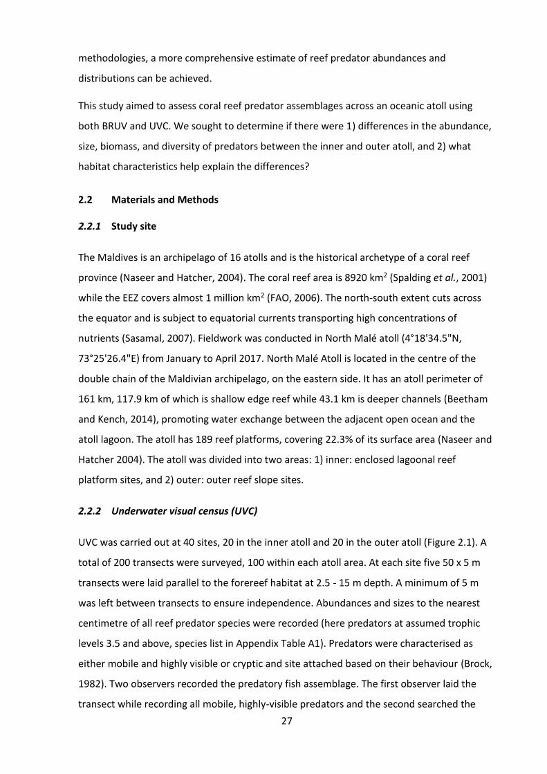
27

methodologies, a more comprehensive estimate of reef predator abundances and

distributions can be achieved.

This study aimed to assess coral reef predator assemblages across an oceanic atoll using

both BRUV and UVC. We sought to determine if there were 1) differences in the abundance,

size, biomass, and diversity of predators between the inner and outer atoll, and 2) what

habitat characteristics help explain the differences?

2.2 Materials and Methods

2.2.1 Study site

The Maldives is an archipelago of 16 atolls and is the historical archetype of a coral reef

province (Naseer and Hatcher, 2004). The coral reef area is 8920 km2 (Spalding et al., 2001)

while the EEZ covers almost 1 million km2 (FAO, 2006). The north-south extent cuts across

the equator and is subject to equatorial currents transporting high concentrations of

nutrients (Sasamal, 2007). Fieldwork was conducted in North Malé atoll (4°18'34.5"N,

73°25'26.4"E) from January to April 2017. North Malé Atoll is located in the centre of the

double chain of the Maldivian archipelago, on the eastern side. It has an atoll perimeter of

161 km, 117.9 km of which is shallow edge reef while 43.1 km is deeper channels (Beetham

and Kench, 2014), promoting water exchange between the adjacent open ocean and the

atoll lagoon. The atoll has 189 reef platforms, covering 22.3% of its surface area (Naseer and

Hatcher 2004). The atoll was divided into two areas: 1) inner: enclosed lagoonal reef

platform sites, and 2) outer: outer reef slope sites.

2.2.2 Underwater visual census (UVC)

UVC was carried out at 40 sites, 20 in the inner atoll and 20 in the outer atoll (Figure 2.1). A

total of 200 transects were surveyed, 100 within each atoll area. At each site five 50 x 5 m

transects were laid parallel to the forereef habitat at 2.5 - 15 m depth. A minimum of 5 m

was left between transects to ensure independence. Abundances and sizes to the nearest

centimetre of all reef predator species were recorded (here predators at assumed trophic

levels 3.5 and above, species list in Appendix Table A1). Predators were characterised as

either mobile and highly visible or cryptic and site attached based on their behaviour (Brock,

1982). Two observers recorded the predatory fish assemblage. The first observer laid the

transect while recording all mobile, highly-visible predators and the second searched the

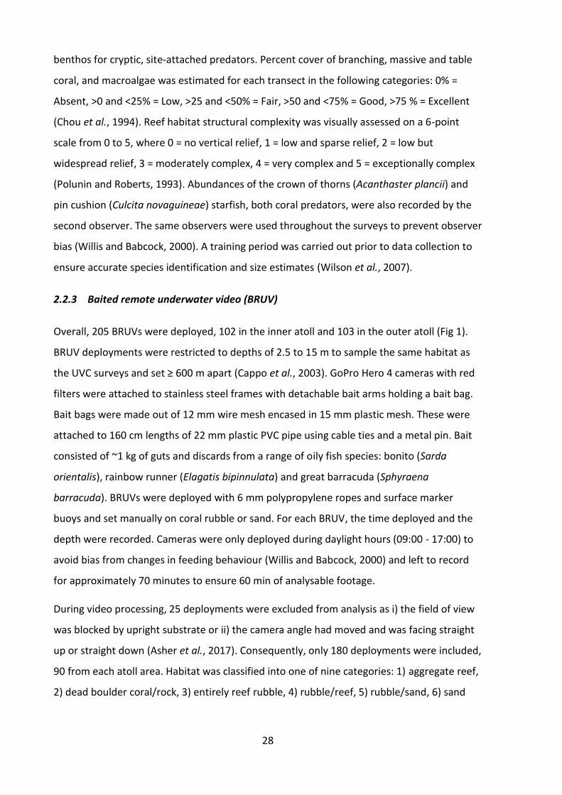
28

benthos for cryptic, site-attached predators. Percent cover of branching, massive and table

coral, and macroalgae was estimated for each transect in the following categories: 0% =

Absent, >0 and <25% = Low, >25 and <50% = Fair, >50 and <75% = Good, >75 % = Excellent

(Chou et al., 1994). Reef habitat structural complexity was visually assessed on a 6-point

scale from 0 to 5, where 0 = no vertical relief, 1 = low and sparse relief, 2 = low but

widespread relief, 3 = moderately complex, 4 = very complex and 5 = exceptionally complex

(Polunin and Roberts, 1993). Abundances of the crown of thorns (Acanthaster plancii) and

pin cushion (Culcita novaguineae) starfish, both coral predators, were also recorded by the

second observer. The same observers were used throughout the surveys to prevent observer

bias (Willis and Babcock, 2000). A training period was carried out prior to data collection to

ensure accurate species identification and size estimates (Wilson et al., 2007).

2.2.3 Baited remote underwater video (BRUV)

Overall, 205 BRUVs were deployed, 102 in the inner atoll and 103 in the outer atoll (Fig 1).

BRUV deployments were restricted to depths of 2.5 to 15 m to sample the same habitat as

the UVC surveys and set ≥ 600 m apart (Cappo et al., 2003). GoPro Hero 4 cameras with red

filters were attached to stainless steel frames with detachable bait arms holding a bait bag.

Bait bags were made out of 12 mm wire mesh encased in 15 mm plastic mesh. These were

attached to 160 cm lengths of 22 mm plastic PVC pipe using cable ties and a metal pin. Bait

consisted of ~1 kg of guts and discards from a range of oily fish species: bonito (Sarda

orientalis), rainbow runner (Elagatis bipinnulata) and great barracuda (Sphyraena

barracuda). BRUVs were deployed with 6 mm polypropylene ropes and surface marker

buoys and set manually on coral rubble or sand. For each BRUV, the time deployed and the

depth were recorded. Cameras were only deployed during daylight hours (09:00 - 17:00) to

avoid bias from changes in feeding behaviour (Willis and Babcock, 2000) and left to record

for approximately 70 minutes to ensure 60 min of analysable footage.

During video processing, 25 deployments were excluded from analysis as i) the field of view

was blocked by upright substrate or ii) the camera angle had moved and was facing straight

up or straight down (Asher et al., 2017). Consequently, only 180 deployments were included,

90 from each atoll area. Habitat was classified into one of nine categories: 1) aggregate reef,

2) dead boulder coral/rock, 3) entirely reef rubble, 4) rubble/reef, 5) rubble/sand, 6) sand

29

Figure 2.1. Location of the underwater visual census (UVC) and baited remote underwater

video (BRUV) locations. a) Maldives location in the north Indian Ocean (3.2028° N,

73.2207° E), b) North Malé Atoll in the central Maldives archipelago (4.4167° N, 73.5000°

E), and c) the UVC and BRUV inner and outer survey locations in North Malé Atoll.

30

flat, 7) sand with reef in view, 8) sand with scattered coral/rock and 9) spur and groove, the

first habitat type being the most dominant of the two identified (Asher et al., 2017).Reef

habitat structural complexity was visually assessed on a 6-point scale (see above) (Polunin

and Roberts 1993). Analysis of footage was focused solely on upper trophic level fish

predators i.e. all shark, Aulostomidae, Carangidae, Fistulariidae, Scombridae and Serranidae

species and larger bodied, more mobile Lutjanidae and Lethrinidae species (see Table A1 for

full species list). Predators were identified to the lowest taxonomic level of species in most

cases, but where species could not be identified, individuals were pooled at the genus level

(Espinoza et al., 2014). For each species, the maximum number seen at any one time on the

whole video (MaxN) was recorded (Harvey et al., 2012). Video analysis began after a

settlement period (min 02:00 – max 08:00 minutes) had elapsed (Kiggins et al., 2018). The

settlement period was characterised as over when all sand or sediment had settled and

visibility returned to normal and at least a minute had passed since the BRUV was moved or

repositioned.

2.2.4 Data Analysis

The following statistical procedures were carried out for both UVC and BRUV data using

PRIMER 6 (v. 6.1.15) with the add-on PERMANOVA+ (v. 1.0.5) (Anderson et al. 2008) and R

version 3.5.2 (R Core Team, 2017) linked with RStudio version 1.1.463 (RStudio Team, 2012).

Species richness for each dataset was determined using the species accumulation curve in

the vegan R package (Oksanen et al., 2018). Curves were generated using 100 permutations

and the “exact” method, which finds the expected mean species richness. 95% confidence

intervals were calculated from standard deviations. Only individuals identified to species

level were included.

Spatial variation in predator populations

UVC assemblage data were analysed at the transect level and BRUV assemblage data at the

BRUV level. Where BRUV sites were repeat sampled on different days each deployment was

counted as an independent sample. Predator abundance data were square root transformed

to reduce right skewness from large outliers and because square root transformation can be

applied to zero values. A resemblance matrix was created based on Bray-Curtis similarity

measures. Using the R vegan package (Oksanen et al., 2018), data were graphically

compared using non-metric multi-dimensional scaling (nMDS) with a Kruskal fit scheme set

31

to 3 and a minimum stress level of 0.01. If there were clear outliers, these were removed

and an additional nMDS plot was carried out on a subset of the data (see supplemental

material for all nMDS plots; Figure A1 and A2). Significantly correlated species were

extracted and overlaid on the nMDS plots as vectors. Differences in the predator assemblage

occurring between atoll areas and among sites were investigated using a nested model in

PERMANOVA+ (Type III Sum of Squares, under a reduced model with 9999 permutations),

where site (UVC: 40 levels and BRUV: 39 levels) was a random factor nested within the fixed

factor area (2 levels). Species contributing to between-area dissimilarity and within-area

similarity were identified using the SIMPER function (Clarke and Warwick, 2001).

UVC predator biomass data was calculated using length-weight relationships available on

FishBase (http://fishbase.org) with the exception of Aethaloperca rogaa where length-

weight relationships were taken from Mapleston et al. (2009). Spatial differences in UVC

predator biomass were investigated using a Generalized Linear Model (GLM) with transect

level biomass as the response variable and site nested within area as the predictor variables.

Model normality and homogeneity assumptions were assessed by plotting predicted values

against residuals, predicted values against standardised residuals, and qqplots of

standardised residuals. Biomass data were log transformed to satisfy model assumptions. An

analysis of variance (ANOVA) was applied to determine whether effects were significant (p <

0.05). A second GLM was run with the same parameters but without the nurse shark,

Nebrius ferrugineus, as three large (1.9 – 2.5 m) individuals were recorded on only one

transect in the inner atoll.

Variation in predator body size between atoll areas was investigated for each predator

family individually using a linear mixed effects model with the R package lme4 (Bates et al.,

2015). Body size (cm) was the response variable, area was a fixed effect and species was a

random effect. Model assumptions were checked as above and data were log transformed

to meet assumptions when necessary. When the predator family only had one recorded

species (Aulostomidae, Carcharhinidae, Scorpaenidae), an ANOVA with body size (cm) as the

response variable and area as the predictor variable was used. Size data were checked for

normality and homogeneity of variances using a Shapiro-Wilks test and a Levene’s test

respectively. When data did not conform to these parameters, a non-parametric Kruskal-

Wallis test was used. Although two species of Carangidae were recorded, C. ignobilis was

only observed once in the inner atoll. This observation was removed from analysis and an

http://fishbase.org/

32

ANOVA was used. Fistulariidae and Ginglymostomatidae were only recorded in the inner

atoll so no size-based comparisons were made.

Correlation with environmental variables

Using PRIMER, environmental data were normalised as they were measured on different

scales. For each entry of a variable, the mean of the variable is subtracted and the value is

divided by the standard deviation for that variable (Clarke and Gorley, 2006). UVC

environmental variables consisted of depth, complexity, branching coral cover (BC), massive

coral cover (MC), table coral cover (TC), algal cover (AC), abundance of crown of thorns

starfish (COTS) and abundance of pin cushion starfish (PIN) while BRUV environmental

variables consisted of depth, complexity and habitat type. Variables were assessed for

collinearity using pairs plots and by calculating the variance inflation factor (VIF) using the

vifstep method in the usdm R package (Naimi et al., 2014). VIF quantifies the severity of

collinearity between predictor variables. The vifstep method calculates VIF for all variables in

a stepwise fashion. It excludes the variable with a VIF > specified threshold, repeating the

process until no variables have a VIF > specified threshold. Here, the VIF threshold was set to

3 (Zuur et al., 2010). Data were compared using Principal Coordinates Analysis (PCO) based

on Euclidean distance similarity measures with overlaid vectors of Pearson’s correlated

environmental variables. Differences in environmental variables between inner and outer

atoll were investigated using a nested model in PERMANOVA+ (Type III Sum of Squares,

under a reduced model with 9999 permutations), where site (UVC: 40 levels and BRUV: 39

levels) was a random factor nested within the random factor area (2 levels).

To investigate the relationships between the predator assemblage and the respective

environmental variables (Table A2), the RELATE function in PRIMER 6 (v. 6.1.15) with a

Spearman’s Rank Correlation coefficient and 9999 permutations (Clarke and Warwick 2001)

was used. These correlations were further tested using a distance-based multiple linear

regression model (DISTLM) in PERMANOVA+ (v. 1.0.5) (Clarke and Gorley, 2006), which

models the relationship between a multivariate distance-based dataset, as described by a

resemblance matrix, and the variables (Clarke and Gorley, 2006) using distance based

redundancy analysis (dbRDA) (Clarke and Gorley, 2006). Relationships were first analysed

using marginal tests. The Best selection procedure was used as it incorporates and examines

the selection criterion for all possible combinations of predictor variables, with an AICc

selection criterion and 9999 permutations of the raw data to obtain p-values for each

33

individual predictor variable (Clarke and Gorley, 2006). AICc values indicate the goodness of

a model fit to the data and the model with the lowest AICc value was considered the most

parsimonious (Symonds and Moussalli, 2011).

2.3 Results

A total of 6524 predators of 47 species and ten families were recorded from the 200

transects that surveyed 50,000 m2 of reef (Figure 2.2A) and the 10,800 minutes of examined

footage from 180 BRUVs (90 in each area) (Figure 2.2B). Species accumulation plots showed

similar patterns and indicated that the sampling effort of each method was sufficient to

record most of the predators occurring in the area surveyed (Figure 2.3). However, both

methods showed higher predator species richness in the inner atoll compared to the outer

atoll, and this difference was greatest for the BRUVs.

2.3.1 Spatial variation in predator populations

Similar numbers of individuals and species were recorded in each atoll area (

Table 2.1). Five species were only recorded in the inner atoll (Carcharhinus falciformis,

Elagatis bipinnulata, Epinephelus ongus, Lethrinus harak and Lethrinus microdon) while

seven species were only recorded in the outer atoll (Carcharhinus amblyrhynchos,

Epinephelus malabaricus, Epinephelus tauvina, Lutjanus decussatus, Lutjanus fulvus, Macolor

macularis and Negaprion acutidens; Table A1).

Table 2.1. Summary of collected reef predator data in inner and outer atoll areas by

underwater visual census (UVC) and baited remote underwater video (BRUV).

Inner Outer

UVC BRUV Total UVC BRUV Total

Individuals 1786 1527 3313 2339 872 3211

Species 33 34 39 33 31 41 Species unique to method 5 6 10 8

Families 10 8 10 8 8 10

34

Figure 2.2. A) Abundance from underwater visual census (UVC) and B) MaxN from baited remote underwater video (BRUV) of predator

families in inner and outer atoll. Individual points are A) 250 m2 transects and B) BRUV deployments.

35

Figure 2.3. Species accumulation curves derived from the cumulative number of UVC

transects and BRUV deployments in both inner and outer atoll. Bars represent 95%

confidence intervals derived from standard deviation.

Total recorded predator biomass was 0.29 t ha-1 in the inner atoll and 0.25 t ha-1 in the outer

atoll. The biomass of Carcharinidae, Lethrinidae, Lutjanidae and Serranidae were greater in

the outer atoll while biomasses of Aulostomidae, Carangidae and Scombridae were greater

in the inner atoll (Figure 2.4). There was no significant difference in total predator biomass

between areas (ANOVA, p <0.05) but there was a highly significant difference in biomass

among sites within areas (ANOVA, F1,39 = 2.08, p = <0.001). When Nebrius ferrugineus was

removed from biomass calculations, total predator biomass was significantly greater in the

outer atoll (ANOVA, F1 = 4.51, p = <0.05) and there were still significant differences among

sites within each area (ANOVA, F1,39 = 1.82, p = p <0.05).

The size of Aulostomidae (ANOVA, p > 0.05), Carcharinidae (ANOVA, p > 0.05) and

Scorpaenidae (Kruskal-Wallis, p > 0.05) did not differ between atoll areas but Carangidae

were larger in the outer atoll (mean inner: 28.56 cm; outer: 39.75 cm; ANOVA, F1,11 = 12.68,

p = < 0.001). Linear mixed effects models suggested no difference in mean size of

Scombridae between atoll areas (mean inner: 49.67 cm; outer: 49.00 cm), but Lethrinidae

(mean inner 21.79 cm; outer: 24.74 cm), Lutjanidae (mean inner: 23.04 cm; outer: 30.46

cm), and Serranidae (mean inner: 18.81 cm; outer: 18.99 cm) were all significantly larger in

the outer atoll (Table 2.2; Figure 2.5).

36

Table 2.2. Differences in predator body size between inner and outer atoll areas as

determined by linear mixed effects models. Separate models were run on each individual

family.

Formula: Size ~ Area + (1 | Species)

Estimate SE df t p-value

Lethrinidae (Intercept) 21.87 1.32 1.51 16.56 0.01 *

Area 2.96 0.78 174.66 3.79 0.00 *** Lutjanidae

(Intercept) 25.69 2.61 4.43 9.83 0.00 *** Area 6.39 1.59 129.76 4.01 0.00 ***

Scombridae (Intercept) 45.76 12.48 1.08 3.67 0.16

Area -2.62 4.51 4.00 -0.58 0.59 Serranidae

(Intercept) 20.28 1.72 11.98 11.77 0.00 *** Area 2.30 0.28 1631.84 8.13 0.00 ***

Figure 2.4. Biomass (kg) of predator families recorded by underwater visual census (UVC).

Values are on a log10 scale.

37

The nMDS plot of the UVC predator data suggested different inner and outer atoll predator

assemblages, while that of the BRUV data suggested greater overlap between areas (Figure

2.6). There were highly significant differences in the predator assemblage between atoll

areas (Nested PERMANOVA, UVC = F1 = 17.57, p = <0.001; BRUV = F1 = 4.07, p = <0.001) and

among sites (Nested PERMANOVA, UVC = F38 = 2.21, p = <0.001; BRUV = F37 = 1.40, p =

<0.001). SIMPER analysis revealed a high level of dissimilarity in biota between atoll areas

(SIMPER UVC = 63.94%, driven by Cephalopholis leopardus, C. argus, and Anyperodon

leucogrammicus; BRUV = 74.11%, driven by Caranx melampygus and C. argus;

Table 2.3). Within areas, similarity of predator assemblages recorded using UVC was

moderate (SIMPER, inner: 41.10%, driven by C. argus, A. leucogrammicus, and Monotaxis

grandoculis; outer: 49.12%, driven by C. argus and C. leopardus), while similarity of those

recorded using BRUV was low (SIMPER, inner: 29.07%, driven by Aethaloperca rogaa,

Lutjanus bohar, and C. argus; outer: 33.37%, driven by C. argus, A. rogaa, and L. bohar; (

Table 2.3).

Table 2.3. Main species contributing to between-area dissimilarity and within-area

similarity using both UVC and BRUV abundance data. Species contributing below 9% are

not shown.

Dissimilarity between Similarity within area

Species Areas Inner Outer

UVC C. leopardus 13.73% - 30.41% C. argus 11.22% 34.62% 40.56% A. leucogrammicus 10.04% 18.44% - A. rogaa 9.97% 15.39% 12.39% M. grandoculis 9.17% 19.35% -

BRUV C. melampygus 9.95% - - C. argus 9.08% 12.07% 32.23% A. rogaa - 30.63% 17.64% L. bohar - 20.86% 14.67% M. grandoculis - 10.30% - C. nigripinnis - - 12.31%

38

Figure 2.5. Total length (cm) of predators belonging to four families where there were

significant differences between inner and outer atoll, as indicated by ANOVA and linear

mixed effects models. Vertical bars represent the median.

39

Figure 2.6. Non-metric multidimensional scaling (nMDS) of predator abundance data from

A) underwater visual census (UVC) and B) baited remote underwater video (BRUV).

Species that are significantly correlated (p < 0.05) are overlaid. UVC (1-10) and BRUV (1-3,

11-17): 1: Aethaloperca rogaa; 2: Aprion virescens; 3: Caranx melampygus; 4:

Cephalopholis spiloparea; 5: Epinephelus fasciatus; 6: Epinephelus malabaricus; 7:

Epinephelus merra; 8: Gnathodentex aureolineatu; 9: Macolor niger; 10: Pterois

antennata; 11: Cephalopholis argus; 12: Cephalopholis leopardus; 13: Cephalopholis

nigripinnis; 14: Cephalopholis spp; 15: Epinephelus spilotoceps; 16: Lutjanus bohar; 17:

Nebrius ferrugineus.

2.3.2 Correlation with environmental variables

None of the UVC or BRUV environmental predictor variables were collinear. Environmental

data varied significantly between areas (Nested PERMANOVA, UVC = F1 = 11.95, p = <0.001;

BRUV = F1 = 15.99, p = <0.001) and among sites (Nested PERMANOVA, UVC = F38 = 5.89, p =

<0.001; BRUV = F37 = 1.58, p = <0.05). The first two axes of a PCO explained 82.88% of the

total variation in the BRUV environmental data and showed areas to be relatively separate.

There was similar separation between atoll areas in the UVC environmental data but the first

two axes of the PCO only explained 43.1% of the total variation in the data and the points

were more clustered.

The predator assemblage was correlated with the environmental data collected using UVC

(RELATE, Rho = 0.115, p <0.05) and BRUV (RELATE, Rho = 0.157, p <0.05). With the UVC data,

marginal tests showed depth (Pseudo-F = 25.73, p <0.001, Prop. variation = 0.12), BC

40

(Pseudo-F = 7.10, p <0.001, Prop. variation = 0.3), MC (Pseudo-F = 8.12, p <0.001, Prop.

variation = 0.04), TC (Pseudo-F = 2.73, p <0.05, Prop. variation = 0.01), complexity (Pseudo-F

= 3.57, p <0.005, Prop. variation = 0.02) and PIN (Pseudo-F = 5.18, p <0.001, Prop. variation =

0.03) had a significant interaction with the predator assemblage. The most parsimonious

model included depth, BC, MC and complexity (DISTLM; AICc = 1479.1), which when

visualised using a dBRDA explained 87.2% of the variation in the fitted data but only 13.6%

of the total variation in the data (Figure 2.7A). For the BRUV data, marginal tests showed

complexity (Pseudo-F = 3.18, p <0.005, Prop. variation = 0.02), depth (Pseudo-F = 3.26, p

<0.001, Prop. variation = 0.02) and habitat type (Pseudo-F = 2.31, p <0.05 Prop. variation =

0.01) as having a highly significant correlation with the predator assemblage, but the final

best model included only depth and complexity (DISTLM; AICc = 1377.8). Results visualised

using a dbRDA explained 100% of the variation in the fitted data but only 3.7% of the total

variation in the data (Figure 2.7B).

2.4 Discussion

There were several distinct differences between the inner lagoonal and outer edge reef

habitats. In contrast to previous studies, density and diversity of predators were similar

between the inner lagoonal and outer forereef slopes (Friedlander et al., 2010; Dale et al.,

2011), but there were significant differences in species composition. Furthermore, when the

rarely recorded Nebrius ferrugineus was omitted, biomass was significantly greater along the

outer reef slopes. Lethrinidae, Lutjanidae, and Serranidae, were also significantly larger in

the outer atoll, so despite being more numerically abundant in the inner atoll, their mean

biomass was greater along the outer reef slopes. Schooling species belonging to these

families (e.g. Gnathodentex aureolineatus and Lutjanus kasmira) were more frequently

recorded in the outer atoll (Table A1) and several large bodied species of Lutjanidae and

Serranidae were also uniquely recorded in the outer atoll (e.g. Epinephelus malabaricus,

Lutjanus decussatus, Lutjanus fulvus, and Macolor macularis).

These findings are consistent with ontogenetic shifts in habitat use. Although teleost reef

predators often have smaller home ranges (Nash et al., 2015), some species of Lutjanidae,

Lethrinidae and Serranidae may move tens to hundreds of kilometres between habitat types

as they undergo ontogenetic shifts, moving from juvenile nurseries such as mangroves and

seagrasses to their adult habitat on coral reefs (Williams, 1991; Green et al., 2015).

41

Figure 2.7. Distance-based redundancy analysis (dbRDA) of Bray-Curtis dissimilarities calculated from square-root transformed abundances

of reef predator species vs. environmental predictor variables. The most parsimonious model was chosen using the AICc selection criterion

and included A) complexity, depth, branching coral (BC), and massive coral (MC) for the underwater visual census (UVC) predator data, and

B) depth and complexity for the baited remote underwater video (BRUV) predator data.

42

The presence of juvenile nursery habitats close to coral reefs increases adult biomass

(Mumby et al., 2004; Nagelkerken, 2007) while a lack of nursery habitats has been linked to

lower adult densities and the absence of some species (Olds et al., 2012; Wen et al., 2013).

The significant differences in predator sizes and abundances between inner and outer atoll

found here are consistent with ontogenetic habitat shifts, and indicate that the inner atoll

lagoon may be an important nursery habitat for many of these predator species. In the

British Virgin Islands, nearly half the reef fishes exhibited ontogenetic shifts between lagoons

and forereefs and almost all species were significantly larger in the reef habitat than in the

lagoon (Gratwicke et al., 2006). Furthermore, even isolated nursery habitats are utilized by

juvenile emperors, suggesting that ontogenetic migrations of these species act to connect

adult and juvenile habitats (Nakamura et al., 2009). In North Malé Atoll, the proximity of the

edge and lagoonal reefs to each other, in addition to the relatively shallow nature of the

lagoon, may facilitate a high degree of mobility and connectivity between inner and outer

atoll (Berkström et al., 2013).

Differences in the reef habitat between atoll areas may also play a role. The outer reef

slopes provide a larger, more continuous reef area compared to the shallow inner reefs,

where soft bottom habitat is extensive. Large piscivorous fish are more abundant in areas of

higher live coral cover with greater habitat structural complexity (Connell and Kingsford,

1998) and growth rates and abundances of predatory fishes tend to be higher when prey

densities are greater (Beukers-Stewart et al., 2011). Higher prey availability is also a key

driver of ontogenetic emigrations of snappers and emperors from nearshore to coral reef

habitats (Kimirei et al., 2013). The larger body sizes and school sizes in the outer atoll, in

addition to the unique occurrence of several of these species, suggest that this habitat may

be of a higher quality, providing sufficient food and space to fit the requirements of these

predator species. However, only a detailed assessment of the available habitat and prey

assemblages will help determine the factors influencing predator distributions.

Several families had a greater biomass in the inner atoll, including Aulostomidae,

Carangidae, Fistulariidae and Ginglymostomatidae. Aulostomidae were rarely recorded

along the outer edge reefs although their habitat preferences include reefs extending to the

continental slope (Bowen et al., 2001). Competition from the greater numbers of Lutjanidae

and Serranidae may play a role in limiting their numbers in the outer atoll. Higher numbers

of the bluefin trevally, C. melampygus, were the main contribution to the greater biomass of

43

Carangidae. C. melampygus is an important mobile predator that is prominent in nearshore

waters (Hobson, 1979; Sancho, 2000). Their diet consists of diurnally active prey,

predominantly from shallow-water habitats (Sudekum et al., 1991), which suggests they may

enter the lagoon during the day to hunt. The lagoon may also represent an important

nursery ground for this species, as juvenile C. melampygus occupy shallow-water protected

environments such as lagoons and estuaries (Smith and Parrish, 2002). As no UVC surveys or

BRUV deployments were conducted at night, it is not certain whether their numbers would

increase along the outer edge reefs after dark. Fistulariidae and Ginglymostomatidae had a

greater biomass in the inner atoll, but only because biomass estimates were derived solely

from UVC. Fistulariidae prefer coastal areas with soft bottoms (Fritzsche, 1976) and were

recorded in both atoll areas with BRUVs, but the UVC surveys were conducted solely on hard

reef substrate. Ginglymostomatidae were frequently recorded in both inner and outer atoll

on BRUVs but biomass estimates came from the occurrence of several large N. ferrugineus

on two transects in the inner atoll, while none were recorded during UVC in the outer atoll.

Future work would benefit from the inclusion of biomass estimates from several survey

methods and from conducting surveys at night.

Several species were recorded solely in one atoll area. Two of the species unique to the

outer atoll were the grey reef shark, Carcharhinus amblyrhynchos, and the lemon shark,

Negaprion acutidens. Grey reef sharks prefer forereef habitats over lagoons (Papastamatiou

et al., 2018) and although juvenile lemon sharks are atoll lagoon residents (Filmalter et al.,

2013), adults move to deeper coastal reef habitats (Compagno, 1984). Conversely, the silky

shark, Carcharhinus falciformis, and the rainbow runner, Elagatis bipinnulata, were recorded

exclusively in the inner atoll by the BRUVs. These are not typically reef-associated species

(Bonfil, 1993) but the BRUVs were effective in recording their use of the deep water

channels between the shallow inner reefs. Channels act as important habitat corridors,

enhancing connectivity between the inner lagoonal and outer reef slopes, with energy

moving from one area to another through a range of hydrodynamic processes (Sasamal,

2007; Rogers et al., 2017; Green et al., 2019). These corridors also facilitate movement of

mobile marine species, with marine predators taking advantage of them for foraging (Hastie

et al., 2016). The thumbprint, L. harak, and smalltooth, L. microdon, emperors were also only

observed in the inner atoll on BRUVs. Emperors forage extensively over sandy bottoms

where they predate on less mobile prey (Kulbicki et al., 2005). While the BRUVs were

44

deployed over a range of hard and soft bottom substrates, the UVC surveys were conducted

solely on hard bottom reef substrate. In addition, BRUVs will attract these species to the bait

while UVC typically requires high replication to record such species (Dulvy et al., 2003).

These discrepancies between the survey methods may explain the absence of the emperors

from the UVC dataset. Moreover, these species are not necessarily exclusive to one area.

The one-hour BRUV soak time and lack of long term and night time sampling are likely to

lead to underrepresentation or absence of rarer species (Asher et al., 2017).

The asymptotes of the species accumulation plots indicated that the BRUV and UVC surveys

were sufficient to obtain an accurate measure of species richness and, although actual

values varied, predator family abundance patterns were similar for both methods between

areas. However, several species uniquely recorded with either UVC or BRUV underline the

importance of using more than one survey methodology when assessing fish populations.

For example, sharks were almost exclusively recorded with BRUVs. The teleost predators

identified through the BRUV footage have small home ranges (Nash et al., 2015) and will not

travel far in response to a bait plume, but sharks, being more mobile, may follow bait plumes

to investigate the origin of the scent. This is one of the biases of this methodology (Willis and

Babcock 2000; Cappo et al. 2003; Harvey et al. 2012) but it is also why BRUVs are effective in

tandem with UVC, which underrepresents more mobile, transient species (MacNeil et al.,

2008). In contrast, the species recorded solely during UVC, such as the strawberry grouper,

Cephalopholis spiloparaea, the honeycomb grouper, Epinephelus merra and the spotfin

lionfish, Pterois antennata, are more cryptic and wary. These species may be near the BRUV

but their cryptic nature, the habitat complexity and the angle of the camera mean they may

be missed.

Our analysis found a clear interaction of the predator assemblage data with live branching

and massive coral cover, which accords with previous studies (Bell and Galzin, 1984;

Komyakova et al., 2013). Depth and complexity were important variables for models of both

the UVC and the BRUV assemblage data. Structural complexity on reefs provides important

habitat structure and refuge for prey communities. It is linked to increased fish biomass and

abundance, and declines are predicted to significantly reduce fisheries productivity (Rogers

et al., 2014). However, predator growth rates decrease at reefs of higher complexity as

increased refuge space allows more prey to hide, reducing available food, so reefs with

intermediate complexity are most productive in terms of predator communities (Rogers et

45

al., 2018). The relationship between predator assemblage data and structural complexity is

complicated, but its inclusion in both models reinforces its importance in structuring

predator assemblages (Ferrari et al., 2017). Depth was the second predictor included in both

models. Reef fish communities vary dramatically with depth (Friedlander et al., 2010; Schultz

et al., 2014; Jankowski et al., 2015) as predator abundances and species compositions

change (Asher et al., 2017; Tuya et al., 2017). Its inclusion in both models is further evidence

that it plays a key role in structuring predator communities.

Total biomass of all recorded predators (inner atoll 0.29 t ha-1, outer atoll 0.25 t ha-1) was

similar to that found at other remote but inhabited and exploited atolls (Kiritimati ~0.2 t ha-

1, Tabuaeran ~0.3 t ha-1 (Sandin et al., 2008)), and it was considerably lower than at unfished,

uninhabited atolls and islands (Palmyra ~1.8 t ha-1, Kingman ~5.2 t ha-1 (Sandin et al., 2008);

Chagos Archipelago ~3 – 7.75 t ha-1 (Graham et al., 2013)). Although the Maldives are

considered underexploited (Newton et al. 2007), this indicates that these predator species

are likely overfished. Reef fisheries provide an important source of food to both tourists and

increasingly locals, and the rise in reef fish catch is evidence of a growing demand for these

resources (Sattar et al., 2014). Reef predators typically dominate the reef fish catch with

fishermen targeting Carangidae, Lutjanidae and Serranidae using handlines (Sattar et al.,

2011; Sattar et al., 2012; Sattar et al., 2014). Although more recent information on the status

of the reef fishery is lacking, significant declines in the mean length of the ten most exploited

grouper species (Sattar et al., 2011) and of key target species Lutjanus bohar and L. gibbus

(Sattar et al. 2014) suggest the fishery is already overexploited.

While predators were recorded throughout the sites surveyed, the relatively low total

biomass recorded here is indicative of an exploited system (Friedlander et al., 2010).

Recovery of exploited systems to pristine conditions and a high biomass of apex predators is

estimated to take decades and involve large area closures (Myers and Worm, 2003; Robbins

et al., 2006). While this may be unrealistic to achieve, careful management of the reef fish

populations in the Maldives is required to prevent irreversible loss of these key predatory

species. Nonetheless, the total number of predator species recorded was higher than several

other studies assessing reef fish communities in remote or semi-pristine areas, a probable

outcome given that the Indian Ocean is a region of moderately high species richness

(Roberts et al., 2002).

46

Globally, reef predator populations are declining and species richness is being lost due to

climate change and a range of direct anthropogenic stressors (Friedlander and DeMartini,

2002b; Hempson et al., 2017b; Hughes et al., 2017a). To date, little information exists on

reef predator communities and their distributions in the Maldives. Evidently, lagoonal reefs

are important habitats hosting diverse and abundant reef predator populations, which may

have been previously undervalued. Predator communities are important in terms of

biodiversity and available resources, so there is an urgent need to manage them carefully in

the face of climate change, rapidly increasing tourism, and fisheries expansion to prevent

future declines.


47

Chapter 3 Novel tri-isotope ellipsoid approach reveals dietary variation in sympatric predators

3.1 Introduction

Trophic interactions are key regulators of community dynamics and ecosystem function.

Food web and population dynamics are driven by resource availability, with sympatric

species often in direct competition with each other (Schoener, 1983). Resource partitioning

often occurs among co-occurring species to reduce inter- and intraspecific competition when

resources are limited (Schoener, 1974). Often linked to body size or ontogeny (Werner and

Gilliam, 1984), increasing evidence suggests that individuals may vary in their resource usage

compared to conspecifics of the same age and size (Araújo et al., 2011). As trophic energy

dissipates up food webs, food resource scarcity is likely to be an important driver of foraging

behaviour in large predators. Consumers may alter their foraging to include underutilised

resources when competition is high, leading to dietary specialisations within populations

(Bolnick et al., 2003).

Predators (here referring to upper trophic level sharks and teleosts) are thought to play an

important role in structuring communities. Through their foraging, they may alter prey

behaviour (Lima and Dill, 1990) and, being more mobile, may couple distinct food chains

(McCauley et al., 2012c), altering energy flows and stabilising food webs (McCann et al.,

2005; Rooney et al., 2006). Feeding specialisations have been extensively documented in

upper trophic level vertebrate populations, particularly fishes (Bolnick et al., 2003; Araújo et

al., 2011). While marine predators are often considered to be dietary generalists (Costa,

1993; Gallagher et al., 2017), they may vary significantly in their trophic ecology at both the

individual and species levels. Such specialisations can alter community dynamics (Bolnick et

al., 2011), so species-level assessments of trophodynamics will not account for differing

ecological roles (Matich et al., 2011).

Stable isotope ratios in animal tissues provide unique dietary perspectives and reveal

important facets of resource use (Bearhop et al., 2004) as they reflect assimilation of prey

material into consumer bodies over time (Post, 2002). Carbon (δ13C) and sulfur (δ34S) isotope

data help elucidate the production sources responsible for the energy flow in the food web,

while nitrogen (δ15N) suggests the relative trophic position at which an animal is feeding

48

(Minagawa and Wada, 1984; Pinnegar and Polunin, 1999; Connolly et al., 2004; Croisetière

et al., 2009). Different animal tissues have different turnover rates (Tieszen et al., 1983) with

fast turnover tissues (e.g. plasma or liver) representing short-term diet while slow turnover

tissues (e.g. muscle) represent long-term diet (Carter et al., 2019). Consequently, muscle

tissue can help identify consistent patterns in predator resource use (Vander Zanden et al.,

2015; Carter et al., 2019).

Studies of vertebrate marine predator trophic niches and dietary specialisations have

focussed on elasmobranchs (Matich et al., 2011; Gallagher et al., 2017; Shipley et al., 2018;

Shiffman et al., 2019) and birds (Patrick et al., 2014; Bodey et al., 2018), with most studies

focussing on only a few co-occurring species. There is a lack of isotopic information on

resource partitioning among co-occurring teleost predators (Matley et al., 2017), particularly

in the tropics (Cameron et al., 2019). This is despite the fact that coral reefs often support a

high biomass and diversity of sympatric teleost predators (Stevenson et al., 2007;

Friedlander et al., 2010), a factor thought to increase the occurrence of dietary specialisation

(Araújo et al., 2011). Coral reefs, along with their predator populations, are currently

experiencing unprecedented worldwide declines due to a range of anthropogenic and

climate-related stressors (Friedlander and DeMartini, 2002b; Hughes et al., 2017a). Given

their potential stabilising roles in food web dynamics, knowledge of sympatric reef predator

trophodynamics and resource partitioning is important for predicting how reef communities

will respond to change (Matich et al., 2011).

To our knowledge, no study to date has considered the isotopic niche partitioning of teleost

coral reef predators across multiple, co-occurring families. Greater understanding of spatial

and intraspecific variation in predator feeding patterns is essential to predict how species

will respond to fluctuations in resource availability as environments change (Matley et al.,

2017; Shiffman et al., 2019). Here, we use a tri-isotope ellipsoid approach to examine the

isotopic niches of seven key teleost coral reef predator species to determine whether

predator resource use varies 1) spatially and/or 2) intraspecifically, and 3) whether their

isotopic niches overlap.

49


3.2.1 Study site and sample collection

Fieldwork was conducted in North Malé Atoll, Republic of the Maldives (N 04°26.154’, E 73°

29.902’) from January to April 2017. Sampling occurred at sites across two distinct reef

areas: 1) inner: enclosed lagoonal reef platforms (hereafter ‘inner atoll’) and 2) outer: outer

reef slopes (hereafter ‘outer atoll’) (Figure A3).

In each area seven reef predator species belonging to three families were sampled

opportunistically: groupers (Serranidae: Aethaloperca rogaa, redmouth; Anyperodon

leucogrammicus, slender; Cephalopholis argus, peacock; Cephalopholis miniata, coral hind),

snappers (Lutjanidae: Lutjanus bohar, red; Lutjanus gibbus, humpback), and jack (Caranx

melampygus, bluefin trevally). Predators (trophic level ≥ 3.5) were chosen for sampling

based on their status as key fishery target species (Sattar et al., 2014) and being dominant

components of the predator assemblage biomass in both inner and outer atoll areas (first

author, unpublished data). Predators were caught using rod and reel, handlines and pole

spears. For each individual, the total length (cm) was recorded and then a sample of dorsal

white muscle tissue (1-2 g wet mass) was removed. Sampling was conducted non-lethally

where possible using a 4 mm biopsy punch. All tissue sampling was carried out in compliance

with UK Home Office Scientific Procedures (Animals) Act Requirements and approved by the

Newcastle University Animal Welfare and Ethical Review Body (Project ID No: 526). Only

adults (>15 cm) were sampled to limit possible ontogenetic dietary shifts.

Tissue samples were oven dried at 50°C for 24 hours, redried using a freeze drier, and then

ground to a fine homogenous powder using a pestle and mortar. Subsamples of 2.5 mg of

tissue were weighed into 3 x 5 mm tin capsules and sequentially analysed for δ15N, δ13C, and

δ34S using a PyroCube elemental analyser (Elementar, Hanau, Germany) interfaced with an

Elementar VisION isotope ratio mass spectrometer at the East Kilbride (UK) node of the

Natural Environment Research Council Life Sciences Mass Spectrometry Facility in August

2017. Stable isotope ratios are reported using the delta (δ) notation which for δ13C, δ15N, or

δ34S is: [(𝑅𝑠𝑎𝑚𝑝𝑙𝑒/𝑅𝑠𝑡𝑎𝑛𝑑𝑎𝑟𝑑 ) − 1], where R is the ratio of the heavy to light isotope (e.g.

13C/12C), and measured values are expressed in per mil (‰).

50

International reference materials were placed at the start and end of each N/C/S run (~140-

150 samples) to correct for accuracy and drift. Materials used were USGS40 (glutamic acid)

for δ13C and δ15N (analytical precision (s.d) δ13C = 0.07; δ15N = 0.16) and silver sulfide

standards IAEA- S1, S2 and S3 for δ34S (analytical precision (s.d.) = 0.17, 0.59 and 1.46

respectively). Internal reference materials were placed every ten samples. Materials used

were MSAG2 (a solution of methanesulfonamide and gelatin), M2 (a solution of methionine,

gelatin, glycine) and 15N-enriched alanine and SAAG2 (a solution of sulfanilamide, gelatin and

13C-enriched alanine) (Table A3). A randomly spaced study-specific reference was also used

(one mature individual [TL = 41.4 cm] of A. leucogrammicus, analytical precision (s.d.) δ13C =

0.14, δ15N = 0.27 and δ34S = 0.73 respectively, n = 31) (Table A3).

High lipid content in fish muscle tissue can skew carbon isotope data interpretations as lipids

are depleted in 13C relative to proteins (Focken and Becker, 1998). Carbon stable isotope

data were lipid corrected arithmetically when the C:N ratio of the muscle tissue was > 3.7

using the mass balance equation from Sweeting et al. (2006):

(1) 𝛿13Cprotein =(𝛿13Csample x C:Nsample) + (7 x (C:Nsample−C:Nprotein))

C:Nsample

Here, C:N protein was 3.7 determined by Fry et al. (2003) from shrimp muscle protein C:N.

3.2.2 Ellipsoid Metrics

The “SIBER” package in R (Jackson et al. 2011) provides methods for analysing bivariate

stable isotope data although such methods are applicable to any bivariate normally

distributed data. We extend these methods to the three-dimensional case in order to apply

ellipsoids to trivariate data and calculate their overlap.

Ellipsoid volume can be estimated analytically from the sample covariance matrix by

decomposition into their respective Eigenvalues and Eigenvectors. In the three-dimensional

case, the square root of the Eigenvalues represents the three orthogonal axes, one semi-

major and two semi-minor (a, b and c respectively), that describe the standard ellipsoid,

synonymous to the 2-dimensional standard ellipse (Jackson et al., 2011). The standard

ellipsoid captures approximately 20% of the data (Fox et al., 2007), which can be

subsequently rescaled to capture any desired proportion of data. The volume of the ellipsoid

is then taken to be 4

3𝜋𝑎𝑏𝑐 which we denote SEV (standard ellipsoid volume). As with SEA

51

(standard ellipse area), SEV is biased to underestimation of volume when sample sizes are

small (Jackson et al., 2011). A small sample size correction for degrees of freedom following

Fox et al. (2007) can be applied to correct for such bias giving SEVC, equivalent to SEAc

(Jackson et al., 2011), only here the correction factor is 𝑛−1

𝑛−3 as the ellipsoids are in three

dimensions.

To quantify uncertainty in SEV estimates, a Bayesian framework was developed by

generalising code in the SIBER package to the n-dimensional case (Jackson et al., 2011). Data

are assumed to be well described by the multivariate normal distribution and Bayesian

posteriors of the mean and covariance structures estimated using JAGS (Just Another Gibbs

Sampler) via the R package RJAGS (Plummer, 2018). Ellipsoid volume can subsequently be

estimated from each covariance draw to provide a posterior estimate of SEV, which we

denote SEVB. Sensitivity analysis indicates that this Bayesian approach slightly

underestimates population SEV at small sample sizes (approximately 𝑛 ≤ 8, see Figure A4).

To estimate the degree of overlap between two ellipsoids, we used a numerical approach,

utilising the packages “rgl” (Adler et al., 2018) and “geometry” (Habel et al., 2019). Ellipsoids

were approximated by three-dimensional meshes: a series of vertices that lie on the ellipsoid

surface forming quadrilateral faces. The intersection of these two meshes is then

approximated by a third mesh, the convex hull of which estimates the ellipsoid overlap

volume. This method underestimates volumes as convex surfaces are approximated by

planar faces, however this bias is reduced as the number of vertices used to represent the

ellipsoids increases, which can be iteratively increased by subdividing faces (see Figure A5).

As with estimating SEVB, we use a Bayesian approach to estimate data covariance structures

and calculate overlap for each paired posterior draw to provide a posterior estimate of

overlap. Functions for estimating SEV, SEVC, SEVB and overlap posteriors are provided in the

supporting information to the online publication (https://doi.org/10.1002/ece3.5779).

3.2.3 Data Analysis: Application

The ranges in carbon (CR), nitrogen (NR) and sulfur (SR) isotope values for each predator

were calculated (Layman et al., 2007b). Using the MVN R Package (Korkmaz et al., 2014),

multivariate normality was checked using Mardia’s test (Mardia, 1970) as it can calculate a

corrected version of skewness for small sample sizes (< 20). All species in each area


52

conformed to multivariate normality (p > 0.05) with the exception of L. gibbus and L. bohar

in the inner atoll. Both had normal kurtosis (p > 0.05) but were non-normally skewed (p <

0.05). Univariate normality tests showed that δ34S was normally distributed for both species,

δ15N was only normally distributed for L. gibbus, and both had non-normally distributed

δ13C. The non-normality was driven by one L. gibbus with a more positive δ13C and two L.

bohar that had more positive δ13C and lower δ15N respectively. As all the other data

conformed to multivariate normality and these data points represent individuals with

differing resource uses (Jackson et al., 2011), data were considered well described by the

multivariate normal distribution for all further analysis.

For each species in each area, Bayesian estimates for the multivariate normal distribution of

the data were calculated (15000 iterations with a burn in of 10000 and a thinning factor of

25). Bayesian ellipsoids were fit to 75% of the data (EVB) and their median volume and

interquartile range (25 – 75 %) was determined. The degree of ellipsoid overlap between

species within each area was calculated based on EVB where Bayesian posteriors were

determined from 7500 iterations with a burn in of 5000 and a subdivision value of 4. Overlap

was expressed as a median percentage with 95% credible intervals where 100% indicates

completely overlapping ellipsoids and 0% indicates entirely distinct ellipsoids. When the

overlap between two species was ≥ 60%, niche overlap was considered significant (Matley et

al., 2017). Outer atoll L. bohar were excluded as only one fish was caught.

Individual body size may also influence trophic interactions; we tested for this using Mixed-

Effects Models with the R package lme4 (Bates et al., 2015). The δ13C, δ15N or δ34S stable

isotope value was the response variable, with area (inner/outer) and total length (mm) (and

their interaction) as fixed effects, and total length (mm) nested within species as a random

effect. Model normality and homogeneity assumptions were checked by plotting model

residuals. Significant effects were determined using the R package lmerTest (Kuznetsova et

al., 2017) which provides p-values for lmer model fits via Satterthwaite's degrees of freedom

method. Statistical power to detect size-related effects was determined using the simr R

package (Green and MacLeod, 2016). All analyses were carried out in R Statistical Software

version 3.5.2 (R Core Team, 2017) and RStudio version 1.1.383 (RStudio Team, 2012).

53

3.3 Results

There were substantial differences in the isotope values among the seven species sampled in

both areas (Table 3.1). δ13C ranged from -18.00 (Aethaloperca rogaa, outer) to -10.11

(Lutjanus bohar, inner), δ15N ranged from 10.11 (L. bohar, inner) to 14.59 (Lutjanus gibbus,

outer), and δ34S ranged from 17.06 (Caranx melampygus, inner) to 21.02 (A. rogaa, outer).

In the inner atoll, the median niche volume of L. bohar (25.62) was five times larger than the

niches of the other predators. Excluding L. bohar, C. miniata median niche volume (3.22) was

half the size of the niches of the other predators, while that of C. argus was double the size

(8.10). C. melampygus and L. gibbus had median niche volumes that were of a similar size

(4.21 and 4.76 respectively) and A. rogaa and A. leucogrammicus had niches of a similar size

(6.22 and 5.53 respectively) (Table 3.2; Figure 3.1). In the outer atoll, the median niche

volume of L. gibbus (20.63) was five times larger than the niches of the other predators. The

niche volumes of all the other predators were of similar size (6.45– 7.96), except for C. argus

which had the smallest median niche volume (4.32) (Table 3.2; Figure 3.2).

All predators had larger median isotopic niche volumes in the outer atoll than in the inner

atoll, except for C. argus (inner: 8.10; outer: 4.32) (Table 3.2; Figure 3.1 and Figure 3.2).

Median niche volume of L. gibbus in the outer atoll (20.63) was four times larger than the

niche volume of their inner atoll conspecifics (4.76). C. miniata had a median niche volume

twice as large in the outer atoll (inner: 3.22; outer: 7.06), while the niches of A.

leucogrammicus and C. melampygus were only 1.5 times larger in the outer atoll (Table 3.2;

Figure 3.1 and Figure 3.2).

There were no effects of body size or area on predator δ15N and δ34S values (Table A4) but

statistical power was low (Median (95% CI) δ15N: 9% (4–16) and δ34S: 14% (8–22). Statistical

power to detect size effects was highest for δ13C (Median (95% CI) δ13C: 70% (60 – 77)) but

there were no overall size effects on predator δ13C values. However, they were significantly

more negative in the outer atoll (p < 0.01) and there was a significant effect of size

interacting with area (p < 0.05) (Table A4).

54

Table 3.1. Summary information for the predators in inner and outer atoll. Mean δ13C, δ15N, and δ34S values are in per mil (‰) with SE in

brackets. CR: δ13C range, NR: δ15N range, SR: δ34S range.

Family Species Area n Size (mm) δ13C (‰) CR δ15N (‰) NR δ34S (‰) SR

Carangidae Caranx melampygus Inner 10 248-410 -16.47 (0.22) 3.50 12.39 (0.17) 0.48 18.12 (0.15) 1.20

Outer 6 372-461 -15.80 (0.02) 0.93 12.44 (0.20) 1.48 18.25 (0.16) 1.29

Lutjanidae Lutjanus bohar Inner 12 210-370 -15.36 (0.63) 7.06 12.36 (0.29) 2.94 18.59 (0.18) 0.70

Outer 1 185 -14.87 (0.00) 12.97 (0.00) 17.94 (0.00)

Lutjanus gibbus Inner 13 244-357 -16.36 (0.15) 2.96 12.58 (0.08) 0.02 19.14 (0.17) 1.51

Outer 9 287-420 -16.26 (0.60) 7.84 12.99 (0.32) 3.54 18.96 (0.33) 2.84

Serranidae Aethaloperca rogaa Inner 11 164-278 -16.08 (0.26) 2.72 12.77 (0.07) 0.14 19.49 (0.17) 0.99

Outer 11 148-336 -17.11 (0.17) 4.02 12.99 (0.16) 0.96 19.79 (0.18) 1.95

Anyperodon leucogrammicus Inner 10 238-346 -15.60 (0.19) 1.91 12.94 (0.11) 0.11 19.49 (0.17) 0.79

Outer 10 262-426 -15.61 (0.04) 3.37 12.81 (0.15) 0.42 19.28 (0.01) 0.17

Cephalopholis argus Inner 11 186-342 -15.46 (0.23) 2.81 12.77 (0.08) 0.01 19.32 (0.26) 1.78

Outer 10 190-345 -16.14 (0.19) 2.42 12.29 (0.08) 0.72 19.58 (0.14) 0.53

Cephalopholis miniata Inner 11 160-320 -16.92 (0.10) 2.87 12.73 (0.06) 0.21 19.73 (0.17) 1.47

Outer 10 161-298 -16.88 (0.22) 4.23 12.64 (0.10) 1.26 19.55 (0.20) 0.52

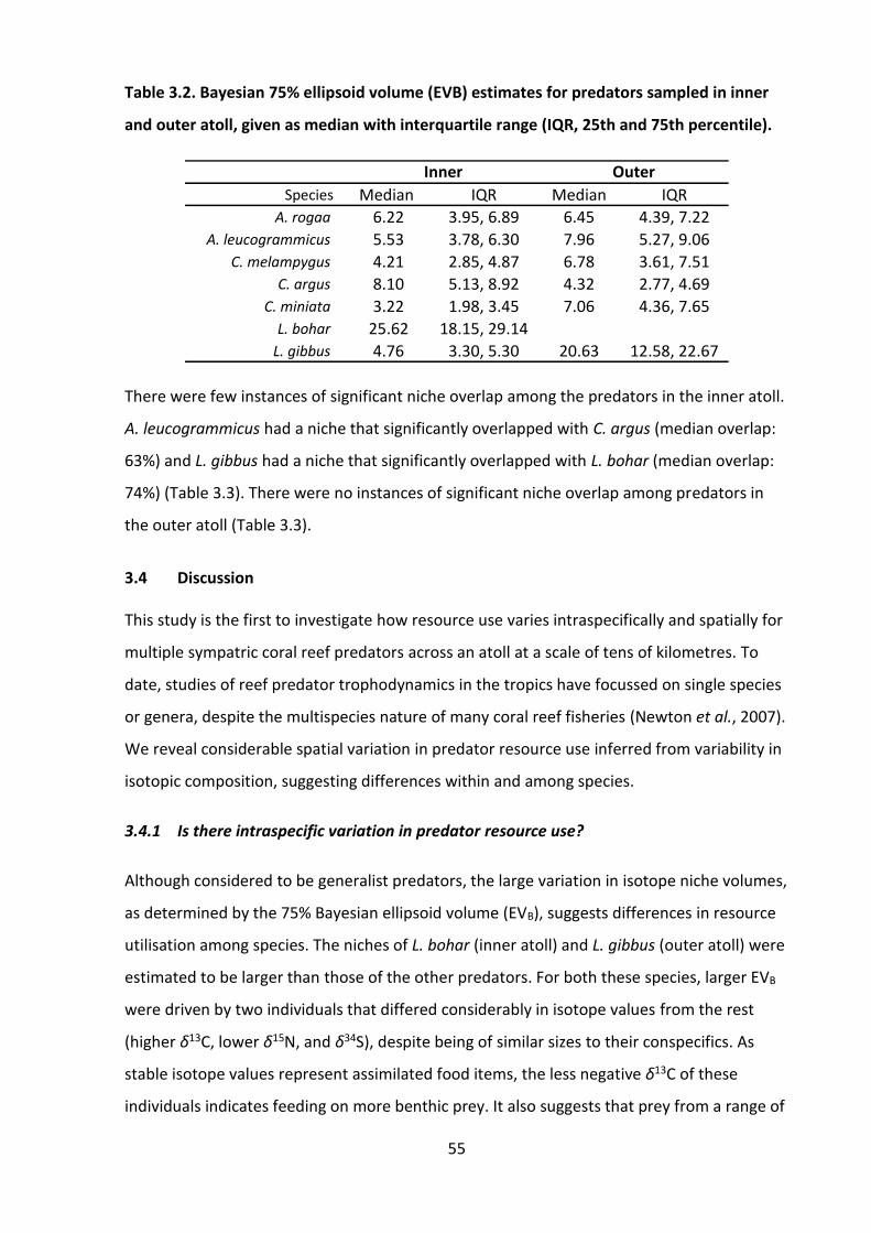
55

Table 3.2. Bayesian 75% ellipsoid volume (EVB) estimates for predators sampled in inner

and outer atoll, given as median with interquartile range (IQR, 25th and 75th percentile).

There were few instances of significant niche overlap among the predators in the inner atoll.

A. leucogrammicus had a niche that significantly overlapped with C. argus (median overlap:

63%) and L. gibbus had a niche that significantly overlapped with L. bohar (median overlap:

74%) (Table 3.3). There were no instances of significant niche overlap among predators in

the outer atoll (Table 3.3).

3.4 Discussion

This study is the first to investigate how resource use varies intraspecifically and spatially for

multiple sympatric coral reef predators across an atoll at a scale of tens of kilometres. To

date, studies of reef predator trophodynamics in the tropics have focussed on single species

or genera, despite the multispecies nature of many coral reef fisheries (Newton et al., 2007).

We reveal considerable spatial variation in predator resource use inferred from variability in

isotopic composition, suggesting differences within and among species.

3.4.1 Is there intraspecific variation in predator resource use?

Although considered to be generalist predators, the large variation in isotope niche volumes,

as determined by the 75% Bayesian ellipsoid volume (EVB), suggests differences in resource

utilisation among species. The niches of L. bohar (inner atoll) and L. gibbus (outer atoll) were

estimated to be larger than those of the other predators. For both these species, larger EVB

were driven by two individuals that differed considerably in isotope values from the rest

(higher δ13C, lower δ15N, and δ34S), despite being of similar sizes to their conspecifics. As

stable isotope values represent assimilated food items, the less negative δ13C of these

individuals indicates feeding on more benthic prey. It also suggests that prey from a range of

Species Median IQR Median IQRA. rogaa 6.22 3.95, 6.89 6.45 4.39, 7.22

A. leucogrammicus 5.53 3.78, 6.30 7.96 5.27, 9.06

C. melampygus 4.21 2.85, 4.87 6.78 3.61, 7.51C. argus 8.10 5.13, 8.92 4.32 2.77, 4.69

C. miniata 3.22 1.98, 3.45 7.06 4.36, 7.65L. bohar 25.62 18.15, 29.14

L. gibbus 4.76 3.30, 5.30 20.63 12.58, 22.67

Inner Outer

56

production sources are available to the predators across the atoll seascape. This hypothesis

is supported by isotope values of primary consumers, which had large but similar ranges in

both atoll areas (Inner δ13C -18.26 to -11.93; δ15N 6.70 to 12.39; δ34S 18.14 to 22.40; Outer

δ13C -17.49 to -11.77; δ15N 6.24 to 11.74; δ34S 18.79 to 20.42) (Skinner et al., 2019).

There is little published information on the movements of L. bohar and L. gibbus specifically;

snappers generally have high site fidelity, but this can vary spatially (Farmer and Ault, 2011;

Pittman et al., 2014). As such, these isotope data give insight into their foraging behaviours

in the absence of spatial tracking methods to assess resource partitioning. In the Bahamas,

δ13C values of Lutjanus griseus and Lutjanus apodus indicated consistent intraspecific

variability in space and resource use, with some individuals exploiting different areas of a

creek and more marine-based resources, while others did not (Hammerschlag-Peyer and

Layman, 2010). In our Maldives data, some individuals of L. bohar and L. gibbus appeared to

be feeding on more benthic prey (less negative δ13C) at lower trophic levels (lower δ15N).

Stomach contents data indicate that both L. bohar and L. gibbus are capable of feeding on a

range of prey, foraging predominantly on reef-associated fish but also partly on crustaceans

(Randall and Brock, 1960; Talbot, 1960; Wright et al., 1986). The isotopic differences among

individuals sampled within the same area suggests they may have alternative feeding

strategies focusing on different prey. This specialisation within populations may explain how

coral reefs can support a high density of co-occurring predators.

3.4.2 Is there spatial variation in predator resource use?

Community-wide isotope metrics (Layman et al., 2007a) suggested that all four grouper

species (A. rogaa, A. leucogrammicus, C. argus and C. miniata) varied in their resource use

spatially. All four had larger NR values in the outer atoll, and with the exception of C. argus,

they all had larger CR values in the outer atoll. Although δ15N values of a corallivore,

Chaetodon meyeri, and a nocturnal planktivore, Myripristis violacea, were significantly

higher in the outer atoll, the differences in mean values were small (~1‰) and isotopic

values of all other prey species were similar between areas (Skinner et al., 2019).

Furthermore, δ13C and δ15N values of coral host and particulate organic matter (POM) are

consistent around the Maldives and do not vary between inner and outer atoll (Radice et al.,

2019). This suggests that the differences in predator CR and NR ranges are a direct result of

feeding on different combinations of prey, rather than differences in baseline isotope values.

57

Figure 3.1. 75% ellipsoids corrected for small sample size generated using δ13C, δ15N and δ34S data for predators in the inner atoll. See

rotating GIF in supporting information with online publication (https://doi.org/10.1002/ece3.5779).


58

Figure 3.2. 75% ellipsoids corrected for small sample size generated using δ13C, δ15N and δ34S data for predators in the outer atoll. See

rotating GIF in supporting information with online publication (https://doi.org/10.1002/ece3.5779).


59

Stomach contents data show that A. rogaa, C. argus, and C. miniata feed primarily on reef-

associated fish from a range of families that are sustained by multiple production sources

(Harmelin-Vivien and Bouchon, 1976; Shpigel and Fishelson, 1991; Dierking et al., 2011).

While no stomach contents data was available for A. leucogrammicus, it occupies the same

reef habitat as the other groupers (Sluka and Reichenbach, 1995), so likely has a similar diet.

The larger CR and NR of these species could indicate that their prey rely on a wide range of

production sources. Where benthic and pelagic food webs overlap such as here, predators

might have access to prey from two food webs (i.e. planktivores and herbivores) while

remaining in the same habitat (Matich et al., 2011). Furthermore, C. argus in particular

displays extensive foraging plasticity allowing it to take advantage of small scale fluctuations

in prey availability (Karkarey et al., 2017), a behaviour possibly reflected in the larger CR and

NR ranges.

Interestingly, and in contrast to the patterns identified with the CR and NR ranges, A.

leucogrammicus and C. miniata had larger SR ranges (δ34S: 18.60-20.29 and 18.70-20.65

respectively) in the inner atoll, despite having smaller CR and NR ranges and isotopic niches

there. The δ34S isotope values revealed that these two species may be feeding on prey

reliant on a range of production sources, including more benthic-sustained detritivores

(mean ± s.d. δ34S: 18.14 ± 0.22) and herbivores (mean ± s.d. δ34S: 19.66 ± 0.22) (Skinner et

al., 2019). Assessing the resource use of these two predators in the inner atoll based solely

on δ13C and δ15N values may have missed this intricacy, as the δ13C and δ15N values were

indicative of feeding on more pelagic prey from higher trophic levels (evidenced by lower

δ13C and higher δ15N). In food web studies, δ34S is often overlooked, despite its ability to

help distinguish between different marine producers (Connolly et al., 2004) and reveal

resource usage intricacies and pathways (Croisetière et al., 2009; Gajdzik et al., 2016) that

may be masked using only δ13C or δ15N. The primary reason for this is that measuring δ34S is

typically more challenging, and thus more costly, than measuring δ13C or δ15N. However,

recent technological advances and new instruments mean that δ13C, δ15N and δ34S can be

measured from the same sample aliquot with a high level of precision (Fourel et al., 2015).

Given these advances and the relative ease of now measuring δ34S, we strongly suggest that

more studies incorporate δ34S to employ the tri-isotope ellipsoid approach that we present

here.

60

With the exception of C. argus, all predators had larger isotopic niches in the outer atoll.

Given the similarity in prey and primary producer isotope values between atoll areas (Radice

et al., 2019; Skinner et al., 2019), it seems likely that this spatial variation in resource use is

linked to variations in resource availability (Araújo et al., 2011). The oceanic rim reefs of the

outer atoll had higher live branching coral and habitat structural complexity following the

2016 bleaching event compared to inner atoll reefs (first author, unpublished data). Coral

cover is strongly linked to fish species richness (Komyakova et al., 2013) and reefs with

higher complexity and coral cover support greater densities of smaller-bodied (<20 cm) fish

(Alvarez-Filip et al., 2011). Although prey fish biomass was similar between atoll areas,

densities of planktivores were greater along the outer edge reefs (first author, unpublished

data). This may lead to increased specialisation and population niche size, a hypothesis

supported by the larger isotopic niche volumes of the predator populations in the outer

atoll.

Inner atoll L. gibbus had an isotopic niche volume (EVB) a tenth the size of the outer atoll

population. Spatial differences in L. gibbus feeding have previously been recorded; it has a

crab dominated diet in Japan (Nanami and Shimose, 2013) but a forage fish (clupeid)

dominated diet in Yemen (Ali et al., 2016). Differential preferences for crabs, which are

benthic, and clupeids, which are pelagic, may explain the differing range in δ13C and δ34S

values between atoll areas found here. Furthermore, the smaller EVB of the inner atoll

population may mean individuals are consistently feeding on a similar but select group of

prey. As isotope values of key prey species were similar in both atoll areas (Skinner et al.,

2019), this further supports the hypothesis that there is spatial variation in resource

availability across the atoll.

61

Table 3.3. Median percentage overlap in ellipsoids (Bayesian 75% ellipsoid generated using δ13C, δ15N and δ34S data) with 95% credible

intervals showing the uncertainty in the overlap estimates between each pair of predator species. The table is to be read across each row:

for example, in the inner atoll 46% of the A. rogaa ellipsoid overlapped with the A. leucogrammicus ellipsoid, and 53% of the A.

leucogrammicus ellipsoid overlapped with the A. rogaa ellipsoid. Significant overlap (≥ 60%) is in bold. Overlap was only determined for

predators in the same atoll area.

A. rogaa A. leu C. mel C. argus C. miniata L. bohar L. gibbus

A. rogaa - 46 (18 - 77) 1 (0 - 14) 57 (24 - 86) 30 (11 - 52) 39 (11 - 78) 31 (9 - 57)

A. leu 53 (24 - 85) - 0 (0 - 4) 63 (33 - 95) 12 (0 - 29) 18 (0 - 52) 16 (0 - 39)

C. melampygus 2 (0 - 20) 0 (0 - 5) - 0 (0 - 8) 5 (0 - 23) 57 (30 - 94) 29 (7 - 56)

C. argus 45 (20 - 75) 42 (18 -70) 0 ( 0 - 4) - 10 (0 - 26) 30 (8 - 64) 14 (0 - 31)

C. miniata 57 (25 - 94) 21 (0 - 56) 6 (0 - 30) 27 (0 - 64) - 46 (13 - 85) 53 (24 - 86)

L. bohar 10 (2 - 23) 4 (0 - 12) 10 (3 - 20) 10 (2 - 23) 6 (1 - 14) - 14 (5 - 26)

L. gibbus 41 (15 - 70) 18 (0 - 42) 26 (6 - 50) 24 (0 - 50) 36 (12 - 61) 74 (48 - 100) -

A. rogaa - 29 (7 - 59) 10 (0 - 35) 20 (2 - 44) 47 (22 - 79) - 56 (25 - 89)

A. leu 23 (5 - 43) - 9 (0 - 32) 16 (1 - 38) 26 (4 - 54) - 51 (20 - 82)

C. melampygus 10 (0 - 34) 12 (0 - 36) - 3 (0 - 19) 17 (0 - 47) - 34 (7 - 69)

C. argus 31 (5 - 61) 31 (5 - 65) 5 (0 - 35) - 55 (23 - 90) - 29 (2 - 76)

C. miniata 44 (17 - 76) 31 (4 - 60) 17 (0 - 43) 33 (11 - 65) - - 46 (9 - 85)

L. gibbus 18 (5 - 36) 20 (6 - 42) 11 (2 - 27) 7 (0 - 17) 16 (4 - 32) - -

Inn

er

Ou

ter

62

3.4.3 Do the isotopic niches of sympatric predators overlap?

The degree of niche overlap was low; there were only two occurrences of significant niche

overlap in the inner atoll and none in the outer atoll. This might suggest that the level of

competition among these species is low in both areas with predators feeding on a variety of

different resources. Overlapping niches do not conclusively equate to increased competition

for resources (Layman et al., 2012; Gallagher et al., 2017). All predators had a larger degree

of niche overlap with Lutjanus bohar (inner) and Lutjanus gibbus (outer) due to the

exceptionally large niches of these two species, but the level of direct competition may be

lower. Predators could be feeding on prey over different spatiotemporal scales, which would

reduce their direct competition. Alternatively, due to protein turnover and prey isotope

signature integration into muscle tissue over time, predators may be feeding on ecologically

different diets but still express similar isotope values, confounding interpretation of the level

of competition existing in the community.

It is worth noting that not all predators caught in the same location necessarily derive their

nutrition from that locality though. The bluefin trevally, Caranx melampygus, had a distinct

isotopic niche which overlapped minimally with the niches of the other predators in both

atoll areas. C. melampygus is a transient, midwater predator with an extensive territory

(Holland et al., 1996; Sancho, 2000) and is the most mobile of all the predators sampled. It

regularly makes crepuscular migrations of 1-2 km between different habitats (Meyer and

Honebrink, 2005). Furthermore, it was the only predator to occupy a similar isotopic niche in

both areas, suggesting it may use resources from across the atoll. Stomach contents data

indicate it feeds predominantly on nekton spanning multiple trophic levels, with little

reliance on crustaceans or cephalopods (Meyer et al., 2001). Consequently, this separation is

likely attributable to differing habitat usage and prey encounters compared to the other

more reef-associated and site-attached species (Sluka and Reichenbach, 1995).

Ontogenetic shifts in feeding strategies are well documented (Werner and Gilliam, 1984;

Kimirei et al., 2013), but adults may also vary in their resource use as a function of their size.

Here, body size did not appear to drive niche variability; there was no relationship between

body size and δ13C, δ15N, or δ34S. Although there was a significant relationship between δ13C

and the interaction between area and body size, the effect was weak. However, statistical

power was low and the ability to detect relationships may have been limited due to small

63

sample sizes and limited size ranges; size-based shifts in feeding might have been observed

with greater replication. While more depth is needed in these data, it seems size-based

effects on adult predator resource use are absent or weak here (Layman et al., 2005;

Gallagher et al., 2017; Matley et al., 2017; Shipley et al., 2018). Within the diverse food webs

of coral reefs where prey sizes vary, strong relationships with body size may be masked as

predators target large primary consumers (Layman et al., 2005).

Predators are often thought to be dietary generalists but we show inter- and intra-specific

differences in resource use with minimal significant niche overlap, highlighting how trophic

resource use varies among sympatric reef predators at a scale of tens of kilometres. We did

not specifically test for individual specialisation but several individuals of Lutjanus appeared

to be feeding in completely different ways to their conspecifics. Individual specialisation is

not ubiquitous in marine predator populations (Matich et al., 2011), but small sample sizes

of these predators means statistical power to detect potential differences was limited, thus

underestimating intraspecific trophic variation. Feeding specialisations are linked to

ecological opportunity, and are thought to be more common where resource diversity and

density of competing individuals are greater (Araújo et al., 2011). This makes coral reefs a

prime location for predators to demonstrate vastly different individual feeding behaviours.

Predators may provide stability to communities by linking separate food chains (McCann et

al., 2005; Rooney et al., 2006), but individual dietary specialisations could alter this

ecological linkage role (Matich et al., 2011) with potential consequences for ecosystem

resilience. Detailed information on individual predator resource use is required to identify

their ecological role and help understand how they will respond to environmental change.


64

Chapter 4 Prevalence of pelagic dependence among coral reef predators across an atoll seascape

4.1 Introduction

Until recently, species interactions and nutrient transfer across habitat boundaries and the

impact of species declines beyond individual ecosystems were seldom considered (Lundberg

and Moberg, 2003). However, ecosystems are now recognised to be linked by flows of

organisms and energetic materials (Huxel and McCann, 1998) yet understanding the

trophodynamics (the flow of energy) (Lindeman, 1942) of a food web is challenging,

particularly for complex marine systems such as coral reefs where spatial variation can be

high (Bierwagen et al., 2018).

Once thought to be somewhat ecologically closed (Odum and Odum, 1955; Hamner et al.,

2007), coral reef ecosystems are subject to upwelling and tidal energy, which drive an

exchange of plankton, water and nutrients with the ocean (Hamner et al., 2007; Lowe and

Falter, 2015). Upwelling often occurs through wind-driven wind-water interactions; surface

water is displaced by the wind and replaced by colder nutrient-rich deeper waters.

Phytoplankton, a bottom-up driver of ocean production, is often more abundant near islands

and atolls (Doty and Oguri, 1956; Gove et al., 2016). Since Darwin (1842) it has been

hypothesised that the surrounding ocean provides a major source of nutrition to coral reef

communities. Fish on outer reef edges can benefit from this exogenous source (Wyatt et al.,

2012a) but intense feeding by outer reef communities (Genin et al., 2009) means the

energetic material seaward of the reef is different from that in lagoons (Hamner et al.,

2007). Furthermore, various hydrodynamic processes such as breaking waves and tides are

needed to deliver ocean water into the lagoons (Lowe et al., 2009), suggesting lagoonal reef

fish may not have access to the same resources.

Reef fish communities demonstrate increased reliance on oceanic production seaward of the

reef but greater reliance on reef production inshore and into lagoons (Wyatt et al., 2012b;

Gajdzik et al., 2016; Le Bourg et al., 2017), indicating that the quantity and quality of food

available to inner-reef fish varies substantially (Wyatt et al., 2012b). Variation in nutrient

availability and content to the inner and outer reef habitats may lead to spatial differences in

reef communities. Indeed, planktivorous fish communities are more abundant with

65

increasing proximity to the ocean (Friedlander et al., 2010). Aggregations of these

planktivorous fish, the “wall of mouths” (Hamner et al., 1988), form on the outer edge of

many reefs where they take advantage of increased plankton prey abundances (Wyatt et al.,

2013). The community structure of a coral reef is thus heavily influenced by the adjacent

ocean (Letourneur, 1996; Garcia et al., 2018). Oceanic production is a key driver of forereef

fish biomass (Williams et al., 2015; Robinson et al., 2017) but quantitative estimates of its

contribution to lagoonal reef fish biomass are lacking.

Highly mobile reef predators often rely on production sources from outside their primary

habitat (McCauley et al., 2012c; Papastamatiou et al., 2015) and benefit from the

aggregations of planktivores (Matley et al., 2018). Some of these predators are partly reliant

on oceanic energy fluxes (McCauley et al., 2012c; Frisch et al., 2014; Frisch et al., 2016),

while others are supported by benthic primary production (Hilting et al., 2013). To date most

of the understanding of these food web relationships comes from studies of reef sharks or

from outer forereef slope communities (Papastamatiou et al., 2010; McCauley et al., 2012c;

Frisch et al., 2014; Frisch et al., 2016). This raises the question of the ubiquity of planktonic

reliance in reef fishery target predator communities and whether it extends to those in atoll

lagoons.

With climate change, oceanic productivity is projected to decline, particularly at low

latitudes, and reef predators could be affected. As surface waters warm and sea ice

disappears, nutrients will be trapped and transferred to the deep ocean, leading to surface

nutrient reductions and a decline in primary production and carbon export (Moore et al.,

2018). Yet the extent of coral reef fishery target species reliance on pelagic production,

particularly inside atoll lagoons, is little known. Our study aimed to: 1) determine the level of

contribution of planktonic production sources to fishery target reef predator biomass and 2)

identify whether this varies between inner lagoonal and outer atoll edge reefs, and among

species. In order to address 1) we had to assess fishery target predator species prevalence

and biomass across the atoll. We hypothesise that planktonic reliance will be greater along

outer edge reefs with reduced reliance in the lagoon where predators will rely more on reef-

based production sources.

66


4.2.1 Study site

The Maldives consists of 16 atolls comprising ocean-facing edge reefs and enclosed lagoons

with patch reefs (Naseer and Hatcher, 2004). The coral reef area is small (8920 km2)

(Spalding et al., 2001) while the pelagic ocean area within the Exclusive Economic Zone

covers ~1 million km2 (FAO, 2006). Ocean current flow direction fluctuates with the

monsoon. During the Northeast Monsoon, the current flows to the west increasing

production on the west coast (Sasamal, 2007), while during the Southwest Monsoon

currents flow to the east increasing primary production on the eastern side (Anderson et

al., 2011). Fieldwork was conducted in North Malé atoll (4°18'34.5"N, 73°25'26.4"E) which is

located on the eastern side of the archipelago from January to April 2017 (NE monsoon). The

atoll was divided into two areas: inner atoll/lagoon and outer atoll/edge reef (Figure 4.1).

Figure 4.1. UVC sampling sites in inner lagoonal and outer edge reef areas of North Malé

atoll.

67

4.2.2 Predator community assessments

Underwater visual census (UVC) was used to quantify fishery target predator biomass. UVC

was conducted at 40 sites (20 in each area) covering 50,000 m2. These reef fish predators

(hereafter “predators”) were mostly piscivore apex predators occupying the upper level of

the food chain at assumed trophic positions ≥3. Predators were classified as fishery target

species based on current practice in the Maldives from visits to the Malé fish market (C.

Skinner, personal observation) and from Sattar et al. (2014). Only forereef habitat was

surveyed. At each site five 50 x 5 m transects were laid haphazardly (minimum 5 m apart)

but parallel to the reef at 3 - 10 m depth. Abundance and size (cm) of all predators were

recorded. Predators were characterised based on their behaviour as more mobile or more

site-attached (Brock, 1982). Two observers recorded the predator assemblage; the first laid

the transect and recorded mobile species and the second searched for cryptic, site-attached

species, e.g. smaller Serranidae. The same observers were used throughout the surveys to

prevent observer bias (Willis and Babcock, 2000). Site-level averages of fish biomass were

calculated. All UVC fishery target predator biomass data were calculated using length-weight

relationships available on FishBase (http://fishbase.org) with the exception of Aethaloperca

rogaa where length-weight relationships were taken from Mapleston et al. (2009).

4.2.3 Fish collection

Fish were collected opportunistically from sites across inner and outer atoll areas for stable

isotope analysis (Figure 4.1). Total length (cm) of each individual was recorded. Samples (1-2

g wet mass) of white muscle tissue from the dorsal musculature adjacent to the dorsal fin

were removed. White dorsal muscle was used because it is less variable in δ13C and δ15N

than other tissues (Pinnegar and Polunin, 1999).

Sampled predators were selected based on their prevalence in UVC data, presence in both

inner and outer atoll areas, inclusion of species from the dominant fishery target families,

and their high trophic position. Nine species belonging to four families were sampled:

groupers (Serranidae: Aethaloperca rogaa, redmouth grouper, n = 22; Anyperodon

leucogrammicus, slender grouper, n = 20; Cephalopholis argus, peacock grouper, n = 21;

Cephalopholis miniata, coral hind, n = 21), snappers (Lutjanidae: Aphareus furca, jobfish, n =

8; Lutjanus bohar, red snapper, n = 13; Lutjanus gibbus, humpback snapper, n = 22;),

http://fishbase.org/

68

emperors (Lethrinidae: Lethrinus obsoletus, orange-striped emperor, n = 5) and jacks

(Carangidae: Caranx melampygus, bluefin trevally, n = 16). Predators were captured using

rod and reel, handlines, and pole spears. Where possible (e.g. when caught using handlines),

sampling was non-lethal using 4 mm biopsy punches (Henderson et al., 2016).

Different primary producers vary in ratios of δ13C and δ34S, with distinct values typically

associated with benthic versus planktonic algae (France, 1995) and marine habitat types

respectively. Food web analysis typically uses δ13C, but δ34S helps to discriminate between

different production pathways as there is often greater variability in mean S isotopic value of

sources compared to C or N (Connolly et al., 2004). Here, food sources were characterised

through sampling a range of primary consumers that feed on specific food groups. Primary

consumers can be used as a reference baseline for elucidating trophic positions in the food

web with greater certainty than those of primary producers as they incorporate variability

and have slower tissue turnover times (Cabana and Rasmussen, 1996; Vander Zanden and

Rasmussen, 1999). Primary consumers were chosen based on dietary information from the

published literature. Six energy pathways were represented: 1) benthic algae (Acanthurus

leucosternon, powderblue surgeonfish, 6 inner, 11 outer (Robertson et al., 1979)); 2) hard

corals (Chaetodon meyeri, scrawled butterflyfish, 5 inner, 11 outer (Sano, 1989)); 3) detritus

(Pearsonothuria graeffei, blackspotted sea cucumber, 7 inner, 8 outer (Purcell et al., 2012)),

4) diurnal plankton (Caesio xanthonota, yellowback fusilier, 11 inner, 2 outer (Bellwood,

1988); Caesio varilineata, variable-lined fusilier, 12 inner (Bellwood, 1988); Decapterus

macarellus, mackerel scad, 20 inner (Smith-Vaniz, 1995); Pterocaesio pisang, banana fusilier,

12 inner (Bellwood, 1988)); 5) nocturnal plankton (Myripristis violacea, lattice soldierfish, 11

inner, 6 outer (Hobson, 1991)) and 6) diel vertically migrating (DVM) plankton (Uroteuthis

duvaucelii, Indian Ocean squid, 7 outer (Islam et al., 2018)). Although an effort was made to

consistently sample primary consumers, U. duvaucelii does not feed directly on DVM

plankton but on small crustaceans and fishes (e.g. bottom dwelling sea robins, Trigla sp

(Islam et al., 2018)). However, they reside at depths of 30 – 170 m and feed primarily at

night when they migrate to shallower waters, so they were considered a suitably

representative proxy for DVM plankton. Several species of planktivores were sampled to

control for the greater variability occurring across plankton communities. Primary consumer

species were collected using pole spears or from Malé fish market.

69

4.2.4 Stable isotope analysis

Tissue samples were oven dried at 50°C for 24 hours and then freeze dried before grinding

to a homogenous powder using a pestle and mortar. Approximately 2.5 mg was weighed

into 3 x 5 mm tin capsules and analysed for δ13C, δ15N and δ34S using a PyroCube elemental

analyser (Elementar, Hanau, Germany) interfaced with an Elementar VisION IRMS at the

NERC Life Sciences Mass Spectrometry Facility, East Kilbride, UK. Four international

reference materials were used at the start and end of each C/N/S run and three internal

reference materials every ten samples to ensure accuracy and correct for drift (Table A3).

Analytical precision (s.d.) for international standard USGS40 was 0.1 and 0.2 for δ13C and

δ15N respectively, and for IAEA- S1, S2, and S3 it was 0.2, 0.6 and 1.5 for δ34S respectively.

Analytical precision (s.d.) for internal reference materials M2, MSAG2, and SAAG2 was 3.2,

0.1, and 0.1 for δ13C, 3.2, 0.2, and 0.1 for δ15N and 1.7, 0.5, and 0.5 for δ34S respectively.

Accuracy between runs was assessed using a randomly spaced study-specific reference

(mature Anyperodon leucogrammicus, TL = 41.4 cm). Analytical precision (s.d.) was 0.1 for

δ13C, 0.3 for δ15N, and 0.7 for δ34S.

Carbon stable isotope data were lipid corrected arithmetically when the C:N ratio of the

muscle tissue was > 3.7 using the mass balance equation of Sweeting et al. (2006):

(1) 𝛿𝑝𝑟𝑜𝑡𝑒𝑖𝑛 =(𝛿𝑠𝑎𝑚𝑝𝑙𝑒 𝑥 𝐶:𝑁𝑠𝑎𝑚𝑝𝑙𝑒) + (7 𝑥 (𝐶:𝑁𝑠𝑎𝑚𝑝𝑙𝑒−𝐶:𝑁𝑝𝑟𝑜𝑡𝑒𝑖𝑛))

𝐶:𝑁𝑠𝑎𝑚𝑝𝑙𝑒

Lipid corrections were applied to only 20 predator samples (A. rogaa, C. melampygus, C.

miniata, L. gibbus) and 12 primary consumer samples (exclusively P. graeffei). Mean (s.d.)

differences in δ13C values after correction were 1.2 (1.0) and 1.0 (0.9) respectively.

4.2.5 Data analysis

All analyses were carried out using R Statistical Software version 3.5.1 (R Core Team, 2017)

and RStudio version 1.1.383 (RStudio Team, 2012).

Predator abundance data were square root transformed and a Bray-Curtis similarity matrix

was made. Using the “vegan” R package (Oksanen et al., 2018), differences in predator

abundances between areas were assessed using a PERMANOVA with 999 permutations.

Species contributing to these differences were identified using SIMPER analysis.

70

Bayesian stable isotope mixing models were run using the R package “MixSIAR” (Stock and

Semmens, 2016a) to ascertain the predators’ principal food sources. Each model was run

using three tracers (δ13C, δ15N and δ34S) with area (inner/outer) as a fixed factor and species

as a random factor. The error term Residual * Process was selected as residual error

incorporates potential variation involving consumers e.g. differences in metabolic rate or

digestibility, while process error incorporates variation related to the sampling process (e.g.

L. bohar n = 1 sample size in the outer atoll) (Stock and Semmens, 2016b). Models were run

using the “very long” MCMC parameters. Model convergence was assessed using the trace

plots and the Gelman-Rubin and Geweke diagnostic tests.

Source contribution estimates can be highly uncertain when there are too many sources

(Ward et al., 2011). For the best separation of source contributions, it is recommended that

sources are combined prior to analysis based on biological knowledge and similar isotopic

values (a priori) or, where source isotope values differ, estimated proportional contributions

are combined following analysis (a posteriori) (Phillips et al., 2005). Here, sources were

represented by the sampled primary consumer species. Sources were combined a priori

when they were 1) the same species or represented the same food source and 2) there were

no significant differences in their isotope values. δ13C, δ15N, and δ34S values of the 1) primary

consumer species sampled in both inner and outer atoll areas and 2) the four diurnal

planktivore species were compared using ANOVAs or, where data did not conform to

normality or homeoscedascity, Kruskal-Wallis tests. In some cases, source isotope values

may be statistically different even when they have similar isotope values. When this

occurred, the mean isotope values of each source were calculated. If the difference in the

mean values was small (~1‰), they were combined a priori (Phillips et al., 2014).

A mean isotopic value and standard deviation was determined for each group to represent

the different sources in the mixing models. Several sources were then combined a posteriori.

This approach allows each individual source to be included in the running of the model while

combining sources after may provide a narrower combined distribution with greater

biological relevance (Phillips et al., 2005; Phillips et al., 2014). Differences in the δ13C, δ15N,

and δ34S values of the reef-based group and planktonic source group were assessed using a

Kruskal-Wallis test.

71

Trophic discrimination factors (TDF, Δ) vary depending on many factors and inappropriate

TDF can result in misinterpretations. Because of this, four models were run using different

TDF. TDFs were chosen as they were calculated based on white muscle tissue from upper

trophic level predatory fish in marine environments and when plotted, the consumer data

were inside the polygon made by the source data. Model 1 used in situ values field

estimated from Palmyra Atoll for Δδ13C and Δδ15N: +1.2 (SD ± 1.9) and +2.1 (SD ± 2.8)

respectively (McCauley et al. 2012b). Little published information is available on Δδ34S but it

is thought to be around 0‰ (Peterson and Fry, 1987). In a feeding study of European sea

bass (Dicentrarchus labrax), Barnes and Jennings (2007) calculated Δδ34S to be -0.53 (SD ±

0.04) but it ranged from -1.59 to +0.26. Therefore Δδ34S SD was increased to 1.0 to

incorporate this variability and provide additional model parameter space. Model 2 used the

Δδ13C = +0.4 (SD ± 0.2) and Δδ15N = +2.3 (SD ± 0.3) for aquatic environments from

McCutchan Jr et al. (2003) and the same Δδ34S as model 1. Model 3 used values from

(Vander Zanden et al., 1999) for carnivores, Δδ13C = +0.9 (SD ± 1.0) and Δδ15N = +3.2 (SD ±

0.4) and the same Δδ34S as model 1. Model 4 used Δδ13C +1.2 (SD ± 1.9) and Δδ15N +2.1 (SD

± 2.8) from McCauley et al. (2012c) and a Δδ34S of +1.9 (SD ± 0.51) for aquatic environments

from McCutchan Jr et al. (2003), however the model did not converge and the consumer

source data were outside the source mixing polygon.

The predictive accuracy of the different models was compared using the R package “loo”

(Vehtari et al., 2018) (Table A8). LOO (leave-one-out-cross-validation) assesses Bayesian

model prediction accuracy (Vehtari et al., 2017). The model with the lowest LOO value and

the highest Akaike weight was Model 1, which is presented in the results (Stock et al., 2018).

4.3 Results

Of 30 fishery target species in five families recorded by UVC, nine in four families were

sampled for stable isotope analysis in both inner and outer atoll areas (Figure 4.1). The

average predator biomass (± s.d.) across the study sites was 127.9 ± 107.9 kg ha-1 (100.3 ±

78.7 kg ha-1 inner; 155.5 ± 126.9 kg ha-1 outer). The sampled species constituted 58% of

the predator assemblage (60% or 60.6 ± 39.8 kg ha-1 inner; 55% or 84.8 ± 66.2 kg ha-1

outer). The predator assemblages differed between atoll areas (perMANOVA, 999

permutations, p < 0.01) but only one of the sampled predators, A. leucogrammicus,

contributed significantly to this (SIMPER, p < 0.01) and it was more abundant in the inner

72

atoll. Mean δ13C values (± s.e.) ranged from -17.1 ± 0.2 to -13.3 ± 1.4 (A. rogaa, outer atoll to

L. obsoletus, inner atoll), δ15N from 12.1 ± 0.4 to 13.4 ± 0.1 (L. obsoletus, inner atoll to L.

obsoletus, outer atoll) and δ34S from 16.2 ± 0.7 to 19.8 ± 0.2 (L. obsoletus, inner atoll to A.

rogaa, outer atoll) (Figure 4.2; Table A5).

There were significant differences in isotopes of three primary consumer species between

atoll areas: Chaetodon meyeri (hard coral) (ANOVA, δ15N: F1,14 = 6.5, p < 0.05), Myripristis

violacea (nocturnal plankton) (Kruskal-Wallis, δ15N: χ21,15 = 4.5, p < 0.05), and Pearsonothuria

graeffei (detritus) (ANOVA, δ15N: F1,13 = 4.7, p < 0.05; δ13C: F1,13 = 14.9, p < 0.05; and δ34S:

F1,13 = 8.0, p < 0.05) Table A6). These differences were small (~1‰) so these sources were

combined a priori (Table A7; Figure A6). There were no significant differences in values

between areas for the remaining primary consumer species (ANOVA or Kruskal-Wallis, p >

0.05). δ15N and δ34S values did not differ significantly among diurnal planktivores Caesio

varilineata (mean ± s.e.: δ15N 11.5 ± 0.1; δ34S 19.1 ± 0.2), Caesio xanthonota (mean ± s.e.:

δ15N 11.6 ± 0.3; δ34S 18.9 ± 0.3), Decapterus macarellus (mean ± s.e.: δ15N 11.7 ± 0.2; δ34S

19.2 ± 0.2) or Pterocaesio pisang (mean ± s.e.: δ15N 11.5 ± 0.1; δ34S 18.9 ± 0.3) (ANOVA, p >

0.05) but δ13C values did (Kruskal-Wallis, δ13C: χ21,53 = 30.1, p < 0.01), Table A6). As the

differences in δ13C values were small (~1‰) these species were combined into one food

source group (hereafter “Diurnal planktivores” (Table A7; Figure A6).

A posteriori, the food sources (represented by primary consumers) benthic algae, coral and

detritus were combined into one “reef” source group (hereafter “reef” sources) while

nocturnal plankton, diurnal plankton and DVM plankton were combined into one “plankton”

source group. The δ13C and δ15N values of the reef-based and planktonic-based primary

consumers were highly significantly different (δ13C: Kruskal-Wallis, χ21 = 80.6, p < 0.01 and

δ15N: χ21 = 67.9, p < 0.01 respectively) (Figure 4.2a; Figure A6a). Planktonic primary

consumers all had more negative δ13C signatures while reef primary consumers had less

negative δ13C, indicating benthic energy pathways (Figure 4.2a, Figure A6a). The reef-based

and plankton-based δ34S scarcely differed (χ21 = 1.9, p > 0.05) (Figure 4.2b, Figure A6b).

Of the four Bayesian stable isotope mixing models, models 3 and 4 had a 0% probability of

being the best model so they were not included in the results (Table A8). Model 1 had a 55%

probability of being the best model and model 2 had a 45% probability of being the best

73

model (Figure 4.3; Table A8). While both model 1 and 2 showed the same trends (Figure

4.3), the output from model 1 is presented here as it had the highest weight (Table A8).

Figure 4.2. Mean isotope values (± SE) of a) δ13C and δ15N and b) δ13C and δ34S of combined

primary consumers (triangles) sampled to represent end-members and reef predators

sampled in inner (circle) and outer (square) atoll. Predator species labelled in group order

are: CM = Caranx melampygus, LO = Lethrinus obsoletus, AF = Aphareus furca, LB =

Lutjanus bohar, LG = Lutjanus gibbus, AL = Anyperodon leucogrammicus, AR =

Aethaloperca rogaa, CA = Cephalopholis argus, CM = Cephalopholis miniata.

All nine predators were predominantly (65 – 88%) sustained by planktonic food sources in

both inner and outer atoll (Figure 4.3; Table A9). Median plankton reliance was highest for L.

obsoletus in the inner atoll (88%) and lowest for C. argus in the outer atoll (65%). Differences

in reliance between areas for each species were small and ranged from 0.1-11%.

Groupers in both areas derived 65-80% of their biomass from planktonic food sources while

reef sources contributed only 20-35%. Between areas, contributions did not vary by more

than 6%. A. rogaa had higher median planktonic reliance in the outer atoll (80% outer, 74%

inner), while C. argus had higher median reliance in the inner atoll (70% inner, 65% outer).

Median values for A. leucogrammicus and C. miniata were equal in both atoll areas (75%

both; 72% inner, 73% outer respectively). Credible intervals were similar for all groupers.

74

The snapper, emperor and jack median planktonic reliance range was 68-88%. Both A. furca

and L. gibbus had higher median planktonic reliance in the outer atoll than in the inner atoll

(75% outer, 68% inner; 84% outer, 73% inner respectively), whereas L. bohar had a slightly

higher median reliance on plankton in the inner atoll (77% inner, 73% outer). L. obsoletus

had almost equal median planktonic reliance in both areas (86% inner, 88% outer). Of all the

predators, L. gibbus had the biggest difference in median reliance between atoll areas (11%).

Credible intervals for L. gibbus were small while those for L. obsoletus and outer atoll L.

bohar were largest. C. melampygus had greater median plankton reliance in the inner atoll

(73% inner, 69% outer) and credible intervals were similar to the groupers. There was

substantial overlap in the proportional planktonic contribution estimates of all the predators

in both areas.

4.4 Discussion

Planktonic production was the primary contributor to reef fishery target predator biomass

regardless of proximity to the open ocean. These results add to growing evidence

(McCauley et al., 2012c; Wyatt et al., 2012b; Frisch et al., 2014) that oceanic production is

crucial for sustaining the biomass of many coral reef fish communities; this planktonic

dependence is prevalent among the main predators and in the present case it clearly

extends to lagoonal reefs. These identified linkages are not necessarily ubiquitous to coral

reef systems however. In the Northwestern Hawaiian Islands, over 90% of apex predator

biomass was sustained by benthic primary production (Hilting et al., 2013), highlighting

how trophodynamics may vary substantially spatially, even among similar systems.

Plankton was the predominant contributor to biomass for all of the predators sampled.

These predator families have a known reliance on nekton (Kulbicki et al., 2005). Given the

high diversity and biomass of planktivores on Maldivian reefs (McClanahan, 2011; Moritz

et al., 2017) and the relatively small home ranges of the sampled predators (Sluka and

Reichenbach, 1995; Sattar, 2009; Karkarey et al., 2017), we hypothesise that they link

adjacent pelagic and reef ecosystems by primarily feeding on planktivorous prey. Cross-

system linkages, similar to those found here, are increasingly being documented. In the

Solomon Islands, the piscivorous coral trout Plectropomus leopardus is sustained by

feeding on planktivorous fish (Greenwood et al., 2010). In Palmyra atoll, a circuitous

ecological interaction chain was discovered where δ15N from seabird guano over preferred

75

Figure 4.3. Results of two Bayesian mixing models with applied trophic discrimination factors, which determined the plankton source

contribution to the nine reef predators in both inner and outer atoll. Thick bars represent credible intervals 25-75% while thin bars

represent 2.5-97.5%. Black dots represent the medians (50%). a: Model 1 had a 55% probability of being the best model; b: model 2 had a

45% probability of being the best model.

76

native forests led to increased abundances and biomasses of zooplankton in adjacent

waters (McCauley et al., 2012a). Similarly in the Chagos Archipelago, on islands free of

invasive rats, seabird densities were higher, leading to increased N deposition from offshore

foraging, increasing reef fish community biomass (Graham et al., 2018). These semi-pristine

environments provide an opportunity to identify these linkages and determine how

anthropogenic and climate-induced impacts may affect them.

The high degree of planktonic dependence in predators on lagoonal reefs suggests that

planktonic resources are readily available across both atoll areas. Similarly, coral host and

POM δ13C and δ15N did not differ between inner and outer reefs in the central Maldives

(Radice et al., 2019). Although there is little published information on the internal

hydrodynamics of North Malé atoll, these results suggest that lagoonal waters are providing

planktonic subsidies to inner reef communities, but it is unclear whether they come from

outside the atoll or from internal hydrodynamic characteristics of the lagoon. In Palmyra

atoll, inner and outer regions are well connected by a range of hydrodynamic processes

(Rogers et al., 2017). Mixing inside lagoons arises from wave forcing over reef crests, and

vortices (generated from the wake of flow separation from currents hitting the atoll) help

to redistribute water to different regions (Rogers et al., 2017). Internal waves and surface

downwelling are also key distributors of particulate rich waters (Williams et al., 2018a).

However, these findings are in contrast to Ningaloo, Western Australia and Mo’orea,

French Polynesia, where δ13C and fatty acids of reef fish (Wyatt et al., 2012b) and the

δ13C, δ15N, and δ34S of damselfish (Gajdzik et al., 2016) respectively showed a gradient in

oceanic reliance, decreasing into the lagoons. While the lagoons of both Ningaloo and

Mo’orea are fairly constricted, North Malé lagoon is substantially more open. We

hypothesise that the porosity and open nature of the atoll render lagoonal conditions

similar to the open ocean. Future work to identify how nutrients circulate and enter into

the lagoons would allow this transfer of energetic materials to be better understood.

The Maldives experiences substantial monsoonal fluctuations in production (Radice et al.,

2019). As such, timing and location of sampling may influence the degree of planktonic

reliance. Here, sampling occurred on the eastern side of the archipelago during the NE

season, i.e. when production is supposedly lower. Additionally, due to the double chain

nature of the Maldivian archipelago, the outer atoll sites surveyed were adjacent to other

atolls, rather than to the pelagic ocean. Despite this, planktonic production was the

77

predominant contributor to predator biomass. This further supports the hypothesis that

the porosity of the atoll allows oceanic resources to permeate, and as a result, Maldivian

coral reefs are heavily influenced by the open ocean regardless of location and season.

Although interspecific differences in plankton reliance were apparent, median values

were high and similar between areas for each species. L. obsoletus had the highest

plankton reliance in both areas (~87%). Emperors often forage over soft bottom habitats

where they feed on prey such as molluscs and crustaceans (Kulbicki et al., 2005). Many of

these may reflect planktonic signatures as they feed on plankton via filter feeding

(Jørgensen, 1966) or in the water column at night (McMahon et al., 2016). Lethrinus

nebulosus on Ningaloo reef slopes also relies on oceanic production but in the lagoon it is

sustained by reef-based production (Wyatt et al., 2012b), perhaps further indication that

variation in lagoonal hydrodynamics may influence food web structure. However, inner

atoll L. obsoletus mean δ13C values were closer to the reef-based primary consumers, and

both inner and outer atoll L. obsoletus source contributions had large credible intervals.

While these were likely confounded by small sample size (n = inner 3, outer 2), they may

also reflect variability in the range of isotope values. Inner atoll L. obsoletus isotope values

covered a broader range (range δ13C: 4.8‰, δ15N: 1.5‰, δ34S: 2.3‰) than in the outer

atoll (range δ13C: 0.2‰; δ15N: 0.2‰; δ34S: 0.3‰), indicating that individuals in the lagoon

have a larger isotopic niche than their forereef conspecifics. Niche width depends on the

diversity of resources available (Araújo et al., 2011) and so the greater availability of soft

bottom habitat in the lagoon may offer a wider range of prey.

Outer atoll C. argus had the lowest plankton reliance (65%). C. argus are generalist

predators that prey on a wide range of reef-associated fish (Harmelin-Vivien and Bouchon,

1976; Dierking et al., 2011), so greater benthic reliance is probable. However, the median

value of 65% indicates that two thirds of their biomass is supported by planktonic subsidies,

higher than expected given previous dietary studies. C. argus can exhibit foraging plasticity

(Karkarey et al., 2017) and readily switch prey groups (Shpigel and Fishelson, 1989). As such,

they may be opportunistically foraging on planktivores, a dominant component of

Maldivian reefs (McClanahan, 2011). Similarly on the Great Barrier Reef, Plectropomus

species primarily foraged on the most abundant prey families, Pomacentridae and

Caesionidae, indicating that they were opportunistic generalists (Matley et al., 2018). The

ability of C. argus to switch prey may confer a competitive advantage, allowing them to

78

survive fluctuations in prey communities resulting from environmental change (Karkarey et

al., 2017).

The predator assemblage differed significantly between areas, but only one of the sampled

predators, A. leucogrammicus, contributed significantly. Evidently, the sampled predators

constitute an important part of the assemblage and are key components of the biomass in

each area. Furthermore, irrespective of minor differences in median plankton reliance, all

the predators had substantially overlapping credible intervals. Even L. gibbus, where

median plankton reliance differed most between areas (inner 75%, outer 86%), had credible

intervals which overlapped considerably with the other species. This may indicate a degree

of interspecific competition, raising the question of how they partition resources. Further

investigation of their dietary niches is the recommended next step for this work.

UVC has been the main method for assessing reef fish populations but it can under-sample

more mobile species (Willis and Babcock, 2000; White et al., 2013). To account for such

shortcomings, 50 m transects (a total of 1250 m2 surveyed reef at each site from five

transects) were used to increase the likelihood of encountering mobile predators (McCauley

et al., 2012c), while baited underwater video deployed in the same areas (C. Skinner et al.

unpublished data) identified the same fish species as the most prevalent.

Multiple primary consumers were sampled to attempt to comprehensively characterise the

potential production sources at the base of the reef food web. Planktivorous primary

consumers may differ isotopically due to differing preferences among the diverse plankton

taxa, so several planktivorous primary consumers were sampled. Although the primary

consumers representing “reef” and “plankton” separated out isotopically, future studies

would benefit from validating each primary consumer by characterising the food source they

represent and including multiple primary consumers to represent each end member, e.g.

bristle-toothed surgeonfish Ctenochaetus striatus as an alternate detritivore (Tebbett et al.,

2018) or chevron butterflyfish Chaetodon trifascialis as an alternate corallivore (McMahon et

al., 2012).

Reef predators are important fishery targets, providing food security and ecosystem

services to millions globally (Cinner et al., 2018). Herein, they are found to play an

important ecological role linking adjacent ecosystems (McCauley et al., 2012c). Projected

declines in oceanic productivity, particularly at low latitudes (Bopp et al., 2013; Moore et

79

al., 2018), may severely impact these Maldivian predators and the linkages they

construct. Marine protected areas (MPAs) are widely used in coral reef conservation but

reliance of many reef fish on non-reef production sources suggests the protection MPAs

offer is susceptible to climate-induced changes. To adequately address these potential

impacts on coral reef food webs, managers need to move towards management plans

that transcend the boundaries of these threatened ecosystems.

80

Chapter 5 Carbon isotopes of essential amino acids highlight pelagic subsidies to predators on oceanic coral reefs

5.1 Introduction

Coral reefs are considered to be productive hotspots in oligotrophic deserts (Darwin, 1842)

but their food webs are complex (Bierwagen et al., 2018) and the mechanisms through

which they maintain exceptionally high diversity and biomass remain poorly understood.

There is increasing evidence that oceanic production sources are fundamentally important in

sustaining reef fish communities (McCauley et al., 2012c; Frisch et al., 2014; Frisch et al.,

2016; Matley et al., 2018; Skinner et al., 2019), particularly on degraded forereef slopes

(Morais and Bellwood, 2019). One mechanism of this may be through small benthic fish (<50

mm in length) which drive the productivity of coral reefs; an abundant and continuous

supply of larvae connect adjacent pelagic and reef systems while adults provide fodder for a

range of predators (Brandl et al., 2019).

Bulk stable isotope data have been important in exploring these reef-pelagic linkages but

they lack resolution, for example co-occurring sources may not be isotopically distinct

(Skinner et al., 2019; Whiteman et al., 2019), preventing accurate separation. The isotopic

data that characterise food-web baselines will also vary with environmental conditions

(Boecklen et al., 2011; Larsen et al., 2013), requiring robust sampling of dietary sources to

compare data across spatial and temporal scales (Hadwen et al., 2010; Liew et al., 2019).

Furthermore, as macromolecules are often not directly routed to consumer tissue, there is a

trophic fractionation factor between consumer and diet (DeNiro and Epstein, 1978) which

varies substantially among species (Wyatt et al., 2010b).

Advances in technology now allow the profiling of specific biochemical compounds, such as

amino acids. Amino acids are the building blocks of protein and they can be categorised as:

essential (EAA, organisms cannot synthesize them de novo), conditionally essential (de novo

synthesis requires specific physiological conditions), or non-essential (organism can

synthesise them de novo) (Whiteman et al., 2019). The δ13C value of an individual amino acid

(“13C fingerprints”) helps reveal its mode of carbon acquisition; it derives from the specific

synthesis pathways involved (Larsen et al., 2009). As organisms cannot synthesize EAAs de

81

novo, fractionation between diet and consumer is minimal and the δ13C values of consumer

amino acids represent the primary producer sources of carbon (McMahon et al., 2010). Even

when bulk values vary, δ13C primary producer fingerprints are robust to differing growth and

environmental conditions (Vokhshoori et al., 2014; Larsen et al., 2015; McMahon et al.,

2015a) and broad patterns are consistent across studies and labs (Liew et al., 2019).

In both terrestrial and aquatic systems (Larsen et al., 2009; Larsen et al., 2013; McMahon et

al., 2015a; McMahon et al., 2016), EAAs show distinct separation among primary producers

with different carbon origins. In fact, amino acid δ13C values of aquatic primary producers

are especially distinct (Arthur et al., 2014; Wang et al., 2018). In Chapter 4, Bayesian mixing

models using bulk stable isotope data indicated that key fishery target reef predators were

predominantly sustained by planktonic production sources, even inside atoll lagoons.

However, due to the methodological constraints associated with the lower resolution of bulk

stable isotopes and the inability to separate isotopically similar planktonic sources, the origin

of this pelagic production remains unclear. Phytoplankton are primarily composed of amino

acids (Nguyen and Harvey, 1997; Hedges et al., 2002) and different plankton community

regimes have previously been separated using δ13C amino acid values (McMahon et al.,

2015a). This suggests that planktonic sources with different origins may have distinct δ13C

EAA values, providing additional resolution to disentangle the sources of planktonic carbon

sustaining predators on reefs.

Bulk stable isotope data vary in their resolution of relationships between body size and

trophic ecology (Layman et al., 2005; Ou et al., 2017; Dalponti et al., 2018). Organisms may

change their diets over time; larger body size allows a wider range of prey to be exploited

(Scharf et al., 2000), which would lead to changes in stable isotope values. Very few studies

to date (e.g. McMahon et al., 2012; Vane et al., 2018) have used the greater power of EAA

δ13C data to investigate how resource use might change with increasing body size and how

this might affect isotope values. To determine how consumers will respond to

environmental change and fluctuations in resource availability, knowledge of their resource

use and how it varies with increasing body size or spatially is needed.

Here, δ13C values of EAAs were used to help trace the origin of the organic carbon sustaining

predator biomass across an oceanic atoll. The main questions addressed were: 1) Do δ13CEAA

82

values vary spatially or with body size? 2) Do primary consumers have distinct δ13CEAA

values? 3) If so, are there differences in predator planktonic resource usage spatially?


5.2.1 Tissue sampling procedure

Sampling occurred across sites in both inner and outer atoll areas of North Malé Atoll,

Maldives (Figure 4.1). Samples were collected from reef slopes between 7 - 25 m depth

during the NE monsoonal period (January – April 2017 and December 2018) to avoid any

seasonal fluctuations in production sources and their signatures.

Four grouper species were selected for sampling as they were the most abundant upper

trophic level (assumed TL ≥ 4) groupers in both inner and outer atoll, reach a range of sizes

allowing for comparison of resource use at different lengths, and are a key component of the

local reef fishery (Sattar et al., 2014). Samples of white dorsal muscle tissue (~1g wet mass)

were removed from the redmouth (Aethaloperca rogaa), slender (Anyperodon

leucogrammicus), peacock (Cephalopholis argus), and coral hind (Cephalopholis miniata).

Fish were sampled from both inner and outer atoll using a pole spear and across a large size

range relative to their maximum body size (A. rogaa 148 – 342 mm; A. leucogrammicus 166

– 426 mm; C. argus 186 – 345 mm; C. miniata 152 – 320 mm). Care was taken not to sample

juveniles (< 15 cm) to control for dietary changes related to ontogeny. All tissue sampling

was carried out in compliance with UK Home Office Scientific Procedures (Animals) Act

Requirements.

Samples were collected from primary consumer species to represent end-member food

sources. Six energy pathways were identified: 1) benthic algae: powderblue surgeonfish,

Acanthurus leucosternon (samples n = 7 inner, 6 outer) (Robertson et al., 1979); 2) detritus:

bristletooth surgeonfish, Ctenochaetus striatus (n = 7 inner, 6 outer) (McMahon et al., 2016);

3) coral: scrawled butterflyfish, Chaetodon meyeri (n = 3 inner, 6 outer) (Sano, 1989), 4)

diurnal reef plankton: variable-lined fusilier, Caesio varilineata (n = 2 inner, 4 outer),

yellowback fusilier, Caesio xanthonota, (n = 1 inner, 7 outer) (Bellwood, 1988; Hamner et al.,

1988; Russ et al., 2017); 5) nocturnal reef plankton: lattice soldierfish, Myripristis violacea (n

= 6 inner, 6 outer) (Hobson, 1991); 6) pelagic plankton: mackerel scad, Decapterus

83

macarellus (n = 7 outer) (Smith-Vaniz, 1995), Indian Ocean squid, Uroteuthis duvauceli (n = 7

outer) (Islam et al., 2018).

5.2.2 Amino acid (AA) derivatisation and stable isotope analysis

Amino acid derivatisation followed the protocol devised by Corr et al. (2007). Muscle tissue

was oven dried at 50°C for 48 hours and then ground to a fine powder using a pestle and

mortar. An aliquot of ground tissue (~1.5 mg) was added to a culture tube together with 50

µl of internal standard norleucine (400 µg/mL), then hydrolysed with 6M HCl (100°C for 24

hours) under N2 gas to displace any oxygen present. Hydrolysed samples were dried using a

stream of N2 whilst being heated on a block at 70°C, then resuspended in 0.1M HCl and

stored in a freezer until ready for the next stage.

Using ion-exchange chromatography, the AA fraction was isolated with Dowex® 50WX8

hydrogen form resin (200 - 400 mesh). Resin was prepared by soaking overnight in 3M

NaOHaq, then washing five times with Milli-Q® water before storing in 6M HCl. Approximately

1mL of prepared resin was added to a glass flash column and washed six times with 2 ml of

MilliQ water, then the sample was added to the column. Salts were eluted by adding 5 ml of

MilliQ water. The AA fraction was eluted by adding 5 ml of 2M NH4OH, collecting it in a clean

tube and drying it using a stream of N2 (70°C). Esterification of the AA fraction was carried

out by adding 0.25 ml of a 4:1 mixture of isopropanol and acetyl chloride to the AA fraction

and heating for 1 hour (100°C). The reaction was then quenched by placing the culture tubes

in a freezer for at least 15 minutes, before removing the reagents under a gentle stream of

N2 (40°C). To ensure all residual solvent was removed, the sample was twice re-dissolved in

0.25 ml of dichloromethane (DCM) and then dried under a gentle steam of N2 (40°C).

Acetylation was achieved by adding 1 ml of a mixture of acetone:triethylamine:acetic

anhydride (5:2:1) to each sample and heating for 10 minutes (60°C). Reagents were

evaporated under a very gentle stream of N2 at room temperature. Liquid-liquid separation

was then performed to isolate the derivatised amino acid fraction by adding 2 ml of ethyl

acetate and 1 ml of saturated NaCl to each sample and vortexing then leaving to settle. Once

the layers had separated, the top layer was drawn off and collected into a clean vial. This

was repeated three times. All organic phases were combined and dried under a very gentle

stream of N2 (room temperature). Any residual water was removed with two successive 1 ml

84

aliquots of DCM and evaporated under a very gentle stream of N2 (ice bath). Samples were

then stored in a freezer until they could be screened.

For screening, the derivatised AAs were resuspended in ethyl acetate and analysed using gas

chromatography with an Agilent 7890 gas chromatograph with flame ionization detection

(GC/FID), fitted with a DB-35 column 30m x 0.32mm x 0.5µm (Agilent), and an Agilent

G4513A autosampler (Agilent Technologies, Santa Clara, CA, USA). The GC oven temperature

was set to the following program: 70°C (hold 2 minutes) to 150°C at 15°C min-1, then to

210°C at 2°C min-1, then to 270°C at 8°C min-1. The injection mode was Cold on Column (COC)

and the injection volume was 1 µl with helium carrier gas at a flow rate of 2.00 ml/minute.

The δ13C isotopic compositions of the AAs were analysed using a GC/IRMS. A Thermo

Scientific (Bremen, Germany) Delta V Plus isotope-ratio mass spectrometer (IRMS) was fitted

with a Trace GC Ultra Oven, GC Isolink, and a ConFlo 4 for interface. The GC was fitted with a

DB-35 column 30m x 0.32mm x 0.5µm (Agilent). The oven was set as follows: 40°C (hold 5

minutes) to 120°C at 15°C min-1, then to 180°C at 3°C min-1, then to 210°C at 1.5°C min-1,

then to 270°C at 5°C (hold 7 minutes).

Pulses of reference gas (CO2) were introduced into the IRMS instrument during the analysis

giving rise to peaks with known δ13C values (13C:12C ratio relative to Pee Dee Belemnite).

These reference pulses were used to calculate the analyte peaks in each chromatogram.

Identification of the derivatised amino acids was achieved by matching the peak elution

times with those from a mixed amino acid standard (derivatised) containing (alanine [Ala],

glycine [Gly], valine [Val], leucine [Leu], norleucine [Nle], threonine [Thr], serine [Ser],

proline [Pro], aspartic acid [Asp], glutamic acid [Glu], hydroxyproline [Hyd], phenylalanine

[Phe], lysine [Lys] and tyrosine [Tyr]). All GC/FID work and GC/IRMS work was carried out at

the Bristol Node of the NERC Life Sciences Mass Spectrometry Facility, UK.

To account for the change in measured values arising from the addition of carbon atoms

during the derivatisation process, a correction factor was determined for each amino acid

(Table A10). The correction factor calculation was:

1) ((𝑐𝑑 𝑥 𝑚𝑒𝑎𝑠𝑢𝑟𝑒𝑑 𝑣𝑎𝑙𝑢𝑒 𝑜𝑓 𝑠𝑡𝑎𝑛𝑑𝑎𝑟𝑑) − (𝑐 𝑥 𝑢𝑛𝑑𝑒𝑟𝑖𝑣𝑎𝑡𝑖𝑠𝑒𝑑 13𝐶 𝑣𝑎𝑙𝑢𝑒))

𝑑

where c is the number of carbon atoms in the amino acid, d is the number of carbons added

during the derivatisation process, and cd is the total number of carbon atoms in the

85

derivative group. The correction factor for each amino acid was then applied to the raw

measured values of the samples using the following equation:

2) ((𝑐𝑑 𝑥 𝑚𝑒𝑎𝑠𝑢𝑟𝑒𝑑 𝑣𝑎𝑙𝑢𝑒 𝑜𝑓 𝑠𝑡𝑎𝑛𝑑𝑎𝑟𝑑) − (𝑑 𝑥 𝑢𝑛𝑑𝑒𝑟𝑖𝑣𝑎𝑡𝑖𝑠𝑒𝑑 13𝐶 𝑣𝑎𝑙𝑢𝑒))

𝑐

All primary consumer data (except for the pelagic primary consumers D. macarellus and U.

duvauceli) were derivatised and analysed by Zhu (2019).

5.2.3 Data analysis

Isotopic signatures were derived from the five EAAs: leucine (Leu), lysine (Lys), phenylalanine

(Phe), threonine (Thr), and valine (Val). Analyses were carried out in R 3.5.2 (R Core Team,

2017) interfaced with RStudio 1.1.463 (RStudio Team, 2012).

Essential amino acid δ13C values were normalised to their respective sample means (denoted

as δ13CEAAn). For each sample, the mean value of all five EAAs was calculated and then

subtracted from the absolute EAA δ13C values (denoted as δ13CEAAa). Normalising the

individual δ13CEAA values to the mean removes natural variability in δ13C values of the

individual amino acids arising from differing environmental (Larsen et al., 2013; Larsen et al.,

2015; McMahon et al., 2015a) or laboratory or study conditions (Liew et al.). Using this

method, trends in δ13C fingerprints are consistent and data across studies is compatible,

allowing the major carbon sources of the predators to be investigated.

As groupers were sampled during two different time periods, differences in their δ13CEAAn

values between years were investigated using permutation tests with the R package coin

(Hothorn et al., 2008). For each grouper species in each area, permutation tests of

independence with 9999 resamples were conducted to identify whether δ13CEAAn values of

each amino acid varied between years. Following this, linear mixed effects models were run

using the package lme4 (Bates et al., 2015) to investigate spatial and body size effects on

grouper δ13CEAAn values. The δ13CEAAn value was the response variable with grouper species as

a random effect and area (inner/outer) and body size (mm) as fixed effects. All model

assumptions were checked by plotting the model residuals using histograms and qqplots,

and plotting residuals vs fitted values. Wald tests were used to determine significant effects.

Primary consumers were collected from both inner and outer atoll so spatial differences in

their δ13CEAAn values were investigated using permutation tests of independence with 9999

86

resamples with the coin package (Hothorn et al., 2008). Where two primary consumer

species were collected to represent the same food source, permutation tests of

independence determined whether there were any differences in their δ13CEAAn values.

Multivariate signatures of the δ13CEAAn values were visualised with principal component

analysis (PCA) for the a) groupers, b) primary consumers, and c) groupers and primary

consumers using the covariance matrices.

To quantify the contribution of the different food sources to the four grouper species in both

inner and outer atoll, a Bayesian stable isotope mixing model was run for each species using

the MixSIAR package (Stock and Semmens, 2016a). Primary consumer δ13CEAAn values were

separated into representative source groups using k-medoids clustering analysis based on

the PAM (partitioning around medoids) algorithm (Kaufman and Rousseeuw, 1990). A

medoid is a point in the cluster for which the average dissimilarity between it and all the

other points in the cluster is minimal. K-medoids clustering is thus less sensitive to outliers

than k-means clustering, which uses the mean of points in the cluster. Clustering was carried

out using the cluster package (Maechler et al., 2018) and the factoextra package

(Kassambara and Mundt, 2017). The optimal number of clusters was determined using the

gap statistic which compares output values of clustering with different numbers of groups to

output values from clustering under a reference null distribution of the data (Tibshirani et

al., 2001). The optimal number of clusters is that with the largest gap statistic, meaning the

clustering structure is far from a random distribution of points. Mean and s.d. values were

calculated for each cluster to represent source means in the mixing models.

The trophic discrimination factor was set to 0.1 ± 1.0 % as essential AAs undergo minimal

fractionation up the food chain (McMahon et al., 2016). A larger standard deviation value

was included to provide the model with additional parameter space. Consumer data were

individual grouper δ13CEAAn values. For each model, area (inner/outer) was included as a fixed

factor and body size (mm) was included as a continuous variable. Each model was run with

process x residual error terms to incorporate any variation in consumer digestibility or

variation related to the sampling process (Stock and Semmens, 2016b). Model MCMC

parameters were set to short (chain length = 50000, burn = 25000, thin = 25, chains = 3).

Model convergence was assessed using two diagnostics: Gelman-Rubin and Geweke. The

Gelman-Rubin diagnostic provides a convergence summary based on multiple chains. Model

87

parameters with a German-Rubin diagnostic > 1.1 are considered to have not converged.

The Geweke diagnostic assesses convergence by comparing means from the first and last

part of a Markov chain. If the samples are drawn from a stationary part of the chain then the

two means are equal and the Geweke statistic has a standard normal distribution. Here,

models were considered converged when no variables had a Gelman-Rubin diagnostic > 1.05

and based on the Geweke diagnostic less than 5% of the variables were outside the 95% CI.

Differences in the relative contribution of the dominant food source to groupers between

atoll areas was tested for using a permutation test of independence (9999 permutations).

5.3 Results

In total, δ13CEAAn values from 72 samples of four species of grouper and 67 samples of eight

primary consumer species from both inner and outer atoll were analysed (Table 5.1). The

range in Thr and Phe δ13Cn values was greatest (12.86 and 12.07 respectively), followed by

Leu (6.45), Val (6.43) and Lys (6.37).

Only inner atoll Anyperodon leucorgrammicus Phe δ13CEAAn values and outer atoll

Cephalopholis miniata Leu δ13CEAAn values differed significantly between sampling years

(Permutation tests of independence, 9999 resamples, p = 0.046 and p = 0.049 respectively).

As a result, all groupers from both sampling years were combined for all subsequent

analyses. Atoll area and body size had no significant effect on any of the grouper δ13CEAAn

values (Table 5.2).

There were no significant differences in any of the δ13CEAAn values of Acanthurus

leucosternon, Caesio varilineata, Caesio xanthonota, or Myripristis violacea between inner

and outer atoll (Permutation tests of independence, 9999 resamples, p > 0.05), so samples

from both atoll areas were pooled for each species (Table A11). Chaetodon meyeri Leu and

Lys δ13CEAAn values differed significantly between atoll areas (Permutation tests of

independence, 9999 resamples, p = 0.038 and p = 0.034 respectively) and Ctenochaetus

striatus Phe δ13CEAAn values differed significantly between areas (Permutation tests of

independence, 9999 resamples, p = 0.047), so samples from each area were not pooled.

88

Table 5.1. Summary data of δ13CEAA absolute values for individual primary consumer and grouper species.

Species Code Group Area n Leu Lys Phe Thr Val

Acanthurus leucosternon AcLeu PC: benthic algae Inner 7 -17.82 ± 1.16 -17.28 ± 0.90 -16.59 ± 0.99 -16.01 ± 1.29 -20.07 ± 1.09 Outer 6 -18.27 ± 2.18 -18.29 ± 2.29 -16.04 ± 1.51 -15.73 ± 1.64 -21.43 ± 2.36

Aethaloperca rogaa AeRog Predator Inner 9 -21.38 ± 1.31 -14.74 ± 1.31 -23.61 ± 1.19 -6.56 ± 1.88 -20.33 ± 2.13 Outer 9 -21.98 ± 0.77 -14.76 ± 0.77 -24.46 ± 1.35 -6.18 ± 1.05 -21.39 ± 1.14

Anyperodon leucogrammicus AnyLeu Predator Inner 9 -20.51 ± 0.91 -14.43 ± 0.83 -23.65 ± 1.77 -6.29 ± 1.75 -19.99 ± 1.18 Outer 9 -20.45 ± 1.30 -13.75 ± 1.62 -23.37 ± 1.62 -5.70 ± 1.79 -19.63 ± 1.18

Caesio varilineata CaVa PC: reef plankton Inner 2 -24.96 ± 1.13 -18.84 ± 0.18 -21.47 ± 0.40 -13.91 ± 0.24 -25.70 ± 0.17 Outer 4 -24.48 ± 1.34 -18.95 ± 1.17 -21.89 ± 1.02 -14.60 ± 1.62 -25.71 ± 2.54

Caesio xanthonota CaXa PC: reef plankton Inner 1 -23.81 ± 0.00 -18.17 ± 0.00 -21.10 ± 0.00 -12.91 ± 0.00 -24.49 ± 0.00 Outer 7 -22.92 ± 1.19 -18.13 ± 1.36 -21.23 ± 1.26 -12.97 ± 1.99 -23.15 ± 1.83

Cephalopholis argus CeAr Predator Inner 9 -20.21 ± 1.24 -13.62 ± 1.26 -23.02 ± 0.97 -5.60 ± 1.70 -19.60 ± 1.39 Outer 9 -21.30 ± 1.48 -14.58 ± 1.23 -24.56 ± 0.91 -7.08 ± 1.98 -20.36 ± 2.69

Cephalopholis miniata CeMin Predator Inner 9 -21.31 ± 0.68 -15.43 ± 1.14 -23.34 ± 1.53 -5.93 ± 1.09 -20.58 ± 1.62 Outer 9 -21.69 ± 0.42 -15.20 ± 1.10 -25.00 ± 1.56 -7.02 ± 1.66 -20.23 ± 0.89

Chaetodon meyeri ChMe PC: coral Inner 3 -21.78 ± 1.15 -13.55 ± 0.41 -16.12 ± 1.18 -10.24 ± 2.03 -22.71 ± 0.63 Outer 6 -18.73 ± 0.84 -12.48 ± 1.33 -14.48 ± 0.64 -7.45 ± 0.67 -20.33 ± 1.45

Ctenochaetus striatus CtSt PC: detritus Inner 6 -19.24 ± 1.89 -17.00 ± 1.17 -17.24 ± 1.41 -14.75 ± 1.35 -19.20 ± 2.17 Outer 6 -19.02 ± 2.74 -16.73 ± 1.76 -15.00 ± 2.01 -13.61 ± 2.13 -19.23 ± 3.28

Decapterus macarellus DeMa PC: pelagic plankton Outer 4 -22.91 ± 1.06 -15.69 ± 0.94 -24.62 ± 1.42 -7.96 ± 0.92 -22.20 ± 0.88

Myripristis violacea MyVi PC: nocturnal plankton Inner 6 -22.95 ± 0.25 -17.74 ± 0.15 -21.30 ± 1.16 -13.01 ± 0.69 -23.69 ± 1.23 Outer 6 -23.69 ± 2.04 -18.08 ± 0.92 -20.84 ± 1.19 -12.94 ± 1.03 -23.70 ± 2.29

Uroteuthis duvaucelii UrDe PC: pelagic plankton Outer 4 -23.79 ± 0.61 -16.82 ± 0.86 -24.92 ± 0.79 -9.01 ± 0.86 -23.25 ± 0.99

89

Table 5.2. Atoll area and body size effects on grouper δ13CEAAn values. N =72 for each amino acid.

Formula: δ13CEAAn ~ Area * Size + (1|Species)

Leucine Lysine Phenylalanine Threonine Valine

Intercept -3.50 (0.44) *** 2.07 (0.53) *** -6.41 (0.83) *** 10.23 (0.78) *** -2.33 (0.80) **

Area -0.58 (0.59)

1.09 (0.70)

-1.17 (1.10)

0.83 (1.03)

0.05 (1.07)

Size -0.00 (0.00)

0.00 (0.00)

0.00 (0.00)

0.00 (0.00)

-0.00 (0.00)

Area * Size 0.00 (0.00) -0.00 (0.00) 0.00 (0.00) -0.00 (0.00) 0.00 (0.00)

AIC 157.26

181.23

242.14

233.58

238.37

Log Likelihood -72.63

-84.62

-115.07

-110.79

-113.19

Var: species (Intercept) 0.02

0.06

0

0.01

0

Var: Residual 0.30 0.42 1.10 0.96 1.04 ***p < 0.001, **p < 0.01, *p < 0.05

90

There were no significant differences in any of the δ13CEAAn values between the two pelagic

primary consumers Decapterus macarellus and Uroteuthis duvauceli (Permutation tests of

independence, 9999 resamples, p > 0.05), so these two species were hereafter considered as

one “pelagic plankton” source group. Between the caesionids, Caesio varilineata and C.

xanthonota, there were significant differences in the Phe and Val δ13CEAAn values

(Permutation tests of independence, 9999 resamples, p = 0.032 and p = 0.033 respectively)

so these two species were not combined (Table A11).

The first two axes of the PCA of the grouper δ13CEAAn values explained 69.2% of the variation

and showed no clear grouping of species or atoll area (Figure 5.1; Table 5.3). The PCA of the

primary consumers showed separation of the different groups, particularly axis one, which

explained 68.1% of the variation, while the second principal component axis explained 21.4%

of the variation (Figure 5.1Figure 5.2A; Table 5.3). The separation along PC1 appeared to

split the primary consumers into three distinct groups: 1) pelagic plankton, 2) reef plankton,

nocturnal plankton, coral, and 3) benthic algae and detritus. A third PCA visualised the

associations between the groupers and the primary consumers and the groupers were

closest to the pelagic plankton group (Figure 5.2B; Table 5.3).

Table 5.3. Eigenvectors and variance explained (%) for the four principal components (PC)

of the PC analysis used to visualise the δ13CEAAn values of 1) groupers, 2) primary

consumers, and 3) groupers and primary consumers plotted together from both inner and

outer atoll.

PC1 PC2 PC3 PC4

1) Groupers

Leu 0.81 0.21 -0.22 0.49

Lys -0.08 0.62 0.78 -0.02

Phe -0.66 0.43 -0.61 -0.10

Thr -0.60 -0.72 0.25 0.23

Val 0.87 -0.32 -0.01 -0.38

Variance 44.40 24.83 21.75 9.02

2) Primary consumers

Leu 0.90 0.13 -0.40 0.12

Lys -0.91 -0.06 0.04 0.40

Phe 0.69 -0.69 0.20 -0.01

Thr -0.95 0.15 -0.09 -0.26

Val 0.61 0.74 0.27 0.05

Variance 68.09 21.44 5.58 4.88

91

PC1 PC2 PC3 PC4

3) Groupers and primary consumers

Leu 0.87 0.28 0.28 -0.30

Lys -0.88 -0.15 0.42 0.14

Phe 0.84 -0.51 -0.05 0.18

Thr -0.95 0.12 -0.19 -0.21

Val 0.17 0.96 -0.02 0.23

Variance 63.51 25.88 5.83 4.78

Figure 5.1. Principal components analysis (PCA) of the δ13CEAAn values of four groupers in

both inner and outer atoll. Arrows show the direction and magnitude of the eigenvectors

for each essential amino acid. PC1 (x-axis) and PC2 (y-axis) explain 69.2% of the variation in

the data. I = inner atoll; O = outer atoll. AeRog = Aethaloperca rogaa; AnyLeu =

Anyperodon leucogrammicus; CeAr = Cephalopholis argus; CeMi = Cephalopholis miniata.

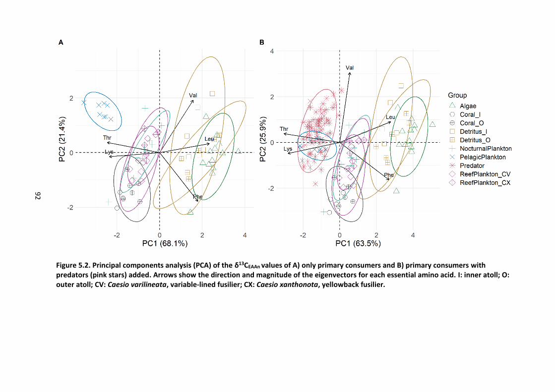
92

Figure 5.2. Principal components analysis (PCA) of the δ13CEAAn values of A) only primary consumers and B) primary consumers with predators (pink stars) added. Arrows show the direction and magnitude of the eigenvectors for each essential amino acid. I: inner atoll; O: outer atoll; CV: Caesio varilineata, variable-lined fusilier; CX: Caesio xanthonota, yellowback fusilier.

93

Based on the gap statistic and the k-medoids cluster analysis (Figure 5.3), the primary

consumers were split into four groups, representing: 1) algae/detritus, 2) coral, 3) reef

plankton, and 4) pelagic plankton. When running Bayesian isotope mixing models, sources

can be combined a posteriori based on biological knowledge (Phillips et al., 2005; Phillips et

al., 2014). Here, after the mixing models had run, the source groups representing coral and

algae/detritus were combined into one group named “Reef Benthic”.

Figure 5.3. K-medoids cluster analysis of primary consumer species sampled to represent

food sources. Clustering was based on the normalised δ13C values of essential amino acids

Leu, Lys, Phe, Thr and Val. EAM: epilithic algal matrix. Species codes are in Table 5.1.

The mixing models indicated that all four groupers derived the majority (95-99%) of their

food from pelagic production sources in both inner and outer atoll (Figure 5.4). Median

pelagic source reliance was significantly greater in the outer atoll (98-99%) than in the inner

atoll (95-97%) (Permutation test of independence, 9999 resamples, Z = -2.38, p =0.028).

Patterns in pelagic reliance were consistent between atoll areas among the groupers. Of all

four groupers, Aethaloperca rogaa consistently had the highest median pelagic reliance,

followed by Cephalopholis miniata, Anyperodon leucogrammicus and C. argus. Median

reliance on benthic reef and reef plankton sources was higher in the inner atoll (1.5-3% and

1-1.6% respectively) than in the outer atoll (0.4-1% and 0.3-0.6% respectively). Credible

intervals were consistently larger for groupers in the inner atoll than in the outer atoll.

94

Figure 5.4. Food source contributions for four grouper species in inner and outer atoll, as

determined by Bayesian isotope mixing models. Black bars represent 95% credible

intervals (2.5–97.5%), coloured bars represent interquartile ranges (25-75%) and black dots

represent the median (50%). Green = pelagic plankton, orange = reef benthic, purple = reef

plankton.

5.4 Discussion

Primary consumer δ13C values of essential amino acids showed good discrimination among

clusters broadly representing benthic algae/detritus, coral, reef plankton (diurnal and

nocturnal) and pelagic plankton. The proximity of benthic algae and detritus to each other is

not surprising. Although the powderblue surgeonfish, Acanthurus leucrosternon, is classified

as a herbivore (Robertson et al., 1979) and the lined bristletooth, Ctenochaetus striatus, is

classified as a detritivore (McMahon et al., 2016), it is likely that they are not strictly feeding

on a single homogenous production source. Furthermore, much of the detrital material they

are feeding on may have been of algal origin; the epilithic algal matrix (Wilson et al., 2003).

Diurnal and nocturnal reef plankton and coral were also isotopically similar to each other,

perhaps indicative of coral heterotrophy, with the fusiliers (Caesio varilineata and C.

xanthonota), soldierfish (Myripristis vittata) and corals feeding on localised reef-based

95

plankton that are supported by the same phytoplankton sources (Hamner et al., 1988;

Hobson, 1991; Alldredge and King, 2009). A novel finding here is that the δ13CEAA values of

the reef plankton and the pelagic plankton primary consumers were distinct from one

another. Mackerel scad, Decapterus macarellus, and Indian Ocean squid, Uroteuthis

duvauceli, are found in deeper oceanic waters and U. duvauceli come to the surface to feed

at night (Smith-Vaniz, 1986; Islam et al., 2018). Their δ13CEAA values may be a proxy for a

pelagic, deep-water vertically migrating plankton community (Hays, 2003) that is distinct

from the localised reef plankton community comprised predominantly of copepods

(Alldredge and King, 2009).

Pelagic plankton, rather than reef plankton, primarily sustained all groupers. This linkage

likely arises through a range of mechanisms. Oceanic atolls, like those in the Maldives, have

an enhanced biomass of mesopelagic prey such as lanternfish and euphausiids (Bradbury et

al., 1970; Letessier et al., 2016) which migrate to the surface waters to feed at night. In

addition, surface slicks (convergence of surface waters forming above internal waves)

accumulate pelagic marine organisms close to shore; in slicks half (50.1%) the larval fish are

pelagic compared to 26.4% in ambient waters, and densities of deep-water mesopelagic

larval fish are 2.7-fold higher in slicks compared to ambient waters (Gove et al., 2019).

Furthermore, particularly in the Indian Ocean, small benthic reef fish larvae are a key

component of the ichthyoplankton and connect the reef-pelagic interface. Juveniles and

adults provide 60% of consumed biomass on reefs, a contribution until now overlooked

(Brandl et al., 2019). The combination of enhanced mesopelagic prey and consistently

available cryptobenthic fauna suggests these reefs may be a sink of pelagic energy (Letessier

et al., 2016; Brandl et al., 2019). Conversely, on the Great Barrier Reef, open ocean water-

column pathways supported only 57% of reef fish productivity on forereef slopes, however

this contribution was expected to be higher on oceanic reefs (Morais and Bellwood, 2019).

Currently, little information exists on δ13CEAA incorporation rates or the timeframe that they

may represent, however I hypothesise that the predominantly pelagic δ13CEAA values of the

groupers is indicative of an atoll-wide food web fuelled by pelagic subsidies.

Even inside the atoll lagoons, groupers were almost exclusively reliant on pelagic production

sources. Extensive mixing of oceanic waters renders lagoonal conditions in the Maldives

reefs akin to the open ocean (Rogers et al., 2017), contributing to the consistently high

pelagic reliance across the atoll. These findings correlate with the bulk isotope data (Chapter

96

4, Skinner et al., 2019) and previous research that found no difference in coral host and POM

δ13C and δ15N between inner and outer reefs in the Maldives (Radice et al., 2019), providing

further evidence of a well-mixed system where oceanic nutrients are available throughout.

In contrast, several studies have found an increasing reliance of consumers on oceanic

nutrients with proximity to the open ocean (Wyatt et al., 2012b; Gajdzik et al., 2016). In the

Red Sea, foraging by the snapper Lutjanus ehrenbergii was more benthic on shelf reefs and

more planktonic on oceanic reefs (as identified by δ13CEAA values), but it was unclear

whether this difference arose from a reliance on different food items in each location or

from differing levels of planktonic inputs to the same food webs (McMahon et al., 2016).

Similarly, here, while oceanic nutrients are clearly available throughout, it is uncertain

whether the groupers are consistently selecting pelagic-derived prey or all the food webs

across the atoll are supported by pelagic inputs. Gut contents data or feeding observations

in this locale may provide important additional information which could help tease apart

these two hypotheses.

Grouper δ13CEAAn suggest all four species derive their carbon from the same pathways

regardless of size. Previous research indicates δ13CEAA values remain consistent across taxa

(McMahon et al., 2016) and differing growth rates (Larsen et al., 2015), although the latter

study investigated this for the marine diatom, Thalassiosira weissflogii, only so how this

varies among upper level consumers is unknown. While growth rate is partly dependent on

food availability, pelagic reef fish have higher growth rates as they exploit adjacent pelagic

prey (Morais and Bellwood, 2018). A. rogaa, which had the greatest pelagic reliance, also has

the highest reported growth rate, while C. argus, which had the lowest pelagic reliance, also

has the lowest reported growth rate (Mapleston et al., 2009). Future work would benefit

from including a greater number of predator samples across all sizes to investigate size

effects on δ13CEAA with greater statistical power. However, due to time constraints associated

with the derivatisation process and the high cost of processing samples for compound-

specific stable isotope analysis this was beyond the scope of this study. Although the number

of studies utilising δ13C of amino acids is increasing, the incorporation rates of AA from diet

to consumer are scarcely known; there is substantial variation among amino acids (Bradley

et al., 2014; Downs et al., 2014; Whiteman et al., 2018) and how this varies among taxa is

uncertain (Whiteman et al., 2019). Consequently, the dietary timeframe represented by

these values is unclear.

97

This is the first study to characterise multiple planktonic sources for reefs using δ13CEAA

values. Previous research on reefs in the Red Sea used calanoid copepods to represent

pelagic plankton signatures (McMahon et al., 2016). The Red Sea is a relatively enclosed,

oligotrophic body of water, with limited exchanges with the adjacent Indian Ocean (Racault

et al., 2015), but planktonic primary production and N2 fixation differ between open water

and nearshore reef settings (Tilstra et al., 2018). Furthermore, POM increases to the South

with increased proximity to nutrient-rich Indian Ocean water (Kürten et al., 2016).

Consequently, the pelagic plankton signature derived from reef-based calanoid copepods

(McMahon et al., 2016) may have been similar to that of the nearshore reef plankton of this

study. Additional sampling of plankton from the open water and further South nearer to the

Indian Ocean may have resulted in a distinct and separate pelagic plankton isotopic

signature such as that found here.

As with all emerging technologies, there is still much that is unknown about δ13CEAA data.

Firstly, fractionation of EAA stable isotopes between diet and consumer is thought to be

minimal (McMahon et al., 2010), but this may not be the case. Increasing evidence suggests

that EAAs may not be directly routed from dietary material but instead are assimilated from

symbiotic gut microbes (Newsome et al., 2011). Alternatively, EAAs may undergo extensive

catabolism when absorbed by cells lining the gut (Metges, 2000). Both of these phenomena

would lead to non-zero fractionation factors but are as yet relatively unexplored (Whiteman

et al., 2019). Here, despite using a small fractionation factor for the mixing models, a larger

standard deviation value was used to provide additional model parameter space (0.1 ± 1.0

%) in the absence of accurate fractionation factors. However, if the δ13CEAA fractionation

values are similar to that for non-essential amino acids (-0.5 – 2.4‰) (McMahon et al.,

2015b), the mixing model may have been too constrained to find an appropriate solution.

Consequently, this may expound the rigidity and lack of variation in the food source

contribution estimates presented here. As compound-specific stable isotope analysis

becomes a more popular tool to investigate trophodynamics, a greater understanding of the

mechanisms through which EAAs are integrated by consumers will be required, and is the

recommended next step for future work.

Secondly, all the primary consumer samples (with the exception of the pelagic U. duvauceli

and D. macarellus) were derivatised and analysed separately to the pelagic primary

consumers and the groupers. The strong pelagic reliance of the groupers may be influenced

98

by differences in δ13CEAA values between studies arising from: 1) derivatising with different

batches of reagents, and 2) the calibration settings of the GC/IRMS at different times (Zhang

et al., 2012), causing the groupers to be closest isotopically to the pelagic primary consumers

run at the same time as them. However, by using consistent laboratory standards and

normalising the δ13CEAA data to the mean, values should be comparable between studies

(Larsen et al., 2013; Larsen et al., 2015; McMahon et al., 2015a; Liew et al., 2019), especially

when samples were collected in the field at the same time and run on the same GC/IRMS. As

such, it is unlikely that the strong pelagic signature arises solely from differences in δ13CEAA

values, but future research should focus on how varying lab or GC/IRMS conditions may

influence δ13CEAA values and their ecological interpretation. In addition, several grouper

samples were collected at a different time to the others. However, not only were they

caught during the same monsoonal season in the same location and no significant

differences in values were identified, but δ13CEAA values are thought to be robust to seasonal

fluctuations (Larsen et al., 2015) and δ13CEAAn values show even less variability (McMahon et

al., 2015a).

Finally, while fusiliers are classic reef planktivores, due to their highly mobile nature (Russ et

al., 2017), they may not have been the most appropriate proxy for localised reef plankton in

this context. Moreover, as groupers are typically more reef-associated it is uncertain to what

degree they would predate on them, perhaps explaining the lack of reliance on reef plankton

sources. Sampling of other more site-attached planktivores such as balistids (Odonus niger),

pomacentrids (Chromis spp) and serranids (Pseudanthias spp), which are all frequently found

in grouper stomach contents (Shpigel and Fishelson, 1989; St John, 1999; Dierking et al.,

2011; Meyer and Dierking, 2011), is the recommended next step for this work.

While coral reefs worldwide are experiencing unprecedented losses of live coral cover

(Hughes et al., 2017b), fish productivity on those that rely on pelagic subsidies may be more

resilient to coral bleaching than previously thought (Morais and Bellwood, 2019). Groupers

are a fundamental component of the Maldivian reef fishery (Sattar et al., 2014) and their

exceptionally high pelagic reliance found here suggests that fishery predictions based solely

on reef-associated habitat loss may be misleading (Robinson et al., 2019b).

99

Chapter 6 Disentangling the drivers of coral reef food webs

6.1 Introduction

Understanding food web dynamics and the drivers of community structure is a central goal

in ecology. But food webs are complex, with vast numbers of species connected via multiple

linkages, so disentangling the trophic interactions driving community composition can be

complicated (Polis and Strong, 1996). In marine systems, predator-prey interactions are well

studied (Hobson, 1979; Baum and Worm, 2009; Allain et al., 2012) but the key drivers of

predator distributions and how prey assemblages influence predators is often unclear.

Predator survival is reliant on access to food so investigating predator-prey species

distributions across spatial scales may offer insight into the biotic and abiotic factors that

drive predator community structure (Beukers-Stewart et al., 2011; Sandom et al., 2013).

Identifying the drivers of community structure is important to determine how communities

may respond to changing environments, and a better understanding of predator-prey

relationships may facilitate this. Furthermore, knowledge of carbon pathways and energetic

linkages is fundamental in assessing food web function and resilience.

On coral reefs, site-attached piscivorous reef predators (lutjanids, serranids) play an

important role in structuring prey communities (Boaden and Kingsford, 2015) and

contributing to ecosystem integrity and resilience by maintaining biodiversity (McCann et al.,

2005; Rooney et al., 2006; Ceccarelli and Ayling, 2010). The bulk and compound-specific

stable isotope data presented in Chapters 4 and 5 indicated that the sampled reef predators

were all primarily sustained by planktonic production sources. This ecological linkage is likely

generated through feeding on planktivores (Matley et al., 2018; Skinner et al., 2019), a

dominant component of the Maldivian reef fish biomass (Moritz et al., 2017), and there was

little contribution from other prey fish groups. This suggests that there may be a relationship

between predator and planktivore abundance, with biomass of one influenced by the other.

However, findings from previous research investigating the relationships between reef

predators and their prey are unclear. Strong positive relationships were identified between

abundances of reef predators and their prey on the Great Barrier Reef (Stewart and Jones,

2001; Beukers-Stewart et al., 2011) and prey biomass was considered an important driver of

reef-associated shark abundances in the Chagos archipelago (Tickler et al., 2017). In

100

contrast, a longer-term study in the US Virgin Islands identified a negative correlation

between predator abundance and the maximum number of co-occurring prey, and no

overall relationship between predator and prey abundances (Hixon and Beets, 1993). This

latter case may be the result of wrongly assuming “prey” of the predators in some instances.

In addition to predator and prey densities, environmental variables such as depth and

structural complexity are also important in explaining relationships between these groups.

Structural habitat complexity provides refuge for prey from predation, with higher levels of

complexity detrimental to predator growth rates, potentially altering food web dynamics

(Graham and Nash, 2013; Rogers et al., 2018). Furthermore, species compositions of both

predator and prey fish communities change with depth (Jankowski et al., 2015; Asher et al.,

2017). However, due to the indirect nature of these variables, relationships are challenging

to interpret and often overlooked using traditional predator prey models. Consequently,

how all these variables interact and which are most important in driving predator biomass is

unknown.

Studies investigating community structure often rely on modelling techniques (e.g. general

linear models) that examine the impact of a few variables on a single biological endpoint

response, such as abundance, diversity or biomass (Lefcheck and Freckleton, 2016; Bruder et

al., 2019). These approaches do not account for the fact that ecosystems are networks

comprised of multiple interlinked multitrophic biotic interactions, further influenced by a

range of environmental factors (Seibold et al., 2018; Bruder et al., 2019). As such, fully

understanding the relationships between predators, their prey, and the surrounding habitat

can prove complicated. Structural equation models (SEMs) can incorporate multiple

interrelated predictor and response variables (Lefcheck and Freckleton, 2016), making them

a useful method for understanding complex systems with both direct and indirect linkages

(Shipley, 2002; Grace, 2006; Grace et al., 2010). Hypothetical pathways between variables

are identified a priori and are expressed in equation form, with response variables driven by

one or multiple predictor variables. These response variables then become predictors for

other variables, forming a sequence of causal relationships (Fan et al., 2016; Lefcheck and

Freckleton, 2016). Hence, in complex systems such as coral reefs, SEMs can more accurately

estimate the importance of multiple interlinked biotic and abiotic factors in structuring reef

predator biomass than other multivariate or linear modelling techniques.

101

The data generated in this thesis offer the unique chance to test whether fish community

structure is primarily driven by 1) habitat structural complexity or 2) food (prey) availability.

Using SEMs, I examine which biotic or abiotic variables are most important in driving site-

attached piscivorous reef predator biomass and whether the carbon pathways identified

with stable isotopes in previous chapters are evident. I hypothesise that structural

complexity will be the most important driver of all prey groups as it provides refuge from

predation (Graham and Nash, 2013) and planktivore biomass will be the key driver of

predator biomass demonstrated by the stable isotope data in Chapters 4 and 5.


6.2.1 Site selection

All fieldwork was conducted in North Malé Atoll, Maldives (N 04° 25’ 46.2”, E 73° 30’ 4.3”).

Surveys were split between two areas: the inner lagoonal reefs (hereafter “Inner”), and the

outer edge reefs (hereafter “Outer”).

6.2.2 Underwater Visual Census (UVC)

UVC was conducted at a total of 40 sites, 20 in each atoll area between March to April 2018

(Figure 6.1). At each site, two 30 x 5 m transects were randomly surveyed parallel to the

forereef slope between depths of 3 – 15 m. All transects were a minimum of 10 m apart to

reduce overlap. The entire fish community of all sizes was recorded to genus or species level

depending on their diet and body morphometries (Table A12 and A13: full species list and

classifications). When members of the same genus all consumed the same diet and had a

similar body shape they were only recorded to genus, however when diet or body shape

differed within the genus, fish were recorded to species level. Blennies were split into two

groups depending on whether they were sabretooth blennies or not, and gobies were

separated into either reef gobies or sand gobies (Kuiter, 2014). All UVC surveys were

conducted by the same two observers who were fully trained in fish identification and size

estimations. The fish community was split into larger, more mobile species (Acanthuridae,

Lutjanidae, Lethrinidae) and smaller, cryptic site-attached species (Blenniidae, Gobiidae,

Pomacanthidae). The first observer swam while reeling out the transect and recording all the

mobile fish that would be disturbed, while the second observer swept one side of the

transect first and then the second side, searching all the holes and refuges for hidden fish.

102

Along the transect, the benthic substrate type was recorded every 50 cm. Complexity was

measured by draping a fine-link chain along a 10 m section of the transect tape from 10 – 20

m. The place the chain reached on the transect tape was then recorded. Complexity was

calculated using equation 1, where a number closer to 1 signified a flat, low relief reef while

a number closer to 0 indicated a reef of high complexity.

Eqn 1) 𝑅𝑒𝑒𝑓 𝑐𝑜𝑚𝑝𝑙𝑒𝑥𝑖𝑡𝑦 =𝑐ℎ𝑎𝑖𝑛 𝑚𝑒𝑎𝑠𝑢𝑟𝑒𝑚𝑒𝑛𝑡

10 𝑥 100

Figure 6.1. Sites (40) on North Malé Atoll where underwater visual census (UVC) was

conducted.

6.2.3 Data analysis

Data were analysed in R statistical software version 3.5.2 (R Core Team, 2017). Fish biomass

was calculated using published length-weight relationship data on Fishbase (Froese and

Pauly, 2018). When only the genus was recorded, the length-weight data for the most

common species (C Skinner, unpublished data) on the reefs was used. Fish were categorised

into six functional feeding groups based on the literature and FishBase: predator, benthic

carnivore, corallivore, EAMvore (epilithic algal matrix-vores), omnivore or planktivore (Table

103

A12 and A13). All prey fish > 20 cm were removed from further analysis as it was assumed

they were too large to be fed on by the predators (St John, 1999; Dunic and Baum, 2017). As

the focus of the stable isotope work in previous chapters has been on fishery target, reef-

associated predators, all transient (Elagatis bipinnulata and Gymnosarda unicolor) and non-

target predator species (Aulostomus chinensis, Fistularia commersonii, Gnathodentex

aureolineatus, Monotaxis grandoculis, Pterois antennata and P. volitans) were removed

from further analysis.

Structural Equation Modelling (SEM) and path analysis were used to explore the

relationships between the predators, their prey and their environment. SEM uses a variance-

covariance matrix to test the relationship between pathways. Models are fit using

maximum-likelihood estimation, which continually refines parameter value estimates to

minimise differences between the observed and expected variance-covariance matrices

(Lefcheck and Freckleton, 2016). A full conceptual model was developed to explore which

biotic and abiotic variables influence reef predator biomass (Figure 6.2). Depth and atoll area

were considered predictors of the benthic habitat. Benthic habitat and underlying geology

determines structural complexity but atoll location (e.g. inner or outer atoll) may also have

an influence. Benthic habitat and structural complexity were considered to be variables that

structure biomass of all prey fish groups. Finally, biomass of all prey fish groups and

structural complexity were considered predictors of predator biomass.

At each site, benthic cover, prey and predator biomass data were averaged across both

transects. Benthic habitat and fish biomass data were first explored separately to visualise

patterns in the community structure. Principal Component Analysis (PCA) was used to

capture and simplify the complex nature of the multivariate benthic community data using

the FactoMineR package (Le et al., 2008) and the FactoExtra package (Kassambara and

Mundt, 2017). PCA generates a two dimensional ordination which helps to visualise patterns

and reduce dimensionality when using many quantitative variables. The multivariate

homogeneity of group dispersions was subsequently calculated for each atoll area group on

a Euclidean distance matrix of the data to determine the mean distance-to-centroid of the

sites using the vegan package (Oksanen et al., 2018). The scores for the first two PC

orthogonal axes for each site were subsequently extracted and used as explanatory variables

for the benthic habitat in the SEM. The mean structural complexity and biomass of each fish

functional group at each site were plotted onto the extracted PC1 and PC2 coordinates of

104

the benthic variables to further visualise relationships in fish and benthic community

structure.

Figure 6.2. Conceptual pathway model of the biotic and abiotic variables influencing reef

predator biomass.

Before testing the SEM model, pairwise plots were used to inspect outliers and to assess

collinearity between variables. All variables were checked for normality using a Shapiro-

Wilks test and fish biomass data and depth were log-transformed. Some variables remained

non-normal after transformation. To account for this, a bootstrapping approach based on

1000 draws was used to estimate the model test-statistics and the standard errors for the

SEM parameter estimates (Rosseel, 2012). Using the lavaan package (Rosseel, 2012), the

conceptual full model was fit with all predicted pathways. Following this, non-significant

pathways were removed until the most parsimonious model was achieved. Standardised

coefficients were used to assess the importance of predictor variable paths as they can be

used to compare variables measured on different scales (Kwan and Chan, 2011). Model fit

was assessed by looking at the root mean square error of approximation (RMSEA), the

comparative fit index (CFI), the Bayes Information Criterion (BIC) and the standard errors of

the parameter estimates. Models with an RMSEA < 0.08 (Browne and Cudeck, 1992) and a

CFI > 0.95 (Hu and Bentler, 1998) are considered a reasonable fit for SEM models, i.e. the

105

model is able to reproduce the variance-covariance matrix of the data. The most

parsimonious model was the model with the greatest number of significant pathways, the

lowest RMSEA and BIC, and the highest CFI.

6.3 Results

6.3.1 Benthic and fish community data

In total, fish from 31 families were identified to either family level (Apogonidae, Mullidae,

Synodontidae), genus (33 genera) or species (90 species) and classified based on their

feeding behaviours (Table A12).

A PCA revealed substantial separation in the benthic variables between areas along PC axis 1

explaining 29.7% of the variation in the data (Figure 6.3). Sites in the outer atoll were more

clustered than those in the inner atoll; average distance to median was 21.23 for inner atoll

sites and 14.48 for outer atoll sites. The variables driving the outer atoll sites were live coral,

crustose coralline algae (CCA) and algae (i.e. turf and macroalgae), while the variables

contributing most to the inner atoll sites were sand, rock and rubble. The PCA separated

sites by whether they had more biotic or abiotic substrate along the first axis and by

whether they had more coral or algal cover along the second axis.

Figure 6.3. Principal components analysis (PCA) of the benthic community with

eigenvectors overlaid showing the benthic categories contributing to the PC1 and PC2

axes, which explain 46.7% of the variation in the data.

106

Structural complexity was similar between inner (mean ± s.d. = 0.66 ± 0.08) and outer atoll

sites (mean ± s.d. = 0.70 ± 0.05) with plots on the PC1 and PC2 coordinates revealing no clear

patterns (Figure 6.4). Plots of the fish biomass on the PC1 and PC2 coordinates indicated that

the distribution of predator biomass (Figure 6.5a) across all sites was similar to that of the

corallivores (Figure 6.5b) and planktivores (Figure 6.5f), all of which had greater biomass in

the outer atoll.

Figure 6.4. Mean site-level structural complexity plotted on the PC1 and PC2 coordinates

for each site. A number closer to 1 signifies a flat, low relief reef while a number closer to 0

indicates a reef of high complexity. Points are scaled to values, with larger points

indicating values closer to 1 (low relief) while smaller points indicate values closer to 0

(high relief). Circles = inner atoll, triangle = outer atoll.

6.3.2 SEM model

Full model

The mean RMSEA for the full (null) model was 0.138 and the CFI was 0.71, both of which

indicate a poor fit (Figure 6.6). The chi square was significant (χ2 = 45.76, d.f. = 26, p = 0.01)

suggesting that the predictive model did differ from the observed data. The BIC was 692.70.

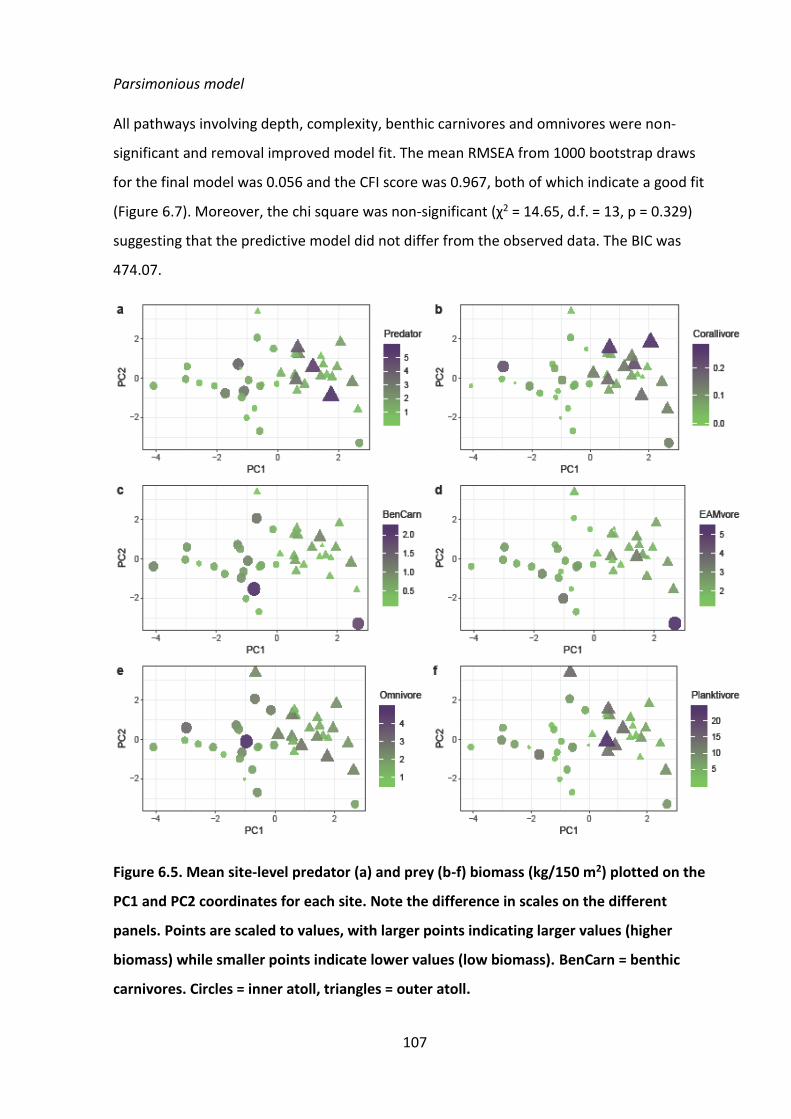
107

Parsimonious model

All pathways involving depth, complexity, benthic carnivores and omnivores were non-

significant and removal improved model fit. The mean RMSEA from 1000 bootstrap draws

for the final model was 0.056 and the CFI score was 0.967, both of which indicate a good fit

(Figure 6.7). Moreover, the chi square was non-significant (χ2 = 14.65, d.f. = 13, p = 0.329)

suggesting that the predictive model did not differ from the observed data. The BIC was

474.07.

Figure 6.5. Mean site-level predator (a) and prey (b-f) biomass (kg/150 m2) plotted on the

PC1 and PC2 coordinates for each site. Note the difference in scales on the different

panels. Points are scaled to values, with larger points indicating larger values (higher

biomass) while smaller points indicate lower values (low biomass). BenCarn = benthic

carnivores. Circles = inner atoll, triangles = outer atoll.

108

6.3.3 Pathways

Full model

In the full (null) model (Figure 6.6), only three pathways were significant (Table 6.1): atoll

area significantly influenced both PC1 and complexity and PC2 significantly influenced the

EAMvores (Table 6.1).

Parsimonious model

Not all pathways retained in the most parsimonious model (Figure 6.7) were significant

(Table 6.2), but they all improved model fit (Figure A7). Area significantly predicted PC1 and

PC2. PC1 significantly influenced corallivore biomass and PC2 significantly influenced

EAMvore biomass. Predator biomass was driven by corallivore and planktivore biomass, but

the latter relationship was not significant. Predator and EAMvore biomass covaried. The

pathways between area and PC2, PC1 and corallivore, and predator and corallivore, were

not significant in the full model but became so in the parsimonious model after other

pathways had been removed.

Table 6.1. Parameter estimates for the SEM involving analysis of all pathways in the full

(null) model. Significant pathways (p < 0.05) are in bold.

From To Estimate SE Z-value P-value

PC1 ~ Depth -0.041 0.336 -0.503 0.615

PC1 ~ Area 0.758 0.387 6.389 0.000 PC2 ~ Depth 0.015 0.582 0.082 0.935 PC2 ~ Area 0.350 0.476 1.820 0.069

Complexity ~ PC1 -0.347 0.010 -1.441 0.149

Complexity ~ PC2 -0.274 0.012 -1.239 0.215

Complexity ~ Area 0.584 0.026 3.042 0.002

Corallivore ~ PC1 0.360 0.175 1.943 0.052 Corallivore ~ PC2 0.135 0.150 1.126 0.260 Corallivore ~ Complexity -0.131 4.968 -0.611 0.541 Planktivore ~ PC1 0.142 0.089 0.954 0.340 Planktivore ~ PC2 0.183 0.109 1.325 0.185 Planktivore ~ Complexity -0.099 2.338 -0.615 0.538 BenthicCarnivore ~ PC1 -0.229 0.057 -1.389 0.165

BenthicCarnivore ~ PC2 -0.199 0.095 -0.955 0.340 BenthicCarnivore ~ Complexity -0.134 1.520 -0.748 0.454 EAMvore ~ PC1 0.117 0.026 0.734 0.463 EAMvore ~ PC2 -0.438 0.045 -2.082 0.037 EAMvore ~ Complexity 0.114 0.602 0.756 0.449

109

Omnivore ~ PC1 0.094 0.036 0.624 0.533 Omnivore ~ PC2 0.207 0.043 1.483 0.138 Omnivore ~ Complexity -0.219 1.204 -1.048 0.294 Predator ~ BenthicCarnivore 0.092 0.219 0.516 0.606 Predator ~ EAMvore -0.117 0.428 -0.714 0.475 Predator ~ Omnivore -0.035 0.365 -0.175 0.861 Predator ~ Corallivore 0.258 0.079 1.468 0.142 Predator ~ Planktivore 0.124 0.151 0.588 0.557 Predator ~ Complexity -0.108 2.372 -0.477 0.633

Figure 6.6. The full (null) model of path analysis results exploring the abiotic and biotic

drivers of reef predator biomass. Single arrows indicate causal paths. Thick arrows indicate

significant relationships and thin arrows denote a non-significant relationship. Model fit

was assessed using the root mean square error of approximation (RMSEA), the

comparative fit index (CFI) and the Bayes Information Criterion (BIC). Models are

considered a good fit when RMSEA < 0.08 and CFI > 0.95.

110

Table 6.2. Parameter estimates for the structural equation model involving analysis of all

pathways in the parsimonious model. Significant pathways (p < 0.05) are in bold.

From To Estimate SE Z-value P-value

PC1 ~ Area 0.730 0.359 6.647 0.000 PC2 ~ Area 0.360 0.367 2.431 0.015 Corallivore ~ PC1 0.356 0.163 2.030 0.042 EAMvore PC2 -0.466 0.044 -2.321 0.020 Predator ~ Corallivore 0.291 0.056 2.408 0.016 Predator ~ Planktivore 0.139 0.132 0.767 0.443 Covariances

Predator ~~ EAMvore -0.224 0.026 -1.400 0.162

6.4 Discussion

The final parsimonious SEM provides a unique insight into the structuring of the atoll coral

reef food web. This approach has allowed the complex and indirect linkages driving predator

biomass to be further explored, pathways which traditional linear modelling techniques

might overlook. The parsimonious model revealed significant linkages between predators,

prey and the habitat, with carbon pathways seemingly flowing up the food web from

primary producers to the predators via their prey. This highlights the extent of connectivity

in these systems, with indirect associations likely equally important drivers of predator

community structure.

Atoll location (inner/outer) was a significant driver of the benthic cover (PC1 and PC2); inner

and outer atoll sites were almost entirely distinct from one another indicating substantial

spatial variation. This is consistent with other studies that have recorded differences in reef

habitat between lagoons and outer edge reefs (Brown et al., 2018), particularly in the

Maldives (Morri et al., 2015; Pisapia et al., 2016). While sites in the inner atoll were

characterised by sand, rock and rubble due to the greater availability of soft bottom habitat,

outer atoll sites had a higher percentage of live coral cover (inner = 15.61% ± 10.43; outer =

28.24% ± 6.31). This difference in live coral cover between inner and outer atoll sites may be

related to their degree of exposure. Being adjacent to the open ocean, the outer atoll sites

are subject to strong oceanic currents that could help alleviate temperature stress, reducing

the level of bleaching-induced coral morality (Safaie et al., 2018; Pisapia et al., 2019).

111

Figure 6.7. The parsimonious model of path analysis results exploring the abiotic and biotic

drivers of reef predator biomass. Single arrows indicate causal paths with standardised

path coefficients. Thick arrows indicate significant relationships with stars showing the

significance level (* = p < 0.05, *** = P < 0.001). Thin arrows indicate a non-significant

relationship and dotted arrows signify covariance. Model fit was assessed using the root

mean square error of approximation (RMSEA), the comparative fit index (CFI) and the

Bayes Information Criterion (BIC). Models are considered a good fit when RMSEA < 0.08,

CFI > 0.95.

Several of the prey groups were significantly linked to the benthic habitat. Positive

relationships have been recorded between fish functional groups and the abundance of their

preferred food type (Floeter et al., 2007), suggesting food availability is a key driver of their

populations. Live coral cover (represented by PC1), rather than complexity or depth, was a

significant positive driver of corallivore biomass. Numerous studies have identified positive

relationships between corallivores and live coral cover (Bell and Galzin, 1984; Bouchon-

Navaro and Bouchon, 1989; Jennings et al., 1996; Darling et al., 2017), with substantial

declines recorded following mass coral bleaching events (Wilson et al., 2006; Robinson et al.,

2019a), even when reef structural complexity is maintained (Benkwitt et al., 2019). This

112

suggests that food availability may be more important for maintaining corallivore

populations than habitat structure. Recently the Maldives has experienced significant

declines in live coral cover due to mass bleaching (Pisapia et al., 2019). Given the

relationship identified here and in previous studies, and the obligate nature of their feeding,

corallivores may be seriously impacted following the loss of live coral from successive

bleaching events. Algal cover (represented by PC2) was a significant positive driver of

EAMvore biomass. Although turf and macroalgae were combined into one group for the

analyses, macroalgae cover was low across the atoll (inner: 4.02% ± 5.57; outer = 2.01% ±

3.07) so this relationship was likely driven by turf algae cover (inner: 21.72% ± 11.85; outer =

33.20% ± 10.20). Positive relationships between herbivores and turf algae are common, as

fish tend to aggregate in zones of highest food availability (Williams and Polunin, 2001; Russ,

2003). However, at higher levels of wave exposure, while algal turf increases, herbivore

biomass decreases (Williams et al., 2013; Heenan et al., 2016), signifying that there is a wave

exposure threshold beyond which this positive relationship is decoupled.

No significant relationships were identified for the benthic carnivores, omnivores, or

planktivores. There are several possible explanations for this. Firstly, food source data were

absent for these prey groups. Benthic carnivores and omnivores often feed on invertebrates,

while planktivores feed on plankton, but these food sources were not recorded during the

surveys. Furthermore, these prey items may not be strongly associated with the habitat

variables that were measured here. Consequently, trophic interactions arising between

these prey groups and their environment would have been overlooked. Secondly, these

groups are dietary generalists, which may preclude the model from identifying any strong

relationships. Future work would benefit from including measures of all potential food items

to accurately investigate all potential trophic interactions. Thirdly, although each species has

been classified based on their feeding behaviour as reported in the literature, increasing

evidence (e.g. isotope data in Chapter 3) suggests that there is substantial individual and

spatial variation within populations. Categorising feeding behaviours at the species level may

mask the individual dietary intricacies so common in nature. Finally, while previous studies

have identified live coral cover and structural complexity as important variables driving

planktivore communities (Darling et al., 2017; Russ et al., 2017), no significant relationships

were identified in the final model presented here. Many planktivore species are highly

mobile so population estimates during UVC are susceptible to substantial temporal variation

113

(McClanahan et al., 2007; MacNeil et al., 2008). Consequently, detection of significant

relationships may have occurred had the data been collected at a different time.

Corallivores were the only prey group to significantly influence predator biomass, despite

being the group with the lowest overall biomass and the smallest species richness.

Carangidae, Lutjanidae and Serranidae predate on a range of reef-associated fish species but

corallivores are not considered a major component of their diet (Meyer et al., 2001; Dierking

et al., 2011; Ali et al., 2016; Dance et al., 2018). However, as corallivores are driven by food

availability and are strongly associated with the habitat (Boaden and Kingsford, 2015), their

biomass may be a proxy for a healthier reef state characterised by a greater percentage of

live coral cover, which in turn supports a greater biomass of predators. In contrast,

reductions in live coral cover have been linked to both declines in corallivore (Rice et al.,

2019) and reef predator (Sandin et al., 2008) populations. Although the pathway between

planktivores and predators was not significant, its inclusion in the final model substantially

improved model fit. Numerous studies indicate that reef predators are sustained by

planktivores (Ali et al., 2016; Matley et al., 2018; Skinner et al., 2019) confirming that this

relationship is an important one. As discussed above, planktivore populations experience

substantial spatial and temporal variability (Kingsford, 1989; Malcolm et al., 2007) which

may have precluded a significant relationship from being identified with this dataset.

Depth and complexity were not included in the most parsimonious model. Unlike previous

studies (Graham and Nash, 2013; Rogers et al., 2014; Schultz et al., 2014; Jankowski et al.,

2015; Ferrari et al., 2017), they did not appear to be important variables structuring either

the predator or prey community. However, the gradients in complexity and depth recorded

here may not be comparable to the studies where they were identified as important. For

example, here, all transects were conducted on the upper forereef slope in a relatively

narrow depth range (3 – 15m), so depth-related changes in community biomass may have

been missed. Furthermore, mean complexity was similar between atoll locations (mean ±

s.d.: inner 0.66 ± 0.08; outer 0.70 ± 0.05) with a relatively narrow gradient (inner 0.52 – 0.89;

outer 0.60 – 0.79), possibly linked to a flattening of the reefs following the 2016 bleaching

event (Newman et al., 2015; Pisapia et al., 2019). While atoll area was a significant driver of

structural complexity in the full model, no complexity pathways were included in the

parsimonious model. It is possible that inherent variability in structural complexity and

depth between inner and outer atoll was represented by, and incorporated into, the atoll

114

area variable. Area was subsequently identified as an important driver of differences

between sites while any influence of depth or complexity was masked, precluding their

incorporation in the final model. Moreover, the complexity measure used here may not offer

any different information compared to the benthic PC axes. For example, measures of live

coral cover or rubble, here interpreted in terms of food availability, also intrinsically provide

habitat for refuge. Consequently, the relationship between the benthic habitat and the prey

community may also include an inherent refuge influence. Future work would benefit from

incorporating measures of refuge availability (e.g. hole size and abundance) into models,

while surveying transects across a greater range of depths and levels of complexity.

Reef food webs are complex with many interrelating trophic interactions. Although the

underwater visual surveys were extensive, not all energy pathways were investigated during

this study, most notably those involving invertebrates. Arriving at robust solutions with a

SEM requires a lot of data as the model is evaluating multiple hypotheses simultaneously

(Grace, 2006; Lefcheck and Freckleton, 2016). Although the final model was a good fit,

additional insight into the predator-prey-habitat relationships occurring on these reefs might

have been achieved with a larger dataset, or with the inclusion of additional parameters

such as invertebrate biomass, primary production or temperature. Despite this, the final

model gives a reasonable representation of the reef food web and a better understanding of

the interactions occurring between organisms. It does contrast with the stable isotope data

in Chapters 4 and 5 though, suggesting that the pathways that are important to the food

web may not necessarily structure it or the biomass of predators. Food availability, rather

than abiotic variables such as reef structural complexity or depth, appears to be the primary

driver of predator-prey relationships in this system. However, as benthic composition and

structural complexity are interrelated, the PCA may inherently include some habitat refuge

information, which warrants further study. The distinct spatial structuring of the benthic

cover also highlights the importance of incorporating spatial variation into analyses, as reefs

vary considerably at the local and global scale. Ultimately, although SEMs provide a unique

tool to gain insight into systems with many complex processes, capturing all predator-prey-

habitat relationships is impossible. However, the model presented here offers a novel

perspective on the importance of food availability in structuring reef communities, and

rather challenges the contention (Chapters 4 and 5) that planktonic feeding is driving

predator biomass.

115

Chapter 7 General discussion

7.1 Overview

This thesis provided a unique perspective on reef predator assemblages and their complex

trophodynamics, advancing our current knowledge of coral reef food webs. One of the

strengths of this thesis has been the use of multiple statistical and survey methodologies to

investigate these energetic linkages, which allowed greater insight into the complex

interactions on these reefs. The combination of both underwater visual census (UVC) and

baited remote underwater video (BRUV) identified the primary drivers of reef predator

community structure (aim one), while bulk and compound-specific stable isotope analysis

determined the origin of the carbon sustaining their biomass (aim three). Bulk stable isotope

data also identified inter- and intraspecific variations in predator resource use (aim two).

The implications of these findings are discussed below.

7.2 Reef-pelagic connectivity and coral reef resilience

One of the major findings of this thesis is that planktonic subsidies are a key contributor to

reef predator biomass (Chapter 4, Skinner et al., 2019), and that it is likely that these

subsidies are of a deep-water, mesopelagic origin (Chapter 5). While the importance of

planktonic inputs to reef communities is now being realised (McCauley et al., 2012c; Frisch

et al., 2014; Matley et al., 2018), the origin of this material has not been fully considered.

The data in this thesis offer the opportunity to revisit how we view coral reef communities.

Rather than being isolated ecosystems somehow teeming with life, it is evident that the

adjacent pelagic ocean exerts a substantial influence and mesopelagic subsidies may play a

vital role sustaining reef food webs. However, the characteristics, origins and delivery

mechanisms of these inputs remain to be explored. While the compound-specific stable

isotope analysis here offers new insight, it also raises questions. Specifically, where is this

material coming from and how is it being incorporated into the food chain? What drives it

and what does it contain? Can it be better characterised and traced? There are also

questions regarding the interpretation of the δ13C essential amino acid (EAA) data, as

mechanisms are not yet fully understood. For example, are EAAs routed directly to

consumer tissue from their diet or are there transformative interactions with the gut

microbiome? What is the integration rate and turnover time of EAA to consumer tissues?

How do animal activity levels and body size affect these mechanisms? Do these mechanisms

116

vary inter- and intraspecifically and among EAAs? These questions are at the forefront of the

emerging field of compound-specific stable isotope analysis and represent an exciting new

era in food web studies. Currently, answers to these questions are lacking. However, a first

step might involve sampling mesopelagic prey from around the atolls to determine their

δ13CEAA signature or attaining a better understanding of the flow dynamics and water

circulation (i.e. presence and frequency of internal waves) of the archipelago. Both these

areas of research would provide important information that could help characterise and

measure these allochthonous inputs.

This work was carried out in the central Maldives, where seasonally alternating equatorial

currents determine the degree of primary production available to reef communities

(Sasamal, 2007; Anderson et al., 2011). However, conducting the same work across the more

northern or southern parts of the Maldivian archipelago, or elsewhere in the Indian Ocean

or around the world, might have yielded different results. Spatial fluctuations in primary

production and differences in atoll physiography (e.g. being more enclosed or more open)

might both influence the degree of planktonic reliance of a reef food web. Several studies

have demonstrated increased reliance of reef communities on oceanic nutrients with

increasing proximity to the open ocean (i.e. from inner lagoons to outer shelf reefs) (Wyatt

et al., 2012b; Gajdzik et al., 2016; McMahon et al., 2016; Le Bourg et al., 2017). To date,

there has been little research on how planktonic reliance might vary globally across

gradients of primary production or in relation to the degree of water circulation. However,

stable isotope δ15N values of several coral reef fish species were closely linked to gradients in

oceanic primary production and species had larger dietary niche widths where primary

production was greater (Miller et al., 2019; Zgliczynski et al., 2019). This suggests that reef

trophodynamics do vary spatially and in relation to available primary production, and this

warrants further study.

The role of coprophagy (feeding on faeces) in connecting the reef-pelagic interface must also

be considered. While fish from all trophic levels excrete material regularly, diurnal

planktivores that dominate the water column (e.g. caesionids, damselfishes), produce

substantial amounts of low-density faeces. The majority of this material is ingested by other

fish, primarily herbivores and detritivores (Robertson, 1982), representing an important

energetic subsidy to the reef food web (Hobson, 1991). Furthermore, the faecal material

may be enriched in δ15N compared to various benthic algal groups, leading to the herbivores

117

and detritivores that readily consume it having higher δ15N values (Zgliczynski et al., 2019).

Here, bulk stable isotope δ15N values of the herbivore Acanthurus leucosternon and the

detritivore Pearsonothuria graeffei were consistently low (δ15N mean ± sd: 6.24 ± 0.16 to

8.30 ± 0.81; Table A7). Furthermore, δ13C values of essential amino acids of A. leucosternon

and the detritivore Ctenochaetus striatus showed relatively clear separation from the reef

planktivores Caesio varilineata and C. xanthanota (Figure 5.2), suggesting coprophagy may

not be a dominant component of the diet of these species. Regardless, given the huge

biomass of planktivores on Maldivian reefs (Figure 7.1) and the amount of material that they

excrete, coprophagy likely plays an important role providing energetic subsidies to reef food

webs here, and sampling other herbivore or detritivore species might evidence this.

Ocean-reef connectivity may have implications for coral reef resilience. Globally, coral reefs

are under threat from a range of anthropogenic and climate-related stressors. Successive

coral bleaching events have caused significant declines in live coral cover worldwide (Hughes

et al., 2017b; Pisapia et al., 2019), resulting in persistent shifts in coral (Hughes et al., 2018b)

and reef fish assemblages (Robinson et al., 2019a). The vulnerability and the resilience (the

capacity to recover from a disturbance) of individual reefs to these threats is not uniform

however, as the natural carrying capacity of coral reefs varies across environmental

gradients (Heenan et al., 2019). Consequently, coral reef food webs supported by planktonic

production sources may be more resilient to bleaching-induced coral mortality than reefs

that are more reliant on benthic production sources. However, climate change is also

predicted to cause declines in ocean production (e.g. from increased stratification, light

limitation) (Asch et al., 2018), which would have serious ramifications for reefs that are

primarily supported by oceanic inputs. Furthermore, results of a DISTLM (Chapter 2) and a

SEM (Chapter 6) indicated that live coral cover and corallivores respectively were important

significant drivers of the predator assemblage, suggesting that loss of live coral cover might

influence reef predators despite the lack of a direct association (i.e. stable isotope evidence).

Interactions with, and the influence of, reef structural complexity should be considered

when determining what structures the predator assemblage. While structural complexity

was not included in the final SEM (Chapter 6), it is likely that it did exert some influence

given that benthic cover and structural complexity are interrelated. Multiple studies have

highlighted its importance in structuring reef fish assemblages by providing refuge and

supporting fish productivity (Chapter 2, Graham and Nash, 2013; Rogers et al., 2014;

118

Newman et al., 2015; Rogers et al., 2018). It also facilitates pelagic coupling by mediating the

ability of planktivores to trap plankton on reefs (Morais and Bellwood, 2019). As such,

structural complexity is an intrinsic component of reefs and continued reef flattening will

surely affect reef food webs worldwide (Graham et al., 2006; Newman et al., 2015),

regardless of whether they are sustained by benthic or pelagic inputs.

Predicting how these fish communities will respond to environmental change remains a

challenge, however, this thesis highlights how current views of coral reef systems need to

change. The extent of connectivity with the open ocean, regardless of exposure or level of

degradation (Morais and Bellwood, 2019), shows how coral reef management plans must

transcend ecosystem boundaries. Localised management efforts involving the setup of MPAs

may not be sufficient for reef communities reliant on oceanic production. Future work

should investigate the complex interactions between live coral cover, structural complexity,

primary production and water circulation, to better understand how coral reefs worldwide

may respond to changing environmental conditions.

7.3 Nature is complicated

Investigating an animal’s resource use and foraging patterns can help determine its

functional role within an ecosystem. This is important in identifying how it might respond to

change, which facilitates appropriate management. The bulk stable isotope data (Chapter 3)

highlighted how predator resource use can vary both spatially and among and within

species, regardless of body size. Predators may couple adjacent food webs through their

foraging, constructing linkages which provide stability to ecosystems (McCann et al., 2005),

but variations in their resource use indicate these linkages are not identical, and in some

cases may be entirely absent. Consequently, their ecological roles may be vastly different,

but species-level categorisations will hide this. However, these intra-specific feeding

specialisations may help promote population resilience to environmental change, as

individuals are reliant on a wider range of resources. Occurrences of feeding specialisations

are greater where resource diversity is high (Araújo et al., 2011), suggesting coral reefs are a

prime location for them to occur. Coral reef fish that show variations in their resource use

may therefore be more resilient to environmental change than previously thought.

Ecologists attempt to categorise functional traits to better understand ecosystem function,

but this conflicts with the natural variability inherent in complex systems such as coral reefs.

119

This is evident in Chapter 6, where interactions between several of the prey groups (benthic

carnivores, omnivores, and planktivores) and any biotic or abiotic factors proved too

complicated to disentangle. It is possible that the absence of significant relationships

involving these groups was an artefact of the broad categorisations of species into various

prey functional groups, which did not account for any individual differences in resource use.

For example, 20 individual species, seven genera, and two whole groups (sand and reef

gobies) were classified as omnivores based on the literature. Omnivores, by definition,

forage on a range of food sources, so it is perhaps not surprising that no clear relationships

were identified with the measures of benthic cover. However, they are an important part of

the fish assemblage on these reefs; they had the third greatest biomass behind planktivores

and EAMvores (Figure 7.1). Attempting to neatly classify species into discrete categories

based on their functional traits may overlook important processes occurring in these

ecosystems, particularly as many assumed “functions” lack empirical evidence (Bellwood et

al., 2019). However, to accurately assess ecosystem function, these energetic linkages must

be identified before they disappear.

What are the implications of this for studies of ecosystem function globally? Here,

considerable variation in species resource use was recorded at a scale of tens of kilometres

within the same atoll. This signifies that care should be taken in extrapolating species-

specific information on resource use to other locations, even within the same geographic

region, particularly as resource variability also varies at these scales. Individual assessments

of species resource usage across different spatial scales and at different body sizes may be

required for an accurate interpretation of their functional roles. Furthermore, dietary

intricacies were discovered here despite relatively few select species being investigated,

suggesting that dietary variation may be more prevalent. The degree of dietary specialisation

across other trophic levels and amongst other functional groups remains little explored.

Management approaches that make species-level assumptions from spatially restricted

samples or use strategies based on body size (e.g. the Maldivian grouper fishery; Sattar et

al., 2014), might overlook these differences in feeding behaviours. Accounting for this

variation will help to accurately understand how species will respond to change, but

investigating intraspecific variations in resource use across large spatial scales is a

monumental task.

120

Figure 7.1. Log transformed biomass data of fish functional groups in both inner and outer

areas of North Malé atoll, Maldives. BenCarn: benthic carnivore, EAM: epilithic algal

matrix. Note low corallivore biomass due to post-bleaching reef state.

7.4 Declining predators, increasing tourists: the Maldivian experience

The present extensive underwater survey data indicate that the Maldives has diverse and

ubiquitous reef predator populations, found not only along the outer edge reefs but also

inside the atoll lagoon (Chapter 2; Chapter 6). Overall biomass was low compared to other

uninhabited, unfished reefs (e.g. Palmyra atoll in the Northern Line Islands and the Chagos

archipelago; Sandin et al., 2008; Graham et al., 2013), suggesting population declines might

have occurred relative to unfished levels. However, coral reefs have varying natural carrying

capacities and reef fish biomass distributions are scale dependent. Alternatively, Maldivian

reefs may represent “middle-driven” systems, where the greatest biomass occurs at

intermediate consumer levels (i.e. planktivores), rather than being top-heavy (Heenan et al.,

2019), a hypothesis supported by the data collected for Chapter 6. Regardless, tourists, and

increasingly locals, are relying on reef fish for food, and reef predators (e.g. snappers and

groupers), are an important part of the catch (Sattar et al., 2014). Since tourism began in the

Maldives in the 1970s the sector has continued to grow (Domroes, 2001), with tourist

arrivals increasing by an average of 7.8% each year from 2013 to 2017 (Ministry Of Tourism,

2018). As the number of tourists continues to grow, the demand for reef fish will increase

121

with it. Although islands that host tourist resorts do not allow fishing on their house reefs

(Moritz et al., 2017; Cowburn et al., 2018), guest fishing trips to nearby reefs occur on an

almost daily basis (Skinner, pers. obs.). Currently, recording of resort landings data is

voluntary (Sattar et al., 2014) so the impact of these trips has not been quantified, even

though they occur at the national scale. Given the continued expansion of the tourism sector

and the increasing number of resorts, it is highly recommended that these exploitative

activities be monitored and incorporated into the Maldives reef fishery management plan.

Loss of reef habitat from bleaching-induced coral mortality (Pisapia et al., 2019) may also be

having an impact on reef predator assemblages. The last mass bleaching event in the

Maldives occurred in 2016 (Pisapia et al., 2019), the year before the first surveys were

conducted (Chapter 2). Consequently, the surveys in 2017 and 2018 may have documented

reef predator assemblages as they experienced habitat-related declines. In support of this

hypothesis, despite surveying almost identical sites in 2017 (Chapter 2) and 2018 (Chapter

6), there were stark differences in the species composition between years (Table 7.1).

Several of the species contributing to these differences were highly mobile. They were likely

not recorded in consecutive years because of 1) their transient nature and 2) differences in

transect lengths between years (50 m in 2017; 30 m in 2018). Several site-attached grouper

species were also not recorded in consecutive years, probably because their cryptic

behaviour made them harder to detect. However, as several species of Epinephelus were still

unique to each year, there appeared to be a continued presence, albeit a shift in species

composition. Most striking, however, was the complete absence of emperors (Lethrinus

obsoletus) and four species of snapper (Lutjanus decussatus, L. fulvus, L. monostigma, and

Macolor niger) from the surveys in 2018. Although purely speculative, this might suggest

that these reef-associated and relatively site-attached predators (Nash et al., 2015) are in

decline following the loss of suitable reef habitat and steadily increasing exploitation (Sattar

et al., 2012; Sattar et al., 2014). As water temperatures continue to rise, a fourth global

bleaching event is likely within the next decade (Hughes et al., 2017b). This indicates that

reef fish assemblages in the Maldives will be subjected to an unprecedented level of impact

from a combination of stressors. The long-term effects of this are unknown, but will surely

result in continued declines in reef predator populations if adequate management measures

(e.g. mandatory reporting of resort catch, minimum landing sizes) are not in place.

122

Table 7.1. Reef predator species recorded by underwater visual census conducted on reefs

in North Malé atoll in 2017 and 2018. ✝ indicates a transient species.

Both years Only 2017 Only 2018

Aethaloperca rogaa Carangoides ferdau✝

Cephalopholis sexmaculata

Anyperodon leucogrammicus Caranx ignobilis ✝

Diploprion bifasciatum

Aphareus furca Epinephelus fuscoguttatus Elagatis bipinnulata✝

Aprion virescens Epinephelus malabaricus Epinephelus longispinis

Aulostomus chinensis Epinephelus ongus Epinephelus macrospilos

Caranx melampygus Gymnosarda unicolor ✝ Epinephelus polyphekadion

Cephalopholis argus Lethrinus obsoletus

Cephalopholis leopardus Lutjanus decussatus

Cephalopholis miniata Lutjanus fulvus

Cephalopholis nigripinnis Lutjanus monostigma

Cephalopholis spiloparaea Macolor niger

Epinephelus fasciatus Sarda orientalis ✝

Epinephelus merra Triaenodon obesus✝

Epinephelus spilotoceps

Fistularia commersonii

Gnathodentex aureolineatus

Lutjanus bohar

Lutjanus gibbus

Lutjanus kasmira

Macolor macularis

Monotaxis grandoculis

Plectropomus areolatus

Plectropomus laevis

Pterois antennata

Variola louti

123

7.5 Concluding remarks

This thesis highlights the extent of connectivity between coral reefs and the surrounding

ocean, providing evidence that coral reef food webs are heavily subsidised by pelagic inputs.

These inputs are likely mesopelagic in origin, identifying an important energetic link between

nutrient-rich deeper waters and shallow reef communities, potentially established via local

wind-driven upwelling and internal waves. While this may signify increased resilience of

these reef communities to a loss of live coral cover from mass bleaching, they will be at an

increased risk from climate-induced declines in oceanic primary production.

These data also provide evidence that predator resource use varies considerably both

spatially and within populations. Rather than being generalists, some predators have

individual feeding behaviours that are entirely different from their conspecifics. This

highlights how care must be taken when classifying a species’ functional role, as species-

level assumptions will overlook these intricacies. Food availability rather than habitat

structure may be the primary driver of fish assemblages on these reefs, suggesting

fluctuations in prey arising from loss of suitable reef habitat may have serious ramifications

for reef predator communities.

While it might appear that there are no winners, with most reef communities at risk in some

way, this thesis provides much needed insight into the complex trophic interactions of coral

reefs. This will enable managers to make informed decisions that take into account the

resource requirements of these predator species that are a dominant component of coral

reef fish assemblages. Clearly, coral reefs are not isolated ecosystems but inextricably linked

with the surrounding ocean. Management strategies should focus on a seascape approach

that incorporates ecology and oceanography, integrating findings across disciplines and

spatial scales, and transcending the boundaries of these threatened ecosystems.

124

“In nature we never see anything isolated, but everything in connection

with something else which is before it, beside it, under it and over it.”

Johann Wolfgang von Goeth

125

Appendices

A.1 Appendix for Chapter 2

Figure A1. Non-metric multidimensional scaling (MDS) plot of UVC data with outliers of

transects 70, 126 and 127. Transect 70 had no recorded predators except five Epinephelus

merra, a rare species. Transect 126 and 127 were from the same inner atoll site that had

high abundances of C. spiloparea and C. nigripinnis compared to other transects.

Figure A2. Non-metric multidimensional scaling (MDS) plot of BRUV data showing an

outlier of BRUV 143. This video had no recorded predators for the entirety of the video

footage except one C. falciformis, a rare species only recorded twice during all

deployments.

126

Table A1. Total number of individual predators recorded in inner and outer atoll with UVC

and BRUV. 1 = species only recorded during UVC, 2 = species only recorded during BRUV, *

= aggregating/schooling species.

Family Species Inner Outer

UVC BRUV UVC BRUV

Aulostomidae Aulostomus chinensis 26 2 3 1 Carangidae Carangoides ferdau 1 2 - -

Caranx ignobilis 1 7 - 6

Caranx melampygus 46 281 4 63

Elagatis bipinnulata² - 8 - - Carcharhinidae Carcharhinus amblyrhynchos² - - - 2

Carcharhinus falciformis² - 2 - -

Carcharhinus melanopterus² - 17 - 11

Carcharhinus spp - - - 1

Negaprion acutidens² - - - 1

Triaenodon obesus 1 15 3 10 Fistulariidae Fistularia commersonii 17 75 - 12

Ginglymostomatidae Nebrius ferrugineus 4 16 - 19 Lethrinidae Gnathodentex aureolineatus* 651 210 734 117

Lethrinus harak² - 1 - -

Lethrinus microdon² - 9 - -

Lethrinus obsoletus 6 3 1 5

Lethrinus spp - 5 - 7

Monotaxis grandoculis 148 82 91 87 Lutjanidae Aphareus furca 1 1 5 3

Aprion virescens 2 5 - 8

Lutjanus bohar 49 125 71 80

Lutjanus decussatus¹ - - 1 -

Lutjanus fulvus¹ - - 1 -

Lutjanus gibbus* 76 224 95 9

Lutjanus kasmira* 36 114 255 66

Lutjanus monostigma¹ 1 - 7 -

Macolor macularis¹ - - 2 -

Macolor niger - - 1 1 Scombridae Gymnosarda unicolor 6 4 6 -

Sarda orientalis 3 15 1 - Scorpaenidae Pterois antennata 3 - 3 -

Serranidae Aethaloperca rogaa 124 98 130 71

Anyperodon leucogrammicus 134 15 47 2

Cephalopholis argus 234 67 367 128

Cephalopholis leopardus 54 24 289 42

Cephalopholis miniata 44 8 4 4

Cephalopholis nigripinnis 9 14 23 69

Cephalopholis spiloparaea¹ 5 - 53 -

Cephalopholis spp - 24 - 9

127

Epinephelus fasciatus - 2 16 5

Epinephelus fuscoguttatus 8 7 9 1

Epinephelus malabaricus¹ - - 1 -

Epinephelus merra¹ 43 - 1 -

Epinephelus ongus¹ 2 - - -

Epinephelus spilotoceps 13 2 107 10

Epinephelus spp - 5 - 2

Epinephelus tauvina² - - - 2

Plectropomus areolatus 11 8 2 1

Plectropomus laevis 9 10 2 3

Plectropomus spp - 4 - 4

Variola louti 18 15 4 10 Variola spp - 1 - -

12

8

Table A2. Description of the predictor variables used to investigate the structure of the predator assemblages.

Dependent variable

Description Survey

method Mean ± s.d. Range Reference

Depth BRUV deployment or UVC transect depth in metres

UVC BRUV

7.72 ± 2.96 m 7.90 ± 2.03 m

2.5 – 14.8 m 2.5 – 12.40 m

(Friedlander et al., 2010; Schultz et al., 2014; Jankowski

et al., 2015) Complexity Visually assessed on a 6 point

scale (Polunin and Roberts, 1993) UVC

BRUV 2.14 ± 0.78 1.78 ± 0.83

0 - 4 0 - 4

(Rogers et al., 2014; Rogers et al., 2018)

Habitat type Visually assessed from video

footage into 9 categories (Asher et al., 2017)

BRUV

(Espinoza et al., 2014)

Live branching coral Percentage cover visually

assessed into five categories (Chou et al., 1994)

UVC

0 - 2

(Bell and Galzin, 1984; Komyakova et al., 2013;

Boaden and Kingsford, 2015)

Live massive coral 0 - 2 Live table coral 0 - 1

Algal cover 0 - 2 PIN Pin cushion starfish abundance UVC 0.53 ± 0.85 0 - 4 (Bruckner and Coward, 2019)

COTS Crown of thorn starfish abundance

UVC 0.68 – 1.88 0 - 16 (Kayal et al., 2012)

129


Figure A3. Fish tissue sampling sites in North Malé atoll, Republic of the Maldives. Fish

sampling sites were located in either the inner lagoonal reefs (inner) or along the outer

edge reefs (outer).

130

Figure A4. Bias estimation plots for population standard ellipsoid volume (SEV) as a

function of sample size (n, on log scale) based on 𝑺𝑬�̂� (left hand plot), after small sample

size correction 𝑺𝑬�̂�𝑪 (middle plot), and the Bayesian estimation 𝑺𝑬�̂�𝑩 taken as the

median posterior value (right hand plot) following methods described by Jackson et al.

(2011). Note that the y-axis is restricted for clarity leaving some extreme values outside

the depicted boundaries. Grey point are the results of 10000 total simulations, with heavy

black line the median value for a given n. Thin black line shows perfect estimate of y = 0.

Populations were defined by drawing from a Wishart distribution with degrees of freedom

ρ = 3 and the scale matrix V = [𝟐 𝟎 𝟎𝟎 𝟐 𝟎𝟎 𝟎 𝟐

] using the MASS’ package in R (Venables and

Ripley, 2002; R Core Team, 2017). Bayesian posteriors were determined from 15000

iterations with a burn in of 10000 and a thinning factor of 25.

131

Figure A5. Density histograms of difference in overlap volume calculated from 75% 𝑺𝑬�̂�𝑩

for A. rogaa and A. leucogrammicus data (15000 iterations with a burn in of 10000 and a

thinning factor of 25) with increasing number of subdivisions used for mesh approximation

of ellipsoids: 1 to 2 (a); 2 to 3 (b); 3 to 4 (c); and 4 to 5 (d). Differences rapidly converge to

zero beyond 4 subdivisions. Note that both the x and y axes differ for each plot. Mesh

construction and overlap approximation done using the packages ‘rgl’ (Adler et al., 2018)

and ‘geometry’ (Habel et al., 2019) respectively in R (R Core Team, 2017), see code

provided in supplement to paper online (https://doi.org/10.1002/ece3.5779).

132

Table A3. Accepted and measured values ± SD of the international, internal and study-

specific reference materials used during the stable isotope analyses. International

standards were USGS40 (glutamic acid) for δ13C and δ15N (Qi et al., 2003) and silver sulfide

standards IAEA- S1, S2 and S3 for δ34S (Coplen and Krouse, 1998). The internal reference

materials were MSAG2 (a solution of methanesulfonamide and gelatin), M2 (a solution of

methionine, gelatin, glycine and 15N-enriched alanine) and SAAG2 (a solution of

sulfanilamide, gelatin and 13C-enriched alanine). The selected internal references cover a

large range of isotopic composition and are in solution form, so easily dispensed by

syringe.

Accepted values Measured values

Reference Material δ15N δ13C δ34S n δ15N δ13C δ34S

International IAEA-S1 Mean -0.3 11 0.01

SD * 0.17

International IAEA-S2 Mean 22.62 12 22.16

SD 0.20 0.59

International IAEA-S3 Mean -

32.49 12 -

31.61

SD 0.20 1.46

International USGS40 Mean -4.5 -26.39 12 -4.52 -26.37

SD 0.1 0.04 0.16 0.07

Internal M2 Mean 32.70 -34.28 14.43 78 32.33 -33.82 13.92

SD 0.27 0.11 0.46 3.19 3.24 1.67

Internal MSAG2 Mean 2.24 -21.23 6.18 116 2.21 -21.36 6.20

SD 0.09 0.12 0.43 0.23 0.09 0.53

Internal SAAG2 Mean 4.55 -5.78 0.04 65 4.64 -5.67 0.38

SD 0.06 0.12 0.36 0.10 0.10 0.52

Study-specific

Anyperodon leucogrammicus

Mean 31 12.53 -13.40 19.80

SD 0.27 0.14 0.73

* = exact value defining scale

133

Table A4. Linear mixed effects models of differences in predator δ13C, δ15N and δ34S

isotope values with body size and between atoll areas. The number presented is the model

coefficient with the standard error in brackets. Significance level is denoted using asterisks

where *** = p < 0.001, ** = p < 0.01 and * = p < 0.05.

Formula: Isotope ~ Size + Area + Area * Size + (1 + Size | Species) δ13C δ15N δ34S

(Intercept) -14.63 (0.67)*** 12.19 (0.38)*** 18.51 (0.42)***

Size -0.01 (0.00) 0.00 (0.00) 0.00 (0.00)

Area -2.25 (0.85)** -0.30 (0.43) 0.04 (0.53)

Size:Area 0.01 (0.00)* 0.00 (0.00) -0.00 (0.00)

AIC 435.74 254.56 315.78

Num. obs. 135 135 135

13

4


Table A5. Mean (± S.E) body length (mm) and stable isotope (δ13C, δ15N, δ34S) values (‰) for each reef predator species sampled in both

inner and outer atoll.

Family Species Area n

Carangidae Caranx melampygus Inner 10 327.30 ± 23.58 -16.47 ± 0.22 12.39 ± 0.17 18.12 ± 0.15

Outer 6 414.83 ± 14.27 -15.80 ± 0.20 12.44 ± 0.20 18.25 ± 0.16

Lethrinidae Lethrinus obsoletus Inner 3 377.33 ± 19.33 -13.32 ± 1.37 12.09 ± 0.45 16.27 ± 0.66

Outer 2 332.00 ± 4.00 -14.81 ± 0.09 13.36 ± 0.07 18.49 ± 0.12

Lutjanidae Aphareus furca Inner 6 325.16 ± 8.86 -17.21 ± 0.05 12.21 ± 0.08 18.88 ± 0.17

Outer 2 479.00 ± 55.00 -16.59 ± 0.40 13.09 ± 0.07 18.62 ± 0.18

Lutjanus bohar Inner 12 304.41 ± 13.65 -15.36 ± 0.63 12.36 ± 0.29 18.59 ± 0.18

Outer 1 185.00 ± 0.00 -14.87 ± 0.00 12.97 ± 0.00 17.94 ± 0.00

Lutjanus gibbus Inner 13 287.92 ± 9.75 -16.36 ± 0.15 12.58 ± 0.08 19.14 ± 0.17

Outer 9 318.88 ± 13.32 -16.26 ± 0.60 12.99 ± 0.32 18.96 ± 0.33

Serranidae Aethaloperca rogaa Inner 11 227.81 ± 10.12 -16.08 ± 0.26 12.77 ± 0.07 19.49 ± 0.17

Outer 11 265.90 ± 17.96 -17.11 ± 0.17 12.99 ± 0.16 19.79 ± 0.18

Anyperodon leucogrammicus Inner 10 275.55 ± 12.65 -15.60 ± 0.19 12.94 ± 0.11 19.49 ± 0.17

Outer 10 331.70 ± 17.47 -15.61 ± 0.04 12.81 ± 0.15 19.28 ± 0.01

Cephalopholis argus Inner 11 260.81 ± 14.95 -15.46 ± 0.23 12.77 ± 0.08 19.32 ± 0.26

Outer 10 257.80 ± 13.75 -16.14 ± 0.19 12.29 ± 0.08 19.58 ± 0.14

Cephalopholis miniata Inner 11 269.63 ± 12.50 -16.92 ± 0.10 12.73 ± 0.06 19.73 ± 0.17

Outer 10 232.00 ± 13.11 -16.88 ± 0.22 12.64 ± 0.10 19.55 ± 0.20

Length (mm) δ13

C δ15

N δ34

S

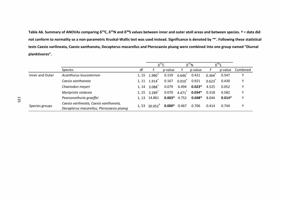
13

5

Table A6. Summary of ANOVAs comparing δ13C, δ15N and δ34S values between inner and outer atoll areas and between species. † = data did

not conform to normality so a non-parametric Kruskal-Wallis test was used instead. Significance is denoted by ‘*’. Following these statistical

tests Caesio varilineata, Caesio xanthanota, Decapterus macarellus and Pterocaesio pisang were combined into one group named “Diurnal

planktivores”.

Species df F p-value F p-value F p-value Combined

Inner and Outer Acanthurus leucosternon 1, 15 1.980† 0.159 0.646

† 0.421 0.364† 0.547 Y

Caesio xanthanota 1, 11 1.914† 0.167 0.010† 0.921 0.623† 0.430 Y

Chaetodon meyeri 1, 14 3.088† 0.079 6.494 0.023* 4.525 0.052 Y

Myripristis violacea 1, 15 3.289† 0.070 4.471† 0.034* 0.318 0.582 Y

Pearsonothuria graeffei 1, 13 14.861 0.003* 4.752 0.048* 8.044 0.014* Y

Species groupsCaesio varilineata, Caesio xanthonota,

Decapterus macarellus, Pterocaesio pisang1, 53 30.052† 0.000* 0.467 0.706 0.414 0.744 Y

δ13C δ15N δ34S

13

6

Table A7. Mean (± S.E) stable isotope (δ13C, δ15N, δ34S) values (‰) for each primary consumer species sampled in both inner and outer atoll.

Bold indicates statistical differences in isotope values of the samples species were found between areas using ANOVA or Kruskal-Wallis

tests. When differences in the mean were small (~1‰), samples from each area were combined for each group.

Source Species Area

Coral Chaetodon meyeri Inner -11.93 ± 0.46 11.22 ± 0.24 21.11 ± 0.23

Coral Chaetodon meyeri Outer -13.14 ± 0.49 10.37 ± 0.20 20.42 ± 0.19

Detritus Pearsonothuria graeffei Inner -12.67 ± 0.23 6.70 ± 0.14 18.14 ± 0.22

Detritus Pearsonothuria graeffei Outer -11.77 ± 0.12 6.24 ± 0.16 18.93 ± 0.17

Diurnal plankton Caesio varilineata Inner -18.26 ± 0.08 11.46 ± 0.09 19.01 ± 0.18

Diurnal plankton Caesio xanthonota Inner -17.05 ± 0.34 11.55 ± 0.32 18.92 ± 0.35

Diurnal plankton Caesio xanthonota Outer -17.49 ± 0.00 11.74 ± 0.49 18.79 ± 0.41

Diurnal plankton Decapterus macarellus Inner -17.19 ± 0.27 11.71 ± 0.15 19.22 ± 0.19

Diurnal plankton Pterocaesio pisang Inner -18.02 ± 0.17 11.48 ± 0.10 18.94 ± 0.33

DVM plankton Uroteuthis duvauceli Inner -17.94 ± 0.01 12.39 ± 0.17 22.40 ± 0.53

Benthic algae Acanthurus leucosternon Inner -13.65 ± 0.67 8.30 ± 0.81 19.66 ± 0.17

Benthic algae Acanthurus leucosternon Outer -14.16 ± 0.37 7.92 ± 0.13 19.71 ± 0.21

Nocturnal plankton Myripristis violacea Inner -16.76 ± 0.18 11.91 ± 0.11 20.04 ± 0.15

Nocturnal plankton Myripristis violacea Outer -17.04 ± 0.08 11.58 ± 0.07 19.91 ± 0.13

δ13C δ15N δ34S

13

7

Table A8. Comparison of mixing models fit using MixSIAR on the reef predator diet data using four different trophic discrimination factors.

dLOOic = difference in LOOic between each model and the model with the lowest LOOic (Stock et al., 2018). The model with the lowest

LOOic and the highest weight was presented in the results. Model 1 had a 55% probability of being the best model while model 2 had a 45%

probability of being the best model suggesting both are equally good. * indicates the model did not converge.

Model Δδ13C Δδ15N Δδ34S LOOic SE (LOOic) dLOOic SE (dLOOic) Weight

1 1.2 ± 1.9 2.1 ± 2.8 -0.53 ± 1.00 609 61.7 0 - 0.55

2 0.4 ± 0.2 2.3 ± 0.3 -0.53 ± 1.00 609.4 60.5 0.4 14.3 0.45

3 0.9 ± 1.0 3.2 ± 0.4 -0.53 ± 1.00 665.8 63 56.8 16.3 0

4* 1.2 ± 1.9 2.1 ± 2.8 1.9 ± 0.51 824 75.7 215 22.4 0

138

Table A9. Credible intervals of plankton source contribution for two three-source (δ13C,

δ15N, δ34S) Bayesian stable isotope mixing models with different trophic discrimination

factors (TDF, Δ), run to ascertain likely food source contributions for nine reef predator

species. Model 1: Δδ13C +1.2 (SD ± 1.9), Δδ15N +2.1 (SD ± 2.8), Δδ34S -0.53 (SD ± 1.00) and

Model 2: Δδ13C +0.4 (SD ± 0.2), Δδ15N +2.3 (SD ± 0.3), Δδ34S -0.53 (SD ± 1.00).

Species Area Q_0.025 Q_0.25 Q_0.5 Q_0.75 Q_0.975

Model 1

Aethaloperca rogaa Inner 0.661 0.716 0.740 0.764 0.809

Aethaloperca rogaa Outer 0.732 0.782 0.807 0.832 0.877

Anyperodon leucogrammicus Inner 0.632 0.716 0.750 0.776 0.822

Anyperodon leucogrammicus Outer 0.636 0.718 0.751 0.782 0.830

Aphareus furca Inner 0.573 0.644 0.683 0.722 0.800

Aphareus furca Outer 0.626 0.711 0.751 0.790 0.857

Caranx melampygus Inner 0.643 0.703 0.733 0.763 0.814

Caranx melampygus Outer 0.584 0.659 0.695 0.731 0.800

Cephalopholis argus Inner 0.616 0.676 0.704 0.728 0.775

Cephalopholis argus Outer 0.560 0.625 0.654 0.680 0.728

Cephalopholis miniata Inner 0.643 0.693 0.719 0.743 0.789

Cephalopholis miniata Outer 0.644 0.702 0.732 0.760 0.814

Lethrinus obsoletus Inner 0.703 0.821 0.879 0.928 0.986

Lethrinus obsoletus Outer 0.728 0.814 0.858 0.907 0.983

Lutjanus bohar Inner 0.659 0.739 0.772 0.802 0.859

Lutjanus bohar Outer 0.554 0.676 0.735 0.788 0.884

Lutjanus gibbus Inner 0.649 0.703 0.728 0.754 0.801

Lutjanus gibbus Outer 0.755 0.810 0.838 0.863 0.910

Model 2

Aethaloperca rogaa Inner 0.606 0.678 0.710 0.735 0.778

Aethaloperca rogaa Outer 0.673 0.738 0.767 0.794 0.838

Anyperodon leucogrammicus Inner 0.526 0.613 0.656 0.697 0.761

Anyperodon leucogrammicus Outer 0.531 0.622 0.669 0.713 0.771

Aphareus furca Inner 0.552 0.63 0.668 0.702 0.762

Aphareus furca Outer 0.576 0.689 0.732 0.771 0.840

Caranx melampygus Inner 0.585 0.655 0.683 0.708 0.747

Caranx melampygus Outer 0.607 0.682 0.715 0.752 0.821

Cephalopholis argus Inner 0.559 0.644 0.676 0.704 0.744

Cephalopholis argus Outer 0.533 0.613 0.643 0.669 0.709

Cephalopholis miniata Inner 0.646 0.695 0.720 0.744 0.786

Cephalopholis miniata Outer 0.621 0.680 0.712 0.742 0.794

Lethrinus obsoletus Inner 0.555 0.682 0.751 0.827 0.955

Lethrinus obsoletus Outer 0.659 0.776 0.831 0.881 0.970

Lutjanus bohar Inner 0.414 0.554 0.649 0.707 0.772

Lutjanus bohar Outer 0.332 0.645 0.734 0.809 0.899

Lutjanus gibbus Inner 0.601 0.678 0.707 0.732 0.771

Lutjanus gibbus Outer 0.599 0.745 0.782 0.810 0.857

139

Figure A6. Mean isotope values (± SE) of a) δ13C and δ15N and b) δ13C and δ34S of all

primary consumers sampled to represent different end-members in both inner (●) and

outer (▲) atoll before they were combined a priori. Boxes show a posteriori groupings.

Four species of diurnal planktivores were sampled: CV: Caesio varilineata, CX: Caesio

xanthanota, DM: Decapterus macarellus and PP: Pterocaesio pisang.

140


Table A10. The number of carbon atoms involved in the amino acid derivatisation process

which are used to calculate a correction factor for each amino acid.

Amino AcidNo. C atoms

(c)

No. C atoms

added in

derivative

group (d)

Total C atoms

in derivative

group (cd)

Underivatised 13

C value

Average

GC/C/IRMS

value

Correction

Factor

Alanine 3 5 8 -26.11 -35.46 -41.07

Aspartic acid 4 8 12 -7.69 -34.91 -48.52

Glutamic acid 5 8 13 -13.3 -30.32 -40.95

Glycine 2 5 7 -40.99 -39.70 -39.18

Hydroxyproline 5 7 12 -34.97

Luecine 6 5 11 -22.53 -32.75 -45.02

Lysine 6 7 13 -22.24 -34.52 -45.05

Norluecine 6 5 11 -34.92

Phenylalanine 9 5 14 -30.27 -36.87 -48.74

Proline 5 5 10 -10.64 -25.67 -40.70

Serine 3 7 10 -36.5 -43.09 -45.91

Threonine 4 7 11 -30.56 -42.53 -49.38

Tyrosine 9 7 16 -16.94 -31.34 -49.86

Valine 5 5 10 -26.17 -36.61 -47.05

14

1

Table A11. Summary of permutation tests of independence investigating differences in normalised δ13C values of essential amino acids of

primary consumers between inner and outer atoll area and between species. Significant differences (p < 0.05) are highlighted in bold.

Leucine Lysine Pheylalanine Threonine Valine

Test Species Z p-value Z p-value Z p-value Z p-value Z p-value

Area Acanthurus leucosternon 0.126 0.909 1.245 0.320 -1.655 0.090 -1.347 0.229 1.529 0.131

Area Chaetodon meyeri -1.780 0.038 1.924 0.034 1.390 0.172 -1.109 0.295 -0.413 0.765

Area Ctenochaetus striatus 1.081 0.309 1.278 0.228 -1.972 0.047 -0.908 0.398 1.287 0.246

Area Myripristis violacea 1.132 0.293 0.650 0.554 -0.962 0.396 -0.528 0.647 -0.148 0.898

Area Caesio varilineata -1.403 0.134 -0.084 1.000 0.682 0.734 1.258 0.330 -0.188 0.934

Area Caesio xanthonota -0.793 0.432 0.716 0.717 0.800 0.713 0.614 0.720 -1.420 0.141

Species C. varilineata & C. xanthonota -0.886 0.413 1.795 0.059 2.112 0.032 -0.214 0.840 -2.089 0.033

Species U. duvauceli & D. macarellus -0.018 1.000 0.497 0.632 -1.553 0.119 0.835 0.456 0.600 0.593

142


Figure A7. The model of path analysis results exploring the abiotic and biotic variables

influencing reef predator biomass without the planktivore pathway. This model was a

poorer fit than the model presented in the results (Figure 6.7). Single arrows indicate

indicate causal paths with standardised path coefficients. Thick arrows indicate significant

relationships with stars denoting the significance level (* = p < 0.05, ** = p < 0.01, *** =

P < 0.001) and dotted arrows signify covariance.

143

Table A12. List of all prey species recorded during underwater visual census and their

functional groups.

Family Species Functional

group Reference

Acanthuridae Acanthurus auranticavus E (Robertson, 1982)

Acanthurus leucocheilus E (Green and Bellwood, 2009)

Acanthurus leucosternon E (Green and Bellwood, 2009)

Acanthurus mata E (Hiatt and Strasburg, 1960)

Acanthurus nigricauda E (Choat et al., 2002)

Acanthurus nigrofuscus E (Green and Bellwood, 2009)

Acanthurus thompsoni P (Hobson, 1974)

Acanthurus tristis E (Green and Bellwood, 2009)

Ctenochaetus striatus E (Choat et al., 2002)

Ctenochaetus truncatus E (Eggertsen et al., 2019)

Naso brevirostris O (Choat et al., 2002)

Naso elegans E (Green and Bellwood, 2009)

Naso hexacanthus P (Choat et al., 2002)

Naso thynnoides P (Durville et al., 2003)

Zebrasoma desjardinii E (Choat, 1991)

Zebrasoma scopas E (Choat et al., 2002)

Apogonidae B (Hobson, 1974)

Balistidae Balistapus undulatus O (Hiatt and Strasburg, 1960)

Balistoides conspicillum B (Patankar et al., 2018)

Melichthys indicus O (Patankar et al., 2018)

Odonus niger P (Patankar et al., 2018)

Sufflamen bursa O (Patankar et al., 2018)

Blenniidae Blennies E (Durville et al., 2003)

Sabretooth blennies B (Durville et al., 2003)

Caesionidae Caesio spp P (Russ et al., 2017)

Pterocaesio spp P (Russ et al., 2017)

Chaetodontidae Chaetodon auriga O (Hobson, 1974)

Chaetodon collare C (Allen et al., 1998)

Chaetodon falcula B (Narayani et al., 2015)

Chaetodon guttatissimus O (Durville et al., 2003)

Chaetodon kleinii O (Sano, 1989)

Chaetodon madagaskariensis O (Durville et al., 2003)

Chaetodon melannotus O (Sano, 1989)

Chaetodon meyeri C (Sano, 1989)

Chaetodon triangulum C (Chandler et al., 2016)

Chaetodon trifasciatus C (Narayani et al., 2015)

Chaetodon xanthocephalus O (Durville et al., 2003)

Forcipiger flavissimus O (Hobson, 1974)

Forcipiger longirostris B (Hobson, 1974)

Hemitaurichthys zoster O (Hobson, 1974)

Heniochus pleurotaenia P (Lieske and Myers, 2009)

Cirrhitidae Paracirrhites spp O (Hobson, 1974)

144

Diodontidae Diodon liturosus B (Patankar et al., 2018)

Gobiidae Reef gobies O (Hiatt and Strasburg, 1960)

Sand gobies O (Hiatt and Strasburg, 1960)

Haemulidae Plectorhinchus spp O (Durville et al., 2003)

Holocentridae Myripristis spp P (Hobson, 1974)

Neoniphon spp B (Durville et al., 2003)

Sargocentron spp B (Durville et al., 2003)

Labridae Anampses meleagrides B (Durville et al., 2003)

Bodianus spp B (Hobson, 1974)

Cheilinus spp B (Hobson, 1974)

Cheilio inermis B (Ormond, 1980)

Cirrhilabrus exquisitus B (Durville et al., 2003)

Coris spp B (Hobson, 1974)

Epibulus spp B (Hiatt and Strasburg, 1960)

Gomphosus caeruleus B (Hobson, 1974)

Halichoeres spp B (Hobson, 1974)

Hemigymnus spp B (Hiatt and Strasburg, 1960)

Hologymnosus spp B (Durville et al., 2003)

Labrichthys unilineatus C (Westneat, 2001)

Labroides spp B (Hiatt and Strasburg, 1960)

Macropharyngodon bipartitus B (Hobson, 1974)

Novaculichthys taeniourus B (Hiatt and Strasburg, 1960)

Oxycheilinus digramma B (Durville et al., 2003)

Pseudocheilinus spp B (Hobson, 1974)

Stethojulis albovittata B (Hiatt and Strasburg, 1960)

Thalassoma amblycephalum P (Hobson, 1974)

Thalassoma spp B (Hobson, 1974)

Wetmorella spp B (Westneat, 2001)

Microdesmidae Ptereleotris evides P (Durville et al., 2003)

Monacanthidae Amanses scopas C (Durville et al., 2003)

Oxymonacanthus longirostris C (Patankar et al., 2018)

Paraluteres prionurus O (Cornic, 1987)

Mullidae B (Hobson, 1974)

Nemipteridae Scolopsis spp B (Hiatt and Strasburg, 1960)

Ostraciidae Ostracion meleagris O (Patankar et al., 2018)

Pempheridae Parapriacanthus ransonneti P (Durville et al., 2003)

Pempheris vanicolensis P (Durville et al., 2003)

Pinguipedidae Parapercis spp B (Hiatt and Strasburg, 1960)

Pomacanthidae Apolemichthys trimaculatus O (Durville et al., 2003)

Centropyge multispinis O (Alwany, 2009)

Pomacanthus imperator B (Alwany, 2009)

Pygoplites diacanthus O (Alwany, 2009)

Pomacentridae Abudefduf vaigiensis P (Frédérich et al., 2009)

Amblyglyphidodon spp O (Durville et al., 2003)

Amphiprion spp O (Durville et al., 2003)

Chromis spp P (Hobson, 1974)

Dascyllus spp O (Frédérich et al., 2009)

Plectroglyphidodon spp E (Frédérich et al., 2009)

145

Pomacentrus caeruleus P (Frédérich et al., 2009)

Pomacentrus chrysurus E (Allen, 1991)

Pomacentrus indicus O (Durville et al., 2003)

Pomacentrus pavo O (Frédérich et al., 2008)

Pomacentrus philippinus O (Durville et al., 2003)

Priacanthidae Priacanthus hamrur B (Hobson, 1974)

Scaridae Cetoscarus spp E (Plass-Johnson et al., 2013)

Chlorurus spp E (Green and Bellwood, 2009)

Hipposcarus spp E (Green and Bellwood, 2009)

Scarus spp E (Hobson, 1974)

Serranidae Pseudanthias spp P (Durville et al., 2003)

Siganidae Siganus spp E (Hiatt and Strasburg, 1960)

Synodontidae O (Hiatt and Strasburg, 1960)

Tetraodontidae Arothron spp O (Hobson, 1974)

Canthigaster spp O (Hobson, 1974)

Zanclidae Zanclus cornutus B (Hobson, 1974)

146

Table A13. List of all fishery target, reef-associated teleost predators recorded on

underwater visual census.

Genus Species

Carangidae Caranx melampygus Lutjanidae Aphareus furca

Aprion virescens

Lutjanus bohar

Lutjanus gibbus

Lutjanus kasmira

Macolor macularis

Serranidae Aethaloperca rogaa

Anyperodon leucogrammicus

Cephalopholis argus

Cephalopholis leopardus

Cephalopholis miniata

Cephalopholis nigripinnis

Cephalopholis sexmaculata

Cephalopholis spiloparaea

Epinephelus fasciatus

Epinephelus longispinis

Epinephelus macrospilos

Epinephelus merra

Epinephelus polyphekadion

Epinephelus spilotoceps

Plectropomus areolatus

Plectropomus laevis Variola louti

147

References

Adam, M.S. (2006) Vulnerability and adaptation assessment of the fisheries sector in the

Maldives - NAPA Project. Male, Maldives: Ministry of Environment, Energy and Water.

Adam, M.S. and Sinan, H. (2013) Coastal and Marine Fisheries Management in the Maldives.

Bangladesh: SAARC Agriculture Centre (SAC).

Adler, D., Murdoch, D. and others (2018) 'rgl: 3D Visualization Using OpenGL. R package

version 0.99.16. https://CRAN.R-project.org/package=rgl'.

Ali, M.K.H., Belluscio, A., Ventura, D. and Ardizzone, G. (2016) 'Feeding ecology of some fish

species occurring in artisanal fishery of Socotra Island (Yemen)', Marine Pollution

Bulletin, 105(2), pp. 613-28.

Allain, V., Fernandez, E., Hoyle, S., Caillot, S., Jurado-Molina, J.A., S and Nicol, S. (2012)

'Interaction between Coastal and Oceanic Ecosystems of the Western and Central

Pacific Ocean through Predator- Prey Relationship Studies', PLoS ONE, 7(5), p. e36701.

Alldredge, A.L. and King, J.M. (2009) 'Near-surface enrichment of zooplankton over a shallow

back reef: implications for coral reef food webs', Coral Reefs, 28(4), pp. 895-908.

Allen, G.R. (1991) Damselfishes of the world. Melle, Germany: Mergus Publishers.

Allen, G.R., Steene, R.C. and Allen, M. (1998) A guide to angelfishes & butterflyfishes. Perth:

Odyssey.

Alvarez-Filip, L., Gill, J.A. and Dulvy, N.K. (2011) 'Complex reef architecture supports more

small-bodied fishes and longer food chains on Caribbean reefs', Ecosphere, 2(10), p.

art118.

Alwany, M.A. (2009) 'Distribution and feeding ecology of the angelfishes (Pomacanthidae) in

Shalateen region, Red Sea, Egypt', Egyptian Journal of Aquatic Biology & Fisheries,

13(1), pp. 79 - 91.

Anderson, R.C., Adam, M.S. and Goes, J.I. (2011) 'From monsoons to mantas: seasonal

distribution of Manta alfredi in the Maldives', Fisheries Oceanography, 20(2), pp. 104-

113.

Araújo, M.S., Bolnick, D.I. and Layman, C.A. (2011) 'The ecological causes of individual

specialisation', Ecology Letters, 14(9), pp. 948-958.

ttps://CRAN.R-project.org/package=rgl'.

148

Araújo, M.S., Bolnick, D.I., Machado, G., Giaretta, A.A. and dos Reis, S.F. (2007) 'Using d13C

stable isotopes to quantify individual-level diet variation', Oecologia, 152(4), pp. 643-

54.

Arim, M., Bozinovic, F. and Marquet, P.A. (2007) 'On the relationship between trophic

position, body mass and temperature: reformulating the energy limitation hypothesis',

Oikos, 116(9), pp. 1524-1530.

Arthur, K.E., Kelez, S., Larsen, T., Choy, C.A. and Popp, B.N. (2014) 'Tracing the biosynthetic

source of essential amino acids in marine turtles using d13C fingerprints', Ecology,

95(5), pp. 1285-93.

Asch, R.G., Cheung, W.W.L. and Reygondeau, G. (2018) 'Future marine ecosystem drivers,

biodiversity, and fisheries maximum catch potential in Pacific Island countries and

territories under climate change', Marine Policy, 88, pp. 285-294.

Asher, J., Williams, I.D. and Harvey, E.S. (2017) 'An Assessment of Mobile Predator

Populations along Shallow and Mesophotic Depth Gradients in the Hawaiian

Archipelago', Scientific Reports, 7(1), p. 3905.

Barbier, E.B., Hacker, S.D., Kennedy, C., Koch, E.W., Stier, A.C. and Silliman, B.R. (2011) 'The

value of estuarine and coastal ecosystem services', Ecological Monographs, 81(2), pp.

169-193.

Barnes, C. and Jennings, S. (2007) 'Effect of temperature, ration, body size and age on

sulphur isotope fractionation in fish', Rapid Communications In Mass Spectrometry,

21(8), pp. 1461-7.

Barnett, A., Abrantes, K.G., Seymour, J. and Fitzpatrick, R. (2012) 'Residency and spatial use

by reef sharks of an isolated seamount and its implications for conservation', PLoS One,

7(5), p. e36574.

Barros, N.B., Ostrom, P.H., Stricker, C.A. and Wells, R.S. (2010) 'Stable isotopes differentiate

bottlenose dolphins off west-central Florida', Marine Mammal Science, 26(2), pp. 324-

336.

Bascompte, J., Melian, C.J. and Sala, E. (2005) 'Interaction strength combinations and the

overfishing of a marine food web', Proceedings of the National Academy of Sciences,

102(15), pp. 5443-7.

Bates, D., Maechler, M., Bolker, B. and Walker, S. (2015) 'Fitting Linear Mixed-Effects Models

Using lme4.', Journal of Statistical Software, 67(1), pp. 1-48.

149

Baum, J.K. and Worm, B. (2009) 'Cascading top-down effects of changing oceanic predator

abundances', Journal of Animal Ecology, 78(4), pp. 699-714.

Bearhop, S., Adams, V.E., Waldron, S., Fuller, R.A. and Macleod, H. (2004) 'Determining

trophic niche width: a novel approach using stable isotope analysis', Journal of Animal

Ecology, 73(5), pp. 1007-1012.

Beetham, E.P. and Kench, P.S. (2014) 'Wave energy gradients and shoreline change on

Vabbinfaru platform, Maldives', Geomorphology, 209, pp. 98-110.

Bell, K. and Galzin, R. (1984) 'Influence of live coral cover on coral-reef fish communities.',

Marine Ecology Progress Series, 15(3), pp. 265-274.

Bellwood, D.R. (1988) 'Seasonal changes in the size and composition of the fish yield from

reefs around Apo Island, Central Philippines, with notes on methods of yield

estimation', Journal of Fish Biology, 32(6), pp. 881-893.

Bellwood, D.R., Streit, R.P., Brandl, S.J. and Tebbett, S.B. (2019) 'The meaning of the term

‘function’ in ecology: A coral reef perspective', Functional Ecology, 33(6), pp. 948-961.

Benkwitt, C.E., Wilson, S.K. and Graham, N.A.J. (2019) 'Seabird nutrient subsidies alter

patterns of algal abundance and fish biomass on coral reefs following a bleaching

event', Global Change Biology, 25(8), pp. 2619-2632.

Berkström, C., Gullström, M., Lindborg, R., Mwandya, A.W., Yahya, S.A.S., Kautsky, N. and

Nyström, M. (2012) 'Exploring ‘knowns’ and ‘unknowns’ in tropical seascape

connectivity with insights from East African coral reefs', Estuarine, Coastal and Shelf

Science, 107, pp. 1-21.

Berkström, C., Lindborg, R., Thyresson, M. and Gullström, M. (2013) 'Assessing connectivity

in a tropical embayment: Fish migrations and seascape ecology', Biological

Conservation, 166, pp. 43-53.

Beukers-Stewart, B.D., Beukers-Stewart, J.S. and Jones, G.P. (2011) 'Behavioural and

developmental responses of predatory coral reef fish to variation in the abundance of

prey', Coral Reefs, 30(3), pp. 855-864.

Bierwagen, S.L., Heupel, M.R., Chin, A. and Simpfendorfer, C.A. (2018) 'Trophodynamics as a

Tool for Understanding Coral Reef Ecosystems', Frontiers in Marine Science, 5(24), pp.

1-13.

Blaber, S.J.M. (2000) Tropical Estuarine Fishes: Ecology, Exploitation and Conservation.

Oxford: Blackwell.

150

Boaden, A.E. and Kingsford, M.J. (2015) 'Predators drive community structure in coral reef

fish assemblages', Ecosphere., 6(4), pp. 1-33.

Bodey, T.W., Cleasby, I.R., Votier, S.C., Hamer, K.C., Newton, J., Patrick, S.C., Wakefield, E.D.

and Bearhop, S. (2018) 'Frequency and consequences of individual dietary

specialisation in a wide-ranging marine predator, the northern gannet', Marine Ecology

Progress Series, 604, pp. 251-262.

Boecklen, W.J., Yarnes, C.T., Cook, B.A. and James, A.C. (2011) 'On the Use of Stable Isotopes

in Trophic Ecology', Annual Review of Ecology, Evolution, and Systematics, 42(1), pp.

411-440.

Bolnick, D.I., Amarasekare, P., Araújo, M.S., Bürger, R., Levine, J.M., Novak, M., Rudolf,

V.H.W., Schreiber, S.J., Urban, M.C. and Vasseur, D. (2011) 'Why intraspecific trait

variation matters in community ecology', Trends In Ecology and Evolution, 26(4), pp.

183–192.

Bolnick, D.I., Svanbäck, R., Fordyce, J.A., Yang, L.H., Davis, J.M., Hulsey, C.D. and Forister,

M.L. (2003) 'The Ecology of Individuals: Incidence and Implications of Individual

Specialization', The American Naturalist, 161(1), pp. 1-28.

Bonfil, R. (1993) The Biology and Ecology of the Silky Shark, Carcharhinus falciformis, from

the Campeche Bank, México Silver Spring, MD: NOAA/NMFS.

Bopp, L., Resplandy, L., Orr, J.C., Doney, S.C., Dunne, J.P., Gehlen, M., Halloran, P., Heinze, C.,

Ilyina, T., Séférian, R., Tjiputra, J. and Vichi, M. (2013) 'Multiple stressors of ocean

ecosystems in the 21st century: projections with CMIP5 models', Biogeosciences,

10(10), pp. 6225-6245.

Bouchon-Navaro, Y. and Bouchon, C. (1989) 'Correlations between chaetodontid fishes and

coral communities of the Gulf of Aqaba (Red Sea).', Environmental Biology of Fishes,

25, pp. 47-60.

Bowen, B.W., Bass, A.L., Rocha, L.A., Grant, W.S. and Robertson, D.R. (2001) 'Phylogeography

Of The Trumpetfishes (Aulostomus): Ring Species Complex On A Global Scale',

Evolution, 55(5), pp. 1029–1039.

Bradbury, M., Abbot, D., Bovbjerg, R., Mariscal, R., Fielding, W.C., Barber, R.T., Pearse, V.B.,

Proctor, S.J., Ogden, J.C., Wourms, J.P., Taylor Jr., L.R., Christofferson, J.G.,

Christofferson, J.P., McPhearson, R.M., Wynne, M.J. and Stromberg Jr., P.M. (1970)

International Symposium on Biological Sound Scattering in the Ocean. Maury Center

for Ocean Science, Washington, DC.

151

Bradley, C.J., Madigan, D.J., Block, B.A. and Popp, B.N. (2014) 'Amino Acid Isotope

Incorporation and Enrichment Factors in Pacific Bluefin Tuna, Thunnus orientalis', PLOS

ONE, 9(1), p. e85818.

Brandl, S.J., Tornabene, L., Goatley, C.H.R., Casey, J.M., Morais, R.A., Côté, I.M., Baldwin,

C.C., Parravicini, V., Schiettekatte, N.M.D. and Bellwood, D.R. (2019) 'Demographic

dynamics of the smallest marine vertebrates fuel coral reef ecosystem functioning',

Science, 364(6446), pp. 1189-1192.

Brock, R.E. (1982) 'A critique of the visual census method for assessing coral-reef fish

populations', Bulletin of Marine Science, 32, pp. 269-276.

Brown, K.T., Bender-Champ, D., Kubicek, A., van der Zande, R., Achlatis, M., Hoegh-Guldberg,

O. and Dove, S.G. (2018) 'The Dynamics of Coral-Algal Interactions in Space and Time

on the Southern Great Barrier Reef', Frontiers in Marine Science, 5(181).

Browne, M.W. and Cudeck, R. (1992) 'Alternative Ways of Assessing Model Fit', Sociological

Methods & Research, 21(2), pp. 230-258.

Bruckner, A.W. and Coward, G. (2019) 'Abnormal density of Culcita schmideliana delays

recovery of a reef system in the Maldives following a catastrophic bleaching event',

Marine and Freshwater Research, 70(2), pp. 292-301.

Bruder, A., Frainer, A., Rota, T. and Primicerio, R. (2019) 'The Importance of Ecological

Networks in Multiple-Stressor Research and Management', Frontiers in Environmental

Science, 7(59).

Bunn, S.E. and Boon, P.I. (1993) 'What sources of organic carbon drive food webs in

billabongs? A study based on stable isotope analysis.', Oecologia, 96(1), pp. 85-94.

Burkholder, D.A., Heithaus, M.R., Fourqurean, J.W., Wirsing, A. and Dill, L.M. (2013) 'Patterns

of top-down control in a seagrass ecosystem: could a roving apex predator induce a

behaviour-mediated trophic cascade?', Journal of Animal Ecology, 82(6), pp. 1192-

1202.

Cabana, G. and Rasmussen, J.B. (1996) 'Comparison of aquatic food chains using nitrogen

isotopes', Proceedings of the National Academy of Sciences of the United States of

America, 93(20), pp. 10844-10847.

Calabrese, J.M. and Fagan, W.F. (2004) 'A comparison-shopper's guide to connectivity

metrics', Frontiers in Ecology and the Environment, 2(10), pp. 529-536.

152

Cameron, C.K., Sundqvist, M.K., Keith, S.K., Caradonna, P.J., Mousing, E.A., Nilsson, K.A.,

Metcalfe, D.B. and Classen, A.T. (2019) 'Uneven global distribution of food web studies

under climate change', Ecosphere, 10(3), p. e02645.

Cappo, M., De'ath, G. and Speare, P. (2007) 'Inter-reef vertebrate communities of the Great

Barrier Reef Marine Park determined by baited remote underwater video stations.',

Marine Ecology Progress Series, 350, pp. 209-221.

Cappo, M., Harvey, E.S., Malcolm, H. and Speare, P. (2003) 'Potential of video techniques to

monitor diversity, abundance and size of fish in studies of marine protected areas', in

Beumer, J.P., Grant, A. and Smith, D.C. (eds.) Aquatic Protected Areas. What works best

and how do we know? Cairns edition edn. University of Queensland, Queensland, pp.

455-464.

Carpenter, K.E., Abrar, M., Aeby, G., Aronson, R.B., Banks, S., Bruckner, A., Chiriboga, A.,

Cortés, J., Delbeek, J.C., DeVantier, L., Edgar, G.J., Edwards, A.J., Fenner, D., Guzmán,

H.M., Hoeksema, B.W., Hodgson, G., Johan, O., Licuanan, W.Y., Livingstone, S.R., Lovell,

E.R., Moore, J.A., Obura, D.O., Ochavillo, D., Polidoro, B.A., Precht, W.F., Quibilan,

M.C., Reboton, C., Richards, Z.T., Rogers, A.D., Sanciangco, J., Sheppard, A., Sheppard,

C., Smith, J., Stuart, S., Turak, E., Veron, J.E.N., Wallace, C., Weil, E. and Wood, E.

(2008) 'One-Third of Reef-Building Corals Face Elevated Extinction Risk from Climate

Change and Local Impacts', Science, 321(5888), pp. 560-563.

Carpenter, S.R., Kitchell, J.F. and Hodgson, J.R. (1985) 'Cascading Trophic Interactions and

Lake Productivity: Fish predation and herbivory can regulate lake ecosystems',

BioScience, 35(10), pp. 634-639.

Carr, M.H., Neigel, J.E., Estes, J.A., Andelman, S., Warner, R.R. and Largier, J.L. (2003)

'Comparing marine and terrestrial ecosystems: Implications for the design of coastal

marine reserves', Ecological Applications, 13(sp1), pp. 90-107.

Carreón-Palau, L., Parrish, C.C., del Angel-Rodríguez, J.A., Pérez-España, H. and Aguiñiga-

García, S. (2013) 'Revealing organic carbon sources fueling a coral reef food web in the

Gulf of Mexico using stable isotopes and fatty acids', Limnology and Oceanography,

58(2), pp. 593-612.

Cartamil, D.P., Vaudo, J., Lowe, C.G., Wetherbee, B.M. and Holland, K.N. (2003) 'Diel

movement patterns of the Hawaiian stingray, Dasyatis lata: implications for ecological

interactions between sympatric elasmobranch species.', Marine Biology, 142, pp. 841-

847.

153

Carter, W.A., Bauchinger, U. and McWilliams, S.R. (2019) 'The Importance of Isotopic

Turnover for Understanding Key Aspects of Animal Ecology and Nutrition', Diversity,

11(5), p. 84.

Casey, J.M., Baird, A.H., Brandl, S.J., Hoogenboom, M.O., Rizzari, J.R., Frisch, A.J., Mirbach,

C.E. and Connolly, S.R. (2017) 'A test of trophic cascade theory: fish and benthic

assemblages across a predator density gradient on coral reefs', Oecologia, 183(1), pp.

161-175.

Ceccarelli, D. and Ayling, T. (2010) Role, importance and vulnerability of top predators on the

Great Barrier Reef - A review.Great Barrier Reef Marine Park Authority.

Chandler, J.F., Burn, D., Berggren, P. and Sweet, M.J. (2016) 'Influence of Resource

Availability on the Foraging Strategies of the Triangle Butterflyfish Chaetodon

triangulum in the Maldives', PLOS ONE, 11(3), p. e0151923.

Chen, P.-Y., Chen, C.-C., Chu, L. and McCarl, B. (2015) 'Evaluating the economic damage of

climate change on global coral reefs', Global Environmental Change, 30, pp. 12-20.

Chivers, D.P., McCormick, M.I., Allan, B.J.M. and Ferrari, M.C.O. (2016) 'Risk assessment and

predator learning in a changing world: understanding the impacts of coral reef

degradation', Scientific Reports, 6, p. 32542.

Choat, J.H. (1991) 'The biology of herbivorous fishes on coral reefs.', in Sale, P.F. (ed.) The

ecology of fishes on coral reefs. San Diego, CA: Academic Press, pp. 120-155.

Choat, J.H., Clements, K.D. and Robbins, W.D. (2002) 'The trophic status of herbivorous

fishes on coral reefs', Marine Biology, 140(3), pp. 613-623.

Chou, L.M., Wilkinson, C.R., Licuanan, W.R.Y., Alino, P., Cheshire, A.C., Loo, M.G.K.,

Tangjaitrong, S., Sudara, S., Ridzwan, A.R. and Soekarno (1994) Third ASEAN-Australia

Symposium on Living Coastal Resources. Bangkok, Thailand: Chulalongkorn University.

Christensen, V., Coll, M., Piroddi, C., Steenbeek, J., Buszowski, J. and Pauly, D. (2014) 'A

century of fish biomass decline in the ocean', Marine Ecology Progress Series, 512, pp.

155-166.

Cinner, J.E., Huchery, C., MacNeil, M.A., Graham, N.A.J., McClanahan, T.R., Maina, J., Maire,

E., Kittinger, J.N., Hicks, C.C., Mora, C., Allison, E.H., D’Agata, S., Hoey, A., Feary, D.A.,

Crowder, L., Williams, I.D., Kulbicki, M., Vigliola, L., Wantiez, L., Edgar, G., Stuart-Smith,

R.D., Sandin, S.A., Green, A.L., Hardt, M.J., Beger, M., Friedlander, A., Campbell, S.J.,

Holmes, K.E., Wilson, S.K., Brokovich, E., Brooks, A.J., Cruz-Motta, J.J., Booth, D.J.,

154

Chabanet, P., Gough, C., Tupper, M., Ferse, S.C.A., Sumaila, U.R. and Mouillot, D.

(2016) 'Bright spots among the world’s coral reefs', Nature, 535, p. 416.

Cinner, J.E., Maire, E., Huchery, C., MacNeil, M.A., Graham, N.A.J., Mora, C., McClanahan,

T.R., Barnes, M.L., Kittinger, J.N., Hicks, C.C., D’Agata, S., Hoey, A.S., Gurney, G.G.,

Feary, D.A., Williams, I.D., Kulbicki, M., Vigliola, L., Wantiez, L., Edgar, G.J., Stuart-

Smith, R.D., Sandin, S.A., Green, A., Hardt, M.J., Beger, M., Friedlander, A.M., Wilson,

S.K., Brokovich, E., Brooks, A.J., Cruz-Motta, J.J., Booth, D.J., Chabanet, P., Gough, C.,

Tupper, M., Ferse, S.C.A., Sumaila, U.R., Pardede, S. and Mouillot, D. (2018) 'Gravity of

human impacts mediates coral reef conservation gains', Proceedings of the National

Academy of Sciences, 115(27), pp. E6116-E6125.

Clark, R.D., Pittman, S., Caldow, C., Christensen, J., Roque, B., Appeldoorn, R.S. and Monaco,

M.E. (2009) 'Nocturnal fish movement and trophic flow across habitat boundaries in a

coral reef ecosystem (SW Puerto Rico)', Caribbean Journal of Science, 45(2-3), pp. 282-

303.

Clarke, K. and Warwick, R. (2001) 'Change in marine communities: an approach to statistical

analysis and interpretation.', PRIMER-E, Plymouth.

Clarke, K.R. and Gorley, R.N. (2006) PRIMER v6: User Manual/Tutorial. Plymouth: PRIMER-E

Ltd.

Colléter, M., Valls, A., Guitton, J., Lyne, M., Arreguín- Sánchez, F., Christensen, V., Gascuel,

D., D. and Pauly, D. (2013) EcoBase: a repository solution to gather and communicate

information from EwE models (Fisheries Centre Research Report 21(1).). Fisheries

Centre, University of British Columbia, Canada. [Online]. Available at: https://hal-

agrocampus-ouest.archives-ouvertes.fr/hal-01103442.

Compagno, L.J.V. (1984) Sharks of the world: an annotated and illustrated catalogue of shark

species known to date. Rome: FAO.

Connell, S.D. and Kingsford, M.J. (1998) 'Spatial, temporal and habitat-related variation in

the abundance of large predatory fish at One Tree Reef, Australia', Coral Reefs, 17(1),

pp. 49-57.

Connolly, R.M., Guest, M.A., Melville, A.J. and Oakes, J.M. (2004) 'Sulfur stable isotopes

separate producers in marine food-web analysis', Oecologia, 138(2), pp. 161-167.

Coplen, T.B. and Krouse, H.R. (1998) 'Sulphur isotope data consistency improved', Nature,

392, p. 32.

Cornic, A. (1987) Poissons de l'Ile Maurice. Ile Maurice: Stanley Rose Hill.

ttps://hal-agrocampus-ouest.archives-ouvertes.fr/hal-01103442.

ttps://hal-agrocampus-ouest.archives-ouvertes.fr/hal-01103442.

155

Corr, L.T., Berstan, R. and Evershed, R.P. (2007) 'Optimisation of derivatisation procedures

for the determination of δ13C values of amino acids by gas

chromatography/combustion/isotope ratio mass spectrometry', Rapid

Communications in Mass Spectrometry, 21(23), pp. 3759-3771.

Costa, D.P. (1993) 'The relationship between reproductive and foraging energetics and the

evolution of the Pinnipedia.', Symposium of the Zoological Society of London, 66, pp.

293–314.

Costanza, R. and Mageau, M. (1999) 'What is a healthy ecosystem?', Aquatic Ecology, 33(1),

pp. 105–115.

Cowburn, B., Moritz, C., Birrell, C., Grimsditch, G. and Abdulla, A. (2018) 'Can luxury and

environmental sustainability co-exist? Assessing the environmental impact of resort

tourism on coral reefs in the Maldives', Ocean & Coastal Management, 158, pp. 120-

127.

Croisetière, L., Hare, L., Tessier, A. and Cabana, G. (2009) 'Sulphur stable isotopes can

distinguish trophic dependence on sediments and plankton in boreal lakes', Freshwater

Biology, 54(5), pp. 1006-1015.

Crook, D.A., Lowe, W.H., Allendorf, F.W., Erős, T., Finn, D.S., Gillanders, B.M., Hadwen, W.L.,

Harrod, C., Hermoso, V., Jennings, S., Kilada, R.W., Nagelkerken, I., Hansen, M.M.,

Page, T.J., Riginos, C., Fry, B. and Hughes, J.M. (2015) 'Human effects on ecological

connectivity in aquatic ecosystems: Integrating scientific approaches to support

management and mitigation', Science of The Total Environment, 534, pp. 52-64.

Dale, J.J., Meyer, C.G. and Clark, C.E. (2011) 'The Ecology of Coral Reef Top Predators in the

Papahānaumokuākea Marine National Monument', Journal of Marine Biology, 2011,

pp. 1-14.

Dalponti, G., Guariento, R.D. and Caliman, A. (2018) 'Hunting high or low: body size drives

trophic position among and within marine predators', Marine Ecology Progress Series,

597, pp. 39-46.

Dance, K.M., Rooker, J.R., Shipley, J.B., Dance, M.A. and Wells, R.J.D. (2018) 'Feeding ecology

of fishes associated with artificial reefs in the northwest Gulf of Mexico', PLOS ONE,

13(10), p. e0203873.

Darling, E.S., Graham, N.A.J., Januchowski-Hartley, F.A., Nash, K.L., Pratchett, M.S. and

Wilson, S.K. (2017) 'Relationships between structural complexity, coral traits, and reef

fish assemblages', Coral Reefs, 36(2), pp. 561-575.

156

Darwin, C. (1842) The Structure and Distribution of Coral Reefs. Being the first part of the

geology of the voyage of the Beagle, under the command of Capt. Fitzroy, R.N. during

the years 1832 to 1836. London.

Dauby, P. (1989) 'The stable carbon isotope ratios in benthic food webs of the Gulf of Calvi,

Corsica', Continental Shelf Research, 9(2), pp. 181-195.

Davidson, L.N.K., Krawchuk, M.A. and Dulvy, N.K. (2016) 'Why have global shark and ray

landings declined: improved management or overfishing?', Fish and Fisheries, 17(2),

pp. 438-458.

DeMartini, E.E., Friedlander, A.M., Sandin, S.A. and Sala, E. (2008) 'Differences in fish-

assemblage structure between fished and unfished atolls in the northern Line Islands,

central Pacific', Marine Ecology Progress Series, 365, pp. 199-215.

DeNiro, M.J. and Epstein, S. (1978) 'Influence of diet on the distribution of carbon isotopes in

animals', Geochim. Cosmochim. Acta., 42, pp. 495-506.

Dierking, J., Williams, I.D. and Walsh, W.J. (2011) 'Diet composition and prey selection of the

introduced grouper species peacock hind (Cephalopholis argus) in Hawaii.', Fishery

Bulletin, 107(4), pp. 464-476.

Domroes, M. (2001) 'Conceptualising State-Controlled Resort Islands for an Environment-

Friendly Development of Tourism: The Maldivian Experience', Singapore Journal of

Tropical Geography, 22(2), pp. 122-137.

Doty, M.S. and Oguri, M. (1956) 'The Island Mass Effect.', Journal of Conservation, 22, pp. 33-

37.

Downs, E.E., Popp, B.N. and Holl, C.M. (2014) 'Nitrogen isotope fractionation and amino

acid turnover rates in the Pacific white shrimp Litopenaeus vannamei', Marine Ecology


Dulvy, N.K., Baum, J.K., Clarke, S., Compagno, L.J.V., Cortés, E., Domingo, A., Fordham, S.,

Fowler, S., Francis, M.P., Gibson, C., Martínez, J., Musick, J.A., Soldo, A., Stevens, J.D.

and Valenti, S. (2008) 'You can swim but you can't hide: the global status and

conservation of oceanic pelagic sharks and rays', Aquatic Conservation: Marine and

Freshwater Ecosystems, 18(5), pp. 459-482.

Dulvy, N.K., Sadovy, Y. and Reynolds, J.D. (2003) 'Extinction vulnerability in marine

populations', Fish and Fisheries, 4, pp. 25-64.

Dunic, J.C. and Baum, J.K. (2017) 'Size structuring and allometric scaling relationships in coral

reef fishes', Journal of Animal Ecology, 86(3), pp. 577-589.

157

Duplisea, D.E. (2000) The ecological hierarchy, model complexity, predictive ability and

robust management. Copenhagen: International Council for the Exploration of the Sea.

Durville, P., Chabanet, P. and Quod, J.P. (2003) 'Visual Census of the Reef Fishes in the

Natural Reserve of the Glorieuses Islands (Western Indian Ocean)', Western Indian

Ocean J. Mar. Sci., 2(2), pp. 95–104.

Eggertsen, M., Chacin, D.H., Åkerlund, C., Halling, C. and Berkström, C. (2019) 'Contrasting

distribution and foraging patterns of herbivorous and detritivorous fishes across

multiple habitats in a tropical seascape', Marine Biology, 166(4), p. 51.

Espinoza, M., Cappo, M., Heupel, M.R., Tobin, A.J. and Simpfendorfer, C.A. (2014)

'Quantifying shark distribution patterns and species-habitat associations: implications

of marine park zoning', PLoS One, 9(9), p. e106885.

Espinoza, M., Ledee, E.J.I., Simpfendorfer, C.A., Tobin, A.J. and Heupel, M.R. (2015)

'Contrasting movements and connectivity of reef-associated sharks using acoustic

telemetry: implications for management', Ecological Applications, 25(8), pp. 2101-

2118.

Estes, J.A., Danner, E.M., Doak, D.F., Konar, D.B., Springer, A.M., Steinberg, P.D., Tinker, M.T.

and Williams, T.M. (2004) 'Complex trophic interactions in kelp forest ecosystems',

Bulletin of Marine Science, 74(3), pp. 621-638.

Estes, J.A. and Duggins, D.O. (1995) 'Sea Otters and Kelp Forests in Alaska: Generality and

Variation in a Community Ecological Paradigm', Ecological Monographs, 65(1), pp. 75-

100.

Estes, J.A., Tinker, M.T., Williams, T.M. and Doak, D.F. (1998) 'Killer whale predation on sea

otters linking oceanic and nearshore ecosystems', Science, 282(5388), pp. 473-476.

Fan, Y., Chen, J., Shirkey, G., John, R., Wu, S.R., Park, H. and Shao, C. (2016) 'Applications of

structural equation modeling (SEM) in ecological studies: an updated review',

Ecological Processes, 5(1), p. 19.

FAO (2006) Review of the state of world marine capture fisheries management: Indian

Ocean. Rome.

Farmer, N.A. and Ault, J.S. (2011) 'Grouper and snapper movements and habitat use in Dry

Tortugas, Florida', Marine Ecology Progress Series, 433, pp. 169-184.

Ferrari, R., Malcom, H.A., Byrne, M., Friedman, A., Williams, S.B., Schultz, A., Jordan, A.R. and

Figueira, W.F. (2017) 'Habitat structural complexity metrics improve predictions of fish

abundance and distribution.', Ecography, 41, pp. 1077–1091.

158

Filmalter, J.D., Dagorn, L. and Cowley, P.D. (2013) 'Spatial behaviour and site fidelity of the

sicklefin lemon shark Negaprion acutidens in a remote Indian Ocean atoll', Marine

Biology, 160(9), pp. 2425-2436.

Fishelson, L. (1998) 'Behaviour, socio‐ecology and sexuality in damselfishes

(Pomacentridae)', Italian Journal of Zoology, 65(sup1), pp. 387-398.

Floeter, S.R., Krohling, W., Gasparini, J.L., Ferreira, C.E.L. and Zalmon, I.R. (2007) 'Reef fish

community structure on coastal islands of the southeastern Brazil: the influence of

exposure and benthic cover', Environmental Biology of Fishes, 78(2), pp. 147-160.

Focken, U. and Becker, K. (1998) 'Metabolic fractionation of stable carbon isotopes:

implications of different proximate compositions for studies of the aquatic food webs

using δ13C data', Oecologia, 115(3), pp. 337-343.

Fourel, F., Lécuyer, C. and Balter, V. (2015) 'New Frontiers for Sulfur Isotopic Analyses',

Procedia Earth and Planetary Science, 13, pp. 232-239.

Fox, J., Friendly, M. and Monette, G. (2007) 'Visual hypothesis tests in multivariate linear

models: The heplots package for R', DSC 2007: Directions in Statistical Computing.

France, R.L. (1995) 'Carbon-13 enrichment in benthic compared to planktonic algae:

foodweb implications. ', Marine Ecology Progress Series, 124, pp. 307-312.

Frédérich, B., Fabri, G., Lepoint, G., Vandewalle, P. and Parmentier, E. (2009) 'Trophic niches

of thirteen damselfishes (Pomacentridae) at the Grand Récif of Toliara, Madagascar',

Ichthyological Research, 56(1), pp. 10-17.

Frédérich, B., Pilet, A., Parmentier, E. and Vandewalle, P. (2008) 'Comparative trophic

morphology in eight species of damselfishes (Pomacentridae)', Journal of Morphology,

269(2), pp. 175-88.

Friedlander, A. and DeMartini, E. (2002a) 'Contrasts in density, size, and biomass of reef

fishes between the northwestern and the main Hawaiian islands: the effects of fishing

down apex predators', Marine Ecology Progress Series, 230, pp. 253-264.

Friedlander, A.M. and DeMartini, E.E. (2002b) 'Contrasts in density, size, and biomass of reef

fishes between the northwestern and the main Hawaiian islands: the effects of fishing

down apex predators.', Marine Ecology Progress Series, 230, pp. 253-264.

Friedlander, A.M., Sandin, S.A., DeMartini, E.E. and Sala, E. (2010) 'Spatial patterns of the

structure of reef fish assemblages at a pristine atoll in the central Pacific', Marine

Ecology Progress Series, 410, pp. 219-231.

159

Frisch, A.J., Ireland, M. and Baker, R. (2014) 'Trophic ecology of large predatory reef fishes:

energy pathways, trophic level, and implications for fisheries in a changing climate',

Marine Biology, 161(1), pp. 61-73.

Frisch, A.J., Ireland, M., Rizzari, J.R., Lönnstedt, O.M., Magnenat, K.A., Mirbach, C.E. and

Hobbs, J.-P.A. (2016) 'Reassessing the trophic role of reef sharks as apex predators on

coral reefs', Coral Reefs, 35(2), pp. 459-472.

Fritzsche, R.A. (1976) 'A Review Of The Cornetfishes, Genus Fistularia (Fistulariidae), With A

Discussion Of Intrageneric Relationships And Zoogeography', Bulletin of Marine

Science, 26(2), pp. 196-204.

Froese, R. and Pauly, D. (2018) FishBase World Wide Web electronic publication.

www.fishbase.org, version (10/2018).

Fry, B. (1988) 'Food web structure on Georges Bank from stable C, N, and S isotopic

compositions', Limnology and Oceanography, 33(5), pp. 1182-1190.

Fry, B., Baltz, D.M., Benfield, M.C., Fleeger, J.W., Gace, A., Haas, H.L. and Quiñones-Rivera,

Z.J. (2003) 'Stable isotope indicators of movement and residency for brown shrimp

(Farfantepenaeus aztecus) in coastal Louisiana marshscapes', Estuaries, 26(1), pp. 82-

97.

Fulton, E.A., Smith, A.D.M. and Johnson, C.R. (2003) 'Effect of complexity on marine

ecosystem models', Marine Ecology Progress Series, 253, pp. 1-16.

Gajdzik, L., Parmentier, E., Sturaro, N. and Frédérich, B. (2016) 'Trophic specializations of

damselfishes are tightly associated with reef habitats and social behaviours', Marine

Biology, 163(12).

Gallagher, A.J., Shiffman, D.S., Byrnes, E.E., Hammerschlag-Peyer, C.M. and Hammerschlag,

N. (2017) 'Patterns of resource use and isotopic niche overlap among three species of

sharks occurring within a protected subtropical estuary', Aquatic Ecology, 51(3), pp.

435-448.

Garcia, J., Pelletier, D., Carpentier, L., Roman, W. and Bockel, T. (2018) 'Scale-dependency of

the environmental influence on fish β-diversity: Implications for ecoregionalization and

conservation', Journal of Biogeography, 45(8), pp. 1818-1832.

Genin, A., Monismith, S.G., Reidenhbach, M.A., Yahel, G. and Koseff, J.R. (2009) 'Intense

benthic grazing of phytoplankton in a coral reef', Limnology and Oceanography, 54(3),

pp. 938-951.

https://newcastle-my.sharepoint.com/personal/a8210450_newcastle_ac_uk/Documents/PhD/Thesis%20final%20with%20revisions/ww.fishbase.org,

160

Gove, J.M., McManus, M.A., Neuheimer, A.B., Polovina, J.J., Drazen, J.C., Smith, C.R.,

Merrifield, M.A., Friedlander, A.M., Ehses, J.S., Young, C.W., Dillon, A.K. and Williams,

G.J. (2016) 'Near-island biological hotspots in barren ocean basins', Nature

Communications, 7(10581).

Gove, J.M., Whitney, J.L., McManus, M.A., Lecky, J., Carvalho, F.C., Lynch, J.M., Li, J.,

Neubauer, P., Smith, K.A., Phipps, J.E., Kobayashi, D.R., Balagso, K.B., Contreras, E.A.,

Manuel, M.E., Merrifield, M.A., Polovina, J.J., Asner, G.P., Maynard, J.A. and Williams,

G.J. (2019) 'Prey-size plastics are invading larval fish nurseries', Proceedings of the

National Academy of Sciences, 116(48), pp. 24143-24149.

Grace, J.B. (2006) Structural equation modeling and natural systems. New York: Cambridge

University Press.

Grace, J.B., Anderson, M.J., Olff, H. and Scheiner, S.M. (2010) 'On the specification of

structural equation models for ecological systems', Ecological Monographs, 80(1), pp.

67–87.

Graham, N.A., Wilson, S.K., Jennings, S., Polunin, N.V., Bijoux, J.P. and Robinson, J. (2006)

'Dynamic fragility of oceanic coral reef ecosystems', Proceedings of the National

Academy of Sciences of the United States of America, 103(22), pp. 8425-9.

Graham, N.A.J. and Nash, K.L. (2013) 'The importance of structural complexity in coral reef

ecosystems', Coral Reefs, 32(2), pp. 315-326.

Graham, N.A.J., Pratchett, M.S., McClanahan, T.R. and Wilson, S.K. (2013) 'The Status of

Coral Reef Fish Assemblages in the Chagos Archipelago, with Implications for Protected

Area Management and Climate Change', in Sheppard, C. (ed.) Coral Reefs of the United

Kingdom Overseas Territories. Dordrecht: Springer.

Graham, N.A.J., Spalding, M.D. and Sheppard, C.R.C. (2010) 'Reef shark declines in remote

atolls highlight the need for multi-faceted conservation action', Aquatic Conservation:

Marine and Freshwater Ecosystems, 20(5), pp. 543-548.

Graham, N.A.J., Wilson, S.K., Carr, P., Hoey, A.S., Jennings, S. and MacNeil, M.A. (2018)

'Seabirds enhance coral reef productivity and functioning in the absence of invasive

rats', Nature, 559(7713), pp. 250-253.

Gratwicke, B., Petrovic, C. and Speight, M.R. (2006) 'Fish distribution and ontogenetic habitat

preferences in non-estuarine lagoons and adjacent reefs', Environmental Biology of

Fishes, 76(2), pp. 191-210.

161

Green, A.L. and Bellwood, D.R. (2009) Monitoring Functional Groups of Herbivorous Reef

Fishes as Indicators of Coral Reef Resilience: A Practical Guide for Coral Reef Managers

in the Asia Pacific Region. Gland, Switzerland: IUCN working group on Climate Change

and Coral Reefs. IUCN.

Green, A.L., Maypa, A.P., Almany, G.R., Rhodes, K.L., Weeks, R., Abesamis, R.A., Gleason,

M.G., Mumby, P.J. and White, A.T. (2015) 'Larval dispersal and movement patterns of

coral reef fishes, and implications for marine reserve network design', Biological

Reviews, 90(4), pp. 1215-1247.

Green, P. and MacLeod, C.J. (2016) 'simr: an R package for power analysis of generalised

linear mixed models by simulation.', Methods in Ecology and Evolution, 7(4), pp. 493-

498.

Green, R.H., Jones, N.L., Rayson, M.D., Lowe, R.J., Bluteau, C.E. and Ivey, G.N. (2019)

'Nutrient fluxes into an isolated coral reef atoll by tidally driven internal bores',

Limnology and Oceanography, 64(2), pp. 461-473.

Greenwood, N.D.W., Sweeting, C.J. and Polunin, N.V.C. (2010) 'Elucidating the

trophodynamics of four coral reef fishes of the Solomon Islands using δ15N and δ13C',

Coral Reefs, 29(3), pp. 785-792.

Habel, K., Grasman, R., Gramacy, R.B., Mozharovskyi, P. and Sterratt, D.C. (2019) 'geometry:

Mesh Generation and Surface Tessellation. R package version 0.4.2. https://CRAN.R-

project.org/package=geometry'.

Haddad, N.M., Brudvig, L.A., Clobert, J., Davies, K.F., Gonzalez, A., Holt, R.D., Lovejoy, T.E.,

Sexton, J.O., Austin, M.P., Collins, C.D., Cook, W.M., Damschen, E.I., Ewers, R.M.,

Foster, B.L., Jenkins, C.N., King, A.J., Laurance, W.F., Levey, D.J., Margules, C.R.,

Melbourne, B.A., Nicholls, A.O., Orrock, J.L., Song, D.-X. and Townshend, J.R. (2015)

'Habitat fragmentation and its lasting impact on Earth’s ecosystems', Science Advances,

1(2), p. e1500052.

Hadwen, W.L., Spears, M. and Kennard, M.J. (2010) 'Temporal variability of benthic algal

δ13C signatures influences assessments of carbon flows in stream food webs',

Hydrobiologia, 651(1), pp. 239-251.

Hammerschlag-Peyer, C.M. and Layman, C.A. (2010) 'Intrapopulation variation in habitat use

by two abundant coastal fish species', Marine Ecology Progress Series, 415, pp. 211-

220.

ttps://CRAN.R-project.org/package=geometry'.

ttps://CRAN.R-project.org/package=geometry'.

162

Hammerschlag, N., Barley, S.C., Irschick, D.J., Meeuwig, J.J., Nelson, E.R. and Meekan, M.G.

(2018) 'Predator declines and morphological changes in prey: evidence from coral

reefs depleted of sharks', Marine Ecology Progress Series, 586, pp. 127-139.

Hammerschlag, N., Luo, J.G., Irschick, D.J. and Ault, J.S. (2012) 'A Comparison of Spatial and

Movement Patterns between Sympatric Predators: Bull Sharks (Carcharhinus leucas)

and Atlantic Tarpon (Megalops atlanticus)', Plos One, 7(9), p. e45958.

Hamner, W.M., Colin, P.L. and Hamner, P.P. (2007) 'Export-import dynamics of zooplankton

on a coral reef in Palau', Marine Ecology Progress Series, 334, pp. 83-92.

Hamner, W.M., Jones, M.S., Carleton, J.H., Hauri, I.R. and Williams, D.M. (1988)

'Zooplankton, planktivorous fish, and water currents on a windward reef face: Great

Barrier Reef, Australia.', Bulletin of Marine Science, 42(3), pp. 459-479.

Harborne, A.R., Selwyn, J.D., Lawson, J.M. and Gallo, M. (2017) 'Environmental drivers of

diurnal visits by transient predatory fishes to Caribbean patch reefs', Journal of Fish

Biology, 90(1), pp. 265-282.

Harmelin-Vivien, M.L. and Bouchon, C. (1976) 'Feeding Behavior of Some Carnivorous Fishes

(Serranidae and Scorpaenidae) from Tulear (Madagascar)', Marine Biology, 37, pp. 329-

340.

Hartmann, D.L., Klein Tank, A.M.G., Rusticucci, M., Alexander, L.V., Brönnimann, S., Charabi,

Y., Dentener, F.J., Dlugokencky, E.J., Easterling, D.R., Kaplan, A., Soden, B.J., Thorne,

P.W., Wild, M. and Zhai, P.M. (2013) 'Observations: atmosphere and surface.', in

Stocker, T.F., Qin, D., Plattner, G.-K., Tignor, M., Allen, S.K., Boschung, J., Nauels, A.,

Xia, Y., Bex, V. and Midgley, M. (eds.) Climate Change 2013: The Physical Science Basis.

Contribution of Working Group I to the Fifth Assessment Report of the

Intergovernmental Panel on Climate Change. Cambridge, United Kingdom and New

York, NY, USA: Cambridge University Press.

Harvey, E.S., Newman, S.J., McLean, D.L., Cappo, M., Meeuwig, J.J. and Skepper, C.L. (2012)

'Comparison of the relative efficiencies of stereo-BRUVs and traps for sampling tropical

continental shelf demersal fishes', Fisheries Research, 125-126, pp. 108-120.

Hastie, G.D., Russell, D.J.F., Benjamins, S., Moss, S., Wilson, B. and Thompson, D. (2016)

'Dynamic habitat corridors for marine predators; intensive use of a coastal channel by

harbour seals is modulated by tidal currents', Behavioral Ecology and Sociobiology,

70(12), pp. 2161-2174.

Hays, G.C. (2003) Dordrecht. Springer Netherlands.

163

Hedges, J.I., Baldock, J.A., Gélinas, Y., Lee, C., Peterson, M.L. and Wakeham, S.G. (2002) 'The

biochemical and elemental compositions of marine plankton: A NMR perspective',

Marine Chemistry, 78(1), pp. 47-63.

Heenan, A., Hoey, A.S., Williams, G.J. and Williams, I.D. (2016) 'Natural bounds on

herbivorous coral reef fishes', Proceedings of the Royal Society B: Biological Sciences,

283(1843), p. 20161716.

Heenan, A., Williams, G.J. and Williams, I.D. (2019) 'Natural variation in coral reef trophic

structure across environmental gradients', Frontiers in Ecology and the Environment.

Heithaus, M.R., Hamilton, I.M., Wirsing, A.J. and Dill, L.M. (2006) 'Validation of a

randomization procedure to assess animal habitat preferences: microhabitat use of

tiger sharks in a seagrass ecosystem', Journal of Animal Ecology, 75(3), pp. 666-76.

Heithaus, M.R., Wirsing, A.J., Burkholder, D., Thomson, J. and Dill, L.M. (2009) 'Towards a

predictive framework for predator risk effects: the interaction of landscape features

and prey escape tactics', Journal of Animal Ecology, 78(3), pp. 556-562.

Hempson, T.N., Graham, N.A.J., MacNeil, M.A., Hoey, A.S. and Almany, G.R. (2017a)

'Mesopredator trophodynamics on thermally stressed coral reefs', Coral Reefs, 37(1),

pp. 135-144.

Hempson, T.N., Graham, N.A.J., MacNeil, M.A., Williamson, D.H., Jones, G.P. and Almany,

G.R. (2017b) 'Coral reef mesopredators switch prey, shortening food chains, in

response to habitat degradation', Ecology and Evolution, 7(8), pp. 2626-2635.

Henderson, C.J., Stevens, T.F. and Lee, S.Y. (2016) 'Assessing the suitability of a non-lethal

biopsy punch for sampling fish muscle tissue', Fish Physiology and Biochemistry, 42(6),

pp. 1521-1526.

Heymans, J.J., Coll, M., Link, J.S., Mackinson, S., Steenbeek, J., Walters, C. and Christensen, V.

(2016) 'Best practice in Ecopath with Ecosim food-web models for ecosystem-based

management', Ecological Modelling, 331, pp. 173-184.

Hiatt, R.W. and Strasburg, D.W. (1960) 'Ecological Relationships of the Fish Fauna on Coral

Reefs of the Marshall Islands', Ecological Monographs, 30(1), pp. 65-127.

Hilderbrand, G.V., Hanley, T.A., Robbins, C.T. and Schwartz, C.C. (1999) 'Role of brown bears

(Ursus arctos) in the flow of marine nitrogen into a terrestrial ecosystem', Oecologia,

121, pp. 546-550.

164

Hilting, A.K., Currin, C.A. and Kosaki, R.K. (2013) 'Evidence for benthic primary production

support of an apex predator–dominated coral reef food web', Marine Biology, 160(7),

pp. 1681-1695.

Hixon, M.A. and Beets, J.P. (1993) 'Predation, Prey Refuges, and the Structure of Coral-Reef

Fish Assemblages', Ecological Monographs, 63(1), pp. 77-101.

Hobson, E.S. (1974) 'Feeding relationships of Teleostean fishes on coral reefs in Kona,

Hawaii.', Fishery Bulletin, 72, pp. 915–931.

Hobson, E.S. (1979) 'Interactions Between Piscivorous Fishes and Their Prey', in Clepper, H.E.

(ed.) Predator-Prey Systems in Fisheries Management. Washington, D.C.: Sport Fishing

Inst., pp. 231-242.

Hobson, E.S. (1991) 'Trophic relationships of fishes specialized to feed on zooplankters above

coral reefs.', in Sale, P.F. (ed.) The Ecology of Fishes on Coral Reefs. San Diego, USA:

Academic Press, pp. 69-95.

Hoegh-Guldberg, O., Mumby, P.J., Hooten, A.J., Steneck, R.S., Greenfield, P., Gomez, E.,

Harvell, C.D., Sale, P.F., Edwards, A.J., Caldeira, K., Knowlton, N., Eakin, C.M., Iglesias-

Prieto, R., Muthiga, N., Bradbury, R.H., Dubi, A. and Hatziolos, M.E. (2007) 'Coral Reefs

Under Rapid Climate Change and Ocean Acidification', Science, 318(5857), pp. 1737-

1742.

Holland, K.N., Lowe, C.G. and Wetherbee, B.M. (1996) 'Movements and dispersal patterns of

blue trevally (Caranx melampygus) in a fisheries conservation zone', Fisheries Research,

25(3-4), pp. 279-292.

Holling, C.S. (1973) 'Resilience and stability of ecological systems', Annual Review of Ecology

and Systematics, 4, pp. 1-23.

Hothorn, T., Hornik, K., van de Wiel, M.A. and Zeileis, A. (2008) 'Implementing a class of

permutation tests: The coin package', Journal of Statistical Software, 28(8), pp. 1-23.

Hu, L.-t. and Bentler, P.M. (1998) 'Fit indices in covariance structure modeling: Sensitivity to

underparameterized model misspecification', Psychological Methods, 3(4), pp. 424-

453.

Hughes, T.P., Anderson, K.D., Connolly, S.R., Heron, S.F., Kerry, J.T., Lough, J.M., Baird, A.H.,

Baum, J.K., Berumen, M.L., Bridge, T.C., Claar, D.C., Eakin, C.M., Gilmour, J.P., Graham,

N.A.J., Harrison, H., Hobbs, J.-P.A., Hoey, A.S., Hoogenboom, M., Lowe, R.J., McCulloch,

M.T., Pandolfi, J.M., Pratchett, M., Schoepf, V., Torda, G. and Wilson, S.K. (2018a)

165

'Spatial and temporal patterns of mass bleaching of corals in the Anthropocene',

Science, 359(6371), pp. 80-83.

Hughes, T.P., Barnes, M.L., Bellwood, D.R., Cinner, J.E., Cumming, G.S., Jackson, J.B.C.,

Kleypas, J., van de Leemput, I.A., Lough, J.M., Morrison, T.H., Palumbi, S.R., van Nes,

E.H. and Scheffer, M. (2017a) 'Coral reefs in the Anthropocene', Nature, 546(7656), pp.

82-90.

Hughes, T.P., Kerry, J.T., Álvarez-Noriega, M., Álvarez-Romero, J.G., Anderson, K.D., Baird,

A.H., Babcock, R.C., Beger, M., Bellwood, D.R., Berkelmans, R., Bridge, T.C., Butler, I.R.,

Byrne, M., Cantin, N.E., Comeau, S., Connolly, S.R., Cumming, G.S., Dalton, S.J., Diaz-

Pulido, G., Eakin, C.M., Figueira, W.F., Gilmour, J.P., Harrison, H.B., Heron, S.F., Hoey,

A.S., Hobbs, J.-P.A., Hoogenboom, M.O., Kennedy, E.V., Kuo, C.-y., Lough, J.M., Lowe,

R.J., Liu, G., McCulloch, M.T., Malcolm, H.A., McWilliam, M.J., Pandolfi, J.M., Pears, R.J.,

Pratchett, M.S., Schoepf, V., Simpson, T., Skirving, W.J., Sommer, B., Torda, G.,

Wachenfeld, D.R., Willis, B.L. and Wilson, S.K. (2017b) 'Global warming and recurrent

mass bleaching of corals', Nature, 543, pp. 373–377.

Hughes, T.P., Kerry, J.T., Baird, A.H., Connolly, S.R., Dietzel, A., Eakin, C.M., Heron, S.F., Hoey,

A.S., Hoogenboom, M.O., Liu, G., McWilliam, M.J., Pears, R.J., Pratchett, M.S., Skirving,

W.J., Stella, J.S. and Torda, G. (2018b) 'Global warming transforms coral reef

assemblages', Nature, 556(7702), pp. 492-496.

Hunt, B.P.V., Allain, V., Menkes, C., Lorrain, A., Graham, B., Rodier, M., Pagano, M. and

Carlotti, F. (2015) 'A coupled stable isotope-size spectrum approach to understanding

pelagic food-web dynamics: A case study from the southwest sub-tropical Pacific',

Deep Sea Research Part II: Topical Studies in Oceanography, 113, pp. 208-224.

Hutchinson, G.E. (1957) 'Concluding remarks', Cold Spring Harbor Symposia on Quantitative

Biology, 22, pp. 415– 427.

Huxel, G.R. and McCann, K. (1998) 'Food web stability: The influence of trophic flows across

habitats', American Naturalist, 152(3), pp. 460-469.

Hyndes, G.A., Nagelkerken, I., McLeod, R.J., Connolly, R.M., Lavery, P.S. and Vanderklift, M.A.

(2014) 'Mechanisms and ecological role of carbon transfer within coastal seascapes',

Biological reviews of the Cambridge Philosophical Society, 89(1), pp. 232-54.

Hyslop, E.J. (1980) 'Stomach contents analysis-a review of methods and their application ',

Journal of Fish Biology, 17, pp. 411-429.

166

Ishikawa, N.F. (2018) 'Use of compound-specific nitrogen isotope analysis of amino acids in

trophic ecology: assumptions, applications, and implications', Ecological Research,

33(5), pp. 825-837.

Islam, R., Hajisamae, S., Pradit, S., Perngmak, P. and Paul, M. (2018) 'Feeding habits of two

sympatric loliginid squids, Uroteuthis (Photololigo) chinensis (Gray, 1849) and

Uroteuthis (Photololigo) duvaucelii (d’Orbigny, 1835), in the lower part of the South

China Sea', Molluscan Research, 38(3), pp. 155-162.

Jackson, A.L., Inger, R., Parnell, A.C. and Bearhop, S. (2011) 'Comparing isotopic niche widths

among and within communities: SIBER - Stable Isotope Bayesian Ellipses in R', Journal

of Animal Ecology, 80(3), pp. 595-602.

Jankowski, M.W., Graham, N.A.J. and Jones, G.P. (2015) 'Depth gradients in diversity,

distribution and habitat specialisation in coral reef fishes: implications for the depth-

refuge hypothesis', Marine Ecology Progress Series, 540, pp. 203-215.

Jennings, S., Boullé, D.P. and Polunin, N.V.C. (1996) 'Habitat correlates of the distribution

and biomass of Seychelles' reef fishes.', Environmental Biology of Fishes, 46, pp. 15-25.

Jones, G.P., McCormick, M.I., Srinivasan, M. and Eagle, J.V. (2004) 'Coral decline threatens

fish biodiversity in marine reserves', Proceedings of the National Academy of Sciences

of the United States of America, 101(21), pp. 8251-8253.

Jørgensen, C.B. (1966) Biology of Suspension Feeding. Pergamon, New York. .

Karkarey, R., Alcoverro, T., Kumar, S. and Arthur, R. (2017) 'Coping with catastrophe:

foraging plasticity enables a benthic predator to survive in rapidly degrading coral

reefs', Animal Behaviour, 131, pp. 13-22.

Kassambara, A. and Mundt, F. (2017) 'Factoextra: Extract and Visualize the Results of

Multivariate Data Analyses. R package version 1.0.5. https://CRAN.R-

project.org/package=factoextra'.

Kaufman, L. and Rousseeuw, P.J. (1990) Finding Groups in Data. New York: John Wiley &

Sons.

Kayal, M., Vercelloni, J., Lison de Loma, T., Bosserelle, P., Chancerelle, Y., Geoffroy, S.,

Stievenart, C., Michonneau, F., Penin, L., Planes, S. and Adjeroud, M. (2012) 'Predator

Crown-of-Thorns Starfish (Acanthaster planci) Outbreak, Mass Mortality of Corals, and

Cascading Effects on Reef Fish and Benthic Communities', PLOS ONE, 7(10), p. e47363.

ttps://CRAN.R-project.org/package=factoextra'.

ttps://CRAN.R-project.org/package=factoextra'.

167

Kiggins, R.S., Knott, N.A. and Dvis, A.R. (2018) 'Miniature baited remote underwater video

(mini-BRUV) reveals the response of cryptic fishes to seagrass cover', Environmental

Biology of Fishes, 101(12), pp. 1717-1722.

Kim, S.L., Casper, D.R., Galván-Magaña, F., Ochoa-Díaz, R., Hernández-Aguilar, S.B. and Koch,

P.L. (2012) 'Carbon and nitrogen discrimination factors for elasmobranch soft tissues

based on a long-term controlled feeding study', Environmental Biology of Fishes, 95(1),

pp. 37-52.

Kimirei, I.A., Nagelkerken, I., Trommelen, M., Blankers, P., van Hoytema, N., Hoeijmakers, D.,

Huijbers, C.M., Mgaya, Y.D. and Rypel, A.L. (2013) 'What Drives Ontogenetic Niche

Shifts of Fishes in Coral Reef Ecosystems?', Ecosystems, 16(5), pp. 783-796.

Kindlmann, P. and Burel, F. (2008) 'Connectivity measures: a review', Landscape Ecology, 23,

pp. 879-890.

Kingsford, M.J. (1989) 'Distribution patterns of planktivorous reef fish along the coast of

northeastern New Zealand', Marine Ecology Progress Series, 54, pp. 13-24.

Kneib, R.T. (2002) 'Salt marsh ecoscapes and production transfers by estuarine nekton in the

Southeastern United States', in Weinstein, M.P., Kreeger, D.A. and Kneib, R.T. (eds.)

Concepts and Controversies in Tidal Marsh Ecology. Netherlands: Springer, pp. 267-

291.

Komyakova, V., Munday, P.L. and Jones, G.P. (2013) 'Relative importance of coral cover,

habitat complexity and diversity in determining the structure of reef fish communities',

PLoS One, 8(12), p. e83178.

Korkmaz, S., Goksuluk, D. and Zararsiz, G. (2014) 'MVN: An R Package for Assessing

Multivariate Normality. ', The R Journal, 6(2), pp. 151-162.

Kuiter, R.H. (2014) Fishes of the Maldives: Indian Ocean. Cairns, Australia: Atoll Editions.

Kulbicki, M. (1988) 6th International Coral Reef Symposium. Townsville.

Kulbicki, M., Bozec, Y.-M., Labrosse, P., Letourneur, Y., Mou-Tham, G. and Wantiez, L. (2005)

'Diet composition of carnivorous fishes from coral reef lagoons of New Caledonia',

Aquatic Living Resources, 18(3), pp. 231-250.

Kürten, B., Al-Aidaroos, A.M., Kürten, S., El-Sherbiny, M.M., Devassy, R.P., Struck, U.,

Zarokanellos, N., Jones, B.H., Hansen, T., Bruss, G. and Sommer, U. (2016) 'Carbon and

nitrogen stable isotope ratios of pelagic zooplankton elucidate ecohydrographic

features in the oligotrophic Red Sea', Progress in Oceanography, 140, pp. 69-90.

168

Kuznetsova, A., Brockhoff, P.B. and Christensen, R.H.B. (2017) 'lmerTest Package: Tests in

Linear Mixed Effects Models', Journal of Statistical Software, 82(13), pp. 1-26.

Kwan, J.L.Y. and Chan, W. (2011) 'Comparing standardized coefficients in structural equation

modeling: a model reparameterization approach', Behavior Research Methods, 43(3),

pp. 730-745.

Larsen, T., Bach, L.T., Salvatteci, R., Wang, Y.V., Andersen, N., Ventura, M. and McCarthy,

M.D. (2015) 'Assessing the potential of amino acid 13C patterns as a carbon source

tracer in marine sediments: effects of algal growth conditions and sedimentary

diagenesis', Biogeosciences, 12(16), pp. 4979-4992.

Larsen, T., Taylor, D.L., Leigh, M.B. and O'Brien, D.M. (2009) 'Stable isotope fingerprinting: a

novel method for identifying plant, fungal, or bacterial origins of amino acids', Ecology,

90(12), pp. 3526-3535.

Larsen, T., Ventura, M., Andersen, N., O’Brien, D.M., Piatkowski, U. and McCarthy, M.D.

(2013) 'Tracing Carbon Sources through Aquatic and Terrestrial Food Webs Using

Amino Acid Stable Isotope Fingerprinting', PLOS ONE, 8(9), p. e73441.

Layman, C.A., Allgeier, J.E., Rosemond, A.D., Dahlgren, C.P. and Yeager, L.A. (2011) 'Marine

fisheries declines viewed upside down: human impacts on consumer-driven nutrient

recycling.', Ecological Applications, 21, pp. 343-349.

Layman, C.A., Araujo, M.S., Boucek, R., Hammerschlag-Peyer, C.M., Harrison, E., Jud, Z.R.,

Matich, P., Rosenblatt, A.E., Vaudo, J.J., Yeager, L.A., Post, D.M. and Bearhop, S. (2012)

'Applying stable isotopes to examine food-web structure: an overview of analytical

tools', Biological Reviews, 87(3), pp. 545-562.

Layman, C.A., Arrington, D.A., Montan, C.G. and Post, D.M. (2007a) 'Can stable isotope ratios

provide for community-wide measures of trophic structure?', Ecology, 88(1), pp. 42-48.

Layman, C.A., Quattrochi, J.P., Peyer, C.M. and Allgeier, J.E. (2007b) 'Niche width collapse in

a resilient top predator following ecosystem fragmentation', Ecology Letters, 10(10),

pp. 937-44.

Layman, C.A., Winemiller, K.O., Arrington, D.A. and Jepsen, D.B. (2005) 'Body size and trophic

position in a diverse tropical food web', Ecology, 89(9), pp. 2530–2535.

Le Bourg, B., Letourneur, Y., Bănaru, D., Blanchot, J., Chevalier, C., Mou-Tham, G., Lebreton,

B. and Pagano, M. (2017) 'The same but different: stable isotopes reveal two

distinguishable, yet similar, neighbouring food chains in a coral reef', Journal of the

Marine Biological Association of the United Kingdom, pp. 1-9.

169

Le, S., Josse, J. and Husson, F. (2008) 'FactoMineR: An R Package for Multivariate Analysis.',

Journal of Statistical Software., 25(1), pp. 1-18.

Lefcheck, J.S. and Freckleton, R. (2016) 'piecewiseSEM: Piecewise structural

equation modelling inr for ecology, evolution, and systematics', Methods in Ecology

and Evolution, 7(5), pp. 573-579.

Letessier, T.B., Cox, M.J., Meeuwig, J.J., Boersch-Supan, P.H. and Brierley, A.S. (2016)

'Enhanced pelagic biomass around coral atolls', Marine Ecology Progress Series, 546,

pp. 271-276.

Letourneur, Y. (1996) 'Dynamics of fish communities on Reunion fringing reefs, Indian Ocean.

I. Patterns of spatial distribution.', Journal of Experimental Marine Biology and Ecology,

195(1), pp. 1-30.

Libby, W., Berger, R., Mead, J., Alexander, G. and Ross, J. (1964) 'Replacement rates for

human tissue from atmospheric radiocarbon.', Science, 146, pp. 1170-1172.

Libralato, S., Pranovi, F., Stergiou, K.I. and Link, J. (2014) 'Trophodynamics in marine ecology:

70 years after Lindeman', Marine Ecology Progress Series, 512, pp. 1-7.

Lieske, E. and Myers, R. (2009) Coral reef fishes. Princeton University Press.

Liew, J.H., Chua, K.W.J., Arsenault, E.R., Thorp, J.H., Suvarnaraksha, A., Amirrudin, A. and

Yeo, D.C.J. (2019) 'Quantifying terrestrial carbon in freshwater food webs using amino

acid isotope analysis: Case study with an endemic cavefish', Methods in Ecology and

Evolution, 10(9), pp. 1594-1605.

Lima, S.L. and Dill, L.M. (1990) 'Behavioral decisions made under the risk of predation: a

review and prospectus', Canadian Journal of Zoology, 68(4), pp. 619-640.

Lindeman, R.L. (1942) 'The Trophic-Dynamic Aspect of Ecology', Ecology, 23(4), pp. 399-417.

Lowe, R.J. and Falter, J.L. (2015) 'Oceanic forcing of coral reefs', Annual Review of Marine

Science, 7, pp. 43-66.

Lowe, R.J., Falter, J.L., Monismith, S.G. and Atkinson, M.J. (2009) 'Wave-Driven Circulation of

a Coastal Reef–Lagoon System', Journal of Physical Oceanography, 39(4), pp. 873-893.

Loya, Y., Sakai, K., Yamazato, K., Nakano, Y., Sambali, H. and van Woesik, R. (2001) 'Coral

bleaching: the winners and the losers', Ecology Letters, 4(2), pp. 122-131.

Lundberg, J. and Moberg, F. (2003) 'Mobile Link Organisms and Ecosystem Functioning:

Implications for Ecosystem Resilience and Management', Ecosystems, 6(1), pp. 0087-

0098.

170

MacNeil, M.A., Graham, N.A.J., Cinner, J.E., Wilson, S.K., Williams, I.D., Maina, J., Newman,

S., Friedlander, A.M., Jupiter, S., Polunin, N.V.C. and McClanahan, T.R. (2015) 'Recovery

potential of the world's coral reef fishes', Nature, 520, p. 341.

MacNeil, M.A., Graham, N.A.J., Conroy, M.J., Fonnesbeck, C.J., Polunin, N.V.C., Rushton, S.P.,

Chabanet, P. and McClanahan, T.R. (2008) 'Detection heterogeneity in underwater

visual-census data', Journal of Fish Biology, 73(7), pp. 1748-1763.

Maechler, M., Rousseeuw, P., Struyf, A., Hubert, M. and Hornik, K. (2018) 'cluster: Cluster

Analysis Basics and Extensions', R package version 2.0.7-1.

Malcolm, H.A., Gladstone, W., Lindfield, S., Wraith, J. and Lynch, T.P. (2007) 'Spatial and

temporal variation in reef fish assemblages of marine parks in New South Wales,

Australia: baited video observations', Marine Ecology Progress Series, 350, pp. 277-

290.

Malej, A., Faganeli, J. and Pezdic, J. (1993) 'Stable-isotope and biochemical fractionation in

the marine pelagic food-chain - the jellyfish pelagia-noctiluca and net zooplankton',

Marine Biology, 116(4), pp. 565-570.

Mapleston, A., Currey, L.M., Williams, A.J., Pears, R., Simpfendorfer, C.A., Penny, A.L., Tobin,

A.J. and Welch, D. (2009) Comparative biology of key inter-reefal serranid species on

the Great Barrier Reef. Cairns: Reef and Rainforest Research Centre Limited.

Mardia, K.V. (1970) 'Measures of Multivariate Skewness and Kurtosis with Applications',

Biometrika, 57(3), pp. 519-530.

Marine Research Centre and Marine Conservation Society (2011) Management plan for the

Maldives grouper fishery.

Matich, P., Heithaus, M.R. and Layman, C.A. (2011) 'Contrasting patterns of individual

specialization and trophic coupling in two marine apex predators', Journal of Animal

Ecology, 80(1), pp. 294-305.

Matley, J.K., Maes, G.E., Devloo-Delva, F., Huerlimann, R., Chua, G., Tobin, A.J., Fisk, A.T.,

Simpfendorfer, C.A. and Heupel, M.R. (2018) 'Integrating complementary methods to

improve diet analysis in fishery-targeted species', Ecology and Evolution, 8(18), pp.

9503-9515.

Matley, J.K., Tobin, A.J., Simpfendorfer, C.A., Fisk, A.T. and Heupel, M.R. (2017) 'Trophic

niche and spatio-temporal changes in the feeding ecology of two sympatric species of

coral trout (Plectropomus leopardus and P. laevis)', Marine Ecology Progress Series,

563, pp. 197-210.

171

McCann, K.S., Rasmussen, J.B. and Umbanhowar, J. (2005) 'The dynamics of spatially coupled

food webs', Ecology Letters, 8(5), pp. 513-23.

McCauley, D.J., Desalles, P.A., Young, H.S., Dunbar, R.B., Dirzo, R., Mills, M.M. and Micheli, F.

(2012a) 'From wing to wing: the persistence of long ecological interaction chains in

less-disturbed ecosystems', Scientific Reports, 2, p. 409.

McCauley, D.J., Hoffmann, E., Young, H.S. and Micheli, F. (2012b) 'Night shift: expansion of

temporal niche use following reductions in predator density', PLoS One, 7(6), p.

e38871.

McCauley, D.J., Young, H.S., Dunbar, R.B., Estes, J.A., Semmens, B.X. and Michel, F. (2012c)

'Assessing the effects of large mobile predators on ecosystem connectivity', Ecological

Applications, 22(6), pp. 1711-1717.

McClanahan, T.R. (2011) 'Coral reef fish communities in management systems with

unregulated fishing and small fisheries closures compared with lightly fished reefs -

Maldives vs. Kenya', Aquatic Conservation: Marine and Freshwater Ecosystems, 21(2),

pp. 186-198.

McClanahan, T.R., Graham, N.A.J., Maina, J., Chabanet, P., Bruggemann, J.H. and Polunin

(2007) 'Influence of instantaneous variation on estimates of coral reef fish populations

and communities', Marine Ecology Progress Series, 340, pp. 221-234.

McCutchan Jr, J., Lewis Jr, W., Kendall, C. and McGrath, C. (2003) 'Variation in trophic shift

for stable isotope ratios of carbon, nitrogen, and sulfur', OIKOS, 102, pp. 378-390.

McMahon, K.W., Berumen, M.L. and Thorrold, S.R. (2012) 'Linking habitat mosaics and

connectivity in a coral reef seascape', PNAS, 109(38), pp. 15372-15376.

McMahon, K.W., Fogel, M.L., Elsdon, T.S. and Thorrold, S.R. (2010) 'Carbon isotope

fractionation of amino acids in fish muscle reflects biosynthesis and isotopic routing

from dietary protein', Journal of Animal Ecology, 79(5), pp. 1132-1141.

McMahon, K.W., Hamady, L.L. and Thorrold, S.R. (2013) 'A review of ecogeochemistry

approaches to estimating movements of marine animals', Limnology and

Oceanography, 58(2), pp. 697-714.

McMahon, K.W., McCarthy, M.D., Sherwood, O.A., Larsen, T. and Guilderson, T.P. (2015a)

'Millennial-scale plankton regime shifts in the subtropical North Pacific Ocean', Science,

350(6267), pp. 1530-1533.

172

McMahon, K.W., Polito, M.J., Abel, S., McCarthy, M.D. and Thorrold, S.R. (2015b) 'Carbon

and nitrogen isotope fractionation of amino acids in an avian marine predator, the

gentoo penguin (Pygoscelis papua)', Ecology and Evolution, 5(6), pp. 1278-1290.

McMahon, K.W., Thorrold, S.R., Houghton, L.A. and Berumen, M.L. (2016) 'Tracing carbon

flow through coral reef food webs using a compound-specific stable isotope approach',

Oecologia, 180(3), pp. 809-21.

Metges, C.C. (2000) 'Contribution of Microbial Amino Acids to Amino Acid Homeostasis of

the Host', The Journal of Nutrition, 130(7), pp. 1857S-1864S.

Meyer, A.L. and Dierking, J. (2011) 'Elevated size and body condition and altered feeding

ecology of the grouper Cephalopholis argus in non-native habitats', Marine Ecology


Meyer, C.G., Holland, K.N., Wetherbee, B.M. and Lowe, C.G. (2001) 'Diet, resource

partitioning and gear vulnerability of Hawaiian jacks captured in fishing tournaments.',

Fisheries Research, 53, pp. 105-113.

Meyer, C.G. and Honebrink, R.R. (2005) 'Transintestinal Expulsion of Surgically Implanted

Dummy Transmitters by Bluefin Trevally—Implications for Long-Term Movement

Studies', Transactions of the American Fisheries Society, 134(3), pp. 602-606.

Meyer, J.L. and Schultz, E.T. (1985) 'Migrating haemulid fishes as a source of nutrients and

organic-matter on coral reefs', Limnology and Oceanography, 30(1), pp. 146-156.

Mill, A.C., Sweeting, C.J., Barnes, C., Al-Habsi, S.H. and MacNeil, M.A. (2008) 'Mass-

spectrometer bias in stable isotope ecology', Limnology and Oceanography-Methods,

6, pp. 34-39.

Miller, S.D., Zgliczynski, B.J., Fox, M.D., Kaufman, L.S., Michener, R.H., Sandin, S.A. and

Hamilton, S.L. (2019) 'Niche width expansion of coral reef fishes along a primary

production gradient in the remote central Pacific', Marine Ecology Progress Series, 625,

pp. 127-143.

Mills, L., Soule, M. and Doak, D. (1993) 'The keystone-species concept in ecology and

conservation', BioScience, 43(4), pp. 219-224.

Minagawa, M. and Wada, E. (1984) 'Stepwise enrichment of 15N along food chains: Further

evidence and the relation between δ15N and animal age', Geochimica et Cosmochimica

Acta, 48(1), pp. 135-140.

173

Ministry Of Tourism (2018) Tourism Yearbook 2018. Republic of Maldives: Statistics &

Research Section, Ministry of Tourism. [Online]. Available at:

http://www.tourism.gov.mv/statistics/arrival-updates/.

Moore, J.K., Weiwei, F., Primeau, F., Britten, G.L., Lindsay, K., Long, M., Doney, S.C.,

Mahowald, N., Hoffman, F. and Randerson, J.T. (2018) 'Sustained climate warming

drives declining marine biological productivity', Science Advances, 359, pp. 1139–1143.

Morais, R.A. and Bellwood, D.R. (2018) 'Global drivers of reef fish growth', Fish and Fisheries,

19(5), pp. 1-16.

Morais, R.A. and Bellwood, D.R. (2019) 'Pelagic Subsidies Underpin Fish Productivity on a

Degraded Coral Reef', Current Biology, 29(9), pp. 1521-1527.e6.

Moritz, C., Ducarme, F., Sweet, M.J., Fox, M.D., Zgliczynski, B., Ibrahim, N., Basheer, A.,

Furby, K.A., Caldwell, Z.R., Pisapia, C., Grimsditch, G., Abdulla, A. and Beger, M. (2017)

'The “resort effect”: Can tourist islands act as refuges for coral reef species?', Diversity

and Distributions, 23(11), pp. 1301-1312.

Morri, C., Montefalcone, M., Lasagna, R., Gatti, G., Rovere, A., Parravicini, V., Baldelli, G.,

Colantoni, P. and Bianchi, C.N. (2015) 'Through bleaching and tsunami: Coral reef

recovery in the Maldives', Marine Pollution Bulletin, 98(1), pp. 188-200.

Mumby, P.J., Edwards, A.J., Ernesto Arias-González, J., Lindeman, K.C., Blackwell, P.G., Gall,

A., Gorczynska, M.I., Harborne, A.R., Pescod, C.L., Renken, H., C. C. Wabnitz, C. and

Llewellyn, G. (2004) 'Mangroves enhance the biomass of coral reef fish communities in

the Caribbean', Nature, 427(6974), pp. 533-536.

Mumby, P.J., Steneck, R.S., Edwards, A.J., Ferrari, R., Coleman, R., Harborne, A.R. and Gibson,

J.P. (2012) 'Fishing down a Caribbean food web relaxes trophic cascades', Marine

Ecology Progress Series, 445, pp. 13-24.

Munday, P.L., Donelson, J.M., Dixson, D.L. and Endo, G.G.K. (2009) 'Effects of ocean

acidification on the early life history of a tropical marine fish', Proceedings of the Royal

Society B: Biological Sciences, 276(1671), pp. 3275-3283.

Munk, W.H. and Sargent, M.C. (1954) Adjustment of Bikini Atoll to ocean waves.

Washington, DC: US Gov. Print. Off.

Munroe, S.E., Heupel, M.R., Fisk, A.T., Logan, M. and Simpfendorfer, C.A. (2015) 'Regional

movement patterns of a small-bodied shark revealed by stable-isotope analysis',

Journal of Fish Biology, 86(5), pp. 1567-86.

ttp://www.tourism.gov.mv/statistics/arrival-updates/

174

Myers, R.A., Baum, J.K., Shepherd, T.D., Powers, S.P. and Peterson, C.H. (2007) 'Cascading

Effects of the Loss of Apex Predatory Sharks from a Coastal Ocean', Science, 315(5820),

pp. 1846-1850.

Myers, R.A. and Worm, B. (2003) 'Rapid worldwide depletion of predatory fish communities',

Nature, 423, pp. 280-283.

Myers, R.A. and Worm, B. (2005) 'Extinction, survival or recovery of large predatory fishes',

Philosophical transactions of the Royal Society of London. Series B: Biological sciences,

360(1453), pp. 13-20.

Nagelkerken, I. (2007) 'Are non-estuarine mangroves connected to coral reefs through fish

migration?', Bulletin of Marine Science, 80(3), pp. 595-607.

Nagelkerken, I., Blaber, S.J.M., Bouillon, S., Green, P., Haywood, M., Kirton, L.G., Meynecke,

J.O., Pawlik, J., Penrose, H.M., Sasekumar, A. and Somerfield, P.J. (2008a) 'The habitat

function of mangroves for terrestrial and marine fauna: a review', Aquatic Botany, 89,

pp. 155-185.

Naimi, B., Hamm, N., Groen, T.A., Skidmore, A.K. and Toxopeus, A.G. (2014) 'Where is

positional uncertainty a problem for species distribution modelling?', Ecography, 37,

pp. 191-203.

Nakamura, Y., Horinouchi, M., Sano, M. and Shibuno, T. (2009) 'The effects of distance from

coral reefs on seagrass nursery use by 5 emperor fishes at the southern Ryukyu Islands,

Japan', Fisheries Science, 75(6), p. 1401.

Nanami, A. and Shimose, T. (2013) 'Interspecific differences in prey items in relation to

morphological characteristics among four lutjanid species (Lutjanus decussatus, L.

fulviflamma, L. fulvus and L. gibbus)', Environmental Biology of Fishes, 96(5), pp. 591-

602.

Narayani, S., Venu, S., Arun Kumar, M. and Ram, B.S. (2015) 'Ecomorphology of the Feeding

Characteristics in Selected Reef Fishes from South Andaman Islands: A Preliminary

Study', Journal of Marine Biology and Oceanography, 4(2).

Naseer, A. and Hatcher, B.G. (2004) 'Inventory of the Maldives coral reefs using

morphometrics generated from Landsat ETM+ imagery', Coral Reefs, 23(1), pp. 161-

168.

Nash, K.L., Welsh, J.Q., Graham, N.A. and Bellwood, D.R. (2015) 'Home-range allometry in

coral reef fishes: comparison to other vertebrates, methodological issues and

management implications', Oecologia, 177(1), pp. 73-83.

175

Nelson, J., Chanton, J., Coleman, F. and Koenig, C. (2011) 'Patterns of stable carbon isotope

turnover in gag, Mycteroperca microlepis, an economically important marine piscivore

determined with a non-lethal surgical biopsy procedure', Environmental Biology of

Fishes, 90(3), pp. 243-252.

Newman, S.P., Meesters, E.H., Dryden, C.S., Williams, S.M., Sanchez, C., Mumby, P.J. and

Polunin, N.V.C. (2015) 'Reef flattening effects on total richness and species responses

in the Caribbean', Journal of Animal Ecology, 84(6), pp. 1678-1689.

Newsome, S.D., Fogel, M.L., Kelly, L. and del Rio, C.M. (2011) 'Contributions of direct

incorporation from diet and microbial amino acids to protein synthesis in Nile tilapia',

Functional Ecology, 25(5), pp. 1051-1062.

Newsome, S.D., Martinez del Rio, C., Bearhop, S. and Phillips, D.L. (2007) 'A niche for isotopic

ecology', Frontiers in Ecology and the Environment, 5(8), pp. 429-436.

Newton, K., Cote, I.M., Pilling, G.M., Jennings, S. and Dulvy, N.K. (2007) 'Current and future

sustainability of island coral reef fisheries', Current Biology, 17(7), pp. 655-8.

Nguyen, R.T. and Harvey, H.R. (1997) 'Protein and amino acid cycling during phytoplankton

decomposition in oxic and anoxic waters', Organic Geochemistry, 27(3), pp. 115-128.

Nielsen, J.M., Popp, B.N. and Winder, M. (2015) 'Meta-analysis of amino acid stable nitrogen

isotope ratios for estimating trophic position in marine organisms', Oecologia, 178(3),

pp. 631-42.

Nielsen, J.M. and Winder, M. (2015) 'Seasonal dynamics of zooplankton resource use

revealed by carbon amino acid stable isotope values', Marine Ecology Progress Series,

531, pp. 143-154.

O'Leary, J.K., Micheli, F., Airoldi, L., Boch, C., De Leo, G., Elahi, R., Ferretti, F., Graham, N.A.J.,

Litvin, S.Y., Low, N.H., Lummis, S., Nickols, K.J. and Wong, J. (2017) 'The Resilience of

Marine Ecosystems to Climatic Disturbances', BioScience, 67(3), pp. 208-220.

Odum, H.T. and Odum, E.P. (1955) 'Trophic structure and productivity of a windward coral

reef community on Eniwetok Atoll.', Ecological Monographs, 25, pp. 291-320.

Ogden, J.C. (1997) 'Marine Managers Look Upstream for Connections', Science, 278(5342),

pp. 1414-1415.

Oksanen, J., Blanchet, G.F., Friendly, M., Kindt, R., Legendre, P., McGlinn, D., Minchin, P.R.,

O'Hara, R.B., Simpson, G.L., Solymos, P., Stevens, M.H.H., Szoecs, E. and Wagner, H.

(2018) 'vegan: Community Ecology Package. R package version 2.5-2. https://CRAN.R-

project.org/package=vegan'.

ttps://CRAN.R-project.org/package=vegan'.

ttps://CRAN.R-project.org/package=vegan'.

176

Olds, A.D., Connolly, R.M., Pitt, K.A. and Maxwell, P.S. (2012) 'Habitat connectivity improves

reserve performance', Conservation Letters, 5(1), pp. 56-63.

Ormond, R.F.G. (1980) 'Aggressive mimicry and other interspecific feeding associations

among Red Sea coral reef predators', Journal of Zoology, 191(2), pp. 247-262.

Osgood, G.J. and Baum, J.K. (2015) 'Reef sharks: recent advances in ecological understanding

to inform conservation', Journal of Fish Biology, 87(6), pp. 1489-523.

Ou, C., Montaña Carmen, G. and Winemiller Kirk, O. (2017) 'Body size–trophic position

relationships among fishes of the lower Mekong basin', Royal Society Open Science,

4(1), p. 160645.

Pandolfi, J.M., Bradbury, R.H., Sala, E., Hughes, T.P., Bjorndal, K.A., Cooke, R.G., McArdle, D.,

McClenachan, L., Newman, M.J.H., Paredes, G., Warner, R.R. and Jackson, J.B.C. (2003)

'Global Trajectories of the Long-Term Decline of Coral Reef Ecosystems', Science,

301(5635), pp. 955-958.

Papastamatiou, Y.P., Bodey, T.W., Friedlander, A.M., Lowe, C.G., Bradley, D., Weng, K.,

Priestley, V. and Caselle, J.E. (2018) 'Spatial separation without territoriality in shark

communities', Oikos, 127(6), pp. 767-779.

Papastamatiou, Y.P., Friedlander, A.M., Caselle, J.E. and Lowe, C.G. (2010) 'Long-term

movement patterns and trophic ecology of blacktip reef sharks (Carcharhinus

melanopterus) at Palmyra Atoll', Journal of Experimental Marine Biology and Ecology,

386(1-2), pp. 94-102.

Papastamatiou, Y.P., Lowe, C.G., Caselle, J.E. and Friedlander, A.M. (2009) 'Scale-dependent

effects of habitat on movements and path structure of reef sharks at a predator-

dominated atoll', Ecology, 90(4), pp. 996-1008.

Papastamatiou, Y.P., Meyer, C.G., Kosaki, R.K., Wallsgrove, N.J. and Popp, B.N. (2015)

'Movements and foraging of predators associated with mesophotic coral reefs and

their potential for linking ecological habitats', Marine Ecology Progress Series, 521, pp.

155-170.

Patankar, V., Paranjape, A., Tyabji, Z., Wagh, T. and Marathe, A. (2018) 'Occurrence and

distribution of tetraodontiform fishes of the Andaman and Nicobar Islands, India',

Check List, 14(3), pp. 529–537.

Patrick, S.C., Bearhop, S., Grémillet, D., Lescroël, A., Grecian, W.J., Bodey, T.W., Hamer, K.C.,

Wakefield, E., Le Nuz, M. and Votier, S.C. (2014) 'Individual differences in searching

177

behaviour and spatial foraging consistency in a central place marine predator', Oikos,

123(1), pp. 33-40.

Pauly, D., Christensen, V., Guénette, S., Pitcher, T.J., Sumaila, U.R., Walters, C.J., Watson, R.

and Zeller, D. (2002) 'Towards sustainability in world fisheries', Nature, 418, pp. 689-

695.

Peterson, B.J. and Fry, B. (1987) 'Stable isotopes in ecosystem studies', Annual Review of

Ecology and Systematics, 18, pp. 293-320.

Peterson, B.J. and Howarth, R.W. (1986) 'Sulfur and carbon isotopes as tracers of salt-marsh

organic matter flow', Ecology, 67, pp. 865-874.

Phillips, D.L. (2012) 'Converting isotope values to diet composition: the use of mixing

models', Journal of Mammalogy, 93(2), pp. 342-352.

Phillips, D.L. and Gregg, J.W. (2003) 'Source partitioning using stable isotopes: coping with

too many sources', Oecologia, 136(2), pp. 261-9.

Phillips, D.L., Inger, R., Bearhop, S., Jackson, A.L., Moore, J.W., Parnell, A.C., Semmens, B.X.

and Ward, E.J. (2014) 'Best practices for use of stable isotope mixing models in food-

web studies', Canadian Journal of Zoology, 92(10), pp. 823-835.

Phillips, D.L., Newsome, S.D. and Gregg, J.W. (2005) 'Combining sources in stable isotope

mixing models: alternative methods', Oecologia, 144(4), pp. 520-7.

Phillips, M.L., Clark, W.R., Nusser, S.M., Sovada, M.A. and Greenwood, R.J. (2004) 'Analysis of

predator movement in prairie landscapes with contrasting grassland composition',

Journal of Mammalogy, 85(2), pp. 187-195.

Pinnegar, J.K. and Polunin, N.V.C. (1999) 'Differential fractionation of delta C-13 and delta N-

15 among fish tissues: implications for the study of trophic interactions', Functional

Ecology, 13(2), pp. 225-231.

Pinnegar, J.K. and Polunin, N.V.C. (2000) 'Contributions of stable-isotope data to elucidating

food webs of Mediterranean rocky littoral fishes', Oecologia, 122(3), pp. 399-409.

Pinnegar, J.K. and Polunin, N.V.C. (2006) 'Planktivorous damselfish support significant

nitrogen and phosphorus fluxes to Mediterranean reefs', Marine Biology, 148(5), pp.

1089-1099.

Pisapia, C., Burn, D. and Pratchett, M.S. (2019) 'Changes in the population and community

structure of corals during recent disturbances (February 2016-October 2017) on

Maldivian coral reefs', Scientific Reports, 9(1), p. 8402.

178

Pisapia, C., Burn, D., Yoosuf, R., Najeeb, A., Anderson, K.D. and Pratchett, M.S. (2016) 'Coral

recovery in the central Maldives archipelago since the last major mass-bleaching, in

1998', Scientific Reports, 6, p. 34720.

Pittman, S.J., Monaco, M.E., Friedlander, A.M., Legare, B., Nemeth, R.S., Kendall, M.S., Poti,

M., Clark, R.D., Wedding, L.M. and Caldow, C. (2014) 'Fish with chips: tracking reef fish

movements to evaluate size and connectivity of Caribbean marine protected areas',

PLoS One, 9(5), p. e96028.

Plass-Johnson, J.G., McQuaid, C.D. and Hill, J.M. (2013) 'Stable isotope analysis indicates a

lack of inter- and intra-specific dietary redundancy among ecologically important coral

reef fishes', Coral Reefs, 32(2), pp. 429-440.

Plummer, M. (2018) 'rjags: Bayesian Graphical Models using MCMC. R package version 4-8.

https://CRAN.R-project.org/package=rjags'.

Polis, G.A. and Strong, D.R. (1996) 'Food Web Complexity and Community Dynamics', The

American Naturalist, 147(5), pp. 813-846.

Polunin, N.V.C. and Pinnegar, J.K. (2002) 'Trophic ecology and the structure of marine food

webs', in Hart, P. and Reynolds, J. (eds.) Handbook of Fish & Fisheries. Oxford:

Blackwell Publishing, pp. 301-320.

Polunin, N.V.C. and Roberts, C.M. (1993) 'Greater biomass and value of target coral-reef

fishes in two small Caribbean marine reserves', Marine Ecology Progress Series, 100,

pp. 167-176.

Post, D.M. (2002) 'Using Stable Isotopes to Estimate Trophic Position: Models, Methods, and

Assumptions', Ecology, 83(3), pp. 703-718.

Power, M.E. (1990) 'Effects of Fish in River Food Webs', Science, 250(4982), pp. 811-814.

Pratchett, M.S., Thompson, C.A., Hoey, A.S., Cowman, P.F. and Wilson, S.K. (2018) 'Effects of

Coral Bleaching and Coral Loss on the Structure and Function of Reef Fish

Assemblages.', in van Oppen, M.J.H. and Lough, J.M. (eds.) Coral Bleaching. Springer

International Publishing.

Purcell, S.W., Samyn, Y. and Conand, C. (2012) Commercially important sea cucumbers of the

world. . Rome: FAO.

Qi, H., Coplen, T.B., Geilmann, H., Brand, W.A. and Böhlke, J.K. (2003) 'Two new organic

reference materials for δ13C and δ15N measurements and a new value for the δ13C of

NBS 22 oil', Rapid Communications in Mass Spectrometry, 17(22), pp. 2483-2487.

ttps://CRAN.R-project.org/package=rjags'.

179

R Core Team (2017) R: A language and environment for statistical computing. [Computer

program]. R Foundation for Statistial Computing. Available at: Retrieved from

http://www.R-project.org.

Racault, M.-F., Raitsos, D.E., Berumen, M.L., Brewin, R.J.W., Platt, T., Sathyendranath, S. and

Hoteit, I. (2015) 'Phytoplankton phenology indices in coral reef ecosystems:

Application to ocean-color observations in the Red Sea', Remote Sensing of

Environment, 160, pp. 222-234.

Radice, V.Z., Hoegh‐Guldberg, O., Fry, B., Fox, M.D., Dove, S.G. and Dorrepaal, E. (2019)

'Upwelling as the major source of nitrogen for shallow and deep reef‐building corals

across an oceanic atoll system', Functional Ecology, 33(6), pp. 1120-1134.

Randall, J.E. and Brock, V.E. (1960) 'Observations on the ecology of Epinephelinae and

Lutjanid fishes of the Society Islands, with emphasis on food habits', Transactions of

the American Fisheries Society, 891, pp. 9-16.

Rice, M.M., Ezzat, L. and Burkepile, D.E. (2019) 'Corallivory in the Anthropocene: Interactive

Effects of Anthropogenic Stressors and Corallivory on Coral Reefs', Frontiers in Marine

Science, 5(525).

Richards, B.L., Williams, I.D., Vetter, O.J. and Williams, G.J. (2012) 'Environmental Factors

Affecting Large-Bodied Coral Reef Fish Assemblages in the Mariana Archipelago', PLOS

ONE, 7(2), p. e31374.

Robbins, W.D., Hisano, M., Connolly, S.R. and Choat, J.H. (2006) 'Ongoing collapse of coral-

reef shark populations.', Current Biology, 16, pp. 2314-2319.

Roberts, C.M., McClean, C.J., Vernon, J.E.N., Hawkins, J.P., Allen, G.R., McAllister, D.E.,

Mittermeier, C.G., Schueler, F.W., Spalding, M., Wells, F., Vynne, C. and T.B., W. (2002)

'Marine biodiversity hotspots and conservation priorities for tropical reefs.', Science,

295(5558), pp. 1280-1284.

Robertson, D.R. (1982) 'Fish Feces as Fish Food on a Pacific Coral Reef', Marine Ecology


Robertson, D.R., Polunin, N.V.C. and Leighton, K. (1979) 'The behavioral ecology of three

Indian Ocean surgeonfishes (Acanthurus lineatus, A. leucosternon and Zebrasoma

scopas): their feeding strategies, and social and mating systems', Environmental

Biology of Fishes, 4(2), pp. 125-170.

ttp://www.R-project.org./

180

Robinson, J.P., Williams, I.D., Edwards, A.M., McPherson, J., Yeager, L., Vigliola, L., Brainard,

R.E. and Baum, J.K. (2017) 'Fishing degrades size structure of coral reef fish

communities', Global Change Biology, 23(3), pp. 1009-1022.

Robinson, J.P.W., Wilson, S.K., Jennings, S. and Graham, N.A.J. (2019a) 'Thermal stress

induces persistently altered coral reef fish assemblages', Global Change Biology, 25(8),

pp. 2739-2750.

Robinson, J.P.W., Wilson, S.K., Robinson, J., Gerry, C., Lucas, J., Assan, C., Govinden, R.,

Jennings, S. and Graham, N.A.J. (2019b) 'Productive instability of coral reef fisheries

after climate-driven regime shifts', Nature Ecology & Evolution, 3(2), pp. 183-190.

Roessig, J.M., Woodley, C.M., Cech, J.J. and Hansen, L.J. (2004) 'Effects of global climate

change on marine and estuarine fishes and fisheries', Reviews in Fish Biology and

Fisheries, 14(2), pp. 251-275.

Roff, G., Doropoulos, C., Rogers, A., Bozec, Y.M., Krueck, N.C., Aurellado, E., Priest, M.,

Birrell, C. and Mumby, P.J. (2016) 'The Ecological Role of Sharks on Coral Reefs', Trends

in Ecology and Evolution, 31(5), pp. 395-407.

Rogers, A., Blanchard, J.L. and Mumby, P.J. (2014) 'Vulnerability of coral reef fisheries to a

loss of structural complexity', Current Biology, 24(9), pp. 1000-5.

Rogers, A., Blanchard, J.L., Newman, S.P., Dryden, C.S. and Mumby, P.J. (2018) 'High refuge

availability on coral reefs increases the vulnerability of reef-associated predators to

overexploitation', Ecology, 99(2), pp. 450–463.

Rogers, J.S., Monismith, S.G., Fringer, O.B., Koweek, D.A. and Dunbar, R.B. (2017) 'A coupled

wave-hydrodynamic model of an atoll with high friction: Mechanisms for flow,

connectivity, and ecological implications', Ocean Modelling, 110, pp. 66-82.

Rooney, N., McCann, K., Gellner, G. and Moore, J.C. (2006) 'Structural asymmetry and the

stability of diverse food webs', Nature, 442(7100), pp. 265-9.

Rosseel, Y. (2012) 'lavaan: An R Package for Structural Equation Modeling.', Journal of

Statistical Software, 48(2), pp. 1-36.

RStudio Team (2012) RStudio: Integrated Development for R [Computer program]. Boston,

MA. Available at: http://www.rstudio.com/.

Ruppert, J.L.W., Travers, M.J., Smith, L.L., Fortin, M.-J. and Meekan, M.G. (2013) 'Caught in

the Middle: Combined Impacts of Shark Removal and Coral Loss on the Fish

Communities of Coral Reefs', PLoS One, 8(9), p. e74648.

ttp://www.rstudio.com/

181

Russ, G.R. (2003) 'Grazer biomass correlates more strongly with production than with

biomass of algal turfs on a coral reef', Coral Reefs, 22(1), pp. 63-67.

Russ, G.R., Aller-Rojas, O.D., Rizzari, J.R. and Alcala, A.C. (2017) 'Off-reef planktivorous reef

fishes respond positively to decadal-scale no-take marine reserve protection and

negatively to benthic habitat change', Marine Ecology, 38(3), p. e12442.

Ruttenberg, B.I., Hamilton, S.L., Walsh, S.M., Donovan, M.K., Friedlander, A., DeMartini, E.,

Sala, E. and Sandin, S.A. (2011) 'Predator-induced demographic shifts in coral reef fish

assemblages', PLoS One, 6(6), p. e21062.

Safaie, A., Silbiger, N.J., McClanahan, T.R., Pawlak, G., Barshis, D.J., Hench, J.L., Rogers, J.S.,

Williams, G.J. and Davis, K.A. (2018) 'High frequency temperature variability reduces

the risk of coral bleaching', Nature Communications, 9(1), p. 1671.

Sancho, G. (2000) 'Predatory behaviors of Caranx melamypgus (Carangidae) feeding on

spawning reef fishes: a novel ambushing strategy', Bulletin of Marine Science, 66(2),

pp. 487–496.

Sandin, S.A., Smith, J.E., DeMartini, E., Dinsdale, E.A., Donner, S.D., Friedlander, A.M.,

Konotchick, T., Malay, M., Maragos, J.E., Obura, D., Pantos, O., Paulay, G., Richie, M.,

Rohwer, F., Schroeder, R.E., Walsh, S.M., Jackson, J.B.C., Knowlton, N. and Sala, E.

(2008) 'Baselines and Degradation of Coral Reefs in the Northern Line Islands', PLoS

ONE, 3(2), p. e1548.

Sandom, C., Dalby, L., Flojgaard, C., Kissling, W.D., Lenoir, J., Sandel, B., Trøjelsgaard, K.,

Ejrnæs, R. and Svenning, J.-C. (2013) 'Mammal predator and prey species richness are

strongly linked at macroscales.', Ecology, 94(5), pp. 1112-1122.

Sano, M. (1989) 'Feeding habits of Japanese butterflyfishes (Chaetodontidae)', Env. Biol.

Fish., 25(1-3), pp. 195-203.

Sasamal, S.K. (2007) 'Island wake circulation off Maldives during boreal winter, as visualised

with MODIS derived chlorophyll‐a data and other satellite measurements',

International Journal of Remote Sensing, 28(5), pp. 891-903.

Sattar, S.A. (2009) Reef fish tagging programme – Baa Atoll pilot project. Malé, Maldives:

Marine Research Centre/Atoll Ecosystem Conservation Project.

Sattar, S.A., Andrefouet, A., Andréfouët, S., Ahsan, M., Adam, M.S., Anderson, C.R. and Scott,

L. (2012) 'Status of the coral reef fishery in an atoll country under tourism

development: The case of central Maldives', Atoll Research Bulletin, 590, pp. 163–186.

182

Sattar, S.A., Najeeb, A., Afzal, M.S., Islam, F., Wood, E., Darwin Reef Rish Project, Marine

Research Centre and Society, M.C. (2011) Review of the Maldivian Grouper Fishery and

Export Industry.

Sattar, S.A., Wood, E., Islam, F. and Najeeb, A. (2014) Current status of the reef fisheries of

Maldives and recommendations for management. Marine Research Centre/Marine

Conservation Society (UK).

Scharf, F.S., Juanes, F. and Rountree, R.A. (2000) 'Predator size-prey size relationships of

marine fish predators: interspecific variation and effects of ontogeny and body size on

trophic-niche breadth', Marine Ecology Progress Series, 208, pp. 229-248.

Schmitz, O.J., Hawlena, D. and Trussell, G.C. (2010) 'Predator control of ecosystem nutrient

dynamics', Ecology Letters, 13(10), pp. 1199-1209.

Schoener, T.W. (1974) 'Resource Partitioning in Ecological Communities', Science, 185(4145),

pp. 27-39.

Schoener, T.W. (1983) 'Field Experiments on Interspecific Competition', The American

Naturalist, 122(2), pp. 240-285.

Schultz, A.L., Malcolm, H.A., Bucher, D.J., Linklater, M. and Smith, S.D. (2014) 'Depth and

medium-scale spatial processes influence fish assemblage structure of unconsolidated

habitats in a subtropical marine park', PLoS One, 9(5), p. e96798.

Seibold, S., Cadotte, M.W., MacIvor, J.S., Thorn, S. and Müller, J. (2018) 'The Necessity of

Multitrophic Approaches in Community Ecology', Trends in Ecology & Evolution, 33(10),

pp. 754-764.

Sheaves, M. (2009) 'Consequences of ecological connectivity: the coastal ecosystem mosaic',

Marine Ecology Progress Series, 391, pp. 107-115.

Shiffman, D.S., Gallagher, A.J., Boyle, M.D., Hammerschlag-Peyer, C.M. and Hammerschlag,

N. (2012) 'Stable isotope analysis as a tool for elasmobranch conservation research: a

primer for non-specialists', Marine and Freshwater Research, 63, pp. 635-643.

Shiffman, D.S., Kaufman, L., Heithaus, M. and Hammerschlag, N. (2019) 'Intraspecific

differences in relative isotopic niche area and overlap of co-occurring sharks', Aquatic

Ecology, 53(2), pp. 233-250.

Shipley, B. (2002) Cause and correlation in biology: a user's guide to path analysis, structural

equations and causal inference. Cambridge: Cambridge University Press.

183

Shipley, O.N., Murchie, K.J., Frisk, M.G., O’Shea, O.R., Winchester, M.M., Brooks, E.J.,

Pearson, J. and Power, M. (2018) 'Trophic niche dynamics of three nearshore benthic

predators in The Bahamas', Hydrobiologia, 813(1), pp. 177-188.

Shpigel, M. and Fishelson, L. (1989) 'Food habits and prey selection of three species of

groupers from the genus Cephalopholis (Serranidae: Teleostei)', Environmental Biology

of Fishes, 24(1), pp. 67-73.

Shpigel, M. and Fishelson, L. (1991) 'Territoriality and associated behaviour in three species

of the genus Cephalopholis (Pisces: Serranidae) in the Gulf of Aqaba, Red Sea', Journal

of Fish Biology, 38(6), pp. 887-896.

Skinner, C., Newman, S.P., Mill, A.C., Newton, J. and Polunin, N.V.C. (2019) 'Prevalence of

pelagic dependence among coral reef predators across an atoll seascape.', Journal of

Animal Ecology, 88(10), pp. 1564-1574.

Sluka, R.D. and Reichenbach, N. (1995) 'Grouper Density and Diversity at Two Sites in the

Republic of Maldives', Atoll Research Bulletin, 438(435).

Smith-Vaniz, W.F. (1986) 'Carangidae', in Smith, M.M. and Heemstra, P.C. (eds.) Smiths' sea

fishes. Berlin: Springer-Verlag, pp. 638-661.

Smith-Vaniz, W.F. (1995) Carangidae. Rome: FAO.

Smith, G.C. and Parrish, J.D. (2002) 'Estuaries as Nurseries for the Jacks Caranx ignobilis and

Caranx melampygus (Carangidae) in Hawaii', Estuarine, Coastal and Shelf Science,

55(3), pp. 347-359.

Spaet, J.L.Y., Nanninga, G.B. and Berumen, M.L. (2016) 'Ongoing decline of shark populations

in the Eastern Red Sea', Biological Conservation, 201, pp. 20-28.

Spalding, M., Ravilious, C. and Green, E.P. (2001) World Atlas of Coral Reefs. Berkeley, USA:

University of California Press.

St John, J. (1999) 'Ontogenetic changes in the diet of the coral reef grouper Plectropomus

leopardus (Serranidae): patterns in taxa, size and habitat of prey', Mar Ecol Prog Ser,

180, pp. 233-246.

Staddon, P., Lindo, Z., Crittenden, P.D., Gilbert, F. and Gonzalez, A. (2010) 'Connectivity, non-

random extinction and ecosystem function in experimental metacommunities',

Ecology Letters, 13(5), pp. 543-52.

Stapp, P., Polis, G.A. and Piñero, F.S. (1999) 'Stable isotopes reveal strong marine and El Niño

effects on island food webs', Nature, 401, pp. 467-469.

184

Stevens, J.D., Bonfil, R., Dulvy, N.K. and Walker, P.A. (2000) 'The effects of fishing on sharks,

rays, and chimaeras (chondrichthyans), and the implications for marine ecosystems.',

ICES Journal of Marine Science, 57, pp. 476-494.

Stevenson, C., Katz, L.S., Micheli, F., Block, B., Heiman, K.W., Perle, C., Weng, K., Dunbar, R.

and Witting, J. (2007) 'High apex predator biomass on remote Pacific islands', Coral

Reefs, 26(1), pp. 47-51.

Stewart, B.D. and Jones, G.P. (2001) 'Associations between the abundance of piscivorous

fishes and their prey on coral reefs: implications for prey fish mortality', Marine

Biology, 138, pp. 383-397.

Stier, A.C., Hanson, K.M., Holbrook, S.J., Schmitt, R.J. and Brooks, A.J. (2014) 'Predation and

landscape characteristics independently affect reef fish community organization',

Ecology, 95(5), pp. 1294–1307.

Stock, B.C., Jackson, A.L., Ward, E.J., Parnell, A.C., Phillips, D.L. and Semmens, B.X. (2018)

'Analyzing mixing systems using a new generation of Bayesian tracer mixing models',

PeerJ, 6, p. e5096.

Stock, B.C. and Semmens, B.X. (2016a) 'MixSIAR GUI User Manual', Version 3.1. .

Stock, B.C. and Semmens, B.X. (2016b) 'Unifying error structures in commonly used biotracer

mixing models.', Ecology, 97(10), pp. 2562-2569.

Stribling, J.M., Cornwell, J.C. and Currin, C. (1998) 'Variability of stable sulfur isotopic ratios

in Spartina alterniflora', Marine Ecology Progress Series, 166, pp. 73-81.

Sudekum, A.E., Parrish, J.D., Radtke, R.L. and Ralston, S. (1991) 'Life History and Ecology of

Large Jacks in Undisturbed, Shallow, Oceanic Communities', Fishery Bulletin. U.S., 89,

pp. 493-513.

Svobodová, J., Kreisinger, J., Šálek, M., Koubová, M. and Albrecht, T. (2011) 'Testing

mechanistic explanations for mammalian predator responses to habitat edges',

European Journal of Wildlife Research, 57(3), pp. 467-474.

Sweeting, C.J., Polunin, N.V. and Jennings, S. (2006) 'Effects of chemical lipid extraction and

arithmetic lipid correction on stable isotope ratios of fish tissues.', Rapid

Communications in Mass Spectrometry, 20(4), pp. 595-601.

Symonds, M.R.E. and Moussalli, A. (2011) 'A brief guide to model selection, multimodel

inference and model averaging in behavioural eclogy using Akaike's information

criterion', Behavioral Ecology and Sociobiology, 65, pp. 13-21.

185

Talbot, F.H. (1960) 'Notes on the biology of the Lutjanidae (Pisces) of the East African coast,

with special reference to Lutjanus bohar (Forsskål). ', Annals of the South African

Museum, 45, pp. 549-573.

Tansley, A.G. (1935) 'The Use and Abuse of Vegetational Concepts and Terms', Ecology,

16(3), pp. 284-307.

Tebbett, S.B., Goatley, C.H.R., Huertas, V., Mihalitsis, M. and Bellwood, D.R. (2018) 'A

functional evaluation of feeding in the surgeonfish Ctenochaetus striatus: the role of

soft tissues', Royal Society Open Science, 5(1), p. 171111.

Tibshirani, R., Walther, G. and Hastie, T. (2001) 'Estimating the number of clusters in a data

set via the gap statistic', Journal of the Royal Statistical Society: Series B (Statistical

Methodology), 63(2), pp. 411-423.

Tickler, D.M., Letessier, T.B., Koldewey, H.J. and Meeuwig, J.J. (2017) 'Drivers of abundance

and spatial distribution of reef-associated sharks in an isolated atoll reef system', PLoS

One, 12(5), p. e0177374.

Tieszen, L.L., Boutton, T.W., Tesdahl, K.G. and Slade, N.A. (1983) 'Fractionation and turnover

of stable carbon isotopes in animal-tissues - implications for d13C analysis of diet',

Oecologia, 57(1-2), pp. 32-37.

Tilstra, A., van Hoytema, N., Cardini, U., Bednarz, V.N., Rix, L., Naumann, M.S., Al-Horani, F.A.

and Wild, C. (2018) 'Effects of Water Column Mixing and Stratification on Planktonic

Primary Production and Dinitrogen Fixation on a Northern Red Sea Coral Reef',

Frontiers in Microbiology, 9(2351).

Tuya, F., Herrero-Barrencua, A., Bosch, N.E., Abreu, A.D. and Haroun, R. (2017) 'Reef fish at a

remote tropical island (Principe Island, Gulf of Guinea): disentangling taxonomic,

functional and phylogenetic diversity patterns with depth', Marine and Freshwater

Research, 69(3), p. 395.

Ushan, M., Wood, E., Saleem, M. and Sattar, S. (2012) 12th International Coral Reef

Symposium. Cairns, Australia, 9-13 July 2012.

van Hooidonk, R., Maynard, J., Tamelander, J., Gove, J., Ahmadia, G., Raymundo, L., Williams,

G., Heron, S.F. and Planes, S. (2016) 'Local-scale projections of coral reef futures and

implications of the Paris Agreement', Scientific Reports, 6(1), p. 39666.

Vander Zanden, J.M., Casselman, J.M. and Rasmussen, J.B. (1999) 'Stable isotope evidence

for the food web consequences of species invasions in lakes', Nature, 401, pp. 464-467.

186

Vander Zanden, M.J., Clayton, M.K., Moody, E.K., Solomon, C.T. and Weidel, B.C. (2015)

'Stable Isotope Turnover and Half-Life in Animal Tissues: A Literature Synthesis', PLOS

ONE, 10(1), p. e0116182.

Vander Zanden, M.J. and Rasmussen, J.B. (1999) 'Primary Consumer δ13C and δ15N and the

Trophic Position of Aquatic Consumers', Ecology, 80(4), pp. 1395-1404.

Vane, K., Larsen, T., Scholz-Böttcher, B.M., Kopke, B. and Ekau, W. (2018) 'Ontogenetic

resource utilization and migration reconstruction with δ13C values of essential amino

acids in the Cynoscion acoupa otolith', Ecology and Evolution, 8(19), pp. 9859-9869.

Vehtari, A., Gabry, J., Yao, Y. and Gelman, A. (2018) loo: Efficient leave-one-out cross-

validation and WAIC for Bayesian models. (Version 2.00) [Computer program].

Available at: https://CRAN.R-project.org/package=loo.

Vehtari, A., Gelman, A. and Gabry, J. (2017) 'Practical Bayesian model evaluation using leave-

one-out cross-validation and WAIC', Statistics and Computing, 27(5), pp. 1413-1432.

Venables, W.N. and Ripley, B.D. (2002) Modern Applied Statistics with S. Fourth Edition. edn.

New York: Springer.

Vokhshoori, N.L., Larsen, T. and McCarthy, M.D. (2014) 'Reconstructing δ13C isoscapes of

phytoplankton production in a coastal upwelling system with amino acid isotope

values of littoral mussels', Marine Ecology Progress Series, 504, pp. 59-72.

Wang, Y.V., Wan, A.H.L., Lock, E.-J., Andersen, N., Winter-Schuh, C. and Larsen, T. (2018)

'Know your fish: A novel compound-specific isotope approach for tracing wild and

farmed salmon', Food Chemistry, 256, pp. 380-389.

Ward, E.J., Semmens, B.X., Phillips, D.L., Moore, J.W. and Bouwes, N. (2011) 'A quantitative

approach to combine sources in stable isotope mixing models', Ecosphere, 2(2), p.

art19.

Wen, C.K.C., Almany, G.R., Williamson, D.H., Pratchett, M.S., Mannering, T.D., Evans, R.D.,

Leis, J.M., Srinivasan, M. and Jones, G.P. (2013) 'Recruitment hotspots boost the

effectiveness of no-take marine reserves', Biological Conservation, 166, pp. 124-131.

Werner, E.E. and Gilliam, J.F. (1984) 'The Ontogenetic Niche and Species Interactions in Size-

Structured Populations', Annual Review of Ecology and Systematics, 15(1), pp. 393-425.

Westneat, M.W. (2001) 'Labridae. Wrasses, hogfishes, razorfishes, corises, tuskfishes.', in

Carpenter, K.E. and Niem, V. (eds.) FAO species identification guide for fishery

purposes. The living marine resources of the Western Central Pacific. Rome: FAO, pp.

3381-3467.

https://cran.r-project.org/package=loo

187

White, J., Simpfendorfer, C.A., Tobin, A.J. and Heupel, M.R. (2013) 'Application of baited

remote underwater video surveys to quantify spatial distribution of elasmobranchs at

an ecosystem scale', Journal of Experimental Marine Biology and Ecology, 448, pp. 281-

288.

Whiteman, J., Elliott Smith, E., Besser, A. and Newsome, S. (2019) 'A Guide to Using

Compound-Specific Stable Isotope Analysis to Study the Fates of Molecules in

Organisms and Ecosystems', Diversity, 11(1), p. 8.

Whiteman, J.P., Kim, S.L., McMahon, K.W., Koch, P.L. and Newsome, S.D. (2018) 'Amino acid

isotope discrimination factors for a carnivore: physiological insights from leopard

sharks and their diet', Oecologia, 188(4), pp. 977-989.

Williams, D.M. (1991) 'Patterns and processes in the distribution of coral reef fishes', in Sale,

P.F. (ed.) The Ecology of Fishes on Coral Reefs. San Diego: Academic Press, pp. 437-474.

Williams, G.J. and Graham, N.A.J. (2019) 'Rethinking coral reef functional futures', Functional

Ecology, 33(6), pp. 942-947.

Williams, G.J., Sandin, S.A., Zgliczynski, B.J., Fox, M.D., Gove, J.M., Rogers, J.S., Furby, K.A.,

Hartmann, A.C., Caldwell, Z.R., Price, N.N. and Smith, J.E. (2018a) 'Biophysical drivers of

coral trophic depth zonation', Marine Biology, 165(60), pp. 1-15.

Williams, G.J., Smith, J.E., Conklin, E.J., Gove, J.M., Sala, E. and Sandin, S.A. (2013) 'Benthic

communities at two remote Pacific coral reefs: effects of reef habitat, depth, and wave

energy gradients on spatial patterns', PeerJ, 1, p. e81.

Williams, I. and Polunin, N. (2001) 'Large-scale associations between macroalgal cover and

grazer biomass on mid-depth reefs in the Caribbean', Coral Reefs, 19(4), pp. 358-366.

Williams, I.D., Baum, J.K., Heenan, A., Hanson, K.M., Nadon, M.O. and Brainard, R.E. (2015)

'Human, oceanographic and habitat drivers of central and western Pacific coral reef

fish assemblages', PLoS One, 10(4), p. e0120516.

Williams, J.J., Papastamatiou, Y.P., Caselle, J.E., Bradley, D. and Jacoby, D.M.P. (2018b)

'Mobile marine predators: an understudied source of nutrients to coral reefs in an

unfished atoll', Proceedings of the Royal Society: Biological Sciences, 285, p. 20172456.

Willis, A.J. (1997) 'The ecosystem: an evolving concept viewed historically.', Functional

Ecology, 11(2), pp. 268-271.

Willis, T.J. and Babcock, R.C. (2000) 'A baited underwater video system for the determination

of relative density of carnivorous reef fish', Marine and Freshwater Research, 51(8), pp.

755-763.

188

Wilson, S.K., Bellwood, D.R., Choat, J.H. and Furnas, M. (2003) 'Detritus in the epilithic algal

matrix and its use by coral reef fishes', Oceanography and marine biology: an annual

review, 41, pp. 279-309.

Wilson, S.K., Graham, N.A.J. and Polunin, N.V.C. (2007) 'Appraisal of visual assessments of

habitat complexity and benthic composition on coral reefs', Marine Biology, 151, pp.

1069-1076.

Wilson, S.K., Graham, N.A.J., Pratchett, M.S., Jones, G.P. and Polunin, N.V.C. (2006) 'Multiple

disturbances and the global degradation of coral reefs: are reef fishes at risk or

resilient?', Global Change Biology, 12(11), pp. 2220-2234.

Woodhead, A.J., Hicks, C.C., Norström, A.V., Williams, G.J. and Graham, N.A.J. (2019) 'Coral

reef ecosystem services in the Anthropocene', Functional Ecology, 33(6), pp. 1023-

1034.

Wright, A., Dalzell, P.J. and Richards, A.H. (1986) 'Some aspects of the biology of the red

bass, Lutjanus bohar (Forsskal), from the Tigak Islands, Papua New Guinea', Journal of

Fish Biology, 28(5), pp. 533-544.

Wyatt, A.S.J., Falter, J.L., Lowe, R.J., Humphries, S. and Waite, A.M. (2012a) 'Oceanographic

forcing of nutrient uptake and release over a fringing coral reef', Limnology and

Oceanography, 57(2), pp. 401-419.

Wyatt, A.S.J., Lowe, R.J., Humphries, S. and Waite, A.M. (2010a) 'Particulate nutrient fluxes

over a fringing coral reef: relevant scales of phytoplankton production and

mechanisms of supply', Marine Ecology Progress Series, 405, pp. 113-130.

Wyatt, A.S.J., Lowe, R.J., Humphries, S. and Waite, A.M. (2013) 'Particulate nutrient fluxes

over a fringing coral reef: Source-sink dynamics inferred from carbon to nitrogen ratios

and stable isotopes', Limnology and Oceanography, 58(1), pp. 409-427.

Wyatt, A.S.J., Waite, A.M. and Humphries, S. (2010b) 'Variability in Isotope Discrimination

Factors in Coral Reef Fishes: Implications for Diet and Food Web Reconstruction', PLoS

One, 5(10), p. e13682.

Wyatt, A.S.J., Waite, A.M. and Humphries, S. (2012b) 'Stable isotope analysis reveals

community-level variation in fish trophodynamics across a fringing coral reef', Coral

Reefs, 31(4), pp. 1029-1044.

Zgliczynski, B.J., Williams, G.J., Hamilton, S.L., Cordner, E.G., Fox, M.D., Eynaud, Y., Michener,

R.H., Kaufman, L.S. and Sandin, S.A. (2019) 'Foraging consistency of coral reef fishes

across environmental gradients in the central Pacific', Oecologia.

189

Zhang, Y., Tobias, H.J., Sacks, G.L. and Brenna, J.T. (2012) 'Calibration and data processing in

gas chromatography combustion isotope ratio mass spectrometry', Drug testing and

analysis, 4(12), pp. 912-922.

Zhu, Y. (2019) Studies in the stable isotope ecology of coral reef-fish food webs. Newcastle

University PhD Thesis.

Zuur, A.F., Ieno, E.N. and Elphick, C.S. (2010) 'A protocol for data exploration to avoid

common statistical problems', Methods in Ecology and Evolution, 1(1), pp. 3-14.

Vol.:(0123456789)1 3

Marine Biology (2020) 167:19 https://doi.org/10.1007/s00227-019-3634-x

ORIGINAL PAPER

The importance of oceanic atoll lagoons for coral reef predators

Christina Skinner1 · Aileen C. Mill1 · Steven P. Newman1,2 · S. Nadia Alsagoff2 · Nicholas V. C. Polunin1

Received: 20 August 2019 / Accepted: 17 December 2019 © The Author(s) 2020

AbstractPredators on coral reefs play an important ecological role structuring reef fish communities and are important fishery tar-gets. It is thought that reef predator assemblages increase in density and diversity from inner lagoonal to outer edge reefs. Oceanic atolls may differ though, as nutrients are available throughout. Reef predator populations are declining, but there is little known about how their distributions may vary across oceanic atolls. Using a combination of underwater visual census and baited remote underwater video, this study aimed to compare reef predator populations between inner and outer reefs of North Malé Atoll (Maldives) and determine which reef metrics may drive any differences in assemblage structure. We found that predator assemblages were significantly different between inner and outer atoll. Body sizes of several predator families were consistently larger in the outer atoll, however, abundance, biomass and species richness were similar between outer edge reefs and inner lagoonal reefs suggesting atoll lagoons may be undervalued habitats. Depth and complexity were consistently important predictors of the predator assemblage. Inner atoll lagoonal habitat is equally as important for reef predator assemblages as outer reef slopes, although the dominant species differ. This study provides important information on reef predator populations in the Maldives, where detailed assessments of the reef predator assemblage are lacking but the reef fishery is thriving and annual catch will continue to increase.

Introduction

Coral reef predators play an important role in structuring reef fish communities (Clark et al. 2009; Roff et al. 2016). They regulate the composition and dynamics of prey assem-blages, directly through predation and indirectly through the modification of prey behaviour (Ceccarelli and Ayling 2010; Roff et al. 2016). Locally abundant teleosts such as snappers, emperors and groupers are an important part of the reef predator assemblage, making regular movements between hard and adjacent soft bottom habitats (Berkström

et al. 2012; Green et al. 2015). They also substantially con-tribute to coral reef fishery yields, providing livelihoods to millions of people globally. Currently, populations of sharks and other reef fishes are experiencing worldwide decline (Graham et al. 2010; Roff et al. 2016), but their removal can result in community-wide impacts which may destabilise the food web (Bascompte et al. 2005).

In both terrestrial and marine systems, predators show a preference for edge habitats (Phillips et al. 2004; Heithaus et al. 2006), such as forest grassland edges (Svobodová et al. 2011), forereef ledges (Papastamatiou et al. 2009) and outer shelf areas (Cappo et al. 2007). Consequently, reef predators may increase in density and diversity from shallow, lagoonal habitats to outer reef slopes (Friedlander et al. 2010; Dale et al. 2011). Outer reef habitats may provide a greater avail-ability of resources, for example they host aggregations of planktivorous fishes (Hamner et al. 1988, 2007) that take advantage of increased plankton prey abundance (Wyatt et al. 2013) and sustain reef predators (Frisch et al. 2014; Matley et al. 2018).

In the Maldives, atolls are characterised by an oceanic outer reef slope with deep channels separating inner shal-low, lagoonal reefs from the adjacent open ocean. A range of hydrodynamic processes such as equatorial currents and

Responsible Editor: S. Hamilton.

Reviewed by undisclosed experts.

Electronic supplementary material The online version of this article (https ://doi.org/10.1007/s0022 7-019-3634-x) contains supplementary material, which is available to authorized users.

* Christina Skinner [email protected]

1 School of Natural and Environmental Sciences, Newcastle University, Newcastle upon Tyne NE1 7RU, UK

2 Banyan Tree Marine Lab, Vabbinfaru, Republic of Maldives

http://orcid.org/0000-0001-8490-2615

http://crossmark.crossref.org/dialog/?doi=10.1007/s00227-019-3634-x&domain=pdf

https://doi.org/10.1007/s00227-019-3634-x

Marine Biology (2020) 167:19

1 3

19 Page 2 of 16

local upwelling facilitate water mixing within the Maldivian archipelago (Sasamal 2007), enhancing biological produc-tivity. Consequently, unlike more closed systems, nutritional resources are available throughout the atolls and into the lagoons due to the extensive water circulation (Radice et al. 2019). Furthermore, tourist resort islands, often located inside atoll lagoons, act as refuges for reef fish communi-ties, because fishing is often prohibited there. As such, resort islands support a higher diversity of commercial fish species, such as groupers, than other permanently inhabited islands (Moritz et al. 2017). Inner lagoonal reef habitats may thus be equally as important to reef predator assemblages as outer edge reefs (Skinner et al. 2019).

Fisheries in the Maldives traditionally focused on tuna, but the annual reef fishery catch has increased (Sattar et al. 2014) due to a growing demand for reef fish from tourists (Ministry of Tourism 2018). Moreover, the 2009–2013 Maldives Strategic Action Plan identified expansion and diversification of the fisheries sector as a national priority (Adam and Sinan 2013), signifying further development and exploitation of the reef fish fishery. Although the Maldives was classified as one of the most underexploited fisheries in the Indian Ocean (Newton et al. 2007; MacNeil et al. 2015), there are no unfished or historically “pristine” coral reef eco-systems in the region (McClanahan 2011). In addition, cur-rent estimates suggest that the reef fishery is approaching the limit of its maximum sustainable yield (Sattar et al. 2014) and prior to 1998 sharks were intensively fished (Ushan et al. 2012). There is thus an urgent need to assess abundance and distribution of reef predator populations to determine which atoll habitats are important.

All survey methods for assessing abundances of fishes have their strengths and weaknesses, so, to accurately assess predator populations, multiple methods are desired that take into account inherent interspecific differences in body size, habitat association, aggregative or schooling behaviour, mobility (particularly in the case of elasmobranchs), or the response to the presence of divers or various types of equip-ment (Kulbicki 1988; Willis and Babcock 2000; White et al. 2013). Underwater visual census (UVC) allows a compre-hensive sampling of smaller, resident species that are harder to detect, however time underwater is limited and high rep-lication is required to detect rarer (or more mobile) species (Dulvy et al. 2003). Conversely, baited remote underwater video (BRUV) offers a non-invasive and non-destructive technique that can cover a wide geographic area, depth range and number of habitats (Harvey et al. 2013). BRUV is particularly useful in assessing occurrences of larger, more mobile species (Willis and Babcock 2000; Cappo et al. 2003; Harvey et al. 2012; White et al. 2013). However, it can be difficult and time consuming to identify species from the video footage and there is a potential bias aris-ing from attracting species to the bait (Willis and Babcock

2000; Cappo et al. 2003; Harvey et al. 2012; Espinoza et al. 2014). By combining these two survey methodologies, a more comprehensive estimate of reef predator abundances and distributions can be achieved.

This study aimed to assess coral reef predator assem-blages across an oceanic atoll using both BRUV and UVC. We sought to determine if there were: (1) differences in the abundance, size, biomass, and diversity of predators between the inner and outer atoll, and (2) what habitat characteristics help explain the differences?

Materials and methods

Study site

The Maldives is an archipelago of 16 atolls and is the histori-cal archetype of a coral reef province (Naseer and Hatcher 2004). The coral reef area is 8920 km2 (Spalding et al. 2001), while the EEZ covers almost 1 million km2 (FAO 2006). The north–south extent cuts across the equator and is subject to equatorial currents transporting high concentra-tions of nutrients (Sasamal 2007). Fieldwork was conducted in North Malé Atoll (4°18′34.5 N, 73°25′26.4 E) from Janu-ary to April 2017. North Malé Atoll is located in the centre of the double chain of the Maldivian archipelago, on the eastern side. It has an atoll perimeter of 161 km, 117.9 km of which is shallow edge reef while 43.1 km is deeper chan-nels (Beetham and Kench 2014), promoting water exchange between the adjacent open ocean and the atoll lagoon. The atoll has 189 reef platforms, covering 22.3% of its surface area (Naseer and Hatcher 2004). The atoll was divided into two areas: (1) inner: enclosed lagoonal reef platform sites, and (2) outer: outer reef slope sites.

Underwater visual census (UVC)

UVC was carried out at 40 sites, 20 in the inner atoll and 20 in the outer atoll (Fig. 1). A total of 200 transects were surveyed, 100 within each area. At each site, five 50 × 5 m transects were laid parallel to the forereef habitat at 2.5–15 m depth. A minimum of 5 m was left between transects. Abundance and size to the nearest centimetre of all reef predator species were recorded (here predators at assumed trophic levels 3.5 and above, species list in Appendix Table S1). Predators were characterised as either mobile and highly visible or cryptic and site attached based on their behaviour (Brock 1982). Two observers recorded the predatory fish assemblage. The first observer laid the transect while recording all mobile, highly visible preda-tors, and the second searched the benthos for cryptic, site-attached predators. Percent cover of branching, massive and table coral, and algae was estimated for each transect in the


1 3

Page 3 of 16 19

A B

C

Fig. 1 Underwater visual census (UVC) and baited remote under-water video (BRUV) survey locations. a Maldives location in the north Indian Ocean (3.2028° N, 73.2207° E), b North Malé Atoll in

the central Maldives archipelago (4.4167° N, 73.5000° E), and c the UVC and BRUV inner and outer survey locations in North Malé Atoll


1 3

19 Page 4 of 16

following categories: 0% = absent, > 0 and < 25% = low, > 25 and < 50% = fair, > 50 and < 75% = good, > 75% = excellent (Chou et al. 1994). Reef habitat structural complexity was visually assessed on a 6-point scale from 0 to 5, where 0 = no vertical relief, 1 = low and sparse relief, 2 = low but wide-spread relief, 3 = moderately complex, 4 = very complex and 5 = exceptionally complex (Polunin and Roberts 1993). Abundance of crown of thorns (Acanthaster planci) and pin cushion starfish (Culcita novaguineae) starfish were also recorded by the second observer. The same observers were used throughout the surveys to prevent observer bias (Willis and Babcock 2000). A training period was carried out prior to data collection to ensure accurate species identification and size estimates (Wilson et al. 2007).

Baited remote underwater video (BRUV)

Overall, 205 BRUVs were deployed, 102 in the inner atoll and 103 in the outer atoll (Fig. 1). BRUV deployments were restricted to depths of 2.5–15 m to sample the same habi-tat as the UVC surveys and set ≥ 600 m apart (Cappo et al. 2003). For each BRUV, a single GoPro Hero 4 camera with a red filter was attached to a stainless steel frame with a detachable bait arm holding a bait bag. Bait bags were made out of 12 mm wire mesh encased in 15 mm plastic mesh. These were attached to 160 cm lengths of 22 mm plastic PVC pipe using cable ties and a metal pin. Bait consisted of ~ 1 kg of guts and discards from a range of oily fish spe-cies: bonito (Sarda orientalis), rainbow runner (Elagatis bipinnulata) and great barracuda (Sphyraena barracuda). BRUVs were deployed with 6 mm polypropylene ropes and surface marker buoys and set manually on coral rubble or sand. For each BRUV, the time deployed and the depth were recorded. Cameras were only deployed during daylight hours (09:00–17:00) to avoid bias from changes in feeding behaviour (Willis and Babcock 2000) and left to record for approximately 70 min to ensure there was 60 min of analys-able footage.

During video processing, 25 deployments were excluded from analysis as (1) the field of view was blocked by upright substrate or (2) the camera angle had moved and was fac-ing straight up or straight down (Asher et al. 2017). Conse-quently, only 180 deployments were included, 90 from each atoll area. Habitat was classified into one of nine categories: (1) aggregate reef, (2) dead boulder coral/rock, (3) entirely reef rubble, (4) rubble/reef, (5) rubble/sand, (6) sand flat, (7) sand with reef in view, (8) sand with scattered coral/rock and (9) spur and groove, the first habitat type being the most dominant of the two identified (Asher et al. 2017). Reef habitat structural complexity was visually assessed using the same 6-point scale of vertical relief as for the UVC sur-veys (see above) (Polunin and Roberts 1993). Analysis of footage was focused solely on fish predators, i.e. all sharks,

Aulostomidae, Carangidae, Fistulariidae, Scombridae and Serranidae species and larger bodied, more mobile Lutja-nidae and Lethrinidae species (see Table S1 for full spe-cies list). Predators were identified to the lowest taxonomic level of species in most cases, but where species could not be identified, individuals were pooled at the genus level (Espinoza et al. 2014). For each species, the maximum number seen at any one time on the whole video (MaxN) was recorded (Harvey et al. 2012). Video analysis began after a settlement period (min 02:00–max 08:00 min) had elapsed (Kiggins et al. 2018). The settlement period was characterised as over when all sand or sediment had settled and visibility returned to normal and at least a minute had passed since the BRUV was moved or repositioned.

Data analysis

The following statistical procedures were carried out for both UVC and BRUV data using PRIMER 6 (v. 6.1.15) with the add-on PERMANOVA+ (v. 1.0.5) (Anderson et al. 2008) and R version 3.5.2 (R Core Team 2017) linked with R Studio version 1.1.463 (RStudio Team 2012).

Species richness for each dataset was determined using the species accumulation curve in the vegan R package (Oksanen et al. 2018). Curves were generated using 100 per-mutations and the “exact” method, which finds the expected mean species richness. 95% confidence intervals were calcu-lated from standard deviations. Only individuals identified to species level were included.


UVC assemblage data were analysed at the transect level and BRUV assemblage data at the BRUV level. Where BRUV sites were repeat sampled on different days, each deployment was counted as an independent sample. Predator abundance data were square root transformed and a resem-blance matrix was created based on Bray–Curtis similarity measures. Using the R vegan package (Oksanen et al. 2018), data were graphically compared using non-metric multidi-mensional scaling (nMDS) with a Kruskal fit scheme set to 3 and a minimum stress level of 0.01. If there were clear out-liers that were entirely distinct from the other points, these were removed and an additional nMDS plot was carried out on a subset of the data (see supplemental material for all MDS plots, Fig S1 and S2). Significantly correlated species were extracted and overlaid on the nMDS plots as vectors. Differences in the predator assemblage occurring between atoll areas and among sites were investigated using a nested model in PERMANOVA+ (Type III sum of squares, under a reduced model with 9999 permutations), where site (UVC: 40 levels and BRUV: 39 levels) was a random factor nested within the fixed factor area (two levels). Species contributing


1 3

Page 5 of 16 19

to between-area dissimilarity and within-area similarity were identified using the SIMPER function (Clarke and Warwick 2001).

UVC predator biomass data were calculated using length–weight relationships available on FishBase (https ://fishb ase.org) with the exception of Aethaloperca rogaa where length–weight relationships were taken from Maples-ton et al. (2009). Spatial differences in UVC predator bio-mass were investigated using a generalized linear model (GLM) with transect level biomass as the response variable and site nested within area as the predictor variable. Model normality and homogeneity assumptions were assessed by plotting predicted values against residuals, predicted values against standardised residuals, and q–q plots of standard-ised residuals. Biomass data were log10 transformed to sat-isfy model assumptions. An analysis of variance (ANOVA) was applied to determine whether effects were significant (p < 0.05). A second GLM was run with the same parameters but without the nurse shark, Nebrius ferrugineus, as three large (1.9–2.5 m) individuals were recorded on only one transect in the inner atoll.

Variation in predator body size between atoll areas was investigated for each predator family individually using a linear mixed effects model with the R package lme4 (Bates et al. 2015). Body size (cm) was the response variable, area was a fixed effect and species was a random effect. Model assumptions were checked as above and data were log trans-formed to meet assumptions when necessary. When the predator family only had one recorded species (Aulostomi-dae, Carcharhinidae, Scorpaenidae), an ANOVA with body size (cm) as the response variable and area as the predictor variable was used. Size data were checked for normality and homogeneity of variances using a Shapiro–Wilk’s test and a Levene’s test, respectively. When data did not conform to these parameters, a non-parametric Kruskal–Wallis test was used. Although two species of Carangidae were recorded, Caranx ignobilis was only observed once in the inner atoll. This observation was removed from analysis and an ANOVA was used. Fistulariidae and Ginglymostomatidae were only recorded in the inner atoll so no size-based comparisons were made.


Using PRIMER, environmental data were normalised. For each entry of a variable, the mean of the variable is sub-tracted and the value is divided by the standard deviation for that variable (Clarke and Gorley 2006). UVC environ-mental variables consisted of depth, complexity (Comp), branching coral cover (BC), massive coral cover (MC), table coral cover (TC), algal cover (AC), abundance of crown of thorns starfish (COTS) and abundance of pin cushion star-fish (PIN), while BRUV environmental variables consisted

of depth, complexity and habitat type. Data were compared using principal coordinate analysis (PCO) based on Euclid-ean distance similarity measures with overlaid vectors of Pearson’s correlated environmental variables. Differences in environmental variables between inner and outer atoll were investigated using a nested model in PERMANOVA+ (Type III sum of squares, under a reduced model with 9999 permu-tations), where site (UVC: 40 levels and BRUV: 39 levels) was a random factor nested within the fixed factor area (two levels).

To investigate the relationships between the predator assemblage and the respective environmental variables (Table S2), the RELATE function in PRIMER 6 (v. 6.1.15) with a Spearman’s rank correlation coefficient and 9999 per-mutations (Clarke and Warwick 2001) was used. These cor-relations were further tested using a distance-based multiple linear regression model (DISTLM) in PERMANOVA+ (v. 1.0.5) (Anderson et al. 2008), which models the relationship between a multivariate distance-based dataset, as described by a resemblance matrix, and the variables (Anderson et al. 2008) using distance-based redundancy analysis (dbRDA) (Legendre and Anderson 1999). Relationships were first ana-lysed using marginal tests. No starting terms were specified for the model. The Best selection procedure was used as it incorporates and examines the selection criterion for all possible combinations of predictor variables, with an AICc selection criterion and 9999 permutations of the raw data to obtain p values for each individual predictor variable (Anderson et al. 2008). AICc values indicate the goodness of a model fit to the data and the model with the lowest AICc value was considered the most parsimonious (Symonds and Moussalli 2011).

Results

A total of 6524 predators of 47 species and ten families were recorded from the 200 transects that surveyed 50,000 m2 of reef (Fig. 2a) and the 10,800 min of examined footage from 180 BRUVs (90 in each area) (Fig. 2b). Species accu-mulation plots showed similar patterns and indicated that the sampling effort of each method was sufficient to record most of the predators occurring in the area surveyed (Fig. 3). However, both methods showed higher predator species rich-ness in the inner atoll compared to the outer atoll, and this difference was greatest for the BRUVs.


Similar numbers of species were recorded in each atoll area (Table 1), although five species were only recorded in the inner atoll (Carcharhinus falciformis, Elagatis bipinnulata, Epinephelus ongus, Lethrinus harak and Lethrinus microdon),

https://fishbase.org

https://fishbase.org


1 3

19 Page 6 of 16

while seven species were only recorded in the outer atoll (Carcharhinus amblyrhynchos, Epinephelus malabaricus, Epinephelus tauvina, Lutjanus decussatus, Lutjanus fulvus, Macolor macularis and Negaprion acutidens; Table S1).

Total recorded predator biomass was 0.29 t ha−1 in the inner atoll and 0.25 t ha−1 in the outer atoll. The biomass of Carcharhinidae, Lethrinidae, Lutjanidae and Serranidae was greater in the outer atoll, while biomasses of Aulostomidae, Carangidae and Scombridae were greater in the inner atoll (Fig. 4). There was no significant difference in total predator biomass between areas (ANOVA, p < 0.05), but there was a highly significant difference in biomass among sites within areas (ANOVA, F (1,39) = 2.08, p ≤ 0.001). When Nebrius ferrugineus was removed from biomass calculations, total predator biomass was significantly greater in the outer atoll (ANOVA, F (1) = 4.51, p ≤ 0.05) and there were still signifi-cant differences among sites within each area (ANOVA, F (1,39) = 1.82, p ≤ 0.05).

The size of Aulostomidae (ANOVA, p > 0.05), Carcharin-idae (ANOVA, p > 0.05) and Scorpaenidae (Kruskal–Wallis, p > 0.05) did not differ between atoll areas, but Carangidae were larger in the outer atoll (mean inner: 28.56 cm; outer: 39.75 cm; ANOVA, F (1,11) = 12.68, p ≤ 0.001). Linear mixed effects models suggested no difference in mean size

Serranidae

Scorpaenidae

Scombridae

Lutjanidae

Lethrinidae

Ginglymostomatidae

Fistulariidae

Carcharhinidae

Carangidae

Aulostomidae

5202510150

Abundance

Family

A

Serranidae

Scombridae

Lutjanidae

Lethrinidae

Ginglymostomatidae

Fistulariidae

Carcharhinidae

Carangidae

Aulostomidae

0 20 40 60 80 100 120

MaxN

Family

BArea

Inner

Outer

Fig. 2 a Abundance from underwater visual census (UVC) and b MaxN from baited remote underwater video (BRUV) of predator families in inner and outer atoll. Individual points are a 250 m2 transects and b BRUV deployments

0 20 40 60 80 100

05

1015

2025

3035

Samples

Spe

cies

ric

hnes

s

BRUV InnerBRUV OuterUVC InnerUVC Outer

Fig. 3 Species accumulation curves derived from the cumulative number of underwater visual census (UVC) transects and baited remote underwater video (BRUV) deployments in both inner and outer atoll. Bars represent 95% confidence intervals derived from standard deviation


1 3

Page 7 of 16 19

of Scombridae between atoll areas (mean inner: 49.67 cm; outer: 49.00 cm), but Lethrinidae (mean inner 21.79 cm; outer: 24.74 cm), Lutjanidae (mean inner: 23.04 cm; outer: 30.46 cm), and Serranidae (mean inner: 18.81 cm; outer:

18.99 cm) were all significantly larger in the outer atoll (Table 2; Fig. 5).

The nMDS plot of the UVC predator data revealed relatively distinct inner and outer atoll predator assem-blages, while that of the BRUV data suggested greater

Table 1 Summary of recorded predator data

Summary of collected reef predator data in inner and outer atoll areas by underwater visual census (UVC) and baited remote underwater video (BRUV)

Inner Outer

UVC BRUV Both UVC BRUV Both

Individuals (mean ± sd) 9.56 ± 6.01 16.97 ± 24.72 13.07 ± 17.90 10.81 ± 4.04 9.69 ± 10.42 10.28 ± 7.75Species 33 34 39 33 31 41Species unique to method 5 6 10 8Families 10 8 10 8 8 10

Fig. 4 Biomass (kg) of predator families recorded by underwater visual census (UVC). Values are on a log10 scale

Serranidae

Scorpaenidae

Scombridae

Lutjanidae

Lethrinidae

Ginglymostomatidae

Fistulariidae

Carcharhinidae

Carangidae

Aulostomidae

10−2 10−1 100 101 102

Log10 biomass (kg)

Family

Area

Inner

Outer

Table 2 Linear mixed effects model of differences in predator body sizes between areas

Separate models were run on each individual family with body size as the response variable, area as a fixed factor and species as a random factor

Formula: size − area + (1 | species) df t p value

Estimate SE

Lethrinidae Intercept 21.87 1.32 1.51 16.56 0.01 * Area 2.96 0.78 174.66 3.79 0.00 ***

Lutjanidae Intercept 25.69 2.61 4.43 9.83 0.00 *** Area 6.39 1.59 129.76 4.01 0.00 ***

Scombridae Intercept 45.76 12.48 1.08 3.67 0.16 Area -2.62 4.51 4.00 -0.58 0.59

Serranidae Intercept 20.28 1.72 11.98 11.77 0.00 *** Area 2.30 0.28 1631.84 8.13 0.00 ***


1 3

19 Page 8 of 16

overlap between areas (Fig. 6). There were highly sig-nificant differences in the predator assemblage between atoll areas (Nested PERMANOVA, UVC = F(1) = 17.57, p ≤ 0.001; BRUV = F(1) = 4.07, p ≤ 0.001) and among sites (Nested PERMANOVA, UVC = F(38) = 2.21, p ≤ 0.001; BRUV = F(37) = 1.40, p ≤ 0.001). SIMPER analysis revealed a high level of dissimilarity in biota between atoll areas (SIMPER UVC = 63.94%, driven by Cephalopholis leopardus, C. argus, and Anyperodon leucogrammicus;

BRUV = 74.11%, driven by Caranx melampygus and C. argus; Table 3). Within areas, similarity of predator assem-blages recorded using UVC was moderate (SIMPER, inner: 41.10%, driven by C. argus, A. leucogrammicus, and Mono-taxis grandoculis; outer: 49.12%, driven by C. argus and C. leopardus), while similarity of those recorded using BRUV was low (SIMPER, inner: 29.07%, driven by Aethaloperca rogaa, Lutjanus bohar, and C. argus; outer: 33.37%, driven by C. argus, A. rogaa, and L. bohar; Table 3).

C. melampygus

20 25 30 35 40 45Caran

gidae

G. aureolineatus

M. grandoculis

L. obsoletus

030201

Lethrinidae

L. kasmira

L. bohar

L. gibbus

L. monostigma

L. fulvus

A. furca

M. niger

10 20 30 40 50

Lutjan

idae

C. leopardus

E. merra

C. miniata

C. spiloparaea

C. nigripinnis

A. rogaa

C. argus

A. leucogrammicus

E. spilotoceps

P. laevis

P. areolatus

V. louti

E. fuscoguttatus

0504030201

Size (cm)

Serranidae

AreaInnerOuter

Fig. 5 Total length (cm) of predators belonging to four families where there were significant differences between inner and outer atoll, as indi-cated by ANOVA and linear mixed effects models. Vertical bars represent the median


1 3

Page 9 of 16 19


Environmental data varied significantly between areas (Nested PERMANOVA, UVC = F(1) = 11.95, p < 0.001; BRUV = F(1) = 15.99, p < 0.001) and among sites (Nested PERMANOVA, UVC = F(38) = 5.89, p < 0.001; BRUV = F(37) = 1.58, p < 0.05). The first two axes of a PCO explained 82.88% of the total variation in the BRUV envi-ronmental data and showed areas to be relatively distinct (Fig. S3). There was similar separation between atoll areas in the UVC environmental data, but the first two axes of the

PCO only explained 43.1% of the total variation in the data and the points were more clustered (Fig. S3).

The predator assemblage was correlated with the environ-mental data collected using UVC (RELATE, Rho = 0.115, p < 0.05) and BRUV (RELATE, Rho = 0.157, p < 0.05). With the UVC data, marginal tests showed that depth (Pseudo-F = 25.73, p < 0.001, Prop. variation = 0.12), BC (Pseudo-F = 7.10, p < 0.001, Prop. variation = 0.3), MC (Pseudo-F = 8.12, p < 0.001, Prop. variation = 0.04), TC (Pseudo-F = 2.73, p < 0.05, Prop. variation = 0.01), com-plexity (Pseudo-F = 3.57, p < 0.005, Prop. variation = 0.02)

1

23 4567 8910

Stress level = 0.16

−1

0

1

−1 0 1

NMDS1

NMDS2

UVC

1

23

11

1213

14

1516

17

Stress level = 0.19

−1

0

1

−1 0 1

NMDS1

NMDS2

BRUV

Area

Inner

Outer

Fig. 6 Non-metric multidimensional scaling (nMDS) of predator abundance data from a underwater visual census (UVC) and b baited remote underwater video (BRUV). Species that are significantly cor-related (p < 0.05) are overlaid as vectors. UVC (1–10) and BRUV (1–3, 11–17): 1: Aethaloperca rogaa; 2: Aprion virescens; 3: Caranx melampygus; 4: Cephalopholis spiloparaea; 5: Epinephelus fasciatus;

6: Epinephelus malabaricus; 7: Epinephelus merra; 8: Gnathodentex aureolineatus; 9: Macolor niger; 10: Pterois antennata; 11: Cepha-lopholis argus; 12: Cephalopholis leopardus; 13: Cephalopholis nigripinnis; 14: Cephalopholis spp.; 15: Epinephelus spilotoceps; 16: Lutjanus bohar; 17: Nebrius ferrugineus

Table 3 Main species contributing to between area and within area dissimilarity using both UVC and BRUV abundance data. Species contributing below 9% are not shown

Species Dissimilarity between Similarity within

Areas (%) Inner (%) Outer (%)

UVC Cephalopholis leopardus 13.73 – 30.41 Cephalopholis argus 11.22 34.62 40.56 Anyperodon leucogrammicus 10.04 18.44 – Aethaloperca rogaa 9.97 15.39 12.39 Monotaxis grandoculis 9.17 19.35 –

BRUV Caranx melampygus 9.95 – – Cephalopholis argus 9.08 12.07 32.23 Aethaloperca rogaa – 30.63 17.64 Lutjanus bohar – 20.86 14.67 Monotaxis grandoculis – 10.30 – Cephalopholis nigripinnis – – 12.31


1 3

19 Page 10 of 16

and PIN (Pseudo-F = 5.18, p < 0.001, Prop. variation = 0.03) had a significant interaction with the predator assemblage. The most parsimonious model included depth, BC, MC and complexity (DISTLM; AICc = 1479.1), which when visu-alised using a dBRDA explained 87.2% of the variation in the fitted data but only 13.6% of the total variation in the data (Fig. 7a). For the BRUV data, marginal tests showed that complexity (Pseudo-F = 3.18, p < 0.005, Prop. varia-tion = 0.02), depth (Pseudo-F = 3.26, p < 0.001, Prop. varia-tion = 0.02) and habitat type (Pseudo-F = 2.31, p < 0.05 Prop. variation = 0.01) had a highly significant correlation with the predator assemblage, but the final best model included only depth and complexity (DISTLM; AICc = 1377.8). Results visualised using a dbRDA explained 100% of the variation in the fitted data but only 3.7% of the total variation in the data (Fig. 7b).

Discussion

There were several distinct differences between the inner lagoonal and outer edge reef habitats. In contrast to previ-ous studies, density and diversity of predators were simi-lar between the inner lagoonal and outer forereef slopes (Friedlander et al. 2010; Dale et al. 2011), but there were significant differences in species composition. Further-more, when the rarely recorded Nebrius ferrugineus was omitted, biomass was significantly greater along the outer reef slopes. Lethrinidae, Lutjanidae, and Serranidae, were also significantly larger in the outer atoll, so despite being more numerically abundant in the inner atoll, their mean biomass was greater along the outer reef slopes. School-ing species belonging to these families (e.g. Gnathodentex aureolineatus and Lutjanus kasmira) were more frequently

recorded in the outer atoll (Table S1) and several large bodied species of Lutjanidae and Serranidae were also uniquely recorded in the outer atoll (e.g. Epinephelus malabaricus, Lutjanus decussatus, Lutjanus fulvus, and Macolor macularis).

These findings are consistent with shifts in habitat usage related to ontogeny. Although teleost reef predators often have relatively small home ranges (Nash et al. 2015), some species of Lutjanidae, Lethrinidae and Serranidae may move tens to hundreds of kilometres between habitat types as they undergo ontogenetic shifts, moving from juvenile nurser-ies such as mangroves and seagrasses to their adult habi-tat on coral reefs (Williams 1991; Green et al. 2015). The presence of juvenile nursery habitats close to coral reefs increases adult biomass (Mumby et al. 2004; Nagelkerken 2007), while a lack of nursery habitats has been linked to lower adult densities and the absence of some species (Olds et al. 2012; Wen et al. 2013). The significant differences in predator sizes and abundances between inner and outer atoll found here are consistent with ontogenetic habitat shifts, and indicate that the inner atoll lagoon may be an important nursery habitat for many of these predator species. In the British Virgin Islands, nearly half the reef fishes exhibited ontogenetic shifts between lagoons and forereefs and almost all species were significantly larger in the reef habitat than in the lagoon (Gratwicke et al. 2006). Furthermore, even isolated nursery habitats are utilized by juvenile emperors, suggesting that ontogenetic migrations of these species act to connect adult and juvenile habitats (Nakamura et al. 2009). In North Malé Atoll, the proximity of the edge and lagoonal reefs to each other, in addition to the relatively shallow nature of the lagoon, may facilitate a high degree of mobility and connectivity between inner and outer atoll (Berkström et al. 2013).

Fig. 7 Distance-based redundancy analysis (dbRDA) of Bray–Curtis dissimilarities calculated from square root transformed abundance of reef predator species vs. environmental predictor variables. The most parsimonious model was chosen using the AICc selection criterion

and included a complexity, depth, branching coral (BC), and massive coral (MC) for the underwater visual census (UVC) predator data, and b depth and complexity for the baited remote underwater video (BRUV) predator data


1 3

Page 11 of 16 19

Differences in the reef habitat between atoll areas may also play a role. The outer reef slopes provide a larger, more continuous reef area compared to the shallow inner reefs, where soft bottom habitat is extensive. Large pisciv-orous fish are more abundant in areas of higher live coral cover with greater habitat structural complexity (Connell and Kingsford 1998), and growth rates and abundances of predatory fishes tend to be higher when prey densi-ties are greater (Beukers-Stewart et al. 2011). Higher prey availability is also a key driver of ontogenetic emigrations of snappers and emperors from nearshore to coral reef habitats (Kimirei et al. 2013). The larger body sizes and school sizes in the outer atoll, in addition to the unique occurrence of several of these species, suggest that this habitat may be of a higher quality, providing sufficient food and space to fit the requirements of these predator species. However, only a detailed assessment of the avail-able habitat and prey assemblages will help determine the factors influencing predator distributions.

Several families had a greater biomass in the inner atoll, including Aulostomidae, Carangidae, Fistulariidae and Ginglymostomatidae. Aulostomidae were rarely recorded along the outer reef slopes, although their habitat prefer-ences include reefs extending to the continental slope (Bowen et al. 2001). Competition from the greater numbers of Lutjanidae and Serranidae may play a role in limiting their numbers in the outer atoll. Higher numbers of the blue-fin trevally, Caranx melampygus, were the main contribution to the greater biomass of Carangidae. C. melampygus is an important mobile predator that is prominent in nearshore waters (Hobson 1979; Sancho 2000). Their diet consists of diurnally active prey, predominantly from shallow-water habitats (Sudekum et al. 1991), which suggests they may enter the lagoon during the day to hunt. The lagoon may also represent an important nursery ground for this species, as juvenile C. melampygus occupy shallow-water protected environments, such as lagoons and estuaries (Smith and Par-rish 2002). As no UVC surveys or BRUV deployments were conducted at night, it is not certain whether their numbers would increase along the outer reef slopes after dark. Fis-tulariidae and Ginglymostomatidae had a greater biomass in the inner atoll, but only because biomass estimates were derived solely from UVC. Fistulariidae prefer coastal areas with soft bottoms (Fritzsche 1976) and were recorded in both atoll areas with BRUVs, but the UVC surveys were conducted solely on hard reef substrate. Ginglymostomati-dae were frequently recorded in both inner and outer atoll on BRUVs, but biomass estimates came from the occur-rence of several large N. ferrugineus on two transects in the inner atoll, while none were recorded during UVC in the outer atoll. Future work would benefit from the inclusion of biomass estimates from several survey methods and from conducting surveys at night.

Several species were recorded solely in one atoll area. Two of the species unique to the outer atoll were the grey reef shark, Carcharhinus amblyrhynchos, and the lemon shark, Negaprion acutidens. Grey reef sharks prefer forer-eef habitats over lagoons (Papastamatiou et al. 2018) and although juvenile lemon sharks are atoll lagoon residents (Filmalter et al. 2013), adults move to deeper coastal reef habitats (Compagno 1984). Conversely, the silky shark, Carcharhinus falciformis, and the rainbow runner, Elagatis bipinnulata, were recorded exclusively in the inner atoll by the BRUVs; these are not typically reef-associated species (Bonfil 1993) but the BRUVs were effective in recording their use of the channels between the shallow inner reefs. Channels act as important habitat corridors, enhancing con-nectivity between the inner lagoonal and outer reef slopes, with energy moving from one area to another through a range of hydrodynamic processes (Sasamal 2007; Rogers et al. 2017; Green et al. 2019). These corridors also facilitate movement of mobile marine species, with marine predators taking advantage of them for foraging (Hastie et al. 2016). The thumbprint, Lethrinus harak, and smalltooth, L. micro-don, emperors were also only observed in the inner atoll on BRUVs. Emperors forage extensively over sandy bot-toms where they predate on less mobile prey (Kulbicki et al. 2005). While the BRUVs were deployed over a range of hard and soft bottom substrates, the UVC surveys were conducted solely on hard bottom reef substrate. In addition, BRUVs will attract these species to the bait, while UVC typically requires high replication to record such species (Dulvy et al. 2003). These discrepancies between the survey methods may explain the absence of the emperors from the UVC dataset. Moreover, these species are not necessarily exclusive to one area. The 1-h BRUV soak time and lack of long-term and night time sampling are likely to lead to underrepresentation or absence of rarer species (Asher et al. 2017).

The asymptotes of the species accumulation plots sug-gested that the BRUV and UVC surveys were sufficient to obtain an accurate measure of species richness and, although actual values varied, predator family abundance patterns were similar for both methods between areas. However, several species uniquely recorded with either UVC or BRUV underline the importance of using more than one survey methodology when assessing fish pop-ulations. For example, sharks were almost exclusively recorded with BRUVs. BRUVs are more effective at recording carnivores (Langlois et al. 2010) and heavily exploited species that are wary of divers (Lindfield et al. 2014). The teleost predators identified through the BRUV footage have small home ranges (Nash et al. 2015) and will not travel far in response to a bait plume, but sharks, being more mobile, may follow bait plumes to investi-gate the origin of the scent. This is one of the biases of this methodology (Willis and Babcock 2000; Cappo et al.


1 3

19 Page 12 of 16

2003; Harvey et al. 2012), but it is also why BRUVs are effective in tandem with UVC, which underrepresents more mobile, transient species (MacNeil et al. 2008). In contrast, the species recorded solely during UVC, such as the strawberry grouper, Cephalopholis spiloparaea, the honeycomb grouper, Epinephelus merra and the spotfin lionfish, Pterois antennata, are more cryptic and wary. These species may be near the BRUV but their cryptic nature, the habitat complexity and the angle of the camera mean they may be missed.

Our analysis found a clear interaction of the predator assemblage data with live branching and massive coral cover, which accords with previous studies (Bell and Gal-zin 1984; Komyakova et al. 2013). Depth and complexity were important variables for models of both the UVC and the BRUV assemblage data. Structural complexity on reefs provides important habitat structure and refuge for prey assemblages and is linked to increased fish biomass and abundance (Rogers et al. 2014). While structural complexity is also important for predator assemblages, reefs of interme-diate complexity are most suitable for their productivity, as the increased refuge space on higher complexity reefs allows more prey to hide, thereby reducing available food (Rogers et al. 2018). The relationship between predator assemblage data and structural complexity is complicated, but its inclu-sion in both models reinforces its importance in structuring predator assemblages (Ferrari et al. 2017). Depth was the second predictor included in both models. Reef fish commu-nities vary dramatically with depth (Friedlander et al. 2010; Schultz et al. 2014; Jankowski et al. 2015), as predator abun-dances and species compositions change (Asher et al. 2017; Tuya et al. 2017). Its inclusion in both models is further evidence that it also plays a key role in structuring predator assemblages.

Total biomass of all recorded predators (inner atoll 0.29 t ha−1, outer atoll 0.25 t ha−1) was similar to that found at other remote but inhabited and exploited atolls (Kiritimati ~ 0.2 t ha−1, Tabuaeran ~ 0.3 t ha−1 (Sandin et al. 2008)), and it was considerably lower than at unfished, uninhabited atolls and islands (Palmyra ~ 1.8 t ha−1, King-man ~ 5.2 t ha−1 (Sandin et al. 2008); Chagos Archipel-ago ~ 3–7.75 t ha−1 (Graham et al. 2013)). Although the Maldives are considered underexploited (Newton et al. 2007), this indicates that these predator species are likely overfished. Reef fisheries provide an important source of food to both tourists and increasingly locals, and the rise in reef fish catch is evidence of a growing demand for these resources (Sattar et al. 2014). Reef predators typi-cally dominate the reef fish catch with fishermen target-ing Carangidae, Lutjanidae and Serranidae using handlines (Sattar et al. 2011, 2012, 2014). Although more recent information on the status of the reef fishery is lacking, significant declines in the mean length of the ten most

exploited grouper species (Sattar et al. 2011) and of key target species Lutjanus bohar and L. gibbus (Sattar et al. 2014) suggest the fishery is already overexploited.

In addition to the outer reef slopes, reef fisherman in Baa Atoll, North and South Ari Atoll, and Vaavu Atoll target patch reef edges and small isolated submerged reefs (locally known as thila) in the lagoon, but there is little information available on which habitats fishers target in North Malé Atoll (Sattar et al. 2012). Furthermore, although resort islands within atoll lagoons often prohibit fishing on their house reefs (Domroes 2001; Moritz et al. 2017), they organise reg-ular recreational fishing trips to reefs nearby. Catches from these recreational trips are also dominated by upper level reef predators (e.g. C. melampygus, Cephalopholis miniata, L. bohar, L. gibbus, Lethrinus olivaceus), with an estimated 68,000 individuals caught on an annual basis, often of a small size (Sattar et al. 2014). Currently, recording of resort landings data is voluntary (Sattar et al. 2014), so the full impact of these trips has not been accurately quantified, despite the fact that they occur at a national scale. Given the consistent removal of reef predators through both com-mercial and recreational fishing, it is likely that lagoonal reefs are being substantially exploited yet their predator populations are largely unstudied. While predators were recorded throughout the sites surveyed, the relatively low total biomass recorded here is indicative of an exploited sys-tem (Friedlander et al. 2010). Recovery of exploited systems to intact (or nearly intact) conditions and a high biomass of apex predators is estimated to take decades and involve large area closures (Myers and Worm 2003; Robbins et al. 2006). While this may be unrealistic to achieve, careful manage-ment of the reef fish populations in the Maldives is required to prevent irreversible loss of these key predatory species.

Globally reef predator populations are declining and spe-cies richness is being lost due to climate change and a range of direct anthropogenic stressors (Friedlander and DeMar-tini 2002; Hempson et al. 2017; Hughes et al. 2017). To date, little information exists on reef predator assemblages and their distributions in the Maldives. Evidently, lagoonal reefs are important habitats hosting diverse and abundant reef predator populations which may have been previously undervalued. Predator assemblages are important in terms of biodiversity and available resources, so there is an urgent need to manage them carefully in the face of climate change, rapidly increasing tourism, and fisheries expansion to pre-vent future declines in their populations.

Acknowledgements We thank Shameem Ali, Mohamed Arzan, Ali Nasheed and Mike Zhu for their help with fieldwork and the rest of the Banyan Tree and Angsana staff for their support. We thank the two reviewers who improved the manuscript through their comments. CS was supported by a Newcastle University Faculty of Science, Agri-culture and Engineering Doctoral Training Award studentship and a cooperative agreement with Banyan Tree.


1 3

Page 13 of 16 19

Author contributions CS, ACM, SPN and NVCP conceived the ideas and designed the methodology. CS and SNA collected the data and CS processed and analysed the data. CS wrote the first draft of the manuscript and all authors commented on previous versions of the manuscript. All authors read and approved the final manuscript.

Data availability The datasets collected and analysed during the current study are available in the Marine Data Archive repository, https ://doi.org/10.14284 /388.

Compliance with ethical standards

Conflict of interest The authors declare that they have no conflict of interest.

Ethical approval All applicable international, national, and/or insti-tutional guidelines for the care and use of animals were followed. All work was conducted under research permit no: (OTHR)30-D/INDIV/2016/515 granted by the Republic of the Maldives Ministry of Fisheries and Agriculture. Newcastle University Animal Welfare and Ethical Review Body approved the project (Project ID: 526). CS was supported by a Newcastle University Faculty of Science, Agriculture and Engineering Doctoral Training Award studentship and a coopera-tive agreement with Banyan Tree.

Open Access This article is licensed under a Creative Commons Attri-bution 4.0 International License, which permits use, sharing, adapta-tion, distribution and reproduction in any medium or format, as long as you give appropriate credit to the original author(s) and the source, provide a link to the Creative Commons licence, and indicate if changes were made. The images or other third party material in this article are included in the article’s Creative Commons licence, unless indicated otherwise in a credit line to the material. If material is not included in the article’s Creative Commons licence and your intended use is not permitted by statutory regulation or exceeds the permitted use, you will need to obtain permission directly from the copyright holder. To view a copy of this licence, visit http://creat iveco mmons .org/licen ses/by/4.0/.

References

Adam MS, Sinan H (2013) Coastal and marine fisheries manage-ment in the Maldives. SAARC Agriculture Centre (SAC), Bangladesh

Anderson MJ, Gorley RN, Clarke KR (2008) PERMANOVA+ for PRIMER: guide to software and statistical methods. PRIMER-E, Plymouth

Asher J, Williams ID, Harvey ES (2017) An assessment of mobile predator populations along shallow and mesophotic depth gra-dients in the Hawaiian Archipelago. Sci Rep 7:3905. https ://doi.org/10.1038/s4159 8-017-03568 -1

Bascompte J, Melian CJ, Sala E (2005) Interaction strength combina-tions and the overfishing of a marine food web. Proc Natl Acad Sci 102:5443–5447. https ://doi.org/10.1073/pnas.05015 62102

Bates D, Maechler M, Bolker B, Walker S (2015) Fitting linear mixed-effects models using lme4. J Stat Softw 67:1–48. https ://doi.org/10.18637 /jss.v067.i01

Beetham EP, Kench PS (2014) Wave energy gradients and shoreline change on Vabbinfaru platform, Maldives. Geomorphology 209:98–110. https ://doi.org/10.1016/j.geomo rph.2013.11.029

Bell K, Galzin R (1984) Influence of live coral cover on coral-reef fish communities. Mar Ecol Prog Ser 15:265–274

Berkström C, Gullström M, Lindborg R, Mwandya AW, Yahya SAS, Kautsky N, Nyström M (2012) Exploring ‘knowns’ and ‘unknowns’ in tropical seascape connectivity with insights from east African coral reefs. Estuar Coast Shelf Sci 107:1–21. https ://doi.org/10.1016/j.ecss.2012.03.020

Berkström C, Lindborg R, Thyresson M, Gullström M (2013) Assess-ing connectivity in a tropical embayment: fish migrations and seascape ecology. Biol Conserv 166:43–53. https ://doi.org/10.1016/j.bioco n.2013.06.013

Beukers-Stewart BD, Beukers-Stewart JS, Jones GP (2011) Behav-ioural and developmental responses of predatory coral reef fish to variation in the abundance of prey. Coral Reefs 30:855–864. https ://doi.org/10.1007/s0033 8-011-0792-9

Bonfil R (1993) The biology and ecology of the silky shark, Carcharhi-nus falciformis, from the Campeche Bank. México NOAA/NMFS, Silver Spring

Bowen BW, Bass AL, Rocha LA, Grant WS, Robertson DR (2001) Phylogeography of the trumpetfishes (Aulostomus): ring species complex on a global scale. Evolution 55:1029–1039

Brock RE (1982) A critique of the visual census method for assessing coral-reef fish populations. Bull Mar Sci 32:269–276

Cappo M, De’ath G, Speare P (2007) Inter-reef vertebrate commu-nities of the Great Barrier Reef Marine Park determined by baited remote underwater video stations. Mar Ecol Prog Ser 350:209–221

Cappo M, Harvey ES, Malcolm H, Speare P (2003) Potential of video techniques to monitor diversity, abundance and size of fish in studies of marine protected areas. In: Beumer JP, Grant A, Smith DC (eds) Aquatic protected areas what works best and how do we know?. University of Queensland, Queensland, pp 455–464

Ceccarelli D, Ayling T (2010) Role, importance and vulnerability of top predators on the Great Barrier Reef—a review. Great Barrier Reef Marine Park Authority

Chou LM, Wilkinson CR, Licuanan WRY, Alino P, Cheshire AC, Loo MGK, Tangjaitrong S, Sudara S, Ridzwan AR, Soekarno SS (1994) Status of coral reefs in the ASEAN region. In: Wilkinson CR, Sudara S, Chou LM (eds) Third ASEAN-Australia Sympo-sium on Living Coastal Resources. Chulalongkorn University, Bangkok, pp 1–10

Clark RD, Pittman S, Caldow C, Christensen J, Roque B, Appeldoorn RS, Monaco ME (2009) Nocturnal fish movement and trophic flow across habitat boundaries in a coral reef ecosystem (SW Puerto Rico). Caribb J Sci 45:282–303. https ://doi.org/10.18475 /cjos.v45i2 .a15

Clarke K, Warwick R (2001) Change in marine communities: an approach to statistical analysis and interpretation. PRIMER-E, Plymouth

Clarke KR, Gorley RN (2006) PRIMER v6: user manual/tutorial. PRIMER-E Ltd, Plymouth

Compagno LJV (1984) Sharks of the world: an annotated and illus-trated catalogue of shark species known to date. FAO, Rome

Connell SD, Kingsford MJ (1998) Spatial, temporal and habitat-related variation in the abundance of large predatory fish at One Tree Reef, Australia. Coral Reefs 17:49–57. https ://doi.org/10.1007/s0033 80050 094

Dale JJ, Meyer CG, Clark CE (2011) The ecology of coral reef top predators in the Papahānaumokuākea Marine National Monu-ment. J Mar Biol 2011:1–14. https ://doi.org/10.1155/2011/72560 2

Domroes M (2001) Conceptualising state-controlled resort islands for an environment-friendly development of tourism: the Maldiv-ian experience. Singap J Trop Geogr 22:122–137. https ://doi.org/10.1111/1467-9493.00098

Dulvy NK, Sadovy Y, Reynolds JD (2003) Extinction vulnerability in marine populations. Fish Fish 4:25–64

https://doi.org/10.14284/388

https://doi.org/10.14284/388

http://creativecommons.org/licenses/by/4.0/

https://doi.org/10.1038/s41598-017-03568-1

https://doi.org/10.1038/s41598-017-03568-1

https://doi.org/10.1073/pnas.0501562102

https://doi.org/10.18637/jss.v067.i01


https://doi.org/10.1016/j.geomorph.2013.11.029

https://doi.org/10.1016/j.ecss.2012.03.020

https://doi.org/10.1016/j.ecss.2012.03.020

https://doi.org/10.1016/j.biocon.2013.06.013


https://doi.org/10.1007/s00338-011-0792-9

https://doi.org/10.18475/cjos.v45i2.a15

https://doi.org/10.18475/cjos.v45i2.a15

https://doi.org/10.1007/s003380050094

https://doi.org/10.1007/s003380050094

https://doi.org/10.1155/2011/725602

https://doi.org/10.1155/2011/725602

https://doi.org/10.1111/1467-9493.00098

https://doi.org/10.1111/1467-9493.00098


1 3

19 Page 14 of 16

Espinoza M, Cappo M, Heupel MR, Tobin AJ, Simpfendorfer CA (2014) Quantifying shark distribution patterns and species-habitat associations: implications of marine park zoning. PLoS ONE 9:e106885. https ://doi.org/10.1371/journ al.pone.01068 85

FAO (2006) Review of the state of world marine capture fisheries man-agement: Indian Ocean, Rome

Ferrari R, Malcom HA, Byrne M, Friedman A, Williams SB, Schultz A, Jordan AR, Figueira WF (2017) Habitat structural complexity metrics improve predictions of fish abundance and distribution. Ecography 41:1077–1091. https ://doi.org/10.1111/ecog.02580

Filmalter JD, Dagorn L, Cowley PD (2013) Spatial behaviour and site fidelity of the sicklefin lemon shark Negaprion acutidens in a remote Indian Ocean atoll. Mar Biol 160:2425–2436. https ://doi.org/10.1007/s0022 7-013-2237-1

Friedlander AM, DeMartini EE (2002) Contrasts in density, size, and biomass of reef fishes between the northwestern and the main Hawaiian islands: the effects of fishing down apex predators. Mar Ecol Prog Ser 230:253–264

Friedlander AM, Sandin SA, DeMartini EE, Sala E (2010) Spatial patterns of the structure of reef fish assemblages at a pristine atoll in the central Pacific. Mar Ecol Prog Ser 410:219–231. https ://doi.org/10.3354/meps0 8634

Frisch AJ, Ireland M, Baker R (2014) Trophic ecology of large pred-atory reef fishes: energy pathways, trophic level, and implica-tions for fisheries in a changing climate. Mar Biol 161:61–73. https ://doi.org/10.1007/s0022 7-013-2315-4

Fritzsche RA (1976) A review of the cornetfishes, genus Fistularia (Fistulariidae), with a discussion of intrageneric relationships and zoogeography. Bull Mar Sci 26:196–204

Graham NAJ, Pratchett MS, McClanahan TR, Wilson SK (2013) The status of coral reef fish assemblages in the Chagos Archi-pelago, with implications for protected area management and climate change. In: Sheppard C (ed) Coral reefs of the United Kingdom overseas territories. Springer, Dordrecht

Graham NAJ, Spalding MD, Sheppard CRC (2010) Reef shark declines in remote atolls highlight the need for multi-fac-eted conservation action. Aquat Conser Mar Freshw Ecosyst 20:543–548. https ://doi.org/10.1002/aqc.1116

Gratwicke B, Petrovic C, Speight MR (2006) Fish distribution and ontogenetic habitat preferences in non-estuarine lagoons and adjacent reefs. Environ Biol Fishes 76:191–210. https ://doi.org/10.1007/s1064 1-006-9021-8

Green AL, Maypa AP, Almany GR, Rhodes KL, Weeks R, Abesamis RA, Gleason MG, Mumby PJ, White AT (2015) Larval disper-sal and movement patterns of coral reef fishes, and implica-tions for marine reserve network design. Biol Rev 90:1215–1247. https ://doi.org/10.1111/brv.12155

Green RH, Jones NL, Rayson MD, Lowe RJ, Bluteau CE, Ivey GN (2019) Nutrient fluxes into an isolated coral reef atoll by tidally driven internal bores. Limnol Oceanogr 64:461–473. https ://doi.org/10.1002/lno.11051

Hamner WM, Colin PL, Hamner PP (2007) Export-import dynam-ics of zooplankton on a coral reef in Palau. Mar Ecol Prog Ser 334:83–92. https ://doi.org/10.3354/meps3 34083

Hamner WM, Jones MS, Carleton JH, Hauri IR, Williams DM (1988) Zooplankton, planktivorous fish, and water currents on a wind-ward reef face: Great Barrier Reef, Australia. Bull Mar Sci 42:459–479

Harvey ES, Newman SJ, McLean DL, Cappo M, Meeuwig JJ, Skepper CL (2012) Comparison of the relative efficiencies of stereo-BRUVs and traps for sampling tropical continental shelf demersal fishes. Fish Res 125–126:108–120. https ://doi.org/10.1016/j.fishr es.2012.01.026

Harvey E, McLean D, Frusher S, Haywood M, Newman SJ, Williams A (2013) The use of BRUVs as a tool for assessing marine

fisheries and ecosystems: a review of the hurdles and potential. University of Western Australia, Perth

Hastie GD, Russell DJF, Benjamins S, Moss S, Wilson B, Thomp-son D (2016) Dynamic habitat corridors for marine predators; intensive use of a coastal channel by harbour seals is modu-lated by tidal currents. Behav Ecol Sociobiol 70:2161–2174. https ://doi.org/10.1007/s0026 5-016-2219-7

Heithaus MR, Hamilton IM, Wirsing AJ, Dill LM (2006) Valida-tion of a randomization procedure to assess animal habitat preferences: microhabitat use of tiger sharks in a seagrass ecosystem. J Anim Ecol 75:666–676. https ://doi.org/10.1111/j.1365-2656.2006.01087 .x

Hempson TN, Graham NAJ, MacNeil MA, Williamson DH, Jones GP, Almany GR (2017) Coral reef mesopredators switch prey, shortening food chains, in response to habitat degradation. Ecol Evol 7:2626–2635. https ://doi.org/10.1002/ece3.2805

Hobson ES (1979) interactions between piscivorous fishes and their prey. In: Clepper HE (ed) Predator-prey systems in fisheries man-agement. Sport Fishing Inst, Washington, pp 231–242

Hughes TP, Barnes ML, Bellwood DR, Cinner JE, Cumming GS, Jack-son JBC, Kleypas J, van de Leemput IA, Lough JM, Morrison TH, Palumbi SR, van Nes EH, Scheffer M (2017) Coral reefs in the Anthropocene. Nature 546:82–90. https ://doi.org/10.1038/natur e2290 1

Jankowski MW, Graham NAJ, Jones GP (2015) Depth gradients in diversity, distribution and habitat specialisation in coral reef fishes: implications for the depth-refuge hypothesis. Mar Ecol Prog Ser 540:203–215. https ://doi.org/10.3354/meps1 1523

Kiggins RS, Knott NA, Dvis AR (2018) Miniature baited remote underwater video (mini-BRUV) reveals the response of cryptic fishes to seagrass cover. Environ Biol Fishes 101:1717–1722

Kimirei IA, Nagelkerken I, Trommelen M, Blankers P, van Hoytema N, Hoeijmakers D, Huijbers CM, Mgaya YD, Rypel AL (2013) What drives ontogenetic niche shifts of fishes in coral reef eco-systems? Ecosystems 16:783–796. https ://doi.org/10.1007/s1002 1-013-9645-4

Komyakova V, Munday PL, Jones GP (2013) Relative importance of coral cover, habitat complexity and diversity in determining the structure of reef fish communities. PLoS ONE 8:e83178. https ://doi.org/10.1371/journ al.pone.00831 78

Kulbicki M (1988) Correlation between catch data from bottom longlines and fish censuses in the SW lagoon of New Caledo-nia. In: 6th International Coral Reef Symposium, Townsville, pp 305–312

Kulbicki M, Bozec Y-M, Labrosse P, Letourneur Y, Mou-Tham G, Wantiez L (2005) Diet composition of carnivorous fishes from coral reef lagoons of New Caledonia. Aquat Living Res 18:231–250. https ://doi.org/10.1051/alr:20050 29

Langlois TJ, Harvey ES, Fitzpatrick B, Meeuwig JJ, Shedrawi G, Watson DL (2010) Cost-efficient sampling of fish assemblages: comparison of baited video stations and diver video transects. Aquat Biol 9:155–168

Legendre P, Anderson M (1999) Distance-based redundancy analysis: testing multispecies hypotheses responses in multifactorial eco-logical experiments. Ecol Monogr 69:1–24

Lindfield SJ, Harvey ES, McIlwain JL, Halford AR (2014) Silent fish surveys: bubble-free diving highlights inaccuracies associated with SCUBA-based surveys in heavily fished areas. Methods Ecol Evol 5:1061–1069. https ://doi.org/10.1111/2041-210x.12262

MacNeil MA, Graham NAJ, Cinner JE, Wilson SK, Williams ID, Maina J, Newman S, Friedlander AM, Jupiter S, Polunin NVC, McClanahan TR (2015) Recovery potential of the world’s coral reef fishes. Nature 520:341. https ://doi.org/10.1038/natur e1435 8

MacNeil MA, Graham NAJ, Conroy MJ, Fonnesbeck CJ, Pol-unin NVC, Rushton SP, Chabanet P, McClanahan TR (2008)

https://doi.org/10.1371/journal.pone.0106885

https://doi.org/10.1111/ecog.02580

https://doi.org/10.1007/s00227-013-2237-1

https://doi.org/10.1007/s00227-013-2237-1

https://doi.org/10.3354/meps08634

https://doi.org/10.1007/s00227-013-2315-4

https://doi.org/10.1002/aqc.1116

https://doi.org/10.1007/s10641-006-9021-8

https://doi.org/10.1007/s10641-006-9021-8

https://doi.org/10.1111/brv.12155

https://doi.org/10.1002/lno.11051

https://doi.org/10.1002/lno.11051


https://doi.org/10.1016/j.fishres.2012.01.026

https://doi.org/10.1016/j.fishres.2012.01.026

https://doi.org/10.1007/s00265-016-2219-7

https://doi.org/10.1111/j.1365-2656.2006.01087.x

https://doi.org/10.1111/j.1365-2656.2006.01087.x


https://doi.org/10.1038/nature22901



https://doi.org/10.1007/s10021-013-9645-4

https://doi.org/10.1007/s10021-013-9645-4



https://doi.org/10.1051/alr:2005029

https://doi.org/10.1111/2041-210x.12262



1 3

Page 15 of 16 19

Detection heterogeneity in underwater visual-census data. J Fish Biol 73:1748–1763. https ://doi.org/10.1111/j.1095-8649.2008. 02067 .x

Mapleston A, Currey LM, Williams AJ, Pears R, Simpfendorfer CA, Penny AL, Tobin A, Welch D (2009) Comparative biology of key inter‐reefal serranid species on the Great Barrier Reef. Project milestone report to the marine and tropical sciences research facility. Reef and Rainforest Research Centre Limited, Cairns

Matley JK, Maes GE, Devloo-Delva F, Huerlimann R, Chua G, Tobin AJ, Fisk AT, Simpfendorfer CA, Heupel MR (2018) Integrating complementary methods to improve diet analysis in fishery-tar-geted species. Ecol Evol 8:9503–9515. https ://doi.org/10.1002/ece3.4456

McClanahan TR (2011) Coral reef fish communities in management systems with unregulated fishing and small fisheries closures compared with lightly fished reefs—Maldives vs. Kenya. Aquat Conserv Mar Freshw Ecosyst 21:186–198. https ://doi.org/10.1002/aqc.1172

Ministry Of Tourism (2018) Tourism yearbook 2018. Statistics & Research Section, Ministry of Tourism, Republic of Maldives

Moritz C, Ducarme F, Sweet MJ, Fox MD, Zgliczynski B, Ibrahim N, Basheer A, Furby KA, Caldwell ZR, Pisapia C, Grimsditch G, Abdulla A, Beger M (2017) The “resort effect”: can tourist islands act as refuges for coral reef species? Divers Distrib 23:1301–1312. https ://doi.org/10.1111/ddi.12627

Mumby PJ, Edwards AJ, Ernesto Arias-González J, Lindeman KC, Blackwell PG, Gall A, Gorczynska MI, Harborne AR, Pescod CL, Renken H, Wabnitz CC, Llewellyn G (2004) Mangroves enhance the biomass of coral reef fish communities in the Caribbean. Nature 427:533–536. https ://doi.org/10.1038/natur e0228 6

Myers RA, Worm B (2003) Rapid worldwide depletion of predatory fish communities. Nature 423:280–283

Nagelkerken I (2007) Are non-estuarine mangroves connected to coral reefs through fish migration? Bull Mar Sci 80:595–607

Nakamura Y, Horinouchi M, Sano M, Shibuno T (2009) The effects of distance from coral reefs on seagrass nursery use by 5 emperor fishes at the southern Ryukyu Islands, Japan. Fish Sci 75:1401. https ://doi.org/10.1007/s1256 2-009-0163-4

Naseer A, Hatcher BG (2004) Inventory of the Maldives coral reefs using morphometrics generated from Landsat ETM+ imagery. Coral Reefs 23:161–168. https ://doi.org/10.1007/s0033 8-003-0366-6

Nash KL, Welsh JQ, Graham NA, Bellwood DR (2015) Home-range allometry in coral reef fishes: comparison to other vertebrates, methodological issues and management implications. Oeco-logia 177:73–83. https ://doi.org/10.1007/s0044 2-014-3152-y

Newton K, Cote IM, Pilling GM, Jennings S, Dulvy NK (2007) Cur-rent and future sustainability of island coral reef fisheries. Curr Biol 17:655–658. https ://doi.org/10.1016/j.cub.2007.02.054

Oksanen J, Blanchet GF, Friendly M, Kindt R, Legendre P, McGlinn D, Minchin PR, O’Hara RB, Simpson GL, Solymos P, Stevens MHH, Szoecs E, Wagner H (2018) vegan: Community ecology package. R package version 2.5-2

Olds AD, Connolly RM, Pitt KA, Maxwell PS (2012) Habitat con-nectivity improves reserve performance. Conserv Lett 5:56–63. https ://doi.org/10.1111/j.1755-263X.2011.00204 .x

Papastamatiou YP, Bodey TW, Friedlander AM, Lowe CG, Bradley D, Weng K, Priestley V, Caselle JE (2018) Spatial separation without territoriality in shark communities. Oikos 127:767–779. https ://doi.org/10.1111/oik.04289

Papastamatiou YP, Lowe CG, Caselle JE, Friedlander AM (2009) Scale-dependent effects of habitat on movements and path structure of reef sharks at a predator-dominated atoll. Ecology 90:996–1008. https ://doi.org/10.1890/08-0491.1

Phillips ML, Clark WR, Nusser SM, Sovada MA, Greenwood RJ (2004) Analysis of predator movement in prairie landscapes with contrasting grassland composition. J Mammal 85:187–195. https ://doi.org/10.1644/1545-1542

Polunin NVC, Roberts CM (1993) Greater biomass and value of target coral-reef fishes in 2 small Caribbean marine reserves. Mar Ecol Prog Ser 100:167–176. https ://doi.org/10.3354/meps1 00167

R Core Team (2017) R: a language and environment for statistical computing. R Foundation for Statistical Computing, Vienna

Radice VZ, Hoegh-Guldberg O, Fry B, Fox MD, Dove SG, Dorrepaal E (2019) Upwelling as the major source of nitrogen for shallow and deep reef-building corals across an oceanic atoll system. Funct Ecol 33:1120–1134. https ://doi.org/10.1111/1365-2435.13314

Robbins WD, Hisano M, Connolly SR, Choat JH (2006) Ongoing col-lapse of coral-reef shark populations. Curr Biol 16:2314–2319

Roff G, Doropoulos C, Rogers A, Bozec YM, Krueck NC, Aurellado E, Priest M, Birrell C, Mumby PJ (2016) The ecological role of sharks on coral reefs. Trends Ecol Evol 31:395–407. https ://doi.org/10.1016/j.tree.2016.02.014

Rogers A, Blanchard JL, Mumby PJ (2014) Vulnerability of coral reef fisheries to a loss of structural complexity. Curr Biol 24:1000–1005. https ://doi.org/10.1016/j.cub.2014.03.026

Rogers A, Blanchard JL, Newman SP, Dryden CS, Mumby PJ (2018) High refuge availability on coral reefs increases the vulnerabil-ity of reef-associated predators to overexploitation. Ecology 99:450–463

Rogers JS, Monismith SG, Fringer OB, Koweek DA, Dunbar RB (2017) A coupled wave-hydrodynamic model of an atoll with high friction: mechanisms for flow, connectivity, and ecological implications. Ocean Model 110:66–82. https ://doi.org/10.1016/j.ocemo d.2016.12.012

RStudio Team (2015) RStudio: integrated development for R. RStudio, Inc., Boston, MA. http://www.rstud io.com/

Sancho G (2000) Predatory behaviors of Caranx melampygus (Carangi-dae) feeding on spawning reef fishes: a novel ambushing strategy. Bull Mar Sci 66:487–496

Sandin SA, Smith JE, DeMartini E, Dinsdale EA, Donner SD, Fried-lander AM, Konotchick T, Malay M, Maragos JE, Obura D, Pantos O, Paulay G, Richie M, Rohwer F, Schroeder RE, Walsh SM, Jackson JBC, Knowlton N, Sala E (2008) Baselines and degradation of coral reefs in the northern line islands. PLoS ONE 3:e1548. https ://doi.org/10.1371/journ al.pone.00015 48.g001

Sasamal SK (2007) Island wake circulation off Maldives during boreal winter, as visualised with MODIS derived chlorophyll—a data and other satellite measurements. Int J Remote Sens 28:891–903. https ://doi.org/10.1080/01431 16060 08584 59

Sattar SA, Najeeb A, Afzal MS, Islam F, Wood E (2011) Review of the Maldivian grouper fishery and export industry. Darwin Reef Fish Project/Marine Research Centre/MCS UK. Male, Republic of Maldives

Sattar SA, Andrefouet A, Andréfouët S, Ahsan M, Adam MS, Ander-son CR, Scott L (2012) Status of the coral reef fishery in an atoll country under tourism development: the case of central Mal-dives. Atoll Res Bull 590:163–186

Sattar SA, Wood E, Islam F, Najeeb A (2014) Current status of the reef fisheries of Maldives and recommendations for management. Marine Research Centre/Marine Conservation Society, UK

Schultz AL, Malcolm HA, Bucher DJ, Linklater M, Smith SD (2014) Depth and medium-scale spatial processes influence fish assem-blage structure of unconsolidated habitats in a subtropical marine park. PLoS ONE 9:e96798. https ://doi.org/10.1371/journ al.pone.00967 98

Skinner C, Newman SP, Mill AC, Newton J, Polunin NVC (2019) Prevalence of pelagic dependence among coral reef predators

https://doi.org/10.1111/j.1095-8649.2008.02067.x

https://doi.org/10.1111/j.1095-8649.2008.02067.x





https://doi.org/10.1111/ddi.12627



https://doi.org/10.1007/s12562-009-0163-4

https://doi.org/10.1007/s00338-003-0366-6

https://doi.org/10.1007/s00338-003-0366-6

https://doi.org/10.1007/s00442-014-3152-y

https://doi.org/10.1016/j.cub.2007.02.054

https://doi.org/10.1111/j.1755-263X.2011.00204.x

https://doi.org/10.1111/oik.04289

https://doi.org/10.1890/08-0491.1

https://doi.org/10.1644/1545-1542



https://doi.org/10.1111/1365-2435.13314

https://doi.org/10.1016/j.tree.2016.02.014



https://doi.org/10.1016/j.ocemod.2016.12.012


http://www.rstudio.com/

https://doi.org/10.1371/journal.pone.0001548.g001

https://doi.org/10.1080/01431160600858459




1 3

19 Page 16 of 16

across an atoll seascape. J Anim Ecol 88:1564–1574. https ://doi.org/10.1111/1365-2656.13056

Smith GC, Parrish JD (2002) Estuaries as nurseries for the jacks Caranx ignobilis and Caranx melampygus (Carangidae) in Hawaii. Estuar Coast Shelf Sci 55:347–359. https ://doi.org/10.1006/ecss.2001.0909

Spalding M, Ravilious C, Green EP (2001) World atlas of coral reefs. University of California Press, Berkeley

Sudekum AE, Parrish JD, Radtke RL, Ralston S (1991) Life history and ecology of large jacks in undisturbed, shallow, oceanic com-munities. Fish Bull US 89:493–513

Svobodová J, Kreisinger J, Šálek M, Koubová M, Albrecht T (2011) Testing mechanistic explanations for mammalian predator responses to habitat edges. Eur J Wildl Res 57:467–474. https ://doi.org/10.1007/s1034 4-010-0455-0

Symonds MRE, Moussalli A (2011) A brief guide to model selection, multimodel inference and model averaging in behavioural ecol-ogy using Akaike’s information criterion. Behav Ecol Sociobiol 65:13–21

Tuya F, Herrero-Barrencua A, Bosch NE, Abreu AD, Haroun R (2017) Reef fish at a remote tropical island (Principe Island, Gulf of Guinea): disentangling taxonomic, functional and phylogenetic diversity patterns with depth. Mar Freshw Res 69:395. https ://doi.org/10.1071/mf172 33

Ushan M, Wood E, Saleem M, Sattar S (2012) Maldives sharkwatch report for 2009–2010. In: 12th International Coral Reef Sympo-sium, Cairns, Australia.

Wen CKC, Almany GR, Williamson DH, Pratchett MS, Manner-ing TD, Evans RD, Leis JM, Srinivasan M, Jones GP (2013) Recruitment hotspots boost the effectiveness of no-take marine reserves. Biol Conserv 166:124–131. https ://doi.org/10.1016/j.bioco n.2013.06.017

White J, Simpfendorfer CA, Tobin AJ, Heupel MR (2013) Application of baited remote underwater video surveys to quantify spatial dis-tribution of elasmobranchs at an ecosystem scale. J Exp Mar Biol Ecol 448:281–288. https ://doi.org/10.1016/j.jembe .2013.08.004

Williams DM (1991) Patterns and processes in the distribution of coral reef fishes. In: Sale PF (ed) The ecology of fishes on coral reefs. Academic Press, San Diego, pp 437–474

Willis TJ, Babcock RC (2000) A baited underwater video system for the determination of relative density of carnivorous reef fish. Mar Freshw Res 51:755–763. https ://doi.org/10.1071/mf000 10

Wilson SK, Graham NAJ, Polunin NVC (2007) Appraisal of visual assessments of habitat complexity and benthic composition on coral reefs. Mar Biol 151:1069–1076

Wyatt ASJ, Lowe RJ, Humphries S, Waite AM (2013) Particulate nutrient fluxes over a fringing coral reef: source-sink dynam-ics inferred from carbon to nitrogen ratios and stable iso-topes. Limnol Oceanogr 58:409–427. https ://doi.org/10.4319/lo.2013.58.1.0409

Publisher’s Note Springer Nature remains neutral with regard to jurisdictional claims in published maps and institutional affiliations.

https://doi.org/10.1111/1365-2656.13056

https://doi.org/10.1111/1365-2656.13056

https://doi.org/10.1006/ecss.2001.0909

https://doi.org/10.1006/ecss.2001.0909

https://doi.org/10.1007/s10344-010-0455-0

https://doi.org/10.1007/s10344-010-0455-0

https://doi.org/10.1071/mf17233




https://doi.org/10.1016/j.jembe.2013.08.004


https://doi.org/10.4319/lo.2013.58.1.0409

https://doi.org/10.4319/lo.2013.58.1.0409

Ecology and Evolution. 2019;00:1–11. | 1www.ecolevol.org

1 | INTRODUC TION

Trophic interactions are key regulators of community dynamics and ecosystem function. Food web and population dynamics are driven by resource availability, with sympatric species often in direct com‐petition with each other (Schoener, 1983). Resource partitioning often occurs among co‐occurring species to reduce inter‐ and intra‐specific competition when resources are limited (Schoener, 1974). Often linked to body size or ontogeny (Werner & Gilliam, 1984), increasing evidence suggests that individuals may vary in their re‐source usage compared with conspecifics of the same age and size (Araújo, Bolnick, & Layman, 2011). As trophic energy dissipates up food webs, food resource scarcity is likely to be an important driver of foraging behavior in large predators. Consumers may alter their

foraging to include underutilized resources when competition is high, leading to dietary specializations within populations (Bolnick et al., 2003).

Predators (here referring to upper trophic level sharks and te‐leosts) are thought to play an important role in structuring commu‐nities. Through their foraging, they may alter prey behavior (Lima & Dill, 1990) and, being more mobile, may couple distinct food chains (McCauley et al., 2012), altering energy flows and stabilizing food webs (McCann, Rasmussen, & Umbanhowar, 2005; Rooney, McCann, Gellner, & Moore, 2006). Feeding specializations have been extensively documented in upper trophic level vertebrate pop‐ulations, particularly fishes (Araújo et al., 2011; Bolnick et al., 2003). While marine predators are often considered to be dietary general‐ists (Costa, 1993; Gallagher, Shiffman, Byrnes, Hammerschlag‐Peyer,

Received:30August2019 | Revised:1October2019 | Accepted:4October2019DOI: 10.1002/ece3.5779

O R I G I N A L R E S E A R C H

Novel tri‐isotope ellipsoid approach reveals dietary variation in sympatric predators

Christina Skinner1 | Aileen C. Mill1 | Steven P. Newman1,2 | Jason Newton3 | Matthew R. D. Cobain1 | Nicholas V. C. Polunin1

This is an open access article under the terms of the Creative Commons Attribution License, which permits use, distribution and reproduction in any medium, provided the original work is properly cited.© 2019 The Authors. Ecology and Evolution published by John Wiley & Sons Ltd.

1School of Natural and Environmental Sciences, Newcastle University, Newcastle, UK2Banyan Tree Marine Lab, Vabbinfaru, Republic of the Maldives3NERC Life Sciences Mass Spectrometry Facility, Scottish Universities Environmental Research Centre, East Kilbride, UK

CorrespondenceChristina Skinner, School of Natural and Environmental Sciences, Newcastle University, Newcastle, UK.Email: [email protected]

Funding informationNewcastle University; Banyan Tree Holdings; Natural Environment Research Council LSMSF, Grant/Award Number: EK266‐02/16

AbstractSympatric species may partition resources to reduce competition and facilitate co‐existence. While spatial variation and specialization in feeding strategies may be prevalent among large marine predators, studies have focussed on sharks, birds, and marine mammals. We consider for the first time the isotopic niche partitioning of co‐occurring, teleost reef predators spanning multiple families. Using a novel tri‐isotope ellipsoid approach, we investigate the feeding strategies of seven of these species across an atoll seascape in the Maldives. We demonstrate substantial spatial varia‐tion in resource use of all predator populations. Furthermore, within each area, there was evidence of intraspecific variation in feeding behaviors that could not wholly be attributed to individual body size. Assessing species at the population level will mask these intraspecific differences in resource use. Knowledge of resource use is impor‐tant for predicting how species will respond to environmental change and spatial variation should be considered when investigating trophic diversity.

K E Y W O R D S

coral reef, foraging, individual specialization, stable isotopes

www.ecolevol.org

mailto:

https://orcid.org/0000-0001-8490-2615

http://orcid.org/0000-0001-7594-3693

https://orcid.org/0000-0003-1701-3986


mailto:[email protected]

2 | SKINNER Et al.

& Hammerschlag, 2017), they may vary significantly in their trophic ecology at both the individual and species levels. Such specializa‐tions can alter community dynamics (Bolnick et al., 2011), so species‐level assessments of trophodynamics will not account for differing ecological roles (Matich, Heithaus, & Layman, 2011).

Stable isotope ratios in animal tissues provide unique dietary perspectives and reveal important facets of resource use (Bearhop, Adams, Waldron, Fuller, & Macleod, 2004) as they reflect assimila‐tion of prey material into consumer bodies over time (Post, 2002). Carbon (δ13C) and sulfur (δ34S) isotope data help elucidate the pro‐duction sources responsible for the energy flow in the food web, while nitrogen (δ15N) suggests the relative trophic position at which an animal is feeding (Connolly, Guest, Melville, & Oakes, 2004; Croisetière, Hare, Tessier, & Cabana, 2009; Minagawa & Wada, 1984; Pinnegar & Polunin, 1999). Different animal tissues have dif‐ferent turnover rates (Tieszen, Boutton, Tesdahl, & Slade, 1983) with fast turnover tissues (e.g., plasma or liver) representing short‐term diet while slow turnover tissues (e.g., muscle) represent long‐term diet (Carter, Bauchinger, & McWilliams, 2019). Consequently, muscle tissue can help identify consistent patterns in predator resource use (Carter et al., 2019; Vander Zanden, Clayton, Moody, Solomon, & Weidel, 2015).

Studies of vertebrate marine predator trophic niches and di‐etary specializations have focussed on elasmobranchs (Gallagher et al., 2017; Matich et al., 2011; Shiffman, Kaufman, Heithaus, & Hammerschlag, 2019; Shipley et al., 2018) and birds (Bodey et al., 2018; Patrick et al., 2014), with most studies focussing on only a few co‐occurring species. There is a lack of isotopic information on re‐source partitioning among co‐occurring teleost predators (Matley, Tobin, Simpfendorfer, Fisk, & Heupel, 2017), particularly in the trop‐ics (Cameron et al., 2019). This is despite the fact that coral reefs often support a high biomass and diversity of sympatric teleost pred‐ators (Friedlander, Sandin, DeMartini, & Sala, 2010; Stevenson et al., 2007), a factor thought to increase the occurrence of dietary spe‐cialization (Araújo et al., 2011). Coral reefs, along with their predator populations, are currently experiencing unprecedented worldwide declines due to a range of anthropogenic and climate‐related stress‐ors (Friedlander & DeMartini, 2002; Hughes et al., 2017). Given their potential stabilizing roles in food web dynamics, knowledge of sym‐patric reef predator trophodynamics and resource partitioning is im‐portant for predicting how reef communities will respond to change (Matich et al., 2011).

To our knowledge, no study to date has considered the isoto‐pic niche partitioning of teleost coral reef predators across multiple, co‐occurring families. Greater understanding of spatial and intra‐specific variation in predator feeding patterns is essential to predict how species will respond to fluctuations in resource availability as environments change (Matley et al., 2017; Shiffman et al., 2019). Here, we use a tri‐isotope ellipsoid approach to examine the isotopic niches of seven key teleost coral reef predator species to determine whether predator resource use varies 1) spatially and/or 2) intraspe‐cifically, and 3) whether their isotopic niches overlap.

2 | MATERIAL S AND METHODS

2.1 | Study site and sample collection

Fieldwork was conducted in North Malé atoll, Republic of the Maldives(N04°26.154′,E73°29.902′)fromJanuarytoApril2017.Sampling occurred at sites across two distinct reef areas, the inner lagoonal reefs (hereafter “inner atoll”) and atoll‐rim outer reef slopes (hereafter “outer atoll”) atoll (Figure S1).

In each area, seven reef predator species belonging to three families were sampled opportunistically: groupers (Serranidae: Aethaloperca rogaa, redmouth; Anyperodon leucogrammicus, slen‐der; Cephalopholis argus, peacock; Cephalopholis miniata, coral hind), snappers (Lutjanidae: Lutjanus bohar, red; Lutjanus gibbus, hump‐back), and jack (Caranx melampygus, bluefin trevally). Predators (tro‐phiclevel≥3.5)werechosenforsamplingbasedontheirstatusaskey fishery target species (Sattar, Wood, Islam, & Najeeb, 2014) and being dominant components of the predator assemblage biomass in both inner and outer atoll areas (first author, unpublished data). Predators were caught using rod and reel, handlines and pole spears. For each individual, the total length (cm) was recorded, and then, a sample of dorsal white muscle tissue (1–2 g wet mass) was removed. Sampling was conducted nonlethally where possible using a 4 mm biopsy punch. All tissue sampling was carried out in compliance with UK Home Office Scientific Procedures (Animals) Act Requirements and approved by the Newcastle University Animal Welfare and Ethical Review Body (Project ID No: 526). Only adults were sampled to limit possible ontogenetic dietary shifts.

Tissue samples were oven‐dried at 50°C for 24 hr, redried using a freeze drier, and then ground to a fine homogenous powder using a pestle and mortar. Subsamples of 2.5 mg of tissue were weighed into 3 × 5 mm tin capsules and sequentially analyzed for δ15N, δ13C, and δ34S using a PyroCube elemental analyser (Elementar, Hanau, Germany) interfaced with an Elementar VisION isotope ratio mass spectrometer at the East Kilbride (UK) node of the Natural Environment Research Council Life Sciences Mass Spectrometry Facility in August 2017. Stable isotope ratios are reported using the delta (δ) notation which for δ13C, δ15N, or δ34S is: [(Rsample∕Rstandard)−1]

, where R is the ratio of the heavy to light isotope (e.g., 13C/12C), and measured values are expressed in per mil (‰).

International reference materials were placed at the start and end of each N/C/S run (~140–150 samples) to correct for accuracy and drift. Materials used were USGS40 (glutamic acid) for δ13C and δ15N (analytical precision (SD) δ13C = 0.07; δ15N = 0.16) and silver sulfide standards IAEA‐S1, S2, and S3 for δ34S (analytical precision (SD) = 0.17, 0.59, and 1.46, respectively). Internal reference materi‐als were placed every 10 samples. Materials used were MSAG2 (a solution of methanesulfonamide and gelatin), M2 (a solution of me‐thionine, gelatin, glycine), and 15N‐enriched alanine and SAAG2 (a solution of sulfanilamide, gelatin, and 13C‐enriched alanine) (Table S1). A randomly spaced study‐specific reference was also used (one mature individual [TL = 41.4 cm] of A. leucogrammicus, analytical

| 3SKINNER Et al.

precision (SD) δ13C = 0.14, δ15N = 0.27, and δ34S = 0.73, respectively, n = 31) (Table S1).

High lipid content in fish muscle tissue can skew carbon isotope data interpretations as lipids are depleted in 13C relative to proteins (Focken & Becker, 1998). Carbon stable isotope data were lipid corrected arithmetically when the C:N ratio of the muscle tissue was > 3.7 using the mass balance equation from Sweeting, Polunin, and Jennings (2006):

Here, C:N protein was 3.7 determined by Fry et al. (2003) from shrimp muscle protein C:N.

2.2 | Ellipsoid metrics

The “SIBER” package in R (Jackson, Inger, Parnell, & Bearhop, 2011) provides methods for analyzing bivariate stable isotope data al‐though such methods are applicable to any bivariate normally dis‐tributed data. We extend these methods to the three‐dimensional case in order to apply ellipsoids to trivariate data and calculate their overlap.

Ellipsoid volume can be estimated analytically from the sample covariance matrix by decomposition into their respective eigenval‐ues and eigenvectors. In the three‐dimensional case, the square root of the eigenvalues represents the three orthogonal axes, one semi‐major and two semiminor (a, b, and c, respectively), that describe the standard ellipsoid, synonymous to the two‐dimensional standard ellipse (Jackson et al., 2011). The standard ellipsoid captures approx‐imately 20% of the data (Friendly 2007), which can be subsequently rescaled to capture any desired proportion of data. The volume of the ellipsoid is then taken to be (4∕3)�abc which we denote SEV. As with SEA, SEV is biased to underestimation of volume when sample sizes are small (Jackson et al., 2011). A small sample size correction for degrees of freedom following Friendly (2007) can be applied to correct for such bias giving SEVC, equivalent to SEAc (Jackson et al., 2011), and only here, the correction factor is (n−1)∕(n−3) as the ellipsoids are in three dimensions.

To quantify uncertainty in SEV estimates, a Bayesian framework was developed by generalizing code in the SIBER package to the n‐dimensional case (Jackson et al., 2011). Data are assumed to be well described by the multivariate normal distribution and Bayesian posteriors of the mean and covariance structures estimated using JAGS via the R package RJAGS (Plummer, 2018). Ellipsoid volume can subsequently be estimated from each covariance draw to pro‐vide a posterior estimate of SEV, which we denote SEVB. Sensitivity analysis indicates that this Bayesian approach slightly underesti‐mates population SEV at small sample sizes (approximately n≤8,seeFigure S2).

To estimate the degree of overlap between two ellipsoids, we used a numerical approach, utilizing the packages “rgl” (Adler et al., 2018) and “geometry” (Habel, Grasman, Gramacy, Mozharovskyi,

& Sterratt, 2019). Ellipsoids were approximated by three‐dimen‐sional meshes: a series of vertices that lie on the ellipsoid surface forming quadrilateral faces. The intersection of these two meshes is then approximated by a third mesh, the convex hull of which estimates the ellipsoid overlap volume. This method underes‐timates volumes as convex surfaces are approximated by planar faces; however, this bias is reduced as the number of vertices used to represent the ellipsoids increases, which can be iteratively in‐creased by subdividing faces (see Figure S3). As with estimating SEVB, we use a Bayesian approach to estimate data covariance structures and calculate overlap for each paired posterior draw to provide a posterior estimate of overlap. Functions for estimating SEV, SEVC, SEVB, and overlap posteriors are provided in an R script in the supplementary.

2.3 | Data analysis: application

The ranges in carbon (CR), nitrogen (NR), and sulfur (SR) isotope val‐ues for each predator were calculated (Layman, Quattrochi, Peyer, & Allgeier, 2007). Using the MVN R Package (Korkmaz, Goksuluk, & Zararsiz, 2014), multivariate normality was checked using Mardia's test (Mardia, 1970) as it can calculate a corrected version of skew‐ness for small sample sizes (<20). All species in each area conformed to multivariate normality (p > .05) with the exception of L. gibbus and L. bohar in the inner atoll. Both had normal kurtosis (p > .05) but were non‐normally skewed (p < .05). Univariate normality tests showed that δ34S was normally distributed for both species, δ15N was only normally distributed for L. gibbus, and both had non‐normally dis‐tributed δ13C. The non‐normality was driven by one L. gibbus with a more positive δ13C and two L. bohar that had more positive δ13C and lower δ15N, respectively. As all the other data conformed to multi‐variate normality and these data points represent individuals with differing resource uses (Jackson et al., 2011), data were considered well described by the multivariate normal distribution for all further analysis.

For each species in each area, Bayesian estimates for the multi‐variate normal distribution of the data were calculated (15,000 iter‐ations with a burn‐in of 10,000 and a thinning factor of 25). Bayesian ellipsoids were fit to 75% of the data (EVB), and their median volume and interquartile range (25%–75%) were determined. The degree of ellipsoid overlap between species within each area was calculated based on EVB where Bayesian posteriors were determined from 7,500 iterations with a burn‐in of 5,000 and a subdivision value of 4. Overlap was expressed as a median percentage with 95% credible intervals where 100% indicates completely overlapping ellipsoids and 0% indicates entirely distinct ellipsoids. When the overlap be‐tweentwospecieswas≥60%,nicheoverlapwasconsideredsignifi‐cant (Matley et al., 2017). Outer atoll L. bohar were excluded as only one fish was caught.

Individual body size may also influence trophic interactions; we tested for this using mixed‐effects models with the R package lme4 (Bates, Maechler, Bolker, & Walker, 2015). The δ13C, δ15N, or δ34S sta‐ble isotope values were the response variable, with area (inner/outer)

(1)δ13Cprotein=

(δ13Csample×C:Nsample)+ (7× (C:Nsample−C:Nprotein))

C:Nsample

4 | SKINNER Et al.

and total length (mm) (and their interaction) as fixed effects and total length (mm) nested within species as a random effect. Model normal‐ity and homogeneity assumptions were checked by plotting model residuals. Significant effects were determined using the R package lmerTest (Kuznetsova, Brockhoff, & Christensen, 2017) which pro‐vides p‐values for lmer model fits via Satterthwaite's degrees of freedom method. Statistical power to detect size‐related effect was determined using the simr R package (Green & MacLeod, 2016). All analyses were carried out in R Statistical Software version 3.5.2 (R Core Team, 2017) and RStudio version 1.1.383 (RStudio Team, 2012).

3 | RESULTS

There were substantial differences in the isotope values among the seven species sampled in both areas (Table 1). δ13C ranged from −18.00(A. rogaa,outer)to−10.11(Lutjanus bohar, inner), δ15N ranged from 10.11 (L. bohar, inner) to 14.59 (L. gibbus, outer), and δ34S ranged from 17.06 (C. melampygus, inner) to 21.02 (A. rogaa, outer).

In the inner atoll, the median niche volume of L. bohar (25.62) was five times larger than the niches of the other predators. Excluding L. bohar, C. miniata median niche volume (3.22) was half the size of the niches of the other predators, while that of C. argus was double the size (8.10). C. melampygus and L. gibbus had median niche vol‐umes that were of a similar size (4.21 and 4.76, respectively), and A. rogaa and A. leucogrammicus had niches of a similar size (6.22 and 5.53, respectively) (Table 2; Figure 1).

In the outer atoll, the median niche volume of L. gibbus (20.63) was five times larger than the niches of the other predators. The niche volumes of all the other predators were of similar size (6.45–7.96), except for C. argus which had the smallest median niche vol‐ume (4.32) (Table 2; Figure 2).

All predators had larger median isotopic niche volumes in the outer atoll than in the inner atoll, except for C. argus (inner: 8.10; outer: 4.32) (Table 2; Figures 1 and 2). Median niche volume of L. gib‐bus in the outer atoll (20.63) was four times larger than the niche volume of their inner atoll conspecifics (4.76). C. miniata had a me‐dian niche volume twice as large in the outer atoll (inner: 3.22; outer:

TA B L E 1 Summary information for the predators in inner and outer atoll

Family Species Area n Size (mm) δ13C (‰) CR δ15N (‰) NR δ34S (‰) SR

Carangidae Caranx melampygus Inner 10 248–410 −16.47(0.22) 3.50 12.39 (0.17) 0.48 18.12 (0.15) 1.20

Outer 6 372–461 −15.80(0.02) 0.93 12.44 (0.20) 1.48 18.25 (0.16) 1.29

Lutjanidae Lutjanus bohar Inner 12 210–370 −15.36(0.63) 7.06 12.36 (0.29) 2.94 18.59 (0.18) 0.70

Outer 1 185 −14.87(0.00) 12.97 (0.00) 17.94 (0.00)

Lutjanus gibbus Inner 13 244–357 −16.36(0.15) 2.96 12.58 (0.08) 0.02 19.14 (0.17) 1.51

Outer 9 287–420 −16.26(0.60) 7.84 12.99 (0.32) 3.54 18.96 (0.33) 2.84

Serranidae Aethaloperca rogaa Inner 11 164–278 −16.08(0.26) 2.72 12.77 (0.07) 0.14 19.49 (0.17) 0.99

Outer 11 148–336 −17.11(0.17) 4.02 12.99 (0.16) 0.96 19.79 (0.18) 1.95

Anyperodon leucogrammicus Inner 10 238–346 −15.60(0.19) 1.91 12.94 (0.11) 0.11 19.49 (0.17) 0.79

Outer 10 262–426 −15.61(0.04) 3.37 12.81 (0.15) 0.42 19.28 (0.01) 0.17

Cephalopholis argus Inner 11 186–342 −15.46(0.23) 2.81 12.77 (0.08) 0.01 19.32 (0.26) 1.78

Outer 10 190–345 −16.14(0.19) 2.42 12.29 (0.08) 0.72 19.58 (0.14) 0.53

Cephalopholis miniata Inner 11 160–320 −16.92(0.10) 2.87 12.73 (0.06) 0.21 19.73 (0.17) 1.47

Outer 10 161–298 −16.88(0.22) 4.23 12.64 (0.10) 1.26 19.55 (0.20) 0.52

Note: Mean δ13C, δ15N, and δ34S values are in per mil (‰) with SE in brackets.Abbreviations: CR: δ13C range, NR: δ15N range, SR: δ34S range.

Species

Inner Outer

Median IQR Median IQR

Aethaloperca rogaa 6.22 3.95, 6.89 6.45 4.39, 7.22

Anyperodon leucogrammicus 5.53 3.78, 6.30 7.96 5.27, 9.06

Caranx melampygus 4.21 2.85, 4.87 6.78 3.61, 7.51

Cephalopholis argus 8.10 5.13, 8.92 4.32 2.77, 4.69

Cephalopholis miniata 3.22 1.98, 3.45 7.06 4.36, 7.65

Lutjanus bohar 25.62 18.15, 29.14

Lutjanus gibbus 4.76 3.30, 5.30 20.63 12.58, 22.67

TA B L E 2 Bayesian 75% ellipsoid volume (EVB) estimates for predators sampled in inner and outer atoll, given as median with interquartile range (IQR, 25th and 75th percentile)

| 5SKINNER Et al.

7.06), while the niches of A. leucogrammicus and C. melampygus were only 1.5 times larger in the outer atoll (Table 2; Figures 1 and 2).

There were no effects of body size or area on predator δ15N and δ34S values (Table S2) but statistical power was low (Median [95% CI] δ15N: 9% [4–16] and δ34S: 14% [8–22]). Statistical power to detect size effects was highest for δ13C (Median (95% CI) δ13C: 70% (60 – 77)) but there were no overall size effects on predator δ13C values. However, they were significantly more negative in the outer atoll (p < .01) and there was a significant effect of size interacting with area (p < .05) (Table S2).

There were few instances of significant niche overlap among the predators in the inner atoll. A. leucogrammicus had a niche that significantly overlapped with C. argus (median overlap: 63%), and

L. gibbus had a niche that significantly overlapped with L. bohar (median overlap: 74%) (Table 3). There were no instances of sig‐nificant niche overlap among predators in the outer atoll (Table 3).

4 | DISCUSSION

This study is the first to investigate how resource use varies intraspe‐cifically and spatially for multiple sympatric coral reef predators across an atoll seascape. To date, most studies of reef predator trophody‐namics in the tropics have focussed on single species or genera, de‐spite the multispecies nature of many coral reef fisheries (Newton, Cote, Pilling, Jennings, & Dulvy, 2007). We reveal considerable spatial

F I G U R E 1 75% ellipsoids corrected for small sample size generated using δ13C, δ15N, and δ34S data for predators in the inner atoll

F I G U R E 2 75% ellipsoids corrected for small sample size generated using δ13C, δ15N, and δ34S data for predators in the inner atoll

6 | SKINNER Et al.

variation in predator resource use inferred from variability in isotopic composition, suggesting differences within and among species.

4.1 | Is there intraspecific variation in predator resource use?

Although considered to be generalist predators, the large variation in isotope niche volumes, as determined by the 75% Bayesian ellipsoid volume (EVB), suggests differences in resource utilization among species. The niches of L. bohar (inner atoll) and L. gibbus (outer atoll) were estimated to be larger than those of the other predators. For both these species, larger EVB was driven by two individuals that dif‐fered considerably in isotope values from the rest (higher δ13C, lower δ15N, and δ34S), despite being of similar sizes to their conspecifics. As stable isotope values are time‐integrated indicators of assimilated food items, the less negative δ13C of these individuals indicates con‐sistent feeding on more benthic prey. It also suggests that prey from a range of production sources are available to the predators across the atoll seascape. This hypothesis is supported by isotope values of primary consumers, which had large but similar ranges in both atoll areas (Inner δ13C−18.26to−11.93;δ15N 6.70 to 12.39; δ34S 18.14 to 22.40; Outer δ13C−17.49to−11.77;δ15N 6.24 to 11.74; δ34S 18.79 to 20.42) (Skinner, Newman, Mill, Newton, & Polunin, 2019b).

There is little published information on the movements of L. bohar and L. gibbus specifically; snappers generally have high site fidelity, although this can vary spatially (Farmer & Ault, 2011; Pittman et al., 2014). As such, these isotope data give insight in to their foraging behaviors in the absence of spatial tracking methods to assess re‐source partitioning. In the Bahamas, δ13C values of Lutjanus griseus and Lutjanus apodus indicated consistent intraspecific variability in space and resource use, with some individuals exploiting different

areas of a creek and more marine‐based resources, while others did not (Hammerschlag‐Peyer & Layman, 2010). In our Maldives data, some individuals of L. bohar and L. gibbus appeared to be feeding on more benthic prey (less negative δ13C) at lower trophic levels (lower δ15N). Stomach content data indicate that both L. bohar and L. gibbus are capable of feeding on a range of prey, foraging predominantly on reef‐associated fish but also partly on crustaceans (Randall & Brock, 1960; Talbot, 1960; Wright, Dalzell, & Richards, 1986). The isotopic differences among individuals sampled within the same area sug‐gest they may have alternative feeding strategies focusing on dif‐ferent prey. This specialization within populations may explain how coral reefs can support a high density of co‐occurring predators.

4.2 | Is there spatial variation in predator resource use?

Community‐wide isotope metrics (Layman, Arrington, Montan, & Post, 2007) suggested that all four grouper species (A. rogaa, A. leu‐cogrammicus, C. argus, and C. miniata) varied in their resource use spatially. All four had larger NR values in the outer atoll, and with the exception of C. argus, they all had larger CR values in the outer atoll. Although δ15N values of a corallivore, Chaetodon meyeri, and a noc‐turnal planktivore, Myripristis violacea, were significantly higher in the outer atoll, the differences in mean values were small (~1‰) and isotopic values of all other prey species were similar between areas (Skinner et al., 2019b). Furthermore, δ13C and δ15N values of coral host and particulate organic matter (POM) are consistent around the Maldives and do not vary between inner and outer atoll (Radice et al., 2019). This suggests that the differences in predator CR and NR ranges are a direct result of feeding on different combinations of prey, rather than differences in baseline isotope values.

TA B L E 3 Median percentage overlap in ellipsoids (Bayesian 75% ellipsoid generated using δ13C, δ15N, and δ34S data) with 95% credible intervals showing the uncertainty in the overlap estimates between each pair of predator species

A. rogaa A. leu C. mel C. argus C. miniata L. bohar L. gibbus

Inner A. rogaa — 46 (18–77) 1 (0–14) 57 (24–86) 30 (11–52) 39 (11–78) 31 (9–57)

A. leu 53 (24–85) — 0 (0–4) 63 (33–95) 12 (0–29) 18 (0–52) 16 (0–39)

C. melampygus 2 (0–20) 0 (0–5) — 0 (0–8) 5 (0–23) 57 (30–94) 29 (7–56)

C. argus 45 (20–75) 42 (18–70) 0 ( 0–4) — 10 (0–26) 30 (8–64) 14 (0–31)

C. miniata 57 (25–94) 21 (0–56) 6 (0–30) 27 (0–64) — 46 (13–85) 53 (24–86)

L. bohar 10 (2–23) 4 (0–12) 10 (3–20) 10 (2–23) 6 (1–14) — 14 (5–26)

L. gibbus 41 (15–70) 18 (0–42) 26 (6–50) 24 (0–50) 36 (12–61) 74 (48–100) —

Outer A. rogaa — 29 (7–59) 10 (0–35) 20 (2–44) 47 (22–79) — 56 (25–89)

A. leu 23 (5–43) — 9 (0–32) 16 (1–38) 26 (4–54) — 51 (20–82)

C. melampygus 10 (0–34) 12 (0–36) — 3 (0–19) 17 (0–47) — 34 (7–69)

C. argus 31 (5–61) 31 (5–65) 5 (0–35) — 55 (23–90) — 29 (2–76)

C. miniata 44 (17–76) 31 (4–60) 17 (0–43) 33 (11–65) — — 46 (9–85)

L. gibbus 18 (5–36) 20 (6–42) 11 (2–27) 7 (0–17) 16 (4–32) — —

Note: The table is to be read across each row: for example, in the inner atoll 46% of the Aethaloperca rogaa ellipsoid overlapped with the Anyperodon leucogrammicus ellipsoid, and 53% of the A. leucogrammicus ellipsoid overlapped with the A. rogaaellipsoid.Significantoverlap(≥60%)isinbold.Overlap was only determined for predators in the same atoll area.

| 7SKINNER Et al.

Stomach content data show that A. rogaa, C. argus, and C. miniata feed primarily on reef‐associated fish from a range of families that are sustained by multiple production sources (Dierking, Williams, & Walsh, 2011; Harmelin‐Vivien & Bouchon, 1976; Shpigel & Fishelson, 1991). While no stomach content data were available for A. leuco‐grammicus, it likely has a similar diet to the other groupers. The larger CR and NR of these species could indicate that their prey rely on a wide range of production sources. Where benthic and pelagic food webs overlap such as here, predators might have access to prey from two food webs (i.e., planktivores and herbivores) while remaining in the same habitat (Matich et al., 2011). Furthermore, C. argus in particular displays extensive foraging plasticity allowing it to take advantage of small scale fluctuations in prey availability (Karkarey, Alcoverro, Kumar, & Arthur, 2017), a behavior possibly reflected in the larger CR and NR ranges.

Interestingly, and in contrast to the patterns identified with the CR and NR ranges, A. leucogrammicus and C. miniata had larger SR ranges (δ34S: 18.60–20.29 and 18.70–20.65, respectively) in the inner atoll, despite having smaller CR and NR ranges and isotopic niches there. The δ34S isotope values revealed that these two spe‐cies may be feeding on prey reliant on a range of production sources, including more benthic‐sustained detritivores (mean ± SD δ34S: 18.14 ± 0.22) and herbivores (mean ± SD δ34S: 19.66 ± 0.22) (Skinner et al., 2019b). Assessing the resource use of these two inner atoll predators solely based on δ13C and δ15N values may have missed this intricacy, as the δ13C and δ15N values were indicative of feeding on more pelagic prey from higher trophic levels (evidenced by lower δ13C and higher δ15N). In food web studies, δ34S is often overlooked, despite its ability to help distinguish between different marine pro‐ducers (Connolly et al., 2004) and reveal resource usage intricacies and pathways (Croisetière et al., 2009; Gajdzik, Parmentier, Sturaro, & Frédérich, 2016) that may be masked using only δ13C or δ15N. The primary reason for this is that measuring δ34S is typically more challenging, and thus more costly, than measuring δ13C or δ15N. However, recent technological advances and new instruments mean that δ13C, δ15N, and δ34S can be measured from the same sample aliquot with a high level of precision (Fourel, Lécuyer, & Balter, 2015). Given these advances and the relative ease of measuring δ34S, we strongly suggest that more studies incorporate δ34S to employ the tri‐isotope ellipsoid approach that we present here.

With the exception of C. argus, all predators had larger isotopic niches in the outer atoll. Given the similarity in prey and primary producer isotope values between atoll areas (Radice et al., 2019; Skinner et al., 2019b), it seems likely that this spatial variation in re‐source use is linked to variations in resource availability (Araújo et al., 2011). The oceanic rim reefs of the outer atoll had higher live branching coral and habitat structural complexity following the 2016 bleaching event compared with inner atoll reefs (first author, unpub‐lished data). Coral cover is strongly linked to fish species richness (Komyakova, Munday, & Jones, 2013), and reefs with higher com‐plexity and coral cover support greater densities of smaller‐bodied (<20 cm) fish (Alvarez‐Filip, Gill, & Dulvy, 2011). Although prey fish biomass was similar between atoll areas, densities of planktivores

were greater along the outer edge reefs (first author, unpublished data). This may lead to increased specialization and population niche size, a hypothesis supported by the larger isotopic niche volumes of the predator populations in the outer atoll.

Inner atoll L. gibbus had an isotopic niche volume (EVB) a tenth the size of the outer atoll population. Spatial differences in L. gibbus feeding have previously been recorded; it has a crab‐dominated diet in Japan (Nanami & Shimose, 2013) but a forage fish (clupeid)‐dom‐inated diet in Yemen (Ali, Belluscio, Ventura, & Ardizzone, 2016). Differential preferences for crabs, which are benthic, and clupeids, which are pelagic, may explain the differing range in δ13C and δ34S values between atoll areas found here. Furthermore, the smaller EVB of the inner atoll population may mean individuals are consistently feeding on a similar but select group of prey. As isotope values of key prey species were similar in both atoll areas (Skinner et al., 2019b), this further supports the hypothesis that there is spatial variation in resource availability across the atoll.

4.3 | Do the isotopic niches of sympatric predators overlap?

The degree of niche overlap was low; there were only two occur‐rences of significant niche overlap in the inner atoll and none in the outer atoll. This might suggest that the level of competition among these species is low in both areas with predators feeding on a variety of different resources. Overlapping niches do not conclu‐sively equate to increased competition for resources (Gallagher et al., 2017; Layman et al., 2012). All predators had a larger degree of niche overlap with Lutjanus bohar (inner) and L. gibbus (outer) due to the exceptionally large niches of these two species, but the level of direct competition may be lower. Predators could be feeding on prey over different spatiotemporal scales, which would reduce their direct competition. Alternatively, due to protein turnover and prey isotope signature integration into muscle tissue over time, predators may be feeding on ecologically different diets but still express similar isotope values, confounding interpretation of the level of competi‐tion existing in the community.

It is worth noting that not all predators caught in the same location necessarily derive their nutrition from that locality though. The blue‐fin trevally, C. melampygus, had a distinct isotopic niche which over‐lapped minimally with the niches of the other predators in both atoll areas. C. melampygus is a transient, midwater predator with an exten‐sive territory (Holland, Lowe, & Wetherbee, 1996; Sancho, 2000) and is the most mobile of all the predators sampled. It regularly makes crepuscular migrations of 1–2 km between different habitats (Meyer & Honebrink, 2005). Furthermore, it was the only predator to occupy a similar isotopic niche in both areas, suggesting it may use resources from across the atoll. Stomach content data indicate it feeds predom‐inantly on nekton spanning multiple trophic levels, with little reliance on crustaceans or cephalopods (Meyer, Holland, Wetherbee, & Lowe, 2001). Consequently, this separation is likely attributable to differing habitat usage and prey encounters compared to the other more reef‐associated and site‐attached species (Sluka & Reichenbach, 1995).

8 | SKINNER Et al.

Ontogenetic shifts in feeding strategies are well documented (Kimirei et al., 2013; Werner & Gilliam, 1984), but adults may also vary in their resource use as a function of their size. Here, body size did not appear to drive niche variability; there was no relationship between body size and δ13C, δ15N, or δ34S. Although there was a significant relationship between δ13C and the interaction between area and body size, the effect was weak. However, statistical power was low and the ability to detect relationships may have been limited due to small sample sizes and limited size ranges; size‐based shifts in feeding might have been observed with greater replication. While more depth is needed in these data, it seems size‐based effects on adult predator resource use are absent or weak here (Gallagher et al., 2017; Layman, Winemiller, Arrington, & Jepsen, 2005; Matley et al., 2017; Shipley et al., 2018). Within the diverse food webs of coral reefs where prey sizes vary, strong relationships with body size may be masked as predators target large primary consumers (Layman et al., 2005).

Predators are often thought to be dietary generalists but we show inter‐ and intraspecific differences in resource use with min‐imal significant niche overlap, highlighting how trophic resource use varies among sympatric reef predators at a scale of tens of kilometers. We did not specifically test for individual specializa‐tion but several individuals of Lutjanus appeared to be feeding in completely different ways to their conspecifics. Individual special‐ization is not ubiquitous in marine predator populations (Matich et al., 2011), but small sample sizes of these predators mean statisti‐cal power to detect potential differences was limited, thus under‐estimating intraspecific trophic variation. Feeding specializations are linked to ecological opportunity and are thought to be more common where resource diversity and density of competing in‐dividuals are greater (Araújo et al., 2011). This makes coral reefs a prime location for predators to demonstrate vastly different individual feeding behaviors. Predators may provide stability to communities by linking separate food chains (McCann et al., 2005; Rooney et al., 2006), but individual dietary specializations could alter this ecological linkage role (Matich et al., 2011) with poten‐tial consequences for ecosystem resilience. Detailed information on individual predator resource use is required to identify their ecological role and help understand how they will respond to en‐vironmental change.

ACKNOWLEDG MENTS

We thank Shameem Ali, Arzan Mohamed, Ali Nasheed, and Mike Zhu for their help with sample collection and the rest of the Banyan Tree and Angsana staff for their support. All work was conducted under research permit no: (OTHR)30‐D/INDIV/2016/515 granted by the Republic of the Maldives Ministry of Fisheries and Agriculture. Sample analysis funding was provided by NERC LSMSF Grant EK266‐02/16. CS was supported by a Newcastle University SAgE DTA studentship and a cooperative agreement with Banyan Tree. We also thank two anonymous reviewers whose comments greatly improved the manuscript.

CONFLIC T OF INTERE S T

None declared.

AUTHOR CONTRIBUTIONS

CS, ACM, SPN, and NVCP conceived the ideas, all authors designed the methodology, CS collected the data, CS and JN processed the samples, CS and MRDC analyzed the data, CS led the writing of the manuscript, and all authors contributed to revisions.

DATA AVAIL ABILIT Y S TATEMENT

Data used in this study are available from the Dryad Digital Repository: https ://doi.org/10.5061/dryad.7jj53hb (Skinner, Newman, Mill, Newton, & Polunin, 2019a).

ORCID

Christina Skinner https://orcid.org/0000‐0001‐8490‐2615

Jason Newton http://orcid.org/0000‐0001‐7594‐3693

Matthew R. D. Cobain https://orcid.org/0000‐0003‐1701‐3986

R E FE R E N C E S

Adler, D., Murdoch, D., Nenadic, O., Urbanek, S., Chen, M., Gebhardt, A., Bolker, B., …, Eddelbuettel, D., (2018). rgl: 3D visualization using OpenGL. R package version 0.99.16. https ://CRAN.R‐proje ct.org/packa ge=rgl

Ali, M. K. H., Belluscio, A., Ventura, D., & Ardizzone, G. (2016). Feeding ecology of some fish species occurring in artisanal fishery of Socotra Island (Yemen). Marine Pollution Bulletin, 105, 613–628. https ://doi.org/10.1016/j.marpo lbul.2016.01.051

Alvarez‐Filip, L., Gill, J. A., & Dulvy, N. K. (2011). Complex reef archi‐tecture supports more small‐bodied fishes and longer food chains on Caribbean reefs. Ecosphere, 2, art118. https ://doi.org/10.1890/es11‐00185.1

Araújo, M. S., Bolnick, D. I., & Layman, C. A. (2011). The ecological causes of individual specialisation. Ecology Letters, 14, 948–958. https ://doi.org/10.1111/j.1461‐0248.2011.01662.x

Bates, D., Maechler, M., Bolker, B., & Walker, S. (2015). Fitting linear mixed‐effects models using lme4. Journal of Statistical Software, 67, 1–48. https ://doi.org/10.18637/ jss.v067.i01

Bearhop, S., Adams, V. E., Waldron, S., Fuller, R. A., & Macleod, H. (2004). Determining trophic niche width: A novel approach using stable iso‐tope analysis. Journal of Animal Ecology, 73, 1007–1012. https ://doi.org/10.1111/j.0021‐8790.2004.00861.x

Bodey, T. W., Cleasby, I. R., Votier, S. C., Hamer, K. C., Newton, J., Patrick, S. C., … Bearhop, S. (2018). Frequency and consequences of indi‐vidual dietary specialisation in a wide‐ranging marine predator, the northern gannet. Marine Ecology Progress Series, 604, 251–262. https ://doi.org/10.3354/meps1 2729

Bolnick, D. I., Amarasekare, P., Araújo, M. S., Bürger, R., Levine, J. M., Novak, M., Rudolf, V. H. W., …, Vasseur, D. (2011). Why intraspecific trait variation matters in community ecology. Trends in Ecology & Evolution, 26, 183–192. https ://doi.org/10.1016/j.tree.2011.01.009

Bolnick, D. I., Svanbäck, R., Fordyce, J. A., Yang, L. H., Davis, J. M., Hulsey, C. D., & Forister, M. L. (2003). The ecology of individuals: Incidence

https://doi.org/10.5061/dryad.7jj53hb

https://orcid.org/0000-0001-8490-2615

https://orcid.org/0000-0001-8490-2615

http://orcid.org/0000-0001-7594-3693

http://orcid.org/0000-0001-7594-3693

https://orcid.org/0000-0003-1701-3986

https://orcid.org/0000-0003-1701-3986

https://CRAN.R-project.org/package=rgl

https://CRAN.R-project.org/package=rgl

https://doi.org/10.1016/j.marpolbul.2016.01.051

https://doi.org/10.1016/j.marpolbul.2016.01.051

https://doi.org/10.1890/es11-00185.1

https://doi.org/10.1890/es11-00185.1

https://doi.org/10.1111/j.1461-0248.2011.01662.x

https://doi.org/10.1111/j.1461-0248.2011.01662.x


https://doi.org/10.1111/j.0021-8790.2004.00861.x

https://doi.org/10.1111/j.0021-8790.2004.00861.x





| 9SKINNER Et al.

and Implications of Individual Specialization. The American Naturalist, 161, 1–28. https ://doi.org/10.1086/343878

Cameron, C. K., Sundqvist, M. K., Keith, S. K., Caradonna, P. J., Mousing, E. A., Nilsson, K. A., … Classen, A. T. (2019). Uneven global distri‐bution of food web studies under climate change. Ecosphere, 10, e02645. https ://doi.org/10.1002/ecs2.2645

Carter, W. A., Bauchinger, U., & McWilliams, S. R. (2019). The Importance of Isotopic turnover for understanding key aspects of animal ecology and nutrition. Diversity, 11, 84. https ://doi.org/10.3390/d1105 0084

Connolly, R. M., Guest, M. A., Melville, A. J., & Oakes, J. M. (2004). Sulfur stable isotopes separate producers in marine food‐web analysis. Oecologia, 138, 161–167. https ://doi.org/10.1007/s00442‐003‐1415‐0

Costa, D. P. (1993). The relationship between reproductive and forag‐ing energetics and the evolution of the Pinnipedia. Symposia of the Zoological Society of London, 66, 293–314.

Croisetière, L., Hare, L., Tessier, A., & Cabana, G. (2009). Sulphur sta‐ble isotopes can distinguish trophic dependence on sediments and plankton in boreal lakes. Freshwater Biology, 54, 1006–1015. https ://doi.org/10.1111/j.1365‐2427.2008.02147.x

Dierking, J., Williams, I. D., & Walsh, W. J. (2011). Diet composition and prey selection of the introduced grouper species peacock hind (Cephalopholis argus) in Hawaii. Fishery Bulletin, 107, 464–476. http://fishb ull.noaa.gov/1074/dierk ing.pdf

Farmer, N. A., & Ault, J. S. (2011). Grouper and snapper movements and habitat use in Dry Tortugas, Florida. Marine Ecology Progress Series, 433, 169–184. https ://doi.org/10.3354/meps0 9198

Focken, U., & Becker, K. (1998). Metabolic fractionation of stable car‐bon isotopes: Implications of different proximate compositions for studies of the aquatic food webs using δ13C data. Oecologia, 115, 337–343. https ://doi.org/10.1007/s0044 20050525

Fourel, F., Lécuyer, C., & Balter, V. (2015). New frontiers for sulfur iso‐topic analyses. Procedia Earth and Planetary Science, 13, 232–239. https ://doi.org/10.1016/j.proeps.2015.07.055

Friendly, M. (2007). HE plots for Multivariate General Linear Models. Journal of Computational and Graphical Statistics, 16, 421–444.

Friedlander, A. M., & DeMartini, E. E. (2002). Contrasts in density, size, and biomass of reef fishes between the northwestern and the main Hawaiian islands: The effects of fishing down apex predators. Marine Ecology Progress Series, 230, 253–264. https ://doi.org/10.3354/meps2 30253

Friedlander, A. M., Sandin, S. A., DeMartini, E. E., & Sala, E. (2010). Spatial patterns of the structure of reef fish assemblages at a pristine atoll in the central Pacific. Marine Ecology Progress Series, 410, 219–231. https ://doi.org/10.3354/meps0 8634

Fry, B., Baltz, D. M., Benfield, M. C., Fleeger, J. W., Gace, A., Haas, H. L., & Quiñones‐Rivera, Z. J. (2003). Stable isotope indicators of move‐ment and residency for brown shrimp (Farfantepenaeus aztecus) in coastal Louisiana marshscapes. Estuaries, 26, 82–97. https ://doi.org/10.1007/bf026 91696

Gajdzik, L., Parmentier, E., Sturaro, N., & Frédérich, B. (2016). Trophic spe‐cializations of damselfishes are tightly associated with reef habitats and social behaviours. Marine Biology, 163, https ://doi.org/10.1007/s00227‐016‐3020‐x

Gallagher, A. J., Shiffman, D. S., Byrnes, E. E., Hammerschlag‐Peyer, C. M., & Hammerschlag, N. (2017). Patterns of resource use and isoto‐pic niche overlap among three species of sharks occurring within a protected subtropical estuary. Aquatic Ecology, 51, 435–448. https ://doi.org/10.1007/s10452‐017‐9627‐2

Green, P., & MacLeod, C. J. (2016). simr: An R package for power analysis of generalised linear mixed models by simulation. Methods in Ecology and Evolution, 7, 493–498. https ://doi.org/10.1111/2041‐210X.12504

Habel, K., Grasman, R., Gramacy, R. B., Mozharovskyi, P., & Sterratt, D. C. (2019). geometry: Mesh generation and surface tessellation. R pack‐age version 0.4.2. Retrieved from https ://CRAN.R‐proje ct.org/packa ge=geometry

Hammerschlag‐Peyer, C. M., & Layman, C. A. (2010). Intrapopulation variation in habitat use by two abundant coastal fish species. Marine Ecology Progress Series, 415, 211–220. https ://doi.org/10.3354/meps0 8714

Harmelin‐Vivien, M. L., & Bouchon, C. (1976). Feeding behavior of some carnivorous fishes (Serranidae and Scorpaenidae) from Tulear (Madagascar). Marine Biology, 37, 329–340. https ://doi.org/10.1007/BF003 87488

Holland, K. N., Lowe, C. G., & Wetherbee, B. M. (1996). Movements and dispersal patterns of blue trevally (Caranx melampygus) in a fisher‐ies conservation zone. Fisheries Research, 25, 279–292. https ://doi.org/10.1016/0165‐7836(95)00442‐4

Hughes, T. P., Barnes, M. L., Bellwood, D. R., Cinner, J. E., Cumming, G. S., Jackson, J. B. C., … Scheffer, M. (2017). Coral reefs in the Anthropocene. Nature, 546, 82–90. https ://doi.org/10.1038/natur e22901

Jackson, A. L., Inger, R., Parnell, A. C., & Bearhop, S. (2011). Comparing isotopic niche widths among and within communities: SIBER ‐ stable isotope Bayesian ellipses in R. Journal of Animal Ecology, 80, 595–602. https ://doi.org/10.1111/j.1365‐2656.2011.01806.x

Karkarey, R., Alcoverro, T., Kumar, S., & Arthur, R. (2017). Coping with catastrophe: Foraging plasticity enables a benthic predator to sur‐vive in rapidly degrading coral reefs. Animal Behaviour, 131, 13–22. https ://doi.org/10.1016/j.anbeh av.2017.07.010

Kimirei, I. A., Nagelkerken, I., Trommelen, M., Blankers, P., van Hoytema, N., Hoeijmakers, D., Huijbers, C. M., ..., Rypel, A. L. (2013). What drives ontogenetic niche shifts of fishes in coral reef ecosystems? Ecosystems, 16, 783–796. https ://doi.org/10.1007/s10021‐013‐9645‐4

Komyakova, V., Munday, P. L., & Jones, G. P. (2013). Relative importance of coral cover, habitat complexity and diversity in determining the structure of reef fish communities. PLoS ONE, 8, e83178. https ://doi.org/10.1371/journ al.pone.0083178

Korkmaz, S., Goksuluk, D., & Zararsiz, G. (2014). MVN: An R package for assessing multivariate normality. The R Journal, 6, 151–162. https ://doi.org/10.32614/ RJ‐2014‐031

Kuznetsova, A., Brockhoff, P. B., & Christensen, R. H. B. (2017). lmerTest package: Tests in linear mixed effects models. Journal of Statistical Software, 82, 1–26. https ://doi.org/10.18637/ jss.v082.i13

Layman, C. A., Araujo, M. S., Boucek, R., Hammerschlag‐Peyer, C. M., Harrison, E., Jud, Z. R., Matich, P., …, Bearhop, S. (2012). Applying stable isotopes to examine food‐web structure: An overview of analytical tools. Biological Reviews, 87, 545–562. https ://doi.org/10.1111/j.1469‐185X.2011.00208.x

Layman, C. A., Arrington, D. A., Montan, C. G., & Post, D. M. (2007). Can stable isotope ratios provide for community‐wide mea‐sures of trophic structure? Ecology, 88, 42–48. https ://doi.org/ 10.1890/0012‐9658(2007)88[42:CSIRP F]2.0.CO;2

Layman, C. A., Quattrochi, J. P., Peyer, C. M., & Allgeier, J. E. (2007). Niche width collapse in a resilient top predator following eco‐system fragmentation. Ecology Letters, 10, 937–944. https ://doi.org/10.1111/j.1461‐0248.2007.01087.x

Layman, C. A., Winemiller, K. O., Arrington, D. A., & Jepsen, D. B. (2005). Body size and trophic position in a diverse tropical food web. Ecology, 89, 2530–2535. https ://doi.org/10.1890/04‐1098

Lima, S. L., & Dill, L. M. (1990). Behavioral decisions made under the risk of predation: A review and prospectus. Canadian Journal of Zoology, 68, 619–640. https ://doi.org/10.1139/z90‐092

Mardia, K. V. (1970). Measures of Multivariate Skewness and Kurtosis with Applications. Biometrika, 57, 519–530. https ://doi.org/10.2307/2334770

Matich, P., Heithaus, M. R., & Layman, C. A. (2011). Contrasting pat‐terns of individual specialization and trophic coupling in two marine apex predators. Journal of Animal Ecology, 80, 294–305. https ://doi.org/10.1111/j.1365‐2656.2010.01753.x

https://doi.org/10.1086/343878

https://doi.org/10.1002/ecs2.2645

https://doi.org/10.3390/d11050084

https://doi.org/10.1007/s00442-003-1415-0

https://doi.org/10.1111/j.1365-2427.2008.02147.x

https://doi.org/10.1111/j.1365-2427.2008.02147.x

http://fishbull.noaa.gov/1074/dierking.pdf

http://fishbull.noaa.gov/1074/dierking.pdf


https://doi.org/10.1007/s004420050525

https://doi.org/10.1016/j.proeps.2015.07.055




https://doi.org/10.1007/bf02691696

https://doi.org/10.1007/bf02691696

https://doi.org/10.1007/s00227-016-3020-x

https://doi.org/10.1007/s00227-016-3020-x

https://doi.org/10.1007/s10452-017-9627-2

https://doi.org/10.1007/s10452-017-9627-2

https://doi.org/10.1111/2041-210X.12504

https://CRAN.R-project.org/package=geometry

https://CRAN.R-project.org/package=geometry



https://doi.org/10.1007/BF00387488

https://doi.org/10.1007/BF00387488

https://doi.org/10.1016/0165-7836(95)00442-4

https://doi.org/10.1016/0165-7836(95)00442-4



https://doi.org/10.1111/j.1365-2656.2011.01806.x

https://doi.org/10.1016/j.anbehav.2017.07.010

https://doi.org/10.1007/s10021-013-9645-4

https://doi.org/10.1007/s10021-013-9645-4



https://doi.org/10.32614/RJ-2014-031

https://doi.org/10.32614/RJ-2014-031


https://doi.org/10.1111/j.1469-185X.2011.00208.x

https://doi.org/10.1111/j.1469-185X.2011.00208.x

https://doi.org/10.1890/0012-9658(2007)88%5B42:CSIRPF%5D2.0.CO;2

https://doi.org/10.1890/0012-9658(2007)88%5B42:CSIRPF%5D2.0.CO;2

https://doi.org/10.1111/j.1461-0248.2007.01087.x

https://doi.org/10.1111/j.1461-0248.2007.01087.x

https://doi.org/10.1890/04-1098

https://doi.org/10.1139/z90-092

https://doi.org/10.2307/2334770

https://doi.org/10.2307/2334770

https://doi.org/10.1111/j.1365-2656.2010.01753.x

https://doi.org/10.1111/j.1365-2656.2010.01753.x

10 | SKINNER Et al.

Matley, J. K., Tobin, A. J., Simpfendorfer, C. A., Fisk, A. T., & Heupel, M. R. (2017). Trophic niche and spatio‐temporal changes in the feeding ecology of two sympatric species of coral trout (Plectropomus leopar‐dus and P. laevis). Marine Ecology Progress Series, 563, 197–210. https ://doi.org/10.3354/meps1 1971

McCann, K. S., Rasmussen, J. B., & Umbanhowar, J. (2005). The dynamics of spatially coupled food webs. Ecology Letters, 8, 513–523. https ://doi.org/10.1111/j.1461‐0248.2005.00742.x

McCauley, D. J., Young, H. S., Dunbar, R. B., Estes, J. A., Semmens, B. X., & Michel, F. (2012). Assessing the effects of large mobile predators on ecosystem connectivity. Ecological Applications, 22, 1711–1717. https ://doi.org/10.1890/11‐1653.1

Meyer, C. G., Holland, K. N., Wetherbee, B. M., & Lowe, C. G. (2001). Diet, resource partitioning and gear vulnerability of Hawaiian jacks captured in fishing tournaments. Fisheries Research, 53, 105–113. https ://doi.org/10.1016/S0165‐7836(00)00285‐X

Meyer, C. G., & Honebrink, R. R. (2005). Transintestinal expulsion of surgically implanted dummy transmitters by bluefin trevally—Implications for long‐term movement studies. Transactions of the American Fisheries Society, 134, 602–606. https ://doi.org/10.1577/t04‐082.1

Minagawa, M., & Wada, E. (1984). Stepwise enrichment of 15N along food chains: Further evidence and the relation between δ15N and animal age. Geochimica Et Cosmochimica Acta, 48, 135–140.

Nanami, A., & Shimose, T. (2013). Interspecific differences in prey items in relation to morphological characteristics among four lut‐janid species (Lutjanus decussatus, L. fulviflamma, L. fulvus and L. gibbus). Environmental Biology of Fishes, 96, 591–602. https ://doi.org/10.1007/s10641‐012‐0049‐7

Newton, K., Cote, I. M., Pilling, G. M., Jennings, S., & Dulvy, N. K. (2007). Current and future sustainability of island coral reef fish‐eries. Current Biology, 17, 655–658. https ://doi.org/10.1016/j.cub.2007.02.054

Patrick, S. C., Bearhop, S., Grémillet, D., Lescroël, A., Grecian, W. J., Bodey, T. W., … Votier, S. C. (2014). Individual differences in searching behaviour and spatial foraging consistency in a cen‐tral place marine predator. Oikos, 123, 33–40. https ://doi.org/10.1111/j.1600‐0706.2013.00406.x

Pinnegar, J. K., & Polunin, N. V. C. (1999). Differential fractionation of delta C‐13 and delta N‐15 among fish tissues: Implications for the study of trophic interactions. Functional Ecology, 13, 225–231. https ://doi.org/10.1046/j.1365‐2435.1999.00301.x

Pittman, S. J., Monaco, M. E., Friedlander, A. M., Legare, B., Nemeth, R. S., Kendall, M. S., … Caldow, C. (2014). Fish with chips: Tracking reef fish movements to evaluate size and connectivity of Caribbean marine protected areas. PLoS ONE, 9, e96028. https ://doi.org/10.1371/journ al.pone.0096028

Plummer, M. (2018). rjags: Bayesian graphical models using MCMC. R package version 4‐8. Retrieved from https ://CRAN.R‐proje ct.org/packa ge=rjags

Post, D. M. (2002). Using stable isotopes to estimate trophic posi‐tion: Models, methods, and assumptions. Ecology, 83, 703–718. ht tps ://doi.org/10.1890/0012‐9658(2002)083[0703:USITE T]2.0.CO;2

R Core Team (2017). R: A language and environment for statistical comput‐ing. Vienna, Austria: R Foundation for Statistical Computing.

Radice, V. Z., Hoegh‐Guldberg, O., Fry, B., Fox, M. D., Dove, S. G., & Dorrepaal, E. (2019). Upwelling as the major source of nitro‐gen for shallow and deep reef‐building corals across an oce‐anic atoll system. Functional Ecology, 33, 1120–1134. https ://doi.org/10.1111/1365‐2435.13314

Randall, J. E., & Brock, V. E. (1960). Observations on the ecology of Epinephelinae and Lutjanid fishes of the Society Islands, with em‐phasis on food habits. Transactions of the American Fisheries Society, 891, 9–16.

Rooney, N., McCann, K., Gellner, G., & Moore, J. C. (2006). Structural asymmetry and the stability of diverse food webs. Nature, 442, 265–269. https ://doi.org/10.1038/natur e04887

RStudio Team. (2012). RStudio: Integrated Development for R. Boston, MA: RStudio, Inc.

Sancho, G. (2000). Predatory behaviors of Caranx melamypgus (Carangidae) feeding on spawning reef fishes: A novel ambushing strategy. Bulletin of Marine Science, 66, 487–496.

Sattar, S. A., Wood, E., Islam, F., & Najeeb, A. (2014). Current status of the reef fisheries of Maldives and recommendations for manage‐ment. Darwin Reef Fish Project. Marine Research Centre/Marine Conservation Society (UK).

Schoener, T. W. (1974). Resource partitioning in ecological communities. Science, 185, 27–39. https ://doi.org/10.1126/scien ce.185.4145.27

Schoener, T. W. (1983). Field experiments on interspecific com‐petition. The American Naturalist, 122, 240–285. https ://doi.org/10.1086/284133

Shiffman, D. S., Kaufman, L., Heithaus, M., & Hammerschlag, N. (2019). Intraspecific differences in relative isotopic niche area and overlap of co‐occurring sharks. Aquatic Ecology, 53, 233–250. https ://doi.org/10.1007/s10452‐019‐09685‐5

Shipley, O. N., Murchie, K. J., Frisk, M. G., O'Shea, O. R., Winchester, M. M., Brooks, E. J., … Power, M. (2018). Trophic niche dynamics of three nearshore benthic predators in The Bahamas. Hydrobiologia, 813, 177–188. https ://doi.org/10.1007/s10750‐018‐3523‐1

Shpigel, M., & Fishelson, L. (1991). Territoriality and associated be‐haviour in three species of the genus Cephalopholis (Pisces: Serranidae) in the Gulf of Aqaba, Red Sea. Journal of Fish Biology, 38, 887–896. https ://doi.org/10.1111/j.1095‐8649.1991.tb036 28.x

Skinner, C., Newman, S. P., Mill, A. C., Newton, J., & Polunin, N. V. C. (2019a). Data from: Prevalence of pelagic dependence among coral reef predators across an atoll seascape. Dryad Digital Repository. https ://doi.org/10.5061/dryad.7jj53hb

Skinner, C., Newman, S. P., Mill, A. C., Newton, J., & Polunin, N. V. C. (2019b). Prevalence of pelagic dependence among coral reef preda‐tors across an atoll seascape. Journal of Animal Ecology, 88(10), 1564–1574. https ://doi.org/10.1111/1365‐2656.13056

Sluka, R. D., & Reichenbach, N. (1995). Grouper density and diversity at two sites in the Republic of Maldives. Atoll Research Bulletin, 438. https ://digit alcom mons.liber ty.edu/bio_chem_fac_pubs/27

Stevenson, C., Katz, L. S., Micheli, F., Block, B., Heiman, K. W., Perle, C., Weng, K., ..., Witting, J. (2007). High apex predator biomass on re‐mote Pacific islands. Coral Reefs, 26, 47–51. https ://doi.org/10.1007/s00338‐006‐0158‐x

Sweeting, C. J., Polunin, N. V., & Jennings, S. (2006). Effects of chemical lipid extraction and arithmetic lipid correction on stable isotope ra‐tios of fish tissues. Rapid Communications in Mass Spectrometry, 20, 595–601. https ://doi.org/10.1002/rcm.2347

Talbot, F. H. (1960). Notes on the biology of the Lutjanidae (Pisces) of the East African coast, with special reference to Lutjanus bohar (Forsskål). Annals of the South African Museum, 45, 549–573.

Tieszen, L. L., Boutton, T. W., Tesdahl, K. G., & Slade, N. A. (1983). Fractionation and turnover of stable carbon isotopes in animal‐tis‐sues ‐ implications for δ13C analysis of diet. Oecologia, 57, 32–37. https ://doi.org/10.1007/bf003 79558

Vander Zanden, M. J., Clayton, M. K., Moody, E. K., Solomon, C. T., & Weidel, B. C. (2015). Stable isotope turnover and half‐life in animal tissues: A literature synthesis. PLoS ONE, 10, e0116182. https ://doi.org/10.1371/journ al.pone.0116182

Werner, E. E., & Gilliam, J. F. (1984). The ontogenetic niche and spe‐cies interactions in size‐structured populations. Annual Review of Ecology and Systematics, 15, 393–425. https ://doi.org/10.1146/annur ev.es.15.110184.002141

Wright, A., Dalzell, P. J., & Richards, A. H. (1986). Some aspects of the biology of the red bass, Lutjanus bohar (Forsskal), from the Tigak



https://doi.org/10.1111/j.1461-0248.2005.00742.x

https://doi.org/10.1111/j.1461-0248.2005.00742.x

https://doi.org/10.1890/11-1653.1

https://doi.org/10.1016/S0165-7836(00)00285-X

https://doi.org/10.1577/t04-082.1

https://doi.org/10.1577/t04-082.1

https://doi.org/10.1007/s10641-012-0049-7

https://doi.org/10.1007/s10641-012-0049-7



https://doi.org/10.1111/j.1600-0706.2013.00406.x

https://doi.org/10.1111/j.1600-0706.2013.00406.x

https://doi.org/10.1046/j.1365-2435.1999.00301.x



https://CRAN.R-project.org/package=rjags

https://CRAN.R-project.org/package=rjags

https://doi.org/10.1890/0012-9658(2002)083%5B0703:USITET%5D2.0.CO;2

https://doi.org/10.1890/0012-9658(2002)083%5B0703:USITET%5D2.0.CO;2

https://doi.org/10.1111/1365-2435.13314

https://doi.org/10.1111/1365-2435.13314


https://doi.org/10.1126/science.185.4145.27

https://doi.org/10.1086/284133

https://doi.org/10.1086/284133

https://doi.org/10.1007/s10452-019-09685-5

https://doi.org/10.1007/s10452-019-09685-5

https://doi.org/10.1007/s10750-018-3523-1

https://doi.org/10.1111/j.1095-8649.1991.tb03628.x


https://doi.org/10.1111/1365-2656.13056

https://digitalcommons.liberty.edu/bio_chem_fac_pubs/27

https://doi.org/10.1007/s00338-006-0158-x

https://doi.org/10.1007/s00338-006-0158-x

https://doi.org/10.1002/rcm.2347

https://doi.org/10.1007/bf00379558



https://doi.org/10.1146/annurev.es.15.110184.002141

https://doi.org/10.1146/annurev.es.15.110184.002141

| 11SKINNER Et al.

Islands, Papua New Guinea. Journal of Fish Biology, 28, 533–544. https ://doi.org/10.1111/j.1095‐8649.1986.tb051 91.x

SUPPORTING INFORMATION

Additional supporting information may be found online in the Supporting Information section.

How to cite this article: Skinner C, Mill AC, Newman SP, Newton J, Cobain MRD, Polunin NVC. Novel tri‐isotope ellipsoid approach reveals dietary variation in sympatric predators. Ecol Evol. 2019;00:1–11. https ://doi.org/10.1002/ece3.5779




J Anim Ecol. 2019;00:1–11. | 1wileyonlinelibrary.com/journal/jane

Received:7December2018 | Accepted:6June2019DOI:10.1111/1365-2656.13056

R E S E A R C H A R T I C L E

Prevalence of pelagic dependence among coral reef predators across an atoll seascape

Christina Skinner1 | Steven P. Newman1,2 | Aileen C. Mill1 | Jason Newton3 | Nicholas V. C. Polunin1

ThisisanopenaccessarticleunderthetermsoftheCreativeCommonsAttributionLicense,whichpermitsuse,distributionandreproductioninanymedium,providedtheoriginalworkisproperlycited.©2019TheAuthors.Journal of Animal EcologypublishedbyJohnWiley&SonsLtdonbehalfofBritishEcologicalSociety

1SchoolofNaturalandEnvironmentalSciences,NewcastleUniversity,NewcastleuponTyne,UK2BanyanTreeMarineLab,Vabbinfaru,RepublicoftheMaldives3NERCLifeSciencesMassSpectrometryFacility,ScottishUniversitiesEnvironmentalResearchCentre,EastKilbride,UK

CorrespondenceChristinaSkinnerEmail:[email protected]

Funding informationNERC,Grant/AwardNumber:EK266-02/16

HandlingEditor:ChrisHarrod

Abstract1. Coralreeffoodwebsarecomplex,varyspatiallyandremainpoorlyunderstood.Certainlargepredators,notablysharks,aresubsidizedbypelagicproductiononouterreefslopes,buthowwidespreadthisdependenceisacrossallteleostfisherytargetspeciesandwithinatollsisunclear.

2. NorthMaléAtoll(Maldives)includesoceanicbarrieraswellaslagoonalreefs.Ninefishery targetpredatorsconstitutingca.55%of the local fishery targetspeciesbiomassatassumedtrophiclevels3–5wereselectedforanalysis.Datawerede-rivedfromcarbon(δ13C),nitrogen(δ15N)andsulphur(δ34S)stableisotopesfrompredatorwhitedorsalmusclesamples,andprimaryconsumerspeciesrepresent-ingproductionsourceend-members.

3. Three-sourceBayesianstableisotopemixingmodelsshowedthatuptakeofpe-lagic production extends throughout the atoll, with predatory fishes showingequalplanktonicreliancebetweeninnerandouteredgereefs.Medianplanktoncontributionwas65%–80%forallgroupersand68%–88%foranemperor,ajackandsnappers.

4. Lagoonalandatolledgepredatorsareequallyatriskfromanthropogenicandcli-mate-inducedchanges,whichmayimpactthelinkagestheyconstruct,highlightingtheneedformanagementplansthattranscendtheboundariesofthisthreatenedecosystem.

K E Y W O R D S

climatechange,connectivity,foraging,plankton,stableisotopes,trophicecology,trophodynamics

www.wileyonlinelibrary.com/journal/jane

mailto:

https://orcid.org/0000-0001-8490-2615


mailto:[email protected]

2 | Journal of Animal Ecology SKINNER Et al.

1 | INTRODUC TION

Until recently, species interactions and nutrient transfer acrosshabitat boundaries and the impact of species declines beyondindividual ecosystems were seldom considered (Lundberg &Moberg, 2003).However, ecosystems arenow recognized tobelinked by flows of organisms and energetic materials (Huxel &McCann,1998),yetunderstandingthetrophodynamics(theflowofenergy)(Lindeman,1942)ofafoodwebischallenging,particu-larlyforcomplexmarinesystemssuchascoralreefswherespatialvariationcanbehigh(Bierwagen,Heupel,Chin,&Simpfendorfer,2018).

Once thought to be somewhat ecologically closed (Hamner,Colin,&Hamner,2007;Odum&Odum,1955),coralreefecosys-temsaresubjecttoupwellingandtidalenergy,whichdriveanex-changeofplankton,waterandnutrientswiththeocean(Hamneret al., 2007; Lowe & Falter, 2015). Phytoplankton, a bottom-updriverofoceanproductivity,isoftenmoreabundantnearislandsandatolls (Doty&Oguri,1956;Goveetal.,2016).SinceDarwin(1842),ithasbeenhypothesizedthatthesurroundingoceanpro-videsamajorsourceofnutritiontocoralreefcommunities.Fishonouterreefedgescanbenefitfromthisexogenoussource(Wyatt,Falter,Lowe,Humphries,&Waite,2012),but intensefeedingbyouterreefcommunities(Genin,Monismith,Reidenhbach,Yahel,&Koseff,2009)meanstheenergeticmaterialseawardofthereefisdifferentfromthatinlagoons(Hamneretal.,2007).Furthermore,various hydrodynamic processes are needed to deliver oceanwater into the lagoons (Lowe, Falter, Monismith, & Atkinson,2009), suggesting lagoonal reef fishmaynot have access to thesame resources.

Reef fish communities demonstrate increased reliance onoceanic production seaward of the reef but greater reliance onreef production inshore and into lagoons (LeBourg et al., 2017;Gajdzik, Parmentier, Sturaro, & Frédérich, 2016; Wyatt, Waite,&Humphries, 2012), indicating that the quantity and quality offoodavailabletoinnerreeffishvariessubstantially(Wyatt,Waite,etal.,2012).Variation innutrientavailabilityandcontent to theinnerandouterreefhabitatsmayleadtospatialdifferencesinreefcommunities. Indeed, planktivorous fish communities are moreabundant with increasing proximity to the ocean (Friedlander,Sandin,DeMartini,&Sala,2010).Aggregationsoftheseplanktivo-rousfish,the“wallofmouths”(Hamner,Jones,Carleton,Hauri,&Williams,1988),formontheouteredgeofmanyreefswheretheytake advantage of increased plankton prey abundances (Wyatt,Lowe,Humphries,&Waite,2013).Thecommunitystructureofacoralreefisthusheavilyinfluencedbytheadjacentocean(Garcia,Pelletier, Carpentier, Roman, & Bockel, 2018; Letourneur, 1996;Lowe&Falter,2015).Oceanicproductivityisakeydriveroffore-reeffishbiomass(Robinsonetal.,2017;Williamsetal.,2015),butquantitativeestimatesofitscontributiontolagoonalreeffishbio-massarelacking.

Highlymobile reefpredatorsoften relyonproductionsourcesfromoutside theirprimaryhabitat (McCauley,Young,etal.,2012;

Papastamatiou,Meyer,Kosaki,Wallsgrove,&Popp,2015)andbene-fitfromtheaggregationsofplanktivores(Matleyetal.,2018).Someofthesepredatorsarepartlyreliantonoceanicenergyfluxes(Frisch,Ireland,&Baker,2014;Frischetal.,2016;McCauley,Young,etal.,2012),while others are supported by benthic primary production(Hilting,Currin,&Kosaki,2013).Todate,mostoftheunderstandingofthesefoodwebrelationshipscomesfromstudiesofreefsharksorfromouterforereefslopecommunities(Frischetal.,2014,2016;McCauley,Young,etal.,2012;Papastamatiou,Friedlander,Caselle,&Lowe,2010).Thisraisesthequestionoftheubiquityofplanktonicrelianceinreeffisherytargetpredatorcommunitiesandwhetheritextendstothoseinatolllagoons.

Withclimatechange,oceanicproductivityisprojectedtodeclineparticularlyatlowlatitudes(Mooreetal.,2018)andreefpredatorscouldbeaffected.Yet,theextentofcoralreeffisherytargetspeciesreliance on pelagic production, particularly inside atoll lagoons, islittleknown.Ourstudyaimedto:(1)determinethelevelofcontribu-tionofplanktonicproductionsourcestofisherytargetreefpredatorbiomassand(2)identifywhetherthisvariesbetweeninnerlagoonalandouteratolledgereefs,andamongspecies.Inordertoaddress(1),wehadtoassessfisherytargetpredatorspeciesprevalenceandbio-massacrosstheatoll.Wehypothesizethatplanktonicreliancewillbegreateralongouteredgereefswithreducedrelianceinthelagoonwherepredatorswillrelymoreonreef-basedproductionsources.

2 | MATERIAL S AND METHODS

2.1 | Study site

TheMaldivesconsistsof16atollscomprisingocean-facingedgereefsandenclosedlagoonswithpatchreefs(Naseer&Hatcher,2004).Thecoralreefareaissmall(8,920km2)(Spalding,Ravilious,&Green,2001),whilethepelagicoceanareawithintheExclusiveEconomicZonecov-ers~1millionkm2 (FAO,2006).Oceancurrentflowdirectionfluctu-ateswiththemonsoon.DuringtheNortheastMonsoon,thecurrentflowstothewestincreasingproductivityonthewestcoast(Sasamal,2007),whileduringtheSouthwestMonsoon,thecurrentsflowtotheeast increasing primary productivity on the eastern side (Anderson,Adam,&Goes,2011).Fieldworkwasconducted inNorthMaléAtoll(4°18′34.5″N,73°25′26.4″E),whichis locatedontheeasternsideofthearchipelagofromJanuarytoApril2017 (NEMonsoon).Theatollwasdividedintotwoareas:inneratoll/lagoonandouteratoll/edgereef.

2.2 | Predator community assessments

Underwatervisualcensus(UVC)wasusedtoquantifyfisherytargetpredator biomass. Underwater visual censuswas conducted at 40sites(20ineacharea)covering50,000m2.Thesereeffishpredators(hereafter“predators”)weremostlypiscivoreapexpredatorsoccupy-ingtheupperlevelofthefoodchainatassumedtrophicpositions≥3.PredatorswereclassifiedasfisherytargetspeciesbasedoncurrentpracticeintheMaldivesfromvisitstotheMaléfishmarket(C.Skinner,personal observation) and from Sattar, Wood, Islam, and Najeeb

| 3Journal of Animal EcologySKINNER Et al.

(2014).Onlyforereefhabitatwassurveyed.Ateachsite,five50×5mtransectswerelaidhaphazardly(minimum5mapart)butparalleltothereefat3–10mdepth.Abundanceandsize(cm)ofallpredatorswererecorded.Predatorswerecharacterizedbasedontheirbehav-iourasmoremobileormoresite-attached(Brock,1982).Twoobserv-ersrecordedthepredatorassemblage;thefirstlaidthetransectandrecordedmobilespecies,andthesecondsearchedforcryptic,site-at-tachedspecies,forexamplesmallerSerranidae.Thesameobserverswereusedthroughoutthesurveystopreventobserverbias(Willis&Babcock,2000).Site-levelaveragesoffishbiomasswerecalculated.AllUVCfisherytargetpredatorbiomassdatawerecalculatedusinglength–weight relationships available on FishBase (http://fishbase.org)withtheexceptionofAethaloperca rogaawhere length–weightrelationshipsweretakenfromMaplestonetal.(2009).

2.3 | Fish collection

Fish were collected opportunistically from sites across inner andouteratollareasforstable isotopeanalysis (Figure1).Total length(cm)ofeach individualwasrecorded.Samples (1–2gwetmass)ofwhitemuscletissuefromthedorsalmusculatureadjacenttothedor-sal finwere removed.Whitedorsalmusclewasusedbecause it is

less variable in δ13Candδ15Nthanothertissues(Pinnegar&Polunin,1999).

Sampledpredatorswereselectedbasedon theirprevalence inUVCdata,presenceinbothinnerandouteratollareas,inclusionofspeciesfromthedominantfisherytargetfamilies,andtheirhightro-phicposition.Ninespeciesbelongingtofourfamiliesweresampled:groupers(Serranidae:A. rogaa,redmouthgrouper,n = 22; Anyperodon leucogrammicus, slender grouper,n = 20; Cephalopholis argus, pea-cockgrouper,n = 21; Cephalopholis miniata,coralhind,n=21),snap-pers (Lutjanidae:Aphareus furca, jobfish,n = 8; Lutjanus bohar, redsnapper,n = 13; Lutjanus gibbus,humpbacksnapper,n=22),emper-ors(Lethrinidae:Lethrinus obsoletus,orange-stripedemperor,n=5)andjacks(Carangidae:Caranx melampygus,bluefintrevally,n=16).Predators were captured using rod and reel, handlines and polespears.Wherepossible(e.g.whencaughtusinghandlines),samplingwasnon-lethalusing4-mmbiopsypunches(Henderson,Stevens,&Lee,2016).

Differentprimaryproducersvaryinratiosofδ13Candδ34S,withdistinct values typically associatedwithbenthic versus planktonicalgae (France, 1995) andmarine habitat types, respectively. Foodweb analysis typically uses δ13C, but δ34S helps to discriminatebetween different production pathways as there is often greatervariability in mean S isotopic value of sources compared to C orN (Connolly, Guest,Melville, &Oakes, 2004). Here, food sourceswere characterized through sampling a range of primary consum-ers that feed on specific food groups. Primary consumers can beusedasareferencebaselineforelucidatingtrophicpositionsinthefoodwebwithgreatercertaintythanthoseofprimaryproducersasthey incorporatevariability andhave slower tissue turnover times(Cabana&Rasmussen,1996;VanderZanden&Rasmussen,1999).Primaryconsumerswerechosenbasedondietaryinformationfromthepublishedliterature.Sixenergypathwayswererepresented:(a)benthic algae (Acanthurus leucosternon, powderblue surgeonfish,6 inner,11outer (Robertson,Polunin,&Leighton,1979)); (b)hardcorals (Chaetodon meyeri, scrawled butterflyfish, 5 inner, 11 outer(Sano,1989)); (c)detritus (Pearsonothuria graeffei,blackspottedseacucumber, 7 inner, 8 outer (Purcell, Samyn, & Conand, 2012)); (d)diurnal plankton (Caesio xanthonota, yellowback fusilier, 11 inner,2 outer (Bellwood, 1988);Caesio varilineata, variable-lined fusilier,12 inner (Bellwood, 1988); Decapterus macarellus, mackerel scad,20inner(Smith-Vaniz,1995);Pterocaesio pisang,bananafusilier,12inner(Bellwood,1988)); (e)nocturnalplankton(Myripristis violacea,latticesoldierfish,11inner,6outer(Hobson,1991));and(f)dielver-ticallymigrating(DVM)plankton(Uroteuthis duvaucelii,IndianOceansquid,7outer (Islam,Hajisamae,Pradit,Perngmak,&Paul,2018)).Althoughaneffortwasmade toconsistently sampleprimarycon-sumers,U. duvauceliidoesnotfeeddirectlyonDVMplanktonbutonsmallcrustaceansandfishes(e.g.bottom-dwellingsearobins,Trigla sp.(Islametal.,2018)).However,theyresideatdepthsof30–170mandfeedprimarilyatnightwhentheymigratetoshallowerwaters,so theywereconsidereda suitably representativeproxy forDVMplankton.Several speciesofplanktivoreswere sampled tocontrolfor the greater variability occurring across plankton communities.

F I G U R E 1 FishsamplingsitesininnerlagoonalandouteredgereefareasofNorthMaléAtoll.InsetisRepublicoftheMaldives

0 52.5 Kilometres

AreaInner

Outer

http://fishbase.org

http://fishbase.org


PrimaryconsumerspecieswerecollectedusingpolespearsorfromMaléfishmarket.

2.4 | Stable isotope analysis

Tissue samples were oven-dried at 50°C for 24 hr and thenfreeze-dried before grinding to a homogenous powder usinga pestle and mortar. Approximately 2.5 mg was weighed into3 × 5 mm tin capsules and analysed for δ13C, δ15N and δ34Susing a PyroCube elemental analyser (Elementar) interfacedwithanElementarVisIONIRMSattheNERCLifeSciencesMassSpectrometry Facility, East Kilbride, UK. Stable isotope ratiosare reportedusing thedelta (δ)notationwithmeasuredvaluesexpressed in per mil (‰), where δ is [(Rsample/Rstandard) – 1] x1000andR is theratioofheavyto light isotope (e.g.13C/12C).Four international reference materials were used at the startandendofeachC/N/Srunandthreeinternalreferencemateri-als every ten samples to ensure accuracy and correct for drift(Table S1). Analytical precision (SD) for international standardUSGS40was0.1and0.2forδ13Candδ15N,respectively,andforIAEA-S1,IAEA-S2andIAEA-S3,itwas0.2,0.6and1.5forδ34S,respectively.Analyticalprecision(SD)forinternalreferencema-terialsM2,MSAG2 and SAAG2was 3.2, 0.1 and 0.1 for δ13C,3.2,0.2and0.1 forδ15Nand1.7,0.5and0.5 forδ34S, respec-tively. Accuracy between runswas assessed using a randomlyspaced study-specific reference (mature A. leucogrammicus, TL=41.4cm).Analyticalprecision(SD)was0.1forδ13C,0.3forδ15Nand0.7forδ34S.

Carbon stable isotope datawere lipid-corrected arithmeticallywhen theC:N ratio of themuscle tissuewas>3.7using themassbalanceequationofSweeting,Polunin,andJennings(2006):

Lipid corrections were applied to only 20 predator samples(A. rogaa, C. melampygus, C. miniata, L. gibbus) and 12 primaryconsumer samples (exclusively P. graeffei). Mean (SD) differ-ences in δ13Cvaluesaftercorrectionwere1.2(1.0)and1.0(0.9),respectively.

2.5 | Statistical analyses

All analyses were carried out using r Statistical Software version3.5.1(RDevelopmentCoreTeam,2010)andRStudioversion1.1.383(RStudioTeam,2012).

Predatorabundancedataweresquare-root-transformed,andaBray–Curtissimilaritymatrixwasmade.Usingthe“vegan”rpackage(Oksanenetal.,2018),differencesinpredatorabundancesbetweenareaswereassessedusingaperMANOVAwith999permutations.Species contributing to these differences were identified usingSIMPERanalysis.

Bayesian stable isotope mixing models were run using ther package “MixSiar” (Stock& Semmens, 2016a) to ascertain thepredators'principalfoodsources.Eachmodelwasrunusingthreetracers(δ13C,δ15Nandδ34S)witharea(inner/outer)asafixedfactorandspeciesasarandomfactor.TheerrortermResidual*Processwasselectedasresidualerror incorporatespotentialvariation in-volvingconsumers,forexampledifferencesinmetabolicrateordi-gestibility,whileprocesserrorincorporatesvariationrelatedtothesamplingprocess(e.g.L. bohar n=1samplesizeintheouteratoll)(Stock&Semmens,2016b).Modelswererunusingthe“verylong”MCMC parameters. Model convergence was assessed using thetraceplotsandtheGelman–RubinandGewekediagnostictests.

Source contribution estimates can be highly uncertain whenthere are toomany sources (Ward, Semmens, Phillips,Moore, &Bouwes,2011).Forthebestseparationofsourcecontributions,itisrecommendedthatsourcesarecombinedpriortoanalysisbasedonbiologicalknowledgeandsimilarisotopicvalues(apriori)or,wheresource isotope values differ, that estimated proportional contri-butions are combined following analysis (a posteriori) (Phillips,Newsome,&Gregg,2005).Here,sourceswererepresentedbythesampledprimaryconsumerspecies.Sourceswerecombinedaprioriwhen(a)theywerethesamespeciesortheyrepresentedthesamefoodsourceand (b) therewerenosignificantdifferences in theirisotopevalues.δ13C,δ15Nandδ34Svaluesofthe(a)primarycon-sumerspeciessampledinbothinnerandouteratollareasand(b)thefourdiurnalplanktivorespecieswerecomparedusingANOVAsor,wheredatadidnotconformtonormalityorhomoscedasticity,Kruskal–Wallistests.Insomecases,sourceisotopevaluesmaybestatisticallydifferentevenwhentheyhavesimilar isotopevalues.Whenthisoccurred,themeanisotopevaluesofeachsourcewerecalculated. If thedifference in themeanvalueswas small (~1‰),theywerecombinedapriori(Phillipsetal.,2014).

Amean isotopicvalueandstandarddeviationwasdeterminedforeachgrouptorepresentthedifferentsourcesinthemixingmod-els.Severalsourceswerethencombinedaposteriori.Thisapproachallowseach individual source tobe included in the runningof themodelwhilecombiningsourcesaftermayprovideanarrowercom-bined distributionwith greater biological relevance (Phillips et al.,2014,2005).Differences in theδ13C,δ15Nandδ34Svaluesof thereef-basedgroupandplanktonicsourcegroupwereassessedusingaKruskal–Wallistest.

Trophic discrimination factors (TDF, Δ) vary depending onmany factors, and inappropriate TDF can result in misinterpre-tations. Because of this, four models were run using differentTDFs. Trophic discrimination factors were chosen as they werecalculatedbasedonwhitemuscletissuefromuppertrophiclevelpredatory fish in marine environments, and when plotted, theconsumerdatawereinsidethepolygonmadebythesourcedata.Model 1usedinsituvaluesfield-estimatedfromPalmyraAtollforΔδ13CandΔδ15N:+1.2(SD±1.9)and+2.1(SD±2.8),respectively(McCauley, Young, et al., 2012). Little published information isavailable on Δδ34S,butitisthoughttobearound0‰(Peterson&Fry,1987).InafeedingstudyofEuropeanseabass(Dicentrarchus

(1)�protein=

(

�sample×C:Nsample

)

+(

7×(

C:Nsample−C:Nprotein

))

C:Nsample


labrax),BarnesandJennings(2007)calculatedΔδ34Stobe−0.53(SD±0.04),but it rangedfrom−1.59to+0.26.Therefore,Δδ34SSDwasincreasedto1.0toincorporatethisvariabilityandprovideadditionalmodelparameterspace.Model 2usedtheΔδ13C=+0.4(SD±0.2)andΔδ15N=+2.3 (SD±0.3) foraquaticenvironmentsfrom McCutchan, Lewis, Kendall, and McGrath (2003) and thesame Δδ34Sasmodel1.Model 3usedvaluesfromVanderZanden,Casselman, and Rasmussen (1999) for carnivores,Δδ13C = +0.9(SD±1.0)andΔδ15N=+3.2(SD±0.4)andthesameΔδ34Sasmodel1. Model 4 used Δδ13C+1.2(SD±1.9)andΔδ15N+2.1(SD±2.8)fromMcCauley,Young,etal.(2012)andaΔδ34Sof+1.9(SD±0.51)foraquaticenvironmentsfromMcCutchanetal.(2003);however,themodeldidnotconvergeandtheconsumersourcedatawereoutsidethesourcemixingpolygon.

Thepredictiveaccuracyofthedifferentmodelswascomparedusing the r package “loo” (Vehtari, Gabry, Yao, & Gelman, 2018)(TableS5).Leave-one-out-cross-validation(LOO)assessesBayesianmodel prediction accuracy (Vehtari, Gelman,&Gabry, 2017). Themodelwith the lowest LOO value and the highest Akaikeweightwas model 1,whichispresentedintheresults(Stocketal.,2018).However, the same patterns remained with the different TDFs(FigureS2).Althoughmedianvaluesofplanktoncontributionsvary,thefundamentalconceptsareconsistent:(a)planktonicrelianceisasignificantcontributortofisherytargetreefpredatorbiomass,and(b)thisrelianceextendsintoinneratollareas.

3 | RESULTS

Of30fisherytargetspeciesinfivefamiliesrecordedbyUVC,nineinfourfamiliesweresampledforstableisotopeanalysisinbothinner

andouteratollareas(Figure1).Theaveragepredatorbiomass(±SD)acrossthestudysiteswas127.9±107.9kg/ha(100.3±78.7kg/hainner;155.5±126.9kg/haouter).Thesampledspeciesconstituted58%ofthepredatorassemblage (60%or60.6±39.8kg/ha inner;55%or84.8±66.2kg/haouter).Thepredatorassemblagesdifferedbetweenatollareas(perMANOVA,999permutations,p<.01),butonlyoneofthesampledpredators,A. leucogrammicus,contributedsignificantlytothis(SIMPER,p< .01)anditwasmoreabundantinthe inneratoll.Meanδ13Cvalues (±SE) rangedfrom−17.1±0.2to−13.3±1.4 (A. rogaa, outer atoll, toL. obsoletus, inner atoll),δ15Nfrom12.1±0.4to13.4±0.1(L. obsoletus,inneratoll,toL. obsoletus,outeratoll)andδ34Sfrom16.2±0.7to19.8±0.2(L. obsoletus,inneratoll,toA. rogaa,outeratoll;Figure2a,b;TableS2).

Thereweresignificantdifferencesinisotopicdataofthreepri-maryconsumer speciesbetweenatoll areas:C. meyeri (hardcoral)(ANOVA,δ15N:F1,14=6.5,p<.05);M. violacea(nocturnalplankton)(Kruskal–Wallis,δ15N:�2

1,15=4.5,p< .05);andP. graeffei (detritus)

(ANOVA,δ15N:F1,13=4.7,p<.05;δ13C:F1,13=14.9,p<.05;andδ

34S:F1,13=8.0,p<.05;TableS3).Thesedifferencesweresmall(~1‰)sothesesourceswerecombinedapriori (TableS4;FigureS3).Therewerenosignificantdifferencesbetweentheareasfortheremainingprimaryconsumerspecies(ANOVAorKruskal–Wallis,p>.05).δ15Nand δ34SvaluesdidnotdiffersignificantlyamongdiurnalplanktivoresC. varilineata (mean±SE: δ15N11.5±0.1;δ34S19.1±0.2),C. xan‐thonota(mean±SE: δ15N11.6±0.3;δ34S18.9±0.3),D. macarellus (mean±SE: δ15N11.7±0.2;δ34S19.2±0.2)orP. pisang(mean±SE: δ15N11.5±0.1;δ34S18.9±0.3)(ANOVA,p>.05)butδ13Cvaluesdid(Kruskal–Wallis,δ13C:�2

1,53=30.1,p<.01;TableS3).Asthediffer-

ences in δ13Cvaluesweresmall(~1‰),thesespecieswerecombinedintoonefoodsourcegroup(hereafter“Diurnalplanktivores”[TableS4;FigureS3]).

F I G U R E 2 Meanisotopevalues(±SE)of(a)δ13Candδ15Nand(b)δ13Candδ34Sofcombined“reef”and“plankton”primaryconsumergroups(circles)sampledtorepresentdifferentend-membersandreefpredatorssampledininneratollandouteratoll.Predatorsingrouporder:CM=Caranx melampygus,LO=Lethrinus obsoletus,AF=Aphareus furca,LB=Lutjanus bohar,LG=Lutjanus gibbus,AL=Anyperodon leucogrammicus,AR=Aethaloperca rogaa,CA=Cephalopholis argus,CM=Cephalopholis miniata

CM

CMLO

LO

AF

AF

LB

LB

LG

LG

AR

AR ALAL

CA

CA

CM

CM

8

9

10

11

12

13

−12−13−14−15−16−17

δ13C (‰)

δ15N

(‰

)

CMCM

LO

LO

AFAF

LB

LB

LG

LG

AR

ARAL

AL

CACA

CM

CM

16

17

18

19

20

−12−13−14−15−16−17

δ13C (‰)

δ34S

(‰

)

InnerOuterPlanktonReef

Group

CarangidaeLethrinidaeLutjanidaePlanktonReefSerranidae


Aposteriori,thefoodsources(representedbytheprimarycon-sumers) benthic algae, coral anddetrituswere combined intoone“reef”foodsourcegroup(hereafter“reef”sources),whilenocturnalplankton,diurnalplanktonandDVMplanktonwerecombinedintoone“plankton”foodsourcegroup.Theδ13Candδ15Nvaluesofthereef-based and planktonic-based primary consumer end-memberswere highly significant different (δ13C: Kruskal–Wallis,�2

1 = 80.6,

p < .01; and δ15N:�21=67.9,p<.01,respectively;Figure2a;Figure

S3a).Planktonicprimaryconsumersallhadmorenegativeδ13Csig-natures,whilereef-basedprimaryconsumershadlessnegativeδ13C,indicatingbenthicenergypathways(Figure2a;FigureS3a).Thereef-basedandplankton-basedδ34Sscarcelydiffered(�2

1=1.9,p>.05;

Figure2b;FigureS3b).Mixingmodels indicated that all nine predatorswerepredom-

inantly (65%–88%) sustained by planktonic food sources in bothinnerandouteratolls(Figure3;TableS6).Medianplanktonreliancewashighest forL. obsoletus inthe inneratoll (88%)and lowestforC. argus in the outer atoll (65%). Differences in reliance betweenareasforeachspeciesweresmallandrangedfrom0.1%to11%.

Groupers in both areas derived 65%–80% of their biomassfromplanktonic foodsources,while reefsourcescontributedonly20%–35%.Betweenareas,contributionsdidnotvarybymorethan6%.A. rogaahadhighermedianplanktonicrelianceintheouteratoll(80%outer,74%inner),whileC. argushadhighermedianrelianceinthe inneratoll (70% inner,65%outer).Medianvalues forA. leuco‐grammicus and C. miniatawereequalinbothatollareas(75%both;72%inner,73%outer,respectively).Credibleintervalsweresimilarforallfourgrouperspecies.

Themedianplanktonicreliancerangeofsnappers,emperorandjackwas68%–88%.BothA. furca and L. gibbushadhighermedianplanktonic reliance in the outer atoll than in the inner atoll (75%outer, 68% inner; 84% outer, 73% inner, respectively), whereasL. boharhadaslightlyhighermedianrelianceonplanktonintheinner

atoll (77% inner, 73% outer). Lethrinus obsoletus had almost equalmedianplanktonicrelianceinbothareas(86%inner,88%outer).Ofallthepredators,L. gibbushadthebiggestdifferenceinmedianreli-ancebetweenatollareas(11%).CredibleintervalsforL. gibbus were small,whilethoseforL. obsoletusandouteratollL. boharwerelarg-est.Caranx melampygushadgreatermedianplanktonrelianceintheinneratoll(73%inner,69%outer),andcredibleintervalsweresimilartothegroupers.Therewassubstantialoverlap intheproportionalplanktoniccontributionestimatesofallthepredatorsinbothareas.

4 | DISCUSSION

Planktonicproductionwas theprimarycontributor to reef fisherytargetpredatorbiomassregardlessofproximitytotheopenocean.Theseresultsaddtogrowingevidence(Frischetal.,2014;McCauley,Young,etal.,2012;Wyatt,Waite,etal.,2012)thatoceanicproduc-tivity is crucial for sustaining the biomass ofmany coral reef fishcommunities; this planktonic dependence is prevalent among themain predators, and in the present case, it clearly extends to la-goonal reefs. These identified linkages are not necessarily ubiqui-toustocoralreefsystems,however.IntheNorthwesternHawaiianIslands,over90%ofapexpredatorbiomasswassustainedbybenthicprimaryproduction(Hiltingetal.,2013),highlightinghowtrophody-namicsmayvarysubstantiallyspatially,evenamongsimilarsystems.

Plankton was the predominant contributor to biomass for allof the predators sampled. These predator families have a knownreliance on nekton (Kulbicki et al., 2005). Given the high diver-sity andbiomassof planktivoresonMaldivian reefs (McClanahan,2011;Moritzetal.,2017)and the relatively smallhome rangesofthesampledpredators(Karkarey,Alcoverro,Kumar,&Arthur,2017;Sattar,2009;Sluka&Reichenbach,1995),wehypothesizethattheylink adjacent pelagic and reef ecosystems by primarily feeding on

F I G U R E 3 ResultsofBayesianmixingmodelwithappliedtrophicdiscriminationfactors,whichdeterminedtheplanktonsourcecontributiontotheninereefpredatorsinbothinnerandouteratolls.Thickbarsrepresentcredibleintervals25%–75%,whilethinbarsrepresent2.5%–97.5%.Blackdotsrepresentthemedians(50%)

Aethalopercarogaa

Anyperodonleucogrammicus

Aphareusfurca

Caranxmelampygus

Cephalopholisargus

Cephalopholisminiata

Lethrinusobsoletus

Lutjanusbohar

Lutjanusgibbus

0.0 0.1 0.2 0.3 0.4 0.5 0.6 0.7 0.8 0.9 1.0

Outer

Inner

Outer

Inner

Outer

Inner

Outer

Inner

Outer

Inner

Outer

Inner

Outer

Inner

Outer

Inner

Outer

Inner

Plankton source contribution


planktivorous prey. Cross-system linkages, similar to those foundhere, are increasingly being documented. In the Solomon Islands,the piscivorous coral troutPlectropomus leopardus is sustained byfeeding on planktivorous fish (Greenwood, Sweeting, & Polunin,2010).InPalmyraAtoll,acircuitousecologicalinteractionchainwasdiscovered where δ15N from seabird guano over preferred nativeforestsledtoincreasedabundancesandbiomassesofzooplanktoninadjacentwaters(McCauley,Desalles,etal.,2012).SimilarlyintheChagosArchipelago,onislandsfreeofinvasiverats,seabirddensi-tieswere higher, leading to increasedNdeposition fromoffshoreforaging, increasing reef fish community biomass (Graham et al.,2018).Thesesemi-pristineenvironmentsprovideanopportunitytoidentify these linkages anddeterminehowanthropogenic and cli-mate-inducedimpactsmayaffectthem.

Thehighdegreeofplanktonicdependence inpredatorson la-goonalreefssuggeststhatplanktonicresourcesarereadilyavailableacrossbothatollareas.Similarly,coralhostandPOMδ13Candδ15NdidnotdifferbetweeninnerandouterreefsinthecentralMaldives(Radiceetal.,2019).Althoughthere is littlepublishedinformationon the internal hydrodynamics ofNorthMaléAtoll, these resultssuggestthat lagoonalwatersareprovidingplanktonicsubsidiestoinner reefcommunities,but it isunclearwhether theycomefromoutside theatoll or from internal hydrodynamic characteristicsofthelagoon.InPalmyraAtoll, innerandouterregionsarewellcon-nectedbyarangeofhydrodynamicprocesses(Rogers,Monismith,Fringer,Koweek,&Dunbar,2017).Mixinginsidelagoonsarisesfromwaveforcingoverreefcrestsandvortices,generatedfromthewakeofflowseparationfromcurrentshittingtheatoll,helptoredistrib-utewatertodifferentregions(Rogersetal.,2017).Internalwavesandsurfacedownwellingarealsokeydistributorsofparticulate-richwaters (Williamsetal.,2018).However,thesefindingsare incon-trasttoNingaloo,WesternAustralia,andMo'orea,FrenchPolynesia,where δ13Candfattyacidsofreeffish(Wyatt,Waite,etal.,2012)andtheδ13C,δ15Nandδ34Sofdamselfish(Gajdziketal.,2016),re-spectively, showed a gradient in oceanic reliance, decreasing intothe lagoons.While the lagoonsofbothNingalooandMo'oreaarefairlyconstricted,NorthMalélagoonissubstantiallymoreopen.Wehypothesizethattheporosityandopennatureoftheatollrenderla-goonalconditionssimilartotheopenocean.Futureworktoidentifyhownutrientscirculateandenterintothelagoonswouldallowthistransferofenergeticmaterialstobebetterunderstood.

The Maldives experiences substantial monsoonal fluctuationsinproductivity(Radiceetal.,2019).Assuch,timingandlocationofsamplingmayinfluencethedegreeofplanktonicreliance.Here,sam-plingoccurredontheeasternsideofthearchipelagoduringtheNEseason,thatiswhenproductivityissupposedlylower.Additionally,due to the double chain nature of theMaldivian archipelago, theouteratollsitessurveyedwereadjacenttootheratolls,ratherthanto the pelagic ocean.Despite this, planktonic productionwas thepredominantcontributortopredatorbiomass.Thisfurthersupportsthehypothesisthattheporosityoftheatollallowsoceanicresourcestopermeate,andasaresult,Maldiviancoralreefsareheavilyinflu-encedbytheopenoceanregardlessoflocationandseason.

Although interspecific differences in plankton reliance wereapparent,median valueswere high and similar between areas foreachspecies.Lethrinus obsoletushadthehighestplanktonrelianceinbothareas(~87%).Emperorsoftenforageoversoftbottomhabitatswheretheyfeedonpreysuchasmolluscsandcrustaceans(Kulbickietal.,2005).Manyofthesemayreflectplanktonicsignaturesastheyfeedonplanktonviafilterfeeding(Jørgensen,1966)orinthewatercolumnatnight(McMahon,Thorrold,Houghton,&Berumen,2016).Lethrinus nebulosus onNingaloo reef slopes also relies on oceanicproductivity,butinthelagoon,itissustainedbyreef-basedproduc-tion(Wyatt,Waite,etal.,2012),perhapsfurtherindicationthatvari-ationinlagoonalhydrodynamicsmayinfluencefoodwebstructure.Lethrinus obsoletus also had larger credible intervals.While thesewere likelyconfoundedbysmallsamplesize (n= inner3,outer2),theymayalsoreflectvariabilityintherangeofisotopevalues.InneratollL. obsoletusisotopevaluescoveredabroaderrange(rangeδ13C:4.8‰;δ15N:1.5‰;andδ34S:2.3‰) than in theouteratoll (rangeδ13C:0.2‰;δ15N:0.2‰;andδ34S:0.3‰),indicatingthatindividualsinthelagoonhavealargerisotopicnichethantheirforereefconspe-cifics.Nichewidthdependsonthediversityofresourcesavailable(Araújo, Bolnick,& Layman, 2011). The greater availability of softbottomhabitatinthelagoonmayofferawiderrangeofprey.

Outer atoll C. argus had the lowest plankton reliance (65%).Cephalopholis argusaregeneralistpredatorsthatpreyonawiderangeof reef-associated fish (Dierking,Williams,&Walsh,2011;Harmelin-Vivien & Bouchon, 1976), so greater benthic reliance is probable.However, themedianvalueof65% indicates that twothirdsof theirbiomass is supported by planktonic subsidies, higher than expectedgivenpreviousdietarystudies.Cephalopholis arguscanexhibitforagingplasticity(Karkareyetal.,2017)andreadilyswitchpreygroups(Shpigel&Fishelson,1989).Assuch,theymaybeopportunisticallyforagingonplanktivores,adominantcomponentofMaldivianreefs(McClanahan,2011). Similarly on theGreat Barrier Reef,Plectropomus species pri-marilyforagedonthemostabundantpreyfamilies,PomacentridaeandCaesionidae,indicatingthattheywereopportunisticgeneralists(Matleyetal.,2018).TheabilityofC. argustoswitchpreymayconferacompet-itiveadvantage,allowingthemtosurvivefluctuationsinpreycommuni-tiesresultingfromenvironmentalchange(Karkareyetal.,2017).

The predator assemblage differed significantly between areas,butonlyoneofthesampledpredators,A. leucogrammicus,contrib-uted significantly. Evidently, the sampled predators constitute animportant part of the assemblage and are key components of thebiomassineacharea.Furthermore,irrespectiveofminordifferencesinmedianplanktonreliance,allthepredatorshadsubstantiallyover-lapping credible intervals. Even L. gibbus, where median planktonreliancedifferedmost between areas (inner75%, outer 86%), hadcredibleintervals,whichoverlappedconsiderablywiththeotherspe-cies.Thismayindicateadegreeofinterspecificcompetition,raisingthequestionofhowtheypartitionresources.Furtherinvestigationoftheirdietarynichesistherecommendednextstepforthiswork.

Underwatervisualcensushasbeenthemainmethodforassess-ingreeffishpopulations,butitcanundersamplemoremobilespe-cies(White,Simpfendorfer,Tobin,&Heupel,2013;Willis&Babcock,


2000).Toaccountforsuchshortcomings,50-mtransects(atotalof1,250m2surveyedreefateachsitefromfivetransects)wereusedtoincreasethelikelihoodofencounteringmobilepredators(McCauley,Young,etal.,2012),whilebaitedunderwatervideodeployedinthesameareas(C.Skinneretal.unpublisheddata)identifiedthesamefishspeciesasthemostprevalent.

Multipleprimaryconsumersweresampled toattempt tocom-prehensively characterize the potential production sources at thebaseof the reef foodweb.Planktivorousprimary consumersmaydiffer isotopically due to differing preferences among the diverseplankton taxa, so several planktivorous primary consumers weresampled.Althoughtheprimaryconsumersrepresenting“reef”and“plankton”separatedout isotopically, futurestudieswouldbenefitfromvalidatingeachprimaryconsumerbycharacterizing the foodsource they represent and including multiple primary consumersto represent each end-member, for example bristle-toothed sur-geonfishCtenochaetus striatus asanalternatedetritivore (Tebbett,Goatley,Huertas,Mihalitsis,&Bellwood,2018)orchevronbutter-flyfishChaetodon trifascialis as an alternate corallivore (McMahon,Berumen,&Thorrold,2012).

Reef predators are important fishery targets, providing foodsecurity and ecosystem services to millions globally (Cinner etal.,2018).Herein,theyarefoundtoplayanimportantecologicalrole linkingadjacentecosystems(McCauley,Young,etal.,2012).Projecteddeclinesinoceanicproductivity,particularlyatlowlati-tudes(Boppetal.,2013;Mooreetal.,2018),mayseverelyimpacttheseMaldivianpredatorsandthelinkagestheyconstruct.Marineprotected areas (MPAs) are widely used in coral reef conserva-tion,butrelianceofmanyreeffishonnon-reefproductionsourcessuggests theprotectionMPAsoffer is susceptible to climate-in-duced changes. To adequately address these potential impactson coral reef foodwebs,managers need tomove towardsman-agementplansthattranscendtheboundariesofthesethreatenedecosystems.

ACKNOWLEDG EMENTS

We thankMike Zhu,MohamedArzan, ShameemAli, AliNasheedand Nadia Alsagoff for their help with fieldwork andMatthew RDCobainforhelpfuldiscussionsandadviceaboutBayesianstableisotopemixingmodels.Wealsothankthetwoanonymousreview-ers whose comments greatly improved the paper. All work wasconducted under research permit (OTHR)30-D/INDIV/2016/515grantedby theRepublicof theMaldivesMinistryofFisheriesandAgriculture. Newcastle University Animal Welfare and EthicalReview Body approved the project (Project ID: 526). Tissue sam-plingwascarriedoutincompliancewithUKHomeOfficeScientificProcedures(Animals)ActRequirements.

AUTHORS' CONTRIBUTIONS

Allpersonswhoqualifyunderauthorshipcriteriaare listedasau-thors,andalltakeresponsibilityforthecontentofthearticle.C.S.,

S.P.N. and N.V.C.P. formulated the ideas; C.S., S.P.N., A.C.M. andN.V.C.P. developed methodology; C.S. conducted fieldwork; C.S.andJ.N.processedsamples;A.C.M.andC.S.analysedthedata;C.S.wrotethemanuscript;andallauthorseditedthemanuscript.

DATA AVAIL ABILIT Y S TATEMENT

DatausedinthisstudyareavailablefromtheDryadDigitalRepos-itory: https://doi.org/10.5061/dryad.7jj53hb (Skinner, Newman,Mill,Newton,&Polunin,2019).

ORCID

Christina Skinner https://orcid.org/0000-0001-8490-2615

R E FE R E N C E S

Anderson, R. C., Adam, M. S., & Goes, J. I. (2011). From mon-soons to mantas: Seasonal distribution of Manta alfredi in theMaldives. Fisheries Oceanography, 20, 104–113. https://doi.org/10.1111/j.1365-2419.2011.00571.x

Araújo,M.S.,Bolnick,D.I.,&Layman,C.A.(2011).Theecologicalcausesofindividualspecialisation.Ecology Letters,14,948–958.https://doi.org/10.1111/j.1461-0248.2011.01662.x

Barnes, C., & Jennings, S. (2007). Effect of temperature, ration,body size and age on sulphur isotope fractionation in fish. Rapid Communications in Mass Spectrometry, 21, 1461–1467. https://doi.org/10.1002/rcm.2982

Bellwood,D.R.(1988).SeasonalchangesinthesizeandcompositionofthefishyieldfromreefsaroundApoIsland,CentralPhilippines,withnotesonmethodsofyieldestimation.Journal of Fish Biology,32, 881–893. https://doi.org/10.1111/j.1095-8649.1988.tb05431.x

Bierwagen,S.L.,Heupel,M.R.,Chin,A.,&Simpfendorfer,C.A.(2018).Trophodynamics as a tool for understanding coral reef ecosys-tems. Frontiers in Marine Science, 5, 24. https://doi.org/10.3389/fmars.2018.00024

Bopp,L.,Resplandy,L.,Orr,J.C.,Doney,S.C.,Dunne,J.P.,Gehlen,M.,…Vichi,M. (2013).Multiple stressors of ocean ecosystems in the21st century: Projections with CMIP5 models. Biogeosciences, 10,6225–6245.https://doi.org/10.5194/bg-10-6225-2013

Brock,R.E.(1982).Acritiqueofthevisualcensusmethodforassessingcoral-reeffishpopulations.Bulletin of Marine Science,32,269–276.

Cabana, G., & Rasmussen, J. B. (1996). Comparison of aquatic foodchainsusingnitrogenisotopes.Proceedings of the National Academy of Sciences of the United States of America,93,10844–10847.https://doi.org/10.1073/pnas.93.20.10844

Cinner, J. E.,Maire, E.,Huchery,C.,MacNeil,M.A.,Graham,N.A. J.,Mora,C.,…Mouillot,D.(2018).Gravityofhumanimpactsmediatescoralreefconservationgains.Proceedings of the National Academy of Sciences of the United States of America,115(27),E6116–E6125.https://doi.org/10.1073/pnas.1708001115

Connolly, R. M., Guest, M. A., Melville, A. J., & Oakes, J. M. (2004).Sulfur stable isotopes separate producers in marine food-webanalysis. Oecologia, 138, 161–167. https://doi.org/10.1007/s00442-003-1415-0

Darwin,C.,&Jackson,C.(1842).Thestructureanddistributionofcoralreefs:Beingthefirstpartofthegeologyofthevoyageofthe‘Beagle,’under thecommandofCapt.Fitzroy,R.N.,during theyears1832to1836.Journal of the Royal Geographical Society of London,12,115.https://doi.org/10.2307/1797986


https://orcid.org/0000-0001-8490-2615

https://orcid.org/0000-0001-8490-2615

https://doi.org/10.1111/j.1365-2419.2011.00571.x

https://doi.org/10.1111/j.1365-2419.2011.00571.x

https://doi.org/10.1111/j.1461-0248.2011.01662.x

https://doi.org/10.1111/j.1461-0248.2011.01662.x





https://doi.org/10.3389/fmars.2018.00024

https://doi.org/10.3389/fmars.2018.00024

https://doi.org/10.5194/bg-10-6225-2013

https://doi.org/10.1073/pnas.93.20.10844

https://doi.org/10.1073/pnas.93.20.10844



https://doi.org/10.1007/s00442-003-1415-0

https://doi.org/10.1007/s00442-003-1415-0

https://doi.org/10.2307/1797986


Dierking, J., Williams, I. D., & Walsh, W. J. (2011). Diet compositionandpreyselectionoftheintroducedgrouperspeciespeacockhind(Cephalopholis argus)inHawaii.Fishery Bulletin,107,464–476.

Doty, M. S., & Oguri, M. (1956). The island mass effect. Journal of Conservation,22,33–37.https://doi.org/10.1093/icesjms/22.1.33

FAO(2006).Reviewofthestateofworldmarinecapturefisheriesman-agement:IndianOcean.InC.DeYoung(Ed.),FAO fisheries technical paper(p.458).Rome,Italy:FAO.

France, R. L. (1995). Carbon-13 enrichment in benthic compared toplanktonic algae: Foodweb implications. Marine Ecology Progress Series,124,307–312.https://doi.org/10.3354/meps124307

Friedlander,A.M.,Sandin,S.A.,DeMartini,E.E.,&Sala,E.(2010).Spatialpatternsofthestructureofreeffishassemblagesatapristineatollin thecentralPacific.Marine Ecology Progress Series,410,219–231.https://doi.org/10.3354/meps08634

Frisch,A.J.,Ireland,M.,&Baker,R.(2014).Trophicecologyoflargepred-atoryreeffishes:Energypathways,trophiclevel,andimplicationsforfisheries inachangingclimate.Marine Biology,161,61–73.https://doi.org/10.1007/s00227-013-2315-4

Frisch,A. J., Ireland,M.,Rizzari, J.R., Lönnstedt,O.M.,Magnenat,K.A.,Mirbach,C.E.,&Hobbs,J.-P.-A.(2016).Reassessingthetrophicroleofreefsharksasapexpredatorsoncoralreefs.Coral Reefs,35,459–472.https://doi.org/10.1007/s00338-016-1415-2

Gajdzik, L., Parmentier, E., Sturaro,N.,& Frédérich, B. (2016). Trophicspecializationsofdamselfishesaretightlyassociatedwithreefhabi-tatsandsocialbehaviours.Marine Biology,163,163–249.https://doi.org/10.1007/s00227-016-3020-x

Garcia, J., Pelletier,D., Carpentier, L., Roman,W.,&Bockel, T. (2018).Scale-dependency of the environmental influence on fish β-diver-sity: Implications for ecoregionalization and conservation. Journal of Biogeography, 45, 1818–1832. https://doi.org/10.1111/jbi. 13381

Genin,A.,Monismith,S.G.,Reidenhbach,M.A.,Yahel,G.,&Koseff,J.R. (2009). Intensebenthicgrazingofphytoplankton inacoralreef.Limnology and Oceanography,54,938–951.https://doi.org/10.5670/oceanog.2002.25

Gove,J.M.,McManus,M.A.,Neuheimer,A.B.,Polovina,J.J.,Drazen,J. C., Smith, C. R., …Williams, G. J. (2016). Near-island biologicalhotspots inbarrenoceanbasins.Nature Communications,7,10581.https://doi.org/10.1038/ncomms10581

Graham, N. A. J., Wilson, S. K., Carr, P., Hoey, A. S., Jennings, S., &MacNeil,M.A.(2018).Seabirdsenhancecoralreefproductivityandfunctioning in the absence of invasive rats.Nature,559, 250–253.https://doi.org/10.1038/s41586-018-0202-3

Greenwood, N. D. W., Sweeting, C. J., & Polunin, N. V. C. (2010).Elucidating the trophodynamics of four coral reef fishes of theSolomonIslandsusingδ15Nandδ13C.Coral Reefs,29,785–792.https://doi.org/10.1007/s00338-010-0626-1

Hamner,W.M.,Colin,P.L.,&Hamner,P.P.(2007).Export-importdynam-icsofzooplanktononacoralreef inPalau.Marine Ecology Progress Series,334,83–92.https://doi.org/10.3354/meps334083

Hamner,W.M.,Jones,M.S.,Carleton,J.H.,Hauri,I.R.,&Williams,D.M.(1988).Zooplankton,planktivorousfish,andwatercurrentsonawindwardreefface:GreatBarrierReef,Australia.Bulletin of Marine Science,42(3),459–479.

Harmelin-Vivien, M. L., & Bouchon, C. (1976). Feeding behavior ofsomecarnivorousfishes(SerranidaeandScorpaenidae)fromTulear(Madagascar).Marine Biology,37,329–340.https://doi.org/10.1007/BF00387488

Henderson,C.J.,Stevens,T.F.,&Lee,S.Y.(2016).Assessingthesuitabil-ityofanon-lethalbiopsypunchforsamplingfishmuscletissue.Fish Physiology and Biochemistry,42,1521–1526.https://doi.org/10.1007/s10695-016-0237-z

Hilting, A. K., Currin, C. A., & Kosaki, R. K. (2013). Evidence for ben-thic primary production support of an apex predator–dominated

coral reef food web.Marine Biology, 160, 1681–1695. https://doi.org/10.1007/s00227-013-2220-x

Hobson,E.S.(1991).Trophicrelationshipsoffishesspecializedtofeedonzooplanktersabovecoralreefs. InP.F.Sale (Ed.),The ecology of fishes on coral reefs(pp.69–95).SanDiego,CA:AcademicPress.

Huxel,G.R.,&McCann,K.(1998).Foodwebstability:Theinfluenceoftrophicflowsacrosshabitats.The American Naturalist,152,460–469.https://doi.org/10.1086/286182

Islam,R.,Hajisamae,S.,Pradit,S.,Perngmak,P.,&Paul,M.(2018).Feedinghabitsoftwosympatricloliginidsquids,Uroteuthis(Photololigo)chin‐ensis(Gray,1849)andUroteuthis(Photololigo)duvaucelii(d'Orbigny,1835),inthelowerpartoftheSouthChinaSea.Molluscan Research,38,155–162.https://doi.org/10.1080/13235818.2017.1409066

Jørgensen, C. B. (1966). Biology of suspension feeding. New York, NY:Pergamon.

Karkarey,R.,Alcoverro,T.,Kumar,S.,&Arthur,R.(2017).Copingwithca-tastrophe:Foragingplasticityenablesabenthicpredatortosurviveinrapidlydegradingcoralreefs.Animal Behaviour,131,13–22.https://doi.org/10.1016/j.anbehav.2017.07.010

Kulbicki,M., Bozec, Y.-M., Labrosse, P., Letourneur, Y.,Mou-Tham,G.,&Wantiez, L. (2005).Diet compositionof carnivorous fishes fromcoral reef lagoons ofNewCaledonia.Aquatic Living Resources,18,231–250.https://doi.org/10.1051/alr:2005029

Le Bourg, B., Letourneur, Y., Bănaru, D., Blanchot, J., Chevalier, C.,Mou-Tham,G.,…Pagano,M.(2017).Thesamebutdifferent:Stableisotopes reveal two distinguishable, yet similar, neighbouring foodchainsinacoralreef.Journal of the Marine Biological Association of the United Kingdom, 98(7), 1589–1597. https://doi.org/10.1017/s0025315417001370

Letourneur,Y. (1996).Dynamicsof fishcommunitiesonReunionfring-ing reefs, Indian Ocean. I. Patterns of spatial distribution. Journal of Experimental Marine Biology and Ecology, 195, 1–30. https://doi.org/10.1016/0022-0981(95)00089-5

Lindeman,R.L.(1942).Thetrophic-dynamicaspectofecology.Ecology,23,399–417.https://doi.org/10.2307/1930126

Lowe,R.J.,&Falter,J.L.(2015).Oceanicforcingofcoralreefs.Annual Review of Marine Science,7(1),43–66.https://doi.org/10.1146/annurev-marine-010814-015834

Lowe, R. J., Falter, J. L., Monismith, S. G., & Atkinson, M. J. (2009).Wave-drivencirculationofacoastal reef-lagoonsystem.Journal of Physical Oceanography,39,873–893.https://doi.org/10.1175/2008JPO3958.1

Lundberg, J., &Moberg, F. (2003).Mobile link organisms and ecosys-tem functioning: Implications for ecosystem resilience and man-agement. Ecosystems, 6, 0087–0098. https://doi.org/10.1007/s10021-002-0150-4

Mapleston,A., Currey, L.M.,Williams,A. J., Pears, R., Simpfendorfer,C. A., Penny, A. L., …Welch, D. (2009).Comparative biology of key inter‐reefal serranid species on the Great Barrier Reef.Projectmilestonereporttothemarineandtropicalsciencesresearchfacility(pp.55).Cairns,Australia:ReefandRainforestResearchCentreLimited.

Matley, J. K.,Maes,G. E.,Devloo-Delva, F.,Huerlimann, R., Chua,G.,Tobin, A. J., … Heupel, M. R. (2018). Integrating complementarymethodstoimprovedietanalysisinfishery-targetedspecies.Ecology and Evolution,8(18),9503–9515.https://doi.org/10.1002/ece3.4456

McCauley,D. J.,Desalles, P.A., Young,H. S.,Dunbar, R.B.,Dirzo, R.,Mills,M.M.,&Micheli,F.(2012).Fromwingtowing:Thepersistenceof long ecological interaction chains in less-disturbed ecosystems.Scientific Reports,2,409.https://doi.org/10.1038/srep00409

McCauley,D.J.,Young,H.S.,Dunbar,R.B.,Estes,J.A.,Semmens,B.X.,&Michel,F.(2012).Assessingtheeffectsoflargemobilepredatorson ecosystem connectivity. Ecological Applications, 22, 1711–1717.https://doi.org/10.1890/11-1653.1

McClanahan, T. R. (2011). Coral reef fish communities in manage-mentsystemswithunregulatedfishingandsmall fisheriesclosures

https://doi.org/10.1093/icesjms/22.1.33



https://doi.org/10.1007/s00227-013-2315-4

https://doi.org/10.1007/s00227-013-2315-4

https://doi.org/10.1007/s00338-016-1415-2

https://doi.org/10.1007/s00227-016-3020-x

https://doi.org/10.1007/s00227-016-3020-x

https://doi.org/10.1111/jbi.13381

https://doi.org/10.1111/jbi.13381

https://doi.org/10.5670/oceanog.2002.25

https://doi.org/10.5670/oceanog.2002.25

https://doi.org/10.1038/ncomms10581

https://doi.org/10.1038/s41586-018-0202-3

https://doi.org/10.1007/s00338-010-0626-1

https://doi.org/10.1007/s00338-010-0626-1


https://doi.org/10.1007/BF00387488

https://doi.org/10.1007/BF00387488

https://doi.org/10.1007/s10695-016-0237-z

https://doi.org/10.1007/s10695-016-0237-z

https://doi.org/10.1007/s00227-013-2220-x

https://doi.org/10.1007/s00227-013-2220-x

https://doi.org/10.1086/286182

https://doi.org/10.1080/13235818.2017.1409066



https://doi.org/10.1051/alr:2005029

https://doi.org/10.1017/s0025315417001370

https://doi.org/10.1017/s0025315417001370

https://doi.org/10.1016/0022-0981(95)00089-5

https://doi.org/10.1016/0022-0981(95)00089-5

https://doi.org/10.2307/1930126

https://doi.org/10.1146/annurev-marine-010814-015834

https://doi.org/10.1146/annurev-marine-010814-015834

https://doi.org/10.1175/2008JPO3958.1

https://doi.org/10.1175/2008JPO3958.1

https://doi.org/10.1007/s10021-002-0150-4

https://doi.org/10.1007/s10021-002-0150-4


https://doi.org/10.1038/srep00409

https://doi.org/10.1890/11-1653.1


compared with lightly fished reefs – Maldives vs. Kenya. Aquatic Conservation: Marine and Freshwater Ecosystems,21,186–198.https://doi.org/10.1002/aqc.1172

McCutchan, J. Jr, Lewis, W. Jr, Kendall, C., & McGrath, C. (2003).Variation in trophic shift for stable isotope ratios of car-bon, nitrogen, and sulfur. Oikos, 102, 378–390. https://doi.org/10.1034/j.1600-0706.2003.12098.x

McMahon,K.W.,Berumen,M.L.,&Thorrold,S.R.(2012).Linkinghabi-tatmosaicsandconnectivityinacoralreefseascape.Proceedings of the National Academy of Sciences of the United States of America,109,15372–15376.https://doi.org/10.1073/pnas.1206378109

McMahon, K.W., Thorrold, S. R., Houghton, L. A., & Berumen,M. L.(2016). Tracing carbon flow through coral reef foodwebs using acompound-specific stable isotope approach.Oecologia, 180, 809–821.https://doi.org/10.1007/s00442-015-3475-3

Moore,J.K.,Weiwei,F.,Primeau,F.,Britten,G.L.,Lindsay,K.,Long,M.,…Randerson,J.T.(2018).Sustainedclimatewarmingdrivesdeclin-ingmarinebiologicalproductivity.Science Advances,359,1139–1143.https://doi.org/10.1126/science.aao6379

Moritz,C.,Ducarme,F.,Sweet,M.J.,Fox,M.D.,Zgliczynski,B.,Ibrahim,N.,…Beger,M.(2017).The“resorteffect”:Cantouristislandsactasrefugesforcoralreefspecies?Diversity and Distributions,23,1301–1312.https://doi.org/10.1111/ddi.12627

Naseer,A.,&Hatcher,B.G.(2004).InventoryoftheMaldivescoralreefsusingmorphometricsgeneratedfromLandsatETM+imagery.Coral Reefs,23,161–168.https://doi.org/10.1007/s00338-003-0366-6

Odum,H.T.,&Odum,E.P. (1955).Trophic structureandproductivityof awindward coral reef community on EniwetokAtoll.Ecological Monographs,25,291–320.https://doi.org/10.2307/1943285

Oksanen,J.,Blanchet,G.F.,Friendly,M.,Kindt,R.,Legendre,P.,McGlinn,D.,…Wagner,H.(2018).vegan: Community ecology package.Rpack-ageversion2.5-2.Retrievedfromhttps://CRAN.R-project.org/package=vegan

Papastamatiou, Y. P., Friedlander, A. M., Caselle, J. E., & Lowe, C. G.(2010).Long-termmovementpatternsandtrophicecologyofblack-tipreefsharks(Carcharhinus melanopterus)atPalmyraAtoll.Journal of Experimental Marine Biology and Ecology,386,94–102.https://doi.org/10.1016/j.jembe.2010.02.009

Papastamatiou, Y. P.,Meyer, C. G., Kosaki, R. K.,Wallsgrove, N. J., &Popp,B.N.(2015).Movementsandforagingofpredatorsassociatedwithmesophoticcoralreefsandtheirpotentialforlinkingecologicalhabitats.Marine Ecology Progress Series, 521, 155–170. https://doi.org/10.3354/meps11110

Peterson,B. J.,&Fry,B. (1987). Stable isotopes inecosystemstudies.Annual Review of Ecology and Systematics,18,293–320.https://doi.org/10.1146/annurev.ecolsys.18.1.293

Phillips,D.L.,Inger,R.,Bearhop,S.,Jackson,A.L.,Moore,J.W.,Parnell,A.C.,…Ward,E.J. (2014).Bestpracticesforuseofstableisotopemixingmodelsinfood-webstudies.Canadian Journal of Zoology,92,823–835.https://doi.org/10.1139/cjz-2014-0127

Phillips,D.L.,Newsome,S.D.,&Gregg,J.W.(2005).Combiningsourcesinstableisotopemixingmodels:Alternativemethods.Oecologia,144,520–527.https://doi.org/10.1007/s00442-004-1816-8

Pinnegar, J.K.,&Polunin,N.V.C. (1999).Differential fractionationofdeltaC-13anddeltaN-15among fish tissues: Implications for thestudyoftrophicinteractions.Functional Ecology,13,225–231.https://doi.org/10.1046/j.1365-2435.1999.00301.x

Purcell,S.W.,Samyn,Y.,&Conand,C.(2012).Commerciallyimportantseacucumbersoftheworld.InFAO species catalogue for fishery pur‐poses(p.150).Rome,Italy:FAO.

R Development Core Team (2010). R: A language and environment for statistical computing. Vienna, Austria: R Foundation for StatisticalComputing.

Radice, V. Z., Hoegh-Guldberg, O., Fry, B., Fox,M. D., Dove, S. G., &Dorrepaal,E. (2019).Upwellingasthemajorsourceofnitrogenfor

shallowanddeepreef-buildingcoralsacrossanoceanicatollsystem.Functional Ecology,https://doi.org/10.1111/1365-2435.13314

Robertson,D.R.,Polunin,N.V.C.,&Leighton,K.(1979).ThebehavioralecologyofthreeIndianOceansurgeonfishes(Acanthurus lineatus,A. leucosternon and Zebrasoma scopas):Theirfeedingstrategies,andso-cialandmatingsystems.Environmental Biology of Fishes,4,125–170.https://doi.org/10.1007/BF00005448

Robinson,J.P.,Williams,I.D.,Edwards,A.M.,McPherson,J.,Yeager,L.,Vigliola,L.,…Baum,J.K.(2017).Fishingdegradessizestructureofcoral reef fishcommunities.Global Change Biology,23,1009–1022.https://doi.org/10.1111/gcb.13482

Rogers,J.S.,Monismith,S.G.,Fringer,O.B.,Koweek,D.A.,&Dunbar,R.B. (2017).Acoupledwave-hydrodynamicmodelofanatollwithhighfriction:Mechanismsforflow,connectivity,andecologicalim-plications.Ocean Modelling, 110, 66–82. https://doi.org/10.1016/j.ocemod.2016.12.012

RStudioTeam(2012).RStudio: Integrated Development for R.Boston,MA:RStudio.

Sano, M. (1989). Feeding habits of Japanese butterflyfishes(Chaetodontidae).Environmental Biology of Fishes,25,195–203.https://doi.org/10.1007/BF00002212

Sasamal, S. K. (2007). Islandwake circulation offMaldives during bo-realwinter,asvisualisedwithMODISderivedchlorophyll-adataandothersatellitemeasurements.International Journal of Remote Sensing,28,891–903.https://doi.org/10.1080/01431160600858459

Sattar,S.A. (2009).Reef fish tagging programme – Baa Atoll pilot project (p. 39). Malé, Maldives: Marine Research Centre/Atoll EcosystemConservationProject.

Sattar, S. A., Wood, E., Islam, F., & Najeeb, A. (2014). Current status of the reef fisheries of Maldives and recommendations for manage‐ment. Darwin Reef Fish Project. Marine Research Centre/MarineConservationSociety(UK).

Shpigel,M., & Fishelson, L. (1989). Food habits and prey selection ofthreespeciesofgroupersfromthegenusCephalopholis(Serranidae:Teleostei). Environmental Biology of Fishes, 24, 67–73. https://doi.org/10.1007/BF00001611

Skinner,C.,Newman, S.P.,Mill,A.C.,Newton, J.,&Polunin,N.V.C.(2019).Data from:Prevalenceof pelagic dependence among coralreef predators across an atoll seascape. Dryad Digital Repository,https://doi.org/10.5061/dryad.7jj53hb

Sluka,R.D.,&Reichenbach,N.(1995).Grouperdensityanddiversityattwo sites in the Republic ofMaldives.Atoll Research Bulletin,438,1–16

Smith-Vaniz, W. F. (1995). Carangidae. In W. Fischer, F. Krupp, W.Schneider,C.Sommer,K.E.Carpenter,&V.Niem(Eds.),FAO species identification guide for fishery purposes. Eastern Central Atlantic.Rome,Italy:FAO.

Spalding,M.,Ravilious,C.,&Green,E.P.(2001).World atlas of coral reefs. Berkeley,CA:UniversityofCaliforniaPress.

Stock,B.C., Jackson,A.L.,Ward,E. J.,Parnell,A.C.,Phillips,D.L.,&Semmens,B.X.(2018).Analyzingmixingsystemsusinganewgener-ationofBayesiantracermixingmodels.PeerJ,6,e5096.https://doi.org/10.7717/peerj.5096

Stock,B.C.,&Semmens,B.X.(2016a).MixSIAR GUI user manual.Stock,B.C.,&Semmens,B.X.(2016b).Unifyingerrorstructuresincom-

monlyusedbiotracermixingmodels.Ecology,97,2562–2569.https://doi.org/10.1002/ecy.1517

Sweeting,C.J.,Polunin,N.V.,&Jennings,S.(2006).Effectsofchemicallipidextractionandarithmeticlipidcorrectiononstableisotopera-tiosof fishtissues.Rapid Communications in Mass Spectrometry,20,595–601.https://doi.org/10.1002/rcm.2347

Tebbett,S.B.,Goatley,C.H.R.,Huertas,V.,Mihalitsis,M.,&Bellwood,D.R. (2018).A functional evaluationof feeding in the surgeonfishCtenochaetus striatus: The role of soft tissues. Royal Society Open Science,5,171111.https://doi.org/10.1098/rsos.171111



https://doi.org/10.1034/j.1600-0706.2003.12098.x

https://doi.org/10.1034/j.1600-0706.2003.12098.x


https://doi.org/10.1007/s00442-015-3475-3

https://doi.org/10.1126/science.aao6379

https://doi.org/10.1111/ddi.12627

https://doi.org/10.1007/s00338-003-0366-6

https://doi.org/10.2307/1943285

https://CRAN.R-project.org/package=vegan

https://CRAN.R-project.org/package=vegan





https://doi.org/10.1146/annurev.ecolsys.18.1.293

https://doi.org/10.1146/annurev.ecolsys.18.1.293

https://doi.org/10.1139/cjz-2014-0127

https://doi.org/10.1007/s00442-004-1816-8

https://doi.org/10.1046/j.1365-2435.1999.00301.x

https://doi.org/10.1046/j.1365-2435.1999.00301.x

https://doi.org/10.1111/1365-2435.13314

https://doi.org/10.1007/BF00005448

https://doi.org/10.1111/gcb.13482



https://doi.org/10.1007/BF00002212

https://doi.org/10.1007/BF00002212

https://doi.org/10.1080/01431160600858459

https://doi.org/10.1007/BF00001611

https://doi.org/10.1007/BF00001611


https://doi.org/10.7717/peerj.5096

https://doi.org/10.7717/peerj.5096

https://doi.org/10.1002/ecy.1517

https://doi.org/10.1002/ecy.1517


https://doi.org/10.1098/rsos.171111


VanderZanden,J.M.,Casselman,J.M.,&Rasmussen,J.B.(1999).Stableisotope evidence for the foodweb consequences of species inva-sionsinlakes.Nature,401,464–467.https://doi.org/10.1038/46762

VanderZanden,M.J.,&Rasmussen,J.B.(1999).Primaryconsumerδ13Cand δ15Nandthetrophicpositionofaquaticconsumers.Ecology,80,1395–1404. https://doi.org/10.1890/0012-9658(1999)080[1395:P-CCANA]2.0.CO;2

Vehtari,A.,Gabry,J.,Yao,Y.,&Gelman,A.(2018).loo: Efficient leave‐one‐out cross‐validation and WAIC for Bayesian models.R.package.

Vehtari, A., Gelman, A., & Gabry, J. (2017). Practical Bayesian modelevaluation using leave-one-out cross-validation and WAIC.Statistics and Computing, 27, 1413–1432. https://doi.org/10.1007/s11222-016-9696-4

Ward,E.J.,Semmens,B.X.,Phillips,D.L.,Moore,J.W.,&Bouwes,N.(2011). A quantitative approach to combine sources in stable iso-tope mixing models. Ecosphere, 2, art19. https://doi.org/10.1890/es10-00190.1

White, J., Simpfendorfer, C. A., Tobin, A. J., & Heupel, M. R. (2013).Applicationofbaitedremoteunderwatervideosurveystoquantifyspatialdistributionofelasmobranchsatanecosystemscale.Journal of Experimental Marine Biology and Ecology,448,281–288.https://doi.org/10.1016/j.jembe.2013.08.004

Williams,G.J.,Sandin,S.A.,Zgliczynski,B.J.,Fox,M.D.,Gove,J.M.,Rogers,J.S.,…Smith,J.E.(2018).Biophysicaldriversofcoraltrophicdepth zonation. Marine Biology, 165, 60. https://doi.org/10.1007/s00227-018-3314-2

Williams,I.D.,Baum,J.K.,Heenan,A.,Hanson,K.M.,Nadon,M.O.,&Brainard,R.E.(2015).Human,oceanographicandhabitatdriversofcentralandwesternPacificcoral reef fishassemblages.PLoS ONE,10,e0120516.https://doi.org/10.1371/journal.pone.0120516

Willis, T. J., & Babcock, R. C. (2000). A baited underwater video sys-tem for the determination of relative density of carnivorous reef

fish. Marine and Freshwater Research, 51, 755–763. https://doi.org/10.1071/mf00010

Wyatt,A.S. J.,Falter, J.L., Lowe,R. J.,Humphries,S.,&Waite,A.M.(2012).Oceanographicforcingofnutrientuptakeandreleaseoverafringingcoralreef.Limnology and Oceanography,57,401–419.https://doi.org/10.4319/lo.2012.57.2.0401

Wyatt, A. S. J., Lowe, R. J., Humphries, S., & Waite, A. M. (2013).Particulatenutrientfluxesoverafringingcoralreef:Source-sinkdy-namicsinferredfromcarbontonitrogenratiosandstableisotopes.Limnology and Oceanography,58,409–427.https://doi.org/10.4319/lo.2013.58.1.0409

Wyatt, A. S. J.,Waite, A.M., & Humphries, S. (2012). Stable isotopeanalysis reveals community-level variation in fish trophodynamicsacrossafringingcoralreef.Coral Reefs,31,1029–1044.https://doi.org/10.1007/s00338-012-0923-y

SUPPORTING INFORMATION

Additional supporting information may be found online in theSupportingInformationsectionattheendofthearticle.

How to cite this article:SkinnerC,NewmanSP,MillAC,NewtonJ,PoluninNVC.Prevalenceofpelagicdependenceamongcoralreefpredatorsacrossanatollseascape.J Anim Ecol. 2019;00:1–11. https://doi.org/10.1111/1365-2656.13056

https://doi.org/10.1038/46762

https://doi.org/10.1890/0012-9658(1999)080%5B1395:PCCANA%5D2.0.CO;2

https://doi.org/10.1890/0012-9658(1999)080%5B1395:PCCANA%5D2.0.CO;2

https://doi.org/10.1007/s11222-016-9696-4

https://doi.org/10.1007/s11222-016-9696-4

https://doi.org/10.1890/es10-00190.1

https://doi.org/10.1890/es10-00190.1



https://doi.org/10.1007/s00227-018-3314-2

https://doi.org/10.1007/s00227-018-3314-2




https://doi.org/10.4319/lo.2012.57.2.0401

https://doi.org/10.4319/lo.2012.57.2.0401

https://doi.org/10.4319/lo.2013.58.1.0409

https://doi.org/10.4319/lo.2013.58.1.0409

https://doi.org/10.1007/s00338-012-0923-y

https://doi.org/10.1007/s00338-012-0923-y

https://doi.org/10.1111/1365-2656.13056

https://doi.org/10.1111/1365-2656.13056

Elucidating coral reef predator trophodynamics across an ...

Documents

Transcript of Elucidating coral reef predator trophodynamics across an ...