Effects of Implements of Husbandry(Farm Equipment) on

Pavement Performance

Lev Khazanovich, Principal Investigator Department of Civil Engineering

University of Minnesota

April 2012Research Project

Final Report 2012-08

To request this document in an alternative format, call Bruce Lattu at 651-366-4718 or 1-800-657-3774 (Greater Minnesota); 711 or 1-800-627-3529 (Minnesota Relay). You may also send an e-mail to bruce.lattu@state.mn.us. (Please request at least one week in advance).

Technical Report Documentation Page

1. Report No. 2. 3. Recipients Accession No.

MN/RC 2012-08

4. Title and Subtitle 5. Report Date

Effects of Implements of Husbandry (Farm Equipment) on

Pavement Performance

April 2011

6.

7. Author(s) 8. Performing Organization Report No.

Jason Lim, Andrea Azary, Lev Khazanovich, Shiyun Wang,

Sunghwan Kim, Halil Ceylan, and Kasthurirangan

Gopalakrishnan

9. Performing Organization Name and Address 10. Project/Task/Work Unit No.

Department of Civil Engineering

University of Minnesota

500 Pillsbury Dr. SE

Minneapolis, MN 55455

CTS Project #2008013

TPF-5(148)

11. Contract (C) or Grant (G) No.

(c) 89261 (wo) 79

12. Sponsoring Organization Name and Address 13. Type of Report and Period Covered

Minnesota Department of Transportation

Research Services Section

395 John Ireland Blvd., MS 330

St. Paul, MN 55155

Final Report

14. Sponsoring Agency Code

15. Supplementary Notes

http://www.lrrb.org/pdf/201208.pdf

16. Abstract (Limit: 250 words)

The effects of farm equipment on the structural behavior of flexible and rigid pavements were investigated in this

study. The project quantified the difference in pavement behavior caused by heavy farm equipment as compared to

a typical 5-axle, 80 kip semi-truck. This research was conducted on full scale pavement test sections designed and

constructed at the Minnesota Road Research facility (MnROAD). The testing was conducted in the spring and fall

seasons to capture responses when the pavement is at its weakest state and when agricultural vehicles operate at a

higher frequency, respectively.

The flexible pavement sections were heavily instrumented with strain gauges and earth pressure cells to measure

essential pavement responses under heavy agricultural vehicles, whereas the rigid pavement sections were

instrumented with strain gauges and linear variable differential transducers (LVDTs).

The full scale testing data collected in this study were used to validate and calibrate analytical models used to

predict relative damage to pavements. The developed procedure uses various inputs (including axle weight, tire

footprint, pavement structure, material characteristics, and climatic information) to determine the critical pavement

responses (strains and deflections). An analysis was performed to determine the damage caused by various types

of vehicles to the roadway when there is a need to move large amounts agricultural product.

17. Document Analysis/Descriptors 18. Availability Statement

Load limits, Damage, Stress, Strain, Axle loads, Instrumented

pavement, MnROAD, Full scale testing, Failure, Pavement

distress, Flexible pavements, Rigid pavements, Farm vehicles,

Prototype tests, Strain gages

No restrictions. Document available from:

National Technical Information Services,

Alexandria, Virginia 22312

19. Security Class (this report) 20. Security Class (this page) 21. No. of Pages 22. Price

Unclassified Unclassified 550

Effects of Implements of Husbandry (Farm Equipment) on Pavement Performance

Final Report

Prepared by:

Jason Lim Andrea Azary

Lev Khazanovich

Department of Civil Engineering University of Minnesota

Shiyun Wang

Sunghwan Kim Halil Ceylan

Kasthurirangan Gopalakrishnan

Department of Civil Engineering Iowa State University

 

April 2012  

Published by:

Minnesota Department of Transportation Research Services Section

395 John Ireland Boulevard, Mail Stop 330 St. Paul, Minnesota 55155

This report represents the results of research conducted by the authors and does not necessarily represent the views or policies of the Local Road Research Board, the Minnesota Department of Transportation, the University of Minnesota, or Iowa State University. This report does not contain a standard or specified technique.

The authors, the Local Road Research Board, the Minnesota Department of Transportation, the University of Minnesota, and Iowa State University do not endorse products or manufacturers. Any trade or manufacturers’ names that may appear herein do so solely because they are considered essential to this report.

1

Table of Contents

Chapter 1. Introduction ............................................................................................................... 1

Background ................................................................................................................................. 1

Objectives and Methodology ...................................................................................................... 2

Organization ................................................................................................................................ 3

Chapter 2. Literature Review...................................................................................................... 5

1999 Iowa Department of Transportation (DOT) Study (Fanous, 1999) .................................... 5

2001 Minnesota DOT Scoping Study (Oman, 2001) .................................................................. 9

2002 South Dakota DOT Study (Sebaaly, 2002) ...................................................................... 15

2005 Minnesota DOT Study (Phares, 2004) ............................................................................. 23

Chapter 3. Test Sections ........................................................................................................... 24

Instrumentation .......................................................................................................................... 26

Flexible Pavement Sections ...................................................................................................... 26

Rigid Pavement Sections ........................................................................................................... 33

Instrumentation .......................................................................................................................... 34

Data Acquisition System ........................................................................................................... 39

Field Testing .............................................................................................................................. 39

Workplan Details ....................................................................................................................... 43

Vehicle Measurements .............................................................................................................. 44

Traffic Wander Measurements .................................................................................................. 45

Tekscan ...................................................................................................................................... 46

Test Overview ........................................................................................................................... 49

Pavement Distress Monitoring .................................................................................................. 51

Chapter 4. Data Processing and Archiving ............................................................................... 53

Determining Vehicle Traffic Wander........................................................................................ 53

Pavement Response Data .......................................................................................................... 57

Determining Sensor Status ........................................................................................................ 57

Peak-Pick Analysis .................................................................................................................... 60

Summarizing Peak-Pick Output ................................................................................................ 66

Tekscan Measurement ............................................................................................................... 70

Data Archiving .......................................................................................................................... 72

Pavement Response Data .......................................................................................................... 72

Video Files ................................................................................................................................ 73

Peak-Pick Output ....................................................................................................................... 74

Chapter 5. Preliminary Data Analysis (Flexible Pavements) ................................................... 76

Effect of Vehicle Traffic Wander .............................................................................................. 76

Effect of Seasonal Changes ....................................................................................................... 77

Effect of Time of Testing .......................................................................................................... 82

Effect of Pavement Structure .................................................................................................... 87

Effect of Vehicle Weight ........................................................................................................... 98

Effect of Vehicle Type ............................................................................................................ 102

Effect of the Number of Axles ................................................................................................ 107

Effect of Axle Weight ............................................................................................................. 110

Effect of Tire Type .................................................................................................................. 114

Effects of Vehicle Speed ......................................................................................................... 123

Effects of Early Fall vs. Late Fall ........................................................................................... 127

Tekscan Measurements ........................................................................................................... 127

Summary (Flexible Pavements) .............................................................................................. 133

Chapter 6. Preliminary Data Analysis (Rigid Pavements) ..................................................... 135

Spring 2008 ............................................................................................................................. 135

Fall 2008 .................................................................................................................................. 140

Spring 2009 ............................................................................................................................. 144

Fall 2009 .................................................................................................................................. 150

Spring 2010 ............................................................................................................................. 157

Fall 2010 .................................................................................................................................. 163

Seasonal Effect on Pavement Responses ................................................................................ 176

Effect of Vehicle Type on Pavement Tensile Strains ............................................................. 181

Effect of Load Levels on Pavement Tensile Strains ............................................................... 184

Effect of Load Levels on Pavement LVDT Deflections ......................................................... 186

Effect of Vehicle Type on Pavement LVDT Deflections ....................................................... 187

Effect of Pavement Thickness on Pavement Strains ............................................................... 188

Effect of Seasonal Variation on Pavement Tensile Strains ..................................................... 189

Discussion of Results .............................................................................................................. 191

Chapter 7. Modeling ............................................................................................................... 195

Preliminary Computer Modeling ............................................................................................ 195

Traffic Wander Simulation ...................................................................................................... 200

Chapter 8. Actual Computer Modeling .................................................................................. 202

Finite Element Modeling and Damage Analysis ..................................................................... 202

Comparisons of ISLAB 2005 Predictions and Field Measurements ....................................... 202

One Axle ................................................................................................................................. 229

Two Axles ............................................................................................................................... 230

Three Axles ............................................................................................................................. 233

Pavement Damage Prediction ................................................................................................. 240

Summary ................................................................................................................................. 242

Discussion of Corner Cracking ............................................................................................... 242

TONN2010 .............................................................................................................................. 245

Inputs ....................................................................................................................................... 249

Structural Responses ............................................................................................................... 253

Damage Analysis ..................................................................................................................... 257

Validation and Calibration ...................................................................................................... 259

Projected Stress Procedure ...................................................................................................... 261

Asphalt Thickness Sensitivity Analysis .................................................................................. 272

Analysis ................................................................................................................................... 275

Summary ................................................................................................................................. 287

Chapter 9. Conclusions ........................................................................................................... 288

References (Iowa State) .............................................................................................................. 292

References (University of Minnesota) ........................................................................................ 296

Appendix A. Test Program Example

Appendix B. Vehicle Axle Weight and Dimension

Appendix C. Sensor Status

Appendix D. Pavement Response Data

Appendix E. Tekscan Measurements

Appendix F. Cell 83 Forensic

Appendix G. Analysis of Field Data

Appendix H. Comparisons of ISLAB2005 Predictions and Field Measurements

Appendix I. Pavement Damage Predictions without Slab Curling Behavior

Appendix J. Pavement Damage Predictions with Slab Curling Behavior

Appendix K. VB Based Excel Macro Program

Appendix L. HAVED2011 Users Guide

Appendix M. Projected Stress Procedure

List of Figures

Figure 2.1. PCC instrumentation layout (Fanous, 1999) ................................................................ 6 Figure 2.2. Field test strain data for the PCC pavement under grain semi, average axle weight = 17,000 lbs. (Fanous, 1999) .............................................................................................................. 7 Figure 2.3. Layout of Instrumentation on US212 Sections (Sebaaly, 2002) ................................ 17 Figure 2.4. Layout of Instrumentation on SD26 Sections (Sebaaly, 2002) .................................. 18 Figure 3.1. Aerial view of flexible pavement test sections cell 83 and 84 at the farm loop ......... 24 Figure 3.2. Cross-sectional view of (a) “thin” flexible pavement section, cell 83 (b) “thick” flexible pavement section, cell 84 ................................................................................................. 25 Figure 3.3. Rigid pavement test sections cell 32 and cell 54 at the low volume loop .................. 26 Figure 3.4. Flexible pavement instrumentation (a) H-shape asphalt strain gauge (b) earth pressure cell ................................................................................................................................................. 27 Figure 3.5. Megadec-TCS and NI data acquisition systems ......................................................... 28 Figure 3.6. Cross-sectional instrumentation detail of (a) cell 83 (b) cell 84 ................................ 30 Figure 3.7. Sensor layout for flexible pavement sections (a) cell 83 (b) cell 84 .......................... 31 Figure 3.8. Flexible pavement sections sensor designations for westbound lanes of (a) cell 83 (b) cell 84 ............................................................................................................................................ 32 Figure 3.9. Example of strain response waveform ....................................................................... 33 Figure 3.10. Rigid pavement instrumentation (a) linear variable differential transducer (LVDT) (b) bar shape strain gauge (c) horizontal clip gauge ..................................................................... 35 Figure 3.11. Cross-sectional instrumentation detail of (a) cell 32 (b) cell 54 .............................. 36 Figure 3.12. Sensor layout for rigid pavement sections (a) cell 32 (b) cell 54 ............................. 37 Figure 3.13. Rigid pavement sections sensor designations for eastbound lanes of (a) cell 32 (b) cell 54 ............................................................................................................................................ 38 Figure 3.14. MnROAD pavement response data collection system ............................................. 39 Figure 3.15. Images of tested vehicles .......................................................................................... 43 Figure 3.16. Weighing vehicles using portable scales .................................................................. 45 Figure 3.17. Permanent steel scale and painted scale at cell 84 ................................................... 46 Figure 3.18. Traffic wander measurements (a) using the Panasonic video camera (b) for a vehicle pass ................................................................................................................................................ 46 Figure 3.19. Tekscan hardware components (a) 5400N sensor mats (b) Evolution Handle ........ 47 Figure 3.20. 5400NQ sensor map layout (adopted from Tekscan User Manual [8]) ................... 48 Figure 3.21. Failure at cell 83 westbound lane on 18th March 2009 ............................................. 51 Figure 3.22. Failure at cell 83 westbound lane on 19th March 2009 ............................................. 51 Figure 3.23. Slippage cracks ......................................................................................................... 52 Figure 4.1. Snapshot of wheel edge offset for vehicle R5 measured as 14 in at cell 83 ............... 54 Figure 4.2. Zoomed in area of the snapshot .................................................................................. 55 Figure 4.3. Wheel edge and wheel center offsets for a generic 11 in. tire width .......................... 56 Figure 4.4. Response from a working strain gauge ...................................................................... 58 Figure 4.5. Response from a working earth pressure cell ............................................................. 58 Figure 4.6. Response from a working LVDT ............................................................................... 59 Figure 4.7. Response from a non-working strain gauge ............................................................... 59 Figure 4.8. Response from a non-working LVDT ........................................................................ 60 Figure 4.9. Peak-pick start-up screen ............................................................................................ 61 Figure 4.10. Successful automatic selection of peak-pick analysis for a five axle vehicle .......... 64

Figure 4.11. Sensor waveform requiring manual selection of peak-pick analysis for a five axle vehicle ........................................................................................................................................... 65 Figure 4.12. Demonstration of relative offset, and traffic wander ................................................ 68 Figure 4.13. Example of footprint (a) measured using Tekscan (b) multi-circular area representation ................................................................................................................................ 72 Figure 5.1. Asphalt strain axle responses for vehicle T6 at 80% load level ................................. 77 Figure 5.2. Subgrade stress axle responses for vehicle T6 at 80% load level .............................. 77 Figure 5.3. Cell 83 angled asphalt strain generated by vehicle Mn80 .......................................... 79 Figure 5.4. Cell 84 longitudinal asphalt strain generated by vehicle Mn80 ................................. 80 Figure 5.5. Cell 84 transverse asphalt strain generated by vehicle Mn80 .................................... 80 Figure 5.6. Cell 83 vertical subgrade stress generated by vehicle Mn80 ..................................... 81 Figure 5.7. Cell 84 vertical subgrade stress generated by vehicle Mn80 ..................................... 81 Figure 5.8. Cell 84 longitudinal asphalt strain generated by Mn80 in spring 2009 ...................... 83 Figure 5.9. Cell 84 longitudinal asphalt strain generated by Mn80 in fall 2009 .......................... 84 Figure 5.10. Cell 84 vertical subgrade stress generated by Mn80 in spring 2009 ........................ 84 Figure 5.11. Cell 84 vertical subgrade stress generated by Mn80 in fall 2009 ............................. 85 Figure 5.12. Morning and afternoon maximum longitudinal asphalt strains at cell 84 for vehicles loaded at 80% load level in spring 2009 ....................................................................................... 85 Figure 5.13. Morning and afternoon maximum longitudinal asphalt strains at cell 84 for vehicles loaded at 100% load level in fall 2009 .......................................................................................... 86 Figure 5.14. Morning and afternoon maximum vertical subgrade stresses at cell 84 for vehicles loaded at 100% load level in spring 2009 ..................................................................................... 86 Figure 5.15. Morning and afternoon maximum vertical subgrade stresses at cell 84 for vehicles loaded at 100% load level in fall 2009 .......................................................................................... 87 Figure 5.16. Maximum asphalt strains between cell 83 and 84 for fall 2008 at 80% load level .. 88 Figure 5.17. Maximum subgrade stresses between cell 83 and 84 for fall 2008 at 80% load level....................................................................................................................................................... 89 Figure 5.18. Maximum asphalt strains between cell 83 and 84 for spring 2009 at 80% load level....................................................................................................................................................... 89 Figure 5.19. Maximum subgrade stresses between cell 83 and 84 for spring 2009 at 80% load level ............................................................................................................................................... 90 Figure 5.20. Maximum asphalt strains between cell 83 and 84 for fall 2009 at 100% load level 90 Figure 5.21. Maximum subgrade stresses between cell 83 and 84 for fall 2009 at 100% load level....................................................................................................................................................... 91 Figure 5.22. Maximum asphalt strains of cell 84 for spring 2010 at 100% load level ................. 91 Figure 5.23. Maximum subgrade stresses of cell 84 for spring 2010 at 100% load level ............ 92 Figure 5.24. Cell 83 vertical subgrade stress generated by R5 in spring 2009 at 80% load level 93 Figure 5.25. Cell 84 vertical subgrade stress generated by R5 in spring 2009 at 80% load level 93 Figure 5.26. Cell 83 vertical subgrade stress generated by T6 in fall 2009 at 100% load level ... 94 Figure 5.27. Cell 84 vertical subgrade stress generated by T6 in fall 2009 at 100% load level ... 94 Figure 5.28. Cross-section view of pave and unpaved sections ................................................... 95 Figure 5.29. Cell 83 angled asphalt strain generated by R5 in spring 2009 at 80% load level .... 96 Figure 5.30. Cell 84 longitudinal asphalt strain generated by R5 in spring 2009 at 80% load level....................................................................................................................................................... 96 Figure 5.31. Cell 84 transverse asphalt strain generated by R5 in spring 2009 at 80% load level 97 Figure 5.32. Cell 83 angled asphalt strain generated by T6 in fall 2009 at 100% load level ....... 97

Figure 5.33. Cell 84 longitudinal asphalt strain generated by T6 in fall 2009 at 100% load level98 Figure 5.34. Cell 84 transverse asphalt strain generated by T6 in fall 2009 at 100% load level .. 98 Figure 5.35. Cell 84 longitudinal asphalt strain generated by S5 in spring 2009 at various vehicle weights .......................................................................................................................................... 99 Figure 5.36. Cell 84 transverse asphalt strain generated by S5 in spring 2009 at various vehicle weights .......................................................................................................................................... 99 Figure 5.37. Cell 84 vertical subgrade stress generated by S5 in spring 2009 at various vehicle weights ........................................................................................................................................ 100 Figure 5.38. Cell 84 longitudinal asphalt strain generated by T6 in fall 2009 at various vehicle weights ........................................................................................................................................ 100 Figure 5.39. Cell 84 transverse asphalt strain generated by T6 in fall 2009 at various vehicle weights ........................................................................................................................................ 101 Figure 5.40. Cell 84 vertical subgrade stress generated by T6 in fall 2009 at various vehicle weights ........................................................................................................................................ 101 Figure 5.41. Longitudinal asphalt strain at cell 84 generated by vehicles tested at 0%, 25%, 50%, and 80% in spring 2009 .............................................................................................................. 104 Figure 5.42. Transverse asphalt strain at cell 84 generated by vehicles tested at 0%, 25%, 50%, and 80% in spring 2009 .............................................................................................................. 104 Figure 5.43. Vertical subgrade stress at cell 84 generated by vehicles tested at 0%, 25%, 50%, and 80% in spring 2009 .............................................................................................................. 105 Figure 5.44. Longitudinal asphalt strain at cell 84 generated by vehicles tested at 0%, 50%, and 80% in fall 2009 .......................................................................................................................... 105 Figure 5.45. Transverse asphalt strain at cell 84 generated by vehicles tested at 0%, 50%, and 80% in fall 2009 .......................................................................................................................... 106 Figure 5.46. Vertical subgrade stress at cell 84 generated by vehicles tested at 0%, 50%, and 80% in fall 2009 .................................................................................................................................. 106 Figure 5.47. Vehicles with increasing tank capacity and number of axles ................................. 108 Figure 5.48. Cell 84 vertical subgrade stress generated by vehicles T6, T7, and T8 at 100% load level in fall 2009 ......................................................................................................................... 109 Figure 5.49. Adjusted angled asphalt strain response from cell 83 for vehicle T6 ..................... 111 Figure 5.50. Adjusted vertical subgrade stress response from cell 83 for vehicle T6 ................ 111 Figure 5.51. Adjusted longitudinal asphalt strain response from cell 84 for vehicle T6 ............ 112 Figure 5.52. Adjusted transverse asphalt strain response from cell 84 for vehicle T6 ............... 112 Figure 5.53. Adjusted vertical subgrade stress response from cell 84 for vehicle T6 ................ 113 Figure 5.54. Adjusted asphalt strain responses for vehicle T6 between cells 83 and 84 ............ 113 Figure 5.55. Adjusted subgrade stress responses for vehicle T6 between cells 83 and 84 ......... 114 Figure 5.56. Straight trucks denoted as (a) vehicle S4 fitted with radial tires (b) vehicle S5 fitted with flotation tires ....................................................................................................................... 115 Figure 5.57. Contact area measurements for vehicles S4 and S5 ............................................... 116 Figure 5.58. Average contact pressure measurements for vehicles S4 and S5 ........................... 117 Figure 5.59. Measured footprints for the third axle of vehicle S4 and S5 with corresponding axle weight .......................................................................................................................................... 118 Figure 5.60. Cell 83 angled asphalt strain generated at 0% load level for vehicles S4 and S5 .. 119 Figure 5.61. Cell 83 vertical subgrade stress generated at 0% load level for vehicles S4 and S5..................................................................................................................................................... 120

Figure 5.62. Cell 84 longitudinal asphalt strain generated at 0% load level for vehicles S4 and S5..................................................................................................................................................... 120 Figure 5.63. Cell 84 vertical subgrade stress generated at 0% load level for vehicles S4 and S5..................................................................................................................................................... 121 Figure 5.64. Cell 83 angled asphalt strain generated at 80% load level for vehicles S4 and S5 121 Figure 5.65. Cell 83 vertical subgrade stress generated at 80% load level for vehicles S4 and S5..................................................................................................................................................... 122 Figure 5.66. Cell 84 longitudinal asphalt strain generated at 80% load level for vehicles S4 and S5 ................................................................................................................................................ 122 Figure 5.67. Cell 84 vertical subgrade stress generated at 80% load level for vehicles S4 and S5..................................................................................................................................................... 123 Figure 5.68. Cell 83 angled asphalt strain generated by vehicle T6 at various speeds in fall 2009..................................................................................................................................................... 124 Figure 5.69. Cell 83 vertical subgrade stress generated by vehicle T6 at various speeds in fall 2009............................................................................................................................................. 125 Figure 5.70. Cell 84 longitudinal asphalt strain generated by vehicle T6 at various speeds in fall 2009............................................................................................................................................. 125 Figure 5.71. Cell 84 transverse asphalt strain generated by vehicle T6 at various speeds in fall 2009............................................................................................................................................. 126 Figure 5.72. Cell 84 vertical subgrade stress generated by vehicle T6 at various speeds in fall 2009............................................................................................................................................. 126 Figure 5.73. Effects of subgrade stresses in early fall vs. late fall .............................................. 127 Figure 5.74. Measured footprints for the third and fourth axles of vehicle T1 with corresponding axle weight .................................................................................................................................. 129 Figure 5.75. Change in contact area as axle load increases for vehicle T1’s axles .................... 130 Figure 5.76. Change in average contact pressure as axle load increases for vehicle T1’s axles 130 Figure 5.77. Contact area comparison between 0% and 80% load levels .................................. 131 Figure 5.78. Average contact pressure comparison between 0% and 80% load levels .............. 132 Figure 5.79. Second axle footprint of vehicle T7 (a) measured using Tekscan (b) multi-circular area representation ...................................................................................................................... 133 Figure 6.1. Cell 32 pavement strain comparison under various vehicle-load combinations during spring 2008 field testing.............................................................................................................. 137 Figure 6.2. Cell 54 pavement strain comparison under various vehicle-load combinations during spring 2008 field testing.............................................................................................................. 138 Figure 6.3. Effect of pavement thickness on pavement strain under 50% load level during spring 2008 field testing......................................................................................................................... 139 Figure 6.4. Effect of pavement thickness on pavement strain under 80% load level during spring 2008 field testing......................................................................................................................... 139 Figure 6.5. Cell 32 pavement strain comparison during fall 2008 field testing .......................... 142 Figure 6.6. Cell 54 pavement strain comparison during fall 2008 field testing .......................... 142 Figure 6.7. Effect of pavement thickness on pavement strain under 0% load level during fall 2008 field testing......................................................................................................................... 143 Figure 6.8. Effect of pavement thickness on pavement strain under 80% load level during fall 2008 field testing......................................................................................................................... 144 Figure 6.9. Pavement strain produced by Mn80 from different sensors ..................................... 146

Figure 6.10. Pavement strain comparisons introduced by R4 on cell 54 during spring 2009 field testing .......................................................................................................................................... 147 Figure 6.11. Cell 54 pavement strain responses during spring 2009 field testing at 50% load level..................................................................................................................................................... 148 Figure 6.12. Cell 54 pavement strain responses during spring 2009 field testing at 80% load level..................................................................................................................................................... 148 Figure 6.13. Strain comparisons between radio and flotation tire at 50% load level ................. 149 Figure 6.14. Strain comparisons between radio and flotation tire at 80% load level ................. 150 Figure 6.15. Pavement strains from all 9 sensors produced by Mn80 on cell 54 ....................... 152 Figure 6.16. Pavement strain produced by Mn80 from all three sensors on cell 32 ................... 152 Figure 6.17. Pavement strain comparisons introduced by R5 on both cell 32 and 54 during fall 2009 field testing......................................................................................................................... 153 Figure 6.18. Cell 32 pavement strain responses during fall 2009 field testing at 50% load level..................................................................................................................................................... 154 Figure 6.19. Cell 54 pavement strain responses during fall 2009 field testing at 50% load level..................................................................................................................................................... 154 Figure 6.20. Cell 32 pavement strain responses during fall 2009 field testing at 100% load level..................................................................................................................................................... 155 Figure 6.21. Cell 54 pavement strain responses during fall 2009 field testing at 100% load level..................................................................................................................................................... 155 Figure 6.22. Effect of traffic wander on pavement strains on cell 32, Mn80, fall 2009 testing season .......................................................................................................................................... 156 Figure 6.23. Effect of traffic wander on pavement strains on cell 54, Mn80, fall 2009 testing season .......................................................................................................................................... 157 Figure 6.24. Aggravated corner break from fall 2009 testing cycle ........................................... 159 Figure 6.25. New corner break on cell 32 during spring 2010 testing ........................................ 159 Figure 6.26. Pavement strains from all 8 sensors produced by Mn80 on cell 54 ....................... 160 Figure 6.27. Pavement strain comparisons introduced by R6 on cell 54 during spring 2010 field testing .......................................................................................................................................... 161 Figure 6.28. Pavement strain comparisons introduced by T6 on cell 54 during spring 2010 field testing .......................................................................................................................................... 161 Figure 6.29. Cell 54 pavement strain responses during spring 2010 field testing at 50% load level..................................................................................................................................................... 162 Figure 6.30. Cell 54 pavement strain responses during spring 2010 field testing at 100% load level ............................................................................................................................................. 163 Figure 6.31. Sensor cross-section layout for cell 32 during fall 2010 field testing .................... 164 Figure 6.32. New corner break on cell 32 during fall 2010 testing ............................................ 165 Figure 6.33. Pavement strains from 6 sensors produced by Mn80 on cell 54 ............................ 166 Figure 6.34. Pavement deflections from 7 sensors produced by Mn80 on cell 54 ..................... 167 Figure 6.35. Pavement tensile strain comparison for all 4 sensors on cell 32 ............................ 167 Figure 6.36. Cell 32 pavement strain responses for T6 during fall 2010 field testing ................ 168 Figure 6.37. Cell 54 pavement strain responses for T6 during fall 2010 field testing ................ 168 Figure 6.38. Cell 32 pavement strain responses for G1 during fall 2010 field testing ............... 169 Figure 6.39. Cell 54 pavement strain responses for G1 during fall 2010 field testing ............... 169 Figure 6.40. Effect of pavement thickness on pavement strain under empty T6 during fall 2010 field testing.................................................................................................................................. 170

Figure 6.41. Effect of pavement thickness on pavement strain for T6 at 100% load level during fall 2010 field testing .................................................................................................................. 171 Figure 6.42. Cell 54 pavement deflection for T6 and G1 during fall 2010 field testing ............ 172 Figure 6.43. Cell 32 pavement deflection under empty vehicles during fall 2010 field testing . 172 Figure 6.44. Cell 54 pavement deflection under empty vehicles during fall 2010 field testing . 173 Figure 6.45. Cell 32 pavement strain under fully loaded vehicles during fall 2010 field testing 173 Figure 6.46. Cell 54 pavement strain under fully loaded vehicles during fall 2010 field testing 174 Figure 6.47. Effect of empty vehicles and relative offset to pavement deflections during 2010 field testing.................................................................................................................................. 175 Figure 6.48. Effect of fully loaded vehicles and relative offset to pavement deflections during 2010 field testing......................................................................................................................... 175 Figure 6.49. Effect of seasonal changes for Mn80 on pavement strains .................................... 176 Figure 6.50. Effect of seasonal changes for Mn102 on pavement strain between spring 2009, fall 2009 and spring 2010 field data .................................................................................................. 177 Figure 6.51. Effect of seasonal changes for R5 on pavement strain between spring 2009 and fall 2009 field data ............................................................................................................................. 178 Figure 6.52. Effect of seasonal changes for T6 on pavement strain between spring 2009, fall 2009 and spring 2010 field data .................................................................................................. 178 Figure 6.53. Effect of seasonal changes for T7 on pavement strain between spring 2009 and fall 2009 field data ............................................................................................................................. 179 Figure 6.54. Effect of seasonal changes for T8 on pavement strain between spring 2009 and fall 2009 field data ............................................................................................................................. 179 Figure 6.55. Effect of seasonal changes for T6 on pavement strain between fall 2009, spring 2010 and fall 2010 field data ...................................................................................................... 180 Figure 6.56. Effect of vehicle type on pavement strains ............................................................. 181 Figure 6.57. Vehicle order on cell 32 at 80% load level ............................................................. 182 Figure 6.58. Vehicle order on cell 32 at 100% load level ........................................................... 182 Figure 6.59. 3D vehicle comparisons for cell 32 ........................................................................ 183 Figure 6.60. Vehicle order on cell 54 at 80% load level ............................................................. 183 Figure 6.61. Vehicle order on cell 54 at 100% load level ........................................................... 184 Figure 6.62. 3D vehicle comparisons cell 54 .............................................................................. 184 Figure 6.63. Effect of G1 load level on pavement tensile strains ............................................... 185 Figure 6.64. Effect of S5 vehicle load level on pavement tensile strains ................................... 185 Figure 6.65. Effect of T6 load levels on pavement tensile strains .............................................. 186 Figure 6.66. Effect of R6 load levels on pavement tensile strains .............................................. 186 Figure 6.67. Effect of load level on pavement deflections ......................................................... 187 Figure 6.68. Effect of vehicle type on pavement LVDT deflections on cell 54 when agricultural vehicles are fully loaded ............................................................................................................. 187 Figure 6.69 Effect of vehicle type on pavement LVDT deflections on cell 54 when agricultural vehicles are empty ....................................................................................................................... 188 Figure 6.70. Effect of pavement thickness on pavement strains at 0% load level ...................... 189 Figure 6.71. Effect of pavement thickness on pavement strains at 100% load level .................. 189 Figure 6.72. Effect of seasonal variation on pavement tensile strains of Mn80 ......................... 190 Figure 6.73. Effect of seasonal variation on pavement tensile strains of Mn102 ....................... 190 Figure 6.74. Order of field measurement of critical tensile strains on cell 32 at 80% load level 191

Figure 6.75. Order of field measurement of critical tensile strains on cell 32 at 100% load level..................................................................................................................................................... 192 Figure 6.76. Order of field measurement of critical tensile strains on cell 54 at 80% load level 193 Figure 6.77 Order of field measurement of critical tensile strains on cell 54 at 100% load level..................................................................................................................................................... 193 Figure 7.1. Vehicle T7’s first axle footprint modeling using (a) equivalent net contact area (b) equivalent gross contact area (c) multi-circular area representation .......................................... 197 Figure 7.2. Vehicle T7’s third axle footprint modeling using (a) equivalent net contact area (b) equivalent gross contact area (c) multi-circular area representation .......................................... 198 Figure 7.3. Normalized measured and simulated longitudinal and transverse asphalt strains ... 201 Figure 7.4. Normalized measured and simulated vertical subgrade stress ................................. 201 Figure 8.1. Bottom slab stress comparisons between ISLAB2005 output and field measurements for R6 when ΔT = 0 .................................................................................................................... 203 Figure 8.2. Top slab stress comparisons between ISLAB2005 output and field measurements for R6 when ΔT = 0 .......................................................................................................................... 204 Figure 8.3. Bottom slab stresses comparisons between the ISLAB2005 output and field measurements for T6 when k = 200 psi/in .................................................................................. 205 Figure 8.4. Top slab stresses comparisons between the ISLAB2005 output and field measurements for R6 when k = 200 psi/in ................................................................................. 205 Figure 8.5. Bottom slab stresses comparisons between the ISLAB2005 output and field measurements for G1 when k = 200 psi/in ................................................................................. 206 Figure 8.6. Top slab stresses comparisons between the ISLAB2005 output and field measurements for G1 when k = 200 psi/in ................................................................................. 207 Figure 8.7. Bottom slab stresses comparisons between the ISLAB2005 output and field measurements for Mn80 when k = 200 psi/in ............................................................................. 208 Figure 8.8. Top slab stresses comparisons between the ISLAB2005 output and field measurements for Mn80 when k = 200 psi/in ............................................................................. 208 Figure 8.9. Critical load and structural response location for JPCP bottom-up transverse cracking (NCHRP 1-37A) ......................................................................................................................... 214 Figure 8.10. Two loading cases for Mn80 without slab curling behavior .................................. 214 Figure 8.11. Critical location for Mn80 without slab curling ..................................................... 215 Figure 8.12. Two loading cases for T6 without slab curling behavior ....................................... 216 Figure 8.13. Critical locations for T6 without slab curling behavior .......................................... 216 Figure 8.14. Critical load and structural response location for JPCP joint faulting analysis (NCHRP 2004)............................................................................................................................ 217 Figure 8.15. Faulting damage critical location for Mn80 ........................................................... 217 Figure 8.16. Deflections produced by Mn80 for two different loading cases ............................ 218 Figure 8.17. Stress ratio vs. Nf for representative vehicles for cell 54 ....................................... 219 Figure 8.18. Stress ratio vs. Nf for representative vehicles for cell 32 ....................................... 220 Figure 8.19. Cell 54 and 32 comparisons in terms of Nf ............................................................ 220 Figure 8.20. Faulting damage comparison between cell 32 and cell 54 without slab curling behavior....................................................................................................................................... 221 Figure 8.21. Curling of PCC slab due to negative temperature gradients plus critical traffic loading positions resulting in high tensile stress at the top of the slab (NCHRP 1-37A report) 228 Figure 8.22. Two loading cases for G1 ....................................................................................... 229 Figure 8.23. Critical locations for case I and II .......................................................................... 230

Figure 8.24. Three loading cases for T6 ..................................................................................... 231 Figure 8.25. Critical location for T6 and MnTruck .................................................................... 232 Figure 8.26. Loading cases for R6 on 20 feet long slab ............................................................. 232 Figure 8.27. Critical locations for R6 on 20 feet slab ................................................................. 233 Figure 8.28. Loading scenarios for T7 on 10 feet slab ............................................................... 234 Figure 8.29. Critical locations for T7 on 10 feet slab ................................................................. 235 Figure 8.30. Loading scenarios for T7 on 15 feet slab ............................................................... 235 Figure 8.31. Critical locations for T7 on 15 feet long slab ......................................................... 236 Figure 8.32. Loading scenarios for S1 on 10 feet slab ................................................................ 237 Figure 8.33. Critical locations for S1 on 10 feet slab ................................................................. 238 Figure 8.34. Loading scenarios for S1 on 15 feet slab ................................................................ 238 Figure 8.35. Critical locations for S1 on 15 feet slab ................................................................. 239 Figure 8.36. Loading scenarios for S1 on 20 feet slab ................................................................ 239 Figure 8.37. Critical locations for S1 on 20 feet slab ................................................................. 240 Figure 8.38. Temperature damage analysis for cell 32 ............................................................... 241 Figure 8.39. Temperature damage analysis for cell 54 ............................................................... 242 Figure 8.40. Cell 32 stress distribution for G1 at the top of the slab .......................................... 245 Figure 8.41. MnPAVE Mohr-Coulomb Criterion input screen .................................................. 247 Figure 8.42. Tekscan tire footprint and equal area circle representation .................................... 250 Figure 8.43. MnPAVE climate window ..................................................................................... 252 Figure 8.44. Location of evaluation points in the structural model ............................................ 254 Figure 8.45. Location of evaluation points in the structural model ............................................ 255 Figure 8.46. Plan view of loads on pavement surface ................................................................ 255 Figure 8.47. Relative subgrade damagef the heaviest axle in the spring 2009 testing season at 80% loading ................................................................................................................................ 260 Figure 8.48. Measured maximum subgrade stresses normalized to Mn80 subgrade stress ....... 260 Figure 8.49. Measured subgrade stress at 80% loading in the spring 2009 testing season ........ 261 Figure 8.50. Adjusted R4 subgrade stress vs. axle weight .......................................................... 264 Figure 8.51. Subgrade Stresses at 100% Loading ....................................................................... 266 Figure 8.52. Measured and calculated subgrade stresses from the vehicle S4 ........................... 267 Figure 8.53. Subgrade stress (83PG4), 100% loading, fall 2009 testing season for Mn80, T6, T7 and T8 ......................................................................................................................................... 268 Figure 8.54. AC Strain, 100% Loading, Fall 2009 Testing Season ............................................ 271 Figure 8.55. AC Strain, 100% Loading, Fall 2009 Testing Season ............................................ 271 Figure 8.56. AC Cracking Damage for Vehicles Tested, Cell 84, 80% Loading ....................... 272 Figure 8.57. DAM RUT with changing asphalt thickness .......................................................... 273 Figure 8.58. DAM AC with changing asphalt thickness ............................................................ 274 Figure 8.59. SR with changing asphalt thickness ....................................................................... 275 Figure 8.60. Relative rutting damage from heaviest axle; cell 84,100% loading ....................... 276 Figure 8.61. Relative rutting damage from heaviest axle; cell 83,100% loading ....................... 277 Figure 8.62. Subgrade stress (84PG4) for vehicles Mn80, T6, T7 and T8 ................................. 278 Figure 8.63. Vehicle weights and axle weights at 100% loading for fall 2009 .......................... 278 Figure 8.64. Linear regression for S4 ......................................................................................... 280 Figure 8.65. Number of Passes to Haul 1,000,000 Gallons of Product Each Year for 20 Years 281 Figure 8.66. MnPAVE analysis set up ........................................................................................ 282 Figure 8.67. 7-TONN road, asphalt damage ............................................................................... 285

Figure 8.68. 7-TONN road, subgrade damage ............................................................................ 285 Figure 8.69. 10-TONN road, asphalt damage ............................................................................. 286 Figure 8.70. 10-TONN road, subgrade damage .......................................................................... 286

List of Tables

Table 2.1. Summary of Calculated and Measured Strain in the E-29 PCC Pavement (Fanous, 1999) ............................................................................................................................................... 7 Table 2.2. Maximum Stresses in PCC Pavements with Different Thickness (Adapted from Fanous, 1999) .................................................................................................................................. 8 Table 2.3. Pavement Layer Moduli (Oman, 2001) ....................................................................... 13 Table 2.4. Spring Modeling Results (Oman, 2001) ...................................................................... 13 Table 2.5. Fall Modeling Results (Oman, 2001) .......................................................................... 14 Table 2.6. Tires Type Used on Various Agricultural Equipment (Sebaaly, 2002) ....................... 16 Table 2.7. Summary of Vehicle-Load level Combinations Considered Damaging to Flexible Pavement Relative to the 18-Kip Single Axle Truck (Sebaaly, 2002) ......................................... 20 Table 3.1. Pavement Geometric Structure of Flexible Pavement Sections .................................. 25 Table 3.2. Pavement Geometric Structure of Rigid Pavement Sections ....................................... 26 Table 3.3. List of Vehicles Tested ................................................................................................ 41 Table 3.4. Tekscan Tested Vehicle List ........................................................................................ 49 Table 3.5. Overview of Previous Test .......................................................................................... 50 Table 4.1. Example Offset Table for R5 and T6 at 100% Load Level ......................................... 54 Table 4.2. Sample Vehicle Tire Configuration ............................................................................. 57 Table 4.3. Peak-Pick Program Options ......................................................................................... 62 Table 4.4. Description of Peak-Pick Output Result File ............................................................... 66 Table 4.5. Peak-Pick Summary ..................................................................................................... 69 Table 4.6. Peak-Pick Max-Min ..................................................................................................... 70 Table 4.7. Description of Folders and Subfolders for Raw Pavement Response Files ................ 73 Table 4.8. Description of Folders and Subfolders for Video Files ............................................... 74 Table 4.9. Format for Folders and Subfolders for Peak-Pick Output Files .................................. 75 Table 5.1. Number of Passes Made by Mn80 at the Flexible Pavement Section ......................... 79 Table 5.2. Gross Weight for Vehicles Tested during Spring 2009 ............................................. 102 Table 5.3. Gross Weight for Vehicles Tested during Fall 2009 ................................................. 103 Table 5.4. Vehicle T6 Axle Weights at Various Load Levels .................................................... 103 Table 5.5. Axle Weights of Vehicles T6, T7, and T8 at 100% in Fall 2009 .............................. 109 Table 5.6. Tekscan Summary for Vehicle S4 and S5 ................................................................. 116 Table 5.7. Tank and Truck Weights for Vehicles S4 and S5 ...................................................... 119 Table 5.8. Computed Actual Speeds for Vehicle T6 .................................................................. 127 Table 5.9. Heaviest Axle at 80% Load Level ............................................................................. 131 Table 6.1. Statistical Analysis for Fall 2009, Cell 54, Mn102 .................................................... 135 Table 6.2. Sensor Working Status during Spring 2008 Field Testing ........................................ 136 Table 6.3. Sensor Status during Fall 2008 Field Testing ............................................................ 141 Table 6.4. PCC Pavement Sensor Status for Spring 2009 Test .................................................. 145 Table 6.5. PCC Pavement Sensor Status of Fall 2009 Test ........................................................ 151 Table 6.6. Sensor Status for PCC Test Section Cell 54 and Cell 32 ........................................... 158 Table 6.7. Sensor Status for PCC Test Section Cell 54 and Cell 32 ........................................... 165 Table 6.8. Vehicles Tested at 80% Load Level on Cell 32 ......................................................... 191 Table 6.9. Vehicles Tested at 100% Load Level on Cell 32 ....................................................... 192 Table 7.1. Equivalent Net and Gross Contact Areas for Vehicle T7 .......................................... 199 Table 7.2. Multi-Circular Area Representation Values for Vehicle T7’s First and Third Axle . 199

Table 7.3. Maximum Computed Responses for Vehicle T7’s First and Third Axle .................. 199 Table 7.4. BISAR Pavement Structure Input Parameters ........................................................... 200 Table 8.1. ISLAB2005 Adjustment Factors ............................................................................... 209 Table 8.2. Critical Loading and Damage Locations for Mn80 without Slab Curling ................ 215 Table 8.3. Critical Loading and Damage Locations for T6 without Slab Curling Behavior ...... 216 Table 8.4. Critical Loading Locations for Faulting Damage by Mn80 without Slab Curling Behavior ...................................................................................................................................... 218 Table 8.5. Relative Damage to Mn80 ......................................................................................... 222 Table 8.6. Relative Damage to Mn102 ....................................................................................... 225 Table 8.7. Critical loading and damage locations for G1 ........................................................... 230 Table 8.8. Critical Loading and Damage Locations for Two Rear Axle Vehicle ...................... 231 Table 8.9. Critical Loading and Damage Locations for R6 on 20 Ft Slab ................................. 233 Table 8.10. Critical Loading and Damage Locations for T7 on 10 Feet Slab ............................ 234 Table 8.11. Critical Locations for T7 on 15 Feet Slab ................................................................ 236 Table 8.12. Critical Locations for S1 on 10 Feet Slab ................................................................ 237 Table 8.13. Critical Locations for S1 on 15 Feet Slab ................................................................ 238 Table 8.14. Critical Locations for S1 on 20 Feet Slab ................................................................ 239 Table 8.15. Maximum Moment Locations from the Slab Corner along the Joint (ft) ................ 243 Table 8.16. Max. Bending Stresses and Their Locations ........................................................... 244 Table 8.17. Seasonal Moduli Adjustment Factors for Base and Subgrade ................................. 253 Table 8.18. Measured Weight of the Heaviest Axle for Each Vehicle Tested in Spring 2009 at 80% Loading ............................................................................................................................... 259 Table 8.19. Testing Season, Load Level and Vehicle Axle Weight for R4 ................................ 261 Table 8.20. Linear Regression Equation and Projected Weight at 100% Loading for R4 ......... 262 Table 8.21. Vehicle Axle Weights at 100% Loading ................................................................. 262 Table 8.22 Maximum Measured Subgrade Stress (84PG4) Spring 2008 ................................... 263 Table 8.23 Determination of Mn80 Subgrade Stress Factors Spring 2008 ................................ 263 Table 8.24 Adjusted Subgrade Stresses for R4 ........................................................................... 264 Table 8.25. Linear Regression Equation for Projected Stress at 100% Loading for R4 ............. 265 Table 8.26. Projected Subgrade Stresses for Remaining Vehicles ............................................. 265 Table 8.27. SR Indexes for the Early Spring Season, 80% Loading .......................................... 268 Table 8.28. SR Indexes for the Early Spring Season, 100% Loading ........................................ 269 Table 8.29. DDI Indexes for the Early Spring Season, 80% Loading ........................................ 269 Table 8.30. DDI Indexes for the Early Spring Season, 100% Loading ...................................... 270 Table 8.31. SR and DDI Indexes for the Early Spring Season, 80% Loading, 2.5-in AC Layer Thickness, for Cell 83 ................................................................................................................. 270 Table 8.32. Relative Rutting Damage Parameters for Vehicles Tested ...................................... 273 Table 8.33. Relative AC Damage Parameters for Vehicles Tested ............................................ 274 Table 8.34. SR Parameters for Vehicles Tested ......................................................................... 275 Table 8.35. Maximum Amount of Product to Be Carried in Each Vehicle ................................ 279 Table 8.36. Measured Weights at Different Load Levels for S4 ................................................ 279 Table 8.37. Number of Axles Affected by Weight in Tank ........................................................ 281 Table 8.38. DAM AC and DAM RUT Data for Cell 83 and Cell 84, 100% Loading, Fall Testing Season ......................................................................................................................................... 282 Table 8.39. MnPAVE Equivalent Number of ESALs ................................................................ 283 Table 8.40. Equivalent Number of Passes .................................................................................. 284

Table 8.41. Equivalent Number of Passes .................................................................................. 284

Executive Summary

The Pooled Fund study “Effects of Implements of Husbandry (Farm Equipment) on Pavement Performance” project started in 2007 and was sponsored by the Minnesota Department of Transportation, Iowa Department of Transportation, Illinois Department of Transportation, Wisconsin Department of Transportation, the Minnesota Local Road Research Board (LRRB), and industry partners including Professional Nutrient Applicators Association of Wisconsin (PNAAW), Minnesota Custom Manure Applicators Association, Iowa Commercial Nutrient Applicators Association, Midwest Professional Nutrient Applicators Association, AgCo, CaseNewHolland (CNH), John Deere, GEA Houle, Husky Farm Equipment, Bridgestone/Firestone, Michelin, Titan Tire, Minnesota Pork Producers (MNPork), and Professional Dairy Producers of Wisconsin.

The objective of this study was to investigate the effects of farm equipment on the structural responses (stresses and strains) of flexible and rigid pavements. Furthermore, the project aimed to quantify the pavement damage caused by heavy farm equipment as compared to the damage caused by a typical 5-axle, 80 kip semi-truck. Various axle loads, vehicle weights, vehicle speeds, wheel types, and traffic wander were investigated. Four typical pavement sections at the MnROAD testing facility including two newly constructed flexible pavements and two existing rigid pavements were tested. Models were developed to evaluate the pavement damage from the heavy vehicles based upon reactions in the different pavement sections.

Two flexible pavement sections were constructed and instrumented specifically for this study at the farm loop including a section representing a typical 10-ton road with a 5.5-in. asphalt layer and a 9.0-in. gravel base as well as a section representing a 7-ton road with a 3.5-in. asphalt layer with an 8.0-in. gravel base. In addition to that, two existing rigid pavement sections were tested at the MnROAD low-volume loop including a doweled 7.5-in. concrete layer with 12-in. class-6 base as well as an undoweled 5.0-in. thick concrete layer with 1.0-in. Class-1f base on top of a 6.0-in. Class-1c subbase.

The flexible pavement sections were heavily instrumented with strain gauges and earth pressure cells to measure essential pavement responses under heavy agricultural vehicles, whereas the rigid pavement sections were instrumented with strain gauges and linear variable differential transducers (LVDTs). Testing was conducted in the spring and fall seasons to capture responses when the pavement is at its weakest state or when agricultural vehicles operate at a higher frequency. The actual tire footprint measurements of the tested vehicles was also obtained using a Tekscan device.

The analysis of the data collected for this study clearly demonstrated that traffic wander, seasonal effect, pavement structure, and vehicle type and configuration have a pronounced effect on the pavement responses. Failure of the 3.5-inch asphalt concrete (AC) section occurred in spring 2009 in the west bound lane and in fall 2009 in the east bound lane. Although AC cracking could not be completely ruled out as the cause of failure, it is more likely that the pavement first failed in the base or subgrade. Upon conclusion of the study, the 5.5-inch asphalt concrete section had not shown significant distresses. The failure initiated at locations with a thinner AC thickness, around 2.5 inches, but propagated several yards in both directions. Due to continued heavy trafficking of failed areas, a portion of the 3.5-inch asphalt concrete section was

damaged beyond repair. Failure in the eastbound direction occurred in August 2009 when testing was conducted in very hot weather and when the base and subgrades were close to fully saturated. Significant movements of the pavement surface, visible to the naked eye, could be observed prior to failure. This indicates that the base failed before visible distresses appeared in the surface.

The corner break observed in the 5.0-in. PCC section during the fall 2009 field testing cycle was aggravated during the spring 2010 test cycles. In addition to previously observed corner cracks, another corner crack occurred seven slabs ahead of the 5.0-in. concrete section. Further investigations were carried out to identify the cause of the relative corner cracking damage caused by farm vehicles on the 5.0-in. concrete section using theoretical models. It was found that as the temperature gradient increases, the bending stresses on top of the slab increases. The finite element calculated stress distribution showed that the maximum bending stress is located at 4.5 ft away from the slab corner and there is a bending zone that propagates from the slab joint to the slab edge. On the other hand, field observations revealed that the corner cracks only occurred 2.5 ft away from the slab corner. The difference between the theoretical results and the actual field observations could be attributed to the quality of the concrete construction or other unknown factors. One of these factors could be the built-in temperature gradient, which can affect the maximum bending stress due to the amount of curl in the slab.

Analysis of subgrade stresses measured in the flexible pavement sections showed that a fully loaded 1,000 bushel grain cart with three axles caused the highest subgrade stresses and asphalt strains. It was followed by fully loaded Terragators 9203 and 3104. It should be noted, however, that the manufacturers do not recommend the use of these three fully-loaded vehicles on a paved surface. However, those vehicles that are designed to be used on paved surfaces also induced higher subgrade stresses than a standard 5-axle semi truck. The experiment also confirmed that the pavement responses are governed mainly by axle weight, not the gross vehicle weight. Hence, increasing the number of axles is beneficial, although it is important to ensure even load distribution among axles.

Another conclusion from this study is that pavement damage can be reduced if the most unfavorable environmental conditions – e.g. fully saturated and/or thawed base/subgrade or high AC temperature – are avoided. Based on other observations from this study, it was found that the presence of a paved shoulder reduces damage potential in flexible pavements. It is important to note that if an asphalt shoulder is provided, farm implement traffic should be restricted from traveling on the paved shoulder. In the absence of a paved shoulder, allowing the farm implement vehicle to drive in the middle of the road reduces the risk of pavement failure. This in itself can present safety issues. If a paved shoulder is present, the equipment can run in the normal wheel paths.

The field data collected in this study were used to validate and calibrate analytical models used to predict relative damage to pavements. The developed procedure uses various inputs (including axle weight, tire footprint, pavement structure, material characteristics, and climatic information) to determine the critical pavement responses (strains and deflections) for each season using the layered elastic program MnLAYER. The subsequent damage analysis requires the maximum vertical strain at the top of the subgrade; maximum difference of vertical deflections at the top and bottom surfaces of the base; minimum ratio of the critical stress and

first principal stress at the base mid-depth; and maximum horizontal strain at the bottom of the AC layer.

After the critical responses are determined for each season, the damage analysis is performed to calculate relative damage and damage indexes. This analysis involves subgrade rutting damage; AC fatigue cracking damage; base shear failure; and base deformation. Whereas rutting and fatigue damage account for performance over time, both base deformation and failure in shear are indicators of one-time failure under load. The developed procedure permits the quantification of relative damage by various vehicles, including farm implements, for conditions that differ from those tested experimentally at MnROAD. For example, the procedure clearly demonstrates that pavement damage, and the potential of one-time failure during the spring thaw, decreases when the pavement thickness increases.

An analysis was performed to determine the damage caused by various types of vehicles to the roadway when there is a need to move large amounts agricultural product (for example, 1 million gallons of product). This analysis considers the benefits and drawbacks of moving larger amounts of product in a few passes as compared to more frequent passes with lower weights. This analysis was performed on both the 7-ton and 10-ton roads for design lives of 20 years assuming the product is moved every year. It was found that the majority of vehicles induced one-time failure in the 7-ton road at full capacity loading. However, for the 10-ton road the asphalt damage was negligible. It was also shown that limiting the axle weight to the legal limit significantly reduces the overall damage to the pavement.

Temperature damage analyses were conducted to investigate the effect of temperature curling combined with the heavy agricultural vehicle’s loading on pavement performance. It was found that top-down cracking is more critical than bottom-up cracking when a pavement experiences a negative temperature gradient coupled with heavy loading. Corner cracking initiated from the top interior of the slab and propagated to the edge and bottom of the slab. For the same slab, as temperature gradient increases, the bottom stresses decrease while the top tensile stresses increase. For the same temperature gradient and subgrade support, as the slab thickness increases, both the bottom and the top tensile stresses decrease. For the same temperature gradient and slab thickness, as the modulus of subgrade support increases, both the bottom and top tensile stresses decrease. Under the same mechanical loading, pavement damage does not always increase with an increase in pavement temperature gradient and stops increasing as the pavement temperature gradient reach a limit. The limit varies for different vehicles and pavement structure properties.

There is a significant difference in magnitude of damage to PCC pavements for the various types of farm equipment. The finite element (FE) model, ISLAB2005, is capable of predicting the rigid pavement responses under complicated heavy agricultural farm equipment. Seasonal change, traffic wander, vehicle loading/configurations, pavement thickness, slab length, and modulus of subgrade support are all important factors that should be considered in a rigid pavement design procedure. The following recommendations are made based on the study findings. Fully loaded farm equipment should not be allowed to drive on pavements as they cause significant damage. Pavement responses are minimized when driven 18-24 in. away from the slab edge. When applicable, dowel bars are recommended at pavement joints to minimize the joint faulting damage to the pavement due to temperature curling coupled with heavy farm equipment loading.

Tandem or tridem axles are preferred for all farm equipment to help distribute the load and minimize rigid pavement damage. The thickness of the asphalt layer also contributes to the amount of pavement damage done by the vehicles.

1

Chapter 1. Introduction

The agricultural industry is one of the largest industries in the United States especially in the Midwest region. According to the Minnesota Department of Agriculture, seven of the top ten agricultural producers in the nation are located in the Midwest as of 2008 [1]. However over the past decade, there has been a declining trend of the number of farms nationwide according to the 2007 Census of Agriculture as the number of farms in MN is shrinking, the average size is increasing. Even so, U.S farms experienced an increase in sales in agricultural products between 2002 and 2007 [2]. This increase in production numbers developed a demand for higher efficiency within the industry. The farm equipment manufacturers responded by improving farming techniques as well as producing equipment with greater capacity. Modern agricultural equipment are fitted with innovations such as improved tire designs, flotation tires, and steerable axles. However, increasing the capacity leads to larger and heavier equipment.

This rapid shift in equipment size has raised concerns within the pavement industry as these large and heavy vehicles are being operated on public highways and local roads. Pavement design methodologies and state statutes are not quick enough to respond to this change in the agricultural industry, hence there is potential for these vehicles to cause significant pavement damage. The agricultural vehicles are defined as “implements of husbandry” in the Minnesota statutes. At present, the law states that all “implements of husbandry” are exempted from axle weight and gross vehicle weight restrictions in Minnesota. However implements of husbandry must comply with the 500 lbs per inch of tire width restriction. Therefore, these vehicles are capable of legally operating on public roads with very large loads as long as the tires are sufficiently wide. Although some restrictions exist, they are typically difficult to enforce and most vary from state to state [3, 4]. There are still a number of states in the Midwest which completely exempt agricultural vehicles from any load restrictions. On the other hand, some studies have been conducted to address pavement damage generated by heavy agricultural vehicle loading.

Background

A field study conducted in 1999 by the Iowa Department of Transportation evaluated the effects of several heavy agricultural vehicles on both flexible and rigid pavements. The study concluded that in the spring season, agricultural vehicles with 20% increase in axle weight over the reference 20,000 lb single axle, dual tire configuration semi truck would produce the same effect on flexible pavements as a 40% increase in the fall season. Based on the results, the state of Iowa passed legislation which placed restrictions on the allowable loads of agricultural vehicles [5, 6]. The South Dakota Department of Transportation conducted a similar study in 2001 combining field testing and theoretical modeling. Results from the study recommended that regulations regarding certain types of agricultural vehicles should be changed. For instance, the Terragator models 8103 and 8144 should only be allowed to operate empty on unpaved roads and flexible pavements. Single axle grain carts should only be allowed to operate at the legal load limit on unpaved roads and flexible pavements [7].

The Minnesota Department of Transportation performed a scoping study in 2001, which investigates the impact of agricultural vehicles on Minnesota’s low volume roads and whether these vehicles are responsible for pavement damage across the state. Reviews on several county

2

roads revealed that pavement damage was indeed caused by heavy vehicle loading. However, it was indefinite as to whether the damages were caused solely by agricultural vehicle loading since other types of heavy equipment also travel on the reviewed county sections. This study suggested that the Minnesota statutes should be simplified and revised based on the findings of previous studies. Additionally, the study also recommended that a thorough field study should be conducted at the MnROAD test facility [3].

Another study conducted by South Dakota DOT in 2002 evaluated the impact of farm equipment on flexible pavements. One of the findings from this study was that Terra-Gator 8103-8144 and Grain Cart are more damaging than the 18,000 lbs single axle truck when they are over loaded (Sebaaly, 2002). In 2005, the Minnesota DOT again performed a synthesis study to address the impact of overweight farm equipment on roads and bridges. The study concluded that the implements of those farm equipment could potentially cause significant damage to the pavements. One of the recommendations of this study was that a comprehensive study, including a detailed field study was required to better document the impact of farm equipment on low volume roads (Phares, 2004).

Initiated in early 2007, this study provides a better understanding of the interaction of farm equipment with the pavement structures, which will facilitate more rational regulation of spring load restrictions, with respect to acceptance of new designs and innovations in vehicle configuration. The findings will help highway agencies to design roads that are more capable of resisting damage related to heavy loading with complex gear configuration.

Pavement responses were analyzed for determining the relative magnitude of road damage associated with various variables, which include vehicle configuration, speed, relative offset from the pavement edge line and their gross weight at different loading conditions.

Objectives and Methodology

The main objectives of this research are to determine pavement responses generated by selected types of agricultural vehicles and to compare them to responses generated by a typical 5-axle semi truck. To accomplish this, a full scale accelerated pavement test was conducted at the MnROAD test facility with resources acquired from the Transportation Pooled Fund Program. Two flexible pavement sections were constructed and instrumented specifically for this study at the farm loop. One of the sections represents a typical 10-ton road with a 5.5 in. asphalt layer and a 9.0 in. gravel base. The other section represents a 7-ton road with a 3.5 in. asphalt layer with an 8.0 in. gravel base. In addition to that, two existing rigid pavement sections were tested at the low volume loop. One of the rigid pavement sections is doweled and consists of a 7.5 in. concrete layer with 12 in. class-6 base. The other section is undoweled and consists of a 5.0 in. thick concrete layer with 1.0 in. class-1f base on top of a 6.0 in. class-1c subbase.

The flexible pavement sections were heavily instrumented with strain gauges, earth pressure cells, and linear variable differential transducers (LVDTs) to measure essential pavement responses under heavy agricultural vehicles whereas the rigid pavement sections were instrumented with strain gauges and LVDTs. Testing was scheduled to be conducted in the spring and fall seasons to capture responses when the pavement is deemed to be at its weakest state. On top of that, various agricultural vehicles operate at a higher frequency in the spring and

3

fall seasons. A crucial piece of measurement which was absent in previous studies is the measurement of vehicle traffic wander. Vehicle traffic wander was measured in this study by video recording the vehicle passes as they travel on top of scales installed onto the pavement surface. Also included in this study was the actual tire footprint measurement of the tested vehicles. This measurement was successfully obtained using the Tekscan device.

Two typical instrumented PCC pavement sections to measure the critical pavement responses and validate the theoretical pavement response model, ISLAB2005 were used. The test sections were constructed in the early fall/summer of 2007. Pavement response data collection started in March, 2008 and was completed by August, 2010.

Design of the test program was to accommodate various control variables identified prior to the field test. These control variables include but are not limited to vehicle load levels, target wheelpath, target speed, and tire pressure. The test developments and overview as well as testing procedures are explained in the subsequent chapters. Data reduction process and preliminary data analysis of the effects of the aforementioned control variables, pavement structure, and environmental factors on pavement responses under heavy agricultural vehicle loadings are presented herein.

The specific objectives of this research are:

• To determine pavement responses under various types of agricultural equipment. This objective was accomplished through measuring in-situ pavement responses under a series of combination of axle load, vehicle travel speed, and different wanders from the edge lines of the pavement.

• To compare these pavement responses to that under a typical 5-axle semi tractor-trailer. The objective was achieved by comparing the pavement responses with the corresponding responses for Mn80 trucks and Mn102 trucks.

• To validate the theoretical pavement responses models. This objective was fulfilled by comparing the in-situ pavement response with the computer model output.

• To recommend policies for state DOT regulations of farm equipment. Factors that could cause significant damage to the low volume road were established and then recommendations were made accordingly.

Organization

This document contains nine major chapters. Chapter 1 gives a brief introduction to the research that was performed. Chapter 2 gives a literature review of the research topic at hand. Chapter 3 describes details of the pavement test sections and testing procedures. Chapter 4 contains information regarding data processing on all collected data. Chapter 5 describes the results of this study, which is based on analysis and observations for the flexible pavement test sections. Chapter 6 describes the results of this study, which is based on analysis and observations for the rigid pavement test sections. Chapter 7 includes computer modeling using layered elastic theory

4

and Chapter 8 describes actual computer modeling methods, which were implemented in this study. Chapter 9 concludes the findings of this research study.

5

Chapter 2. Literature Review

There has been little work done to specifically quantify the impact of agricultural equipment on pavement performance, but significant work has been done in order to investigate the effects of tire pressure on pavement performance. This chapter outlines and summarizes four previous studies relative to this study that were conducted to determine the effect of implements of husbandry on various types of pavements. Those studies were conducted in Iowa, Minnesota, South Dakota and then again in Minnesota and are summarized in chronological order.

1999 Iowa Department of Transportation (DOT) Study (Fanous, 1999)

Introduction The Iowa county road pavements are relatively thinner than the state road pavements and therefore are more susceptible to the damage from heavy loaded farm equipment. As farm sizes increase in Iowa, the size and weights of implements of husbandry increases as well. As a result of this increase, there will be higher axle weights than the legal limit allows because of fewer axles for those implements. Because of the high correlation between the pavement stress and vehicle’s axle weight, concerns have been raised that possible damage could result from these large implements of husbandry.

With House File 651, The Iowa General Assembly initiated a phased program of weight restriction for the implement of husbandry farm equipment in 1999. Effective from July 1 of 1999, all the farm equipment must comply with the bridge weight restriction. Additionally, targeted farm equipment (fence-line feeders, grain carts, and tank wagons) manufactured on or after July 1, 2001, must be within 20 percent of commercial-vehicle axle-weight restrictions in order to legally travel on Iowa’s roadways. The phase-in schedule for compliance of the weight restrictions gives the legislature more time to more carefully investigate the relative damage of farm equipment. House File 268 also instructed the Iowa DOT to conduct a further study to study the effect of tracked vehicles on the Iowa roadway system.

Iowa DOT conducted a study in 1999 to address this concern. The objective of the study was to determine the effects of the implements of husbandry on Iowa’s county road pavements. Several farm equipment, including variously configured grain carts, tank wagons and fence-line feeders were investigated. The possible mitigating effects of flotation tires and tracks on the transfer of axle weight to the roadway were investigated as well. A fully study of the relative damage caused by various vehicle configurations on a wide range of pavement structures would require several years and could not be covered by the study. Therefore, the study only provides preliminary results based on limited experimental and analytical work under static loading condition of farm equipment.

6

Field Testing and Analysis of the PCC Pavement The PCC pavement on E-29 in Jones County, Iowa, was used in the study. The pavement section was 22 feet wide and 15 feet long with a thickness of 7 inches. Strain, temperature and moisture sensors were installed inside of the PCC pavement to analyze the effect of different loading types on the pavement. It is believed that the highest tension stresses exhibit near the surface at the joint/edge corners and near the bottom along the PCC pavement edge. Sensors were positioned as close as possible to those areas that typically resist those high tensions due to vehicle traffic. Figure 2.1 is a graphical illustration of the sensor layout of this study. The gauges in the corners were placed approximately 5.5 inches up from the pavement subgrade. The gages embedded at the middle of the slab were placed 1.5 inches up from the pavement subgrade. A total of 11 sensors were instrumented.

Figure 2.1. PCC instrumentation layout (Fanous, 1999)

The pavement response data were used to calibrate and verify the analytical models. The critical strain or stress value under a dual-wheeled, single-axle configuration (20,000 lbs) reference load was taken as the reference response.

The time-strain histories were plotted and compared for each vehicle configuration and load level. Figure 2.2 is a graphical demonstration of the field test strain data for the PCC pavement loaded by a single-axle grain semi with an axle weight of 17,000 lbs. The time-strain relationship of each vehicle as they traveled along the pavement revealed that grain carts could result in more damage compared with other vehicles.

7

Figure 2.2. Field test strain data for the PCC pavement under grain semi, average axle weight = 17,000 lbs. (Fanous, 1999)

The study has shown that the tracked wagon is more efficient in distributing load than other types of farm equipment and therefore induces less pavement response. However, the study was limited to tracked wagon and an 18,000-lb single axle semi for comparison. Additionally, the impact of traffic wander, speed, etc. on pavement performance were not studied in detail.

Software programs KENSLAB, developed by Huang (1993) and ANSYS (1999) were chosen to carry out the analyses of these concrete pavements. The finite element analyses were also conducted to calibrate and verify the experimental results of pavement responses for the PCC pavements. The elastic modulus for the spring, summer, and fall of the subgrade was assumed to be 175 psi/in, 230 psi/in, and 115 psi/in, respectively. Table 2.1 is a summary of the maximum measured strain and the maximum strain obtained from the numerical analyses caused by each load.

Table 2.1. Summary of Calculated and Measured Strain in the E-29 PCC Pavement (Fanous, 1999)

Table 2.2 summarizes the analytical and experimental results which show some discrepancies attributed mainly to the uncertainty of the parameters, such as the actual elastic modulus, thickness of the pavement, and the subgrade reaction. Disregarding the discrepancies, both the

8

analytical and experimental results agreed with each other and revealed similar behavior of PCC pavement.

Analysis of Additional PCC Pavements Three additional PCC pavements with thickness of 7, 8, and 9 inches, were tested under different loading configurations and spring condition and were also analyzed by both KENSLAB and ANSYS. For fall condition, numerical analysis was only performed using ANSYS. The applied load on the tracked wagon was at the maximum-allowed load of 96,000 pounds. The results obtained from analyzing the PCC pavements using KENSLAB and the ANSYS finite-element program are listed as shown in Table 2.2.

Table 2.2. Maximum Stresses in PCC Pavements with Different Thickness (Adapted from Fanous, 1999)

Season Program Load

Configuration (Axle Load)

Stress (psi) 7-in Thick Pavement

8-in Thick Pavement

9-in Thick Pavement

Spring

KENSLAB

Single-axle dual-tire

semi, 20,000 lbs

435 358 300

Tracked wagon,

96,000 lbs 242 215 204

ANSYS

Single-axle dual-tire

semi, 20,000 lbs

441 363 304

Tracked wagon,

96,000 lbs 246 236 220

Fall ANSYS

Single-axle dual-tire

semi, 20,000 lbs

379 312 154

Tracked wagon,

96,000 lbs 164 158 154

As shown in Table 2.2, the pavement stress produced from both KENSLAB and ANSYS are close to each other. Additionally, the results illustrate that a tracked wagon loaded at the maximum loads of 96,000 pounds induced less pavement stress compared to the single-axle dual-tire semi.

9

Conclusion The results of the experimental and finite-element analyses has shown that the tracked wagon induces lower pavement stress and strain compared with a standard single-axle dual-tire semi. Therefore, it is concluded that a tracked-wagon is more efficient than the other types of husbandry vehicles regarding to the relative pavement damage. However, it is recommended that the results should be interpreted carefully because of the limited number of experiments and testing on limited pavements.

Limitations This study was conducted in a short time period and therefore could not cover all the other influence factors. The limitations of the study are listed as following.

• Only 2 vehicles were tested, including a reference vehicle

• Pavement response due to dynamic loading was not studied

• This study was limited at pseudo-static loading, that is, crawling moving loads

• Seasonal effect of the various configurations of vehicles corresponding to different loadings were not studied

As mentioned above, it would require several years to conduct a full study to determine the relative damaging power of different farm equipment on various types of pavements.

2001 Minnesota DOT Scoping Study (Oman, 2001)

Introduction The number of farms in Minnesota decreased by 33% to 81,000 while the average farm size increased 40% to 356 acres. The farm equipment carrying capacity increased dramatically with the larger farms and continuously improving farming technologies. As a result, larger and larger husbandry farm equipment started operating on Minnesota’s public highway and local roads.

In Minnesota, the implements of husbandry are only restricted by the amount of load per inch of tire width. Therefore, it is legal for very large loads to travel on highways if the vehicles are wide enough. Several states, including Minnesota and Iowa, realized that these heavier vehicles could cause excessive amount of damage to the roadway system.

In order to investigate the severity of the problem in Minnesota, Minnesota DOT conducted a survey of Minnesota’s 87 county engineers. The objective of this survey was to collect opinions on the severity of the damage caused by the large farm equipment from the engineers who deal with low volume roads on a daily basis. The survey had questions regarding the presence, type, and severity of pavement damage that may be attributable to farm equipment.

The overall objective of this project was to summarize the general scope of the problem in Minnesota. Other than a brief literature and law review, three other tasks were accomplished as listed below.

10

• A survey of Minnesota county engineers

• Field visit of selected sites, and

• An assessment of typical agricultural loads and their effect on the pavement structure.

Background There are no consistent laws for load restrictions on farm equipment among all states. A majority of the states work independently regarding highway and bridge load restrictions. However, among all 50 states, three trends could be generalized as follows.

• No load restriction on agricultural equipment in Michigan, Illinois, and Kansas for incidental travel on any roadways.

• North Dakota, Wisconsin, Missouri, Indiana, and California require agricultural equipment to meet all load limits unless a permit has been issued.

• Load exemptions are offered for agricultural equipment in Minnesota, Iowa, South Dakota, and Nebraska.

A brief history and background regarding the load restrictions on farm equipment for some of the states are summarized and listed in the following paragraphs.

Minnesota Law

A telephone interview was conducted with Dennis Lachowitzer, MnDOT office of Motor Carrier Services, to provide a brief history of the load restrictions on farm equipment in Minnesota. According to Lachowitzer, there were no specific exemptions for the agricultural equipment before the 1990s and therefore all the farm equipment have to meet all laws pertaining to highways. However, the laws were changed in 1993 and the agricultural equipment loads had to remain below 500 lbs/in. of tire width, regardless if it was regarding a pavement or a bridge. Agricultural equipment is exempt for most laws that apply to vehicles travelling on highways and thus there is no axle or gross vehicle weight limitation. As a result, significant damage to bridges and pavements could be caused by these farm equipment. Therefore, it is necessary to investigate further regarding to the bridge safety.

Effective in October 2000, winter spreading of manure can only be permitted where water quality is not likely affected by the runoff of nutrients, according to Minnesota Pollution Control Agency (PCA). One of the negative effects of this restriction is that farmers would spread manure as soon as spring thaw occurs. According to MnDOT’s spring load restriction study, implements of husbandry cause the maximum pavement damage on highways in spring season.

Iowa Law

As stated previously, there was no load regulation in Iowa for agricultural equipment before 1999. Effective on July 1, 1999, all existing fence-line feeders, grain carts, and manure tankers must comply with bridge postings of load restrictions. The law was revised again and requires

11

that manufacturers must comply with the new regulations as well for all the fence-line feeders, grain cart, and manure tankers manufactured after the effective day of the new law. After July 1, 2005, all fence-line feeders, grain carts, and manure tankers are required to comply with the new load limits in order to drive on Iowa’s highway.

South Dakota Law

In the state of South Dakota, all the farm equipment are not permitted to travel on Interstate and must comply with all spring load restrictions. Within a 50 mile radius of any farm and a maximum speed of 50 mph, agricultural equipment are allowed to travel with a 5 percent load increase higher than the load restrictions, either axle load or weight per inch of tire.

Nebraska Law

In Nebraska, “Floater-spreader” is exempted to drive on the highway with three conditions. The first one is that the maximum gross vehicle weight cannot exceed 48,000 lbs. The second one is that flotation tires must be used. The third and the last condition is that the floater-spreader must remain under 30 mph. All other agricultural equipment are required to have a permit if it exceeds the weight limits.

Law Enforcement

Due to the lack of personnel, the Minnesota State Patrol is only high volume highways and interstate. As a result, the law enforcement became the responsibility of local officials. However, it is hard for the local officials to enforce the weight limit because they do not have necessary resources in terms of both personnel and weighting equipment.

Other Issues

It is still debatable whether the flotation tire could cause significant damage to a pavement since it is designed to operate at low inflation pressures and reduce rutting depth in the field. Additionally, it is believed that pavement damage increases as the vehicle speed decreases. Therefore, not only the large axle weight, but also the speed of agricultural equipment contributes additional damage to the pavement.

Research and Analysis County Engineer Survey

Forty-eight out of 87 counties responded to the survey and 65 percent of respondents indicated that there is a potential problem with agricultural equipment induced pavement damage. So it is believed that agricultural equipment are responsible for some pavement damage in Minnesota.

Grain wagon, grain carts, and manure tanker are the three most frequent types of farm equipment that travel on highways, according to the response of the county engineers. Alligator cracking and rutting are the two most predominant distresses identified by the county engineers for flexible pavement.

12

The county engineers also provided some comments as parts of the survey and the following summarized problems were mentioned repeatedly.

• Improve law enforcement

• Change laws to restrict total load magnitude

• Educate farming industry about damage caused by heavy vehicle

• 10-ton design standard as a minimum for county roads

• Increase funding for county roads

• Add vehicle restrictions/taxes for “implements of husbandry”

Site Reviews A number of sites in southeastern Minnesota were reviewed on Friday, January 5, 2001. All the sites were county state aid highways (CSAH) and were located in Fillmore, Winona, Wabasha, and Goodhue.

In Fillmore County, Graded in 1942 and paved in 1982, the CSAH 11 roadway overall condition was poor. Extensive transverse cracking, rutting, and fatigue cracking were present everywhere. CSAH 2 road in Fillmore County was paved in 1982 and the road condition was fair. Significant amount of cracking have been found on a horizontal curve two miles west of Chatfield compared to the other sections. CSAH 31 in Winona County was originally resurfaced in 1964 and overlaid in 1977 and 1988. The overall condition of the road ranged from poor to good. There is no dramatic rutting, alligator cracking, and shoulder damage. The structure damage of the road was minor. CSAH 4 in Wabasha County is a 13-mile long highway surfaced in 1990 or later. The overall condition of the road was good. No evident rutting; however, there were some longitudinal cracks in the wheel path. CSAH 1 in Goodhue County was surfaced in 1985 and the overall condition was good. Only one section was found to have some rutting and alligator cracking.

Typical Agricultural Loads A general idea of the load magnitude was determined via the internet for two companies: Killbros, a large grain wagon and cart manufacturer, and Balzer, a large liquid manure tanker manufacturer. Several of the typical loads then were selected and modeled using elastic layered analysis method to calculate damage factor from the predicted strain and those induced by a standard 18-kip dual single axle truck. The load distribution was assumed to be uniform and circular while it is non-uniform contact pressure due to the tread pattern in the real world. The damage factor was expressed as index value which is the damage caused by the agriculture equipment divided by the damage caused by a standard 18-kips dual single axle truck. Seasoning effect was also analyzed by choosing different modulus of pavement materials. Table 2.3 summarized the modulus values that were used for the elastic layered analysis.

13

Table 2.3. Pavement Layer Moduli (Oman, 2001)

Material Modulus Values, psi Spring Fall

HMA 987,000 987,000 Granular Base 10,000 26,000

Subgrade 15,000 15,000

The results for spring and fall season modeling are shown as following in Table 2.4 and Table 2.5.

Table 2.4. Spring Modeling Results (Oman, 2001)

HMA thickness (in) Equipment Type Fatigue Index

Rutting Index

2

Grain Wagon 0.1 0.1 Manure Tanker -

1 0.3 1.4 Manure Tanker -

2 0.3 11.7 Grain Cart 0.3 15.3

4

Grain Wagon 0.1 0.1 Manure Tanker -

1 0.5 1 Manure Tanker -

2 1.6 12.1 Grain Cart 1.7 17.9

6

Grain Wagon 0.1 0.1 Manure Tanker -

1 0.7 0.9 Manure Tanker -

2 3 13.6 Grain Cart 3 19.2

14

Table 2.5. Fall Modeling Results (Oman, 2001)

HMA thickness (in) Equipment Type Fatigue Index

Rutting Index

2

Grain Wagon 0.1 0.1 Manure Tanker -

1 0.2 1.5 Manure Tanker -

2 0.3 11.6 Grain Cart 0.1 15

4

Grain Wagon 0.1 0.1 Manure Tanker -

1 0.5 1.1 Manure Tanker -

2 1.1 12.5 Grain Cart 1.1 17.4

6

Grain Wagon 0.1 0.1 Manure Tanker -

1 0.7 1 Manure Tanker -

2 2.4 13.8 Grain Cart 2.4 18.7

Based on the results from Table 2.4 and Table 2.5, it could be seen that as the thickness of the HMA pavement increases, the pavement damage index increases. Heavy agricultural equipment are more damaging than the standard 18-kip dual single tire truck, in terms of rutting. It is also evident that grain wagon consistently cause only 10 percent of the damage caused by a standard 18-kip dual tire truck. This is because the axle load of the standard truck is over twice as large as the grain wagon. However, the grain wagon has two axles, which will cause twice the damage than the standard truck.

Seasonal effects do not appear to be so significant by comparing Table 2.4 and Table 2.5. Both the fatigue and rutting in the spring are greater than that in the fall because of the decreased support conditions of weaker base.

Conclusion and Recommendations The brief analysis of typical agricultural equipment showed that certain types of farm equipment could possibly exceed the Minnesota legal load limit. It could be concluded that the large agricultural axle loads are responsible for significant rutting occurring on Minnesota highways. Additionally, it was found that flotation tires do provide some benefit to reduce the fatigue and rutting damage.

The result of the study shows that it was uncertain that whether the farm equipment were responsible for some specific pavement damage or not. Additionally, there was not enough

15

available information to quantitatively estimate the pavement damage due to the heavy farm equipment.

The study recommended a thorough study should be conducted in Minnesota at the MnROAD testing site.

2002 South Dakota DOT Study (Sebaaly, 2002)

Introduction As stated in previous studies, agricultural equipment operated on highway have become larger and heavier, and therefore produce more damage to the pavement. The lack of the information regarding the impact of agricultural equipment on the pavement has made it difficult for the legislature to implement load restrictions.

In 2000, the South Dakota DOT conducted a study to evaluate the impact of agricultural equipment on flexible pavements. The research contains both field testing and numerical modeling of the pavement structure to evaluate its response to agricultural equipment. Two flexible pavements, a thin one and a thick one, were instrumented and tested with four different types of farm equipment, two types of Terragators, a grain cart, and a tracked tractor and a standard 18-kip axle load truck.

Background The extensive literature search has shown that there was little work that has been done related to the off-road equipment on flexible pavements. However, the 1999 Iowa DOT farm equipment study, shown previously, was utilized as the background of this research. Since the 1999 Iowa DOT study was already summarized previously, therefore, no further discussion will be repeated at this section.

Evaluated Equipment A total number of five different vehicles, including four agricultural equipment and a standard 18-kip truck, were tested throughout the study. These farm equipment are:

• Terragators: used to apply chemicals in the field. There are two models of the Terragators:

o Model 8103 equipped with a single tire on the steering axle and two tires on the drive axle

o Model 8144 equipped with two tires on both the steering and drive axles

• Grain cart: used to transport grains in the field. The grain cart is pulled by a single two-tired axle tractor.

• Tracked Tractor: used to pull equipment in the field. It is equipped with tracks on both the steering and driving axles.

Table 2.6 shows the different tires and sized used on each agricultural equipment tested.

16

Table 2.6. Tires Type Used on Various Agricultural Equipment (Sebaaly, 2002)

Impact of Off-Road Equipment Based on Field Measurements Two pavement sections were instrumented as shown in Figure 2.4 and Figure 2.5. Field testing was conducted during fall (Sep. 14-15, 2000), spring (April 4-5, 2001), and Summer (August 28-29, 2001) seasons. Pavement responses were collected on the field under five replicate runs of each vehicle load combination.

17

Figure 2.3. Layout of Instrumentation on US212 Sections (Sebaaly, 2002)

18

Figure 2.4. Layout of Instrumentation on SD26 Sections (Sebaaly, 2002)

For the field data collected, if the pressure is less than 5 psi, deflection is less than 5 mils or strain response is less than 25 microns, then it indicates that the specific load and vehicle

19

combination does not cause a significant damage to the pavements, and therefore it will be excluded from the analysis.

The “response ratio” is defined as the ratio of pavement response under each vehicle load combination of farm equipment over the pavement response under a standard 18-kip single axle unit truck. After a careful review of the data, it is believed that only a response ratio greater than 1.3 should be considered significantly more damaging than a 18-kip single axle unit truck when the repeatability, interference of the embedded sensors, and the variation in the actual dynamic loading are recognized.

Table 2.7 summarized all the response ratio results that are higher than 1.3 for all the vehicle-load combinations. Cell left bland means that the response ratio are lower than 1.30 and therefore were discarded. Based on the summary of the field data shown in Figure 2.4, the following conclusion could be drawn:

• At most cases, tracked tractor and the Terragators produces less damage than a 18-kips standard unit truck when they are empty.

• Terragators 8103 introduced the highest pavement strain at the bottom of the HMA pavement during the spring time when it is fully loaded.

• When the terragators and the grain cart are loaded over legal limit, they are more damaging than the 18-kips single axle standard truck at both locations and all three seasons.

• The type of subgrade soil has a significant impact on the response ratio of the various vehicles.

20

Table 2.7. Summary of Vehicle-Load level Combinations Considered Damaging to Flexible Pavement Relative to the 18-Kip Single Axle Truck (Sebaaly, 2002)

Impact of Off-Road Equipment Based on Theoretical Modeling Since pavement materials properties changes dramatically as the seasonal changes, a set of four seasonal resilient modulus values were established for each pavement structure within each soil class for the theoretical modeling study of the project. The theoretical modeling approach of the impact of agricultural equipment on the flexible pavements consisted of the following steps:

• Identify the appropriate performance models for fatigue and rutting of flexible pavements.

21

• Use a theoretical model to calculate the response of the pavements under the loading conditions imparted by the Terragators and grain cart which are required by the performance models.

• Evaluate the fatigue and rutting load equivalency factors (LEF) for Terragators and grain carts.

AASHTO 2002 pavement Design Guide fatigue and rutting performance model was selected for the numerical study. Fatigue distress for flexible pavement is inversely related to the tensile stress at the bottom of the HMA layer while the rutting magnitude is determined by the resilient compressive strain of each pavement layer. Rutting that is 0.5 inches or greater was considered failure in the research.

Rutting in the HMA layer is calculated by the following equation:

εp/εr = 1.781*10-4N0.4262T2.028 Equation 2.1

where:

εp = plastic compressive strain at middle of HMA layer (microns) εr = resilient compressive strain at middle of HMA layer (microns) N = number of load repetitions T = average temperature of the HMA layer (F)

Rutting in the base and subgrade layers is predicted by the following equation:

Εp/εr = a Nb Equation 2.2

where:

εp = plastic compressive strain at middle of base or on top of subgrade (microns) εr = resilient compressive strain at middle of base or on top of subgrade (microns) N = number of load repetitions a and b = constants

3D-MOVE, a pavement analysis model that is capable of handling the necessary requirements for the research, was selected to evaluate the pavement response under each vehicle-load combination.

The fatigue Load Equivalency Factors (LEF) is the ratio of the tensile strain at the bottom of the HMA layer under each vehicle-load combination to the tensile strength under the 18-kips single axle standard unit truck, raised to the 5th power. Equation 2-1 and 2-2 were then used calculate the corresponding rutting depth for each layer. Permanent deformations were also calculated to calculate the rutting LEFs. Similar to fatigue LEF, the rutting LEF is the ratio of the rutting caused by each vehicle-load combination to the total rutting caused by an 18-kip single axle standard unit truck.

22

Based on the LEFs results for fatigue and rutting, the following conclusions were drawn for the 1.5 inches HMA pavement over 6” and 12” CAB base.

• Fatigue damage caused by one trip of empty terragators is equivalent to 51-150 trips of the standard unit truck.

• Fatigue damage caused by one trip of fully load terragators is equivalent to 230-605 trips of the standard unit truck.

• Fatigue damage caused by one trip of legally loaded grain cart is equivalent to 77-240 trips of the standard unit truck.

• Fatigue damage caused by one trip of overloaded grain cart is equivalent to 264-799 trips of the standard unit truck.

However, when the HMA pavement thickness increased to 3”-7”, the summaries could be made as following.

• One trip of the empty terragators is equivalent to 1-3 trips of the standard unit truck.

• One trip of the loaded terragators is equivalent to 2-20 trips of the standard unit truck.

• One trip of the legally loaded grain cart is equivalent to 1-5 trips of the standard unit truck.

• One trip of the over loaded grain cart is equivalent to 1-20 trips of the standard unit truck.

As shown from the comparison, it is apparent that the thickness of the HMA pavement could significantly reduce the pavement damage.

Comparative Damage Cost Analysis This analysis was aimed to assess the pavement damage relative to the cost of transporting the commodities on the agricultural equipment. The comparison was made between the agricultural equipment and standard highway vehicles. Based on the comparison results, it is concluded that the tridem axle truck is the most efficient transportation vehicles for grains compared with other single, double, or triple terragators loads.

Conclusions and Recommendations From the field testing and theoretical modeling results, it could be concluded that Terra-Gator 8103 and 8144 and Grain Cart are more damaging than the 18,000 lbs single axle truck when they are over loaded. Therefore, it is recommended that terragators should only be allowed to travel empty on flexible pavement. For jobs that requires single or multiple terragators loads, a tridem axle truck is proved to be the most effective method to transport the chemicals, according to the cost and comparison analysis.

Grain cart has been found to be more damaging than a standard unit truck when they are over loaded. Therefore, it is recommended that grain cart should only be allowed to travel on the

23

highway at the legal load limit. It is also found from the study that a legally-loaded tridem axle truck would be far less damaging even compared to a legally-loaded grain cart.

2005 Minnesota DOT Study (Phares, 2004)

In 2005, Minnesota DOT again performed a synthesis study to address the impact of overweight farm equipment on Minnesota pavement and bridges. Currently in Minnesota, farm equipment are solely restricted to 500 lbs per inch of tire width without any axle or gross vehicle weight restrictions. The study found that agricultural vehicle could introduce damage levels of several hundred times than that of the design condition. In addition to the heavy weight nature of the agricultural vehicles, their wide wheel spacing and slow moving characteristics could further exacerbate the damage to the pavement systems. The study concluded that the implements of those farm equipment could potentially cause significant damage to the pavements. The study also concluded that the metric currently used in Minnesota for load restrictions is not sufficient to predict the potential damage cause by agricultural equipment to the pavement systems. The study recommended a comprehensive study, including a detailed field study to better document the impact of farm equipment on low volume roads.

24

Chapter 3. Test Sections

Two rigid and two flexible pavement sections at the MnROAD test facility were utilized to determine pavement responses generated by various types of agricultural vehicles and typical 5-axle semi-trucks. MnROAD is a full-scale accelerated pavement testing facility that gives researchers a unique, real-life laboratory to study and evaluate pavement performance (Snyder, 2008). MnROAD is located along Interstate 94 forty miles northwest of Minneapolis/St. Paul. It contains more than 50 test cells on three different segments including a portion of Interstate 94 (I-94). The cells represent a high traffic volume road, a low traffic volume road loop, and farm loop. Each testing cell is approximately 500 feet long and varies from types of subgrade, aggregate base, and surface material to roadbed structure and drainage methods.

A total of four instrumented pavement sections were tested throughout this field study including two newly constructed flexible pavement sections and two rigid pavement sections. The flexible pavement sections were constructed at the stockpile area of the MnROAD test facility known as the farm loop and the rigid pavement sections are located at the MnROAD low volume test loop. The flexible pavement consists of two sections, cell 83 and cell 84 which represent the “thin” and “thick” sections, respectively. The two rigid pavement sections, cell 32 and cell 54 also representing “thin” and “thick” sections, respectively.

Figure 3.1 and Figure 3.2 show the aerial view and cross-sectional details, while Table 3.1 summarizes the pavement structure of the flexible pavement section. Figure 3.3 shows the rigid pavement sections at the low volume loop and the pavement structures are given in Table 3.2.

The following image is taken from Google Inc. (2012) Google Earth (Version 6.2.1.6014(beta) [Software].

Figure 3.1. Aerial view of flexible pavement test sections cell 83 and 84 at the farm loop

25

(a)

(b)

Figure 3.2. Cross-sectional view of (a) “thin” flexible pavement section, cell 83 (b) “thick” flexible pavement section, cell 84

Table 3.1. Pavement Geometric Structure of Flexible Pavement Sections

Section Cell 84 (Thick section) Cell 83 (Thin section) Surface 5.5 in. thick HMA with PG58-34 3.5 in. thick HMA with PG58-34

Base 9 in. gravel aggregate 8 in. gravel aggregate

Subgrade A-6 subgrade soil (existing subgrade soil)

A-6 subgrade soil (existing subgrade soil)

Shoulder 6 ft paved shoulder 6 ft aggregate shoulder

26

Figure 3.3. Rigid pavement test sections cell 32 and cell 54 at the low volume loop

Table 3.2. Pavement Geometric Structure of Rigid Pavement Sections

Section Cell 54 (Thick section) Cell 32 (Thin section)

Surface 7.5 in. thick PCC 15 ft × 12 ft with 1 in. dowel

5 in. thick PCC 10 ft × 12 ft undoweled

Base 12 in. Class-6 1 in. Class-1f 6 in. Class-1c

Subgrade A-6 subgrade soil (existing subgrade soil)

A-6 subgrade soil (existing subgrade soil)

Instrumentation

In order to obtain in situ pavement responses generated by various types of heavy agricultural equipment, the pavement test sections were heavily instrumented with sensors which are able to measure major responses within the pavement structure. Both flexible and rigid pavement sections employ a slightly different instrumentation scheme.

Flexible Pavement Sections

Instrumentation of both cell 83 and 84 of the flexible pavement sections are similar. Horizontal asphalt strain gauges were placed at the bottom of the asphalt layer to measure dynamic strain

27

response under moving traffic loads. The flexible pavement was instrumented with the H-shape asphalt embedment strain gauge ASG-152 by Construction Technologies Laboratories (CTL) shown in Figure 3.4(a). Earth pressure cells were placed on top of the subgrade layer to measure dynamic vertical stress response under moving traffic loads. The earth pressure cells installed at the flexible pavement sections were Geokon 3500 with Ashkroft K1 transducers shown in Figure 3.4(b). Additionally, linear variable differential transducers (LVDT) were installed at mid-depth of the base layer to measure vertical and horizontal displacements in the base layer. It is also important to determine environmental effects within the pavement structure during testing periods. Therefore the flexible pavement sections were equipped with thermocouple trees and time domain reflectometry (TDR) to measure variations in temperature and in situ moisture contents, respectively. All the above sensors were connected to the MnROAD data acquisition systems: the Megadec-TCS for strain gauges and earth pressure cells and the NI system for the LVDTs as shown in Figure 3.5.

(a) (b)

Figure 3.4. Flexible pavement instrumentation (a) H-shape asphalt strain gauge (b) earth pressure cell

28

Figure 3.5. Megadec-TCS and NI data acquisition systems

Both traffic lanes (eastbound and westbound) of the flexible pavement sections were instrumented. On the westbound lane, both cells 83 and 84 include of nine asphalt strain gauges, three earth pressure cells, three LVDTs, one thermocouple tree, and one TDR each. Figure 3.6 shows the cross-sectional detail of the instrumentation and Figure 3.7 shows the sensor layout for cells 83 and 84 for the westbound lane. Similar layout was replicated for the eastbound lane with the exception of LVDTs.

The strain gauge array was separated into three sets to capture critical pavement responses under the various types of axle configurations found on agricultural vehicles. This sensor arrangement allows for redundancy in the measurements. Emphasis was made on the outer wheel path of the vehicles hence the first set of strain gauges was installed one foot from the pavement edge. The next two sets were spaced two feet apart transverse to the direction of traffic. For each strain gauge set, a corresponding earth pressure cell was installed along the same transverse offset. Each strain gauge set consists of three orientations which were placed longitudinally, angled at 45º, and transversely to the direction of traffic. These three strain gauges were installed two feet apart longitudinally. LVDTs were installed with two feet spacing longitudinally and three feet from the pavement edge. Both the thermocouple and TDR were installed at center lane with four feet apart longitudinally.

Because of the wide variety of sensor orientations and positions, an appropriate sensor labeling system was adopted. Longitudinal, angled, and transverse strain gauges were denoted as LE, AE, and TE, respectively. All earth pressure cells were denoted as PG. Each sensor set corresponds to the transverse offset from the pavement edge therefore numeric labels were used to denote these sensor sets. The westbound lane sensor sets were numbered 4, 5, and 6 with set 4 being closest to the pavement edge and set 6 being closest to center lane. On the eastbound lane, sensor sets were numbered 1, 2, and 3 with 1 being closest to the pavement edge and 3 being closest to center lane. Final designation for those sensors had the following form: [cell #]-

Megadec-TCS

S t

NI System

29

[Sensor type]-[Set #]. For example, the angled strain gauge closest to the pavement edge of cell 83 was designated as 83AE4. Instrumentation of LVDTs on the westbound lanes of the flexible sections were placed three feet from the pavement edge. The purpose of the LVDTs was to measure displacements in the base layer in three directions; two horizontally in longitudinal and transverse directions and one vertically. These sensors were denoted as AL1, AH2, and AV3, respectively. Because LVDTs were installed at one transverse offset, the numeric notations from the above sensors do not apply. For example, the vertically oriented LVDT of cell 84 was denoted as 84AV3. Figure 3.8 shows the sensor designations on the sensor layout for westbound lanes of the flexible pavement sections cells 83 and 84.

30

Traffic Direction

3.5"

HM

A8.

0" A

ggre

gate

Bas

eS

ubgr

ade

Soi

l2' 2' 2' 2'8' 10'

4"

Strain GaugeEarth Pressure CellLVDT

(a)

Traffic Direction

5.5"

HM

A9.

0" A

ggre

gate

Bas

eSu

bgra

de S

oil

Strain GaugeEarth Pressure CellLVDT

4.5"

2' 2' 2' 2' 2'13'

(b)

Figure 3.6. Cross-sectional instrumentation detail of (a) cell 83 (b) cell 84

31

-20

-15

-10

-5

0

5

10

15

20

-10 -8 -6 -4 -2 0 2 4 6 8 10

Transverse Offset [ft]

Long

itudi

nal O

ffset

[ft]

Strain GaugeEarth Pressure CellLVDTThermocoupleTDR

Traf

fic D

irect

ion

Cen

ter L

ine

Pav

emen

t Edg

e to

6 ft

Agg

rega

te

Sho

ulde

r

Inner Wheelpath Outer Wheelpath

(a)

-20

-15

-10

-5

0

5

10

15

20

-10 -8 -6 -4 -2 0 2 4 6 8 10

Transverse Offset [ft]

Long

itudi

nal O

ffset

[ft]

Strain GaugeEarth Pressure CellLVDTThermocoupleTDR

Traf

fic D

irect

ion

Cen

ter L

ine

Pave

men

t Edg

e to

6 ft

Pav

ed

Shou

lder

Inner Wheelpath Outer Wheelpath

(b) Figure 3.7. Sensor layout for flexible pavement sections (a) cell 83 (b) cell 84

32

(a) (b)

Figure 3.8. Flexible pavement sections sensor designations for westbound lanes of (a) cell 83 (b) cell 84

As mentioned previously, the data acquisition systems employed in this study to collect pavement response data were the Megadec-TCS system for strain gauges and earth pressure cells and the NI system for the LVDTs as shown in Figure 3.5. These systems collect response measurements at the rate of 1,200 data points per second (1,200 Hz) and each vehicle pass typically have a collection time of fifteen to eighteen seconds. In total there are approximately 18,000 to 22,000 data points per sensor. These data points provide a response waveform of the asphalt strains, subgrade stresses, and base deflections of a vehicle pass. Figure 3.9 shows an example of the strain response waveform obtained from a particular strain gauge.

33

Strain Gauge

-600

-400

-200

0200

400

600

800

1000

0 2 4 6 8 10 12 14 16 18 20

Time [sec]

Stra

in [1

0-6]

Figure 3.9. Example of strain response waveform

Rigid Pavement Sections

Parallel and adjacent to the Interstate 94 is the low volume road which is a 2.5 mile closed loop with two traffic lanes. Two PCC pavement sections in the low volume road loop are cell 32 and cell 54 which were originally constructed in September of 1998 and October of 2000 respectively as part of low volume testing pavement. These PCC pavement testing sections were retrofitted in June of 2000 and October of 2004 specifically for the purpose of this project.

The rigid pavement sections used for testing were cell 32 and 54 of the low volume loop at the MnROAD test facility. Cell 32 is an undoweled PCC pavement which consists of a 5.0-inch thick concrete layer with seven inches of gravel base and A6 clay subgrade soil. The joint spacing and lane width of PCC section is 10 feet and 12 feet, respectively. Aggregate shoulders were adjacent to both lanes of cell 32. Cell 54 was constructed in October, 2004 on the straight portion of the MnROAD low volume road loop conterminous with the curved portion on the southeast side. It is doweled with 1” epoxy-coated carbon-steel dowels and the cross-section consists of 7.5 inches of concrete layer with 12 inches of Class 6sp type of gravel base. Aggregate shoulders are adjacent to both lanes of cell 54.

The 7.5-inch thick concrete slab was paved using concrete mixture made from Mesabi Select Hard Rock Aggregate (a waste rock from taconite mining in Northern Minnesota) as the only coarse aggregate. This mineral aggregate was obtained from overburdens in the iron ore ledges, contains less iron than the ore, and has high potential for its use in roadways.

Class 6sp is special sandy gravel with the lowest percentage of fine at about 4.7% according to Unified Soil Classification (USC). Additionally, based on the gradation tests conducted by MnDOT, Class 6sp base material has the lowest optimum water content at approximately 6.8% compared with other aggregate base materials utilized at MnROAD testing facility. The University of Illinois at Urbana-Champaign (UIUC) tested the rapid shear strength tests in 1998

34

and suggested that Class 6sp material is the strongest material of the four bases tested and the least susceptible to changes in moisture content (Thomson, 1998).

Frost susceptibility tests were conducted by US Army Cold Regions Research and Engineering Laboratory (CRREL) in 1990 and concluded that Class 6sp material’s frost susceptibility appeared to be negligible and suggested that frost susceptibility of the base material may increase with increasing freeze-thaw cycles (Bigl & Berg, 1990).

Instrumentation

These sections were instrumented during the initial construction however additional sensors were installed at strategic locations of the rigid pavement sections in this study. Vertical deflections at the edge of the concrete slabs were measured using linear variable differential transducers (LVDT). LVDTs installed were the Lucas Schaevitz HCD-500 DT as shown in Figure 3.10(a). Concrete strain gauges were embedded at the top and bottom of the concrete layer to measure dynamic strain responses in the horizontal direction under moving traffic loads. These bar shaped concrete strain gauges were Tokyo Sokki PML-60 as shown in Figure 3.10(b). Additionally, horizontal movements between the concrete slabs particularly at the joints were monitored using horizontal clip gauges. The Tokyo Sokki PI-5 horizontal clip gauges (Figure 3.10(c)) were installed at saw cut joints of the rigid pavement concrete slab. The rigid pavement test sections were also equipped with thermocouple trees to measure pavement temperature at various depths of the concrete and base layers. The same data acquisition systems that were used at the flexible pavement section were also used at the rigid pavement section. The NI system and the Megadec-TCS system collected LVDT measurements and strain measurements, respectively.

35

(a) (b)

(c) Figure 3.10. Rigid pavement instrumentation (a) linear variable differential transducer (LVDT) (b) bar shape strain gauge (c) horizontal clip gauge

The tests performed at the rigid pavement sections were conducted in the eastbound lanes. It should be noted that instrumentation of the rigid pavement sections (cell 32 and 54) are different from one another. For cell 32 only the embedded bar shape strain gauges were installed in addition to thermocouples. A total of ten strain gauges were installed at cell 32: five of which measure strain transverse to the direction of traffic, two in the longitudinal direction, and three strain gauges were angled at 45º. These strain gauges were installed at the near surface to measure strains at the top of the concrete layer. Cell 54 consists of a wider array of sensors compared to cell 32. Cell 54 was instrumented with four vertical LVDTs at the slab edge, six horizontal LVDTs and six horizontal clip gauges in between joints, three strain gauges embedded at the edge of the concrete slab, and six more strain gauges at the edge of the concrete slab. Thermocouples were also installed in cell 54 at varying depths. Figure 3.11 shows the cross-sectional detail of the instrumentation and Figure 3.12 shows the sensor layout for cells 32 and 54 for the eastbound lane.

36

5.0"

PC

CSu

bgra

de S

oil

1.0"

Cla

ss-1

f 6.

0" C

lass

-1c

5' 3' 1' 1'

~0.2"

Traffic Direction

Strain Gauge

(a)

Traffic Direction

7.5"

PC

C12

.0"

Cla

ss-6

Subg

rade

So

il

Strain Gauge

Horizontal LVDTVertical LVDT

Clip Gauge

4.25' 3.25'

7.5' 7.3' 0.3'

~0.4"

~0.1"

~0.5"

~0.5" 3.0"

3.5"

(b)

Figure 3.11. Cross-sectional instrumentation detail of (a) cell 32 (b) cell 54

37

-2

0

2

4

6

8

10

12

-2 0 2 4 6 8 10 12 14Transverse Offset [ft]

Long

itudi

nal O

ffset

[ft]

Cen

ter L

ine/

Lo

ngitu

dina

l Joi

nt

Outer Wheelpath

Pave

men

t Edg

e to

10

ft A

ggre

gate

Sh

ould

er

Transverse Joint

Transverse Joint

Traf

fic D

irect

ion

Strain Gauge

(a)

-2

0

2

4

6

8

10

12

14

16

18

-2 0 2 4 6 8 10 12 14Transverse Offset [ft]

Long

itudi

nal O

ffset

[ft]

Cen

ter L

ine/

Lo

ngitu

dina

l Joi

nt

Outer Wheelpath

Pav

emen

t Edg

e to

10

ft A

ggre

gate

Transverse Joint

Transverse Joint

Traf

fic D

irect

ion

Strain Gauge

Horizontal LVDTVertical LVDT

`

Clip Gauge

(b) Figure 3.12. Sensor layout for rigid pavement sections (a) cell 32 (b) cell 54

38

(a)

(b) Figure 3.13. Rigid pavement sections sensor designations for eastbound lanes of (a) cell 32 (b) cell 54

Similar to the flexible pavement sections, each of the installed sensors was given a unique sensor label. Sensors were labeled according to their cell location, sensor type, and number as such: [cell #]-[Sensor type]-[Sensor #]. Strain gauges were denoted as CE and SS whereas LVDTs and clip gauges were denoted as DT and HC, respectively. For cell 54, several sensors were overlapped as seen in the layout view (Figure 3.12(b)). It should be noted that the horizontal LVDTs are 0.5 in. above the horizontal clip gauges (i.e. LVDTs 54DT1 to 54DT6 are placed above clip gauges 54HC1 to 54HC6, respectively). Strain gauges 54SS1 and 54SS3 are located 6 in. above strain gauges 54SS2 and 54SS4, respectively. Sensor 54SS5 is located 5.5 in. above

39

54SS6. Unfortunately, these designations do not provide information regarding the sensor orientations. Figure 3.13 shows the sensor designations for both cell 32 and 54.

Data Acquisition System

Data acquisition for this research study was accomplished with various types of electronic data collection systems at MnROAD as shown in Figure 3.15. Pavement responses data were collected electronically. All the sensors embedded into each test section were wired into the cabinet as shown in the upper left picture in Figure 3.15.

MnROAD data acquisition system starts to record response measurements when a test vehicle approaches a testing cell and passes a trigger. These systems collected response measurements at a rate of 1,200 data points per second (1,200 Hz) and each vehicle pass typically has a collection time of fifteen to eighteen seconds (Lim, 2011). Approximately 18,000 to 22,000 data points per sensor were recorded under one vehicle run.

Figure 3.14. MnROAD pavement response data collection system

Field Testing

A total of seven field test runs with various types of test vehicles were conducted in 2008, 2009, and 2010. Two rounds of test vehicle runs representing spring and fall conditions were conducted in each year. Spring testing was selected to study subgrade soil bearing capacity restriction under thawing conditions after winter freezing condition. Pavement response data was also collected in late August representing fall condition when the subgrade was fully recovered from its compromised stiffness.

A significant portion of heavy agricultural traffic occurs in spring and fall seasons. Pavement behavior and corresponding damage accumulation during these seasons can be quite different.

40

Temperature and moisture variations induce changes in the material properties of the pavement structure. To account for these effects, field testing was conducted twice a year, in March and August.

Tests conducted in March aimed to evaluate pavement behavior under spring conditions. During the spring season, the frozen layers within the pavement structure begin to thaw, saturating the layers with trapped water. This saturation creates a cohesionless condition mainly in the base and subgrade layers resulting in a generally weakened state of the pavement structure.

In the fall season, a relatively high volume of heavily loaded agricultural vehicles can be expected. The asphalt layer is also less stiff than in spring, and more prevalent damage to the asphalt layer can be expected under similar loading conditions. While September is the month most representative of typical fall conditions, testing was conducted in August due to unavailability of agricultural vehicles and operators supplied by the industry. In this document, tests conducted in August were referred to as fall season tests. Since August is one of the hottest months of the year in Minnesota, the results obtained for August may be somewhat conservative for fall conditions. A November, 2010 test was also conducted to gather data at temperatures midway between March and August data.

Large amounts of information were obtained during testing, most importantly strain, stress, and deflection data of the pavement through the heavily instrumented pavement sections. Pavement response data were collected using two data acquisition systems set up by MnROAD personnel. The Megadec-TCS system controlled and collected data from the strain gauges and earth pressure cells whereas the NI system was dedicated only to the LVDTs. Every successful vehicle pass corresponded to one Megadec-TCS file and one NI file. Each of these files has a unique filename and was recorded in the test program data logs. In addition to that, information regarding the tested vehicles was also obtained such as vehicle axle configurations, wheel dimensions, and wheel weights at different load levels. It was also determined that traffic wander is a crucial piece of information in this study which was measured for every vehicle pass. Since agricultural vehicles have complex tire patterns, the footprint of each vehicle was recorded at various load levels. This was made possible with the use of the Tekscan device which is capable of measuring tire contact area and contact pressure.

Field testing was conducted in 2008, 2009, and 2010. For each round of testing, a test program was developed specifically for the availability of vehicles and manpower. A total of twelve agricultural vehicles were tested throughout the duration of this study. An additional two typical five-axle semi tractor-trailers was included in the test to be used as reference vehicles. These semis have a gross vehicle weight of 80 kips and 102 kips labeled as Mn80 and Mn102, respectively. Due to the large number of vehicles, each vehicle was given a unique vehicle ID to simplify the identification process. A list of vehicles that were tested in this study is included in Table 3.3. Images of all tested vehicles are shown in Figure 3.15.

It should be noted that throughout the duration of this study, the names S3 and R5 are said to represent the same vehicle. The vehicle T3 and T6 are also the same vehicle.

41

Table 3.3. List of Vehicles Tested

Vehicle ID Type Vehicle Make Size # of Axles

Spring 08

Fall 08

Spring 09

Fall 09

Spring 10

Fall 10

Nov 10

S4 Truck Homemade 4,400 gal 3 ● ● S5 Truck Homemade 4,400 gal 3 ● ● S3 Terragator AGCO Terragator 8204 1,800 gal 2 ● R4 Terragator AGCO Terragator 9203 2,400 gal 2 ● ● R5 Terragator AGCO Terragator 8144 2,300 gal 2 ● ● R6 Terragator AGCO Terragator 3104 4,200 gal 2 ●

T1 Tanker John Deere 8430 w/ Houle tank 6,000 gal 4 ●

T2 Tanker M. Ferguson 8470 w/ Husky tank 4,000 gal 4 ●

T6

Tanker John Deere 8430 w/ Husky tank 6,000 gal 4 ● ●

Tanker John Deere 8230 w/ Husky tank 6,000 gal 4 ● ● ●

Tanker New Holland TG245 w/ Husky tank 6,000 gal 4 ●

Tanker John Deere 8100 w/ Husky tank 6,000 gal 4 ●

T7 Tanker Case IH 245 w/ Houle tank 7,300 gal 5 ● Tanker Case IH 335 w/ Houle tank 7,300 gal 5 ● Tanker Case IH 275 w/ Houle tank 7,300 gal 5 ●

T8 Tanker Case IH 485 w/ Houle tank 9,500 gal 6 ● Tanker Case IH 335 w/ Houle tank 9,500 gal 6 ● ●

G1 Grain Cart Case IH 9330 w/ Parker 938 cart 1,000 bushels 3 ●

Mn80 Semi Truck Navistar NA 5 ● ● ● ● ● ● ● Mn102 Semi Truck Mack NA 5 ● ● ● ●

42

S4 (Homemade 4,400 gal – radial tires) S5 (Homemade 4,400 gal – flotation tires)

S3 (AGCO Terragator 8204) R4 (AGCO Terragator 9203)

R5 (AGCO Terragator 8144) R6 (AGCO Terragator 3104)

T1 (John Deere 8430, 6,000 gal) T2 (M. Ferguson 8470, 4,000 gal)

43

T6 (John Deere 8230, 6,000 gal) T7 (Case IH 335, 7,300 gal)

T8 (Case IH 335, 9,500 gal) G1 (Case IH 9330, 1,000 bushels)

Mn80 (Navistar 80-kip) Mn102 (Mack 102-kip)

Figure 3.15. Images of tested vehicles

Workplan Details

The test program was developed to include a range of vehicle load levels (weight), target wheel path (offset), target speed, and tire pressure. The test program was also developed to increase the redundancy of vehicle passes in order to obtain a more complete and repeatable data set. However, number of vehicle passes was governed by time and manpower constraints.

Field testing was normally carried out in five days, four on the flexible pavement sections and one on the rigid pavement sections. Each day on the flexible pavement corresponds to a

44

different load level. Since only one day of testing was dedicated to rigid pavement sections, only two load levels could be tested.

An estimated eight hours per day were available for testing. Approximately two hours were used for measuring vehicle weights, loading and unloading of the tanks, and lunch break. Actual testing was performed in the remaining six hours. A minimum target interval of 1.5 minutes between passes was selected to provide enough time for the pavement to recover before the subsequent vehicle pass. Thus a total of 240 passes per day was estimated. This estimation was used as a guideline which was adopted after the fall 2008 test. Fewer passes were made if onsite problems were encountered and conversely, additional passes were made when weighing, loading or unloading was completed quicker. Flexible pavement sections consisted of westbound lanes of cells 83 and 84 (traffic was switched to cell 83 eastbound when the westbound lane failed). Rigid pavement sections consisted of eastbound lanes of cells 32 and 54.

Vehicles were tested at five load levels: 0%, 25%, 50%, 80%, and 100% of capacity. This was achieved by filling the manure tanks with water and the grain cart with actual grain. The industry provided professional drivers experienced with the equipment being tested to ensure safe operation. At every load level, the weights of each wheel on every axle of the tested vehicles were measured using portable weighing scales provided by MnROAD. Vehicles were also tested at various target speeds: creep, 5 mph, 10 mph, and high speed (approximately 15 to 25 mph). Testing at operating speeds was not possible due to insufficient distance at the end of the test sections for the vehicles to slow down.

One of the objectives of the test program was to evaluate the effect of vehicle traffic wander on pavement responses. The pavement edges were marked as the fog line (shoulder stripe) and vehicles were directed to travel with the target offsets of 0 in., 12 in., or 24 in. from the fog line. To determine the actual wheel paths, scales were painted onto the pavement surfaces in fall 2008 which were later replaced by permanent steel scales. Videos of the vehicle passes were recorded using a video camera.

As the tests were conducted, the data acquisition operator recorded the actual time of each vehicle pass and the corresponding data files, which were saved by two of the data acquisition systems. This step was necessary to remove any false triggering of the acquisition system and to make sure that the acquired data files corresponded correctly to the pass information. An example of the test program is shown in Appendix A.

Vehicle Measurements

The test program required vehicles to be tested at varying load levels. For each load level, measurements of all vehicle weights were obtained using portable scales. Portable scales were placed in front of each of the vehicles’ wheels and the vehicles were carefully driven to place each wheel on top of the scales. It was ensured that the entire vehicle was leveled and no weight bias occurred between axles and between wheels. Figure 3.16 shows an example obtaining weight measurements using the portable scales. Additionally, vehicle axle configurations, wheel spacing, and wheel widths were measured for all tested vehicles. Appendix B contains the vehicle axle weights and dimensions.

45

Figure 3.16. Weighing vehicles using portable scales

Traffic Wander Measurements

As was discussed earlier, the test program required the vehicles to travel at various distances (offsets) from the pavement edges. These offsets were targeted at 0, 12, and 24 in. from the pavement edges and were based on the center of the most rear axle for every vehicle to maintain consistency. Although vehicle operators were often precise with their steering control to achieve the target offsets, it was still important to determine the vehicles’ actual positions. To achieve this objective length scales were installed and vehicle positions were recorded during each pass.

Initially, scales were painted onto the pavement surface using scaled pavement stencils but the paint was quickly fading with increasing number of traffic. Therefore, steel scales with 1 in. teeth spaced 1 in. apart were fabricated and installed onto the pavement surface at each of the test sections (i.e. cells 83, 84, 32, and 54) as a more permanent solution. Figure 3.17 shows the initial painted scale and the more permanent steel scale installed at cell 84 of the flexible pavement section. The scales were installed as close as possible to the sensor locations but not too close as it may affect pavement response measurements. Video cameras were placed at each cell of the test sections and configured to produce the optimal view of the scale. A Sony and a Panasonic video camera were used in this measurement. Figure 3.18 shows the video camera used for this measurement and an example of a vehicle pass as it drives over the painted scale.

46

Figure 3.17. Permanent steel scale and painted scale at cell 84

(a) (b)

Figure 3.18. Traffic wander measurements (a) using the Panasonic video camera (b) for a vehicle pass

Video recordings of each vehicle pass were taken as the vehicle travels across the scales. Camera operators began recording the videos as the vehicle approaches the scale and calls out the test number and vehicle ID in the video recording. This ensures that the videos can be properly matched with the corresponding data files and pass information. The videos were later viewed and evaluated individually to determine the actual vehicle offsets.

Tekscan

As mentioned previously, heavy agricultural vehicles are equipped with tires which have complex load distributions in terms of tire-soil interaction. Characteristics of these tires depend on the construction whether they are radial ply or bias ply. In addition to that, there are also flotation tires which are now increasingly common in the agricultural industry. Flotation tires are designed to have a much wider footprint and lower inflation pressure compared to conventional tires. These tires have tread patterns (tire lugs) which allow the vehicle to maneuver safely and efficiently as well as provide the vehicle with adequate support over soft

Steel scale

Painted scale

47

materials. In the agricultural industry, a larger footprint and lower inflation pressure is sought after because it helps to reduce rutting and compaction of the soil in the field.

In this study, measurements of tire footprint and vertical contact pressure were obtained using a device called Tekscan. This device consists of four sensorial mats (model 5400N) and four data handles (Evolution Handles) with attached USB cables as shown in Figure 3.19. Each of the sensorial mats is approximately 24 in. by 36 in. with a sensing area of 22.76 in. by 34.80 in. The mats were placed according to the 5400NQ sensor map as per Tekscan Inc. recommendation shown in Figure 3.20. This setup requires four 5400N sensorial mats to be positioned in a two by two arrangement. Using the 5400NQ setup, the sensing area is 45.51 in. by 69.61 in. Each sensorial mat was connected to one Evolution Handle as shown in Figure 3.20 and connected to the USB ports of the computer. Data was collected using the I-Scan version 5.90 software.

(a) (b)

Figure 3.19. Tekscan hardware components (a) 5400N sensor mats (b) Evolution Handle

The Tekscan setup and testing involved the following steps [8]:

1. The 5400N sensorial mats and Evolution Handles were placed as shown in Figure 3.20. Sensorial mats were placed on top of a flat steel sheet to protect it from the underlying rough pavement surface. These mats were also protected with plastic sheets to prevent damage from the vehicle pass.

2. Handles A and B are positioned from left to right along the top of the array while handles C and D are positioned from left to right along the bottom of the array.

3. Sensorial mats A and D were placed with the words “This Side Up” facing right side up while sensorial mats B and C were positioned with the words “This Side Up” facing down.

4. All sensorial mats were clamped to the corresponding handles according to their positions.

5. The handles were connected to a computer and checks were performed to ensure that all connections were secured and complete.

48

6. The Sensor OK LED must be lit green to indicate that sensorial mats were correctly inserted to the handles. The Power LED must be lit green to indicate handles are receiving power and has been initialized by the computer.

7. The I-Scan version 5.90 software was launched and the 5400NQ sensor map was selected together with all four available handles.

8. Sensitivity of sensorial mats and recording parameters were configured prior to conducting the test. Note that equilibration of the sensors was not performed during actual testing due to lack of resources (uniform pressure loading apparatus).

9. Test vehicles were driven over the sensorial mats of the 5400NQ setup while the I-Scan software records information from the pass. Note that the 5400NQ setup was wide enough to only accommodate one side of the vehicle’s axle.

10. As the vehicle proceeds over the sensorial mats, the vehicle operator was not allowed to execute any steering adjustments, accelerate, or decelerate while the tires are on or approaching the mats.

Figure 3.20. 5400NQ sensor map layout (adopted from Tekscan User Manual [8])

Testing was limited to the availability of the vehicles but Tekscan measurements were obtained for almost all the vehicles tested in the farm loop as shown in Table 3.4.

Sensorial

mat A

Sensorial

mat C

Sensorial

mat B

Sensorial

mat D

49

Table 3.4. Tekscan Tested Vehicle List

Test Date Vehicles Load Levels [%]

March 17th 2008 S4, S5, T1 0, 50, 80

March 26rd 2008 S3, T2, T6, Mn80 0, 50, 80

August 28th 2008 R4, T7 0, 25, 80

August 29th 2008 T8 0, 25, 80

Test Overview

The following experiments were conducted during each round of testing:

• Spring 2008 (March 17th to 19th and 24th to 26th) o Tested seven vehicles; S3, S4, S5, T1, T2, T6, and Mn80. o Load levels: 0%, 25%, 50%, and 80%. o Vehicle speeds: creep, 5 mph, and 10 mph. o Vehicle offsets: 0 and 12 in. o Tire pressure for vehicle T1: 33 and 42 psi. o No measurements of traffic wander.

• Fall 2008 (August 26th to 29th) o Tested five vehicles; R4, T6, T7, T8, and Mn80. o Load levels: 0%, 25%, 50%, and 80%. o Vehicle speeds: creep, 5 mph, and 10 mph. o Vehicle offsets: 0 and 12 in. o Excluded need to change tire pressure. All vehicles have tire pressures which

they normally operate by. o Scales were painted onto the pavement surface and videos of vehicle wheel path

were recorded to estimate traffic wander. • Spring 2009 (March 16th to 20th)

o Tested nine vehicles; S4, S5, R4, R5, T6, T7, T8, Mn80, and Mn102. o Load levels: 0%, 25%, 50%, and 80%. o Vehicle speeds: 5 mph, 10 mph, and high speed (15 to 25 mph). Excluded creep

speed. o Vehicle offsets: 0 and 12 in. o Permanent steel scales were installed onto the pavement to assist in traffic wander

estimation. o Failure occurred at cell 83 westbound during test at 50% load level. Failure was

propagated at 80% load level. o Failed section was patched for upcoming tests.

• Fall 2009 (August 24th to 28th) o Tested six vehicles; R5, T6, T7, T8, Mn80, and Mn102. o Load levels: 0%, 50%, and 100%. Excluded 25% load level.

50

o Vehicle speeds: 5 mph, 10 mph, and high speed. o Vehicle offsets: 0, 12, and 24 in. 24 in offsets were included due to

recommendations from the technical committee. o Failure at patched section of cell 83 westbound during test at 0% load level on the

first day. Testing was switched to cell 83 eastbound. o Failure at cell 83 eastbound during test at 50% load level on the second day.

Testing was switched back to cell 83 westbound with steel sheets placed over failure section.

o Failure propagated at cell 83 westbound during test at 100% load level. o Failure sections on both east and westbound lanes of cell 83 were not fixed for

consecutive tests. Instead, steel sheets which were placed will remain for future tests. Additional steel sheets were placed at propagated failure sections.

• Spring 2010 (March 15th to 18th) o Tested four vehicles; R6, T6, Mn80, and Mn102. o Load levels: 0%, 50%, and 100%. o Vehicle speeds: 10 mph and high speed. 5 mph vehicle speeds were excluded. o Vehicle offsets: 0, 12, and 24 in. o Existing failure on cell 83 westbound continued to propagate. o Both westbound and eastbound lanes of cell 83 were dismissed from future tests.

• Fall 2010 (August 18th to 19th) o Tested four vehicles; T6, G1, Mn80, and Mn102. o Load levels: 0% and 100%. Other load levels were excluded due to availability of

vehicle G1. o Vehicle speeds: 10mph only. Other vehicles speeds were excluded from the test. o Vehicles offsets: 0, 12, and 24 in.

• November 2010 (November 18th) o Tested two vehicles;Mn80 and T6. o Load level: 100%. o Vehicle speeds: 10mph and High Speed o Vehicles offsets: 0, 12, and 24 in.

Table 3.5 summarizes the number of vehicle passes made on the flexible (AC sections) and rigid (PCC sections) pavement sections for each round of testing.

Table 3.5. Overview of Previous Test

Test Season Test Dates Vehicle Passes AC PCC

Spring 2008 March 17th – 19th & 24th – 26th 400 48 Fall 2008 August 26th – 29th 282 72

Spring 2009 March 16th – 20th 960 170 Fall 2009 August 24th – 28th 782 360

Spring 2010 March 15th – 18th 776 344 Fall 2010 August 18th – 19th 426 204

November 2010 November 2010 120 0 Total 3,746 1,198

51

Pavement Distress Monitoring

After each round of testing, distress surveys were conducted. Initial signs of pavement distress were observed on the third day of testing during spring 2009 (18th of March 2009). At cell 83 westbound lane, a longitudinal crack developed approximately 12 in. away from the pavement edge. The condition of the pavement surrounding the longitudinal crack further deteriorated with increasing number of vehicle passes. At the end of the following day of testing (19th of March 2009), the pavement section had completely failed in extreme rutting. The total length of the rut was approximately 31.5 ft. at just 14.5 ft. away from the closest sensor location. Figure 3.21 and Figure 3.22 show the initial longitudinal crack and the subsequent rutting failure of cell 83 westbound lane in spring 2009.

Figure 3.21. Failure at cell 83 westbound lane on 18th March 2009

Figure 3.22. Failure at cell 83 westbound lane on 19th March 2009

The failed section of cell 83 westbound lane was repaired and patched in preparation for fall 2009 test. On 24th August 2009 which was the first day of testing in fall 2009, the patched area experienced slippage cracks shown in Figure 3.23. This failure was due to insufficient bonding between the wearing and binder courses of the asphalt layer. Testing was shifted to cell 83 eastbound lane where it unexpectedly failed on the 25th August 2009. Before testing was shifted back to cell 83 westbound lane, the previous slippage cracks were overlaid with ¾ in. steel plates in an attempt to slow down the pavement deterioration as number of vehicle passes and load levels increase. However, deterioration of that section was imminent and rutting at the pavement

52

edge continued to propagate until the last day of fall 2009 test (27th August 2009). A forensic study was conducted on the failure site. A report prepared by the Minnesota Department of Transportation is included in Appendix F [9].

Figure 3.23. Slippage cracks

53

Chapter 4. Data Processing and Archiving

Since a large amount of information was collected in this study, it was necessary to develop procedures for efficient processing and archiving of the collected data. Raw data acquired directly from the field tests needed to be summarized in a usable format for analysis. The raw data includes video files showing vehicle traffic wander, pavement response data containing time history of asphalt strains, subgrade stresses, and base deflections generated by the vehicles, and Tekscan measurements containing contact area and contact pressure information of the tested vehicles. This chapter contains information pertaining to initial processing of this information and organization into summary tables. This is followed by a description of the data organization and archiving that was developed to provide convenient accessibility to the data for subsequent analysis.

The data processing consisted of several steps:

• Determine actual vehicle wander positions by reviewing the videos taken at the time of each vehicle passing through the steel scale.

• Extract maximum and minimum values of critical pavement responses from properly working sensors by reviewing the pavement response measurements collected under each vehicle pass and running software called “Peak-Pick program” developed for MnDOT by the researchers at the Department of Electrical and Computer Engineering, University of Minnesota.

• Summarize all the critical values of pavement responses by employing Microsoft Excel’s Visual Basic based program developed by University of Minnesota.

Determining Vehicle Traffic Wander

Test vehicles were directed to travel at lateral distances of 0 in., 12 in., and 24 in. away from the pavement edge. The actual traffic wander could be significantly different from the target offsets. To provide the necessary precision for interpreting the data the actual vehicle offsets were measured. Scales were installed on the pavement surface at both cells of both test sections and video cameras were used to record the vehicle pass as it travels across the scale. As the vehicle approaches the scales, the camera operator mentioned the test number and vehicle ID as per the test program so that the videos could be matched with the corresponding data file and pass information.

The video files were stored in an external hard disk. Depending on the video camera manufacturer, the video files were saved in different file extensions. Videos recorded using a Panasonic camera have extensions “.mod” while files ending with extension “.moi” were ignored. Videos from the Sony camera have file extensions “.mts”. After transferring the video files, they were then played in a preferred media player. During this step, identification of the video file corresponding to the test number and vehicle ID was performed. Once the video file was matched to its corresponding pass information, it was renamed according to the following format: [Load Level]-Pass Number]-[Target Speed]-[Vehicle ID]-[Cell Number]. For example, a raw video file named MOV006.mod of cell 83, Day 1 (08-24-09) was found to correspond to

54

test number two for vehicle R5. Hence the file was renamed to 0%-1-5-R5-C83. The next step involved determining the actual offset of the vehicles’ wheel path as described below:

1. For each vehicle pass, video files were played in a preferred media player. The video was paused when the last axle of the vehicle was directly on top of the steel scale (see Figure 4.1).

2. The red strip on the steel scale placed on the outer edge of the fog line (pavement edge) was designated as the origin. Wheel paths toward the centerline of the pavement were considered to be positive while toward the shoulder were considered to be negative.

3. The wheel edge offset was obtained by counting the number of teeth and gaps (each 1 in. wide) from the origin to the last visible tooth or gap at the edge of the wheel of the vehicle’s last axle (see Figure 4.2).

4. Wheel center offset was obtained by simply adding the wheel edge offset to half the tire width of the last axle.

Table 4.1. Example Offset Table for R5 and T6 at 100% Load Level

Cell Day Test #

Actual Time

Pass # Vehicle Weight Speed Target

Offset

Original Video

Filename

Renamed Video

Filename

Wheel Edge Offset

Wheel Center Offset

54 1 2 12:25 1 R5 0 5 24 MOV006 0%-1-5-R5-C54 14 34

54 1 31 12:41 5 T6 0 10 0 MOV021 0%-5-10-T6-C54 -6 9.5

Figure 4.1. Snapshot of wheel edge offset for vehicle R5 measured as 14 in at cell 83

55

Figure 4.2. Zoomed in area of the snapshot

Origin

12 in. 14 in. Edge of tire

56

Figure 4.3. Wheel edge and wheel center offsets for a generic 11 in. tire width

0

12

-12

6

-6

Wheel path 1

Wheel path 2 W

heel path 3

Tire width: 11 in.

Wheel Edge Offsets

Wheel path 1: 3

Wheel path 2: 0

Wheel path 3: -6

Toward centerline

Toward shoulder

Direction of traffic

57

Table 4.2 presents both the tire width and half width of the last axle of each vehicle tested at MnROAD testing facility during fall 2009 season.

Table 4.2. Sample Vehicle Tire Configuration

Vehicle Tire width (in) Half tire width (in) R5 40 20 R6 38 19 T6 31 15.5 T7 27 13.5 T8 28 14.0

Mn80 25 12.5 Mn102 26 13.0

Mn80 and Mn102 are tandem axle vehicles with dual tires. The dual tires were treated as a single tire unit. For example, the single tire width of Mn80 and Mn102 is only 11 inches. The 25 inches of Mn80 tire width and the 26 inches of Mn102 in Table 4.2 is obtained by adding two single tire width of a dual tire (22 inches) with the empty spacing between those single tires (3 inches for Mn80 and 4 inches for Mn102).

Pavement Response Data

Several steps were required in analyzing the pavement response data. This includes the strain and stress data files acquired through the Megadec-TCS acquisition system and the LVDT data files acquired through the NI acquisition system. The process began with determination of which sensors were properly functioning. Next, the Peak-Pick analysis was performed on the data files to extract pertinent axle responses. The Peak-Pick output files were then filtered and arranged in a format, which was convenient to perform further analysis.

Determining Sensor Status

Before any data analysis was performed, it was imperative to determine which of the installed sensors were giving adequate responses. This check was done randomly for each day of testing for at least five percent of the collected data. Example responses from a properly functioning strain gauge, earth pressure cell, and LVDT are shown in Figure 4.4 through Figure 4.6. Examples of responses from improperly functioning sensors are shown in Figure 4.7 and Figure 4.8. Improperly functioning sensors were determined when no trace of the response was found or the response was too noisy. A list of the sensor status for each test season is included in Appendix C.

58

Strain Gauge

-600

-400

-200

0200

400

600

800

1000

0 2 4 6 8 10 12 14 16 18 20

Time [sec]

Stra

in [1

0-6]

Figure 4.4. Response from a working strain gauge

Earth Pressure Cell

-1

0

1

2

3

4

5

6

0 2 4 6 8 10 12 14 16 18 20

Time [sec]

Stre

ss [p

si]

Figure 4.5. Response from a working earth pressure cell

59

LVDT

-0.01

0

0.01

0.02

39:57 39:59 40:01 40:02 40:04 40:06 40:08 40:09

Time [min:sec]

Disp

lace

men

t [in

]

Figure 4.6. Response from a working LVDT

Strain Gauge

-6

-4

-2

0

2

4

6

0 2 4 6 8 10 12 14 16 18 20

Time [sec]

Stra

in [1

0-6]

Figure 4.7. Response from a non-working strain gauge

60

LVDT

-0.02

-0.01

0

0.01

0.02

0.03

39:57 39:59 40:01 40:02 40:04 40:06 40:08 40:09

Time [min:sec]

Disp

lace

men

t [in

]

Figure 4.8. Response from a non-working LVDT

Peak-Pick Analysis

Due to the large amount of data points collected from one vehicle pass, a reduction process was necessary to extract characteristic parameters for each response measurement. To achieve this, a Peak-Pick program, developed for MnDOT by the University of Minnesota Department of Electrical and Computer Engineering, was employed. For the purpose of this analysis, the Peak-Pick program was found to have sufficient efficiency in locating maximum and minimum pavement responses from the time history measurements generated by the vehicle pass. The following figure (Figure 4.9) shows the start-up screen for the Peak-Pick program and Table 4.3Error! Reference source not found. gives a description of each of the options available on the start-up screen. Further elaboration of the information acquired for Table 4.3 and the Peak-Pick program can be found in the Peak-Pick User Guide [10].

61

Figure 4.9. Peak-pick start-up screen

62

Table 4.3. Peak-Pick Program Options

Option Description

Peak-Picking Modes

Seven modes are available for peak picking: Auto, semi-auto, manual, output correction, sensor label correction, output file split, and FWD. In this analysis, only the auto and manual modes were utilized.

Data Delimiter Data delimiter of the input files can be either space, comma, or tab separated. Data files used in this analysis are comma separated.

Baseline Selection Baseline selections can be either initial as well as final baseline only or include intermediate baseline values. This option was left at initial and baseline values only.

Data File Type Four options are available for data type: DOS1, DOS2, WINDOWS, and NI. Two of these selections were used in the analysis: WINDOWS and NI.

Results Plotting Feature

The plotting feature can be either turned on or off for storing the result plots for the response trace analyzed. This option was turned on to enable future checks if necessary.

Trigger Data Some data files contain a trigger column and should be identified before proceeding with the analysis.

Supplementary Time Stamp

Supplementary time stamps can be present in the form of IRIGB or CIRIG information. In this analysis, no time stamps were present.

Number of Vehicle Axles

This program accommodates 2, 3, 4, 5, and 6 vehicle axles.

Sensor Designators

Sensor designators for the collected data files follow the MnROAD format.

Trace Quality Trace quality can be either good or bad. This option is especially useful as an additional filtering if the trace is bad.

Vehicle Type A feature which provides additional picking accuracy for a MnROAD type semi truck. The other option was selected for a non MnROAD semi truck.

Peak-Pick analysis was performed on all collected strain, stress, and deflection data. For this analysis, there were two methods for the data to be analyzed: automatic and manual modes. The automatic mode was the preferred approach. However, in some occasions the peaks and troughs of the waveform were not successfully detected. For those cases manual selection mode was required. In the manual selection, the Peak-Pick user manually picked the peaks of the

63

waveform. A description of the analysis process using Peak-Pick starting with the automatic selection and followed by manual selection mode is shown below.

Automatic Selection for Strain and Stress Data Files (from Megadec-TCS System) 1. The number of axles on each vehicle tested was identified prior to running the analysis. 2. Data files from the Megadec-TCS acquisition system for strain and stress measurements

were previewed to determine if a trigger column was present. 3. On the Peak-Pick start-up window, the following options were selected;

• Picking Mode: Auto • Data Delimiter: Comma • Baseline Selection: Initial and Final • Data File Type: WINDOWS style • Results Plotting Feature: On • Trigger Data: Determined by previewing data files • Supplementary Time Stamp: None • Number of Vehicle Axles: Determined in step 1 • Sensor Designators: MnROAD • Trace Quality: Good, unless a majority of response measurements are bad • Vehicle Type: Other, unless the data file belongs to the MnROAD semi trucks (i.e.

Mn80 or Mn102) 4. The “Submit” button was clicked and input data files to be analyzed were selected. 5. The directory in which the output file was to be written in was selected. The output file

directories were arranged in a systematic file structure discussed later. 6. Finally, sensors that need to be analyzed were selected. Improperly functioning sensors

were excluded in the selection. Since sensor names are unique from cell to cell, input data file selection corresponds to the same cell of the pavement section.

Automatic Selection for LVDT Data Files (from NI System) 1. Similar to strain and stress data files, the number of vehicle axles and presence of the

trigger column in the data file was determined. 2. All selected options on the Peak-Pick start-up window remained the same as for the strain

and stress data files except the following: • Data File Type: NI style

3. The remaining steps were identical to the strain and stress data file. Peak-Pick auto selection mode generates three output items for each input data file after completing the analysis. The items are named in the following format:

o “Results_Auto[input filename].ASC” – contains results of analyzed sensors from the input file.

o “Not_Analyzed_Auto[input filename].ASC” – contains a list of non-analyzed sensors from the input file.

o “pp[input filename]” – a folder containing the result plots for both analyzed and non-analyzed sensors from the input file.

64

As stated previously, there were some occasions in which the Peak-Pick program under automatic selection mode was unable to analyze a waveform of the pavement response measurement belonging to a particular sensor. In these cases the manual selection mode was employed to determine the peaks and troughs of the response measurement for the unanalyzed sensor. Figure 4.10 shows an example of a successful automatic mode analysis and Figure 4.11 shows an example of an unanalyzed sensor waveform which requires manual mode. Unanalyzed sensors corresponding to the input file were listed in files named “Not_Analyzed_Auto[input filename].ASC”. It is worth mentioning that some limitations exist for the Peak-Pick automatic selection mode. The detection of the baseline heavily depends on the overall response waveform. If the waveform itself did not contain a consistent baseline, Peak-Pick may select the tail end of the waveform as the baseline. Additionally, if the axle responses peak below the baseline, Peak-Pick will not be able to select them automatically. In these cases, manual selection of the peaks was required. The following steps describe the Peak-Pick manual selection process.

Figure 4.10. Successful automatic selection of peak-pick analysis for a five axle vehicle

65

Figure 4.11. Sensor waveform requiring manual selection of peak-pick analysis for a five axle vehicle

Manual Selection for Strain and Stress (Megadec-TCS System) and LVDT (NI System) 1. The list of sensors which required manual analysis with Peak-Pick was obtained from the

“Not_Analyzed_Auto[input filename].ASC” file for the corresponding input file. 2. Presence of the trigger column and number of vehicle axles were identified for the input

data file. 3. All selected options on the Peak-Pick start-up window remained the same as for the strain

and stress data files except the following: • Picking Mode: Manual • Data File Type: WINDOWS style for strain and stress data, NI style for LVDT data

4. The “Submit” button was clicked and the input data file corresponding to the sensor(s) that were not analyzed in automatic mode was selected.

5. Unanalyzed sensors listed within the corresponding “Not_Analyzed_Auto[input filename].ASC” file were selected.

6. When manually selecting peaks, instructions appeared in the Peak-Pick window. 7. First, the region of interest was zoomed in to magnify the waveform. Next, the peak axle

responses were selected. After this, Peak-Pick will automatically detect the troughs. If peak selections were unsatisfactory, the option to re-pick peaks was selected. Additionally, changes to baseline selections were made if automatic baseline values were inappropriate.

8. This process was repeated for subsequent unanalyzed sensors within the input data file.

66

Peak-Pick manual selection mode generates two output items for each input data file after completing the analysis. The items are named in the following format:

o “Results_Manual[input filename].ASC” – file containing results of analyzed sensors from the input file.

o “pp[input filename]” – folder containing the resultant plots for the analyzed sensors from the input file.

Summarizing Peak-Pick Output

Both outputs from the automatic, “Results_Auto[input filename].ASC” and manual, “Results_Manual[input filename].ASC” selection modes generate results in the same format. The following table (Table 4.4Error! Reference source not found.) gives a description of each column in the output file.

Table 4.4. Description of Peak-Pick Output Result File

Column Number Column Name Description

1 Cell Number Cells 83 and 84 for flexible pavement and cells 32 and 54 for rigid pavement sections.

2 Sensor Alphabetical designations given to strain gauges, earth pressure cells, and LVDTs.

3 Sensor Number Numerical designations given strain gauges, earth pressure cells, and LVDTs immediately after alphabetical designation.

4 Data Collection Date Date in which input data file was collected. 5 Hour Hour in which input data file was collected. 6 Minute Minute in which input data file was collected. 7 Second Second in which input data file was collected. 8 Elapsed Time Elapsed time (in seconds) from the start of the sensor

response waveform where the point was extracted. 9 Point Identifier Identifies the point as baseline (B#), inflection point

(IP#), or axle response (AX#). 10 Point Value Value of response at each point. 11 Peak/Trough/Baseline Identifies if the point selected is baseline (B), peak (P),

or trough (T). This decision is based on the initial baseline.

12 Signal-Noise Ratio Signal-to-noise ratio (SNR) of the sensor response waveform.

13 Analysis Date Date in which input file was analyzed using Peak-Pick. The first three columns of the output file represent the sensor identifiers. The following four columns show the time and date when the data was collected. Columns eight to eleven contain the bulk of the information required for this study. The remaining two columns were used for verification and quality control purposes.

67

Peak-Pick stores the results in a format which is not customized for this study. To simplify subsequent data analyses, the essential information from the automatic and manual selection output files were combined and arranged into a fashion defined by the columns shown in Table 4.5. Unlike the Peak-Pick output results file, each row in the summary table should correspond to the results for one sensor. In addition, all values corresponding to each sensor were adjusted by subtracting the base value reading.

An additional table was created on top of the Peak-Pick Summary table. This table contains the maximum and minimum values for each sensor response as perTable 4.5 titled Peak-Pick Max-Min. This table was also supplemented with information such as actual vehicle speed computed from the axle responses, vehicle traffic wander, and vehicle offset relative to the sensor location.

Due to the vast amount of the data files, a Microsoft Excel’s Visual Basic for Application (Excel Macro) was employed to automatically summarize Peak-Pick outputs. The auto process not only saved large amount of time on summarizing the specific data, but also calculated the vehicle speed. It is known that the speed of a vehicle is the distance traveled by the vehicle divided by the time it passes from one point to another. The distance that was used for calculating the speed is the distance from the first peak to the second peak. In a similar way, the elapsed time from the peak-pick output was then used as the time it takes for the vehicle to pass the sensor between its first axle and the second axle.

Additionally, the automated process could calculate the relative offset for each of the testing runs. Relative offset is defined as the distance from the center of the real wheel to the sensor location. In order to calculate the relative offset, wheel center offset was used as an input and sensor locations were automatically embedded in the Excel Macro. As shown in Figure 4.12, the wheel center offset could be calculated by adding half the width of the rear wheel to the traffic wander which was previously recorded. Since the sensor location is known, relative offset for a specific vehicle run for a specific sensor could be calculated by z = x - y + a/2 as shown in Figure 4.12. A positive value of relative offset means that wheel is driven toward the centerline of the pavement while a negative value of relative offset means that the wheel is driven toward the shoulder of the pavement. Please refer to Appendix K for the detailed VB based Excel Macro.

68

Figure 4.12. Demonstration of relative offset, and traffic wander

69

Table 4.5. Peak-Pick Summary

Column Number Column Name Description

1 Peak-Pick Output Directory

Directory where Peak-Pick output files were stored.

2 Peak-Pick Output Filename

Peak-Pick output filename in .ASC format.

3 Vehicle ID Unique designations given to tested vehicles. 4 Pass Number Number which acts as an identifier for a particular

combination of controlled test parameters. This number was used when extracting or cross-referencing data for any parameter combinations.

5 Wheel Center Offset Observed distance from the outer edge of the last axle of the vehicle’s tire to the pavement edge.

6 Cell Number Cells 83 and 84 for flexible pavement and cells 32 and 54 for rigid pavement section.

7 Sensor ID Flexible pavement sections consist of nine strain gauges (LEs, AEs, TEs), three earth pressure cells (PGs), and three LVDTs each. Rigid pavement sections; cell 54 contains four strain gauges and ten LVDTs, cell 32 contains six strain gauges and two earth pressure cells.

8 Elapsed Time (n) Elapsed time (in seconds) from the start of the sensor response waveform at which point n was extracted.

9 Point Identifier (n) Identifies point n as baseline (B#), inflection point (IP#), or axle response (AX#).

10 Point Value (n) Extracted value at point n of the response trace. Units for strain, stress, and deflection correspond to the raw data file.

11 Peak/Trough/Baseline (n)

Identifies if point n selected is baseline (B), peak (P), or trough (T). This decision is based on the initial baseline.

70

Table 4.6. Peak-Pick Max-Min

Column Number

Column Name Description

1 Peak-Pick Output Directory

Directory where Peak-Pick output files were stored.

2 Peak-Pick Output Filename

Peak-Pick output filename in .ASC format.

3 Vehicle ID Unique designations given to tested vehicles. 4 Pass Number Number which acts as an identifier for a particular combination of

controlled test parameters. This number was used when extracting or cross-referencing data for any parameter combinations.

5 Wheel Center Offset

Observed distance from the outer edge of the last axle of the vehicle’s tire to the pavement edge.

6 Sensor ID Flexible pavement sections consist of nine strain gauges (LEs, AEs, TEs), three earth pressure cells (PGs), and three LVDTs each. Rigid pavement sections; cell 54 contains four strain gauges and ten LVDTs, cell 32 contains six strain gauges and two earth pressure cells.

7 Axle Axle corresponding to maximum value. 8 Max Value Maximum value of all point values. 9 Axle Axle corresponding to minimum value. 10 Min Value Minimum value of all point values. 11 Speed 1 Actual speed computed from time elapsed and distance between

first two axles. 12 Speed 2 Actual speed computed from time elapsed and distance between

second and third axles. 13 Relative

Offset Wheel center offset relative to sensor location.

Tekscan Measurement

The objective of conducting the Tekscan test was to obtain tire footprints and contact pressure distributions for the vehicles tested in this study. Tekscan measurements were used to obtain the relative pressure distributions for each wheel at various load levels. These distributions were then adjusted using the total wheel weight to obtain the actual pressure distribution. This involved the following steps:

1. Save Tekscan measurements into the “.fsx” format file. 2. Open the “.fsx” file using the I-Scan software. 3. For each wheel, identify the frames with the clearest footprint measurment. 4. Perform linear calibration by selecting the “Tools” pull-down menu and providing length,

force, and pressure units.

71

5. Select the “Frame” button to input the frame number identified earlier for a wheel. 6. Enter the total applied force which corresponds to the wheel load at the tested load level. 7. Save the calibration file (.cal) and movie file (.fsx) separately.

This process was repeated for each wheel in the remaining axles contained in the “.fsx” movie file. A calibration file exists for each wheel. These calibration files can be loaded separately for further analysis through the calibration menu by selecting the “Load Calibration File” button.

The following describes the process to estimate the tire’s contact area together with its load distribution from Tekscan measurements.

1. The Tekscan “.fsx” file was opened in I-Scan. The calibration file corresponding to the wheel of interest was loaded and the frame identified in the above process containing the footprint measurement was selected.

2. In the “File” pull-down menu, the “Save ASCII” option was chosen. A “Save ASCII” window appears. Frame data was selected for “Data Type” and “Current Frame” for Movie Range. Note that frame data should be in terms of contact pressure. The file was then saved as an ASCII, ".asf” file.

3. Load the saved ASCII file in Microsoft Excel. Notice that each cell in the Excel spreadsheet corresponds to one sensel of the Tekscan sensorial mat. Values in the cells represent the pressure exerted onto the sensel. Each sensel has the dimensions 0.6693 in. × 0.6693 in. or area of 0.44796 in2.

4. Coordinates for each cell in both the horizontal and vertical directions of the entire frame with the origin located at the bottom left corner were introduced.

5. Non-zero entries of the frame were determined to indentify the outline of the gross area of the footprint.

6. Although the contact area and contact pressure of the vehicle’s footprint was obtained directly from the I-Scan, the values were double checked in this process by multiplying the number of nonzero cells by the sensel area of 0.44796 in2 to obtain the net contact area, Anet. The contact pressure was determined by dividing the known wheel load by this net area.

7. The net area was carefully dissected into separate sections shaped as squares (equal number of horizontal and vertical cells of nonzero entries). A maximum number of ten sections were permitted to estimate the net area. This was done by selectively counting the cells in both directions making sure that the dissected squares do not overlap.

8. Each section was represented as a circular area with evenly distributed load in the layered elastic analysis. Therefore, each section must be transformed into a circle with equal area.

9. The centroid of each section weighted by the applied pressure of each sensel was determined. Pressure at sensel i was denoted as Pi located at coordinates (xi, yi).

10. The x-coordinate and y-coordinate of the centroid of section n was denoted as nx and ny , respectively where;

( )( )∑

∑=ni

niin P

Pxx and

( )( )∑

∑=ni

niin P

Pyy

72

11. Coordinates computed here were converted into inches by multiplying with the sensel dimensions of 0.6693 in. in both directions.

12. The area of each section, An was computed by multiplying the number of nonzero cells within the section by the sensel area of 0.44796 in2. Knowing the area of each section, the radius, rn was subsequently computed.

13. The load applied, Fn onto each section n was determined through

( )totalnet

nn F

AA

F

= , where Ftotal is the applied wheel load.

The above approach makes use of the applied pressure on each sensel to estimate locations of each section. The location and size of the section’s circular area conceptually represents the load distribution of the footprint. Hence it is possible to have these areas overlap. The following figure (Figure 4.13) illustrates an example of the estimated contact area for a particular footprint.

(a) (b)

Figure 4.13. Example of footprint (a) measured using Tekscan (b) multi-circular area representation

Data Archiving

A consistent structure of folders and sub-folders was created to systematically archive the data collected in each test run. The organization process began with reference to the test program for a given test day and season. Video recordings and Peak-Pick output files were also organized in a similar fashion.

Pavement Response Data

The raw data files were divided and placed into separate folders and subfolders according to the test date, cell number, set number, and data type. The file organization structure with described tiers of folders and subfolders are shown in Table 4.7. The following is an example for a case of strain and stress raw data from 24th August 2009 at 0% load level for cell 84.

73

• Field data 08-24-09 0% load

• Cell 83 • Cell 84

o 08-24-09_set1_0%_LVDT-C84 o 08-24-09_set1_0%_SP-C84 o 08-24-09_set2_0%_LVDT-C84 o 08-24-09_set2_0%_SP-C84

Raw data files 08-25-09 50% load 08-26-09 50% & 100% load 08-27-09 100% load 08-28-09 50% & 100% load concrete

Table 4.7. Description of Folders and Subfolders for Raw Pavement Response Files

Folder Tier Designation Description

1 Field data The root folder containing all pertinent raw data.

2 [Date]-[Load%] A subfolder for each day of testing and load levels.

3 [cell #] A subfolder for each cell.

4 [Date]-[Set #]-[Load%]-[Data Type]-[cell #]

A subfolder for each set and data type. There were generally 2 types of data; SP (for strain and pressure) and LVDT. The cell number was included in the designation for clarity.

5 Raw data files Each data file was named corresponding to the cell number, date of testing, and set number. Each file corresponds to a particular test in accordance with the filled test program.

Video Files

The video files were stored according to test date and cell number. Table 4.8 shows the file organization structure for archiving the video files. The following is an example for video files recorded on 26th August 2008 at 0% load level for cell 84.

• Videos o 08-26-08

Cell 83 Cell 84

• Video files

74

o 08-27-08 o 08-28-08 o 08-29-08

Table 4.8. Description of Folders and Subfolders for Video Files

Folder Tier Designation Description

1 Videos The root folder containing all video files. 2 [Date] A subfolder for each day of testing. 3 [Cell #] A subfolder for each cell. 4 Video files Each video file was named according to load level, pass number,

target speed, target offset, and vehicle ID.

Peak-Pick Output

The output files generated from the Peak-Pick analysis organized in a similar fashion to the raw data pavement response file structure. In addition to the file structure for raw data files, two new tiers were added with naming conventions “[Cell #]-[Load Level]-[Vehicle ID]” and “[Peak-Pick Selection Mode] Results”. The Peak-Pick output result files should be organized according to the format shown in Table 4.9Error! Reference source not found.. An example for the case of 0% load level, cell 84, Strain and Stress data, Set 2, Vehicle T6 is shown subsequently.

• Peak-Pick Results 0% load

• Cell 83 • Cell 84

o 08-24-09_set1_0%_LVDT-C84 o 08-24-09_set1_0%_SP-C84 o 08-24-09_set2_0%_LVDT-C84 o 08-24-09_set2_0%_SP-C84

C84_0%_Mn80 C84_0%_Mn102 C84_0%_R5 C84_0%_T6

• Auto_Results o Peak-Pick auto output files

• Manual_Results o Peak-Pick manual output files

50% load 100% load 50% load concrete 100% load concrete

75

Table 4.9. Format for Folders and Subfolders for Peak-Pick Output Files

Folder Tier Designation Description

1 Peak-Pick Results The root folder containing all pertinent Peak-Pick data.

2 [Load%] A subfolder for every load level.

3 [Cell #] A subfolder for each cell.

4 [Date]-[Set #]-[Load%]-[Data Type]-[Cell #]

A subfolder for each set and data type. There are 2 types of data; SP (for strain and pressure) and LVDT. The cell # is included in the designation for clarity.

5 [Cell #]-[Load%]-[Vehicle]

A subfolder for each tested vehicle.

6 [P-P Selection Mode]-Results

A subfolder separating auto or manual peak selections in Peak-Pick.

7 P-P output files Generated output files from running Peak-Pick.

76

Chapter 5. Preliminary Data Analysis (Flexible Pavements)

A preliminary evaluation of relative pavement damage induced by various types of agricultural equipment was conducted by comparing measured pavement responses (asphalt strains and subgrade stresses) generated by these vehicles. This section presents the analysis based on a comparison of the maximum responses obtained from the vehicle passes. As described in the previous chapter the Peak-Pick program was used to extract the maximum response.

Pavement responses are influenced not only by axle loading but also other factors including environmental effects, pavement structure, and vehicle wheel path (traffic wander). Therefore, these factors should be accounted for in the analysis. The effect of vehicle traffic wander, seasonal changes, time of testing, pavement structure, vehicle weight, tire type, and vehicle speed on measured asphalt strains and subgrade stresses are discussed below.

Effect of Vehicle Traffic Wander

The test workplan was designed to accommodate the effects of vehicle wheel path wander. Target offsets were set at various transverse distances from the fog line or shoulder stripe, which the vehicle operator was directed to follow. In addition, the actual traffic wander was measured during the test as explained in the previous chapters.

The results of the testing confirmed the importance of the traffic wander parameter. It was observed that traffic wander not only affects the maximum response from the same vehicle, but also affects which axle would result in the maximum response. Figure 5.1 and Figure 5.2 show an example of maximum asphalt strains and subgrade stresses, respectively, for five passes generated by vehicle T6 axles at an 80% load level in spring 2009. Note that the horizontal axis in those plots (rear axle relative offset) denotes the distance from the center of the most rear wheel axle relative to the location of the sensor (in the case for vehicle T6, the most rear axle is axle 4). It can also be observed that when the rear axle is centered above a sensor, the front axles pass the sensor with an offset. Figure 5.1 demonstrates that the maximum asphalt strains are generated by T6 from the rear axle when the offset is -2 in. For offsets from 11 to 15 in. the maximum asphalt strain is not only reduced by approximately one-third, but the front axles caused higher stains that the rear. It can be observed from Figure 5.2 that the maximum subgrade stress from the T6 vehicle occurs when the offset is 3 in. At this offset and all others, the last axle caused the maximum stress. However, the magnitude of the maximum stress dropped sharply when the offset increased to 11 or more inches.

77

Figure 5.1. Asphalt strain axle responses for vehicle T6 at 80% load level

Subgrade Stress (83PG4)

0

4

8

12

16

20

-2 3 11 14 15

Rear axle relative offset [in]

Stre

ss [p

si] Axle 1

Axle 2Axle 3Axle 4

Figure 5.2. Subgrade stress axle responses for vehicle T6 at 80% load level

Effect of Seasonal Changes

The properties of a pavement structure are very dependent on environmental conditions such as moisture content and temperature. In winter, the saturated base and subgrade layers begin to freeze, causing a significant increased in stiffness. As the temperature increases, the frozen base layer begins to thaw, resulting in excess water. This excess water becomes trapped between the impermeable asphalt layer and the frozen subgrade within the pavement structure. During this period, the cohesionless and saturated base and subgrade layers will experience a decrease in stiffness and strength as thawing continues. The overall structural capacity of the pavement will be reduced significantly. This is the main reason for spring load restrictions in regions experiencing freeze-thaw environments. Furthermore, the elastic and viscoelastic properties of

78

the asphalt layer are both susceptible to temperature changes. At low temperatures, asphalt becomes stiff and behaves as a brittle material. At higher temperatures, the asphalt stiffness is reduced and the material is more ductile.

With these effects in mind, field testing was conducted twice a year (spring and fall seasons). Test vehicles were selected based on availability, application frequency, and recommendations by the industry. Ideally, each vehicle should have been tested at least once in the spring and once in the fall season. However, due to availability constraints, this could not be fulfilled. It should be noted that in some instances, a slightly different type of tractor model was tested in place of the original tractor with the tanker remaining the same. To maintain consistency, the capacity and axle configuration of these replacement tractors were aimed to be as similar to the original as possible.

MnROAD’s standard 80-kip truck Mn80 was used as the control vehicle throughout the duration of this study. Therefore its pavement responses were used as the reference measurements to evaluate the effects of seasonal changes on pavement response. It is important to note that the number of passes made by Mn80 varied for different testing days. Fewer passes of Mn80 could result in less coverage of different wheel path offsets. This has potential to ultimately affect the maximum response measurements since the offset causing the highest response may not have been covered. The number of passes made by Mn80 on a particular test day at the flexible pavement section is summarized in Table 5.1. Figure 5.3 through Figure 5.7 show the maximum asphalt strain and subgrade stress values on cells 83 and 84, from Mn80, for each test day. It can be observed that there are significant seasonal variations in the measured stresses and strains. In addition, there are some significant daily fluctuations in the measured responses due to temperature variation.

79

Table 5.1. Number of Passes Made by Mn80 at the Flexible Pavement Section

Day Number of Passes S08-day1 2 S08-day2 4 F08-day1 15 F08-day2 20 F08-day3 5 S09-day1 15 S09-day2 13 S09-day3 12 S09-day4 20 F09-day1 29 F09-day2 28 F09-day3 41 F09-day4 44 S10-day1 68 S10-day2 71 S10-day3 72 F10-day1 68 F10-day2 74 Nov-10 60 TOTAL 661

Figure 5.3. Cell 83 angled asphalt strain generated by vehicle Mn80

The spike in fall 09 was caused by external factors influencing the strain gauge. Cell 83 failed during fall 09 resulting in no data for spring 10 and fall 10.

80

Figure 5.4. Cell 84 longitudinal asphalt strain generated by vehicle Mn80

Figure 5.5. Cell 84 transverse asphalt strain generated by vehicle Mn80

81

Mn80 Subgrade Stress (83PG4)

0

5

10

15

20

25

S08

-day

1

S08

-day

2

F08-

day1

F08-

day2

F08-

day3

S09

-day

1

S09

-day

2

S09

-day

3

S09

-day

4

F09-

day1

F09-

day2

F09-

day3

F09-

day4

S10

-day

1

S10

-day

2

S10

-day

3

F10-

day1

F10-

day2

Test day

Stre

ss [p

si]

Figure 5.6. Cell 83 vertical subgrade stress generated by vehicle Mn80

Cell 83 failed during fall 09, resulting in no data for spring 10 and fall 10.

Figure 5.7. Cell 84 vertical subgrade stress generated by vehicle Mn80

Figure 5.3 through Figure 5.5 show that measured asphalt strains were lower in the spring seasons compared to the fall seasons for both cells 83 and 84. In the spring, the average angled strain (strain gauge 83AE4) in cell 83 was only 23% of the average angled strain in fall. Average longitudinal strain (strain gauge 84LE4) in cell 84 during spring was 34% of the average longitudinal strain during fall. Average transverse strain (strain gauge 84TE4) in cell 84 during spring was 25% of the average transverse strain in fall. This trend was anticipated since with warmer pavement temperatures, asphalt stiffness is reduced which leads to higher strains.

82

A 2-sample t-test was performed to compare maximum asphalt strains generated between spring and fall seasons. At a 0.05 significance level, the t-test indicated that the strain responses in the spring were significantly lower than in the fall. It was also observed that transverse strains were generally larger than longitudinal strains under vehicle Mn80. The higher strain measurements in fall suggest that the asphalt layer is more susceptible to fatigue-like damage during that season.

The unusually large angled strains in cell 83 during fall 2009 testing were assumed to be caused by additional external factors influencing the strain gauge. The pavement section at cell 83 failed during spring 2009 due to a longitudinal crack followed by immense rutting at approximately fifteen feet from the sensor array. The failed section was repaired in preparation for fall 2009 but once again failed during testing. In this case the failure was located approximately four feet from the sensor array. This failure most likely caused changes within the pavement structure and in turn affected the material properties of the structure within close proximity of the strain gauge. Conversely, the pavement section at cell 84 exhibited no visible damage.

For cell 83 (earth pressure cell 83PG4), the average maximum subgrade stress in the spring was 90% of the maximum stresses in the fall; for cell 84 (earth pressure cell 84PG4) it was 95%. Although this implies that subgrade stresses were only slightly higher in fall compared to spring, there were no strong correlations with test seasons for measured vertical subgrade stresses. A spike in subgrade stress occurred on day 1 of spring 2009. A possible explanation for this occurrence is the frequent freeze-thaw cycle in spring. During spring (or late spring), the frozen base and subgrade layers should begin to thaw, greatly reducing the stiffness and strength of those layers. The reason that the spike on day 1 of spring 2009 shows otherwise could be due to the subgrade layer which was still frozen and had not yet thawed. Excluding the spike on day 1 of spring 2009, the t-test indicated that there was a difference between maximum measured subgrade stresses in the fall and spring seasons at cell 83 but not at cell 84. A more thorough examination should be performed to investigate subgrade stresses as a function of moisture content within the base and subgrade layers.

The above comparisons of the responses from the 80-kip MnRoad truck (Mn80) could not be reproduced for other agricultural vehicles directly because the vehicle weights were varied for every day. In order to demonstrate the seasonal effects on pavement responses for other vehicles, a correction factor was introduced (shown in “Effect of Vehicle and Axle Weight”). Apart from the apparent effects of seasonal changes on pavement responses, the above results also suggest that daily fluctuations in asphalt strains and subgrade stresses exist. The subsequent section examines how temperature changes during the day affect pavement responses.

Effect of Time of Testing

The test workplan was designed to account for changing pavement temperatures as well. For example, during the time of testing in one day the pavement temperature varied from 80 ºF to 87 ºF in the fall of 2009 and from 40 ºF to 50 ºF in the spring of 2009. Since the asphalt layer properties are highly sensitive to temperature changes, it is crucial to capture pavement responses generated by these heavy vehicles at various pavement temperatures. To do so, testing for one day at the same load level was conducted in halves: in the morning and in the afternoon. By

83

doing so, the larger difference between pavement temperatures was successfully distinguished where morning tests (AM) represent colder temperatures and afternoon (PM) tests represent warmer temperatures.

For the sake of this comparison, the maximum axle response measurements from each of the vehicle passes were extracted and plotted against the last axles’ position relative to the sensor location. Figure 5.8 through Figure 5.11 show the maximum response distribution across the pavement width relative to the sensor location at cell 84 for vehicle Mn80 for spring and fall seasons. Figure 5.12 through Figure 5.15 show the extracted maximum strain and stress responses between morning and afternoon tests for cell 84 during spring and fall seasons for tested vehicles.

Figure 5.8. Cell 84 longitudinal asphalt strain generated by Mn80 in spring 2009

84

Figure 5.9. Cell 84 longitudinal asphalt strain generated by Mn80 in fall 2009

Mn80 Subgrade Stress (84PG4) S09

0

2

4

6

8

10

12

14

-25 -15 -5 5 15 25

Rear axle relative offset [in]

Stre

ss [p

si]

AMPM

Figure 5.10. Cell 84 vertical subgrade stress generated by Mn80 in spring 2009

85

Mn80 Subgrade Stress (84PG4) F09

0

2

4

6

8

10

12

14

-25 -15 -5 5 15 25

Rear axle relative offset [in]

Stre

ss [p

si]

AMPM

Figure 5.11. Cell 84 vertical subgrade stress generated by Mn80 in fall 2009

Figure 5.12. Morning and afternoon maximum longitudinal asphalt strains at cell 84 for vehicles loaded at 80% load level in spring 2009

86

Figure 5.13. Morning and afternoon maximum longitudinal asphalt strains at cell 84 for vehicles loaded at 100% load level in fall 2009

Subgrade Stress (84PG4) 80% S09

0

5

10

15

20

Mn80 R4 R5 S4 S5 T6 T7 T8

Vehicles

Stre

ss [p

si]

AMPM

Figure 5.14. Morning and afternoon maximum vertical subgrade stresses at cell 84 for vehicles loaded at 100% load level in spring 2009

87

Subgrade Stress (84PG4) 100% F09

0

5

10

15

20

25

Mn102 Mn80 R5 T6 T7 T8

Vehicles

Stre

ss [p

si]

AMPM

Figure 5.15. Morning and afternoon maximum vertical subgrade stresses at cell 84 for vehicles loaded at 100% load level in fall 2009

Figure 5.8 through Figure 5.11 indicate that Mn80 passes in the afternoon (PM) generated larger asphalt strains and subgrade stresses compared to tests performed in the morning (AM). For the same relative offset, longitudinal asphalt strains measured in spring 2009 exhibit a difference of approximately 50% between AM and PM testing. However, the difference for similar offsets was roughly 30% in fall 2009. On the other hand, recorded subgrade stresses yielded a 30% difference in spring and 20% difference in fall between AM and PM testing. It is evident that temperature changes effect both strain and stress responses. This observation for vehicle Mn80 is a recurring trend for all other tested vehicles. Figure 5.12 through Figure 5.15 represent the extracted maximum strain and stress responses generated by the respective vehicles across the pavement width between morning and afternoon tests. The paired t-test was performed to test the significance between morning and afternoon responses for agricultural vehicles loaded at 80% and 100% load levels in spring 2009 and fall 2009 tests, respectively. At a 0.05 significance level, the t-test indicated that both asphalt strains and subgrade stresses measured in the spring and fall seasons were indeed larger in the afternoon than in the morning.

Preliminary observations suggest that asphalt strains and subgrade stresses were significantly lower in the morning than in the afternoon. To be more precise in evaluating this issue, pavement response measurements should be corrected for asphalt temperature. Additionally, pavement distress development was not observed during testing in the morning sessions and significant displacements of the pavement surface were clearly visible in the afternoon sessions as the loaded agricultural vehicles made their passes. The pavement cross-section characteristics also influenced pavement responses as discussed in the next section.

Effect of Pavement Structure

Two flexible pavement sections were constructed specifically for this study at the MnROAD facility. Table 3.1 describes the structural geometry of the flexible pavement sections. The objective was to evaluate the effect of asphalt and base layer thicknesses as well as shoulder type

88

on pavement responses. To achieve this objective the maximum strain and stress responses across the pavement width were extracted for each vehicle and compared between cell 83 (thin section) and cell 84 (thick section). Due to failure of longitudinal and transverse strain gauges in cell 83 and angled strain gauge in cell 84, a comparison between strains with the same orientation was not possible. Instead, the largest strain value between the longitudinal and transverse strains from cell 84 were compared against angled strains from cell 83. Bar charts in Figure 5.16 through Figure 5.23 show the measured responses.

Figure 5.16. Maximum asphalt strains between cell 83 and 84 for fall 2008 at 80% load level

89

Subgrade Stress 80% F08

0

5

10

15

20

25

30

Mn80 R4 T6 T7

Vehicles

Stre

ss [p

si]

Cell 83Cell 84

Figure 5.17. Maximum subgrade stresses between cell 83 and 84 for fall 2008 at 80% load level

Figure 5.18. Maximum asphalt strains between cell 83 and 84 for spring 2009 at 80% load level

90

Subgrade Stress 80% S09

0

5

10

15

20

25

Mn80 R4 R5 S4 S5 T6 T7 T8

Vehicles

Stre

ss [p

si]

Cell 83Cell 84

Figure 5.19. Maximum subgrade stresses between cell 83 and 84 for spring 2009 at 80% load level

Figure 5.20. Maximum asphalt strains between cell 83 and 84 for fall 2009 at 100% load level

91

Subgrade Stress 100% F09

0

5

10

15

20

25

30

Mn102 Mn80 R5 T6 T7 T8

Vehicles

Stre

ss [p

si]

Cell 83Cell 84

Figure 5.21. Maximum subgrade stresses between cell 83 and 84 for fall 2009 at 100% load level

Figure 5.22. Maximum asphalt strains of cell 84 for spring 2010 at 100% load level

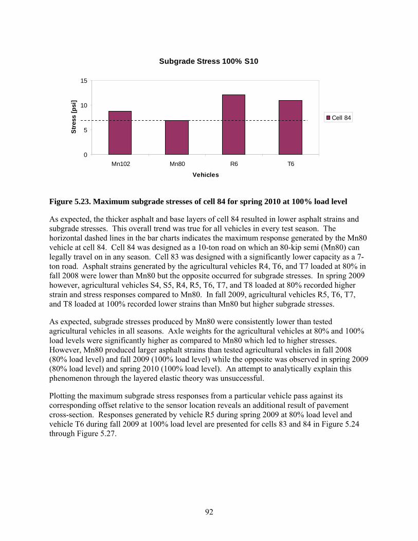
92

Subgrade Stress 100% S10

0

5

10

15

Mn102 Mn80 R6 T6

Vehicles

Stre

ss [p

si]

Cell 84

Figure 5.23. Maximum subgrade stresses of cell 84 for spring 2010 at 100% load level

As expected, the thicker asphalt and base layers of cell 84 resulted in lower asphalt strains and subgrade stresses. This overall trend was true for all vehicles in every test season. The horizontal dashed lines in the bar charts indicates the maximum response generated by the Mn80 vehicle at cell 84. Cell 84 was designed as a 10-ton road on which an 80-kip semi (Mn80) can legally travel on in any season. Cell 83 was designed with a significantly lower capacity as a 7-ton road. Asphalt strains generated by the agricultural vehicles R4, T6, and T7 loaded at 80% in fall 2008 were lower than Mn80 but the opposite occurred for subgrade stresses. In spring 2009 however, agricultural vehicles S4, S5, R4, R5, T6, T7, and T8 loaded at 80% recorded higher strain and stress responses compared to Mn80. In fall 2009, agricultural vehicles R5, T6, T7, and T8 loaded at 100% recorded lower strains than Mn80 but higher subgrade stresses.

As expected, subgrade stresses produced by Mn80 were consistently lower than tested agricultural vehicles in all seasons. Axle weights for the agricultural vehicles at 80% and 100% load levels were significantly higher as compared to Mn80 which led to higher stresses. However, Mn80 produced larger asphalt strains than tested agricultural vehicles in fall 2008 (80% load level) and fall 2009 (100% load level) while the opposite was observed in spring 2009 (80% load level) and spring 2010 (100% load level). An attempt to analytically explain this phenomenon through the layered elastic theory was unsuccessful.

Plotting the maximum subgrade stress responses from a particular vehicle pass against its corresponding offset relative to the sensor location reveals an additional result of pavement cross-section. Responses generated by vehicle R5 during spring 2009 at 80% load level and vehicle T6 during fall 2009 at 100% load level are presented for cells 83 and 84 in Figure 5.24 through Figure 5.27.

93

R5 Subgrade Stress (83PG4) 80% S09

0

5

10

15

20

-10 -5 0 5 10 15 20 25

Rear axle relative offset [in]

Stre

ss [p

si]

AMPM

Figure 5.24. Cell 83 vertical subgrade stress generated by R5 in spring 2009 at 80% load level

R5 Subgrade Stress (84PG4) 80% S09

0

5

10

15

20

-10 -5 0 5 10 15 20 25

Rear axle relative offset [in]

Stre

ss [p

si]

AMPM

Figure 5.25. Cell 84 vertical subgrade stress generated by R5 in spring 2009 at 80% load level

94

T6 Subgrade Stress (83PG4) 100% F09

0

5

10

15

20

25

30

-20 -15 -10 -5 0 5 10 15 20

Rear axle relative offset [in]

Stre

ss [p

si]

AMPM

Figure 5.26. Cell 83 vertical subgrade stress generated by T6 in fall 2009 at 100% load level

T6 Subgrade Stress (84PG4) 100% F09

0

5

10

15

20

25

30

-20 -15 -10 -5 0 5 10 15 20

Rear axle relative offset [in]

Stre

ss [p

si]

AMPM

Figure 5.27. Cell 84 vertical subgrade stress generated by T6 in fall 2009 at 100% load level

It was observed that for cell 84, measured subgrade stresses are reduced when the offset is significantly different from zero (directly over the sensor, approximately 15 in. from the pavement lane edge). This decrease can be observed for both positive (toward the shoulder) and negative (towards the centerline) offsets. The recorded subgrade stresses for wheel path locations above the sensor were twice as high as those recorded for the wheel paths closer to the pavement edge for both vehicles R5 and T6. It should be noted that the reduction in the maximum measured stress does not mean there is a reduction in the maximum subgrade stresses. The maximum subgrade stress occurs directly under the load, so it cannot be measured for the offset wheel paths due to lack of sensors under those locations.

95

Unlike cell 84, cell 83 did not exhibit significant reduction in the measured subgrade stress for positive wheel path offsets. This means that deviation in the wheel path toward the pavement edge does not reduce subgrade stresses at the pressure cell location which is 16 in. away from the pavement edge. It is reasonable to assume that the maximum subgrade stress directly below the axle loads at positive offsets is much higher than those measured by the earth pressure cell. This suggests that absence of a paved shoulder significantly increases the maximum subgrade stresses when the wheel path is near the pavement edge as illustrated in Figure 5.28.

Figure 5.28. Cross-section view of pave and unpaved sections

A similar effect was observed for asphalt strains. Figure 5.29 through Figure 5.34 show that when the traffic path is translated toward the shoulder and away from the sensor the measured asphalt strains in cell 84 are significantly reduced. However, cell 83 measured strains were not reduced for similar loading conditions. For vehicle R5, strain responses were decreased by approximately 7% as the wheel path approaches the pavement edge for cell 83. For cell 84 longitudinal strain, the decrease was roughly 50% and 70% for transverse strain. For vehicle T6, the decrease in angle strain for cell 83 was only 2% and the decrease for cell 84 longitudinal strain was approximately 25%. For the transverse strain in cell 84, there was an increase of 4% as the vehicle’s wheel path approached the pavement edge. The difference in responses of cells 83 and 84 for different wheel path locations are due to the effect of different pavement shoulders. Cell 83 has an aggregate shoulder and cell 84 has an asphalt shoulder. Cell 83, which has an aggregate shoulder, experienced higher coverage of the critical responses at the sensor location than cell 84. This clearly demonstrates the importance of the structural benefits of the asphalt shoulder.

P1a

P2a

P1b

P2b

Sensor 84PG4

Sensor 83PG4

Paved Shoulder (Cell 84) Aggregate Shoulder (Cell 83)

AC layer

AC layer

P1a = P2a

P1b = P2b

96

Figure 5.29. Cell 83 angled asphalt strain generated by R5 in spring 2009 at 80% load level

Figure 5.30. Cell 84 longitudinal asphalt strain generated by R5 in spring 2009 at 80% load level

97

Figure 5.31. Cell 84 transverse asphalt strain generated by R5 in spring 2009 at 80% load level

Figure 5.32. Cell 83 angled asphalt strain generated by T6 in fall 2009 at 100% load level

98

Figure 5.33. Cell 84 longitudinal asphalt strain generated by T6 in fall 2009 at 100% load level

Figure 5.34. Cell 84 transverse asphalt strain generated by T6 in fall 2009 at 100% load level

Effect of Vehicle Weight

The pavement responses in cell 84 from vehicles S5 for spring 2009 and T6 for fall 2009 are presented in Figure 5.35 through Figure 5.40. The maximum strain and stress responses from a particular vehicle pass were plotted against its corresponding offset relative to the sensor location. Figure 5.35 through Figure 5.37 show the response measurements for vehicle S5 and

99

Figure 5.38 through Figure 5.40 for vehicle T6. Gross vehicle weights were shown in the legends.

Figure 5.35. Cell 84 longitudinal asphalt strain generated by S5 in spring 2009 at various vehicle weights

Figure 5.36. Cell 84 transverse asphalt strain generated by S5 in spring 2009 at various vehicle weights

100

S5 Subgrade Stress (84PG4) S09

0

4

8

12

16

20

-15 -10 -5 0 5 10 15 20 25 30

Rear axle relative offset [in]

Stre

ss [p

si] 25 kip

34 kip43 kip55 kip

Figure 5.37. Cell 84 vertical subgrade stress generated by S5 in spring 2009 at various vehicle weights

Figure 5.38. Cell 84 longitudinal asphalt strain generated by T6 in fall 2009 at various vehicle weights

101

Figure 5.39. Cell 84 transverse asphalt strain generated by T6 in fall 2009 at various vehicle weights

T6 Subgrade Stress (84PG4) F09

0

5

10

15

20

25

-20 -15 -10 -5 0 5 10 15 20 25

Rear axle relative offset [in]

Stre

ss [p

si]

40 kip64 kip90 kip

Figure 5.40. Cell 84 vertical subgrade stress generated by T6 in fall 2009 at various vehicle weights

It can be observed that longitudinal and transverse strain responses generated by vehicle S5 (Figure 5.35 and Figure 5.36) steadily increase as vehicle weight increases. However, subgrade stresses for vehicle S5 for a gross weight of 25,000 lb (25 kip) were larger than at 55,000 lb (55 kip). This can be explained by referring to Figure 5.7 from the “Effects of Seasonal Changes” section which clearly shows a spike on the first day of spring 2009 testing for the Mn80 truck. This test day corresponds to the same day in which vehicle S5 was tested at 25 kip. Measurements collected on that day also resulted in the same trend for the other vehicles. An

102

increase in longitudinal strains and subgrade stresses as vehicle weight increases was also observed for vehicle T6 in fall 2009 as shown in Figure 5.38 and Figure 5.40, respectively. Responses for transverse strains however were not as clear and no strong correlation was observed between transverse strains with gross vehicle weight for T6. Overall, there was an increase in stresses and strains as vehicle weight increases. However, it should be noted that tests for different vehicle weights (load levels) were conducted on different days, hence daily fluctuations and seasonal effects should be accounted for. Strain responses in spring were typically much cleaner compared to fall and can be caused by several factors including change in characteristics of the asphalt layer, frequency of vehicle passes, and time interval between vehicle passes. It should be noted that the figures represent the maximum responses from the vehicles, and not from individual axles. An increase in gross vehicle weight did not lead to a proportional increase in axle weight as will be discussed in subsequent chapters.

Effect of Vehicle Type

Testing was conducted with the agricultural vehicles loaded at different load levels: 0%, 25%, 50%, 80%, and 100% of full tank capacity while control vehicles Mn80 and Mn102 remain the same weight. Weights of all vehicles were measured for every load level and this information is summarized in Appendix B. Table 5.2 and Table 5.3 summarize the gross weight of the vehicles for spring 2009 and fall 2009, respectively. This section focuses on changes in pavement responses as vehicle weight changes. An increase in vehicle weight should be reflected by an increase in pavement responses. As stated above, pavement responses for vehicle Mn80 at cell 84 were used as a benchmark to compare responses for other vehicles. Figure 5.41 through Figure 5.46 show the maximum strain and stress responses for agricultural vehicles for spring 2009 and fall 2009 at cell 84.

Table 5.2. Gross Weight for Vehicles Tested during Spring 2009

Vehicle Gross Vehicle Weight [lb] 0% 25% 50% 80%

S4 27,860 36,260 46,980 57,580 S5 25,180 34,040 42,940 54,840 R4 36,520 41,180 48,060 53,240 R5 31,480 35,520 39,600 43,740 T6 38,780 50,620 63,240 70,220 T7 58,540 72,840 88,050 103,600 T8 58,900 80,340 102,080 123,840

Mn80 79,560

103

Table 5.3. Gross Weight for Vehicles Tested during Fall 2009

Vehicle Gross Vehicle Weight [lb] 0% 50% 80%

R5 31,730 39,950 47,100 T6 39,710 64,400 89,500 T7 45,100 75,600 105,200 T8 58,200 97,600 134,200

Mn80 81,090

Analysis of Figure 5.41 through Figure 5.46 shows that, as a general trend, an increase in vehicle weight leads to an increase in pavement responses. However, this increase is not proportional to the increase in vehicle weight, and for some vehicles, the responses decreased when the vehicle weight increased. Several factors may have contributed to this trend:

• Since different vehicle weights were conducted on different days, the climatic factors such as temperature could have affected the results. Vehicle Mn80 to adjust the results for this effect.

• The increase in gross vehicle weight does not lead to a proportional increase in vehicle axle weights. As can be observed from Table 5.4, an increase in gross weight for vehicle T6 significantly affects axle weights for the 3rd and 4th axles, while the 1st and 2nd axles are mostly unaffected. Moreover, the second axle has the highest axle weight for 0% and 50%, while the 4th axle has the highest weight for 80% and 100% loading. The maximum responses shown in Figure 5.41 through Figure 5.46 can be produced by various axles for different load levels.

Table 5.4. Vehicle T6 Axle Weights at Various Load Levels

Axle 0% 25% 50% 80% [lb] [lb] [lb] [lb]

Axle 1 13,220 12,660 11,940 11,600 Axle 2 17,600 17,700 20,860 22,420 Axle 3 7,140 12,420 16,620 22,440 Axle 4 7,900 13,760 19,760 26,640 Total 45,860 56,540 69,180 83,100

104

Figure 5.41. Longitudinal asphalt strain at cell 84 generated by vehicles tested at 0%, 25%, 50%, and 80% in spring 2009

Figure 5.42. Transverse asphalt strain at cell 84 generated by vehicles tested at 0%, 25%, 50%, and 80% in spring 2009

105

Subgrade Stress (84PG4) S09

0

5

10

15

20

25

30

35

0% 25% 50% 80%

Load Level [%]

Stre

ss [p

si]

Mn80R4R5S4S5T6T7T8

Figure 5.43. Vertical subgrade stress at cell 84 generated by vehicles tested at 0%, 25%, 50%, and 80% in spring 2009

Figure 5.44. Longitudinal asphalt strain at cell 84 generated by vehicles tested at 0%, 50%, and 80% in fall 2009

106

Figure 5.45. Transverse asphalt strain at cell 84 generated by vehicles tested at 0%, 50%, and 80% in fall 2009

Subgrade Stress (84PG4) F09

0

5

10

15

20

25

0% 50% 100%

Load Level [%]

Str

ess

[psi

] Mn80R5T6T7T8

Figure 5.46. Vertical subgrade stress at cell 84 generated by vehicles tested at 0%, 50%, and 80% in fall 2009

One of the objectives of this study was to compare pavement responses from various agricultural vehicles to a standard 5-axle 80-kip semi truck which was represented by the Mn80 vehicle. Figure 5.41 through Figure 5.46 show that agricultural vehicles tested in this study at 80% and 100% of full capacity produce higher subgrade stresses (84PG4) compared to the standard 5-axle 80-kip semi truck (Mn80) in both spring and fall seasons. An increase in subgrade stresses compared to Mn80 ranged from 4% to 80% in spring 2009 and 35% to 80% in fall 2009 for agricultural vehicles loaded over 80% load level. On the other hand, asphalt strain levels

107

generated by the agricultural vehicles were dependent on test season. In spring, both longitudinal (84LE4) and transverse (84TE4) strains generated by Mn80 were typically smaller than the agricultural vehicles except for vehicle T6 for 84LE4 and vehicles R4 and R5 for 84TE4, even at 100% load capacity. In the fall, this trend was reversed with Mn80 producing larger strains than the other agricultural vehicles. In the spring of 2009 the S4 and T7 vehicles resulted in asphalt strains 20% and 48% higher than the Mn80 truck strains, respectively. In fall 2009, the difference in asphalt strain between vehicle T7 and Mn80 truck was -20%. An attempt to explain this trend using layered elastic analysis was not successful. Comparisons between the pavement responses across the pavement width generated by the agricultural vehicles and Mn80 are presented in Appendix D.

Effect of the Number of Axles

In the past decade, vehicle manufacturers of the agricultural industry began to design and produce larger equipment with larger capacities. However in order to be operating legally on public roads, axle weight restrictions must be met. To help achieve this goal, vehicles are equipped with additional axles. In this study the responses from vehicles T6, T7, and T8 shown in Figure 5.47 were compared. These vehicles are equipped with four, five, and six total axles, respectively, and have tank capacities of 6,000 gallons, 7,300 gallons, and 9,500 gallons, respectively. The following table (Table 5.5

108

Table 5.5) shows the axle weights of these vehicles loaded up to 100% when tested in fall 2009. Figure 5.48 shows the vertical subgrade stress responses at cell 84 generated by those three vehicles.

T6 – 4 axles (John Deere 8230, 6,000 gal) T7 - 5 axles (Case IH 335, 7,300 gal)

T8 – 6 axles (Case IH 335, 9,500 gal)

Figure 5.47. Vehicles with increasing tank capacity and number of axles

109

Table 5.5. Axle Weights of Vehicles T6, T7, and T8 at 100% in Fall 2009

Equipment Axle T6 (6,000 gal) T7 (7,300 gal) T8 (9,500 gal) [lb] [lb] [lb]

Tractor Axle 1 8,100 6,900 14,800 Axle 2 21,400 19,800 25,200

Tanker

Axle 3 26,500 26,300 23,300 Axle 4 33,500 26,200 23,700 Axle 5 26,000 23,500 Axle 6 23,700

Total vehicle weight 89,500 105,200 134,200

Tankers Subgrade Stress (84PG4) F09 100%

0

5

10

15

20

25

-25 -20 -15 -10 -5 0 5 10 15 20

Rear axle relative offset [in]

Stre

ss [p

si]

T6T7T8

Figure 5.48. Cell 84 vertical subgrade stress generated by vehicles T6, T7, and T8 at 100% load level in fall 2009

Analysis of Table 5.5 shows that although the gross weight of T6 is the lowest amongst these vehicles, its last axles exhibited the highest load (33,500 lb). Vehicle T8 had the highest gross weight. However, since the tanker had four axles, each of them resulted in a relatively low axle weight of 23,700 lb. It is interesting to note that the most loaded axle was not an axle on the tanker, but rather a rear tractor axle (axle two) which had a weight of 25,200 lb. As should be expected, vehicle T6 resulted in the highest subgrade stress while vehicle T8 resulted in the lowest subgrade stress.

Referring to Table 5.5, note that the first two axles for all three vehicles belong to the tractor. The axle weights of interest here are those belonging to the tankers which are axles three to six. Increasing the tank capacity evidently increases the overall vehicle weight. By adding axles to the tankers the weight per axle was successfully decreased with vehicle T6 having the heaviest tanker axle at 33,500 lb, T7 at 26,300 lb and T8 at 23,700 lb. Figure 5.43 and Figure 5.46 show that vertical subgrade stresses for T6 was largest followed by T7 and finally T8 for both spring 2009 and fall 2009 test. Figure 5.48 above clearly shows that vehicle T6 generates larger

110

subgrade stresses than the other two vehicles. Hence, for a larger tank capacity, equipping the tanker with additional axles can potentially reduce the generated subgrade stresses. Unfortunately, a similar trend was not observed for asphalt strains. It is worth mentioning that this comparison may not accurately describe the benefits of having additional axles since the tankers of vehicles T6, T7, and T8 were of non similar sizes. It should also be noted that the axle design on T6 allows the user to adjust axle spacing to balance the weight equally between the axles. Rebalancing would have reduced the weight of the rear axle but T6’s average axle weights would still have been heavier than T7 or T8.

Effect of Axle Weight

As was discussed above, the effect of gross vehicle weight on pavement responses did not show consistent results. This was attributed to several factors: 1) an increase in gross vehicle weight is not proportionally distributed to the axle weights 2) the maximum response 3) different vehicle weights were tested on different days under different temperature conditions. To account for this effect, the response from the rear axle of vehicle T6 was analyzed. A simple correction factor, di, was introduced to account for climatic effects. This correction factor is based on responses obtained from the control vehicle Mn80 as shown in the following equation.

i

iT

iMn

oMniTiT d

6

80

8066

σσσ

σσ =

= Equation5.1

Where iT 6σ is the adjusted subgrade stress from the rear axle of vehicle T6 for ith day

iT 6σ is the measured subgrade stress from the rear axle of vehicle T6 on ith day

oMn80σ is the reference subgrade stress for vehicle Mn80

iMn80σ is the measured subgrade stress for vehicle Mn80 on ith day

id is the ratio between measured subgrade stress on ith day and reference stress for vehicle Mn80

A similar equation was used to determine adjusted strain values by substituting strain measurements for stress measurements in Equation5.1. To maintain consistency the correction factor is always based on the responses generated by the heaviest axle of Mn80. The adjustment process was performed on the maximum response generated by the heaviest axle of the vehicle of interest across the entire pavement width. This step is important to identify the relationship between axle responses and axle weight instead of using the maximum response across the vehicle axles and total vehicle weight which may be misleading. Strain and stress responses for vehicle T6 from cell 83 and 84 were adjusted for every day of testing for fall 2008, spring 2009, fall 2009, and spring 2010. Response measurements on the fourth day of testing during fall 2008

111

were selected as the reference Mn80 response. The relationship between adjusted strain and stress responses and axle weight for vehicle T6 is shown in the following figures (Figure 5.49 to Figure 5.53). Figure 5.54 and Figure 5.55 show a comparison between both cells 83 and 84. This evaluation was made by selecting the maximum between adjusted longitudinal (84LE4) and transverse (84TE4) strains from cell 84 and comparing it to angled strain (83AE4) of cell 83.

Figure 5.49. Adjusted angled asphalt strain response from cell 83 for vehicle T6

Adjusted T6 Subgrade Stress (83PG4)

0

5

10

15

20

25

30

35

0 5000 10000 15000 20000 25000 30000 35000 40000

Axle weight [lb]

Stre

ss [p

si]

F08S09F09

Figure 5.50. Adjusted vertical subgrade stress response from cell 83 for vehicle T6

112

Figure 5.51. Adjusted longitudinal asphalt strain response from cell 84 for vehicle T6

Figure 5.52. Adjusted transverse asphalt strain response from cell 84 for vehicle T6

113

Adjusted T6 Subgrade Stress (84PG4)

0

5

10

15

20

25

0 5000 10000 15000 20000 25000 30000 35000 40000

Axle weight [lb]

Stre

ss [p

si] S09

F09F08S10

Figure 5.53. Adjusted vertical subgrade stress response from cell 84 for vehicle T6

Figure 5.54. Adjusted asphalt strain responses for vehicle T6 between cells 83 and 84

114

Adjusted T6 Subgrade Stress

0

5

10

15

20

25

30

35

0 5000 10000 15000 20000 25000 30000 35000 40000

Axle weight [lb]

Stre

ss [p

si]

Cell 83Cell 84

Figure 5.55. Adjusted subgrade stress responses for vehicle T6 between cells 83 and 84

The purpose of this exercise was to negate daily fluctuations in measured responses. It was observed that adjusted subgrade stress responses for vehicle T6 from both cells 83 and 84 have a linear relationship with axle weight, where a stronger linear correlation exists for cell 84. Adjusted asphalt strains from cells 83 and 84 increase with increasing axle weight. However, there is a significant scatter and the relationship is nonlinear. A possible explanation is the effect of traffic wander and higher sensitivity to temperature effect that cannot be accounted for with a simple adjustment such as the one described above. This effect requires further investigation.

Effect of Tire Type

In the agricultural industry, flotation tires are becoming increasingly popular due to its wider footprint and lower inflation pressure which allows the vehicle to travel over soil and unbound aggregate material with minimal compaction and rutting. With a wider footprint coupled with low inflation pressure, the wheel load is distributed over a larger area thus minimizing the exerted pressure onto the soil. This has proven to be immensely beneficial in the industry where less soil compaction and rutting decreases soil damage. An issue arises as to whether this characteristic can be translated directly to pavement performance.

In this section, two similar straight trucks with the same tank capacity of 4,400 gallons were fitted with two different tire types on the tanks, one with regular radial ply dual tire configuration, and the other with a flotation single tire configuration. Vehicle S4 was fitted with the radials and S5 with flotation tires as shown in Figure 5.56. Comparisons were made using contact area and contact pressure measurements from Tekscan. Additionally, asphalt strains and subgrade stresses produced by these two vehicles were evaluated.

115

(a) (b)

Figure 5.56. Straight trucks denoted as (a) vehicle S4 fitted with radial tires (b) vehicle S5 fitted with flotation tires

Tekscan measurements for both vehicles S4 and S5 were taken at load levels of 0%, 50%, and 80%. Because of the size constraint of the Tekscan equipment, only one side of each vehicle axle was recorded. The measurements were then calibrated with the actual wheel load corresponding to the load level. Table 5.6 summarizes the Tekscan results for both S4 and S5. In order to visualize the growth in contact area and change in contact pressure as wheel load increases, a simple plot was prepared as shown in Figure 5.57 and Figure 5.58. Additionally, an illustration of how the contact areas of the third axle for both vehicles change with increasing axle weight is shown in Figure 5.59.

116

Table 5.6. Tekscan Summary for Vehicle S4 and S5

Vehicle Load Level Axle Filename

Wheel Load Frame

Contact Area

Average Pressure

[%] [lb] [in2] [psi]

S4

0 1 S2_A1LA 5,580 7 56.89 98.1 0 2 S2_A2-3LB 3,680 26 52.41 70.2 0 3 S2_A2-3LB 3,400 45 44.35 76.7 50 1 S2_A1RC50 6,040 211 68.54 88.1 50 2 S2_A2-3RD50 7,800 18 96.31 81 50 3 S2_A2-3RC50 8,040 30 104.38 77 80 1 S2_A1RB80 6,460 30 79.74 81 80 2 S2_A2-3RA80 9,680 85 103.03 94 80 3 S2_A2-3RB80 10,300 98 126.77 81.2

S5

0 1 S1_A1LA 6,400 16 72.57 88.2 0 2 S1_A2-3LA 4,300 10 51.52 83.5 0 3 S1_A2-3LA 3,460 21 50.62 68.4 50 1 S1_A1RA50 7,900 51 81.53 96.9 50 2 S1_A2-3RA50 7,500 50 83.77 89.5 50 3 S1_A2-3RB50 8,390 76 103.48 81.1 80 1 S1_A1RA80 8,780 54 89.14 98.5 80 2 S1_A2-3RA80 9,980 22 105.72 94.4 80 3 S1_A2-3RA80 10,000 33 136.63 73.2

Contact Area

020406080

100120140160

0 2000 4000 6000 8000 10000 12000

Wheel load [lb]

Area

[in

2 ] S4 (radials)S5 (flotations)Linear (S4 (radials))Linear (S5 (flotations))

Figure 5.57. Contact area measurements for vehicles S4 and S5

117

Average Contact Pressure

0

20

40

60

80

100

120

0 2000 4000 6000 8000 10000 12000

Wheel load [lb]

Pres

sure

[psi

]

S4 (radials)S5 (flotations)Linear (S4 (radials))Linear (S5 (flotations))

Figure 5.58. Average contact pressure measurements for vehicles S4 and S5

118

S4 – Axle 3 – 8,700 lb S4 – Axle 3 – 16,280 lb S4 – Axle 3 – 21,460 lb

S5 – Axle 3 – 7,100 lb S5 – Axle 3 – 15,340 lb S5 – Axle 3 – 20,040 lb

Figure 5.59. Measured footprints for the third axle of vehicle S4 and S5 with corresponding axle weight

119

Vehicles S4 and S5 are equipped with tires that can deform under load and still maintain their structural capacity. Regular radial ply dual tires fitted onto vehicle S4 and flotation tires fitted onto vehicle S5 demonstrate an increase in contact area as the wheel load increases. A trendline fitted across the data points in Figure 5.57 shows that both tire types were similar in terms of contact area growth. With that being said, the average contact pressure for both vehicles also increased with wheel load levels but the increase was not as significant because of the larger contact area. There was no significant difference between the two tire types as shown in Figure 5.58.

Recognizing that the contact area and average contact pressure for both vehicles were very similar, the pavement response measurements were also evaluated to distinguish any benefits of flotation tires on pavement performance. To accomplish this comparison, the analysis was performed by excluding responses generated by the steering axles of both these vehicles. This ensures that the comparison was made exclusively between radial and flotation tires on the vehicles’ tanks. Table 5.7 shows the total tank weights for both vehicles S4 and S5. Figure 5.60 through Figure 5.67 show cells 83 and 84 pavement responses generated at load levels of 0% and 80% during spring 2009.

Table 5.7. Tank and Truck Weights for Vehicles S4 and S5

Load Level S4’s Tank S5’s Tank 0% 15,180 lb 14,040 lb 80% 40,980 lb 39,440 lb

Figure 5.60. Cell 83 angled asphalt strain generated at 0% load level for vehicles S4 and S5

120

Subgrade Stress (83PG4) 0% S09

0

2

4

6

8

10

-15 -10 -5 0 5 10 15 20

Rear axle relative offset [in]

Stre

ss [p

si]

S4S5

Figure 5.61. Cell 83 vertical subgrade stress generated at 0% load level for vehicles S4 and S5

Figure 5.62. Cell 84 longitudinal asphalt strain generated at 0% load level for vehicles S4 and S5

121

Subgrade Stress (84PG4) 0% S09

0

2

4

6

8

10

-15 -10 -5 0 5 10 15 20

Rear axle relative offset [in]

Stre

ss [p

si]

S4S5

Figure 5.63. Cell 84 vertical subgrade stress generated at 0% load level for vehicles S4 and S5

Figure 5.64. Cell 83 angled asphalt strain generated at 80% load level for vehicles S4 and S5

122

Subgrade Stress (83PG4) 80% S09

0

3

6

9

12

15

-10 -5 0 5 10 15 20

Rear axle relative offset [in]

Stre

ss [p

si]

S4S5

Figure 5.65. Cell 83 vertical subgrade stress generated at 80% load level for vehicles S4 and S5

Figure 5.66. Cell 84 longitudinal asphalt strain generated at 80% load level for vehicles S4 and S5

123

Subgrade Stress (84PG4) 80% S09

0

3

6

9

12

15

-10 -5 0 5 10 15 20

Rear axle relative offset [in]

Stre

ss [p

si]

S4S5

Figure 5.67. Cell 84 vertical subgrade stress generated at 80% load level for vehicles S4 and S5

Results show that vehicle S4 produces larger asphalt strains and subgrade stresses at 0% load levels on both cells 83 and 84. When loaded to 80%, maximum asphalt strains of both vehicles at cell 83 remain similar but the distribution across the pavement width did not. Maximum responses for vehicle S5 were recorded when the vehicles’ wheel path was close to the sensor. For vehicle S4, the maximum occurs when the wheel path was toward the pavement shoulder (positive direction). At cell 84, the response distributions across the pavement width show a decreasing trend as both vehicles travel away from the sensor toward the shoulder. This not only shows the benefits of a paved shoulder but also allows for a more objective representation between responses of both vehicles S4 and S5. Although maximum values were approximately similar, vehicle S4 was observed to consistently produce slightly larger strains and stresses across the pavement width.

The observed pavement response distributions in cell 83 can be attributed to the difference in axle configuration between the two vehicles. Vehicle S4 was equipped with dual radial tires whereas S5 was equipped with a single flotation tire on the rear axles. Because of the dual tire configuration (the half axle load is applied onto two separate wheels) the observed response distribution for vehicle S4 occurred when one side of the dual tires was completely on the aggregate shoulder and the other on the asphalt pavement. On the other hand, the center of the applied load of vehicle S5 was confined within the footprint of a single flotation tire which allows for a more uniform distribution of the vehicle weight.

Effects of Vehicle Speed

Asphalt layers have viscoelastic properties and thus the stress-strain relationship is dependent on the loading rate. In general, the longer the duration of the load, the higher the asphalt strains. In this study, vehicles were tested at creep speed, 5 mph, 10 mph, and high speed (approximately 15 mph to 25 mph) to investigate the dependence of both asphalt strains and subgrade stresses on loading rate. Unfortunately, vehicles could not be tested at operating speeds (approximately 35

124

mph) due to the layout of the farm loop testing site. Nevertheless, vehicle T6 was presented here for tests performed in fall 2009 at 100% load level. Figure 5.68 through Figure 5.72 show the pavement responses across the pavement width relative to the sensor location. The following figures show the measured strain and stress measurements corresponding to target vehicle speeds. To ensure that the target speeds accurately describe the actual speed of the vehicle, the elapsed time of the axle responses obtained through the results of the Peak-Pick analysis was used to calculate the actual speed. Knowing the spacing between the vehicles’ axles and the time between axle responses, the actual speed of the vehicle was determined. For this computation, it was sufficient to utilize the time elapsed of the first and second axle. The time elapsed recorded under the earth pressure cells (PG sensors) was used because it provided the cleanest and most consistent response waveform. The actual speed of vehicle T6 presented in this section is summarized in Table 5.8.

Figure 5.68. Cell 83 angled asphalt strain generated by vehicle T6 at various speeds in fall 2009

125

T6 Subgrade Stress (83PG4) 100% F09

0

5

10

15

20

25

30

-25 -20 -15 -10 -5 0 5 10 15 20

Rear axle relative offset [in]

Stre

ss [p

si]

10mph5mphHiSpd

Figure 5.69. Cell 83 vertical subgrade stress generated by vehicle T6 at various speeds in fall 2009

Figure 5.70. Cell 84 longitudinal asphalt strain generated by vehicle T6 at various speeds in fall 2009

126

Figure 5.71. Cell 84 transverse asphalt strain generated by vehicle T6 at various speeds in fall 2009

T6 Subgrade Stress (84PG4) 100% F09

0

5

10

15

20

25

30

-25 -20 -15 -10 -5 0 5 10 15 20

Rear axle relative offset [in]

Stre

ss [p

si]

10mph5mphHiSpd

Figure 5.72. Cell 84 vertical subgrade stress generated by vehicle T6 at various speeds in fall 2009

127

Table 5.8. Computed Actual Speeds for Vehicle T6

Target Speed Actual Average Speed Standard Deviation Cell 83 Cell 84 Cell 83 Cell 84

5 mph 5.32 mph 5.30 mph 0.08 mph 0.08 mph 10 mph 10.36 mph 10.26 mph 0.46 mph 0.27 mph

High Speed 15.23 mph 15.56 mph 0.78 mph 0.29 mph

Analysis of Table 5.8 shows that the actual vehicle speeds were consistent with the target speeds. The standard deviations were no more than 1 mph from the average actual speed. Also, at high speeds, T6 was travelling at an average of 15.23 mph. The pavement responses show no strong correlation with vehicle speed. It was expected that asphalt strains should be highest for passes at 5 mph, and decrease as the vehicle speed increased. This trend was not obvious for vehicle T6 as well as other vehicles. Therefore, it can be concluded that strains were not significantly affected for the range of speeds and conditions of this study.

Effects of Early Fall vs. Late Fall

Figure 5.73. Effects of subgrade stresses in early fall vs. late fall

Figure 5.73 indicates that in both November 2010 and August 2010, the subgrade stresses generated by T6 were higher than those generated by the Mn80 vehicle. It can also be seen that the subgrade stresses for both T6 and Mn80 were higher in August 2010 than in November 2010. This is most likely due to the stiffening of the pavement due to the temperatures dropping.

Tekscan Measurements

Heavy agricultural vehicles are equipped with tires which possess complex load distributions. As explained in the previous section, tire footprints are different for various tire types and load

128

levels. The purpose of conducting the Tekscan testing was to measure the tire footprint of the agricultural vehicles and obtain the tire loading pattern as vehicle weight increases. Vehicle T1 was used as an example in this section.

Vehicle T1 consists of a John Deere 8430 tractor pulling a 6,000 gallon Houle tank. The first two axles belong to the tractor and the last two belong to the tank. When the tank is loaded, the majority of the total vehicle weight is shifted to the last two axles (i.e. axles three and four). An example of the tire footprints belonging to the third and fourth axles of vehicle T1 as axle weight increases are shown in Figure 5.74. The subsequent figure (Figure 5.75) shows the change in contact area for each axle as the axle weight increases. The left side vertical axis represents the contact area for the bar plots and the right side vertical axis represents the axle load for the line plots. The same type of figure was presented for average contact pressure shown in Figure 5.76 with the left side vertical axis representing the contact pressure. Appendix E contains the change in contact area and contact pressure with axle weight for other vehicles tested with Tekscan.

Additionally, an overall comparison was made across all vehicles tested with Tekscan. The comparison was performed by selecting values for the axle with the highest axle weight when loaded to 80% load level. The values for that same axle were extracted at 0% load level to determine changes in contact area and contact pressure. Table 5.9 summarizes the heaviest axle for all vehicles. Figure 5.77 illustrates the changes for contact area between 0% and 80% load levels whereas Figure 5.78 shows the changes in contact pressure.

129

T1 – Axle 3 – 6,280 lb T1 – Axle 3 – 16,760 lb T1 – Axle 3 – 21,000 lb

T1 – Axle 4 – 7,980 lb T1 – Axle 4 – 19,550 lb T1 – Axle 4 – 24,680 lb

Figure 5.74. Measured footprints for the third and fourth axles of vehicle T1 with corresponding axle weight

130

Vehicle T1 Contact Area

0

50

100

150

200

250

300

1 2 3 4

Axle

Area

[in

2 ]

0

10,000

20,000

30,000

40,000

50,000

Axle

wei

ght [

lb] 0% area

50% area80% area0% load50% load80% load

Figure 5.75. Change in contact area as axle load increases for vehicle T1’s axles

Vehicle T1 Contact Pressure

0

40

80

120

160

1 2 3 4

Axle

Pres

sure

[psi

]

0

10,000

20,000

30,000

40,000

50,000

Axle

wei

ght [

lb] 0% pressure

50% pressure80% pressure0% load50% load80% load

Figure 5.76. Change in average contact pressure as axle load increases for vehicle T1’s axles

131

Table 5.9. Heaviest Axle at 80% Load Level

Vehicle Axle Axle Weight [lb] S4 3 20,240 S5 3 19,900 R4 2 38,420 S3 2 30,600 T1 4 24,680 T2 3 16,920 T6 4 26,640 T7 2 22,680 T8 4 20,360

Mn80 (80 kip) 5 18,000

Contact Area (based on heaviest axle at 80%)

0

50

100

150

200

250

300

S4 S5 R4 S3 T1 T2 T6 T7 T8Mn8

0

Vehicles

Area

[in

2 ]

0

10,000

20,000

30,000

40,000

50,000

Axle

wei

ght [

lb]

0% area80% area0% load80% load

Figure 5.77. Contact area comparison between 0% and 80% load levels

Figure 5.77 has data missing for the vehicle T8 that was never gathered.

132

Contact Pressure (based on heaviest axle at 80%)

0

40

80

120

160

S4 S5 R4 S3 T1 T2 T6 T7 T8Mn8

0

Vehicles

Pres

sure

[psi

]

0

10,000

20,000

30,000

40,000

50,000

Axle

wei

ght [

lb]

0% pressure80% pressure0% load80% load

Figure 5.78. Average contact pressure comparison between 0% and 80% load levels

Figure 5.75 shows that as the axle load increases the contact area increases as well. The increase in axle load has a minimal effect on average contact pressure as shown in Figure 5.76. The increase in average contact pressure is not significant due to the increase in contact area as shown in Figure 5.77. For the majority of vehicles, an increase in axle load also leads to an increase in contact pressure, although not proportionally. In some cases, the contact pressure decreased with increasing load as shown in Figure 5.78 for vehicles R4 and T7. Contact pressure for vehicle S3 however increased more than the other vehicles. This can be explained by how little the contact area expanded under the 80% load level. It should be noted that for all vehicles tested with Tekscan, except T2, their measured axle weights loaded at 80% were higher than the maximum axle weight measured for Mn80. It is also worth noting that there are potential errors when performing the Tekscan test and processing the Tekscan data. For instance, Tekscan measurements could be affected by the acceleration of the vehicle as it rolls across the sensorial mat. This acceleration can cause the material inside the vehicle tank to shift which affects the exerted load between axles. Additionally, the Tekscan tests were performed with a moving load but the post calibration was performed statically which may have a slight effect on the results.

Apart from obtaining the contact area and average contact pressure of these vehicles, manipulating the Tekscan measurements provided additional information regarding the loading pattern and load distribution of these tires. Knowing the load distributions of these complex tires greatly increases the accuracy in computer modeling. The conventional method of applying load to mimic a vehicle footprint in layered elastic theory is by approximating it with a uniformly distributed circular area. However, the complexity of agricultural vehicles’ tires is not precisely modeled as such. Instead of using one loaded circular area, the entire actual footprint was estimated with several smaller circles called the multi-circular area representation. Figure 5.79 shows multi-circular area estimation for the second axle of vehicle T7. The effect of modeling the footprint using the gross area versus the multi-circular area estimation was quite considerable. This information was extensively used in the layered elastic modeling section discussed in the next chapter.

133

(a) (b)

Figure 5.79. Second axle footprint of vehicle T7 (a) measured using Tekscan (b) multi-circular area representation

Summary (Flexible Pavements)

As stated previously, pavement responses are influenced by axle loads, environmental effects, pavement structure, and vehicle wheel path. Preliminary analysis showed that the transverse location of the vehicles’ wheel path affects which axle was responsible for the maximum pavement responses.

Asphalt strain responses were consistently lower in the spring compared to the fall season. However, observations showed no strong correlation between subgrade stresses and seasonal changes. Testing performed in the morning resulted in lower asphalt strains and subgrade stresses compared to testing performed in the afternoon. Agricultural vehicles loaded at 80% and 100% load levels recorded larger subgrade stresses compared to the control vehicle (Mn80) during testing in both spring and fall seasons. Asphalt strains generated by the agricultural vehicles in the spring tests recorded higher asphalt strains than vehicle Mn80. However, testing conducted in the fall seasons resulted in vehicle Mn80 producing larger asphalt strains compared to the tested agricultural vehicles.

Thicker asphalt and base layers resulted in lower asphalt strain and subgrade stress responses. Additionally, the absence of a paved shoulder greatly increased both asphalt strain and subgrade stress measurements as the vehicles’ wheel path approached the pavement edge. Analysis showed that an increase in gross vehicle weight resulted in an increase in pavement responses. No significant benefits were observed between flotation tires and radial tires in pavement responses. Preliminary analysis showed no significant effect of the range of tested vehicle speed.

134

Tekscan measurements showed that the agricultural vehicles’ contact areas increased as axle weight increased. The increase in average contact areas was not significant as the contact area increased from an increase in the axle weight.

135

Chapter 6. Preliminary Data Analysis (Rigid Pavements)

A total of seven comprehensive field testing runs were conducted throughout a three year span. Large amounts of pavement response measurements, field observation video files and pictures were taken during each field test run. This chapter presents the analysis results of each field test run highlighting the impact of agricultural vehicles on rigid pavement critical responses and significant distress.

Since this research study started in 2008, some of the sensors did not survive and deteriorated from a large number of vehicle test runs. A broken sensor gives high noise level output. Therefore, the broken sensors and improperly functioning sensors were identified and were excluded from the data analysis to minimize bias and error.

Various factors could influence rigid pavement responses. These factors include types of vehicles, vehicle load levels, traffic relative offsets, pavement geometric features, environmental condition, etc. In the first stage of analyses, a comprehensive statistical analysis (F-test) was performed to determine which variables significantly influence rigid pavement responses in this study. Table 6.1 presents a summary of the statistical analysis results for fall 2009 test program on cell 54 as an illustration.

An F-test result can be expressed in terms of a p-value, which represents the weight of evidence for rejecting the null hypothesis. The null hypothesis is the equality of mean of difference between comparisons of pavement responses under each variable. The null hypothesis can be rejected, i.e. the mean of difference between comparisons are significantly different and the variable associated with pavement responses is a significant parameter, if the p-value is less than the selected significance level (α). A Type I error (α) of 0.05 was used for all paired t-tests.

Table 6.1. Statistical Analysis for Fall 2009, Cell 54, Mn102

Variables t Ratio Prob.>|t| Significant?

Vehicle speed (mph) -0.04 0.9645 No

Relative Offset (in) 11.74 <0.0001* Yes

Based on the statistical analysis, speed was not statistically significant with respect to rigid pavement response measurements under the circumstances of this study. Therefore, the effect of the speed was not investigated in detailed analysis addressed in the following sub sections. This is within the expectation since the speeds of the test vehicles are 5, 10, or 15 mph which are relatively slow.

Spring 2008

Spring 2008 was the period of first field test run for this study. The primary objective of spring 2008 test run was to evaluate the field test program and data processing methodologies. An overview of the spring 2008 field test program is as follows:

136

• Test data for rigid pavements: March 24th to 26th, 2008 (Test periods of spring 2008 test: March 17th to 19th and March 24th to March 26th 2008)

• Tested vehicles: S1, S2, S3, T1, T2, T3, and Mn80 • Load levels: 50% and 80% • Vehicle speeds: static (creep), 5 mph, and 10 mph • Vehicle offset: 0 and 12 in • Tire pressure for vehicle T1: 33 and 42 psi • Properly tested vehicles identified after date processing: S3, T2, and T3 • No measurements of traffic wander • Total of 48 runs

A total of six vehicles were tested under two different load levels, 50% and 100% at crawling speed for both cell 32 and 54. However, the three vehicles (S3, T2, and T3) were identified as properly tested vehicles after data processing described in Chapter 3. The recording of traffic wander was not properly conducted so it was recommended to use offset scale with video recording. Analysis for spring 2008 was focused on a comparison of the maximum responses obtained from among the vehicle passes.

Sensor Status and Field Observation spring 2008 field testing was conducted from March 17 to March 19, and March 24 to March 26, on six different vehicles (S1, S2, S3, T1, T2, T3) at two load levels (50% and 80%). Apparent pavement distress was not observed during the course of testing on both cell 32 and 54. Table 6.2 is the summary of the sensor status during the spring 2008 field testing after data processing. Sensor status marked as “no” means that the sensor was not working at the time of the testing and thus was excluded from the data analysis. The extremely cold weather at the time of field testing for spring 2008 might have rendered sensors inoperational.

Table 6.2. Sensor Working Status during Spring 2008 Field Testing

Cell 54 Cell 32

Strain Working status Strain Working

status 54CE101 yes 32CE101 no 54HC101 no 32CE103 no 54HC102 no 32CE109 no 54HC103 no 32CE111 no 54HC104 no 32CE115 yes 54HC105 no 32CE117 no 54HC106 no 32CE138 yes

32CE139 yes

32PG101 no

As shown inTable 6.2, the one and the only functional sensor on cell 54 was “54CE101” during spring 2008 field testing. Therefore, pavement responses from sensor “54CE101” were analyzed

137

for cell 54. The maximum tensile strain was chosen for comparison regardless of the sensor location on cell 32 even though there were three different strain sensors and they have different orientations. This is because traffic wander was not recorded at the time of testing and all vehicles paths were targeted at 0 in. and 12 in. offset.

Effect of Vehicle Types and Load Levels on Pavement Strains The pavement responses from three vehicles (S3, T2, and T3) were identified to be recorded properly during the spring 2008 field testing. Figure 6.1 is a graphical representation of the maximum tensile strain induced by S3, T2, and T3 on cell 32 with half loaded (50%) and full loaded (100%) conditions.

As seen in Figure 6.1, it is apparent that pavement strains introduced by 80% loaded agricultural vehicles are more than four times than those by 50% loaded vehicles for cell 32. Additionally, it is observed that the maximum tensile strains of S3 with 50% loaded are higher than those of T2 and T3. The maximum tensile strains of T3 are higher than those of S3 and T2 under 100 % loaded condition. It is interesting to note that S3 could provide higher response than T2 under same load levels although the gross weight of S3 is less than T2.

Figure 6.1 presents the maximum tensile strains produced by different vehicle-load combinations for cell 54. Similar to observations from cell 54, strains under 80% load level are higher than those of 50% load level. Only small strains differences (about 0.2 to 2 micro strains) are observed among tested vehicles. This could be attributed to the PCC pavement on cell 54 being 7.5 in. thick which is 2.5 inches thicker than cell 32. Dowel bars on cell 54 may help reduce the sensitivity of the PCC pavement due to heavy loading as well.

Figure 6.1. Cell 32 pavement strain comparison under various vehicle-load combinations during spring 2008 field testing

138

Figure 6.2. Cell 54 pavement strain comparison under various vehicle-load combinations during spring 2008 field testing

Effect of Pavement Thickness on Pavement Strains The pavement strain responses obtained from spring 2008 field testing were compared at same load level to investigate the effect of the pavement thickness on pavement responses. Figure 6.3 compared the pavement strain response measurements of three vehicles under 50% load level at cell 32 (5 inches of PCC thickness) and cell 54 (7.5 inches of PCC thickness). It is observed that the pavement strains on cell 32 are higher than cell 54 for all vehicles loaded at 50%. This is understandable because the PCC pavement on cell 54 is 2.5 in. thicker than that on cell 32. T2 provided the lowest pavement maximum strain under 50% load level on both pavement sections (cell 32 and cell 54). The strain difference between cell 32 and cell 54 of T2 are the smallest compared with those of the others. This is because T2 is a tandem axle tanker and it has a smaller tank compared to T3.

139

Figure 6.3. Effect of pavement thickness on pavement strain under 50% load level during spring 2008 field testing

Figure 6.4. Effect of pavement thickness on pavement strain under 80% load level during spring 2008 field testing

Figure 6.4 is a graphical presentation of the effect of the pavement thickness on pavement strain under 80% load level during spring 2008 field testing. As seen in Figure 6.4, pavement strains on cell 32 are higher than cell 54 for all vehicles loaded at 80%. Additionally, by comparing Error! Reference source not found. and Figure 6.4, it is easy to see that the differences among pavement strains of vehicles become smaller as the slab thickness increases. This result illustrates the effect of pavement thickness on PCC tensile strain measurements.

140

Effect of Tire Type on Pavement Strain Vehicle S1 has tandem axles with single flotation tire while S2 has tandem axle with dual radial tires. Both S1 and S2 have a 4,400 gallon tank and strains produced by them were compared to study the effect of tire type on the pavement responses. Comparisons were made only on cell 54 when both vehicles are 80% loaded. By comparing the maximum strain produced by both vehicles, it was found that S1 produced a strain of 7.44 µε while S2 introduced a strain of 7.97 µε. The differences are insignificant and comparisons cannot really be made since there were only eight runs.

Spring 2008 Summary The following preliminary findings were made using limited data collected in spring 2008.

• As load level increases, all PCC pavement responses increase. • Two-axle vehicle of S3 (Ag-Chem) could provide higher PCC pavement strains than T2

under same load levels although the gross weight (1,800 gallons) of S3 is less than that (4400 gallons) of T2.

• The thinner the rigid pavement, the more sensitive the responses.

Based on the spring 2008 field testing results, it was recommended that more runs should have been performed for a thoroughly comparison. The effect of traffic wander on pavement performance should be investigated using proper recording system. The use of offset scale with video recording was recommended for this purpose.

Fall 2008

A total of five farm vehicles were tested during fall 2008 field testing. A brief overview of the fall 2008 field testing is shown as follows:

• Test data for rigid pavements: August 29th, 2008 (Test periods of fall 2008 test: August 26th to August 29th, 2008)

• Tested vehicle: R4, T3, T4, T5, and Mn80 • Load levels: 0% and 80% • Vehicle speeds: static (creep), 5 mph, and 10 mph • Vehicle offset: 0 and 12 in. • All vehicles have tire pressures which they normally operated by • Scales for traffic wander were painted on the pavement surface and videos of vehicle

wheel path were recorded to measure the traffic wander • Total of 72 runs

Although scales for traffic wander were painted onto the pavement surface using scaled pavement stencils, the paint quickly faded with increasing traffic. The actual traffic offsets were difficult to determine by reviewing recorded videos of vehicle wheel path movements. The permanent steel scales with video recording were recommended for use in future tests. Similar to spring 2008 test analysis, analysis for fall 2008 was focused on a comparison of the maximum responses obtained from the vehicle passes. The effect of the vehicle speed was not studied during fall 2008 field testing.

141

Sensor Status and Field Observation Five vehicles (R4, T3, T4, T5, and Mn80) were extensively tested on cell 32 and cell 54 on August 29th, 2008. No visible pavement distresses were observed throughout the testing course. Table 6.3 summarizes the fall 2008 field testing sensor status identified during data processing. Sensors that are marked “yes” were working sensors and the associated data were analyzed. Sensors that were noisy or not working were excluded from the analysis process.

Table 6.3. Sensor Status during Fall 2008 Field Testing

Cell 54 Cell 32

Strain Working status LVDT status Strain Working status

54CE101 yes 54DT101 no 32CE101 yes 54CE102 yes 54DT102 no 32CE103 yes 54CE103 no 54DT103 no 32CE109 yes 54CE104 yes 54DT104 yes 32CE111 no 54CE105 yes 54DT105 yes 32CE115 no 54CE106 yes 54DT106 yes 32CE117 no 54CE107 no 54DT107 yes

54DT108 no 54DT109 yes

Although multiple sensors were functional at the time of testing during fall 2008 field testing on both cell 32 and cell 54, only the maximum tensile strains were chosen for comparison due to lack of traffic wander information.

Effect of Vehicle Types and Load levels on Pavement Strains The maximum tensile strains of various vehicle-load combinations obtained from cell 32 and cell 54 are illustrated in Figure 6.5 and Figure 6.6, respectively. These figures demonstrate that pavement strains under 80% load level are definitely higher than those under 0% for cell 32 for all vehicles. R4 provided higher maximum tensile strains among agricultural vehicles in both of cell 32 and cell 54. At 80% of load level in cell 32, the maximum tensile strains of both of T3 and T5 were not higher than that of Mn80 truck (See Figure 6.5). At 0% of load level in both of cell 32 and cell 54, the maximum tensile strains of both of T3 and T5 were not higher than that of Mn80 truck (See Figure 6.5 and Figure 6.6). These results indicate that the tankers tested in fall 2008 could provide maximum tensile strains comparable to Mn80 truck.

142

Figure 6.5. Cell 32 pavement strain comparison during fall 2008 field testing

Figure 6.6. Cell 54 pavement strain comparison during fall 2008 field testing

Among all the vehicles, R4 produced the highest tensile strain on both cell 32 and cell 54. This is because R4 is single axle Terragator and the front axle includes only one tire.

Effect of Pavement Thickness on Pavement Strains The effect of the PCC pavement thickness on pavement strains was investigated by testing two of the cells with different slab thicknesses. Cell 54 has a slab thickness of 7.5 inches while (the pavement of) cell 32 is 5 inches thick. Figure 6.7 is a graphical representation of the maximum tensile strain comparisons induced by tested vehicles under 0% load level on both cell 32 and 54.

143

As seen in Figure 6.7, the tensile strains of farm vehicles under 0% of load level are not much different in both of cell 32 and cell 54. Only Mn80 truck produces lower tensile strains at cell 54 than at cell 32. However, most of agricultural vehicles strain measurements except T5 at cell 54 were lower than cell 32.

Figure 6.7. Effect of pavement thickness on pavement strain under 0% load level during fall 2008 field testing

Figure 6.8 is a graphical representation of the maximum tensile strain comparisons induced by tested vehicles under 80% load level on both cell 32 and 54.

As seen in Figure 6.8, the tensile strains of farm vehicles under 80% of load level on cell 32 are higher than those on cell 54 except for T5. This exception could be attributed to different relative offsets corresponding to each of the maximum tensile strains compared in Figure 6.8. Additionally, the reason that pavement responses produced on cell 32 is higher than those on cell 54 is because cell 32 is 2.5 in. thinner than cell 54 and thus is more sensitive to heavy loading.

144

Figure 6.8. Effect of pavement thickness on pavement strain under 80% load level during fall 2008 field testing

Fall 2008 Summary The following preliminary findings were made using limited data collected in spring 2008.

• As load levels increases, all PCC pavement responses increase. • The maximum tensile strains produced by single axle Terragator R4 are higher than those

of the others for both cell 32 and cell 54. • The tankers, T3 (tandem axle), T4 (Tridem axle), and T5 (Quad axle), tested in fall 2008

provided maximum tensile strains comparable to Mn80 truck. • The effect of pavement thickness is prominent at higher load level for farm equipment.

The use of traffic wander scale painted on surface of PCC slab was not desirable to determine actual traffic offset. The permanent steel scales with video recording were recommended for use in future tests.

Spring 2009

Seven farm vehicles (S4, S5, R4, R6, T7, and T8) were studies along with two control vehicles (Mn80 and Mn102) during the spring 2009 field testing cycle. Two load levels of 50% and 80% were used for all the farm equipment along with investigation of the effect of PCC slab thickness, traffic wander, and vehicle types/gear configurations on the pavement responses. A brief overview is shown as follows:

• Test data for rigid pavements: March 20th, 2009 (Test periods of spring 2009 test: March 16th to March 20th, 2009)

• Tested vehicles: S4, S5, R4, R5, T6, T7, T8, Mn80 and Mn102 • Load levels: 50% and 80% • Vehicle speeds: 5 mph, 10 mph and high speed (15-20 mph)

145

• Vehicle offsets: 0 and 12 in. • Permanent steel scales were installed onto the pavement to estimate traffic wander • Total of 170 runs

Sensor Status and Field Observation Nine vehicles, including seven farm vehicles and two MnROAD standard semi-trucks, were circulated and tested on cell 32 and cell 54. During the course of the testing, the corner crack was observed on cell 32 while no apparent distress was observed on cell 54.

The sensors status at cell 54 and cell 32 were examined through data processing procedure and summarized in Table 6.4. For cell 54, all four longitudinal strain sensors and three out of 10 LVDTs were properly working during the course of the field testing. All six strains sensors were not functioning well on cell 32. Since the permanent steel scales were used to estimate the actual traffic wander, highest pavement response values of each relative offset on each vehicle were analyzed in spring 2009 test.

Table 6.4. PCC Pavement Sensor Status for Spring 2009 Test

Cell 54 Cell 32

TCS Working

status LVDT status TCS Working

status 54CE001 yes 54DT001 no 32CE101 no 54CE002 yes 54DT002 no 32CE103 no 54CE003 yes 54DT003 no 32CE109 no 54CE006 yes 54DT005 no 32CE111 no 54DT006 yes 32CE115 no 54DT007 yes 32CE117 no 54DT008 yes 54DT009 no, noisy 54DT010 no 54DT004

Effect of Sensor Location and Relative Offset on Pavement Strains As shown in Table 6.4, four strain sensors on cell 54 were functional during spring 2009 field testing. All four sensors were embedded in the PCC slab at different locations. In order to investigate the effect of sensor location on the pavement strain and to choose a critical sensor output for consistent data analysis, pavement strains produced by Mn80 from each of sensor on cell 54 are investigated as shown Figure 6.9. As presented in Figure 6.9Error! Reference source not found., sensor “54CE3” produced the highest pavement tensile strains among all four sensors for various relative offset. Therefore, pavement tensile strain responses from sensor “54CE3” produced by various agricultural vehicles are utilized for further analysis.

146

Figure 6.9. Pavement strain produced by Mn80 from different sensors

None of the strain sensors were functional during spring 2009 field testing on cell 32, therefore, data analysis were not performed for cell 32 for this testing season.

Effect of Load Levels and Relative Offset on Pavement Strains The effects of the load levels (50% and 80%) with relative offsets on the pavement strains introduced by various vehicles were investigated in spring 2009 test program. The pavement strain responses at cell 54 were plotted along with corresponding relative offset of each run of the tested vehicles in Figure 6.10. As shown in Figure 6.10, it is easily found that the strain responses decrease dramatically as the relative offset increases. Terra-gator R4 produced similar pavement strain when it was 50% and 80% loaded. In comparison to the Mn80, the higher pavement strains of R4 were observed as the relative offset changes. Please refer to Appendix B for the other vehicles tested since they produced similar trends.

147

Figure 6.10. Pavement strain comparisons introduced by R4 on cell 54 during spring 2009 field testing

Effect of Vehicle Types with Relative Offsets on Pavement Strains All the maximum strain responses generated by all tested vehicles at cell 54 are plotted in Figure 6.11 for 50% of load level and Figure 6.12 for 100% of load level. As seen in Figure 6.11, the stain responses decrease dramatically as the relative offset increases. Strain responses for MnROAD vehicles (Mn80 or Mn102) at cell 54 were used as a benchmark to compare responses for other vehicles. In comparison to strain responses of Mn80 under 50% of load level, higher strain responses were observed at the strain responses of R4 at less than 0 inches of relative offset and strain responses of T8 at higher than 0 inches of relative offset. Strain responses of T8 at higher than 0 inch of relative offset were even higher than those of Mn102. The strain responses of other farm vehicles tested were same as or less than those of Mn80 and Mn102.

148

Figure 6.11. Cell 54 pavement strain responses during spring 2009 field testing at 50% load level

Figure 6.12. Cell 54 pavement strain responses during spring 2009 field testing at 80% load level

Figure 6.12 is graphical comparison for the strain introduced by all the vehicles at 80% load level. Similar to Figure 6.11, it illustrates that as the relative offset increases, the pavement strain decreases. Higher strain responses of R4 and T8 were observed in comparisons to strain responses of Mn80 under 100% of load level.

149

Effect of Tire Type on Pavement Responses S4 and S5 were tested in spring 2009 to investigate the effect of the tire type on pavement responses. S4 is a straight truck which has a tandem axle with dual radial tires while S5 has a tandem axle with single flotation tire. Both S4 and S5 have a 4,400 gallons Husky tank.

Figure 6.13 presents strain response comparisons between S4 and S5 at their 50% load level on cell 54. According to these comparisons, S4 with dual tires resulted in slightly higher pavement strain than S5 with single flotation tire.

Figure 6.13. Strain comparisons between radio and flotation tire at 50% load level

Figure 6.14 presents strain response comparisons between S4 and S5 at their 80% load level. Similar to Figure 6.13, it illustrates that S4 produces similar pavement strain with S5. The results demonstrate that flotation tires are more advantageous to reduce the pavement responses introduced by straight truck at relative low load level. Pavement strain response becomes identical as load level increase to 80%. Therefore, it could be concluded that flotation tire are not helpful to reduce pavement response when straight trucks are loaded more than half of the tank.

150

Figure 6.14. Strain comparisons between radio and flotation tire at 80% load level

Spring 2009 Summary The following preliminary findings were made using data collected in spring 2009.

• The pavement strain responses decrease as the relative offset increases. • Higher strain responses of R4 and T8 were observed in comparisons to strain responses

of Mn80 under 50% and 100% of load levels. • The strain responses of other farm vehicles tested were same as or less than those of

Mn80 and Mn102. • Comparisons between S4 and S5 illustrate that flotation tires could be helpful in reducing

the pavement responses when vehicle are half loaded. • The use of permanent steel scales with video recording was successfully implemented in

determination of actual traffic wander.

Fall 2009

Four different vehicles (R5, T6, T7 and T8) were tested during the fall 2009 testing cycle. Mn80 and Mn102 were used as control vehicles for each run of the farm vehicles. The effect of PCC slab thickness, traffic wander, vehicle types/gear configurations, load levels were investigated as part of the field data analysis. A brief overview is summarized as following:

• Test data for rigid pavements: August 28th, 2009 (Test periods of fall 2009 test: August 24th to August 28th, 2009)

• Tested six vehicles: R5, T6, T7, T8, Mn80 and Mn102 • Load levels: 50% (tested in the morning) and 100% (tested in the afternoon) • Vehicle Speeds: 10 mph, and high speed • Vehicle offset: 0, 12, and 24 in. 24 in. offset was included due to recommendations from

technical committee. • Total of 360 runs on each of the PCC slab

151

Sensor Status and Field Observation A new corner break was observed on cell 32 while no visible damage was observed on cell 54. Table 6.5 outlines all the sensor status for PCC test sections of cell 54 and cell 32. In cell 54, all of strain gauges were properly working while eight out of 10 LVDT gauges were either noisy or not responsive to any loading applied. For cell 32, half of strain gauges were still working and produced authentic pavement response measurements. As described previously, those sensors designated with either “no” or “noisy” were not included in the analysis of this study since it would induce significant amount of bias and errors to the results.

Table 6.5. PCC Pavement Sensor Status of Fall 2009 Test

Cell 54 Cell 32 TCS status LVDT status TCS status

54CE001 yes 54DT101 dt 7 noisy 32CE115 yes 54CE002 yes 54DT102 dt 8 noisy 32CE119 noisy 54CE003 yes 54DT103 dt 9 no 32CE133 no

54CS101 yes 54DT104 dt 10 noisy 32CE135 no

54CS102 yes 54DT105 dt 11 no 32CE138 yes

54CS103 yes 54DT106 dt 12 no 32CE139 yes

54CS104 yes 54DT107 dt 13 yes

54CS105 yes 54DT108 dt 14 noisy

54CS106 yes 54DT109 dt 15 yes

54DT110 dt 16 noisy

As shown in Table 6.5, all 9 strain sensors were functional during fall 2009 field testing. Pavement strains from all these 9 sensors produced by Mn80 are graphically presented in Figure 6.15. As presented in Figure 6.15, pavement strain from sensor “54CS6” exhibited the highest value among all nine strain sensors. This is because sensor “54CS6” is located at middle edge, bottom of the slab where the critical bending stress occurs when pavement experience heavy farm equipment loading. Therefore, strains produced by all farm equipment during fall 2009 test season on cell 54 from this sensor were chosen for future data analysis.

152

Figure 6.15. Pavement strains from all 9 sensors produced by Mn80 on cell 54

Similar to cell 54, there strain sensors on cell 32 were functional according to Table 6.5. Strains produced by Mn80 from all these three sensors were graphically presented in Figure 6.16. As presented in Figure 6.16, pavement strain produced by Mn80 exported from sensor “32CE139” exhibited the highest value for all positive relative offset. Strain from sensor “32CE138” exhibited a negative correlation between relative offset and pavement tensile strains because this sensor is located at 6 feet from the slab edge, middle of the slab, thus it will give a large relative offset for each vehicle pass. Additionally, both the left and right tires of the vehicles could have an effect of the sensor readings. Therefore, it was determined that pavement strain produced by Mn80 exported from sensor “32CE139” should be utilized for all fall 2009 field data analysis on cell 32.

Figure 6.16. Pavement strain produced by Mn80 from all three sensors on cell 32

153

Effect of Load Levels and Relative Offset on Pavement Strains The effects of load levels, (50% and 100%), and relative offset on pavement strains were investigated. Strain responses generated by R5 at various load levels on cell 32 and 54 were shown as following in Figure 6.17.

As shown in 6-17, strain responses introduced by R5 at 100% load level were higher than those introduced by R5 at 50% load level for both cell 32 and cell 54. It was observed that the R5 produced similar strains on both PCC slabs when the relative offsets were greater than 25 inches. The pavement strain response on cell 54 increase sharply than those on cell 32 as the relative offsets decrease. Similar finding could be observed for the other vehicles (T6, T7, and T8). Refer to Appendix G for graphical strain responses comparisons for these vehicles under different load level.

Figure 6.17. Pavement strain comparisons introduced by R5 on both cell 32 and 54 during fall 2009 field testing

Effect of Vehicles and Relative Offset on Pavement Strains The effects of different vehicles at 50% load level and relative offset on pavement strain responses were illustrated as shown in Figure 6.18 and Figure 6.19. The gross vehicle weight of control vehicle Mn80 and Mn102 were kept consistent for comparisons.

The strain responses generated by most of farm vehicles tested at cell 32 and cell 54 were same as or less than those of Mn80 and Mn102. However, the strain responses generated by T8 at cell 54 were higher than MnROAD vehicles when the relative offset was bigger than 30 inches. In comparisons of the magnitude of the pavement strain response between Figure 6.18 and Figure 6.19, it was found that pavement strain measurements at cell 32 are greater than those at cell 54. This is related that the slab thickness of cell 54 is 7.5 inches while that of cell 32 is 5 inches.

154

Figure 6.18. Cell 32 pavement strain responses during fall 2009 field testing at 50% load level

Figure 6.19. Cell 54 pavement strain responses during fall 2009 field testing at 50% load level

Figure 6.20 and Figure 6.21 are graphical comparisons of the pavement strain responses generated by various vehicles when they were fully loaded and tested on cell 32 and cell 54, respectively.

155

Figure 6.20. Cell 32 pavement strain responses during fall 2009 field testing at 100% load level

As shown in Figure 6.20, the strain responses generated by T6, T7, and T8 at cell 32 were observed higher than those of Mn80 and Mn102. However, the strain responses generated by most farm vehicles tested at cell 54 were same as or less than those of Mn80 and Mn102. Some of strain responses generated by T8 at cell 54 were observed higher than MnROAD vehicles when the relative offset was bigger than 20 inches. Additionally, by comparing the magnitude of the strain response from Figure 6.20 and Figure 6.21, it could be easily found that pavement strain on cell 32 are higher than that produced on cell 54.

Figure 6.21. Cell 54 pavement strain responses during fall 2009 field testing at 100% load level

156

Effect of Vehicle Traffic Wander on Pavement Tensile Strains Traffic wanders were set during each field testing for the vehicle operator to follow in order to study the effect of vehicle traffic wander on the pavement performance. Figure 6.22 presents the effect of traffic wander on the tensile strains produced by Mn80 during fall 2009 field testing on cell 32.

As demonstrated in Figure 6.22, as the traffic wander increases, pavement tensile strain decreases. Additionally, pavement tensile strain stops decreasing as traffic wander increases to 20 inches. Sensor “32CE138” is shows the opposite trend of the other two sensors, this is simply because this sensor is a located right at the center of the slab and the sensor output would have been effected by both sides of tires of the farm equipment.

Figure 6.22. Effect of traffic wander on pavement strains on cell 32, Mn80, fall 2009 testing season

The tensile strains corresponding to their corresponding traffic wander for each of the sensors in cell 54 produced by Mn80 during fall 2009 field testing are presented in Figure 6.23. Figure 6.23 shows that as the relative offset increases, the pavement tensile strain decreases. Additionally, Figure 6.23 demonstrates that as the traffic wander exceeds 15 inches, pavement tensile strains stop decreasing.

157

Figure 6.23. Effect of traffic wander on pavement strains on cell 54, Mn80, fall 2009 testing season

Fall 2009 Summary The following preliminary findings were made using data collected in fall 2009.

• Pavement strain response increases as the load level increases. • The pavement strain responses could be reduced to minimum if vehicle’s wheel center

travels 40 in. away from the sensor location. • At 50% of load level, the strain responses generated by most of farm vehicles tested at

cell 32 and cell 54 were same as or less than those of Mn80 and Mn102. • At 100% of load level, the strain responses generated by tankers tested (T6, T7, and T8)

at cell 32 were observed higher than those of Mn80 and Mn102 but the strain responses generated by most farm vehicles tested at cell 54 were same as or less than those of Mn80 and Mn102.

• The pavement strain measurements on cell 32 (5 in. PCC slab) are greater than those on cell 54 (7.5 in. PCC slab).

Spring 2010

During the spring 2010 field testing cycle, two farm vehicles of R6 and T6 were tested on two different load levels of 50% and 100%. Mn80 and Mn102 were used as control vehicles for each run of the farm vehicles. Similar to previous test programs, the effect of PCC slab thickness, traffic wander, vehicle types/gear configurations, load levels were investigated as part of the field data analysis. A brief overview of spring 2010 field testing program is summarized as following:

• Test data for rigid pavements: March 18th, 2010 (Test periods of spring 2010 test: March 15th to March 18th, 2010)

• Tested four vehicles: R6, T6, Mn80 and Mn102

158

• Load levels: 50% and 100% for the morning testing session and 100% for the afternoon testing session

• Vehicle offset: 0, 12, and 24 in. • Vehicle speed: 10 mph and high speed (15-20 mph) • Total of 344 runs on each of the PCC slab

Sensor Status and Field Observation The sensor status of PCC pavement sections cell 54 and 32 were summarized as shown in Table 6.6 after reviewing the raw pavement response measurements. It was found that all the strain sensor measurements at cell 32 and most of LVDT sensors at cell 54 were noisy or totally out of service. Sensors may have deteriorated due to the severe environment and heavy loaded from previous testing cycles. Pavement response measurements from properly functional sensors at cell 54 were only included in the spring 2010 data analysis.

Table 6.6. Sensor Status for PCC Test Section Cell 54 and Cell 32

Cell 54 Cell 32 TCS status LVDT status TCS status

54CE101 no 54DT101 yes 32CE115 noisy 54CE102 yes 54DT102 noisy 32CE119 noisy 54CE103 yes 54DT103 yes 32CE123 noisy 54CE104 yes 54DT104 no 32CE131 noisy 54CE105 yes 54DT105 yes 32CE133 noisy 54CE106 yes 54DT106 no 32CE135 noisy 54CE107 yes 54DT107 noisy 32CE138 noisy 54CE108 yes 54DT108 noisy 32CE139 noisy 54CE109 yes 54DT109 no 54DT110 noisy

No visible distress was observed on cell 54. On the cell 32, the corner break observed during the fall 2009 field testing cycle aggravated during the spring 2010 test cycles as seen in Figure 6.24.

159

Figure 6.24. Aggravated corner break from fall 2009 testing cycle

Additional new corner cracks were observed on cell 32 during spring 2010. Figure 6.25 presents one of new corner breaks on cell 32 during spring 2010 field data collecting process.

Figure 6.25. New corner break on cell 32 during spring 2010 testing

The crack width and depth are comparatively smaller compared with the one shown in Figure 6.24. However, this corner break could eventually become the one shown in Figure 6.24 if traffic continues to run.

These corner cracks could be due to the bending of the concrete slab and lack of the subgrade support as well as the heavy loading of farm equipment and MnROAD trucks. Water is also responsible for all those corner breaks because pumping were caused while vehicle were

160

traveling through those pavement joints. As the vehicle approached the joint, the tire pushed the concrete slab downward. Water accumulated underneath the concrete pavement slab was then extruded upward. The extruded water brought fine soil particles with them and therefore left a hollow space underneath of the concrete slab.

On cell 54, 8 out of 9 strain sensors were functional during spring 2010 field testing. Pavement strain responses produced by Mn80 from all these 8 sensors are graphically presented in Figure 6.26. As presented in Figure 6.26, strain value exported from sensor “54CE109” exhibited the highest value among all 9 sensors for all corresponding relative offset. Therefore, it is determined that strain values exported from “54CE109” were chosen for spring 2010 field data analysis.

Figure 6.26. Pavement strains from all 8 sensors produced by Mn80 on cell 54

As shown in Table 6.6, all strain sensors on cell 32 were nonfunctional during spring 2010 field testing. Therefore, data analysis was not conducted for spring 2010.

Effect of Load Levels and Relative Offset on Pavement Strains For illustration, the strain responses comparisons on two load levels of R6 and T6 are presented in Figure 6.27 and Figure 6.28, respectively. Terra-Gator of R6 and tanker of T6 were tested at two different load levels of 50% and 100% on cell 54 during spring 2010 field testing.

Figure 6.27 illustrates that the pavement strain responses generated by R6 decrease as the relative offset increases. It could also be found that R6 introduces higher pavement strain when it is fully loaded compared to half loaded.

161

Figure 6.27. Pavement strain comparisons introduced by R6 on cell 54 during spring 2010 field testing

Figure 6.28 presents that T6 produces higher pavement strain response when it is fully loaded compared to half loaded. It was also found pavement strain decreases as the relative offset increases.

Figure 6.28. Pavement strain comparisons introduced by T6 on cell 54 during spring 2010 field testing

Effect of Vehicles and Relative Offset on Pavement Strains Comparisons of the effect of Terra-Gator R6 and Tanker T6 along with Mn80 and Mn102 as the control vehicles on pavement strain responses were made. Figure 6.29 presents these

162

comparisons at their 50% load level. Terra-gator of R6 results in higher pavement strain responses than Mn80 and comparable pavement strain responses than Mn102. However, Tanker of T6 provides similar pavement strain responses with both of Mn80 and Mn102.

Figure 6.29. Cell 54 pavement strain responses during spring 2010 field testing at 50% load level

Similar to Figure 6.29, Figure 6.30 also illustrates that Terra-gator of R6 at their 100% load level produce comparable pavement strain responses than Mn102 and Tanker of T6 provide lower pavement strain responses than both of Mn80 and Mn102. In Figure 6.29 and Figure 6.30, the pavement strain responses within less than 40 inches of relative offset decreases dramatically as relative offset increases. When the relative offset is greater than 40 inches, pavement strain produced by all vehicles are identical and it stopped decreasing.

163

Figure 6.30. Cell 54 pavement strain responses during spring 2010 field testing at 100% load level

Spring 2010 Summary Although all the sensors at cell 32 did not function well, sensors in cell 54 produced meaningful data and clear trend could be found from the previous figures. The following findings were made using data collected in spring 2010.

• As the load level increases, the strain differences generated by R6 and T6 became more apparent.

• Terra-gator of R6 results in higher pavement strain responses than Mn80 and comparable pavement strain responses than Mn102. However, Tanker of T6 provides lower pavement strain responses than both of Mn80 and Mn102.

• As relative offset increases, the pavement strain decreases dramatically when the relative offset is less than 30 inches.

• When the relative offset is greater than 30 inches, pavement strain produced by all vehicles are identical and it stopped decreasing.

Fall 2010

Two farm vehicles of T6 and G1 were tested on both cell 32 and cell 54 during the fall 2010 field testing. Mn80 and Mn102 were the standard semi-truck testing together with farm vehicles for comparison. The effect of load levels, relative offsets, vehicle types on both pavement strain and deflection responses were studied and summarized in the following subsections. A brief overview of fall 2010 testing program is summarized as follows:

• Test date for rigid pavements: August 18th and 19th, 2010 (Test periods of fall 2010 test: August 18th to August 19th, 2010)

• Tested four vehicles: G1, T6, Mn80 and Mn102 • Load Levels: 0% and 100%.

164

• Vehicle speed: 10 mph • Vehicle offsets: 0, 12, and 24 in. • Total of 204 vehicles passes

Sensor Status and Field Observation Since all sensors at cell 32 were not functioning during previous field testing, four edge mounted strain sensors were retrofitted at cell 32. Figure 6.31 presents the cross-section of the new installed sensors location at cell 32. Please note that the locations of those four new retrofitted strain gauges on cell 32 are different from the previously installed strain sensors, which was installed at the time of slab casting.

Figure 6.31. Sensor cross-section layout for cell 32 during fall 2010 field testing

The sensor status of PCC pavement sections cell 54 and 32 were summarized as shown in Table 6.7 after reviewing the raw pavement response measurements. It was found that all the new retrofitted strain sensor measurements at cell 32 and 7 out of 10 LVDTs at cell 54 were working properly. Only one strain sensors did not function well on cell 54.

165

Table 6.7. Sensor Status for PCC Test Section Cell 54 and Cell 32

Cell 54 Cell 32 TCS status LVDT status TCS status

54CE001 no 54DT101 dt 7 yes 32CS101 yes 54CS101 yes 54DT102 dt 8 yes 32CS102 yes 54CS102 yes 54DT103 dt 9 yes 32CS103 yes

54CS103 yes 54DT104 dt 10 yes 32CS104 yes

54CS104 yes 54DT105 dt 11 yes

54CS105 yes 54DT106 dt 12 yes

54CS106 yes 54DT107 dt 13 no

54DT108 dt 14 no

54DT109 dt 15 yes

54DT110 dt 16 no

In addition to previously occurred corner cracks, another corner crack as shown in Figure 6.32 occurred seven slabs ahead of the sensored cell 32 slab. The slab is located where testing vehicles speed up to achieve the planned speed requirement. The crack width is so tiny that it is hardly to visualize. However, the crack length covered almost half of the slab width and length, which is far greater than previous corner breaks.

Figure 6.32. New corner break on cell 32 during fall 2010 testing

166

Various factors including heavy loading of grain cart and large amount of load repetition might has contributed to this new corner break. However, it is not clear which vehicle is the dominating one to make this crack.

As presented in Table 6.7, 6 out of 7 strain gauges were functional during fall 2010 field testing and pavement tensile strain produced by Mn80 on these 6 sensors are graphically presented in Figure 6.33. As shown in Figure 6.33, pavement tensile strain produced by Mn80 from sensor “54CS106” exhibited the highest value among all 6 different sensors. Therefore, pavement tensile strains exported from sensor “54CS106” were chosen for further data analysis for fall 2010 field testing on cell 54.

Figure 6.33. Pavement strains from 6 sensors produced by Mn80 on cell 54

As presented in Table 6.7, 7 out of 10 LVDTs were functional during fall 2010 field testing and pavement deflections produced by Mn80 on these 7 sensors are graphically presented in Figure 6.34. As shown in Figure 6.34, pavement deflections produced by Mn80 from sensor “54DT109 dt15” exhibited the highest value among all 7 different sensors. This sensor is embedded at the corner, edge of the slab and thus it is reasonable that it will produce the highest pavement deflection. Therefore, pavement deflections exported from sensor “54DT109 dt15” were chosen for further data analysis for fall 2010 field testing on cell 54.

167

Figure 6.34. Pavement deflections from 7 sensors produced by Mn80 on cell 54

On cell 32, as shown in Table 6.7, all four strain gauges were functional at the time of fall 2010 field testing and pavement tensile strain produced by Mn80 on these four strain gauges are graphically presented in Figure 6.35.

Figure 6.35. Pavement tensile strain comparison for all 4 sensors on cell 32

As shown in Figure 6.35, pavement tensile strain from sensor “32CS101” exhibited the highest value for most of the relative offset. However, tensile strain from sensor “32CS102” exhibited the highest value as the relative offset decreases to 12 in. Additionally, sensor “32CS102” is embedded at the middle-edge, bottom of the slab according to Figure 6.35 where the critical pavement stress and strain occurs. Therefore, pavement tensile strains from sensor “32CS102” were chosen for the further data analysis for fall 2010 field testing on cell 32.

168

Effect of Load Levels and Relative Offset on Pavement Strains The pavements strain responses generated by tested vehicles under two load levels with relative offsets presents in Figure 6.36 through 6.39. Overall, it could be observed that the pavement strain responses decrease as the relative offset increases.

As seen in Figure 6.36, the pavement strain responses generated by T6 under 100% load level is approximately 40% higher than that of empty T6 (0% load level) on cell 32. The difference of pavement strain responses between 100% and 0% of load levels become greater as the relative offset approaches to zero. Similar findings are observed at Figure 6.37 for cell 54 pavement strain response of T6.

Figure 6.36. Cell 32 pavement strain responses for T6 during fall 2010 field testing

Figure 6.37. Cell 54 pavement strain responses for T6 during fall 2010 field testing

169

Figure 6.38 presents cell 32 pavement strain responses generated by G1. The pavement strain responses are more than double when G1 is fully loaded compared to empty. Pavement strain exhibited extreme values when the relative offset is less than 20 inches when G1 is fully loaded.

Figure 6.38. Cell 32 pavement strain responses for G1 during fall 2010 field testing

Figure 6.39. Cell 54 pavement strain responses for G1 during fall 2010 field testing

Figure 6.39 shows the cell 54 pavement strain responses with relative offset when G1 were empty and fully loaded. The magnitude of the strain response under fully loaded (100%) grain cart G1 is 250% higher than that of for empty G1 (0%).

Effect of Pavement Thickness on Pavement Strains The effect of pavement thickness on pavement strain measurements was investigated by comparing the pavement strain responses produced by the same vehicle under the same loading

170

level on the same PCC slab. Figure 6.40 compares the tensile pavement strain produced by T6 at 0% of load level on cell 32 and 54. Based on the comparison, it could be found that pavement strain responses produced by T6 on cell 32 is about 50% greater than those produced on cell 54.

Figure 6.40. Effect of pavement thickness on pavement strain under empty T6 during fall 2010 field testing

A similar trend could also be found in Figure 6.41. Pavement strain produced by T6 at 100% load level on cell 32 is approximately 50% greater than those produced on cell 54. These results indicates that the increasing the pavement thickness by 2.5 inches could result in about 50% of strain responses reduction for T6. Additionally, it could be found that as relative offset beyond 40 inches, the pavement tensile strain would not decreases anymore. This illustrates that if the edge of the rear tire of T6 could be driven 24 in. away from the pavement edge, the pavement tensile strain responses could be reduced to minimum.

171

Figure 6.41. Effect of pavement thickness on pavement strain for T6 at 100% load level during fall 2010 field testing

The effects of pavement thickness on pavement strain for other vehicles (G1, Mn80, and Mn102) are presented in Appendix G for reference.

Effect of Load Levels and Relative Offset on Pavement Deflections Pavement deflection response and relative offset during fall 2010 field testing for cell 54 was summarized and plotted as shown in the following Figure 6.42. G1 is a single axle grain-cart while T6 is a tandem axle tanker. The axle weight of G1 could as high as 57 kips when it is fully loaded with 1000 bushels of corn while it is 25 kips and 31 kips for the tandem axle of T6 when the tank is fully loaded with water. Figure 6.42 illustrates that the pavement deflection decreases as the relative offset increases. As the figure shows, both T6 and G1 result in higher pavement deflection when they are fully loaded compared to when they are empty on cell 54. Figure 6.42 also illustrates that the pavement deflection induced by G1 is slightly higher than that of for T6 when they are fully loaded. Additionally, both T6 and G1 produce similar deflection when they are empty.

172

Figure 6.42. Cell 54 pavement deflection for T6 and G1 during fall 2010 field testing

Effect of Vehicles and Relative Offset on Pavement Strains The effect of various vehicles-load combinations to the pavement strains were summarized in Figure 6.43 through Figure 6.46.

Figure 6.43 compared the cell 32 pavement strains under G1 and T6 when they are empty with those of two standard unit semi-trucks. The gross weight of Mn80 and Mn102 was kept constant throughout the entire field testing as for comparison. Based on the comparison, Mn102 generated the highest pavement strain responses than the other three vehicles when the relative offset is less than 20 in. on cell 32. T6 on cell 32 induces lower pavement strain responses than standard unit semi-truck of Mn80.

Figure 6.43. Cell 32 pavement deflection under empty vehicles during fall 2010 field testing

173

Similar to Figure 6.43, Figure 6.44 illustrates that the highest pavement strain responses are observed from Mn102 four vehicles on cell 54. However, the cell 54 pavement strain response differences under different vehicles are comparatively smaller than that of for cell 32. This is partially due to the pavement structure that cell 54 is 2.5 inches thicker than cell 32 and thus is not as sensitive as cell 32 under heavy loading.

Figure 6.44. Cell 54 pavement deflection under empty vehicles during fall 2010 field testing

Cell 32 pavement strain responses verses relative offset under various vehicles when they are fully loaded (100% of load level) are summarized and shown as shown in Figure 6.45.

Figure 6.45. Cell 32 pavement strain under fully loaded vehicles during fall 2010 field testing

174

As illustrated in Figure 6.45, G1 with 100% of load level produces the highest pavement strain responses while Mn80 introduces the least. The sequence of producing the most pavement strain has been reversed when the agricultural vehicles loaded from empty and fully loaded.

Cell 54 pavement strain response versus relative offset under tested vehicles are summarized and shown in Figure 6.46. Among all fully loaded vehicles, G1 apparently induced the highest pavement strain response while Mn80 produced the least. The pavement strains differenced produced by other vehicles except G1 are comparatively minor.

Figure 6.46. Cell 54 pavement strain under fully loaded vehicles during fall 2010 field testing

By comparing Figure 6.45 and Figure 6.46, it could found that the maximum pavement strains induced by farm vehicles on cell 54 were reduced more than half compared to the cell 32.

Effect of Vehicles and Relative Offset on Pavement Deflections The effect of various vehicles and relative offset to pavement deflections are summarized and plotted as shown in Figure 6.47 and Figure 6.48.

Figure 6.47 compared pavement deflection induced by G1 and T6 when they are empty with those by two control vehicles of Mn80 and Mn102. The graphical representation shows that both Mn80 and Mn102 result in higher pavement deflection responses than both of G1 and T6 when they are empty (0% of load level).

175

Figure 6.47. Effect of empty vehicles and relative offset to pavement deflections during 2010 field testing

However, the pavement deflection responses of all tested vehicles are much closer to each other (see Figure 6.47) when the vehicles are fully loaded. In fact, G1 has introduced slightly higher pavement deflection responses.

Figure 6.48. Effect of fully loaded vehicles and relative offset to pavement deflections during 2010 field testing

Fall 2010 Summary Based on the field testing results for fall 2010, the following conclusions could easily be drawn.

• As loads level increases, all PCC pavement responses increase.

176

• One-axle vehicles of G1 (Grain-Cart) results in higher PCC pavement responses than Mn80 and Mn102 when it is fully loaded with 1000 bushels of corn.

• Both of G1 and T6 produces the lower pavement responses than Mn80 and Mn102 when they are empty (0% of load level).

• When the relative offset is less than 5 inches, pavement responses exhibited extreme values when G1 is fully loaded.

Seasonal Effect on Pavement Responses

Field test program was designed to conduct twice a year in the spring and fall seasons to investigate seasonal effect on rigid pavement responses. Ideally, each vehicle should have been tested at least once in the spring and once in the fall season. However, due to vehicles availability constraints, all farm vehicles could not be tested in both of spring and fall season. At 50% of load level, three agricultural vehicles (R5, T6, T7, and T8) were able to compare pavement responses results of spring and fall test. At 100% of load level, only one agricultural vehicle of T6 was able to compare pavement responses results of spring and fall test. MnROAD standard trucks of Mn80 and Mn102 as the control vehicle was also used to investigate seasonal effect.

MnRoad Standard Trucks (Mn80 and Mn102) Figure 6.49 presents the comparisons of the strain values produced by Mn80 during spring 2009, fall 2009, spring 2010 and fall 2010, respectively. Based on the comparisons, it is found that the pavement strains produced by Mn80 during all seasons are similar to each other when the relative offset is greater than 34 in. Strain responses produced by Mn80 during spring 2009 are slightly lower than those produced during other seasons. Strain responses produced by Mn80 during fall 2010 are slightly higher than those produced in the other seasons.

Figure 6.49. Effect of seasonal changes for Mn80 on pavement strains

177

Figure 6.50 presents the comparison of the strain values produced by Mn102 during spring 2009, fall 2009, spring 2010 and fall 2010, respectively.

Figure 6.50. Effect of seasonal changes for Mn102 on pavement strain between spring 2009, fall 2009 and spring 2010 field data

Based on the comparisons, it is found that the pavement strain values produced by Mn102 during spring 2009 field testing cycle is lower than the others. Tensile strains produced during the other three seasons are similar to each other. As the relative offset exceeds 24 inches, strain produced during all seasons became identical.

50% Load Level Figure 6.51 compares the strains introduced by Terragator R5 at 50% load level during spring 2009 and fall 2009, respectively. It is found that pavement tensile strains produced by R5 during fall 2009 are higher than those produced in spring 2009.

178

Figure 6.51. Effect of seasonal changes for R5 on pavement strain between spring 2009 and fall 2009 field data

Figure 6.52 graphically demonstrates the comparisons between the strains produced by T6 during spring 2009, fall 2009 and spring 2010, respectively. According to the figure, it could be found that as pavement strain produced during fall 2009 field testing cycle is much higher than those produced in the other two cycles when the relative offset is less than 14 inches. As relative offset increases, no significant differences could be found between the pavement tensile strains produced among all those three seasons.

Figure 6.52. Effect of seasonal changes for T6 on pavement strain between spring 2009, fall 2009 and spring 2010 field data

179

Figure 6.53 shows the comparisons of the strain responses produced by T7 during spring 2009 and fall 2009 field testing cycles. Figure 6.54 presents responses the comparisons of the strain value produced by T7 during spring 2009 and fall 2009 field testing cycles. In these figures, pavement strain responses produced during the spring season is higher than ones produced during the fall season. However, the variations among strain responses in Figure 6.53 and Figure 6.54 are much higher than the previous comparison figures.

Figure 6.53. Effect of seasonal changes for T7 on pavement strain between spring 2009 and fall 2009 field data

Figure 6.54. Effect of seasonal changes for T8 on pavement strain between spring 2009 and fall 2009 field data

180

100% Load Level Strain comparisons at 100% load level could only be made to one agricultural vehicle of T6. This is because new vehicles were tested at different field testing cycles. Figure 6.55 compares the strain values produced by T6 during fall 2009, spring 2010 and fall 2010 field testing cycle, respectively.

Based on the comparison, it could be easily found that T6 produced similar pavement strain among all testing seasons as the relative offset is greater than zero inches. Note that seasonal strain comparisons at 50% load level utilized spring 2009 and fall 2009 test results. This could be explained by the freeze subgrade and therefore gives lower pavement strain responses during the spring 2010 testing cycle.

Figure 6.55. Effect of seasonal changes for T6 on pavement strain between fall 2009, spring 2010 and fall 2010 field data

Summary of the Seasonal Effect on Pavement Responses The effects of seasonal changes on the pavement responses produced by limited number of vehicles loaded at 50% and 100% of load level were studied in this section. It is well known that during the spring thawing period, the subgrade becomes saturated and thus the modulus of the subgrade support becomes very low. Therefore, pavement responses during the spring thawing period are expected to be higher than those in other seasons.

Some data showed that the pavement responses during the fall season are greater than those produced in spring. However, some data demonstrated the opposite direction. This could be attributed to the partial thawing of the subgrade at the time of field testing. Therefore, pavement could exhibit lower strain when the subgrade support is frozen and act like solid. Similar finding was reported by Oman (2001).

181

Effect of Vehicle Type on Pavement Tensile Strains

The effect of vehicle type on pavement tensile strains were studied and shown in Figure 6.56. As shown in Figure 6.56Error! Reference source not found., Grain-cart G1 produced the highest pavement tensile strains among all five vehicles when they are fully loaded. This is attributed by the most axle weight of 57 kips for G1 when it is fully loaded while the axle weight for the other vehicles are less. Vehicle G1, R6, and T6 produced higher pavement tensile strains than standard semi-truck while S5, which has the least axle weight of 20 kips, produced the least.

Figure 6.56. Effect of vehicle type on pavement strains

Figure 6.57 through Figure 6.62 show the rank of the maximum tensile strain comparison produced by each of the agricultural vehicles on both cell 32 and 54 at different load levels. As presented in Figure 6.57, vehicle S3 produced the highest maximum tensile strain while T5 produced the least among all six 80% loaded agricultural vehicles on cell 32.

182

Figure 6.57. Vehicle order on cell 32 at 80% load level

Figure 6.58 presents the rank of the maximum tensile strains produced by five fully loaded pieces of farm equipment and two standard MnROAD semi-trucks, Mn80 and Mn102 on cell 32. As shown in the figure, G1 produced the highest pavement tensile strains while vehicle R5 produced the lowest. Figure 6.59 shows a 3D tensile strains comparison of all the vehicles tested on cell 32 at 0%, 50%, 80%, and 100% load level.

Figure 6.58. Vehicle order on cell 32 at 100% load level

183

Figure 6.59. 3D vehicle comparisons for cell 32

Similar to cell 32, Error! Reference source not found.6.60 and Figure 6.61 present the order of the maximum tensile strains produced by farm equipment at 80% and 100% load levels, respectively. As shown in Figure 6.60, for 80% load level, R4 produced the highest critical tensile strains among the 10 farm equipment tested while T7 produced the lowest strains. However, as shown in Figure 6.61, for 100% load level, grain-cart G1 produced the highest critical tensile strains in the pavement structure while T7 produced the lowest strains.

0

10

20

30

40

50

60

R4 S4 T3 S5 R5 T8 T5 T4 T6 T7

Tens

ile S

trai

n, µ

ε

Vehicle

C54_80%

Figure 6.60. Vehicle order on cell 54 at 80% load level

184

Figure 6.61. Vehicle order on cell 54 at 100% load level

Figure 6.62 is a 3D maximum tensile strain comparison produced by various agricultural vehicles on cell 54 at 0%, 50%, 80%, and 100%.

Figure 6.62. 3D vehicle comparisons cell 54

Effect of Load Levels on Pavement Tensile Strains

This section investigates the correlations between the pavement responses and the vehicle’s load level. Agricultural vehicles were loaded at different load levels at different load levels, 0%, 25%, 50%, 80% and 100% of full tank capacity, of full tank capacity, while control vehicles Mn80 and Mn102 were kept the same at 80, and 102 kips respectively.

185

Figure 6.63 through Figure 6.66 present the maximum tensile strains produced by each of those agricultural vehicles at different load levels in comparison with standard semi-truck Mn80. Analyses of Figure 6.63 through Figure 6.66 show that, as a general trend, the maximum tensile strain increases as the load level increases. However, the increases of the maximum tensile strain are not proportional to the increase of the load level. This is attributed to the complexity of the agricultural vehicle’s configuration and the increase in gross vehicle weight not being proportional to the increase of the axle weight. Therefore, the maximum tensile strain is governed by the maximum axle weight, instead of maximum gross vehicle weight.

Figure 6.63. Effect of G1 load level on pavement tensile strains

Figure 6.64. Effect of S5 vehicle load level on pavement tensile strains

186

Figure 6.65. Effect of T6 load levels on pavement tensile strains

Figure 6.66. Effect of R6 load levels on pavement tensile strains

Effect of Load Levels on Pavement LVDT Deflections

Figure 6.67 is a graphical demonstration of the pavement deflection produced by G1 and T6 at 0% and 100% load level during fall 2010 field testing on cell 54. As seen in Figure 6-67 pavement deflection decreases as relative offset increases. Additionally, G1 exhibited the higher pavement deflections than T6 when they are fully loaded. This was attributed to that the maximum axle weight for G1 being 26 kips heavier than T6 when they were fully loaded. However, with an empty tank, T6 produced slightly higher pavement deflections than those produced by G1 because the maximum axle weight for T6 is 6 kips heavier than that for G1.

187

Figure 6.67. Effect of load level on pavement deflections

Effect of Vehicle Type on Pavement LVDT Deflections

Since LVDT sensors were only embedded on cell 54, the effect of vehicle types on pavement LVDT deflections were only able to be conducted by comparing G1, T6, and the two standard semi-trucks, Mn80 and Mn102. As presented in Figure 6.68, G1 produced the highest pavement deflections while Mn80 produced the lowest when the agricultural vehicles were fully loaded. This is because that G1’s axle weight (57 kips) was three times more than that for Mn80’s (18 kips), and of course, Mn80 exhibited the least axle weight among all four vehicles.

Figure 6.68. Effect of vehicle type on pavement LVDT deflections on cell 54 when agricultural vehicles are fully loaded

188

However, Figure 6.69 is shows the results were different when agricultural vehicles were empty compared to Error! Reference source not found.. As presented in Figure 6.69, Mn102 produced the highest pavement deflections while G1 produced the lowest. This is attributed to the highest axle weight of Mn102 being 23 kips compared to 11 kips for G1 when G1 was empty. Mn80 exhibited the second highest pavement deflections while T6 exhibited the second lowest pavement deflections among all four vehicles when the agricultural vehicles were empty.

Figure 6.69 Effect of vehicle type on pavement LVDT deflections on cell 54 when agricultural vehicles are empty

Effect of Pavement Thickness on Pavement Strains

The effect of pavement thickness on pavement strains is investigated in this study by varying pavement thickness: 5 inches thick pavement for cell 32 and 7.5 inches thick pavement for cell 54. Figure 6.70 and Figure 6.71 are the two presentations of the effect of the pavement thickness on pavement strains produced by G1 at 0% and 100% load level, respectively.

As presented in Figure 6.70 and Figure 6.71, pavement strains produced by G1 on cell 32 are generally greater than those produced on cell 54. However, the strains differences are more apparent when G1 is fully loaded than those produced by G1 when it is empty.

189

Figure 6.70. Effect of pavement thickness on pavement strains at 0% load level

Figure 6.71. Effect of pavement thickness on pavement strains at 100% load level

Effect of Seasonal Variation on Pavement Tensile Strains

Field tests were conducted twice a year, spring and fall, to investigate seasonal effects on rigid pavement responses. Ideally, each vehicle should have been tested twice a year, once in the spring and once in the fall. However, due to vehicle availability constraints, all farm vehicles could not be tested in both seasons. Therefore, MnROAD standard trucks Mn80 and Mn102 were used to investigate the seasonal effect on pavement tensile strains. The following figures present the pavement tensile strains produced during spring 2009, fall 2009, spring 2010, and fall 2010 by Mn80 and Mn102, respectively.

190

Figure 6.72. Effect of seasonal variation on pavement tensile strains of Mn80

Figure 6.73. Effect of seasonal variation on pavement tensile strains of Mn102

Based on the comparisons, it is found that the pavement tensile strains produced by both MnROAD trucks during the spring 2009 field testing cycle are lower than the other testing seasons. Tensile strains produced during the other three seasons are similar to each other. Theoretically, the subgrade during spring season becomes saturated and hence the modulus of the subgrade reaction is comparably lower than that during the fall. Therefore, it is expected that pavement tensile strains during spring season are higher than those during the fall. However, the field data shown that the seasonal effects are not as significant as expected. This is attributed to the partial thawing subgrade during the spring testing seasons because pavement could exhibit lower strain when the subgrade support is frozen and act more solid.

191

Discussion of Results

Order of Field Measurement of Critical Tensile Strains on Cell 32 Six different types of farm equipment were tested during two different seasons at 80% load level on cell 32 (see Table 6.8). The critical pavement tensile strains were summarized and shown in Figure 6.74.

Table 6.8. Vehicles Tested at 80% Load Level on Cell 32

Season Vehicle Max. Axle Weight (kips)

Sensor ID

Spring 2008

S3 31

32CE139

T2 17

Fall 2008

R4 38 T6 27 T7 21 T8 20

As shown in Figure 6.74, S3, Terra-Gator, produced the highest critical tensile strains on cell 32 while T8 produced the lowest when they were 80% loaded.

Figure 6.74. Order of field measurement of critical tensile strains on cell 32 at 80% load level

192

Seven different pieces of farm equipment were tested during two different seasons at 100% load level on cell 32 (see Table 6.9). The critical pavement tensile strains were summarized and shown in Figure 6.75.

Table 6.9. Vehicles Tested at 100% Load Level on Cell 32

Season Vehicle Max. Axle weight (kips)

Sensor ID

Fall 2009

R5 30

32CE139

T6 34 T7 26 T8 24

Mn80 18 Mn102 23

Fall 2010 G1 57 32CS102

As shown in Figure 6.75, G1 produced the highest critical tensile strains on cell 32 while R5 produced the lowest when all farm equipment are 80% loaded.

Figure 6.75. Order of field measurement of critical tensile strains on cell 32 at 100% load level

Order of Field Measurement of Critical Tensile Strains on Cell 54 Figure 6.76 and Figure 6.77 present the order of field measurements of critical tensile strains on cell 54 when the farm equipment was loaded at 80% and 100% load levels, respectively. At 80%

193

load level, R4 produced the highest pavement tensile strains, while T7 produced the lowest strains.

0

10

20

30

40

50

60

R4 S4 T3 S5 R5 T8 T5 T4 T6 T7

Tens

ile S

trai

n, µ

ε

Vehicle

C54_80%

Figure 6.76. Order of field measurement of critical tensile strains on cell 54 at 80% load level

Based on the comparison in Figure 6.77, G1 produced the highest tensile strains while T7 produced the lowest strains. Four vehicles (G1, R6, Mn102, and T6) produced higher pavement tensile strains than the standard MnROAD truck Mn80. Three vehicles (R5, T7 and T8) produced lower pavement tensile strains than the standard MnROAD truck Mn80.

Figure 6.77 Order of field measurement of critical tensile strains on cell 54 at 100% load level

194

The maximum tensile strains produced from sensor 54CS6 are chosen for the comparison in Figure 6.76.

195

Chapter 7. Modeling

Preliminary Computer Modeling

Background Although the full-scale testing provided a wealth of information on pavement responses from agricultural equipment, it could not cover all the combinations of vehicle types and site conditions. To address this limitation, an analytical model capable of extrapolating the results of the field testing should be developed. Although development of such a model is beyond the scope of this document, some preliminary modeling efforts related to verification of trends observed in the study and material parameter identification have been conducted. This chapter summarizes some of these activities.

In the past, various mechanical models have been utilized to predict pavement responses from heavy vehicle loading. Loulizi et al. (2006) conducted 3D finite element modeling using the general purpose finite element package, ABAQUS, to validate pavement responses collected at the Virginia Smart Road [11]. Novak et al. (2003) performed 3D finite element analysis using the general purpose software, ADINA, along with a sophisticated method of determining contact stresses of radial tires. The method employs applied contact stresses in the vertical, longitudinal, and transverse directions [12]. Park et al. (2005) conducted 3D finite element analysis using ABAQUS and used measured tire contact stresses from the vehicle-road-surface-pressure-transducer-array (VRSPTA). The ABAQUS results were then compared to layered elastic analysis using BISAR and were found to be comparable [13]. Siddharthan et al. (2005) investigated pavement responses of off-road vehicles with complex tire patterns through a 3D moving load finite layer analysis. The applied tire contact stresses were also obtained through VRSPTA. It was found that predicted responses differed from field measured values by up to approximately 30 percent [14].

Layered elastic theory was utilized as the main modeling tool at this stage of the project. This is largely due to its common use in pavement design methodologies and also for its simplicity and low computational time. The major assumptions within the layered elastic theory include:

1. Layers are homogenous, isotropic, and linear elastic. 2. No body forces or temperature strains are considered. 3. Each layer has finite thickness except the last layer which has infinite depth. 4. Layers are infinite in the lateral direction. 5. There are no discontinuities within each layer. 6. Load is applied statically and uniformly over a circular area giving an axisymmetric

solution.

A more detailed derivation of the layered elastic theory is described by Huang (2004) [15].

In this section, layered elastic theory was utilized to investigate the importance of detailed modeling of tire contact area and pressure of agricultural vehicles. Two layered elastic programs, MnLayer and BISAR, were used throughout this study. Additionally, a backcalculation framework using an optimization tool known as DAKOTA was presented. This backcalculation method made use of measured stresses and strains under vehicle loading and

196

falling weight deflectometer (FWD) deflections to determine the pavement layers’ elastic moduli.

Vehicle Contact Area Analysis In the past, several studies have been conducted on the effects of tire-pavement interaction on pavement responses. Most of these studies have used numerical methods in analysis. These studies suggested that obtaining realistic representations of the tire footprint and contact stresses are crucial in achieving a more accurate prediction of pavement responses in the modeling process [12, 14, 16]. In this study, Tekscan measurements of the footprint of agricultural vehicles’ tires were utilized to model pavement-tire interaction using the layered elastic software, BISAR. This allowed for a comparison with simplified tire-contact modeling using the equivalent net area and the equivalent gross area. These comparisons are described below.

Figure 7.1 and Figure 7.2 illustrate the contact areas used in this analysis for T7s first and third axles, respectively. Figure 7.1(a) shows the actual footprint measured using Tekscan, which represents the net contact area. This net area was converted into an equivalent circular area. Figure 7.1(b) shows the footprint within a boxed area, which represents the gross contact area. This gross area was also converted into an equivalent circular area. Figure 7.1(c) shows the multi-circular area derived from the actual footprint and weighted by the calibrated pressure distribution. The same sequence is shown in Figure 7.2 for the third axle. The first axles’ equivalent net area was determined to be 75.26 in2 with a radius of 4.89 in. The gross area was 236.97 in2 with a radius of 8.69 in. The third axle’s equivalent net and gross areas were 189.49 in2 and 380.77 in2, respectively. The corresponding radii were 7.77 in. and 11.01 in., respectively. Load information for the equivalent net and gross contact areas for both axles are shown in Table 7.1. Table 7.2 summarizes the values of the multi-circular area estimation contact areas including the load coordinates with the origin located at the centroid of the footprint.

Pavement geometric structure mimics those of cell 84, with asphalt and base layer thicknesses of 5.5 in. and 9.0 in., respectively. Pavement material properties used for this analysis represent typical elastic moduli values for the pavement layers [6, 17]. Elastic moduli for the asphalt, base and subgrade were assigned to be 500 ksi, 25 ksi, and 10 ksi, respectively. Poisson’s ratios were assumed to be 0.35, 0.40, and 0.45 for the asphalt, base and subgrade layers, respectively.

A layered elastic analysis program, BISAR, was used to simulate the pavement responses that were measured in the field such as longitudinal (xx) and transverse (yy) strains at the bottom of the asphalt layer and vertical (zz) stresses at the top of the subgrade. Analysis points for equivalent contact area cases (net and gross) were located under the center of the load. For multi-circular tire footprint representation, analysis points were spaced 2.5 in. apart in both the x and y directions. A grid over the evaluation points from -7.5 in. to 7.5 in. in both the x and y directions was used in analysis of the first axle. A grid over the evaluation points from -7.5 in. to 7.5 in. in the x direction and -7.5 in. to 10 in. in the y direction was used in analysis of the third axle. Additional analysis points were placed directly under each circle of the multi-circular loads for both axle cases.

197

(a)

(b)

(c)

Figure 7.1. Vehicle T7’s first axle footprint modeling using (a) equivalent net contact area (b) equivalent gross contact area (c) multi-circular area representation

198

(a)

(b)

(c) Figure 7.2. Vehicle T7’s third axle footprint modeling using (a) equivalent net contact area (b) equivalent gross contact area (c) multi-circular area representation

199

Table 7.1. Equivalent Net and Gross Contact Areas for Vehicle T7

Axle Area Area Radius Load Pressure [in2] [in] [lb] [psi]

Axle 1 Net 75.26 4.89 4860 64.58 Axle 1 Gross 236.97 8.69 4860 20.51 Axle 3 Net 189.49 7.77 8780 46.34 Axle 3 Gross 380.77 11.01 8780 23.06

Table 7.2. Multi-Circular Area Representation Values for Vehicle T7’s First and Third Axle

Axle Section x-coord y-coord Area Radius Load Pressure [in] [in] [in2] [in] [lb] [psi]

Axle 1

1 -6.10 1.99 5.38 1.31 347.13 64.58 2 -5.21 -3.28 8.06 1.60 520.70 64.58 3 -1.83 5.40 9.41 1.73 607.48 64.58 4 -2.88 -1.33 7.17 1.51 462.84 64.58 5 1.03 2.11 8.06 1.60 520.70 64.58 6 1.07 -5.28 15.23 2.20 983.54 64.58 7 5.80 5.19 11.20 1.89 723.19 64.58 8 4.26 -1.89 10.75 1.85 694.27 64.58

Axle 3

1 -3.64 8.11 14.78 2.17 684.96 46.34 2 -3.97 0.12 34.49 3.31 1598.25 46.34 3 -5.06 -5.00 7.62 1.56 352.86 46.34 4 0.94 8.53 23.29 2.72 1079.34 46.34 5 0.98 -0.26 24.19 2.77 1120.85 46.34 6 -1.19 -6.27 28.67 3.02 1328.42 46.34 7 5.29 8.61 22.85 2.70 1058.58 46.34 8 6.38 0.54 21.05 2.59 975.56 46.34 9 4.17 -6.16 12.54 2.00 581.18 46.34

Table 7.3. Maximum Computed Responses for Vehicle T7’s First and Third Axle

Axle Area Longitudinal

AC Strain (xx) Transverse AC

Strain (yy)

Vertical Subgrade Stress

(zz) [×10-6] [×10-6] [psi]

Axle 1 Net 154.0 154.0 3.27

Gross 90.0 90.0 2.95 Multi-circular 99.6 97.3 3.01

Axle 3 Net 184.0 184.0 5.49

Gross 122.0 122.0 4.91 Multi-circular 163.0 139.0 5.10

200

Results of the layered elastic analysis are shown in Table 7.3. As expected, strain and stress responses computed using equivalent net contact area were larger than those calculated using the equivalent gross contact area. These discrepancies were more profound for asphalt strains than subgrade stresses. This can be explained by the complexity of the tire footprint and how it affects near surface responses. As the analysis point moves away from the applied load, the effects of the load distribution geometry (footprint) are less significant. One of the benefits of modeling using both net and gross contact areas is the ability to establish a lower and upper limit in computed responses. However, multi-circular representation of the tire contact generally provides a more accurate and realistic representation of the vehicle load distribution and improved the accuracy in response prediction. This proves to be an important aspect to be considered especially when it comes to simulating responses as a function of traffic wander.

Traffic Wander Simulation

To further evaluate the importance of vehicle traffic wander, a layered elastic simulation using BISAR was performed for a footprint belonging to the third axle of vehicle T7 using the multi-circular footprint estimation as previously mentioned. This analysis was performed to show that changes in the lateral direction of the wheel load would affect the resulting strain at the bottom of the asphalt layer and stress on top of the subgrade. The simulated pavement structure mimics the pavement section of cell 84 with details shown in Table 7.4. Figure 7.2(c) shows the footprint obtained using Tekscan and corresponding multi-circular footprint estimation used for the layered elastic analysis. Evaluation points were situated along the lateral direction from the center of the load to simulate various vehicle offsets. To validate the field observation that traffic wander influences pavement responses, simulated asphalt strains and subgrade stresses were compared to the measurements obtained from the field. Pavement responses generated by vehicle T7’s third axle were examined. To eliminate the effects of layer material properties and focus on the effects of traffic wander on pavement responses, the simulated longitudinal and transverse asphalt strains were normalized using their respective maximum simulated strain values. This normalization was also performed for simulated subgrade stresses. In addition to that, field measurements were also normalized to their respective maximum values. Figure 7.3 shows the resulting normalized measured and simulated transverse and longitudinal asphalt strains and Figure 7.4 shows the resulting normalized measured and simulated vertical subgrade stresses.

Table 7.4. BISAR Pavement Structure Input Parameters

Layer Elastic Modulus Poisson’s Ratio Thickness 1. Asphalt 500,000 psi 0.35 5.50 in.

2. Base 15,000 psi 0.40 9.00 in. 3. Subgrade 7,000 psi 0.45

201

Normalized AC Strain

-0.5

0

0.5

1

1.5

-15 -10 -5 0 5 10 15 20 25

Axle 3 relative offset [in]

Norm

aliz

ed s

train

[ ]

Longitudinal (meas)Transverse (meas)Longitudinal (sim)Transverse (sim)

Figure 7.3. Normalized measured and simulated longitudinal and transverse asphalt strains

Normalized Subgrade Stress

0

0.5

1

1.5

-15 -10 -5 0 5 10 15 20 25

Axle 3 relative offset [in]

Norm

aliz

ed s

tress

[ ]

Vertical (meas)Vertical (sim)

Figure 7.4. Normalized measured and simulated vertical subgrade stress

Figure 7.3 and Figure 7.4 show an excellent agreement between measured and simulated trends. Figure 7.3 shows that both measured and calculated strains significantly decrease as the load moves away from the sensor. This trend is pronounced for the transverse strains as compared to longitudinal strains, although for the longitudinal strains it is significant. For example, deviation of the footprint more than 15 in. from the sensor caused a reduction in longitudinal strains by more than half. For the same deviation from the sensor, the transverse strain decreases from tension to compression. Similar trends can be observed in Figure 7.4 for subgrade stresses. For example, deviation of the footprint more than 15 in. from the sensor caused a reduction in subgrade stress by half. This analysis shows that field measurements and theoretical predictions agree that the applied load position has a profound effect on pavement responses.

202

Chapter 8. Actual Computer Modeling

Finite Element Modeling and Damage Analysis

This chapter presents detailed procedure and results of Finite Element (FE) modeling and damage analysis for determination of the relative damage from various types of farm equipment compared to the standard 18 wheel semi-trailers (Mn80 and Mn102) in rigid pavements under different site conditions and design features.

Comparisons of ISLAB 2005 Predictions and Field Measurements

The rigid pavement analysis model of ISLAB2005 was employed to estimate the pavement responses for damage predictions of concrete pavements. To achieve this objective, the measured and predicted pavement responses were compared. ISLAB2005 is a FE modeling program developed for predicting rigid pavement responses under traffic and temperature loading. ISLAB2005 allows the user to manual define the number of the nodes, pavement layers, and complicated wheel configurations/loadings.

Three farm vehicles of R6, T6 and G1 were selected in these comparisons to exam the accuracy of the ISLAB2005 predictions. These vehicles were considered to have high risk of distress damage based on field measurement results. The standard MnROAD truck of Mn80 was also selected as a control vehicle.

A parametric study was performed by varying two dominant variables: modulus of subgrade support (k) and slab temperature differences (ΔT) in order to identify proper ISLAB2005 inputs for pavement response predictions close to field measurements. Since ISLAB2005 could only allow static loading condition, the loading position of the each vehicle began at the first axle of the vehicle touches the beginning of the slab and then was moved along the traffic direction every 5 inches until the last axle of the vehicle leaves the slab to simulate the dynamic loading condition.

The slab width was set to 12 feet; slab length was set to 15 feet for all the runs to represent cell 54. The mesh size was set to 6 in. by 6 in. A concrete elastic modulus of 4.5 x 106 psi was used in PCC martial property inputs. The PCC coefficient of thermal expansion was set to 5.5 x 10-6 /oF for the entire runs. The load transfer efficiency for the x-direction (vertical to traffic direction) in the ISLAB2005 was set to 40% while that was 50% for the y-direction (traffic direction). The following factorial inputs were utilized in varying modulus of subgrade reaction (k) and slab temperature differences (ΔT).

Modulus of subgrade reaction (psi/in.): 50, 100, 200, 300

Slab Temperature Differences (oF): 40, 30, 20, 10, 0, -10, -20, -30, -40

Comparisons between the ISLAB2005 outputs and the field measurements were made as a function of time. The field strain measurements were converted into stress responses using a concrete elastic modulus of 4.5 x 106 psi in these comparisons. A large number of figures resulted through these comparisons. Only representative figures are presented here for illustration. Other figures could be found in Appendix H.

203

Figure 8.1 presents the bottom slab stress comparisons between the field measurements and ISLAB2005 predictions of for agricultural vehicle of R6 under no slab temperature difference between the top and bottom of the slab. Figure 8.2 presents the top slab stress comparisons under same condition of Figure 8.1. In these figures, the positive sign is tension and the negative sign is compression.

Figure 8.1. Bottom slab stress comparisons between ISLAB2005 output and field measurements for R6 when ΔT = 0

As the peaks shown in Figure 8.1, all the ISLAB 2005 predictions are greater than the actual field measurements for various values of moduli of subgrade reaction. It could be also found that as the modulus of the subgrade reaction increases, the tensile stress at the bottom of the slab decreases. Additionally, Figure 8.1 illustrates the tensile stress at the bottom of the slab is significantly greater than the compressive stress. Thus it further demonstrates that tensile stress at the bottom of the slab under no slab temperature difference is the crucial to mechanistic-based pavement design procedure.

In comparison to Figure 8.1, the peaks in Figure 8.2 are downwards and the compressive stress at the top of the slab is significantly greater than tensile stresses. The comparisons also demonstrate that ISLAB2005 overestimate the pavement responses produced by Terragator R6. For the compression, the magnitude of the over estimation is approximately six times for k-value of 50 and it decreases to three times when k-value increased to 300.

204

Figure 8.2. Top slab stress comparisons between ISLAB2005 output and field measurements for R6 when ΔT = 0

After reviewing all the factorial runs for R6, the following findings were observed:

• The greater modulus of subgrade reaction, the less maximum tensile stress. • The tensile stress at the bottom of the slab is more critical than the tensile stress at the top

of the slab under no slab temperature difference condition. • Conservative speaking, ISLAB2005 provides at least two times overestimation for the

Terra-gator R6 with a subgrade support modulus of 300. • The maximum tensile stress stop decreasing as the temperature difference is greater than

-20 oF for all the modulus of subgrade supports. • For the same slab temperature difference, the maximum tensile stress difference of k-

value of 200 and k-value of 300 is not significant.

Overall, ISLAB predictions under a k-value of 200 with a temperature difference of -20 oF could provide pavement responses close to field measurements. Noted that R6 was tested during spring 2010, thus a linear temperature difference of -20 oF might be close to spring temperature condition in MnROAD test section.

Figure 8.3 and Figure 8.4 presents the graphical top and bottom slab stress comparisons between the field measurements and ISLAB2005 output for T6 at the modulus of subgrade reaction are 50 psi/in.

205

Figure 8.3. Bottom slab stresses comparisons between the ISLAB2005 output and field measurements for T6 when k = 200 psi/in

Based on the comparisons in Figure 8.3, it could be found that the maximum tensile tress at the bottom of the slab decreases as the temperature difference increases. Additionally, both the field measurement and the ISLAB2005 output have shown that the last axle of T6 produced the highest pavement stress responses.

Figure 8.4 is graphical representation of the top slab stresses comparison between ISLAB2005 outputs and the field measurements for T6 when the modulus of subgrade reaction is 50 psi/in. Similar to Figure 8.2, Figure 8.4 illustrates that the thermal curling behavior is not negligible at the top of the slab since the top slab tensile stress increases dramatically as the temperature difference increases.

Figure 8.4. Top slab stresses comparisons between the ISLAB2005 output and field measurements for R6 when k = 200 psi/in

206

Based on the investigation for all the statistical comparison for all the factorial runs for T6, it could be found that a temperature difference of -20 oF along with a modulus of subgrade of 200 psi/in. give the closest results with the actual field measurement. It should be noted that the sensors embedded in the concrete pavement are roughly 0.5 inches above the bottom of the concrete slab. Therefore, the actual field measurement of the bending edge stress at the bottom of the slab would be slightly higher than sensors recorded measurements which were used in comparisons.

Figure 8.5 is a graphical representation of the bottom slab stresses comparisons between ISLAB2005 outputs and the actual field measurements for G1 when the subgrade modulus is 200 psi/in. Based on the comparison in Figure 8.5, it could be found that the peak tensile stress at the bottom of the slab produced by G1 is significantly greater than those produced by the other vehicles. The peak tensile stress produced by G1 with temperature difference of 0 oF is approximately 600 psi while that of 450 psi for T6.

Figure 8.5. Bottom slab stresses comparisons between the ISLAB2005 output and field measurements for G1 when k = 200 psi/in

Figure 8.6 is graphical representation of the top slab stresses comparisons between ISLAB2005 outputs and the actual field measurements for G1 when the subgrade modulus is 200 psi/in. Based on the comparison in Figure 8.6, it could be found that the bending stress at the top of the slab produced by G1 with no temperature difference provide the best match with the actual field measurements.

207

Figure 8.6. Top slab stresses comparisons between the ISLAB2005 output and field measurements for G1 when k = 200 psi/in

It can be summarized that the pavement edge stress produced by G1 under the 200 psi/in of modulus of the subgrade reaction and the 0 of temperature difference gives the closest match with the actual field measurement.

Since all three parametric studies for R6, T6 and G1 all agreed with a 200 psi/in. of modulus of subgrade reaction would produce the closed pavement edge stresses between the ISLAB 2005 predictions and the actual field measurements, factorial ISLAB 2005 runs for Mn80 were only conducted by varying the slab temperature differences.

Figure 8.7 displays the bottom slab stress comparisons between the ISLAB2005 outputs and the field measurements for Mn80 when the modulus of subgrade support is 200 psi/in. Based on the comparison, it has shown that the slab edge bending stress at the bottom of the slab introduced with no temperature difference provides the closes match with the actual field measurement. This result further agrees with the findings concluded from the previous parametric study for the other vehicles.

208

Figure 8.7. Bottom slab stresses comparisons between the ISLAB2005 output and field measurements for Mn80 when k = 200 psi/in

Similar to Figure 8.7, Figure 8.8 compares the top slab bending stresses produced by Mn80 with various values of slab temperature difference when the modulus of subgrade support reaction is 200 psi/in. Based on the comparison results from Figure 8.8, it could be found that the top bending stress produced by Mn80 with no slab temperature difference produced the closest pavement response by ISLAB2005 compared to the field measurements.

Figure 8.8. Top slab stresses comparisons between the ISLAB2005 output and field measurements for Mn80 when k = 200 psi/in

The following findings could be made from the comparisons of ISLAB 2005 Predictions and Field Measurements:

209

• The greater modulus of subgrade reaction, the less maximum tensile stress. • The tensile stress at the bottom of the slab is more critical than the tensile stress at the top

of the slab under no slab temperature difference between top and bottom of slab. • The slab bending stress predictions of ISLAB2005 are higher than field stresses reopens

generated by all three farm equipment (R6, T6 and G1). Due to the irregular vehicle configuration and tire type, it is difficult to accurately estimate the contact area and the tire contact pressure as inputs of ISLAB 2005.

• ISLAB2005 provide good agreement of the actual field measurements of standard semi-truck Mn80. This is because that Mn80 has standard flat tires which can make estimation of the contact area and the tire contact pressure easier.

• For the same slab temperature difference, the difference between the maximum tensile stress under k-value of 200 and k-value of 300 is not statistically significant.

In summary, a parametric study was conducted to identify the proper ISLAB2005 inputs resulting in pavement response close to field measurements. It has been found that a 200 psi/in. of modulus of subgrade support represent the actual field subgrade conditions of tested cell 32 and cell 54. This parametric study also indicates curling behavior might be occurred in tested sections during the spring testing seasons but not during fall testing season.

Adjustment of ISLAB 2005 Prediction Results ISLAB 2005 prediction results for each vehicle were adjusted using the peak tensile stress ratio of field measurements to ISLAB 2005 predictions. Table 8.1 summarizes the adjustment factors for all those three farm vehicles along with a standard semi-truck Mn80 studied in previous section.

Table 8.1. ISLAB2005 Adjustment Factors

Mn80 R6 T6 G1 Field Measurement 79.7 109.0 138.4 256.6 ISLAB 2005 98.1 390.4 365.8 577.6 Adjustment Factor 1.23 3.58 2.64 2.25

As shown in Table 8.1, Terra-gator R6 has the highest calibration factor of 3.58 while Mn80 has the lowest calibration factor of 1.23. An adjustment factor of 2.43 was assumed to use for the other farm vehicles in damage analysis.

Damage Analysis Damage analysis was conducted to determine the relative damage from various types of farm vehicles compared to the damage caused by a standard truck. The primary distresses in jointed plain concrete pavement (JPCP) include faulting and transverse cracking. New mechanistic-empirical method for rigid pavement design developed under NCHRP 1-37A (NCHRP 2007) Adapted the faulting and transvers to predict the rigid pavement performance in a given deign service life.

Transverse cracking of PCC slabs includes either bottom-up or top-down cracking depending on the traffic loading, curling and warping behaviors occurring, material properties, and

210

construction practices. A critical response of rigid pavement for bottom-up cracking is characterized as tensile stress at the bottom of the slab when vehicle’s axles are near the midway of longitudinal edge of PCC slab. A critical response of rigid pavement for top-down cracking is characterized as tensile stress at the top of the slab when a combination of axles of vehicle loads the opposite ends of a slab simultaneously under high negative temperature gradients.

Repeated loading of vehicle could result in fatigue damage at critical response locations which could eventually propagate nearby and become visible on the surface of the pavements. Therefore, the fatigue damage analysis of critical pavement response was performed for all the farm vehicles and then was compared with a standard 80-kips semi-truck (Mn80).

Transverse joint faulting is one of the main distress problems occurring in JPCP. Joint faulting is defined as the difference in elevation between adjacent joints at a transverse joint. Many factors could attribute to the development of faulting including repeated heavy axle loading, insufficient load transfer at a transverse joint, erodible base or subgrade material, and free moisture in the pavement structure.

When excess moisture during the spring thawing period exists in a pavement structure with an erodible base or underlying fine-grained subgrade materials, repeated heavy loading could cause pumping of excess water along with fine materials from the bottom of the slab through the transverse joint or along the shoulder. This pumping process eventually will result in void below the slab corner when vehicle loading leaves the slab. Pumping is caused by rapid vertical deflection of the leave slab at a transverse joint, which leads to the ejection of water with fine materials.

In addition, some of the fine materials that are not ejected by the pumping process will be deposited under the approach slab corner. This deposition process will eventually cause the elevation rise of the approach slab. The combination of the approach slab elevation rise and lose of the subgrade support of the leave slab can lead to significant faulting at the two adjacent joints, especially for joints without dowel bars. Corner crack can eventually occur because of the significant faulting damage. Faulting damage analysis was also conducted for all farm vehicles and compared with a standard 80-kips semi-truck.

Selection of Damage Model The damage models for transverse cracking (fatigue damage) and faulting employed by the Mechanistic-Empirical Pavement Design Guide (MEPDG) was selected in this study. The MEPDG is recognized as one of comprehensive pavement design procedures using existing mechanistic-empirical technologies.

Fatigue Damage Model The MEPDG fatigue damage model adapted the following equation to calculate the fatigue damage. The general expression for fatigue damage accumulations considers all critical factors for JPCP transverse cracking. The detail descriptions of fatigue damage model are given as followings:

211

Where,

FD = total fatigue damage (top down or bottom up) nj,j,k,… = applied number of load applications at condition i, j, k, l, m, n. Ni,j, k, … = allowable number of load application at condition i, j, k, l, m, n.

i = age (accounts for change in PCC modulus of rupture, layer bonding condition, deterioration of should LTE).

j = month (accounts for change in base and effective dynamic modulus of subgrade reaction). k = axle type (single, tandem, and tridem for bottom-up cracking, short,

medium, and long wheelbase for top-down cracking). l = load level (incremental load for each axle type). m = temperature difference. n = traffic path.

The applied number of load applications (ni,j,k,l,m,n) is the actual number of axle type (k) of load level (l) that passed through traffic path (n) under each condition (age, season, and temperature difference. The allowable number of load repetitions is the number of the load cycles at which fatigue failure is expected (corresponding to 50 percent slab cracking) and is a function of the applied stress and PCC strength. The allowable number of load repetitions is determined by the following fatigue model:

Where, Ni,j,k,… = allowable number of load applications at condition i, j, k, l, m, n MRi = PCC modulus of rupture at age i, psi σi,j,k,.. = applied stress at condition i, j, k, l, m, n C1 = calibration constant = 2.0 C2 = calibration constant = 1.22

As seen previous equations, the fatigue damage could be characterized as allowable number of load repetitions (Nf). The Nf of all farm vehicles were estimated and compared with one of a standard 80-kips semi-truck.

Faulting Damage Model The MEPDG faulting damage model adopts an incremental approach to predict the transverse joint faulting. A faulting increment is determined at each month and the faulting level calculated in previous month affects the magnitude of increment for next month. The faulting at each month is determined as a sum of faulting increments from all previous months in the pavement life

212

since the traffic opening. The detail descriptions of faulting damage model are given as followings:

Where,

Faultm = mean joint faulting at the end of month m, in. ΔFaulti = incremental change (monthly) in mean transverse joint

faulting during month i, in. FAULTMAXi = maximum mean transverse joint faulting for month i, in. FAULTMAX0 = initial maximum mean transverse joint faulting, in. EROD = base/subbase erodibility factor. DEi = differential deformation energy accumulated during month i.

curling = maximum mean monthly slab corner upward deflection PCC due to temperature curling and moisture warping

Ps = overburden on subgrade, lb. P200 = percent subgrade material passing #200 sieve. WetDays = average annual number of wet days (greater than 0.1 in rainfall)

C1 through C8 and C12, C34 are national calibration constant:

C12 = C1 + C2 × FR0.25 C34 = C3 + C4 × FR0.25

C1 = 1.29 C5 = 250 C2 = 1.1 C6 = 0.4 C3 = 0.001725 C7 = 1.2 C4 = 0.008 FR = base freezing index defined as percentage of time the top base temperature is below freezing (30oF) temperature.

By reviewing the faulting damage model, it could be found that the mean joint faulting at the end of month m highly depends on the differential energy. The differential energy (DE) is defined as

213

the energy difference in the elastic subgrade deformation under the loaded slab (leave) and the unloaded slab (approach):

DE = k/2 (wl+wul)(wl-wul) Equation 8.1

Where,

DE = differential energy of subgrade deformation wl = corner deflection under the loaded slab

wul = corner deflection under the unloaded slab k = modulus of subgrade reaction

The term of wl + wul is the free corner deflection which represents the total flexibility of the two adjacent slabs. Higher flexibility means greater differential energy and the joint faulting potential.

The term of wl – wu is the corner deflection difference between the two adjacent slabs. Greater difference means higher joint faulting. No faulting will occur if without any differential deflection at the corner. The differential corner deflection depends on the free corner deflection and the load transfer efficiency (LTE). The transverse joints LTE was set to 50% and the longitudinal joint LTE was set to 40% for this damage analysis.

Based on the data availability, the faulting damage analysis was conducted in terms of DE which is the only variable that could be control and measurement during the MnROAD field testing. DE induced by each of the farm equipment are compared with those produced by a standard 80-kips semi-truck.

Damage Analysis without Slab Curling Behavior The critical loading condition and pavement responses were determined for rigid pavements where slab curling did not occur. Note that slab curling results from temperature difference between top and bottom of slab. It have been recognized that the critical rigid pavement response is tensile stress at the bottom of the slab when single wheel axles are near the midway of longitudinal edge of PCC slab (critical loading location) under no slab temperature difference condition. However, most farm vehicles have more than two axles and most likely their gross vehicle weights are significantly greater than standard semi-truck. The critical loading and response locations were identified in the first step of the damage analysis.

Identification of Critical Locations It have been recognized that the critical rigid pavement response for fatigue damage is tensile stress at the bottom of the slab when single wheel axles are near the midway of longitudinal edge of PCC slab (critical loading location) under no slab temperature difference condition as shown in Figure 8.9, according to NCHRP 1-37A report.

214

Figure 8.9. Critical load and structural response location for JPCP bottom-up transverse cracking (NCHRP 1-37A)

For husbandries that has only one rear axle, the critical damage locations are all determined to be at the center edge of the slab. Therefore, it will not be discussed any further in this section. However, most farm vehicles have more than two axles and most likely their gross vehicle weights are significantly greater than standard semi-truck. The critical load and structural response location for JPCP bottom-up fatigue cracking might different from s standard semi-truck. Therefore, the critical load and structural response locations for fatigue damage were identified in the first step of the damage analysis for the farm vehicles.

As first step of damage analysis, the critical locations were determined for each vehicle using ISLAB2005. For illustration, only representative vehicles are discussed in this section although a lot of ISLAB 2005 simulations were conducted. The information regarding determination of critical locations for all vehicles presents in Appendix I.

Two representing loading scenarios, as shown in Figure 8.10, were studied to investigate the critical loading locations for Mn80. Case I loading is where halfway between the last two axles right on top of the center of the slab while loading case II is where the last axle of Mn80 right at the edge, midway from the slab joint.

Figure 8.10. Two loading cases for Mn80 without slab curling behavior

The maximum bending stresses at the top and bottom of the slab are compared for loading case I and II. The comparison results are shown in Table 8.2.

215

Table 8.2. Critical Loading and Damage Locations for Mn80 without Slab Curling

Vehicle Loading Case

Max. Bending Stress (psi) Critical Loading/ Damage Location Top Bottom

Mn80 I 140 435 Case I/Bottom II 189 405 Based on the comparison results in Table 8.2, the critical fatigue damage loading location for Mn80 was determined as the loading case I that half way between the last two axles of Mn80 located at the edge, center of the PCC slab. Figure 8.15 is graphical representation of the faulting critical loading location where the last axle of Mn80 locates at the corner of the leave slab.

Figure 8.11 is a graphical stress distribution for the two loading cases. As seen in the figure, the highest tensile stress is always underneath the wheel. However, the magnitude of the tensile stress varies for different loading cases and thus loading case I is determined to be the most critical loading cases for Mn80.

Figure 8.11. Critical location for Mn80 without slab curling

Similar to Mn80, Tanker T6 has two rear axles. However, the axle spacing of T6 are significantly greater than that for Mn80 and the tire pressure and axle weight of the very last axle is significant greater than the second last axle. Therefore, the critical loading and damage locations of T6 may different with Mn80. Figure 8.12 illustrates two typical loading cases for T6 on a 10 ft slab. Loading case I is when the median of the last two axles locates at the center, edge of the slab while loading case II shows the last axle locates on the edge, midway from the slab joint.

216

Figure 8.12. Two loading cases for T6 without slab curling behavior

The maximum bending stresses at the top and bottom of the slab were compared for these two loading cases. The comparison results are shown as following in Table 8.3. As shown in the table, the maximum bending stresses at the bottom of the slab are significantly greater than those at the top of the slab. Among these two loading cases, loading case II produces the highest bending stresses at the bottom of the slab and thus it is determined to be the critical loading location.

Table 8.3. Critical Loading and Damage Locations for T6 without Slab Curling Behavior

Vehicle Loading Case

Max. Bending Stress (psi) Critical Loading/ Damage Location Top Bottom

Mn80 I 287 704 Case II/Bottom II 250 755 Figure 8.13 presents the principal stress distribution at the bottom of the slab for both the T6 loading cases. As seen in the figure, loading case II produces higher pavement tensile stress at the bottom of the slab than loading case I therefore, it is determined that loading case II would be the critical loading location for T6.

Figure 8.13. Critical locations for T6 without slab curling behavior

217

MEPDG use differential deflection across joint as critical response of faulting when repeated heavy axle loads come near transverse joints (critical loading condition of faulting) as shown in Figure 8.14 (NCHRP 1-37A report).

Figure 8.14. Critical load and structural response location for JPCP joint faulting analysis (NCHRP 2004)

In this study, various loading scenarios were studied for different farm vehicles regarding to investigate the critical loading case that produces highest pavement faulting at the slab joint. Two typical loading scenarios were prepared in ISLAB as shown in Figure 8.15.

Figure 8.15. Faulting damage critical location for Mn80

In Figure 8.15, loading case I shows that the last axle of Mn80 is right at the corner of the leave slab while loading case II shows that both the axle are at the approach slab and the rear axle is at the corner of the slab.

The maximum deflections produced in these two different loading scenarios were compared and shown in Table 8.4. As seen in Table 8.4, loading case I produces the most pavement deflection and thus it is determined to be the critical loading location for faulting damage analysis.

218

Table 8.4. Critical Loading Locations for Faulting Damage by Mn80 without Slab Curling Behavior

Vehicle Loading Case

Max. Deflection (in.) Critical Loading/ Damage Location Top Bottom

Mn80 I 0.0394 0.0394 Case I II 0.0365 0.0365 Figure 8.16 is a graphical presentation of the deflections produced by Mn80 under two different loading scenarios described in Figure 8.15. As seen in the figure, the maximum deflection always occurs at the corner of the slab.

Figure 8.16. Deflections produced by Mn80 for two different loading cases

Pavement Damage Predictions Rigid pavement damage predictions for each farm vehicle were made from critical response results of ISLAB 2005 simulations considering the various PCC slab design features and subgrade conditions as shown in following.

Slab thickness (h, in.): 5, 7, and 10 Slab Length (L, feet): 10, 15, and 20 Modulus of subgrade support (k, psi/in.): 50, 100, 150, 200, 250, and 300

Note that the PCC coefficient of the thermal expansion was set to 5.5 x 10-6/oF, the elasticity of concrete was set to 4.5 x 106 psi, and PCC slab’s poison’s ratio was set to 0.15 for all ISLAB 2005. The ISLAB 2005 results utilized for damage predictions of all vehicles presents in Appendix I.

Maximum edge tensile stresses at the midway of the bottom slab as critical responses of fatigue damage were calculated using ISLAB 2005. These tensile stress responses were utilized to estimate fatigue damage in term of Nf. The stress ratio, defined as the ratio of maximum stress to the modulus of rupture of the concrete, was required to compute Nf. It is speculated that if the stress ratio is less than 0.5, no fatigue damage occurs regardless the number of the load repetitions. On the other hand, if the stress ratio is over 0.5, fatigue damage is expected to occur to the PCC slab (Huang, 1993). The modulus of rupture of the PCC slab was calculated by adopting the following equations:

219

f’c = (MR/9.5)2 psi Equation 8.2

E = 33ρ3/2(f’c)1/2 psi Equation 8.3

For PCC that has an elastic modulus of 4.5 x 106 psi and poison’s ratio of 0.15, the modulus of rupture of the concrete was calculated to be 705 psi.

Figure 8.17 presents the allowable number of load repetitions with stress ratio for five representative vehicles tested on cell 54. As seen Figure 8.17, only the stress ratio of Mn80 is below 0.5 but stress ratios for all farm vehicles exceeded 0.5. This result indicates these farm vehicles have higher fatigue damage potential than Mn80. Grain-cart of G1 exhibited the lowest allowable number of load repetitions to failure, which means that grain-cart has the highest fatigue damage potential among tested vehicles.

Figure 8.17. Stress ratio vs. Nf for representative vehicles for cell 54

Figure 8.18 presents the allowable number of load repetitions with stress ratio for five representative vehicles tested on cell 32. In comparisons to observations from Figure 8.17, the stress ratios for all five representative vehicles exceeded 0.5 at cell 32. R6 and T6 had similar stress ratio and the number of load repetitions to failure.

220

Figure 8.18. Stress ratio vs. Nf for representative vehicles for cell 32

Figure 8.19 better presents comparisons of fatigue damage predictions between at cell 32 and cell 54. It could be observed that the number of load repetitions to failure could be significantly reduced by increasing the 2.5 of PCC slab thickness.

Figure 8.19. Cell 54 and 32 comparisons in terms of Nf

For faulting damage analysis, the maximum differential deflections between the loaded slab and the unloaded slab as critical responses of faulting damage were calculated from ISLAB 2005 results. These deflection responses were utilized to estimate faulting damage in term of differential energy (DE).

Figure 8.20 presents the differential energy comparison at both cell 32 and 54 under those five representative vehicles. As seen in the figure, differential energy on cell 32 is always greater than

221

those on cell 54, regardless of the vehicles. Among all the vehicles, G1 produces the highest differential energy, which means G1 has the highest potential to cause faulting damage to the pavement system.

Figure 8.20. Faulting damage comparison between cell 32 and cell 54 without slab curling behavior

Relative damage, defined as the ratio of the stress ratio for farm equipment to the stress ratio of Mn80 and Mn102. A ratio value of 1 means the damage is equivalent to the control vehicle and a ratio of 2 means the damage is twice as severe as the control vehicle. Table 8.5 and Table 8.6 summarize the relative damage of various farm equipment to Mn80 and Mn102 respectively.

222

Table 8.5. Relative Damage to Mn80

h k L Vehicles in. psi/in. in. Mn102 G1 R4 R5 R6 S1 S2 S4 S5 T6 T7 T8 5 50 120 1.39 2.69 2.04 1.48 2.10 1.61 1.36 1.60 1.08 1.89 1.41 1.26 5 100 120 1.38 2.56 1.94 1.39 2.01 1.60 1.37 1.60 1.11 1.90 1.44 1.28 5 150 120 1.38 2.44 1.87 1.33 1.93 1.59 1.37 1.59 1.12 1.89 1.44 1.28 5 200 120 1.37 2.35 1.81 1.29 1.87 1.58 1.36 1.58 1.13 1.87 1.43 1.28 5 250 120 1.37 2.27 1.77 1.26 1.82 1.57 1.35 1.57 1.13 1.86 1.43 1.27 5 300 120 1.37 2.21 1.73 1.23 1.78 1.56 1.35 1.56 1.14 1.84 1.42 1.27 7 50 120 1.39 2.77 2.11 1.55 2.12 1.60 1.32 1.58 1.03 1.84 1.34 1.21 7 100 120 1.39 2.73 2.07 1.51 2.11 1.61 1.35 1.60 1.06 1.88 1.39 1.24 7 150 120 1.39 2.68 2.03 1.47 2.09 1.61 1.36 1.60 1.08 1.89 1.41 1.26 7 200 120 1.38 2.63 1.99 1.43 2.06 1.61 1.37 1.60 1.10 1.90 1.43 1.27 7 250 120 1.38 2.58 1.96 1.41 2.02 1.61 1.37 1.60 1.10 1.90 1.43 1.28 7 300 120 1.38 2.53 1.93 1.38 1.99 1.60 1.37 1.60 1.11 1.89 1.44 1.28 10 50 120 1.39 2.74 2.10 1.56 2.07 1.55 1.27 1.54 0.98 1.77 1.26 1.14 10 100 120 1.39 2.77 2.11 1.56 2.11 1.58 1.31 1.57 1.01 1.81 1.31 1.18 10 150 120 1.39 2.77 2.11 1.55 2.12 1.60 1.33 1.58 1.03 1.84 1.34 1.21 10 200 120 1.39 2.76 2.09 1.53 2.12 1.60 1.34 1.59 1.04 1.86 1.36 1.22 10 250 120 1.39 2.74 2.08 1.52 2.12 1.61 1.35 1.60 1.06 1.87 1.38 1.24 10 300 120 1.39 2.73 2.07 1.51 2.11 1.61 1.35 1.60 1.06 1.88 1.39 1.24 5 50 180 1.38 2.44 1.82 1.31 1.99 1.46 1.24 1.45 1.13 1.65 1.18 1.08 5 100 180 1.38 2.43 1.83 1.31 1.99 1.53 1.31 1.53 1.16 1.79 1.28 1.16 5 150 180 1.38 2.38 1.81 1.29 1.96 1.56 1.34 1.56 1.17 1.84 1.32 1.20 5 200 180 1.38 2.33 1.80 1.27 1.92 1.57 1.35 1.57 1.18 1.86 1.34 1.21 5 250 180 1.38 2.28 1.78 1.25 1.89 1.58 1.36 1.58 1.18 1.86 1.35 1.22 5 300 180 1.37 2.23 1.77 1.24 1.86 1.58 1.36 1.58 1.19 1.86 1.35 1.23

223

Table 8.5. Relative Damage to Mn80 (cont.)

h k L Vehicles in. psi/in. in. Mn102 G1 R4 R5 R6 S1 S2 S4 S5 T6 T7 T8 7 50 180 1.38 2.35 1.77 1.28 1.91 1.31 1.12 1.30 1.10 1.39 1.02 0.94 7 100 180 1.38 2.42 1.80 1.31 1.97 1.41 1.21 1.41 1.12 1.57 1.13 1.04 7 150 180 1.38 2.44 1.82 1.31 1.99 1.47 1.25 1.46 1.14 1.67 1.20 1.09 7 200 180 1.38 2.44 1.83 1.31 2.00 1.50 1.28 1.50 1.15 1.73 1.24 1.13 7 250 180 1.38 2.43 1.83 1.31 1.99 1.52 1.31 1.52 1.16 1.77 1.27 1.15 7 300 180 1.38 2.42 1.82 1.30 1.99 1.54 1.32 1.54 1.16 1.80 1.29 1.17 10 50 180 1.37 2.23 1.73 1.24 1.79 1.15 1.01 1.15 1.09 1.16 0.90 0.82 10 100 180 1.38 2.30 1.75 1.27 1.86 1.25 1.08 1.24 1.09 1.30 0.97 0.90 10 150 180 1.38 2.35 1.77 1.29 1.91 1.31 1.13 1.31 1.10 1.40 1.03 0.95 10 200 180 1.38 2.38 1.79 1.30 1.94 1.36 1.16 1.35 1.11 1.47 1.07 0.99 10 250 180 1.38 2.40 1.80 1.30 1.96 1.39 1.19 1.39 1.12 1.53 1.11 1.02 10 300 180 1.38 2.42 1.81 1.31 1.97 1.42 1.21 1.41 1.12 1.58 1.14 1.04 5 50 240 1.36 2.41 1.79 1.28 1.87 1.43 1.23 1.43 1.12 1.64 1.22 1.09 5 100 240 1.36 2.38 1.79 1.27 1.85 1.50 1.29 1.50 1.14 1.71 1.29 1.15 5 150 240 1.35 2.32 1.77 1.24 1.81 1.52 1.31 1.52 1.15 1.74 1.32 1.18 5 200 240 1.35 2.27 1.74 1.22 1.78 1.53 1.31 1.53 1.15 1.75 1.34 1.19 5 250 240 1.34 2.21 1.72 1.20 1.75 1.53 1.32 1.53 1.16 1.76 1.34 1.20 5 300 240 1.34 2.16 1.69 1.19 1.73 1.53 1.32 1.53 1.16 1.76 1.35 1.20 7 50 240 1.37 2.32 1.73 1.23 1.82 1.28 1.22 1.28 1.10 1.53 1.09 0.97 7 100 240 1.36 2.39 1.78 1.27 1.86 1.39 1.22 1.39 1.12 1.61 1.18 1.05 7 150 240 1.36 2.41 1.79 1.28 1.87 1.45 1.24 1.44 1.12 1.65 1.23 1.10 7 200 240 1.36 2.40 1.80 1.28 1.86 1.47 1.26 1.47 1.13 1.68 1.26 1.13 7 250 240 1.36 2.39 1.79 1.27 1.85 1.49 1.28 1.49 1.14 1.70 1.28 1.14 7 300 240 1.35 2.37 1.79 1.26 1.84 1.50 1.29 1.50 1.14 1.72 1.30 1.16

224

Table 8.5. Relative Damage to Mn80 (cont.)

h k L Vehicles in. psi/in. in. Mn102 G1 R4 R5 R6 S1 S2 S4 S5 T6 T7 T8 10 50 240 1.37 2.15 1.64 1.15 1.72 1.07 1.21 1.13 1.08 1.44 0.98 0.85 10 100 240 1.37 2.26 1.69 1.21 1.79 1.21 1.22 1.20 1.09 1.49 1.05 0.92 10 150 240 1.37 2.32 1.73 1.24 1.83 1.28 1.22 1.28 1.10 1.53 1.10 0.97 10 200 240 1.37 2.36 1.75 1.25 1.85 1.33 1.22 1.33 1.11 1.57 1.13 1.01 10 250 240 1.36 2.38 1.77 1.26 1.86 1.37 1.22 1.37 1.11 1.59 1.16 1.04 10 300 240 1.36 2.40 1.78 1.27 1.86 1.40 1.22 1.39 1.12 1.61 1.19 1.06

225

Table 8.6. Relative Damage to Mn102

h k L Vehicles in. psi/in. in. Mn80 G1 R4 R5 R6 S1 S2 S4 S5 T6 T7 T8 5 50 120 0.72 1.94 1.47 1.07 1.51 1.16 0.98 1.16 0.78 1.36 1.02 0.91 5 100 120 0.72 1.85 1.41 1.01 1.45 1.16 0.99 1.16 0.80 1.37 1.04 0.93 5 150 120 0.73 1.77 1.36 0.97 1.40 1.16 0.99 1.15 0.81 1.37 1.04 0.93 5 200 120 0.73 1.71 1.32 0.94 1.36 1.15 0.99 1.15 0.82 1.36 1.04 0.93 5 250 120 0.73 1.66 1.29 0.92 1.33 1.14 0.99 1.14 0.83 1.35 1.04 0.93 5 300 120 0.73 1.61 1.26 0.90 1.30 1.14 0.98 1.14 0.83 1.34 1.04 0.93 7 50 120 0.72 1.99 1.52 1.12 1.52 1.15 0.95 1.14 0.74 1.32 0.96 0.87 7 100 120 0.72 1.97 1.49 1.09 1.52 1.16 0.97 1.15 0.77 1.35 1.00 0.90 7 150 120 0.72 1.93 1.46 1.06 1.51 1.16 0.98 1.16 0.78 1.36 1.02 0.91 7 200 120 0.72 1.90 1.44 1.04 1.48 1.16 0.99 1.16 0.79 1.37 1.03 0.92 7 250 120 0.72 1.87 1.42 1.02 1.46 1.16 0.99 1.16 0.80 1.37 1.04 0.92 7 300 120 0.72 1.83 1.40 1.00 1.44 1.16 0.99 1.16 0.80 1.37 1.04 0.93 10 50 120 0.72 1.98 1.51 1.13 1.49 1.12 0.92 1.11 0.71 1.27 0.91 0.82 10 100 120 0.72 1.99 1.52 1.12 1.51 1.14 0.94 1.13 0.73 1.31 0.94 0.85 10 150 120 0.72 1.99 1.52 1.11 1.53 1.15 0.95 1.14 0.74 1.32 0.97 0.87 10 200 120 0.72 1.98 1.51 1.10 1.53 1.16 0.96 1.15 0.75 1.34 0.98 0.88 10 250 120 0.72 1.98 1.50 1.09 1.53 1.16 0.97 1.15 0.76 1.35 0.99 0.89 10 300 120 0.72 1.97 1.49 1.08 1.52 1.16 0.97 1.15 0.77 1.35 1.00 0.90 5 50 180 0.72 1.77 1.32 0.95 1.44 1.06 0.90 1.05 0.82 1.20 0.86 0.78 5 100 180 0.72 1.76 1.32 0.95 1.44 1.11 0.95 1.11 0.84 1.29 0.93 0.84 5 150 180 0.73 1.73 1.32 0.93 1.42 1.13 0.97 1.13 0.85 1.33 0.96 0.87 5 200 180 0.73 1.69 1.31 0.92 1.40 1.14 0.98 1.14 0.86 1.35 0.97 0.88 5 250 180 0.73 1.65 1.30 0.91 1.37 1.15 0.99 1.15 0.86 1.35 0.98 0.89 5 300 180 0.73 1.62 1.29 0.90 1.35 1.15 0.99 1.15 0.86 1.36 0.99 0.89

226

Table 8.6. Relative Damage to Mn102 (cont.)

h k L Vehicles in. psi/in. in. Mn80 G1 R4 R5 R6 S1 S2 S4 S5 T6 T7 T8 7 50 180 0.73 1.70 1.28 0.93 1.38 0.95 0.82 0.95 0.80 1.01 0.74 0.68 7 100 180 0.73 1.75 1.31 0.95 1.43 1.02 0.88 1.02 0.81 1.14 0.82 0.75 7 150 180 0.72 1.77 1.32 0.95 1.44 1.06 0.91 1.06 0.82 1.21 0.87 0.79 7 200 180 0.72 1.77 1.32 0.95 1.45 1.09 0.93 1.09 0.83 1.25 0.90 0.82 7 250 180 0.72 1.76 1.32 0.95 1.45 1.10 0.95 1.10 0.84 1.28 0.92 0.83 7 300 180 0.73 1.75 1.32 0.94 1.44 1.12 0.96 1.12 0.84 1.30 0.94 0.85 10 50 180 0.73 1.62 1.26 0.90 1.30 0.84 0.74 0.83 0.79 0.85 0.65 0.60 10 100 180 0.73 1.67 1.27 0.92 1.35 0.91 0.79 0.90 0.79 0.95 0.71 0.65 10 150 180 0.73 1.71 1.29 0.93 1.39 0.95 0.82 0.95 0.80 1.02 0.75 0.69 10 200 180 0.73 1.73 1.30 0.94 1.41 0.98 0.84 0.98 0.81 1.07 0.78 0.71 10 250 180 0.73 1.74 1.30 0.95 1.42 1.01 0.86 1.01 0.81 1.11 0.80 0.74 10 300 180 0.73 1.75 1.31 0.95 1.43 1.03 0.88 1.02 0.81 1.14 0.82 0.75 5 50 240 0.73 1.77 1.31 0.94 1.37 1.05 0.90 1.05 0.82 1.21 0.90 0.80 5 100 240 0.74 1.76 1.32 0.93 1.36 1.11 0.95 1.10 0.84 1.26 0.95 0.85 5 150 240 0.74 1.72 1.31 0.92 1.34 1.12 0.97 1.12 0.85 1.29 0.98 0.87 5 200 240 0.74 1.68 1.29 0.91 1.32 1.13 0.98 1.13 0.86 1.30 0.99 0.88 5 250 240 0.74 1.65 1.28 0.89 1.30 1.14 0.98 1.14 0.86 1.31 1.00 0.89 5 300 240 0.75 1.61 1.26 0.88 1.29 1.14 0.98 1.14 0.86 1.31 1.00 0.90 7 50 240 0.73 1.69 1.26 0.90 1.33 0.94 0.89 0.93 0.80 1.12 0.80 0.71 7 100 240 0.73 1.75 1.30 0.93 1.37 1.02 0.89 1.02 0.82 1.18 0.87 0.77 7 150 240 0.73 1.77 1.32 0.94 1.37 1.06 0.91 1.06 0.83 1.21 0.91 0.81 7 200 240 0.74 1.77 1.32 0.94 1.37 1.08 0.93 1.08 0.83 1.24 0.93 0.83 7 250 240 0.74 1.76 1.32 0.94 1.37 1.10 0.94 1.10 0.84 1.26 0.95 0.84 7 300 240 0.74 1.75 1.32 0.93 1.36 1.11 0.95 1.11 0.84 1.27 0.96 0.85

227

Table 8.6. Relative Damage to Mn102 (cont.)

h k L Vehicles in. psi/in. in. Mn80 G1 R4 R5 R6 S1 S2 S4 S5 T6 T7 T8 10 50 240 0.73 1.57 1.20 0.84 1.26 0.78 0.89 0.83 0.79 1.06 0.72 0.62 10 100 240 0.73 1.65 1.24 0.88 1.31 0.88 0.89 0.88 0.80 1.09 0.77 0.68 10 150 240 0.73 1.70 1.26 0.90 1.34 0.94 0.89 0.94 0.80 1.12 0.80 0.71 10 200 240 0.73 1.73 1.28 0.92 1.35 0.98 0.89 0.97 0.81 1.15 0.83 0.74 10 250 240 0.73 1.74 1.29 0.93 1.36 1.00 0.89 1.00 0.81 1.17 0.85 0.76 10 300 240 0.73 1.76 1.30 0.93 1.37 1.02 0.89 1.02 0.82 1.18 0.87 0.78

228

The following findings are drawn from the rigid pavement damage analysis without considering curling behavior for agricultural vehicles:

• Based on damage analysis results, Farm vehicles have higher fatigue and faulting damage risk on rigid pavements rather than a standard 80kip semi-truck.

• Among farm vehicles, G1 and R6 have more damage potential. • By increasing the slab thickness for 2 inches, the number of load repetitions to failure

could be improved significantly. • The relative damage for cell 54 is greater than cell 32 which demonstrates that longer and

thicker slab has higher relative damage for the same farm equipment.

Damage Analysis with Slab Curling Behavior Repeated loading by heavy farm vehicles with certain axle spacing when the pavement is exposed to negative temperature gradients (the top of the slab colder than the bottom of the slab) may results in high tensile stress at the top of the slab, which eventually results in top-down cracking of the PCC slab. The critical loading and response locations for top-down cracking differ from the bottom-cracking. As seen in Figure 8.21, the fatigue damge model for top-down cracking in MEPDG utilizes maxim tensile stress at top of slab as critical response locations when a combination of axle loads the opposite end of a slab simultaneously (critical loading locations).

Figure 8.21. Curling of PCC slab due to negative temperature gradients plus critical traffic loading positions resulting in high tensile stress at the top of the slab (NCHRP 1-37A report)

Identification of Critical Locations The critical loading location for top-down cracking differs from the bottom-cracking and it involves a combination of axle that loads the opposite end of a slab simultaneously. However, the critical loading location and the critical damage location of the slab may vary for various farm vehicles having complicate axle configuration and different slab length. Generally the critical loading locations and the critical damage locations would not change as the change of slab thickness and the modulus of subgrade support. In this section, the critical loading locations and the critical damage locations corresponding to each slab length for those representative vehicles (G1, Mn80, Mn102, R6, S1, T6 and T7) with considering slab curling were investigated.

The determination process of the critical loading condition is a time consuming process and is impractical to perform all possible combinations of ISLAB2005 input parameters. Therefore, it was assumed that the PCC slab thickness and the modulus of subgrade support following

229

variables do not affect the critical loading locations. A 5 inch slab thickness was used while a k-value of 50 was used for this process. Slab temperature difference of -10 oF was used because it is an accepted value in United State and is adapted by MEPDG for temperature damage analysis.

One Axle

Among all the representative vehicles, G1 and R6 have one rear axle. As the picture shown in Appendix A shown, R6 only have two axles in total, and the axle spacing between the front and the rear axle is 226 inches. However, G1 has two axles for the tractor and one axle for the grain cart. The axle spacing between the last axle of the tractor and the rear axle for G1 is 260 inches. For a slab of 20 feet (240 inches) long, the whole vehicle of R6 would be fit in and therefore damage analysis for the last axle is inadequate. Thus for slab of 20 feet, R6 is categorized into two axle vehicle group.

For single axle loading on the pavement slab, it is known that the bending stress at the edge, midway from the slab is crucial for the fatigue damage. Two different loading scenarios of G1 as shown in Figure 8.22, Case I shows the axle locates at center edge of the slab and Case II shows the axle was at corner of the slab, were investigated to determine a critical loading location. The maximum tensile stress responses at the top and bottom of the slab were compared to determine the critical damage locations. The results of the comparisons are summarized as shown in Table 8.7. The slab length for this illustration is 10 feet long with a slab thickness of 5 inches while the modulus of the subgrade support was set to 50 psi/in.

Figure 8.22. Two loading cases for G1

Table 8.7 illustrates that Case I loading location is the most critical loading scenario that fatigue damage could be expected because the bending stress at the bottom, midway from the slab, slab was 1358 psi which is significantly higher than a typical MR of 705 psi.

230

Table 8.7. Critical loading and damage locations for G1

Vehicle Loading Case

Max. Bending Stress (psi) Critical Loading/ Damage Location Top Bottom

G1 I 509 1358 Case I/Bottom II 818 647 Figure 8.23 graphically demonstrates that critical damage location varies as the critical loading location varies. Positive value means tensile while negative value stands for compression. Since concrete is known for its compressive strength, normally higher than 3,000 psi, the compressive stress damage is therefore not considered. For Case I, the critical tensile stress is located at the edge, midway from the slab. For Case II, the maximum tensile stress is located at the middle of the slab close to the adjacent slab. Note that the tensile stress in Case II propagates from the center to the edge of the slab. This propagation could eventually cause the corner break if the top tensile stress exceeds the modulus of rupture.

Figure 8.23. Critical locations for case I and II

For 10 or 15 feet slab, since the slab cannot accommodate the whole vehicle, the critical loading and damage locations for R6 are located at where the last axle of the vehicles at the edge, midway from the slab. This critical loading and damage locations are the same as for G1, as case I at the bottom, edge and midway from the slab.

Two Axles

Four of the representative vehicles (Mn80, Mn102, R6 and T6) have two rear axles. R6 is categorized in this group because a 20 feet slab would accommodate the whole vehicle and the critical loading and damage may vary as the slab length changes. Figure 8.24 compares three loading cases for T6 on a 10 feet long slab. Loading case I is where the rear axle of the vehicle locates at the edge corner of the slab. Loading case II is where the middle of two axles locates at the center of the slab, and loading case III shows that the rear axle itself locates at the edge, midway from the slab.

231

Figure 8.24. Three loading cases for T6

The maximum bending stress at the top and bottom of slab are compared in the following Table 8.8. Based on the comparison in Table 8.8, T6 in loading case III produced the highest bending stress of 931 psi at the bottom edge, midway from the slab. Therefore, the critical loading location is determined as case III loading. The bottom of the slab is still the critical damage location even though curling occurs.

Table 8.8. Critical Loading and Damage Locations for Two Rear Axle Vehicle

Vehicle Loading Case

Max. Bending Stress (psi) Critical loading/ damage Location Top Bottom

T6 I 731 737

Case III/Bottom II 462 802 III 484 931

Mn80 I 399 417

Case II/Bottom II 209 555 III 284 478

Mn102 I 539 607

Case II/Bottom II 261 770 III 359 683

Similar loading scenarios as T6 were performed and analyzed for other vehicles (Mn80 and Mn102) as control vehicles. The maximum bending stress produced by those vehicles for different scenarios are compared. The critical loading and damage locations were determined for each vehicle. The comparisons and critical loading and damage locations are all summarized as shown in Table 8.8.

According to the comparison in Table 8.8, the critical loading for both Mn80 and Mn102 is case II loading. The critical damage location is at the bottom of the last axle located. It is reasonable that Mn102 has similar critical loading and damage location because they have the same vehicle configuration, but just different weight. Mn102 is roughly 102 kips in gross vehicle weight while it is 80 kips for Mn80.

Figure 8.25 is graphical demonstration of the critical loading and damage locations for T6 and MnTruck (including both Mn80 and Mn102). The red portion of the graph is where the highest

232

tensile stress occurs since the positive value for tension and negative value for compression. The legend for MnROAD truck is originally from Mn80 and the number corresponding to each other could only applied to Mn80, but not Mn102. Refer to Table 8.8 for detailed top and bottom tensile stress produced by Mn102.

Figure 8.25. Critical location for T6 and MnTruck

As discussed in previous section, R6, which has two axles, is categorized into two axles vehicle for slab of 20 feet long. The critical loading and damage locations are specifically determined for R6 on a 20 feet long slab in this section. Figure 8.26 illustrates two possible loading cases for R6 on a slab of 20 feet long. Loading case I shows that R6 just fit into the 20 feet long slab and its two axles locates right at the two corner of the slab simultaneously. Midway between the two axles is right at the mid of the slab. Loading case II shows that the rear axle of R6 is right on the center, edge of the slab.

Figure 8.26. Loading cases for R6 on 20 feet long slab

Similar to the previous step, the maximum bending stress at the top and bottom of the slab are compared for R6 as shown in Table 8.9. Based on the comparison, it could be concluded that R6 could be treated as single axle vehicle for temperature damage analysis for various slag length ranged from 10 feet to 20 feet. The critical loading location is at where the last axle of R6 located

233

at the center edge of the slab. Of course, the critical damage location is at the bottom, edge, midway from the slab.

Table 8.9. Critical Loading and Damage Locations for R6 on 20 Ft Slab

Vehicle Loading Case

Max. Bending Stress (psi) Critical loading/ damage Location Top Bottom

R6 I 633 672

Case II/Bottom II 283 929 A graphical demonstration of the critical loading and damage is shown in Figure 8.27. As discussed in previous sections, positive value for tension and negative value for compression. The red area in the graph is where the highest tensile stress located at.

Figure 8.27. Critical locations for R6 on 20 feet slab

Again, Figure 8.27 further demonstrates that R6 could be treated as single axle vehicle and the critical loading location is where the rear axle locates at the edge, midway from the slab, and this is also the critical damage location.

Three Axles

Among those representative vehicles, T7, and S1 have three axles. T7 has a 7,300 gallon tank which support by three axles. S1 is a straight truck which has one steering axle and two drive axles. Because of the complexity, total of 10 different loading scenarios were prepared and carefully studied. However, due to large amount of data, only four typical loading cases (top 4 most critical loading cases) are presented in this section. A graphical representation of the loading cases for T6 on slab of 10 feet long is shown as following in Figure 8.28.

234

Figure 8.28. Loading scenarios for T7 on 10 feet slab

In Figure 8.28, loading case I is where the first axle locates at the edge, midway from the joint, and case II is where the first of the three axles locates at the corner edge of the slab. Loading case III shows second (mid) axle locates at the edge, midway from the joint, while case IV is where the median of the last two axles locates at the edge, midway from the slab joint. It is recommended to carefully distinguish the loading differences between loading case I and III because they appeared similar in Figure 8.28.

Similar to previous steps, the maximum tensile stress at the top and bottom of the slab are extracted from the ISLAB 2005 outputs and summarized as shown in Table 8.10. As shown in Table 8.10, the critical loading location for T7 on 10 feet slab is determined to be case I where first axle locates at the edge, midway from the slab joint. The reason why case IV is not chosen is because the bottom tensile stress between these two loadings scenarios are similar, however, the maximum bending stress at the top of the slab for case II is significantly greater than that in case IV. The critical damage location is determined at the bottom of the slab where the first axle located at.

Table 8.10. Critical Loading and Damage Locations for T7 on 10 Feet Slab

Vehicle Loading Case

Max. Bending Stress (psi) Critical loading/ damage Location Top Bottom

T7

I 571 692

Case II/Bottom II 572 607 III 538 536 IV 388 721

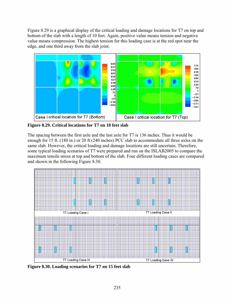
235

Figure 8.29 is a graphical display of the critical loading and damage locations for T7 on top and bottom of the slab with a length of 10 feet. Again, positive value means tension and negative value means compression. The highest tension for this loading case is at the red spot near the edge, and one third away from the slab joint.

Figure 8.29. Critical locations for T7 on 10 feet slab

The spacing between the first axle and the last axle for T7 is 136 inches. Thus it would be enough for 15 ft. (180 in.) or 20 ft (240 inches) PCC slab to accommodate all three axles on the same slab. However, the critical loading and damage locations are still uncertain. Therefore, some typical loading scenarios of T7 were prepared and run on the ISLAB2005 to compare the maximum tensile stress at top and bottom of the slab. Four different loading cases are compared and shown in the following Figure 8.30.

Figure 8.30. Loading scenarios for T7 on 15 feet slab

236

As shown in Figure 8.30, loading case I is that the first axle locates right at the edge, corner of the approach slab, and loading case II is that the first axle locates at the edge, midway from the slab joint. Loading case III shows that the middle axle of the vehicle locates right at the edge, midway from the slab joint, and loading case IV shows that the median of the last two axles is right at the edge, midway from the slab.

Maximum bending stress for all loading cases were extracted from the ISLAB2005 output and summarized as shown in the following Table 8.11.

Table 8.11. Critical Locations for T7 on 15 Feet Slab

Vehicle Loading Case

Max. Bending Stress (psi) Critical loading/ damage Location Top Bottom

T7

I 565 657

Case I/Bottom II 409 662 III 430 526 IV 480 616

According to Table 8.11, the maximum tensile stress at the bottom of the slab between case I and case II are only 5 psi difference. However, their maximum bending stresses at the top of the slab are significantly different. The top slab tensile stress for case I is 156 psi greater than it for case II. Therefore, case I is determined to be more critical loading locations for T7 on a 15 feet slab. The critical damage location is still at the bottom of the slab. However, high damage risk exists at the top of the slab.

Figure 8.31. Critical locations for T7 on 15 feet long slab

Figure 8.31 graphically shows the comparison of the stress distribution at the top and bottom of the slab for loading case I. Note that for top slab, the red zone expands from the center, midway from the slab all the way to the edge, quarter way through the approaching slab. Potential corner crack could be initiated because of this tensile stress zone.

For slab with 20 feet length, the comparison results showed the same as 15 feet slab and therefore, it will not be discussed anymore. Straight truck S1 has three axle in total, one front

237

steering axle, and two dual axles in the back. The spacing between the first axle and the second axle is 177.5 inches while the spacing between the last two axles is 56 inches. For a 10 feet (180 inches) slab, it could not accommodate the whole vehicle on one slab simultaneously. Neither could the slab accommodate the first two axles of S1. Therefore, for a slab of 10 feet long, the critical loading locations are similar to either the single axle case.

For the single axle case, the critical loading location locates at when the front steering tire right on the edge, midway from the slab joint. The critical damage locations would be at the bottom edge of the slab, midway from the slab joint. For dual axle case, the critical loading location is when the median of the last two axles locates on the edge, midway from the slab joint. The critical damage location is located near to the bottom edge of the slab, midway from the slab joint. However, the magnitude of the maximum bending stress for those cases is uncertain.

Figure 8.32 graphically demonstrates this two loading scenarios for S1 on a 10 feet slab. Loading case I shows the median of the last two axles locates on the edge, midway from the slab joint, and case II shows the front axle locates at the edge, midway from the slab joint.

Figure 8.32. Loading scenarios for S1 on 10 feet slab

The maximum of the bending stress at the top and bottom of the slab were extracted from ISLAB 2005 output and summarized as shown in Table 8.12. As shown in Table 8.12, loading case II is the critical loading location and the critical damage location is at the bottom, midway from the slab joint.

Table 8.12. Critical Locations for S1 on 10 Feet Slab

Vehicle Loading Case

Max. Bending Stress (psi) Critical loading/ damage Location Top Bottom

S1 I 266 691 Case II/Bottom II 471 800 Figure 8.33 shows the comparison results for the two loading cases studied for S1 on a 10 feet slab. As discussed before, the red spot is where the highest tensile stress exists. Case II exhibited the highest tensile stress at the bottom of the slab.

238

Figure 8.33. Critical locations for S1 on 10 feet slab

For slab with 15 feet slab, it could barely accommodate the first two axles of S1 on one slab. Figure 8.34 demonstrates two typical loading cases for S1. Loading case I shows that the steering axle of S1 locates at the edge, midway from the slab joint, and loading case II shows that the first two axle just barely fit into the 15 feet slab. Other loading cases are not discussed here because they have been discussed in previous sections.

Figure 8.34. Loading scenarios for S1 on 15 feet slab

Table 8.13 summarizes the maximum bending stresses at the top and bottom of the slab for those two loading scenarios shown in Figure 8.34. As shown in Table 8.13, the maximum bending stress is produced by loading case I at the bottom of the slab. Similar to 10 feet slab, the steering axle of S1 at the edge, midway from the slab joint, still produced the highest bending stress at the bottom of the slab. This demonstrates that for S1, the front steering axle has higher damage risk than the duals in the back.

Table 8.13. Critical Locations for S1 on 15 Feet Slab

Vehicle Loading

Case Max. Bending Stress (psi) Critical loading/

damage Location Top Bottom

S1 I 234 720

Case I/Bottom II 455 676

Figure 8.35 is a graphical display of the stress distribution for these two different loading scenarios. As discussed before, positive value means tension and negative value means compression. Notes that the critical damage location for case I is located at the edge, bottom

239

slab, midway from the slab joint. However, for loading case II, the critical damage location is located at where the left front wheel located at.

Figure 8.35. Critical locations for S1 on 15 feet slab

For slab of 20 feet (240 inches) in length, it could either accommodate the first two axles of S1, or the whole vehicle which is 233.5 inches from the center of the first axle to the center of the last axle. Several typical loading scenarios were carefully reviewed and two representative cases are shown in Figure 8.36.

As shown in Figure 8.36, loading case I shows that the front steering axle of S1 is right on the edge, midway from the slab joint, and loading case II is where the median of the first two axles at the edge, midway from the slab joint.

Figure 8.36. Loading scenarios for S1 on 20 feet slab

Maximum bending stresses are extracted from the ISLAB2005 outputin Table 8.14. Based on the comparison form Table 8.14, the critical l

and summarized as shown oading location is

determined to be loading case II which is the median of the first two axles locates at the edge, midway from the slab joint. The critical damage location is at the bottom of the slab, midway from the slab joint.

Table 8.14. Critical Locations for S1 on 20 Feet Slab

Vehicle Loading

Case Max. Bending Stress (psi) Critical loading/

damage Location Top Bottom

S1 I 267 685

Case II/Bottom II 302 692

240

Figure 8.37 displays the graphical demonstration of the stress distribution introduced by S1 for two different loading scenarios. Loading case II is determined to be the critical loading location. The maximum tensile stress located at the a few feet away from the next slab joint, at the bottom of the slab.

Figure 8.37. Critical locations for S1 on 20 feet slab

Pavement Damage Prediction

As following the determination of the critical loading and response locations from the previous step, rigid pavement damage predictions for representative farm vehicle were made from critical response results of ISLAB 2005 simulations considering the various PCC slab design features and subgrade conditions as shown in following.

Slab length (L, feet): 10, 15, and 20 Slab thickness (h, in.): 5, 7, and 10 Modulus of Subgrade Support (k, psi/in.): 50, 100, 150, 200, 250, 300 Temperature differential (oF/in.): -2, -4, and -6

The temperature gradients used in this study was only focused on the damage attributed by negative temperature differential (curl-up of slab). A MEPDG pavement damage model was utilized for this temperature damage analysis as well. Faulting and fatigue damage equations of MEPDG described previously were utilized in pavement damage predictions.

Maximum tensile stresses at the top and bottom of the slab were computed from the ISLAB2005 and are compared to each other. In the case when a bending stress at the top of the slab is greater than that at the bottom, the bending stress at the top of the slab therefore is selected to calculate the number of the load repetitions to failure in fatigue damage analysis. It was found that comparison of pavement response under a curled slab should only be made within the same slab thickness (N. Buch, 2004). Therefore, pavement stresses under different farm vehicles are compared by the same slab thickness. Two cases that match cell 32 and cell 54 are shown in this section. Temperature damage analysis results for other cases could be found in Appendix I.

Figure 8.38 is a bar chart comparison of Nf under various farm equipment for different temperature gradient on cell 32. A gradient of -2 oF/in. means that for cell 32, the top slab is -10 oF colder than the bottom of the slab. According to the comparison in Figure 8.38, it could be found that for vehicle T7, as temperature gradient increases, the number of loading repetition to

241

failure decreases. However, for vehicle like Mn102, T6, R6 and G1, as the temperature gradient increases, Nf increases. This is because of change of the critical loading locations for different vehicles. This finding also confirms and explains why Tanker is more critical in the fall season test and Terragator is more critical in the spring season testing.

For vehicle Mn80 and S1, -4 oF/in. gives the highest Nf. Additionally, Figure 8.38 also illustrates that G1 produced the highest pavement damage among all those representative vehicles. Terragator R6 has the second highest risk of fatigue damage to the PCC pavement.

Figure 8.38. Temperature damage analysis for cell 32

Figure 8.39 graphically compared the Nf corresponding to vehicle for different temperature gradient on cell 54 slab. This figure further demonstrates that as the temperature gradient increases, Nf decreases for all vehicles except for R6 and G1. R6 and G1 have the highest Nf when the slab experiences a temperature gradient of -4 oF/in. For other vehicles, like Mn80, Mn102, S1, T7 and T6, the comparison indicates that as the temperature gradient increases, the fatigue damage increases. However, the change in Nf due to temperature gradient is larger for Mn80 as the other vehicles.

242

Figure 8.39. Temperature damage analysis for cell 54

As indicated from the previous comparisons, the curling of the slab coupling heavy farm equipment loadings could significantly reduce the pavement life by reducing Nf. It was originally suspected that Nf would decreases, and thus gives a shorter pavement life as the temperature gradient increases. However, the comparison results shown that Nf does not necessary decreases as the temperature gradient increases for certain vehicles.

Summary

The following findings are drawn from the rigid pavement damage analysis with slab curling behavior for agricultural vehicles:

• Based on damage analysis results, farm vehicles have higher fatigue and faulting damage risk on rigid pavements rather than a standard 80kip semi-truck.

• Among farm vehicles, G1 and R6 have more damage potential. • For farm equipment, as the temperature gradient increases, the fatigue damage increases.

However, the change in Nf due to temperature gradient is larger for Mn80 as the other vehicles.

Discussion of Corner Cracking

Corner cracks are diagonal cracks that meet both the longitudinal and transverse joint within 6 ft, measured from the corner of the slab (Lee, 2002). The crack usually extends through the entire thickness of the slab. Load repetitions combined with loss of subgrade support, poor load transfer across the joint, curling and warping stresses usually causes corner breaks. Ioannides et al. (1985) found that the maximum moment occurs at a distance of 1.8 c0.32 l0.59 from the corner, in which c is the side length of a square contact area and l is the radius of the relative stiffness. The radius of the relative stiffness could be calculated as following:

l = 0.25

243

in which E is the elastic modulus of concrete, h is the thickness of the slab, v is Poisson ratio of concrete, and k is the modulus of subgrade reaction. In all examples presented in this section, a modulus of 4 x 106 psi and a Poisson ration of 0.15 are assumed for the PCC concrete slab.

As discussed in previous chapter, apparent corner cracks occurred during the spring 2010 field testing on cell 32. Cell 32 PCC slabs are 12 ft wide, 10 ft long, and the thickness of the slab is 5 inches. It was found there was no temperature gradient during the time of the testing and the pavement has a modulus of subgrade support of 200 psi/in. The elastic modulus of the concrete was assumed as 4.5 x 106 psi with a Poisson’s ratio of 0.15. Comparisons were made between Ioannides’ maximum moment location and the ISLAB2005 output for various representative vehicles.

Similar to damage analysis with temperature gradient, and farm equipment, G1, Mn80, Mn102, R6, S1, T6, and T7 were chosen to further investigate the relative corner cracking damage caused by those farm equipment on cell 32 PCC slab.

At the first stage, G1 was chosen to study the effect of the modulus of the subgrade support and the temperature gradients on the maximum tensile stress location due to corner loading. Table 8.15 listed and compared all the results from finite elements solutions and Ioannides et al. theoretical solutions.

Table 8.15. Maximum Moment Locations from the Slab Corner along the Joint (ft)

Case No. k-value psi/in.

ISLAB 2005 FE solutions Ioannides et al.

1.8 c0.32 l0.59 Temperature Gradient (oF/in.) -2 -4 -6

1 10 6.0 6.0 6.0 3.7 2 20 6.0 6.0 6.0 3.4 3 30 5.5 5.5 5.5 3.2 4 100 5.0 5.0 5.0 2.6 5 150 4.5 5.0 5.0 2.5 6 200 4.5 4.5 5.0 2.4 7 250 4.5 4.5 4.5 2.3 8 300 4.5 4.5 4.5 2.3

According to Table 8.15, it was found that temperature curling does not have significant effect on the locations where the maximum tensile stresses located at. Additionally, the improvement of subgrade is more effective in reducing the distance of which the maximum tensile stress location to the edge of the slab.

Differences exist between the ISLAB2005 output and the theoretical bending moment locations. Compared to Ioannides method, ISLAB2005 gives greater distances. The magnitude is roughly about 1.6 times greater than the Ioannides’ method. Therefore, a calibration factor of 1.6 should be applied if Ioannides’ method is used for calculating the distance from the slab corner to where the maximum tensile stress located at. Table 8.16 summarizes all the maximum bending stresses produced by various representative farm equipment under different temperature gradients.

244

Table 8.16. Max. Bending Stresses and Their Locations

Vehicle

Max. bending Stress (psi) Distance from the corner, ft

Ioannides et al.

1.8 c0.32 l0.59

Adjustment factor

Temperature Gradient (oF/in.)

0 -2 -4 -6

Mn80 299 375 453 527 3.5 1.7 2.06

Mn102 414 490 569 645 3.5 1.6 2.19 G1 429 505 595 685 4.5 2.4 1.88 R6 496 594 689 779 5.0 2.0 2.5 S1 365 442 523 599 3.5 1.6 2.19 T6 460 537 621 712 3.5 1.7 2.06 T7 400 454 543 630 2.5* 1.9 1.32 T8 363 409 488 578 2.5* 1.8 1.39

*distance along the slab edge

As shown in Table 8.16, it is found that as the temperature gradient increases, the bending stresses on the top of the slab increases. Among all eight representative vehicles, R6 produced the highest bending stresses at the top of the slab 5 ft away from the slab corner along the joint, regardless of the temperature gradient. G1 produced the second highest bending stresses at the top of the slab 4.5 ft away from the corner of the slab. Differences still exist between the finite element and the theoretical results for the location of where the maximum bending stresses location, thus calibration factors should be used if the theoretical method is applied.

Figure 8.40 is a graphical representation of the stress distribution for G1 at the top of the cell 32 slab. As shown in Figure 8.40, the maximum bending stress is located at 4.5 ft away from the slab corner and there is a bending zone that propagates from the slab joint to the slab edge. This bending stress zone eventually could lead to the corner cracks if the bending moments are high enough.

245

Figure 8.40. Cell 32 stress distribution for G1 at the top of the slab

Even though the field observation found that the corner cracks only occurred 2.5 ft away from the slab corner, the bias could be caused by the quality of the concrete or other factors. If there is a weak point in the concrete due to poor mixing or casting, the crack would not have reached to where the maximum bending moments located at, and then it will start to crack. The demonstration in Figure 8.40 is rather a concept than to prove the corner crack have to occur at the exactly point where the maximum bending moments located at. The crack could also possibly occur at the buffer zone where the junction of the maximum and the minimum bending stress zone.

This study also demonstrates that there is very high possibility for the corner cracking to occur if there is a temperature curling combined with heavy farm equipment loading at the corner of the slab.

TONN2010

TONN2010 evaluates damage from standard 18-kip heavy axle loads on performance of flexible pavements. It incorporates the following damage models:

• MnPAVE subgrade rutting damage model • MnPAVE base shear failure model • MnPAVE AC fatigue cracking damage model • Base deformation model

In this study, the damage models from TONN2010 were adopted to evaluate the effect of heavy agricultural equipment of performance. A brief description of the TONN2010 damage models is provided below.

246

Subgrade Permanent Deformation Models Permanent deformation, also known as rutting, is the failure of a pavement due to poor consolidation or lateral movement of layer materials due to repeated vehicle loads. Rutting of sub-surface pavement layers occurs when the strength or stiffness of a sub-surface layer is either lower than required or somehow compromised. The MnPAVE model of Equation 8.10 utilizes a similar model to the Asphalt Institute model (Asphalt Institute 1983).

35.20261.0 −⋅= cdN ε Equation 8.10

It should be noted that the MnPAVE rutting damage model assesses only rutting damage in the subgrade and does not consider damage in the granular base layer.

Base Shear Failure Criteria A maximum allowable stress criterion has been implemented in MnPAVE to protect against aggregate base failure (see Figure 8.41). The failure criterion is based on the traditional Mohr-Coulomb criterion and has the following form:

)

245tan(2)

245(tan 2

311φφσσσ +⋅⋅++⋅=< C

critical Equation 8.11

φ = internal friction angle (°)

C = cohesion

1σ = maximum allowable major principal stress

3σ = minor principal stress or confining pressure for the triaxial test

This criterion states that the base fails when the maximum shear stress 1σ exceeds the critical value.

critical1σ . Therefore, the ratio of these two parameters, SR=critical11 /σσ is an indicator of how

close the base is to shear failure when it is loaded by an axle load. The smaller this ratio is the less likely the base will fail.

It should be noted that MnPAVE assumes the same Mohr-Coulomb criterion parameters, C and φ

φ , it is not realistic for cohesion, C. Indeed, in early spring, after base thawing, cohesion may be much lower than for the rest of the year, even for the same moisture conditions. When the base is frozen, the cohesion is very high.

To address this limitation, TONN2010 adopted the following seasonal cohesion values

CscC ii =

Where:

, for the material regardless of the season at which the stresses in the base are computed. Although this assumption might be reasonable for the internal friction angle,

247

Ci = seasonal cohesion for the base layer for season i

C = MnPAVE Late spring default cohesion for Class 5 base (= 6 psi)

sci = seasonal cohesion adjustment factors; by default are equal to 10, 0.2, 1, 1.3, and 1 for the MnPave winter, early spring, late spring, summer, and fall seasons, respectively.

Figure 8.41. MnPAVE Mohr-Coulomb Criterion input screen

Fatigue Cracking Models Traditional asphalt concrete (AC) cracking models assume cracking begins at the bottom of the asphalt layer and propagates upward to the surface [bottom-up], where the cracking is initially due to tensile stresses and strains at the bottom of the asphalt layer under the load. The intensity of these strains and stresses depends on the magnitude and geometry of the axle loading and properties of the pavement system (i.e. layer thicknesses, moduli, etc.). Pavement damage in fatigue cracking is typically defined as the ratio of the number of load applications to the allowable number of load applications. Asphalt fatigue transfer functions relate the number of load repetitions to reach certain levels of failure in cracking (i.e. crack initiation, 10-percent cracked area of the pavement surface, etc.) to the maximum strains at the bottom of the AC layer. The MnPAVE form of the Asphalt Institute model for the allowable number of load repetitions is as follows (Finn et al. 1977, Chadbourn et al 2002):

248

854.0291.331 10 −−− ⋅⋅⋅⋅= EKCN hFf ε Equation 8.12

where C is a correction factor based on air voids and binder content and KF1 is a shift factor that accounts for calibration with existing R-value designs, hε is the maximum tensile horizontal strain at the bottom of the AC layer, and E is the AC modulus. MnPAVE requires computing AC tensile strains for each of the five MnPAVE seasons. The AC fatigue damage is computed for each season and accumulated according to Miner’s fatigue rule.

Base Deformations The MnPAVE rutting model does not consider rutting in the base layer. The MEPDG uses the following equation to predict rutting in the unbound base:

βρ

εε

εβ

−

=∆ n

r

osoilvsssoilp ehk 11)( Equation 8.13

where:

∆p(Soil) = Permanent or plastic deformation in the layer/sublayer, in.

n = Number of axle load applications.

εo = Intercept determined from laboratory repeated load permanent deformation tests, in/in.

εr = Resilient strain imposed in laboratory test to obtain material properties εo, β, and ρ, in/in.

εv = Average vertical resilient or elastic strain in the layer/sublayer and calculated by the structural response model, in/in.

hSoil = Thickness of the unbound layer/sublayer, in.

ks1 = Global calibration coefficients; ks1=1.673 for granular materials and 1.35 for fine-grained materials.

βs1 = Local calibration constant for the rutting in the unbound layers; the local calibration constant was set to 1.0 for the global calibration effort.

( )cWLog 017638.061119.0 −−=β Equation 8.15

( )( )

β

βρ

1

9

9

10110

−= oC

Equation 8.16

249

0075.09

1

9

1 =

= b

r

br

o MaMaLnC Equation 8.17

Wc = Water content, percent.

Mr = Resilient modulus of the unbound layer or sublayer, psi.

a1,9 = Regression constants; a1=0.15 and a9=20.0.

b1,9 = Regression constants; b1=0.0 and b9=0.0.

The field-calibrated MEPDG procedure divides the base layer into thin sublayers and computes permanent deformations in the individual sublayers. Vertical strains should be determined at multiple locations to account for the effect of traffic wander. Although the MEPDG procedure is theoretically sound and robust, it is also too complex to be implemented in the proposed study. Therefore, an alternative simplified version of the procedure was proposed. It is based on the observation that if the properties of the base layer do not vary with depth, then rutting in the base layer according to the MEPDG can be expressed

∑∑==

==n

iiii

n

ihRut

11εχεχ Equation 8.18

Where Rut is the rutting in the base layer, ε i is the vertical strain in the sublayer I, and χ is the coefficient. If the number of sublayers is increasing then Equation 8 can be re-written as follows:

( )h

hn

iiin

wwdzhRut −=== ∫∑=

∞− 001

lim χεχεχ Equation 8.19

Where w0 is the vertical deflection at the top of the base layer, wh is the vertical deflection at the bottom of the base.

Equation 8.19 suggests that limiting the difference between the vertical deflections at the top and bottom base surfaces would reduce a potential of the base rutting.

Inputs

To compare damage caused by heavy agricultural equipment with the damage caused by a standard 18-kip single axle load, the user should provide the following information:

• Axle load geometry and magnitude • Pavement structure characteristics • Climate conditions

Detailed requirements for each of the group of inputs are provided below.

250

Axle loading To characterize the effect of axle loading on pavement responses, the user should provide information on the magnitude of axle load or tire-pavement contact stresses and geometry of a tire footprint. In this study only normal tire-pavement contact stresses were considered and shear stresses were ignored. This is justified by the following two reasons. The majority of pavement damage models, including the Minnesota Department of Transportation MnPAVE damage models and the American Association of State Highway and Transportation Officials (AASHTO) Mechanistic-Empirical Pavement Design Guide (M-EPDG) do not consider contact shear stresses. In addition, the device for measurement of tire-pavement contact stresses used in this study was capable of measurement of normal stresses only. Therefore, it was not feasible to obtain reliable information on the shear stress distribution.

Two loading problems are considered in each analysis:

• A half axle of a standard 18-kip single axle load • A half axle of the farm equipment axle

The standard half-axle was modeled by two 3.8-in radius circular loads with pressure of 100 psi. The farm equipment half-axle loading was modeled using multiple circular loads with various radii. The number of the circles, their radii, and coordinates of the centroids were determined based on the results of Tekscan measurements. Figure 8.42 presents the tire footprint from Tekscan and the corresponding representation of the footprint by a series of circular loads. The applied pressure was summed to be the same for each circle and was determined by dividing the load magnitude by the footprint area.

Figure 8.42. Tekscan tire footprint and equal area circle representation

Pavement Structure The structure of a given pavement significantly affects structural responses (stresses, strains, and deflections) caused by axle loading. To enable computing these responses, the user should

251

provide information on pavement layer thicknesses and elastic properties. In this study, a simple pavement consisting of a single asphalt layer, base, subgrade, and stiff bedrock was considered. The base layer was assumed to be 12-in thick, so it may also include an upper portion of the compacted subgrade. The effective properties of the layer should be provided. The subgrade depth to the bedrock may vary from 12 to 240 inches. The latter limit represents a condition where no bedrock is present.

For each layer, in the pavement system, except the bedrock, the user should provide elastic properties (moduli of elasticity and Poisson’s ratios) as well as the interface conditions. In this study, it was assumed that all layers are fully bonded, which is a typical assumption in flexible pavement analysis. The following Poisson’s ratios were assumed:

• Asphalt layer: 0.35 • Base: 0.4 • Subgrade: 0.45

Elastic moduli of asphalt and unbound materials are sensitive to temperature and moisture conditions, respectively. The asphalt modulus was assigned for the reference temperature of 72oF and the base and subgrade elastic moduli were assigned for typical summer conditions. These moduli were adjusted in the analysis using the climatic inputs described in the next section.

Climatic Inputs Environmental effects have a major influence on pavement performance. Mechanistic-empirical design procedures offer a rational approach for accounting of these effects by subdividing the pavement performance period into time increments and adjusting pavement system properties according to representative temperature and moisture conditions for the pavement. Different design procedures use different time intervals. For example, the MEPDG uses one month time increments. Although this permits refinement of the design process, it also creates an unnecessary complexity. In this study, MnPave was used.

MnPAVE considers five seasons (Ovik, 2000):

• Early spring: The season when the aggregate base is thawed and nearly saturated, but the subgrade remains frozen.

• Late spring: The season when the aggregate base has drained and regained partial strength, but the subgrade is thawed, near saturated, and weak.

• Summer: The season when the aggregate base is almost fully recovered, but the subgrade has only regained partial strength.

• Fall: The season when both the aggregate base and subgrade have fully recovered. • Winter: The season when all pavement layers are frozen.

The duration of each season is dependent on the geographic location of the pavement section and the climate it experiences. MnPAVE software provides information on the duration and average seasonal air temperatures for each season at the specific location being evaluated. A screen shot showing this information is given in Figure 8.43.

252

In this study, the MnPAVE seasons were adopted for pavement evaluation process. The seasonal durations were adopted to be equal to the MnPAVE durations. The mean air temperatures for all of the seasons except for early spring were adopted. Field testing at MnROAD indicated that although the mean air temperature may be low due to low nighttime temperatures, the high daytime temperatures induce a relatively high asphalt layer temperature causing a reduction in asphalt stiffness for several hours. Therefore, significant damage can be accumulated in the afternoon during this time. To address this issue, the mean air temperature for early spring was assumed to be equal to the late spring mean air temperature.

Figure 8.43. MnPAVE climate window

In addition to the mean air temperature and the duration of each season, the user should provide the ratios of the elastic moduli of the base and subgrade compared to the corresponding summer values. Table 8.17 presents adjustment factors for each season used in this study. These factors were adopted from the corresponding MnPAVE default values.

253

Table 8.17. Seasonal Moduli Adjustment Factors for Base and Subgrade

Layer Winter Early Late Summer Fall

Spring Spring Base 10 0.35 0.65 0.95 1

Subgrade 10 10 0.65 1 1

Structural Responses

To compare damage caused by heavy agricultural equipment and the standard axle loading, the critical pavement responses (strains and deflections) are computed using the layered elastic program MnLAYER (Khazanovich and Wang 2010) for each season. The subsequent damage analysis requires determination of the following structural responses:

Maximum vertical strain at the top of the subgrade Maximum difference of vertical deflections at the top and bottom surfaces of the base Minimum ratio of the critical stress and first principal stress at the base mid-depth Maximum horizontal strain at the bottom of the AC layer

It should be noted that the vertical displacements at the bottom of the asphalt layer are equal to the vertical displacements at the top of the base layer. The vertical displacements at the bottom of the base layer are equal to the vertical displacements at the top of the subgrade. These observations permit significant reduction in the number of points at which the responses have to be determined.

Since simple footprint geometry is assumed for the standard single axle load, the most likely locations of the maximum responses can be narrowed down based on the past experience. Therefore, the responses are determined for the following locations:

Point A. Bottom of the AC layer, under the center of the wheel Point B. 6-inches into the base layer, under the center of the wheel Point C. Top of the subgrade layer, under the center of the wheel Point D. Top of the base layer, mid-distance between the wheels Point E. 6-inches into the base layer, mid-distance between the wheels Point F. 12-inches below the top of the base layer, mid-distance between the wheels

254

A B E C

D

F

Figure 8.44. Location of evaluation points in the structural model

The maximum principal horizontal strain computed at point A is used in the subsequent AC damage calculation. The vertical strain computed at point C is needed for subgrade rutting damage analysis. Stresses computed at points B and E are used to compute the principle and critical stresses as defined by Equation 8.11. These stresses are used to compute the strength to stress ratios. The lowest strength to stress ratio, SRc, is used in the subsequent analysis as defined in Equation 8.29.

Geometry of the agricultural equipment tire footprint can be quite complex. Therefore, it is difficult to guess locations of the maximum responses prior to the analysis. To address this challenge, the responses were evaluated for the following layers of points (see Figure 8.45):

Layer A. Bottom of the AC layer Layer B. Mid-depth of the base layer Layer C. Top of the subgrade layer

Each layer consisted of 100 points organized in either a 10 X 10 or a 5 X 20 mesh equally spaced in x- and y- directions (see Figure 8.46). The horizontal coordinates of the points did not vary from layer to layer. The coordinates of the end points is either a user-provided input or determined from the minimum and maximum horizontal coordinates of the centers of the circular loads in the agricultural equipment tire footprint. From horizontal strains computed at each point of Layer A, the maximum horizontal strain is determined and used in the subsequent AC damage calculation. The maximum vertical strain among the vertical strains computed for points in Layer C is needed for subgrade rutting damage analysis. Critical and principal stresses computed at points of Layer B are used to compute the strength to stress ratios. The lowest strength to stress ratio, SRc, from all the loads being considered, is used in the subsequent damage analysis. Finally, the maximum difference

255

between deflections of the points in Layer A and the corresponding points in Layer C is used in the base damage analysis.

Figure 8.45. Location of evaluation points in the structural model

Figure 8.46. Plan view of loads on pavement surface

The structural responses should be computed for each MnPAVE season. Although the layer thicknesses, load geometry and locations of the evaluation points do not vary from season to

256

season, the layer moduli are adjusted to account for seasonal variations in asphalt temperature as well as subgrade and base moisture content.

To determine representative seasonal AC moduli values, the average seasonal pavement temperature need to be calculated. TONN2010 adopted the MnPAVE procedure. The following equation is used:

64

344

11 ++

−

++=

zzTaTp ii Equation 8.20

Where

Tpi = average seasonal pavement temperature at depth z for season i (oF)

Tai = average seasonal air temperature for season i (oF)

z = depth at which material temperature is to be predicted, in

The average seasonal air temperature for any Minnesota location can be found from the MnPAVE design software “climate” screen.

After the seasonal pavement temperatures are determined, the corresponding AC moduli are determined using the equation developed by Lukanen et al, (1998) from the analysis of the Long Term Pavement Performance (LTPP) Seasonal Monitoring Program (SMP) data:

( )refseas TTsloperefseas EE −×= 10 Equation 8.21

The magnitude of the slope in the equation above depends on the individual characteristics of the mix such as the binder properties and aggregate characteristics. The range encountered in the LTPP SMP study for the slope was roughly bounded by -0.015 to -0.030. In this study, a slope value of -0.020 was adopted.

The elastic properties of unbound materials are moisture dependent. Since moisture conditions vary from season to season, the backcalculated base and subgrade moduli are adjusted using the following equations:

day

ibaseibase b

bsEE *, = Equation 8.22

day

isubgrisubgr s

ssEE *, = Equation 8.23

where

Ebase = backcalculated base modulus

257

Ebase,i = average base modulus for season i

bsi = base modulus season adjustment factor for season i.

bday = base modulus adjustment factor accounting for a difference in the

moisture conditions for the test day. By default it is equal to the season adjustment factor for the season of testing.

Esubgr = backcalculated subgrade modulus

Esubgr,i = average subgrade modulus for season i

ssi = subgrade modulus season adjustment factor for season i.

sday = subgrade modulus adjustment factor accounting for a difference in the

moisture conditions for the test day. By default it is equal to the season adjustment factor for the season of testing.

Damage Analysis

After the critical responses are determined for each season, the damage analysis is performed to calculate relative damage and damage indexes. It involves:

• Subgrade rutting damage analysis • Base shear failure analysis • AC fatigue cracking damage analysis • Base deformation analysis

The allowable number of load repetitions is determined using the following equation:

35.2, 0261.0 −= viiRUTN ε Equation 8.24

iRUTN , = allowable number of ESALs for season i in terms of subgrade damage.

iB,ε = maximum vertical subgrade strain for season i combinations of elastic properties

To determine a relative damage in terms of rutting for season i from a passage of a heavy axle of an agricultural equipment, the following equation can be used:

Equation 8.25

Similarly, the number load applications to failure in AC cracking was determined in HAVED2011 using the following equation:

258

Equation 8.26

Where

iA,ε = maximum principal horizontal strain at the bottom of AC layer for season i combinations of elastic properties

EACi = AC elastic modulus for season i.

To determine a relative damage in terms of AC cracking for season i from a passage of a heavy axle of an agricultural equipment, the following equation can be used:

Equation 8.27

HAVED2011 uses the ratios of the first principle stress and critical stress and the difference in the base deflections to evaluate bearing capacity of the pavement and obtain a road rating based on the maximum axle load rather than the number of load applications. In this study, the TONN2010 approach was modified for estimation of the maximum allowable axle loading. The following indexes were suggested:

1

1

σσ

criticaliSR = Equation 8.28

ii DW

DDI 1= Equation 8.29

Where

σ 1 = major principal stress

σ1critical = critical stress defined by equation (2)

DDI = differential deflection index

DWi = difference in the vertical deflections of the top and bottom base surfaces (in microns) computed for a season i.

The following failure criteria are suggested:

*SRSRi < Equation 8.30

*ii DDIDDI ≤ Equation 8.31

259

SR* and DDI *i are the calibration parameters depending on pavement material properties

The procedure described above is incorporated into a FORTRAN code. The program incorporates MnLAYER for simulation of pavement loading by an 18-kip single axle load and the axle of interest. After that, it computes the relative damage in subgrade rutting and AC cracking induced by the axle of interest compared to the standard 18-kip axle, as well as the maximum SR and DDI parameters.

Validation and Calibration

To validate the procedure, spring 2009 test data at an 80% loading level for cell 84 was simulated for each vehicle tested in that season. Table 8.18 shows the measured weight of the heaviest axle for each vehicle. Figure 8.47 shows the resulting relative subgrade damage from the heaviest axle. One can observe that according to the simulation a passage of the heaviest axle of each vehicle resulted in higher subgrade damage than from a passage of the heaviest axle of the Mn80 truck. The highest damage was predicted for vehicle R4.

Table 8.18. Measured Weight of the Heaviest Axle for Each Vehicle Tested in Spring 2009 at 80% Loading

Vehicle Axle Measured Weight of

Heaviest Axle (lbs)

R4 2 39,340 S3 2 26,960 S4 3 21,460 S5 3 20,040 T6 4 22,460 T7 3 22,840 T8 4 21,280

Mn80 4 and 5 34,080 To verify these predictions, the maximum measured subgrade stresses from each vehicle from all the measurements made on that day were determined (see Figure 8.48) and compared with the predicted relative rutting damage. One can observe that indeed all the vehicles induced higher subgrade stresses than the Mn80 truck and the Terragator R4 induced the highest stress. The relative ranking of subgrade stresses was mostly similar to the ranking of the relative subgrade damage. There was, however, one noticeable discrepancy. The measured subgrade stress from vehicle S4 was lower than from many vehicles, like T6, T7, and T8, whereas the predicted relative rutting damage was very similar if not higher.

260

Figure 8.47. Relative subgrade damagef the heaviest axle in the spring 2009 testing season at 80% loading *Note: Only vehicles tested in the spring 09 testing season are included in Figure 8.47 as the comparison in Figure 8.48 uses only vehicles tested in the spring 09 testing season.

Figure 8.48. Measured maximum subgrade stresses normalized to Mn80 subgrade stress

To investigate this discrepancy, an additional analysis of the simulated and measured data was conducted. First, the predicted subgrade stresses were determined for each vehicle and normalized to the subgrade stresses from the Mn80 truck. The trend of the calculated subgrade stresses followed the trend of the predicted relative subgrade damage and the discrepancy between the ranking of the predicted measured and calculated stresses from S4 and other vehicles was observed. After that, a detailed comparison of the measured stresses from the S4 and T6 vehicles was conducted.

261

Figure 8.49. Measured subgrade stress at 80% loading in the spring 2009 testing season

Projected Stress Procedure

Despite having an extensive testing schedule, not every load level for every vehicle was able to be tested. Most vehicles were tested at an 80% load level, but not every vehicle was tested at a 100% load level. The Mn80 and Mn102 trucks were always considered to be 100% loaded. In order to make not only a “fair” comparison amongst vehicles, but also to help validate the HAVED2011 model, a projected stress procedure was developed to predict the heaviest vehicle axle weights and stresses at 100% loading.

The projected heaviest axle weights at 100% loading were found using a linear regression. For as many seasons as testing was performed in, a linear regression was made for each specific vehicles’ load levels tested and corresponding vehicle axle weights. This was the case with the vehicle R4, which was only ever tested at 0, 25, 50 and 80% load levels. Table 8.19 shows the testing season, load level, and corresponding vehicle axle weights for the vehicle R4.

Table 8.19. Testing Season, Load Level and Vehicle Axle Weight for R4

Testing Season Fall 2008 Spring 2009 Load Level 0 25 50 80 0 25 50 80

Vehicle Axle Weights 23840 28640 32820 38420 23720 28160 34440 39340

Using all the data available for each vehicle, a linear regression equation was developed from which the vehicle axle weight at 100% loading could be projected. This information is summarized in Table 8.20 below for the vehicle R4.

262

Table 8.20. Linear Regression Equation and Projected Weight at 100% Loading for R4

Slope 190.45 Intercept 23792.38

Projected Weight At 100% 42837.85

In the event that a vehicle was in fact measured at 100% loading, the heaviest vehicle axle weight measured was used in the analysis instead of using a projected heaviest axle weight at 100% loading. This was the case with the vehicle G1 for example. In fall 2010, the G1 vehicle was measured at 100% loading and the corresponding heaviest axle weight was 57,200 lbs. This is the axle weight that was used in determining the projected stress at 100% loading.

Table 8.21 summarizes the vehicle axle weights at 100% loading.

Table 8.21. Vehicle Axle Weights at 100% Loading

Mn102 25600 Mn80 19300

R4 42838 R5 29950 S4 24108 S5 23234 T6 33900 T7 26600 T8 23700 T1 29362 T3 33900 R6 41900 G1 57200

In order to determine the projected stress values at 100% loading, the seasonal effects had to be taken out of the measured stress values. To accomplish this, the fall 2008 testing season was designated as the baseline season and all other testing season stress values were normalized against this season.

The first step was to find the measured maximum subgrade stress values (84PG4) for the vehicles tested during each testing season. An example of this can be seen in Table 8.22.

263

Table 8.22 Maximum Measured Subgrade Stress (84PG4) Spring 2008

Maximum Measured Subgrade Stress (84PG4) Spring 2008

Vehicle 0% 25% 50% 80%

[psi] [psi] [psi] [psi]

Mn80 8.9 NA 12.55 NA S4 5.47 6.89 9.95 12.55 S5 8.13 8.74 13.17 15.55 T1 5.38 10.45 14.06 15.95

The remaining testing season’s maximum measured subgrade stress (84PG4) data can be found in Appendix M.

The baseline was then selected as the maximum measured stress from the Mn80 vehicle in the fall 2008 testing season at an 80% load level, which was 10.98 psi. A Mn80 subgrade stress factor was developed to normalize the measured Mn80 subgrade stress values during each season to the Mn80 subgrade stress value measured during the baseline season, fall 2008. The Mn80 subgrade stress factor was simply the ratio of the maximum measured subgrade stress value at a given load level, during a given season to that of the maximum measured subgrade stress value for the Mn80 vehicle at an 80% loading in the fall 2008 testing season. Table 8.23 summarizes the Mn80 subgrade stress factors for the spring 08 season at the respective load levels tested during that season for the Mn80 vehicle. The ratio calculated was specific to the day of testing. It is known that the Mn80 truck was always considered fully loaded.

Table 8.23 Determination of Mn80 Subgrade Stress Factors Spring 2008

Spring 2008 Fall 2008 Load Level Test

Measured Subgrade Stress (psi) (For Mn80)

Measured Subgrade Stress (psi)

(For Mn80)

Mn80 Subgrade

Stress Factor

0% 8.9 10.98 0.8104 50% 12.55 10.98 1.1428

The Mn80 subgrade stress factors for the remaining seasons can be found in Appendix M.

To correct the maximum measured subgrade stresses of all the vehicles in all the seasons tested, each maximum measured subgrade stress for a given season, load level and vehicle was adjusted by dividing the maximum measured subgrade stress value for that specific vehicle, season and load level by the Mn80 subgrade stress factor corresponding to the same load level and testing season. This is shown in Table 8.24 for the vehicle R4.

264

Table 8.24 Adjusted Subgrade Stresses for R4

Season - Load Level

Maximum Measured Subgrade Stress

(psi)

Mn80 Subgrade Stress Factor

Axle Weight

(lbs)

Adjusted Subgrade

Stress (psi)

S09 - 0% 24.2232 1.112778559 23720 21.768212 S09 - 25% 16.92822 1.011699655 28160 16.732456 S09 - 50% 16.52897 0.88421275 34440 18.693430 S09 - 80% 18.95551 0.636523906 39340 29.779729 F08 - 0% 13.99 1.137365319 23840 12.300357 F08 - 50% 13.66 0.868732197 32820 15.724063 F08 - 80% 16.29 0.999861586 38420 16.292255

The adjusted subgrade stresses for all the remaining vehicles can be found in Appendix M.

Using all the data available for the maximum axle weights as well as the adjusted subgrade stresses for each vehicle, a linear regression was then used to project the subgrade stress at 100% loading. The adjusted subgrade stress versus the axle weights was first plotted for each vehicle. This is seen in Figure 8.50 for the vehicle R4. From this, a regression equation was developed.

Figure 8.50. Adjusted R4 subgrade stress vs. axle weight

This information for the regression equation is summarized in Table 8.25 below for the vehicle R4.

265

Table 8.25. Linear Regression Equation for Projected Stress at 100% Loading for R4

Slope 0.000392 Intercept 6.403213

Projected Weight At 100% 42837.85 Projected Stress At 100% 23.18361

After plugging in the projected weight at 100% loading, the projected stress at 100% loading is obtained.

The remaining projected stresses are summarized below in Table 8.26.

Table 8.26. Projected Subgrade Stresses for Remaining Vehicles

Vehicle Slope Intercept Projected Weight At

100% Projected Stress At

100% S4 0.00058 2.714 24108.13 16.82 S5 0.00045 4.992 23233.99 15.65 R5 0.00036 4.372 29950.00 15.19 T7 0.00054 3.290 26600.00 17.74 T8 0.00030 6.964 26600.00 15.05 T6 0.00043 4.504 33900.00 19.40 T1 0.00049 2.731 29362.00 17.11 T3 0.00050 2.560 33900.00 19.69 R6 0.00023 8.991 41900.00 18.86 G1 0.00039 0.856 57200.00 23.69

The relative order of the subgrade stresses for the vehicles tested is shown in Figure 8.51.

266

Figure 8.51. Subgrade Stresses at 100% Loading

Measured responses are affected by many factors, including a relative position of the wheel path with respect to a sensor. As it can be observed from Figure 8.49, although T6 resulted in higher subgrade stresses, it is not clear if readings from S4 were not adversely affected by the wander, i.e. there was no passage directly over the pressure gage. To eliminate the effect of traffic wander on the measured maximum stresses, a procedure for the stress adjustment was developed. From the MnLAYER predictions, a stress profile was developed and matched with the measured stresses (see Figure 8.50). It can be observed that MnLAYER predicts a similar effect of the traffic wander on the subgrade stress magnitude. Moreover, it indicates that the most critical position of the axle with respect to the pressure gage sensor was not evaluated in the field test. Therefore, this phenomenon partially explains lower measured subgrade stresses for S4 than for other vehicles like T6, T7, and T8. Another factor that may contribute to the discrepancy between the measured stresses and the predicted damage is a possible error in the axle weight measurement. In spring 2008 the axle weight of the heaviest axle of S4 was 20,240 lbs. In spring 2009 it was 21,460 lbs. We compare this finding with the weight of another axle which did not change significantly between seasons (19,320 and 19,520 lb in 2008 and 2009, respectively). Taking these considerations into account, one can conclude that the predicted rutting damage agrees fairly well with the measured subgrade stresses.

267

Figure 8.52. Measured and calculated subgrade stresses from the vehicle S4

Cell 83 (3.5-in AC section) failed in spring of 2009. Throughout the duration of the study, cell 84 (5.5-in AC section) did not show significant distresses even after having been loaded at 100% load level in fall 2009 and subsequent test seasons. Many factors could have caused the pavement failure so it is hard to pinpoint the exact cause of failure, however based on the data from this study and previous knowledge; educated guesses can be made as to what caused the failure.

It was reasoned that the pavement first failed in the base or subgrade layer, although AC cracking could not be completely ruled out as the cause of failure. It was specifically seen that the base layer was very weak in the spring 2009 testing season. Cell 83 also, did not have a paved shoulder and it has since been shown that the presence of a paved shoulder reduces damage potential. In the absence of a paved shoulder, allowing vehicles to drive in the middle of roads (away from the edge) reduces a risk of pavement failure. In this study, all vehicles in all seasons resulted in high subgrade stresses and were higher than the standard 18-kip vehicle. Subgrade stresses were specifically very high in the fall 2009 testing season as can be seen in Figure 8.53.

268

Figure 8.53. Subgrade stress (83PG4), 100% loading, fall 2009 testing season for Mn80, T6, T7 and T8

The rutting damage analysis presented above gives a good indication of a relative damage caused by axle loading during a rutting damage accumulation process, but is not suitable for failure analysis. To address this limitation, two other HAVED2011 indexes were evaluated. Table 8.26 presents the stress ratios calculated for the vehicles participating in spring 2009 testing for 80% load level and Table 8.27 presents the stress ratios for all the vehicles for 100% load level. One can observe that none of the vehicles exhibited a SR lower than 1 for cell 84 even for the 100% load level. Meanwhile, every vehicle exhibited a SR less than 1 for cell 83 and several vehicles exhibited a SR less than 0.9, which demonstrates higher potential for failure.

Table 8.27. SR Indexes for the Early Spring Season, 80% Loading

Vehicle Cell 83 Cell 84 R4 0.9534 1.098 S3 0.9211 1.0954 S4 0.8763 1.0893 S5 0.91 1.1271 T6 0.9787 1.1567 T7 0.9832 1.1588 T8 0.8844 1.0965

Mn80 0.8877 1.1329 Mn102 0.841 1.0703

T1 0.9006 1.0997 T2 0.9621 1.1784

269

Table 8.28. SR Indexes for the Early Spring Season, 100% Loading

Vehicle Cell 83 Cell 84 R4 0.9405 1.0815 S3 0.9248 1.1005 S4 0.8536 1.058 S5 0.8738 1.0792 T6 0.9074 1.0597 T7 0.9526 1.1175 T8 0.864 1.0685

Mn80 0.8877 1.1329 Mn102 0.841 1.0703

T1 0.8692 1.057 T2 0.9246 1.1267

A similar analysis was performed for the DDI parameter. Tables 8.28 and 8.29 summarize the results for the vehicles in spring 2009 testing for 80% load level and for all the vehicles for 100% load level, respectively. One can observe that for cell 84 this parameter is computed to be greater than 1.4 for all vehicles at 80% loading, whereas all the vehicles except the Mn80 truck and T2 vehicle resulted in this parameter lower than 1.3 for the spring 2009 testing season. For 100 percent loading, all vehicles resulted in a DDI greater than 1.3 for cell 84, whereas for cell 83 several vehicles resulted in a DDI close to or less than 1.

Table 8.29. DDI Indexes for the Early Spring Season, 80% Loading

Vehicle Cell 83 Cell 84 R4 0.9634 1.4428 S3 1.0686 1.6666 S4 1.1424 1.9293 S5 1.2 2.0553 T6 1.2114 1.981 T7 1.224 1.9885 T8 1.1436 1.932

Mn80 1.3356 2.2877 Mn102 1.0688 1.8356

T1 1.0653 1.796 T2 1.3891 2.3646

270

Table 8.30. DDI Indexes for the Early Spring Season, 100% Loading

Vehicle Cell 83 Cell 84 R4 0.8847 1.3249 S3 1.0941 1.7047 S4 1.0169 1.7173 S5 1.0371 1.7703 T6 0.8026 1.3124 T7 1.0455 1.6985 T8 1.0316 1.7429

Mn80 1.3356 2.2877 Mn102 1.0688 1.8356

T1 0.8954 1.5096 T2 1.1785 2.0061

A forensic study conducted on the failed portion of cell 83 indicated that the asphalt layer thickness on the failed subsection was less than designed and equal to 2.5 in. To evaluate the effect of reduced asphalt thickness, cell 83 was simulated with a 2.5-in thick AC layer as well. Table 8.30 presents the computed SR and DDI parameters for all the vehicles from the spring 2009 testing season. One can observe that a decrease in AC thickness lead to further decrease in the SR and DDI parameters. Many vehicles exhibited a SR less than 0.8 and a DDI less than 0.9. This means that limiting these parameters are good indicators of failure potential and must be limited. For the materials used in construction of the MnROAD test cells, it is reasonable to assume that SR and DDI values exceeding 1 and 1.3, respectively should be considered safe. On the other hand, SR and DDI values less than 0.8 and 0.9, respectively, should be considered as indicators of high failure potential.

Table 8.31. SR and DDI Indexes for the Early Spring Season, 80% Loading, 2.5-in AC Layer Thickness, for Cell 83

Vehicle SR DDI R4 0.8615 0.8115 S3 0.8008 0.8756 S4 0.733 0.8582 S5 0.7741 0.8988 T6 0.874 0.952 T7 0.8812 0.9696 T8 0.7446 0.8672

Mn80 0.7245 0.9959 Mn102 0.6867 0.7944

T1 0.7648 0.8025 T2 0.8309 1.0492

271

Data obtained in this study led to the belief that cracking in the AC layer is less likely to cause failure. This idea was formed partially by considering strain data obtained from the Peak-Pick analysis. In spring 2009, only S4 and S5 vehicles resulted in higher strains than strains caused by the Mn80 truck. The S4 and S5 vehicles were not tested in fall 2009 when the east-bound lane of cell 83 failed. Mn80 and Mn102 trucks were responsible for the highest strains in the fall 2009 testing season.

Figure 8.54. AC Strain, 100% Loading, Fall 2009 Testing Season

Figure 8.55. AC Strain, 100% Loading, Fall 2009 Testing Season

The relative AC damage calculated in this study (see Figure 8.56) also shows that the damage from the farm equipment was similar to or less than the damage from the Mn80 truck. It should

272

be noted, however, that AC layer failure cannot be completely ruled out as the cause of failure. The AC strains are very sensitive to the vehicle pass. It is quite possible that the measured strains did not record the highest strains. Also, only bottom surface AC strains were measured. Longitudinal cracking is often caused by high top surface strains. Measurement and modeling of these responses was out of the scope of this study.

Figure 8.56. AC cracking damage for vehicles tested, cell 84, 80% loading

Asphalt Thickness Sensitivity Analysis

The developed model was used to perform an asphalt thickness sensitivity analysis and compare the relative damage of the vehicles with varying asphalt thicknesses. The relative rutting damage, relative AC damage, and SR parameters for vehicles tested were obtained for asphalt thicknesses of 2.5, 3.5, 4.5 and 6 inches, respectively. The results were consistent with what would be expected. As the thickness of the asphalt layer increased, the relative amount of damage increased in most cases. The results can be seen in Table 8.31, Table 8.32 and Table 8.33 below. This can be explained by reasoning that for thin pavements there is a redistribution of the loads on the pavement. When the pavement becomes thicker, the tire footprint becomes less important and the axle weight takes on greater importance. This is most likely why the relative damage becomes higher. When the pavement becomes thicker, it can sustain more passes of the 18-kip single axle load. Table 8.31 presents relative damage compared to the 18-kip single axle load.

273

Table 8.32. Relative Rutting Damage Parameters for Vehicles Tested

DAM RUT

2.5

Inches 3.5

Inches 4.5

Inches 6

Inches R4 2.4593 2.9002 3.2818 3.7129 S3 1.9294 2.1253 2.285 2.4628 S4 1.6518 1.6106 1.5854 1.5625 S5 1.374 1.3267 1.2939 1.245 T6 1.4434 1.472 1.4962 1.5226 T7 1.413 1.4591 1.4941 1.5306 T8 1.5952 1.5499 1.5274 1.5098

Mn80 1.1126 1.0825 1.0503 1.0068 Mn102 1.8511 1.7919 1.7318 1.6528

T1 1.8707 1.7973 1.7759 1.7808 T2 1.0337 0.9848 0.9563 0.9311

Figure 8.57. DAM RUT with changing asphalt thickness

274

Table 8.33. Relative AC Damage Parameters for Vehicles Tested

DAM AC

2.5

Inches 3.5

Inches 4.5

Inches 6

Inches R4 1.188 2.615 4.2217 6.6369 S3 2.277 3.4669 4.3709 5.7528 S4 2.403 3.413 4.1032 4.9588 S5 1.2029 1.9916 2.5726 3.1835 T6 0.2115 0.5105 0.8281 1.3274 T7 0.4168 0.7895 1.2142 1.8008 T8 1.691 2.8844 3.7098 4.6146

Mn80 2.262 3.2149 3.739 4.0659 Mn102 4.4497 6.3352 7.3712 7.9673

T1 1.9527 2.4688 2.7279 3.06 T2 0.2732 0.5915 0.8749 1.271

Figure 8.58. DAM AC with changing asphalt thickness

275

Table 8.34. SR Parameters for Vehicles Tested

SR

2.5

Inches 3.5

Inches 4.5

Inches 6

Inches R4 0.8615 0.9534 1.0377 1.149 S3 0.8008 0.9211 1.0234 1.1555 S4 0.733 0.8763 1.0009 1.1622 S5 0.7741 0.91 1.0356 1.204 T6 0.874 0.9787 1.081 1.221 T7 0.8812 0.9832 1.0839 1.2224 T8 0.7446 0.8844 1.0084 1.1693

Mn80 0.7245 0.8877 1.0292 1.2188 Mn102 0.6867 0.841 0.9735 1.1511

T1 0.7648 0.9006 1.0171 1.1682 T2 0.8309 0.9621 1.0867 1.2548

Figure 8.59. SR with changing asphalt thickness

Analysis

Relative Subgrade Damage Not every vehicle was tested at 100% capacity. To address this limitation, maximum axle weights were projected for the vehicles tested at 80% capacity and below. The subgrade rutting analysis program was performed for both cell 83 (3.5-in AC section) and cell 84 (5.5-in AC section). Figure 8.60 and Figure 8.61 provide the resulting relative rutting damage from the heaviest axle at 100% loading for cell 84 and cell 83, respectively. One can observe that every vehicle tested in this study produces higher subgrade rutting damage than a standard Mn80 truck.

276

Therefore, if a pavement has weight restrictions for commercial traffic it should also apply to heavy agricultural equipment. One can also observe that the R4, R6, G1, and T6 vehicles at 100% loading induce significantly higher subgrade rutting damage than the remaining vehicles. It should be noted, however, that according to the manufactures, the R4, R6, and G1 vehicles should not be loaded at 100% capacity when traveling on paved surfaces.

Figure 8.60. Relative rutting damage from heaviest axle; cell 84,100% loading

277

Figure 8.61. Relative rutting damage from heaviest axle; cell 83,100% loading

Effect of Vehicle Weight A fully loaded T6 vehicle resulted in much higher subgrade stresses than the T7 and T8 vehicles (see Figure 8.62). The relative rutting damage analysis presented above confirms this observation. In this study, the T6, 6000 gal vehicle at 100% loading weighed 60.0 kips. A T7, 7300 gal vehicle at 100% loading weighed 79.5 kips. Finally, the T8, 9500 gal vehicle weighed 94.2 kips at 100% loading as shown in Figure 8.63. One can see that the relative rutting damage is not correlated to the gross vehicle weight. It should be noted that this is only the tanker weight, not the weight of the tractor unit and tanker. At the same time, the maximum axle weights measured in this study were 33.5, 26.3, and 23.7 kips for vehicles T6, T7, and T8, respectively. A significantly higher maximum axle weight explains why the T6 vehicle resulted in higher measured subgrade stresses and computed rutting damage. The results showed the importance of the load distribution along axles. This is very important especially for a two axle tanker. We found that increasing the number of axles is beneficial even though the vehicle weight increases.

278

Figure 8.62. Subgrade stress (84PG4) for vehicles Mn80, T6, T7 and T8

Figure 8.63. Vehicle weights and axle weights at 100% loading for fall 2009

Transferring Product Analysis Vehicle comparisons were made throughout this project, and were typically compared against the standard Mn80, 6,000 gallon truck, and the Mn102, 8,500 gallon vehicles. An analysis was performed to address the question, “which vehicle is the least damaging if you have 1,000,000 gallons of product that needs to be moved?” This analysis was performed on both the 7-ton and 10-ton roads for design lives of 20 years assuming the product is moved every year. The method of this analysis and the results are presented in this section.

279

The first step to doing this analysis was to find the total weight of the material that could be carried in the tanker of each vehicle. This meant taking the weight of the vehicle filled with a product and subtracting the weight of the empty vehicle so that only the amount of product in the tank remained. Table 8.34 summarizes the maximum amount of product that could be carried in each vehicle.

Table 8.35. Maximum Amount of Product to Be Carried in Each Vehicle

Summary of Vehicle Weights Used in Analysis Vehicle Heaviest Weight Full Heaviest Weight Empty Difference

R6 74,700 42,050 32,650 S4 60,409* 25,000 35,409 S5 64,590* 28,100 36,490 T6 89,500 39,710 49,790 T7 105,200 45,100 60,100 T8 134,200 58,200 76,000 T1 91,975* 44,500 47,475 T2 63,742* 30,780 32,962

The values shown with an asterisk in Table 8.34 represent values that have a projected weight at 100% loading. The vehicles S4, S5, T1, and T2 were not measured at 100% loading so these values were projected based on a linear regression of the levels that were tested and the associated vehicle weights. The projected weight at 100% loading was found based on the other measured weights found for each vehicle. An example of finding projected weight is shown for the S4 vehicle below. The projected weights for the other vehicles were found in the same manner. For the vehicle S4, the load levels tested and their measured weights at each load level were obtained and are shown in Table 8.35.

Table 8.36. Measured Weights at Different Load Levels for S4

S4 Load Level (%) Measured Weight (lbs)

0 24,960 25 33,800 50 43,160 80 53,100

From these measured weights, a linear regression was performed and the projected value at 100% loading could then be found from the resulting equation from the linear regression. The graph and equation for S4 is shown in Figure 8.64.

280

Figure 8.64. Linear regression for S4

Once these values were found, the number of passes required for each vehicle assuming a material with a specific weight other than water was being moved was found. This was done by assuming there was 1,000,000 gallons of the product to be moved, and assuming the material weighed 8.3 lbs per gallon. It was assumed that 1,000,000 gallons of the material was moved every year for a period of 20 years. Thus, the number of passes was found by the following equation:

Where the maximum amount of product is the maximum amount of product each vehicle can hold as is shown in Table 8.34. This equation then gives the total number of passes it would take to haul 1,000,000 gallons of the product each year for 20 years. This data is presented in Table 8.36.

281

Figure 8.65. Number of Passes to Haul 1,000,000 Gallons of Product Each Year for 20 Years

Vehicle Number of Passes R6 5,084 S4 4,688 S5 4,549 T6 3,334 T7 2,762 T8 2,184 T1 3,497 T2 5,036

Mn80 3,333 Mn102 2,353

To get a sense of the equivalent damage moving this product will produce, it needs to be distributed amongst the appropriate number of axles being affected for each vehicle. Table 8.37 shows the number of axles the weight is considered to act on for each vehicle.

Table 8.37. Number of Axles Affected by Weight in Tank

Vehicle Number of Axles R6 1 S4 2 S5 2 T6 2 T7 3 T8 4

Mn80 2 Mn102 2

T1 2 T2 2

In order to find the equivalent number of passes, the DAM AC and DAM RUT values for cell 83 and cell 84 at 100% loading was also needed. These values were obtained using the HAVED2011 program and are summarized in Table 8.38.

282

Table 8.38. DAM AC and DAM RUT Data for Cell 83 and Cell 84, 100% Loading, Fall Testing Season

Cell 83 Cell 84 Vehicle DAM AC DAM RUT DAM AC DAM RUT

R6 1.0456 3.108 2.8997 3.5894 S4 3.9334 2.1094 5.8626 2.0627 S5 2.1703 1.9057 3.5247 1.8316 T6 1.697 5.7711 4.3249 5.3428 T7 0.9511 2.14 2.2388 2.2096 T8 2.9742 1.9785 5.1428 1.9355

Mn80 3.2 1.08 3.8 1.01 Mn102 6.3 1.8 7.5 1.7

T1 3.6208 2.7699 4.6056 2.7262 T2 0.695 1.4417 1.597 1.382

The allowable number of ESALs was also needed to find the damage from moving the product. This was found using MnPAVE. The set-up used in the MnPAVE analysis is shown below in Figure 8.65.

Figure 8.66. MnPAVE analysis set up

The results of MnPAVE are summarized in Table 8.39.

283

Table 8.39. MnPAVE Equivalent Number of ESALs

Allowable Number of ESALs 7-TONN road (3.5-in thick AC pavement ) 10-TONN road (5.5-in thick AC pavement )

AC Fatigue 1,400,000 13,400,000 Subgrade Rutting 320,000 940,000

The following equation demonstrates how to find the AC Fatigue damage using the DAM AC index values. This same calculation can be done using the DAM RUT index values. In order to find the equivalent number of passes, the following calculation was used.

In this equation:

Number of Axles = The number of axles affected by weight in tank DAM AC = The DAM AC index values found from HAVED2011

Number of Passes = The total number of passes it would take to haul 1,000,000 gallons of the material each year for 20 years.

MnPAVE Equivalent Number of ESALs = The equivalent number of ESALs as found from the MnPAVE analysis.

It should be noted that T6 has two axles which are affected by the weight of the tanker, however the measured data showed significant differences in the way the weight is distributed amongst the back two axels. Because of this finding, the DAM AC and DAM RUT indexes were not simply doubled to account for two axels, but rather HAVED2011 was run for each back axle individually and the DAM AC and DAM RUT values for the back two axels were summed to obtain a more accurate result.

The equivalent number of passes was found for both cell 83 and cell 84. The results are summarized in Table 8.40.

284

Table 8.40. Equivalent Number of Passes

Cell 83 Damage Cell 84 Damage Vehicle AC Fatigue DAM RUT AC Fatigue DAM RUT

R6 0.003820923 0.049380551 0.001096491 0.019389906 S4 0.026507599 0.061806391 0.00408829 0.02054894 S5 0.014192596 0.054183715 0.002385137 0.017706136 T6 0.004066546 0.060127699 0.00107243 0.018926217 T7 0.005664465 0.055413894 0.00137974 0.019453488 T8 0.018676802 0.054018257 0.003341805 0.017967043

Mn80 0.015336413 0.022504519 0.001884167 0.007154167 Mn102 0.021308824 0.026470588 0.002625 0.0085

T1 0.018199334 0.060532306 0.002395446 0.020256283 T2 0.005031381 0.045378428 0.001196345 0.014789773

The damage values in the table below can be normalized to the Mn80 damage values so that it can be seen how much equivalent damage is done by the vehicles at a 100% load level as an 80,000 lb semi. Table 8.41. Equivalent Number of Passes

Cell 83 Damage Cell 84 Damage AC Fatigue DAM RUT AC Fatigue DAM RUT

R6 0.249140591 2.194250453 0.581950008 2.710295412 S4 1.728409309 2.746399112 2.169812973 2.872303652 S5 0.925418219 2.407681542 1.265884075 2.474940269 T6 0.265156266 2.67180556 0.569179908 2.645481577 T7 0.369347448 2.462345185 0.732281162 2.71918282 T8 1.21780771 2.400329329 1.773624631 2.511409504

Mn80 1 1 1 1 Mn102 1.38942685 1.176234338 1.393188608 1.188118757

T1 1.186674746 2.689784483 1.271355458 2.831396443 T2 0.328067652 2.016414037 0.634946372 2.067294907

285

Figure 8.67. 7-TONN road, asphalt damage

Figure 8.68. 7-TONN road, subgrade damage

286

Figure 8.69. 10-TONN road, asphalt damage

Figure 8.70. 10-TONN road, subgrade damage

These results are shown in Figures 8.66 – 8.69 above. It can be seen in looking at the results of the subgrade damage that all vehicles exhibit higher subgrade damage in equivalent passes than the Mn80 and Mn102 vehicles. It appears that as you move to the 10-ton road the asphalt damage is negligible. In the case of the 7-ton road, while the damage may appear to be negligible, it is important to remember that the results presented are for the fall testing season. The results will be higher in spring and a spring loading restriction may still be required. It is also seen that in general the asphalt damage is less than the subgrade rutting damage, meaning it

287

is important to look at the subgrade rutting damage. It was shown that the 10-ton road will feel less damage than the 7-ton road most likely due to the thickness being greater on the 10-ton road.

Summary

As a result of the damage analysis model, the relative amounts of damage for the vehicles tested were modeled. It was found that increasing the number of axles was beneficial even if the vehicle weight increases. The R4, R6, and G1 vehicles were found to have higher amounts of relative damge. It should be noted, however, that according to the manufactures, the R4, R6, and G1 vehicles should not be loaded at 100% capacity when traveling on paved surfaces.

It was also found as a result of this analysis that the results of the subgrade damage that all vehicles exhibit higher subgrade damage in equivalent passes than the Mn80 and Mn102 vehicles. It appears that as you move to the 10-ton road the asphalt damage is negligible. In the case of the 7-ton road, while the damage may appear to be negligible, it is important to remember that the results found were for the fall testing season. The results will be higher in spring and a spring loading restriction may still be required.

An asphalt sensitivity analysis was performed and showed that the thicker your asphalt layer becomes, the more you are increasing the strength and stiffness of the pavement matrix and the less damage will be developed. Other results of the damage analysis showed that cracking in the AC layer is less likely to cause failure. In spring 2009, only S4 and S5 vehicles resulted in higher strains than strains caused by the Mn80 truck. Mn80 and Mn102 trucks were responsible for the highest strains in the fall 2009 testing season. In this study, all vehicles in all seasons resulted in high subgrade stresses and were higher than the standard 18-kip vehicle.

288

Chapter 9. Conclusions

Prior to this research project, there had been only limited investigations of the effects of farm implements on rigid and flexible pavements. So the first success of the project is the existence of the project work itself, as it addresses an issue that is important to 1) local and state transportation agencies, who wish to monitor the service life of their pavements, and 2) members of the agricultural industry, who wish to most effectively utilize their equipment without degrading roadways that are necessary to their work.

The objectives of this study are to determine pavement response under various types of agricultural equipment (including the impacts of different tires and additional axles) and to compare this response to that produced by a typical 5-axle tractor-trailer. For this study, an entirely new road was built at MnROAD, the “farm loop.” The test roadway, constructed in 2007, is typical of many rural, low-volume flexible county pavements. One section represented a typical 7-ton road in Minnesota and the other represented a typical 10-ton road. In addition, Two existing rigid pavement sections from the MnROAD Low Volume loop were utilized in this study.

Two major objectives are tied to this pooled fund:

1. Determine the pavement response under various types of agricultural equipment (including the impacts of different tires, additional axles, axle loads, vehicle speeds, tire footprint, etc) through instrumented pavements at MnROAD.

2. Compare this response to that under a typical 5-axle semi tractor-trailer and develop recommendations for determination of relative damage caused by farm equipment if any.

To account for the effect of environmental conditions (temperature effects on behavior of asphalt and concrete layers and moisture effects on behavior of base and subgrade layers), testing was conducted twice a year for three years. Testing in March were conducted every year in the beginning of spring load restriction period to capture the effect of heavy farm equipment loading on pavement behavior during spring thawing. August testing were conducted to evaluate the effect of heavy axle loading in fall conditions when the farm equipment traffic is very high. In addition to its extensive experimental component, the project work also included the use of analytical models to predict pavement damage or distresses given various critical inputs. This modeling work used experimental data to calibrate the model and improve predictions for damage to the pavement. Programs used for this work in both flexible and rigid analysis included MnLayer, MEPDG, ISLAB2005, and TONN2010.

Key observations from the experimental work and conclusions from the combined experimental and analytical work are as follows:

• The experiment demonstrated that pavement structural characteristics, axle weights, seasonal effects, traffic wander, and vehicle type/configuration have a pronounced effect on the pavement responses.

• It was observed at MnROAD that pavement thickness is extremely important in resisting one-time failure. Extensive structural failure and severe rutting were

289

observed on the 7-ton section, which is paved with a thinner layer of asphalt and unpaved shoulder. In spring 2009, cell 83 failed in the west bound lane. Failure was observed to initiate at thinner AC thicknesses, around 2.5 inches, in the by-design 3.5 inch AC section. The cracking due to this failure then propagated in several directions. Due to continued heavy trafficking of failed areas, which was conducted to mimic in-field conditions, a portion of the 3.5-inch asphalt concrete section was damaged beyond repair. In fall of 2009 the section failed in the east bound lane. This suggests that 7-ton roads do not hold up under this kind of heavy equipment.

• Similar to flexible pavements, several corner breaks in the 5.0-in. concrete section cell 32 were observed and further aggravated with increased traffic loading causing pumping and loss of subgrade support.

• Another observation form this study is that the 10-ton section, cell 84,v which is paved with a thicker layer of asphalt and an asphalt shoulder and does not require spring load restriction on commercial traffic, did not show any signs of distress despite obtaining a larger number of heavy load applications than the 7-ton section. At the same time, a thicker 7-in thick PCC pavement 54 did not exhibit significant distresses.

• Analysis of measured and simulated pavement responses (stresses, strains, and deflections) demonstrated that pavement damage can be reduced if the most unfavorable environmental conditions – e.g. fully saturated and/or thawed base/subgrade or high AC temperature – are avoided. For example, asphalt strains and subgrade stresses from the same vehicles were usually higher during afternoon testing when asphalt temperature was the higher then in the morning. Additionally, there were no signs of distress propagation in the early morning sessions while visible damage was observed in some of the afternoon sessions. Also, both asphalt strains and subgrade stresses were lower in the late fall (November) testing than in the August testing when the ambient temperature was significantly higher.

• The experiment confirmed that pavement responses are governed mainly by axle weight, not gross vehicle weight. Hence, increasing the number of axles is beneficial, although it is important to ensure even load distribution among axles.

• The three highest levels of measured stress at the top of the subgrade and strain at the bottom of the AC layer were caused, respectively, by a fully loaded 1,000 bushel grain cart, a fully loaded Terragator 9203, and a fully loaded Terragator 3104. These three fully-loaded vehicles are also the highest ranked vehicles producing higher tensile strain measurements at the bottom of the PCC slab. Manufacturers do not recommend the use of these three fully-loaded vehicles on a paved surface. However, those vehicles that are designed to be used on paved surfaces also induced higher subgrade stresses than a standard 5-axle, 80 kip semi-truck.

• The lateral position of the vehicle’s wheel path or traffic wander relative to the sensor location had a profound effect on the measured responses. Actual measurements of the vehicle traffic wander provided pavement response distribution across the

290

pavement width relative to the sensor location. Maximum responses may be generated by different vehicle axles depending on response type, load level, and axle configuration.

• The presence of a paved shoulder reduces damage potential. In the absence of a paved shoulder, allowing the vehicle to drive in the middle of the roads, reduces the risk of pavement failure. As the vehicle moved toward the pavement edge, measured pavement responses decreased significantly with the presence of a paved shoulder. An unpaved (aggregate) shoulder provided little support at the pavement edge resulting in the lack of any decrease in pavement responses as the vehicle moved toward the shoulder. Therefore, the presence of a paved shoulder reduces damage potential by increasing the effect of traffic wander. In the absence of a paved shoulder, allowing to drive in the middle of roads (away from the edge) reduces a risk of pavement failure. It should be noted that townships in Wisconsin began implementing this recommendation designating certain roads as one way except for emergency traffic for limited time period (2-3 days).

• Benefits of flotation tires (on vehicle S5) over radial ply tires (on vehicle S4) were

not significant. Changes in contact area and average contact pressure were similar as axle weight increases for both tire types. The pavement responses across the pavement width were slightly higher for vehicle S4 with radial tires.

• The effect of vehicle speed on pavement responses was not significant in this study.

This may be due to the narrow range of tested vehicle speeds (up to 25 mph). • Layered elastic programs BISAR and MnLayer were used in the modeling responses

in flexible pavements. Tekscan measurements were used to obtain a multi-circular area estimation of the vehicles’ footprint. This detailed modeling of the tire footprint yielded a more realistic representation of the actual vehicle loading. Using the multi-circular area estimation and BISAR, the effect of traffic wander on pavement responses was reconfirmed.

• Modeling analysis conducted for flexible pavements demonstrated that pavement

damage and the potential of one-time failure during spring thaw decreases when the pavement thickness increases. Simulations showed that a majority of the vehicles used in this experiment had a potential to induce one-time failure in the 7-ton road at full capacity loading. However, for the 10-ton road the simulated damage was much smaller and a risk of one-time failure was significantly lower.

• Similar to flexible pavements, simulations of rigid pavements under loading by a

majority of the vehicles used in this experiment indicate that the use of higher PCC thickness (7-inch) of JPCP could significantly reduce the PCC damage in comparison with lower PCC thickness (5-inch).

291

• For rigid pavements, modeling analysis determined that top-down cracking is more critical than bottom-up cracking when a pavement experiences a negative temperature gradient coupled with the kind of heavy loading induced by farm implements.

• Based on simulations using finite element models, the project research recommends that farm implements should be driven 18-24 in. away from the slab edge to minimize pavement responses. Furthermore, if possible, dowel bars are recommended to minimize faulting due to the coupled effect of temperature curling and heavy farm implement loading.

292

References (Iowa State)

AGCO. (2011). AGCO Products. Retrieved March 7, 2011, from http://www.agcocorp.com/products/terragator.aspx

Ara, I. E. (2004). Guide for Mechanistic-Emerical Design of New and Rehabilitated Pavement Structures. Report 1-37A. Washington, D.C.: NCHRP.

Bly, P. T. (2010). Allowable Axle Loads on Pavements. St. Paul, MN: Minnesota Department of Transportation.

Buch, N. (2004). A Preliminary Mechanistic Evaluation of PCC Cross-Sections Using ISLAB2000 - A Parametric Study. Lansing, MI: Michigan Department of Transportation.

Burnham, T. (2001). Construction Report For MN/ROAD PCC Test Cells 32, 52, and 53. St. Paul, MN: Minnesota Department of Transportation.

Burnham, T. (2005). Seasonal Load Response Behavior of a Thin PCC Pavement. Maplewood, MN: 8th International Conference on Low-Volume Roads.

Burnham, T. T. (2007). Development of A Computer Program For Selecting Peak Dynamic Sensor Responses From Pavement Testing. St. Paul, MN: Minnesota Department of Transportation.

Clyne, T. R. (2008). 2007 Low Volume Road & Farm Loop Cells 33, 34, 35, 77, 78, 79, 83, 84. Maplewood, MN: Minnesota Department of Transportation.

Clyne, T. R. (2008). “2007 MnROAD Research Projects: Construction Experiences and Preliminary Results.” Third International Conference on Accelerated Pavement Testing. Maplewood, MN: Minnesota Department of Transportation.

Emmanuel, G., Fernando, D. M. (2006). Evaluation of Effects of Tire Size and Inflation Pressure on Tire Contact Stresses and Pavement Response. College Station, TX: Texas Transportation Institute, The Texas A&M Unversity System.

Fanous, F. C. (1999). Response of Iowa Pavements to Heavy Agricultural Loads. Ames, IA: Iowa Department of Transportation.

Fernando, E. M. (2006). Evaluation of Effects of Tire Size and Inflation Pressure on Tire Contact Stresses and Pavement Response. Austin, TX: Texas Department of Transportation.

Forst, J. (1998). Calibration of Rigid Pavement Structural Model Using Mn/ROAD Field Data. Minneapolis, MN: Department of Civil Engineering, University of Minnesota.

Gillespie, T. K. (1992). Effects of Heavy Vehicle Characteristics on Pavement Response and Performance. Washington, D.C.: NCHRP.

293

Hawkins, N. K. (2009). Improving Safety for Slow Moving Vehicles on Iowa's High-Speed Rural Roadways. Ames, IA: Iowa Department of Transportation.

Hiller, J. (2007). Development of Mechanistic-Empirical Principles For Jointed Plain Concrete pavement Fatigue Design. Champaign, IL: University of Illinois at Urbana-Champaign.

Hoegh, K. K. (2010). “Local Calibration of MEPDG Rutting Model For MnROAD Test Sections.” Transportation Research Board 89th Annual Meeting. Washington, D.C.: TRB.

Huang, Y. (1993). Pavement Analysis and Design. Englewood Cliffs, NJ: Prentice-Hall, Inc.

Ioannides, A. A. (1993). Load Equivalency Concepts: A Mechanistic Reappraisal. (p. 42). Washington, D.C.: TRB.

Ioannides, A. T. (1985). Westergaard Solutions Reconsidered. (p. 13). Washington, D.C.: TRB.

Izevbekhai, B. A. (2008). MnROAD Cell 54: Cell Constructed With Mesabi-Select (Taconite-Overburden) Aggregate; Construction and Early Performance. St. Paul, MN: Minnesota Department of Transportation.

Janno, V. A. (1996). PCC Airfield Pavement Response During Thaw-Weakening Periods. Washington, D.C.: Federal Aviation Administration, Office of the Chief of Engineers.

Johnson, A. C. (2009). 2008 MnRoad Phase II Construction Report. Maplewood, MN: Minnesota Department of Transportation.

Kenis, W. G. (1997). Pavement Primary Response to Dynamic Loading. Mclean, VA: Office of Engineering Research and Development, FHWA.

Killingsworth, H. V. (1998). Analysis Relating to Pavement Material Characterizations and Their Effects on Pavement Performance. Austin, TX: Brent Rauhut Engineering, Inc.

Kim, D. S. (2005). “Effects of Supersingle Tire Loadings on Pavements.” Journal of Transportation Engineering, 732.

Lau, W. (2001). MnROAD Offline Data Peak-picking Program User Manual. Rev. 1. St. Paul, MN: University of Minnesota ECE Department.

Lee, Y. L. (2002). Corner Loading and Curling Stress Analysis for Concrete Pavements - an Alternative Approach. (p. 576). Ottowa, Ontario, Canada: NRC Research Press.

Lukanen, E. (2005). Load Testing of Instrumented Pavement Sections. St. Paul, MN: Minnesota Department of Transportation.

Marshek, K. M., Chen, H. H., Connell, R. B., Saraf, C. L. (1986). Effect of Truck Tire Inflation Pressure and Axle Load on Flexible and Rigid Pavement Performance. Washington D.C.: TRB.

294

OECD. (1992). Dynamic Loading of Pavement. Paris, France: Organisation for Economic Co-Operation and Development.

Oman, M. V. (2001). Scoping Study: Impact of Agricultural Equipment on Minnesota's Low Volume Roads. Maplewood, MN: Minnesota Department of Transportation.

Peterson, L. (2005). Continuous Compaction Control MnROAD Demonstration. Maplewood & St. Paul, MN: Minnesota Department of Transportation, FHWA.

Phan, T. C. (2008). Case Study of Seasonal Variation in the Subgrade and Subbase Layers of Highway US 20. Ames, IA: Iowa Department of Transportation.

Phares, B. W. (2004). Impacts of Overweight Implements of Husbandry on Minnesota Roads and Bridges. St. Paul, MN: Minnesota Department of Transportation.

Qi, X. M. (2003). “Strain Response in ALF Modified-Binder Pavement Study.” 2nd International Conference on Accelerated Pavement Testing, McLean, VA.

Raj, V. Siddharthan, J. Y. (1998). “Pavment Strain From Moving Dynamic 3-D Load Distribution.” Journal of Transportation Engineering.

Rajib B., Mallick, T. E. (2009). Pavement Engineering. Boca Raton, FL: Taylor & Francis Group, CRC Press.

Sargand, S. (2002). Hot Weather Load Test. Athens, OH: Department of Civil Engineering, Ohio University.

Sebaaly, P. S. (2002). Effect of Off-Road Tires on Flexible & Granular Pavements. Pierre, SD: South Dakota Department of Transportation.

Siddharthan, R. Y. (1998). “Pavement Strain From Moving Dynamic 3D Load Distribution.” Journal of Transportation Engineering, ASCE, 557.

Snyder, M. (2008). Lessons Learned From Mn/ROAD (1992-2006): Final Report. Minneapolis, MN: American Concrete Pavement Association.

Truss, D. (2004). Pavement Deflection Data As a Tool For The Prediction of Freeze/Thaw Response. Knoxville, TN: University of Tennessee.

Wendy, L., Allen, W. F. (1989). Response of Pavement to freeze-thaw cycles, Lebanon, New Hampshire, Regional Airport. Hanover, N.H.: U.S. Army Cold Regions Research and Engineering Laboratory.

Worel, B. A. (2006). MnROAD Low Volume Road Performance Related to Traffic Loadings. Maplewood, MN: Minnesota Department of Transportation.

295

Worel, B. C. (2006). “MnROAD Low Volume Road Lessons Learned.” 9th International Conference on Low-Volume Roads. Maplewood, MN: Minnesota Department of Transportation.

Xicheng Qi, T. M. (2006). “Pavement Responses from the Full-Scale Accelerated Performance Testing for Superpave and Structural Validation.” American Society of Civil Engineers, Proceedings of Sessions of GeoShangHai, Shanghai, China, 75-86.

296

References (University of Minnesota)

[1] Minnesota Department of Agriculture. (2010). Agriculture - The Foundation of Minnesota's Economy. Retrieved in 2010 from

http://www.mda.state.mn.us/news/publications/kids/maitc/agprofile.pdf.

[2] United States Department of Agriculture. (2009). 2007 Census of Agriculture. Retrieved in 2010 from http://www.agcensus.usda.gov/Publications/2007/Full_Report/index.asp.

[3] Phares, B. M, Wipf, T., Ceylan, H. (2005). Impacts of Overweight Implements of Husbandry on Minnesota Roads and Bridges. Synthesis Report MN/RC-2005-05. St. Paul, MN: Minnesota Department of Transportation.

[4] Oman, M., Deusen, D. V., Olson, R. (2001). Scoping Study: Impact of Agricultural Equipment on Minnesota's Low Volume Roads. St. Paul, MN: Minnesota Department of Transportation.

[5] Fanous, F., Coree, B., Wood, D. (1999). Response of Iowa Pavements to Heavy Agricultural Loads. Ames, IA: Center for Transportation Research and Education at Iowa State University.

[6] Fanous, F., Coree, B., Wood, D. (2000). Response of Iowa Pavements to a Tracked Agricultural Vehicle. Ames, IA: Center for Transportation Research and Education at Iowa State University.

[7] Sebaaly, P. E., Siddharthan, R. V., El-Desouky, M., Pirathapan, Y., Hitti, E., Vivekanathan, Y. (2002). Effects of Off-Road Tires on Flexible and Granular Pavements. Final Report SD1999-15-F. Pierre, SD: South Dakota Department of Transportation.

[8] Tekscan, Inc. (2007). I-Scan® User Manual v.5.9x. Boston, MA.

[9] Clyne, T. (2009). Cell 83 Forensic. St. Paul, MN: Minnesota Department of Transportation.

[10] Srirangarajan, S., Tewfik, S. H. (2007). MnROAD Offline Data Peak-Picking Program User Guide. Minneapolis, MN: Department of Electrical and Computer Engineering, University of Minnesota.

[11] Loulizi, A., Al-Qadi, I. L., Elseifi, M. (2006). “Difference between In Situ Flexible Pavement Measured and Calculated Stresses and Strains.” Journal of Transportation Engineering, 132(7), 574-579.

[12] Novak, M., Birgisson, B., Roque, R. (2003). “Tire Contact Stresses and Their Effects on Instability Rutting of Asphalt Mixture Pavements.” Transportation Research Record, 1853, 150-156

297

[13] Park, D., Fernando, E., Leidy, J. (2005). “Evaluation of Predicted Pavement Response with Measured Tire Contact Stresses.” Transportation Research Record, 1919, 160-170.

[14] Siddharthan, R. V., Sebaaly, P. E., El-Desouky, M., Strand, D., Huft, D. (2005). “Heavy Off-Road Vehicle Tire-Pavement Interactions and Response.” Journal of Transportation Engineering, 131(3), 239-247.

[15] Huang, Y. H. (2004). Pavement Analysis and Design (Second Edition). Upper Saddle River, NJ: Pearson Prentice Hall.

[16] Al-Qadi, I. L., Yoo, P. J., Elseifi, M. A., Janajreh, I. (2005). “Effects of Tire Configurations on Pavement Damage.” Journal of the Association of Asphalt Paving Technologists, 74, 921-962.

[17] Sebaaly, P. E., Siddharthan, R. V., El-Desouky, M., Strand, D., Huft, D. (2003). “Effect of Off-Road Equipment on Flexible Pavements.” Transportation Research Record, 1821, 29-38.

[18] Sandia National Laboratories. (2010). DAKOTA, A Multilevel Parallel Object-Oriented Framework for Design Optimization, Parameter Estimation, Uncertainty Quantification, and Sensitivity Analysis Version 5.0 User’s Manual. St. Paul, MN.

[19] Willis, J. R., Timm, D. (2009). “Repeatability of Asphalt Strain Measurements Under Falling Weight Deflectometer Loading.” Transportation Research Record, 2094, 3-11.

[20] de Jong, D.L., Peutz, M.G. F., Korswagen, A.R. (1979) Computer Program BISAR, Layered Systems under Normal and Tangential Surface Loads. Amsterdam, The Netherlands: Koninklijke/Shell Laboratorium.

[21] Khazanovich, L., Wang, Q. (2007). “MnLayer High-Performance Layered Elastic Analysis Program.” Transportation Research Record, 2037, 63-75.

[22] Willis, J. R. (2008). “A Synthesis of Practical and Appropriate Instrumentation Use for Accelerated Pavement Testing in the United States.” Proceedings, International Conference on Accelerated Pavement Testing 2008. Madrid, Spain.

[23] Theyse, H. L. (2002). Stiffness, Strength, and Performance of Unbound Aggregate Material: Application of South African HVS and Laboratory Results to California Flexible Pavements. Davis, CA: University of California Pavement Research Center.

[24] Von Quintus, H. L., Simpson, A. L. (2002). Back-Calculation of Layer Parameters for LTPP Test Sections, Volume II: Layered Elastic Analysis for Flexible and Rigid Pavements. Final Report FHWA-RD-01-113. Washington, D.C.: Federal Highway Administration.

298

[25] de Beer, M., Fisher, C., Jooste, F. (1997). “Determination of Pneumatic Tyre/Pavement Interface Contact Stresses under Moving Loads and Some Effects on Pavements with Thin Asphalt Surfacing Layers.” Proceedings, Eighth International Conference of Asphalt Pavements, Seattle, WA, 1, 179-226.

[26] Chadbourn, B. A., Newcomb, D. E., Timm, D. H. (1997). “Measured and Theoretical Comparisons of Traffic Loads and Pavement Response Distributions.” Proceedings, Eighth International Conference of Asphalt Pavements, Seattle, WA, 1, 229-238.

[27] Dai, S. T., Van Deusen, D., de Beer, M., Rettner, D., Cochran, G. (1997). “Investigation of Flexible Pavement Response to Truck Speed and FWD Load Through Instrumented Pavements.” Proceedings, Eighth International Conference of Asphalt Pavements, Maplewood, MN, 1, 141-160.

[28] Weissman, S. L. (1999). “Influence of Tire-Pavement Contact Stress Distribution on Development of Distress Mechanisms in Pavements.” Transportation Research Record, 1655, 161-167.

[29] Gillespie, T. D., Karamihas, S. M., Cebon, D., Sayers, M. W., Nasim, M. A., Hansen, W., Ehsan, N. (1992). Effects of Heavy Vehicle Characteristics on Pavement Responses and Performance. Final Report UMTRI 92-2. Washington, D.C.: National Cooperative Highway Research Program.

[30] Gaurav, S., Wojtkiewicz, S., Khazanovich, L. (in-press). “Optimal Design of Flexible Pavements using a Framework of DAKOTA and MEPDG.” International Journal of Pavement Engineering.

[31] Moore, D. S., McCabe, G. P., Craig, B. A. (2009). Introduction to the Practice of Statistics (Sixth Edition). New York, NY: W. H. Freeman and Company.

[32] Das, B. M. (2005). Fundamentals of Geotechnical Engineering (Second Edition). Toronto, Canada: Thomson Canada Limited.

[33] Chou, P. C., Pagano, N. J. (1992). Elasticity: Tensor, Dyadic, and Engineering Approaches. New York, NY: Dover.

Appendix A. Test Program Example

A-1

The following shows a portion of the test program used for cell 83 during the March 16, 2009 test. Table A.1 shows the test program before the start of testing with the actual time, strain gauge filename and LVDT filename columns empty. The empty columns were filled in during the test as shown in Table A.2. It should be mentioned that the Megadec-TCS filenames correspond to the data file collected for strain and stress measurements and the NI filenames correspond to the displacement measurements.

A-2

Table A.1. Example of Empty Test Program

Test #

Actual Time

Pass

Vehicle

Load Level [%]

Speed [mph]

Offset [in]

Cell 83 Megadec-TCS

Filename NI Filename

1 1 S4 0 5 12 2 1 S5 0 5 12 3 1 T6 0 5 12 4 1 T7 0 5 12 5 1 T8 0 5 12 6 1 Mn80 0 5 12

7 1 MN102 0 5 12

8 2 S4 0 5 0 9 2 S5 0 5 0 10 2 T6 0 5 0 11 2 T7 0 5 0 12 2 T8 0 5 0 13 2 Mn80 0 5 0

14 2 MN102 0 5 0

15 3 S4 0 10 0 16 3 S5 0 10 0 17 3 T6 0 10 0 18 3 T7 0 10 0 19 3 T8 0 10 0 20 3 Mn80 0 10 0

21 3 MN102 0 10 0

A-3

Table A.2. Example of Filled Test Program

Test #

Actual Time

Pass

Vehicle

Load Level [%]

Speed [mph]

Offset [in]

Cell 83

Megadec-TCS Filename NI Filename

1 10:56 AM 1 S4 0 5 12 Cell 83 03-16-09 Set1_1_2 Cell 83 LVDT 3-16-09_0001

2 11:00 AM 1 S5 0 5 12 Cell 83 03-16-09 Set1_1_3 Cell 83 LVDT 3-16-09_0002

3 11:01 AM 1 T6 0 5 12 Cell 83 03-16-09 Set1_1_4 Cell 83 LVDT 3-16-09_0003

4 11:03 AM 1 T7 0 5 12 Cell 83 03-16-09 Set1_1_5 Cell 83 LVDT 3-16-09_0004

5 11:06 AM 1 T8 0 5 12 Cell 83 03-16-09 Set1_1_6 Cell 83 LVDT 3-16-09_0005

6 11:08 AM 1 Mn80 0 5 12 Cell 83 03-16-09 Set1_1_7 Cell 83 LVDT 3-16-09_0006

7 11:09 AM 1 MN102 0 5 12 Cell 83 03-16-09 Set1_1_8 Cell 83 LVDT 3-16-

09_0007

8 11:11 AM 2 S4 0 5 0 Cell 83 03-16-09 Set1_1_9 Cell 83 LVDT 3-16-09_0008

9 11:13 AM 2 S5 0 5 0 Cell 83 03-16-09 Set1_1_10

Cell 83 LVDT 3-16-09_0009

10 11:14 AM 2 T6 0 5 0 Cell 83 03-16-09 Set1_1_11

Cell 83 LVDT 3-16-09_0010

11 11:16 AM 2 T7 0 5 0 Cell 83 03-16-09 Set1_1_12

Cell 83 LVDT 3-16-09_0011

12 11:17 AM 2 T8 0 5 0 Cell 83 03-16-09 Set1_1_13

Cell 83 LVDT 3-16-09_0012

13 11:18 AM 2 Mn80 0 5 0 Cell 83 03-16-09 Set1_1_14

Cell 83 LVDT 3-16-09_0013

14 11:19 AM 2 MN102 0 5 0 Cell 83 03-16-09

Set1_1_15 Cell 83 LVDT 3-16-

09_0014

A-4

Test #

Actual Time

Pass

Vehicle

Load Level [%]

Speed [mph]

Offset [in]

Cell 83

Megadec-TCS Filename NI Filename

15 11:20 AM 3 S4 0 10 0 Cell 83 03-16-09 Set1_1_16

Cell 83 LVDT 3-16-09_0015

16 11:21 AM 3 S5 0 10 0 Cell 83 03-16-09 Set1_1_17

Cell 83 LVDT 3-16-09_0016

17 11:22 AM 3 T6 0 10 0 Cell 83 03-16-09 Set1_1_18

Cell 83 LVDT 3-16-09_0017

18 11:23 AM 3 T7 0 10 0 Cell 83 03-16-09 Set1_1_19

Cell 83 LVDT 3-16-09_0018

19 11:24 AM 3 T8 0 10 0 Cell 83 03-16-09 Set1_1_20

Cell 83 LVDT 3-16-09_0019

20 11:25 AM 3 Mn80 0 10 0 Cell 83 03-16-09 Set1_1_21

Cell 83 LVDT 3-16-09_0020

21 11:25 AM 3 MN102 0 10 0 Cell 83 03-16-09

Set1_1_22 Cell 83 LVDT 3-16-

09_0021

Appendix B. Vehicle Axle Weight and Dimension

B-1

Vehicle axle weights are tabulated in this section for all tested load levels and test seasons. All weights were measured and presented in pounds as shown in Table B.1 through Table B.6. Consequently, the axle configurations and dimensions of tested vehicles are presented as shown in Figure B. through Figure B.. All dimensions were measured and presented in inches.

B-2

Table B.1. Vehicle Axle Weights for Spring 2008 Test

B-3

Table B.2. Vehicle Axle Weights for Fall 2008 Test

B-4

Table B.3. Vehicle Axle Weights for Spring 2009 Test

B-5

Table B.4. Vehicle Axle Weights for Fall 2009 Test

B-6

Table B.5. Vehicle Axle Weights for Spring 2010 Test

Table B.6. Vehicle Axle Weights for Fall 2010 Test

B-7

Figure B.1. Dimensions for vehicles S4, S5, and G1

B-8

Figure B.2. Dimensions for vehicles R4, R5, and R6

B-9

Figure B.3. Dimensions for vehicles T6, T7, and T8

B-10

Figure B.4. Dimensions for vehicles Mn80 and Mn102

Appendix C. Sensor Status

C-1

This section contains the status of sensors located in the flexible pavement sections. This includes sensors from the Megadec-TCS and NI data acquisition systems. Sensor status for all tested seasons for both cells 83 and 84 are presented in Table C.1and Table C.2, respectively.

C-2

Table C.1. Sensor Status for Cell 83

System Sensor Spring 2008 Fall 2008 Spring 2009 Fall 2009 Spring 2010 Fall 2010

Meg

adec

-TC

S

83TE4 working working not working not working not working not working

83TE5 working working working working not working not working

83TE6 working not working not working not working not working not working

83LE4 not working not working not working not working not working not working

83LE5 working working working working working not working

83LE6 not working not working working working working not working

83AE4 working working working working not working not working

83AE5 not working not working not working not working not working not working

83AE6 working working working working working not working

83PG4 working working working working not working not working

83PG5 working working working working not working not working

83PG6 working working working working not working not working

NI

83AL1 not working working working not working not working not working

83AH2 not working working working not working not working not working

83AV3 not working working working not working not working not working

C-3

Table C.2. Sensor Status for Cell 84

System Sensor Spring 2008 Fall 2008 Spring 2009 Fall 2009 Spring 2010 Fall 2010 November 2010 M

egad

ec-T

CS

84TE4 working working working working working working working

84TE5 working working working working working working working

84TE6 not working not working not working not working not working not working not working

84LE4 working working working working working working working

84LE5 working working working working working working working

84LE6 not working not working not working not working not working not working not working

84AE4 not working not working not working not working not working not working not working

84AE5 working working working working working working working

84AE6 working working working working working working working

84PG4 working working working working working working working

84PG5 working working working working working working working

84PG6 working working working working working working working

NI

84AL1 not working working not working not working not working working working

84AH2 not working not working working working working not working not working

84AV3 not working not working working not working not working not working not working

** table from allsensorstatus spreadsheet

Appendix D. Pavement Response Data

D-1

This section provides charts of pavement responses generated by all tested agricultural vehicles compared against the responses generated by the control vehicle Mn80. Only pavement responses at the highest load levels tested for each test season were presented here. For cell 83, sensors 83AE4 and 83PG4 are presented. For cell 84, sensors 84LE4, 84TE4, and 84PG4 are presented. Additionally, the pavement responses were plotted against the vehicles’ wheel path relative to the sensor location. Figure D. through Figure D.5 show responses for testing during the fall 2008 season. Figure D.6 through Figure D.15 show responses for tests conducted in the spring 2009 season. Figure D.16 through Figure D.25 show responses for tests conducted in fall 2009. Figure D.26 through Figure D.28 show responses for tests conducted in spring 2010 and Figure D.29 through Figure D.34 show responses for tests conducted in fall 2010.

Fall 2008

Figure D.1. Cell 83 angled asphalt strain at 80% load level in fall 2008 for vehicles Mn80, R4, T6, and T7

D-2

Subgade Stress (83PG4) 80% F08

0

5

10

15

20

25

30

-20 -15 -10 -5 0 5 10 15 20

Rear axle relative offset [in]

Stre

ss [p

si] Mn80

R4T6T7

Figure D.2. Cell 83 subgrade stress at 80% load level in fall 2008 for vehicles Mn80, R4, T6, and T7

Figure D.3. Cell 84 longitudinal asphalt strain at 80% load level in fall 2008 for vehicles Mn80, R4, T6, and T7

D-3

Figure D.4. Cell 84 transverse asphalt strain at 80% load level in fall 2008 for vehicles Mn80, R4, T6, and T7

Subgade Stress (84PG4) 80% F08

0

5

10

15

20

25

30

-20 -15 -10 -5 0 5 10 15 20

Rear axle relative offset [in]

Stre

ss [p

si] Mn80

R4T6T7

Figure D.5. Cell 84 subgrade stress at 80% load level in fall 2008 for vehicles Mn80, R4, T6, and T7 **fall 2008 charts from c83&c84 50vs80 #4 F08

D-4

Spring 2009

Figure D.6. Cell 83 angled asphalt strain at 80% load level in spring 2009 for vehicles Mn80, S4, S5, R4, and R5

Figure D.7. Cell 83 angled asphalt strain at 80% load level in spring 2009 for vehicles Mn80, T6, T7, and T8

D-5

Subgrade Stress (83PG4) 80% S09

0

5

10

15

20

25

-15 -10 -5 0 5 10 15 20 25

Rear axle relative offset [in]

Stre

ss [p

si] Mn80

S4S5R4R5

Figure D.8. Cell 83 subgrade stress at 80% load level in spring 2009 for vehicles Mn80, S4, S5, R4, and R5

Subgrade Stress (83PG4) 80% S09

0

5

10

15

20

25

-15 -10 -5 0 5 10 15 20 25

Rear axle relative offset [in]

Stre

ss [p

si] Mn80

T6T7T8

Figure D.9. Cell 83 subgrade stress at 80% load level in spring 2009 for vehicles Mn80, T6, T7, and T8

D-6

Figure D.10. Cell 84 longitudinal asphalt strain at 80% load level in spring 2009 for vehicles Mn80, S4, S5, R4, and R5

Figure D.11. Cell 84 longitudinal asphalt strain at 80% load level in spring 2009 for vehicles Mn80, T6, T7, and T8

D-7

Figure D.12. Cell 84 transverse asphalt strain at 80% load level in spring 2009 for vehicles Mn80, S4, S5, R4, and R5

Figure D.13. Cell 84 transverse asphalt strain at 80% load level in spring 2009 for vehicles Mn80, T6, T7, and T8

D-8

Subgrade Stress (84PG4) 80% S09

0

5

10

15

20

25

-15 -10 -5 0 5 10 15 20 25

Rear axle relative offset [in]

Stre

ss [p

si] Mn80

S4S5R4R5

Figure D.14. Cell 84 subgrade stress at 80% load level in spring 2009 for vehicles Mn80, S4, S5, R4, and R5

Subgrade Stress (84PG4) 80% S09

0

5

10

15

20

25

-15 -10 -5 0 5 10 15 20 25

Rear axle relative offset [in]

Stre

ss [p

si] Mn80

T6T7T8

Figure D.15. Cell 84 subgrade stress at 80% load level in spring 2009 for vehicles Mn80, T6, T7, and T8 **spring 09 plots from 80% 10mph #4 S09

D-9

Fall 2009

Figure D.16. Cell 83 angled asphalt strain at 100% load level in fall 2009 for vehicles Mn80, Mn102, and R5

Figure D.17. Cell 83 angled asphalt strain at 100% load level in fall 2009 for vehicles Mn80, T6, T7, and T8

D-10

Subgrade Stress (83PG4) 100% F09

0

10

20

30

-30 -20 -10 0 10 20

Rear axle relative offset [in]

Stre

ss [p

si]

Mn80Mn102R5

Figure D.18. Cell 83 subgrade stress at 100% load level in fall 2009 for vehicles Mn80, Mn102, and R5

Subgrade Stress (83PG4) 100% F09

0

10

20

30

-30 -20 -10 0 10 20

Rear axle relative offset [in]

Stra

in [1

0-6] Mn80

T6T7T8

Figure D.19. Cell 83 subgrade stress at 100% load level in fall 2009 for vehicles Mn80, T6, T7, and T8

D-11

Figure D.20. Cell 84 longitudinal asphalt strain at 100% load level in fall 2009 for vehicles Mn80, Mn102, and R5

Figure D.21. Cell 84 longitudinal asphalt strain at 100% load level in fall 2009 for vehicles Mn80, T6, T7, and T8

D-12

Figure D.22. Cell 84 transverse asphalt strain at 100% load level in fall 2009 for vehicles Mn80, Mn102, and R5

Figure D.23. Cell 84 transverse asphalt strain at 100% load level in fall 2009 for vehicles Mn80, T6, T7, and T8

D-13

Subgrade Stress (84PG4) 100% F09

0

10

20

30

-30 -20 -10 0 10 20

Rear axle relative offset [in]

Stre

ss [p

si]

Mn80Mn102R5

Figure D.24. Cell 84 subgrade stress at 100% load level in fall 2009 for vehicles Mn80, Mn102, and R5

Subgrade Stress (84PG4) 100% F09

0

10

20

30

-30 -20 -10 0 10 20

Rear axle relative offset [in]

Stra

in [1

0-6] Mn80

T6T7T8

Figure D.25. Cell 84 subgrade stress at 100% load level in fall 2009 for vehicles Mn80, T6, T7, and T8 **fall2009 plots from 100% 10mph #4 F09

D-14

Spring 2010

Figure D.26. Cell 84 longitudinal asphalt strain at 100% load level in spring 2010 for vehicles Mn80, Mn102, R6, and T6

Figure D.27. Cell 84 transverse asphalt strain at 100% load level in spring 2010 for vehicles Mn80, Mn102, R6, and T6

D-15

Subgrade Stress (84PG4) 100% S10

0

5

10

15

-30 -20 -10 0 10 20 30

Rear axle relative offset [in]

Stre

ss [p

si] Mn80

Mn102R6T6

Figure D.28. Cell 84 subgrade stress at 100% load level in spring 2010 for vehicles Mn80, Mn102, R6, and T6 **s10 plots from 100% allspd #4 S10

Fall 2010

Figure D.29. Cell 84 longitudinal asphalt strain at 100% load level in fall 2010 for vehicles Mn80, Mn102, and T6

D-16

Figure D.30. Cell 84 longitudinal asphalt strain at 100% load level in fall 2010 for vehicles Mn80, Mn102, and G1

Figure D.31. Cell 84 transverse asphalt strain at 100% load level in fall 2010 for vehicles Mn80, Mn102, and T6

D-17

Figure D.32. Cell 84 transverse asphalt strain at 100% load level in fall 2010 for vehicles Mn80, Mn102, and G1

Subgrade Stress (84PG4) 100% F10

0

10

20

30

-40 -30 -20 -10 0 10 20 30

Rear axle relative offset [in]

Stre

ss [p

si]

Mn80Mn102T6

Figure D.33. Cell 84 subgrade stress at 100% load level in fall 2010 for vehicles Mn80, Mn102, and T6

D-18

Subgrade Stress (84PG4) 100% F10

0

10

20

30

-40 -30 -20 -10 0 10 20 30

Rear axle relative offset [in]

Stre

ss [p

si]

Mn80Mn102G1

Figure D.34. Cell 84 subgrade stress at 100% load level in fall 2010 for vehicles Mn80, Mn102, and G1 **plots from 100% combi #4 F10

November 2010

Figure D.35. Cell 84 longitudinal asphalt strain at 100% load level in Nov 2010 for vehicles Mn80 and T6

D-19

Figure D.36. Cell 84 transverse asphalt strain at 100% load level in Nov 2010 for vehicles Mn80 and T6

Figure D.37. Cell 84 subgrade stress at 100% load level in Nov 2010 for vehicles Mn80 and T6

Appendix E. Tekscan Measurements

E-1

This section includes the measured contact area and average contact pressure for vehicles tested using Tekscan. Contact area and average contact pressure were plotted for each of the vehicle’s axles. The left vertical axes of the following plots correspond to the measured contact area or average contact pressure. The right vertical axes correspond to the axle weight. Tekscan measurements are shown in Figure E.1 through Figure E.20.

Vehicle S4 Contact Area

0

50

100

150

200

250

300

1 2 3

Axle

Area

[in

2 ]

0

10,000

20,000

30,000

40,000

50,000

Axle

wei

ght [

lb] 0% area

50% area80% area0% load50% load80% load

Figure E.1. Contact area for vehicle S4 at 0%, 50%, and 80% load levels

Vehicle S4 Contact Pressure

0

40

80

120

160

1 2 3

Axle

Pres

sure

[psi

]

0

10,000

20,000

30,000

40,000

50,000

Axle

wei

ght [

lb] 0% pressure

50% pressure80% pressure0% load50% load80% load

Figure E.2. Average contact pressure for vehicle S4 at 0%, 50%, and 80% load levels

E-2

Vehicle S5 Contact Area

0

50

100

150

200

250

300

1 2 3

Axle

Area

[in

2 ]

0

10,000

20,000

30,000

40,000

50,000

Axle

wei

ght [

lb] 0% area

50% area80% area0% load50% load80% load

Figure E.3. Contact area for vehicle S5 at 0%, 50%, and 80% load levels

Vehicle S5 Contact Pressure

0

40

80

120

160

1 2 3

Axle

Pres

sure

[psi

]

0

10,000

20,000

30,000

40,000

50,000

Axle

wei

ght [

lb] 0% pressure

50% pressure80% pressure0% load50% load80% load

Figure E.4. Average contact pressure for vehicle S5 at 0%, 50%, and 80% load levels

E-3

Vehicle R4 Contact Area

0

50

100

150

200

250

300

1 2

Axle

Area

[in

2 ]

0

10,000

20,000

30,000

40,000

50,000

Axle

wei

ght [

lb] 0% area

25% area80% area0% load25% load80% load

Figure E.5. Contact area for vehicle R4 at 0%, 25%, and 80% load levels

Vehicle R4 Contact Pressure

0

40

80

120

160

1 2

Axle

Pres

sure

[psi

]

0

10,000

20,000

30,000

40,000

50,000

Axle

wei

ght [

lb] 0% pressure

25% pressure80% pressure0% load25% load80% load

Figure E.6. Average contact pressure for vehicle R4 at 0%, 25%, and 80% load levels

E-4

Vehicle R5 Contact Area

0

50

100

150

200

250

300

1 2

Axle

Area

[in

2 ]

0

10,000

20,000

30,000

40,000

50,000

Axle

wei

ght [

lb] 0% area

50% area80% area0% load50% load80% load

Figure E.7. Contact area for vehicle R5 at 0%, 50%, and 80% load levels

Vehicle R5 Contact Pressure

0

40

80

120

160

1 2

Axle

Pres

sure

[psi

]

0

10,000

20,000

30,000

40,000

50,000

Axle

wei

ght [

lb] 0% pressure

50% pressure80% pressure0% load50% load80% load

Figure E.8. Average contact pressure for vehicle R5 at 0%, 50%, and 80% load levels

E-5

Vehicle T1 Contact Area

0

50

100

150

200

250

300

1 2 3 4

Axle

Area

[in

2 ]

0

10,000

20,000

30,000

40,000

50,000

Axle

wei

ght [

lb] 0% area

50% area80% area0% load50% load80% load

Figure E.9. Contact area for vehicle T1 at 0%, 50%, and 80% load levels

Vehicle T1 Contact Pressure

0

40

80

120

160

1 2 3 4

Axle

Pres

sure

[psi

]

0

10,000

20,000

30,000

40,000

50,000

Axle

wei

ght [

lb] 0% pressure

50% pressure80% pressure0% load50% load80% load

Figure E.10. Average contact pressure for vehicle T1 at 0%, 50%, and 80% load levels

E-6

Vehicle T2 Contact Area

0

50

100

150

200

250

300

1 2 3 4

Axle

Area

[in

2 ]

0

10,000

20,000

30,000

40,000

50,000

Axle

wei

ght [

lb] 0% area

50% area80% area0% load50% load80% load

Figure E.11. Contact area for vehicle T2 at 0%, 50%, and 80% load levels

Vehicle T2 Contact Pressure

0

40

80

120

160

1 2 3 4

Axle

Pres

sure

[psi

]

0

10,000

20,000

30,000

40,000

50,000

Axle

wei

ght [

lb] 0% pressure

50% pressure80% pressure0% load50% load80% load

Figure E.12. Average contact pressure for vehicle T2 at 0%, 50%, and 80% load levels

E-7

Vehicle T6 Contact Area

0

50

100

150

200

250

300

1 2 3 4

Axle

Area

[in

2 ]

0

10,000

20,000

30,000

40,000

50,000

Axle

wei

ght [

lb] 0% area

50% area80% area0% load50% load80% load

Figure E.13. Contact area for vehicle T6 at 0%, 50%, and 80% load levels

Vehicle T6 Contact Pressure

0

40

80

120

160

1 2 3 4

Axle

Pres

sure

[psi

]

0

10,000

20,000

30,000

40,000

50,000

Axle

wei

ght [

lb] 0% pressure

50% pressure80% pressure0% load50% load80% load

Figure E.14. Average contact pressure for vehicle T6 at 0%, 50%, and 80% load levels

E-8

Vehicle T7 Contact Area

0

50

100

150

200

250

300

1 2 3 4 5

Axle

Area

[in

2 ]

0

10,000

20,000

30,000

40,000

50,000

Axle

wei

ght [

lb] 0% area

25% area80% area0% load25% load80% load

Figure E.15. Contact area for vehicle T7 at 0%, 25%, and 80% load levels

Vehicle T7 Contact Pressure

0

40

80

120

160

1 2 3 4 5

Axle

Pres

sure

[psi

]

0

10,000

20,000

30,000

40,000

50,000

Axle

wei

ght [

lb] 0% pressure

25% pressure80% pressure0% load25% load80% load

Figure E.16. Average contact pressure for vehicle T7 at 0%, 25%, and 80% load levels

E-9

Vehicle T8 Contact Area

0

50

100

150

200

250

300

3 4 5 6

Axle

Area

[in

2 ]

0

10,000

20,000

30,000

40,000

50,000

Axle

wei

ght [

lb]

80% area80% load

Figure E.17. Contact area for vehicle T8 at 80% load level

Vehicle T8 Contact Pressure

0

40

80

120

160

3 4 5 6

Axle

Pres

sure

[psi

]

0

10,000

20,000

30,000

40,000

50,000

Axle

wei

ght [

lb]

80% pressure80% load

Figure E.18. Average contact pressure for vehicle T8 at 80% load level

E-10

Vehicle Mn80 Contact Area

0

50

100

150

200

250

300

1 2 3 4 5

Axle

Area

[in

2 ]

0

10,000

20,000

30,000

40,000

50,000

Axle

wei

ght [

lb]

80 kip area80 kip load

Figure E.19. Contact area for vehicle Mn80 at 80 kip

Vehicle Mn80 Contact Pressure

0

40

80

120

160

1 2 3 4 5

Axle

Pres

sure

[psi

]

0

10,000

20,000

30,000

40,000

50,000Ax

le w

eigh

t [lb

]

80 kip pressure80 kip load

Figure E.20. Average contact pressure for vehicle Mn80 at 80 kip

Appendix F. Cell 83 Forensic

F-1

The following is the report prepared by Tim Clyne from the Minnesota Department of Transportation on the October 7th 2009 [9]. This report contains the details of forensic studies performed on the failure at cell 83.

Introduction

Cell 83 developed a major failure in the westbound lane during spring 2009 testing of heavy farm equipment. MnROAD researchers conducted a forensic investigation over the summer to determine the cause of pavement failure. It was determined that the failure was primarily due to a weak clay subgrade. The failed area was patched in preparation for fall 2009 testing.

Soon after load testing began this fall, the patch in the westbound lane began to fail. Therefore, traffic was switched over to the eastbound lane on cell 83 to continue to collect data. Unfortunately the eastbound lane developed a failure after only a few passes of the heavy farm equipment. Traffic was switched back over to the westbound lane in cell 83, with steel plates bridging the failure, to complete the load testing.

As a result, a second forensic investigation was conducted on cell 83 on October 7, 2009. The goal was to determine the cause of pavement failure, focusing on the base and subgrade layers.

Figure F.1. Pavement failure in cell 83 eastbound lane

Methodology

The forensic activities were quite simple in this investigation. A transverse trench (2 ft long × 8 ft wide) was cut across the pavement at station 1002+62. The pavement layers were removed one by one with a small backhoe, while the transverse profile of each layer was surveyed with a rod and level. This would enable the investigators to observe the shape of each layer. Three dynamic cone penetrometer (DCP) tests were performed at the top of the base layer to obtain a measure of the shear strength of the gravel base and clay subgrade layers. A sample of the class 5 aggregate base material was taken to the Maplewood Lab to perform resilient modulus testing at a later date. The moisture contents of base and subgrade samples were measured. Finally, four cores were taken to investigate the position and orientation of asphalt strain gauges.

F-2

After the forensic investigation was completed, the trench was filled in with on site gravel materials. The gravel was placed in approximately 6 in. lifts and compacted with a vibratory plate compactor. If necessary the patch will be covered with a steel plate to accommodate load testing in spring 2010.

Figure F.2. Forensic sctivities: (a) removing material with backhoe, (b) forensic trench, (c) compacting backfill, (d) asphalt core with strain gauge

Results

Transverse profiles The results of the rod and level surveys are shown in Figure F.3 and Figure F.4. Figure F.3 shows the elevations of each layer, taking the datum as the top of the asphalt pavement layer at the centerline. The HMA and base layers show the same transverse profile, indicating that the failure is not in the aggregate base layer. Figure F.4 shows the thickness of each structural layer in the pavement. The HMA and base layers are relatively constant across the lane at approximately the design thickness. However, the clay borrow layer thickness takes a big dip in the wheel path, indicating that it failed under traffic and got pushed out to the shoulder.

A B

C D

F-3

-40

-35

-30

-25

-20

-15

-10

-5

00 2 4 6 8 10 12

Distance from Centerline, ft

Surv

ey E

leva

tion,

in

HMA

Base

Clay Borrow

Native Subgrade

Figure F.3. Rod and level survey elevations

F-4

0.0

5.0

10.0

15.0

20.0

25.0

30.00 2 4 6 8 10 12

Distance from Centerline, ft

Laye

r Thi

ckne

ss, i

n

HMA

Base

Clay Borrow

Figure F.4. Surveyed layer thicknesses

Dynamic Cone Penetrometer (DCP) The results of DCP testing are shown in Figure F.5. The “good” area away from the rut generally showed lower penetration values in the base and subgrade layers than the “bad” areas near the rut. The aggregate base layer showed about 10 mm per blow in the good area, while the bad areas showed between 18 and 30 mm per blow. Likewise, the clay borrow layer showed between 40 and 60 mm per blow in the good area as opposed to 50 to 70 mm per blow in the bad area. Again this data indicates that the clay borrow layer was the cause of the pavement failure.

F-5

0

100

200

300

400

500

600

0 10 20 30 40 50 60 70

Depth per Blow, mmD

epth

from

Top

of B

ase,

mm

good areatop of hump

bottom of rut

Figure F.5. Dynamic cone penetrometer results

Moisture Content The moisture contents of the aggregate base and clay borrow layers sampled during the forensic investigation are shown in Table F.1. The clay borrow layer was definitely above optimum moisture content, which led to decreased strength and stiffness in that layer.

Table F.1. Moisture contents of unbound layers

Material Offset from CL

Moisture Content

Class 5 10 ft 8.3% Class 5 6 ft 6.7%

Clay Borrow 8 ft 20.8%

HMA Cores Six-inch diameter cores were taken over four of the asphalt strain gauges in order to determine their position and orientation. Cores were taken over gauges LE4, TE4, and AE4 in the westbound lane and gauge TE1 in the eastbound lane. The three westbound gauges were easily located within the cores, although the center of the gauges was about 2 inches off from the center of the cores. The three gauges seemed to be in the correct position and orientation. However, gauge TE1 was not found at the bottom of the core hole, indicating that our initial measurements may be off. Further coring efforts to locate more sensors was abandoned.

aggregate base depth(design)

F-6

Conclusions

All of the data collected during this forensic activity indicated that the clay borrow layer was the cause for the pavement failure. The material got wet due to poor drainage facilities on site, thereby weakening the layer significantly so that it was unable to stand up to traffic. Both the survey and DCP results confirm that the aggregate base layer was adequate and that the clay borrow layer was responsible for the failure.

Appendix G. Analysis of Field Data

G-1

In this appendix, figures, not shown in Chapter 5, are shown here for reference.

Figure G.1. Pavement strain comparisons introduced by R5 on cell 54 during spring 2009 field testing

Figure G.2. Pavement strain comparisons introduced by S4 on cell 54 during spring 2009 field testing

G-2

Figure G.3. Pavement strain comparisons introduced by S5 on cell 54 during spring 2009 field testing

Figure G.4. Pavement strain comparisons introduced by T6 on cell 54 during spring 2009 field testing

G-3

Figure G.5. Pavement strain comparisons introduced by T7 on cell 54 during spring 2009 field testing

Figure G.6. Pavement strain comparisons introduced by T8 on cell 54 during spring 2009 field testing

Figure G.7to Figure G.9 illustrate the pavement strain comparisons introduced by T6, T7 and T8 at different load levels on both PCC slabs during fall 2009 field testing cycle.

G-4

Figure G.7. Pavement strain comparisons introduced by T6 on both cell 32 and 54 during fall 2009 field testing

Figure G.8. Pavement strain comparisons introduced by T7 on both cell 32 and 54 during fall 2009 field testing

G-5

Figure G.9. Pavement strain comparisons introduced by T8 on both cell 32 and 54 during fall 2009 field testing

Similar to the strain introduced by R5, All vehicles introduced higher pavement strains when they were fully loaded compared to only half loaded. Additionally, cell 32 is more sensitive to traffic loading in terms of pavement responses than cell 54. This is because cell 32 is 5 in. thick while cell 54 is 7.5 in. thick.

Figure F.10 to Figure G.13 continues the investigation of the effect of pavement thickness on pavement tensile strain produced by G1, Mn80, and Mn102 on cell 32 and 54. Comparisons were conducted between the pavement strains produced by G1 under 0% and 100% load level while that is constant for Mn80 and Mn102. These four figures again illustrate that pavement strain on cell 32 produced by the same vehicle under the same loading conditions is significantly greater than those on cell 54 and this demonstrates that increasing pavement thickness is a very effective method to reduce the pavement responses and damages.

G-6

Figure G.10. Effect of pavement thickness on pavement strains produced by G1 at 0% load level during fall 2010 field testing

Figure G.11. Effect of pavement thickness on pavement strains produced by G1 at 100% load level during fall 2010 field testing

G-7

Figure G.12. Effect of pavement thickness on pavement strains produced by Mn80 during fall 2010 field testing

Figure G.13. Effect of pavement thickness on pavement strains produced by Mn102 during fall 2010 field testing

H-1

Appendix H. Comparisons of ISLAB2005 Predictions and Field Measurements

H-2

When comparing the ISLAB 2005 results with actual field measurements, only those cases that match the field conditions were shown in Chapter 8. All the comparisons for the other comparison results, therefore, are shown in this appendix for reference.

Figure H.1. Bottom slab stresses comparisons between the ISLAB2005 output and field measurements for R6 when ΔT = -10

Figure H.2. Bottom slab stresses comparisons between the ISLAB2005 output and field measurements for R6 when ΔT = -20

H-3

Figure H.3. Bottom slab stresses comparisons between the ISLAB2005 output and field measurements for R6 when ΔT = -30

Figure H.4. Bottom slab stresses comparisons between the ISLAB2005 output and field measurements for R6 when ΔT = -40

H-4

Figure H.5. Top slab stresses comparisons between the ISLAB2005 output and field measurements for R6 when ΔT = -10

Figure H.6. Top slab stresses comparisons between the ISLAB2005 output and field measurements for R6 when ΔT = -20

H-5

Figure H.7. Top slab stresses comparisons between the ISLAB2005 output and field measurements for R6 when ΔT = -30

Figure H.8. Top slab stresses comparisons between the ISLAB2005 output and field measurements for R6 when ΔT = -40

H-6

Figure H.9. Bottom slab stresses comparisons between the ISLAB2005 output and field measurements for T6 when k = 50 psi/in

Figure H.10. Bottom slab stresses comparisons between the ISLAB2005 output and field measurements for T6 when k = 100 psi/in

H-7

Figure H.11. Bottom slab stresses comparisons between the ISLAB2005 output and field measurements for T6 when k = 300 psi/in

Figure H.12. Top slab stresses comparisons between the ISLAB2005 output and field measurements for T6 when k = 50 psi/in

H-8

Figure H.13. Top slab stresses comparisons between the ISLAB2005 output and field measurements for T6 when k = 100 psi/in

Figure H.14. Top slab stresses comparisons between the ISLAB2005 output and field measurements for T6 when k = 300 psi/in

H-9

Figure H.15. Bottom slab stresses comparisons between the ISLAB2005 output and field measurements for G1 when k = 50 psi/in

Figure H.16. Bottom slab stresses comparisons between the ISLAB2005 output and field measurements for G1 when k = 100 psi/in

H-10

Figure H.17. Bottom slab stresses comparisons between the ISLAB2005 output and field measurements for G1 when k = 300 psi/in

Figure H.18. Top slab stresses comparisons between the ISLAB2005 output and field measurements for G1 when k = 50 psi/in

H-11

Figure H.19. Top slab stresses comparisons between the ISLAB2005 output and field measurements for G1 when k = 100 psi/in

Figure H.20. Top slab stresses comparisons between the ISLAB2005 output and field measurements for G1 when k = 300 psi/in

Appendix I. Pavement Damage Predictions without Slab Curling Behavior

I-1

For damage analyses without temperature gradient, only two cases that match cell 32 and cell 54 field conditions are presented in previous sections. All the fatigue and faulting damage results for the other 52 cases are presented in this appendix. Vehicles will be presented in an alphabetic order according to their ID.

The number of load repetitions (Nf) will be plotted versus stress ratio for all 54 factorial runs for each vehicles. After the master curves representation, damage analyses results are plotted in separated figures to investigate the effect the slab thickness, slab length, and the modulus of the subgrade support to the pavement performance.

Figure I.1 is a graphical representation for the fatigue damage analyses for G1 for all 54 factorial runs of ISLAB2005. A stress ratio of 0.5 was set as shown in the figure to demonstrate how many cases of the pavement design would sustain G1.

Figure I.1. Fatigue damage analysis for G1

Bases on the illustration in Figure I.1, stress ratio for all cases are all 0.5 or above which means that G1 would create fatigue damage to the all 54 pavement design cases. Figure I.2 investigated the effect of pavement thickness and the modulus of the subgrade to the fatigue damage on a 10 feet slab.

I-2

Figure I.2. Fatigue damage analysis for G1 on 10 feet slab

As shown in Figure I.2, either increase pavement thickness or improve the modulus of subgrade support would significantly improve pavement service life. The increase of pavement thickness is more effective in reducing the pavement fatigue damage than improving the modulus of subgrade support. Similar trend could also be found from Figure I.3 and Figure I.4 which demonstrate the effect of the slab thickness and the modulus of subgrade support to the pavement performance on a 15 feet slab and a 20 feet slab, respectively.

Figure I.3. Fatigue damage analysis for G1 on 15 feet slab

I-3

Figure I.4. Fatigue damage analysis for G1 on 20 feet slab

Figure I.5 studies the effect of the slab length to the pavement performance on a 5 inches thick PCC slab. Based on the comparison results for different modulus of the subgrade support, it was determined that Nf does not necessary increases as the slab length increases. For a very low subgrade support, it has shown that longer slab would increase the pavement life, but not significantly. However, as the k-value is 150 psi/in. or greater, the comparisons shown that a 15 feet slab would give the highest Nf value.

Figure I.5. Fatigue damage analysis for G1 on a 5 in. thick pavement

I-4

Figure I.7. Fatigue damage analysis for G1 on a 7 in. thick pavement

Similar to Figure I.5, Figure I.6 illustrated similar trend that as the k-value increases, pavement sustainability increases. As slab length increases, Nf increases when the subgrade modulus is 200 psi/in. or less. Additionally, as k-value greater than 250 psi/in., Nf is the highest for a 15 feet slab.

Figure I.7 displays the comparisons of the effect of the slab length on the pavement performance on 10 in. thick pavement. According to Figure I.7, it could be found that as the k-value increases, Nf increases generally. However, a 10 feet slab would give the longest pavement to sustain the damage from G1 when the subgrade modulus is 100 psi/in. or less. However, as the k-value increases above 100 psi/in., 20 feet slab give the highest Nf.

Figure I.8. Fatigue damage analysis for G1 on 10 in. thick pavement

I-5

A statistical analysis was performed to investigate the effect of the slab thickness, slab length, modulus of subgrade support to the pavement performance in terms of stress ratio. The results are shown in Figure I.1.

Table I.1. Statistical Analysis Results for G1 on Stress Ratio

Response Stress Ratio

Summary of Fit

RSquare 0.992283

RSquare Adj 0.99148 Root Mean Square Error 0.036782

Mean of Response 1.009259 Observations (or Sum Wgts) 54

Analysis of Variance

Source DF Sum of Squares

Mean Square F Ratio

Model 5 8.3506309 1.67013 1234.474 Error 48 0.0649395 0.00135 Prob > F

C. Total 53 8.4155704 <.0001*

Lack Of Fit Source DF Sum of

Squares Mean Square F Ratio

Lack Of Fit 12 0.04587280 0.003823 7.2177 Pure Error 36 0.01906667 0.000530 Prob > F Total Error 48 0.06493947 <.0001*

Max RSq 0.9977

Parameter Estimates

Term Estimate Std Error t Ratio Prob>|t| Intercept 2.4925267 0.02202 113.20 <.0001*

H -0.182568 0.002588 -70.53 <.0001* K -0.001721 5.862e-5 -29.35 <.0001*

(h-7.33333)*(k-175) 0.0003695 2.853e-5 12.95 <.0001* (h-7.33333)*(h-7.33333) 0.0257037 0.001781 14.43 <.0001*

(k-175)*(k-175) 6.6032e-6 8.026e-7 8.23 <.0001* Based on the statistical analysis, it was found that the independent variable L does not significant effect the dependent variable stress ratio. Therefore, it could be concluded slab length does not have any effect on the fatigue damage of the PCC pavement. Theoretically, the stress ratio (SR) could be calculated from the following equation:

I-6

SR = 2.49 - 0.18h - 0.0017k + 0.0003695 * (h-7.33) * (k-175) + 0.0257

* (h-7.33)2 + 6.6*10-6 * (k-175)2 Equation I-1

Where:

SR = stress ratio, which is defined the ratio of maximum stress produced by farm equipment to modulus of rupture of the concrete

k = modulus of subgrade support, psi/in.

h = thickness of PCC slab, in.

Figure I.9. Faulting damage analysis for G1 on 10 ft slab

I-7

Figure I.10. Faulting damage analysis for G1 on 15 ft slab

Figure I.11. Faulting damage analysis for G1 on 20 ft slab

I-8

Figure I.12. Fatigue damage analysis for Mn80

Figure I.13. Fatigue damage analysis for Mn80 on 10 ft slab

I-9

Figure I.14. Fatigue damage analysis for Mn80 on 15 ft slab

Figure I.15. Fatigue damage analysis for Mn80 on 20 ft slab

I-10

Figure I.16. Faulting damage analysis for Mn80 on 10 ft slab

Figure I.17. Faulting damage analysis for Mn80 on 15 ft slab

I-11

Figure I.18. Faulting damage analysis for Mn80 on 20 ft slab

Figure I.19. Fatigue damage for Mn102

I-12

Figure I.20. Fatigue damage analysis for Mn102 on 10 ft slab

Figure I.21. Fatigue damage analysis for Mn102 on 15 ft slab

I-13

Figure I.22. Fatigue damage analysis for Mn102 on 20 ft slab

Figure I.23. Faulting damage analysis for Mn102 on 10 ft slab

I-14

Figure I.24. Faulting damage analysis for Mn102 on 15 ft slab

Figure I.25. Faulting damage analysis for Mn102 on 20 ft slab

I-15

Figure I.26. Fatigue damage analysis for R4

Figure I.27. Fatigue damage analysis for R4 on 10 ft slab

I-16

Figure I.28. Fatigue damage analysis for R4 on 15 ft slab

Figure I.29. Fatigue damage analysis for R4 on 20 ft slab

I-17

Figure I.30. Faulting damage analysis for R4 on 10 ft slab

Figure I.31. Faulting damage analysis for R4 on 15 ft slab

I-18

Figure I.32. Faulting damage analysis for R4 on 20 ft slab

Figure I.33. Fatigue damage analysis for R5

I-19

Figure I.34. Fatigue damage analysis for R5 on 10 ft slab

Figure I.35. Fatigue damage analysis for R5 on 15 ft slab

I-20

Figure I.36. Fatigue damage analysis for R5 on 20 ft slab

Figure I.37. Faulting damage analysis for R5 on 10 ft slab

I-21

Figure I.38. Faulting damage analysis for R5 on 15 ft slab

Figure I.39. Faulting damage analysis for R5 on 20 ft slab

I-22

Figure I.40. Fatigue damage analysis for R6

Figure I.41. Fatigue damage analysis for R6 on 10 ft slab

I-23

Figure I.42. Fatigue damage analysis for R6 on 15 ft slab

Figure I.43. Fatigue damage analysis for R6 on 20 ft slab

I-24

Figure I.44. Faulting damage analysis for R6 on 10 ft slab

Figure I.45. Faulting damage analysis for R6 on 15 ft slab

I-25

Figure I.46. Faulting damage analysis for R6 on 20 ft slab

Figure I.47. Fatigue damage analysis for S1

I-26

Figure I.48. Fatigue damage analysis for S1 on 10 ft slab

Figure I.49. Fatigue damage analysis for S1 on 15 ft slab

I-27

Figure I.50. Fatigue damage analysis for S1 on 20 ft slab

Figure I.51. Faulting damage analysis for S1 on 10 ft slab

I-28

Figure I.52. Faulting damage analysis for S1 on 15 ft slab

Figure I.53. Faulting damage analysis for S1 on 20 ft slab

I-29

Figure I.54. Fatigue damage analysis for S2

Figure I.55. Fatigue damage analysis for S2 on 10 ft slab

I-30

Figure I.56. Fatigue damage analysis for S2 on 15 ft slab

Figure I.57. Fatigue damage analysis for S2 on 20 ft slab

I-31

Figure I.58. Faulting damage analysis for S2 on 10 ft slab

Figure I.59. Faulting damage analysis for S2 on 15 ft slab

I-32

Figure I.60. Faulting damage analysis for S2 on 20 ft slab

Figure I.61. Fatigue damage analysis for S4

I-33

Figure I.62. Fatigue damage analysis for S4 on 10 ft slab

Figure I.63. Fatigue damage analysis for S4 on 15 ft slab

I-34

Figure I.64. Fatigue damage analysis for S4 on 20 ft slab

Figure I.65. Faulting damage analysis for S4 on 10 ft slab

I-35

Figure I.66. Faulting damage analysis for S4 on 15 ft slab

Figure I.67. Faulting damage analysis for S4 on 20 ft slab

I-36

Figure I.68. Fatigue damage analysis for S5

Figure I.69. Fatigue damage analysis for S5 on 10 ft slab

I-37

Figure I.70. Fatigue damage analysis for S5 on 15 ft slab

Figure I.71. Fatigue damage analysis for S5 on 20 ft slab

I-38

Figure I.72. Faulting damage analysis for S5 on 10 ft slab

Figure I.73. Faulting damage analysis for S5 on 15 ft slab

I-39

Figure I.74. Faulting damage analysis for S5 on 20 ft slab

Figure I.75. Fatigue damage analysis for T6

I-40

Figure I.76. Fatigue damage analysis for T6 on 10 ft slab

Figure I.77. Fatigue damage analysis for T6 on 15 ft slab

I-41

Figure I.78. Fatigue damage analysis for T6 on 20 ft slab

Figure I.79. Faulting damage analysis for T6 on 10 ft slab

I-42

Figure I.80. Faulting damage analysis for T6 on 15 ft slab

Figure I.81. Faulting damage analysis for T6 on 20 ft slab

I-43

Figure I.82. Fatigue damage analysis for T7 on 10 ft slab

Figure I.83. Fatigue damage analysis for T7 on 10 ft slab

I-44

Figure I.84. Fatigue damage analysis for T7 on 15 ft slab

Figure I.85. Fatigue damage analysis for T7 on 20 ft slab

I-45

Figure I.86. Faulting damage analysis for T7 on 10 ft slab

Figure I.87. Faulting damage analysis for T7 on 15 ft slab

I-46

Figure I.88. Faulting damage analysis for T7 on 20 ft slab

Figure I.89. Fatigue damage analysis for T8

I-47

Figure I.90. Fatigue damage analysis for T8 on 10 ft slab

Figure I.91. Fatigue damage analysis for T8 on 15 ft slab

I-48

Figure I.92. Fatigue damage analysis for T8 on 20 ft slab

Figure I.93. Faulting damage analysis for T8 on 10 ft slab

I-49

Figure I.94. Faulting damage analysis for T8 on 15 ft slab

Figure I.95. Faulting damage analysis for T8 on 20 ft slab

Appendix J. Pavement Damage Predictions with Slab Curling Behavior

J-1

Due to limited space, temperature damage analyses results and graphical representation that were not shown in previous sections are presented at here for reference. In this appendix, the effect of the temperature gradients (-2, -4, and -6 oF/in.) coupling with heavy farm equipment loading are further investigated for different pavement structures. Tensile stress at the top and bottom of the slab were compared with each other and the higher one was picked for the damage analysis, in terms of number of loading repetitions to failure Nf. A list of full factorial runs are summarized as following:

Slab length (L, feet): 10, 15, and 20 Slab thickness (h, in.): 5, 7, and 10 Modulus of Subgrade Support (k, psi/in.): 50, 100, 150, 200, 250, 300 Temperature differential (oF/in.): -2, -4, and -6

Table J.1. Temperature Fatigue Damage Analysis for Mn80

Run No.

E h μ k L ΔT σ (psi) Nf

Stress Ratio

psi In. in/in. pci in. oF Top Bottom σγ/MOR 1 4.50E+06 5 0.15 50 120 -10.0 209 555 4.8E+02 0.79 2 4.50E+06 5 0.15 50 120 -20.0 263 529 7.0E+02 0.75 3 4.50E+06 5 0.15 50 120 -30.0 313 505 1.0E+03 0.72 4 4.50E+06 5 0.15 100 120 -10.0 226 462 2.2E+03 0.66 5 4.50E+06 5 0.15 100 120 -20.0 298 427 4.9E+03 0.61 6 4.50E+06 5 0.15 100 120 -30.0 361 405 8.6E+03 0.57 7 4.50E+06 5 0.15 150 120 -10.0 233 412 7.1E+03 0.58 8 4.50E+06 5 0.15 150 120 -20.0 313 378 1.9E+04 0.54 9 4.50E+06 5 0.15 150 120 -30.0 384 361 1.6E+04 0.51 10 4.50E+06 5 0.15 200 120 -10.0 235 381 1.8E+04 0.54 11 4.50E+06 5 0.15 200 120 -20.0 321 348 5.4E+04 0.49 12 4.50E+06 5 0.15 200 120 -30.0 398 336 1.0E+04 0.48 13 4.50E+06 5 0.15 250 120 -10.0 235 359 3.6E+04 0.51 14 4.50E+06 5 0.15 250 120 -20.0 326 329 1.2E+05 0.47 15 4.50E+06 5 0.15 250 120 -30.0 408 319 8.0E+03 0.45 16 4.50E+06 5 0.15 300 120 -10.0 234 343 6.7E+04 0.49 17 4.50E+06 5 0.15 300 120 -20.0 329 314 1.2E+05 0.45 18 4.50E+06 5 0.15 300 120 -30.0 415 308 6.7E+03 0.44 19 4.50E+06 7 0.15 50 120 -14.0 237 240 2.8E+07 0.34 20 4.50E+06 7 0.15 50 120 -28.0 253 213 1.0E+07 0.30 21 4.50E+06 7 0.15 50 120 -42.0 281 194 1.4E+06 0.28 22 4.50E+06 7 0.15 100 120 -14.0 237 202 3.8E+07 0.29 23 4.50E+06 7 0.15 100 120 -28.0 286 174 1.0E+06 0.25 24 4.50E+06 7 0.15 100 120 -42.0 329 161 1.2E+05 0.23 25 4.50E+06 7 0.15 150 120 -14.0 245 181 1.8E+07 0.26 26 4.50E+06 7 0.15 150 120 -28.0 307 157 3.3E+05 0.22

J-2

Run No.

E h μ k L ΔT σ (psi) Nf

Stress Ratio

psi In. in/in. pci in. oF Top Bottom σγ/MOR 27 4.50E+06 7 0.15 150 120 -42.0 356 150 4.0E+04 0.21 28 4.50E+06 7 0.15 200 120 -14.0 252 168 1.1E+07 0.24 29 4.50E+06 7 0.15 200 120 -28.0 320 148 1.8E+05 0.21 30 4.50E+06 7 0.15 200 120 -42.0 373 145 2.3E+04 0.21 31 4.50E+06 7 0.15 250 120 -14.0 256 158 7.9E+06 0.22 32 4.50E+06 7 0.15 250 120 -28.0 329 143 1.2E+05 0.20 33 4.50E+06 7 0.15 250 120 -42.0 383 142 1.6E+04 0.20 34 4.50E+06 7 0.15 300 120 -14.0 258 151 6.5E+06 0.21 35 4.50E+06 7 0.15 300 120 -28.0 336 139 8.9E+04 0.20 36 4.50E+06 7 0.15 300 120 -42.0 390 141 1.3E+04 0.20

J-3

Table J.1. Temperature Fatigue Damage Analysis for Mn80 (cont.)

Run No.

E h μ k L ΔT σ (psi) Nf

Stress Ratio

psi In. in/in. pci in. oF Top Bottom σγ/MOR 37 4.50E+06 10 0.15 50 120 -20.0 64 191 7.1E+09 0.27 38 4.50E+06 10 0.15 50 120 -40.0 86 182 2.7E+10 0.26 39 4.50E+06 10 0.15 50 120 -60.0 108 174 1.0E+11 0.25 40 4.50E+06 10 0.15 100 120 -20.0 82 168 3.4E+11 0.24 41 4.50E+06 10 0.15 100 120 -40.0 119 154 6.8E+12 0.22 42 4.50E+06 10 0.15 100 120 -60.0 148 146 2.8E+13 0.21 43 4.50E+06 10 0.15 150 120 -20.0 97 150 1.5E+13 0.21 44 4.50E+06 10 0.15 150 120 -40.0 141 136 1.9E+14 0.19 45 4.50E+06 10 0.15 150 120 -60.0 173 132 1.3E+11 0.19 46 4.50E+06 10 0.15 200 120 -20.0 108 137 5.3E+14 0.19 47 4.50E+06 10 0.15 200 120 -40.0 157 126 3.4E+12 0.18 48 4.50E+06 10 0.15 200 120 -60.0 192 125 6.2E+09 0.18 49 4.50E+06 10 0.15 250 120 -20.0 117 127 1.5E+16 0.18 50 4.50E+06 10 0.15 250 120 -40.0 169 119 2.5E+11 0.17 51 4.50E+06 10 0.15 250 120 -60.0 207 120 8.7E+08 0.17 52 4.50E+06 10 0.15 300 120 -20.0 124 119 4.1E+16 0.17 53 4.50E+06 10 0.15 300 120 -40.0 180 114 3.8E+10 0.16 54 4.50E+06 10 0.15 300 120 -60.0 219 116 2.2E+08 0.16 55 4.50E+06 5 0.15 50 180 -10.0 198 491 1.3E+03 0.70 56 4.50E+06 5 0.15 50 180 -20.0 255 431 4.4E+03 0.61 57 4.50E+06 5 0.15 50 180 -30.0 305 389 1.4E+04 0.55 58 4.50E+06 5 0.15 100 180 -10.0 223 388 1.4E+04 0.55 59 4.50E+06 5 0.15 100 180 -20.0 298 328 1.2E+05 0.46 60 4.50E+06 5 0.15 100 180 -30.0 362 290 3.3E+04 0.41 61 4.50E+06 5 0.15 150 180 -10.0 232 344 6.4E+04 0.49 62 4.50E+06 5 0.15 150 180 -20.0 317 283 2.0E+05 0.40 63 4.50E+06 5 0.15 150 180 -30.0 390 248 1.3E+04 0.35 64 4.50E+06 5 0.15 200 180 -10.0 236 317 2.0E+05 0.45 65 4.50E+06 5 0.15 200 180 -20.0 327 257 1.3E+05 0.36 66 4.50E+06 5 0.15 200 180 -30.0 407 225 8.2E+03 0.32 67 4.50E+06 5 0.15 250 180 -10.0 236 299 4.9E+05 0.42 68 4.50E+06 5 0.15 250 180 -20.0 333 239 9.9E+04 0.34 69 4.50E+06 5 0.15 250 180 -30.0 419 209 5.9E+03 0.30 70 4.50E+06 5 0.15 300 180 -10.0 236 286 1.1E+06 0.41 71 4.50E+06 5 0.15 300 180 -20.0 337 225 8.5E+04 0.32 72 4.50E+06 5 0.15 300 180 -30.0 428 198 4.7E+03 0.28

J-4

Table J.1. Temperature Fatigue Damage Analysis for Mn80 (cont.)

Run No.

E h μ k L ΔT σ (psi) Nf

Stress Ratio

psi In. in/in. pci in. oF Top Bottom σγ/MOR 73 4.50E+06 7 0.15 50 180 -14.0 107 317 2.0E+05 0.45 74 4.50E+06 7 0.15 50 180 -28.0 149 265 4.1E+06 0.38 75 4.50E+06 7 0.15 50 180 -42.0 187 232 5.8E+07 0.33 76 4.50E+06 7 0.15 100 180 -14.0 138 227 9.2E+07 0.32 77 4.50E+06 7 0.15 100 180 -28.0 194 179 4.6E+09 0.25 78 4.50E+06 7 0.15 100 180 -42.0 239 156 3.1E+07 0.22 79 4.50E+06 7 0.15 150 180 -14.0 157 186 1.5E+10 0.26 80 4.50E+06 7 0.15 150 180 -28.0 222 142 1.5E+08 0.20 81 4.50E+06 7 0.15 150 180 -42.0 276 127 1.9E+06 0.18 82 4.50E+06 7 0.15 200 180 -14.0 169 162 2.7E+11 0.23 83 4.50E+06 7 0.15 200 180 -28.0 243 122 2.2E+07 0.17 84 4.50E+06 7 0.15 200 180 -42.0 303 113 4.0E+05 0.16 85 4.50E+06 7 0.15 250 180 -14.0 178 146 5.6E+10 0.21 86 4.50E+06 7 0.15 250 180 -28.0 259 109 6.1E+06 0.16 87 4.50E+06 7 0.15 250 180 -42.0 325 106 1.4E+05 0.15 88 4.50E+06 7 0.15 300 180 -14.0 184 134 1.9E+10 0.19 89 4.50E+06 7 0.15 300 180 -28.0 272 101 2.5E+06 0.14 90 4.50E+06 7 0.15 300 180 -42.0 342 103 7.0E+04 0.15 91 4.50E+06 10 0.15 50 180 -20.0 72 202 1.5E+09 0.29 92 4.50E+06 10 0.15 50 180 -40.0 110 163 9.1E+11 0.23 93 4.50E+06 10 0.15 50 180 -60.0 134 138 3.8E+14 0.20 94 4.50E+06 10 0.15 100 180 -20.0 92 137 5.4E+14 0.19 95 4.50E+06 10 0.15 100 180 -40.0 134 101 1.7E+15 0.14 96 4.50E+06 10 0.15 100 180 -60.0 158 86 2.6E+12 0.12 97 4.50E+06 10 0.15 150 180 -20.0 104 104 4.7E+20 0.15 98 4.50E+06 10 0.15 150 180 -40.0 147 75 3.4E+13 0.11 99 4.50E+06 10 0.15 150 180 -60.0 172 67 1.5E+11 0.10 100 4.50E+06 10 0.15 200 180 -20.0 113 84 5.3E+18 0.12 101 4.50E+06 10 0.15 200 180 -40.0 157 61 3.3E+12 0.09 102 4.50E+06 10 0.15 200 180 -60.0 189 59 8.7E+09 0.08 103 4.50E+06 10 0.15 250 180 -20.0 120 71 2.7E+17 0.10 104 4.50E+06 10 0.15 250 180 -40.0 168 53 3.1E+11 0.08 105 4.50E+06 10 0.15 250 180 -60.0 207 55 8.4E+08 0.08 106 4.50E+06 10 0.15 300 180 -20.0 125 61 3.2E+16 0.09 107 4.50E+06 10 0.15 300 180 -40.0 181 49 3.3E+10 0.07 108 4.50E+06 10 0.15 300 180 -60.0 221 53 1.8E+08 0.08

J-5

Table J.1. Temperature Fatigue Damage Analysis for Mn80 (cont.)

Run No.

E h μ k L ΔT σ (psi) Nf

Stress Ratio

psi In. in/in. pci in. oF Top Bottom σγ/MOR 109 4.50E+06 5 0.15 50 240 -10.0 198 456 2.5E+03 0.65 110 4.50E+06 5 0.15 50 240 -20.0 259 369 2.6E+04 0.52 111 4.50E+06 5 0.15 50 240 -30.0 313 298 2.4E+05 0.42 112 4.50E+06 5 0.15 100 240 -10.0 224 373 2.2E+04 0.53 113 4.50E+06 5 0.15 100 240 -20.0 303 284 4.0E+05 0.40 114 4.50E+06 5 0.15 100 240 -30.0 373 213 2.2E+04 0.30 115 4.50E+06 5 0.15 150 240 -10.0 233 337 8.5E+04 0.48 116 4.50E+06 5 0.15 150 240 -20.0 322 246 1.6E+05 0.35 117 4.50E+06 5 0.15 150 240 -30.0 403 177 9.0E+03 0.25 118 4.50E+06 5 0.15 200 240 -10.0 236 314 2.3E+05 0.45 119 4.50E+06 5 0.15 200 240 -20.0 332 224 1.0E+05 0.32 120 4.50E+06 5 0.15 200 240 -30.0 422 156 5.6E+03 0.22 121 4.50E+06 5 0.15 250 240 -10.0 237 299 5.1E+05 0.42 122 4.50E+06 5 0.15 250 240 -20.0 338 209 8.0E+04 0.30 123 4.50E+06 5 0.15 250 240 -30.0 434 143 4.1E+03 0.20 124 4.50E+06 5 0.15 300 240 -10.0 236 287 9.8E+05 0.41 125 4.50E+06 5 0.15 300 240 -20.0 341 197 7.1E+04 0.28 126 4.50E+06 5 0.15 300 240 -30.0 442 133 3.4E+03 0.19 127 4.50E+06 7 0.15 50 240 -14.0 129 255 8.2E+06 0.36 128 4.50E+06 7 0.15 50 240 -28.0 228 170 8.6E+07 0.24 129 4.50E+06 7 0.15 50 240 -42.0 294 116 6.6E+05 0.17 130 4.50E+06 7 0.15 100 240 -14.0 149 178 5.3E+10 0.25 131 4.50E+06 7 0.15 100 240 -28.0 261 92 5.4E+06 0.13 132 4.50E+06 7 0.15 100 240 -42.0 334 55 9.3E+04 0.08 133 4.50E+06 7 0.15 150 240 -14.0 160 145 1.6E+12 0.21 134 4.50E+06 7 0.15 150 240 -28.0 278 62 1.7E+06 0.09 135 4.50E+06 7 0.15 150 240 -42.0 357 49 3.9E+04 0.07 136 4.50E+06 7 0.15 200 240 -14.0 173 125 1.3E+11 0.18 137 4.50E+06 7 0.15 200 240 -28.0 289 51 8.9E+05 0.07 138 4.50E+06 7 0.15 200 240 -42.0 372 48 2.3E+04 0.07 139 4.50E+06 7 0.15 250 240 -14.0 182 112 2.8E+10 0.16 140 4.50E+06 7 0.15 250 240 -28.0 296 48 5.8E+05 0.07 141 4.50E+06 7 0.15 250 240 -42.0 384 49 1.6E+04 0.07 142 4.50E+06 7 0.15 300 240 -14.0 189 103 9.9E+09 0.15 143 4.50E+06 7 0.15 300 240 -28.0 302 47 4.2E+05 0.07 144 4.50E+06 7 0.15 300 240 -42.0 393 50 1.2E+04 0.07

J-6

Table J.1. Temperature Fatigue Damage Analysis for Mn80 (cont.)

Run No.

E h μ k L ΔT σ (psi) Nf

Stress Ratio

psi In. in/in. pci in. oF Top Bottom σγ/MOR 145 146 147

4.50E+06 4.50E+06 4.50E+06

10 10 10

0.15 0.15 0.15

50 50 50

240 240 240

-20.0 -40.0 -60.0

119 188 227

143 77 43

1.1E+14 1.0E+10 9.7E+07

0.20 0.11 0.06

148 149 150

4.50E+06 4.50E+06 4.50E+06

10 10 10

0.15 0.15 0.15

100 100 100

240 240 240

-20.0 -40.0 -60.0

148 221 260

71 26 23

2.6E+13 1.7E+08 5.5E+06

0.10 0.04 0.03

151 152 153

4.50E+06 4.50E+06 4.50E+06

10 10 10

0.15 0.15 0.15

150 150 150

240 240 240

-20.0 -40.0 -60.0

163 240 280

39 22 22

8.3E+11 2.8E+07 1.5E+06

0.06 0.03 0.03

154 155 156

4.50E+06 4.50E+06 4.50E+06

10 10 10

0.15 0.15 0.15

200 200 200

240 240 240

-20.0 -40.0 -60.0

173 253 294

26 21 23

1.2E+11 9.4E+06 6.5E+05

0.04 0.03 0.03

157 158 159

4.50E+06 4.50E+06 4.50E+06

10 10 10

0.15 0.15 0.15

250 250 250

240 240 240

-20.0 -40.0 -60.0

181 263 305

23 21 24

3.4E+10 4.5E+06 3.7E+05

0.03 0.03 0.03

160 161 162

4.50E+06 4.50E+06 4.50E+06

10 10 10

0.15 0.15 0.15

300 300 300

240 240 240

-20.0 -40.0 -60.0

186 271 313

22 21 25

1.4E+10 2.6E+06 2.4E+05

0.03 0.03 0.04

J-7

Table J.2. Temperature Faulting Damage Analysis for Mn80

Run No.

E h μ k L ΔT Deflection (in) DE psi In. in/in. pci in. oF Wl Wul

1 4.50E+06 5 0.15 50 120 -10.0 0.0968 0.0454 0.18 2 4.50E+06 5 0.15 50 120 -20.0 0.0829 0.0314 0.15 3 4.50E+06 5 0.15 50 120 -30.0 0.0697 0.0180 0.11 4 4.50E+06 5 0.15 100 120 -10.0 0.0520 0.0217 0.11 5 4.50E+06 5 0.15 100 120 -20.0 0.0413 0.0108 0.08 6 4.50E+06 5 0.15 100 120 -30.0 0.0308 0.0000 0.05 7 4.50E+06 5 0.15 150 120 -10.0 0.0365 0.0142 0.08 8 4.50E+06 5 0.15 150 120 -20.0 0.0274 0.0049 0.05 9 4.50E+06 5 0.15 150 120 -30.0 0.0182 -0.0049 0.02 10 4.50E+06 5 0.15 200 120 -10.0 0.0286 0.0106 0.07 11 4.50E+06 5 0.15 200 120 -20.0 0.0205 0.0023 0.04 12 4.50E+06 5 0.15 200 120 -30.0 0.0120 -0.0069 0.01 13 4.50E+06 5 0.15 250 120 -10.0 0.0237 0.0084 0.06 14 4.50E+06 5 0.15 250 120 -20.0 0.0163 0.0009 0.03 15 4.50E+06 5 0.15 250 120 -30.0 0.0083 -0.0080 0.00 16 4.50E+06 5 0.15 300 120 -10.0 0.0203 0.0071 0.05 17 4.50E+06 5 0.15 300 120 -20.0 0.0135 0.0000 0.03 18 4.50E+06 5 0.15 300 120 -30.0 0.0059 -0.0087 -0.01 19 4.50E+06 7 0.15 50 120 -14.0 0.0803 0.0389 0.12 20 4.50E+06 7 0.15 50 120 -28.0 0.0630 0.0214 0.09 21 4.50E+06 7 0.15 50 120 -42.0 0.0467 0.0049 0.05 22 4.50E+06 7 0.15 100 120 -14.0 0.0386 0.0147 0.06 23 4.50E+06 7 0.15 100 120 -28.0 0.0242 0.0000 0.03 24 4.50E+06 7 0.15 100 120 -42.0 0.0100 -0.0150 -0.01 25 4.50E+06 7 0.15 150 120 -14.0 0.0248 0.0073 0.04 26 4.50E+06 7 0.15 150 120 -28.0 0.0119 -0.0061 0.01 27 4.50E+06 7 0.15 150 120 -42.0 -0.0016 -0.0209 -0.03 28 4.50E+06 7 0.15 200 120 -14.0 0.0180 0.0039 0.03 29 4.50E+06 7 0.15 200 120 -28.0 0.0059 -0.0088 0.00 30 4.50E+06 7 0.15 200 120 -42.0 -0.0071 -0.0236 -0.05 31 4.50E+06 7 0.15 250 120 -14.0 0.0139 0.0020 0.02 32 4.50E+06 7 0.15 250 120 -28.0 0.0025 -0.0103 -0.01 33 4.50E+06 7 0.15 250 120 -42.0 -0.0103 -0.0249 -0.06 34 4.50E+06 7 0.15 300 120 -14.0 0.0113 0.0009 0.02 35 4.50E+06 7 0.15 300 120 -28.0 0.0003 -0.0112 -0.02 36 4.50E+06 7 0.15 300 120 -42.0 -0.0124 -0.0258 -0.08

J-8

Table J.2. Temperature Faulting Damage Analysis for Mn80 (cont.)

Run No.

E h μ k L ΔT Deflection (in) DE Psi In. in/in. pci in. oF Wl Wul

37 4.50E+06 10 0.15 50 120 -20.0 0.0716 0.0378 0.09 38 4.50E+06 10 0.15 50 120 -40.0 0.0519 0.0179 0.06 39 4.50E+06 10 0.15 50 120 -60.0 0.0331 -0.0011 0.03 40 4.50E+06 10 0.15 100 120 -20.0 0.0303 0.0111 0.04 41 4.50E+06 10 0.15 100 120 -40.0 0.0128 -0.0068 0.01 42 4.50E+06 10 0.15 100 120 -60.0 -0.0046 -0.0250 -0.03 43 4.50E+06 10 0.15 150 120 -20.0 0.0168 0.0028 0.02 44 4.50E+06 10 0.15 150 120 -40.0 0.0003 -0.0144 -0.02 45 4.50E+06 10 0.15 150 120 -60.0 -0.0170 -0.0329 -0.06 46 4.50E+06 10 0.15 200 120 -20.0 0.0102 -0.0010 0.01 47 4.50E+06 10 0.15 200 120 -40.0 -0.0059 -0.0180 -0.03 48 4.50E+06 10 0.15 200 120 -60.0 -0.0234 -0.0369 -0.08 49 4.50E+06 10 0.15 250 120 -20.0 0.0063 -0.0031 0.00 50 4.50E+06 10 0.15 250 120 -40.0 -0.0095 -0.0202 -0.04 51 4.50E+06 10 0.15 250 120 -60.0 -0.0274 -0.0394 -0.10 52 4.50E+06 10 0.15 300 120 -20.0 0.0038 -0.0044 0.00 53 4.50E+06 10 0.15 300 120 -40.0 -0.0119 -0.0216 -0.05 54 4.50E+06 10 0.15 300 120 -60.0 -0.0302 -0.0412 -0.12 55 4.50E+06 5 0.15 50 180 -10.0 0.0917 0.0418 0.17 56 4.50E+06 5 0.15 50 180 -20.0 0.0756 0.0254 0.13 57 4.50E+06 5 0.15 50 180 -30.0 0.0599 0.0094 0.09 58 4.50E+06 5 0.15 100 180 -10.0 0.0505 0.0208 0.11 59 4.50E+06 5 0.15 100 180 -20.0 0.0387 0.0089 0.07 60 4.50E+06 5 0.15 100 180 -30.0 0.0265 -0.0039 0.03 61 4.50E+06 5 0.15 150 180 -10.0 0.0359 0.0140 0.08 62 4.50E+06 5 0.15 150 180 -20.0 0.0262 0.0040 0.05 63 4.50E+06 5 0.15 150 180 -30.0 0.0155 -0.0075 0.01 64 4.50E+06 5 0.15 200 180 -10.0 0.0284 0.0106 0.07 65 4.50E+06 5 0.15 200 180 -20.0 0.0198 0.0018 0.04 66 4.50E+06 5 0.15 200 180 -30.0 0.0101 -0.0090 0.00 67 4.50E+06 5 0.15 250 180 -10.0 0.0236 0.0085 0.06 68 4.50E+06 5 0.15 250 180 -20.0 0.0159 0.0006 0.03 69 4.50E+06 5 0.15 250 180 -30.0 0.0069 -0.0097 -0.01 70 4.50E+06 5 0.15 300 180 -10.0 0.0204 0.0072 0.05 71 4.50E+06 5 0.15 300 180 -20.0 0.0133 -0.0002 0.03 72 4.50E+06 5 0.15 300 180 -30.0 0.0047 -0.0100 -0.01

J-9

Table J.2. Temperature Faulting Damage Analysis for Mn80 (cont.)

Run No.

E h μ k L ΔT Deflection (in) DE psi In. in/in. pci in. oF Wl Wul

73 4.50E+06 7 0.15 50 180 -14.0 0.0699 0.0299 0.10 74 4.50E+06 7 0.15 50 180 -28.0 0.0477 0.0073 0.06 75 4.50E+06 7 0.15 50 180 -42.0 0.0262 -0.0149 0.01 76 4.50E+06 7 0.15 100 180 -14.0 0.0339 0.0107 0.05 77 4.50E+06 7 0.15 100 180 -28.0 0.0160 -0.0078 0.01 78 4.50E+06 7 0.15 100 180 -42.0 -0.0030 -0.0285 -0.04 79 4.50E+06 7 0.15 150 180 -14.0 0.0220 0.0050 0.03 80 4.50E+06 7 0.15 150 180 -28.0 0.0060 -0.0120 -0.01 81 4.50E+06 7 0.15 150 180 -42.0 -0.0121 -0.0322 -0.07 82 4.50E+06 7 0.15 200 180 -14.0 0.0162 0.0024 0.03 83 4.50E+06 7 0.15 200 180 -28.0 0.0012 -0.0137 -0.02 84 4.50E+06 7 0.15 200 180 -42.0 -0.0165 -0.0337 -0.09 85 4.50E+06 7 0.15 250 180 -14.0 0.0127 0.0010 0.02 86 4.50E+06 7 0.15 250 180 -28.0 -0.0014 -0.0146 -0.03 87 4.50E+06 7 0.15 250 180 -42.0 -0.0191 -0.0344 -0.10 88 4.50E+06 7 0.15 300 180 -14.0 0.0104 0.0002 0.02 89 4.50E+06 7 0.15 300 180 -28.0 -0.0032 -0.0150 -0.03 90 4.50E+06 7 0.15 300 180 -42.0 -0.0210 -0.0349 -0.12 91 4.50E+06 10 0.15 50 180 -20.0 0.0549 0.0224 0.06 92 4.50E+06 10 0.15 50 180 -40.0 0.0275 -0.0055 0.02 93 4.50E+06 10 0.15 50 180 -60.0 0.0007 -0.0332 -0.03 94 4.50E+06 10 0.15 100 180 -20.0 0.0209 0.0022 0.02 95 4.50E+06 10 0.15 100 180 -40.0 -0.0036 -0.0232 -0.03 96 4.50E+06 10 0.15 100 180 -60.0 -0.0297 -0.0510 -0.09 97 4.50E+06 10 0.15 150 180 -20.0 0.0099 -0.0036 0.01 98 4.50E+06 10 0.15 150 180 -40.0 -0.0134 -0.0286 -0.05 99 4.50E+06 10 0.15 150 180 -60.0 -0.0404 -0.0571 -0.12 100 4.50E+06 10 0.15 200 180 -20.0 0.0047 -0.0062 0.00 101 4.50E+06 10 0.15 200 180 -40.0 -0.0184 -0.0311 -0.06 102 4.50E+06 10 0.15 200 180 -60.0 -0.0463 -0.0605 -0.15 103 4.50E+06 10 0.15 250 180 -20.0 0.0017 -0.0077 -0.01 104 4.50E+06 10 0.15 250 180 -40.0 -0.0214 -0.0327 -0.08 105 4.50E+06 10 0.15 250 180 -60.0 -0.0502 -0.0628 -0.18 106 4.50E+06 10 0.15 300 180 -20.0 -0.0002 -0.0085 -0.01 107 4.50E+06 10 0.15 300 180 -40.0 -0.0236 -0.0337 -0.09 108 4.50E+06 10 0.15 300 180 -60.0 -0.0531 -0.0644 -0.20

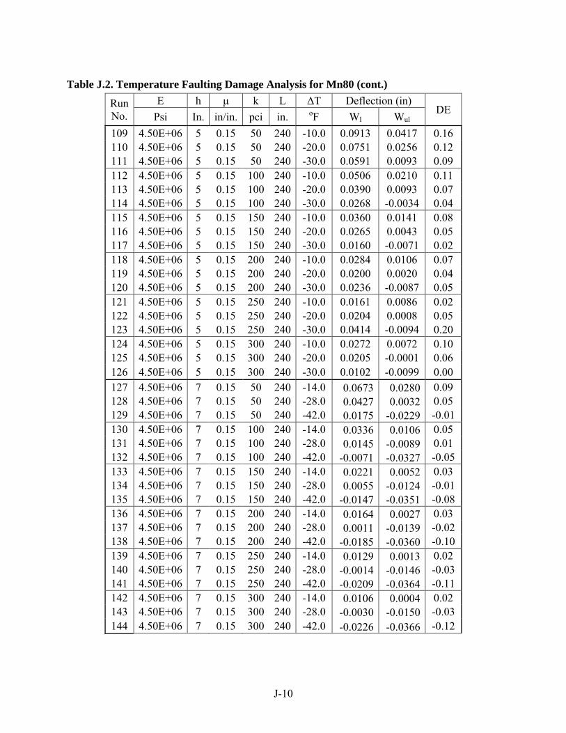
J-10

Table J.2. Temperature Faulting Damage Analysis for Mn80 (cont.)

Run No.

E h μ k L ΔT Deflection (in) DE Psi In. in/in. pci in. oF Wl Wul

109 4.50E+06 5 0.15 50 240 -10.0 0.0913 0.0417 0.16 110 4.50E+06 5 0.15 50 240 -20.0 0.0751 0.0256 0.12 111 4.50E+06 5 0.15 50 240 -30.0 0.0591 0.0093 0.09 112 4.50E+06 5 0.15 100 240 -10.0 0.0506 0.0210 0.11 113 4.50E+06 5 0.15 100 240 -20.0 0.0390 0.0093 0.07 114 4.50E+06 5 0.15 100 240 -30.0 0.0268 -0.0034 0.04 115 4.50E+06 5 0.15 150 240 -10.0 0.0360 0.0141 0.08 116 4.50E+06 5 0.15 150 240 -20.0 0.0265 0.0043 0.05 117 4.50E+06 5 0.15 150 240 -30.0 0.0160 -0.0071 0.02 118 4.50E+06 5 0.15 200 240 -10.0 0.0284 0.0106 0.07 119 4.50E+06 5 0.15 200 240 -20.0 0.0200 0.0020 0.04 120 4.50E+06 5 0.15 200 240 -30.0 0.0236 -0.0087 0.05 121 4.50E+06 5 0.15 250 240 -10.0 0.0161 0.0086 0.02 122 4.50E+06 5 0.15 250 240 -20.0 0.0204 0.0008 0.05 123 4.50E+06 5 0.15 250 240 -30.0 0.0414 -0.0094 0.20 124 4.50E+06 5 0.15 300 240 -10.0 0.0272 0.0072 0.10 125 4.50E+06 5 0.15 300 240 -20.0 0.0205 -0.0001 0.06 126 4.50E+06 5 0.15 300 240 -30.0 0.0102 -0.0099 0.00 127 4.50E+06 7 0.15 50 240 -14.0 0.0673 0.0280 0.09 128 4.50E+06 7 0.15 50 240 -28.0 0.0427 0.0032 0.05 129 4.50E+06 7 0.15 50 240 -42.0 0.0175 -0.0229 -0.01 130 4.50E+06 7 0.15 100 240 -14.0 0.0336 0.0106 0.05 131 4.50E+06 7 0.15 100 240 -28.0 0.0145 -0.0089 0.01 132 4.50E+06 7 0.15 100 240 -42.0 -0.0071 -0.0327 -0.05 133 4.50E+06 7 0.15 150 240 -14.0 0.0221 0.0052 0.03 134 4.50E+06 7 0.15 150 240 -28.0 0.0055 -0.0124 -0.01 135 4.50E+06 7 0.15 150 240 -42.0 -0.0147 -0.0351 -0.08 136 4.50E+06 7 0.15 200 240 -14.0 0.0164 0.0027 0.03 137 4.50E+06 7 0.15 200 240 -28.0 0.0011 -0.0139 -0.02 138 4.50E+06 7 0.15 200 240 -42.0 -0.0185 -0.0360 -0.10 139 4.50E+06 7 0.15 250 240 -14.0 0.0129 0.0013 0.02 140 4.50E+06 7 0.15 250 240 -28.0 -0.0014 -0.0146 -0.03 141 4.50E+06 7 0.15 250 240 -42.0 -0.0209 -0.0364 -0.11 142 4.50E+06 7 0.15 300 240 -14.0 0.0106 0.0004 0.02 143 4.50E+06 7 0.15 300 240 -28.0 -0.0030 -0.0150 -0.03 144 4.50E+06 7 0.15 300 240 -42.0 -0.0226 -0.0366 -0.12

J-11

Table J.2. Temperature Faulting Damage Analysis for Mn80 (cont.)

Run No.

E h μ k L ΔT Deflection (in) DE psi In. in/in. pci in. oF Wl Wul

145 4.50E+06 10 0.15 50 240 -20.0 0.0464 0.0149 0.05 146 4.50E+06 10 0.15 50 240 -40.0 0.0121 -0.0201 -0.01 147 4.50E+06 10 0.15 50 240 -60.0 -0.0241 -0.0585 -0.07 148 4.50E+06 10 0.15 100 240 -20.0 0.0172 -0.0011 0.01 149 4.50E+06 10 0.15 100 240 -40.0 -0.0133 -0.0332 -0.05 150 4.50E+06 10 0.15 100 240 -60.0 -0.0508 -0.0729 -0.14 151 4.50E+06 10 0.15 150 240 -20.0 0.0078 -0.0055 0.00 152 4.50E+06 10 0.15 150 240 -40.0 -0.0215 -0.0370 -0.07 153 4.50E+06 10 0.15 150 240 -60.0 -0.0608 -0.0780 -0.18 154 4.50E+06 10 0.15 200 240 -20.0 0.0034 -0.0075 0.00 155 4.50E+06 10 0.15 200 240 -40.0 -0.0257 -0.0388 -0.08 156 4.50E+06 10 0.15 200 240 -60.0 -0.0664 -0.0810 -0.21 157 4.50E+06 10 0.15 250 240 -20.0 0.0008 -0.0085 -0.01 158 4.50E+06 10 0.15 250 240 -40.0 -0.0284 -0.0399 -0.10 159 4.50E+06 10 0.15 250 240 -60.0 -0.0700 -0.0828 -0.24 160 4.50E+06 10 0.15 300 240 -20.0 -0.0009 -0.0092 -0.01 161 4.50E+06 10 0.15 300 240 -40.0 -0.0303 -0.0406 -0.11 162 4.50E+06 10 0.15 300 240 -60.0 -0.0728 -0.0843 -0.27

J-12

Table J.3. Temperature Fatigue Damage Analysis for Mn102

Run No.

E h μ k L ΔT σ (psi) Nf

Stress Ratio

psi In. in/in. pci in. oF Top Bottom σγ/MOR 1 4.50E+06 5 0.15 50 120 -10.0 261 770 6.2E+01 1.09 2 4.50E+06 5 0.15 50 120 -20.0 316 744 7.5E+01 1.05 3 4.50E+06 5 0.15 50 120 -30.0 367 718 9.0E+01 1.02 4 4.50E+06 5 0.15 100 120 -10.0 278 649 1.6E+02 0.92 5 4.50E+06 5 0.15 100 120 -20.0 351 611 2.4E+02 0.87 6 4.50E+06 5 0.15 100 120 -30.0 417 583 3.3E+02 0.83 7 4.50E+06 5 0.15 150 120 -10.0 284 584 3.3E+02 0.83 8 4.50E+06 5 0.15 150 120 -20.0 366 544 5.5E+02 0.77 9 4.50E+06 5 0.15 150 120 -30.0 440 519 8.1E+02 0.74 10 4.50E+06 5 0.15 200 120 -10.0 285 541 5.8E+02 0.77 11 4.50E+06 5 0.15 200 120 -20.0 374 503 1.1E+03 0.71 12 4.50E+06 5 0.15 200 120 -30.0 453 481 1.5E+03 0.68 13 4.50E+06 5 0.15 250 120 -10.0 284 512 9.1E+02 0.73 14 4.50E+06 5 0.15 250 120 -20.0 377 474 1.8E+03 0.67 15 4.50E+06 5 0.15 250 120 -30.0 461 456 2.3E+03 0.65 16 4.50E+06 5 0.15 300 120 -10.0 281 489 1.3E+03 0.69 17 4.50E+06 5 0.15 300 120 -20.0 379 454 2.7E+03 0.64 18 4.50E+06 5 0.15 300 120 -30.0 466 438 2.1E+03 0.62 19 4.50E+06 7 0.15 50 120 -14.0 143 470 1.9E+03 0.67 20 4.50E+06 7 0.15 50 120 -28.0 184 453 2.7E+03 0.64 21 4.50E+06 7 0.15 50 120 -42.0 221 436 3.9E+03 0.62 22 4.50E+06 7 0.15 100 120 -14.0 170 403 9.0E+03 0.57 23 4.50E+06 7 0.15 100 120 -28.0 228 376 2.0E+04 0.53 24 4.50E+06 7 0.15 100 120 -42.0 276 356 4.0E+04 0.51 25 4.50E+06 7 0.15 150 120 -14.0 185 361 3.4E+04 0.51 26 4.50E+06 7 0.15 150 120 -28.0 254 330 1.1E+05 0.47 27 4.50E+06 7 0.15 150 120 -42.0 309 315 2.2E+05 0.45 28 4.50E+06 7 0.15 200 120 -14.0 196 330 1.1E+05 0.47 29 4.50E+06 7 0.15 200 120 -28.0 272 302 4.3E+05 0.43 30 4.50E+06 7 0.15 200 120 -42.0 331 292 1.1E+05 0.41 31 4.50E+06 7 0.15 250 120 -14.0 204 308 3.1E+05 0.44 32 4.50E+06 7 0.15 250 120 -28.0 284 282 1.1E+06 0.40 33 4.50E+06 7 0.15 250 120 -42.0 351 277 4.9E+04 0.39 34 4.50E+06 7 0.15 300 120 -14.0 210 291 7.8E+05 0.41 35 4.50E+06 7 0.15 300 120 -28.0 294 268 6.4E+05 0.38 36 4.50E+06 7 0.15 300 120 -42.0 366 267 2.8E+04 0.38

J-13

Table J.3. Temperature Fatigue Damage Analysis for Mn102 (cont.)

Run No.

E h μ k L ΔT σ (psi) Nf

Stress Ratio

psi In. in/in. pci in. oF Top Bottom σγ/MOR 37 4.50E+06 10 0.15 50 120 -20.0 77 264 4.4E+06 0.37 38 4.50E+06 10 0.15 50 120 -40.0 98 254 8.6E+06 0.36 39 4.50E+06 10 0.15 50 120 -60.0 120 246 1.7E+07 0.35 40 4.50E+06 10 0.15 100 120 -20.0 94 235 4.4E+07 0.33 41 4.50E+06 10 0.15 100 120 -40.0 133 219 2.1E+08 0.31 42 4.50E+06 10 0.15 100 120 -60.0 163 208 7.4E+08 0.29 43 4.50E+06 10 0.15 150 120 -20.0 110 214 3.8E+08 0.30 44 4.50E+06 10 0.15 150 120 -40.0 155 195 3.7E+09 0.28 45 4.50E+06 10 0.15 150 120 -60.0 191 187 7.0E+09 0.27 46 4.50E+06 10 0.15 200 120 -20.0 122 197 3.0E+09 0.28 47 4.50E+06 10 0.15 200 120 -40.0 173 180 4.0E+10 0.25 48 4.50E+06 10 0.15 200 120 -60.0 211 175 5.1E+08 0.25 49 4.50E+06 10 0.15 250 120 -20.0 131 184 2.1E+10 0.26 50 4.50E+06 10 0.15 250 120 -40.0 187 169 1.3E+10 0.24 51 4.50E+06 10 0.15 250 120 -60.0 228 168 8.6E+07 0.24 52 4.50E+06 10 0.15 300 120 -20.0 139 173 1.3E+11 0.25 53 4.50E+06 10 0.15 300 120 -40.0 198 161 2.7E+09 0.23 54 4.50E+06 10 0.15 300 120 -60.0 242 162 2.4E+07 0.23 55 4.50E+06 5 0.15 50 180 -10.0 246 712 9.5E+01 1.01 56 4.50E+06 5 0.15 50 180 -20.0 303 651 1.6E+02 0.92 57 4.50E+06 5 0.15 50 180 -30.0 355 606 2.6E+02 0.86 58 4.50E+06 5 0.15 100 180 -10.0 274 571 3.9E+02 0.81 59 4.50E+06 5 0.15 100 180 -20.0 350 509 9.5E+02 0.72 60 4.50E+06 5 0.15 100 180 -30.0 417 467 2.0E+03 0.66 61 4.50E+06 5 0.15 150 180 -10.0 284 508 9.6E+02 0.72 62 4.50E+06 5 0.15 150 180 -20.0 370 446 3.1E+03 0.63 63 4.50E+06 5 0.15 150 180 -30.0 446 407 3.2E+03 0.58 64 4.50E+06 5 0.15 200 180 -10.0 287 471 1.9E+03 0.67 65 4.50E+06 5 0.15 200 180 -20.0 380 408 7.9E+03 0.58 66 4.50E+06 5 0.15 200 180 -30.0 462 371 2.2E+03 0.53 67 4.50E+06 5 0.15 250 180 -10.0 287 445 3.2E+03 0.63 68 4.50E+06 5 0.15 250 180 -20.0 385 382 1.6E+04 0.54 69 4.50E+06 5 0.15 250 180 -30.0 472 347 1.8E+03 0.49 70 4.50E+06 5 0.15 300 180 -10.0 285 425 5.1E+03 0.60 71 4.50E+06 5 0.15 300 180 -20.0 387 363 1.4E+04 0.51 72 4.50E+06 5 0.15 300 180 -30.0 479 329 1.6E+03 0.47

J-14

Table J.3. Temperature Fatigue Damage Analysis for Mn102 (cont.)

Run No.

E h μ k L ΔT σ (psi) Nf

Stress Ratio

psi In. in/in. pci in. oF Top Bottom σγ/MOR 73 4.50E+06 7 0.15 50 180 -14.0 127 468 2.0E+03 0.66 74 4.50E+06 7 0.15 50 180 -28.0 169 412 7.0E+03 0.58 75 4.50E+06 7 0.15 50 180 -42.0 204 374 2.1E+04 0.53 76 4.50E+06 7 0.15 100 180 -14.0 162 350 5.0E+04 0.50 77 4.50E+06 7 0.15 100 180 -28.0 220 297 5.7E+05 0.42 78 4.50E+06 7 0.15 100 180 -42.0 266 268 3.3E+06 0.38 79 4.50E+06 7 0.15 150 180 -14.0 182 295 6.2E+05 0.42 80 4.50E+06 7 0.15 150 180 -28.0 250 246 1.2E+07 0.35 81 4.50E+06 7 0.15 150 180 -42.0 305 224 3.6E+05 0.32 82 4.50E+06 7 0.15 200 180 -14.0 195 262 4.9E+06 0.37 83 4.50E+06 7 0.15 200 180 -28.0 271 216 2.7E+06 0.31 84 4.50E+06 7 0.15 200 180 -42.0 334 200 9.5E+04 0.28 85 4.50E+06 7 0.15 250 180 -14.0 205 240 2.9E+07 0.34 86 4.50E+06 7 0.15 250 180 -28.0 287 197 1.0E+06 0.28 87 4.50E+06 7 0.15 250 180 -42.0 356 185 4.0E+04 0.26 88 4.50E+06 7 0.15 300 180 -14.0 212 224 1.3E+08 0.32 89 4.50E+06 7 0.15 300 180 -28.0 300 183 4.8E+05 0.26 90 4.50E+06 7 0.15 300 180 -42.0 374 176 2.2E+04 0.25 91 4.50E+06 10 0.15 50 180 -20.0 79 299 4.9E+05 0.42 92 4.50E+06 10 0.15 50 180 -40.0 117 257 7.1E+06 0.36 93 4.50E+06 10 0.15 50 180 -60.0 142 228 8.7E+07 0.32 94 4.50E+06 10 0.15 100 180 -20.0 95 218 2.4E+08 0.31 95 4.50E+06 10 0.15 100 180 -40.0 139 176 7.4E+10 0.25 96 4.50E+06 10 0.15 100 180 -60.0 165 156 6.0E+11 0.22 97 4.50E+06 10 0.15 150 180 -20.0 106 175 9.5E+10 0.25 98 4.50E+06 10 0.15 150 180 -40.0 152 139 1.0E+13 0.20 99 4.50E+06 10 0.15 150 180 -60.0 182 126 2.7E+10 0.18 100 4.50E+06 10 0.15 200 180 -20.0 116 148 2.6E+13 0.21 101 4.50E+06 10 0.15 200 180 -40.0 167 119 4.1E+11 0.17 102 4.50E+06 10 0.15 200 180 -60.0 206 111 9.9E+08 0.16 103 4.50E+06 10 0.15 250 180 -20.0 127 130 5.2E+15 0.18 104 4.50E+06 10 0.15 250 180 -40.0 183 106 2.4E+10 0.15 105 4.50E+06 10 0.15 250 180 -60.0 225 103 1.2E+08 0.15 106 4.50E+06 10 0.15 300 180 -20.0 136 117 8.4E+14 0.17 107 4.50E+06 10 0.15 300 180 -40.0 196 97 3.4E+09 0.14 108 4.50E+06 10 0.15 300 180 -60.0 241 98 2.6E+07 0.14

J-15

Table J.3. Temperature Fatigue Damage Analysis for Mn102 (cont.)

Run No.

E h μ k L ΔT σ (psi) Nf

Stress Ratio

psi In. in/in. pci in. oF Top Bottom σγ/MOR 109 4.50E+06 5 0.15 50 240 -10.0 245 661 1.5E+02 0.94 110 4.50E+06 5 0.15 50 240 -20.0 306 574 3.7E+02 0.81 111 4.50E+06 5 0.15 50 240 -30.0 361 502 1.1E+03 0.71 112 4.50E+06 5 0.15 100 240 -10.0 274 544 5.6E+02 0.77 113 4.50E+06 5 0.15 100 240 -20.0 353 454 2.6E+03 0.64 114 4.50E+06 5 0.15 100 240 -30.0 425 381 5.1E+03 0.54 115 4.50E+06 5 0.15 150 240 -10.0 283 491 1.3E+03 0.70 116 4.50E+06 5 0.15 150 240 -20.0 372 400 9.9E+03 0.57 117 4.50E+06 5 0.15 150 240 -30.0 455 327 2.6E+03 0.46 118 4.50E+06 5 0.15 200 240 -10.0 285 458 2.4E+03 0.65 119 4.50E+06 5 0.15 200 240 -20.0 382 367 1.7E+04 0.52 120 4.50E+06 5 0.15 200 240 -30.0 471 295 1.9E+03 0.42 121 4.50E+06 5 0.15 250 240 -10.0 285 435 4.0E+03 0.62 122 4.50E+06 5 0.15 250 240 -20.0 387 344 1.5E+04 0.49 123 4.50E+06 5 0.15 250 240 -30.0 482 273 1.5E+03 0.39 124 4.50E+06 5 0.15 300 240 -10.0 283 418 6.2E+03 0.59 125 4.50E+06 5 0.15 300 240 -20.0 389 327 1.4E+04 0.46 126 4.50E+06 5 0.15 300 240 -30.0 489 256 1.3E+03 0.36 127 4.50E+06 7 0.15 50 240 -14.0 134 395 1.2E+04 0.56 128 4.50E+06 7 0.15 50 240 -28.0 228 308 3.2E+05 0.44 129 4.50E+06 7 0.15 50 240 -42.0 295 249 6.2E+05 0.35 130 4.50E+06 7 0.15 100 240 -14.0 164 292 7.3E+05 0.41 131 4.50E+06 7 0.15 100 240 -28.0 260 203 5.7E+06 0.29 132 4.50E+06 7 0.15 100 240 -42.0 335 148 9.2E+04 0.21 133 4.50E+06 7 0.15 150 240 -14.0 184 246 1.6E+07 0.35 134 4.50E+06 7 0.15 150 240 -28.0 277 157 1.8E+06 0.22 135 4.50E+06 7 0.15 150 240 -42.0 357 108 3.8E+04 0.15 136 4.50E+06 7 0.15 200 240 -14.0 198 219 2.0E+08 0.31 137 4.50E+06 7 0.15 200 240 -28.0 288 131 9.2E+05 0.19 138 4.50E+06 7 0.15 200 240 -42.0 372 87 2.3E+04 0.12 139 4.50E+06 7 0.15 250 240 -14.0 207 201 8.3E+08 0.28 140 4.50E+06 7 0.15 250 240 -28.0 300 113 4.8E+05 0.16 141 4.50E+06 7 0.15 250 240 -42.0 384 76 1.6E+04 0.11 142 4.50E+06 7 0.15 300 240 -14.0 214 187 3.6E+08 0.27 143 4.50E+06 7 0.15 300 240 -28.0 314 101 2.4E+05 0.14 144 4.50E+06 7 0.15 300 240 -42.0 395 74 1.1E+04 0.10

J-16

Table J.3. Temperature Fatigue Damage Analysis for Mn102 (cont.)

Run No.

E h μ k L ΔT σ (psi) Nf

Stress Ratio

psi In. in/in. pci in. oF Top Bottom σγ/MOR 145 4.50E+06 10 0.15 50 240 -20.0 121 236 3.9E+07 0.33 146 4.50E+06 10 0.15 50 240 -40.0 149 166 5.2E+11 0.23 147 4.50E+06 10 0.15 50 240 -60.0 163 125 8.4E+11 0.18 148 4.50E+06 10 0.15 100 240 -20.0 173 146 1.2E+11 0.21 149 4.50E+06 10 0.15 100 240 -40.0 180 80 3.5E+10 0.11 150 4.50E+06 10 0.15 100 240 -60.0 186 50 1.4E+10 0.07 151 4.50E+06 10 0.15 150 240 -20.0 192 104 6.4E+09 0.15 152 4.50E+06 10 0.15 150 240 -40.0 223 45 1.4E+08 0.06 153 4.50E+06 10 0.15 150 240 -60.0 231 34 6.2E+07 0.05 154 4.50E+06 10 0.15 200 240 -20.0 242 80 2.4E+07 0.11 155 4.50E+06 10 0.15 200 240 -40.0 255 34 8.4E+06 0.05 156 4.50E+06 10 0.15 200 240 -60.0 264 33 4.3E+06 0.05 157 4.50E+06 10 0.15 250 240 -20.0 265 63 4.1E+06 0.09 158 4.50E+06 10 0.15 250 240 -40.0 273 31 2.3E+06 0.04 159 4.50E+06 10 0.15 250 240 -60.0 283 33 1.2E+06 0.05 160 4.50E+06 10 0.15 300 240 -20.0 297 52 5.5E+05 0.07 161 4.50E+06 10 0.15 300 240 -40.0 308 31 3.1E+05 0.04 162 4.50E+06 10 0.15 300 240 -60.0 317 35 2.1E+05 0.05

J-17

Table J.4. Temperature Faulting Damage Analysis for Mn102

Run No.

E h μ k L ΔT Deflection (in) DE psi In. in/in. pci in. oF Wl Wul

1 4.50E+06 5 0.15 50 120 -10.0 0.1390 0.0872 0.29 2 4.50E+06 5 0.15 50 120 -20.0 0.1263 0.0741 0.26 3 4.50E+06 5 0.15 50 120 -30.0 0.1141 0.0615 0.23 4 4.50E+06 5 0.15 100 120 -10.0 0.0784 0.0434 0.21 5 4.50E+06 5 0.15 100 120 -20.0 0.0683 0.0331 0.18 6 4.50E+06 5 0.15 100 120 -30.0 0.0585 0.0231 0.14 7 4.50E+06 5 0.15 150 120 -10.0 0.0567 0.0291 0.18 8 4.50E+06 5 0.15 150 120 -20.0 0.0480 0.0203 0.14 9 4.50E+06 5 0.15 150 120 -30.0 0.0396 0.0117 0.11 10 4.50E+06 5 0.15 200 120 -10.0 0.0453 0.0220 0.16 11 4.50E+06 5 0.15 200 120 -20.0 0.0376 0.0142 0.12 12 4.50E+06 5 0.15 200 120 -30.0 0.0300 0.0066 0.09 13 4.50E+06 5 0.15 250 120 -10.0 0.0382 0.0179 0.14 14 4.50E+06 5 0.15 250 120 -20.0 0.0311 0.0107 0.11 15 4.50E+06 5 0.15 250 120 -30.0 0.0242 0.0037 0.07 16 4.50E+06 5 0.15 300 120 -10.0 0.0332 0.0151 0.13 17 4.50E+06 5 0.15 300 120 -20.0 0.0266 0.0085 0.10 18 4.50E+06 5 0.15 300 120 -30.0 0.0202 0.0020 0.06 19 4.50E+06 7 0.15 50 120 -14.0 0.1113 0.0782 0.16 20 4.50E+06 7 0.15 50 120 -28.0 0.0952 0.0617 0.13 21 4.50E+06 7 0.15 50 120 -42.0 0.0799 0.0459 0.11 22 4.50E+06 7 0.15 100 120 -14.0 0.0576 0.0352 0.10 23 4.50E+06 7 0.15 100 120 -28.0 0.0440 0.0213 0.07 24 4.50E+06 7 0.15 100 120 -42.0 0.0311 0.0080 0.05 25 4.50E+06 7 0.15 150 120 -14.0 0.0392 0.0213 0.08 26 4.50E+06 7 0.15 150 120 -28.0 0.0272 0.0090 0.05 27 4.50E+06 7 0.15 150 120 -42.0 0.0155 -0.0029 0.02 28 4.50E+06 7 0.15 200 120 -14.0 0.0299 0.0146 0.07 29 4.50E+06 7 0.15 200 120 -28.0 0.0189 0.0034 0.03 30 4.50E+06 7 0.15 200 120 -42.0 0.0079 -0.0078 0.00 31 4.50E+06 7 0.15 250 120 -14.0 0.0242 0.0108 0.06 32 4.50E+06 7 0.15 250 120 -28.0 0.0140 0.0004 0.02 33 4.50E+06 7 0.15 250 120 -42.0 0.0035 -0.0104 -0.01 34 4.50E+06 7 0.15 300 120 -14.0 0.0205 0.0083 0.05 35 4.50E+06 7 0.15 300 120 -28.0 0.0108 -0.0015 0.02 36 4.50E+06 7 0.15 300 120 -42.0 0.0006 -0.0120 -0.02

J-18

Table J.4. Temperature Faulting Damage Analysis for Mn102 (cont.)

Run No.

E h μ k L ΔT Deflection (in) DE Psi In. in/in. pci in. oF Wl Wul

37 4.50E+06 10 0.15 50 120 -20.0 0.0951 0.0738 0.09 38 4.50E+06 10 0.15 50 120 -40.0 0.0764 0.0547 0.07 39 4.50E+06 10 0.15 50 120 -60.0 0.0587 0.0366 0.05 40 4.50E+06 10 0.15 100 120 -20.0 0.0442 0.0302 0.05 41 4.50E+06 10 0.15 100 120 -40.0 0.0276 0.0132 0.03 42 4.50E+06 10 0.15 100 120 -60.0 0.0119 -0.0029 0.01 43 4.50E+06 10 0.15 150 120 -20.0 0.0272 0.0160 0.04 44 4.50E+06 10 0.15 150 120 -40.0 0.0119 0.0004 0.01 45 4.50E+06 10 0.15 150 120 -60.0 -0.0031 -0.0150 -0.02 46 4.50E+06 10 0.15 200 120 -20.0 0.0187 0.0092 0.03 47 4.50E+06 10 0.15 200 120 -40.0 0.0043 -0.0055 0.00 48 4.50E+06 10 0.15 200 120 -60.0 -0.0106 -0.0209 -0.03 49 4.50E+06 10 0.15 250 120 -20.0 0.0138 0.0053 0.02 50 4.50E+06 10 0.15 250 120 -40.0 -0.0001 -0.0089 -0.01 51 4.50E+06 10 0.15 250 120 -60.0 -0.0153 -0.0244 -0.05 52 4.50E+06 10 0.15 300 120 -20.0 0.0105 0.0029 0.02 53 4.50E+06 10 0.15 300 120 -40.0 -0.0030 -0.0111 -0.02 54 4.50E+06 10 0.15 300 120 -60.0 -0.0186 -0.0269 -0.06 55 4.50E+06 5 0.15 50 180 -10.0 0.1310 0.0806 0.27 56 4.50E+06 5 0.15 50 180 -20.0 0.1149 0.0644 0.23 57 4.50E+06 5 0.15 50 180 -30.0 0.0992 0.0487 0.19 58 4.50E+06 5 0.15 100 180 -10.0 0.0765 0.0418 0.21 59 4.50E+06 5 0.15 100 180 -20.0 0.0646 0.0300 0.16 60 4.50E+06 5 0.15 100 180 -30.0 0.0528 0.0182 0.12 61 4.50E+06 5 0.15 150 180 -10.0 0.0562 0.0286 0.18 62 4.50E+06 5 0.15 150 180 -20.0 0.0464 0.0189 0.13 63 4.50E+06 5 0.15 150 180 -30.0 0.0365 0.0091 0.09 64 4.50E+06 5 0.15 200 180 -10.0 0.0452 0.0219 0.16 65 4.50E+06 5 0.15 200 180 -20.0 0.0367 0.0135 0.12 66 4.50E+06 5 0.15 200 180 -30.0 0.0280 0.0049 0.08 67 4.50E+06 5 0.15 250 180 -10.0 0.0382 0.0179 0.14 68 4.50E+06 5 0.15 250 180 -20.0 0.0306 0.0104 0.10 69 4.50E+06 5 0.15 250 180 -30.0 0.0228 0.0026 0.06 70 4.50E+06 5 0.15 300 180 -10.0 0.0333 0.0152 0.13 71 4.50E+06 5 0.15 300 180 -20.0 0.0264 0.0084 0.09 72 4.50E+06 5 0.15 300 180 -30.0 0.0191 0.0011 0.05

J-19

Table J.4. Temperature Faulting Damage Analysis for Mn102 (cont.)

Run No.

E h μ k L ΔT Deflection (in) DE psi In. in/in. pci in. oF Wl Wul

73 4.50E+06 7 0.15 50 180 -14.0 0.0956 0.0645 0.12 74 4.50E+06 7 0.15 50 180 -28.0 0.0737 0.0423 0.09 75 4.50E+06 7 0.15 50 180 -42.0 0.0532 0.0215 0.06 76 4.50E+06 7 0.15 100 180 -14.0 0.0511 0.0294 0.09 77 4.50E+06 7 0.15 100 180 -28.0 0.0337 0.0118 0.05 78 4.50E+06 7 0.15 100 180 -42.0 0.0166 -0.0055 0.01 79 4.50E+06 7 0.15 150 180 -14.0 0.0356 0.0181 0.07 80 4.50E+06 7 0.15 150 180 -28.0 0.0205 0.0029 0.03 81 4.50E+06 7 0.15 150 180 -42.0 0.0049 -0.0130 -0.01 82 4.50E+06 7 0.15 200 180 -14.0 0.0276 0.0126 0.06 83 4.50E+06 7 0.15 200 180 -28.0 0.0139 -0.0011 0.02 84 4.50E+06 7 0.15 200 180 -42.0 -0.0006 -0.0161 -0.03 85 4.50E+06 7 0.15 250 180 -14.0 0.0227 0.0094 0.05 86 4.50E+06 7 0.15 250 180 -28.0 0.0101 -0.0032 0.01 87 4.50E+06 7 0.15 250 180 -42.0 -0.0040 -0.0177 -0.04 88 4.50E+06 7 0.15 300 180 -14.0 0.0194 0.0074 0.05 89 4.50E+06 7 0.15 300 180 -28.0 0.0075 -0.0046 0.01 90 4.50E+06 7 0.15 300 180 -42.0 -0.0061 -0.0186 -0.05 91 4.50E+06 10 0.15 50 180 -20.0 0.0718 0.0528 0.06 92 4.50E+06 10 0.15 50 180 -40.0 0.0452 0.0258 0.03 93 4.50E+06 10 0.15 50 180 -60.0 0.0202 0.0003 0.01 94 4.50E+06 10 0.15 100 180 -20.0 0.0319 0.0189 0.03 95 4.50E+06 10 0.15 100 180 -40.0 0.0090 -0.0044 0.00 96 4.50E+06 10 0.15 100 180 -60.0 -0.0139 -0.0281 -0.03 97 4.50E+06 10 0.15 150 180 -20.0 0.0188 0.0082 0.02 98 4.50E+06 10 0.15 150 180 -40.0 -0.0024 -0.0134 -0.01 99 4.50E+06 10 0.15 150 180 -60.0 -0.0251 -0.0368 -0.05 100 4.50E+06 10 0.15 200 180 -20.0 0.0124 0.0033 0.01 101 4.50E+06 10 0.15 200 180 -40.0 -0.0078 -0.0175 -0.02 102 4.50E+06 10 0.15 200 180 -60.0 -0.0310 -0.0412 -0.07 103 4.50E+06 10 0.15 250 180 -20.0 0.0086 0.0005 0.01 104 4.50E+06 10 0.15 250 180 -40.0 -0.0111 -0.0198 -0.03 105 4.50E+06 10 0.15 250 180 -60.0 -0.0350 -0.0439 -0.09 106 4.50E+06 10 0.15 300 180 -20.0 0.0061 -0.0012 0.01 107 4.50E+06 10 0.15 300 180 -40.0 -0.0133 -0.0212 -0.04 108 4.50E+06 10 0.15 300 180 -60.0 -0.0378 -0.0459 -0.10

J-20

Table J.4. Temperature Faulting Damage Analysis for Mn102 (cont.)

Run No.

E h μ k L ΔT Deflection (in) DE Psi In. in/in. pci in. oF Wl Wul

109 4.50E+06 5 0.15 50 240 -10.0 0.1309 0.0805 0.27 110 4.50E+06 5 0.15 50 240 -20.0 0.1147 0.0643 0.23 111 4.50E+06 5 0.15 50 240 -30.0 0.0986 0.0482 0.19 112 4.50E+06 5 0.15 100 240 -10.0 0.0766 0.0420 0.21 113 4.50E+06 5 0.15 100 240 -20.0 0.0650 0.0304 0.17 114 4.50E+06 5 0.15 100 240 -30.0 0.0533 0.0187 0.12 115 4.50E+06 5 0.15 150 240 -10.0 0.0563 0.0287 0.18 116 4.50E+06 5 0.15 150 240 -20.0 0.0467 0.0192 0.14 117 4.50E+06 5 0.15 150 240 -30.0 0.0369 0.0096 0.10 118 4.50E+06 5 0.15 200 240 -10.0 0.0453 0.0220 0.16 119 4.50E+06 5 0.15 200 240 -20.0 0.0369 0.0138 0.12 120 4.50E+06 5 0.15 200 240 -30.0 0.0283 0.0053 0.08 121 4.50E+06 5 0.15 250 240 -10.0 0.0382 0.0179 0.14 122 4.50E+06 5 0.15 250 240 -20.0 0.0308 0.0106 0.10 123 4.50E+06 5 0.15 250 240 -30.0 0.0230 0.0029 0.07 124 4.50E+06 5 0.15 300 240 -10.0 0.0333 0.0152 0.13 125 4.50E+06 5 0.15 300 240 -20.0 0.0265 0.0085 0.09 126 4.50E+06 5 0.15 300 240 -30.0 0.0193 0.0014 0.06 127 4.50E+06 7 0.15 50 240 -14.0 0.0930 0.0621 0.12 128 4.50E+06 7 0.15 50 240 -28.0 0.0684 0.0375 0.08 129 4.50E+06 7 0.15 50 240 -42.0 0.0446 0.0135 0.05 130 4.50E+06 7 0.15 100 240 -14.0 0.0509 0.0292 0.09 131 4.50E+06 7 0.15 100 240 -28.0 0.0324 0.0107 0.05 132 4.50E+06 7 0.15 100 240 -42.0 0.0132 -0.0085 0.01 133 4.50E+06 7 0.15 150 240 -14.0 0.0358 0.0183 0.07 134 4.50E+06 7 0.15 150 240 -28.0 0.0202 0.0027 0.03 135 4.50E+06 7 0.15 150 240 -42.0 0.0031 -0.0146 -0.02 136 4.50E+06 7 0.15 200 240 -14.0 0.0279 0.0129 0.06 137 4.50E+06 7 0.15 200 240 -28.0 0.0140 -0.0010 0.02 138 4.50E+06 7 0.15 200 240 -42.0 -0.0019 -0.0171 -0.03 139 4.50E+06 7 0.15 250 240 -14.0 0.0230 0.0097 0.05 140 4.50E+06 7 0.15 250 240 -28.0 0.0102 -0.0030 0.01 141 4.50E+06 7 0.15 250 240 -42.0 -0.0049 -0.0184 -0.04 142 4.50E+06 7 0.15 300 240 -14.0 0.0196 0.0076 0.05 143 4.50E+06 7 0.15 300 240 -28.0 0.0077 -0.0042 0.01 144 4.50E+06 7 0.15 300 240 -42.0 -0.0070 -0.0192 -0.05

J-21

Table J.4. Temperature Faulting Damage Analysis for Mn102 (cont.)

Run No.

E H μ k L ΔT Deflection (in) DE psi In. in/in. pci in. oF Wl Wul

145 4.50E+06 10 0.15 50 240 -20.0 0.0623 0.0439 0.05 146 4.50E+06 10 0.15 50 240 -40.0 0.0290 0.0103 0.02 147 4.50E+06 10 0.15 50 240 -60.0 -0.0040 -0.0232 -0.01 148 4.50E+06 10 0.15 100 240 -20.0 0.0281 0.0152 0.03 149 4.50E+06 10 0.15 100 240 -40.0 0.0000 -0.0131 -0.01 150 4.50E+06 10 0.15 100 240 -60.0 -0.0308 -0.0448 -0.05 151 4.50E+06 10 0.15 150 240 -20.0 0.0167 0.0063 0.02 152 4.50E+06 10 0.15 150 240 -40.0 -0.0088 -0.0197 -0.02 153 4.50E+06 10 0.15 150 240 -60.0 -0.0403 -0.0517 -0.08 154 4.50E+06 10 0.15 200 240 -20.0 0.0112 0.0021 0.01 155 4.50E+06 10 0.15 200 240 -40.0 -0.0131 -0.0227 -0.03 156 4.50E+06 10 0.15 200 240 -60.0 -0.0456 -0.0554 -0.10 157 4.50E+06 10 0.15 250 240 -20.0 0.0078 -0.0002 0.01 158 4.50E+06 10 0.15 250 240 -40.0 -0.0158 -0.0243 -0.04 159 4.50E+06 10 0.15 250 240 -60.0 -0.0492 -0.0578 -0.12 160 4.50E+06 10 0.15 300 240 -20.0 0.0057 -0.0017 0.00 161 4.50E+06 10 0.15 300 240 -40.0 -0.0177 -0.0254 -0.05 162 4.50E+06 10 0.15 300 240 -60.0 -0.0518 -0.0595 -0.13

J-22

Table J.5. Temperature Fatigue Damage for G1

Run No.

E h μ k L ΔT σ (psi) Nf

Stress Ratio

psi In. in/in. pci in. oF Top Bottom σγ/MOR 1 4.50E+06 5 0.15 50 120 -10.0 509 1358 7.9E+00 1.93 2 4.50E+06 5 0.15 50 120 -20.0 579 1320 8.5E+00 1.87 3 4.50E+06 5 0.15 50 120 -30.0 647 1286 9.1E+00 1.82 4 4.50E+06 5 0.15 100 120 -10.0 411 1114 1.4E+01 1.58 5 4.50E+06 5 0.15 100 120 -20.0 501 1071 1.6E+01 1.52 6 4.50E+06 5 0.15 100 120 -30.0 588 1039 1.8E+01 1.47 7 4.50E+06 5 0.15 150 120 -10.0 360 981 2.2E+01 1.39 8 4.50E+06 5 0.15 150 120 -20.0 461 938 2.6E+01 1.33 9 4.50E+06 5 0.15 150 120 -30.0 556 909 2.9E+01 1.29 10 4.50E+06 5 0.15 200 120 -10.0 329 892 3.2E+01 1.26 11 4.50E+06 5 0.15 200 120 -20.0 435 849 3.9E+01 1.20 12 4.50E+06 5 0.15 200 120 -30.0 535 825 4.5E+01 1.17 13 4.50E+06 5 0.15 250 120 -10.0 308 826 4.5E+01 1.17 14 4.50E+06 5 0.15 250 120 -20.0 416 785 5.7E+01 1.11 15 4.50E+06 5 0.15 250 120 -30.0 521 762 6.6E+01 1.08 16 4.50E+06 5 0.15 300 120 -10.0 294 775 6.1E+01 1.10 17 4.50E+06 5 0.15 300 120 -20.0 404 735 8.0E+01 1.04 18 4.50E+06 5 0.15 300 120 -30.0 509 714 9.3E+01 1.01 19 4.50E+06 7 0.15 50 120 -14.0 371 845 4.0E+01 1.20 20 4.50E+06 7 0.15 50 120 -28.0 425 820 4.6E+01 1.16 21 4.50E+06 7 0.15 50 120 -42.0 476 797 5.3E+01 1.13 22 4.50E+06 7 0.15 100 120 -14.0 336 722 8.8E+01 1.02 23 4.50E+06 7 0.15 100 120 -28.0 415 684 1.2E+02 0.97 24 4.50E+06 7 0.15 100 120 -42.0 487 660 1.5E+02 0.94 25 4.50E+06 7 0.15 150 120 -14.0 317 642 1.7E+02 0.91 26 4.50E+06 7 0.15 150 120 -28.0 410 605 2.6E+02 0.86 27 4.50E+06 7 0.15 150 120 -42.0 494 588 3.2E+02 0.83 28 4.50E+06 7 0.15 200 120 -14.0 303 587 3.2E+02 0.83 29 4.50E+06 7 0.15 200 120 -28.0 407 553 4.9E+02 0.78 30 4.50E+06 7 0.15 200 120 -42.0 500 540 5.8E+02 0.77 31 4.50E+06 7 0.15 250 120 -14.0 294 545 5.5E+02 0.77 32 4.50E+06 7 0.15 250 120 -28.0 405 514 8.7E+02 0.73 33 4.50E+06 7 0.15 250 120 -42.0 504 507 9.8E+02 0.72 34 4.50E+06 7 0.15 300 120 -14.0 286 512 9.0E+02 0.73 35 4.50E+06 7 0.15 300 120 -28.0 403 485 1.4E+03 0.69 36 4.50E+06 7 0.15 300 120 -42.0 507 481 9.8E+02 0.68

J-23

Table J.5. Temperature Fatigue Damage for G1 (cont.)

Run No.

E h μ k L ΔT σ (psi) Nf

Stress Ratio

psi In. in/in. pci in. oF Top Bottom σγ/MOR 37 4.50E+06 10 0.15 50 120 -20.0 228 473 1.8E+03 0.67 38 4.50E+06 10 0.15 50 120 -40.0 261 460 2.3E+03 0.65 39 4.50E+06 10 0.15 50 120 -60.0 293 447 3.1E+03 0.63 40 4.50E+06 10 0.15 100 120 -20.0 229 425 5.1E+03 0.60 41 4.50E+06 10 0.15 100 120 -40.0 283 403 9.1E+03 0.57 42 4.50E+06 10 0.15 100 120 -60.0 330 389 1.4E+04 0.55 43 4.50E+06 10 0.15 150 120 -20.0 231 389 1.4E+04 0.55 44 4.50E+06 10 0.15 150 120 -40.0 299 364 3.0E+04 0.52 45 4.50E+06 10 0.15 150 120 -60.0 353 356 4.1E+04 0.50 46 4.50E+06 10 0.15 200 120 -20.0 233 360 3.5E+04 0.51 47 4.50E+06 10 0.15 200 120 -40.0 310 338 8.0E+04 0.48 48 4.50E+06 10 0.15 200 120 -60.0 370 335 2.5E+04 0.47 49 4.50E+06 10 0.15 250 120 -20.0 236 337 8.3E+04 0.48 50 4.50E+06 10 0.15 250 120 -40.0 319 319 1.8E+05 0.45 51 4.50E+06 10 0.15 250 120 -60.0 384 321 1.6E+04 0.46 52 4.50E+06 10 0.15 300 120 -20.0 237 319 1.9E+05 0.45 53 4.50E+06 10 0.15 300 120 -40.0 327 305 1.3E+05 0.43 54 4.50E+06 10 0.15 300 120 -60.0 395 311 1.1E+04 0.44 55 4.50E+06 5 0.15 50 180 -10.0 488 1262 9.6E+00 1.79 56 4.50E+06 5 0.15 50 180 -20.0 561 1198 1.1E+01 1.70 57 4.50E+06 5 0.15 50 180 -30.0 628 1150 1.3E+01 1.63 58 4.50E+06 5 0.15 100 180 -10.0 408 1038 1.8E+01 1.47 59 4.50E+06 5 0.15 100 180 -20.0 502 970 2.3E+01 1.38 60 4.50E+06 5 0.15 100 180 -30.0 590 922 2.8E+01 1.31 61 4.50E+06 5 0.15 150 180 -10.0 362 921 2.8E+01 1.31 62 4.50E+06 5 0.15 150 180 -20.0 466 850 3.9E+01 1.20 63 4.50E+06 5 0.15 150 180 -30.0 565 803 5.1E+01 1.14 64 4.50E+06 5 0.15 200 180 -10.0 333 842 4.1E+01 1.19 65 4.50E+06 5 0.15 200 180 -20.0 444 769 6.3E+01 1.09 66 4.50E+06 5 0.15 200 180 -30.0 548 723 8.7E+01 1.03 67 4.50E+06 5 0.15 250 180 -10.0 314 784 5.7E+01 1.11 68 4.50E+06 5 0.15 250 180 -20.0 427 710 9.6E+01 1.01 69 4.50E+06 5 0.15 250 180 -30.0 536 664 1.4E+02 0.94 70 4.50E+06 5 0.15 300 180 -10.0 300 738 7.8E+01 1.05 71 4.50E+06 5 0.15 300 180 -20.0 416 663 1.4E+02 0.94 72 4.50E+06 5 0.15 300 180 -30.0 526 618 2.2E+02 0.88

J-24

Table J.5. Temperature Fatigue Damage for G1 (cont.)

Run No.

E h μ k L ΔT σ (psi) Nf

Stress Ratio

psi In. in/in. pci in. oF Top Bottom σγ/MOR 73 4.50E+06 7 0.15 50 180 -14.0 336 795 5.4E+01 1.13 74 4.50E+06 7 0.15 50 180 -28.0 391 735 8.0E+01 1.04 75 4.50E+06 7 0.15 50 180 -42.0 439 695 1.1E+02 0.99 76 4.50E+06 7 0.15 100 180 -14.0 321 642 1.8E+02 0.91 77 4.50E+06 7 0.15 100 180 -28.0 399 584 3.3E+02 0.83 78 4.50E+06 7 0.15 100 180 -42.0 468 551 5.0E+02 0.78 79 4.50E+06 7 0.15 150 180 -14.0 310 564 4.2E+02 0.80 80 4.50E+06 7 0.15 150 180 -28.0 403 508 9.6E+02 0.72 81 4.50E+06 7 0.15 150 180 -42.0 485 481 1.4E+03 0.68 82 4.50E+06 7 0.15 200 180 -14.0 302 513 8.9E+02 0.73 83 4.50E+06 7 0.15 200 180 -28.0 406 459 2.4E+03 0.65 84 4.50E+06 7 0.15 200 180 -42.0 497 437 1.2E+03 0.62 85 4.50E+06 7 0.15 250 180 -14.0 295 476 1.7E+03 0.67 86 4.50E+06 7 0.15 250 180 -28.0 407 424 5.3E+03 0.60 87 4.50E+06 7 0.15 250 180 -42.0 505 406 1.0E+03 0.58 88 4.50E+06 7 0.15 300 180 -14.0 289 447 3.1E+03 0.63 89 4.50E+06 7 0.15 300 180 -28.0 408 396 8.0E+03 0.56 90 4.50E+06 7 0.15 300 180 -42.0 512 382 9.0E+02 0.54 91 4.50E+06 10 0.15 50 180 -20.0 196 480 1.6E+03 0.68 92 4.50E+06 10 0.15 50 180 -40.0 229 432 4.4E+03 0.61 93 4.50E+06 10 0.15 50 180 -60.0 256 400 1.0E+04 0.57 94 4.50E+06 10 0.15 100 180 -20.0 207 381 1.7E+04 0.54 95 4.50E+06 10 0.15 100 180 -40.0 257 336 8.9E+04 0.48 96 4.50E+06 10 0.15 100 180 -60.0 298 312 2.5E+05 0.44 97 4.50E+06 10 0.15 150 180 -20.0 215 328 1.2E+05 0.47 98 4.50E+06 10 0.15 150 180 -40.0 277 289 8.8E+05 0.41 99 4.50E+06 10 0.15 150 180 -60.0 327 273 1.3E+05 0.39 100 4.50E+06 10 0.15 200 180 -20.0 221 294 6.4E+05 0.42 101 4.50E+06 10 0.15 200 180 -40.0 293 260 7.1E+05 0.37 102 4.50E+06 10 0.15 200 180 -60.0 349 250 5.3E+04 0.35 103 4.50E+06 10 0.15 250 180 -20.0 226 270 2.8E+06 0.38 104 4.50E+06 10 0.15 250 180 -40.0 305 240 3.6E+05 0.34 105 4.50E+06 10 0.15 250 180 -60.0 366 236 2.8E+04 0.33 106 4.50E+06 10 0.15 300 180 -20.0 230 252 1.1E+07 0.36 107 4.50E+06 10 0.15 300 180 -40.0 316 226 2.1E+05 0.32 108 4.50E+06 10 0.15 300 180 -60.0 380 226 1.8E+04 0.32

J-25

Table J.5. Temperature Fatigue Damage for G1 (cont.)

Run No.

E h μ k L ΔT σ (psi) Nf

Stress Ratio

psi In. in/in. pci in. oF Top Bottom σγ/MOR 109 4.50E+06 5 0.15 50 240 -10.0 482 1226 1.0E+01 1.74 110 4.50E+06 5 0.15 50 240 -20.0 556 1133 1.3E+01 1.61 111 4.50E+06 5 0.15 50 240 -30.0 627 1056 1.7E+01 1.50 112 4.50E+06 5 0.15 100 240 -10.0 406 1024 1.9E+01 1.45 113 4.50E+06 5 0.15 100 240 -20.0 504 926 2.7E+01 1.31 114 4.50E+06 5 0.15 100 240 -30.0 597 845 4.0E+01 1.20 115 4.50E+06 5 0.15 150 240 -10.0 361 915 2.9E+01 1.30 116 4.50E+06 5 0.15 150 240 -20.0 471 815 4.7E+01 1.16 117 4.50E+06 5 0.15 150 240 -30.0 575 732 8.1E+01 1.04 118 4.50E+06 5 0.15 200 240 -10.0 341 840 4.1E+01 1.19 119 4.50E+06 5 0.15 200 240 -20.0 449 740 7.7E+01 1.05 120 4.50E+06 5 0.15 200 240 -30.0 560 657 1.5E+02 0.93 121 4.50E+06 5 0.15 250 240 -10.0 331 784 5.7E+01 1.11 122 4.50E+06 5 0.15 250 240 -20.0 432 684 1.2E+02 0.97 123 4.50E+06 5 0.15 250 240 -30.0 549 602 2.7E+02 0.85 124 4.50E+06 5 0.15 300 240 -10.0 323 739 7.7E+01 1.05 125 4.50E+06 5 0.15 300 240 -20.0 420 640 1.8E+02 0.91 126 4.50E+06 5 0.15 300 240 -30.0 539 558 4.6E+02 0.79 127 4.50E+06 7 0.15 50 240 -14.0 328 725 8.6E+01 1.03 128 4.50E+06 7 0.15 50 240 -28.0 384 634 1.9E+02 0.90 129 4.50E+06 7 0.15 50 240 -42.0 433 572 3.8E+02 0.81 130 4.50E+06 7 0.15 100 240 -14.0 318 591 3.0E+02 0.84 131 4.50E+06 7 0.15 100 240 -28.0 400 495 1.2E+03 0.70 132 4.50E+06 7 0.15 100 240 -42.0 472 434 1.8E+03 0.62 133 4.50E+06 7 0.15 150 240 -14.0 310 523 7.5E+02 0.74 134 4.50E+06 7 0.15 150 240 -28.0 409 424 5.2E+03 0.60 135 4.50E+06 7 0.15 150 240 -42.0 495 366 1.2E+03 0.52 136 4.50E+06 7 0.15 200 240 -14.0 303 479 1.6E+03 0.68 137 4.50E+06 7 0.15 200 240 -28.0 415 378 6.7E+03 0.54 138 4.50E+06 7 0.15 200 240 -42.0 511 322 9.2E+02 0.46 139 4.50E+06 7 0.15 250 240 -14.0 297 445 3.2E+03 0.63 140 4.50E+06 7 0.15 250 240 -28.0 418 344 6.1E+03 0.49 141 4.50E+06 7 0.15 250 240 -42.0 522 290 7.6E+02 0.41 142 4.50E+06 7 0.15 300 240 -14.0 292 419 5.9E+03 0.59 143 4.50E+06 7 0.15 300 240 -28.0 420 318 5.8E+03 0.45 144 4.50E+06 7 0.15 300 240 -42.0 531 266 6.7E+02 0.38

J-26

Table J.5. Temperature Fatigue Damage for G1 (cont.)

Run No.

E h μ k L ΔT σ (psi) Nf

Stress Ratio

psi In. in/in. pci in. oF Top Bottom σγ/MOR 145 4.50E+06 10 0.15 50 240 -20.0 188 411 7.3E+03 0.58 146 4.50E+06 10 0.15 50 240 -40.0 221 337 8.5E+04 0.48 147 4.50E+06 10 0.15 50 240 -60.0 248 293 7.1E+05 0.41 148 4.50E+06 10 0.15 100 240 -20.0 203 309 2.9E+05 0.44 149 4.50E+06 10 0.15 100 240 -40.0 254 238 9.1E+06 0.34 150 4.50E+06 10 0.15 100 240 -60.0 295 201 6.0E+05 0.29 151 4.50E+06 10 0.15 150 240 -20.0 213 259 5.9E+06 0.37 152 4.50E+06 10 0.15 150 240 -40.0 278 191 1.7E+06 0.27 153 4.50E+06 10 0.15 150 240 -60.0 328 161 1.2E+05 0.23 154 4.50E+06 10 0.15 200 240 -20.0 222 228 8.5E+07 0.32 155 4.50E+06 10 0.15 200 240 -40.0 296 162 5.8E+05 0.23 156 4.50E+06 10 0.15 200 240 -60.0 353 137 4.4E+04 0.19 157 4.50E+06 10 0.15 250 240 -20.0 228 205 8.3E+07 0.29 158 4.50E+06 10 0.15 250 240 -40.0 311 142 2.7E+05 0.20 159 4.50E+06 10 0.15 250 240 -60.0 373 122 2.2E+04 0.17 160 4.50E+06 10 0.15 300 240 -20.0 234 188 5.0E+07 0.27 161 4.50E+06 10 0.15 300 240 -40.0 324 127 1.5E+05 0.18 162 4.50E+06 10 0.15 300 240 -60.0 389 111 1.3E+04 0.16

J-27

Table J.6. Temperature Faulting Damage Analysis for G1

Run No.

E H μ k L ΔT Deflection (in.) DE psi in. in/in. pci in. oF Wl Wul

1 4.50E+06 5 0.15 50 120 -10.0 0.2220 0.1020 0.97 2 4.50E+06 5 0.15 50 120 -20.0 0.2091 0.0889 0.90 3 4.50E+06 5 0.15 50 120 -30.0 0.1966 0.0762 0.82 4 4.50E+06 5 0.15 100 120 -10.0 0.1313 0.0599 0.68 5 4.50E+06 5 0.15 100 120 -20.0 0.1212 0.0495 0.61 6 4.50E+06 5 0.15 100 120 -30.0 0.1115 0.0396 0.54 7 4.50E+06 5 0.15 150 120 -10.0 0.0956 0.0438 0.54 8 4.50E+06 5 0.15 150 120 -20.0 0.0871 0.0350 0.48 9 4.50E+06 5 0.15 150 120 -30.0 0.0789 0.0265 0.41 10 4.50E+06 5 0.15 200 120 -10.0 0.0759 0.0349 0.45 11 4.50E+06 5 0.15 200 120 -20.0 0.0684 0.0272 0.39 12 4.50E+06 5 0.15 200 120 -30.0 0.0612 0.0197 0.34 13 4.50E+06 5 0.15 250 120 -10.0 0.0633 0.0293 0.39 14 4.50E+06 5 0.15 250 120 -20.0 0.0565 0.0222 0.34 15 4.50E+06 5 0.15 250 120 -30.0 0.0500 0.0154 0.28 16 4.50E+06 5 0.15 300 120 -10.0 0.0544 0.0253 0.35 17 4.50E+06 5 0.15 300 120 -20.0 0.0482 0.0188 0.30 18 4.50E+06 5 0.15 300 120 -30.0 0.0422 0.0125 0.24 19 4.50E+06 7 0.15 50 120 -14.0 0.1610 0.0740 0.51 20 4.50E+06 7 0.15 50 120 -28.0 0.1447 0.0575 0.44 21 4.50E+06 7 0.15 50 120 -42.0 0.1290 0.0416 0.37 22 4.50E+06 7 0.15 100 120 -14.0 0.0931 0.0387 0.36 23 4.50E+06 7 0.15 100 120 -28.0 0.0792 0.0246 0.28 24 4.50E+06 7 0.15 100 120 -42.0 0.0659 0.0110 0.21 25 4.50E+06 7 0.15 150 120 -14.0 0.0673 0.0267 0.29 26 4.50E+06 7 0.15 150 120 -28.0 0.0552 0.0142 0.21 27 4.50E+06 7 0.15 150 120 -42.0 0.0434 0.0020 0.14 28 4.50E+06 7 0.15 200 120 -14.0 0.0534 0.0205 0.24 29 4.50E+06 7 0.15 200 120 -28.0 0.0424 0.0091 0.17 30 4.50E+06 7 0.15 200 120 -42.0 0.0316 -0.0022 0.10 31 4.50E+06 7 0.15 250 120 -14.0 0.0445 0.0166 0.21 32 4.50E+06 7 0.15 250 120 -28.0 0.0344 0.0062 0.14 33 4.50E+06 7 0.15 250 120 -42.0 0.0243 -0.0046 0.07 34 4.50E+06 7 0.15 300 120 -14.0 0.0382 0.0140 0.19 35 4.50E+06 7 0.15 300 120 -28.0 0.0288 0.0042 0.12 36 4.50E+06 7 0.15 300 120 -42.0 0.0193 -0.0061 0.05

J-28

Table J.6. Temperature Faulting Damage Analysis for G1 (cont.)

Run No.

E h μ k L ΔT Deflection (in.) DE psi In. in/in. pci in. oF Wl Wul

37 4.50E+06 10 0.15 50 120 -20.0 0.1216 0.0620 0.27 38 4.50E+06 10 0.15 50 120 -40.0 0.1027 0.0429 0.22 39 4.50E+06 10 0.15 50 120 -60.0 0.0845 0.0246 0.16 40 4.50E+06 10 0.15 100 120 -20.0 0.0641 0.0261 0.17 41 4.50E+06 10 0.15 100 120 -40.0 0.0470 0.0088 0.11 42 4.50E+06 10 0.15 100 120 -60.0 0.0304 -0.0081 0.04 43 4.50E+06 10 0.15 150 120 -20.0 0.0438 0.0146 0.13 44 4.50E+06 10 0.15 150 120 -40.0 0.0279 -0.0015 0.06 45 4.50E+06 10 0.15 150 120 -60.0 0.0121 -0.0181 -0.01 46 4.50E+06 10 0.15 200 120 -20.0 0.0332 0.0091 0.10 47 4.50E+06 10 0.15 200 120 -40.0 0.0183 -0.0062 0.03 48 4.50E+06 10 0.15 200 120 -60.0 0.0027 -0.0230 -0.05 49 4.50E+06 10 0.15 250 120 -20.0 0.0267 0.0059 0.08 50 4.50E+06 10 0.15 250 120 -40.0 0.0124 -0.0089 0.01 51 4.50E+06 10 0.15 250 120 -60.0 -0.0029 -0.0258 -0.08 52 4.50E+06 10 0.15 300 120 -20.0 0.0222 0.0039 0.07 53 4.50E+06 10 0.15 300 120 -40.0 0.0084 -0.0107 -0.01 54 4.50E+06 10 0.15 300 120 -60.0 -0.0068 -0.0276 -0.11 55 4.50E+06 5 0.15 50 180 -10.0 0.2091 0.0935 0.87 56 4.50E+06 5 0.15 50 180 -20.0 0.1927 0.0770 0.78 57 4.50E+06 5 0.15 50 180 -30.0 0.1768 0.0609 0.69 58 4.50E+06 5 0.15 100 180 -10.0 0.1264 0.0570 0.64 59 4.50E+06 5 0.15 100 180 -20.0 0.1145 0.0450 0.55 60 4.50E+06 5 0.15 100 180 -30.0 0.1027 0.0330 0.47 61 4.50E+06 5 0.15 150 180 -10.0 0.0932 0.0425 0.52 62 4.50E+06 5 0.15 150 180 -20.0 0.0834 0.0327 0.44 63 4.50E+06 5 0.15 150 180 -30.0 0.0737 0.0227 0.37 64 4.50E+06 5 0.15 200 180 -10.0 0.0746 0.0343 0.44 65 4.50E+06 5 0.15 200 180 -20.0 0.0662 0.0259 0.37 66 4.50E+06 5 0.15 200 180 -30.0 0.0578 0.0172 0.30 67 4.50E+06 5 0.15 250 180 -10.0 0.0626 0.0290 0.38 68 4.50E+06 5 0.15 250 180 -20.0 0.0551 0.0214 0.32 69 4.50E+06 5 0.15 250 180 -30.0 0.0475 0.0137 0.26 70 4.50E+06 5 0.15 300 180 -10.0 0.0540 0.0251 0.34 71 4.50E+06 5 0.15 300 180 -20.0 0.0472 0.0183 0.28 72 4.50E+06 5 0.15 300 180 -30.0 0.0403 0.0112 0.22

J-29

Table J.6. Temperature Faulting Damage Analysis for G1 (cont.)

Run No.

E H μ k L ΔT Deflection (in.) DE psi in. in/in. pci in. oF Wl Wul

73 4.50E+06 7 0.15 50 180 -14.0 0.1429 0.0596 0.42 74 4.50E+06 7 0.15 50 180 -28.0 0.1209 0.0373 0.33 75 4.50E+06 7 0.15 50 180 -42.0 0.1001 0.0160 0.24 76 4.50E+06 7 0.15 100 180 -14.0 0.0846 0.0323 0.31 77 4.50E+06 7 0.15 100 180 -28.0 0.0669 0.0143 0.21 78 4.50E+06 7 0.15 100 180 -42.0 0.0497 -0.0034 0.12 79 4.50E+06 7 0.15 150 180 -14.0 0.0622 0.0228 0.25 80 4.50E+06 7 0.15 150 180 -28.0 0.0469 0.0073 0.16 81 4.50E+06 7 0.15 150 180 -42.0 0.0316 -0.0089 0.07 82 4.50E+06 7 0.15 200 180 -14.0 0.0499 0.0179 0.22 83 4.50E+06 7 0.15 200 180 -28.0 0.0362 0.0040 0.13 84 4.50E+06 7 0.15 200 180 -42.0 0.0221 -0.0113 0.04 85 4.50E+06 7 0.15 250 180 -14.0 0.0419 0.0148 0.19 86 4.50E+06 7 0.15 250 180 -28.0 0.0295 0.0021 0.11 87 4.50E+06 7 0.15 250 180 -42.0 0.0162 -0.0126 0.01 88 4.50E+06 7 0.15 300 180 -14.0 0.0363 0.0127 0.17 89 4.50E+06 7 0.15 300 180 -28.0 0.0248 0.0009 0.09 90 4.50E+06 7 0.15 300 180 -42.0 0.0121 -0.0134 0.00 91 4.50E+06 10 0.15 50 180 -20.0 0.0972 0.0405 0.20 92 4.50E+06 10 0.15 50 180 -40.0 0.0707 0.0135 0.12 93 4.50E+06 10 0.15 50 180 -60.0 0.0456 -0.0121 0.05 94 4.50E+06 10 0.15 100 180 -20.0 0.0510 0.0145 0.12 95 4.50E+06 10 0.15 100 180 -40.0 0.0278 -0.0091 0.03 96 4.50E+06 10 0.15 100 180 -60.0 0.0045 -0.0337 -0.06 97 4.50E+06 10 0.15 150 180 -20.0 0.0346 0.0065 0.09 98 4.50E+06 10 0.15 150 180 -40.0 0.0132 -0.0157 -0.01 99 4.50E+06 10 0.15 150 180 -60.0 -0.0093 -0.0401 -0.11 100 4.50E+06 10 0.15 200 180 -20.0 0.0261 0.0029 0.07 101 4.50E+06 10 0.15 200 180 -40.0 0.0057 -0.0187 -0.03 102 4.50E+06 10 0.15 200 180 -60.0 -0.0164 -0.0430 -0.16 103 4.50E+06 10 0.15 250 180 -20.0 0.0209 0.0008 0.05 104 4.50E+06 10 0.15 250 180 -40.0 0.0013 -0.0203 -0.05 105 4.50E+06 10 0.15 250 180 -60.0 -0.0209 -0.0446 -0.19 106 4.50E+06 10 0.15 300 180 -20.0 0.0173 -0.0004 0.04 107 4.50E+06 10 0.15 300 180 -40.0 -0.0017 -0.0212 -0.07 108 4.50E+06 10 0.15 300 180 -60.0 -0.0241 -0.0457 -0.23

J-30

Table J.6. Temperature Faulting Damage Analysis for G1 (cont.)

Run No.

E h μ k L ΔT Deflection (in.) DE psi In. in/in. pci in. oF Wl Wul

109 4.50E+06 5 0.15 50 240 -10.0 0.2071 0.0927 0.86 110 4.50E+06 5 0.15 50 240 -20.0 0.1906 0.0763 0.76 111 4.50E+06 5 0.15 50 240 -30.0 0.1741 0.0596 0.67 112 4.50E+06 5 0.15 100 240 -10.0 0.1261 0.0570 0.63 113 4.50E+06 5 0.15 100 240 -20.0 0.1143 0.0452 0.55 114 4.50E+06 5 0.15 100 240 -30.0 0.1024 0.0331 0.47 115 4.50E+06 5 0.15 150 240 -10.0 0.0932 0.0425 0.52 116 4.50E+06 5 0.15 150 240 -20.0 0.0836 0.0329 0.44 117 4.50E+06 5 0.15 150 240 -30.0 0.0738 0.0230 0.37 118 4.50E+06 5 0.15 200 240 -10.0 0.0747 0.0344 0.44 119 4.50E+06 5 0.15 200 240 -20.0 0.0664 0.0260 0.37 120 4.50E+06 5 0.15 200 240 -30.0 0.0579 0.0174 0.31 121 4.50E+06 5 0.15 250 240 -10.0 0.0626 0.0290 0.38 122 4.50E+06 5 0.15 250 240 -20.0 0.0552 0.0215 0.32 123 4.50E+06 5 0.15 250 240 -30.0 0.0476 0.0138 0.26 124 4.50E+06 5 0.15 300 240 -10.0 0.0540 0.0252 0.34 125 4.50E+06 5 0.15 300 240 -20.0 0.0473 0.0183 0.28 126 4.50E+06 5 0.15 300 240 -30.0 0.0404 0.0113 0.23 127 4.50E+06 7 0.15 50 240 -14.0 0.1390 0.0571 0.40 128 4.50E+06 7 0.15 50 240 -28.0 0.1142 0.0320 0.30 129 4.50E+06 7 0.15 50 240 -42.0 0.0896 0.0072 0.20 130 4.50E+06 7 0.15 100 240 -14.0 0.0837 0.0319 0.30 131 4.50E+06 7 0.15 100 240 -28.0 0.0647 0.0128 0.20 132 4.50E+06 7 0.15 100 240 -42.0 0.0452 -0.0074 0.10 133 4.50E+06 7 0.15 150 240 -14.0 0.0620 0.0229 0.25 134 4.50E+06 7 0.15 150 240 -28.0 0.0461 0.0068 0.16 135 4.50E+06 7 0.15 150 240 -42.0 0.0289 -0.0115 0.05 136 4.50E+06 7 0.15 200 240 -14.0 0.0499 0.0181 0.22 137 4.50E+06 7 0.15 200 240 -28.0 0.0359 0.0038 0.13 138 4.50E+06 7 0.15 200 240 -42.0 0.0202 -0.0133 0.02 139 4.50E+06 7 0.15 250 240 -14.0 0.0420 0.0150 0.19 140 4.50E+06 7 0.15 250 240 -28.0 0.0294 0.0021 0.11 141 4.50E+06 7 0.15 250 240 -42.0 0.0147 -0.0142 0.00 142 4.50E+06 7 0.15 300 240 -14.0 0.0365 0.0129 0.17 143 4.50E+06 7 0.15 300 240 -28.0 0.0248 0.0009 0.09 144 4.50E+06 7 0.15 300 240 -42.0 0.0109 -0.0148 -0.01

J-31

Table J.6. Temperature Faulting Damage Analysis for G1 (cont.)

Run No.

E H μ k L ΔT Deflection (in.) DE psi In. in/in. pci in. oF Wl Wul

145 4.50E+06 10 0.15 50 240 -20.0 0.0871 0.0318 0.16 146 4.50E+06 10 0.15 50 240 -40.0 0.0537 -0.0021 0.07 147 4.50E+06 10 0.15 50 240 -60.0 0.0206 -0.0363 -0.02 148 4.50E+06 10 0.15 100 240 -20.0 0.0466 0.0108 0.10 149 4.50E+06 10 0.15 100 240 -40.0 0.0180 -0.0185 0.00 150 4.50E+06 10 0.15 100 240 -60.0 -0.0126 -0.0513 -0.12 151 4.50E+06 10 0.15 150 240 -20.0 0.0321 0.0044 0.08 152 4.50E+06 10 0.15 150 240 -40.0 0.0059 -0.0230 -0.04 153 4.50E+06 10 0.15 150 240 -60.0 -0.0238 -0.0554 -0.19 154 4.50E+06 10 0.15 200 240 -20.0 0.0245 0.0016 0.06 155 4.50E+06 10 0.15 200 240 -40.0 -0.0001 -0.0248 -0.06 156 4.50E+06 10 0.15 200 240 -60.0 -0.0300 -0.0572 -0.24 157 4.50E+06 10 0.15 250 240 -20.0 0.0198 0.0000 0.05 158 4.50E+06 10 0.15 250 240 -40.0 -0.0037 -0.0256 -0.08 159 4.50E+06 10 0.15 250 240 -60.0 -0.0342 -0.0584 -0.28 160 4.50E+06 10 0.15 300 240 -20.0 0.0166 -0.0010 0.04 161 4.50E+06 10 0.15 300 240 -40.0 -0.0061 -0.0261 -0.10 162 4.50E+06 10 0.15 300 240 -60.0 -0.0372 -0.0592 -0.32

J-32

Table J.7. Temperature Fatigue Damage Analyses for R6

Run No.

E h μ k L ΔT σ (psi) Nf

Stress Ratio

psi In. in/in. pci in. oF Top Bottom σγ/MOR 1 4.50E+06 5 0.15 50 120 -10.0 277 1069 1.6E+01 1.52 2 4.50E+06 5 0.15 50 120 -20.0 342 1034 1.8E+01 1.47 3 4.50E+06 5 0.15 50 120 -30.0 402 1006 2.0E+01 1.43 4 4.50E+06 5 0.15 100 120 -10.0 305 865 3.6E+01 1.23 5 4.50E+06 5 0.15 100 120 -20.0 387 828 4.4E+01 1.17 6 4.50E+06 5 0.15 100 120 -30.0 461 807 5.0E+01 1.14 7 4.50E+06 5 0.15 150 120 -10.0 315 758 6.8E+01 1.08 8 4.50E+06 5 0.15 150 120 -20.0 406 725 8.6E+01 1.03 9 4.50E+06 5 0.15 150 120 -30.0 488 709 9.7E+01 1.01 10 4.50E+06 5 0.15 200 120 -10.0 319 692 1.1E+02 0.98 11 4.50E+06 5 0.15 200 120 -20.0 416 660 1.5E+02 0.94 12 4.50E+06 5 0.15 200 120 -30.0 504 648 1.6E+02 0.92 13 4.50E+06 5 0.15 250 120 -10.0 319 645 1.7E+02 0.91 14 4.50E+06 5 0.15 250 120 -20.0 420 613 2.3E+02 0.87 15 4.50E+06 5 0.15 250 120 -30.0 512 604 2.6E+02 0.86 16 4.50E+06 5 0.15 300 120 -10.0 318 608 2.5E+02 0.86 17 4.50E+06 5 0.15 300 120 -20.0 423 577 3.6E+02 0.82 18 4.50E+06 5 0.15 300 120 -30.0 518 571 3.9E+02 0.81 19 4.50E+06 7 0.15 50 120 -14.0 151 679 1.2E+02 0.96 20 4.50E+06 7 0.15 50 120 -28.0 201 656 1.5E+02 0.93 21 4.50E+06 7 0.15 50 120 -42.0 246 636 1.8E+02 0.90 22 4.50E+06 7 0.15 100 120 -14.0 184 568 4.0E+02 0.81 23 4.50E+06 7 0.15 100 120 -28.0 253 538 6.1E+02 0.76 24 4.50E+06 7 0.15 100 120 -42.0 309 522 7.7E+02 0.74 25 4.50E+06 7 0.15 150 120 -14.0 203 500 1.1E+03 0.71 26 4.50E+06 7 0.15 150 120 -28.0 282 473 1.8E+03 0.67 27 4.50E+06 7 0.15 150 120 -42.0 346 464 2.1E+03 0.66 28 4.50E+06 7 0.15 200 120 -14.0 216 453 2.7E+03 0.64 29 4.50E+06 7 0.15 200 120 -28.0 302 431 4.4E+03 0.61 30 4.50E+06 7 0.15 200 120 -42.0 372 429 4.7E+03 0.61 31 4.50E+06 7 0.15 250 120 -14.0 225 420 5.9E+03 0.60 32 4.50E+06 7 0.15 250 120 -28.0 317 402 9.3E+03 0.57 33 4.50E+06 7 0.15 250 120 -42.0 391 405 8.7E+03 0.57 34 4.50E+06 7 0.15 300 120 -14.0 232 394 1.2E+04 0.56 35 4.50E+06 7 0.15 300 120 -28.0 329 380 1.8E+04 0.54 36 4.50E+06 7 0.15 300 120 -42.0 406 387 8.3E+03 0.55

J-33

Table J.7. Temperature Fatigue Damage Analyses for R6 (cont.)

Run No.

E h μ k L ΔT σ (psi) Nf

Stress Ratio

psi In. in/in. psi in. oF Top Bottom σγ/MOR 37 4.50E+06 10 0.15 50 120 -20.0 387 82 1.5E+04 0.12 38 4.50E+06 10 0.15 50 120 -40.0 374 108 2.1E+04 0.15 39 4.50E+06 10 0.15 50 120 -60.0 363 136 3.1E+04 0.19 40 4.50E+06 10 0.15 100 120 -20.0 342 103 6.8E+04 0.15 41 4.50E+06 10 0.15 100 120 -40.0 323 150 1.5E+05 0.21 42 4.50E+06 10 0.15 100 120 -60.0 313 185 2.5E+05 0.26 43 4.50E+06 10 0.15 150 120 -20.0 309 121 2.9E+05 0.17 44 4.50E+06 10 0.15 150 120 -40.0 291 175 7.9E+05 0.25 45 4.50E+06 10 0.15 150 120 -60.0 285 214 1.1E+06 0.30 46 4.50E+06 10 0.15 200 120 -20.0 284 135 1.1E+06 0.19 47 4.50E+06 10 0.15 200 120 -40.0 269 194 3.0E+06 0.28 48 4.50E+06 10 0.15 200 120 -60.0 268 235 3.2E+06 0.33 49 4.50E+06 10 0.15 250 120 -20.0 265 146 4.0E+06 0.21 50 4.50E+06 10 0.15 250 120 -40.0 254 209 9.2E+06 0.30 51 4.50E+06 10 0.15 250 120 -60.0 257 252 7.0E+06 0.36 52 4.50E+06 10 0.15 300 120 -20.0 249 155 1.3E+07 0.22 53 4.50E+06 10 0.15 300 120 -40.0 242 221 2.3E+07 0.31 54 4.50E+06 10 0.15 300 120 -60.0 249 265 3.9E+06 0.38 55 4.50E+06 5 0.15 50 180 -10.0 281 960 2.4E+01 1.36 56 4.50E+06 5 0.15 50 180 -20.0 347 903 3.0E+01 1.28 57 4.50E+06 5 0.15 50 180 -30.0 406 863 3.7E+01 1.22 58 4.50E+06 5 0.15 100 180 -10.0 311 779 5.9E+01 1.10 59 4.50E+06 5 0.15 100 180 -20.0 397 718 9.0E+01 1.02 60 4.50E+06 5 0.15 100 180 -30.0 473 681 1.2E+02 0.97 61 4.50E+06 5 0.15 150 180 -10.0 322 689 1.1E+02 0.98 62 4.50E+06 5 0.15 150 180 -20.0 418 626 2.1E+02 0.89 63 4.50E+06 5 0.15 150 180 -30.0 504 591 3.0E+02 0.84 64 4.50E+06 5 0.15 200 180 -10.0 326 631 2.0E+02 0.89 65 4.50E+06 5 0.15 200 180 -20.0 429 567 4.1E+02 0.80 66 4.50E+06 5 0.15 200 180 -30.0 521 533 6.5E+02 0.76 67 4.50E+06 5 0.15 250 180 -10.0 326 589 3.1E+02 0.83 68 4.50E+06 5 0.15 250 180 -20.0 434 523 7.6E+02 0.74 69 4.50E+06 5 0.15 250 180 -30.0 532 491 6.6E+02 0.70 70 4.50E+06 5 0.15 300 180 -10.0 325 557 4.7E+02 0.79 71 4.50E+06 5 0.15 300 180 -20.0 437 489 1.3E+03 0.69 72 4.50E+06 5 0.15 300 180 -30.0 538 458 6.0E+02 0.65

J-34

Table J.7. Temperature Fatigue Damage Analyses for R6 (cont.)

Run No.

E h μ k L ΔT σ (psi) Nf

Stress Ratio

psi In. in/in. pci in. oF Top Bottom σγ/MOR 73 4.50E+06 7 0.15 50 180 -14.0 172 618 2.2E+02 0.88 74 4.50E+06 7 0.15 50 180 -28.0 229 565 4.2E+02 0.80 75 4.50E+06 7 0.15 50 180 -42.0 274 534 6.5E+02 0.76 76 4.50E+06 7 0.15 100 180 -14.0 186 482 1.5E+03 0.68 77 4.50E+06 7 0.15 100 180 -28.0 253 435 4.1E+03 0.62 78 4.50E+06 7 0.15 100 180 -42.0 308 413 6.9E+03 0.59 79 4.50E+06 7 0.15 150 180 -14.0 208 416 6.4E+03 0.59 80 4.50E+06 7 0.15 150 180 -28.0 286 372 2.3E+04 0.53 81 4.50E+06 7 0.15 150 180 -42.0 349 357 3.8E+04 0.51 82 4.50E+06 7 0.15 200 180 -14.0 222 375 2.1E+04 0.53 83 4.50E+06 7 0.15 200 180 -28.0 309 333 9.7E+04 0.47 84 4.50E+06 7 0.15 200 180 -42.0 379 324 1.9E+04 0.46 85 4.50E+06 7 0.15 250 180 -14.0 232 345 6.1E+04 0.49 86 4.50E+06 7 0.15 250 180 -28.0 326 306 1.3E+05 0.43 87 4.50E+06 7 0.15 250 180 -42.0 401 301 9.7E+03 0.43 88 4.50E+06 7 0.15 300 180 -14.0 240 322 1.6E+05 0.46 89 4.50E+06 7 0.15 300 180 -28.0 340 285 7.6E+04 0.40 90 4.50E+06 7 0.15 300 180 -42.0 418 285 6.1E+03 0.40 91 4.50E+06 10 0.15 50 180 -20.0 115 384 1.6E+04 0.54 92 4.50E+06 10 0.15 50 180 -40.0 158 341 7.0E+04 0.48 93 4.50E+06 10 0.15 50 180 -60.0 191 316 2.1E+05 0.45 94 4.50E+06 10 0.15 100 180 -20.0 132 294 6.6E+05 0.42 95 4.50E+06 10 0.15 100 180 -40.0 184 257 7.0E+06 0.36 96 4.50E+06 10 0.15 100 180 -60.0 225 242 2.3E+07 0.34 97 4.50E+06 10 0.15 150 180 -20.0 142 247 1.6E+07 0.35 98 4.50E+06 10 0.15 150 180 -40.0 202 217 2.5E+08 0.31 99 4.50E+06 10 0.15 150 180 -60.0 250 210 1.2E+07 0.30 100 4.50E+06 10 0.15 200 180 -20.0 149 217 2.7E+08 0.31 101 4.50E+06 10 0.15 200 180 -40.0 216 194 2.8E+08 0.27 102 4.50E+06 10 0.15 200 180 -60.0 269 192 3.0E+06 0.27 103 4.50E+06 10 0.15 250 180 -20.0 154 196 3.4E+09 0.28 104 4.50E+06 10 0.15 250 180 -40.0 229 178 7.4E+07 0.25 105 4.50E+06 10 0.15 250 180 -60.0 284 180 1.2E+06 0.26 106 4.50E+06 10 0.15 300 180 -20.0 160 181 3.5E+10 0.26 107 4.50E+06 10 0.15 300 180 -40.0 239 166 3.0E+07 0.24 108 4.50E+06 10 0.15 300 180 -60.0 295 173 6.2E+05 0.25

J-35

Table J.7. Temperature Fatigue Damage Analyses for R6 (cont.)

Run No.

E h μ k L ΔT σ (psi) Nf

Stress Ratio

psi In. in/in. pci in. oF Top Bottom σγ/MOR 109 4.50E+06 5 0.15 50 240 -10.0 283 929 2.7E+01 1.32 110 4.50E+06 5 0.15 50 240 -20.0 354 838 4.2E+01 1.19 111 4.50E+06 5 0.15 50 240 -30.0 419 763 6.6E+01 1.08 112 4.50E+06 5 0.15 100 240 -10.0 313 771 6.2E+01 1.09 113 4.50E+06 5 0.15 100 240 -20.0 405 677 1.3E+02 0.96 114 4.50E+06 5 0.15 100 240 -30.0 489 600 2.7E+02 0.85 115 4.50E+06 5 0.15 150 240 -10.0 324 690 1.1E+02 0.98 116 4.50E+06 5 0.15 150 240 -20.0 426 595 2.9E+02 0.84 117 4.50E+06 5 0.15 150 240 -30.0 521 518 7.9E+02 0.73 118 4.50E+06 5 0.15 200 240 -10.0 327 637 1.8E+02 0.90 119 4.50E+06 5 0.15 200 240 -20.0 436 541 5.8E+02 0.77 120 4.50E+06 5 0.15 200 240 -30.0 538 464 6.1E+02 0.66 121 4.50E+06 5 0.15 250 240 -10.0 327 597 2.8E+02 0.85 122 4.50E+06 5 0.15 250 240 -20.0 441 501 1.1E+03 0.71 123 4.50E+06 5 0.15 250 240 -30.0 548 425 5.3E+02 0.60 124 4.50E+06 5 0.15 300 240 -10.0 325 567 4.1E+02 0.80 125 4.50E+06 5 0.15 300 240 -20.0 443 470 1.9E+03 0.67 126 4.50E+06 5 0.15 300 240 -30.0 554 395 4.8E+02 0.56 127 4.50E+06 7 0.15 50 240 -14.0 152 545 5.5E+02 0.77 128 4.50E+06 7 0.15 50 240 -28.0 223 452 2.7E+03 0.64 129 4.50E+06 7 0.15 50 240 -42.0 288 387 1.5E+04 0.55 130 4.50E+06 7 0.15 100 240 -14.0 190 432 4.4E+03 0.61 131 4.50E+06 7 0.15 100 240 -28.0 265 335 9.0E+04 0.48 132 4.50E+06 7 0.15 100 240 -42.0 328 272 1.2E+05 0.39 133 4.50E+06 7 0.15 150 240 -14.0 213 376 2.0E+04 0.53 134 4.50E+06 7 0.15 150 240 -28.0 301 279 4.5E+05 0.40 135 4.50E+06 7 0.15 150 240 -42.0 372 218 2.3E+04 0.31 136 4.50E+06 7 0.15 200 240 -14.0 228 341 7.2E+04 0.48 137 4.50E+06 7 0.15 200 240 -28.0 325 243 1.4E+05 0.35 138 4.50E+06 7 0.15 200 240 -42.0 403 186 9.0E+03 0.26 139 4.50E+06 7 0.15 250 240 -14.0 238 315 2.2E+05 0.45 140 4.50E+06 7 0.15 250 240 -28.0 343 218 6.5E+04 0.31 141 4.50E+06 7 0.15 250 240 -42.0 427 163 4.8E+03 0.23 142 4.50E+06 7 0.15 300 240 -14.0 246 296 5.9E+05 0.42 143 4.50E+06 7 0.15 300 240 -28.0 357 199 3.8E+04 0.28 144 4.50E+06 7 0.15 300 240 -42.0 446 147 3.1E+03 0.21

J-36

Table J.7. Temperature Fatigue Damage Analyses for R6 (cont.)

Run No.

E h μ k L ΔT σ (psi) Nf

Stress Ratio

psi in. in/in. pci in. oF Top Bottom σγ/MOR 145 4.50E+06 10 0.15 50 240 -20.0 117 306 3.5E+05 0.43 146 4.50E+06 10 0.15 50 240 -40.0 146 227 9.2E+07 0.32 147 4.50E+06 10 0.15 50 240 -60.0 161 179 4.6E+10 0.25 148 4.50E+06 10 0.15 100 240 -20.0 171 215 3.5E+08 0.30 149 4.50E+06 10 0.15 100 240 -40.0 179 138 4.8E+10 0.20 150 4.50E+06 10 0.15 100 240 -60.0 184 97 1.9E+10 0.14 151 4.50E+06 10 0.15 150 240 -20.0 186 171 1.5E+10 0.24 152 4.50E+06 10 0.15 150 240 -40.0 218 97 2.4E+08 0.14 153 4.50E+06 10 0.15 150 240 -60.0 223 61 1.4E+08 0.09 154 4.50E+06 10 0.15 200 240 -20.0 237 144 3.8E+07 0.20 155 4.50E+06 10 0.15 200 240 -40.0 250 73 1.2E+07 0.10 156 4.50E+06 10 0.15 200 240 -60.0 257 43 7.2E+06 0.06 157 4.50E+06 10 0.15 250 240 -20.0 260 125 5.8E+06 0.18 158 4.50E+06 10 0.15 250 240 -40.0 268 56 3.3E+06 0.08 159 4.50E+06 10 0.15 250 240 -60.0 276 43 1.9E+06 0.06 160 4.50E+06 10 0.15 300 240 -20.0 290 111 8.2E+05 0.16 161 4.50E+06 10 0.15 300 240 -40.0 301 44 4.5E+05 0.06 162 4.50E+06 10 0.15 300 240 -60.0 309 43 2.9E+05 0.06

J-37

Table J.8. Temperature Faulting Damage Analyses for R6

Run No.

E H μ k L ΔT Deflection (in.) DE psi in. in/in. pci in. oF Wl Wul

1 4.50E+06 5 0.15 50 120 -10.0 0.1659 0.0878 0.50 2 4.50E+06 5 0.15 50 120 -20.0 0.1534 0.0753 0.45 3 4.50E+06 5 0.15 50 120 -30.0 0.1412 0.0631 0.40 4 4.50E+06 5 0.15 100 120 -10.0 0.0956 0.0476 0.34 5 4.50E+06 5 0.15 100 120 -20.0 0.0856 0.0376 0.30 6 4.50E+06 5 0.15 100 120 -30.0 0.0759 0.0280 0.25 7 4.50E+06 5 0.15 150 120 -10.0 0.0695 0.0338 0.28 8 4.50E+06 5 0.15 150 120 -20.0 0.0609 0.0252 0.23 9 4.50E+06 5 0.15 150 120 -30.0 0.0525 0.0169 0.19 10 4.50E+06 5 0.15 200 120 -10.0 0.0555 0.0266 0.24 11 4.50E+06 5 0.15 200 120 -20.0 0.0478 0.0189 0.19 12 4.50E+06 5 0.15 200 120 -30.0 0.0403 0.0115 0.15 13 4.50E+06 5 0.15 250 120 -10.0 0.0465 0.0222 0.21 14 4.50E+06 5 0.15 250 120 -20.0 0.0395 0.0152 0.17 15 4.50E+06 5 0.15 250 120 -30.0 0.0326 0.0083 0.12 16 4.50E+06 5 0.15 300 120 -10.0 0.0402 0.0191 0.19 17 4.50E+06 5 0.15 300 120 -20.0 0.0337 0.0126 0.15 18 4.50E+06 5 0.15 300 120 -30.0 0.0273 0.0062 0.11 19 4.50E+06 7 0.15 50 120 -14.0 0.1292 0.0718 0.29 20 4.50E+06 7 0.15 50 120 -28.0 0.1133 0.0558 0.24 21 4.50E+06 7 0.15 50 120 -42.0 0.0979 0.0404 0.20 22 4.50E+06 7 0.15 100 120 -14.0 0.0696 0.0341 0.18 23 4.50E+06 7 0.15 100 120 -28.0 0.0560 0.0205 0.14 24 4.50E+06 7 0.15 100 120 -42.0 0.0429 0.0075 0.09 25 4.50E+06 7 0.15 150 120 -14.0 0.0486 0.0218 0.14 26 4.50E+06 7 0.15 150 120 -28.0 0.0365 0.0097 0.09 27 4.50E+06 7 0.15 150 120 -42.0 0.0246 -0.0022 0.04 28 4.50E+06 7 0.15 200 120 -14.0 0.0377 0.0158 0.12 29 4.50E+06 7 0.15 200 120 -28.0 0.0266 0.0048 0.07 30 4.50E+06 7 0.15 200 120 -42.0 0.0154 -0.0067 0.02 31 4.50E+06 7 0.15 250 120 -14.0 0.0310 0.0123 0.10 32 4.50E+06 7 0.15 250 120 -28.0 0.0207 0.0020 0.05 33 4.50E+06 7 0.15 250 120 -42.0 0.0099 -0.0092 0.00 34 4.50E+06 7 0.15 300 120 -14.0 0.0264 0.0100 0.09 35 4.50E+06 7 0.15 300 120 -28.0 0.0166 0.0002 0.04 36 4.50E+06 7 0.15 300 120 -42.0 0.0061 -0.0109 -0.01

J-38

Table J.8. Temperature Faulting Damage Analyses for R6 (cont.)

Run No.

E h μ k L ΔT Deflection (in.) DE psi in. in/in. pci in. oF Wl Wul

37 4.50E+06 10 0.15 50 120 -20.0 0.1073 0.0652 0.18 38 4.50E+06 10 0.15 50 120 -40.0 0.0887 0.0466 0.14 39 4.50E+06 10 0.15 50 120 -60.0 0.0708 0.0287 0.10 40 4.50E+06 10 0.15 100 120 -20.0 0.0521 0.0264 0.10 41 4.50E+06 10 0.15 100 120 -40.0 0.0353 0.0096 0.06 42 4.50E+06 10 0.15 100 120 -60.0 0.0193 -0.0064 0.02 43 4.50E+06 10 0.15 150 120 -20.0 0.0333 0.0140 0.07 44 4.50E+06 10 0.15 150 120 -40.0 0.0178 -0.0015 0.02 45 4.50E+06 10 0.15 150 120 -60.0 0.0023 -0.0173 -0.02 46 4.50E+06 10 0.15 200 120 -20.0 0.0239 0.0081 0.05 47 4.50E+06 10 0.15 200 120 -40.0 0.0092 -0.0067 0.00 48 4.50E+06 10 0.15 200 120 -60.0 -0.0063 -0.0228 -0.05 49 4.50E+06 10 0.15 250 120 -20.0 0.0183 0.0047 0.04 50 4.50E+06 10 0.15 250 120 -40.0 0.0040 -0.0098 -0.01 51 4.50E+06 10 0.15 250 120 -60.0 -0.0116 -0.0262 -0.07 52 4.50E+06 10 0.15 300 120 -20.0 0.0145 0.0026 0.03 53 4.50E+06 10 0.15 300 120 -40.0 0.0006 -0.0118 -0.02 54 4.50E+06 10 0.15 300 120 -60.0 -0.0153 -0.0284 -0.09 55 4.50E+06 5 0.15 50 180 -10.0 0.1594 0.0803 0.47 56 4.50E+06 5 0.15 50 180 -20.0 0.1431 0.0640 0.41 57 4.50E+06 5 0.15 50 180 -30.0 0.1274 0.0480 0.35 58 4.50E+06 5 0.15 100 180 -10.0 0.0941 0.0458 0.34 59 4.50E+06 5 0.15 100 180 -20.0 0.0822 0.0340 0.28 60 4.50E+06 5 0.15 100 180 -30.0 0.0704 0.0222 0.22 61 4.50E+06 5 0.15 150 180 -10.0 0.0691 0.0332 0.28 62 4.50E+06 5 0.15 150 180 -20.0 0.0594 0.0236 0.22 63 4.50E+06 5 0.15 150 180 -30.0 0.0495 0.0137 0.17 64 4.50E+06 5 0.15 200 180 -10.0 0.0554 0.0265 0.24 65 4.50E+06 5 0.15 200 180 -20.0 0.0470 0.0181 0.19 66 4.50E+06 5 0.15 200 180 -30.0 0.0384 0.0094 0.14 67 4.50E+06 5 0.15 250 180 -10.0 0.0466 0.0222 0.21 68 4.50E+06 5 0.15 250 180 -20.0 0.0391 0.0148 0.16 69 4.50E+06 5 0.15 250 180 -30.0 0.0313 0.0068 0.12 70 4.50E+06 5 0.15 300 180 -10.0 0.0403 0.0192 0.19 71 4.50E+06 5 0.15 300 180 -20.0 0.0335 0.0124 0.15 72 4.50E+06 5 0.15 300 180 -30.0 0.0263 0.0050 0.10

J-39

Table J.8. Temperature Faulting Damage Analyses for R6 (cont.)

Run No.

E H μ k L ΔT Deflection (in.) DE psi in. in/in. pci in. oF Wl Wul

73 4.50E+06 7 0.15 50 180 -14.0 0.1146 0.0556 0.25 74 4.50E+06 7 0.15 50 180 -28.0 0.0924 0.0327 0.19 75 4.50E+06 7 0.15 50 180 -42.0 0.0711 0.0106 0.12 76 4.50E+06 7 0.15 100 180 -14.0 0.0637 0.0277 0.16 77 4.50E+06 7 0.15 100 180 -28.0 0.0459 0.0096 0.10 78 4.50E+06 7 0.15 100 180 -42.0 0.0280 -0.0090 0.04 79 4.50E+06 7 0.15 150 180 -14.0 0.0453 0.0183 0.13 80 4.50E+06 7 0.15 150 180 -28.0 0.0299 0.0027 0.07 81 4.50E+06 7 0.15 150 180 -42.0 0.0136 -0.0148 0.00 82 4.50E+06 7 0.15 200 180 -14.0 0.0356 0.0136 0.11 83 4.50E+06 7 0.15 200 180 -28.0 0.0217 -0.0005 0.05 84 4.50E+06 7 0.15 200 180 -42.0 0.0063 -0.0173 -0.03 85 4.50E+06 7 0.15 250 180 -14.0 0.0296 0.0108 0.09 86 4.50E+06 7 0.15 250 180 -28.0 0.0167 -0.0024 0.03 87 4.50E+06 7 0.15 250 180 -42.0 0.0020 -0.0186 -0.04 88 4.50E+06 7 0.15 300 180 -14.0 0.0254 0.0090 0.08 89 4.50E+06 7 0.15 300 180 -28.0 0.0134 -0.0035 0.02 90 4.50E+06 7 0.15 300 180 -42.0 -0.0009 -0.0194 -0.06 91 4.50E+06 10 0.15 50 180 -20.0 0.0835 0.0390 0.14 92 4.50E+06 10 0.15 50 180 -40.0 0.0561 0.0107 0.08 93 4.50E+06 10 0.15 50 180 -60.0 0.0295 -0.0169 0.01 94 4.50E+06 10 0.15 100 180 -20.0 0.0398 0.0130 0.07 95 4.50E+06 10 0.15 100 180 -40.0 0.0158 -0.0119 0.01 96 4.50E+06 10 0.15 100 180 -60.0 -0.0089 -0.0383 -0.07 97 4.50E+06 10 0.15 150 180 -20.0 0.0250 0.0050 0.04 98 4.50E+06 10 0.15 150 180 -40.0 0.0027 -0.0185 -0.03 99 4.50E+06 10 0.15 150 180 -60.0 -0.0215 -0.0446 -0.11 100 4.50E+06 10 0.15 200 180 -20.0 0.0176 0.0013 0.03 101 4.50E+06 10 0.15 200 180 -40.0 -0.0037 -0.0215 -0.04 102 4.50E+06 10 0.15 200 180 -60.0 -0.0282 -0.0477 -0.15 103 4.50E+06 10 0.15 250 180 -20.0 0.0131 -0.0008 0.02 104 4.50E+06 10 0.15 250 180 -40.0 -0.0075 -0.0231 -0.06 105 4.50E+06 10 0.15 250 180 -60.0 -0.0325 -0.0495 -0.18 106 4.50E+06 10 0.15 300 180 -20.0 0.0102 -0.0021 0.01 107 4.50E+06 10 0.15 300 180 -40.0 -0.0101 -0.0241 -0.07 108 4.50E+06 10 0.15 300 180 -60.0 -0.0356 -0.0509 -0.20

J-40

Table J.8. Temperature Faulting Damage Analyses for R6 (cont.)

Run No.

E h μ k L ΔT Deflection (in.) DE psi in. in/in. pci in. oF Wl Wul

109 4.50E+06 5 0.15 50 240 -10.0 0.1596 0.0815 0.47 110 4.50E+06 5 0.15 50 240 -20.0 0.1434 0.0653 0.41 111 4.50E+06 5 0.15 50 240 -30.0 0.1272 0.0492 0.34 112 4.50E+06 5 0.15 100 240 -10.0 0.0944 0.0464 0.34 113 4.50E+06 5 0.15 100 240 -20.0 0.0827 0.0347 0.28 114 4.50E+06 5 0.15 100 240 -30.0 0.0709 0.0230 0.23 115 4.50E+06 5 0.15 150 240 -10.0 0.0692 0.0335 0.28 116 4.50E+06 5 0.15 150 240 -20.0 0.0597 0.0239 0.22 117 4.50E+06 5 0.15 150 240 -30.0 0.0499 0.0141 0.17 118 4.50E+06 5 0.15 200 240 -10.0 0.0555 0.0266 0.24 119 4.50E+06 5 0.15 200 240 -20.0 0.0472 0.0183 0.19 120 4.50E+06 5 0.15 200 240 -30.0 0.0386 0.0097 0.14 121 4.50E+06 5 0.15 250 240 -10.0 0.0466 0.0223 0.21 122 4.50E+06 5 0.15 250 240 -20.0 0.0392 0.0148 0.16 123 4.50E+06 5 0.15 250 240 -30.0 0.0314 0.0070 0.12 124 4.50E+06 5 0.15 300 240 -10.0 0.0403 0.0192 0.19 125 4.50E+06 5 0.15 300 240 -20.0 0.0336 0.0124 0.15 126 4.50E+06 5 0.15 300 240 -30.0 0.0264 0.0051 0.10 127 4.50E+06 7 0.15 50 240 -14.0 0.1124 0.0550 0.24 128 4.50E+06 7 0.15 50 240 -28.0 0.0877 0.0301 0.17 129 4.50E+06 7 0.15 50 240 -42.0 0.0632 0.0054 0.10 130 4.50E+06 7 0.15 100 240 -14.0 0.0637 0.0283 0.16 131 4.50E+06 7 0.15 100 240 -28.0 0.0451 0.0097 0.10 132 4.50E+06 7 0.15 100 240 -42.0 0.0254 -0.0104 0.03 133 4.50E+06 7 0.15 150 240 -14.0 0.0456 0.0189 0.13 134 4.50E+06 7 0.15 150 240 -28.0 0.0299 0.0032 0.07 135 4.50E+06 7 0.15 150 240 -42.0 0.0123 -0.0154 -0.01 136 4.50E+06 7 0.15 200 240 -14.0 0.0360 0.0141 0.11 137 4.50E+06 7 0.15 200 240 -28.0 0.0220 0.0001 0.05 138 4.50E+06 7 0.15 200 240 -42.0 0.0055 -0.0176 -0.03 139 4.50E+06 7 0.15 250 240 -14.0 0.0299 0.0112 0.10 140 4.50E+06 7 0.15 250 240 -28.0 0.0171 -0.0018 0.04 141 4.50E+06 7 0.15 250 240 -42.0 0.0014 -0.0190 -0.04 142 4.50E+06 7 0.15 300 240 -14.0 0.0256 0.0092 0.09 143 4.50E+06 7 0.15 300 240 -28.0 0.0137 -0.0030 0.03 144 4.50E+06 7 0.15 300 240 -42.0 -0.0014 -0.0197 -0.06

J-41

Table J.8. Temperature Faulting Damage Analyses for R6 (cont.)

Run No.

E H μ k L ΔT Deflection (in.) DE psi in. in/in. pci in. oF Wl Wul

145 4.50E+06 10 0.15 50 240 -20.0 0.0742 0.0319 0.11 146 4.50E+06 10 0.15 50 240 -40.0 0.0399 -0.0033 0.04 147 4.50E+06 10 0.15 50 240 -60.0 0.0045 -0.0404 -0.04 148 4.50E+06 10 0.15 100 240 -20.0 0.0362 0.0104 0.06 149 4.50E+06 10 0.15 100 240 -40.0 0.0070 -0.0196 -0.02 150 4.50E+06 10 0.15 100 240 -60.0 -0.0256 -0.0547 -0.12 151 4.50E+06 10 0.15 150 240 -20.0 0.0232 0.0039 0.04 152 4.50E+06 10 0.15 150 240 -40.0 -0.0034 -0.0239 -0.04 153 4.50E+06 10 0.15 150 240 -60.0 -0.0358 -0.0586 -0.16 154 4.50E+06 10 0.15 200 240 -20.0 0.0166 0.0008 0.03 155 4.50E+06 10 0.15 200 240 -40.0 -0.0085 -0.0257 -0.06 156 4.50E+06 10 0.15 200 240 -60.0 -0.0414 -0.0605 -0.20 157 4.50E+06 10 0.15 250 240 -20.0 0.0126 -0.0009 0.02 158 4.50E+06 10 0.15 250 240 -40.0 -0.0116 -0.0267 -0.07 159 4.50E+06 10 0.15 250 240 -60.0 -0.0451 -0.0618 -0.22 160 4.50E+06 10 0.15 300 240 -20.0 0.0099 -0.0020 0.01 161 4.50E+06 10 0.15 300 240 -40.0 -0.0137 -0.0273 -0.08 162 4.50E+06 10 0.15 300 240 -60.0 -0.0479 -0.0628 -0.25

J-42

Table J.9. Temperature Fatigue Damage Analyses for S1

Run No.

E h μ k L ΔT σ (psi) Nf

Stress Ratio

psi in. in/in. pci in. oF Top Bottom σγ/MOR 1 4.50E+06 5 0.15 50 120 -10.0 471 800 5.2E+01 1.13 2 4.50E+06 5 0.15 50 120 -20.0 515 772 6.2E+01 1.09 3 4.50E+06 5 0.15 50 120 -30.0 558 756 6.9E+01 1.07 4 4.50E+06 5 0.15 100 120 -10.0 457 680 1.2E+02 0.96 5 4.50E+06 5 0.15 100 120 -20.0 518 654 1.6E+02 0.93 6 4.50E+06 5 0.15 100 120 -30.0 581 646 1.7E+02 0.92 7 4.50E+06 5 0.15 150 120 -10.0 440 618 2.2E+02 0.88 8 4.50E+06 5 0.15 150 120 -20.0 513 594 2.9E+02 0.84 9 4.50E+06 5 0.15 150 120 -30.0 584 592 3.0E+02 0.84 10 4.50E+06 5 0.15 200 120 -10.0 425 577 3.6E+02 0.82 11 4.50E+06 5 0.15 200 120 -20.0 505 556 4.7E+02 0.79 12 4.50E+06 5 0.15 200 120 -30.0 581 558 3.4E+02 0.79 13 4.50E+06 5 0.15 250 120 -10.0 411 548 5.3E+02 0.78 14 4.50E+06 5 0.15 250 120 -20.0 496 528 7.0E+02 0.75 15 4.50E+06 5 0.15 250 120 -30.0 576 533 3.6E+02 0.76 16 4.50E+06 5 0.15 300 120 -10.0 398 525 7.3E+02 0.74 17 4.50E+06 5 0.15 300 120 -20.0 487 506 9.9E+02 0.72 18 4.50E+06 5 0.15 300 120 -30.0 571 515 3.9E+02 0.73 19 4.50E+06 7 0.15 50 120 -14.0 290 479 1.6E+03 0.68 20 4.50E+06 7 0.15 50 120 -28.0 306 461 2.3E+03 0.65 21 4.50E+06 7 0.15 50 120 -42.0 325 450 2.9E+03 0.64 22 4.50E+06 7 0.15 100 120 -14.0 274 413 7.0E+03 0.59 23 4.50E+06 7 0.15 100 120 -28.0 327 396 1.1E+04 0.56 24 4.50E+06 7 0.15 100 120 -42.0 373 393 1.2E+04 0.56 25 4.50E+06 7 0.15 150 120 -14.0 282 373 2.2E+04 0.53 26 4.50E+06 7 0.15 150 120 -28.0 346 362 3.3E+04 0.51 27 4.50E+06 7 0.15 150 120 -42.0 399 366 1.0E+04 0.52 28 4.50E+06 7 0.15 200 120 -14.0 287 346 5.8E+04 0.49 29 4.50E+06 7 0.15 200 120 -28.0 358 340 3.7E+04 0.48 30 4.50E+06 7 0.15 200 120 -42.0 415 351 6.6E+03 0.50 31 4.50E+06 7 0.15 250 120 -14.0 289 327 1.3E+05 0.46 32 4.50E+06 7 0.15 250 120 -28.0 366 325 2.8E+04 0.46 33 4.50E+06 7 0.15 250 120 -42.0 425 341 5.1E+03 0.48 34 4.50E+06 7 0.15 300 120 -14.0 290 312 2.6E+05 0.44 35 4.50E+06 7 0.15 300 120 -28.0 371 314 2.4E+04 0.45 36 4.50E+06 7 0.15 300 120 -42.0 432 334 4.3E+03 0.47

J-43

Table J.9. Temperature Fatigue Damage Analyses for S1 (cont.)

Run No.

E h μ k L ΔT σ (psi) Nf

Stress Ratio

psi in. in/in. pci in. oF Top Bottom σγ/MOR 37 4.50E+06 10 0.15 50 120 -20.0 168 263 4.6E+06 0.37 38 4.50E+06 10 0.15 50 120 -40.0 176 253 9.8E+06 0.36 39 4.50E+06 10 0.15 50 120 -60.0 185 246 1.7E+07 0.35 40 4.50E+06 10 0.15 100 120 -20.0 161 236 4.1E+07 0.33 41 4.50E+06 10 0.15 100 120 -40.0 182 224 1.2E+08 0.32 42 4.50E+06 10 0.15 100 120 -60.0 210 222 1.6E+08 0.31 43 4.50E+06 10 0.15 150 120 -20.0 160 216 2.9E+08 0.31 44 4.50E+06 10 0.15 150 120 -40.0 203 209 6.8E+08 0.30 45 4.50E+06 10 0.15 150 120 -60.0 233 210 5.1E+07 0.30 46 4.50E+06 10 0.15 200 120 -20.0 171 202 1.5E+09 0.29 47 4.50E+06 10 0.15 200 120 -40.0 218 199 2.4E+08 0.28 48 4.50E+06 10 0.15 200 120 -60.0 248 204 1.5E+07 0.29 49 4.50E+06 10 0.15 250 120 -20.0 179 192 6.4E+09 0.27 50 4.50E+06 10 0.15 250 120 -40.0 229 193 7.9E+07 0.27 51 4.50E+06 10 0.15 250 120 -60.0 258 199 6.8E+06 0.28 52 4.50E+06 10 0.15 300 120 -20.0 185 183 1.6E+10 0.26 53 4.50E+06 10 0.15 300 120 -40.0 237 189 3.8E+07 0.27 54 4.50E+06 10 0.15 300 120 -60.0 264 196 4.3E+06 0.28 55 4.50E+06 5 0.15 50 180 -10.0 234 720 8.9E+01 1.02 56 4.50E+06 5 0.15 50 180 -20.0 295 657 1.5E+02 0.93 57 4.50E+06 5 0.15 50 180 -30.0 350 614 2.3E+02 0.87 58 4.50E+06 5 0.15 100 180 -10.0 256 620 2.2E+02 0.88 59 4.50E+06 5 0.15 100 180 -20.0 335 554 4.9E+02 0.79 60 4.50E+06 5 0.15 100 180 -30.0 405 514 8.8E+02 0.73 61 4.50E+06 5 0.15 150 180 -10.0 262 569 4.0E+02 0.81 62 4.50E+06 5 0.15 150 180 -20.0 351 501 1.1E+03 0.71 63 4.50E+06 5 0.15 150 180 -30.0 431 463 2.2E+03 0.66 64 4.50E+06 5 0.15 200 180 -10.0 262 535 6.3E+02 0.76 65 4.50E+06 5 0.15 200 180 -20.0 358 467 2.0E+03 0.66 66 4.50E+06 5 0.15 200 180 -30.0 448 430 3.0E+03 0.61 67 4.50E+06 5 0.15 250 180 -10.0 261 511 9.2E+02 0.72 68 4.50E+06 5 0.15 250 180 -20.0 362 441 3.5E+03 0.63 69 4.50E+06 5 0.15 250 180 -30.0 458 407 2.4E+03 0.58 70 4.50E+06 5 0.15 300 180 -10.0 265 491 1.3E+03 0.70 71 4.50E+06 5 0.15 300 180 -20.0 364 421 5.6E+03 0.60 72 4.50E+06 5 0.15 300 180 -30.0 465 388 2.1E+03 0.55

J-44

Table J.9. Temperature Fatigue Damage Analyses for S1 (cont.)

Run No.

E h μ k L ΔT σ (psi) Nf

Stress Ratio

psi in. in/in. pci in. oF Top Bottom σγ/MOR 73 4.50E+06 7 0.15 50 180 -14.0 129 409 7.7E+03 0.58 74 4.50E+06 7 0.15 50 180 -28.0 180 355 4.2E+04 0.50 75 4.50E+06 7 0.15 50 180 -42.0 224 324 1.5E+05 0.46 76 4.50E+06 7 0.15 100 180 -14.0 160 335 9.2E+04 0.47 77 4.50E+06 7 0.15 100 180 -28.0 221 285 1.1E+06 0.40 78 4.50E+06 7 0.15 100 180 -42.0 274 262 2.2E+06 0.37 79 4.50E+06 7 0.15 150 180 -14.0 178 298 5.3E+05 0.42 80 4.50E+06 7 0.15 150 180 -28.0 251 251 1.1E+07 0.36 81 4.50E+06 7 0.15 150 180 -42.0 313 243 2.5E+05 0.34 82 4.50E+06 7 0.15 200 180 -14.0 189 274 2.2E+06 0.39 83 4.50E+06 7 0.15 200 180 -28.0 273 230 2.4E+06 0.33 84 4.50E+06 7 0.15 200 180 -42.0 340 236 7.3E+04 0.34 85 4.50E+06 7 0.15 250 180 -14.0 198 257 7.2E+06 0.36 86 4.50E+06 7 0.15 250 180 -28.0 288 218 9.0E+05 0.31 87 4.50E+06 7 0.15 250 180 -42.0 362 232 3.3E+04 0.33 88 4.50E+06 7 0.15 300 180 -14.0 204 244 2.1E+07 0.35 89 4.50E+06 7 0.15 300 180 -28.0 301 213 4.5E+05 0.30 90 4.50E+06 7 0.15 300 180 -42.0 379 230 1.8E+04 0.33 91 4.50E+06 10 0.15 50 180 -20.0 95 222 1.6E+08 0.31 92 4.50E+06 10 0.15 50 180 -40.0 133 184 2.1E+10 0.26 93 4.50E+06 10 0.15 50 180 -60.0 159 171 1.8E+11 0.24 94 4.50E+06 10 0.15 100 180 -20.0 109 172 1.6E+11 0.24 95 4.50E+06 10 0.15 100 180 -40.0 157 149 3.5E+12 0.21 96 4.50E+06 10 0.15 100 180 -60.0 186 145 1.5E+10 0.21 97 4.50E+06 10 0.15 150 180 -20.0 120 146 4.3E+13 0.21 98 4.50E+06 10 0.15 150 180 -40.0 171 136 1.7E+11 0.19 99 4.50E+06 10 0.15 150 180 -60.0 201 137 1.7E+09 0.19 100 4.50E+06 10 0.15 200 180 -20.0 128 134 1.7E+15 0.19 101 4.50E+06 10 0.15 200 180 -40.0 182 130 2.8E+10 0.18 102 4.50E+06 10 0.15 200 180 -60.0 215 133 3.2E+08 0.19 103 4.50E+06 10 0.15 250 180 -20.0 135 125 9.9E+14 0.18 104 4.50E+06 10 0.15 250 180 -40.0 190 126 7.7E+09 0.18 105 4.50E+06 10 0.15 250 180 -60.0 234 130 4.9E+07 0.18 106 4.50E+06 10 0.15 300 180 -20.0 141 119 1.9E+14 0.17 107 4.50E+06 10 0.15 300 180 -40.0 203 124 1.3E+09 0.18 108 4.50E+06 10 0.15 300 180 -60.0 249 129 1.3E+07 0.18

J-45

Table J.9. Temperature Fatigue Damage Analyses for S1 (cont.)

Run No.

E h μ k L ΔT σ (psi) Nf

Stress Ratio

psi in. in/in. pci in. oF Top Bottom σγ/MOR 109 4.50E+06 5 0.15 50 240 -10.0 267 685 1.2E+02 0.97 110 4.50E+06 5 0.15 50 240 -20.0 338 586 3.2E+02 0.83 111 4.50E+06 5 0.15 50 240 -30.0 396 500 1.1E+03 0.71 112 4.50E+06 5 0.15 100 240 -10.0 249 604 2.6E+02 0.86 113 4.50E+06 5 0.15 100 240 -20.0 332 503 1.1E+03 0.71 114 4.50E+06 5 0.15 100 240 -30.0 407 416 6.4E+03 0.59 115 4.50E+06 5 0.15 150 240 -10.0 256 560 4.4E+02 0.79 116 4.50E+06 5 0.15 150 240 -20.0 348 460 2.3E+03 0.65 117 4.50E+06 5 0.15 150 240 -30.0 436 374 3.9E+03 0.53 118 4.50E+06 5 0.15 200 240 -10.0 257 531 6.7E+02 0.75 119 4.50E+06 5 0.15 200 240 -20.0 355 431 4.4E+03 0.61 120 4.50E+06 5 0.15 200 240 -30.0 452 347 2.7E+03 0.49 121 4.50E+06 5 0.15 250 240 -10.0 258 509 9.4E+02 0.72 122 4.50E+06 5 0.15 250 240 -20.0 359 410 7.5E+03 0.58 123 4.50E+06 5 0.15 250 240 -30.0 462 327 2.2E+03 0.46 124 4.50E+06 5 0.15 300 240 -10.0 265 492 1.3E+03 0.70 125 4.50E+06 5 0.15 300 240 -20.0 361 393 1.2E+04 0.56 126 4.50E+06 5 0.15 300 240 -30.0 469 312 2.0E+03 0.44 127 4.50E+06 7 0.15 50 240 -14.0 191 342 7.0E+04 0.48 128 4.50E+06 7 0.15 50 240 -28.0 256 284 1.2E+06 0.40 129 4.50E+06 7 0.15 50 240 -42.0 302 259 4.4E+05 0.37 130 4.50E+06 7 0.15 100 240 -14.0 205 282 1.3E+06 0.40 131 4.50E+06 7 0.15 100 240 -28.0 278 218 1.7E+06 0.31 132 4.50E+06 7 0.15 100 240 -42.0 334 209 9.6E+04 0.30 133 4.50E+06 7 0.15 150 240 -14.0 207 253 9.3E+06 0.36 134 4.50E+06 7 0.15 150 240 -28.0 287 190 9.6E+05 0.27 135 4.50E+06 7 0.15 150 240 -42.0 359 192 3.6E+04 0.27 136 4.50E+06 7 0.15 200 240 -14.0 206 235 4.3E+07 0.33 137 4.50E+06 7 0.15 200 240 -28.0 296 175 6.0E+05 0.25 138 4.50E+06 7 0.15 200 240 -42.0 377 185 2.0E+04 0.26 139 4.50E+06 7 0.15 250 240 -14.0 204 222 1.6E+08 0.31 140 4.50E+06 7 0.15 250 240 -28.0 303 165 4.1E+05 0.23 141 4.50E+06 7 0.15 250 240 -42.0 391 181 1.3E+04 0.26 142 4.50E+06 7 0.15 300 240 -14.0 204 212 4.7E+08 0.30 143 4.50E+06 7 0.15 300 240 -28.0 311 159 2.7E+05 0.22 144 4.50E+06 7 0.15 300 240 -42.0 405 178 8.6E+03 0.25

J-46

Table J.9. Temperature Fatigue Damage Analyses for S1 (cont.)

Run No.

E h μ k L ΔT σ (psi) Nf

Stress Ratio

psi in. in/in. pci in. oF Top Bottom σγ/MOR 145 4.50E+06 10 0.15 50 240 -20.0 117 192 6.0E+09 0.27 146 4.50E+06 10 0.15 50 240 -40.0 182 154 2.7E+10 0.22 147 4.50E+06 10 0.15 50 240 -60.0 216 141 2.9E+08 0.20 148 4.50E+06 10 0.15 100 240 -20.0 151 140 1.2E+13 0.20 149 4.50E+06 10 0.15 100 240 -40.0 216 116 2.8E+08 0.16 150 4.50E+06 10 0.15 100 240 -60.0 251 118 1.1E+07 0.17 151 4.50E+06 10 0.15 150 240 -20.0 166 116 4.4E+11 0.16 152 4.50E+06 10 0.15 150 240 -40.0 236 103 4.2E+07 0.15 153 4.50E+06 10 0.15 150 240 -60.0 276 112 1.9E+06 0.16 154 4.50E+06 10 0.15 200 240 -20.0 174 101 1.1E+11 0.14 155 4.50E+06 10 0.15 200 240 -40.0 249 98 1.3E+07 0.14 156 4.50E+06 10 0.15 200 240 -60.0 296 108 5.7E+05 0.15 157 4.50E+06 10 0.15 250 240 -20.0 180 92 3.5E+10 0.13 158 4.50E+06 10 0.15 250 240 -40.0 259 95 6.1E+06 0.13 159 4.50E+06 10 0.15 250 240 -60.0 314 107 2.3E+05 0.15 160 4.50E+06 10 0.15 300 240 -20.0 186 86 1.4E+10 0.12 161 4.50E+06 10 0.15 300 240 -40.0 270 92 2.8E+06 0.13 162 4.50E+06 10 0.15 300 240 -60.0 328 106 1.2E+05 0.15

J-47

Table J.10. Temperature Faulting Damage Analyses for S1

Run No.

E H μ k L ΔT Deflection (in) DE psi in. in/in. pci in. oF Wl Wul

1 4.50E+06 5 0.15 50 120 -10.0 0.1175 0.0556 0.27 2 4.50E+06 5 0.15 50 120 -20.0 0.1033 0.0413 0.22 3 4.50E+06 5 0.15 50 120 -30.0 0.0897 0.0276 0.18 4 4.50E+06 5 0.15 100 120 -10.0 0.0653 0.0283 0.17 5 4.50E+06 5 0.15 100 120 -20.0 0.0544 0.0172 0.13 6 4.50E+06 5 0.15 100 120 -30.0 0.0437 0.0064 0.09 7 4.50E+06 5 0.15 150 120 -10.0 0.0469 0.0193 0.14 8 4.50E+06 5 0.15 150 120 -20.0 0.0377 0.0100 0.10 9 4.50E+06 5 0.15 150 120 -30.0 0.0286 0.0006 0.06 10 4.50E+06 5 0.15 200 120 -10.0 0.0373 0.0149 0.12 11 4.50E+06 5 0.15 200 120 -20.0 0.0292 0.0067 0.08 12 4.50E+06 5 0.15 200 120 -30.0 0.0209 -0.0019 0.04 13 4.50E+06 5 0.15 250 120 -10.0 0.0314 0.0123 0.10 14 4.50E+06 5 0.15 250 120 -20.0 0.0240 0.0048 0.07 15 4.50E+06 5 0.15 250 120 -30.0 0.0164 -0.0033 0.03 16 4.50E+06 5 0.15 300 120 -10.0 0.0272 0.0105 0.09 17 4.50E+06 5 0.15 300 120 -20.0 0.0205 0.0036 0.06 18 4.50E+06 5 0.15 300 120 -30.0 0.0133 -0.0040 0.02 19 4.50E+06 7 0.15 50 120 -14.0 0.0955 0.0464 0.17 20 4.50E+06 7 0.15 50 120 -28.0 0.0778 0.0286 0.13 21 4.50E+06 7 0.15 50 120 -42.0 0.0610 0.0116 0.09 22 4.50E+06 7 0.15 100 120 -14.0 0.0478 0.0192 0.10 23 4.50E+06 7 0.15 100 120 -28.0 0.0330 0.0042 0.05 24 4.50E+06 7 0.15 100 120 -42.0 0.0186 -0.0106 0.01 25 4.50E+06 7 0.15 150 120 -14.0 0.0317 0.0107 0.07 26 4.50E+06 7 0.15 150 120 -28.0 0.0186 -0.0027 0.03 27 4.50E+06 7 0.15 150 120 -42.0 0.0052 -0.0170 -0.02 28 4.50E+06 7 0.15 200 120 -14.0 0.0237 0.0067 0.05 29 4.50E+06 7 0.15 200 120 -28.0 0.0117 -0.0057 0.01 30 4.50E+06 7 0.15 200 120 -42.0 -0.0011 -0.0198 -0.04 31 4.50E+06 7 0.15 250 120 -14.0 0.0190 0.0045 0.04 32 4.50E+06 7 0.15 250 120 -28.0 0.0076 -0.0074 0.00 33 4.50E+06 7 0.15 250 120 -42.0 -0.0048 -0.0213 -0.05 34 4.50E+06 7 0.15 300 120 -14.0 0.0158 0.0031 0.04 35 4.50E+06 7 0.15 300 120 -28.0 0.0050 -0.0084 -0.01 36 4.50E+06 7 0.15 300 120 -42.0 -0.0071 -0.0221 -0.07

J-48

Table J.10. Temperature Faulting Damage Analyses for S1 (cont.)

Run No.

E h μ k L ΔT Deflection (in) DE psi in. in/in. pci in. oF Wl Wul

37 4.50E+06 10 0.15 50 120 -20.0 0.0837 0.0442 0.13 38 4.50E+06 10 0.15 50 120 -40.0 0.0637 0.0240 0.09 39 4.50E+06 10 0.15 50 120 -60.0 0.0446 0.0048 0.05 40 4.50E+06 10 0.15 100 120 -20.0 0.0372 0.0145 0.06 41 4.50E+06 10 0.15 100 120 -40.0 0.0193 -0.0036 0.02 42 4.50E+06 10 0.15 100 120 -60.0 0.0018 -0.0217 -0.02 43 4.50E+06 10 0.15 150 120 -20.0 0.0217 0.0052 0.03 44 4.50E+06 10 0.15 150 120 -40.0 0.0050 -0.0119 -0.01 45 4.50E+06 10 0.15 150 120 -60.0 -0.0120 -0.0300 -0.06 46 4.50E+06 10 0.15 200 120 -20.0 0.0141 0.0009 0.02 47 4.50E+06 10 0.15 200 120 -40.0 -0.0019 -0.0158 -0.02 48 4.50E+06 10 0.15 200 120 -60.0 -0.0190 -0.0342 -0.08 49 4.50E+06 10 0.15 250 120 -20.0 0.0097 -0.0014 0.01 50 4.50E+06 10 0.15 250 120 -40.0 -0.0059 -0.0181 -0.04 51 4.50E+06 10 0.15 250 120 -60.0 -0.0232 -0.0367 -0.10 52 4.50E+06 10 0.15 300 120 -20.0 0.0068 -0.0029 0.01 53 4.50E+06 10 0.15 300 120 -40.0 -0.0086 -0.0195 -0.05 54 4.50E+06 10 0.15 300 120 -60.0 -0.0262 -0.0384 -0.12 55 4.50E+06 5 0.15 50 180 -10.0 0.1119 0.0527 0.24 56 4.50E+06 5 0.15 50 180 -20.0 0.0956 0.0364 0.20 57 4.50E+06 5 0.15 50 180 -30.0 0.0797 0.0203 0.15 58 4.50E+06 5 0.15 100 180 -10.0 0.0638 0.0279 0.16 59 4.50E+06 5 0.15 100 180 -20.0 0.0520 0.0161 0.12 60 4.50E+06 5 0.15 100 180 -30.0 0.0400 0.0041 0.08 61 4.50E+06 5 0.15 150 180 -10.0 0.0464 0.0194 0.13 62 4.50E+06 5 0.15 150 180 -20.0 0.0367 0.0097 0.09 63 4.50E+06 5 0.15 150 180 -30.0 0.0266 -0.0006 0.05 64 4.50E+06 5 0.15 200 180 -10.0 0.0371 0.0151 0.12 65 4.50E+06 5 0.15 200 180 -20.0 0.0288 0.0067 0.08 66 4.50E+06 5 0.15 200 180 -30.0 0.0197 -0.0027 0.04 67 4.50E+06 5 0.15 250 180 -10.0 0.0313 0.0125 0.10 68 4.50E+06 5 0.15 250 180 -20.0 0.0238 0.0049 0.07 69 4.50E+06 5 0.15 250 180 -30.0 0.0155 -0.0038 0.03 70 4.50E+06 5 0.15 300 180 -10.0 0.0272 0.0107 0.09 71 4.50E+06 5 0.15 300 180 -20.0 0.0204 0.0038 0.06 72 4.50E+06 5 0.15 300 180 -30.0 0.0127 -0.0045 0.02

J-49

Table J.10. Temperature Faulting Damage Analyses for S1 (cont.)

Run No.

E H μ k L ΔT Deflection (in) DE psi in. in/in. pci in. oF Wl Wul

73 4.50E+06 7 0.15 50 180 -14.0 0.0833 0.0368 0.14 74 4.50E+06 7 0.15 50 180 -28.0 0.0603 0.0134 0.09 75 4.50E+06 7 0.15 50 180 -42.0 0.0376 -0.0097 0.03 76 4.50E+06 7 0.15 100 180 -14.0 0.0428 0.0155 0.08 77 4.50E+06 7 0.15 100 180 -28.0 0.0245 -0.0030 0.03 78 4.50E+06 7 0.15 100 180 -42.0 0.0049 -0.0239 -0.03 79 4.50E+06 7 0.15 150 180 -14.0 0.0290 0.0088 0.06 80 4.50E+06 7 0.15 150 180 -28.0 0.0130 -0.0076 0.01 81 4.50E+06 7 0.15 150 180 -42.0 -0.0051 -0.0275 -0.05 82 4.50E+06 7 0.15 200 180 -14.0 0.0221 0.0057 0.05 83 4.50E+06 7 0.15 200 180 -28.0 0.0074 -0.0095 0.00 84 4.50E+06 7 0.15 200 180 -42.0 -0.0099 -0.0288 -0.07 85 4.50E+06 7 0.15 250 180 -14.0 0.0179 0.0039 0.04 86 4.50E+06 7 0.15 250 180 -28.0 0.0042 -0.0106 -0.01 87 4.50E+06 7 0.15 250 180 -42.0 -0.0126 -0.0294 -0.09 88 4.50E+06 7 0.15 300 180 -14.0 0.0150 0.0028 0.03 89 4.50E+06 7 0.15 300 180 -28.0 0.0021 -0.0111 -0.02 90 4.50E+06 7 0.15 300 180 -42.0 -0.0144 -0.0297 -0.10 91 4.50E+06 10 0.15 50 180 -20.0 0.0638 0.0267 0.08 92 4.50E+06 10 0.15 50 180 -40.0 0.0350 -0.0026 0.03 93 4.50E+06 10 0.15 50 180 -60.0 0.0063 -0.0323 -0.03 94 4.50E+06 10 0.15 100 180 -20.0 0.0264 0.0048 0.03 95 4.50E+06 10 0.15 100 180 -40.0 0.0007 -0.0218 -0.02 96 4.50E+06 10 0.15 100 180 -60.0 -0.0271 -0.0514 -0.10 97 4.50E+06 10 0.15 150 180 -20.0 0.0142 -0.0015 0.01 98 4.50E+06 10 0.15 150 180 -40.0 -0.0102 -0.0273 -0.05 99 4.50E+06 10 0.15 150 180 -60.0 -0.0388 -0.0576 -0.14 100 4.50E+06 10 0.15 200 180 -20.0 0.0083 -0.0043 0.01 101 4.50E+06 10 0.15 200 180 -40.0 -0.0155 -0.0298 -0.06 102 4.50E+06 10 0.15 200 180 -60.0 -0.0451 -0.0608 -0.17 103 4.50E+06 10 0.15 250 180 -20.0 0.0049 -0.0058 0.00 104 4.50E+06 10 0.15 250 180 -40.0 -0.0187 -0.0312 -0.08 105 4.50E+06 10 0.15 250 180 -60.0 -0.0491 -0.0629 -0.19 106 4.50E+06 10 0.15 300 180 -20.0 0.0027 -0.0067 -0.01 107 4.50E+06 10 0.15 300 180 -40.0 -0.0209 -0.0322 -0.09 108 4.50E+06 10 0.15 300 180 -60.0 -0.0522 -0.0645 -0.22

J-50

Table J.10. Temperature Faulting Damage Analyses for S1 (cont.)

Run No.

E h μ k L ΔT Deflection (in) DE psi in. in/in. pci in. oF Wl Wul

109 4.50E+06 5 0.15 50 240 -10.0 0.1113 0.0520 0.24 110 4.50E+06 5 0.15 50 240 -20.0 0.0952 0.0359 0.19 111 4.50E+06 5 0.15 50 240 -30.0 0.0791 0.0200 0.15 112 4.50E+06 5 0.15 100 240 -10.0 0.0637 0.0277 0.16 113 4.50E+06 5 0.15 100 240 -20.0 0.0522 0.0162 0.12 114 4.50E+06 5 0.15 100 240 -30.0 0.0404 0.0043 0.08 115 4.50E+06 5 0.15 150 240 -10.0 0.0464 0.0193 0.13 116 4.50E+06 5 0.15 150 240 -20.0 0.0369 0.0098 0.09 117 4.50E+06 5 0.15 150 240 -30.0 0.0269 -0.0004 0.05 118 4.50E+06 5 0.15 200 240 -10.0 0.0371 0.0150 0.12 119 4.50E+06 5 0.15 200 240 -20.0 0.0289 0.0068 0.08 120 4.50E+06 5 0.15 200 240 -30.0 0.0200 -0.0025 0.04 121 4.50E+06 5 0.15 250 240 -10.0 0.0313 0.0124 0.10 122 4.50E+06 5 0.15 250 240 -20.0 0.0239 0.0050 0.07 123 4.50E+06 5 0.15 250 240 -30.0 0.0157 -0.0037 0.03 124 4.50E+06 5 0.15 300 240 -10.0 0.0272 0.0107 0.09 125 4.50E+06 5 0.15 300 240 -20.0 0.0205 0.0038 0.06 126 4.50E+06 5 0.15 300 240 -30.0 0.0128 -0.0044 0.02 127 4.50E+06 7 0.15 50 240 -14.0 0.0815 0.0354 0.13 128 4.50E+06 7 0.15 50 240 -28.0 0.0567 0.0107 0.08 129 4.50E+06 7 0.15 50 240 -42.0 0.0316 -0.0148 0.02 130 4.50E+06 7 0.15 100 240 -14.0 0.0425 0.0152 0.08 131 4.50E+06 7 0.15 100 240 -28.0 0.0237 -0.0036 0.03 132 4.50E+06 7 0.15 100 240 -42.0 0.0027 -0.0259 -0.03 133 4.50E+06 7 0.15 150 240 -14.0 0.0290 0.0088 0.06 134 4.50E+06 7 0.15 150 240 -28.0 0.0129 -0.0076 0.01 135 4.50E+06 7 0.15 150 240 -42.0 -0.0061 -0.0285 -0.06 136 4.50E+06 7 0.15 200 240 -14.0 0.0222 0.0058 0.05 137 4.50E+06 7 0.15 200 240 -28.0 0.0076 -0.0094 0.00 138 4.50E+06 7 0.15 200 240 -42.0 -0.0103 -0.0293 -0.08 139 4.50E+06 7 0.15 250 240 -14.0 0.0180 0.0040 0.04 140 4.50E+06 7 0.15 250 240 -28.0 0.0045 -0.0103 -0.01 141 4.50E+06 7 0.15 250 240 -42.0 -0.0127 -0.0296 -0.09 142 4.50E+06 7 0.15 300 240 -14.0 0.0152 0.0029 0.03 143 4.50E+06 7 0.15 300 240 -28.0 0.0024 -0.0109 -0.02 144 4.50E+06 7 0.15 300 240 -42.0 -0.0144 -0.0297 -0.10

J-51

Table J.10. Temperature Faulting Damage Analyses for S1 (cont.)

Run No.

E H μ k L ΔT Deflection (in) DE psi in. in/in. pci in. oF Wl Wul

145 4.50E+06 10 0.15 50 240 -20.0 0.0572 0.0214 0.07 146 4.50E+06 10 0.15 50 240 -40.0 0.0224 -0.0137 0.01 147 4.50E+06 10 0.15 50 240 -60.0 -0.0142 -0.0519 -0.06 148 4.50E+06 10 0.15 100 240 -20.0 0.0235 0.0024 0.03 149 4.50E+06 10 0.15 100 240 -40.0 -0.0068 -0.0290 -0.04 150 4.50E+06 10 0.15 100 240 -60.0 -0.0434 -0.0677 -0.14 151 4.50E+06 10 0.15 150 240 -20.0 0.0126 -0.0028 0.01 152 4.50E+06 10 0.15 150 240 -40.0 -0.0158 -0.0330 -0.06 153 4.50E+06 10 0.15 150 240 -60.0 -0.0540 -0.0729 -0.18 154 4.50E+06 10 0.15 200 240 -20.0 0.0074 -0.0051 0.00 155 4.50E+06 10 0.15 200 240 -40.0 -0.0203 -0.0347 -0.08 156 4.50E+06 10 0.15 200 240 -60.0 -0.0597 -0.0755 -0.21 157 4.50E+06 10 0.15 250 240 -20.0 0.0044 -0.0063 0.00 158 4.50E+06 10 0.15 250 240 -40.0 -0.0230 -0.0356 -0.09 159 4.50E+06 10 0.15 250 240 -60.0 -0.0634 -0.0772 -0.24 160 4.50E+06 10 0.15 300 240 -20.0 0.0024 -0.0071 -0.01 161 4.50E+06 10 0.15 300 240 -40.0 -0.0249 -0.0362 -0.10 162 4.50E+06 10 0.15 300 240 -60.0 -0.0660 -0.0784 -0.27

J-52

Table J.11. Temperature Fatigue Damage Analyses for T6

Run No.

E h μ k L ΔT σ (psi) Nf

Stress Ratio

psi in. in/in. pci in. oF Top Bottom σγ/MOR 1 4.50E+06 5 0.15 50 120 -10.0 462 802 5.1E+01 1.14 2 4.50E+06 5 0.15 50 120 -20.0 526 787 5.6E+01 1.12 3 4.50E+06 5 0.15 50 120 -30.0 589 771 6.2E+01 1.09 4 4.50E+06 5 0.15 100 120 -10.0 398 745 7.4E+01 1.06 5 4.50E+06 5 0.15 100 120 -20.0 483 722 8.8E+01 1.02 6 4.50E+06 5 0.15 100 120 -30.0 565 698 1.1E+02 0.99 7 4.50E+06 5 0.15 150 120 -10.0 362 710 9.7E+01 1.01 8 4.50E+06 5 0.15 150 120 -20.0 458 681 1.2E+02 0.97 9 4.50E+06 5 0.15 150 120 -30.0 549 655 1.5E+02 0.93 10 4.50E+06 5 0.15 200 120 -10.0 367 683 1.2E+02 0.97 11 4.50E+06 5 0.15 200 120 -20.0 445 651 1.6E+02 0.92 12 4.50E+06 5 0.15 200 120 -30.0 538 624 2.1E+02 0.89 13 4.50E+06 5 0.15 250 120 -10.0 367 661 1.5E+02 0.94 14 4.50E+06 5 0.15 250 120 -20.0 450 627 2.0E+02 0.89 15 4.50E+06 5 0.15 250 120 -30.0 528 600 2.7E+02 0.85 16 4.50E+06 5 0.15 300 120 -10.0 365 643 1.7E+02 0.91 17 4.50E+06 5 0.15 300 120 -20.0 451 607 2.5E+02 0.86 18 4.50E+06 5 0.15 300 120 -30.0 528 582 3.4E+02 0.83 19 4.50E+06 7 0.15 50 120 -14.0 313 442 3.4E+03 0.63 20 4.50E+06 7 0.15 50 120 -28.0 362 432 4.3E+03 0.61 21 4.50E+06 7 0.15 50 120 -42.0 409 422 5.5E+03 0.60 22 4.50E+06 7 0.15 100 120 -14.0 299 412 7.1E+03 0.58 23 4.50E+06 7 0.15 100 120 -28.0 372 395 1.1E+04 0.56 24 4.50E+06 7 0.15 100 120 -42.0 438 381 3.8E+03 0.54 25 4.50E+06 7 0.15 150 120 -14.0 290 392 1.2E+04 0.56 26 4.50E+06 7 0.15 150 120 -28.0 378 371 1.9E+04 0.53 27 4.50E+06 7 0.15 150 120 -42.0 455 357 2.6E+03 0.51 28 4.50E+06 7 0.15 200 120 -14.0 285 377 2.0E+04 0.53 29 4.50E+06 7 0.15 200 120 -28.0 382 354 1.7E+04 0.50 30 4.50E+06 7 0.15 200 120 -42.0 467 343 2.0E+03 0.49 31 4.50E+06 7 0.15 250 120 -14.0 280 365 2.9E+04 0.52 32 4.50E+06 7 0.15 250 120 -28.0 386 341 1.5E+04 0.48 33 4.50E+06 7 0.15 250 120 -42.0 477 333 1.7E+03 0.47 34 4.50E+06 7 0.15 300 120 -14.0 276 355 4.1E+04 0.50 35 4.50E+06 7 0.15 300 120 -28.0 388 331 1.4E+04 0.47 36 4.50E+06 7 0.15 300 120 -42.0 484 326 1.5E+03 0.46

J-53

Table J.11. Temperature Fatigue Damage Analyses for T6 (cont.)

Run No.

E h μ k L ΔT σ (psi) Nf

Stress Ratio

psi in. in/in. pci in. oF Top Bottom σγ/MOR 37 4.50E+06 10 0.15 50 120 -20.0 188 231 6.1E+07 0.33 38 4.50E+06 10 0.15 50 120 -40.0 217 227 9.9E+07 0.32 39 4.50E+06 10 0.15 50 120 -60.0 246 221 1.7E+07 0.31 40 4.50E+06 10 0.15 100 120 -20.0 193 218 2.4E+08 0.31 41 4.50E+06 10 0.15 100 120 -40.0 242 209 2.5E+07 0.30 42 4.50E+06 10 0.15 100 120 -60.0 282 203 1.3E+06 0.29 43 4.50E+06 10 0.15 150 120 -20.0 199 208 7.8E+08 0.29 44 4.50E+06 10 0.15 150 120 -40.0 260 197 5.8E+06 0.28 45 4.50E+06 10 0.15 150 120 -60.0 306 193 3.5E+05 0.27 46 4.50E+06 10 0.15 200 120 -20.0 205 199 1.1E+09 0.28 47 4.50E+06 10 0.15 200 120 -40.0 273 189 2.3E+06 0.27 48 4.50E+06 10 0.15 200 120 -60.0 323 187 1.5E+05 0.26 49 4.50E+06 10 0.15 250 120 -20.0 210 193 5.9E+08 0.27 50 4.50E+06 10 0.15 250 120 -40.0 284 183 1.2E+06 0.26 51 4.50E+06 10 0.15 250 120 -60.0 337 182 8.4E+04 0.26 52 4.50E+06 10 0.15 300 120 -20.0 214 187 3.7E+08 0.27 53 4.50E+06 10 0.15 300 120 -40.0 292 179 7.1E+05 0.25 54 4.50E+06 10 0.15 300 120 -60.0 349 179 5.2E+04 0.25 55 4.50E+06 5 0.15 50 180 -10.0 389 873 3.5E+01 1.24 56 4.50E+06 5 0.15 50 180 -20.0 460 815 4.7E+01 1.16 57 4.50E+06 5 0.15 50 180 -30.0 525 769 6.3E+01 1.09 58 4.50E+06 5 0.15 100 180 -10.0 359 749 7.2E+01 1.06 59 4.50E+06 5 0.15 100 180 -20.0 450 689 1.1E+02 0.98 60 4.50E+06 5 0.15 100 180 -30.0 534 647 1.7E+02 0.92 61 4.50E+06 5 0.15 150 180 -10.0 372 688 1.2E+02 0.98 62 4.50E+06 5 0.15 150 180 -20.0 467 628 2.0E+02 0.89 63 4.50E+06 5 0.15 150 180 -30.0 546 590 3.1E+02 0.84 64 4.50E+06 5 0.15 200 180 -10.0 377 647 1.7E+02 0.92 65 4.50E+06 5 0.15 200 180 -20.0 474 589 3.1E+02 0.83 66 4.50E+06 5 0.15 200 180 -30.0 557 553 4.6E+02 0.78 67 4.50E+06 5 0.15 250 180 -10.0 375 617 2.3E+02 0.88 68 4.50E+06 5 0.15 250 180 -20.0 475 560 4.5E+02 0.79 69 4.50E+06 5 0.15 250 180 -30.0 560 526 4.5E+02 0.75 70 4.50E+06 5 0.15 300 180 -10.0 371 594 2.9E+02 0.84 71 4.50E+06 5 0.15 300 180 -20.0 472 536 6.2E+02 0.76 72 4.50E+06 5 0.15 300 180 -30.0 559 504 4.5E+02 0.72

J-54

Table J.11. Temperature Fatigue Damage Analyses for T6 (cont.)

Run No.

E h μ k L ΔT σ (psi) Nf

Stress Ratio

psi in. in/in. pci in. oF Top Bottom σγ/MOR 73 4.50E+06 7 0.15 50 180 -14.0 249 527 7.2E+02 0.75 74 4.50E+06 7 0.15 50 180 -28.0 300 476 1.7E+03 0.68 75 4.50E+06 7 0.15 50 180 -42.0 345 440 3.6E+03 0.62 76 4.50E+06 7 0.15 100 180 -14.0 257 431 4.4E+03 0.61 77 4.50E+06 7 0.15 100 180 -28.0 331 379 1.8E+04 0.54 78 4.50E+06 7 0.15 100 180 -42.0 395 353 1.1E+04 0.50 79 4.50E+06 7 0.15 150 180 -14.0 261 384 1.6E+04 0.55 80 4.50E+06 7 0.15 150 180 -28.0 349 337 5.2E+04 0.48 81 4.50E+06 7 0.15 150 180 -42.0 426 318 5.0E+03 0.45 82 4.50E+06 7 0.15 200 180 -14.0 263 355 4.1E+04 0.50 83 4.50E+06 7 0.15 200 180 -28.0 362 312 3.3E+04 0.44 84 4.50E+06 7 0.15 200 180 -42.0 448 299 3.0E+03 0.42 85 4.50E+06 7 0.15 250 180 -14.0 263 336 8.9E+04 0.48 86 4.50E+06 7 0.15 250 180 -28.0 371 295 2.4E+04 0.42 87 4.50E+06 7 0.15 250 180 -42.0 464 288 2.1E+03 0.41 88 4.50E+06 7 0.15 300 180 -14.0 265 320 1.7E+05 0.45 89 4.50E+06 7 0.15 300 180 -28.0 378 283 1.9E+04 0.40 90 4.50E+06 7 0.15 300 180 -42.0 477 280 1.7E+03 0.40 91 4.50E+06 10 0.15 50 180 -20.0 139 312 2.6E+05 0.44 92 4.50E+06 10 0.15 50 180 -40.0 169 275 2.0E+06 0.39 93 4.50E+06 10 0.15 50 180 -60.0 194 249 1.4E+07 0.35 94 4.50E+06 10 0.15 100 180 -20.0 157 246 1.7E+07 0.35 95 4.50E+06 10 0.15 100 180 -40.0 202 208 7.7E+08 0.29 96 4.50E+06 10 0.15 100 180 -60.0 240 191 2.8E+07 0.27 97 4.50E+06 10 0.15 150 180 -20.0 170 210 5.8E+08 0.30 98 4.50E+06 10 0.15 150 180 -40.0 227 179 9.5E+07 0.25 99 4.50E+06 10 0.15 150 180 -60.0 272 170 2.5E+06 0.24 100 4.50E+06 10 0.15 200 180 -20.0 180 188 1.0E+10 0.27 101 4.50E+06 10 0.15 200 180 -40.0 246 164 1.7E+07 0.23 102 4.50E+06 10 0.15 200 180 -60.0 297 160 5.7E+05 0.23 103 4.50E+06 10 0.15 250 180 -20.0 188 174 1.0E+10 0.25 104 4.50E+06 10 0.15 250 180 -40.0 261 154 5.1E+06 0.22 105 4.50E+06 10 0.15 250 180 -60.0 316 154 2.1E+05 0.22 106 4.50E+06 10 0.15 300 180 -20.0 195 163 3.7E+09 0.23 107 4.50E+06 10 0.15 300 180 -40.0 274 149 2.1E+06 0.21 108 4.50E+06 10 0.15 300 180 -60.0 332 150 1.0E+05 0.21

J-55

Table J.11. Temperature Fatigue Damage Analyses for T6 (cont.)

Run No.

E h μ k L ΔT σ (psi) Nf

Stress Ratio

psi in. in/in. pci in. oF Top Bottom σγ/MOR 109 4.50E+06 5 0.15 50 240 -10.0 383 818 4.7E+01 1.16 110 4.50E+06 5 0.15 50 240 -20.0 455 737 7.8E+01 1.05 111 4.50E+06 5 0.15 50 240 -30.0 523 671 1.3E+02 0.95 112 4.50E+06 5 0.15 100 240 -10.0 358 710 9.6E+01 1.01 113 4.50E+06 5 0.15 100 240 -20.0 460 627 2.0E+02 0.89 114 4.50E+06 5 0.15 100 240 -30.0 555 561 4.4E+02 0.80 115 4.50E+06 5 0.15 150 240 -10.0 369 657 1.5E+02 0.93 116 4.50E+06 5 0.15 150 240 -20.0 475 573 3.8E+02 0.81 117 4.50E+06 5 0.15 150 240 -30.0 572 508 3.8E+02 0.72 118 4.50E+06 5 0.15 200 240 -10.0 370 621 2.2E+02 0.88 119 4.50E+06 5 0.15 200 240 -20.0 476 537 6.1E+02 0.76 120 4.50E+06 5 0.15 200 240 -30.0 576 473 3.6E+02 0.67 121 4.50E+06 5 0.15 250 240 -10.0 367 594 2.9E+02 0.84 122 4.50E+06 5 0.15 250 240 -20.0 473 510 9.3E+02 0.72 123 4.50E+06 5 0.15 250 240 -30.0 573 447 3.8E+02 0.63 124 4.50E+06 5 0.15 300 240 -10.0 362 573 3.8E+02 0.81 125 4.50E+06 5 0.15 300 240 -20.0 468 489 1.3E+03 0.69 126 4.50E+06 5 0.15 300 240 -30.0 569 426 4.0E+02 0.60 127 4.50E+06 7 0.15 50 240 -14.0 239 467 2.0E+03 0.66 128 4.50E+06 7 0.15 50 240 -28.0 293 386 1.5E+04 0.55 129 4.50E+06 7 0.15 50 240 -42.0 338 333 7.9E+04 0.47 130 4.50E+06 7 0.15 100 240 -14.0 254 374 2.1E+04 0.53 131 4.50E+06 7 0.15 100 240 -28.0 331 293 1.1E+05 0.42 132 4.50E+06 7 0.15 100 240 -42.0 406 246 8.3E+03 0.35 133 4.50E+06 7 0.15 150 240 -14.0 261 334 9.7E+04 0.47 134 4.50E+06 7 0.15 150 240 -28.0 363 253 3.1E+04 0.36 135 4.50E+06 7 0.15 150 240 -42.0 445 211 3.2E+03 0.30 136 4.50E+06 7 0.15 200 240 -14.0 264 309 3.0E+05 0.44 137 4.50E+06 7 0.15 200 240 -28.0 382 229 1.7E+04 0.33 138 4.50E+06 7 0.15 200 240 -42.0 466 191 2.1E+03 0.27 139 4.50E+06 7 0.15 250 240 -14.0 272 291 7.5E+05 0.41 140 4.50E+06 7 0.15 250 240 -28.0 394 213 1.2E+04 0.30 141 4.50E+06 7 0.15 250 240 -42.0 478 179 1.6E+03 0.25 142 4.50E+06 7 0.15 300 240 -14.0 278 278 1.7E+06 0.39 143 4.50E+06 7 0.15 300 240 -28.0 400 201 9.8E+03 0.29 144 4.50E+06 7 0.15 300 240 -42.0 493 181 1.3E+03 0.26

J-56

Table J.11. Temperature Fatigue Damage Analyses for T6 (cont.)

Run No.

E h μ k L ΔT σ (psi) Nf

Stress Ratio

psi in. in/in. pci in. oF Top Bottom σγ/MOR 145 4.50E+06 10 0.15 50 240 -20.0 130 269 2.9E+06 0.38 146 4.50E+06 10 0.15 50 240 -40.0 199 203 1.3E+09 0.29 147 4.50E+06 10 0.15 50 240 -60.0 240 166 2.7E+07 0.24 148 4.50E+06 10 0.15 100 240 -20.0 152 185 1.7E+10 0.26 149 4.50E+06 10 0.15 100 240 -40.0 230 126 6.9E+07 0.18 150 4.50E+06 10 0.15 100 240 -60.0 274 100 2.2E+06 0.14 151 4.50E+06 10 0.15 150 240 -20.0 168 148 3.4E+11 0.21 152 4.50E+06 10 0.15 150 240 -40.0 249 94 1.3E+07 0.13 153 4.50E+06 10 0.15 150 240 -60.0 294 83 6.6E+05 0.12 154 4.50E+06 10 0.15 200 240 -20.0 189 126 9.9E+09 0.18 155 4.50E+06 10 0.15 200 240 -40.0 273 79 2.3E+06 0.11 156 4.50E+06 10 0.15 200 240 -60.0 327 87 1.3E+05 0.12 157 4.50E+06 10 0.15 250 240 -20.0 204 111 1.2E+09 0.16 158 4.50E+06 10 0.15 250 240 -40.0 288 81 9.0E+05 0.11 159 4.50E+06 10 0.15 250 240 -60.0 351 90 4.8E+04 0.13 160 4.50E+06 10 0.15 300 240 -20.0 215 101 3.3E+08 0.14 161 4.50E+06 10 0.15 300 240 -40.0 303 83 4.0E+05 0.12 162 4.50E+06 10 0.15 300 240 -60.0 371 93 2.4E+04 0.13

J-57

Table J.12. Temperature Faulting Damage Analyses for T6

Run No.

E H μ k L ΔT Deflection (in) DE psi in. in/in. pci in. oF Wl Wul

1 4.50E+06 5 0.15 50 120 -10.0 0.1544 0.0795 0.44 2 4.50E+06 5 0.15 50 120 -20.0 0.1407 0.0655 0.39 3 4.50E+06 5 0.15 50 120 -30.0 0.1272 0.0518 0.34 4 4.50E+06 5 0.15 100 120 -10.0 0.0923 0.0432 0.33 5 4.50E+06 5 0.15 100 120 -20.0 0.0815 0.0323 0.28 6 4.50E+06 5 0.15 100 120 -30.0 0.0708 0.0216 0.23 7 4.50E+06 5 0.15 150 120 -10.0 0.0687 0.0309 0.28 8 4.50E+06 5 0.15 150 120 -20.0 0.0595 0.0217 0.23 9 4.50E+06 5 0.15 150 120 -30.0 0.0504 0.0127 0.18 10 4.50E+06 5 0.15 200 120 -10.0 0.0557 0.0246 0.25 11 4.50E+06 5 0.15 200 120 -20.0 0.0476 0.0166 0.20 12 4.50E+06 5 0.15 200 120 -30.0 0.0396 0.0086 0.15 13 4.50E+06 5 0.15 250 120 -10.0 0.0473 0.0207 0.23 14 4.50E+06 5 0.15 250 120 -20.0 0.0400 0.0135 0.18 15 4.50E+06 5 0.15 250 120 -30.0 0.0327 0.0062 0.13 16 4.50E+06 5 0.15 300 120 -10.0 0.0414 0.0181 0.21 17 4.50E+06 5 0.15 300 120 -20.0 0.0347 0.0114 0.16 18 4.50E+06 5 0.15 300 120 -30.0 0.0279 0.0047 0.11 19 4.50E+06 7 0.15 50 120 -14.0 0.1151 0.0666 0.22 20 4.50E+06 7 0.15 50 120 -28.0 0.0977 0.0488 0.18 21 4.50E+06 7 0.15 50 120 -42.0 0.0808 0.0316 0.14 22 4.50E+06 7 0.15 100 120 -14.0 0.0631 0.0303 0.15 23 4.50E+06 7 0.15 100 120 -28.0 0.0483 0.0153 0.11 24 4.50E+06 7 0.15 100 120 -42.0 0.0339 0.0007 0.06 25 4.50E+06 7 0.15 150 120 -14.0 0.0448 0.0189 0.12 26 4.50E+06 7 0.15 150 120 -28.0 0.0316 0.0056 0.07 27 4.50E+06 7 0.15 150 120 -42.0 0.0186 -0.0077 0.02 28 4.50E+06 7 0.15 200 120 -14.0 0.0352 0.0134 0.11 29 4.50E+06 7 0.15 200 120 -28.0 0.0232 0.0014 0.05 30 4.50E+06 7 0.15 200 120 -42.0 0.0109 -0.0111 0.00 31 4.50E+06 7 0.15 250 120 -14.0 0.0293 0.0103 0.09 32 4.50E+06 7 0.15 250 120 -28.0 0.0182 -0.0009 0.04 33 4.50E+06 7 0.15 250 120 -42.0 0.0065 -0.0129 -0.02 34 4.50E+06 7 0.15 300 120 -14.0 0.0252 0.0083 0.08 35 4.50E+06 7 0.15 300 120 -28.0 0.0147 -0.0022 0.03 36 4.50E+06 7 0.15 300 120 -42.0 0.0035 -0.0138 -0.03

J-58

Table J.12. Temperature Faulting Damage Analyses for T6 (cont.)

Run No.

E h μ k L ΔT Deflection (in) DE psi in. in/in. pci in. oF Wl Wul

37 4.50E+06 10 0.15 50 120 -20.0 0.0937 0.0632 0.12 38 4.50E+06 10 0.15 50 120 -40.0 0.0737 0.0428 0.09 39 4.50E+06 10 0.15 50 120 -60.0 0.0544 0.0233 0.06 40 4.50E+06 10 0.15 100 120 -20.0 0.0448 0.0242 0.07 41 4.50E+06 10 0.15 100 120 -40.0 0.0267 0.0059 0.03 42 4.50E+06 10 0.15 100 120 -60.0 0.0092 -0.0120 0.00 43 4.50E+06 10 0.15 150 120 -20.0 0.0283 0.0119 0.05 44 4.50E+06 10 0.15 150 120 -40.0 0.0115 -0.0052 0.01 45 4.50E+06 10 0.15 150 120 -60.0 -0.0055 -0.0226 -0.04 46 4.50E+06 10 0.15 200 120 -20.0 0.0201 0.0061 0.04 47 4.50E+06 10 0.15 200 120 -40.0 0.0041 -0.0102 -0.01 48 4.50E+06 10 0.15 200 120 -60.0 -0.0130 -0.0277 -0.06 49 4.50E+06 10 0.15 250 120 -20.0 0.0152 0.0029 0.03 50 4.50E+06 10 0.15 250 120 -40.0 -0.0003 -0.0130 -0.02 51 4.50E+06 10 0.15 250 120 -60.0 -0.0177 -0.0307 -0.08 52 4.50E+06 10 0.15 300 120 -20.0 0.0120 0.0008 0.02 53 4.50E+06 10 0.15 300 120 -40.0 -0.0032 -0.0147 -0.03 54 4.50E+06 10 0.15 300 120 -60.0 -0.0210 -0.0328 -0.09 55 4.50E+06 5 0.15 50 180 -10.0 0.1501 0.0751 0.42 56 4.50E+06 5 0.15 50 180 -20.0 0.1338 0.0587 0.36 57 4.50E+06 5 0.15 50 180 -30.0 0.1179 0.0427 0.30 58 4.50E+06 5 0.15 100 180 -10.0 0.0912 0.0421 0.33 59 4.50E+06 5 0.15 100 180 -20.0 0.0792 0.0302 0.27 60 4.50E+06 5 0.15 100 180 -30.0 0.0673 0.0183 0.21 61 4.50E+06 5 0.15 150 180 -10.0 0.0684 0.0306 0.28 62 4.50E+06 5 0.15 150 180 -20.0 0.0586 0.0209 0.22 63 4.50E+06 5 0.15 150 180 -30.0 0.0487 0.0111 0.17 64 4.50E+06 5 0.15 200 180 -10.0 0.0557 0.0246 0.25 65 4.50E+06 5 0.15 200 180 -20.0 0.0473 0.0162 0.20 66 4.50E+06 5 0.15 200 180 -30.0 0.0386 0.0077 0.14 67 4.50E+06 5 0.15 250 180 -10.0 0.0474 0.0208 0.23 68 4.50E+06 5 0.15 250 180 -20.0 0.0399 0.0134 0.18 69 4.50E+06 5 0.15 250 180 -30.0 0.0322 0.0057 0.13 70 4.50E+06 5 0.15 300 180 -10.0 0.0415 0.0182 0.21 71 4.50E+06 5 0.15 300 180 -20.0 0.0347 0.0114 0.16 72 4.50E+06 5 0.15 300 180 -30.0 0.0276 0.0044 0.11

J-59

Table J.12. Temperature Faulting Damage Analyses for T6 (cont.)

Run No.

E H μ k L ΔT Deflection (in) DE psi in. in/in. pci in. oF Wl Wul

73 4.50E+06 7 0.15 50 180 -14.0 0.1047 0.0564 0.19 74 4.50E+06 7 0.15 50 180 -28.0 0.0827 0.0340 0.14 75 4.50E+06 7 0.15 50 180 -42.0 0.0617 0.0127 0.09 76 4.50E+06 7 0.15 100 180 -14.0 0.0587 0.0259 0.14 77 4.50E+06 7 0.15 100 180 -28.0 0.0408 0.0078 0.08 78 4.50E+06 7 0.15 100 180 -42.0 0.0231 -0.0102 0.02 79 4.50E+06 7 0.15 150 180 -14.0 0.0423 0.0164 0.11 80 4.50E+06 7 0.15 150 180 -28.0 0.0268 0.0008 0.05 81 4.50E+06 7 0.15 150 180 -42.0 0.0107 -0.0158 -0.01 82 4.50E+06 7 0.15 200 180 -14.0 0.0337 0.0119 0.10 83 4.50E+06 7 0.15 200 180 -28.0 0.0197 -0.0021 0.04 84 4.50E+06 7 0.15 200 180 -42.0 0.0047 -0.0178 -0.03 85 4.50E+06 7 0.15 250 180 -14.0 0.0283 0.0093 0.09 86 4.50E+06 7 0.15 250 180 -28.0 0.0154 -0.0036 0.03 87 4.50E+06 7 0.15 250 180 -42.0 0.0012 -0.0186 -0.04 88 4.50E+06 7 0.15 300 180 -14.0 0.0245 0.0076 0.08 89 4.50E+06 7 0.15 300 180 -28.0 0.0125 -0.0044 0.02 90 4.50E+06 7 0.15 300 180 -42.0 -0.0012 -0.0190 -0.05 91 4.50E+06 10 0.15 50 180 -20.0 0.0768 0.0472 0.09 92 4.50E+06 10 0.15 50 180 -40.0 0.0501 0.0199 0.05 93 4.50E+06 10 0.15 50 180 -60.0 0.0245 -0.0061 0.01 94 4.50E+06 10 0.15 100 180 -20.0 0.0354 0.0150 0.05 95 4.50E+06 10 0.15 100 180 -40.0 0.0121 -0.0088 0.00 96 4.50E+06 10 0.15 100 180 -60.0 -0.0116 -0.0333 -0.05 97 4.50E+06 10 0.15 150 180 -20.0 0.0218 0.0054 0.03 98 4.50E+06 10 0.15 150 180 -40.0 0.0000 -0.0170 -0.02 99 4.50E+06 10 0.15 150 180 -60.0 -0.0234 -0.0413 -0.09 100 4.50E+06 10 0.15 200 180 -20.0 0.0151 0.0011 0.02 101 4.50E+06 10 0.15 200 180 -40.0 -0.0057 -0.0205 -0.04 102 4.50E+06 10 0.15 200 180 -60.0 -0.0296 -0.0451 -0.12 103 4.50E+06 10 0.15 250 180 -20.0 0.0111 -0.0012 0.02 104 4.50E+06 10 0.15 250 180 -40.0 -0.0091 -0.0224 -0.05 105 4.50E+06 10 0.15 250 180 -60.0 -0.0338 -0.0475 -0.14 106 4.50E+06 10 0.15 300 180 -20.0 0.0085 -0.0026 0.01 107 4.50E+06 10 0.15 300 180 -40.0 -0.0114 -0.0235 -0.06 108 4.50E+06 10 0.15 300 180 -60.0 -0.0368 -0.0491 -0.16

J-60

Table J.12. Temperature Faulting Damage Analyses for T6 (cont.)

Run No.

E h μ k L ΔT Deflection (in) DE psi in. in/in. pci in. oF Wl Wul

109 4.50E+06 5 0.15 50 240 -10.0 0.1496 0.0747 0.42 110 4.50E+06 5 0.15 50 240 -20.0 0.1333 0.0584 0.36 111 4.50E+06 5 0.15 50 240 -30.0 0.1169 0.0420 0.30 112 4.50E+06 5 0.15 100 240 -10.0 0.0913 0.0421 0.33 113 4.50E+06 5 0.15 100 240 -20.0 0.0796 0.0305 0.27 114 4.50E+06 5 0.15 100 240 -30.0 0.0676 0.0187 0.21 115 4.50E+06 5 0.15 150 240 -10.0 0.0684 0.0307 0.28 116 4.50E+06 5 0.15 150 240 -20.0 0.0589 0.0212 0.23 117 4.50E+06 5 0.15 150 240 -30.0 0.0490 0.0115 0.17 118 4.50E+06 5 0.15 200 240 -10.0 0.0557 0.0246 0.25 119 4.50E+06 5 0.15 200 240 -20.0 0.0474 0.0164 0.20 120 4.50E+06 5 0.15 200 240 -30.0 0.0389 0.0080 0.14 121 4.50E+06 5 0.15 250 240 -10.0 0.0474 0.0208 0.23 122 4.50E+06 5 0.15 250 240 -20.0 0.0400 0.0135 0.18 123 4.50E+06 5 0.15 250 240 -30.0 0.0324 0.0060 0.13 124 4.50E+06 5 0.15 300 240 -10.0 0.0415 0.0182 0.21 125 4.50E+06 5 0.15 300 240 -20.0 0.0348 0.0115 0.16 126 4.50E+06 5 0.15 300 240 -30.0 0.0278 0.0046 0.11 127 4.50E+06 7 0.15 50 240 -14.0 0.1019 0.0540 0.19 128 4.50E+06 7 0.15 50 240 -28.0 0.0770 0.0290 0.13 129 4.50E+06 7 0.15 50 240 -42.0 0.0525 0.0043 0.07 130 4.50E+06 7 0.15 100 240 -14.0 0.0583 0.0255 0.14 131 4.50E+06 7 0.15 100 240 -28.0 0.0393 0.0066 0.08 132 4.50E+06 7 0.15 100 240 -42.0 0.0194 -0.0136 0.01 133 4.50E+06 7 0.15 150 240 -14.0 0.0424 0.0165 0.11 134 4.50E+06 7 0.15 150 240 -28.0 0.0263 0.0005 0.05 135 4.50E+06 7 0.15 150 240 -42.0 0.0086 -0.0178 -0.02 136 4.50E+06 7 0.15 200 240 -14.0 0.0339 0.0121 0.10 137 4.50E+06 7 0.15 200 240 -28.0 0.0196 -0.0021 0.04 138 4.50E+06 7 0.15 200 240 -42.0 0.0032 -0.0191 -0.04 139 4.50E+06 7 0.15 250 240 -14.0 0.0285 0.0095 0.09 140 4.50E+06 7 0.15 250 240 -28.0 0.0155 -0.0034 0.03 141 4.50E+06 7 0.15 250 240 -42.0 0.0000 -0.0196 -0.05 142 4.50E+06 7 0.15 300 240 -14.0 0.0247 0.0078 0.08 143 4.50E+06 7 0.15 300 240 -28.0 0.0127 -0.0042 0.02 144 4.50E+06 7 0.15 300 240 -42.0 -0.0022 -0.0198 -0.06

J-61

Table J.12. Temperature Faulting Damage Analyses for T6 (cont.)

Run No.

E H μ k L ΔT Deflection (in) DE psi in. in/in. pci in. oF Wl Wul

145 4.50E+06 10 0.15 50 240 -20.0 0.0671 0.0381 0.08 146 4.50E+06 10 0.15 50 240 -40.0 0.0336 0.0044 0.03 147 4.50E+06 10 0.15 50 240 -60.0 0.0004 -0.0294 -0.02 148 4.50E+06 10 0.15 100 240 -20.0 0.0314 0.0113 0.04 149 4.50E+06 10 0.15 100 240 -40.0 0.0028 -0.0177 -0.02 150 4.50E+06 10 0.15 100 240 -60.0 -0.0283 -0.0501 -0.09 151 4.50E+06 10 0.15 150 240 -20.0 0.0196 0.0033 0.03 152 4.50E+06 10 0.15 150 240 -40.0 -0.0066 -0.0236 -0.04 153 4.50E+06 10 0.15 150 240 -60.0 -0.0385 -0.0563 -0.13 154 4.50E+06 10 0.15 200 240 -20.0 0.0137 -0.0002 0.02 155 4.50E+06 10 0.15 200 240 -40.0 -0.0113 -0.0260 -0.06 156 4.50E+06 10 0.15 200 240 -60.0 -0.0442 -0.0595 -0.16 157 4.50E+06 10 0.15 250 240 -20.0 0.0102 -0.0021 0.01 158 4.50E+06 10 0.15 250 240 -40.0 -0.0141 -0.0273 -0.07 159 4.50E+06 10 0.15 250 240 -60.0 -0.0481 -0.0615 -0.18 160 4.50E+06 10 0.15 300 240 -20.0 0.0079 -0.0032 0.01 161 4.50E+06 10 0.15 300 240 -40.0 -0.0161 -0.0280 -0.08 162 4.50E+06 10 0.15 300 240 -60.0 -0.0509 -0.0629 -0.21

J-62

Table J.13. Temperature Fatigue Damage Analyses for T7

Run No.

E h μ k L ΔT σ (psi) Nf

Stress Ratio

psi in. in/in. pci in. oF Top Bottom σγ/MOR 1 4.50E+06 5 0.15 50 120 -10.0 538.40 536.11 6.0E+02 0.76 2 4.50E+06 5 0.15 50 120 -20.0 596.34 500.55 2.8E+02 0.71 3 4.50E+06 5 0.15 50 120 -30.0 652.57 473.50 1.6E+02 0.67 4 4.50E+06 5 0.15 100 120 -10.0 482.59 490.93 1.3E+03 0.70 5 4.50E+06 5 0.15 100 120 -20.0 559.58 449.98 4.5E+02 0.64 6 4.50E+06 5 0.15 100 120 -30.0 633.51 426.21 1.9E+02 0.60 7 4.50E+06 5 0.15 150 120 -10.0 443.51 462.23 2.2E+03 0.66 8 4.50E+06 5 0.15 150 120 -20.0 530.04 413.62 6.8E+02 0.59 9 4.50E+06 5 0.15 150 120 -30.0 613.75 399.51 2.3E+02 0.57 10 4.50E+06 5 0.15 200 120 -10.0 413.49 441.11 3.5E+03 0.63 11 4.50E+06 5 0.15 200 120 -20.0 505.79 386.05 1.0E+03 0.55 12 4.50E+06 5 0.15 200 120 -30.0 596.05 380.36 2.9E+02 0.54 13 4.50E+06 5 0.15 250 120 -10.0 389.31 424.33 5.2E+03 0.60 14 4.50E+06 5 0.15 250 120 -20.0 485.51 363.82 1.4E+03 0.52 15 4.50E+06 5 0.15 250 120 -30.0 580.07 365.64 3.5E+02 0.52 16 4.50E+06 5 0.15 300 120 -10.0 369.21 410.38 7.4E+03 0.58 17 4.50E+06 5 0.15 300 120 -20.0 468.16 347.42 2.0E+03 0.49 18 4.50E+06 5 0.15 300 120 -30.0 566.09 353.96 4.1E+02 0.50 19 4.50E+06 7 0.15 50 120 -14.0 328.89 287.03 1.2E+05 0.41 20 4.50E+06 7 0.15 50 120 -28.0 372.13 259.02 2.3E+04 0.37 21 4.50E+06 7 0.15 50 120 -42.0 413.17 235.74 6.9E+03 0.33 22 4.50E+06 7 0.15 100 120 -14.0 327.53 255.56 1.3E+05 0.36 23 4.50E+06 7 0.15 100 120 -28.0 392.95 229.70 1.2E+04 0.33 24 4.50E+06 7 0.15 100 120 -42.0 452.97 220.43 2.7E+03 0.31 25 4.50E+06 7 0.15 150 120 -14.0 324.41 240.31 1.4E+05 0.34 26 4.50E+06 7 0.15 150 120 -28.0 404.27 219.46 8.8E+03 0.31 27 4.50E+06 7 0.15 150 120 -42.0 472.08 217.09 1.8E+03 0.31 28 4.50E+06 7 0.15 200 120 -14.0 320.42 228.88 1.7E+05 0.32 29 4.50E+06 7 0.15 200 120 -28.0 409.75 213.84 7.6E+03 0.30 30 4.50E+06 7 0.15 200 120 -42.0 482.59 215.42 1.5E+03 0.31 31 4.50E+06 7 0.15 250 120 -14.0 316.13 219.45 2.1E+05 0.31 32 4.50E+06 7 0.15 250 120 -28.0 412.05 210.30 7.1E+03 0.30 33 4.50E+06 7 0.15 250 120 -42.0 488.80 213.58 1.3E+03 0.30 34 4.50E+06 7 0.15 300 120 -14.0 311.76 212.39 2.6E+05 0.30 35 4.50E+06 7 0.15 300 120 -28.0 412.83 207.73 7.0E+03 0.29 36 4.50E+06 7 0.15 300 120 -42.0 492.57 210.99 1.3E+03 0.30

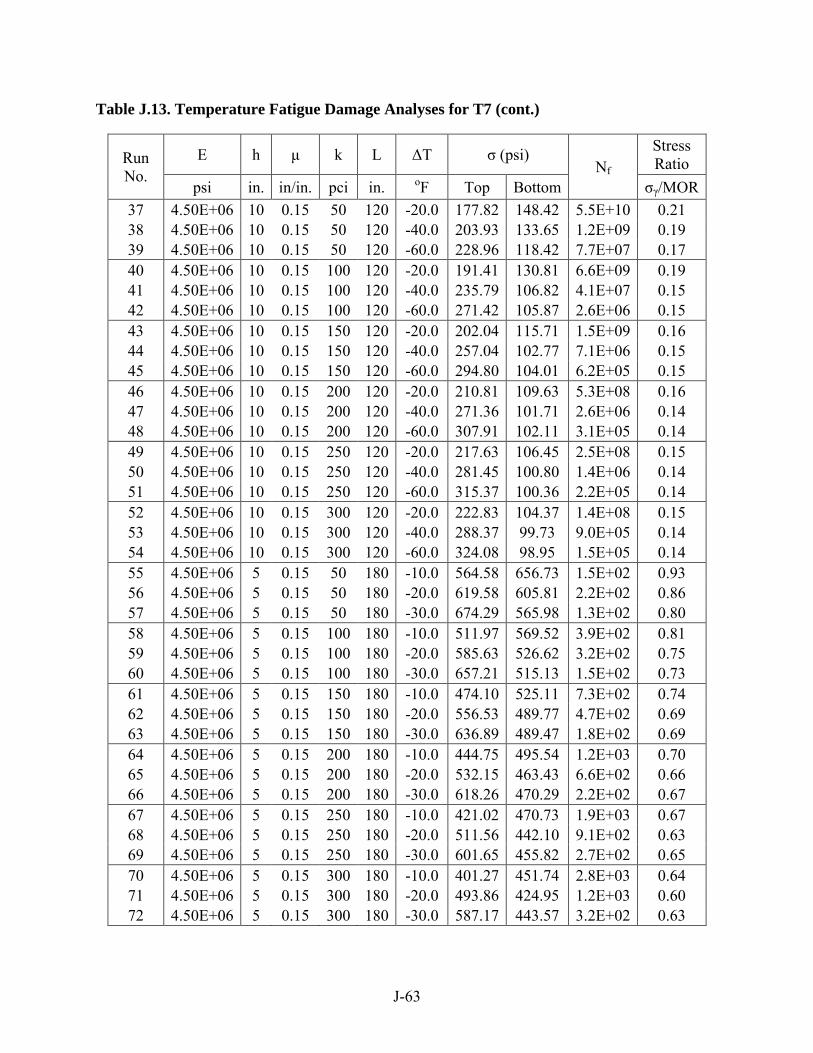
J-63

Table J.13. Temperature Fatigue Damage Analyses for T7 (cont.)

Run No.

E h μ k L ΔT σ (psi) Nf

Stress Ratio

psi in. in/in. pci in. oF Top Bottom σγ/MOR 37 4.50E+06 10 0.15 50 120 -20.0 177.82 148.42 5.5E+10 0.21 38 4.50E+06 10 0.15 50 120 -40.0 203.93 133.65 1.2E+09 0.19 39 4.50E+06 10 0.15 50 120 -60.0 228.96 118.42 7.7E+07 0.17 40 4.50E+06 10 0.15 100 120 -20.0 191.41 130.81 6.6E+09 0.19 41 4.50E+06 10 0.15 100 120 -40.0 235.79 106.82 4.1E+07 0.15 42 4.50E+06 10 0.15 100 120 -60.0 271.42 105.87 2.6E+06 0.15 43 4.50E+06 10 0.15 150 120 -20.0 202.04 115.71 1.5E+09 0.16 44 4.50E+06 10 0.15 150 120 -40.0 257.04 102.77 7.1E+06 0.15 45 4.50E+06 10 0.15 150 120 -60.0 294.80 104.01 6.2E+05 0.15 46 4.50E+06 10 0.15 200 120 -20.0 210.81 109.63 5.3E+08 0.16 47 4.50E+06 10 0.15 200 120 -40.0 271.36 101.71 2.6E+06 0.14 48 4.50E+06 10 0.15 200 120 -60.0 307.91 102.11 3.1E+05 0.14 49 4.50E+06 10 0.15 250 120 -20.0 217.63 106.45 2.5E+08 0.15 50 4.50E+06 10 0.15 250 120 -40.0 281.45 100.80 1.4E+06 0.14 51 4.50E+06 10 0.15 250 120 -60.0 315.37 100.36 2.2E+05 0.14 52 4.50E+06 10 0.15 300 120 -20.0 222.83 104.37 1.4E+08 0.15 53 4.50E+06 10 0.15 300 120 -40.0 288.37 99.73 9.0E+05 0.14 54 4.50E+06 10 0.15 300 120 -60.0 324.08 98.95 1.5E+05 0.14 55 4.50E+06 5 0.15 50 180 -10.0 564.58 656.73 1.5E+02 0.93 56 4.50E+06 5 0.15 50 180 -20.0 619.58 605.81 2.2E+02 0.86 57 4.50E+06 5 0.15 50 180 -30.0 674.29 565.98 1.3E+02 0.80 58 4.50E+06 5 0.15 100 180 -10.0 511.97 569.52 3.9E+02 0.81 59 4.50E+06 5 0.15 100 180 -20.0 585.63 526.62 3.2E+02 0.75 60 4.50E+06 5 0.15 100 180 -30.0 657.21 515.13 1.5E+02 0.73 61 4.50E+06 5 0.15 150 180 -10.0 474.10 525.11 7.3E+02 0.74 62 4.50E+06 5 0.15 150 180 -20.0 556.53 489.77 4.7E+02 0.69 63 4.50E+06 5 0.15 150 180 -30.0 636.89 489.47 1.8E+02 0.69 64 4.50E+06 5 0.15 200 180 -10.0 444.75 495.54 1.2E+03 0.70 65 4.50E+06 5 0.15 200 180 -20.0 532.15 463.43 6.6E+02 0.66 66 4.50E+06 5 0.15 200 180 -30.0 618.26 470.29 2.2E+02 0.67 67 4.50E+06 5 0.15 250 180 -10.0 421.02 470.73 1.9E+03 0.67 68 4.50E+06 5 0.15 250 180 -20.0 511.56 442.10 9.1E+02 0.63 69 4.50E+06 5 0.15 250 180 -30.0 601.65 455.82 2.7E+02 0.65 70 4.50E+06 5 0.15 300 180 -10.0 401.27 451.74 2.8E+03 0.64 71 4.50E+06 5 0.15 300 180 -20.0 493.86 424.95 1.2E+03 0.60 72 4.50E+06 5 0.15 300 180 -30.0 587.17 443.57 3.2E+02 0.63

J-64

Table J.13. Temperature Fatigue Damage Analyses for T7 (cont.)

Run No.

E h μ k L ΔT σ (psi) Nf

Stress Ratio

psi in. in/in. pci in. oF Top Bottom σγ/MOR 73 4.50E+06 7 0.15 50 180 -14.0 336.82 377.68 1.9E+04 0.54 74 4.50E+06 7 0.15 50 180 -28.0 378.19 333.23 1.9E+04 0.47 75 4.50E+06 7 0.15 50 180 -42.0 414.88 300.44 6.6E+03 0.43 76 4.50E+06 7 0.15 100 180 -14.0 338.62 315.36 7.8E+04 0.45 77 4.50E+06 7 0.15 100 180 -28.0 399.49 281.92 1.0E+04 0.40 78 4.50E+06 7 0.15 100 180 -42.0 445.44 286.17 3.2E+03 0.41 79 4.50E+06 7 0.15 150 180 -14.0 336.68 283.59 8.5E+04 0.40 80 4.50E+06 7 0.15 150 180 -28.0 408.25 275.37 7.9E+03 0.39 81 4.50E+06 7 0.15 150 180 -42.0 459.15 284.33 2.4E+03 0.40 82 4.50E+06 7 0.15 200 180 -14.0 333.23 270.58 9.8E+04 0.38 83 4.50E+06 7 0.15 200 180 -28.0 412.15 271.79 7.1E+03 0.39 84 4.50E+06 7 0.15 200 180 -42.0 466.29 281.49 2.1E+03 0.40 85 4.50E+06 7 0.15 250 180 -14.0 329.21 261.96 1.2E+05 0.37 86 4.50E+06 7 0.15 250 180 -28.0 413.88 269.39 6.8E+03 0.38 87 4.50E+06 7 0.15 250 180 -42.0 473.98 278.59 1.8E+03 0.40 88 4.50E+06 7 0.15 300 180 -14.0 325.00 254.82 1.4E+05 0.36 89 4.50E+06 7 0.15 300 180 -28.0 414.46 267.49 6.7E+03 0.38 90 4.50E+06 7 0.15 300 180 -42.0 489.63 275.63 1.3E+03 0.39 91 4.50E+06 10 0.15 50 180 -20.0 214.06 212.21 3.7E+08 0.30 92 4.50E+06 10 0.15 50 180 -40.0 237.60 179.75 3.5E+07 0.25 93 4.50E+06 10 0.15 50 180 -60.0 255.12 155.77 8.2E+06 0.22 94 4.50E+06 10 0.15 100 180 -20.0 204.21 167.80 1.2E+09 0.24 95 4.50E+06 10 0.15 100 180 -40.0 237.39 141.54 3.5E+07 0.20 96 4.50E+06 10 0.15 100 180 -60.0 259.53 141.16 5.9E+06 0.20 97 4.50E+06 10 0.15 150 180 -20.0 203.47 143.60 1.3E+09 0.20 98 4.50E+06 10 0.15 150 180 -40.0 241.64 140.08 2.4E+07 0.20 99 4.50E+06 10 0.15 150 180 -60.0 273.63 138.55 2.2E+06 0.20 100 4.50E+06 10 0.15 200 180 -20.0 210.99 137.44 5.2E+08 0.19 101 4.50E+06 10 0.15 200 180 -40.0 249.70 138.58 1.3E+07 0.20 102 4.50E+06 10 0.15 200 180 -60.0 301.00 136.38 4.5E+05 0.19 103 4.50E+06 10 0.15 250 180 -20.0 216.33 135.93 2.8E+08 0.19 104 4.50E+06 10 0.15 250 180 -40.0 259.11 137.13 6.1E+06 0.19 105 4.50E+06 10 0.15 250 180 -60.0 326.42 134.68 1.3E+05 0.19 106 4.50E+06 10 0.15 300 180 -20.0 220.47 134.97 1.8E+08 0.19 107 4.50E+06 10 0.15 300 180 -40.0 274.86 135.72 2.1E+06 0.19 108 4.50E+06 10 0.15 300 180 -60.0 346.27 133.09 5.8E+04 0.19

J-65

Table J.13. Temperature Fatigue Damage Analyses for T7 (cont.)

Run No.

E h μ k L ΔT σ (psi) Nf

Stress Ratio

psi in. in/in. pci in. oF Top Bottom σγ/MOR 109 4.50E+06 5 0.15 50 240 -10.0 541.41 583.33 3.3E+02 0.83 110 4.50E+06 5 0.15 50 240 -20.0 595.45 553.68 2.9E+02 0.79 111 4.50E+06 5 0.15 50 240 -30.0 648.94 536.40 1.6E+02 0.76 112 4.50E+06 5 0.15 100 240 -10.0 495.92 538.88 6.0E+02 0.76 113 4.50E+06 5 0.15 100 240 -20.0 569.07 504.40 4.0E+02 0.72 114 4.50E+06 5 0.15 100 240 -30.0 639.62 495.72 1.8E+02 0.70 115 4.50E+06 5 0.15 150 240 -10.0 461.56 504.65 1.0E+03 0.72 116 4.50E+06 5 0.15 150 240 -20.0 543.73 470.94 5.6E+02 0.67 117 4.50E+06 5 0.15 150 240 -30.0 623.39 471.79 2.1E+02 0.67 118 4.50E+06 5 0.15 200 240 -10.0 434.48 476.93 1.7E+03 0.68 119 4.50E+06 5 0.15 200 240 -20.0 521.81 446.76 7.7E+02 0.63 120 4.50E+06 5 0.15 200 240 -30.0 607.47 454.43 2.5E+02 0.64 121 4.50E+06 5 0.15 250 240 -10.0 412.37 453.61 2.7E+03 0.64 122 4.50E+06 5 0.15 250 240 -20.0 502.99 426.88 1.0E+03 0.61 123 4.50E+06 5 0.15 250 240 -30.0 592.85 441.22 3.0E+02 0.63 124 4.50E+06 5 0.15 300 240 -10.0 393.85 433.60 4.2E+03 0.61 125 4.50E+06 5 0.15 300 240 -20.0 486.66 410.83 1.4E+03 0.58 126 4.50E+06 5 0.15 300 240 -30.0 579.82 430.03 3.5E+02 0.61 127 4.50E+06 7 0.15 50 240 -14.0 336.48 303.59 8.6E+04 0.43 128 4.50E+06 7 0.15 50 240 -28.0 400.55 290.36 9.7E+03 0.41 129 4.50E+06 7 0.15 50 240 -42.0 470.63 291.92 1.9E+03 0.41 130 4.50E+06 7 0.15 100 240 -14.0 324.38 282.67 1.4E+05 0.40 131 4.50E+06 7 0.15 100 240 -28.0 382.08 274.91 1.7E+04 0.39 132 4.50E+06 7 0.15 100 240 -42.0 465.84 289.13 2.1E+03 0.41 133 4.50E+06 7 0.15 150 240 -14.0 324.97 269.46 1.4E+05 0.38 134 4.50E+06 7 0.15 150 240 -28.0 393.31 269.05 1.2E+04 0.38 135 4.50E+06 7 0.15 150 240 -42.0 490.80 286.39 1.3E+03 0.41 136 4.50E+06 7 0.15 200 240 -14.0 323.17 259.37 1.5E+05 0.37 137 4.50E+06 7 0.15 200 240 -28.0 399.01 265.75 1.0E+04 0.38 138 4.50E+06 7 0.15 200 240 -42.0 508.76 283.18 9.5E+02 0.40 139 4.50E+06 7 0.15 250 240 -14.0 320.30 251.27 1.7E+05 0.36 140 4.50E+06 7 0.15 250 240 -28.0 402.17 263.55 9.3E+03 0.37 141 4.50E+06 7 0.15 250 240 -42.0 518.87 279.86 8.1E+02 0.40 142 4.50E+06 7 0.15 300 240 -14.0 317.01 244.55 2.0E+05 0.35 143 4.50E+06 7 0.15 300 240 -28.0 403.95 261.83 8.8E+03 0.37 144 4.50E+06 7 0.15 300 240 -42.0 524.85 276.97 7.4E+02 0.39

J-66

Table J.13. Temperature Fatigue Damage Analyses for T7 (cont.)

Run No.

E h μ k L ΔT σ (psi) Nf

Stress Ratio

psi in. in/in. pci in. oF Top Bottom σγ/MOR 145 4.50E+06 10 0.15 50 240 -20.0 252.64 153.92 9.9E+06 0.22 146 4.50E+06 10 0.15 50 240 -40.0 321.47 151.08 1.6E+05 0.21 147 4.50E+06 10 0.15 50 240 -60.0 372.56 155.27 2.3E+04 0.22 148 4.50E+06 10 0.15 100 240 -20.0 239.96 143.57 2.8E+07 0.20 149 4.50E+06 10 0.15 100 240 -40.0 331.43 148.91 1.1E+05 0.21 150 4.50E+06 10 0.15 100 240 -60.0 399.44 152.91 1.0E+04 0.22 151 4.50E+06 10 0.15 150 240 -20.0 234.43 138.32 4.6E+07 0.20 152 4.50E+06 10 0.15 150 240 -40.0 346.24 147.27 5.8E+04 0.21 153 4.50E+06 10 0.15 150 240 -60.0 418.86 150.98 6.0E+03 0.21 154 4.50E+06 10 0.15 200 240 -20.0 230.73 135.93 6.5E+07 0.19 155 4.50E+06 10 0.15 200 240 -40.0 357.46 145.72 3.8E+04 0.21 156 4.50E+06 10 0.15 200 240 -60.0 432.93 149.52 4.2E+03 0.21 157 4.50E+06 10 0.15 250 240 -20.0 230.93 134.66 6.4E+07 0.19 158 4.50E+06 10 0.15 250 240 -40.0 366.28 144.28 2.8E+04 0.20 159 4.50E+06 10 0.15 250 240 -60.0 443.96 148.27 3.3E+03 0.21 160 4.50E+06 10 0.15 300 240 -20.0 232.22 133.88 5.7E+07 0.19 161 4.50E+06 10 0.15 300 240 -40.0 373.47 143.06 2.2E+04 0.20 162 4.50E+06 10 0.15 300 240 -60.0 462.92 147.23 2.2E+03 0.21

J-67

Table J.14. Temperature Faulting Damage Analyses for T7

Run No.

E h μ k L ΔT Deflection (in.) DE psi in. in/in. pci in. oF Wl Wul

1 4.50E+06 5 0.15 50 120 -10.0 0.1299 0.0694 0.30 2 4.50E+06 5 0.15 50 120 -20.0 0.1151 0.0546 0.26 3 4.50E+06 5 0.15 50 120 -30.0 0.1007 0.0402 0.21 4 4.50E+06 5 0.15 100 120 -10.0 0.0727 0.0338 0.21 5 4.50E+06 5 0.15 100 120 -20.0 0.0614 0.0225 0.16 6 4.50E+06 5 0.15 100 120 -30.0 0.0502 0.0113 0.12 7 4.50E+06 5 0.15 150 120 -10.0 0.0526 0.0228 0.17 8 4.50E+06 5 0.15 150 120 -20.0 0.0431 0.0133 0.13 9 4.50E+06 5 0.15 150 120 -30.0 0.0335 0.0037 0.08 10 4.50E+06 5 0.15 200 120 -10.0 0.0420 0.0175 0.15 11 4.50E+06 5 0.15 200 120 -20.0 0.0337 0.0092 0.11 12 4.50E+06 5 0.15 200 120 -30.0 0.0252 0.0006 0.06 13 4.50E+06 5 0.15 250 120 -10.0 0.0354 0.0144 0.13 14 4.50E+06 5 0.15 250 120 -20.0 0.0279 0.0068 0.09 15 4.50E+06 5 0.15 250 120 -30.0 0.0201 -0.0010 0.05 16 4.50E+06 5 0.15 300 120 -10.0 0.0308 0.0123 0.12 17 4.50E+06 5 0.15 300 120 -20.0 0.0239 0.0054 0.08 18 4.50E+06 5 0.15 300 120 -30.0 0.0166 -0.0019 0.04 19 4.50E+06 7 0.15 50 120 -14.0 0.1065 0.0651 0.18 20 4.50E+06 7 0.15 50 120 -28.0 0.0880 0.0465 0.14 21 4.50E+06 7 0.15 50 120 -42.0 0.0700 0.0286 0.10 22 4.50E+06 7 0.15 100 120 -14.0 0.0535 0.0267 0.11 23 4.50E+06 7 0.15 100 120 -28.0 0.0379 0.0110 0.07 24 4.50E+06 7 0.15 100 120 -42.0 0.0226 -0.0042 0.02 25 4.50E+06 7 0.15 150 120 -14.0 0.0358 0.0150 0.08 26 4.50E+06 7 0.15 150 120 -28.0 0.0220 0.0011 0.04 27 4.50E+06 7 0.15 150 120 -42.0 0.0081 -0.0130 -0.01 28 4.50E+06 7 0.15 200 120 -14.0 0.0270 0.0096 0.06 29 4.50E+06 7 0.15 200 120 -28.0 0.0144 -0.0030 0.02 30 4.50E+06 7 0.15 200 120 -42.0 0.0013 -0.0166 -0.03 31 4.50E+06 7 0.15 250 120 -14.0 0.0217 0.0067 0.05 32 4.50E+06 7 0.15 250 120 -28.0 0.0100 -0.0052 0.01 33 4.50E+06 7 0.15 250 120 -42.0 -0.0025 -0.0184 -0.04 34 4.50E+06 7 0.15 300 120 -14.0 0.0182 0.0048 0.05 35 4.50E+06 7 0.15 300 120 -28.0 0.0071 -0.0064 0.00 36 4.50E+06 7 0.15 300 120 -42.0 -0.0050 -0.0193 -0.05

J-68

Table J.14. Temperature Faulting Damage Analyses for T7 (cont.)

Run No.

E h μ k L ΔT Deflection (in.) DE psi in. in/in. pci in. oF Wl Wul

37 4.50E+06 10 0.15 50 120 -20.0 0.0947 0.0662 0.11 38 4.50E+06 10 0.15 50 120 -40.0 0.0738 0.0453 0.08 39 4.50E+06 10 0.15 50 120 -60.0 0.0538 0.0252 0.06 40 4.50E+06 10 0.15 100 120 -20.0 0.0424 0.0243 0.06 41 4.50E+06 10 0.15 100 120 -40.0 0.0236 0.0055 0.03 42 4.50E+06 10 0.15 100 120 -60.0 0.0053 -0.0129 -0.01 43 4.50E+06 10 0.15 150 120 -20.0 0.0251 0.0111 0.04 44 4.50E+06 10 0.15 150 120 -40.0 0.0075 -0.0065 0.00 45 4.50E+06 10 0.15 150 120 -60.0 -0.0101 -0.0245 -0.04 46 4.50E+06 10 0.15 200 120 -20.0 0.0166 0.0049 0.03 47 4.50E+06 10 0.15 200 120 -40.0 -0.0001 -0.0119 -0.01 48 4.50E+06 10 0.15 200 120 -60.0 -0.0176 -0.0300 -0.06 49 4.50E+06 10 0.15 250 120 -20.0 0.0116 0.0015 0.02 50 4.50E+06 10 0.15 250 120 -40.0 -0.0045 -0.0150 -0.03 51 4.50E+06 10 0.15 250 120 -60.0 -0.0221 -0.0331 -0.08 52 4.50E+06 10 0.15 300 120 -20.0 0.0084 -0.0006 0.01 53 4.50E+06 10 0.15 300 120 -40.0 -0.0073 -0.0169 -0.03 54 4.50E+06 10 0.15 300 120 -60.0 -0.0252 -0.0353 -0.09 55 4.50E+06 5 0.15 50 180 -10.0 0.1262 0.0652 0.29 56 4.50E+06 5 0.15 50 180 -20.0 0.1099 0.0488 0.24 57 4.50E+06 5 0.15 50 180 -30.0 0.0938 0.0327 0.19 58 4.50E+06 5 0.15 100 180 -10.0 0.0718 0.0327 0.20 59 4.50E+06 5 0.15 100 180 -20.0 0.0599 0.0208 0.16 60 4.50E+06 5 0.15 100 180 -30.0 0.0479 0.0087 0.11 61 4.50E+06 5 0.15 150 180 -10.0 0.0523 0.0225 0.17 62 4.50E+06 5 0.15 150 180 -20.0 0.0426 0.0127 0.12 63 4.50E+06 5 0.15 150 180 -30.0 0.0326 0.0026 0.08 64 4.50E+06 5 0.15 200 180 -10.0 0.0420 0.0174 0.15 65 4.50E+06 5 0.15 200 180 -20.0 0.0335 0.0090 0.10 66 4.50E+06 5 0.15 200 180 -30.0 0.0248 0.0001 0.06 67 4.50E+06 5 0.15 250 180 -10.0 0.0354 0.0144 0.13 68 4.50E+06 5 0.15 250 180 -20.0 0.0279 0.0069 0.09 69 4.50E+06 5 0.15 250 180 -30.0 0.0200 -0.0012 0.05 70 4.50E+06 5 0.15 300 180 -10.0 0.0308 0.0124 0.12 71 4.50E+06 5 0.15 300 180 -20.0 0.0240 0.0055 0.08 72 4.50E+06 5 0.15 300 180 -30.0 0.0167 -0.0020 0.04

J-69

Table J.14. Temperature Faulting Damage Analyses for T7 (cont.)

Run No.

E h μ k L ΔT Deflection (in.) DE psi in. in/in. pci in. oF Wl Wul

73 4.50E+06 7 0.15 50 180 -14.0 0.0979 0.0558 0.16 74 4.50E+06 7 0.15 50 180 -28.0 0.0754 0.0332 0.11 75 4.50E+06 7 0.15 50 180 -42.0 0.0537 0.0113 0.07 76 4.50E+06 7 0.15 100 180 -14.0 0.0496 0.0226 0.10 77 4.50E+06 7 0.15 100 180 -28.0 0.0316 0.0044 0.05 78 4.50E+06 7 0.15 100 180 -42.0 0.0135 -0.0141 0.00 79 4.50E+06 7 0.15 150 180 -14.0 0.0336 0.0127 0.07 80 4.50E+06 7 0.15 150 180 -28.0 0.0180 -0.0031 0.02 81 4.50E+06 7 0.15 150 180 -42.0 0.0015 -0.0204 -0.03 82 4.50E+06 7 0.15 200 180 -14.0 0.0256 0.0082 0.06 83 4.50E+06 7 0.15 200 180 -28.0 0.0115 -0.0062 0.01 84 4.50E+06 7 0.15 200 180 -42.0 -0.0039 -0.0227 -0.05 85 4.50E+06 7 0.15 250 180 -14.0 0.0208 0.0057 0.05 86 4.50E+06 7 0.15 250 180 -28.0 0.0078 -0.0076 0.00 87 4.50E+06 7 0.15 250 180 -42.0 -0.0070 -0.0236 -0.06 88 4.50E+06 7 0.15 300 180 -14.0 0.0176 0.0042 0.04 89 4.50E+06 7 0.15 300 180 -28.0 0.0054 -0.0084 -0.01 90 4.50E+06 7 0.15 300 180 -42.0 -0.0090 -0.0241 -0.07 91 4.50E+06 10 0.15 50 180 -20.0 0.0810 0.0519 0.10 92 4.50E+06 10 0.15 50 180 -40.0 0.0535 0.0241 0.06 93 4.50E+06 10 0.15 50 180 -60.0 0.0273 -0.0023 0.02 94 4.50E+06 10 0.15 100 180 -20.0 0.0342 0.0158 0.05 95 4.50E+06 10 0.15 100 180 -40.0 0.0104 -0.0083 0.00 96 4.50E+06 10 0.15 100 180 -60.0 -0.0138 -0.0332 -0.05 97 4.50E+06 10 0.15 150 180 -20.0 0.0192 0.0050 0.03 98 4.50E+06 10 0.15 150 180 -40.0 -0.0029 -0.0176 -0.02 99 4.50E+06 10 0.15 150 180 -60.0 -0.0268 -0.0425 -0.08 100 4.50E+06 10 0.15 200 180 -20.0 0.0120 0.0002 0.01 101 4.50E+06 10 0.15 200 180 -40.0 -0.0091 -0.0218 -0.04 102 4.50E+06 10 0.15 200 180 -60.0 -0.0334 -0.0469 -0.11 103 4.50E+06 10 0.15 250 180 -20.0 0.0079 -0.0024 0.01 104 4.50E+06 10 0.15 250 180 -40.0 -0.0127 -0.0240 -0.05 105 4.50E+06 10 0.15 250 180 -60.0 -0.0376 -0.0497 -0.13 106 4.50E+06 10 0.15 300 180 -20.0 0.0053 -0.0039 0.00 107 4.50E+06 10 0.15 300 180 -40.0 -0.0151 -0.0254 -0.06 108 4.50E+06 10 0.15 300 180 -60.0 -0.0405 -0.0516 -0.15

J-70

Table J.14. Temperature Faulting Damage Analyses for T7 (cont.)

Run No.

E h μ k L ΔT Deflection (in.) DE psi in. in/in. pci in. oF Wl Wul

109 4.50E+06 5 0.15 50 240 -10.0 0.1247 0.0644 0.29 110 4.50E+06 5 0.15 50 240 -20.0 0.1083 0.0480 0.24 111 4.50E+06 5 0.15 50 240 -30.0 0.0919 0.0315 0.19 112 4.50E+06 5 0.15 100 240 -10.0 0.0715 0.0327 0.20 113 4.50E+06 5 0.15 100 240 -20.0 0.0597 0.0209 0.16 114 4.50E+06 5 0.15 100 240 -30.0 0.0478 0.0090 0.11 115 4.50E+06 5 0.15 150 240 -10.0 0.0522 0.0225 0.17 116 4.50E+06 5 0.15 150 240 -20.0 0.0426 0.0129 0.12 117 4.50E+06 5 0.15 150 240 -30.0 0.0328 0.0030 0.08 118 4.50E+06 5 0.15 200 240 -10.0 0.0419 0.0174 0.15 119 4.50E+06 5 0.15 200 240 -20.0 0.0337 0.0092 0.10 120 4.50E+06 5 0.15 200 240 -30.0 0.0250 0.0005 0.06 121 4.50E+06 5 0.15 250 240 -10.0 0.0354 0.0144 0.13 122 4.50E+06 5 0.15 250 240 -20.0 0.0280 0.0070 0.09 123 4.50E+06 5 0.15 250 240 -30.0 0.0202 -0.0009 0.05 124 4.50E+06 5 0.15 300 240 -10.0 0.0308 0.0124 0.12 125 4.50E+06 5 0.15 300 240 -20.0 0.0241 0.0056 0.08 126 4.50E+06 5 0.15 300 240 -30.0 0.0169 -0.0017 0.04 127 4.50E+06 7 0.15 50 240 -14.0 0.0942 0.0529 0.15 128 4.50E+06 7 0.15 50 240 -28.0 0.0694 0.0280 0.10 129 4.50E+06 7 0.15 50 240 -42.0 0.0450 0.0034 0.05 130 4.50E+06 7 0.15 100 240 -14.0 0.0487 0.0220 0.09 131 4.50E+06 7 0.15 100 240 -28.0 0.0298 0.0030 0.04 132 4.50E+06 7 0.15 100 240 -42.0 0.0099 -0.0174 -0.01 133 4.50E+06 7 0.15 150 240 -14.0 0.0334 0.0126 0.07 134 4.50E+06 7 0.15 150 240 -28.0 0.0173 -0.0035 0.02 135 4.50E+06 7 0.15 150 240 -42.0 -0.0004 -0.0222 -0.04 136 4.50E+06 7 0.15 200 240 -14.0 0.0256 0.0083 0.06 137 4.50E+06 7 0.15 200 240 -28.0 0.0113 -0.0062 0.01 138 4.50E+06 7 0.15 200 240 -42.0 -0.0051 -0.0238 -0.05 139 4.50E+06 7 0.15 250 240 -14.0 0.0209 0.0059 0.05 140 4.50E+06 7 0.15 250 240 -28.0 0.0078 -0.0074 0.00 141 4.50E+06 7 0.15 250 240 -42.0 -0.0078 -0.0244 -0.07 142 4.50E+06 7 0.15 300 240 -14.0 0.0177 0.0044 0.04 143 4.50E+06 7 0.15 300 240 -28.0 0.0055 -0.0081 -0.01 144 4.50E+06 7 0.15 300 240 -42.0 -0.0096 -0.0246 -0.08

J-71

Table J.14. Temperature Faulting Damage Analyses for T7 (cont.)

Run No.

E h μ k L ΔT Deflection (in.) DE psi in. in/in. pci in. oF Wl Wul

145 4.50E+06 10 0.15 50 240 -20.0 0.0711 0.0427 0.08 146 4.50E+06 10 0.15 50 240 -40.0 0.0378 0.0092 0.03 147 4.50E+06 10 0.15 50 240 -60.0 0.0050 -0.0242 -0.01 148 4.50E+06 10 0.15 100 240 -20.0 0.0300 0.0120 0.04 149 4.50E+06 10 0.15 100 240 -40.0 0.0018 -0.0167 -0.01 150 4.50E+06 10 0.15 100 240 -60.0 -0.0291 -0.0488 -0.08 151 4.50E+06 10 0.15 150 240 -20.0 0.0168 0.0029 0.02 152 4.50E+06 10 0.15 150 240 -40.0 -0.0091 -0.0239 -0.04 153 4.50E+06 10 0.15 150 240 -60.0 -0.0405 -0.0564 -0.12 154 4.50E+06 10 0.15 200 240 -20.0 0.0106 -0.0011 0.01 155 4.50E+06 10 0.15 200 240 -40.0 -0.0143 -0.0270 -0.05 156 4.50E+06 10 0.15 200 240 -60.0 -0.0466 -0.0603 -0.15 157 4.50E+06 10 0.15 250 240 -20.0 0.0069 -0.0032 0.00 158 4.50E+06 10 0.15 250 240 -40.0 -0.0173 -0.0286 -0.06 159 4.50E+06 10 0.15 250 240 -60.0 -0.0505 -0.0626 -0.17 160 4.50E+06 10 0.15 300 240 -20.0 0.0046 -0.0045 0.00 161 4.50E+06 10 0.15 300 240 -40.0 -0.0194 -0.0296 -0.08 162 4.50E+06 10 0.15 300 240 -60.0 -0.0533 -0.0643 -0.19

Appendix K. VB Based Excel Macro Program

K-1

In this appendix, a sample VB based Excel Macro program that was used for spring 2009 field data summarization is listed. Please be noted that differences may exist between the programs used for different seasons because of the sensor location and working status. The following one from spring 2009 is just one of the samples.

Sub Openfile() Dim i, loopfiles As Integer Sheets("info").Select Cells(3, 1).Select loopfiles = Selection.CurrentRegion.Rows.Count For i = 1 To loopfiles Sheets("info").Select fdir = Cells(i + 2, 1).Value & "\" file = Cells(i + 2, 2).Value fname = fdir & file Workbooks.OpenText Filename:=fname, Origin:=437, StartRow:=1, DataType:=xlDelimited, TextQualifier:= _ xlDoubleQuote, ConsecutiveDelimiter:=False, Tab:=True, Semicolon:=False, _ Comma:=True, Space:=False, Other:=False, FieldInfo:=Array(Array(1, 1), _ Array(2, 1), Array(3, 1), Array(4, 1), Array(5, 1), Array(6, 1), Array(7, 1), Array(8, 1), _ Array(9, 1), Array(10, 1), Array(11, 1), Array(12, 1), Array(13, 1)), _ TrailingMinusNumbers:=True Cells.Select Selection.Copy Windows("pickmePCC.xls").Activate Sheets("data").Select ActiveSheet.Paste ActiveCell.Offset(0, 8).Range("A1").Select Windows(file).Activate Application.CutCopyMode = False ActiveWindow.Close '-------------------------------------------- ' Runs subroutine to balance and arrange data '-------------------------------------------- Call Balance Call Arrange '---------------------------------------------- ' Clears data sheet after running Arrange macro '----------------------------------------------

K-2

Sheets("data").Select ActiveCell.Offset(-1, 0).Range("A1").Select Selection.End(xlToRight).Select Range(Selection, Selection.End(xlToLeft)).Select Range(Selection, Selection.End(xlUp)).Select Selection.ClearContents Selection.End(xlToLeft).Select Selection.End(xlUp).Select Next i Call Info Call MinMax Call RelOffsetPCC Call Speed Call Results End Sub Sub Balance() '---------------------------------------------------------------------- ' This subroutine zeros the peak-pick results with respect to B1 values '---------------------------------------------------------------------- Dim base As Double Sheets("data").Select Cells(1, 9).Select Do If ActiveCell.Value = "B1" Then '--------------------------------------------------- ' Updates cell P1 with new base values if cell is B1 '--------------------------------------------------- base = ActiveCell.Offset(0, 1).Value Cells(1, 16).Value = base '------------------------------- ' Proceeds with balancing values '------------------------------- ActiveCell.Offset(0, 6) = ActiveCell.Offset(0, 1) - base ActiveCell.Offset(1, 0).Select Else

K-3

'---------------------------------------------------- ' Reuses base value and proceed with balancing values '---------------------------------------------------- base = Cells(1, 16).Value ActiveCell.Offset(0, 6) = ActiveCell.Offset(0, 1) - base ActiveCell.Offset(1, 0).Select End If Loop Until IsEmpty(ActiveCell.Offset(0, 1)) '------------------------------------------------ ' Replaces unbalanced values with balanced values '------------------------------------------------ Columns("O:O").Select Selection.Cut Columns("J:J").Select ActiveSheet.Paste Cells(1, 16).Delete Cells(1, 9).Select End Sub Sub Arrange() '---------------------------------------------------------------------- ' This subroutine arranges information from peak-pick generated results '---------------------------------------------------------------------- Sheets("data").Select Cells(1, 9).Select Do If ActiveCell.Value = "B1" Then '------------------------------------------ ' Inserts a new row if cell entry is B1 '------------------------------------------ Sheets("arrange").Select ActiveCell.Offset(1, 0).Range("A1").Select Selection.End(xlToLeft).Select '-------------------------- ' Displays analyzed sensors '-------------------------- Sheets("data").Select

K-4

ActiveCell.Offset(0, -8).Range("A1:C1").Select Selection.Copy Sheets("arrange").Select ActiveCell.Offset(0, 5).Range("A1").Select ActiveSheet.Paste ActiveCell.Offset(0, 3).Range("A1").Select Sheets("data").Select ActiveCell.Offset(0, 8).Range("A1").Select '------------------------------------------- ' Executes copy-paste for needed information '------------------------------------------- ActiveCell.Offset(0, -1).Range("A1:D1").Select Selection.Copy Sheets("arrange").Select ActiveSheet.Paste ActiveCell.Offset(0, 4).Range("A1").Select Sheets("data").Select ActiveCell.Offset(1, 1).Range("A1").Select Else '------------------------------------------- ' Executes copy-paste for needed information '------------------------------------------- ActiveCell.Offset(0, -1).Range("A1:D1").Select Selection.Copy Sheets("arrange").Select ActiveSheet.Paste ActiveCell.Offset(0, 4).Range("A1").Select Sheets("data").Select ActiveCell.Offset(1, 1).Range("A1").Select End If '------------------------------------- ' Stops loop when no more rows present '------------------------------------- Loop Until IsEmpty(ActiveCell.Offset(0, 1)) '--------------------------------------------------- ' Brings ActiveCell back to next executable position '--------------------------------------------------- Sheets("arrange").Select ActiveCell.Offset(1, 0).Range("A1").Select

K-5

Selection.End(xlToLeft).Select End Sub Sub Info() '---------------------------------------------------------------------- ' This subroutine displays pass information into arrange sheet '---------------------------------------------------------------------- Dim i, loopinfo As Integer Sheets("info").Select Cells(3, 1).Select loopinfo = Selection.CurrentRegion.Rows.Count Sheets("arrange").Select Cells(1, 1).Select For i = 1 To loopinfo ActiveCell.Offset(1, 0).Select passinfo = Sheets("info").Range("A" & i + 2 & ":E" & i + 2) Do While Not IsEmpty(ActiveCell.Offset(0, 5)) ActiveCell.Range("A1:E1") = passinfo ActiveCell.Offset(1, 0).Select Loop Next i Columns("E:E").Select Selection.NumberFormat = "General" End Sub Sub MinMax() '----------------------------------------------------------------- ' This subroutine sorts and determines the min-max for each sensor '----------------------------------------------------------------- Sheets("arrange").Range("A1").Select Dim i, j, k, l, looprows, loopcolumns As Integer 'set dimensions for variables

K-6

Worksheets("arrange").Range("A1:IV65536").Sort _ Key1:=Worksheets("arrange").Range("F1"), _ Key2:=Worksheets("arrange").Range("G1"), _ Key3:=Worksheets("arrange").Range("H1") Cells(1, 1).Select looprows = Selection.CurrentRegion.Rows.Count 'gets # of rows in region, exclude spaces loopcolumns = Selection.CurrentRegion.Columns.Count 'gets # of columns in region, exclude spaces 'j0 = 0 ' insert predetermined # for columns? 'set j loop parameters for axle removal 'k governs # of point values 'l governs column to start with after axle removal If Sheets("info").Cells(2, 7).Value = 0 Then k = (loopcolumns - 5 - 3) / 4 l = 7 ElseIf Sheets("info").Cells(2, 7).Value = 1 Then k = ((loopcolumns - 5 - 3) / 4) - 3 l = 19 ElseIf Sheets("info").Cells(2, 7).Value = 2 Then k = ((loopcolumns - 5 - 3) / 4) - 7 l = 35 End If 'begin loops For i = 1 To looprows 'loops for the # of rows 'sets the initial values for max and min 'these values must be outside j loop because it needs to be updated Cells(i, loopcolumns + 2) = Cells(i, 6).Value & Cells(i, 7).Value & Cells(i, 8).Value Cells(i, loopcolumns + 4) = -19999 'for max Cells(i, loopcolumns + 6) = 19999 'for min For j = 1 To k 'loops for the # of columns (will modify for peak pick) 'for max, updates cell if found larger value and extracts point If Cells(i, l + (j * 4)).Value >= Cells(i, loopcolumns + 4).Value Then Cells(i, loopcolumns + 4).Value = Cells(i, l + (j * 4)).Value Cells(i, loopcolumns + 3).Value = Cells(i, l + (j * 4) - 1).Value End If 'for min, updates cell if found smaller value and extracts point

K-7

If Cells(i, l + (j * 4)).Value <= Cells(i, loopcolumns + 6).Value Then Cells(i, loopcolumns + 6).Value = Cells(i, l + (j * 4)).Value Cells(i, loopcolumns + 5).Value = Cells(i, l + (j * 4) - 1).Value End If Next j Next i End Sub Sub RelOffsetPCC() '--------------------------------------------------------------- ' This subroutine calculates the relative offset for each sensor ' Only included Cell 54 here ' Still need to include sensor locations for Cell 32 '--------------------------------------------------------------- Sheets("arrange").Select Cells(1, 6).Select loopcolumns = Selection.CurrentRegion.Columns.Count Do If ActiveCell.Value = 54 Then If ActiveCell.Offset(0, 2).Value = 1 Or ActiveCell.Offset(0, 2).Value = 2 Or ActiveCell.Offset(0, 2).Value = 3 Then '6" ActiveCell.Offset(0, loopcolumns + 3) = 6 - ActiveCell.Offset(0, -1).Value ActiveCell.Offset(1, 0).Select ElseIf ActiveCell.Offset(0, 2).Value = 101 Or ActiveCell.Offset(0, 2).Value = 102 Or ActiveCell.Offset(0, 2).Value = 103 Or ActiveCell.Offset(0, 2).Value = 104 Or ActiveCell.Offset(0, 2).Value = 105 Or ActiveCell.Offset(0, 2).Value = 106 Then '-3" ActiveCell.Offset(0, loopcolumns + 3) = -3 - ActiveCell.Offset(0, -1).Value ActiveCell.Offset(1, 0).Select ElseIf ActiveCell.Offset(0, 2).Value = 4 Or ActiveCell.Offset(0, 2).Value = 5 Or ActiveCell.Offset(0, 2).Value = 6 Or ActiveCell.Offset(0, 2).Value = 7 Or ActiveCell.Offset(0, 2).Value = 8 Or ActiveCell.Offset(0, 2).Value = 9 Then '-3" ActiveCell.Offset(0, loopcolumns + 3) = -3 - ActiveCell.Offset(0, -1).Value ActiveCell.Offset(1, 0).Select

K-8

ElseIf ActiveCell.Offset(0, 2).Value = "107 dt 13" Or ActiveCell.Offset(0, 2).Value = "108 dt 14" Or ActiveCell.Offset(0, 2).Value = "109 dt 15" Or ActiveCell.Offset(0, 2).Value = "110 dt 16" Then '-3" ActiveCell.Offset(0, loopcolumns + 3) = -3 - ActiveCell.Offset(0, -1).Value ActiveCell.Offset(1, 0).Select ElseIf ActiveCell.Offset(0, 2).Value = "101 dt 7" Or ActiveCell.Offset(0, 2).Value = "104 dt 10" Then '12" ActiveCell.Offset(0, loopcolumns + 3) = 12 - ActiveCell.Offset(0, -1).Value ActiveCell.Offset(1, 0).Select ElseIf ActiveCell.Offset(0, 2).Value = "102 dt 8" Or ActiveCell.Offset(0, 2).Value = "105 dt 11" Then '72" ActiveCell.Offset(0, loopcolumns + 3) = 72 - ActiveCell.Offset(0, -1).Value ActiveCell.Offset(1, 0).Select ElseIf ActiveCell.Offset(0, 2).Value = "103 dt 9" Or ActiveCell.Offset(0, 2).Value = "106 dt 12" Then '132" ActiveCell.Offset(0, loopcolumns + 3) = 132 - ActiveCell.Offset(0, -1).Value ActiveCell.Offset(1, 0).Select End If ElseIf ActiveCell.Value = 32 Then If ActiveCell.Offset(0, 2).Value = 101 Or ActiveCell.Offset(0, 2).Value = 102 Then '103.32" ActiveCell.Offset(0, loopcolumns + 3) = 103.32 - ActiveCell.Offset(0, -1).Value ActiveCell.Offset(1, 0).Select ElseIf ActiveCell.Offset(0, 2).Value = 103 Or ActiveCell.Offset(0, 2).Value = 104 Then '30.84" ActiveCell.Offset(0, loopcolumns + 3) = 30.84 - ActiveCell.Offset(0, -1).Value ActiveCell.Offset(1, 0).Select ElseIf ActiveCell.Offset(0, 2).Value = 105 Or ActiveCell.Offset(0, 2).Value = 106 Then '32.64" ActiveCell.Offset(0, loopcolumns + 3) = 32.64 - ActiveCell.Offset(0, -1).Value ActiveCell.Offset(1, 0).Select ElseIf ActiveCell.Offset(0, 2).Value = 107 Or ActiveCell.Offset(0, 2).Value = 108 Then '8.64" ActiveCell.Offset(0, loopcolumns + 3) = 8.64 - ActiveCell.Offset(0, -1).Value ActiveCell.Offset(1, 0).Select ElseIf ActiveCell.Offset(0, 2).Value = 109 Or ActiveCell.Offset(0, 2).Value = 110 Then '103.44" ActiveCell.Offset(0, loopcolumns + 3) = 103.44 - ActiveCell.Offset(0, -1).Value

K-9

ActiveCell.Offset(1, 0).Select ElseIf ActiveCell.Offset(0, 2).Value = 115 Or ActiveCell.Offset(0, 2).Value = 116 Then '16.5" ActiveCell.Offset(0, loopcolumns + 3) = 16.5 - ActiveCell.Offset(0, -1).Value ActiveCell.Offset(1, 0).Select ElseIf ActiveCell.Offset(0, 2).Value = 119 Or ActiveCell.Offset(0, 2).Value = 120 Then '186.24" ActiveCell.Offset(0, loopcolumns + 3) = 186.24 - ActiveCell.Offset(0, -1).Value ActiveCell.Offset(1, 0).Select ElseIf ActiveCell.Offset(0, 2).Value = 123 Or ActiveCell.Offset(0, 2).Value = 124 Then '257.76" ActiveCell.Offset(0, loopcolumns + 3) = 257.76 - ActiveCell.Offset(0, -1).Value ActiveCell.Offset(1, 0).Select ElseIf ActiveCell.Offset(0, 2).Value = 131 Or ActiveCell.Offset(0, 2).Value = 132 Then '266.4" ActiveCell.Offset(0, loopcolumns + 3) = 266.4 - ActiveCell.Offset(0, -1).Value ActiveCell.Offset(1, 0).Select ElseIf ActiveCell.Offset(0, 2).Value = 133 Or ActiveCell.Offset(0, 2).Value = 134 Then '276" ActiveCell.Offset(0, loopcolumns + 3) = 276 - ActiveCell.Offset(0, -1).Value ActiveCell.Offset(1, 0).Select ElseIf ActiveCell.Offset(0, 2).Value = 135 Or ActiveCell.Offset(0, 2).Value = 136 Then '281.64" ActiveCell.Offset(0, loopcolumns + 3) = 281.64 - ActiveCell.Offset(0, -1).Value ActiveCell.Offset(1, 0).Select ElseIf ActiveCell.Offset(0, 2).Value = 138 Then '72" ActiveCell.Offset(0, loopcolumns + 3) = 72 - ActiveCell.Offset(0, -1).Value ActiveCell.Offset(1, 0).Select ElseIf ActiveCell.Offset(0, 2).Value = 139 Then '8" ActiveCell.Offset(0, loopcolumns + 3) = 8 - ActiveCell.Offset(0, -1).Value ActiveCell.Offset(1, 0).Select End If End If Loop Until IsEmpty(ActiveCell.Offset(0, 1)) End Sub

K-10

Sub Results() '----------------------------------------------------------------- ' This subroutine prints pertaining information onto results sheet '----------------------------------------------------------------- ActiveCell.Offset(0, -2).Columns("A:E").EntireColumn.Select Selection.Copy Sheets("results").Select ActiveSheet.Paste Selection.End(xlToRight).Select ActiveCell.Offset(0, 1).Range("A1").Select Sheets("arrange").Select ActiveCell.Offset(0, 1).Range("A1").Select Selection.End(xlToRight).Select Selection.End(xlToRight).Select Range(Selection, Selection.End(xlToRight)).Select Range(Selection, Selection.End(xlDown)).Select Application.CutCopyMode = False Selection.Copy Sheets("results").Select ActiveSheet.Paste ActiveCell.Rows("1:1").EntireRow.Select Application.CutCopyMode = False Selection.Insert Shift:=xlDown Cells(1, 1).Select ActiveCell.Formula = "File Directory" ActiveCell.Offset(0, 1).Formula = "File" ActiveCell.Offset(0, 2).Formula = "Vehicle" ActiveCell.Offset(0, 3).Formula = "Pass #" ActiveCell.Offset(0, 4).Formula = "Wheel Offset" ActiveCell.Offset(0, 5).Formula = "Sensor" ActiveCell.Offset(0, 6).Formula = "Axle" ActiveCell.Offset(0, 7).Formula = "Max Value" ActiveCell.Offset(0, 8).Formula = "Axle" ActiveCell.Offset(0, 9).Formula = "Min Value" ActiveCell.Offset(0, 10).Formula = "Speed1" ActiveCell.Offset(0, 11).Formula = "Speed2" ActiveCell.Offset(0, 12).Formula = "Relative Offset" End Sub Sub Speed() '--------------------------------------------------------------- ' This subroutine calculates the speed of the vehicle per sensor '---------------------------------------------------------------

K-11

Sheets("arrange").Select Cells(1, 3).Select loopcolumns = Selection.CurrentRegion.Columns.Count Do If ActiveCell.Value = "Mn102" Then AxleSpacing1 = 205 AxleSpacing2 = 50 Time1 = ActiveCell.Offset(0, 14).Value Time2 = ActiveCell.Offset(0, 30).Value Time3 = ActiveCell.Offset(0, 38).Value ActiveCell.Offset(0, loopcolumns + 4) = (3600 / 63360) * (AxleSpacing1 / (Time2 - Time1)) ActiveCell.Offset(0, loopcolumns + 5) = (3600 / 63360) * (AxleSpacing2 / (Time3 - Time2)) ActiveCell.Offset(1, 0).Select ElseIf ActiveCell.Value = "Mn80" Then AxleSpacing1 = 210 AxleSpacing2 = 52 Time1 = ActiveCell.Offset(0, 14).Value Time2 = ActiveCell.Offset(0, 30).Value Time3 = ActiveCell.Offset(0, 38).Value ActiveCell.Offset(0, loopcolumns + 4) = (3600 / 63360) * (AxleSpacing1 / (Time2 - Time1)) ActiveCell.Offset(0, loopcolumns + 5) = (3600 / 63360) * (AxleSpacing2 / (Time3 - Time2)) ActiveCell.Offset(1, 0).Select ElseIf ActiveCell.Value = "R4" Then AxleSpacing = 267 Time1 = ActiveCell.Offset(0, 14).Value Time2 = ActiveCell.Offset(0, 30).Value ActiveCell.Offset(0, loopcolumns + 4) = (3600 / 63360) * (AxleSpacing / (Time2 - Time1)) ActiveCell.Offset(1, 0).Select ElseIf ActiveCell.Value = "R5" Or ActiveCell.Value = "S3" Then AxleSpacing = 185 Time1 = ActiveCell.Offset(0, 14).Value Time2 = ActiveCell.Offset(0, 30).Value

K-12

ActiveCell.Offset(0, loopcolumns + 4) = (3600 / 63360) * (AxleSpacing / (Time2 - Time1)) ActiveCell.Offset(1, 0).Select ElseIf ActiveCell.Value = "R6" Then AxleSpacing = 226 Time1 = ActiveCell.Offset(0, 14).Value Time2 = ActiveCell.Offset(0, 30).Value ActiveCell.Offset(0, loopcolumns + 4) = (3600 / 63360) * (AxleSpacing / (Time2 - Time1)) ActiveCell.Offset(1, 0).Select ElseIf ActiveCell.Value = "S4" Or ActiveCell.Value = "S2" Then AxleSpacing1 = 180 AxleSpacing2 = 56 Time1 = ActiveCell.Offset(0, 14).Value Time2 = ActiveCell.Offset(0, 30).Value Time3 = ActiveCell.Offset(0, 38).Value ActiveCell.Offset(0, loopcolumns + 4) = (3600 / 63360) * (AxleSpacing1 / (Time2 - Time1)) ActiveCell.Offset(0, loopcolumns + 5) = (3600 / 63360) * (AxleSpacing2 / (Time3 - Time2)) ActiveCell.Offset(1, 0).Select ElseIf ActiveCell.Value = "S1" Or ActiveCell.Value = "S5" Then AxleSpacing1 = 196 AxleSpacing2 = 52 Time1 = ActiveCell.Offset(0, 14).Value Time2 = ActiveCell.Offset(0, 30).Value Time3 = ActiveCell.Offset(0, 38).Value ActiveCell.Offset(0, loopcolumns + 4) = (3600 / 63360) * (AxleSpacing1 / (Time2 - Time1)) ActiveCell.Offset(0, loopcolumns + 5) = (3600 / 63360) * (AxleSpacing2 / (Time3 - Time2)) ActiveCell.Offset(1, 0).Select ElseIf ActiveCell.Value = "T6" Then AxleSpacing1 = 121 AxleSpacing2 = 234 Time1 = ActiveCell.Offset(0, 14).Value Time2 = ActiveCell.Offset(0, 26).Value Time3 = ActiveCell.Offset(0, 34).Value ActiveCell.Offset(0, loopcolumns + 4) = (3600 / 63360) * (AxleSpacing1 / (Time2 - Time1)) ActiveCell.Offset(0, loopcolumns + 5) = (3600 / 63360) * (AxleSpacing2 / (Time3 - Time2)) ActiveCell.Offset(1, 0).Select

K-13

ElseIf ActiveCell.Value = "T7" Then AxleSpacing1 = 120 AxleSpacing2 = 223 Time1 = ActiveCell.Offset(0, 14).Value Time2 = ActiveCell.Offset(0, 30).Value Time3 = ActiveCell.Offset(0, 38).Value ActiveCell.Offset(0, loopcolumns + 4) = (3600 / 63360) * (AxleSpacing1 / (Time2 - Time1)) ActiveCell.Offset(0, loopcolumns + 5) = (3600 / 63360) * (AxleSpacing2 / (Time3 - Time2)) ActiveCell.Offset(1, 0).Select ElseIf ActiveCell.Value = "T8" Then AxleSpacing1 = 141 AxleSpacing2 = 225 Time1 = ActiveCell.Offset(0, 14).Value Time2 = ActiveCell.Offset(0, 30).Value Time3 = ActiveCell.Offset(0, 38).Value ActiveCell.Offset(0, loopcolumns + 4) = (3600 / 63360) * (AxleSpacing1 / (Time2 - Time1)) ActiveCell.Offset(0, loopcolumns + 5) = (3600 / 63360) * (AxleSpacing2 / (Time3 - Time2)) ActiveCell.Offset(1, 0).Select ElseIf ActiveCell.Value = "T3" Then AxleSpacing1 = 121 AxleSpacing2 = 234 Time1 = ActiveCell.Offset(0, 14).Value Time2 = ActiveCell.Offset(0, 30).Value Time3 = ActiveCell.Offset(0, 38).Value ActiveCell.Offset(0, loopcolumns + 4) = (3600 / 63360) * (AxleSpacing1 / (Time2 - Time1)) ActiveCell.Offset(0, loopcolumns + 5) = (3600 / 63360) * (AxleSpacing2 / (Time3 - Time2)) ActiveCell.Offset(1, 0).Select ElseIf ActiveCell.Value = "T4" Then AxleSpacing1 = 120 AxleSpacing2 = 223 Time1 = ActiveCell.Offset(0, 14).Value Time2 = ActiveCell.Offset(0, 30).Value Time3 = ActiveCell.Offset(0, 38).Value ActiveCell.Offset(0, loopcolumns + 4) = (3600 / 63360) * (AxleSpacing1 / (Time2 - Time1)) ActiveCell.Offset(0, loopcolumns + 5) = (3600 / 63360) * (AxleSpacing2 / (Time3 - Time2))

K-14

ActiveCell.Offset(1, 0).Select ElseIf ActiveCell.Value = "T5" Then AxleSpacing1 = 141 AxleSpacing2 = 225 Time1 = ActiveCell.Offset(0, 14).Value Time2 = ActiveCell.Offset(0, 30).Value Time3 = ActiveCell.Offset(0, 38).Value ActiveCell.Offset(0, loopcolumns + 4) = (3600 / 63360) * (AxleSpacing1 / (Time2 - Time1)) ActiveCell.Offset(0, loopcolumns + 5) = (3600 / 63360) * (AxleSpacing2 / (Time3 - Time2)) ActiveCell.Offset(1, 0).Select ElseIf ActiveCell.Value = "T1" Or ActiveCell.Value = "T2" Then AxleSpacing1 = 121 AxleSpacing2 = 234 Time1 = ActiveCell.Offset(0, 14).Value Time2 = ActiveCell.Offset(0, 30).Value Time3 = ActiveCell.Offset(0, 38).Value ActiveCell.Offset(0, loopcolumns + 4) = (3600 / 63360) * (AxleSpacing1 / (Time2 - Time1)) ActiveCell.Offset(0, loopcolumns + 5) = (3600 / 63360) * (AxleSpacing2 / (Time3 - Time2)) ActiveCell.Offset(1, 0).Select End If Loop Until IsEmpty(ActiveCell.Offset(0, 1)) End Sub

Appendix L. HAVED2011 Users Guide

L-1

The damage analysis procedure developed in this study has been implemented into a FORTRAN program HAVED2011. To execute the program, the user has to create an input file containing information about the pavement structure, climatic data, layer moduli and loads. The file should be saved in the same directory as the program HAVED2011. To execute the program, the name of the batch file to be run should be typed in the DOS prompt in the same directory where HAVED2011is located:

Figure L.1 shows a screenshot with the command line with batch file name “a”:

Figure L.1. Example of HAVED2011 execution

After execution, the program will create the following output files:

• Input_file_name_Tdam.out – a file containing the details of damage calculation from 18-kip single axle loads

• SFdamsum.out – a file containing relative AC cracking and rutting damage parameters, as well as SR and DDI values.

The output files can be opened using Windows Notepad.

The user-created input file should have the following format:

Line 1. Pavement structure

Hac Hbase Hsubgr

Hac – thickness of the asphalt layer. Hac should be not less than 2 in and not greater than 12 in.

L-2

Hbase – thickness of the base layer. Hbase should be not less than 3 in and not greater than 48 in.

Hsubgr – thickness of the subgrade layer (i.e. the layer between the base and the rigid bedrock).

Hsubgr should be no less than 12 in and no greater than 240 in. If the specified Hsubgr is less than12 in, the subgrade thickness is considered unknown and the analysis will be performed for several subgrade thicknesses

Example:

5.5 12 0

In this example the asphalt layer thickness is 5.5 in, the base layer thickness is 12 in and the subgrade thickness is unknown.

Line 2. Layer Moduli

Mac Mbase Msubgr

Mac – modulus of the asphalt layer.

Mbase – modulus of the base layer.

Msubgr – modulus of the subgrade layer (i.e. the layer between the base and the rigid bedrock).

Example:

220000.00 22000.00 15000.00

Line 3. Traf

Traf is the design traffic in ESALs

Example:

270000

Line 4. Seasonal duration information

Days(1) Days(2) Days(3) Days(4) Days(5)

Where

Days(1) = number of days in the winter season

Days(2) = number of days in the early season

Days(3) = number of days in the late spring season

L-3

Days(4) = number of days in the Summer season

Days(5) = number of days in the fall season

Example:

100 15 55 105 90

In this example there are 100 days in the winter season, 15 days in the early spring, 55 days in the later spring, 105 days in the Summer, and 90 days in the fall season,

Line 5. Mean air temperature in each season

Airtemp(1) Airtemp(2) Airtemp(3) Airtemp(4) Airtemp(5)

where

Airtemp(1) = mean air temperature for the winter season, oF

Airtemp(2) = mean air temperature for the early spring season, oF

Airtemp(3) = mean air temperature for the late spring season, oF

Airtemp(4) = mean air temperature for the summer season, oF

Airtemp(5) = mean air temperature for the fall season, oF

Example:

18 50 50 70 41

In this example the mean air temperature in the winter is 18oF, the mean air temperature in the early spring is 50 oF, the mean air temperature in the late spring is 50 oF, and the mean air temperature in the Summer is 70 oF, and the mean air temperature in the fall is 41oF.

Line 6. Seasonal base modulus adjustment factors

adjB(1) adjB(2) adjB(3) adjB(4) adjB(5)

where

adjB(1) = base modulus adjustment factor for the winter season, oF

adjB(2) = base modulus adjustment factor for the early spring season, oF

adjB(3) = base modulus adjustment factor for the late spring season, oF

adjB(4) = base modulus adjustment factor for the Summer season, oF

L-4

adjB(5) = base modulus adjustment factor for the fall season, oF

Example:

10 0.35 0.65 0.95 1

In this example the base modulus adjustment factor for the winter is 10, the base modulus adjustment factor for the early spring is 0.35, the base modulus adjustment factor for late spring is 0.65, and the base modulus adjustment factor for the Summer is 0.95, the base modulus adjustment factor for the fall is 1.

Line 7. Seasonal subgrade modulus adjustment factors

adjB(1) adjB(2) adjB(3) adjB(4) adjB(5)

where

adjS(1) = Subgrade modulus adjustment factor for the winter season, oF

adjS(2) = Subgrade modulus adjustment factor for the early spring season, oF

adjS(3) = Subgrade modulus adjustment factor for the late spring season, oF

adjS(4) = Subgrade modulus adjustment factor for the Summer season, oF

adjS(5) = Subgrade modulus adjustment factor for the fall season, oF

Example:

10 10 0.65 1 1

In this example the subgrade modulus adjustment factor for the winter is 10, the subgrade modulus adjustment factor for the early spring is 0.35, the subgrade modulus adjustment factor for late spring is 0.65, and the subgrade modulus adjustment factor for the Summer is 1, the subgrade modulus adjustment factor for the fall is 0.8.

Input file example1.txt

5.5 12 0

220000.00 22000.00 15000.00

270000

100 15 55 105 90

18 50 50 70 41

10 0.35 0.65 0.95 1

L-5

10 10 0.65 1 1

The program creates the following output files:

example1_Tdam.out

SFdamsum.out

An input file summarizing the Tekscan analysis was created for each axle of each vehicle. The input files summarize the pressure, radius, and x and y coordinates of the equal area circle representations created in doing the Tekscan analysis. This file is also where the user can input the size of the mesh to be used in the analysis.

Line 1. Input File Name

The name given to the input file should describe the vehicle, axle and load level being looked at.

Example:

S4FullAxle3

In this example the vehicle being looked at is S4. The third axle at 100% loading is being analyzed.

Line 2. Mesh Size

On/Off Dimension 1 Dimension 2

On/Off - This value can be either a 0 or 1. When this value is a 1, the user can define the size of the

mesh being used. When this value is a 0, the size of the mesh is the default 10 X 10.

Dimension 1 – This value is one of the default dimensions of the mesh being used. This is left as 10

when the default mesh is 10 X 10.

Dimension 2 – This value is one of the default dimensions of the mesh being used. This is left as 10

when the default mesh is 10 X 10.

Example:

1 10 10

Line 3. Mesh Coordinates

L-6

XDim1 XDim2 YDim1 YDim2

XDim1 – This value is the lower bound coordinate on the mesh size in the x-direction.

XDim2 – This value is the upper bound coordinate on the mesh size in the x-direction.

YDim1 – This value is the lower bound coordinate on the mesh size in the y-direction.

YDim2 – This value is the lower bound coordinate on the mesh size in the y-direction.

Example:

3 9 5 17.229

In this example, the mesh would be divided into 10 sections from coordinates 3 to 9 in the x-direction and into 10 sections from coordinates 5 to 17.229 in the y-direction.

Line 4. Number of Representative Loads

This value represents the number of circular wheel loads as found in the Tekscan analysis.

Example:

4

In this example, the tire footprint for S4 Axle 3, was represented by 4 circular wheel loads.

Line 5-x. Tekscan Data

Pressure Radius X-Coordinate Y-Coordinate PH1 PH2

Pressure – This value is the pressure found in the Tekscan analysis for the representative wheel

load being considered.

Radius – This value is the radius found in the Tekscan analysis for the representative wheel

load being considered.

X-Coordinate – This value is the x-coordinate of the centroid found in the Tekscan analysis for the

representative wheel load being considered.

Y-Coordinate – This value is the y-coordinate of the centroid found in the Tekscan analysis for the

representative wheel load being considered.

L-7

PH1 – This value is simply a place holder and should be left as 0.

PH2 – This value is simply a place holder and should be left as 0.

Example:

63.20018762 3.738171084 3.458277363 17.09144943 0.00 0.00

63.20018762 3.924262168 8.650424102 17.22862084 0.00 0.00

63.20018762 3.226320933 4.056305187 5.484956898 0.00 0.00

63.20018762 3.776123032 8.305171421 5.291223302 0.00 0.00

Vehicle Input file example1.txt

S4FullAxle3

1 10 10

3 9 5 17.229

4

63.20018762 3.738171084 3.458277363 17.09144943 0.00 0.00

63.20018762 3.924262168 8.650424102 17.22862084 0.00 0.00

63.20018762 3.226320933 4.056305187 5.484956898 0.00 0.00

63.20018762 3.776123032 8.305171421 5.291223302 0.00 0.00

An input file was also created for each vehicle to be used as a correction factor in the event any of the pressures or radius values found in the Tekscan analysis needed to be adjusted. This was used in cases where the Tekscan analysis was done for vehicles at 80% loading but results were needed for 100% loading. These input files were given the name corVehicleName, where the vehicle name was the vehicle of interest.

Line 1. Number of Vehicles

This value is the number of vehicles being considered in the given correction factor input file.

Example:

1

L-8

In this case, the correction factors used in this file are applied to only one vehicle, namely, the vehicle of interest.

Line 2. Correction Factors

Pressure Radius

Pressure – This value is the value multiplied to the Tekscan pressure values in order to adjust them to

the appropriate load level.

Radius – This value is the value multiplied to the Tekscan radius values in order to adjust them to

the appropriate load level.

Example:

1

1 1

In this example, all the correction values are 1, meaning the pressure and radius values given in the input file summarizing the Tekscan data is correct and is not being adjusted.

corS4.txt

1

1 1

Appendix M. Projected Stress Procedure

M-1

Table M.1. Maximum Measured Subgrade Stress (84PG4) Fall 2008

Fall 08 Maximum Measured Subgrade Stress Vehicle 0% 25% 50% 80%

[psi] [psi] [psi] [psi]

Mn80 12.49 0 9.54 10.98 R4 13.99 15.53 13.66 16.29 T3 7.06 11.27 11.73 15.86 T4 8.6019 NA NA NA T5 7.76 NA NA NA T7 NA 9.38 9.37 12.74

Table M.2. Maximum Measured Subgrade Stress (84PG4) Spring 2009

Spring 09 Maximum Measured Subgrade Stress Vehicle 0% 25% 50% 80%

[psi] [psi] [psi] [psi]

Mn102 21.56 16.94 14.44 NA Mn80 12.22 11.11 9.71 6.99

R4 22.45 16.61 16.29 17.14 R5 9.73 12.45 11.36 12.59 S4 11.35 9.31 9.84 11.35 S5 8.79 9.15 9.11 10.07 T6 7.17 9.19 11.71 12.78 T7 9.92 9.99 11.58 12.44 T8 9.31 8.755 10.1 12.26

Table M.3. Maximum Measured Subgrade Stress (84PG4) Fall 2009

Fall 09 Maximum Measured Subgrade Stress Vehicle 0% 50% 100%

[psi] [psi] [psi]

Mn102 15.56 15.99 16.14 Mn80 9.31 11.99 12.6

R5 10.47 13.56 17.4 T6 7.18 15.77 22.15 T7 13.48 18.74 T8 9.82 12.34 18.42

M-2

Table M.4. Maximum Measured Subgrade Stress (84PG4) Spring 2010

Spring 10 Maximum Measured Subgrade Stress Vehicle 0% 50% 100%

[psi] [psi] [psi]

Mn102 9.98 8.75 Mn80 8 7.43 6.94

R6 9.878 10.22 12.1 T6 5.197 8.18 10.95

Table M.5. Maximum Measured Subgrade Stress (84PG4) Fall 2010

Fall 10 Maximum Measured Subgrade Stress Vehicle 0% 100%

[psi] [psi]

Mn102 13.45 13.6 Mn80 11.77 10.94

T6 9.27 17.6 G1 5.41 23.6

Table M.6. Determination of Mn80 Subgrade Stress Factors Fall 2008

Fall 08 Fall 2008 Load Level Vehicle

Measured Subgrade Stress (psi)

Measured Subgrade Stress (psi)

Mn80 Subgrade Stress Factor

0% Mn80 12.49 10.98 1.1373 50% Mn80 9.54 10.98 0.8687 80% Mn80 10.98 10.98 0.9998

Table M.7. Determination of Mn80 Subgrade Stress Factors Spring 2009

Spring 2009 Spring 2009 Load Level Vehicle

Measured Subgrade Stress (psi)

Measured Subgrade Stress (psi)

Mn80 Subgrade Stress Factor

0% Mn80 12.22 10.98 1.1127 25% Mn80 11.11 10.98 1.0116 50% Mn80 9.71 10.98 0.8842 80% Mn80 6.99 10.98 0.6365

M-3

Table M.8. Determination of Mn80 Subgrade Stress Factors Fall 2009

Fall 2009 Fall 2009 Load Level Vehicle

Measured Subgrade Stress (psi)

Measured Subgrade Stress (psi)

Mn80 Subgrade Stress Factor

0% Mn80 9.31 10.98 0.8477 50% Mn80 11.99 10.98 1.0918

100% Mn80 12.6 10.98 1.1473

Table M.9. Determination of Mn80 Subgrade Stress Factors Spring 2010

Spring 2010 Spring 2010 Load Level Vehicle

Measured Subgrade Stress (psi)

Measured Subgrade Stress (psi)

Mn80 Subgrade Stress Factor

0% Mn80 8 10.98 0.7284 50% Mn80 7.43 10.98 0.6765

100% Mn80 6.94 10.98 0.6319

Table M.10. Determination of Mn80 Subgrade Stress Factors Fall 2010

Fall 2010 Fall 2010 Load Level Vehicle

Measured Subgrade Stress (psi)

Measured Subgrade Stress (psi)

Mn80 Subgrade Stress Factor

0% Mn80 11.77 10.98 1.0718 50% Mn80 10.94 10.98 0.9962

Table M.11. Adjusted Subgrade Stresses for S4

Season - Load Level

Maximum Measured Subgrade Stress

(psi)

Mn80 Subgrade Stress Factor

Axle Weight (lbs)

Adjusted Subgrade

Stress (psi)

S09 - 0% 11.35 1.112778559 8700 10.19969329 S09 - 25% 9.31 1.011699655 12420 9.202335842 S09 - 50% 9.84 0.88421275 16280 11.12854344 S09 - 80% 11.35 0.636523906 21460 17.83122346 S08 - 0% 5.47 0.810452469 6820 6.749316225

S08 - 50% 9.95 1.142829044 15540 8.706464064

M-4

Table M.12. Adjusted Subgrade Stresses for S5

Season - Load Level

Maximum Measured Subgrade Stress

(psi)

Mn80 Subgrade Stress Factor

Axle Weight (lbs)

Adjusted Subgrade

Stress (psi)

S09 - 0% 8.79 1.112778559 7100 7.899145728 S09 - 25% 9.15 1.011699655 10840 9.044186139 S09 - 50% 9.11 0.88421275 15340 10.30295028 S09 - 80% 10.07 0.636523906 20040 15.82030134 S08 - 0% 8.13 0.810452469 7080 10.03143344

S08 - 50% 13.17 1.142829044 15150 11.52403334

Table M.13. Adjusted Subgrade Stresses for R5

Season - Load Level

Maximum Measured Subgrade Stress

(psi)

Mn80 Subgrade Stress Factor

Axle Weight (lbs)

Adjusted Subgrade

Stress (psi)

S09 - 0% 9.73 1.112778559 16240 8.743878036 S09 - 25% 12.45 1.011699655 19940 12.30602376 S09 - 50% 9.11 0.88421275 23340 10.30295028 S09 - 80% 10.07 0.636523906 26960 15.82030134 F09 - 0% 10.47 0.84778792 16440 12.34978672

F09 - 50% 13.56 1.091834282 23500 12.41946716 F09 100% 17.4 1.147382147 29950 15.16495619

Table M.14. Adjusted Subgrade Stresses for T7

Season - Load Level

Maximum Measured Subgrade Stress

(psi)

Mn80 Subgrade Stress Factor

Axle Weight (lbs)

Adjusted Subgrade

Stress (psi)

S09 - 0% 9.92 1.112778559 8680 8.9146218 S09 - 25% 9.99 1.011699655 13180 9.874472079 S09 - 50% 11.58 0.88421275 17930 13.09639563 S09 - 80% 12.44 0.636523906 22440 19.54364933

Fall 09 - 50% 13.48 1.091834282 17100 12.34619596 Fall 09 - 100% 18.74 1.147382147 26000 16.33283213

F08 - 50% 9.37 0.868732197 15900 10.78583254 F08 - 80% 12.74 0.999861586 21120 12.74176364

M-5

Table M.15. Adjusted Subgrade Stresses for T8

Season - Load Level

Maximum Measured Subgrade Stress

(psi)

Mn80 Subgrade Stress Factor

Axle Weight (lbs)

Adjusted Subgrade

Stress (psi)

S09 - 0% 9.31 1.112778559 7880 8.366444452 S09 - 25% 8.755 1.011699655 13240 8.653754059 S09 - 50% 10.1 0.88421275 19400 11.42259032 S09 - 80% 12.26 0.636523906 22460 19.2608634 F09 - 0% 9.82 0.84778792 7900 11.58308554

F09 - 50% 12.34 1.091834282 20300 11.30208147 F09 - 100% 18.42 1.147382147 33500 16.05393638

Table M.16. Adjusted Subgrade Stresses for T6

Season - Load Level

Maximum Measured Subgrade Stress

(psi)

Mn80 Subgrade Stress Factor

Axle Weight

(lbs)

Adjusted Subgrade Stress

(psi) S09 - 0% 7.17 1.112778559 7880 6.443330475

S09 - 25% 9.19 1.011699655 13240 9.083723564 S09 - 50% 11.71 0.88421275 19400 13.24341907 S09 - 80% 12.78 0.636523906 22460 20.07780052

Fall 09 - 0% 7.18 0.84778792 7900 8.469099205 Fall 09 - 50% 15.77 1.091834282 20300 14.44358385 Fall 09 - 100% 22.15 1.147382147 33500 19.30481492

S10 - 0% 5.197 0.728496602 8000 7.13386993 S10 - 50% 8.18 0.676591219 21400 12.09001798 S10 - 100% 10.95 0.631970802 33900 17.32674986 F10 - 0% 9.27 1.071800625 7900 8.648996636

F10 - 100% 17.6 0.996219103 31400 17.66679634

Table M.17. Adjusted Subgrade Stresses for T1

Season - Load Level

Maximum Measured Subgrade Stress

(psi)

Mn80 Subgrade Stress Factor

Axle Weight (lbs)

Adjusted Subgrade

Stress (psi)

S08 - 0% 5.38 0.810452469 7980 6.638267146 S08 - 50% 14.06 1.142829044 19550 12.30280249

M-6

Table M.18. Adjusted Subgrade Stresses for T3

Season - Load Level

Maximum Measured Subgrade Stress

(psi)

Mn80 Subgrade Stress Factor

Axle Weight (lbs)

Adjusted Subgrade

Stress (psi)

F08 - 0% 7.06 1.137365319 7480 6.207328359 F08 - 50% 11.73 0.868732197 20820 13.50243497 F08 - 80% 15.86 0.999861586 26900 15.86219556

Table M.19. Adjusted Subgrade Stresses for R6

Season - Load Level

Maximum Measured Subgrade Stress

(psi)

Mn80 Subgrade Stress Factor

Axle Weight (lbs)

Adjusted Subgrade

Stress (psi)

S10 - 0% 9.878 0.728496602 17900 13.55943182 S10 - 50% 10.22 0.676591219 28700 15.10513249 S10 - 100% 12.1 0.631970802 41900 19.14645418

Table M.20. Adjusted Subgrade Stresses for G1

Season - Load Level

Maximum Measured Subgrade Stress

(psi)

Mn80 Subgrade Stress Factor

Axle Weight (lbs)

Adjusted Subgrade

Stress (psi)

F10 - 0% 5.41 1.071800625 10500 5.047580561 F10 - 100% 23.6 0.996219103 57200 23.68956782