Efficient Representation of Large-Alphabet

Probability Distributions

Aviv Adler, Jennifer Tang, Yury Polyanskiy

MIT EECS Department, Cambridge, MA, USA

adlera@mit.edu, jstang@mit.edu, yp@mit.edu

Abstract

A number of engineering and scientific problems require representing and manipulating probability

distributions over large alphabets, which we may think of as long vectors of reals summing to 1. In some

cases it is required to represent such a vector with only b bits per entry. A natural choice is to partition

the interval r0, 1s into 2b uniform bins and quantize entries to each bin independently. We show that

a minor modification of this procedure – applying an entrywise non-linear function (compander) fpxq

prior to quantization – yields an extremely effective quantization method. For example, for b “ 8p16q

and 105-sized alphabets, the quality of representation improves from a loss (under KL divergence) of

0.5p0.1q bits/entry to 10´4p10´9q bits/entry. Compared to floating point representations, our compander

method improves the loss from 10´1p10´6q to 10´4p10´9q bits/entry. These numbers hold for both real-

world data (word frequencies in books and DNA k-mer counts) and for synthetic randomly generated

distributions. Theoretically, we set up a minimax optimality criterion and show that the compander

fpxq 9 ArcSinhpa

p12qpK logKqxq achieves near-optimal performance, attaining a KL-quantization

loss of — 2´2b log2 K for a K-letter alphabet and bÑ8. Interestingly, a similar minimax criterion for

the quadratic loss on the hypercube shows optimality of the standard uniform quantizer. This suggests

that the ArcSinh quantizer is as fundamental for KL-distortion as the uniform quantizer for quadratic

distortion.

This work was supported in part by the NSF grant CCF-2131115 and sponsored by the United States Air Force Research

Laboratory and the United States Air Force Artificial Intelligence Accelerator and was accomplished under Cooperative

Agreement Number FA8750-19-2-1000. The views and conclusions contained in this document are those of the authors and

should not be interpreted as representing the official policies, either expressed or implied, of the United States Air Force

or the U.S. Government. The U.S. Government is authorized to reproduce and distribute reprints for Government purposes

notwithstanding any copyright notation herein.

1

arX

iv:2

205.

0375

2v2

[cs

.IT

] 1

5 M

ay 2

022

I. COMPANDER BASICS AND DEFINITIONS

Consider the problem of quantizing the probability simplex 4K´1 “ tx P RK : x ě

0,ř

i xi “ 1u of alphabet size K,1 i.e. of finding a finite subset Y Ď 4K´1 to represent

the entire simplex. Each x P 4K´1 is associated with some y “ ypxq P Y , and the objective

is to find a set Y and an assignment such that the difference between the values x P 4K´1

and their representations y P Y are minimized; while this can be made arbitrarily small by

making Y arbitrarily large, the objective is to do this efficiently for any given fixed size M .

Since x,y P 4K´1, they both represent probability distributions over a size-K alphabet. Hence,

a natural way to measure the quality of the quantization is to use the KL (Kullback-Leibler)

divergence DKLpxyq, which corresponds to the excess code length for lossless compression and

is commonly used as a way to compare probability distributions. (Note that we want to minimize

the KL divergence.)

While one can consider how to best represent the vector x as a whole, in this paper we

consider only scalar quantization methods in which each element xj of x is handled separately,

since we showed in [1] that for Dirichlet priors on the simplex, methods using scalar quantization

perform nearly as well as optimal vector quantization. Scalar quantization is also typically simpler

and faster to use, and can be parallelized easily. Our scalar quantizer is based on companders

(portmanteau of ‘compressor’ and ‘expander’), a simple, powerful and flexible technique first

explored by Bennett in 1948 [2] in which the value xj is passed through a nonlinear function f

before being quantized. We discuss the background in greater depth in Section III, in particular

to compare certain previously-known results to Theorem 1.

In what follows, log is always base-e unless otherwise specified.

1) Encoding: Companders require two things: a monotonically increasing function f : r0, 1s Ñ

r0, 1s (we denote the set of such functions as F) and an integer N representing the number of

quantization levels, or granularity. To simplify the problem and algorithm, we use the same f

for each element of the vector x “ px1, . . . , xKq P 4K´1 (see Remark 1). To quantize x P r0, 1s,

the compander computes fpxq and applies a uniform quantizer with N levels, i.e. encoding x

to nNpxq P rN s if fpxq P pn´1N, nNs; this is equivalent to nNpxq “ rfpxqN s.

1While the alphabet has K letters, 4K´1 is K ´ 1 dimensional due to the constraint that the entries sum to 1.

2

This encoding system partitions r0, 1s into bins Ipnq:

x P Ipnq “ f´1´´n´ 1

N,n

N

ı¯

ðñ nNpxq “ n (1)

where f´1 denotes the preimage under f .

2) Decoding: To decode n P rN s, we pick some pypnq P Ipnq to represent all x P Ipnq; for

a given x (at granularity N ), its representation is denoted pypxq “ pypnN pxqq. This is usually the

midpoint of the bin or, if x is drawn randomly from a prior2 p, the centroid (the mean within

bin Ipnq). The midpoint of Ipnq can be computed as pf´1pn´1Nq ` f´1p n

Nqq2 and we denote it

as ypnq. The centroid of Ipnq is defined as

rypnq “ EX„prX |X P Ipnqs . (2)

We will discuss this in greater detail in Section I-4.

Handling each element of x separately means the decoded values may not sum to 1, so we

normalize the vector after decoding. Thus, if x is the input,

yipxq “pypxiq

řKj“1 pypxjq

(3)

the vector y “ ypxq “ py1pxq, . . . , yKpxqq P 4K´1 is the output of the compander.3 We

refer to py “ pypxq “ ppypx1q, . . . , pypxKqq as the raw reconstruction of x, and y as the nor-

malized reconstruction. (We generally use the p accent to mark values dependent on the raw

reconstruction.) If the raw reconstruction uses centroid decoding, we likewise denote it using

ry “ rypxq “ prypx1q, . . . , rypxKqq.

Thus, any x P 4K´1 requires Krlog2N s bits to store; to encode and decode, only f and N

need to be stored (as well as the prior if using centroid decoding). Another major advantage is

that a single f can work well over many or all choices of N , making the design more flexible.

3) KL divergence loss: The loss incurred by representing x as ypxq is the KL divergence

DKLpxypxqq “Kÿ

i“1

xi logxi

yipxq. (4)

Although this loss function has some strange properties (for instance DKLpxyq ‰ DKLpyxq and

it doesn’t obey the triangle inequality) it measures the amount of ‘mis-representation’ created

2Priors on 4K´1 induce priors over r0, 1s for each entry.3This notation reflects the fact that each entry of the normalized reconstruction depends on the entire vector x due to the

normalization step.

3

by representing the probability vector x by another probability vector ypxq, and is hence is a

natural thing to minimize. In particular, it represents the excess code length created by trying to

encode the output of x using a code built for ypxq, as well as having connections to hypothesis

testing (a natural setting in which the ‘difference’ between probability distributions is studied).

4) Distributions from a prior: Much of our work concerns the case where x P 4K´1 is drawn

from some prior Px (to be commonly denoted as simply P ). Using a single f for each entry

means we can WLOG assume that P is symmetric over the alphabet, as permuting the letter

indices does not affect the KL divergence. We denote the set of such priors as P4K .

Remark 1. In principle, given a nonsymmetric prior Px over 4K´1 with marginals p1, . . . , pK ,

we could quantize each letter’s value with a different compander f1, . . . , fK , giving more accu-

racy than using a single f (at the cost of higher complexity). However, the symmetrization of Px

over the letters (by permuting the indices randomly after generating X „ Px) yields a prior in

P4K on which any single f will have the same (overall) performance and cannot be improved on

by using varying fi. Thus, considering symmetric Px suffices to derive our minimax compander

(which performs well across all Px whose marginals are continuous probability distributions).

While the random probability vector comes from a prior P P P4K , our analysis will rely

on decomposing the loss so we can deal with one letter at a time. Hence, we work with the

marginals p of P (which are identical since P is symmetric), which we refer to as single-letter

distributions and are probability distributions over r0, 1s.

We let P denote the class of probability distributions over r0, 1s that are absolutely continuous

with respect to the Lebesgue measure. We denote elements of P by their probability density

functions (PDF), e.g. p P P; the cumulative distribution function (CDF) associated with p is

denoted Fp and satisfies F 1ppxq “ ppxq and Fppxq “şx

0pptq dt (since Fp is monotonic, its

derivative exists almost everywhere). Note that while p P P does not have to be continuous, its

CDF Fp must be absolutely continuous. Following common terminology [3], we refer to such

probability distributions as continuous.

Let P1K “ tp P P : EX„prXs “ 1Ku. Note that P P P4K implies its marginals are in P1K .

5) Expected loss and preliminary results: For P P P4K , f P F and granularity N , we define

the expected loss:

LKpP, f,Nq “ EX„P rDKLpXypXqqs . (5)

4

This is the value we want to minimize.

Remark 2. WhileX and ypXq are random, they are also probability vectors. The KL divergence

DKLpXypXqq is the divergence between X and ypXq themselves, not the prior distributions

over 4K´1 they are drawn from.

Note that LKpP, f,Nq can almost be decomposed into a sum of K separate expected values

(one per entry), except the normalization step (3) depends on the vector as a whole. Hence, we

define the raw loss:

rLKpP, f,Nq “ EX„P

”

Kÿ

i“1

Xi logpXirypXiqq

ı

. (6)

We also define for p P P , the single-letter loss as

rLpp, f,Nq “ EX„p“

X logpXrypXqq‰

(7)

The raw loss is useful because it bounds the (normalized) expected loss and is decomposable into

single-letter losses. Note that both raw and single-letter loss are defined with centroid decoding.

Proposition 1. For P P P4K with marginals p,

LKpP, f,Nq ď rLKpP, f,Nq “ K rLpp, f,Nq . (8)

Proof. Since

LpP, f,Nq “ EX„PDKLpX||Y q (9)

“ rLKpP, f,Nq ` EX„P

«

log

˜

Kÿ

k“1

rYk

¸ff

. (10)

Since ErrYks “ ErXks for all k,řKk“1 ErrYks “

řKk“1 ErXks “ 1. Because log is concave, by

Jensen’s Inequality

EX„P

„

log´

Kÿ

k“1

rYk

¯

ď log´

E”

Kÿ

k“1

rYk

ı¯

“ logp1q “ 0 (11)

and we are done.

To derive our results about worst-case priors (for instance, Theorem 3), we will also be

interested in rLpp, f,Nq even when p is not known to be a marginal of some P P P4K .

5

Remark 3. Though one can define raw loss and single-letter loss without centroid decoding

(replacing ry in (6) or (7) with another decoding method py), doing so removes much of their

usefulness. This is because the resulting expected loss can be dominated by the difference between

ErXs and ErpypXqs, potentially even making it negative; specifically, the Taylor expansion of

X logpXpypXqq has X ´ pypXq in its first term, which can have negative expectation.

While this can make the expected ‘raw loss’ general decoding negative, it cannot be exploited

to make the (normalized) expected loss negative4 because the normalization step yipXq “

pypXiqř

j pypXjq cancels out the problematic term. Centroid decoding avoids this problem by

ensuring ErXs “ ErpypXqs, removing the issue.

As we will show, when N is large these values are roughly proportional to N´2 (for well-

chosen f ) and hence we define the asymptotic single-letter loss:

rLpp, fq “ limNÑ8

N2rLpp, f,Nq . (12)

We similarly define rLKpP, fq and LKpP, fq. While the limit in (12) does not exist for every

p, f , we will show that one can ensure it exists by choosing an appropriate f (which works

against any p P P), and cannot gain much by not doing so.

II. MAIN RESULTS

We demonstrate, theoretically and experimentally, the efficacy of companding for quantizing

probability distributions with KL divergence loss. Though our theoretical results are asymptotic

as N Ñ 8 and focus on raw loss (which uses centroid decoding), the experimental loss of the

various companders with midpoint decoding (normalized) closely tracks the raw loss predicted

theoretically, even for quantization levels as low as N “ 256 (8 bits per value).

A. Theoretical Results

We first define a set of ‘well-behaved’ companders:

Definition 1. Define F : Ď F to be the set of f such that for each f there exist constants c ą 0

and α P p0, 12s for which fpxq ´ cxα is still monotonically increasing.

4As expected, since negative KL loss between probability distributions is not possible.

6

This is equivalent to f 1pxq ě c α xα´1 for all x where f 1 is defined (which is almost everywhere

since f is monotonic). We also define the following function on p and f :

Definition 2. For p P P and f P F , let

L:pp, fq “1

24

ż 1

0

ppxqf 1pxq´2x´1 dx (13)

“

ż

r0,1s

1

24f 1pxq´2x´1 dp . (14)

Then the asymptotic loss of f against p satisfies:

Theorem 1. For any p P P and f P F ,

lim infNÑ8

N2rLpp, f,Nq ě L:pp, fq . (15)

Furthermore, if f P F : then an exact result holds:

rLpp, fq “ L:pp, fq ă 8 . (16)

Essentially, as long as you select a compander f from the ‘well-behaved’ set F :, for large

granularities N the single-letter loss will be approximated by

rLpp, f,Nq « N´2L:pp, fq . (17)

The lower bound (15) shows that even for f R F :,

rLpp, f,Nq Á N´2L:pp, fq (18)

i.e. the quantizer cannot do better than N´2L:pp, fq loss (as N Ñ 8) by choosing f R F :.

Theorem 2. The best loss against source p P P is

inffPF

rLpp, fq “minfPF

L:pp, fq “1

24

´

ż 1

0

pppxqx´1q13dx

¯3

(19)

where the optimal compander against p is

fppxq “ arg minfPFL:pp, fq “

şx

0ppptqt´1q13 dt

ş1

0ppptqt´1q13 dt

(20)

(satisfying f 1ppxq9 pppxqx´1q13).

If fp P F :, it achieves the value from (19) and (as minimizer of L:pp, fq) it has the smallest

asymptotic loss against p. If fp R F :, we use the following:

7

Proposition 2. For any f P F and δ P p0, 1s, the functions

fp,δpxq “ p1´ δqfppxq ` δx12 (21)

satisfy fp,δ P F : and

limδÑ0

rLpp, fp,δq “ limδÑ0

L:pp, fp,δq “ L:pp, fpq . (22)

Thus, you can imitate fp arbitrarily closely by mixing it with x12 (or any xα for α P p0, 12s

will also work); the mixture is by definition in F :. This (with Theorem 1) shows there is no

real advantage to using f R F :, so we restrict our analysis to f P F :, for which (13) holds.

Since the prior P generating x is usually unknown, we give a compander which performs

well against any prior. This is closely linked to the following probability density on r0, 1s:

Proposition 3. For alphabet size K ą 4, there is a unique cK P r14, 3

4s such that if aK “

p4pcKK logK ` 1qq13 and bK “ 4a2K ´ aK , then the following density is in P1K:

p˚Kpxq “ paKx13` bKx

43q´32 (23)

Furthermore, limKÑ8 cK “ 12.

We call p˚K the maximin single-letter density.

The optimal compander against p˚K is the minimax compander:

f˚Kpxq “ArcSinhp

a

cKpK logKqxq

ArcSinhp?cKK logKq

. (24)

Note that f˚K P F : (see Remark 4). The source p˚K and compander f˚K then form an ‘equilibrium’:

Theorem 3. The minimax compander f˚K and maximin single-letter density p˚K satisfy

suppPP1K

rLpp, f˚Kq “ inffPF:

suppPP1K

rLpp, fq (25)

“ suppPP1K

inffPF:

rLpp, fq “ inffPF:

rLpp˚K , fq (26)

which is equal to rLpp˚K , f˚Kq and satisfies

rLpp˚K , f˚Kq “ ΘpK´1 log2Kq . (27)

This theorem importantly implies the following:

8

Corollary 1. For any prior P P P4K ,

LKpP, f˚Kq ď rLKpP, f˚Kq “ Θplog2Kq . (28)

There also exists P ˚ P P4K such that for any P P P4

K

inffPF

rLKpP ˚, fq ěK ´ 1

2KrLKpP, f˚Kq “ Θplog2Kq . (29)

The constant-factor gap exists because P ˚ P P4K is a stronger constraint than p˚K P P1K .

For any K, cK can be approximated numerically. To simplify the quantizer, we can use cK « 12

for large K to get the approximate minimax compander:

f˚˚K pxq “ArcSinhp

a

p12qpK logKqxq

ArcSinhpa

p12qK logKq. (30)

This is close to optimal without needing to compute cK :

Theorem 4. Suppose that K is sufficiently large so that cK P r 12p1`εq

, 1`ε2s. Then for any p P P ,

rLpp, f˚˚K q ď p1` εqrLpp, f˚Kq . (31)

Remark 4. While f˚K and f˚˚K might appear complicated, ArcSinhp?zq “ logp

?z`

?z ` 1q is

fairly simple. Taking the Taylor expansion also confirms that they are in F :.

Note that (20) (Theorem 2) suggests that the natural form of an optimal compander against

p is a normalized incomplete integral, which is hard to use. Thus, the closed-form expressions

of f˚K and f˚˚K is a welcome surprise.

Using the minimax compander f˚K or approximate minimax compander f˚˚K on P P P4K with

granularity N , we have a bound on the average KL divergence:

EX„P rDKLpXY qs “ O`

N´2 log2K˘

. (32)

Remark 5. If we use the uniform quantizer, by contrast, there exists a P P P4K where we have

EX„P rDKLpXY qs “ Θ`

K2N´2 logN˘

. (33)

The dependence on N is greater than N´2 (thus yielding rLpp, fq “ 8) and the dependence on

K is quadratic. This shows that, generally speaking, the uniform quantizer is very bad since it

risks increasingly high loss relative to more suitable companders; specifically, by Theorem 1,

any f P F : is guaranteed to have loss 9N´2 for all priors.

9

Additionally, (33) is by no means the worst possible for the uniform quantizer; it is just

sufficient to show how it may perform much, much worse than well-chosen companders.

Remark 6. Instead of the KL divergence loss on the simplex, we can do a similar analysis

to find the minimax compander for L22 loss on the unit hypercube. It turns out, the solution is

given by the identity function fpxq “ x corresponding to the standard (non-companded) uniform

quantization. (See Section VI.)

The above are all ‘average case’ results, where X is drawn from a prior P (which is fixed

as N Ñ 8). In the worst-case problem, x is chosen to maximize loss and can depend on N

(decoding is midpoint by default since there is no prior and hence no well-defined centroid):

Theorem 5. The minimax compander with midpoint decoding achieves worst-case loss

maxxP4K´1

DKLpxyq “ O`

N´2 log2K˘

. (34)

Remark 7. When b is the number of bits used to quantize each value in the probability vector,

using the approximate minimax compander yields a worst-case loss on the order of 2´2b log2K.

Using optimal vector quantization (as explored in [4]), the loss is an order between 2´2b KK´1

and 2´2b KK´1 logK. Thus, our result using companders is within a factor 22bpK´1q log2K of the

optimal loss. (The bound 2´2b KK´1 logK is not associated with an explicit quantization scheme.

One is only shown to exist.)

B. Experimental Results

We compare the performance of five quantizers, with granularities N “ 28 and N “ 216, on

three types of datasets: (i) random synthetic distributions drawn from the uniform prior over

the simplex;5 (ii) frequency of words in books;6 and (iii) frequency of k-mers in DNA.7 Our

quantizers are:

5We draw 1000 random samples and average over these for our results.6These frequencies are computed from text available on the Natural Language Toolkit (NLTK) libraries for Python. For each

text, we get tokens (single words or punctuation) from each text and simply count the occurrence of each token7For a given sequence of DNA, the set of k-mers are the set of length k substrings which appear in the sequence. We use

the human genome as the source for our DNA sequences. Parts of the sequence marked as repeats are removed.

10

0.2 0.4 0.6 0.8 1.0Compander Power

10 3

10 2

10 1

100KL

Div

erge

nce

KL Divergence of Word Frequencies in Booksausten-emma 7806 wordsbible-kjv 13769 wordscarroll-alice 3015 wordsmelville-moby_dick 19311 wordsmilton-paradise 10750 wordswhitman-leaves 14329 wordsausten-emma theor. opt.bible-kjv theor. opt.carroll-alice theor. opt.melville-moby_dick theor. opt.milton-paradise theor. opt.whitman-leaves theor. opt.

Fig. 1. Power compander fpxq “ xs performance with different powers s used to quantize frequency of words in books.

Number of distinct words in each book is shown in the legend. The theoretical optimal power s “ 1logK

is plotted where K is

the number of distinct words.

‚ Approximate Minimax Compander: As given by (30). Using the approximate minimax

compander is much simpler than the minimax compander since the constant cK does not

need to be computed, and by Theorem 4 it has almost identical performance for large K.

‚ Truncation: Uniform quantization (equivalent to fpxq “ x), which truncates the least

significant bits. This is the natural way of quantizing values in r0, 1s.

‚ Float and bfloat16: For 8-bit encodings (N “ 28), we use a floating point implementation

which allocates 4 bits to the exponent and 4 bits to the mantissa. For 16-bit encodings

(N “ 216), we use bfloat16, a standard which is commonly used in machine learning [5].

‚ Exponential Density Interval (EDI): This is the quantization method we used in an

achievability proof in [1]. It is designed for the uniform prior over the simplex.

‚ Power Compander: The compander is fpxq “ xs, a natural class of functions from r0, 1s

to r0, 1s. We optimize s and find that s “ 1logeK

asymptotically minimizes KL divergence,

and also gives close to the best performance empirically. To see the effects of different

powers s on the performance of the power compander, see Figure 1.

Because a well-defined prior doesn’t always exist for these datasets (and for simplicity) we

use midpoint decoding for all the companders. When a probability value of exactly 0 appears,

we do not use companding and instead quantize the value to 0, i.e. the value 0 has its own bin.

11

102 103 104 105

Number of Symbols (K)

10 5

10 4

10 3

10 2

10 1

100

KL D

iver

genc

e

KL Divergence with Granularity N = 256Rand Unif truncateRand Unif EDIRand Unif powerRand Unif minimaxRand Unif floatBook truncateBook EDIBook powerBook minimaxBook floatDNA truncateDNA EDIDNA powerDNA minimaxDNA float

102 103 104 105

Number of Symbols (K)

10 9

10 7

10 5

10 3

10 1

KL D

iver

genc

e

KL Divergence with Granularity N = 65536Rand Unif truncateRand Unif EDIRand Unif powerRand Unif minimaxRand Unif bfloat16Book truncateBook EDIBook powerBook minimaxBook bfloat16DNA truncateDNA EDIDNA powerDNA minimaxDNA bfloat16

Fig. 2. Plot comparing the performance of the truncation compander, the EDI compander, floating points, the power compander,

and the approximate minimax compander (30) on probability distributions of various sizes.

Our main experimental results are given in Figure 2, showing the KL divergence between

the original distribution x and its quantized version y versus alphabet size K. The approximate

minimax compander performs well against all sources. For truncation, the KL divergence in-

creases with K and is generally fairly large. The EDI quantizer works well for the synthetic

uniform prior (as it should), but for real-world datasets like word frequency in books, it performs

badly (sometimes even worse than truncation). The power compander performs similarly to the

minimax compander and is worse only by a constant.8

8Theorem 5 also holds for the power compander with different constants.

12

The experiments demonstrate that the approximate minimax compander achieves low loss

on the entire ensemble of data (even for relatively small granularity, such as N “ 256) and

outperforms both truncation and floating-point implementations on the same number of bits.

Additionally, its closed-form expression (and entrywise application) makes it simple to implement

and computationally inexpensive. Thus it can be easily added to existing systems to lower storage

requirements at little or no cost to fidelity.

C. Paper Organization

We provide background and discuss previous work on companders in Section III. We prove

Theorem 1 in Section IV (though proofs of some lemmas and propositions leading up to it

are given in Section A). In Section V, we optimize over (13) to get the maximin single-letter

distribution and minimax compander, thus showing Theorems 2 and 3 and Corollary 1 (leaving

Theorem 4 for Section C-C). We prove Theorem 5 in Section D. In Section VI we discuss

companders for losses other than KL divergence.

III. BACKGROUND

Companders (also spelled “compandors”) were introduced by Bennett in 1948 [2] as a way

to quantize speech signals, where it is advantageous to give finer quantization levels to weaker

signals and coarser levels to larger signals. Bennett gives a first order approximation that the

mean-square error in this system is given by

1

12N2

ż b

a

ppxq

pf 1pxqq2dx (35)

where N is the number quantization levels, a and b are the minimum and maximum values of the

input signal, p is the probability density of the input signal, and f 1 is the slope of the compressor

function placed before the uniform quantization. This formula is similar to our (13) except that we

have an extra x´1 since we are working with KL divergence. Others have expanded on this line of

work. In [6], the authors studied the same problem and determined the optimal compressor under

mean-square error, a result which parallels our result (19). However, results like those in [2], [6]

are stated either as first order approximations or make simplfying assumptions. For example, in

[6], the authors state that they assume the values pypnq are close together enough that probabilities

over each bin are approximately uniform. Their results proceed from this assumption. Our work

rigorously addresses these assumptions, showing they hold under very general conditions.

13

Generalizations of Bennett’s formula are also studied when instead of mean-square error, the

loss is the expected rth moment loss E ¨ r. This is computed for vectors of length K in [7] and

[8]. The typical examples of companders used in engineering are µ-law and A-law companders

[9]. For the µ-law compander, [6] and [10] argue that for a large enough constant µ, in the case

of mean-squared error, the distortion becomes independent of the signal.

Quantizing probability distributions is a common topic, though typically the loss function is

a norm and not KL divergence [11]. Quantizing for KL divergence is considered in our earlier

work [1], where we focus on average KL loss for Dirichlet priors.

A similar problem to quantizing under KL divergence is information k-means. This is the

problem of clustering n points ai to k centers aj to minimize the KL divergences between the

points and their associated centers. Theoretical aspects of this are explored in [12] and [13].

Information k-means has been implemented for several different applications [14], [15], [16].

There are also other works that study clustering with a slightly different but related metric [17],

[18], [19]; however, the focus of these works is to analyze data rather than reduce storage.

IV. ASYMPTOTIC SINGLE-LETTER LOSS

In this section we give the proof of Theorem 1 (though the proofs of some lemmas must be

sketched). We use the following notation:

‚ Given an interval I we define yI to be its midpoint and rI to be its width, so that by

definition

I “ ryI ´ rI2, yI ` rI2s . (36)

Note that if I Ď r0, 1s then rI ď 2yI .

‚ Given probability distribution p and interval I , p|I denotes p restricted to I , i.e. X „ p|I is

the same as X „ p conditioned on X P I . We also define the probability mass of I under

p as πp,I “ PX„prX P Is. If πp,I “ 0, we let p|I be uniform on I by default.

‚ Given probability distribution p and interval I , we denote the centroid of I under p as

ryp,I :“ EX„p|I rXs “ EX„prX |X P Is . (37)

If this is undefined because PX„prX P Is “ 0 then by the convention on p|I , we have

ryp,I “ yI (the centroid under a uniform distribution is the midpoint).

14

‚ Given two probability distributions p, q (over the same domain), we define their Kolmogorov-

Smirnov distance (KS distance) to be

dKSpp, qq “ Fp ´ Fq8 “ supx|Fppxq ´ Fqpxq| (38)

(recall that Fp, Fq are the CDFs of p, q).

‚ We use standard order-of-growth notation (which are also used in Section II). We review

these definitions here for clarity, especially as we will use some of the rarer concepts (in

particular, small-ω). For a parameter t and functions aptq, bptq, we say:

aptq “ Opbptqq ðñ lim suptÑ8

|aptqbptq| ă 8 (39)

aptq “ Ωpbptqq ðñ lim inftÑ8

|aptqbptq| ą 0 (40)

aptq “ Θpbptqq ðñ aptq “ Opbptqq, aptq “ Ωpbptqq . (41)

We use small-o notation to denote the strict versions of these:

aptq “ opbptqq ðñ limtÑ8

|aptqbptq| “ 0 (42)

aptq “ ωpbptqq ðñ limtÑ8

|aptqbptq| “ 8 . (43)

Sometimes we will want to indicate order-of-growth as t Ñ 0 instead of t Ñ 8; this will

be explicitly mentioned in that case.

When I “ Ipnq is a bin of the compander, we can replace it with pnq in the notation, i.e.

ypnq “ yIpnq (so the midpoint of the bin containing x at granularity N is denoted ypnN pxqq and

the width of the bin is rpnN pxqq). When I and/or p are fixed, we will sometimes drop them from

the notation, i.e. ryI or even just ry to denote the centroid of I under p.

A. The Local Loss Function

One key to the proof is the following perspective: instead of considering X „ p directly, we

(equivalently) first select bin Ipnq with probability πp,pnq, and then select X „ p|pnq. The expected

loss can then be considered within bin Ipnq. This makes it useful to define:

Definition 3. Given probability measure p and interval I Ď r0, 1s, the single-interval loss of I

under p is

`p,I “ EX„p|I rX logpXryp,Iqs . (44)

15

As before, if p and/or I is fixed and clear, we can drop it from the notation (and if I “ Ipnq is

a bin, we can denote the local loss as `p,pnq). This can be interpreted as follows: if we quantize

all x P I to the centroid ryI , then `p,I is the expected loss of X „ p conditioned on X P I . Thus

the values of `p,pnq can be used as an alternate means of computing the single-letter loss:

rLpp, f,Nq “ EX„prX logpXrypXqqs (45)

“

Nÿ

n“1

πp,pnqEX„p|pnqrX logpXryp,pnqqs (46)

“

Nÿ

n“1

πp,pnq`p,pnq (47)

“

ż

r0,1s

`p,pnN pxqq dp . (48)

Thus the normalized single-letter loss (whose limit is the asymptotic single-letter loss (12)) is

N2rLpp, f,Nq “

ż

r0,1s

N2 `p,pnN pxqq dp . (49)

For single-letter density p and compander f , we define the local loss function at granularity N :

gNpxq “ N2 `p,pnN pxqq . (50)

We also define the asymptotic local loss function:

gpxq “1

24f 1pxq´2x´1 . (51)

Theorem 1 is therefore equivalent to:

lim infNÑ8

ż

gN dp ě

ż

g dp for all p P P , f P F (52)

and limNÑ8

ż

gN dp “

ż

g dp for all p P P , f P F : . (53)

To prove (52) and (53), we show:

Proposition 4. For all p P P , f P F , if X „ p then

limNÑ8

gNpXq “ gpXq almost surely. (54)

Proposition 5. Let f be a compander and c ą 0 and α P p0, 1s such that fpxq ´ cxα is

monotonically increasing. Letting gN be the local loss functions as in (50) and

hpxq “ p22α` α221α´2

qpcαq´2x1´2α` c´1α21α´2 (55)

16

then gNpxq ď hpxq for all x,N . Additionally, if α ď 12 thenş

r0,1sh dp ă 8.

The lower bound (52) then follows immediately from Proposition 4 and Fatou’s Lemma; and

when f P F :, by Proposition 5 there is some h which is integrable over p and dominates all

gN , thus showing (53) by the Dominated Convergence Theorem.

To prove Proposition 4, we use the following facts:

‚ For any x at which f is differentiable, when N is large

rpnN pxqq « N´1f 1pxq´1 . (56)

‚ For any x at which Fp is differentiable, p|I will be approximately uniform over any

sufficiently small I containing x.

‚ For a sufficently small interval I containing x and such that p|I approximately uniform,

`p,I «1

24r2Ix´1 . (57)

Putting these together, we get that if Fp and f are both differentiable at x then when N is large,

gNpxq “ N2 `p,pnN pxqq (58)

« N2 1

24r2pnN pxqq

x´1«

1

24f 1pxq´2x´1

“ gpxq (59)

as we wanted. We formally state each of these steps in Section IV-B (due to space constraints,

most proofs are in the appendix), and combine them to prove Proposition 4 in Section IV-C.

The proof of Proposition 5 is given in Section IV-D, along with its own set of definitions and

lemmas needed to show it.

B. Preliminaries for Proposition 4

We first generalize the idea of bins (1). The bin around x P r0, 1s at granularity N is the

interval I “ Ipnq containing x such that fpIq “ rpn ´ 1qN, nN s for some n P rN s. This

notion relies on integers because fpIq “ rpn ´ 1qN, nN s for integers n,N . We remove the

dependence on integers while keeping the basic structure (an interval I about x whose image

fpIq is a given size):

Definition 4. For any x P r0, 1s, θ P r0, 1s, and ε ą 0, we define the pseudo-bin Ipx,θ,εq as the

interval satisfying:

Ipx,θ,εq “ rx´ θrpx,θ,εq, x` p1´ θqrpx,θ,εqs where (60)

rpx,θ,εq “ inf`

r : fpx` p1´ θqrq ´ fpx´ θrq ě ε˘

(61)

17

The interpretation of this is that Ipx,θ,εq is the minimal interval x such that |fpIpx,θ,εqq| ě ε

and such that x occurs at θ within Ipx,θ,εq, i.e. a θ fraction of Ipx,θ,εq falls below x and 1´ θ falls

above. Its width is rpx,θ,εq. This implies that bins are a special type of pseudo-bins. Specifically,

for any x and N (and any compander f ),

IpnN pxqq “ Ipx,θ,1Nq for some θ P r0, 1s . (62)

We now consider the size of pseudo-bins as εÑ 0:

Lemma 1. If f is differentiable at x, then

limεÑ0

ε´1rpx,θ,εq “ f 1pxq´1 (63)

(including going to 8 when f 1pxq “ 0). The limit converges uniformly over θ P r0, 1s.

The proof is given in Section A-A. Note that applying this to bins means limNÑ8NrpnN pxqq “

f 1pxq´1, and hence when f 1pxq ą 0 we have rpnN pxqq “ N´1f 1pxq´1 ` opN´1q.

For any interval I , we want to measure how close p is to uniform over I using the distance

measure dKSpp, qq from (38). We will show that when F 1ppxq “ ppxq is well-defined and positive

at x, p is approximately uniform on any sufficiently small interval I around x. Formally:

Proposition 6. If ppxq “ F 1ppxq ą 0 is well-defined, then for every ε ą 0 there is a δ ą 0 such

that for all intervals I such that x P I and rI ď δ,

dKSpp|I , unifIq ď ε . (64)

We give the proof in Section A-B. This allows us to use the following:

Proposition 7. Let p be a probability measure and I be an interval containing x such that

rI ď x4 and dKSpp|I , unifIq ď ε where ε ď 12. Then

|`p,I ´ `unifI | ď 2εr2Ix´1`Opr3

Ix´2q . (65)

Recall that `p,I is the interval loss of I under distribution p when all points in I are quantized

to ryp,I , the centroid of the interval. We give the proof of Proposition 7 in Section A-C.

Proposition 8. For any x ą 0 and any sequence of intervals I1, I2, ¨ ¨ ¨ Ď r0, 1s all containing x

such that rIi Ñ 0 as iÑ 8,

`unifIi“

1

24r2Iix´1

`Opr3Iix´2q . (66)

18

The proof is in Section A-D.

Note that the above lemmas are all about asymptotic behavior as intervals shrink to 0 in width;

to deal with the (edge) case where they don’t, we need the following lemma:

Lemma 2. For any I such that PX„prX P Is ą 0, there is some aI ą 0 such that

`p,J ě aI for any J Ě I . (67)

We give the proof in Section A-E.

C. Proof of Proposition 4

We now combine the above results to prove Proposition 4, i.e. that limNÑ8 gNpXq “ gpXq

almost surely when X „ p. Because p P P (i.e. it is a continuous probability distribution) we

will treat the bins as closed sets, i.e. Ipnq “ rfpn´1Nq´1, fp n

Nq´1s; this does not affect anything

since the resulting overlap is only a finite set of points.

Proof. Since p P P then when X „ p the following hold with probability 1:

1) 0 ă X ă 1;

2) f 1pXq is well-defined;

3) ppXq “ F 1ppXq is well defined;

4) ppXq ą 0.

This is because if p P P , and |S| denotes the Lebesgue measure of set S, then

|S| “ 0 ùñ PX„prX P Ss “ 0 (68)

This immediately implies 1) since t0, 1u is measure-0.

Additionally, by Lebesgue’s differentiation theorem for monotone functions, any monotonic

function on r0, 1s is differentiable almost everywhere on r0, 1s (i.e. excluding at most a measure-

0 set), and compander f and CDF Fp are monotonic. This implies 2) and 3). Finally, 4) follows

because the set of X such that ppXq “ 0 has probability 0 under p by definition.

Therefore, we can fix X „ p and assume it satisfies the above properties.

We now consider the bin size rpnN pXqq as N Ñ 8; there are two cases, (a) limNÑ8 rpnN pXqq “ 0

and (b) lim supNÑ8 rpnN pXqq ą 0. For case (b), since the length of the interval does not go to

zero, gNpXq “ N2`p,pnN pXqq Ñ 8; additionally, gpXq “ 8 by default since case (b) requires

that f 1pXq “ 0, and so gNpXq Ñ gpXq as we want.

19

Case (a): In this case (which holds for all X if f P F :), any δ ą 0 there is some sufficiently

large N˚ (which can depend on X) such that

N ě N˚ùñ rpnN pXqq ď δ . (69)

By Proposition 6, for any ε ą 0 there is some δ ą 0 such that for all intervals I where X P I

and rI ď δ, we have dKSpp|I , unifIq ď ε. Putting this together implies that for any ε ą 0, there

is some sufficiently large N˚ε such that for all N ě N˚

ε ,

dKSpp|pnN pXqq, unifpnN pXqqq ď ε . (70)

i.e. p is ε close to uniform on IpnN pXqq. Furthermore, we can always choose ε ď 12 and N˚ε

sufficiently large that rpnN pXqq ď X4 (since limNÑ8 rpnN pXqq “ 0). Under these conditions, for

N ą N˚ε we can apply Proposition 7 and get

|`p,pnN pXqq ´ `unifpnN pXqq| ď 2εr2

pnN pXqqX´1

`Opr3pnN pXqq

X´2q . (71)

We can then turn this around: as N Ñ 8, we have εÑ 0 and hence ε “ op1q (as N Ñ 8), so

|`p,pnN pXqq ´ `unifpnN pXqq| “ opr2

pnN pXqqX´1

q . (72)

We then apply Proposition 8 (note that since rpnN pXqq ď X4 and X ď 2ypnN pXqq, we know

automatically that rpnN pXqq ď ypnN pXqq2) to get that

`unifpnN pXqq“

1

24r2pnN pXqq

y´1pnN pXqq

`Opr3pnN pXqq

X´2q (73)

However, since X is fixed and rpnN pXqq Ñ 0 as N Ñ 0 (and |X ´ ypnN pXqq| ď rpnN pXqq since

they are both in the bin IpnN pXqq), we know that ypnN pXqq “ Xp1` op1qq where op1q is in terms

of N (as N Ñ 8). Hence (noting that p1 ` op1qq´1 is still 1 ` op1q and Opr3pnN pXqq

X´2q is

op1qr2pnN pXqq

X´1) we can re-write the above and combine with (72) to get

`unifpnN pXqq“

1

24p1` op1qqr2

pnN pXqqX´1 (74)

ùñ `p,pnN pXqq “1

24p1` op1qqr2

pnN pXqqX´1 . (75)

We now split things into two cases: (i) f 1pXq ą 0; (ii) f 1pXq “ 0.

Case i (f 1pXq ą 0): For all N there is a θ P r0, 1s such that IpnN pXqq “ IpX,θ,1Nq (bins are

pseudo-bins, see Definition 4). Thus, by Lemma 1 (which shows uniform convergence over θ),

limNÑ8

NrpnN pXqq “ f 1pXq´1 (76)

20

Thus, we may re-write as a little-o and plug into gNpXq:

rpnN pXqq “ N´1f 1pXq´1` opN´1

q (77)

“ N´1f 1pXq´1p1` op1qq (78)

ùñ gNpXq “ N2`p,pnN pXqq (79)

“ N2 1

24p1` op1qqr2

pnN pXqqX´1 (80)

“ N2 1

24p1` op1qqN´2f 1pXq´2X´1 (81)

“1

24p1` op1qqf 1pXq´2X´1 (82)

implying limNÑ8 gNpXq “ gpXq as we wanted.

Case ii (f 1pXq “ 0): As before, for any N there is some θ P r0, 1s such that IpnN pXqq “

IpX,θ,1Nq. Thus, by Lemma 1 and as f 1pXq “ 0, we have

limNÑ8

NrpnN pXqq “ 8 . (83)

since the convergence in Lemma 1 is uniform over θ. We can then re-write this as a little-ω:

rpnN pXqq “ ωpN´1q . (84)

This implies that

gNpXq “ N2`p,pnN pXqq (85)

“ N2 1

24p1` op1qqr2

pnN pXqqX´1 (86)

“ N2 1

24p1` op1qqωpN´2

qX´1 (87)

“ ωp1q (88)

where ωp1q means limNÑ8 gNpXq “ 8. But since f 1pXq “ 0, by convention we have gpXq “124f 1pXq´2X´1 “ 8 and so limNÑ8 gNpXq “ gpXq as we wanted.

Case (b): lim supNÑ8 rpnN pXqq ą 0. Note that this can only happen if f 1pXq “ 0, so gpXq “

8; hence our goal is to show that limNÑ8 gNpXq “ 8.

Related to the above, this only happens if f is not strictly monotonic at X , i.e. if there is some

a ă X or some b ą X such that fpXq “ fpaq or fpXq “ b (or both). If both, ra, bs Ď IpnN pXqq

for all N . Since ppXq is well-defined and positive, any nonzero-width interval containing X has

positive probability mass under p. Thus, by Lemma 2, there exists some α ą 0 such that all

J Ě ra, bs satisfies `p,J ě α. But then gNpXq ě N2α and goes to 8.

21

If only a exists, we divide the granularities N into two classes: first, N such that IpnN pXqq has

lower boundary exactly at X (which can happen if fpXq is rational), and second, N such that

IpnN pXqq has lower boundary below X . Call the first class N p1qp1q, N p1qp2q, . . . and the second

N p2qp1q, N p2qp2q, . . . . Then as no b exists, limiÑ8 rpnNp1qpiq

pXqq“ 0, i.e. the bins corresponding to

the first class shrink to 0 and the asymptotic argument applies to them, showing gNp1qpiqpXq Ñ 8.

For the second class, for any i, we have IpnNp2qpiqpXqq Ě ra,Xs and so we have an α ą 0 lower

bound of the interval loss, and multiplying by N2 takes it to 8. Thus since both subsequences

of N take gNpXq to 8, we are done. An analogous argument holds if b exists but not a.

As this holds for any X under conditions 1-4, which happens almost surely, we are done.

D. Proof of Proposition 5

To finish our Dominated Convergence Theorem (DCT) argument, we to prove Proposition 5,

which gives an integrable function h dominating all the local loss functions gN . As with

Proposition 4, we do this in stages. We first define:

Definition 5. For any interval I , let

`˚I “ supq`q,I (89)

where q is a probability distribution over r0, 1s. If I “ Ipnq we can denote this as `˚pnq.

Since `q,I is only affected by q|I (i.e. what q does outside of I is irrelevant), we can restrict

q to be a probability distribution over I without affecting the value of `˚I . The question is thus:

what is the maximum single-interval loss which can be produced on interval I?

Then, we can use the upper bound

gNpxq “ N2`p,pnN pxqq ď N2`˚pnN pxqq . (90)

This has the benefit of simplifying the term by removing p. We now bound `˚I :

Lemma 3. For any interval I , `˚I ď12r2I y´1I .

We give the proof in Section A-F. We can then add the above result to (90) in order to obtain

gNpxq ď N2`˚pnN pxqq ď N2 1

2r2pnN pxqq

y´1pnN pxqq

(91)

However, it is hard to use this as the boundaries of IpnN pxqq in relation to x are inconvenient.

Instead, use an interval which is ‘centered’ at x in some way, with the help of the following:

22

Lemma 4. If I Ď I 1, then `˚I ď `˚I 1 .

Proof. This follows as any q over I is also a distribution over I 1 (giving 0 probability to I 1zI).

Thus, if we can find some interval J such that IpnN pxqq Ď J (but of the right size) and which

had more convenient boundaries, we can use that instead. We define:

Definition 6. For compander f at scale N and x P r0, 1s, define the interval

Jf,N,x “ f´1´”

fpxq ´1

N, fpxq `

1

N

ı

X r0, 1s¯

(92)

As mentioned, we want this because it contains IpnN pxqq:

Lemma 5. For any strictly monotonic f and integer N ,

IpnN pxqq Ď Jf,N,x (93)

Proof. Since f is strictly monotonic, it has a well-defined inverse f´1.

By definition the bin IpnN pxqq, when passed through the compander f , returns rn´1N, nNs, i.e.

fpIpnN pxqqq “”n´ 1

N,n

N

ı

. (94)

Note that this interval has width 1N and includes fpxq and (by definition) it is in r0, 1s. Hence,

fpIpnN pxqqq Ď”

fpxq ´1

N, fpxq `

1

N

ı

X r0, 1s (95)

ùñ fpIpnN pxqqq Ď fpJf,N,xq (96)

ùñ IpnN pxqq Ď Jf,N,x (97)

and we are done.

Now we can consider the importance of f P F :: by dominating a monomial cxα, we can

‘upper bound’ the interval Jf,N,x by the equivalent interval with the compander f˚pxq “ cxα

(i.e. Jf,N,x Ď Jf˚,N,x), which is then much nicer to work with.9 This also guarantees that f is

strictly monotonic.

Lemma 6. If f1, f2 P F are strictly monotonic increasing companders such that f2 ´ f1 is also

monotonically increasing (not necessarily strictly) and f1p0q “ 0, then for any x P r0, 1s and N ,

Jf2,N,x Ď Jf1,N,x (98)

9While f˚pxq may not map to all of r0, 1s, it’s a valid compander (but sub-optimal as it only uses some of the N labels).

23

The proof is given in Section A-G. Finally, we need a quick lemma concerning the guarantee

that if f P F :, the function gpxq “ 124f 1pxq´2x´1 is integrable under any distribution p:

Lemma 7. Let f P F :, and let gpxq “ 124f 1pxq´2x´1. Then for any probability distribution p

over r0, 1s,ż

r0,1s

g dp ă 8 . (99)

Proof. If f P F :, then there is some c ą 0 and α P p0, 12s such that fpxq ´ cxα is monotoni-

cally increasing. Thus (whenever it is well-defined, which is almost everywhere by Lebesgue’s

differentiation theorem for monotone functions) we have f 1pxq ě cαxα´1 and since α P p0, 12s,

we have 1´ 2α ě 0. Thus, for all x P r0, 1s,

0 ď gpxq ď1

24c´2α´2x1´2α

ď1

24c´2α´2 (100)

which of course implies thatş

r0,1sg p ă 8.

We can now prove Proposition 5, which will complete the proof of Theorem 1.

Proof of Proposition 5. As before, let f˚pxq “ cxα; thus f˚p0q “ 0 so we can apply Lemma 6.

We begin, as outlined in (91), with:

gNpxq “ N2`p,pnN pxqq (101)

ď N2`˚pnN pxqq (102)

ď N2`˚Jf,N,x (103)

ď N2`˚Jf˚,N,x (104)

where (102) follows from the definition of `˚I ; (103) follows from Lemmas 4 and 5; and (104)

follows from Lemma 6. However, since f˚pxq “ cxα, we have a specific formula we can work

with. We have f 1˚pxq “ αcxα´1 and f´1˚ pzq “ pzcq

1α “ c´1αz1α. Note that this means we

can re-write

hpxq “ p22α` α221α´2

qf 1˚pxq´2x´1

` c´1α21α´2 (105)

which sheds some light on the structure of hpxq. Using Lemma 7 proves thatş

r0,1sh dp is finite

if f P F , which occurs when α ď 12.

Fix a value of x. Let rNpxq be the width of Jf˚,N,x. We consider two cases: (i) cxα ă 1N ;

and (ii) cxα ě 1N .

24

Case (i): This implies fpJf˚,N,xq Ď r0, 2N s so

x ă c´1αN´1α (106)

ùñ rNpxq ď c´1αpN2q´1α (107)

Then, as Jf˚,N,x has lower boundary 0 in this case, ypnN pxqq “ rNpxq2. Thus, using (91),

gNpxq ď N2 1

2rNpxq

2y´1pnN pxqq

(108)

ď c´1α2´1αN´1α`2 . (109)

If α ď 12, then N´1α`2 is maximized at N “ 1, and thus

gNpxq ď c´1α2´1α . (110)

If α ą 12, the value N´1α`2 is maximized for the largest possible N still satisfying Case (i).

Since cxα ă 1N , this implies that N ă c´1x´α. Then,

gNpxq ď c´1αpc´1x´αq´1α`22´1α (111)

“ c´2x1´2α2´1α (112)

“ α2pcαxα´1

q´2x´12´1α (113)

“ α2f 1˚pxq´2x´12´1α . (114)

Thus, for Case (i) we have that for any a P p0, 1s,

gNpxq ď α2f 1˚pxq´2x´12´1α

` c´1α2´1α . (115)

Case (ii): When cxα ě 1N , since x P I ùñ yI ě x2 (the midpoint of an interval cannot

be less than half the largest element of the interval), we can upper-bound gNpxq (using (104)

and Lemma 3) by

gNpxq ď N2 1

2rNpxq

2y´1Jf˚,N,x

ď N2rNpxq2x´1 . (116)

We then bound rNpxq using the Fundamental Theorem of Calculus: since f is monotonically

increasing, for any a ď b,ż b

a

f 1ptq dt ď fpbq ´ fpaq (117)

25

(any discontinuities can only make f increase faster). Additionally rNpxq “ b1´a1 where fpb1q “

maxpfpxq ` 1N, 1q and fpa1q “ fpxq ´ 1N (since it’s Case (ii) we know fpxq ´ 1N ě 0

and since f P F : is strictly monotonic a1, b1 are unique). Thus, if we define a2, b2 such thatż x

a2

f 1ptq dt “ 1N andż b2

x

f 1ptq dt “ 1N (118)

(or a2 “ 0 or b2 “ 1 if they exceed the r0, 1s bounds) we have rNpxq ď b2 ´ a2. Then, because

f ´ f˚ is monotonically increasing, we can define a3, b3 whereż x

a3

f 1˚ptq dt “ 1N andż b3

x

f 1˚ptq dt “ 1N (119)

and get that rNpxq ď b3 ´ a3 (also allowing b3 ě 1 if necessary). This yields:

rNpxq ď c´1α

ż minp1,cxα`1Nq

maxp0,cxα´1Nq

pf´1˚ q

1pzq dz (120)

“ c´1α

ż minp1,cxα`1Nq

maxp0,cxα´1Nq

α´1z1α´1 dz (121)

ď c´1α

ż minp1,cxα`1Nq

maxp0,cxα´1Nq

α´1pcxα ` 1Nq1α´1 dz (122)

ď c´1α

ż cxα`1N

cxα´1N

α´1pcxα ` 1Nq1α´1 dz (123)

“ p2Nqc´1αα´1pcxα ` 1Nq1α´1 (124)

ùñ rNpxq ď p2Nqc´1αα´1

pcxα ` 1Nq1α´1 (125)

ď 2N´1c´1αα´1p2cxαq1α´1 (126)

“ N´1c´1αα´121αpcxαq1α´1 (127)

“ 21αN´1`

c´1α´1x1´α˘

(128)

“ 21αN´1f 1˚pxq´1 (129)

Thus, we can incorporate this into our bound (116)

gNpxq ď N2rNpxq2x´1 (130)

ď 22αf 1˚pxq´2x´1 . (131)

So, hpxq, as the sum of the two cases, upper bounds gNpxq no matter what.

We can also note that if α ď 12, then x1´2α ď 1 and hence we can upper-bound h by a

constant. Thusş

r0,1sh dp “ EX„prhpXqs ă 8 trivially, for any p, and we are done.

This completes the proof of (16) in Theorem 1.

26

V. MINIMAX COMPANDER

Theorem 1 showed that for f P F :, the asymptotic single-letter loss is equivalent to

rLpp, fq “1

24

ż 1

0

ppxqf 1pxq´2x´1dx . (132)

Using this, we can analyze what is the ‘best’ compander f we can choose and what is the ‘worst’

single-letter density p in order to show Theorems 2 and 3 and their related results.

A. Optimizing for Best Compander

We show Theorem 2 and Proposition 2 together. They follow from Theorem 1 by finding

f P F which minimizes L:pp, fq, by optimizing over f 1. Since f : r0, 1s Ñ r0, 1s is monotonic,

we use constraints f 1pxq ě 0 andş1

0f 1pxq dx “ 1. We solve the following:

minimize L:pp, fq “1

24

ż 1

0

ppxqf 1pxq´2x´1 dx

subject toż 1

0

f 1pxq dx “ 1 and f 1pxq ě 0 for all x P r0, 1s

The function L:pp, fq is convex in f 1, and thus first order conditions show optimality. Let λpxq

be a function such thatş1

0λpxqdx “ 0. We derive:

d

dt

1

24

ż 1

0

ppxq`

f 1pxq ` t λpxq˘´2

x´1 dx (133)

“1

24

ż 1

0

ppxqx´1 d

dt

`

f 1pxq ` t λpxq˘´2

dx (134)

“ ´1

12

ż 1

0

ppxqx´1`

f 1pxq ` t λpxq˘´3

λpxq dx (135)

“ ´1

12

ż 1

0

ppxqx´1f 1pxq´3λpxq dx pat t “ 0q (136)

9 ´1

12

ż 1

0

λpxq dx “ 0 if f 1pxq9 pppxqx´1q13 (137)

since λpxq integrates to 0. Thus, such f satisfies the first-order optimality condition under the

constraintş

f 1pxq dx “ 1. This gives f 1ppxq9 pppxqx´1q13 and fp0q “ 0 and fp1q “ 1, from

which (19) and (20) follow. If fp P F :, then fp “ arg minf rLpp, fq, and for any other f P F ,

rLpp, fpq “ L:pp, fpq ď L:pp, fq ď lim infNÑ8

N2rLpp, f,Nq (138)

If fp R F :, for any δ ą 0 define fp,δ “ p1 ´ δqfp ` δx12 (as in (21)). Then fp,δ ´ δx12 “

p1 ´ δqfp is monotonically increasing so f P F :, so Theorem 1 applies to fp,δ; additionally,

27

fp,δ´p1´ δqfp “ δx12 is monotonically increasing as well so f 1p,δ ě p1´ δqf1p. Hence, plugging

into the L: formula gives:

rLpp, fp,δq “ L:pp, fp,δq ď L:pp, fpqp1´ δq´2 . (139)

Taking δ Ñ 0 (and noting that F : Ď F) thus shows that

L:pp, fpq “ inffPF:

rLpp, fq . (140)

This finishes the proofs of Theorem 2 and Proposition 2.

Remark 8. Since we know the corresponding single-letter source p for a Dirichlet prior, using

this p with Theorem 2 gives us the optimal compander for Dirichlet priors on any alphabet size.

This gives us a better quantization method than EDI which was discussed in Section II-B. This

optimal compander is called the beta compander and its details are given in Section B-A.

B. Minimax and Approximate Minimax Companders

To prove Theorem 3 and Corollary 1, we first consider what density p maximizes

1

24

ˆż 1

0

pppxqx´1q13dx

˙3

(141)

(equation (19)), i.e. is most difficult to quantize with a compander.

Using calculus of variations to maximizeż 1

0

pppxqx´1q13 dx (142)

(which of course maximizes (19)) subject to ppxq ě 0 andş1

0ppxq dx “ 1, we find that maximizer

is ppxq “ 12x´12. However, while interesting, this is only for a single letter; and because ErXs “

13 under this distribution, it is clearly impossible to construct a prior over the simplex (whose

output vector must sum to 1) with this marginal (unless K “ 3).

Hence, we add an expected value constraint to the problem of maximizing (142), giving:

maximizeż 1

0

`

ppxqx´1˘13

dx (143)

subject toż 1

0

ppxq dx “ 1; (144)ż 1

0

ppxqx dx “1

K; (145)

and ppxq ě 0 for all x (146)

28

We can solve this again using variational methods (we are maximizing a concave function so

satisfying first order conditions are enough to ensure optimality). A function ppxq ą 0 is optimal

if, for any λpxq whereż 1

0

λpxq dx “ 0 andż 1

0

λpxqx dx “ 0 (147)

the following holds:

d

dt

ż 1

0

x´13`

ppxq ` t λpxq˘13

dx “ 0 . (148)

We have by the same logic as before:

d

dt

ż 1

0

x´13`

ppxq ` t λpxq˘13

dx “1

3

ż 1

0

x´13`

ppxq ` t λpxq˘´23

λpxq dx (149)

“1

3

ż 1

0

x´13ppxq´23λpxq dx pat t “ 0q (150)

Thus, if we can arrange things so that there are constants aK , bK such that

x´13ppxq´23“ aK ` bKx (151)

this ensures (150) equals zero. In that case,

x´13ppxq´23“ aK ` bKx (152)

ðñ ppxq´23“ aKx

13` bKx

43 (153)

ðñ ppxq “`

aKx13` bKx

43˘´32 (154)

This yields the maximin density p˚K (23) from Theorem 3, where aK , bK are set to meet the

constraints (144) and (145). Exact formulas for aK , bK are difficult to find. We will give more

details on aK , bK after the next step.

We want to determine the optimal compander for the maximin density (154). We know from

(137) that we need to first compute

φpxq “

ż x

0

z´13`

aKz13` bKz

43˘´12

dz “2ArcSinh

´b

bKxaK

¯

?bK

. (155)

The best compander fpxq is proportional to (155) and is exactly given by fpxq “ φpxqφp1q.

The resulting compander, which we call the minimax compander, is

fpxq “ArcSinh

´b

bKxaK

¯

ArcSinh´b

bKaK

¯ . (156)

29

Given the form of fpxq, it is natural to determine an expression for the ratio bKaK . We can

parameterize both aK and bK by bKaK and then examine how bKaK behaves as a function of

K. The constraints on aK and bK give that

aK “ 413pbKaK ` 1q´13 (157)

bK “ 4a´2K ´ aK . (158)

The ratio bKaK grows approximately as K logK. Hence, we choose to parameterize

bKaK “ cKK logK . (159)

To satisfy the constraints, we get that .25 ă cK ă .75 so long as K ą 24 (the details are in

Section C-A), and Lemma 11 in Section C-B shows that cK Ñ 12 as K Ñ 8.

We can express aK , bK in terms of cK :

aK “ 413pcKK logK ` 1q´13 (160)

bK “ 4a´2K ´ aK (161)

“ 413pcKK logK ` 1q23 ´ 413

pcKK logK ` 1q´13 (162)

“ 413pcKK logKq23p1` op1qq . (163)

We use here that for large K, the second term in (162) is negligible compared to the first.

Thus we get the minimax compander and approximate minimax compander, respectively:

f˚Kpxq “ArcSinh

´

a

pcKK logKqx¯

ArcSinh`?

cKK logK˘ (164)

« f˚˚K pxq “ArcSinhp

a

pp12qK logKqxq

ArcSinhpa

p12qK logKq. (165)

The minimax compander minimizes the maximum (raw) loss against all densities in P1K , while

the approximate minimax compander performs very similarly but is more applicable since it can

be used without computing cK .

To compute the loss of the minimax compander, we can use (19) to get

L:pp˚K , f˚Kq “

1

24

˜

2ArcSinh`?

cKK logK˘

?bK

¸3

(166)

30

Substituting we get

L:pp˚K , f˚Kq “

1

24

8`

log`?

cKK logK `?cKK logK ` 1

˘˘3

2cKK logKp1` op1qq(167)

“1

24

plog 4pcKK logKqq3

2cKK logKp1` op1qq (168)

“1

24

log2K

Kp1` op1qq . (169)

In fact, not only is f˚K optimal against the maximin density p˚K , but (as alluded to in the name

‘minimax compander’) it minimizes the maximum asymptotic loss over all p P P1K . More

formally we show that pf˚K , p˚Kq is a saddle point of L:.

The function L:pp, fq is concave (actually linear) in p and convex in f 1, and we can show

that the pair pf˚K , p˚Kq form a saddle point, thus proving (25)-(26) from Theorem 3.

We can compute that

pf˚Kq1pxq9 pp˚Kpxqx

´1q13 (170)

“ x´13paKx

13` bKx

43q´12 (171)

“1

?aKx` bKx2

. (172)

Assume we set aK and bK to the appropriate values for K. For any p P P1K ,

L:pp, f˚Kq “

ż 1

0

ppxqx´1ppf˚Kq

1pxqq´2dx (173)

“

ż 1

0

ppxqx´1paKx` bKx

2qdx (174)

“

ż 1

0

ppxqpaK ` bKxqdx (175)

“ aK ` bK1

K(176)

i.e. L:pp, f˚Kq doesn’t depend on p. Since f˚K is the optimal compander against the maximin

compander p˚K we can therefore conclude:

suppPP1K

L:pp, f˚Kq “ L:pp˚K , f˚Kq (177)

“ inffPF

L:pp˚K , fq “ suppPP1K

inffPF

L:pp, fq . (178)

Since it is always true that

suppPP1K

inffPF

L:pp, fq ď inffPF

suppPP1K

L:pp, fq , (179)

31

this completes showing that pf˚K , p˚Kq is a saddle point.

Furthermore, f˚K P F : (specifically it behaves as a multiple of x12 near 0), so rLpp, f˚Kq “

L:pp, f˚Kq for all p, thus showing that f˚K performs well against any p P P1K . Using (13) with

the expressions for p˚K and f˚K and (169) gives (27). This completes the proof of Theorem 3.

Remark 9. While the power compander fpxq “ x1 logK is not minimax optimal, it has similar

properties to the minimax compander and differs in loss by at most a constant factor. We analyze

the power compander in Section B-B.

C. Existence of Priors with Given Marginals

While p˚K is the worst density in P1K , it is unclear whether a prior P ˚ on 4K´1 exists with

marginals p˚K – even though p˚K has the correct expectation so that K copies will sum to 1 in

expectation, it may not be possible to correlate them to guarantee they sum to 1. However, it is

possible to construct a prior P ˚ whose marginals are as hard to quantize, up to a constant, as

p˚K , by use of clever correlation between the letters. We start with a lemma:

Lemma 8. Let p P P1K . Then there exists a joint distribution of pX1, . . . , XKq such that (i)

Xi „ p for all i P rKs and (ii)ř

iPrKsXi ď 2, guaranteed.

Proof. Let F be the cumulative distribution function of p. Define the quantile function F´1 as

F´1puq “ inftx : F pxq ě uu. (180)

We break r0, 1s into K uniform sub-intervals Ii “ ppi ´ 1qK, iKs (let I1 “ r0, 1Ks). We

then generate X1, X2, . . . , XK jointly by the following procedure:

1) Choose a permutation σ : rKs Ñ rKs uniformly at random (from K! possibilities).

2) Let Uk „ unifIσpkq independently for all k.

3) Let Xk “ F´1pUkq.

Now we considerř

kXk. Let bi “ F´1pikq for i “ 0, 1, . . . , K. Note that if σpkq “ i then

Uk P ppi ´ 1qK, iKs and hence Xk “ F´1pUkq P rbi´1, bis. Therefore Xσ´1piq P rbi´1, bis and

32

thus for any permutation σ,Kÿ

i“1

bi´1 ď

Kÿ

i“1

Xσ´1piq ď

Kÿ

i“1

bi (181)

“

´

Kÿ

i“1

bi´1

¯

` bK ´ b0 (182)

ď

´

Kÿ

i“1

bi´1

¯

` 1 ď 2 (183)

Note that we usedKÿ

i“1

bi´1 ď

Kÿ

i“1

ErXσ´1piqs “ KEX„prXs “ 1 . (184)

Lemma 8 shows a joint distribution of Z1, . . . , ZK´1 such that Zi „ p˚K for all i andřK´1i“1 Zi ď

2 (guaranteed) exists. Then, if Xi “ Zi2 for all i P rK ´ 1s, we haveřK´1i“1 Xi ď 1. Then

setting XK “ 1´řK´1i“1 Xi ě 0 ensures that pX1, . . . , XKq is a probability vector. Denoting this

prior P ˚hard and letting p˚˚K pxq “ 2p˚Kp2xq (so Zi „ p˚K ùñ Xi „ p˚˚K ) we get that

inffPF

rLKpP ˚hard, fq ě pK ´ 1q inffPF

rLpp˚˚K , fq (185)

“ pK ´ 1q1

2L:pp˚K , f

˚Kq ě

1

2

K ´ 1

KsupPPP4

K

rLKpP, f˚Kq . (186)

The last inequality holds because p˚K is the maximin density (under expectation constraints). To

make P ˚hard symmetric, we permute the letter indices randomly without affecting the raw loss;

thus we get Corollary 1. To show how to get (186) from (185), we have

inffPF

rLp2p˚Kp2xq, fq “1

24

ˆż 1

0

p2p˚Kp2xqx´1q13dx

˙3

(187)

“1

24

ˆż 1

0

p2p˚Kpuq2u´1q13 1

2du

˙3

(188)

“1

2L:pp˚K , f˚q (189)

In Figure 3, we validate the distribution P ˚hard by showing the performance of each compander

when quantizing random distributions drawn from P ˚hard. For the minimax compander, the KL

divergence loss on the worst-case prior looks to be within a constant of that for the other datasets.

33

102 103 104 105

Number of Symbols (K)

10 9

10 7

10 5

10 3

10 1

101

KL D

iver

genc

e

KL Divergence with Granularity N = 65536P*hard truncateP*hard EDIP*hard minimaxP*hard bfloat16Book truncateBook EDIBook minimaxBook bfloat16DNA truncateDNA EDIDNA minimaxDNA bfloat16

Fig. 3. Each compander (or quantization method) is used on random distributions drawn from the prior P˚hard. Comparison is

given to when each compander is used on the books and DNA datasets.

VI. COMPANDERS FOR OTHER DISTANCES AND SPACES

While our primary focus has been KL divergence over the simplex, for context we compare

our results to what the same compander analysis would give for other loss functions like squared

Euclidean distance (L22) and absolute distance (L1). For a vector x and its representation y let

L22px,yq “

ÿ

i

pxi ´ yiq2 (190)

L1px,yq “ÿ

i

|xi ´ yi| (191)

For squared Euclidean distance, asymptotic loss was already given by (35) in [2]. Note that the

formula scales as 1N2. It turns out that the maximin single-letter distribution over a bounded

interval is the uniform distribution. Thus, the minimax compander for L22 is simply the identity

function. Uniform quantization is indeed the ‘right’ choice for quantizing a hypercube in high-

dimensional space. (For unbounded spaces, L22 loss does not scale with 1N2.)

If we add the expected value constraint to the L22 compander optimization problem, we can

derive the best square distance compander for the probability simplex. For alphabet size K, we

get that the minimax compander for L22 is given by

fL22,Kpxq “

a

1`KpK ´ 2qx´ 1

K ´ 2(192)

34

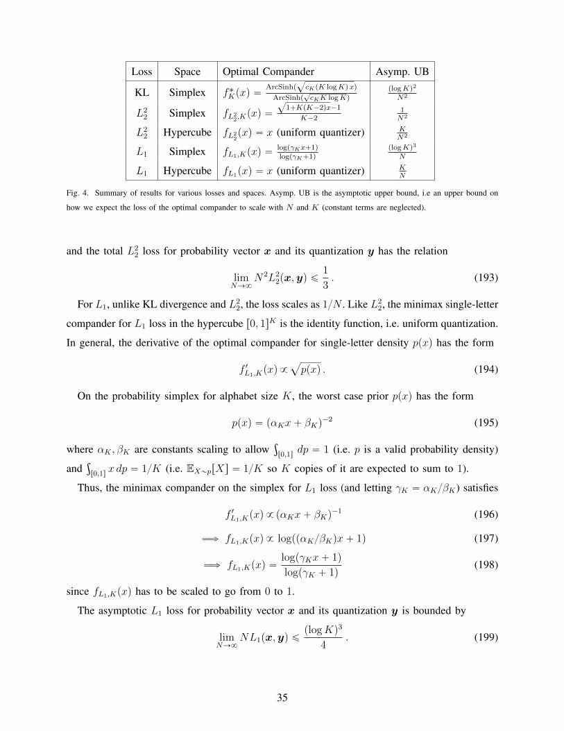
Loss Space Optimal Compander Asymp. UB

KL Simplex f˚Kpxq “ArcSinhp

?cKpK logKqxq

ArcSinhp?cKK logKq

plogKq2

N2

L22 Simplex fL2

2,Kpxq “

?1`KpK´2qx´1

K´21N2

L22 Hypercube fL2

2pxq “ x (uniform quantizer) K

N2

L1 Simplex fL1,Kpxq “logpγKx`1qlogpγK`1q

plogKq3

N

L1 Hypercube fL1pxq “ x (uniform quantizer) KN

Fig. 4. Summary of results for various losses and spaces. Asymp. UB is the asymptotic upper bound, i.e an upper bound on

how we expect the loss of the optimal compander to scale with N and K (constant terms are neglected).

and the total L22 loss for probability vector x and its quantization y has the relation

limNÑ8

N2L22px,yq ď

1

3. (193)

For L1, unlike KL divergence and L22, the loss scales as 1N . Like L2

2, the minimax single-letter

compander for L1 loss in the hypercube r0, 1sK is the identity function, i.e. uniform quantization.

In general, the derivative of the optimal compander for single-letter density ppxq has the form

f 1L1,Kpxq9

a

ppxq . (194)

On the probability simplex for alphabet size K, the worst case prior ppxq has the form

ppxq “ pαKx` βKq´2 (195)

where αK , βK are constants scaling to allowş

r0,1sdp “ 1 (i.e. p is a valid probability density)

andş

r0,1sx dp “ 1K (i.e. EX„prXs “ 1K so K copies of it are expected to sum to 1).

Thus, the minimax compander on the simplex for L1 loss (and letting γK “ αKβK) satisfies

f 1L1,Kpxq9 pαKx` βKq

´1 (196)

ùñ fL1,Kpxq9 logppαKβKqx` 1q (197)

ùñ fL1,Kpxq “logpγKx` 1q

logpγK ` 1q(198)

since fL1,Kpxq has to be scaled to go from 0 to 1.

The asymptotic L1 loss for probability vector x and its quantization y is bounded by

limNÑ8

NL1px,yq ďplogKq3

4. (199)

35

VII. ACKNOWLEDGEMENTS

We would like to thank Anthony Philippakis for his guidance on the DNA k-mer experiments.

REFERENCES

[1] Aviv Adler, Jennifer Tang, and Yury Polyanskiy, “Quantization of random distributions under KL divergence,” in 2021

IEEE International Symposium on Information Theory (ISIT), 2021, pp. 2762–2767.

[2] W. R. Bennett, “Spectra of quantized signals,” The Bell System Technical Journal, vol. 27, no. 3, pp. 446–472, 1948.

[3] G. Grimmett and D. Stirzaker, Probability and Random Processes, Oxford University Press, 2001.

[4] Jennifer Tang, Divergence Covering, Ph.D. thesis, Massachusetts Institute of Technology, 2022.

[5] Dhiraj Kalamkar, Dheevatsa Mudigere, Naveen Mellempudi, Dipankar Das, Kunal Banerjee, Sasikanth Avancha,

Dharma Teja Vooturi, Nataraj Jammalamadaka, Jianyu Huang, Hector Yuen, et al., “A study of bfloat16 for deep learning

training,” arXiv preprint arXiv:1905.12322, 2019.

[6] P.F. Panter and W. Dite, “Quantization distortion in pulse-count modulation with nonuniform spacing of levels,” Proceedings

of the IRE, vol. 39, no. 1, pp. 44–48, 1951.

[7] P. Zador, “Asymptotic quantization error of continuous signals and the quantization dimension,” IEEE Transactions on

Information Theory, vol. 28, no. 2, pp. 139–149, 1982.

[8] A. Gersho, “Asymptotically optimal block quantization,” IEEE Transactions on Information Theory, vol. 25, no. 4, pp.

373–380, 1979.

[9] Michele Lewis and SC MTSA, “A-law and mu-law companding implementations using the tms320c54x,” 1997.

[10] Bernard Smith, “Instantaneous companding of quantized signals,” The Bell System Technical Journal, vol. 36, no. 3, pp.

653–710, 1957.

[11] S. Graf and H. Luschgy, Foundations of Quantization for Probability Distributions, Lecture Notes in Mathematics. Springer

Berlin Heidelberg, 2007.

[12] Noam Slonim and Naftali Tishby, “Agglomerative information bottleneck,” in Proceedings of the 12th International

Conference on Neural Information Processing Systems, Cambridge, MA, USA, 1999, NIPS’99, p. 617–623, MIT Press.

[13] Naftali Tishby, Fernando C Pereira, and William Bialek, “The information bottleneck method,” arXiv preprint

physics/0004057, 2000.

[14] Fernando Pereira, Naftali Tishby, and Lillian Lee, “Distributional clustering of English words,” in Proceedings of the

ACL, 1993, pp. 183–190.

[15] Bin Jiang, Jian Pei, Yufei Tao, and Xuemin Lin, “Clustering uncertain data based on probability distribution similarity,”

IEEE Transactions on Knowledge and Data Engineering, vol. 25, no. 4, pp. 751–763, 2013.

[16] Jie Cao, Zhiang Wu, Junjie Wu, and Wenjie Liu, “Towards information-theoretic k-means clustering for image indexing,”

Signal Processing, vol. 93, no. 7, pp. 2026–2037, 2013.

[17] Inderjit Dhillon and Subramanyam Mallela, “A divisive information-theoretic feature clustering algorithm for text

classification,” Journal of machine learning research, vol. 3, pp. 1265–1287, 04 2003.

[18] Frank Nielsen, “Jeffreys centroids: A closed-form expression for positive histograms and a guaranteed tight approximation

for frequency histograms,” IEEE Signal Processing Letters, vol. 20, no. 7, pp. 657–660, 2013.

[19] R. Veldhuis, “The centroid of the symmetrical Kullback-Leibler distance,” IEEE Signal Processing Letters, vol. 9, no. 3,

pp. 96–99, 2002.

36

APPENDIX ORGANIZATION

Appendix A: We fill in the details on the lemmas and propositions used in the proof of

Theorem 1. In Sections A-A to A-E we cover the results needed to prove Proposition 4, while

in Sections A-F and A-G we cover the results needed to prove Proposition 5.

Appendix B: We develop and analyze other types of companders, specifically beta com-

panders, which are optimized to quantize vectors from Dirichlet priors (Section B-A), and

power companders, which have the form fpxq “ xs and have properties similar to the minimax

compander (Section B-B). Supplemental experimental results are also provided.

Appendix C: We analyze the minimax compander and approximate minimax compander

more deeply, showing that cK P r14, 34s (Section C-A) and limKÑ8 cK “ 12 (Section C-B).

We also show that when cK « 12, the approximate minimax compander has performance close

to the minimax compander against all priors p P P (Section C-C). Supplemental experimental

results are also provided.

Appendix D: We prove Theorem 5, showing bounds on the worst-case loss (adversari-

ally selected x, rather than from a prior) for the power, minimax, and approximate minimax

companders.

APPENDIX A

ASYMPTOTIC SINGLE-LETTER LOSS PROOFS

In this appendix, we fill in the details on the lemmas and propositions used in the proof of

Proposition 4 (showing that the local loss functions gN converge to the asymptotic local loss

function g a.s. when the input X is distributed according to p P P), including proofs for all

results from Section IV-B (specifically Lemmas 1 and 2 and Propositions 6 to 8). This is covered

in Sections A-A to A-E.

We then fill in the details of the lemmas for the proof of Proposition 5 (showing the existence

of an integrable h dominating gN when the compander f is from the ‘well-behaved’ set F :),

specifically Lemmas 3 and 6.

A. Proof of Lemma 1

Proof. Note that for fixed θ and x, rpx,θ,εq is nonnegative and monotonically decreases as ε

decreases. Thus limεÑ0 rpx,θ,εq ě 0 is well defined.

37

We first assume that limεÑ0 rpx,θ,εq “ 0 for all θ P r0, 1s. Let sθprq be defined as

sθprq :“fpx` p1´ θqrq ´ fpx´ θrq

r. (200)

We want to show that limrÑ0 sθprq “ f 1pxq for all θ P r0, 1s, and that this limit is uniform

over θ P r0, 1s. For θ P t0, 1u we get respectively the right and left derivatives and since f is

differentiable at x we are done for those cases. For θ P p0, 1q we write:

sθprq “fpx` p1´ θqrq ´ fpx´ θrq

r(201)

“fpx` p1´ θqrq ´ fpxq

r`fpxq ´ fpx´ θrq

r(202)

“ p1´ θqfpx` p1´ θqrq ´ fpxq

p1´ θqr` θ

fpx´ θrq ´ fpxq

´θr. (203)

This implies

limrÑ0

sθprq “ limrÑ0

ˆ

p1´ θqfpx` p1´ θqrq ´ fpxq

p1´ θqr` θ

fpx´ θrq ´ fpxq

´θr

˙

(204)

“ p1´ θqf 1pxq ` θf 1pxq “ f 1pxq . (205)

Furthermore we note that the convergence is uniform over θ P r0, 1s. This is because for any

α ą 0, there is a δ ą 0 such that for |r| ď δ,ˇ

ˇ

ˇ

ˇ

fpx` rq ´ fpxq

r´ f 1pxq

ˇ

ˇ

ˇ

ˇ

ď α . (206)

But |r| ď δ ùñ | ´ θr| ď δ and |p1´ θqr| ď δ. Thus,

|sθprq ´ f1pxq| “

ˇ

ˇ

ˇ

ˇ

p1´ θqfpx` p1´ θqrq ´ fpxq

p1´ θqr` θ

fpx´ θrq ´ fpxq

´θr´ f 1pxq

ˇ

ˇ

ˇ

ˇ

(207)

ď

ˇ

ˇ

ˇ

ˇ

p1´ θqfpx` p1´ θqrq ´ fpxq

p1´ θqr´ p1´ θqf 1pxq

ˇ

ˇ

ˇ

ˇ

`

ˇ

ˇ

ˇ

ˇ

θfpx´ θrq ´ fpxq

´θr´ θf 1pxq

ˇ

ˇ

ˇ

ˇ

(208)

ď p1´ θqα ` θα (209)

“ α . (210)

38

Thus we have uniform convergence of sθprq to f 1pxq over all θ P r0, 1s as r Ñ 0. Since

rpx,θ,εq Ñ 0 as εÑ 0,

f 1pxq “ limεÑ0

sθprpx,θ,εq

q (211)

“ limεÑ0

fpx` p1´ θqrpx,θ,εqq ´ fpx´ θrpx,θ,εqq

rpx,θ,εq(212)

“ limεÑ0

ε

rpx,θ,εq(213)

ùñ limεÑ0

ε´1 rpx,θ,εq “ f 1pxq´1 (214)

as we wanted. The third equality comes from the definition of rpx,θ,εq (61) and the fact that f 1pxq

is well-defined.

Now we need to consider what happens if limεÑ0 rpx,θ,εq ‰ 0 for some values of θ; this can

either be because the limit is positive or because the limit doesn’t exist, but in either case it is

clearly only possible if f is not strictly monotonic at x and hence only if f 1pxq “ 0. Additionally,

it can only happen if f is flat at x, i.e. there is either some a ă x or some a ą x such that

fpaq “ fpxq (or both). In this case, for any 0 ă θ ă 1, Ipx,θ,εq contains the interval between a

and x and hence rpx,θ,εq ě |x´ a|. For θ “ 0 and θ “ 1, either rpx,θ,εq is bounded away from 0,

or it approaches 0; in the first case, ε´1rpx,θ,εq Ñ 8 by default, while in the second the proof

for the limεÑ0 rpx,θ,εq “ 0 case holds.

Thus, for all values of θ P r0, 1s, we know that limεÑ0 ε´1rpx,θ,εq “ 8 as we need; and this

is uniform over θ because for any θ P p0, 1q we have ε´1rpx,θ,εq ě ε´1|x´ a|, meaning that for

any large α ą 0, we can choose ε˚ small enough so that for all ε ă ε˚ all of the following

hold: (i) ε´1|x ´ a| ą α; (ii) ε´1rpx,0,εq ą α; and (iii) ε´1rpx,0,εq ą α. Thus, we have uniform

convergence and we are done.

B. Proof of Proposition 6

Proof. We can assume that ε ď 12 (if not, just use the value of δ corresponding to ε “ 12).

Let δ ą 0 be such that for all x1 such that |x1 ´ x| ď δ,ˇ

ˇ

ˇ

Fppx1q ´ Fppxq

x1 ´ x´ ppxq

ˇ

ˇ

ˇď ppxqε8 (215)

Since the derivative ppxq “ F 1ppxq is well-defined, this δ must exist. Then for x1 P I ,ˇ

ˇpFppx1q ´ Fppxqq ´ px

1´ xqppxq

ˇ

ˇ ď |x1 ´ x|ppxqε8 (216)

ď rIppxqε8 (217)

39

Now let x2 also be such that |x2 ´ x| ď δ. Then

ˇ

ˇpFppx2q ´ Fppx

1qq ´ px2 ´ x1qppxq

ˇ

ˇ (218)

“ˇ

ˇppFppx2q ´ Fppxqq ´ px

2´ xqppxqq (219)

´ ppFppx1q ´ Fppxqq ´ px

1´ xqppxqq

ˇ

ˇ (220)

ď rIppxqε4 (221)

Let x1 be the lower boundary of I , so x1 ` rI is the upper boundary of I (for which the above

of course applies). Then we get

ˇ

ˇpFppx1` rIq ´ Fppx

1qq ´ rIppxq

ˇ

ˇ ď rIppxqε4 (222)

ùñ

ˇ

ˇ

ˇ

Fppx1 ` rIq ´ Fppx

1q

rIppxq´ 1

ˇ

ˇ

ˇď ε4 . (223)

Then we know that for any x2 P I ,

Fp|I px2q “

Fppx2q ´ Fppx

1q

Fppx1 ` rIq ´ Fppx1q. (224)

By (221) we know that

px2 ´ x1qppxq´rIppxqε4 ď Fppx2q ´ Fppx

1q

ď px2 ´ x1qppxq ` rIppxqε4 (225)

ùñ rIppxqppx2´ x1qrI ´ ε4q ď Fppx

2q ´ Fppx

1q

ď rIppxqppx2´ x1qrI ` ε4q (226)

and by (223) we know that

rIppxq ´ rIppxqε4 ď Fppx` rIq ´ Fppx1q

ď rIppxq ` rIppxqε4 (227)

ùñ rIppxqp1´ ε4q ď Fppx` rIq ´ Fppx1q

ď rIppxqp1` ε4q . (228)

40

Noting that px2 ´ x1qrI “ FunifI px2q P r0, 1s is the CDF of the uniform distribution on I , we

get that

Fp|I px2q ě

rIppxqppx2 ´ x1qrI ´ ε4q

rIppxqp1` ε4q(229)

“px2 ´ x1qrI ´ ε4

1` ε4(230)

ě FunifI px2q ´ ε (231)

and similarly that

Fp|I px2q ď

rIppxqppx2 ` x1qrI ´ ε4q

rIppxqp1´ ε4q(232)

“px2 ´ x1qrI ` ε4

1´ ε4(233)

ď FunifI px2q ` ε (234)

and hence for such a δ ą 0 we have for all I containing x and such that rI ď δ we have

|Fp|I px2q ´ FunifI px

2q| ď ε (235)

for all x2 P I . For x2 R I “ rx1, x1 ` rIs we then observe that

Fp|I px2q “ FunifI px

2q “

$

’

&

’

%

0 if x2 ă x1

1 if x2 ą x1 ` rI

(236)

thus finishing the proof.

C. Proof of Proposition 7

Proof. Let ξ “ ryp,I ´ yI . Then:

|ξ| “

ˇ

ˇ

ˇ

ˇ

ż

I

`

PX„p|I rX ě xs ´ PX„unifI rX ě xs˘

dx

ˇ

ˇ

ˇ

ˇ

(237)

ď

ż

I

ˇ

ˇPX„p|I rX ě xs ´ PX„unifI rX ě xsˇ

ˇ dx (238)

ď rIε . (239)

For any distribution q and any fixed value z, define the shift operator Tzpqq to denote the

distribution of X´z where X „ q (i.e. just shift it by z). Note that Tryp,I pp|Iq and TyI punifIq are

41

both constructed to have expectation 0, and in particular TyI punifIq is the uniform distribution

over an interval of width rI centered at 0. Additionally,

dKSpTryp,I pp|Iq, TyI punifIqq ď dKSpTryp,I pp|Iq, Tryp,I punifIqq (240)

` dKSpTryp,I punifIq, TyI punifIqq (241)

ď 2ε (242)

since dKSp¨, ¨q is a metric, dKSpq1, q2q “ dKSpTzpq1q, Tzpq2qq for any q1, q2 and z, and

dKSpTz1punifIq, Tz2punifIqq ď |z2 ´ z1|rI . (243)

For convenience, let q1 “ Tryp,I pp|Iq and q2 “ TyI punifIq, and let Z1 „ q1 and Z2 „ q2. We

know the following: ErZ1s “ ErZ2s “ 0; dKSpq1, q2q ď 2ε; and q1, q2 have support on r´rI , rIs.

Let ηi “ ErZi1s ´ ErZi

2s. Then we can compute the following:

|ηi| “

ˇ

ˇ

ˇ

ˇ

ż riI

0

pPrZi1 ě xs ´ PrZi

2 ě xsq dx´

ż riI

0

pPrZi1 ď ´xs ´ PrZi

2 ď ´xsq dx

ˇ

ˇ

ˇ

ˇ

(244)

If i is odd, then we do a u-substitution with u “ x1i and get

|ηi| “

ˇ

ˇ

ˇ

ˇ

ż riI

0

pPrZ1 ě x1is ´ PrZ2 ě x1i

sq dx´

ż 0

´riI

pPrZ1 ď ´x1is ´ PrZi

2 ď ´x1isq dx

ˇ

ˇ

ˇ

ˇ

(245)

“ i

ˇ

ˇ

ˇ

ˇ

ż rI

0

ui´1pPrZ1 ě us ´ PrZ2 ě usq du´

ż 0

´rI

ui´1pPrZ1 ď us ´ PrZ2 ď usq du

ˇ

ˇ

ˇ

ˇ

(246)

ď 2

ż rI

0

iui´12εdu “ 4εriI (247)

Similarly if i is even we get

|ηi| “

ˇ

ˇ

ˇ

ˇ

ż riI

0

pPrZ1 ě x1is ´ PrZ2 ě x1i

sq dx`

ż 0

´riI

pPrZ1 ď ´x1is ´ PrZi

2 ď ´x1isq dx

ˇ

ˇ

ˇ

ˇ

(248)

“ i

ˇ

ˇ

ˇ

ˇ

ż rI

0

ui´1pPrZ1 ě us ´ PrZ2 ě usq du`

ż 0

´rI

ui´1pPrZ1 ď us ´ PrZ2 ď usq du

ˇ

ˇ

ˇ

ˇ

(249)

ď 2

ż rI

0

iui´12εdu “ 4εriI (250)

and we can conclude that |ηi| ď 4εriI in general.

42

Then we can take the respective Taylor expansions: let X1 „ p|I and X2 „ unifI (and

Z1 „ q1, Z2 „ q2 as above). We get

`p,I “ ErX1 logpX1ryp,Iqs (251)

“ ryp,IErpZ1ryp,I ` 1q logpZ1ryp,I ` 1qs (252)

“ ryp,IE„

Z1ryp,I `pZ1ryp,Iq

2

2´pZ1ryp,Iq

3

6p1` ηq2

(253)

where η is a number between 0 and Z1ryp,I (we get this using Lagrange’s formula for the error).

Since Z1 ` ryp,I P I , we know that

ryp,I ´ rI ď z ` ryp,I ď ryp,I ` rI . (254)

Since rI ă x4 and ryp,I ě x´rI (as x, ryp,I share the width-rI interval I), we get that ryp,I ą 3rI ,

and therefore

2

3ryp,I ă Z1 ` ryp,I ă

4

3ryp,I (255)

ùñ´1

3ă Z1ryp,I ă

1

3. (256)

This gives that |η| ă 13. Using this and the fact that ErZ1s “ 0 by construction, we can write

(253) as

`p,I ď1

2ErZ2

1 sryp,I `|ErZ3

1 s|

83pryp,Iq

´2 (257)

ď1

2ErZ2

1 sryp,I `r3I

83px´ rIq2. (258)

Since rI ă x4, we know that x´ rI ą p34qx, and hence

`p,I ď1

2ErZ2

1 sryp,I ` p23qr3Ix´2 . (259)

Hence we get

`p,I “1

2ErZ2

1 sryp,I `Opr3Ix´2q . (260)

Because x´rI ď yI as well (and Z2 has support on r´rI , rIs) we can repeat the above arguments

to conclude similarly that

`unifI “1

2ErZ2

2 syI `Opr3Ix´2q . (261)

Hence their difference is

|`p,I ´ `unifI | ď1

2

ˇ

ˇErZ21 sryp,I ´ ErZ2

2 syIˇ

ˇ`Opr3Ix´2q (262)

43

Taking the main term, we split it into three parts:

ˇ

ˇErZ21 sryp,I ´ ErZ2

2 syIˇ

ˇ ďˇ

ˇErZ21 sryp,I ´ ErZ2

1 sxˇ

ˇ (263)

`ˇ

ˇErZ22 syI ´ ErZ2

2 sxˇ

ˇ (264)

`ˇ

ˇErZ21 sx´ ErZ2

2 sxˇ

ˇ . (265)

The first part (263) can be bounded by

ˇ

ˇErZ21 sryp,I ´ ErZ2

1 sxˇ

ˇ ď |ErZ21 s| |1ryp,I ´ 1x| (266)

ď r2I

|x´ ryp,I |

ryp,Ix(267)

ď p43qr3Ix´2 (268)

“ Opr3Ix´2q . (269)

An analogous argument bounds (264), giving

ˇ

ˇErZ22 syI ´ ErZ2

2 sxˇ

ˇ “ Opr3Ix´2q . (270)

Finally, (265) follows from

ˇ

ˇErZ21 sx´ ErZ2

2 sxˇ

ˇ “ |η2|x´1ď 4εr2

Ix´1 . (271)

Thus, plugging it all into (262) we get

|`p,I ´ `unifI | ď 2εr2Ix´1`Opr3

Ix´2q . (272)

D. Proof of Proposition 8

Proof. Let i˚ be such that rIi˚ ď x4 for all i ě i˚ (since limiÑ8 rIi “ 0 this exists) and WLOG

consider the sequence of i ě i˚. The result then follows from the Taylor series of `unifIi, as

shown by (261) (see proof of Proposition 7 in Section A-C). Keeping the definition from the

proof of Proposition 7, we let Z2 „ TyIi punifIiq, i.e. uniform over a width-rIi interval centered

at 0. Thus we have ErZ22 s “

112r2Ii

and hence (261) yields

`unifIi“

1

2ErZ2

2 syIi `Opr3Ix´2q (273)

“1

24r2Iiy´1Ii`Opr3

Iix´2q (274)

44

But yIi and x share the interval Ii and hence as rIi Ñ 0,

yIi “ x`OprIiq (275)

“ xp1`OprIix´1qq (276)

ùñ y´1Ii“ x´1

p1`OprIix´1qq (277)

since when rIi is very small, OprIix´1q is very small so p1`OprIix

´1q´1 “ 1`OprIix´1q (the

inverse of a value close to 1 is also close to 1). Thus, we can replace y´1Ii

in (274) to get

`unifI “1

24r2Iix´1

`Opr3Iix´2q (278)

as we wanted.

E. Single-Interval Loss Function Properties and Proof of Lemma 2

We prove Lemma 2 here; to do so, we show a few lemmas concerning the single-interval loss

function `p,I . First, we show an alternative formula for `p,I which sheds some light on it:

Lemma 9. For any p, I ,

`p,I “ EX„p|I rX logXs ´ ryp,I logpyp,Iq (279)

Proof. We compute `p,I as follows:

`p,I “ EX„prX logpXryp,Iq |X P Is (280)

“ EX„p|I rX logpXryp,Iqs (281)

“ EX„p|I rX logpXq ´X logpryp,Iqs (282)

“ EX„p|I rX logXs ´ EX„p|I rXs logpryp,Iq (283)

“ EX„p|I rX logXs ´ ryp,I logpyp,Iq (284)

since ryp,I “ EX„p|I rXs.

We now want to show that it really does represent something resembling a loss function: first,

that it is nonnegative, and second that it achieves equality if and only if X „ p on I is known

for sure (so the decoded value can be guaranteed to equal X).

Lemma 10. For any p and I Ď r0, 1s (even p is not continuous),

`p,I ě 0 (285)

45

with equality if and only if there is some z P I s.t.

PX„prX “ z |X P Is “ 1 . (286)

Proof. Using Lemma 9, if we define the function hptq “ t log t then since h is strictly convex,

by Jensen’s Inequality (where all expectations are over X „ p|I)

`p,I “ ErhpXqs ´ hpErXsq ě 0 (287)

with equality if and only if X „ p|I is fixed with probability 1.

This yields the following corollary:

Corollary 2. If p P P and I has nonzero width,

`p,I ą 0 . (288)

This follows because p P P is continuous and so cannot have all its mass on a particular value

in any nonzero-width I . If I has zero probability mass under p, then `p,I defaults to the interval

loss under a uniform distribution.

Finally, we can prove Lemma 2. Recall that it shows that if I has nonzero probability mass

under p, one cannot get the interval loss to approach 0 by choosing J Ě I , i.e. if p P P and I

is such that PX„prX P Is ą 0, then there is some α ą 0 (which can depend on I) such that

`p,J ě α for all J Ě I . (289)

Proof of Lemma 2. We can re-write `p,J as

`p,J “ EX„prX logpXryp,Jq |X P Js (290)

“

ż

J

ppxqş

Jdpx logpxryp,Jq dz (291)

whereş

Jdp is just the integral representation of PX„prX P Js.

Therefore, since p P P , `p,J is continuous at J with respect to the boundaries of J (the inverse

probability mass pş

Jdpq´1 is continuous since

ş

Jdp ě

ş

Idp ą 0).

Thus, we can consider `p,J as a continuous function over the boundaries of J on the domain

where I Ď J Ď r0, 1s; this domain can be represented as a closed subset of r0, 1s2 and hence is

compact. Thus, by the Weierstrass extreme value theorem, `J,p achieves its minimum α on this

domain, and by Corollary 2 it must be positive.

Hence, we have shown that there is an α ą 0 such that for any J Ě I , `p,J ą α.

46

F. Proof of Lemma 3

Proof. We WLOG restrict ourselves to q which are probability distributions over I . Let PIdenote the set of probability distributions over I (not necessarily continuous) and P 1I denote the

set of probability distributions over I which place all the probability mass on the boundaries

yI ´ rI2 and yI ` rI2, i.e. for all q1 P P 1I we have

PX„q1rX P tyI ´ rI2, yI ` rI2us “ 1 . (292)

We then make the following claim:

Claim 1: For all q P PI , exists q1 P P 1I such that `q,I ď `q1,I .

This follows from the convexity of the function x logpxq and the definition of `q,I , i.e.

`q,I “ EX„qrX logpXyq,Iqs (293)

(since q in this case is a distribution over I , we removed the condition X P I as it is redundant).

In particular, if q1 is the (unique) distribution in P 1I such that EX„q1rXs “ yq,I (i.e. we move all

the probability mass to the boundary but keep the expected value the same), then `q1,I can be

computed by considering the average over the linear function which connects the end points of

X logpXyq,Iq over I . Because of convexity, this linear function is always greater than or equal

to X logpXyq,Iq on I , and therefore `q,I ď `q1,I . Thus, Claim 1 holds and we can restrict our

attention to P 1I .

For simplicity we introduce a linear mapping z from r´12, 12s to I: for θ P r´12, 12s, let

zpθq “ yI ` θrI (so zp´12q “ yI ´ rI2 is the lower boundary of I , zp12q “ yI ` rI2 is the

upper boundary, and zp0q “ yI is the midpoint). We also specially denote a “ zp´12q to be

the lower boundary and b “ zp12q to be the upper boundary. Then, since any q P P 1I can only

assign probabilities to a and b, we can parametrize all q P P 1I : let qpθq denote the distribution

assigning probability 12`θ to the upper boundary b and 12´θ to the lower boundary a. Then

this gives the nice formula:

yqpθq,I “ yI ` θrI “ zpθq (294)

i.e. qpθq is the unique distribution in P 1I with expectation zpθq. This brings us to our next claim:

Claim 2: `qpθq,I ď 2`qp0q,I for any θ P r´12, 12s. Ignoring the redundant condition X P I ,

we use

`q,I “ EX„qrX logpXqs ´ ryq,I logpryq,Iq (295)

47

to re-write `qpθq,I as follows:

`qpθq,I “ p12´ θqa logpaq ` p12` θqb logpbq ´ zpθq logpzpθqq (296)

This implies that

`qpθq,I ď `qpθq,I ` `qp´θq,I (297)

“`

a logpaq ` b logpbq˘

´`

zpθq logpzpθqq ` zp´θq logpzp´θqq˘

(298)

ď`

a logpaq ` b logpbq˘

´ 2yI logpyIq (299)

“ 2`qp0q,I (300)

where the inequality follows because x logpxq is convex and the mean of zpθq and zp´θq is

zp0q “ yI , showing Claim 2.

Claim 3: 2`qp0q,I ď12r2I y´1I .

This comes from rewriting according to (295) and then applying the Taylor series expansion

of p1` tq logp1` tq. Define t “ rIp2yIq ď 1 (otherwise I R r0, 1s), we get:

2`qp0q,I (301)

“`

a logpaq ` b logpbq˘

´ 2yI logpyIq (302)

“ pyI ´ rI2q logpyI ´ rI2q ` pyI ` rI2q logpyI ` rI2q ´ 2yI logpyIq (303)

“ pyI ´ rI2qplogpyI ´ rI2q ´ logpyIqq ` pyI ` rI2qplogpyI ` rI2q ´ logpyIqq (304)

“ yI`

p1´ tq logp1´ tq ` p1` tq logp1` tq˘

(305)

We can use the inequality that p1´ tq logp1´ tq ` p1` tq logp1` tq ď 2t2 for |t| ď 1, to get

2`qp0q,I ď 2yIt2“

1

2r2I y´1I (306)

This resolves Claim 3.

The lemma then follows from Claims 1, 2, and 3.

G. Proof of Lemma 6

Proof. First, note that the above conditions imply that f2pxq ě f1pxq and that f 12pxq ě f 11pxq for

all x where both are defined (almost everywhere).

Let Jfi,N,x “ rai, bis for i “ 1, 2. We will prove that a1 ď a2 and b1 ě b2. Note that by

definition if f1pxq ´ 1N ď 0 then a1 “ 0 and a1 ď a2 happens by default; thus this is also

48

the case if f2pxq ´ 1N ď 0 since f2 ě f1 means this implies f1pxq ´ 1N ď 0. Meanwhile, if

f2pxq ` 1N ě 1 we have

1N ě 1´ f2pxq ě f2p1q ´ f2pxq ě f1p1q ´ f1pxq (307)

meaning that b1 “ 1 (and b2 “ 1) so b1 ě b2; and similarly f1pxq ` 1N ě 1 simply implies

b1 “ 1 ě b2.

Thus we don’t need to worry about the boundaries hitting 0 or 1 (i.e. we can ignore the

‘Xr0, 1s’ in the definition), as the needed result easily holds whenever it happens.

Then a1 and a2 are the values for whichż x

a2

f 12ptq dt “

ż x

a1

f 11ptq dt “ 1N (308)

But since 0 ď f 11ptq ď f 12ptq, we know thatż x

a2

f 12ptq dt “ 1N “

ż x

a1

f 11ptq dt ď

ż x

a1

f 12ptq dt (309)

which implies that a2 ě a1. An analogous proof on the opposite side proves b1 ě b2 and hence

Jf2,N,x “ ra2, b2s Ď ra1, b1s “ Jf1,N,x (310)

as we needed.

APPENDIX B

BETA AND POWER COMPANDERS

In this appendix, we analyze beta companders, which are optimal companders for symmetric

Dirichlet priors and are based on the normalized incomplete beta function (Section B-A) and

power companders, which have the form fpxq “ xs and which have properties similar to the

minimax compander when s “ 1 logK (Section B-B).

We also add supplemental experimental results. First, we compare the beta compander with

truncation (identity compander) and the EDI (Exponential Density Interval) compander we

developed in [1] in the case of the uniform prior on 4K´1 (which is equivalent to a Dirichlet

prior with all parameters set to 1), on book word frequencies, and on DNA kmer frequencies.

EDI was, in a sense, developed to minimize the expected KL divergence loss for the uniform

prior (specifically to remove dependence on K) as a means of proving a result on rate distortion;

beta was then directly developed for all Dirichlet priors.

49

Second, we compare the theoretical prediction for the power compander against various data

sets; this demonstrates a close match to the theoretical performance for synthetic (uniform

on 4K´1) data and DNA kmer frequencies, while the power compander performs better on

book word frequencies. Note that this is not a contradiction, as the theoretical prediction is for

its performance on the worst possible prior – it instead indicates that book word frequencies

are somehow more suited to power companders than the uniform distribution or DNA kmer

frequencies.

Finally, we compare how quickly the beta and power companders converge to their theoretical

limits (with uniform prior); specifically how quickly N2rLpp, f,Nq converges to rLpp, fq. The

results show that for large K (« 105), both are already very close by N “ 28 “ 256; while for

smaller values of K, power companders still converge very quickly while beta companders may

take even until N “ 216 “ 65536 or beyond to be close.

A. Beta Companders for Symmetric Dirichlet Priors

Definition 7. When X is drawn from a Dirichlet distribution with parameters α “ α1, . . . , αK ,

we use the notation X „ Dirpαq. When α1 “ ¨ ¨ ¨ “ αK “ α, then X is drawn from a symmetric

Dirichlet with parameter α and we use the notation X „ DirKpαq.

As a corollary to Theorem 2, we get that the optimal compander for the symmetric Dirichlet

distribution is the following:

Corollary 3. When x „ DirKpαq, let ppxq be the associated single-letter density (same for all

elements due to symmetry). The optimal compander for p satisfies

f 1pxq “ B´α ` 1

3,pK ´ 1qα ` 2

3

¯´1

xpα´2q3p1´ xqppK´1qα´1q3 (311)

where Bpa, bq is the Beta function. Therefore, fpxq is the normalized incomplete Beta function

Ixppα ` 1q3, ppK ´ 1qα ` 2q3q.

Then

rLpp, fq “1

2B´α ` 1

3,pK ´ 1qα ` 2

3

¯3

Bpα, pK ´ 1qαq´1 (312)

This result uses the following fact:

50

102 103 104 105

Number of Symbols (K)

10 5

10 4

10 3

10 2

10 1

100

KL D

iver

genc

e

comparing companders with N = 256Rand. Dir. identityRand. Dir. expRand. Dir. betaBook identityBook expBook betaucsc DNA identityucsc DNA expucsc DNA beta

102 103 104 105

Number of Symbols (K)

10 9

10 7

10 5

10 3

10 1

KL D

iver

genc

e

comparing companders with N = 65536Rand. Dir. identityRand. Dir. expRand. Dir. betaBook identityBook expBook betaucsc DNA identityucsc DNA expucsc DNA beta

Fig. 5. Comparing the beta compander and the EDI method. The random data is drawn with DirKp1q (i.e. uniform).

Fact 1. For X „ Dirpα1, . . . , αKq, the marginal distribution on Xk is Xk „ Betapαk, βkq,

where βk “ř

j‰k αj . When the prior is symmetric with parameter α, we get that all Xk are

distributed according to Betapα, pK ´ 1qαq.

Remark 10. Since (312) scales with K´1, this means that pLKpDirKpαq, fq is constant with

respect to K. This is consistent with what we get with the EDI compander (see [1]).

We will call the compander f derived from integrating (311) the beta compander. (This is

because integrating (311) gives an incomplete beta function.) The beta compander naturally

performs better than the EDI method since this compander is optimized to do so. We can see

the comparison in Figure 5 that on random uniform distributions, the beta compander is better

than the EDI method by a constant amount for all K.

The beta compander is not the easiest algorithm to implement however. It is necessary to

compute an incomplete beta function in order to find the compander function f , which is not

known to have a closed form expression. We reiterate Remark 4 that it is indeed interesting that

the minimax compander, on the other hand, does have a closed form.

51

102 103 104 105

Number of Symbols (K)

10 8

KL D

iver

genc

e

KL Divergence with Granularity N = 65536Theor. Avg powerRand Unif powerBook powerDNA power

Fig. 6. Comparing theoretical performance (315) of the power compander to experimental results.

B. Analysis of the Power Compander

Starting with Theorem 1, we can use the asymptotic analysis to understand why the power

compander works well for all distributions.

Proposition 9. Let single-letter density p be the marginal probability of one letter on any

symmetric probability distribution P over K letters. For the power compander fpxq “ xs where

s ď 12,

rLpp, fq ď1

K

1

24s´2K2s (313)

and for any prior P P P4K ,

rLKpP, xsq ď1

24s´2K2s . (314)

Optimizing over s gives

rLKpP, fq ďe2

24plogKq2 . (315)

Proof. Since fpxq “ xs we have that f 1pxq “ sxs´1. Using Theorem 1, this gives

rLpp, fq “1

24s´2

ż 1

0

x1´2sppxqdx “1

24s´2EX„prX1´2s

s . (316)

The function x1´2s is increasing and also a concave function. We want to find the maximin

prior distribution P P P4K (with marginals p) with the constraint

ÿ

i

EXi„prXis “ 1 (317)

52

(another constraint is that values of p are such that must sum to one, but we give a weaker

constraint here).

We want to choose P to maximizeÿ

i

EXi„prX1´2si s “ EpX1,...,XKq„P

«

ÿ

i

X1´2si

ff

. (318)

By concavity (even ignoring any constraint that P is symmetric), the maximum solution is given

when X1 “ ¨ ¨ ¨ “ XK . Therefore, the maximin P is such that the marginal on one letter p is

p

ˆ

1

K

˙

“ 1 . (319)

The probability mass function where 1K occurs with probability 1 is a limit point of a

continuous density which is of the form

ppxq “1

2εon x P

„

1

K´ ε,

1

K` ε

(320)

and 0 otherwise. We use this since we are restricting to continuous probability distribution.

Evaluating with this gives

rLpp, fq “1

24s´2EX„prX1´2s

s (321)

ď1

24s´2

ˆ

1

K

˙1´2s

(322)

“1

K

1

24s´2K2s (323)

which shows (315). Multiplying by K gives rLKpP, fq for symmetric P .

Note that for any non-symmetric P , we can always symmetrize P to a symmetric prior Psym

by averaging over all random permutations of the indices. Because the loss rLKpP, fq is concave

in P , the symmetrized prior Psym will give an higher value, that is rLKpP, fq ď rLKpPsym, fq.

Hence rLKpP, fq ď 124s´2K2s holds for all priors.

Finding the s which minimizes 124s´2K2s is equivalent to finding s which minimizes s logK´

log s.

0 “d

dss logK ´ log s “ logK ´

1

s(324)

ùñ s “1

logK. (325)

We can plug this back into our equation, using the fact that elogK “ K implies that K1 logK “ e.

53

Our final result is that using fpxq “ x1 logK gives that for any prior P

rLKpP, fq ďe2

24plogKq2 . (326)

The power compander turns out to give guarantees bounds on the value on rLKpP, fq when f

is chosen so that s “ 1logK. We show the comparison between this theoretical result on raw

loss with the experimental results in Figure 6.

C. Converging to Theoretical

For both the power compander and the beta compander, we show in Figure 7 how quickly

the experimental results converge to the theoretical results. Experimental results have a fixed

granularity N whereas the theoretical results assume that N Ñ 8. The plots show that by

N “ 216 (each value gets 16 bits), the experimental results for the power compander are very

close to the theoretical results, and even for N “ 28 they are not so far. For the beta compander,

the experimental results are close to the theoretical when K is large. When K “ 100, the results

for N “ 216 is not that close to the theoretical result, which demonstrates the effect of using

unnormalized (or raw) values. The difference between normalizing and not normalizing gets

smaller as K increases.

APPENDIX C

MINIMAX AND APPROXIMATE MINIMAX COMPANDERS

In this appendix, we analyze the minimax compander and approximate minimax compander.

Specifically, we analyze the constant cK , to show that it falls in r14, 34s (Section C-A) and that

limKÑ8 cK “ 12 (Section C-B). We also show that when cK is close to 12, the approximate

minimax compander (which is the same as the minimax compander except it replaces cK with

12) has performance close to the minimax compander against all priors p P P (Section C-C).

A. Analysis of Minimax Companding Constant

1) Determining bounds on cK: If aK , bK ě 0, then ppxq is well-behaved (and bigger than 0).

54

100 500 1000 5000 1×104 5×104 1×105

5

10

15

20

25

30

35

40

K (alphabet size)

KLDivergence*N^2

Theoretical Limit for Power Compander and Uniform Prior

Theoretical

N = 16

N = 256

N = 4096

N = 65536

100 500 1000 5000 1×104 5×104 1×105

0.88

0.89

0.90

0.91

0.92

0.93

K (alphabet size)

KLDivergence*N^2

Theoretical Limit for Beta Compander and Uniform Prior

Theoretical

N = 16

N = 256

N = 4096

N = 65536

Fig. 7. Comparing theoretical expression rLpp, fq with experimental result. The KL divergence value of the experimental results

are multiplied to N2 in order to be comparable to rLpp, fq.

102 103 104 105

Number of Symbols (K)

10 9

4 × 10 10

6 × 10 10

2 × 10 9

3 × 10 9

KL D

iver

genc

e

KL Divergence with Granularity N = 65536Theor. Avg minimaxRand Unif minimaxBook minimaxDNA minimax

Fig. 8. Comparing theoretical performance (169) of the approximate minimax compander to experimental results.

55

We need aK and bK to be such that ppxq is a density that integrates to 1 and also that ppxq

has expected value of 1K. To do this, first we compute that

EX„prXs “ż 1

0

x`

aKx13` bKx

43˘´32

dx (327)

“´2

bK?aK ` bK

`

2ArcSinh´b

bKaK

¯

b32K

(328)

The constraint thatş1

0ppxq dx “ 1 requires that aK

?aK ` bK “ 2. We can use this to get

EX„prXs “´aKbK

`

aKb

aKbK` 1ArcSinh

´b

bKaK

¯

bK(329)

“´1

r`

b

1r` 1ArcSinh p

?rq

r(330)

“´1

r`

b

1r` 1 log

`?r `

?r ` 1

˘

r(331)

where we use r “ bKaK . We will find upper and lower bounds in order to approximate what

r should be. Using (331), we can get

EX„prXs ď1

2

log r

r(332)

so long as r ą 3. If we choose r “ c1K logK and set c1 “ .75, then

EX„prXs ď1

2

logpc1K logKq

c1K logK(333)

ď1

2c1K`

log logK

2c1K logK`

log c1

2c1K logKď

1

K(334)

so long as K ą 4. Similarly, we have

EX„prXs ě1

3

log r

r(335)

for all r. If we choose r “ c2K logK and set c2 “ .25, then

EX„prXs ě1

3

logpc2K logKq

c2K logKě

1

K(336)

so long as K ą 24.

Changing the value of c changes the value of EX„prXs continuously. Hence, for each K ą 24,

there exists a cK so that if r “ cKK logK, then

EX„prXs “1

K. (337)

The analysis above gives that .25 ă cK ă .75.

56

B. Limiting value of cK

Lemma 11. In the limit, cK Ñ 12.

Proof. We start with r “ bKaK“ cKK logK, and we need to meet the condition that

´1

r`

b

1r` 1 log

`?r `

?r ` 1

˘

r“

1

K. (338)

Substituting we get

1

K“

´1

cKK logK`

b

1cKK logK

` 1 log`?

cKK logK `?cKK logK ` 1

˘

cKK logK(339)

ùñ cK “´1

logK`

b

1cKK logK

` 1 log`?

cKK logK `?cKK logK ` 1

˘

logK(340)

Let c “ limKÑ8 cK . Since cK is bounded, we know that limKÑ8 cKK logK Ñ 8 since cK is

bounded above by 34.

c “ limKÑ8

´1

logK`

c

1

cKK logK` 1

log`?

cKK logK `?cKK logK ` 1

˘

logK(341)

“ 0` 1 limKÑ8

log`

2?cKK logK

˘

logK(342)

“ limKÑ8

log 2` 12

log cK `12

logK ` 12

log logK

logK(343)

“1

2(344)

C. Approximate Minimax Compander vs. Minimax Compander

For any K, cK can be approximated numerically. To simplify the quantizer, recall we can use

cK «12

for large K to get the approximate minimax compander (30).

This is close to optimal without needing to compute cK . Here we prove Theorem 4.

Proof. Since f˚K , f˚˚K P F :, we know that

rLpp, f˚Kq “ L:pp, f˚Kq and rLpp, f˚˚K q “ L:pp, f˚˚K q . (345)

57

We define the corresponding asymptotic local loss functions

g˚pxq “1

24pf˚Kq

1pxq´2x´1 and g˚˚pxq “

1

24pf˚˚K q

1pxq´2x´1 (346)

so that our goal is to proveż

g˚˚ dp ď p1` εq

ż

g˚ dp . (347)

Let γ˚ “ cKpK logKq and γ˚˚ “ 12pK logKq (the constants in f˚K and f˚˚K respectively) and

let φ˚pxq “ ArcSinhp?γ˚xq and φ˚˚pxq “ ArcSinhp

?γ˚˚xq. Then

pφ˚q1pxq “

?γ˚

2?x?γ˚x` 1

and pφ˚˚q1pxq “?γ˚˚

2?x?γ˚˚x` 1

. (348)

Note that f˚Kpxq “ φ˚pxqφ˚p1q and f˚˚K pxq “ φ˚˚pxqφ˚˚p1q. We now split into two cases: (i)

cK ą 12 and (ii) cK ă 12.

In case (i) (which implies γ˚ ą γ˚˚, and note that γ˚γ˚˚ “ 2cK ď 1 ` ε), we get for all

x P r0, 1s,

pφ˚q1pxq

pφ˚˚q1pxq“

c

γ˚

γ˚˚

c

γ˚˚x` 1

γ˚x` 1P r1,

a

γ˚γ˚˚s Ď r1,?

1` εs (349)

sinceb

γ˚˚x`1γ˚x`1

P ra

γ˚˚γ˚, 1s. Because γ˚ ě γ˚˚ and ArcSinh is an increasing function, we

know that φ˚p1q ě φ˚˚p1q. Thus, for any x P r0, 1s,

pf˚˚K q1pxq “

pφ˚˚q1pxq

φ˚˚p1q(350)

ě

1?1`εpφ˚q1pxq

φ˚p1q(351)

“1

?1` ε

pf˚Kq1pxq (352)

ùñ pf˚˚K q1pxq´2

ď p1` εqpf˚Kq1pxq´2 (353)

ùñ g˚˚pxq ď p1` εqg˚pxq (354)

ùñ

ż

g˚˚ dp ď p1` εq

ż

g˚ dp (355)

which is what we wanted to prove.

Case (ii), where cK ă 12 (implying γ˚˚ ą γ˚) can be proved analogously:

pφ˚˚q1pxq

pφ˚q1pxq“

c

γ˚˚

γ˚

c

γ˚x` 1

γ˚˚x` 1P r1,

a

γ˚˚γ˚s Ď r1,?

1` εs (356)

58

which then gives us pφ˚˚q1pxq ě pφ˚q1pxq and

φ˚˚p1q “

ż 1

0

pφ˚˚q1ptq dt (357)

ď?

1` ε

ż 1

0

pφ˚q1ptq dt (358)

ď p?

1` εqφ˚p1q . (359)

Thus, for any x P r0, 1s,

pf˚˚K q1pxq “

pφ˚˚q1pxq

φ˚˚p1q(360)

ěpφ˚q1pxq

p?

1` εqφ˚p1q(361)

“1

?1` ε

pf˚Kq1pxq (362)

ùñ pf˚˚K q1pxq´2

ď p1` εqpf˚Kq1pxq´2 (363)

ùñ g˚˚pxq ď p1` εqg˚pxq (364)

ùñ

ż

g˚˚ dp ď p1` εq

ż

g˚ dp (365)

completing the proof for both cases.

We show the comparison of the theoretical (asymptotic in K result) of the approximate

minimax compander with the experimental results in Figure 8.

APPENDIX D

WORST-CASE ANALYSIS

In this section, we prove Theorem 5 which applies both to the minimax compander and the

power compander. Since we are dealing with worst-case (i.e. not a random x) the centroid is

not defined; therefore this theorem works with the midpoint decoder. Thus, the (raw) decoded

value of x is ypnN pxqq.

Additionally, we are not using the raw reconstruction but the normalized reconstruction, and

hence it does not suffice to deal with a single letter at a time. Thus, we will work with a full

probability vector x P 4K´1.

Proof of Theorem 5. Let x P 4K´1 be the vector we are quantizing, with ith element (out of

K, summing to 1) xi; since we are dealing with midpoint decoding, our (raw) decoded value of

xi is ynN pxiq. For simplicity, let us denote it as yi, and the normalized value as yi “ yi`ř

j yj˘

.

59

Let δi “ yi ´ xi be the difference between the raw decoded value yi and the original value

xi. Then:

DKL pxyq “ÿ

i

xi logxiyi

(366)

“ÿ

i

xi logxiyi` log

´

ÿ

i

yi

¯

(367)

“ÿ

i

pyi ´ δiq logyi ´ δiyi

` log´

1`ÿ

i

δi

¯

(368)

Next we use that logp1` zq ď z.

DKL pxyq ďÿ

i

pyi ´ δiq´δiyi`ÿ

i

δi (369)

“ÿ

i

´δi `ÿ

i

δ2i

yi`ÿ

i

δi (370)

“ÿ

i

pyi ´ xiq2

yi(371)

(note that in (369) we used the inequality logp1` zq ď z on both appearances of the logarithm,

as well as the fact that yi ´ δi “ xi ě 0).

We now consider each bin Ipnq induced by f . For simplicity let the dividing points between

the bins be denoted by

βpnq “ f´1´ n

N

¯

“ ypnq ` rpnq2 (372)

so that Ipnq “ pβpn´1q, βpnqs. Since all the companders we are discussing are strictly monotonic,

there is no ambiguity. Then, the Mean Value Theorem (since the minimax compander, the

approximate minimax compander, and the power compander are all continuous), for each Ipnq

there is some value zpnq such that

f 1pzpnqq “fpβpnqq ´ fpβpn´1qq

βpnq ´ βpn´ 1q“ N´1r´1

pnq (373)

(since fpβpnqq ´ fpβpn´1qq “ nN ´ pn´ 1qN “ 1N and βpnq ´ βpn´1q “ rpnq by definition).

Thus, we can re-write this as follows:

rpnq “ N´1f 1pzpnqq´1 . (374)

We will also denote the following for simplicity: Ii “ IpnN pxiqq; ri “ rpnN pxiqq; and zi “ zpnN pxiqq

(the bin, bin length, and bin mean value corresponding to xi).

60

Trivially, since zi P Ii, we know that zi2ď yi. Thus, we can derive (since yi is the midpoint

of Ii and xi P Ii, we know that |yi ´ xi| ď ri2) that

DKL pxyq ďÿ

i

pyi ´ xiq2

yi(375)

ď1

4

ÿ

i

r2i

yi(376)

ď1

4

ÿ

i

1

N2pzi2qpf 1pziqq2(377)

“1

2N´2

ÿ

i

1

zipf 1pziqq2. (378)

Note that while we are using midpoint decoding for our quantization, for the purposes of analysis,

it is more convenient to express the all the terms in the KL divergence loss using the mean value.

We now examine the worst case performance of the three companders: the power compander,

the minimax compander, and the approximate minimax compander.

Power compander: In this case, we have

fpxq “ xs and f 1pxq “ sxs´1 (379)

for s “ 1logK

(which is optimal for minimizing raw distortion against worst-case priors). This

yields

DKL pxyq ď1

2N´2s´2

ÿ

i

1

ziz2s´2i

(380)

“1

2N´2s´2

ÿ

i

z1´2si (381)

So long as s ă 12 (which occurs for K ą 7), the function z1´2si is concave in zi. Thus,

replacing all zi by their average will increase the value. Furthermore, Ks “ K1

logK “ e. Thus,

we can derive:

DKL pxyq ď1

2N´2s´2K

ˆř

i ziK

˙1´2s

(382)

“1

2N´2

plogKq2e2´

ÿ

i

zi

¯1´2s

(383)

ďe2

2N´2

plogKq2 max!

1,ÿ

i

zi

)

(384)

Next, we need to bound max t1,ř

i ziu. Assume thatř

i zi ą 1 (otherwise our bound is just

1). Then, we note the following:ř

i xi “ 1 by definition; s´1 “ logK); and

ri “ N´1f 1pziq´1“ N´1s´1z1´s

i . (385)

61

This allows us to make the following derivation:ÿ

i

|zi ´ xi| ď1

2

ÿ

i

ri (386)

ùñÿ

i

zi ďÿ

i

xi `1

2N´1s´1

ÿ

i

z1´si (387)

“ 1`1

2N´1 logpKqK

ˆř

i ziK

˙1´s

(388)

“ 1`e

2N´1 logpKq

´

ÿ

i

zi

¯1´s

(389)

ď 1`e

2N´1 logpKq

´

ÿ

i

zi

¯

(390)

We get (388) by the same concavity trick: because z1´si is concave in zi, replacing each individual

zi with their average can only increase the sum. We get (389) because Ks “ K1

logK “ e.

We can combine terms withř

i zi.´

1´e

2N´1 logK

¯

ÿ

i

zi ď 1 (391)

This then implies thatÿ

i

zi ď1

1´ e2N´1 logK

(392)

“N

N ´ e2

logK“ 1`

e

2

logK

N ´ e2

logK(393)

For the bound to hold we need that N ą e2

logK. Furthermore, if N ě e logK, we get thatř

i zi ď 2. Assuming this and combining (384) with (393), we have

DKLpxyq ďe2

2N´2

plogKq2 max

"

1,

ˆ

1`e

2

logK

N ´ e2

logK

˙*

(394)

“e2

2N´2

plogKq2ˆ

1`e

2

logK

N ´ e2

logK

˙

(395)

When N ě e logK, this becomes the pleasing

DKLpxyq ď e2N´2plogKq2 (396)

Minimax compander and approximate minimax compander: Since they are very similar in

form, it is convenient to do both at once. Let c be a constant which is either cK if we

62

are considering the minimax compander, or 12

if we’re considering the approximate minimax

compander; and let γ “ cK logK. Then our compander and its derivative will have the form

fpxq “ArcSinhp

?γxq

ArcSinhp?γq

(397)

f 1pxq “1

2ArcSinhp?γq

?γ

?x?

1´ γx(398)

ùñ f 1pxq´1“ 2ArcSinhp

?γq

c

x

γ` x2 (399)

This then yields that

ri “ N´1f 1pziq´1 (400)

“ 2N´1ArcSinhp?γq

c

ziγ` z2

i (401)

Then we can derive from (378) that

DKLpxyq ď1

2N´2

p2ArcSinhp?γqq2

ÿ

i

ziγ` z2

i

zi(402)

“ 2N´2pArcSinhp

?γqq2

˜

K

γ`ÿ

i

zi

¸

(403)

ď 2N´2pArcSinhp

?γqq2

˜

K

γ`max

#

1,ÿ

i

zi

+¸

(404)

Assuming thatř

i zi ą 1 (otherwise the bound is just 1),ÿ

i

|zi ´ xi| ďÿ

i

ri2

(405)

ùñÿ

i

zi ďÿ

i

xi `N´1ArcSinhp

?γq

ÿ

i

c

ziγ` z2

i (406)

“ 1`N´1ArcSinhp?γq

ÿ

i

c

ziγ` z2

i (407)

To bound the sum in (407), using the fact that?¨ is concave (so averaging the inputs of a sum

63

of square roots makes it bigger), we getÿ

i

c

ziγ` z2

i ďÿ

i

c

ziγ`

b

z2i (408)

ď K

ˆ ř

i ziKpcK logKq

˙12

`ÿ

i

zi (409)

ď

ˆ ř

i zic logK

˙12

`ÿ

i

zi (410)

ď

ř

i zipc logKq12

`ÿ

i

zi (411)

“

´

ÿ

i

zi

¯

ˆ

1`1

pc logKq12

˙

(412)

ď 2´

ÿ

i

zi

¯

(413)

Then (407) becomesÿ

i

zi ď 1` 2N´1ArcSinhp?γq´

ÿ

i

zi

¯

(414)

Since we haveř

i zi on both sides of the equation, we can combine these terms like before.

p1´ 2N´1ArcSinhp?γqq

ÿ

i

zi ď 1 (415)

ùñÿ

i

zi ďN

N ´ 2ArcSinhp?γq

(416)

Combining these and using the expression ArcSinhp?zq “ logp

?z ` 1 `

?zq ď logp2

?z ` 1q

we get from (404) that

DKLpxyq ď 2N´2pArcSinhp

?γqq2

ˆ

K

γ`

N

N ´ 2ArcSinhp?γq

˙

(417)

“ 2N´2pArcSinhp

a

cK logKqq2ˆ

K

cK logK`

N

N ´ 2ArcSinhp?cK logKq

˙

(418)

ď 2N´2plogp2

a

cK logK ` 1qq2ˆ

1

c logK`

N

N ´ 2 logp2?cK logK ` 1q

˙

(419)

This holds for all N ą 2 logp2?cK logK` 1q; furthermore, if N ą 6 logp2

?cK logK` 1q, the

second term in the parentheses is at most 32 (and if N is larger, this term goes to 1). Since c

64

is between 14 and 34 (as it is either cK or 12), the first term is sufficiently small that we can

bound the entire parenthesis term by 2. Then,

DKLpxyq ď 4N´2plogp2

a

cK logK ` 1qq2 (420)

ď 4N´2plogp3

a

cK logKqq2 (421)

“ N´2plogpcK logKq ` 2 log 3q2 (422)

“ N´2`

plogKq2 `OpplogKqplog logKqq˘

. (423)

Note that whether c is cK or 12, it is always between 14 and 34, and so it has no effect on

the order of growth. We also note that the above (stated more crudely) is an order of growth

within OpN´2plogKq2q.

65