Efficient Processing of a Rainfall Simulation Watershed on an FPGA-Based Architecture with Fast...

Hindawi Publishing CorporationEURASIP Journal on Embedded SystemsVolume 2009, Article ID 318654, 19 pagesdoi:10.1155/2009/318654

Research Article

Efficient Processing of a Rainfall SimulationWatershed onan FPGA-Based Architecture with Fast Access toNeighbourhood Pixels

Lee Seng Yeong, ChristopherWing Hong Ngau, Li-Minn Ang, and Kah Phooi Seng

School of Electrical and Electronics Engineering, The University of Nottingham, 43500 Selangor, Malaysia

Correspondence should be addressed to Lee Seng Yeong, [email protected]

Received 15 March 2009; Accepted 9 August 2009

Recommended by Ahmet T. Erdogan

This paper describes a hardware architecture to implement the watershed algorithm using rainfall simulation. The speed of thearchitecture is increased by utilizing a multiple memory bank approach to allow parallel access to the neighbourhood pixel values.In a single read cycle, the architecture is able to obtain all five values of the centre and four neighbours for a 4-connectivitywatershed transform. The storage requirement of the multiple bank implementation is the same as a single bank implementationby using a graph-based memory bank addressing scheme. The proposed rainfall watershed architecture consists of two parts. Thefirst part performs the arrowing operation and the second part assigns each pixel to its associated catchment basin. The paperdescribes the architecture datapath and control logic in detail and concludes with an implementation on a Xilinx Spartan-3 FPGA.

Copyright © 2009 Lee Seng Yeong et al. This is an open access article distributed under the Creative Commons Attribution License,which permits unrestricted use, distribution, and reproduction in any medium, provided the original work is properly cited.

1. Introduction

Image segmentation is often used as one of the main stagesin object-based image processing. For example, it is oftenused as a preceding stage in object classification [1–3]and object-based image compression [4–6]. In both theseexamples, image segmentation precedes the classification orcompression stage and is used to obtain object boundaries.This leads to an important reason for using the watershedtransform for segmentation as it results in the detectionof closed boundary regions. In contrast, boundary-basedmethods such as edge detection detect places where there isa difference in intensity. The disadvantage of this method isthat there may be gaps in the boundary where the gradientintensity is weak. By using a gradient image as input into thewatershed transform, qualities of both the region-based andboundary-based methods can be obtained.

This paper describes a watershed transform implementedon an FPGA for image segmentation. The watershed algo-rithm chosen for implementation is based on the rainfallsimulation method described in [7–9]. There is an imple-mentation of a rainfall-based watershed algorithm on hard-ware proposed in [10], using a combination of a DSP and an

FPGA. Unfortunately, the authors do not give much detailson the hardware part and their architecture. Other sourceshave implemented a watershed transform on reconfigurablehardware based on the immersion watershed techniques[11, 12]. There are two advantages of using a rainfall-basedwatershed algorithm over the immersion-based techniques.The first advantage is that the watershed lines are formedin-between the pixels (zero-width watershed). The secondadvantage is that every pixel would belong to a segmentedregion. In immersion-based watershed techniques, the pixelsthemselves form the watershed lines. A common problemthat arises from this is that these watershed lines may havea width greater than one pixel (i.e., the minimum resolutionin an image). Also, pixels that form part of the watershed linedo not belong to a region. Other than leading to inaccuraciesin the image segmentation, this also slows down the regionmerging process that usually follows the calculation of thewatershed transform. Other researchers have proposed usinga hill-climbing technique for their watershed architecture[13]. This technique is similar to that of rainfall simulationexcept that it starts from the minima and climbs by thesteepest slope. With suitable modifications, the techniques

2 EURASIP Journal on Embedded Systems

proposed in this paper can also be applied for implementinga hill-climbing watershed transform.

This paper describes a hardware architecture to imple-ment the watershed algorithm using rainfall simulation.The speed of the architecture is increased by utilizing amultiple memory bank approach to allow parallel accessto the neighbourhood pixel values. This approach has theadvantage of allowing the centre and neighbouring pixelvalues to be obtained in a single clock cycle without the needfor storing multiple copies of the pixel values. Comparedto the memory architecture proposed in [14], our proposedarchitecture is able to obtain all five values required forthe watershed transform in a single read cycle. The methoddescribed in [14] requires two read cycles, one read cycle forthe centre pixel value using the Centre Access Module (CAM)and another read cycle for the neighbouring pixels using theNeighbourhood Access Module (NAM).

The paper is structured as follows. Section 2 willdescribe the implemented watershed algorithm. Section 3will describe a multiple bank memory storage method basedon graph analysis. This is used in the watershed architectureto increase processing speed by allowing multiple values (i.e.,the centre and neighbouring values) to be read in a singleclock cycle. This multiple bank storage method has the samememory requirement as methods which store the pixel valuesin a single bank. The watershed architecture is described intwo parts, each with their respective examples. The parts aresplit up based on their functions in the watershed transformas shown in Figure 1. Section 4 describes the first part ofthe architecture, called “Architecture-Arrowing” which is fol-lowed by an example of its operation in Section 5. Similarly,Section 6 describes the second part of the architecture, called“Architecture-Labelling” which is followed by an example ofits operation in Section 7. Section 8 describes the synthesisand implementation on a Xilinx Spartan-3 FPGA. Section 9summarizes this paper.

2. TheWatershed Algorithm Based onRainfall Simulation

The watershed transformation is based on visualizing animage in three dimensions: two spatial coordinates versusgrey levels. The watershed transform used is based on therainfall simulation method proposed in [7]. This methodsimulates how falling rain water flows from higher levelregions called peaks to lower level regions called valleys. Therain drops that fall over a point will flow along the path ofthe steepest descent until reaching a minimum point.

The general processes involved in calculating the water-shed transform is shown in Figure 1. Generally, a gradientimage is used as input to the watershed algorithm. By usinga gradient image the catchment basins should correspondto the homogeneous grey level regions of the image. Acommon problem to the watershed transform is that it tendsto oversegment the image due to noise or local irregularitiesin the gradient image. This can be corrected using a regionmerging algorithm or by preprocessing the image prior tothe application of the watershed transform.

Watershed (region detect)

Gradient image (edge detect)

Region merging

Arrowing Labelling

Label all pixels to their respective catchment

basins

Find steepest descending path for each pixel and

label accordingly

Figure 1: General preprocessing and postprocessing steps involvedwhen using the watershed. Also it shows the two main steps involvedin the watershed transform. Firstly find the direction of steepestdescending path and label the pixels to point in that direction. Usingthe direction labels, the pixels will be relabelled to match the labelof their corresponding catchment basin.

2

1

4

3

(a)

−1 −3

−2

−4

(b)

Figure 2: The steepest descending path direction priority andnaming convention used to label the direction of the steepestdescending path. (a) shows the criterion used when determiningorder of steepest descendent path when there is more than onepossible path; that is, the pixel has two or more lower neighbourswith equivalent values. Paths are numbered in increasing priorityfrom the left moving in a clockwise direction towards the right andto the bottom. Shown here is the path with the highest prioritylabelled as 1 to the lowest priority, labelled as 4. (b) shows labelsused to indicate direction of the steepest descent path. The labelsshown correspond with the direction of the arrows.

The watershed transform starts by labelling each inputpixel to indicate the direction of the steepest descent. In otherwords, each pixel points to its neighbour with the smallestvalue. There are two neighbour connectivity approachesthat can be used. The first approach called 8-connectivityconsiders all eight neighbours surrounding the pixel andthe second approach called 4-connectivity only considers theneighbours to its immediate north, south, east, and west. Inthis paper, we use the 4-connectivity approach. The directionlabels are chosen to be negative values from −1 → −4 sothat it will not overlap with the catchment basin labellingwhich will start from 1. These direction labels are shownin Figure 2. There are four different possible direction labelsfor each pixel for neighbours in the vertical and horizontaldirections. This process of finding the steepest descendingpath is repeated for all pixels so that every pixel will point

EURASIP Journal on Embedded Systems 3

Pixel has at least one lower neighbour

All pixels have at least one lower

neighbour

All pixels are of lesser values than their neighbour

Pixel has no lower neighbour

Label to the lowest neighbour

Label as minima

Normal

Minima

Edge + inner

Inner

Edge

Plateau

Label all pixels to point to their

respective lowest neighbour

Iteratively classify as edge or inner

Label all pixels as minima

Pixels have similar valued neighbours

A plateau is a group of connected pixels

with the same value

Nonplateau

Pixel has no similar valued neighbours

Pixel type/class

Group have lower, similar, and/or higher-valued neighbours

Plateau-edgePlateau-inner

Nonplateau-minima

Plateau-(Edge + inner)Edge: dark greyInner: light grey

Example of the different types of pixels encountered during labelling of

the steepest descending path

10 9 8 35 20

20 20 40 45

20 38

37 26

3920

20

2020

20

20 20 20

20202020202020

20 24 59

10 12 10 7

6 1 11 8

14114

10 14 22

20

60 49 45 27 19 17 14 10

216202429475562

Figure 3: Various arrowing conditions that occur.

to the direction of steepest descent. If a pixel or a group ofsimilar valued pixels which are connected has no neighbourswith a lower value, it becomes a regional minima. Followingthe steepest descending paths for each pixel will lead to aminimum (or regional minima). All pixels along the steepestdescending path will be assigned the label of that minimumto form a catchment basin. Catchment basins are formed bythe minimum and all pixels leading to it. Using this method,the region boundary lines are formed by the edges of thepixels that separate the different catchment basins.

The earlier description assumed that there will always beonly one lower-valued neighbour or none at all. However,this is often not the case. There are two other conditionsthat can occur during the pixel labelling operation: (1) whenthere is more than one steepest descending paths becausetwo or more lowest-valued neighbours have the same value,and (2) when the current pixel value is the same as anyof its neighbours. The second condition is called a plateaucondition and increases the complexity in determining thesteepest descending path.

These two conditions are handled as follows.

(1) If a pixel has more than one steepest descending path,the steepest descending path is simply selected basedon a predefined priority criterion. In the proposedalgorithm, the highest priority is given to those goingup from the left and decreases as we move to the rightand down. The order of priority is shown in Figure 2.

(2) If the image has regions where the pixels have thesame value and are not a regional minimum, they arecalled nonminima plateaus. The nonminima plateausare a group of pixels which can be divided into twogroups.

(i) Descending edge pixels of the plateau. This groupconsists of every pixel in the plateau whichhas a neighbour with a lower value. Thesepixels simply labelled with the direction to theirlower-valued neighbour.

(ii) Inner pixels. This group consists of every pixelwhose neighbours have equal or higher valuesthan its own value.

Figure 3 shows a summary of the various arrowingconditions that may occur. Normally, the geodesic distancesfrom the inner points to the descending edge are determinedto obtain the shortest path. In our watershed transform thisstep has been simplified by eliminating the need to explicitlycalculate and store the geodesic distance. The method usedcan be thought of as a shrinking plateau. Once the edges ofa plateau has been labelled with the direction of the steepestdescent, the inner pixels neighbouring these edge pixels willpoint to those edges. These edges will be “stripped” andthe neighbouring inners will become the new edges. Thisis performed until all the pixels in the plateau have beenlabelled with the path of steepest descent (see Section 4.7 formore information).


358910

7101210

8116

14114

20221410

20202020

27454960

29475562 2

20

20

20

20

20

20

19

24

592420

454020

393820

263720

202020

202020

101417

1620

0

0

1

1 765432

2

3

4

5

6

7

10 9 8 35

7101210

6 811

4 1411

59242020

45402020

39382020

26372020

10 202214

20 202020

60 274549

62 294755

20202020

20202020

10141719

2162024

2111

2333

3333

3333

2222

4222

4333

4333

3333

3333

4333

4444

4333

4333

4444

4444

(a) Original input values. Values are typically those from a gradient image

Row numbering convention

Columnnumberingconvention

(b) Identification of catchment basins which are formed by the local minima (indicated in circles) and plateaus (shaded). Direction of the steepest path is indicated by the arrows

(d) Region labelling. All pixels which“flow” to a particular catchment basinwill assume that catchment basin’s label. The catchment basins have been circled and the pixels that are associated with it are labelled and shaded correspondingly

(c) Labelling of the pixels based on the direction of the path of steepest descent.The earlier circled catchment basins are given a catchment basin label indicated by the bold lettering in the circles. All paths to that catchment basin will assume that catchment basin’s label

Labelling convention for thevarious paths are also indicatedby the negative values at the end

of the direction arrows.

The steepest descending paths arelabelled from the left moving in

a clockwise direction withincreasing priority. This prioritydefinition is used to determinewhat is the steepest descendingpath to choose when there are

two or more lowest-valuedneighbours with the same value.

The steepest descending directionpriority

and the steepest descending path

labelling convention.

−1 −3

−2

−4

1 −4

2

−3 −1

−3 −1

4

−3 −3

3 3

3 3

−4 −4 −4

−4 −1 −1 −1

−1 −1 −1 −4

−1 −1 −1 −4

−1 −1 −1 −4

−2 −2 −2 −2

−2 −2 −1 −2

−2 −2 −2 −3

−3 −3 −3 −3

−1 −4 −4 −4

−4 −4 −4 −4

−3 −3 −3 −4

−2 −3 −3

Figure 4: Example of four-connectivity watershed performed on an 8 × 8 sample data. (a) shows the original gradient image values. (b)shows the direction of the steepest descending path for each pixel. Minima are highlighted with circles. (c) shows pixels where the steepestdescending paths and minima have been labelled. The labels used for the direction of the steepest descending path are shown on the rightside of the figure. (d) shows the 8 × 8 data fully labelled. The pixels have been assigned to the label of their respective minima forming acatchment basin.

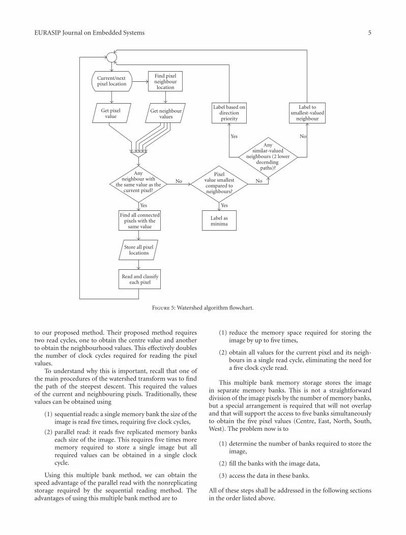
The final step once all the pixels have been labelledwith the direction of steepest descent is to assign themlabels that correspond to the label of their respectiveminimum/minima. This is done by scanning each pixel andto follow the path indicated by each pixel to the next pixel.This is performed repeatedly until a minimum/minima isreached. All the pixel in the path are then assigned to the labelof that minimum/minima. An example of all the algorithmsteps is shown in Figure 4. The operational flowchart of thewatershed algorithm is shown in Figure 5.

3. Graph-BasedMemory Implementation

Before going into the details of our architecture, we willdiscuss a multiple bank memory storage scheme based ongraph analysis. This is used to speed up operations by allow-ing all five pixel values required for the watershed transformto be read in a single clock cycle with the same memorystorage requirement as a single bank implementation. Asimilar method has been proposed in [14]. However, theirmethod requires twice the number of read cycles compared


Find pixelneighbourlocation

Get pixelvalue

Anyneighbour with

the same value as thecurrent pixel?

Find all connectedpixels with the

same value

Label asminima

Store all pixellocations

Read and classifyeach pixel

Pixelvalue smallestcompared toneighbours?

Anysimilar-valued

neighbours (2 lowerdecending paths)?

Get neighbourvalues

Label based ondirectionpriority

Label tosmallest-valued

neighbour

Current/next pixel location

No

Yes

Yes

No

No

Yes

Figure 5: Watershed algorithm flowchart.

to our proposed method. Their proposed method requirestwo read cycles, one to obtain the centre value and anotherto obtain the neighbourhood values. This effectively doublesthe number of clock cycles required for reading the pixelvalues.

To understand why this is important, recall that one ofthe main procedures of the watershed transform was to findthe path of the steepest descent. This required the valuesof the current and neighbouring pixels. Traditionally, thesevalues can be obtained using

(1) sequential reads: a single memory bank the size of theimage is read five times, requiring five clock cycles,

(2) parallel read: it reads five replicated memory bankseach size of the image. This requires five times morememory required to store a single image but allrequired values can be obtained in a single clockcycle.

Using this multiple bank method, we can obtain thespeed advantage of the parallel read with the nonreplicatingstorage required by the sequential reading method. Theadvantages of using this multiple bank method are to

(1) reduce the memory space required for storing theimage by up to five times,

(2) obtain all values for the current pixel and its neigh-bours in a single read cycle, eliminating the need fora five clock cycle read.

This multiple bank memory storage stores the imagein separate memory banks. This is not a straightforwarddivision of the image pixels by the number of memory banks,but a special arrangement is required that will not overlapand that will support the access to five banks simultaneouslyto obtain the five pixel values (Centre, East, North, South,West). The problem now is to

(1) determine the number of banks required to store theimage,

(2) fill the banks with the image data,

(3) access the data in these banks.

All of these steps shall be addressed in the following sectionsin the order listed above.


Two distinctive subgraphs with

4-neighbourhood connectivity

Each number represents a different bank

(a) Shows neighbourhood graph for 4-neighbour connectivity. Each pixel can be represented by a vertex (node); two distinct subgraphs arise from this and have been highlighted. All vertices within each subgraph is fully connected (via edges) to all its neighbours

Notice that each vertex is not connected to any of its four neighbours, that is, the grey dots are not connected to the blackones

(b) Combined subgraph with nonoverlapping labels.The nonoverlapping nature allows the concurrent access of the centre pixel value and its associated neighbours

Each number has been color coded and corresponds to a singlebank. The complete image is stored in eight different banks

Separate into two subgraphs

Recombine and show colouration of

different banks

2020

0202

2020

0202

1313

3131

1313

6240

1537

4062

3715

6240

1537

4062

3715

6240

1537

4062

3715

6240

1537

4062

3715

6464

4646

6464

4646

5757

7575

5757

Figure 6: N4 connectivity graph. Two sub-graphs combined to produce an 8-bank structure allowing five values to be obtained concurrently.

3.1. Determining How Many Banks Are Needed. This sectionwill describe how the number of banks needed to allowsimultaneous access is determined. This depends on (1) thenumber of neighbour connectivity and (2) the number ofvalues to be obtained in one read cycle. Here, graph theoryis used to determine the minimum number of databanksrequired to satisfy the following:

(1) any of the values that we want cannot be from thesame bank;

(2) none of the image pixels are stored twice (i.e., noredundancy).

Satisfying these criteria results in the minimum numberof banks required with no additional memory neededcompared to a standard single bank storage scheme.

Imagine every pixel in an image as a region and a vertex(node) will be added to each pixel. For 4-neighbour con-nectivity (N4), the connectivity graph is shown in Figure 6.To determine the number of banks for parallel access canbe viewed as a graph colouration problem, whereby any ofthe parallel values cannot be from the same bank. We ensurethat each of the nodes will have a neighbour of a differentcolour, or in our case number. Each of these colours (ornumbers) corresponds to a different bank. The same methodcan be applied for different connectivity schemes such as 8-neighbour connectivity.

In our implementation of 4-neighbourhood connectivityand five concurrent memory access (for five concurrentvalues), we require eight banks. In the discussion andexamples to follow, we will use these implementationcriteria.


(b) Any filling order is possible. For any filling order, the bank and address within the bank is determined by the same logic in the address bar (see Figure 8) Using a traditional raster scan pattern as an example. The order of bank_select is

(a) Using cardinal directions, CWNES are the centre, west, north, east, and south values, respectively. These correspond to the current pixel, left, top, right, and bottom neighbour values

Scan from top left to bottom right one pixel at atime

ban

k_se

lect

10

20

1

37

20

20

47

16

10

40

4

20

20

20

62

24

35

59

1

20

20

20

49

17

9

20

8

39

14

20

27

10

12

20

14

26

20

20

29

2

01

1 7 37 3 5 1 2 6 0 4 … 5

4 2 6 0 4 2 6 7 3 5

7

45

1

20

20

20

55

20

8

24

6

20

22

20

60

19

10

20

1

38

10

20

45

14

Crossbar

C W N E S

0

1

2

3

4

5

6

7

knab e

ht ni

htiw sserdd

A

0

0

Pixel location (3, 3) as used in the addressing scheme example

1

1

2

2

3

3

4

4

5

5

6

6

7

7

0 1 2 3 4 5 6 7

358910

7101210

8116

14114

59242020

45402020

39382020

26372020

20221410

20202020

27454960

29475562

20202020

20202020

10141719

2162024

Figure 7: Block diagram of graph-based memory storage andretrieval.

3.2. Filling the Banks. After determining how many banks areneeded, we will need to fill the banks. This is done by writing

the individual values one at a time into the respective banks.During the determination of the number of required banks,a pattern emerges from the connectivity graph. An exampleof this pattern is highlighted with a detached bounding boxin Figures 6 and 7.

The eight banks are filled with one value at a time.This can be done in any order. The bank number and bankaddress is calculated using some logic. The same logic isused to determine the bank and bank address during reading(See Section 3.3 for more details on this). For the ease ofexplanation, we shall adopt a raster scan type of sequence.Using this convention, the order of filling is simply the orderof the bank number as it appears from top-left to bottom-right. An example of this is shown in Figure 7.

The group of banks replicates itself every four pixels ineither direction (i.e., right and down). Hence, to determinehow many times the pattern is replicated, the image sizeis simply divided by sixteen. Alternatively, any one of itssides can be divided by four since all images are square.This is important as the addressing for filling the banks (andreading) holds true for square images whose sizes are to thepower of two (i.e. 22, 23, 24). Image sizes which are not squareare simply padded.

3.3. Accessing Data in the Banks. To access the data fromthis multiple bank scheme, we need to know (1) which bankand (2) location within that bank. The addressing schemeis a simple addressing scheme based on the pixel location.A hardware unit called the Address Processor (AP) handlesthe memory addressing. By providing the AP with the pixellocation, it will calculate the address to retrieve that pixelvalue. This address will tell us which bank and locationwithin that bank the pixel value is stored in.

To understand how the AP works, consider a pixelcoordinate which consists of a row and column value with theorigin located at the upper left corner. These two values arerepresented in their binary form and the lowest significantbits for the column and row are used to determine the bank.The number of bits required to represent the number ofbanks is dependent on the total number of banks in thismultiple bank scheme. In our case of eight banks, three bitsfrom the address are needed to determine in which bank thevalue for that particular pixel location is stored in. Thesebinary values go through some logic as shown in Figure 8 orin equation form:

B[2] = r[0]c[0]′ + c[0]r[0]′,

B[1] = r[1]′r[0]′c[1] + r[1]r[0]′c[0]′

+ r[1]′r[0]c[0]′ + r[1]r[0]c[0],

B[0] = r[0],

(1)

where B[0 → 2] represent the three bits that determine thebank number (from 0 → 7). r[0] and r[1] represent thefirst two bits of the row value in binary while c[0] and c[1]represent the first two bits of the column value in binary.


Now that we have determined which bank the value is in;the remainder of the bits is used to determine the location ofthe value within the bank. An example is given in Figure 8(a).

For an image of size y-rows and x-columns, the numberof bits required for addressing will simply be the number ofbits required to store the largest value of the row and columnin binary, that is, no o f address bits = log2(x) + log2(y).

This addressing scheme is shown in Figure 8. (Note thatthe steps described here assume an image with a minimumsize of 4× 4 and increase in powers of 2).

3.4. Sorting the Data from the Banks. After obtaining thefive values from the banks, they need to be sorted accordingto the expected neighbour location output to ensure thatvalues of a particular direction is sent to the right outputposition. This sorting is handled by another hardware unitcalled the Crossbar (CB). In addition, the CB also tags invalidvalues from invalid neighbour conditions which occur at thecorners and edges of the image. This tagging is part of theoutput multiplexer control.

The complete structure for reading from the banks isshown in Figure 9. In this figure, five pixel locations are fedinto the AP which generates five addressees, for the centreand its four neighbours. These five addresses are fed intoall eight banks. However, only the address correspondingto the correct bank is chosen by the add sel x, where x =0 → 7. The addresses fed into the banks will generate eightvalues however, only five will be chosen by the CB. Thesevalues are also sorted using the CB to ensure that the valuescorresponding to the centre pixel and a particular neighbourare output onto the correct data lines. The mux control,CB sel x, is controlled by the same logic that selects theadd sel x.

4. Arrowing Architecture

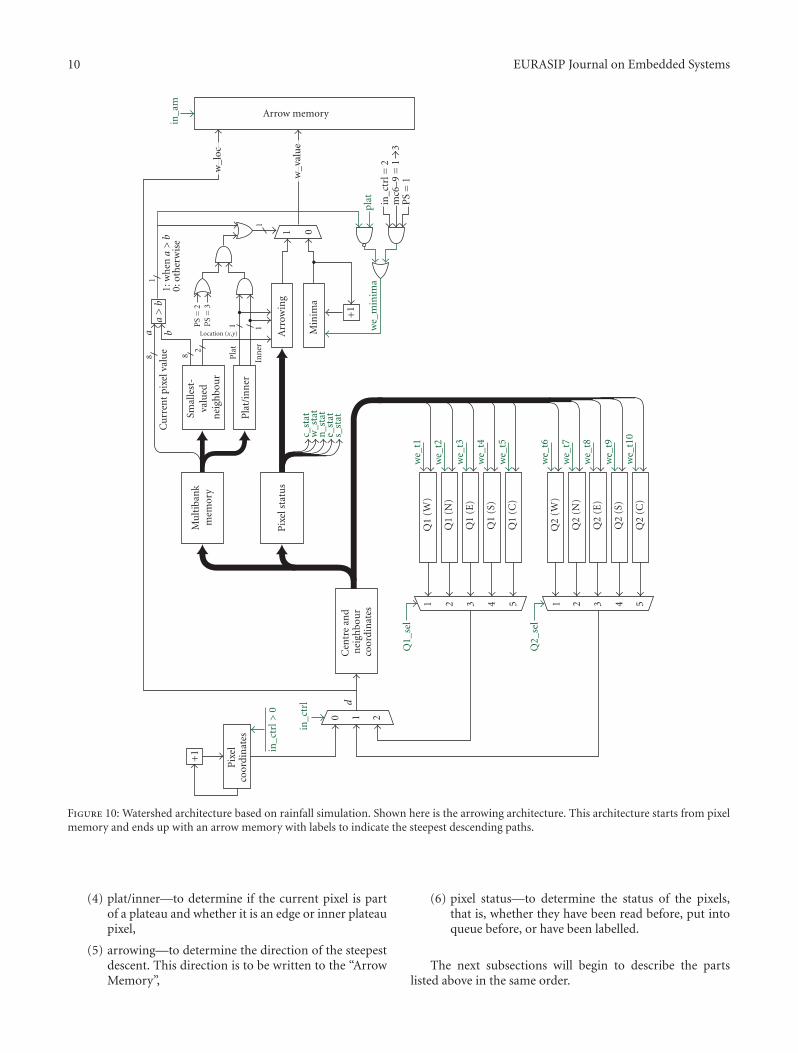
This section will provide the details on the architecture thatperforms the arrowing function of the algorithm. This partof the architecture will describe how we get from Figure 4(a)to Figure 4(c) in hardware. As mentioned in the previousdescription of the algorithm, things are simple when everypixel has a lower neighbour and gets more complicateddue to plateau conditions. Similarly, this plateau conditioncomplicates the architecture. Adding to this complexity is thefact that all neighbour values are obtained simultaneously,and instead of processing one value at a time, we have toprocess five values, the centre and its four neighbours. Thispart of the architecture that performs the arrowing is shownin Figure 10.

When a pixel location is fed into the system, it enters the“Centre and Neighbour Coordinates” block. From this, thecoordinates of the centre and its four neighbours are outputand fed into the “Multibank Memory” block to obtain all thepixel values and the pixel status (PS) from the “Pixel Status”block.

Assuming the normal state, the input pixel will have alower neighbour and no neighbours of the same value, thatis, inner = 0 and plat = 0. The pixel will just be arrowed to the

c[2]

Binary representation of value location of

within the bank

Row value (in binary) Column value (in binary)

c[0]c[1]c[2]log 2

(y)

log 2

(y)

log 2

(x)

log 2

(x)

r[0]r[1]r[2]

MSB LSB

(a) Example of location to address calculations

Determining which bank the data is in

c[0]B[2]

B[1]

B[0]

r[0]

c[1]r[0]r[1]

c[0]r[0]r[1]

c[0]r[0]r[1]

c[0]r[0]

r[0]

r[1]

(3,3)

1 1 00 1 1

c[0]c[1]c[2]r[0]

0

B[2]

1

B[1]

1

B[0]

r[2]

0 1

r[1]

0

c[2]

r[1]r[2]

Bank address logic

Address 2

of

Bank 3

This example is based on the conventionthat the first pixel location is (0,0).

The bank and location within the bankcount start from 0, that is, the first bank is 0 and the last bank is 7. Similarly, the firstaddress location is 0 and the last is 7.

Bank address logic

r[1] c[3]

In the case of 8 banks, 3bits are needed todetermine which bank thedata is located. For 4 and16 banks, 2 bits and 4 bitsare required, respectively.

These values are derivedfrom the LSB of both therow and column values.

In this 8 bank example,the bank number isrepresented by the 3 bitvalue B[0 2].

The location within thatbank is determined by theremaining 3 bits.

B[2] = r[0]c[0]′ + c[0]r[0]′

B[1] = r[1]′r[0]′c[1] + r[1]r[0]′c[0]′

+r[1]′r[0]c[0]′ + r[1]r[0]c[0]B[0] = r[0]

Figure 8: The addressing scheme for the multiple bank graph-basedmemory storage.

nearest neighbour. The Pixel Status (PS) for that pixel will bechanged from 0 → 6 (See Figure 19).

However, if the pixel has a similar valued neighbour,plat = 1 and plateau processing will start. Plateau processingstarts off by finding all the current pixel neighbours of similarvalue and writes them to Q1. Q1 is predefined to be the first


AP-W AP-NAP-C AP-E AP-S

Address processor (AP)

Crossbar (CB)

inv inv inv inv inv

CB

_sel

_0

CB

_sel

_1

CB

_sel

_2

CB

_sel

_3

CB

_sel

_4

add_

sel_

0

add_

sel_

1

add_

sel_

2

add_

sel_

3

add_

sel_

4

add_

sel_

5

add_

sel_

6

add_

sel_

7

Pixel neighbour coordinates

0 1 2 3 4

0 1 2 3 4 5 6 7 8 0 1 2 3 4 5 6 7 8 0 1 2 3 4 5 6 7 8 0 1 2 3 4 5 6 7 8 0 1 2 3 4 5 6 7 8

0 1 2 3 4

C W N E S

C W N E S

0 1 2 3 4 0 1 2 3 4 0 1 2 3 4 0 1 2 3 4 0 1 2 3 4 0 1 2 3 4

B0

(c, r) (c−1, r) (c, r−1) (c+1, r) (c, r+1)

B1 B2 B3 B4 B5 B7B6

Figure 9: 8 Bank memory architecture.

queue to be used. After writing to the queue, the PS of thepixels is changed from 0 → 1. This is to indicate whichpixel locations have been written to queue to avoid duplicateentries in the queue. At the end of this process, all the pixellocations belonging to the plateau will have been written toQ1.

To keep track of the number of elements in Q1 WNES,two sets of memory counters are used. These two sets ofcounters consist of mc1 → mc4 in one set and mc6 →mc9 in another. When writing to Q1 WNES, both sets ofcounters are incremented in parallel but when reading fromQ1 WNES to obtain the neighbouring plateau pixels, onlymc1–4 is decremented while mc6–9 remains unchanged.This means that, at the end of the Stage 1 processing,mc1–4 = 0 and mc6–9 will contain the count of the numberof pixel locations which are contained within Q1 WNES.This is needed to handle the case of a lower completeminima (i.e., a plateau with all inner pixels). When thistype of plateau is encountered, mc1–5 = 0, and Q1 WNESwill be read once again using mc6–9, this time not toobtain the same valued neighbours but to label all the pixellocations within Q1 WNES with the current value stored inthe minima register. Otherwise, mc5 > 0 and values will

be read from Q1 C and subsequently from Q2 WNES andQ1 WNES until all the locations in the plateau have beenvisited and classified. The plateau processing steps and theassociated conditions are shown in Figure 11.

There are other parts which are not shown in the maindiagram but warrants a discussion. These are

(1) memory counters—to determine the number ofunprocessed elements in a queue,

(2) priority encoder—to determine the controls forQ1 sel and Q2 sel.

The rest of the architecture consists of a few main partsshown in Figure 10 and are

(1) centre and neighbour coordinates—to obtain thecentre and neighbour locations,

(2) multibank memory—to obtain the five required pixelvalues,

(3) smallest-valued neighbour—to determine whichneighbour has the smallest value,


Smal

lest

- va

lued

n

eigh

bour

Pla

t/in

ner

Arr

owing

Min

ima

+1

+1

a >

b

Q1

(W)

Q1_

sel

Q1

(N)

Q1

(E)

Q1

(S)

we_

t6

we_

t7

we_

t8

we_

t9

we_

t10

we_

t1

we_

t2

we_

t3

we_

t4

we_

t5

in_c

trl

we_

min

ima

plat

s_st

ate_

stat

n_s

tat

w_s

tat

c_st

at

1

Q1

(C)

2 3

0 1 2

1 0

4 5

Q2

(W)

Q2_

sel

Q2

(N)

Q2

(E)

Q2

(S)

1

Q2

(C)

2 3 4 5

Location (x,y)

Curr

ent pixe

l val

ue

Pla

t

Inn

er1

1

1 1

88

2

in_a

m

w_l

oc

w_v

alu

e

a b1:

wh

en a

> b

0: o

ther

wis

e

PS

= 2

PS

= 3

in_c

trl =

2

PS

= 1

mc6

–9 =

1

3

Cen

tre

and

neigh

bour

coor

din

ates

Pix

elco

ordi

nat

es

in_c

trl >

0

d

Arrow memory

Mu

ltib

ank

mem

ory

Pix

el s

tatu

s

Figure 10: Watershed architecture based on rainfall simulation. Shown here is the arrowing architecture. This architecture starts from pixelmemory and ends up with an arrow memory with labels to indicate the steepest descending paths.

(4) plat/inner—to determine if the current pixel is partof a plateau and whether it is an edge or inner plateaupixel,

(5) arrowing—to determine the direction of the steepestdescent. This direction is to be written to the “ArrowMemory”,

(6) pixel status—to determine the status of the pixels,that is, whether they have been read before, put intoqueue before, or have been labelled.

The next subsections will begin to describe the partslisted above in the same order.


Read from Q2_WNES, label pixels and write

similar valued neighbours to Q1_WNES

Read all similar valued neighbouring pixels

Read from Q1_WNES, label pixels and write

similar valued neighbours to Q2_WNES

Read from Q1_C, label pixels and write similar valued neighbours to

Q2_WNES

Read all from Q1_WNES using mc6–9 and label

with value from minima register

Q1_W

Q1_N

Q1_E

Q1_S

Q1_C

mc1 + mc6

mc2 + mc7

mc3 + mc8

mc4 + mc9

mc5

Plateau processing completed

Start plateau processing

if mc6–9 > 0

if mc6–9 > 0

if mc6–9 = 0if mc1–4 = 0

if mc1–4 > 0

if mc5 = 0 if mc5 > 0

Stag

e 1

Stag

e 2

Stag

e: in

ner

arr

owing

Notes:1. In stage 1 of the processing, mc6–9 is used as a secondary

counter for Q1_WNES and incremented as mc1–4increments but does not decrement when mc1-4 is decremented.In stage 2, if mc5 = 0 (i.e., complete lower minima), mc6–9 is used as the counter to track the number of elements in Q1_WNES. In this state, mc6-9 is decremented when Q1_WNES is read from. However, if mc5 > 0, mc6–9 is reset and resumes the role of memory counter for Q2_WNES.

2. Q1_C is only ever used once and that is during stage 2 of theprocessing.

Figure 11: Stages of Plateau Processing and their various condi-tions.

4.1. Memory Counter. The architecture is a tristate systemwhose state is determined by the condition of whether thequeues, Q1 and Q2, are empty or otherwise. This is shownin Figure 12. These states in turn determine the control ofthe main multiplexer, in ctrl, which is the control of the datainput into the system.

0

2 1

in_ctrl values = state numbers

E1� × E2

E1� × E2

E1 × E2�

E1 × E2

E1 × E2�

E1 × E2�

E1 × E2

E1� × E2

E1� × E2�E1� × E2�

E1 = 1 when Q1 is empty E2 = 1 when Q2 is empty

E1 × E2

Figure 12: State diagram of the architecture-ARROWING.

Memory counter 1

Memory counter 2

Memory counter 9

Memory counter 10

mc1

10

Q1_sel = 1we_t1

Q1_sel = 2we_t2

Q2_sel = 4we_t9

Q2_sel = 5we_t10

+1

mc2

10

+1

mc9

1

...

0

+1

mc10

10

+1

−1

−1

−1

−1

Figure 13: Memory counter for Queue C, W, N, E, and S. Thememory counter is used to determine the number of elements inthe various queues for the directions of Centre, West, North, East,and South.

To determine the initial queue states, Memory Counters(MCs) are used to keep track of how many elements arepending processing in each of the West, North, East, South,and Centre queues. There are five MCs for Q1 and anotherfive for Q2, one counter for each of the queue directions.These MCs are named mc1–5 for Q1 W, Q1 N, Q1 E, Q1 S,


Table 1: Comparison of the number of clock cycles required forreading all five required values and the memory requirements forthe three different methods.

Sequential Parallel Graph-based

Clock cycles 5 1 1

Memory Req. 1x image size 5x image size 1x image size

and Q1 C, respectively, and similarly mc6–10 for Q2 W,Q2 N, Q2 E, Q2 S, and Q2 C respectively. This is shown inFigure 13.

The MCs increase by one count each time an elementis written to the queue. Similarly, the MCs decrease by onecount every time an element is read from the queue. Thisincrement is determined by tracking the write enable we txwhere x = 1 − 10 while the decrement is determined bytracking the values of Q1 sel and Q2 sel.

A special case occurs during the stage one of plateauprocessing, whereby mc6–9 is used to count the number ofelements in Q1 W, Q1 N, Q1 E, and Q1 S, respectively. Inthis stage, mc6–9 is incremented when the queues are writtento but are only decremented when Q1 WNES is read again inthe stage two for complete lower minima labelling.

The MC primarily consists of a register and a multiplexerwhich selects between a (+1) increment or a (−1) decrementof the current register value. Selecting between these twovalues and writing these new values to the register effectivelycount up and down. The update of the MC register value iscontrolled by a write enable, which is an output of a 2-inputXOR. This XOR gate ensures that the MC register is updatedwhen only one of its inputs is active.

4.2. The Priority Encoder. The priority encoder is used todetermine the output of Q1 sel and Q2 sel by comparingthe outputs of the MC to zero. It selects the output from thequeues in the order it is stored, that is, from queue Qx Wto Qx C, x = 1 or 2. Together with the state of in ctrl, Q1 seland Q2 sel will determine the data input into the system. Thelogic to determine the control bits for Q1 sel and Q2 sel isshown in Figure 14.

4.3. Centre and Neighbour Coordinate. The centre andneighbourhood block is used to determine the coordinatesof the pixel’s neighbours and to pass through the centrecoordinate. These coordinates are used to address the variousqueues and multibank memory. It performs an additionand subtraction by one unit on both the row and columncoordinates. This is rearranged and grouped into theirrespective outputs. The outputs from the block are five pixellocations, corresponding to the centre pixel location and thefour neighbours, West (W), North (N), East (E), and South(S). This is shown in Figure 15.

4.4. The Smallest-Valued Neighbour Block. This block is todetermine the smallest-valued neighbour (SVN) and itsposition in relation to the current pixel. This is used todetermine if the current pixel has a lower minima and to findthe steepest descending path to that minima (arrowing).

mc1=

=

=

=

0

mc20

mc30

mc40

=mc5

0

a

b

c

d

e

Pri

orit

y en

coder Q1_sel[0]

Q1_sel[1]

Q1_sel[2]

mc6=

=

=

=

0

mc70

mc80

mc90

=mc100

f

g

h

i

j

Pri

orit

y en

coder Q2_sel[0]

Q2_sel[1]

Q2_sel[2]

(a)

Qx_sel

a/f

a/f

Q1_sel[0]/Q2_sel[0]

Q1_sel[1]/Q2_sel[1]

Q1_sel[2]/Q2_sel[2]

b/g

b/g

c/h

c/h

d/i

d/i

e/j

e/j [2] [1] [0]

000111111

Disable100xxxx0

2010xxx013110xx0114001x0111510101111

Q1_sel[0] = a� + abc� + abcde�Q1_sel[1] = ab� + abc�Q1_sel[2] = abcd� + abcde�

Q2_sel[0] = f � + fgh� + fghij�Q2_sel[1] = fg� + fgh�Q2_sel[2] = fghi� + fghij�

(b)

Figure 14: The priority encoder. (a) shows the controls for Q1 seland Q2 sel using the priority encoders. The output of memorycounters determines the multiplexer control of Q1 sel and Q2 sel.(b) shows the logic of the priority encoders used. There is a special“disable” condition for the multiplexers of Q1 and Q2. This is usedso that the Q1 sel and Q2 sel can have an initial condition and willnot interfere with the memory counters.


Row

Column

C

W

N

E

S

+1

+1

r + 1

r − 1

c + 1

c − 1−1

−1

Figure 15: Inside the Pixel Neighbour Coordinate.

To determine the smallest value pixel, the values of theneighbours are compared two at a time, and the result ofthe comparator is used to select the smaller value of thetwo. The last two values are compared once again and thevalue of the smallest value neighbour will be obtained. As forthe direction of the SVN, the outputs from the 3 stages ofcomparison are used and compared to a truth table. This isshown in Figure 16. This output is passed to the arrowingblock to determine the direction of the steepest descent(when there is a lower neighbour).

4.5. The Plateau-Inner Block. This block is to determinewhether the current pixel is part of a plateau and which typeof plateau pixel it is. The current pixel type will determinewhat is done to the pixel and its neighbours, that is, whetherthey are put back into a queue or otherwise. Essentially,together with the Pixel Status, it helps to determine if a pixelor one of its neighbours should be put back into the queuesfor further processing. When the system is in State 0 (i.e.,processing pixel locations from the PC), the block determinesif the current pixel is part of a plateau. The value of thecurrent pixel is compared to all its neighbours. If any oneof the neighbours has a similar value to the current pixel, it ispart of a plateau and plat = 1. The respective similar valuedneighbours are put into the different queue locations basedon sv W, sv N, sv E, and sv S and the value of pixel status.The logic for this is shown in Figure 17(a).

In any other state, this block is used to determine if thecurrent pixel is an inner (i.e., equal to or smaller than itsneighbours). If the current pixel is an inner, inner = 1. Thisis shown in Figure 17(b). Whether the pixel is an inner ornot will determine the arrowing part of the system. If it is aninner, it will point to the nearest edge.

4.6. The Arrowing Block. This block is to determine thesteepest descending path label for the “Arrow Memory.” Thesteepest path is calculated based on whether the pixel is aninner or otherwise. When processing non-inner pixels thearrowing block generates a direction output based on thelocation of the lowest neighbour obtained from the block“Smallest Valued Neighbour.” If the pixel is an inner, thearrow will simply point to the nearest edge. When there ismore than one possible path to the nearest edge, a priority

<

<

<

WvalueNvalue

EvalueSvalue

01

0

a

b

c

1

01

Value of smallest-valuedneighbour

(a)

x = cy = ac� + bc

xc

yb

a

a b c x y Direction

0 x 0 0 0 W1 x 0 0 1 Nx 0 1 1 0 Ex 1 1 1 1 S

(b)

Figure 16: Inside the Smallest Value Neighbour (SVN) block.(a) The smallest-valued neighbour is determined and selectedusing a set of comparators and multiplexers. (b) The location ofthe smallest-valued neighbour is determined by the selections ofeach multiplexer. This location information used to determine thesteepest descending path and is fed into the arrowing block.

sv_W = 1, when C = Wvalue

sv_N = 1, when C = Nvalue

sv_E = 1, when C = Evalue

sv_S = 1, when C = Svalue

C

C

C

C

Plat

sv_E

sv_S

sv_N

sv_WWvalue

Nvalue

Evalue

Svalue

=

=

=

=

(a)

lv_E

lv_S

lv_N

lv_WC

C

C

C

Inner

Wvalue

Nvalue

Evalue

Svalue

lv_W = 1, when C ≤ Wvalue

lv_N = 1, when C ≤ Nvalue

lv_E = 1, when C ≤ Evalue

lv_S = 1, when C ≤ Svalue

≤

≤

≤

≤

(b)

Figure 17: Inside the Plateau-Inner Block.


encoder in the block is used to select the predefined directionof the highest priority. This is shown in Figure 18 when thesystem is in State = 0, and in any other state where the pixel isnot an inner, this arrowing block uses the information fromthe SVN block and passes it through directly to its own mainmultiplexer, selecting the appropriate value to be written into“Arrow Memory.”

If the current pixel is found to be an inner, the arrowingdirection is towards the highest priority neighbour withthe same value which has been previously labelled. This ispossible because we are labelling the plateau pixels fromthe edge pixels going in, one pixel at a time, ensuring thatthe inners will always point in the direction of the shortestgeodesic distance.

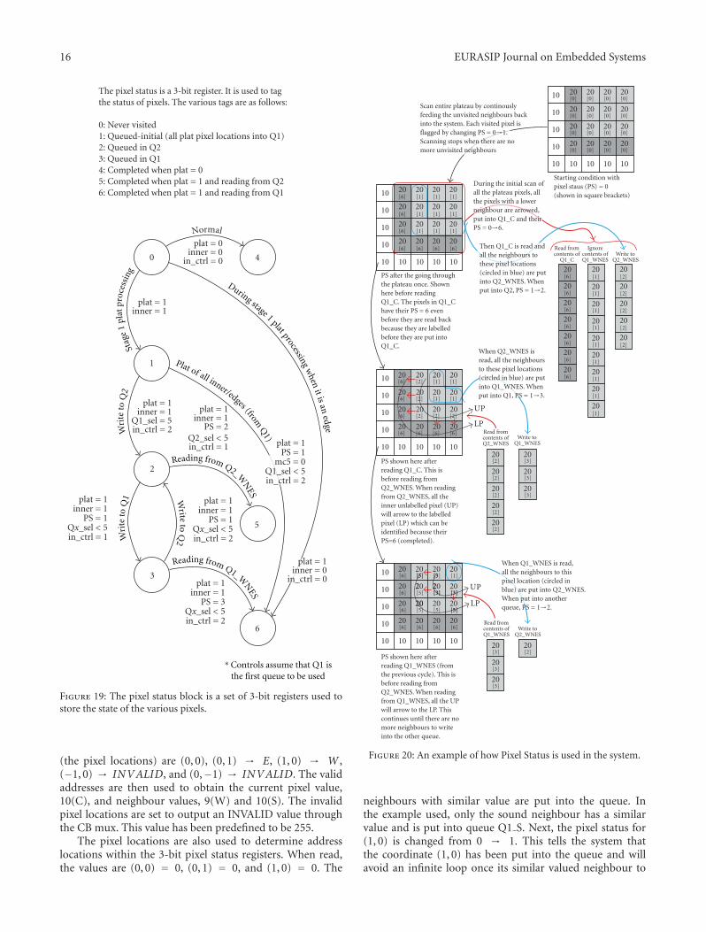
4.7. Pixel Status. One of the most important parts of thissystem is the pixel status (PS) registers. Since six statesare used to flag the pixel, this register requires a 3-bitrepresentation for each pixel location of the image. Thusthe PS registers have as many registers as there are pixelsin the input image. In the system, values from the PS helpdetermine what processes a particular pixel location has gonethrough and whether it has been successfully labelled intothe “Arrow Memory.” The six states and their transitions areshown in Figure 19. The six states are as follows:

(i) 0 : unvisited—nothing has been done to the pixel,

(ii) 1 : queued : initial,

(iii) 2 : queued in Q2,

(iv) 3 : queued in Q1,

(v) 4 : completed when plat = 0,

(vi) 5 : completed when plat = 1 and reading from Q2,

(vii) 6 : completed when plat = 1 and reading from Q1.

To ease understanding of how the plateau conditionsare handled and how the PS is used, we shall introducethe concept of the “Unlabelled pixel (UP)” and “Labelledpixel (LP).” The UP is defined as the “outermost pixel whichhas yet to be labelled.” Using this definition, the arrowingprocedure for the plateau pixels are

(1) arrow to lower-valued neighbour (applicable only ifinner = 0)

(2) arrow to neighbour with PS = 5 according topredefined arrowing priority.

With reference to Figure 20, the PS is used to determinewhich neighbours to the UPs have not been put into the otherqueue, UPs of the same label and LPs.

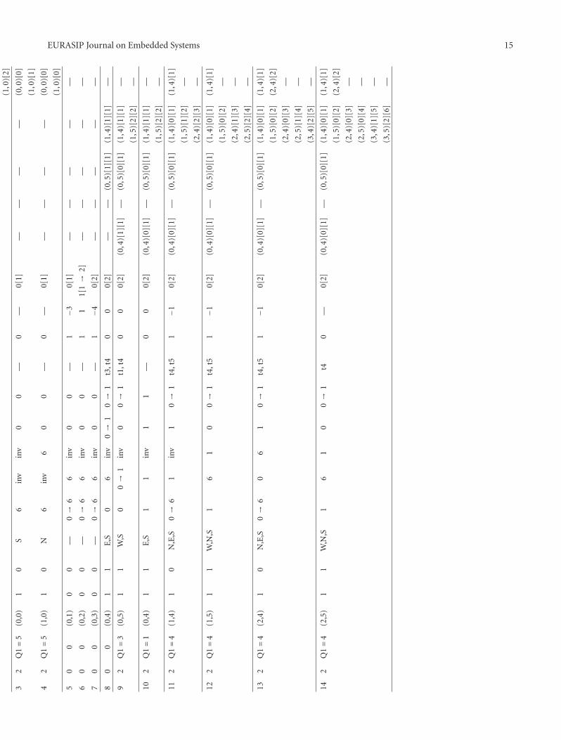
5. Example for the Arrowing Architecture

This example will illustrate the states and various controlsof the watershed architecture for an 8 × 8 sample data. It isthe same sample data shown in Figures 6 and 7. A table withthe various controls, status, and queues for the first 14 clockcycles is shown in Table 2.

0123

01

Direction of steepest

descent

22

x and y from smallest value

neighbour block

01

01

01

01

PS_W

sv_W

5

PS_x are the values read from the pixel status registers from the center (C) and respective neighbours (W, N, E, S).

sv_x are the “same value” conditions obtained from the plat/inner block wherex are the directions W, N, E, S.

6=

PS_C2

PS_C3

ne_W

ne_N

ne_E

ne_S

dir[0]

dir[1]

Pri

orit

y en

coder

PS_N

sv_N

56

=

PS_E

sv_E

56

=

PS_S

sv_S

56

=

=

=

in_ctrl1

=

dir[0] = a�b + a�c�dir[1] = a�b�

adir[0]

dir[1]b

c

a b c d x y mux_ctrl

1 x x x 0 0 00 1 x x 0 1 10 0 1 x 1 0 20 0 0 1 1 1 3

−1−2−3−4

Figure 18: Inside arrowing block.

The initial condition for the system is as follows. TheProgram Counter (PC) starts with the first pixel andgenerates a (0, 0) output representing the first pixel in an(x, y) format.

With both the Q1 and Q2 queues being empty, that is,mc1 → mc10 = 0, the system is in State 0. This sets in ctrl =0 that controls mux1 to select the PC value (in this case (0, 0).This value is incremented on the next clock cycle.

The First Few Steps. This PC coordinate is then fed into thePixel Neighbour Coordinate block. The outputs of this block


(1,0

)[2]

32

Q1=

5(0

,0)

10

S6

inv

inv

00

—0

—0[

1]—

——

—(0

,0)[

0]

(1,0

)[1]

42

Q1=

5(1

,0)

10

N6

inv

60

0—

0—

0[1]

——

——

(0,0

)[0]

(1,0

)[0]

50

0(0

,1)

00

—0→

66

inv

00

—1

−30[

1]—

——

——

60

0(0

,2)

00

—0→

66

inv

00

—1

11[

1→

2]—

——

——

70

0(0

,3)

00

—0→

66

inv

00

—1

−40[

2]—

——

——

80

0(0

,4)

11

E,S

06

inv

0→

10→

1t3

,t4

00

0[2]

——

(0,5

)[1]

[1]

(1,4

)[1]

[1]

—

92

Q1=

3(0

,5)

11

W,S

00→

1in

v0

0→

1t1

,t4

00

0[2]

(0,4

)[1]

[1]

—(0

,5)[

0][1

](1

,4)[

1][1

]—

(1,5

)[2]

[2]

—

102

Q1=

1(0

,4)

11

E,S

11

inv

11

—0

00[

2](0

,4)[

0][1

]—

(0,5

)[0]

[1]

(1,4

)[1]

[1]

—

(1,5

)[2]

[2]

—

112

Q1=

4(1

,4)

10

N,E

,S0→

61

inv

10→

1t4

,t5

1−1

0[2]

(0,4

)[0]

[1]

—(0

,5)[

0][1

](1

,4)[

0][1

](1

,4)[

1]

(1,5

)[1]

[2]

—

(2,4

)[2]

[3]

—

122

Q1=

4(1

,5)

11

W,N

,S1

61

00→

1t4

,t5

1−1

0[2]

(0,4

)[0]

[1]

—(0

,5)[

0][1

](1

,4)[

0][1

](1

,4)[

1]

(1,5

)[0]

[2]

—

(2,4

)[1]

[3]

—

(2,5

)[2]

[4]

—

132

Q1=

4(2

,4)

10

N,E

,S0→

60

61

0→

1t4

,t5

1−1

0[2]

(0,4

)[0]

[1]

—(0

,5)[

0][1

](1

,4)[

0][1

](1

,4)[

1]

(1,5

)[0]

[2]

(2,4

)[2]

(2,4

)[0]

[3]

—

(2,5

)[1]

[4]

—

(3,4

)[2]

[5]

—

142

Q1=

4(2

,5)

11

W,N

,S1

61

00→

1t4

0—

0[2]

(0,4

)[0]

[1]

—(0

,5)[

0][1

](1

,4)[

0][1

](1

,4)[

1]

(1,5

)[0]

[2]

(2,4

)[2]

(2,4

)[0]

[3]

—

(2,5

)[0]

[4]

—

(3,4

)[1]

[5]

—

(3,5

)[2]

[6]

—


Wri

te to

Q2

Wri

te to

Q1 W

rite to Q2

Reading from Q2_WN

ES

Reading from Q1_WN

ES

Normal

During stage 1 plat processing when it is an edge

Plat of all inner/edges (from Q

1)

Stag

e 1 pl

at pro

cess

ing

The pixel status is a 3-bit register. It is used to tag the status of pixels. The various tags are as follows:

0: Never visited1: Queued-initial (all plat pixel locations into Q1)2: Queued in Q23: Queued in Q14: Completed when plat = 05: Completed when plat = 1 and reading from Q26: Completed when plat = 1 and reading from Q1

0 4

1

2

5

3

plat = 1inner = 1

Q1_sel = 5in_ctrl = 2

plat = 1inner = 1

plat = 1inner = 1

PS = 3Qx_sel < 5in_ctrl = 2

plat = 1inner = 1

PS = 2Q2_sel < 5in_ctrl = 1

plat = 1inner = 1


plat = 1inner = 1


plat = 0inner = 0

in_ctrl = 0

plat = 1PS = 1

mc5 = 0Q1_sel < 5in_ctrl = 2

plat = 1inner = 0

in_ctrl = 0

6

∗ Controls assume that Q1 isthe first queue to be used

Figure 19: The pixel status block is a set of 3-bit registers used tostore the state of the various pixels.

(the pixel locations) are (0, 0), (0, 1) → E, (1, 0) → W ,(−1, 0) → INVALID, and (0,−1) → INVALID. The validaddresses are then used to obtain the current pixel value,10(C), and neighbour values, 9(W) and 10(S). The invalidpixel locations are set to output an INVALID value throughthe CB mux. This value has been predefined to be 255.

The pixel locations are also used to determine addresslocations within the 3-bit pixel status registers. When read,the values are (0, 0) = 0, (0, 1) = 0, and (1, 0) = 0. The

20[6]

20[1]

20[1]

20[1]

20[1]

20[1]

20[1]

20[1]

20[1]

20[1]

20[6]

20[6]

20[6]

20[6]

20[6]

20[6]

10

10

10

10

10 10 10 10 10

20[6]

20[2]

20[1]

20[1]

[2]20[1]

20[1]

20[2]

20 20

20[6]

20[6]

20[6]

20 20 20

10

10

10

10

10 10 10 10 10

20[6]

20[5]

20[3]

20[1]

20[5]

20[3]

20[3]

20[5]

20[5]

20[5]

20[6]

20[6]

20[6]

20[6]

20[6]

20[6]

10

10

10

10

10 10 10 10 10

20[6]

20[6]

20[6]

20[6]

20[6]

20[6]

20[6]

20[3]

20[3]

20[3]

20[2]

20[2]

20[2]

20[2]

20[2]

20[2]

20[1]

20[1]

20[1]

20[1]

20[1]

20[1]

20[1]

20[1]

20[1]

20[2]

20[2]

20[2]

20[2]

20[2]

20[3]

20[3]

20[3]

20[0]

20[0]

20[0]

20[0]

20[0]

20[0]

20[0]

20[0]

20[0]

20[0]

20[0]

20[0]

20[0]

20[0]

20[0]

20[0]

10

10

10

10

10 10 10 10 10

UP

LP

[6] [6] [6]

20

[2] [2]

[5]

2

20[5]

[3

2[3] [3]

LP

UP

Scan entire plateau by continouslyfeeding the unvisited neighbours backinto the system. Each visited pixel isflagged by changing PS = 0→1.Scanning stops when there are nomore unvisited neighbours

During the initial scan ofall the plateau pixels, allthe pixels with a lowerneighbour are arrowed,put into Q1_C and theirPS = 0→6.

Then Q1_C is read andall the neighbours tothese pixel locations(circled in blue) are putinto Q2_WNES. Whenput into Q2, PS = 1→2.

PS after the going throughthe plateau once. Shownhere before readingQ1_C. The pixels in Q1_Chave their PS = 6 evenbefore they are read backbecause they are labelledbefore they are put intoQ1_C.

PS shown here afterreading Q1_C. This isbefore reading fromQ2_WNES. When readingfrom Q2_WNES, all theinner unlabelled pixel (UP)will arrow to the labelledpixel (LP) which can beidentified because theirPS=6 (completed).

PS shown here afterreading Q1_WNES (fromthe previous cycle). This isbefore reading fromQ2_WNES. When readingfrom Q1_WNES, all the UPwill arrow to the LP. Thiscontinues until there are nomore neighbours to writeinto the other queue.

When Q1_WNES is read,all the neighbours to thispixel location (circled inblue) are put into Q2_WNES.When put into anotherqueue, PS = 1→2.

When Q2_WNES isread, all the neighboursto these pixel locations(circled in blue) are putinto Q1_WNES. Whenput into Q1, PS = 1→3.

Starting condition withpixel staus (PS) = 0(shown in square brackets)

Read fromcontents of

Q1_C

Read fromcontents ofQ2_WNES

Ignorecontents ofQ1_WNES

Write toQ2_WNES

Write toQ1_WNES

Read fromcontents ofQ1_WNES

Write toQ2_WNES

Figure 20: An example of how Pixel Status is used in the system.

neighbours with similar value are put into the queue. Inthe example used, only the sound neighbour has a similarvalue and is put into queue Q1 S. Next, the pixel status for(1, 0) is changed from 0 → 1. This tells the system thatthe coordinate (1, 0) has been put into the queue and willavoid an infinite loop once its similar valued neighbour to


Pixel coordinate

+1

Reverse arrowing

Arrrow memory Buffer

Path queue

Lab

el m

emor

y

Pixel statuswe_pc

1

0

All memories have a built-in “pixel coordinate to memory

address decoder”

mux

w_loc: memory write location r_loc: memory read location

w_info: memory write data

we_pq: write enable path queue memory we_label: write enable label memory &

pixel status memorywe_pc: write enable for pixel coordinate

incrementation we_buf: write enable for buffer. Value of

CBL is locked in buffer and read from it until “read Q” is completed.

mux: data input selection

we_label

we_label

+1

−1

PQ_counter

we_pq

10

Path queue counter 1

Memory counter for path queue

a

b

if a > 0, b = 1

w_loc

w_loc

w_loc

r_loc

r_loc

we_pq

we_buf

w_value

0>

Figure 21: The watershed architecture: Labelling.

the north (0, 0) finds (1, 0) again. The current pixel location(0, 0) on the other hand is written to Q1 C because itis a plateau pixel but not an inner (i.e., an edge) and isimmediately arrowed. The status for this location (0, 0) ischanged from 0 → 6. Q1 S will contain the pixel location(1, 0). This is read back into the system and mc4 = 1 → 0indicating Q1 S to be empty. The pixel location (1, 0) isarrowed and written into Q1 C. With mc1 − 4 = 0 andmc5 > 0, the pixel locations (0, 0) and (1, 0) is reread into thesystem but nothing is performed because both their PSsequal6 (i.e., completed).

6. Labelling Architecture

This second part of the architecture will describe how weget from Figure 4(c) to Figure 4(d) in hardware. Comparedto the arrowing architecture, the labelling architecture isconsiderably simpler as there are no parallel memory reads.In fact, everything runs in a fairly sequential manner. Part 2of the architecture is shown in Figure 21.

The architecture for Part 2 is very similar to Part 1. Bothare tristate systems whose state depends on the condition

Normal

Fill queue Read queue

PQ

_cou

nter

> 0 PQ

_counter = 0

b = 1 (catchment basin found)

mux = 1

mux = 0

Figure 22: The 3 states in Architecture:Labelling.

of the queues and uses pixel state memory and queuesfor storing pixel locations. The difference is that Part 2architecture only requires a single queue and a single bit pixelstatus register. The three states for the system are shown inFigure 22.


Values are initially read in from the pixel coordinateregister. Whether this pixel location had been processedbefore is checked against the pixel status (PS) register. If it hasnot been processed before (i.e., was never part of any steepestdescending path), it will be written to the Path Queue (PQ).Once PQ is not empty, the system will process the nextpixel along the current steepest descending path. This iscalculated by the “Reverse Arrowing Block” (RAB) using thecurrent pixel location and direction information obtainedfrom the “Arrow Memory.” This process continues until anon-negative value is read from “Arrow Memory.” This non-negative value is called the “Catchment Basin Label” (CBL).Reading a CBL tells that the system a minimum has beenreached and all the pixel locations stored in PQ will belabelled with that CBL and written to “Label Memory.” Atthe same time, the pixel status for the corresponding pixellocations will be updated accordingly from 0 → 1. Now thatPQ is empty; the next value will be obtained from the pixelcoordinate register.

6.1. The Reverse Arrowing Block. This block calculates theneighbour pixel location in the path of the steepest descentgiven the current location and arrowing label. In otherwords, it simply finds the location of the pixel pointed to bythe current pixel.

The output of this block is a simple case of selectingthe appropriate neighbouring coordinate. Firstly the neigh-bouring coordinates are calculated and are fed into a 4-inputmultiplexer. Invalid neighbours are automatically ignored asthey will never be selected. The values in “Arrow Memory”only point to valid pixels. Hence, no special consideration isrequired to handle these cases.

The bulk of the block’s complexity lies in the control ofthe multiplexer. The control is determined by translating thevalue from the “Arrow Memory” into proper control logic.Using a bank of four comparators, the value from “ArrowMemory” is determined by comparing it to four possiblevalid direction labels (i.e., −4 → −1). For each of thesevalues, only one of the comparators will produce a positiveoutcome (see truth table in Figure 23). Any other valuesoutside the valid range will simply be ignored.

The comparator output is then passed through somelogic that will produce a 2-bit output corresponding to themultiplexer control. If the value from “Arrow Memory” is−1, the control logic will be (x = 0, y = 0) correspondingto the West neighbour location. Similarly, if the value from“Arrow Memory” is −2, −3, or −4, the control logic willbe (x = 0, y = 1), (x = 1, y = 0), or (x = 1, y =1) corresponding to the North, East, or South neighbourlocations, respectively. This is shown in Figure 23.

7. Example for the Labelling Architecture

This example will pick up where the previous example hadstopped. In the previous part, the resulting output waswritten to the “Arrow Memory.” It contains the directions ofthe steepest descent (negative values from −1 → −4) andnumbered minima (positive values from 0 → total number

r + 1

r − 1

c + 1

c − 1

Row

Column

W 0

1

2

3

N

E

S

+1

+1

Lower neighbour location

am

am

am

am

=

=

=

=

am = value from arrow memory

a

b

c

d

x

x

y

y

−1

−1

−1

−2

−3

−4

a b c d x y mux_ctrl

1 0 0 0 0 0 00 1 0 0 0 1 10 0 1 0 1 0 20 0 0 1 1 1 3

x = a′b′c′d + a′b′cd′y = a′b′d′d + a′bc′d′

Figure 23: Inside the reverse arrowing block.

of minima) as seen in Figure 4(c). In this part, we will use theinformation stored in “Arrow Memory” to label each pixelwith the label of its respective minimum. Once all associatedpixels to a minimum/minima have been labelled accordingly,a catchment basin is formed.

The system starts off in the normal state and the initialconditions are as follows. PQ counter = 0, mux = 1. In thefirst clock cycle, the first pixel location (0, 0) is read from thepixel location register. Once this has been read in, the pixellocation register will increment to the next pixel location(0, 1). The PS for the first location (0, 0) is 0. This enablesthe write enable for the PQ and the first location is writtento queue. At the same time, the location (0, 0) and direction−3 obtained from “Arrow Memory” are used to find the nextcoordinate (0, 1) in the steepest descending path.

Since PQ is not empty, the system enters the “Fill Queue”state and mux = 0. The next input into the system is the valuefrom the reverse arrowing block, (0, 1), and since PS = 0,it is put into PQ. The next location processed is (0, 2). For(0, 2), PS = 0 and is also written to PQ. However, for thislocation, the value obtained from “Arrow Memory” is 1. Thisis a CBL and is buffered for the process of the next state. Oncea non-negative value from “Arrow Memory” is read (i.e.,b = 1), the system enters the next state which is the “ReadQueue” state. In this state, all the pixel locations stored inPQ is read one at a time and the memory locations in “LabelMemory” corresponding to these locations are written withthe buffered CBL. At the same time, PS is also updated from0 → 1 to reflect the changes made to “Label Memory.” It tellsthe system that the locations from PQ have been processedso that it will not be rewritten when it is encountered again.


Table 3: Results of the implemented architecture on a XilinxSpartan-3 FPGA.

64× 64 image size,

Arrowing

Slice flip flops 423 out of 26,624 (1%)

Occupied slices 2,658 out of 13,312 (19%)

Labelling

Slice flip flops 39 out of 26,624 (1%)

Occupied slices 37 out of 13,312 (1%)

With each read from PQ, PQ counter is decremented. WhenPQ is empty, PQ counter = 0 and the system will return tothe normal state.

In the next clock cycle, (0, 1) is read from the pixelcoordinate register. For (0, 1), PS = 1 and nothing getswritten to PQ and PQ counter remains at 0. The same goesfor (0, 2). When the coordinate (0, 3) is read from the pixelcoordinate register, the whole processes of filling up PQ andreading from PQ and writing to “Label Memory” start again.

8. Synthesis and Implementation

The rainfall watershed architecture was designed in Handel-C and implemented on a Celoxica RC10 board containinga Xilinx Spartan-3 FGPA. Place and route were completedto obtain a bitstream which was downloaded into the FPGAfor testing. The watershed transform was computed by theFPGA architecture, and the arrowing and labelling resultswere verified to have the same values as software simulationsin Matlab. The Spartan-3 FPGA contains a total of 13312slices. The implementation results of the architecture aregiven in Table 3 for an image size of 64 × 64 pixels. Animage resolution of 64 × 64 required 2658 and 37 slices forthe arrowing and labelling architecture, respectively. Thisrepresents about 20% of the chip area on the Spartan-3FPGA.

9. Summary

This paper proposed a fast method of implementing thewatershed transform based on rainfall simulation with amultiple bank memory addressing scheme to allow parallelaccess to the centre and neighbourhood pixel values. In asingle read cycle, the architecture is able to obtain all fivevalues of the centre and four neighbours for a 4-connectivitywatershed transform. This multiple bank memory has thesame footprint as a single bank design. The datapathand control architecture for the arrowing and labellinghardware have been described in detail, and an implementedarchitecture on a Xilinx Spartan-3 FGPA has been reported.The work can be extended to implement an 8-connectivitywatershed transform by increasing the number of memorybanks and working out its addressing. The multiple bankmemory approach can also be applied to other watershedarchitectures such as those proposed in [10–13, 15].

References

[1] S. E. Hernandez and K. E. Barner, “Tactile imaging usingwatershed-based image segmentation,” in Proceedings of theAnnual Conference on Assistive Technologies (ASSETS ’00), pp.26–33, ACM, New York, NY, USA, 2000.

[2] M. Fussenegger, A. Opelt, A. Pjnz, and P. Auer, “Objectrecognition using segmentation for feature detection,” inProceedings of the 17th International Conference on PatternRecognition (ICPR ’04), vol. 3, pp. 41–44, IEEE ComputerSociety, Washington, DC, USA, 2004.

[3] W. Zhang, H. Deng, T. G. Dietterich, and E. N. Mortensen,“A hierarchical object recognition system based on multi-scale principal curvature regions,” in Proceedings of the 18thInternational Conference on Pattern Recognition (ICPR ’06),vol. 1, pp. 778–782, IEEE Computer Society, Washington, DC,USA, 2006.

[4] M. S. Schmalz, “Recent advances in object-based image com-pression,” in Proceedings of the Data Compression Conference(DCC ’05), p. 478, March 2005.

[5] S. Han and N. Vasconcelos, “Object-based regions of interestfor image compression,” in Proceedings of the Data Compres-sion Conference (DCC ’05), pp. 132–141, 2008.

[6] T. Acharya and P.-S. Tsai, JPEG2000 Standard for ImageCompression: Concepts, Algorithms and VLSl Architecturcs,John Wiley & Sons, New York, NY, USA, 2005.

[7] V. Osma-Ruiz, J. I. Godino-Llorente, N. Saaenz-Lechon, andP. Gomez-Vilda, “An improved watershed algorithm based onefficient computation of shortest paths,” Pattern Recognition,vol. 40, no. 3, pp. 1078–1090, 2007.

[8] A. Bieniek and A. Moga, “An efficient watershed algorithmbased on connected components,” Pattern Recognition, vol. 33,no. 6, pp. 907–916, 2000.

[9] H. Sun, J. Yang, and M. Ren, “A fast watershed algorithm basedon chain code and its application in image segmentation,”Pattern Recognition Letters, vol. 26, no. 9, pp. 1266–1274, 2005.

[10] M. Neuenhahn, H. Blume, and T. G. Noll, “Pareto optimaldesign of an FPGA-based real-time watershed image seg-mentation,” in Proceedings of the Conference on Program forResearch on Integrated Systems and Circuits (ProRISC ’04),2004.

[11] C. Rambabu and I. Chakrabarti, “An efficient immersion-based watershed transform method and its prototype archi-tecture,” Journal of Systems Architecture, vol. 53, no. 4, pp. 210–226, 2007.

[12] C. Rambabu, I. Chakrabarti, and A. Mahanta, “Flooding-based watershed algorithm and its prototype hardware archi-tecture,” IEE Proceedings: Vision, Image and Signal Processing,vol. 151, no. 3, pp. 224–234, 2004.

[13] C. Rambabu and I. Chakrabarti, “An efficient hillclimbing-based watershed algorithm and its prototype hardware archi-tecture,” Journal of Signal Processing Systems, vol. 52, no. 3, pp.281–295, 2008.

[14] D. Noguet and M. Ollivier, “New hardware memory manage-ment architecture for fast neighborhood access based on graphanalysis,” Journal of Electronic Imaging, vol. 11, no. 1, pp. 96–103, 2002.

[15] C. J. Kuo, S. F. Odeh, and M. C. Huang, “Image segmentationwith improved watershed algorithm and its FPGA implemen-tation,” in Proceedingsof the IEEE International Symposium onCircuits and Systems (ISCAS ’01), vol. 2, pp. 753–756, Sydney,Australia, May 2001.

Efficient Processing of a Rainfall Simulation Watershed on an FPGA-Based Architecture with Fast...

Documents

Transcript of Efficient Processing of a Rainfall Simulation Watershed on an FPGA-Based Architecture with Fast...