EFFICIENT NEAR-FIELD COMPUTATION FOR RADIATION AND SCATTERING FROM CONDUCTING SURFACES OF ARBITRARY...
19
Progress In Electromagnetics Research, PIER 69, 267–285, 2007 EFFICIENT NEAR-FIELD COMPUTATION FOR RADIATION AND SCATTERING FROM CONDUCTING SURFACES OF ARBITRARY SHAPE K. F. A. Hussein Microwave Engineering Department Electronics Research Institute Dokki, Cairo, Egypt Abstract—A new algorithm for numerical evaluation of the fields in the near zone of conducting scatterers or antennas of arbitrary shape is developed in the present work. This algorithm is simple, fast, robust and is based on a preceding calculation of the current flowing on the conducting surface using the electric filed integral equation (EFIE) technique that employs the Rao-Wilton-Glisson (RWG) basis functions. To examine the validity of the near field computational algorithm developed in the present work, it is applied to calculate the near field due to plane wave incidence on a variety of conducting scatterers. The solution obtained for the fields in the near zone is found to satisfy the boundary conditions on both planar and curved scatterer surfaces and the edge condition for structures possessing edges or corners. The solutions obtained using the new algorithm are compared with those obtained using some commercial packages that employ the finite-difference-time-domain (FDTD). The algorithm defined in the present work gives results which are more accurate in describing the fields near the edges than the results obtained using the FDTD. 1. INTRODUCTION The integral equation technique is one of the most widely used electromagnetic techniques up till now [1–5]. However, most of the literatures concerned with this technique give attention to the evaluation of the current, input impedance and far field rather than the evaluation of the near field. The present paper concentrates on developing an algorithm that accurately evaluates the near field as a subsequent computation after the evaluation of the current flowing on
-
Upload
independent -
Category
Documents
-
view
4 -
download
0
Transcript of EFFICIENT NEAR-FIELD COMPUTATION FOR RADIATION AND SCATTERING FROM CONDUCTING SURFACES OF ARBITRARY...
Progress In Electromagnetics Research, PIER 69, 267–285, 2007
EFFICIENT NEAR-FIELD COMPUTATION FORRADIATION AND SCATTERING FROM CONDUCTINGSURFACES OF ARBITRARY SHAPE
K. F. A. Hussein
Microwave Engineering DepartmentElectronics Research InstituteDokki, Cairo, Egypt
Abstract—A new algorithm for numerical evaluation of the fieldsin the near zone of conducting scatterers or antennas of arbitraryshape is developed in the present work. This algorithm is simple, fast,robust and is based on a preceding calculation of the current flowingon the conducting surface using the electric filed integral equation(EFIE) technique that employs the Rao-Wilton-Glisson (RWG) basisfunctions. To examine the validity of the near field computationalalgorithm developed in the present work, it is applied to calculatethe near field due to plane wave incidence on a variety of conductingscatterers. The solution obtained for the fields in the near zone is foundto satisfy the boundary conditions on both planar and curved scatterersurfaces and the edge condition for structures possessing edges orcorners. The solutions obtained using the new algorithm are comparedwith those obtained using some commercial packages that employ thefinite-difference-time-domain (FDTD). The algorithm defined in thepresent work gives results which are more accurate in describing thefields near the edges than the results obtained using the FDTD.
1. INTRODUCTION
The integral equation technique is one of the most widely usedelectromagnetic techniques up till now [1–5]. However, most ofthe literatures concerned with this technique give attention to theevaluation of the current, input impedance and far field rather thanthe evaluation of the near field. The present paper concentrates ondeveloping an algorithm that accurately evaluates the near field as asubsequent computation after the evaluation of the current flowing on
268 Hussein
the surface of the radiator or scatterer using the EFIE and method ofmoments (MoM).
The most important and critical quantities to be calculatedwhen treating electromagnetic radiation and scattering problems usingcomputational techniques are the near field and current quantities. Thefar field can be entirely determined from the current in the scattereror from the near field in the vicinity of the scatterer. For realizingthe validity of the solutions obtained by a numerical technique, theboundary conditions on the scatterer surface and the edge conditionsfor open scatterers must be satisfied.
An appropriate method that can deal efficiently with theelectromagnetic problems of thin conducting surfaces is the EFIEtechnique, described by Rao, Wilton and Glisson [6]. An integralequation is formulated for the unknown current on the scatteringsurface. The integral equation is then converted to a linear system ofequations, which can be solved using well-known numerical techniques.Once the current distribution on the antenna surface is obtained, thenear field, far field and the antenna characteristics can be directlyobtained.
The method used in [6] to evaluate the surface integrals requiredto formulate the EFIE depends on the transformation of the integrandsfrom the Cartesian coordinates to the so-called normalized areacoordinates or simplex coordinates. This enables the expression ofeach integral as a double integral which is evaluated on the areaof each triangular patch. For each combination of triangular patchpairs, three independent integrals must be numerically evaluated. Theapplication of such a transformation results in a huge number of doublesurface integrals which requires a huge computer memory and longcomputational time.
A more efficient and optimized alternative to compute theintegrals computation involved in the EFIE technique when appliedto conducting surfaces is used in the present work. This techniquedepends on dividing each triangular patch into a number of sub-triangles. In this way, the surface integral over each patch isexpressed as a finite summation over the sub-triangles constitutingthis patch. Using the same triangular patches model of the scatterer,the latter technique considerably reduces the numerical effort requiredfor obtaining accurate results for the current on the scatterer.
The geometrical modeling using cubical pieces (as the cellsemployed in FDTD), is appropriate only for planar or piecewiseplanar scatterers. For smoothly curved surfaces, cubical pieces areused to build a staircase model, which causes enormous troubles inelectromagnetic computations [7]. The staircase model, even if a very
Progress In Electromagnetics Research, PIER 69, 2007 269
large number of such pieces is used, is still not able to conform theactual surface or boundary. Staircase model possesses corners andedges all over the scatterer model which is not the case for actualsmooth surfaces. This results in that some of the near field componentsmay incorrectly exhibit edge behavior at the points of the scatterersurface although the actual surface is smooth. Moreover, the boundaryconditions are not accurately satisfied when a staircase model is used.Thus, a staircase model generally results in unavoidable spurioussolutions. The analysis of errors introduced by such an approximationhas been proposed in the literature for overcoming the problem ofstaircase model. Some of them are those employing a globallycurvilinear grid [8], using contour path FDTD (CPFDTD) [9] and usinglocally conformal grid [10] for modeling curved surfaces. However,each of the above approaches has its limitations and may suffer frominstability. Moreover, much sophistication may be involved in modelingcurved surfaces and may be impractical for treating arbitrarily-shapedsurfaces. Furthermore, a severe problem may appear when thesemethods are used to treat closed surfaces; that is for closed structuresthere is no mechanism for dissipating the spuriously generated energyand, hence, stable meaningful results are not usually obtainable [10].
The most strong point of the EFIE method is its efficienttreatment of perfectly or highly conducting surfaces. Only the surfaceof the scatterer or radiator is meshed; no “air region” around theantenna or the scatterer needs to be meshed. For conducting wireantennas, the treatment is even more efficient since only a one-dimensional discretization of the wire is undertaken. Moreover, theEFIE automatically incorporates the “radiation condition” i.e., thecorrect behavior of the field far from the source (proportional to 1/rin free space). No near-to-far field transformation is required. In theEFIE, the working variable is the current density, from which manyimportant antenna parameters (impedance, gain, radiation patternetc.) may be derived, some directly and some via straightforwardnumerical integration. In conclusion, one can state the fact that theEFIE is preferred to FDTD and the other computational techniquesfor radiation and scattering problems involving perfectly or highlyconducting bodies without the existence of inhomogeneous dielectricsor penetrable materials [1]
2. FORMULATION OF THE EFIE FOR THE CURRENTON THE CONDUCTING SCATTERER
The electric field radiated due to a surface charge density σ and currentJ flowing on a conducting surface, S, can be obtained by the following
270 Hussein
expression.E(r) = −jωA(r) −∇Φ(r) (1)
where A(r) is the magnetic vector potential defined as
A(r) =µ
4π
∫S
Je−jk|r−r′|
|r − r′| dS′, (2)
and Φ(r) is the electric scalar potential defined as
Φ(r) =1
4πε
∫S
σe−jk|r−r′|
|r − r′| dS′, (3)
where r′ is a point on S and r is a point in the near or far zone of freespace. The surface charge density σ is related to the surface divergenceof the current J flowing on S through the equation of continuity,
∇s · J = −jωσ (4)
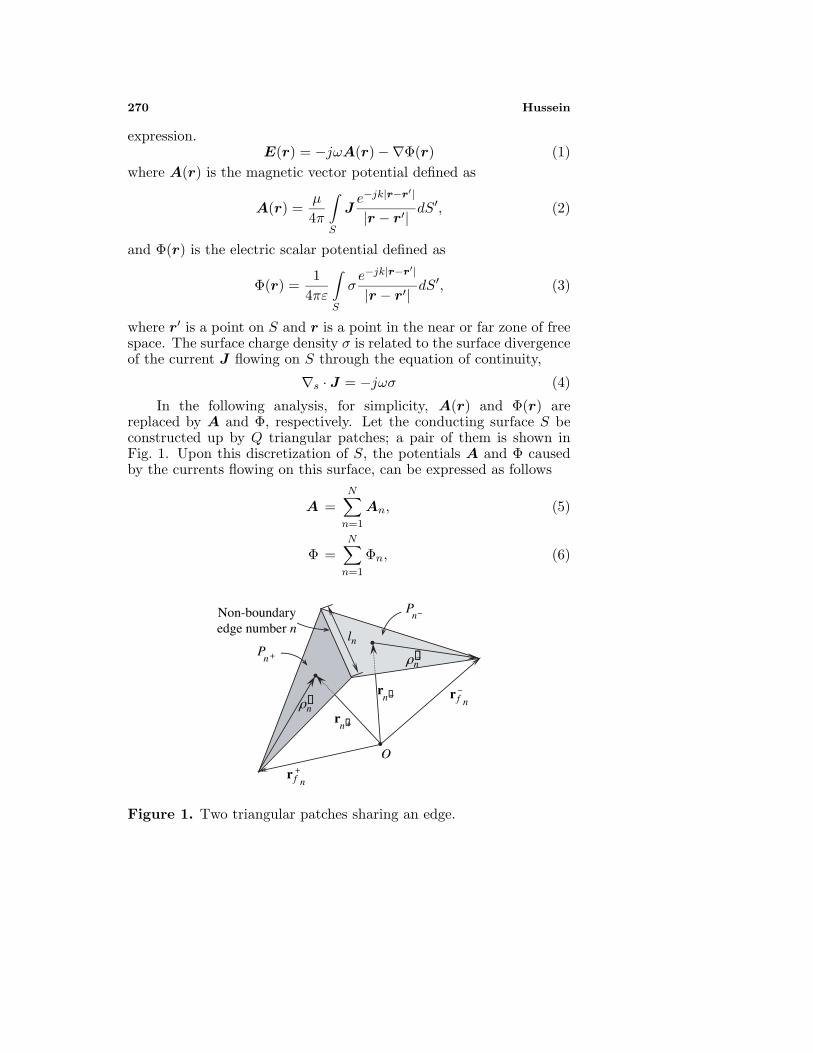
In the following analysis, for simplicity, A(r) and Φ(r) arereplaced by A and Φ, respectively. Let the conducting surface S beconstructed up by Q triangular patches; a pair of them is shown inFig. 1. Upon this discretization of S, the potentials A and Φ causedby the currents flowing on this surface, can be expressed as follows
A =N∑
n=1
An, (5)
Φ =N∑
n=1
Φn, (6)
nfr
nP
��nP
��nr
��nr
Non-boundary edge number n
nl
O
��n�ρ
��n�ρ
nfr−−
−
−
+
+
+
Figure 1. Two triangular patches sharing an edge.
Progress In Electromagnetics Research, PIER 69, 2007 271
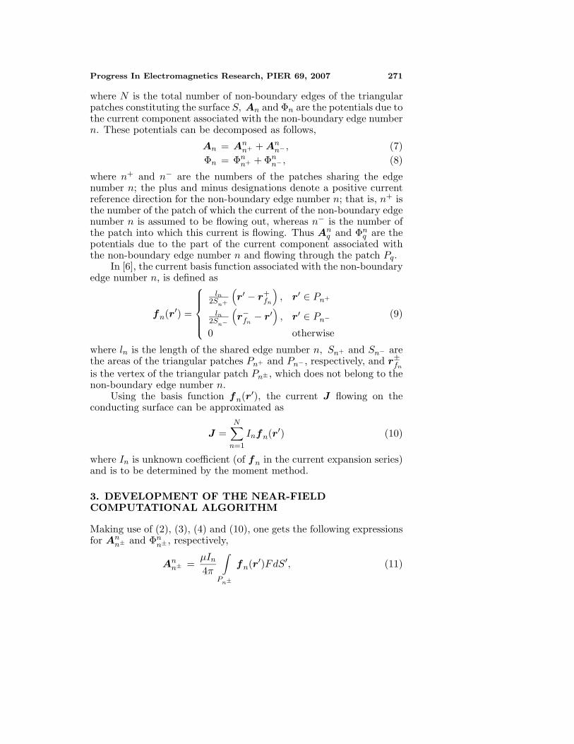
where N is the total number of non-boundary edges of the triangularpatches constituting the surface S, An and Φn are the potentials due tothe current component associated with the non-boundary edge numbern. These potentials can be decomposed as follows,
An = Ann+ + An
n− , (7)Φn = Φn
n+ + Φnn− , (8)
where n+ and n− are the numbers of the patches sharing the edgenumber n; the plus and minus designations denote a positive currentreference direction for the non-boundary edge number n; that is, n+ isthe number of the patch of which the current of the non-boundary edgenumber n is assumed to be flowing out, whereas n− is the number ofthe patch into which this current is flowing. Thus An
q and Φnq are the
potentials due to the part of the current component associated withthe non-boundary edge number n and flowing through the patch Pq.
In [6], the current basis function associated with the non-boundaryedge number n, is defined as
fn(r′) =
ln2Sn+
(r′ − r+
fn
), r′ ∈ Pn+
ln2Sn−
(r−
fn− r′
), r′ ∈ Pn−
0 otherwise
(9)
where ln is the length of the shared edge number n, Sn+ and Sn− arethe areas of the triangular patches Pn+ and Pn− , respectively, and r±
fn
is the vertex of the triangular patch Pn± , which does not belong to thenon-boundary edge number n.
Using the basis function fn(r′), the current J flowing on theconducting surface can be approximated as
J =N∑
n=1
Infn(r′) (10)
where In is unknown coefficient (of fn in the current expansion series)and is to be determined by the moment method.
3. DEVELOPMENT OF THE NEAR-FIELDCOMPUTATIONAL ALGORITHM
Making use of (2), (3), (4) and (10), one gets the following expressionsfor An
n± and Φnn± , respectively,
Ann± =
µIn
4π
∫Pn±
fn(r′)FdS′, (11)
272 Hussein
Φnn± = − µIn
4πjωε
∫Pn±
∇s · fn(r′)FdS′, (12)
where
F =e−jkR
R, (13)
R = |r − r′| (14)
Using the definition of fn, given by (9), one gets the followingexpressions for An
n± and Φnn± , respectively,
Ann± = ± µInln
8πSn±
∫Pn±
(r′ − r±
fn
)FdS′, (15)
Φnn± = ∓ Inln
4πjωεSn±
∫Pn±
FdS′, (16)
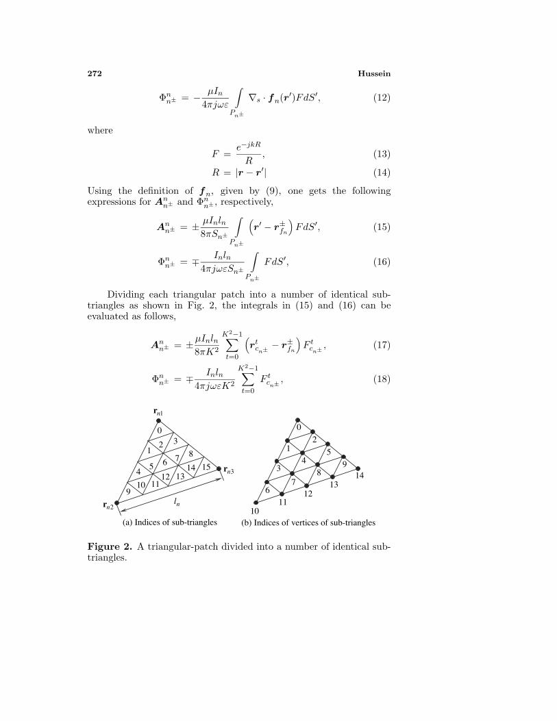
Dividing each triangular patch into a number of identical sub-triangles as shown in Fig. 2, the integrals in (15) and (16) can beevaluated as follows,
Ann± = ±µInln
8πK2
K2−1∑t=0
(rt
cn± − r±fn
)F t
cn± , (17)
Φnn± = ∓ Inln
4πjωεK2
K2−1∑t=0
F tcn± , (18)
0
1nr
nl2nr
3nr
12 3
45 6 7 8
1314 15
9 10 11
12
0
1 2
34
5
7 8
9
1314
6
1011
12
(a) Indices of sub-triangles (b) Indices of vertices of sub-triangles
Figure 2. A triangular-patch divided into a number of identical sub-triangles.
Progress In Electromagnetics Research, PIER 69, 2007 273
where K is the number of sub-triangles to which a triangular patchis divided, rt
cq is the centroid of the sub-triangle number t on thetriangular patch Pq,
F tcq =
e−jkRtcq
Rtcq
, (19)
andRt
cq =∣∣∣r − rt
cq
∣∣∣ (20)
Let us define the following series,
Sq =K2−1∑t=0
F tcq (21)
Sq =K2−1∑t=0
rtcqF
tcq (22)
Making use of (21) and (22), expressions (17) and (18) can be rewrittenas
Ann± = ±µInln
8πK2
[Sn± − Sn±r±
fn
], (23)
Φnn± = ∓ Inln
4πjωεK2Sn± (24)
The straightforward way of thinking to numerically evaluate thepotentials A and Φ suggests that for each non-boundary edge n, thequantities Sn+ ,Sn− ,Sn+ , and Sn− are first calculated using (21), (22)and then the quantities An
n+ ,Ann− ,Φn
n+ , and Φnn− are calculated using
(23), (24) and finally, the potentials A and Φ are calculated using (5)–(6). However, if this algorithm is applied a considerable time will bewasted because most of the quantities Sn+ ,Sn− ,Sn+ , and Sn− may becalculated two or three times. A more efficient scheme suggests thatthe quantities Sq, Sq are calculated for q = 1, 2, 3, . . . , Q and stored inthe computer memory. When the expressions (23), (24) are then used,for each n, the proper quantities are restored from the memory. Fora closed surface, this method would save two-third the computationaltime required if the last algorithm were used.
274 Hussein
4. CALCULATION OF THE ELECTRIC FIELD IN THENEAR ZONE
The electric field components can be numerically calculated bydiscretizing equation (1) in the space as follows.
Ex = −jωAx − ∆Φ∆x
(25)
Ey = −jωAy −∆Φ∆y
(26)
Ez = −jωAz −∆Φ∆z
(27)
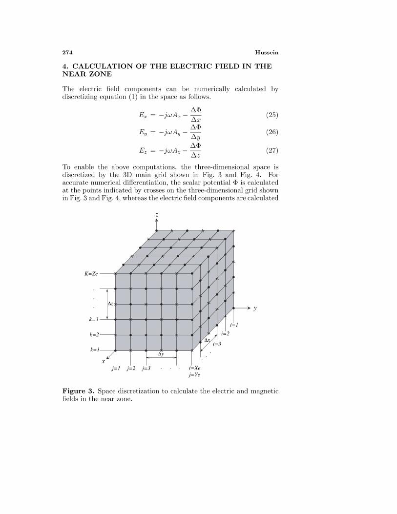
To enable the above computations, the three-dimensional space isdiscretized by the 3D main grid shown in Fig. 3 and Fig. 4. Foraccurate numerical differentiation, the scalar potential Φ is calculatedat the points indicated by crosses on the three-dimensional grid shownin Fig. 3 and Fig. 4, whereas the electric field components are calculated
∆y
�∆x
�∆z
z
y
x
i=1
i=2
i=3
i=Xe j=Ye
. .
.
j=1 j=2 j=3 . . .
k=1
k=2
k=3
K=Ze
.
.
.
Figure 3. Space discretization to calculate the electric and magneticfields in the near zone.
Progress In Electromagnetics Research, PIER 69, 2007 275
at the intermediate points which are indicated by dots. The points ofthe grid are arranged such that each point is defined by three indicesi = 1, 2, 3, . . . , Ie, j = 1, 2, 3, . . . , Je and k = 1, 2, 3, . . . ,Ke. Theselection of the points at which a potential or field quantity is calculatedcan be described as follows. The scalar potential Φ is calculated atthe points whose indices summation i + j + k is even whereas thecomponents of the vector magnetic potential are calculated at theintermediate points, i.e. the points whose indices summation is odd.In this way, the electric field components can be calculated as follows.
Ex
∣∣∣i,j,k
= −jωAx
∣∣∣i,j,k
− 1∆x
(Φ
∣∣∣i+1,j,k
− Φ∣∣∣i−1,j,k
)(28)
Ey
∣∣∣i,j,k
= −jωAy
∣∣∣i,j,k
− 1∆y
(Φ
∣∣∣i,j+1,k
− Φ∣∣∣i,j−1,k
)(29)
Ez
∣∣∣i,j,k
= −jωAz
∣∣∣i,j,k
− 1∆z
(Φ
∣∣∣i,j,k+1
− Φ∣∣∣i,j,k−1
)(30)
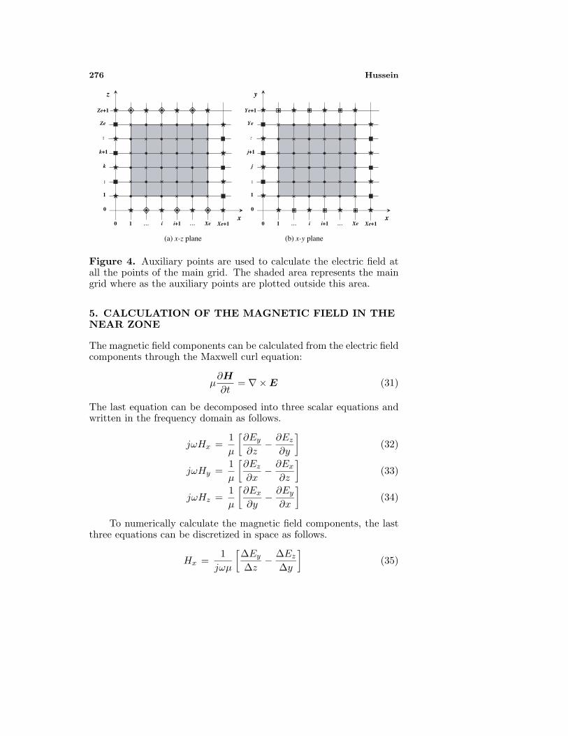
It is clear that the components of the electric field are calculated atthe same points of calculating the components of the magnetic vectorpotential. To enable the calculation of all the components of theelectric field at all the points of the main grid specified for this, thescalar potential must be calculated at other (auxiliary) points lyingjust outside the main grid. These auxiliary points are indicated aspentagonal stars as shown in Fig. 4. Table 1 indicates the potentialor field component that should be calculated at the points having thedesignations shown in Fig. 4.
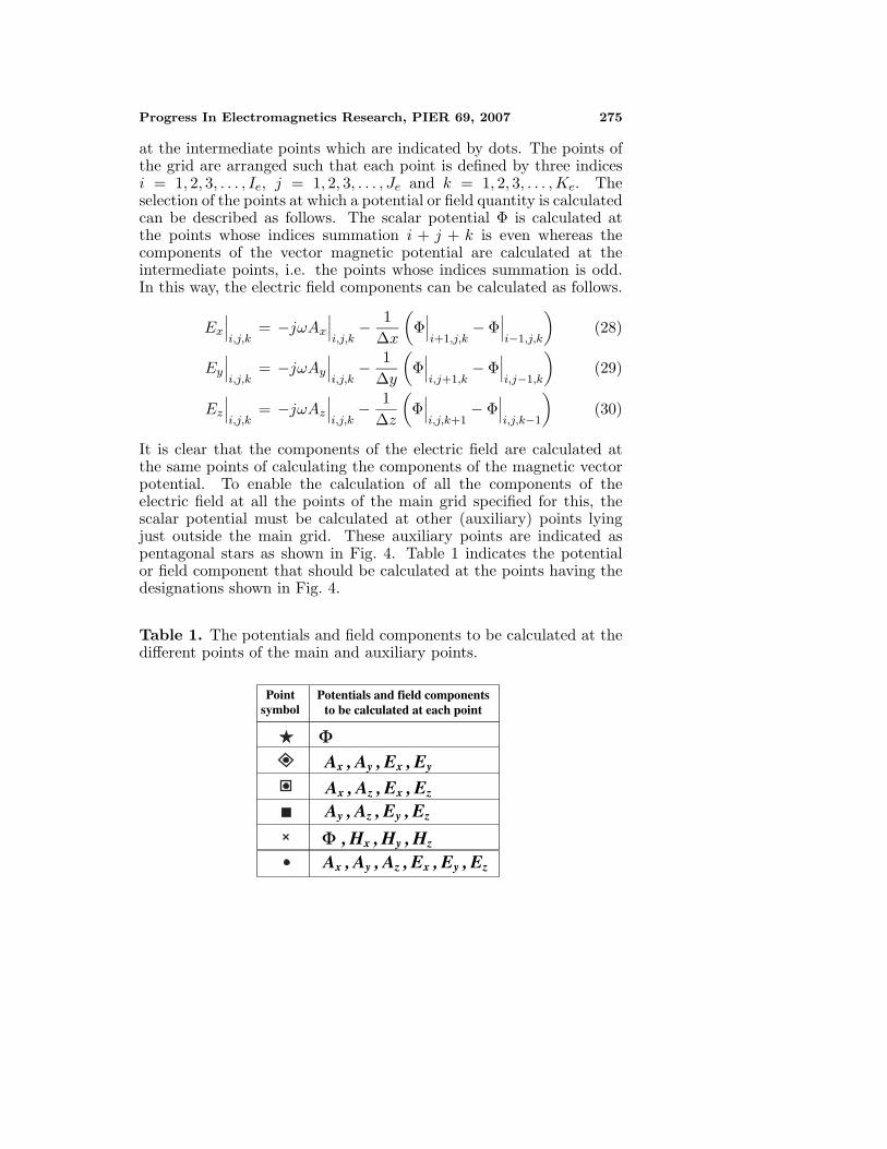
Table 1. The potentials and field components to be calculated at thedifferent points of the main and auxiliary points.
Ax , Az , Ex , Ez
Ax , Ay , Ex , Ey
Ay , Az , Ey , Ez
�Φ
�Φ , Hx , Hy , Hz Ax , Ay , Az , Ex , Ey , Ez
Point symbol
Potentials and field components to be calculated at each point
276 Hussein
x
z
i+1… i0 Xe
0
:
k+1
Ze
k
1
1
…
:
Xe+1
Ze+1
x
y
i+1… i0 Xe
0
:
j+1
Ye
j
1
1
…
:
Xe+1
Ye+1
(a) x-z plane (b) x-y plane
Figure 4. Auxiliary points are used to calculate the electric field atall the points of the main grid. The shaded area represents the maingrid where as the auxiliary points are plotted outside this area.
5. CALCULATION OF THE MAGNETIC FIELD IN THENEAR ZONE
The magnetic field components can be calculated from the electric fieldcomponents through the Maxwell curl equation:
µ∂H
∂t= ∇× E (31)
The last equation can be decomposed into three scalar equations andwritten in the frequency domain as follows.
jωHx =1µ
[∂Ey
∂z− ∂Ez
∂y
](32)
jωHy =1µ
[∂Ez
∂x− ∂Ex
∂z
](33)
jωHz =1µ
[∂Ex
∂y− ∂Ey
∂x
](34)
To numerically calculate the magnetic field components, the lastthree equations can be discretized in space as follows.
Hx =1
jωµ
[∆Ey
∆z− ∆Ez
∆y
](35)
Progress In Electromagnetics Research, PIER 69, 2007 277
Hy =1
jωµ
[∆Ez
∆x− ∆Ex
∆z
](36)
Hz =1
jωµ
[∆Ex
∆y− ∆Ey
∆x
](37)
Using the same three-dimensional grid of Fig. 3, the magneticfield components are calculated at the points whose indices summationi + j + k is even, i.e., at the same locations of calculating the scalarpotential, Φ; this can be done through the following equations.
Hx
∣∣∣i,j,k
=1
jωµ
Ey
∣∣∣i,j,k+1
− Ey
∣∣∣i,j,k−1
∆z−
Ez
∣∣∣i,j+1,k
− Ez
∣∣∣i,j−1,k
∆y
(38)
Hy
∣∣∣i,j,k
=1
jωµ
Ez
∣∣∣i+1,j,k
− Ez
∣∣∣i−1,j,k
∆x−
Ex
∣∣∣i,j,k+1
− Ex
∣∣∣i,j,k−1
∆z
(39)
Hz
∣∣∣i,j,k
=1
jωµ
Ex
∣∣∣i,j+1,k
− Ex
∣∣∣i,j−1,k
∆y−
Ey
∣∣∣i+1,j,k
− Ey
∣∣∣i−1,j,k
∆x
(40)
The electric field components are calculated at the auxiliary pointsjust outside the main grid, which are indicated as solid square blocks,squares containing dots and rhombuses containing dots as shown inFig. 4. If this is done, the three components of the magnetic field canbe calculated at all the selected points of the main grid, which areindicated by crosses in Figures 3 and 4.
In this way, the six field components Ex, Ey, Ez, Hx, Hy, Hz, areall calculated at all the selected points of the main grid.
6. RESULTS AND DISCUSSION
To examine the validity of the near field computational algorithmdeveloped in the present work, it is applied to calculate the nearfield due to a variety of conducting scatterers. As a first examination,the solution obtained for he fields in the near zone should satisfy theboundary conditions and the edge condition for open structures. Thesolutions obtained using the present algorithm are, also, comparedwith those obtained using some commercial packages that employ othercomputational techniques such as FDTD.
In the following, we present some results concerning the scatteringof plane waves from flat square plates and cylindrical structures. For a
278 Hussein
stringent test of the employed computational technique, it is intendedto include curvatures and/or edges in the scatterer body to examinethe boundary conditions and the field behavior at edges.
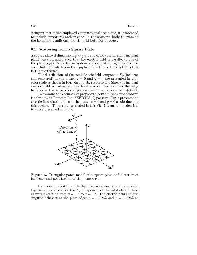
6.1. Scattering from a Square Plate
A square plate of dimensions 12λ×
12λ is subjected to a normally incident
plane wave polarized such that the electric field is parallel to one ofthe plate edges. A Cartesian system of coordinates, Fig. 5, is selectedsuch that the plate lies in the xy-plane (z = 0) and the electric field isin the x-direction.
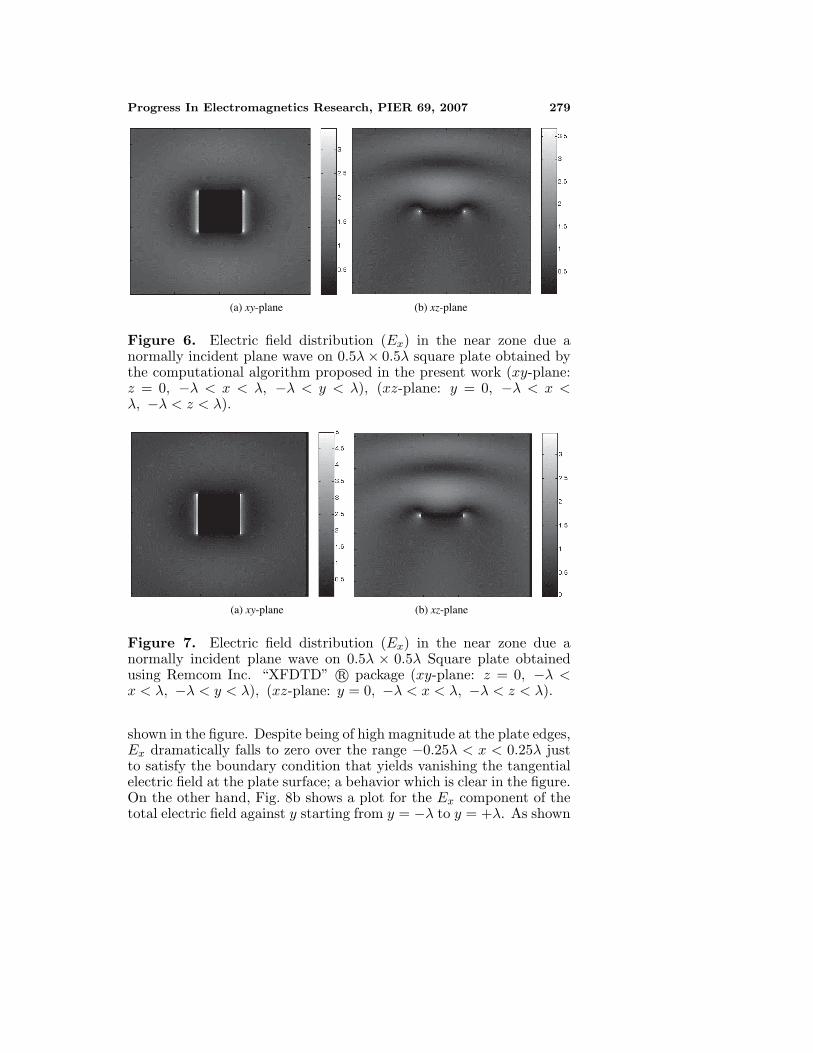
The distributions of the total electric field component Ex (incidentand scattered) in the planes z = 0 and y = 0 are presented in graycolor scale as shown in Figs. 6a and 6b, respectively. Since the incidentelectric field is x-directed, the total electric field exhibits the edgebehavior at the perpendicular plate edges x = −0.25λ and x = +0.25λ.
To examine the accuracy of proposed algorithm, the same problemis solved using Remcom Inc. “XFDTD” r© package. Fig. 7 presents theelectric field distributions in the planes z = 0 and y = 0 as obtained bythis package. The results presented in this Fig. 7 seems to be identicalto those presented in Fig. 6.
iE
Direction of incidence
z
y x
Figure 5. Triangular-patch model of a square plate and direction ofincidence and polarization of the plane wave.
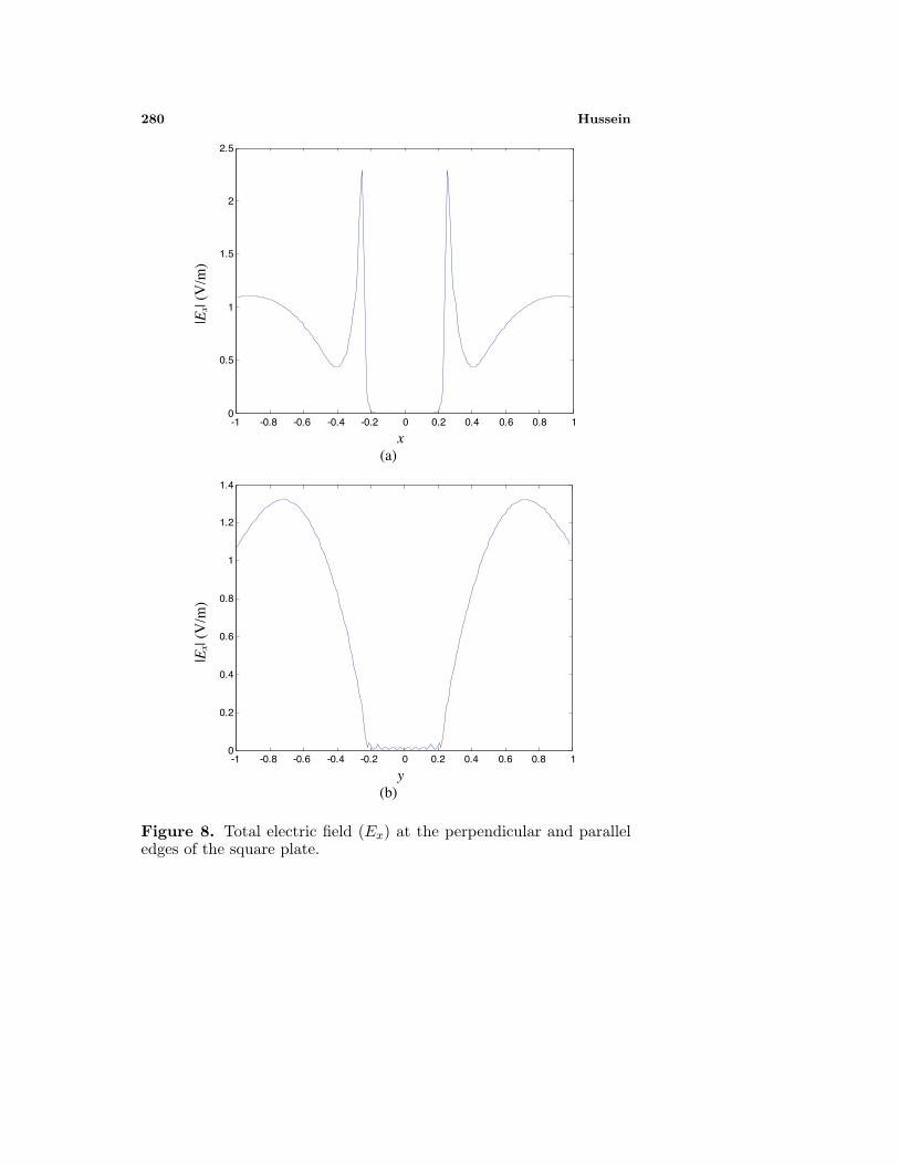
For more illustration of the field behavior near the square plate,Fig. 8a shows a plot for the Ex component of the total electric fieldagainst x starting from x = −λ to x = +λ. The electric field exhibitssingular behavior at the plate edges x = −0.25λ and x = +0.25λ as
Progress In Electromagnetics Research, PIER 69, 2007 279
(a) xy-plane (b) xz-plane
Figure 6. Electric field distribution (Ex) in the near zone due anormally incident plane wave on 0.5λ× 0.5λ square plate obtained bythe computational algorithm proposed in the present work (xy-plane:z = 0, −λ < x < λ, −λ < y < λ), (xz-plane: y = 0, −λ < x <λ, −λ < z < λ).
(a) xy-plane (b) xz-plane
Figure 7. Electric field distribution (Ex) in the near zone due anormally incident plane wave on 0.5λ × 0.5λ Square plate obtainedusing Remcom Inc. “XFDTD” r© package (xy-plane: z = 0, −λ <x < λ, −λ < y < λ), (xz-plane: y = 0, −λ < x < λ, −λ < z < λ).
shown in the figure. Despite being of high magnitude at the plate edges,Ex dramatically falls to zero over the range −0.25λ < x < 0.25λ justto satisfy the boundary condition that yields vanishing the tangentialelectric field at the plate surface; a behavior which is clear in the figure.On the other hand, Fig. 8b shows a plot for the Ex component of thetotal electric field against y starting from y = −λ to y = +λ. As shown
280 Hussein
|Ex|
(V/m
)
-1 -0.8 -0.6 -0.4 -0.2 0 0.2 0.4 0.6 0.8 10
0.5
1
1.5
2
2.5
x
(a)
|Ex|
(V/m
)
-1 -0.8 -0.6 -0.4 -0.2 0 0.2 0.4 0.6 0.8 10
0.2
0.4
0.6
0.8
1
1.2
1.4
y
(b)
Figure 8. Total electric field (Ex) at the perpendicular and paralleledges of the square plate.
Progress In Electromagnetics Research, PIER 69, 2007 281
0 0.1 0.2 0.3 0.4 0.5 0.6 0.7 0.8 0.9 1
|Ex|
(V/m
)
0
0.5
1
1.5
2
2.5
3
3.5
4
4.5
5EFIEXFDTD
x
| (V
/m)
0 0.1 0.2 0.3 0.4 0.5 0.6 0.7 0.8 0.9 10
0.2
0.4
0.6
|Ex
0.8
1
1.2
1.4EFIEXFDTD
y
| (V
/m)
|Ex
0 0.2 0.4 0.6 0.8 1 1.2 1.4 1.6 1.8 20
0.2
0.4
0.6
0.8
1
1.2
1.4
1.6
1.8
2EFIEXFDTD
z
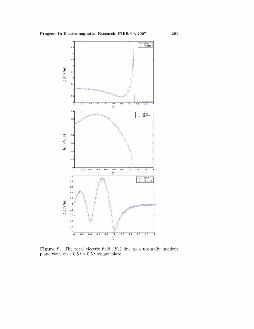
Figure 9. The total electric field (Ex) due to a normally incidentplane wave on a 0.5λ× 0.5λ square plate.
282 Hussein
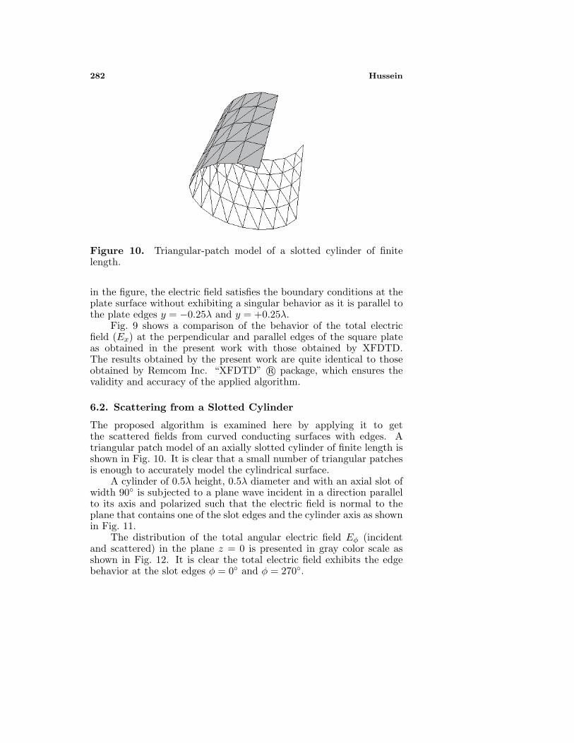
Figure 10. Triangular-patch model of a slotted cylinder of finitelength.
in the figure, the electric field satisfies the boundary conditions at theplate surface without exhibiting a singular behavior as it is parallel tothe plate edges y = −0.25λ and y = +0.25λ.
Fig. 9 shows a comparison of the behavior of the total electricfield (Ex) at the perpendicular and parallel edges of the square plateas obtained in the present work with those obtained by XFDTD.The results obtained by the present work are quite identical to thoseobtained by Remcom Inc. “XFDTD” r© package, which ensures thevalidity and accuracy of the applied algorithm.
6.2. Scattering from a Slotted Cylinder
The proposed algorithm is examined here by applying it to getthe scattered fields from curved conducting surfaces with edges. Atriangular patch model of an axially slotted cylinder of finite length isshown in Fig. 10. It is clear that a small number of triangular patchesis enough to accurately model the cylindrical surface.
A cylinder of 0.5λ height, 0.5λ diameter and with an axial slot ofwidth 90◦ is subjected to a plane wave incident in a direction parallelto its axis and polarized such that the electric field is normal to theplane that contains one of the slot edges and the cylinder axis as shownin Fig. 11.
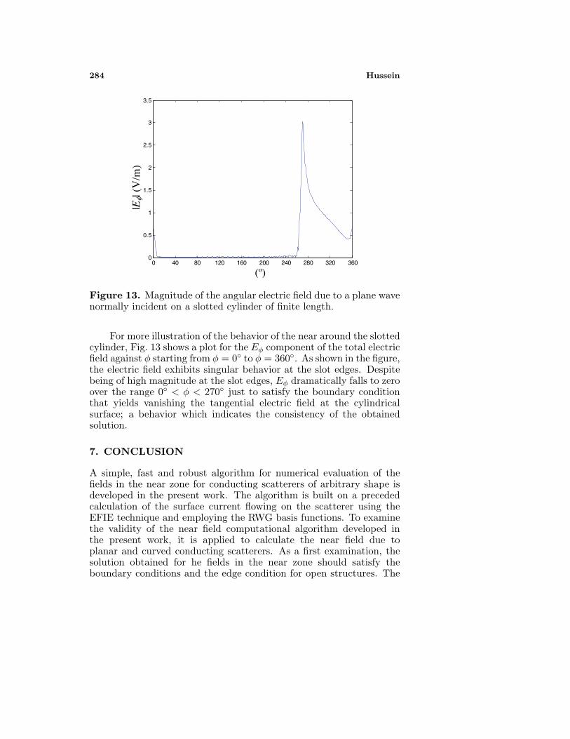
The distribution of the total angular electric field Eφ (incidentand scattered) in the plane z = 0 is presented in gray color scale asshown in Fig. 12. It is clear the total electric field exhibits the edgebehavior at the slot edges φ = 0◦ and φ = 270◦.
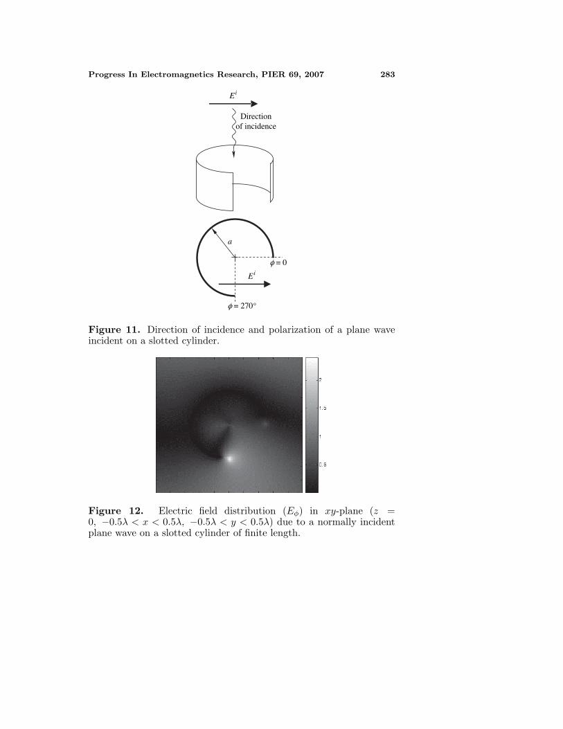
Progress In Electromagnetics Research, PIER 69, 2007 283
iE
Direction of incidence
a
�φ = 0
�φ = 270
iE
o
Figure 11. Direction of incidence and polarization of a plane waveincident on a slotted cylinder.
Figure 12. Electric field distribution (Eφ) in xy-plane (z =0, −0.5λ < x < 0.5λ, −0.5λ < y < 0.5λ) due to a normally incidentplane wave on a slotted cylinder of finite length.
284 Hussein
|Eφ|
(V/m
)
0 40 80 120 160 200 240 280 320 3600
0.5
1
1.5
2
2.5
3
3.5
(º)
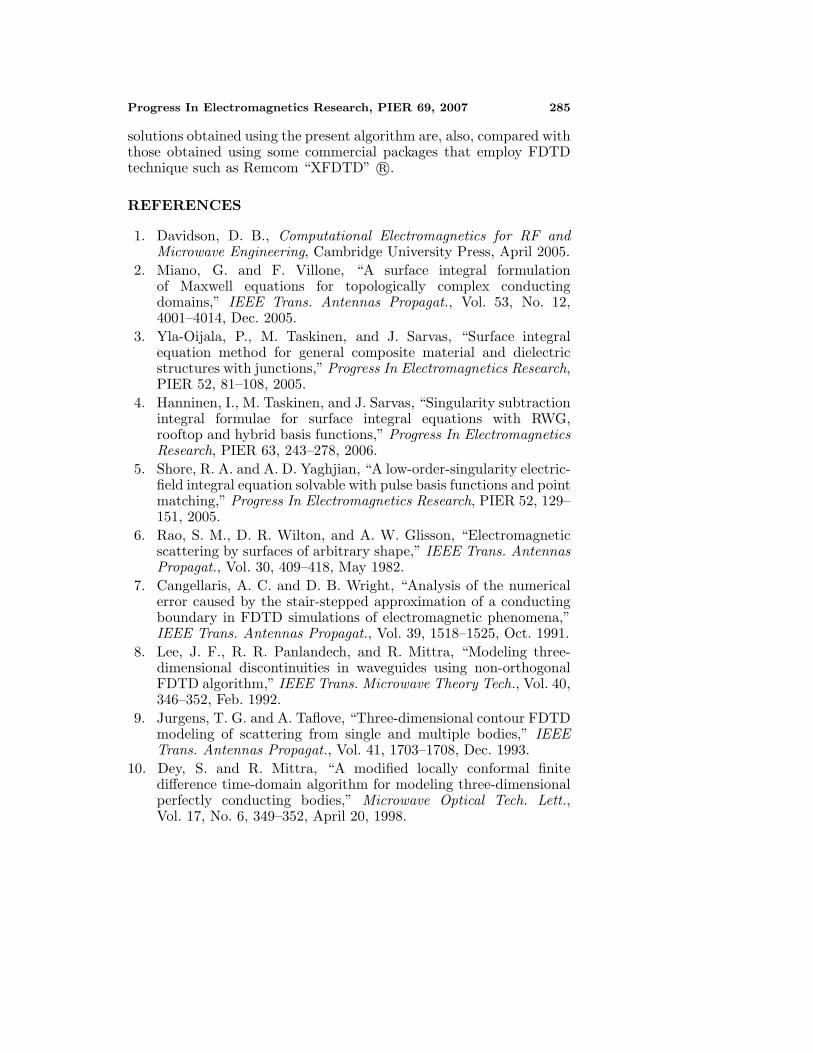
Figure 13. Magnitude of the angular electric field due to a plane wavenormally incident on a slotted cylinder of finite length.
For more illustration of the behavior of the near around the slottedcylinder, Fig. 13 shows a plot for the Eφ component of the total electricfield against φ starting from φ = 0◦ to φ = 360◦. As shown in the figure,the electric field exhibits singular behavior at the slot edges. Despitebeing of high magnitude at the slot edges, Eφ dramatically falls to zeroover the range 0◦ < φ < 270◦ just to satisfy the boundary conditionthat yields vanishing the tangential electric field at the cylindricalsurface; a behavior which indicates the consistency of the obtainedsolution.
7. CONCLUSION
A simple, fast and robust algorithm for numerical evaluation of thefields in the near zone for conducting scatterers of arbitrary shape isdeveloped in the present work. The algorithm is built on a precededcalculation of the surface current flowing on the scatterer using theEFIE technique and employing the RWG basis functions. To examinethe validity of the near field computational algorithm developed inthe present work, it is applied to calculate the near field due toplanar and curved conducting scatterers. As a first examination, thesolution obtained for he fields in the near zone should satisfy theboundary conditions and the edge condition for open structures. The
Progress In Electromagnetics Research, PIER 69, 2007 285
solutions obtained using the present algorithm are, also, compared withthose obtained using some commercial packages that employ FDTDtechnique such as Remcom “XFDTD” r©.
REFERENCES
1. Davidson, D. B., Computational Electromagnetics for RF andMicrowave Engineering, Cambridge University Press, April 2005.
2. Miano, G. and F. Villone, “A surface integral formulationof Maxwell equations for topologically complex conductingdomains,” IEEE Trans. Antennas Propagat., Vol. 53, No. 12,4001–4014, Dec. 2005.
3. Yla-Oijala, P., M. Taskinen, and J. Sarvas, “Surface integralequation method for general composite material and dielectricstructures with junctions,” Progress In Electromagnetics Research,PIER 52, 81–108, 2005.
4. Hanninen, I., M. Taskinen, and J. Sarvas, “Singularity subtractionintegral formulae for surface integral equations with RWG,rooftop and hybrid basis functions,” Progress In ElectromagneticsResearch, PIER 63, 243–278, 2006.
5. Shore, R. A. and A. D. Yaghjian, “A low-order-singularity electric-field integral equation solvable with pulse basis functions and pointmatching,” Progress In Electromagnetics Research, PIER 52, 129–151, 2005.
6. Rao, S. M., D. R. Wilton, and A. W. Glisson, “Electromagneticscattering by surfaces of arbitrary shape,” IEEE Trans. AntennasPropagat., Vol. 30, 409–418, May 1982.
7. Cangellaris, A. C. and D. B. Wright, “Analysis of the numericalerror caused by the stair-stepped approximation of a conductingboundary in FDTD simulations of electromagnetic phenomena,”IEEE Trans. Antennas Propagat., Vol. 39, 1518–1525, Oct. 1991.
8. Lee, J. F., R. R. Panlandech, and R. Mittra, “Modeling three-dimensional discontinuities in waveguides using non-orthogonalFDTD algorithm,” IEEE Trans. Microwave Theory Tech., Vol. 40,346–352, Feb. 1992.
9. Jurgens, T. G. and A. Taflove, “Three-dimensional contour FDTDmodeling of scattering from single and multiple bodies,” IEEETrans. Antennas Propagat., Vol. 41, 1703–1708, Dec. 1993.
10. Dey, S. and R. Mittra, “A modified locally conformal finitedifference time-domain algorithm for modeling three-dimensionalperfectly conducting bodies,” Microwave Optical Tech. Lett.,Vol. 17, No. 6, 349–352, April 20, 1998.