Effects of mechanical vibration on designed steel-based plate ...

Open Access.© 2021 B. Wangsa Lenggana et al., published by De Gruyter. This work is licensed under the Creative CommonsAttribution 4.0 License

Curved and Layer. Struct. 2021; 8:225–240

Research Article

Bhre Wangsa Lenggana, Aditya Rio Prabowo*, Ubaidillah Ubaidillah, Fitrian Imaduddin,Eko Surojo, Haris Nubli, and Ristiyanto Adiputra

Effects of mechanical vibration on designedsteel-based plate geometries: behavioralestimation subjected to applied material classesusing finite-element methodhttps://doi.org/10.1515/cls-2021-0021Received Feb 03, 2021; accepted Apr 29, 2021

Abstract: A research subject in structural engineering isthe problem of vibration under a loading object. The two-dimensional (2D) model of a structure under loading is anexample. In general, this case uses an object that is given arandom frequency, which then causes various changes inshape depending on the frequencymodel. To determine thedifference in performance by looking at the different formsof each mode, modal analysis with ANSYS was used. Thesamples to be simulated were metal plates with three vari-ations of the model, namely, a virgin metal plate withoutany holes or stiffness, plates with given holes, and metalplates with stiffness on one side. The model was simulatedwith modal analysis, so that 20 natural frequencies wererecorded. The sample also used different materials: low-carbon steel materials (AISI 304), marine materials (AISI1090), and ice-class materials (AR 235). Several random-frequency models proved the deformation of different ob-jects. Variations of sheet-metal designs were applied, suchas pure sheet metal, giving holes to the sides, and stiffeningthe simulated metal sheet.

Keywords: modal analysis, random vibration, designedplate, steel class, finite-element method

*Corresponding Author: Aditya Rio Prabowo: Department ofMechanical Engineering, Universitas Sebelas Maret, Surakarta,Indonesia; Email: [email protected] Lenggana, Ubaidillah Ubaidillah, Fitrian Imadud-din, Eko Surojo: Department of Mechanical Engineering, Universi-tas Sebelas Maret, Surakarta, IndonesiaHaris Nubli: Interdisciplinary Program of Marine ConvergenceDesign, Pukyong National University, Busan, South KoreaRistiyanto Adiputra: Department of Marine Systems Engineering,Kyushu University, Fukuoka, Japan

1 IntroductionIn recent years, structural engineering has become a pop-ular topic of discussion. The problem of the vibration ofa structure under loading or a moving force, which is in-cluded in the problem of moving loading, has become a re-search topic because vibration is a common case of moving-load problems, such as in railroads, overhead cranes, bal-listic systems, magnetic discs, cable lines, building plates,and bridges. To achieve certain objectives, simulated two-dimensional modeling and efficient analytical methods arerequired for the reliable design and maintenance of a struc-ture. In addition, this modeling and these methods can beused to accurately predict the vibration characteristics ofstructures. In general, structures under moving loads aremodeled as one- (1D) or two-dimensional (2D) structures.

In this regard, several analytical methods were pro-posed for the vibration analysis of the problem of movingloads in one- and two-dimensional models. Some of themare the modal-analysis [1–4], integral-transformation (ITM)[5–7], Galerkin [8, 9], differential-quadrature [10, 11], finite-difference [12, 13], finite-element method (FEM) [14–18],dynamic-stiffness [19, 20], and frequency-domain spectral-element (SEM) [21–25] methods. The finite-element method(FEM) is a numerical procedure that can be applied tosolve a wide variety of problems in engineering and sci-ence. In general, this method is used to solve steady, tran-sient, and linear and nonlinear problems in electromag-netic fields, structural analysis, and fluid dynamics [1]. Thefinite-elementmethodhas themainadvantage of being ableto handle all kinds of geometries and nonhomogeneousmaterials without the need to change computer-code for-mulations. The idea of this method is to break the probleminto a large number of planes, each with a simple geometry,to facilitate problem solving. As a result, the domain breaksdown into a number of small elements, and the problemgoes from small but difficult to solve to large and relatively

https://doi.org/10.1515/cls-2021-0021

226 | B. Wangsa Lenggana et al.

easy to solve. Through the process of discretization, linearalgebra problems are formed with many unknowns. In anelectromagnetic case, a discretization scheme, as impliedby FEM, which implicitly combines most of the theoreti-cal features of the analyzed problem, is the best solutionfor obtaining accurate results in problems with complex,nonlinear geometries [2, 3]. This method can also be usedfor complex differential equations that are very difficult tosolve.

To investigate the vibrational characteristics of com-plex structures subjected to moving loads, FEM is exten-sively used. The shape function used in FEM is indepen-dent of the vibration frequency of a structure. FEM gen-erally requires the very fine discretization of structures toobtain reliable solutions, especially in the high-frequencyrange [26–28]. This paper analyzes a series of designedplate geometries that are set as representative of structuralcomponents. Several steel classes are applied to the platesin a finite-element simulation as consideration of variousstructural types, e.g., marine and offshore structures, andinland infrastructure. Vibrational analysis is the focus ofthe current work, which is directed to quantify the naturalfrequency characteristics of the designed plates.

2 Literature review

2.1 Introduction to finite-element method

The finite-element method (FEM) is process analysis car-ried out by dividing a certain quantity into smaller piecesto obtain a large-class engineering analysis solution. Math-ematically, FEM is an approximate approach that serves tosolve field problems. The finite-elementmethod is also com-monly referred to as finite-element analysis (FEA) [16, 23].One of the reasons for using FEA is because it is a powerfulcomputational technique used to solve various engineeringproblems, especially those with complex geometries thatare subject to general boundary conditions. Analysis wascarried out with field variables that varied from point topoint. Thus, this analysis has an infinite number of solu-tions in the domain [23]. Thismakes the problemneed fairlycomplex analysis. For that reason, using FEA is necessary.In reality, the system comprises a number of parts – expres-sion elements – that are not known in terms of the assumedfunction estimates in each element. For each element, avariational or weighted residual method is applied to createa systematic approximate solution [26]. These functions areusually called interpolation functions, and are then enteredin terms of field variables at certain points, called nodes.

The nodes that are formed are connected to the connectedelements and are usually located along the boundary of theelement. This method is used as an analytical tool to solveengineering problems because the degree of flexibility indistinguishing irregular domains from finite elements. Ingeneral, the use of FEA is carried out to create new productdesigns and improve the development of existing products.This makes FEA popular for researchers to verify proposeddesigns prior to a prototyping or construction process. Thegoal is to find out the feasibility of a design produced foran application. FEA is very widely used in the structuralfield [15]. Structural analysis consists of linear and nonlin-ear models. The linear model considers simple parametersand assumes that the material does not undergo plasticdeformation, while the nonlinear model assumes that thestructure undergoes plastic deformation as a result of theinitial load. In general, FEA uses three types of analysis,namely, 1D modeling to solve beam, rod, and frame ele-ments; 2D modeling, which is useful for solving field-stressand plane-strain problems; and 3D modeling, which is use-ful for solving complex solid structures.

2.2 Implementation of FE calculation

Several years earlier, solutions for plate deflection underdifferent boundary conditions were proposed by severalresearchers. Bhattacharya investigated plate deflection un-der static and dynamic loading using new finite-differenceanalysis. The actual mode shape of the plates of each nodewas found in this study, and this approach provides afourth-order biharmonic equation that varies from nodeto node [29]. A mathematical approach to the large deflec-tion of rectangular plates was also presented by Defu andSheikh [30], who analyzed on the basis of second-degreeand fourth-order Von Karman partial differential equations.In their research, lateral deflection with respect to the ap-plied load was found, which made this solution usablein the direct practical analysis of plates under differentboundary conditions [30]. In the same field, Bakker et al.studied a forecast analysis method for large deflections ofrectangular thin plates with simple supported boundaryconditions under the action of transverse loads. This ap-proach was taken to find initial deflection shape and thetotal plate. From this analysis, the deflection behavior ofthe plate size under transverse load can be expressed asa function of the plane stiffness of the plate before buck-ling [31]. Furthermore, research was carried out by Liewet al., who developed the differential quadrature methodand the harmonic differential quadrature method for thestatic analysis of three-dimensional rectangular plates. A

Effects of mechanical vibration on designed steel-based plate geometries | 227

study conducted by Liew et al. aimed to find the bendingand bending of plates that were supported and clampedonly at boundary conditions [32].

In the utilization of FEA, some researchers made useof it in solving the perforated-plate problem. Jain analyzedthe effect of the ratio of a perforated plate D/A (D is holediameter, and A is plate width) on the stress concentrationand deflection factors in isotropic and orthotropic platesunder transverse static loading [33]. The point put forwardby Jain (2009) was related to and supported by researchby Chaudhuri (1987), who presented the theory of stressanalysis using the rhombic array of alternating method forseveral circular holes [34–36]. In that study, the effect ofstress concentration on perforated laminated plates usingthe finite-elementmethodwas investigated. Then, Paul andRao presented a theory for the evaluation of stress concen-tration factors for thick laminated plate andfiber-reinforcedplastic (FRP) with the help of the Lo-Christensen-Wu high-order bending theory under transverse loading [37].

Furthermore, in the last few decades, authors devel-oped examining plates with stiffeners. Although rigid rect-angular plates are thoroughly studied, the application ofstiffeners to round plates is not very popular. The deflectionin isotropic coiled plates subjected to two stiffening ringsunder static pressure was studied by Steen and Byklum.The used methodology was with clamped boundary condi-tions during analysis. Previously, Troipsky worked on rigidplates under bending, stability, and vibration. Pape andFox presented an infinite series approach to the correctnessof the plate aspect ratio using a rigid elastic beam [36–38].

Further development was carried out by Xuan et al.,who performed element refinement using the boundaryintegral method. Das et al. developed a fairly general clas-sical method that could be applied to all boundary condi-tions. Meanwhile, Jain in his research presented analysisof stress concentrations and deflections on isotropic andorthotropic rectangular plates with circular holes undertransverse statistical loading. His research assessed threetypes of elements to solve the problem of square triggerswith various boundary and load conditions [33, 39, 40].

The plasticity characteristics and external lateral load-ing of an elastoplastic plate were developed by Moshaiovand Vorus using an integral equation formulation forbending an elastoplastic plate. Formulations for Kirchhoffplate analysis with subregions by varying thickness forthe boundary element method were also developed by re-searchers such as Paiva and Aliabadi. The developmentcan be used to analyze the floor of a building in such away that the integral equation of the curvature boundaryof the points located at the zone interface is inferred veryeasily, which allows for the bending moment to be ob-

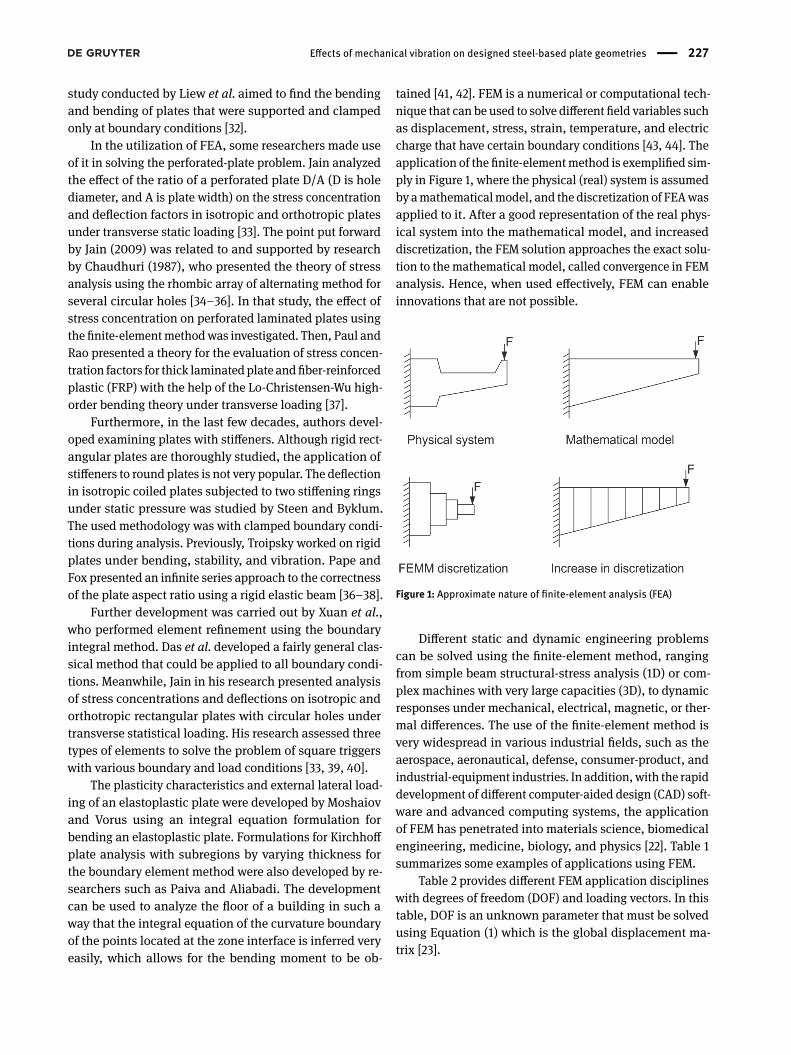
tained [41, 42]. FEM is a numerical or computational tech-nique that can be used to solve different field variables suchas displacement, stress, strain, temperature, and electriccharge that have certain boundary conditions [43, 44]. Theapplication of the finite-elementmethod is exemplified sim-ply in Figure 1, where the physical (real) system is assumedby amathematicalmodel, and the discretization of FEAwasapplied to it. After a good representation of the real phys-ical system into the mathematical model, and increaseddiscretization, the FEM solution approaches the exact solu-tion to the mathematical model, called convergence in FEManalysis. Hence, when used effectively, FEM can enableinnovations that are not possible.

Figure 1: Approximate nature of finite-element analysis (FEA)

Different static and dynamic engineering problemscan be solved using the finite-element method, rangingfrom simple beam structural-stress analysis (1D) or com-plex machines with very large capacities (3D), to dynamicresponses under mechanical, electrical, magnetic, or ther-mal differences. The use of the finite-element method isvery widespread in various industrial fields, such as theaerospace, aeronautical, defense, consumer-product, andindustrial-equipment industries. In addition,with the rapiddevelopment of different computer-aided design (CAD) soft-ware and advanced computing systems, the applicationof FEM has penetrated into materials science, biomedicalengineering, medicine, biology, and physics [22]. Table 1summarizes some examples of applications using FEM.

Table 2 provides different FEM application disciplineswith degrees of freedom (DOF) and loading vectors. In thistable, DOF is an unknown parameter that must be solvedusing Equation (1) which is the global displacement ma-trix [23].


Table 1: Finite-element method (FEM) applications [22]

Field Application examplesSolid/structural

mechanicsWind-turbine blade design optimization, structure-failure analysis, crash simulation,

nuclear-reactor component integrity analysis, beam and truss design and optimization,limit-load analysis

Heat conduction Combustion engine, cooling and casting modelling, electronic cooling modellingAcoustic flow Seepage analysis, aerodynamic analysis of cars and airplanes, air-conditioning modelling

of buildingsElectronics/

electromagneticsElectromagnetic-interference suppression analysis, sensor and actuator field calculations,

antenna-design performance predictions

Table 2: Degrees of freedom (DOF) and loading vectors for different disciplines using FEM

Discipline DOF (U) Loading vector (R)Solid-structure mechanics Displacement Force

Electrostatic Electropotential Charge densityHeat conduction Temperature Heat flux

Computational fluid dynamics (CFD) Displacement potential, pressure, velocity Particle velocity, fluxesMagnetostatic Magnetic potential Magnetic intensity

In general, the value of stiffness and mass on a struc-tural plate is known in the form of a matrix. Stiffness andmass matrices are denoted by [K] and [M], respectively;then, the equation ofmotion of the system can be expressedas in Equation (1).

[M] {u} + [K] {u} = {0} , (1)

where {u} and {u} are the acceleration and displacementvectors, respectively, so that in free vibration, the valuesof the acceleration and displacement vectors can be for-mulated according to Equations (2) and (3) as follows [24].

{u} = {u} eiωt (2)

{u} = ω2 {u} eiωt , (3)

where {u} is the amplitude of the vector {u}; thus, Equa-tion (1) can be substituted into Equation (4) as follows [24].(

[K] − ω2 [M]){u} = {0} (4)

To obtain the characteristic equation of an attachedstructural plate, Equation (5) is used [24].

[K] − ω2 [M]= 0. (5)

FEM is most widely used in linear and nonlinear staticanalyses. The various types of static problems that the FEMsolves in this area include the analysis of elastic, elastoplas-tic, and viscoplastic beams, frames, plates, shells, and solid

structures. Typically, static analysis includes the analysisof stress, strain, and displacement under static loading forone-, two-, or three-dimensional problems. In this chapter,the general theory of elasticity is discussed. In addition,the general formulation of the stiffness of 1D, 2D, and 3Delements is discussed with the detailed formulation of thestiffness matrix of the beam elements. After that, generalsolutionmethods of static analysis are shown for linear andnonlinear problems. The global equation for static analysisis the same as that in Equation (1), and solving for the staticproblem is exactly the same as the one mentioned above inthe general FEM procedure.

The main objective of any stress analysis is to find thedistribution of displacement and stress under static loadingand limit conditions. The following equations are fulfilled ifthere is an analytical solution to a particular problem basedon elasticity theory. Table 3 shows the types of equationsin 1D, 2D, and 3D problems.

Problems that exist in real life are often solvedby takinga mathematical approach. In addition to a mathematicalapproach, either experimenting by producing a prototypemodel with a certain scale or the original is also a solutionto finding the solution to a problem. Mathematical model-ing is a process of interpreting existing problems with theaim of simplifying and accelerating problem solving. Thismakes mathematical modeling both challenging and de-manding, as the use ofmathematics and computers to solvereal-world problems is extensive and affects all branchesof learning.


Table 3: Type and number of equations in 1D, 2D, and 3D problems [25]

Types Number of equationsof equation 3D problems 2D problems 1D problems

Equilibrium equation 3 2 1Stress-displacement relation 6 3 1

Strain-stress relation 6 3 1Total no. of equations 15 8 1

Problem solving with a mathematical modeling ap-proach is possible with software. A powerful finite-elementpiece of software for analyzing different problems is ANSYS.Various problems can be overcome with ANSYS such aselasticity, fluid flow, heat transfer, and electromagnetism.Nonlinear and transient analyzes can also be completedwith the software. In general, ANSYS analysis has the fol-lowing steps for problem solving: First, modeling, a processthat includes the definition of system geometry and the se-lection ofmaterial properties. In this step, the user can drawa 2D or 3D representation of the problem. Second, meshing.This step involves discretizing the model according to pre-defined geometric elements [22–24]. This is followed by theretrieval of the result and solution, and this step involvesapplying boundary and load conditions to the system, andresolving problems. Lastly, post-processing, which involvesplotting the nodal solution (unknown parameter), whichmay be displacement, stress, or reactive force.

2.3 Modal analysis and random vibration

The natural or resonant frequency is a fundamental reso-nance mode of a vibrating system. The natural frequencycan also be defined as the frequency that vibrates when un-der a small impact load for a certain period of time. Impor-tant parameters that can represent the dynamic response ofa test object in a vibration test are the natural frequency andmode shape of the object. To identify a dynamic characteris-tic such as natural frequency, the shape of the mode can beestablished using modal analysis [45, 46]. Modal analysisis based on the fact that the vibrational response of a lineartime variant dynamic system can be expressed as a linearcombination of a series of simple harmonic motions callednatural vibration mode. The natural mode of vibration isgenerally determined entirely by its physical propertiessuch as mass, strength, damping, and spatial distribution;this is also because the natural mode of vibration is inher-ent in dynamic systems [47–50]. Modal analysis is oftenused to abstract the modal parameters of a system, includ-ing natural frequency, mode shape, and modal damping

ratio. This parameter depends only on the system itself, butdominates the system response to excitation. Modal anal-ysis is the fundamental response of analysis and is of in-creasing concern. Experimental modal analysis (EMA) canestimate the natural frequency, mode shape, and dampingvalue of a measured structure [51]. The finite-element (FE)model structure can be validated by comparing the experi-mental natural frequency and mode shape with the resultsof FE model analysis. Modal analysis is a technology of lin-ear analysis that is used to determine the natural-frequencystructure and vibration modes. In modal analysis, the onlyeffective load is the zero-displacement limit. If a certain de-gree of freedom (DOF) determines a nonzero displacementlimit, the program replaces the degrees of freedom with azero displacement limit [52, 53].

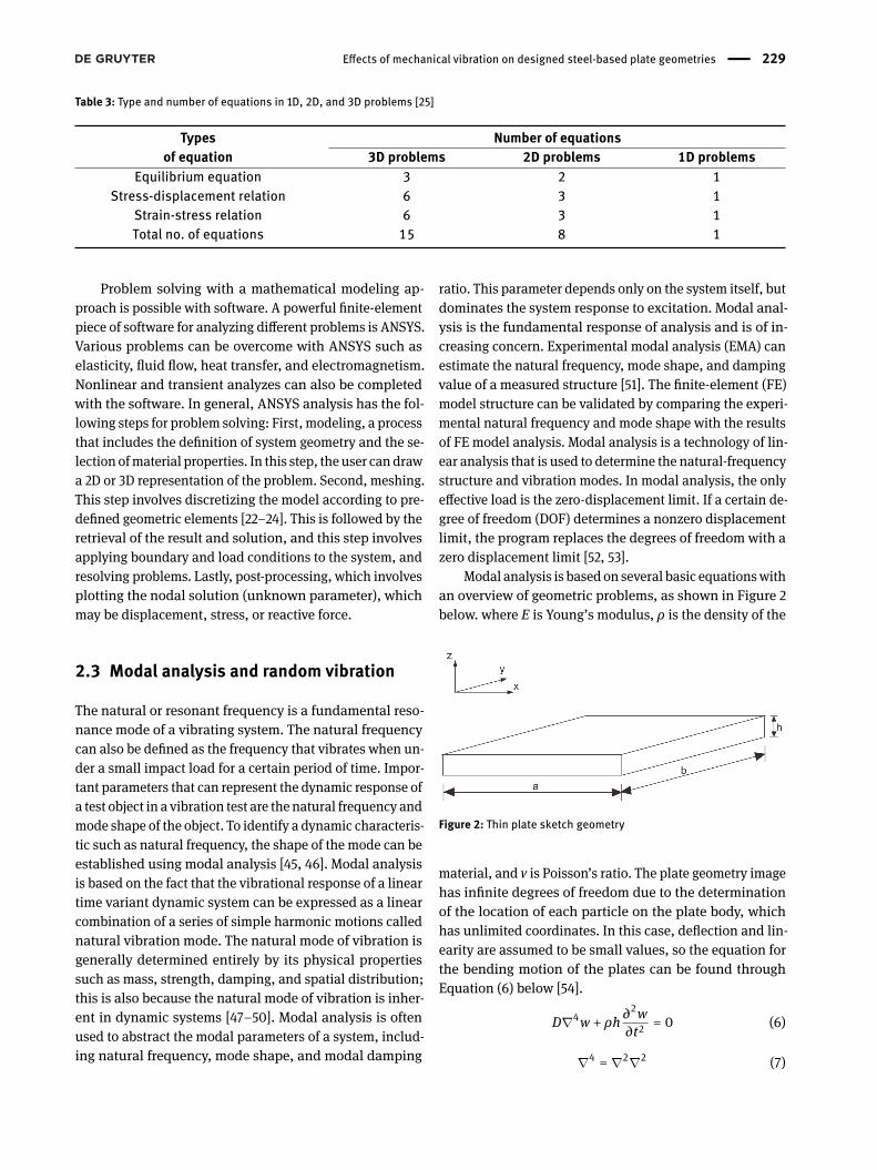
Modal analysis is based on several basic equationswithan overview of geometric problems, as shown in Figure 2below. where E is Young’s modulus, ρ is the density of the

Figure 2: Thin plate sketch geometry

material, and v is Poisson’s ratio. The plate geometry imagehas infinite degrees of freedom due to the determinationof the location of each particle on the plate body, whichhas unlimited coordinates. In this case, deflection and lin-earity are assumed to be small values, so the equation forthe bending motion of the plates can be found throughEquation (6) below [54].

D∇4w + ρh ∂2w∂t2 = 0 (6)

∇4 = ∇2∇2 (7)


D = Eh3

12(1 − v2

) , (8)

where w is the transverse deflection,∇2 is Laplacian, andEquation (8) is the plate flexural rigidity. Deflection is afunction of x and y spatial coordinates, and from time func-tion t. If the equation ofmotion is filledwith formdeflectionfunctions, then the equation of motion can be written asfollows.

w (x, y, t) = ∅ (x, y) q (t) , (9)

where∅ (x, y) is a function satisfying the plate boundaryconditions, and q (t) is the corresponding general coordi-nate. By adding the equations of motion and separatingthe variables, Equations (10) and (11) can be obtained [54].

∇4∅ − ω2

D ∅ = 0 (10)

d2qdt2 + ω

2

ρh q = 0 (11)

where ω is the natural frequency. The solutions of Equa-tions (10) and (11) are solutions to infinite sets of eigenval-ues and functions (or eigenvectors). In this case, the bound-ary conditions determine the natural frequency, and the ini-tial conditions determine the contribution of each mode ac-cording to the vibration of the plate. To determine the natu-ral frequency, several methods can generally be used, suchas the Rayleigh, Rayleigh-Ritz, and FEMmethods, shownin Equations (12), (14), and (15), respectively [54].

ω2 = Vmax12hρ

s∅ (x, y) dxdy

(12)

Vmax =12ρhω

2x

∅2 (x, y) dxdy (13)

ωn =λna2

√Dρh , (14)

where Vmax is the maximal velocity that can be formulatedaccording to Equation (13), a is an unknown constant, andλn is the frequency parameter. In Equation (14), Rayleigh–Ritz, the natural frequency is written in the form of ωn [54].

f = ω2π , (15)

where ω is the natural circular frequency and f is the nat-ural frequency. In Equation (15) of the FEM method, theequation of motion for the structure is formulated accord-ing to Equations (1–5).

Random-vibration analysis is used to determine theresponse of the structure under random loading. ANSYS

uses the power spectral density (PSD) spectrum as analy-sis of random vibrations from the load input. Power spec-tral density is a probability statistical method and the root-mean-square value of a random variable, including themeasurement of random-vibration energy and frequencyinformation. The power spectrum can be in the form of dis-placement, velocity, acceleration or power spectral density,and in other forms [55–59].

2.4 Pioneer works in FEM and structuralvibration

FEM was first developed through advances in aircraft-structure analysis. The development of the FEM foundationwas first carried out by Courant in the 1940s. In 1956, thestiffness matrix for frames, beams, and other elements wasdeveloped by Courant and others [60–64]. In the 1960s, theterm “finite element” was first coined and used by Claugh;later, Zienkiewicz and Chung published the first book onFEM in 1967. Computer FEM codes appeared during the1970s, and to this day, advanced FEM codes are availablefor solving various field problems [65–70]. In the last fewdecades, FEM has shown very significant developments,especially in FEM software, including the introduction ofp elements, integration sensitivity, FEM code on desktopcomputers, and the development of robust CAD programsfor modeling complex geometries. A history of FEM is sum-marized in Table 4 [22].

Table 4: Type and number of equations in 1D, 2D, and 3D problems

Year Major milestone1943 Variation method which laid foundation of FEM

(Courant)1956 Stiffness method for beams, trusses1960 Term “finite element” coined1967 First book of FEM by Zienkiewicz and Chung1970 FEM applied to nonlinear problems and large de-

formations1970s Computer implementation on solving FEM1980s Used in microcomputers and GUIs1990s Large structural system analysis, nonlinear and

dynamic problems2000s Multiphysics and multiscale problems2014s Powerful FEA tools


3 Materials and methods

3.1 Setting and configuration forfinite-element analysis

3.1.1 Design sketch

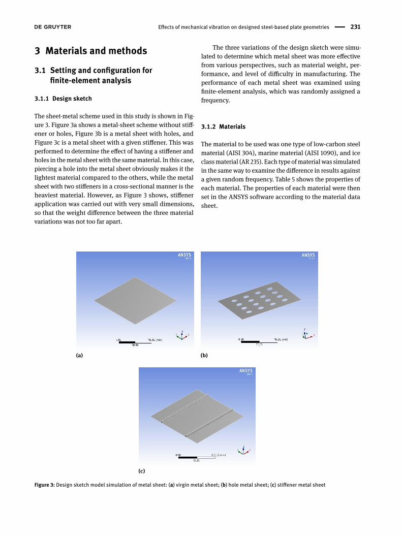
The sheet-metal scheme used in this study is shown in Fig-ure 3. Figure 3a shows a metal-sheet scheme without stiff-ener or holes, Figure 3b is a metal sheet with holes, andFigure 3c is a metal sheet with a given stiffener. This wasperformed to determine the effect of having a stiffener andholes in themetal sheet with the samematerial. In this case,piercing a hole into the metal sheet obviously makes it thelightest material compared to the others, while the metalsheet with two stiffeners in a cross-sectional manner is theheaviest material. However, as Figure 3 shows, stiffenerapplication was carried out with very small dimensions,so that the weight difference between the three materialvariations was not too far apart.

The three variations of the design sketch were simu-lated to determine which metal sheet was more effectivefrom various perspectives, such as material weight, per-formance, and level of difficulty in manufacturing. Theperformance of each metal sheet was examined usingfinite-element analysis, which was randomly assigned afrequency.

3.1.2 Materials

The material to be used was one type of low-carbon steelmaterial (AISI 304), marine material (AISI 1090), and iceclassmaterial (AR 235). Each type ofmaterial was simulatedin the sameway to examine the difference in results againsta given random frequency. Table 5 shows the properties ofeach material. The properties of each material were thenset in the ANSYS software according to the material datasheet.

(a)

(b)

(c)

Figure 3: Design sketch model simulation of metal sheet: (a) virgin metal sheet; (b) hole metal sheet; (c) stiffener metal sheet


Table 5:Material properties of low-carbon steel AISI 304, AR 235, and AISI 1090 carbon steel

Properties Ice-class material Marine class material Low-carbon steel UnitTensile strength, ultimate 792 696 505 MPaTensile strength, yield 482.63 540 215 MPaModulus elasticity 210 210 200 GPaPoisson’s ratio 0.3 0.3 0.29 -Shear modulus 80 80 80 GPaDensity 7.8 7.8 8 g/cc

3.1.2.1 Low-carbon steelCarbon steel is a type of alloy steel consisting of iron (Fe)and carbon (C) elements, where iron is the basic elementand carbon is the main alloying element. In the steel-making process, the addition of other chemical elements,such as sulfur (S), phosphorus (P), silicon (Si), manganese(Mn), and other chemical elements is in accordance withthe desired properties of the steel. Low-carbon steel is steelwith carbon-element content in a steel structure of less than0.3% C. This low-carbon steel has high toughness and duc-tility, but low hardness andwear resistance. In general, thistype of steel is used as raw material for the manufacture ofbuilding structural components, building pipes, bridges,car bodies, and others.

3.1.2.2 Marine materialsMarine materials generally use high-strength low-alloysteel materials. In this case, the material used is a typeof HSLA steel material, namely, AR 235 Abrasion ResistingSteel. Abrasion Resisting Steel AR 235 is medium carbonand highmanganese. This type of steel is tough and is wear-resistance ductile enough to allow for specific machining.The chemical composition of this type of steel gives aBrinellhardness of about 235 under as-roll conditions and tensilestrength of about 115,000 psi. Abrasion-resistant steel has 2to 10 times the service life ofmild steelwhenused in scraperblades, mixers, manure-moving equipment, loaders, con-veyors, scoop gear, pull-conveyor bottoms, spouts, shovels,mine screens, troughs, hoppers, truck body dumps, con-crete buckets, fan blades, ore jumps, tail sluices, bucketlips, rock screens, loading channels, agitator oars, dredgepump liners, grinding pans, liner plates, and sluice gates.This steel, if not too cold, takes a 90∘ bend to a reasonableradius with a thickness of up to about 3/8 inches withoutany fracture by being gently bent (in degrees) until formingis complete. Formore difficult forming and all heavier gaugeforming, the gauge must be heated and shaped while hot.Heat forming should take place at an ambient temperatureof 1500∘F. If the steel is allowed to cool slowly, its abrasive

resistance qualities are not lost, nor are there any cracks ordistortion. High-carbon steels such as this grade should notbe worked by any method when it is very cold. This grade,due to its high hardness and toughness, is rather difficultfor machines to work with. However, ordinary high-speedtools are more than capable of machining when needed.

3.1.2.3 Ice-class materialsIce-class material is generally applied in the shipping sec-tor, and is also known as polar-class material. This materialis usually used for ship hullswith certain requirements. Thelayered structure is a rigid plate element that is in contactwith the hull of the ship and is subject to ice loads. This re-quirement applies to an inboard level that is lower than theheight of the adjacent truss or parallel supports, or 2.5 timesthe depth of the frame cutting the layered structure. Thethickness of the lining and the slightest amount of installedstiffening is such that the level of attachment of the requiredends for the shell frame must be ascertained. Class associa-tions have various rules covering requirements and qualifi-cations on ships intended to operate in icy waters, a set ofrulesmade up of several ice notations.Meanwhile, notationgenerally depends on the geographic area of operation, anddiffers with respect to operational capability and structuralstrength. Depending on the ship’s destination and area ofoperation, the owner is responsible for selecting the appro-priate ice-class notation on the ship. Initially, the elasticapproach and structural capacity definition put forwardby the Finnish–Swedish Ice Class Rules (FSICR) regardingships were used to ensure safe operations in the Baltic Seaduring winter. In this case, prescribed notations are thoseused to determine the minimal requirements for enginepower and ice reinforcement for the ship, assuming thaticebreaker assistance is available when needed. Initiallythe regulations were aimed at operating merchant shipscrossing ice routes. All polar-class vessels require effectiveprotection against abrasion caused by ice and against corro-sion. The most important part of this protection is appliedto all surface coatings of polar-class ships. Polar-class ves-


sels have a minimal corrosion/abrasion addition tc = 1.0mm applied to all internal structures within the hull areareinforced by ice, including layered members adjacent toshells, and rigid nets and flanges.

3.1.3 Geometry and boundary condition

Three different sheet-metal designs with the same materialwere simulated against a given random vibration. Further-

(a)

(b)

(c)

Figure 4: Technical drawing of models and sketch application: (a) virgin metal sheet; (b) hole metal sheet; (c) stiffener metal sheet


more, 20 modes of total deformation for each sheet wereseen in value, but not all formsof the total deformationwereshown. Two form modes of total deformation were shown.This mode was taken because it represents a change inthe shape of each design. Each metal-sheet design had thesame main dimensions of 180 × 180 mm. The first designwas a metal sheet without any variation in either holes or

stiffener, the second design was a perforated metal sheetwith 16 holes and a diameter of 15 mm in each hole, andthe third design was a sheet metal with two stiffeners asshown in Figure 3a–c with a thickness of 2 mm.

The total deformation of eachmetal sheet was obtainedthrough modal analysis simulation in ANSYS. In additionto using modal analysis, a harmonic-response simulation

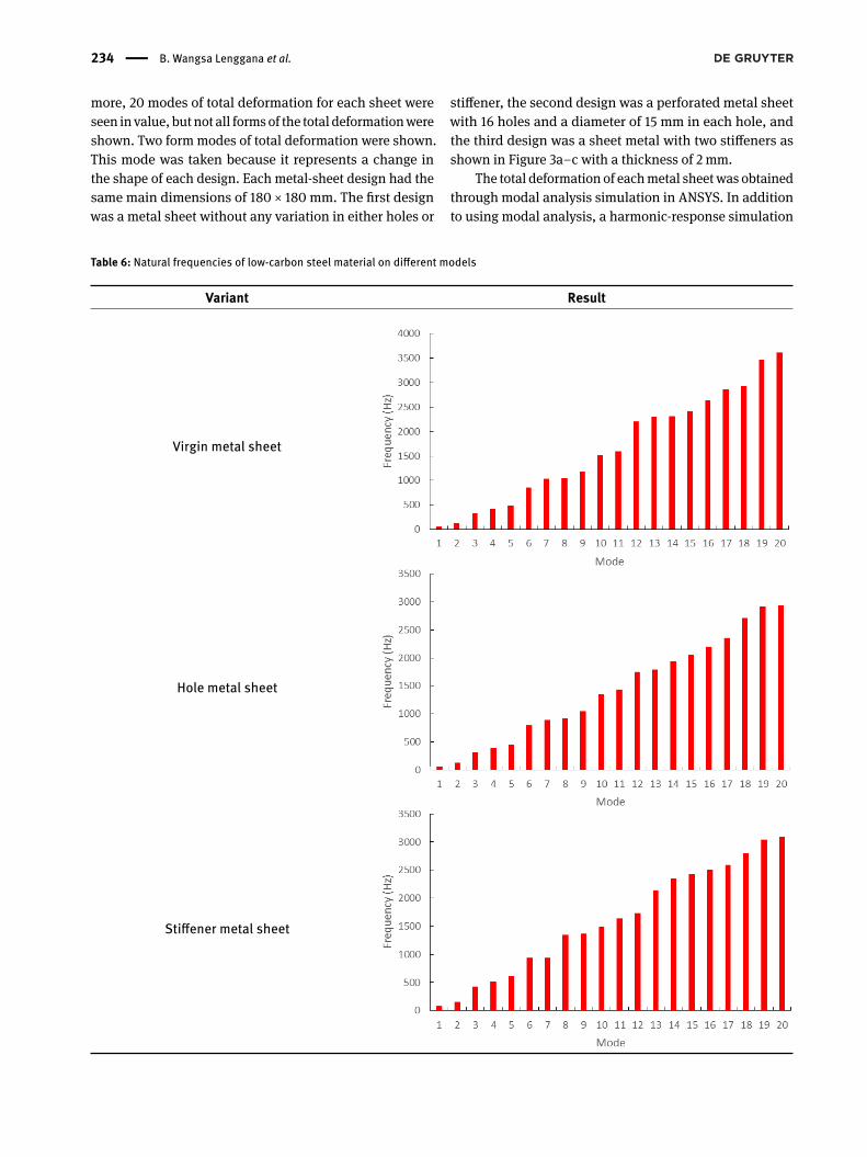
Table 6: Natural frequencies of low-carbon steel material on different models

Variant Result

Virgin metal sheet

Hole metal sheet

Stiffener metal sheet


Table 7: Natural frequencies of low-carbon steel, marine, and ice-class materials on different models

ModeNatural frequency (Hz)

Virgin Hole StiffenerLow Marine Ice class Low Marine Ice class Low Marine Ice class

1 52.509 54.447 54.621 50.57 52.401 52.569 82.028 84.944 85.2152 129.56 133.76 134.19 125.05 129.11 129.53 152.45 157.4 157.93 333.29 344.95 346.06 312.71 323.67 324.7 430.23 444.99 446.414 420.55 435.9 437.29 386.65 400.32 401.6 520.29 538.81 540.545 483.05 499.41 501.01 457.41 472.89 474.4 617.91 638.57 640.626 850.48 879.29 882.1 793.07 819.82 822.44 936.88 969.41 972.517 1032.0 1070.5 1073.9 895.41 927.99 930.95 938.04 971.15 974.268 1048.7 1085.7 1089.2 923.18 955.67 958.73 1351.5 1398.8 1403.39 1181.3 1224.5 1228.4 1046.3 1083.4 1086.9 1369.5 1416.3 1420.810 1508.9 1562.1 1567.1 1354.5 1401.4 1405.9 1497.9 1549.5 1554.411 1596.7 1652.0 1657.3 1435.0 1484.6 1489.3 1641.0 1697.3 1702.712 2201.5 2281.2 2288.5 1751.4 1814.1 1819.9 1732.7 1797.0 1802.713 2297.2 2384.1 2391.7 1795.9 1861.3 1867.3 2139.0 2215.9 2223.014 2309.8 2389.7 2397.4 1932.9 2001.9 2008.3 2355.5 2437.2 2445.015 2420.1 2508.8 2516.9 2056.4 2127.8 2134.7 2424.7 2510.5 2518.516 2635.0 2729.8 2738.5 2199.5 2276.8 2284.1 2503.1 2588.9 2597.217 2857.3 2960.5 2970.0 2356.5 2439.7 2447.6 2592.7 2684.7 2693.318 2933.2 3030.2 3039.9 2713.4 2803.6 2812.5 2798.5 2890.9 2900.119 3476.4 3599.1 3610.6 2922.1 3025.3 3035.0 3042.1 3154.8 3164.920 3613.5 3739.7 3751.7 2940.1 3045.2 3055.0 3089.1 3198.2 3208.4

model was also established in ANSYS to obtain the fre-quency value for the amplitude of the metal sheet. In per-forming the harmonic-response simulation process, oneside of the metal sheet was set as the fixed mode, and thesheet metal was given a constant force of 300 N. Figure 4ashows the dimensions of the design sketch used in thesimulation, while Figure 4b is a design application modelrepresented by a design scheme.

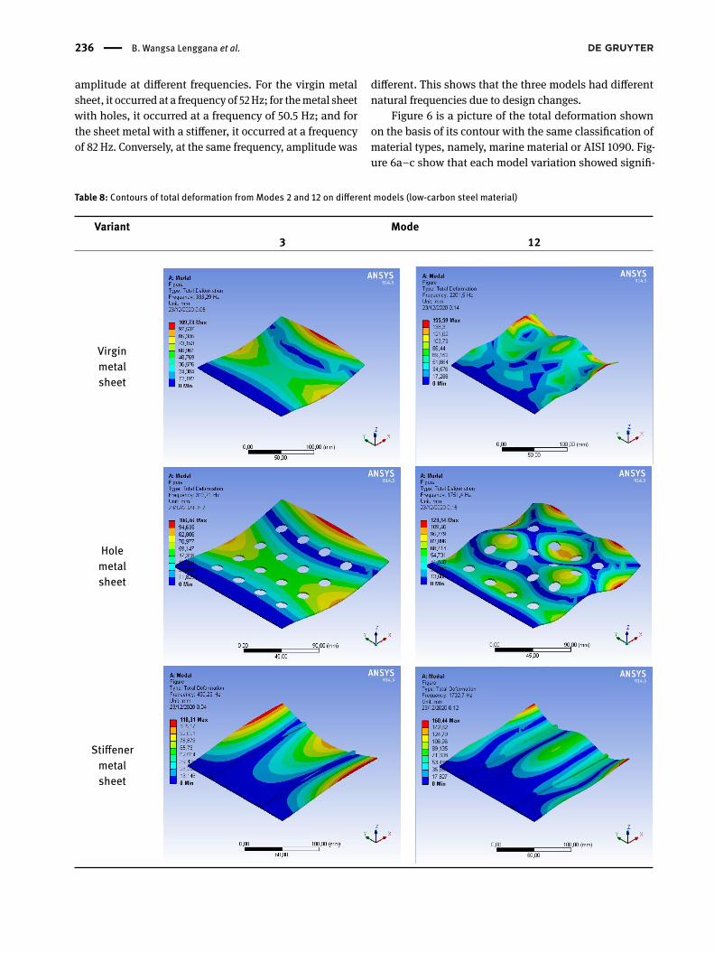
4 Results and discussionThe natural frequency of each sheet-metal design was ob-tained through modal analysis in ANSYS. Natural frequen-cies are shown in Tables 6 and 7, which are graphs and val-ues in Hz. There were differences in the natural-frequencyvalues of each sheet-metal design. Some examples are nat-ural frequencies in Modes 3 and 12 for sheet metals. InMode 3, the sheet metal without holes and a stiffener had anatural-frequency value of 333.29 Hz, the sheet metal withholes had a natural-frequency value of 312.71 Hz, while thesheet metal with a stiffener had a natural-frequency valueof 430.23 Hz. The sheet metal with stiffener application had

the largest natural-frequency value in Mode 3. However, inMode 12, the largest natural-frequency value was achievedby the sheet-metal design without holes and stiffener, andthe natural-frequency value for the sheet metal with a stiff-ener was even smaller than the natural-frequency value ofthe sheet metal with holes.

The natural-frequency value for the sheet metal with-out holes and stiffener reached 2201.5 Hz, the natural-frequency value for the sheet metal with holes was 1751.4Hz, and the sheet metal with a stiffener had the lowestvalue of 1732.7 Hz because Modes 3 and 12 had differentdeformations, which Table 8 shows. Table 8 also shows thecontours of pressure distribution and shape that occurredin Modes 3 and 12 for each design.

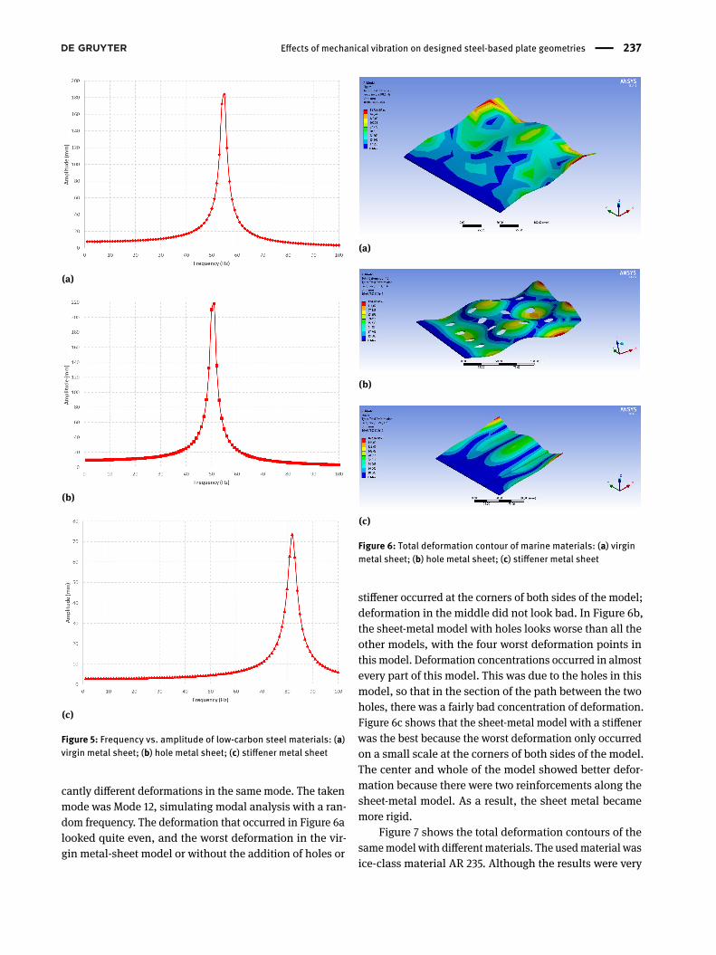
Figure 4 shows a graph of the frequency and amplitudethat occurred in all the models with the same material: (a)virgin metal sheet, (b) sheet metal with holes, and (c) sheet-metal model with stiffener application. Figure 5 shows thatthe largest amplitude occurred in the metal-sheet modelwith a hole, while the sheet-metal model with a stiffenerwas the model with the lowest amplitude. The amplitudesof the models of the virgin metal sheet, metal sheet withholes, and metal sheet with stiffener were 188, 218, and73.6 mm, respectively. Each model experienced maximal


amplitude at different frequencies. For the virgin metalsheet, it occurred at a frequency of 52Hz; for themetal sheetwith holes, it occurred at a frequency of 50.5 Hz; and forthe sheet metal with a stiffener, it occurred at a frequencyof 82 Hz. Conversely, at the same frequency, amplitude was

different. This shows that the three models had differentnatural frequencies due to design changes.

Figure 6 is a picture of the total deformation shownon the basis of its contour with the same classification ofmaterial types, namely, marine material or AISI 1090. Fig-ure 6a–c show that each model variation showed signifi-

Table 8: Contours of total deformation from Modes 2 and 12 on different models (low-carbon steel material)

Variant Mode3 12

Virginmetalsheet

Holemetalsheet

Stiffenermetalsheet


(a)

(b)

(c)

Figure 5: Frequency vs. amplitude of low-carbon steel materials: (a)virgin metal sheet; (b) hole metal sheet; (c) stiffener metal sheet

cantly different deformations in the same mode. The takenmode was Mode 12, simulating modal analysis with a ran-dom frequency. The deformation that occurred in Figure 6alooked quite even, and the worst deformation in the vir-gin metal-sheet model or without the addition of holes or

(a)

(b)

(c)

Figure 6: Total deformation contour of marine materials: (a) virginmetal sheet; (b) hole metal sheet; (c) stiffener metal sheet

stiffener occurred at the corners of both sides of the model;deformation in the middle did not look bad. In Figure 6b,the sheet-metal model with holes looks worse than all theother models, with the four worst deformation points inthis model. Deformation concentrations occurred in almostevery part of this model. This was due to the holes in thismodel, so that in the section of the path between the twoholes, there was a fairly bad concentration of deformation.Figure 6c shows that the sheet-metal model with a stiffenerwas the best because the worst deformation only occurredon a small scale at the corners of both sides of the model.The center and whole of the model showed better defor-mation because there were two reinforcements along thesheet-metal model. As a result, the sheet metal becamemore rigid.

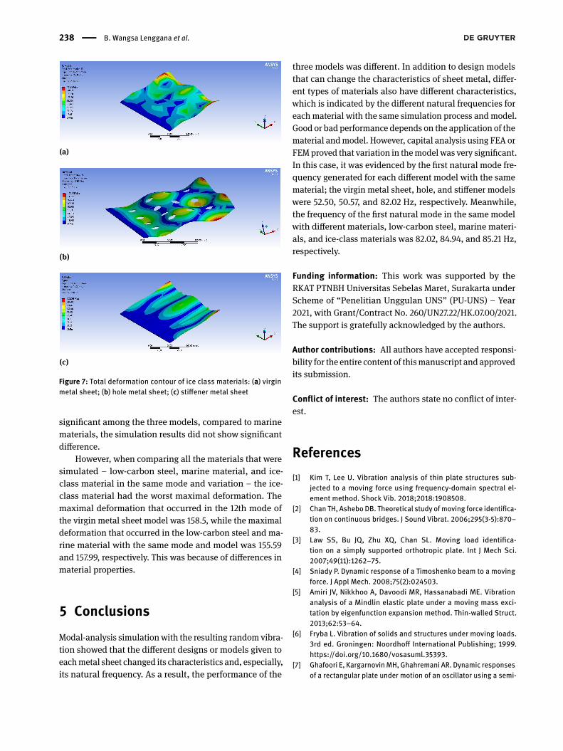
Figure 7 shows the total deformation contours of thesamemodel with differentmaterials. The usedmaterial wasice-class material AR 235. Although the results were very


(a)

(b)

(c)

Figure 7: Total deformation contour of ice class materials: (a) virginmetal sheet; (b) hole metal sheet; (c) stiffener metal sheet

significant among the three models, compared to marinematerials, the simulation results did not show significantdifference.

However, when comparing all the materials that weresimulated – low-carbon steel, marine material, and ice-class material in the same mode and variation – the ice-class material had the worst maximal deformation. Themaximal deformation that occurred in the 12th mode ofthe virgin metal sheet model was 158.5, while the maximaldeformation that occurred in the low-carbon steel and ma-rine material with the same mode and model was 155.59and 157.99, respectively. This was because of differences inmaterial properties.

5 ConclusionsModal-analysis simulation with the resulting random vibra-tion showed that the different designs or models given toeachmetal sheet changed its characteristics and, especially,its natural frequency. As a result, the performance of the

three models was different. In addition to design modelsthat can change the characteristics of sheet metal, differ-ent types of materials also have different characteristics,which is indicated by the different natural frequencies foreach material with the same simulation process and model.Good or bad performance depends on the application of thematerial andmodel. However, capital analysis using FEA orFEMproved that variation in themodel was very significant.In this case, it was evidenced by the first natural mode fre-quency generated for each different model with the samematerial; the virgin metal sheet, hole, and stiffener modelswere 52.50, 50.57, and 82.02 Hz, respectively. Meanwhile,the frequency of the first natural mode in the same modelwith different materials, low-carbon steel, marine materi-als, and ice-class materials was 82.02, 84.94, and 85.21 Hz,respectively.

Funding information: This work was supported by theRKAT PTNBH Universitas Sebelas Maret, Surakarta underScheme of “Penelitian Unggulan UNS” (PU-UNS) – Year2021, with Grant/Contract No. 260/UN27.22/HK.07.00/2021.The support is gratefully acknowledged by the authors.

Author contributions: All authors have accepted responsi-bility for the entire content of thismanuscript and approvedits submission.

Conflict of interest: The authors state no conflict of inter-est.

References[1] Kim T, Lee U. Vibration analysis of thin plate structures sub-

jected to a moving force using frequency-domain spectral el-ement method. Shock Vib. 2018;2018:1908508.

[2] Chan TH, Ashebo DB. Theoretical study ofmoving force identifica-tion on continuous bridges. J Sound Vibrat. 2006;295(3-5):870–83.

[3] Law SS, Bu JQ, Zhu XQ, Chan SL. Moving load identifica-tion on a simply supported orthotropic plate. Int J Mech Sci.2007;49(11):1262–75.

[4] Sniady P. Dynamic response of a Timoshenko beam to a movingforce. J Appl Mech. 2008;75(2):024503.

[5] Amiri JV, Nikkhoo A, Davoodi MR, Hassanabadi ME. Vibrationanalysis of a Mindlin elastic plate under a moving mass exci-tation by eigenfunction expansion method. Thin-walled Struct.2013;62:53–64.

[6] Fryba L. Vibration of solids and structures under moving loads.3rd ed. Groningen: Noordhoff International Publishing; 1999.https://doi.org/10.1680/vosasuml.35393.

[7] Ghafoori E, KargarnovinMH, Ghahremani AR. Dynamic responsesof a rectangular plate under motion of an oscillator using a semi-

https://doi.org/10.1680/vosasuml.35393


analytical method. J Vib Control. 2011;17(9):1310–24.[8] Bajer CI, Dyniewicz B. Numerical analysis of vibrations of

structures under moving inertial load. Berlin: Springer; 2012.https://doi.org/10.1007/978-3-642-29548-5.

[9] Shadnam MR, Rofooei FR, Mofid M, Mehri B. Periodicity in theresponse of nonlinear plate, under moving mass. Thin-walledStruct. 2002;40(3):283–95.

[10] Yang Y, Ding H, Chen LQ. Dynamic response to a moving load of aTimoshenko beam resting on a nonlinear viscoelastic foundation.Acta Mech Sin. 2013;29(5):718–27.

[11] Vosoughi AR, Malekzadeh P, Razi H. Response of moderatelythick laminated composite plates on elastic foundation sub-jected to moving load. Compos Struct. 2013;97:286–95.

[12] Wang X, Jin C. Differential quadrature analysis of moving loadproblems. Adv Appl Math Mech. 2016;8(4):536–55.

[13] Esmailzadeh E, Ghorashi M. Vibration analysis of Timo-shenko beams subjected to a traveling mass. J Sound Vibrat.1997;199(4):615–28.

[14] Gbadeyan JA, Dada MS. Dynamic response of a Mindlin elasticrectangular plate under a distributed moving mass. Int J MechSci. 2006;48(3):323–40.

[15] Wu JS, Lee ML, Lai TS. The dynamic analysis of a flat plate underamoving load by the finite element method. Int J Numer MethodsEng. 1987;24(4):743–62.

[16] Wu JJ, Whittaker AR, Cartmell MP. The use of finite element tech-niques for calculating the dynamic response of structures tomoving loads. Comput Struc. 2000;78(6):789–99.

[17] Ghafoori E, Asghari M. Dynamic analysis of laminated compositeplates traversed by a moving mass based on a firstorder theory.Compos Struct. 2010;92(8):1865–76.

[18] Mohebpour SR, Malekzadeh P, Ahmadzadeh AA. Dynamic analy-sis of laminated composite plates subjected to a moving oscilla-tor by FEM. Compos Struct. 2011;93(6):1574–83.

[19] Baltzis KB. The finite element method magnetics (FEMM) free-ware package:May it serve as an educational tool in teachingelectromagnetics? Educ Inf Technol. 2010;15(1):19–36.

[20] Meeker D. Finite element method magnetics version 4.2 usermanual;2015.

[21] Li WH, Du H, Guo NQ. Finite element analysis and simulation eval-uation of a magnetorheological valve. Int J Adv Manuf Technol.2003;21(6):438–45.

[22] ChenX, Liu Y. Finite elementmodeling and simulationwith ANSYSWorkbench. 2nd ed. Florida: CRC Press; 2011.

[23] Madenci E, Guven I. The finite element method and applicationsin engineering using ANSYS. New York: Springer; 2006.

[24] Wu J. Free vibration characteristics of a rectangular plate carryingmultiple three-degree-of-freedom spring–mass systems usingequivalent mass method. Int J Solids Struct. 2006;43(3-4):727–46.

[25] Ewins D. Modal Testing:Theory and Practice. New York: JohnWiley and Sons; 1984.

[26] Jrad W, Mohri F, Robin G, Daya EM, Al-Hajjar J. Analytical andfinite element solutions of free and forced vibration of unre-strained and braced thin-walled beams. J Vib Control. 2020;26(5-6):255–76.

[27] Dimitri R, Fantuzzi N, Tornabene F, Zavarise G. Innovative nu-merical methods based on SFEM and IGA for computing stressconcentrations in isotropic plates with discontinuities. Int J MechSci. 2016;118:166–87.

[28] Louhghalam A, Igusa T, Park C, Choi S, Kim K. Analysis of stressconcentrations in plates with rectangular openings by a com-bined conformal mapping – Finite element approach. Int J SolidsStruct. 2011;48(13):1991–2004.

[29] Vanam BC, Rajyalakshmi M, Inala R. Static analysis of anisotropic rectangular plate using finite element analysis (FEA). J.Mech Eng Res. 2012;4:148–62.

[30] Elsheikh A, Wang D. Large-deflection mathematical analysis ofrectangular plates. J Eng Mech. 2005;131(8):809–21.

[31] Bakker MC, Rosmanit M, Hofmeyer H. Approximate large deflec-tion analysis of simply supported rectangular plates under trans-verse loading using plate post-buckling solution. Thin-walledStruct. 2008;46(11):1224–35.

[32] Liew KM, Teo TM, Han JB. Three-dimensional static solutions ofrectangular plates by variant differential quadrature method. IntJ Mech Sci. 2001;43(7):1611–28.

[33] Alaimo A, Orlando C, Valvano S. Analytical frequency responsesolution for composite plates embedding viscoelastic layers.Aerosp Sci Technol. 2019;92:429–45.

[34] Valvano S, Alaimo A, Orlando C. Sound transmission analysis ofviscoelastic compositemultilayered shells structures. Aerospace(Basel). 2019;6(6):69.

[35] Jain NK. Analysis of stress concentration and deflection in-isotropic and orthotropic rectangular plates with central circu-lar hole under transverse static loading. Int J MechMecharon Eng.2009;3:1513–9.

[36] Chaudhuri RA. Stress concentration around a part through holeweakening laminated plate. Comput Struc. 1987;27(5):601–9.

[37] Paul TK, Rao KM. Finite element evaluation of stress concentra-tion factor of thick laminated plates under transverse loading.Comput Struc. 1989;48(2):311–7.

[38] Steen E, Byklum E. Approximate buckling strength analysis ofplates with arbitrarily oriented stiffeners. Proceedings of the17th Nordic Seminar on Computational Mechanics;2004.

[39] Troipsky MS. Stiffened plates, bending, stability, and vibration.J Appl Mech. 1976;44(3):516.

[40] Pape D, Fox AJ. Deflection Solutions for Edge Stiffened Plates.Proceedings of the 2006 IJME - INTERTECH Conference; 2006.

[41] Xuan HN, Rabczuk T, Alain SP, Dedongnie JF. A smoothed finiteelement method for plate analysis. Comput Methods Appl MechEng. 2008;197(13-16):1184–203.

[42] Das D, Prasanth S, Saha K. A variational analysis for large deflec-tion of skew plates under uniformly distributed load through do-main mapping technique. Int J Eng Sci Technol. 2009;1:16–32.

[43] Alaimo A, Orlando C, Valvano S. An alternative approach formodal analysis of stiffened thin-walled structures with advancedplate elements. Eur J Mech A, Solids. 2019;77:103820.

[44] Valvano S, Alaimo A, Orlando C. Analytical analysis of soundtransmission in passive damped multilayered shells. ComposStruct. 2020;253:112742.

[45] Moshaiov MA, Vorus WS. Elasto-plastic plate bending analysisby a boundary element method with initial plastic moments. IntJ Solids Struct. 1986;22(11):1213–29.

[46] Paiva JB, Aliabadi MH. Bending moments at interfaces ofthin zoned plates with discrete thickness by the boundary ele-ment method. Eng Anal Bound Elem. 2004;28(7):747–51.

[47] Ramkrishna D, Kumar KK, Krishna Y. Modal testing of beamsusing Translation-AngularPiezo-beam (TAP) accelerometer. AdvVib Eng. 2008;7:7–14.

https://doi.org/10.1007/978-3-642-29548-5


[48] Hu S, Chen W, Gou XF. Modal analysis of fractional derivationdamping model of frequency-dependent viscoelastic soft matter.Adv Vib Eng. 2011;10:187–96.

[49] Liu F, Fan R. Experimental Modal Analysis and Random Vibra-tion Simulation of Printed Circuit Board Assembly. Adv Vib Eng.2013;15:489–98.

[50] Fei WH, Kun-kun J, Zi-peng G. Random vibration analysis for thechassis frame of hydraulic truck based on ANSYS. J Chem Pharm.2014;6:849–52.

[51] De Boni LA, Lima da Silva IN. Monitoring the transesterifica-tion reaction with laser spectroscopy. Fuel Process Technol.2011;92(5):1001–6.

[52] Turner WM, Clough RW, Martin RW, Topp L. Stiffness anddeflection analysis of complex structures. J Aeronaut Sci.1956;25(9):805–23.

[53] Timoshenko WS, Goodier JN. Theory of elasticity. 3rd ed. NewYork: McGraw-Hill; 1970.

[54] Song O. Modal analysis of a cantilever plate. New Jersey: NewJersey Institute of Technology; 1986.

[55] Bahiuddin I, Mazlan SA, Shapiai I, Imaduddin F, Ubaidillah, ChoiSB. Ubaidillah, Choi SB. Constitutive models of magnetorheolog-ical fluids having temperature-dependent prediction parameter.Smart Mater Struct. 2018;27(9):095001.

[56] Suyitno ZA, Ahmad AS, Argatya TS. Ubaidillah. Optimizationparameters and synthesis of fluorine doped tin oxide for dye-sensitized solar cells. Appl Mech Mater. 2014;575:689–95.

[57] Ridwan R, Prabowo AR, Muhayat N, Putranto T, Sohn JM. Tensileanalysis and assessment of carbon and alloy steels using FEapproach as an idealization of material fractures under collisionand grounding. Curved Layer Struct. 2020;7(1):188–98.

[58] Prabowo AR, Laksono FB, Sohn JM. Investigation of structuralperformance subjected to impact loading using finite elementapproach:case of ship-container collision. Curved Layer Struct.2020;7(1):17–28.

[59] Shabdin MK, Rahman MA, Mazlan SA. Ubaidillah, Hapipi NM,Adiputra D, Aziz SAA, Bahiuddin I, Choi SB. Material characteri-zations of gr-based magnetorheological elastomer for possiblesensor applications:Rheological and resistivity properties. Ma-terials (Basel). 2019;12(3):391.

[60] Courant R. Variational methods for the solution of problemsof equilibrium and vibration. Bull New Ser Am Math Soc.1943;49(1):1–23.

[61] Prabowo AR, Sohn JM. Nonlinear dynamic behaviors of outershell and upper deck structures subjected to impact loading inmaritime environment. Curved Layer Struct. 2019;6(1):146–60.

[62] Clough RW. The finite element method in plane stress analysis.Proceedings of the 2nd ASCE Conference on Electronic Computa-tion; 1960.

[63] Zienkiewicz OC, Cheung YK. The finite element method in struc-tural and continuum mechanics. Volume 1. New York: McGraw-Hill. New York; 1967.

[64] Prabowo AR, Sohn JM, Putranto T. Crashworthiness perfor-mance of stiffened bottom tank structure subjected to impactloading conditions:Ship-rock interaction. Curved Layer Struct.2019;6(1):245–58.

[65] Clough RW. Original formulation of the finite element method.ASCE Structures Congress Session on Computer Utilization inStructural Engineering; 1989.

[66] Argyris J, Tenek L. Recent advances in computational ther-mostructural analysis of composite plates and shells with strongnonlinearities. Appl Mech Rev. 1997;50(5):285–306.

[67] Prabowo AR, Cao B, Sohn JM, Bae DM. Crashworthiness assess-ment of thin-walled double bottom tanker:Influences of seabedto structural damage and damage-energy formulae for groundingdamage calculations. J Ocean Eng Sci. 2020;5(4):387–400.

[68] Tatsumi A, Fujikubo M. Ultimate strength of container shipssubjected to combined hogging moment and bottom localloads part 1:Nonlinear finite element analysis. Mar Structures.2020;69:102683.

[69] PrabowoAR, DoQT, Cao B, Bae DM. Land andmarine-based struc-tures subjected to explosion loading:A review on critical trans-portation and infrastructure. Procedia Struct Integr. 2020;27:77–84.

[70] Pasaoglu Bozkurt A. Effects ofmechanical vibration onminiscrewimplants and bone: fem analysis. Int Orthod. 2019 Mar;17(1):38–44.

Effects of mechanical vibration on designed steel-based plate ...

Documents

Transcript of Effects of mechanical vibration on designed steel-based plate ...