Effects of field plot size on prediction accuracy of aboveground biomass in airborne laser...

Mauya et al. Carbon Balance and Management (2015) 10:10 DOI 10.1186/s13021-015-0021-x

RESEARCH Open Access

Effects of field plot size on prediction accuracy ofaboveground biomass in airborne laserscanning-assisted inventories in tropicalrain forests of TanzaniaErnest William Mauya1*, Endre Hofstad Hansen1, Terje Gobakken1, Ole Martin Bollandsås1,Rogers Ernest Malimbwi2 and Erik Næsset1

Abstract

Background: Airborne laser scanning (ALS) has recently emerged as a promising tool to acquire auxiliaryinformation for improving aboveground biomass (AGB) estimation in sample-based forest inventories. Underdesign-based and model-assisted inferential frameworks, the estimation relies on a model that relates the auxiliaryALS metrics to AGB estimated on ground plots. The size of the field plots has been identified as one source ofmodel uncertainty because of the so-called boundary effects which increases with decreasing plot size. Recent re-search in tropical forests has aimed to quantify the boundary effects on model prediction accuracy, but evidence ofthe consequences for the final AGB estimates is lacking. In this study we analyzed the effect of field plot size onmodel prediction accuracy and its implication when used in a model-assisted inferential framework.

Results: The results showed that the prediction accuracy of the model improved as the plot size increased. Theadjusted R2 increased from 0.35 to 0.74 while the relative root mean square error decreased from 63.6 to 29.2%.Indicators of boundary effects were identified and confirmed to have significant effects on the model residuals.Variance estimates of model-assisted mean AGB relative to corresponding variance estimates of pure field-basedAGB, decreased with increasing plot size in the range from 200 to 3000 m2. The variance ratio of field-based esti-mates relative to model-assisted variance ranged from 1.7 to 7.7.

Conclusions: This study showed that the relative improvement in precision of AGB estimation when increasingfield-plot size, was greater for an ALS-assisted inventory compared to that of a pure field-based inventory.

Keywords: Airborne laser scanning; Model-assisted estimation; Plot size; Aboveground biomass

BackgroundTropical forests play an important role in the global car-bon cycle as they store about 40% of the global terres-trial carbon, and absorb larger amounts of CO2 from theatmosphere than any other vegetation type [1]. Despitetheir potential, tropical forests continue to be exploitedat alarming rates, by being converted into secondary for-est and many other forms of land use. In an effort toconserve tropical forests, the United Nations Framework

* Correspondence: [email protected] of Ecology and Natural Resource Management, NorwegianUniversity of Life Sciences, P.O. Box 5003, Oslo, NO 1432, Ås, NorwayFull list of author information is available at the end of the article

© 2015 Mauya et al.; licensee Springer. This is aAttribution License (http://creativecommons.orin any medium, provided the original work is p

Convention on Climate Change (UNFCCC) has devel-oped the mechanism called Reducing Emissions fromDeforestation and Forest Degradation in tropical coun-tries (REDD+). There is high interest in seeing such ini-tiatives to take form, but a key limitation for successfulimplementation of REDD+ is reliable methods for quan-tifying forest aboveground biomass (AGB) [2,3]. Suchmethods are important because payments for carbon off-sets under REDD+ are based on estimates of carbonstock and stock changes over time. Moreover, AGB in-formation is also useful for understanding the contribu-tion of the tropical forests to the global carbon cycle andecosystem processes [4].

n Open Access article distributed under the terms of the Creative Commonsg/licenses/by/4.0), which permits unrestricted use, distribution, and reproductionroperly credited.

mailto:[email protected]

http://creativecommons.org/licenses/by/4.0

Mauya et al. Carbon Balance and Management (2015) 10:10 of 14

Airborne laser scanning (ALS) has emerged as one ofthe most promising remote sensing technologies to sup-port AGB forest inventories in boreal-, temperate-, andtropical forests [5]. A particular strength of ALS for for-est applications is its ability to accurately characterizethe three-dimensional (3D) structure of the forest canopy[6]. Such information is more useful for forest inventoriesthan the information from other remote sensing tech-niques see e.g. [7]. Height and density metrics derivedfrom the ALS data has been reported to be highly corre-lated with AGB see e.g. [8,9]. Furthermore, ALS has shownto be superior to other remote sensing data sources be-cause the relationship between AGB and the remotelysensed information has a much higher saturation level forALS compared to other types remote sensing. Because ofthis, ALS is a highly appropriate choice of technique inhigh-biomass forests. Based on its potential, ALS has re-cently been recommended for Monitoring, Reporting andVerification (MRV) systems under REDD+ initiatives [10].Estimation of AGB using ALS is often carried out

according to the area-based approach (ABA) [11]. InABA, empirical models between various metrics derivedfrom the ALS data and AGB values obtained in geo-referenced field sample plots are fitted. The area ofinterest is then tessellated into grid cells [12] with thesame size as the plots [13,14] and the developed modelsare used to provide cell-wise predictions of AGB. Finally,estimates for the particular area of interest (forest stand,forest property, village, district, or nation) are providedby summing the individual cell predictions. For some es-timation approaches, adjustment of model predictionbias [15] is also carried out.As indicated above, the modeled relationship between

ALS metrics and ground-based values is of fundamentalimportance for the outcome of the ALS-assisted estima-tion. The use of field plot data for model developmentrequires co–registration of field plot location with theALS data [16,17]. In an ALS-assisted inventory, thepoint cloud is extracted only within the plot perimeter.However, in field measurements trees are treated as be-ing inside plots if the center point of the stem is insidethe plot. This is a challenge in ALS-assisted forest inven-tory, since the crowns of trees just outside the plotborder partly extend into the plot area which means thatthe ALS data will be affected by trees that are not regis-tered in field. Conversely, also trees just inside the plotextend their crowns beyond the plot boundary. Thismeans that there may be mismatch between the datacaptured in field and from the air.In order to reduce these boundary effects, it has been

suggested in a number of studies to use larger plots inALS-assisted forest inventory see e.g. [18,19]. This is be-cause, as plot size increases, the perimeter to area ratiodecreases and thus the plots include a lower proportion

of boundary-related elements. Similarly, the relative andnegative influence of a given plot positioning error is re-duced because the relative overlap between the field-and ALS-data becomes larger as plot size increases.Reduction in model errors are also expected by increas-ing plot size due to so-called spatial averaging of the er-rors [20], because both the field observations and theALS data capture more of the spatial variation as theyincrease in size. Thus, as plot sizes increase, the vari-ances of field-based and ALS-assisted estimates are ex-pected to be reduced, which means that fewer plots areneeded to reach a certain precision of an AGB estimate.However, large plots also have disadvantages by beingmore complicated to measure, which may affect the timeconsumption for collecting field measurements [21],This makes it challenging to select the “optimal” plotsize that balances the tradeoff between plot size, samplesize (number of plots), on-plot costs, traveling costs andprecision of ALS-assisted AGB estimates in different for-est types.As indicated above, plot size has a profound effect on

the precision of ALS-assisted AGB estimates for severalreasons. Likewise, the plot size has an impact on theprecision of pure field-based estimates for reasons men-tioned above; larger plots capture more of the variabilityin the area of interest and thus precision will tend to im-prove as long as the sample size is kept constant. A keyquestion is therefore if larger plots will favor ALS-assisted estimation precision to the same extent as it fa-vors field-based estimation precision. Different responsesto plot size should have a direct impact on how tropicalALS-assisted field sample surveys should be designed astheir designs currently are “optimized” for pure field-based estimation.Forest sample surveys are often designed according to

design-based (probability-based) principles. Simple ran-dom sampling is one of these principles, and analyticaland so-called design-unbiased estimators and corre-sponding variance estimators exist for a great number ofsuch designs. When auxiliary data such as those ac-quired by ALS are at hand for the entire area of interest,or at least with partial coverage of the area of interest,use of these data can greatly improve the precision overa pure field-based estimate assuming the same design.The inferential framework applied under probabilitysampling when a model is used to predict AGB usingthe ALS data is known as design-based model-assisted(MA) estimation. In the MA framework, the model isused to predict AGB for grid cells and then AGB issummed over all grid cells as indicated in the ABA, butin addition to that, the model predictions for the groundsamples are used to provide an estimate of bias in themodel predictions, which corrects the pure model-basedestimate. Several studies see e.g. [22-24] have indicated

Table 1 Selected ALS metrics for different plot sizes

Plot size (m2) n Selected variablesa

200 30 D0.F D1.L log.H80.F

300 30 D1.L log.H90.F log.D0.L

400 30 H80.F D1.L

500 30 H70.F D1.L

600 30 H70.F D1.L

700 30 H90.F D1.L

800 30 H90.F D1.L

900 30 H90.L D1.L

1000 30 Hsd.L D1.L log.D0.F

1100 30 D3.F D2.L log.H10.F

1200 30 Hmean.F D1.L

1300 30 H70.F D1.L

1400 30 D3.F D2.L log.H10.F

1500 30 H70.F D1.L

1600 30 H60.F D1.L

1700 30 H60.F D1.L

1800 30 H60.F D1.L

1900 30 H60.F D1.L

2000 25 H60.F D1.L

2100 25 H60.F D1.L

2200 24 H60.F D1.L

2300 24 H60.F D1.L

2400 24 H70.F D1.F

2500 22 H70.F D1.F

2600 22 H70.F D1.F

2700 22 H70.F D1.F

2800 22 H70.F D1.F

2900 22 H70.F D1.F

3000 22 H60.F D1.FaD0.F, D1F.and D3.F = Canopy densities corresponding to the proportion of firstechoes above fraction #0 (2 m), #1 and #3 (see text). aD0.L, D1.L andD2L. = Canopy densities corresponding to the proportion of last echoes abovefraction #0 (2 m), #1 and #2 (see text).H10.F, H60.F, H70.F, H80.F and H90.F. = ALS height percentiles of the canopyheight for the first echo.Hsd.L = Standard deviation of the canopy height of the first echoes.Hmean.F = Arithmetic mean of the first echo ALS canopy height.


the potential of MA estimation in reducing the varianceof AGB estimates in boreal forests, but apart from someindications provided by [23], neither of them has ana-lyzed how the variance of the estimates is affected bychanges in field plot sizes. In tropical forests where thecurrent study was conducted, there is even less know-ledge regarding performance of MA estimation usingALS with varying plot sizes. Several tropical studies haveexamined the effects of plot size on model prediction ac-curacy See e.g. [25-27], but none of them have assessedthe effects on the precision of AGB estimates and com-pared such precision estimates with corresponding pre-cision of field-based AGB estimates using the samesampling design, which is of fundamental importancefor designing future sample surveys serving multiplepurposes and estimation approaches.The objectives of this study were to (1) examine the

effects of field plot size on AGB regression model qual-ity, (2) assess plot boundary effect and its impact onmodel quality based on the field data, and (3) quantifythe precision of ALS-assisted estimates of AGB relativeto field-based estimates of AGB assuming the same de-sign for different plot sizes. The study was conducted intropical rain forest in Tanzania with high AGB densities,which was expected to represent a particular challengein terms of large boundary effects.

ResultsEffects of field plot size on ALS AGB predictionsTo assess the effect of plot size on ALS assisted forestinventory, we first fitted the regression models for eachof the plot sizes. The independent variables selected var-ied between the models developed for the different plotsizes (Table 1). The number of variables varied betweentwo and three. For all models, the parameter estimateswere significantly different from zero (p < 0.05) and theVIF values were <10, indicating acceptable levels ofmulticolinearity. The variability explained by separatemodels (i.e. adjusted R2) improved as the plot size in-creased, with few exceptions (Figure 1a). The adjustedR2 ranged from 0.35 for the plot size of 200 m2 to 0.74for the plot size of 3000 m2. The RMSE% values forLOOCV decreased non-linearly with increasing plot size,from 63.8 to 29.2% (Figure 1b). The MPE% values(Figure 1b) and the pattern of under predictions for plotswith high AGB were relatively lower for larger plots com-pared smaller (Figure 2). However, it should be noted thatthe number of the larger plots was relatively small.

Boundary effectsBoundary effects were studied by analyzing how the rela-tive residual errors of the models were affected by theground reference AGB of the trees in an outer bufferzone for different field plot sizes. Our results showed

that SAGBbuffer and MAGBbuffer contributed to explain-ing the variation in the relative residual errors(Table 2). Relating the absolute value of the relative re-sidual with plot size using simple linear regressionmodel indicated that there was a highly significant ef-fect of plot size (p < 0.0001). Furthermore, the param-eter estimate for plot size was negative showing thatthe relative residual is larger in absolute terms forsmall plots compared to larger plots (Table 3).

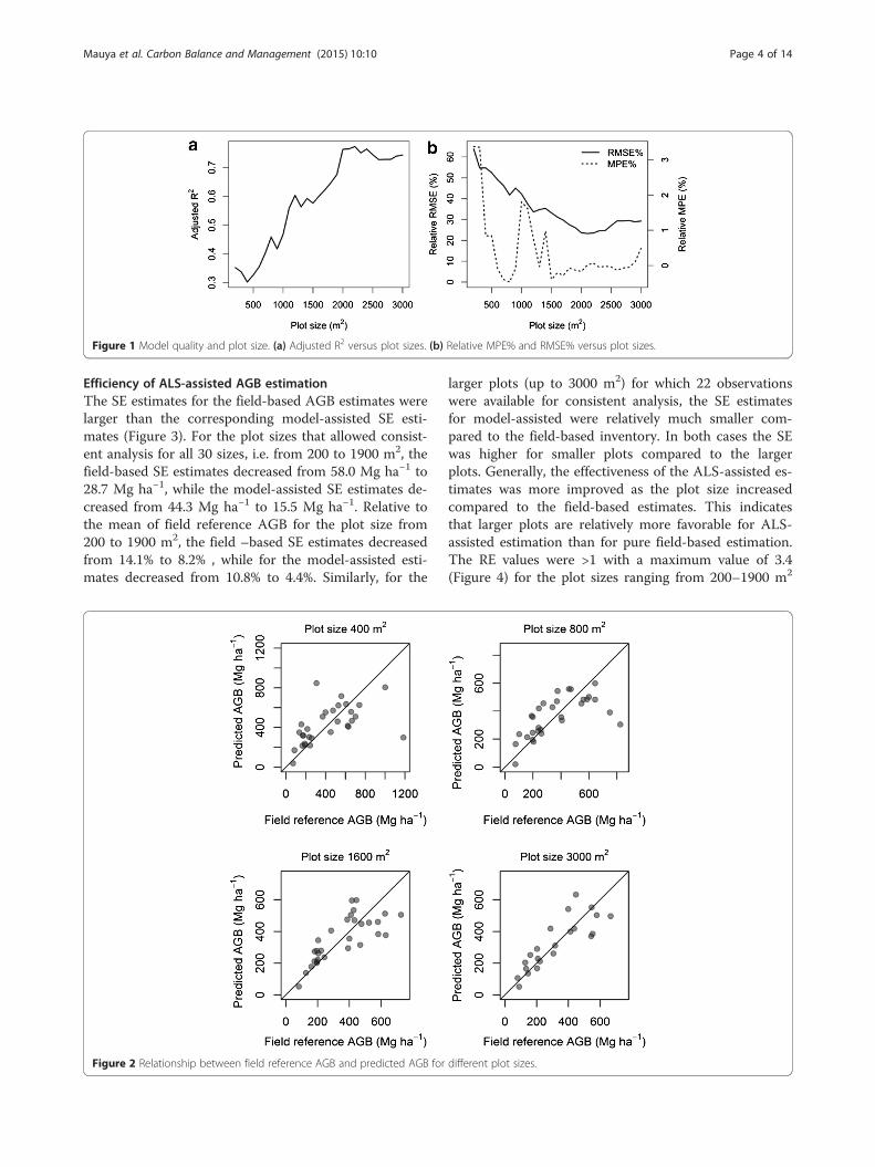
Figure 1 Model quality and plot size. (a) Adjusted R2 versus plot sizes. (b) Relative MPE% and RMSE% versus plot sizes.


Efficiency of ALS-assisted AGB estimationThe SE estimates for the field-based AGB estimates werelarger than the corresponding model-assisted SE esti-mates (Figure 3). For the plot sizes that allowed consist-ent analysis for all 30 sizes, i.e. from 200 to 1900 m2, thefield-based SE estimates decreased from 58.0 Mg ha−1 to28.7 Mg ha−1, while the model-assisted SE estimates de-creased from 44.3 Mg ha−1 to 15.5 Mg ha−1. Relative tothe mean of field reference AGB for the plot size from200 to 1900 m2, the field –based SE estimates decreasedfrom 14.1% to 8.2% , while for the model-assisted esti-mates decreased from 10.8% to 4.4%. Similarly, for the

Figure 2 Relationship between field reference AGB and predicted AGB for

larger plots (up to 3000 m2) for which 22 observationswere available for consistent analysis, the SE estimatesfor model-assisted were relatively much smaller com-pared to the field-based inventory. In both cases the SEwas higher for smaller plots compared to the largerplots. Generally, the effectiveness of the ALS-assisted es-timates was more improved as the plot size increasedcompared to the field-based estimates. This indicatesthat larger plots are relatively more favorable for ALS-assisted estimation than for pure field-based estimation.The RE values were >1 with a maximum value of 3.4(Figure 4) for the plot sizes ranging from 200–1900 m2

different plot sizes.

Table 2 Coefficient estimates for models explaining residual errors of AGB using information extractedfrom buffer zones

Models1 Modelparameter

3 m buffer 6 m buffer

Parameter estimate p-value AIC Parameter estimate p-value AIC

Model 1 Intercept −0.0159 0.8022 297 −0.1835 0.0206 6542SAGBbuffer 0.0838 <0.0001 0.1892 <0.0001

Model 2 Intercept −0.0321 0.5826 266 0.0501 0.4674 6632MAGBbuffer 0.4865 <0.0001 0.7015 <0.0001

1Models = Two models; Model 1 uses SAGBbuffer as fixed effects with plot identity as random effect. Model 2 uses MAGBbuffer with plot identity as random effect(see text).2SAGBbuffer = Ratio of either sum of AGB at the buffer to the ground reference AGB per hectare, MAGBbuffer = ratio of Maximum AGB at the buffer to the groundreference AGB per hectare (see text).


for which we have a complete dataset of 30 plots. Forthe other set with plot size up to 3000 m2 the maximumRE value was 7.7. It should be noted that the peak inrelative efficiency for the smallest dataset (22 plots) inFigure 4 was caused by considerable change in the ob-served AGB for a single plot when increasing the plotsize beyond 2000 m2. The increasing AGB was due to alarge tree that was included in the plot measurementsonce the plot radius exceeded 25 m. This illustrates thatin a small dataset the results can be sensitive to indi-vidual observations and even to the presence of indivi-dual trees.

DiscussionThe findings of this study demonstrated the importanceof choosing appropriate field plot sizes in ALS-assistedforest inventories in tropical forests. This is particularlyimportant given that field campaigns are expensive andtime consuming, and linking field measurements withremotely sensed data in the most effective mannerwould benefit both REDD+ implementations, togetherwith all other studies related to forest carbon cycle. Thecurrent study extends previous research conducted intropical forests, by having a dataset with a wide range ofplot sizes. Furthermore, most of the previous studieshave used rectangular plots.See e.g. [18,26], whereas in this case circular plots have

been used. Circular plots are more convenient for re-mote sensing studies compared to square or rectangularplots because only a single coordinate together with aplot radius are needed to match the two data sourcesgeographically [19,28,29]. Circular plots are also withincertain sizes easier to establish in the field because theyhave one dimension (i.e. radius) that defines the plot

Table 3 Parameter estimates for the model relatingrelative residual in absolute form and plot sizes

Coefficients Parameter estimates p-value

Intercept 0.5060 <0.0001

Plot size −0.0002 <0.0001

boundary. The use of circular plots minimizes the plotboundary effects because of a smaller circumference toarea ratio than all other plot shapes. However, the visi-bility from the plot center to the perimeter on a circularplot is increasingly hampered as the plots get larger,which increase per tree measurement time for theborder trees. An increase of the area of a rectangularplot would not necessarily mean increased marginal cost(cost of including one more tree) if the width of the plotis kept constant and inclusion of trees are made withreference to the long side. However, rectangular plotsare in general more difficult to establish. For example, inrugged terrain it can be difficult to keep the sidesparallel.Our findings demonstrated empirically the positive ef-

fects of increasing plot sizes on improved predictivepower of the AGB models. The model fit (adjusted R2)of the regression models was improved as plot size in-creased. Reduced circumference to area ratio, spatialaveraging, and less effect of positioning errors are prob-ably the main reasons. The fit of our models are in linewith previous ALS-based studies in both tropical forestsand temperate forests. For example, [30] reported R2 of0.78 in the tropical rainforest of Hawaii islands while[31] reported R2 of 0.64 in a tropical rainforest of WestAfrica. Furthermore, results from the cross-validationshowed smaller RMSE% and MPE% (Figure1b) for largerplots compared to smaller plots. Similar trends havebeen reported and discussed by other authors in bothtemperate and tropical forests see e.g. [32].Plot boundary effects have been discussed in previous

studies see e.g. [16,33] as one among the sources ofmodel error in ALS-assisted inventories, particularlywhen relying on small plots. We demostrated this in twosteps; first by relating relative residuals to the sum ofAGB per hectare for all trees in the buffer (SAGBbuffer )and the maximum AGB per hectare for the largest treein the buffer (MAGBbuffer ) where we noted that theirimportance were depending on the size of the buffer.The buffer conditions as expressed both by (MAGBbuffer)and (SAGBbuffer), seemed to have more impact on the

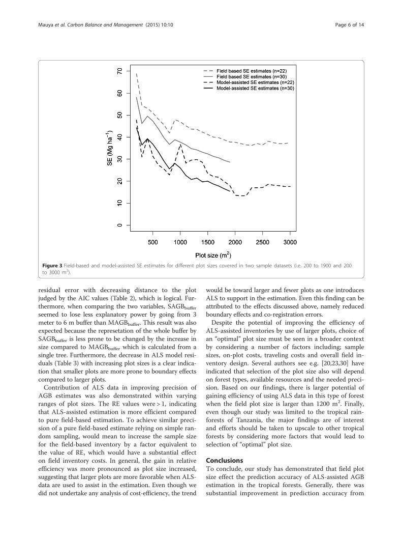
Figure 3 Field-based and model-assisted SE estimates for different plot sizes covered in two sample datasets (i.e. 200 to 1900 and 200to 3000 m2).


residual error with decreasing distance to the plotjudged by the AIC values (Table 2), which is logical. Fur-thermore, when comparing the two variables, SAGBbufferseemed to lose less explanatory power by going from 3meter to 6 m buffer than MAGBbuffer. This result was alsoexpected because the represetation of the whole buffer bySAGBbuffer is less prone to be changed by the increase insize compared to MAGBbuffer which is calculated from asingle tree. Furthermore, the decrease in ALS model resi-duals (Table 3) with increasing plot sizes is a clear indica-tion that smaller plots are more prone to boundary effectscompared to larger plots.Contribution of ALS data in improving precision of

AGB estimates was also demonstrated within varyingranges of plot sizes. The RE values were > 1, indicatingthat ALS-assisted estimation is more efficient comparedto pure field-based estimation. To achieve similar preci-sion of a pure field-based estimate relying on simple ran-dom sampling, would mean to increase the sample sizefor the field-based inventory by a factor equivalent tothe value of RE, which would have a substantial effecton field inventory costs. In general, the gain in relativeefficiency was more pronounced as plot size increased,suggesting that larger plots are more favorable when ALS-data are used to assist in the estimation. Even though wedid not undertake any analysis of cost-efficiency, the trend

would be toward larger and fewer plots as one introducesALS to support in the estimation. Even this finding can beattributed to the effects discussed above, namely reducedboundary effects and co-registration errors.Despite the potential of improving the efficiency of

ALS-assisted inventories by use of larger plots, choice ofan “optimal” plot size must be seen in a broader contextby considering a number of factors including; samplesizes, on-plot costs, traveling costs and overall field in-ventory design. Several authors see e.g. [20,23,30] haveindicated that selection of the plot size also will dependon forest types, available resources and the needed preci-sion. Based on our findings, there is larger potential ofgaining efficiency of using ALS data in this type of forestwhen the field plot size is larger than 1200 m2. Finally,even though our study was limited to the tropical rain-forests of Tanzania, the major findings are of interestand efforts should be taken to upscale to other tropicalforests by considering more factors that would lead toselection of “optimal” plot size.

ConclusionsTo conclude, our study has demonstrated that field plotsize effect the prediction accuracy of ALS-assisted AGBestimation in the tropical forests. Generally, there wassubstantial improvement in prediction accuracy from

Figure 4 Relative efficiency for different plot sizes.


larger plots compared to smaller plots. Indicators ofboundary effects were also identified and confirmed tohave significant effects on the model quality. From apurely technical point of view, our results suggested thatit is relatively more favorable to increase the plot sizewhen ALS is used to enhance the estimates. This studyshowed that there is a relative improvement in precisionof ALS-assisted AGB estimation, compared to purefield-based estimation up to around 3000 m2 in this typeof forest. However, the maximum plot size of 3000 m2 inthe current study leaves an open question as to whetherthere are any additional gains in relative precision be-yond this size. Future studies should be conducted toquantify the contribution of ALS to improve estimationprecision for even larger plots as the basis for design offuture inventories in tropical rainforests. Similar studiesshould also be conducted in other types of tropical forests.

MethodsSite descriptionThe study was conducted in Amani nature reserve(ANR), which is situated in the southern part of the EastUsambara Mountains in northern Tanzania (Figure 5). Itwas gazetted in 1997 with a protected area of 8,380 ha.ANR lies between 5°14' - 5° 04' S and 38° 30' - 38°40' E,with an altitudinal range of 190 to 1130 m above sealevel [34]. Rainfall is heavy at higher altitudes and in the

southeast of the mountain, with an average of 1900 mmannually. The dry seasons are from June to August andJanuary to March, but rainfall is frequent throughout theyear. The mean annual temperature is 20.6°C [35].

Data collectionSampling designAn initial probability sample of 173 field plots with anaverage size of 900 m2 were established across ANR ac-cording to a systematic design (450 m × 900 m distancebetween plots) in 1999–2000 by a non-governmentalconservation and development organization, FrontierTanzania [34] (Figure 5). The plots were revisited andre-measured in 2008–2012. In order to analyse plot sizeeffects on AGB estimates, a small sub-sample of 30 largeplots was established. Measurements on the 30 plotswere acquired in a separate campaign after completionof measurements of the large sample. Due to high travelcosts and long walking distances in the very steep andrough terrain, establishing a probability sample of 30large plots across the entire study area was cost-prohibitive. Instead we developed a sampling strategyby which we took advantage of the a priori knowledgeof the distribution of AGB in the large probability sam-ple and selected purposefully three sub-regions withinthe study area in which the initial plots were revisited.There is a strong altitude-dependent AGB gradient in

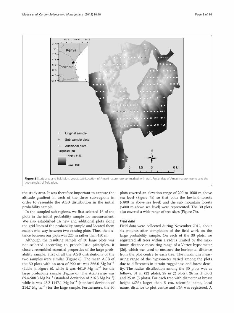
Figure 5 Study area and field plots layout. Left: Location of Amani nature reserve (marked with star). Right: Map of Amani nature reserve and thetwo samples of field plots.


the study area. It was therefore important to capture thealtitude gradient in each of the three sub-regions inorder to resemble the AGB distribution in the initialprobability sample.In the sampled sub-regions, we first selected 16 of the

plots in the initial probability sample for measurement.We also established 14 new and additional plots alongthe grid-lines of the probability sample and located themexactly mid-way between two existing plots. Thus, the dis-tance between our plots was 225 m rather than 450 m.Although the resulting sample of 30 large plots was

not selected according to probabilistic principles, itclosely resembled essential properties of the large prob-ability sample. First of all the AGB distributions of thetwo samples were similar (Figure 6). The mean AGB ofthe 30 plots with an area of 900 m2 was 366.0 Mg ha−1

(Table 4, Figure 6), while it was 461.9 Mg ha−1 for thelarge probability sample (Figure 6). The AGB range was69.4-908.3 Mg ha−1 (standard deviation of 216.3 Mg ha−1)while it was 43.2-1147.1 Mg ha−1 (standard deviation of214.7 Mg ha−1) for the large sample. Furthermore, the 30

plots covered an elevation range of 200 to 1000 m abovesea level (Figure 7a) so that both the lowland forests(<800 m above sea level) and the sub mountain forests(>800 m above sea level) were represented. The 30 plotsalso covered a wide range of tree sizes (Figure 7b).

Field dataField data were collected during November 2012, aboutsix mounts after completion of the field work on thelarge probability sample. On each of the 30 plots, weregistered all trees within a radius limited by the max-imum distance measuring range of a Vertex hypsometer[36], which was used to measure the horizontal distancefrom the plot centre to each tree. The maximum meas-uring range of the hypsometer varied among the plotsdue to differences in terrain ruggedness and forest dens-ity. The radius distribution among the 30 plots was asfollows; 31 m (22 plots), 28 m (2 plots), 26 m (1 plot)and 25 m (5 plots). For each tree with diameter at breastheight (dbh) larger than 5 cm, scientific name, localname, distance to plot centre and dbh was registered. A

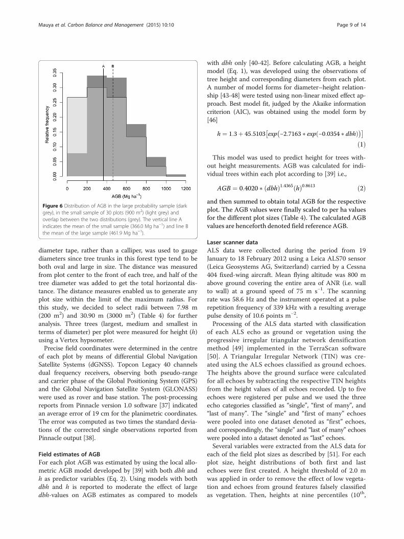
Figure 6 Distribution of AGB in the large probability sample (darkgrey), in the small sample of 30 plots (900 m2) (light grey) andoverlap between the two distributions (grey). The vertical line Aindicates the mean of the small sample (366.0 Mg ha−1) and line Bthe mean of the large sample (461.9 Mg ha−1).


diameter tape, rather than a calliper, was used to gaugediameters since tree trunks in this forest type tend to beboth oval and large in size. The distance was measuredfrom plot center to the front of each tree, and half of thetree diameter was added to get the total horizontal dis-tance. The distance measures enabled us to generate anyplot size within the limit of the maximum radius. Forthis study, we decided to select radii between 7.98 m(200 m2) and 30.90 m (3000 m2) (Table 4) for furtheranalysis. Three trees (largest, medium and smallest interms of diameter) per plot were measured for height (h)using a Vertex hypsometer.Precise field coordinates were determined in the centre

of each plot by means of differential Global NavigationSatellite Systems (dGNSS). Topcon Legacy 40 channelsdual frequency receivers, observing both pseudo-rangeand carrier phase of the Global Positioning System (GPS)and the Global Navigation Satellite System (GLONASS)were used as rover and base station. The post-processingreports from Pinnacle version 1.0 software [37] indicatedan average error of 19 cm for the planimetric coordinates.The error was computed as two times the standard devia-tions of the corrected single observations reported fromPinnacle output [38].

Field estimates of AGBFor each plot AGB was estimated by using the local allo-metric AGB model developed by [39] with both dbh andh as predictor variables (Eq. 2). Using models with bothdbh and h is reported to moderate the effect of largedbh-values on AGB estimates as compared to models

with dbh only [40-42]. Before calculating AGB, a heightmodel (Eq. 1), was developed using the observations oftree height and corresponding diameters from each plot.A number of model forms for diameter–height relation-ship [43-48] were tested using non-linear mixed effect ap-proach. Best model fit, judged by the Akaike informationcriterion (AIC), was obtained using the model form by[46]

h ¼ 1:3þ 45:5103 exp −2:7163 � exp −0:0354 � dbhð Þ�� ð1Þ

This model was used to predict height for trees with-out height measurements. AGB was calculated for indi-vidual trees within each plot according to [39] i.e.,

AGB ¼ 0:4020 � dbhð Þ1:4365 hð Þ0:8613 ð2Þand then summed to obtain total AGB for the respectiveplot. The AGB values were finally scaled to per ha valuesfor the different plot sizes (Table 4). The calculated AGBvalues are henceforth denoted field reference AGB.

Laser scanner dataALS data were collected during the period from 19January to 18 February 2012 using a Leica ALS70 sensor(Leica Geosystems AG, Switzerland) carried by a Cessna404 fixed-wing aircraft. Mean flying altitude was 800 mabove ground covering the entire area of ANR (i.e. wallto wall) at a ground speed of 75 m s−1. The scanningrate was 58.6 Hz and the instrument operated at a pulserepetition frequency of 339 kHz with a resulting averagepulse density of 10.6 points m−2.Processing of the ALS data started with classification

of each ALS echo as ground or vegetation using theprogressive irregular triangular network densificationmethod [49] implemented in the TerraScan software[50]. A Triangular Irregular Network (TIN) was cre-ated using the ALS echoes classified as ground echoes.The heights above the ground surface were calculatedfor all echoes by subtracting the respective TIN heightsfrom the height values of all echoes recorded. Up to fiveechoes were registered per pulse and we used the threeecho categories classified as “single”, “first of many”, and“last of many”. The “single” and “first of many” echoeswere pooled into one dataset denoted as “first” echoes,and correspondingly, the “single” and “last of many” echoeswere pooled into a dataset denoted as “last” echoes.Several variables were extracted from the ALS data for

each of the field plot sizes as described by [51]. For eachplot size, height distributions of both first and lastechoes were first created. A height threshold of 2.0 mwas applied in order to remove the effect of low vegeta-tion and echoes from ground features falsely classifiedas vegetation. Then, heights at nine percentiles (10th,

Table 4 Summary of field data

Plot size (m2) Number of plots (n) Mean (Mg ha−1) Standard deviation (Mg ha−1) Minimum (Mg ha−1) Maximum (Mg ha−1)

200 30 411.4 323.2 53.3 1179.5

300 30 401.0 257.3 48.2 816.0

400 30 424.5 275.8 72.6 1185.2

500 30 413.8 263.4 77.8 1148.0

600 30 395.3 243.9 87.9 1066.6

700 30 371.8 221.5 75.4 931.7

800 30 363.1 204.4 74.3 824.3

900 30 366.0 216.3 69.4 908.3

1000 30 367.1 210.1 62.4 859.7

1100 30 365.6 203.0 66.4 839.5

1200 30 365.0 193.7 78.4 797.6

1300 30 361.0 190.5 82.1 757.9

1400 30 352.3 184.7 87.3 707.0

1500 30 354.2 180.4 85.5 757.8

1600 30 353.2 174.1 82.2 725.5

1700 30 355.0 170.2 95.6 702.6

1800 30 355.9 163.9 91.5 696.5

1900 30 351.1 159.6 90.7 703.3

2000 25 352.2 170.8 89.6 669.3

2100 25 350.4 168.0 85.5 646.2

2200 24 344.7 169.3 89.3 631.1

2300 24 343.0 167.8 88.5 639.8

2400 24 344.2 171.3 87.9 677.7

2500 22 332.1 175.0 84.4 661.5

2600 22 334.1 183.1 91.8 669.9

2700 22 328.0 179.8 88.6 674.7

2800 22 322.7 177.7 85.4 665.9

2900 22 323.5 177.9 82.5 655.6

3000 22 321.0 179.7 79.7 666.7

Number of plots for the different plot sizes together with mean field reference AGB values with corresponding standard deviation, minimum, and maximum.


20th, …, 90th) of both the first- and last echo distribu-tions were computed to represent canopy height and la-beled H10.F, H20.F, …, H90.F (first echoes) and H10.L,H20.L, …, H90.L (last echoes), respectively. Measures ofcanopy density were also derived for first and lastechoes of each plot size. The range between the lowestALS canopy height (>2 m) and the 95th percentile heightwas divided into 10 vertical fractions of equal height.Canopy densities were then computed as the proportionof ALS echoes above each fraction to total number offirst echoes and labeled D0.F (>2 m), D1.F, …, D9.F.Density variables for the last echo distribution were cal-culated the same way (relative to total number of lastechoes) and labeled D0.L, D1.L, …, D9.L. Furthermore,for both first and last echo height distributions on eachplot, the maximum height (Hmax..F and Hmax.L ), mean

values (Hmean..F and Hmean.L), standard deviation (Hsd.Fand Hsd.L), coefficient of variation (Hcv.F and Hcv.L),and skewness (Hskewness.F and Hskewness.L) were computed.

Data analysesModel developmentMultiple linear regression analysis with ordinary leastsquare regression (OLS) was used to develop the statis-tical models relating the field reference AGB and thepredictor variables from the ALS data. To ensure thatour modelling approaches met the basic assumptions ofOLS, the response variable was transformed to logarith-mic scale [11,52], while for the predictors both log trans-formed and non-transformed variables were used.Separate models with log transformed response andcombination of log transformed and non-transformed

Figure 7 Distributions of field plots, elevation, number of trees per ha and tree sizes. (a) Number of field plots versus elevation. (b) Number oftrees per ha versus tree sizes.


predictor variables were fitted for each of the plot sizes.We decided to fit separate models (unique variablecombinations) for each of the plot sizes, because wewanted the model for each plot size to be the “best”and not be constrained by forcing specific variablesinto the model.Variable selection was conducted by using reg-subset

in the leaps package in R [53]. The selection of the vari-ables was limited to the best combinations of three orfewer variables in order to avoid multicollinearity amongcandidate predictors. The preferred models were chosenbased on the Bayesian information criterion (BIC) [54].Adjusted R2 was also used for assessing the model fitwhile multicollinearity was assessed by computing thevariance inflation factors (VIF). The VIF values were de-termined for the individual β parameters. VIF valuesgreater than 10 were regarded as an indication of multi-collinearity problems [55].Log-transformation of the response variable introduces

a bias when back-transforming to the arithmetic scale.The model for AGB was therefore adjusted for logarith-mic bias according to [56] by adding half of the modelmean square error to the constant term before trans-formation to arithmetic scale.

Model validation and accuracy assessmentIn order to assess the performance of the models foreach plot size, leave-one-out cross–validation (LOOCV)

was performed. One field plot at a time was excludedfrom the dataset, and the model was fitted based on n-1plots to predict the AGB of the left out plot. Here, n de-notes the number of field plots, where i = 1,…, n. Rela-tive root mean square error (RMSE %) and the meanprediction error (MPE%) were used as the measures ofreliability and calculated according to

RMSE% ¼ffiffiffiffiffiffiffiffiffiffiffiffiffiffiffiffiffiffiffiffiffiffiffiffiffiffiffiffiffiffiffiffiffiXn

i¼1yi−byið Þ2=n

qy

� 100 ð3Þ

MPE% ¼Xn

i¼1yi−byið Þ=ny

� 100 ð4Þ

Where yi and byi denote field reference AGB and pre-dicted AGB for plot i, respectively, and �y denotes meanfield reference AGB for all plots. RMSE% is a goodmeasure of how accurately the model predicts the re-sponse and is the most important criterion for fit if themain purpose of the model is prediction [57].

Analysis of boundary effectsTo analyze the boundary effects we studied how the re-sidual errors of the models were related to the field ref-erence AGB of the trees in an outer buffer zone fordifferent field plot sizes. To archive this, we extractedfield reference AGB values for 3 m and 6 m buffers out-side the field plots for the plot sizes of 200–1500 m2 and


200–1100 m2, respectively. We selected the trees withdbh > 10 cm and computed AGB per hectare for the lar-gest tree in the buffer and the total AGB per hectare forall trees in the buffer. To obtain the model residualerror, we first subtracted the ground reference AGBfrom the predicted AGB. Then we calculated the ratiobetween the residuals and the total field reference AGBfor the respective plot (i.e., relative residual). Similar ra-tios between (1) sum of AGB per hectare for all trees inthe buffer (SAGBbuffer) and the field reference AGB forthe plot and (2) the maximum AGB per hectare for thelargest tree in the buffer (MAGBbuffer,) and the field ref-erence AGB for the plot were also computed. Two em-pirical models explaining the variation in the relativeresidual values using either SAGBbuffer or MAGBbuffer asexplanatory variables were developed. Linear mixed ef-fects (LME) regression using nlme add-on package [58]in R was used for model fitting. LME models are linearregression models in which parameters are the sum ofthe fixed and random effects. In this case the fixed ef-fects were either SAGBbuffer or MAGBbuffer while plotidentity was treated as the random effect. We assumedthat each plot will have different random error struc-tures and that the distribution of AGB within these plotsis not independent of one another. To test the effect ofplot sizes on relative residual, we also fitted the linear re-gression model which relates relative residuals in abso-lute form and plot sizes. Absolute value was used becausewe were interested in the magnitude of the residual re-gardless of its sign.

Efficiency of ALS-assisted AGB estimationALS-assisted estimation of AGB within the design-basedand model-assisted inferential framework can greatly im-prove the precision compared to pure field-based esti-mation. The purpose of this analysis was to quantify thegain in estimated precision of using ALS data relative toa pure field-based estimate for increasing plot sizes.A basic requirement for validity of design-based infer-

ence is the availability of a probability sample [59]. Asstated above, the current sample of 30 plots was ob-tained as a subsample of a probability sample, but thesub-sampling was not conducted according to strictprobabilistic principles. However, the sub-sample was se-lected to resemble important properties of the largeprobability sample as closely as practically feasible. Thus,a comparison of variances using the current data and as-suming a probabilistic design will most likely introducea bias in the estimators of unknown magnitude. Like-wise, when a systematic sample is obtained, it is com-mon to adopt design-based estimators assuming e.g.simple random sampling (SRS) although it is well-known that SRS variance estimators usually are posi-tively biased under systematic sampling. The magnitude

of the bias is always unknown for a particular sample be-cause bias is a property of an estimator and not a particularsample. The current analysis was conducted under the as-sumption that the sample at hand would give a meaningfulquantification of the effect of plot size on relative varianceestimates. Thus, in the current study we adopted design-based variance estimators assuming simple random sam-pling and complete cover of ALS data.Assuming SRS, the variance estimator for the field-

based AGB estimate ignoring corrections for finite popu-lation is [60].

bV field ¼Xn

i¼1 yi−�yð Þ2n n−1ð Þ ð5Þ

For model-assisted estimation, the variance estimatorof the so-called generalized regression estimator is [60].

bVALS ¼Xn

i¼1 ei−�eð Þ2n n−1ð Þ ð6Þ

where ei ¼ yi−byi is the model prediction residual for plot

i and �e ¼Xn

i¼1 ein is the mean residual for all plots.

Standard error (SE) was computed as the square root ofthe variance estimates. Finally, the relative efficiency(RE) of ALS-assisted inventory relative to field-based in-ventory was calculated for different plot sizes as the ratioof the two variance estimates, i.e.,

RE ¼ bV field

�bVALS ð7Þ

Values of RE greater than 1.0 indicates higher effi-ciency of ALS-assisted estimates than field-based esti-mates for a given plot size. To achieve consistency in theanalysis across different plot sizes, the dataset was di-vided into two major groups. The first group subject toanalysis comprised all the 30 plots and allowed consist-ent analysis of plot size ranging from 200–1900 m2. Thesecond group allowing analysis from 200 to 3000 m2

consisted of 22 of the plots.

AbbreviationsALS: Airborne laser scanning; ABA: Area-based approach; AGB: Abovegroundbiomass; AIC: Akaike information criterion; ANR: Amani nature reserve;BIC: Bayesian information criterion; dGNSS: differential Global NavigationSatellite Systems; GLONASS: Global Navigation Satellite System; GPS: GlobalPositioning System; LME: Linear mixed effects; LOOCV: leave-one-outcross–validation; MA: Model-assisted; MAGBbuffer,: Maximum AGB per hectarefor the largest tree in the buffer; MPE: Mean prediction error;MRV: Monitoring, Reporting and Verification; OLS: Ordinary least squareregression; REDD+: Reducing Emissions from Deforestation and ForestDegradation in tropical countries; RMSE: Root mean square error;SAGBbuffer: Sum of AGB per hectare for all trees in the buffer; SAR: Syntheticaperture RADAR; SE: Standard error; SRS: Simple random sampling;TIN: Triangular Irregular Network; UNFCCC: United Nations FrameworkConvention on Climate Change; RE: Relative efficiency.


Competing interestsThe authors declare that they have no competing interests.

Author’s contributionsAll the authors have made substantial contribution towards successfulcompletion of this manuscript. Authors; EWM and OMB have been involvedin designing the study, drafting the manuscript, data analysis and write up.EHH has been involved in data analysis and quality control of both raw dataand results. EN and TG have been responsible for designing the ALSacquisition and they were involved in revising the manuscript. REM wasinvolved in critical discussion on the field inventory design and all logisticsrelated to the field data acquisition. All authors read and approved thefinal manuscript.

Author’s informationEWM and EHH are PhD students in forest inventory at Norwegian universityof Life Sciences (NBMU).They are both associated with the forestmensuration group in the university. OMB is the researcher in the samegroup specialized on the application of ALS in forestry. EN and TG are seniorscientists and professors in ALS and forest sampling at NMBU. Both EN andTG, are resource persons for the forest mensuration group at NMBU. REM isprofessor in forest inventory and mensuration at Sokoine university ofAgriculture, Tanzania.

AcknowledgementsThe financial support for this research was provided by Government ofNorway through the two projects entitled “Climate Change Impacts,Adaptation and Mitigation (CCIAM) in Tanzania” and “Enhancing theMeasuring, Reporting and Verification (MRV) of forests in Tanzania throughthe application of advanced remote sensing techniques”. We are highlyacknowledging our field team in Tanzania, and Terratec Norway, forcollecting and processing of the ALS data. We are also grateful to theadministration of ANR for all support, and especially for provision of officespace for establishment of the GPS base station.

Author details1Department of Ecology and Natural Resource Management, NorwegianUniversity of Life Sciences, P.O. Box 5003, Oslo, NO 1432, Ås, Norway.2Department of Forest Mensuration and Management, Sokoine University ofAgriculture, P.O. Box 3013, MorogoroTanzania.

Received: 13 November 2014 Accepted: 29 April 2015

References1. Lewis SL, Lopez-Gonzalez G, Sonké B, Affum-Baffoe K, Baker TR, Ojo LO,

et al. Increasing carbon storage in intact African tropical forests. Nature.2009;457:1003–6.

2. Joseph S, Herold M, Sunderlin WD, Verchot LV. REDD+ readiness: earlyinsights on monitoring, reporting and verification systems of projectdevelopers. Environ Res Lett. 2013;8:034038.

3. Herold M, Skutsch M: Monitoring, reporting and verification for nationalREDD plus programmes: two proposals. Environ Res Lett. 2011;6:014002.

4. Keith H, Mackey BG, Lindenmayer DB. Re-evaluation of forest biomasscarbon stocks and lessons from the world's most carbon-dense forests.Proc Natl Acad Sci. 2009;106:11635–40.

5. Hyyppä J, Hyyppä H, Leckie D, Gougeon F, Yu X, Maltamo M. Review ofmethods of small‐footprint airborne laser scanning for extracting forestinventory data in boreal forests. Int J Remote Sens. 2008;29:1339–66.

6. Vauhkonen J, Maltamo M, McRoberts RE, Næsset E: Introduction toForestry Applications of Airborne Laser Scanning. In: Maltamo M, Næsset E,Vauhkonen J, editors. Forestry applications of airborne laser scanning –concepts and case studies. Dordrecht, Netherlands: Springer; 2014. p. 1–16.

7. Coops NC, Wulder MA, Culvenor DS, St-Onge B. Comparison of forestattributes extracted from fine spatial resolution multispectral and lidar data.Can J Remote Sens. 2004;30:855–66.

8. Hansen EH, Gobakken T, Bollandsås OM, Zahabu E, Næsset E. ModelingAboveground Biomass in Dense Tropical Submontane Rainforest UsingAirborne Laser Scanner Data. Remote Sens. 2015;7:788–807.

9. Ioki K, Tsuyuki S, Hirata Y, Phua M-H, Wong WVC, Ling Z-Y, et al. Estimatingabove-ground biomass of tropical rainforest of different degradation levels

in Northern Borneo using airborne LiDAR. For Ecol Manage.2014;328:335–41.

10. Gautam B, Peuhkurinen J, Kauranne T, Gunia K, Tegel K, Latva-Käyrä P, et al.Estimation of Forest Carbon Using LiDAR-Assisted Multi-Source Programme(LAMP) in Nepal. In: Proceedings of the International Conference onAdvanced Geospatial Technologies for Sustainable Environment andCulture, Pokhara, Nepal. 2013. p. 12–3.

11. Næsset E. Predicting forest stand characteristics with airborne scanning laserusing a practical two-stage procedure and field data. Remote Sens Environ.2002;80:88–99.

12. Næsset E. Estimating timber volume of forest stands using airborne laserscanner data. Remote Sens Environ. 1997;61:246–53.

13. Næsset E, Bjerknes K-O. Estimating tree heights and number of stems inyoung forest stands using airborne laser scanner data. Remote Sens Environ.2001;78:328–40.

14. Næsset E: Area-Based Inventory in Norway–From Innovation to anOperational Reality. In: Maltamo M, Næsset E, Vauhkonen J, editors. Forestryapplications of airborne laser scanning – concepts and case studies.Dordrecht, Netherlands: Springer; 2014. p. 215–240.

15. McRoberts RE, Cohen WB, Naesset E, Stehman SV, Tomppo EO. Usingremotely sensed data to construct and assess forest attribute maps andrelated spatial products. Scand J For Res. 2010;25:340–67.

16. Frazer GW, Magnussen S, Wulder MA, Niemann KO. Simulated impact ofsample plot size and co-registration error on the accuracy and uncertaintyof LiDAR-derived estimates of forest stand biomass. Remote Sens Environ.2011;115:636–49.

17. Gobakken T, Næsset E. Assessing effects of positioning errors and sampleplot size on biophysical stand properties derived from airborne laserscanner data. Can J Forest Res. 2009;39:1036–52.

18. Mascaro J, Detto M, Asner GP, Muller-Landau HC. Evaluating uncertainty inmapping forest carbon with airborne LiDAR. Remote Sens Environ.2011;115:3770–4.

19. Næsset E, Bollandsås OM, Gobakken T, Gregoire TG, Ståhl G. Model-assistedestimation of change in forest biomass over an 11 year period in a samplesurvey supported by airborne LiDAR: A case study with post-stratification toprovide “activity data”. Remote Sens Environ. 2013;128:299–314.

20. Zolkos S, Goetz S, Dubayah R. A meta-analysis of terrestrial abovegroundbiomass estimation using lidar remote sensing. Remote Sens Environ.2013;128:289–98.

21. Asner GP, Mascaro J, Muller-Landau HC, Vieilledent G, Vaudry R, RasamoelinaM, et al. A universal airborne LiDAR approach for tropical forest carbonmapping. Oecologia. 2012;168:1147–60.

22. Gregoire TG, Ståhl G, Næsset E, Gobakken T, Nelson R, Holm S.Model-assisted estimation of biomass in a LiDAR sample survey in HedmarkCounty, Norway This article is one of a selection of papers from ExtendingForest Inventory and Monitoring over Space and Time. Can J Forest Res.2010;41:83–95.

23. Næsset E, Gobakken T, Solberg S, Gregoire TG, Nelson R, Ståhl G, et al.Model-assisted regional forest biomass estimation using LiDAR and InSAR asauxiliary data: A case study from a boreal forest area. Remote Sens Environ.2011;115:3599–614.

24. Ene LT, Næsset E, Gobakken T, Gregoire TG, Ståhl G, Nelson R. Assessing theaccuracy of regional LiDAR-based biomass estimation using a simulationapproach. Remote Sens Environ. 2012;123:579–92.

25. Asner GP, Clark JK, Mascaro J, Vaudry R, Chadwick KD, Vieilledent G, et al.Human and environmental controls over aboveground carbon storage inMadagascar. Carbon balance and management. 2012;7:2.

26. Asner GP, Mascaro J. Mapping tropical forest carbon: Calibrating plotestimates to a simple LiDAR metric. Remote Sens Environ. 2014;140:614–24.

27. Mascaro J, Asner GP, Dent DH, DeWalt SJ, Denslow JS. Scale-dependence ofaboveground carbon accumulation in secondary forests of Panama: A testof the intermediate peak hypothesis. For Ecol Manage. 2012;276:62–70.

28. Adams T, Brack C, Farrier T, Pont D, Brownlie R. So you want to useLiDAR?-a guide on how to use LiDAR in forestry. N Z J For.2011;55:19–23.

29. White JC, Wulder MA, Varhola A, Vastaranta M, Coops NC, Cook BD, et al. Abest practices guide for generating forest inventory attributes fromairborne laser scanning data using an area-based approach. For Chron.2013;89:722–3.

30. Asner GP. Tropical forest carbon assessment: integrating satellite andairborne mapping approaches. Environ Res Lett. 2009;4:034009.


31. Chen Q, Vaglio Laurin G, Battles JJ, Saah D. Integration of airborne lidar andvegetation types derived from aerial photography for mappingaboveground live biomass. Remote Sens Environ. 2012;121:108–17.

32. Gobakken T, Næsset E. Assessing effects of laser point density, groundsampling intensity, and field sample plot size on biophysical standproperties derived from airborne laser scanner data. Can J Forest Res.2008;38:1095–109.

33. Wulder MA, White JC, Nelson RF, Næsset E, Ørka HO, Coops NC, et al. Lidarsampling for large-area forest characterization: A review. Remote SensEnviron. 2012;121:196–209.

34. Doody K, Howell K, Fanning E. Amani Nature Reserve-A biodiversity survey.East Usambara Conservation Area Management Programme, TechnicalPaper 52. In: Ministry of Natural Resources and Tourism Tanzania andFrontier-Tanzania. Tanga. 2001.

35. Hamilton AC, Bensted-Smith R: Forest conservation in the East Usambaramountains, Tanzania. Gland, Switzerland: IUCN; 1989.

36. Haglöf A. Users guide Vertex III and Transponder T3. Långsele, Sweden:Haglöf Sweden, AB; 2002.

37. Anon: Pinnacle User’s Manual; Javad Positioning Systems. In: CA. Edited byJose S. USA; 1999.

38. Naesset E. Effects of differential single-and dual-frequency GPS andGLONASS observations on point accuracy under forest canopies.Photogramm Eng Remote Sens. 2001;67:1021–6.

39. Masota A: Tree allometric models for predicting above- and belowgroundbiomass of tropical rainforests in Tanzania. in press.

40. Feldpausch T, Banin L, Phillips O, Baker T, Lewis S, Quesada C, et al.Height-diameter allometry of tropical forest trees. Biogeosciences.2011;8:1081–106.

41. Banin L, Feldpausch TR, Phillips OL, Baker TR, Lloyd J, Affum-Baffoe K, et al.What controls tropical forest architecture? Testing environmental, structuraland floristic drivers. Glob Ecol Biogeogr. 2012;21:1179–90.

42. Mugasha WA, Bollandsås OM, Eid T. Relationships between diameter andheight of trees in natural tropical forest in Tanzania, Southern Forests. J ForSci. 2013;75:221–37.

43. Nilsson U, Agestam E, Ekö P-M, Elfving B, Fahlvik N, Johansson U, et al.Thinning of Scots pine and Norway spruce monocultures in Sweden. 2010.

44. Ratkowsky DA, Giles DE. Handbook of nonlinear regression models. NewYork: Marcel Dekker; 1990.

45. Richards F. A flexible growth function for empirical use. J Exp Bot.1959;10:290–301.

46. Winsor CP. The Gompertz curve as a growth curve. Proc Natl Acad SciU S A. 1932;18:1.

47. Wykoff WR, Crookston NL, Stage AR. User's guide to the stand prognosismodel. In: US Department of Agriculture, Forest Service, IntermountainForest and Range Experiment Station. 1982.

48. Yang RC, Kozak A, Smith JHG. The potential of Weibull-type functions asflexible growth curves. Can J Forest Res. 1978;8:424–31.

49. Axelsson P. Processing of laser scanner data—algorithms and applications.ISPRS J Photogramm Remote Sens. 1999;54:138–47.

50. Axelsson P. DEM generation from laser scanner data using adaptive TINmodels. Int Arch Photo Remote Sensing. 2000;33:111–8.

51. Næsset E. Practical large-scale forest stand inventory using a small-footprintairborne scanning laser. Scand J For Res. 2004;19:164–79.

52. Hudak AT, Crookston NL, Evans JS, Falkowski MJ, Smith AM, Gessler PE, et al.Regression modeling and mapping of coniferous forest basal area and treedensity from discrete-return lidar and multispectral satellite data. Can JRemote Sens. 2006;32:126–38.

53. Team RC: R: a language and environment for statistical computing. 2013. RFoundation for Statistical Computing, Vienna, Austria. In.:ISBN 3-900051-07-0; 2013.

54. Schwarz G. Estimating the dimension of a model. Ann Stat. 1978;6(2):461–4.55. Fox J, Weisberg S: An R companion to applied regression. United Kingdom:

Sage; 2011.56. Goldberger AS: The interpretation and estimation of Cobb-Douglas

functions. Econometrica: J Econc Soci. 1968:464–472

57. Yoo S, Im J, Wagner JE. Variable selection for hedonic model using machinelearning approaches: A case study in Onondaga County, NY. Landsc UrbanPlan. 2012;107:293–306.

58. Pinheiro J, Bates D, DebRoy SS, Sarkar D: D., and the R Development CoreTeam 2013. nlme: Linear and Nonlinear Mixed Effects Models. R packageversion:3.1-103.

59. McRoberts RE, Næsset E, Gobakken T. Inference for lidar-assisted estimationof forest growing stock volume. Remote Sens Environ. 2013;128:268–75.

60. Sarndal C-E, Swensson B, Wretman J: Model assisted survey sampling. NewYork: Springer-Verlag; 1992.

Submit your manuscript to a journal and benefi t from:

7 Convenient online submission

7 Rigorous peer review

7 Immediate publication on acceptance

7 Open access: articles freely available online

7 High visibility within the fi eld

7 Retaining the copyright to your article

Submit your next manuscript at 7 springeropen.com

Effects of field plot size on prediction accuracy of aboveground biomass in airborne laser...

Documents

Transcript of Effects of field plot size on prediction accuracy of aboveground biomass in airborne laser...