effects of die design, manufacturing and process parameters ...
266
EFFECTS OF DIE DESIGN, MANUFACTURING AND PROCESS PARAMETERS ON CHEVRON AND SURFACE CRACKING OF COPPER WIRE DURING WIRE DRAWING by Floyd Banda (MSc. in Manufacturing Engineering) A thesis submitted in fulfilment of the requirements of the degree of Doctor of Philosophy in Production Engineering and Management. The University of Zambia Lusaka 2018
-
Upload
khangminh22 -
Category
Documents
-
view
0 -
download
0
Transcript of effects of die design, manufacturing and process parameters ...

EFFECTS OF DIE DESIGN, MANUFACTURING AND PROCESS
PARAMETERS ON CHEVRON AND SURFACE CRACKING OF
COPPER WIRE DURING WIRE DRAWING
by
Floyd Banda
(MSc. in Manufacturing Engineering)
A thesis submitted in fulfilment of the requirements of the degree of Doctor of
Philosophy in Production Engineering and Management.
The University of Zambia
Lusaka
2018
DECLARATION
I Floyd Banda do declare that this thesis is my own work, and that it has not been
previously submitted for a degree or other qualification at this or another University.
COPYRIGHT
All rights reserved. No part of this thesis may be reproduced, stored in any retrieval
system, or transmitted in any form by any means, electronic, recording, photocopying, or
otherwise, without permission from the author or the University of Zambia.
© 2018
All rights reserved
University of Zambia
APPROVAL
This thesis of Floyd Banda has been approved as fulfilment of the requirements for the
award of the degree of Doctor of Philosophy in Production Engineering and
Management by the University of Zambia.
NAME SIGNATURE DATE
iv
ABSTRACT
The practice of copper wire drawing has faced problems regarding process, quality and
manufacturing cost and satisfying world market demand of drawn wires. Of great
importance to the practitioner are problems due to the interaction of process parameters
during wire drawing.
The present research study on the “Effects of Die Design, Manufacturing and Process
Parameters on Chevron and Surface Cracking of Copper Wire during Wire Drawing” is
based on multi-pass copper wire drawing studies from the industry and the application of
a scientific approach using the finite element method (FEM). A 2-dimensional
axisymmetric model of multi-pass copper wire drawing was developed using ABAQUS
6.14 to model and simulate the major factors contributing to and influencing the
development of both internal (chevron) and surface cracks during copper wire drawing,
with an emphasis on die bearing length variation. Drawn wire scanning electron
micrographs were used to validate the effects of bearing length variation during copper
wire drawing.
Studies showed that a good selection and application of die geometrical and process
parameters participating as an integral unit in copper wire drawing leads to the
production of a defect-free copper wire. Models showed that, except the exit angle, all
other die geometrical parameters influenced ductile damage.
Studies from the simulations and drawn wire micrographs showed that the Cockroft and
Latham damage criterion was not met in all the multi-pass stages for the internal
centerline nodes, whereas the criterion was met during the second and third multi-pass
stages for the surface nodes. The models showed that internal centreline damage is
minimised when using bearing length values between 30% and 40% while surface
damage is lower when using bearing lengths of 30%.
v
DEDICATION
I humbly and sincerely thank my family, in particular my wife Namonje Nakapizye and
the children Madalitso, Kondwelani and Pyelanji, and all the relatives and friends who
gave me support during the research period. To my recently departed friend and colleague
Eng. Coster Mwaba, thank you for all the help and support you rendered to me, and may
the Lord grant you everlasting mercies.
Above all, I am grateful to the good Lord for according me good health and making
everything possible during the course of my research work.
vi
ACKNOWLEDGEMENTS
My heartfelt gratitude and thanks go to all members of staff of the Department of
Mechanical Engineering in particular and the School of Engineering in general for their
support, patience and encouragement offered to me during my research period. In
particular, I express my gratitude and thanks to my supervisors Prof. L. Siaminwe and
Dr. H.M.Mwenda for their unwavering professional guidance throughout the research
and production of this thesis.
I would like to thank the Dean, Prof M. Muya and the Head of Mechanical Engineering
Department, Mr G.M. Munakaampe for their assistance in ensuring that all the necessary
requirements and logistics to carry out my research work were executed on time. This
made my academic life easier.
I also thank the following for their insights and co-operation during my data collection
from industry: Messiers Chad Hakamangwe, Hussein Hussein and Sundar Singh at Zalco
Limited; Brigadier General Musonda, Mr P. Sinkala and Mr Mwenda at Mupepetwe
Engineering and Contracting Company.
Many thanks go to my two sponsors, the Copperbelt University and the National Science
and Technology Council for their financial support during my research activities. Thanks
also go to Mr G. Mitchell and Mr H. Bowles at Finite Element Analysis Services (PTY)
Limited, South Africa for the technical guidance in finite element and ABAQUS
applications.
vii
TABLE OF CONTENTS
Page
Declaration ...................................................................................................................... i
Copyright ........................................................................................................................ ii
Approval ........................................................................................................................ iii
Abstract ......................................................................................................................... iv
Dedication ....................................................................................................................... v
Acknowledgements ....................................................................................................... vi
Table of Contents ......................................................................................................... vii
List of Figures ................................................................................................................ x
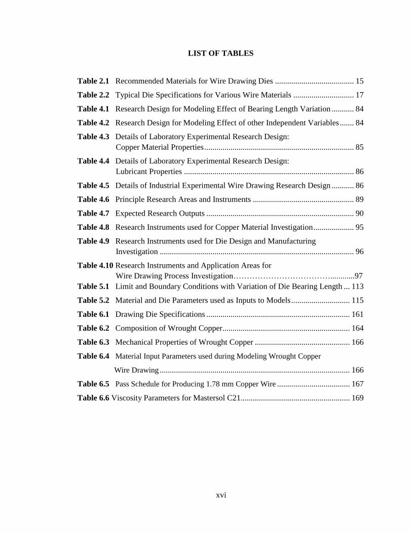
List of Tables ............................................................................................................... xvi
List of Appendices ..................................................................................................... xvii
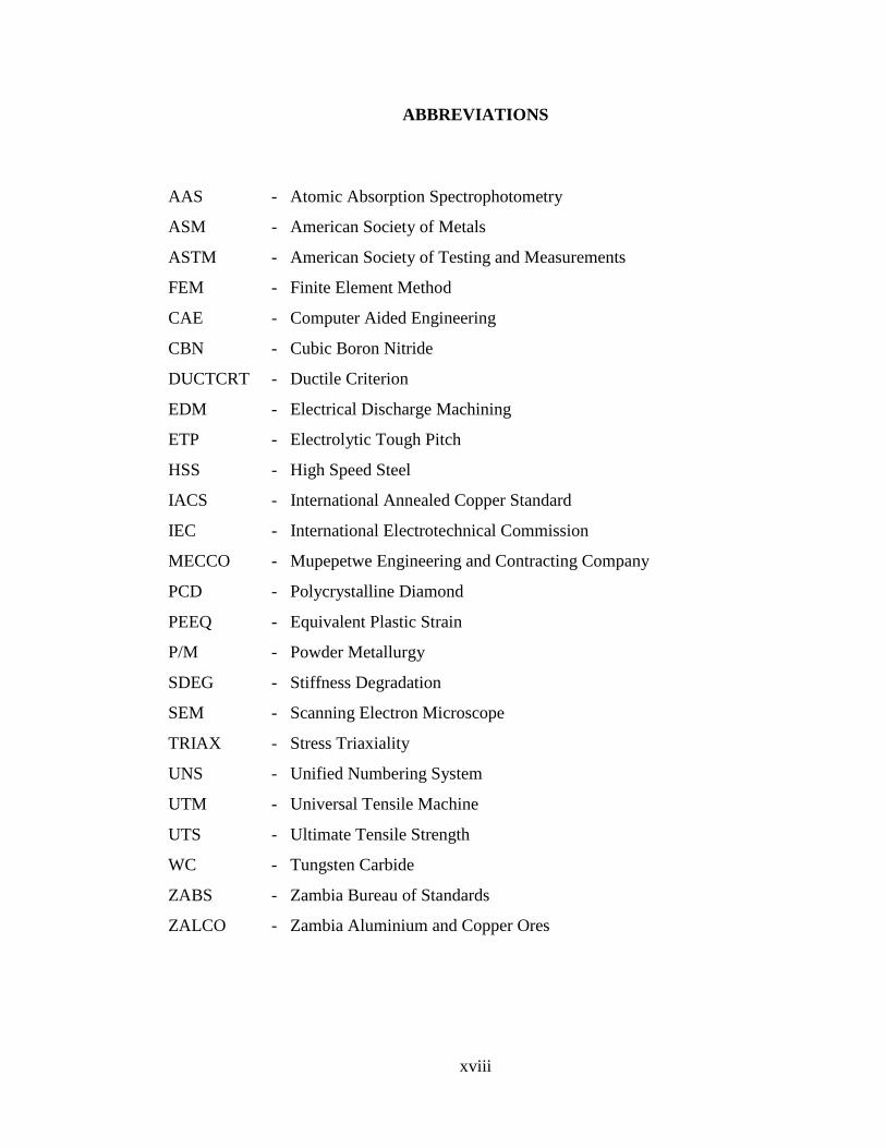
Abbreviations ............................................................................................................ xviii
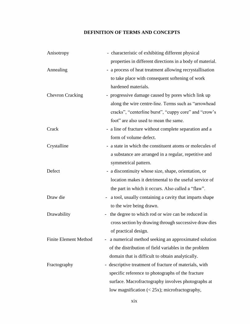
Definition of Terms and Concepts ............................................................................. xix
CHAPTER ONE: INTRODUCTION 1
1.1 Background ................................................................................................................ 1
1.2 Statement of the Problem ........................................................................................... 5
1.3 Objectives of the Investigation ................................................................................. 6
1.4 Delineation and Limitations ..................................................................................... 7
1.5 Significance of Study ................................................................................................ 7
1.6 General Structure of the Thesis ................................................................................ 8
CHAPTER TWO: LITERATURE REVIEW 10
2.1 Introduction .............................................................................................................. 10
2.2 Theory of Wire Drawing ......................................................................................... 10
2.3 Crack Formation during Wire Drawing .................................................................. 34
2.4 Modelling of Wire Drawing Processes ................................................................... 41
2.5 Wire Drawing Focal Research Literature ............................................................... 43
2.6 Research Gap Analysis and Contribution ............................................................... 57
viii
CHAPTER THREE: CONCEPTUAL FRAMEWORK 62
3.1 Introduction .............................................................................................................. 62
3.2 Theoretical Framework ............................................................................................ 62
3.3 Conceptual Framework ........................................................................................... 70
3.4 Die Design and Manufactuing ................................................................................ 79
3.5 Expected Research Outcomes ................................................................................. 81
CHAPTER FOUR: RESEARCH METHODOLOGY 82
4.1 Introduction .............................................................................................................. 82
4.2 Research Design ...................................................................................................... 83
4.3 Die Design and Manufacturing ............................................................................... 87
4.4 Application of the Methods .................................................................................... 92
4.5 Major Research Instruments ................................................................................... 93
4.6 Data Collection ....................................................................................................... 98
4.7 Data Analysis ........................................................................................................ 100
4.8 Limitations ............................................................................................................ 100
4.9 Ethical Considerations .......................................................................................... 101
CHAPTER FIVE: MODELLING AND SIMULATION 102
5.1 Introduction ............................................................................................................ 102
5.2 Finite Element Method .......................................................................................... 102
5.3 Finite Element Software:ABAQUS ...................................................................... 104
5.4 Domain Discretisation .......................................................................................... 105
5.5 Constitutive Equations .......................................................................................... 106
5.6 Underlying Assumptions ...................................................................................... 109
5.7 Computational Conditions .................................................................................... 109
5.8 Results of the Simulations .................................................................................... 114
5.9 General Observations from Simulation Results ................................................... 152
5.10 Summary of Simulation Results Analysis .......................................................... 153

ix
CHAPTER SIX: EXPERIMENTAL DESIGN AND PROCEDURES 155
6.1 Introduction ............................................................................................................ 155
6.2 Experimental Design ............................................................................................. 155
6.3 Equipment and Instrumentation ............................................................................ 155
6.4 Experimental Procedure ........................................................................................ 159
6.5 Results from Experimental Procedure .................................................................. 163
6.6 Experimental Investigation Results Analysis and Discussions ............................. 191
6.7 Summary of Results from Experimental Procedure ............................................. 191
CHAPTER SEVEN: RESULTS ANALYSIS AND DISCUSSIONS 193
7.1 Introduction ............................................................................................................ 193
7.2 General Observations ............................................................................................. 193
7.3 Analysis and Discussion of Results ...................................................................... 193
7.4 Effects of Bearing Length Variation ..................................................................... 208
CHAPTER EIGHT: CONCLUSIONS AND RECOMMENDATIONS 212
8.1 General Conclusions .............................................................................................. 212
8.2 Summary of Conclusions ....................................................................................... 213
8.3 Summary of Contributions ................................................................................... 215
8.4 Suggestions for Further Research ......................................................................... 215
8.5 Recommendations for Implementation ................................................................ 216
REFERENCES ......................................................................................................... 217
APPENDICES ........................................................................................................... 224
x
LIST OF FIGURES
Figure 1.1 Schematic Diagram of a Wire Drawing Simulator .................................... 3
Figure 1.2 Comparative Die Costs for Drawing Copper Wire .................................... 4
Figure 1.3 Wear and Toughness Ranges for Different Die Materials ......................... 5
Figure 2.1 Scheme of Wire Drawing Process ............................................................ 11
Figure 2.2 Schematic of a Draw Bench ..................................................................... 12
Figure 2.3 Multistage Wire Drawing Machine .......................................................... 13
Figure 2.4 Profile of a Drawing Die .......................................................................... 16
Figure 2.5 Flow Sheet for Powder Metallurgy Processing ........................................ 19
Figure 2.6 Compacting Machine ................................................................................ 20
Figure 2.7 Vacuum Furnace........................................................................................ 21
Figure 2.8 Variation of Stress with Strain ................................................................. 27
Figure 2.9 Process Variables in Wire Drawing ......................................................... 29
Figure 2.10 Chevron Cracks in Drawn Copper Wire .................................................. 35
Figure 2.11 Domain for Eulerian Formulation of Wire Drawing ................................ 42
Figure 2.12 Interdependence of Die, Material and Process Parameters
in Wire Drawing ....................................................................................... 44
Figure 2.13 Machine-Die System Level Investigation of Wire Drawing Process ...... 61
Figure 3.1 Die-Wire Interaction and Process Parameters .......................................... 63
Figure 3.2 Material Parameters in Copper Wire Drawing ......................................... 64
Figure 3.3 Conditions for Ductile Damage during Copper Wire Drawing ............... 67
Figure 3.4 Influence of Wire Drawing Parameters on Wire Quality ......................... 69
Figure 3.5 Independent Variables in Copper Wire Drawing ..................................... 72
Figure 3.6 Dependent Variables during Copper Wire Drawing ................................ 75
Figure 3.7 Integrated Model for Copper Wire Output Quality .................................. 78
Figure 3.8 Procedure for Determination of Optimum Variables for Copper Wire
Drawing .................................................................................................... 79
Figure 3.9 Flowchart for Die Design and Prototype Manufacturing ......................... 80
Figure 3.10 Expected Outcomes during Copper Wire Drawing Study ....................... 81
Figure 5.1 The Process of Finite Element Analysis.................................................. 103
xi
Figure 5.2 Stages in an ABAQUS Analysis ............................................................ 105
Figure 5.3 Progressive Damage Curve of an Elasto-Plastic Material ..................... 109
Figure 5.4 Die Parameters and Boundary Conditions Setting ................................. 111
Figure 5.5 Parts Assembly for Multi-Pass Wire Drawing in ABAQUS ................. 111
Figure 5.6 Meshing and Partitioning of Copper Wire Material ............................... 112
Figure 5.7 Rigid Die Nib with Design Parameters .................................................. 114
Figure 5.8 Location of Centreline (306) and Surface (410) Nodes ......................... 115
Figure 5.9 Mises Distribution during Third (3-4) Multi-Pass Stage at
30% Bearing Length ............................................................................... 116
Figure 5.10 Mises Distribution during Third (3-4) Multi-Pass Stage at
35% Bearing Length ............................................................................... 117
Figure 5.11 Mises Distribution during Third (3-4) Multi-Pass Stage at
40% Bearing Length ............................................................................... 117
Figure 5.12 Mises Distribution during Third (3-4) Multi-Pass Stage at
45% Bearing Length ............................................................................... 118
Figure 5.13 Mises Distribution during Third (3-4) Multi-Pass Stage at
50% Bearing Length ............................................................................... 118
Figure 5.14 Distribution of Equivalent Plastic Strain with Die Geometry for
Centreline (306) Node ............................................................................ 121
Figure 5.15 Distribution of Equivalent Plastic Strain with Die Geometry for
Surface (410) Node ................................................................................ 122
Figure 5.16 Distribution of Equivalent Plastic Strain with Drawing Process
Conditions for Centreline (306) Node .................................................... 123
Figure 5.17 Distribution of Equivalent Plastic Strain with Drawing Process
Conditions for Surface (410)Node.......................................................... 124
Figure 5.18 Distribution of Mises Equivalent Stress with Die Geometry for
Centreline (306) Node ............................................................................ 126
Figure 5.19 Distribution of Mises Equivalent Stress with Die Geometry for
Surface (410) Node ................................................................................. 127
Figure 5.20 Distribution of Mises Equivalent Stress with Drawing Process
Conditions for Centreline (306) Node .................................................... 128
Figure 5.21 Distribution of Mises Equivalent Stress with Drawing Process
Conditions for Surface (410) Node......................................................... 129
Figure 5.22 Distribution of Hydrostatic Stress with Die Geometry for
xii
Centreline (306) Node ............................................................................ 130
Figure 5.23 Distribution of Hydrostatic Stress with Die Geometry for
Surface (410) Node ................................................................................. 131
Figure 5.24 Distribution of Hydrostatic Stress with Drawing Process
Conditions for Centreline (306) Node .................................................... 132
Figure 5.25 Distribution of Hydrostatic Stress with Drawing Process
Conditions for Surface (410) Node......................................................... 133
Figure 5.26 Distribution of Stress Triaxiality with Die Geometry for
Centreline (306) Node ............................................................................ 135
Figure 5.27 Distribution of Stress Triaxiality with Die Geometry for
Surface (410) Node ................................................................................. 136
Figure 5.28 Distribution of Stress Triaxiality with Drawing Process
Conditions for Centreline (306) Node .................................................... 137
Figure 5.29 Distribution of Stress Triaxiality with Drawing Process
Conditions for Surface (410) Node......................................................... 138
Figure 5.30 Distribution of Ductile Criterion (DUCTCRT) with Die Geometry for
Centreline (306) Node ............................................................................ 139
Figure 5.31 Distribution of Ductile Criterion (DUCTCRT) with Die Geometry for
Surface (410) Node ................................................................................. 140
Figure 5.32 Distribution of Ductile Criterion (DUCTCRT) with Drawing Process
Conditions for Centreline (306) Node ................................................... 141
Figure 5.33 Distribution of Ductile Criterion (DUCTCRT) with Drawing Process
Conditions for Surface (410) Node......................................................... 142
Figure 5.34 Distribution of Cockroft and Latham Criterion with Die Geometry
for Centreline (306) Node ....................................................................... 144
Figure 5.35 Distribution of Cockroft and Latham Criterion with Die Geometry
for Surface (410) Node ........................................................................... 145
Figure 5.36 Distribution of Cockroft and Latham Criterion with Drawing
Process Conditions for Centreline (306) Node ....................................... 146
Figure 5.37 Distribution of Cockroft and Latham Criterion with Drawing
Process Conditions for Surface (410) Node ........................................... 147
Figure 5.38 Distribution of Damage Value with Die Geometry for
Centreline (306) Node ............................................................................ 148
Figure 5.39 Distribution of Damage Value with Die Geometry for
Centreline (306) Node ............................................................................ 149
Figure 5.40 Distribution of Damage Value with Drawing Process
Conditions for Centreline (306) Node .................................................... 150
xiii
Figure 5.41 Distribution of Damage Value with Drawing Process
Conditions for Surface (306) Node......................................................... 151
Figure 6.1 Olympus B203 Light Microscope ........................................................... 156
Figure 6.2 Quanta FEG 450 Scanning Electron Microscope.................................... 157
Figure 6.3 Tensile Testing Machine TUE C-600 ..................................................... 157
Figure 6.4 Copper Wire Drawing Machine Components ......................................... 158
Figure 6.5 Wire-Die Assembly ................................................................................. 159
Figure 6.6 Prototype Dies used in Copper Wire Drawing ........................................ 160
Figure 6.7 Die Location in Wire Drawing Machine ............................................... 162
Figure 6.8 Intermediate Copper Wire Drawing Machine ......................................... 163
Figure 6.9 Microstructure of Wrought Copper ......................................................... 164
Figure 6.10 Stress-Strain Diagram for Wrought Copper ............................................ 165
Figure 6.11 Cable Plant Flow Chart ........................................................................... 168
Figure 6.12 Die Zone Temperatures and Area Reductions for
Different Wire Sizes ............................................................................... 170
Figure 6.13 Lubricant Temperature Distribution per Wire Size ................................ 171
Figure 6.14 Distribution of Annealing Temperatures at Different Wire Sizes .......... 171
Figure 6.15 Arrangement of Pulleys for Wire Speed Determination ........................ 172
Figure 6.16 Distribution of Wire Speeds during Different Wire Size Production .... 173
Figure 6.17 Distribution of Wire Tension during Production of
Different Wire Sizes ............................................................................... 174
Figure 6.18 Distribution of Drawing Force for Various Die Sizes ............................ 174
Figure 6.19 Copper "Dust" or "Fines" Accumulation with Lubricant ....................... 175
Figure 6.20 Wire Breakages ...................................................................................... 175
Figure 6.21 Frequency of Wire Breaks versus Wire Size.......................................... 176
Figure 6.22 Internal Section Micrograph for Multi-Pass 1-2 at 30%
Bearing Length ....................................................................................... 177
Figure 6.23 Surface Section Micrograph for Multi-Pass 1-2 at 30%
Bearing Length ....................................................................................... 177
Figure 6.24 Internal Section Micrograph for Multi-Pass 2-3 at 30%
Bearing Length ....................................................................................... 178
Figure 6.25 Surface Section Micrograph for Multi-Pass 2-3 at 30%

xiv
Bearing Length ....................................................................................... 178
Figure 6.26 Internal Section Micrograph for Multi-Pass 3-4 at 30%
Bearing Length ....................................................................................... 179
Figure 6.27 Surface Section Micrograph for Multi-Pass 3-4 at 30%
Bearing Length ....................................................................................... 179
Figure 6.28 Internal Section Micrograph for Multi-Pass 4-5 at 30%
Bearing Length ....................................................................................... 180
Figure 6.29 Surface Section Micrograph for Multi-Pass 4-5 at 30%
Bearing Length ....................................................................................... 180
Figure 6.30 Internal Section Micrograph for Multi-Pass 1-2 at 40%
Bearing Length ....................................................................................... 181
Figure 6.31 Surface Section Micrograph for Multi-Pass 1-2 at 40%
Bearing Length ....................................................................................... 181
Figure 6.32 Internal Section Micrograph for Multi-Pass 2-3 at 40%
Bearing Length ....................................................................................... 182
Figure 6.33 Surface Section Micrograph for Multi-Pass 2-3 at 40%
Bearing Length ....................................................................................... 182
Figure 6.34 Internal Section Micrograph for Multi-Pass 3-4 at 40%
Bearing Length ....................................................................................... 183
Figure 6.35 Surface Section Micrograph for Multi-Pass 3-4 at 40%
Bearing Length ....................................................................................... 183
Figure 6.36 Internal Section Micrograph for Multi-Pass 4-5 at 40%
Bearing Length ....................................................................................... 184
Figure 6.37 Surface Section Micrograph for Multi-Pass 4-5 at 40%
Bearing Length ....................................................................................... 184
Figure 6.38 Internal Section Micrograph for Multi-Pass 1-2 at 50%
Bearing Length ....................................................................................... 185
Figure 6.39 Surface Section Micrograph for Multi-Pass 1-2 at 50%
Bearing Length ....................................................................................... 185
Figure 6.40 Internal Section Micrograph for Multi-Pass 2-3 at 50%
Bearing Length ....................................................................................... 186
Figure 6.41 Surface Section Micrograph for Multi-Pass 2-3 at 50%
Bearing Length ....................................................................................... 186
Figure 6.42 Internal Section Micrograph for Multi-Pass 3-4 at 50%
Bearing Length ....................................................................................... 187
xv
Figure 6.43 Surface Section Micrograph for Multi-Pass 3-4 at 50%
Bearing Length ....................................................................................... 187
Figure 6.44 Internal Section Micrograph for Multi-Pass 4-5 at 50%
Bearing Length ....................................................................................... 188
Figure 6.45 Surface Section Micrograph for Multi-Pass 4-5 at 50%
Bearing Length ....................................................................................... 188
Figure 6.46 Measured Void Sizes on a Micrograph .................................................. 189
Figure 6.47 Variation of Measured Internal Crack Length with Bearing Length ..... 190
Figure 6.48 Variation of Measured Surface Crack Length with Bearing Length...... 190
Figure 7.1 Distribution of Drawing Force and Stress during Multi-Pass
Wire Drawing .......................................................................................... 200
Figure 7.2 Distribution of Drawing Force with Die Size during Multi-Pass
Wire Drawing .......................................................................................... 201
Figure 7.3 Distribution of % Elongation and Δ-Parameter with Area Reduction ..... 202
Figure 7.4 Distribution of Strain Rate for Centreline (306) Node ............................. 203
Figure 7.5 Distribution of Strain Rate for Surface (410) Node ................................. 203
Figure 7.6 Variation of Δ - Parameter with Area Reduction for Different Multi-
Passes ....................................................................................................... 205
xvi
LIST OF TABLES
Table 2.1 Recommended Materials for Wire Drawing Dies ....................................... 15
Table 2.2 Typical Die Specifications for Various Wire Materials .............................. 17
Table 4.1 Research Design for Modeling Effect of Bearing Length Variation ........... 84
Table 4.2 Research Design for Modeling Effect of other Independent Variables ....... 84
Table 4.3 Details of Laboratory Experimental Research Design:
Copper Material Properties .......................................................................... 85
Table 4.4 Details of Laboratory Experimental Research Design:
Lubricant Properties .................................................................................... 86
Table 4.5 Details of Industrial Experimental Wire Drawing Research Design ........... 86
Table 4.6 Principle Research Areas and Instruments .................................................. 89
Table 4.7 Expected Research Outputs ......................................................................... 90
Table 4.8 Research Instruments used for Copper Material Investigation .................... 95
Table 4.9 Research Instruments used for Die Design and Manufacturing
Investigation ................................................................................................ 96
Table 4.10 Research Instruments and Application Areas for
Wire Drawing Process Investigation………………………………............97
Table 5.1 Limit and Boundary Conditions with Variation of Die Bearing Length ... 113
Table 5.2 Material and Die Parameters used as Inputs to Models ............................. 115
Table 6.1 Drawing Die Specifications ....................................................................... 161
Table 6.2 Composition of Wrought Copper............................................................... 164
Table 6.3 Mechanical Properties of Wrought Copper ............................................... 166
Table 6.4 Material Input Parameters used during Modeling Wrought Copper
Wire Drawing .............................................................................................. 166
Table 6.5 Pass Schedule for Producing 1.78 mm Copper Wire .................................... 167
Table 6.6 Viscosity Parameters for Mastersol C21...................................................... 169

xvii
LIST OF APPENDICES
Appendix 1: Properties of Pure Copper ....................................................................... 225
Appendix 2: Properties of Wrought Copper ................................................................ 226
Appendix 3: Delta (Δ) Parameter Values For Various Approach Semi angles and
Reductions in Wire Drawing .................................................................. 227
Appendix 4: ABAQUS Simulation Output File .......................................................... 229
Appendix 5: Values from Stress-Strain Diagram for Wrought Copper ...................... 235
Appendix 6: Pass Schedule for Producing Various Copper Wire Sizes ...................... 236
Appendix 7: Die Design Drawings .............................................................................. 238
xviii
ABBREVIATIONS
AAS - Atomic Absorption Spectrophotometry
ASM - American Society of Metals
ASTM - American Society of Testing and Measurements
FEM - Finite Element Method
CAE - Computer Aided Engineering
CBN - Cubic Boron Nitride
DUCTCRT - Ductile Criterion
EDM - Electrical Discharge Machining
ETP - Electrolytic Tough Pitch
HSS - High Speed Steel
IACS - International Annealed Copper Standard
IEC - International Electrotechnical Commission
MECCO - Mupepetwe Engineering and Contracting Company
PCD - Polycrystalline Diamond
PEEQ - Equivalent Plastic Strain
P/M - Powder Metallurgy
SDEG - Stiffness Degradation
SEM - Scanning Electron Microscope
TRIAX - Stress Triaxiality
UNS - Unified Numbering System
UTM - Universal Tensile Machine
UTS - Ultimate Tensile Strength
WC - Tungsten Carbide
ZABS - Zambia Bureau of Standards
ZALCO - Zambia Aluminium and Copper Ores
xix
DEFINITION OF TERMS AND CONCEPTS
Anisotropy - characteristic of exhibiting different physical
properties in different directions in a body of material.
Annealing - a process of heat treatment allowing recrystallisation
to take place with consequent softening of work
hardened materials.
Chevron Cracking - progressive damage caused by pores which link up
along the wire centre-line. Terms such as “arrowhead
cracks”, “centerline burst”, “cuppy core” and “crow’s
foot” are also used to mean the same.
Crack - a line of fracture without complete separation and a
form of volume defect.
Crystalline - a state in which the constituent atoms or molecules of
a substance are arranged in a regular, repetitive and
symmetrical pattern.
Defect - a discontinuity whose size, shape, orientation, or
location makes it detrimental to the useful service of
the part in which it occurs. Also called a “flaw”.
Draw die - a tool, usually containing a cavity that imparts shape
to the wire being drawn.
Drawability - the degree to which rod or wire can be reduced in
cross section by drawing through successive draw dies
of practical design.
Finite Element Method - a numerical method seeking an approximated solution
of the distribution of field variables in the problem
domain that is difficult to obtain analytically.
Fractography - descriptive treatment of fracture of materials, with
specific reference to photographs of the fracture
surface. Macrofractography involves photographs at
low magnification (< 25x); microfractography,
xx
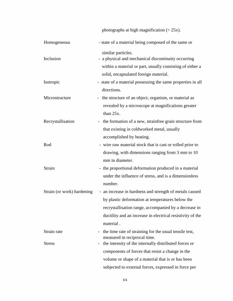
photographs at high magnification (> 25x).
Homogeneous - state of a material being composed of the same or
similar particles.
Inclusion - a physical and mechanical discontinuity occurring
within a material or part, usually consisting of either a
solid, encapsulated foreign material.
Isotropic - state of a material possessing the same properties in all
directions.
Microstructure - the structure of an object, organism, or material as
revealed by a microscope at magnifications greater
than 25x.
Recrystallisation - the formation of a new, strainfree grain structure from
that existing in coldworked metal, usually
accomplished by heating.
Rod - wire raw material stock that is cast or rolled prior to
drawing, with dimensions ranging from 3 mm to 10
mm in diameter.
Strain - the proportional deformation produced in a material
under the influence of stress, and is a dimensionless
number.
Strain (or work) hardening - an increase in hardness and strength of metals caused
by plastic deformation at temperatures below the
recrystallisation range, accompanied by a decrease in
ductility and an increase in electrical resistivity of the
material .
Strain rate - the time rate of straining for the usual tensile test,
measured in reciprocal time.
Stress - the intensity of the internally distributed forces or
components of forces that resist a change in the
volume or shape of a material that is or has been
subjected to external forces, expressed in force per
xxi
unit area.
Wear - damage to a solid surface, generally involving
progressive loss of material, due to a relative motion
between that surface and a contacting surface or
substance.
Wire drawing - a manufacturing process involving pulling wire or
rod repeatedly through a die or dies with the sole
purpose of decreasing the cross-sectional area.
Wire - product from rod or other wire with dimensions from
0.01 mm to 3 mm.
Workability - the degree to which a material may be plastically
deformed prior to fracture.
(Source: John, 1992; Higgins, 1994; Hosford and Caddell, 1983; Liu and Quek, 2003;
Wright, 2011):
1
CHAPTER 1: INTRODUCTION
1.1 Background
The production of copper and copper alloy semis has increased from less than nine
million metric tonnes in the 1980’s to over thirty million metric tonnes in 2015
(International Copper Study Group, 2016). Refined copper is consumed by semi
fabricators or “first users” such as wire rod plants among others. Copper is the best
metal conductor of electricity as it encounters much less resistance compared with other
commonly used metals and is an essential component of energy efficient generators,
motors, transformers, renewable energy production systems, power cables, domestic
subscriber lines, wide and local area networks, mobile phones and personal computers.
In addition, copper's exceptional strength, ductility and resistance to creeping and
corrosion makes it the preferred and safest conductor for commercial and residential
building wiring (International Copper Study Group, 2016).
Copper sets the standard to which other conductors are compared. Copper and copper-
based products are manufactured using extrusion, drawing, rolling, forging, electrolysis
or atomization, welding, to form wire, rod, tube, sheet, plate, strip, castings, powder
and other shapes. Wire drawing is a cold working, net shape manufacturing process
and produces long wires using dies with different profiles. In comparison to other
processes mentioned, wire drawing produces good surface finish, uses low-to-moderate
dies, equipment, and labour costs and requires low-to-moderate operator skills
(Kalpakjian and Schmid, 2010). Cold drawn wire products equally have high strengths
and very close tolerances.
In manufacturing using bulk deformation, more components are rolled and extruded
than they are wire drawn. However, in comparison to rolling, wire drawing offers better
dimensional control, lower capital equipment cost, and extension to small cross
sections. In comparison to extrusion, wire drawing offers continuous processing, lower
capital equipment costs, and extension to small sections (Wright, 2011).
2
Depending on the workpiece material condition, die material and its manufacturing
accuracy, and wire drawing process variables, drawn products can develop several
types of defects that can significantly affect their strength and product quality. Of
particular interest is the presence of chevron cracks (or center bursting) and surface
cracks in copper wire drawing which are prevalent and deteriorate the quality and
functionality of the drawn copper wire (Chia and Patel, 1996). Center bursting in wire
drawing is aligned along the wire axis, thereby reducing the wire tensile resistance and
eventually leading either to process failure, disruption of production or delayed rupture
later on, even in the absence of a load (Zompì and Levi, 2008). Chevron cracking has
been encountered in conditions of small reductions, large die angles, and low frictions
and after severe cold working of the billet (Ahmadi and Farzin, 2008).
Processing of copper into wire involves the technology of wire drawing. The wire
drawing process reduces the cross section of the initial rod using dies into wires of
different cross sections depending on the number of stages or passes of reduction (i.e
number of dies). This is a crucial and value addition stage for wire production. The
wire drawing processing of both ferrous and non-ferrous metals is beset with numerous
challenges which include:
- development of metal forming fluids to improve lubrication in the die-workpiece
interface (Canter, 2009; Kalpakjian and Schmid, 2010). This is due to lubricant
breakdown under severe drawing conditions and the quest for affordable, easily
available and biodegrable lubricants (Solomon, et al., 2010).
- development of solutions for variation in strain and residual stresses (Kalpakjian
and Schmid, 2010). This is attributed to different semi angles and area reductions
which are also affected by wear of the die.
- design and manufacturing accuracy of draw die geometry (Conoptica, 2007;
Kalpakjian and Schmid, 2010). Draw die geometrical parameters have an effect
on wire drawing forces (Kabayama, et al., 2009) and manifestation of cracks
(Norasethasopon, 2003).
- inclusion reduction (Norasethasopon, 2003). Inclusions lead to wire breakage
during processing.
3
The Finite Element Method (FEM) can be used to analyse the complex wire drawing
process. This tool is equally useful in the prediction of occurrence of defects in the
drawn wire. FEM would also supplement the lower capital costs for equipment
installation and running, thus save the organizations involved in wire drawing practice
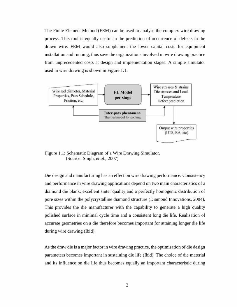
from unprecedented costs at design and implementation stages. A simple simulator
used in wire drawing is shown in Figure 1.1.
Figure 1.1: Schematic Diagram of a Wire Drawing Simulator.
(Source: Singh, et al., 2007)
Die design and manufacturing has an effect on wire drawing performance. Consistency
and performance in wire drawing applications depend on two main characteristics of a
diamond die blank: excellent sinter quality and a perfectly homogenic distribution of
pore sizes within the polycrystalline diamond structure (Diamond Innovations, 2004).
This provides the die manufacturer with the capability to generate a high quality
polished surface in minimal cycle time and a consistent long die life. Realisation of
accurate geometries on a die therefore becomes important for attaining longer die life
during wire drawing (Ibid).
As the draw die is a major factor in wire drawing practice, the optimisation of die design
parameters becomes important in sustaining die life (Ibid). The choice of die material
and its influence on die life thus becomes equally an important characteristic during
4
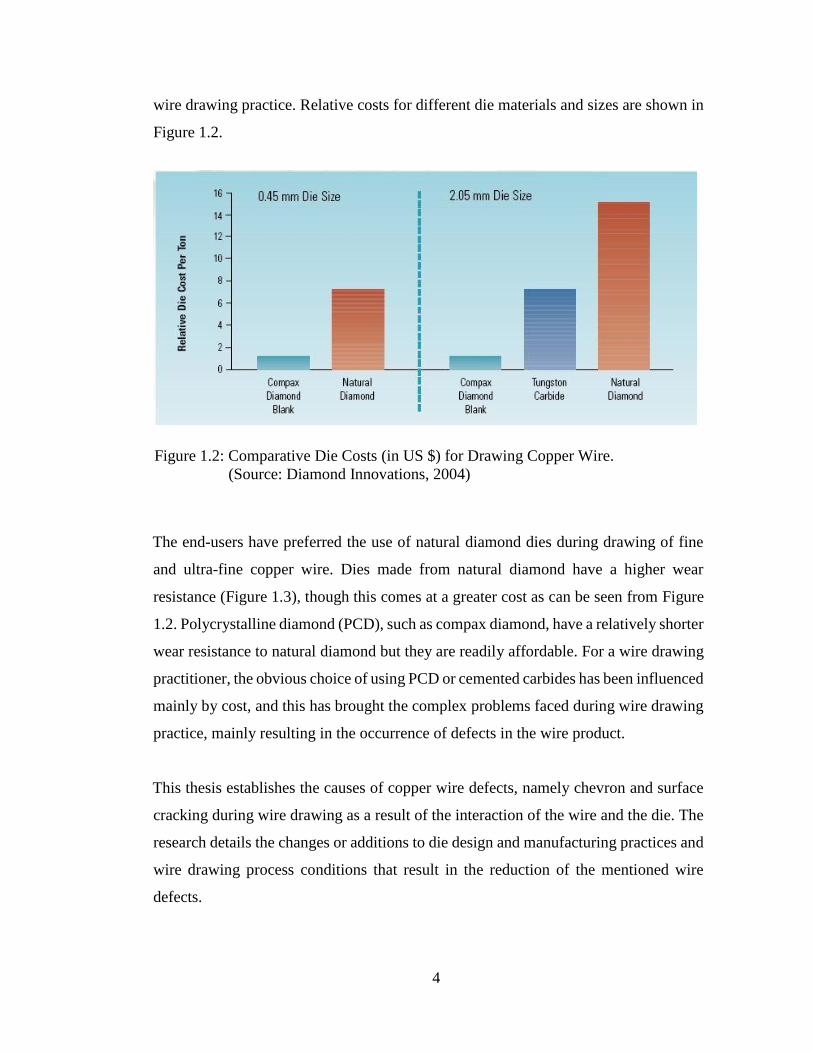
wire drawing practice. Relative costs for different die materials and sizes are shown in
Figure 1.2.
Figure 1.2: Comparative Die Costs (in US $) for Drawing Copper Wire.
(Source: Diamond Innovations, 2004)
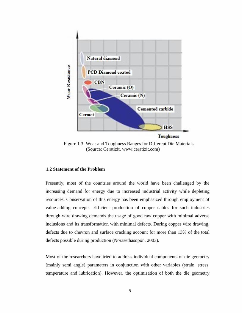
The end-users have preferred the use of natural diamond dies during drawing of fine
and ultra-fine copper wire. Dies made from natural diamond have a higher wear
resistance (Figure 1.3), though this comes at a greater cost as can be seen from Figure
1.2. Polycrystalline diamond (PCD), such as compax diamond, have a relatively shorter
wear resistance to natural diamond but they are readily affordable. For a wire drawing
practitioner, the obvious choice of using PCD or cemented carbides has been influenced
mainly by cost, and this has brought the complex problems faced during wire drawing
practice, mainly resulting in the occurrence of defects in the wire product.
This thesis establishes the causes of copper wire defects, namely chevron and surface
cracking during wire drawing as a result of the interaction of the wire and the die. The
research details the changes or additions to die design and manufacturing practices and
wire drawing process conditions that result in the reduction of the mentioned wire
defects.
5
Figure 1.3: Wear and Toughness Ranges for Different Die Materials.
(Source: Ceratizit, www.ceratizit.com)
1.2 Statement of the Problem
Presently, most of the countries around the world have been challenged by the
increasing demand for energy due to increased industrial activity while depleting
resources. Conservation of this energy has been emphasized through employment of
value-adding concepts. Efficient production of copper cables for such industries
through wire drawing demands the usage of good raw copper with minimal adverse
inclusions and its transformation with minimal defects. During copper wire drawing,
defects due to chevron and surface cracking account for more than 13% of the total
defects possible during production (Norasethasopon, 2003).
Most of the researchers have tried to address individual components of die geometry
(mainly semi angle) parameters in conjunction with other variables (strain, stress,
temperature and lubrication). However, the optimisation of both the die geometry
6
parameters (with consistent manufacturing accuracy) and wire drawing process
parameters in order to eliminate cracks (chevron and surface) is still outstanding.
Further, the combined effect of die geometrical parameters (semi angle, bearing land,
blending radius and back-relief radius) and process parameters on elimination of cracks
during wire drawing has not been addressed. Equally the impact of die design and
manufacturing methods on die wear under different temperature and lubrication
regimes and the combined effects on process and geometrical parameters during wire
drawing leading to crack formation in wire drawing demands attention.
1.3 Objectives of the Investigation
1.3.1 General Objective
The general objective of the research was to develop a copper wire drawing model to
reduce chevron and surface crack formations during the wire drawing process.
1.3.2 Specific Objectives
The specific objectives of the research were:
(i) To establish die design and manufacturing aspects influencing accuracy of
die geometry
(ii) To determine the Δ-parameter values, die geometrical parameters and
process conditions leading to the manifestation of surface and chevron
cracks during wire drawing
(iii) To develop an integrated model for die geometry and process parameters
for multi-pass copper wire drawing
(iv) To validate the developed models using industry-based copper wire drawing
process setup
7
1.4 Delineation and Limitations
The current study examined defects arising from the copper wire’s interaction with the
die, and not as a result of other means. The use of more than two dies during modelling
presented flow problems, hence all multi-pass stages were based on sequences using
two dies. Equally, models of die and wire temperatures which had an impact on die
wear and die life were not done. The effects of process and modifying conditions
leading to wear and die life were not part of the modelling or industrial experiments.
Surface roughness aspects could not be investigated due to the dies being outsourced
and lack of appropriate fixtures for copper wire clamping. Local manufacture of dies
and their consequent maintenance through re-cutting and re-polishing were not possible
due to lack of equipment and necessary instruments. Equally, wire defects due to wear
of the die and other means were not part of this study.
1.5 Significance of Study
A major concern facing the wire industry is the extremely high quantity of surface
defects that are generated during wire drawing by abrasive or delamination wear (Pops,
1997). High manufacturing costs associated with production of superfine wires has
been attributed to the breakage of wires during processing (Norasethasopon and
Yoshida, 2003). Wire drawing practice is faced with many challenges, notable of which
is the elimination of defects in form of cracks in metallic products and the development
and production of draw dies to accurate designs (Conoptica, 2007; Kalpakjian and
Schmid, 2010).
This study is important in that global manufacturing companies involved in copper
wire drawing are finding it difficult and costly to improve the quality of products and
increase production levels significantly, hence failing to cope with the high global
demand for copper wire products (Zompì and Levi, 2008; Norasethasopon and
Yoshida, 2003). Copper-based manufacturing companies also need to adopt
8
technologies and strategies to cope with the global demand for quality drawn copper
wire.
Design of drawing dies and their manufacturing has an effect on the die quality.
Improved die quality will reduce the amount of rejected dies, reduce wire production
halts, and possibly help increase wire drawing speed (Conoptica, 2007).
Potential values obtainable from the study include:
Potential of replicating improvement techniques to similar manufacturing
industries involved in copper value addition
Potential for improved productivity and competitiveness of companies
Reduced defective copper wires used in domestic electrical wiring systems,
with a potential to abate fires in homes and industries
Potential for manufacturing companies continued growth and employment
provision
1.6 General Structure of the Thesis
The thesis is divided into eight chapters and begins with the current chapter which is
the Introduction. The Introduction highlights the rationale for undertaking the study,
thereby laying a foundation for the thesis. The general and specific terms used in the
thesis are explained, including the significance of the research study.
Chapter Two is the Literature Review in which the scope and structure of the study is
reviewed. The chapter also details the general theory base and the theory for study
focus. The identified gaps in the literature are also presented. Chapter Three presents
the Conceptual Framework which highlights the interaction of research variables
used during the study. The Methodology section is presented in Chapter Four in which
the research design and methodology of data acquisition are undertaken. The chapter
also outlines the limitations encountered, including the consideration of ethical issues.

9
Chapter Five is the Modelling and Simulation chapter which presents the theory and
results of copper wire drawing modeling and simulation. The Experimental Design
and Procedures section of the thesis are given in Chapter Six which presents
experimental procedures, equipment and instrumentation used, and the results
pertaining to experimental procedures.
Chapter Seven is the Results Analysis and Discussion section of the thesis and
presents an analysis and discussions of the results from simulations and experimental
procedures. Chapter Eight is the Conclusions and Recommendations section and
gives a summary of the conclusions, contributions and recommendations for further
research.
10
CHAPTER 2: LITERATURE REVIEW
2.1 Introduction
Wire drawing practice has been going on since the 1800’s, though the practice has not
seen much modernisation. The current wire drawing equipment being used globally is the
exact replica of the ancient methods, with improvement being seen in draw die materials,
lubrication methods and the powering of the equipment using modern power systems.
Major studies concerning wire drawing have focused on improved draw die materials,
lubrication methods, optimization of drawing velocities, drawing forces and the draw die
semi angle prediction. The finite element method (FEM) has been applied extensively in
the study for prediction of optimized die design and process parameters. This chapter
presents a review of theoretical and experimental studies undertaken by various scholars
and researchers.
The chapter is divided into five sections. The first section presents the theory of wire
drawing and gives details regarding die design and manufacturing, including materials
and process parameters involved in the wire drawing process. The second section outlines
the theory behind crack initiation and propagation mechanisms during wire drawing.
The third section looks at the application of FEM in wire drawing processes while the
fourth section gives a literature review of the research so far undertaken in copper wire
drawing. The last section discusses the research gaps concerning wire drawing research
and presents the contributions this study makes to the body of knowledge.
2.2 Theory of Wire Drawing
2.2.1 Wire Drawing Process
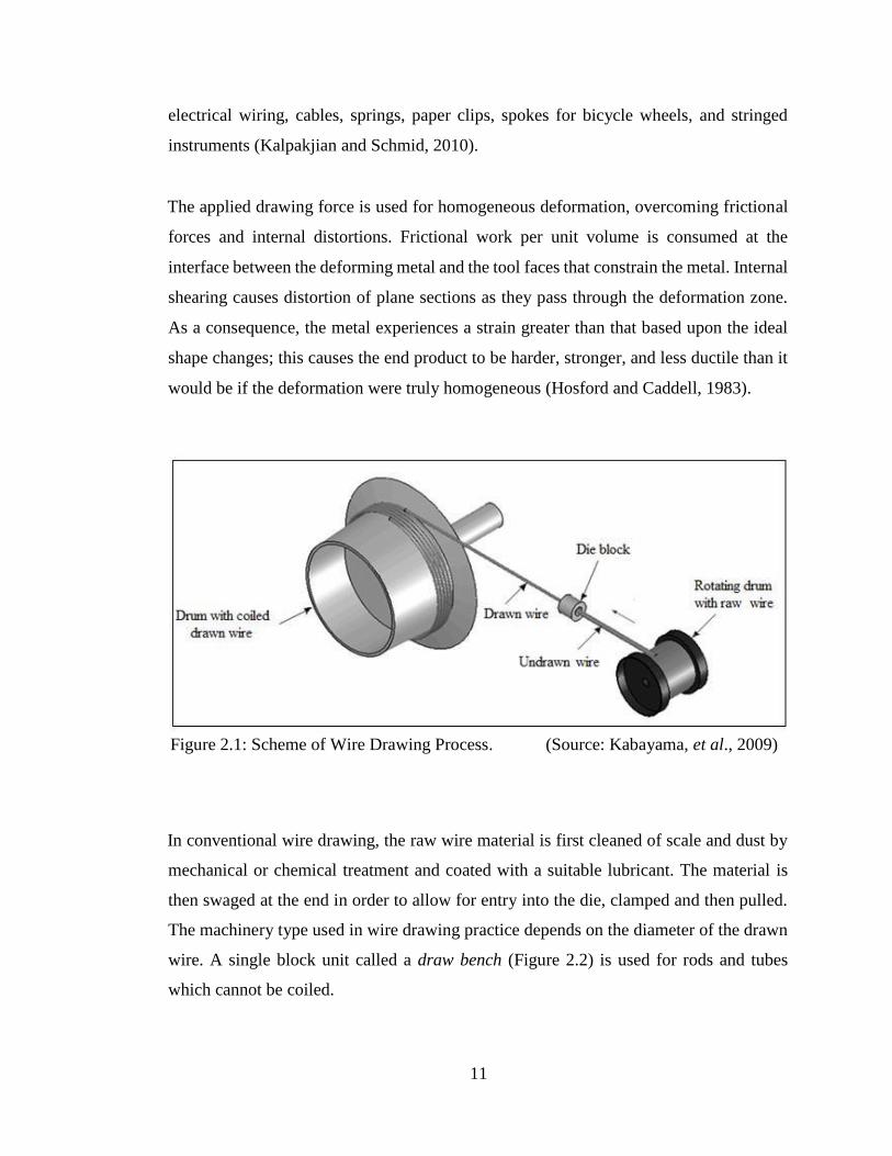
The process of wire drawing involves reducing or changing the cross section of a long
wire by pulling it through a draw die as shown in Figure 2.1. Wire products include
11
electrical wiring, cables, springs, paper clips, spokes for bicycle wheels, and stringed
instruments (Kalpakjian and Schmid, 2010).
The applied drawing force is used for homogeneous deformation, overcoming frictional
forces and internal distortions. Frictional work per unit volume is consumed at the
interface between the deforming metal and the tool faces that constrain the metal. Internal
shearing causes distortion of plane sections as they pass through the deformation zone.
As a consequence, the metal experiences a strain greater than that based upon the ideal
shape changes; this causes the end product to be harder, stronger, and less ductile than it
would be if the deformation were truly homogeneous (Hosford and Caddell, 1983).
Figure 2.1: Scheme of Wire Drawing Process. (Source: Kabayama, et al., 2009)
In conventional wire drawing, the raw wire material is first cleaned of scale and dust by
mechanical or chemical treatment and coated with a suitable lubricant. The material is
then swaged at the end in order to allow for entry into the die, clamped and then pulled.
The machinery type used in wire drawing practice depends on the diameter of the drawn
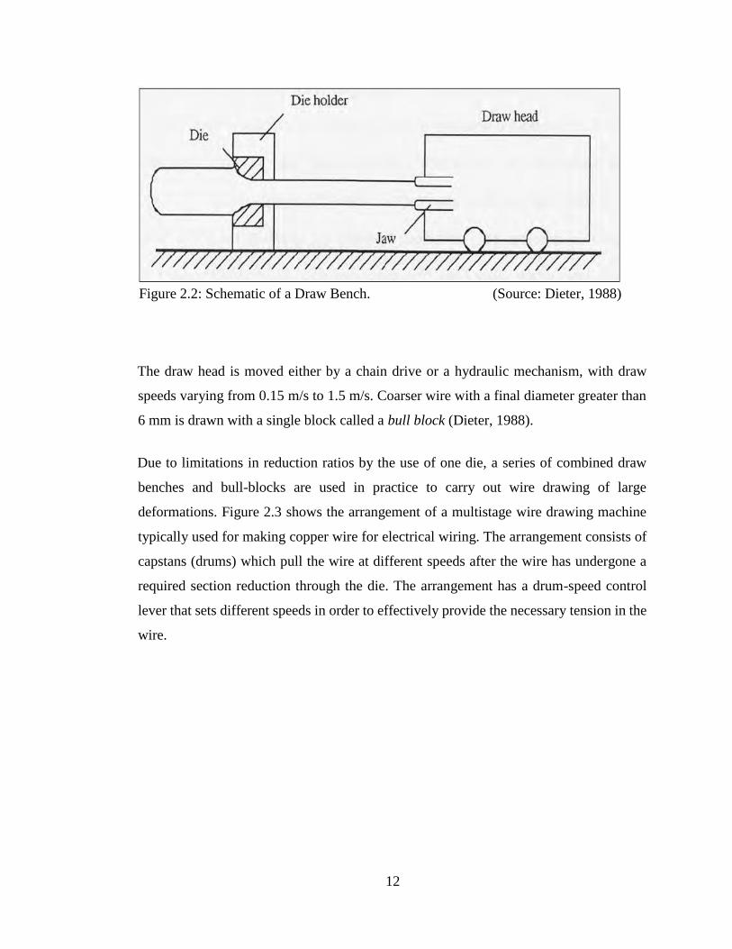
wire. A single block unit called a draw bench (Figure 2.2) is used for rods and tubes
which cannot be coiled.
12
Figure 2.2: Schematic of a Draw Bench. (Source: Dieter, 1988)
The draw head is moved either by a chain drive or a hydraulic mechanism, with draw
speeds varying from 0.15 m/s to 1.5 m/s. Coarser wire with a final diameter greater than
6 mm is drawn with a single block called a bull block (Dieter, 1988).
Due to limitations in reduction ratios by the use of one die, a series of combined draw
benches and bull-blocks are used in practice to carry out wire drawing of large
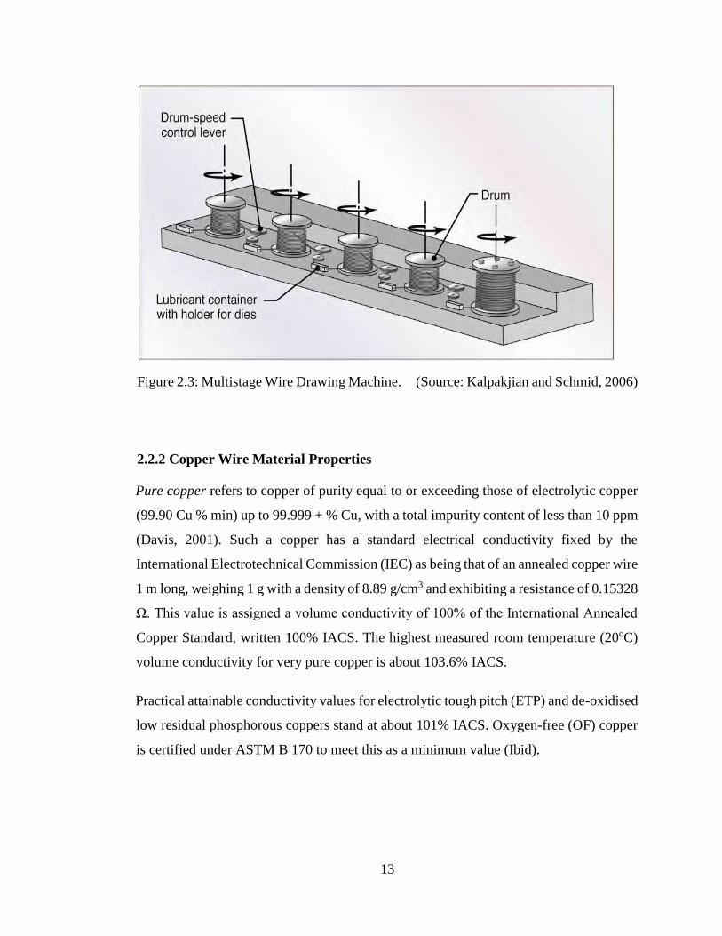
deformations. Figure 2.3 shows the arrangement of a multistage wire drawing machine
typically used for making copper wire for electrical wiring. The arrangement consists of
capstans (drums) which pull the wire at different speeds after the wire has undergone a
required section reduction through the die. The arrangement has a drum-speed control
lever that sets different speeds in order to effectively provide the necessary tension in the
wire.
13
Figure 2.3: Multistage Wire Drawing Machine. (Source: Kalpakjian and Schmid, 2006)
2.2.2 Copper Wire Material Properties
Pure copper refers to copper of purity equal to or exceeding those of electrolytic copper
(99.90 Cu % min) up to 99.999 + % Cu, with a total impurity content of less than 10 ppm
(Davis, 2001). Such a copper has a standard electrical conductivity fixed by the
International Electrotechnical Commission (IEC) as being that of an annealed copper wire
1 m long, weighing 1 g with a density of 8.89 g/cm3 and exhibiting a resistance of 0.15328
Ω. This value is assigned a volume conductivity of 100% of the International Annealed
Copper Standard, written 100% IACS. The highest measured room temperature (20oC)
volume conductivity for very pure copper is about 103.6% IACS.
Practical attainable conductivity values for electrolytic tough pitch (ETP) and de-oxidised
low residual phosphorous coppers stand at about 101% IACS. Oxygen-free (OF) copper
is certified under ASTM B 170 to meet this as a minimum value (Ibid).
14
The mechanical properties of interest for pure copper are shown in Appendix 1. The
purity of copper is influenced by processing methods, hence the copper material to be
used in this write-up refers to wrought copper and copper alloys as given in Appendix 2.
Copper alloys are identified by the Unified Numbering System (UNS) which categorizes
families of alloys based upon their elemental make-up. Wrought products range from
UNS C10000 through UNS C79999; cast products are assigned numbers between UNS
C80000 and UNS C99999 (Copper Development Association, www.copper,org).
2.2.3 Die Materials, Design and Manufacturing
(a) Die Materials
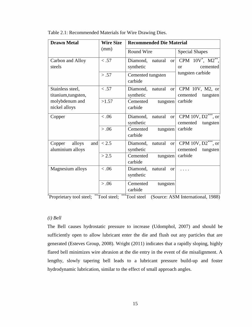
Table 2.1 shows the recommended materials for various wire drawing dies (ASM
International, 1988). The wire drawing die is a precision tool which produces round or
shaped wire to very tight tolerances. Deformation and elongation of wire material takes
place within the profile of the drawing die. A set of dies is required during profile
drawing, which involves various stages of deformation to produce the final profile.
As it can be seen from Table 2.1, wire drawing die materials typically are tool steels and
carbides. Tungsten Carbide dies are used for drawing hard wires, while diamond dies are
the choice for fine wires. For hot drawing, cast-steel dies are used because of their high
resistance to wear at elevated temperatures (Ibid).
(b) Elements of Die Design
Proper die design and the proper selection of reduction sequence per pass are necessary
for ensuring proper material flow in the die, reducing internal or external defects, and
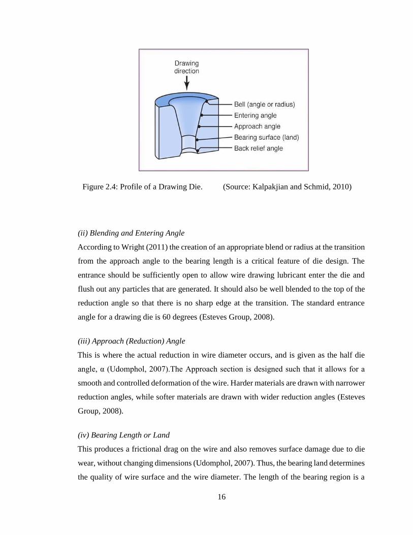
improving surface quality (Conoptica, 2007). The most important elements of die design
are shown in Figure 2.4 and include the Bell or Die Entry Geometry, Blending and
Entering Angle, Approach or Reduction Angle, Bearing Length or Land and Back Relief.
15
Table 2.1: Recommended Materials for Wire Drawing Dies.
Drawn Metal Wire Size
(mm)
Recommended Die Material
Round Wire Special Shapes
Carbon and Alloy
steels
< .57 Diamond, natural or
synthetic
CPM 10V*, M2**,
or cemented
tungsten carbide > .57 Cemented tungsten
carbide
Stainless steel,
titanium,tungsten,
molybdenum and
nickel alloys
< .57 Diamond, natural or
synthetic
CPM 10V, M2, or
cemented tungsten
carbide >1.57 Cemented tungsten
carbide
Copper < .06 Diamond, natural or
synthetic
CPM 10V, D2***, or
cemented tungsten
carbide > .06 Cemented tungsten
carbide
Copper alloys and
aluminium alloys
< 2.5 Diamond, natural or
synthetic
CPM 10V, D2***, or
cemented tungsten
carbide
> 2.5 Cemented tungsten
carbide
Magnesium alloys < .06 Diamond, natural or
synthetic
. . . .
> .06 Cemented tungsten
carbide *Proprietary tool steel; **Tool steel; ***Tool steel (Source: ASM International, 1988)
(i) Bell
The Bell causes hydrostatic pressure to increase (Udomphol, 2007) and should be
sufficiently open to allow lubricant enter the die and flush out any particles that are
generated (Esteves Group, 2008). Wright (2011) indicates that a rapidly sloping, highly
flared bell minimizes wire abrasion at the die entry in the event of die misalignment. A
lengthy, slowly tapering bell leads to a lubricant pressure build-up and foster
hydrodynamic lubrication, similar to the effect of small approach angles.
16
Figure 2.4: Profile of a Drawing Die. (Source: Kalpakjian and Schmid, 2010)
(ii) Blending and Entering Angle
According to Wright (2011) the creation of an appropriate blend or radius at the transition
from the approach angle to the bearing length is a critical feature of die design. The
entrance should be sufficiently open to allow wire drawing lubricant enter the die and
flush out any particles that are generated. It should also be well blended to the top of the
reduction angle so that there is no sharp edge at the transition. The standard entrance
angle for a drawing die is 60 degrees (Esteves Group, 2008).
(iii) Approach (Reduction) Angle
This is where the actual reduction in wire diameter occurs, and is given as the half die
angle, α (Udomphol, 2007).The Approach section is designed such that it allows for a
smooth and controlled deformation of the wire. Harder materials are drawn with narrower
reduction angles, while softer materials are drawn with wider reduction angles (Esteves
Group, 2008).
(iv) Bearing Length or Land
This produces a frictional drag on the wire and also removes surface damage due to die
wear, without changing dimensions (Udomphol, 2007). Thus, the bearing land determines
the quality of wire surface and the wire diameter. The length of the bearing region is a
17
percentage of the nominal wire diameter at about 20 to 50%, though this varies depending
on the material, process used and specifications of the wire to be drawn (Esteves Group,
2008). Wright (2011) indicates that the bearing length may vary from zero to as much as
200% of the wire diameter, though the objection to a large bearing length is the addition
to frictional work, and consequently drawing stresses.
(v) Back Relief
This allows the metal to expand slightly as the wire leaves the die, allowing for gradual
release of elastic energy and also minimising abrasion if the drawing stops or the die is
out of alignment (Udomphol, 2007; Wright, 2011). Wright (2011) argues that the back
relief should be specified with a radius and not an angle in order for it to perform its
functions better, though this complicates die manufacture.
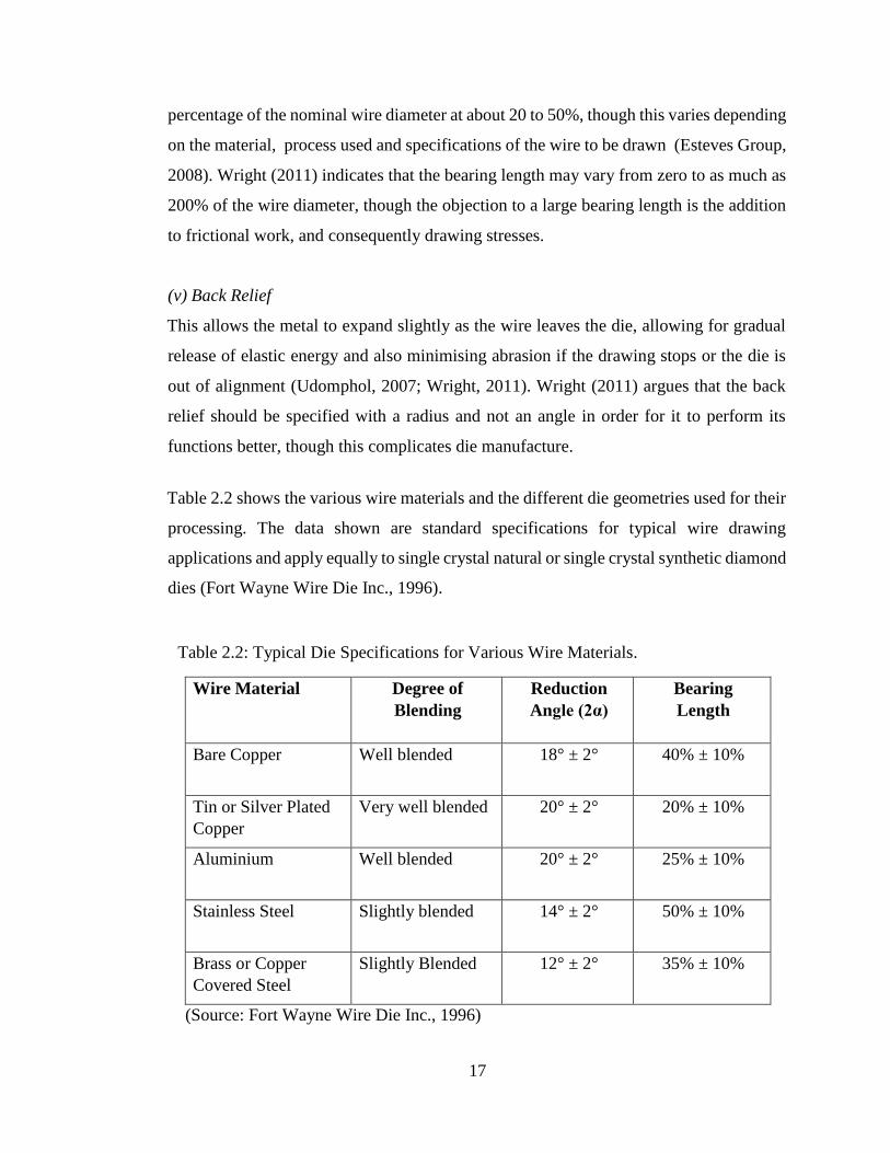
Table 2.2 shows the various wire materials and the different die geometries used for their
processing. The data shown are standard specifications for typical wire drawing
applications and apply equally to single crystal natural or single crystal synthetic diamond
dies (Fort Wayne Wire Die Inc., 1996).
Table 2.2: Typical Die Specifications for Various Wire Materials.
Wire Material Degree of
Blending
Reduction
Angle (2α)
Bearing
Length
Bare Copper Well blended 18° ± 2°
40% ± 10%
Tin or Silver Plated
Copper
Very well blended 20° ± 2°
20% ± 10%
Aluminium Well blended 20° ± 2°
25% ± 10%
Stainless Steel Slightly blended 14° ± 2°
50% ± 10%
Brass or Copper
Covered Steel
Slightly Blended 12° ± 2°
35% ± 10%
(Source: Fort Wayne Wire Die Inc., 1996)
18
In addition to die geometry, the die life depends on its size. Die life is lost by sizing dies
above the minimum allowable diameter. Sizing practice is recommended for improving
die life (Wright, 2011).
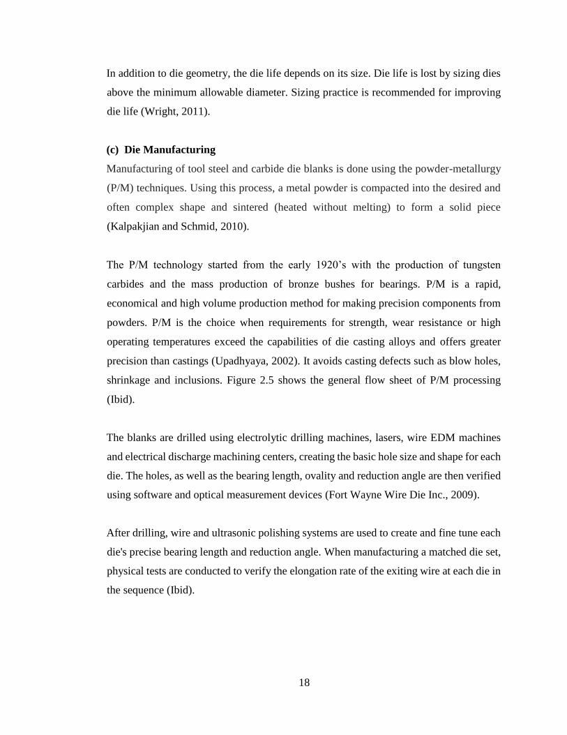
(c) Die Manufacturing
Manufacturing of tool steel and carbide die blanks is done using the powder-metallurgy
(P/M) techniques. Using this process, a metal powder is compacted into the desired and
often complex shape and sintered (heated without melting) to form a solid piece
(Kalpakjian and Schmid, 2010).
The P/M technology started from the early 1920’s with the production of tungsten
carbides and the mass production of bronze bushes for bearings. P/M is a rapid,
economical and high volume production method for making precision components from
powders. P/M is the choice when requirements for strength, wear resistance or high
operating temperatures exceed the capabilities of die casting alloys and offers greater
precision than castings (Upadhyaya, 2002). It avoids casting defects such as blow holes,
shrinkage and inclusions. Figure 2.5 shows the general flow sheet of P/M processing
(Ibid).
The blanks are drilled using electrolytic drilling machines, lasers, wire EDM machines
and electrical discharge machining centers, creating the basic hole size and shape for each
die. The holes, as well as the bearing length, ovality and reduction angle are then verified
using software and optical measurement devices (Fort Wayne Wire Die Inc., 2009).
After drilling, wire and ultrasonic polishing systems are used to create and fine tune each
die's precise bearing length and reduction angle. When manufacturing a matched die set,
physical tests are conducted to verify the elongation rate of the exiting wire at each die in
the sequence (Ibid).
19
Figure 2.5: Flow Sheet for Powder Metallurgy Processing. (Source: Upadhyaya, 2002)
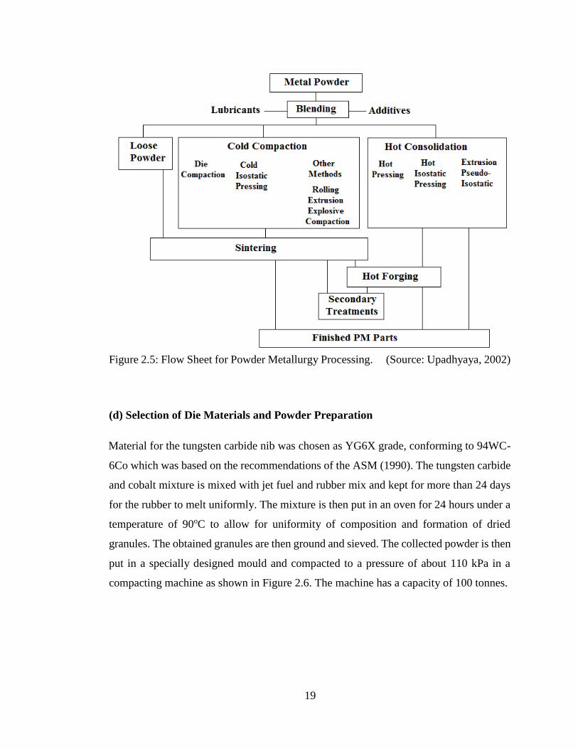
(d) Selection of Die Materials and Powder Preparation
Material for the tungsten carbide nib was chosen as YG6X grade, conforming to 94WC-
6Co which was based on the recommendations of the ASM (1990). The tungsten carbide
and cobalt mixture is mixed with jet fuel and rubber mix and kept for more than 24 days
for the rubber to melt uniformly. The mixture is then put in an oven for 24 hours under a
temperature of 90oC to allow for uniformity of composition and formation of dried
granules. The obtained granules are then ground and sieved. The collected powder is then
put in a specially designed mould and compacted to a pressure of about 110 kPa in a
compacting machine as shown in Figure 2.6. The machine has a capacity of 100 tonnes.
20
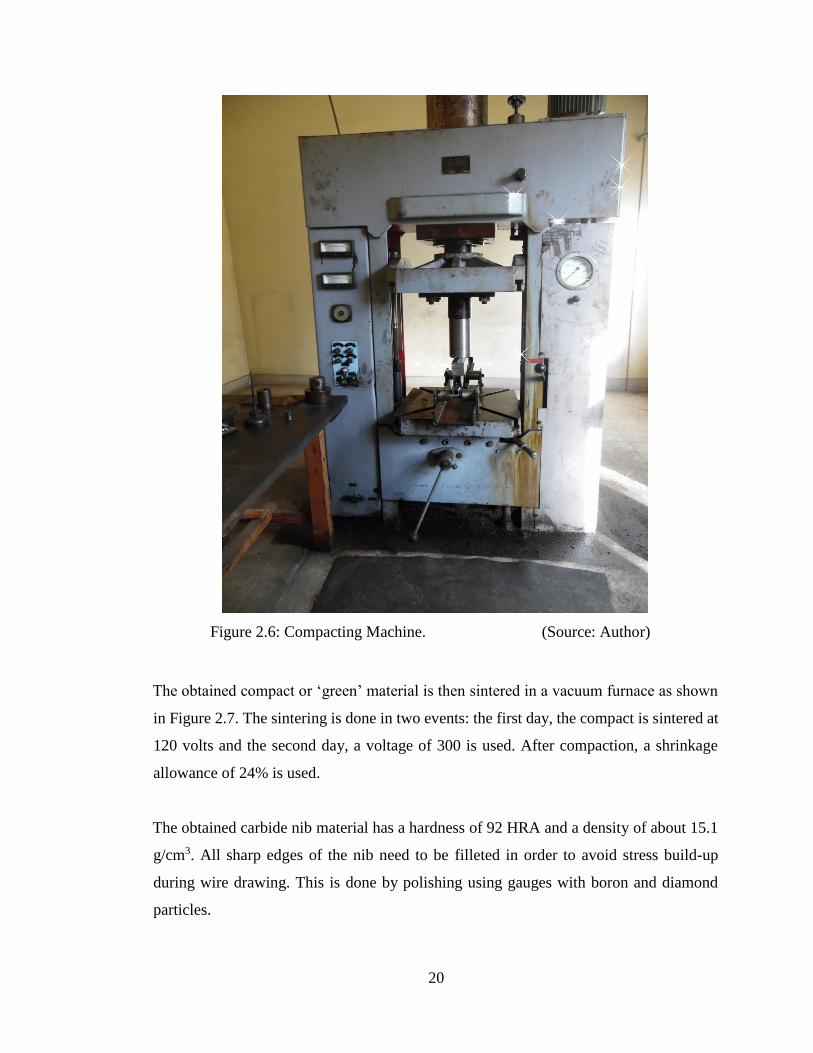
Figure 2.6: Compacting Machine. (Source: Author)
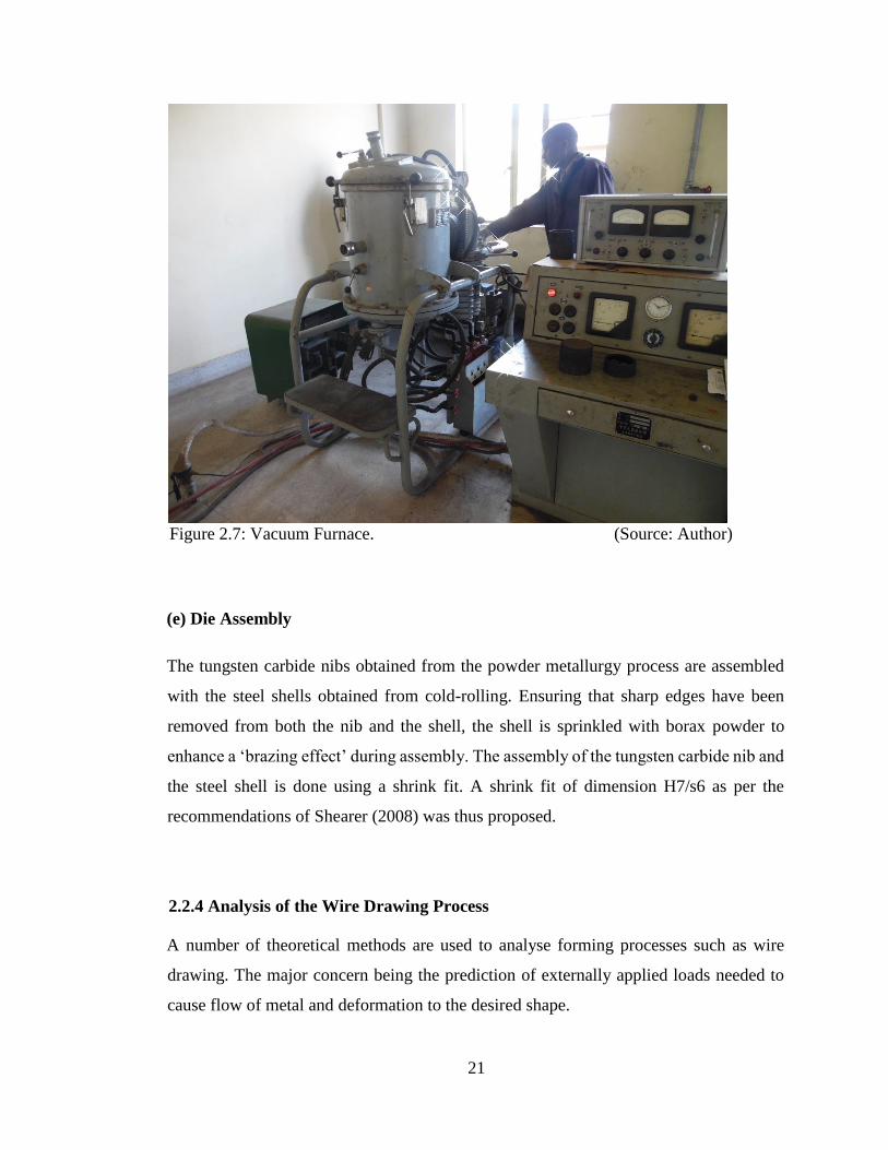
The obtained compact or ‘green’ material is then sintered in a vacuum furnace as shown
in Figure 2.7. The sintering is done in two events: the first day, the compact is sintered at
120 volts and the second day, a voltage of 300 is used. After compaction, a shrinkage
allowance of 24% is used.
The obtained carbide nib material has a hardness of 92 HRA and a density of about 15.1
g/cm3. All sharp edges of the nib need to be filleted in order to avoid stress build-up
during wire drawing. This is done by polishing using gauges with boron and diamond
particles.
21
Figure 2.7: Vacuum Furnace. (Source: Author)
(e) Die Assembly
The tungsten carbide nibs obtained from the powder metallurgy process are assembled
with the steel shells obtained from cold-rolling. Ensuring that sharp edges have been
removed from both the nib and the shell, the shell is sprinkled with borax powder to
enhance a ‘brazing effect’ during assembly. The assembly of the tungsten carbide nib and
the steel shell is done using a shrink fit. A shrink fit of dimension H7/s6 as per the
recommendations of Shearer (2008) was thus proposed.
2.2.4 Analysis of the Wire Drawing Process
A number of theoretical methods are used to analyse forming processes such as wire
drawing. The major concern being the prediction of externally applied loads needed to
cause flow of metal and deformation to the desired shape.
22
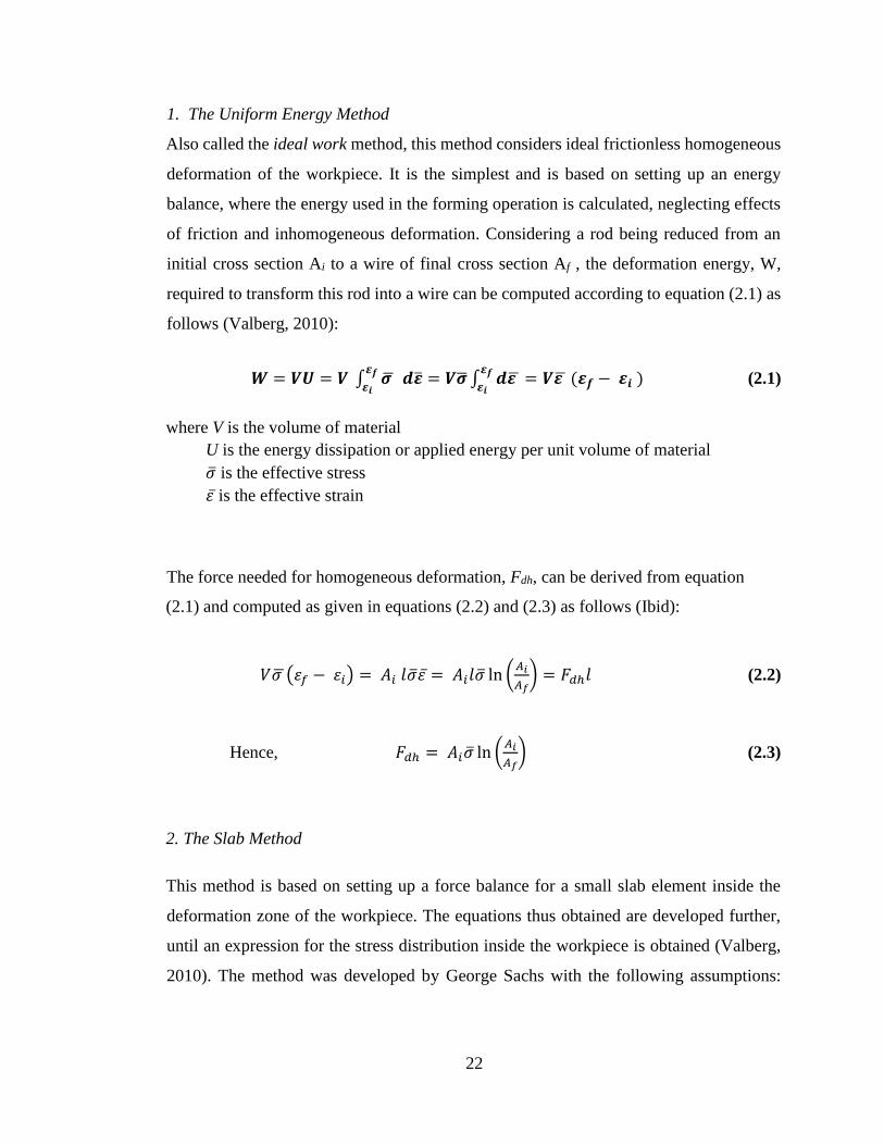
1. The Uniform Energy Method
Also called the ideal work method, this method considers ideal frictionless homogeneous
deformation of the workpiece. It is the simplest and is based on setting up an energy
balance, where the energy used in the forming operation is calculated, neglecting effects
of friction and inhomogeneous deformation. Considering a rod being reduced from an
initial cross section Ai to a wire of final cross section Af , the deformation energy, W,
required to transform this rod into a wire can be computed according to equation (2.1) as
follows (Valberg, 2010):
𝑾 = 𝑽𝑼 = 𝑽 ∫ 𝝈 𝜺𝒇
𝜺𝒊 𝒅�� = 𝑽�� ∫ 𝒅𝜺
𝜺𝒇
𝜺𝒊= 𝑽𝜺 (𝜺𝒇 − 𝜺𝒊 ) (2.1)
where V is the volume of material
U is the energy dissipation or applied energy per unit volume of material
𝜎 is the effective stress
𝜀 is the effective strain
The force needed for homogeneous deformation, Fdh, can be derived from equation
(2.1) and computed as given in equations (2.2) and (2.3) as follows (Ibid):
𝑉𝜎 (𝜀𝑓 − 𝜀𝑖) = 𝐴𝑖 𝑙𝜎𝜀 = 𝐴𝑖𝑙𝜎 ln (𝐴𝑖
𝐴𝑓) = 𝐹𝑑ℎ𝑙 (2.2)
Hence, 𝐹𝑑ℎ = 𝐴𝑖𝜎 ln (𝐴𝑖
𝐴𝑓) (2.3)
2. The Slab Method
This method is based on setting up a force balance for a small slab element inside the
deformation zone of the workpiece. The equations thus obtained are developed further,
until an expression for the stress distribution inside the workpiece is obtained (Valberg,
2010). The method was developed by George Sachs with the following assumptions:
23
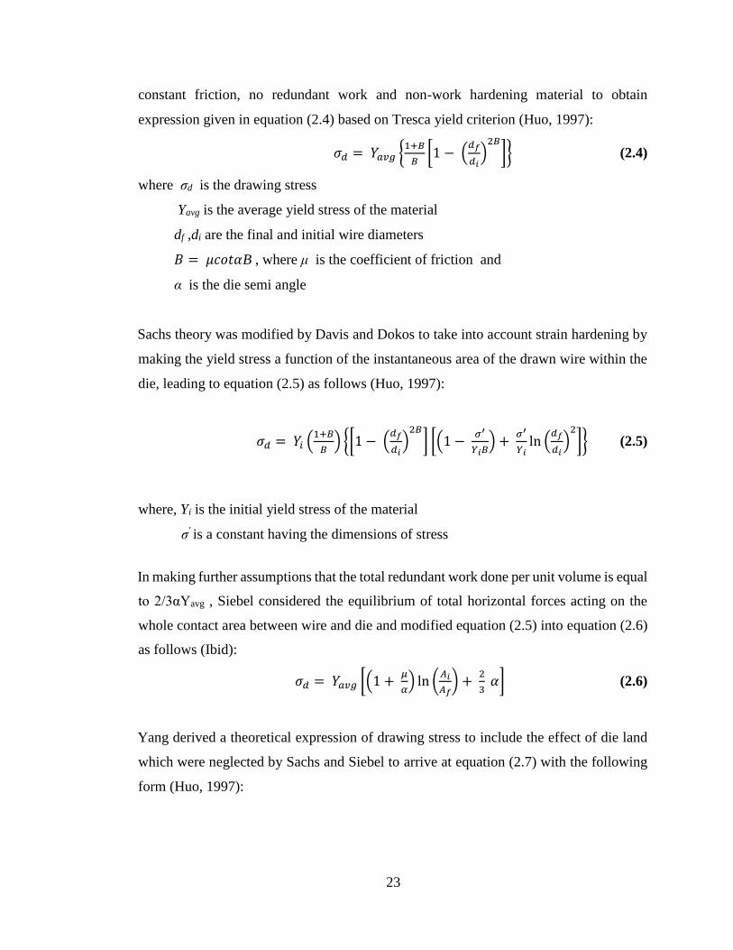
constant friction, no redundant work and non-work hardening material to obtain
expression given in equation (2.4) based on Tresca yield criterion (Huo, 1997):
𝜎𝑑 = 𝑌𝑎𝑣𝑔 {1+𝐵
𝐵[1 − (
𝑑𝑓
𝑑𝑖)
2𝐵
]} (2.4)
where σd is the drawing stress
Yavg is the average yield stress of the material
df ,di are the final and initial wire diameters
𝐵 = 𝜇𝑐𝑜𝑡𝛼B , where μ is the coefficient of friction and
α is the die semi angle
Sachs theory was modified by Davis and Dokos to take into account strain hardening by
making the yield stress a function of the instantaneous area of the drawn wire within the
die, leading to equation (2.5) as follows (Huo, 1997):
𝜎𝑑 = 𝑌𝑖 (1+𝐵
𝐵) {[1 − (
𝑑𝑓
𝑑𝑖)
2𝐵
] [(1 − 𝜎′
𝑌𝑖𝐵) +
𝜎′
𝑌𝑖ln (
𝑑𝑓
𝑑𝑖)
2
]} (2.5)
where, Yi is the initial yield stress of the material
σ' is a constant having the dimensions of stress
In making further assumptions that the total redundant work done per unit volume is equal
to 2/3αYavg , Siebel considered the equilibrium of total horizontal forces acting on the
whole contact area between wire and die and modified equation (2.5) into equation (2.6)
as follows (Ibid):
𝜎𝑑 = 𝑌𝑎𝑣𝑔 [(1 + 𝜇
𝛼) ln (
𝐴𝑖
𝐴𝑓) +
2
3 𝛼] (2.6)
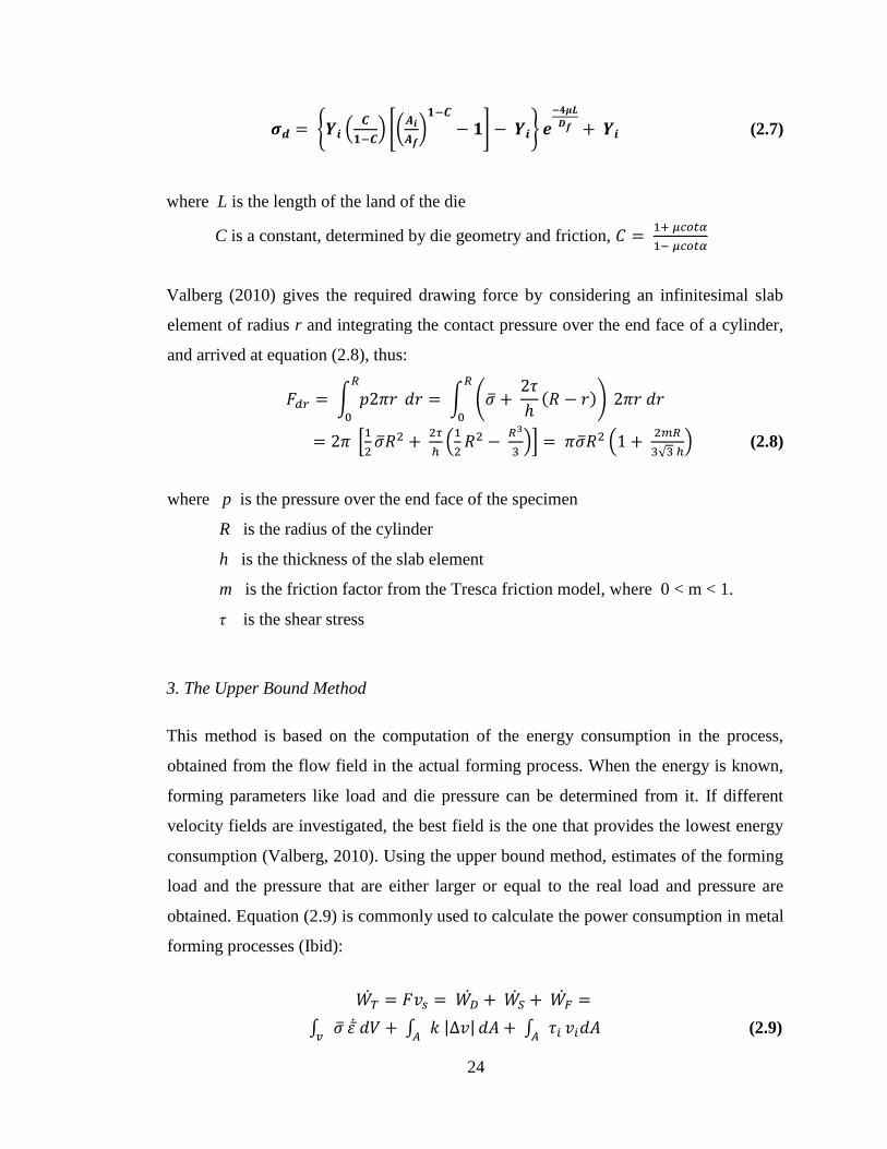
Yang derived a theoretical expression of drawing stress to include the effect of die land
which were neglected by Sachs and Siebel to arrive at equation (2.7) with the following
form (Huo, 1997):
24
𝝈𝒅 = {𝒀𝒊 (𝑪
𝟏−𝑪) [(
𝑨𝒊
𝑨𝒇)
𝟏−𝑪
− 𝟏] − 𝒀𝒊} 𝒆−𝟒𝝁𝑳
𝑫𝒇 + 𝒀𝒊 (2.7)
where L is the length of the land of the die
C is a constant, determined by die geometry and friction, 𝐶 = 1+ 𝜇𝑐𝑜𝑡𝛼
1− 𝜇𝑐𝑜𝑡𝛼
Valberg (2010) gives the required drawing force by considering an infinitesimal slab
element of radius r and integrating the contact pressure over the end face of a cylinder,
and arrived at equation (2.8), thus:
𝐹𝑑𝑟 = ∫ 𝑝2𝜋𝑟𝑅
0
𝑑𝑟 = ∫ (𝜎 + 2𝜏
ℎ(𝑅 − 𝑟))
𝑅
0
2𝜋𝑟 𝑑𝑟
= 2𝜋 [1
2𝜎𝑅2 +
2𝜏
ℎ(
1
2𝑅2 −
𝑅3
3)] = 𝜋𝜎𝑅2 (1 +
2𝑚𝑅
3√3 ℎ) (2.8)
where p is the pressure over the end face of the specimen
R is the radius of the cylinder
h is the thickness of the slab element
m is the friction factor from the Tresca friction model, where 0 < m < 1.
τ is the shear stress
3. The Upper Bound Method
This method is based on the computation of the energy consumption in the process,
obtained from the flow field in the actual forming process. When the energy is known,
forming parameters like load and die pressure can be determined from it. If different
velocity fields are investigated, the best field is the one that provides the lowest energy
consumption (Valberg, 2010). Using the upper bound method, estimates of the forming
load and the pressure that are either larger or equal to the real load and pressure are
obtained. Equation (2.9) is commonly used to calculate the power consumption in metal
forming processes (Ibid):
𝑊𝑇 = 𝐹𝑣𝑠 = 𝑊�� + 𝑊𝑆
+ 𝑊𝐹 =
∫ 𝜎𝑣
𝜀 𝑑𝑉 + ∫ 𝑘 |∆𝑣|𝐴
𝑑𝐴 + ∫ 𝜏𝑖𝐴𝑣𝑖𝑑𝐴 (2.9)

25
where ��𝐷 is the power required to deform the workpiece homogeneously
𝑊𝑠 is the power required to shear-deform the workpiece
𝑊𝐹 is the power consumed due to frictional sliding in the die-workpiece interface
k is the shear flow stress of the material
τi is the shear stress transferred from workpiece to die surface
vi is the sliding velocity of the workpiece material against the die
Shear deformation occurs if some or all of the workpiece material flows through a
velocity discontinuity during the course of forming (Valberg, 2010). With 𝑊𝑆 being equal
to zero in axisymmetric drawing, equation (2.9) is transformed into equation (2.10)
according to Valberg (2010):
𝑾𝑻 = 𝑭𝒗𝒊 = 𝑾𝑫 + 𝑾𝑭
= ∫ ��𝒗
�� 𝒅𝑽 + ∫ 𝝉𝒊𝒗𝒊 𝒅𝑨𝑨
= 𝝅𝑹𝟐��𝒗𝒊 + 𝟐𝝅𝒎
𝟑
��
√𝟑
𝒗𝒊 𝑹𝟑
𝒉 (2.10)
The drawing force is, thus, given according to equation (2.11) as follows:
𝐹𝑑𝑟 = 𝑊𝑇
𝑣𝑠= 𝜋𝑅2𝜎 (1 +
2𝑚𝑅
3√3ℎ) (2.11)
4. The Slip Line Field Theory
The analysis using the slip line field theory is based upon a deformation field that is
geometrically consistent with the shape change, with stresses within the field being
statically admissible. The slip lines are the planes of maximum shear stress which are
oriented at 45o to the principal planes (Hosford and Cadell, 1983).The method can be
used to solve axisymmetric forming processes such as wire drawing. Due to its
laboriousness in application and the various assumptions made such as the material being
rigid-perfectly plastic, deformation being by plane strain only, nonconsideration of
26
temperature, strain rate and time effects and consideration of either frictionless or sticking
friction, the method is not very popular according to Huo (1997).
Hosford and Cadell (1983) however indicate that slip-line fields can be applied to
problems with interface conditions intermediate between frictionless and sticking friction
conditions as long as the shear stress, τ, at the interface between die and workpiece is a
constant fraction, m, of the yield stress in shear, k, and given according to equation (2.12),
thus:
𝝉 = 𝒎𝒌 (2.12)
where m is the friction factor, 0 <m< 1.
5. Finite Element Method
Developments due to cheap and efficient computer technology and the implementation
of the Finite Element Method (FEM) into user-friendly, window-based programmes, has
revolutionised the art of metal forming (Valberg, 2010). The FEM is a numerical method
which seeks an approximated solution of the distribution of field variables in the problem
domain into several elements. Known physical laws are then applied to each small
element with a simple geometry.
In FEM, a continuous function of an unknown field variable is approximated using
piecewise linear functions in each sub-domain, called an element formed by nodes (Liu
and Quek, 2003). The unknowns are then the discrete values of the field variable at the
nodes. With proper principles being followed to establish equations for the elements
which are tied to one another, the process leads to a set of linear algebraic simultaneous
equations for the entire system that can be solved easily to yield the required field
variable. Common physical problems solved using the standard FEM include: mechanics
of solids and structures, heat transfer, acoustics, fluid mechanics and others (Ibid).
Analyses of metal forming processes using FEM can be divided into three types according
to the basic assumptions about the behaviour of the material under consideration. These
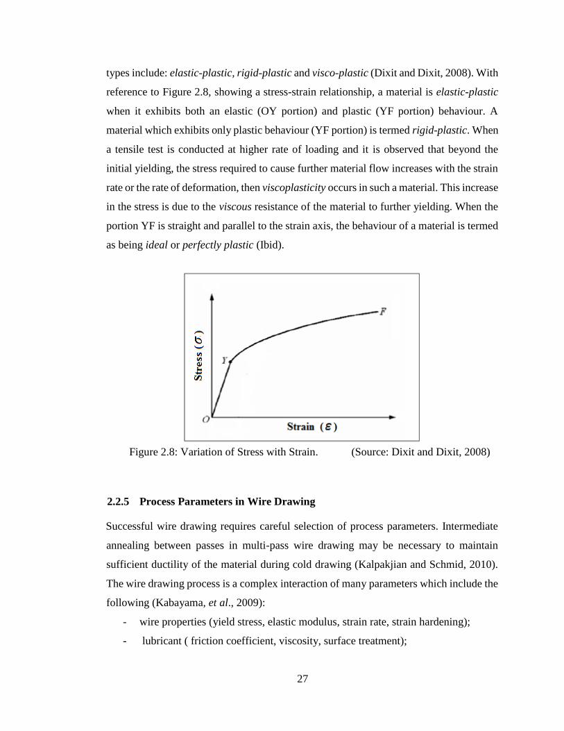
27
types include: elastic-plastic, rigid-plastic and visco-plastic (Dixit and Dixit, 2008). With
reference to Figure 2.8, showing a stress-strain relationship, a material is elastic-plastic
when it exhibits both an elastic (OY portion) and plastic (YF portion) behaviour. A
material which exhibits only plastic behaviour (YF portion) is termed rigid-plastic. When
a tensile test is conducted at higher rate of loading and it is observed that beyond the
initial yielding, the stress required to cause further material flow increases with the strain
rate or the rate of deformation, then viscoplasticity occurs in such a material. This increase
in the stress is due to the viscous resistance of the material to further yielding. When the
portion YF is straight and parallel to the strain axis, the behaviour of a material is termed
as being ideal or perfectly plastic (Ibid).
Figure 2.8: Variation of Stress with Strain. (Source: Dixit and Dixit, 2008)
2.2.5 Process Parameters in Wire Drawing
Successful wire drawing requires careful selection of process parameters. Intermediate
annealing between passes in multi-pass wire drawing may be necessary to maintain
sufficient ductility of the material during cold drawing (Kalpakjian and Schmid, 2010).
The wire drawing process is a complex interaction of many parameters which include the
following (Kabayama, et al., 2009):
- wire properties (yield stress, elastic modulus, strain rate, strain hardening);
- lubricant ( friction coefficient, viscosity, surface treatment);
28
- die geometry (reduction angle, bearing region length, reduction area, and
material).
(a) Deformation Zone and the Δ-parameter
The shape of the deformation zone exerts a strong influence upon the redundant work,
frictional work, and the total drawing forces (Wright, 2011). It also has important effects
on the properties and structure of wire material after drawing; these include homogeneity
of hardness, internal porosity, tendency to open cracks during processing, and residual
stresses.
The area reduction, r, is a measure of the total deformation in metal forming and is given
by the equation (2.13) as follows (Ibid):
𝒓 = 𝑨𝒊− 𝑨𝒇
𝑨𝒊= 𝟏 − (
𝑨𝒇
𝑨𝒊) (2.13)
The deformation zone geometry can be characterized by the Δ-parameter. The shape of
the deformation zone depends on r and the approach angle, α, and is fundamental to
drawing analysis. Wright (2011) gives an approximate numerical value for the Δ–
parameter using equation (2.14):
∆ ≈ (𝛼
𝑟) [1 + (1 − 𝑟)
1
2]2
≈ 4 𝑡𝑎𝑛𝛼
ln[1
(1−𝑟)] (2.14)
Wright (2011) indicates that analyses of wire drawing makes it clear that the shape of the
actual deformation zone is more complicated than a simple trapezoid which is normally
used as the basis for process design and practical analysis. It is the aim of this review to
delve into the reasons for this complication and show how the participating components
within the deformation contributes to crack formation.
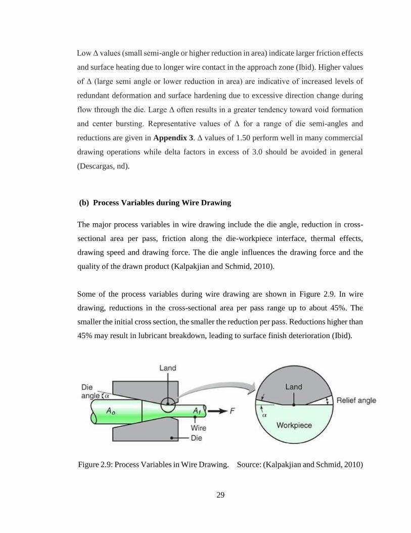
29
Low Δ values (small semi-angle or higher reduction in area) indicate larger friction effects
and surface heating due to longer wire contact in the approach zone (Ibid). Higher values
of Δ (large semi angle or lower reduction in area) are indicative of increased levels of
redundant deformation and surface hardening due to excessive direction change during
flow through the die. Large Δ often results in a greater tendency toward void formation
and center bursting. Representative values of Δ for a range of die semi-angles and
reductions are given in Appendix 3. Δ values of 1.50 perform well in many commercial
drawing operations while delta factors in excess of 3.0 should be avoided in general
(Descargas, nd).
(b) Process Variables during Wire Drawing
The major process variables in wire drawing include the die angle, reduction in cross-
sectional area per pass, friction along the die-workpiece interface, thermal effects,
drawing speed and drawing force. The die angle influences the drawing force and the
quality of the drawn product (Kalpakjian and Schmid, 2010).
Some of the process variables during wire drawing are shown in Figure 2.9. In wire
drawing, reductions in the cross-sectional area per pass range up to about 45%. The
smaller the initial cross section, the smaller the reduction per pass. Reductions higher than
45% may result in lubricant breakdown, leading to surface finish deterioration (Ibid).
Figure 2.9: Process Variables in Wire Drawing. Source: (Kalpakjian and Schmid, 2010)
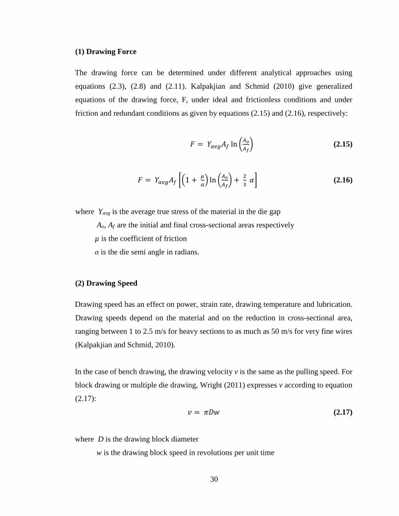
30
(1) Drawing Force
The drawing force can be determined under different analytical approaches using
equations (2.3), (2.8) and (2.11). Kalpakjian and Schmid (2010) give generalized
equations of the drawing force, F, under ideal and frictionless conditions and under
friction and redundant conditions as given by equations (2.15) and (2.16), respectively:
𝐹 = 𝑌𝑎𝑣𝑔𝐴𝑓 ln (𝐴𝑜
𝐴𝑓) (2.15)
𝐹 = 𝑌𝑎𝑣𝑔𝐴𝑓 [(1 + 𝜇
𝛼) ln (
𝐴𝑜
𝐴𝑓) +
2
3 𝛼] (2.16)
where Yavg is the average true stress of the material in the die gap
Ao, Af are the initial and final cross-sectional areas respectively
µ is the coefficient of friction
α is the die semi angle in radians.
(2) Drawing Speed
Drawing speed has an effect on power, strain rate, drawing temperature and lubrication.
Drawing speeds depend on the material and on the reduction in cross-sectional area,
ranging between 1 to 2.5 m/s for heavy sections to as much as 50 m/s for very fine wires
(Kalpakjian and Schmid, 2010).
In the case of bench drawing, the drawing velocity v is the same as the pulling speed. For
block drawing or multiple die drawing, Wright (2011) expresses v according to equation
(2.17):
𝑣 = 𝜋𝐷𝑤 (2.17)
where D is the drawing block diameter
w is the drawing block speed in revolutions per unit time
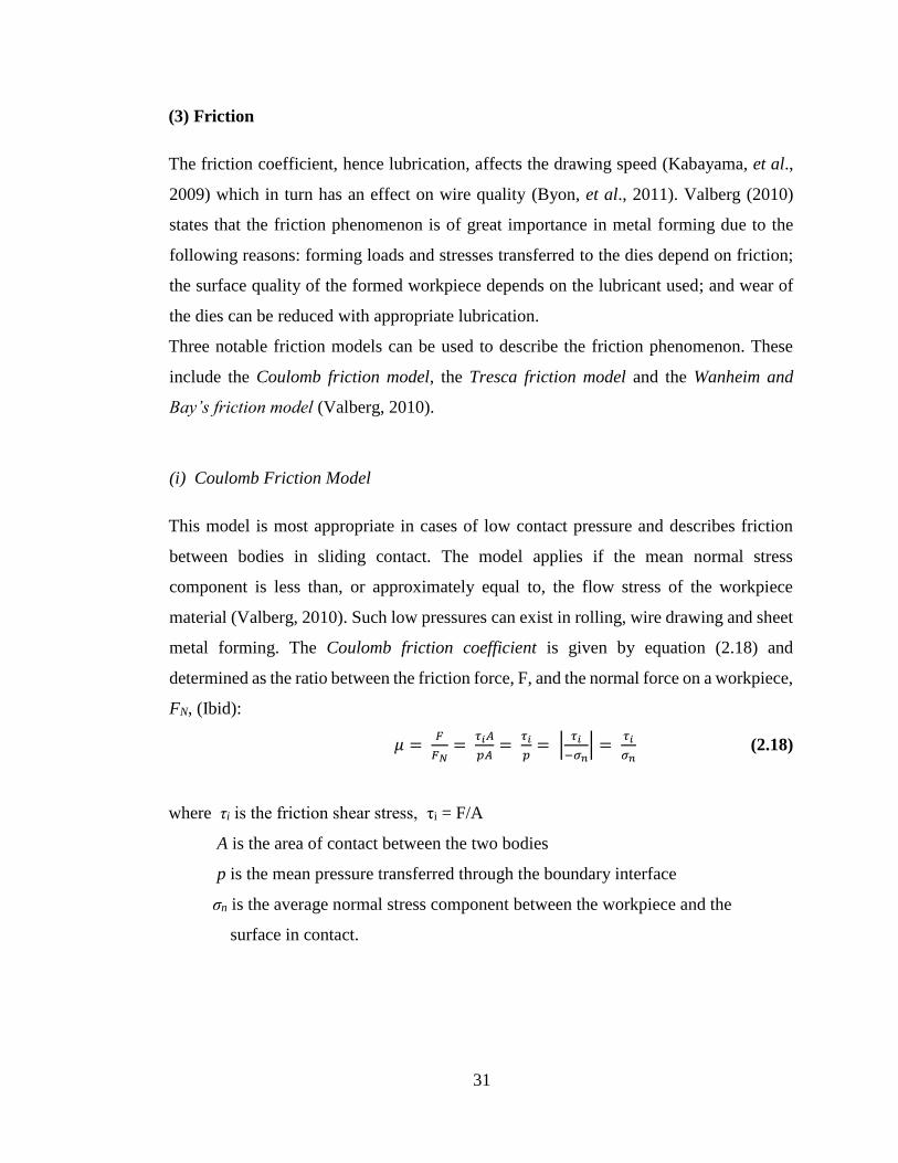
31
(3) Friction
The friction coefficient, hence lubrication, affects the drawing speed (Kabayama, et al.,
2009) which in turn has an effect on wire quality (Byon, et al., 2011). Valberg (2010)
states that the friction phenomenon is of great importance in metal forming due to the
following reasons: forming loads and stresses transferred to the dies depend on friction;
the surface quality of the formed workpiece depends on the lubricant used; and wear of
the dies can be reduced with appropriate lubrication.
Three notable friction models can be used to describe the friction phenomenon. These
include the Coulomb friction model, the Tresca friction model and the Wanheim and
Bay’s friction model (Valberg, 2010).
(i) Coulomb Friction Model
This model is most appropriate in cases of low contact pressure and describes friction
between bodies in sliding contact. The model applies if the mean normal stress
component is less than, or approximately equal to, the flow stress of the workpiece
material (Valberg, 2010). Such low pressures can exist in rolling, wire drawing and sheet
metal forming. The Coulomb friction coefficient is given by equation (2.18) and
determined as the ratio between the friction force, F, and the normal force on a workpiece,
FN, (Ibid):
𝜇 = 𝐹
𝐹𝑁=
𝜏𝑖𝐴
𝑝𝐴=
𝜏𝑖
𝑝= |
𝜏𝑖
−𝜎𝑛| =
𝜏𝑖
𝜎𝑛 (2.18)
where τi is the friction shear stress, τi = F/A
A is the area of contact between the two bodies
p is the mean pressure transferred through the boundary interface
σn is the average normal stress component between the workpiece and the
surface in contact.
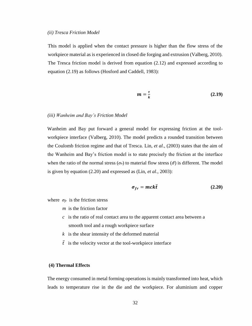
32
(ii) Tresca Friction Model
This model is applied when the contact pressure is higher than the flow stress of the
workpiece material as is experienced in closed die forging and extrusion (Valberg, 2010).
The Tresca friction model is derived from equation (2.12) and expressed according to
equation (2.19) as follows (Hosford and Caddell, 1983):
𝒎 =𝝉
𝒌 (2.19)
(iii) Wanheim and Bay’s Friction Model
Wanheim and Bay put forward a general model for expressing friction at the tool-
workpiece interface (Valberg, 2010). The model predicts a rounded transition between
the Coulomb friction regime and that of Tresca. Lin, et al., (2003) states that the aim of
the Wanheim and Bay’s friction model is to state precisely the friction at the interface
when the ratio of the normal stress (σn) to material flow stress (𝜎) is different. The model
is given by equation (2.20) and expressed as (Lin, et al., 2003):
𝝈𝒇𝒓 = 𝒎𝒄𝒌�� (2.20)
where σfr is the friction stress
m is the friction factor
c is the ratio of real contact area to the apparent contact area between a
smooth tool and a rough workpiece surface
k is the shear intensity of the deformed material
𝑡 is the velocity vector at the tool-workpiece interface
(4) Thermal Effects
The energy consumed in metal forming operations is mainly transformed into heat, which
leads to temperature rise in the die and the workpiece. For aluminium and copper

33
workpieces which are seldom formed at high temperatures, radiation effects are less
significant at these low temperatures and can thus be neglected without much error
(Valberg, 2010). If radiation effects and cooling to the surrounding air is neglected,
equation (2.21) can be used to estimate the temperature, T, in a workpiece during metal
forming (Ibid):
𝑻 = 𝑻𝒐 + ∆𝑻𝑫 + ∆𝑻𝒇 − ∆𝑻𝑻 (2.21)
where, To is the initial temperature of the workpiece
ΔTD is the temperature increase in the workpiece due to dissipated
deformation energy during forming
ΔTf is the temperature increase due to friction in the interface between die
and workpiece
ΔTT is the temperature decrease in the workpiece because of cooling by
colder dies
The temperature increase in the workpiece due to dissipated deformation energy
during forming is given by equation (2.22) as follows (Valberg, 2010):
∆𝑻𝑫 = 𝜷
𝒄𝝆𝝈 �� (2.22)
where, β is a factor compensating for energy stored in the workpiece
(approximately equal to 0.95)
c is the heat capacity of the workpiece material
ρ is the density of the workpiece material
Wright (2011) modified equation (2.22) to give equation (2.23) as follows:
𝑇𝑊 − 𝑇𝑜 = 𝜑 𝜎𝑎 ln[
1
(1−𝑟)]
𝑐𝜌 (2.23)
where Tw is the temperature due to dissipated total deformation energy
φ is the redundant work factor
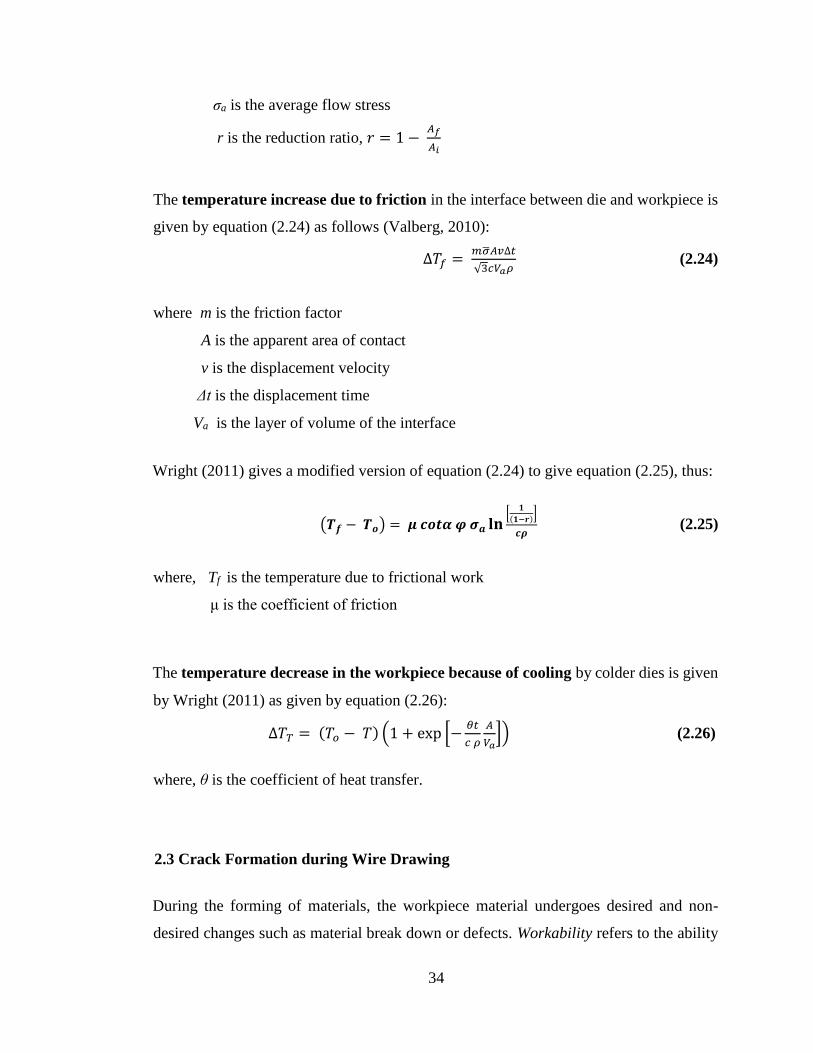
34
σa is the average flow stress
r is the reduction ratio, 𝑟 = 1 − 𝐴𝑓
𝐴𝑖
The temperature increase due to friction in the interface between die and workpiece is
given by equation (2.24) as follows (Valberg, 2010):
∆𝑇𝑓 = 𝑚��𝐴𝑣∆𝑡
√3𝑐𝑉𝑎𝜌 (2.24)
where m is the friction factor
A is the apparent area of contact
v is the displacement velocity
Δt is the displacement time
Va is the layer of volume of the interface
Wright (2011) gives a modified version of equation (2.24) to give equation (2.25), thus:
(𝑻𝒇 − 𝑻𝒐) = 𝝁 𝒄𝒐𝒕𝜶 𝝋 𝝈𝒂 𝐥𝐧[
𝟏
(𝟏−𝒓)]
𝒄𝝆 (2.25)
where, Tf is the temperature due to frictional work
μ is the coefficient of friction
The temperature decrease in the workpiece because of cooling by colder dies is given
by Wright (2011) as given by equation (2.26):
∆𝑇𝑇 = (𝑇𝑜 − 𝑇) (1 + exp [−𝜃𝑡
𝑐 𝜌
𝐴
𝑉𝑎]) (2.26)
where, θ is the coefficient of heat transfer.
2.3 Crack Formation during Wire Drawing
During the forming of materials, the workpiece material undergoes desired and non-
desired changes such as material break down or defects. Workability refers to the ability
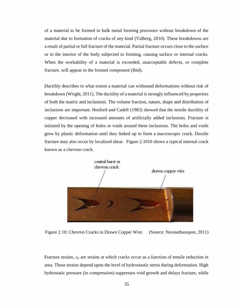
35
of a material to be formed in bulk metal forming processes without breakdown of the
material due to formation of cracks of any kind (Valberg, 2010). These breakdowns are
a result of partial or full fracture of the material. Partial fracture occurs close to the surface
or in the interior of the body subjected to forming, causing surface or internal cracks.
When the workability of a material is exceeded, unacceptable defects, or complete
fracture, will appear in the formed component (Ibid).
Ductility describes to what extent a material can withstand deformations without risk of
breakdown (Wright, 2011). The ductility of a material is strongly influenced by properties
of both the matrix and inclusions. The volume fraction, nature, shape and distribution of
inclusions are important. Hosford and Cadell (1983) showed that the tensile ductility of
copper decreased with increased amounts of artificially added inclusions. Fracture is
initiated by the opening of holes or voids around these inclusions. The holes and voids
grew by plastic deformation until they linked up to form a macroscopic crack. Ductile
fracture may also occur by localized shear. Figure 2.1010 shows a typical internal crack
known as a chevron crack.
Figure 2.10: Chevron Cracks in Drawn Copper Wire. (Source: Norasethasopon, 2011)
Fracture strains, εf, are strains at which cracks occur as a function of tensile reduction in
area. These strains depend upon the level of hydrostastic stress during deformation. High
hydrostatic pressure (in compression) suppresses void growth and delays fracture, while
36
hydrostatic tension accelerates void growth and decreases ductility. Hosford and Cadell
(1983) further state that fracture strains depend on the process geometry.
Hosford and Cadell (1983) stated that the distinction on whether fracture strains depended
on the level of the largest principal stress, σ1, rather than on the hydrostatic stress, σm,
was not of importance. This is due to the fact that σm and σ1 usually increase or decrease
together as evident from equation (2.27) which shows the flow stress condition:
𝝈𝒎 + 𝟏
𝟑�� ≤ 𝝈𝟏 ≤ 𝝈𝒎 +
𝟐
𝟑�� (2.27)
2.3.1 Fracture Criteria
In order to cause plastic deformation, a particular level of stress (the yield strength) must
be reached. For most ductile metals such as copper, both the extent of deformation and
the change in shape of the original body can continue if the stress to initial yielding is
continually increased. Mathematical expressions known as yield criteria are used to
predict if or when yielding will occur under combined stress states in terms of particular
properties of the metal being stressed (Hosford and Caddell, 1983). The two commonly
used general yielding criteria are the Tresca and Von Mises criteria.
(a) Tresca Criterion (maximum shear stress criterion)
This criterion postulates that yielding will occur when the largest shear stress reaches a
critical value. The criterion predicts yielding according to equations (2.8) under the
following conditions (Ibid):
𝝈𝒎𝒂𝒙 − 𝝈𝒎𝒊𝒏 = 𝑪 (2.28i)
𝝈𝟏 − 𝝈𝟑 = 𝑪; 𝒊𝒇 𝝈𝟏 > 𝝈𝟐 > 𝝈𝟑 (2.28ii)
To evaluate constant C, a state of uniaxial tension may be used. In uniaxial tension, σmax=
σ1, σ2 =σ3 = 0, and yielding occurs when σ1 = Y, the yield strength. In that case, equation
(2.9) is used, thus:
37
𝝈𝟏 − 𝝈𝟑 = 𝒀 = 𝑪 (2.29)
Yielding occurs when the maximum shear stress reaches the yield strength or the shear
yield strength, k, in pure shear (when σmax = σ1, σmin = σ3 = - σ1, σ2 = 0) and given by
equations (2.30), thus:
𝜎1 = 𝑘 (2.30i)
𝜎1 − 𝜎3 = 2𝜎1 = 2𝑘 = 𝐶 (2.30ii)
The Tresca Criterion, is thus given by equation (2.31) as follows:
𝜎1 − 𝜎3 = 𝑌 = 2𝑘 (2.31)
𝜎1, 𝜎2 and 𝜎3 are the principal stresses.
Expressed in general shear situations using τ, equation (2.32) is thus used:
𝒌 = 𝝉𝒎𝒂𝒙 = 𝝉𝒚 (2.32)
(b) Von Mises Criterion (distortion energy criterion)
Under this criterion yielding will occur when some value of the root-mean shear stress
reaches a constant and given by equation (2.33) as follows (Hosford and Caddell, 1983):
√[(𝝈𝟏− 𝝈𝟐)𝟐+ (𝝈𝟐− 𝝈𝟑)𝟐+ (𝝈𝟑−𝝈𝟏)𝟐
𝟑] = 𝑪𝟏 (2.33)
Equivalently,
(𝝈𝟏 − 𝝈𝟐)𝟐 + (𝝈𝟐 − 𝝈𝟑)𝟐 + (𝝈𝟑 − 𝝈𝟏)𝟐 = 𝑪𝟐 (2.34)
At yielding in uniaxial tension, σ1 = Y; σ2 = σ3 = 0; C2 = 2Y2
For pure shear, with σ1 = k = - σ3 and σ2 = 0, C2 = 6k2.
38
The Von Mises Criterion is thus expressed according to equation (2.35):
(𝝈𝟏 − 𝝈𝟐)𝟐 + (𝝈𝟐 − 𝝈𝟑)𝟐 + (𝝈𝟑 − 𝝈𝟏)𝟐 = 𝟐𝒀𝟐 = 𝟔𝒌𝟐 (2.35)
In a more general form, the criterion can be written according to equation (2.36), thus
(Ibid):
(𝝈𝒙 − 𝝈𝒚)𝟐
+ (𝝈𝒚 − 𝝈𝒛)𝟐
+ (𝝈𝒛 − 𝝈𝒙)𝟐 + 𝟔(𝝉𝒙𝒚𝟐 + 𝝉𝒚𝒛
𝟐 + 𝝉𝒛𝒙𝟐 ) = 𝟐𝒀𝟐 = 𝟔𝒌𝟐
(2.36)
where 𝜎𝑥, 𝜎𝑦 , 𝜎𝑧 are the normal stresses directed along x, y and z axes, while 𝜏𝑥𝑦 is the
shear stress directed along the xy-plane.
Udomphol (2007) simplifies the two criteria as:
Tresca Criterion: τy = τmax = 0.5 σo
Von Mises Criterion: τy = τmax = 0.577 σo
Accordingly, the difference in the maximum shear stress prediction from both criteria lies
between 0-15%. Experiments have confirmed that the von Mises criterion is more
accurate than the Tresca criterion in describing the actual situations (Udomphol, 2007).
Hosford and Cadell (1983), Ahmadi and Farzin (2008), Xue (2007), Komori (2003) and
Bao (2003) presented some more criteria associated with ductile fracture. Bao (2003)
states that fracture occurs at a point in a body when the following scalar function reaches
a critical value C according to equation (2.37):
∫ 𝒈(𝝈𝒊𝒋)��𝒇
𝟎 𝒅�� = 𝑪 (2.37)
where g is a weighting function of the stress tensor σij
C is a calibration constant or damage indicator
Some of the empirical models based on the relationship in equation (2.37) include
the following:
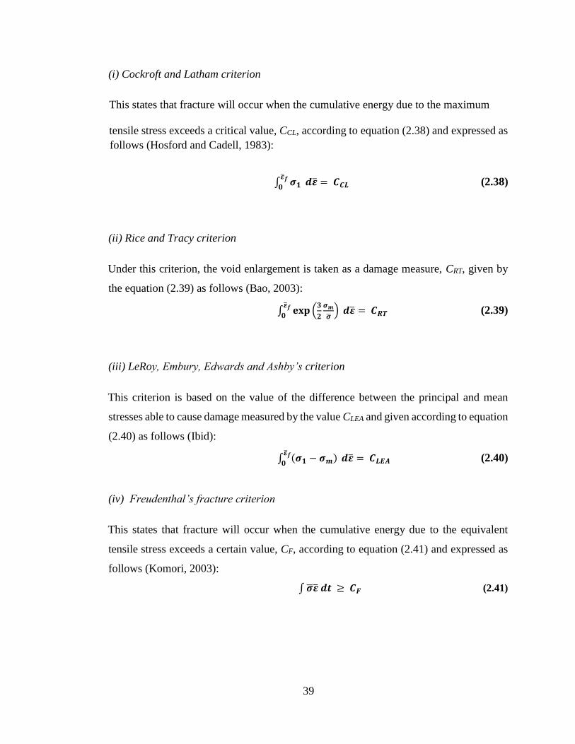
39
(i) Cockroft and Latham criterion
This states that fracture will occur when the cumulative energy due to the maximum
tensile stress exceeds a critical value, CCL, according to equation (2.38) and expressed as
follows (Hosford and Cadell, 1983):
∫ 𝝈𝟏��𝒇
𝟎 𝒅�� = 𝑪𝑪𝑳 (2.38)
(ii) Rice and Tracy criterion
Under this criterion, the void enlargement is taken as a damage measure, CRT, given by
the equation (2.39) as follows (Bao, 2003):
∫ 𝐞𝐱𝐩 (𝟑
𝟐
𝝈𝒎
��) 𝒅��
��𝒇
𝟎= 𝑪𝑹𝑻 (2.39)
(iii) LeRoy, Embury, Edwards and Ashby’s criterion
This criterion is based on the value of the difference between the principal and mean
stresses able to cause damage measured by the value CLEA and given according to equation
(2.40) as follows (Ibid):
∫ (𝝈𝟏 − 𝝈𝒎)��𝒇
𝟎 𝒅�� = 𝑪𝑳𝑬𝑨 (2.40)
(iv) Freudenthal’s fracture criterion
This states that fracture will occur when the cumulative energy due to the equivalent
tensile stress exceeds a certain value, CF, according to equation (2.41) and expressed as
follows (Komori, 2003):
∫ ���� 𝒅𝒕 ≥ 𝑪𝑭 (2.41)
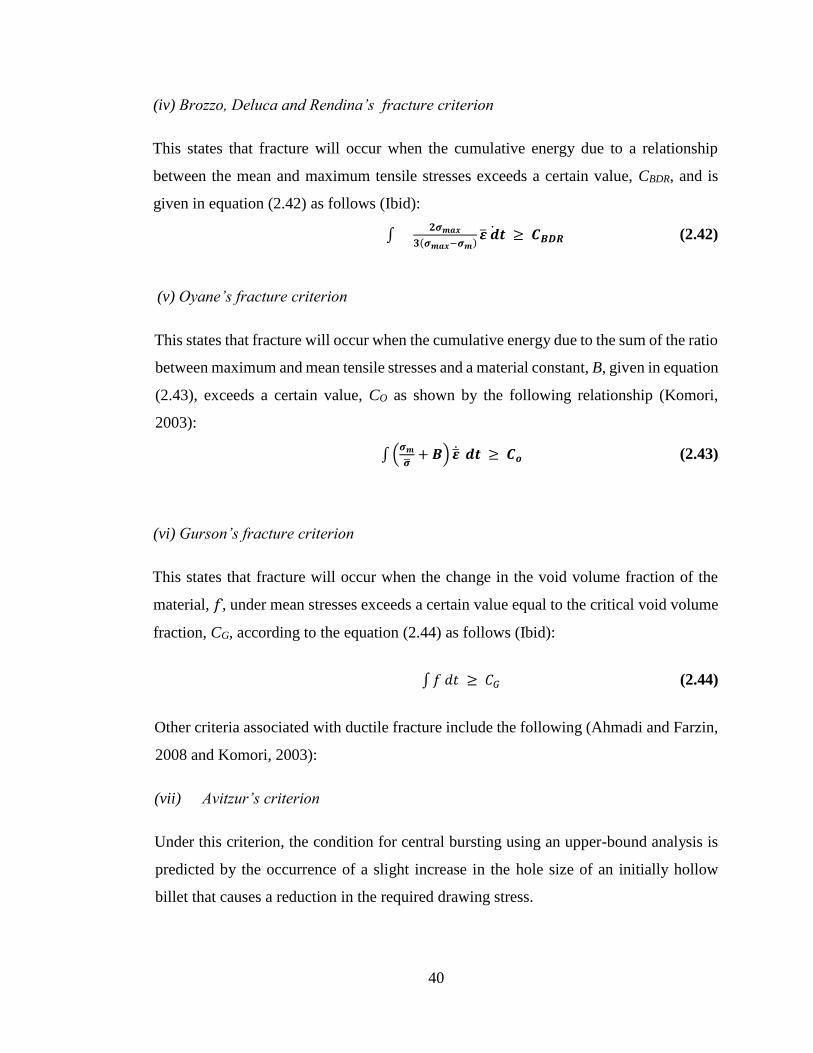
40
(iv) Brozzo, Deluca and Rendina’s fracture criterion
This states that fracture will occur when the cumulative energy due to a relationship
between the mean and maximum tensile stresses exceeds a certain value, CBDR, and is
given in equation (2.42) as follows (Ibid):
∫𝟐𝝈𝒎𝒂𝒙
𝟑(𝝈𝒎𝒂𝒙−𝝈𝒎)�� 𝒅𝒕 ≥ 𝑪𝑩𝑫𝑹 (2.42)
(v) Oyane’s fracture criterion
This states that fracture will occur when the cumulative energy due to the sum of the ratio
between maximum and mean tensile stresses and a material constant, B, given in equation
(2.43), exceeds a certain value, CO as shown by the following relationship (Komori,
2003):
∫ (𝝈𝒎
��+ 𝑩) �� 𝒅𝒕 ≥ 𝑪𝒐 (2.43)
(vi) Gurson’s fracture criterion
This states that fracture will occur when the change in the void volume fraction of the
material, 𝑓 , under mean stresses exceeds a certain value equal to the critical void volume
fraction, CG, according to the equation (2.44) as follows (Ibid):
∫ 𝑓 𝑑𝑡 ≥ 𝐶𝐺 (2.44)
Other criteria associated with ductile fracture include the following (Ahmadi and Farzin,
2008 and Komori, 2003):
(vii) Avitzur’s criterion
Under this criterion, the condition for central bursting using an upper-bound analysis is
predicted by the occurrence of a slight increase in the hole size of an initially hollow
billet that causes a reduction in the required drawing stress.

41
(viii) Hydrostatic Stress criterion
This criterion states that whenever the hydrostatic stress at a point on the centreline in the
deformation zone becomes zero and is compressive elsewhere, there is fracture initiation
leading to central bursting.
(ix) Critical Void Growth criterion
Along the die axis, if the mean stress component is initially tensile, the voids then begin
to grow and coalesce, leading to central bursting.
Although Bao (2003) argues that the preceding metal forming criteria lacks a solid
foundation and are based on observation, experience and mathematical simplicity
performed using a restricted range of stress state, the versatility of their use has been
demonstrated by Reddy, et al.,(2000), Tvergaard and Hutchinson (2002), Komori (2003),
Xue (2007) and Benesova, et al.,(2008) among others.
This current research study makes use of the Von Mises yielding criterion and then uses
the Cockroft and Latham fracture criterion to show damage in and on the copper wire.
This choice was done because the Abaqus software that was used was able to show the
von Mises stresses for yielding. Adding the maximum von Mises stresses and the
accumulated strains resulted in the Cockroft and Latham criterion which was thus used
to detect failure or fracture at a node.
2.4 Modeling of Wire Drawing Processes
In modeling of metal forming processes, Eulerian formulation is convenient for processes
like rolling, drawing and extrusion, whereas the updated Lagrangian formulation is
convenient for the processes like forging, deep drawing and sheet bending. In the Eulerian
formulation a control volume is chosen as the domain for analysis. A typical control
volume for wire drawing is shown in Figure 2., with half the wire being shown due to its
symmetry (Dixit and Dixit, 2008).

42
Figure 2.11: Domain for Eulerian Formulation of Wire Drawing.
(Source: Dixit and Dixit, 2008)
Dixit and Dixit (2008) state that in choosing the control volume, boundaries AB and EF
need to be placed sufficiently away from the die interface CD so as to simplify the
boundary conditions on these boundaries by taking advantage of the uniform velocity
fields existing there. Possible plastic boundaries should also be shown, with all
boundaries not known a priori but need to be determined as part of the solution.
Since heat is dissipated during metal forming due to deformation and mechanical energy,
temperature rise in processes like wire drawing is comparatively small, hence the
processes being assumed as isothermal during modeling. For isothermal processes, the
velocity field, vi, the strain field, 𝜀𝑖��, and the stress field, σij, in the control volume are
governed by equations (2.45), (2.46), (2.47), (2.48) and (2.49) as follows (Ibid):
(1) Strain rate – velocity relations
𝜀𝑖𝑗 = 1
2 (𝑣𝑖𝑗 + 𝑣𝑖𝑗) (2.45)
(2) Elastic-plastic stress-strain rate relations
(a) in plastic zone
𝜀𝑘𝑘 = 𝜎𝑘𝑘
3𝐾 , 𝜀𝑖𝑗 =
1
2𝜇 𝜎𝑖𝑗 +
3𝜀𝑒𝑞𝑝
2𝜎𝑒𝑞 𝜎𝑖𝑗 (2.46)
where, 𝝈𝒆𝒒 = 𝝈𝒀 + 𝑲 (𝜺𝒆𝒒𝒑
)𝒏
(2.47)

43
(b) in elastic zone
𝜀𝑘𝑘 = 𝜎𝑘𝑘
3𝐾 , 𝜀𝑖𝑗 =
1
2𝜇 𝜎𝑖𝑗 (2.48)
In the relations above, the superscript .. denotes a Jaumann stress state.
(3) Equations of motion
𝜌 (𝜕𝑣𝑖
𝜕𝑡+ 𝑣𝑖,𝑗𝑣𝑗) = 𝜌𝑏𝑖 + 𝜎𝑖𝑗,𝑗 (2.49)
If the density is unknown, then the equations of conservation of mass are needed. For
isothermal processes, change in density is very small, hence ρ can be treated as a constant.
The equations (2.45), (2.46), (2.47), (2.48) and (2.49) and their subcomponents are
differential equations in spatial variables xj and time t. Boundary and initial conditions
are required for solving these equations (Ibid).
2.5 Wire Drawing Focal Research Literature
The focal research literature regarding copper wire drawing was categorised under the
following themes: inclusion effects, die geometry and design effects, die wear and failure
effects, temperature effects, stress and strain effects, friction and lubrication effects,
practice-related effects, process optimisation and fracture criteria. The interdependence
of these themes is shown in Figure 2.12.
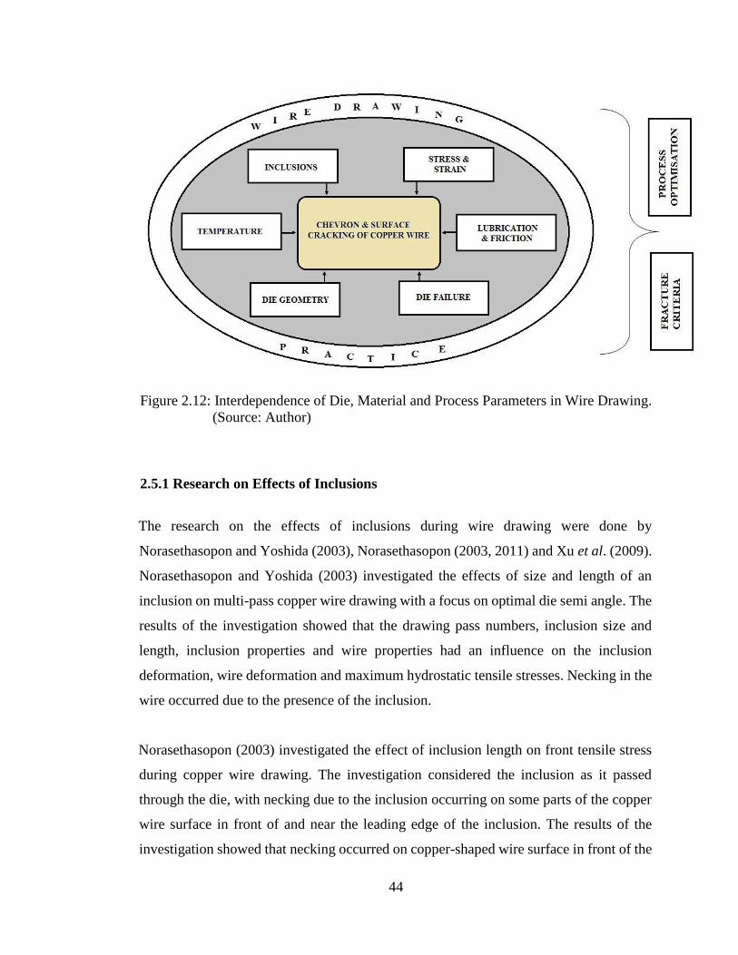
44
Figure 2.12: Interdependence of Die, Material and Process Parameters in Wire Drawing.
(Source: Author)
2.5.1 Research on Effects of Inclusions
The research on the effects of inclusions during wire drawing were done by
Norasethasopon and Yoshida (2003), Norasethasopon (2003, 2011) and Xu et al. (2009).
Norasethasopon and Yoshida (2003) investigated the effects of size and length of an
inclusion on multi-pass copper wire drawing with a focus on optimal die semi angle. The
results of the investigation showed that the drawing pass numbers, inclusion size and
length, inclusion properties and wire properties had an influence on the inclusion
deformation, wire deformation and maximum hydrostatic tensile stresses. Necking in the
wire occurred due to the presence of the inclusion.
Norasethasopon (2003) investigated the effect of inclusion length on front tensile stress
during copper wire drawing. The investigation considered the inclusion as it passed
through the die, with necking due to the inclusion occurring on some parts of the copper
wire surface in front of and near the leading edge of the inclusion. The results of the
investigation showed that necking occurred on copper-shaped wire surface in front of the
45
inclusion near the inclusion boundary and its magnitude increased proportionally with
inclusion size and length. A short inclusion length ratio (1 > Li/Di > 0.2) strongly
influenced tensile stresses in a wire while, a long inclusion ratio (Li/Di > 1.0) did not
affect inclusion front tensile stresses.
Research on possible internal defects which could be formed during wire drawing of a
steel rod on the production line of a draw bench and models of the initiation and
propagation rule of central flaw were done by Xu, et al. (2009). The experimental results
from the research showed that as a result of the wire material containing defects, the
probability of crack expansion in the final two or one drawing was great in multi-pass
drawing, and that a friction coefficient of 0.1 and a pullout angle of approximately 8°
were optimal. The fracture toughness of the material (the J-integral) increased with
increasing die angle, friction coefficient and the defect dimension. Improving the
lubrication conditions in wire drawing reduced the rate of broken wires. Wire breakage
did not happen when the diameter of the disc-shaped surface crack in the center of the
wire was less than 30μm.
The research by Norasethasopon (2011) was aimed at predicting the initiation of internal or
chevron cracks in drawn copper shaped-wire. An inclusion of sintered tungsten carbide (WC)
was used and assumed to be introduced in the wire during processing. The results revealed
that inclusion deformation occurred when copper wire was repeatedly drawn and that the
drawing pass numbers strongly influenced wire deformation, inclusion deformation and
the maximum principal stresses. The research also showed that a large number of drawing
passes could be performed without chevron crack initiation when the initial inclusion size
ratios were below the critical inclusion size ratio of 0.001 (measured as length of
inclusion, Li, over initial wire diameter, Di, or Li/D). Chevron cracks, leading to wire
breaking, occurred when the inclusion size was larger than the critical inclusion size.
The background to the optimality of the 8o die semi angle in the experiment by
Norasethasopon (2003) needed to be given in order to make a comparative analysis with
the other processing parameters. Norasethasopon (2011) stated that crack initiation
occurred if the tensile strain-energy density reached a critical value described by a ductile
46
fracture criterion according to Cockroft and Latham. Though the critical value was given,
the study did not demonstrate how the obtained inclusion size ratios related to the critical
value. The study also gave equations for obtaining the drawing stress (equation 2.4), but
did not show a free body equilibrium diagram to explain force analysis at an element in
the reduction zone.
The study paper by Xu, et al. (2009) indicated that the J-integral value increased with
increasing angle of the drawing die, the friction coefficient between drawing die and wire
and the initial dimension of the flaw in the input material. However, the study did not
show how the J-integral was being applied in this case in order to show the relationship
of parameters under study. The optimisation analysis needed to be clearly demonstrated
with verification experiments being undertaken to justify the choice of optimum
parameters.
2.5.2 Research on Effects of Die Geometry and Design
Research on the effects of die geometry and design were done by McAllen and Phelan
(2005), McAllen and Phelan (2007), Campos, et al. (2006), Zompì and Levi (2008),
Ahmadi and Farzin (2008), Kabayama, et al. (2009), León, et al. (2010) and Hassan and
Hashim (2015).
McAllen and Phelan (2005) demonstrated that irrespective of the die approach angle, α,
and at reduction ratios of 9%, 18% and 25%, central burst formation was relatively high,
whereas central burst was lower at area reductions ratios of 5% and 39% and also when
the effective strain varied periodically along the wire surface. Further research by
McAllen and Phelan (2007) indicated that the influence of the die land or die bearing
length on the formation of damage in wire drawing had not been fully clarified. For
varying friction conditions, the bearing length showed a negligible effect on the effective
stress, effective strain and damage distributions in the drawn wire.
47
Campos, et al. (2006) evaluated the effect of the die semi angle on the coefficient of
friction during the axisymmetric drawing of copper. Tungsten carbide dies with semi
angles of 2o, 3o, 4o, 5o and 6o were used with a molybdenum bisulphide industrial grease
as the lubricant. The results showed that as the semi angle increased, the friction
coefficient initially reduced and then increased, with the optimum die semi angle being
reached at 4o.
Zompì and Levi (2008) researched on the process parameters and evaluated the stress and
strain patterns in copper wire drawing. The results of the research showed that the die
angle and the reduction ratio were the two major linear effects. Smaller die angles (from
6.5o to 9o), larger drawing ratios (from 20% to 25%) and effective prior annealing led to
large drawing forces but lower damage of the product, while the effect of friction
coefficients was small. Annealing was needed in order to relieve residual strains and
restore capability to withstand substantial plastic deformation.
Ahmadi and Farzin (2008) investigated the geometric and friction conditions causing
chevron cracking or central bursting in steel wire drawing. The finite element analysis
and experimental results showed that chevron cracking occurred under conditions of
relatively small area reductions and large die angles (15o) where the mean stress was
mostly tensile, and that low friction conditions (µ = 0.05 ) increased the tendency of
central bursting.
Kabayama, et al. (2009) investigated the influence of die geometry on stress distribution
on annealed electrolytic copper wire. The results of the experimental investigation
showed that the wire drawing force and friction coefficient values decreased with
increased drawing speed. A die semi angle of 5o produced wire drawing forces of up to
23.2% and friction coefficients up to 60.5% lower than those for a die with semi angle of
9o. The finite element analysis of the draw die reduction zone showed maximum radial
stresses on the surface and the intermediate region while the maximum axial stress was
on the surface. The residual stress was intense on the reduction zone for a semi angle of
9o, and was permanent with important influences on fatigue properties after the

48
completion of the wire drawing process. The simulation results showed tensile axial stress
on the wire surface and compression stress in the intermediate region.
León, et al. (2010) researched on the effect of die angle, percentage of section reduction,
friction coefficient and wire cracking due to strain hardening during wire drawing of a
5052 aluminium alloy. The results obtained showed that the manifestation of cracks on
and in the wire depended mainly on the semi-cone angle of the die and on the percentage
of section reduction. A high value of plastic deformation in the material could lead to
excessive cracking inside the wire. The most significant effect on the plastic deformation
was the section reduction, followed by the semi-cone angle of the die and the friction
coefficient.
The analysis by Hassan and Hashim (2015) when drawing aluminium wire showed that
increasing the bearing length effected a proportional increase in the drawing force at
higher die semi angles (9 to 15o). This was evident under conditions of constant area
reduction (10%). A similar effect was observed at conditions of constant semi angles
(10o) but increasing area reductions (10%, 20% and 30%).
Kabayama, et al. (2009) studied the effects of the deformation zone and the bearing
regions on stress distribution. Whereas it was easier to see the effect of the approach angle
on stress distribution, the effect of the two bearing region variations (35% and 50%) on
axial and radial stress distributions was not easily seen from the presented graphs. Hassan
and Hashim, (2015) observed the effect of bearing length variation on drawing force by
varying both the area reduction and approach angle. This is difficult to infer whether the
observed effect was due to bearing length change, area reduction change or change in
approach angle.
In the analysis of León, et al. (2010), the mentioned accumulated damage was difficult to
perceive as there were no units given and components of the modified damage equation
(equation 2.37) indicated so. Similarly, Ahmadi and Farzin, (2008) needed to further
clarify their statement that predictions based on Avitzur, hydrostatic stress and critical
void criteria were more conservative than the other mentioned fracture criteria. Table

49
No.2 on the predictions of central bursting according to different criteria needed to show
consistency in using the parameters. Five values of the semi die angle (15o) were used
against only two values of a different semi die angle (6o), and then the 15o die angles were
repeated as the area reduction was increased.
The restriction of the use of a “unity” delta parameter by Campos, et al. (2006) in order
to reduce redundant work is an over-elaboration. Wright (2011) states that the principle
motivation for maintaining a constant delta parameter is to maintain reasonably consistent
drawing mechanics such as die pressure, redundant work and centerline tension. This
constancy is dependent on the maintenance of other parameters (such as semi angle and
area reduction).
Zompì and Levi (2008) used an empirical third order polynomial with descriptions of
components x, y, z, A, B and C missing from the polynomial despite being referred to,
while Vega, et al. (2009) gave the bearing length as a percentage of the final drawn wire
diameter, not as an absolute value. As most practitioners express the bearing length as a
fraction of the final wire diameter, more theoretical backing as to why the bearing length
is expressed as such is needed, especially knowing that other die design applications do
not incorporate a bearing section.
The results given by McAllen and Phelan (2007) indicating an oscillating or up and down
nature of the damage values versus wire diameter required clarification as to whether the
same set of points were maintained during the analysis.
2.5.3 Research on Effects of Heat
Heat effects during wire drawing were researched by Palkowski, et al. (2003), Singh, et
al. (2007) and Vega, et al. (2009). Palkowski et al. (2003) researched on the temperature
conditions for cold forming of non-ferrous wires in the drawing and continuous annealing
process by means of simulation and experimental production. The results of the research
showed that approximately 60% of the deformation energy inside the wire was converted
50
into heat. This heat is normally taken up by the lubricant, whose viscosity decreases at
higher temperatures.
Singh et al. (2007) researched on a comprehensive simulation model for multi-pass wire
drawing operation, taking into account deformation and thermal effects in the dies,
cooling in between the dies and linking mechanical properties of the final wire to the
deformation. Models for wire drawing simulation based on actual plant information
which included deformation of wire, heat generation and dissipation in the wire and the
dies, cooling of the wire in the atmosphere and on the cooling drum were developed. The
experimental results showed that while machine related parameters were independent of
the wire and pass schedule, it was observed that the values of friction depended on a
number of parameters which could not be directly measured or correlated easily. Thus
deformation energy leading to heat had an effect on the value of the friction coefficient,
and consequently affecting the ‘stick-slip’ mechanism during wire drawing, with a
likelihood of wire necking and breakage.
An investigation of multi-pass drawing speeds and friction coefficient and their effect on
temperature in a copper wire was done by Vega, et al. (2009). The investigation was
aimed at developing a model with the capability to predict the optimum drawing force
and temperature corresponding to different speeds varying between 1 and 7 m/s. The
results of the investigation showed that maximum drawing stresses and temperature were
obtained at higher speeds (7m/s), while the coefficient of friction increased with
temperature rise. The temperature reached a maximum value of 67o C close to the
interface, just above the bearing. The results thus showed that increasing the drawing
speed led to an increase in die and lubricant temperature, thereby effecting an increase in
interface friction. Wire breakage at elevated temperatures was possible.
Singh, et al. (2007) should have specified the parameters upon which friction depended
and should also have explained the phenomenon of heat to plastic work partition and how
the values are arrived at. Palkowski, et al. (2003) needed to explain why it was necessary
that the transition radii in dies changed when drawing different materials. The
temperature conditions in the drawn copper wire needed to be elaborated more in terms
of sectional distribution and effectiveness of measurements.
51
2.5.4 Research on Effects of Stress and Strain
The behaviour of materials during wire drawing was researched by Atkins and Cadell
(1968), Gálvez, et al. (2002), Cho, et al. (2006), Hervias, et al. (2009) and Salcedo, et al.
(2010). Atkins and Cadell (1968) conducted an analytical research in drawing copper,
brass, steel and aluminium. They demonstrated analytically how the use of a mean yield
stress underestimated the working loads or stresses needed to draw metal in comparison
to loads predicted by more exact means which incorporate strain hardening relationships.
Further, redundant work was shown to be influenced by the delta parameter. Atkins and
Cadell (1968) stated that in computing the drawing stress, a factor to compensate for
redundant work needed to be included.
Gálvez, et al. (2002) researched on the strain rate effect on the mechanical behaviour of
a ferritic steel wire and developed a numerical model of the wire drawing process. The
results of the experiments showed that the strain rate during wire drawing had a decisive
influence on the material flow and hence should be taken into account when calculating
drawing forces, the friction coefficient and the stress and strain fields when making
ductile failure predictions.
Cho, et al. (2006) investigated the effects of drawing deformation and annealing on the
volume fractions and microstructures of the (111) and (100) grain fiber components in
copper. Bonding wires of 25 μm size were formed. The performed isothermal annealing
experiments were focused on recrystallization and grain fiber growth in the bonding wire.
The results of the experiment showed that the (100) grains were located under the surface
and the (111) grains occurred mainly in the centre. A combination of drawing and
annealing resulted in the elongation of the grain fibers and an intermixing of the (100)
and (111) fiber grains. Further drawing was seen to decrease the (100) fiber grains while
the (111) fiber grains increased with increased reduction area. Overall, increased drawing
deformation reduced the grain size while annealing increased the grain size.
Hervias, et al. (2009) carried out investigations to measure the residual stresses in ferritic
and pearlitic steel rods. The rods were subjected to a two-pass treatment, with the first
pass being a 20 % area reduction while the second one being a 1 % area reduction. The
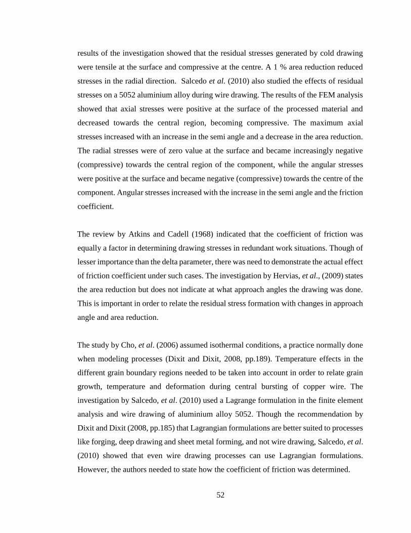
52
results of the investigation showed that the residual stresses generated by cold drawing
were tensile at the surface and compressive at the centre. A 1 % area reduction reduced
stresses in the radial direction. Salcedo et al. (2010) also studied the effects of residual
stresses on a 5052 aluminium alloy during wire drawing. The results of the FEM analysis
showed that axial stresses were positive at the surface of the processed material and
decreased towards the central region, becoming compressive. The maximum axial
stresses increased with an increase in the semi angle and a decrease in the area reduction.
The radial stresses were of zero value at the surface and became increasingly negative
(compressive) towards the central region of the component, while the angular stresses
were positive at the surface and became negative (compressive) towards the centre of the
component. Angular stresses increased with the increase in the semi angle and the friction
coefficient.
The review by Atkins and Cadell (1968) indicated that the coefficient of friction was
equally a factor in determining drawing stresses in redundant work situations. Though of
lesser importance than the delta parameter, there was need to demonstrate the actual effect
of friction coefficient under such cases. The investigation by Hervias, et al., (2009) states
the area reduction but does not indicate at what approach angles the drawing was done.
This is important in order to relate the residual stress formation with changes in approach
angle and area reduction.
The study by Cho, et al. (2006) assumed isothermal conditions, a practice normally done
when modeling processes (Dixit and Dixit, 2008, pp.189). Temperature effects in the
different grain boundary regions needed to be taken into account in order to relate grain
growth, temperature and deformation during central bursting of copper wire. The
investigation by Salcedo, et al. (2010) used a Lagrange formulation in the finite element
analysis and wire drawing of aluminium alloy 5052. Though the recommendation by
Dixit and Dixit (2008, pp.185) that Lagrangian formulations are better suited to processes
like forging, deep drawing and sheet metal forming, and not wire drawing, Salcedo, et al.
(2010) showed that even wire drawing processes can use Lagrangian formulations.
However, the authors needed to state how the coefficient of friction was determined.
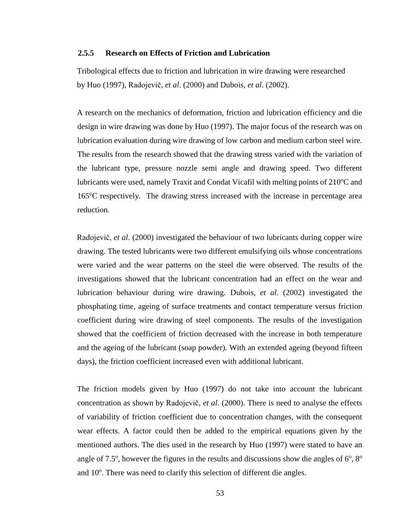
53
2.5.5 Research on Effects of Friction and Lubrication
Tribological effects due to friction and lubrication in wire drawing were researched
by Huo (1997), Radojevič, et al. (2000) and Dubois, et al. (2002).
A research on the mechanics of deformation, friction and lubrication efficiency and die
design in wire drawing was done by Huo (1997). The major focus of the research was on
lubrication evaluation during wire drawing of low carbon and medium carbon steel wire.
The results from the research showed that the drawing stress varied with the variation of
the lubricant type, pressure nozzle semi angle and drawing speed. Two different
lubricants were used, namely Traxit and Condat Vicafil with melting points of 210oC and
165oC respectively. The drawing stress increased with the increase in percentage area
reduction.
Radojevič, et al. (2000) investigated the behaviour of two lubricants during copper wire
drawing. The tested lubricants were two different emulsifying oils whose concentrations
were varied and the wear patterns on the steel die were observed. The results of the
investigations showed that the lubricant concentration had an effect on the wear and
lubrication behaviour during wire drawing. Dubois, et al. (2002) investigated the
phosphating time, ageing of surface treatments and contact temperature versus friction
coefficient during wire drawing of steel components. The results of the investigation
showed that the coefficient of friction decreased with the increase in both temperature
and the ageing of the lubricant (soap powder). With an extended ageing (beyond fifteen
days), the friction coefficient increased even with additional lubricant.
The friction models given by Huo (1997) do not take into account the lubricant
concentration as shown by Radojevič, et al. (2000). There is need to analyse the effects
of variability of friction coefficient due to concentration changes, with the consequent
wear effects. A factor could then be added to the empirical equations given by the
mentioned authors. The dies used in the research by Huo (1997) were stated to have an
angle of 7.5o, however the figures in the results and discussions show die angles of 6o, 8o
and 10o. There was need to clarify this selection of different die angles.
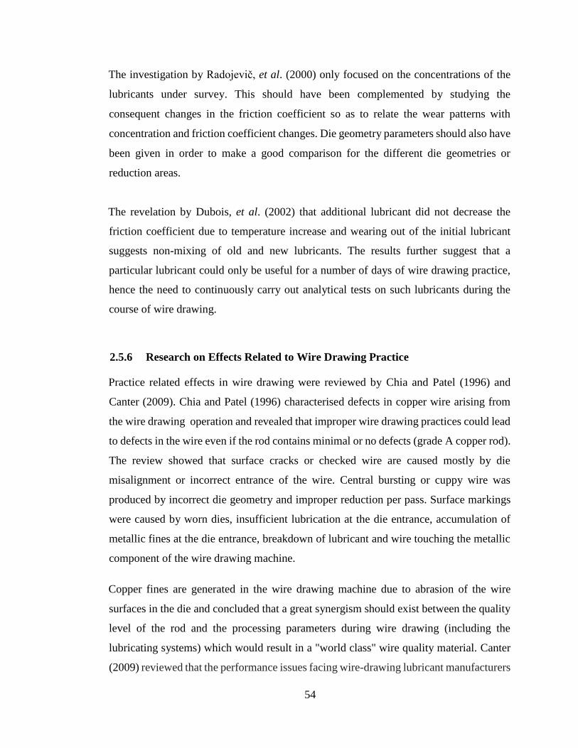
54
The investigation by Radojevič, et al. (2000) only focused on the concentrations of the
lubricants under survey. This should have been complemented by studying the
consequent changes in the friction coefficient so as to relate the wear patterns with
concentration and friction coefficient changes. Die geometry parameters should also have
been given in order to make a good comparison for the different die geometries or
reduction areas.
The revelation by Dubois, et al. (2002) that additional lubricant did not decrease the
friction coefficient due to temperature increase and wearing out of the initial lubricant
suggests non-mixing of old and new lubricants. The results further suggest that a
particular lubricant could only be useful for a number of days of wire drawing practice,
hence the need to continuously carry out analytical tests on such lubricants during the
course of wire drawing.
2.5.6 Research on Effects Related to Wire Drawing Practice
Practice related effects in wire drawing were reviewed by Chia and Patel (1996) and
Canter (2009). Chia and Patel (1996) characterised defects in copper wire arising from
the wire drawing operation and revealed that improper wire drawing practices could lead
to defects in the wire even if the rod contains minimal or no defects (grade A copper rod).
The review showed that surface cracks or checked wire are caused mostly by die
misalignment or incorrect entrance of the wire. Central bursting or cuppy wire was
produced by incorrect die geometry and improper reduction per pass. Surface markings
were caused by worn dies, insufficient lubrication at the die entrance, accumulation of
metallic fines at the die entrance, breakdown of lubricant and wire touching the metallic
component of the wire drawing machine.
Copper fines are generated in the wire drawing machine due to abrasion of the wire
surfaces in the die and concluded that a great synergism should exist between the quality
level of the rod and the processing parameters during wire drawing (including the
lubricating systems) which would result in a "world class" wire quality material. Canter
(2009) reviewed that the performance issues facing wire-drawing lubricant manufacturers
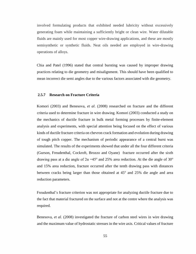
55
involved formulating products that exhibited needed lubricity without excessively
generating foam while maintaining a sufficiently bright or clean wire. Water dilutable
fluids are mainly used for most copper wire-drawing applications, and these are mostly
semisynthetic or synthetic fluids. Neat oils needed are employed in wire-drawing
operations of alloys.
Chia and Patel (1996) stated that central bursting was caused by improper drawing
practices relating to die geometry and misalignment. This should have been qualified to
mean incorrect die semi angles due to the various factors associated with die geometry.
2.5.7 Research on Fracture Criteria
Komori (2003) and Benesova, et al. (2008) researched on fracture and the different
criteria used to determine fracture in wire drawing. Komori (2003) conducted a study on
the mechanics of ductile fracture in bulk metal forming processes by finite-element
analysis and experiments, with special attention being focused on the effect of various
kinds of ductile fracture criteria on chevron crack formation and evolution during drawing
of tough pitch copper. The mechanism of periodic appearance of a central burst was
simulated. The results of the experiments showed that under all the four different criteria
(Gurson, Freudenthal, Cockroft, Brozzo and Oyane) fracture occurred after the sixth
drawing pass at a die angle of 2α =45o and 25% area reduction. At the die angle of 30o
and 15% area reduction, fracture occurred after the tenth drawing pass with distances
between cracks being larger than those obtained at 45o and 25% die angle and area
reduction parameters.
Freudenthal’s fracture criterion was not appropriate for analyzing ductile fracture due to
the fact that material fractured on the surface and not at the centre where the analysis was
required.
Benesova, et al. (2008) investigated the fracture of carbon steel wires in wire drawing
and the maximum value of hydrostatic stresses in the wire axis. Critical values of fracture

56
strains using the Cockroft-Latham criterion (which relates principal and equivalent
stresses and strains) were determined when the wire was drawn through three dies, with
different die semi angles (8°, 10° and 12°), using the FEM with the softwares Deform
2D, ABAQUS and Forge 2. The results from the investigation showed that central
bursting occurred due to a corresponding increase in the area reduction, material flow
stress, effective strain and number of passes, and that the maximum values of fracture
were reached in the cross-section of the wire, where the deformation zone proceeded to
the bearing zone or at its initial part. In these areas, the lowest values of the hydrostatic
stress were in the wire axis. Effective strain versus fracture curves were parallel and above
those where no fracture occurred, with the slope corresponding to the factor of stress
concentration.
Using the Cockroft-Latham criterion for different semi-angles when drawing high carbon
steel wires, Benesova, et al. (2008) demonstrated that central bursting occurred due to a
corresponding increase in the area reduction, material flow stress, effective strain and
number of passes when using the software Deform 2D. The research elaborated more
when the software Deform 2D was used for the FEM, while the use of the ABAQUS and
Forge 2 softwares was only limited to hydrostatic stress distributions in the approach and
bearing regions. The applicability of all the softwares used was not therefore
comprehensive.
The study by Komori (2003) using different fracture criteria on chevron crack formation
could be augmented by the observation that Cockroft and Latham’s and Brozzo et al.’s
criteria only agree well with experiments for internal or chevron crack studies, while
Freudenthal’s criterion would be more appropriate to surface crack studies. The results
given by McAllen and Phelan (2007) indicating an oscillating or up and down nature of
the damage values versus wire diameter required clarification as to whether the same set
of points were maintained during the analysis.
In the categorization of workability, Wright (2011), Hosford and Caddell (1983) and
Valberg (2010) referred to the Cockroft and Latham criterion as a commonly applied

57
criterion. Bao (2003) clarified this by stating that the applicability should be based on the
range of a stress state.
Wright (2011) gave good practical applications of temperature measurements, but failed
short of adding the temperature component due to cooling in equation (2.26) as given by
Valberg (2010) in equation (2.22). This could be a source of errors in practical
determination of the overall heat effects during wire drawing.
2.6 Research Gap Analysis and Contribution
2.6.1 Research Gap Analysis
This research aims to provide contributions to the field of wire drawing and extend it in
terms of both content and processes. The extended literature provides wire drawing
practice in relatively broad aspects. Firstly, this research attempts to provide more
specific and comprehensive means of wire drawing by focusing on die geometry and the
effects of the Δ-parameter during medium size copper wire drawing. Secondly, the factors
underlying defect-free wire drawing practice will be developed through integrated
qualitative and quantitative research means.
The research on inclusion effects (Norasethasopon, 2003; Norasethasopon, 2011;
Norasethasopon and Yoshida, 2003) has gaps concerning the relative effect of metallic
and nonmetallic inclusions, sizes and stress build-up relative to wire breakage. Inclusion
effects equally need to be analysed when other parameters (die half angle, reduction per
pass, strain, coefficient of friction) vary during wire processing.
Some of the gaps concerning die geometry effects include the variation of the Δ-parameter
(die angle and deformation zone changes) and the other die geometries (bell, bearing land,
exit angle) with other processing parameters (friction and strain) on crack initiation
during wire drawing. The effect of die geometry on stress distribution was shown by
Kabayama, et al. (2009), but effect of this stress on crack formation still needs to be
analysed. Ahmadi and Farzin (2008) tested the different fracture criteria for varying die
58
semi angle, area reduction and friction coefficient. Whereas Hassan and Hashim (2015)
demonstrated the effect of bearing length on drawing force, there is need to test a fracture
criterion during draw die bearing length variation whilst keeping the other die parameters
constant.
Investigation of temperature during wire drawing was done by Palkowski, et al. (2003),
Singh, et al. (2007) and Vega, et al. (2009) through the effect of drawing speed on
temperature and stress due to deformation, heat and friction conditions. The possible
research gap in this involves the investigation of heat distribution due to redundant work
along the wire centre line, where chevron cracking manifests.
On stress and strain effects during wire drawing, investigations have been done on plastic
deformation and modification of material mechanical properties during wire drawing,
including the maximum values of damage reached in the cross section of the wire, where
the deformation zone proceeds to the bearing zone or at its initial part. Gaps in this
research category include the need to investigate the effect of material property variation
on crack formation and understanding the profile and length of the deformation zone
during wire drawing.
Concerning friction and lubrication effects, different lubricants on drawing speeds and
stresses have been investigated. The possible research gap here is to investigate the
relative transport mechanism of surface and inner wire material layers, the concentration
of lubricants and their effects on the heat distribution and consequent chevron and surface
cracking.
2.6.2 Research Contribution
Whereas most of the literature concerning wire drawing deals with temperature, friction,
lubrication and die geometry whose focus is normally the semi angle and percentage
reduction, this research extends the focus on die geometry by further analyzing the effect
of the bearing length on both surface and internal crack formation during copper wire
drawing. Secondly, the integrated approach of looking at all the factors involved during
59
wire drawing provides operational decision making tools necessary for the optimisation
of the process and consequent reduction or elimination of both internal and surface cracks
during wire drawing of copper. This research, thus, extends the investigations by
Kabayama, et al., (2009) and Hassan and Hashim (2015) by focusing more on bearing
length change when other factors are maintained constant, incorporating the Δ-parameter
and including die manufacturing mechanisms in the investigations.
A proposed system and subsystem level of analysis is shown in Figure 2.13 as a guide to
the machine-die system level investigation of the wire drawing process. The figure
indicates that a comprehensive understanding and analysis of the wire drawing process
needs to be undertaken at three levels, namely:
(i) Material Level
Under this level, all the physical properties and characteristics regarding the die, wire and
lubricant materials need to be taken into consideration. Of great importance is the
chemical composition (including metallic and non-metallic inclusions) of the wire to be
drawn.
(ii) Process Level
Under this level, the modifying conditions during wire drawing need to be understood.
Temperature of both the lubricant and the dies, the stress and strain components
obtainable in the wire being drawn, and the friction and lubricating conditions all have
an effect on the overall performance of the wire drawing process.
(iii) Die Level
Once the material and process conditions have been taken into account, the third level of
analysis is the die level. Under this level, all aspects of the die including the internal
geometry and its consequent wear and failure, need to be understood. The condition of
the die has an effect on the wire drawing process.
(iv) Integration and Optimisation Level
Under this level, the control of parameters at material, process and die levels is important
in order to produce a defect-free wire product. Control of parameters is done so that
better-performing or optimal parameters are obtained in order to avert or substantially

60
reduce the defects leading to product failure. Different fracture criteria may be used to
assess the parameters.
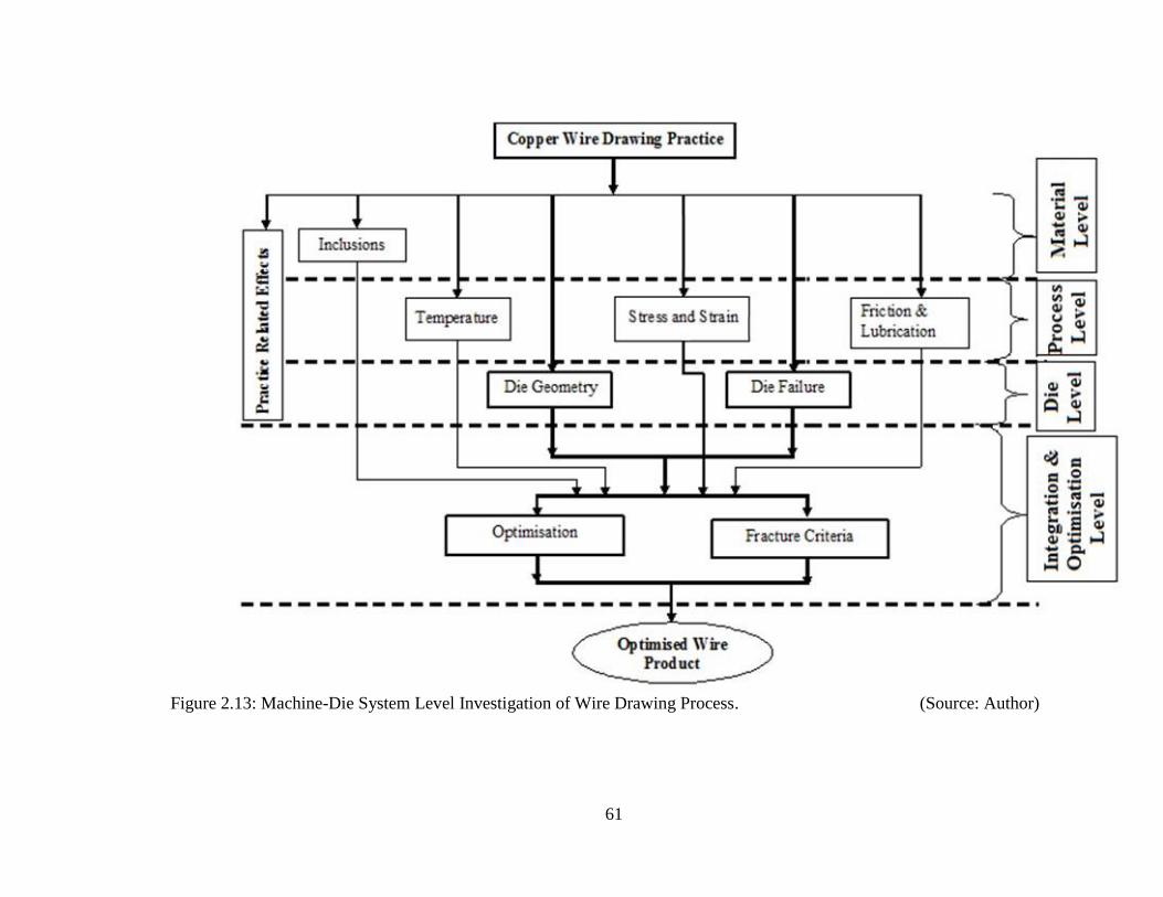
61
Figure 2.13: Machine-Die System Level Investigation of Wire Drawing Process. (Source: Author)
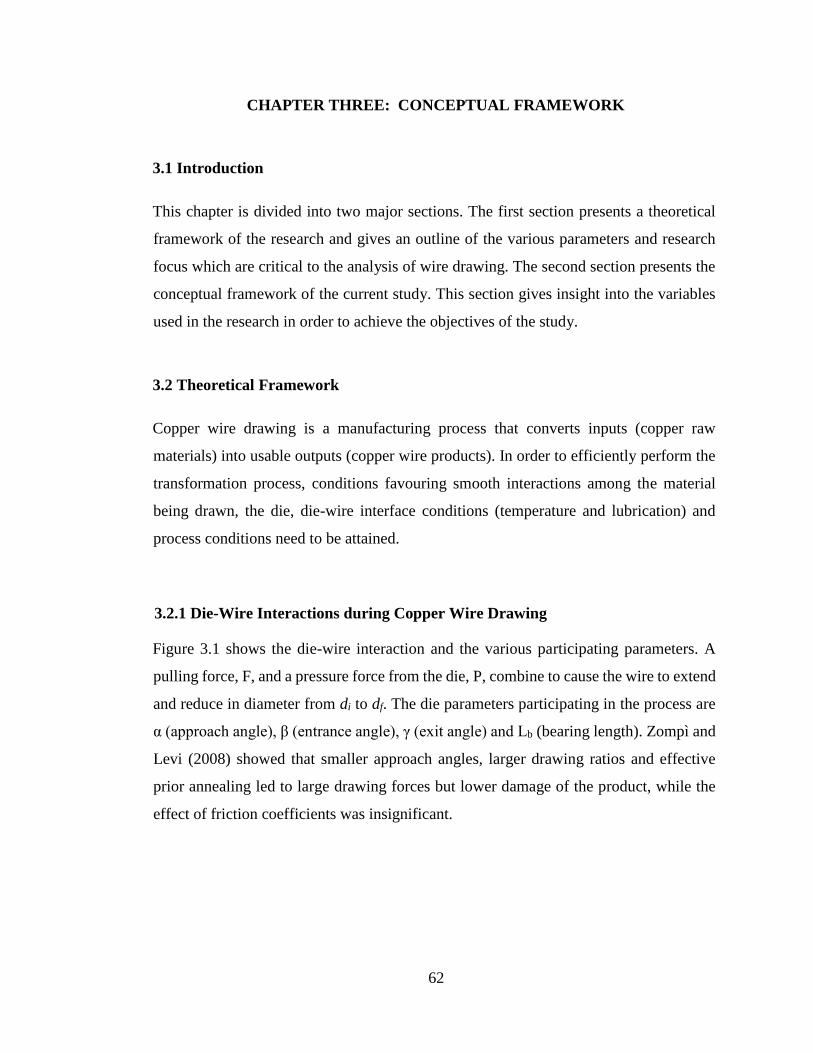
62
CHAPTER THREE: CONCEPTUAL FRAMEWORK
3.1 Introduction
This chapter is divided into two major sections. The first section presents a theoretical
framework of the research and gives an outline of the various parameters and research
focus which are critical to the analysis of wire drawing. The second section presents the
conceptual framework of the current study. This section gives insight into the variables
used in the research in order to achieve the objectives of the study.
3.2 Theoretical Framework
Copper wire drawing is a manufacturing process that converts inputs (copper raw
materials) into usable outputs (copper wire products). In order to efficiently perform the
transformation process, conditions favouring smooth interactions among the material
being drawn, the die, die-wire interface conditions (temperature and lubrication) and
process conditions need to be attained.
3.2.1 Die-Wire Interactions during Copper Wire Drawing
Figure 3.1 shows the die-wire interaction and the various participating parameters. A
pulling force, F, and a pressure force from the die, P, combine to cause the wire to extend
and reduce in diameter from di to df. The die parameters participating in the process are
α (approach angle), β (entrance angle), γ (exit angle) and Lb (bearing length). Zompì and
Levi (2008) showed that smaller approach angles, larger drawing ratios and effective
prior annealing led to large drawing forces but lower damage of the product, while the
effect of friction coefficients was insignificant.

63
Figure 3.1: Die-Wire Interaction and Process Parameters. (Source: Author)
3.2.2 Material Conditions during Copper Wire Drawing
During the wire drawing process, the copper wire interacts with the die (commonly
tungsten carbide or synthetic diamond) at the wire-die interface where the lubricant
participates. The applied drawing force causes deformation by overcoming friction forces
and internal distortions. Within the material being drawn, internal shearing occurs, hence
distortion of internal plane sections resulting in the metal experiencing higher strain and
the end product becoming harder, stronger, and less ductile (Hosford and Caddell, 1983).
Norasethasopon and Yoshida (2003) showed that the inclusion properties, size and length
and wire properties had an influence on the inclusion deformation, wire deformation and
maximum hydrostatic tensile stresses.
Figure 3.2 shows the interacting materials in the copper wire drawing process and their
respective parameters. The figure shows that during works on the rod, the types and
percentages of inclusions, the hardness and the surface roughness of the rod will
determine the mechanical properties of the exiting wire. The hardness and surface
roughness of the die have an impact on the wear and life of the die during its interaction
with the rod and wire material properties. The concentration and viscosity of the lubricant
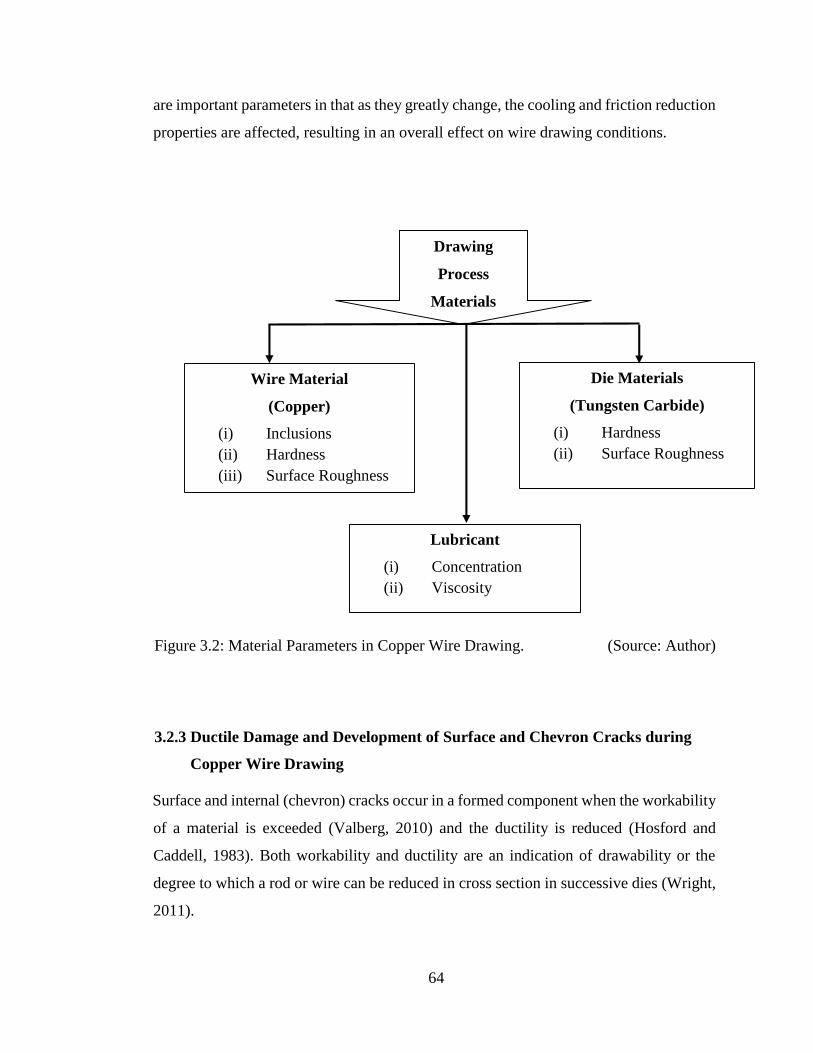
64
are important parameters in that as they greatly change, the cooling and friction reduction
properties are affected, resulting in an overall effect on wire drawing conditions.
Figure 3.2: Material Parameters in Copper Wire Drawing. (Source: Author)
3.2.3 Ductile Damage and Development of Surface and Chevron Cracks during
Copper Wire Drawing
Surface and internal (chevron) cracks occur in a formed component when the workability
of a material is exceeded (Valberg, 2010) and the ductility is reduced (Hosford and
Caddell, 1983). Both workability and ductility are an indication of drawability or the
degree to which a rod or wire can be reduced in cross section in successive dies (Wright,
2011).
Drawing
Process
Materials
Die Materials
( Tungsten Carbide )
( ) i Hardness
( ii ) Surface Roughness
Wire Material
( Copper )
( i ) Inclusions
( ) ii Hardness
( iii ) Surface Roughness
Lubricant
( i ) Concentration
( ii ) Viscosity
65
Chevron cracking occurs under conditions of tensile stresses under small area reductions
and large die angles and low friction conditions (Ahmadi and Farzin, 2008). The
probability of crack expansion in the final two or one drawing was great in an eight-pass
drawing (Xu, et al., 2009).
According to Chia and Patel (1996) surface cracks are caused by die wear, insufficient
lubrication, accumulation of metallic fines at the die entrance, breakdown of lubricant
and wire touching the metallic component of the wire drawing machine.
The formation of cracks during wire drawing is predicted using the following four
parameters:
(i) Die Geometry Parameters
The approach angle (α), the bearing length (Lb), the entrance angle (β) and the exit angle
(γ) are the die geometry parameters under study and predicted to affect the formation of
chevron and surface cracks (Ahmadi and Farzin, 2008; Kabayama et al.. Zompì and
Levi, 2008; Kabayama, et al. 2009; Hassan and Hashim, 2015; Wright, 2011).
(ii) Wire Drawing Process Parameters
The interaction of the wire and the die presents a contact surface. Due to this interaction,
the wire velocity (vdr), the coefficient of friction (μ) and the interface temperature (Tint)
have an effect on the formation of cracks both on the surface and at the wire centreline
(Huo, 1997; Ahmadi and Farzin, 2008; Xu, et al. 2009).
(iii) Ductility Parameters
The percent elongation (El) and the percent area reduction (Ar) for each given pass are
critical parameters for ductility which is the extent to which a material can withstand
deformations without risk of breakdown, or formation of cracks. The initial and final
wire diameters, di and df are the input parameters used in ductility measurement (Wright,
2011).
66
(v) Workability Index
The workability index, C, for ductile fracture is determined using the Cockroft and
Latham ductile fracture criterion. The input parameters are (Hosford and Caddell, 1983;
Valberg, 2010; Wright, 2011):
Fracture strain, εf
Maximum tensile stress, σmax
Effective strain, εeff
Whereas the workability index C can change its value at each rod or wire drawing pass,
the ductility parameters (El and Ar) are maintained constant for a given drawing pass.
Hence, both the ductility and workability conditions need to be fulfilled at each pass
(Wright, 2011).
An increase in the ductility parameter Ar signals the presence of necking, leading to the
wire section unable to carry the drawing load and consequently breaking. Decrease in
Ar is an indication of lack of plastic flow in the material, and annealing is used to
maintain the flow of material (Ibid).
Figure 3.3 shows the conditions necessitating the application of the workability index,
specifically the Cockroft and Latham criterion, during copper wire drawing. The figure
shows that for fracture to occur in a ductile material, the criterion for ductile damage
(DUCTCRT) and the critical value of the Cockroft and Latham criterion should have
been met. These conditions arise due to the presence of a maximum stress and a
cumulative strain.
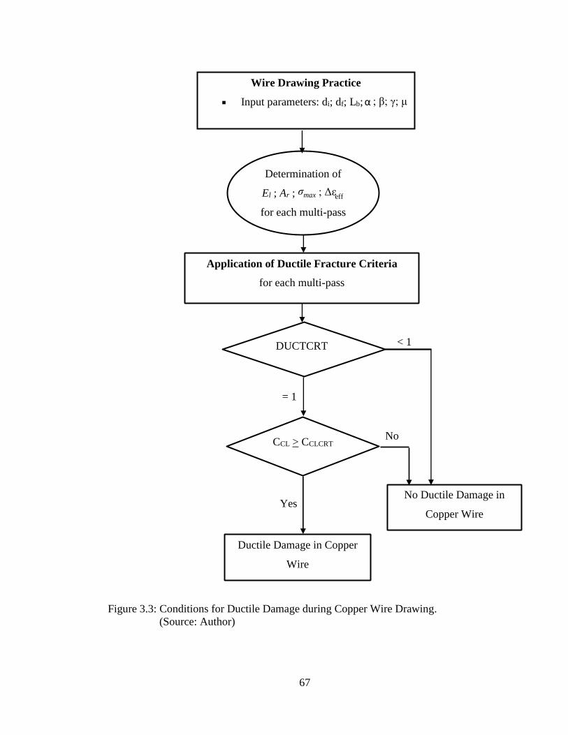
67
Figure 3.3: Conditions for Ductile Damage during Copper Wire Drawing.
(Source: Author)
Wire Drawing Practice
Input parameters : d i ; d f ; L b ; α ; β; γ; μ
Determination of
E l ; A r ; σ max ; Δε eff
for each m ulti - pass
Application of Ductile Fracture Criteri a
for each multi - pass
DUCTCRT
= 1
1 <
C CL > C CL CRT
No Ductile Damage in
Copper Wire
Ductile Damage in Copper
Wire
Yes
No

68
3.2.4 Die Wear during Copper Wire Drawing
Wear is the major reason for die replacement and affects the tolerance of the formed
part, metal flow, die life and economics of the drawing process Lee, et al. (2012).
Research by Yang, et al. (2007) showed that wear and tear behaviours were different in
different die zones, with the approach and bearing zones registering the most severe
wear. Hollinger, et al. (2003) showed that die wear rate reached a maximum value at the
entrance to the approach zone.
According to the ASM Handbook (ASM International, 1988), two types of die materials
are recommended for use when drawing copper material. Natural and synthetic diamond
die materials are recommended for drawing copper wires of diameters less than 2.06
mm, whereas for diameters greater than 2.06 mm cemented carbide die materials are
used.
Die geometry influences the process parameters, including heat generation, during wire
drawing (Campos et al., 2006; Zompì and Levi, 2008; Ahmadi and Farzin, 2008;
Kabayama et al., 2009; León et al., 2010; Vega et al., 2009). Tribological effects due
to friction and lubrication during wire drawing were investigated by Huo (1997),
Radojevič et al. (2000) and Dubois et al. (2002).
Since die wear has an influence on the tolerance, and hence the quality of the formed
parts and the general economics of the forming process (Lee et al., 2012), the presence
of surface cracks is influenced by wear. This was demonstrated by Panjan, et al., (2005)
who showed that die wear occurs when burrs appear on the copper profile surface.
Figure 3.4 shows the interacting influence of die materials, die and process parameters
and modifying conditions on die wear and crack formation. The figure shows that
depending on the die materials in use, a good selection of die geometry and process
parameters, with monitored modifying conditions, will reduce die wear, increase die life
and thus guarantee a good quality of wire.
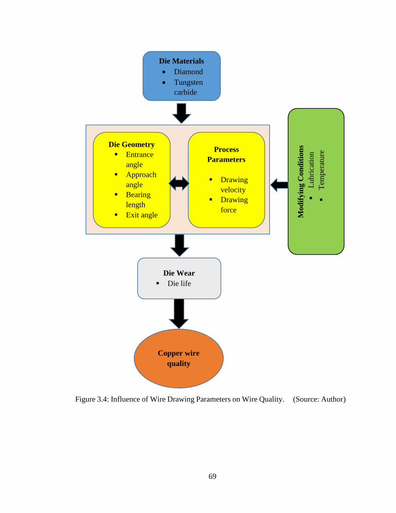
69
Figure 3.4: Influence of Wire Drawing Parameters on Wire Quality. (Source: Author)
Die Materials
Diamond
Tungsten
carbide
Mod
ifyin
g C
on
dit
ion
s
Lubri
cati
on
Tem
per
ature
Die Wear
Die life
Copper wire
quality
Die Geometry
Entrance
angle
Approach
angle
Bearing
length
Exit angle
Process
Parameters
Drawing
velocity
Drawing
force
70
3.3 Conceptual Framework
Different levels of interactions among the properties of the copper wire material, die
material and geometry, and the process conditions lead to the formation of wire drawing
conditions promoting the presence of, or lack of, surface and internal defects in the
copper wire.
3.3.1 Research Variables in Copper Wire Drawing Process
The research variables needed to fully analyse copper wire drawing arise from the
parameters indicated in Figures 3.1, 3.2, 3.3 and 3.4. The parameters can be classified
as being independent and dependent variables.
(a) Independent Variables
Independent variables are the parameters to be varied or manipulated by the researcher.
They are antecedents or the presumed cause. During both simulation and experiments,
the independent variable is the parameter to be controlled and manipulated. In the non-
experimental case, such as in the die design and manufacturing process where there is
no experimental manipulation, the independent variable is the variable that 'logically'
has some effect on a dependent variable (Kerlinger, 1986).
The independent variables which participated in the study were:
▪ area reduction
▪ approach angle
▪ entrance angle
▪ bearing length
▪ die exit angle
▪ drawing velocity
▪ coefficient of friction

71
(b) Dependent Variables
The dependent variable refers to the status of the 'effect' (or outcome) in which the
researcher is interested (Rosenthal and Rosnow, 1991). The dependent variables used
in this research were:
▪ drawing force
▪ die temperature
▪ drawing stress
▪ strain rate
▪ damage value
3.3.2 Independent Variables
The major independent variable associated with the die geometrical parameters, bearing
length, was varied while keeping the other die geometrical parameters (Δ-parameter,
entrance angle, exit angle) and process conditions (drawing velocity, coefficient of
friction and wire material properties) constant during the study.
The choice of optimum independent parameters was based on iterative modelling from
which a parameter with less effect on damage value was chosen. Figure 3.5 shows the
categorisation of the different independent variables based on die geometry, process
conditions and wire material properties. The figure shows that the underlying parameters
within each variable have an influence on the progression of wire drawing.
(1) Material State Based Independent Variables
The following are the independent variables pertaining to material properties used in
copper wire drawing study:
(i) Inclusions, Ninc
These are both non-metallic and metallic additions to a material’s composition. They
affect the quality of the input wire and stress distribution in the wire (Norasethasopon,
2003). The inclusions were assumed and kept constant during the study.
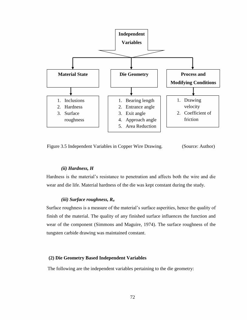
72
Figure 3.5 Independent Variables in Copper Wire Drawing. (Source: Author)
(ii) Hardness, H
Hardness is the material’s resistance to penetration and affects both the wire and die
wear and die life. Material hardness of the die was kept constant during the study.
(iii) Surface roughness, Ra
Surface roughness is a measure of the material’s surface asperities, hence the quality of
finish of the material. The quality of any finished surface influences the function and
wear of the component (Simmons and Maguire, 1974). The surface roughness of the
tungsten carbide drawing was maintained constant.
(2) Die Geometry Based Independent Variables
The following are the independent variables pertaining to the die geometry:
Independent
Variables
Die Geometry Process a nd
Modifying Conditions
Material State
1. Bearing length
2. Entrance angle
3. Exit angle
4. Approach angle
5. Area Reduction
1. Drawing
velocity
2. Coefficient of
friction
1. Inclusions
2. Hardness
3. Surface
roughness
73
(i) Approach angle, α
The Approach Angle is designed such that it allows for a smooth and controlled
deformation of the wire. Harder materials, larger area reductions and bigger elongations
require smaller approach angles of between 6o to 8o , whereas softer materials, smaller
area reductions and shorter elongations are drawn with bigger approach angles ranging
from 8o to 10o (Esteves Group, 2008). The approach angle was initially varied then
maintained constant. This was based both on models performed and on the findings by
Norasethasopon and Yoshida, (2003) and Kabayama, et al., (2009) where an approach
angle of 9o was determined as being optimum.
(ii) Area reduction, Ar
The area reduction characterises the extent of deformations imposed on a workpiece,
hence influences the redundant work, frictional work and drawing forces (Valberg,
2010; Hosford and Caddell, 1983). In the study, which is a multi-pass wire drawing, the
area reduction was initially varied at each pass, ranging from 10% to 20%, and then
maintained constant.
Both the area reduction and the approach angle are used to compute the Δ-parameter
which characterizes the shape of the deformation zone and is used as a predictor of void
formation. Void formation and centre bursting are attributed to higher values of Δ (above
3.0) which are indicative of high levels of redundant deformation and surface hardening
(Descargas, nd).
(iii) Die entrance angle, β
The entrance angle facilitates for a smooth transition to the approach zone and
conditions of lower die angles, and thus a lower Δ-parameter. This reduces redundant
work, die pressure, and centerline tension at the end of the pass (Wright, 2011). The
entrance angle, therefore, has an effect on the following: redundant work, die pressure,
die wear and central bursting. The entrance angle was initially varied and then
maintained constant at 30o during the study.
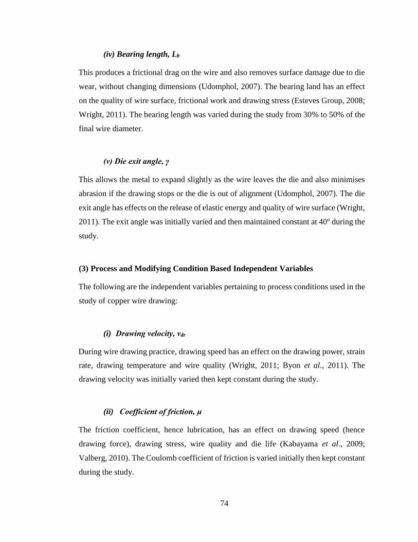
74
(iv) Bearing length, Lb
This produces a frictional drag on the wire and also removes surface damage due to die
wear, without changing dimensions (Udomphol, 2007). The bearing land has an effect
on the quality of wire surface, frictional work and drawing stress (Esteves Group, 2008;
Wright, 2011). The bearing length was varied during the study from 30% to 50% of the
final wire diameter.
(v) Die exit angle, γ
This allows the metal to expand slightly as the wire leaves the die and also minimises
abrasion if the drawing stops or the die is out of alignment (Udomphol, 2007). The die
exit angle has effects on the release of elastic energy and quality of wire surface (Wright,
2011). The exit angle was initially varied and then maintained constant at 40o during the
study.
(3) Process and Modifying Condition Based Independent Variables
The following are the independent variables pertaining to process conditions used in the
study of copper wire drawing:
(i) Drawing velocity, νdr
During wire drawing practice, drawing speed has an effect on the drawing power, strain
rate, drawing temperature and wire quality (Wright, 2011; Byon et al., 2011). The
drawing velocity was initially varied then kept constant during the study.
(ii) Coefficient of friction, μ
The friction coefficient, hence lubrication, has an effect on drawing speed (hence
drawing force), drawing stress, wire quality and die life (Kabayama et al., 2009;
Valberg, 2010). The Coulomb coefficient of friction is varied initially then kept constant
during the study.
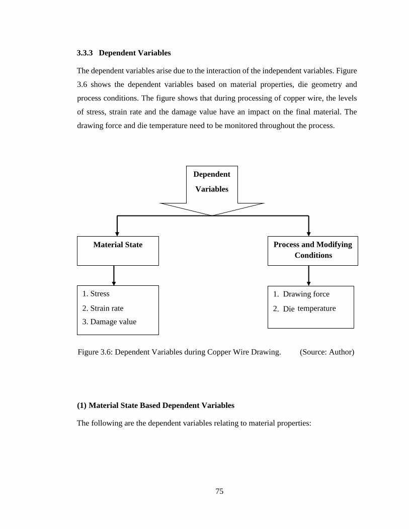
75
3.3.3 Dependent Variables
The dependent variables arise due to the interaction of the independent variables. Figure
3.6 shows the dependent variables based on material properties, die geometry and
process conditions. The figure shows that during processing of copper wire, the levels
of stress, strain rate and the damage value have an impact on the final material. The
drawing force and die temperature need to be monitored throughout the process.
Figure 3.6: Dependent Variables during Copper Wire Drawing. (Source: Author)
(1) Material State Based Dependent Variables
The following are the dependent variables relating to material properties:
D ependent
Variables
Process and Modifying
Co nditions
Material State
1 . Drawing force
2 . Die
temperature
1 . S tress
2 . Strain rate
3. Damage value

76
(i) Drawing stress, σd
Drawing stresses have an effect on the drawability of copper wire and are a result of the
interaction of the material yield stress, the Δ-parameter, the friction coefficient and the
bearing length.
(ii) Strain rate, 𝜺
Strain is the ratio of the change in dimension to the original dimension of the copper
wire material, while strain rate is the rate at which this strain occurs. Changes in strain
rate have a significant impact on wire flow stress (Wright, 2011).
(2) Die Geometry Based Dependent Variables
The following is the dependent variable used in the study of die geometry during copper
wire drawing:
(i) Die wear, δ
Die wear is as a result of contact force between the wire and the die, the temperature and
tribological conditions at the wire-die interface
(3) Process and Modifying Condition Based Dependent Variables
Dependent variables used in the study of process conditions during wire drawing include
the following:
(i) Drawing force, Fdr
The drawing force under friction and redundant conditions is based on the friction
coefficient, the value of the Δ-parameter and the flow stress (Kalpakjian and Schmid,
2010).
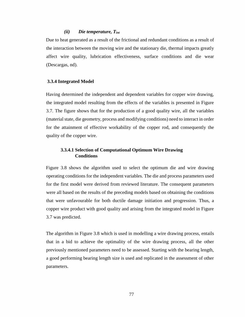
77
(ii) Die temperature, Tint
Due to heat generated as a result of the frictional and redundant conditions as a result of
the interaction between the moving wire and the stationary die, thermal impacts greatly
affect wire quality, lubrication effectiveness, surface conditions and die wear
(Descargas, nd).
3.3.4 Integrated Model
Having determined the independent and dependent variables for copper wire drawing,
the integrated model resulting from the effects of the variables is presented in Figure
3.7. The figure shows that for the production of a good quality wire, all the variables
(material state, die geometry, process and modifying conditions) need to interact in order
for the attainment of effective workability of the copper rod, and consequently the
quality of the copper wire.
3.3.4.1 Selection of Computational Optimum Wire Drawing
Conditions
Figure 3.8 shows the algorithm used to select the optimum die and wire drawing
operating conditions for the independent variables. The die and process parameters used
for the first model were derived from reviewed literature. The consequent parameters
were all based on the results of the preceding models based on obtaining the conditions
that were unfavourable for both ductile damage initiation and progression. Thus, a
copper wire product with good quality and arising from the integrated model in Figure
3.7 was predicted.
The algorithm in Figure 3.8 which is used in modelling a wire drawing process, entails
that in a bid to achieve the optimality of the wire drawing process, all the other
previously mentioned parameters need to be assessed. Starting with the bearing length,
a good performing bearing length size is used and replicated in the assessment of other
parameters.
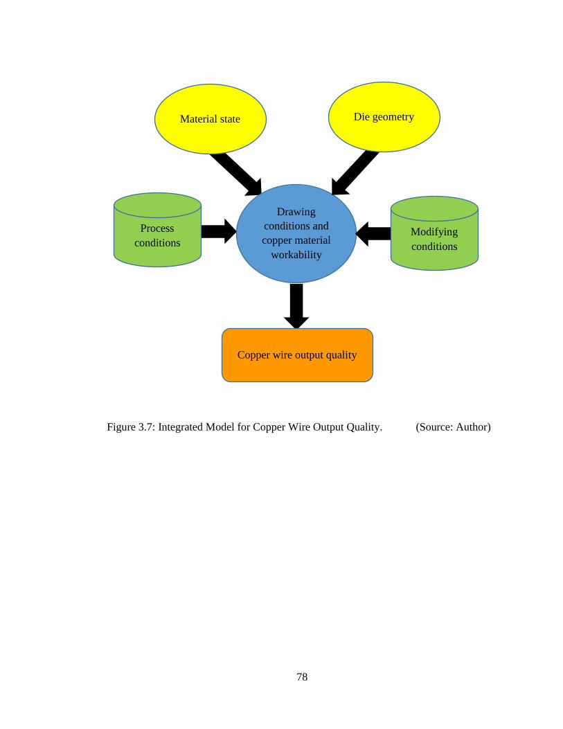
78
Figure 3.7: Integrated Model for Copper Wire Output Quality. (Source: Author)
Drawing
Conditions and
Copper Material
Workability
Drawing
conditions and
copper material
workability
Copper wire output quality
Process
conditions Modifying
conditions
Material state Die geometry
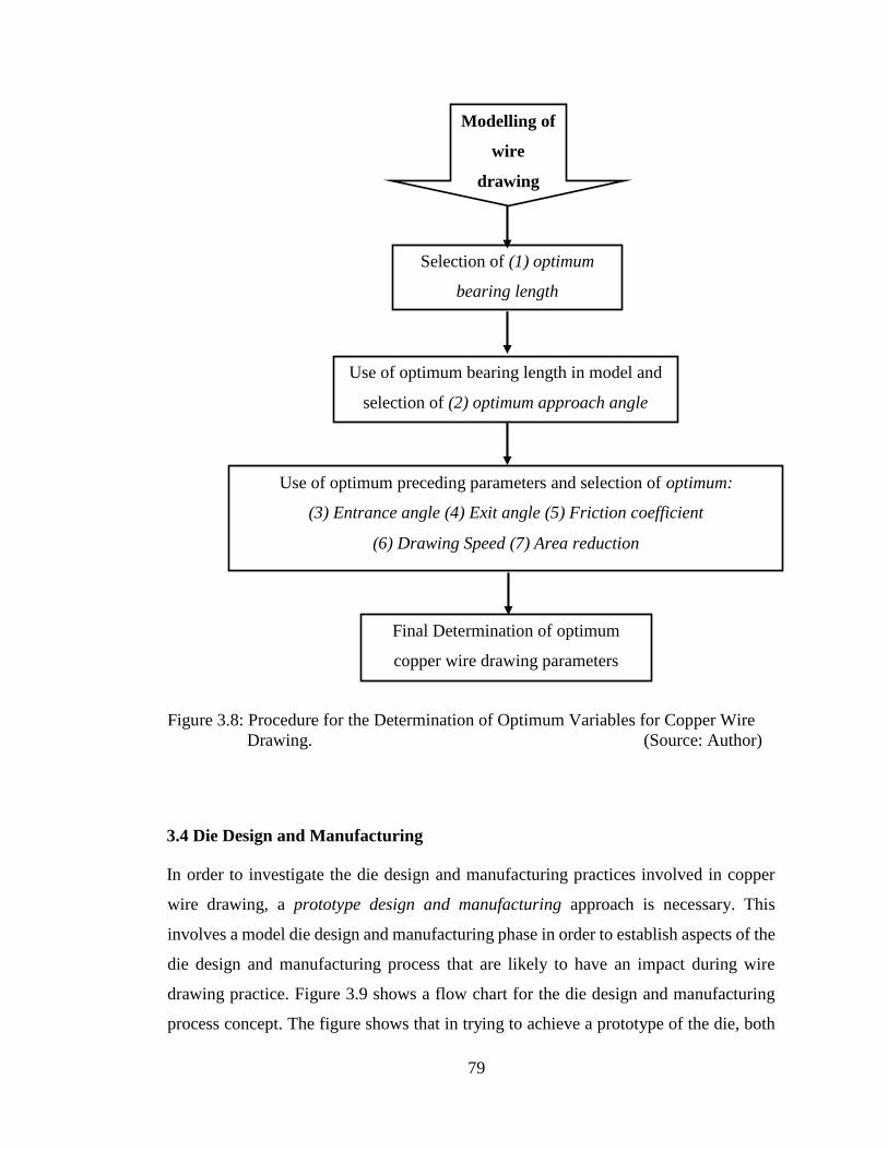
79
Figure 3.8: Procedure for the Determination of Optimum Variables for Copper Wire
Drawing. (Source: Author)
3.4 Die Design and Manufacturing
In order to investigate the die design and manufacturing practices involved in copper
wire drawing, a prototype design and manufacturing approach is necessary. This
involves a model die design and manufacturing phase in order to establish aspects of the
die design and manufacturing process that are likely to have an impact during wire
drawing practice. Figure 3.9 shows a flow chart for the die design and manufacturing
process concept. The figure shows that in trying to achieve a prototype of the die, both
Selection of (1) optimum
bearing length
Modelling of
wire
drawing
Use of optimum bearing length in model and
selection of (2) optimum approach angle
Use of optimum preceding parameters and selection of op timum :
(3) Entrance angle Exit angle (5) Friction coefficient (4)
Drawing Speed (7) Area reduction (6)
Final Determination of optimum
copper wire drawing parameters
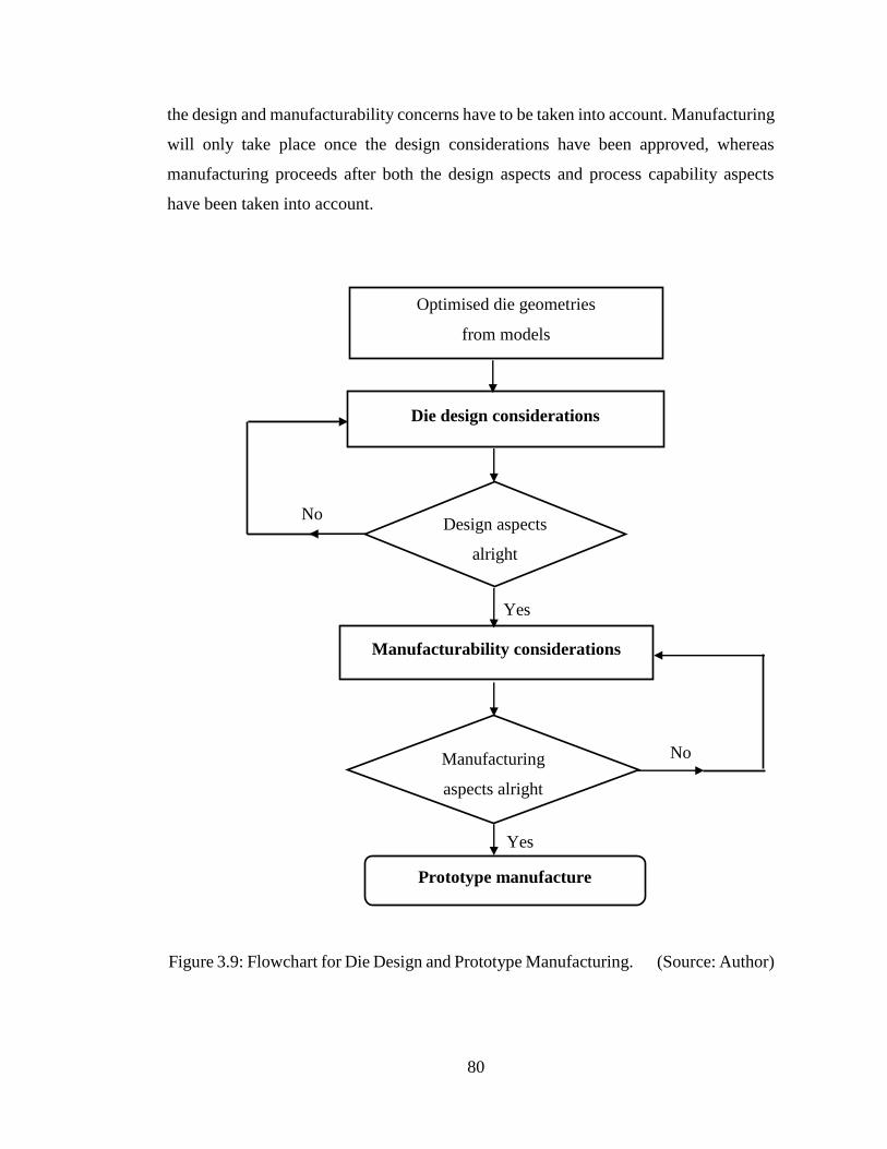
80
the design and manufacturability concerns have to be taken into account. Manufacturing
will only take place once the design considerations have been approved, whereas
manufacturing proceeds after both the design aspects and process capability aspects
have been taken into account.
Figure 3.9: Flowchart for Die Design and Prototype Manufacturing. (Source: Author)
Optimised die geometries
from models
Die design c onsiderations
D esign aspects
alright
Manufacturability considerations
Yes
No
Manufacturing
aspects a lright
Prototype manufacture
Yes
No
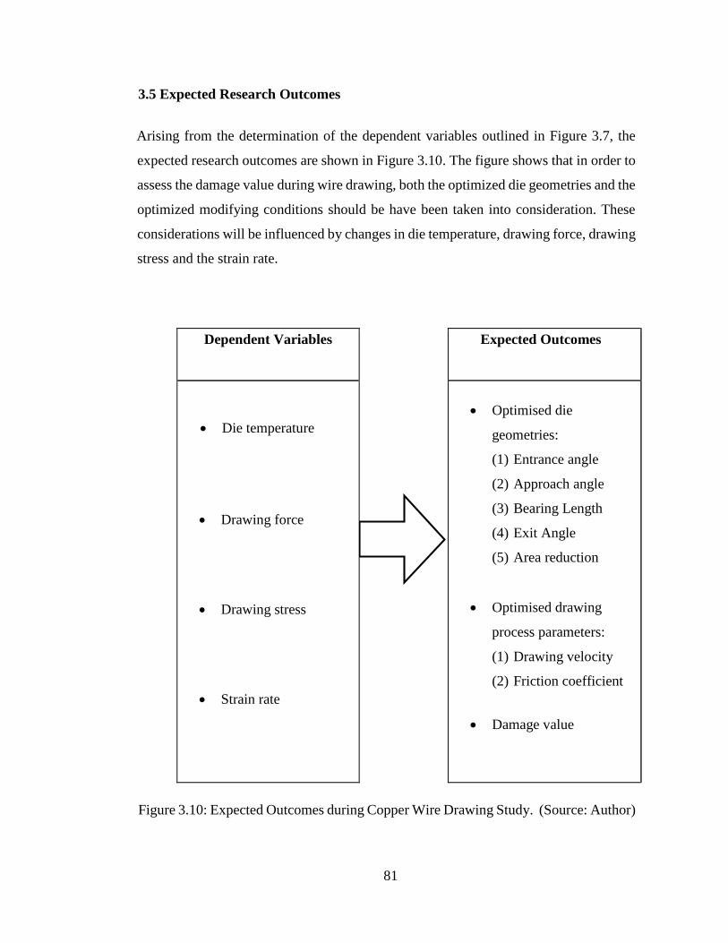
81
3.5 Expected Research Outcomes
Arising from the determination of the dependent variables outlined in Figure 3.7, the
expected research outcomes are shown in Figure 3.10. The figure shows that in order to
assess the damage value during wire drawing, both the optimized die geometries and the
optimized modifying conditions should be have been taken into consideration. These
considerations will be influenced by changes in die temperature, drawing force, drawing
stress and the strain rate.
Dependent Variables
Expected Outcomes
Die temperature
Drawing force
Drawing stress
Strain rate
Optimised die
geometries:
(1) Entrance angle
(2) Approach angle
(3) Bearing Length
(4) Exit Angle
(5) Area reduction
Optimised drawing
process parameters:
(1) Drawing velocity
(2) Friction coefficient
Damage value
Figure 3.10: Expected Outcomes during Copper Wire Drawing Study. (Source: Author)
82
CHAPTER FOUR: RESEARCH METHODOLOGY
4.1 Introduction
The research is based on the mechanics and production technology of bulk deformation
and copper metallurgy in wire drawing. In order to find solutions to such complex
phenomena which involve stress analysis and solid mechanics problems, the FEM
approach is used. This numerical or computational approach is widely used to determine
the distribution of stress field variables governing processes of metal forming.
The purpose of the research was to investigate the die design, manufacturing practices
and copper wire drawing process conditions leading to chevron and surface crack
formation. This was done by both developing a copper wire drawing model using the
finite element method and experimental investigations of copper wire drawing. In order
to achieve the mentioned objectives, the influence of different die geometries and
process conditions for copper wire drawing were studied.
The independent variables which participated in the study included the area reduction,
approach angle, die entrance angle, bearing length, die exit angle, drawing velocity,
coefficient of friction, wire material properties, while the dependent variables were the
drawing stress and strain, die wear, drawing force and die-wire interface temperature.
Parametric studies of these factors were carried out in order to establish their effect on
chevron and surface crack formation during copper wire drawing.
Each of the die geometrical parameters (area reduction, approach angle, entrance angle,
bearing length and die exit angle) were varied while keeping the drawing velocity,
coefficient of friction and wire material properties constant against the dependent
variables. The optimum die geometries and operating conditions during copper wire
drawing were thus derived.
Therefore, this chapter discusses how the research was designed and the methods that
were used in order to achieve the intended objectives. Also highlighted are limitations
and ethical considerations of the research.

83
4.2 Research Design
4.2.1 General Method
The general method involved modelling and simulation of factors involved in copper
wire drawing and carrying out industrial experiments, with an extended literature review
of the die design and manufacturing process. The FEM approach was used with
ABAQUS 6.14 software to model the problem. This was done for the purpose of
studying the effect of die geometries and process conditions on chevron and surface
cracking during copper wire drawing.
4.2.2 Specific Procedures
(i) Modelling and Simulation of the Copper Wire Drawing Process
Initially theoretical data pertaining to the major factors involved in copper wire drawing
process was used to model and simulate a copper wire drawing process. This data was
then analysed and used for comparative analysis with actual experimental data to
optimise the wire drawing process. Using the FEM, a computational and geometrical
model of copper wire drawing was developed. This incorporated die design, copper wire
material properties and dimensions and drawing process conditions. A simulation of the
model was then done and analysed. This was followed by an optimisation process which
was undertaken in order to identify optimum operating conditions for the process. Table
4.1 gives details of parameters used in the modelling and simulation runs for
investigating the effect of bearing length variation, while Table 4.2 provides details of
parameters used for investigating other die geometry and process condition effects. The
bearing length was fixed at 40% in order to isolate its effects on wire drawing, having
been determined as being optimal at 40%.
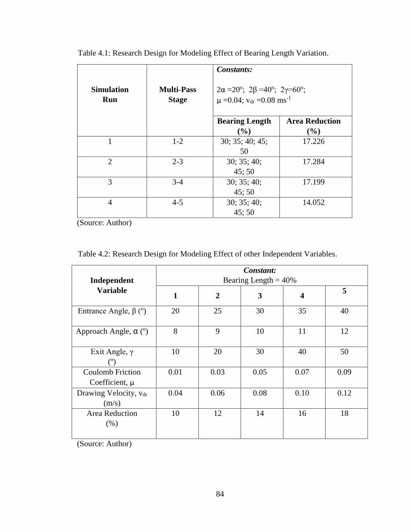
84
Table 4.1: Research Design for Modeling Effect of Bearing Length Variation.
Simulation
Run
Multi-Pass
Stage
Constants:
2α =20o; 2β =40o; 2γ=60o;
μ =0.04; vdr =0.08 ms-1
Bearing Length
(%)
Area Reduction
(%)
1 1-2 30; 35; 40; 45;
50
17.226
2 2-3 30; 35; 40;
45; 50
17.284
3 3-4 30; 35; 40;
45; 50
17.199
4 4-5 30; 35; 40;
45; 50
14.052
(Source: Author)
Table 4.2: Research Design for Modeling Effect of other Independent Variables.
Independent
Variable
Constant:
Bearing Length = 40%
1 2 3 4 5
Entrance Angle, β (o)
20 25 30 35 40
Approach Angle, α (o)
8 9 10 11 12
Exit Angle, γ
(o)
10 20 30 40 50
Coulomb Friction
Coefficient, μ
0.01 0.03 0.05 0.07 0.09
Drawing Velocity, vdr
(m/s)
0.04 0.06 0.08 0.10 0.12
Area Reduction
(%)
10 12 14 16 18
(Source: Author)
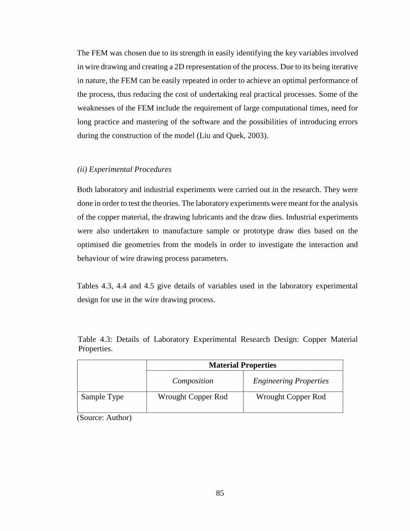
85
The FEM was chosen due to its strength in easily identifying the key variables involved
in wire drawing and creating a 2D representation of the process. Due to its being iterative
in nature, the FEM can be easily repeated in order to achieve an optimal performance of
the process, thus reducing the cost of undertaking real practical processes. Some of the
weaknesses of the FEM include the requirement of large computational times, need for
long practice and mastering of the software and the possibilities of introducing errors
during the construction of the model (Liu and Quek, 2003).
(ii) Experimental Procedures
Both laboratory and industrial experiments were carried out in the research. They were
done in order to test the theories. The laboratory experiments were meant for the analysis
of the copper material, the drawing lubricants and the draw dies. Industrial experiments
were also undertaken to manufacture sample or prototype draw dies based on the
optimised die geometries from the models in order to investigate the interaction and
behaviour of wire drawing process parameters.
Tables 4.3, 4.4 and 4.5 give details of variables used in the laboratory experimental
design for use in the wire drawing process.
Table 4.3: Details of Laboratory Experimental Research Design: Copper Material
Properties.
Material Properties
Composition Engineering Properties
Sample Type Wrought Copper Rod Wrought Copper Rod
(Source: Author)
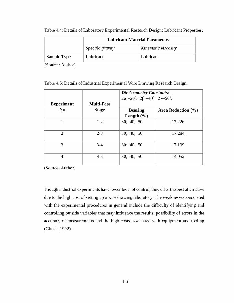
86
Table 4.4: Details of Laboratory Experimental Research Design: Lubricant Properties.
Lubricant Material Parameters
Specific gravity Kinematic viscosity
Sample Type Lubricant Lubricant
(Source: Author)
Table 4.5: Details of Industrial Experimental Wire Drawing Research Design.
Experiment
No
Multi-Pass
Stage
Die Geometry Constants:
2α =20o; 2β =40o; 2γ=60o;
Bearing
Length (%)
Area Reduction (%)
1 1-2 30; 40; 50 17.226
2 2-3 30; 40; 50 17.284
3 3-4 30; 40; 50 17.199
4 4-5 30; 40; 50 14.052
(Source: Author)
Though industrial experiments have lower level of control, they offer the best alternative
due to the high cost of setting up a wire drawing laboratory. The weaknesses associated
with the experimental procedures in general include the difficulty of identifying and
controlling outside variables that may influence the results, possibility of errors in the
accuracy of measurements and the high costs associated with equipment and tooling
(Ghosh, 1992).
87
4.3 Die Design and Manufacturing
The prototype die design and manufacturing approach used involved design of die
geometry parameters and their manufacturability, impacting on the wire drawing
process. Both die and manufacturing considerations were established.
4.3.1 Die Design Considerations
2D and 3D design drawings of a tungsten carbide draw die were made using ABAQUS
and Solidworks softwares. The designs were based on optimised parameters from the
FEM models and simulations, and process experimental procedure. The model designs
were then subjected to a die design consideration process which focused on the
following aspects (Society of Manufacturing Engineers , 1962; Shearer, 2008):
(i) Die Geometry
The design of the draw die conformed to the exact shape of the die, hence the exact
shape and size of the wire product.
(ii) Tensile strength
The designed draw die had to withstand the applied loads without fracture.
(iii) Hardness
The designed draw die had to have appropriate hardness levels to withstand wear or
abrasion under normal operating conditions.
(iv) Corrosion
The designed draw die had to withstand a corrosive environment or medium during wire
drawing practice.
(v) Impact resistance
The draw die had to have the necessary toughness and ability to resist breaking.
(vi) Friction conditions
The draw die needed to be able to maintain a lubricant in the die-wire interface, and thus
reduce friction between the die and wire.
88
(vii) Fatigue
The designed draw die had to withstand breakage under conditions of repeated cyclic
loads.
(viii) Thermal properties
The draw die needed to be able to maintain its strength at elevated temperatures.
(ix) Stress risers
All stress risers or stress concentrations in the designed draw die were eliminated.
4.3.2 Die Manufacturability Considerations
Having determined the die design aspects, a prototype draw die was manufactured based
on a consideration of the following manufacturability aspects (Upadhyaya, 2002; Suchy,
2006; Shearer, 2008).
(i) Nature of die raw material
Tungsten carbide grain properties and characteristics based on the specific method of
producing the raw powder.
(ii) Outline of part and its size
Sharp and feather edges were avoided in the prototype draw die.
(iii) Applicable tolerance ranges
Dimensional and geometrical tolerance ranges were not too tight or out of ordinary.
(iv) Surface finish
A functional smoothness of the die surface was maintained.
(v) Attachment and assembly methods
Due to the brittle nature of tungsten carbide, the die nib was joined to a tougher steel
material.
Tables 4.6 and 4.7 show details of the research instruments used and the expected
outputs.
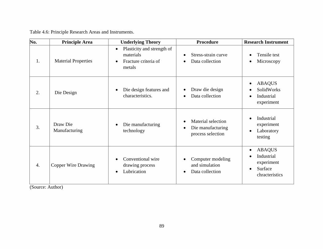
89
Table 4.6: Principle Research Areas and Instruments.
No. Principle Area Underlying Theory Procedure Research Instrument
1. Material Properties
Plasticity and strength of
materials
Fracture criteria of
metals
Stress-strain curve
Data collection
Tensile test
Microscopy
2. Die Design Die design features and
characteristics.
Draw die design
Data collection
ABAQUS
SolidWorks
Industrial
experiment
3. Draw Die
Manufacturing
Die manufacturing
technology
Material selection
Die manufacturing
process selection
Industrial
experiment
Laboratory
testing
4. Copper Wire Drawing
Conventional wire
drawing process
Lubrication
Computer modeling
and simulation
Data collection
ABAQUS
Industrial
experiment
Surface
chracteristics
(Source: Author)
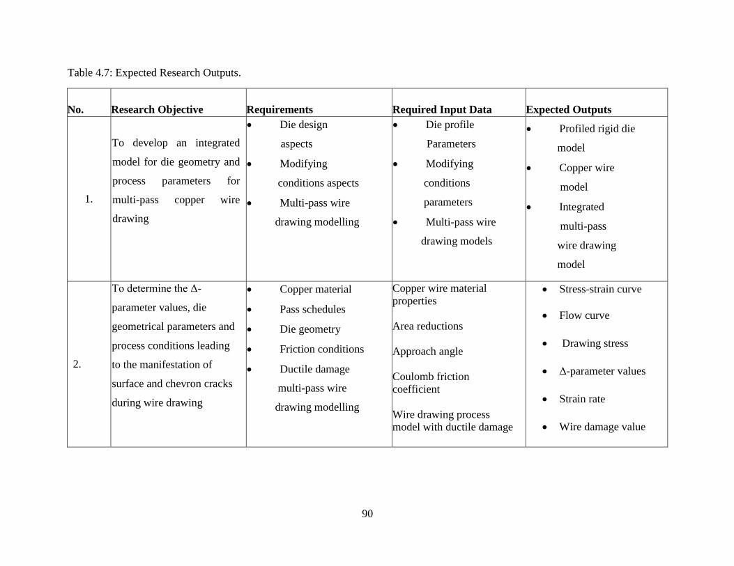
90
Table 4.7: Expected Research Outputs.
No.
Research Objective
Requirements
Required Input Data
Expected Outputs
1.
To develop an integrated
model for die geometry and
process parameters for
multi-pass copper wire
drawing
Die design
aspects
Modifying
conditions aspects
Multi-pass wire
drawing modelling
Die profile
Parameters
Modifying
conditions
parameters
Multi-pass wire
drawing models
Profiled rigid die
model
Copper wire
model
Integrated
multi-pass
wire drawing
model
2.
To determine the Δ-
parameter values, die
geometrical parameters and
process conditions leading
to the manifestation of
surface and chevron cracks
during wire drawing
Copper material
Pass schedules
Die geometry
Friction conditions
Ductile damage
multi-pass wire
drawing modelling
Copper wire material
properties
Area reductions
Approach angle
Coulomb friction coefficient
Wire drawing process model with ductile damage
Stress-strain curve
Flow curve
Drawing stress
Δ-parameter values
Strain rate
Wire damage value
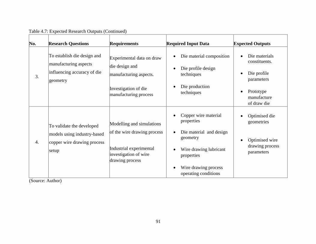
91
Table 4.7: Expected Research Outputs (Continued)
No.
Research Questions
Requirements
Required Input Data
Expected Outputs
3.
To establish die design and
manufacturing aspects
influencing accuracy of die
geometry
Experimental data on draw
die design and
manufacturing aspects.
Investigation of die
manufacturing process
Die material composition
Die profile design
techniques
Die production
techniques
Die materials constituents.
Die profile
parameters
Prototype
manufacture
of draw die
4.
To validate the developed
models using industry-based
copper wire drawing process
setup
Modelling and simulations
of the wire drawing process
Industrial experimental
investigation of wire
drawing process
Copper wire material
properties
Die material and design
geometry
Wire drawing lubricant
properties
Wire drawing process
operating conditions
Optimised die
geometries
Optimised wire
drawing process
parameters
(Source: Author)
92
4.4 Application of the Methods
(i) The FEM Approach
The FEM approach is based on three stages which involve procedural modelling,
simulation and visualisation of the process. The first stage or computational modelling
involves four steps which include: modelling the geometry, meshing or discretisation of
the geometry, specification of material properties and specification of boundary, initial
and loading conditions.
The geometry of the model is meshed or discretised by using a number of elements
which are made up of grids and nodes (Liu and Quek, 2003). In this stage, which is a
pre-processing stage, the raw wire and die materials are specified, designed and
analysed. This stage is important due to the need for change or variation of the die profile
parameters and processing conditions (indepenedent variables) which are necessary for
the current research.
The second stage of the FEM approach involves simulation of the model and this is
based mainly on energy principles. In this stage, the created computational model is fed
to the solver to solve the discretised system and simultaneous equations for the variables
at the nodes of the mesh. This is a processing stage and is necessary for obtaining the
dependent variables of the wire drawing process.
The third and last stage of the FEM approach is a post-processing stage. In this stage the
results from the processing stage are visualised. This is necessary because the
information generated after processing is a large amount of digital data which needs to
be interpolated, analysed and presented. Thus 2D objects and field variables can be
displayed. This stage is important for analysis and decision-making concerning the
simulated wire drawing process.
93
(ii) Experimental Procedures
Industrial experiments were done to get data in form of images, movements and
behaviour of mechanical systems during die manufacturing and wire drawing. The die
manufacturing process was studied in order to fully understand the design, materials and
manufacturing technology of the draw die. Design drawings were then made with full
material and die geometry specifications in order to manufacture prototype dies.
Laboratory experiments were undertaken in order to obtain both copper wire material
properties and behaviour, and the draw die material properties. Wire drawing
experiments were conducted based on the current industrial setup of the local firms
involved in copper wire drawing. The experiments conducted involved the medium size
(1.78 mm diameter) copper wires. This was done in order to validate the data obtained
from the FEM approach, and thus optimise the actual process with the aim of reducing
defects during the drawing process.
4.5 Major Research Instruments
In order to carry out this research, information and data on die design, manufacturing
and copper wire drawing process and practices was collected using the major research
instruments given in Tables 4.6 and 4.7. Tables 4.8, 4.9 and 4.10 show details of the
various research instruments used and their principle application areas.
(i) Microscopes
An electron microscope, Olympus make and model CH2, was used to determine the
microstructure of the 8 mm raw copper rods. A scanning electron microscope (SEM),
model Quanta FEG 450, was used to detect the level and size of defects in the copper
rod microstructure. The SEM was appropriate in that both macro (surface based) and
micro (internal) defect analysis could be done with high resolution. This is because the
SEM is able to give magnifications of up to 5000X in order to expose both the micro-
and macro-defects.
94
(ii) Tensile Tester
A universal tensile testing machine, model TUE C-600, with a load cell capacity of 12
to 600 kN capacity and a load accuracy of 1% of indicated load, was used for obtaining
the wire material mechanical properties. The test was appropriate for obtaining the
stress-strain data under tensile force conditions.
(iii) Wire Drawing Machine
An industrial intermediate copper wire drawing machine, model HT-450 13D, was used
in the determination of the wire drawing process parameters. The wire drawing machine
was the source of work and power, hence important in the analysis of process efficiency.
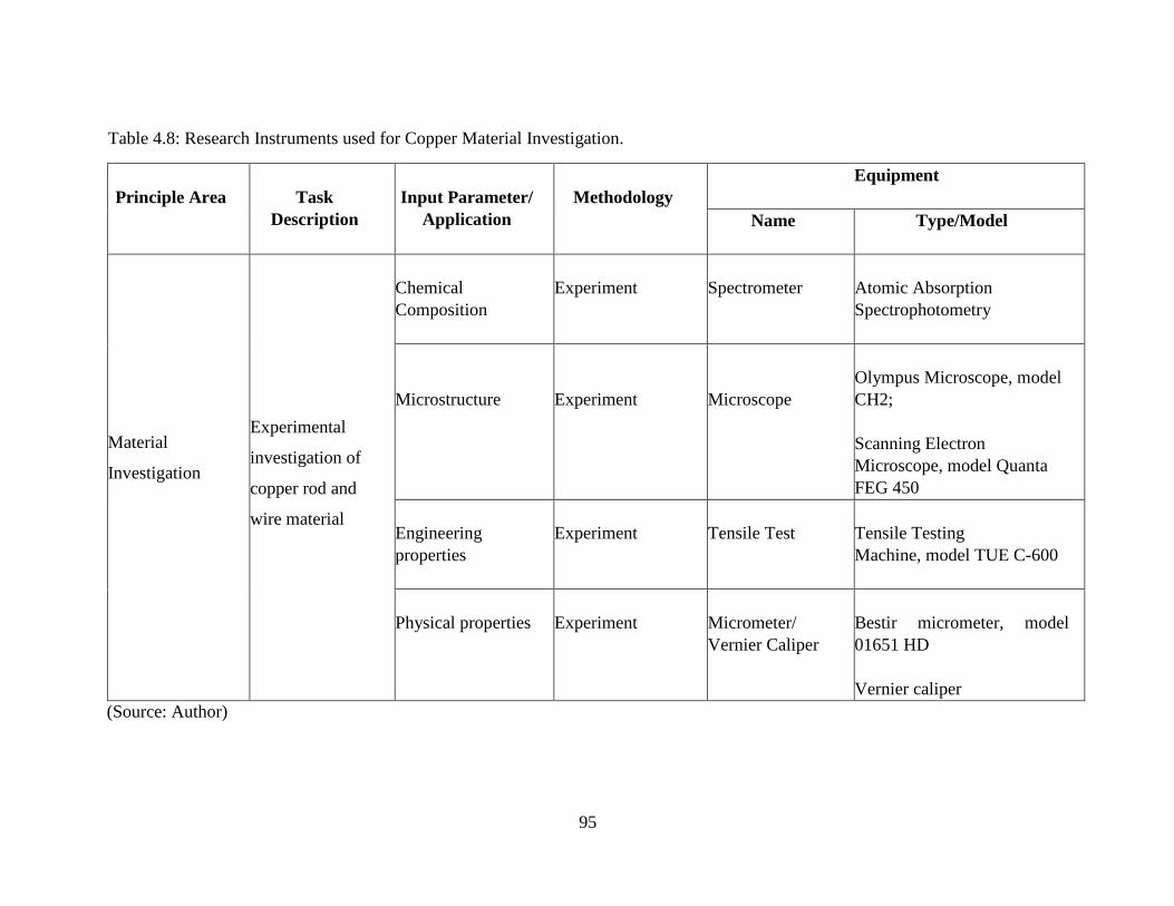
95
Table 4.8: Research Instruments used for Copper Material Investigation.
Principle Area
Task
Description
Input Parameter/
Application
Methodology
Equipment
Name Type/Model
Material
Investigation
Experimental
investigation of
copper rod and
wire material
Chemical
Composition
Experiment
Spectrometer
Atomic Absorption
Spectrophotometry
Microstructure
Experiment
Microscope
Olympus Microscope, model
CH2;
Scanning Electron
Microscope, model Quanta
FEG 450
Engineering
properties
Experiment
Tensile Test
Tensile Testing
Machine, model TUE C-600
Physical properties
Experiment
Micrometer/
Vernier Caliper
Bestir micrometer, model
01651 HD
Vernier caliper
(Source: Author)

96
Table 4.9: Research Instruments used for Die Design and Manufacturing Investigation.
Principle Area
Task Description
Input Parameter/
Application
Methodology
Equipment/Software
Name Type/Model
Die Design
Die
Design
Design Methods
Design and
Draughting
ABAQUS CAE
Solidworks 2012
2D and 3D
Drawings
Die
Manufacturing
Die Manufacturing
Manufacturing
Methods and
Practices
Industrial
Experiment
Digital Camera
Powder
Metallurgy
Equipment
Samsung WB 1100F
Compacting machine
Sintering machine
(Source: Author)

97
Table 4.10: Research Instruments and Application Areas for Wire Drawing Process Investigation.
Principle Area
Task Description
Input / Output
Parameter or
Application
Methodology Equipment/Software
Name Type/ Model
Multi-pass Copper
Wire
Drawing Process
(Modelling and
Analysis)
Finite Element
Modelling of the Wire
Drawing
Process and Coupling
with Excel spreadsheets
2D ABAQUS wire
and die drawings
Material
specification
Processing
conditions
2D draughting
Material CAE input
Boundary and
processing conditions
input
2D ABAQUS
CAE
ABAQUS
modelling
Spreadsheet
Analysis
ABAQUS 6.14
software
Microsoft
Excel
Multi-pass Copper
Wire
Drawing Process
(Experimental
Procedure)
Experimental Analysis
of the Wire Drawing
Process
Die Temperature Experiment Contact
Thermocouple
TWOK Digital
Thermometer
Drawing Velocity Experiment Velocity tester Bushnell
velocity gun
Wire surface and
internal cracks
Experiment
Microscopy
Scanning
Electron
Microscope
(Source: Author)

98
4.6 Data Collection
Wire drawing practice in Zambia is mainly concentrated along the main line of rail in
the Central, Copperbelt and Lusaka provinces of Zambia due to the availability of the
copper raw material. Apart from the raw materials, the wire drawing industries are also
critically dependent on draw die and drawing lubricant supply. Due to the high technical
skills needed for draw die design and manufacturing, only one draw die local
manufacturing entity located in Central Province currently exists. Lubricant supply is
readily available and offered by a number of local oil marketing companies whose
offices are found along the main line of rail.
The copper wire drawing firms obtain their raw copper materials from the same local
sources which are the mining companies, hence the consistency in the raw copper
materials being analysed. The population of copper wire drawing firms is currently four
companies in Zambia.
Out of the population of four, two companies were used for investigation. The 8 mm
raw wrought copper rod material was collected from one company. The raw rods were
then subjected to both rod breakdown and intermediate wire drawing at a second
location due to the use of prototype design dies. For each die, about 50 metres of drawn
wire were obtained and investigated.
During the modelling and simulation of the wire drawing process, five sets of varying
bearing length (30%, 35%, 40%, 45% and 50%) were used and the following data for
each multi-pass stage and for two nodes (one surface and one internal) was collected:
- Mises equivalent and hydrostatic stresses
- Equivalent plastic strains and strain rates
- Stress triaxiality values
- Drawing forces
- Damage values
- Cockroft and Latham fracture criterion values
99
During both the laboratory and industrial experiments, data was collected on the
following parameters:
- Engineering properties of copper
- Microstructure of undrawn copper
- Drawing speeds
- Die temperatures
- Lubricant temperatures and properties
- Microstructure of drawn copper (with defect investigation)
Data on the engineering properties and microstructure of the raw wrought copper rods
was collected using the universal tensile testing machine and the microscopes. Data on
drawing speeds, die and lubricant temperatures was collected in-situ during the wire
drawing process, using a velocity gun and a digital thermometer respectively. Data on
the properties of the lubricant was collected by collecting a sample of the raw lubricant
which was then subjected to a laboratory kinematic viscosity test.
Data on the investigation of defects arising from the wire drawing process was collected
by obtaining sections of the drawn wire from each multi-pass stage using three different
die bearing sections sets (30%, 40% and 50%) and subjecting the wire sections to both
surface and internal microstructure investigation.
The raw materials and copper wires used in the study were fully representative of the
current local wire drawing population. The use of an industrial wire drawing machine
for purposes of this study was arrived at due to lack of laboratory equipment at local
learning institutions.
The data collected was reliable in that it was from the actual industrial practice. The
industrial experiments taken at different shifts and for over a month was sufficient for a
good analysis of the process.
100
4.7 Data Analysis
The data collected from simulations for each node and each pass was analysed
qualitatively using the stress pattern contours and quantitatively by querying the value
of each parameter during the modelling process. The quantitative data was collected by
noting the querried values and inserting them into Microsoft excel sheets, from which
graphs were then plotted for analysis.
The data collected from industrial experiments for each varying bearing set was
analysed quantitatively by noting the value of each parameter during the wire drawing
process. Data on microstructure tests was analysed qualitatively by using scanning
electron micrographs for each multi-pass stage.
In both cases, the data obtained was subjected to removal of measurement errors and
averaged for a standard value of the measured parameter. The major factors involved in
copper wire drawing were varied to obtain predictive optimum values from the
simulation. The optimum values of the parameters acted as comparative yardsticks to
the experimental procedures. From the experimental procedures, standard operational
parameters were established. A comparison of the two sets of data (simulated and
experimentally obtained) was then done.
4.8 Limitations
Industrial experimental procedures have the limitation of company production targets
which hinder the careful and repetitive nature of the required experiments. Unlike with
ordinary laboratory experiments, administration of necessary instruments during a
production run thus becomes difficult. Often, permission has to be sought through
management hierarchy. Despite the limitations mentioned above, all necessary steps
were taken to ensure that the required sample size and quality of data was worthwhile.
101
4.9 Ethical considerations
Potential ethical problems in this research included the possibility of being involved in
an industrial dispute due to subjection to company employee rules and the need to
safeguard company records and secrets. Thus, line supervisors and managers were
consulted and permission sought before any procedure was undertaken. Equally, all data
obtained from the companies was treated with the strictest confidence.

102
CHAPTER FIVE: MODELLING AND SIMULATION
5.1 Introduction
This chapter is divided into four major sections. The first section presents a theoretical
background to the Finite Element Method (FEM) and the software ABAQUS 6.14 and
its application to the current study. The second section presents the computational
conditions used in modelling and simulation of the copper wire drawing process. This
section gives insight into the different copper wire material properties, die geometry and
wire drawing variables used in the research in order to achieve the objectives of the study.
The third section presents results of the simulation using damage for ductile metals
procedure for selected surface and centerline nodes.
5.2 Finite Element Method
The Finite Element Method (FEM) is used in engineering practice to model and solve
physical problems involving solids, structures, fluids and heat transfer (Bathe, 1996). The
physical problem as applied in this case is the drawing of copper wire by metal forming.
The copper wire is subjected to loading as it passes through a drawing die. This physical
problem is idealised by a mathematical model which is governed by differential
equations. The mathematical model is solved by the finite element analysis based on the
behaviour of the material under consideration, namely elastic-plastic, rigid-plastic and
visco-plastic. For the current study, the elastic-plastic behaviour of material is used in the
FEM.
Figure 5.1 gives a summary of the FEM. The figure shows that the FEM is a numerical
procedure, hence it is necessary to assess the accuracy of the solution. The solution is
normally repeated with refined solution parameters (such as finer meshes) until a
sufficient accuracy is reached (Ibid).
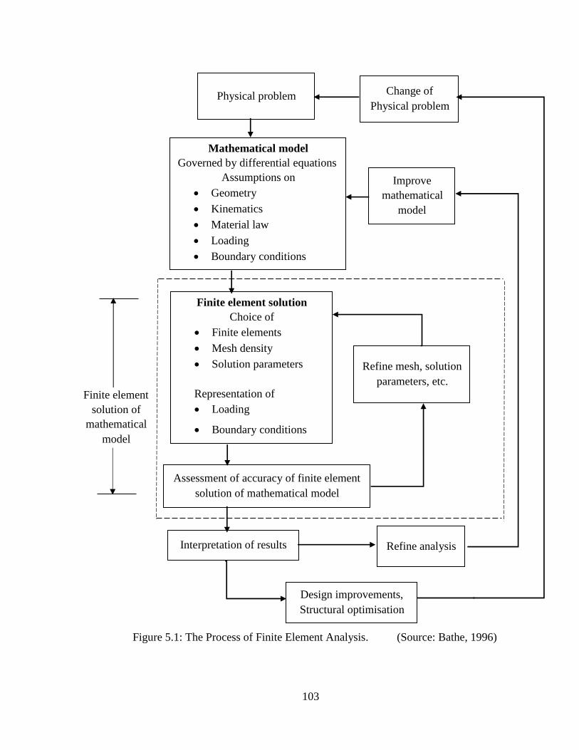
103
Figure 5.1: The Process of Finite Element Analysis. (Source: Bathe, 1996)
Physical problem Change of
Physical problem
Mathematical model
Governed by differential equations
Assumptions on
Geometry
Kinematics
Material law
Loading
Boundary conditions
Improve
mathematical
model
Finite element solution
Choice of
Finite elements
Mesh density
Solution parameters
Representation of
Loading
Boundary conditions
Refine mesh, solution
parameters, etc.
Assessment of accuracy of finite element
solution of mathematical model
Interpretation of results Refine analysis
Design improvements,
Structural optimisation
Finite element
solution of
mathematical
model
104
5.3 Finite Element Software: ABAQUS
ABAQUS 6.14 is a suite of engineering simulation programmes based on the finite
element method that can solve problems involving linear and non-linear analyses. It
contains an extensive library of elements that can model virtually any geometry.
ABAQUS contains an extensive list of material models that can simulate the behaviour
of many engineering materials which include metals, polymers, composites, rubber,
reinforced concrete, crushable and resilient foams, soils and rocks. A complete ABAQUS
analysis consists of the following three distinct stages (Dassault Systèmes, 2014a):
(a) Preprocessing
In this stage, the model of the physical problem is defined graphically or with a text
editor, and an ABAQUS input file is created.
(b) Simulation
In this stage, a Standard or Explicit ABAQUS packager solves the numerical problem
defined in the model.
(c) Postprocessing
This stage evaluates the results once the simulation has been completed. This is done
interactively using the Visualisation module of ABAQUS. The Visualisation module
reads the output database file and has a variety of options for displaying the results,
including contour plots, animations, deformed shape plots and X-Y plots. Figure 5.2
shows how the three stages are linked together by files in ABAQUS.
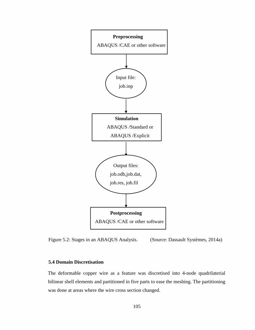
105
Figure 5.2: Stages in an ABAQUS Analysis. (Source: Dassault Systèmes, 2014a)
5.4 Domain Discretisation
The deformable copper wire as a feature was discretised into 4-node quadrilaterial
bilinear shell elements and partitioned in five parts to ease the meshing. The partitioning
was done at areas where the wire cross section changed.
Pre processing
ABAQUS /CAE or other software
Input file:
job.inp
Simulation
ABAQUS /Standard or
ABAQUS /Explicit
Output file s :
job.odb,job.dat,
job.res, job.fil
Postprocessing
ABAQUS /CAE or other software

106
5.5 Constitutive Equations
The governing equations for state variables are invoked by element interconnection
requirements corresponding to the equilibrium of nodal force increments, ΔF. For
corresponding displacement increments, ΔU, the interconnection requirements are given
by equation (5.1) according to Bathe (1996):
∆𝐹 = 𝐾∆𝑈 (5.1)
In equation (5.1), K is the stiffness matrix which is an assembly of matrices that allow for
deformation, material incompressibility, and rigid body rotation in the elastic-plastic
finite element method. The solution to equation (5.1) gives unknown values of ΔU, hence
allows the deformation of the workpiece to be determined. From the deformations thus
obtained, stresses and strains can be determined.
The mathematical models used during modelling of the copper wire drawing process arise
from the constitutive models of metal plasticity and isotropic elasto-plasticity.
5.5.1 Metal Plasticity Constitutive Models
ABAQUS Standard/Explicit can be used to model metal plasticity. Metal plasticity
models are either rate-dependent or independent, with a Mises yield surface for isotropic
materials. For relatively high strain rate applications as obtainable in metal forming, the
rate dependence can be presented using equation (5.2) as follows (Dassault Systèmes,
2014a):
𝜀𝑝𝑙 = 𝐷 (��
𝜎0− 1)
𝑛
, 𝑓𝑜𝑟 𝜎 ≥ 𝜎0 (5.2)
where, 𝜀𝑝𝑙 is the equivalent plastic strain
𝜎 is the yield stress at non-zero plastic strain
𝜎0 is the static yield stress which may depend on plastic strain (εpl),
temperature (θ) and other factors (fi)
D, n are material parameters which can be functions of temperature and
other factors
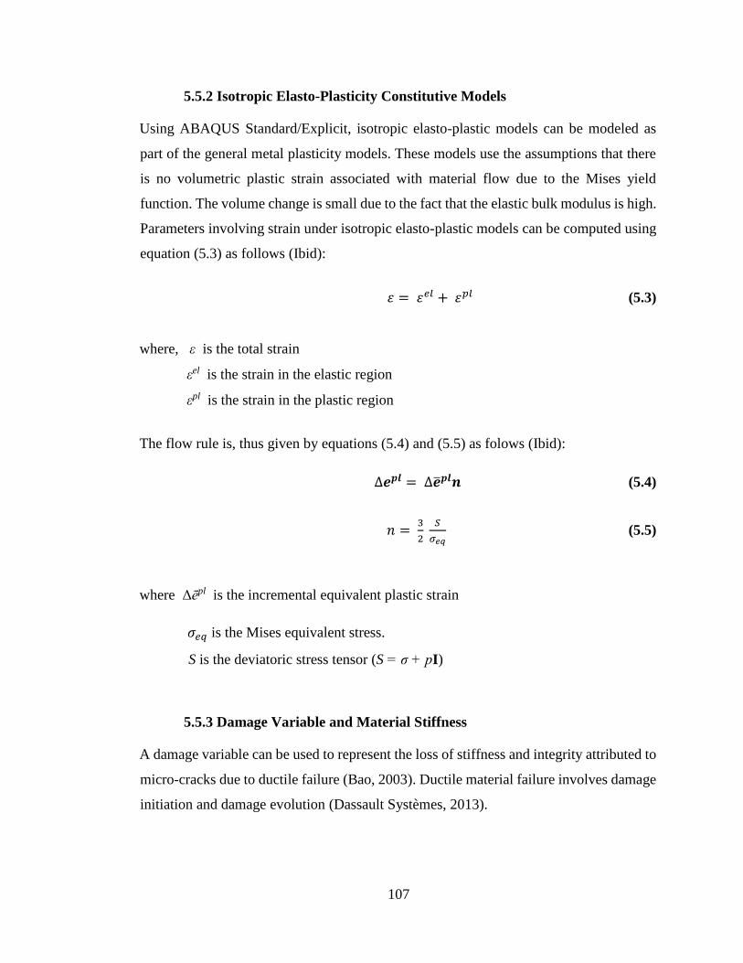
107
5.5.2 Isotropic Elasto-Plasticity Constitutive Models
Using ABAQUS Standard/Explicit, isotropic elasto-plastic models can be modeled as
part of the general metal plasticity models. These models use the assumptions that there
is no volumetric plastic strain associated with material flow due to the Mises yield
function. The volume change is small due to the fact that the elastic bulk modulus is high.
Parameters involving strain under isotropic elasto-plastic models can be computed using
equation (5.3) as follows (Ibid):
𝜀 = 𝜀𝑒𝑙 + 𝜀𝑝𝑙 (5.3)
where, ε is the total strain
εel is the strain in the elastic region
εpl is the strain in the plastic region
The flow rule is, thus given by equations (5.4) and (5.5) as folows (Ibid):
∆𝒆𝒑𝒍 = ∆��𝒑𝒍𝒏 (5.4)
𝑛 = 3
2
𝑆
𝜎𝑒𝑞 (5.5)
where Δēpl is the incremental equivalent plastic strain
𝜎𝑒𝑞 is the Mises equivalent stress.
S is the deviatoric stress tensor (S = σ + pI)
5.5.3 Damage Variable and Material Stiffness
A damage variable can be used to represent the loss of stiffness and integrity attributed to
micro-cracks due to ductile failure (Bao, 2003). Ductile material failure involves damage
initiation and damage evolution (Dassault Systèmes, 2013).
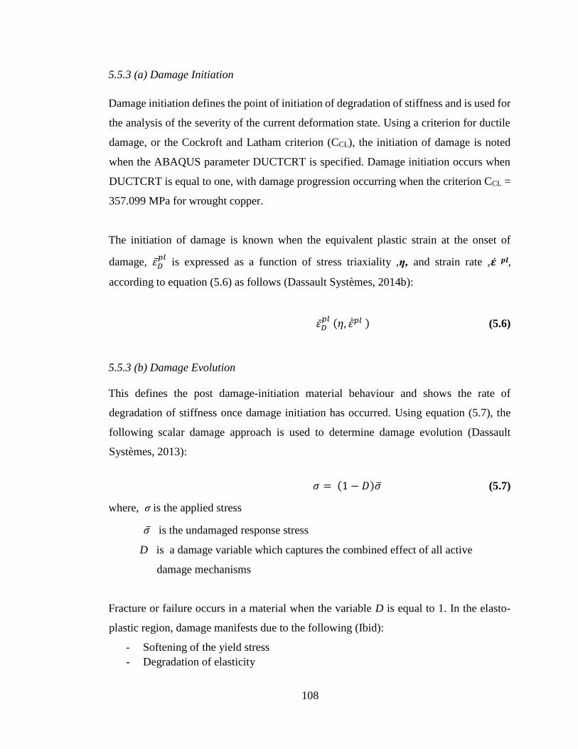
108
5.5.3 (a) Damage Initiation
Damage initiation defines the point of initiation of degradation of stiffness and is used for
the analysis of the severity of the current deformation state. Using a criterion for ductile
damage, or the Cockroft and Latham criterion (CCL), the initiation of damage is noted
when the ABAQUS parameter DUCTCRT is specified. Damage initiation occurs when
DUCTCRT is equal to one, with damage progression occurring when the criterion CCL =
357.099 MPa for wrought copper.
The initiation of damage is known when the equivalent plastic strain at the onset of
damage, 𝜀��𝑝𝑙
is expressed as a function of stress triaxiality ,η, and strain rate ,𝜺 𝒑𝒍,
according to equation (5.6) as follows (Dassault Systèmes, 2014b):
𝜀��𝑝𝑙 (𝜂, 𝜀 𝑝𝑙 ) (5.6)
5.5.3 (b) Damage Evolution
This defines the post damage-initiation material behaviour and shows the rate of
degradation of stiffness once damage initiation has occurred. Using equation (5.7), the
following scalar damage approach is used to determine damage evolution (Dassault
Systèmes, 2013):
𝜎 = (1 − 𝐷)𝜎 (5.7)
where, σ is the applied stress
𝜎 is the undamaged response stress
D is a damage variable which captures the combined effect of all active
damage mechanisms
Fracture or failure occurs in a material when the variable D is equal to 1. In the elasto-
plastic region, damage manifests due to the following (Ibid):
- Softening of the yield stress
- Degradation of elasticity
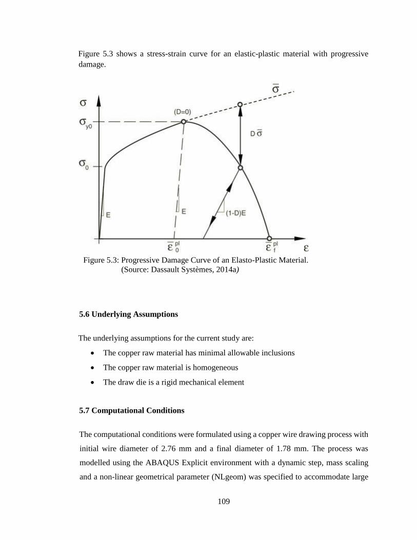
109
Figure 5.3 shows a stress-strain curve for an elastic-plastic material with progressive
damage.
Figure 5.3: Progressive Damage Curve of an Elasto-Plastic Material.
(Source: Dassault Systèmes, 2014a)
5.6 Underlying Assumptions
The underlying assumptions for the current study are:
The copper raw material has minimal allowable inclusions
The copper raw material is homogeneous
The draw die is a rigid mechanical element
5.7 Computational Conditions
The computational conditions were formulated using a copper wire drawing process with
initial wire diameter of 2.76 mm and a final diameter of 1.78 mm. The process was
modelled using the ABAQUS Explicit environment with a dynamic step, mass scaling
and a non-linear geometrical parameter (NLgeom) was specified to accommodate large
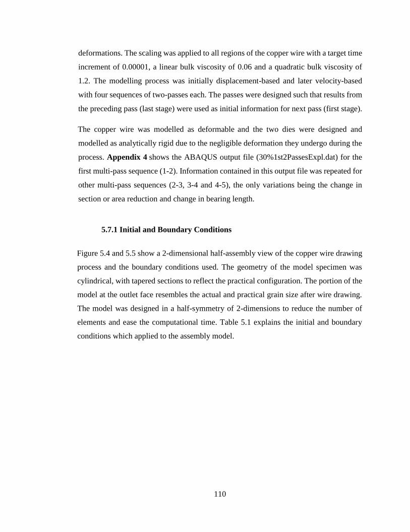
110
deformations. The scaling was applied to all regions of the copper wire with a target time
increment of 0.00001, a linear bulk viscosity of 0.06 and a quadratic bulk viscosity of
1.2. The modelling process was initially displacement-based and later velocity-based
with four sequences of two-passes each. The passes were designed such that results from
the preceding pass (last stage) were used as initial information for next pass (first stage).
The copper wire was modelled as deformable and the two dies were designed and
modelled as analytically rigid due to the negligible deformation they undergo during the
process. Appendix 4 shows the ABAQUS output file (30%1st2PassesExpl.dat) for the
first multi-pass sequence (1-2). Information contained in this output file was repeated for
other multi-pass sequences (2-3, 3-4 and 4-5), the only variations being the change in
section or area reduction and change in bearing length.
5.7.1 Initial and Boundary Conditions
Figure 5.4 and 5.5 show a 2-dimensional half-assembly view of the copper wire drawing
process and the boundary conditions used. The geometry of the model specimen was
cylindrical, with tapered sections to reflect the practical configuration. The portion of the
model at the outlet face resembles the actual and practical grain size after wire drawing.
The model was designed in a half-symmetry of 2-dimensions to reduce the number of
elements and ease the computational time. Table 5.1 explains the initial and boundary
conditions which applied to the assembly model.
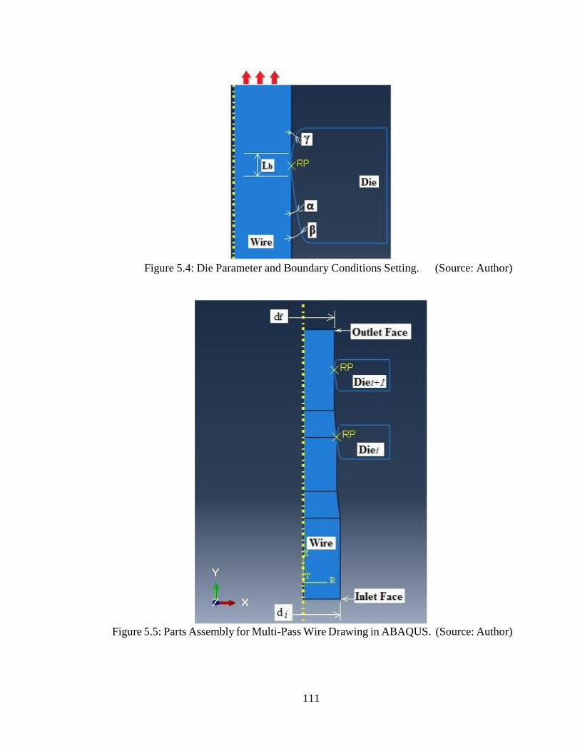
111
Figure 5.4: Die Parameter and Boundary Conditions Setting. (Source: Author)
Figure 5.5: Parts Assembly for Multi-Pass Wire Drawing in ABAQUS. (Source: Author)
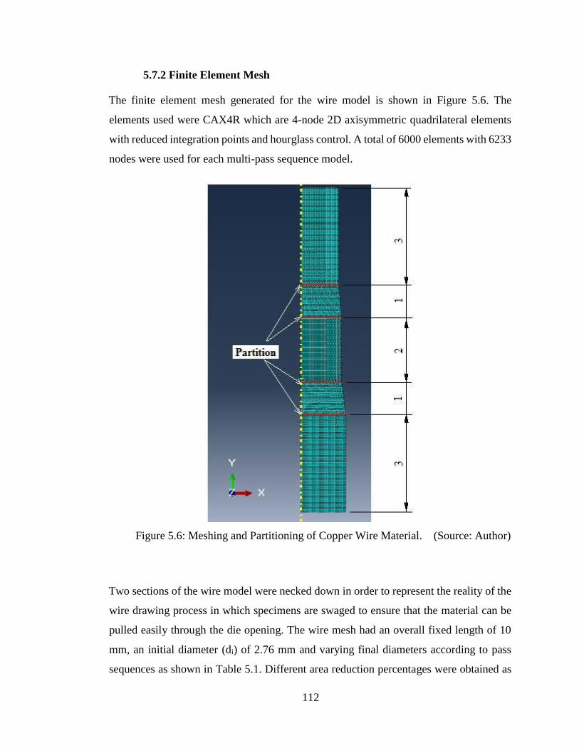
112
5.7.2 Finite Element Mesh
The finite element mesh generated for the wire model is shown in Figure 5.6. The
elements used were CAX4R which are 4-node 2D axisymmetric quadrilateral elements
with reduced integration points and hourglass control. A total of 6000 elements with 6233
nodes were used for each multi-pass sequence model.
Figure 5.6: Meshing and Partitioning of Copper Wire Material. (Source: Author)
Two sections of the wire model were necked down in order to represent the reality of the
wire drawing process in which specimens are swaged to ensure that the material can be
pulled easily through the die opening. The wire mesh had an overall fixed length of 10
mm, an initial diameter (di) of 2.76 mm and varying final diameters according to pass
sequences as shown in Table 5.1. Different area reduction percentages were obtained as

113
a result of the varying final diameters. The wire mesh had a fixed global size of 0.0005
with partitioned edge sizes of 30 each.
Table 5.1: Limit and Boundary Conditions with Variation of Die Bearing Length.
Multipass
Sequences
Feature
Geometries
Initial Conditions Boundary
Conditions
1 – 2
2 – 3
3 – 4
4 – 5
Copper Wire
di = 2.76 mm
d1 = 2.55 mm
d2 = 2.32 mm
d3 = 2.11 mm
d4 = 1.92 mm
d5 = 1.78 mm
(i) 0.08 ms-1
velocity
of outlet face
along y- axis
(ii) Centreline
symmetry
(U1=0)
Diei
α = 10o; β = 40o; γ =
30o
Lb = (30; 35;
40; 45;
50%)df
Encastre boundary
condition (U=0;R=0)
for die reference point
(RP)
Die-Wire
Interaction
μ = 0.04
(Source: Author)
5.7.3 Contact Conditions and the Rigid Die
Kinematic contact was applied as a mechanical constraint between the wire contact
surface and the die external surfaces. Finite sliding was specified at the contact, with a
Coulomb friction coefficient of 0.04 maintained in all models except for models involving
friction coefficient variation which were varied.
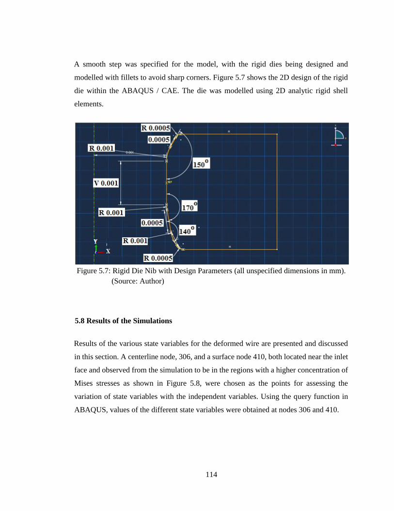
114
A smooth step was specified for the model, with the rigid dies being designed and
modelled with fillets to avoid sharp corners. Figure 5.7 shows the 2D design of the rigid
die within the ABAQUS / CAE. The die was modelled using 2D analytic rigid shell
elements.
Figure 5.7: Rigid Die Nib with Design Parameters (all unspecified dimensions in mm).
(Source: Author)
5.8 Results of the Simulations
Results of the various state variables for the deformed wire are presented and discussed
in this section. A centerline node, 306, and a surface node 410, both located near the inlet
face and observed from the simulation to be in the regions with a higher concentration of
Mises stresses as shown in Figure 5.8, were chosen as the points for assessing the
variation of state variables with the independent variables. Using the query function in
ABAQUS, values of the different state variables were obtained at nodes 306 and 410.
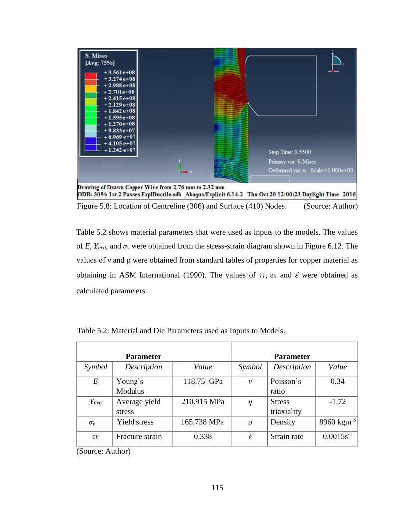
115
Figure 5.8: Location of Centreline (306) and Surface (410) Nodes. (Source: Author)
Table 5.2 shows material parameters that were used as inputs to the models. The values
of E, Yavg, and σy were obtained from the stress-strain diagram shown in Figure 6.12. The
values of ν and ρ were obtained from standard tables of properties for copper material as
obtaining in ASM International (1990). The values of h, εfr and �� were obtained as
calculated parameters.
Table 5.2: Material and Die Parameters used as Inputs to Models.
Parameter
Parameter
Symbol Description Value Symbol Description Value
E Young’s
Modulus
118.75 GPa ν Poisson’s
ratio
0.34
Yavg Average yield
stress
210.915 MPa η Stress
triaxiality
-1.72
σy Yield stress 165.738 MPa ρ Density 8960 kgm-3
εfr Fracture strain 0.338 𝜀 Strain rate 0.0015s-1
(Source: Author)
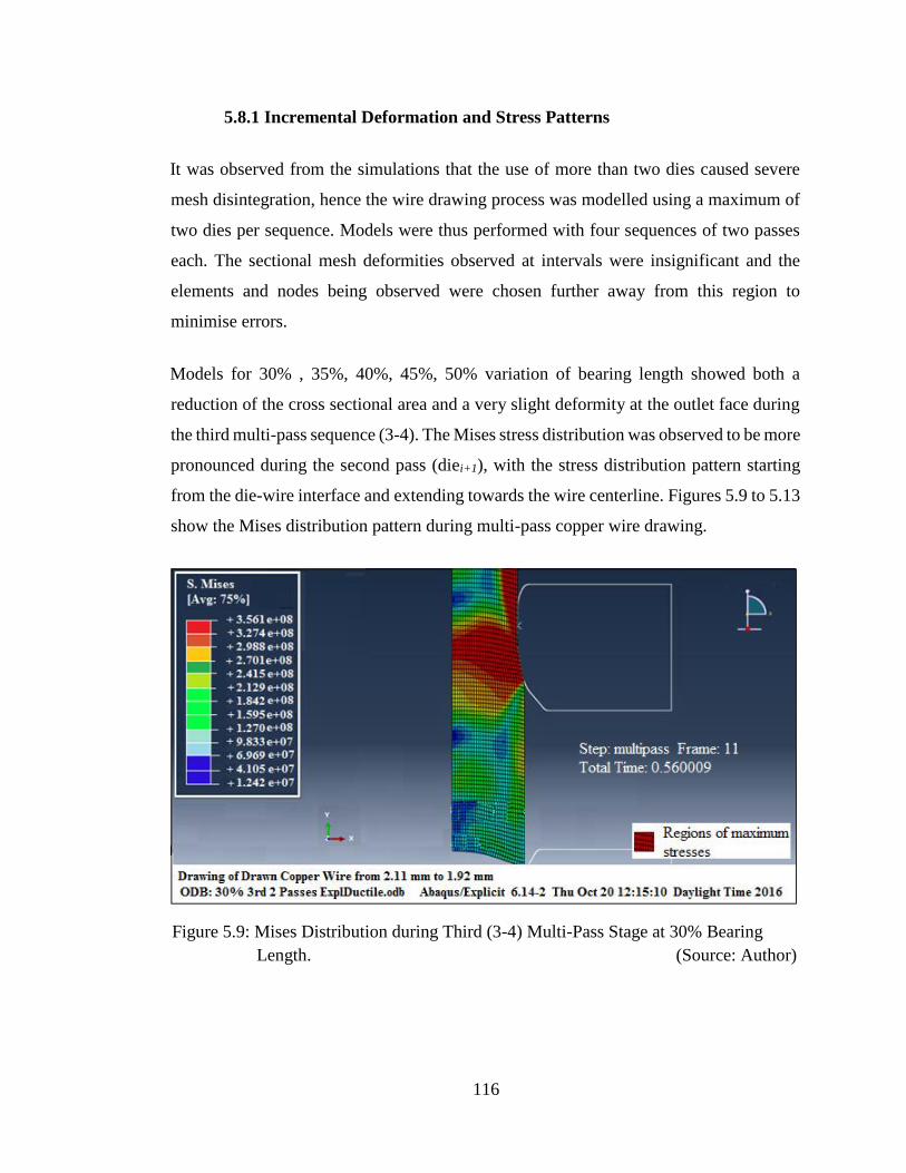
116
5.8.1 Incremental Deformation and Stress Patterns
It was observed from the simulations that the use of more than two dies caused severe
mesh disintegration, hence the wire drawing process was modelled using a maximum of
two dies per sequence. Models were thus performed with four sequences of two passes
each. The sectional mesh deformities observed at intervals were insignificant and the
elements and nodes being observed were chosen further away from this region to
minimise errors.
Models for 30% , 35%, 40%, 45%, 50% variation of bearing length showed both a
reduction of the cross sectional area and a very slight deformity at the outlet face during
the third multi-pass sequence (3-4). The Mises stress distribution was observed to be more
pronounced during the second pass (diei+1), with the stress distribution pattern starting
from the die-wire interface and extending towards the wire centerline. Figures 5.9 to 5.13
show the Mises distribution pattern during multi-pass copper wire drawing.
Figure 5.9: Mises Distribution during Third (3-4) Multi-Pass Stage at 30% Bearing
Length. (Source: Author)
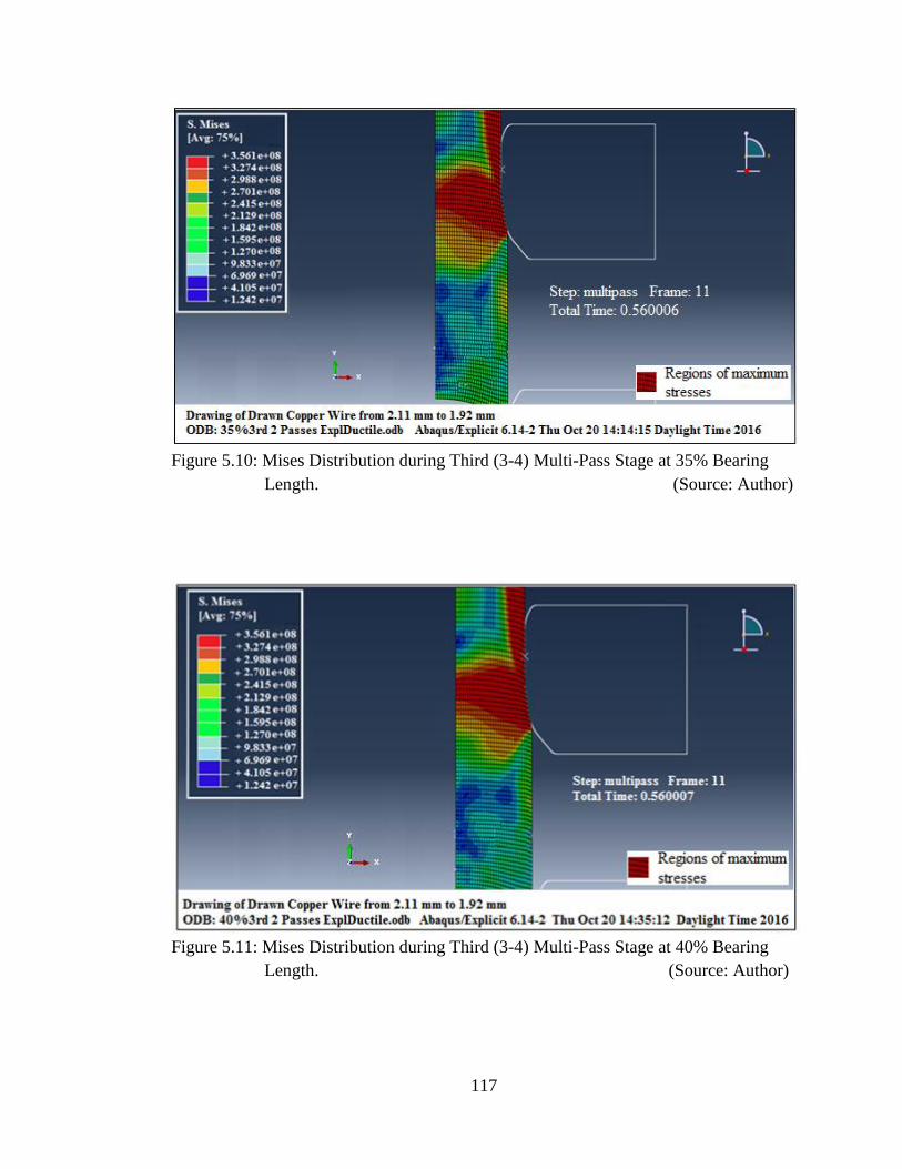
117
Figure 5.10: Mises Distribution during Third (3-4) Multi-Pass Stage at 35% Bearing
Length. (Source: Author)
Figure 5.11: Mises Distribution during Third (3-4) Multi-Pass Stage at 40% Bearing
Length. (Source: Author)

118
Figure 5.12: Mises Distribution during Third (3-4) Multi-Pass Stage at 45% Bearing
Length. (Source: Author)
Figure 5.13: Mises Distribution during Third (3-4) Multi-Pass Stage at 50% Bearing
Length. (Source: Author)
119
Models for the entrance angle showed some mesh deformity at the outlet face for entrance
angles of 20o, 25o, 30o, 35o and 40o during the third multi-pass sequence.
Modelling with approach angles of less than 8o was not possible due to severe mesh
disintegration, especially during the first multi-pass sequence (1-2). The von Mises
distribution was more pronounced during all the second multi-pass sequences (3-4) where
values of up to 315 MPa were attained when using a 10o approach angle.
Models for friction coefficient showed outlet face mesh deformity at values of 0.07 and
above, especially during the second and third multi-pass sequences. Models for exit angle
variation showed no changes.
Speeds of values less than 0.03 ms-1 were too slow for the models as the passage through
the dies could not be completed, whereas speeds of more than 0.12 ms-1 showed severe
mesh disintegration in the models, especially during the second and third multi-pass
sequences.
Area reduction models showed no deformations in the 10% and 12% area reduction
models. Small deformities at the outlet face were observed during the last multi-pass
sequences at 14% and 16% area reductions, whereas the same was observed during the
third and last multi-pass sequences at 18% area reduction. All multi-pass sequences using
the 20% area reduction showed increasing levels of mesh disintegration and sectional
deformity, with the last multi-pass sequence showing a severe mesh deformation at the
outlet face. Models with area reduction above 18% were not used in the analysis.
5.8.2 Distribution of State Variables with Independent Variables
(i) Equivalent Plastic Strain Distribution
The total accumulation of plastic strain during deformation is given by the equivalent
plastic strain, defined by Dassault Systèmes (2014b) according to equation (5.8) as
follows:
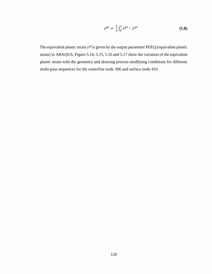
120
𝜀𝑝𝑙 = 2
3∫ 𝜀𝑝𝑙𝑡
0∶ 𝜀𝑝𝑙 (5.8)
The equivalent plastic strain 𝜀𝑝�� is given by the output parameter PEEQ (equivalent plastic
strain) in ABAQUS. Figure 5.14, 5.15, 5.16 and 5.17 show the variation of the equivalent
plastic strain with die geometry and drawing process modifying conditions for different
multi-pass sequences for the centerline node 306 and surface node 410.
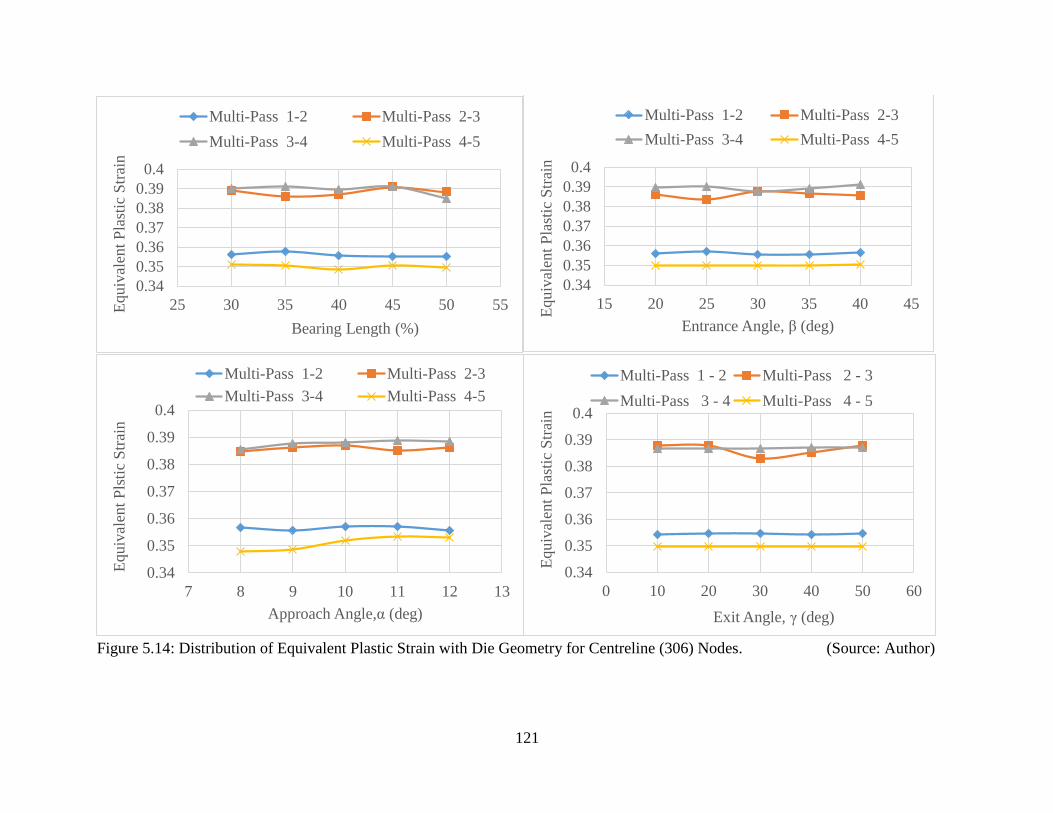
121
Figure 5.14: Distribution of Equivalent Plastic Strain with Die Geometry for Centreline (306) Nodes. (Source: Author)
0.34
0.35
0.36
0.37
0.38
0.39
0.4
25 30 35 40 45 50 55Equiv
alen
t P
last
ic S
trai
n
Bearing Length (%)
Multi-Pass 1-2 Multi-Pass 2-3
Multi-Pass 3-4 Multi-Pass 4-5
0.34
0.35
0.36
0.37
0.38
0.39
0.4
15 20 25 30 35 40 45
Equiv
alen
t P
last
ic S
trai
n
Entrance Angle, β (deg)
Multi-Pass 1-2 Multi-Pass 2-3
Multi-Pass 3-4 Multi-Pass 4-5
0.34
0.35
0.36
0.37
0.38
0.39
0.4
7 8 9 10 11 12 13
Equiv
alen
t P
lsti
c S
trai
n
Approach Angle,α (deg)
Multi-Pass 1-2 Multi-Pass 2-3
Multi-Pass 3-4 Multi-Pass 4-5
0.34
0.35
0.36
0.37
0.38
0.39
0.4
0 10 20 30 40 50 60
Equiv
alen
t P
last
ic S
trai
n
Exit Angle, γ (deg)
Multi-Pass 1 - 2 Multi-Pass 2 - 3
Multi-Pass 3 - 4 Multi-Pass 4 - 5
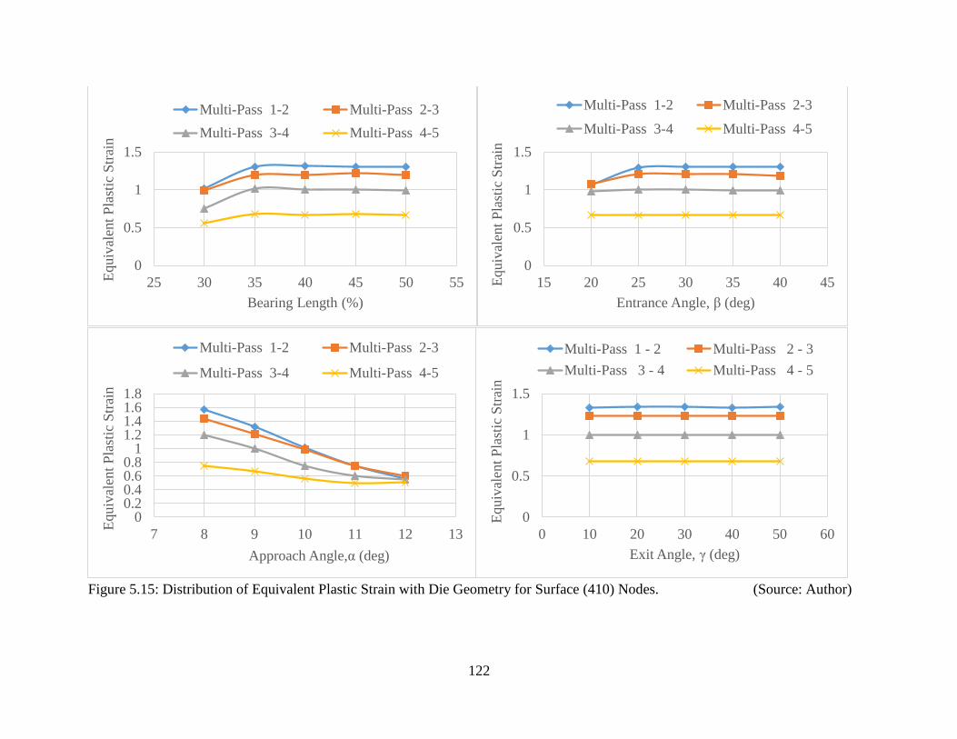
122
Figure 5.15: Distribution of Equivalent Plastic Strain with Die Geometry for Surface (410) Nodes. (Source: Author)
0
0.5
1
1.5
25 30 35 40 45 50 55Equiv
alen
t P
last
ic S
trai
n
Bearing Length (%)
Multi-Pass 1-2 Multi-Pass 2-3
Multi-Pass 3-4 Multi-Pass 4-5
0
0.5
1
1.5
15 20 25 30 35 40 45Equiv
alen
t P
last
ic S
trai
n
Entrance Angle, β (deg)
Multi-Pass 1-2 Multi-Pass 2-3
Multi-Pass 3-4 Multi-Pass 4-5
00.20.40.60.8
11.21.41.61.8
7 8 9 10 11 12 13
Equiv
alen
t P
last
ic S
trai
n
Approach Angle,α (deg)
Multi-Pass 1-2 Multi-Pass 2-3
Multi-Pass 3-4 Multi-Pass 4-5
0
0.5
1
1.5
0 10 20 30 40 50 60
Equiv
alen
t P
last
ic S
trai
n
Exit Angle, γ (deg)
Multi-Pass 1 - 2 Multi-Pass 2 - 3
Multi-Pass 3 - 4 Multi-Pass 4 - 5
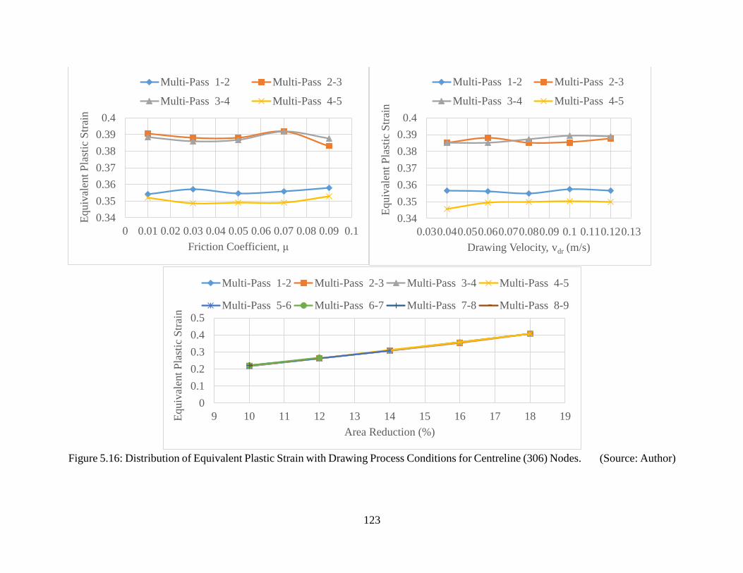
123
Figure 5.16: Distribution of Equivalent Plastic Strain with Drawing Process Conditions for Centreline (306) Nodes. (Source: Author)
0.34
0.35
0.36
0.37
0.38
0.39
0.4
0 0.01 0.02 0.03 0.04 0.05 0.06 0.07 0.08 0.09 0.1
Equiv
alen
t P
last
ic S
trai
n
Friction Coefficient, μ
Multi-Pass 1-2 Multi-Pass 2-3
Multi-Pass 3-4 Multi-Pass 4-5
0.34
0.35
0.36
0.37
0.38
0.39
0.4
0.030.040.050.060.070.080.09 0.1 0.110.120.13
Equiv
alen
t P
last
ic S
trai
n
Drawing Velocity, vdr (m/s)
Multi-Pass 1-2 Multi-Pass 2-3
Multi-Pass 3-4 Multi-Pass 4-5
0
0.1
0.2
0.3
0.4
0.5
9 10 11 12 13 14 15 16 17 18 19Equiv
alen
t P
last
ic S
trai
n
Area Reduction (%)
Multi-Pass 1-2 Multi-Pass 2-3 Multi-Pass 3-4 Multi-Pass 4-5
Multi-Pass 5-6 Multi-Pass 6-7 Multi-Pass 7-8 Multi-Pass 8-9
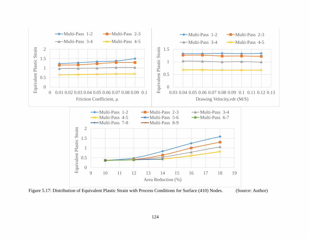
124
Figure 5.17: Distribution of Equivalent Plastic Strain with Process Conditions for Surface (410) Nodes. (Source: Author)
0
0.5
1
1.5
2
0 0.01 0.02 0.03 0.04 0.05 0.06 0.07 0.08 0.09 0.1Equiv
alen
t P
last
ic S
trai
n
Friction Coefficient, μ
Multi-Pass 1-2 Multi-Pass 2-3
Multi-Pass 3-4 Multi-Pass 4-5
0
0.5
1
1.5
0.03 0.04 0.05 0.06 0.07 0.08 0.09 0.1 0.11 0.12 0.13Equiv
alen
t P
last
ic S
trai
n
Drawing Velocity,vdr (M/S)
Multi-Pass 1-2 Multi-Pass 2-3
Multi-Pass 3-4 Multi-Pass 4-5
0
0.5
1
1.5
2
9 10 11 12 13 14 15 16 17 18 19Equiv
alen
t P
last
ic S
trai
n
Area Reduction (%)
Multi-Pass 1-2 Multi-Pass 2-3 Multi-Pass 3-4Multi-Pass 4-5 Multi-Pass 5-6 Multi-Pass 6-7Multi-Pass 7-8 Multi-Pass 8-9
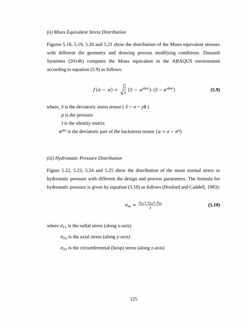
125
(ii) Mises Equivalent Stress Distribution
Figures 5.18, 5.19, 5.20 and 5.21 show the distribution of the Mises equivalent stresses
with different die geometry and drawing process modifying conditions. Dassault
Systèmes (2014b) computes the Mises equivalent in the ABAQUS environment
according to equation (5.9) as follows:
𝑓(𝜎 − 𝛼) = √3
2 (𝑆 − 𝛼𝑑𝑒𝑣): (𝑆 − 𝛼𝑑𝑒𝑣) (5.9)
where, S is the deviatoric stress tensor ( S = σ + pI )
p is the pressure
I is the identity matrix
αdev is the deviatoric part of the backstress tensor (𝛼 = 𝜎 − 𝜎0)
(iii) Hydrostatic Pressure Distribution
Figure 5.22, 5.23, 5.24 and 5.25 show the distribution of the mean normal stress or
hydrostatic pressure with different die design and process parameters. The formula for
hydrostatic pressure is given by equation (5.10) as follows (Hosford and Caddell, 1983):
𝜎𝑚 = 𝜎11+ 𝜎22+ 𝜎33
3 (5.10)
where 𝜎11 is the radial stress (along x-axis)
𝜎22 is the axial stress (along y-axis)
𝜎33 is the circumferential (hoop) stress (along z-axis)
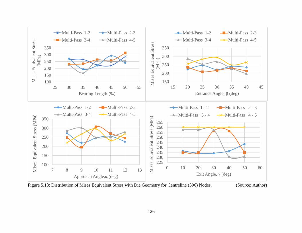
126
Figure 5.18: Distribution of Mises Equivalent Stress with Die Geometry for Centreline (306) Nodes. (Source: Author)
100
150
200
250
300
350
25 30 35 40 45 50 55
Mis
es E
quiv
alen
t S
tres
s
(MP
a)
Bearing Length (%)
Multi-Pass 1-2 Multi-Pass 2-3
Multi-Pass 3-4 Multi-Pass 4-5
150
200
250
300
350
15 20 25 30 35 40 45
Mis
es E
quiv
alen
t S
tres
s
(MP
a)
Entrance Angle, β (deg)
Multi-Pass 1-2 Multi-Pass 2-3
Multi-Pass 3-4 Multi-Pass 4-5
100
150
200
250
300
350
7 8 9 10 11 12 13Mis
es E
quiv
alen
t S
tres
s (M
Pa)
Approach Angle,α (deg)
Multi-Pass 1-2 Multi-Pass 2-3
Multi-Pass 3-4 Multi-Pass 4-5
225230235240245250255260265
0 10 20 30 40 50 60
Mis
es E
quiv
alen
t S
tres
s (M
Pa)
Exit Angle, γ (deg)
Multi-Pass 1 - 2 Multi-Pass 2 - 3
Multi-Pass 3 - 4 Multi-Pass 4 - 5
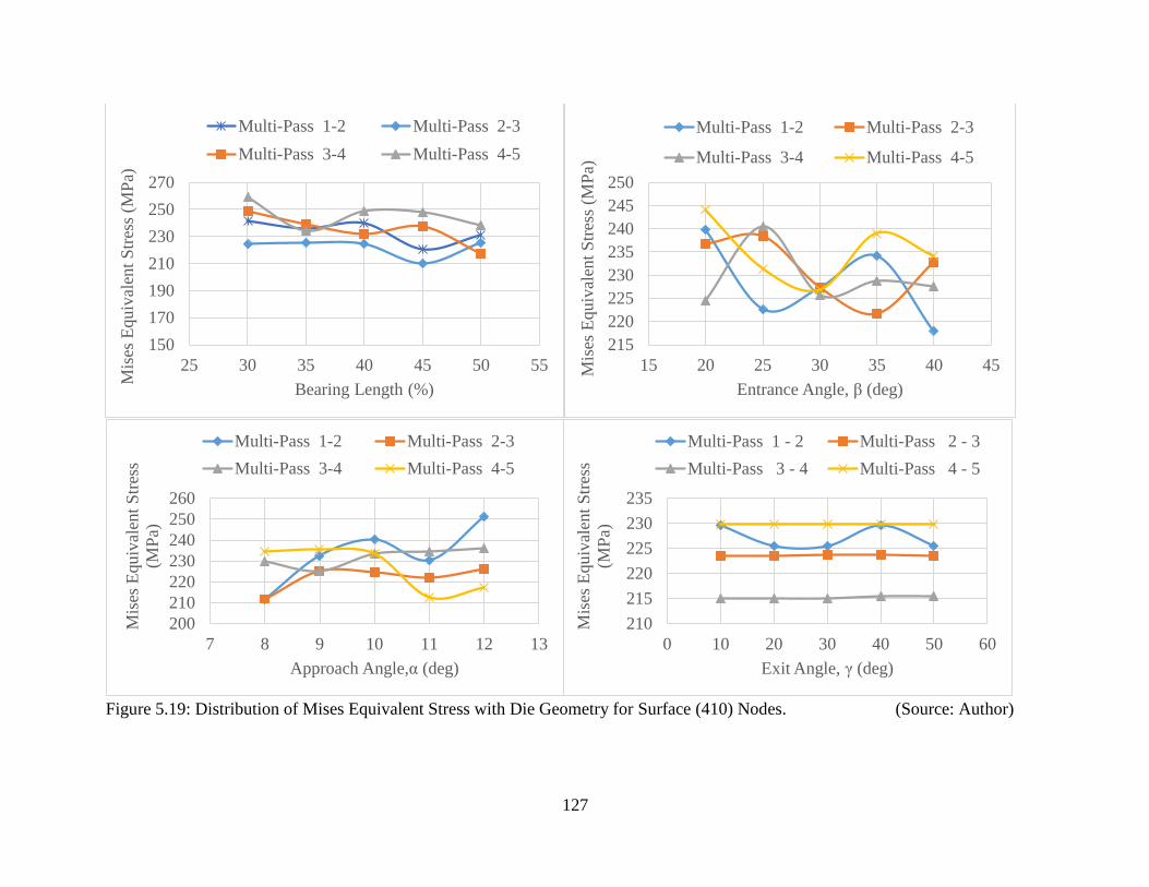
127
Figure 5.19: Distribution of Mises Equivalent Stress with Die Geometry for Surface (410) Nodes. (Source: Author)
150
170
190
210
230
250
270
25 30 35 40 45 50 55
Mis
es E
quiv
alen
t S
tres
s (M
Pa)
Bearing Length (%)
Multi-Pass 1-2 Multi-Pass 2-3
Multi-Pass 3-4 Multi-Pass 4-5
215
220
225
230
235
240
245
250
15 20 25 30 35 40 45Mis
es E
quiv
alen
t S
tres
s (M
Pa)
Entrance Angle, β (deg)
Multi-Pass 1-2 Multi-Pass 2-3
Multi-Pass 3-4 Multi-Pass 4-5
200
210
220
230
240
250
260
7 8 9 10 11 12 13
Mis
es E
quiv
alen
t S
tres
s
(MP
a)
Approach Angle,α (deg)
Multi-Pass 1-2 Multi-Pass 2-3
Multi-Pass 3-4 Multi-Pass 4-5
210
215
220
225
230
235
0 10 20 30 40 50 60
Mis
es E
quiv
alen
t S
tres
s
(MP
a)
Exit Angle, γ (deg)
Multi-Pass 1 - 2 Multi-Pass 2 - 3
Multi-Pass 3 - 4 Multi-Pass 4 - 5
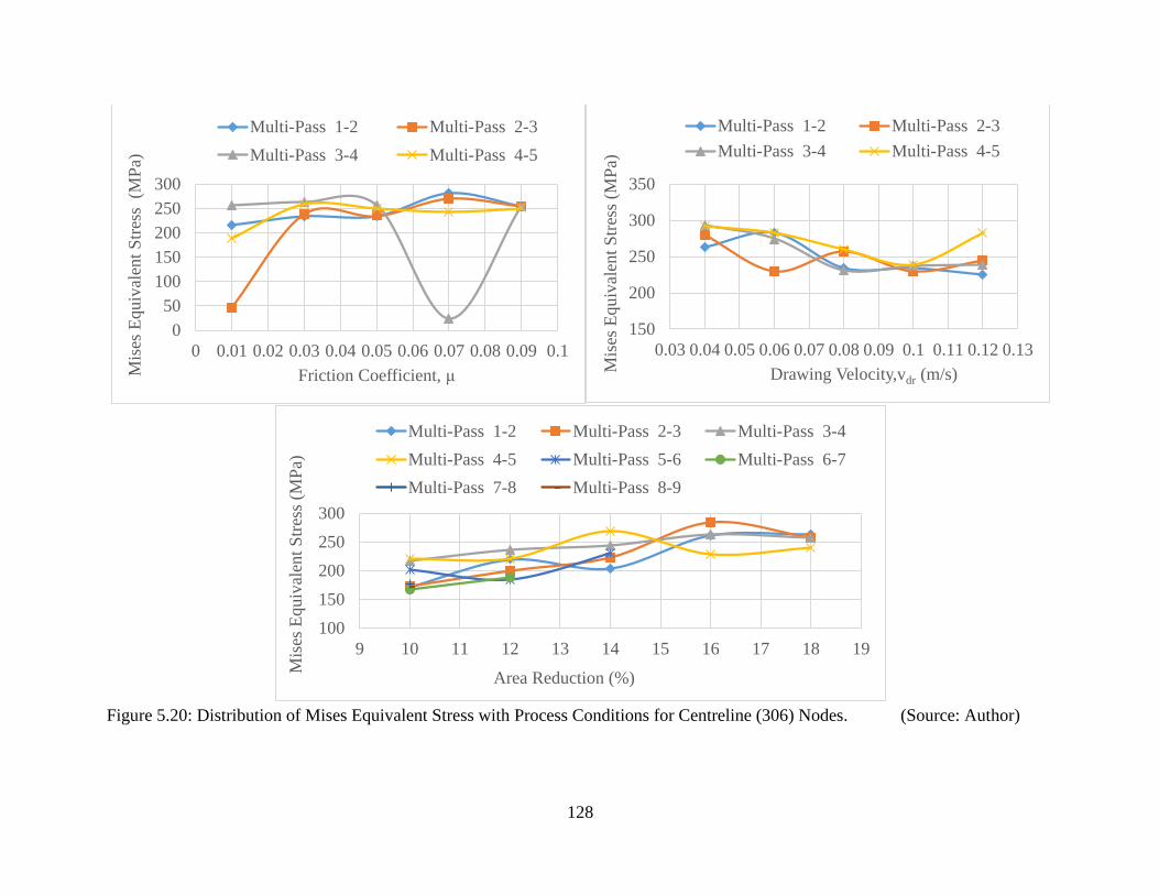
128
Figure 5.20: Distribution of Mises Equivalent Stress with Process Conditions for Centreline (306) Nodes. (Source: Author)
0
50
100
150
200
250
300
0 0.01 0.02 0.03 0.04 0.05 0.06 0.07 0.08 0.09 0.1
Mis
es E
quiv
alen
t S
tres
s (
MP
a)
Friction Coefficient, μ
Multi-Pass 1-2 Multi-Pass 2-3
Multi-Pass 3-4 Multi-Pass 4-5
150
200
250
300
350
0.03 0.04 0.05 0.06 0.07 0.08 0.09 0.1 0.11 0.12 0.13
Mis
es E
quiv
alen
t S
tres
s (M
Pa)
Drawing Velocity,vdr (m/s)
Multi-Pass 1-2 Multi-Pass 2-3
Multi-Pass 3-4 Multi-Pass 4-5
100
150
200
250
300
9 10 11 12 13 14 15 16 17 18 19
Mis
es E
quiv
alen
t S
tres
s (M
Pa)
Area Reduction (%)
Multi-Pass 1-2 Multi-Pass 2-3 Multi-Pass 3-4
Multi-Pass 4-5 Multi-Pass 5-6 Multi-Pass 6-7
Multi-Pass 7-8 Multi-Pass 8-9
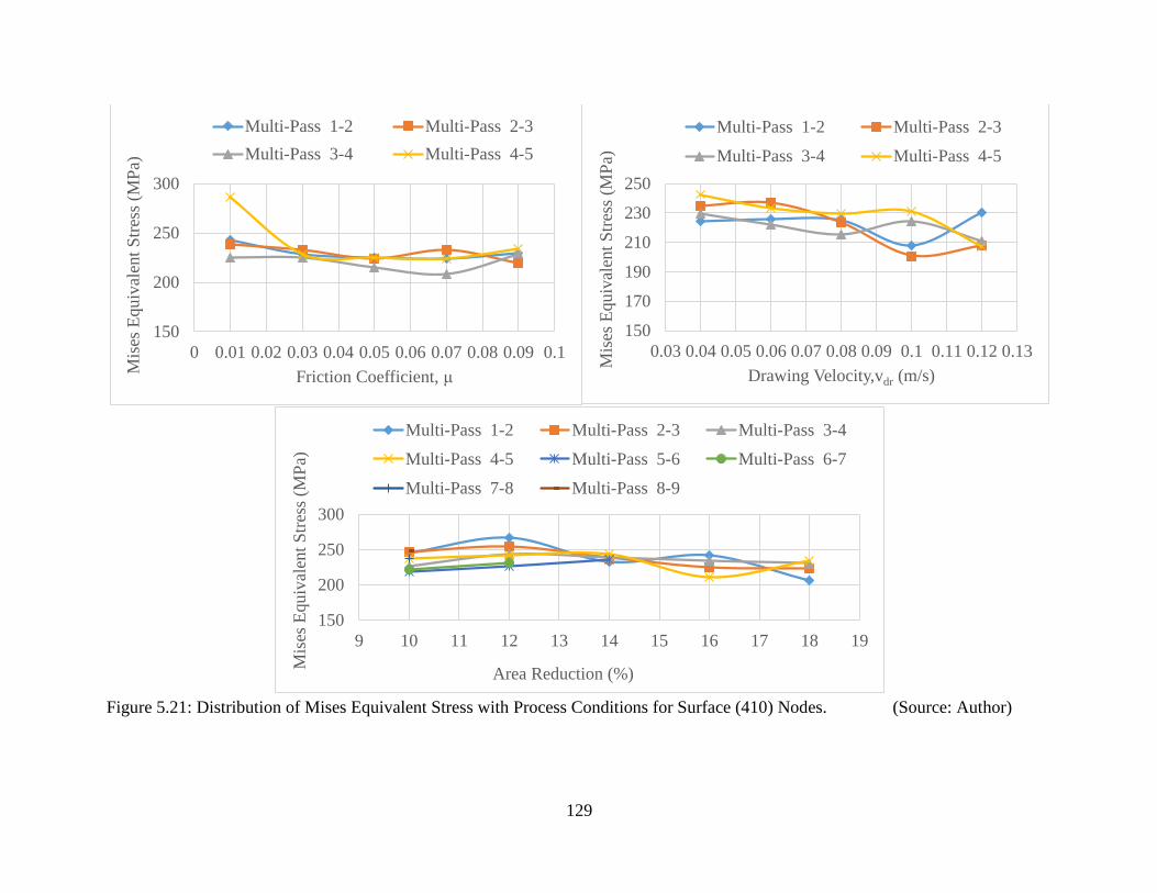
129
Figure 5.21: Distribution of Mises Equivalent Stress with Process Conditions for Surface (410) Nodes. (Source: Author)
150
200
250
300
0 0.01 0.02 0.03 0.04 0.05 0.06 0.07 0.08 0.09 0.1
Mis
es E
quiv
alen
t S
tres
s (M
Pa)
Friction Coefficient, μ
Multi-Pass 1-2 Multi-Pass 2-3
Multi-Pass 3-4 Multi-Pass 4-5
150
170
190
210
230
250
0.03 0.04 0.05 0.06 0.07 0.08 0.09 0.1 0.11 0.12 0.13
Mis
es E
quiv
alen
t S
tres
s (M
Pa)
Drawing Velocity,vdr (m/s)
Multi-Pass 1-2 Multi-Pass 2-3
Multi-Pass 3-4 Multi-Pass 4-5
150
200
250
300
9 10 11 12 13 14 15 16 17 18 19
Mis
es E
quiv
alen
t S
tres
s (M
Pa)
Area Reduction (%)
Multi-Pass 1-2 Multi-Pass 2-3 Multi-Pass 3-4
Multi-Pass 4-5 Multi-Pass 5-6 Multi-Pass 6-7
Multi-Pass 7-8 Multi-Pass 8-9
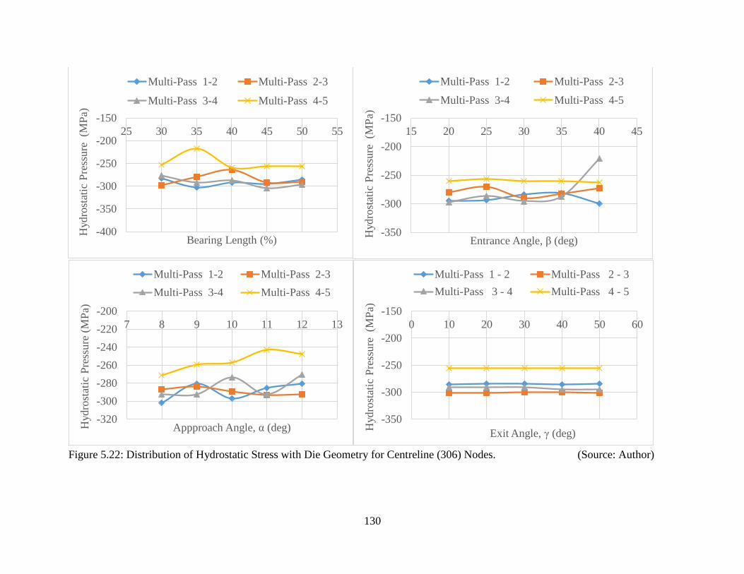
130
Figure 5.22: Distribution of Hydrostatic Stress with Die Geometry for Centreline (306) Nodes. (Source: Author)
-400
-350
-300
-250
-200
-150
25 30 35 40 45 50 55
Hydro
stat
ic P
ress
ure
(M
Pa)
Bearing Length (%)
Multi-Pass 1-2 Multi-Pass 2-3
Multi-Pass 3-4 Multi-Pass 4-5
-350
-300
-250
-200
-150
15 20 25 30 35 40 45
Hydro
stat
ic P
ress
ure
(M
Pa)
Entrance Angle, β (deg)
Multi-Pass 1-2 Multi-Pass 2-3
Multi-Pass 3-4 Multi-Pass 4-5
-320
-300
-280
-260
-240
-220
-200
7 8 9 10 11 12 13
Hydro
stat
ic P
ress
ure
(M
Pa)
Appproach Angle, α (deg)
Multi-Pass 1-2 Multi-Pass 2-3
Multi-Pass 3-4 Multi-Pass 4-5
-350
-300
-250
-200
-150
0 10 20 30 40 50 60
Hydro
stat
ic P
ress
ure
(M
Pa)
Exit Angle, γ (deg)
Multi-Pass 1 - 2 Multi-Pass 2 - 3
Multi-Pass 3 - 4 Multi-Pass 4 - 5
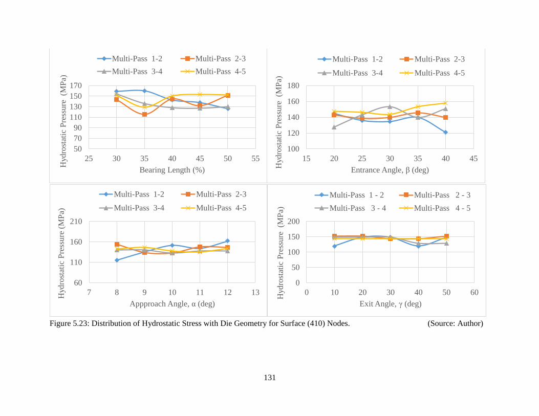
131
Figure 5.23: Distribution of Hydrostatic Stress with Die Geometry for Surface (410) Nodes. (Source: Author)
50
70
90
110
130
150
170
25 30 35 40 45 50 55
Hydro
stat
ic P
ress
ure
(M
Pa)
Bearing Length (%)
Multi-Pass 1-2 Multi-Pass 2-3
Multi-Pass 3-4 Multi-Pass 4-5
100
120
140
160
180
15 20 25 30 35 40 45
Hydro
stat
ic P
ress
ure
(M
Pa)
Entrance Angle, β (deg)
Multi-Pass 1-2 Multi-Pass 2-3
Multi-Pass 3-4 Multi-Pass 4-5
60
110
160
210
7 8 9 10 11 12 13
Hydro
stat
ic P
ress
ure
(M
Pa)
Appproach Angle, α (deg)
Multi-Pass 1-2 Multi-Pass 2-3
Multi-Pass 3-4 Multi-Pass 4-5
0
50
100
150
200
0 10 20 30 40 50 60
Hydro
stat
ic P
ress
ure
(M
Pa)
Exit Angle, γ (deg)
Multi-Pass 1 - 2 Multi-Pass 2 - 3
Multi-Pass 3 - 4 Multi-Pass 4 - 5
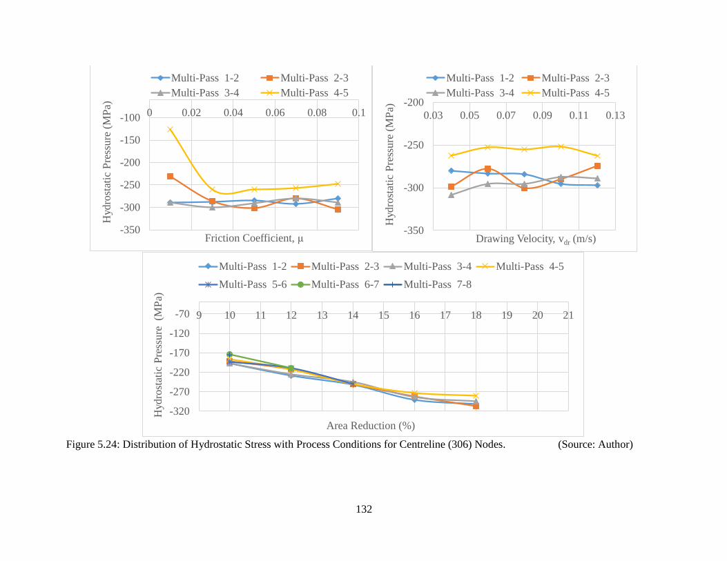
132
Figure 5.24: Distribution of Hydrostatic Stress with Process Conditions for Centreline (306) Nodes. (Source: Author)
-350
-300
-250
-200
-150
-100 0 0.02 0.04 0.06 0.08 0.1H
ydro
stat
ic P
ress
ure
(M
Pa)
Friction Coefficient, μ
Multi-Pass 1-2 Multi-Pass 2-3
Multi-Pass 3-4 Multi-Pass 4-5
-350
-300
-250
-200
0.03 0.05 0.07 0.09 0.11 0.13
Hydro
stat
ic P
ress
ure
(M
Pa)
Drawing Velocity, vdr (m/s)
Multi-Pass 1-2 Multi-Pass 2-3
Multi-Pass 3-4 Multi-Pass 4-5
-320
-270
-220
-170
-120
-70 9 10 11 12 13 14 15 16 17 18 19 20 21
Hydro
stat
ic P
ress
ure
(M
Pa)
Area Reduction (%)
Multi-Pass 1-2 Multi-Pass 2-3 Multi-Pass 3-4 Multi-Pass 4-5
Multi-Pass 5-6 Multi-Pass 6-7 Multi-Pass 7-8
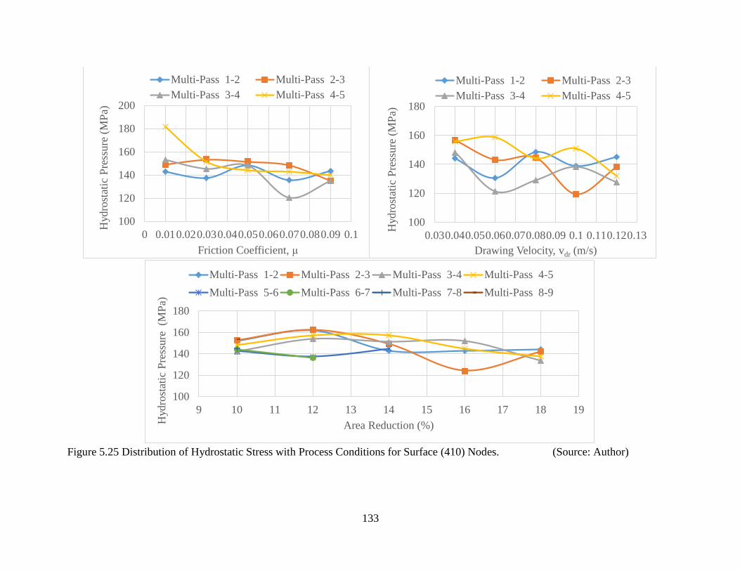
133
Figure 5.25 Distribution of Hydrostatic Stress with Process Conditions for Surface (410) Nodes. (Source: Author)
100
120
140
160
180
200
0 0.010.020.030.040.050.060.070.080.09 0.1
Hydro
stat
ic P
ress
ure
(M
Pa)
Friction Coefficient, μ
Multi-Pass 1-2 Multi-Pass 2-3
Multi-Pass 3-4 Multi-Pass 4-5
100
120
140
160
180
0.030.040.050.060.070.080.09 0.1 0.110.120.13
Hydro
stat
ic P
ress
ure
(M
Pa)
Drawing Velocity, vdr (m/s)
Multi-Pass 1-2 Multi-Pass 2-3
Multi-Pass 3-4 Multi-Pass 4-5
100
120
140
160
180
9 10 11 12 13 14 15 16 17 18 19
Hydro
stat
ic P
ress
ure
(M
Pa)
Area Reduction (%)
Multi-Pass 1-2 Multi-Pass 2-3 Multi-Pass 3-4 Multi-Pass 4-5
Multi-Pass 5-6 Multi-Pass 6-7 Multi-Pass 7-8 Multi-Pass 8-9

134
(iv) Stress Triaxiality Distribution
Stress triaxiality distributions affect the onset of progressive damage in a material. In
ABAQUS, the output parameter TRIAX indicates the stress triaxiality values. Figure
5.26, 5.27, 5.28 and 5.29 show the distribution of stress triaxiality during multi-pass
drawing with different die geometry and drawing process conditions. The stress
triaxiality, η, is expressed by the equation (5.11) as follows (Dassault Systèmes, 2014):
𝜂 = −𝑝
𝜎𝑒𝑞 (5.11)
where, p is the equivalent pressure stress
𝜎𝑒𝑞 is the equivalent Mises stress
(v) Damage Initiation Distribution
Arising from the stress triaxiality distributions and using the ABAQUS output parameter
DUCTCRT, initiation of ductile damage in copper wire was assessed. The models
showed that the ductile criterion parameter (DUCTCRT) was equal to one for all the
multi-pass sequences, except for area reduction models for centerline node (306) where
the DUCTCRT parameter was less than one at area reductions below 16%. Ductile
damage initiation occurred when the ductile criterion parameter was equal to one.
Figure 5.30, 5.31, 5.32 and 5.33 show the distribution of the ductile criterion
(DUCTCRT) parameter with different die design and process parameters.
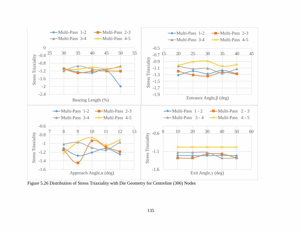
135
Figure 5.26 Distribution of Stress Triaxiality with Die Geometry for Centreline (306) Nodes
-2.4
-2
-1.6
-1.2
-0.8
-0.4
0
25 30 35 40 45 50 55
Str
ess
Tri
axia
lity
Bearing Length (%)
Multi-Pass 1-2 Multi-Pass 2-3
Multi-Pass 3-4 Multi-Pass 4-5
-1.9
-1.7
-1.5
-1.3
-1.1
-0.9
-0.7
-0.5
15 20 25 30 35 40 45
Str
ess
Tri
axia
lity
Entrance Angle,β (deg)
Multi-Pass 1-2 Multi-Pass 2-3
Multi-Pass 3-4 Multi-Pass 4-5
-1.6
-1.4
-1.2
-1
-0.8
-0.6
7 8 9 10 11 12 13
Str
ess
Tri
axia
lity
Approach Angle,α (deg)
Multi-Pass 1-2 Multi-Pass 2-3
Multi-Pass 3-4 Multi-Pass 4-5
-1.6
-1.1
-0.6 0 10 20 30 40 50 60
Str
ess
Tri
axia
lity
Exit Angle,γ (deg)
Multi-Pass 1 - 2 Multi-Pass 2 - 3
Multi-Pass 3 - 4 Multi-Pass 4 - 5
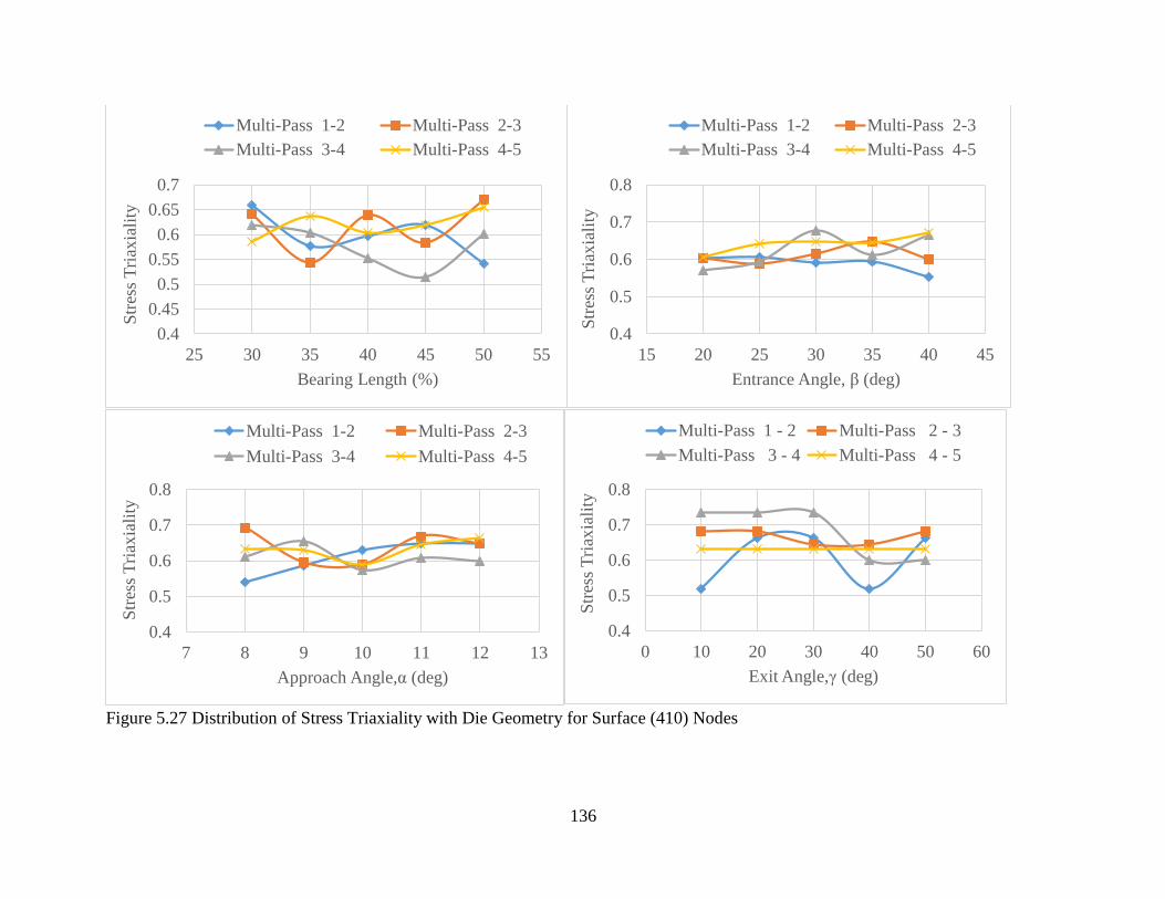
136
Figure 5.27 Distribution of Stress Triaxiality with Die Geometry for Surface (410) Nodes
0.4
0.45
0.5
0.55
0.6
0.65
0.7
25 30 35 40 45 50 55
Str
ess
Tri
axia
lity
Bearing Length (%)
Multi-Pass 1-2 Multi-Pass 2-3
Multi-Pass 3-4 Multi-Pass 4-5
0.4
0.5
0.6
0.7
0.8
15 20 25 30 35 40 45
Str
ess
Tri
axia
lity
Entrance Angle, β (deg)
Multi-Pass 1-2 Multi-Pass 2-3
Multi-Pass 3-4 Multi-Pass 4-5
0.4
0.5
0.6
0.7
0.8
7 8 9 10 11 12 13
Str
ess
Tri
axia
lity
Approach Angle,α (deg)
Multi-Pass 1-2 Multi-Pass 2-3
Multi-Pass 3-4 Multi-Pass 4-5
0.4
0.5
0.6
0.7
0.8
0 10 20 30 40 50 60
Str
ess
Tri
axia
lity
Exit Angle,γ (deg)
Multi-Pass 1 - 2 Multi-Pass 2 - 3
Multi-Pass 3 - 4 Multi-Pass 4 - 5
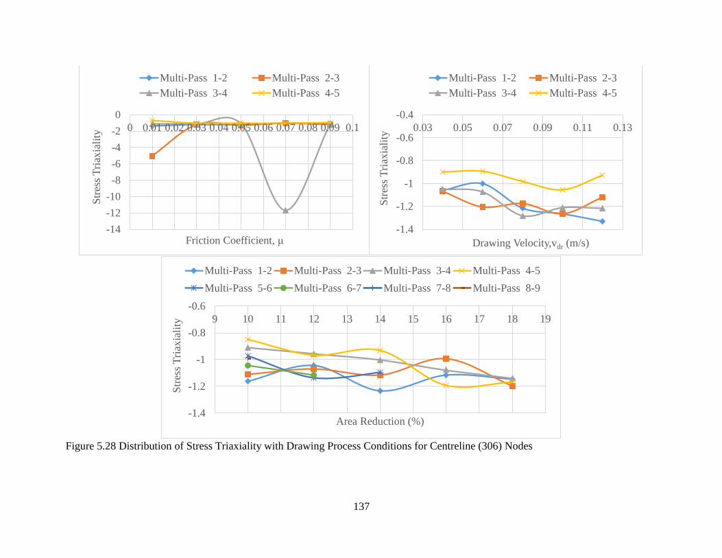
137
Figure 5.28 Distribution of Stress Triaxiality with Drawing Process Conditions for Centreline (306) Nodes
-14
-12
-10
-8
-6
-4
-2
0
0 0.01 0.02 0.03 0.04 0.05 0.06 0.07 0.08 0.09 0.1
Str
ess
Tri
axia
lity
Friction Coefficient, μ
Multi-Pass 1-2 Multi-Pass 2-3
Multi-Pass 3-4 Multi-Pass 4-5
-1.4
-1.2
-1
-0.8
-0.6
-0.4
0.03 0.05 0.07 0.09 0.11 0.13
Str
ess
Tri
axia
lity
Drawing Velocity,vdr (m/s)
Multi-Pass 1-2 Multi-Pass 2-3
Multi-Pass 3-4 Multi-Pass 4-5
-1.4
-1.2
-1
-0.8
-0.6
9 10 11 12 13 14 15 16 17 18 19
Str
ess
Tri
axia
lity
Area Reduction (%)
Multi-Pass 1-2 Multi-Pass 2-3 Multi-Pass 3-4 Multi-Pass 4-5
Multi-Pass 5-6 Multi-Pass 6-7 Multi-Pass 7-8 Multi-Pass 8-9
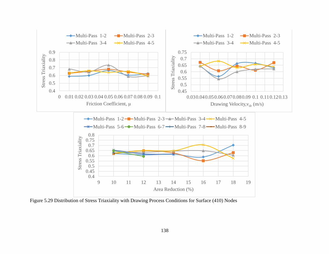
138
Figure 5.29 Distribution of Stress Triaxiality with Drawing Process Conditions for Surface (410) Nodes
0.4
0.5
0.6
0.7
0.8
0.9
0 0.01 0.02 0.03 0.04 0.05 0.06 0.07 0.08 0.09 0.1
Str
ess
Tri
axia
lity
Friction Coefficient, μ
Multi-Pass 1-2 Multi-Pass 2-3
Multi-Pass 3-4 Multi-Pass 4-5
0.45
0.5
0.55
0.6
0.65
0.7
0.75
0.030.040.050.060.070.080.09 0.1 0.110.120.13
Str
ess
Tri
axia
lity
Drawing Velocity,vdr (m/s)
Multi-Pass 1-2 Multi-Pass 2-3
Multi-Pass 3-4 Multi-Pass 4-5
0.40.450.5
0.550.6
0.650.7
0.750.8
9 10 11 12 13 14 15 16 17 18 19
Str
ess
Tri
axia
lity
Area Reduction (%)
Multi-Pass 1-2 Multi-Pass 2-3 Multi-Pass 3-4 Multi-Pass 4-5
Multi-Pass 5-6 Multi-Pass 6-7 Multi-Pass 7-8 Multi-Pass 8-9
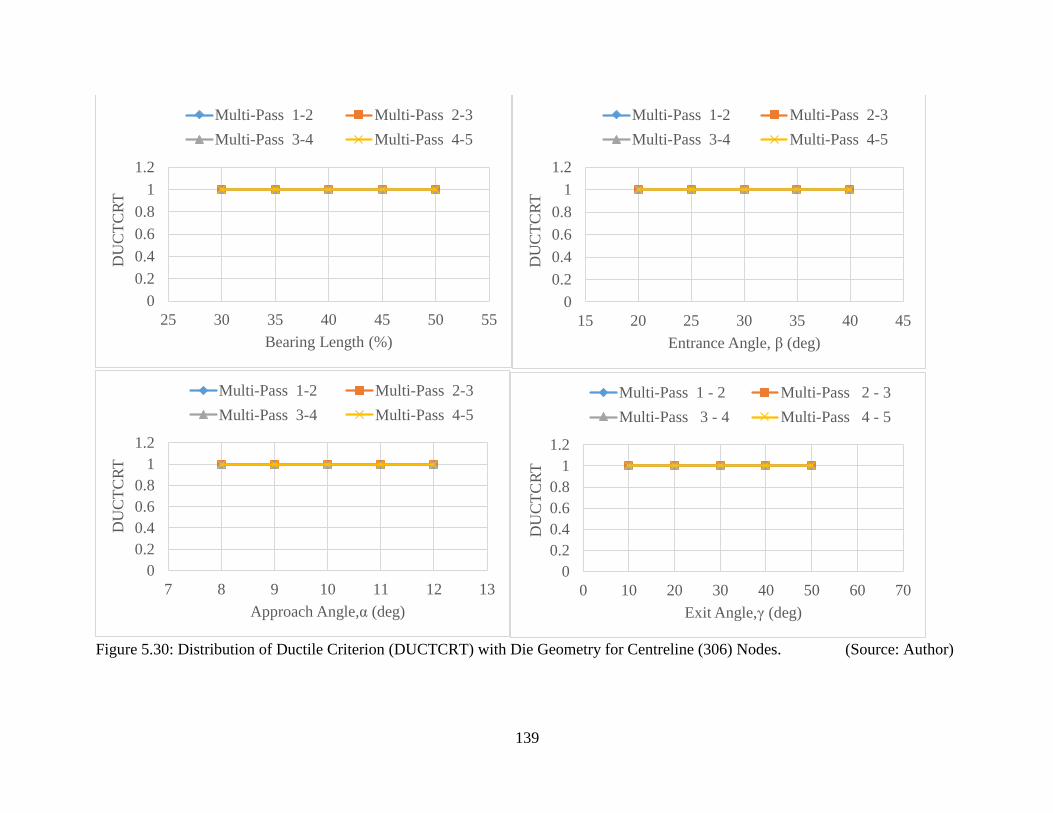
139
Figure 5.30: Distribution of Ductile Criterion (DUCTCRT) with Die Geometry for Centreline (306) Nodes. (Source: Author)
0
0.2
0.4
0.6
0.8
1
1.2
25 30 35 40 45 50 55
DU
CT
CR
T
Bearing Length (%)
Multi-Pass 1-2 Multi-Pass 2-3
Multi-Pass 3-4 Multi-Pass 4-5
0
0.2
0.4
0.6
0.8
1
1.2
15 20 25 30 35 40 45
DU
CT
CR
T
Entrance Angle, β (deg)
Multi-Pass 1-2 Multi-Pass 2-3
Multi-Pass 3-4 Multi-Pass 4-5
0
0.2
0.4
0.6
0.8
1
1.2
7 8 9 10 11 12 13
DU
CT
CR
T
Approach Angle,α (deg)
Multi-Pass 1-2 Multi-Pass 2-3
Multi-Pass 3-4 Multi-Pass 4-5
0
0.2
0.4
0.6
0.8
1
1.2
0 10 20 30 40 50 60 70
DU
CT
CR
T
Exit Angle,γ (deg)
Multi-Pass 1 - 2 Multi-Pass 2 - 3
Multi-Pass 3 - 4 Multi-Pass 4 - 5
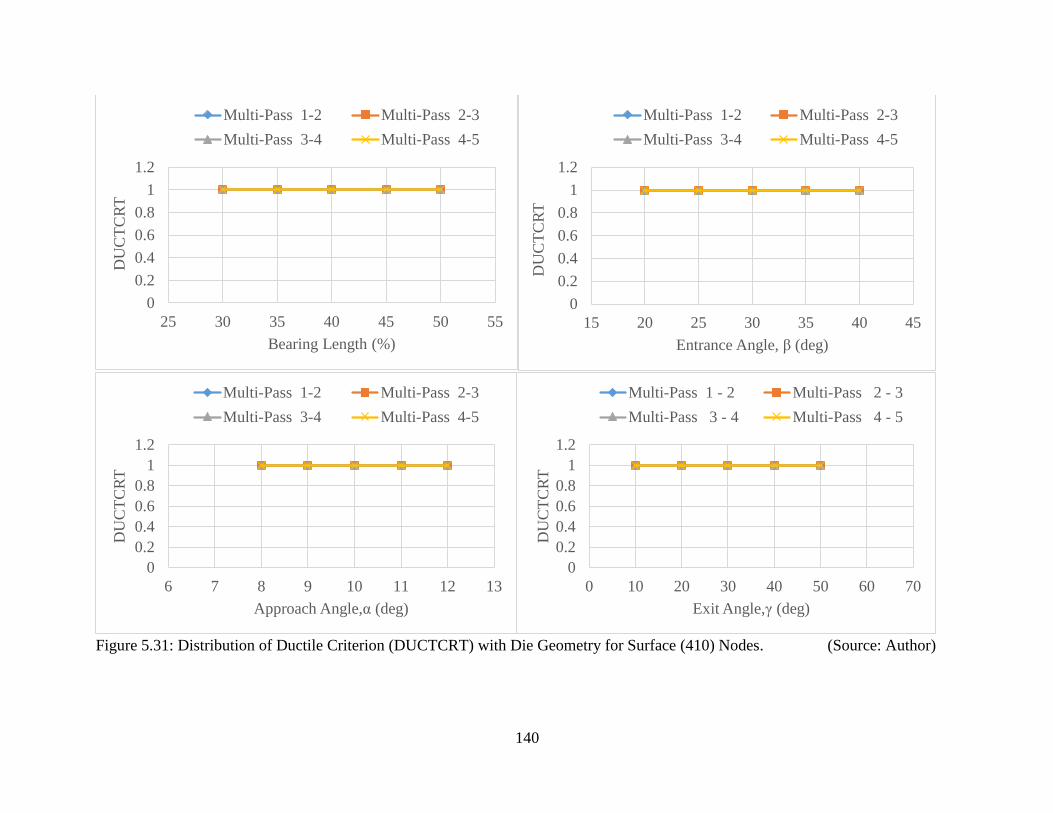
140
Figure 5.31: Distribution of Ductile Criterion (DUCTCRT) with Die Geometry for Surface (410) Nodes. (Source: Author)
0
0.2
0.4
0.6
0.8
1
1.2
25 30 35 40 45 50 55
DU
CT
CR
T
Bearing Length (%)
Multi-Pass 1-2 Multi-Pass 2-3
Multi-Pass 3-4 Multi-Pass 4-5
0
0.2
0.4
0.6
0.8
1
1.2
15 20 25 30 35 40 45
DU
CT
CR
T
Entrance Angle, β (deg)
Multi-Pass 1-2 Multi-Pass 2-3
Multi-Pass 3-4 Multi-Pass 4-5
0
0.2
0.4
0.6
0.8
1
1.2
6 7 8 9 10 11 12 13
DU
CT
CR
T
Approach Angle,α (deg)
Multi-Pass 1-2 Multi-Pass 2-3
Multi-Pass 3-4 Multi-Pass 4-5
0
0.2
0.4
0.6
0.8
1
1.2
0 10 20 30 40 50 60 70
DU
CT
CR
T
Exit Angle,γ (deg)
Multi-Pass 1 - 2 Multi-Pass 2 - 3
Multi-Pass 3 - 4 Multi-Pass 4 - 5
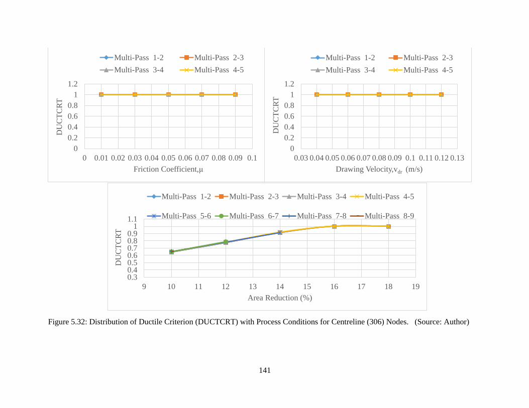
141
Figure 5.32: Distribution of Ductile Criterion (DUCTCRT) with Process Conditions for Centreline (306) Nodes. (Source: Author)
0
0.2
0.4
0.6
0.8
1
1.2
0 0.01 0.02 0.03 0.04 0.05 0.06 0.07 0.08 0.09 0.1
DU
CT
CR
T
Friction Coefficient,μ
Multi-Pass 1-2 Multi-Pass 2-3
Multi-Pass 3-4 Multi-Pass 4-5
0
0.2
0.4
0.6
0.8
1
1.2
0.03 0.04 0.05 0.06 0.07 0.08 0.09 0.1 0.11 0.12 0.13
DU
CT
CR
T
Drawing Velocity,vdr (m/s)
Multi-Pass 1-2 Multi-Pass 2-3
Multi-Pass 3-4 Multi-Pass 4-5
0.30.40.50.60.70.80.9
11.1
9 10 11 12 13 14 15 16 17 18 19
DU
CT
CR
T
Area Reduction (%)
Multi-Pass 1-2 Multi-Pass 2-3 Multi-Pass 3-4 Multi-Pass 4-5
Multi-Pass 5-6 Multi-Pass 6-7 Multi-Pass 7-8 Multi-Pass 8-9
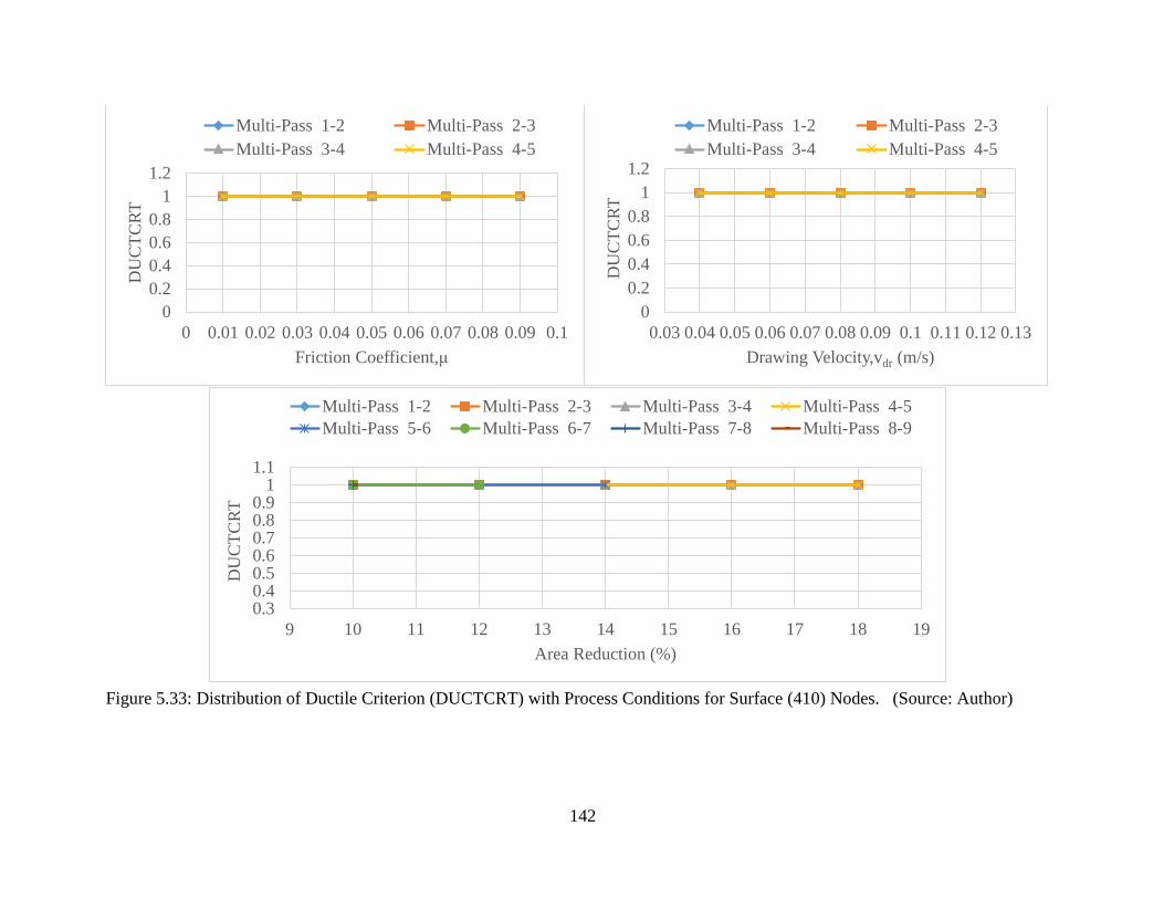
142
Figure 5.33: Distribution of Ductile Criterion (DUCTCRT) with Process Conditions for Surface (410) Nodes. (Source: Author)
0
0.2
0.4
0.6
0.8
1
1.2
0 0.01 0.02 0.03 0.04 0.05 0.06 0.07 0.08 0.09 0.1
DU
CT
CR
T
Friction Coefficient,μ
Multi-Pass 1-2 Multi-Pass 2-3
Multi-Pass 3-4 Multi-Pass 4-5
0
0.2
0.4
0.6
0.8
1
1.2
0.03 0.04 0.05 0.06 0.07 0.08 0.09 0.1 0.11 0.12 0.13
DU
CT
CR
T
Drawing Velocity,vdr (m/s)
Multi-Pass 1-2 Multi-Pass 2-3
Multi-Pass 3-4 Multi-Pass 4-5
0.30.40.50.60.70.80.9
11.1
9 10 11 12 13 14 15 16 17 18 19
DU
CT
CR
T
Area Reduction (%)
Multi-Pass 1-2 Multi-Pass 2-3 Multi-Pass 3-4 Multi-Pass 4-5
Multi-Pass 5-6 Multi-Pass 6-7 Multi-Pass 7-8 Multi-Pass 8-9
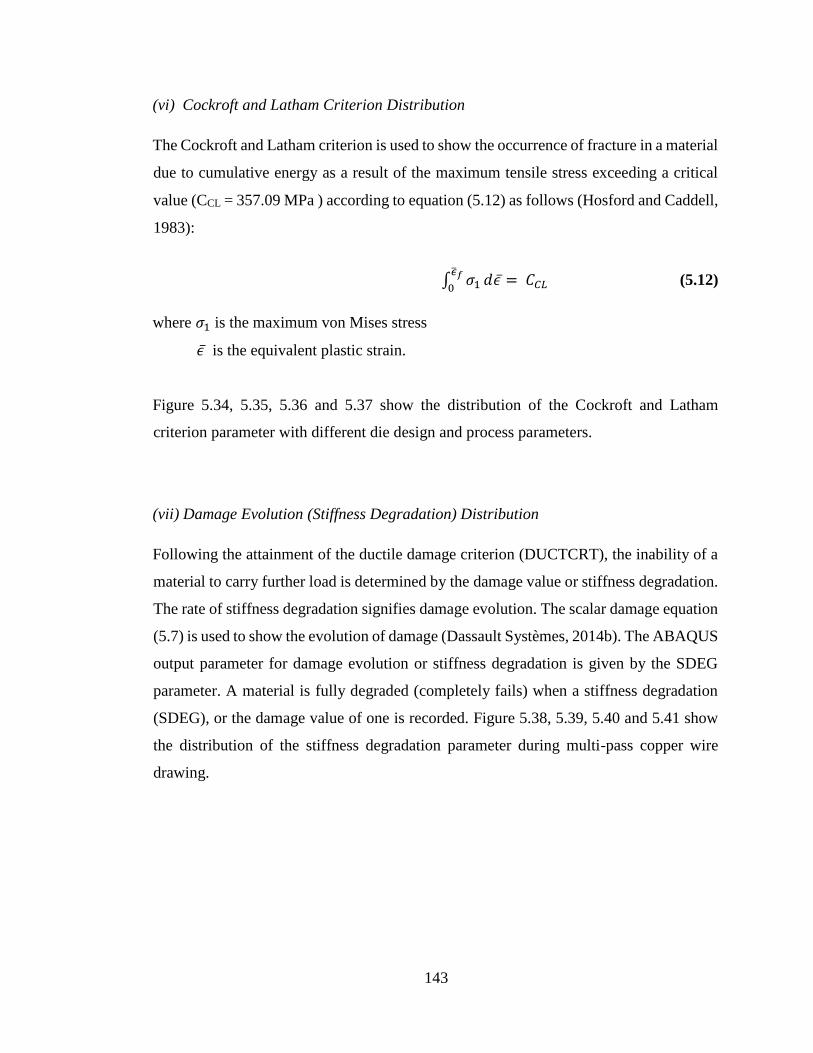
143
(vi) Cockroft and Latham Criterion Distribution
The Cockroft and Latham criterion is used to show the occurrence of fracture in a material
due to cumulative energy as a result of the maximum tensile stress exceeding a critical
value (CCL = 357.09 MPa ) according to equation (5.12) as follows (Hosford and Caddell,
1983):
∫ 𝜎1��𝑓
0𝑑𝜖 = 𝐶𝐶𝐿 (5.12)
where 𝜎1 is the maximum von Mises stress
𝜖 is the equivalent plastic strain.
Figure 5.34, 5.35, 5.36 and 5.37 show the distribution of the Cockroft and Latham
criterion parameter with different die design and process parameters.
(vii) Damage Evolution (Stiffness Degradation) Distribution
Following the attainment of the ductile damage criterion (DUCTCRT), the inability of a
material to carry further load is determined by the damage value or stiffness degradation.
The rate of stiffness degradation signifies damage evolution. The scalar damage equation
(5.7) is used to show the evolution of damage (Dassault Systèmes, 2014b). The ABAQUS
output parameter for damage evolution or stiffness degradation is given by the SDEG
parameter. A material is fully degraded (completely fails) when a stiffness degradation
(SDEG), or the damage value of one is recorded. Figure 5.38, 5.39, 5.40 and 5.41 show
the distribution of the stiffness degradation parameter during multi-pass copper wire
drawing.
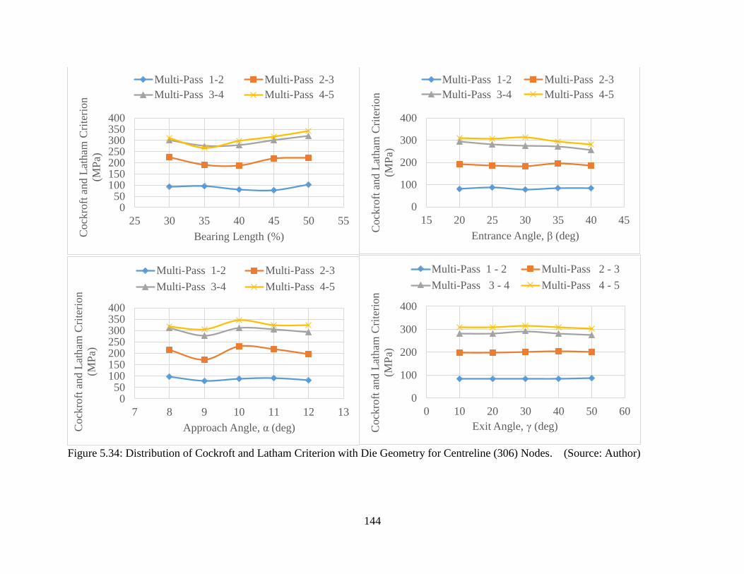
144
Figure 5.34: Distribution of Cockroft and Latham Criterion with Die Geometry for Centreline (306) Nodes. (Source: Author)
050
100150200250300350400
25 30 35 40 45 50 55
Cock
roft
and L
atham
Cri
teri
on
(MP
a)
Bearing Length (%)
Multi-Pass 1-2 Multi-Pass 2-3
Multi-Pass 3-4 Multi-Pass 4-5
0
100
200
300
400
15 20 25 30 35 40 45
Cock
roft
and L
atham
Cri
teri
on
(MP
a)
Entrance Angle, β (deg)
Multi-Pass 1-2 Multi-Pass 2-3
Multi-Pass 3-4 Multi-Pass 4-5
050
100150200250300350400
7 8 9 10 11 12 13
Cock
roft
and L
atham
Cri
teri
on
(MP
a)
Approach Angle, α (deg)
Multi-Pass 1-2 Multi-Pass 2-3
Multi-Pass 3-4 Multi-Pass 4-5
0
100
200
300
400
0 10 20 30 40 50 60
Cock
roft
and L
atham
Cri
teri
on
(MP
a)
Exit Angle, γ (deg)
Multi-Pass 1 - 2 Multi-Pass 2 - 3
Multi-Pass 3 - 4 Multi-Pass 4 - 5

145
Figure 5.35: Distribution of Cockroft and Latham Criterion with Die Geometry for Surface (410) Nodes. (Source: Author)
0
200
400
600
800
25 35 45 55
Cock
roft
and L
atham
Cri
teri
on (M
Pa)
Bearing Length (%)
Multi-Pass 1-2 Multi-Pass 2-3
Multi-Pass 3-4 Multi-Pass 4-5
0
200
400
600
800
15 20 25 30 35 40 45
Cock
roft
and L
atham
Cri
teri
on (M
Pa)
Entrance Angle, β (deg)
Multi-Pass 1-2 Multi-Pass 2-3
Multi-Pass 3-4 Multi-Pass 4-5
0
100
200
300
400
500
600
700
7 9 11 13Cock
roft
and L
atham
Cri
teri
on
(MP
a)
Approach Angle, α (deg)
Multi-Pass 1-2 Multi-Pass 2-3
Multi-Pass 3-4 Multi-Pass 4-5
0
100
200
300
400
500
600
0 10 20 30 40 50 60Cock
roft
and L
atham
Cri
teri
on
(MP
a)
Exit Angle, γ (deg)
Multi-Pass 1 - 2 Multi-Pass 2 - 3
Multi-Pass 3 - 4 Multi-Pass 4 - 5
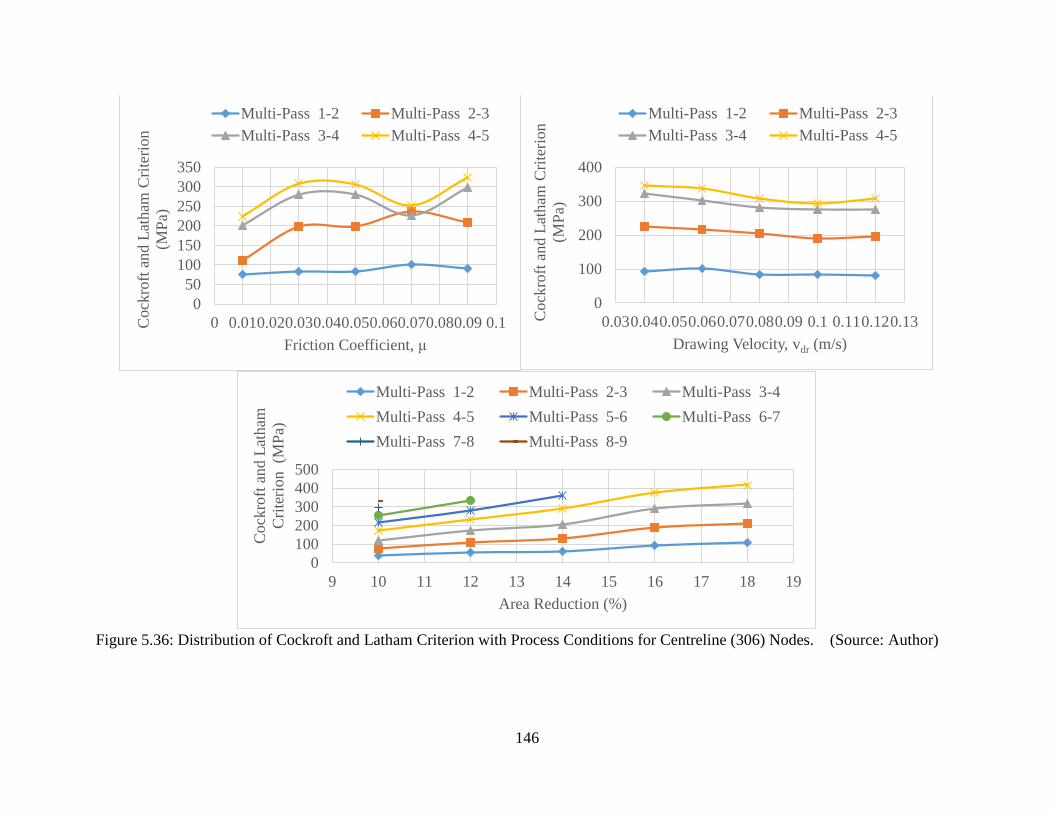
146
Figure 5.36: Distribution of Cockroft and Latham Criterion with Process Conditions for Centreline (306) Nodes. (Source: Author)
0
50
100
150
200
250
300
350
0 0.010.020.030.040.050.060.070.080.09 0.1Cock
roft
and L
atham
Cri
teri
on
(MP
a)
Friction Coefficient, μ
Multi-Pass 1-2 Multi-Pass 2-3
Multi-Pass 3-4 Multi-Pass 4-5
0
100
200
300
400
0.030.040.050.060.070.080.09 0.1 0.110.120.13Cock
roft
and L
atham
Cri
teri
on
(MP
a)
Drawing Velocity, vdr (m/s)
Multi-Pass 1-2 Multi-Pass 2-3
Multi-Pass 3-4 Multi-Pass 4-5
0
100
200
300
400
500
9 10 11 12 13 14 15 16 17 18 19
Cock
roft
an
d L
atham
Cri
teri
on (M
Pa)
Area Reduction (%)
Multi-Pass 1-2 Multi-Pass 2-3 Multi-Pass 3-4
Multi-Pass 4-5 Multi-Pass 5-6 Multi-Pass 6-7
Multi-Pass 7-8 Multi-Pass 8-9
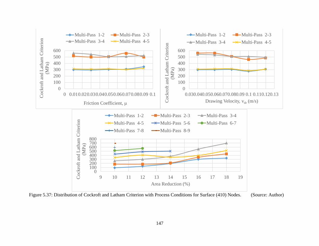
147
Figure 5.37: Distribution of Cockroft and Latham Criterion with Process Conditions for Surface (410) Nodes. (Source: Author)
0
100
200
300
400
500
600
0 0.010.020.030.040.050.060.070.080.09 0.1
Cock
roft
and L
atham
Cri
teri
on
(MP
a)
Friction Coefficient, μ
Multi-Pass 1-2 Multi-Pass 2-3
Multi-Pass 3-4 Multi-Pass 4-5
0
100
200
300
400
500
600
0.030.040.050.060.070.080.09 0.1 0.110.120.13
Cock
roft
and L
atham
Cri
teri
on
(MP
a)
Drawing Velocity, vdr (m/s)
Multi-Pass 1-2 Multi-Pass 2-3
Multi-Pass 3-4 Multi-Pass 4-5
0100200300400500600700800
9 10 11 12 13 14 15 16 17 18 19Cock
roft
and L
atham
Cri
teri
on
(MP
a)
Area Reduction (%)
Multi-Pass 1-2 Multi-Pass 2-3 Multi-Pass 3-4
Multi-Pass 4-5 Multi-Pass 5-6 Multi-Pass 6-7
Multi-Pass 7-8 Multi-Pass 8-9
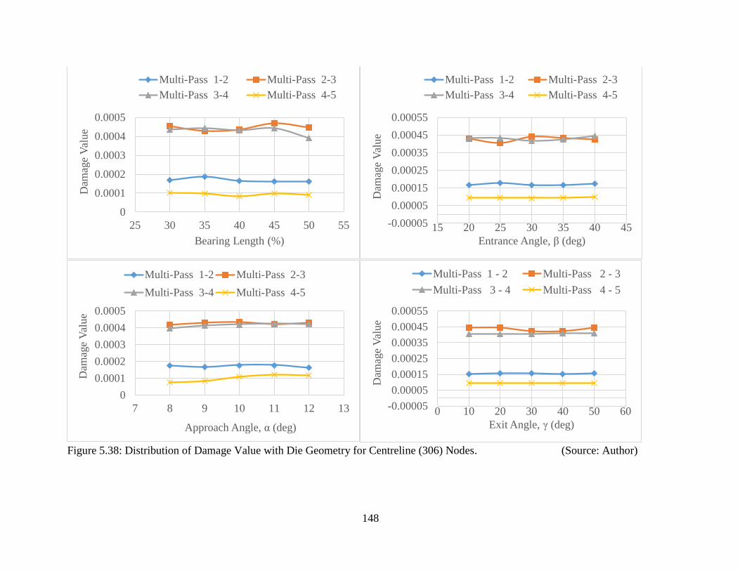
148
Figure 5.38: Distribution of Damage Value with Die Geometry for Centreline (306) Nodes. (Source: Author)
0
0.0001
0.0002
0.0003
0.0004
0.0005
25 30 35 40 45 50 55
Dam
age
Val
ue
Bearing Length (%)
Multi-Pass 1-2 Multi-Pass 2-3
Multi-Pass 3-4 Multi-Pass 4-5
-0.00005
0.00005
0.00015
0.00025
0.00035
0.00045
0.00055
15 20 25 30 35 40 45
Dam
age
Val
ue
Entrance Angle, β (deg)
Multi-Pass 1-2 Multi-Pass 2-3
Multi-Pass 3-4 Multi-Pass 4-5
0
0.0001
0.0002
0.0003
0.0004
0.0005
7 8 9 10 11 12 13
Dam
age
Val
ue
Approach Angle, α (deg)
Multi-Pass 1-2 Multi-Pass 2-3
Multi-Pass 3-4 Multi-Pass 4-5
-0.00005
0.00005
0.00015
0.00025
0.00035
0.00045
0.00055
0 10 20 30 40 50 60
Dam
age
Val
ue
Exit Angle, γ (deg)
Multi-Pass 1 - 2 Multi-Pass 2 - 3
Multi-Pass 3 - 4 Multi-Pass 4 - 5
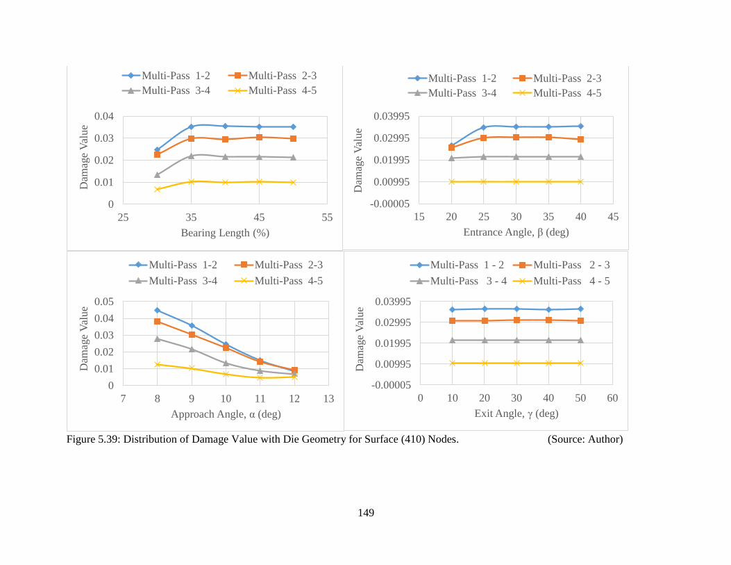
149
Figure 5.39: Distribution of Damage Value with Die Geometry for Surface (410) Nodes. (Source: Author)
0
0.01
0.02
0.03
0.04
25 35 45 55
Dam
age
Val
ue
Bearing Length (%)
Multi-Pass 1-2 Multi-Pass 2-3
Multi-Pass 3-4 Multi-Pass 4-5
-0.00005
0.00995
0.01995
0.02995
0.03995
15 20 25 30 35 40 45
Dam
age
Val
ue
Entrance Angle, β (deg)
Multi-Pass 1-2 Multi-Pass 2-3
Multi-Pass 3-4 Multi-Pass 4-5
0
0.01
0.02
0.03
0.04
0.05
7 8 9 10 11 12 13
Dam
age
Val
ue
Approach Angle, α (deg)
Multi-Pass 1-2 Multi-Pass 2-3
Multi-Pass 3-4 Multi-Pass 4-5
-0.00005
0.00995
0.01995
0.02995
0.03995
0 10 20 30 40 50 60
Dam
age
Val
ue
Exit Angle, γ (deg)
Multi-Pass 1 - 2 Multi-Pass 2 - 3
Multi-Pass 3 - 4 Multi-Pass 4 - 5
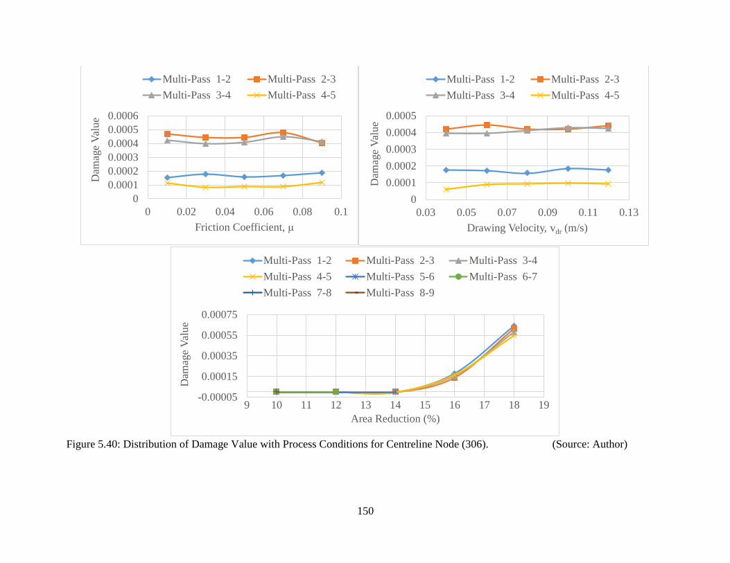
150
Figure 5.40: Distribution of Damage Value with Process Conditions for Centreline Node (306). (Source: Author)
0
0.0001
0.0002
0.0003
0.0004
0.0005
0.0006
0 0.02 0.04 0.06 0.08 0.1
Dam
age
Val
ue
Friction Coefficient, μ
Multi-Pass 1-2 Multi-Pass 2-3
Multi-Pass 3-4 Multi-Pass 4-5
0
0.0001
0.0002
0.0003
0.0004
0.0005
0.03 0.05 0.07 0.09 0.11 0.13
Dam
age
Val
ue
Drawing Velocity, vdr (m/s)
Multi-Pass 1-2 Multi-Pass 2-3
Multi-Pass 3-4 Multi-Pass 4-5
-0.00005
0.00015
0.00035
0.00055
0.00075
9 10 11 12 13 14 15 16 17 18 19
Dam
age
Val
ue
Area Reduction (%)
Multi-Pass 1-2 Multi-Pass 2-3 Multi-Pass 3-4
Multi-Pass 4-5 Multi-Pass 5-6 Multi-Pass 6-7
Multi-Pass 7-8 Multi-Pass 8-9
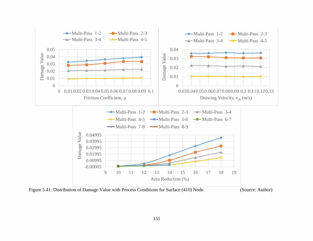
151
Figure 5.41: Distribution of Damage Value with Process Conditions for Surface (410) Node. (Source: Author)
0
0.01
0.02
0.03
0.04
0.05
0 0.01 0.02 0.03 0.04 0.05 0.06 0.07 0.08 0.09 0.1
Dam
age
Val
ue
Friction Coefficient, μ
Multi-Pass 1-2 Multi-Pass 2-3
Multi-Pass 3-4 Multi-Pass 4-5
0
0.01
0.02
0.03
0.04
0.030.040.050.060.070.080.09 0.1 0.110.120.13
Dam
age
Val
ue
Drawing Velocity, vdr (m/s)
Multi-Pass 1-2 Multi-Pass 2-3
Multi-Pass 3-4 Multi-Pass 4-5
-0.00005
0.00995
0.01995
0.02995
0.03995
0.04995
9 10 11 12 13 14 15 16 17 18 19
Dam
age
Val
ue
Area Reduction (%)
Multi-Pass 1-2 Multi-Pass 2-3 Multi-Pass 3-4
Multi-Pass 4-5 Multi-Pass 5-6 Multi-Pass 6-7
Multi-Pass 7-8 Multi-Pass 8-9

152
5.8.3 Selection of Optimum Parameters from Simulation Results
The selection of optimum parameters was based on a combination of minimal mesh
distortion and minimum values during distributions for damage value or stiffness
degradation, equivalent Mises stresses responsible for yielding and damage formation
and the Cockroft and Latham criterion. The results of the simulations show that the
following die and process independent variables are predicted to give optimum wire
drawing performance with reduced centerline material damage when producing a 1.78
mm copper wire with four dies:
▪ a bearing length of 40%,
▪ a semi-approach angle of 9o,
▪ a semi-entrance angle of 30o,
▪ a semi-exit angle of 40o,
▪ a friction coefficient of 0.03,
▪ a drawing speed of 0.1 ms-1
▪ area reductions of not more than 16% during the last multi-pass stage
The design of the die parameters which were used for the validation of the simulation
results was based on the optimum parameters obtained, except for the area reductions.
The area reductions were maintained as obtaining in the plant in order to assess the effects
of the die geometry.
5.9. General Observations from Simulation Results
Consistency of the simulations was done by maintaining the same meshing and
interaction properties. Accuracy of the simulations was achieved by maintaining the
same time scaling factor of 1 with a target time increment of 0.00001.
Results of the simulation study indicated the following:
(1) Peaks for centerline ductile damage using Cockroft and Latham criterion were
observed at the following points:
bearing lengths of 50% (multi-pass sequences 1-2, 2-3, 3-4 and 4-5);
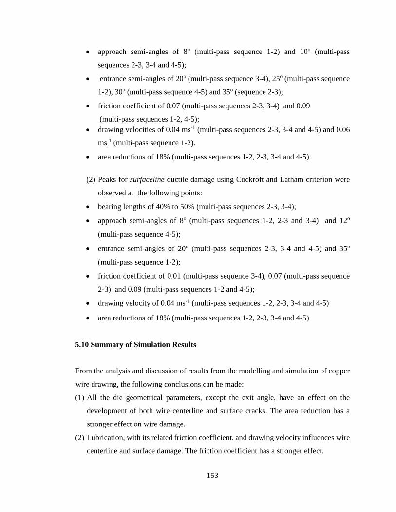
153
approach semi-angles of 8o (multi-pass sequence 1-2) and 10o (multi-pass
sequences 2-3, 3-4 and 4-5);
entrance semi-angles of 20o (multi-pass sequence 3-4), 25o (multi-pass sequence
1-2), 30o (multi-pass sequence 4-5) and 35o (sequence 2-3);
friction coefficient of 0.07 (multi-pass sequences 2-3, 3-4) and 0.09
(multi-pass sequences 1-2, 4-5);
drawing velocities of 0.04 ms-1 (multi-pass sequences 2-3, 3-4 and 4-5) and 0.06
ms-1 (multi-pass sequence 1-2).
area reductions of 18% (multi-pass sequences 1-2, 2-3, 3-4 and 4-5).
(2) Peaks for surfaceline ductile damage using Cockroft and Latham criterion were
observed at the following points:
bearing lengths of 40% to 50% (multi-pass sequences 2-3, 3-4);
approach semi-angles of 8o (multi-pass sequences 1-2, 2-3 and 3-4) and 12o
(multi-pass sequence 4-5);
entrance semi-angles of 20o (multi-pass sequences 2-3, 3-4 and 4-5) and 35o
(multi-pass sequence 1-2);
friction coefficient of 0.01 (multi-pass sequence 3-4), 0.07 (multi-pass sequence
2-3) and 0.09 (multi-pass sequences 1-2 and 4-5);
drawing velocity of 0.04 ms-1 (multi-pass sequences 1-2, 2-3, 3-4 and 4-5)
area reductions of 18% (multi-pass sequences 1-2, 2-3, 3-4 and 4-5)
5.10 Summary of Simulation Results
From the analysis and discussion of results from the modelling and simulation of copper
wire drawing, the following conclusions can be made:
(1) All the die geometrical parameters, except the exit angle, have an effect on the
development of both wire centerline and surface cracks. The area reduction has a
stronger effect on wire damage.
(2) Lubrication, with its related friction coefficient, and drawing velocity influences wire
centerline and surface damage. The friction coefficient has a stronger effect.
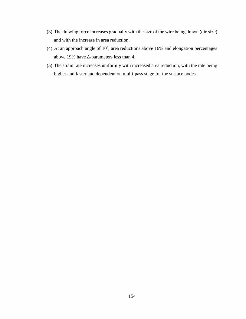
154
(3) The drawing force increases gradually with the size of the wire being drawn (die size)
and with the increase in area reduction.
(4) At an approach angle of 10o, area reductions above 16% and elongation percentages
above 19% have Δ-parameters less than 4.
(5) The strain rate increases uniformly with increased area reduction, with the rate being
higher and faster and dependent on multi-pass stage for the surface nodes.

155
CHAPTER SIX: EXPERIMENTAL DESIGN AND PROCEDURES
6.1 Introduction
This chapter is divided into five major sections. The first section presents the
experimental design used in undertaking the experiments. The second section gives an
overview of major equipment and instruments used in the laboratory and industrial
experiments. Section three explains details of the experimental procedures carried out.
The fourth section presents results from the laboratory and industrial experiments.
.
6.2 Experimental Design
The research involved understanding material properties, the copper wire drawing
practice and die manufacturing. Laboratory experiments were undertaken for wire and
die material property analysis, while industrial experiments were done for wire drawing
and validation of models.
The raw material for both laboratory microstructure and other engineering properties
determination and further industrial experiments was a 7.9 mm wrought copper rod. This
rod was drawn through a rod breakdown machine to a 2.76 mm diameter copper wire for
further wire drawing analysis on the intermediate wire drawing machine and for scanning
electron microscopy analysis.
Tungsten carbide dies were designed and manufactured according to the simulated
optimum die designs and used in obtaining the wire drawing independent and dependent
variables in the plant.
6.3 Equipment and Instrumentation
The major equipment used in the laboratory and industrial experiments are explained
below.

156
6.3.1 Laboratory Experiments and Equipment
(i) Microscopy and Spectrophotometry
A light microscope, Olympus B203 with a magnification of up to 100X was used for
microstructure analysis of the raw copper. Figure 6.1 shows the Olympus light
microscope. The chemical composition of the copper rod was determined using both
atomic absorption spectrophotometry (AAS) and scanning electron microscopy analysis.
Figure 6.1: Olympus B203 Light Microscope. (Source: Author)
(ii) Scanning Electron Microscope (SEM)
The Quanta FEG 450 Scanning Electron Microscope was used for both material micro-
and macrostructure analysis, and elemental analysis. The Quantax Esprit 1.9 software
was used on the SEM to obtain chemical composition of the raw copper materials. Figure
6.2 shows the Quanta FEG SEM.
(iii) Universal Tensile Testing Machine (UTM)
A universal tensile testing machine, TUE C- 600 with an accuracy of +/- 1% and a
capacity of 12 to 600 kN was used for carrying out tensile testing. Figure 6.3 shows the
universal tensile testing machine.
Light
microscope
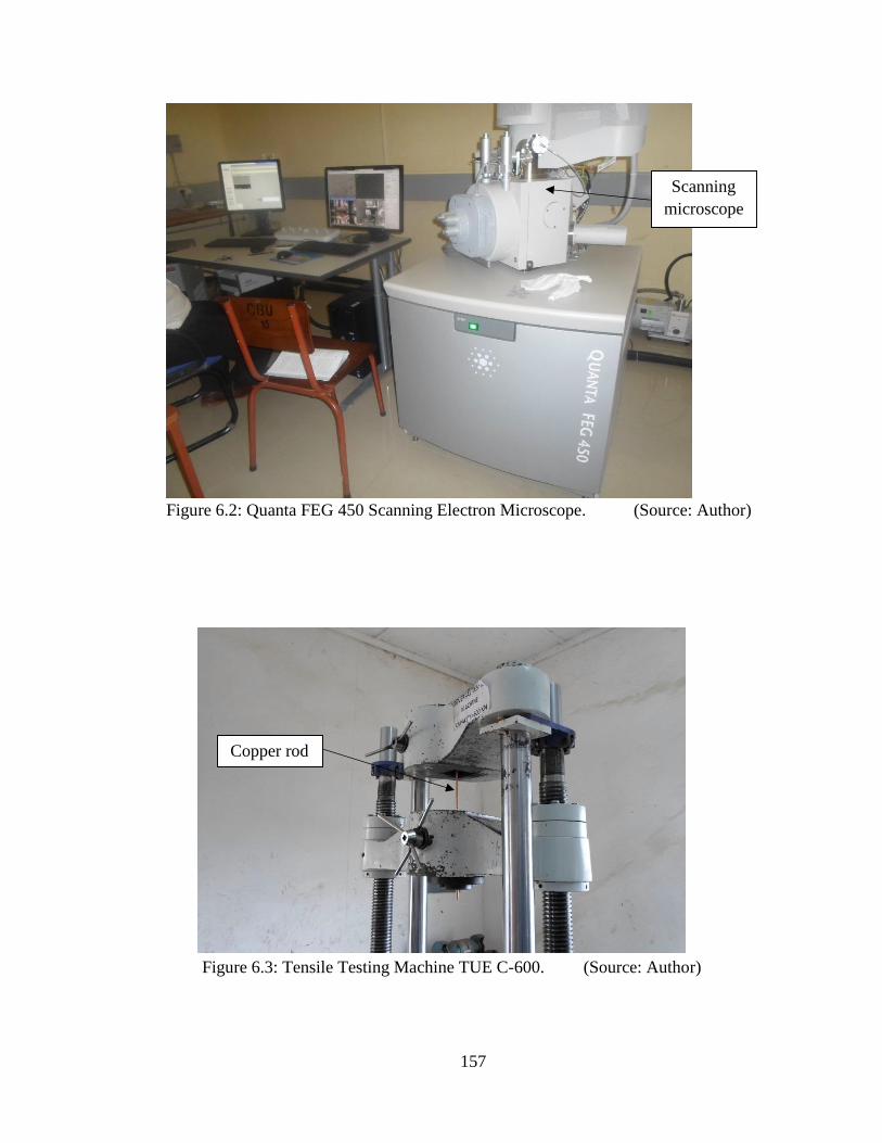
157
Figure 6.2: Quanta FEG 450 Scanning Electron Microscope. (Source: Author)
Figure 6.3: Tensile Testing Machine TUE C-600. (Source: Author)
Copper rod
Scanning
microscope
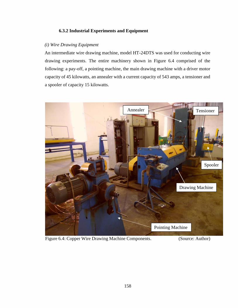
158
6.3.2 Industrial Experiments and Equipment
(i) Wire Drawing Equipment
An intermediate wire drawing machine, model HT-24DTS was used for conducting wire
drawing experiments. The entire machinery shown in Figure 6.4 comprised of the
following: a pay-off, a pointing machine, the main drawing machine with a driver motor
capacity of 45 kilowatts, an annealer with a current capacity of 543 amps, a tensioner and
a spooler of capacity 15 kilowatts.
Figure 6.4: Copper Wire Drawing Machine Components. (Source: Author)
Drawing Machine
Pointing Machine
Annealer Tensioner
Spooler
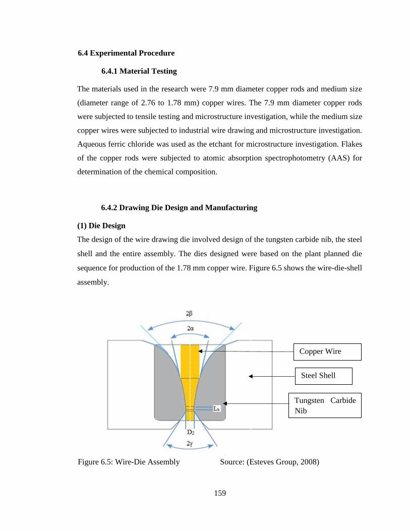
159
6.4 Experimental Procedure
6.4.1 Material Testing
The materials used in the research were 7.9 mm diameter copper rods and medium size
(diameter range of 2.76 to 1.78 mm) copper wires. The 7.9 mm diameter copper rods
were subjected to tensile testing and microstructure investigation, while the medium size
copper wires were subjected to industrial wire drawing and microstructure investigation.
Aqueous ferric chloride was used as the etchant for microstructure investigation. Flakes
of the copper rods were subjected to atomic absorption spectrophotometry (AAS) for
determination of the chemical composition.
6.4.2 Drawing Die Design and Manufacturing
(1) Die Design
The design of the wire drawing die involved design of the tungsten carbide nib, the steel
shell and the entire assembly. The dies designed were based on the plant planned die
sequence for production of the 1.78 mm copper wire. Figure 6.5 shows the wire-die-shell
assembly.
Figure 6.5: Wire-Die Assembly Source: (Esteves Group, 2008)
Copper Wire
Steel Shell
Tungsten Carbide
Nib
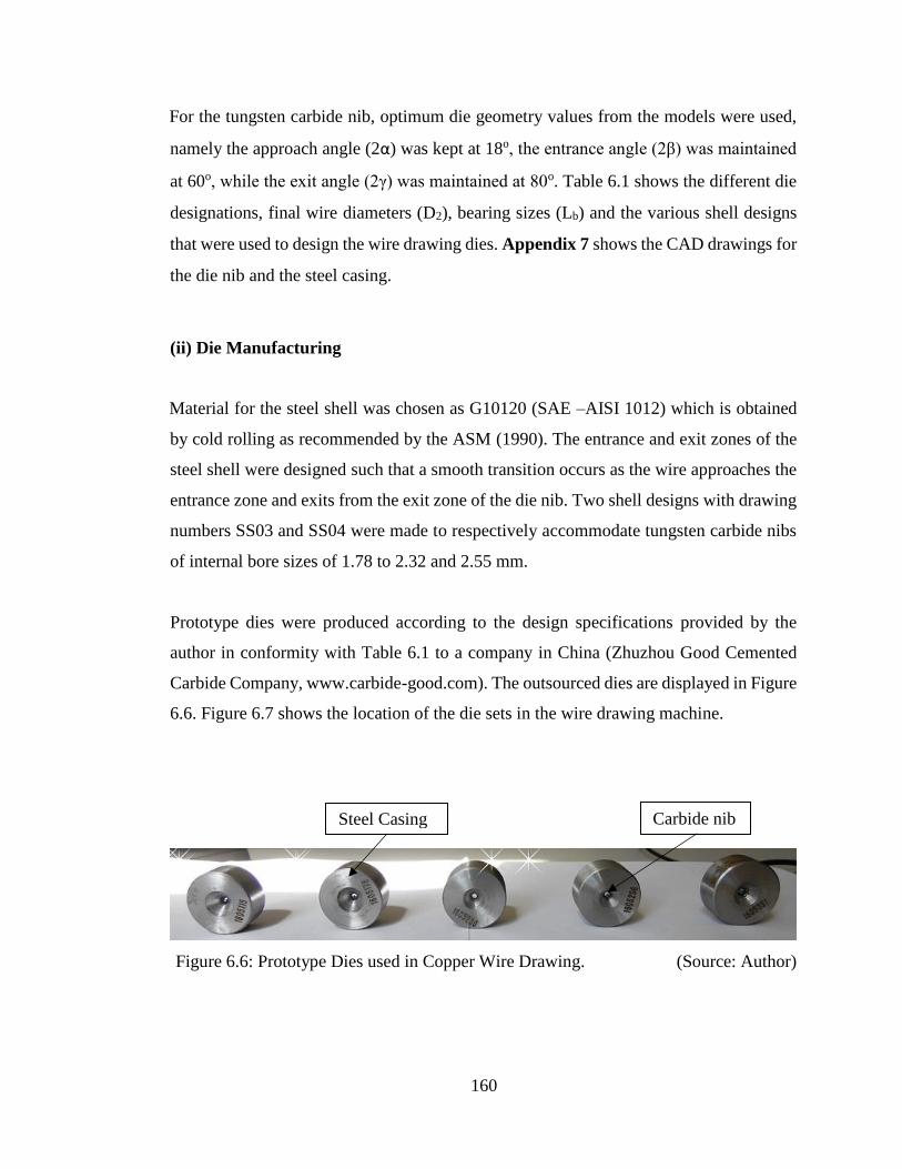
160
For the tungsten carbide nib, optimum die geometry values from the models were used,
namely the approach angle (2α) was kept at 18o, the entrance angle (2β) was maintained
at 60o, while the exit angle (2γ) was maintained at 80o. Table 6.1 shows the different die
designations, final wire diameters (D2), bearing sizes (Lb) and the various shell designs
that were used to design the wire drawing dies. Appendix 7 shows the CAD drawings for
the die nib and the steel casing.
(ii) Die Manufacturing
Material for the steel shell was chosen as G10120 (SAE –AISI 1012) which is obtained
by cold rolling as recommended by the ASM (1990). The entrance and exit zones of the
steel shell were designed such that a smooth transition occurs as the wire approaches the
entrance zone and exits from the exit zone of the die nib. Two shell designs with drawing
numbers SS03 and SS04 were made to respectively accommodate tungsten carbide nibs
of internal bore sizes of 1.78 to 2.32 and 2.55 mm.
Prototype dies were produced according to the design specifications provided by the
author in conformity with Table 6.1 to a company in China (Zhuzhou Good Cemented
Carbide Company, www.carbide-good.com). The outsourced dies are displayed in Figure
6.6. Figure 6.7 shows the location of the die sets in the wire drawing machine.
Figure 6.6: Prototype Dies used in Copper Wire Drawing. (Source: Author)
Steel Casing Carbide nib
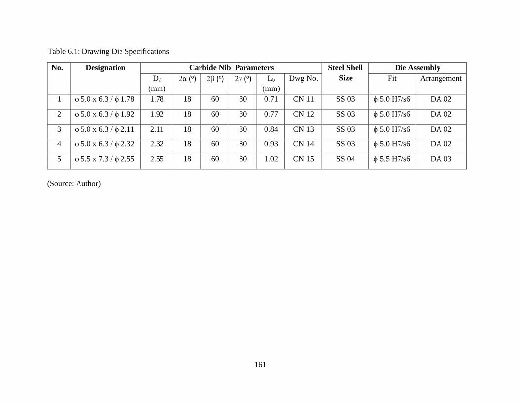
161
Table 6.1: Drawing Die Specifications
No. Designation Carbide Nib Parameters Steel Shell
Size
Die Assembly
D2
(mm)
2α (o) 2β (o) 2γ (o) Lb
(mm)
Dwg No. Fit Arrangement
1 ϕ 5.0 x 6.3 / ϕ 1.78 1.78 18 60 80 0.71 CN 11 SS 03 ϕ 5.0 H7/s6 DA 02
2 ϕ 5.0 x 6.3 / ϕ 1.92 1.92 18 60 80 0.77 CN 12 SS 03 ϕ 5.0 H7/s6 DA 02
3 ϕ 5.0 x 6.3 / ϕ 2.11 2.11 18 60 80 0.84 CN 13 SS 03 ϕ 5.0 H7/s6 DA 02
4 ϕ 5.0 x 6.3 / ϕ 2.32 2.32 18 60 80 0.93 CN 14 SS 03 ϕ 5.0 H7/s6 DA 02
5 ϕ 5.5 x 7.3 / ϕ 2.55 2.55 18 60 80 1.02 CN 15 SS 04 ϕ 5.5 H7/s6 DA 03
(Source: Author)
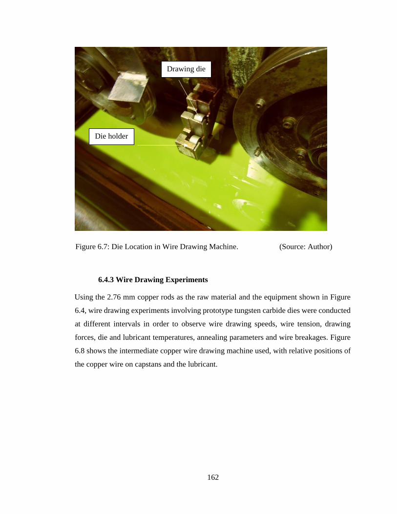
162
Figure 6.7: Die Location in Wire Drawing Machine. (Source: Author)
6.4.3 Wire Drawing Experiments
Using the 2.76 mm copper rods as the raw material and the equipment shown in Figure
6.4, wire drawing experiments involving prototype tungsten carbide dies were conducted
at different intervals in order to observe wire drawing speeds, wire tension, drawing
forces, die and lubricant temperatures, annealing parameters and wire breakages. Figure
6.8 shows the intermediate copper wire drawing machine used, with relative positions of
the copper wire on capstans and the lubricant.
Die holder
Drawing die
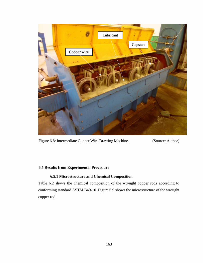
163
Figure 6.8: Intermediate Copper Wire Drawing Machine. (Source: Author)
6.5 Results from Experimental Procedure
6.5.1 Microstructure and Chemical Composition
Table 6.2 shows the chemical composition of the wrought copper rods according to
conforming standard ASTM B49-10. Figure 6.9 shows the microstructure of the wrought
copper rod.
Copper wire
Lubricant
Capstan

164
Table 6.2: Composition of Wrought Copper.
Constituent Elements (norm. wt %)
Sb As Cd Fe Pb Mn Ni Ag Zn Cu
<0.04 <0.01 <0.002 0.12 <0.01 0.002 0.003 <0.01 0.04 Bal.
(Source: Author)
Figure 6.9: Microstructure of Wrought Copper. (Source: Author)
6.5.2 Mechanical Properties of Wrought Copper Rods
A standard density of 8960 kgm-3 and a Poisson standard value of 0.34 were used in all
formulations as per the recommendations of ASM International (1990). Tables 6.3 and
Metallic inclusion
Copper matrix
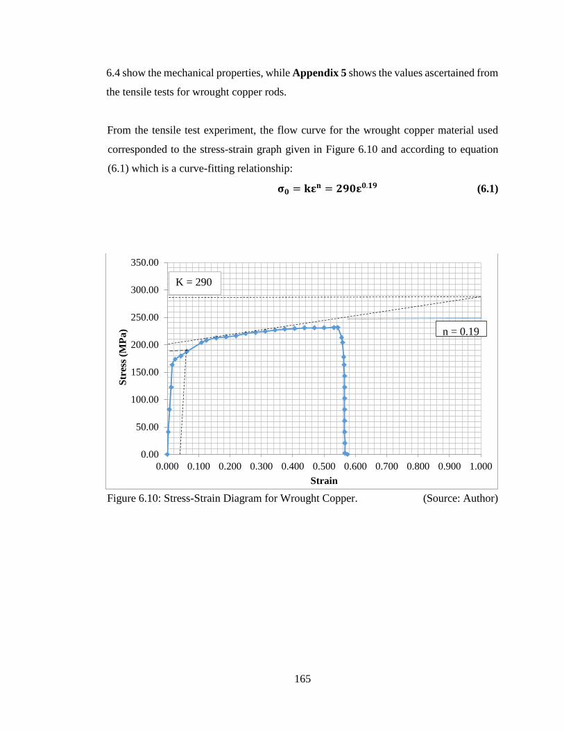
165
6.4 show the mechanical properties, while Appendix 5 shows the values ascertained from
the tensile tests for wrought copper rods.
From the tensile test experiment, the flow curve for the wrought copper material used
corresponded to the stress-strain graph given in Figure 6.10 and according to equation
(6.1) which is a curve-fitting relationship:
𝛔𝟎 = 𝐤𝛆𝐧 = 𝟐𝟗𝟎𝛆𝟎.𝟏𝟗 (6.1)
Figure 6.10: Stress-Strain Diagram for Wrought Copper. (Source: Author)
0.00
50.00
100.00
150.00
200.00
250.00
300.00
350.00
0.000 0.100 0.200 0.300 0.400 0.500 0.600 0.700 0.800 0.900 1.000
Str
ess
(MP
a)
Strain
K = 290
n = 0.19
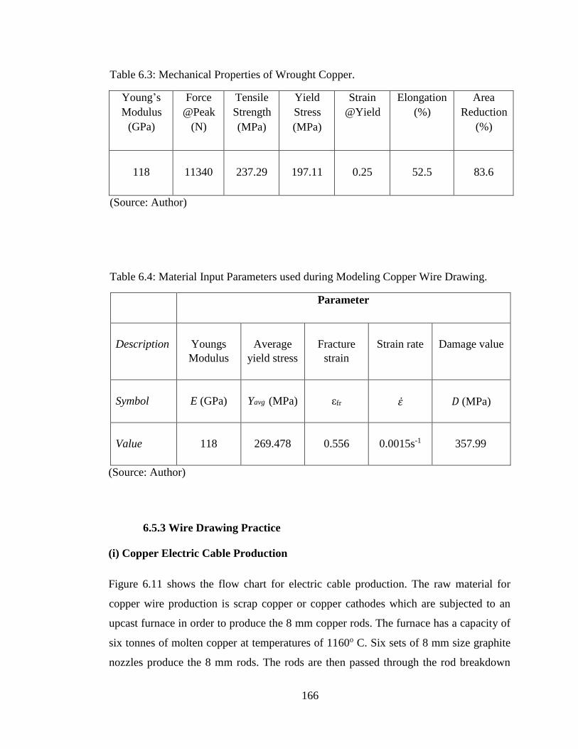
166
Table 6.3: Mechanical Properties of Wrought Copper.
Young’s
Modulus
(GPa)
Force
@Peak
(N)
Tensile
Strength
(MPa)
Yield
Stress
(MPa)
Strain
@Yield
Elongation
(%)
Area
Reduction
(%)
118
11340
237.29
197.11
0.25
52.5
83.6
(Source: Author)
Table 6.4: Material Input Parameters used during Modeling Copper Wire Drawing.
Parameter
Description
Youngs
Modulus
Average
yield stress
Fracture
strain
Strain rate
Damage value
Symbol
E (GPa)
Yavg (MPa)
εfr
𝜀
𝐷 (MPa)
Value
118
269.478
0.556
0.0015s-1
357.99
(Source: Author)
6.5.3 Wire Drawing Practice
(i) Copper Electric Cable Production
Figure 6.11 shows the flow chart for electric cable production. The raw material for
copper wire production is scrap copper or copper cathodes which are subjected to an
upcast furnace in order to produce the 8 mm copper rods. The furnace has a capacity of
six tonnes of molten copper at temperatures of 1160o C. Six sets of 8 mm size graphite
nozzles produce the 8 mm rods. The rods are then passed through the rod breakdown
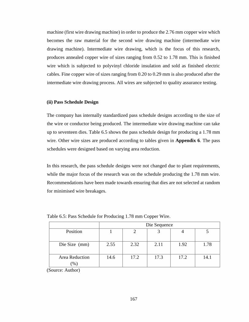
167
machine (first wire drawing machine) in order to produce the 2.76 mm copper wire which
becomes the raw material for the second wire drawing machine (intermediate wire
drawing machine). Intermediate wire drawing, which is the focus of this research,
produces annealed copper wire of sizes ranging from 0.52 to 1.78 mm. This is finished
wire which is subjected to polyvinyl chloride insulation and sold as finished electric
cables. Fine copper wire of sizes ranging from 0.20 to 0.29 mm is also produced after the
intermediate wire drawing process. All wires are subjected to quality assurance testing.
(ii) Pass Schedule Design
The company has internally standardized pass schedule designs according to the size of
the wire or conductor being produced. The intermediate wire drawing machine can take
up to seventeen dies. Table 6.5 shows the pass schedule design for producing a 1.78 mm
wire. Other wire sizes are produced according to tables given in Appendix 6. The pass
schedules were designed based on varying area reduction.
In this research, the pass schedule designs were not changed due to plant requirements,
while the major focus of the research was on the schedule producing the 1.78 mm wire.
Recommendations have been made towards ensuring that dies are not selected at random
for minimised wire breakages.
Table 6.5: Pass Schedule for Producing 1.78 mm Copper Wire.
Die Sequence
Position 1 2 3 4 5
Die Size (mm) 2.55 2.32 2.11 1.92 1.78
Area Reduction
(%)
14.6 17.2 17.3 17.2 14.1
(Source: Author)
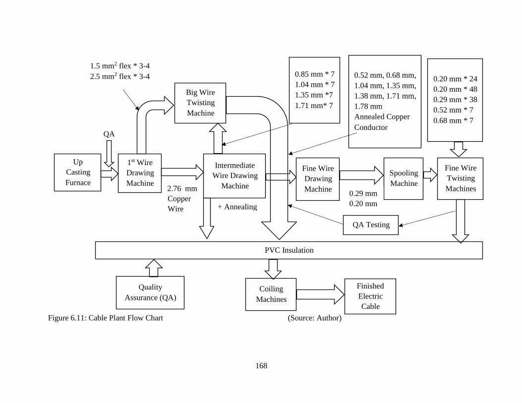
168
Figure 6.11: Cable Plant Flow Chart (Source: Author)
Up
Casting
Furnace
1st Wire
Drawing
Machine
Intermediate
Wire Drawing
Machine
Fine Wire
Drawing
Machine
Spooling
Machine
Fine Wire
Twisting
Machines
PVC Insulation
Quality
Assurance (QA) Coiling
Machines
Finished
Electric
Cable
+ Annealing
Big Wire
Twisting
Machine
0.85 mm * 7
1.04 mm * 7
1.35 mm *7
1.71 mm* 7
2.76 mm
Copper
Wire
0.52 mm, 0.68 mm,
1.04 mm, 1.35 mm,
1.38 mm, 1.71 mm,
1.78 mm
Annealed Copper
Conductor
0.29 mm
0.20 mm
QA Testing
0.20 mm * 24
0.20 mm * 48
0.29 mm * 38
0.52 mm * 7
0.68 mm * 7
QA
1.5 mm2 flex * 3-4
2.5 mm2 flex * 3-4
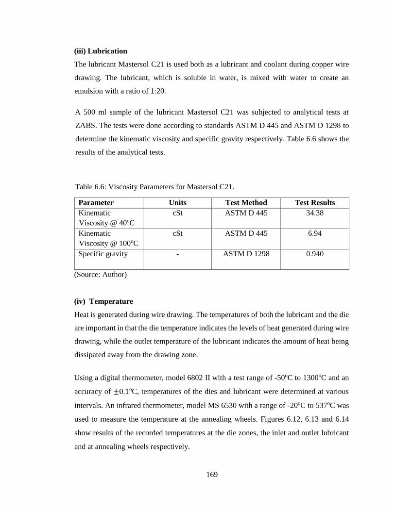
169
(iii) Lubrication
The lubricant Mastersol C21 is used both as a lubricant and coolant during copper wire
drawing. The lubricant, which is soluble in water, is mixed with water to create an
emulsion with a ratio of 1:20.
A 500 ml sample of the lubricant Mastersol C21 was subjected to analytical tests at
ZABS. The tests were done according to standards ASTM D 445 and ASTM D 1298 to
determine the kinematic viscosity and specific gravity respectively. Table 6.6 shows the
results of the analytical tests.
Table 6.6: Viscosity Parameters for Mastersol C21.
Parameter Units Test Method Test Results
Kinematic
Viscosity @ 40oC
cSt ASTM D 445 34.38
Kinematic
Viscosity @ 100oC
cSt ASTM D 445 6.94
Specific gravity - ASTM D 1298 0.940
(Source: Author)
(iv) Temperature
Heat is generated during wire drawing. The temperatures of both the lubricant and the die
are important in that the die temperature indicates the levels of heat generated during wire
drawing, while the outlet temperature of the lubricant indicates the amount of heat being
dissipated away from the drawing zone.
Using a digital thermometer, model 6802 II with a test range of -50oC to 1300oC and an
accuracy of ±0.1oC, temperatures of the dies and lubricant were determined at various
intervals. An infrared thermometer, model MS 6530 with a range of -20oC to 537oC was
used to measure the temperature at the annealing wheels. Figures 6.12, 6.13 and 6.14
show results of the recorded temperatures at the die zones, the inlet and outlet lubricant
and at annealing wheels respectively.
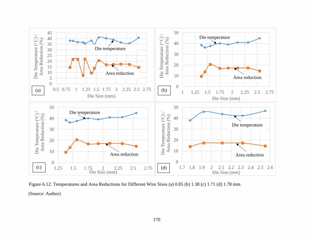
170
Figure 6.12: Temperatures and Area Reductions for Different Wire Sizes (a) 0.85 (b) 1.38 (c) 1.71 (d) 1.78 mm.
(Source: Author)
0
5
10
15
20
25
30
35
40
45
0.5 0.75 1 1.25 1.5 1.75 2 2.25 2.5 2.75
Die
Tem
per
ature
(o C
) /
Are
a R
educt
ion (
%)
Die Size (mm)
Die temperature
Area reduction
0
10
20
30
40
50
1 1.25 1.5 1.75 2 2.25 2.5 2.75
Die
Tem
per
ature
(o C
) /
Are
a R
educt
ion (
%)
Die Size (mm)
Die temperature
Area reduction
0
10
20
30
40
50
1.25 1.5 1.75 2 2.25 2.5 2.75
Die
Tem
per
ature
(oC
)/
Are
a R
educt
ion (
%)
Die Size (mm)
0
10
20
30
40
50
1.7 1.8 1.9 2 2.1 2.2 2.3 2.4 2.5 2.6D
ie T
emper
ature
(oC
) /
Are
a R
educt
ion (
%)
Die Size (mm)
Die temperature
Area reduction
Die temperature
Area reduction
(a) (b)
(c) (d)
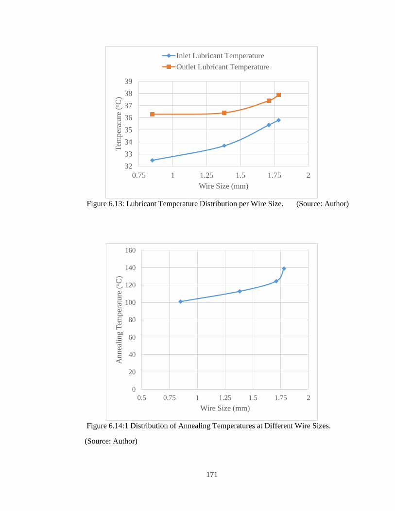
171
Figure 6.13: Lubricant Temperature Distribution per Wire Size. (Source: Author)
Figure 6.14:1 Distribution of Annealing Temperatures at Different Wire Sizes.
(Source: Author)
32
33
34
35
36
37
38
39
0.75 1 1.25 1.5 1.75 2
Tem
per
ature
(oC
)
Wire Size (mm)
Inlet Lubricant Temperature
Outlet Lubricant Temperature
0
20
40
60
80
100
120
140
160
0.5 0.75 1 1.25 1.5 1.75 2
Annea
ling T
emper
ature
(oC
)
Wire Size (mm)
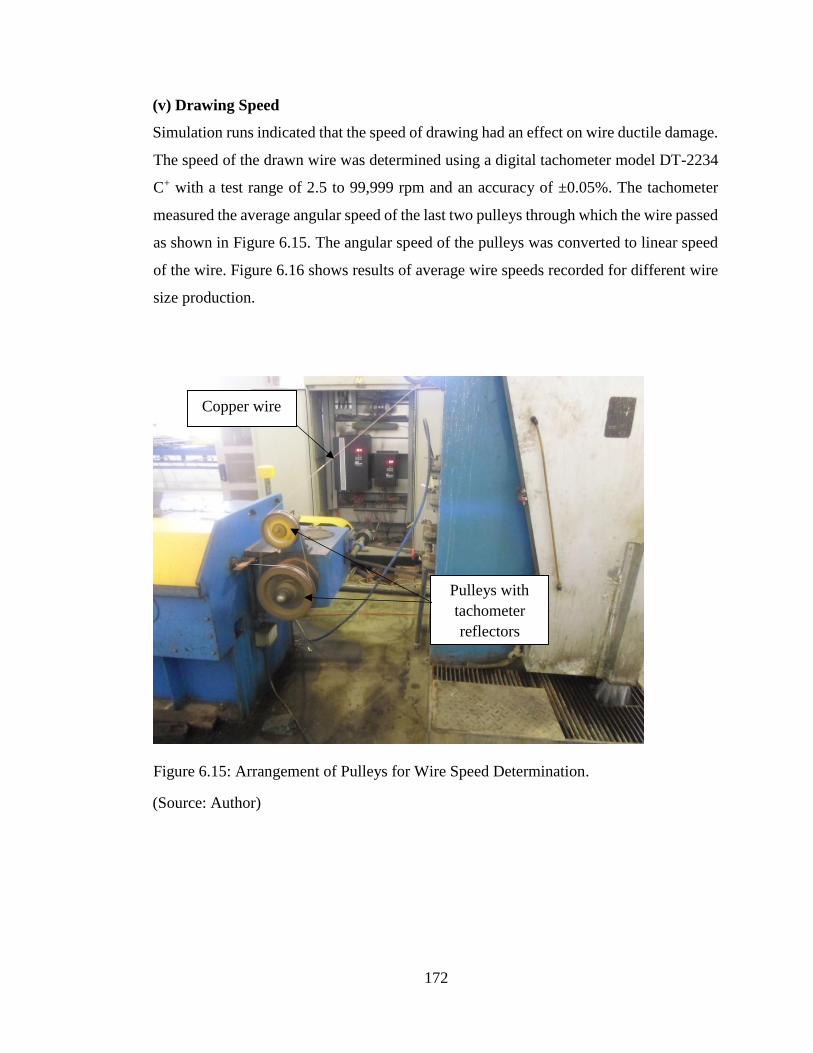
172
(v) Drawing Speed
Simulation runs indicated that the speed of drawing had an effect on wire ductile damage.
The speed of the drawn wire was determined using a digital tachometer model DT-2234
C+ with a test range of 2.5 to 99,999 rpm and an accuracy of ±0.05%. The tachometer
measured the average angular speed of the last two pulleys through which the wire passed
as shown in Figure 6.15. The angular speed of the pulleys was converted to linear speed
of the wire. Figure 6.16 shows results of average wire speeds recorded for different wire
size production.
Figure 6.15: Arrangement of Pulleys for Wire Speed Determination.
(Source: Author)
Copper wire
Pulleys with
tachometer
reflectors
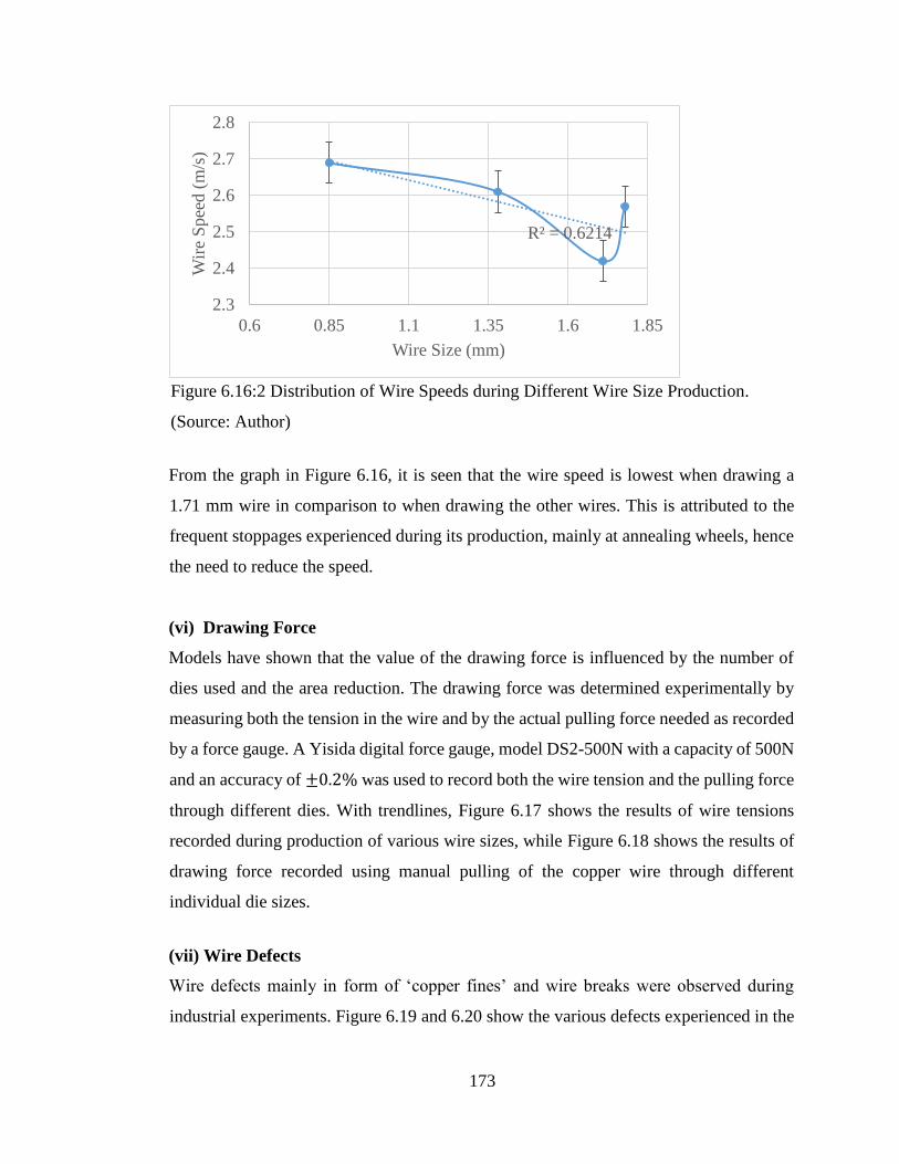
173
Figure 6.16:2 Distribution of Wire Speeds during Different Wire Size Production.
(Source: Author)
From the graph in Figure 6.16, it is seen that the wire speed is lowest when drawing a
1.71 mm wire in comparison to when drawing the other wires. This is attributed to the
frequent stoppages experienced during its production, mainly at annealing wheels, hence
the need to reduce the speed.
(vi) Drawing Force
Models have shown that the value of the drawing force is influenced by the number of
dies used and the area reduction. The drawing force was determined experimentally by
measuring both the tension in the wire and by the actual pulling force needed as recorded
by a force gauge. A Yisida digital force gauge, model DS2-500N with a capacity of 500N
and an accuracy of ±0.2% was used to record both the wire tension and the pulling force
through different dies. With trendlines, Figure 6.17 shows the results of wire tensions
recorded during production of various wire sizes, while Figure 6.18 shows the results of
drawing force recorded using manual pulling of the copper wire through different
individual die sizes.
(vii) Wire Defects
Wire defects mainly in form of ‘copper fines’ and wire breaks were observed during
industrial experiments. Figure 6.19 and 6.20 show the various defects experienced in the
R² = 0.6214
2.3
2.4
2.5
2.6
2.7
2.8
0.6 0.85 1.1 1.35 1.6 1.85
Wir
e S
pee
d (
m/s
)
Wire Size (mm)
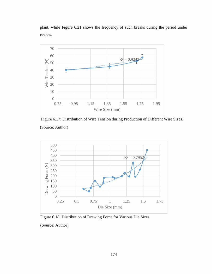
174
plant, while Figure 6.21 shows the frequency of such breaks during the period under
review.
Figure 6.17: Distribution of Wire Tension during Production of Different Wire Sizes.
(Source: Author)
Figure 6.18: Distribution of Drawing Force for Various Die Sizes.
(Source: Author)
R² = 0.9242
0
10
20
30
40
50
60
70
0.75 0.95 1.15 1.35 1.55 1.75 1.95
Wir
e T
ensi
on
(N
)
Wire Size (mm)
R² = 0.7952
0
50
100
150
200
250
300
350
400
450
500
0.25 0.5 0.75 1 1.25 1.5 1.75
Dra
win
g F
orc
e (N
)
Die Size (mm)
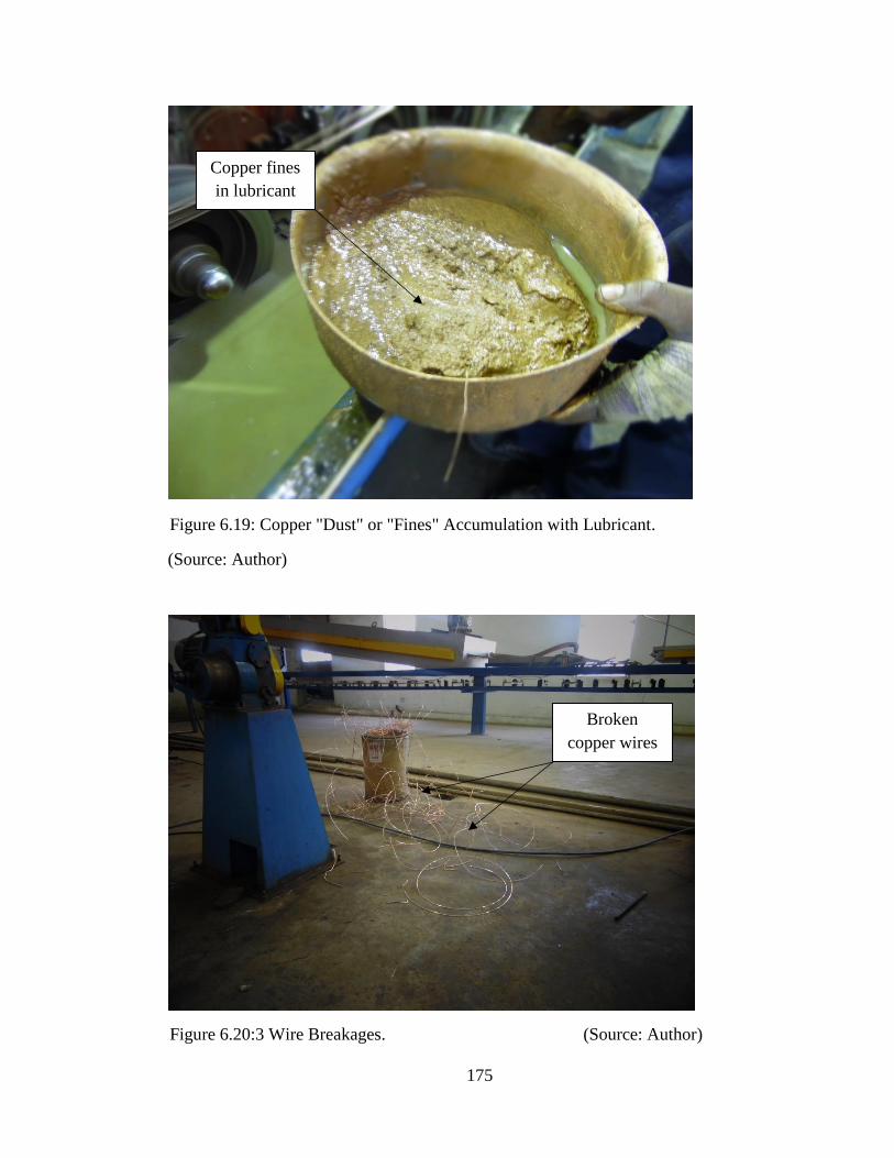
175
Figure 6.19: Copper "Dust" or "Fines" Accumulation with Lubricant.
(Source: Author)
Figure 6.20:3 Wire Breakages. (Source: Author)
Copper fines
in lubricant
Broken
copper wires
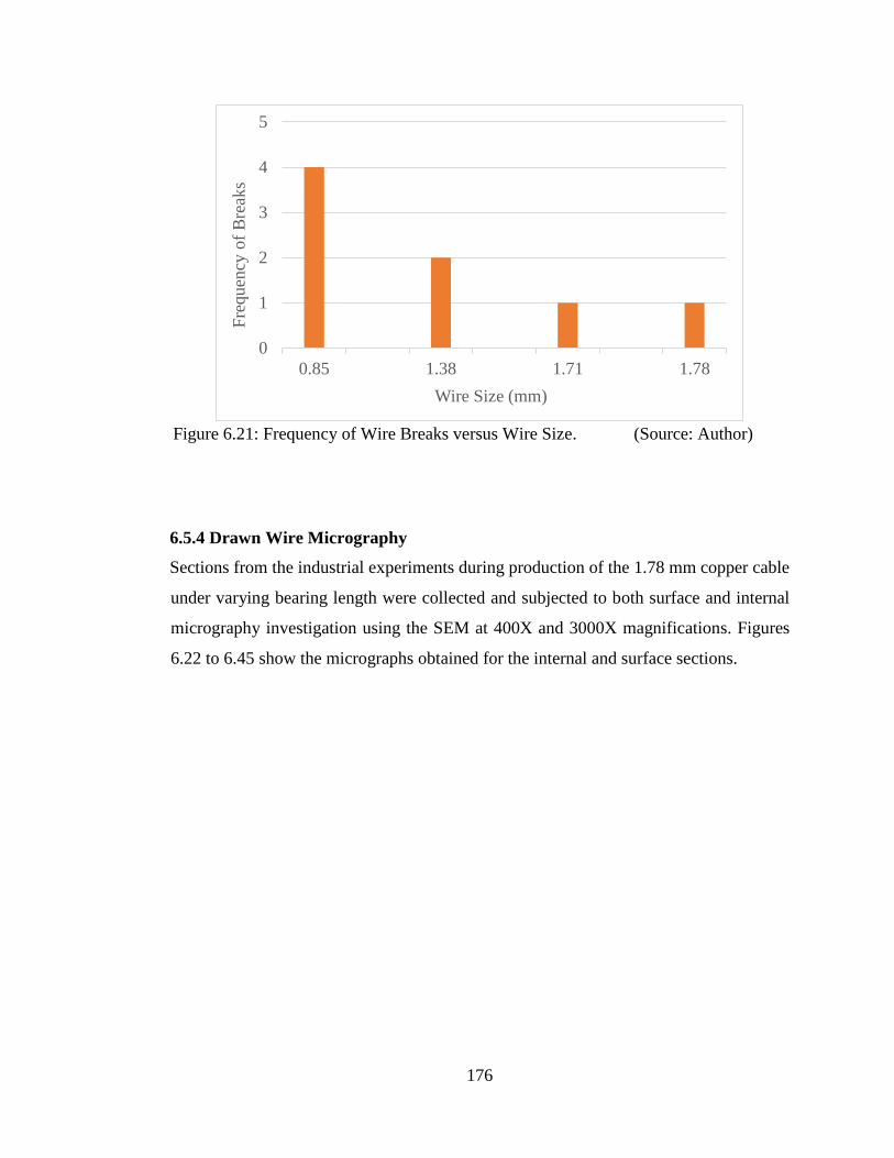
176
Figure 6.21: Frequency of Wire Breaks versus Wire Size. (Source: Author)
6.5.4 Drawn Wire Micrography
Sections from the industrial experiments during production of the 1.78 mm copper cable
under varying bearing length were collected and subjected to both surface and internal
micrography investigation using the SEM at 400X and 3000X magnifications. Figures
6.22 to 6.45 show the micrographs obtained for the internal and surface sections.
0
1
2
3
4
5
0.85 1.38 1.71 1.78
Fre
quen
cy o
f B
reak
s
Wire Size (mm)
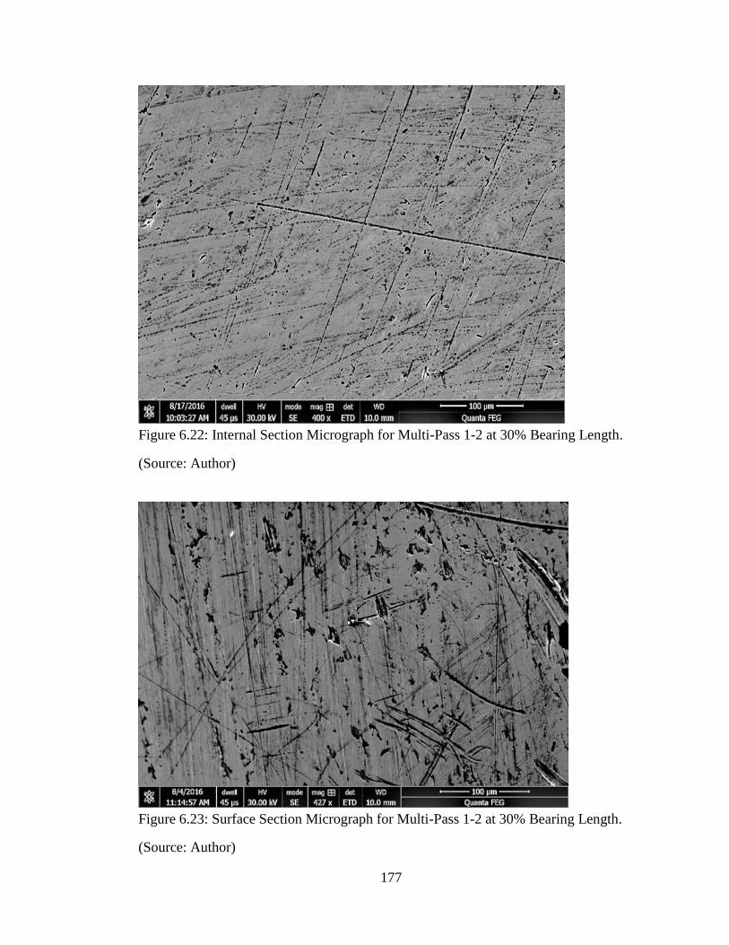
177
Figure 6.22: Internal Section Micrograph for Multi-Pass 1-2 at 30% Bearing Length.
(Source: Author)
Figure 6.23: Surface Section Micrograph for Multi-Pass 1-2 at 30% Bearing Length.
(Source: Author)
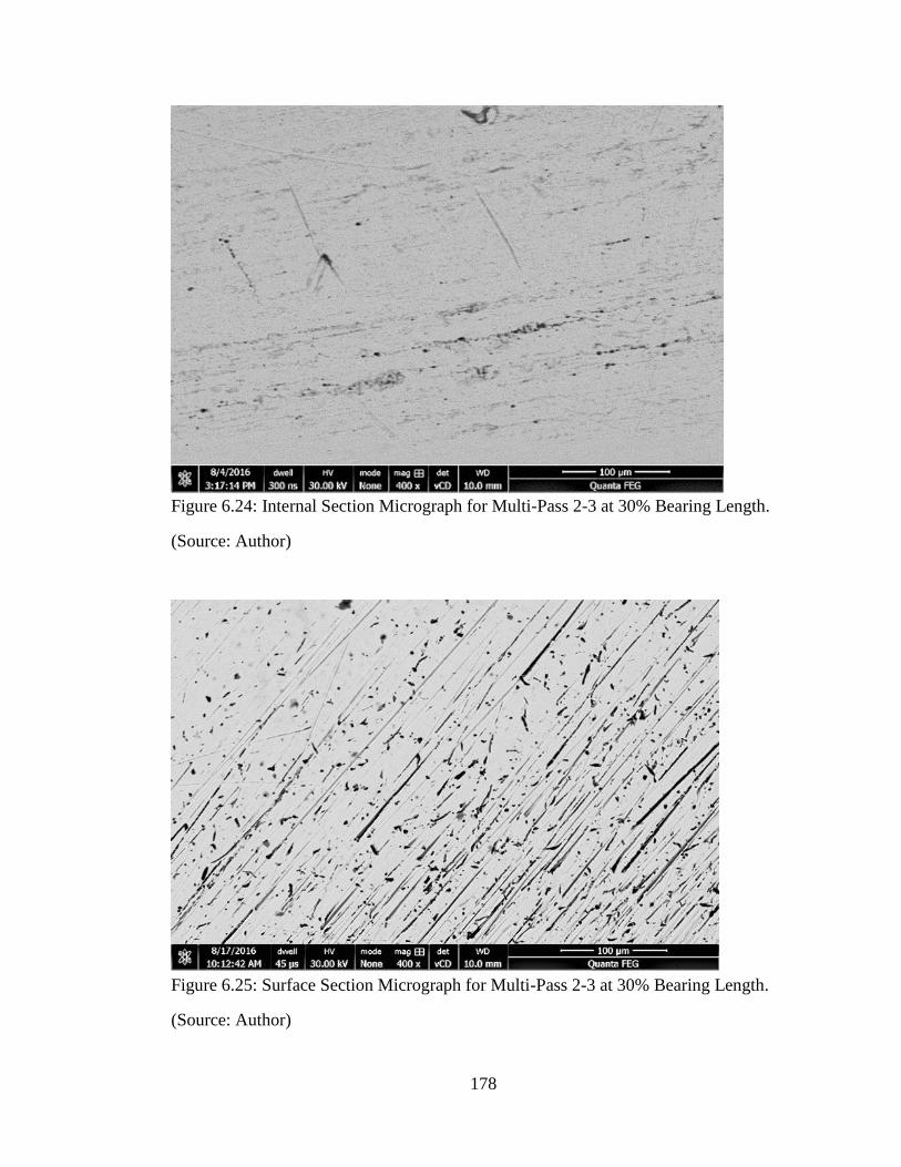
178
Figure 6.24: Internal Section Micrograph for Multi-Pass 2-3 at 30% Bearing Length.
(Source: Author)
Figure 6.25: Surface Section Micrograph for Multi-Pass 2-3 at 30% Bearing Length.
(Source: Author)
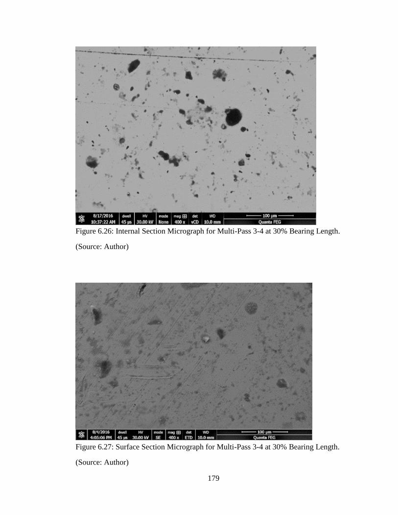
179
Figure 6.26: Internal Section Micrograph for Multi-Pass 3-4 at 30% Bearing Length.
(Source: Author)
Figure 6.27: Surface Section Micrograph for Multi-Pass 3-4 at 30% Bearing Length.
(Source: Author)

180
Figure 6.28: Internal Section Micrograph for Multi-Pass 4-5 at 30% Bearing Length.
(Source: Author)
Figure 6.29: Surface Section Micrograph for Multi-Pass 4-5 at 30% Bearing Length.
(Source: Author)
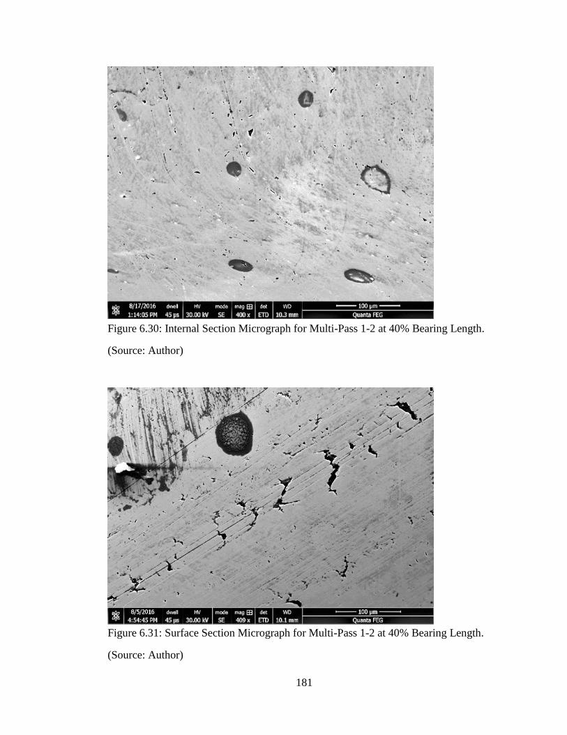
181
Figure 6.30: Internal Section Micrograph for Multi-Pass 1-2 at 40% Bearing Length.
(Source: Author)
Figure 6.31: Surface Section Micrograph for Multi-Pass 1-2 at 40% Bearing Length.
(Source: Author)
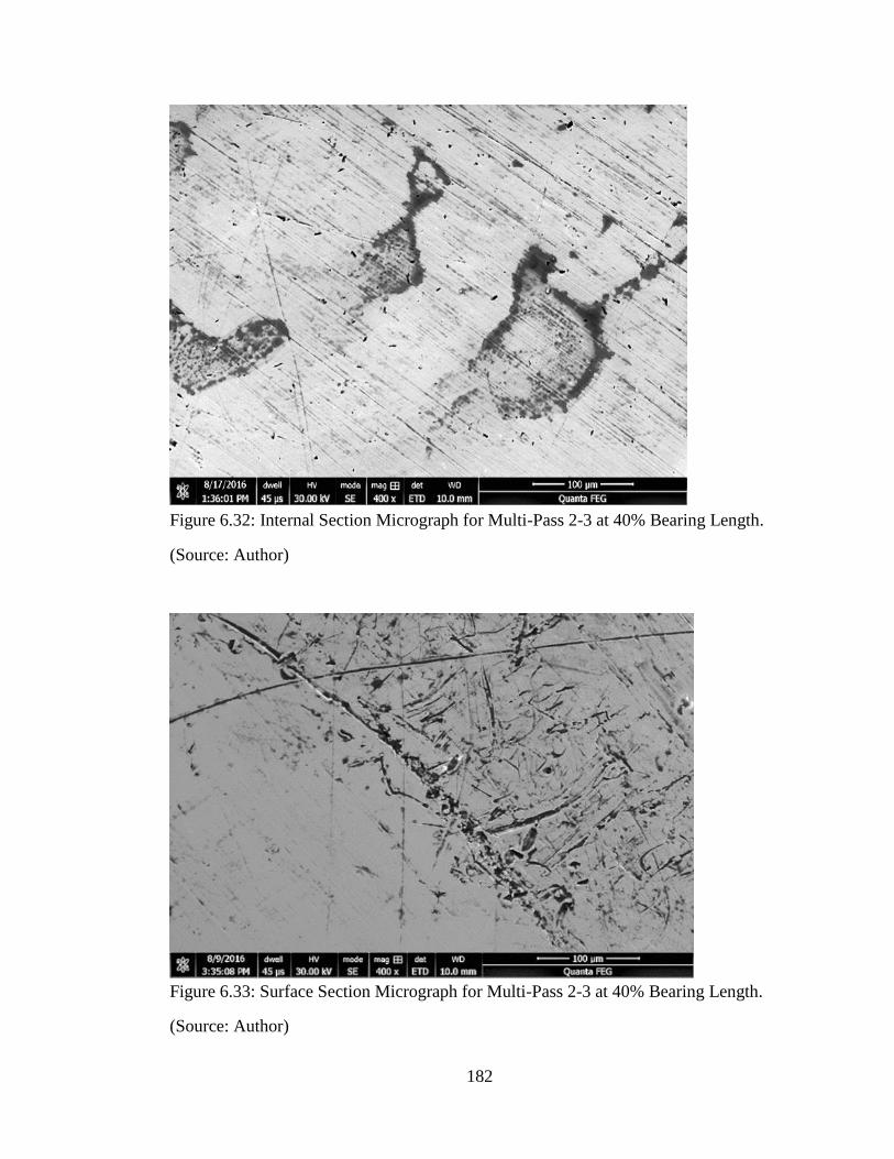
182
Figure 6.32: Internal Section Micrograph for Multi-Pass 2-3 at 40% Bearing Length.
(Source: Author)
Figure 6.33: Surface Section Micrograph for Multi-Pass 2-3 at 40% Bearing Length.
(Source: Author)
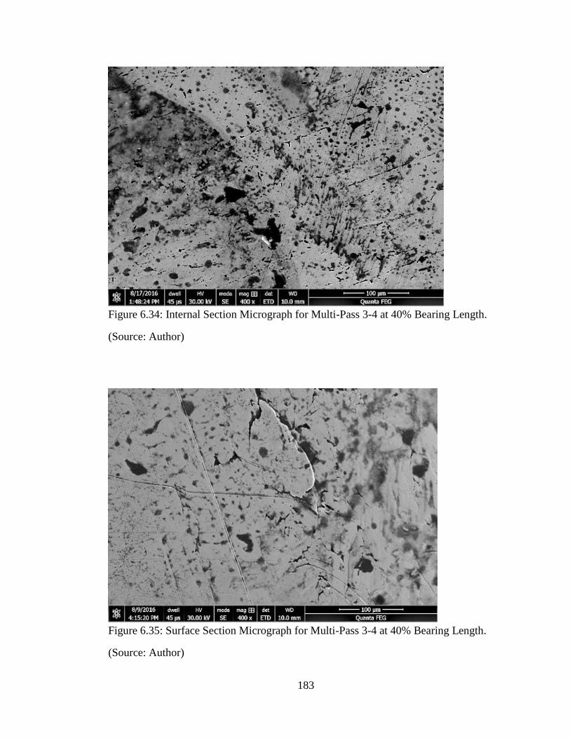
183
Figure 6.34: Internal Section Micrograph for Multi-Pass 3-4 at 40% Bearing Length.
(Source: Author)
Figure 6.35: Surface Section Micrograph for Multi-Pass 3-4 at 40% Bearing Length.
(Source: Author)
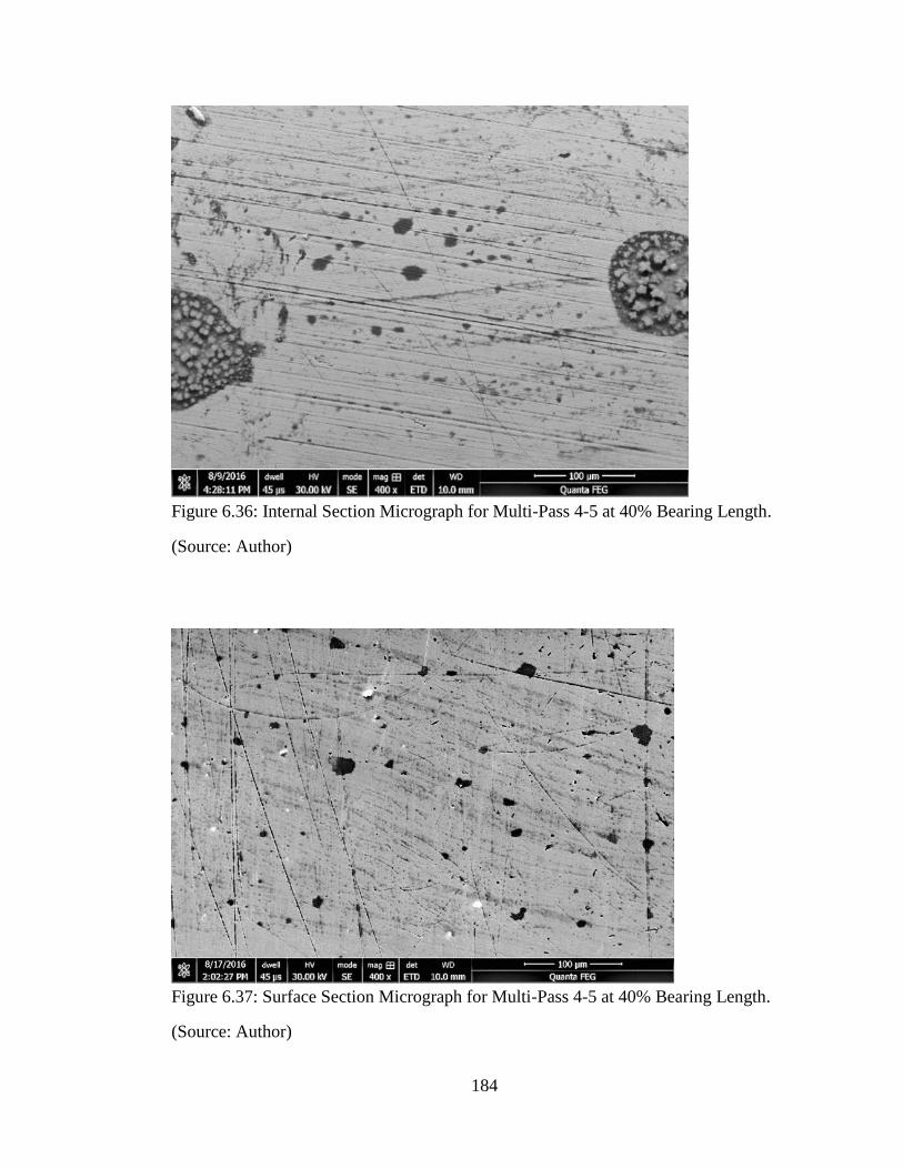
184
Figure 6.36: Internal Section Micrograph for Multi-Pass 4-5 at 40% Bearing Length.
(Source: Author)
Figure 6.37: Surface Section Micrograph for Multi-Pass 4-5 at 40% Bearing Length.
(Source: Author)
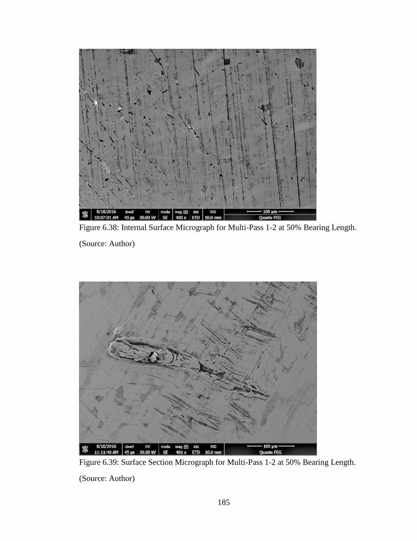
185
Figure 6.38: Internal Surface Micrograph for Multi-Pass 1-2 at 50% Bearing Length.
(Source: Author)
Figure 6.39: Surface Section Micrograph for Multi-Pass 1-2 at 50% Bearing Length.
(Source: Author)

186
Figure 6.40: Internal Section Micrograph for Multi-Pass 2-3 at 50% Bearing Length.
(Source: Author)
Figure 6.41: Surface Section Micrograph for Multi-Pass 2-3 at 50% Bearing Length.
(Source: Author)
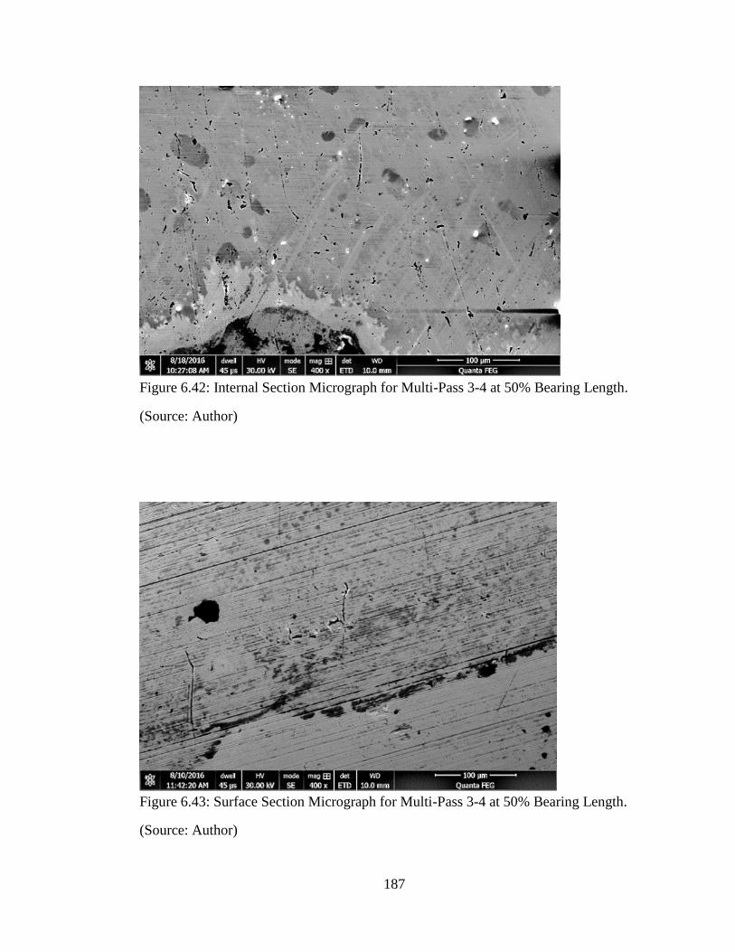
187
Figure 6.42: Internal Section Micrograph for Multi-Pass 3-4 at 50% Bearing Length.
(Source: Author)
Figure 6.43: Surface Section Micrograph for Multi-Pass 3-4 at 50% Bearing Length.
(Source: Author)
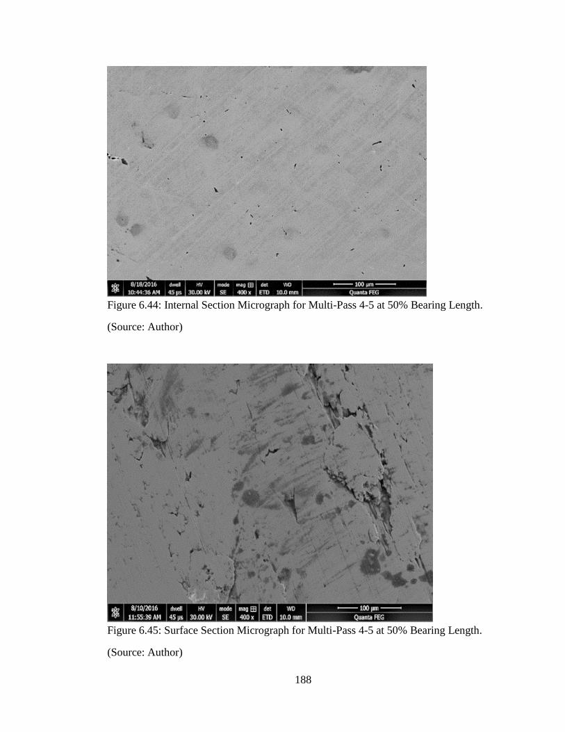
188
Figure 6.44: Internal Section Micrograph for Multi-Pass 4-5 at 50% Bearing Length.
(Source: Author)
Figure 6.45: Surface Section Micrograph for Multi-Pass 4-5 at 50% Bearing Length.
(Source: Author)
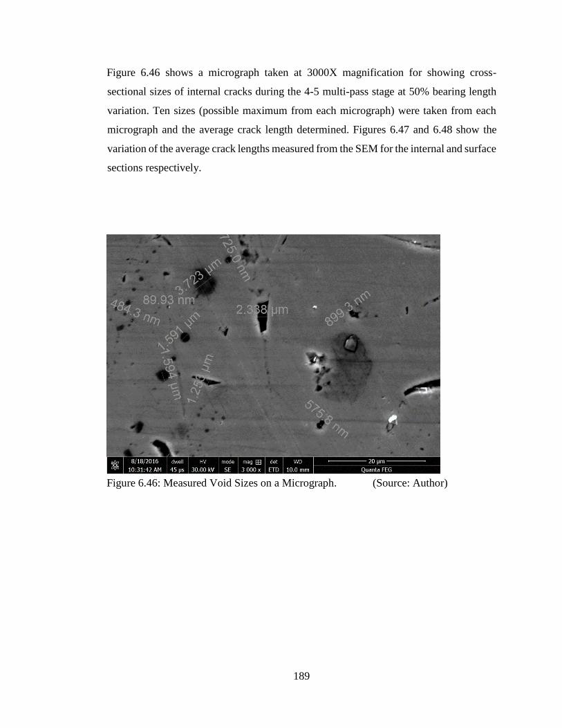
189
Figure 6.46 shows a micrograph taken at 3000X magnification for showing cross-
sectional sizes of internal cracks during the 4-5 multi-pass stage at 50% bearing length
variation. Ten sizes (possible maximum from each micrograph) were taken from each
micrograph and the average crack length determined. Figures 6.47 and 6.48 show the
variation of the average crack lengths measured from the SEM for the internal and surface
sections respectively.
Figure 6.46: Measured Void Sizes on a Micrograph. (Source: Author)
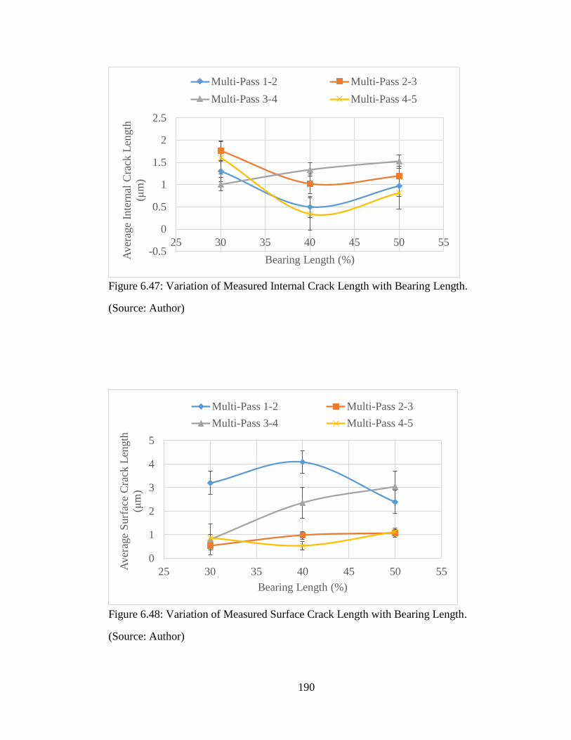
190
Figure 6.47: Variation of Measured Internal Crack Length with Bearing Length.
(Source: Author)
Figure 6.48: Variation of Measured Surface Crack Length with Bearing Length.
(Source: Author)
-0.5
0
0.5
1
1.5
2
2.5
25 30 35 40 45 50 55
Av
erag
e In
tern
al C
rack
Len
gth
(μm
)
Bearing Length (%)
Multi-Pass 1-2 Multi-Pass 2-3
Multi-Pass 3-4 Multi-Pass 4-5
0
1
2
3
4
5
25 30 35 40 45 50 55Aver
age
Surf
ace
Cra
ck L
ength
(μm
)
Bearing Length (%)
Multi-Pass 1-2 Multi-Pass 2-3
Multi-Pass 3-4 Multi-Pass 4-5

191
6.6 General Observations from Industrial Experiments
The industrial wire drawing experiments were conducted with well-functioning
machinery, and the experiments were stable and repeatable.
6.7 Summary of Results from Experimental Procedures
Results of the experimental procedures indicated the following:
(1) Presence of second phase particles within the copper material with different
grain sizes. Iron has the highest percentage of metallic inclusions in the two
copper samples, with the wrought copper taking a higher percentage.
(2) Pass schedule designs showed that the wire drawing practice was concentrated
on the use of Δ-parameter values above 3. This was typical for low area
reductions and high approach angles under conditions of increased levels of
redundant deformation and surface hardening. Annealing the copper wire was,
thus, inevitable.
(3) The lubricant did not suffer much loss of its viscosity properties due to the fairly
low operating temperatures. Lubrication was thus effective, though the
presence of copper ‘fines’ compromised the inherent properties.
(4) Larger size dies, with corresponding higher area reductions, recorded higher
temperatures.
(5) Production of larger size wire required higher annealing temperatures.
(6) Drawing speeds were higher when drawing smaller size wire.
(7) Tension in the wire during wire drawing increased with increased wire size
being produced. The drawing force showed an accelerated increase with
increased die size. High wear and shorter consequent die life were therefore likely
for larger dies than smaller dies.
(8) Tendency of a wire break was higher when drawing smaller size wires.
192
(9) Micrographs showed less internal damage at 40% bearing length while dies
with 30% bearing length showed less surface damage.
193
CHAPTER SEVEN: RESULTS ANALYSIS AND DISCUSSIONS
7.1 Introduction
The overall effects of die geometry parameters, process parameters, manufacturing
aspects and wire drawing practice influencing formation of chevron and surface crack in
copper during wire drawing as obtained from the simulation and experimental studies
were analysed and discussed.
This chapter presents observations and detailed discussions based on the comparative
analysis of results from the modelling and simulations and industrial experiments
involving bearing length variation.
7.2 General Observations
The current research study on copper wire drawing involved development of a copper
wire drawing model and establishment of die design and manufacturing practices and
processing conditions leading to chevron and surface crack formation.
Validation of the results from modelling was done by using micrographs from the wire
drawing industrial experiments. The micrographs showed that there was more internal
wire damage when using bearing lengths of 30% and 50%, whereas more surface damage
was seen when using bearing lengths of 50%. This was evident in the simulations which
showed the same pattern. Therefore, there was a high degree of confidence that the results
presented and discussed were reliable.
7.3 Analysis and Discussion of Results
The results presented were two-fold: results from modelling and simulation as presented
in Figures 5.14 to 5.41, and results from laboratory and industrial experiments as
presented in Figures 6.12 to 6.48.
194
7.3.1 Analysis and Discussion of Simulation Results
All the copper wire drawing models were based on a four sequence multi-pass stages,
except for the models involving area reduction which used up to eight sequences.
(a) Effects of Die Geometry Independent Variables
Effects of the die geometry and area reduction on equivalent plastic strain were presented
in Figures 5.14 5.15, 5.16 and 5.17. Figures 5.34, 5.35, 5.36, 5.37, 5.38, 5.39, 5.40 and
5.41 presented the effects of the die geometry and area reduction on damage value
(stiffness degradation) and the Cockroft and Latham criterion leading to ductile damage
of the copper wire.
(i) Effects of Entrance Angle
The figures showed that for the centerline nodes, both the plastic strain and damage
values were high during the second (2-3) and third (3-4) multi-pass stages. The Cockroft
and Latham criterion showed that ductile damage was high during the third (3-4) and
fourth (4-5) multi-pass stages, with highest values at 20o entrance angle.
For the surface nodes, the figures showed that both the equivalent plastic strain and
damage values were high during the first (1-2) and second (2-3) multi-pass stages. For
the Cockroft and Latham criterion, it was shown that ductile damage was highest during
the third (3-4) multi-pass stage, with highest value at 20o entrance angle and the criterion
being reached.
The figures showed that the entrance angle had a very minimal effect on ductile damage.
From the simulations it was observed that contact between the wire and the entrance zone
was more evident at the first die (diei) than the second die (diei+1). Opening of the
entrance zone by way of larger entrance angles removes contact between the copper wire
and the entrance zone. This is in accordance with Wright (2011) and Esteves Group
(2008) that an open bell minimizes abrasion on the wire and facilitates lubricant entry.
195
(ii) Effects of Approach Angle
The figures in chapter five showed that for the centerline nodes, the Cockroft and Latham
criterion showed that ductile damage was high during the third (3-4) and fourth (4-5)
multi-pass stages, with peaks at 10o approach angle for most of the passes. The equivalent
plastic strain and damage values were high during the second (2-3) and third (3-4) multi-
pass stages.
For the surface nodes, the figures showed that both the plastic strain and damage values
were high during the first (1-2) and second (2-3) multi-pass stages. The Cockroft and
Latham criterion showed that ductile damage was highest during the third (3-4) multi-
pass stage, with highest value at 8o approach angle and the criterion being reached.
The figures showed that the approach angle had a strong effect on ductile damage. In
agreement with Zompì and Levi (2008), smaller approach angles presented less damage
to the centerline nodes. The simulations also showed that the axial stresses were
compressive for centerline node and tensile for surface nodes, which is in accordance
with the findings by Kabayama et al. (2009).
(iii) Effects of Exit Angle
From the figures, it was shown that for the centerline nodes, the equivalent plastic strain
and damage values were high during the second (2-3) and third (3-4) multi-pass stages.
The Cockroft and Latham criterion showed that ductile damage was high during the third
(3-4) and fourth (4-5) multi-pass stages.
The figures also showed that for the surface nodes, both the plastic strain and damage
values were high during the first (1-2) and second (2-3) multi-pass stages. The Cockroft
and Latham criterion showed that ductile damage was high during the second (2-3) and
third (3-4) multi-pass stage, with no peaks being recorded.
From the figures, it was shown that the exit angle had no effect on ductile damage. This
is supported by Wright (2011) and Esteves Group (2008) that the exit angle or back relief

196
allows the wire to exit freely from the bearing region, thus minimizing scrapping of the
exiting wire.
(iv) Effects of Bearing Length
It was shown from the figures that for the centerline nodes, the equivalent plastic strain
and damage values were high during the second (2-3) and third (3-4) multi-pass stages.
The equivalent Mises stresses were tensile and showed an increase with increased bearing
length during the second (2-3) and third (3-4) multi-pass stages. The hydrostatic stresses
were compressive and high during the first (1-2) and third (3-4) multi-pass stages while
the stress triaxiality was high during the first (1-2) and second (2-3) multi-pass stages.
Ductile damage using the Cockroft and Latham criterion was shown to be high during
the third (3-4) and fourth (4-5) multi-pass stages, with peaks at 30 and 50% bearing
lengths. The critical criterion value of 357.09 MPa was however not met.
For the surface nodes, it was shown from the figures that the equivalent plastic strain and
damage values were high during the first (1-2) and second (2-3) multi-pass stages. The
equivalent Mises stresses were also tensile and reduced with increased bearing length
during the second (2-3) and fourth (4-5) multi-pass stages. The hydrostatic stresses were
tensile and fluctuated during the second (2-3) multi-pass stage, while the stress triaxiality
equally fluctuated during most of the multi-pass stages. Ductile damage using the
Cockroft and Latham criterion was shown to be high during the second (2-3) and third
(3-4) multi-pass stages, with a peak at 30% bearing length and during which the critical
criterion value of 357.09 MPa was met.
The figures showed that the bearing length had an effect on wire ductile damage. Contrary
to the findings by McAllen and Phelan (2007), the influences of the bearing length on
equivalent strain and damage are not negligible. The findings show that in agreement
with Benesova et al. (2008) the highest damage values based on the Cockroft and Latham
criterion are found in the later (fourth) multi-pass stage where the hydrostatic stress is
lowest and compressive.
197
(v) Effects of Area Reduction
In considering the results of figures for the centerline nodes, the equivalent plastic strain
for all multi-passes increased with increasing area reduction while the damage value was
zero up to 14% area reduction after which the increase in damage value had an
accelerated form. Ductile damage using the Cockroft and Latham criterion increased with
area reduction for all multi-passes and the critical damage value was met during the fourth
(4-5) multi-pass stages at area reductions above 16%.
For the surface nodes, the equivalent plastic strain and damage values increased with
increasing area reduction and were highest and lowest during the first (1-2) and fourth
(4-5) multi-pass stages respectively. The Cockroft and Latham criterion showed an
increase in ductile damage with increasing area reduction for all multi-passes and was
highest during the third (3-4) multi-pass stage. The critical criterion value of 357.09 MPa
was met at 16% area reductions during the third (3-4) and fourth (4-5) multi-passes and
at 18% area reduction during the second (2-3) multi-pass.
The figures showed that the area reduction had a very strong effect on wire ductile
damage. This is an agreement with the theory of Avitzur (1983) and Wright (2011). The
results support the findings by McAllen and Phelan (2005), Zompì and Levi (2008),
Kabayama et al. (2009) and Hassan and Hashim (2015) where increased area reduction
led to an increased tendency for wire damage.
(b) Effects of Drawing Process Conditions
The influences of the friction coefficient and drawing speed on equivalent plastic strain
were presented in Figures 5.16 and 5.17, while Figures 5.36, 5.37, 5.40 and 5.41 presented
the effects on damage value (stiffness degradation) and the Cockroft and Latham criterion
leading to ductile damage of the copper wire.
198
(i) Effects of Coulomb Friction Coefficient
For the centerline nodes, both the plastic strain and damage values were high during the
second (2-3) and third (3-4) multi-pass stages. The Cockroft and Latham criterion showed
that ductile damage was high during the third (3-4) and fourth (4-5) multi-pass stages,
with peaks at 0.09 for both multi-passes.
For the surface nodes, the figures showed that both the equivalent plastic strain and
damage values were high during the first (1-2) and second (2-3) multi-pass stages. The
Cockroft and Latham criterion showed that ductile damage was highest during the second
(2-3) and third (3-4) multi-pass stages, during which the critical criterion was met. The
highest value of 0.07 friction coefficient was attained during the second multi-pass stage.
The figures showed that the friction coefficient had an effect on ductile damage. Wright
(2011) indicates that friction has an effect on development of fracture inside and outside
the wire surface due to the persistence of sticking and the intermittent release of local
surface frictional stress. The findings are supported by Valberg (2010) who stated that
the quality of a drawn surface depended on the lubricant used.
(ii) Effects of Drawing Speed
From the figures for both the equivalent plastic strain and damage values for centerline
nodes, both were high during the second (2-3) and third (3-4) multi-pass stages. Although
the criterion was not met, the ductile damage using the Cockroft and Latham criterion
showed high values during the third (3-4) and fourth (4-5) multi-pass stages, with damage
reducing with increasing drawing speed.
Figures for the surface nodes show that both the equivalent plastic strain and the damage
values were high during the first (1-2) and second (2-3) multi-pass stages. The Cockroft
and Latham criterion showed that ductile damage was highest during the second (2-3)
and third (3-4) multi-pass stages, during which the critical criterion was met. Damage
reduced with increasing drawing speed for these multi-pass stages.
199
From the figures, it was seen that the drawing speed had an effect on ductile damage.
Wright (2011) indicates that the drawing speed had a direct effect on lubricant film
thickness and the related coefficient of friction.
(c) Effects on Dependent Variables
Effects of the die geometry parameter variation on dependent variables and their
influence on the Cockroft and Latham criterion leading to ductile damage of the copper
wire are presented in the following sections:
(i) Influence on Drawing Force
A generalised equation of the drawing force, Fd, under friction and redundant conditions
is given by equation (7.1) according to Kalpakjian and Schmid (2010):
𝐹𝑑 = 𝑌𝑎𝑣𝑔𝐴𝑓 [(1 + 𝜇
𝛼) ln (
𝐴𝑖
𝐴𝑓) +
2
3 𝛼] (7.1)
Figure 7.1 shows the distribution of drawing forces for the area reductions used during
the different multi-pass wire drawing stages, while Figure 7.2 shows the distribution of
force with die size.
It is seen from Figure 7.1 that the drawing force rises with increased reduction ratios,
while Figure 7.2 shows that the drawing force also increases with the die or wire size
being drawn.
The findings agree with the works of Zompì and Levi (2008) that large drawing ratios
led to large drawing forces.
(ii) Influence on Drawing Stress
Figure 7.1 shows the distribution of the drawing stress with area reductions for multi-
pass wire drawing. The drawing stress, σd, is computed based on the slab method, under
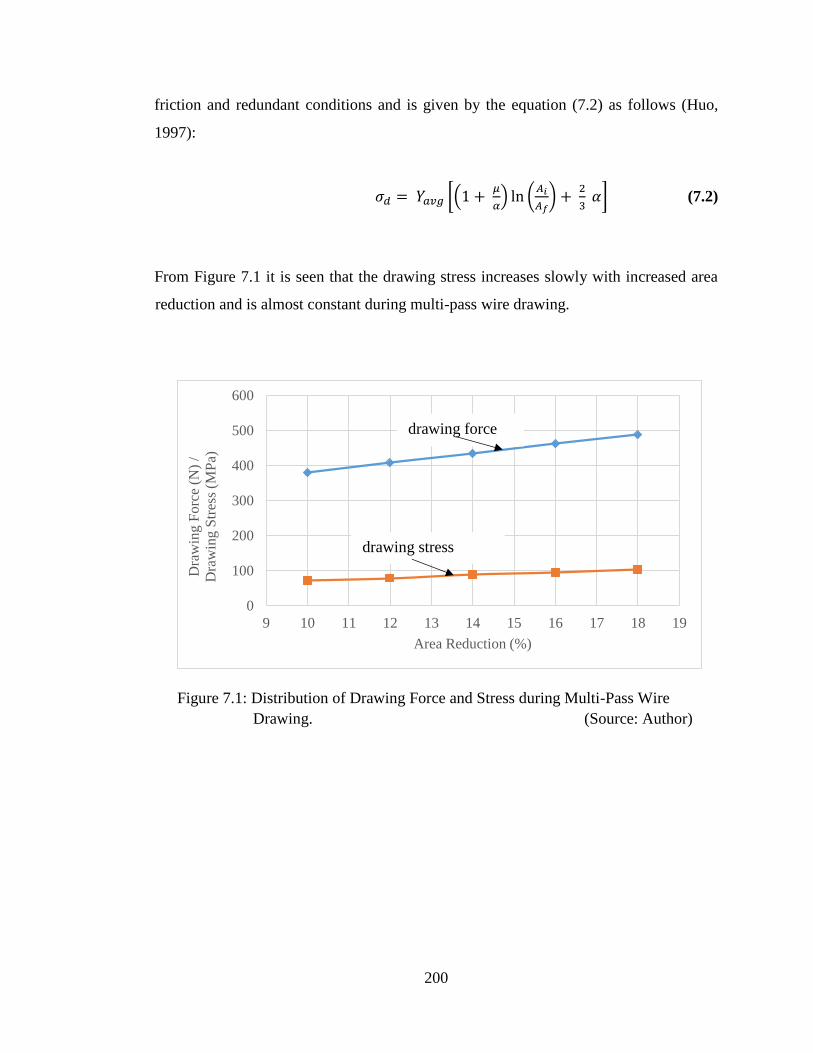
200
friction and redundant conditions and is given by the equation (7.2) as follows (Huo,
1997):
𝜎𝑑 = 𝑌𝑎𝑣𝑔 [(1 + 𝜇
𝛼) ln (
𝐴𝑖
𝐴𝑓) +
2
3 𝛼] (7.2)
From Figure 7.1 it is seen that the drawing stress increases slowly with increased area
reduction and is almost constant during multi-pass wire drawing.
Figure 7.1: Distribution of Drawing Force and Stress during Multi-Pass Wire
Drawing. (Source: Author)
DDra
0
100
200
300
400
500
600
9 10 11 12 13 14 15 16 17 18 19
Dra
win
g F
orc
e (N
) /
Dra
win
g S
tres
s (M
Pa)
Area Reduction (%)
drawing force
drawing stress
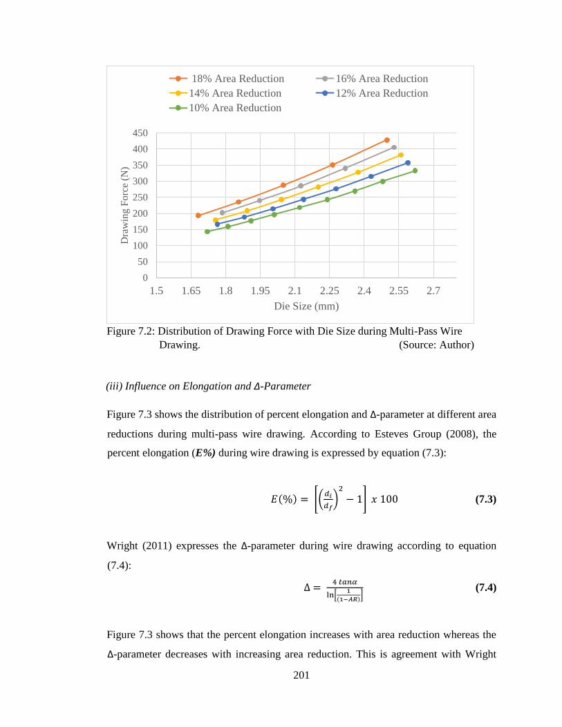
201
Figure 7.2: Distribution of Drawing Force with Die Size during Multi-Pass Wire
Drawing. (Source: Author)
(iii) Influence on Elongation and Δ-Parameter
Figure 7.3 shows the distribution of percent elongation and Δ-parameter at different area
reductions during multi-pass wire drawing. According to Esteves Group (2008), the
percent elongation (E%) during wire drawing is expressed by equation (7.3):
𝐸(%) = [(𝑑𝑖
𝑑𝑓)
2
− 1] 𝑥 100 (7.3)
Wright (2011) expresses the Δ-parameter during wire drawing according to equation
(7.4):
∆ = 4 𝑡𝑎𝑛𝛼
ln[1
(1−𝐴𝑅)] (7.4)
Figure 7.3 shows that the percent elongation increases with area reduction whereas the
Δ-parameter decreases with increasing area reduction. This is agreement with Wright
0
50
100
150
200
250
300
350
400
450
1.5 1.65 1.8 1.95 2.1 2.25 2.4 2.55 2.7
Dra
win
g F
orc
e (N
)
Die Size (mm)
18% Area Reduction 16% Area Reduction
14% Area Reduction 12% Area Reduction
10% Area Reduction
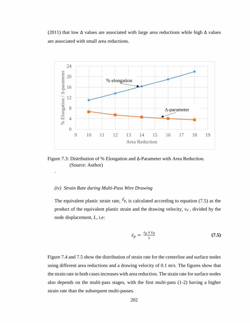
202
(2011) that low Δ values are associated with large area reductions while high Δ values
are associated with small area reductions.
Figure 7.3: Distribution of % Elongation and Δ-Parameter with Area Reduction.
(Source: Author)
.
(iv) Strain Rate during Multi-Pass Wire Drawing
The equivalent plastic strain rate, , is calculated according to equation (7.5) as the
product of the equivalent plastic strain and the drawing velocity, vd , divided by the
node displacement, L, i.e:
𝜀�� = 𝜀𝑝 𝑥 𝑣𝑑
𝐿 (7.5)
Figure 7.4 and 7.5 show the distribution of strain rate for the centerline and surface nodes
using different area reductions and a drawing velocity of 0.1 m/s. The figures show that
the strain rate in both cases increases with area reduction. The strain rate for surface nodes
also depends on the multi-pass stages, with the first multi-pass (1-2) having a higher
strain rate than the subsequent multi-passes.
0
4
8
12
16
20
24
9 10 11 12 13 14 15 16 17 18 19
% E
longat
ion /
Δ-p
aram
eter
Area Reduction
% elongation
Δ-parameter

203
Figure 7.4: Distribution of Strain Rate for Centreline Node (306). (Source: Author)
Figure 7.5: Distribution of Strain Rate for Surface Node (410). (Source: Author)
00.20.40.60.8
11.2
9 10 11 12 13 14 15 16 17 18 19
Str
ain
Rat
e (
/s)
Area Reduction (%)
Multi-Pass 1-2 Multi-Pass 2-3 Multi-Pass 3-4
Multi-Pass 4-5 Multi-Pass 5-6 Multi-Pass 6-7
Multi-Pass 7-8 Multi-Pass 8-9
00.5
11.5
22.5
33.5
9 10 11 12 13 14 15 16 17 18 19
Str
ain R
ate
(/s)
Area Reduction (%)
Multi-Pass 1-2 Multi-Pass 2-3 Multi-Pass 3-4
Multi-Pass 4-5 Multi-Pass 5-6 Multi-Pass 6-7
Multi-Pass 7-8 Multi-Pass 8-9
204
7.3.2 Analysis and Discussion of Experimental Procedures Results
The copper wire drawing experimental procedures were mainly based on the multi-pass
sequence involving the 2.55, 2.32, 2.11, 1.92 and 1.78 dies. Other multi-pass sequences
used were based on the pass schedules as given in Appendix 6.
(a) Effects of copper material state
It was seen from the ascertained chemical composition that the raw wrought copper rods
contained metallic elements within the prescribed limits by the standard ASTM B49-10.
The microstructure showed the presence of second phase particles with varying grain
sizes within the copper material matrix. Iron showed the highest percentage of metallic
inclusions. This could be attributed to the nature of the production processes, where
during electro refining steel starter sheets are used, or that the molten copper comes into
contact with steel boundaries during rod formation.
Of greater importance to wire drawing is the presence of silver. Silver is partially soluble
in copper and forms an inclusion or second phase (Wright, 2011) within the copper
matrix. The presence of silver particles is a likely source of micro-void initiation and
progression, leading to wire failure during wire drawing (Norasethasopon, 2011). The
results of the tensile tests for the wrought copper were given in Tables 6.3 and 6.4, and
Appendix 5.
(b) Effects from die design and manufacturing
During 2D design and simulation of the copper wire drawing process, it was observed
that the use of non-filleted die regions were seen to result in larger Mises stresses during
wire movement. This was evidence of possible flow problems by the introduction of
‘stress risers’ during simulations. This agreed with the recommendations by Society of
Manufacturing Engineers (1962) and Shearer (2008) that all stress raisers needed to be
removed.
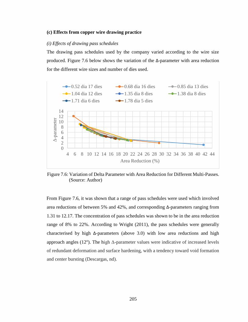
205
(c) Effects from copper wire drawing practice
(i) Effects of drawing pass schedules
The drawing pass schedules used by the company varied according to the wire size
produced. Figure 7.6 below shows the variation of the Δ-parameter with area reduction
for the different wire sizes and number of dies used.
Figure 7.6: Variation of Delta Parameter with Area Reduction for Different Multi-Passes.
(Source: Author)
From Figure 7.6, it was shown that a range of pass schedules were used which involved
area reductions of between 5% and 42%, and corresponding Δ-parameters ranging from
1.31 to 12.17. The concentration of pass schedules was shown to be in the area reduction
range of 8% to 22%. According to Wright (2011), the pass schedules were generally
characterised by high Δ-parameters (above 3.0) with low area reductions and high
approach angles (12o). The high Δ-parameter values were indicative of increased levels
of redundant deformation and surface hardening, with a tendency toward void formation
and center bursting (Descargas, nd).
02468
101214
4 6 8 10 12 14 16 18 20 22 24 26 28 30 32 34 36 38 40 42 44
Δ-p
aram
eter
Area Reduction (%)
0.52 dia 17 dies 0.68 dia 16 dies 0.85 dia 13 dies
1.04 dia 12 dies 1.35 dia 8 dies 1.38 dia 8 dies
1.71 dia 6 dies 1.78 dia 5 dies
206
(ii) Effects of lubrication and lubrication temperatures
The lubricant Mastersol C21 which was used both as a lubricant and coolant during
copper wire drawing was subjected to analytical tests at ZABS according to standards
ASTM D 445 and ASTM D 1298. According to equation (7.6) the kinematic viscosity,
v, is related to the dynamic viscosity, μ, and the density, ρ, as follows (Rajput, 2014):
𝑣 = 𝜇
𝜌 (7.6)
It was thus seen that at a working temperature of 40oC, the dynamic viscosity was equal
to 34.38 cSt, whereas at a temperature of 100oC, the dynamic viscosity dropped about
five times to a value of 6.94 cSt. This is in agreement with Rajput (2014) that the viscosity
of a lubricant decreases with increase in temperature due to the decrease in the shear
stress of the lubricant. As the lubricant temperature was maintained below 45oC
throughout the experiments, there were no major changes in viscosity. There was,
therefore, no major changes in the viscosity of the lubricant. Lubrication was, thus
effective.
(iii) Effects of die temperatures
The temperatures at die faces during wire drawing were seen to increase with increase in
die or wire size. This was due to the fact that larger wires or die sizes needed larger
drawing forces, hence increased die-wire temperatures.
(iv) Effects of drawing speed
The drawing speeds were generally low for larger wire size production and higher for
smaller size wires. The drawing speeds were observed to be on average low as they
ranged from 2.4 to 2.7 m/s for the medium size wires (Kalpakjian and Schmid, 2010).
According to Huo (1997) the drawing speed has an effect on drawing force and drawing
stress in that a change in drawing speed results in a change in the flow stress of the drawn
material and also changed the lubrication and friction characteristics in the wire drawing.

207
(v) Effects of drawing force
The drawing force increased with increasing wire size, thus necessitating the use of lower
speeds for larger size wires. This was done in order to reduce the drawing stress and thus
reduce the volume of defects due to wire breakages.
(vi) Effects on wire damage
Generation of ‘copper fines’ happened throughout the wire drawing process. The fines
were evident at wire entry (first die) and at wire exit (last die) due to the deposit of dry
fines. For the other dies, the copper fines were collected in the lubricant.
It was observed that wire breakage occurrences were more for smaller size wires (less
than 1.04 mm) than larger size wires greater than 1.04 mm. This is attributed to the fact
that the smaller size wires were drawn at higher speeds while the larger wires were drawn
using lower speeds.
Results from microscopy showed that during all multi-passes both internal micro-voids
and surface cracks were unavoidable during wire drawing. Cracks on the surface of the
wire were more pronounced than the internal micro-voids as discussed below:
(a) Multi-Pass 1-2
During the first multi-pass, internal micro-voids were more evident at 30% and 50% than
at 40% bearing length. Surface cracking was very pronounced at 30% bearing length,
while at 40% bearing length signs of surface chevron cracking was evident and the 50%
bearing length surface showed signs of sheared surfaces.
(b) Multi-Pass 2-3
The second multi-pass was characterized by more internal micro-void formation during
the 40% and 50% than at 30% bearing length. Surface cracking was very pronounced at
30% and 40% bearing length, while at 50% bearing length the extent of surface cracking
was reduced. This could be attributed to the facts that for internal micro-voids the
relaxation of material during the 40% bearing length happens, hence the pronounced
208
micro-voids. The seemingly reduction of surface cracks at 50% bearing length could be
due to the ‘forming’ effect on the already cracked surfaces, thus closing up the cracks.
(c) Multi-Pass 3-4
From the micrographs, it was seen that the third multi-pass had fewer internal micro-
voids in the 30% than the 40% and 50% bearing length. Surface cracking was more
evident during the 40% and 50% bearing lengths. As damage is progressive, the
behaviour of internal voids could be due to movements in shear layers due to drawing
stress, thus the micrographs only being captured for layers with minimal void formation.
Surface cracking could be due to the afore-said, whereby forming effects due to wire
interaction with the die occasion a smoother surface than the preceding layers.
(d) Multi-Pass 4-5
The last multi-pass stage during wire drawing practice was characterised by more internal
micro-voids at 30% and 50% than at 40% bearing length. Surface cracking was equally
more pronounced at 30% and 50% bearing lengths, while at 40% bearing length signs of
surface micro-voids were evident. This characteristic behaviour in the last multi-pass
could be due to the fact that ‘impact’ damage during wire entry to the die zone effected
damage at 30% bearing length, while progression of micro-voids and consequent
movement of shear layers effected increased damage during the 50% bearing length.
Measurement of micro-void sizes across the length at 3000X magnification showed that
the average internal crack length was highest during the 30% bearing length, and lowest
during the 40% bearing length. Surface crack measurements showed that the average
crack length was highest at 50% and lowest at 30% bearing length.
7.4 Effects of Bearing Length Variation
(a) Centreline (Internal) Damage
Effects of the bearing length on damage value (stiffness degradation) and the Cockroft
and Latham criterion leading to ductile damage of the copper wire in simulations showed
higher damage during the second (2-3) and third (3-4) multi-pass stages. Progressive
damage using the Cockroft and Latham criterion was high during the third (3-4) and
209
fourth (4-5) multi-pass stages, with peaks at 30 and 50% bearing lengths. The equivalent
plastic strain was high during the second (2-3) and third (3-4) multi-pass stages, while
the hydrostatic pressure was principally compressive and increased during the second (2-
3) and third (3-4) multi-pass stages.
A critical look at the Mises contours in Figures 5.9 to 5.13 showed that the Mises stresses
progressed from the surface contours towards the centreline during the movement of the
copper wire. The density of highly stressed areas towards the centreline tended to be
higher at 50% than at 30% bearing length variations. This is evident from the stick-slip
effect postulated by Avitzur (1983).
From the simulation models it was shown that progressive damage using the Cockroft
and Latham criterion was high at relatively low drawing speeds and periodic friction
coefficient values. This can be due to the longer periods of wire in contact with the die
surface, hence the larger being the die-wire contact area and consequently, the drag or
frictional effets being prolonged for such surfaces. The copper wire surface layers in
contact with the die tend to move slower than the centreline layers, thus effecting velocity
difference between the surface layers and the centreline layers.
Scanning image micrographs in Figures 6.32 and 6.40 showed that the second (2-3)
multi-pass was characterized by more internal micro-void formation during the 40% and
50% bearing length variation than the 30% bearing length as shown in Figure 6.24.
During the third (3-4) multi-pass more internal micro-voids were observed in the 40%
and 50% bearing length (Figures 6.34 and 6.42) than in the 30% bearing length variation
(Figure 6.26). The fourth (4-5) multi-pass stage was characterised by more internal micro-
voids at 30% and 50% (Figures 6.28 and 6.44) than at 40% bearing length (Figure 6.36).
The findings were in agreement with McAllen and Phelan (2005) for area reductions of
17% where the plastic strain and centreline damage were shown to be high during the
second and third multi-pass stages. The findings by Komori (2003) and Benesova, et al.,
(2008) can be supported here that ductile fracture is likely at later multi-pass stages and
210
when hydrostatic stresses are compressive for wire centreline sections. It can be inferred
thus, that at higher area reductions and at bearing lengths of 50%, centreline damage is
higher. Smaller bearing length values (40% and below) are preferrable for reduced
internal damage.
(b) Surface (External) Damage
For the surface nodes, it was shown that both equivalent plastic strain and damage values
were high during the first (1-2) and second (2-3) multi-pass stages. Ductile damage using
the Cockroft and Latham criterion was shown to be high during the second (2-3) and third
(3-4) multi-pass stages. Damage was seen to be lower during the 30% bearing length
variation than during the 40% to 50% bearing length range.
Scanned micrographs of drawn surfaces during the first (1-2) multi-pass showed evidence
of chevron cracking at 40% bearing length (Figure 6.31), with the 50% bearing length
surfaces displaying sheared sections (Figure 6.39). The second multi-pass (2-3) showed
less surface cracking during the 50% bearing length variation (Figure 6.41) than the 30%
and 40% bearing length range (Figures 6.25 and 6.33). The third (3-4) multi-pass showed
increased surface cracking during the 40% to 50% bearing length range (Figures 6.35 and
6.43).
In agreement with McAllen and Phelan (2005), it can be inferred that increased plastic
strain for area reductions of 17% where the plastic strain and surface damage were shown
to be high during the second and third multi-pass stages. The observed generation of
copper fines and as attributted to by Chia and Patel (1996) could be as a result of a
prolonged wire to die contact surface, exacerbated by a possibility of non-aligned wire
movement. It can be inferred thus, that at higher area reductions and at bearing lengths of
40% and above, surface damage is higher. Smaller bearing length values (30%) are
preferrable for reduced surface damage.
211
7.4.1 Summary of the Effects of Bearing Length Variation
From the analysis in section 7.4, it can be summarised that variation of the bearing length
has an effect on progressive damage of copper wire during wire drawing.
For both wire centerline or internal surfaces and external surfaces, bearing lengths of not
more than 40% are recommended for reduced internal and surface damage.

212
CHAPTER EIGHT: CONCLUSIONS AND RECOMMENDATIONS
8.1 General Conclusions
From the research carried out in the study, the following conclusions can be made:
(1) With the exception of the exit angle, all the die geometrical parameters, lubrication,
temperature and drawing speed had an influence on the development of both wire
centerline and surface cracks.
(2) Ductile damage was more evident in the second (2-3) and third (3-4) multi-pass stages
where area reductions of 17% were attained.
(3) The area reduction had a stronger effect on damage, although drawing at area
reductions above 18% using smaller approach angles of 9o kept the Δ-parameter
below the recommended threshold of 3.
(4) Bearing length values between 30% and 40% gave better wire performance in relation
to wire centerline damage which is more troublesome than wire surface damage.
Bearing lengths of 30% gave wire surface less damage.
(5) Use of lubrication during wire drawing is emphasised, with the need to control the
lubricant temperatures arising from die-wire contact. Most wire drawing setups use
flood lubrication which is directed at die blocks. This maintains effective lubrication
through reduction of die working temperatures which have an effect on lubricant
viscosity.
(6) Drawing wires above 1.04 mm demands larger drawing forces. This is compromised
by the relative reduction of the drawing speed which lowers the effectiveness of
lubrication. The wires thus become prone especially to surface damage. Such wires
should therefore be drawn using higher area reductions.
(7) The accelerated strain rate with area reduction renders the wire surface layers more
prone to strain hardening and cracking. The use of annealing the wire after each pass
213
may be a better, though expensive, method than the usually practiced annealing of
the final wire.
8.2 Summary of Conclusions
The following conclusions arising from the findings and addressing the research
objectives can be made:
(i) Establishment of die design and manufacturing aspects influencing
accuracy of die geometry
Low cost tungsten carbide nibs assembled in carbon steel casings are used at low
production volume levels. High wire drawing volume levels and fine wires
demands the use of polycrystalline or natural diamond nibs assembled in stainless
steel casings.
Design of die profile geometries is easily done using computer aided software.
Smooth fillets along the die nib geometrical surface are emphasized.
Accurate mould design is essential to producing an accurate die nib
The type of die nib material used (tungsten carbide or polycrystalline diamond)
is likely to affect the life of the die, with the polycrystalline diamond projected to
have a longer die life than tungsten carbide.
(ii) Determination of the Δ-parameter values, die geometrical parameters
and process conditions leading to the manifestation of surface and
chevron cracks during wire drawing
The following die geometrical parameters promote wire damage:
Smaller entrance angles of 20o are likely to cause both internal and surface wire
damage
Bearing lengths of 50% inflict centerline damage while 40% to 50% bearing
lengths cause surface damage
214
Approach angles of 10 or 12o are likely to cause centerline damage, whereas
approach angles of 8o are likely to cause surface damage
High friction coefficients of 0.07 and 0.09, signifying low lubrication regimes,
are likely to cause both centerline and surface damage
Low drawing speeds, typical when drawing wires larger than 1.04 mm, promote
internal and surface damage
High temperatures (above 40oC) reduce the viscosity of the lubricant, increase
the friction coefficient and promote wire damage
High area reductions (above 18%) with very small approach angles give small Δ-
parameter values and promote crack formation due to increased friction. Low area
reductions (below 16%) with large approach angles promote surface hardening
and redundant deformation, thus promoting crack formation. A ‘balanced-effect’
between these two regions is needed.
(iii) Development of an integrated model for die geometry and process
parameters for multi-pass copper wire drawing
Correctly designed die geometrical parameters (entrance angle, approach angle,
bearing length, area reduction) and process parameters (temperature, drawing
speed, friction coefficient and lubrication) participate in an integrated manner
towards the production of a defect-free copper wire.
(iv) Validation of the developed models using industry-based copper wire
drawing process setup
Based on the results and analysis of both the models and scanning micrographs, the
following are optimum bearing length parameters:
Centreline damage is minimized when using bearing length values between 30%
and 40% while surface damage is minimal when using bearing lengths of 30%.
215
8.3 Summary of Research Contributions
(1) The study has given contributions concerning the preferred use of 40% bearing
lengths during copper wire drawing practice. This region has shown that favourable
wire drawing conditions in regard to the internal and surface ductile damage are
obtainable when utilized.
(2) The research has delved into new territory regarding analysis of micro-voids inside
and on the outside of copper wire surfaces. Using defect micrographs, the quality of
internal and external copper wire surfaces can be easily assessed.
(3) The study has also explored new concerns arising from the industrial wire drawing
practice that unlike having pass schedules designed based on constant area reduction
or constant Δ-parameter, a combination of both concepts is preferred.
8.4 Suggestions for Further Research
(1) Further analysis, modelling and experimental investigation into the effects of the
entrance angle on ductile damage during copper wire drawing, especially when large
reduction angles are used. Preliminary modelling has shown that the entrance angle
has an effect on ductile damage.
(2) The effects of wear and lubrication mechanisms in the die bearing region and their
impact on both internal and external wire damage need investigation.
(3) The determination of critical crack or micro-void sizes impacting on wire
performance by assessment with elongation and electrical resistivity is necessary.
(4) Need for the development and application of shorter time-to-market moulds for die
nib manufacture when using conventional powder metallurgy equipment.
216
8.5 Recommendations for Implementation
(1) Wire drawing practitioners to always have a Tool Room which should ensure that dies
are procured according to technical specifications by engineers and an inventory of
all dies is kept for die maintenance purposes.
(2) Wire die practitioners to stick to the planned die sequences and not use any available
similar size die. This practice impacts on the Δ-parameter and therefore the onset of
wire damage.
(3) Wire drawing machinery manufacturers to incorporate effective pressure-based
sieving systems with easily removable basins for collection of copper ‘fines’ which
compromise the viscosity of the lubricant.
(4) Incorporation of an annealer after rod breakdown to improve flow properties of the
2.76 mm raw wire before being subjected to intermediate wire drawing.
217
REFERENCES
Ahmadi, F. and Farzin, M., (2008), Investigating Geometric and Friction Conditions
Causing Chevron Cracks in Wire Drawing Process using FEM. Steel Research
International Journal, Volume 2, pp. 382-388.
ASM International, (1990), Properties and Selection Non Ferrous Alloys and Special-
Purpose Materials. In: ASM Handbook Vol 02 . ASM International .
ASM International, (1988), Vol 14: Forming and Forging. ASM Handbook. ASM
International.
ASM International, (1990), Properties and Selections of Irons, Steels and High-
Performance Alloys. In: Vol 01 ASM Handbook Vol 01. ASM International, p. 1618.
ASTM International, (2010), Standard Specification for Copper Rod Drawing Stock for
Electrical Purposes, Designation: B49-10. ASTM International.
Atkins, A. and Caddell, R., (1968), The Incorporation of Work Hardening and Redundant
Work in Rod-Drawing Analyses. International Journal of Mechanical Sciences,
Pergamon Press, Volume 10, pp. 15-28.
Avitzur, B., (1983), Handbook of Metal-Forming Processes. New York: John Wiley and
Sons, Inc. ISBN 0 471 03474 6.
Bao, Y., (2003), Prediction of Ductile Crack Formation in Uncracked Bodies, PhD
Thesis. Massachusetts: Massachusetts Institute of Technology.
Bathe, K.-J., (1996), Finite Element Procedures. New Jersey: Prentice Hall. New Jersey:
Prentice Hall.
Benesova, S., Krnac, J., Wludzik, R. and Pilarczyk, J., (2008), Application of Cockroft-
Latham Criterion in FEM Analysis of Wire Fracture in Conventional Drawing of High
Carbon Steel Wires. [Online] Available at: http://home.zcu.cz/~sbenesov/Pittsburgh08.
Doc, [Accessed 14-03-2012].
Byon, S. M., Lee, S.J., Lee, D.W., Lee, Y.H. and Lee,Y., (2011), Effect of Coating
Material and Lubricant on Forming Force and Surface Defects in Wire Drawing Process.
Transactions of the Nonferrous Metal Society of China, pp. 104-110.
218
Campos, H. B., Reis, R.I., Corrêa, E.C.S., Aguilar, M.T.P. and Cetlin, P.R., (2006),
Variation of Friction Coefficient with Die Semi-Angle in the Axisymetric Drawing of
Copper, 17º CBECIMAT - Congresso Brasileiro de Engenharia e Ciência dos Materiais,
15 - 19 de Novembro, Foz do Iguaçu, Brasil.
Canter, N., (2009), Challenges in Formulating Metal Forming Fluids. Tribology and
Lubrication Technology, pp. 56-63.
Ceratizit, n.d. Drawing Tools for Wire Production. [Online] Available at:
http://www.ceratizit.com , [Accessed 08-03-2012].
Chia, E. and Patel, G., (1996), Characterisation of Rod and Wire Defects Produced
During The Manufacturing of Copper. Wire Journal International, pp. 50-59.
Cho, J. et al., 2006. Investigation of Recrystallisation and Grain Growth of Copper and
Gold Bonding Wires. Metallurgical and Materials Transactions , Volume 37 A, pp. 3085-
3097.
Cho, J.H., Rollett, A.D., Cho, J.-S., Park, Y.-J., Moon, J.-T. and Oh, K.H., (2006),
Investigation of Recrystallization and Grain Growth of Copper and Gold Bonding Wires.
Metallurgical and Materials Transactions, Volume 37A, pp. 3085-3097.
Conoptica, (2007), Drawing Die Profile: Inner Geometry Measurement, Application
Note 002. [Online] Available at: http://www.conoptica.com, [Accessed 08 03 2012].
Copper Development Association, n.d. The Copper Advantage: A Guide to Working with
Copper and Copper Alloys. [Online] Available at:http://www.copper.org/publications/
pub_list/pdf/a1360.pdf, [Accessed 06-03-2013].
Dassault Systèmes, (2013), Modelling Fracture and Failure with Abaqus. Dassault
Systèmes.
Dassault Systèmes, (2014a), ABAQUS 6.14: Theory Guide. Dassault Systèmes.
Dassault Systèmes, (2014b), ABAQUS Analysis Users Guide. Dassault Systèmes.
Davis, J.,(ed), (2001), Copper and Copper Alloys. ASM Specialty Handbook. ASM
International.
219
Descargas, (nd), Theory of Wire Drawing, [Online] Available from:
http://www.antaac.org.mx/descargas/TheoryOfWire drawing.pdf, Retrieved:[24-03-
2012].
Diamond Innovations, (2004), Compax Diamond Die Blanks. [Online]
Available at: http://www.diamondinnovations.com, [Accessed 22-08-2012].
Dieter, G., (1988), Mechanical Metallurgy. McGraw Hill.
Dixit, P. and Dixit, U., (2008), Modelling of Metal Forming and Machining Processes by
Finite Element and Soft Computing Methods. Springer. e-ISBN 978-1-84800-189-3.
Dubois, A., Lazzarotto, L., Dubar, L. and Oudin, J., (2002), A Multi-Step Lubricant
Evaluation Strategy for Wire Drawing–Extrusion–Cold Heading Sequence. Wear
Journal, Volume 249, pp. 951-961.
Esteves Group, (2008), The e-Wizard: Your Wire Die Handbook. [Online]
Available at: http://www.estevesgroup.com/ewizard/esteves_ewizard_en/
[Accessed 25 01 2013].
Fort Wayne Wire Die Inc., (1996), Single Crystal Diamond Dies: Specifications.
[Online] Available at: http://www.fwwd.com/images/Pdfs/FWWD-SCD_specs.pdf
[Accessed 25 01 2013].
Fort Wayne Wire Die Inc., (2009), Wire Die Manufacturing. [Online]
Available at: http://www.fwwd.com, [Accessed 22 08 2012].
Gálvez, F., Atienza, J., Ruiz, J. and Elices, M., (2002), The Effect of Strain Rate on Steel
Wires Failure During Cold Drawing. [Online] Available at:
http://www.mater.upm.es/fgalvez/PDF/MSMSE%2010%20(2002)%20167-276.pdf
[Accessed 08-03-2012].
Ghosh, B., (1992), Scientific Method and Social Research. New Delhi: Sterling.
Hassan, A. and Hashim, A., (2015), Three Dimensional Finite Element Analysis of Wire
Drawing Process. Universal Journal of Mechanical Engineering, 3(3), pp. 71-82.
Hervias, J.R., Hofmann, M., Kornmeier, J.R., Luzin, V. and Elices. M., (2009), Residual
Stresses in Cold-Drawn Rods: Effect of a Novel Post-Drawing Treatment. JCPDS-
International Centre for Diffraction Data, ISSN 1097-0002, pp. 747-754.

220
Higgins, R., (1994), The Properties of Engineering Materials. Arnold.
Hofstee, E., (2006), Constructing a Good Dissertation: A Practical Guide to Finishing a
Master's, MBA or PhD on Schedule. Sandton: EPE.
Hollinger, S., Depraetere, E. and Giroux, O., (2003), Wear Mechanism of Tungsten
Carbide Dies during Wet Drawing of Steel Tyre Cords. Wear Journal , Volume 255, pp.
1291-1299.
Hosford, W. and Caddell, R., (1983), Metal Forming: Mechanics and Metallurgy.
Englewood Cliffs: Prentice-Hall International, Inc. ISBN 0-13-577214-1.
Huo, B., (1997), Lubrication Efficiency and Die Design in Wire Dawing: PhD Thesis,
Birmingham: University of Aston.
International Copper Study Group, (2016), World Copper Fact Book 2016, Lisbon:
International Copper Study Group.
John, V., (1992), Introduction to Engineering Materials. 3rd ed. Macmillan.
Kabayama, L., Taguchi, S. and Martínez, G., (2009), The Influence of Die Geometry on
Stress Distribution by Experimental and FEM Simulation on Electrolytic Copper Wire
Drawing. Materials Research, 12(3), pp. 281-285.
Kalpakjian, S. and Schmid, S., (2006), Manufacturing Engineering and Technology. 5th
ed. Pearson. ISBN 0-13-148965-8.
Kalpakjian, S. and Schmid, S., (2010), Manufacturing Engineering and Technology. 6th
ed. Pearson.
Kerlinger, F., (1986), Foundations of Behavioural Research. Holt Rinehart and Winston
Inc.
Komori, K., (2003), Effect of Ductile Fracture Criteria on Chevron Crack Formation and
Evolution in Drawing. International Journal of Mechanical Sciences, Volume 45, pp.
141-160.
Lee, K., Lee, S. and Kim, B., (2012), Advanced Simulation of Die Wear Caused by Wire
Vibrations during Wire Drawing Process. Transactions of Nonferrous Metals Society of
China, Volume 22, pp. 1723-1731.
221
León, J., Luis, C.J., Salcedo, Luri, D.R., Puertas, I. and Pérez, I., (2010), Effect of the
Die Geometry on the Imparted Damage in Wire Drawing. 14th International
Research/Expert Conference, pp. 73-76.
Lin, X., Xiao, H. and Zhang, Z., (2003), Research on the Selection of Friction Models in
the Finite Element Simulation of Warm Extrusion. ACTA Metallurgica Sinica, XVI(2),
pp. 90-96.
Liu, G. and Quek, S., (2003), The Finite Element Method: A Practical Course. Oxford:
Butterworth Heinemann.
McAllen, P. and Phelan, P., (2005), A Method for the Prediction of Ductile Fracture by
Central Bursts in Axisymmetric Extrusion. Proceedings of the Institution of Mechanical
Engineers, Part C: Journal of Mechanical Engineering Science, pp. 237-250.
McAllen, P. and Phelan, P., (2007), Numerical Analysis of Axisymmetric Wire Drawing
by Means of a Coupled Damage Model. Journal of Materials Processing Technology,
Volume 183, pp. 210-218.
Norasethasopon, S., (2003), Effects of Inclusion on Inclusion Front Tensile Stress During
Copper-Shaped Wire drawing by 2D FEA. Naresuan University Journal, Vol.11, No.2,
pp. 11-18.
Norasethasopon, S., (2011), Chevron Crack Initiation in Multi-Pass Drawing of Inclusion
Copper-Shaped Wire. Materials and Minerals, Vol.21, No.1, pp. 1-8.
Norasethasopon, S. and Yoshida, K., (2003), Influence of an Inclusion on Multi-Pass
Copper-Shaped Wire Drawing by 2D Finite Element Analysis. IJE Transactions B:
Applications, Vol.16, No.3, pp. 279-292.
Palkowski, H., Kleiber, M. and Groth, C., (2003), 21st CAD-FEM Users Meeting.
Potsdam.
Panjan, P., Bončina, I., Bevk, J. and Čekada, M., (2005), PVD Hard Coatings Applied
for the Wear Protection of Drawing Dies. Surface and Coatings Technology , Volume
200, pp. 133-136.
Panteghini, A. and Genna, F., (2010), An Engineering Analytical Approach to the Design
of Cold Wire Drawing Processes for Strain-hardening Materials, International Journal of
Material Forming, Vol.3, pp.279-289.
222
Pops, H., (1997), The Metallurgy of Copper Wire. [Online], Available at:
http://www.copper.org/publications/newsletters/innovations/1997/12/wiremetallurgy.ht
ml, [Accessed 23-03-2012].
Radojevič, M., Radojičič, M., Nakič, M. and Babič, M., (2000), Lubricant as a Parameter
of Processing Tribomechanical System in the Process of Wire Drawing. Tribology in
Industry, Vol.22, Nos. 1 & 2, pp. 23-27.
Rajput, R., (2014), Fluid Mechanics and Hydraulic Machines. S.Chand.
Reddy, N., Dixit, P. and Lal, G., (2000), Ductile Fracture Criteria and its Prediction in
Axisymmetric Drawing. International Journal of Machine Tools and Manufacture,
Volume 40, pp. 95-111.
Rosenthal, R. and Rosnow, R., (1991), Essentials of Behavioural Research: Methods and
Data Analysis. McGraw-Hill Inc.
Salcedo, D., Luis, C.J., León, J., Luri, R., Puertas, I. and Pérez, I., (2010), Analysis of
Residual Stresses in Wire Drawing Processes, 14th International Research/Expert
Conference “Trends In The Development of Machinery and Associated Technology”,
TMT 2010, Mediterranean Cruise, 11-18 September, pp.69 -72.
Shearer, T., (2008), The Designer's Guide to Tungsten Carbide. General Carbide.
Simmons, C. and Maguire, D., (1974), A Manual of Engineering Drawing Practice.
Edward Arnold.
Singh, S.K., Gautham, B.P., Goyal, S., Joshi, A. and Gudadhe, D., (2007), Development
of a Virtual Wire Drawing Tool for Process Analysis and Optimization. Wire Journal
International, pp. 72-78.
Society of Manufacturing Engineers , (1962), Fundamentals of Tool Design. Prentice-
Hall Inc.
Solomon, N., Chika, M., Famous, A., Chioma, O. and Ebele, E., (2010). Development of
New Copper Wire drawing Lubricant. Journal of Applied Sciences Research, Vol.6,
No.11, pp. 1669-1673.
Suchy, I., (2006), Handbook of Die Design. McGraw Hill.

223
Tvergaard, V. and Hutchinson, J., (2002), Two Mechanisms of Ductile Fracture: Void by
Void Growth versus Multiple Void Interaction. International Journal of Solids and
Structures, Volume 39, pp. 3581-3597.
Udomphol, T., (2007), Drawing of Rods, Wires and Tubes. Suranaree University of
Technology [Online] Available at: http://www.sut.ac.th/engineering/Metal/pdf/
MetForm/05_Drawing%20of%20rod-wire%20and%20tubes.pdf, [Accessed 08 03
2012].
Upadhyaya, G., (2002), Powder Metallurgy Technology. Cambridge International
Science Publishing. ISBN 1- 898326 40-1.
Valberg, H. S., (2010), Applied Metal Forming, Including FEM Analysis. Cambridge:
Cambridge University Press. ISBN 9780-521-51823-9.
Vega, G., Haddi, A. and Imad, A., (2009), Temperature Effects on Wire-Drawing
Process: Experimental Investigation. [Online] Available at: http://web.univ-ubs.fr/
limatb/EG2M/Disc_Seminaire/ESAFORM_09/data/pdf/paper195psohm.pdf
[Accessed 06-03-2012].
Wright, R., (2011), Wire Technology: Process Engineering and Metallurgy. Butterworth-
Heinemann. ISBN 978-0-12-382092-1.
Xue, L., (2007), Ductile Fracture Modelling - Theory, Experimental Investigation and
Numerical Verification: PhD Thesis, Massachusetts: Massachusetts Institute of
Technology.
Xu, G., Fang, F. and Li, Z., (2009), Optimisation of the Technology of Wire Drawing
Based on Finite Element Modeling. Modern Applied Science, 3(5), pp. 193-198.
Yang, X., Deng, J., Wang, H. and Ze, X., (2007), Wear Behaviors and Lubrication
Medium of TiC/Al2O3 Ceramic Wire Drawing Dies. Transactions of Non-Ferrous Metal
Society of China, Volume 17, pp. s663-s666.
Zhuzhou Good Cemented Carbide Co. Ltd, n.d. [Online]
Available at: http:// www.carbide-good.com, [Accessed 06-09-2016]
Zompì, A. and Levi, R., (2008), Advances in Wire Drawing Process by Theoretical and
Numerical Analysis. [Online] Available at: http://www.utfscience.de
[Accessed 06-03-2012].

224
APPENDICES

225
Appendix 1: Properties of Pure Copper
Condition Tensile
Strength
Yield
Strength at
0.5 %
extension
under load
Poissons
ratio
Elastic modulus
(GPa)
Strain
hardening
Exponent
Elongation Reduction
in Area
Hardness
(HRB)
Tension Shear
Annealed 209 33 0.343 125 46.4 0.54 60 92
Cold
Drawn 344 333.4 0.364 112 14 88 37
(Source: Davis, 2001)

226
Appendix 2: Properties of Wrought Copper (@2mm wire section)
UNS Number
Chemical
Composition
(%)
Condition
Physical Properties
Mechanical properties
ρ
g/cm3
EC
MegaSiemen
s/cm @ 20oC
TC
W/m oK @
20oC
E
(MPa)
σ
(MPa)
τ
(MPa)
PE*
C10100
(Oxygen Free
Electrolytic
Copper - ETP)
99.99 Cu;
0.0004 Sb;
0.0005 As;
0.0005 O;
0.0003 P;
0.0002 Te
Annealed
(OS050)
8.94
0.591
391.1
117000
241
165
35
Cold
Worked
(H04)
8.94
0.591
391.1
117000
379
200
1
C10200
(Oxygen Free
- OF)
99.95 Cu;
0.001 O
8.94
0.591
391.1
117000
(Source: Copper Development Association)
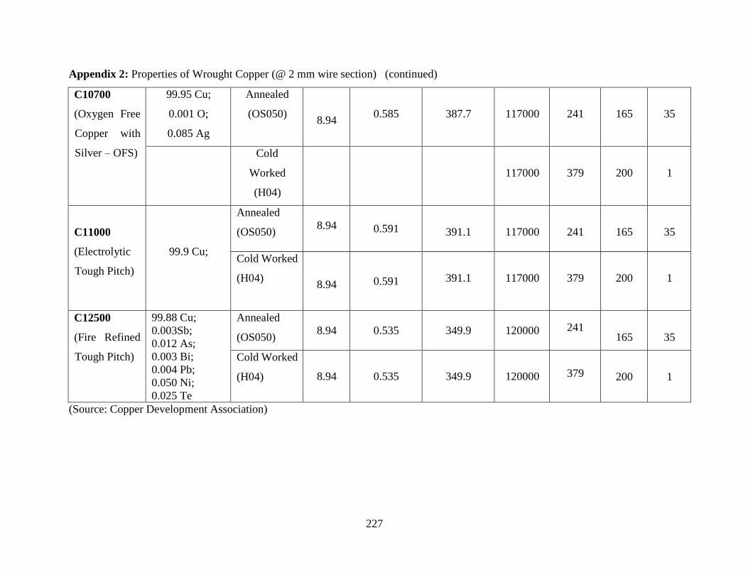
227
Appendix 2: Properties of Wrought Copper (@ 2 mm wire section) (continued)
C10700
(Oxygen Free
Copper with
Silver – OFS)
99.95 Cu;
0.001 O;
0.085 Ag
Annealed
(OS050)
8.94
0.585
387.7
117000
241
165
35
Cold
Worked
(H04)
117000
379
200
1
C11000
(Electrolytic
Tough Pitch)
99.9 Cu;
Annealed
(OS050)
8.94
0.591
391.1
117000
241
165
35
Cold Worked
(H04)
8.94
0.591
391.1
117000
379
200
1
C12500
(Fire Refined
Tough Pitch)
99.88 Cu;
0.003Sb;
0.012 As;
0.003 Bi;
0.004 Pb;
0.050 Ni;
0.025 Te
Annealed
(OS050) 8.94 0.535 349.9 120000 241
165
35
Cold Worked
(H04) 8.94 0.535 349.9 120000 379
200
1
(Source: Copper Development Association)
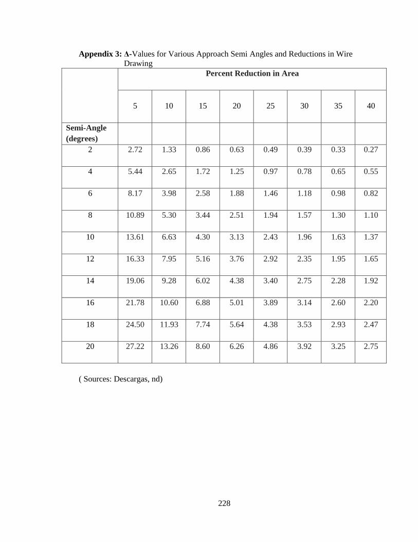
228
Appendix 3: Δ-Values for Various Approach Semi Angles and Reductions in Wire
Drawing
( Sources: Descargas, nd)
Percent Reduction in Area
5 10 15 20 25 30 35
40
Semi-Angle
(degrees)
2
2.72 1.33 0.86 0.63 0.49 0.39 0.33 0.27
4
5.44 2.65 1.72 1.25 0.97 0.78 0.65 0.55
6
8.17 3.98 2.58 1.88 1.46 1.18 0.98 0.82
8
10.89 5.30 3.44 2.51 1.94 1.57 1.30 1.10
10
13.61 6.63 4.30 3.13 2.43 1.96 1.63 1.37
12
16.33 7.95 5.16 3.76 2.92 2.35 1.95 1.65
14
19.06 9.28 6.02 4.38 3.40 2.75 2.28 1.92
16
21.78 10.60 6.88 5.01 3.89 3.14 2.60 2.20
18
24.50 11.93 7.74 5.64 4.38 3.53 2.93 2.47
20
27.22 13.26 8.60 6.26 4.86 3.92 3.25 2.75

229
Appendix 4: ABAQUS Simulation Output File (30%1st2PasesExplDuctile.dat)
ABAQUS 6.14-2 Date 20-Oct-2015 Time 12:00:29
* * * * * * * * * * * * * * * * * * * * * * * * * * * * * *
* ***************** *
* * N O T I C E * *
* ***************** *
* ABAQUS 6.14-2 *
* *
* Please make sure you are using release 6.14 manuals *
* plus the notes accompanying this release. *
* * * * * * * * * * * * * * * * * * * * * * * * * * * * * *
PROCESSING PART, INSTANCE, AND ASSEMBLY INFORMATION
*******************************************************
END PROCESSING PART, INSTANCE, AND ASSEMBLY INFORMATION
***********************************************************
OPTIONS BEING PROCESSED
***************************
*Heading
Drawing of Drawn Copper Wire from 2.76 to 2.32 mm
*Node
*Nset, nset=ASSEMBLY_DIE1-1_DIE1-1-REFPT_
*Nset, nset=ASSEMBLY_DIE1-1_REFPT
*Node
*Nset, nset=ASSEMBLY_DIE2-1_DIE2-1-REFPT_
*Nset, nset=ASSEMBLY_DIE2-1_REFPT
*Node
*Element, type=CAX4R
*Nset, nset=ASSEMBLY_WIRE-1_ALL
*Nset, nset=ASSEMBLY_WIRE-1_CENTRELINE
*Nset, nset=ASSEMBLY_WIRE-1_INLETSURFACE

230
*Nset, nset=ASSEMBLY_WIRE-1_OUTLETFACE
*Elset, elset=ASSEMBLY_WIRE-1_ALL
*Elset, elset=ASSEMBLY_WIRE-1_CENTRELINE
*Elset, elset=ASSEMBLY_WIRE-1_INLETSURFACE
*Elset, elset=ASSEMBLY_WIRE-1_OUTLETFACE
*Elset, elset=ASSEMBLY_WIRE-1__CENTRELINE_S2
*Elset, elset=ASSEMBLY_WIRE-1__CENTRELINE_S4
*Elset, elset=ASSEMBLY_WIRE-1__CONTACSURFACE_S2
*Elset, elset=ASSEMBLY_WIRE-1__CONTACSURFACE_S4
*Elset, elset=ASSEMBLY_WIRE-1__INLETSURFACE_S3
*Elset, elset=ASSEMBLY_WIRE-1__OUTLETSURFACE_S3
*rigidbody, refnode=ASSEMBLY_DIE1-1_DIE1-1-REFPT_,
analyticalsurface=ASSEMBLY_DIE1-1_DIE1SURF
*rigidbody, refnode=ASSEMBLY_DIE2-1_DIE2-1-REFPT_,
analyticalsurface=ASSEMBLY_DIE2-1_DIE2SURF
*rigidbody, refnode=ASSEMBLY_DIE1-1_DIE1-1-REFPT_,
analyticalsurface=ASSEMBLY_DIE1-1_DIE1SURF
*rigidbody, refnode=ASSEMBLY_DIE2-1_DIE2-1-REFPT_,
analyticalsurface=ASSEMBLY_DIE2-1_DIE2SURF
*rigidbody, refnode=ASSEMBLY_DIE1-1_DIE1-1-REFPT_,
analyticalsurface=ASSEMBLY_DIE1-1_DIE1SURF
*rigidbody, refnode=ASSEMBLY_DIE2-1_DIE2-1-REFPT_,
analyticalsurface=ASSEMBLY_DIE2-1_DIE2SURF
*rigidbody, refnode=ASSEMBLY_DIE1-1_DIE1-1-REFPT_,
analyticalsurface=ASSEMBLY_DIE1-1_DIE1SURF
*rigidbody, refnode=ASSEMBLY_DIE2-1_DIE2-1-REFPT_,
analyticalsurface=ASSEMBLY_DIE2-1_DIE2SURF
*surface, type=SEGMENTS, name=ASSEMBLY_DIE1-1_DIE1SURF
*surface, type=SEGMENTS, name=ASSEMBLY_DIE2-1_DIE2SURF
*surface, type=ELEMENT, name=ASSEMBLY_WIRE-1_INLETSURFACE
*surface, type=ELEMENT, name=ASSEMBLY_WIRE-1_OUTLETSURFACE

231
*surface, type=ELEMENT, name=ASSEMBLY_WIRE-1_CENTRELINE
*surface, type=ELEMENT, name=ASSEMBLY_WIRE-1_CONTACSURFACE
*surface, type=SEGMENTS, name=ASSEMBLY_DIE1-1_DIE1SURF
*surface, type=SEGMENTS, name=ASSEMBLY_DIE2-1_DIE2SURF
*surface, type=ELEMENT, name=ASSEMBLY_WIRE-1_INLETSURFACE
*surface, type=ELEMENT, name=ASSEMBLY_WIRE-1_OUTLETSURFACE
*surface, type=ELEMENT, name=ASSEMBLY_WIRE-1_CENTRELINE
*surface, type=ELEMENT, name=ASSEMBLY_WIRE-1_CONTACSURFACE
*rigidbody, refnode=ASSEMBLY_DIE1-1_DIE1-1-REFPT_,
analyticalsurface=ASSEMBLY_DIE1-1_DIE1SURF
*rigidbody, refnode=ASSEMBLY_DIE2-1_DIE2-1-REFPT_,
analyticalsurface=ASSEMBLY_DIE2-1_DIE2SURF
*material, name="Drawn Copper"
*damageinitiation, criterion=DUCTILE
*damageevolution, type=DISPLACEMENT
*density
*elastic
*plastic
*surfaceinteraction, name=FRICTION
*friction
*solidsection, elset=ASSEMBLY_WIRE-1_ALL, controls=EC-1, material="Drawn
Copper"
*sectioncontrols, name=EC-1, elementdeletion=YES
*rigidbody, refnode=ASSEMBLY_DIE1-1_DIE1-1-REFPT_,
analyticalsurface=ASSEMBLY_DIE1-1_DIE1SURF
*rigidbody, refnode=ASSEMBLY_DIE2-1_DIE2-1-REFPT_,
analyticalsurface=ASSEMBLY_DIE2-1_DIE2SURF
*rigidbody, refnode=ASSEMBLY_DIE1-1_DIE1-1-REFPT_,
analyticalsurface=ASSEMBLY_DIE1-1_DIE1SURF
*rigidbody, refnode=ASSEMBLY_DIE2-1_DIE2-1-REFPT_,
analyticalsurface=ASSEMBLY_DIE2-1_DIE2SURF

232
*solidsection, elset=ASSEMBLY_WIRE-1_ALL, controls=EC-1, material="Drawn
Copper"
*solidsection, elset=ASSEMBLY_WIRE-1_ALL, controls=EC-1, material="Drawn
Copper"
*rigidbody, refnode=ASSEMBLY_DIE1-1_DIE1-1-REFPT_,
analyticalsurface=ASSEMBLY_DIE1-1_DIE1SURF
*rigidbody, refnode=ASSEMBLY_DIE2-1_DIE2-1-REFPT_,
analyticalsurface=ASSEMBLY_DIE2-1_DIE2SURF
*friction
*elementoutput, directions=YES
*rigidbody, refnode=ASSEMBLY_DIE1-1_DIE1-1-REFPT_,
analyticalsurface=ASSEMBLY_DIE1-1_DIE1SURF
*rigidbody, refnode=ASSEMBLY_DIE2-1_DIE2-1-REFPT_,
analyticalsurface=ASSEMBLY_DIE2-1_DIE2SURF
*amplitude, name=AMP-1, definition=SMOOTHSTEP
*output, field
*output, history, variable=PRESELECT, frequency=1
*Step, name="multipass drawing", nlgeom=YES
*Step, name="multipass drawing", nlgeom=YES
*dynamic, explicit
*fixedmassscaling, elset=ASSEMBLY_WIRE-1_ALL, dt=1e-05, type=BELOWMIN
*boundary
*boundary, amplitude=AMP-1, type=VELOCITY
*boundary
*boundary
*output, field
*nodeoutput
*elementoutput, directions=YES
*contactoutput
*output, history, variable=PRESELECT, frequency=1
*endstep
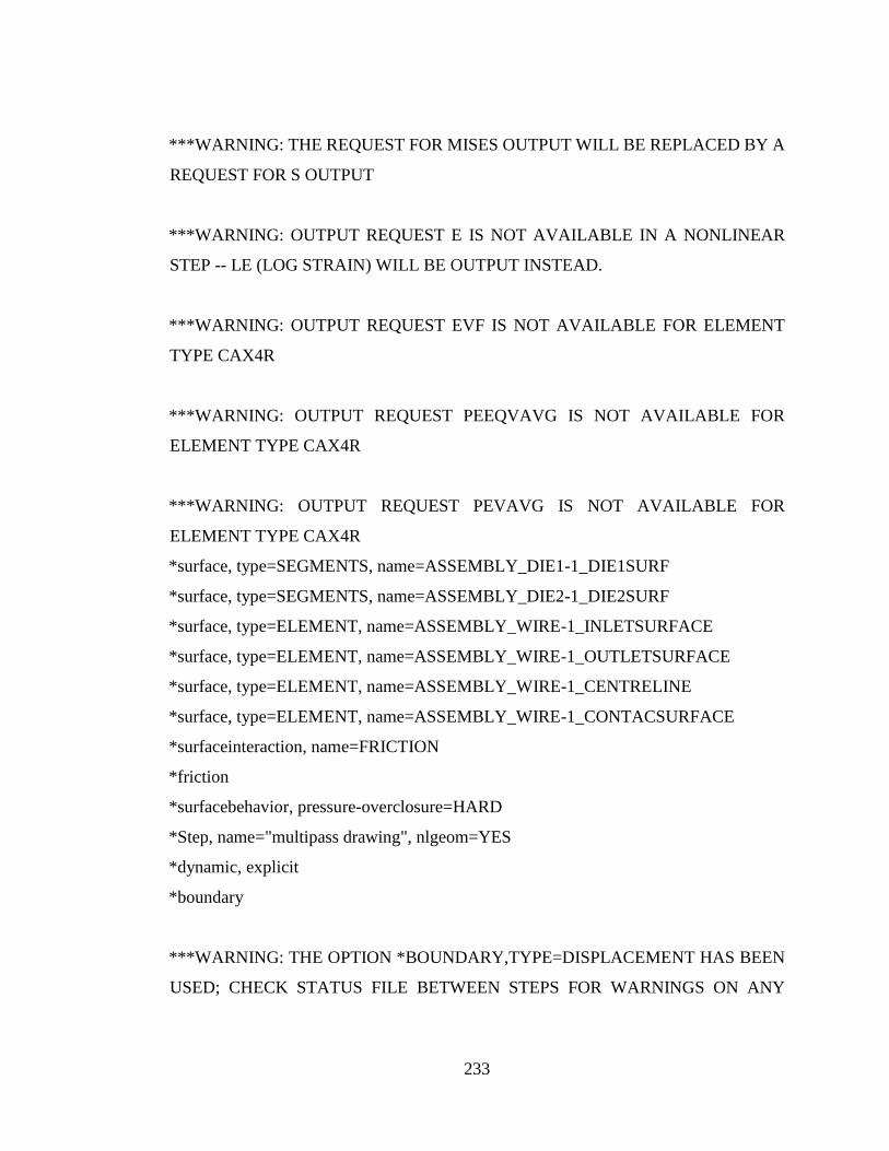
233
***WARNING: THE REQUEST FOR MISES OUTPUT WILL BE REPLACED BY A
REQUEST FOR S OUTPUT
***WARNING: OUTPUT REQUEST E IS NOT AVAILABLE IN A NONLINEAR
STEP -- LE (LOG STRAIN) WILL BE OUTPUT INSTEAD.
***WARNING: OUTPUT REQUEST EVF IS NOT AVAILABLE FOR ELEMENT
TYPE CAX4R
***WARNING: OUTPUT REQUEST PEEQVAVG IS NOT AVAILABLE FOR
ELEMENT TYPE CAX4R
***WARNING: OUTPUT REQUEST PEVAVG IS NOT AVAILABLE FOR
ELEMENT TYPE CAX4R
*surface, type=SEGMENTS, name=ASSEMBLY_DIE1-1_DIE1SURF
*surface, type=SEGMENTS, name=ASSEMBLY_DIE2-1_DIE2SURF
*surface, type=ELEMENT, name=ASSEMBLY_WIRE-1_INLETSURFACE
*surface, type=ELEMENT, name=ASSEMBLY_WIRE-1_OUTLETSURFACE
*surface, type=ELEMENT, name=ASSEMBLY_WIRE-1_CENTRELINE
*surface, type=ELEMENT, name=ASSEMBLY_WIRE-1_CONTACSURFACE
*surfaceinteraction, name=FRICTION
*friction
*surfacebehavior, pressure-overclosure=HARD
*Step, name="multipass drawing", nlgeom=YES
*dynamic, explicit
*boundary
***WARNING: THE OPTION *BOUNDARY,TYPE=DISPLACEMENT HAS BEEN
USED; CHECK STATUS FILE BETWEEN STEPS FOR WARNINGS ON ANY

234
JUMPS PRESCRIBED ACROSS THE STEPS IN DISPLACEMENT VALUES OF
TRANSLATIONAL DOF. FOR ROTATIONAL
DOF MAKE SURE THAT THERE ARE NO SUCH JUMPS. ALL JUMPS IN
DISPLACEMENTS ACROSS STEPS ARE IGNORED
*boundary, amplitude=AMP-1, type=VELOCITY
*boundary
*boundary
*contactpair, interaction=FRICTION, mechanicalconstraint=KINEMATIC,
cpset=INT-1
*contactpair, interaction=FRICTION, mechanicalconstraint=KINEMATIC,
cpset=INT-2
*endstep
P R O B L E M S I Z E
NUMBER OF ELEMENTS IS 6000
NUMBER OF NODES IS 6233
NUMBER OF NODES DEFINED BY THE USER 6233
TOTAL NUMBER OF VARIABLES IN THE MODEL 12468
(DEGREES OF FREEDOM PLUS MAX NO. OF ANY LAGRANGE MULTIPLIER
VARIABLES. INCLUDE *PRINT,SOLVE=YES TO GET THE ACTUAL NUMBER.)
END OF USER INPUT PROCESSING
JOB TIME SUMMARY
USER TIME (SEC) = 0.80000
SYSTEM TIME (SEC) = 0.10000
TOTAL CPU TIME (SEC) = 0.90000
WALLCLOCK TIME (SEC) = 1
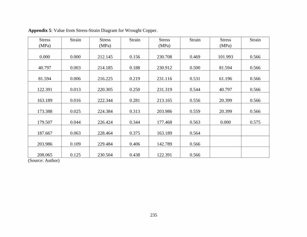
235
Appendix 5: Value from Stress-Strain Diagram for Wrought Copper.
Stress
(MPa)
Strain Stress
(MPa)
Strain Stress
(MPa)
Strain Stress
(MPa)
Strain
0.000 0.000 212.145 0.156 230.708 0.469 101.993 0.566
40.797 0.003 214.185 0.188 230.912 0.500 81.594 0.566
81.594 0.006 216.225 0.219 231.116 0.531 61.196 0.566
122.391 0.013 220.305 0.250 231.319 0.544 40.797 0.566
163.189 0.016 222.344 0.281 213.165 0.556 20.399 0.566
173.388 0.025 224.384 0.313 203.986 0.559 20.399 0.566
179.507 0.044 226.424 0.344 177.468 0.563 0.000 0.575
187.667 0.063 228.464 0.375 163.189 0.564
203.986 0.109 229.484 0.406 142.789 0.566
208.065 0.125 230.504 0.438 122.391 0.566
(Source: Author)
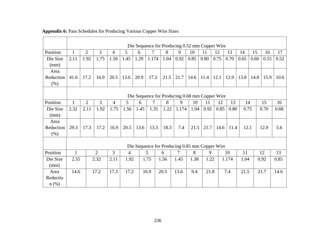
236
Appendix 6: Pass Schedules for Producing Various Copper Wire Sizes
Die Sequence for Producing 0.52 mm Copper Wire
Position 1 2 3 4 5 6 7 8 9 10 11 12 13 14 15 16 17
Die Size
(mm)
2.11 1.92 1.75 1.56 1.45 1.29 1.174 1.04 0.92 0.85 0.80 0.75 0.70 0.65 0.60 0.55 0.52
Area
Reduction
(%)
41.6
17.2
16.9
20.5
13.6
20.9
17.2
21.5
21.7
14.6
11.4
12.1
12.9
13.8
14.8
15.9
10.6
Die Sequence for Producing 0.68 mm Copper Wire
Position 1 2 3 4 5 6 7 8 9 10 11 12 13 14 15 16
Die Size
(mm)
2.32 2.11 1.92 1.75 1.56 1.45 1.35 1.22 1.174 1.04 0.92 0.85 0.80 0.75 0.70 0.68
Area
Reduction
(%)
29.3
17.3
17.2
16.9
20.5
13.6
13.3
18.3
7.4
21.5
21.7
14.6
11.4
12.1
12.9
5.6
Die Sequence for Producing 0.85 mm Copper Wire
Position 1 2 3 4 5 6 7 8 9 10 11 12 13
Die Size
(mm)
2.55 2.32 2.11 1.92 1.75 1.56 1.45 1.38 1.22 1.174 1.04 0.92 0.85
Area
Reductio
n (%)
14.6 17.2 17.3 17.2 16.9 20.5 13.6 9.4 21.8 7.4 21.5 21.7 14.6
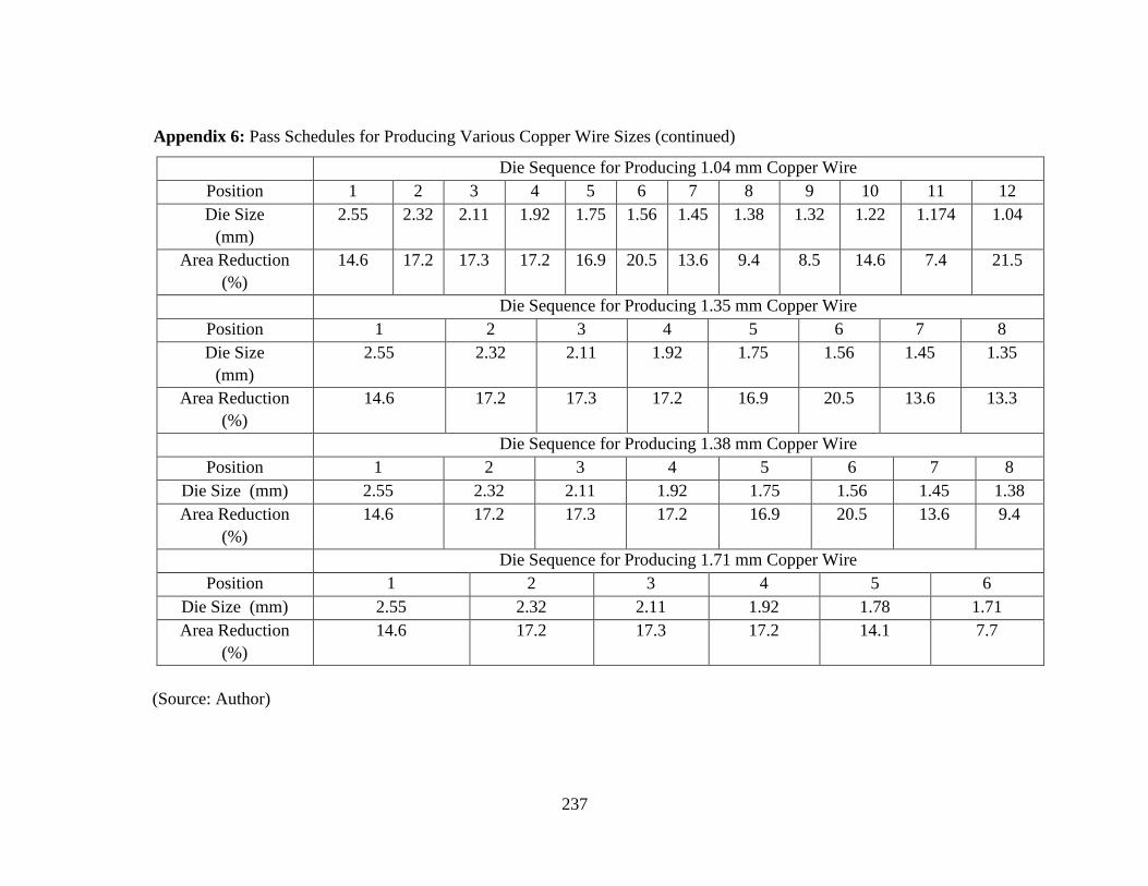
237
Appendix 6: Pass Schedules for Producing Various Copper Wire Sizes (continued)
Die Sequence for Producing 1.04 mm Copper Wire
Position 1 2 3 4 5 6 7 8 9 10 11 12
Die Size
(mm)
2.55 2.32 2.11 1.92 1.75 1.56 1.45 1.38 1.32 1.22 1.174 1.04
Area Reduction
(%)
14.6 17.2 17.3 17.2 16.9 20.5 13.6 9.4 8.5 14.6 7.4 21.5
Die Sequence for Producing 1.35 mm Copper Wire
Position 1 2 3 4 5 6 7 8
Die Size
(mm)
2.55 2.32 2.11 1.92 1.75 1.56 1.45 1.35
Area Reduction
(%)
14.6 17.2 17.3 17.2 16.9 20.5 13.6 13.3
Die Sequence for Producing 1.38 mm Copper Wire
Position 1 2 3 4 5 6 7 8
Die Size (mm) 2.55 2.32 2.11 1.92 1.75 1.56 1.45 1.38
Area Reduction
(%)
14.6 17.2 17.3 17.2 16.9 20.5 13.6 9.4
Die Sequence for Producing 1.71 mm Copper Wire
Position 1 2 3 4 5 6
Die Size (mm) 2.55 2.32 2.11 1.92 1.78 1.71
Area Reduction
(%)
14.6 17.2 17.3 17.2 14.1 7.7
(Source: Author)
238
Appendix 7: Die Design Drawings
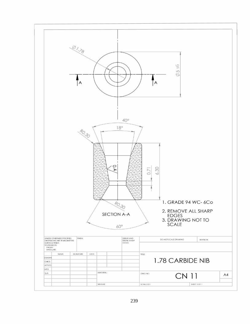
239
s6
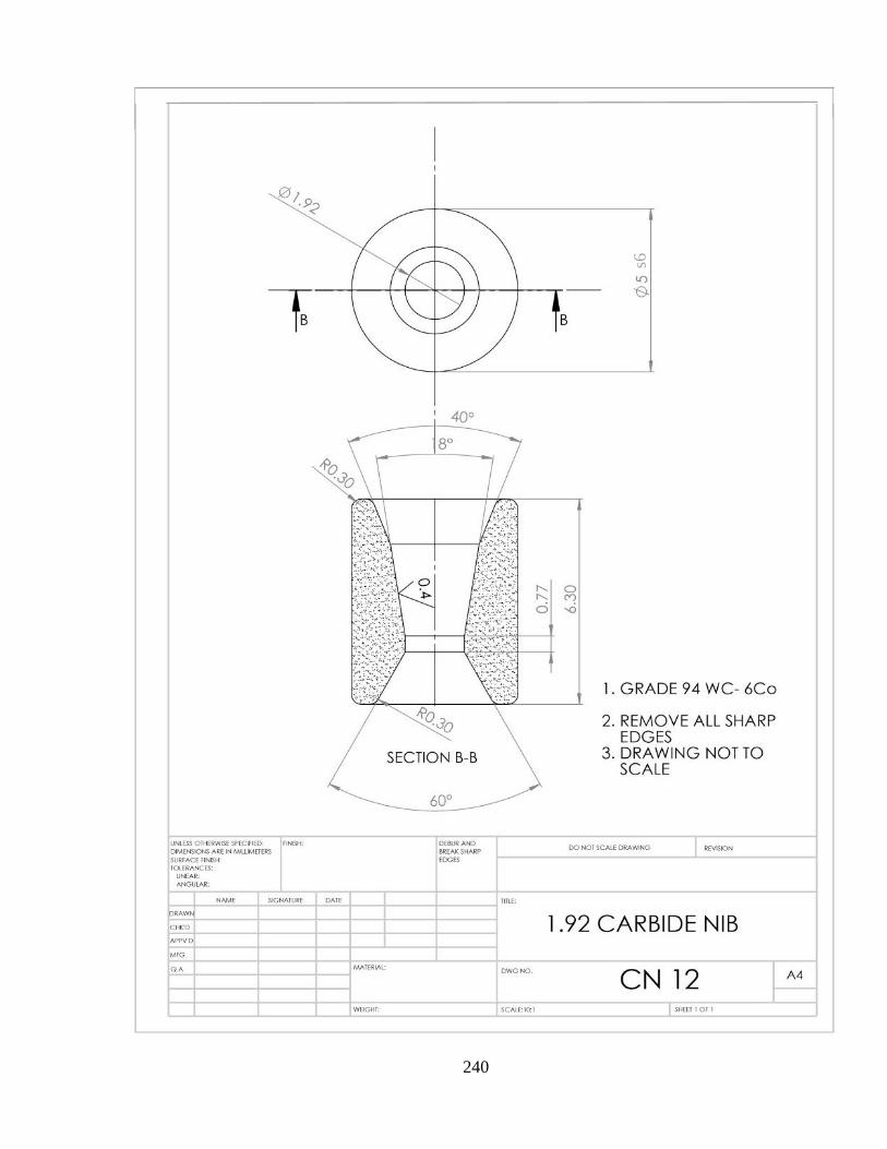
240
s6
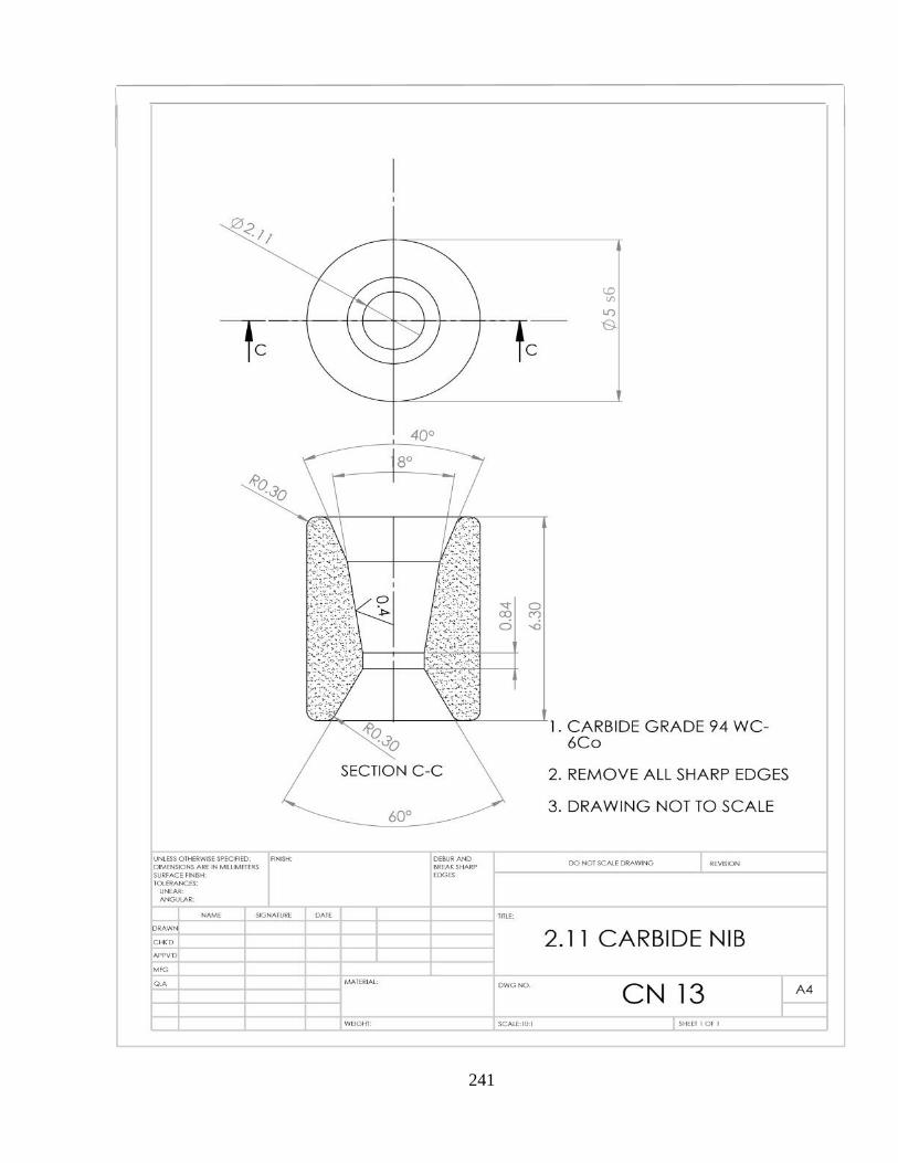
241
s6

242
s6
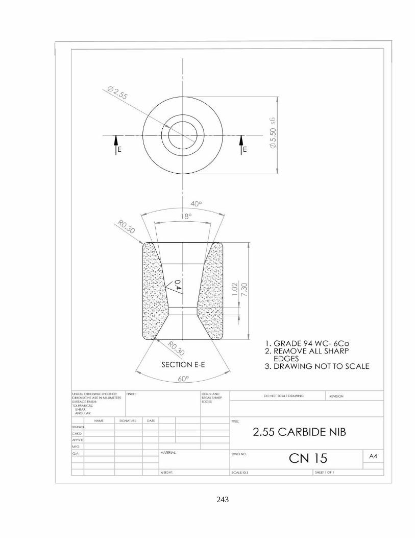
243
s6
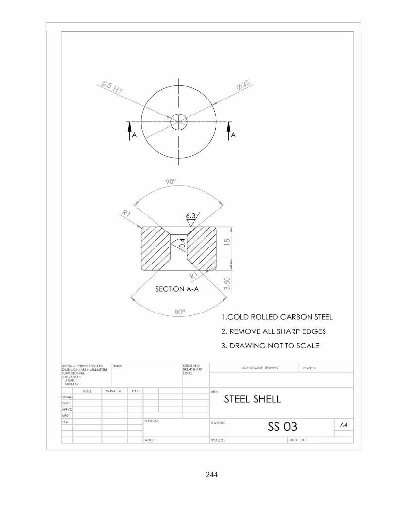
244