Effective two-phase flow in heterogeneous media under temporal

pressure fluctuations

Diogo Bolster,1 Marco Dentz,1 and Jesus Carrera2

Received 17 September 2008; revised 11 February 2009; accepted 20 February 2009; published 9 May 2009.

[1] We study the combined effect of spatial heterogeneity and temporal pressurefluctuations on the dispersion of the saturation of a displacing fluid during injection intoan immiscible one. In a stochastic modeling framework, we define two different dispersionquantities, one which measures the front uncertainty due to temporal pressurefluctuations and another one which quantifies the actual spreading and dispersion of thesaturation front in a typical medium realization. We derive an effective large-scale flowequation for the saturation of the displacing fluid that is characterized by a nonlocaldispersive flux term. From the latter we derive measures for the spread of the saturationfront due to spatiotemporal fluctuations. Our analysis demonstrates that temporalfluctuations enhance the front uncertainty but not the average spreading of the saturationfront. The analytical developments are complemented by numerical simulations of the fulltwo-phase flow problem. Correct assessment of the spread of the saturation front is ofimportance to several applications, including the assessment of the sequestration potentialof a carbon dioxide storage site, for example. Spreading enhances the surface area betweenthe fluids, which in turn enhances the dissolution and entrapment efficiency. The latterfacilitates reactions and thus the sequestration of CO2 in stable forms. Our study providesa theoretical basis for the design of injection strategies to optimize dispersion and tominimize uncertainty of the saturation front.

Citation: Bolster, D., M. Dentz, and J. Carrera (2009), Effective two-phase flow in heterogeneous media under temporal pressure

fluctuations, Water Resour. Res., 45, W05408, doi:10.1029/2008WR007460.

1. Introduction

[2] The injection of one fluid into another in geologicalporous media is one of great interest in the fields ofpetroleum engineering [Lake, 1989], gas storage and morerecently, with the ever increasing awareness of climatechange, the sequestration of anthropogenic CO2 in deepsaline aquifers [Bachu, 2000]. The study of such flowsrequires a multiphase modeling approach and a manner tostudy this is to manipulate the mass balance equations of theindividual phases in such a manner as to write governingequations that look similar to advection-dispersion equa-tions for single phase flows. According to Bear [1972], amultiphase flow problem can be cast into an equation thatlooks much like an advection-dispersion type equation forthe saturation S(x, t) of an immiscible fluid such that

@S x; tð Þ@t

þ v x; S x; tð Þ½ � � rS x; tð Þ

þ r � D x; S x; tð Þ½ �rS x; tð Þ ¼ 0: ð1Þ

[3] Note that the latter is highly nonlinear as the drift v aswell as the dispersion coefficient D depend on the saturation

S(x, t) via the dependence of capillary pressure and relativepermeability on saturation as will be outlined below. While(1) has the appearance of an advection-diffusion equationcaution must be taken with this analogy as the nonlinearitiescan lead to behavior that is very different from the tradi-tional linear advection diffusion equation used for solutetransport.[4] Multiphase flow in homogeneous porous media has

been studied extensively over the years [Marle, 1981, andreferences therein]. However, in most geological porousmedia the properties of the medium, such as the permeabil-ity, fluctuate over a large range of values. From a practicalperspective it is desirable to describe the flow through sucha medium on a large scale, which requires a qualitative andquantitative understanding of the impact of small-scaleheterogeneities and temporal pressure fluctuations on theeffective flow behavior. While it is not necessarily possibleto resolve the full medium heterogeneity on all scales, it isnot generally necessary to do so as we are typically seekingan integral understanding of the system behavior on a largescale. Stochastic modeling [e.g., Dagan, 1989; Gelhar,1993] provides an efficient and systematic framework tointegrate spatiotemporal fluctuations into an effective flowdescription and to assess fluctuation-induced uncertaintiesof the large-scale system characteristics. With this approachthe permeability field is modeled as a typical realization ofan (ergodic) correlated spatial random process and temporalpressure fluctuations are modeled as an (ergodic) correlatedtemporal random process [e.g., Dentz and Carrera, 2003].The results presented herein are readily extendable to

1Department of Geotechnical Engineering and Geosciences, TechnicalUniversity of Catalonia, Barcelona, Spain.

2Institute of Environmental Analysis and Water Studies, CSIC,Barcelona, Spain.

Copyright 2009 by the American Geophysical Union.0043-1397/09/2008WR007460$09.00

W05408

WATER RESOURCES RESEARCH, VOL. 45, W05408, doi:10.1029/2008WR007460, 2009ClickHere

for

FullArticle

1 of 14

periodic fluctuation patterns too. The effective flow behav-ior can then be determined by averaging of all possiblerealizations of the respective ensembles [e.g., Tartakovskyand Neuman, 1998b, 1998a]. It is often tacitly assumed thatthe ensemble averaged flow parameters are representative ofthe effective large-scale behavior within a single realization.This, however, is not self-evident. The physical meaning oflarge-scale coefficients depends intrinsically on how theyare defined as an ensemble average.[5] Many multiphase flow processes, including the afore-

mentioned oil displacement and carbon sequestration prob-lems, are modeled as ideal displacements, which consist ofone fluid displacing another immiscible one. In theseapplications quantifying the spread of the saturation frontdue to heterogeneities can be an important task. In order tooptimize oil recovery one may want to minimize suchspreading effects, while for the geological sequestration ofCO2 it may be desirable to maximize the surface areabetween the CO2 and the host fluid in order to increasedissolution and entrapment of CO2, thus enhancing seques-tration efficiency.[6] For the case of single phase solute transport it is well

known that the heterogeneities lead to a heterogeneous flowpath structure, resulting in greater travel distances along onepath compared to another [e.g., Kitanidis, 1988; Dentz etal., 2000; Fiori, 2001; Cirpka and Attinger, 2003; Dentzand Carrera, 2003]. This results in greater mixing on themacroscale, which can be captured by a macrodispersionterm [e.g.,Gelhar and Axness, 1983;Dagan, 1989]. Becauseof the formal similarity of the advection-dispersion equationfor the transport of a solute and the nonlinear advection-dispersion type equation (1) for the saturation one mightexpect a similar mixing effect by the heterogeneities in animmiscible displacement flow. As the two fluids are immis-cible, macrodispersion here does not reflect physical mix-ing, but rather a spreading of the saturation distribution.[7] Langlo and Espedal [1995] explicitly determined a

macrodispersion coefficient that models the dispersive fluxin an effective equation for the saturation of the wettingphase in immiscible two-phase flow. They used a perturba-tion approach in flow scenarios with and without capillaryforces. Their result for the macrodispersion coefficient issimilar to the one obtained for heterogeneity-induced solutespreading in single phase flow.[8] Cvetkovic and Dagan [1996] studied this macrodis-

persion effect in an immiscible flow scenario using theBuckley-Leverett approximation, i.e., disregarding capillarypressure and gravity. Applying a Lagrangian perturbationapproach they found a dispersive large-scale effect, which,however, is not explicitly determined.[9] Neuweiler et al. [2003] used a perturbation theory

approach in order to determine a large-scale mixing param-eter for the displacing fluid for the flow problem in a twodimensional heterogeneous porous medium. They devel-oped an explicit definition of a large-scale mixing coeffi-cient for the nonlinear problem.[10] Kinzelbach and Ackerer [1986] and Rehfeldt and

Gelhar [1992] pointed out that temporal pressure fluctua-tions can lead to enhanced solute dispersion in heteroge-neous media. Dentz and Carrera [2003] and Cirpka andAttinger [2003] quantify the interaction of temporal pressurefluctuations and spatial heterogeneity using a perturbation

analysis in the fluctuations of the spatial and temporalrandom fields.[11] In section 2 we present the mathematical model that

we use to study this problem. In section 3 we quantify theimpact of medium heterogeneities on the effective large-scale flow behavior, which, using moments, we quantify bya ‘‘macrodispersion’’ coefficient. We also define an ensem-ble quantity that measures the uncertainty of the saturationfront due to spatiotemporal fluctuation. In section 4 westudy the problem at hand numerically and quantitativelycompare the results.

2. Model

2.1. Two-Phase Flow

[12] The flow of two immiscible fluids in a porousmedium is described by the coupledmomentum conservationand mass conservation equations. Momentum conservationis expressed by Darcy’s law, which reads as [Bear, 1972]

q ið Þ x; tð Þ ¼ k xð Þkri Sið Þmi

rpi x; tð Þ þ rige3½ �; ð2Þ

where q(i)(x, t) and pi(x, t) are specific discharge andpressure of fluid i, mi and ri are viscosity and density offluid i, k(x) is the intrinsic permeability of the porousmedium, kri[Si(x, t)] is the relative permeability of phase i(which depends on saturation); e3 denotes the unit vector in3 direction. Mass conservation for each fluid is given by[Bear, 1972]

@

@twriSi x; tð Þ þ r � riq ið Þ x; tð Þ ¼ 0: ð3Þ

[13] We assume here that the medium and the fluid areincompressible so that porosity w and density ri of eachfluid are constant. The saturations Si of each fluid sum up toone and the difference of the pressures in each fluid definesthe capillary pressure pc(S)

S1 þ S2 ¼ 1 ð4Þ

p1 p2 ¼ pc S1ð Þ; ð5Þ

where i = 1 indicates the nonwetting fluid. In the followingwe focus on the saturation of fluid 1 and drop the subscriptin the following. From the incompressibility conditions andmass conservation, it follows that the divergence of the totalspecific discharge q(x, t) = q(1)(x, t) + q(2)(x, t) is zero:

r � q x; tð Þ ¼ 0: ð6Þ

Eliminating q(1)(x, t) from equation (3) in favor of q(x, t),one obtains [Bear, 1972]

@S x; tð Þ@t

þ @

@Sy Sð Þ q x; tð Þ þ k xð Þl2 Sð ÞgDre3ð Þ½ � � rS x; tð Þ

þ y Sð Þl2 Sð ÞgDr@k xð Þ@x3

r

� y Sð Þk xð Þl2 Sð Þ dpc Sð ÞdS

rS x; tð Þ� �

¼ 0; ð7Þ

2 of 14

W05408 BOLSTER ET AL.: EFFECTIVE TWO-PHASE FLOW IN HETEROGENEOUS MEDIA W05408

where Dr = r2 r1. We set w = 1 for simplicity (which isequivalent to rescaling time). The fractional flow functiony(S) is defined by

y Sð Þ ¼ l1 Sð Þl1 Sð Þ þ l2 Sð Þ ; ð8Þ

where the phase mobilities li are defined as the ratio ofrelative permeability to fluid viscosity, li = ki(S)/mi.Equation (7) is similar to (1) and in the absence of thebuoyancy term it is identical; the nonlinear drift v(t) isdefined by the second term and the nonlinear (capillary)dispersion coefficient by the third term on the right of (7).[14] Here, we want to focus on problems where viscous

forces dominate the flow and as such we neglect theinfluence of buoyancy and capillary pressure. This problemof immiscible two phase viscous dominated flow is com-monly known as the Buckley-Leverett problem. With theseapproximations, the governing equation (7) reduces to theBuckley-Leverett equation

@S x; tð Þ@t

þ dy Sð ÞdS

q x; tð Þ � rS x; tð Þ ¼ 0: ð9Þ

[15] In this work we consider the commonly studiedproblem of one fluid displacing another immiscible one.As was done by Neuweiler et al. [2003], we focus on fluidmovement in a horizontal two-dimensional porous mediumwhich is initially filled with fluid 2. Such a scenarioeliminates buoyancy effects. We focus on neutrally stabledisplacement cases. Fluid 1 is injected along a line at a fixedrate, displacing fluid 2. We consider flow far away from thedomain boundaries and thus disregard boundary effects.The resulting mean pressure gradient is then aligned with theone direction of the coordinate system. The correspondinghomogeneous multiphase flow problem is d = 1 dimensional.

2.2. Homogeneous Solution

[16] Before studying the heterogeneous problem webriefly summarize the classical homogeneous case here.We denote the homogeneous solution as S0 as this corre-sponds to the zeroth-order perturbation solution outlined inAppendix A. The governing equation is given by

@S0 x; tð Þ@t

þ q tð Þ dy S0ð ÞdS0

@S0 x; tð Þ@x1

¼ 0: ð10Þ

The solution of this problem is discussed extensively inmany textbooks [e.g., Marle, 1981]. Because of thehyperbolic nature of (10) the displacing fluid develops ashock front. Using the method of characteristics and theshock condition, one derives for S0(x, t)

S0 x1; tð Þ ¼ Srx1

xf tð Þ

� �H xf tð Þ x1� �

; ð11Þ

where H(x) is the heaviside step function [Abramowitz andStegun, 1970] and the front position xf(t) is obtained frommass balance considerations as

xf tð Þ ¼dy Sf

� �dSf

Z t

0

dt0q t0ð Þ; ð12Þ

with Sf the front saturation. The latter is determined by theWelge tangent method [e.g., Marle, 1981]. The rearsaturation Sr[x1/xf(t)] behind the shock front is obtained by

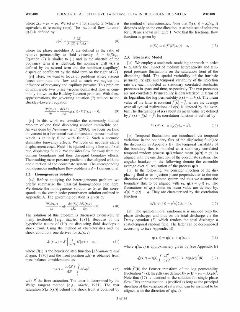
the method of characteristics. Note that S0(x, t) = S0(x1, t)depends only on the one direction. A sample set of solutionsfor (10) are shown in Figure 1. Note that the fractional flowfunction is given by

y S0ð Þ ¼ y Srð ÞH xf tð Þ x1� �

: ð13Þ

2.3. Stochastic Model

[17] We employ a stochastic modeling approach in orderto quantify the impact of medium heterogeneity and tem-poral pressure fluctuations on the saturation front of thedisplacing fluid. The spatial variability of the intrinsicpermeability k(x) and temporal variability of the injectionrate are each modeled as stationary correlated stochasticprocesses in space and time, respectively. The two processesare not correlated. Permeability is characterized in terms ofits logarithm, the log permeability f(x) = ln k(x). The mean

value of the latter is constant f xð Þ = f , where the averageover all typical realizations of k(x) is denoted by the over-bar. The fluctuations of f(x) about its mean value are definedby f 0(x) = f(x) f . Its correlation function is defined by

f 0 xð Þf 0 x0ð Þ � s2ff Cff x x0ð Þ: ð14Þ

[18] Temporal fluctuations are introduced via temporalvariations in the boundary flux of the displacing fluid(seethe discussion in Appendix B). The temporal variability ofthe boundary flux is modeled as a stationary correlatedtemporal random process q(t) whose mean hq(t)i = qe1 isaligned with the one direction of the coordinate system. Theangular brackets in the following denote the ensembleaverage over all realization of the process q(t).[19] In the following, we consider injection of the dis-

placing fluid at an injection plane perpendicular to the onedirection of the coordinate system and thus we assume theboundary flux to be aligned with e1, q(t) = q(t) e1. Thefluctuations of q(t) about its mean value are defined by,q0(t) = q(t) q. They are characterized by the correlationfunction

hq0 tð Þq0 t0ð Þi ¼ q2s2t Ct t t0ð Þ: ð15Þ

[20] The spatiotemporal randomness is mapped onto thephase discharges and thus on the total discharge via theDarcy equation (2), which renders the total discharge aspatiotemporal random field. The latter can be decomposedaccording to (see Appendix B)

q x; tð Þ ¼ q tð Þe1 þ q0 x; tð Þ; ð16Þ

where q0(x, t) is approximately given by (see Appendix B)

q0i x; tð Þ ¼ q tð ÞZ

dkd

2pð Þdexp ik � xð Þpi kð Þ~f 0 kð Þ; ð17Þ

with ~f 0(k) the Fourier transform of the log permeabilityfluctuation f 0(x); the pi(k) are defined by pi(k) = di1 kik1/k

2.Note that (17) is identical to the solution for single phaseflow. This approximation is justified as long as the principaldirection of the variation of saturation can be assumed to bealigned with the direction of q(x, t).

W05408 BOLSTER ET AL.: EFFECTIVE TWO-PHASE FLOW IN HETEROGENEOUS MEDIA

3 of 14

W05408

[21] Thus, we obtain for the velocity correlation

q0i x; tð Þq0j x0; t0ð Þ � s2ff Cij x x0ð Þq tð Þq t0ð Þ; ð18Þ

where we defined

Cij xð Þ ¼Z

dkd

2pð Þdexp ik � xð Þpi kð Þpj kð Þ~Cff kð Þ; ð19Þ

where ~Cff (k) is the Fourier transform of the log conductivityfluctuations.[22] Here we have found specific conditions under which

we approximate the covariance of the velocity field as thecovariance of a single phase flow field. However, one mustbe cautious in doing this as this may not be correct for theunstable or stabilizing cases. In the unstable case viscousfingering dominates while for the stabilizing case thevelocity field is no longer stationary as the velocity variancein the vicinity of the front is suppressed [e.g., Noetinger etal., 2004].

3. Large-Scale Flow Behavior

[23] In the following, we derive large-scale flow equa-tions by averaging the original local-scale flow equation.We define measures for the front spreading due to spatio-temporal fluctuations and for the front uncertainty due totemporal fluctuations. On the basis of these considerationswe suggest a large-scale effective flow equation for theaverage saturation.

3.1. Average Flow Equation

[24] In analogy to solute transport in heterogeneousmedia [e.g., Gelhar and Axness, 1983; Koch and Brady,

1987; Neuman, 1993; Cushman et al., 1994], here the spreadof the space average saturation front S x; tð Þ due to spatialheterogeneity is modeled by a non-Markovian effectiveequation. Note that an effective equation is in general non-Markovian [e.g., Zwanzig, 1961;Kubo et al., 1991;Koch andBrady, 1987;Cushman et al., 1994;Neuman, 1993], which isexpressed by spatiotemporal nonlocal flux terms. Undercertain conditions, these fluxes can be localized.[25] We follow the methodology routinely applied when

deriving average dynamics [e.g., Koch and Brady, 1987;Neuman, 1993; Cushman et al., 1994; Tartakovsky andNeuman, 1998a], which consists of (1) separating thesaturation into mean and fluctuating components, (2) estab-lishing a (nonclosed) system of equations for the averagesaturation and the saturation fluctuations, and (3) closing thesystem by disregarding terms that are of higher order in thefluctuations. It is known that perturbative solutions ofadvective-dispersion equations can sometimes result inbimodal behavior of averaged concentration fields [Jarmanand Russell, 2003; Morales-Casique et al., 2006; Jarmanand Tartakovsky, 2008]. However, herein we do not encoun-ter such concerns.[26] Substituting (16) into (19) the local-scale equation

for the saturation S(x, t) is given by

@S x; tð Þ@t

þ q tð Þ � ry Sð Þ þ q0 x; tð Þ � ry Sð Þ ¼ 0: ð20Þ

[27] In analogy to the decomposition of total dischargeand permeability, we assume that the saturation can bedecomposed into its spatial ensemble average S x; tð Þ �S x; tð Þ and fluctuations about it:

S x; tð Þ ¼ S x; tð Þ þ S0 x; tð Þ: ð21Þ

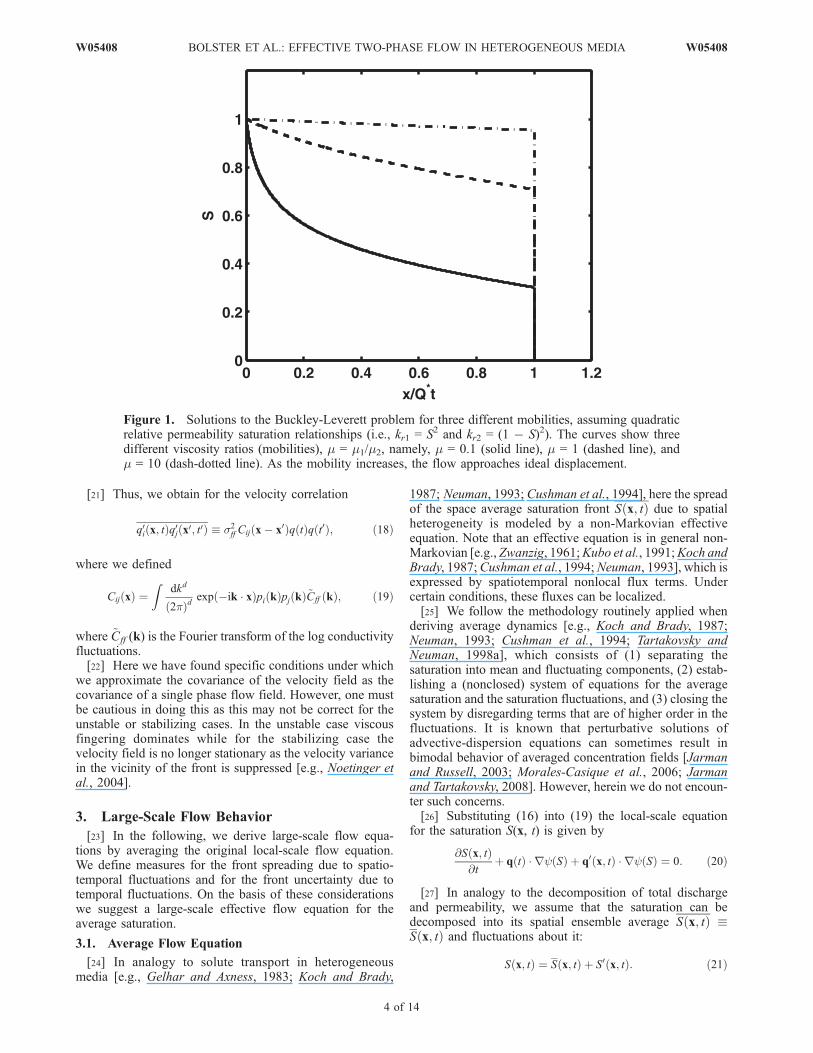
Figure 1. Solutions to the Buckley-Leverett problem for three different mobilities, assuming quadraticrelative permeability saturation relationships (i.e., kr1 = S2 and kr2 = (1 S)2). The curves show threedifferent viscosity ratios (mobilities), m = m1/m2, namely, m = 0.1 (solid line), m = 1 (dashed line), andm = 10 (dash-dotted line). As the mobility increases, the flow approaches ideal displacement.

4 of 14

W05408 BOLSTER ET AL.: EFFECTIVE TWO-PHASE FLOW IN HETEROGENEOUS MEDIA W05408

[28] Furthermore assuming that the saturation fluctua-tions are small, we can expand the fractional flow functionabout the mean saturation according to

y Sð Þ ¼ y S� �

þdy S

� �dS

S0 x; tð Þ þ . . . : ð22Þ

We take this expansion to O(S0) only as it has been shownthat higher-order terms play an unimportant role [Efendievand Durolfsky, 2002; Neuweiler et al., 2003].[29] Inserting (21) and (22) into (20), we obtain

@S x; tð Þ@t

þ @S0 x; tð Þ@t

þ q tð Þ � ry S� �

þ q tð Þ � rdy S

� �dS

S0 x; tð Þ

þ q0 x; tð Þ � ry S� �

¼ q0 x; tð Þ � rdy S

� �dS

S0 x; tð Þ: ð23Þ

[30] Averaging the latter over the spatial ensemble gives

@S x; tð Þ@t

þ q tð Þ � ry S� �

¼ r � q0 x; tð ÞS0 x; tð Þdy S

� �dS

: ð24Þ

Subtracting (24) from (23), we obtain an equation for thesaturation fluctuations

@S0 x; tð Þ@t

þ q tð Þ � rdy S

� �dS

S0 x; tð Þ ¼ q0 x; tð Þ � ry S� �

q0 x; tð Þ � rdy S

� �dS

S0 x; tð Þ þ r � q0 x; tð ÞS0 x; tð Þdy S

� �dS

: ð25Þ

This system of equations is not closed with respect to theaverage saturation. Our closure approximation consists indisregarding terms which are quadratic in the fluctuations in(25). Thus (25) reduces to

@S0 x; tð Þ@t

þ q tð Þ � rdy S

� �dS

S0 x; tð Þ ¼ q0 x; tð Þ � ry S� �

: ð26Þ

This is then solved with the associated Green function, i.e.,

S0 x; tð Þ ¼ Z t

0

Zddx0G x; tjx0; t0ð Þq0 x0; t0ð Þ � r0y S x0; t0ð Þ

� �; ð27Þ

where G(x, tjx0, t0) solves

@G x; tjx0; t0ð Þ@t

þ q tð Þ � rdy S

� �dS

G0 x; tjx0; t0ð Þ ¼ 0 ð28Þ

for the initial condition G(x, tjx0, t0) = d(x x0). Inserting(26) into (24), we obtain a nonlinear upscaled equation forthe (space) average saturation

@S x; tð Þ@t

þ q tð Þ �d S

� �dS x; tð Þ

rS x; tð Þ

r �Z t

0

dt0Z

ddx0dy S

� �dS x; tð Þ

k x; tjx0; t0ð Þdy S

� �dS x0; t0ð Þ

" #r0S x0; t0ð Þ ¼ 0;

ð29Þ

where we define the kernel

kij x; tjx0; t0ð Þ ¼ q0i x; tð ÞG x; tjx0; t0ð Þq0j x0; t0ð Þ: ð30Þ

[31] Equation (29) has a similar structure as (1), but ischaracterized by a spatiotemporal nonlocal dispersive flux.As outlined above, such nonlocal fluxes typically occurwhen averaging. Note that the nonlinear character of thetwo-phase problem is preserved during the upscaling exer-cise. The nonlinearity of the problem is quasi-decoupled interms of the Green function; equation (28) for G(x, tjx0, t0) islinear but depends on the average saturation. Appendix Cprovides explicit perturbation theory expressions for theGreen function.

3.2. The Kernel

[32] Approximating the Green function G(x, tjx0, t0) by(C4), where we assume that the average saturation isreasonably represented by the homogeneous zeroth-ordersaturation S0 according to

G x; tjx0; t0ð Þ ¼ G0 x1; tjx01; t0� �

d y y0ð Þ: ð31Þ

The kernel, defined in (30), becomes

kij x; tjx0; t0ð Þ ¼ kij x1; tjx01; t0� �

d y y0ð Þ; ð32Þ

where kij(x1, tjx01, t0) is defined by

kij x1; tjx01; t0� �

¼ s2ff Cij x1 x01

� �q tð Þq t0ð Þ 1

x1 tð Þ dx01

x1 t0ð Þ x1

x1 tð Þ

� �:

ð33Þ

Here we set Cij(x1, t, t0) � Cij(x, t, t

0)jy=0 and x1(t) =Rt0

dt0q(t0). In the following section, we determine effectivemeasures for the spread of the front saturation depending onthe kernel kij(x1, tjx01, t0). Contributions in transversedirections vanish, because of the particular displacementscenario under consideration [see also Neuweiler et al.,2003]. Thus, we focus our attention on the spread of thesaturation in one direction.

3.3. Saturation Dispersion

[33] We quantify the front spreading in single realizationsof the temporal random process in terms of spatial momentsand then perform the ensemble average over the resultingobservables. This procedure quantifies the combined effectof spatial and temporal fluctuations on the spread of thesaturation front. Later we quantify the uncertainty of thefront position due to purely temporal fluctuations. AppendixF illustrates the definitions of macrodispersion presented byNeuweiler et al. [2003] and Langlo and Espedal [1995] interms of our developments here.3.3.1. Spatial Moment Equations[34] The objective here is to quantify the impact of

heterogeneity and temporal fluctuations on the spread ofthe saturation front. In analogy to transport in single phaseflow and given the similarity of the large-scale flowequation (29) with the advection-dispersion equation it istempting to quantify the spread of the saturation distributionin terms of its spatial moments. However, the displacementof one fluid by another corresponds to a continuous injec-

W05408 BOLSTER ET AL.: EFFECTIVE TWO-PHASE FLOW IN HETEROGENEOUS MEDIA

5 of 14

W05408

tion in the analog case of solute transport in single phaseflow. In the latter case, the spreading of the solute frontcannot be quantified satisfactorily by the moments of theconcentration distribution, but rather by the moments of itsderivative in flow direction. Thus, here, instead of consid-ering moments of saturation, we consider the moments ofthe derivative of the saturation in the i direction:

si x; tð Þ ¼ A1 @S x; tð Þ@xi

; ð34Þ

where A is the area of the injection plane located at x1 = 0.This is motivated by the fact that the homogeneous solutiondevelops a shock front, which is captured sharply by aderivative. We now normalize s1(x, t) to 1:Z

x1>0

ddxs1 x; tð Þ ¼ 1: ð35Þ

[35] The first and second moments of s1(x, t) in the onedirection are given by

m1ð Þ1 ¼

Zddxxis1 x; tð Þ and m

2ð Þ11 ¼

Zddxx2i s1 x; tð Þ: ð36Þ

With these we can calculate the second centered moment,k11 = m11

(2) m1(1)m1

(1), which we can use to define aneffective longitudinal dispersion coefficient. The equationgoverning the evolution of k11 is derived in Appendix Dand is given by

@k11 tð Þ@t

¼ q tð Þ 2A1

Zddxy S x; tð Þ

� �Z t

0

dt0q t0ð Þ

24

35

2A1

Zddx

Z t

0

dt0Z

ddx0dy S

� �dS x; tð Þ

k1j x; tjx0; t0ð Þ

� @

@x0jy S x0; t0ð Þ� �

: ð37Þ

We identify the second term as the one that measures theactual spread of the saturation front due to spatialheterogeneity. In the absence of heterogeneity, the widthof the saturation distribution behind the shock front isquantified by the first term on the right side. In that case, itquantifies a purely advective widening due to different flowvelocities at the front and behind the front (see AppendixG). It grows in leading order with the square of time.Nevertheless, the saturation dispersion at the front acts(nonlinearly) on the width of the saturation distributionbehind the disperse front.3.3.2. Front Dispersion[36] We now define the longitudinal macrodispersion

coefficient diis (t) in terms of the second term on the right

side of (37) by

ds11 tð Þ ¼ A1

Zddx

Z t

0

dt0Z

ddx0dy S

� �dS x; tð Þ

k1j x; tjx0; t0ð Þ

@

@x0jy S x0; t0ð Þ� �

: ð38Þ

In order to evaluate (38), we approximate the averagesaturation by S = S0(x1, t), and substitute the kernel (32) toobtain

ds11 tð Þ ¼ s2ff

Zdx1

Z t

0

dt0Z10

dx01x1

x1 tð ÞC11 x1 x01� �

q tð Þq t0ð Þ

� 1

x1 tð Þ dx01

x1 t0ð Þ x1

x1 tð Þ

� �@

@x01y S0

x01xf t0ð Þ

� �� �; ð39Þ

where we used expression (C1) for dy(S0)/dS0.[37] As outlined in Appendix E this can be simplified to

ds11 tð Þ ¼ s2ff q tð Þ

Zqt0

dx1C11 x1ð Þ þ s2ff

Z t

0

dt0q0 t0ð Þq tð ÞC11 qtð Þ: ð40Þ

On average this gives

ds11 tð Þ� �

¼ s2ff q

Zqt0

dx1C11 x1ð Þ þ s2ff s

2t q

2C11 qtð ÞZ t

0

dt0Ct t0ð Þ:

ð41Þ

The contribution due to temporal fluctuations decays to zerowith increasing time as C11(qt) tends to zero for times largerthan tu = l/q. Thus, there is no significant contribution tofront spreading due to temporal fluctuations. This isdifferent from solute transport in single phase flow. In thiscase, there is a persistent macroscopic dispersion effect dueto the interaction of spatial heterogeneity, temporal fluctua-tions [Dentz and Carrera, 2003] and local dispersion. Thelatter is the crucial (irreversible) mechanism, whichactivates heterogeneity and temporal fluctuations as amacroscopic spreading effect. Here, such irreversibility islacking. The multiphase flow problem is fully reversible.Thus, temporal fluctuations play only a minor role for frontspreading. In the presence of capillary dispersion asexpressed by the nonlinear dispersive flux in (7), this maybe different. However, this must be investigated in moredetail as the influence of such a nonlinear dispersive flux isnot obvious.[38] The uncertainty associated with the front location

due to temporal pressure fluctuations can be quantified interms of the moments defined above as

s2m tð Þ ¼ m1 tð Þ m

1ð Þ1 tð Þ

D Eh i2� �: ð42Þ

Inserting (D3) into (42), we obtain

s2m tð Þ ¼ q2s2

t

Z t

0

dt0Z t

0

dt00Ct t0 t00ð Þ: ð43Þ

Thus, the front uncertainty grows linearly with time forshort-range temporal correlation of the pressure fluctua-tions. Note that the temporal center of mass fluctuationsgive rise to an artificial (ensemble) dispersion effect, whichoccurs for the saturation distribution averaged over the

6 of 14

W05408 BOLSTER ET AL.: EFFECTIVE TWO-PHASE FLOW IN HETEROGENEOUS MEDIA W05408

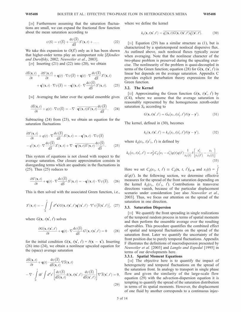
temporal ensemble. A measure for this ensemble dispersioneffect is the temporal derivative of (43), i.e., 1

2

ds2m tð Þdt

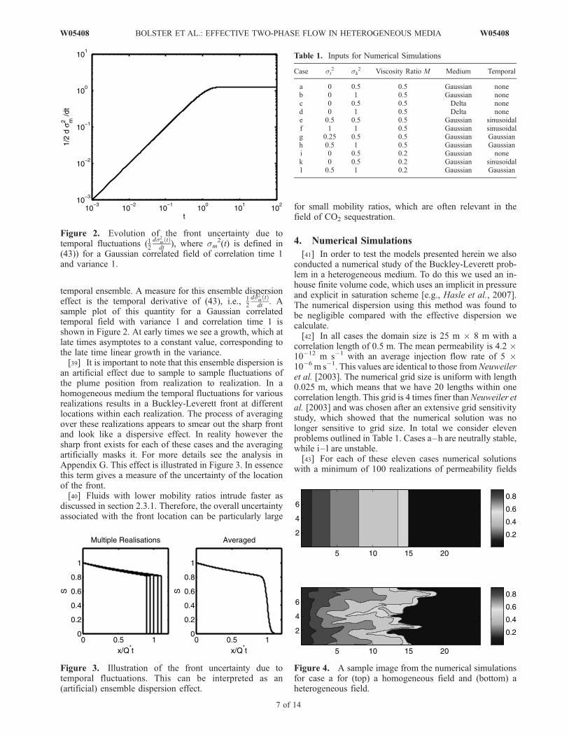
. Asample plot of this quantity for a Gaussian correlatedtemporal field with variance 1 and correlation time 1 isshown in Figure 2. At early times we see a growth, which atlate times asymptotes to a constant value, corresponding tothe late time linear growth in the variance.[39] It is important to note that this ensemble dispersion is

an artificial effect due to sample to sample fluctuations ofthe plume position from realization to realization. In ahomogeneous medium the temporal fluctuations for variousrealizations results in a Buckley-Leverett front at differentlocations within each realization. The process of averagingover these realizations appears to smear out the sharp frontand look like a dispersive effect. In reality however thesharp front exists for each of these cases and the averagingartificially masks it. For more details see the analysis inAppendix G. This effect is illustrated in Figure 3. In essencethis term gives a measure of the uncertainty of the locationof the front.[40] Fluids with lower mobility ratios intrude faster as

discussed in section 2.3.1. Therefore, the overall uncertaintyassociated with the front location can be particularly large

for small mobility ratios, which are often relevant in thefield of CO2 sequestration.

4. Numerical Simulations

[41] In order to test the models presented herein we alsoconducted a numerical study of the Buckley-Leverett prob-lem in a heterogeneous medium. To do this we used an in-house finite volume code, which uses an implicit in pressureand explicit in saturation scheme [e.g., Hasle et al., 2007].The numerical dispersion using this method was found tobe negligible compared with the effective dispersion wecalculate.[42] In all cases the domain size is 25 m � 8 m with a

correlation length of 0.5 m. The mean permeability is 4.2 �1012 m s1 with an average injection flow rate of 5 �106 m s1. This values are identical to those fromNeuweileret al. [2003]. The numerical grid size is uniform with length0.025 m, which means that we have 20 lengths within onecorrelation length. This grid is 4 times finer thanNeuweiler etal. [2003] and was chosen after an extensive grid sensitivitystudy, which showed that the numerical solution was nolonger sensitive to grid size. In total we consider elevenproblems outlined in Table 1. Cases a–h are neutrally stable,while i–l are unstable.[43] For each of these eleven cases numerical solutions

with a minimum of 100 realizations of permeability fields

Figure 2. Evolution of the front uncertainty due totemporal fluctuations (1

2

ds2mðtÞdt

), where sm2(t) is defined in

(43)) for a Gaussian correlated field of correlation time 1and variance 1.

Figure 3. Illustration of the front uncertainty due totemporal fluctuations. This can be interpreted as an(artificial) ensemble dispersion effect.

Table 1. Inputs for Numerical Simulations

Case st2 sk

2 Viscosity Ratio M Medium Temporal

a 0 0.5 0.5 Gaussian noneb 0 1 0.5 Gaussian nonec 0 0.5 0.5 Delta noned 0 1 0.5 Delta nonee 0.5 0.5 0.5 Gaussian sinusoidalf 1 1 0.5 Gaussian sinusoidalg 0.25 0.5 0.5 Gaussian Gaussianh 0.5 1 0.5 Gaussian Gaussiani 0 0.5 0.2 Gaussian nonek 0 0.5 0.2 Gaussian sinusoidall 0.5 1 0.2 Gaussian Gaussian

Figure 4. A sample image from the numerical simulationsfor case a for (top) a homogeneous field and (bottom) aheterogeneous field.

W05408 BOLSTER ET AL.: EFFECTIVE TWO-PHASE FLOW IN HETEROGENEOUS MEDIA

7 of 14

W05408

were conducted. The effective dispersion coefficient wasthen calculated using (D3), (D4) and (38).[44] A sample contour of the saturation field for a

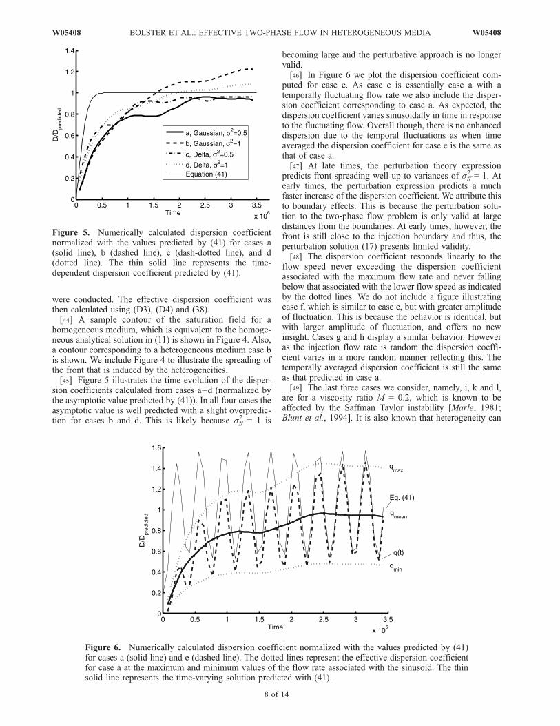
homogeneous medium, which is equivalent to the homoge-neous analytical solution in (11) is shown in Figure 4. Also,a contour corresponding to a heterogeneous medium case bis shown. We include Figure 4 to illustrate the spreading ofthe front that is induced by the heterogeneities.[45] Figure 5 illustrates the time evolution of the disper-

sion coefficients calculated from cases a–d (normalized bythe asymptotic value predicted by (41)). In all four cases theasymptotic value is well predicted with a slight overpredic-tion for cases b and d. This is likely because sff

2 = 1 is

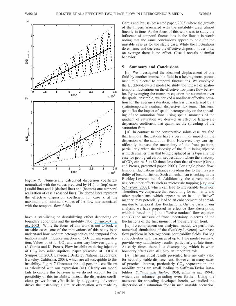
becoming large and the perturbative approach is no longervalid.[46] In Figure 6 we plot the dispersion coefficient com-

puted for case e. As case e is essentially case a with atemporally fluctuating flow rate we also include the disper-sion coefficient corresponding to case a. As expected, thedispersion coefficient varies sinusoidally in time in responseto the fluctuating flow. Overall though, there is no enhanceddispersion due to the temporal fluctuations as when timeaveraged the dispersion coefficient for case e is the same asthat of case a.[47] At late times, the perturbation theory expression

predicts front spreading well up to variances of sff2 = 1. At

early times, the perturbation expression predicts a muchfaster increase of the dispersion coefficient. We attribute thisto boundary effects. This is because the perturbation solu-tion to the two-phase flow problem is only valid at largedistances from the boundaries. At early times, however, thefront is still close to the injection boundary and thus, theperturbation solution (17) presents limited validity.[48] The dispersion coefficient responds linearly to the

flow speed never exceeding the dispersion coefficientassociated with the maximum flow rate and never fallingbelow that associated with the lower flow speed as indicatedby the dotted lines. We do not include a figure illustratingcase f, which is similar to case e, but with greater amplitudeof fluctuation. This is because the behavior is identical, butwith larger amplitude of fluctuation, and offers no newinsight. Cases g and h display a similar behavior. Howeveras the injection flow rate is random the dispersion coeffi-cient varies in a more random manner reflecting this. Thetemporally averaged dispersion coefficient is still the sameas that predicted in case a.[49] The last three cases we consider, namely, i, k and l,

are for a viscosity ratio M = 0.2, which is known to beaffected by the Saffman Taylor instability [Marle, 1981;Blunt et al., 1994]. It is also known that heterogeneity can

Figure 5. Numerically calculated dispersion coefficientnormalized with the values predicted by (41) for cases a(solid line), b (dashed line), c (dash-dotted line), and d(dotted line). The thin solid line represents the time-dependent dispersion coefficient predicted by (41).

Figure 6. Numerically calculated dispersion coefficient normalized with the values predicted by (41)for cases a (solid line) and e (dashed line). The dotted lines represent the effective dispersion coefficientfor case a at the maximum and minimum values of the flow rate associated with the sinusoid. The thinsolid line represents the time-varying solution predicted with (41).

8 of 14

W05408 BOLSTER ET AL.: EFFECTIVE TWO-PHASE FLOW IN HETEROGENEOUS MEDIA W05408

have a stabilizing or destabilizing effect depending onboundary conditions and the mobility ratio [Tartakovsky etal., 2003]. While the focus of this work is not to look atunstable cases, one of the motivations of this study is tounderstand how medium heterogeneities and temporal fluc-tuations might influence injection of CO2 during sequestra-tion. Values of M for CO2 and water vary between 1

5and 1

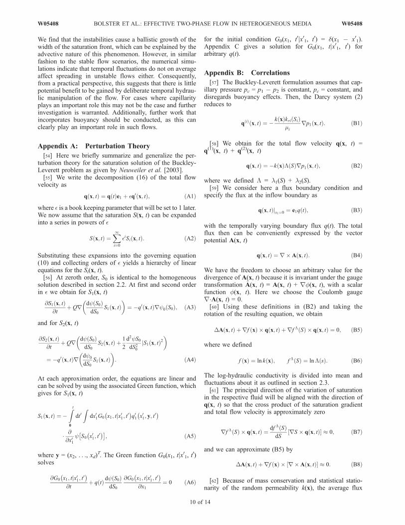
50(J. Garcia and K. Preuss, Flow instabilities during injectionof CO2 into saline aquifers, paper presented at TOUGHSymposium 2003, Lawrence Berkeley National Laboratory,Berkeley, California, 2003), which are all susceptible to thisinstability. Figure 7 illustrates the ‘‘dispersion’’ coefficientas calculated with our expression (41). Clearly our modelfails to capture this behavior as we do not account for thepossibility of this instability. Instead the dispersion coeffi-cient grows linearly/ballistically suggesting advectiondrives the instability; a similar observation was made by

Garcia and Preuss (presented paper, 2003) where the growthof the fingers associated with the instability grew almostlinearly in time. As the focus of this work was to study theinfluence of temporal fluctuations in the flow it is worthnoting that the same conclusions appear to hold for theunstable case as for the stable case. While the fluctuationsdo enhance and decrease the effective dispersion over time,on average there is no effect. Case l reveals a similarbehavior.

5. Summary and Conclusions

[50] We investigated the idealized displacement of onefluid by another immiscible fluid in a heterogenous porousmedium subjected to temporal fluctuations. We employedthe Buckley-Leverett model to study the impact of spatio-temporal fluctuations on the effective two-phase flow behav-ior. By averaging the transport equation for saturation overthe spatial ensemble, we derived a nonlinear effective equa-tion for the average saturation, which is characterized by aspatiotemporally nonlocal dispersive flux term. This termquantifies the impact of spatial heterogeneity on the spread-ing of the saturation front. Using spatial moments of thegradient of saturation we derived an effective large-scaledispersion coefficient that quantifies the spreading of thesaturation front.[51] In contrast to the conservative solute case, we find

that temporal fluctuations have a very minor impact on thedispersion of the saturation front. However, they can sig-nificantly increase the uncertainty of the front position,particularly when the viscosity of the fluid being injectedis much smaller than that being displaced as is typically thecase for geological carbon sequestration where the viscosityof CO2 can be 5 to 80 times less than that of water (Garciaand Preuss, presented paper, 2003). For single phase flow,temporal fluctuations enhance spreading due to the irrevers-ibility of local diffusion. Such a mechanism is lacking in theBuckley-Leverett model. Additionally, the current modelneglects other effects such as microscale trapping [Pop andSchweizer, 2007], which can lead to irreversible behavior.Therefore, we conjecture that accounting for capillarity andother mechanisms, which appear to act in a ‘‘diffusive’’manner, may potentially lead to an enhancement of spread-ing due to temporal flow fluctuations. On the basis of ouranalysis, we have proposed an effective flow description,which is based on (1) the effective nonlocal flow equationand (2) the measure of front uncertainty in terms of thefluctuations of the first moment of the saturation front.[52] To complement our analytical model, we performed

numerical simulations of the (Buckley-Leverett) two-phaseflow problem in heterogeneous permeability fields. For logconductivities with variances of up to 1 the model seems toprovide very satisfactory results, particularly at late times.At early times there is a discrepancy, which is whenboundary effects can still play an important role.[53] The analytical results presented here are only valid

for neutrally stable displacement. However, in many casesof practical interest, particularly CO2 sequestration, themobility ratios are small leading to Saffman-Taylor insta-bilities [Saffman and Taylor, 1958; Blunt et al., 1994],which can enhance spreading even further. Using themeasures for spreading developed herein, we studied thedispersion of a saturation front in such unstable scenarios.

Figure 7. Numerically calculated dispersion coefficientnormalized with the values predicted by (41) for (top) casesj (solid line) and k (dashed line) and (bottom) one temporalrealization of case a (dashed line). The dotted lines representthe effective dispersion coefficient for case k at themaximum and minimum values of the flow rate associatedwith the temporal flow fields.

W05408 BOLSTER ET AL.: EFFECTIVE TWO-PHASE FLOW IN HETEROGENEOUS MEDIA

9 of 14

W05408

We find that the instabilities cause a ballistic growth of thewidth of the saturation front, which can be explained by theadvective nature of this phenomenon. However, in similarfashion to the stable flow scenarios, the numerical simu-lations indicate that temporal fluctuations do not on averageaffect spreading in unstable flows either. Consequently,from a practical perspective, this suggests that there is littlepotential benefit to be gained by deliberate temporal hydrau-lic manipulation of the flow. For cases where capillarityplays an important role this may not be the case and furtherinvestigation is warranted. Additionally, further work thatincorporates buoyancy should be conducted, as this canclearly play an important role in such flows.

Appendix A: Perturbation Theory

[54] Here we briefly summarize and generalize the per-turbation theory for the saturation solution of the Buckley-Leverett problem as given by Neuweiler et al. [2003].[55] We write the decomposition (16) of the total flow

velocity as

q x; tð Þ ¼ q tð Þe1 þ �q0 x; tð Þ; ðA1Þ

where � is a book keeping parameter that will be set to 1 later.We now assume that the saturation S(x, t) can be expandedinto a series in powers of �

S x; tð Þ ¼X1i¼0

�iSi x; tð Þ: ðA2Þ

Substituting these expansions into the governing equation(10) and collecting orders of � yields a hierarchy of linearequations for the Si(x, t).[56] At zeroth order, S0 is identical to the homogeneous

solution described in section 2.2. At first and second orderin � we obtain for S1(x, t)

@S1 x; tð Þ@t

þ Qr dy S0ð ÞdS0

S1 x; tð Þ� �

¼ q0 x; tð Þry0 S0ð Þ; ðA3Þ

and for S2(x, t)

@S2 x; tð Þ@t

þ Qr dy S0ð ÞdS0

S2 x; tð Þ þ 1

2

d2yS0dS20

jS1 x; tð Þ2� �

¼ q0 x; tð Þr dy0

dS0S1 x; tð Þ

� �: ðA4Þ

At each approximation order, the equations are linear andcan be solved by using the associated Green function, whichgives for S1(x, t)

S1 x; tð Þ ¼ Z t

0

dt0Z

dx01G0 x1; tjx01; t0� �

q01 x01; y; t0� �

� @@x01

y S0 x01; t0� �� �; ðA5Þ

where y = (x2, . . ., xd)T. The Green function G0(x1, tjx01, t0)

solves

@G0 x1; tjx01; t0� �@t

þ q tð Þ dy S0ð ÞdS0

@G0 x1; tjx01; t0� �@x1

¼ 0 ðA6Þ

for the initial condition G0(x1, t0jx01, t0) = d(x1 x01).Appendix C gives a solution for G0(x1, tjx01, t0) forarbitrary q(t).

Appendix B: Correlations

[57] The Buckley-Leverett formulation assumes that cap-illary pressure pc = p1 p2 is constant, pc = constant, anddisregards buoyancy effects. Then, the Darcy system (2)reduces to

q ið Þ x; tð Þ ¼ k xð Þkri Sið Þmi

rp1 x; tð Þ: ðB1Þ

[58] We obtain for the total flow velocity q(x, t) =q(1)(x, t) + q(2)(x, t)

q x; tð Þ ¼ k xð ÞL Sð Þrp1 x; tð Þ; ðB2Þ

where we defined L = l1(S) + l2(S).[59] We consider here a flux boundary condition and

specify the flux at the inflow boundary as

q x; tð Þjx1¼0 ¼ e1q tð Þ; ðB3Þ

with the temporally varying boundary flux q(t). The totalflux then can be conveniently expressed by the vectorpotential A(x, t)

q x; tð Þ ¼ r � A x; tð Þ: ðB4Þ

We have the freedom to choose an arbitrary value for thedivergence of A(x, t) because it is invariant under the gaugetransformation A(x, t) = A(x, t) + rf(x, t), with a scalarfunction f(x, t). Here we choose the Coulomb gauger�A(x, t) = 0.[60] Using these definitions in (B2) and taking the

rotation of the resulting equation, we obtain

DA x; tð Þ þ rf xð Þ � q x; tð Þ þ rf L Sð Þ � q x; tð Þ ¼ 0; ðB5Þ

where we defined

f xð Þ ¼ ln k xð Þ; f L Sð Þ ¼ lnL sð Þ: ðB6Þ

The log-hydraulic conductivity is divided into mean andfluctuations about it as outlined in section 2.3.[61] The principal direction of the variation of saturation

in the respective fluid will be aligned with the direction ofq(x, t) so that the cross product of the saturation gradientand total flow velocity is approximately zero

rf L Sð Þ � q x; tð Þ ¼ df L Sð ÞdS

rS � q x; tð Þ½ � � 0; ðB7Þ

and we can approximate (B5) by

DA x; tð Þ þ rf xð Þ � r � A x; tð Þ½ � � 0: ðB8Þ

[62] Because of mass conservation and statistical statio-narity of the random permeability k(x), the average flux

10 of 14

W05408 BOLSTER ET AL.: EFFECTIVE TWO-PHASE FLOW IN HETEROGENEOUS MEDIA W05408

must be equal to the boundary flux and thus the rotation ofA(x, t) can be decomposed into

r� A x; tð Þ ¼ e1q tð Þ þ r � A0 x; tð Þ: ðB9Þ

Inserting the latter into (B8), we obtain for A0(x, t)

DA0 x; tð Þ ¼ rf 0 xð Þ � e1q tð Þ rf 0 xð Þ � r � A0 x; tð Þ½ �:ðB10Þ

[63] Disregarding terms that are quadratic in the fluctua-tions and assuming flow far away from the injectionboundary, the latter gives the well known first-order ap-proximation for q0(x, t) [e.g., Gelhar and Axness, 1983;Rehfeldt and Gelhar, 1992; Dentz and Carrera, 2005]

q0i x; tð Þ ¼ q tð ÞZ

ddk

2pð Þdexp ik � xð Þ di1

k1ki

k2

� �~f0kð Þ; ðB11Þ

where ~f 0(k) is the Fourier-transform of the log-hydraulicconductivity fluctuations.

Appendix C: Green Function

[64] Using the method of characteristics for the homoge-nous Buckley-Leverett problem, it can be shown that thederivative of the fractional flow function at S0(x1, t) is given by

dy0

dS0¼ x1

x1 tð Þ ; ðC1Þ

where we defined

x1 tð Þ ¼Z t

0

dtq tð Þ: ðC2Þ

This yields for (A6)

@G0 x1; tjx01; t0� �@t

þ d

dtln x1 tð Þ½ � @

@x1x1G

00 x1; tjx01; t0� �

¼ 0: ðC3Þ

[65] Equation (C3) can be solved using the method ofcharacteristics, which gives

G0 x1; tjx01; t0� �

¼ 1

x1 tð Þ dx1

x1 tð Þ x01

x1 t0ð Þ

� �: ðC4Þ

For constant spatial mean velocity, q(t) = q, the Greenfunction is given by [e.g., Neuweiler et al., 2003]

g0 x1; tjx01; t0� �

¼ 1

td

x1

t x01

t0

� �: ðC5Þ

Appendix D: Moment Equations

[66] Taking the derivative of (29) with respect to xi resultsin an equation for si(x, t)

@si x; tð Þ@t

þ q tð Þ � @@xi

dy S� �

dS x; tð Þs x; tð Þ

@

@xir �

Z t

0

dt0Z

ddx0dy S

� �dS x; tð Þ

k x; tjx0; t0ð Þdy S

� �dS x0; t0ð Þ

" #s x0; t0ð Þ ¼ 0:

ðD1Þ

[67] Multiplying (D1) with xi and integrating over spacegives an equation for the center of mass in the i direction,

@m1ð Þi tð Þ@t

¼ q tð Þ � A1

Zddxry S x; tð Þ

� �: ðD2Þ

Here the mean flow and pressure fluctuations are alignedwith the 1 direction so that we obtain

@m1ð Þi tð Þ@t

¼ di1q tð Þ � A1

Zddx

@

@x1y S x; tð Þ� �

¼ di1q tð ÞA1

Zdd1yy S x ¼ 0; y; tð Þ

� �¼ di1q tð Þ; ðD3Þ

where we have used the boundary condition S(x, t)jx1=0 = 1and the definition of the fractional flow function (8).Relation (D3) expresses mass conservation of the injectedfluid.[68] Analogously, multiplying (D1) with x1

2 and integrat-ing over space gives an equation for the longitudinal secondmoment,

@m2ð Þ11 tð Þ@t

¼ 2q tð Þ � A1

Zddxy S x; tð Þ

� �

2A1

Zddx

Z t

0

dt0Z

ddx0dy S

� �dS x; tð Þ

k1j x; tjx0; t0ð Þ

� @@x0j

y S x0; t0ð Þ� �

: ðD4Þ

Thus, the growth of the width of the saturation distributionis given by

@k11 tð Þ@t

¼ q tð Þ 2A1

Zddxy S x; tð Þ

� �Z t

0

dt0q t0ð Þ

24

35

2A1

Zddx

Z t

0

dt0Z

ddx0dy S

� �dS x; tð Þ

k1j x; tjx0; t0ð Þ

� @@x0j

y S x0; t0ð Þ� �

: ðD5Þ

Appendix E: Dispersion Coefficient

[69] Starting from (39) we execute the x1-integration,yielding

ds11 tð Þ ¼ s2ff

Z t

0

dt0Z10

dx01x01

x1 t0ð ÞC11

x01x1 t0ð Þ x1 tð Þ x1 t0ð Þ½ �

� �

� q tð Þq t0ð Þ @

@x01y S0

x01xf t0ð Þ

� �� �: ðE1Þ

After rescaling x01 with x1(t0) we obtain

ds11 tð Þ ¼ s2ff

Z t

0

dt0Z10

dx01x01C11 x01 x1 tð Þ x1 t0ð Þ½ �

� �

� q tð Þq t0ð Þ @

@x01y S0 x01=C

� �� �; ðE2Þ

W05408 BOLSTER ET AL.: EFFECTIVE TWO-PHASE FLOW IN HETEROGENEOUS MEDIA

11 of 14

W05408

where C = dy(Sf)/dSf. Changing variables from t0 to x1(t0)

(dt0 = q(t0)1 dx1(t0)) gives

ds11 tð Þ ¼ s2ff

Zx1 tð Þ

0

dx1

Z10

dx01x01C11 x01 x1 tð Þ x1½ �

� �

� q tð Þ @

@x01y S0 x01=C

� �� �: ðE3Þ

Shifting x1 by x1(t) and subsequent rescaling with x01 gives

ds11 tð Þ ¼ s2ff

Zx1 tð Þ

0

dx1

Z10

dx01C11 x1ð Þq tð Þ @

@x01y S0 x01=C

� �� �:

ðE4Þ

And finally after executing the x01 integration we obtain

ds11 tð Þ ¼ s2ff q tð Þ

Zx1 tð Þ

0

dx1C11 x1ð Þ: ðE5Þ

We now expand the integral for x1(t) = qt +Rt0

dt0q0(t0), whichgives in lowest order

ds11 tð Þ ¼ s2ff q tð Þ

Zqt0

dx1C11 x1ð Þ þZ t

0

dt0q0 t0ð ÞC11 qtð Þ

24

35: ðE6Þ

Appendix F: Alternative Measures for FrontSpreading

[70] Neuweiler et al. [2003] defined a macrodispersioncoefficient by looking at Fickian analogues to the (nonlocal)dispersive flux resulting from the upscaling exercise insection 3.1:

j x; tð Þ ¼Z t

0

dt0Z

ddx0dy S

� �dS x; tð Þ

k x; tjx0; t0ð Þr0y S x0; t0ð Þ� �

: ðF1Þ

[71] Amacrodispersion coefficient according toNeuweileret al. [2003] is then defined by setting

ji x; tð Þ � dyij tð Þ

@

@xjy S x; tð Þ� �

: ðF2Þ

[72] The macrodispersion coefficients are obtained bymultiplying (F2) by xj and integration of the resultingexpression over space. This gives

dyij tð Þ ¼

Zddxy S x; tð Þ

� �� �1

�Z

ddx

Z t

0

dt0Z

ddx0xjdy S

� �dS x; tð Þ

kil x; tjx0; t0ð Þ

� @@x0l

y S x0; t0ð Þ� �

: ðF3Þ

[73] This definition is identical to the one used byNeuweiler et al. [2003]. In lowest-order erturbation theory,we obtain for the denominator

A

Zdx1y S0

x1

Cx1 tð Þ

� �� �¼ ABx1 tð Þ; ðF4Þ

where we define

B � C

Zddxy S0 x1ð Þ½ �: ðF5Þ

[74] Thus, we get for the macrodispersion coefficient inlowest-order perturbation theory

d 11 tð Þ ¼

�2ffBx1 tð Þ

Zdx1

Z t

0

dt0Z10

dx01x21

x1 tð ÞC11 x1 x01� �

q tð Þq t0ð Þ

� 1

x1 tð Þ x01

x1 t0ð Þ x1

x1 tð Þ

� �@

@x01 S0

x01xf t0ð Þ

� �� �; ðF6Þ

where we used expression (C1) for dy(S0)/dS0. Executingthe x1 integration yields

dy11 tð Þ ¼

s2ff

B

Z t

0

dt0Z10

dx01x01

2

x1 t0ð Þ2C11

x01x1 t0ð Þ x1 tð Þ x1 t0ð Þ½ �

� �

� q tð Þq t0ð Þ @

@x01y S0

x01xf t0ð Þ

� �� �: ðF7Þ

[75] After rescaling x01 with x1(t0) we obtain

dy11 tð Þ ¼

s2ff

B

Z t

0

dt0Z10

dx01x012C11 x01 x1 tð Þ x1 t0ð Þ½ �

� �

� q tð Þq t0ð Þ @

@x01y S0 x01=C

� �� �; ðF8Þ

where C = dy(Sf)/dSf. Changing variables from t0 to x1(t0)

(dt0 = q(t0)1 dx1(t0)) gives

dy11 tð Þ ¼

s2ff

B

Zx1 tð Þ

0

dx1

Z10

dx01x012q tð ÞC11 x01 x1 tð Þ x1½ �

� �

� @

@x01y S0 x01=C

� �� �: ðF9Þ

Shifting x1 by x1(t) and subsequent rescaling with x01 gives

dy11 tð Þ ¼

s2ff

B

Zx1 tð Þ

0

dx1

Z10

dx01x01q tð ÞC11 x1ð Þ @

@x01y S0 x01=C

� �� �:

ðF10Þ

[76] And finally we obtain after integration by parts

dy11 tð Þ ¼ s2

ff q tð ÞZx1 tð Þ

0

dx1C11 x1ð Þ; ðF11Þ

12 of 14

W05408 BOLSTER ET AL.: EFFECTIVE TWO-PHASE FLOW IN HETEROGENEOUS MEDIA W05408

which is identical to the expression obtained from themoment equations. Following Neuweiler et al. [2003], weinsert C11(x1) = ld(x1) and obtain

dy11 tð Þ ¼ s2

ff lq tð Þ: ðF12Þ

[77] Thus, on average, there is no contribution to themacrodispersion coefficient due to temporal fluctuations.[78] Langlo and Espedal [1995] used a more process-

oriented definition for the macrodispersion coefficient interms of the dispersive flux term in (29). Assuming thatk(x, tjx0, t0) is sharply peaked about x and t, the flux term in(29) can be localized in space and time, which yields

@S x; tð Þ@t

þ q tð Þ � ry S� �

r �dy S

� �dS

d x; tð Þdy S

� �dS

rS x; tð Þ ¼ 0;

ðF13Þ

where we defined

d x; tð Þ ¼Z t

0

dt0Z

ddx0k x; tjx0; t0ð Þ: ðF14Þ

The latter is similar to the macrodispersion coefficient asidentified by Langlo and Espedal [1995].

Appendix G: Spatially Homogeneous Medium

[79] Here we consider flow in spatially homogeneousmedium under temporal pressure fluctuations. We demon-strate an artificial dispersion effect due to temporal pressurefluctuations when considering the moments of the timeaveraged saturation and analyze the purely advective wid-ening of the saturation distribution behind the front.[80] As given in section 3.3, we determine the width of

the saturation distribution in a homogeneous medium interms of the moments of

s0ð Þ1 x1; tð Þ ¼ A1 @

@x1S0 x1; tð Þ: ðG1Þ

We immediately obtain for the first moment of s(0)(x1, t)

m1ð Þ1 tð Þ ¼

Z t

0

dt0q t0ð Þ ðG2Þ

as a consequence of mass conservation. The second momentis given by

dm2ð Þ11 tð Þdt

¼ 2q tð ÞZ

ddx1y S0 x1; tð Þ½ �: ðG3Þ

[81] The saturation S0(x1, t) in a homogeneous mediumhas a sharp front. It is given by (11). Thus, (G3) assumes theform

m2ð Þ11 tð Þ ¼

dy Sf� �dSf

Z t

0

dt0q t0ð Þ

24

352 Z1

0

dx1y Sr x1ð Þ½ �: ðG4Þ

G1. Average Width of Saturation

[82] We obtain for the width k11(t) in a single realizationof the pressure fluctuations

k11 tð Þ ¼Z t

0

dt0q t0ð Þ

24

352

dy Sf� �dSf

Z1

0

dx1y Sr x1ð Þ½ � 1

24

35: ðG5Þ

The latter, however, is not related to actual spreading of thesaturation front. The spread of the saturation front isquantified by the second term on the right side of (D4).[83] The (temporal) ensemble average of the latter is

given by

hk11 tð Þi ¼ qtð Þ2þZ t

0

dt0Z t

0

dt00hq0 t0ð Þq0 t00ð Þi

24

35

�dy Sf

� �dSf

Z1

0

dx1y Sr x1ð Þ½ � 1

24

35: ðG6Þ

The fluctuation-induced contribution measures the uncer-tainty of the front position in the homogeneous mediumfrom realization to the realization of the pressure fluctua-tions, see Figure 3. It does not contribute to the spreading ofthe saturation front.

G2. Width of the Average Saturation

[84] The width of the average saturation front is given bythe ensemble second centered moment

kens11 tð Þ ¼ m

2ð Þ11 tð Þ

D E m

1ð Þ1 tð Þ

D E2

: ðG7Þ

We obtain for k11ens by using (G4) and (G2)

kens11 tð Þ ¼ hk11 tð Þi þ

Z t

0

dt0Z t

0

dt00hq0 t0ð Þq0 t00ð Þi: ðG8Þ

Thus, the second centered moment of the average saturationquantifies a purely advective spreading effect due totemporal fluctuations of the front position that aresuppressed in (G6), which measures the advective wideningof the saturation distribution behind the front.

[85] Acknowledgments. The authors would also like to thank the‘‘CIUDEN’’ initiative for their financial contribution to this work. Addi-tionally, D.B. and M.D. gratefully acknowledge the financial support of theSpanish Ministry of Science and Innovation (MCI) through the ‘‘Juan de laCierva’’ and ‘‘Ramon y Cajal’’ programs.

ReferencesAbramowitz, M., and I. Stegun (1970), Handbook of Mathematical Func-tions, Dover, New York.

Bachu, S. (2000), Sequestration of CO2 in geological media: Criteria andapproach for site selection in response to climate change, Energy Con-vers. Manage., 41(9), 953–970, doi:10.1016/S0196-8904(99)00149-1.

Bear, J. (1972), Dynamics of Fluids in Porous Media, Elsevier, New York.Blunt, M. J., J. W. Barker, B. Rublin, M. Mansfeld, I. Culverwell, and M.Christie (1994), Predictive theory for viscous fingering in compositionaldisplacement, SPE Reservoir Eng., 36, 73–80.

W05408 BOLSTER ET AL.: EFFECTIVE TWO-PHASE FLOW IN HETEROGENEOUS MEDIA

13 of 14

W05408

Cirpka, O. A., and S. Attinger (2003), Effective dispersion in heterogeneousmedia under random transient flow conditions,Water Resour. Res., 39(9),1257, doi:10.1029/2002WR001931.

Cushman, J. H., X. Hu, and T. R. Ginn (1994), Nonequilibrium statisticalmechanics of preasymptotic dispersion, J. Stat. Phys., 75(5–6), 859–878.

Cvetkovic, V., and G. Dagan (1996), Reactive transport and immiscibleflow in geological media. II. Applications, Proc. R. Soc. London, Ser. A,452, 303–328.

Dagan, G. (1989), Flow and Transport in Porous Formations, Springer,New York.

Dentz, M., and J. Carrera (2003), Effective dispersion in temporally fluc-tuating flow through a heterogeneous medium, Phys. Rev. E, 68, 036310,doi:10.1103/PhysRevE.68.036310.

Dentz, M., and J. Carrera (2005), Effective solute transport in temporallyfluctuating flow through heterogeneous media, Water Resour. Res., 41,W08414, doi:10.1029/2004WR003571.

Dentz, M., H. Kinzelbach, S. Attinger, and W. Kinzelbach (2000), Temporalbehavior of a solute cloud in a heterogeneous porousmedium: 1. Point-likeinjection, Water Resour. Res, 36(12), 3591–3604.

Efendiev, Y., and L. J. Durlofsky (2002), Numerical modeling of subgridheterogeneity in two phase flow simulations, Water Resour. Res., 38(8),1128, doi:10.1029/2000WR000190.

Fiori, A. (2001), On the influence of local dispersion in solute transportthrough formations with evolving scales of heterogeneity, Water Resour.Res., 37(2), 235–242.

Gelhar, L. (1993), Stochastic Subsurface Hydrology, Prentice Hall,Englewood Cliffs, N. J.

Gelhar, L., and C. Axness (1983), Three-dimensional stochastic analysis ofmacrodispersion in aquifers, Water Resour. Res., 19(1), 161–180.

Hasle, G., K.-A. Lie, and E. Quak (2007), Geometric Modelling, NumericalSimulation, and Optimization, Springer, Berlin.

Jarman, K. D., and T. F. Russell (2003), Eulerian moment equation for 2-Dstochastic immiscible flow, Multiscale Modeling Simul., 1, 598–608.

Jarman, K. D., and A. M. Tartakovsky (2008), Divergence of solutions tosolute transport moment equations, Geophys. Res. Lett., 35, L15401,doi:10.1029/2008GL034495.

Kinzelbach, W., and P. Ackerer (1986), Modelisation du transport de con-taminant dans un champ d’ecoulement non-permanent, Hydrogeologie,2, 197–205.

Kitanidis, P. K. (1988), Prediction by the method of moments of transport inheterogeneous formations, J. Hydrol., 102, 453–473.

Koch, D. L., and J. F. Brady (1987), A non-local description of advection-diffusion with application to dispersion in porous media, J. Fluid Mech.,180, 387–403.

Kubo, R., M. Toda, and N. Hashitsume (1991), Statistical Physics II, Non-Equilibrium Statistical Mechanics, Springer, Berlin.

Lake, L. (1989), Enhanced Oil Recovery, Prentice Hall, Englewoods Cliffs,N. J.

Langlo, P., and M. Espedal (1995), Macrodispersion for two-phase, immis-cible flow in porous media, Adv. Water Resour., 17, 297–316.

Marle, C. M. (1981), Multiphase Flow in Porous Media, Inst. Fr. du Pet,Paris.

Morales-Casique, E., S. P. Neuman, and A. Guadagnini (2006), Non-localand localized analyses of non-reactive solute transport in bounded ran-domly heterogeneous porous media: Computational analysis, Adv. WaterResour., 29, 1399–1418.

Neuman, S. P. (1993), Eulerian-Lagrangian theory of transport in space-time nonstationary velocity fields: Exact nonlocal formalism by condi-tional moments and weak approximation, Water Resour. Res., 29(3),633–645.

Neuweiler, I., S. Attinger, W. Kinzelbach, and P. King (2003), Large scalemixing for immiscible displacement in heterogenous porous media,Transp. Porous Media, 51, 287–314.

Noetinger, B., V. Artus, and L. Ricard (2004), Dynamics of the water-oilfront for two-phase, immiscible flow in heterogeneous porous media. 2.Isotropic media, Transp. Porous Media, 56, 305–328.

Pop, I. S., and B. Schweizer (2007), On the homogenization of the Buckley-Leverett equation including trapping effects at the micro scale, Proc. Appl.Math. Mech., 7, 1,024,701–1,024,702.

Rehfeldt, K. R., and L. W. Gelhar (1992), Stochastic analysis of dispersionin unsteady flow in heterogeneous aquifers, Water Resour. Res., 28(8),2085–2099.

Saffman, P. G., and G. I. Taylor (1958), The penetration of a fluid into aporous medium or Hele-Shaw cell containing a more viscous liquid,Proc. R. Soc. London, Ser. A, 245, 312–329.

Tartakovsky, A. M., S. P. Neuman, and R. J. Lenhard (2003), Immisciblefront evolution in randomly heterogeneous porous media, Phys. Fluids,15, 3331–3341.

Tartakovsky, D. M., and S. P. Neuman (1998a), Transient flow in boundedrandomly heterogeneous domains: 1. Exact conditional moment equa-tions and recursive approximations, Water Resour. Res., 34(1), 1–12.

Tartakovsky, D. M., and S. P. Neuman (1998b), Transient effective hydrau-lic conductivities under slowly and rapidly varying mean gradients inbounded three-dimensional random media, Water Resour. Res., 34(1),21–32.

Zwanzig, R. (1961), Memory effects in irreversible thermodynamics, Phys.Rev., 124, 983–992.

D. Bolster and M. Dentz, Department of Geotechnical Engineering and

Geosciences, Technical University of Catalonia, E-08034 Barcelona, Spain.(diogobolster@gmail.com)

J. Carrera, Institute of Environmental Analysis and Water Studies,CSIC, Barcelona E-08034, Spain.

14 of 14

W05408 BOLSTER ET AL.: EFFECTIVE TWO-PHASE FLOW IN HETEROGENEOUS MEDIA W05408