5722 Phys. Chem. Chem. Phys., 2011, 13, 5722–5727 This journal is c the Owner Societies 2011

Cite this: Phys. Chem. Chem. Phys., 2011, 13, 5722–5727

Effective solvent mediated potentials of Na+ and Cl� ions in aqueous

solution: temperature dependence

Alexander Mirzoev and Alexander P. Lyubartsev*

Received 4th November 2010, Accepted 18th January 2011

DOI: 10.1039/c0cp02397c

The effective solvent-mediated potentials for Na+ and Cl� ions in aqueous solution were

calculated in a wide range of temperatures from 0 to 100 1C. The potentials have been determined

using the inverse Monte Carlo approach, from the ion–ion radial distribution functions computed

in 50 ns molecular dynamics simulations of ions and explicit water molecules. We further

separated the effective potentials into a short-range part and an electrostatic long-range part

represented by a coulombic potential with some dielectric permittivity. We adjusted the value of

the dielectric permittivity to provide the fastest possible decay of the short-range potentials at

larger distances. The obtained temperature dependence of the dielectric permittivity follows well

the experimental data. We show also that the largest part of the temperature dependence of the

effective potentials can be attributed to the temperature-dependent dielectric permittivity.

1. Introduction

Multiscale modeling techniques aiming at consistent, hierarchical

development of molecular models from the atomistic level to

the mesoscale have received increasing attention during the

last decade. This interest originates in the understanding that

it is impossible to model many important phenomena in

biophysics and soft matter at the atomistic level due to the

large size of these systems, as well as due to too long time

needed for them to equilibrate. An evident way to attain

progress in addressing the mesoscale problem is to use

coarse-grained and/or implicit solvent models, which contain

only important, principal features of the studied system while

unimportant ones (local details of the molecular structure,

solvent) are disregarded. A practical way to build such models

was suggested in paper,1 where the Inverse Monte Carlo

(IMC) method was introduced allowing us to reconstruct

coarse-grained interaction potentials from radial distribution

functions determined in atomistic simulations. Related

approaches, appeared recently and addressing the same

problem, are iterative Boltzmann inversion,2,3 the force

matching approach,4 use of integral equations based on the

hypernetted chain5,6 or the Yvon–Born–Green theory.7 During

the last decades, these methods were applied for computations

of effective solvent-mediated potentials for various systems: ion

solutions,8,9 ion–DNA interactions,10 various molecular

liquids,7,11,12 coarse-grained lipid models,13–15 and polymers.3,6

A principal problem with effective coarse-grained potentials

derived from atomistic simulations is that they, by the way of

their definition, are dependent on thermodynamics conditions,

such as temperature and concentration of different compo-

nents.6,16,17 In some cases this dependence may be weak or of

no importance, but in principle, thermodynamical transfer-

ability of the effective potentials should be controlled in

each specific case. In this paper we investigate temperature

dependence of the effective solvent mediated potentials

between ions in aqueous solution.

Ion solutions, and specifically Na+–Cl�aqueous solution,

have been extensively studied during the last decades.9,18–24

This interest is motivated by the great importance of ions and

their solutions in many areas of biophysics and physical

chemistry. One of the simple models of ionic solutions, often

used in investigation of polyelectrolytes including biological

macromolecules, is the primitive electrolyte model25–28

describing solvent as a continuum medium and the ions as hard

spheres interacting by potentialqiqj

4pe0er(where qi and qj are ion

charges, r is the interionic distance, e0 is the vacuum dielectric

permittivity and e is the relative permittivity of the solvent).

Clearly, this expression is a rather rough approximation on

short distances between the ions when the intermediate solvent

cannot be considered as a continuum due to its molecular

structure. Also, specific short-range features of ion–ion inter-

actions, including van der Waals forces, are not taken into

account within the primitive model.

Solvent-mediated interionic effective potentials, taking into

account the molecular structure of the solvent and specific

short-range interactions, can be built from atomistic molecular

dynamics simulations as it was done in a number of previous

studies.1,5,8,29 Hess et al.9 investigated concentration depen-

dence of NaCl ion–ion effective potentials constructed from

atomistic simulations. It was shown that the main part of this

Division of Physical Chemistry, Department of Materials andEnvironmental Chemistry, Stockholm University, SE-106 91Stockholm, Sweden. E-mail: alexander.lyubartsev@mmk.su.se

PCCP Dynamic Article Links

www.rsc.org/pccp PAPER

This journal is c the Owner Societies 2011 Phys. Chem. Chem. Phys., 2011, 13, 5722–5727 5723

dependence can be attributed to the change of the effective

dielectric permittivity, which decreases with the ion concentration,

affecting the long-range behaviour of the effective potentials.

Taking into account concentration-dependence of the dielectric

permittivity, osmotic coefficients of ions can be reproduced in

a wide concentration range.9,21 Nevertheless the temperature

dependence of the ion–ion effective potential and the corre-

sponding effective dielectric permittivity has not been studied

yet. In this work we address this problem and calculate the

effective potentials for Na+ and Cl� ions in aqueous solution

for a wide range of temperatures from 0 to 100 1C. Furthermore,

we show that computation of the effective potentials provide

an alternative route to determine static dielectric permittivity

in molecular liquids which may further contribute to our

general understanding of dielectric properties of various

solutions.

2. Models and methods

2.1 Explicit water molecular dynamics simulations

Atomistic molecular dynamics (MD) simulations of 20 Na+Cl�

ion pairs dissolved in 1000 water molecules (which correspond

to ion concentration E 1.0 M) have been performed in the

range of temperatures from 0 to 100 1C. Water was presented

by the flexible simple point charge (SPC-F) model by Toukan

and Rahman.30 For the ion–ion and ion–water interactions,

Smith–Dang parameters were used:31 sNa = 2.35 A, eNa =

0.544 kJ mol�1, sCl = 4.4 A, eCl = 0.42 kJ mol�1, together

with the Lorentz–Berthelot rules for cross-interactions. The

system was put into a cubic periodic box, and long range

electrostatic interactions were treated by the Ewald method.32

The equations of motion were integrated by the constant-

temperature–constant-pressure molecular dynamics algorithm,33

with Nose–Hoover relaxation parameters for 50 fs for the

thermal bath and for 1 ps for the volume fluctuations. The

double time step algorithm by Tuckerman et al.,34 with a short

time step of 0.25 fs for intramolecular and short-range inter-

actions (within 5 A distance) and a long time step of 2.5 fs for

longer range interactions (between 5 A and 12 A cutoff), has

been implemented. Eleven temperature points were chosen

between 273 K and 373 K with a step of 10 K, and the

pressure was set to 1 bar for all of them. For each temperature,

50 ns MD simulation was performed and the first 5 ns was

treated as equilibration. Configurations were saved in the

trajectories each 1 ps, and they were used for subsequent

calculation of NaNa, NaCl, and ClCl radial distribution

functions. The MD simulations were performed by the

MDynaMix software package.35

2.2 Calculation of effective ion–ion potentials by the inverse

Monte Carlo method

The method of reconstruction of effective pair potentials from

the corresponding RDFs, using an iterative inverse Monte

Carlo procedure, was published elsewhere.1 The inverse

simulations were carried out in the NVT ensemble conditions,

using the same number of ions and average periodic cell size as

in the corresponding atomistic MD simulations, but without

explicit water molecules. Thus possible size effects on the

RDFs should be essentially avoided. Potential of the mean

force U(r) = �kTln(g(r)) was taken as the starting trial

potential, and then was refined in about 20 IMC iterations,

allowing to reach a complete convergence between newly

generated RDF and the reference ones. Each iteration

consisted of 5 � 107 Monte Carlo steps of which first

1 � 107 steps were considered as equilibration. The long range

part of the electrostatic interaction, outside the cut-off distance

(which was set to half of the box length), was treated using

the Ewald summation method for coulombic potential with

dielectric permittivity defined initially as for pure water at

ambient temperature (e = 80), and then optimized according

to the procedure described below.

2.3 Effective pair potential decomposition and computation of

effective dielectric permittivity

By analogue with previous studies,1,5,9 we used decomposition of

the effective potential into a short-range part and a long-range

electrostatic part, the latter being defined by the macroscopic

dielectric permittivity:

UijeffðrÞ ¼ Uij

srðrÞ þqiqj

4pe0erð1Þ

The potentialUijeff(r) is the one coming from the IMC procedure,

thus choice of dielectric permittivity e defines the short range

partUijsr(r). The second part of this decomposition is supposed to

account for all long-range interactions, that is why improper

choice of e value will produce a certain long-range contribution

in Uijsr(r). Since dielectric permittivity depends on temperature,

the initial guess e = 80.0 (which had been proven to be a good

choice for the SPC-F water model at T = 298 K),8 may not be

optimal for other temperatures. By a proper choice of e, the longrange component of Uij

sr(r) can be minimized. A complicating

circumstance is that, in the case of ion solution, the long-range

parts of all three potentials, namely Na–Na, Na–Cl and Cl–Cl,

should be minimized by varying the same value of e. We used the

following procedure to obtain values of the dielectric permittivity

providing fastest decay of all three short-range potentials with

distance. First, we introduce numerical criteria of a short range

potential deviation from zero at large distances:

WðUijsrðrÞÞ ¼

Zr2r1

jr2UijsrðrÞjdr ð2Þ

where r2 factor implies a higher weight of larger distances,

r1 and r2 are the lower and upper boundaries of the range of

distances defining the long-range part (the r2 value is taken as the

cut-off of RDF and tabulated effective potential, which is

also equal to half of the box size). The absolute value in

eqn (2) is used in order to deal with oscillations of the short

range part of the potential, which are typical for effective ion–ion

potentials.5,8

Taking in mind eqn (1), we can write for the short-range

part of the potential:

WðUijsrðrÞÞ ¼

Zr2r1

r2ðUijeffðrÞ �

qiqj

4pe0erÞ

��������dr ð3Þ

5724 Phys. Chem. Chem. Phys., 2011, 13, 5722–5727 This journal is c the Owner Societies 2011

Assume that we define the long-range coulombic potential

using another value of permittivity e%. This, according to (1),

introduces a new short-range potential as:

Uijsr ¼ Uij

srðrÞ þqiqj

4pe0r1

e� 1

e

� �ð4Þ

Now we shall find the optimal e%, which produces the fastest

decay of all three short range potentials according to criteria

defined by eqn (2). We minimize the sum:

W(U%NaNasr (r)) + W(U%NaCl

sr (r)) + W(U%ClClsr (r)) (5)

by varying e%. The optimized value of e% can be considered as

effective dielectric permittivity corresponding to the given

thermodynamic conditions (temperature, concentration). We

need to remember however that the value of the effective

dielectric permittivity may affect the IMC procedure itself

through Ewald treatment of the long-range part of the effective

potential (outside the cutoff distance). We therefore rerun the

IMC simulation with the new corrected value of e. After 3–4

such iterations e% values stop to change and reach convergence.

They are considered as final optimized values of the dielectric

permittivity.

3. Results and discussion

3.1 Atomistic MD simulation results

Previous simulations of NaCl ion solution described by the

model used in this work have been carried out at temperature

298 K.5,8,36 In order to test briefly the applicability of

this model at other than ambient temperature, we compare

the density obtained in our NPT-MD simulations with the

experimental one.37 The results are presented in Fig. 1.

Unfortunately we found density data for 1 M NaCl solution

only in a rather narrow temperature interval, that is why we

plot also pure water data for the whole temperature range.

Direct comparison of the MD simulation results with experi-

mental temperature dependence of the density of Na+–Cl�

solution and pure water shows quite reasonable agreement.

The computed r(T) dependence shows the same trend as

pure water in the 20–100 1C temperature range, but does not

show nearly temperature-independent behavior in the range

0–10 1C. This is a known deficiency of the SPC water model,

which is unable to reproduce the water density maximum at

4 1C.38 Anyway, the overall agreement with experimental data

can be considered as an argument for reliability of the explicit

solvent MD simulations.

Ion–ion radial distribution functions obtained in MD

simulations are displayed in Fig. 2. They all show strong

dependence on the temperature. The curves for all 3 ion–ion

pairs are clearly ordered from lower to higher temperature

within each oscillation of the RDFs. The general trend is that

the first peak of RDF between likewise ions is decreasing at

higher temperatures, while the first peak of NaCl RDF is

increasing, showing higher tendency to form ion pairs at

higher temperatures.

The accuracy of RDF calculations is very important for

producing reliable effective potentials. Our previous studies5

have shown that reliable estimation of ion–ion RDFs, and

especially the height of the first peak of RDFs, requires

simulations on at least 10 ns time scale. To be on a safe side,

we carried out 50 ns simulations for each temperature point,

and performed a test on whether such trajectories are long

enough for producing stable radial distribution functions. In

Fig. 3 we displayed RDF calculated during the first 20 nano-

seconds of the trajectory after finishing the equilibration period,

another RDF calculated during the following 25 ns of the same

trajectory, and the RDF averaged over the whole trajectory.

There are no major deviations in the curves, and difference of

the curves does not exceed a few percent. This indicates that the

5 ns period was enough for equilibration and following 45 ns of

simulation provides reasonable amount of data to produce

smooth and stable RDF. The same kind of behavior was

observed for all other temperatures and ion pairs.

3.2 Inverse Monte Carlo results

The computed ion–ion RDFs were passed to the inverse Monte

Carlo procedure, where 20 iterations were performed for each

temperature point. The value of the regularization parameter

defining the factor for potential correction in the IMC procedure

Fig. 1 Temperature dependence of the density of Na+–Cl� aqueous

solution. Green squares—explicit water MD simulations (this work),

red circles—experimental data for Na+–Cl� aqueous solution,37 blue

triangles—experimental data for pure water.39

Fig. 2 Radial distribution functions for Na+–Na+, Na+–Cl� and

Cl�–Cl� ion pairs for different temperatures. Arrows show direction

of the temperature growth in the same order as in the legend.

This journal is c the Owner Societies 2011 Phys. Chem. Chem. Phys., 2011, 13, 5722–5727 5725

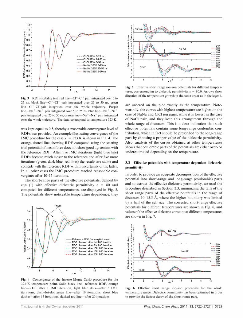
was kept equal to 0.5, thereby a reasonable convergence level of

RDFs was provided. An example illustrating convergency of the

IMC procedure for the case T = 323 K is shown in Fig. 4. The

orange dotted line showing RDF computed using the starting

trial potential of mean force does not show good agreement with

the reference RDF. After five IMC iterations (light blue line)

RDFs become much closer to the reference and after five more

iterations (green, dark blue, red lines) the results are stable and

coincide with the reference RDF within uncertainty of the latter.

In all other cases the IMC procedure reached reasonable con-

vergence after 10–15 iterations.

The short-range parts of the effective potentials, defined by

eqn (1) with effective dielectric permittivity e = 80 and

computed for different temperatures, are displayed in Fig. 5.

The potentials show noticeable temperature dependence, they

are ordered on the plot exactly as the temperature. Note-

worthily, the curves with highest temperature are highest in the

case of NaNa and ClCl ion pairs, while it is lowest in the case

of NaCl pair, and they keep this arrangement through the

whole range of distances. This is a clear indication that such

effective potentials contain some long-range coulombic con-

tribution, which in fact should be prescribed to the long-range

part by choosing a proper value of the dielectric permittivity.

Also, analysis of the curves obtained at other temperatures

shows that coulombic parts of the potentials are either over- or

underestimated depending on the temperature.

3.3 Effective potentials with temperature-dependent dielectric

permittivity

In order to provide an adequate decomposition of the effective

potential into short-range and long-range (coulombic) parts

and to extract the effective dielectric permittivity, we used the

procedure described in Section 2.3, minimizing the tails of the

short range parts of the effective potentials in the range of

distances 10–15.5 A, where the higher boundary was limited

by a half of the cell size. The corrected short-range effective

potentials for different temperatures are shown in Fig. 6, and

values of the effective dielectric constant at different temperatures

are shown in Fig. 7.

Fig. 3 RDFs stability test: red line—Cl�–Cl� pair integrated over 5 to

25 ns, black line—Cl�–Cl� pair integrated over 25 to 50 ns, green

line—Cl�–Cl�pair integrated over the whole trajectory. Purple

line—Na+–Na+ pair integrated over 5 to 25 ns, blue line—Na+–Na+

pair integrated over 25 to 50 ns, orange line—Na+–Na+ pair integrated

over the whole trajectory. The data correspond to temperature 323 K.

Fig. 4 Convergence of the Inverse Monte Carlo procedure for the

323 K temperature point. Solid black line—reference RDF, orange

line—RDF after 1 IMC iteration, light blue dots—after 5 IMC

iterations, dash-dot-dot green line—after 10 iterations, short blue

dashes—after 15 iterations, dashed red line—after 20 iterations.

Fig. 5 Effective short range ion–ion potentials for different tempera-

tures, corresponding to dielectric permittivity e = 80.0. Arrows show

direction of the temperature growth in the same order as in the legend.

Fig. 6 Effective short range ion–ion potentials for the whole

temperature range. Dielectric permittivity has been optimized in order

to provide the fastest decay of the short-range part.

5726 Phys. Chem. Chem. Phys., 2011, 13, 5722–5727 This journal is c the Owner Societies 2011

As it can be seen from Fig. 6, effective short range potentials

calculated with corrected dielectric permittivity do not show

strong temperature dependence. They also become practically

equal to zero at distances larger than 10 A. Though certain

difference between the curves can be noted, it is substantially

less than it was in the case of uncorrected potentials in Fig. 5.

Moreover, the curves in Fig. 6, while showing some trends

indicated by arrows in the figure, do not follow the same order

as the temperature, which indicates that a large part of the

difference between them is from statistical uncertainty.

Another important result of this analysis is the values of the

effective dielectric permittivity obtained for different tempera-

tures, Fig. 7. As expected, dielectric permittivity decreases

with temperature. We compare the computed values of the

dielectric permittivity with experimental data for pure water40

as well as for 1 M NaCl solution (for the latter, experimental

data are available only for a limited temperature interval

5–35 1C, and they were complemented by an extrapolation

formula from work 40). Finally, we have computed dielectric

permittivity directly from atomistic simulations using the

following expression for water dipoles fluctuations41:

e ¼ 1þ hM2i � hMi2

3e0VkTð6Þ

where M is the sum of molecular dipole moments (taken over

all water molecules) and V is the volume of the simulation cell.

One can see that the two ways of calculation of dielectric

permittivity are consistent with each other and are in line with

experiment, though direct computations from atomistic MD

provide more stable results. Uncertainties of the values of

dielectric permittivity defined from the asymptotic behavior of

the effective potentials come from the uncertainties in the

ion–ion RDFs, as well as from the fitting procedure which is

done in the range of distances where oscillations of the

effective potentials due to the molecular structure of water

do not disappear completely. Computations of effective

potentials in a larger simulation cell may provide more

accurate estimation of the dielectric permittivity.

4. Conclusions

We have computed effective solvent-mediated potentials for

Na+ and Cl� ions in water for the range of temperatures

between 0 and 100 1C. Some temperature dependence of the

potentials has been observed. We decomposed the potentials

into short-range and long-range (coulombic) parts by choosing

effective dielectric permittivity e which provides the fastest decay

of the short range part. The e-corrected short-range potentials

turned out to be much less temperature dependent. Taking in

mind that a similar effect was previously observed for concen-

tration dependence of ion–ion effective potentials,9 we can

conclude that thermodynamically non-transferable (that is tem-

perature and concentration dependent) part of the effective

NaCl ion–ion potentials consists essentially in the long-range

coulombic contribution, which can be described by the con-

centration- and temperature-dependent dielectric permittivity,

while the short-range interaction is essentially invariant with

respect to the change of thermodynamical conditions.

Several reservations about the above conclusion should be

made. First, our study covers the temperature range for liquid

water at normal pressure, and the conclusion about transfer-

ability of the short-range part of the effective potentials does

not necessarily propagate beyond this range, e.g. to the super-

critical conditions. Previous molecular dynamics studies of

NaCl solution at supercritical conditions42,43 have shown that

the water structure around ions changes largely when the the

temperature is raised to a supercritical one, and at such

conditions even the short range part of the effective potentials

may show considerable change compared to the ambient

conditions. Second, the short range potentials are expected

to be specific to the kind of solvent, and need to be recalculated

for other solvents than water. Third, for large bulky ions, the

hydrophobic interactions become more important, which may

lead to stronger temperature dependence of the short-range part

of effective potentials.

The decomposition of the effective potentials described in

the paper may be of importance for further use of the effective

ion–ion potentials in different conditions, including their

interactions with polyelectrolytes and charged biomacro-

molecules. One can expect that the short range part of various

ion–polyion effective potentials will be specific for different

sites of the polyion, but largely not dependent on the

temperature and ion concentration. On the other hand, the

long-range part of the effective potentials will be determined

by the charges of the coarse-grained sites and effective

dielectric constant, the latter being dependent on the temperature

and ion concentration. Also, decomposition of the effective

potential into the coulombic part, which can be treated by a

fast Ewald (PME or P3M) summation technique, and short-

range part with a short (of the order 10–12 A) cutoff distance

would provide better performance in large scale mesoscopic

simulations employing these potentials.

Furthermore, the presented approach represents an alternative

way of determination of the dielectric permittivity in molecular

Fig. 7 Dielectric permittivity of Na+–Cl� water solution at 1 M

concentration. Green triangles—values calculated in the present work

from the long-range behavior of the effective potentials; blue circles—

values calculated from the dipole fluctuations (eqn (6)); purple dash

line—experimental data for pure water; orange points—experimental

values referring to 1 M NaCl water solution; yellow line—wide range

extrapolation of the experimental data. The experimental data were

taken from Peyman et al.40

This journal is c the Owner Societies 2011 Phys. Chem. Chem. Phys., 2011, 13, 5722–5727 5727

solvents. The dipole fluctuation expression (6) is valid only for

rigid molecular models (more rigorously, for point dipoles,

which still can be considered as a good approximation for

water molecules). Computation of static dielectric permittivity

from the long-range asymptotic of effective potentials can be

used for higher molecular weight solvents such as alcohols, ionic

liquids, etc.

Acknowledgements

This work has been supported by the Swedish Research

Council (Vetenskapsradet), grant 70525601. We are thankful

to the High Performance Computing Center North (HPC2N)

at Umea University, Umea, for granting computer facilities.

References

1 A. P. Lyubartsev and A. Laaksonen, Phys. Rev. E: Stat. Phys.,Plasmas, Fluids, Relat. Interdiscip. Top., 1995, 52, 3730–3737.

2 A. K. Soper, Chem. Phys., 1996, 202, 295–306.3 D. Reith, M. Putz and F. Muller-Plathe, J. Comput. Chem., 2003,24, 1624–1636.

4 W. G. Noid, J.-W. Chu, G. S. Ayton, V. Krishna, S. Izvekov,G. A. Voth, A. Das and H. C. Andersen, J. Chem. Phys., 2008, 128,244114.

5 A. P. Lyubartsev and S. Marcelja, Phys. Rev. E: Stat. Phys.,Plasmas, Fluids, Relat. Interdiscip. Top., 2002, 65, 041202.

6 V. Krakoviak, J. P. Hansem and A. A. Louis, Phys. Rev. E: Stat.Phys., Plasmas, Fluids, Relat. Interdiscip. Top., 2003, 67, 041801.

7 J. W. Mullinax andW. G. Noid, J. Chem. Phys., 2010, 133, 124107.8 A. P. Lyubartsev and A. Laaksonen, Phys. Rev. E: Stat. Phys.,Plasmas, Fluids, Relat. Interdiscip. Top., 1997, 55, 5689–5696.

9 B. Hess, C. Holm and N. van der Vegt, Phys. Rev. Lett., 2006, 96,147801.

10 A. P. Lyubartsev and A. Laaksonen, J. Chem. Phys., 1999, 111,11207–11215.

11 A. Villa, C. Peter and N. F. A. van der Vegt, J. Chem. TheoryComput., 2010, 6, 2434–2444.

12 A. Lyubartsev, A. Mirzoev, L. Chen and A. Laaksonen, FaradayDiscuss., 2010, 144, 43–56.

13 A. P. Lyubartsev, Eur. Biophys. J., 2005, 35, 53–61.14 S. Izvekov and G. A. Voth, J. Chem. Theory Comput., 2006, 2,

637–648.15 S. Izvekov and G. A. Voth, J. Phys. Chem. B, 2009, 113,

4443–4455.

16 A. A. Louis, J. Phys.: Condens. Matter, 2002, 14, 9187–9206.17 V. Krishna, W. G. Noid and G. A. Voth, J. Chem. Phys., 2009,

131, 024103.18 E. Guardia, R. Rey and J. A. Padro, J. Chem. Phys., 1991, 95,

2823–2831.19 E. Guardia, R. Rey and J. A. Padro, Chem. Phys., 1991, 155,

187–195.20 M. Canales and G. Sese, J. Chem. Phys., 1998, 109, 6004–6011.21 B. Hess, C. Holm and N. van der Vegt, J. Chem. Phys., 2006, 124,

164509.22 B. Hess and N. F. A. van der Vegt, J. Chem. Phys., 2007, 127,

234508.23 I. Kalcher and J. Dzubiella, J. Chem. Phys., 2009, 130, 134507.24 S. Gavryushov and P. Linse, J. Phys. Chem. B, 2006, 110,

10878–10887.25 P. Mills, C. Anderson and M. T. Record, J. Phys. Chem., 1985, 89,

3984–3994.26 B. Jayram and D. L. Beveridge, Annu. Rev. Biophys. Biomol.

Struct., 1996, 25, 367–394.27 E. Allahyarov, G. Gompper and H. Lowen, Phys. Rev. E: Stat.,

Nonlinear, Soft Matter Phys., 2004, 69, 041904.28 P. Linse, Adv. Polym. Sci., 2005, 185, 111–162.29 A. Savelyev and G. A. Papoian, J. Phys. Chem. B, 2009, 113,

7785–7793.30 K. Toukan and A. Rahman, Phys. Rev. B, 1985, 31, 2643–2648.31 D. E. Smith and L. X. Dang, J. Chem. Phys., 1994, 100, 3757–3766.32 M. P. Allen and D. J. Tildesley, Computer simulation of liquids,

Clarendon Press, New York, NY, USA, 1989.33 S. Melchionna, G. Ciccotti and B. L. Holian,Mol. Phys., 1993, 78,

533–544.34 M. Tuckerman, B. J. Berne and G. J. Martyna, J. Chem. Phys.,

1992, 97, 1990–2001.35 A. P. Lyubartsev and A. Laaksonen, Comput. Phys. Commun.,

2000, 128, 565–589.36 A. P. Lyubartsev and A. Laaksonen, J. Phys. Chem., 1996, 100,

16410–16418.37 L. A. Romankiw and I. M. Chou, J. Chem. Eng. Data, 1983, 28,

300–305.38 W. Jorgensen and C. Jenson, J. Comput. Chem., 1998, 19,

1179–1186.39 G. S. Kell, J. Chem. Eng. Data, 1975, 20, 97–105.40 A. Peyman, C. Gabriel and E. H. Grant, Bioelectromagnetics,

2007, 28, 264–274.41 J. Caillol, D. Levesque and J. Weis, J. Chem. Phys., 1986, 85,

6645–6657.42 P. B. Balbuena, K. P. Johnston and P. J. Rossky, J. Phys. Chem.,

1996, 100, 2706–2715.43 S. Koneshan and J. C. Rasaiah, J. Chem. Phys., 2000, 113,

8125–8137.