Behavior Genetics, Vol. 28, No. 1, 1998

Effect of Within-Strain Sample Size on QTL Detectionand Mapping Using Recombinant Inbred Mouse Strains

J. K. Belknap1,2

Received 17 Dec. 1996—Final 10 Aug. 1997

Increasing the number of mice used to calculate recombinant inbred (RI) strain meansincreases the accuracy of determining the phenotype associated with each genotype(strain), which in turn enhances quantitative trait locus (QTL) detection and mapping.The purpose of this paper is to examine quantitatively the effect of within-strain samplesize (n) on additive QTL mapping efficiency and to make comparisons with F2 andbackcross (BC) populations, where each genotype is represented by only a single mouse.When 25 RI strains are used, the estimated equivalent number of F2 mice yielding thesame power to detect QTLs varies inversely as a function of the heritability of the traitin the RI population (hRI). For example, testing 25 strains with « = 10 per strain isapproximately equivalent to 160 F2 mice when hRI = 0.2, but only 55 when hRI = 0.6.While increasing n is always beneficial, the gain in power as n increases is greatest whenhRI is low and is much diminished at high hRI values. Thus, when hRI is high, there islittle advantage of large n, even when n approaches infinity. A cost analysis suggestedthat RI populations are more cost-effective than conventional selectively genotyped F2

populations at hRI values likely to be seen in behavioral studies. However, with DNApooling, this advantage is greatly reduced and may be reversed depending on the valuesof hRI and n.

INTRODUCTION

A common question in the design of experimentsis to how to allocate subjects to cells in an exper-imental design to obtain the highest relative effi-ciency (RE), where RE reflects the power to detecttreatment effects (smallest error term) when differ-ent designs of the same sample size are compared(Sokal and Rohlf, 1995). RE can also be expressedas the ratio of sample sizes for experimental de-signs yielding the same power. For example, if we

1 Research Service (151W), VA Medical Center, and PortlandAlcohol Research Center, Department of Behavioral Neuro-science, Oregon Health Sciences University, Portland,Oregon 97201.

2 To whom correspondence should be addressed at ResearchService (151W), Portland, Oregon 97201. Fax: (503) 721-7985. e-mail: belknajo@ohsu.edu.

are limited to 100 mice, is it better to test 100 re-combinant inbred (RI) strains with one mouse perstrain or 25 strains with four mice per strain? Ingeneral, the first is the better choice (Sokal andRohlf, 1995; Knapp and Bridges, 1990), but whenevery available strain is routinely tested, as is usu-ally the case in the mouse, there is no option con-cerning the number of RI strains. The only choiceis the selection of the within strain sample size, orn. In this paper, the RE at varying values of n isexamined when the number of strains is fixed atthe maximum number available, and comparisonsare made with segregating F2 or BC populations.

For QTL mapping studies in the mouse, themajor disadvantage of RI strains compared to seg-regating populations is the limited number of gen-

290001-8244/98/0100-0029$15.00/0 C 1998 Plenum Publishing Corporation

KEY WORDS: Recombinant inbred strain; quantitative trait locus; chromosome mapping; quan-titative genetics; mouse.

30 Belknap

otypes available. Since each genotype is repre-sented by a single RI strain, the largest existing RIsets, the B X D, A X B/B X A, and LS X SS sets,are limited to no more than 26 or 27 distinct gen-otypes (Taylor, 1995; DeFries et al., 1989). Sinceone or two strains per set often reproduce toopoorly to include in most RI studies, 25 strains isa reasonable upper limit for the existing mouse RIsets. In contrast, segregating (F2 or BC) populationscan involve any number of genotypes, since eachgenotype is represented by a single mouse, andlarge numbers can be generated.

However, RI strains have at least three advan-tages over segregating populations (Bailey, 1981;Plomin and McClearn, 1993). First, they have allthe advantages of any inbred strain, including directcomparisons of genetic and phenotypic informationacross time, traits, and laboratories on the same setof readily available and stable genotypes. Second,RI strains are homozygous at all loci, which ismore informative for QTL mapping than the usu-ally intermediate-scoring heterozygotes comprisinghalf of F2 populations, or the total absence of onehomozygote class in BC populations. Third, bytesting several animals per strain, replicate meas-urements on the same genotype can be made toassess more accurately the phenotype associatedwith each genotype. This increases the power todetect QTLs compared to testing only one mouseper genotype (Knapp and Bridges, 1990; Soller andBeckman, 1990). In an F2 or BC, in contrast, eachgenotype is represented by only a single mouse thatcannot be replicated. The implications of these dif-ferences are examined below.

METHODS AND RESULTS

Only additive effects of QTLs are considered,since dominance effects do not occur in RI strainsdue to the absence of heterozygotes. It is presumedthroughout that all populations are tested for thesame trait and are derived from the same two in-bred strains, thus allelic frequencies of p = q =0.5 are assumed at all loci. We define n as the num-ber of mice per genotype (strain), Nstr as the numberof strains, and N as the total number of animals inan experiment. Since each genotype in an F2 or BCis represented by a single mouse, n = 1 in all cases,but n > 1 is typical in RI experiments. It is as-sumed for simplicity that n is the same for all RI

strains, therefore, NRI = n X Nstr. When n is une-qual, average n can be substituted.

Quantitative Genetic Considerations. Whendata from individual mice (not strain means) areused in quantitative genetic analyses, we can par-tition the variance in the usual way for an RI pop-ulation as follows. This partitioning is similar tothat in a segregating population when there is nodominance variation [Eq. (A)]: VP = VA + VE, andthe heritability (hRI) is given by VA/(VA + VE),where VP is the phenotypic (trait) variance, VA isthe additive genetic component of variance, and VE

is the environmental component of variance. Thevalue of hRI can be estimated in several ways. Thefirst is to use R2 from a one-way ANOVA by RIstrain, or SSstrain/SStotal. The second way is to usecomponents of variance between and within strainscalculated from the same one-way ANOVA (Heg-mann and Possidente, 1981; Belknap et al., 1996).The third method, and perhaps the simplest, is touse the variance of strain means to estimate VA anddivide by VP. In this case, adjustments are oftenneeded to correct for the fact that the variance ofstrain means contains a portion of VE (Hegmannand Possidente, 1981).

VQTL is the additive genetic variance due to aQTL and is calculated in an RI population as (MA1

— MA2)2/4, where MA1 — MA2 is the difference in

phenotypic means between the two homozygoteclasses at a QTL or closely linked marker. In Fal-coner's terminology, MA1 — MA2 is equal to twicethe average effect of a single gene substitution (Fal-coner and Mackay, 1996). One-half of this value,or (MA1 — MA2)

2/8, gives an estimate of VQTL to beexpected in an F2 population for the same QTL,and half of the F2 estimate gives the expected BCestimate (Kearsey and Pooni, 1996). To determinehQTL, these VQTL estimates are divided by VP, thephenotypic variance in each population.

While VA in an RI population can be expectedto be double that in a comparable F2 and quadruplethat in a BC (Kearsey and Pooni, 1996), what canwe expect for the heritability? The heritabilities ineach population for the same trait will also differapproximately in proportion to VA, that is, hRI ~2hF2 ~ 4hBc, if VP remains about the same in allthree populations. However, VP may not be equal,especially when hRI is large. The twofold greatervalue of VA in RI vs. F2 populations (i.e., VA(RI) =2VA(F2)) can be expected to cause VP to be larger inRI populations by an amount equal to 1/2vA(RI).

QTL Detection and Mapping in RI Mouse Strains 31

Thus, VP(F2) = VP(RI) — 1/2VA(RI). From this, a moreaccurate estimate of hF2 from RI data can be ob-tained by taking into account the expected ine-quality in VP, as follows [Eq. (B)]: hF2 =l/2VA(RI)/(Vp(RI) - 1/2VA(RI)) = 1/2hRI/(1 - 1/2hRI).[For a BC, hBC = l/4hRI/(1 - 3/4hRI).] Thereforethe ratio of hRI/hF2 will be 2(1 - 1/2hRI) rather than2. The same is also true at the QTL level; the her-itability of a QTL (hQTL), or VQTL/VP in an RI pop-ulation, is expected to be somewhat less thandouble that in a comparable F2 and quadruple thatin a comparable BC. More accurately, when theinequality of VP noted above is accounted for [Eq.(C], hQTL(F2) = 1/2hRIQTL(RI)/(1 - 1/2hRI) for a givenQTL. The above equations assume that each indi-vidual mouse is a data point for ANOVA, and thatVE is approximately the same in RI, F2, and BCpopulations. The equality of VE assumption may bereasonable for some behavioral traits and not forothers (e.g., Hyde, 1973).

Effect of Within-Strain Sample Size, n. Whathappens when n > 1 and strain means are used inthe analysis rather than individual mice? In thiscase, the genotypic value is the mean of measure-ments on n mice per strain, providing a more ac-curate assessment of the phenotype associated witheach genotype compared to n = 1. For RI strains,the variance partitioning based on strain means (x)is as follows [Eq. (D)]: VPx = VA + VE/n (Sollerand Beckmann, 1990), and the heritability (hRI–x)is given by FA/(FA + FE/n), where VPx is the phe-notypic variance of strain means and hRI–x is theheritability of strain means. hRI–x reflects the degreeto which the variance of strain means, VPx, is dueto genetic sources of variation. As n increases, thecontribution of the environmental component to VPx

decreases by a factor of 1/n (Soller and Beckmann,1990). This has the effect of increasing the herita-bility based on strain means in an RI population asa function of n. As n becomes very large, hRI–x

approaches 1.0 because the contribution of the en-vironmental component of variance is approachingzero, causing VPx to approach VA in value. Whenthis happens, the variance of phenotypic strainmeans, VPx, provides a good estimate of VA. How-ever, in many reports in the literature, it is oftenoverlooked that this estimate is biased upwardwhen hRI–x is considerably less than unity. Correc-tions for this bias can be made by multiplying VPx

by the estimate of hRI–x taken from Fig. 1, whicheliminates this source of bias. Much the same is

true for standard (non-RI) inbred strains when theanalysis is carried out within and between strainsin the same manner.

The same relationship between hRI and hRI–x

outlined above also applies to the heritability of aQTL based on individual mice compared to thatcalculated from strain means. The heritability of aQTL is the proportion of the phenotypic variancedue to a QTL and is given by hQTL = VQTL/VP =VQTL/(VA + VE) when data from individual mice arethe basis for the analysis. When strain means areused, the heritability of a QTL becomes [Eq. (E)]:hRI–x = VQTL/VPX = VQTL/(VA + VE/n), which in-creases as n increases in a directly parallel mannerto hRI–x. In other words, as n increases, the propor-tionate increase in hRI–x and hRI–x will be thesame; thus the present analysis applies to both.

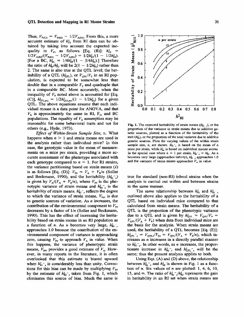
Using Eqs. (A) and (D) above, the relationshipbetween hRI–x and hRI is shown in Fig. 1 as a func-tion of n. Six values of n are plotted: 1, 4, 6, 10,15, and I. The ratio of hRI–x/hRI represents the gainin heritability in an RI set when strain means are

Fig. 1. The expected heritability of strain means (hRI–x), or theproportion of the variance in strain means due to additive ge-netic sources, plotted as a function of the heritability of thetrait (hRI), or the proportion of the total variance due to additivegenetic sources. Plots for varying values of the within strainsample size, n, are shown. hRI–x is based on the mean of nmice per strain, while hRI is based on individual mouse scores.In the special case where n = 1 per strain, hRI–x = hRI. As nbecomes very large (approaches infinity), hRI–x approaches 1.0and the variance of strain means approaches VA in value.

32 Belknap

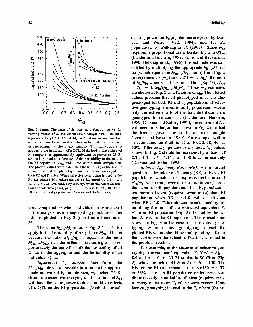
Fig. 2. Inset: The ratio of hRI–x/hRI as a function of hRI forvarying values of n, the within-strain sample size. This ratiorepresents the gain in heritability when strain means based on« mice are used compared to when individual mice are usedin partitioning the phenotypic variance. This same ratio alsoapplies to the heritability of a QTL. Main body: The estimatedF2 sample size approximately equivalent in power to 25 RIstrains is plotted as a function of the heritability of the trait inthe RI population (hRI), and n, the within-strain sample size.The plotted values were calculated from Eq. (F) in the text. Itis assumed that all phenotyped mice are also genotyped forboth RI and F2 mice. When selective genotyping is used in theF2, the plotted NF2 values should be increased by 2.3-, 1.5-,1.3-, 1.15-, or 1.08-fold, respectively, when the selection frac-tion for selective genotyping in both tails is 10, 20, 30, 40, or50% of the total population (Darvasi and Soller, 1992).

used compared to when individual mice are usedin the analysis, as in a segregating population. Thisratio is plotted in Fig. 2 (inset) as a function ofhRI.

The same hRI–x/hRI ratios in Fig. 2 (inset) alsoapply to the heritability of a QTL, or hQTL. This isbecause the ratio hRI–x/hRI is equal to the ratiohQTL–x/hQTL, i.e., the effect of increasing n is pro-portionately the same for both the heritability of allQTLs in the aggregate and the heritability of anindividual QTL.

Equivalent F2 Sample Size. From thehRI–x/hRI ratio, it is possible to estimate the approx-imate equivalent F2 sample size, NF2, when 25 RIstrains are tested with varying n. This estimated NF2

will have the same power to detect additive effectsof a QTL as the RI population. [Methods for cal-

culating power for F2 populations are given by Dar-vasi and Soller (1992, 1994), and for RIpopulations by Belknap et al. (1996).] Since NF2

required is proportional to the heritability of a QTL(Lander and Botstein, 1989; Soller and Beckmann,1990; Belknap et al., 1996), this estimate was cal-culated by multiplying the appropriate hRI–x/hRI ra-tio (which equals the hQTL–x/hQTL ratio) from Fig. 2(inset) times 25 (Nstr) times 2(1 - l/2hRI), the ratioof hRI/hF2 when n = 1 for both. Thus [Eq. (F)], NF2

= 2(1 - l/2hR I)(hR I–x/hR I)N s t r . These NF2 estimatesare shown in Fig. 2 as a function of hRI. The plottedvalues presume that all phenotyped mice are alsogenotyped for both RI and F2 populations. If selec-tive genotyping is used in an F2 population, whereonly the extreme tails of the trait distribution aregenotyped to reduce cost (Lander and Botstein,1989; Darvasi and Soller, 1992), the equivalent NF2

will need to be larger than shown in Fig. 2 to offsetthe loss in power due to the restricted sample(Lander and Botstein, 1989). For example, with aselection fraction (both tails) of 10, 20, 30, 40, or50% of the total population, the plotted NF2 valuesshown in Fig. 2 should be increased by a factor of2.3-, 1.5-, 1.3-, 1.15-, or 1.08-fold, respectively(Darvasi and Soller, 1992).

Relative Efficiency Ratio (RE). An importantquestion is the relative efficiency (RE) of F2 vs. RIpopulations, which can be expressed as the ratio ofNF 2 /NR I when the power to detect additive QTLs isthe same in both populations. Thus, F2 populationsare more efficient (require fewer mice) than RIpopulations when RE is <1.0 and less efficientwhen RE > 1.0. This ratio can be calculated by de-termining the ratio of the estimated equivalent F2

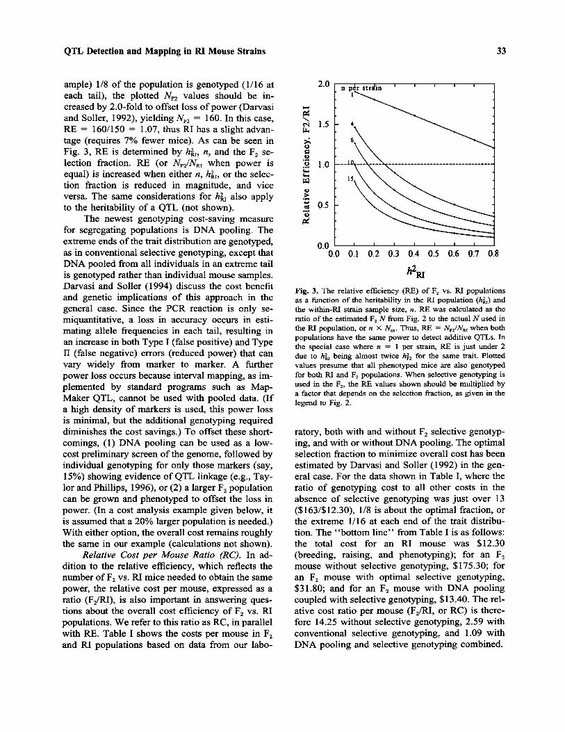
N for an RI population (Fig. 2) divided by the ac-tual N used in the RI population. These results areshown in Fig. 3 in the case of no selective geno-typing. When selective genotyping is used, theplotted RE values should be multiplied by a factorthat varies with the selection fraction, as noted inthe previous section.

For example, in the absence of selective gen-otyping, the estimated equivalent F2 N when hRI =0.4 and n = 6 for 25 RI strains is 80 (from Fig.2), while the actual RI N is 25 X 6 = 150. TheRE for the RI experiment is thus 80/150 = 0.53,or 53%. Thus, an RI population under these con-ditions is only about half as efficient (requires twiceas many mice) as an F2 of the same power. If se-lective genotyping is used in the F2 where (for ex-

QTL Detection and Mapping in RI Mouse Strains 33

ample) 1/8 of the population is genotyped (1/16 ateach tail), the plotted NF2 values should be in-creased by 2.0-fold to offset loss of power (Darvasiand Soller, 1992), yielding NF2 = 160. In this case,RE = 160/150 = 1.07, thus RI has a slight advan-tage (requires 7% fewer mice). As can be seen inFig. 3, RE is determined by hRI, n, and the F2 se-lection fraction. RE (or NF2/NRI when power isequal) is increased when either n, hRI, or the selec-tion fraction is reduced in magnitude, and viceversa. The same considerations for hRI also applyto the heritability of a QTL (not shown).

The newest genotyping cost-saving measurefor segregating populations is DNA pooling. Theextreme ends of the trait distribution are genotyped,as in conventional selective genotyping, except thatDNA pooled from all individuals in an extreme tailis genotyped rather than individual mouse samples.Darvasi and Soller (1994) discuss the cost benefitand genetic implications of this approach in thegeneral case. Since the PCR reaction is only se-miquantitative, a loss in accuracy occurs in esti-mating allele frequencies in each tail, resulting inan increase in both Type I (false positive) and TypeII (false negative) errors (reduced power) that canvary widely from marker to marker. A furtherpower loss occurs because interval mapping, as im-plemented by standard programs such as Map-Maker QTL, cannot be used with pooled data. (Ifa high density of markers is used, this power lossis minimal, but the additional genotyping requireddiminishes the cost savings.) To offset these short-comings, (1) DNA pooling can be used as a low-cost preliminary screen of the genome, followed byindividual genotyping for only those markers (say,15%) showing evidence of QTL linkage (e.g., Tay-lor and Phillips, 1996), or (2) a larger F2 populationcan be grown and phenotyped to offset the loss inpower. (In a cost analysis example given below, itis assumed that a 20% larger population is needed.)With either option, the overall cost remains roughlythe same in our example (calculations not shown).

Relative Cost per Mouse Ratio (RC). In ad-dition to the relative efficiency, which reflects thenumber of F2 vs. RI mice needed to obtain the samepower, the relative cost per mouse, expressed as aratio (F2/RI), is also important in answering ques-tions about the overall cost efficiency of F2 vs. RIpopulations. We refer to this ratio as RC, in parallelwith RE. Table I shows the costs per mouse in F2

and RI populations based on data from our labo-

Fig. 3. The relative efficiency (RE) of F2 vs. RI populationsas a function of the heritability in the RI population (hRI) andthe within-RI strain sample size, n. RE was calculated as theratio of the estimated F2 N from Fig. 2 to the actual N used inthe RI population, or n X Nstr. Thus, RE = NF2/NRI when bothpopulations have the same power to detect additive QTLs. Inthe special case where n = 1 per strain, RE is just under 2due to hRI being almost twice hF2 for the same trait. Plottedvalues presume that all phenotyped mice are also genotypedfor both RI and F2 populations. When selective genotyping isused in the F2, the RE values shown should be multiplied bya factor that depends on the selection fraction, as given in thelegend to Fig. 2.

ratory, both with and without F2 selective genotyp-ing, and with or without DNA pooling. The optimalselection fraction to minimize overall cost has beenestimated by Darvasi and Soller (1992) in the gen-eral case. For the data shown in Table I, where theratio of genotyping cost to all other costs in theabsence of selective genotyping was just over 13($163/$12.30), 1/8 is about the optimal fraction, orthe extreme 1/16 at each end of the trait distribu-tion. The "bottom line" from Table I is as follows:the total cost for an RI mouse was $12.30(breeding, raising, and phenotyping); for an F2

mouse without selective genotyping, $175.30; foran F2 mouse with optimal selective genotyping,$31.80; and for an F2 mouse with DNA poolingcoupled with selective genotyping, $13.40. The rel-ative cost ratio per mouse (F2/RI, or RC) is there-fore 14.25 without selective genotyping, 2.59 withconventional selective genotyping, and 1.09 withDNA pooling and selective genotyping combined.

34 Belknap

Relative Total Cost Ratio (RTC). The totalcost (TC) of an experiment is given by the numberof mice multiplied by the cost per mouse. The rel-ative total cost ratio (RTC) of F2/RI is thus RE XRC when the power to detect QTLs is the same inboth populations. For example, when hRI = 0.4(hF2 = 0.25) and n = 10, typical values for manybehavioral traits, F2 populations without selectivegenotyping will be RE (0.35 from Fig. 3) X 14.25(from Table I), or five times as costly compared toRI populations of the same power.

When selective genotyping is used, RC de-clines to 2.59 in our example (Table I). In this case,RTC = RE (from Fig. 3 X 2) X RC (2.59). The

factor of 2 for RE is to offset the loss in powerwhen selective genotyping of this magnitude (1/8)is practiced. Multiplying by 2 gives the RE valueexpected if no selective genotyping was used. (Thisis necessary because the RE values shown in Fig.3 presume no selective genotyping.) For example,when hRI = 0.4 and n = 10, RTC = RE (0.35 fromFig. 3 X 2) X 2.59 (from Table I) = 1.8. There-fore, F2 populations will be 1.8 times as costlycompared to RI populations of the same power. Forn = 6, RTC rises to almost threefold. Figure 4shows RTC values as a function of hRI for n = 6and 10, based on RE values taken from Fig. 3 andRC from Table I. Note that RTC will increase (F2

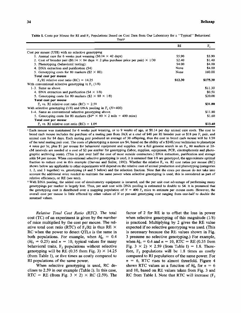
Table I. Costs per Mouse for RI and F2 Populations Based on Cost Data from Our Laboratory for a "Typical" BehavioralTraita

Cost per mouse (US$) with no selective genotyping1. Animal care for 6 weeks past weaning ($0.14 X 42 days)2. Cost of breeder pair ($0.14 X 84 days X 2 plus purchase price per pair) X 1/303. Phenotyping (behavioral testing):4. DNA extraction and purification ($4)5. Genotyping costs for 80 markers ($2 X 80):Total cost per mouse

F2/RI relative cost ratio (RC) = 14.25With conventional selective genotyping in F2 (1/8)

1-3. Same as above.4. DNA extraction and purification ($4 X 1/8)5. Genotyping costs for 80 markers ($2 X 80 X 1/8)Total cost per mouse

F2 vs. RI relative cost ratio (RC) = 2.59With selective genotyping (1/8) and DNA pooling in F2 (N=400)

1—4. Same as conventional selective genotyping above.5. Genotyping costs for 80 markers ($4* X 80 X 2 tails – 400 mice)Total cost per mouse

F2 vs. RI relative cost ratio (RC) = 1.09

RI

$5.90$2.40$4.00NoneNone

$12.30

F2

$5.90$1.40$4.00$4.00

160.00

$175.30

$11.30$0.50

$20.00

$31.80

$11.80$1.60

$13.40a Each mouse was maintained for 6 weeks past weaning, or to 9 weeks of age, at $0.14 per day animal care costs. The cost to

breed each mouse includes the purchase of a mating pair from JAX at a cost of $48 per RI breeder pair or $18 per F1 pair, andanimal care for 84 days. Each mating pair produced an average of 30 offspring, thus the cost to breed each mouse will be 1/30of the total mating pair cost. The costs of phenotyping a mouse are $4, based on the ability of a $24K/year technician to phenotype4 mice per hr, plus $1 per mouse for behavioral equipment and supplies. For a full genome search in an F2, 80 markers at 20-cM intervals are needed at a cost of $2 per marker for genotyping (labor, supplies, equipment, PCR, electrophoresis and photo-graphic archiving costs). (This is just over half the cost of most outside contractors.) DNA extraction, purification and storageadds $4 per mouse. When conventional selective genotyping is used, it is assumed that 1/8 are genotyped, the approximate optimalfraction to reduce cost in this example (Darvasi and Soller, 1992). Whether the relative F2 vs. RI cost ratios per mouse (RC)shown below are applicable to other experiments will depend on the relative cost of animal production and phenotyping (categories1, 2, and 3 together) vs. genotyping (4 and 5 below) and the selection fraction. Note that the costs per mouse do not take intoaccount the additional mice needed to maintain the same power when selective genotyping is used; this is considered as part ofrelative efficiency, or RE (see text).

b With DNA pooling, the added cost of densitometry equipment is incurred, and the per unit cost advantage of performing manygenotypings per marker is largely lost. Thus, per unit cost with DNA pooling is estimated to double to $4. It is presumed thatthe genotyping cost is distributed over a mapping population of N = 400 F2 mice to estimate per mouse costs. However, theoverall cost per mouse is little effected by other values of N or per-unit genotyping cost ranging from one-half to double theassumed values.

QTL Detection and Mapping in RI Mouse Strains 35

will cost relatively more than equivalent RI popu-lations) when either hRI or n decreases, and viceversa.

With selective genotyping and DNA pooling,RC declines to 1.09 in our example (Table I). Asbefore, RTC = RE X RC, or RE (from Fig. 3 X2.4) X RC (1.09). The factor of 2.4 reflects thegreater number of mice needed to offset the loss inpower due to selective genotyping (2.0-fold) andDNA pooling (1.2-fold) used together.

The horizontal dashed line in Fig. 4 showsRTC = 1.0, when both populations have the same

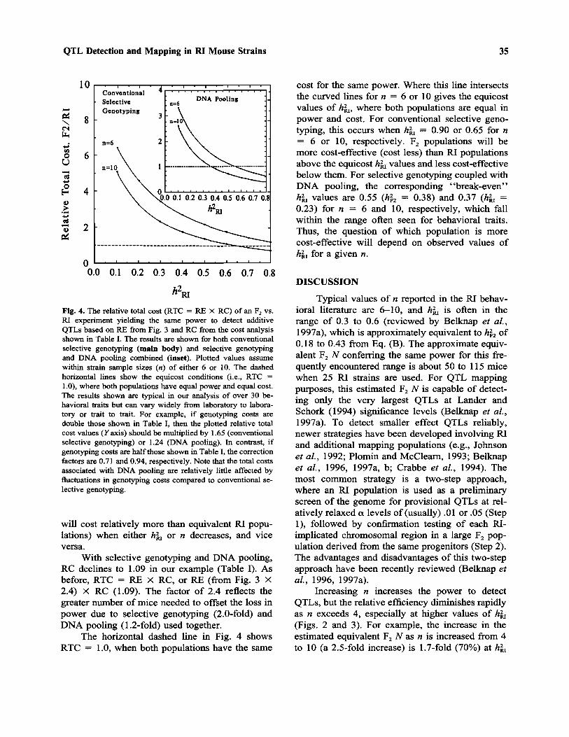
cost for the same power. Where this line intersectsthe curved lines for n = 6 or 10 gives the equicostvalues of hRI, where both populations are equal inpower and cost. For conventional selective geno-typing, this occurs when hRI = 0.90 or 0.65 for n= 6 or 10, respectively. F2 populations will bemore cost-effective (cost less) than RI populationsabove the equicost hRI values and less cost-effectivebelow them. For selective genotyping coupled withDNA pooling, the corresponding "break-even"hRI values are 0.55 (hF2 = 0.38) and 0.37 (hRI =0.23) for n = 6 and 10, respectively, which fallwithin the range often seen for behavioral traits.Thus, the question of which population is morecost-effective will depend on observed values ofhRI for a given n.

DISCUSSION

Typical values of n reported in the RI behav-ioral literature are 6-10, and hRI is often in therange of 0.3 to 0.6 (reviewed by Belknap et al.,1997a), which is approximately equivalent to hF2 of0.18 to 0.43 from Eq. (B). The approximate equiv-alent F2 N conferring the same power for this fre-quently encountered range is about 50 to 115 micewhen 25 RI strains are used. For QTL mappingpurposes, this estimated F2 N is capable of detect-ing only the very largest QTLs at Lander andSchork (1994) significance levels (Belknap et al.,1997a). To detect smaller effect QTLs reliably,newer strategies have been developed involving RIand additional mapping populations (e.g., Johnsonet al., 1992; Plomin and McClearn, 1993; Belknapet al., 1996, 1997a, b; Crabbe et al., 1994). Themost common strategy is a two-step approach,where an RI population is used as a preliminaryscreen of the genome for provisional QTLs at rel-atively relaxed a levels of (usually) .01 or .05 (Step1), followed by confirmation testing of each RI-implicated chromosomal region in a large F2 pop-ulation derived from the same progenitors (Step 2).The advantages and disadvantages of this two-stepapproach have been recently reviewed (Belknap etal., 1996, 1997a).

Increasing n increases the power to detectQTLs, but the relative efficiency diminishes rapidlyas n exceeds 4, especially at higher values of hRI

(Figs. 2 and 3). For example, the increase in theestimated equivalent F2 N as n is increased from 4to 10 (a 2.5-fold increase) is 1.7-fold (70%) at hRI

Fig. 4. The relative total cost (RTC = RE X RC) of an F2 vs.RI experiment yielding the same power to detect additiveQTLs based on RE from Fig. 3 and RC from the cost analysisshown in Table I. The results are shown for both conventionalselective genotyping (main body) and selective genotypingand DNA pooling combined (inset). Plotted values assumewithin strain sample sizes (n) of either 6 or 10. The dashedhorizontal lines show the equicost conditions (i.e., RTC =1.0), where both populations have equal power and equal cost.The results shown are typical in our analysis of over 30 be-havioral traits but can vary widely from laboratory to labora-tory or trait to trait. For example, if genotyping costs aredouble those shown in Table I, then the plotted relative totalcost values (Y axis) should be multiplied by 1.65 (conventionalselective genotyping) or 1.24 (DNA pooling). In contrast, ifgenotyping costs are half those shown in Table I, the correctionfactors are 0.71 and 0.94, respectively. Note that the total costsassociated with DNA pooling are relatively little affected byfluctuations in genotyping costs compared to conventional se-lective genotyping.

36 Belknap

= 0.1 but is only about 4% when hRI = 0.8. WhenhRI = 0.3 to 0.6, as is often the case in the behav-ioral literature, the increase in equivalent F2 N isonly about 1.1- to 1.3-fold (10-30%) in responseto the 2.5-fold (150%) increase in n (and N). More-over, inspection of Figs. 2 and 3 shows that theadded burden of testing 15 or more mice per strain,compared to only 6 or 10, for traits with high hRI

(say, >0.5) is probably not economically justified.While increasing n under these conditions is notefficient in terms of animal numbers, perhaps amore important question is, Is it cost-effective?This question is discussed below.

Since QTL mapping is inherently a large-scaleenterprise, the costs per trait are high and oftenbeyond the resources of many laboratories. This, inturn, inhibits progress. For this reason, the study ofrelative costs of one experimental design vs. an-other for QTL detection is an especially importantconsideration. As an example of a cost analysis ofF2 vs. RI populations, data from our laboratory arepresented in Table I. They roughly follow the costefficiency analysis explicated by Sokal and Rohlf(1995).

We compared the cost of an individual RImouse vs. an F2 mouse for QTL detection using thecost structure shown in Table I. While all pheno-typed RI mice are also genotyped, this is generallynot the case in segregating populations. A commonpractice to minimize F2 genotyping costs is to em-ploy conventional selective genotyping, where onlyindividual mice at the extreme ends of the trait dis-tribution are genotyped (Lander and Botstein,1989; Darvasi and Soller, 1992). While effective indramatically reducing costs, selective genotypinghas several disadvantages that must also be consid-ered. Mapping accuracy and power are somewhatreduced (Darvasi and Soller, 1992; Darvasi, 1997)and the newer and more powerful multiple regres-sion-based QTL analyses, e.g., Jansen (1993), Zeng(1994), Manly and Cudmore (1996) and Basten etal. (1996), cannot be used. Also, the assessment ofinteractions among QTLs is weakened, as is theanalysis of linked QTLs (Lin and Ritland, 1966).Finally, QTL results emerging from selective vsnonselective genotyping can, at times, be surpris-ingly different when the selection fraction is small,as observed, for example, by Gershenfeld et al.(1997) using a selection fraction of 0.12 (0.06 ineach tail). This raises questions about whether ahighly restricted sample is (1) increasing the sam-

pling error to serious levels or (2) magnifying thespurious effects of experimental artifacts that causeextreme scores for reasons unrelated (or poorly re-lated) to genotype (phenocopies). Thus, there areseveral reasons to avoid selective genotyping, es-pecially when the selection fraction is small.

Generally, whether RI populations are morecost-effective (less costly) than a comparable F2

will depend on the relative efficiency ratio, or RE(which depends on hRI, n, and the selection frac-tion) and the relative cost ratio per mouse, or RC(which depends on the costs of genotyping relativeto the other costs, and the selection fraction), all ofwhich can vary widely from trait to trait and lab-oratory to laboratory. Darvasi and Soller (1992)discuss the cost implications of selective genotyp-ing in the general case. For the cost data shown inTable I, the equicost value of hRI, when RI and F2

populations of equal power are also equal in cost,was 0.65 for n = 10 and 0.90 for n = 6, whenoptimal (for cost) conventional selective genotyp-ing was practiced (Fig. 4). Since most behavioraltraits will have hRI values less than the equicostvalue, RI populations generally will be more cost-effective than F2 populations with similar RC valuesto our example, even when selective genotyping isoptimized to reduce cost. The cost advantage of RIover segregating populations is severalfold at lowhRI and disappears as hRI reaches the equicost value.When hRI = 0.4 (hF2 = 0.25) and n = 10, for ex-ample, typical values in our experience, the costadvantage is just under twofold from Fig. 4 (the F2

population is almost twice as costly) under the costconditions shown in Table I, a major difference.This difference is even larger with smaller n; forexample, it is almost threefold when n = 6.

When selective genotyping and DNA poolingof each tail is used, equicost hRI is 0.55 (hF2 = 0.38)for n = 6 and 0.37 (hF2 = 0.23) for n = 10, valueswhich fall in the range typically seen for behavioraltraits. Thus, when DNA pooling is used under thecost conditions of our example (Table I), F2 com-pared to RI populations will be more cost-effective(cost less) for traits with heritabilities above thisequicost value and less cost-effective below them.

The conclusion drawn above concerning rel-ative total cost strictly hold only for traits with arelative cost ratio per mouse (RC) similar to thatused in our example (Table I). However, our ex-ample is typical of our experience with over 30traits subjected to QTL analyses. Actual costs from

QTL Detection and Mapping in RI Mouse Strains 37

other laboratories can easily be substituted for thevalues shown in Table I to obtain more accuratecost evaluations for a particular experiment. (AMathCad worksheet is available from the author forthis purpose.)

Throughout this paper, dominance variation inthe F2 has been ignored, since this source does notexist in the RIs. However, dominance provides an-other source of QTL information that can increasepower to detect QTLs showing dominance, thus in-creasing F2 power and cost-effectiveness. On theother hand, the opposite can occur for QTLs show-ing no dominance, because the assessment of bothadditive and dominance effects in the QTL analysis(e.g., MapMaker QTL) requires a twofold morestringent p value as the threshold for statistical sig-nificance than do additive effects alone (Lander andSchork, 1994), which effectively reduces the powerand F2 cost-effectiveness.

Overall, the use of RI populations to gain QTLinformation in behavioral studies has much to rec-ommend it for cost as well as other reasons notedelsewhere (Bailey, 1981; Belknap et al., 1996,1997a; Plomin and McClearn, 1993). This is es-pecially true if the within-strain sample size, n, isreasonably adjusted for the expected heritability(i.e., using smaller n when hRI is high, and viceversa), which can greatly reduce RI costs relativeto F2 conferring equal power. However, of all thecosts considered, those of genotyping are likely tobe most affected by advances in technology, whichwill likely make F2 and other segregating popula-tions more attractive economically than they are atpresent.

ACKNOWLEDGMENTS

This work was supported by a VA Merit Re-view Program from the Department of VeteransAffairs and by NIH Grants AA06243, AA10760,DA05228, and DA10913.

REFERENCES

Bailey, D. W. (1981). Recombinant inbred strains and bilinealcongenic strains. In Foster, H. L., Small, J. D., and Fox,J. G. (eds.), The Mouse in Biomedical Research, Vol. I,Academic Press, New York, pp. 223-239.

Basten, C. J., Weir, B. S., and Zeng, Z.-B. (1996). QTL Car-tographer: A Reference Manual and Tutorial for QTLMapping, Department of Statistics, North Carolina StateUniversity, Raleigh.

Belknap, J. K., Mitchell, S. R., O'Toole, L. A., Helms, M. L.,and Crabbe, J. C. (1996). Type I and Type II error ratesfor quantitative trait loci (QTL) mapping studies usingrecombinant inbred mouse strains. Behav. Genet. 26:149-160.

Belknap, J. K., Dubay, C., Crabbe, J. C., and Buck, K. J.(1997a). Mapping quantitative trait loci for behavioraltraits in the mouse. In Blum, K., and Noble, E. P. (eds.),Handbook of Psychiatric Genetics, CRC Press, Boca Ra-ton, FL, Chap. 25.

Belknap, J. K., Richards, S. P., O'Toole, L. A., Helms, M. L.,and Phillips, T. J. (1997b). Short-term selective breedingas a tool for QTL mapping: Alcohol preference drinkingin mice. Behav. Genet. 27:55-66.

Crabbe, J. C., Belknap, J. K., and Buck, K. J. (1994). Geneticanimal models of alcohol and drug abuse. Science 264:1715-1723.

Darvasi, A. (1997). The effect of selective genotyping on QTLmapping accuracy. Mammal. Genome 8:67-68.

Darvasi, A., and Soller, M. (1992). Selective genotyping fordetermination of linkage between a marker locus and aquantitative trait locus. Theor. Appl. Genet. 85:353-359.

Darvasi, A., and Soller, M. (1994). Selective DNA pooling fordetermination of linkage between a molecular marker anda quantitative trait locus. Genetics 138:1365-1373.

DeFries, J. C., Wilson, J. R., Erwin, V. G., and Petersen, D.R. (1989). LS X SS recombinant inbred strains of mice:initial characterization. Alc. Clin. Exp. Res. 13:196-200.

Falconer, D. S., and MacKay, T. F. C. (1996). Introduction toQuantitative Genetics, 4th ed., Longman, Essex, UK.

Gershenfeld, H. K., Neumann, P. E., Mathis, C., Crawley, J.N., Li, X., and Paul, S. M. (1997). Mapping quantitativetrait loci for open-field behavior in mice. Behav. Genet.27:201-210.

Hegmann, J., and Possidente, B. (1981). Estimating geneticcorrelations from inbred strains. Behav. Genet. 11:103-114.

Hyde, J. S. (1973). Genetic homeostasis and behavior: Anal-ysis, data and theory. Behav. Genet. 3:233-245.

Jansen, R. C. (1993). Interval mapping of multiple quantitativetrait loci. Genetics 135:205-211.

Johnson, T. E., DeFries, J. C., and Markel, P. (1992). Mappingquantitative trait loci for behavioral traits in the mouse.Behav. Genet. 22:635-653.

Kearsey, M. J., and Pooni, H. S. (1996). The Genetical Anal-ysis of Quantitative Traits, Chapman and Hall, London.

Knapp, S. J., and Bridges, W. C. (1990). Using molecularmarkers to estimate quantitative trait locus parameters:Power and genetic variances for unreplicated and repli-cated progeny. Genetics 126:769-777.

Lander, E. S., and Schork, N. J. (1994). Genetic dissection ofcomplex traits. Science 265:2037-2048.

Lander, E. S., and Botstein, D. (1989). Mapping mendelianfactors underlying quantitative traits using RFLP linkagemaps. Genetics 121: 185-199.

Lin, J.-Z., and Ritland, K. (1996). The effects of selective gen-otyping on estimates of proportion of recombination be-tween linked quantitative trait loci. Theor. Appl. Genet.93:1261-1266.

Manly, K. E., and Cudmore, R. (1996). Map Manager QT: AProgram for Genetic Mapping, Roswell Park Cancer In-stitute, Buffalo, NY.

Plomin, R., and McClearn, G. E. (1993). Quantitative trait locianalysis and alcohol-related behaviors. Behav. Genet. 23:197-212.

Sokal, R. R., and Rohlf, F. J. (1995). Biometry, Freeman, SanFrancisco.

Soller, M., and Beckmann, J. S. (1990). Marker-based mappingof quantitative trait loci using replicated progenies. Theor.Appl. Genet. 80:205-208.

Taylor, B. A. (1995). Recombinant inbred strains. In Lyon, M.F., and Searle, A. G. (eds.), Genetic Variants and Strainsof the Laboratory Mouse, 3rd ed., Oxford UniversityPress, Oxford, UK.

38 Belknap

Taylor, B. A., and Phillips, S. J. (1996). Detection of obesityQTLs on mouse chromosomes 1 and 7 by selective DNApooling. Genomics 34:389-398.

Zeng, Z.-B. (1994). Precision mapping of quantitative traitloci. Genetics 136:1457-1468.

Edited by David Fulker