EFFECT OF INDUSTRIAL POLLUTION ON THE SPATIAL ...

American Journal of Environmental Science, 9 (2): 120-129, 2013 ISSN: 1553-345X ©2013 Science Publication doi:10.3844/ajessp.2013.120.129 Published Online 9 (2) 2013 (http://www.thescipub.com/ajes.toc)

Corresponding Author: Islam Mir Sujaul, Faculty of Civil Engineering and Earth Resources, University Malaysia Pahang, Highway Tun Razak, 26300 Gambang, Pahang Malaysia

120 Science Publications

AJES

EFFECT OF INDUSTRIAL POLLUTION ON THE SPATIAL VARIATION OF SURFACE WATER QUALITY

Islam Mir Sujaul, Mohammed Amjed Hossain, Mohamad Ali Nasly and Md Abdus Sobahan

Faculty of Civil Engineering and Earth Resources, University Malaysia Pahang, Highway Tun Razak, 26300 Gambang, Pahang, Malaysia

Received 2012-09-15, Revised 2012-11-23; Accepted 2013-05-09

ABSTRACT

Surface water quality deterioration is the impact of anthropogenic activities at the study areas due to rapid industrialization. The study was done to know the spatial variation of the water quality of the Tunggak River and surrounding area because of industrial activities. In-situ parameters and ex-situ data of chemical, bio-chemical parameters and heavy metals were collected monthly to fulfill the objectives. The samples were collected from 10 selected stations and analyses were carried out using standard methods. Heavy metals were determined by using Inductively Coupled Plasma Mass Spectrometry (ICP-MS). SPSS statistical software was used for data analysis. The results of the study revealed that industrial effluents were the major source of pollutants and caused of spatial variation among the stations. Less amount of Dissolved Oxygen (DO) and higher concentration of Chemical Oxygen Demand (COD), Biochemical Oxygen Demand (BOD), ammoniacal-nitrogen and heavy metals made the water un-usable except irrigation. Analyzed surface water was classified based on Department of Environment-Water Quality Index (DOE-WQI) Malaysia and found that the maximum stations except lower and uppermost were in class IV (highly polluted). Pollution rate was higher in the middle stations due to large number of industries were located in the middle and they discharged all their effluents in the river stream. Due to tidal interference in the lower stream and minimum industry in the upper stream pollution was less in those stations. Keywords: Water Quality Index (WQI), Chemical Oxygen Demand (COD), Biochemical Oxygen Demand

(BOD), Ammoniacal Nitrogen, Heavy Metal

1. INTRODUCTION

Water is the most delicate part of the environment which is essential for human and industrial development. In the last few decades the demand of fresh water rises tremendously due to increasing population and rapid industrialization (Yisa and Jimoh, 2010). At the same time the pace of fresh water deterioration by anthropogenic activities is coupled with the ever-growing demands of water resources (Charkhabi and Sakizadeh, 2006). Due to the addition of industrial effluents containing organic pollutant and heavy metals into the river water the quality of water is deteriorating. The natural and anthropogenic metal contamination in aquatic ecosystem leads to the need of characterizing their impact on environment (Mary-Lou and Taillefert, 2008).

Malaysia is subsidized with bounty of natural water resources that contributes significantly to the socio-economic development of the country (Moorthy and Jeyabalan, 2012). But the situation is shifting every day with industrialization, urbanization and population growth. Department of Environment in their Environmental Quality Report 2009 showed that 46% river water of Malaysia is polluted which is higher than previous couple of years (DOE, 2011).

Malaysia has a number of industrial estates all over the country of which Gebeng is one and main industrial area in Kuantan, Pahang. It is located near Kuantan Port. Since 1970s the area is increasing with industrialization. Including petrochemical, multifarious industries are been established in this area. The Tunggak, which is carrying wastes of the estate, is one of the important rivers in

brought to you by COREView metadata, citation and similar papers at core.ac.uk

provided by UMP Institutional Repository

https://core.ac.uk/display/159180514?utm_source=pdf&utm_medium=banner&utm_campaign=pdf-decoration-v1

Islam Mir Sujaul et al. / American Journal of Environmental Science 9 (2): 120-129, 2013


AJES

Pahang which is adjacent to this area. The real scenario is the rapid developments including the petrochemical industries are generating effluents which contain high concentrations of conventional and non-conventional pollutants that deteriorating the water quality of the river.

The study was conducted with the objectives to identify the nature of the water quality parameters and to expose the spatial variation of water quality of the adjacent river due to industrial activities.

2. MATERIALS AND METHODS

2.1. Study Area and Selection of Station

The geographical location of Gebeng area is 3° 55’ 0” to 4° 01’ 0” N and 103° 22; 0” to 103° 27’ 0” E (Fig. 1). The Tunggak River originated from the hilly region of Gebeng area. It meets with another river namely Balok at near Angler marine centre and ultimately flows into South China Sea. Normal tide occurred every day twice and water goes at about 3 km. upstream from the sea. Sampling stations selection was done considering the land use-pattern, point-sources of pollution, vegetation and river network. A total of 10 stations were selected for sampling. The GPS system was used to determine the actual coordinate of sampling stations.

2.2. Sampling, Data collection and Sample Analysis

Water samples were collected monthly from pre-selected 10 stations during dry and wet season on 2011-12. During samples collection, in-situ data of pH, temperature, DO, turbidity, salinity, EC and TDS were also collected using YSI. APHA and HACH standard procedure was followed during sampling, sample transportation and preservation (Andrew and Franson, 2005; HACH, 2005). The three replicates of the physico-chemical parameters of the sampling water were measured at each selected sites and laboratory. Nitrogen was measured spectrometrically where, ammoniacal-N was assessed in nessler method and nitrate-N was estimated in cadmium reduction method. Sulphate and Phosphorous were also determined by using spectrophotometer and the measuring method was sulfavar 4 and ascorbic acid method respectively. Bio-chemical parameter COD measurement was done in COD reactor digestion method and BOD was analyzed in APHA method 5210. After collecting BOD samples initial reading was collected as soon as possible and then the BOD bottles were kept in incubator at 20↑8°C temperatures for 5 days. After 5 days final reading was taken and BOD was calculated with the following formulae.

Fig. 1. Map of study area showing sampling stations

BOD (mg/L) = (DOi-DO5)/P; where, DOi = DO (mg/L) of diluted sample about 15 min after preparation, DO5 = DO (mg/L) of diluted sample after 5 days incubation at 20°C and P = decimal volumetric fraction of sample.

For Total Suspended Solid (TSS) concentration, samples were analyzed in gravimetric method and heavy metals were determined by ICP-MS spectrometry. All tests were done within 7 days of sample collection.

2.3. Data Analysis

The statistical analysis of data was carried out using SPSS 16.0. Correlation matrix was done for the identification of the smallest number of common factors that best explain for the correlation among the parameters (Charkhabi and Sakizadeh, 2006). Mean values of each parameter were compared with Analysis of Variance (ANOVA).

2.4. Water Quality Index

The Water Quality Index (WQI) is a concept and the base of the concept is the comparison of water quality parameters with their respective regulatory standards (Khan et al., 2003). In the present study, water quality index calculation was done by using DOE-WQI. Based



AJES

on the concentration of DO, BOD, COD, ammoniacal-N, SS and pH the WQI was calculated (Norhayati, 1981; Haque et al., 2010). It was done on the sub-indices of those parameters whose values obtain from a series of equations (Norhayati, 1981; Haque et al., 2010; DOE, 2011).

For WQI calculation the following formula was used:

( )

WQI 0.22*SIDO 0.19*SIBOD

0.16*SICOD 0.15*SIAN

0.16*SISS 0.12*SIPH

* denote multiplication

= ++ +

+ +

where, SI is the sub index function for the selected parameters and the coefficient are weighting factors for the respected sub index.

3. RESULTS AND DISCUSSION

3.1. In-Situ Parameters

In Malaysian river, water temperature usually ranges from 24°C to 31.3°C (UKM-DOE, 2000) and Malaysian normal water temperature is 27-31°C (Saad et al., 2008). The Table 1 shows that, water temperature of the study area varied from 26.16°C to 35.24°C. As can be seen, temperature was found beyond the Malaysian standard at station 4 to 8 and other 5 stations within the normal limit. Higher temperature at station 4 to 8 was perhaps due to high air temperature within the area (Pilgrim et al., 1998; Bonacci et al., 2008) and obviously the industrial effluents (Nedeau et al., 2003).

The spatial variation of pH values was identical among the stations. The ranges varied from 4.16 to 9.12 (Table 1). However, the highest mean pH value 8.02 was recorded at station 6 followed by station 5 and 7; but, the values of pH of those stations along with stations 2, 3 and 4 were within the Malaysian standard (DOE, 2008). On the other hand, the pH values of station 8, 9 and10 were recorded very low. That might be due to the addition of wastes with acidic nature generated from mining and chemical industries. Furthermore, water of stations 8, 9 and10 contained a considerable amount of chromium which was negatively correlated with pH and fewer amounts of nitrate nitrogen and cobalt having positive correlation (Table 2 and 3). Conductivity was found within the normal limit at maximum stations except 1, 2 and 3 (Table 2); where, the saline water entered everyday during tide (Haris and Omar, 2008) from the South China Sea.

The Table 1 also shows the DO concentrations at different stations of the study area. DO values were observed very low at all stations; the lowest value 1.10

mg L−1 was recorded at station 2 and the highest 4.4 mg L−1 was at station 1. The lowest concentration of DO was perhaps due to high temperature and BOD which was the result of industrial effluents; excessive BOD use huge amount of dissolved oxygen. According to the classification of INWQS Malaysia, the stations 1, 5, 7 and 8 were classified under class III and the rest were in class IV based on DO concentration (DOE, 2008).

TDS concentration was recorded higher in the lower stream compare to the uppermost. Stations 1 and 2 which were situated at the lower part contained the highest amount of TDS (Table 1) and the water of those two stations was in class IV based on TDS result (DOE, 2008). In fact, there was a branch of the river carryings pollutant from some agricultural and homestead areas and in between those stations a mangrove forest was present; again, tide was a normal phenomenon there. Due to tidal interference (Ideriah et al., 2010), forested area (Lawson, 2011) and agricultural and homestead wastes (Ogedengbe and Akinbile, 2010) TDS amount of those two stations found higher. Meanwhile, TDS at station 7 to10 were in permissible limits 500 mg L−1 (DOE, 2008) (Table 1).

Turbidity level varied from 2.10 NTU at station 9 to 34.50 NTU at station 5 (Table 1); only station 9 was found in normal level whether rest of all contained higher value of turbidity according to the INWQS, Malaysia. Non-point sources of pollution like runoff from newly developed industrial areas and agricultural land associated with point sources may be the cause of high turbidity (Wilson, 2010).

3.2. Ex-Situ Parameters

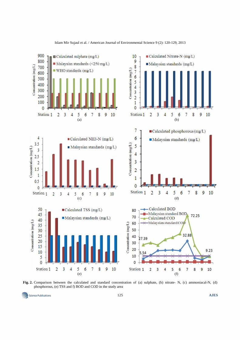
Collecting samples from sampling sites were analyzed in laboratory for determining the amount of Sulphate (SO4), Nitrate-Nitrogen (NO3-N), NH3-N, Phosphate-Phosphorus (PO4

3-), BOD, COD and TSS. The calculated amounts of these parameters were compared with the Malaysian standards in Fig. 2.

Sulphur was determined as SO4 and the results showed that the lowest amount of sulphate was recorded 1.90 mg L−1 (range 1.00-3.00) at station 9 and the highest amount was recorded 875.00 mg L−1 (with range 580-1220) at station 1 (Table 2). Except station 1and 7 the level was within the Malaysian standard limit and only the station 1 was found beyond the WHO standard limit (Fig. 2a). It might be due to station 1 was near the sea that contained higher level of sulphate (WHO, 2004) and station 7 was adjacent with some industries which discharged sulphur rich effluents into the river.



AJES

Table 1. Range, mean and SD for in-situ parameters of 10 sampling stations with geographical location Station Location (GPS) Temperature Conductivity DO TDS Turbidity No. with elevation (m) (°C) pH (µS/cm) (mg/L) (mg/L) (NTU) 1. N 03°56'35.04” and Range 27.05-30.17 5.66-7.02 14200-27080 2.62-4.40 9040-24300 7.69-22.50 E 103°22’32.1”(10) mean SD 28.78 6.26 18013 3.30 16137 16.66 1.07 0.52 4946 0.61 7691 6.41 2. 'N 03°57’19.44” and Range 28.04-29.2 6.97-7.71 7700-13660 1.10-2.17 5160-7270 10.05-24.70 E 103°22’59.94” (7) mean SD 28.55 7.25 10880.0 1.58 6250 17.72 5.81 0.59 0.34 2836.00 0.41 1088.00 3. ‘N 03°57’39.6” and Range 29.01-29.81 7.32-8.40 1244-1800 1.33-1.80 650-869 9.78-20.70 E 03°23’14.64” (7) mean SD 29.34 7.69 1395 1.69 767 13.70 0.38 0.38 207 0.36 112 3.90 4. N 03°57’54.18” and Range 30.92-32.57 7.51-8.51 1119-1320 1.62-4.12 527-821 10.05-17.27 E 103°23’22.86” (8) mean SD 31.74 7.95 1212 2.71 613 14.14 0.75 0.35 95 0.96 108 3.42 5. N 03°58’12.54” and Range 30.92-33.1 6.96-8.95 1380-1630 1.93-3.91 642-748 11.26-34.50 E 103°23’23.28” (9) Mean SD 31.98 7.96 1505 3.12 700 23.44 1.07 0.99 107 0.91 50 12.03 6. N 03°58’33.6” and Range 31.63-34.14 7.25-9.12 1423-1740 1.56-3.16 649-778 11.73-28.80 E 103°23’14.28” (13) mean SD 32.88 8.02 1585 2.32 715 20.98 1.35 0.76 164 0.79 68 8.01 7. 03°59’13.44” and Range 33.2-35.24 6.77-8.60 923-1210 2.85-3.93 203-529 6.69-12.35 E 103°23’16.92” (13) Mean SD 33.78 7.65 1068 3.28 365 9.82 0.88 0.62 149 0.51 171 2.30 8. N 03°59’16.44” and Range 32.5-34.1 4.16-5.42 51-58 2.78-4.25 19.6-24.8 4.83-10.06 E 103°23’17.46” (12) Mean SD 33.27 4.96 55 3.38 21.78 6.59 0.56 0.29 3.31 0.59 2.25 1.81 9. N 03°59’27.42” and Range 26.16-27.4 4.23-6.70 20-27 1.93-3.05 7.7-8.7 2.10-6.02 E 103°24’12.18” (9) Mean SD 26.78 5.13 24 2.34 8.15 3.87 0.61 1.04 3.39 0.38 0.47 1.56 10. N 03°59’37.62” and Range 31.12-31.75 5.14-6.40 713-787 2.36-3.01 333-379 7.7-12.24 E 103°24’45.3” (10) Mean SD 31.45 5.86 750.0 2.66 354 10.11 0.29 0.44 36.01 0.22 22.12 2.09 Table 2. Range, SD and mean of ex-situ water quality parameters for 10 sampling stations in the study area NO3- NH4

+ N PO43- SO4

2- TSS Cr Co Cu Pb Stations N mg/L mg/L mg/L mg/L mg/L mg/L mg/L mg/L mg/L Range 0.02-0.073 0.65-1.82 0.06-0.59 580-1220 35.0-75.0 0.00- 0.035 0.0809-0.10 0.287-0.553 0.492-0.596 1 SD 0.026 0.63 0.271 314.56 15.394 0.014 0.014 0.143 0.052 Mean 0.0465 1.24 0.335 875 47.165 0.0082 0.0926 0.4496 0.5415 Range 0.1-0.35 2.36-3.00 0.60-2.07 59-320 29.0-72.0 0.000 0.219-0.228 0.00-0.010 0.489-0.504 2 SD 0.127 0.297 0.780 140.41 15.587 0.000 0.0051 0.006 0.0079 Mean 0.2235 2.625 1.35 188.5 41.085 0.000 0.2243 0.0033 0.4956 Range 0.00-0.45 3.20-4.05 1.03-1.74 20-67 10.0-20.0 0.000 0.165-0.184 0.0 0.471-0.489 3 SD 0.243 0.352 0.368 24.66 3.817 0.000 0.0095 0.0 0.0103 Mean 0.225 3.465 1.395 43.5 14.165 0.000 0.174 0.0 0.4827 Range 0.01-2.70 1.21-3.25 0.55-1.20 20-70 12.0-21.0 0.000 0.246-0.257 0.0 0.470-0.496 4 SD 1.298 1.061 0.342 26.31 3.507 0.000 0.0059 0.0 0.014 Mean 1.15 2.185 0.88 46.65 14.665 0.000 0.2505 0.0 0.4801 Range 0.00-4.50 1.29-3.25 0.34-1.54 37-63 17.0-23.0 0.000 0.561-0.665 0.0 0.480-0.508 5 SD 2.274 0.981 0.618 12.38 2.16 0.000 0.0532 0.0 0.014 Mean 2.035 2.17 0.93 48.75 18.585 0.000 0.6191 0.0 0.4937 Range 0.00-3.70 0.87-3.35 0.61-1.03 17-39 16.0-17.0 0.000 0.651-0.701 0.0 0.218-0.241 6 SD 1.629 1.342 0.206 11.0 0.547 0.000 0.0263 0.0 0.012 Mean 1.385 2.105 0.835 28.4 16.085 0.000 0.6716 0.0 0.2322 Range 0.01-0.42 0.86-1.76 0.05-0.85 170-339 10.0-19.0 0.003-0.111 0.0 0.287-0.553 0.222-0.244 7 SD 0.216 0.448 0.016 86.68 3.502 0.062 0.0 0.1426 0.012 Mean 0.205 1.34 0.07 255.835 14.335 0.0395 0.0 0.4496 0.2349 Range 0.00-0.01 0.96-1.72 0.02-0.04 2.00-7.00 9.0-16.0 0.041-0.089 0.0 0.0 0.219-0.241 8 SD 0.005 0.292 0.007 1.79 2.927 0.028 0.0 0.0 0.011 Mean 0 1.515 0.025 4.835 11.835 0.0575 0.0 0.0 0.2305 Range 0 0.16-0.37 0.01-0.10 1.00-3.00 2.0-36 0.002-0.053 0.090-0.095 0.0 0.487-0.494 9 SD 0 0.094 0.034 0.89 13.155 0.027 0.0030 0 0.004 Mean 0 0.245 0.02 1.915 9.5 0.032 0.092 0.0 0.4896 Range 0.19-0.25 1.88-2.37 0.07-12.30 30-49 5.0-15.0 0.00-0.0583 0.0 0.0 0.2224-0.2318 10 SD 0.023 0.197 6.644 8.69 3.983 0.028 0.0 0.0 0.005 Mean 0.23 2.215 6.315 40.915 10.25 0.0161 0.0 0.0 0.2283



AJES

Table 3. Correlation coefficient (r) for water quality parameter in the study area pH DO NO3

-N NH4+N PO4

3- SO42- TSS Cr Co Cu Pb

pH 1.0 DO -0.2502 1.0000 NO3

-N 0.6721* 0.0783 1.0000 NH4

+N 0.5934 -0.5319 0.2754 1.0000 PO4

3- -0.1017 -0.1895 -0.0441 0.3667 1.0000 SO4

2- -0.0514 0.339 -0.2912 -0.2340 -0.1943 1.0000 TSS 0.0995 -0.0647 -0.1409 0.0593 -0.178 0.8058** 1.000 Cr -0.6931* 0.5264 -0.5435 -0.6069 -0.2214 -0.1054 -0.377 1.0000 Co 0.6439* -0.1858 0.8920** 0.2970 -0.1567 -0.2270 0.0314 -0.6295 1.0000 Cu 0.0364 0.525 -0.3155 -0.3721 -0.2863 0.8152** 0.4424 0.2154 -0.3565 1.0000 Pb 0.1503 -0.2975 0.0832 0.0692 -0.2923 0.3405 0.5182 -0.5277 0.1369 -0.0089 1

Nitrogen was assessed as NO3-N and NH3-N. The Table 2 shows that, the highest amount of NO3-N was observed at station 5 valued 2.035 mg L−1. Nitrate is commonly found in surface water as contaminant (Ji et al., 2012); however, in the present study it was observed within the safe level (<0.4) at every station (DOE, 2008) (Fig. 2b). The concentration of another nitrogenous compound NH3-N which is one of the most important parameters for water quality was recorded higher at all stations that was beyond the permissible limit (DOE, 2008) (Fig. 2c). As can be seen, the range was 0.16-0.37 mg L−1 (mean 0.25 mg L−1) at station 9 to 3.40-4.05 mg L−1 (mean 3.47 mg L−1) at station 3 (Table 2). Similar of most of the parameters, middle stations were found loaded with nitrogen too; as they received most of the effluents from the industries including polymer, chemical, metal, gas and power and manufacturing and wooden industries of Gebeng area.

Phosphorous in the form of PO43- was recorded the

highest 6.30 mg L−1 at station 10 and the lowest 0.02 mg L−1 at station 9 (Table 2). Comparison between calculated and standard level of PO4

3- in the study area (Fig. 2d) stated that, stations 1 to 6 and 10 were found loaded with PO4

3- concentration beyond the Malaysian standard limit and stations 7 to 9 were observed within the permissible level (DOE, 2008).

In the study area, TSS was observed almost below the standard levels (Fig. 2e). Nevertheless, station 1 and 2 contained higher amount of TSS compared to Malaysian standard limit; because of forested area, tidal disturbance (Law et al., 2007), homestead and agricultural practices in between station 1 and 2.

Figure 2 Comparison between the calculated and standard concentration of (a) sulphate, (b) nitrate- N, (c) ammoniacal-N, (d) phosphorous, (e) TSS and (f) BOD and COD in the study area

BOD and COD were analyzed and the results were compared to the Malaysian standard limit in Fig. 2f. The

Figure shows that, BOD concentration was the highest 32.88 mg L−1 at station 7 and the lowest 4.225 mg L−1 at station 9. Figure 2f also stated that the BOD values of all stations were beyond the standards limit of Malaysia and the values found maximum in the mid-stream region. This was perhaps because of industrial activities (Walakira and Okot-Okumu, 2011) in the area and it was substantial in mid-region. The result indicated that, high load of organic pollutant from industrial wastes proliferate the decomposer organisms causing reduction of DO followed by increase BOD in surface water (Gyawali et al., 2012). Similarly, the concentration of COD was also as same as BOD (Fig. 2f). The higher amount of COD indicated that, the surface water was highly polluted; as it is the demonstrable parameter to examine the extent of pollution in water (Amirkolaie, 2008). However, COD level recorded safe at stations 9 and 10 (DOE, 2008).

According to the INWQS classification, the stations 3 to 7 were classified under class V, station 2, 8 and 10 were found in class IV and station 1 and 9 were categorized as class III based on BOD concentration. Again, based on COD concentration station 7 was in class IV and stations 1 to 6 and 8 were classified under class III.

3.3. Heavy Metal

The water samples were analyzed for determining heavy metal contamination and result showed that surface water of the study area contained lead(Pb), cobalt(Co), copper (Cu), chromium (Cr), zinc (Zn) and barium (Ba). The study results have been compared with the Malaysian standards and presented in Fig. 3.

Figure 3a demonstrated that, the amount of Pb was observed in toxic level all over the area and the observed concentration was above the WHO as well as Malaysian standard at all stations.



AJES

(a) (b)

(c) (d)

(e) (f) Fig. 2. Comparison between the calculated and standard concentration of (a) sulphate, (b) nitrate- N, (c) ammoniacal-N, (d)

phosphorous, (e) TSS and f) BOD and COD in the study area



AJES

(a) (b)

(c) (d)

(e) (f) Fig. 3. Comparison between the calculated and standard concentration of (a) Pb, (b) Co, (c) Cu, (d) Cr, (e) Ba and (f) Zn in the study area



AJES

Table 4. Surface water classification in the study area based on DOE-WQI Monitoring station Calculated WQI value Water class Monitoring station Calculated WQI value Water class Station 1 54.99 III Station2 47.77 IV Station 3 44.35 IV Station 4 45.38 IV Station 5 44.36 IV Station 6 44.26 IV Station 7 39.33 IV Station 8 51.57 IV Station 9 62.90 III Station 10 55.08 III

The values were varied from 0.2283 mg/L (range 0.2224-0.2318) at station 10 to 0.5415 mg L−1 (range 0.4915-0.5961) at station 1 (Table 2). The main source of Pb was the discharge of Pb containing industrial wastes from gas based power industry, refining, metal and mining industries (USEPA, 2012). Some industries discharged their waste water through pipeline which may also be the potential sources of Pb (Al-Othman et al., 2012).

Regarding Co; it was found toxic with higher concentration compare to the standard limit at station 2 to 6 Fig. 3b and station 1 and 9 was observed within the standard level (Nagpal, 2004). Similar to the other parameters, it was also higher in mid-region. Densely populated industries in the mid-stream might be contributed to high level of cobalt in that area. However, Co was not found at station 7, 8 and10 (Table 2).

Copper and chromium were found to be almost in acceptable level with some exceptions. Fig. 3c shows that, the concentration of Cu was found higher at station 1 and 7; regarding station 1 it might be because of anthropogenic sources and shipping (Kuantan port) (Shanka et al., 2004) and at station 7 was probably for the correlation with SO4 (Table 3); as the station contained more amount of SO4. At the same time, Cr observed higher at station 8 which was beyond the standard level. Probably the cause was low pH value (Table 1) of that station which was negatively correlated with chromium (Table 3). Except those three stations Cu and Cr observed very low or zero at other stations Fig. 3c and 3d. Other two elements Ba and Zn were determined and compared with standard level in Fig. 3e and f. The figures showed that the observed level were within the Malaysian standard level (DOE, 2008).

3.4. Water Quality Index

The DOE-WQI values were computed to classify the surface water quality of the study area. Table 4 shows the surface water classifictaion based on the calculated DOE-WQI values. As can be seen, water of station 2 to 8 was classified as class IV (highly polluted). As the concentration of most of the parameters found higher in the mid-region; the water quality of the middle stations were found more deteriorated; and the water of those

stations (station 2 to 8) were found to be un-usable without irrigation (DOE, 2008). However, the station 1 at lower stream and stations 9 and 10 at upper stream were classified as class III; that might be because of the tidal interference in the lower stream and less industrial activities at the uppermost.

4. CONCLUSION

This study revealed that the pollution level was comparatively higher in the mid-stations; where, the industrial activities are more compare to other parts. As a result, more effluents were adding to the stream and thus caused high pollution. On the other hand, due to tidal interference at lower stream and less industrial activities at upper stream caused less pollution in lower and upper stations. Considering the analytical results, it is clear that the major source of pollutant was the industrial wastes containing organic, inorganic pollutant and heavy metals, associated with some homesteads and a few agricultural practices. Higher variability was due to higher anthropogenic activities. Based on the classification the water of the area was found to be unusable except irrigation. Hence, the pollution is rising with the rising of industries. So, attempt should be taken immediately to reduce the pollution level of the river as well as surface water of the study areas. For the reduction of pollution, close monitoring of industrial activities should be ensured and emphasis also be given on recycling of industrial wastes of their own before discharging them to the river flow.

5. ACKNOWLEDGEMENT

Researchers are grateful to the University Malaysia Pahang and Faculty of Civil Engineering and Earth resources for funding through the project RDU: 110354

6. REFERENCES

Al-Othman, A.Z., G.E. El-Desoky, A.M. AL-Othman, M.A.M. Aboul-Soud and M.A. Habila et al., 2012. Lead in drinking water and human blood in Riyadh City, Saudi Arabia. Arab J. Geosci. DOI: 10.1007/s12517-012-0551-4



AJES

Amirkolaie, A.K., 2008. Environmental Impact of nutrient discharged by aquaculture waste water on the Haraz river. J. Fish Aquat. Sci., 3: 275-279. DOI: 10.3923/jfas.2008.275.279

Andrew, D.E. and M.A.H. Franson, 2005. Standard Methods for Examination of Water and Wastewater. 21th Edn., American Public Health Association, ISBN-10: 0875530478, pp: 1200.

Bonacci, O., D. Trninic and T. Roje-Bonacci, 2008. Analysis of the water temperature regime of the Danube and its tributaries in Croatia. Hydrol. Proc., 22: 1014-1021. DOI: 10.1002/hyp.6975

Charkhabi, A.H. and M. Sakizadeh, 2006. Assessment of spatial variation of water quality parameters in the most polluted branch of the Anzali wetland, northern Iran. Polish J. Environ. Stud., 15: 395-403.

DOE, 2008. Interim National Water Quality Standards for Malaysia.

DOE, 2011. Environmental Quality Report 2009: River Water Quality.

Gyawali, S., K. Techato and C. Yuangyai, 2012. Effects of industrial waste disposal on the surface water quality of U-tapao River, Thailand. Proceedings of the 3rd International Conference on Environment Science and Engieering, (ESE’ 12), IPCBEE,

IACSIT Press, Singapoore, pp: 109-113. HACH, 2005. Water Analysis Guide. 1st Edn., ASTM,

USA., Philadelphia, pp: 212. Haque, M.A., Y.F. Huang and T.S. Lee, 2010. Seberang

Perai rice scheme irrigation water quality assessment. J. Instit. Eng. Malaysia, 71: 42-49.

Haris, H. and W.M.W. Omar, 2008. The effects of tidal events on water quality in the coastal area of Petani River Basin, Malaysia. Proceedings of the International Conference on Environmental Research and Technology, Jul. 22-22, School of Biology, Pulau Pinang, Malaysia.

Ideriah, T.J.K., O. Amachree and H.O. Stanley, 2010. Assessment of water quality along Amadi creek in Portharcourt, Nigeria. Sci. Afr., 9: 150-162.

Ji, M.K., W.B. Park, M.A. Khan and A.I. Reda et al., 2012. Nitrate and ammonium ions removal from groundwater by a hybrid system of zero-valent iron combined with adsorbents. J. Environ. Monit., 14: 1153-1158. DOI: 10.1039/C2EM10911E

Khan, F., T Husain and A. Lumb, 2003. Water quality evaluation and trend analysis in selected watersheds of the Atlantic region of Canada. Environ. Monit. Assess., 88: 221-242. DOI: 10.1023/A: 1025573108513

Law, P.L., I.N. Law, H.H. Lau and F.W.L. Kho, 2007. Impacts of barrage flushing and flooding in operations on upstream total suspended solids. Int. J. Environ. Sci. Tech., 4: 75-83.

Lawson, E.O., 2011. Physico-chemical parameters and heavy metal contents of water from the mangrove swamps of Lagos Lagoon. Lagos, Nigeria, Adv. Biol. Res., 5: 08-21.

Mary-Lou, T.W. and M. Taillefert, 2008. Remote in situ voltammetric techniques to characterize the biogeochemical cycling of trace metals in aquatic systems. J. Environ. Monit., 10: 30-54. DOI: 10.1039/B714439N

Moorthy, R. and G. Jeyabalan, 2012. Ethics and sustainability: A review of water policy and management. Am. J. Applied Sci., 9: 24-31. DOI: 10.3844/ajassp.2012.24.31

Nagpal, N.K., 2004. Technical Report-Water Quality

Guidelines For Cobalt. Nedeau, E.J., R.W. Merritt and M.G. Kaufman, 2003.

The effect of an industrial effluent on an urban stream benthic community: Water quality Vs. habitat quality. Environ. Pollut., 123: 1-13. DOI: 10.1016/S0269-7491(02)00363-9

Norhayati, M., 1981. Indices for water quality in a river, Unpublished dissertation in partial fulfillment of the requirements for the degree of Doctor of Philosophy. Asian Institute of Technology, Bangkok.

Ogedengbe, K. and C.O. Akinbile, 2010. Comparative analysis of the impact of industrial and agricultural effluent on Ona stream in Ibadan. Nigeria, New York Sci. J., 3: 25-33.

Pilgrim, J.M., X. Fang and H.G. Ste Fan, 1998. Stream temperature correlations with air temperatures in minnesota: Implications for climate warming. J. Am. Water Res. Assoc., 34: 1109-1121. DOI: 10.1111/j.1752-1688.1998.tb04158.x

Saad, M., F. Naemah, N.A. Rahman, N. Norulaini and A. Kadir et al., 2008. Project Report: Identification of Pollution Sources within the Sungai Pinang River Basin. Universiti Sains Malaysia.

Shanka, G.C., S.A. Skrabalb, R.F. Whitehead and R.J. Kieber, 2004. Strong copper complexation in an organic-rich estuary: The importance of allochthonous dissolved organic matter. Marine Chem., 88: 21-39. DOI: 10.1016/j.marchem.2004.03.001

UKM-DOE, 2000. Project pengawasan biologi dan indicator biologi. Bureau of Consultancy and Innovation. University Kebangsaan Malaysia-Department of Environment, Bangi.



AJES

USEPA, 2012. Brief overview of lead in the environment. Washinton, DC.

Walakira, P. and J. Okot-Okumu, 2011. Impact of Industrial effluents on water quality of streams in Nakawa-Ntinda. Uganda, J. Applied Sci. Environ. Manage., 15: 289-296.

WHO, 2004. Sulfate in Drinking-water: Background document for development of WHO Guidelines for Drinking-water Quality. World Health Organization.

Wilson, P.C., 2010. Water Quality Notes: Water Clarity. University of Florida.

Yisa, J. and T. Jimoh, 2010. Analytical studies on water quality index of river Landzu. Am. J. Applied Sci., 7: 453-458. DOI: 10.3844/ajassp.2010.453.458

EFFECT OF INDUSTRIAL POLLUTION ON THE SPATIAL ...

Documents

Transcript of EFFECT OF INDUSTRIAL POLLUTION ON THE SPATIAL ...