(EE01) LC-DAD-MS/MS hardware manual - European ...
58
______________________________________________________________________________________________________ This project has been funded with support from the European Commission. This publication reflects the views only of the authors, and the Commission cannot be held responsible for any use which may be made of the information contained therein. (EE01) LC-DAD-MS/MS hardware manual Lab exercise: Qualitative analysis using LC-DAD-MS/MS Course: Isolation and characterization of natural products Author: Dejan Orčić (University of Novi Sad, Faculty of Sciences) Preparation: Dejan Orčić (University of Novi Sad, Faculty of Sciences) Special thanks to Sanja Berežni (University of Novi Sad, Faculty of Sciences) for contribution
-
Upload
khangminh22 -
Category
Documents
-
view
0 -
download
0
Transcript of (EE01) LC-DAD-MS/MS hardware manual - European ...
______________________________________________________________________________________________________
This project has been funded with support from the European Commission. This publication reflects the views only of the authors,
and the Commission cannot be held responsible for any use which may be made of the information contained therein.
(EE01) LC-DAD-MS/MS hardware manual
Lab exercise: Qualitative analysis using LC-DAD-MS/MS
Course: Isolation and characterization of natural products
Author: Dejan Orčić (University of Novi Sad, Faculty of Sciences)
Preparation: Dejan Orčić (University of Novi Sad, Faculty of Sciences)
Special thanks to Sanja Berežni (University of Novi Sad, Faculty of Sciences) for contribution

______________________________________________________________________________________________________
This project has been funded with support from the European Commission. This publication reflects the views only of the authors,
and the Commission cannot be held responsible for any use which may be made of the information contained therein.
(EE01) Uputstvo za LC-DAD-MS/MS
instrument
Vežba: Kvalitativna LC-DAD-MS/MS analiza
Kurs: Izolacija i karakterizacija prirodnih proizvoda
Autor: Dejan Orčić (Univerzitet u Novom Sadu, Prirodno-matematički
fakultet)
Tehnička priprema: Dejan Orčić (Univerzitet u Novom Sadu, Prirodno-
matematički fakultet)
Zahvaljujemo se Sanji Berežni (Univerzitet u Novom Sadu, Prirodno-matematički fakultet) za
doprinos

00:00 Flowpath check
Before starting with LC‐DAD‐MS‐MS analysis, several routine maintenance operations and checks need to be performed.
First, we need to check the entire flowpath through the system. Namely, every capillary in the system can be disconnected and reconnected in different ways for various purposes (e.g. maintenance, adaptation for specific analysis, testing etc.) so we need to check whether the configuration is appropriate for our needs. In this case the mobile phase components flow from the reservoirs, through degasser, into the pump heads, through pressure dampers, mixer, pressure sensor, into the purge valve, to automated liquid sampler injector hex valve, to left heat exchanger, through in‐line filter, through the column, to post‐column heat exchanger, to DAD flow cell, and then into MS diverter valve.
Additionally, if needed, we can check whether all the connections are tightened sufficiently, otherwise we could have some leaks.
We can also check whether reservoirs for waste from LC and MS are empty, in order to prevent spilling.
Finally, we can also check the column. The column is the one we need for our analysis. It is mounted the right way – it follows the flowpath. With new columns it is not an issue, but with old‐fashioned columns, they should never be mounted in reverse, since the entrance frit is not dense enough to retain the stationary phase particles.
00:00 Provera toka mobilne faze
Pre nego što se započne sa LC‐DAD‐MS‐MS analizom, neophodno je obaviti niz pripremnih operacija i provera.
Kao prvo, neophodno je proveriti ceo tok mobilne faze kroz sistem. Naime, svaka kapilara u sistemu može se prespojiti na različite načine (za potrebe održavanja, prilagođavanja potrebama specifičnih analiza, dijagnostike i sl.) te se mora proveriti da li je trenutna konfiguracija adekvatna za naše potrebe. U našem slučaju, komponente mobilne faze teku iz rezervoara, kroz degazer, u glave pumpe, kroz prigušnice, mešač, senzor pritiska, ventil za ispiranje, do šestokrakog ventila autosemplera, u levi izmenjivač toplote, kroz pretkolonski filter, kolonu, postkolonski izmenjivač toplote, DAD protočnu ćeliju i u prespojni ventil masenog spektrometra.
Dodatno, ako je potrebno, može se proveriti da li svi spojevi dobro zaptivaju – u protivnom, može doći do curenja.
Mogu se proveriti i po potrebi isprazniti rezervoari za otpad iz LC i MS, da bi se izbeglo prelivanje.
Na kraju, možemo proveriti i kolonu. Kolona na instrumentu jeste ona koja nam je potrebna za analizu. Postavljena je u pravom smeru – strelica prati tok mobilne faze. Dok kod novih kolona to nije bitno, stari modeli se ne smeju obrnuto montirati, jer je ulazna frita nedovoljno gusta da zadrži čestice stacionarne faze.
02:42 MS support devices check
In the case of LC‐MS analysis, we should also check support devices.
First, air compressor and nitrogen generator – for start, it should be on. In this case, we can see that "high duty" and "service" indicators are lit, meaning very soon do a professional maintenance needs to be performed. The pressure is still OK.
Next, the rough pump works, but there is a lot of oil in mist trap. We should transfer it back to the pump body by opening a gas balast valve. Vacuum will now drain the oil back into the pump. When the oil is drained, we should close the gas balast valve – we should never leave it opened. If the instrument is shut down, and then powered on with the opened gas balast valve, there is a certain risk that the oil will be drawn into the MS, contaminating it catastrophically.
The final thing we should check is level of oil in the pump. So, the level is quite low, maybe ~1 cm above the minimum level, so we should refill the pump soon.
02:42 Provera pomoćnih uređaja
U slučaju LC‐MS analize, trebalo bi proveriti i pomoćne uređaje.
Kao prvo, kompresor sa azot‐generatorom treba da bude uključen. U našem slučaju, može se zapaziti da su lampice "high duty" i "service" upaljene, što znači da bi uskoro trebalo izvršiti profesionalno održavanje uređaja, ali je u ovom trenutku pritisak još uvek zadovoljavajući.
Dalje, gruba pumpa radi, ali se zapaža dosta ulja u hvataču magle, te bi ga trebalo vratiti u telo pumpe otvaranjem gas balast ventila. Vakuum će ulje iz hvatača povući u pumpu. Kada je proces gotov, ventil treba zatvoriti – nikada ga ne ostavljati otvorenog. Naime, ako se instrument isključi i zatim ponovo uključi uz otvoren gas balast ventil, može doći do povlačenja ulja u MS, što bi rezultovalo katastrofalnom kontaminacijom.
Na kraju, treba proveriti i nivo ulja u gruboj pumpi. U našem slučaju, nivo je prilično nizak, oko 1 cm iznad minimuma, te bi pumpu uskoro trebalo dopuniti.
04:12 Software start & computer check
We start the Instrument Control software. Of course, all the LC modules should have been physically turned on and allowed to perform a self‐test prior to this. Otherwise, the software will just block.
The modules are networked, and need to report to their server (in our case, DAD), and than DAD reports to the software. Network problems can, of course, occur, but in this case, all the modules have reported to the software, none is missing and we don't have any error reports. If some module
04:12 Pokretanje softvera i provera računara
Pokrećemo Instrument Control softver. Prethodno, svi LC moduli moraju biti fizički uključeni i mora im se dozvoliti da izvrše samotestiranje. U protivnom, softver će blokirati.
Moduli su umreženi i moraju se javiti svom serveru (u našem slučaju, DAD), koji se dalje javlja softveru. Pritom, kao i kod svake mreže, može doći do problema u komunikaciji. U našem slučaju, svi moduli su se uredno prijavili softveru, nijedan ne nedostaje i nema nikakvih poruka o greškama. Ako bi neki od modula nedostajao u dijagramu sistema, ili bi sistem
is missing from the system diagram or an error appeared, we would need to shut down the software, kill all of its processes, and then restart the module or the entire instrument.
In addition to software, if we have numerous samples, we should also check whether there is enough free space on hard drive. Additionally, the hard drive should be defragmented often, because heavily fragmented drive slows down the data transfer which can disrupt the communication between the instrument and the computer, and that would break the analysis.
prijavljivao grešku, morali bismo da zatvorimo softver, prekinemo sve njegove pozadinske procese i zatim restartujemo problematični modul ili ceo uređaj.
Ukoliko se analizira veliki broj uzoraka, neophodno je proveriti da li je na hard‐disku raspoloživo dovoljno prostora. Dodatno, hard‐disk treba često defragmentisati, jer fragmentacija usporava transfer podataka, što može dovesti do prekida komunikacije između instrumenta i računara i prekida analize.
05:39 Mobile phase preparation
The next step is to prepare the mobile phase components. We should use high purity solvents. Components prepared from non‐HPLC grade chemicals (including ultrapure water) should be filtered through a membrane filter, to prevent flowpath blocking. Pay attention to use membrane filter that is compatible with your mobile phase. For example, regenerated cellulose is generally quite stable, but cellulose nitrate should not be used with alcohols, acetonitrile etc. – it will actually dissove!
The next step is to de‐gass to mobile phase components. Even if there is a inline vacuum degasser in the HPLC system, this is recommendable, since solvents can sometimes dissolve large amounts of air, that the degasser will not be able to remove, and which could form bubbles in the HPLC system. There are several degassing techniques. We use sonication (treatment with ultrasound); it is not very efficient method, but in combination with vacuum degasser it is sufficient.
If a novel mobile phase is used that contains inoganic additives (e.g. phosphate buffer) we should always check if precipitation can occur upon mixing with organic phase (e.g. methanol). We mix different ratios in a test tube and check if precipitate is formed. If so, the combination cannot be used. We may try to reduce buffer concentration or to change the organic phase.
Also, we should make sure that all the components are fully miscible. So, we cannot use e.g. water and halogenated solvent since they do not mix.
An additional point: for aqueous mobile phases, it may be good to use amber bottles to prevent formation of microorganisms. It can also be beneficial for mobile phases containing labile components.
05:39 Priprema mobilne faze
Sledeći korak je priprema komponenti mobilne faze. Koriste se rastvarači visoke čistoće. Komponente pripremljene od hemikalija koje nisu specifično namenjene za HPLC, uključujući ultračistu vodu, treba procediti kroz membranski filter da bi se sprečilo začepljenje sistema. Mora se obratiti pažnja da se koristi membranski filter koji je kompatibilan sa datom mobilnom fazom. Na primer, regenerisana celuloza je generalno prilično otporna, dok se nitrat celuloze ne sme koristiti za alkohole, acetonitril itd. – doći će do rastvaranja.
Naredni korak je degaziranje komponenti mobilne faze. Ovo se preporučuje čak i ako HPLC sistem poseduje vakuumski degazer, jer rastvarači ponekad mogu sadržati velike količine rastvorenog vazduha koje degazer neće moći da ukloni, a što može rezultovati izdvajanjem mehurića u sistemu. Postoji nekoliko metoda za degaziranje. U našem slučaju, koristimo tretman ultrazvukom, koji nije preterano efikasan, ali je u kombinaciji sa vakuum degazerom dovoljan.
Ako se priprema nova (do sada netestirana) mobilna faza koja sadrži neorganske aditive (npr. fosfatni pufer), uvek treba proveriti da li pri mešanju sa organskom fazom (npr. metanolom) dolazi do taloženja. U epruvetama se mešaju komponente mobilne faze u različitim odnosima i posmatra da li dolazi do formiranja taloga (u kom slučaju se data kombinacija ne može koristiti). Rešenje može biti smanjenje koncentracije pufera ili promena organske komponente.
Trebalo bi proveriti i da li su sve komponente mobilne faze potpuno mešljive. Nije moguće korišćenje npr. kombinacije vode i halogenovanog rastvarača, koji se ne mešaju.
U slučaju vodene faze, može biti poželjno korišćenje boca od tamnog stakla kako bi se usporio razvoj mikroorganizama. Ovakve boce poželjne su i kod mobilnih faza koje sadrže nestabilne komponente.
08:28 Pump priming
Now, we can place our mobile phase reservoirs onto the instrument. But first, we should flush the solvent lines and pumps with our mobile phase components.
One extremely important note: if the solvent line is filled with organic solvents (e.g. iPrOH), and we want to use a mobile phase containing some inorganic components (e.g. some buffer), we should never directly flush the solvent line with the buffer. Buffer will precipitate in the channels and completely block the flowpath. Instead, we should first flush out the isopropanol with water, and only then flush the channel with the buffer.
If we transferred the solvent line directly into the mobile
08:28 Prajmovanje pumpe
Postavljamo boce sa mobilnom fazom na instrument. Prvo moramo da isperemo kanale i pumpe komponentama mobilne faze.
Veoma važna napomena: ako je kanal ispunjen organskim rastvaračem (npr. iPrOH), a želimo da koristimo mobilnu fazu koja sadrži neorganske supstance (npr. pufer), nikada ne smemo da odmah ispiramo kanal tom fazom jer će doći do taloženja pufera u kanalima i potpunog začepljenja toka. Umesto toga, prvo se izopropanol isteruje vodom i tek zatim kanal ispira puferom.
Ako bismo cevčicu za rastvarač uronili direktno u bocu sa mobilnom fazom, kontaminirali bismo mobilnu fazu

phase reservoir, we would contaminate it with previous solvent (isopropanol). Instead, we will first use just a small amount (up to 50 mL) just to wash the frit and the channel.
We open the purge valve (to bypass the column, so now our mobile phase goes directly to the waste), and we set the maximum flow (5 mL/min) and 100 % on one channel (A), and start the pump.
For the entire time, we should monitor for gas bubbles in the visible parts of flowpath. In the end, we should not have any bubbles. We also need to check whether the pressure in the system is OK. In our case, it is ~7 bar. If the pressure with the opened purge exceeds 10–20 bar, it means that purge valve frit is blocked and should be replaced before proceeding.
... We can switch solvent B (methanol) to 100 %. We can also transfer solvent A line into the main reservoir. We should avoid touching the tubing parts that will go into the solvent, to prevent contamination. The intake frit should reach the bottom of the flask.
If we suspect or we if can see that there are bubbles in the system, we should purge it more. Otherwise, we can shut down the pump, and close the purge valve. Never close the purge valve with the flow on, because the pressure will spike.
We inform the software of the total available volume of solvents (in our case, 120 mL of solvent A and 0.5 L of solvent B). This way, if the pump runs out of the solvent, it will know it beforehand and will stop the analysis.
The adequate volume of mobile phase to be prepared should be calculated in advance, according to the method and number of samples to be analyzed. Of course, we should increase it by a safety factor.
prethodnim rastvaračem (izopropanolom). Zbog toga, prvo malom količinom (do 50 mL) mobilne faze ispiramo ulaznu fritu i početak cevčice.
Otvaramo ventil za ispiranje (da zaobiđemo kolonu, tako da mobilna faza odlazi direktno u otpad), postavljamo maksimalan protok (5 mL/min) i 100 % na jednom kanalu (A) i startujemo pumpu.
Sve vreme kontrolišemo javljaju li se mehurići u vidljivim delovima toka (plastičnim cevčicama). Do kraja ispiranja, svi mehurići moraju biti uklonjeni. Takođe moramo da proverimo da li je pritisak u sistemu prihvatljiv. U našem slučaju je ~7 bar. Ukoliko je pritisak uz otvoren ventil za ispiranje prelazi 10–20 bar, frita ventila je začepljena i treba je zameniti.
... Sada možemo da prebacimo kanal B (metanol) na 100 %. Takođe, možemo prebaciti i cevčicu kanala A u bocu sa mobilnom fazom. Pritom, izbegavamo dodirivanje dela cevi koji se uranja u rastvarač, da ne bi došlo do kontaminacije. Ulazna frita treba da bude uronjena do dna boce.
Ako vidimo (ili pretpostavljamo prisustvo) mehurića u sistemu, nastavljamo sa ispiranjem sistema. U protivnom, možemo ugasiti pumpu i zatvoriti ventil za ispiranje (nikada ne zatvarati ventil uz uključen protok, jer će doći do naglog skoka pritiska).
Softver obaveštavamo o ukupnoj raspoloživoj zapremini rastvarača (u našem slučaju,120 mL faze A i 0.5 L faze B). Zahvaljujući tome, ako pumpa ostane bez rastvarača, softver će to blagovremeno znati i zaustaviti analizu.
Količinu mobilne faze koju treba pripremiti izračunati unapred, na osnovu metode i broja uzoraka koji će biti analizirani (naravno, povećati je za faktor sigurnosti).
13:30 MS tuning
Now that the pumps are primed, we can tune the MS, if needed. We have to turn on MS and allow it to stabilize.
... Now that the MS is ready, we can perform the tune, e.g. checktune in negative mode. MS will draw the tuning mix from the appropriate reservoar and calibrate m/z axis, sensitivities and some other critical parameters.
... After the completed tuning, we can inspect the report, and compare it with the previous ones or check if all the required parameters are within the prescribed limits. This way, we can detect e.g. if we have a contamination or drop in sensitivity.
13:30 Tjuniranje MS
Nakon što su pumpe prajmovane, možemo po potrebi tjunirati MS. Pre toga, neophodno je uključiti MS i pustiti ga da se stabilizuje.
Kada je MS spreman, možemo izvršiti tjuniranje, npr. Checktune u negativnom modu. MS će povući smešu za tjuniranje iz odgovarajućeg rezervoara i kalibrisati m/z osu, osetljivost i još neke kritične parametre.
Kada je tjuniranje završeno, analiziramo izveštaj i poredimo ga sa prethodnim ili proveravamo da li su svi ključni parametri u preporučenim opsezima. Na ovaj način može se detektovati npr. kontaminacija sistema ili pad osetljivosti.
14:39 Instrument conditioning
Now we finally enter or load the method to be used. It is advisable to go through all the parameters and inspect them – there is always a chance another user made (on purpose or accidentaly) some changes.
We should now equilibrate the column. We will turn all the module on, and we will just let the starting mobile phase run through it for a while (e.g. 20 column volumes, that is about 15–20 min). During the equilibration, we should monitor the pressure and detector signals. The pressure will change, as the system is flushed with the new solvent and the column equilibrated. Do not proceed with the analysis until pressure
14:39 Kondicioniranje instrumenta
Sada konačno možemo uneti ili učitati metodu koja će biti korišćena. Preporučljivo je uvek pregledati sve parametre – uvek postoji mogućnost da je neki drugi korisnik, slučajno ili namerno, uneo izmene.
Prvo je potrebno kondicionirati kolonu. Uključujemo sve module i puštamo da mobilna faza teče kroz sistem neko vreme (npr. 20 zapremina kolone, što je u našem slučaju oko 15–20 min). U toku uravnotežavanja, pratimo pritisak i signal sa detektora. Pritisak će se menjati kako se sistem ispira novim rastvaračem i kolona uravnotežuje. Tek kada se pritisak i signal sa detektora stabilizuju može se započeti sa analizom.
and detector signals are constant.
The pressure can be very indicative – if it is unusually high, it indicates flowpath blocking. If it is too low, there may be a leak in the system. We should also check for the pressure ripple. If it is high (e.g. 10–20 bar), it indicates there is an air bubble in the pump, and the pump should be purged again. Ripple of about 1–2 bar is normal, and corresponds to normal pump pistons movement.
If using MS, we can also check for m/z assignation – it should not significantly deviate from integers (for low m/z, not more than 0.1–0.2 units with low‐resolution instruments such as quadrupole). If there is a significant deviation, we should tune the MS again.
If the equilibrium is reached, we can balance(zero) the DAD.
At this point, we should also inspect for leaks, and tighten any loose connections or even replace faulty fittings.
Now the instrument is ready for analysis of samples.
Pritisak je veoma informativan – ako je neuobičajeno visok, ukazuje na začepljenje toka. Ako je prenizak, moguće je da postoji curenje u sistemu. Uvek treba prekontrolisati i oscilacije pritiska. Ako su visoke (10–20 bar), to ukazuje na mehurić vazduha u pumpi i neophodno je ponovo prajmovati. Oscilacije od oko 1–2 bar su uobičajene i posledica su normalnog kretanja klipova pumpe.
Ukoliko se koristi MS, poželjno je proveriti m/z vrednosti (u pozadinskom signalu/standardu/uzorku), koje kod LRMS (kao što je kvadrupol) pri niskim m/z ne bi smele da odstupaju od celobrojnih vrednosti za više od 0.1–0.2 jedinice. Ako je odstupanje značajno, ponovo tjunirati MS.
Kada je postignuta ravnoteža, možemo nulirati DAD.
U ovom trenutku, treba proveriti ima li curenja u sistemu i, po potrebi, dotegnuti spojeve ili zameniti neispravne fitinge.
Instrument je sada spreman za analizu uzoraka.
17:37 Sample loading
We should have our samples ready by now. The samples should be dissolved in the appropriate solvent, that ensures solubility, is miscible with mobile phase components, and (if
we inject large volumes, more that 1–2 L), is not too strong.
The samples should be placed into autosampler vials. Before that, they should be mixed well and filtered through the appropriate syringe filter. If the sample volume is too low, we should use vial inserts, otherwise the liquid level will be too low and the sample will not be drawn during injection.
The vials should be compatible with the autosampler, and the septa should be compatible with the sample. If the sample is photosensitive, we should use amber vials and shut down the autosampler illumination.
We place all the samples into the autosampler tray. Each position is labelled – plate 1 vial A1, plate 1 vial A2 etc.
If using volatile solvents and/or long sequences, the autosampler should be cooled down (either using an internal thermostat or, if unavailable, by cooling the lab).
17:37 Postavljanje uzoraka
U ovom trenutku, potrebni su nam pripremljeni uzorci. Uzorci moraju biti rastvoreni u pogodnom rastvaraču, koji osigurava rastvorljivost svih komponenti, mešljiv je sa komponentama mobilne faze i (ukoliko se injektuju velike zapremine, iznad 1–
2 L) nije prejak eluens.
Uzorci se smeštaju u autosemplerske viale. Prethodno, moraju biti dobro izmešani i proceđeni kroz odgovarajući membranski filter. Ako je zapremina uzorka premala, koristiti inserte za viale – u protivnom, nivo tečnosti biće prenizak i prilikom injektovanja uzorak neće biti povučen u iglu.
Viali treba da po dimenzijama i tipu budu kompatibilni sa autosemplerom, a septa treba da bude kompatibilna sa uzorkom (rastvaračem). Ako je uzorak osetljiv na svetlost, koristiti viale od tamnog stakla i isključiti unutrašnje osvetljenje autosemplera.
Viale postavljamo u stalak autosemplera. Svaka pozicija je numerisana: plate 1 vial A1, plate 1 vial A2...
Ako se koriste isparljivi rastvarači i/ili duge sekvence, autosempler bi trebalo hladiti (korišćenjem internog termostata ili, ako nije dostupan, hlađenjem laboratorije) da bi se izbeglo isparavanje.
19.33 Worklist preparation
We can now prepare a worklist. We configure the most important parameters (explained in EE02). The worklist should include all the relevant data on the samples.
Do not forget to include the appropriate blanks, and to prepare a vial with washing solvent (e.g. iPrOH), placed into a defined position .
We also tend to include a wash solvent and a conditioning sample into the worklist. We will include one wash before the worklist and one at the end. Will will inject one real sample (conditioning sample) before our main worklist. This sample should saturate the most active sites on the stationary phases (the acquired datafile will be deleted afterwards). After the sequence, we also like to include one injection of pure organic solvent using a method that pumps only the stong phase (in
19.33 Priprema sekvence
Sada možemo da postavimo sekvencu. Podešavamo najvažnije parametre (objašnjeno u EE02). U sekvencu bi trebalo uneti sve bitne podatke o uzorcima.
Obavezno uključiti i odgovarajuće slepe probe, kao i vial sa rastvaračem za pranje (npr. iPrOH) postavljenim u definisanu poziciju.
U našoj laboratoriji, praktikujemo da u sekvencu uključimo i pranje (rastvarač) i uzorak za kondicioniranje. Jedno pranje ubacujemo na početak sekvence, drugi na kraj. Pre glavne sekvence injektujemo i jedan realni uzorak (uzorak za kondicioniranje). On ima funkciju da zasiti najaktivnija mesta na stacionarnoj fazi i odgovarajući fajl biće kasnije obrisan. Na kraju sekvence, praktikujemo da uključimo jedno injektovanje čistog organskog rastvarača po metodi koja podrazumeva
this case, methanol) so as to completely wash the column and post‐column sections of instrument, and to fill the column with organic solvent so it will be ready for storage.
The worklist should also include safety measures – scripts to be run after the worklish is completed, and to be run if something goes wrong (if the worklist is interrupted). In both cases, we will use SCP_InstrumentStandby script that will shut down the pumps, column heater, DAD lamps and MS N2 flow.
If everything is in order, we start the worklist.
During the worklist run, we should monitor the instrument's behaviour for a while. For example, we can inspect the pressure changes during the analysis. We expect some defined profile, characteristic for water‐methanol gradients (pressure will slowly rise as the methanol content reaches ~50 %, then rapidly decrease to low values due to low viscosity of pure methanol, then spike after the run, since starting composition is pumped again, than re‐equilibrate to starting pressure during the post‐run), and if it was different, it would indicate something is wrong (e.g. problems with pumping).
pumpanje samo jake faze (u ovom slučaju, metanola), čime se potpuno pere kolona i postkolonski delovi instrumenta, a kolona puni organskim rastvaračem tako da je spremna za skladištenje.
Sekvenca treba da sadrži i sigurnosne mere – makroe koji se izvršavaju nakon što je sekvenca završena ili ako se pojavi problem (sekvenca je prekinuta). U oba slučaja, mi koristimo SCP_InstrumentStandby makro koji će ugasiti pumpe, grejač kolone, DAD lampe i tok azota u MS.
Ako je sve u redu, pokrećemo sekvencu.
U na početku sekvence, pratimo ponašanje instrumenta. Na primer, možemo kontrolisati promenu pritiska tokom analize. Pritisak prati određeni trend, karakterističan za voda‐metanol gradijent (pritisak će sporo rasti dok metanol ne dostigne ~50 %, zatim brzo opadati do niskih vrednosti zahvaljujući niskoj viskoznosti čistog metanola, nakon analize naglo skočiti pošto se ponovo pumpa početna mobilna faza, i zatim postepeno uravnotežiti na početnu vrednost tokom post‐run‐a) i eventualna odstupanja ukazuju na probleme (npr. probleme sa pumpanjem).
23:55 Post‐run maintenance
After the analysis is completed, we should flush the column with the organic solvent (e.g. MeOH or ACN, without any additives), to wash it from all the sample components and prepare it for storage. If buffers were used, to prevent precipitation, first we should purge the "aqueous" channel with water, and flush the column with aqueous‐organic mobile phase, and only then switch to pure organic phase.
During the periods of inactivity, the "aqueous" channel should be kept filled with organic solvents, never with water, because after a few days algae growth may occur in water and the instrument will be contaminated.
We should also wash the ion source with distilled water. If solid deposits are formed, more aggresive treatments such as sonication or abrasive cleaning may be necessary.
Now the system is ready for the next user.
23:55 Završne operacije
Nakon što je analiza završena, kolona se ispira organskim rastvaračem (npr. MeOH ili ACN, bez aditiva) da bi se uklonile zaostale komponente uzorka i kolona pripremila za odlaganje. Ako su korišćeni puferi, da bi se sprečilo taloženje, prvo se "vodeni" kanal ispira vodom, zatim kolona ispira vodeno‐organskom mobilnom fazom i tek tada prebacuje na čisto organsku fazu.
Tokom perioda inaktivnosti, "vodeni" kanal čuva se ispunjen organskim rastvaračem, nikada vodom, jer već nakon nekoliko dana može doći do rasta algi u vodi i kontaminacije instrumenta.
Jonski izvor takođe treba isprati destilovanom vodom. Ako su prisutne čvrste naslage, mogu biti neophodni agresivniji tretmani kao što je ultrazvuk ili struganje.
Sistem je sada spreman za narednog korisnika.

______________________________________________________________________________________________________
This project has been funded with support from the European Commission. This publication reflects the views only of the authors,
and the Commission cannot be held responsible for any use which may be made of the information contained therein.
(EE02) MassHunter InstrumentControl
manual
Lab exercise: Qualitative analysis using LC-DAD-MS/MS
Course: Isolation and characterization of natural products
Author: Dejan Orčić (University of Novi Sad, Faculty of Sciences)
Preparation: Dejan Orčić (University of Novi Sad, Faculty of Sciences)
Special thanks to Sanja Berežni (University of Novi Sad, Faculty of Sciences) for contribution

______________________________________________________________________________________________________
This project has been funded with support from the European Commission. This publication reflects the views only of the authors,
and the Commission cannot be held responsible for any use which may be made of the information contained therein.
(EE02) Uputstvo za MassHunter
InstrumentControl
Vežba: Kvalitativna LC-DAD-MS/MS analiza
Kurs: Izolacija i karakterizacija prirodnih proizvoda
Autor: Dejan Orčić (Univerzitet u Novom Sadu, Prirodno-matematički
fakultet)
Tehnička priprema: Dejan Orčić (Univerzitet u Novom Sadu, Prirodno-
matematički fakultet)
Zahvaljujemo se Sanji Berežni (Univerzitet u Novom Sadu, Prirodno-matematički fakultet) za
doprinos
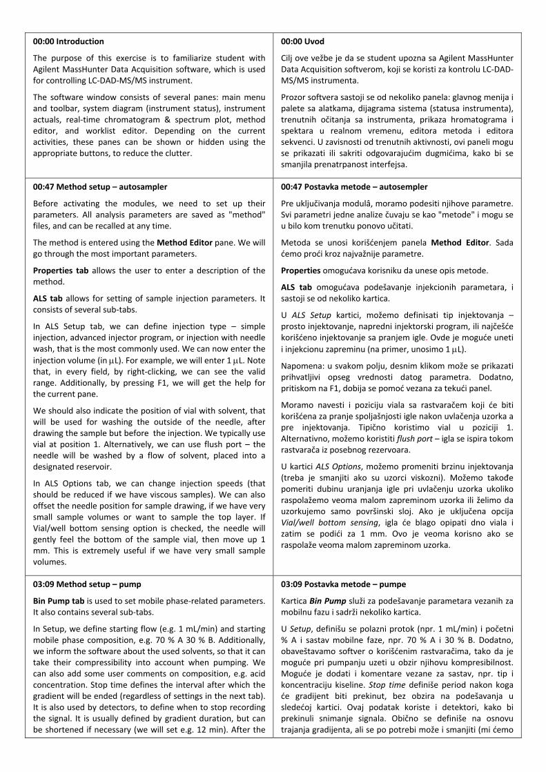
00:00 Introduction
The purpose of this exercise is to familiarize student with Agilent MassHunter Data Acquisition software, which is used for controlling LC‐DAD‐MS/MS instrument.
The software window consists of several panes: main menu and toolbar, system diagram (instrument status), instrument actuals, real‐time chromatogram & spectrum plot, method editor, and worklist editor. Depending on the current activities, these panes can be shown or hidden using the appropriate buttons, to reduce the clutter.
00:00 Uvod
Cilj ove vežbe je da se student upozna sa Agilent MassHunter Data Acquisition softverom, koji se koristi za kontrolu LC‐DAD‐MS/MS instrumenta.
Prozor softvera sastoji se od nekoliko panela: glavnog menija i palete sa alatkama, dijagrama sistema (statusa instrumenta), trenutnih očitanja sa instrumenta, prikaza hromatograma i spektara u realnom vremenu, editora metoda i editora sekvenci. U zavisnosti od trenutnih aktivnosti, ovi paneli mogu se prikazati ili sakriti odgovarajućim dugmićima, kako bi se smanjila prenatrpanost interfejsa.
00:47 Method setup – autosampler
Before activating the modules, we need to set up their parameters. All analysis parameters are saved as "method" files, and can be recalled at any time.
The method is entered using the Method Editor pane. We will go through the most important parameters.
Properties tab allows the user to enter a description of the method.
ALS tab allows for setting of sample injection parameters. It consists of several sub‐tabs.
In ALS Setup tab, we can define injection type – simple injection, advanced injector program, or injection with needle wash, that is the most commonly used. We can now enter the
injection volume (in L). For example, we will enter 1 L. Note that, in every field, by right‐clicking, we can see the valid range. Additionally, by pressing F1, we will get the help for the current pane.
We should also indicate the position of vial with solvent, that will be used for washing the outside of the needle, after drawing the sample but before the injection. We typically use vial at position 1. Alternatively, we can use flush port – the needle will be washed by a flow of solvent, placed into a designated reservoir.
In ALS Options tab, we can change injection speeds (that should be reduced if we have viscous samples). We can also offset the needle position for sample drawing, if we have very small sample volumes or want to sample the top layer. If Vial/well bottom sensing option is checked, the needle will gently feel the bottom of the sample vial, then move up 1 mm. This is extremely useful if we have very small sample volumes.
00:47 Postavka metode – autosempler
Pre uključivanja modulâ, moramo podesiti njihove parametre. Svi parametri jedne analize čuvaju se kao "metode" i mogu se u bilo kom trenutku ponovo učitati.
Metoda se unosi korišćenjem panela Method Editor. Sada ćemo proći kroz najvažnije parametre.
Properties omogućava korisniku da unese opis metode.
ALS tab omogućava podešavanje injekcionih parametara, i sastoji se od nekoliko kartica.
U ALS Setup kartici, možemo definisati tip injektovanja – prosto injektovanje, napredni injektorski program, ili najčešće korišćeno injektovanje sa pranjem igle. Ovde je moguće uneti
i injekcionu zapreminu (na primer, unosimo 1 L).
Napomena: u svakom polju, desnim klikom može se prikazati prihvatljivi opseg vrednosti datog parametra. Dodatno, pritiskom na F1, dobija se pomoć vezana za tekući panel.
Moramo navesti i poziciju viala sa rastvaračem koji će biti korišćena za pranje spoljašnjosti igle nakon uvlačenja uzorka a pre injektovanja. Tipično koristimo vial u poziciji 1. Alternativno, možemo koristiti flush port – igla se ispira tokom rastvarača iz posebnog rezervoara.
U kartici ALS Options, možemo promeniti brzinu injektovanja (treba je smanjiti ako su uzorci viskozni). Možemo takođe pomeriti dubinu uranjanja igle pri uvlačenju uzorka ukoliko raspolažemo veoma malom zapreminom uzorka ili želimo da uzorkujemo samo površinski sloj. Ako je uključena opcija Vial/well bottom sensing, igla će blago opipati dno viala i zatim se podići za 1 mm. Ovo je veoma korisno ako se raspolaže veoma malom zapreminom uzorka.
03:09 Method setup – pump
Bin Pump tab is used to set mobile phase‐related parameters. It also contains several sub‐tabs.
In Setup, we define starting flow (e.g. 1 mL/min) and starting mobile phase composition, e.g. 70 % A 30 % B. Additionally, we inform the software about the used solvents, so that it can take their compressibility into account when pumping. We can also add some user comments on composition, e.g. acid concentration. Stop time defines the interval after which the gradient will be ended (regardless of settings in the next tab). It is also used by detectors, to define when to stop recording the signal. It is usually defined by gradient duration, but can be shortened if necessary (we will set e.g. 12 min). After the
03:09 Postavka metode – pumpe
Kartica Bin Pump služi za podešavanje parametara vezanih za mobilnu fazu i sadrži nekoliko kartica.
U Setup, definišu se polazni protok (npr. 1 mL/min) i početni % A i sastav mobilne faze, npr. 70 % A i 30 % B. Dodatno, obaveštavamo softver o korišćenim rastvaračima, tako da je moguće pri pumpanju uzeti u obzir njihovu kompresibilnost. Moguće je dodati i komentare vezane za sastav, npr. tip i koncentraciju kiseline. Stop time definiše period nakon koga će gradijent biti prekinut, bez obzira na podešavanja u sledećoj kartici. Ovaj podatak koriste i detektori, kako bi prekinuli snimanje signala. Obično se definiše na osnovu trajanja gradijenta, ali se po potrebi može i smanjiti (mi ćemo

gradient is completed, the solvent ratio resets to starting conditions, and system needs to re‐equilibrate. Post time is used to define this re‐equilibration period, which can be calculated or estimated from experiments (in our case, it is 3 min). Max pressure limit is set to the highest pressure the pump and column can withstand, according to manufacturer's specifications (in our case, it is 600 bar). If the pressure exceeds this value, the system will automatically go into shutdown to prevent damage.
In Timetable tab, we define the gradient. The gradient is entered in the form of timepoints – we define % of phase B at the beginning and the end of ramps. E.g. in our case, the gradient will start from 30 % B, increase % B so that it reaches 70 % in 6th minute of analysis, keep increasing it so that it reaches 100 % at 12th minute, and keep it constant until 15th minute.
In Options tab, we can say the software to take into account solvents' compressibility when pumping. We can also ask it to record mobile phase composition, flow and pressure in the datafile, alongside the chromatograms, which can be used for troubleshooting. Finally, we can define maximum flow gradient. In our case, it is 0.1 mL/min/min. It means that, if we set 1 mL/min flow, and turn the pump on, it will not immediately start pumping at 1 mL/min (which would cause a pressure spike, and could potentially disturb the stationary phase). Instead, it will slowly, continuously increase it at rate of 0.1 mL/min each minute. So, it will take 10 min to reach the defined flow rate.
ga podesiti na npr. 12 min).
Nakon što je gradijent završen, odnos rastvarača vraća se na početni sastav i sistemu je potrebno vreme za ponovno uravnoteženje. Period uravnoteženja daje se kao Post time i računa ili procenjuje na osnovu eksperimenta (u našem slučaju, iznosi 3 min). Maksimalni pritisak definiše se kao najivši pritisak koji kolona i pumpa mogu da podnesu, prema specifikacijama proizvođača (u našem slučaju, 600 bar). Ako pritisak premaši ovu vrednosti, sistem se automatski gasi da bi se sprečila oštećenja.
U kartici Timetable, definišemo gradijent. Gradijent se unosi u vidu tačaka – definiše se % mobilne faze B na početku i kraju rampi. U našem slučaju, gradijent kreće od 30 % B, povećava % B tako da dostigne 70 % u 6. minutu analize, nastavlja sa povećanjem tako da dostigne 100 % u 12. minutu, i drži ga konstantnim do 15. minuta.
U kartici Options, može se zadati softveru da uzme u obzir kompresibilnost rastvarača prilikom pumpanja. Može mu se zadati i da zajedno sa hromatogramom čuva zapis o sastavu mobilne faze, protoku i pritisku u datafile, za potrebe dijagnostike. Konačno, možemo definisati i maksimalni gradijent protoka. U našem slučaju, on je 0.1 mL/min/min. To znači da, ako podesimo protok od 1 mL/min i uključimo pumpu, ona neće odmah početi da pumpa sa tim protokom (što bi rezultovalo skokom pritiska i moglo bi da naruši stacionarnu fazu). Umesto toga, protok će postepeno rasti brzinom od 0.1 mL/min svakog minuta, odn. biće potrebno 10 min da se postigne zadati protok.
06:58 Method setup – column compartment
Column tab allows for setting up the thermostats. In our case, the left thermostat is used for mobile phase pre‐heating and column heating, while the right one is used for thermostating the column effluent to the same temperature as DAD, to prevent signal ripples. So, we set the left temperature to e.g. 50 °C, and the right one to "same as detector cell".
06:58 Postavka metode – odeljak za kolonu
Column kartica omogućava podešavanje termostatâ. U našem slučaju, levi termostat koristi se za predgrevanje mobilne faze i zagrevanje kolone, dok se desni koristi za termostatiranje efluensa na temperaturu DAD, kako bi se sprečile oscilacije signala. Zbog toga, temperaturu levog termostata podešavamo na npr. 50 °C a desnog na "same as detector cell".
07:27 Method setup – DAD
DAD‐SL tab is used to set up the diode‐array detector.
In the Setup tab, we can define up to 8 signals to be monitored. These signals can later be opened in Data Analysis software as Signal A, Signal B etc. For each signal, we define wavelength and bandwidth. For example, 260/16 means the absorbance will be measured in 252–268 nm range. Additionally, we can define the reference signal wavelength and bandwidth. It should be some wavelength our sample is known not to absorb at, e.g. 550/100 nm.
The signal will be recorded until the pump stop time. Peak Width/Response Time is related to time constant, used for short‐term noise smoothing. It should be close to the width at half‐height of the narrowest expected peak. We know, from experience, that our peaks are about 6 s at the baseline, so we could use 2 s or 4 s.
In addition to these discrete signals, DAD can also record a continuous spectrum within a defined wavelength range, e.g. 200–600 nm with 2 nm steps.
In Options, we can indicate the lamps needed for the analysis
07:27 Postavka metode – DAD
DAD‐SL kartica koristi se za podešavanje detektora sa nizom dioda.
U Setup kartici, može se definisati do 8 signala koji će biti praćeni. Ove signale je kasnije moguće otvoriti u Data Analysis softveru kao Signal A, Signal B itd. Za svaki signal, definiše se talasna dužina i širina trake. Na primer, 260/16 znači da će apsorbancija biti merena u opsegu 252–268 nm. Dodatno, može se definisati i talasna dužina referentnog signala, što bi trebala biti talasna dužina na kojoj ispitivani uzorak ne apsorbuje, npr. 550/100 nm.
Signal će se snimati do Stop time definisanog kod pumpe. Parametar Peak Width/Response Time vezan je za vremensku konstantu korišćenu za glačanje kratkotrajnog šuma. Treba da bude blizak širini na poluvisini najužeg očekivanog pika. Iz iskustva znamo da naši pikovi imaju širinu pri baznoj liniji od oko 6 s, te treba da koristimo 2 s ili 4 s.
Uz navedene diskretne signale, DAD može takođe da snima i kontinualni spektar u definisanom opsegu talasnih dužina, npr. 200–600 nm u koracima od 2 nm.

(that will automatically turn on when we ask the system to turn on), as well as ask the system to autobalance the detector prior to each run.
U Options kartici mogu se zadati lampe koje će biti potrebne za analizu i koje će se automatski uključiti kada naredimo uključivanje sistema, kao i da li želimo da se detektor automatski nulira pre svake analize.
09:29 Method setup – MS
MS QQQ tab is used to set up the MS parameters.
The ion source to be used (in this case, ESI) is selected by Ion source drop menu. Time filtering is equivalent to DAD's Peak Width. We can enter e.g. 3 s = 0.05 min. Time segments table is used for defining the MS experiments to be run and polarity (positive/negative mode). Additionally, we can choose whether the effluent will actually be transfered to MS – to reduce contamination, we can divert the effluent directly to waste whenever no peaks of interest elute. We can also select whether signal should be saved into a file (note: MassHunter demands at least some MS signal to be recorded – even if only DAD is used, at least one segment with MS has to be checked).
If acquisition parameters (e.g. modes or scan types) are to be varied throughout the run, additional time segments should be used. They can be added by right clicking and selecting option Add Row. The first segment starts immediatelly, while for the other segments we need to define the starting time (e.g. starting from 5 min, go into negative mode).
Source panel is used for setting ion source parameters – drying gas temperature, drying gas flow (e.g. 10 L/min), nebulizer pressure (e.g. 50 psi) and capillary voltage (e.g. 4 kV). These values are selected based on mobile phase flow and composition (generally, higher flows and less volatile mobile phases require more intense desolvatation – higher temperature, higher flow, higher pressure).
In Chromatograms and Instrument panels, we can define additional signals that will be shown in the real‐time plot. I usually monitor MS signal (TIC or BPC), one or more UV/VIS signals, and for diagnostics, pressure and mobile phase composition and flow.
Acquisition panel is the most complex, and its content depends on Scan type for the selected time segment. For example, if we select MS2Scan, we are asked to enter starting and ending m/z, as well as fragmentor voltage and scan time. If we select MS2SIM, we only enter m/z of the ion to be monitored, and fragmentor voltage and scan time. If we select MRM, we enter precursor ion and product ion m/z values, as well as fragmentor voltage, collision energy and scan time. Note that, if we select any of the scan types (MS2Scan, Product Ion Scan, Precursor Ion Scan, Neutral Loss and Neutral Gain), only up to 4 Scan segments will be allowed for a given Time Segment. For other modes, such as SIM or MRM, such limitations do not exist.
After we completely set‐up the method, we can save it by File/Save As/Method.
09:29 Postavka metode – MS
MS QQQ kartica koristi se za postavku MS parametara.
Jonski izvor koji će se koristiti (u ovom slučaju, ESI) bira se u Ion source padajućem meniju. Time filtering je ekvivalent parametru Peak Width kod DAD. Može se uneti npr. 3 s = 0.05 min. Tabela sa vremenskim segmentima koristi se za definisanje MS eksperimenata koji će biti izvedeni i polariteta (pozitivni/negativni mod). Dodatno, može se izabrati da li će efluens sa HPLC zapravo biti prosleđen u MS – u cilju smanjenja kontaminacije, možemo tok efluensa preusmeriti direktno u otpad kad god ne eluiraju pikovi od interesa. Takođe, može se zadati da li će signal biti sačuvan u datafile (napomena: MassHunter zahteva da bar neki MS signal bude snimljen – čak i ako se koristi samo DAD, mora postojati bar jedan segment koji koristi MS).
Ako je u toku analize neophodno menjati parametre akvizicije (npr. polaritet ili tip MS eksperimenata), koriste se dodatni vremenski segmenti koji se dodaju desnim klikom i opcijom Add Row. Prvi segment kreće odmah, dok se za ostale mora definisati startno vreme (npr. "počevši od 5 min, pređi u negativni mod").
Panel Source koristi se za podešavanje parametara jonskog izvora – temperature gasa za sušenje, protoka gasa za sušenje (npr. 10 L/min), pritiska nebulajzera (e.g. 50 psi) i napona kapilare (e.g. 4 kV). Ove vrednosti biraju se na osnovu protoka i sastava mobilne faze (generalno, viši protoci i manje isparljive mobilne faze zahtevaju agresivniju desolvataciju – više temperature, viši protoci gasa, viši pritisci).
U panelu Chromatograms and Instrument, mogu se definisati dodatni signali koji će biti prikazani u panelu sa prikazom hromatograma i spektara u realnom vremenu. Mi obično pratimo MS signal (TIC ili BPC), jedan ili više UV/VIS signala i, za dijagnostiku, pritisak, protok i sastav mobilne faze.
Panel Acquisition je najsloženiji i njegov sadržaj zavisi od tipa akvizicije u okviru datog vremenskog segmenta. Na primer, ako se odabere MS2Scan, unose se početna i krajnja m/z, kao i napon fragmentora i vreme skeniranja. Ako se odabere MS2SIM, unose se samo m/z jona koji se prati, i napon fragmentora i vreme skeniranja. Ako se odabere MRM, unosimo m/z prekursora i produkta, kao i napon fragmentora, kolizionu energiju i vreme skeniranja. Treba napomenuti da, ako se odabere neki od sken modova (MS2Scan, Product Ion Scan, Precursor Ion Scan, Neutral Loss i Neutral Gain), po jednom vremenskom segmentu dozvoljeno je najviše 4 sken segmenta. Kod drugih modova, kao što su SIM i MRM, ovakva ograničenja ne postoje.
Nakon što je metoda potpuno podešena, čuvamo je opcijom File/Save As/Method.
14:06 Running a single sample
Now, if we need to run a single sample, we do it using Sample tab.
Of these fields, several have to be set: Sample position
14:06 Analiza pojedinačnih uzoraka
Ako želimo da analiziramo pojedinačni uzorak, koristimo Sample karticu.
Nekoliko ponuđenih polja moraju biti podešena: u Sample

indicates its co‐ordinates in the autosampler tray. The tray is organized like this – we have two plates, with enumerated rows and columns (so, we have positions 1A1, 1A2, 1B3 etc.). Datafile path and filename should also be indicated. Injection volume can be left ‐1 if the value specified in the method should be used, or we can override it with any other value. In addition to these fields, we can also enter additional comments into Name, Custom and Comment field.
When everything is set, and if the instrument is on and ready, we can start the run by selecting Run/Interactive sample or by pressing F5.
position definišu se koordinate uzorka u autosempleru. Autosempler sadrži dva stalka (plates) sa numerisanim redovima i kolonama (pozicije su označene kao 1A1, 1A2, 1B3 itd.). Putanja i ime datafile‐a se takođe moraju navesti. Za injekcionu zapreminu se ostavlja –1 ako se koristi vrednost iz metode, ili se ona može zaobići unosom neke druge vrednosti. Uz ova obavezna polja, moguće je uneti i dodatne komentare u polja Name, Custom i Comment.
Kada je sve podešeno i instrument je uključen i spreman, možemo započeti analizu opcijom Run/Interactive sample ili pritiskom na F5.
15:39 Worklists
If we need to run more samples, we create a worklist. First, we open Worklist menu, and select Worklist Run Parameters. In this dialog, we define: operator's name (this is optional), part of method to be run (only acquisition, or also data analysis), method path (the directory containing method to be used; note: do not point to the method itself, which is also a directory), datafile path (the directory that will store datafiles), scripts (macros to run before the worklist, after the succesful completion, and after any completion – we select Instrument Standby, that will stop the pump, shut down column heating, DAD lamps, and MS N2 flow and heating after the instrument has finished the analysis or if anything goes wrong). We do not use Overlapped injection – if this option is enabled both in method and worklist, the next run will start before the current one is finished, to save some time. Clear sample selection after run – if will simply uncheck the samples in the worklist when they are completed, making it easier to see which is the next sample. Wait Time for Ready – this is the maximum time to wait for system modules to get ready for the run. If exceeded (e.g. if heater cannot achieve the required temperature), the worklist will be terminated.
When everything is set, we can enter the worklist. We display the Worklist table by clicking on [W]. Worklist table consists of numerous columns, but only several are absolutely necessary. We can actually configure them by right‐clicking and selecting Show/Hide/Order Columns. We need Sample Position (e.g. 1A1), Method Name (only from the directory we selected) and Datafile Name. All the other fields can be shown or hidden as needed. Samples are entered manually, one by one, by using Add/Insert sample, or they can be added in series, by Add/Insert Multiple Samples (e.g. we can add 5 samples that will be called Sample1 to Sample5, that will be recorded using this scan method, and the positions will be from B1 to B5. The samples are then automatically added; we can edit some details, if needed. Note that these parameters can also be directly pasted from e.g. Notepad or Excel.
When everything is set, we can save the worklist, and if the instrument is on and ready, we can start the run by selecting Run/Worklist or simply by pressing F4.
15:39 Sekvence
Ako je potrebno da analiziramo veći broj uzoraka, kreiramo sekvencu. Za početak, otvaramo Worklist meni i biramo opciju Worklist Run Parameters. U ovom prozoru definišemo: ime operatera (opciono), delove metode koji se izvršavaju (samo akvizicija ili i obrada), putanju do foldera u kome se nalazi metoda koja će se koristiti (napomena: ne navoditi putanju do same metode, koja je takođe folder), putanju do foldera u kome će se čuvati datafile‐ovi, makroe (koji će biti aktivirani pre sekvence, nakon uspešnog završetka i nakon bilo kakvog završetka; biramo Instrument Standby, koji će zaustaviti pumpe, ugasiti zagrevanje kolone, DAD lampe i tok N2 i zagrevanje MS nakon što je analiza završena ili prekinuta zbog problema). Ne koristimo Overlapped injection; ako bi ova opcija bila aktivirana i u metodi i u sekvenci, sledeća analiza započinjala bi pre završetka tekuće, u cilju uštede vremena. Ako je opcija Clear sample selection after run aktivirana, uzorak u sekvenci će biti markiran nakon uspešne analize, što olakšava praćenje toka sekvence. Wait Time for Ready je maksimalno vreme čekanja da svi moduli sistema budu spremni za analizu. Ako se premaši (npr. termostat ne može da postigne zadatu temperaturu) sekvenca se prekida.
Kada je sve podešeno, može se uneti sekvenca. Sekvencu prikazujemo klikom na [W] ikonicu. Tabela se sastoji od brojnih kolona, od kojih je samo nekoliko zaista neophodno. Kolone se mogu podesiti desnim klikom i izborom opcije Show/Hide/Order Columns. Kolone koje su nam potrebne su Sample Position (pozicija uzorka, npr. 1A1), Method Name (naziv metode, iz prethodno odabranog foldera) i Datafile Name (naziv datafile‐a). Sva druga polja mogu se prikazati ili sakriti po potrebi. Uzorci se mogu uneti ručno, jedan po jedan, koristeći opciju Add/Insert Sample, ili grupno, opcijom Add/Insert Multiple Samples (npr. možemo dodati 5 uzoraka, na pozicijama B1–B5, koji će nositi nazive Uzorak1–Uzorak5 i biti snimljeni po datoj sken metodi). Uzorci će biti automatski dodati, nakon čega je moguće korigovati detalje, ako je potrebno. Parametri se takođe mogu direktno kopirati iz Notepad‐a ili Excel‐a.
Kada je sve podešeno, sekvencu je moguće sačuvati i, ako je instrument uključen i spreman, moguće je započeti analizu opcijom Run/Worklist ili pritiskom na F4.
20:00 Other options
In addition to Method and Worklist Editor, we have several other important panels.
In the Real Time Plot [R], we can see the current chromatogram and other signals. We can right‐click to change
20:00 Ostale opcije
Pored panela za postavku metode i sekvence, softver sadrži još nekoliko korisnih panela.
Prikaz u realnom vremenu (Real Time Plot) omogućava praćenje tekućeg hromatograma i drugih signala. Desni klik

it – we can display binary pump flow, mobile phase composition, we can plot signals from detectors, so we can monitor what is happening in our system.
Additionally, we can display UV or MS spectrum of the current effluent.
In the System [S] panel, we actually have several fields. Instrument Actuals can be used for displaying various diagnostic parameters. For each module, we have a wide range of parameters to be selected, and they can be used for diagnosing whether and why the system is not ready, if something is wrong etc.
These two buttons – ON and Standby – are used to manually turn on or off all the modules at the same time.
And here, in the System Diagram, we have some additional settings for each module. For example, for autosampler, we can configure the type of plates (e.g. if we want to use 96‐well plates instead of standard 54‐vial plates, we can configure it here, and then the instrument will know how to position the autosampler needle correctly). We can also use this menu to turn on/off the tray illumination (internal lighting of the autosampler).
And here we can control the pump, so we can turn it on/off. We also can enter the solvent levels. This way, we can inform the software about the amount of mobile phase that is available for the analysis, and if the volume falls below the limit we entered, the system will not allow the analysis – it will stop.
In the column section, we can turn the thermostat on, or we can also set it to be turned on at the selected time.
For DAD, we can turn lamps on, we can balance the detector, or do some performance testing
For MS, we can turn it on/off, we can switch the effluent flow to MS or to waste, and we can vent the instrument, which is an opperation necessary before shutting the entire instrument down for some maintenance operation or just prolonged idle period.
omogućava izmene – možemo prikazati protok kroz binarnu pumpu, sastav mobilne faze, signale sa detektorâ itd, tako da možemo pratiti stanje sistema.
Dodatno, možemo prikazati UV ili MS spektar trenutnog efluensa.
U panelu System imamo nekoliko polja. Instrument Actuals omogućava prikaz različitih dijagnostičkih parametara. Za svaki modul dostupan je širok spektar parametara koji se mogu izabrati i koji mogu biti korišćeni za uzvršivanje da li i zašto sistem nije spreman, da li postoji neki problem itd.
Dva dugmeta – ON i Standby – koriste se za istovremeno pokretanje ili gašenje svih modula.
System Diagram obezbeđuje dodatna podešavanja za svaki modul. Na primer, u slučaju autosemplera, moguće je podesiti tip nosača (npr. ako želimo da koristimo mikrotitar‐ploče umesto standardnog stalka za 54 viala) da bi instrument znao kako da tačno pozicionira iglu autosemplera. Preko ovog menija moguće je i uključiti ili isključiti unutrašnje osvetljenje autosemplera.
U slučaju pumpe, možemo je uključiti/isključiti, Takođe, možemo uneti zapremine rastvaračâ, čime obaveštavamo softver o količini mobilne faze dostupne za analizu. Ako zapremina padne ispod zadatog limita, sistem neće dozvoliti analizu i zaustaviće sekvencu.
U slučaju odeljka za kolonu, možemo uključiti termostat, kao i zadati da se on automatski uključi u određeno vreme.
Kod DAD, možemo uključiti lampe, nulirati detektor, ili izvesti testove za verifikaciju performansi.
Kod MS, možemo uključiti/isključiti detektor, tok efluensa preusmeriti na MS ili u otpad, ili ventovati instrument (što je operacija neophodna pre gašenja instrumenta radi održavanja ili pri dužim periodima neaktivnosti).

______________________________________________________________________________________________________
This project has been funded with support from the European Commission. This publication reflects the views only of the authors,
and the Commission cannot be held responsible for any use which may be made of the information contained therein.
(EE07) MassHunter Qualitative Analysis
tutorial
Lab exercise: Qualitative analysis using LC-DAD-MS/MS
Course: Isolation and characterization of natural products
Author: Dejan Orčić (University of Novi Sad, Faculty of Sciences)
Preparation: Dejan Orčić (University of Novi Sad, Faculty of Sciences)
Special thanks to Sanja Berežni (University of Novi Sad, Faculty of Sciences) for contribution

______________________________________________________________________________________________________
This project has been funded with support from the European Commission. This publication reflects the views only of the authors,
and the Commission cannot be held responsible for any use which may be made of the information contained therein.
(EE07) Vodič za MassHunter Qualitative
Analysis
Vežba: Kvalitativna LC-DAD-MS/MS analiza
Kurs: Izolacija i karakterizacija prirodnih proizvoda
Autor: Dejan Orčić (Univerzitet u Novom Sadu, Prirodno-matematički
fakultet)
Tehnička priprema: Dejan Orčić (Univerzitet u Novom Sadu, Prirodno-
matematički fakultet)
Zahvaljujemo se Sanji Berežni (Univerzitet u Novom Sadu, Prirodno-matematički fakultet) za
doprinos
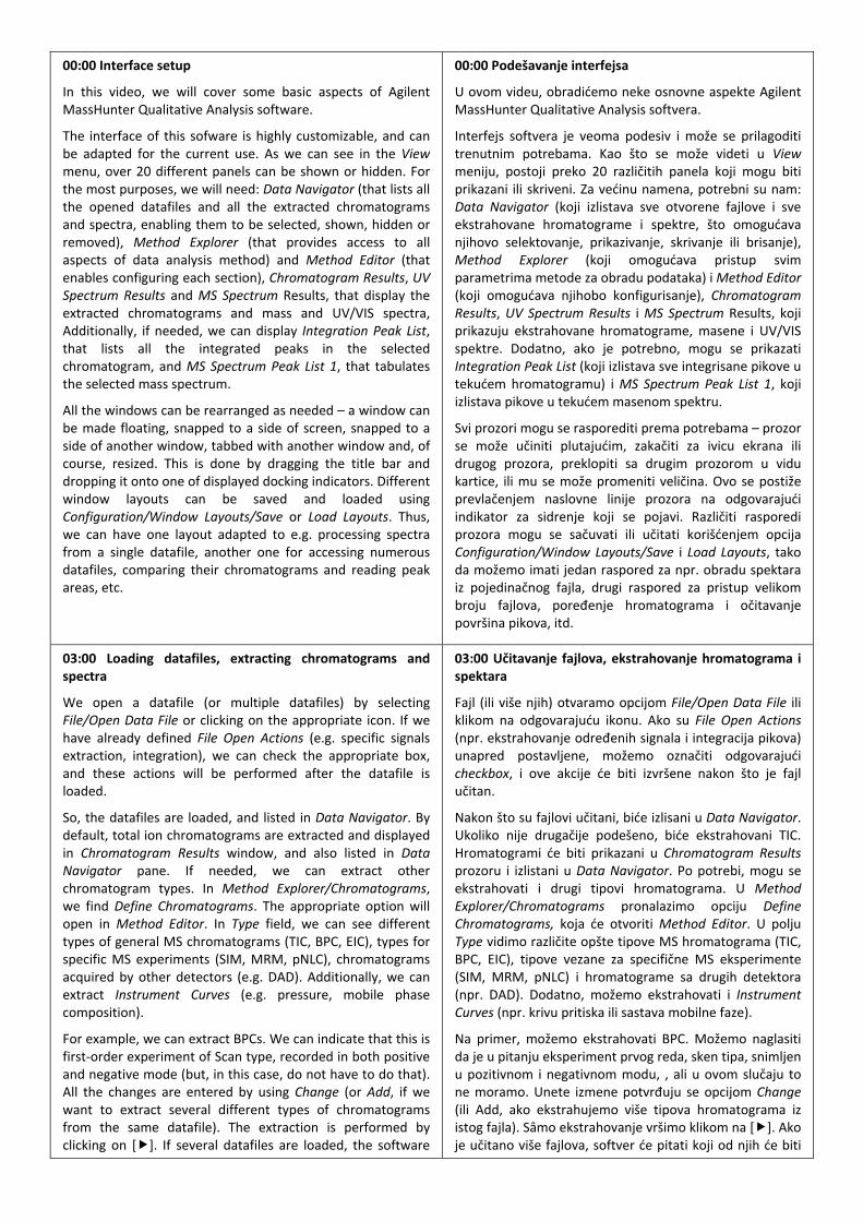
00:00 Interface setup
In this video, we will cover some basic aspects of Agilent MassHunter Qualitative Analysis software.
The interface of this sofware is highly customizable, and can be adapted for the current use. As we can see in the View menu, over 20 different panels can be shown or hidden. For the most purposes, we will need: Data Navigator (that lists all the opened datafiles and all the extracted chromatograms and spectra, enabling them to be selected, shown, hidden or removed), Method Explorer (that provides access to all aspects of data analysis method) and Method Editor (that enables configuring each section), Chromatogram Results, UV Spectrum Results and MS Spectrum Results, that display the extracted chromatograms and mass and UV/VIS spectra, Additionally, if needed, we can display Integration Peak List, that lists all the integrated peaks in the selected chromatogram, and MS Spectrum Peak List 1, that tabulates the selected mass spectrum.
All the windows can be rearranged as needed – a window can be made floating, snapped to a side of screen, snapped to a side of another window, tabbed with another window and, of course, resized. This is done by dragging the title bar and dropping it onto one of displayed docking indicators. Different window layouts can be saved and loaded using Configuration/Window Layouts/Save or Load Layouts. Thus, we can have one layout adapted to e.g. processing spectra from a single datafile, another one for accessing numerous datafiles, comparing their chromatograms and reading peak areas, etc.
00:00 Podešavanje interfejsa
U ovom videu, obradićemo neke osnovne aspekte Agilent MassHunter Qualitative Analysis softvera.
Interfejs softvera je veoma podesiv i može se prilagoditi trenutnim potrebama. Kao što se može videti u View meniju, postoji preko 20 različitih panela koji mogu biti prikazani ili skriveni. Za većinu namena, potrebni su nam: Data Navigator (koji izlistava sve otvorene fajlove i sve ekstrahovane hromatograme i spektre, što omogućava njihovo selektovanje, prikazivanje, skrivanje ili brisanje), Method Explorer (koji omogućava pristup svim parametrima metode za obradu podataka) i Method Editor (koji omogućava njihobo konfigurisanje), Chromatogram Results, UV Spectrum Results i MS Spectrum Results, koji prikazuju ekstrahovane hromatograme, masene i UV/VIS spektre. Dodatno, ako je potrebno, mogu se prikazati Integration Peak List (koji izlistava sve integrisane pikove u tekućem hromatogramu) i MS Spectrum Peak List 1, koji izlistava pikove u tekućem masenom spektru.
Svi prozori mogu se rasporediti prema potrebama – prozor se može učiniti plutajućim, zakačiti za ivicu ekrana ili drugog prozora, preklopiti sa drugim prozorom u vidu kartice, ili mu se može promeniti veličina. Ovo se postiže prevlačenjem naslovne linije prozora na odgovarajući indikator za sidrenje koji se pojavi. Različiti rasporedi prozora mogu se sačuvati ili učitati korišćenjem opcija Configuration/Window Layouts/Save i Load Layouts, tako da možemo imati jedan raspored za npr. obradu spektara iz pojedinačnog fajla, drugi raspored za pristup velikom broju fajlova, poređenje hromatograma i očitavanje površina pikova, itd.
03:00 Loading datafiles, extracting chromatograms and spectra
We open a datafile (or multiple datafiles) by selecting File/Open Data File or clicking on the appropriate icon. If we have already defined File Open Actions (e.g. specific signals extraction, integration), we can check the appropriate box, and these actions will be performed after the datafile is loaded.
So, the datafiles are loaded, and listed in Data Navigator. By default, total ion chromatograms are extracted and displayed in Chromatogram Results window, and also listed in Data Navigator pane. If needed, we can extract other chromatogram types. In Method Explorer/Chromatograms, we find Define Chromatograms. The appropriate option will open in Method Editor. In Type field, we can see different types of general MS chromatograms (TIC, BPC, EIC), types for specific MS experiments (SIM, MRM, pNLC), chromatograms acquired by other detectors (e.g. DAD). Additionally, we can extract Instrument Curves (e.g. pressure, mobile phase composition).
For example, we can extract BPCs. We can indicate that this is first‐order experiment of Scan type, recorded in both positive and negative mode (but, in this case, do not have to do that). All the changes are entered by using Change (or Add, if we want to extract several different types of chromatograms from the same datafile). The extraction is performed by clicking on []. If several datafiles are loaded, the software
03:00 Učitavanje fajlova, ekstrahovanje hromatograma i spektara
Fajl (ili više njih) otvaramo opcijom File/Open Data File ili klikom na odgovarajuću ikonu. Ako su File Open Actions (npr. ekstrahovanje određenih signala i integracija pikova) unapred postavljene, možemo označiti odgovarajući checkbox, i ove akcije će biti izvršene nakon što je fajl učitan.
Nakon što su fajlovi učitani, biće izlisani u Data Navigator. Ukoliko nije drugačije podešeno, biće ekstrahovani TIC. Hromatogrami će biti prikazani u Chromatogram Results prozoru i izlistani u Data Navigator. Po potrebi, mogu se ekstrahovati i drugi tipovi hromatograma. U Method Explorer/Chromatograms pronalazimo opciju Define Chromatograms, koja će otvoriti Method Editor. U polju Type vidimo različite opšte tipove MS hromatograma (TIC, BPC, EIC), tipove vezane za specifične MS eksperimente (SIM, MRM, pNLC) i hromatograme sa drugih detektora (npr. DAD). Dodatno, možemo ekstrahovati i Instrument Curves (npr. krivu pritiska ili sastava mobilne faze).
Na primer, možemo ekstrahovati BPC. Možemo naglasiti da je u pitanju eksperiment prvog reda, sken tipa, snimljen u pozitivnom i negativnom modu, , ali u ovom slučaju to ne moramo. Unete izmene potvrđuju se opcijom Change (ili Add, ako ekstrahujemo više tipova hromatograma iz istog fajla). Sâmo ekstrahovanje vršimo klikom na []. Ako je učitano više fajlova, softver će pitati koji od njih će biti
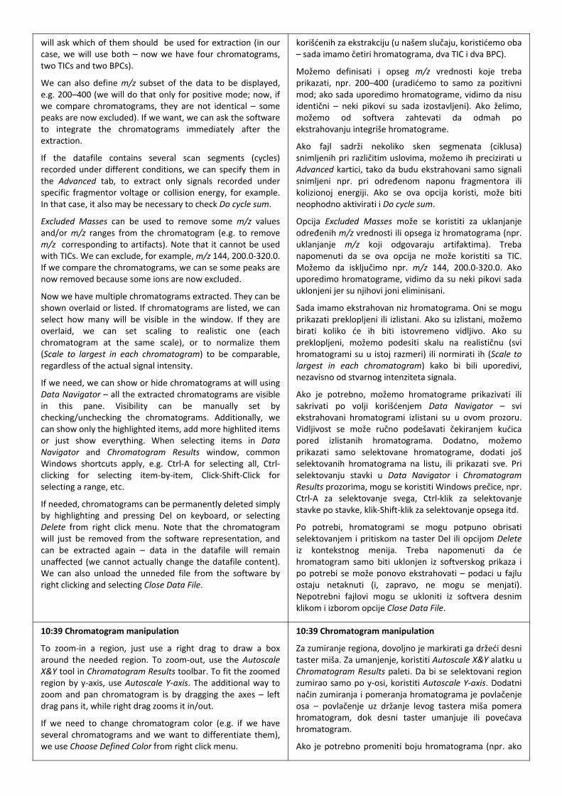
will ask which of them should be used for extraction (in our case, we will use both – now we have four chromatograms, two TICs and two BPCs).
We can also define m/z subset of the data to be displayed, e.g. 200–400 (we will do that only for positive mode; now, if we compare chromatograms, they are not identical – some peaks are now excluded). If we want, we can ask the software to integrate the chromatograms immediately after the extraction.
If the datafile contains several scan segments (cycles) recorded under different conditions, we can specify them in the Advanced tab, to extract only signals recorded under specific fragmentor voltage or collision energy, for example. In that case, it also may be necessary to check Do cycle sum.
Excluded Masses can be used to remove some m/z values and/or m/z ranges from the chromatogram (e.g. to remove m/z corresponding to artifacts). Note that it cannot be used with TICs. We can exclude, for example, m/z 144, 200.0‐320.0. If we compare the chromatograms, we can se some peaks are now removed because some ions are now excluded.
Now we have multiple chromatograms extracted. They can be shown overlaid or listed. If chromatograms are listed, we can select how many will be visible in the window. If they are overlaid, we can set scaling to realistic one (each chromatogram at the same scale), or to normalize them (Scale to largest in each chromatogram) to be comparable, regardless of the actual signal intensity.
If we need, we can show or hide chromatograms at will using Data Navigator – all the extracted chromatograms are visible in this pane. Visibility can be manually set by checking/unchecking the chromatograms. Additionally, we can show only the highlighted items, add more highlited items or just show everything. When selecting items in Data Navigator and Chromatogram Results window, common Windows shortcuts apply, e.g. Ctrl‐A for selecting all, Ctrl‐clicking for selecting item‐by‐item, Click‐Shift‐Click for selecting a range, etc.
If needed, chromatograms can be permanently deleted simply by highlighting and pressing Del on keyboard, or selecting Delete from right click menu. Note that the chromatogram will just be removed from the software representation, and can be extracted again – data in the datafile will remain unaffected (we cannot actually change the datafile content). We can also unload the unneded file from the software by right clicking and selecting Close Data File.
korišćenih za ekstrakciju (u našem slučaju, koristićemo oba – sada imamo četiri hromatograma, dva TIC i dva BPC).
Možemo definisati i opseg m/z vrednosti koje treba prikazati, npr. 200–400 (uradićemo to samo za pozitivni mod; ako sada uporedimo hromatograme, vidimo da nisu identični – neki pikovi su sada izostavljeni). Ako želimo, možemo od softvera zahtevati da odmah po ekstrahovanju integriše hromatograme.
Ako fajl sadrži nekoliko sken segmenata (ciklusa) snimljenih pri različitim uslovima, možemo ih precizirati u Advanced kartici, tako da budu ekstrahovani samo signali snimljeni npr. pri određenom naponu fragmentora ili kolizionoj energiji. Ako se ova opcija koristi, može biti neophodno aktivirati i Do cycle sum.
Opcija Excluded Masses može se koristiti za uklanjanje određenih m/z vrednosti ili opsega iz hromatograma (npr. uklanjanje m/z koji odgovaraju artifaktima). Treba napomenuti da se ova opcija ne može koristiti sa TIC. Možemo da isključimo npr. m/z 144, 200.0‐320.0. Ako uporedimo hromatograme, vidimo da su neki pikovi sada uklonjeni jer su njihovi joni eliminisani.
Sada imamo ekstrahovan niz hromatograma. Oni se mogu prikazati preklopljeni ili izlistani. Ako su izlistani, možemo birati koliko će ih biti istovremeno vidljivo. Ako su preklopljeni, možemo podesiti skalu na realističnu (svi hromatogrami su u istoj razmeri) ili normirati ih (Scale to largest in each chromatogram) kako bi bili uporedivi, nezavisno od stvarnog intenziteta signala.
Ako je potrebno, možemo hromatograme prikazivati ili sakrivati po volji korišćenjem Data Navigator – svi ekstrahovani hromatogrami izlistani su u ovom prozoru. Vidljivost se može ručno podešavati čekiranjem kućica pored izlistanih hromatograma. Dodatno, možemo prikazati samo selektovane hromatograme, dodati još selektovanih hromatograma na listu, ili prikazati sve. Pri selektovanju stavki u Data Navigator i Chromatogram Results prozorima, mogu se koristiti Windows prečice, npr. Ctrl‐A za selektovanje svega, Ctrl‐klik za selektovanje stavke po stavke, klik‐Shift‐klik za selektovanje opsega itd.
Po potrebi, hromatogrami se mogu potpuno obrisati selektovanjem i pritiskom na taster Del ili opcijom Delete iz kontekstnog menija. Treba napomenuti da će hromatogram samo biti uklonjen iz softverskog prikaza i po potrebi se može ponovo ekstrahovati – podaci u fajlu ostaju netaknuti (i, zapravo, ne mogu se menjati). Nepotrebni fajlovi mogu se ukloniti iz softvera desnim klikom i izborom opcije Close Data File.
10:39 Chromatogram manipulation
To zoom‐in a region, just use a right drag to draw a box around the needed region. To zoom‐out, use the Autoscale X&Y tool in Chromatogram Results toolbar. To fit the zoomed region by y‐axis, use Autoscale Y‐axis. The additional way to zoom and pan chromatogram is by dragging the axes – left drag pans it, while right drag zooms it in/out.
If we need to change chromatogram color (e.g. if we have several chromatograms and we want to differentiate them), we use Choose Defined Color from right click menu.
10:39 Chromatogram manipulation
Za zumiranje regiona, dovoljno je markirati ga držeći desni taster miša. Za umanjenje, koristiti Autoscale X&Y alatku u Chromatogram Results paleti. Da bi se selektovani region zumirao samo po y‐osi, koristiti Autoscale Y‐axis. Dodatni način zumiranja i pomeranja hromatograma je povlačenje osa – povlačenje uz držanje levog tastera miša pomera hromatogram, dok desni taster umanjuje ili povećava hromatogram.
Ako je potrebno promeniti boju hromatograma (npr. ako

To integrate the chromatogram, several methods are available, and are accessible through Method Explorer / Chromatogram window. For example, we can use MS integrator. For each integrator, many options are available, such as filters based on peak size, peak count etc. We integrate the chromatogram by pressing []. Integration results (peak list) are displayed in Integration Peak List, and can be copied into e.g. Notepad. For each peak, numerous parameters can be displayed. We can choose them by right‐clicking on the table header, and selecting Add/Remove Columns. We can actually display retention time, area, area%, MS base peak for each chromatographic peak, peak start and end time, width at half‐maximum, height, symmetry etc.
If needed, peaks can be manually integrated by selecting the appropriate tool in Chromatogram Results, and defining or correcting a peak baseline by left‐dragging. Note that integration filters still apply. Thus, if we defined that only large peaks should be integrated, manual integration of small peaks will be ignored.
Peaks can also be annotated by using the appropriate tool in Chromatogram Results. We can add image (e.g. structure) or text (e.g. some comment). We can define numerous parameters.
The chromatograms can be copied and pasted into other software. When the Chromatogram Results window is in focus and chromatogram is selected, we just click Copy to Clipboard or use Ctrl‐C. Now we can paste the chromatogram into another software, e.g. PowerPoint.
imamo prikazano više hromatograma i želimo da ih razlikujemo), koristimo Choose Defined Color opciju iz kontekstnog menija.
Dostupno je više metoda za integraciju hromatograma, koje su dostupne u Method Explorer / Chromatogram prozoru. Na primer, možemo da koristimo MS integrator. Za svaki integrator, dostupne su brojne opcije, kao što su filteri vezani za veličinu pika, broj pikova itd. Integrišemo hromatogram klikom na []. Rezultati integracije (lista pikova) prikazani su u prozoru Integration Peak List, i mogu se kopirati u npr. Notepad. Za svaki pik mogu se prikazati brojni parametri, koji se mogu odabrati desnim klikom na zaglavlje tabele i odabirom opcije Add/Remove Columns. Možemo prikazati retenciono vreme, površinu pika, procenat od ukupne površine, osnovni jon u masenom spektru, vreme početka i kraja pika, širinu na poluvisini, visinu, simetriju itd.
Ako je potrebno, pikovi se mogu manuelno integrisati selektovanjem odgovarajuće alatke u Chromatogram Results i definisanjem ili ispravljanjem bazne linije razvlačenjem uz pritisnut levi taster miša. Treba napomenuti da integracioni filteri i dalje važe – ako je definisano da samo veliki pikovi treba da budu integrisani, mali pikovi će biti integrisani i pri manuelnoj integraciji.
Pikovi se mogu označiti korišćenjem alatke Annotate u Chromatogram Results. Možemo dodati sliku (npr. strukturu) ili tekst (npr. neki komentar). Mogu se podesiti i brojni parametri vezani za formatiranje.
Hromatogrami se mogu kopirati i zalepiti u druge programe. Kada je Chromatogram Results prozor u fokusu i hromatogram je selektovan, odabrati Copy to Clipboard ili koristiti Ctrl‐C. Hromatogram (u vidu slike) može se sada zalepiti u drugi program, npr. PowerPoint.
15:23 Working with UV/VIS chromatograms
In addition to mass chromatograms, we can also extract UV/VIS chromatograms. In Define Chromatograms window, choose Other Chromatograms as a type and DAD1 as a detector. Several types of traces can be extracted: signals (designated A, B, C etc.) as defined in the acquisition method, total wavelength chromatogram (TWC), or extracted wavelength chromatogram (EWC) for a defined wavelength range (say, 300 nm with 80 nm bandwidth, i.e. 260–340 nm, with 550 nm/100 nm bandwidth as a reference). Again, we click on Change and [].
If we zoom in and integrate the same peaks, we can see that MS chromatograms lags about 0.04 min behind DAD. This is because it takes some time for effluent to physically cross distance between DAD and MS. To autocorrect this, we use Adjust Delay Time option in Chromatograms. We enter MS and DAD retention times for the same peak, calculate the difference, and then by clicking Adjust Delay Time the lagging chromatogram will be shifted to correct for delay.
15:23 Rad sa UV/VIS hromatogramima
Pored masenih hromatograma, možemo ekstrahovati i UV/VIS hromatograme. U Define Chromatograms prozoru biramo Other Chromatograms kao tip i DAD1 kao detektor. Moguće je ekstrahovati nekoliko tipova signala: signale (označene A, B, C etc.) definisane u akvizicionoj metodi, ukupni hromatogram (total wavelength chromatogram, TWC) ili hromatogram po određenoj talasnoj dužini (extracted wavelength chromatogram, EWC) za zadati opseg talasnih dužina (npr. 300 nm uz širinu spektralne trake od 80 nm, tj. 260–340 nm, uz 550 nm/100 nm kao referencu). Ponovo, klikćemo na Change i [].
Ako zumiramo i integrišemo isti pik u MS i DAD hromatogramu, vidimo da MS hromatogram kasni oko 0.04 min za DAD. To je zato što je efluensu potrebno vreme da fizički pređe put od DAD do MS. Ovo možemo automatski korigovati opcijom Adjust Delay Time u Chromatograms sekciji. Unosimo retenciona vremena istog pika na MS i DAD, rečunamo razliku, i zatim klikom na Adjust Delay Time zaostajući hromatogram biće pomeren.
17:48 Spectra extraction and manipulation
Both MS and UV/VIS spectra can be easily extracted by
17:48 Ekstrahovanje i rad sa spektrima
I MS i UV/VIS spektri lako se mogu ekstrahovati

double‐clickling on a selected point in the appropriate chromatogram. However, to compensate for short‐term noise, it is better to average several spectra, which is done by selecting a range by left dragging (Range Select tool, which is default, should be active), and then double clicking on the marked range or click Extract MS Spectrum option. Now we have averaged spectrum from a selected range.
To correct for background signal, we can select a background region, Extract the Background Spectrum, select the peak spectrum and click on Subtract Background Spectrum. Alternatively, we can select the peak spectrum, click on Subtract Any Spectrum, and then click on background spectrum. We can do that both for MS and UV.
The another way to extract purified spectrum is to use Peak Select tool (which is only enabled if we have integrated peaks). We select the peak and then click on Extract Peak Spectrum option. The software will automatically take averaged peak spectrum, averaged baseline spectrum, and subtract them.
Again, all the extracted spectra can be shown, hidden or deleted through Data Navigator.
In the case of mass spectrum, MS Spectrum Peaks One tabulates various useful information, including the spectrum itself, but also some other characteristics which are especially useful if we have HRMS and automatic interpretation. This table can be copied and pasted in e.g. Notepad or Excel. If too many or too few ions are labeled, this can be changed by Adjust Peak Threshold. Only the peaks with abundance above the selected level will be shown.
As with chromatograms, spectra can also be zoomed and annotated by using the appropriate tools.
For purpose of spectrum interpretation, m/z differences can be directly read and labelled by using Delta Mass Caliper. We just drag from one to another peak, and peak m/z difference will be displayed (e.g. in this case, it is 22, which indicates proton and sodium adducts).
By double left clicking on a spectrum, EIC/EWC chromatogram at selected m/z or wavelength can easily be extracted.
dvostrukim klikom na željenu tačku u odgovarajućem hromatogramu. Međutim, u cilju kompenzovanja kratkotrajnog šuma, bolje je usrednjiti nekoliko spektara, što se postiže markiranjem opsega uz pritisnut levi taster miša (pritom, Range Select alatka treba da bude aktivna) i zatim dvostrukim klikom na opseg ili odabirom opcije Extract MS Spectrum option. Sada imamo usrednjeni spektar za dati opseg.
U cilju korekcije na pozadinski signal, markiramo region sa čistom pozadinom, biramo opciju Extract the Background Spectrum, zatim selektujemo spektar pika i biramo opciju Subtract Background Spectrum. Alternativno, možemo selektovati spektar pika, kliknuti na Subtract Any Spectrum i zatim na prethodno ekstrahovani spektar pozadine. Korekcija pozadine moguća je i kod MS i kod UV.
Drugi način za ekstrahovanje prečišćenog spektra je korišćenje alatke Peak Select tool (koja je dostupna samo ako su pikovi već integrisani). Selektujemo pik i kliknemo na Extract Peak Spectrum opciju. Softver će automatski ekstrahovati usrednjeni spektar pika i od njega oduzeti usrednjeni spektar bazne linije.
Svi ekstrahovani spektri mogu se prikazati, sakriti ili izbrisati preko Data Navigator‐a.
U slučaju masenih spektara, MS Spectrum Peaks One izlistava razne korisne informacije, uključujući sâm spektar, kao i karakteristike koje su korisne ako se obrađuju maseni spektri visoke rezolucije (HRMS) i koristi automatska interpretacija. Tabela se može kopirati i zalepiti npr. u Notepad ili Excel. Ako je označeno i izlistano previše ili premalo jona, to se može izmeniti opcijom Adjust Peak Threshold. Samo pikovi sa obilnošću većom od naznačene biće izlistani.
Kao i u slučaju hromatograma, spektri se mogu zumirati i označavati (anotirati) korišćenjem odgovarajućih alatki.
Za potrebe interpretacije spektara, m/z razlike mogu se direktno očitavati i označavati korišćenjem alatke Delta Mass Caliper. Nakon prostog razvlačenja uz pritisnuti levi taster miša, m/z razlika će biti prikazana (npr. u našem slučaju 22, što ukazuje na adukte sa protonom i natrijumom).
Dvostrukim levim klikom na spektar, lako se može ekstrahovati EIC/EWC hromatogram na odabranoj m/z ili talasnoj dužini.
23:12
In this tutorial, we have covered only the most basic options of Agilent MassHunter Qualitative Analysis software. In addition to those, there are many advanced options – the software is also capable of chromatogram deconvolution (finding peaks and extracting their pure chromatograms and spectra from the MS chromatogram), determination of molecular formula from molecular weight (if the data was acquired by HRMS), library search (by using its own procedures or by interfacing with NIST MS Search program) etc.
23:12
U ovom vodiču, pokrili smo samo osnovne opcije Agilent MassHunter Qualitative Analysis softvera. Pored njih, postoje brojne napredne opcije – softver je sposoban za dekonvoluciju hromatograma (pronalaženje pikova i ekstrahovanje njihovh čistih hromatograma i spektara iz MS hromatograma), određivanje molekulske formule iz molekulske mase (ako su podaci dobijeni pomoću HRMS), bibliotečka pretraga (korišćenjem internih procedura ili povezivanjem sa NIST MS Search softverom) itd.

______________________________________________________________________________________________________
This project has been funded with support from the European Commission. This publication reflects the views only of the authors,
and the Commission cannot be held responsible for any use which may be made of the information contained therein.
(EE09) Identification of secondary
biomolecules by LC-DAD-MS/MS –
supplementary material
Lab exercise: Identification and quantification of secondary
biomolecules in plant material by LC-DAD-MS/MS
Course: Isolation and characterization of natural products
Author: Dejan Orčić (University of Novi Sad, Faculty of Sciences)
Preparation: Dejan Orčić (University of Novi Sad, Faculty of Sciences)
Special thanks to Sanja Berežni (University of Novi Sad, Faculty of Sciences) for contribution
______________________________________________________________________________________________________
This project has been funded with support from the European Commission. This publication reflects the views only of the authors,
and the Commission cannot be held responsible for any use which may be made of the information contained therein.
(EE09) Identifikacija sekundarnih
biomolekula pomoću LC-DAD-MS/MS –
dopunski materijal
Vežba: Identifikacija i kvantifikacija sekundarnih biomolekula u
biljnom materijalu pomoću LC-DAD-MS/MS
Kurs: Izolacija i karakterizacija prirodnih proizvoda
Autor: Dejan Orčić (Univerzitet u Novom Sadu, Prirodno-matematički
fakultet)
Tehnička priprema: Dejan Orčić (Univerzitet u Novom Sadu, Prirodno-
matematički fakultet)
Zahvaljujemo se Sanji Berežni (Univerzitet u Novom Sadu, Prirodno-matematički fakultet) za
doprinos
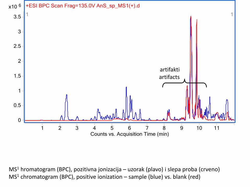
MS1 hromatogram (BPC), pozitivna jonizacija – uzorak (plavo) i slepa proba (crveno) MS1 chromatogram (BPC), positive ionization – sample (blue) vs. blank (red)
artifakti artifacts

MS1 hromatogram (BPC), negativna jonizacija – uzorak (plavo) i slepa proba (crveno) MS1 chromatogram (BPC), negative ionization – sample (blue) vs. blank (red)
artifakti artifacts

MS1 hromatogram (BPC), zumiran region sa lignanima – PI (plavo) i NI (crveno) MS1 chromatogram (BPC), zoomed lignan region – PI (blue) and NI (red)
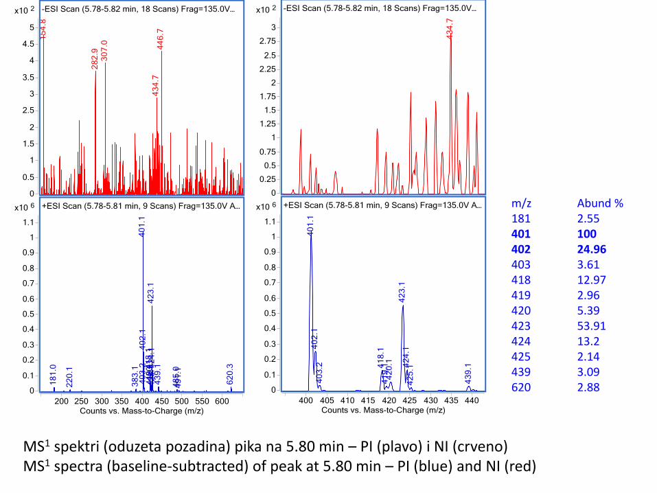
MS1 spektri (oduzeta pozadina) pika na 5.80 min – PI (plavo) i NI (crveno) MS1 spectra (baseline-subtracted) of peak at 5.80 min – PI (blue) and NI (red)
m/z Abund % 181 2.55 401 100 402 24.96 403 3.61 418 12.97 419 2.96 420 5.39 423 53.91 424 13.2 425 2.14 439 3.09 620 2.88

UV spektar (oduzeta pozadina) pika na 5.80 min UV spectrum (baseline-subtracted) of peak at 5.80 min

MS2 spektri, pozitivna jonizacija, Vcol = 5–35 V MS2 spectra, positive ionization, Vcol = 5–35 V
Obilnost / Abundance, %
m/z 5 V 15 V 25 V 35 V
401 8.5
383 100 85.2
365 4.9 12.7
334 1.2 8.1
223 2.8 15.7
181 33.8 100 100 100
161 6.2 32.2 15.8
148 16.7
135 4.0 17.9 22.3 28.8
131 3.4 22.8 35.5 35.6
123 1.8
103 11.0
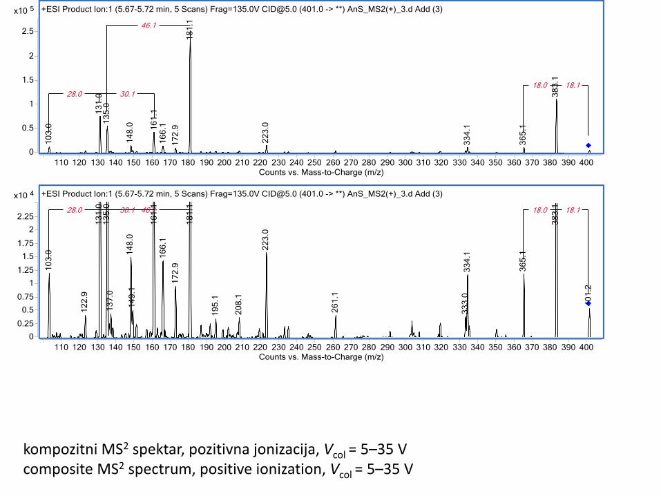
kompozitni MS2 spektar, pozitivna jonizacija, Vcol = 5–35 V composite MS2 spectrum, positive ionization, Vcol = 5–35 V

supstitucija substitution
doprinos contribution
ArH [A]+, [A']
+ [B]
+ [C+H]
+ [C+H]
+ 7-oxo
- Δ=0 Δ=78 91+ 117+ 187+ 201+
(OH) Δ=16 Δ=94 107+ 133+ 203+ 217+
(OMe) Δ=30 Δ=108 121+ 147+ 217+ 231+
(OH)2 Δ=32 Δ=110 123+ 149+ 219+ 233+
(OCH2O) Δ=44 Δ=122 135+ 161+ 231+ 245+
(OMe)(OH) Δ=46 Δ=124 137+ 163+ 233+ 247+
(OH)3 Δ=48 Δ=126 139+ 165+ 235+ 249+
(OMe)2 Δ=60 Δ=138 151+ 177+ 247+ 261+
(OCH2O)(OH) Δ=60 Δ=138 151+ 177+ 247+ 261+
(OMe)(OH)2 Δ=62 Δ=140 153+ 179+ 249+ 263+
(OCH2O)(OMe) Δ=74 Δ=152 165+ 191+ 261+ 275+
(OMe)2(OH) Δ=76 Δ=154 167+ 193+ 263+ 277+
(OMe)3 Δ=90 Δ=168 181+ 207+ 277+ 291+
mase uobičajenih gubitaka i fragmenata kod lignana weights of common fragments and losses from lignans

H+
OH
O+
R1
R2
CH2
O+
R1
R2
[M+H]+
+
[A]+
+
[A']+
H2O
H2O
[M+H-H2O]+
[M+H-2H2O]+
C+ CH2
R1
CH+
CH2
R1
CH+
R1
[B]+
a
I
aa
I
a
a'
a'
a
a'
a
b
b
a'
OH
O+
R1
R2
CH2
O+
R1
R2
H2O
[M+H-H2O]+
O
O
R1
R2
H+
[M+H]+
a'
a'
a'
a'
H2O
[M+H-2H2O]+
I
II
II O
O
R1
R2
H+
II
O
O
R1
[C+H]+
H+
R2HArH =
[C+H-CO]+ [C+H-CO2]+
R1
CH2
+
R1
R2
CH2
+
R2
(minor)
O
O
R2
R1
putevi fragmentacije ariltetralinskih i dibenzobutirolaktonskih lignana fragmentation pathways of aryltetralin and dibenzobutyrolactone lignan
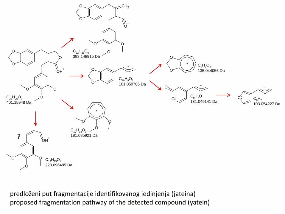
predloženi put fragmentacije identifikovanog jedinjenja (jateina) proposed fragmentation pathway of the detected compound (yatein)
O
O
O
OH+
O
O
O
C22
H25
O7
401.15948 Da
CH2O
O
O+
O
O
O
C22
H23
O6
383.148915 Da
O
O
O
+
C10
H13
O3
181.085921 Da
O
O
+
C10
H9O
2
161.059706 Da
O
O
+C
8H
7O
2
135.044056 Da
C
O+
C9H
7O
131.049141 DaC
+
C8H
7
103.054227 Da
OH+
O
O
O C12
H15
O4
223.096485 Da
?

______________________________________________________________________________________________________
This project has been funded with support from the European Commission. This publication reflects the views only of the authors,
and the Commission cannot be held responsible for any use which may be made of the information contained therein.
(EE10) Quantification of secondary
biomolecules by LC-DAD-MS/MS
Lab exercise: Identification and quantification of secondary
biomolecules in plant material by LC-DAD-MS/MS
Course: Isolation and characterization of natural products
Author: Dejan Orčić (University of Novi Sad, Faculty of Sciences)
Preparation: Dejan Orčić (University of Novi Sad, Faculty of Sciences)
Special thanks to Sanja Berežni (University of Novi Sad, Faculty of Sciences) for contribution
______________________________________________________________________________________________________
This project has been funded with support from the European Commission. This publication reflects the views only of the authors,
and the Commission cannot be held responsible for any use which may be made of the information contained therein.
Aims:
The aim of the exercise is to provide insight into manual optimization of
parameters for quantitative LC-MS/MS analysis.
Outcomes:
After succesful completion of the exercise, the student is able to:
• describe steps of ESI-MS/MS parameters optimization for quantitative
analysis,
• create/adapt acquisition methods, process experimental data and choose
optimal parameter values,
• process quantitative LC-MS/MS analysis results.

______________________________________________________________________________________________________
This project has been funded with support from the European Commission. This publication reflects the views only of the authors,
and the Commission cannot be held responsible for any use which may be made of the information contained therein.
Equipment
• HPLC instrument (Agilent Technologies series 1200) with:
• degasser,
• binary pump,
• autosampler,
• thermostatted column compartment,
• DAD and
• ESI-QqQ-MS/MS detector (Agilent Technologies series 6410A)
• reversed-phase column (Zorbax XDB-C18, 50 mm 4.6 mm, 1.8 μm, or
equivalent)
• common lab equipment:
• 10–100 μL and 100–1000 μL micropipettes,
• mobile phase filtration unit,
• ultrapure water preparation unit,
• syringes and syringe filters (e.g. RC),
• ultrasonic bath,
• 2 mL autosampler vials, etc.

______________________________________________________________________________________________________
This project has been funded with support from the European Commission. This publication reflects the views only of the authors,
and the Commission cannot be held responsible for any use which may be made of the information contained therein.
Materials
• ultrapure water
• formic acid (p.a. or better)
• mobile phase A: 0.05 % aqueous formic acid
• mobile phase B: methanol (gradient grade or better)
• iso-propanol (HPLC grade or better)
• selected sample: chamomile extract, diluted with 1:1 aqueous methanol (to
the final concentrations 25 mg of drug per 1 mL and 0.5 mg of drug per 1
mL), membrane-filtered
• working standard: 10 g/mL of apigenin 7-O-glucoside and 2.0 g/mL of
apigenin in 1:1 aqueous methanol
• diluted working standards: serial 1:1 dilutions in 1:1 aqueous methanol
______________________________________________________________________________________________________
This project has been funded with support from the European Commission. This publication reflects the views only of the authors,
and the Commission cannot be held responsible for any use which may be made of the information contained therein.
In this exercise, HPLC-MS/MS for quantification of selected secondary
biomolecules will be developed, and used for their quantification in selected plant
extract.
It is assumed that the student:
• has basic knowledge of LC-DAD-MS/MS principles,
• is familiarized with Agilent Mass Hunter Data Acquisition software operation,
• is familiar with qualitative analysis using LC-DAD-MS/MS (software operation),
• has basic skills with spreadsheet software (e.g. Microsoft Excel).

______________________________________________________________________________________________________
This project has been funded with support from the European Commission. This publication reflects the views only of the authors,
and the Commission cannot be held responsible for any use which may be made of the information contained therein.
(EE10) Kvantifikacija sekundarnih
biomolekula pomoću LC-DAD-MS/MS
Vežba: Identifikacija i kvantifikacija sekundarnih biomolekula u
biljnom materijalu pomoću LC-DAD-MS/MS
Kurs: Izolacija i karakterizacija prirodnih proizvoda
Autor: Dejan Orčić (Univerzitet u Novom Sadu, Prirodno-matematički
fakultet)
Tehnička priprema: Dejan Orčić (Univerzitet u Novom Sadu, Prirodno-
matematički fakultet)
Zahvaljujemo se Sanji Berežni (Univerzitet u Novom Sadu, Prirodno-matematički fakultet) za
doprinos
______________________________________________________________________________________________________
This project has been funded with support from the European Commission. This publication reflects the views only of the authors,
and the Commission cannot be held responsible for any use which may be made of the information contained therein.
Ishodi:
Cilj vežbe je da studenta uputi u postupak manuelne optimizacije parametara za
kvantitativnu LC-MS/MS analizu.
Ciljevi:
Nakon uspešno završene vežbe, student je u stanju da:
• opiše korake u procesu optimizacije parametara ESI-MS/MS instrumenta za
kvantitativnu analizu,
• postavi/adaptira metode za akviziciju, obradi rezultate eksperimenata i
odabere optimalne vrednosti parametara,
• obradi rezultate kvantitativne LC-MS/MS analize.

______________________________________________________________________________________________________
This project has been funded with support from the European Commission. This publication reflects the views only of the authors,
and the Commission cannot be held responsible for any use which may be made of the information contained therein.
(EE12) Semi-preparative HPLC
Lab exercise: Isolation of selected natural product from plant
material by semi-preparative HPLC
Course: Isolation and characterization of natural products
Author: Dejan Orčić (University of Novi Sad, Faculty of Sciences)
Preparation: Dejan Orčić (University of Novi Sad, Faculty of Sciences)
Special thanks to Sanja Berežni (University of Novi Sad, Faculty of Sciences) for contribution

______________________________________________________________________________________________________
This project has been funded with support from the European Commission. This publication reflects the views only of the authors,
and the Commission cannot be held responsible for any use which may be made of the information contained therein.
Aims:
The aim of the exercise is to provide insight into optimization of semi-
preparative HPLC separation conditions, and performing the
separation.
Outcomes:
After succesful completion of the exercise, the student is able to:
• describe steps of pHPLC conditions optimization and possible
problems,
• create/adapt pHPLC method and perform experimental separation.

______________________________________________________________________________________________________
This project has been funded with support from the European Commission. This publication reflects the views only of the authors,
and the Commission cannot be held responsible for any use which may be made of the information contained therein.
Introduction
In this exercise, semi-preparative HPLC will be
used to isolate pure components from complex
mixture. The sample is pre-fractionated
methanolic extract of Anhtriscus sylvestris
plant, which contains numerous lignans with
potent anti-cancer activity.
The isolation will be performed on Agilent
Technologies 1200 series HPLC, consisting of
solvent degasser, binary analytical pump,
automated liquid sampler, thermostated column
compartment and diode-array detector (DAD).
Additonally, ESI-QqQ-MS/MS can be attached
as a detector during the development step, to
identify the peaks of interest. The system is
powered by Agilent Technologies MassHunter
Workstation software.

______________________________________________________________________________________________________
This project has been funded with support from the European Commission. This publication reflects the views only of the authors,
and the Commission cannot be held responsible for any use which may be made of the information contained therein.
For preparative separations, large-diameter columns are used to increase
loading capacity and reduce number of runs needed to fractionate the entire
amount of sample. In this exercise, Zorbax Eclipse XDB-C18 column, 25 cm
long, with 9.6 mm internal diameter and 5 m particles will be used. Depending
on the nature of the sample, over 10 mg can be injected onto this column and
separated in a single run.
Comparison of
analytical and semi-
preparative column.
______________________________________________________________________________________________________
This project has been funded with support from the European Commission. This publication reflects the views only of the authors,
and the Commission cannot be held responsible for any use which may be made of the information contained therein.
After chromatographic separation (and, optionally, detection), selected
regions of chromatogram are collected. The selection can be based on
time/volume or by signal, and can be performed manually or automatically.
In this exercise, manual collection will be used, that is the most labor-
intensive (requires the constant presence of an operator) but is also the
most flexible – peaks of very different sizes and shapes (even overlapping
peaks), and with varying retention times, can be reliably collected. The exit
from DAD flow cell is connected to a tubing that will be used to forward the
fractions into test tubes. The tubing should be as short as practically
possible, to prevent long delay times (e.g. time differences between peak
detection and appearance in the effluent).
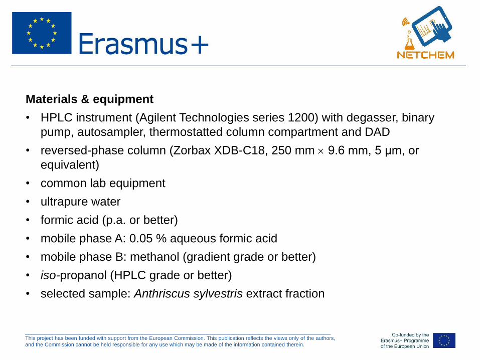
______________________________________________________________________________________________________
This project has been funded with support from the European Commission. This publication reflects the views only of the authors,
and the Commission cannot be held responsible for any use which may be made of the information contained therein.
Materials & equipment
• HPLC instrument (Agilent Technologies series 1200) with degasser, binary
pump, autosampler, thermostatted column compartment and DAD
• reversed-phase column (Zorbax XDB-C18, 250 mm 9.6 mm, 5 μm, or
equivalent)
• common lab equipment
• ultrapure water
• formic acid (p.a. or better)
• mobile phase A: 0.05 % aqueous formic acid
• mobile phase B: methanol (gradient grade or better)
• iso-propanol (HPLC grade or better)
• selected sample: Anthriscus sylvestris extract fraction

______________________________________________________________________________________________________
This project has been funded with support from the European Commission. This publication reflects the views only of the authors,
and the Commission cannot be held responsible for any use which may be made of the information contained therein.
(EE12) Semi-preparativna HPLC
Vežba: Izolacija odabranih prirodnih proizvoda iz biljnog
materijala semi-preparativnom HPLC
Kurs: Izolacija i karakterizacija prirodnih proizvoda
Autor: Dejan Orčić (Univerzitet u Novom Sadu, Prirodno-matematički
fakultet)
Tehnička priprema: Dejan Orčić (Univerzitet u Novom Sadu, Prirodno-
matematički fakultet)
Zahvaljujemo se Sanji Berežni (Univerzitet u Novom Sadu, Prirodno-matematički fakultet) za
doprinos
______________________________________________________________________________________________________
This project has been funded with support from the European Commission. This publication reflects the views only of the authors,
and the Commission cannot be held responsible for any use which may be made of the information contained therein.
Ciljevi:
Cilj vežbe je da studenta uputi u postupak optimizacije uslova za
semipreparativno HPLC razdvajanje i izvođenje samog razdvajanja.
Ishodi:
Nakon uspešno završene vežbe, student je u stanju da:
• piše korake u procesu optimizacije uslova pHPLC razdvajanja i navede
potencijalne probleme,
• postavi/adaptira pHPLC metodu i u praksi izvede razdvajanje.
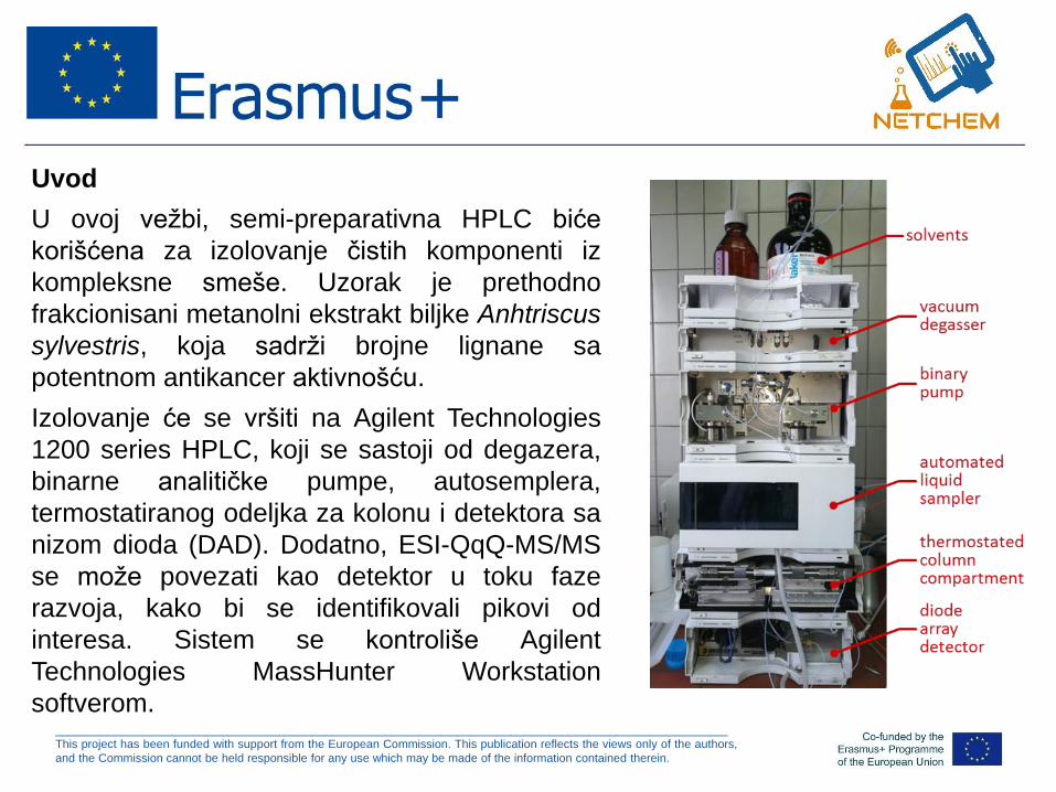
______________________________________________________________________________________________________
This project has been funded with support from the European Commission. This publication reflects the views only of the authors,
and the Commission cannot be held responsible for any use which may be made of the information contained therein.
Uvod
U ovoj vežbi, semi-preparativna HPLC biće
korišćena za izolovanje čistih komponenti iz
kompleksne smeše. Uzorak je prethodno
frakcionisani metanolni ekstrakt biljke Anhtriscus
sylvestris, koja sadrži brojne lignane sa
potentnom antikancer aktivnošću.
Izolovanje će se vršiti na Agilent Technologies
1200 series HPLC, koji se sastoji od degazera,
binarne analitičke pumpe, autosemplera,
termostatiranog odeljka za kolonu i detektora sa
nizom dioda (DAD). Dodatno, ESI-QqQ-MS/MS
se može povezati kao detektor u toku faze
razvoja, kako bi se identifikovali pikovi od
interesa. Sistem se kontroliše Agilent
Technologies MassHunter Workstation
softverom.

______________________________________________________________________________________________________
This project has been funded with support from the European Commission. This publication reflects the views only of the authors,
and the Commission cannot be held responsible for any use which may be made of the information contained therein.
Za preparativna razdvajanja koriste se kolone velikog prečnika, kako bi se
povećao kapacitet i smanjio broj ciklusa neophodnih za frakcionisanje
celokupne količine uzorka. U ovoj vežbi koristiće se Zorbax Eclipse XDB-C18
kolona dužine 25 cm, unutrašnjeg prečnika 9,6 mm, sa česticama od 5 m. U
zavisnosti od prirode uzorka, moguće je injektovanje i frakcionisanje i preko 10
mg uzorka.
Poređenje analitičke
i semipreparativne
kolone

______________________________________________________________________________________________________
This project has been funded with support from the European Commission. This publication reflects the views only of the authors,
and the Commission cannot be held responsible for any use which may be made of the information contained therein.
Nakon hromatografskog razdvajanja i, poželjno, detekcije, odabrani
segmenti hromatograma se sakupljaju. Izbor segmenata se može zasnivati
na vremenu/zapremini ili signalu, i sakupljanje se može izvesti ručno ili
automatski.
U ovoj vežbi koristiće se ručno sakupljanje, koje zahteva najviše ljudskog
rada (zahteva konstantno prisustvo operatera) ali je i najfleksibilnije – pikovi
veoma različitih veličina i oblika (čak i preklapajući pikovi) i varirajućih
retencionih vremena mogu biti pouzdano sakupljeni. Izlaz sa DAD protočne
ćelije povezan je na kapilaru koja će biti korišćena za prosleđivanje frakcija
u epruvete. Kapilara treba da bude što kraća da bi se izbegla duga vremena
zadržavanja (razlike između vremena detekcije pika i njegove pojave u
efluentu).

______________________________________________________________________________________________________
This project has been funded with support from the European Commission. This publication reflects the views only of the authors,
and the Commission cannot be held responsible for any use which may be made of the information contained therein.
Pribor i materijal
• HPLC instrument (Agilent Technologies series 1200) sa degazerom,
binarnom pumpom, autosemplerom, termostatiranim odeljkom za kolonu i
DAD
• reverzno-fazna kolona (Zorbax XDB-C18, 250 mm 9.6 mm, 5 μm, ili
ekvivalentna)
• uobičajeni laboratorijski pribor
• ultračista voda
• mravlja kiselina (p.a. ili bolja)
• mobilna faza A: 0.05 % vodeni rastvor mravlje kiseline
• mobilna faza B: metanol (gradient grade ili bolji)
• izo-propanol (HPLC kvaliteta ili bolji)
• uzorak: frakcija ekstrakta Anthriscus sylvestris

______________________________________________________________________________________________________
This project has been funded with support from the European Commission. This publication reflects the views only of the authors,
and the Commission cannot be held responsible for any use which may be made of the information contained therein.
(EE12c) Semi-preparative HPLC –
supplementary material
Lab exercise: Isolation of selected natural product from plant
material by semi-preparative HPLC
Course: Isolation and characterization of natural products
Author: Dejan Orčić (University of Novi Sad, Faculty of Sciences)
Preparation: Dejan Orčić (University of Novi Sad, Faculty of Sciences)
Special thanks to Sanja Berežni (University of Novi Sad, Faculty of Sciences) for contribution

______________________________________________________________________________________________________
This project has been funded with support from the European Commission. This publication reflects the views only of the authors,
and the Commission cannot be held responsible for any use which may be made of the information contained therein.
(EE12c) Semi-preparativna HPLC –
dopunski materijal
Vežba: Izolacija odabranih prirodnih proizvoda iz biljnog
materijala semi-preparativnom HPLC
Kurs: Izolacija i karakterizacija prirodnih proizvoda
Autor: Dejan Orčić (Univerzitet u Novom Sadu, Prirodno-matematički
fakultet)
Tehnička priprema: Dejan Orčić (Univerzitet u Novom Sadu, Prirodno-
matematički fakultet)
Zahvaljujemo se Sanji Berežni (Univerzitet u Novom Sadu, Prirodno-matematički fakultet) za
doprinos

O
O
R
R
O
O
O
R
R
O
O
R
R
OH
O
O
R
R
O
O
R
R
O
O
O
R
R
OH
O
O
R
R
O
O
O
R
R
O
O
R
R
OH
expected structural classes
with approx. absorption maxima of chromophores
~330 nm
~280 nm

mAU vs. Acquisition Time (min)1 2 3 4 5 6 7 8 9 10 11 12 13 14 15 16 17 18 19 20 21 22 23
0.2 L
1 L
2 L
3 L
4 L
5 L
6 L
injection volume optimization
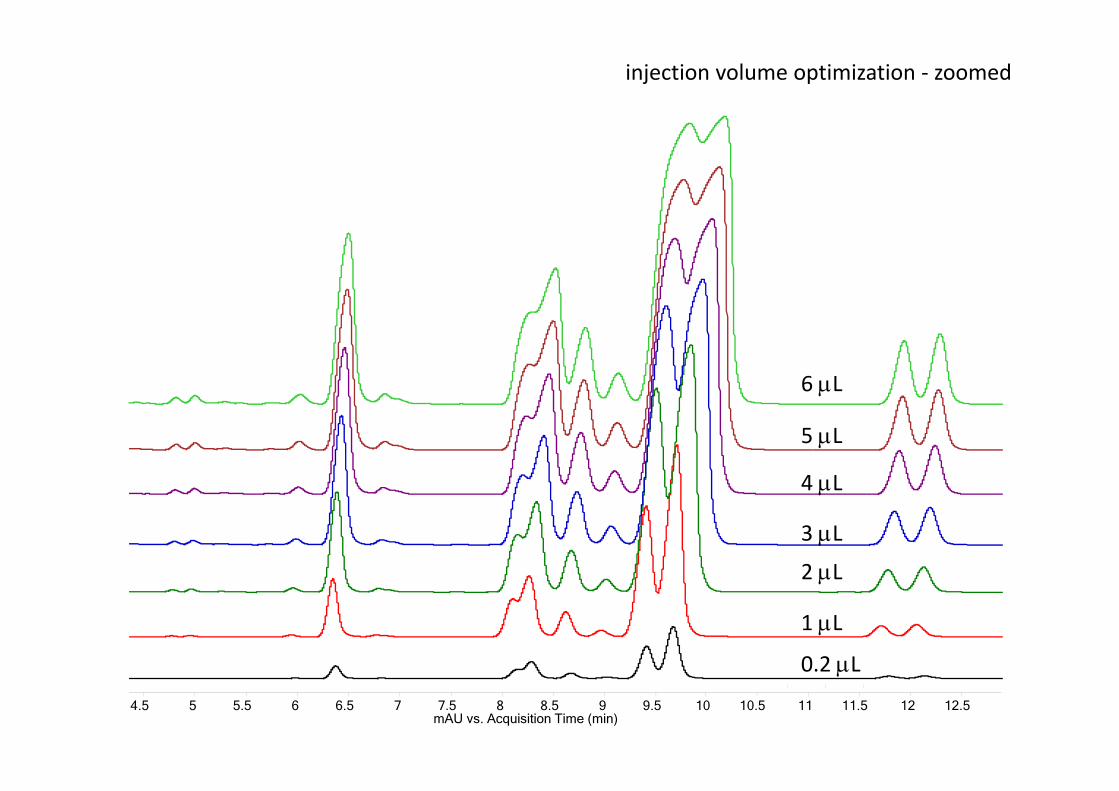
injection volume optimization ‐ zoomed
mAU vs. Acquisition Time (min)4.5 5 5.5 6 6.5 7 7.5 8 8.5 9 9.5 10 10.5 11 11.5 12 12.5
0.2 L
1 L
2 L
3 L
4 L
5 L
6 L

2x10
-0.5
0
0.5
1
1.5
2
2.5
3
3.5
4
4.5
5
5.5
6
6.5
7
7.5
8
8.5
DAD1 - TWC F7.3.1_06_test_6ul_short .d
mAU vs. Acquisition Time (min)1 2 3 4 5 6 7 8 9 10 11 12 13 14 15 16
421 35a5b
6 7 8 9 1110
fractions definition

F1 F2 F3 F4
after each run
evaporation
fraction (in MeOH + H2O + formic acid)
n
CHCl3 layerevaporation
MeOH removal