education sector analysis methodological guidelines
410
VOLUME 1 International Institute for Educational Planning EDUCATION SECTOR ANALYSIS METHODOLOGICAL GUIDELINES
-
Upload
khangminh22 -
Category
Documents
-
view
1 -
download
0
Transcript of education sector analysis methodological guidelines

VOLUME 1
International Institutefor Educational Planning
EDUCATION SECTOR ANALYSISMETHODOLOGICAL GUIDELINES

Nota beneThe ideas and opinions expressed in this document are those of the authors and do not necessarily reflect theviews of UNESCO, UNICEF, the World Bank or the Global Partnership for Education. The designations used in this publication and the presentation of data do not imply that UNESCO, UNICEF, theWorld Bank or the Global Partnership for Education have adopted any particular position with respect to thelegal status of the countries, territories, towns or areas, their governing bodies or their frontiers or boundaries.
ISBN: 978-92-806-4715-0September, 2014
Layout : by Reg’ - www.designbyreg.dphoto.com

With the financial support of:
International Institutefor Educational Planning
VOLUME 1
METHODOLOGICAL GUIDELINESEDUCATION SECTOR ANALYSIS
SECTOR-WIDE ANALYSIS, WITH EMPHASIS ON PRIMARY AND SECONDARY EDUCATION

2 EDUCATION SECTOR ANALYSIS METHODOLOGICAL GUIDELINES - Volume 1
Table of Contents 2
List of Examples 6List of Tables 10List of Figures and Maps 14List of Boxes 16
Foreword 18Acknowledgements 20Acronyms and Abbreviations 22Introduction 27
CHAPTER 1 33CONTEXT OF THE DEVELOPMENT OF THE EDUCATION SECTOR
Introduction 36SECTION 1: THE SOCIAL, HUMANITARIAN AND DEMOGRAPHIC CONTEXTS 37
1.1 The Evolution of the Total Population and the School-Aged Population 381.2 Basic Social Indicators 421.3 Impact of HIV/AIDS and Malaria on Education 451.4 The Composite Social Context Index 481.5 Linguistic Context 491.6 Humanitarian context 50
SECTION 2: THE MACROECONOMIC AND PUBLIC FINANCE CONTEXTS 512.1 GDP and GDP per Capita Trends 522.2 Public Resources 542.3 Public Expenditure 562.4 The Composite Economic Context Index 582.5 The Composite Global Context Index 592.6 Future Prospects 61
CHAPTER 2 65ENROLMENT, INTERNAL EFFICIENCY AND OUT-OF-SCHOOL CHILDREN
Introduction 69SECTION 1: THE EVOLUTION OF ENROLMENT AND EDUCATION SYSTEM ENROLMENTCAPACITY 69
1.1 The Evolution of Enrolment 691.2 Evolution of Enrolment Capacity: Gross Enrolment Rate Computation 72
SECTION 2: SCHOOL COVERAGE: SCHOOLING PROFILES, SCHOOL LIFE EXPECTANCY AND EDUCATION PYRAMIDS 77
2.1 Schooling Profiles and Retention 772.2 School Life Expectancy 832.3 Education Pyramids 85

Sector-Wide Analysis, with Emphasis on Primary and Secondary Education 3
SECTION 3: THE SUPPLY AND DEMAND ISSUES ON ACCESS AND RETENTION 873.1 Access-Related Supply and Demand 873.2 Retention-Related Supply and Demand 933.3 Bottleneck Analysis 98
SECTION 4: INTERNAL EFFICIENCY 1004.1 Repetition 1014.2 Internal Efficiency Coefficient 107
SECTION 5: OUT-OF-SCHOOL CHILDREN 1105.1 Estimation of the Share and Number of Out-of-School 1105.2 Who are the Out-of-School Children? 115
CHAPTER 3 121COST AND FINANCING
Introduction 125SECTION 1: PUBLIC EDUCATION EXPENDITURE 127
1.1 Government Spending 1271.2 Evolution of Public Expenditure by Type of Spending 1311.3 The Distribution of Spending Across Sub-Sectors 1321.4 Detailed Analysis of Public Recurrent Expenditure for the Most Recent Year 1341.5 External Funding 140
SECTION 2: PUBLIC EDUCATION RECURRENT UNIT COSTS 1432.1 Macro Estimation of Public Recurrent Expenditure per Pupil 1432.2 Breakdown of Public Recurrent Unit Costs 1482.3 Analysis of the Status and Remuneration of Teachers 152
SECTION 3: HOUSEHOLD CONTRIBUTIONS TO EDUCATION 1573.1 Private Unit Costs by Education Level 1583.2 Education Cost-Sharing between the Government and Families 1603.3 Breakdown of Average Private Unit Costs by Spending Item and Level 162
SECTION 4: THE COST OF SCHOOL INFRASTRUCTURE 164
CHAPTER 4 169QUALITY, SYSTEM CAPACITY AND MANAGEMENT
Introduction 173SECTION 1: ASSESSMENT OF STUDENT LEARNING 174
1.1 National Examinations and Admissions Tests 1751.2 National Learning Assessments 1771.3 International Standardised Learning Assessments 1781.4 Using Household Surveys and Literacy Levels as a Proxy Measure of Quality 180
SECTION 2: ANALYSIS OF SYSTEM CAPACITY 1832.1 Evaluation of the Conversion of Resources into Results by Schools 1832.2 Analysis of the Factors Associated with Learning Outcomes 1852.3 The Analysis of Factors’ Cost-Effectiveness 1932.4 Institutional Analysis 194
INTRO
DU
CTION
TABLE OF CO
NTEN
TS

4 EDUCATION SECTOR ANALYSIS METHODOLOGICAL GUIDELINES - Volume 1
SECTION 3: MANAGEMENT OF TEACHERS 1973.1 Quantitative aspects of the management of teachers 1973.2 Qualitative aspects of the management of teachers 205
SECTION 4: THE MANAGEMENT OF OTHER RESOURCES AND OF TEACHING TIME 2154.1 Management of resources other than teachers 2154.2 Monitoring Effective Teaching Time 218
CHAPTER 5 227EXTERNAL EFFICIENCY
Introduction 230SECTION 1: THE ECONOMIC IMPACT OF EDUCATION 232
1.1 Description of the Labour Market 2321.2 Labour Market Structure and Dynamics 2351.3 Employability of Education System Leavers and Graduates 2391.4 Economic Return of Different Education Levels 2441.5 The Training-Employment Balance (Macro Approach) 2461.6 Anticipation of Future Labour Market Needs 249
SECTION 2: THE SOCIAL IMPACT OF EDUCATION 2522.1 The Choice of Social Development Variables 2522.2 Estimation of the Net Effects of Education 2552.3 Consolidation of the Net Social Effect of Education 261
CHAPTER 6 267 EQUITY
Introduction 269SECTION 1: EQUITY IN ENROLMENT AND LEARNING ACHIEVEMENTS 273
1.1 The Absolute Gap in Performance between Two Groups 2741.2 The Parity Index 2751.3 The Parity Line 2771.4 Scatter Charts 2781.5 Maps 2791.6 Social Mobility Tables 2811.7 Odds Ratios 2831.8 Marginal Effects and Odds Ratios Based on Econometric Models 284
SECTION 2: MEASURING EQUITY IN THE DISTRIBUTION OF PUBLIC RESOURCES 2882.1 The Structural Distribution of Public Education Resources 2892.2 Distributive Equity in Public Education Expenditure: Social Disparities in
the Appropriation of Education Resources and Benefit Incidence Analysis 299

Sector-Wide Analysis, with Emphasis on Primary and Secondary Education 5
ANNEXES 307
GENERAL ANNEXES 308Annex 0: Basic Elements of Econometrics 308
CHAPTER 1 ANNEXES 314Annex 1.1: Demographic Data Quality and Corrections 314Annex 1.2: Calculation of the Average Annual Growth Rate 319Annex 1.3: Current and Constant Prices 320Annex 1.4: Methodology of Calculation of the Composite Context Indexes 323
CHAPTER 2 ANNEXES 324Annex 2.1: Assessing Internal Efficiency by Means of Cohort Analysis 324Annex 2.2: Calculation Method for School Life Expectancy Based on Gross Enrolment Rates
and average enrolment rates 329Annex 2.3: Measuring Progress towards Universal Primary Education 331Annex 2.4: The Schooling Profiles 338
CHAPTER 3 ANNEXES 346Annex 3.1: Technical Note on the Adjustment of the Share of Recurrent Expenditure
by Education Level According to Standard Cycle Durations 346Annex 3.2: Sample Questionnaire to Collect Data on International Aid from
Development Partners 348Annex 3.3: Methodology for the Consolidation of Financial Data 350
CHAPTER 4 ANNEXES 360Annex 4.1: Calculation of the R² Determination Coefficient with an Excel-type Spreadsheet 360Annex 4.2: Teachers’ Socio-Professional Context: Dimensions to Consider 361Annex 4.3: Sample Questionnaire to Appraise the Socio-Professional Teaching Context
(To be adapted to each country context) 364Annex 4.4: Modelisation of Primary Education Results 371Annex 4.5: Correlation of Student and Teacher Characteristics with Learning Outcomes 373Annex 4.6: Calculation of School Indices (the Performance Index, Resources Index and
Efficiency Index), based on the Example of The Gambia 375Annex 4.7: Computation of the School Value-Added Indicator 378Annex 4.8: School profile, based on the Example of The Gambia 379Annex 4.9: Flow of Exam Result Information, Cameroon 380
CHAPTER 5 ANNEXES 381Annex 5.1: Methodology for the Estimation of Net Income, Expected Income and
Rates of return 381Annex 5.2: The Main Types of Survey Used in Labour Market Analysis 385Annex 5.3: Selection of a Representative Sample for the Analysis of the Status of Education
System Leavers in the Workplace 387Annex 5.4: Graduate Tracer Studies 390Annex 5.5: Interview Checklist for the Qualitative Analysis of Education Sector Institutional
Steering Mechanisms for the Education-Training balance (to be adapted to country context) 393
INTRO
DU
CTION
TABLE OF CO
NTEN
TS

6 EDUCATION SECTOR ANALYSIS METHODOLOGICAL GUIDELINES - Volume 1
CHAPTER 6 ANNEXES 394Annex 6.1: Classification of Countries According to Primary Enrolment Gender Disparities,
Comparing the Absolute Gap and the Gender Parity Index 394Annex 6.2: The Respective Weights of Schooling Stages in Explaining Global Disparities in
the Enrolment of Different Groups 396Annex 6.3: Modeling/Simulation of the Schooling Profile According to the Socioeconomic
Characteristics of Children 398Annex 6.4: Equity in the Distribution of Education Inputs 399Annex 6.5: Structural Distribution of Public Education Expenditure when Schooling Profile
Data is Unavailable 401Annex 6.6: Intermediate Computation of the Appropriation Index 404
LIST OF EXAMPLES
EXAMPLE 1.1 40(Demographic Context): The DemographicContext of Côte d’Ivoire, 2010
EXAMPLE 1.2 44(Social Context): Social Context of Malawi, 2010
EXAMPLE 1.3 47(HIV/AIDS Impact): The Impact of HIV/AIDS on Education, Congo, 2010
EXAMPLE 1.4 53(Macroeconomic Context): MacroeconomicContext, Mali, 2010
EXAMPLE 1.5 55(Public Resources): Mauritania’s PublicResources, 2010
EXAMPLE 1.6 57(Public Expenditure and Deficit): Government Revenue, Expenditure andDeficit, The Gambia, 2011
EXAMPLE 1.7 61(Public Resource and Expenditure Projection):Projected Government Resources andExpenditure, Mali, 2010
EXAMPLE 2.1 70(Education System Structure): Structure of the Beninese Education System, 2010
EXAMPLE 2.2 71(Evolution of Enrolment): Enrolment Trends by Level, The Gambia, 2000/01-2009/10
EXAMPLE 2.3 73(GER Analysis): Gross Enrolment Rates, by Level and in International Context, Congo, 1986-2005
EXAMPLE 2.4 82(Schooling and Retention Profiles): Cross Section Schooling and RetentionProfiles, Mali, 2004/05 and 2007/08
EXAMPLE 2.5 86(Education Pyramids): Education Pyramids for Malawi, 2007 and Sub-Saharan Africa,2005/06
EXAMPLE 2.6 89(Regional Analysis of School Supply andDemand): Analysis of Supply and Demand in Terms of School Access, by District,The Gambia, 2009
EXAMPLE 2.7 91(Modelisation of Primary Access Demand):Correlation of the Distance to School with the Demand for Primary Access, Mauritania, 2008

Sector-Wide Analysis, with Emphasis on Primary and Secondary Education 7
EXAMPLE 2.8 92(Analysis of Factors Affecting Access-RelatedDemand): Causes of Non-Attendance andDissatisfaction with School Mentioned byParents, Benin, 2003
EXAMPLE 2.9 93(Analysis of Supply - Incomplete Schools):Distribution of Schools According to theGrades Offered, Burkina Faso, 2006/07
EXAMPLE 2.10 95(Impact of Incomplete Schools on Retention):Regional Supply and Demand Issues and theirImpact on Retention, Mali, 2006/07-2007/08
EXAMPLE 2.11 97(Analysis of Factors Affecting Retention-Related Demand): Simulation of CompletionRates According to Socioeconomic Factors,Congo, 2005
EXAMPLE 2.12 103(Analysis of Repetition): Historical RepetitionTrends for 2000-08 and InternationalPerspective, Rwanda
EXAMPLE 2.13 105(Analysis of Factors Associated WithRepetition): Econometric Modelisation ofSchool and Classroom Factors Related toRepetition, Chad, 2006
EXAMPLE 2.14 109(Internal Efficiency Coefficients): Total,Dropout-Related and Repetition-RelatedInternal Efficiency, Rwanda, 2002/03-2008
EXAMPLE 2.15 116(Out-of-School Profiling): Magnitude of Out-of-School and Characteristics of Out-of-School Children, Mauritania, 2008
-------------------------------------------------------------------
EXAMPLE 3.1 130(Breakdown of Public Education Expenditureby Type and Source): Public EducationExpenditure, The Gambia, 2001-09
EXAMPLE 3.2 132(Breakdown of Public Education Expenditureby Nature): Public Education Expenditure,Benin, 1992-2006
EXAMPLE 3.3 135(Distribution of Public Education Expenditurein Regional Context): Public EducationExpenditure by Level, Mali, 2008
EXAMPLE 3.4 137(Analysis of Personnel Expenditure): Public Education Personnel Expenditure,Congo, 2009
EXAMPLE 3.5 138(Analysis of Non-Salary Expenditure): Public Expenditure by Function and Level,Benin, 2006
EXAMPLE 3.6 141(Analysis of External Aid - National): Donor Financing for the Education Sector,Malawi, 2005/06-2007/08
EXAMPLE 3.7 142(Analysis of External Aid - International):International Comparison of External Fundingof Education Systems, 2008 or MRY
EXAMPLE 3.8 144(Analysis of Unit Costs by Cycle): Unit Costs and their Relative Value, by Level,Côte d’Ivoire, 2007
EXAMPLE 3.9 145(Historical Trends in Unit Costs): Evolution of Public Unit Costs by Level, Mauritania,1998-2008
EXAMPLE 3.10 146(Unit Costs in International Perspective):International Comparison of Unit Costs,2006 or MRY
EXAMPLE 3.11 150(Breakdown of Unit Costs): Breakdown ofPublic Expenditure per Pupil, Benin, 2006
EXAMPLE 3.12 151(Analysis of Pupil to Teacher Ratios): Pupil toTeacher Ratios, Côte d’Ivoire, 2007
EXAMPLE 3.13 153(Analysis of Teaching Salaries by Status):Comparison of Teacher Remuneration byStatus and Cycle, Mali, 2008
INTRO
DU
CTION
TABLE OF CO
NTEN
TS

EXAMPLE 4.6 189(Econometric Modelisation of Prior SchoolingFactors): Analysis of Prior Schooling Factors onthe Basis of the Initial Level of Students’Learning Outcomes, Mali, 2006
EXAMPLE 4.7 193(Analysis of the Cost-Efficiency of FactorsAffecting Quality): Theoretical Illustration
EXAMPLE 4.8 199(Analysis of Required Growth in TeacherNumbers): Comparison of Past and FutureRequired Growth in Teacher Numbers, Benin,2000-09
EXAMPLE 4.9 201(Projection of Retirement-Related Attrition):Estimation of Retirement-Related Departuresfrom the Teaching Profession in Cameroon,Benin and Guinea-Bissau, 2003-30
EXAMPLE 4.10 204(Analysis of Past Growth and Future Needsin Teaching Staff): Compared Analysis in PastGrowth and Future Teaching StaffRequirements, Benin, 2009/10
EXAMPLE 4.11 206(Use of Competency Assessments to Evaluatethe Quality of Teacher Training): Evaluation ofTeachers’ Skills through Skills Assessments,Guinea-Bissau, 2009
EXAMPLE 4.12 209(Analysis of the Consistency of TeacherPostings): Consistency in the Posting ofPrimary Teachers, Burkina Faso, 2006/07
EXAMPLE 4.13 216(Analysis of the Consistency in the Allocationof Other Educational Inputs): Analysis of theConsistency in the Allocation of PrimaryTextbooks, Mali, 2007/08
EXAMPLE 4.14 219(Abadzi’s Model of Instructional Time Loss):Analysis of Lost Learning Time, Mali, 2009/10
EXAMPLE 4.15 221(Typical Questions to Evaluate TeacherAbsenteeism): Typical questions to assess teacherabsenteeism, PASEC, SACMEQ and PETS
EXAMPLE 4.16 222(Analysis of the Causes of TeacherAbsenteeism): The Main Causes of TeacherAbsenteeism, Benin, 2004/05
8 EDUCATION SECTOR ANALYSIS METHODOLOGICAL GUIDELINES - Volume 1
EXAMPLE 3.14 155(Teaching Salaries in the National Context):National Comparison of TeacherRemuneration, Burkina Faso, 2003
EXAMPLE 3.15 159Estimation of Household Education Spendingby Level, Congo, 2005
EXAMPLE 3.16 160(Public-Private Education Cost-Sharing): Cost-Sharing of Education Costs between the Government and Families, by Level,Mauritania, 2008
EXAMPLE 3.17 162(Breakdown of Private Unit Costs): Breakdown of Average Household EducationSpending by Item, The Gambia, 2009
EXAMPLE 3.18 163(Analysis of Building Costs): Primary andSecondary Education Construction Costs andInstitutional Mechanisms, Benin 2011
-------------------------------------------------------------------
EXAMPLE 4.1 176(Historical Analysis of Exam Results): Evolution of Certificate of SecondaryEducation Examination (CSEE) Results,Tanzania, 2000-09
EXAMPLE 4.2 178(Analysis of Knowledge Acquired throughouta Cycle through National Assessments):Results of the Primary Cycle NationalAssessment, Mali, 2007
EXAMPLE 4.3 179(International Comparative Analysis ofLearning Outcomes through InternationalAssessments): Malawi and other AnglophoneAfrican Countries’ Math and Reading Results,2007
EXAMPLE 4.4 182(Use of Literacy Rates to Assess LearningOutcomes): Adult Literacy Levels by Numberof Years of Education, InternationalComparison, 2000-05
EXAMPLE 4.5 184(Analysis of the Conversion of Resources intoResults): School Performance and Resources,Guinea, 2003/04
Sector-Wide Analysis, with Emphasis on Primary and Secondary Education 9
EXAMPLE 5.11 259(Social Impact of Education by Level –Logistical Model): Impact of Each Level ofEducation on the Probability of Knowing atLeast One Modern Contraceptive Method(Theoretical Approach)
EXAMPLE 5.12 262(Consolidated Net Social Effect of Education):Global Social Impact of Different EducationLevels, Sierra Leone, 2010
-------------------------------------------------------------------
EXAMPLE 6.1 274(Absolute Gap): Gender Disparities in PrimaryAccess, Mali, 2007/08
EXAMPLE 6.2 275(Absolute Gap): Cumulative Disparities inAccess to Primary Levels, The Gambia, 2006
EXAMPLE 6.3 276(Parity Index): PCR Disparities, bySocioeconomic Characteristics, Malawi, 2006
EXAMPLE 6.4 277(Parity Line): Regional Disparities in the GIRs,by Gender, Mauritania, 2007/08
EXAMPLE 6.5 278(Scatter Chart): Relationship between BasicEducation Coverage and Teacher Availability,The Gambia, 2009
EXAMPLE 6.6 280(Maps): Disparities in End of Lower SecondaryExam (CSEE) Results, Tanzania, 2009
EXAMPLE 6.7 282(Mobility Table): Theoretical DifferentiatedSchool Careers of Professionals’ and Farmers’Children
EXAMPLE 6.8 284(Odds Ratios): Theoretical Relative Probabilityof Secondary Intake, for Professionals’ andFarmers’ Children
EXAMPLE 6.9 285(Marginal Effects, Regression): Disparities inLearning Achievements: the Net Effects ofGender, Area of Residence, and HouseholdWealth, The Gambia, 2009/10
EXAMPLE 5.1 234(Employment Indicators): Historical Perspectiveof the Usually Active and EmployedPopulation, Sao Tomé and Principe, 2000-10
EXAMPLE 5.2 238(Distribution of Employment): Type ofEmployment, by Sector, SocioprofessionalStatus and Age Group, The Gambia, 2008/09
EXAMPLE 5.3 239(Employability): Analysis of the EmploymentStatus of Education System Leavers, Burundi,2006
EXAMPLE 5.4 243(Income Performance of Education):Annual Average Income, by Education Level,The Gambia, 2009
EXAMPLE 5.5 245(Economic Return of Education): Analysis ofthe Rates of Return on Investment in DifferentEducation Levels, Benin, 2006
EXAMPLE 5.6 247(Training-Employment Balance, by Formal/Informal): Alignment of WorkplaceSupply and Demand of Different EducationLevels, Mali, 2009
EXAMPLE 5.7 248(Training-Employment Balance, bySocioprofessional Status): Employment Statusof Education Graduates/Leavers, by Level,Mali, 2006
EXAMPLE 5.8 249(Projection of the Demand for Skills, byQualification Level): Determination of themost Promising Education Levels in Terms ofEmployment, Sao Tomé and Principe, 2010
EXAMPLE 5.9 250(Projection of Demand for Skills, by Sector):Determination of Promising Sectors in Termsof Employment, Sao Tomé and Principe, 2010
EXAMPLE 5.10 256(Social Impact of Education by Level – LinearModel): Impact of Each Education Level onAge at First Childbirth (Theoretical Approach)
INTRO
DU
CTION
TABLE OF CO
NTEN
TS

10 EDUCATION SECTOR ANALYSIS METHODOLOGICAL GUIDELINES - Volume 1
EXAMPLE 6.14 298(Linear Interpolation - Share of ResourcesAbsorbed by the 10 Percent Most Educated): The Distribution of Education Resources, The Gambia, 2006
EXAMPLE 6.15 299(Comparative Analysis): Education ResourcesConsumed by the 10 Percent Most Educated,Sub-Saharan Africa, 2009 or MRY
EXAMPLE 6.16 301(Relative Representativity Coefficients): SocialDistribution of Children by Education Level,The Gambia, 2006
EXAMPLE 6.17 304(Benefit Incidence Analysis and RelativeAppropriation Index): Social Disparities in theAppropriation of Education Resources, The Gambia, 2006
EXAMPLE 6.10 287(Odds Ratios’ Regression): Disparities inPrimary Retention, by SocioeconomicCharacteristic, Tanzania, 2006
EXAMPLE 6.11 292(Distributive Equity): Structural Distribution of Public Education Resources, Based on theSchooling Profile, The Gambia, 2006
EXAMPLE 6.12 294(Lorenz Curve and Share of ResourcesConsumed by the 10% most Educated):The Distribution of Public EducationResources, The Gambia, 2006
EXAMPLE 6.13 295(Gini Coefficient): The Distribution ofEducation Resources, The Gambia, 2006
Table 2.1 71Enrolment Trends, by Education Level and Type of Provider, The Gambia, 2000/01-2009/10
Table 2.2 73Gross Enrolment Rates, by Level, Congo, 1986-2005
Table 2.3 74Gross Enrolment Rates by Level, Congo and African Averages, 2003/04 or MRY
Table 2.4 87Two Examples of the Effect of School Supply andDemand on Access
Table 2.5 91Modelisation of the Correlation between Distanceto School and Basic Education Access (ChildrenAged 11 to 12 Years), Mauritania, 2008
Table 2.6 93Distribution of Schools According to the Number of Grades Offered and Enrolment, Burkina Faso,2006/07
Table 2.7 95Share of Schools and Pupils Facing GradeDiscontinuity between 2006/07 and 2007/08, byGrade, Mali
Table 1.1 40Evolution of the Total and School-Aged Populations,Côte d’Ivoire, 1988-2020
Table 1.2 48Composite Social Context Index, ECOWASCountries, 2010 or MRY
Table 1.3 53GDP and GDP per capita Trends, Mali, 1995-2008
Table 1.4 56The Evolution of Public Resources, Mauritania,1995-2008
Table 1.5 57Total Government Revenue, Expenditure and Deficit, The Gambia, 2004-10
Table 1.6 58Composite Economic Context Index, CEMACCountries, 2010 or MRY
Table 1.7 59Composite Global Context Index, SADC Countries,2010 or MRY
Table 1.8 60Key Social and Economic Indicators, Liberia, 2010
Table 1.9 61Macro and Resource Forecasts for RecurrentEducation Expenditure, Mali, 2009-12
LIST OF TABLES

Sector-Wide Analysis, with Emphasis on Primary and Secondary Education 11
Table 3.9 147International Comparison of Public Unit Costs by Level, 2006 or MRY
Table 3.10 147Structure of Unit Costs in Relation to Primary UnitCosts, Various African Countries, 2006 or MRY
Table 3.11 150Breakdown of Public Expenditure per Pupil inGovernment Schools, Benin, 2006
Table 3.12 151Public Pupil to Teacher Ratio in InternationalPerspective, Côte d’Ivoire, 2007
Table 3.13 153Distribution of Personnel and AverageRemuneration, by Status and Level, Mali, 2008
Table 3.14 155Occupation and Annual Income of Individuals Aged25 to 35 years, by Number of Years of TrainingReceived and Job Sector, Burkina Faso, 2003
Table 3.15 157Types of Household Education Spending
Table 3.16 159Estimation of Household Education Spending by Level, Congo, 2005
Table 3.17 161Public-Private Cost-Sharing of Recurrent EducationExpenditure, by Level, Mauritania, 2008
Table 3.18 162Distribution of Household Education Spending, The Gambia, 2009
Table 3.19 163Cross-Country Comparison of the Distribution of Household Education Spending, by Type, 2009 or MRY
Table 3.20 165Cost of a School Module of Three Classrooms, a Storeroom and Director’s Office, by Source of Funding, Benin, 2011
Table 3.21 166Annualised Cost of a Furnished Classroom, Based on the Type of Roof, Benin, 2011
-------------------------------------------------------------------Table 4.1 174Summary Description of Learning OutcomesAssessment Usually Available for Education Sector Analysis
Table 4.2 178Average Scores and Knowledge Levels in Languageand Math, Primary Grades 2, 4 and 6, Mali, 2007
Table 2.8 97Simulation of Completion Rates through LogisticRegressions, by Gender, Wealth Quintile andDistance to School, Congo, 2005
Table 2.9 99Adaptation of Tanahashi model to the educationsector
Table 2.10 104Repetition Trend for the Primary Cycle, by Grade,Rwanda, 2002-2008
Table 2.11 105Modelisation of Primary Cycle Repetition, Chad, 2007
Table 2.12 109Internal Efficiency Coefficients in Primary andSecondary Education, Rwanda, 2002-2008
Table 2.13 116Estimation of the Number of Out-of-School,Mauritania, 2008
Table 2.14 117Characteristics of Out-of-School Children Aged 8 to 13 Years, Mauritania, 2008
-------------------------------------------------------------------
Table 3.1 130Breakdown of Education Financing, by Type and Source, The Gambia, 2001-09
Table 3.2 132Structure of Public Education Expenditure, by Nature, Benin, 1992-2006
Table 3.3 135International Comparison of the Structure ofRecurrent Education Expenditure, by Level(Francophone Countries of Sub-Saharan Africa)
Table 3.4 137Education Sector Personnel and Related SalaryExpenditure (Payroll in Millions of CFAF), Congo, 2009
Table 3.5 138Distribution of Public Recurrent EducationExpenditure, by Function, Benin, 2006
Table 3.6 141Donor Financing and Extra-Budgetary Grants to Education Sector, Malawi, 2005/06-2007/08
Table 3.7 144Public Unit Costs, by Level and Field of Study, Côte d’Ivoire, 2007
Table 3.8 146Evolution of Public Education Unit Costs,Mauritania, 1998-2008
INTRO
DU
CTION
TABLE OF CO
NTEN
TS

12 EDUCATION SECTOR ANALYSIS METHODOLOGICAL GUIDELINES - Volume 1
Table 5.1 230The Four Analytical Dimensions of the ExternalEfficiency of Education
Table 5.2 236Economic Sectors, Sectors of Activity and ActivityBranches
Table 5.3 238Structure of the Labour Market, The Gambia, 2009
Table 5.4 239Employment Status of the Active Population, by Age Group, 2006
Table 5.5 241Normative Approach to the Qualifications Requiredby Employment Type
Table 5.6 242Under-Employment (Over Qualification) Rate, by Level of Education – Model Table
Table 5.7 243Annual Average Expected and Projected Income,by Education Level, 2009
Table 5.8 245Private and Social Return on Investment inEducation, Benin, 2006
Table 5.9 247Training-Employment Balance Sheet, Mali, 2009
Table 5.10 248Distribution of the Active Population (25 to 34Years), by Level of Education and EmploymentStatus, Mali, 2006
Table 5.11 249Employed Population by Level of Qualification, Sao Tomé and Principe, 2010
Table 5.12 250Positions Available, by Activity Branch, Sao Toméand Principe, 2003-2010
Table 5.13 256Results of the Linear Econometric Estimation of Age at First Childbirth (Theoretical Example)
Table 5.14 257Simulation of the Age at First Childbirth Accordingto the Number of Years of Education (TheoreticalExample)
Table 5.15 258Effect of Each Education Level on the Age at FirstChildbirth (Theoretical Example)
Table 5.16 260Results of the Logistical Econometric Estimation ofthe Probability of Knowing at Least One ModernContraceptive Method (Theoretical Example)
Table 4.3 189Modelisation of Grade 2 Learning Outcomes, Mali, 2006
Table 4.4 193Comparative Analysis of the Cost-Effectivenessof Math Textbooks and Seats in Terms of LearningOutcomes
Table 4.5 199Comparison of the Past Growth in Teacher Numberswith the Growth Required to Meet Future Demand,Government Schools, Benin, 2000-09
Table 4.6 203Example of Projected Annual New TeacherRequirements Provided by an Education Ministry,2010-20
Table 4.7 203Example of an Extract of an Education Ministry’sTeacher Database
Table 4.8 203Template for the Presentation of Annual TeacherTraining Requirements
Table 4.9 204Physical Capacities and Requirements in Pre-serviceTeacher Training, Government Teachers, Benin,2009/10
Table 4.10 206Share of Teachers with Insufficient Skills, Guinea-Bissau, 2009
Table 4.11 206Map of Primary Teachers’ Skill Gaps in Math andPortuguese, Guinea-Bissau, 2009
Table 4.12 210Degree of Randomness (1-R²) in the Allocation ofPrimary Teachers, 24 African Countries
Table 4.13 217Degree of Randomness (1-R², %) in the Allocationof Textbooks in Government and CommunityPrimary Schools, by Region, Mali, 2007-08
Table 4.14 218Computation of the Textbook-Student and UsefulTextbook-Student Ratios, by Grade
Table 4.15 222Main Causes of Teacher Absenteeism,According to Headmasters, Benin, 2004-05

Sector-Wide Analysis, with Emphasis on Primary and Secondary Education 13
Table 6.7 287Primary Retention Factors, Tanzania, 2006
Table 6.8a 289School Coverage (GER) and Education Unit Costs,by Education Level, in Two Fictitious Countries withIdentical School Coverage, but Different Unit Costs
Table 6.8b 290School Coverage (GER) and Education Unit Costs,by Education Level, in Two Fictitious Countries withIdentical Unit Costs, but Different School Coverage
Table 6.9 291Structural Distribution of Public EducationResources, Theoretical Computation Framework
Table 6.10 292Structural Distribution of Public EducationExpenditure among a Cohort of 100 Students, The Gambia, 2006
Table 6.11 296Computation of the Gini Coefficient
Table 6.12 301Social Distribution of Children Aged 5-24 Years, by Education Level, The Gambia, 2006
Table 6.13 304Social Disparities in the Appropriation of PublicEducation Resources, The Gambia, 2006
Table 5.17 260Simulation of the Probability of Knowing at LeastOne Modern Contraceptive Method by Number ofYears of Education (Theoretical Example)
Table 5.18 262Distribution of the Social Impact of Education, by Level and Type of Behaviour, Sierra Leone, 2010
-------------------------------------------------------------------
Table 6.1 274Gender Disparities in Access to the First Cycle ofBasic Education, Mali, 2007/08
Table 6.2 275Cumulative Disparities in Access Rates to VariousSchool Levels, The Gambia, 2006
Table 6.3 276Parity Index for the Primary Completion Rate, by Children’s Socioeconomic Characteristic,Malawi, 2006
Table 6.4 281Mobility Table Calculation Formula
Table 6.5a 282Comparative School Achievement of Professionals’and Farmers’ Children (Outcome Table)
Table 6.5b 282Comparative Origin of Children Finishing Primary atBest and Starting Secondary at Least (Origin Table)
Table 6.6 286Econometric Modeling of Aggregate EGRA Scoresfor Grade 3 Primary Pupils, The Gambia, 2009/10
INTRO
DU
CTION
TABLE OF CO
NTEN
TS
14 EDUCATION SECTOR ANALYSIS METHODOLOGICAL GUIDELINES - Volume 1
Figure 2.13 98Tanahashi model: determinants of service coverage(health sector)
Figure 2.14 103Repetition Trends by Level, Rwanda, 2000/01-2008,Percent
Figure 2.15 104Repetition Rates at Primary Schools in AfricanCountries, circa 2006
Figure 2.16 111Children’s attendance Status, By age, Sierra Leone,2010
Figure 2.17 114Share of Children Having Accessed School,Tanzania, 2006
Figure 2.18 116Probabilistic Schooling Profile for Basic Education,Mauritania, 2008
-------------------------------------------------------------------
Figure 3.1 126Summary of the Different Levels of Financial Trade-offs
Figure 3.2 127The Stages of Public Expenditure
Figure 3.3 131Education Share of Public Recurrent Expenditure,The Gambia and ECOWAS Countries, 2009 or MRY
Figure 3.4 142Comparison of the Contribution of External Fundingto Education Expenditure, for Countries with GDPper Capita between US$500 and US$1,500, 2008or MRY
Figure 3.5 161International Comparison of the Share of RecurrentEducation Expenditure Borne by Governments,by Level, Mauritania, 2004-08
-------------------------------------------------------------------
Figure 4.1 176CSEE Pass Rates, by Type of Candidate, Tanzania,2000-09
Figure 4.2 179SACMEQ Reading and Mathematics Scores, 2007
Figure 1.1 51Relation between GDP, Tax Income, ExternalResources, and Public Expenditure
Figure 1.2 55International Comparison of Domestic PublicResources, Countries whose GDP per capita isbetween US$500 and US$1,500, 2007 or MRY
-------------------------------------------------------------------
Figure 2.1 70The Structure of the Beninese Education System
Figure 2.2 79Schematic Representation of the Schooling Profile
Figure 2.3 80Schematic Schooling Profiles and their Interpretation
Figure 2.4 82Cross section Schooling Profiles, Mali, 2004/05 and 2007/08
Figure 2.5 82Expected Basic Education Retention Profile, Mali, 2004/05 and 2007/08
Figure 2.6 85The Components of the Education Pyramid
Figure 2.7 86Educational Pyramid for Malawi, 2007
Figure 2.8 86Educational Pyramid for Sub-Saharan Africa,2005/06
Figure 2.9 89Relation of Basic Education GER to Number ofTeachers per 1,000 Youth (7 to 15 Years), by District, The Gambia, 2009
Map 2.1 89Supply and Demand Diagnosis, by District, The Gambia, 2009
Figure 2.10 92Reasons for Non-Attendance Stated by Parents,Benin, 2003
Figure 2.11 92Causes of Dissatisfaction with School Stated byParents, Benin, 2003
Figure 2.12 95Education Supply and Demand Seen through GradeContinuity and Retention, by Region, Mali, 2007/08
LIST OF FIGURES AND MAPS

Sector-Wide Analysis, with Emphasis on Primary and Secondary Education 15
Figure 6.1 271Proportion of Children Aged 6-11 with and without a Disability who Are in School
Figure 6.2 275Cumulative Disparities in Access Rates to VariousSchool Levels, The Gambia, 2006
Figure 6.3 277Gender Parity in Primary Enrolment, Mauritania,2007/08
Figure 6.4 279Relation of Basic Education GER to Number ofTeachers per 1,000 Youth (7 to 15 Years), by District, The Gambia, 2009
Map 6.1 280Map of Disparities in CSEE Results, by Region,Tanzania, 2009
Figure 6.5 293Lorenz Curve
Figure 6.6 294Lorenz Curve, The Gambia, 2006
Figure 6.7 297Estimation of the Share of Resources Consumed by the 10% Most Educated
Figure 6.8 299Share of Public Resources Consumed by the 10Percent Most Educated, Sample of Sub-SaharanAfrican Countries, 2009 or MRY
Figure 6.9 302Relative Representativity Coefficients, bySocioeconomic Characteristic and Education Level,The Gambia, 2006
Figure 4.3 182Adult Literacy According to Schooling Completed,Selected Countries, 2000-05
Figure 4.4 184Unit Costs and Exam Success Rates, GovernmentSchools, Guinea, 2003/04
Figure 4.5 185The Causal Analysis of Learning Outcomes
Figure 4.6 190Net effect of factors linked to learning outcomes(Model 1)
Figure 4.7 201Projected Number of Retirement-Related Departuresamong Permanent and Contract Teachers,Cameroon, Benin and Guinea-Bissau, 2003-30
Figure 4.8 209Consistency in the Allocation of Teachers amongGovernment Primary Schools, Burkina Faso,2006/07
Map 4.1 216Textbook-Student Ratio, Public and CommunityPrimary Schools, Mali, 2007/08
Figure 4.9 219Abadzi’s Model of Instructional Time Loss
Figure 4.10 220Effective Learning Days, Mali, 2009/10
-------------------------------------------------------------------
Figure 5.1 231External Efficiency Issues
Figure 5.2 238Evolution of the Economically Active and EmployedPopulation, Sao Tomé and Principe, 2000-10
Figure 5.3 240Unemployment, by Education Level, Burundi, 2006
Figure 5.4 243Average Income of the 25-34 Age Group, by Levelof Education, Selected countries, 2006 or MRY
Figure 5.5 257Evolution of Age at First Childbirth According to theNumber of Years of Education (Theoretical Example)
Figure 5.6 261Evolution of the Probability of Knowing at LeastOne Modern Contraceptive Method According tothe Number of Years of Education (TheoreticalExample)
INTRO
DU
CTION
TABLE OF CO
NTEN
TS

16 EDUCATION SECTOR ANALYSIS METHODOLOGICAL GUIDELINES - Volume 1
Box 4.5 202Suggested Questions for the Appraisal of TeacherAttrition
Box 4.6 207Suggested Questions for the Appraisal of theQuality of Teacher Training
Box 4.7 211Suggested Questions for the Appraisal of TeacherPosting Practices
Box 4.8 212PASEC Questions for the Appraisal of Teachers’ JobSatisfaction
Box 4.9 213SABER (Systems Approach for Better EducationResults) – Teachers
Box 4.10 223Suggested Questions for the Appraisal of TeacherAbsenteeism Management
Box 4.11 223The Service Delivery Indicators (SDI) Initiative
-------------------------------------------------------------------
Box 5.1 233Employment Indicators
-------------------------------------------------------------------
Box 6.1 270Children with disabilities and access to education
Box 2.1 75The Limitations of the GER and NER in DescribingSchool Coverage
Box 2.2 84Simplified Formula of School Life Expectancy
Box 2.3 102The Negative Impact of Repetition on SchoolingEfficiency
Box 2.4 111Explanation of Out-of-School
-------------------------------------------------------------------
Box 3.1 129The financial effort for education
Box 3.2 149Breakdown of Recurrent Unit Costs
-------------------------------------------------------------------
Box 4.1 191Randomised Impact Evaluations
Box 4.2 195Suggested Questions for the Appraisal ofInstitutional Accountability Mechanisms and ofIncentive Frameworks and the Production,Publication and Use of Reliable PedagogicalManagement Data
Box 4.3 198Estimation of potential future teacher needs
Box 4.4 200Suggested Questions for the Appraisal ofRecruitment Policies
LIST OF BOXES

© W
orld
Ban
k /
Régi
s L’
Hos
tis
INTRO
DU
CTION
TABLE OF CO
NTEN
TS
Sector-Wide Analysis, with Emphasis on Primary and Secondary Education 17

18 EDUCATION SECTOR ANALYSIS METHODOLOGICAL GUIDELINES - Volume 1
ForewordMany developing countries have placed education at the centre of their social and economicdevelopment strategies and have invested in strengthening the ability of their educationsystems to enrol more children and youth. As a result, enrolment rates are much highertoday than they were in the 1980s, and the average number of years of schooling hasincreased dramatically in the past 25 years.
Yet, although much has been achieved, many challenges remain. In 2012, pre-primary grossenrolment rate in the low income countries was only 19 percent. Worldwide, 58 millionprimary and another 63 million lower secondary school-aged children were still out ofschool, some dropping out too early and others never even entering school. Girls, childrenwith disabilities, rural dwellers, and those from poor families are at a distinct disadvantagewhen it comes to schooling and learning, especially when these sources of disadvantageoverlap.
Above all, learning levels in developing countries are dismally low. Millions of children whogo to school do not learn the basics. Out of around 650 million children of primary schoolage, as many as 250 million either do not reach Grade 4 or have not learned to read orwrite. Although young people are spending a lot more time in school and training, they aretoo seldom acquiring the knowledge and skills they will need to lead productive workinglives. This takes a heavy toll on the prospects for inclusive growth and poverty reduction intheir countries.
The Millennium Development Goals and Education for All goals remain an unfinishedbusiness. Today, as the post-2015 agenda and implementation modalities are being definedthrough large consultations and intense debates worldwide, the ability of education systemsto deliver better quality education presents a critical challenge. Evidence-based analyticalwork to inform and monitor national education sector plans may help to meet thischallenge, but only, of course, if the findings from these analyses serve as a basis for reform.Greater ownership of evidence and education sector analyses and improved capacity to usethese are needed to ensure that this happens.

Sector-Wide Analysis, with Emphasis on Primary and Secondary Education 19
These guidelines, a joint product of more than 25 UNESCO, World Bank, UNICEF, and GPESecretariat education economists and specialists who have been providing technical supportto government teams during the last 15 years, constitute a substantive contribution tofulfilling the need for more evidence. They present methodologies for the analysis of policyissues with the aim of strengthening the knowledge required for the development of moreequitable and efficient education sector plans. They can help provide government teamswith increased autonomy with the process of data collection, analysis and interpretation asthey also include detailed tools for the interpretation of findings. But while governmentteams responsible for monitoring and planning education policies are the target audiencefor this work, other potential users include development partners, research centres anduniversities. Ultimately, the goal is for these guidelines to encourage greater accountabilityfor better and more equitable education and learning, from the classroom to the halls ofpolicymaking, and for greater effectiveness in the use of public and external resources.
INTRO
DU
CTION
FOREW
ORD
Josephine BourneAssociate Director Education
UNICEF
Elizabeth M. KingDirector EducationThe World Bank
Ann Therese Ndong-JattaDirector
Regional Bureau for Education in Africa UNESCO
Alice P. AlbrightChief Executive Officer
Global Partnership for Education

20 EDUCATION SECTOR ANALYSIS METHODOLOGICAL GUIDELINES - Volume 1
AcknowledgementsThe guidelines were jointly prepared by a team of staff and consultants from UNESCO (Pôlede Dakar of the International Institute for Educational Planning - IIEP and other UNESCODakar office staff), the World Bank, UNICEF and GPE Secretariat. They are an enhancedupdate of the guidelines prepared in 2001 by Alain Mingat (Research Director at the CNRS,University of Burgundy, France, previously Lead Education Economist, World Bank),Ramahatra Rakotomalala (Senior Education Specialist, World Bank) and Jee-Peng Tan(Education Advisor, World Bank).
The team who prepared the current guidelines was led by Mathieu Brossard (Lead Economist,Human Development Program Leader, World Bank Africa Region, previously Senior EducationAdvisor, UNICEF) and consisted of:
• UNESCO: Diane Coury (Education Policy Analyst, Pôle de Dakar); Beifith Kouak Tiyab(Education Policy Analyst, Pôle de Dakar); Olivier Pieume (Education Policy Analyst, Pôlede Dakar); Jean-Claude Ndabananiye (Education Policy Analyst, Pôle de Dakar); Alain-Patrick Nkengne Nkengne (Education Policy Analyst, Pôle de Dakar); Jean-Luc Yaméogo(Education Policy Analyst, Pôle de Dakar); Hervé Huot-Marchand (Program Specialist, TVET,UNESCO Dakar Office); Blandine Ledoux (Senior Country Operations Officer, GlobalPartnership for Education, previously Education Policy Analyst, Pôle de Dakar); RokhayaDiawara (Program Specialist, Early Childhood Development, UNESCO Dakar Office); KoffiSegniagbeto (Education Policy Analyst, Pôle de Dakar, previously Consultant, EducationEconomist, World Bank); Mohammed Bougroum (Professor, Cadi Ayyad University,previously Head, Pôle de Dakar); Guillaume Husson (Education Policy Analyst, Pôle deDakar); and Hassana Alidou (Director, UNESCO Abuja Office, previously, Chief, Section forBasic to Higher Education and Learning, UNESCO Dakar Office).
• World Bank: Jean-Pierre Jarousse (Consultant, Lead Education Economist); Luc-CharlesGacougnolle (Consultant, Senior Education Economist); and Jutta Franz (Consultant, TVETLead Specialist).
• UNICEF: Kokou Amelewonou (Statistical Officer, Global Partnership for Education,previously, Statistician, UNICEF Niger Country Office); Jean-Mathieu Laroche (EducationChief, Djibouti Country Office, previously Education Policy Analyst, Pôle de Dakar);Alassane Ouedraogo (Education Statistician, Headquarters); Nicolas Reuge (EducationSpecialist, West and Central Africa Regional Office); and Jennifer Hofmann (EducationSpecialist, West and Central Africa Regional Office).
The preparation of these guidelines also benefitted from substantial inputs from: Borel Foko(Senior Education Economist, African Development Bank, previously Education Policy Analyst,Pôle de Dakar) and Francis Ndem (Senior Education Economist, African Development Bank,previously Education Economist at the Ministry of Education in Togo, funded by the AgenceFrançaise de Développement).

Sector-Wide Analysis, with Emphasis on Primary and Secondary Education 21
Authors also wish to thank Alain Mingat (Research Director at the CNRS, University ofBurgundy, France); Ann Therese Ndong-Jatta (Director, UNESCO Dakar Office); ShantayananDevarajan (Chief Economist, World Bank Africa Region); Elizabeth King (Director, Education,World Bank); Ritva Reinika (Director, Human Development, World Bank Africa Region); PeterMateru (Sector Manager, Education, West and Central Africa, World Bank); JosephineBourne (Associate Director, Education, UNICEF); Changu Mannathoko (Senior EducationAdvisor, UNICEF); Jordan Naidoo (Senior Education Advisor, UNICEF); Luis Crouch (ChiefTechnical Officer, Research Triangle Institute); Paul Coustère (Country Support Team Lead,Global Partnership for Education); Jim Ackers (Regional Education Advisor, UNICEF East Asiaand Pacific); Dina Craissati (Regional Education Advisor, UNICEF Middle East and NorthAfrica); Yumiko Yokozeki (Regional Education Advisor, UNICEF West and Central Africa);Margarita Focas Licht (Interim Country Support Team Lead, Global Partnership forEducation); Douglas Lehman (Senior Country Operations Officer, Global Partnership forEducation); and Jean-Marc Bernard (Monitoring and Evaluation Team Lead, GlobalPartnership for Education) for their precious guidance; Barnaby Rooke (Consultant, WorldBank) for the translation work; Céline and Régis L’Hostis for the graphic design; AdrianaCunha Costa (Programme Assistant, World Bank); Nancy Vega (Programme Assistant,UNICEF); Jonathan Jourde (Communication Officer, Pôle de Dakar); Malli Kamimura(Communication Officer, UNICEF); Shota Hatakeyama (Junior Education Economist, UNICEF);and Liz Grossman (Consultant, Pôle de Dakar) for the formatting and editing; as well as allthe government team members – too numerous to name individually – who havecontributed over the years to the preparation of education sector analyses, whose abstractsare used in these guidelines.
These guidelines were further enriched through a peer-review chaired by ShantayananDevarajan (Chief Economist, World Bank, Africa Region). Authors thank the following peersfor their constructive comments: Luis Benveniste (Sector Manager, Education, East Asia andPacific, World Bank); Andreas Blom (Lead Education Specialist, World Bank); Michael Drabble(Senior Education Specialist, World Bank); Deon Filmer (Lead Economist, World Bank);Cornelia Jesse (Operations Officer, World Bank); Daniel Kelly (Consultant, EducationEconomist, UNICEF); Elizabeth King (Director, Education, World Bank); Kirsten Majgaard(Consultant, Senior Education Economist, World Bank); Nor Shirin Md Mokhtar (EducationSpecialist, UNICEF); Sophie Naudeau (Senior Education Specialist, World Bank); MichelleNeuman (Education Specialist, World Bank); Adama Ouedraogo (Senior Education Specialist,World Bank); Serge Péano (Lead Education Specialist, International Institute for EducationalPlanning, UNESCO); Ramahatra Rakotomalala (Senior Education Specialist, World Bank);Jamil Salmi (Consultant, Lead Education Specialist, World Bank); and Jee-Peng Tan(Education Advisor, World Bank).
The preparation of these guidelines was made possible thanks to the financial support ofUNESCO Pôle de Dakar, World Bank, UNICEF and the Education Program Development Fundof the Global Partnership for Education.
INTRO
DU
CTION
ACKNO
WLEDG
EMEN
TS

Acronym Volume Signification
ADRA Vol 2 Adventist Development and Relief Agency (NGO)
AER Vol 1 Average Enrolment Rate
AIDS Vol 1&2 Acquired Immune Deficiency Syndrome
BREDA Vol 1&2 UNESCO’s Regional Bureau for Education in Africa
CAMES Vol 2 African and Malagasy Council for Higher Education
CAR Vol 1&2 Central African Republic
CBA Vol 2 Competency-based Approach
CBT Vol 2 Complementary Basic Training
CEMAC Vol 1 Economic and Monetary Community of Central Africa
CFAF Vol 1 CFA Franc
CNRS Vol 1 Centre National de la Recherche Scientifique
CONFEMEN Vol 1 Conférence des ministres de l'Education des Etats et gouvernements de la Francophonie
CSEE Vol 1 Certificate of Secondary Education Examination
CSR Vol 1 Country Status Report
CWIQ Vol 1&2 Core Welfare Indicator Questionnaire
DFID Vol 1 Department for International Development
DHS Vol 1&2 Demographic and Health Survey
DIT Vol 2 Diploma in International Trade
DRC Vol 2 Democratic Republic of Congo
ECD Vol 1&2 Early childhood development
ECERS Vol 2 Early Childhood Environment Rating Scale
ECOWAS Vol 1 Economic Community of West African States
ECVM Vol 2 Household living conditions surveys
EFA Vol 1&2 Education for All
EGMA Vol 1&2 Early Grade Mathematics Assessment
EGRA Vol 1&2 Early Grade Reading Assessment
EMIS Vol 1 Education Management Information System
ENS Vol 1 Ecole Normale Supérieure (Teacher Training Institution)
FPR Vol 2 Female Participation Rate
FTE Vol 2 Full-time equivalent
FTI Vol 1 Fast Track Initiative (Now the GPE)
GDP Vol 1&2 Gross domestic product
22 EDUCATION SECTOR ANALYSIS METHODOLOGICAL GUIDELINES - Volume 1
Acronyms and Abbreviations

GER Vol 1&2 Gross Enrolment Rate
GIR Vol 1 Gross Intake Rate
GPE Vol 1&2 Global Partnership for Education
GPI Vol 1 Gender Parity Index
GIZ Vol 1&2 German Cooperation Agency
HDI Vol 1 Human Development Index
HECDI Vol 2 Holistic Early Childhood Development Index
HIPC Vol 1 Highly Indebted Poor Countries – Multilateral debt relief initiative
HIV Vol 1&2 Human immunodeficiency virus
ICT Vol 2 Information and communication technologies
IDB Vol 1 Islamic Development Bank
IDE Vol 2 Institute of Distance Education
IEC Vol 1&2 Internal Efficiency Coefficient
IHS Vol 2 Integrated Household Survey
ILO Vol 1&2 International Labour Office
ILO Vol 1 International Labour Organisation
IMF Vol 1&2 International Monetary Fund
INS Vol 2 Institut National des Statistiques
INSAE Vol 2 Institut National des Statistiques et de l'Analyse Economique
ISCED Vol 2 International Standard Classification of Education
JSS Vol 1 Junior Secondary School
KAP Vol 2 Knowledge, Attitude and Practice (Survey approach)
LAMP Vol 2 Literacy Assessment Monitoring Programme
MBB Vol 2 Marginal Budgeting for Bottlenecks
MDG Vol 2 Millennium Development Goals
MICS Vol 1&2 Multiple Indicators Cluster Survey
MK Vol 2 Malawi Kwacha
MRY Vol 1&2 Most Recent Year
NER Vol 1 Net Enrolment Rate
NFE Vol 2 Non-formal education
NGO Vol 1&2 Non-governmental organisation
OECD Vol 1 Organisation for Economic Cooperation and Development
Sector-Wide Analysis, with Emphasis on Primary and Secondary Education 23
INTRO
DU
CTION
ACRON
YMS AN
D ABBREVIATION
S

OLS Vol 1 Ordinary Least Squares
OOS Vol 1 Out-of-School
ORS Vol 2 Oral rehydration salts
OVC Vol 2 Orphans and vulnerable children
PASEC Vol 1&2 Programme d'Analyse des Systèmes Éducatifs de la CONFEMEN
PCR Vol 1 Primary Completion Rate
PETS Vol 1 Public Expenditure Tracking Survey
PRSP Vol 1&2 Poverty Reduction Strategic Paper
PTA Vol 1 Parent-Teacher Association
PTR Vol 1&2 Pupil-teacher ratio
RAMAA Vol 2 Research to Measure the Learning Outcomes of Literacy Programme Participants
SABER Vol 1&2 Systems Approach for Better Education Results
SACMEQ Vol 1&2 Southern and Eastern Africa Consortium for Monitoring Educational Quality
SADC Vol 1&2 South African Development Community
SCR Vol 2 Secondary Completion Rate
SLE Vol 1 School life-expectancy
SSA Vol 2 Sub-Saharan Africa
STD Vol 1 Sexually transmissible disease
TEVET Vol 2 Technical, Entrepreneurial, Vocational Education and Training
TEVETA Vol 2 Technical, Entrepreneurial, Vocational Education and Training Authority
TIMSS Vol 1 Trends in Mathematics and Science Study
TTISSA Vol 1 Teacher Training Initiative for Sub-Saharan Africa
TVET Vol 1&2 Technical and Vocational Education and Training
UC Vol 1&2 Unit cost
UIS Vol 2 UNESCO Institute of Statistics
UNAIDS Vol 1 Joint United Nations Programme on HIV/AIDS
UNDP Vol 1 United Nations Development Programme
UNESCO Vol 1&2 United Nations Educational, Scientific and Cultural Organisation
UNICEF Vol 1&2 United Nations Children’s Fund
UPE Vol 1 Universal Primary Education
USAID Vol 1 American Cooperation Agency
UWEZO Vol 1 'Capability' in Kiswahili. Student literacy and numeracy assessment Initiative in Kenya, Tanzania and Uganda
WB Vol 2 World Bank
WCARO Vol 1 UNICEF’s West and Central Africa Regional Office
WDI Vol 2 World Development Indicators
WFP Vol 1 World Food Programme
WHO Vol 1&2 World Health Organisation
24 EDUCATION SECTOR ANALYSIS METHODOLOGICAL GUIDELINES - Volume 1

© W
orld
Ban
k /
Régi
s L’
Hos
tis
Sector-Wide Analysis, with Emphasis on Primary and Secondary Education 25
INTRO
DU
CTION
ACRON
YMS AN
D ABBREVIATION
S

26 EDUCATION SECTOR ANALYSIS METHODOLOGICAL GUIDELINES - Volume 1
© W
orld
Ban
k /
Régi
s L’
Hos
tis

Sector-Wide Analysis, with Emphasis on Primary and Secondary Education 27
Introduction
Education levels have risen sharply in developing world over
the last decade. Nevertheless, many countries are still far
from reaching of universal primary completion. In addition,
education systems face current and growing challenges on other
fronts: disparities that affect the poor, girls and children/youth
living in rural areas are still striking; learning outcomes are
generally below expected standards; training does not sufficiently
match labour market demand or reflect the skills needed for
economic growth; and sector management, efficiency and
accountability are largely improvable.
INTRO
DU
CTION

28 EDUCATION SECTOR ANALYSIS METHODOLOGICAL GUIDELINES - Volume 1
BACKGROUND AND PARTNERSHIPS
In 1999, guidelines were developed for preparing country-specific education sector analyses,named Education Country Status Reports (CSR), aiming to enable decision makers to orientnational policy on the basis of a factual diagnosis of the overall education sector and toprovide relevant analytical information for the dialogue between government, developmentpartners and civil society.
Since then, around 70 CSR-type reports, covering more than 40 countries, have beenprepared thanks to partnerships between government and development partners teams(usually the World Bank, UNICEF and UNESCO; but African Development Bank, AfD andGIZ have also supported the preparation of several CSRs) and a learning-by-doing approachthat allowed to build analytical capacity of government teams. Reports have been preparedmainly for African countries, although horizons recently expanded, with Yemen for instance.
CSRs are usually instrumental in the preparation or revision of governments’ educationsector plans, as required by the donor community to qualify for Global Partnership forEducation (GPE) financing, among others. They have also been used for preparing donor-supported operations and the education sections of Poverty Reduction Strategic Papers(PRSP).
RATIONALE
The rationale for more detailed and updated CSR guidelines is threefold.
Primarily, it relates to the political economy of the policy dialogue and reform process. Inorder to maximise the chances of analytical findings being turned into reforms, governmentsmust increase their ownership of the process and internalisation of the analysis. Providinggovernment teams with more detailed methodological guidelines will help build nationalanalytical capacities and enhance the preparation of education sector analysis withprogressively less external support, a necessary condition for increasing governmentownership.
Secondly, the present guidelines constitute a valuable update of the 1999 guidelines, asrequested by government teams in charge of analysis and by reports’ users: (i) expandingcoverage to the entire education spectrum, from early childhood development to highereducation; and (ii) presenting detailed and practical methodological approaches to analysis.These are all the more helpful that the scope and methodologies used for analysingeducation systems have evolved tremendously over the last 13 years, in particular thanks toan increase in the availability of data and surveys.

Sector-Wide Analysis, with Emphasis on Primary and Secondary Education 29
Finally, the approach proposed in the guidelines and their content are in line with the movinglandscape of international aid for education. Support is less and less often project-basedand more and more often program-based, which requires education sector analysis of theentire education system. Development partners are stepping up their efforts towards aidharmonisation and coordination, putting emphasis on joint support to the implementationof education sector plans whose preparation and/or updates require a holistic analysis ofthe education system, including economic analysis.
The guidelines and the way to use them are also aligned with the global strategies andvisions of the development partners supporting the preparation of this kind of analyticalreport. One of UNESCO’s priorities is national capacity strengthening, which is enhancedby the learning-by-doing and country-ownership approach recommended for theapplication of these guidelines. UNICEF has recently reaffirmed its focus on equity throughits vision (“A Promise Renewed”) in favour of the most disadvantaged children and young,alongside with the setting up of new analytical, monitoring and planning tools (such asbottleneck analysis, Monitoring of Results for Equity Systems –MORES, and Simulations forEquity in Education - SEE). These guidelines will be very useful for supporting theimplementation of these tools, in particular as they lead to providing good quality data andanalysis. Finally, the approach is also in line with the World Bank Africa Strategy that is basedon the three pillars of knowledge, partnership and financing. CSR-type education sectoranalyses contribute to education sector knowledge, are prepared in partnership and areinstrumental for countries to gain access to financing.
TARGETED AUDIENCE/USERS
The primary audience and key users these guidelines are addressed to are government teamsin charge of education sector analysis. Teams often include the ministries of education,finance, planning, social affairs and labour, national statistical institutes and civil societyrepresentatives (teacher and student unions, parent associations). Other potential usersinclude research centres, universities and development partners (in particular their technicalstaff). The guidelines were prepared in English and French.
INTRO
DU
CTION

30 EDUCATION SECTOR ANALYSIS METHODOLOGICAL GUIDELINES - Volume 1
OUTLINE AND CONTENT
The guidelines are articulated in two volumes:
• The first includes six sector-wide thematic areas: context; access; cost and financing;quality, system capacity and management; external efficiency; and equity.
• The second covers four specific sub-sectors: early childhood development; highereducation; literacy and non formal education; and technical and vocational educationand training. There are no primary and secondary general education specific chaptersbecause the volume 1 covers already largely those sub-sectors.
Each guidelines’ chapter starts with an overview that includes the objective, key policy issuesto address, analytical methods and usual data sources.
The guidelines offer practical tools for data processing and analysis (data check procedures,definitions and formulas of indicators and analytical methodologies). They also containqualitative tools (such as examples of questionnaires for stakeholder interviews), a relativelynew aspect in CSR-type reports. They are illustrated with numerous examples from existingCSR-type reports, offering presentations and discussions of findings. Examples are mainly(but not only) from African countries’ education sector analysis because so far themethodology has been mainly applied in African countries. That being said, examples arerelevant and easily replicable in countries from other continents.
The approaches to analysis offered here mainly focus on the use of existing raw data andsurveys (that are often underutilised) rather than preparing new field surveys. At the sametime, the guidelines put emphasis on the need to build/reinforce sustainable educationmanagement information systems (EMIS), able to produce good and timely data. Cross-checking administrative data with household survey data is usually helpful for improvingEMIS.
These guidelines were prepared by more than 25 education economists and specialists fromUNESCO, World Bank, UNICEF and GPE Secretariat (see the Acknowledgments section),who have been involved in preparing education sector analysis and in training governmentteams over the last 15 years. Consequently the guidelines focus more specifically onmethodologies where capacity gaps are the widest, based on the experience of the supportprovided to government teams.

Sector-Wide Analysis, with Emphasis on Primary and Secondary Education 31
RECOMMENDATIONS FOR A RELEVANT USE OF THE GUIDELINES
Although the guidelines aim to be comprehensive, country contexts vary. Government teamsare encouraged to select the chapters and sections relevant to their analysis "à la carte"according to their main education policy issues and specific data constraints.
It is also highly recommended that, at the end of the process, teams collect key findings ofthe different chapters and present them in a policy-relevant way, in an executive summaryor policy matrix. An Education Sector Analysis is like a jigsaw which sheds light on reformoptions only once the different analytical pieces are articulated and balanced. Then it canbe a helpful policy making tool for decision makers and partners seeking to increase equity,service delivery efficiency and learning outcomes of the national education system.
The guidelines encourage placing emphasis on cross-country comparisons. The use of acommon detailed methodological guide will further strengthen the comparability acrosscountries of the different country-specific analytical reports and their use in each country-specific report prepared.
INTRO
DU
CTION

32 EDUCATION SECTOR ANALYSIS METHODOLOGICAL GUIDELINES - Volume 1
© W
orld
Ban
k /
Régi
s L’
Hos
tis

Sector-Wide Analysis, with Emphasis on Primary and Secondary Education 33
CHAPTER 1CONTEXT OF THE DEVELOPMENTOF THE EDUCATIONSECTOR› Chapter Objective:To analyse the socio-demographic,humanitarian and macroeconomic contextsaffecting the education sector, including pasttrends and future prospects.
CON
TEXT OF THE DEVELO
PMEN
T OF THE EDUCATIO
N SECTO
RCH
APTER 1

34 EDUCATION SECTOR ANALYSIS METHODOLOGICAL GUIDELINES - Volume 1
1. THE SOCIAL, HUMANITARIAN AN DEMOGRAPHIC CONTEXTS
ISSUEThe demographic, humanitarian and social development contexts have a critical and direct impacton education policy given that they determine both the number of children to enrol and the socialconstraints the education system faces.
OBJECTIVES• Analyse past trends and future projections for the total population and the school-aged
population to identify the constraints placed by demographics on the education system; • Analyse key social indicators that define the national social development context; • Evaluate the prevalence of given illnesses or epidemics (HIV/AIDS, malaria, and so on) likely to
have a significant impact on the school-aged population and education sector staff; and• Evaluate the risks associated with natural disasters and with conflicts and their impact on the
education system.
METHODS• Study the distribution of the total population and the school-aged population by age, gender
and location, including past trends and future prospects. When appropriate, consider migrationwaves, such as refugees or groups displaced due to conflict;
• Review the country’s situation in both historical and geographic perspectives, based on socialdevelopment indicators (malnutrition, infant mortality, the share of the population living underthe poverty line, literacy, and so on);
• Evaluate the HIV/AIDS and malaria prevalence rates in the total population, among youth, andfor the active population, and their impact on the education system (children orphaned byHIV/AIDS, share of teachers affected by illness, and so on);
• Describe the country’s linguistic situation; and• Describe the risks associated with natural disasters and with conflicts and their impact on the
education system.
SOURCES• National: Official population data and projections; social indicators and linguistic information
based on population census and household surveys; national contingency plan; conflict analysis;vulnerability analysis; and
• International: United Nations Population Division; UN specialised agencies (UNAIDS, WHO, UNDP,UNICEF, UNHCR, and so on).

Sector-Wide Analysis, with Emphasis on Primary and Secondary Education 35
2. THE MACROECONOMIC AND PUBLIC FINANCE CONTEXTS
ISSUEThe evaluation of education systems’ development prospects requires knowledge of themacroeconomic constraints a country faces and some understanding of its budgetary room formanoeuvre.
OBJECTIVE• Evaluate the current and projected levels of resources available for public expenditure, and
education in particular.
METHODS• Study past trends in GDP, budget resources (as a % of GDP), and external resources; and compare
the indicators to those of other countries of similar development levels; and• Project future scenarios for GDP, tax income, and public resources.
SOURCES• National: National budget and macroeconomic data, from national statistical institutes and the
ministries of planning, economy, development, finance and/or the budget; education ministries’budgets;
• Data on external funding of the education sector, from the relevant donor or technical partners’thematic group when available, or from the OECD-DAC; and
• International: Estimations and projections of GDP and GDP growth prepared by the World Bankand the IMF.
CON
TEXT OF THE DEVELO
PMEN
T OF THE EDUCATIO
N SECTO
RCH
APTER 1

36 EDUCATION SECTOR ANALYSIS METHODOLOGICAL GUIDELINES - Volume 1
IntroductionSocial, demographic, humanitarian and economic factors are critical considerations in theanalysis of the development of education systems given their influences in the short,medium and long term on the school-aged population and the quality of educationservices.1 The analysis of the demographic context enables the estimation and planning ofthe number of children the system will have to provide services for. It also identifies socialand humanitarian factors that may provide further constraints to the development ofeducation, such as poverty, which can affect education demand and learning outcomes.2
The analysis of a country’s macroeconomics and public finance enables the estimation ofpast public expenditure, and the resources allocated to education in particular, as well asthose likely to be available in the future. The identification of demographic and economicconstraints to the development of the education sector are the first step, prior to any furtherin-depth reflection on the scope for implementing new policies. This provides the frameworkwith which realistic policies must comply. The forecast of such constraints by educationministries should facilitate improved ownership of the final allocations, generally determinedby the budget and finance ministries, to achieve greater control of education sector policy.

Sector-Wide Analysis, with Emphasis on Primary and Secondary Education 37
The age distribution of the population and its evolution determine the size of the school-aged population, the starting point of any education policy. This analysis will provide thenumber of children to be enrolled at each level, which is a starting point for assessingrequirements in terms of resources, including teaching staff, pedagogical material,textbooks, and classrooms.
The main objective is thus to document the demographic evolution over the previous 10 to15 years, and the most likely projections for the future, both for the total population andthe school-aged population, by level. The distinction by gender and location (bothurban/rural area of residence and region or district) is advisable.
It is important throughout this demographic analysis to consider the impact of exceptionalphenomenon that may affect or alter the structure or size of the population, such as war,forced migration, and HIV/AIDS. The resulting projections will be key for the analysis ofenrolment (Chapter 2) and equity (Chapter 6).
Beyond the purely demographic dimension, it is helpful to present some basic socialindicators that facilitate the understanding of specific social situations that can impact thedemand for education, or its supply. These include the share of the population living belowthe poverty line, malnutrition indicators, orphanhood, infant mortality (as a further reflectionof living conditions), the prevalence of HIV/AIDS and malaria, adult literacy, natural disasterand conflict risks, etc.
SECTION
1THE SOCIAL, HUMANITARIAN ANDDEMOGRAPHIC CONTEXTS
CON
TEXT OF THE DEVELO
PMEN
T OF THE EDUCATIO
N SECTO
RCH
APTER 1
38 EDUCATION SECTOR ANALYSIS METHODOLOGICAL GUIDELINES - Volume 1
THE EVOLUTION OF THE TOTAL POPULATIONAND THE SCHOOL-AGED POPULATION
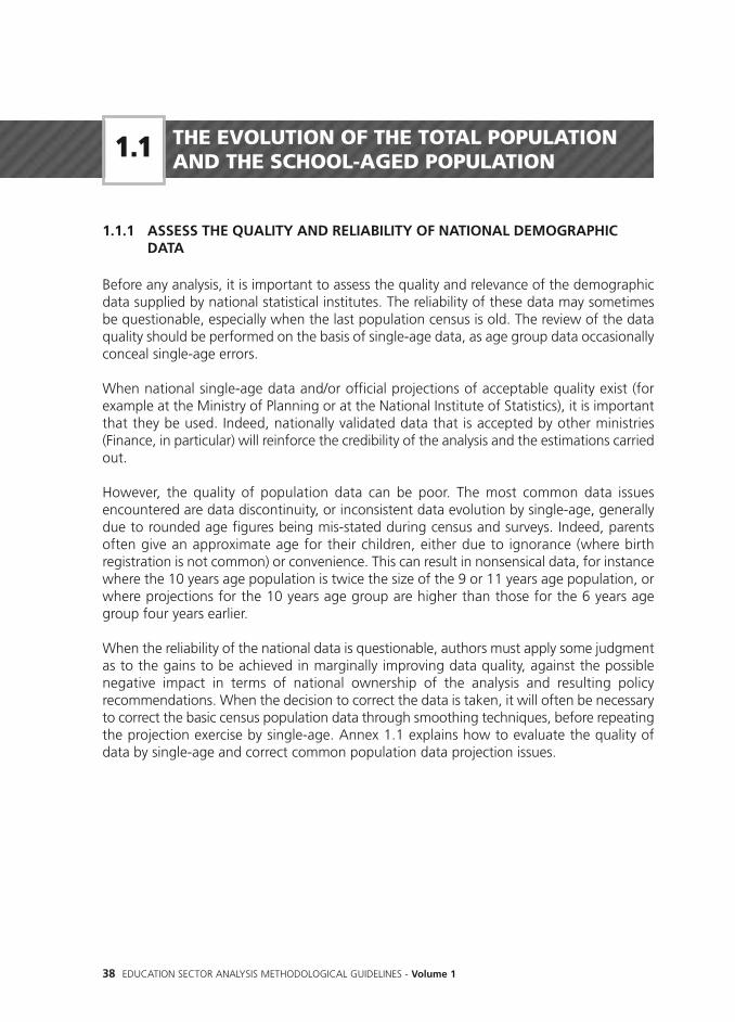
1.1.1 ASSESS THE QUALITY AND RELIABILITY OF NATIONAL DEMOGRAPHICDATA
Before any analysis, it is important to assess the quality and relevance of the demographicdata supplied by national statistical institutes. The reliability of these data may sometimesbe questionable, especially when the last population census is old. The review of the dataquality should be performed on the basis of single-age data, as age group data occasionallyconceal single-age errors.
When national single-age data and/or official projections of acceptable quality exist (forexample at the Ministry of Planning or at the National Institute of Statistics), it is importantthat they be used. Indeed, nationally validated data that is accepted by other ministries(Finance, in particular) will reinforce the credibility of the analysis and the estimations carriedout.
However, the quality of population data can be poor. The most common data issuesencountered are data discontinuity, or inconsistent data evolution by single-age, generallydue to rounded age figures being mis-stated during census and surveys. Indeed, parentsoften give an approximate age for their children, either due to ignorance (where birthregistration is not common) or convenience. This can result in nonsensical data, for instancewhere the 10 years age population is twice the size of the 9 or 11 years age population, orwhere projections for the 10 years age group are higher than those for the 6 years agegroup four years earlier.
When the reliability of the national data is questionable, authors must apply some judgmentas to the gains to be achieved in marginally improving data quality, against the possiblenegative impact in terms of national ownership of the analysis and resulting policyrecommendations. When the decision to correct the data is taken, it will often be necessaryto correct the basic census population data through smoothing techniques, before repeatingthe projection exercise by single-age. Annex 1.1 explains how to evaluate the quality ofdata by single-age and correct common population data projection issues.
1.1

• Key Definition
Sector-Wide Analysis, with Emphasis on Primary and Secondary Education 39
1.1.2 COMPUTING POPULATION GROWTH RATES
The analysis should describe the past trends in the evolution of the total population, as wellas those for the official age groups equivalent to each education cycle. Annual populationgrowth rates will be most appropriate.
1.1.3 COMPUTING THE SCHOOL DEMOGRAPHIC PSEUDO‐DEPENDENCY RATIO
The value, evolution, and relative ranking of the school demographic pseudo-dependencyratio are further helpful indicators. The ratio varies considerably among countries, andreflects the demographic (and then economic pressure) on education supply and demand.The school demographic pseudo-dependency ratio (DPDR) is the share of the school-agedpopulation relative to the total population:
The ratio can be interpreted through two complementary approaches: (i) the proportion ofthe population in need of education services, as indicated by the ratio itself, and (ii) theproportion of the population potentially contributing to finance the education system(because they are active), either directly or through taxes, as indicated by the complementaryshare of the population (1 - DDR, see section 1.1.4). Countries with greater shares of school-aged children have proportionately lower shares of active adults.
Example 1.1 below, drawn from the Côte d’Ivoire CSR, 2010, illustrates the analysis ofcorrected and smoothed population single-age data. The age groups used are the officialschooling ages for each education level (preschool, primary, lower secondary and upper
The average annual growth rate of a given population between years X and Y isobtained through the following formula (See Annex 1.2 for further details):
Therefore, where the period of interest is 2000 to 2010, the average annual growth rate is:
See Annex 1.2 for more details on the way to compute average annual growth rate.
Official school ages should be used for the school-aged population.
DPDR =School - Aged Population
Total Population
- 1
110Population2010
Population2000( )
- 1
1Y-XPopulationY
PopulationX( )
• Key Definition
CON
TEXT OF THE DEVELO
PMEN
T OF THE EDUCATIO
N SECTO
RCH
APTER 1

EXAMPLE 1.1
40 EDUCATION SECTOR ANALYSIS METHODOLOGICAL GUIDELINES - Volume 1
secondary). The analysis clearly underlines the evolution of the population between the twocensus years and projected evolutions, including those for the future school-agedpopulation.
(Demographic Context): The Demographic Context of Côte d’Ivoire, 2010Source: Quoted and translated from Côte d’Ivoire CSR, 2010.
TABLE 1.1 - Evolution of the Total and School-Aged Populations (Thousand), Côte d’Ivoire, 1988-2020
Age-group
3-5
6-11
12-15
16-18
Total Population
Male
-
905.8
443.4
323.2
5,527.3
Female
-
951
467
285.7
5,288.4
1988 Census
Total
-
1,856.8
910.4
609
10,815.7
Male
752.6
1,343.6
774.1
507.2
7,844.7
Female
712.2
1,259.9
746
532.1
7,522
1998 Census
Total
1,464.8
2,603.5
1,520.1
1,039.3
15,366.7
Male
817.6
1,443.6
893.9
619.4
10,024
Female
820.3
1,423.7
845
582.5
9,633.8
2006 Projection
Total
1,637.9
2,867.3
1 739
1,201.9
19,657.7
Male
1,245.9
2,125.6
1,187.2
787.4
14,348.6
Female
1,231.5
2,113.8
1,188
790.5
13,900.7
2020 Projection
Total
2,477.5
4,239.4
2,375.2
1,577.9
28,249.3
Côte d’Ivoire carried out general population and housing censuses in 1988 and 1998. Table 1.1provides the main evolutions made apparent by the two censuses, as well as projections for 2006(used as the reference year for the CSR) and 2020 (used as the mid‐term horizon for prospectiveanalysis).
FindingsOver the 1988-98 inter-census period, the total resident population grew from 10,815,694 to15,366,672 inhabitants, equivalent to an annual average growth rate of 3.6 percent. This rateconsolidates both the natural growth of the 1988 resident population and the return fromabroad of part of the positive migratory balance that characterised the 1988-98 period, estimatedat 1.2 million people. Thus the natural population growth rate is effectively 2.7 percent per yearover the period.
The projections of the total population are based on an annual growth of 3.1 percent between1998 and 2006, and 2.6 percent between 2006 and 2020, given the demographic transitionunderway and minor immigration. On this basis, the national population would reach 19.7million by 2006 and 28.2 million by 2020.
The population of primary school age (6 to 11 years) increased from 1,856,838 in 1988 to2,603,500 in 1998, implying an annual average growth rate of 3.4 percent. This is slightly lowerthan the growth of the total population, suggesting that the country had already started aprocess of demographic transition in the 1990s.3 The post-1998 projections (both the nationalstatistics and United Nations figures) incorporate this transition process into their estimations.This implies that the future growth rate of the young population will be lower than between1988 and 1998. The young population is expected to grow by 2.4 percent over the 1998-2020period, against 3.4 percent for the 1988-98 period.

• Key Definition
Sector-Wide Analysis, with Emphasis on Primary and Secondary Education 41
1.1.4 COMPUTING THE DEMOGRAPHIC DEPENDENCY RATIO
The previous indicator is in fact an adaptation of a common indicator in demography andeconomy: the demographic dependency ratio. This indicator can also be usefully analysed,as it provides information not only on the weight of the school age population, but also onthe demographic and economic pressure of all the non-working population (children andelderly) compared to the active, or productive, population – the one which contributes tonational wealth and revenues of the state.
Overall, even if the demographic constraint will remain significant in the immediate future (thenumber of youth aged 6 to 11 years is expected to reach 4.24 million in 2020, up 47 percentfrom 2.87 million in 2006), the figures reflect a gradual reduction of this age group’s growthrate.
The demographic pseudo-dependency ratio for the group of children aged 6 to 11 years iscomputed as 16.9 percent in 1998 (2,603.5 / 15,366.7); the ratio is expected to drop to just15.0 percent in 2020 (4,239.4/28,249.3). This implies a reduction in the relative weight of school-aged youth in the global population, and a concomitant increase in the active adult populationpotentially contributing to finance the education system, from 83.1 percent (1–0.169) to 85.0percent (1–0.150).
The demographic dependency ratio is the number of children, youth and elderly (thedependents) as a percentage of the potentially active population:
Various conventions are used to define these ages: OECD for instance uses the age group 20-65 as the active population, while the younger and older age groups are the dependentpopulation. In contrast, the United Nations use the age group 15-65 for the productivepopulation. In any case, if historical or geographic comparisons are done, caution should exerciseto ensure that the same definitions are used.
DDR =Dependent Population (children and elderly)
Active Population
CON
TEXT OF THE DEVELO
PMEN
T OF THE EDUCATIO
N SECTO
RCH
APTER 1

42 EDUCATION SECTOR ANALYSIS METHODOLOGICAL GUIDELINES - Volume 1
BASIC SOCIAL INDICATORS
In order to describe the social development context of a country, its evolution, and to placeit in international perspective, comparing it to other countries with similar levels ofdevelopment, the most relevant and commonly available indicators are:
• The share of the population living below the poverty line.This population group is the most financially and socially vulnerable. It is typically thepopulation group with least access to education services also, due to: (i) direct (schoolfees, school supplies) and indirect (uniforms, transport) costs; (ii) opportunity costs(foregone earnings associated with time spent at school instead of working); and (iii)poverty-related vulnerability (illness resulting from the lack of access to health services,wounds resulting from labor). When conducting international comparisons, the povertyline established by the United Nations is preferable to the national threshold, althoughthis can also be used. The Gini coefficient may also be used to illustrate the inequality inthe distribution of national wealth (See Chapter 6 for an explanation of its computationand use);
• The share of the urban population.It is generally easier to provide education services in urban areas, given their higherpopulation density, than to scarcely populated villages in rural areas. Children living inurban areas are also more exposed to cultural and educational events, and to writtenmaterial (books, newspapers, advertising, and so on), which favors both literacy andschool results;
• The demographic density rate.Population density is of particular interest and relevance given its direct impact oneducation logistics. Lightly populated areas are more difficult to provide education servicesto, given the relatively high cost for the system to provide infrastructure and staff for smallgroups, and/or the need for children to cover great distances to reach the nearest school.The lightly populated areas may also need different teaching approaches, such asmultigrade teaching/multigrade classrooms. Regional variations are particularly worthy ofanalysis;
• The adult literacy rate.The literacy rate of individuals aged over 15 years reflects not only the past achievementsof an education system (in terms of the number of people educated and the quality ofthe education received), but also the socioeconomic context in which children are raised.Research has demonstrated that the children of literate parents are more likely to beenrolled in school, and achieve better learning outcomes;
1.2

Sector-Wide Analysis, with Emphasis on Primary and Secondary Education 43
• The malnutrition rate and the infant mortality rate.These two indicators are used to reflect children’s living conditions, and especially theirsociofinancial vulnerability and their access to health services. The malnutrition rate is alsooften used as an indirect indicator of children’s well-being. At the individual level, it hasoften been demonstrated that malnutrition is a major cause of pupil absenteeism andattention deficit in class;
• The prevalence of disabilities.Disabilities among the population have various kinds of impact on the education system,and their importance is often all the more present in countries that are or have beenaffected by conflict, and/or have health systems that are weak and sometimes allow minordiseases or impairments to turn into lasting and debilitating conditions. The prevalenceof disabilities among the general population informs on the importance of a portion ofthe population that is economically vulnerable and often socially marginalised. In addition,the prevalence of disabilities among the school aged population is an important factorfor the access, learning, and progression of students in the education system. As muchas possible, the data should be disaggregated by gender and types of disabilities. Sourcesfor disability statistics include national data (such as the census, population surveys andadministrative data registries), as well as international data sets and a large number ofrecent studies.4
• HIV/AIDS and malaria adult prevalence rates.The HIV/AIDS pandemic and malaria affect education systems in different ways. Oneimportant aspect is the potential number of orphans, as vulnerable children are oftenmarginalized and less likely to enroll. Another is the number of teaching staff that requirereplacing, temporarily or permanently. When the prevalence rates are high, especially thatof HIV/AIDS, education sector analysts may dedicate a section of Chapter 1 to theirpotential impact on education (See Section 1.3 ahead); and
• The human development index (HDI).The HDI, calculated yearly by UNDP, synthesises three dimensions of human development:(i) life expectancy, measured at birth; (ii) the level of education, measured by the averagelength of schooling received by adults aged over 25 years and the expected schoolingcareers for school-aged children; and (iii) living standards, measured by the logarithm ofgross income per capita, in purchasing power of parity. The index, whose value rangesbetween 0 and 1, generally provides a country’s international ranking. It is thereforehelpful to identify countries of similar HDI levels that can then be used to carry outinternational comparisons throughout the report.
CON
TEXT OF THE DEVELO
PMEN
T OF THE EDUCATIO
N SECTO
RCH
APTER 1

EXAMPLE 1.2
44 EDUCATION SECTOR ANALYSIS METHODOLOGICAL GUIDELINES - Volume 1
(Social Context):Social Context of Malawi, 2010Source: Quoted from Malawi CSR, 2010.
Poverty and Inequality.According to the UNDP development report (2007/08), 63 percent of the Malawian populationis living below the US$2 a day income poverty line and 21 percent below the US$1 a day povertyline. Nevertheless, those percentages are lower than the SADC average (69 percent and 41percent, respectively).
The Gini index (39 in Malawi) indicates significant inequalities in access to resources, services,and opportunities among Malawians. There is a large discrepancy between the average per capitaincome of the richest and the poorest sections of the population. The richest 10 percent ofMalawi’s population have an average per capita income that is 11 times higher than the averageper capita income of the poorest 10 percent. Nevertheless, when compared to other SADCcountries, Malawi appears as one of the least unequal countries. The SADC average of the Giniindex stands at 52.
Malnutrition and the Child Mortality Rate.Malnutrition in Malawi is extensive and a major social development challenge. The prevalenceof malnutrition is estimated to be 49 percent. Dietary diversity and the average amount of caloriesconsumed daily are low across the country (for instance, rural people eat mainly maize).Nationally in 2008, 44 percent of preschoolers were stunted (with 18 percent being severelystunted). These figures have remained more or less constant over the past 15 years. Malawi hasthe highest malnutrition in the SADC region (the SADC average is 33 percent). Malawi’s mortalityrate for children below the age of five is 122 children per every 1,000, which is close to theSADC average of 131.
Adult Literacy Rates.When parents are more literate, they are more likely to enroll their children in school. The adultliteracy rate is clearly a context factor for school demand and it is noteworthy to compare Malawito other countries in that regard. The adult (meaning 15 years and older) literacy rate in Malawiis estimated to be 69 percent, which is better than the African average (62.9 percent) but lowerthan the SADC countries’ average (75.3 percent).
Urbanization Rate. The percentage of people living in an urban setting is also an important context indicator becausethe demand for education is higher in urban areas than in rural ones and it’s easier to delivereducation services in urban areas (for instance because it’s easier to allocate teachers in urbanareas). Malawi however, has a very low urbanization rate with only 17.7 percent of thepopulation living in cities. This proportion is much lower than both the African average (37.9percent) and the SADC countries’ average (35.9 percent).

Sector-Wide Analysis, with Emphasis on Primary and Secondary Education 45
Household surveys, especially MICS and DHS, are often the best sources for many of theseindicators. When data permits, it is appropriate to present a historical perspective of theindicators for the country of study before providing international comparisons.
Example 1.2, drawn from the Malawi CSR, 2010, presents a selection of the indicatorsmentioned above. For each, the text explains the relevance of the chosen indicator, its recentevolution where available, and its level compared to the continent or subregion.
IMPACT OF HIV/AIDS ON EDUCATION
Given the importance of their impact on education supply and demand, quality andmanagement, the specific analysis of HIV/AIDS may be required when the prevalence ratesare high.
HIV/AIDS can have a considerable negative impact on demand for education, in severalways: (i) children who are ill, through birth or blood transfusion for instance, are temporarilyor permanently unable to attend school because of their condition. The stigma related tothe illness also provides disincentives to enrolment; and (ii) the vulnerability of householdswith an affected adult is more acute, especially if the adult is a bread-winner, making theenrolment of children less likely as a result of the financial constraint faced, the need forthe child to care for the affected adult or the need for the child to help with householdchores or productive work. Any and all of the above may have a long-term impact on thestructure of education demand, slowing or delaying expected enrolment growth, andrequiring specific remedial policies.
HIV/AIDS can also have an impact on the supply of education services, as a result of thehigh rate of illness-related absenteeism or death, among teachers, qualified and experiencededucation inspectors, and administrative staff.
1.3
CON
TEXT OF THE DEVELO
PMEN
T OF THE EDUCATIO
N SECTO
RCH
APTER 1

46 EDUCATION SECTOR ANALYSIS METHODOLOGICAL GUIDELINES - Volume 1
How is the impact of HIV/AIDS on education evaluated?To evaluate the impact of HIV/AIDS, the following questions may be answered:
• What is the number of children orphaned by HIV/AIDS? Are their enrolment rates belowthose of other children? and
• What is the impact of HIV/AIDS on children’s absenteeism, drop-out, repetition, andcompletion, by education level? To establish this, authors may compare the indicatorsfor affected children with those of a control group.
• Are teachers affected more than the rest of the population?• What is the impact of HIV/AIDS on teachers’ absenteeism?• What is the impact of the illnesses on the recruitment needs for new and replacement
teachers? and• Would it be helpful to include illness among the job allocation criteria, to facilitate ill
teachers’ access to health centres?
The availability of specific national epidemiological surveys will be particularly helpful inproviding the data required to respond to these questions. Should the detailed informationnot be available, the following steps can be taken:
• On the basis of UNAIDS data on the number of children aged under 17 years orphanedby HIV/AIDS, estimate the number of school-aged orphans, for both the primary andlower secondary cycles; and
• On the basis of UNAIDS past trends in the number of orphans and the probableevolution of the illness, project the number of school-aged orphans for future years.
• In the absence of data on the prevalence rates among national teaching staff, the usualapproach consists in assuming that teachers are affected by the illnesses in equalproportions as the population aged over 15 years, ideally the sub-population of thoseadults who have reached secondary school at least. Indeed, it is known that educationchanges social behaviour and attitudes; as all teachers are educated, this groupconstitutes the best proxy basis for projections.
Example 1.3 below, drawn from the Congo CSR, 2010 presents the overall national situationof the pandemic and regional disparities, before describing the levels of illness-relatedorphanhood and the impact on the teaching staff and resulting recruitment requirements.

EXAMPLE 1.3
Sector-Wide Analysis, with Emphasis on Primary and Secondary Education 47
(HIV/AIDS Impact):The Impact of HIV/AIDS on Education, Congo, 2007Source: Quoted and translated from Congo CSR, 2010.
In its report on the status of the AIDS pandemic of December 2005, UNAIDS estimated that atleast 110,000 Congolese live with AIDS. About 80,000 adults aged 15 to 49 years areseropositive or ill from AIDS, implying a prevalence rate of 4.9 percent. The number of AIDS-related deaths in 2003, including both adults and children, was estimated at 9,700. In 2004,according to the Congolese health ministry, the national AIDS prevalence average concealsconsiderable regional disparities, ranging from 1.0 percent in the Likouala and Plateauxdepartments, 3.3 percent in Brazzaville, to 10 percent in the Sibiti department of Lekoumou.
HIV/AIDS affects the education system through both school-aged children and the teaching staff.The death of parents of children of primary school age increases the number of orphans, makingtheir enrolment comparatively more difficult. Indeed, the difference in the likelihood of enrolmentfor children whose parents are both alive and those whose parents are not is 10 percentagepoints. Overall, as a result of the AIDS pandemic, but also (in fact mainly) due to the unrest thatoccurred in the 1990s, 15 to 16 percent of school-aged children are orphans, amounting to85,000 school-aged children in total, 20,000 of which have been orphaned by HIV/AIDS.
In the near future the number of orphans is expected to drop under the combined effect of: (i)a considerable reduction in the mortality of fathers due to non-AIDS causes (currently 65,000);and (ii) a likely stabilisation in the number of children orphaned by HIV/AIDS (estimated to be40,000 in 2015).
In terms of teaching staff, the prevalence of HIV/AIDS is comparable to the rate for the adultpopulation, of 4.9 percent. Thus, approximately 250 primary teachers are likely to be affected.Projections are not easy to perform, either for the overall population or for teachers in particular,as they depend on changes in individual behaviour and on progress made in making medicaltreatment available. The information available on the patterns of evolution of the illness suggestsdifferences according to Sub-Saharan African regions. In applying the average evolution patternof the illness for central African countries, the prevalence of HIV/AIDS could reach eight to ninepercent by 2015.
On this basis, and assuming that Congo reaches universal primary completion by 2015 andfollows the indicative framework of the Fast Track Initiative (pupil-teacher ratio of 40:1), thenumber of seropositive teachers could reach 1,650 in 2015, of the then projected total of 18,000.The empirical information available suggests that about 180 teachers will need replacing everyyear because of the illness, and that about the same number will die. It would therefore beappropriate to plan for teachers to replace those still practicing, and to increase the number ofteachers undergoing training to compensate for the consequences of HIV/AIDS on the teachingstaff.
CON
TEXT OF THE DEVELO
PMEN
T OF THE EDUCATIO
N SECTO
RCH
APTER 1

48 EDUCATION SECTOR ANALYSIS METHODOLOGICAL GUIDELINES - Volume 1
THE COMPOSITE SOCIAL CONTEXT INDEX
The international comparison of a country’s overall social context can be made more directby the computation of a synthetic composite index of the main social indicators. This indexdeveloped by the Africa Region of the World Bank includes the demographic dependencyrate, child malnutrition, infant mortality, HIV/AIDS prevalence, adult literacy, and the rate ofurbanization (Annex 1.4 explains the calculation methodology).
The index has been specifically built on the basis of the selected variables given theirdemonstrated impact on education systems.5 Table 1.2 presents the index for the EconomicCommunity of West African States (ECOWAS) countries.
Source: World Bank Africa Region database, 2011.
1.4
TABLE 1.2 - Composite Social Context Index, ECOWAS Countries, 2010 or MRY
Benin
Burkina Faso
Cape Verde
Côte d'Ivoire
Gambia, The
Ghana
Guinea
Guinea-Bissau
Liberia
Mali
Niger
Nigeria
Senegal
Sierra Leone
Togo
ECOWAS Countries’ Average
Sub-Saharan African Countries’ Average
Composite Indexof Social ContextECOWAS Country
44.0
37.7
64.5
41.1
50.6
57.9
43.2
45.3
48.3
37.7
33.1
46.7
47.8
40.7
48.1
45.8
50

Sector-Wide Analysis, with Emphasis on Primary and Secondary Education 49
LINGUISTIC CONTEXT
The use of languages is of considerable importance to education, both in terms of supplyand demand, and on a policy level, especially where various official languages exist or variousdialects are spoken. In such countries, a teaching language (or various) must be chosen,where each option offers both opportunities and challenges. To offer education in a singlelanguage that is not the main language of communication of a large proportion of thepopulation is likely to create an additional factor of discrimination in education, potentiallyto the point of exclusion.
Studies of learning outcomes have demonstrated that when children are taught in theirmother tongue, they are quicker to learn, achieve better results in school, and pursue theireducation for longer. On the other hand, offering education in local languages, even if onlyfor the first years of primary, faces several practical challenges. In each chosen language,teaching materials must be produced and teachers must be trained; teacher allocationprocesses must contemplate linguistic ability for specific areas. Finally, the choice may becomplicated by more than one local language being spoken in a given area.
Education sector analysts are therefore invited in this section to:
• Identify the official national language(s), the teaching language(s), and the localdialect(s). Where appropriate, it will be helpful to identify any lingua francas or vehicularlanguages, even if not official, in as much as they federate considerable sections of thepopulation;
• Analyse the share of the population that master the official or teaching language(s),and the share for whom it is the mother tongue. Given that a population's linguisticcharacteristics are very slow to change, the study of a historical perspective of languageuse is superfluous. On the other hand, to offer a regional perspective of language usewill be important; and
• Describe the share of the population that uses the most common language, be it theofficial language or the lingua franca (such as Wolof in Senegal or Sango in the CentralAfrican Republic). This indicator is a useful measure of linguistic uniformity, be it at theregional, departmental, or local level; as such, it provides a general sense of the feasibilityof teaching in a local language.
The information required for this section is generally available in population census orhousehold survey data.
1.5
CON
TEXT OF THE DEVELO
PMEN
T OF THE EDUCATIO
N SECTO
RCH
APTER 1

50 EDUCATION SECTOR ANALYSIS METHODOLOGICAL GUIDELINES - Volume 1
HUMANITARIAN CONTEXT
In countries facing recurring or sporadic humanitarian crises such as natural disasters (floods,drought, earthquakes, volcanic eruptions, etc.), conflicts (armed, political, social or othertypes), or massive population displacement (refugees or internally displaced persons), it isrelevant to analyse the impact of such disasters and conflict on school supply and demandas well as the potential contributions of the education system to conflict mitigation. Indeed,disasters and conflicts can shatter education gains, jeopardise years of investment in theeducation sector, and drastically slow down progress towards set objectives. It is alsoacknowledged that education is not neutral in the face of conflicts that affect the societyat large. Therefore, it is crucial to better understand the relationship between educationand conflict.
This section can describe the main humanitarian risks facing a country, together with theirpotential or actual impact on the education system and the capacity of the country tomanage crises including within the education system itself (vulnerability analysis). In addition,conflict drivers will be analysed - be they relating to political, economic, social or securityfactors. The extent to which the education sector is influenced by these dynamics or iscontributing to them will also be described (conflict analysis).
The recommended method is to build upon the findings of the most recent conflict andvulnerability analyses of the education sector. When relevant, these analyses may feed intoa specific chapter, in particular in high humanitarian risk and post-crisis contexts.
1.6

Sector-Wide Analysis, with Emphasis on Primary and Secondary Education 51
THE MACROECONOMIC AND PUBLIC FINANCECONTEXTS
In addition to the demographic constraint that sets the education needs to be satisfied, thedevelopment of a school system is also framed by national and international fundingopportunities. National funding depends on two variables that do not flow directly fromeducation policy: (i) the level of wealth of a country, measured by the gross domestic product(GDP); and (ii) the state’s capacity to mobilise a share of those resources (through taxes orother public levies), and the size of the share mobilised.
FIGURE 1.1 - Relation between GDP, Tax Income, External Resources, and Public Expenditure
EXTERNALRESOURCES
DOMESTICRESOURCES
RESOURCES
National Budget and Extrabudget. Resources
EXPENDITURE
DOMESTICRESOURCES EDUCATION
BUDGET
BUDGETEXPENDITURE
BudgetDeficit
GDPGDP
The analysis is therefore structured here, as illustrated by Figure 1.1, around the relationbetween national wealth, GDP, and domestic (tax and non-tax) and external resources onthe one hand, and public expenditure, and especially education expenditure, on the other.The detailed analysis of the education budget is dealt with in Chapter 3. Note that Figure1.1 shows the situation of a budget deficit (when national budget expenditures are greaterthan the resources), which is found in most cases; it is however possible to be in a situationof budget surplus (resources are greater than expenditures).
SECTION
2
CON
TEXT OF THE DEVELO
PMEN
T OF THE EDUCATIO
N SECTO
RCH
APTER 1

• Key Definitions
52 EDUCATION SECTOR ANALYSIS METHODOLOGICAL GUIDELINES - Volume 1
GDP AND GDP PER CAPITA TRENDS
The analysis of the evolution of macroeconomic aggregate indicators such as GDP isimportant to understand a country’s overall level of wealth and development. The state’scapacity to levy a share of national wealth for the operation of public services is also crucial,to identify the additional resource mobilisation opportunities for public services in general,and education in particular.
Typically, education sector analysts will present GDP and GDP per capita trends in a tableand comment on them, both in current and constant prices. Current price information isappropriate to explain the present situation and the breakdown of GDP; constant pricesmust be used on the other hand for the analysis of historical trends. This enables correctingfor inflation and making different time-series data comparable.
To convert current prices into constant prices, a GDP deflator (also known as the ConsumerPrice Index) is used, which can generally be found on the World Bank or IMF websites whenit is not available locally (See Annex 1.3 for further detail on the calculation of the GDPdeflator when it is not available). As much as possible, the same source should be used forthe deflator, the constant prices and the current prices GDP figures.
GDP is defined as the total value of the wealth produced in the course of a year by the economicactors (state, private sector and civil society) residing within the national territory. As such, it is ameasure of national wealth. It is generally computed by the ministry of economy, or by thenational statistics institute in charge of national accounts, and is also estimated by the WorldBank and the IMF.
GDP per capita is an indicator of individual wealth, measuring the average wealth byinhabitant, and thus illustrating general living standards:
GPD per capita =GPD
Total Population
2.1

EXAMPLE 1.4(Macroeconomic Context):Macroeconomic Context, Mali, 2010Source: Quoted and translated from Mali CSR, 2010.
Sector-Wide Analysis, with Emphasis on Primary and Secondary Education 53
TABLE 1.3 - GDP and GDP per capita Trends, Mali, 1995-2008
GDP (Billions of FCFA)
In Current Prices
GDP Deflator (Ref. 100 in 2008)
In Constant Prices (2008)
Real GDP Growth Rate
Population (Millions)
GDP per capita (Thousands of FCFA)
In current prices
In constant prices (2008)
1995
1,231
1.53
1,889
6.2
9.6
127,963
196,413
2000
1,725
1.41
2,431
3.2
10.8
159,105
224,285
2005
2,894
1.16
3,350
6.1
12.2
237,086
274,445
2006
3,201
1.10
3,526
5.3
12.6
254,574
280,359
2007
3,425
1.07
3,677
4.3
13.0
264,303
283,809
2008
3,921
1.00
3,921
6.6
13.3
293,720
293,720
Annual AverageGDP Growth
9.3%
5.8%
2.5%
6.6%
3.1%
FindingsIncome per capita has improved very little, given sustained demographic growth. Between 1995and 2008, Mali’s GDP increased by a factor of three in current prices, from FCFA 1,231 billion toFCFA 3,921 billion, equivalent to average annual growth in current prices of 9.3 percent. Realgrowth, adjusted for inflation (i.e., in constant prices), is considerably more modest, althoughnevertheless worthy of note, at 5.8 percent per year, from FCFA 1,889 billion to FCFA 3,921billion over the period.
Furthermore, even if GDP per capita improved between 1995 and 2008, its progression has beenslower than that of GDP given the sustained demographic growth that the country has witnessedover the period. In 2008 constant prices, the annual average growth rate of GDP per capita forthe 1995-2008 period was 3.1 percent, meaning that GDP per capita increased from FCFA196,413 to FCFA 293,720.
CON
TEXT OF THE DEVELO
PMEN
T OF THE EDUCATIO
N SECTO
RCH
APTER 1

54 EDUCATION SECTOR ANALYSIS METHODOLOGICAL GUIDELINES - Volume 1
PUBLIC RESOURCES
Public resources are obtained from two sources: domestic resources and external funding:
• Domestic resourcesDomestic resources are obtained mainly from levies (duties and taxes) applied by the stateto the creation of national wealth. The share of these levies to GDP is referred to as thetax burden (which refers to direct and indirect tax income and compulsory levies, and thenon-tax burden (which includes other resources such as income from state heritage andbusiness, industrial, and financial interests, fines and betting). Taxes generally representthe greatest part of income, except where the state is a shareholder in natural resourceexploitation companies, such as mining or oil. The level of a state’s income thereforedepends mainly on the ability to raise taxes, which is often weak in countries withconsiderable informal economies.
• External ResourcesResources from international aid, also called official development assistance (ODA), arethe main source of external resources. This aid can include loans or grants, under theshape of global budget support (when the funds offered are completely fungible withnational resources), sector budget support (to assist with the development of a particularsector, either through recurrent or capital expenditure), or project funds.
Example 1.5 below illustrates the situation of Mauritania’s public resources, and places it inregional context, showing the great variations that can exist, even between countries ofsimilar levels of economic development. As above, data is offered in both current andconstant prices, to enable historical analysis.
Domestic resources often represent the vast majority of resources available to the state. Ithappens however that, in countries with difficult economic and/or fiscal situations, verylarge amounts of external aid are needed to help the government run its programs. Whenthese represent a large proportion of the resources available, there is a risk of dependencyon external aid, especially when this aid is used to run recurrent budgets. While the aiditself is often crucial to the functioning of the public sector, this places the state in avulnerable situation because of the inherent high volatility of aid and the lack of controlover a large part of the budget. It can thus be useful to review the level of aid dependencyand its evolution, in order to inform on the robustness of the budget.
2.2

EXAMPLE 1.5(Public Resources):Mauritania’s Public Resources, 2010Source: Quoted and translated from Mauritania CSR, 2010.
• Key Definition
Sector-Wide Analysis, with Emphasis on Primary and Secondary Education 55
The external aid dependency rate is, for a given budget year, the amount of external aidexpressed as a percentage of the total budget resources (domestic resources and external aid):
Aid dependency rate = External Aid
Total budget resources
FIGURE 1.2 - International Comparison of Domestic Public Resources, Countries whose GDP percapita is between US$500 and US$1,500, 2007 or MRY
60.0
50.0
40.0
30.0
20.0
10.0
0.0
Average of 18 Countries: 22.6%
Burk
ina
Faso
(200
8)
Com
oros
(200
6)
Tanz
ania
(200
8)
Mal
i (20
08)
Togo
(200
7)
Beni
n (2
007)
Sao
Tom
e-et
-Prin
cipe
Zam
bia
(200
7)
Cam
eroo
n (2
007)
Côte
d'Iv
oire
(200
8)
Sene
gal (
2006
)
Keny
a (2
004)
Chad
(200
7)
Mau
rita
nia
(200
8)
Gha
na (2
007)
Djib
outi
(200
7)
Nig
eria
(200
6)
Leso
tho
(200
6)
Publ
ic D
omes
tic
capita is between US$500 and US$1,500,
60.0
International Comparison of Domestic Public ResourcesFIGURE 1.2 - 2007 or MRcapita is between US$500 and US$1,500,
International Comparison of Domestic Public Resources Y 2007 or MR
Countries whose GDP per,International Comparison of Domestic Public Resources
0.0
10.0
20.0
30.0
40.0
50.0
60.0
Publ
ic D
omes
tic
Mal
i (20
08)
anza
nia
(200
8)TTaCo
mor
os (2
006)
aso
(200
8)Bu
rkin
a F
Se
nega
l (20
06)
ôte
d'Iv
oire
(200
8)
Cam
eroo
n (2
007)
Zam
bia
(200
7)
ome-
et-P
rincip
eSa
o T
Beni
n (2
007)
ogo
(200
7)T
verage of 18 Countries: 22.6%A
Leso
tho
(200
6)
Nig
eria
(200
6)
Djib
outi
(200
7)
Gha
na (2
007)
Mau
rita
nia
(200
8)
Chad
(200
7)
a (2
004)
eny
K
Burk
ina
F
ôt
e d'
Ivoi
re (2
008)
C
Cam
eroo
n (2
007)
Sao
T
Mau
rita
nia
(200
8)
FindingsThe share of domestic resources collected by the state (tax and non-tax burdens) has increasedover the 1995-2008 period. After a considerable rise between 1995 and 2006, from 19.7 percentof GDP to 29.5 percent of GDP, it has dropped slightly since, reaching 25.6 percent of GDP in2008. When compared with African countries with similar national wealth (whose GDP per capitais similar to Mauritania’s, at about US$1,090), domestic public resources vary from 13.6 percentof GDP in Burkina Faso to 50.8 percent of GDP in Lesotho. The average of the 18 countries is22.6 percent, indicating that Mauritania is above the average. The rise of GDP over the periodand the increase of the share of it levied by the state have improved the level of domestic publicresources: (i) in nominal terms, from UM 33.9 billion in 1995 to UM 258.5 billion in 2008; (ii) inreal terms (2008 constant prices), from UM 118.1 billion in 1995 to UM 258.5 billion in 2008,more than double.
CON
TEXT OF THE DEVELO
PMEN
T OF THE EDUCATIO
N SECTO
RCH
APTER 1

56 EDUCATION SECTOR ANALYSIS METHODOLOGICAL GUIDELINES - Volume 1
TABLE 1.4 - The Evolution of Public Resources, Mauritania, 1995-2008
Public Resources (Billions of UM)
Share of GDP (%)
In Constant 2008 UM (Billions)
Domestic Resources (Billions of UM)
Share of GDP (%)
In Constant 2008 UM (Billions)
Per capita (Constant 2008 UM)
External Resources (Billions of UM)
Share of GDP (%)
In Constant 2008 UM (Billions)
1995
33.9
21.4
118.1
31.1
19.7
108.4
47,456
2.8
1.8
9.7
2000
62.1
24.1
150.4
56.3
21.8
136.3
54,337
5.8
2.3
14.1
2005
131.3
26.6
202.7
121.0
24.5
186.8
64,293
10.3
2.1
15.9
2006
466.4
64.3
546.1
214.0
29.5
250.5
83,786
252.5
34.8
295.6
2007
204.3
27.8
238.7
188.0
25.6
219.6
71,417
16.3
2.2
19.0
2008
258.5
28.5
258.5
232.2
25.6
232.2
73,424
26.3
2.9
26.3
Average AnnualGrowth Rate
16.9%
6.2%
16.7%
6.0%
3.4%
18.8%
8.0%
Progress is however more modest when related to the total population. Domestic publicresources per capita, in 2008 constant prices, rose from UM 47,456 in 1995 to UM 73,424 in2008, equivalent to an increase by a factor of 1.5. The evolution over the 2003-08 period wasparticularly irregular, following a peak and trough pattern and reaching a maximum of UM83,786 per capita in 2006.
Table 1.4 also shows that the state has benefitted from considerable financial support in theform of grants, both to finance the budget deficit and specific investment projects (even if thedistinction between both types of funding is not always clear). Although these contributionshave increased overall during the 1995-2000 period, they have demonstrated a relative degreeof volatility, representing a minimum of 0.5 percent of GDP in 1997 and a maximum of 34.8percent of GDP in 2006, in a special political context where the democratic transition wassupported from abroad.
PUBLIC EXPENDITURE
The analysis of public expenditure should both describe the total budget envelope, from whicheducation expenditure is allocated, and observe the evolution of the budget deficit, whichindicates both the vulnerability and flexibility of public finance.
It is important in this analysis to isolate expenditure that is destined for debt repayments,including both domestic debt, due to national financial institutions, and external debt, due tointernational financial institutions, bilateral and multilateral development partners. Debt service
2.3

EXAMPLE 1.6(Public Expenditure and Deficit): Government Revenue, Expenditure and Deficit, The Gambia, 2011Source: Quoted from The Gambia CSR, 2011.
Sector-Wide Analysis, with Emphasis on Primary and Secondary Education 57
effectively reduces the amount of public resources available for domestic policy action.Countries with high levels of debt service are limited in their ability to provide social services,and education in particular.
This section may possibly be consolidated with the previous section, as per Example 1.6 below,drawn from The Gambia CSR, 2011. In this example, the authors chose to express all valuesas percentages of GDP, which avoids the use of the GDP deflator. Indeed, given that GDP andthe observed values (resources and expenditure) are all in the same unit of measurement (theprice of the given year), the percentages are comparable through time.
TABLE 1.5 - Total Government Revenue, Expenditure and Deficit (% of GDP), The Gambia, 2004-10
Revenue and Grants
Domestic Revenue
Grants
Budget Support
Project Grants
Government expenditure and net lending
Recurrent Expenditures
Discretionary expenditures
Interest
External
Domestic
Development Expenditure
External
Domestic
Net lending
Deficit Including grants
Deficit Excluding grants
2004
17.7
14.5
3.1
-
-
21.5
11.7
6.7
5.0
1.3
3.7
9.2
8.7
0.5
0.6
-3.9
-7.0
2005
15.6
14.4
1.2
-
-
21.8
13.3
7.1
6.2
1.3
4.9
8.0
7.4
0.6
0.5
-6.2
-7.4
2006
17.1
16.2
1.0
0.1
0.9
22.3
13.7
8.8
4.9
1.2
3.7
8.4
7.9
0.4
0.3
-5.2
-6.1
2007
17.8
16.9
0.9
0.1
0.8
17.7
12.6
8.7
3.9
1.1
2.8
4.7
3.8
0.9
0.4
0.1
-0.8
2008
16.2
15.2
1.0
0.3
0.7
18.0
13.9
10.8
3.1
0.6
2.5
3.7
2.2
1.5
0.4
-1.8
-2.8
2009
18.7
15.0
3.5
0.7
2.8
22.0
14.0
11.1
2.9
0.6
2.3
7.5
5.2
2.3
0.5
-3.5
-7.0
2010
17.2
13.6
3.7
0
3.7
22.8
13.9
11.3
2.6
0.5
2.2
8.2
6.2
2.1
0.6
-5.6
-9.2
*(% of GDP)
Government revenues including grants have shown a cyclical trend between 2004 and 2010,and decreased slightly over this period from 17.7 percent of GDP in 2004 to 17.2 percent in2010. On the other hand, domestic revenues excluding grants grew steadily between 2004 and2007 (from 14.5 percent of GDP to 16.9 percent) before experiencing a decline in 2008. In 2010,domestic revenues excluding grants represented 13.6 percent of GDP, below the ECOWASaverage estimated at 19.8 percent of GDP. External grants steadily declined between 2004 and2007 from 3.1 percent of GDP to 0.9 percent of GDP, before rising to 3.9 percent of GDP in2009 and dropping to 3.7 in 2010.
CON
TEXT OF THE DEVELO
PMEN
T OF THE EDUCATIO
N SECTO
RCH
APTER 1

58 EDUCATION SECTOR ANALYSIS METHODOLOGICAL GUIDELINES - Volume 1
As a result, expenditures have varied over time. From 21.5 percent of GDP in 2004, governmentexpenditures and net lending increased to 22.3 percent in 2006, and then declined to 17.7percent in 2007, before again increasing to 22.8 percent in 2010. The share of recurrentexpenditure has been more or less constant, and significant, fluctuating between 12 percentand 14 percent of GDP. Despite the 2007 debt relief package, debt interest (particularly that ofdomestic debt) continues to represent a high proportion of recurrent public expenditure,averaging 23 percent between 2007 and 2010 (for example in 2009, debt interest represented2.8/13.8 = 20.3% of the total recurrent expenditure).
Development expenditure is mostly supported by foreign contributions, through grants andloans. The total amount of foreign funding has represented 5 percent of GDP over the last fiveyears (an average of 76 percent of public capital expenditure over the last five years). Althoughthe fiscal deficit (excluding grants) was successfully reduced from 7.0 percent of GDP in 2004 tojust 0.8 percent in 2007 thanks to the debt relief package, it again increased to 9.2 percent ofGDP in 2010.
TABLE 1.6 - Composite Economic Context Index, CEMAC Countries, 2010 or MRY
Cameroun
Congo, Rep.
Gabon
Equatorial Guinea
Central African Republic
Chad
CEMAC Countries’ Average
Sub-Saharan African Average
Index
36.6
71.3
56.0
89.6
38.9
39.3
55.3
50.0
Country
Source: World Bank Africa Region database.
THE COMPOSITE ECONOMIC CONTEXT INDEX
Here again, a comparative international perspective of a country’s global level of economicdevelopment can be provided by the composite economic context index, a synthesis of themain macroeconomic indicators. This index, similar to the composite social context indexdiscussed earlier, has also been developed by the Africa Region of the World Bank. It includesGDP per capita, domestic resources as a share of GDP, real GDP growth, externaldevelopment aid for education and the share of pupils enrolled in private institutions (thebigger this share is, the less public financing is needed for education).
As for the composite social context index, the composite economic context index has beenspecifically built with the above variables given their demonstrated importance for education
2.4

Sector-Wide Analysis, with Emphasis on Primary and Secondary Education 59
THE COMPOSITE GLOBAL CONTEXT INDEX
A combination of both composite indexes mentioned above, social and economic, has alsobeen developed. This composite global context index can be used to summarise thesociodemographic and economic contexts as they apply to the education sector. The scoringsystem is similar to the other context indexes, with an average of 50 and a standarddeviation of 10. The global index can also be used to identify countries with similar contexts,which can then be used for relevant international comparisons when analyzing the resultsof education sector in following chapters. Table 1.7 above presents the composite globalcontext index for the SADC countries.
systems, and has been adjusted so that the average for Sub-Saharan Africa is 50, and thestandard deviation is 10. This facilitates its interpretation and cross-country comparisons.Again, a score below 50 indicates that a macroeconomic context is unfavorable,comparatively speaking.
Table 1.6 below displays the index for CEMAC countries.
2.5
TABLE 1.7 - Composite Global Context Index, SADC Countries, 2010 or MRY
South Africa
Angola
Botswana
Lesotho
Malawi
Maurice
Mozambique
Namibia
Congo, Dem. Rep. of
Seychelles
Swaziland
Tanzania
Zambia
Zimbabwe
SADC Countries’ Average
Sub-Saharan African Average
Index
66.3
52.7
61.7
52.0
46.6
77.3
49.9
58.8
47.9
69.7
50.4
53.6
47.1
44.6
55.6
50.0
Country
Source: World Bank Africa Region database.
CON
TEXT OF THE DEVELO
PMEN
T OF THE EDUCATIO
N SECTO
RCH
APTER 1

60 EDUCATION SECTOR ANALYSIS METHODOLOGICAL GUIDELINES - Volume 1
This section of the report may include a summary profile in its introduction or conclusion,with the main indicators analysed above. This profile will also be a useful quick-referencetool, and will help readers to understand the national context with ease. Table 1.8 offers anexample of a typical country socioeconomic profile. Education sector analysts will determinewhen best to delete, extend, modify or add sections in line with the importance of givenissues for the country under study.
TABLE 1.8 - Key Social and Economic Indicators, Liberia, 2010
CONTEXT SHEET
Sociodemographic Context
Total Population (’000s)
Primary School-Aged Population (’000s)
Demographic Dependency Ratio
Child Malnutrition Rate
Mortality Rate (‰)
HIV/AIDS Prevalence
Adult Literacy Rate
Urbanization Rate
Economic Context
GDP (Millions of constant 2009 US$)
GDP Growth Rate
GDP per capita (constant 2009 US$
Tax Burden (% of GDP)
2000
2,832
466
16%
22.8%
140
3.3%
52.0%
54.0%
2005
651
4.7%
209
15.6%
Global Context Index (Ranking: 24 out of 47)
Mauritius
…
Swaziland
Mozambique
Burundi
Eritrea
Liberia
Kenya
Togo
Democratic Republic of Congo
Uganda
…
South Sudan
ECOWAS Countries’ Average
Sub-Saharan African Countries’ Average
77.3
…
50.4
49.9
49.4
49.3
48.3
48.3
48.0
47.9
47.2
…
32.9
45.7
50.0
2010
4,115
667
16%
20.4%
117
1.5%
59.1%
61.5%
2009
874
5,0%
229
26.9%
Source: Authors’ calculations based on Liberia CSR, 2010 and World Bank data.

EXAMPLE 1.7(Public Resource and Expenditure Projection): Projected Government Resources and Expenditure, Mali, 2010Source: Quoted and translated from Mali CSR, 2010.
Sector-Wide Analysis, with Emphasis on Primary and Secondary Education 61
FUTURE PROSPECTS
Having documented trends over the previous decade, it is useful to speculate on futureperspectives. On the basis of macroeconomic data, future GDP, tax income, and domesticpublic resources can be estimated. This prospective analysis section can be distinct andseparate, or future perspectives can be incorporated into each of the relevant sectionsexamining past trends and the present context. This prospective work is often carried outwithin the elaboration of macroeconomic frameworks, by ministry of economy and finance.In the absence of such official projections, authors may make assumptions as to the stabilityor the evolution of the average annual growth rates considered above. In Example 1.7, theofficial projections developed by the Ministry of Economy and Finance of Mali and validatedby the council of ministers have been used. As stated earlier, the use of official data andstatistics is preferable, when they are available and reliable, to encourage ownership of theanalysis’ conclusions by the government and its partners.
2.6
TABLE 1.9 - Macro and Resource Forecasts for Recurrent Education Expenditure,Mali, 2009-12
GDP (Billions of FCFA)
Income (% of GDP)
Domestic resources, not including grants (Billions of FCFA)
Recurrent Public Expenditure, not including Debt Service (Billions of FCFA)
Recurrent Education Expenditure (% of Total Recurrent Expenditure)
Resources for Recurrent Education Expenditure (Billions of FCFA)
2008
3,912
15.5%
607.3
445.0
28.7%
127.7
2009
4,123
16.4%
701.0
541.5
29.0%
157.2
4,498
16.5%
738.3
573.9
29.3%
168.4
4,900
16.5%
777.3
608.2
29.7%
180.5
5,329
16.6%
819.1
664.4
30.0%
193.3
2010 2011 2012
Forecasts
The resources available for the education sector depend on the evolution of the globalmacroeconomic framework (GDP and government income) and on the share of public resourcesallocated to education. The estimations carried out here are based on the Ministry of Economyand Finance’s accounts for 2008 and 2009, as published in the 2008 report on the economicand social situation of Mali and its perspectives for 2009, and adopted by the council of ministerson July 15, 2009.
FindingsAccording to forecasts, public domestic resources (not including grants) would rise from 15.5percent of GDP in 2008 to 16.6 percent of GDP in 2012; recurrent public expenditure (notincluding debt service) would rise from 11 percent of GDP in 2008 to 13 percent of GDP in 2012.Domestic resources (not including grants) would thus increase from FCFA 607 billion in 2008 to
CON
TEXT OF THE DEVELO
PMEN
T OF THE EDUCATIO
N SECTO
RCH
APTER 1

62 EDUCATION SECTOR ANALYSIS METHODOLOGICAL GUIDELINES - Volume 1
FCFA 819 billion in 2012, and recurrent public expenditure (not including debt service) wouldincrease from FCFA 445 billion in 2008 to FCFA 664 billion in 2012.
It is helpful to indicate that all of these public resources depend on GDP growth, and that if it isweaker than expected, then fewer resources may be mobilised for public expenditure. In 2008,recurrent education expenditure represented 28.7 percent of total recurrent expenditure, notincluding debt service.
Given that budget allocations are cabinet policy decisions, various hypotheses can becontemplated for their evolution over the coming years. The government’s known ambition isthat recurrent education expenditure reaches 30 percent of total recurrent expenditure by 2012.If education continues to be a government priority, the state could be assumed to graduallyincrease the share of public recurrent resources allocated to education over the coming years toreach 30 percent; in the worst case scenario, the share would be assumed to remain constantat its 2008 level. On the basis of these assumptions, the resources likely to be mobilised forrecurrent education expenditure could be around FCFA 193 billion (30 percent) by 2012.
In addition to these estimated amounts, further resources may be mobilised for the educationsystem through capital expenditure, financed on the national budget, and external resources,through overseas development assistance.
Sector-Wide Analysis, with Emphasis on Primary and Secondary Education 63
NOTES
1 Sociopolitical contexts also have an impact on education systems, for which relevant analysis methodologies are presentedin Chapter 4.
2 See also Chapter 6 for approaches to the analysis of disparities and equity.
3 One usually defines demographic transition as the period when population growth rates decline year after year: thepopulation continues to grow but at an increasingly slower pace.
4 For more details see the WHO-World Bank World Report on Disability.
5 To facilitate its interpretation and international comparisons, the index has been adjusted so that its Sub-Saharan Africanaverage is 50 and its standard deviation is 10. Therefore a score below 50 indicates a comparatively unfavorable socialenvironment.
CON
TEXT OF THE DEVELO
PMEN
T OF THE EDUCATIO
N SECTO
RCH
APTER 1

64 EDUCATION SECTOR ANALYSIS METHODOLOGICAL GUIDELINES - Volume 1
© W
orld
Ban
k /
Régi
s L’
Hos
tis

CHAPTER 2ENROLMENT,INTERNAL EFFICIENCYAND OUT-OF-SCHOOLCHILDREN› Chapter Objective:To understand the quantitative performance ofthe education system, for all levels and typesof teaching, in terms of enrolment capacity,coverage of different age groups, obstacles tothe access to and completion of cycles,efficiency and exclusion.
Sector-Wide Analysis, with Emphasis on Primary and Secondary Education 65
ENRO
LMEN
T, INTERN
AL EFFICIENCY AN
D OUT-O
F-SCHOO
L CHILDRENCH
APTER
2

1. THE EVOLUTION OF ENROLMENT AND EDUCATION SYSTEM ENROLMENTCAPACITY
ISSUETo what degree do education systems respond to the population’s quantitative education needs?
OBJECTIVES• Describe historical trends in enrolment by level and school type (public, private, community and
so on) over the past decade;• Analyse the status and trends in enrolment for each level and type of school; and• Analyse national capacity to enroll the entire school-aged population.
METHODS• Present historical enrolment data by level and type of school; and• Calculate gross enrolment rates (GER) by level and their evolution over the past decade, to
establish the system’s physical capacity.
SOURCES• School data from administrative surveys (for enrolment);• Demographic data (to establish the school-aged population and compute the GER), available
from national statistical institutes; and• Household surveys, to compute GERs and compare them with the results obtained above.
2. SCHOOL COVERAGE: SCHOOLING PROFILES, SCHOOL LIFE EXPECTANCY AND EDUCATION PYRAMIDS
ISSUEWhat are the conditions of first year access, intra-cycle retention and cycle completion? What isthe average number of years of education received?
OBJECTIVE• Refine coverage measurement with indicators of access and completion.
METHODS• Compute schooling profiles, equivalent to a succession of access rates;• Calculate school life expectancy; and• Build an education pyramid.
SOURCESAs above.
66 EDUCATION SECTOR ANALYSIS METHODOLOGICAL GUIDELINES - Volume 1

3. THE SUPPLY AND DEMAND ISSUES ON ACCESS AND RETENTION
ISSUEIt is common to explain education systems’ shortfalls in access and retention in terms of aninadequate supply of schooling. Is this hypothesis verified? Are access and retention shortfalls notalso due to weak demand for education on behalf of families? What are the respective scales ofthese supply and demand issues?
OBJECTIVES• Access: Establish whether children’s non-attendance of school is due more to supply or demand
issues; and• Retention: Evaluate if children abandon school, or if schools abandon children, failing to offer
the grades or facilities they need.
METHODSThe direct analysis of demand is complicated by the lack of data and its multiple facets. Supplyshortcomings will be examined first, and on the basis of a simulation of supply, outstandingenrolment gaps will be assumed to be demand-related.• Access: Compare school coverage with supply (measured by the number of schools or teachers
per population) to simulate the impact of greater supply;• Retention: Estimate the share of pupils who cannot pursue their education due to the following
grade being unavailable in their school, to compute the share of new entrants that cannotcomplete a cycle for that reason; and
• Simulate retention rates assuming grade continuity was offered in all schools.
SOURCESAs above.
4. INTERNAL EFFICIENCY
ISSUEInternal efficiency measures the children who complete a cycle as a share of those who access it,and is a key measure of education effectiveness. Dropout and repetition are perturbations that anefficient system should reduce to the minimum.
OBJECTIVES• Analyse student flows (repetition, promotion and dropout), keeping in mind that efficiency can
be measured by the share of pupils who finish the cycle in the minimum number of years;• Compare the gap between the resources effectively mobilised and those required in principle to
effectively educate the same number of pupils, and determine whether the gap is mostly due todropout or repetition; and
• Identify the factors that are associated with dropout and repetition.
METHODS• Analyse student flows through repetition and retention;• Measure the system’s efficiency in the use of public resources with the internal efficiency
coefficient (IEC); and • Analyse the factors that are associated with repetition and dropout based on econometric
models, using school administrative data.
SOURCESAs above.
Sector-Wide Analysis, with Emphasis on Primary and Secondary Education 67
▶
ENRO
LMEN
T, INTERN
AL EFFICIENCY AN
D OUT-O
F-SCHOO
L CHILDRENCH
APTER
2

68 EDUCATION SECTOR ANALYSIS METHODOLOGICAL GUIDELINES - Volume 1
5. OUT-OF-SCHOOL CHILDREN
ISSUEWhat is the number and share of unenrolled children? Did they never have access to school, ordid they drop out? Which children are likely to be in the same situation?
OBJECTIVES• Estimate the number and share of children that are out of school;• Estimate the number and share of children who have never had and never will have access to
school, and those who have dropped out; and• Draw up an outline and estimate the number of enrolled children that are likely to drop out over
the coming years.
METHODS• Use household survey data, and if necessary administrative data, to determine the share of out-
of-school children;• Determine the share of children who have never had access to school, and those who have
dropped out;• Estimate, on the basis of household surveys, the probability that an individual will access school
one day, and deduce the share of children who will probably never access school; and• Describe the characteristics of pupils having abandoned school, and deduce the share of children
with the same characteristics at risk of drop-out.
SOURCESAs above.

Sector-Wide Analysis, with Emphasis on Primary and Secondary Education 69
THE EVOLUTION OF ENROLMENT
The objective of this section is to review approaches to the analysis of key trends in theevolution of enrolment over the last 10 to 15 years. School census data can be used(statistical yearbooks or education management information systems – EMIS – where theyexist). It is however key to ensure that they are exhaustive by comparing the list of schoolsfrom one year to another and detect potential missing ones. It is also important to considerthe under or over reporting of numbers by school directors during the census. There is arisk of over-reporting if a bonus or grant is given according to the number of pupils enrolled.On the other hand, there is a risk of under-reporting if school heads receive fees fromparents that should be transferred in part to central services. Where such phenomena exist,it is helpful to: (i) compare school census data with those collected by the ministry’spedagogical departments (inspectorate networks, pedagogical advisors and so on) and/or(ii) organise a flash-survey in a sample of schools to cross-check the school census data.Later corrections can then be made to the number of enrolled pupils if necessary.As per Example 2.2 below, the enrolment growth dynamic can be determined through theaverage annual growth rate (See Annex 1.2). Distinctions should be made by level(preschool, primary, secondary and so on), type of education (general, technical and so on)and type of school (public, private, community and so on). The respective shares of pupilsenrolled in each type of school may also be analysed over time (to determine the trend inthe evolution of the share of private education, for instance).
The introduction of the chapter may include a presentation of the structure of the educationsystem, with its various cycles, their durations and respective official school ages and possibleschooling careers (showing the bridges between general and technical streams, forinstance). This provides readers, as per Example 2.1, with a good basis to understand theanalyses developed throughout the report.
SECTION
1THE EVOLUTION OF ENROLMENTAND EDUCATION SYSTEMENROLMENT CAPACITY
1.1
ENRO
LMEN
T, INTERN
AL EFFICIENCY AN
D OUT-O
F-SCHOO
L CHILDRENCH
APTER
2
IntroductionThis chapter aims to analyse enrolment, system’s internal efficiency and out-of-schoolchildren. It is divided into five sections: i) the evolution of enrolment and of system’senrolment capacity; ii) school coverage analysis; iii) supply and demand issues; iv) internalefficiency; and v) out-of-school children.

EXAMPLE 2.1
70 EDUCATION SECTOR ANALYSIS METHODOLOGICAL GUIDELINES - Volume 1
(Education System Structure):Structure of the Beninese Education System, 2010Source: Adapted and translated from the Benin CSR, 2010.
FIGURE 2.1 - The Structure of the Beninese Education System
Higher Education(2 -> 7 years)
CEP
Primary educationteacher training
(ENI)
Primary education (6 years)
Pre-primary education (2 years)
Lower GeneralSecondary education
(Grades 9 and 10)Lower
GeneralSecondaryeducation
(4 years)
Lower TechnicalSecondary education
(3-4 years depending on specialisation)
CEAP
CAP
CAP/BEAT*/DIB**
Upper GeneralSecondary
(3 years)
Upper TechnicalSecondary(3-4 years)
Literacyprograms
SpecialEducation
Lower General Secondary education (Grades 7 and 8)
After 5 years of teaching practice
from 14 years old
End of General secon-dary education exam
Technical diploma orEnd of vocational secondary
education exam
End of General LowerSecondary Exam
Other typesof training
Note: * CAP – Vocational Skills Certificate (Certificat d’Aptitude Professionnel); BEAT – Tropical Agriculture Study Certificate(Brevet d’Etudes d’Agriculture Tropicale); DIB – Certified Nurse Diploma (Diplôme d’Infirmier Breveté).
FindingsPre-primary education lasts for two years and is offered by pre-schools to children aged three tofive years. The primary cycle is composed of six grades, the last of which is validated by a primaryschool leaving examination. Primary school pupils are theoretically aged 6 to 11 years. […]
The Beninese education system is divided into four main cycles: preschool, primary, secondary(general and technical) and higher. Vocational training through apprenticeships, literacy,specialised education and teacher training respond in turn to the specific needs of certainpopulation groups. Figure 2.1 describes the succession of these cycles and their articulation.

EXAMPLE 2.2
Sector-Wide Analysis, with Emphasis on Primary and Secondary Education 71
(Evolution of Enrolment):Enrolment Trends by Level, The Gambia, 2000/01-2009/10Source: Adapted from The Gambia CSR, 2011.
TABLE 2.1 - Enrolment Trends, by Education Level and Type of Provider,The Gambia, 2000/01-2009/10
ECD (Including Private) *
Basic
Lower Basic
Government
Grant-Aided
Private
Madrassa
Upper Basic
Government
Grant-Aided
Private
Madrassa
Subtotal
Senior Secondary
Government
Private
Madrassa
Subtotal
Higher Education
Teacher Training
Higher (Excl. Teacher Training)
Subtotal (incl. Teacher Training)
Average Annual Growth Rate
2005-092000/01 2005/06 2008/09 2009/10
9 %
2 %
-1 %
-1 %
17 %
14 %
3 %
2 %
3 %
0 %
16 %
2 %
1 %
4 %
13 %
3 %
29 %
0.1 %
3.9 %
n/a
181,835
138,318
15,923
3,962
23,632
41,493
30,835
6,102
4,200
356
223,328
11,999
3,320
235
15,554
523
1,425
1,948
n/a.
207,474
156,542
18,288
7,512
25,132
67,937
50,090
8,747
5,400
3,700
275,411
18,549
11,353
1,615
31,517
544
5,584
6,128
42,760
224,955
155,731
18,089
13,089
37,256
73,205
51,805
9,980
6,612
4,808
298,160
21,005
14,308
2,267
37,580
785
6,022
6,807
62,145
227,668
152,799
17,756
14,275
42,838
75,613
53,553
9,951
5,452
6,657
303,281
19,943
13,535
2,663
36,141
1,522
5,613
7,155
Number of Students
FindingsSince 2000, The Gambia has witnessed an increase in enrolment at all educational levels. The average annual growth rate in ECD enrolment between 2006 and 2009 was of nine percent.Enrolment dropped between 2006 and 2008, but then surged from 2008 to 2009 due to thepolicy of attaching ECD centres to lower basic schools in deprived communities.
Lower basic enrolment for the 2000-09 period has progressively increased from 181,835 to227,668. Although the average annual growth rate since 2005 is higher for private institutions(17 percent), this level of education is provided mainly by public institutions which in 2009enrolled over 67 percent of all pupils. Since 2005, madrassa enrolment has grown by a reported14 percent. Part of this increase is due to the change of status of some schools achievingaccreditation, from darahs to madrassas. Upper basic enrolment grew considerably from 41,493in 2000 to 75,613 in 2009, with a steady increase since 2005 at an average annual growth rate
Note* : The ECD growth rate is calculated over the 2006-09 period.
ENRO
LMEN
T, INTERN
AL EFFICIENCY AN
D OUT-O
F-SCHOO
L CHILDRENCH
APTER
2

• Key Definition
72 EDUCATION SECTOR ANALYSIS METHODOLOGICAL GUIDELINES - Volume 1
EVOLUTION OF ENROLMENT CAPACITY:GROSS ENROLMENT RATE COMPUTATION
The gross enrolment rate (GER) for a given cycle is obtained by dividing the number of pupilsenrolled at that level by the population of theoretical school age for that level. The GER isan indicator that measures the share of pupils that a country is capable of enrolling, withrespect to the total number of children that should be enrolled.
Theoretical school ages depend on the official cycle access age, and the duration of thecycle. Primary cycles, for instance, vary between four and eight years, according to thecountry. The official age to access grade 1 ranges from five to seven years. So in a countrywhere the official primary cycle access age is six years and the primary cycle lasts for sixyears, the theoretical school age group is 6 to 11 years.
The Gross Enrolment Rate (GER) is the enrolment at a given level of education, regardless ofage, as a percentage of the population in the theoretical school-age group corresponding to thelevel:
GER =Total Enrolment for the Level
Population of the Theorical Age Group for the Level
1.2
of 3 percent. The share of private schools stagnated mainly due to the increase in governmentschools offering the upper basic level in deprived areas, aiming to expand community access tothe full basic cycle. Between 2000 and 2009, enrolment in senior secondary more than doubled,from 15,554 to 36,141 students, which can partly be attributed to the knock-on effect of theimplementation of the Universal Basic Education policy, stipulating nine years of compulsoryschooling. Enrolment in madrassas witnessed the greatest growth.
With an average annual growth rate of 3.9 percent between 2005 and 2009, higher educationenrolment (including teacher training) has increased substantially. The annual average highereducation enrolment growth rate between 2000 and 2009 reaches an impressive 15.5 percentper year (based on calculations from data of the table). This increase is mainly attributable tothe growth in teacher training enrolment that has witnessed an overall average annual growthrate of 29 percent between 2005 and 2009, responding to greater demand, especially in basiceducation, fuelled by the Universal Basic Education policy. In 2009 a new qualification wasintroduced to train and retain more qualified teachers at the lower basic level. The University ofThe Gambia and the Management Development Institute grew most markedly at respectiveaverage annual rates of 27 percent and 18 percent, whereas other institutions witnessed adecrease in enrolment in non-teaching courses.

EXAMPLE 2.3
Sector-Wide Analysis, with Emphasis on Primary and Secondary Education 73
Data on the school-aged population (the denominator term of the formula above) areobtained from population censuses and should be coherent with those analysed inChapter 1. As per Example 2.3 below, the GER may be considered from both national andinternational perspectives.
(GER Analysis): Gross Enrolment Rates, by Level and in InternationalContext, Congo, 1986-2005Source: Adapted and translated from the Congo CSR, 2010.
TABLE 2.2 - Gross Enrolment Rates, by Level, Congo, 1986-2005
1986
1990
1995
2000
2004
2005
HigherTVETPreschool
3.0
2.8
1.1
2.9
7.0
7.3
Primary
146
135
122
87
112
111
LowerSecondary
93
69
66
46
55
61
UpperSecondary
21
17
26
15
14
19
Pupils/100,000
Inhabitants
Students/100,000
Inhabitants
Share ofTotal
Secondary
1,733
573
1,001
739
1,327
1,341
15
7
11
12
17
16
544
452
631
458
329
353
%
National PerspectiveThe evolution of enrolment must be compared to the corresponding school-aged populationgroups to determine the potential education demand that education services face. It is commonpractice to compute gross enrolment rates (GERs). Table 2.2 offers estimations by level since1986.
FindingsTable 2.2 shows that preschool coverage dipped at the end of the 1990s and early 2000s, whenless than three percent of children aged three to five years attended. The rate has more thandoubled since (from 2.9 percent in 2000 to 7.3 percent in 2005). However this coverage remainsweak, as in most Sub-Saharan African countries.
For primary, the GER has been consistently higher than 100 percent, except at the end of the1990s, when the country was undergoing hardship. The rate is artificially inflated by excessivelyhigh repetition (24 percent in 2005, down from close to 40 percent in 1990). If repetition wasexcluded from the computation, coverage (often called the average enrolment rate) would notbe higher than 90 percent.
The GER for lower secondary decreased continuously to reach 46 percent in 2000, barely morethan a third of its level at the beginning of the 1980s. A positive trend has appeared since 2000however: the GER gained 15 percentage points between 2000 and 2005 (rising from 46 percentto 61 percent). At upper secondary, the overall trend in enrolment rates has been a descendingone over a long period. There has been a slight improvement since 2003 however. In terms oftechnical education, the table shows a strong increase since the dip of 2000. In 2005, 1,341
ENRO
LMEN
T, INTERN
AL EFFICIENCY AN
D OUT-O
F-SCHOO
L CHILDRENCH
APTER
2

74 EDUCATION SECTOR ANALYSIS METHODOLOGICAL GUIDELINES - Volume 1
students per 100,000 inhabitants were enrolled, about twice the number of 1990 (573 studentsper 100,000 inhabitants). Technical education has also increased as a share of total secondary(including general and technical and vocational streams), virtually doubling since 1990.
In higher education, there has been a slight increase in enrolment since 2004, estimated at 353students per 100,000 inhabitants in 2005.
International PerspectiveTable 2.3 shows how Congo’s GERs compare with African averages. The comparability of thefigures is limited for Africa overall, on the one hand due to different durations of the primaryand secondary cycles (that may last between five and eight years) and on the other because ofthe significance of the lower and upper secondary cycles (some countries, in fact, only have onesecondary cycle whereas others have two). For these reasons, it is preferable to target the 20francophone African countries with similar education system structures and available data.
TABLE 2.3 - Gross Enrolment Rates by Level, Congo and African Averages,2003/04 or MRY
Congo 2004/05
Africa
Francophone Africa
Range
Anglophone Africa
Other African Countries
General Secondary (%)Preschool (%)
1,341
229
305
27 – 1,379
133
169
Primary (%)
7.3
12.4
4.2
1 – 20
22.4
25.0
Lower
111
92.4
82.4
39 – 134
106.8
90.7
Upper
61
35.6
28.1
11 – 61
44.9
39.3
TVET * Higher *
19
14.9
11.7
2 – 28
18.8
17.0
353
334
297
64 - 622
435
201
Note: The table presents simple averages. * Number of students per 100,000 inhabitants.
FindingsA comparative examination of the GERs for the Congo at different education levels underlinesthe following findings: (i) the weak development of preschool is shared by many countries onthe continent; and (ii) for other levels, coverage is higher in Congo than the regional average.In particular, the coverage of TVET is significantly higher than the average of francophonecountries (by a factor of four). Higher education enrolment is 30 to 50 percent higher than thefrancophone countries’ average.

Sector-Wide Analysis, with Emphasis on Primary and Secondary Education 75
ENRO
LMEN
T, INTERN
AL EFFICIENCY AN
D OUT-O
F-SCHOO
L CHILDRENCH
APTER
2
BOX 2.1The Limitations of the GER and NER in Describing School Coverage
Given that its definition includes children of all ages and repeaters, the GER does not appear tobe a good indicator of school coverage. Although early or late entry is a minor issue (that allchildren attend school is most important), the inclusion of repetition means that the rate isartificially inflated, which is a problem. A child who repeats three primary grades will be includedin the GER for nine years rather than six (See Annex 2.3).
Consequently, the GER is often considered as an indicator of the system’s physical capacity ratherthan one of school coverage: a GER of 50 percent indicates that school infrastructure can onlycater for half of school-aged children. A GER of 100 percent would not imply that all childrenattend school, but that schools have the capacity to educate all children of school age. It istherefore frequent that 70 to 80 percent of school-aged children are effectively enrolled, andthat a significant number of over-aged children still attend school due to repetition. GERs canthus reach or be higher than 100 percent, despite 20 to 30 percent of children being out-of-school. Capacity exists, but is filled with repeaters.
The net enrolment rate (NER) is often used in parallel to the GER to assess school coverage. The NER is defined as:
The NER is a measure of participation, whose value resides in the measure of the enrolment ofa group of theoretical school age for a given cycle. Educationists consider that children makethe most of their education when they follow specifically designed programmes at the intendedage. A given grade’s teaching approaches will be adapted to the corresponding theoretical age,and may be too complex for younger children or inappropriate for older ones. The latter faceadditional issues related to late schooling (higher income-related opportunity cost of education,puberty, maternity and so on).
The NER is thus a measure of school coverage for theoretical age groups, but is unfortunately ill-adapted to measure overall coverage. Its main drawback is to exclude, by definition, late entrants,early starters and repeaters. On the other hand, the NER will account for repeaters two yearsrunning as long as they are still of theoretical school age, even if they never reach the end of thecycle, and at the secondary and higher levels, effective attendance ages are often quite differentto theoretical ages. As a result, the NER can provide totally biased measures of enrolment.
Furthermore, the NER is severely affected by the inaccuracy of single-age data. Children’s reportedages as per school censuses are often wrong, due to children’s or their teachers’ ignorance,particularly when the registration of births is not widespread, or due to amendments to the birthregister.
Finally, both the GER and the NER provide an average value for the entire cycle, which isinsufficient to describe individuals’ schooling careers. For a more complete description, theseindicators must be supplemented with a measure of the share of children who start school(access) and of the share of them who remain in school until the end of the cycle (retention).These descriptions of access and retention levels of an education system are key to enabledecision-makers to define appropriate policies.
NER =Number of enrolment children of theorical school age
Population of theorical school age

76 EDUCATION SECTOR ANALYSIS METHODOLOGICAL GUIDELINES - Volume 1
It is advisable to control for the quality of data when GERs are computed on the basis ofschool statistics and demographic data, by comparing the rates to those obtained throughsimilar calculations based on household survey data. Given that such surveys provide bothfactors (the number of children enrolled and the total number of school-aged children atthe time of the survey) required to compute the rate, this new indicator has the advantageof being independent from demographic projections that can be particularly uncertain whenthe latest population census is not recent.
The computation of the GER on the basis of household surveys nevertheless has thedisadvantage of being based on a sample rather than an exhaustive census. If the sampleis perfectly representative the bias will be minimal, but for the later education levels(especially upper secondary and higher) the number of enrolled students sampled may notbe sufficiently representative to obtain a reliable measure of the GER.
The point therefore is to establish how close the value of the GER obtained by the traditionalmethod is to the value of the GER obtained from household data, to measure their reliability.When the values obtained through both methods are significantly different, the quality ofthe data used should be diagnosed through the following techniques: (i) detailed analysisof the household survey sample and its representativity, and review of the phrasing of thesurvey question on school attendance;6 (ii) evaluation of the quality of demographic data,performing adjustments as required (See Chapter 1); and (iii) analysis of factors that couldpotentially motivate the under or over-reporting of enrolled children during administrativeschool surveys (See Section 1.1).

Sector-Wide Analysis, with Emphasis on Primary and Secondary Education 77
ENRO
LMEN
T, INTERN
AL EFFICIENCY AN
D OUT-O
F-SCHOO
L CHILDRENCH
APTER
2
To compensate the mentioned shortcomings of the GER (see box 2.1 and annex 2.3 formore details), other indicators such as the schooling profile, retention rates and school lifeexpectancy are used.
SCHOOLING PROFILES AND RETENTION
Schooling profiles present the advantage of providing more detailed information onenrolment than the simple average offered by the GER. They give a visual representation ofschooling careers, from cycle access to completion. They also enable the analysis ofretention, providing a more precise enrolment diagnosis. In this section, three mainapproaches to building schooling profiles will be reviewed. These methods each rely ondifferent basic information, each offer a specific interpretation, and they are complementary.
• The Longitudinal Profile follows one cohort of students through the cycle, anddescribes their progression through the successive grades of the cycle.
• The Cross Section Profile describes the conditions of access, at a given time, to thedifferent grades of the cycles (several cohorts are thus considered).
• The Semi-Longitudinal Profile is a combination of the above and describes theexpected schooling career for children starting school, based on the current rates ofpromotion between one grade to the next.
The cross section (or transverse) profile, which is the most straightforward to construct, ispresented below with an explanation of its interpretation. Annex 2.4 presents themethodologies to compute the other schooling profiles.
SECTION
2
SCHOOL COVERAGE:SCHOOLING PROFILES,SCHOOL LIFE EXPECTANCYAND EDUCATIONPYRAMIDS
2.1

• Key Definitions
78 EDUCATION SECTOR ANALYSIS METHODOLOGICAL GUIDELINES - Volume 1
2.1.1 CROSS SECTION SCHOOLING PROFILE
The cross section schooling profile is the series of access rates to each grade of a given cycle.The first point of the profile is the gross intake rate (GIR), defined as the ratio between thenumber of grade 1 new entrants and the population of the official cycle access age. Theanalysis of its evolution is helpful to evaluate the trends in terms of access to Grade 1 ofthe cycle.
The last point of the profile is the access rate to the last grade of the cycle, which measuresthe share of children reaching that grade. For the primary level, this is the indicator thatbest describes the completion of the cycle, even if it is imperfect as it considers the childrenwho enter the last grade of the cycle rather than those who effectively complete that gradeor pass a leaving examination. However, the difference between the number of last gradeentrants and the number of last grade completers is often minimal given that schoolstatistics are often collected part way through the school year. Furthermore, the leavingexam success rates often provide a biased perspective of the completion of the cycle, inparticular when these exams are used as admission tests for the next cycle.
An Access Rate is the number of non-repeaters in a given grade, regardless of age, as apercentage of the population of official school age for that grade:
The Gross Intake Rate (GIR) is the total number of new entrants in the first grade of primaryschool, regardless of age, as a percentage of the population of official primary school access age:
The Primary Completion Rate (PCR) is the total number of pupils in the final grade of primary,net of repeaters, as a percentage of the population of official primary graduation age:
Access Rate to Grade i =Non-Repeaters in Grade i
Population of Theoretical Grade i Age
GIR =New Entrants to Primary Grade 1
Population of Theoretical Grade 1 Age
PCR =Non - Repeaters in Final Grade of Primary
Population of Theoretical Primary Graduation Age

Sector-Wide Analysis, with Emphasis on Primary and Secondary Education 79
Thus, the access rate to the last grade of primary (or primary completion rate – PCR) is thebest measure of primary completion at a given point in time that planners have at theirdisposal. It is the most appropriate to measure the goal of universal primary completion,which is “That all children access the primary cycle and complete it.” The primary completionrate is also important because the duration of the primary cycle (five to seven years,generally) has been determined by several empirical studies to be the minimal amount ofschooling required to achieve sustainable literacy.
The value of the schooling profile resides mainly in its ability, as per Figure 2.2 above, tovisually indicate the level of enrolment for each grade and to easily distinguish betweenaccess and retention issues. It especially distinguishes between the two main factors of weakcycle completion: weak first grade access, and high dropout during the cycle. Figure 2.3below graphically illustrates the most common situations.
It is important to note that the Gross Intake Rate, which constitutes the first point of thecross section schooling profile, includes several cohorts in its calculation (in the numerator),and that its complement to 100 percent is not the proportion of children who do not haveaccess to school. The "access issue" visualized on the profile (see Figure 2.2) is thus notional,
ENRO
LMEN
T, INTERN
AL EFFICIENCY AN
D OUT-O
F-SCHOO
L CHILDRENCH
APTER
2
School Grades
100%
%
First Access issue
FIGURE 2.2 - Schematic Representation of the Schooling Profile
Dropout
(Retention Issue)
GIR
PCR
First Grade Last Grade
FIGURE 2.2
%
100%
GIR
Schematic Representation of the Schooling Profile -FIGURE 2.2 Schematic Representation of the Schooling Profile
First Access issue
GIR
PCR
adeFirst Gr
School Grades
(Retention Issue)
opoutDr
adeLast Gr

80 EDUCATION SECTOR ANALYSIS METHODOLOGICAL GUIDELINES - Volume 1
and its value itself should not be directlyinterpreted. In fact it happens that the GIRis equal to, or greater than, 100 percentbut that an access issue still exists for anumber of children, while this issue is notvisible on the cross section profile. Thisissue of interpretation of the proportion ofchildren who do not have access to schoolcan be resolved thanks to the calculationof a generation access rate from householdsurvey data which is the probability of achild to have access to school one day. Thiscalculation, more complex than that of theindicators presented here, is detailed insection 5.1.2, which specifically deals withthe analysis of children who never haveaccess to school.
Figure 2.3a describes the situation wherethe access issue is small, but only a shareof children who entered first grade reachesthe last grade of the cycle; education policyshould therefore focus on retention issues.In Figure 2.3b a low number of childrenaccess the cycle, but all those who docomplete it; education policy should focushere on barriers to grade 1 access. Figure2.2 illustrates both access and retentionissues, leading to low completion rates;policy will have to address both issues.
FIGURE 2.3 - Schematic Schooling Profiles andtheir Interpretation
(a)
GIR = 100 %
%
%
%
PCR
Grade 1 Last Grade
Dropouts
(c)
100 %
PCR
Grade 1 Last Grade
Dropouts
(b)
100 %
GIR = PCR
Grade 1 Last Grade
Accessissue
GIR
Accessissue
their Interpretation
%
Schematic Schooling Profiles and -FIGURE 2.3
GIR = 100 %
(a)
their Interpretation
Dropouts
Schematic Schooling Profiles and
PCR
%
ade 1Gr
100 %
(b)
adeLast Gr
Dropouts
ade 1Gr
GIR = PCR
100 %
issueAccess
adeLast Gr
%
PCR
100 %
(c)
GIR
Dropouts
issueAccess
ade 1Gr
adeLast Gr

Sector-Wide Analysis, with Emphasis on Primary and Secondary Education 81
Thus, a flat schooling profile constitutes a retention ideal for the system (no dropout).Conversely, a slanted profile reflects the scale of dropout throughout the cycle and indicateslow internal efficiency.7 In this analytical perspective it is helpful to present a retention profile,which is computed in the same way as the schooling profile except that the referencepopulation is the group of children who have gained access to school rather than the entireschool-aged population. The retention profile is then a succession of survival rates (orretention rates) for each grade. The first point of the profile is set at 100 percent. Thefollowing points (equivalent to the survival rates) are obtained by applying each grade’spromotion rate to the previous point.
ENRO
LMEN
T, INTERN
AL EFFICIENCY AN
D OUT-O
F-SCHOO
L CHILDRENCH
APTER
2
• Key DefinitionsThe Effective Promotion Rate is estimated by the total enrolment net of repeaters for a givengrade, as a percentage of total enrolment net of repeaters for the previous grade the year before*:
The Effective Transition Rate (between two cycles) is the effective promotion rate to thefirst grade of the higher cycle.
Note: * A slightly different definition can also be found in the literature: non repeaters in grade i for year t divided by(enrolment in grade i-1 in year t-1 minus repeaters in grade i-1 in year t). That being said, calculations show that thedifference between the two definitions is marginal.
Non Repeaters in Grade i for Year t
Non Repeaters in Grade (i-1) for Year t-1Effective Promotion Rate to Grade i =
In practice, when the Semi-Longitudinal schooling profile (see annex 2.4 for themethodological details) has already been computed, the retention profile can be derivedfrom it quite simply, by dividing each access rate of the schooling profile by the gross intakerate. Given that it only uses school data, this indicator is particularly helpful when thereliability of demographic data is in doubt (especially when they are projections based onold census data).
When the data permits, the analysis may be completed by examining the evolution ofschooling and retention profiles from one school year to another, as per Example 2.4, toreview any changes in terms of Grade 1 access and student flows.

EXAMPLE 2.4(Schooling and Retention Profiles): Cross Section Schooling andRetention Profiles, Mali, 2004/05 and 2007/08Source: Adapted and translated from the Mali CSR, 2010.
FIGURE 2.5 - Expected Basic Education Retention Profile, Mali, 2004/05 and 2007/08
1st 2nd 3rd 4th 5th 6th 7th 8th 9th
100
90
80
70
60
50
40
Pour
cent
2007/08 2004/05
100
77
64
55
Expected Basic Education Retention Profile -FIGURE 2.5
cent
Pour
60
70
80
90
100100
2007/08
,Expected Basic Education Retention Profile
7777
2004/052007/08
2004/05 and 2007/08 Mali,
64
55
64
nd2st140
50
th6th5th4rd3
th9th8th7
Findings Retention in both basic education cycles has been stable between 2004/05 and 2007/08. Of100 pupils entering Grade 1, 77 reach Grade 6 and just 55 reach Grade 9. Universal primaryeducation implies a retention rate of 100 percent at Grade 6.
82 GUIDE MÉTHOLOGIQUE POUR L’ANALYSE DES SYSTÈMES ÉDUCATIFS - Volume 1
The cross section schooling profile enables a finer analysis of schooling careers by visualising theaccess rates by grade, for a given school year.
FIGURE 2.4 - Cross Section Schooling Profiles, Mali, 2004/05 and 2007/08
79
68 54
43
45
33
34
2516
8
8
5
100
90
80
70
60
50
40
30
20
10
0
1st 2nd 3rd 4th 5th 6th 7th 8th 9th 10th 11th 12th
Pour
cent
2007/08 2004/05
- Cross Section Schooling Profiles
cent
FIGURE 2.4
70
80
90
100
79
2004/05 and 2007/08 Mali,, - Cross Section Schooling Profiles
2007/08
2004/05 and 2007/08
2004/052007/08
cent 68
Pour
rd3nd2st1
0
10
20
30
40
50
60 68
th
33
54
8th7th6th5th4
4554
th
25
34
12th11th10th9th
FindingsIn 2007/08, Grade 1 access is estimated at 79 percent which means that about 21 percent ofchildren never access school (against 32 percent in 2004/05). The completion of the primarycycle (6th grade), measuring progress towards universal primary education, has improved, from43 percent in 2004/05 to 54 percent in 2007/08.
In 2007/08, 45 percent of children access the second basic education cycle and 34 percentcomplete it. The access rates to the first and last grades of general secondary are 16 percentand 8 percent respectively.

Sector-Wide Analysis, with Emphasis on Primary and Secondary Education 83
ENRO
LMEN
T, INTERN
AL EFFICIENCY AN
D OUT-O
F-SCHOO
L CHILDRENCH
APTER
2
SCHOOL LIFE EXPECTANCY
Just as life expectancy at birth is an indicator frequently used in demography to evaluatethe level of a country’s human development, school life expectancy is an indicator used toprovide an aggregate measure of the level of coverage provided by a country’s educationsystem. In demography, life expectancy at birth is the average number of years individualsmay hope to live given current levels of mortality. School life expectancy (SLE) is computedin the same way; it is the average number of schooling years the children of a given countrymay hope to complete (repeated years are not included) given the prevailing conditionsoffered by an education system.
To compute school life expectancy, the average of individuals’ respective schooling careerdurations and information on enrolment and individuals’ terminal schooling levels arerequired (what number or share of children finish their education at each level?). Anindividual who has never accessed school has a career of zero years duration; an individualaccessing grade 1 but not reaching grade 2 has a career whose duration is of one year, andso on.
The cross section schooling profile, as a series of access rates to different grades, providesthe information required for the calculation of SLE. For instance, the share of children whofinish their education in grade 5 is the difference between those who access grade 5 andthose who access grade 6. Generally speaking, the share of individuals who end theireducation in grade J (or for whom grade J is the terminal grade) is the difference betweenthe access rate for grade J and the access rate for grade J+1.
The share of pupils for whom a given grade is the terminal one is computed for each gradeoffered, and the school life expectancy is obtained as the average of the numbers of yearscompleted, weighted by the respective proportions of the cohort.
To be more practical, a simplified formula is used to obtain the SLE, computing the sum ofthe access rates to each grade (See Box 2.2 for an explanation of the formula). If care istaken to effectively include the access rates to each grade of education, including thehighest grades of higher education, the sum of access rates represents the duration ofeducation that a child can expect to complete in the prevailing conditions offered by aneducation system.
2.2

84 EDUCATION SECTOR ANALYSIS METHODOLOGICAL GUIDELINES - Volume 1
If the schooling profile is not available, the SLE can also be estimated on the basis of grossenrolment rates and percentage of repeaters (See Annex 2.2).
BOX 2.2Simplified Formula of School Life Expectancy
Generally speaking, SLE can be calculated as follows:
Where j represents the grade, Aj is the access rate to grade j, and N is the last level offered by thesystem. Thus:
However, AN+1 = 0, as N is the last level offered by the system. The above equation can thereforebe written as:
School life expectancy is thus equivalent to the sum of access rates to the different grades.
SLE = j x (Aj - Aj +1) =
N
j=1
j x Aj -
N
j=1
j x Aj -
N
j=1
(j - 1) x Aj
N+1
j=2
j x Aj+1 =
N
j=1
SLE = A1 + (j - (j - 1)) x Aj - N x AN+1
N
j=2
SLE = A1 + Aj =
N
j=2
Aj
N
j=1

Sector-Wide Analysis, with Emphasis on Primary and Secondary Education 85
FIGURE 2.6 - The Components of the Education Pyramid
17
16
15
14
13
12
11
10
9
8
7
6
23%
27%
40%
55%
69%
100%
UPP
ERSE
CO
ND
ARY
THEORETICALAGES
LOW
ERSE
CO
ND
ARY
PRIM
ARY
68%
85%
Number of students per 100 000 inhabitants
Effective transition rate betweenlower and upper secondary.
The size of the arrow is proportionalto the indicator value.
Access rate to the last gradeof upper secondary
Effective transition rate betweenprimary and lower secondary. The size
of the arrow is proportional to theindicator value.
Access rate to the last gradeof primary education.
Access rate to the first grade of primary education (cappedto 100% for countries with a higher value).
Share of pupilsin training/vocational
courses among allsecondary
education pupils
GER = 46%
GER = 100%
GER = 112%
Gross enrolment rate
Access rate to the first gradeof upper secondary
ENRO
LMEN
T, INTERN
AL EFFICIENCY AN
D OUT-O
F-SCHOO
L CHILDRENCH
APTER
2
EDUCATION PYRAMIDS
Education pyramids are another way of representing schooling profiles. They use the accessrates to different levels (to make the presentation more easily understandable only the accessrates to the first and last grades of each cycle are presented) and represent each cycle asthe section of a pyramid, with primary at the base and higher education at the summit. Thevisual presentation of the shares of a cohort at the entry and exit of each cycle is helpful toprovide an evaluation of school coverage and dropout throughout schooling careers in asingle figure. The pyramid also enables the clear visualisation of the transition betweencycles. Figure 2.6 describes the meaning of the various components of the educationpyramid.
Example 2.5 below illustrates the use of the education pyramid to summarise the recentanalyses. Here again, international comparisons can be made.
2.3
Source: Education for All in Africa, UNESCO/BREDA, 2007.
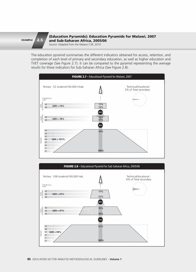
86 EDUCATION SECTOR ANALYSIS METHODOLOGICAL GUIDELINES - Volume 1
FIGURE 2.7 - Educational Pyramid for Malawi, 2007
17
16
15
14
11
12
13
10
9
8
7
6
11%12%
16%17%
35%
100%
UPP
ERSE
CO
ND
ARY
THEORETICALAGES
LOW
ERSE
CO
ND
ARY
PRIM
ARY
64%
49%
%16%%17%
11%12%GER = 14%
GER = 18%
GER = 101%
Tertiary : 52 students/100,000 inhab. Technical/Vocational :2% of Total secondary
FIGURE 2.8 - Educational Pyramid for Sub-Saharan Africa, 2005/06
16
17
15
14
13
12
11
10
9
8
7
6
61%
100%
UPP
ERSE
CO
ND
ARY
THEORETICALAGES
LOW
ER
SEC
ON
DA
RYPR
IMA
RY
60%
74%
GER = 25%
GER = 47%
GER = 99%
Tertiary : 538 students/100,000 hab. Technical/Vocational :6% of Total secondary
35%
45%
17%
21%
EXAMPLE 2.5(Education Pyramids): Education Pyramids for Malawi, 2007 and Sub-Saharan Africa, 2005/06Source: Adapted from the Malawi CSR, 2010.
The education pyramid summarises the different indicators obtained for access, retention, andcompletion of each level of primary and secondary education, as well as higher education andTVET coverage (See Figure 2.7). It can be compared to the pyramid representing the averageresults for these indicators for Sub-Saharan Africa (See Figure 2.8).

Sector-Wide Analysis, with Emphasis on Primary and Secondary Education 87
TABLE 2.4 - Two Examples of the Effect of School Supply and Demand on Access
Case 1
Case 2
Global Access Rate Share of ChildrenFacing Supply Issues
Access Rate withoutSupply Issues
60
60
32
10
88
67
%
Note : In both cases, the global access rate (the weighted average of the respective access rates with and without supply issues) is the same,assuming that none of the children facing supply issues go to school:Case 1: Access rate = 32% x 0% + (100% - 32%) x 88% = 68% x 88% = 60%.Case 2: Access rate = 10% x 0% + (100% - 10%) x 67% = 90% x 67% = 60%.
ENRO
LMEN
T, INTERN
AL EFFICIENCY AN
D OUT-O
F-SCHOO
L CHILDRENCH
APTER
2
THE SUPPLY AND DEMAND ISSUES ON ACCESS AND RETENTION
Experience has shown that it is not sufficient to build schools and train teachers for childrento attend school. There are numerous situations where a significant share of children stayout of school or drop out, despite the availability of adequate infrastructure and personnel.This section aims to estimate the respective impacts of supply and demand issues, identifythe causes of low demand for education, and reach conclusions that may inform educationpolicy.
ACCESS-RELATED SUPPLY AND DEMAND
3.1.1 THEORETICAL APPROACH
One of the most useful results of this type of analysis is to determine the respective sharesof out-of-school children that: (i) live in areas where supply is inexistent or insufficient; and(ii) do not face supply issues in their area, but are not enrolled. In a complementaryapproach, it is interesting to establish how such figures differ by gender, area of residence,and region or province.
Table 2.4 proposes theoretical figures for the share of: (i) children living in areas with nolocal school; and (ii) children who attend school when one is available locally. To illustratethe conclusions that can be drawn, two situations are considered.
SECTION
3
3.1

88 EDUCATION SECTOR ANALYSIS METHODOLOGICAL GUIDELINES - Volume 1
In the first case, 32 percent of children face school supply issues, and 88 percent of thosewith a school nearby access primary grade 1. In such conditions, it is clear that significantprogress must be made in improving school access through supply policies (including schoolbuilding and teacher deployment in areas where they are in short supply). Potentially, theglobal access rate might increase from 60 percent to 88 percent as a result.
In the second case, the situation is starkly different: only 10 percent of children face supplyissues, but the share of those who do not and effectively access school is much lower thanin case 1, at 67 percent. It is therefore expected that even with a standard supply policy,the improvement in the global access rate would be relatively modest, from 60 percent to67 percent. This suggests that under-enrolment is first and foremost explained by low schooldemand (for the service offered).
School characteristics likely to influence demand on behalf of families include: programmecontent, teacher characteristics, school time-tables (over the year or throughout the day)and so on. Indeed, education services may not respond to parents’ needs or expectations.This may be particularly true in highly traditional or withdrawn areas. Families’ demand foreducation is also affected by their capacity to cover schooling costs. These costs are oftenmuch higher than potential school fees (See Chapter 3 on household contributions toeducation).
3.1.2 PRACTICAL METHODOLOGY TO ESTIMATE THE RESPECTIVE WEIGHTS OF SUPPLY AND DEMAND IN SCHOOL ACCESS USING ADMINISTRATIVESCHOOL DATA
The importance of supply and demand factors is likely to differ from one area to anotherwithin a given country, and should therefore be disaggregated by region, province or district,as per Example 2.6 below. A supply index may be created to assist in this process, whichwill enable the comparison of supply conditions between regions. The index may be basedon the number of schools or teachers per region in proportion to the school-agedpopulation, or the average distance to the nearest school. One of these indicators or acombination of several may be compared to the indicator for the outcome, the gross intakerate.
Furthermore, each may be plotted against the national averages, to identify regions wheresupply is lower or higher than the national average. When supply is above the nationalaverage but the access rate is significantly lower, it is likely that demand issues exist. Example2.6, drawn from The Gambia CSR, 2011, provides an illustration.

EXAMPLE 2.6
Sector-Wide Analysis, with Emphasis on Primary and Secondary Education 89
(Regional Analysis of School Supply and Demand): Analysis of Supply and Demand in Terms of School Access, by District, The Gambia, 2009Source: Adapted from The Gambia CSR, 2011.
FIGURE 2.9 - Relation of Basic Education GER to Number of Teachers per 1,000 Youth (7 to 15 Years),by District, The Gambia, 2009
160
140
120
100
80
60
40
20105 15 20 25 30 35 40
Kantora Wuli
Kanifing M. C.F.Brefet
Kiang W.
Niamina W.Kiang C.
L. Baddibou
F. KansalaF. JarrolBanjulF. B. Karanai
L. Saloum
Kombo E.Kombo C.
Niani N. DankunkuU. NiumiSami
Niamina E.Jokadu
U. Baddibou
L. Niumi
Jarra C.
U. SaloumNianija
Fal. West C. Baddibu
Fal. East
Sandu Kombo N.Jarra E.
Kombo S.
F. Bondali
SUPPLY ISSUE
NO ISSUES
DEMAND ISSUE
SUPPLY AND DEMAND ISSUES
Jarra W.
Jang Jag.
Teachers per 1,000 youth (Nb. )
Basi
c Ed
ucat
ion
GER
(%)
Kiang E.
R2 = 0.4392
Relation of Basic Education GER to Number of -FIGURE 2.9 2009he Gambia,Tby District,
eachers per 1,000 TRelation of Basic Education GER to Number of
ears),YYeouth (7 to 15YYoeachers per 1,000
80
100
120
140
160
Basi
c Ed
ucat
ion
GER
(%) Y ISSUESUPPLLY
CKanifing M.
uliWaKantor
2009he Gambia,Tby District,
Ni
.a W
K
N mimi
a WarrarrJJ.
anaiombo SK ombo E.
LL SaloumomK
E.Kanai
L
KarKar.B B.FFF. Banj
BaddibouL.K
.B f t
Niamina W
Kiang W
.BrefetFFF.. C
ag.
l
Ki C
ang JJNO ISSUES
ul arrolKansala
J.FF.Kansala.FFF.
.Kiang C
.Kiang W = 0.43922R
5
East
Nianija
1020
40
60
Basi
c Ed
ucat
ion
GER
(%)
bo
C
alF
252015
eachers per 1,000 youth (Nb.
Sami
Saloum
NS
imiUB
TTe
U
403530
eachers per 1,000 youth (Nb. )
Note: The slanted R² line is equivalent to the expected enrolment ratio for a given level of supply. The vertical dotted line isequivalent to the average supply index.
FindingsThe analysis of education supply and demand issues at the district level shows marked differencesin the levels of expected enrolment and the level of school supply.
The districts that combine below-average supply and a level of enrolment below expectationsface both schooling supply and demand issues. This group includes: Falladu East, CentralBaddibu, Nianija, Falladu West, Upper Saloum, Jarra Central, Kombo North, Upper Baddibu,Jokadu and Niamina East.
The districts whose enrolment is below expectations despite education supply being aboveaverage specifically face a demand issue. This group includes: Upper Niumi, Sami, NorthDankunku, Kiang East, Niani, Lower Saloum, Foni Jarol, Foni Kansala and Foni Bitang Karanai.
The districts where enrolment is higher than expected despite supply being below average mainlyface supply constraints. This group includes: Kantora, Kanifing Municipal Council, Wulli, Sandu,Jarra East, Jarra West, Foni Bondali, Kombo South and Foni Brefet. It would be appropriate toincrease the supply of education in these districts to increase enrolment.
ENRO
LMEN
T, INTERN
AL EFFICIENCY AN
D OUT-O
F-SCHOO
L CHILDRENCH
APTER
2

90 EDUCATION SECTOR ANALYSIS METHODOLOGICAL GUIDELINES - Volume 1
3.1.3 USING HOUSEHOLD SURVEYS DATA FOR THE IDENTIFICATION OF FACTORSAFFECTING ACCESS-RELATED DEMAND
It may be helpful to link the lack of demand for education to school and populationcharacteristics. Two approaches to this analysis are possible: econometric and descriptive.
Econometric AnalysisThis approach will aim to estimate to what extent social and environmental factors areassociated with children’s access to school. On the basis of household survey data, thisapproach may provide information on the importance of the distance to school in thedecision to enroll children, relative to other socioeconomic factors. This will inform potentialsupply-oriented policies: if distance to school is not a major factor for families, buildingmore schools near villages will not improve access rates.
The districts that have a higher level of education supply and a level of enrolment in line with orhigher than expected face no major issues of supply or demand. This group includes: Banjul,Jangjangbureh, Lower Baddibou, Kiang Central, Kiang West and Niamina West.
It may be worthwhile to present the conclusions reached above on a map of the country, to linkthe distribution of issues encountered to other factors, where appropriate.
MAP 2.1 - Supply and Demand Diagnosis, by District, The Gambia, 2009
KanifingKanifing
BrikamaBrikama
KerewanKerewanMansakorikoMansakoriko
JangjangburehJangjangbureh
BasseBasse
Supply and Demand Issues (9)
Demand Issues (11)
No major Issue (7)
Supply Issue (10)
KanifingKanifingewaewaee
gg
BrBr
ngngngng
ikamaikama
ererKK
Supply and Demand DiagnosisMAP 2.1 -
KKKaKa ff ngnggg
rikamarikama
Kaanifing
Brikkama
KerewwawaK
nnorikorikorikorikMM oooo oorikrikrikriksaksakMansakMansakMansakMansak
by District,,Supply and Demand Diagnosis
nManssakoriko
ee
BasseBassesese
ehehngjangburngjangburangjangburangjangburangjangburangjangburJJ
2009he Gambia,T by District,
eengjangburngjangburJangjgjangbureh
Basse
Demand Issues
Supply and Demand Issues
(11)
(9)Supply and Demand Issues
(10)Supply Issue
(7)No major Issue

EXAMPLE 2.7
Sector-Wide Analysis, with Emphasis on Primary and Secondary Education 91
(Modelisation of Primary Access Demand): Correlation of the Distanceto School with the Demand for Primary Access, Mauritania, 2008Source: Adapted and translated from the Mauritania CSR, 2010.
TABLE 2.5 - Modelisation of the Correlation between Distance to School and Basic Education Access(Children Aged 11 to 12 Years), Mauritania, 2008
Variables
Time required to reach the nearest school
Under 15 minutes (Ref Over15 minutes)
Urban Aera (Ref Rural Area)
Boys (Ref Girls)
Living Standard (Ref. Q1 - the Poorest Quintile)
Q2
Q3
Q4
Q5 (the Wealthiest Quintile)
Constant
Coefficients *
0.588
0.472
0.329
0.381
0.670
1.194
1.947
0.878
Note: * All variables are significant at the 1% level.
Table 2.5 presents the results of a statistical analysis that describes to what extent the distanceto school is associated to the probability of accessing basic education for children aged 11 to 12years.
FindingsThe estimation shows that for given sociodemographic characteristics, the probability of accessto basic education is negatively associated with the distance to school. The results indicate thatthe access rate is likely to drop when the time required to reach school is above 15 minutes.
ENRO
LMEN
T, INTERN
AL EFFICIENCY AN
D OUT-O
F-SCHOO
L CHILDRENCH
APTER
2
Descriptive AnalysisThe descriptive analysis is complementary to the econometric analysis described above andis based directly on households’ survey responses. Example 2.8 below presents the mainreasons stated by parents for not sending their children to school, and the reasons for theirlack of satisfaction with school for those who do.

92 EDUCATION SECTOR ANALYSIS METHODOLOGICAL GUIDELINES - Volume 1
FIGURE 2.10 - Reasons for Non-AttendanceStated by Parents, Benin, 2003
FIGURE 2.11 - Causes of Dissatisfactionwith School Stated by Parents, Benin, 2003
40%
35%
30%
25%
20%
15%
10%
5%
0%
Wor
k
Age
Cost
Oth
ers
Usel
essn
ess
Faile
d in
Exa
m
Sick
ness
/Pre
gnan
cy
Mar
riage
Dist
ance
60%
50%
40%
30%
20%
10%
0%
Poor
teac
hing
Oth
er is
sues
Lack
of t
extb
ooks
/le
arni
ng m
ater
ial
Lack
of t
each
ers
Scho
ol in
bad
cond
ition
s
No
prob
lem
Benin,,arentsStated by P
Reasons for Non-Attendance -FIGURE 2.10
5%
10%
15%
20%
25%
30%
35%
40%
2003
Reasons for Non-Attendancewith School Stated by PFIGURE 2.11
10%
20%
30%
40%
50%
60%
2003 Benin,,arentswith School Stated by P
Causes of Dissatisfaction -FIGURE 2.11
Sick
ness
/Pre
gnan
cy
aile
d in
Exa
mF
Usel
essn
ess
Oth
ers
Cost
Age
ork
W
0%
No
prob
lem
Dist
ance
Mar
riage
Sick
ness
/Pre
gnan
cy 0%
10%
cond
ition
sSc
hool
in b
ad
Lack
of t
each
ers
lear
ning
mat
eria
lLa
ck o
f tex
tboo
ks/
Oth
er is
sues
oor t
each
ing
P
Two main reasons lead parents to withdraw their children from school: (i) direct, indirect andopportunity costs (school supplies are too expensive, children’s help/work is needed at home tocontribute to the family economy or take care of younger siblings); and (ii) parents’ perceptionsof school (time-tables are thought inappropriate, academic expectations are thought toostringent and so on). Demand for education is therefore closely related to supply.
FindingsThe results of the Questionnaire on Basic Wellbeing Indicators (QUIBB) carried out in 2003indicate that children’s work is the most common reason for non-attendance of school cited byparents, which tends to confirm that low enrolment is primarily a demand-related issue, even ifschool characteristics fail to satisfy a majority of parents. The other causes mentioned by surveyedparents (about 5,350 households) also seem to reflect demand-side factors, including the ageof children, the cost of schooling and the perceived uselessness of education.
EXAMPLE 2.8(Analysis of Factors Affecting Access-Related Demand): Causes of Non-Attendance and Dissatisfaction with School Mentionedby Parents, Benin, 2003Source: Adapted and translated from the Benin CSR, 2009.

EXAMPLE 2.9
Sector-Wide Analysis, with Emphasis on Primary and Secondary Education 93
(Analysis of Supply - Incomplete Schools): Distribution of SchoolsAccording to the Grades Offered, Burkina Faso, 2006/07Source: Adapted and translated from the Burkina Faso CSR, 2011.
TABLE 2.6 - Distribution of Schools According to the Number of Grades Offered and Enrolment,Burkina Faso, 2006/07
Gradesoffered
Number of Schools
Share ofSchools
Number of Pupils
Share ofPupils
1Grade
2 Grades
3 Grades
4 Grades
5 Grades
6 Grades
Total
963
898
1,423
804
623
3,471
8,182
11.8%
11.0%
17.4%
9.8%
7.6%
42.4%
100.0%
58,510
84,487
174,089
120,708
107,907
1,015,557
1,561,258
3.7%
5.4%
1.2%
7.7%
6.9%
65.0%
100.0%
This example aims to evaluate the extent to which the absence of grade continuity or theavailability of a full cycle explains dropout during a cycle. As a first step each school can beclassified according to the number of years of education offered, and the share of pupils enrolledin incomplete schools calculated for a given school year (See Table 2.6).
FindingsOnly 65 percent of pupils are enrolled in schools offering the complete primary cycle. This doesnot however necessarily mean that 35 percent (100 percent - 65 percent) are facing a supplyshortage at this point of their schooling career. Indeed, some schools open new grades as theirpupils complete the existing ones, or use an alternate year enrolment system. This happens tobe the case in Burkina Faso where Biennial (every two years) recruitment is widespread.
ENRO
LMEN
T, INTERN
AL EFFICIENCY AN
D OUT-O
F-SCHOO
L CHILDRENCH
APTER
2
RETENTION-RELATEDSUPPLY AND DEMAND
Supply and demand factors can also explain school dropout and retention. This section willreview potential causes for these phenomena and establish which are related to schoolsand which are related to families’ expectations.
3.2.1 INCOMPLETE SCHOOLS AND EDUCATION DISCONTINUITY (SUPPLY ISSUE)
A school is classified as incomplete when it does not offer all the grades of a given cycle. Insuch cases the risk of dropout is high, especially if no alternative school nearby offers themissing grades. A first step in this analysis will therefore be to determine, as per Example2.9 below, the proportion of incomplete schools in the education system and the numberof pupils that attend them.
3.2

94 EDUCATION SECTOR ANALYSIS METHODOLOGICAL GUIDELINES - Volume 1
It is worth keeping in mind however, that some schools may be incomplete in a given schoolyear, and yet still offer grade continuity to their pupils and the opportunity to pursue theireducation to the end of the cycle. Indeed, as per Example 2.9, schools in sparsely populatedareas may practice an alternate year enrolment system, whereby new grade 1 enrolmentsare only accepted every two years. Thus, school data may show that only three grades areoffered for any given school year, despite pupils systematically promoting to the followinggrade and being able to complete the cycle. It is also common that some recently openedschools do not initially offer all grades, but gradually inaugurate new successive classes aspupils finish the existing ones, also ensuring that their pupils can complete the cycle.Consequently, even if the analysis on the share of incomplete schools is interesting, it mayoverestimate the scale of education supply discontinuity.
A method (shown in Example 2.10) is therefore offered to evaluate the true extent of gradecontinuity, based on the identification of classes for which the following grade will beunavailable the following year. With the data for two successive school years, it is possibleto identify the number of classes in the first year for which the next grade is unavailable inthe second year, indicating a situation of grade discontinuity. The number and share ofpupils that cannot pursue their education in the same school can then be obtained for eachgrade, by summing up the numbers enrolled in the classes identified. An estimation of theshare of new entrants that will not be able to pursue their schooling to completion of thecycle due to the unavailability of all grades can then be reached by aggregating the sharesobtained for each grade through a multiplication.
On the other hand, the retention rate (through to the last grade of the cycle) for pupilsenrolled in schools with full continuity along the cycle can be computed. This will providean estimation of what the retention rate would be if all schools offered full grade continuity.
It can be noted that the question of supply also includes a qualitative dimension: beyondthe availability of schools themselves, the quality of the education offered has a direct impacton retention (as well as a less direct impact on access). We will however keep the reflectionon these aspects for Chapter 4, which specifically deals with the quality of learning and itslinks with student flows.
3.2.2 PRACTICAL METHODOLOGY TO ESTIMATE THE RESPECTIVE WEIGHTS OFSUPPLY AND DEMAND IN SCHOOL RETENTION USING ADMINISTRATIVESCHOOL DATA
As for school intake, the respective impacts of supply-side and demand-side factors onretention can be estimated at the sub-national level.

EXAMPLE 2.10
Sector-Wide Analysis, with Emphasis on Primary and Secondary Education 95
(Impact of Incomplete Schools on Retention): Regional Supply andDemand Issues and their Impact on Retention, Mali, 2006/07-2007/08Source : Adapted and translated from the Mali CSR, 2010.
TABLE 2.7 - Share of Schools and Pupils Facing Grade Discontinuity between 2006/07 and 2007/08,by Grade, Mali
First Basic Cycle
Grade 1 (No Grade 2)
Grade 2 (No Grade 3)
Grade 3 (No Grade 4)
Grade 4 (No Grade 5)
Grade 5 (No Grade 6)
Cycle Subtotal
Second Basic Cycle
Grade 7 (No Grade 8)
Grade 8 (No Grade 9)
Cycle Subtotal
Share of Schools
7.6%
6.4%
6.6%
7.0%
7.1%
7.0%
8.5%
8.3%
8.4%
Share of Pupils
6.3%
4.9%
4.6%
4.4%
4.7%
5.1%
4.2%
3.9%
4.1%
Bamako
MaliKayes
Mopti
Ségou
Tombouctou
KidalGao
Sikasso
90%
80%
70%
60%
50%
40%
30%
Rete
ntio
n ra
te in
sch
ools
pro
vidi
nggr
ade
cont
inui
ty
% of pupils in a school with grade discontinuity
0% 1% 2% 3% 4% 5% 6% 7% 8% 9%
Supply issue
Supply anddemand issues
Demandissue
Koulikoro
FIGURE 2.12 - Education Supply and Demand Seen through Grade Continuity and Retention,by Region, Mali, 2007/08
Education Supply and Demand Seen through Grade Continuity and Retention, -FIGURE 2.12 2007/08 Mali,by Region,
Education Supply and Demand Seen through Grade Continuity and Retention, Education Supply and Demand Seen through Grade Continuity and Retention,
50%
60%
70%
80%
90%
grad
e co
ntin
uity
ovid
ing
Rete
ntio
n ra
te in
sch
ools
pr
issueDemand
Sikasso
ombouctouT
KayesMali
oBamak
KK
Ségou
Mopti
Kayes
orooro
Supply issue
demand issuesSupply and
oulikoulikKK
30%
40%
2%1%0%
% of pupils in a school with grade discontinuity
Rete
ntio
n ra
te in
sch
ools
pr
5%4%3%2%
% of pupils in a school with grade discontinuity
9%8%7%6%
% of pupils in a school with grade discontinuity
FindingsAt the national level, about five percent of pupils enrolled in the first basic education cycle in2006/07 would not be able to pursue their schooling to the next grade in the same school in2007/08 (See Table 2.7).
The analysis is of greater use still when carried out at the regional level. Figure 2.12 crosses datafor the share of pupils facing grade discontinuity with data for the retention rates expectedshould all schools offer full continuity (estimated as the average retention rate among schoolsthat offer full cycle continuity), by region.
ENRO
LMEN
T, INTERN
AL EFFICIENCY AN
D OUT-O
F-SCHOO
L CHILDRENCH
APTER
2

96 EDUCATION SECTOR ANALYSIS METHODOLOGICAL GUIDELINES - Volume 1
3.2.3 USING HOUSEHOLD SURVEYS DATA FOR THE IDENTIFICATION OF FACTORSAFFECTING RETENTION-RELATED DEMAND
As in the case of access, demand-side factors affect retention and dropout. These includethe evolution of families’ perceptions of the costs and benefits of education throughouttheir children’s schooling careers.8 Household surveys are again helpful to explore the maindimensions of low demand for education, assuming that information on schooling isavailable for two successive years. Questions may be included such as: “Did your child attendschool last year?” and “Is your child attending school this year?”
Econometric models can then be used to attempt to identify the factors that are associatedwith dropout. The correlation of each variable will be directly estimated, as per Example 2.7or Example 2.11, to simulate the completion of a cycle by different population groupsaccordingly.
As for the analysis of access-related supply and demand factors above, it is also possible todescribe the reasons offered by parents for the interruption of their children’s schooling,and their potential general discontent with their local school.
FindingsGenerally speaking, the share of children facing grade discontinuity varies from 1.7 percent inthe Gao region to 8.0 percent in the Ségou region. Figure 2.12 effectively categorises regionsinto four groups according to the supply and demand issues they face:
- Regions of the first group (top right), Kayes and Ségou, have high retention rates in completeschools but a high share of pupils in incomplete schools. It should therefore be possible toimprove retention and the access rates to different grades by improving school supply. Thiscan be achieved by building new classrooms in incomplete schools and through greater useof the single-teacher rural school model.
- The second group (bottom left) comprises the regions of Gao, Kidal, Tombouctou andSikasso. Here, the share of children in incomplete schools is lower, as are the retention ratesin complete schools. The poor retention is more likely to be due to the weakness of demandfor education than to insufficient supply. A demand-oriented policy targeting the population(or the relevant subgroups) will be more appropriate than a classic school supply policy.
- The third group (bottom right), comprising Mopti and Koulikoro, has the peculiarity of highshares of pupils enrolled in incomplete schools and low retention rates, even in completeschools. These regions first and foremost face a supply issue in as much as children cannotpursue their schooling in the same school and are forced to curtail their education. There isalso a demand issue here as even pupils in complete schools do not always finish the cycle.
- The fourth and last group (top left) only comprises Bamako, home to the capital city. Here,high retention rates and a low share of children enrolled in incomplete schools indicate thatthis is the only region with no particular supply or demand issues.

EXAMPLE 2.11
Sector-Wide Analysis, with Emphasis on Primary and Secondary Education 97
(Analysis of Factors Affecting Retention-Related Demand): Simulationof Completion Rates According to Socioeconomic Factors, Congo, 2005Source: Adapted and translated from the Congo CSR, 2010.
TABLEAU 2.8 - Simulation du taux d’achèvement selon le genre, les quintiles de richesse et la durée domicile-école (sur la base de régressions logistiques)
TABLE 2.8 - Simulation of Completion Rates through Logistic Regressions,by Gender, Wealth Quintile and Distance to School, Congo, 2005
WealthQuintile
Distanceto School Girls
Completion Rate
Boys
Q1 (The Poorest Quintile)
Q2
Q3
Q4
Q5 (The Wealthiest Quintile)
> 30 mn
< 30 mn
> 30 mn
< 30 mn
> 30 mn
< 30 mn
> 30 mn
< 30 mn
> 30 mn
< 30 mn
30.5
37.9
43.6
51.8
67.1
73.9
78.7
83.7
89.0
91.8
31.4
38.9
44.7
52.9
68.0
74.7
79.4
84.3
89.4
92.2
This analysis, based on the 2005 Congolese Household Survey, focuses on the disparities thatmay exist in terms of primary completion according to wealth quintile, gender, and the distanceto school. The rates computed here differ from traditional rates in that they are calculated on anindividual basis through econometric models.
FindingsConsidering the extreme groups in this example, a girl from the poorest quintile living over 30minutes away from school is 61 percentage points less likely to complete the cycle than a boyfrom the wealthiest quintile living less than 30 minutes away from school. The ratio ofprobabilities is thus of 1 to 3. The result is almost the same for a girl from the wealthiest quintileand living less than 30 minutes away from school.
The table also indicates that supply issues are more accentuated among the poorest children. Agap in terms of completion of 7.4 percentage points (37.9 – 30.5) between the poorest girlsliving near their school and those living far from their school could be reduced through supplypolicies: the probability of completing school increases by 24 percent (7.4 / 30.5) when schoolsare near girls’ homes. This gap decreases with each wealth quintile however. In terms ofretention, the least favoured population groups are thus comparatively more prejudiced by thedistance to school. This indicates that a supply policy aiming to provide proximity schooling wouldbenefit the poorest families most.
However, the difference of 61 percentage points is mainly explained by demand-side factors:schools are available nearby but children do not attend. In terms of retention, there is nosignificant difference according to gender for children from the wealthiest quintile. The scale ofdemand-side issues is far greater than the supply-side issues. A supply-oriented policy wouldtherefore prove insufficient to correct the disparities.
ENRO
LMEN
T, INTERN
AL EFFICIENCY AN
D OUT-O
F-SCHOO
L CHILDRENCH
APTER
2

98 EDUCATION SECTOR ANALYSIS METHODOLOGICAL GUIDELINES - Volume 1
BOTTLENECK ANALYSIS
UNICEF has developed a conceptual framework called Bottleneck Analysis that allows, whenapplied to the education sector, to identify and quantify the determinants (both supply-sideand demand-side) impeding schooling (or learning outcomes). This tool is very useful forsupporting the preparation of education programmes addressing the identified bottlenecks.Figure 2.13 shows the original framework, designed for the health sector.
The framework is simple, logical and adaptable to the education sector (See Table 2.9 foran example). The quantification of the magnitude of the determinants can be assessedthanks to the methods presented in the guidelines, in particular in Chapters 2 and 4.
FIGURE 2.13 - Tanahashi model: determinants of service coverage (health sector)
Effectiveness coverage
“people who receiveeffective care”
Contact coverage
“people who use service”
Acceptability (initial utilisation)coverage“people who are willing to use service”
Accessibility – geographical access
“people who can use service”
Availability – commodities and HR
Target population
“people for whom service is available”
anahashi model:
fectiveness coverage
T -FIGURE 2.13
Eff
determinants of service coverage (health sector)anahashi model: determinants of service coverage (health sector)
e”fective carefeceivepeople who r
Contact coverage
people who use service
Acceptability (initial utilisation)
e willing to uspeople who ar
Accessibility – geographical access
people who can use service
Acceptability (initial utilisation)
se service
Accessibility – geographical access
vailability – commodities AAv
people for whom service is a
arget populationTTa
vailability – commodities and HR
available
Source: Tanahashi, 1978 “Health service coverage and its evaluation” Bulletin of the WHO 56(2): pp.295-303.
3.3

Sector-Wide Analysis, with Emphasis on Primary and Secondary Education 99
TABLE 2.9 - Adaptation of Tanahashi model to the education sector
1. Availability 1. Availability of commodities
2. Availability of human resources
2. Accessibility 3. Physical access
3. Acceptability 4. Initial utilisation
4. Contact / continued 5. Continued utilisation
5. Effectiveness 6. Effective coverage – quality
1. Availability of educational inputs consideredcritical (class rooms, textbooks,learning materials, etc.) to cover numberof children that are supposed to go to school.
2. Availability of human resources (teachersor qualified teachers) to cover numberof children that are supposed to go to school.
3. Physical access to school (distanceof children from the school, physical access,financial barriers, etc.).
4. Initial utilisationAccess Rate to Grade 1 that can be estimatedthanks to methodologies presented earlier inthe guidelines (using either householdsurvey or EMIS data, see section 2of the present chapter)
5. Continuation of enrolment. Can bemeasured through survival rate or completionrate (see section 2 of the present chapter)
6. Quality output: learning achievement
Health Model Education bottleneck analysis adaptationTanahashi model coverage
ENRO
LMEN
T, INTERN
AL EFFICIENCY AN
D OUT-O
F-SCHOO
L CHILDRENCH
APTER
2
Source: UNICEF WCARO, Designing Pro-equities Strategies – Education Bottleneck Analysis and Costing for WCAR countries, DraftGuidance notes, September 2012

100 EDUCATION SECTOR ANALYSIS METHODOLOGICAL GUIDELINES - Volume 1
SECTION
4 INTERNAL EFFICIENCY9
The quantitative goals of education systems are not limited to increasing the number ofchildren enrolled but also to ensure that children who begin a cycle complete it (do notdropout), and do so in the set number of years (do not repeat). Indeed, the pedagogicalprogrammes of each cycle are developed in such a way as to progressively provide learnerswith a coherent and self-reinforcing set of knowledge and skills. The early abandon of acycle is thus likely to result in the partial or total loss of the knowledge and skills acquiredin the years effectively attended. The most widely mentioned example, including in theseGuidelines, is that of sustainable literacy, acquired during primary education. Indeed, evenif many children know how to read and write before the end of the cycle, it has beenempirically demonstrated that a significant share of adults who did not complete the primarycycle lose their literacy after a number of years if they are not practicing.
Analysing the flow of pupils through a cycle and evaluating internal efficiency consists ofcomparing the number of children that access the first grade of the cycle with the numberthat reach the last grade in the set number of years (without repetition). The smaller thedifference, the more continuous or efficient the system.
Dropout in the course of a cycle, and the repetition of grades prejudice internal efficiency,in the former case because the years of school financed school years of pupils who do notvalidate their cycle or fully achieve the set learning objectives, and in the latter because twoschool years must be financed instead of one to achieve the same learning outcome (SeeBox 2.3 below). Both situations represent suboptimal use or wastage of public andhousehold resources.

• Key Definitions
Sector-Wide Analysis, with Emphasis on Primary and Secondary Education 101
Generally, the two indicators are fairly close. In situations where enrolment increasessignificantly, the share of repeaters may be slightly lower than the repetition rate (given thatthe denominator is greater). The repetition rate is a measure that is more aligned withpedagogical practice: it measures the number of pupils that are refused promotion to thefollowing grade. The share of repeaters presents the advantage of only requiring one yearof data for its computation, and is therefore more immediate.
Example 2.12 illustrates the use of these indicators to describe repetition and its dynamicswithin each cycle and its evolution over recent years. International comparisons can also bedrawn. Here the authors are careful to compare administrative data and household surveydata, enriching the analysis and to ensure data reliability.
REPETITION
Repetition can be measured through two indicators that are close yet different: the repetitionrate and the share of repeaters.
The Share of Repeaters is the percentage of repeaters in a grade or cycle:
The Repetition Rate is the proportion of pupils enrolled in a given grade for a given schoolyear who study in the same grade the following school year:
Share of Repeaters =Number of Repeaters
Total Enrolment
Repetition Rate =Number of Repeaters in Grade i for Year t
Total Enrolment in Grade i for Year (t-1) ENRO
LMEN
T, INTERN
AL EFFICIENCY AN
D OUT-O
F-SCHOO
L CHILDRENCH
APTER
2
4.1

102 EDUCATION SECTOR ANALYSIS METHODOLOGICAL GUIDELINES - Volume 1
BOX 2.3THE NEGATIVE IMPACT OF REPETITION ON SCHOOLING EFFICIENCY
International research on repetition, carried out over a decade, has reached four findings thatquestion the value of too high repetition rates for education systems:
a) The decision to oblige a student to repeat a year is not always fair. A student'sknowledge and skills are not the only explanation for repetition. Decisions often depend onsubjective factors, such as the student's relative position in the class, the environment, theschooling conditions, and the teacher's qualifications (PASEC, 1999). In Côte d'Ivoire, forexample, more than 30 percent of repeaters are not in the lower third of students at thenational level, as measured by the standard PASEC assessment test.
b) The impact of repetition on learning achievements is not empirically proven. Macro-analyses show that the argument aimed at justifying students' repetition for reasons linkedto the quality of education cannot be verified empirically (Mingat and Sosale, 2000). Goodeducation systems (with a high level of student learning) can have a high or low repetitionrate; there is no significant relationship between the students' learning achievement and thefrequency of repetitions. The same is shown in studies at the school level (for instance in Benin,Chad, and Cameroon) which conclude that with equal resources and environment, schoolswhere students have repeated the most grades do not have better results at the end of thecycle (Brossard, 2003; World Bank 2004, 2005). Finally, analyses at an individual level showthat students (except the especially weak) who are made to repeat a year do not improvemore by repeating than by moving on to the next grade (PASEC, 1999; PASEC 2004b).
c) There is a significant negative effect on students who drop out. Studies at country,school, and individual levels reinforce this point. At the macro level, Mingat and Sosale (2000)and Bernard, Simon, Vianou (2005) studies show that repetition increases dropout rates duringthe cycle, and this remains the main obstacle in reaching Universal Primary Enrolment (UPE).The families of students who repeat a year feel that the students are unsuccessful and do notbenefit from being at school. As the opportunity costs always create an argument againstschool attendance, repetition encourages parents to take their children out of school. Mingatand Sosale estimate that one more percentage point of repeaters is associated with a 0.8percentage point increase in the dropout rate. They also show that these negative effects areeven more distinct among the population groups where the demand for schooling is alreadylow (e.g., girls, children from underprivileged economic environments). The results of analysesat the school level support these findings. In Chad, with all other factors being equal, onemore percentage point of repetition is associated with a 0.43 percent lower survival rate (WorldBank, 2005). At the individual level, studies also confirm this trend. In Senegal, at a givenstudent level, the decision to make a Grade 2 student repeat a year increases the risk of thestudent dropping out at the end of the year by 11 percent (PASEC, 2004).
d) Costs are affected. Repetition costs the system two years of study while only one year isvalidated. In other words, for a given budget constraint, repeating students occupy places thatoverload classes and may prevent other children from going to school. The link between therepetition rate and the STR is shown empirically (Mingat and Sosale, 2000 and Pôle de Dakar,2002).
Source: EFA in Africa: Paving the Way for Action, 2005 UNESCO BREDA.
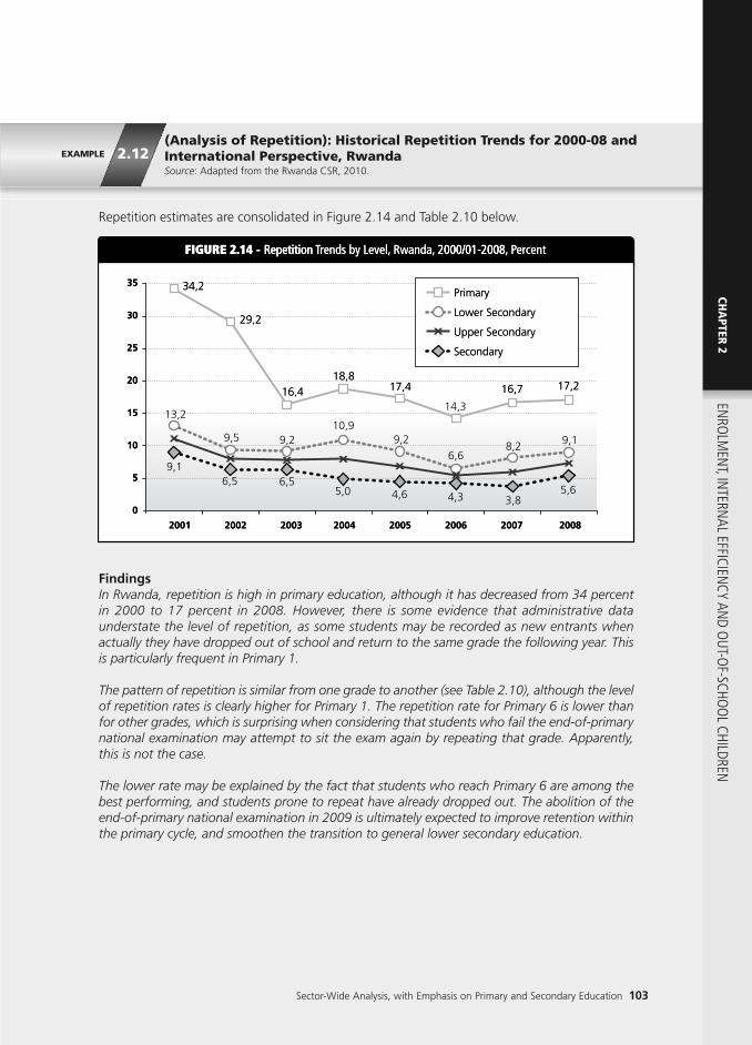
EXAMPLE 2.12(Analysis of Repetition): Historical Repetition Trends for 2000-08 andInternational Perspective, RwandaSource: Adapted from the Rwanda CSR, 2010.
Sector-Wide Analysis, with Emphasis on Primary and Secondary Education 103
ENRO
LMEN
T, INTERN
AL EFFICIENCY AN
D OUT-O
F-SCHOO
L CHILDRENCH
APTER
2
35
30
25
20
15
10
5
0
2001 2002 2003 2004 2005 2006 2007 2008
xxx
xxxx
x
Primary
Lower Secondary
Upper Secondary
Secondary
34,2
29,2
16,418,8
17,4
14,3
16,7 17,2
13,2
9,5 9,210,9
9,26,6
8,2 9,1
9,16,5 6,5
5,0 4,6 4,3
FIGURE 2.14 - Repetition Trends by Level, Rwanda, 2000/01-2008, Percent
3,85,6
Repetition - FIGURE 2.14 2000/01-2008,anda, Rwrends by Level,TRepetition ercent P 2000/01-2008,
10
34 2
29 2
x
13 215
20
25
30
35
29,2
34,2
17,4,18,8
16,4 17,2
Secondary
8 2
16,7
Upper Secondary
Lower Secondary
Primary
2002
x
6 5
2001
0
5
2005
xx
6 5
20042003
x x
2008
xxxxxx
20072006
x
Repetition estimates are consolidated in Figure 2.14 and Table 2.10 below.
FindingsIn Rwanda, repetition is high in primary education, although it has decreased from 34 percentin 2000 to 17 percent in 2008. However, there is some evidence that administrative dataunderstate the level of repetition, as some students may be recorded as new entrants whenactually they have dropped out of school and return to the same grade the following year. Thisis particularly frequent in Primary 1.
The pattern of repetition is similar from one grade to another (see Table 2.10), although the levelof repetition rates is clearly higher for Primary 1. The repetition rate for Primary 6 is lower thanfor other grades, which is surprising when considering that students who fail the end-of-primarynational examination may attempt to sit the exam again by repeating that grade. Apparently,this is not the case.
The lower rate may be explained by the fact that students who reach Primary 6 are among thebest performing, and students prone to repeat have already dropped out. The abolition of theend-of-primary national examination in 2009 is ultimately expected to improve retention withinthe primary cycle, and smoothen the transition to general lower secondary education.

104 EDUCATION SECTOR ANALYSIS METHODOLOGICAL GUIDELINES - Volume 1
FindingsThe Rwandese primary education repetition rate was very close to the average registered for thesubsample of African countries for 2006, but increased from 14.6 to 17.2 percent by 2008.
Figure 2.15 below shows how Rwanda fares in comparison to other African countries in termsof repetition.
Burundi
Madagascar
Lesotho
Rwanda, 2008
Rwanda, 2006
Average Sub-sample
Eritrea
Uganda
Burkina Faso
Benin
Ethiopia
Ghana
Kenya
Mozambique
Tanzania
Niger
0.0 5.0 10.0 15.0 20.0 25.0 30.0
28.8
19.7
18.6
17.2
14.6
13.8
13.7
13.112.0
11.0
9.1
5.8
5.8
5.3
4.9
4.9
FIGURE 2.15 - Repetition Rates at Primary Schools in African Countries, circa 2006 Repetition Rates at Primary Schools in -FIGURE 2.15 African CountriesRepetition Rates at Primary Schools in circa 2006,African Countries
Benin
Burkina Faso
Uganda
eaEritr
verage Sub-sampleA
Rwanda, 2006
Rwanda, 2008
Lesotho
Madagascar
Burundi
.
1
28.8
28.8
5.00.0
Niger
anzaniaTTa
Mozambique
Kenya
Ghana
Ethiopia
Benin
15.0
.
10.05.0
30.025.020.0
30.0
Beyond the cultural factors that often contribute to repetition, it is interesting to review theschool and classroom characteristics that are most closely related to the practice. As for theanalysis of access and retention, econometric models can be used to identify these factorsand assist in the development of policies to reduce repetition, as per Example 2.13 below,drawn from the Chad CSR, 2007.
TABLE 2.10 - Repetition Trend for the Primary Cycle, by Grade, Rwanda, 2002-2008
Percent
2002
2005
2008
DHS 2005
P1
19.1
19.1
18.6
34.4
P2
14.0
16.1
15.9
18.1
P3
14.7
17.3
16.5
19.5
P4
15.8
18.3
18.0
20.3
P5
17.0
18.7
18.7
20.7
P6
17.7
15.0
15.8
16.6

The multiple regression model is the best way to examine the correlation between schoolingconditions and repetition, identifying which variables are the most correlated with repetition andare statistically significant. Table 2.11 presents the results of the estimations based onadministrative school data.
TABLE 2.11 - Modelisation of Primary Cycle Repetition, Chad, 2007
Constant
Context
Urban (Ref. Rural)
Type of School
Private (Ref. Government)
Community (Ref. Government)
Type of Classroom
Share of Permanent or Semi-Permanent Buildings
Teaching Conditions
Share of pupils in multi-grade classes
Classroom Furnishing Index
Number of textbooks (Reading and Math) per pupil
Teacher Characteristics
Share of Women
Type of Qualification
Share with lower secondary certificate (Ref. Share with primary leaving exam)
Share with baccalaureate (Ref. Share with primary leaving exam)
Teacher Status
Share of assistant teachers (Ref. Share of teachers)
Share of community teachers (Ref. Share of teachers)
Age
Share aged between 30 and 49 years (Ref. Share aged under 30 years)
Share aged 50 years or above (Ref. Share aged under 30 years)
Share of the variation explained by the model (%)
Model 1
+ 0.306***
- 0.019*
- 0.080***
- 0.025***
- 0.019**
+ 0.006ns
- 0.016*
+ 0.010*
- 0.045**
- 0.031***
- 0.074***
- 0.003ns
- 0.018ns
16.7
Model 2
+ 0.025***
—
- 0.098***
- 0.021**
- 0.024***
+ 0.007ns
—
+ 0.011*
- 0.076***
+ 0.055***
+ 0.036**
- 0.006ns
+ 0.017ns
15.1
FindingsRepetition varies little according to whether schools are urban or rural (the result is not verysignificant) but repetition is less frequent in private and community schools than in public ones.Repetition is slightly lower for schools with permanent buildings.
EXAMPLE 2.13(Analysis of Factors Associated With Repetition): Econometric Modeli-sation of School and Classroom Factors Related to Repetition, Chad, 2006Source: Adapted and translated from the Chad CSR, 2007.
Sector-Wide Analysis, with Emphasis on Primary and Secondary Education 105
ENRO
LMEN
T, INTERN
AL EFFICIENCY AN
D OUT-O
F-SCHOO
L CHILDRENCH
APTER
2
Source: *Significant at the 1% level; ** Significant at the 5% level; *** Significant at the 10% level; ns Not significant.

106 EDUCATION SECTOR ANALYSIS METHODOLOGICAL GUIDELINES - Volume 1
The results indicate that multi-grade classes are not statistically associated with repetition. Also,the availability of school furniture is of course critical to optimum teaching conditions, but itscorrelation with repetition is fairly limited.
Other findings from the econometric model include: (i) Female teachers (who are rare in Chad –7 percent of the teaching staff, against 30 percent on average for SSA) are correlated with lowerrepetition; (ii) Repetition of pupils is less strongly associated with teachers with the baccalaureatethan with those who hold lower qualifications.; (iii) repetition frequency is slightly lower amongpermanent teachers than among assistant teachers and community teachers.

• Key Definition
Sector-Wide Analysis, with Emphasis on Primary and Secondary Education 107
The Internal Efficiency Coefficient (IEC) is the ratio between the theoretical number of pupil-years required to educate a pupil and the effective average number of pupil-years invested:
IEC =Ideal Number of Pupil - Year
Effective Number of Pupil - Year Invested
ENRO
LMEN
T, INTERN
AL EFFICIENCY AN
D OUT-O
F-SCHOO
L CHILDRENCH
APTER
2
INTERNAL EFFICIENCY COEFFICIENT
Without repetition, any cycle leaver or graduate should have spent the number of yearscompleting the cycle equivalent to its theoretical duration. As mentioned, repetition involvesspending more resources to achieve a given learning outcome, and dropout involvesspending resources on individuals that will not derive the full benefit for themselves orsociety. Thus, the number of pupil-years10 effectively consumed (the number of years ofstudy completed by all pupils, including repeaters and dropouts) should be compared tothe number of leavers or graduates, to establish the average investment in terms of yearsof education per cycle graduate.
The ratio between the theoretical duration of a cycle and the average number of pupil-yearseffectively invested provides the definition of the internal efficiency coefficient (IEC). It iscomprised between 0 and 1, each representing hypothetical extremes: 0 represents asituation where no pupil completes the cycle, regardless of enrolment, repetition anddropout; 1 represents the ideal situation where all children complete the cycle in the setnumber of years (no repetition or dropout). A coefficient of 0.4 indicates that the theoreticalduration of the cycle is just 40 percent of the effective average number of pupil-yearsrequired to complete the cycle. This indicates that 60 percent (= 1 - 0.4) of the pupil-yearsinvested correspond to repetition and drop-out related inefficiency.
4.2
The share of the inefficiency related to dropout and the share related to repetition can beestablished through the computation of partial coefficients that use the number of pupil-years consumed net of repetition (dropout-related IEC), and the number of pupil-yearsconsumed net of dropout (repetition-related IEC). This distinction enables one to establishthe most important factor contributing to a given level of inefficiency. This is helpfulinformation when developing effective education policy with respect to student flows.
It must be noted that to talk of inefficiency, dropout or repetition in terms of wastage isonly acceptable if these phenomenon are excessive, as they can then be interpreted as anet loss for both the education system and the pupils. Repetition may however be marginallybeneficial for some pupils (although it is counter-productive for the system). Also, in absoluteterms, a child dropping out of a six-year cycle after five years is by far preferable to thatperson never having attended school. An IEC of 0.95 should therefore not lead to theconclusion that five percent of pupil-years are lost, because in truth they may well not be

108 EDUCATION SECTOR ANALYSIS METHODOLOGICAL GUIDELINES - Volume 1
lost for everybody. In practice the computation of the IEC relies on the survival rate to thelast grade of the cycle. The survival rate at a given grade is the product of the successiveeffective promotion rates to each grade until the given grade (See Section 2.1 for thedefinition of the effective promotion rate).
The IEC and the partial IECs are calculated as:11
IEC =Duration of the Cycle x Final Grade Survival Rate
i = 1
Final Grade Survival Rate for Grade i
1 - % Repeaters for Grade i
IECDropout =
IECRepetition = IEC IECDropout
Duration of the Cycle x Final Grade Survival Rate
Survival Rate to Grade i =
i = 1
Final Grade
i2
Survival Rate for Grade i
=Non - Repeaters at Grade (i + 1) for School Year (n + 1)
Non - Repeaters at Grade i for School Year n
∏ ii-1PR
ii-1PR
Where : and :
The analysis of the IEC can be carried out in a comparative perspective, by education level,as in Example 2.14 below, and in historical or international perspectives.

EXAMPLE 2.14(Internal Efficiency Coefficients): Total, Dropout-Related andRepetition-Related Internal Efficiency, Rwanda, 2002-2008Source: Adapted from the Rwanda CSR, 2010.
TABLE 2.12 - Internal Efficiency Coefficients in Primary and Secondary Education, Rwanda, 2002-2008
Primary
Internal Efficiency Coefficient
Dropout-Related (without Repetition)
Repetition-Related (without Dropout)
Student-Years Required to Produce One Graduate
Secondary
Internal Efficiency Coefficient
Dropout-Related (without Repetition)
Repetition-Related (without Dropout)
Student-Years Required to Produce One Graduate
2002
56
73
77
12.9
93
102
91
3.6
2008
39
52
76
18.3
82
91
91
4
Table 2.12 below provides an estimation of the internal efficiency of the primary and secondarycycles, summarised by the aggregate internal efficiency coefficient and its two related partialindicators. The latter provide insight into the degree of inefficiency and wastage attributable toperturbation in student flows due to dropout or repetition.
FindingsThe 2008 primary level IEC is low at 39 percent, implying that 61 percent of public resources arewasted on repeated years or schooling-years prior to dropout. This means that the systemeffectively requires 18 student-years to produce one primary level graduate, instead of theplanned six years (perfect efficiency). The situation has worsened since 2002/03, when the IECwas 56 percent. High dropout rates have the greatest adverse impact on primary educationinternal efficiency. Without dropout, the internal efficiency coefficient would have been 76percent. Although efficiency is higher in secondary education, the IEC declined to 82 percent in2008, compared with 91 percent in 2002/03. This can be attributed to dropout, as shown bythe significant decline in the related partial indicator.
Sector-Wide Analysis, with Emphasis on Primary and Secondary Education 109
ENRO
LMEN
T, INTERN
AL EFFICIENCY AN
D OUT-O
F-SCHOO
L CHILDRENCH
APTER
2

110 EDUCATION SECTOR ANALYSIS METHODOLOGICAL GUIDELINES - Volume 1
OUT-OF-SCHOOL CHILDREN
The analysis of out-of-school children takes on a special dimension today, in a contextmarked by the progress in enrolment, but where a still significant share of children do nothave access to full basic education. Achieving universal primary education will requireanalysing this issue to better understand its magnitude and characteristics, and formulateappropriate corrective education policies.
This section does not seek to provide an exhaustive approach to the analysis of out-of-school children. Teams in charge of the Education Sector Analysis may find a detailed analysisof the issue in the UNICEF/UIS, 2010 and World Bank, 2011 documents. Here it will sufficeto present the tools that will enable the readers to answer two fundamental questions: (i)How many children are concerned? and (ii) Who are they?12
ESTIMATION OF THE SHARE AND NUMBER OF OUT-OF-SCHOOL
5.1.1 ESTIMATION OF THE SHARE AND TOTAL NUMBER OF OUT-OF-SCHOOLCHILDREN
Based on Household Survey Data
A first approach to the estimation of out-of-school children is to represent school-agedchildren’s attendance status at the time of the survey (the group aged 5 to 24 years forinstance). For each age, one will distinguish between the shares of children who: (i) neverattended school; (ii) are attending a given cycle (from preschool to higher education); and(iii) have dropped out of school. Figure 2.16 below provides a visual illustration of thisapproach for Sierra Leone.
Figure 2.16 shows that close to 80 percent of children aged nine years are attending primaryschool, and close to 18 percent have never attended school. The share of those havingdropped out is low, but increases with children’s age.
For children of a given age group G (for instance those of basic education school age, 6 to14 years) the number of out-of-school children (OOSC) is the product of the share of out-of-school children (those who never attended, have dropped out or are attendingpreprimary) of that age group and the school-aged population of that age group, whichcan be obtained from population census projections:
OOSCG = Share of OOSCG x Number of Children of Age Group G
SECTION
5
5.1

Sector-Wide Analysis, with Emphasis on Primary and Secondary Education 111
FIGURE 2.16 - Children’s attendance Status, by age, Sierra Leone, 2010
5 6 7 8 9 10 11 12 13 14 15 16 17 18 19 20 21 22 23 24
100
90
80
70
60
50
40
30
20
10
0
Never attendedDrop
HESSS
JSSPrimary
Preschool
%
Age
FIGURE 2.16 -
60
70
80
90
100
by age,s attendance StatusChildren’ 2010, Sierra Leone, by age
0
10
20
30
40
50
98765
%
1716151413121110
Age
2423222120191817
opDrNever attended
PrimaryJSS
SSSHENever attended
eschoolPrPrimary
The number of children having dropped out can be computed by subtracting the numberof children who have never attended school from the total number of OOSC.13
BOX 2.4Explanation of Out-of-School
Definitions of out-of-school vary. That used here is inspired by the definition offered byUNICEF/UIS: An out-of-school child is any child of compulsory school age – generally of primaryor basic education school age – who is not attending a formal primary or basic school.
This definition can be limited to cover only primary, lower secondary or upper secondary school-aged children. Thus, primary school-aged children attending preschool are considered asout-of-school, as well as children attending informal schools (as per the UNICEF/UIS definition).On the other hand, primary school-aged children attending secondary are not considered as out-of-school. This approach tends to overestimate out-of-school, but it ensures comparability ofinternational estimations when administrative or household survey data does not always includepreschool or informal enrolment.
▶
ENRO
LMEN
T, INTERN
AL EFFICIENCY AN
D OUT-O
F-SCHOO
L CHILDRENCH
APTER
2

112 EDUCATION SECTOR ANALYSIS METHODOLOGICAL GUIDELINES - Volume 1
Based on Administrative School Data
The number of out-of-school children can also be computed with the help of administrativeschool data. This can be performed by directly subtracting the number of age group Gchildren enrolled in a primary or secondary school (administrative school data) from the totalnumber of children belonging to this age group (survey projection data):
OOSCG = (Number of Children of Age Group G) - Number of Enrolled Children of Age Group G)
The calculation of adjusted net enrolment rates (ANER) can also be used, where:14
Various methods have been developed to estimate the number of out-of-school children (SeeWorld Bank, 2011 and UNICEF/UIS, 2010). Although approaches to the computation differ, theyall agree on in the need to distinguish among different types of unenrolled children. It is commonto differentiate between those who have never attended, and those who have dropped out (Seefigure below). Further detail can be provided by: (i) differentiating between those who will neverattend school from those who may attend later; and (ii) those at risk of dropout from those whoare not. Although this category is not computed as out-of-school, it provides a quantitativeestimation of the weight of school dropout. Identifying children at risk of dropout is also helpfulto establish appropriate preventive policies.
Attendingchildren
at risk of dropout
ATTENDING CHILDREN OUT-OF-SCHOOL CHILDREN
Attended but dropped out
Never attended
Will attendin the future
Will neverattend
ANERprimary =Number of Primary School Aged Children Enrolled in Primary and Secondary
Total Number of Primary School-Aged Children
This categorisation of out-of-school children enables the elaboration of more appropriate policyresponses to the phenomenon, that will differ according to its nature (access or retention-related)and magnitude.

Sector-Wide Analysis, with Emphasis on Primary and Secondary Education 113
ENRO
LMEN
T, INTERN
AL EFFICIENCY AN
D OUT-O
F-SCHOO
L CHILDRENCH
APTER
2
• Key Definition
This leads to:Share of OOSCPrimary = 100% - ANERPrimary
The number of out-of-school of primary school age can then be deduced:Number of OOSCPrimary = Share of OOSCPrimary x Number of Primary School Aged Children
The quality of this analysis is however always limited by the quality of the single-age schooladministrative data available, which may be limited in countries where birth registration isnot systematic.
5.1.2 ESTIMATION OF THE SHARE AND NUMBER OF OUT-OF-SCHOOL CHILDRENTHAT WILL LIKELY NEVER ENROLL
Among the out-of-school children, a certain number may begin school at a later age, forvarious reasons that may include the distance to school or parents perception that childrenaged six or seven years are too young to attend school. The analysis will thus try to calculatea generation access rate, independent from the age at which children may access school.On the basis of household survey data, it is possible to determine the share of childrenhaving attended school at some point for each age, and deduce the number who are outof school now but will enter school later.15
The graphic representation of these shares enables the visual identification of the ages wherethe rate of school attendance is highest, and the age beyond which the odds of a childattending school are severely reduced. The share of children that will probably never attendschool is obtained by subtracting this attendance rate for those children above the ageidentified from 100 percent. Generally, the cut-off age is found to be in the range of 10 to13 years.
The generation access rate is the probability for an individual to access school, calculated fromhousehold survey data, as the maximum proportion, amongst age groups, of individuals havinghad access to school.
Where T is the age where school attendance has been the highest. The population of age T isused as a reference group for the calculation of the odds of attending school one day, but forreasons related to sample size, it is preferable to use the population group whose ages arecomprised between (T-1) to (T+1). In the Tanzanian example (See Figure 2.17), the age for whichschool attendance is highest is 12 years, so the group aged 11 to 13 years is used for thecomputation.
Generation access rate = Probability for an individual to have access to school one day =
Number of Children Aged (T - 1) to (T +1) Having Attended School
Population Aged (T - 1) to (T + 1)

114 EDUCATION SECTOR ANALYSIS METHODOLOGICAL GUIDELINES - Volume 1
A graphic illustration is given below, using the Tanzania example. The highest schoolattendance rate is for children aged 11 to 12 years, at 95 percent (see Figure 2.17 below).This share can be used as an estimation of the share of younger children who will accessschool at some point. For that age, the share of children who will probably never attendschool is thus five percent (100 percent – 95 percent). Again, many children aged sevenyears (the official age of primary intake) are not yet attending (40 percent), but will probablyattend school in the future.
The share of children who will likely never access school is thus obtained by the followingformula:
Share of Children who Will Never Attend School =100% - Generation Access Rate =
100% - The Highest Probability of age - specific Attendance rate
The number of children of age group G who will likely never attend school is obtained bymultiplying the share of children who will likely never attend school by the population ofchildren of that age group (based on population census projections):
Number of OOSC of Age Group G who Will Likely Never Attend School =Share of Children who Will Never Attend School x Population of Age Group G
100 9080 7060 5040 3020100
5 6 7 8 9 10 11 12 13 14 15 16 17 18 19 20
%
Age
94.9 95.3
FIGURE 2.17 - Share of Children Having Accessed School, Tanzania, 2006 Share of Children Having
%
-FIGURE 2.17
3040 5060 7080 90100
Accessed School,
95.3
Share of Children Having
94.9
2006anzania,TAccessed School,
87650
1020
Age
14131211109
201918171615
Source: CSR Tanzania.

Sector-Wide Analysis, with Emphasis on Primary and Secondary Education 115
ENRO
LMEN
T, INTERN
AL EFFICIENCY AN
D OUT-O
F-SCHOO
L CHILDRENCH
APTER
2
5.1.3 ESTIMATION OF THE SHARE AND NUMBER OF CHILDREN AT RISK OF DROPOUT
Two approaches can be used to estimate the number of children that are at risk of dropoutbefore completing their cycle: (i) The analyses carried out in section 3.2 of the factorsaffecting dropout can be used to deduce the dropout rate, which can in turn be applied tothe enrolled population of that cycle to obtain the share that is at risk of dropout; or (ii)When available, household survey data covering attendance information for two consecutiveyears can be used to calculate the dropout rate by age between those two years, again tobe applied to the number of children enrolled in that cycle.
WHO ARE THE OUT-OF-SCHOOL CHILDREN?
Just as it is important to estimate the magnitude of out-of-school children, so is it to establishwho these children are, where they live and what the main obstacles to accessing schoolare. These characteristics will assist decision-makers in the design and targeting ofappropriate policies.
Household surveys are a valuable source of information, enabling the development ofprofiles of out-of-school children including gender, area of residence, household incomeand employment status characteristics.16 As with all access issues, disparities tend to becumulative and self-reinforcing; only household survey data enables highlighting themultiple dimensions of the phenomenon and to shed appropriate light in view of policymaking.
Example 2.15 below offers a global review of out-of-school children analysis, covering both:(i) the estimation of its magnitude (Section 5.1), differentiating between children who neverattended school and those who dropped out; and (ii) the identification of the characteristicsof the children involved in the phenomenon. This profiling exercise is carried out from twoperspectives: (i) the share of out-of-school children that are girls, poor and so on; and (ii)the share of girls, the poor, rural children and so on that are out-of-school.
5.2

EXAMPLE 2.15
116 EDUCATION SECTOR ANALYSIS METHODOLOGICAL GUIDELINES - Volume 1
(Out-of-School Profiling): Magnitude of Out-of-School andCharacteristics of Out-of-School Children, Mauritania, 2008Source: Adapted and translated from the Mauritania CSR, 2010.
This example aims to provide empirical answers to two questions: (i) How many children of officialschool-age are out of school in Mauritania (how many have never attended, and how manyattended at some point but ended their education prematurely before completing their cycle)?And (ii) What are the personal and social characteristics of out-of-school children? Theprobabilistic schooling profile presented in Figure 2.18 is based on the household living standardssurvey (EPCV, 2008), and covers Mauritanian out-of-school children aged 8 to 13 years.17
FindingsThe share of children of their generation who gained access to the first year of basic education(1AF) is estimated at 88 percent, whereas the share of children of their age group who accessedthe last year of this cycle (6AF) is 37 percent.
The survey data has enabled the estimation of the number of out-of-school children. In 2008 itwas 92,341, equivalent to a quarter of all children aged 8 to 13 years. This population group iscomprised of two types of children: (i) those who never attended school, estimated at 24,488
100%
90%
80%
70%
60%
50%
40%
30%
20%
10%
0%1AF 2AF 3AF 4AF 5AF 6AF
FIGURE 2.18 - Probabilistic Schooling Profile for Basic Education, Mauritania, 2008
Acc
ess
Prob
abili
ty
Classes
Probabilistic Schooling Profile for Basic Education,FIGURE 2.18 Probabilistic Schooling Profile for Basic Education, 2008 Mauritania,Probabilistic Schooling Profile for Basic Education, Probabilistic Schooling Profile for Basic Education,
30%
40%
50%
60%
70%
80%
90%
100%
obab
ility
Acc
ess
Pr
-FIGURE 2.18 Probabilistic Schooling Profile for Basic Education, 2008 Mauritania,Probabilistic Schooling Profile for Basic Education,
1AF0%
10%
20%
4AF3AF2AF
Classes
6AF5AF
TABLE 2.13 - Estimation of the Number of Out-of-School, Mauritania, 2008
Total number of children aged 8 to 13 years
Number of out-of-school children aged 8 to 13 years
Number of children aged 8 to 13 years never attended
Number of children aged 8 to 13 years who dropped out
Percentage Out-of-School
Area of Residence
Rural UrbanTotal
368,765
92,341
24,488
67,853
25.0
168,676
20,514
6,351
14,163
12.2
200,089
71,827
18,137
53,690
35.9

Sector-Wide Analysis, with Emphasis on Primary and Secondary Education 117
or about a quarter of the out-of-school children; and (ii) those who attended at some point butdropped out prematurely, estimated at 67,853.
In order to achieve universal primary education the challenge is to ensure all 92,341 out-of-schoolchildren access school. In-depth profiles may be created to influence the development of policieswhich take into account the social and demographic diversity of the out-of school children.
These profiles may include a social, demographic and economic descriptions of out-of-schoolchildren to help overcome barriers to schooling, target the children concerned, and develop aninclusive education system. Table 2.14 below presents the share of out-of-school childrenaccording to sociodemographic characteristics, as well as the share of children with saidcharacteristics that are out of school.
FindingsOut of the 368,765 children, 92,341 were out of school. The gender gap in out-of-schoolchildren is modest (53 percent are girls and 47 percent are boys). The gap in the probability ofenrolment is more important in terms of area of residence or wealth quintile.
ENRO
LMEN
T, INTERN
AL EFFICIENCY AN
D OUT-O
F-SCHOO
L CHILDRENCH
APTER
2
TABLE 2.14 - Characteristics of Out-of-School Children Aged 8 to 13 Years, Mauritania, 2008
PercentPercent
Area of Residence
Rural
Urban
Gender
Boys
Girls
Wealth Quintile
Q1
Q2
Q3
Q4
Q5
Overall
Percentage Out-of-School, by Characteristic Distribution of Out-of-School, by Characteristic
35.9
12.2
22.9
27.3
39.0
29.3
23.6
13.6
10.0
25.0
77.8
22.2
46.8
53.2
37.4
27.5
19.7
10.2
5.2
100.0
The probability of being out-of-school is estimated at 12.2 percent for urban children, against35.9 percent for those living in rural areas. Rural children represent 78 percent of out-of-schoolchildren, with only 22 percent living in cities. The challenge to achieve universal primaryeducation will therefore largely depend on Mauritania’s capacity to enroll a greater number ofchildren in rural areas. If it is estimated that 92,341 school-aged children are out of school,71,827 of them live in rural areas, and 20,514 live in cities.

118 EDUCATION SECTOR ANALYSIS METHODOLOGICAL GUIDELINES - Volume 1
NOTES
6 In some household surveys for instance, respondents are asked: “Is your child currently attending school?” which can beinterpreted as relating to the physical location of the child at the time of the question. Respondents may answer “No” ifthe survey is carried out during school vacations (or the child is absent from school) even if the child is enrolled. Naturally,the enrolment rate computed on this basis will be lower than that computed on the basis of school data.
7 This chapter will later examine various measures of internal efficiency, including the scale of dropout and the number ofyears wasted in repetition.
8 Such perceptions may evolve along with a child's age as the result of: (i) increasing direct and opportunity costs of schooling(older children may be able to contribute more to the family production, or (ii) girls near puberty are thought to be morevulnerable, and so on); or (iii) decreasing expected returns on education (school quality may be deemed insufficient orinadequate, children with learning difficulties may be thought not to benefit, parents believe basic reading and arithmeticskills are sufficient and so on); or (iv) a combination of both.
9 While the scope of internal efficiency spreads over other dimensions (like the quality of learning, which is dealt with inChapter 4), the analysis here will be limited to the aspects linked to student flows.
10 A pupil-year is defined as one year spent by one student in one grade.
11 There is an alternative method of IEC computation, called the method of reconstituted cohorts, that is dealt with in Annex2.1.
12 A further important question relates to the obstacles to enrolment (See Sections 3.1 and 3.2 in this chapter). Educationsector analysts may also wish to consider the policy options to mitigate the phenomenon available to decision-makers,as described in World Bank, 2011 and UNICEF/UIS, 2010.
13 Knowing one of the variables (the number of dropout-related OOSC or the number of unenrolment-related OOSC)enables the computation of the other by subtracting it from the total number of OOSC. For instance, the number ofdropout-related OOSC = Total OOSC – Unenrolment-Related OOSC.
14 Household survey data can also be helpful here.
15 This data is provided from the responses to the question: “Has your child ever attended school?”
16 Specific surveys on child labor also provide valuable information on out-of-school children. Children’s domestic orproductive activities are often one of the causes for dropout, or a direct consequence of non enrolment (see UNICEF/UIS,2010).
17 In the same way that the probability of Grade 1 primary access was estimated in Section 5.2.1, the probability of accessto each grade can be estimated on the basis of the highest level of attendance noted in the access curve by age. Thesuccession of these probabilistic access rates for each grade constitutes the probabilistic schooling profile.

© W
orld
Ban
k /
Régi
s L’
Hos
tis
Sector-Wide Analysis, with Emphasis on Primary and Secondary Education 119
ENRO
LMEN
T, INTERN
AL EFFICIENCY AN
D OUT-O
F-SCHOO
L CHILDRENCH
APTER
2

120 EDUCATION SECTOR ANALYSIS METHODOLOGICAL GUIDELINES - Volume 1
© W
orld
Ban
k /
Régi
s L’
Hos
tis
Sector-Wide Analysis, with Emphasis on Primary and Secondary Education 121
CHAPTER 3COST ANDFINANCING› Chapter Objective:To offer approaches to the analysis of: (i) the structure of education financing(including by the government, donors andhouseholds), its distribution (by item, educationlevel and type of school) and evolution overtime, and (ii) the breakdown of spending,through recurrent unit costs, householdcontributions, and capital costs.
CHA
PTER3
COST AN
D FINAN
CING

1. EVOLUTION OF EDUCATION EXPENDITURE AND ITS COMPOSITION
ISSUEDoes the country prioritise the education budget? How have priorities between differentexpenditure items and education levels evolved over recent years? Does the distribution ofspending across sub-sectors reflect the education system’s development priorities? What is thelevel of education funding from development partners and how dependent is the sector oninternational aid?
OBJECTIVES• For the last 10 years, detail the amount and breakdown of education spending, differentiating
between recurrent and capital (development) expenditure; • For recent years, detail the distribution of spending by item and level;• For the most recent year, consolidate personnel data from different sources, break down
recurrent expenditure into salary and non-salary expenditure, by level, location and cost-center(central services, decentralised services, schools, and so on); and
• Review the evolution of education financing through international aid;
METHODS• Consolidate overall public education and training expenditure;• Select the most recent year for which expenditure data is available by level;• Compare the different numbers and lists of personnel from various departments, distinguish
between the sector personnel, personnel used by the system but on other ministries’ payrolls,and personnel on the education payroll but practicing elsewhere, and then estimate salaryexpenditure by personnel type; and
• Compile a list of activities financed by partners through projects and budget support (educationsector or global), at least for the chosen reference year.
SOURCES• Detailed executed/actual budget data supplied by the budget division of the finance ministry,
and/or the education ministries’ financial affairs departments;• School survey data, personnel data from the education ministries’ human resource departments
and payroll data from the finance ministry and the civil service commission;• Consolidated school grants expense reports; and• International aid data collected from development partners or the OECD/DAC.
2. ESTIMATION OF UNIT COSTS AND ANALYSIS OF THEIR COMPOSITION
ISSUEWhat is the level of spending per student? What is the trade-off, intentional or not, between thenumber of pupils enrolled and the spending on each? What are the most expensive items of thisspending? What scope exists to change unit costs?
OBJECTIVES• Calculate public recurrent unit costs for each cycle;• Evaluate the respective importance of the different factors of unit costs through a comparative
approach; and• Analyse disparities in teaching salaries by status and how attractive teaching salaries are
compared to other civil servants’ and private sector pay.
122 EDUCATION SECTOR ANALYSIS METHODOLOGICAL GUIDELINES - Volume 1

METHODS• Use a macro approach that consists of dividing the amount of public recurrent expenditure for
each cycle by the number of pupils enrolled in public or private subsidised schools; and• Use a micro approach to detail the different factors of unit costs.
SOURCES• As above; and• For salaries: employment surveys, household surveys (where questionnaires detail individual
income) and data on teacher attrition and loss.
3. ESTIMATION OF HOUSEHOLD CONTRIBUTIONS
ISSUEWhat is the level of household contributions to education? What is the public-private cost-sharingfor each cycle? Do private schooling costs penalise the enrolment of the poorest pupils, especiallyin basic education?
OBJECTIVES• Estimate the level of household education spending and the share of household contributions
to total education spending, by level;• Study the variations in household spending by type of school, location, and parents’
socioeconomic characteristics; and• Analyse the sustainability of household education spending, in particular for the poorest.
METHODS• Calculate average annual household spending by type of school, gender, area of residence and
family income; and• Compare, for each education level, the costs borne by households and those borne by public
financing.
SOURCES• Estimations based on household survey data (living standards surveys, household budget and
consumer surveys and so on).
4. COMPARISON OF THE COST OF DIFFERENT TYPES OF SCHOOLCONSTRUCTION AND OTHER EQUIPMENT
ISSUEHow does the unit cost of the construction of an equipped classroom vary according to thebuilding approach used? What are the unit costs of other types of construction and necessary keyequipment (laboratories and so on)? Are these costs sustainable for the system’s development?What is the importance of capital expenditure in comparison with recurrent expenditure?
OBJECTIVES• Compare the cost of providing an equipped classroom according to the various building options
available nationwide (those used by the state, by communities, by development partners andby NGOs);
▶
Sector-Wide Analysis, with Emphasis on Primary and Secondary Education 123
CHA
PTER3
COST AN
D FINAN
CING
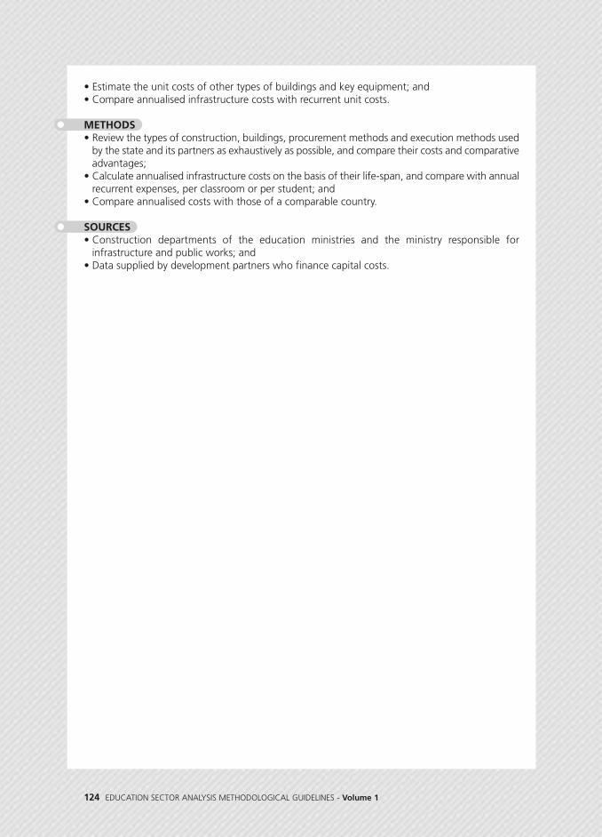
124 EDUCATION SECTOR ANALYSIS METHODOLOGICAL GUIDELINES - Volume 1
• Estimate the unit costs of other types of buildings and key equipment; and• Compare annualised infrastructure costs with recurrent unit costs.
METHODS• Review the types of construction, buildings, procurement methods and execution methods used
by the state and its partners as exhaustively as possible, and compare their costs and comparativeadvantages;
• Calculate annualised infrastructure costs on the basis of their life-span, and compare with annualrecurrent expenses, per classroom or per student; and
• Compare annualised costs with those of a comparable country.
SOURCES• Construction departments of the education ministries and the ministry responsible for
infrastructure and public works; and• Data supplied by development partners who finance capital costs.

Sector-Wide Analysis, with Emphasis on Primary and Secondary Education 125
IntroductionThis chapter explains how to survey and analyse all information pertaining to the resourcesmobilised for the education sector. Although the analysis focuses first and foremost onpublic financing, over which the state has most control, all funding sources are examined(public resources, international aid, private spending). The chapter also deals with the usethat is made of these resources, and especially measures the cost per student (unit costs).
The chapter is divided into four sections: (i) The first analyses the evolution of the volumeof public and external resources mobilised by the sector, from an aggregate perspective. Itanalyses the evolution of public education expenditure by education level and according toits different components (salaries, goods and services, scholarships and other welfare,operating costs). It then analyses, for the most recent year for which data are available, thedetail of these expenditures by level and component; (ii) The second part deals with theestimation of education unit costs for each level, and evaluates the respective importanceof the three main factors of unit costs (average teacher salary, the percentage of recurrentexpenses other than teaching salaries and the pupil to teacher ratio), from national andcomparative international perspectives. It also analyses disparities in teacher salary levelsaccording to their status (civil servants, contract teachers, and community teachers, forinstance); (iii) The third section examines the contribution of households to each cycle andtheir potential impact on enrolment; and (iv) Finally, the fourth section analyses the costsrelated to school construction and equipment.
CHA
PTER3
COST AN
D FINAN
CING

126 EDUCATION SECTOR ANALYSIS METHODOLOGICAL GUIDELINES - Volume 1
FIGURE 3.1 - Summary of the Different Levels of Financial Trade-offs
(1) Intersectortrade-off
(2) Intra-sectortrade-off
(3) Trade-off between unitexpenditure and quantity
(4) Trade-off within the sameunit expenditure
National wealth (GDP)
Domestic resources (budgetary revenue excluding grants)
Expenditure per student (cost) Supply in terms of quantity (gross enrolment rate)
Number of teachers(pupil-teacher ratio)
Other expenditureTeacher salaries
Recurrent public expenditurein education
Public expenditurefor other sectors (health, etc.)
Recurrent public expenditurefor primary education
Public expenditure on other levels(pre-school, non-formal, secondary,technical, tertiary, literacy)
MACROECONOMICAND FISCAL CONTEXT
Figure 3.1 summarises and illustrates the different financial trade-offs, voluntary or not,that are made in education expenditure. The first level (macroeconomic and fiscal context)has been dealt with in Chapter 1. The distribution of spending within and across sub-sectors is analysed in the first section of this chapter, and the last two levels are examinedin section 2.

Sector-Wide Analysis, with Emphasis on Primary and Secondary Education 127
GOVERNMENT SPENDING
Public education expenditure can come from different sources. In some countries, variousministries are in charge of education services, by level (one is in charge of basic educationfor instance, another of secondary and a third of higher education) or by type (generaleducation, higher education and TVET for instance). Some education or trainingprogrammes can be organised or financed by ministries responsible for specific areas (theministries of health, agriculture, justice, or employment for instance). Furthermore, indecentralised contexts, some local institutions can be in charge of multisectoral budgets,of which a share may be allocated to the education sector. The aim of this section is thusto consolidate all public expenditure for education and training activities, independently ofindividual national arrangements, aiming to be exhaustive and to avoid duplication ofaccounts.
Also, despite the availability of official documents (finance laws, budgets), it is important insuch an analysis to determine as precisely as possible what has effectively been spent.Finance laws or budgets indicate spending intent, and not effective spending. This may belower due to governments’ spending capacities or due to issues related to the collection offunds (taxes, duties and so on).18 Effective spending can also be intentionally reduced withrespect to the initial budget, when this is greater than expected, in which case a budgetrevision is generally voted. The analysis will therefore clearly distinguish between the votedbudget and the executed budget, which accounts for what has effectively been spent andincorporates potential further expenditure associated with budget revisions. On the otherhand, there is great tension in this exercise between the search for precision and the will touse the most recent data, as executed budget data is often only available for relatively old
FIGURE 3.2 - The Stages of Public Expenditure
COMMITMENT
Public bodies enter into or become aware of an
obligation (contract) that will generate an expense
VERIFICATION
Confirmation of the service rendered or
receipt of goods and the amount of the liability
incurred
AUTHORISATION
Order/request that the bill be paid and the
public body’s liability cleared
PAYMENT
SECTION
1PUBLIC EDUCATIONEXPENDITURE
1.1
CHA
PTER3
COST AN
D FINAN
CING

• Key Definitions
128 EDUCATION SECTOR ANALYSIS METHODOLOGICAL GUIDELINES - Volume 1
periods (two or even three years back). To use committed expenditure data is a goodcompromise in such cases.
This analysis will examine, in addition to the level of education expenditure, some keyindicators that reflect the importance of this expenditure in the national context. It will focuson two indicators in particular:19
• Public recurrent education expenditure as a share of public recurrent expenditure,excluding debt service. This indicator reflects the priority that is effectively given toeducation by governments within the expenditure over which it has control (for this reasondebt service is excluded, being “compulsory”). This is often considered an indicator ofeffort towards the education sector; Box 3.1 presents the elements to keep in mind whilecalculating it.
• Public recurrent education expenditure as a share of GDP. This indicator places educationexpenditure in the context of national wealth. It is the share of national wealth spent bygovernments on education. This indicator can also be presented as education expenditureper capita as a share of GDP per capita, placing education expenditure in relation to thesize of population and average income.
Recurrent education expenditure may also be examined as a percentage of governments’domestic resources for instance, or total national education expenditure as a share of GDP.
All of these indicators have the advantage of being comparable in both temporal andinternational perspectives. Their evolution over recent years may therefore be examined,before comparing them to those of other countries in the region, or sharing similardevelopment levels.
Recurrent Education Expenditure as a Share of Public Recurrent Expenditure ExcludingDebt Service is the relation of all recurrent education expenditure financed with nationalresources to total recurrent public expenditure excluding the service of debt:
Recurrent Education Expenditure as a Share of GDP is the ratio of total recurrent educationexpenditure to gross domestic product:
Recurrent Public Education ExpenditureRecurrent Public Expenditure, Excluding Debt Service
Recurrent Public Education ExpenditureGross Domestic Product

Sector-Wide Analysis, with Emphasis on Primary and Secondary Education 129
BOX 3.1THE FINANCIAL EFFORT FOR EDUCATION
The financial effort made by countries for the funding of their education is often used bydevelopment partners to determine their own level of financial commitment. This financial effortis generally measured by the share of the education budget in the total national budget. It is thusimportant to properly define both numerator and denominator, in order not to distort thisrepresentation of the national effort.
- The budgets considered in the calculation are recurrent budgets. Investment budgets are oftenmore volatile, which would create artificially great variations in the indicator value. They are alsomore often financed from development partners' programs, which don’t represent the nationaleffort.
- External funding should be excluded from both numerator and denominator, because they donot result from national decisions and effort. In practice, the denominator is thus theexpenditures made from domestic resources, and does not includes external resources (grantsand loans); all education projects and sector budget support financed by development partnerswill also be excluded from the numerator, the only exception is general budget support, forwhich it is difficult to dissociate the funds from domestic resources at the sector level. One maythus keep general budget support both in the recurrent education expenditures and in thedomestic resources.
- As mentioned above, debt service is excluded from the domestic resources. Servicing public debtis mandatory for indebted developing countries, and the amount of resources that the state hasdecision power over is what is left when this service is paid.
The indicator is thus calculated as follows:
National Financial Effort for Education=
Recurrent Education Expenditures financed from domestic resourcesTotal Recurrent Expenditure financed from domestic resources, excluding debt service
Example 3.1 below, drawn from The Gambia CSR, 2011, presents the volume of educationexpenditure, both recurrent and capital, in a summary table, as well as recurrent educationexpenditure as a share of total recurrent expenditure, of national income and of GDP (SeeSection 1.4 for an analysis of international aid).20 This example also presents the country’ssituation in the context of ECOWAS and the continent.
CHA
PTER3
COST AN
D FINAN
CING

EXAMPLE 3.1
130 EDUCATION SECTOR ANALYSIS METHODOLOGICAL GUIDELINES - Volume 1
(Breakdown of Public Education Expenditure by Type and Source):Public Education Expenditure, The Gambia, 2001-09Source: Adapted from The Gambia CSR, 2011.
TABLE 3.1 - Breakdown of Education Financing, by Type and Source, The Gambia, 2001-09
Level of Education Funding (Millions of Dalasis)
Recurrent (Government spending)
Development (Capital)
Government Financing
Donor Financing
Total National Education Expenditure
Total
Recurrent Education Expenditure (Percent)
As a Share of Total Government Recurrent Expenditure*
As a Share of Domestic Revenue (Excluding Grants)
As a Share of GDP
Donor Financing as a Share of the Total Education Budget
Total Government Expenditure as a Share of GDP
142.5
84.2
5.7
78.4
148.2
226.7
16.7
14.4
0.9
34.6
0.9
341.2
249.8
14.7
235.1
355.9
591.0
19.2
9.8
1.6
39.8
1.7
426.8
416.9
29.9
387.1
456.7
843.7
17.2
12.2
1.9
45.9
2.0
479.7
416.3
69.3
347.0
549.0
896.6
17.8
12.0
1.8
38.7
2.1
2001 2007 2008 2009
Donor Financing as a Share of the Total Education Budget
Total Government Expenditure as a Share of GDP
34.6
0.9
39.8
1.7
45.9
2.0
38.7
2.1
Recurrent Education Expenditure (Percent)
The government assumes the majority of recurrent education expenditure, and donorcontributions are devoted largely to development (capital) expenditure. For analytical purposes,spending on government scholarships to support girls’ schooling in upper basic and seniorsecondary schools, generally included in development expenditure, has been considered withinrecurrent expenditure.
FindingsTotal national education expenditure increased from 0.9 percent of GDP in 2001 to 2.1 percentof GDP in 2009. Recurrent education expenditure represents an average of 18 percent ofrecurrent government expenditure, excluding debt service. Most of public education expenditurehas been devoted to recurrent costs, with negligible amounts being spent on investment.However, government capital spending has risen from 4 percent [=5.7/(5.7+142.5)] of total publicexpenditure in 2001 to 13 percent [=69.3/(69.3+479.7)] in 2009.
Figure 3.3 shows that in spending 17.8 of total recurrent expenditure excluding debt service oneducation in 2009, The Gambia ranks well below its neighbours in the ECOWAS sub-region; thispercentage is only higher than those of post-conflict Guinea-Bissau and Liberia (See Figure 3.3),and is below the FTI benchmark of 20 percent. With a sub-regional average of 24 percent, thereis scope for The Gambia to increase the priority given to education in public spending.
Note: * Government recurrent expenditure excludes the service of debt.

Sector-Wide Analysis, with Emphasis on Primary and Secondary Education 131
EVOLUTION OF PUBLIC EXPENDITURE BY TYPE OF SPENDING
The objective of this section is to analyse the distribution of education expenditure by typeof spending. According to the structure of the budget, some budget lines may have to beconsolidated or separated. National budgets are generally composed of two types ofexpenditure: recurrent and capital (also known as development or investment). Withinrecurrent expenditure, the budget lines devoted to personnel, goods and services must beisolated from the budget lines devoted to subsidies and transfers. Scholarships and otherwelfare spending are generally included in the budget line for transfers. Some personnelexpenditure (contract or community teachers paid by the government) may also be includedwithin the budget line for transfers; it is important that they too be isolated.
To summarise, the accounting logic that prevails in budget elaboration often leads thespending items that the analyst seeks to identify to be combined with others. Only a verymindful read of the budget enables these distinctions to be made. As a first step of analysis,attempts should be made to categorize spending items as follows:
• Wages and Salaries: All spending on the salaries, bonuses and expenses of education civilservants, both teaching and non-teaching (administrative, maintenance, security personneland so on) as well as payments by the government (possibly at the decentralised level) toto civil servants, contract/volunteer/ community teachers and other non-teaching
1.2
FIGURE 3.3 - Education Share of Public Recurrent Expenditure, The Gambia and ECOWAS Countries,2009 or MRY
40
35
30
25
20
15
10
5
0
Perc
ent
Gui
nea-
Biss
au
Libe
ria
Gam
bia,
The
Gui
nea
SSA
Aver
age
ECO
NW
AS A
vera
ge
Beni
n
Togo
Burk
ina
Faso
Cape
Ver
de
Côte
D'Iv
oire
Nig
er
Sene
gal
Mal
i
Sier
ra L
eone
Gha
na
- Education Share of Public Recurrent ExpenditureFIGURE 3.3 - Education Share of Public Recurrent Expenditure he Gambia and ECOWAS CountriesT, - Education Share of Public Recurrent Expenditure ,he Gambia and ECOWAS Countries
10
15
20
25
30
35
40
cent
Per
Y2009 or MR
0
5
Libe
ria
Gui
nea-
Biss
au
aso
Burk
ina
Fogo
TBeni
n
age
AS A
ver
ECO
NW
age
SSA
AverGui
neahe T
Gam
bia,
a Le
one
Sier
r
Mal
i
Sene
gal
Nig
er
Côte
D'Iv
oire
erde
Cape
V
Gha
na
CHA
PTER3
COST AN
D FINAN
CING

EXAMPLE 3.2
132 EDUCATION SECTOR ANALYSIS METHODOLOGICAL GUIDELINES - Volume 1
education personnel. The allowances and social benefits received by such staff are alsoincluded in this category, such as retirement funds, health insurance and so on;
• Goods and Services: All spending on goods, excluding capital spending, as well as servicecontracts, subcontracting or consultancy expenses (distribution of pedagogical materials,external audits and so on);
• Subsidies and Transfers: All fund transfers and subsidies to independent educationagencies and institutions (training institutes, universities and so on) as well as schoolgrants;
• Scholarships and Other Welfare: All school feeding, university restaurant and boardingexpenses, as well as the amounts allocated to student scholarships both at home andabroad.
The categories obtained will thus often differ from those presented in the budget. It will benecessary to ensure that they are clearly defined (and calculated in the same way for eachyear covered by the analysis), and that the total effectively coincides with the total educationexpenditure identified in Section 1.1. Annex 3.3 provides the concrete methodology for theconsolidation of financial data.
Example 3.2 below, drawn from the Benin CSR, 2009, illustrates how these spendingcategories and their evolution can be analysed. It offers a presentation of the amounts spentper category, each of which is then analysed in terms of their share of total expenditure. Itis apparent that the authors were unfortunately not able to isolate the remuneration oflocal contract teachers, paid by parent-teacher associations. This remuneration is thereforeincluded in the transfer category, which limits the analysis somewhat. On the other hand,this problem having been identified, the figures and their evolution can be analysed in thisperspective.
(Breakdown of Public Education Expenditure by Nature): Public Education Expenditure, Benin, 1992-2006Source: Translated and Adapted from the Benin CSR, 2009.
TABLE 3.2 - Structure of Public Education Expenditure, by Nature, Benin, 1992-2006
Share of Total (%)
Recurrent Expenditure
Personnel
Goods and Services
Transfers
Equipment
Capital Expenditure
National
International
Total
81.3
45.1
13.7
19.1
3.4
18.7
13.1
5.6
100
84.4
48.8
11.6
21.2
2.7
15.6
7.4
8.3
100
90.1
52.9
9.7
24.8
2.7
9.9
5.4
4.5
100
90.5
54.2
9.7
25.1
1.5
9.5
3.7
5.8
100
2003
85.0
51.5
14.1
17.7
1.7
15.0
5.6
9.4
100
2000
96.9
78.3
8.1
10.5
0.0
3.1
1.2
1.9
100
1992 2004 2005 2006
Note: * Not including the (minimal) expenditure of the literacy subsector.

Sector-Wide Analysis, with Emphasis on Primary and Secondary Education 133
FindingsTable 3.2 illustrates the extreme predominance of recurrent expenditure in total expenditure, asis the case in most education systems, with a share between 80 and 97 percent for the 1992 to2006 period. The share of recurrent expenditure dropped in the 1990s before increasing from2001 onwards. This increase is generally at the expense of capital expenditure, whose share oftotal expenditure dropped considerably, from 15.0 percent in 2000 to 9.5 percent in 2006.
The data also reveals that the share of personnel spending has not significantly increased since2000, having reached 54.2 percent in 2006 from a level of 51.5 percent in 2000, despite theimportant evolution noted in enrolment (mentioned in Chapter 2 of the CSR). This finding doesnot reflect the reality however, given that the salaries of local contract teaching staff forpreschool, primary, general secondary and technical and vocational secondary, recruited in partto respond to the expansion of the system, are paid on public resources transferred to parent-teacher associations (PTAs). In the past they had taken the initiative to recruit this type of teacheron their own resources. These resources, made available to PTAs and included in the transfercategory, are the source of strong growth in the share of transfers since 2000, and the real causeof the structural change of the budget.
Finally, although the reduction of the share of spending devoted to socio-administrativeequipment is less significant (1.5 percent in 2006 against 1.7 percent in 2000), the reduction ofthe share of spending devoted to goods and services (used in part for the purchase ofpedagogical material) is notable, given that it was below 10 percent in 2005, against 14 percentin 2000.
In terms of capital spending, the share of investment spending supported by external funds (i.e.international) has evolved erratically: from 9.4 percent in 2000, it first dropped to 5.6 percent in2003 before rising to 8.3 percent in 2004 and dropping anew to 5.8 percent in 2006. Theevolution of the share of capital spending supported by national funds has not been quite asirregular. An increase from 5.6 percent in 2000 to 13.1 percent in 2003 was neverthelessfollowed by a drop, to reach 3.7 percent in 2006.
CHA
PTER3
COST AN
D FINAN
CING
THE DISTRIBUTION OF SPENDING ACROSS SUB-SECTORS
Executed or committed budgets should be used here to distribute spending among thedifferent education cycles according to their purpose (for instance, transfer spending to giveprimary community teachers a bonus should be accounted for as primary spending). Inpractice, this allocation is not always easy: for instance, budgets often consolidate primaryand secondary administrative spending (or general secondary and technical trainingspending). Some spending items also cover different education levels by their very nature,such as the operational expenses of the planning or human resource departments of theeducation ministry, that provide services to all cycles covered by the ministry. Estimationsare then carried out to distribute these common expenses among levels.21 A breakdown
1.3

134 EDUCATION SECTOR ANALYSIS METHODOLOGICAL GUIDELINES - Volume 1
formula must thus be determined. Usually, the distribution is carried out according to thepro rata of the payroll of active teachers or that of all school personnel, or in their absence,according to the pro rata of spending specifically pertaining to each level. This method isdescribed in Annex 3.3.
The structure of the distribution of spending among different education levels provides anidea of the priority that governments give to each and enables the identification of potentialdesirable adjustments in the priorities, in particular as compared to the policy prioritiesintended.
In this analysis of the national situation, and of the distribution of expenditures across thelocally defined cycles, it can also be helpful to compare the distribution of expenditure bylevel for the country of analysis with that of countries with similar contexts. However, asthe length of the cycles is different in some countries, two approaches can be used to avoidcomparative bias. The first compares the country of interest with others sharing the sameeducation system structure (most francophone countries have a 6-4-3 structure for instance:six years of primary, four years of lower secondary and three years of upper secondary). Thesecond is to erase the difference that may exist among countries in the duration of theireducation cycles by artificially harmonizing those durations through preliminary adjustments(See Annex 3.1).
Example 3.3, drawn from the Mali CSR, 2010, presents the distribution of public educationexpenditure by level and its evolution over recent years, before placing it in a regionalcontext, in comparison with countries whose education system structures are similar.
DETAILED ANALYSIS OF PUBLIC RECURRENTEXPENDITURE FOR THE MOST RECENT YEAR
The aim of this section is to carry out a more detailed analysis of the data used in theprevious section, for the most recent year for which data is available. This analysis will aimto provide additional information on the functional distribution of expenditure,distinguishing between different spending items (teaching and support personnel,pedagogical and service spending, scholarships and other welfare) for each level as well asbetween the various cost-centers responsible for their execution (schools, central anddecentralised services, subsidised private schools and so on). This involves a fairly detailedanalysis, whose coherence must be carefully checked. Experience shows that it is helpful tobegin with a clear description of the distribution of the actively employed personnel, to thenreconstitute the distribution between personnel expenditure and other non-salary spending,and that a preliminary cleaning and consolidation of the personnel data is often necessary.
1.4

EXAMPLE 3.3(Distribution of Public Education Expenditure in Regional Context):Public Education Expenditure by Level, Mali, 2008Source: Adapted from the Mali CSR, 2010 and the Mali CSR, 2007
Sector-Wide Analysis, with Emphasis on Primary and Secondary Education 135
1.4.1 CONSOLIDATION OF THE PERSONNEL DATA
The analysis should begin with an inventory of the personnel. This is justified on the onehand by the importance of salary spending (usually at least two-thirds of the educationbudget) and on the other by the need to clean up and consolidate the data. Indeed, somestaff may be paid on the education budget despite not performing any education system
FindingsThe distribution of public education resources across sub-sectors has significantly evolved overthe last 14 years, although somewhat erratically. The share of recurrent expenditure allocatedto primary education grew from 27.4 percent in 1995 to 35.0 percent in 2004 and 36.5 percentin 2008. This however remains significantly below the 50 percent observed in many othercountries (which is also the Global Partnership for Education benchmark). Other data (not shownin the table) shows that the share of expenditure devoted to lower secondary in 2008 (16.7percent) is below that observed in 2004 (17.8 percent). On the other hand, the share allocatedto upper secondary education has decreased from 16.4 percent in 2004 to 12.9 percent in 2008,and that of technical and vocational education has remained grossly stable, at 9.3 percent in2004 and 9.9 percent in 2008. The reduction in the share allocated to upper secondary between2004 and 2008, although benefitting primary education, has equally benefitted highereducation, whose share grew from 16.3 percent in 2004 to 17.6 percent in 2008.
TABLE 3.3 - International Comparison of the Structure of Recurrent Education Expenditure,by Level (Francophone Countries of Sub-Saharan Africa)
Mali
Mali
Mali
Benin
Burkina Faso
Burundi
Congo
Côte d’Ivoire
Guinea
Guinea Bissau
Niger
CAR
Senegal
Togo
Average of 11 Countries
45.6
43.5
39.5
23.5
17.2
29.9
39.0
34.6
30.8
26.9
26.3
25.0
27.7
39.7
29.1
23.1
16.3
17.6
19.7
22.2
20.0
29.8
20.9
26.4
11.1
13.1
21.0
27.8
20.3
21.1
3.9
5.2
6.5
3.2
4.2
3.1
5.4
1.8
5.3
5.3
3.3
5.0
0.6
1.2
3.5
General and Technical Secondary
27.4
35.0
36.5
53.6
56.4
47.0
25.8
42.7
37.5
56.7
57.3
49.0
43.9
38.8
46.2
Primary
(1995)
(2004)
(2008)
(2006)
(2006)
(2004)
(2005)
(2007)
(2005)
(2006)
(2008)
(2005)
(2004)
(2007)
YearCountry HigherOther
(Pre-primary, Literacy, etc.)
Average of 11 Countries 29.1 21.1 3.546.2
CHA
PTER3
COST AN
D FINAN
CING

136 EDUCATION SECTOR ANALYSIS METHODOLOGICAL GUIDELINES - Volume 1
duties (staff that perform other roles or are transferred to other ministries, and ghostteachers/staff), or conversely, some staff may work in education while being paid on otherministries’ budgets (sports trainers that are paid by the ministry of youth and sports, artteachers that are paid by the ministry of culture and so on). The analysis will be focused onthose personnel paid by the state (or, if relevant, by decentralised public institutions).However, by the same logic, if some personnel paid by the state are posted in public orcommunity school, they should be included in this analysis.
This process is carried out by comparing various data sources, including: (i) school statistics(school staff censuses); (ii) data from the human resource department of the educationministries (databases covering all personnel employed in the sector; in some countries, thismay be limited to staff working in central and decentralised services); and (iii) financeministry payroll data, or in some countries, that of the ministry of civil service.
The reconciliation of figures from different sources often represents an arduous butnecessary task, as it is an indispensable basis for further analysis as well as for the estimationand definition of parameters of the financial simulation model for the sector’s planningprocess. Once the personnel inventory is complete, it is important to reconcile the numberswith the related financial amounts. This must be carried out based on information on thedistribution of personnel by qualification type and salary on the one hand, and informationon average salary levels for each category on the other. It eventually enables theconsolidation of the entire payroll for the sector. Annex 3.3 details the important steps forthe consolidation of these data and the reconstitution of the payroll.
When the gaps between different data sources are significant, it is sometimes helpful topresent the data obtained from each source, and the corrections and adjustments done.
1.4.2 DESCRIPTION OF EDUCATION PERSONNEL AND RELATED SALARYEXPENDITURE, BY LEVEL AND ROLE
Once the personnel data are consolidated, these personnel numbers and associated budgetscan be presented. To that end, staff must be classified according to their job and not theirstatus. It is common that teaching staff carry out administrative duties, in which case theyshould be treated as non-teaching staff for the purpose of the analysis. Personnel musttherefore be broken down into those effectively responsible for teaching activities on onehand (in-class teachers also called "chalk in hand" teachers), and those who carry outadministrative or support duties on the other. Distinction should be made by type ofinstitution (schools, central or decentralised administrative services) and level.
Example 3.4 below, drawn from the Congo CSR, 2010, illustrates the kind of table that canbe produced once the personnel numbers from various sources have been consolidated.This example also shows the relative importance of the respective payroll burdens, andpresents the share of non-teaching staff in a regional perspective.

EXAMPLE 3.4
Sector-Wide Analysis, with Emphasis on Primary and Secondary Education 137
(Analysis of Personnel Expenditure): Public Education PersonnelExpenditure, Congo, 2009Source: Adapted and Translated from Congo CSR, 2010.
Table 3.4 presents the data for active staff working for the three education ministries. Itincorporates the cost of personnel paid for on transfer budget lines such as volunteers or thepersonnel of the Marien Ngouabi University. The distinction between "chalk in hand" teachersand non-teaching staff is obtained by crossing function and posting information.
FindingsOf the 15,045 staff working in Congolese government schools, 34.9 percent [5,256 / (9,789 +5,256)] are employed in non-teaching posts. The share of non-teaching staff in the entireeducation system is significant (54.8 percent); 5,256 members of staff work in schools and 6,636in support services. These figures vary from one education level to another. The share of non-teaching staff in schools is greatest for the preschool level (55 percent). It remains high forprimary (26 percent), and especially for secondary (40.6 percent for lower secondary and 38.0percent for upper secondary). When considering all the education system’s personnel, the shareof non-teaching staff reaches 53.5 percent at the primary level, 58.8 percent in lower secondary,and 55.6 percent in upper secondary. It is greatest at the preschool level, at 75 percent.
TABLE 3.4 - Education Sector Personnel and Related Salary Expenditure(Payroll in Millions of CFAF), Congo, 2009
Preschool
Primary
Civil Servants and Contracted
Volunteers
Lower Secondary
Civil Servants and Contracted
Volunteers
Upper Secondary
Civil Servants and Contracted
Volunteers
Technical Education
Civil Servants and Contracted
Volunteers
Vocational Training Institutes
Civil Servants and Contracted
Volunteers
Teacher Training Colleges
Higher Education
TOTAL
243
4,030
3,211
819
1,732
1,463
269
1,364
1,164
200
1,546
879
667
174
139
35
100
600
9,789
298
1,417
1,374
43
1,183
1,158
25
837
821
16
791
791
147
147
47
536
5,256
435
3,229
3,193
36
1,293
1,268
25
872
864
8
568
568
82
82
52
105
6,636
976
8,676
7,778
898
4,208
3,889
319
3,073
2,849
224
2,904
2,237
667
404
369
35
199
1,241
21,681
254
4,682
4,199
484
2,595
2,357
238
2,373
2,161
213
1,840
1,425
415
252
231
22
156
6,358
18,511
348
1,871
1,845
25
1,755
1,733
22
1,334
1,317
17
835
835
135
135
0
88
3,359
9,725
588
4,260
4,237
23
1,868
1,845
23
1,227
1,219
8
1,219
1,219
177
177
111
187
9,638
1,191
10,813
10,281
532
6,218
5,935
283
4,935
4,697
238
3,894
3,479
415
564
542
22
355
9,904
37,873
“Chalk inhand”
Teachers Schools ServicesTotal
Payroll (in Millions of CFAF)Non-TeachingStaff
Teachers Other(Schools)
Other(Services)
Total
TOTAL 9,789 5,256 6,636 21,681 18,511 9,725 9,638 37,873
CHA
PTER3
COST AN
D FINAN
CING

EXAMPLE 3.5
138 EDUCATION SECTOR ANALYSIS METHODOLOGICAL GUIDELINES - Volume 1
1.4.3 NON-SALARY EXPENDITURE AND THE CONSOLIDATION OF SPENDING BYLEVEL
Non-salary expenditure is examined in this section, and will be broken down as far as ispractical to do so. Spending items such as pedagogical materials, textbooks, operationalcosts, scholarships and other welfare and so on should be differentiated. These items shouldthen be consolidated with the salary expenditure reviewed in the previous subsection, toensure that the total effectively amounts to the total recurrent education budget.
This consolidation will then be distributed among education levels, assigning the appropriateshare of non-targeted administrative expenses to each. Coefficients will be used for thisbreakdown when spending cannot be assigned to a single level, usually the same as thoseused for the salaries related to services provided to multiple levels (See Annex 3.3). Thestructure of recurrent expenditure by education level will then be established, as per Example3.5 below, distinguishing between its different components (teaching staff, non-teachingschool staff, operational costs, administrative costs and scholarships and other welfare).
(Analysis of Non-Salary Expenditure): Public Expenditure by Function and Level, Benin, 2006Source: Adapted and Translated from the Benin CSR, 2009.
MAI
NGE
NERA
LAU
X.
TABLE 3.5 - Distribution of Public Recurrent Education Expenditure, by Function, Benin, 2006
Government Teachers
Community/temporary Teachers
University Research
Subtotal
School Management
School Operational Costs
Subtotal
Sector Administration
(Central/Decentralised Service Personnel)
Central/Decentralised
Services’ Operational Costs *
National Scholarships,
School Grants and University Works
Scholarships abroad and Contributions
to International Schools
Subtotal
TOTAL
—
—
—
0.0
—
2.9
2.9
97.1
100.0
61.7
3.9
—
65.6
—
7.4
7.4
27.0
100.0
52.9
5.6
—
58.5
—
9.6
9.6
31.9
100.0
46.4
—
—
46.4
0.0
26.0
26.0
27.6
100.0
27.9
25.5
—
53.4
17.4
4.3
21.7
24.9
100.0
41.0
18.3
—
59.3
9.5
4.3
13.9
26.8
100.0
14.6
3.2
—
17.8
6.7
6.6
13.4
68.8
100.0
19.4
3.1
—
22.5
3.6
3.4
7.0
70.5
100.0
19.3
—
2.6
21.9
3.3
10.9
14.2
63.9
100.0
40.7
7.5
0.5
48.7
3.6
8.8
12.4
38.9
100.0
62.0
35.1
—
—
14.6
12.4
—
—
16.5
15.4
—
—
14.8
12.9
—
—
13.8
11.0
—
—
15.4
11.3
—
—
31.4
31.1
5.2
—
31.4
32.8
4.9
—
8.3
10.4
38.5
6.7
15.3
13.3
7.8
1.3
Percent Literacy Pre-school
Pri-mary
TeacherTraining
General Secondary
TVET
Lower Upper Level 1 Level 2
Higher All
Note: * Includes 7.9 percent for deconcentrated services, or 1.1 percent of recurrent education expenditure.

Sector-Wide Analysis, with Emphasis on Primary and Secondary Education 139
Three categories of spending are considered here: Main, Auxiliary and General. Main spendingincludes teaching staff expenditure, university research subsidies, and subsidies for the paymentof temporary and local contract teachers. Auxiliary spending includes administrative staffexpenditure, services, and pedagogical materials spending at the school level. In addition to thisexpenditure carried out directly by schools, the education sector incurs General expenses, whichrelate to the management and administration of the sector, both at the central level (ministries)and at the regional administration level. Student grants constitute a further item of Generalexpenditure. Table 3.5 describes the functional distribution of these expenditure items accordingto this classification.
FindingsFor the education system overall, close to half recurrent expenditure is devoted to its Mainfunction (49 percent), 12 percent is devoted to Auxiliary spending and 39 percent to Generalexpenses. The share devoted to the Main function is less today than it was at the end of the1990s: for the primary cycle it has dropped from 73 percent (data not shown in the table) to 59percent of recurrent expenditure; for general secondary from 86 percent (data not shown in thetable) to 56 percent, and for higher education from 29 percent (data not shown in the table) to22 percent. This relative drop has been more significant for the primary and secondary cycles.
This could be explained by the financial constraints that obliged the state to rely on teachercategories that are paid less than permanent government teachers (contract teachers) or thosepartially paid by the government (temporary and local contract teachers), to ensure thateducation is effective. The share devoted to inputs other than teacher salaries has thus increased,which suggests an evolution towards an improvement of the material conditions of study offeredto students, as well as of the system’s management. However, it is possible that the resourcesallocated to Main expenditure items are still low, given the supervision offered to students and/orthe remuneration offered to teachers in light of the heterogeneity of their status.
Generally speaking, the average share of recurrent expenditure devoted to inputs other thanteacher salaries is 52 percent [=100-(40.7+7.5)], although this varies from one level to another,from 34 percent [=100-(61.7+3.9)] for preschool to over 70 percent for TVET and highereducation. It is difficult to make a normative judgment of these scales; international comparativedata may help to appreciate the allocation. They show that the share of expenditure devoted toinputs other than teacher salaries is comparatively higher in Benin for the primary level, lowersecondary and TVET. For primary in particular, the Fast Track Initiative benchmark of 33 percentis significantly surpassed (42 percent [=100-(52.9+5.6)]).
Expenditure other than teacher salaries is in fact mainly composed of General expenditures (over75 percent, based on calculation using data of the table). General administration and operationalexpenditures (of central and decentralised services) each account for approximately 15 percentof recurrent education expenditure, although the share devoted to the operational costs ofdecentralised services is weak, despite such spending being helpful for inspections and thedecentralised management of the system. The share of expenditure devoted to the operationalcosts of central services therefore appears to be considerably higher than that devoted to theoperation of schools (13 percent on average for central services, against 9 percent for schools,or a ratio of 1.4 to 1). This situation is more apparent for TVET (recurrent and operationalexpenditure of central services are 7 times higher than those of schools) and the literacy subsector(12 times higher).
CHA
PTER3
COST AN
D FINAN
CING

140 EDUCATION SECTOR ANALYSIS METHODOLOGICAL GUIDELINES - Volume 1
EXTERNAL FUNDING
The contribution of development partners to education is limited to the financing ofinvestment expenditure in many countries, even if it is also used to fund recurrentexpenditure in some cases.22 Previously, data on international aid was widely dispersed,when this was provided through numerous projects. The evolution of aid disbursementarrangements, and the development of sector program support in particular (budget supportthat is more or less ear-marked for certain ministries or spending items), has increasinglyled to amounts allocated appearing in beneficiary ministries’ budgets. This facilitates theiridentification, but it is not systematic that national budgets provide full traceability of allactivities financed by international aid. In this situation, a quick census of developmentpartners enables the collection of information on the activities financed by level, theamounts committed and those effectively disbursed.
Furthermore, when a country receives global budget support, external resources are fungiblewith national resources and it becomes impossible to precisely determine the share of thisfunding that is allocated to the education sector. In this case, a commonly used proxy isthat the same share of external support is devoted to education as that of the nationalresources. The figures offered in subsection 1.1 of this chapter would then be used. Forinstance, if 20 percent of the budget is allocated to education, it is estimated as a proxythat 20 percent of external budget support is also allocated to the sector.
Firstly the analysis will present the total amount of external funding received by the countryfor its education sector, and its importance in relation to national funding. Secondly, it willbe worthwhile comparing the average value of the aid for education received by the countryover recent years as a share of GDP with that received by other countries in the region, orthose with similar levels of economic and education sector development, to estimate thedegree of dependency of the sector on external funding and its degree of sustainability.
1.5.1 A NATIONAL PERSPECTIVE
At the national level, the analysis may focus on the total volume of aid, the diversity ofdonors and the type of expenditure and activities supported by development partners, asper Example 3.6 below, drawn from the Malawi CSR, 2010. It may also comment on thequality of data, their source, coherence and the reliability of the collection approach. Toassist this collection process, a questionnaire model to be shared with development partnersis offered in Annex 3.2.
1.5

EXAMPLE 3.6
Sector-Wide Analysis, with Emphasis on Primary and Secondary Education 141
1.5.2 AN INTERNATIONAL PERSPECTIVE
For the international comparison, OECD/DAC data should be used. The comparison mayfocus on the level of external funding for the education sector, either as a percentage ofpublic education expenditure, or as a share of GDP. Example 3.7, drawn from the MauritaniaCSR, 2010, presents an international comparison of external education funding.
(Analysis of External Aid - National): Donor Financing forthe Education Sector, Malawi, 2005/06-2007/08Source: Adapted from the Malawi CSR, 2010.
In order to get information on donor activities in the education sector, the analysis used datafrom a survey conducted by DFID.
FindingsDonor contributions play a critical role in the development budget of the government. Based oncalculations using data from the table, on average, their contribution amounts to 86 percent ofthe total development budget. Over 60 percent of donor support to education goes towardsconstruction in primary education. In both 2005/06 and 2006/07 about 63 percent wascommitted to the construction of primary schools (66 percent in 2007/08). The commitmenttowards secondary education is very low, even if it has increased from 1 percent of total donorfinancing in 2005/06 to 3 percent in 2007/08. This increase is due to the current AfricanDevelopment Bank project, which has focused on improvements in secondary education.Universities have received very little official development assistance in the recent past (1 percentin 2005/06 and none in 2006/07 and 2007/08).
TABLE 3.6 - Donor Financing and Extra-Budgetary Grants to Education
Millions de MK
General
Primary
Secondary
Higher
TOTAL
3,973
396
608
1,343
1,092
1,335
40
30
8,818
1,650
243
599
931
409
1,261
40
30,45
5,163
2,619
387
916
2,346
616
1,428
33
—
8,346
2,224
270
739
1,557
510
1,406
30
—
6,737
2,113
460
1,618
1,346
792
1,685
290
—
8,303
General
TA and Other
Construction
Curriculum and books
PRESET
School Feeding
PRESET
Universities
Objective ofAssistance
Committed05/06
Disbursed05/06
Disbursed06/07
Committed07/08
Committed06/07
TOTAL 8,818 5,163 8,346 6,737 8,303
CHA
PTER3
COST AN
D FINAN
CING

EXAMPLE 3.7
142 EDUCATION SECTOR ANALYSIS METHODOLOGICAL GUIDELINES - Volume 1
FindingsIn 2008, external funding represented 13.5 percent of total education sector expenditure and0.6 percent of GDP in Mauritania, against 22.7 percent of total expenditure and 0.9 percent ofGDP in 1995 (based on data not displayed in the figure). Mauritania’s dependency oninternational aid for the education sector therefore appears to be relatively weak.
External funding’s contribution to education expenditure varies between 0.03 percent of GDP(Nigeria) to 4.6 percent of GDP (São Tomé and Príncipe) for comparable countries. For Mauritania,external funding’s contribution to education expenditure represented 0.6 percent of GDP in2008, considerably below the average of African countries whose GDP per capita is betweenUS$ 500 and US$ 1,500 (1.3 percent of GDP).
FIGURE 3.4 - Comparison of the Contribution of External Funding to Education Expenditure,for Countries with GDP per Capita between US$500 and US$1,500, 2008 or MRY
5.0
4.5
4.0
3.5
3.0
2.5
2.0
1.5
1.0
0.5
0.0
Average of the 17 Countries : 1.3%
Shar
e of
GD
P (%
)
Nig
eria
Chad
Côte
d'Iv
oire
Keny
a
Leso
tho
Mau
ritan
ia
Cam
eroo
n
Zam
bia
Togo
Gha
na
Sene
gal
Beni
n
Mal
i
Burk
ina
Faso
Com
oros
Tanz
ania
São
Tom
é an
d Pr
incip
e
for Countries with GDP per Capita between US$500 and US$1,500, - Comparison of the Contribution of External Funding to Education ExpenditureFIGURE 3.4
2.0
vera
2.5
3.0
3.5
4.0
4.5
5.0
e of
GD
P (%
)
veraAA
for Countries with GDP per Capita between US$500 and US$1,500, - Comparison of the Contribution of External Funding to Education Expenditure
age of the 17 Countries : 1.3%age of the 17 Countries : 1 3%
Y 2008 or MRfor Countries with GDP per Capita between US$500 and US$1,500, - Comparison of the Contribution of External Funding to Education Expenditure, - Comparison of the Contribution of External Funding to Education Expenditure
0.0
0.5
1.0
1.5
2.0e of
GD
P (%
)Sh
ar
Côte
d'Iv
oire
Chad
Nig
eria
ogo
T
Zam
bia
Cam
eroo
n
Mau
ritan
ia
Leso
thoa
eny
K
anza
nia
TTaCom
orosaso
Burk
ina
FMal
i
Beni
n
Sene
gal
Gha
na
omé
and
Prin
cipe
TSã
o
(Analysis of External Aid - International): International Comparison of External Funding of Education Systems,2008 or MRY Source: Adapted and Translated from the Mauritania CSR, 2010.
Figure 3.4 shows how Mauritania compares to other African countries of similar income levels,in terms of external aid.

Sector-Wide Analysis, with Emphasis on Primary and Secondary Education 143
The information on total expenditure does not enable an understanding or assessment ofeducation policy in as much as it is not related to the number of pupils the system catersfor. To step from total expenditure to per student spending (unit costs) will thus enable amore detailed analysis of the structure of spending among education levels, but also foreach level through the review of the distribution of spending among the various factors ofrecurrent unit costs.
MACRO ESTIMATION OF PUBLIC RECURRENTEXPENDITURE PER PUPIL
On the basis of aggregate expenditure by level and the number of pupils enrolled, unit costs(spending per student per year) can be computed. The types of spending considered hereare those related to recurrent costs (teaching and non-teaching staff, pedagogical materials,administration, scholarships and other welfare and so on).
Unit cost UCi for a given level i is obtained by dividing total recurrent expenditure REi for thelevel by the number of pupils enrolled at that level NPi:
It is most common to compute unit costs for government education, by dividing publicrecurrent expenditure for a given level by the number of pupils enrolled in governmentschools at that level. As much as possible, as this analysis focuses on the cost of publiceducation, the possible subsidies to private or community schools, as well as the cost ofpublicly paid personnel posted in these schools, should be excluded from the publicexpenditures for the purpose of this analysis.
2.1.1 A NATIONAL PERSPECTIVE
A national perspective of unit costs will calculate unit costs by level and type of school,comparing unit costs for different levels. Example 3.8, drawn from the Côte d’Ivoire CSR,2010, analyses the variation of public unit costs among different cycles.
UCi = REi
NPi
SECTION
2PUBLIC EDUCATION RECURRENTUNIT COSTS
2.1 CHA
PTER3
COST AN
D FINAN
CING

EXAMPLE 3.8
144 EDUCATION SECTOR ANALYSIS METHODOLOGICAL GUIDELINES - Volume 1
(Analysis of Unit Costs by Cycle): Unit Costs and their Relative Value, by Level, Côte d’Ivoire, 2007Source: Adapted and Translated from the Côte d’Ivoire CSR, 2010.
TABLE 3.7 - Public Unit Costs, by Level and Field of Study, Côte d’Ivoire, 2007
Preschool
Primary
General Secondary
Lower
Upper
TVET
Classic Technical Education
1st Cycle
2nd Cycle
Modern Apprenticeships
Traditional Apprenticeships
Higher Education at Home
University
Law and Economics
Arts and Humanities
Sciences
Medicine
Non-University ("Grandes Ecoles")
Training for Industry
Training for Services
Teacher Training
Higher Education Abroad
242
86
191
148
339
1,254
2,428
1,933
2,815
1,699
425
786
607
308
331
825
2,741
2,969
5,530
3,613
1,667
7,447
51
18
41
31
72
267
517
412
600
362
90
168
129
66
71
176
584
633
1,178
770
355
1,586
2.8
1.0
2.2
1.7
3.9
14.6
28.2
22.5
32.7
19.8
4.9
9.1
7.1
3.6
3.8
9.6
31.9
34.5
64.3
42.0
19.4
86.6
Thousandsof CFAF
% of GDPper Capita
Multiple of Primaryeducation UC
*
To facilitate the comparison, unit costs are indicated not only as monetary values, but also as ashare of GDP per capita, and as multiples of the primary education unit cost. In using the unitcost for primary, where enrolment is highest, it is possible to highlight the level of disparities thatexist in unit costs among levels and fields of study.
FindingsThe data in Table 3.7 shows that public unit costs tend to increase with each successive educationlevel and that they vary within each level according to the field of study or approach to training.Unit costs are CFAF 86,000 for primary, CFAF 191,000 for secondary (CFAF 148,000 for lowersecondary and CFAF 339,000 for upper secondary), CFAF 1,254,000 for TVET and CFAF 786,000for higher education.
Within TVET, the variety of fields of study is matched by diverse unit costs. In the Côte d’Ivoirecontext, these courses enlist fairly reduced numbers, hence explaining the high unit costs. It will
Note : * In the current context, this type of education does not absorb public resources; the figure provided here is anestimation of what an improved approach might cost with the support of public funding.

EXAMPLE 3.9
Sector-Wide Analysis, with Emphasis on Primary and Secondary Education 145
2.1.2 A COMPARATIVE HISTORICAL PERSPECTIVE
A further option, as per Example 3.9 drawn from the Mauritania CSR, 2010, is to analysethe evolution of unit costs over recent years in both constant monetary terms and as a shareof GDP per capita, which enables the evaluation of the sustainability of unit costs bymeasuring the burden of a year of education at a given level in reference to the averageeconomic production of the country’s inhabitants.
(Historical Trends in Unit Costs): Evolution of Public Unit Costs by Level,Mauritania, 1998-2008Source: Adapted and Translated from the Mauritania CSR, 2010.
To carry out a direct estimation of education unit costs, the amount of public recurrentexpenditure effectively disbursed for a given year and education level must be divided by thenumber of students enrolled at that level for the given year in public institutions. Table 3.8 showsthe results by level for three years: 1998, 2004 and 2008. Unit costs are presented both inmonetary terms (constant 2008 Ouguiyas) as well as in units of GDP per capita, for each of thethree years considered.
FindingsPublic recurrent expenditure per pupil enrolled in general education varies between UM 39,388for basic education to UM 915,841 for the Ecole Normale Supérieure (Secondary Education
be difficult to anticipate any great expansion of such courses at such unit cost levels. On theother hand, apprenticeships are less expensive, in particular traditional apprenticeships thatprovide training opportunities to many youth. This last training option is likely to be improved tointroduce modern technical elements that are currently lacking, at reasonable cost (See the tablenote).
In terms of higher education, academic training offered by universities costs approximately fivetimes less than vocational training offered in non-university institutions ("Grandes Ecoles").In Universities, education in arts, humanities, and social sciences is provided at at public unit costthat is similar to that of upper secondary. If the amounts spent on scholarships and on othersocial spending were deducted from this unit cost, the pedagogical unit cost would in fact beeven lower on average than that of upper secondary. Furthermore, a student of medicine costsnine times more on average than a student of law or economics.
Training for jobs in industry tends to cost significantly more than training for jobs in the tertiarysector (services). Finally, the annual cost of training an Ivorian student abroad is equivalent tojust over twice the cost of training a student in a "Grande Ecole" training for services, the costof training 12 students in a national government university, or the cost of enrolling 87 pupils inprimary government schools. CH
APTER
3CO
ST AND FIN
ANCIN
G

EXAMPLE 3.10(Unit Costs in International Perspective): International Comparison ofUnit Costs, 2006 or MRYSource: Adapted and Translated from the Burkina Faso CSR, 2010.
Table 3.9 enables the comparison of the structure of unit costs in Burkina Faso with that of acertain number of comparable countries.
FindingsFrom Table 3.9, compared to other countries, Burkina Faso’s unit costs are particularly high forprimary (51 percent higher than the average), for technical education (45 percent higher) andto a lesser extent for upper secondary (8 percent higher). The cost of lower secondary on theother hand appears to be particularly low compared to other countries, whose average is 26.1
146 EDUCATION SECTOR ANALYSIS METHODOLOGICAL GUIDELINES - Volume 1
TABLE 3.8 - Evolution of Public Education Unit Costs, Mauritania, 1998-2008
Preschool
Basic
Lower Secondary
Upper Secondary
Technical
Teacher Training
École Normale Supérieure
Higher (Home)
Higher (Abroad) *
2,948
427,804
51,984
22,914
3,983
699
310
14,368
2,303
—
26,313
94,511
299,300
811,721
271,075
500,700
—
28,828
92,534
334,297
350,886
242,263
383,951
51,764
39,388
103,712
121,735
276,609
689,267
915,841
238,917
728,770
—
11.4
40.9
129.0
351.0
117.0
217.0
—
11.3
36.2
131.0
137.0
95.0
150.0
18.1
13.7
36.2
42.5
96.5
240.4
319.4
83.3
254.2
Number ofStudents
Unit Costs(Constant 2008 Ouguiyas)
Unit Costs(% of GDP per Capita)
2008 1998 2004 2008 1998 2004 2008
Teachers' training) in 2008. The historical perspective and the evolution of unit costs over thedecade (1998-2008) shows that in real terms (constant 2008 Ouguiyas) unit costs increased forbasic education (from UM 26,313 in 1998 to UM 39,388 in 2008) and both cycles of generalsecondary (from UM 94,511 on average in 1998 to UM 103,712 for the first cycle and UM121,735 for the second in 2008). Unit costs dropped for technical education (from UM 299,300in 1998 to UM 276,609 in 2008) and higher education (from UM 271,075 in 1998 to UM 238,917in 2008). On the other hand, public unit costs for scholarship students abroad (including bothgrants and travel) increased considerably, from UM 500,700 in 1998 to UM 728,770 in 2008.
Note: * Only scholarship students
2.1.3 AN INTERNATIONAL PERSPECTIVE
It is also interesting to put these unit costs in international perspective. Per student spendingshould be expressed as a percentage of GDP per capita. As in Example 3.10 drawn fromthe Burkina Faso CSR, 2010, not only the value of unit costs can be compared, but alsotheir variation among education cycles.

Sector-Wide Analysis, with Emphasis on Primary and Secondary Education 147
TABLE 3.9 - International Comparison of Public Unit Costs by Level, 2006 or MRY
Share of GDP per Capita
Burkina Faso - 2006
Burkina Faso - 1999
Benin
Cameroon
Côte d’Ivoire
Guinea
Madagascar
Mali
Mauritania
Niger
CAR
Senegal
Chad
Togo
Average of Comparable Countries
Burkina Faso / Average Ratio
LowerSecondary
UpperSecondary
TVET Higher
16.6
25.0
13.1
7.1
13.0
8.7
11.0
11.1
12.0
20.0
7.2
10.7
7.0
11.0
11.0
1.51
19.3
30.0
10.9
31.6
35.0
13.4
26.7
26.5
39.6
49.0
17.3
14.7
26.8
22.0
26.1
0.74
62.5
84.0
31.9
37.1
72.0
15.7
64.4
117.1
33.8
157.0
28.0
70.3
35.8
34.1
58.1
1.08
180.7
n.d.
120.7
61.0
111.0
121.0
83.0
202.6
188.0
n.d.
91.0
95.0
192.1
104.0
124.5
1.45
215.2
550.0
133.5
83.0
126.0
220.0
190.0
192.9
120.0
515.0
225.0
257.0
412.1
215.0
224.1
0.96
Primary
TABLE 3.10 - Structure of Unit Costs in Relation to Primary Unit Costs, Various African Countries,2006 or MRY
Multiplier
Burkina Faso
Benin
Cameroon
Côte d’Ivoire
Guinea
Madagascar
Mali
Mauritania
Niger
CAR
Senegal
Chad
Togo
Average of Comparable Countries
Lower Sec. Upper Sec. TVET Higher
1
1
1
1
1
1
1
1
1
1
1
1
1
1
1.2
0.8
4.5
2.7
1.5
2.4
2.4
3.3
2.5
2.4
1.4
3.8
2.0
2.38
3.8
2.4
5.2
5.5
1.8
5.9
10.5
2.8
7.9
3.9
6.6
5.1
3.1
5.29
10.9
9.2
8.6
8.5
13.9
7.5
18.3
15.7
n.d.
12.6
8.9
27.4
9.5
11.33
13.1
10.2
11.7
9.7
25.3
17.3
17.4
10.0
25.8
31.3
24.0
58.9
19.5
20.39
Primary
CHA
PTER3
COST AN
D FINAN
CING
percent of GDP per capita, or seven percentage points higher. Higher education is close to theaverage of comparable countries.
Another approach to the analysis of unit costs, without referring to national wealth, consists incomparing their structure and amount to those of primary education. This approach is adoptedin Table 3.10, and consists in attributing the value of 1 to primary unit costs, and calculating themultiplier, relative to those primary unit costs, for each level. To obtain each multiplier, the unitcost for that level as per Table 3.9 (19.3 percent of GDP per capita for lower secondary in BurkinaFaso in 2006, for instance) is divided by the unit cost for primary for the same year (16.6 percentof GDP per capita). Thus, 19.3 / 16.6 = 1.2. Lower secondary unit costs for Burkina Faso in 2006are 1.2 times primary unit costs.

The components of unit costs for each level can be presented as an overview, as per Example3.11 drawn from the Benin CSR, 2009, which enables a better understanding of theirdiversity.
148 EDUCATION SECTOR ANALYSIS METHODOLOGICAL GUIDELINES - Volume 1
BREAKDOWN OF PUBLIC RECURRENT UNIT COSTS
Here the estimation of unit costs will be carried out on the basis of teaching conditions andaverage spending at the student level. These micro estimations of unit costs enable one toeasily develop an analytical approach to the determinants of spending and to carry outstraightforward simulations based on the anticipated future variations of thesedeterminants.
2.2.1 FORMULA FOR THE BREAKDOWN OF UNIT COSTS
The breakdown of unit costs into its different components is based on the following formula(See Box 3.2). Unit costs are:
FindingsIt is apparent that differences in unit costs by level are slightly less significant in Burkina Fasothan in other countries. Burkina Faso’s upper secondary unit costs are 3.8 times primary unitcosts (against 5.3 times on average) and unit costs for TVET are 10.9 times primary unit costs(against 11.3 times on average). The cost difference between primary and lower secondary isindeed considerably less in Burkina Faso than in the comparable countries (lower secondary perstudent costs are 1.2 times those of primary, against 2.4 times on average). This tends to confirmthe relative weakness of lower secondary unit costs in Burkina Faso.
Average Teacher SalaryPupil - Teacher Ratio
+ +Average Non - Teacher Salary
Pupil - Non - Teaching Staff RatioSocial Spending
EnrolmentOperational Costs
Enrolment+
2.2

BOX 3.2BREAKDOWN OF RECURRENT UNIT COSTS
Sector-Wide Analysis, with Emphasis on Primary and Secondary Education 149
Total public recurrent expenditure RE for a given level is broken down between salary (SE) andnon-salary (NSE) expenditure: RE = SE + NSE
In turn, salary expenditure is composed of teaching salaries (RETS) and non-teaching salaries (RENTS),and non-salary expenditure is composed of operational costs (REOC) and social spending (RESS), so:RE = RETS + RENTS + REOC + RESS
Furthermore, unit costs (UC) are the relation between total public recurrent expenditure (RE) andthe number of pupils (NP) enrolled in government schools (See Section 2.1). Unit costs aretherefore the sum of these four expenditure types, by pupil:
Each of these unit costs can, in turn, be broken down into their respective components. If NT
and NNT respectively designate the number of teaching and non-teaching staff for the chosenlevel and AST and ASNT the average salaries for each:
Knowing that = , where the pupil to teacher ratio is PTR = ,
UCTS can be estimated as the relationship between the average teaching salary AST and the PTR:
Similarly, where PNTR is the pupil to non-teacher staff ratio:
Overall, the following global formula for unit costs is therefore reached:
The first term of the formula can be refined by adding class size (CS), the weekly workload ofpupils (in hours – HP) and the weekly workload of teachers (HT). In addition, the teacherreplacement rate RR (the share of teachers needed to replace those absent due to illness,pregnancy and so on) can be added to the formula. Then the formula is adjusted as follows:
UC = = + + + = UCTS + UCNTS + UCOC + UCSSRE NP
RETS
NP
RENTS
NP
REOC
NP
RESS
NP
UCTS = et UNNTS =NT x AST
NP
UCTS = AST
PTR
UCNTS = ASNT
PNTR
UC = + + +AST
PTRASNT
PNTRREOC
NP
RESS
NP
NNT x ASNT
NP
NT
NP
NP
NT
1PTR
= xAST
PTRAST
CSx (1 + RR)HP
HT
CHA
PTER3
COST AN
D FINAN
CING

EXAMPLE 3.11
150 EDUCATION SECTOR ANALYSIS METHODOLOGICAL GUIDELINES - Volume 1
(Breakdown of Unit Costs):Breakdown of Public Expenditure per Pupil, Benin, 2006Source: Adapted and Translated from the Benin CSR, 2009.
Table 3.11 illustrates the breakdown of unit costs in Benin by level, for 2006. Although the datais relatively aggregated, it illustrates the factors that determine the structure and variation ofunit costs from one level to another.
FindingsThe relatively high level of preschool unit costs in comparison to primary unit costs is mostly dueto lower pupil to teacher ratios at this level. The relatively lower unit costs for lower secondary,in comparison to primary unit costs, are basically due to the predominance of less paid teachers.
SECT
OR-W
IDE
SCHO
OL L
EVEL
School Level (Unit cost)
Teaching Staff (Unit cost per pupil)
Average Salary (Civil Servants)
Share of Local Contract or Temporary
Teachers (Full-Time Equivalent)
PTR *
Average Transfer by Local Contract Staff
Member (Full-Time Equivalent) **
Non-Teaching Staff (Unit cost per pupil)
Average Salary (Civil Servants)
Share of Local Contract Staff
PTR *
Average Transfer by Local Contract Staff
Member (Full-Time Equivalent) **
Operational Costs (Unit cost)
Sector-Wide (unit cost)
Salary Unit Costs
Administrative Unit Costs
Social Spending Unit Costs
Percentage benefiting from scholarships
Average Scholarship per Beneficiary
Unit Costs of Other Social Spending
TOTAL UNIT COST (RECURRENT)
280
-
15.1
-
-
-
280
9,229
5,893
3,336
-
-
-
-
9,509
Literacy
50,734
45,592
1,920,836
31.5 (45)
-
-
-
5,142
18,763
10,135
8,628
-
-
-
-
69,496
Preschool
26,793
23,019
1,525,660
47.0 (73)
-
-
-
3,774
12,549
6,489
6,060
-
-
-
-
39,342
Primary
24,182
16,841
1,829,128
36.3 (200)
5.934
1,562,086
15.6
231.0
1,407
8,159
4,537
3,622
-
-
-
-
32,786
LowerSecondary
72,501
58,487
2,506,084
19.3 (64)
9,868
1,559,090
18.7
138.5
4,147
25,667
14,793
10,874
-
-
-
-
95,854
UpperSecondary
108,949
57,933
1,742,008
14.6 (34)
27,817
1,550,658
61.6
25.3
23,200
240,764
109,985
112,707
18,073
349,713
112,205
84,223
2,373,604
11.6 (32)
15,054
1,549,339
46.3
61
12,928
267,840
119,248
130,035
18,557
380,045
158,579
84,907
3,952,291
43 (47)
14,363
1,374,934
48.9
48.9
59,308
251,329
36,582
45,648
169,100
33.6
285,932
72,898
409,908
TVET 1 TVET 2 Higher
TABLE 3.11 - Breakdown of Public Recurrent Expenditure per Pupil in Government Schools, Benin, 2006
28.8
63,811
-
***
***
100
-
29.8 36.0 81.8 69.8 57.2 63.9 Nd
289,038 289,038 340,927 529,604 176,993 186,955 -
- - - 340,927 529,604 176,993 186,955 -
Note: Only recurrent expenditure is considered. Figures are in CFAF unless otherwise indicated.* Figures in parenthesis are ratio estimations assuming no teachers are temporary or on local contracts.** This ratio is an average for all personnel (teaching or not) that is temporary or on local contracts, or their full-time
equivalent. Government contributions to parent-teacher associations are divided by the number of such staff. Thecalculation takes the differences in the average subsidy amount into account according to the education level (one averageis used for preschool and primary, and other averages for are used for lower and upper secondary). For TVET, theestimation is based on the distribution of expenditure carried out by the planning division of the subsector.
*** Estimated average for both levels combined.

EXAMPLE 3.12
Sector-Wide Analysis, with Emphasis on Primary and Secondary Education 151
The following sub-section focuses on the analysis and trade-offs associated with the pupilto teacher ratio (PTR). The other key component of the unit cost, namely the issue of teacherremuneration, because of its complexity and its importance in terms of policy andmanagement, is examined in its own section 2.3.
2.2.2 PUPIL TO TEACHER RATIOS
Where PTRs and their impact on unit costs are concerned, a trade-off must be madebetween: (i) ensuring the best possible working conditions for both pupils and teachers,implying a low PTR; and (ii) offering education to the greatest number of children, which ina context of human and financial resource constraints, would imply higher PTRs. Twoapproaches can contribute to the debate: (i) as above, an international comparison of PTRs;and (ii) a review of the effect of PTRs on pupils’ learning outcomes, which will be dealt within Chapter 4.
Example 3.12 drawn from the Côte d’Ivoire CSR, 2010, analyses the evolution of the PTRsat each level over a decade, and compares them to those of other countries in the region.
(Analysis of Pupil to Teacher Ratios):Pupil to Teacher Ratios, Côte d’Ivoire, 2007Source: Adapted and Translated from the Côte d’Ivoire CSR, 2010.
Table 3.12 places the PTRs for each level in international perspective.
TABLE 3.12 - Public Pupil to Teacher Ratio in International Perspective, Côte d’Ivoire, 2007
Côte d’Ivoire - 2000
Côte d’Ivoire - 2007
Benin
Burkina Faso
Cameroon
Guinea
Madagascar
Mali
Mauritania
Niger
Chad
Togo
Average of the 10 Comparable Countries
Côte d’Ivoire / Comparable Countries
Primary Lower Sec.
Pupil to Teacher Ratio
Upper Sec. Higher
42
39
54
55
63
47
50
63
42
43
72
44
47
0.83
38
45
38
86
31
40
22
46
36
40
39
47
34
1.32
24
21
17
26
29
36
12
23
23
13
48
52
29
0.72
—
33
30
39
28
14
23
60
33
13
48
30
32
1.03
CHA
PTER3
COST AN
D FINAN
CING

152 EDUCATION SECTOR ANALYSIS METHODOLOGICAL GUIDELINES - Volume 1
ANALYSIS OF THE STATUS AND REMUNERATION OF TEACHERS
When carrying out the analysis of salaries, a fair balance must be found between twoconflicting objectives: (i) to recruit and retain the qualified teachers that the system requires(with adequate academic levels and initial training), which implies offering sufficientlyattractive work conditions, both in terms of salary and status; and (ii) to recruit a sufficientnumber of teachers to ensure the system’s development, which implies a relatively lowpayroll burden in a context of scarce resources. There is no norm in the matter, but nationaland international comparisons help to assess whether different teachers’ salaries are
2.3
FindingsCôte d’Ivoire’s position in terms of pupil to teacher ratios is quite striking compared to itsneighbours, depending on the education level considered:
Paradoxically, recent events have not led to an increase in the primary PTR, rather to a decrease.Indeed, it has dropped from 42 to 1 in 2000 to 39 to 1 in 2007, in particular due to therecruitment of teachers paid by parents in the center and north east zones. The internationalperspective shows that Côte d’Ivoire’s situation is relatively favourable, as the average ofcomparable countries is 47 to 1, and its PTR is close to the GPE benchmark of 40 to 1.
For general secondary, the PTR merits critical consideration, as class size has a direct impact onpedagogical approaches and the quality of teaching. PTR and class size are not independent ofcourse, but the average class size is generally greater than the PTR as the number of hours ofteaching that a pupil receives is usually greater than the number of teaching hours that eachteacher provides, due to teachers’ subject specialisations. For instance, for Côte d’Ivoire in 2007,the PTR for lower secondary is estimated at 45 to 1 on average, whereas class size is estimatedto be of 66 pupils on average.
The comparative analysis of PTRs shows significantly different situations for the two secondaryeducation cycles. Lower Secondary witnessed an increase of the indicator between 2000 and2007, rising from 38 to 1 to 45 to 1 despite accounting for teachers paid by parents. Côted’Ivoire’s situation is unfavourable when compared to the average level of the indicator forcomparable countries, of 34 to 1. Côte d’Ivoire’s PTR for lower secondary would have to decreaseby a third to reach the regional average. At upper secondary, the situation quite different, theindicator improved between 2000 and 2007, from 24 to 1 to 21 to 1, which is considerablybetter than the average of comparable countries (29 to 1).
For higher education, the average student to teacher ratio (33 to 1 on average, althoughsignificant variations exist according to the type of institution and field of study) are in line withthe average of other countries.

EXAMPLE 3.13
Sector-Wide Analysis, with Emphasis on Primary and Secondary Education 153
(Analysis of Teaching Salaries by Status): Comparison of TeacherRemuneration by Status and Cycle, Mali, 2008Source: Adapted and Translated from the Mali CSR, 2010.
One of the characteristics of the Malian education system is the great variety of teaching statusand remuneration levels, at every education level.
TABLE 3.13 - Distribution of Personnel and Average Remuneration, by Status and Level,Mali, 2008
Units of GDP per Capita
Civil Servants
State Contract Staff
Subtotal
Local Contract Staff (HIPC Resources)
Local Contract Staff
(Local Resources)Community Teachers (Subsidisedby HIPC Resources)
Community Teachers (Unsubsidised)
Student Teachers
Total
20.9%
8.7%
29.6%
33.2%
2.8%
27.1%
3.7%
3.6%
100.0%
7.7
5.7
7.1
4.4
0.0
0.8
0.0
0.0
3.8
29.2%
7.9%
37.1%
37.6%
3.1%
9.6%
9.4%
3.2%
100.0%
7.8
5.7
7.4
4.4
0.0
0.8
0.0
0.0
4.4
43.4%
23.8%
67.3%
32.7%
100.0%
8.7
5.5
7.7
5.5
6.2
38.5%
23.8%
62.2%
37.8%
100.0%
8.0
5.6
7.1
5.5
6.5
79.4%
20.6%
100.0%
100.0%
17.1
7.4
15.1
15.1
%Staff
AverageSalary
%Staff
AverageSalary
%Staff
AverageSalary
%Staff
AverageSalary
%Staff
AverageSalary
Basic 1 Basic 2 Secondary TVET University
*
Note: * Student teachers receive a scholarship to attend Schoolmaster Training Institutes, equivalent on average to 1.1 units ofGDP per capita.
comparatively low or high. The following approaches provide an idea of the degree offlexibility at countries’ disposal in terms of their teacher salary policies.
The comparative analysis of teachers’ working conditions can be carried out from threedifferent perspectives, dealt with successively: (i) according to different teacher status; (ii) incomparison with other national non-education staff; and (iii) in comparison with teachingstaff from other countries.
These different approaches, illustrated by the examples drawn from the Mali CSR, 2010and the Burkina Faso CSR, 2010 (see Examples 3.13 and 3.14), will aim to highlight issuesrelated to the sustainability of salaries in a context of scarce resources and the competitivityof salaries for education systems that seek to attract more teaching and non-teaching staff.
Analysis by Teacher Status
Teacher salaries are compared according to their status, differentiating between civilservants, temporary or contract teachers and school directors with teaching responsibilities.Further distinctions can be made by level, grade, seniority and so on.
CHA
PTER3
COST AN
D FINAN
CING

154 EDUCATION SECTOR ANALYSIS METHODOLOGICAL GUIDELINES - Volume 1
Comparative National Analysis
Here the salaries of teaching staff are compared to those of civil servants working for othersectors and to private sector workers with similar qualifications. This analysis is generallyperformed on the basis of employment survey data or any other household survey dataproviding information on individuals’ activities and income.
FindingsGenerally speaking, average remuneration increases not only with each education level but alsoaccording to status. In basic education, civil servants represent 20.9 percent and 29.2 percentof the teaching staff of the first and second cycles, and respectively earn the equivalent of 7.7and 7.9 units of GDP per capita. State contract teachers represent 8.7 percent and eight percentof teaching staff at these levels, and earn 5.7 units of GDP per capita on average. Local contractstaff paid on HIPC funds are the main type of teaching staff, and earn an annual equivalent to4.4 units of GDP per capita on average for the two basic education cycles, and 5.5 units of GDPper capita at the secondary level, be it general or technical. The basic level also relies on teacherspaid by local authorities and community teachers that receive a government subsidy of CFAF25,000 per month (over nine months, equivalent to 0.8 units of GDP per capita), communityteachers paid for by families, and student teachers in their last year of training who receive anannual scholarship of 1.1 units of GDP per capita.
In secondary, teacher status and remuneration are also variable. The annual average salary rangesfrom 5.5 units of GDP per capita for teachers contracted by local authorities with HIPC funds, to8.7 units of GDP per capita for civil servants.
It is however important to underline that the gaps in the remuneration of civil servant, statecontract and local authority contract staff on HIPC funds are mainly due to seniority in the system,civil servants being those with most seniority. Indeed, over recent years, status-relatedremuneration gaps have been reduced and differences in salaries according to status for teacherswith similar levels of seniority are extremely weak. On the other hand, subsidies given tocommunity teachers are the same for all, regardless of their seniority.
Generally speaking, the share of civil servants in the teaching profession has dropped, especiallyat the lower levels of the education pyramid. Civil servants only represented 21 percent of firstcycle basic education staff in 2008, against 34 percent in 2004 (data not shown in the table);29 percent of second cycle basic education staff, against 51 percent in 2004 (data not shown inthe table); 43 percent of secondary staff, against 55 percent in 2004 (data not shown in thetable); and 38 percent of TVET staff, against 47 percent in 2004 (data not shown in the table).However, they still represent more than three-quarters of university teaching personnel.

EXAMPLE 3.14
Sector-Wide Analysis, with Emphasis on Primary and Secondary Education 155
Over the coming years it will be necessary to recruit a substantial number of new teachers. Thisis because of: (i) current teaching conditions that are unsatisfactory (pupil to teacher ratios aretoo high); and (ii) the expectation of fast-growing enrolment in response to the universal primaryeducation objective. Two elements must therefore be considered. Firstly, Burkina Faso mustensure that there is a sufficient pool of potential candidates with the required qualifications.Secondly, they must be offered adequate pay to make the profession attractive.
The analysis of the Burkina Faso household survey is instructive, as it offers a view of the nationallabour market and some of its characteristics, both in terms of occupation and remuneration.Table 3.14 provides information on these points for the population aged 25 to 35 years.
FindingsIn terms of employment, a significant number of individuals with 10 to 13 years of training(having completed between Grade 4 and Grade 7 of secondary) are inactive or unemployed. Ofthose with just 10 to 12 years of training (lower secondary leaving examination level), equivalentto the level required of assistant contract primary teachers, 30 percent [=17,771/(17,771+12,988+15,317+13,032)] are unemployed or inactive and 26 percent work in theinformal sector. Furthermore, about 39 percent of individuals having completed 13 years oftraining (baccalaureate level) work in the civil service, 21 percent work in the formal privatesector, and close to 32 percent are unemployed or inactive. It is interesting to note that theshares of individuals having completed 16 years of education working in the civil service (34percent) and the private sector (23 percent) are comparatively lower, whereas 43 percent ofthem are unemployed.
This group of unemployed or inactive youth therefore constitutes a pool of future candidatesfor the teaching profession that should a priori be sufficient.
Table 3.14 also indicates that the level of income (from work only) is significantly better in thepublic sector than in the private sector for youth with a baccalaureate or less. The private sectorhowever, be it formal or informal, appears to offer higher pay to youth having completed 16years of study.
TABLE 3.14 - Occupation and Annual Income of Individuals Aged 25 to 35 years,by Number of Years of Training Received and Job Sector, Burkina Faso, 2003
Unemployed/Inactive
Formal Private Sector
Informal Private Sector
Civil Service
Of which Education Sector
—
511,112
384,258
552,061
680,567
50,600
51,194
147,853
6,315
641
—
714,096
628,009
918,932
769,837
17,771
12,988
15,317
13,032
11,674
—
885,320
733,881
1,039,923
827,818
7,098
4,701
1,921
8,615
6,110
—
2,123,651
1,574,616
1,561,560
1,227,226
8,429
3,398
1,180
6,565
5,435
Income(CFAF)
Number Income(CFAF)
Number Income(CFAF)
Number Income(CFAF)
Number
0-9 Years 10-12 Years 13 Years
Number of Years of Training Received
16 Years
(Teaching Salaries in the National Context): National Comparison of Teacher Remuneration, Burkina Faso, 2003Source: Adapted and Translated from the Burkina Faso CSR, 2010.
CHA
PTER3
COST AN
D FINAN
CING

156 EDUCATION SECTOR ANALYSIS METHODOLOGICAL GUIDELINES - Volume 1
Comparative International Analysis
Here the average teacher salary, or the average salaries of the main categories of teachers,are compared to the average salaries of teachers in countries with similar levels of economicor educational development. This analysis often relies on the average salary expressed inunits of GDP per capita, which places remuneration in the context of each country’s averageincome level.
This analysis confirms that in Burkina Faso, the income of civil servant teachers without abaccalaureate is slightly better than for other private sector workers, although slightly lower thanthe income of other civil servants. The income declared by teachers having completed 13 yearsof education is only higher than that of youth with similar education working in the informalsector. Teachers having completed 16 years of study benefit from lower income levels thanindividuals working in other sectors, public or private.
These various factors suggest that: (i) numerous men and women have academic qualificationsthat are adequate to teach primary and secondary classes; and (ii) the income of civil servantteachers is lower than that of other civil servants on average, but is generally higher than theincome of private sector workers having completed 13 years of education or less.

Sector-Wide Analysis, with Emphasis on Primary and Secondary Education 157
The issue of private education financing is an important one in as much as the achievementof universal primary education implies that the poor also gain access to education. However,even in education systems that are fully governmental, some expenses induced by schoolingmust still be supported by families, such as the purchase of textbooks of stationery, schooltransport, private tuition, school uniforms and so on (See Table 3.15). There is also an indirectcost for families, usually named by economists the opportunity cost or foregone earnings,which relates to the income lost as a result of enrolling children in school rather than havingthem work and contribute to the family income. These opportunity costs can constitute anobstacle to the enrolment of children from the poorest strata of society.
The objective of this section is to document the education expenses supported by families,estimating the average private unit cost of education by level, and how this may varyaccording to the type of school attended, gender and family income. This will later enablethe comparison with public unit costs, from an equity perspective.
SECTION
3HOUSEHOLD CONTRIBUTIONSTO EDUCATION
TABLE 3.15 - Types of Household Education Spending
Payments madeto school
- School Fees - Administrative Charges - Contributions to Parent- Teacher Associations
- Boarding Fees - School Meals
Expendituresby families
- Textbooks - Exercise Books - Other Materials and Supplies - Uniforms
- Room Rental - Food/snacks- School Transport
Other Education Spending
- Private Tuition - Home Tutor - Apprenticeship Costs
- Artistic Training - Other Books - Newspapers, Magazines - Pocket money- Bicycle
Direct Spending Related Spending Other SpendingDirect Spending Related Spending Other Spending
For this estimation, household surveys with both education and spending components aregenerally used. Most such surveys provide information on each individual’s enrolment statusat the time of the survey, and when enrolled, on their level, class and type of schoolattended. The spending component of the questionnaire often provides information onenrolment and school fees, and the cost of books, school supplies, uniforms and sport-wear, school transport, school meals, private tuition, contributions to parent-teacher
CHA
PTER3
COST AN
D FINAN
CING

158 EDUCATION SECTOR ANALYSIS METHODOLOGICAL GUIDELINES - Volume 1
associations, extra-curricular activities and so on. This information is generally collectedduring the previous 12 months. Some household surveys have however a very widecomprehension of education expenditures when collecting data from parents, including forinstance pocket money or an “other expenses” category with few restrictions. It can thusbe useful to refer to the UNESCO Institute for Statistics guidebook for a more precisedefinition (the “Other expenses” column in Table 3.15 above gives examples of expensesthat are too remote to be considered as education expenses).
PRIVATE UNIT COSTSBY EDUCATION LEVEL
Data is available for each enrolled child in some surveys, or as aggregate data for all of thehouseholds’ enrolled children in others. When data is available per child, the estimation ofaverage spending by child and level is obtained by crossing spending data with enrolmentdata. Data can also be provided according to the type of school attended, gender andhousehold income.
When disaggregated data per child is available, the calculation of average spending perpupil at each education level is fairly simple. For each level, the sum of the amounts spentfor each child enrolled at a given level (all households) is divided by the number of childrenconcerned. This global amount must then take into account the survey’s samplingprocedure, to extrapolate the result obtained to the scale of the total population.
However, disaggregated data per child is not always available, or may contain errors oromissions due to the difficulty of retracing detailed past spending for each householdmember. In this instance, econometric models can be used to estimate the breakdown oftotal household education spending by spending item, pupil and education level, based ontotal household education spending and the number of children enrolled at each level. Thisis carried out with the help of linear regressions.
3.1

EXAMPLE 3.15 Estimation of Household Education Spending by Level, Congo, 2005Source: Adapted and Translated from the Congo CSR, 2010.
Sector-Wide Analysis, with Emphasis on Primary and Secondary Education 159
CHA
PTER3
COST AN
D FINAN
CING
Total household education spending (TS) indicated in the survey is broken down accordingto the number Ni of children enrolled at each level i, where i is given a value for each level(1 for preschool, 2 for primary, 3 for lower secondary, 4 for upper secondary, 5 for TVETand 6 for higher education) and the private unit costs for each level (UCi ). Thus an equationis obtained for each household:
TS = (UC1 + N1 ) + (UC2 x N2 ) + (UC3 x N3 ) + (UC4 x N4 ) + (UC5 x N5 ) + (UC6 x N6 )
The econometric modelisation (linear regression without the constant term) of totalspending as a function of the number of children enrolled at each level then enables thecomputation of the UCi coefficients that constitute estimations of the average householdspending per pupil at each level. Again, it is important to take into account the survey’ssampling procedure, to extrapolate the result obtained to the scale of the total population.
The same approach can be applied to average spending by type of school and by pupils’socioeconomic characteristics (gender, income). This carries the advantage of providing areasonable order of magnitude of average spending by level according to children’ssocioeconomic characteristics and type of school.
In some cases, the estimations (be they individual or aggregate) carried out for uppersecondary, TVET and higher education must be used with caution given the low number ofchildren enrolled at these levels that are surveyed, which constitutes a representativity issue.
TABLE 3.16 - Estimation of Household Education Spending by Level, Congo, 2005
Preschool
Primary
Secondary
Lower
Upper
TVET
Higher
Total
Number of Pupils(Enrolment) Per Pupil (UCi)
(CFAF)
Household Spending
Aggregate(Millions of CFAF)
23,320
611,679
223,770
190,193
33,577
43,539
11,710
914,18
85,250
6,946
28,567
28,558
28,610
45,850
71,359
—
1,983
4,249
6,392
5,432
961
1,963
836
15,423
Number of Pupils(Enrolment) Per Pupil (UCi)
(CFAF)
Household Spending
Aggregate(Millions of CFAF)
Total 914,18 — 15,423

EXAMPLE 3.16(Public-Private Education Cost-Sharing): Cost-Sharing of Education Costs between the Government and Families, by Level, Mauritania, 2008Source: Adapted and Translated from the Mauritania CSR, 2010.
Computing the share of the recurrent cost of education that is borne by households for eachlevel is the first step of this analysis.
FindingsTotal household education spending in Mauritania in 2008 was equivalent to 11.5 percent ofthe total recurrent cost of education on average (public expenditure and household spending).With the exception of preschool to which families contribute 72.3 percent, the greatesthousehold contribution is to secondary (21.1 percent for upper secondary and 14.6 percent forlower secondary). Families contribute less to higher education (7.9 percent) and to primaryeducation (11.9 percent).
160 EDUCATION SECTOR ANALYSIS METHODOLOGICAL GUIDELINES - Volume 1
EDUCATION COST-SHARING BETWEEN THE GOVERNMENT AND FAMILIES
On the basis of the analysis of public unit costs carried out in Section 2 of this chapter andthe estimation of private unit costs above, the balance between both can be reviewed froman equity perspective (See also Chapter 6). For instance, where the share of householdcontributions to the cost of higher education is low, the education system reinforcesinequities, as this level benefits mainly the wealthiest families and individuals. Ideally, theshare of costs supported by the government should be greatest at the lower educationlevels, which benefit the greatest number of children regardless of their wealth. This analysisalso enables one to provide policy arguments in favour of budget reallocations, for instancewhen basic education is relatively over-funded by households. The question of privateeducation may also be approached here.
3.2
Survey data provides total education spending per household. The econometric approach basedon explaining total household education spending by the number of children enrolled at eachlevel provides the annual average household spending for the schooling of a child for each level(See Table 3.16). On the basis of these private unit costs and of the actual enrolment by level,an estimation of the aggregate household education spending can then be obtained by leveland overall.
FindingsTotal Congolese household education spending is estimated at CFAF 15.4 billion for 2005. It ismainly composed of school fees and private tuition fees. Average private unit costs increase witheach education level, with the exception of preschool (CFAF 85,250) which is very high due tothe fact that most of the supply is private.

Sector-Wide Analysis, with Emphasis on Primary and Secondary Education 161
CHA
PTER3
COST AN
D FINAN
CING
TABLE 3.17 - Public-Private Cost-Sharing of Recurrent Education Expenditure, by Level, Mauritania, 2008
Average HouseholdSpending per Pupil (UM) (a)
Enrolment (b)
Household Spending (Millions of UM) (c) = (a) x (b)
Public Expenditure
(Millions of UM) (d)Total Recurrent Cost of Education (Millions of UM) (e) = (c) + (d)
Share Borne by Households (%) (c) / (e)
14,729
398
153
551
72.3%
27,050 4,803
473,688
2,275
16,850
19,126
11.9%
13,963
65,896
920
5,391
6,311
14.6%
24,039
30,997
745
2,789
3,535
21.1%
18,475
4,983
92
1,102
1,194
7.7%
20,016
14,699
294
3,433
3,727
7.9%
—
—
4,327
33,182
37,509
11.5%
Preschool Primary TVET Higher TotalLowerSecondary
UpperSecondary
Preschool Primary TVET Higher TotalLowerSecondary
UpperSecondary
Given the higher return on investment for higher education graduates and the predominanceof wealthy students at this level, equity would have households contributing most to this level.The current distribution of public education expenditure is therefore unaligned with an equitableapproach in that it penalises the poorest families through failing to offer them a quality basiceducation. As a second step, the share of the total cost of education that is borne by thegovernment can be compared to the same proportion in comparable countries.
95.0
90.0
85.0
80.0
75.0
70.0
65.0
60.0
55.0
Primary Lower Secondary Upper Secondary Higher
Mauritania
Average of 12comparable African countries
88.185.4
78.9
92.1
75.5
58.0 58.9
77.8
FIGURE 3.5 - International Comparison of the Share of Recurrent Education Expenditure Borneby Governments, by Level, Mauritania, 2004-08
Perc
ent
- International Comparison of the Share of Recurrent Education Expenditure Borne
85.0
88 190.0
95.0
88.1
FIGURE 3.5 Mauritania,
85.4
by Level,,by Governments - International Comparison of the Share of Recurrent Education Expenditure Borne
Mauritania
2004-08
92.1
Mauritania, - International Comparison of the Share of Recurrent Education Expenditure Borne
78.9
Mauritania
- International Comparison of the Share of Recurrent Education Expenditure Borne
Primary
55.0
60.0
65.0
70.0
75.0
80.075.5
cent
Per
Lower Secondary
58 0
Primary HigherUpper Secondary
77.8
78.9

EXAMPLE 3.17(Breakdown of Private Unit Costs): Breakdown of Average HouseholdEducation Spending by Item, The Gambia, 2009Source: Adapted from The Gambia CSR, 2010.
Table 3.18 shows the shares allocated by households to a number of different categories ofspending by level of education.
TABLE 3.18 - Distribution of Household Education Spending, The Gambia, 2009
Preschool
Lower Basic
Upper Basic
Senior Secondary
TVET
Higher
Average
39
48
35
43
25
83
43
20
16
13
8
11
10
14
10
10
11
12
8
8
11
20
10
18
19
22
0
14
0
1
5
6
19
0
3
10
10
11
7
3
0
10
2
4
6
6
12
0
5
School and Registration
Fees
Percent Uniforms & Sports Clothes
Exam Fees
Private Tuition
Other Expenses
Textbooks & School Supplies
Transpor-tation
School andRegistration
Fees
Percent Uniforms & SportsClothes
ExamFees
Private Tuition
Other Expenses
Textbooks& School Supplies
Transpor-tation
Average 43 14 11 14 3 10 5
162 EDUCATION SECTOR ANALYSIS METHODOLOGICAL GUIDELINES - Volume 1
BREAKDOWN OF AVERAGE PRIVATEUNIT COSTS BY SPENDING ITEM AND LEVEL
The following example, drawn from The Gambia CSR, 2010, illustrates the breakdown ofhousehold education spending by type of expense and level of education. This type ofanalysis is helpful to policy makers when they want to consider making a given educationlevel free for families for instance, to inform them as to the type of costs that should beborne by government funding.
3.3
FindingsIt is worthy of note that the Mauritanian government contributes more to every level of education(as a share of the total cost borne by the government and families) than the average of 12 Africancountries for which data is available.
Table 3.17 and Figure 3.5 nevertheless highlight a relative inequity in education funding, asfamilies contribute less to higher education. This should encourage the definition andimplementation of a funding system for the higher education levels that points towards a cost-sharing system where households contribute more, in order to free-up more public resourcesfor the lowest levels of education. Higher Education student loan mechanisms (that may bemeans-tested and reimbursable once students begin work) such as those practiced in SouthAfrica should also be encouraged to facilitate such cost-sharing, as they would also offer childrenfrom more modest backgrounds the opportunity to access higher education.

Sector-Wide Analysis, with Emphasis on Primary and Secondary Education 163
CHA
PTER3
COST AN
D FINAN
CING
FindingsOf the total of D 729 million that households spend annually on education in The Gambia, thelargest shares cover school tuition and registration fees (43 percent), uniforms and sports clothes(14 percent) and transportation to and from school (14 percent). Other spending includestextbooks and other learning materials, private tuition, examination fees and contributions toparent teacher associations.
PercentPercent
TABLE 3.19 - Cross-Country Comparison of the Distribution of Household Education Spending,by Type, 2009 or MRY
Benin
Burkina Faso
Cameroon
Côte d'Ivoire
Gambia, The
Madagascar
Malawi
Mauritania
Niger
Uganda
Sierra Leone
Tanzania
Togo
Average
48.4
63.7
45.7
36.3
53.2
33.6
59.0
37.8
48.9
73.0
20.9
62.4
53.4
48.9
37.2
29.4
37.4
40.1
10.6
30.9
18.2
37.2
38.2
13.3
48.5
26.4
37.8
31.2
14.4
6.9
16.9
23.6
36.2
35.5
22.8
25.0
12.9
13.7
30.6
11.2
8.8
19.9
School Fees and Tuition
Textbooks/OtherMaterials
Other EducationExpenses *
Percent
Average 48.9 31.2 19.9
School Fees and Tuition
Textbooks/OtherMaterials
Other EducationExpenses *
Percent
Note: * Transport, exam fees, uniforms, contributions to parent-teachers associations, etc.
By reclassifying household education spending into three broad categories, namely tuition fees,textbooks and other school supplies and other expenditures, it is possible to better understandhow Gambian households prioritise their expenditures in comparison with other countries.
FindingsGambian households devote a lower share of their education resources to textbooks and otherteaching materials (10.6 percent, against 31.2 percent on average), which is understandablegiven the government’s free textbook scheme for lower, upper and senior secondary levels. Incontrast, the share of Gambian household education spending devoted to other expenses, whichinclude uniforms and transportation, is higher at 36.2 percent than the African average of 19.9percent. In the context of rising poverty levels, many households are unable to afford to sendtheir children to school, especially beyond the lower basic level.

EXAMPLE 3.18(Analysis of Building Costs): Primary and Secondary EducationConstruction Costs and Institutional Mechanisms, Benin 2011Source: Adapted and Translated from the Benin CSR, 2012.
In Benin, school infrastructure (and particularly classrooms built by the government with domesticresources) is built according to typical models adopted by the education ministries for both theprimary and general secondary cycles. Two models are used for each of these levels, accordingto whether a storeroom and a school director’s office are included. Practice at the primary levelhas led to modules being composed of three classrooms, each with a capacity of 50 pupils. Atthe secondary level, modules tend to include four classrooms, which may be complemented bya storeroom and a director's office. These modules are not strictly applied by all stakeholdersthat finance infrastructure; NGOs and some projects financed with external resources use otherapproaches, although with similar capacity.
The cost of building these modules varies according to how the construction is executed andthe materials used, especially the roofing. Two main execution modes and two variants can bedistinguished: execution by task-workers and execution by companies. The execution by task-workers is often used by communities or NGOs. It generally involves the participation of thebeneficiaries with cash, in kind, or with unqualified labour. Communities recruit the workers andNGOs recruit public works technicians to control, supervise and direct the workers on the site.Although the cost of building with this method appears to be relatively low, it is important tounderline that it escapes taxation and that the contribution of beneficiaries is oftenunderestimated. The execution by companies involves central or decentralised authorities issuingan invitation to tender and signing a contract with the chosen provider. Companies undergo thecontrol, follow-up and supervision of works on behalf of the administrations’ technical services.23
164 EDUCATION SECTOR ANALYSIS METHODOLOGICAL GUIDELINES - Volume 1
School buildings constitute a significant proportion of education capital expenditure. Theymerit special attention, in particular with a view to identifying opportunities to free-upbudgetary resources through the use of more competitive building types or approaches andprocurement methods. General education could be analysed in this perspective. TVET couldalso be included in the analysis as it usually involves the use of durable equipment that canbe expensive.
The goal is to review institutional mechanisms, construction methods and their related costs,as per Example 3.18 below. Infrastructure costs may also be compared to recurrent unitcosts, the cost of a teaching post, or analysed by annualising them.
SECTION
4THE COST OF SCHOOLINFRASTRUCTURE
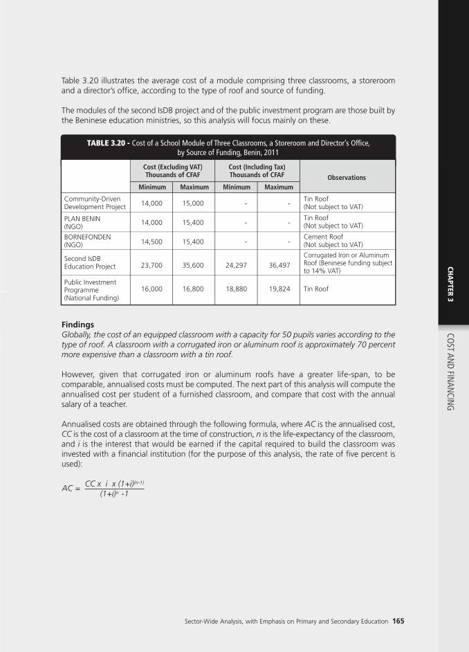
Sector-Wide Analysis, with Emphasis on Primary and Secondary Education 165
CHA
PTER3
COST AN
D FINAN
CING
Table 3.20 illustrates the average cost of a module comprising three classrooms, a storeroomand a director’s office, according to the type of roof and source of funding.
The modules of the second IsDB project and of the public investment program are those built bythe Beninese education ministries, so this analysis will focus mainly on these.
TABLE 3.20 - Cost of a School Module of Three Classrooms, a Storeroom and Director’s Office,by Source of Funding, Benin, 2011
Community-DrivenDevelopment Project
PLAN BENIN(NGO)
BORNEFONDEN(NGO)
Second IsDB Education Project
Public Investment Programme(National Funding)
14,000
14,000
14,500
23,700
16,000
15,000
15,400
15,400
35,600
16,800
-
-
-
24,297
18,880
-
-
-
36,497
19,824
Tin Roof(Not subject to VAT)
Tin Roof(Not subject to VAT)
Cement Roof(Not subject to VAT)
Tin Roof
Corrugated Iron or AluminumRoof (Beninese funding subjectto 14% VAT)
Cost (Excluding VAT)Thousands of CFAF
Minimum Maximum MaximumMinimum
Cost (Including Tax)Thousands of CFAF Observations
Cost (Excluding VAT)Thousands of CFAF
Minimum Maximum MaximumMinimum
Cost (Including Tax)Thousands of CFAF Observations
FindingsGlobally, the cost of an equipped classroom with a capacity for 50 pupils varies according to thetype of roof. A classroom with a corrugated iron or aluminum roof is approximately 70 percentmore expensive than a classroom with a tin roof.
However, given that corrugated iron or aluminum roofs have a greater life-span, to becomparable, annualised costs must be computed. The next part of this analysis will compute theannualised cost per student of a furnished classroom, and compare that cost with the annualsalary of a teacher.
Annualised costs are obtained through the following formula, where AC is the annualised cost,CC is the cost of a classroom at the time of construction, n is the life-expectancy of the classroom,and i is the interest that would be earned if the capital required to build the classroom wasinvested with a financial institution (for the purpose of this analysis, the rate of five percent isused):
AC = CC x i x (1+i)(n-1)
(1+i)n -1

166 EDUCATION SECTOR ANALYSIS METHODOLOGICAL GUIDELINES - Volume 1
FindingsEven when taking the life-span into account in the computation of annualised costs, the tin roofoption looks more cost-effective. As an example, in primary education the tin roof option coststhe annual equivalent of 48.6 percent of the average annual teacher salary whereas the otheroption costs 63.3 percent.
TABLE 3.21 - Annualised Cost of a Furnished Classroom, Based on the Type of Roof, Benin, 2011
Corrugated Ironor Aluminum Roof
Tin Roof
12,536
7,324
35
20
729,111
559,701
14,582
11,194
0.633
0.486
0.866
0.665
Cost Including Tax(Millions of
CFAF)
Life-span(Years)
By Classroom By Pupil * Lower Sec.Primary
Annualised Cost(Thousands of CFAF)
Annualised Cost per Pupil(Multiple of the AverageAnnual Teacher Salary)
Lower Sec.Primary
Annualised Cost per Pupil(Multiple of the AverageAnnual Teacher Salary)
CostIncluding Tax(Millions of
CFAF)
Life-span(Years)
By Classroom By Pupil *
Annualised Cost(Thousands of CFAF)
Note: Considering class capacity of 50 pupils.

Sector-Wide Analysis, with Emphasis on Primary and Secondary Education 167
NOTES
18 The public expenditure cycle (approval, commitment, payment and so on) is relatively complex and long, and some typesof spending cannot be executed for purely technical reasons.
19 These indicators are furthermore part of the indicative framework of the Global Partnership for Education (previouslythe EFA FTI Fast Track Initiative).
20 In several Anglophone SSA countries, capital expenditure is often referred to as development expenditure in budgetdocuments.
21 When one or several education levels have changed their ministerial affiliation various times over recent years, theevolution of the education ministries’ institutional framework over the years covered by the analysis will enable theanalyst to establish where to obtain the information required to reconstitute the spending for each education level.
22 Even when this is the case, such funding is often classified as investment expenditure in national budgets.
23 There are two variants to these execution modes: (i) execution by delegated public works agencies, which is similar tothe execution by companies, and (ii) community-led development, which combines the approaches mentioned.
CHA
PTER3
COST AN
D FINAN
CING

168 EDUCATION SECTOR ANALYSIS METHODOLOGICAL GUIDELINES - Volume 1
© W
orld
Ban
k /
Régi
s L’
Hos
tis

CHAPTER 4QUALITY, SYSTEMCAPACITY ANDMANAGEMENT › Chapter Objective:To offer approaches to the analysis of:(i) learning outcomes and achievements andtheir evolution, offering a selection ofmeasurement indicators; (ii) system capacityfor converting resources into results, and of institutional arrangements and monitoringtools for results-based management; (iii) the management of teacher recruitment,training and posting; and (iv) the managementof other educational resources and of teaching time.
Sector-Wide Analysis, with Emphasis on Primary and Secondary Education 169
CHA
PTER 4Q
UALITY, SYSTEM CAPACITY AN
D MAN
AGEM
ENT

170 EDUCATION SECTOR ANALYSIS METHODOLOGICAL GUIDELINES - Volume 1
1. ASSESSMENT OF STUDENT LEARNING
ISSUEDoes the national education system transfer knowledge as expected? How do learning outcomescompare with those of other countries? How have learning outcomes evolved over recent years?
OBJECTIVES• Study the progress in students’ learning achievements; and• Compare the average student learning with that of comparable countries.
METHODS• Compare the average level of learning outcomes in time through the evolution of average
success rates at national exams and national and international assessments; and • For international comparisons, use the results of standardised assessments carried out by
international programmes and compare the effectiveness of education systems in achievingsustainable literacy.
SOURCESNational exam results data, international assessments of learning outcomes data, and householdsurvey data.
2. ANALYSIS OF SYSTEM CAPACITY
ISSUEWhat is the education system capacity for converting resources into results? What reforms shouldbe implemented to improve students’ learning achievements in the most cost-efficient way? Doadditional resources allocated to schools translate into increased learning outcomes? What toolsand institutional processes exist to promote results-based management (institutional analysis)?
OBJECTIVES• Evaluate the conversion of resources used by schools into learning outcomes by comparing unit
costs and results;• Identify school-level administrative practices and policies that are most effective in improving
quality; analyse the cost-efficiency of different resource usage options in improving learningoutcomes; and
• Carry-out institutional analysis. Evaluate the system’s capacity to identify the efficient andinefficient schools and to use monitoring tools and incentive frameworks for results-basedmanagement.
METHODS• Assess the existence of a correlation between the level of learning outcomes and the resources
available to each school; • Use econometric models that explain student and school success rates according to different
school inputs to identify those factors the most associated with learning achievements. Carryout a cost-efficiency analysis by comparing the cost of different inputs with their estimatedcorrelations with learning outcomes.
• Use institutional analysis qualitative tools to evaluate accountability mechanisms and incentiveframeworks (school inspections, the involvement of school management committees and PTAs,the transparency of information on school performance and so on); and

• Assess the monitoring tools used to compare the performance of different schools and toimplement an incentive framework and results-based management system.
SOURCESSchool data, international standardised learning assessment, national exam results data, thefinancial data produced through the analysis described in Chapter 3, and interviews ofstakeholders.
3. MANAGEMENT OF TEACHERS
ISSUEWhat are teacher recruitment needs? What is the attrition rate? How adequate are nationalcapacities in terms of basic and ongoing teacher training to respond to those needs? Is suchtraining of quality? Is the distribution of teachers among schools aligned with the number ofstudents? What is the level of teachers’ job satisfaction? What social and politico-economic contextfactors affect the profession?
OBJECTIVES • Estimate recruitment and training needs, and the system’s capacity to meet them; • Assess the quality of available training; • Check if the teachers allocated to schools bear effective relation to the number of enrolled
students and if certain regions or schools are disadvantaged in this respect; and• Evaluate teachers' level of job satisfaction as well as the social context of the profession.
METHODS• Calculate the number of untrained teachers (or those needing skills upgrades) as well as the
number of new recruits to train, considering the attrition rate, and compare the figures obtainedwith the places available in teacher training institutes;
• Use quantitative and qualitative surveys to assess the effectiveness of teacher training courses; • Analyse the consistency in teacher postings (and the allocation of other resources) among schools
through the R² coefficient, plotting the number of students against the number of teachers andthrough the qualitative analysis of institutional procedures; and
• Use quantitative and qualitative surveys to assess teachers’ job satisfaction and the profession’ssocial context.
SOURCESTeacher training institute data, school data (on students, teachers), administrative manuals andofficial teacher recruitment and posting procedures, sample surveys that assess teacherabsenteeism and teaching/learning time, qualitative surveys of teachers’ job satisfaction andconsultation processes.
▶
Sector-Wide Analysis, with Emphasis on Primary and Secondary Education 171
CHA
PTER 4Q
UALITY, SYSTEM CAPACITY AN
D MAN
AGEM
ENT

172 EDUCATION SECTOR ANALYSIS METHODOLOGICAL GUIDELINES - Volume 1
4. MANAGEMENT OF OTHER RESOURCES AND OF TEACHING TIME
ISSUEIs the distribution of other resources (subsidies, textbooks, equipment and so on) among regionsand schools equitable? What is the actual annual teaching time and what are the factorscontributing to its reduction?
OBJECTIVES • Assess the extent to which the financial and physical resources allocated to schools bear effective
relation to the number of enrolled students and if certain regions or schools are disadvantagedin this respect; and
• Estimate the extent and causes of loss of learning time.
METHODS• Analyse the consistency in the allocation of educational resources among schools through the
R² coefficient, plotting the number of students against the number of these resources andthrough the qualitative analysis of institutional procedures; and
• Use specific sample surveys to estimate effective teaching time and analyse the possible causesfor the difference with the theoretical number of hours or days.
SOURCESSchool data (on students, textbooks, subsidies and so on), administrative manuals, sample surveysthat assess teaching/learning time.

Sector-Wide Analysis, with Emphasis on Primary and Secondary Education 173
IntroductionIncreasing the number of enrolled children is crucial but insufficient. It is also necessary thatchildren gain effective knowledge. At the primary level, EFA Goal 6 indeed enshrines this,with the aim of “Improving all aspects of the quality of education.” International researchhas also shown that the improvement of the quality of teaching is associated with economicgrowth.24
What is quality in education and how can it be measured? All too often the measurementof quality is assimilated with the resources used to achieve it, such as the student-teacherratio or the level of teachers’ qualifications. The choice of such approaches is generallyexplained by a lack of comparable information on learning achievements for differentcountries. However, even if this seems counter-intuitive, the empirical link between schoolresources and learning outcomes is usually weak.25 Most studies at the micro or macro levelindeed show that much as the level of resources has an impact, this is slighter than theeffectiveness in the use of such resources in explaining differences in learning outcomes. Itis therefore unsatisfactory to use resource indicators instead of results indicators when theseare unavailable.
It is also tempting to use internal efficiency indicators (such as intra-cycle drop-out rates) tomeasure quality. Although such indicators are important to evaluate education systems interms of student flows, they are inadequate to assess the level of students learningachievements at each education level: the relationship between dropout or repetition ratesand learning achievements is not empirically proven. Indeed, the weakness of learningachievements is only one possible cause for dropout. The actual measurement of learningoutcomes is therefore of particular importance.
Section 1 focuses on the assessment of learning outcomes, through a variety of tools, eachaiming to assess the level of knowledge and skills acquired, although with differentobjectives and interpretations. Section 2 aims to analyse system capacity and to identifyfactors linked to improvement of learning outcomes, especially in terms of resourcesavailable in the schools. It proposes an indicator that measures the effectiveness of the useof educational inputs at the school level, presents a method for the identification andanalysis of the factors having a verified relation with students’ learning achievements,discusses how to identify the most cost-effective factors, and offers an approach to thequalitative analysis of institutional and pedagogical management mechanisms (institutionalanalysis). Section 3 then deals with the management of the teaching force, whichconstitutes the most central input, in its quantitative and qualitative aspects; of theseresources. Finally, Section 4 examines methods of assessing the management of othereducational resources and of the teaching time.
CHA
PTER 4Q
UALITY, SYSTEM CAPACITY AN
D MAN
AGEM
ENT

174 EDUCATION SECTOR ANALYSIS METHODOLOGICAL GUIDELINES - Volume 1
TABLE 4.1 - Summary Description of Learning Outcomes Assessment Usually Availablefor Education Sector Analysis
National ExaminationsandAdmissionsTests
Comprehensive Education Ministry
Success Rate - Enable historical comparisons *- Reflect curricula content- Usually available for all education levels, including TVET
- Only cover end-of-cycle grades- International comparisons are not possible- Data is rarely available at the student level
National Assessments
Comprehensiveor Sample
Education Ministry
Assessment Score
- Enable to assess learning outcomes at any level/grade- Reflect curricula content- Data often available at the student level
- International comparisons are not possible- Performed irregularly
StandardisedInternationalAssessments
Sample InternationalOrganisationsand EducationMinistry
AssessmentScore
- Enable international comparisons through standardised tests
- Performed irregularly- Only partially reflect curricula content
Assessmentsof LiteracyLevels throughHouseholdSurveys
Sample NationalStatisticalInstitutes
Literacy Levels (canread “with difficulty,”“fluently” or “cannotread”) of individualshaving followedschool for X numberof years during theiryouth
- Enable international comparisons in some circumstances
- Only measure literacy- Provide an approximate measure of the quality of education offered some time ago
CoverageType ResponsibleInstitution
Commonly UsedMeasure
Pros Cons
Contextual andNon-School Factors
Educational Policyand School Factors
ASSESSMENT OF STUDENTLEARNING
Four types of learning assessment may be used in the context of a sector analysis, and arecomplementary: (i) national examinations; (ii) national assessments; (iii) internationalstandardised assessments; and (iv) household surveys.26 Each category aims to assess thelevel of knowledge and skills acquired, although with different objectives and
Note: To ensure that data is historically comparable, ensure that the marking system does not change from year to year.
SECTION
1

Sector-Wide Analysis, with Emphasis on Primary and Secondary Education 175
interpretations. Before providing examples of their respective uses, Table 4.1 presents asummary of their general characteristics as well as their pros and cons.
For all these assessments, when they are considered over several years, changes in resultsshould be interpreted with caution, in particular when, like in many African countries,enrolments have increased sharply. Results can indeed show a decrease in learningoutcomes, or at least a slower increase than expected. This can be the consequence of a adecline in the quality of the learning conditions (typically greater class sizes or loweravailability of learning materials). But most of the time part of this decrease in results islinked to the fact that, as the coverage of the system improves, more vulnerable children,with less favourable socio-economic and family backgrounds, are now in school and partof the assessment. It will therefore be important to consider the evolution of measuredlearning outcomes in the context of the enrolment increases happening concurrently andto interpret these results accordingly.
Finally, it can be interesting to note that some tests are designed to assess students' specificknowledge or skill (criterion-referenced tests), while some others (norm-referenced test) aremeant to capture the differences between students, based on their knowledge or skills. Theformer kind is often more useful as a regular assessment, to control students' learningagainst the curricula, while the latter, identifying stronger and weaker students, can be morepowerful to identify factors underlying better results in some students.
NATIONAL EXAMINATIONSAND ADMISSIONS TESTS
National exams and admissions tests are designed to fulfill various functions: (i) evaluatethe knowledge/skills acquired by students and thus monitor schools’ learning achievements;(ii) validate each student’s knowledge level and issue an appropriate qualification (for exams);and (iii) select the best students for admission to a given education level or course whereplaces are limited (for admissions tests, although in some countries exams also fulfill thisfunction).
Data on exams and admissions tests are a transversal measure of the level of learningachievements for each cycle, given that they are sat at the end of each. In the context ofsector analysis, national exam and admissions test results (success rates) are not appropriatefor the purpose of international comparisons, as school programmes and exam content varyfrom one country to another. On the other hand, they can be useful to provide historicalperspectives. In that case, it is important to clearly establish that the level of difficulty of thepapers and the severity of marking practices have not changed significantly, which is notoften the case, especially when exams are also used as admission tests to the following
1.1
CHA
PTER 4Q
UALITY, SYSTEM CAPACITY AN
D MAN
AGEM
ENT

EXAMPLE 4.1
176 EDUCATION SECTOR ANALYSIS METHODOLOGICAL GUIDELINES - Volume 1
cycle: the success rate is then determined by the number of seats available rather than theknowledge or skills of the students. Even when the exam is not used as an admission test,political pressures can push governments to alter their difficulty to improve the passing ratesfor instance.
Example 4.1 below, drawn from the Tanzania CSR, shows how to present and interpret theanalysis of the evolution of secondary education exam success rates. The analysis includesthe comparison of the results obtained by government school candidates and those sittingthe exam as private candidates.
(Historical Analysis of Exam Results): Evolution of Certificate of Secondary Education Examination (CSEE) Results, Tanzania, 2000-09Source: Adapted from Tanzania CSR, 2012.
90
80
70
60
50
40
30
20
10
39
78
63
40
64
77
58
77
86
77
8792
70
8389
72
8289
79
8690
59
72
78
54
70
66
73
8488
2000 2001 2002 2003 2004 2005 2006 2007 2008 2009
Private Candidates School Candidates Average
FIGURE 4.1 - CSEE Pass Rates, by Type of Candidate, Tanzania, 2000-09
Pass
Rat
e (%
)
The Certificate of Secondary Education Examination (CSEE) is administered at the end of O–Level(lower secondary). Candidates sit between seven and ten subjects, chosen among: Civiceducation, Kiswahili, English, Mathematics, Social sciences, Technical sciences, Natural sciences,Commercial or Home economics, and various foreign languages. The CSEE is also open to privatecandidates that register directly at the central level. CSEE candidates are awarded an overallgrade called a Division. Divisions I, II, III and IV constitute a pass and Division 0 constitutes a fail.The Division given to a student depends on the number of passes (a pass refers to a grade fromA to D in the subject) obtained in the seven better performed subjects. The CSEE pass ratetherefore refers to the number of candidates who obtained a Division I, II, III or IV over thenumber of candidates who sat the exam.

Sector-Wide Analysis, with Emphasis on Primary and Secondary Education 177
FindingsAfter an increase from 2000 to 2004, CSEE pass rates have shown signs of deterioration overthe 2006 to 2009 period, falling under the 80 percent threshold in 2008, and reaching 66percent in 2009. Private candidates’ pass rates are particularly low, systematically lagging behindthose of school candidates: in 2009, only 54 percent of private candidates passed. Although theproportion of school candidates who passed is better (70 percent), it is lower than in 2007 (90percent). Several reasons might account for this drop: (i) the introduction of the new curriculumin 2005 that was probably not adequately mastered by teachers at the time, given that nosystematic and comprehensive training was conducted; (ii) the lack of alignment of the examquestions with the new curriculum; (iii) the more heterogeneous student backgrounds, resultingfrom the expansion of the secondary level, potentially leading to greater access of students withlearning difficulties; and (iv) tougher marking criteria, associated with the limited number of A-Level seats available.
NATIONAL LEARNING ASSESSMENTS
National assessments can be administered in two ways: (i) on the basis of a representativesample of students; or (ii) comprehensively, covering the entire population group to beevaluated. They enable the measurement of the average level achieved by the educationsystem at a given level in one or several subjects (such as that of primary Grade 4 studentsor that of students aged 11 years) in the light of curriculum content. The assessment isbased on students sitting a standardised test, evaluating knowledge/skill levels withouthaving to wait for the end-of-cycle exam. They therefore shed light on students’ mastery ofcurricula, and can inform policy makers of the results sufficiently early in the cycle toimplement corrective measures where required.
As long as the level of difficulty of the tests does not vary significantly, two consecutiveassessments conducted at the same grade can be used to provide a historical perspectiveof progress in learning outcomes. However, the frequency of such assessments varies fromcountry to country; indeed they are often irregular, and do not offer a basis for internationalcomparisons. The following example, drawn from the Mali CSR, presents the results of anational assessment of the learning achievements of primary Grade 2, Grade 4 and Grade6 students in language and math. The assessment presents the advantage of providing theproportion of students achieving each level of knowledge, such as defined by the EducationMinistry’s pedagogical team. When presenting the analysis, it might be useful to introducebriefly (or at more length in an annex) the meaning of the minimum or reference levelsreferred to in this analysis, in order to provide the reader with a better understanding ofthe level of knowledge that is being measured.
1.2
CHA
PTER 4Q
UALITY, SYSTEM CAPACITY AN
D MAN
AGEM
ENT

EXAMPLE 4.2(Analysis of Knowledge Acquired throughout a Cycle throughNational Assessments): Results of the Primary Cycle NationalAssessment, Mali, 2007Source: Adapted from Mali CSR, 2012.
178 EDUCATION SECTOR ANALYSIS METHODOLOGICAL GUIDELINES - Volume 1
INTERNATIONAL STANDARDISED LEARNINGASSESSMENTS
By definition, the advantage of international assessments is that they enable the comparisonof students’ results from one country to another. It is therefore very helpful to use such datain the context of sector analysis, to place the average level of knowledge/skills acquired bythe children of the country of interest in an international perspective. These assessments are
TABLE 4.2 - Average Scores and Knowledge Levels in Language and Math,Primary Grades 2, 4 and 6, Mali, 2007
Language and Communication
Grade 2
Grade 4
Grade 6
Mathematical and
Technological Sciences
Grade 2
Grade 4
Grade 6
1,388
1,438
1,217
1,388
1,438
1,217
49.6
47.8
62.4
41.8
45.5
49.0
28.1
25.4
22.3
27.6
24.5
23.6
53.2%
57.0%
25.6%
61.3%
54.9%
52.8%
11.1%
28.0%
46.6%
27.8%
36.0%
34.2%
35.7%
15.0%
27.8%
10.9%
9.0%
13.0%
Levels of knowledgeAverage Scores
AverageScores(/100)
StandardDeviation
Below theMinimum
Level
MinimumLevel
Above theMinimum
Level
Enrolment
Contextual andNon-School Factors
Educational Policyand School Factors
The National Centre for Education carried out an assessment of learning achievements in primaryschools in 2007, for both language and communication, and mathematical and technologicalsciences. The assessment covered a representative sample of Grade 2, Grade 4 and Grade 6 students.
FindingsThe evaluation shows that a large share of students are in difficulty, especially in Grades 2 and4 in language and communication, and in all three grades in mathematical and technologicalsciences. Furthermore, the levels achieved vary greatly among students. Results show thatprimary students’ results are generally weak at the beginning of the cycle, but improve towardsthe end, probably because of weaker students dropping out. Indeed, Grade 6 students obtainbetter average results in both subjects than Grade 2 and 4 students, in as much as their averagescore is higher, and students’ results are more homogenous.
1.3

EXAMPLE 4.3
Sector-Wide Analysis, with Emphasis on Primary and Secondary Education 179
(International Comparative Analysis of Learning Outcomes throughInternational Assessments): Malawi and other Anglophone AfricanCountries’ Math and Reading Results, 2007Source: Adapted from the Malawi CSR, 2010.
FindingsCompared to other countries, Malawi fares poorly, being at the bottom of all the SACMEQcountries in English reading and next to last in mathematics (Figure 4.2). Students were amongthe lowest achievers in the region, suggesting that Malawi provided the lowest quality of primaryschooling.
18,6
Seychelles
Mauritius
Kenya
Tanzania
Mozambique
Swaziland
Botswana
AVERAGE
Uganda
South Africa
Lesotho
Zanzibar
Namibia
Zambia
Malawi
0 100 200 300 400 500 600 700
FIGURE 4.2 - SACMEQ Reading and Mathematics Scores, 2007
English ReadingMathematics
usually carried out on a representative sample of students. Their administration is generallyassisted by international institutions in the context of multi-country programmes that usestandardised tests in each participating country. The following example, drawn from theMalawi CSR, shows how to use SACMEQ data to analyse the average level of primarystudents in math and reading, within an international perspective.
CHA
PTER 4Q
UALITY, SYSTEM CAPACITY AN
D MAN
AGEM
ENT

180 EDUCATION SECTOR ANALYSIS METHODOLOGICAL GUIDELINES - Volume 1
At the global level, the Learning Metrics Task Force (LMTF), supported by the UNESCOInstitute of Statistics (UIS) and Brookings Institute (Centre for Universal Education), has beenestablished to improve the measurement of learning globally. The work of the taskforce hasbeen underpinned by working groups of experts and global consultations and has identifiedseven domains for learning: i) Physical well-being; ii) Social and emotional; iii) Culture andthe arts; iv) Literacy and communication; v) Learning approaches and cognition; vi)Numeracy and mathematics; and vii) Science and technology. The taskforce uses, as itsstarting point, the existing international and regional learning assessment programmes,namely: Early Grade Assessment (EGRA), Early Grade Math Assessment (EGMA), LiteracyBoost, Annual Status of Education Report (ASER), UWEZO, Latin American Laboratory forAssessment / Laboratorio Latinoamericano de Evaluacion de la Calidad de la Educacion(LLECE), Progress in International Reading Literacy Study (PIRLS), Programme for InternationalStudent Assessment (PISA), Trends in International Mathematics and Science Study (TIMSS),Literacy Assessment Monitoring Programme (LAMP), the Programme for the Analysis ofthe Educational Systems of CONFEMEN Countries (PASEC) and the Southern and EasternAfrica Consortium for Monitoring Educational Quality (SACMEQ).27 These internationalprogrammes vary according to the education level and the subject being evaluated. Whena country has participated in such a programme more than once, the results can also beused to provide an historical perspective of students’ results, having previously checked thatthe difficulty of the tests has not changed over time.
USING HOUSEHOLD SURVEYS AND LITERACYLEVELS AS A PROXY MEASURE OF QUALITY
In as much as: (i) literacy is a fundamental dimension of students' learning in basic educationand (ii) household surveys can help establish a relationship between the level of literacy andthe number of years of schooling completed during youth, it is possible to use such data tocomplement the analysis of country learning outcomes based on school exams and nationaland international assessments. Countries can then be compared on the basis of theprobability of being literate for individuals having completed the same number of years ofeducation, providing a further measure of effectiveness, or quality.
Many developing countries (in Africa especially) carry out large-scale household surveys(samples include 20,000 to 30,000 individuals) as well as Multiple Indicator Cluster Surveys(MICS, promoted by UNICEF), Demographic and Health Surveys (DHS), or Core WelfareIndicator Questionnaire (CWIQ) surveys. These surveys provide information on: (i) Individuals’literacy levels, and (ii) their schooling careers. Crossing these two data sets allows one toestimate the likelihood of literacy according to the number of years of schooling througheconometric models, and thus reach a measure of the correlation of these years of educationwith sustainable literacy. Some surveys (MICS especially) provide even more detailedinformation on the level of reading skills (“reads fluently,” “reads with difficulty,” “cannotread at all”) by having survey respondents take short tests.28
1.4

Sector-Wide Analysis, with Emphasis on Primary and Secondary Education 181
Given that the aim is to analyse the long-term sustainability of the literacy levels achieved,adults aged 22 to 44 years are generally used for the analysis, to establish if they haveretained the reading skills acquired at school.29 As for the analysis of the impact of educationon social outcomes (See Chapter 5), econometric modelisation is the methodological toolto be used here, which enables an estimation of the net effect of the number of years ofschool on the level of literacy, while holding other factors constant (area of residence, age,income level and so on). The results of the econometric model can then be used to simulatethe evolution of the probability of sustainable literacy according to the number of years ofschooling completed, all other things being equal. Two complementary indicators can thenbe computed to facilitate international comparisons:
1) The simulated probability of literacy for individuals having completed just six years ofschooling (the length of the primary cycle in most countries). This provides a measure ofthe gross long-term production of the cycle, meaning that it estimates the quality of thehuman capital at the end of the cycle, regardless of where individuals developed theirliteracy skills (in or out of school); and
2) The added value provided by the primary cycle is the difference in the probability ofliteracy for individuals with six years of schooling and those without any education.Indeed, in some countries individuals may be literate without having attended school,and thus a share of literacy (that varies from country to country) is the result of factorsother than schooling. Comparing countries on the basis of the value added thereforeenables one to underline the benefits the primary cycle provides, over and above otherfactors of development of human capital.
The limitations of these indicators are that: (i) they only contemplate one of the skills schoolprogrammes aim to impart, that pertaining to reading; (ii) they shed greater light on thequality of education systems in the past than in the present;30 and (iii) they are sensitive tonon-school contexts that may be more or less favourable to the retention of literacy skillsaccording to the country.31 However, while this means that the indicator will not onlymeasure the effect of the education provided in school, it does inform on the whole learningprocess which happens in an individual's life, which is relevant to the goal of developingeducation and knowledge in general.
The following example, drawn from The Gambia CSR, shows how to present and interpretthe results of such an analysis, based on MICS (2000) household survey data.
CHA
PTER 4Q
UALITY, SYSTEM CAPACITY AN
D MAN
AGEM
ENT

EXAMPLE 4.4
182 EDUCATION SECTOR ANALYSIS METHODOLOGICAL GUIDELINES - Volume 1
(Use of Literacy Rates to Assess Learning Outcomes): Adult Literacy Levels by Number of Years of Education, International Comparison, 2000-05Source: Adapted from The Gambia CSR, 2011.
Adu
lt Li
tera
cy R
ate
(%) x
x
100
80
60
40
20
00 1 2 3 4 5 6 7
x x xx
x
x
x
x
8 9
FIGURE 4.3 - Adult Literacy According to Schooling Completed, Selected Countries, 2000-05
Highest Grade Attained
x
Rwanda
Mozambique
Gambia, The
Mali
Average
Literacy levels provide a first idea of the sustainable learning achievements an education systemproduces, considering that one of primary school’s main objectives is to ensure that studentsbecome fully literate. In this context, the number of formal years of schooling needed to producesustainably literate individuals can be used as a measure of the quality of the primary educationsystem: the shorter the schooling required, the higher the quality of the system. A majorconstraint of the literacy analysis is that it is based on the ability of the adult population, andthus reflects the past quality of the education system, not present performance.
Findings The current literacy analysis is based on the 2000 Multi Indicators Cluster Survey (MICS, 2000).It should be interpreted with caution as it is based on information as reported by interviewees(both men and women aged 15 years and above) about their literacy skills and abilities. It showsthat after six years of schooling, barely 45 percent of the adult population were able to readwithout difficulty, a share considerably lower than the average of a sample of 32 Sub-SaharanAfrican countries, of close to 70 percent (See Figure 4.3). This result highlights significantweaknesses in the past primary education system as far as basic learning outcomes areconcerned. The result for Rwanda, with a literacy rate of 98 percent, shows that it is possible toachieve lifelong literacy for the vast majority of students through six years of primary education.
Note: Adult literacy here refers to those adults who can read without difficulty. The average is of 32 SSA countries.

Sector-Wide Analysis, with Emphasis on Primary and Secondary Education 183
CHA
PTER 4
ANALYSIS OF SYSTEM CAPACITY
Section 2 reviews the evaluation of the relationships between human and material resourceson the one hand and improvement of learning outcomes on the other hand. Variousquestions arise: How effective is the conversion of resources into results? What inputs aremost associated with learning outcomes? What resources are most cost-efficient in learningterms? What institutional and technical mechanisms and tools are available for results-basedpedagogical management?
This section aims to provide some answers to these questions. It begins with the comparisonof resources provided to schools with the results on the learning assessment presentedabove. It then explores methods for the identification and analysis of the factors associatedwith students’ learning achievements, and discusses how to identify the most cost-effectivefactors. Finally, it presents an approach to the qualitative analysis of institutional andpedagogical management mechanisms as well as some results-based managementmonitoring tools (institutional analysis).
EVALUATION OF THE CONVERSION OF RESOURCESINTO RESULTS BY SCHOOLS
Like for so many aspects of an education system, the average results in the learningassessments presented in Section 1 tend to hide wide differences between regions, schoolsand students. Because one of the first reflexes is to attribute the weak results to a lack ofresources, it is important to test this assumption against the data. In the context of a givencountry’s education sector analysis, it is thus advisable to estimate the extent to which schoolresults are correlated to the resources available to them.
A simple, and often naïve, way of approaching learning results consists of assuming that inan ideal education system, a school that receives more resources performs better (assumingthat schools operate in similar contexts). According to this logic, a high degree of correlationwould be expected between the level of learning achievements and resources for schoolsin similar contexts. The higher the correlation coefficient, the better the transformation ofresources into results (efficiency). Conversely, a weak coefficient indicates that efficiency isweak and that the allocation of additional resources will not be sufficient to improve results,for which pedagogical management must also be improved.
SECTION
2
2.1
QUALITY, SYSTEM
CAPACITY AND M
ANAG
EMEN
T

EXAMPLE 4.5
184 EDUCATION SECTOR ANALYSIS METHODOLOGICAL GUIDELINES - Volume 1
The analytical approach consists of representing schools (in similar circumstances, forinstance, schools in the same district or in districts with similar socio-economiccharacteristics) on a scatter plot chart, with the available resources on the x-axis, oftenmeasured by per student annual unit costs, and results on the y-axis, measured by a school’saverage score at a standardised assessment or its success rate at an exam.32 Example 4.5illustrates this method, based on the Guinean case.
(Analysis of the Conversion of Resources into Results): School Performance and Resources, Guinea, 2003/04Source: Adapted and translated from the Guinea CSR, 2005.
100%
90%
80%
70%
60%
50%
40%
30%
20%
10%
0%0 50,000 100,000 150,000
End
of p
rimar
y cy
cle
Exam
Suc
cess
Rat
e
Recurrent Unit cost per student (in Guinean Francs)
FIGURE 4.4 - Unit Costs and Exam Success Rates, Government Schools, Guinea, 2003/04
This graphical analysis presents the relationship between unit costs and the success rate at theprimary school leaving exam on a school by school basis (See Figure 4.4 below).
FindingsFigure 4.4 shows both: (i) a high degree of variation in unit costs among schools, from 35,000Guinean Francs to over 100,000 Guinean Francs at the primary level; (ii) a similarly high degreeof variation in exam success rates, that range from 0 percent to 100 percent; and last but notleast that (iii) there is no apparent correlation between these two indicators: schools with higherunit costs do not always achieve better results, and those with the lowest results are not alwaysthe ones with least resources.

Sector-Wide Analysis, with Emphasis on Primary and Secondary Education 185
Such results tend to raise an alarm over the capacity of the system to transform resources(with a cost) into results (especially in terms of learning). There are in fact a number ofreasons why the relationship between cost and results is very weak. For instance, the unitcost is often strongly driven by the teacher cost, and thus the pupil-teacher ratio in eachschool; the cost of other inputs is often marginal compared to the teacher cost, and theirpotential effect is often less visible on such a general overview. More importantly, a numberof factors influencing learning achievements cannot be directly (or at least easily) associatedwith a cost (pedagogical approaches, instruction time…). This calls for a more in-depthanalysis of these factors, and of the institutional and pedagogical mechanisms involved inthe transformation of resources into results.
ANALYSIS OF THE FACTORS ASSOCIATED WITHLEARNING OUTCOMES
Several factors influence the learning process at the school level. Figure 4.5 shows atemporal model of the production of knowledge/skills and illustrates how diverse factorscan influence students’ results.
FIGURE 4.5 - The Causal Analysis of Learning Outcomes
Contextual andContextual andNon-School FactorsNon-School Factors
Contextual andNon-School Factors
Final LevelInitial Level
Educational PolicyEducational Policyand School Factorsand School FactorsEducational Policyand School Factors
Note: The solid line arrows represent the relationships that are often studied whereas the dotted line arrows represent those that areusually not.
2.2
CHA
PTER 4Q
UALITY, SYSTEM CAPACITY AN
D MAN
AGEM
ENT

186 EDUCATION SECTOR ANALYSIS METHODOLOGICAL GUIDELINES - Volume 1
In this figure, the factors of learning outcomes are split into two categories: contextual (ornon-school) factors, and educational policy (or school) factors.33
1) Contextual or non-school factors are those that relate to the environment beyondschool and upon which education policy-makers have little power to act in the shortterm, including children’s personal characteristics, their family context, or the socialstatus of their parents. Although such factors can be highly associated with learningoutcomes, and social policies addressing them do exist, they usually fall beyond thescope of education policy.
2) Educational policy and school factors do fall within the field of action of educationpolicy makers on the other hand. They include school infrastructure, the learningmaterials, the professional characteristics and teaching modes, the monitoring ofteaching staff and so on. These factors are usually presented as key determinants oflearning outcomes, in as much as they affect the very heart of the learning process.
The arrows of Figure 4.5 illustrate relationships that may be current or historical. The arrowsrepresent the process of how these factors affect learning outcomes. Students’ earlierschooling and other historical factors appear as significant in the learning process at a givenpoint in time. If the influence of this educational heritage is unquestionable, it is neverthelessdifficult to obtain historical information on past school and non-school factors affectingstudents’ learning process.
When some of the main factors affecting the learning process cannot be considered in theanalysis, mistaken conclusions could be reached with respect to the effect of those factorsthat are considered. It is therefore necessary to use analysis techniques capable ofsimultaneously accounting for the main factors affecting the learning process and isolatingtheir net impact, independently of the effect of other factors. In the literature, a variety ofnames are used to qualify this effect: the net impact, the net effect and so on. For simplicity’ssake in this guide, the term impact is often used without the qualifying term net.
It is important to note that most methods generally used to identify factors which have aninfluence on learning outcomes are actually based on the analysis of the correlationsbetween the occurrence of these factors and better, or lower, results. It is thus crucial toremember that this type of analysis is essentially descriptive, and that a lot of caution shouldbe exercised when trying to attribute causality in these relationships: the analysis may showthat such a factor is linked with higher results, but that factor may not be the cause of thebetter results; they can for instance both be the consequence of a common cause. Sub-section 2.2.2 indicates methods which allow for a better attribution of effects.

Sector-Wide Analysis, with Emphasis on Primary and Secondary Education 187
2.2.1 DESCRIPTIVE MODELS
The issue can be synthetically represented by the following equation, which presentslearning outcomes as a function of a certain number of factors:Y = f (X1, X2, X3, ….., Xk)
Where:- Y represents the level of learning measured by students results (test scores, exam success
rates and so on); and- Each Xk represents a factor whose association with learning outcomes is to be estimated
(school status, teacher qualifications, the availability of textbooks, repetition and so on).
A measure of Y should then be chosen to represent learning outcomes, and the list of Xk
factors to be included in the analysis should be drawn up. The relationship between eachXk factor and Y, materialised by the f function, can then be determined through econometricmodelisation techniques (See Annex 0), and finally the correlation can be analysed todetermine which of the Xk factors are statistically associated with Y and their respectivelevels of significance. The equation is called the production function or the model of learning outcomes, or justthe model.
The Y variableThe different measures of learning outcomes or indicators that can be used to represent Ywere mentioned in Section 1 of this chapter. They mainly include:
- Student-level data: students’ scores at a test or a standardised assessment; the average ofstudents’ results at an exam; exam success or failure rates and so on; and
- School-level data: averages obtained by schools at exams, tests or standardised assessments;schools’ success rates for a given exam and so on.
The Xk variablesFrom whatever the factors that are included in the equation, the analysis of the determiningfactors will eventually isolate those factors that have a net impact from those that do not.The data related to the included factors are generally collected through surveyquestionnaires.34 Generally speaking, this information includes:
- Students’ characteristics: age, gender, ownership of textbooks, repetition status, parents’literacy, socioeconomic status of home, academic support provided at home (help withhomework, participation in domestic chores and so on);
- Teacher characteristics: gender, academic qualifications, training received, degree ofmotivation and so on;
- Type of pedagogical set-up: type of class (single shift, double shift, multi-grade), class size,availability of teachers’ pedagogical material, teaching practices, collaboration amongteachers to resolve pedagogical issues and so on; and
- School profile: school status, school location, nature of the relationship between the
CHA
PTER 4Q
UALITY, SYSTEM CAPACITY AN
D MAN
AGEM
ENT

188 EDUCATION SECTOR ANALYSIS METHODOLOGICAL GUIDELINES - Volume 1
headmaster and teachers, involvement of parents in the management of the school andso on.
Just as a questionnaire is limited, it is not possible to include all the desired factors. Usually,interest determines which variables are given preference over others. To achieve a moreglobal perspective of the range of questions that may be asked, education sector analystsmay consult the questionnaires of assessments such as EGRA / EGMA (Early Grade ReadingAssessment / Early Grade Mathematics Assessment), PASEC (Programme on the Analysis ofEducation Systems in CONFEMEN), or SACMEQ (Southern and Eastern Africa Consortiumfor Monitoring Educational Quality)35. School statistics annually collected by educationministries can also constitute a valuable source of information to determine which Xk factorsto include in the model.
Explanation of the relationship between Xk and YTo clarify the relationship between each Xk factor and Y it helps to consider that the ffunction is linear. The model can then also be described as:Y = a0 + a1X1 + a2X2 + a3X3 + ….+ akXk
The estimation of the coefficients through a linear regression allows estimating the "netimpact" of each of their respective variables (all other variables being equal) that the analysisseeks to determine.
The technique to solve the equation and interpolate the results depends on the nature ofthe Y variable chosen (quantitative or qualitative). Annex 0 on the econometric methodoffers a presentation of the approach to the resolution of the equation and the interpolationof regression results.36
As mentioned earlier, it is often very difficult to reconstitute all the information relating tostudents’ academic history that has an impact on their current achievements at school. Thereare four ways of dealing with this problem: (i) The first consists of considering that students’initial levels constitute an acceptable synthesis of their prior schooling factors (hence itsdistinctive inclusion in Figure 4.5); (ii) A second approach uses synthetic variables to representprior education; (iii) A third approach accepts that it is impossible to include a realistic variablefor prior schooling and conducts the analysis without one, although being careful to takethis into consideration in the interpretation of results; and (iv) finally, the fourth approachuses alternative evaluation designs, such as the randomised impact evaluation (section 2.2.2).
Some learning assessments, such as those carried out by PASEC, organise tests for the samestudents twice a school year: one to establish their initial level at the beginning of the schoolyear and a second, at the end of the school year, to measure their final level and establishthe effective progress during the school year. The incorporation of the initial level as one ofthe explanatory variables in econometric models that modelise the final level then enablesthe measurement of the impact of school and non-school factors for the same initial level.Table 4.3 provides an example of such a modelisation, based on PASEC data, drawn fromthe Mali CSR, 2007.

Sector-Wide Analysis, with Emphasis on Primary and Secondary Education 189
FindingsA first observation of Table 4.3 is the weak degree of determination of the models, which, atthe end of the day, only explain a small part of the fluctuations observed in the consolidatedend-of-year test scores. The share of the variability of the scores that is “explained by the models”is 24 percent for Grade 2. Other explanatory factors of the level of student learning are thus stillto be identified.
Pupils’ initial level is the determining variable that has the greatest weight (the highestcoefficient). Pupils with high initial levels are those who achieve the best final outcomes, all otherthings being equal. Among other individual characteristics, it is of note that girls’ structural
Contextual andNon-School Factors
TABLE 4.3 - Modelisation of Grade 2 Learning Outcomes, Mali, 2006
Student Variables
Initial level
Female gender
Over-age
Repeated Grade 1
Repeated Grade 2
Teacher/Classroom Variables
Teacher Variables
Has the DEF (Basic Studies Diploma)
Has a post-DEF qualification
Has less than a DEF qualification
Contract status (Ref: civil servant)
Basic training of 1 year or more
Basic training of 1 year or less
Basic training of 1 to 3 months
Received complementary training
Classroom variables
Is Double-Shift
Is multi-grade
Class size
Is located in urban area
Constant
0.4258
- 0.0844
0.1241
- 0.1915
- 0.2373
réf
- 0.3281
- 0.3570
0.3034
0.0807
- 0.1997
- 0.0634
- 0.0017
0.1125
0.2181
***
**
**
***
***
ns
ns
**
ns
ns
ns
ns
ns
ns
***
*
*
***
***
ns
ns
ns
***
ns
ns
ns
ns
ns
ns
0.4223
- 0.0780
0.1214
- 0.1989
- 0.2438
réf
- 0.3100
- 0.3440
réf.
0.3032
0.3145
0.0733
- 0.1836
- 0.0657
- 0.0020
0.1346
0.2212
Coefficient
(R2=0.241) (R2=0.242)
Model 1 Model 2
Sig. Coefficient Sig.
Educational Policyand School Factors
Note: *** Statistically significant at the 1% level; ** statistically significant at the 5% level; * statistically significant at the 10% level; ns not significant.
EXAMPLE 4.6(Econometric Modelisation of Prior Schooling Factors): Analysis ofPrior Schooling Factors on the Basis of the Initial Level of Students’Learning Outcomes, Mali, 2006Source: Adapted and Translated from the Mali CSR, 2007.
CHA
PTER 4Q
UALITY, SYSTEM CAPACITY AN
D MAN
AGEM
ENT

190 EDUCATION SECTOR ANALYSIS METHODOLOGICAL GUIDELINES - Volume 1
-0.4 -0.3 -0.2 -0.1 0 0.1 0.2 0.3 0.4 0.5
Initial level
Female gender
Over-age
Repeated Grade 1
Repeated Grade 2
Has a post-DEF qualification
Has less than a DEF qualification
Contract status
Received complementary training
Double vacation
Double-shift
Multi-grade
Number of students
Urban school
FIGURE 4.6 - Net effect of factors linked to learning outcomes (Model 1)
Net Effect
Effect is statisticallysignificant
Effect is notstatisticallysignificant
The previous example is also an illustration of the danger of trying to attribute causality inresults of such regressions. One can thus be tempted to interpret the negative coefficientof repetition in the model as a sign that repetition has a negative effect on learningoutcome, and that reducing repetition would lead to improved results. However, it is muchmore likely that some students have difficulties in schools, for a range of unknown reasons,and that even after repeating, they remain weaker than other students. What is captured
progress is worse than that of boys (negative coefficient close to 10 percent). On the other hand,pupils older than the official school age progress with greater ease.
The employment status and basic training of teachers cannot be considered simultaneously inthe same model, the correlation between the two being too great. Both models considered differtherefore in including one or the other of these variables. Pupils whose teacher has contractualstatus make better progress (30 percent more) than those who are taught by civil servants (Model1). When the status variable is replaced with one describing the basic vocational training,empirical results are just as clear: a short vocational training course (of one to three months) ispreferable to longer training in as much as most pupils whose teacher has followed one suchcourse make better progress (30 percent more) than pupils whose teacher followed longertraining, or had none (Model 2).
Reflections on the status and level of initial training of teachers should not, however, be detachedfrom those touching on issues such as teacher motivation, job stability and career advancement.Complementary training courses on the other hand, are far from producing the expected results:the results of pupils with teachers having followed one or several ongoing training courses areno better than those of pupils whose teachers followed none.
Figure 4.6 provides a graphic illustration of these findings.

Sector-Wide Analysis, with Emphasis on Primary and Secondary Education 191
by the regression is two consequences (repetition and low results) of a same cause (weakstudent) rather than a causality effect.
The organisation of a test to measure the initial level of students’ performance is expensive,both in terms of resources and time. In some circumstances, this may be plainly impossiblebecause past data collected failed to consider the initial level of students’ learning outcomes.This is particularly the case when an analysis is being performed where the level of learningis assessed only once at the end of the school year, either through the exam success rate orwhere data are not collected on a student by student level, but only at the school level.
Alternative approaches must therefore be explored. The most common practice consists ofcreating one or several synthesis variables for students’ prior schooling. For instance, throughthe analysis of exam success rates, variables can be created to synthesise prior schooling bycalculating an average of the school-level variables over three or four years. The modelisationof the factors affecting the quality of learning outcomes can be carried out at the schoollevel with the help of these synthetic variables.37 Annex 4.4 offers an example where thesuccess rate at the primary leaving exam in Chad is modelised in this way.
BOX 4.1 RANDOMISED IMPACT EVALUATIONS
“Programmes and policies are designed to achieve a certain goal (or set of goals). Impactevaluations estimate programme effectiveness usually by comparing outcomes of those(individuals, communities, schools, etc) who participated in the programme against those whodid not participate. The key challenge in impact evaluation is finding a group of people who didnot participate, but closely resemble the participants, and in particular, the participants if theyhad not received the programme. Measuring outcomes in this comparison group is as close aswe can get to measuring “how participants would have been otherwise.” (termed, “thecounterfactual”). Therefore, our estimate of impact is only as good as our comparison group isequivalent.
A Randomised Evaluation is a type of Impact Evaluation that uses random assignment to allocateresources, run programmes, or apply policies as part of the study design. Like all impactevaluations, the main purpose of randomised evaluations is to determine whether a programmehas an impact, and more specifically, to quantify how large that impact is. Randomised evaluationsare generally considered the most rigorous. They generate a statistically identical comparisongroup, and therefore produce the most accurate (unbiased) results.”
Abstract from: http://www.povertyactionlab.org (accessed on 06/13/2012).
“Why Does Randomised Assignment Produce an Excellent Estimate of the Counterfactual?
As discussed previously, the ideal comparison group will be as similar as possible to the treatmentgroup in all respects, except with respect to its enrolment in the programme that is beingevaluated. The key is that when we randomly select units to assign them to the treatment and
▶
CHA
PTER 4Q
UALITY, SYSTEM CAPACITY AN
D MAN
AGEM
ENT

192 EDUCATION SECTOR ANALYSIS METHODOLOGICAL GUIDELINES - Volume 1
2.2.2 ALTERNATIVE METHODS FOR THE IDENTIFICATION OF THE DETERMINANTSOF LEARNING OUTCOMES
Over recent years, alternative methods have been elaborated to improve the analysis of therelationships between factors and results, and sometimes try to establish an attribution ofimpact to some of these factors. Among the more renowned are the hierarchicaleconometric models (or multilevel models) and the experimental methods (in particularrandomised impact evaluations). Each of these approaches has specific technicalrequirements, pros and cons:
- Hierarchical or multilevel models: such methods are linear regressions that aim to betterestimate the model’s coefficients. Indeed, as students are grouped together in classes,this method proposes to conduct a student-level analysis and cross the results with class-level ones (See Bryk and Raudenbush, 1992 for methodological details). Such methodsenable one to estimate the impact of various factors simultaneously, but raise doubtswith respect to the all other things being equal hypothesis when certain determiningvariables cannot be assorted with data and included in the econometric model beingtested.
- Experimental or randomised impact evaluation models: the use of a random sample ofschools (including a group that benefits from the action whose impact is to be assessedand a group that does not) enables one to ensure that the net impact of the action ofinterest is measured, all other things being equal, in as much as the two groups onlydiffer in this one respect (the action being assessed). This approach does however carrythe disadvantage, comparatively to the methods presented above, of only estimatingthe impact of one factor at a time (See Box 4.1; Asian Development Bank (2006); andDuflo et al. (2008) for further detail).38 Where such impact assessments have been carriedout in a country to measure the effect of a given policy or reform on learningachievements, it is worthwhile to use the results in the context of sector analysis.
comparison groups, that randomised assignment process in itself will produce two groups thathave a high probability of being statistically identical, as long as the number of potentialparticipants to which we apply the randomised assignment process is sufficiently large. Specifically,with a large enough number of observations, the randomised assignment process will producegroups that have statistically equivalent averages for all their characteristics. In turn, those averagesalso tend toward the average of the population from which they are drawn.”
Abstract from Gertler et al., Impact Evaluation in Practice, Word Bank, 2011.

EXAMPLE 4.7
Sector-Wide Analysis, with Emphasis on Primary and Secondary Education 193
THE ANALYSIS OF FACTORS’ COST-EFFECTIVENESS
Section 2.2 has highlighted the fact that several factors can simultaneously have a significantimpact on students’ learning outcomes. However, given that education systems almostsystematically face budgetary constraints, it is rarely possible to implement policies thataddress them all. It is therefore necessary to prioritise interventions to focus on some factorsrather than others. Economists use cost-effectiveness analyses to establish a hierarchy ofimportance of the different factors and help policy-makers to implement more rationalactions to achieve the expected results.
Mathematically, a factor A is considered to be more cost-effective than a factor B if therelation between the net impact of factor A and its unit cost is higher than the relationbetween the net impact of factor B and its unit cost.39 To perform fair and precisecomparisons, the unit costs of each factor must be harmonised to a same period of time,generally a school year. Example 4.7 illustrates the approach.
(Analysis of the Cost-Effectiveness of Factors Affecting Quality)Theoretical Illustration
TABLE 4.4 - Comparative Analysis of the Cost-Effectiveness of Math Textbooks and Seats in Termsof Learning Outcomes
Math Textbooks
Seat in Class
15
5
1.2
1
12.5
5
Net Effect(% of Standard Deviation
(SD) on results)(a)
Annualised Unit Cost(‘000s of
currency unit- CU)(b)
Cost-Efficiency Ratio
(a/b)
Contextual andNon-School Factors
Educational Policyand School Factors
An evaluation of learning outcomes shows that the ownership of a math textbook favours thelearning process and that the availability of a seat in class also has a net impact.
FindingsThe net effect of owning a math textbook on school results is estimated to be 15 percent of astandard deviation. The cost of a textbook is estimated at CU 3,600. Given that the book has auseful lifespan of three years, the annualised cost is considered to be CU 1,200. The availabilityof a seat in class is estimated to have a net impact on school results equivalent to 5 percent ofa standard deviation. The usual cost of a desk/chair unit for two students is CU 16,000, or CU8,000 per student, and its lifespan is expected to be of eight years. Its annualised unit cost istherefore considered to be of CU 1,000.
Results show that math textbooks are more cost-effective than providing students with seats inclass (the cost effectiveness ratio of 12.5 is higher for textbooks than that of seats, of 5).
2.3
CHA
PTER 4Q
UALITY, SYSTEM CAPACITY AN
D MAN
AGEM
ENT

194 EDUCATION SECTOR ANALYSIS METHODOLOGICAL GUIDELINES - Volume 1
In the context of an education sector analysis, this type of finding could also be presentedon a simple graph with the cost of each factor on the x-axis and the net effect of eachfactor on the y-axis. Such a graph could also easily include a greater number of factors whileproviding an intuitive interpretation of their respective impacts.
It is important in this analysis to be careful about the recommendations in terms of policiesthat one may be tempted to make. The impact of factors measured is a marginal impact,and the cost-effectiveness is calculated in reference to an average situation. There arehowever often some threshold effect which can be important, and some saturation effects.In the previous example for instance, the difference in learning outcomes between 3 or 2students per bench might not be great, but if funding for seats were to be interrupted formany years and classes were to be without any seats, learning could be more noticeablyaffected. On the opposite, one would of course not want to purchase so many manualsthat they are more numerous than students. One will therefore exercise caution in drawingconclusions and making recommendations.
INSTITUTIONAL ANALYSIS
Institutional analysis is used for assessing the capacity and efficiency of the administrativestructures in charge of implementing education policies decided by policy makers. Incountries where it is relevant, institutional analysis may be the subject of a full additionalchapter of the education sector analysis. Administration institutional capacities depend onseveral factors that are worth analysing: i) skills and performance of staff; ii) performanceof administrative structures ; iii) functioning of the public administration; and iv) political,economical and social context. Institutional analysis can be carried out by using differentpieces of information: one-to-one or small groups interviews with education officers holdingdifferent kind of positions; official administrative texts (statutory and regulatory texts,Ministries of Education's organisation charts); staff database; and ad-hoc questionnaires tobe used for evaluating existing staff profiles, training needs and functioning of the staff incharge of planning and management of education service delivery.
When education ministries have sufficient resources, both math textbooks and class seats shouldbe financed, as both inputs have a positive impact on school results. Where resources are limitedhowever, and providing all students with both a textbook and a seat is not an option, a choicewill have to be made: buying textbooks is more cost-efficient.
2.4

Sector-Wide Analysis, with Emphasis on Primary and Secondary Education 195
BOX 4.2SUGGESTED QUESTIONS FOR THE APPRAISAL OF INSTITUTIONALACCOUNTABILITY MECHANISMS AND OF INCENTIVE FRAMEWORKS AND THE PRODUCTION, PUBLICATION AND USE OF RELIABLE PEDAGOGICALMANAGEMENT DATA
Production of Management-Level Data • Is there an information system that reliably collects annual data from each school (school
database)?• Is there a database of exam or learning assessment results? If so, are these data merged with
the school database? Is data entered at the student level? Can each student be traced to theirschool?
• Did all the students tested sit the same exams (at the national or regional level)? Are markingpolicies and pass quotas identical for all students?
• Does the ministry compute comparable school-level indicators that synthesise schoolcircumstances and context? Resources? Performance? Efficiency? (See Annex 4.6 that computesthese indicators for The Gambia). If so, does the performance indicator take the relative difficultyof school contexts into account? (See Annex 4.7 describing the calculation of a school value-added indicator).
Diffusion of School Performance Data• Is a statistical yearbook published each year? If so, who receives a copy?• Are profiles or report card tools prepared (for schools, inspectorates, regions) including key
indicators? (See Annex 4.8). If so, what information do they contain? Do they includecomparative school data? Who is given a copy? Are they published where communities canaccess them?
• Is there another system to provide schools with improvement-oriented feedback on theirperformance? (See Annex 4.9 showing how information circulates in Cameroon). Is suchfeedback published where communities can access it?
Promotion of Stakeholders’ Responsibilities and Accountability• Have the expectations in terms of each stakeholder’s contribution (regional directors, inspectors,
pedagogical advisors, headmasters, teachers, school management committees, PTAs and so on)to improve quality been put in writing? If so, how many of the parties are aware of theirresponsibilities?
• Do incentives and disciplinary measures exist, according to whether parties respect theirobligations or not? If so, are these measures effectively applied?
• What mechanisms exist to manage student and teacher absenteeism? Are these measureseffectively applied?
• Where one exists, who chairs the school management committee? What responsibilities doesthe committee have in terms of improving quality? Do its members receive training to supportthe management of the school? Do local communities play a role in improving quality?
▶
CHA
PTER 4Q
UALITY, SYSTEM CAPACITY AN
D MAN
AGEM
ENT

196 EDUCATION SECTOR ANALYSIS METHODOLOGICAL GUIDELINES - Volume 1
Additionally, in countries where the relation between resources and results is weak (see sub-section 2.2), the institutional analysis should assess the existence of institutionalaccountability mechanisms and tools that both give incentives and allow schools to bestuse the resources made available to them. In practice, the analysis can be carried out bystudying existing statutory and regulatory texts and by interviewing panels of stakeholdersincluding those responsible for the education system at different central and local levels,teachers, headmasters, supervisors, pedagogical advisors, PTA and union representatives.Box 4.2 provides a list of suggested questions for the evaluation.
Inspection of and Support to Schools• How often on average are schools visited for supervision or to receive advice?• What criteria are applied to determine which schools to inspect/visit first? Are orders given for
inspectors and pedagogical advisors to visit the least efficient and performing schools first? Arethe most efficient schools visited to study their practices and share them as best practices withthe least efficient schools?
• Are inspection reports made public? Are they shared with school management committees,communities, PTAs?
• Are the recommendations of inspectors and pedagogical advisors to the least performing schoolsfollowed by concrete actions to improve quality (training, exchanges with the best performingschools, support to children with special needs, measures to reduce student and teacherabsenteeism and so on)?
Allocation of Resources and Incentive Frameworks• Do schools receive an autonomous budget? If so, who decides how it is spent? Are such budgets
used to finance school development/improvement plan?• To what extent does the allocation of public resources to schools respond to equity
considerations? Do schools in the most difficult contexts receive more resources?• To what extent does the allocation of public resources to schools aim to encourage better
performance? Do the best performing/most efficient schools receive more resources?

Sector-Wide Analysis, with Emphasis on Primary and Secondary Education 197
MANAGEMENT OF TEACHERS
Once an overall picture of quality has been drawn, and factors linked to quality have beenidentified, it is important to analyse the way key resources – and especially those identified asbeing linked to learning- are managed. Sometimes the analysis above will explicitly identifythe level or nature of the teacher's training as a key factor of their students' learning outcomes;sometimes that information is not readily available for analysis, or the current or past qualityof training is so low that differences are not significant. In any case, among the resourcesrequired to ensure an education of quality, teachers are the most important in as much asthere is no teaching without teachers and that teachers constitute the first budget line of alleducation systems in terms of volume. Consequently, the analysis of the management ofteachers (from the estimation of recruitment and training needs to their posting to specificschools, through the analysis of absenteeism and job satisfaction) constitutes the main priorityof this section.40 The analysis of the management and allocation of other resources will bedealt with in more summary fashion in the second part of this section.
QUANTITATIVE ASPECTS OF THE MANAGEMENT OF TEACHERS
3.1.1 RECRUITMENT
It is recommended to determine whether the recruitment process enables the hiring of thenecessary number of teachers to achieve the education systems’ planned goals, and theretention of the skills that are required for the job. The analytical approach proposed includestwo steps:
◗ Step 1: Compare the annual rate of growth of teacher numbers over recentyears with the growth rate required to meet demand
Information on the number of teachers actively teaching over recent years can be obtainedthrough the planning services or human resource departments of the different ministriesresponsible for education. The national Civil Service Department may also have relevantdata. Data from different sources should be crossed to review the coherence of statisticsbefore computing the growth rates. Note that the work conducted in Chapter 3 to establishthe importance of the salary mass in the education budget should constitute a good startwith regards to the numbers and status of teachers.
SECTION
3
3.1
CHA
PTER 4Q
UALITY, SYSTEM CAPACITY AN
D MAN
AGEM
ENT

198 EDUCATION SECTOR ANALYSIS METHODOLOGICAL GUIDELINES - Volume 1
In order to be able to make the comparison between existing numbers of teachers andprojected needs, some hypotheses are required in order to establish these projected needs.These hypotheses are the results of elaborate sector planning work, involving theconsideration of multiple aspects of the system. If a policy already exists on the matter, thenumbers should be used. Otherwise (or even if it exists, in order to complement it), rapidcalculations based on a couple of indicators allow for indicative numbers. The values forthese indicators can be taken either from their current values or from benchmarks (the GPEindicative framework for instance). If possible, high and low scenarios can be drawn, whichwill produce a range of potential teacher needs. Box 4.3 presents the formulas used for theindicative estimation of the potential teacher needs.
BOX 4.3 ESTIMATION OF POTENTIAL FUTURE TEACHER NEEDS
The method for the estimation of potential future teacher needs differs slightly depending onwhether each teacher is in charge of a class (typical situation in pre-primary and primary) or of asubject, for multiple classes (generally the case in secondary and higher education).
Pre-primary/Primary:
Secondary/Higher Education:
Where: • the projected number of students can be estimated from the projected targetpopulation and the coverage objectives:
• the other indicators can be drawn from their current values or from internationalbenchmarks.
Number of teachers needed = Projected number of students
Pupil - Teacher ratio
Projected number of students = Projected Population of Corresponding Age x Projected Gross Enrolment Ratio
Number of teachers needed =
x xProjected number of students
Class sizeWeekly number
of hours for teachersWeekly number
of hours for students
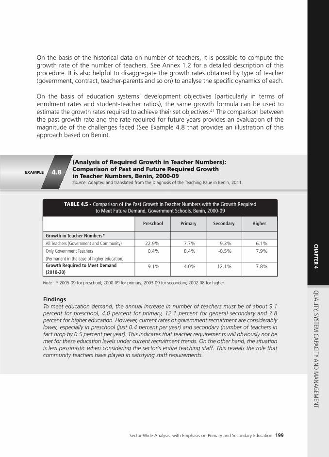
EXAMPLE 4.8
Sector-Wide Analysis, with Emphasis on Primary and Secondary Education 199
On the basis of the historical data on number of teachers, it is possible to compute thegrowth rate of the number of teachers. See Annex 1.2 for a detailed description of thisprocedure. It is also helpful to disaggregate the growth rates obtained by type of teacher(government, contract, teacher-parents and so on) to analyse the specific dynamics of each.
On the basis of education systems’ development objectives (particularly in terms ofenrolment rates and student-teacher ratios), the same growth formula can be used toestimate the growth rates required to achieve their set objectives.41 The comparison betweenthe past growth rate and the rate required for future years provides an evaluation of themagnitude of the challenges faced (See Example 4.8 that provides an illustration of thisapproach based on Benin).
(Analysis of Required Growth in Teacher Numbers): Comparison of Past and Future Required Growth in Teacher Numbers, Benin, 2000-09Source: Adapted and translated from the Diagnosis of the Teaching Issue in Benin, 2011.
TABLE 4.5 - Comparison of the Past Growth in Teacher Numbers with the Growth Requiredto Meet Future Demand, Government Schools, Benin, 2000-09
Growth in Teacher Numbers*
All Teachers (Government and Community)
Only Government Teachers
(Permanent in the case of higher education)Growth Required to Meet Demand(2010-20)
22.9%
0.4%
9.1%
7.7%
8.4%
4.0%
9.3%
-0.5%
12.1%
6.1%
7.9%
7.8%
Preschool Primary Secondary Higher
Contextual andNon-School Factors
Educational Policyand School Factors
FindingsTo meet education demand, the annual increase in number of teachers must be of about 9.1percent for preschool, 4.0 percent for primary, 12.1 percent for general secondary and 7.8percent for higher education. However, current rates of government recruitment are considerablylower, especially in preschool (just 0.4 percent per year) and secondary (number of teachers infact drop by 0.5 percent per year). This indicates that teacher requirements will obviously not bemet for these education levels under current recruitment trends. On the other hand, the situationis less pessimistic when considering the sector’s entire teaching staff. This reveals the role thatcommunity teachers have played in satisfying staff requirements.
Note : * 2005-09 for preschool; 2000-09 for primary; 2003-09 for secondary; 2002-08 for higher.
CHA
PTER 4Q
UALITY, SYSTEM CAPACITY AN
D MAN
AGEM
ENT

200 EDUCATION SECTOR ANALYSIS METHODOLOGICAL GUIDELINES - Volume 1
3.1.2 TEACHERS ATTRITION
In addition to the additional numbers of teachers needed to cover the future needs,recruitment and training of teachers will also have to compensate for the teachers who willleave the profession; this phenomenon is called teacher attrition. The analytical approachto the estimation of teacher attrition involves the assessment of the number of teachersthat abandon the profession, voluntarily or involuntarily, and the review of the causes. Theattrition rate is estimated with the following formula where Ty designates the number ofactive teachers during year y and Ny the number of new recruits during year y:
◗ Step 2: Establish what recruitment policies exist for different teacher types andexamine how they are put into practice
The objective here is to examine what policies exist in terms of teacher selection. Thesuggested analytical approach is qualitative, and based on interviews (of the HR directorsof the education ministries or of other bodies responsible for teacher recruitment) and thereview of published rules and regulations. The purpose is to assess how key requirementssuch as academic qualifications, pre-service training, motivation and so on are taken intoaccount in the recruitment process (See examples of questions to ask in Box 4.4 below). Bynature, there are significant differences in the profiles of teachers recruited by thegovernment and those selected by communities, that are helpful to get data about.42
BOX 4.4SUGGESTED QUESTIONS FOR THE APPRAISAL OF RECRUITMENT POLICIES
1 What academic and professional qualifications are required of teacher candidates?
2 Is pre-service training compulsory?
3 Of what minimum duration?
4 What institutions are responsible for teacher recruitment (education ministries, the civil servicecommission, schools…)?
5 What is the process (registration with a professional association, application, admissions’exams…)?
6 How long is the period between recruitment and effectively starting to teach?
7 How frequent are recruitment campaigns?
8 Does teacher recruitment follow specific rules and regulations? Is a copy available to share?
Attrition rate for year y = Ty - (Ty+1 - Ny+1)
Ty

EXAMPLE 4.9
Sector-Wide Analysis, with Emphasis on Primary and Secondary Education 201
This estimation can be carried out for several years, and the average over a 5 or 10 yearperiod can be computed. It is important that all teachers are included in the computation,including those recruited by communities. Where possible, it is helpful to disaggregate thedata and calculations by teacher type (civil servants, contract teachers, community teachersand so on), which will enable the identification of the categories of teachers that abandonthe profession most. In that case, caution should be given to distinguish between theteacher really leaving the profession and those changing status (community teachersbecoming contract teachers, or contract teachers becoming civil servants for instance).
Once the rate of attrition is known, its causes, as well as the corrective measuresimplemented, should be analysed. Indeed, departures from the profession may have multiplecauses, such as retirement, death, prolonged illness, professional mobility, or resignation.Retirement constitutes the most frequent cause of departure, which it is usually possible toestimate for planning reasons, especially to include the numbers in the estimation of theneeds relating to new teacher recruitment and training. Indeed, by using the retirementconditions imposed on teachers in each country (such as the maximum teaching age of 60years, or the maximum duration of service of 30 years), it is possible to project futureretirement numbers based on age and seniority data. Example 4.9 illustrates this approachfor three countries.
(Projection of Retirement-Related Attrition): Estimation of Retirement-Related Departures from the Teaching Profession in Cameroon, Benin and Guinea-Bissau, 2003-30Source: Adapted from UNESCO-Pôle de Dakar, 2004.
1,400
1,200
1,000
800
600
400
200
0
2003
2005
2007
2009
2011
2013
2015
2017
2019
2021
2023
2025
2027
2029
Cameroon Benin G.Bissau
FIGURE 4.7 - Projected Number of Retirement-Related Departures among Permanentand Contract Teachers, Cameroon, Benin and Guinea-Bissau, 2003-30
CHA
PTER 4Q
UALITY, SYSTEM CAPACITY AN
D MAN
AGEM
ENT

202 EDUCATION SECTOR ANALYSIS METHODOLOGICAL GUIDELINES - Volume 1
The analysis may be completed through a qualitative approach that aims to review themeasures undertaken to compensate for the expected teacher attrition. Interviews may beheld with headmasters, school inspectors and education ministry HR directors (See Box 4.5for suggested questions).
3.1.3 TEACHER TRAINING
The purpose of this section is to establish education sectors’ needs in terms of teachertraining and to examine their capacity (both quantitative and qualitative) to supply them. Inthis perspective, the analytical approach should cover the following steps.
◗ Step 1: Evaluate requirements in teacher training
This evaluation should cover both needs in terms of pre-service training (for the new recruitsrequired for the system’s development) and in terms of in-service training (for active teacherswho were never trained or whose training is insufficient).
On the basis of the established required growth in teacher numbers (See Section 3.1.1above) and the additional number of teachers that will be needed as a result of attrition
FindingsThe number of teachers due to retire is set to increase in all three countries, exceeding 1,000departures by year in Cameroon and Benin. The peak of departures will occur in 2017-18 forboth Benin and Guinea-Bissau, with over 1,250 and 250 departures by year respectively. InCameroon the peak will occur in 2024, with about 1,100 departures per year. These significantnumbers will require a consequently greater recruitment effort on behalf of the respectivegovernments to meet the UPE objective, but should also be taken into account over subsequentyears, to maintain the required number of teachers.
BOX 4.5SUGGESTED QUESTIONS FOR THE APPRAISAL OF TEACHER ATTRITION
1 What procedures are usually followed in cases of teacher attrition?
2 Do institutional or statutory mechanisms exist that contemplate the replacement of teachers?If so, what are they?
3 How are these measures effectively applied?
4 How much time elapses between a teacher’s departure from a school and their replacement?

Sector-Wide Analysis, with Emphasis on Primary and Secondary Education 203
(See Section 3.1.2), it is possible to compute the overall requirement for new teachers inneed of pre-service training (See Table 4.6).
In terms of ongoing training requirements, it is necessary to use data on the qualificationsand training received by active teachers, often available from the planning services of theeducation ministries (See Table 4.7). The main requirement in terms of in-service training isbased on the number of active teachers having received no pre-service training.
TABLE 4.6 - Example of Projected Annual New Teacher Requirements Providedby an Education Ministry, 2010-20
Preschool
Primary
Lower Sec.
Upper Sec.
2009-10
2010-11
2011-12
2012-13
2013-14
2014-15
2015-16
2016-17
2017-18
2018-19
2019-20
232
2,014
1,036
343
224
2,131
1,624
359
236
2,248
1,829
385
248
2,358
2,060
414
258
2,457
2,880
452
268
2,546
3,020
868
276
2,988
3,439
783
242
3,117
3,155
670
273
3,454
3,484
730
284
3,676
3,940
841
242
3,913
4,456
927
253
2,809
2,811
616
AnnualAverage
Contextual andNon-School Factors
Educational Policyand School Factors
With the help of the information gathered, a synthetic table can be compiled (See Table 4.8).
TABLE 4.7 - Example of an Extract of an Education Ministry’s Teacher Database
Contextual andNon-School Factors
Region 1
Region 1
Region 1
Region 1
Region 2
Region 2
Region 2
CA 1
CA 1
CA 2
CA 3
CA 4
CA 4
CA 4
EPP1
EPP2
EPP5
EPP51
EPP61
EPP62
EPP63
1010111
1010112
1010113
1010116
1010119
1010120
1010121
O’ Level
A’ Level
O’ Level
A’ Level + 1 year of Uni.
O’ Level
O’ Level
O’ Level
Yes
Yes
No
No
Yes
No
Yes
CatchmentArea
Region School TeacherReg. Number
TeacherQualification
Pre-service TeacherTraining?
Educational Policyand School Factors
TABLE 4.8 - Template for the Presentation of Annual TeacherTraining Requirements
Preschool
Primary
Lower Secondary
Upper Secondary
TVET
Pre-Service In-Service
Contextual andNon-School Factors
Educational Policyand School Factors
CHA
PTER 4Q
UALITY, SYSTEM CAPACITY AN
D MAN
AGEM
ENT

EXAMPLE 4.10
204 EDUCATION SECTOR ANALYSIS METHODOLOGICAL GUIDELINES - Volume 1
◗ Step 2: Compare current teacher training institutes’ capacities with projectedsystem needs
This analysis enables one to estimate the gap between projected needs and the system’scapacities to train teachers. This requires the collection of data on the physical capacity ofteacher training institutes. To illustrate this approach, the example of Benin is used below.
(Analysis of Past Growth and Future Needs in Teaching Staff): Compared Analysis in Past Growth and Future Teaching StaffRequirements, Benin, 2009/10Source: Adapted from the Diagnosis of the Teaching Issue in Benin, 2011.
TABLE 4.9 - Physical Capacities and Requirements in Pre-service Teacher Training,Government Teachers, Benin, 2009/10
Preschool
Primary
General
Secondary
(Lower and
Upper)
01 ENI : • Allada
05 ENI :• Porto-Novo• Abomey• Djougou• Dogbo• Kandi
02 ENS :• Porto-Novo (Humanities)• Natitingou (Sciences)
300
300 × 5 =
1,500
225 (Only Natitingou)
347
2,157
109 (Only
Natitingou)
2 years
2 years
3 years
174
1,079
75
258
2,107
2,209
Basic TeacherTraining Institutes
UsualPhysicalCapacity
Student-Teacher
Numbers
CurrentDuration of
BasicTraining
AnnualOutput
Annual Need forTeacherTraining
Contextual andNon-School Factors
Educational Policyand School Factors
Table 4.9 shows the global capacity of basic teacher training infrastructure, for teachers ofpreprimary, primary and lower secondary, where the greatest needs are felt.
FindingsThe total basic training capacity is for 300 teachers of the preschool level. Each of the primaryteacher training institutes caters for that same number, providing a total of 1,500 seats for theprimary level. However, the number of teacher trainees undergoing training in academic year2009/10 largely exceeded these figures, which may well translate into poor training conditionsand supervision rates. However, on the basis of these figures and considering the duration ofthe course, the number of teachers that could effectively be trained falls to about 175 forpreprimary and about 1,080 for primary, whereas respective yearly needs in terms of basictraining over the coming years are about 250 and 2,100. The gap between the training capacityand the system’s needs therefore appears to be considerable for these two levels; it wouldincrease further still if the private sub-sector was taken into account.
Note: * ENI (École Nationale d’Instituteurs) and ENS (École Normale Supérieure) are common names for teacher traininginstitutes in Francophone countries.

Sector-Wide Analysis, with Emphasis on Primary and Secondary Education 205
The same kind of analysis should be conducted for in-service training, comparing physicalcapacity with projected requirements.
QUALITATIVE ASPECTS OF THE MANAGEMENT OF TEACHERS
3.2.1 QUALITY OF TEACHER TRAINING
Three complementary approaches can be used to appraise the quality and effectiveness ofthe training received by teachers.
A first approach consists of using evaluations that relate teachers’ professional training withstudents’ learning outcomes. Education sector analysts can refer to Section 3 of this chapterthat explains how econometric models can estimate the size of the correlations of differenttraining courses with learning outcomes.
A second approach is to rely on data from the evaluation of teachers’ pedagogical skillsthat are conducted in some countries, such as Guinea-Bissau, The Gambia or Mauritania.In Guinea-Bissau for instance, over 90 percent of teachers sat math and Portuguese tests inexam conditions, as well as having to complete a survey questionnaire (See Example 4.11).
Finally, a third approach, more qualitative and complementary to the first two, consists ofconducting a series of interviews of the heads of teacher training institutes and/or theinstitutions that use their services (Divisions of examinations and admissions procedures,Divisions of pedagogical inspections and so on). Box 4.6 provides suggested questions forsuch interviews.
The same analytical approach leads to an even greater gap for lower secondary: the number ofteachers that can receive training is just 75 per year; effective needs are 30 times higher. However,it should be noted here that secondary teacher training institutions have been closed since 1987and whereas all primary training centers have gradually reopened from 2008 onwards, only theNatitingou center has reopened to cater for the secondary level, since 2009/10. Even with thefull re-opening of the other two centers, the total number of places per year would barely stretchto 150 (= 75 x 2), far from the required level.
3.2
CHA
PTER 4Q
UALITY, SYSTEM CAPACITY AN
D MAN
AGEM
ENT

EXAMPLE 4.11
206 EDUCATION SECTOR ANALYSIS METHODOLOGICAL GUIDELINES - Volume 1
(Use of Competency Assessments to Evaluate the Quality of TeacherTraining): Evaluation of Teachers’ Skills through Skills Assessments,Guinea-Bissau, 2009Source: Adapted from the Guinea-Bissau CSR, 2010.
The skills assessments used in Guinea-Bissau were of intermediate difficulty in order to appreciatethe full range of teachers’ competencies, considering the variety of teacher statuses. The resultshave enabled the establishment of a detailed database that distinguishes between basicknowledge and teaching skills (See Table 4.10).
On the basis of this data, three teacher profiles have been established, covering both theiracademic and pedagogical skills (in Math and Portuguese):
- Teachers in great need of improved skills (Profile 1);- Teachers with satisfactory skills (Profile 3); and- Teachers considered average (Profile 2).
Crossing the overall skill levels in teaching Portuguese and those in teaching math enables oneto draw up a map of teacher training needs (See Table 4.10 for an illustration of this at theprimary level).
FindingsTable 4.11 shows that 9.9 percent of teachers (dark grey cell) combine skill deficits in bothPortuguese and math, whereas 66.8 (=35.2+10.5+12.8+8.2) percent of teachers have averageto good levels in both subjects (uncoloured cells). On the basis of this simple map a trainingprogramme and supporting tools can be elaborated.
Contextual andNon-School Factors
TABLE 4.10 - Share of Teachers with Insufficient Skills, Guinea-Bissau, 2009
Teaching of Portuguese
Teaching of Math
Teaching of Sciences
Pedagogy and General Teaching Skills
Multi-grade Class Management
Control and Teaching of Large Groups
Reinforcing Academic Skills
64.5%
41.7%
38.0%
30.7%
12.4%
5.4%
12.4%
41.7%
22.6%
17.7%
22.2%
3.7%
4.2%
17.2%
Primary Lower Secondary
Educational Policyand School Factors
TABLE 4.11 - Map of Primary Teachers’ Skill Gaps in Math and Portuguese,Guinea-Bissau, 2009
PORTUGUESE
MATHEMATICS
Profile 1
9.9%
11.7%
1.2%
9.2%
35.2%
12.8%
1.4%
10.5%
8.2%
Profile 1
Profile 2
Profile 3
Profile 2 Profile 3
Contextual andNon-School Factors
Educational Policyand School Factors

Sector-Wide Analysis, with Emphasis on Primary and Secondary Education 207
3.2.2 TEACHER POSTINGS ACROSS SCHOOLS
The analysis of the consistency of the posting of teachers throughout a country is afundamental management issue, that is linked to the principle of equity in learningconditions that would have the number of teachers in a school be proportional to thenumber of students. Thus, all schools with approximately the same number of studentsshould have a comparable number of teachers.
In practice, there are a number of legitimate reasons for two schools with the same numberof students to have different numbers of teachers. There may be positive discriminationpolicies, providing better schooling conditions (including more teachers) in schools operatingin more difficult contexts. There may be some effect of the class sizes: without multigrade
BOX 4.6SUGGESTED QUESTIONS FOR THE APPRAISAL OF THE QUALITYOF TEACHER TRAINING
1 How are teacher training candidates chosen? How are they assessed during and at the endof the course to ensure they acquire the required skills?
2 Do candidates’ knowledge/skill levels at admission enable them to follow the courseefficiently?
3 Do the recruitment procedures attract candidates with the expected profiles?
4 Does the academic content of the courses enable candidates to acquire the requiredteaching skills? What should be improved in this respect?
5 Is the subject content aligned with the classes teachers are later expected to teach? Does itreflect curriculum reforms potentially underway, such as the BEAP (Basic Education in AfricaProgramme) and the CBA (Competency-Based Approach)?
6 What is the proportion of the course devoted to teaching practice?
7 Is the course duration optimal?
8 What is the best type of course organisation to effectively train a great number of teachers(Classes, CD-Roms, e-Learning)?
9 Do assessments cover all the facets of the course (academic knowledge, pedagogical skillsand teaching practice)?
10 Do the assessments effectively ascertain that trainees have indeed acquired the skillsrequired to teach?
11 Is the number of trainers sufficient? Do they have the necessary profile to train teachers intheir respective areas?
CHA
PTER 4
The results of these analyses and surveys enable one to estimate the number of teachersthat require further training and the number that must be added to the number of newuntrained teachers to reach the overall demand for in-service training.
QUALITY, SYSTEM
CAPACITY AND M
ANAG
EMEN
T

208 EDUCATION SECTOR ANALYSIS METHODOLOGICAL GUIDELINES - Volume 1
teaching, two classes of 20 students require two teachers, while 40 students in the sameclass may need only one teacher. More often however, some less controlled reasons explainthe differences in teacher distribution, and when these differences are wide, they generallysignal distribution phenomena that are not well controlled and are inequitable.
The analysis can be performed in two steps. The first consists of adopting a quantitativeapproach that determines the degree of consistency in the posting of teachers nationwide,by evaluating the relation between the number of students and the number of teachers byschool. The second consists of a qualitative approach that researches the reasons of potentialimbalances, analyzing the institutional procedures and technical tools for teacher posting,both in terms of rules and regulations and in terms of their effective application.
◗ Step 1: The quantitative analysis of the consistency of teacher posting amongschools
In the context of the quantitative analysis, it is necessary to distinguish between two typesof situation, where:
1) A single teacher is responsible for a class, as is generally the case for preschool andprimary. Here the relation between the number of students and the number of teachersper school will be used; and
2) A teacher covers various classes or a class has various teachers, as is often the case forsecondary, TVET and higher education. Here the total learning time (measured in hoursof teaching service supplied) per school should be compared to the total number ofhours needed for all students of the school.
The recommended approach consists of using school-level data on the number of studentsand the number of teachers (or the number of teaching hours for the cycles where studentshave several subject-specific teachers43), and plotting both on the same graph. To evaluatethe consistency in the posting of teachers at the national level and to compare this withneighbouring countries, the R² determination coefficient is generally used. The value of thiscoefficient is between 0 and 1: the closer to 1, the greater the relationship between thenumber of students and the number of teachers. Conversely, R²’s complementary coefficient(1-R², usually called the degree of randomness) measures the share of teacher postings thatare explained by factors other than the number of students in a school.44 The greater thedegree of randomness, the greater the inconsistencies in teacher posting.
R² can be easily determined through a graph created with the help of an Excel-typespreadsheet (See Annex 4.1). The interpretation of R² and 1-R² can then be carried out inan historical perspective (analyzing how the coefficient has evolved over recent years) or inan international one. The following example, based on the Burkina Faso CSR, shows howto present and interpret such an analysis.

EXAMPLE 4.12
Sector-Wide Analysis, with Emphasis on Primary and Secondary Education 209
The same analyses can be carried out for each region to appraise the consistency in theposting of teachers inside each, especially when part of the teacher distribution process isdone at the sub-national level. Furthermore, a complementary approach to the analysis ofthe consistency in teacher distributions consists of comparing the differences in the pupilto teacher ratios (PTR) for each region, district or other geographic unit.45 This provides anadditional and helpful perspective in terms of education sector management, given that itenables the identification of potential imbalances and their precise location.
Finally, it is advisable to compute the share of schools for each geographic sub-division thatare under-endowed or over-endowed in comparison with the average PTR. For this, eachschool’s PTR must be calculated and compared to the average to determine the respectiveshares.
(Analysis of the Consistency of Teacher Postings): Consistency inthe Posting of Primary Teachers, Burkina Faso, 2006/07Source: Adapted from the Burkina Faso CSR, 2009.
The data used in this example are drawn from the education ministry planning service’s 2006/07statistical database. The distribution of teachers only covers government schools as these arethe only ones financed by the state. Figure 4.8 gives a glimpse of the situation in 6,960government primary schools in terms of enrolment (the x-axis) and teacher numbers (the y-axis).
R2 = 0.781320
18
16
14
12
10
8
6
4
2
00 200 400 600 800 1,000 1,200
Num
ber
of T
each
ers
Number of Students
FIGURE 4.8 - Consistency in the Allocation of Teachers among Government Primary Schools,Burkina Faso, 2006/07
CHA
PTER 4Q
UALITY, SYSTEM CAPACITY AN
D MAN
AGEM
ENT

◗ Step 2: Analysis of the process of teacher posting to schools
Potential consistency issues in teacher posting may have multiple causes that it will behelpful to review with care. Several factors may be combined, although broadly speakingthey are of two kinds:
1) Lack of definition of administrative procedures, as set out in rules and regulations.Indeed, teacher distribution procedures may be more or less transparent, and the criteria
210 EDUCATION SECTOR ANALYSIS METHODOLOGICAL GUIDELINES - Volume 1
Contextual andNon-School Factors
TABLE 4.12 - Degree of Randomness (1-R²) in the Distribution of Primary Teachers, 24 African Countries
Burundi
Cameroon
Congo, The
Togo
Malawi
Uganda
Côte d’Ivoire
Ethiopia
Madagascar
Mali
Gabon
Central African Republic
51
45
40
37
34
34
33
29
28
27
26
24
Burkina Faso
Rwanda
Mauritania
Zambia
Chad
Niger
Senegal
Guinea-Bissau
Mozambique
Namibia
Guinea
São Tomé and Príncipe
22
21
20
20
20
19
19
16
15
15
9
3
Country Randomness (%) Country Randomness (%)
Educational Policyand School Factors
FindingsGenerally speaking, there is clearly a positive relationship between the two variables consideredin Figure 4.8, meaning that the greater the number of children enrolled, the higher the numberof teachers. However, there are considerable variations around the average. For instance, amongschools with approximately 400 students, the number of teachers ranges from 4 to over 10.There are clearly some consistency issues in the distribution of teachers at the school level.
A complementary approach to assessing the situation in Burkina Faso consists of comparing itwith other countries’ situations. Table 4.12 shows the degree of randomness in the distributionof primary school teachers for a sample of African countries.
FindingsIn Burkina Faso, the value of R² is 0.78. The degree of randomness in the teacher distributionprocess, measured by the 1- R² value, is thus 0.22. This indicates that approximately 22 percentof the teacher posting process among government primary schools is not related to the numberof students but rather to other factors. Burkina Faso’s situation is thus close to the sampleaverage, of 25 percent. Scope for progress therefore exists in making the postings across thecountry more equitable and coherent. Guinea, which adopted a highly structured plan ofteaching staff reposting a couple of years ago, may be considered as a leading example.

Sector-Wide Analysis, with Emphasis on Primary and Secondary Education 211
used for decisions may vary. The situation may be worsened by the lack of capacitiesof the unit responsible for the process; and
2) Lack of respect for the procedure, even when this is clearly defined and transparent.This case shows that administration is satisfactory but subject to contextual pressures.There are usually two stages in such cases: (i) the technical elaboration of a postingplan; and (ii) the review and validation of this plan. It is at this second stage thatdecisions are subject to environmental pressure, in the form of political intromission,or from teachers themselves, according to their personal preferences.
These two categories are simplifications and in truth a variety of situations will beencountered, resembling one or the other to some degree. The analysis of the situationmust highlight the specificity of each country through personal interviews of the educationministry’s HR directors or the officials responsible for the posting of teaching staff (See Box4.7).
BOX 4.7SUGGESTED QUESTIONS FOR THE APPRAISALOF TEACHER POSTING PRACTICES
1 Are teacher postings determined according to specific procedures? Have these beenpublished as a regulatory guide? What are the exact criteria?
2 Are these procedures effectively followed? If so, how?
3 What difficulties are encountered in the application of the procedures?
4 What services are responsible for teaching staff postings?
5 How are the officials responsible for staff postings recruited?
3.2.3 JOB SATISFACTION AND SOCIO-PROFESSIONAL CONTEXT
Job Satisfaction
The evaluation of teachers’ job satisfaction requires specific tools and data. Someinternational assessments are helpful, such as the PASEC assessments that include a questionabout teachers’ willingness to keep their job or their wish to change (See Box 4.8 below).Nevertheless, the analyst should keep in mind that such answers are self-reported. It is thenrecommended to cross-check those answers with all other available data source on thesubject. Generally speaking, all available studies on teachers’ job satisfaction and/ormotivation should be used in the analysis.
CHA
PTER 4Q
UALITY, SYSTEM CAPACITY AN
D MAN
AGEM
ENT

212 EDUCATION SECTOR ANALYSIS METHODOLOGICAL GUIDELINES - Volume 1
The Socio-Professional Context
The analysis of the socio-professional context in which teachers work enables the assessmentof the mechanisms that exist for the discussion, debate and dialogue of educational issues.In this perspective, interviews can be conducted with social stakeholders (such as teacherunion representatives, PTAs and so on) to touch on several thematic issues. Annex 4.2presents a synthetic table of the various dimensions that can be dealt with, and Annex 4.3offers an example of a questionnaire derived from this table and used in the context of theBenin diagnosis of the teaching issue.
Let's note, to conclude this section, that the World Bank, with its partners, has developeda set of frameworks related to various aspects of an education system, called SABER(Systems Approach for Better Education Results). One of those frameworks, related toteachers, is described in Box 4.9; some others, related for instance to EMIS, school autonomyand accountability, or finance, can prove useful for carrying out the insitutional analysisdescribed in section 2.4 of this chapter.
BOX 4.8PASEC QUESTIONS FOR THE APPRAISAL OF TEACHERS’ JOB SATISFACTION
69 If you were to choose your profession again, which of the following fields would you choose(Tick the appropriate box)
⃞ Medical
⃞ Legal
⃞ Agricultural
⃞ Administrative
⃞ Technical
⃞ Financial
⃞ Commercial
⃞ The same again

Sector-Wide Analysis, with Emphasis on Primary and Secondary Education 213
BOX 4.9SABER (SYSTEMS APPROACH FOR BETTER EDUCATION RESULTS) – TEACHERS
The World Bank, with its partners, has developed a framework of tools, indicators andbenchmarks called SABER. SABER - Teachers documents teacher policies for public schools indeveloped and developing countries to inform policy choices and promote policy dialogue,globally.The objective is to produce a systematised set of knowledge products from the experience oftop-performing countries tackling different issues related to teacher policies (e.g., teachertraining, incentives or accountability). SABER - Teachers aims at enhancing the ability of educationanalysts, planners and decision makers to draw on all of the knowledge that the Education Sectorgenerates.
In practice, SABER – Teachers:
- classifies and analyses education systems around the world according to 8 coreteacher policy goals to which all education systems should aim.
- collects information on 10 core teacher policy areas in education systems aroundthe world by administering a set of questionnaires to key informants and gatheringboth qualitative and quantitative data, validated by legal documents.
- shares knowledge products to provide maximum impact in driving teacherperformance through an interactive website, print materials and workshops.Finally, SABER - Teachers hopes to be a knowledge connector, leading policydialogue on teacher policies and embracing acollaborative approach to improve thequality of teaching.
8 core teacher policy goals wereselected because (i) they are relatedto either student or teacherperformance through theoryand/or evidence; (ii) they arepriorities for resource allocationand; (iii) they are actionable (i.e.,governments can have a directinfluence on them through policyreforms).
Education systems are classified asbeing more or less advanced in each ofthese goals on four levels (Latent,Emerging, Established and Mature). Thispolicy goal framework is used to produceCountry Reports, which consist of tailored analyses forspecific countries.
Contextual andNon-School Factors
Educational Policyand School Factors
EFFECTIVETEACHERS
1. Setting clearexpectationsfor teachers
2.Attractingthe best intoteaching
5.Leadingteachers withstrongprincipals
6. Monitoringteaching andlearning
3.Preparingteacherswith usefultraining andexperience7.
Supportingteachers toimproveinstruction
8.Motivatingteachers toperform
4.Matchingteachers’skills withstudents’needs
▶
CHA
PTER 4Q
UALITY, SYSTEM CAPACITY AN
D MAN
AGEM
ENT

214 EDUCATION SECTOR ANALYSIS METHODOLOGICAL GUIDELINES - Volume 1
SABER - Teachers collects information on teacher policy areas by administering questionnairesamong key informants in countries. Data are collected by a local consultant in each country. Thelocal consultant uses a set of questionnaires which are designed to interview key informants andcollect data on teacher policies. Local consultants are required to validate the data they submitby checking the information provided by key informants against the relevant laws and regulationsthat back them up.
The 10 core teacher policy areas are:
- Requirements to enter and remain in teaching
- Initial teacher preparation
- Recruitment and employment
- Teachers’ workload and autonomy
- Professional development
- Compensation (salary and non-salary benefits)
- Retirement rules and benefits
- Monitoring and evaluation of teacher quality
- Teacher representation and voice
- School leadership

THE MANAGEMENT OF OTHER RESOURCES AND OF TEACHING TIME
Sector-Wide Analysis, with Emphasis on Primary and Secondary Education 215
MANAGEMENT OF RESOURCES OTHER THAN TEACHERS
The most important analysis to carry out with respect to the management of other teachinginputs (material and pedagogical resources or financial subsidies) is the study of theconsistency of their allocation among schools. As for the consistency in the posting ofteachers (See Section 3.2.2), the analysis is based on the principle of equity in the learningconditions offered to children i.e. all resources allocated in proportion to schools’ needs. Inthe absence of specific positive discrimination policies, these needs are assumed tocorrespond to the number of students (or teachers/class).
To illustrate, the methodology of analysis of the consistency in the allocation of textbooksis presented below, considering that the same tools and indicators can be used to analysethe consistency in the allocation of any other type of education input made available toschools.
As for the analysis of teacher postings, there are two complementary approaches to evaluatethe degree of consistency in the allocation of textbooks: (i) The first consists of thecomparison of the student-textbook ratios, by subject and geographical area (region, district,community or school). This enables one to reach a measure of the scale of the gaps withrespect to the national average and to identify the schools/areas that are under-endowedor over-endowed; and (ii) The second uses the R2 determination coefficient (and itscomplement the degree of randomness 1- R2) to provide a measure of the degree ofconsistency between the number of textbooks and the number of students, on a school byschool basis. The R2 coefficient can be calculated both at the national level to measure theoverall degree of consistency, but also for each geographic area, to compare themanagement performance of each. Annex 4.1 explains how to compute the R2 coefficientwith the help of a spreadsheet.
Note that, especially in contexts where the curricula have changed, this analysis shouldrelate to, or at least distinguish, the number of manuals, or teacher guides, which areactually relevant to the current curriculum. It is also important to note that collecting dataon learning materials often proves difficult. School censuses are often not very efficient in
SECTION
4
4.1
CHA
PTER 4Q
UALITY, SYSTEM CAPACITY AN
D MAN
AGEM
ENT

EXMPLE 4.13(Analysis of the Consistency in the Allocation of Other EducationalInputs): Analysis of the Consistency in the Allocation of PrimaryTextbooks, Mali, 2007/08Source: Adapted and translated from the Mali CSR, 2010.
MAP 4.1 - Textbook-Student Ratio, Public and Community Primary Schools,Mali, 2007/08
FRENCH TEXTBOOKS MATH TEXTBOOKS
Contextual andNon-School Factors
> 0.79
0.69 < > 0.79
< 0.70
> 0.99
0.89 < > 0.99
< 0.90
Toumbouctou0.75
Mopti0.77
Ségou0.70
Koulikoro0.81
Bamako District0.51
Kaye0.75
Sikasso0.80
Kidal0.90
Gao0.52
Toumbouctou0.93
Mopti0.93
Ségou1.09
Koulikoro1
Bamako District1.03
Kaye0.95
Sikasso1.02
Kidal1.03
Gao0.87
Educational Policyand School Factors
Map 4.1 and Table 4.13 present the degree of divergence of the textbook to student ratio fromthe Malian national average, by region.
FindingsIn Malian primary schools, the average French textbook to student ratio (not shown on the map)is 0.73 (meaning that approximately 3 students share two books) whereas the average math
doing so, partly because of the incentives for schools to under-report their stocks in thehope of getting more materials. Even through school surveys, it is often difficult todistinguish between existing materials and those that students really have access to (in manycases, materials are deemed so precious that they are ironically kept away from children).Particular attention should be paid to the data, and caution should be exercised whenanalysing it.
Example 4.13 is based on the analysis of the consistency of French and math textbookmanagement in Mali, offering a practical illustration of the approach. This example has thefurther advantage of presenting the results in a mapped form, which is more intuitivelyunderstandable to policy-makers.
216 GUIDE MÉTHODOLOGIQUE POUR L’ANALYSE DES SYSTÈMES ÉDUCATIFS - Volume 1

textbook to student ratio is 1 (each student has their own book). The maps show that in bothcases, the regions of Timbuktu, Mopti and Kayes are roughly aligned with the national average,whereas Gao is significantly below it, indicating that the shortage of textbooks is relatively acute.For French, with a ratio of 0.52, two students must share a book in Gao, compared to Kidal thatalmost provides a book to every student (ratio of 0.90). Indeed, the regions of Kidal, Koulikoroand Sikasso’s ratios are above the national average, indicating that their students arecomparatively better endowed, in both subjects. The district of Bamako faces both an acuteshortage of French books, in line with Gao, and a comparatively good endowment of mathbooks, in line with Kidal. Overall, national disparities are significant.
FindingsStrong inter-regional disparities are evidenced by Table 4.13. Overall, the degrees of randomnessin the allocation of textbooks are 73.6 percent for French and 79.5 percent for math, both ofwhich are high and underline the broad scope to improve the management of the resources. Amore detailed analysis shows that in the worst cases (Bamako and Gao), the randomness isalmost total, and for most other regions it is high. Kidal is the exception, with degrees ofrandomness of 29.4 percent for French textbooks and 36.4 percent for math books; the regionshould be used as an example of textbook management by other regional education managers.
TABLE 4.13 - Degree of Randomness (1-R², %) in the Allocation of Textbooks in Governmentand Community Primary Schools, by Region, Mali, 2007-08
French
73.6
95.0
92.4
81.0
29.4
76.1
73.8
77.1
58.7
70.3
79.5
93.6
94.3
83.8
36.4
74.6
80.7
87.7
69.4
74.5
Mali
Region
Bamako
Gao
Kayes
Kidal
Koulikoro
Mopti
Segou
Sikasso
Timbuctoo
Math
Contextual andNon-School Factors
Educational Policyand School Factors
Finally, there is a method that provides a more precise analysis than the above, which consistsof using the notion of useful textbooks. Indeed, students gain no benefit from having morethan one textbook in a given subject, so the surplus can be withdrawn from thecomputation of the textbook to student ratios. This adjustment in the calculations requiresthe use of data by school and grade. The ratio of useful textbook to student is capped at 1for a given grade and subject if the number of books effectively available is higher than thenumber of students enrolled at this grade. Table 4.14 presents a theoretical example of howto compute this ratio. The same adjustment can be made for teaching guide-books.
Analyses sur l’ensemble du système, avec un accent sur les enseignements primaire et secondaire 217
CHA
PTER 4Q
UALITY, SYSTEM CAPACITY AN
D MAN
AGEM
ENT

MONITORING EFFECTIVE TEACHING TIME
The study of teacher absenteeism and more broadly of the loss of effective teaching timerequires data that are often available at the school level but cannot be consolidated at thedistrict, regional, or national level for a number of reasons. Given the negative impact thatthis phenomenon can have on education systems (reduced contact time, full curricula notcovered, weak learning outcomes and so on); it is important to reinforce the collection andconsolidation of such data.
There are many causes of loss of effective teaching time. Teacher absenteeism is one ofthem. But it is also not uncommon that school years are curtailed due to late starts (teacherposting decisions may be taken late, or effective postings may be delayed), because classesare suspended early to prepare for exams, or due to other reasons. When data permits, itis advisable to cover as many of these factors as possible.
Abadzi (2009) developed a good practice that education sector analysis teams are advisedto follow: she developed an analytical model of instructional time loss (See Figure 4.9). Onthe basis of a survey conducted among a sample of classes using spontaneous observations(impromptu visits), it is possible to quantify the different causes of effective teaching timeloss in reference to the official number of school programme hours.
TABLE 4.14 - Computation of the Textbook-Student and Useful Textbook-Student Ratios,by Grade
Grade 1
Grade 2
Grade 3
Grade 4
Grade 5
Grade 6
Total
Textbooks Students Textbook-StudentRatio
Useful Textbook-Student Ratio
UsefulTextbooks
150
150
150
150
0
0
600
100
100
100
100
100
100
600
1.5
1.5
1.5
1.5
0
0
1
100
100
100
100
0
0
400
1
1
1
1
0
0
0.67
Contextual andNon-School Factors
Educational Policyand School Factors
4.2
218 EDUCATION SECTOR ANALYSIS METHODOLOGICAL GUIDELINES - Volume 1

Many of these factors need to be assessed during a school visit. For some of them (teacherabsenteeism for instance), these visits have to be unannounced for the assessment to bereliable. Ideally, it would be the responsibility of the inspectorate to conduct these visits, aspart of their mandate, and compile the information at a central level. However, for practicaland sensibility reasons (these teacher assessments would be nominative), the informationis not so readily available. Specific surveys can however be conducted, with explicitauthorisations from the government and the inspectorate to conduct unannounced visits.
Example 4.13 presents an illustration of the application of this approach in the case of Mali,in the context of a research project supported by USAID.
EXAMPLE 4.14(Abadzi’s Model of Instructional Time Loss):Analysis of Lost Teaching Time, Mali, 2009/10Source: Adapted from Effective Learning Time, 2010.
Contextual andNon-School Factors
FIGURE 4.9 - Abadzi’s Model of Instructional Time Loss
Intended class time as allotted by a government (e.g., 200 days or 1,000 teaching hours)
Time remaining after school closures (strikes, in-service training, extra holidays, weather)
Time remaining after teacher absenteeism and lateness
Time remaining after student absenteeism
Class time devoted to any learning task
Learning time relevant to curriculum
Time remaining after school closures (strikes, in-service training, extra holidays, weather)
Intended class time as allotted by a government (e.g., 200 days or 1,000 teaching hours)
Time remaining after teacher absenteeism and lateness
Time remaining after student absenteeism
Class time devoted to any learning task
Learning time relevant to curriculum
Educational Policyand School Factors
On the basis of a representative sample of a 100 schools and especially designed questionnaires,interviews were carried out in 2009/10 with headmasters, teachers and members of schoolmanagement committees. Class observations were also performed, establishing in detail to whatextent school days’ time-tables were respected for the sample of selected schools. The resultsenabled the assembly of a pyramid of effective teaching time in which each factor contributingto the time lost is considered (See Figure 4.10).
FindingsStudents lose an average of 4.9 days of teaching per year due to the official school calendar notbeing respected. This loss of effective teaching time is mainly due to the late start of the schoolyear (1.2 days), to extended holidays (1.2 days) or to the early start of the summer vacation (1day). On average, teachers are absent for 11.8 days per year. The most common reasonsmentioned are strikes (3.5 days) and teacher training (3 days). Students themselves are absent
Sector-Wide Analysis, with Emphasis on Primary and Secondary Education 219
CHA
PTER 4Q
UALITY, SYSTEM CAPACITY AN
D MAN
AGEM
ENT

Teacher absenteeism, although not always the greatest cause of loss of teaching time, isoften worth analysing in greater detail, as it is important to the image of the teaching forceamongst the education stakeholders (the government and the parents), and because it oftenresults from system issues which can be addressed.
The analysis of teacher absenteeism can be performed in three steps:
◗ Step 1: Estimate the magnitude of teacher absenteeism
In the absence of consolidated data, the most commonly used sources of information toestablish the scale of teacher absenteeism are public expenditure tracking surveys (PETS) orinternational learning assessments. PASEC assessments, for instance, include a question forteachers of the classes sampled where they must indicate the number of days of absence over
Official Learning Time
After TL1 (School closures)
After TL2 (Teacher absenteeism)
After TL3 (Pupil absenteeism)
After TL4 (Truncated Weekly Schedule)
After TL5 (Truncated Daily Timetable)
After TL6 (Time wasted in class)
After writing exercises
172
167
155
138
135
130
122
91
FIGURE 4.10 - Effective Learning Days, Mali, 2009/10
on average for 17 days per year (compared to 9.8 days in Ghana or 3.4 in Tunisia). According toparents, the main reasons are their participation in the family’s domestic or productive activities.
Students receive 24.5 hours of classes per week instead of the 25.2 hours considered in theschool programme. This is equivalent to a loss of 3.4 days of teaching time per year. The lack ofadherence to the calendar approved by headmasters costs a further 4.4 days per year.
Teachers devote 93 percent of their class time to effective learning activities (as opposed to classmanagement or other unrelated activities, data not shown on the graph). The 7 percent loss isequivalent to a further loss of 8.8 days over the school year. Overall, the effective learning timein Malian primary schools is 121.6 days on average, without considering the time devoted towriting exercises, or just 70.7 percent of the official education ministry programme.
220 EDUCATION SECTOR ANALYSIS METHODOLOGICAL GUIDELINES - Volume 1

EXAMPLE 4.15
the previous month, whatever the motive. Likewise, school directors are asked about thenumber of days their teaching staff were absent. The measure of absenteeism is thus generallybased on simple statements, but crossing both sources enables one to determine whetherthe answers given are coherent and reliable.
(Typical Questions to Evaluate Teacher Absenteeism): Typicalquestions to assess teacher absenteeism, PASEC, SACMEQ and PETS
Likewise, SACMEQ assessments contain similar questions on teacher absenteeism.
Contextual andNon-School Factors
Question asked in the Teacher Survey of the PASEC assessment
72. Over the last four weeks, how many days have you been absent from school, excluding school and bank holidays. (Consider illness, strikes, training, attendance of conferences, pay-day, etc.) QM2_72 (Write the number) ....................... days
Question asked in the Headmaster Survey of the PASEC assessment
56. Over the last four weeks, how many days have your teachers been absent from school, excluding school and bank holidays (consider illness, strikes, training, attendance of conferences, pay-day, etc.) (Write the number) Grade 2 teachers ....................... days Grade 6 teachers ....................... days
Educational Policyand School Factors
Contextual andNon-School Factors
Question asked in the Headmaster Survey of the SACMEQ assessment
About how often does the school have to deal with the following behaviours of teachers?Please tick the appropriate box for each statement. Indicate whether this is seen as a serious problem in your school, ticking the appropriate box in the final column.)
32.01 Teachers arriving late at school
32.02 Teacher absenteeism (i.e., unjustified absence)
Never Sometimes Often
Educational Policyand School Factors
Contextual andNon-School Factors
Information about teachers in 2008
Questions asked in the Tanzania PETS survey
Comment
310. Number of teachers on government payroll
which were absent more than 50% of the school year
311. Number of teachers on government payroll May 2008
312. Number of teachers reporting as present at school first week of May 2008
Due to study leave or other
All teachers including those on leave but still being paid
From school logbook, sum of the count of the number of teachers reporting each day
Educational Policyand School Factors
Finally, specific surveys such as PETS conducted in some countries also provide an appraisal ofthe magnitude of absenteeism.
Sector-Wide Analysis, with Emphasis on Primary and Secondary Education 221
CHA
PTER 4Q
UALITY, SYSTEM CAPACITY AN
D MAN
AGEM
ENT

222 EDUCATION SECTOR ANALYSIS METHODOLOGICAL GUIDELINES - Volume 1
EXAMPLE 4.16
◗ Step 2: Identify the main causes of teacher absenteeism
Absenteeism has multiple causes and is not always the sole responsibility of the teachers.The phenomenon is affected by different factors, related to teacher, class or schoolcharacteristics, or to the school environment or management. The same data sources usedto estimate the magnitude of teacher absenteeism may at times be used to identify its maincauses. For instance, headmasters are requested to identify the three main causes of teacherabsenteeism in PASEC assessments. This information can be statistically processed to givean idea of the main causes at the national level. To illustrate, Example 4.16 shows the resultsof this approach for Benin.
Nevertheless, the analyst should keep in mind that such information is just declarative. It isthen recommended to cross-check those answers with all other available data sources onthe subject. Generally speaking, all available studies on causes of teachers’ absenteeismshould be used in the analysis.
(Analysis of the Causes of Teacher Absenteeism):The Main Causes of Teacher Absenteeism, Benin, 2004/05Source: Adapted from the Diagnosis of the Teaching Issue in Benin, 2011.
The use of the 2004/05 PASEC assessment data sheds some light on the causes of teacherabsenteeism, from headmasters’ perspectives.
FindingsThe most frequently mentioned causes of absenteeism are health issues, the collection of paychecks, family motives (including illness, death, marriages and births) and strikes. Of secondaryimportance, other reasons mentioned include the follow-up of administrative issues, a generallack of motivation, the distance from home to school and the involvement in another activity tocomplement the teaching salary.
Contextual andNon-School Factors
TABLE 4.15 - Main Causes of Teacher Absenteeism, According to Headmasters, Benin, 2004-05
Teachers’ health issues
Other activities
General lack of motivation
Distance of home from school
Difficult teaching conditions
Family visits
Family motives (death, marriage, birth, etc.)
Collection of pay check
Strikes
Follow-up of administrative issues
58.3 %
2.2 %
11.5 %
8.6 %
2.2 %
0.7 %
25.9 %
33.8 %
41.7 %
14.4 %
Causes of Absenteeism Frequency
Educational Policyand School Factors
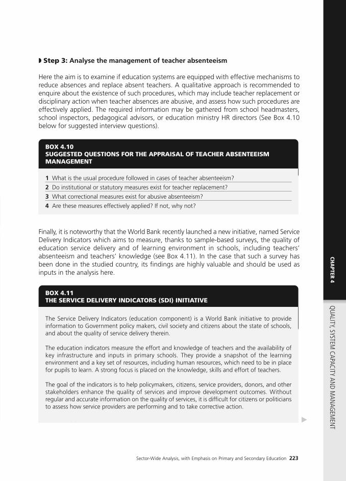
Sector-Wide Analysis, with Emphasis on Primary and Secondary Education 223
CHA
PTER 4
◗ Step 3: Analyse the management of teacher absenteeism
Here the aim is to examine if education systems are equipped with effective mechanisms toreduce absences and replace absent teachers. A qualitative approach is recommended toenquire about the existence of such procedures, which may include teacher replacement ordisciplinary action when teacher absences are abusive, and assess how such procedures areeffectively applied. The required information may be gathered from school headmasters,school inspectors, pedagogical advisors, or education ministry HR directors (See Box 4.10below for suggested interview questions).
Finally, it is noteworthy that the World Bank recently launched a new initiative, named ServiceDelivery Indicators which aims to measure, thanks to sample-based surveys, the quality ofeducation service delivery and of learning environment in schools, including teachers’absenteeism and teachers’ knowledge (see Box 4.11). In the case that such a survey hasbeen done in the studied country, its findings are highly valuable and should be used asinputs in the analysis here.
BOX 4.10SUGGESTED QUESTIONS FOR THE APPRAISAL OF TEACHER ABSENTEEISMMANAGEMENT
1 What is the usual procedure followed in cases of teacher absenteeism?
2 Do institutional or statutory measures exist for teacher replacement?
3 What correctional measures exist for abusive absenteeism?
4 Are these measures effectively applied? If not, why not?
BOX 4.11THE SERVICE DELIVERY INDICATORS (SDI) INITIATIVE
The Service Delivery Indicators (education component) is a World Bank initiative to provideinformation to Government policy makers, civil society and citizens about the state of schools,and about the quality of service delivery therein.
The education indicators measure the effort and knowledge of teachers and the availability ofkey infrastructure and inputs in primary schools. They provide a snapshot of the learningenvironment and a key set of resources, including human resources, which need to be in placefor pupils to learn. A strong focus is placed on the knowledge, skills and effort of teachers.
The goal of the indicators is to help policymakers, citizens, service providers, donors, and otherstakeholders enhance the quality of services and improve development outcomes. Withoutregular and accurate information on the quality of services, it is difficult for citizens or politiciansto assess how service providers are performing and to take corrective action.
▶
QUALITY, SYSTEM
CAPACITY AND M
ANAG
EMEN
T

224 EDUCATION SECTOR ANALYSIS METHODOLOGICAL GUIDELINES - Volume 1
The perspective adopted by the Service Delivery Indicators is that of citizens accessing a service.Hence, the indicators can be viewed as a service delivery report card on education. The indicatorsare designed to be objective, robust and actionable. The data is drawn from a dedicated surveyof schools. All the indicators are based either on assessments or are derived from directobservation by trained enumerators. Where relevant, the focus is on early primary education,and grades three and four in particular, because of the importance of early childhooddevelopment.
To evaluate the feasibility of the Service Delivery Indicators, pilot surveys were implemented inSenegal and Tanzania in 2010. The first post-pilot survey was carried out in Kenya in 2012. Theresults from these studies demonstrate that the Indicators methodology is adequate for providingstrategic information on the quality of service delivery, as experienced by the citizen, in a varietyof contexts.
The core indicators are:
E1: Teacher absence from school
E2: Teacher absence from classroom
E3: Share of teachers with minimum knowledge
E4: Time spent teaching in the classroom
E5: Minimum teaching equipment available
E6: Pupil-teacher ratio
E7: Textbooks per pupil
E8: School infrastructure
E9: Share of school grants received

Sector-Wide Analysis, with Emphasis on Primary and Secondary Education 225
NOTES
24 Hanusek and Woessmann (2007) have shown that a one standard deviation increase in reading and math scores wasassociated with a 2 percentage point increase in the growth rate of GDP per capita. See UNESCO-BREDA (2005) forinstance.
25 See UNESCO-BREDA (2005) for instance.
26 Class tests held by teachers are a fifth category, but their results are rarely tracked for analysis purposes and they do notcomply with minimal standards to allow them to be used as a homogenous tool for the measurement of learning resultsthroughout a country. See Merle (1996), De Landsheere (1980), or Rosenthal and Jacobson (1973) for instance.
27 SACMEQ uses standardised methods/tests that allow for geographic (both cross-country and national) and historicalcomparisons. Marking is adjusted to reach an average of 500. There are eight skill levels for each subject area. Levelsare hierarchical and enable to assess the competencies that students have or have not acquired.
28 Some household surveys do not have respondents take a test but rely on their statement of their reading skills. In suchcases it is important to place the results in perspective given that some individuals overestimate their reading skills. SeeChapter 10 for a discussion on this.
29 The use of this age group holds the further advantage of being the one that is usually used in CSR type sector analysis,which means that data is often available for multiple countries, enabling international comparisons.
30 The likelihood of literacy is calculated on a sample of individuals who were educated over a broad range of years (aged22 to 44 years). The approximate measure of the quality of education provided therefore pertains to an average over acouple of decades (individuals aged 44 years were schooled 30 years ago on average and those aged 22 years about 10years ago).
31 Adult literacy levels do not only depend on the number of years of school completed. Other factors whose impact isdifficult to measure also play a role in the achievement and retention of literacy. For instance, it is easier for individualsliving in cities to maintain their literacy given their greater access to written information and their more frequent use ofit on a day to day basis.
32 It is also possible to perform the same type of analysis by using other school results indicators, such as the retention rateor the repetition rate.
33 The border between these two groups is not watertight. Some factors such as school feeding programmes can beincluded in one or the other of the groups.
34 In international evaluations, there is generally a questionnaire for students, one for teachers and a third for headmasters.
35 The questionnaires can be obtained by contacting the teams in charge of the respective assessments through their web-pages: EGRA/EGMA on www.rti.org, PASEC on www.confemen.org and SACMEQ on www.sacmeq.org.
36 Details on the elaboration and estimation of econometric models can also be found in relevant statistical documents,such as Wonnacott and Wonnacott (1995), Bressoux (2008), Greene (2008), or Kennedy (2008).
37 This approach makes the assumption that students stayed in the same school over the last three or four years. Wheredata permit, the analysis can be limited to the students who attended the school over the previous three to four years.
38 In some cases the survey design does nevertheless measure the impacts of different ways of implementing a given policyor action.
39 This is effectively the ak coefficient of factor Xk in the learning outcomes model.
40 The analysis of teacher remuneration is described in Chapter 3 on cost and financing.
41 It is however important to note that the required growth rate underestimates new recruitment needs that result fromretirement, death, or other reasons (See Section 2.1.5 on attrition rates).
42 The recruitment of community teachers does not always follow an institutionalised procedure. However, theimplementation of policies supporting community teachers in some countries does promote a structured approach(recruitment criteria, remuneration guidelines and so on) that it is helpful to analyse.
43 In that case it is helpful to carry out the analysis by subject.
44 This analysis can be performed considering all teachers, or distinguishing between government and other teachers whenthe information is available, which suggests how the involvement of other players (communities for instance) may improvethe coherence of postings.
45 The student-teacher ratio is obtained by the straightforward division of the number of students by the number ofteachers.
CHA
PTER 4Q
UALITY, SYSTEM CAPACITY AN
D MAN
AGEM
ENT

226 EDUCATION SECTOR ANALYSIS METHODOLOGICAL GUIDELINES - Volume 1
© W
orld
Ban
k /
Régi
s L’
Hos
tis

CHAPTER 5EXTERNAL EFFICIENCY › Chapter Objective:Analyse the extent to which education, andeach level of education or training in particular,contributes to the achievement of nationaleconomic and human development goals.
Sector-Wide Analysis, with Emphasis on Primary and Secondary Education 227
CHA
PTER 5EXTERN
AL EFFICIENCY

228 EDUCATION SECTOR ANALYSIS METHODOLOGICAL GUIDELINES - Volume 1
1. ECONOMIC IMPACT OF EDUCATION
ISSUEDoes education improve the productivity and employability of school or higher education leavers?Does public investment in education and training contribute to growth and economicdevelopment?
OBJECTIVES• Conduct a macroeconomic review of the extent to which the education system is aligned with
labour market requirements, in quantity and quality;• Conduct a microeconomic review of the employment status of school and higher education
leavers in the workplace;• Determine how skills and competencies are valued in the workplace and the relationship
between remuneration and the level of education attained;• Evaluate the return on investments in education and training at the individual and collective
levels; and• Determine the scope to optimise the economic impact of education.
METHODS• Analyse labour market dynamics and structure in terms of the jobs available, by sector, sub-
sector, type of institution, socioprofessional status and main job types;• Determine the extent of unemployment among school and higher education leavers;• Review the training-employment balance in recent years to determine the quantitative
asymmetry between the supply of skills and the supply of jobs;• Evaluate the needs for workers’ qualifications and professionalisation;• Evaluate the training-employment balance through the degree to which individual skills are
valued in the positions occupied by workers;• Evaluate the economic value given to education by the workplace; and• Conduct a cost-benefit analysis by computing the private and social returns on investment in
different education levels.
SOURCESNational employment statistics, reports and surveys, or the employment sections of householdsurveys; tracer studies; household consumer and income-type surveys; demographic populationdata; public and private education spending data (from Chapter 3) and investment climateassessments and surveys.

Sector-Wide Analysis, with Emphasis on Primary and Secondary Education 229
2. SOCIAL IMPACT OF EDUCATION
ISSUEDoes the education system adequately prepare individuals to contribute to national social andhuman development? To what extent does each education and training level contribute?
OBJECTIVES• Evaluate the impact of different education levels on living standards;• Examine the contribution of different education levels to improving health-related behaviours
and outcomes;• Examine the contribution of different education levels to social and civic behaviour; and• Examine the contribution of different education levels to the management of fertility.
METHODSFor each area identified above, the approach consists of:• Selecting appropriate indicators to describe the impact; and• Studying the causal relationship between education and each indicator through linear econometric
models and logistical regressions.
SOURCESHousehold living conditions surveys; demographic and health surveys (DHS); multiple indicatorcluster surveys (MICS); core welfare indicator questionnaires (CWIQ); poverty and social impactanalyses (PSIA) and population census data.
CHA
PTER 5EXTERN
AL EFFICIENCY

230 EDUCATION SECTOR ANALYSIS METHODOLOGICAL GUIDELINES - Volume 1
IntroductionThe usual benchmark of external efficiency is the use by individuals of the knowledge andskills acquired through their education during adulthood. The analysis seeks to measure theextent to which education contributes to individuals’ social utility, as well as to measure thepersonal benefits of the training received. External efficiency is seldom analysed in thecontext of evaluations of education systems, often due to the unavailability or low qualityof the required data.46 The analysis of external efficiency is particularly important to planthe supply of postprimary training, to help direct public funding towards courses thatenhance graduate employability and positively impact on national levels of humandevelopment.
The impacts of education can be divided into two types: economic and social. The economicdimension relates mainly to the relationship between education and the employability andproductivity of school and higher education leavers, but also to the contribution of educationto economic growth. The social dimension covers a plethora of aspects, including mortality,health, fertility, civic attitudes, environmental awareness and so on.47
- Participation in the workplace- Work productivity- Income- Savings
- Economic growth- National production capacity (innovation and the adaptation or use of new knowledge)- Disparities- Government revenues (taxes)- International competitivity- Unemployment
Change in behaviours in terms of: - Reproduction (family planning and fertility, STD prevention, etc.) - Maternal, infant and child health - High-risk behaviours (alcohol and tobacco abuse, high-risk sexual behaviour) - Children’s up-bringing - Civic attitudes and participation - Protection of the environment
- Demography (population growth, demographic transition, demographic dependency ratio)- Public health (life expectancy, vaccination coverage, mortality rates, etc.)- Adaptation and use of new technologies- Conservation of the environment for future generations- Social cohesion- Delinquency
Individual
Collective
Economic Social
TABLE 5.1 - The Four Analytical Dimensions of the External Efficiency of Education
Source: Authors.

Sector-Wide Analysis, with Emphasis on Primary and Secondary Education 231
These impacts, in both their economic and social dimensions, can be noted at both theindividual level (more educated individuals tend to earn more) and the collective level(countries with a better educated workforce tend to have higher growth rates and betterhealth indicators, for instance). The combination of these two types of impact (economicand social on the one hand and individual and collective on the other) provides a frameworkfor the analysis (See Table 5.1).
The analysis of external efficiency can thus proceed according to a vertical reading of thetable, reviewing the economic and social dimensions, or according to a horizontal reading,according to the individual and collective benefits of education. This guide adopts a verticalapproach. Figure 5.1 takes a functional approach to the different issues raised by themeasure of external efficiency. These issues will guide the analyses of this chapter48.
FIGURE 5.1 - External Efficiency Issues
imbalance
requirementsState
Investment
ReinforcedHumanCapital
Graduates/Leavers
OPTIMISE THE IMPACTIN THE WORKPLACE
EDUCATION SYSTEM'S EXTERNAL EFFICIENCY
CONTRIBUTION TO THE WORKPLACE(THROUGH THE STATUS OF SCHOOL LEAVERS)
SOCIOECONOMIC DEVELOPMENT
Inputs(including household
investment)
EDUCATIONSYSTEM
Economic Productivity
Living standards and quality of life
EDUCA
External Efficiency IssuesFIGURE 5.1 -
STEM'S EXTERNAL EFFICIENCYTION SYAAT
External Efficiency Issues
STEM'S EXTERNAL EFFICIENCY
ORKPLA
requirements
imbalance
InvestmentState
IN THE WOPTIMISE THE
(THROUGH
requirements
UTION TCONTRIBCEORKPLA
CTAIMPPAOPTIMISE THE
VERS)TUS OF SCHOOL LEAAVATHE STTA(THROUGH CEORKPLAO THE WUTION T
LeaversGraduates/
household (including
Inputs
STEMSYTIONEDUCAAT
CapitalHuman
ReinforcedPEconomic Pro
Living standards and qu
DEVELOPMENTSOCIOECONOMIC
ductivity
ifeuality of life
investment)household
CHA
PTER 5EXTERN
AL EFFICIENCY
Source: Authors.

232 EDUCATION SECTOR ANALYSIS METHODOLOGICAL GUIDELINES - Volume 1
THE ECONOMIC IMPACT OF EDUCATION
The economic impact of education is mainly appraised through the workplace, which iswhere supply and demand for skills meet. The supply of skills comes from the activepopulation (any person in employment or looking for work), who apply for jobs. Thedemand for skills comes from those institutions (public, private, formal, informal and so on)who offer jobs. The impact of education on the workplace should be appraised both fromthe supply side and the demand side, and especially through the interaction of the two.
Education and training should enhance the employability and productivity in work of schooland higher education leavers. From the perspective of employers, education should enhancehuman capital and the productivity of companies.49 Companies’ main demand of educationsystems is to provide qualified labour, in sufficient quantity and of sufficient quality to meettheir productive requirements. Some sectors of the economy may face a lack of qualifiedlabour, whereas others may have declining labour needs that the education systemnevertheless continues to provide for.
The evaluation of education’s economic impact can therefore focus on: (i) the descriptionof the labour market and its structure (Sections 1.1 and 1.2); (ii) an evaluation ofemployment status and the economic return on investment in education and training(Sections 1.3 and 1.4); and (iii) the balance between the training provided by the educationsystem and the available jobs as well as the estimation of the future needs of the labourmarket (Sections 1.5 and 1.6).
DESCRIPTION OF THE LABOUR MARKET
The description of the main labour market indicators helps to illustrate the national contextand employability status of school and higher education leavers (See Box 5.1).50 Participationin the workplace is first and foremost described by the activity rate. This includes peopleunemployed but actively seeking work (ILO definition), measured by the unemploymentrate. This, in turn, enables the computation of the employment rate. Some authors use abroader definition of unemployment to include discouraged job-seekers, unemployedindividuals who are available to work but have ceased to look. It is often instructive tohighlight the dependency ratio, defined as the number of unemployed to the number ofemployed. In 2007 in France for instance, there were 1.47 unemployed to every worker.
Other indicators are offered to describe employment issues. These include the visibleunderemployment rate (covering the share of the active population only working part-time
SECTION
1
1.1

Sector-Wide Analysis, with Emphasis on Primary and Secondary Education 233
BOX 5.1EMPLOYMENT INDICATORS
Internationally, the International Labour Organisation (ILO) considers that the working agepopulation is that of individuals above 15 years. Indeed, legislation in many countries forbidsaccess to the workplace to individuals not having completed their compulsory schooling (oftennot having completed the primary cycle). However, to be coherent with the fact that in manycountries some children also work and that such activity is often in the informal sector (in thecase of apprenticeships for instance), the working age population can be considered to be thatof say 6 years and above or 10 years and above, depending on the country and the survey.
According to the ILO definitions, the working age population includes the employed, theunemployed (which together are the active population) and the economically inactive. The activepopulation thus includes all working age individuals who either have a job (the employedpopulation), or do not but are actively seeking one and available for work (the unemployedpopulation). The job search may include any initiative undertaken by the unemployed over agiven period: writing applications, joining a labour office, participating in competitions, knockingdoor-to-door and so on.
Computation of the Main Indicators
Working age population = Active population +Economically inactive population
Active population = Employed population + Unemployed population
Source: http://www.ilo.org/global/statistics-and-databases/statistics-overview-and-topics/employment-and-unemployment/lang--en/index.htm
Activity rate =Active Population
Working age Population
Unemployment rate =Unemployed Population
Active Population
Employment rate = = 1 - Unemployment rateEmployed population
Active population
Invisible under employment rate =Persons in invisible under employment
Employed Population
Visible under employment rate =Persons in visible under employment
Employed population
CHA
PTER 5EXTERN
AL EFFICIENCY

80,000
60,000
40,000
20,000
0
Num
bers
2000 2001 2002 2003 2004 2005 2006 2007 2008 2010
Years
Active Population Employed Population
FIGURE 5.2 - Evolution of the Economically Active and Employed Population, Sao Tomé and Principe, 2000-10 - Evolution of the Economically
60,000
80,000
Num
bers
FIGURE 5.2 opulation,Active and Employed P - Evolution of the Economically 2000-10,omé and PrincipeT Sao opulation, 2000-10
0
20,000
40,000
200220012000
Num
bers
2005
Active Population
200420032002
earsYYe2010
Employed Population
200820072006
Figure 5.2 illustrates the comparative evolution of the usually active and employed populationsof Sao Tomé and Principe between 2000 and 2010.
FindingsOver the 2000-10 period, the usually active and the employed populations have both increased.However, there is a widening gap between both indicators over the decade, which reflects theongoing rise of unemployment.
EXAMPLE 5.1(Employment Indicators): Historical Perspective of the Usually Activeand Employed Population, Sao Tomé and Principe, 2000-10Source: Adapted and translated from the Sao Tomé and Principe CSR, 2012.
234 EDUCATION SECTOR ANALYSIS METHODOLOGICAL GUIDELINES - Volume 1
although they would rather work full-time) and the invisible underemployment rate (theshare of the active population who are underpaid (or over-qualified). These two groupsconstitute the underemployed population, and can be used to define the overallunderemployment rate (both visible and invisible), by dividing the number of underemployedby the number of employed.
Almost all analyses carried out in developing countries find unemployment rates (ILOdefinition) to be very low, under five percent. Such rates do not generally reflect theemployment issues faced by many countries. Indeed, with the development of the informalsector (accounting for most of the active population, about 90 percent), the difficulty facedby individuals relates to the conditions and quality of work, such as insufficient hours orwage. Therefore, labour market descriptions must especially focus on the underemploymentindicators mentioned above, that shed greater light on these issues51.

Sector-Wide Analysis, with Emphasis on Primary and Secondary Education 235
Household living conditions surveys and employment surveys52 generally provide thevariables required to compute the labour market indicators53.
LABOUR MARKET STRUCTURE AND DYNAMICS
Beyond the overall employment context presented above, it is important to provide furtherdetails of labour market structure, sectors, activities and the status of the employedpopulation.
1.2.1 BY SECTOR OF ACTIVITY
A sector of activity includes all companies or institutions involved in a same or similar typeof activity. Sectors of activity are commonly divided into three groups: (i) the primary sector(agriculture, farming, fisheries); (ii) the secondary sector (industry and transformation); andthe tertiary sector (business and services). However, AFRISTAT (the Economic and StatisticalObservatory for Sub-Saharan Africa) proposes a distribution of activities by branch. Thescope is broader, including over 300 different branches, which makes it more easilyadaptable to different country contexts.54
Household surveys often provide information on the main activity of companies orinstitutions (be they production or service-oriented) that employ individuals work for, eachbeing referenced according to the products or services offered. Table 5.2 provides anillustrative distribution of activities into nine sectors and 17 activity branches.
Where the data permit, it may be helpful to analyse the productivity of each activity branch,through the efficiency of workers or the historical evolution of their efficiency. In practicalterms, the productivity of a branch is obtained as the ratio between the total production ofthat branch and the total number of hours of work performed by the population employedby it.
1.2
CHA
PTER 5EXTERN
AL EFFICIENCY

236 EDUCATION SECTOR ANALYSIS METHODOLOGICAL GUIDELINES - Volume 1
1.2.2 BY INSTITUTIONAL SECTOR (FORMAL/INFORMAL)
In the economies of developing countries, the labour market is often dual, including a formalsector (public and private) and a more loosely defined informal sector. Informality does notrefer to the workers but the activity that they perform within the economic unit they workfor. The identification of informal activities is generally based on the absence of one of twocriteria: the legal status of the activity (whether the unit is a registered company), andwhether the unit keeps written accounts.
The questions often included in surveys that enable the qualification of an activity as formalor informal are:
PrimaryAgriculture
3 Economic Sectors 9 Activity Sectors
SecondaryIndustry
TertiaryServices
17 Activity Branches
Agriculture
Mining
Construction
Business and sales
Transport
Services
Administration
Education/Health
Production/transformation
Agriculture, hunting and forestry
Fishing, fish farming and aquaculture
Extractive activities
Manufacturing
Production and distribution of electricity, gas and water
Construction, building, public works
Finance (banking, insurance, brokering)
Hotels and restaurants
Estate agents, letting and business services
Activities of extraterritorial organisations
Education
Health and social services
Business, car, motorcycle and other domestic appliancerepair
Transport, supporting transport and communicationactivities
Employmentof home staff
Collective (e.g. drainage)or individual (e.g. hairdressing) services
Public administration (excluding education,health or other individual services)
TABLE 5.2 - Economic Sectors, Sectors of Activity and Activity Branches
Source: Authors.

Sector-Wide Analysis, with Emphasis on Primary and Secondary Education 237
Who does the respondent usually work for? And: Is the company or institution the respondentusually works for or manages a:
• Public administration• Public or public-sector company• Private company• Charity, cooperative, church, NGO• Household or individual?
The three first items of the list are included in the formal sector and the last is generallyconsidered as informal sector work. The forth category includes heterogeneous entities thatmay belong to either the formal or the informal sectors (as is the case of many charities andassociations). If the survey asks: Is the company or institution the respondent usually worksfor registered? positive responses can be used to differentiate.
1.2.3 BY SOCIOPROFESSIONAL STATUS
The structure of the labour market can also be appraised according to the status ofemployees in their work. This is generally approached by differentiating between paidemployment (salaried workers), that includes all workers who have a work contract, andself employment (independent workers), according to the ILO definition:55
Paid Employment1. Senior professionals, engineers and such like;2. Mid-level professionals, foremen;3. Employees, technicians;4. Semi-qualified employees; and5. Manual labour.
Self Employment6. Employers or managers: people who operate their own business, or independently
practice a profession or trade, and hire one or more employees;7. Own-account workers: people who operate their own business, or independently
practice a profession or trade, but hire no employees;8. Unpaid family workers: usually a person who works without pay in a family
economic unit managed by a member of the family or relative and receives noremuneration either in the form of a wage or in kind; and
9. Apprentices: people who enter a company to gain work experience, with or without pay.
CHA
PTER 5EXTERN
AL EFFICIENCY

EXAMPLE 5.2(Distribution of Employment): Type of Employment, by Sector,Socioprofessional Status and Age Group, The Gambia, 2008/09Source: Adapted from The Gambia CSR, 2011.
In household surveys, the question on the socioprofessional status of the employedpopulation generally offers a multiple choice, based on the nine categories outlined above.For some analyses on paid employees specifically, it may be sufficient to consider the activepopulation whose institutional sector is appropriate, as above56.
1.2.4 ACCORDING TO ALL 3 DIMENSIONS: SECTOR ACTIVITY,FORMAL/INFORMAL AND SOCIOPROFESSIONAL STATUS
Combining the three dimensions of sector, degree of formality and employment status willprovide a detailed overview of the labour market. The main reference adopted is usuallythe structure of the labour market by sector, followed by the degree of formality. Whereasformal sector workers are classed by socioprofessional category, informal sector workerscan be classed by activity branch, differentiating between agriculture and non-agriculturework. The following example illustrates the approach based on the case of The Gambia.
238 EDUCATION SECTOR ANALYSIS METHODOLOGICAL GUIDELINES - Volume 1
Formal Jobs
Government
Private
Informal Jobs
Agricultural
Non agricultural
Total Employed
Unemployed/Jobseekers
Student/Inactive
Total
8.6
4.4
4.2
60.1
33.1
27.0
68.8
5.1
26.1
100.0
11.3
5.4
5.9
67.2
33.5
33.7
78.5
6.2
15.3
100.0
12.9
7.4
5.5
73.2
39.4
33.8
86.2
2.4
11.4
100.0
Percent 15-59 Years 25-34 Years 35-59 Years
TABLE 5.3 - Structure of the Labour Market, The Gambia, 2009
The following table shows the distribution of the population by employment status and type of job.
FindingsOverall, 87 percent (not shown in the table) of the total Gambian population is active, includingboth the employed and the unemployed looking for a job. There is a slight difference of fourpercent between the two age groups considered, which is due to a greater proportion of youngerGambians being enrolled as students, thanks to the recent increase in access to higher levels ofeducation.
A vast majority of the employed population aged 15 to 59 years is employed in informal jobs:only 13 percent (=8.6/68.8) have formal jobs, a proportion that tends to increase marginally with

EXAMPLE 5.3(Employability): Analysis of the Employment Status of EducationSystem Leavers, Burundi, 2006Source: Adapted and translated from the Burundi CSR, 2012.
Table 5.4 and Figure 5.3 below highlight the situation of the active population, respectivelydifferentiating between generations and the level of education attained.
TABLE 5.4 - Employment Status of the Active Population, by Age Group, 2006
Employed
Unemployed (ILO definition)
Total
96.4 %
3.6 %
100.0 %
96.8 %
3.2 %
100.0 %
98.3 %
1.7 %
100.0 %
15-34 Years 35-49 Years 50-64 Years
Sector-Wide Analysis, with Emphasis on Primary and Secondary Education 239
EMPLOYABILITY OF EDUCATION SYSTEMLEAVERS AND GRADUATES
The employability of education system leavers can be analysed from three perspectives: (i)access to work; (ii) the optimal use of employment potential (over-qualification); and (iii)remuneration57.
1.3.1 ACCESS TO WORK BY HIGHEST EDUCATION LEVEL ATTAINED
This section analyses the status of youth in the workplace. It especially highlights the extentof unemployment according to the level of education attained by education system leaversor graduates. Example 5.3 illustrates the findings and their potential interpretation, basedon the case of Burundi.
age, reaching 15 percent (= 12.9/86.2) for those aged 35 to 59 years. This indicates that theformal sector has yet to take off in terms of job creation, further supported by the finding thatthe younger generation has more difficulty to find a formal job than the older one.
Agriculture still accounts for 55 percent (=33.1/60.1) of informal employment on average, despitethe fact that the younger population is increasingly working in other sectors, partially as a resultof the progressive rural to urban shift of the informal sector. Informal agricultural employmenteffectively represents 46 percent (=39.4/86.2) of all jobs for the group aged 35 to 59 years, and43 percent (=33.5/78.5) for the group aged 25 to 34 years. The adult unemployment rate (theshare of those aged 15 to 59 years that are unemployed in the active population) is close to sevenpercent [=5.1/(5.1+68.8)]. It is noticeable that the younger generation has considerably greaterdifficulty in finding employment however: seven percent [=6.2/(6.2+78.5)] of active people reportto be looking for a job, against only three percent [=2.4/(2.4+86.2)] of their older peers.
1.3
CHA
PTER 5EXTERN
AL EFFICIENCY

100%
80%
60%
40%
20%
0%
97.3 96.8 83.1 85.4 77.3
2.7 3.216.9 14.6
22.7
2.7 3.216.9 14.6
22.7
Uneducated Primary LowerSecondary
UpperSecondary
Higher
Employed Unemployed (ILO)
FIGURE 5.3 - Unemployment, by Education Level, Burundi, 2006
FIGURE 5.3
by Education Level, - Unemployment,FIGURE 5.3
2006 Burundi, by Education Level,
0%
20%
40%
60%
80%
100% 2.72.777
97.3
Uneducated
2.7
3 23 216.916.9
96.8 83.1
Lower
3.216.9
Primary
Higher
22.722.714.614.6
85.4 77.3
144.622.7
pperU
Secondary
Unemployed (ILO)
Primary
Employed
Higher
Unemployed (ILO)
Secondarypper
FindingsUnemployment is more marked among the younger generation. It rises from 1.7 percent forthose aged 50 to 64 years, to 3.6 percent for those aged 15 to 34 years. As Figure 5.3demonstrates, unemployment affects everybody, from those without education to universitygraduates, through school leavers of all levels. The uneducated are least affected, followed byprimary school leavers. University graduates have the highest unemployment levels, followed bysecondary school leavers (those having completed lower secondary especially).
240 EDUCATION SECTOR ANALYSIS METHODOLOGICAL GUIDELINES - Volume 1
Where the data permit, it is helpful to deepen the analysis of education system leavers byproviding factual information on the quality of the positions held. The degree of instabilityand the level of informality are some of the main concerns of employed people in developingcountries. Unstable jobs are characterised by the contract type. They include short-termcontracts, apprenticeships, internships and temporary work, among others58.
1.3.2 UNDER-EMPLOYMENT
An active individual is considered to be under-employed (or overqualified) if their level oftraining is higher than that usually required by the position held. In most countries,consensus exists with respect to the minimum level of education required for each specificprofessional category (See Table 5.5 below).

Sector-Wide Analysis, with Emphasis on Primary and Secondary Education 241
Determining the degree to which individuals’ qualifications and employment status arealigned according to the table above provides a first approach to the analysis of under-employment, based on a normative approach. A second complementary measure ofunder-employment or over-qualification can be used for the analysis, based on the relativevalue given to individuals by their respective salaries.59 This guide recommends acombination of both. The income-based approach is helpful as individuals earning morethan the average for their qualification level would be considered to be successfullyemployed even if they are technically overqualified for their position.
Thus the situation of a given individual can be described in a two-stage process:
(i) Determination of the theoretical socioprofessional category, based on the number ofyears of education (See Table 5.5 or use an alternative categorisation based on thenational context); and
(ii) Comparison of the effective and theoretical socioprofessional categories, accountingfor the level of income.
If the effective employment status is lower than that justified by the level of qualification,the individual will be considered potentially under-employed (overqualified). If, in addition
Senior professionals, engineers or similar
Mid-level professionals, foremen
Employees, technicians
Semi-qualified employees
Manual labour, unqualified employees, informal sector workers
Higher education (Masters level, or TVET equivalent)
Higher education(Bachelor’s level, or TVET equivalent)
Upper secondary(or TVET equivalent)
Lower secondary (even incomplete)(or TVET equivalent)
Primary (even incomplete)
1
Effective Socioprofessional Status * Required Level of Education **
2
3
4
5
TABLE 5.5 - Normative Approach to the Qualifications Required by Employment Type
Source : Authors.Note: * As per household/employment surveys for the informal sector. ** An alternative classification would be primary (manuallabour), secondary and TVET (semi- and qualified employees) and higher (mid- and senior level professionals). To be determinedaccording to the country context.
CHA
PTER 5EXTERN
AL EFFICIENCY

242 EDUCATION SECTOR ANALYSIS METHODOLOGICAL GUIDELINES - Volume 1
to this, the individual’s income is significantly lower than the mean for individuals of thesame level of qualification, the individual will be considered to be effectively under-employed.
To illustrate, in seeking to determine whether a self-employed individual is under-employed(the approach is the same for a company owner or an apprentice) the employment statusthe person should reach is determined according to their qualifications, as per Table 5.5.The mean income for individuals of this status is then estimated. If the person’s income isbelow this level, they are under-employed. So for instance, a higher education graduateworking in the informal sector earns 150,000 CFA Francs per month. If the mean incomeof senior professionals in paid employment in the modern sector of the economy (jobs thatmost higher education graduates could expect to get) is 125,000 CFA Francs per month,the graduate would not be considered to be under-employed.
On the basis of these estimations, a table can be produced like Table 5.6 below, to detailthe situation of education system leavers on the workplace in terms of their under-employment.
It is also common that no data is available on individuals’ socioprofessional status, in whichcase over-qualification can be determined solely on the basis of income levels. An individualwould then be considered overqualified if their income is below the mean earnings ofindividuals whose level of education is immediately below60.
1.3.3 REMUNERATION BY EDUCATION LEVEL
Research has unequivocally determined the positive impact of education on income. Ratherthan insist on this finding, it will therefore be appropriate to determine how each additionallevel of education contributes to increasing income. To do this, a descriptive analysis shouldfirst be provided of individuals’ income according to their education level, on the basis ofhousehold surveys’ income data. Secondly, the analysis should use Mincer-type models toestimate the expected earnings according to each level of education, all else being equal(See Annex 5.1 for the computation approach). The analysis can then be rounded off bycomputing the return on investment for each education level (See Section 1.4).
TABLE 5.6 - Under-Employment (Over Qualification) Rate, by Level of Education – Model Table
Potential Under-Employment Rate
LevelLevel
Effective Under-Employment Rate
Primary HigherTVETLowerSecondary
UpperSecondary
Source: Authors.Note: Education levels should reflect the national context. * The potential under-employment rate for primary school leavers, forinstance, is the ratio between the number of employed primary school leavers that are potentially overqualified (according to thenormative approach) and the total number of employed primary school leavers.

EXAMPLE 5.4(Income Performance of Education): Annual Average Income, by Education Level, The Gambia, 2009Source: Adapted from The Gambia CSR, 2011.
The following table and graph respectively provide average income according to the level ofeducation and compare the income estimate for The Gambia with that of other countries.
FindingsUnsurprisingly, annual income (regardless of whether unemployment risks are taken into account)increases according to the highest level of education completed. Average annual income rangesfrom D 8,301 for uneducated employed individuals to D 59,276 for those employed that havehigher education. When the unemployed population is taken into account in addition to theemployed population, the respective pay levels drop to D 8,178 and D 51,555 (See Table 5.7above).
TABLE 5.7 - Annual Average Expected and Projected Income, by Education Level, 2009
No Education
Lower Basic Education (LBE)
Upper Basic Education (UBE)
Senior Secondary
TVET
Higher
8,301
11,893
21,088
33,291
37,364
59,276
8,178
11,242
18,354
25,646
31,940
51,555
-
37
63
40
25
* 101
(Dalasis) Average AnnualIncome of the
Employed
Expected Income- with Risk of
Unemployment
Income Mark’upover Previous
Level (%)
Sector-Wide Analysis, with Emphasis on Primary and Secondary Education 243
Note: Includes individuals aged 15 to 59 years. * Higher education is compared with SSE.
FIGURE 5.4 - Average Income of the 25-34 Age Group, by Level of Education, Selected countries, 2006 or MRY
12
10
8
6
4
2
0None LBE UBE SSE TVET Higher
Highest Level Attained
Mali
Congo, The
Mauritania
Gambia, The
Benin
Average
Burkina Faso
0.50.9 0.8
1.2 1.21.8 2.12.4
1.6
2.8 2.7
4.4
Uni
ts o
f G
DP
per
Cap
ita
Average Income of the 25-34 - FIGURE 5.4
4
Gambia, The
6
8
10
12
Uni
ts o
f G
DP
per
Cap
ita
Mauritania
Congo, The
Mali
by Level of Education,,Age GroupAverage Income of the 25-34
Burkina Faso
verageA
Benin
Gambia, The
Mauritania
2006 or MRRY, Selected countries by Level of Education,
Burkina Faso
Y
0
2
LBENone
Uni
ts o
f G
DP
per
Cap
ita
Highest Level Attained
1.8
SSEUBE Higher
1 6
TVET
CHA
PTER 5EXTERN
AL EFFICIENCY

244 EDUCATION SECTOR ANALYSIS METHODOLOGICAL GUIDELINES - Volume 1
ECONOMIC RETURN OF DIFFERENT EDUCATION LEVELS
For economists, education is an investment on behalf of states or individuals based on theexpectation of future benefits (collective or private). Investment in education, as for othertypes of investment, can thus be evaluated in terms of a rate of return. To provide decisionmakers with data to determine which levels of education are most worthy of investment,the rates of return should be computed for each level. By definition, the rate of return of agiven education level is the ratio between the benefits expected to be derived from havingpursued one’s schooling to this level (measured by the expected additional marginal income)and the further cost (public or private) required to complete the level.
In sector analysis it is common to distinguish between the private rate of return (which onlyconsiders household investments in its computation) and the social rate of return (thatconsiders all investments, public or private).61 By definition, the private return on investmentis the higher of the two, as they share the same numerator, but the denominator for thepublic return on investment is higher (See Annex 5.1).
In terms of findings, the comparison of the private rates of return by education level providesa measure of how attractive the prospect of pursuing studies to a given level may be (SeeExample 5.5, based on Benin). For instance, if general secondary schooling is highlysubsidised with public resources and leavers generally earn more than their primarycounterparts, the private return on investment for this level will be very high, which suggeststhat the motivation for individuals to pursue their secondary education would be high.
Higher education is the level that generates the most marginal earning power: universitygraduates earn just over twice the average income of individuals having completed secondaryschool. Attending upper basic also makes a significant difference in earning returns overattending lower basic; in the former case individuals earn 63 percent more on average than inthe latter.
Gambian earnings are lower on average than those of other African countries for individualswith no education, basic education, technical training, or higher education (See Figure 5.4). Inthe case of TVET, the lower earning range (the lowest of all countries but one) nuances thecomparatively good national performance in terms of employability. It is likely that TVETgraduates have to accept jobs even when the salary proposed is far below their expectations. Inother words, they tend to accept jobs below their qualifications. In the case of individuals withsenior secondary school, earnings in The Gambia are similar to the average.
1.4

EXAMPLE 5.5(Economic Return of Education): Analysis of the Rates of Return on Investment in Different Education Levels, Benin, 2006Source: Adapted and translated from the Benin CSR, 2009.
Sector-Wide Analysis, with Emphasis on Primary and Secondary Education 245
As it incorporates the public cost of education in its computation, the social return oninvestment must be interpreted differently. Assuming that individuals’ salaries (especiallythose working in the private sector) reflect their productivity to some extent (meaning theircontribution to economic growth), the social return on investment of a given level willprovide a gross estimation of the economic relevance of investing public resources in thegiven education level.
Where salary data is available from two household surveys conducted at different points intime (5 or 10 years apart), it will be worthwhile analysing the evolution of rates of returnover time, and comparing this evolution with that of enrolment. Naturally, it is expectedthat an increase in the supply of higher education graduates would be followed by a dropin the rate of return for this level (as their relative scarcity drops), unless there is acontemporaneous increase in economic demand (such as through the modern productivesector).
Private
Social
3.7 %
3.3 %
1.3 %
1.2 %
1.6 %
1.0 %
8.5 %
7.1 %
4.8 %
2.9 %
Primary(Compared to No Education)
LowerSecondary
(Compared to Primary)
TVET(Compared to
Primary)
UpperSecondary
(Compared to Lower Secondary)
Higher(Compared to
UpperSecondary)
TABLE 5.8 - Private and Social Return on Investment in Education, Benin, 2006
Table 5.8 provides the private and social returns on investment in education, in 2006 in Benin.
FindingsThe private return on investment is particularly high for upper secondary (8.5 percent), primary(3.7 percent) and higher education (4.8 percent), and weaker for lower secondary and TVET (1.3percent and 1.6 percent respectively). The most beneficial education cycles in terms of individualprofit are thus the completion of primary (which adds great individual value compared to havingno education) or long education careers (upper secondary and higher) that provide considerablybetter income potential than lower secondary or TVET, despite higher unemployment. There isthus a strong incentive in terms of individual profit to reach at least upper secondary, or highereducation if possible.
Social returns on investment are lower in as much as they consider the same benefit as privaterates of return (individuals’ income from work) but higher costs, including the public cost oftraining as well as the private cost. They show that in terms of public investment, in the currentcontext, the most beneficial level of education is upper secondary (return of 7.1 percent) followedby primary (3.3 percent) and higher education (2.9 percent). Lower secondary and TVET haveconsiderably lower rates of return (1.2 percent and 1.0 percent respectively).
CHA
PTER 5EXTERN
AL EFFICIENCY

246 EDUCATION SECTOR ANALYSIS METHODOLOGICAL GUIDELINES - Volume 1
THE TRAINING-EMPLOYMENT BALANCE (MACRO APPROACH)
The alignment (or misalignment) of the supply and demand of work is generally illustratedby a country’s employment and unemployment levels. This section aims to provide amethodological approach to understanding the potential sources of misalignments,evaluating whether education systems provide the labour market with a sufficient numberof adequately trained workers.
Each year the workplace has a set level of demand for labour, and different cohorts ofindividuals enter the labour market. The diversity of profiles available is confronted with thediversity of positions. It is thus appropriate to question the degree to which education systemleavers and graduates correspond (in volume and type) to companies’ needs. The evaluationof any imbalances between the qualifications on offer and the skills required can providedecision makers with the information they need to manage student flows. Indeed, policiesmay choose to encourage or direct pupils towards the levels and types of training that aremost in need in the workplace, and deter pupils from sectors for which there is a surplussupply of labour.
The tool most commonly used for the macro evaluation of this alignment is the training-employment balance sheet. To use this, the following information is required:
- The number and distribution of jobs for two given time-periods: This data can beestimated on the basis of household survey data, or obtained from the authorities thatmonitor employment or national statistical institutes. The data should enable, throughthe use of realistic assumptions, to estimate the average number of jobs available peryear over the period.62 Once adjusted for the unemployment rate, this then provides theaverage number of new active individuals in the workplace, per year.63 In addition tothe number of jobs, the use of data on the sector or branch of activity andsocioprofessional status of workers will enrich the breakdown of the labour force.64
- The average schooling profile over the period (See Chapter 2).
This enables one to estimate the structure of the newly active population, by educationlevel, by applying the percentages of the cohort for which each education level is the lastto the considered group. Example 5.6 below provides an illustration of the use of thetraining-employment balance sheet based on data for Mali.
1.5

EXAMPLE 5.6
(Training-Employment Balance, by Formal/Informal): Alignment of Workplace Supply and Demand of Different Education Levels, Mali, 2009Source: Adapted and translated from the Mali CSR, 2009.
Table 5.9 presents the training-employment balance sheet for Mali in 2009, to establish theimbalance between the supply of and demand for certain skills in the workplace.
Sector-Wide Analysis, with Emphasis on Primary and Secondary Education 247
Distribution of School Leavers/Graduates Distribution of Jobs Available
Highest Level Attained
Higher
Upper secondary and TVET(even if incomplete)
Lower secondary(complete)
Lower secondary(imcomplete)
Primary (complete)
No education(or incomplete primary)
Total of the cohort
Number NumberShare Share7% 2%
2%
33%
47%
15%17%
12%
46%
100% 100%
9%
9%
12,164
28,689
14,467
19,509
14,238
75,934
165,000 165,000
Sector ProfessionM
od
ern
Senior professionals
Employees and qualified workers
Other unqualified jobs
Info
rmal Other informal jobs
Agriculture jobs or otherunidentified
All jobs available
4,000
25,500
3,500
55,000
77,000
TABLE 5.9 - Training-Employment Balance Sheet, Mali, 2009
FindingsThe labour market is characterised by the juxtaposition of two sectors: the modern sector andthe unstructured sector, called the informal sector. Informal agricultural work is still predominant(numbers are in fact increasing) although it represents a dropping share of the total activepopulation. On the other hand, the progression in the number of non-agriculture informal sectorworkers is related to the urban sector of the economy.
There is a considerable imbalance between individuals’ training and the jobs available. Too manyyouth fail to reach the desirable minimum level of education to ensure their employment andbreak the poverty cycle – 46 percent of a given age group have never been to school or droppedout of primary – whereas too many youth are overqualified in terms of the absorption capacityof the modern sector labour market.
This imbalance creates situations of unemployment and over-qualification. Indeed, there arethree times more youth leaving higher education every year than there are senior professionalpositions available, and 1.7 times more secondary school leavers than there are positions foremployees and qualified labour. Furthermore, the number of active youth having never attendedschool (or having dropped out of primary) is about equivalent to the number of agriculture jobs.This is unfortunate from an economic standpoint in as much as the agriculture sector tends toneed individuals having at least completed primary to improve their productivity. Indeed, a farmerwho knows how to read, write and count, uses fertilisers and pesticides more often, and earnsa better income and contributes more to economic growth as a result.
CHA
PTER 5EXTERN
AL EFFICIENCY
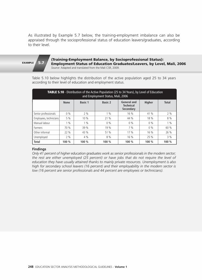
EXAMPLE 5.7
As illustrated by Example 5.7 below, the training-employment imbalance can also beappraised through the socioprofessional status of education leavers/graduates, accordingto their level.
248 EDUCATION SECTOR ANALYSIS METHODOLOGICAL GUIDELINES - Volume 1
Table 5.10 below highlights the distribution of the active population aged 25 to 34 yearsaccording to their level of education and employment status.
FindingsOnly 41 percent of higher education graduates work as senior professionals in the modern sector;the rest are either unemployed (25 percent) or have jobs that do not require the level ofeducation they have usually attained thanks to mainly private resources. Unemployment is alsohigh for secondary school leavers (16 percent) and their employability in the modern sector islow (16 percent are senior professionals and 44 percent are employees or technicians).
Senior professionals
Employees, technicians
Manual labour
Farmers
Other informal
Unemployed
Total
0 %
5 %
1 %
70 %
22 %
2 %
100 %
2 %
10 %
1 %
39 %
43 %
4 %
100 %
1 %
21 %
0 %
19 %
51 %
8 %
100 %
16 %
44 %
0 %
7 %
17 %
16 %
100 %
41 %
18 %
0 %
0 %
16 %
25 %
100 %
2 %
8 %
1 %
60 %
26 %
3 %
100 %
Basic 1 Higher TotalBasic 2 General andTechnical
Secondary
None
TABLE 5.10 - Distribution of the Active Population (25 to 34 Years), by Level of Educationand Employment Status, Mali, 2006
(Training-Employment Balance, by Socioprofessional Status):Employment Status of Education Graduates/Leavers, by Level, Mali, 2006Source: Adapted and translated from the Mali CSR, 2009.

Table 5.11 presents the structure and evolution of the positions available in Sao Tomé and Principeover the 2003-10 period.
FindingsTwo main conclusions can be drawn from the table: (i) the majority of available positions are forindividuals with little or no qualifications (58 percent in 2010 against 60 percent in 2003), andis declining relatively slowly; and (ii) demand for highly qualified candidates has increasedconsiderably. Even if only eight percent of jobs in 2010 required highly qualified workers,numbers have passed from 2,177 in 2003 to 3,742 in 2010, representing 72 percent growthover the period, a much higher rate than the average (overall, the demand for labour increasedby only eight percent over the period).
Highly Qualified
Average Qualifications
Little or No Qualifications
Employed Population
2,177
16,127
27,542
45,846
3,742
17,251
28,528
49,521
5%
35%
60%
100%
8%
35%
58%
100%
+72%
+7%
+4%
+8%
2003-2010Evolution (%)
2003 2010
TABLE 5.11 - Employed Population by Level of Qualification, Sao Tomé and Principe, 2010
Sector-Wide Analysis, with Emphasis on Primary and Secondary Education 249
ANTICIPATION OF FUTURE LABOUR MARKET NEEDS
1.6.1 PROMISING SKILLS AND QUALIFICATIONS
The qualification for a job represents the know-how and knowledge required to performthe related tasks. An individual’s qualifications are the result of the know-how andknowledge acquired either through training or by work experience.
If specialised surveys carried out with companies or on economic prospects are available, itwill be helpful to explore them to determine which qualifications are the most promising(in terms of employment). In addition to such surveys, it may also be helpful to usehousehold or employment survey data for two different years to obtain a historicalperspective of trends in terms of the qualifications found most attractive by the labourmarket.65 Example 5.8 below provides an illustration on the basis of Sao Tomé and Principe.
1.6
EXAMPLE 5.8
(Projection of the Demand for Skills, by Qualification Level):Determination of the most Promising Education Levels in Terms ofEmployment, Sao Tomé and Principe, 2010Source: Adapted and translated from the Sao Tomé and Principe CSR, 2012.
CHA
PTER 5EXTERN
AL EFFICIENCY

250 EDUCATION SECTOR ANALYSIS METHODOLOGICAL GUIDELINES - Volume 1
Finally, tracer surveys measure the employment status of recent graduates, enabling one tocomplete the analysis through comparisons of the employability rates by stream, disciplineand type of job.66
1.6.2 PROMISING SECTORS
In every country, as the economy evolves new professions appear and others dwindle ordisappear, not least as a consequence of new information and communication technologies.Knowledge of the promising sectors and professions enables better planning of the soughttraining-employment balance. To do this, the structure of the labour force must beestimated, covering as many activity branches as possible. Then for each branch the numberof positions available, both currently and for a previous period (generally four years earlier,depending on survey data availability), is estimated. Finally, the growth rate of employmentis computed for each branch. This indicator enables the identification of the branches thatcreate most new jobs and those that appear to be declining. The approach is illustrated bythe case of Sao Tomé and Principe, in Example 5.9 below.
EXAMPLE 5.9
Agriculture
Industry
Business
Services
Employed population
13,393
8,650
12,007
11,796
45,846
13,074
8,419
10,251
17,778
49,521
-2 %
-3 %
-15 %
51 %
8 %
2003-10Growth
2003 2010
TABLE 5.12 - Positions Available, by Activity Branch, Sao Tomé and Principe, 2003-2010
FindingsThe service sector is the most promising in terms of demand for labour, having shown growthabove 50 percent over the 2003-10 period. The supply of TVET and higher education coursesoriented towards this sector should no doubt be reinforced to face such demand and contributeto economic growth. (Service sector jobs relate to communication, transport, catering,maintenance and so on). On the other hand, employment in all other sectors is in decline,especially in the business sector where jobs have contracted by about 15 percent over the period.
(Projection of Demand for Skills, by Sector): Determination of PromisingSectors in Terms of Employment, Sao Tomé and Principe, 2010Source: Adapted and translated from the Sao Tomé and Principe CSR, 2012.

Sector-Wide Analysis, with Emphasis on Primary and Secondary Education 251
1.6.3 TOOLS FOR THE REGULAR MONITORING OF THE TRAINING-EMPLOYMENTBALANCE
To complete the analysis, it is helpful to adopt a qualitative approach in reviewing the tools,initiatives, mechanisms and institutional arrangements that exist to monitor and managethe relationship between training and employment. The analysis should also appraise theefficiency of these tools and mechanisms. Among other comments, it will be interesting tonote the existence of tools for the regular monitoring of education leavers’ outcomes in theworkplace (through career monitoring or tracer surveys). Annex 5.5 proposes a referentialguide of questions and issues that can be dealt with during interviews with the keyeducation sector players.
CHA
PTER 5EXTERN
AL EFFICIENCY

Education also has positive non-economic externalities, as a factor of change in individuals’social behaviour. These effects can include aspects as diverse as health, reproductivebehaviour, high-risk behaviour, or civic attitudes. The different effects can be evaluated atthe household level according to four key dimensions: (i) the promotion of health; (ii) thecontrol of fertility; (iii) civic commitment; and (vi) living conditions.
Measuring the social effects of education will here consist in appraising the impact ofeducation on these four dimensions. This section consists of three parts. The first part dealswith variables that are likely to be used to describe each of the four dimensions, based onthe different surveys that are commonly conducted in developing countries. A practicalillustration of how to evaluate the effects of different education levels on these dimensionsis explained in the second part. Given that the approach is the same for all of the fourdimensions, the illustration will just focus on one, the control of fertility. Finally, the thirdpart consolidates the results for different education levels and their impact on the socialbehaviours considered.
THE CHOICE OF SOCIALDEVELOPMENT VARIABLES
Whatever the dimension considered, three criteria should orient the choice of variables tocharacterise the different social impacts of education:
- Diversity, so that the choice of indicators covers all the facets considered;
- Ownership, so that the variables chosen reflect issues of national importance or coincidewith the country’s selected economic and social development indicators; and
- Availability, depending on the specific household surveys that have been carried out(CWIQ, DHS, MICS and so on) or the availability of data on more specialised populationgroups, especially where there is no operative routine data collection process, such asfor birth registrations.67
THE SOCIAL IMPACT OF EDUCATION
SECTION
2
2.1
252 EDUCATION SECTOR ANALYSIS METHODOLOGICAL GUIDELINES - Volume 1
2.1.1 VARIABLES DESCRIBING THE IMPACT OF EDUCATION ON HEALTH
The questions the analysis seeks to answer include: To what extent do more educatedindividuals more frequently adopt behaviour that is likely to protect or improve their healthand that of their children? Are they more likely to adopt healthy behaviour, use preventivetreatment, or protect themselves against illnesses, including HIV/AIDS and malaria?
In terms of maternal health, DHS, MICS, CWIQ and HIV/AIDS surveys usually provide dataon: (i) the use of iron supplements during pregnancy; (ii) prenatal health care and checks;(iii) the assistance at birth of skilled health personnel; (iv) the use of impregnated mosquitonets; (v) the use of basic health services (before, during and after pregnancy); and (vi)women’s level of knowledge of HIV/AIDS and how to avoid transmission.
Surveys usually provide the following useful information on the health of children (up tothe age of five years): (i) vitamin A supplements; (ii) children’s measurements at birth andnutritional status as they grow; and (iii) survival.
In terms of high-risk behaviour, the following might be considered: (i) use of tobacco; (ii)use of alcohol; (iii) having multiple sexual partners. These later data are sometimes alsoavailable for men, particularly in DHS surveys.
2.1.2 VARIABLES DESCRIBING THE IMPACT OF EDUCATION ON FERTILITY
Although many countries have begun (or indeed finished) their demographic transition68
process, others continue to have difficulties in controlling demographic growth due to highfertility rates. The role of education in the process of controlling demographic growth isunanimously recognised.
In the framework of education sector analysis, the data usually available through householdsurveys enable the evaluation of the impact of education on: (i) women’s age at firstmarriage; (ii) women’s age at first intercourse; (iii) mothers’ age at first childbirth; (iv) thespacing of births (measured by the ratio between the number of years between the firstand last birth at the time of the survey and the number of births over the period); (v)knowledge and use of birth control methods, either traditional or modern; (vi) the numberof live births; and (vii) the number of desired children. Some of these issues are also coveredby surveys targeting men; if so, it is appropriate to analyse such results as well.
2.1.3 VARIABLES DESCRIBING THE IMPACT OF EDUCATION ON CIVIC AND SOCIALCOMMITMENT
Over recent years, the number of cases of conflict in developing countries has increased,particularly in Africa. Political tension, war, threats to the legitimacy of republican institutions
CHA
PTER 5EXTERN
AL EFFICIENCY
Sector-Wide Analysis, with Emphasis on Primary and Secondary Education 253

254 EDUCATION SECTOR ANALYSIS METHODOLOGICAL GUIDELINES - Volume 1
and so on are more and more common. This underlines the need to examine the non-economic components of social well-being and progress in greater depth, which includesocial commitment, interest in politics and involvement in civil society. Education makes apositive contribution to these indicators.
On the basis of DHS/MICS survey data, the link between education and the followingaspects can be studied:
(i) Women’s knowledge of their rights: surveyed women are asked if they believe theycan refuse to have sex with their husband when tired, if they believe they have theright to insist that their husband wear a condom if he has an STD, if they believe thathusbands are entitled to beat their wives, and so on;
(ii) Prevalence of birth registration: Women are asked if their children’s births have beenregistered;
(iii) Female genital mutilation/excision practices: In DHS/MICS surveys, women are askedif they have heard of excision, if they think the practice should be maintained/abandoned, and if they think it is a religious requirement;
(iv) The level of interest in public affairs: some questions enable the analyst to determinewhether respondents listen to the radio, watch television or read a newspaper; and
(v) Sensitisation on gender issues: respondents are asked if they have a preference forthe gender of their children, about the schooling of boys and girls, and so on.
Furthermore, 1-2-3-type surveys69 include a module on democracy and governance. Suchmodules enable a quantified appraisal of governance both from the standpoint of the state’sefficiency and from that of households’ confidence in public institutions. For instance, thefollowing questions may be asked: Are you favourable to democracy? In your opinion, hasdemocracy in your country improved since the early 1990s? Did you participate in the lastelections/have you ever voted? Are you interested in politics? Do you discuss politics withyour entourage? Do you participate in political or union demonstrations?
2.1.4 VARIABLES DESCRIBING THE IMPACT OF EDUCATION ON LIVINGCONDITIONS
Poverty is a multidimensional phenomenon that cannot be reduced to monetary resources(income). Poverty should consider the full living conditions of a household. Householdsurveys enable the collection of several data on living conditions, such as the type ofaccommodation, household spending (in some), dress, leisure, ownership of a phone andso on.

Sector-Wide Analysis, with Emphasis on Primary and Secondary Education 255
Through a factor analysis based on the information collected, it will be possible to constructa synthetic indicator of households’ living conditions that will enable the classification ofhouseholds on a wealth scale.70 It is common to distinguish between five levels of wealth(called quintiles). The first two quintiles (40 percent of households) consist of those familiesliving in the most difficult conditions (the poorest). The variable that determines the linkbetween living conditions and education is thus the qualitative variable that reflects the factthat a household belongs to the first two quintiles, or not.
ESTIMATION OF THE NET EFFECTSOF EDUCATION71
For illustrative purposes, two fertility control variables will be chosen among those identifiedearlier to determine the social impact of education: the age of women at first childbirthand their knowledge of a modern contraceptive method. The same approach to the analysiscan be applied to other areas to determine the effect of education on them, as well as thecontribution of each education level to the overall impact.
2.2.1 IMPACT OF EDUCATION ON THE AGE AT FIRST CHILDBIRTH
The aim of the analysis is to: (i) estimate the evolution of women’s age at first childbirthaccording to the number of years of education they have received, while holding thevariables for other individual characteristics constant;72 and; (ii) compare the relativecontributions of each education level to the overall impact.
Given that the age at first childbirth variable is continuous, it is common practice to estimatethe impact of the number of years of education on the variable through a linear model.73
Linear models enable one to determine how age at first childbirth varies according towomen’s number of years of education, all other things being equal. The followingtheoretical example illustrates the approach.
CHA
PTER 5EXTERN
AL EFFICIENCY
2.2

Number of Years of Education
Number of Years of Education Squared
Women’s Age
Women’s Age Squared
Urban
Level of Income
Level of Income Squared
Constant
0.02150
0.02156
0.33778
-0.00390
-0.07835
1.26378
-1.56285
11.03507
0.00%
0.00%
0.00%
0.02%
0.00%
0.00%
0.01%
0.10%
SignificanceCoefficient (bj )Variable (Xj )
TABLE 5.13 - Results of the Linear Econometric Estimation of Age at First Childbirth(Theoretical Example)
256 EDUCATION SECTOR ANALYSIS METHODOLOGICAL GUIDELINES - Volume 1
Note: Data are for illustrative purposes only.
As the model is linear, the average relationship between the variable to be explained and theexplanatory variables is provided by the following equation:
To simulate the net effect of the number of years of education (all other things being equal), thevariable of interest is varied with respect to the number of years of education, whereas the othervariables are held constant (equal to their average). Table 5.14 illustrates the different steps ofthe computation to perform in the simulation process.
The results of the simulation enable one to draw the graph below that shows the evolution ofthe age at first childbirth according to the number of years of education for a woman whosecharacteristics are those of the average national woman (in terms of age, area of residence andlevel of income).
Y = bj Xj
j
EXAMPLE 5.10(Social Impact of Education by Level – Linear Model): Impact of EachEducation Level on Age at First Childbirth (Theoretical Approach)Source: Authors.
Table 5.13 below presents the results of a linear econometric estimation according to a modelexplaining the age of women at first childbirth, based on: (i) the number of years of educationeffectively completed; and (ii) control variables (women’s age, age squared, area of residence,level of income, level of income squared).74

Sector-Wide Analysis, with Emphasis on Primary and Secondary Education 257
CHA
PTER 5EXTERN
AL EFFICIENCY
Years of Education
Years of Education Squared
Age
Age Squared
Urban
Levelof Income
Level of IncomeSquared
Constant
0.021504
0.021562
0.337776
-0.003898
-0.078354
1.263784
-1.562853
11.035070
Coefficient(bj)
Averageof Xj
Numberof Years of
Education (N)
Variable (Xj)
-
-
30.69258
1,018.0243
0.49441
-0.00423
0.01078
1
A = Coef. x N
B = Coef. x N2
C = Coef. x Avg.
D = Coef. x Avg.
E = Coef. x Avg.
F = Coef. x Avg.
G = Coef. x Avg.
H = Coef. x Avg.
Sum(Simulated Ageat FirstChildbirth)
0 2 4 6 8 10 13
0.000
0.000
10.367
-3.968
-0.039
-0.005
-0.017
11.035
17.4
0.043
0.086
10.36
-3.968
-0.039
-0.005
-0.017
11.03
17.5
0.086
0.345
10.36
-3.968
-0.039
-0.005
-0.017
11.03
17.8
0.129
0.776
10.36
-3.968
-0.039
-0.005
-0,017
11,03
18.3
0.172
1.380
10.36
-3.968
-0.039
-0.005
-0.017
11.03
18.9
0.215
2.156
10.36
-3.968
-0.039
-0.005
-0.017
11.03
19.7
0.280
3.644
10.36
-3.968
-0.039
-0.005
-0.017
11.03
21.3
16
0.344
5.520
10.36
-3.968
-0.039
-0.005
-0.017
11.03
23.2
TABLE 5.14 - Simulation of the Age at First Childbirth According to the Number of Years of Education(Theoretical Example)
Note: Data are for illustrative purposes only.
24
23
22
21
20
19
18
17
160 1 2 3 4 5 6 7 8 10
Years of education
11 12 13 14 15 169
Age
at
first
chi
ldbi
rth
(Yea
rs)
FIGURE 5.5 - Evolution of Age at First Childbirth According to the Number of Years of Education(Theoretical Example)
Age at F
19
20
21
22
23
24
ears
)
- Evolution of FIGURE 5.5
t ch
ildbi
rth
(YYe
heoretical Example)(T
According to the Number of irst Childbirth Age at F
ears of EducationYYeAccording to the Number of
16
17
18
19
Age
at
first
chi
ldbi
rth
(Y
43210
9
ears of educationYYe
1087654
16151413121110
FindingsEducation has a significant impact on the age at first childbirth, showing a quadratic relationship(the variable for the number of years of education squared is significant). The analysis of the lastline of Table 5.14 shows that the effect of education is relatively weak during the primary cycle(six years), with a difference of 0.9 years (=18.3-17.4) between the first childbirth of uneducatedwomen and those with 6 years of education. The impact is more substantial as of lower secondary
Note: Data are for illustrative purposes only.

258 EDUCATION SECTOR ANALYSIS METHODOLOGICAL GUIDELINES - Volume 1
(1.4 years (=19.7-18.3) difference between the end of primary and the end of lower secondary),and remains significant through upper secondary and higher education. The average age at firstchildbirth increases by 1.6 years (=21.3-19.7) for women with upper secondary (compared tothose with lower secondary) and by 1.9 years (= 23.2-21.3) for women with higher education(compared to those with upper secondary).
After simulating the evolution of the age at first childbirth according to the number of years ofeducation, the estimation of the contribution of each level is obtained on the basis of the addedvalue of each education level with respect to the previous level, called the marginal impact. Thecontribution of a level is then the share of the overall variation.
Table 5.15 shows in detail how to perform the estimation of the marginal impact of eacheducation level, based on the last line of Table 5.14.
Level of Education
Age at First Childbirth (Years)
Marginal impact (results)
Impact of Each Education Levelon Age at First Childbirth
Marginal Impact (formula)
Distribution of the TotalImpact (%)
None(1)
Higher(5)
Upper Sec.(4)
Lower Sec.(3)
Primary(2)
Effet totalE = a+b+c+d
17.4 18.3 19.7 21.3 23.2
a = (2)-(1) b = (3)-(2) c = (4)-(3) d = (5)-(4)
15.4 25.0 26.5 33.1 100
0.9 1.4 1.6 1.9 5.8
100 x a/ E 100 x b/ E 100 x c/ E 100 x d/ E Total
TABLE 5.15 - Effect of Each Education Level on the Age at First Childbirth(Theoretical Example)
FindingsThe age at first childbirth increases by 5.8 years (=23.2-17.4) on average for women with highereducation (compared to uneducated women), all other things being equal. This is the total neteffect of education on the variable. Higher education has the highest impact of any level (33percent (=1.9/5.8) of the total impact) and primary education has the lowest impact (15 percent(= 0.9/5.8)). A woman who leaves school with lower secondary for instance will benefit fromonly 40 percent (=15+25) of the overall impact that would be achieved by continuing to highereducation.
Note: Data are for illustrative purposes only.

EXAMPLE 5.11
(Social Impact of Education by Level – Logistical Model): Impact of Each Level of Education on the Probability of Knowing atLeast One Modern Contraceptive Method (Theoretical Approach)Source: Authors.
Sector-Wide Analysis, with Emphasis on Primary and Secondary Education 259
CHA
PTER 5EXTERN
AL EFFICIENCY
2.2.2 IMPACT OF EDUCATION ON THE KNOWLEDGE OF A MODERNCONTRACEPTIVE METHOD
As per the approach adopted above, the objective of this analysis is to: (i) estimate theevolution of the likelihood of women knowing at least one modern contraceptive methodaccording to the number of years of education they have received, while holding thevariables for other individual characteristics constant; and; (ii) compare the relativecontributions of each education level to the overall impact.
MICS/DHS/HIV surveys usually include a series of questions about women’s knowledge ofcontraception. Their responses enable the construction of a qualitative variable that adoptsthe value of 1 when women know of at least one modern contraceptive method, and thevalue of 0 otherwise. As the variable is binary (dummy variable)75, logistical models (and notlinear models as above) are the most appropriate to use in this case.76
The share of women knowing a modern contraceptive method after N years of educationis then estimated according to the following equation:
Xj is the jth explanatory variable (the number of years of education completed, or a controlvariable) and bj is the jth parameter to estimate, that describes the direction of the effect ofXj on P. These parameters are then estimated thanks to specialised statistical software (Stata,SPSS, and so on). As for the linear model, the variable for the number of years of educationis adjusted but the control variables are held constant (equal to their averages).
An illustration of the application of this approach is provided in Example 5.11. To estimatethe respective contributions of each level of education, the same approach as in Example5.10 above is used.
bj Xj
j
P = = where S = , and1
1+expbj Xj -
j
1
1+exp- S
Table 5.16 below presents the results of the logistical econometric estimation according to amodel explaining the likelihood that women know at least one modern contraceptive method,based on: (i) the number of years of education completed; and (ii) control variables (women’sage, age squared, area of residence, level of income, level of income squared).

TABLE 5.16 - Results of the Logistical Econometric Estimation of the Probability of Knowingat Least One Modern Contraceptive Method (Theoretical Example)
Number of Years of Education
Number of Years of Education Squared
Women’s Age
Women’s Age Squared
Urban
Level of Income
Level of Income Squared
Constant
0.845894
0.005487
0.060536
-0.000624
0.127227
4.235022
-7.277579
-5.877556
0.00%
0.05%
0.00%
0.00%
0.00%
0.02%
0.00%
0.01%
SignificanceCoefficient (bj) WaldVariable (Xj)
90,671,542
428,777
645,876
285,073
1,209,981
29,981,813
1,795,904
23,662,970
Note: Data are for illustrative purposes only.
260 EDUCATION SECTOR ANALYSIS METHODOLOGICAL GUIDELINES - Volume 1
Table 5.17 provides the different steps of the calculation to be performed to simulate the netprobability of knowing a contraceptive method according to the number of years of education(all other things being equal).
Years of Education
Years of Education Squared
Age
Age Squared
Urban
Levelof Income
Level of IncomeSquared
Constant
0.84589
0.00549
0.06054
-0.00062
0.12723
4.23502
-7.27758
-5.87756
Coefficient(bj)
Averageof Xj
Numberof Years of
Education (N)
Variable (Xj)
-
-
30.7770
988.0223
0.5375
-0.0084
0.0121
1
A = Coef. x N
B = Coef. x N2
C = Coef. x Avg.
D = Coef. x Avg.
E = Coef. x Avg.
F = Coef. x Avg.
G = Coef. x Avg.
H = Coef. x Avg.
Sum(Probabilityknowing ameans ofcontraception)
0 2 4 6 8 10 13
0.000
0.000
1.863
-0.616
-0.068
0.036
-0.088
-5.878
-4.614
1.0
1.692
0.022
1.863
-0.616
-0.068
0.036
-0.088
-5.878
-2.901
5.2
3.384
0.088
1.863
-0.616
-0.068
0.036
-0.088
-5.878
-1.143
24.2
5.075
0.198
1.863
-0.616
-0.068
0.036
-0.088
-5.878
0.658
65.9
6.767
0.351
1.863
-0.616
-0.068
0.036
-0.088
-5.878
2.504
92.4
8.459
0.549
1.863
-0.616
-0.068
0.036
-0.088
-5.878
4.393
98.8
10.997
0.927
1.863
-0.616
-0.068
-0.036
-0.088
-5.878
7.309
99.9P = 1/(1+exp(-S))(%)
TABLE 5.17 - Simulation of the Probability of Knowing at Least One Modern Contraceptive Methodby Number of Years of Education (Theoretical Example)
Figure 5.6 illustrates the evolution of the probability of knowing at least one means ofcontraception (last line of Table 5.17) according to the number of years of education completed.
Note: Data are for illustrative purposes only.

Sector-Wide Analysis, with Emphasis on Primary and Secondary Education 261
CHA
PTER 5EXTERN
AL EFFICIENCY
1009080706050403020100
0 1 2 3 4 5 6 7 8 10
Number of Years of Education
11 12 139
FIGURE 5.6 - Evolution of the Probability of Knowing at Least One Modern Contraceptive Method Accordingto the Number of Years of Education (Theoretical Example)
Perc
ent
to the Number of
100
- Evolution of the Probability of Knowing at Least One Modern Contraceptive Method FIGURE 5.6heoretical Example)ears of Education (TYYeto the Number of
- Evolution of the Probability of Knowing at Least One Modern Contraceptive Method heoretical Example)
According - Evolution of the Probability of Knowing at Least One Modern Contraceptive Method According
0
0
102030405060708090
100
3210
cent
Per
87654 9 13121110
ears of EducationNumber of YYeears of Education
Illustrative FindingsThe variable with the highest impact on the knowledge of modern contraceptive methods is thenumber of years of education (the highest Wald statistic in Table 5.16 above). The probability ofwomen knowing at least one means of contraception jumps from 1 percent for those withouteducation to 65.9 percent for those having completed primary, to 100 percent for those withhigher education.
Note: Data are for illustrative purposes only.
CONSOLIDATION OF THE NET SOCIAL EFFECT OF EDUCATION
At the end of this section, it is helpful to summarise the results obtained for each of thefour dimensions studied (health, the control of fertility, civic commitment and livingconditions) and compute the cost-efficiency ratios for each level of education. This analysisprovides education sector decision makers with further helpful information to guide theintra-sectoral allocation of resources to optimise the social benefit of education. Example5.12 drawn from the Sierra Leone CSR illustrates the recommended approach.
2.3

EXAMPLE 5.12(Consolidated Net Social Effect of Education): Global Social Impact of Different Education Levels, Sierra Leone, 2010Source: Adapted from the Sierra Leone CSR, 2012.
262 EDUCATION SECTOR ANALYSIS METHODOLOGICAL GUIDELINES - Volume 1
Controlof Fertility
Maternal andChild Health
Female GenitalMutilation
Age at First Childbirth
Total Number of Live Births
Use of Contraception
HIV/AIDS Knowledge Score
Poverty
Average Social Impact for the Level1
Average Social Impact of one Grade2
Public Recurrent Unit Cost per Grade
(Multiple of Primary)
Cost-Efficiency Index = Impact / Cost x 100
Relative Cost- Efficiency (Primary = 100)3
Probability of Being amongthe 40% Poorest
Probability of Home Delivery
Use of Tetanus Toxoidduring Pregnancy
Use of Malaria Prevention Medicineduring Pregnancy
Probability of Approval for Daughters
Probability of at Least One Child Dying
HigherSSSJSSPrimary
45
44
46
45
56
46
42
38
41
33
43.6
7.3
1
0.073
100
20
19
25
22
19
21
22
23
22
16
20.9
7.0
1.6
0.044
59.9
25
25
20
20
17
20
22
24
22
12
20.7
6.9
2.7
0.026
35.0
10
12
9
13
8
13
14
15
15
39
14.8
7.4
18.6
0.004
5.4
TABLE 5.18 - Distribution of the Social Impact of Education,by Level and Type of Behaviour, Sierra Leone, 2010
Table 5.18 consolidates the net social effects of education on different behaviours to determinethe global contribution of each level of education.
Note: 1 Each item of this line is obtained as the simple average of the values of the respective column. For instance, 43.6 =(45+44+46+45+56+46+42+38+41+33)/10. 2 The items of this line are obtained by dividing the impact of each level by thenumber of years for that level. For instance, 7.3=43.6/6. 3 All the items of this line are obtained by dividing the values of theprevious line by the primary level cost-efficiency index. For instance, 59.9=(0.044/0.073)*100.
FindingsOn average, the primary cycle represents almost half (43.6 percent) of the total social impact ofeducation on the behaviours considered. Secondary (combining junior and senior secondary)and higher education respectively account for 41.6 percent and 14.8 percent of the impact.When accounting for the number of years per cycle, a year of primary education accounts for7.3 percent of the total social impact, a year of secondary for 7.0 percent and a year of highereducation for 7.4 percent. On this basis, each year of schooling in Sierra Leone has a marginalimpact on social behaviour of approximately 6.7 percent.The results in the last row of the table underline the very high cost-efficiency of the primary cyclein human development terms, compared to the secondary and especially the tertiary levels.Indeed, the decreasing level of cost-efficiency with each level of education is notable. All costsbeing equal, the efficiency of the primary cycle in enhancing human development is two timeshigher than that of the secondary cycle and 20 times higher than that of tertiary education.

Sector-Wide Analysis, with Emphasis on Primary and Secondary Education 263
CHA
PTER 5EXTERN
AL EFFICIENCY
NOTES
46 Furthermore, because the production of such data is generally the responsibility of institutions that are not part of theeducation and training sector as such, their interest in the issue is often dampened.
47 By being better informed, it is expected that individuals’ participation in the life of the community will be moreappropriate.
48 For all indicators and analyses, it will be important where data permit to provide a historical perspective and aninternational comparison with countries of similar characteristics.
49 Company is used here in a generic sense, to designate any goods and/or services production unit, be it for profit (public,public-owned or private enterprises) or non-profit (public institutions, charities, etc.).
50 Regional employment may also be worthy of analysis, especially for higher education graduates.
51 These issues should be further highlighted in section 1.3 where the quality of employment is analysed.
52 Unless specifically mentioned, the generic term household surveys will be used to encompass any survey with anemployment module.
53 Household surveys often enable more detailed analysis, by disaggregating indicators by individuals’ gender, age, areaof residence and level of education. Whether from administrative or survey data, it is always helpful to provide a recenthistorical perspective.
54 The definition of activity branches adopted by AFRISTAT member countries (the NAEMA classification), is derived fromthe United Nations’ International Standard Industrial Classification (ISIC) by type, industry and economic activity branch.
55 Written or verbal agreement whereby an active individual offers their activity to the service of an employer (in exchangefor remuneration or not).
56 This approach is best especially where no questions were asked to determine an individual’s salary status.
57 It can help to limit analyses to a sample of recent graduates/leavers (See Annex 5.3).
58 Unstable positions are those whose contractual status is temporary. For the analysis, it is common to consider self-employment and unpaid family helpers as members of the active population with instable positions.
59 Finally, a third complementary approach may be used where the data permit, and consists of the qualitative opinion ofindividuals with respect to their under-employment or over-qualification.
60 This definition was introduced by Nauze et al., 2002. Instead of the mean income, the average income minus onestandard deviation is sometimes used.
61 The social return on investment presented in this section is not the same as the social impact of education presented inSection 2 of this chapter.
62 The evolution of the supply of jobs is generally considered to be linear between the two periods considered.
63 For instance, if 100,000 new jobs were available each year over the 2005-10 period and that the unemployment rateamong new graduates/leavers was 10 percent, the training-employment balance should be based on a cohort of 111,111youth (=100,000/(1-10%)).
64 If only the data from one survey is available and that it provides information on individuals’ seniority, the number ofemployed with at least X years of seniority (say 5 years) can provide a gross estimate of the total number of new jobsprovided over the last X years. This number can then be divided by X to obtain an estimate of the annual averagenumber of new jobs.
65 Senior and mid-level professional positions and similar jobs are considered to be highly qualified positions; qualifiedemployers, foremen and technicians are considered to require average qualifications; and self-employed, managers andmanual labour positions are considered to require few qualifications.
66 See Annex 5.4.
67 These surveys may provide information on poverty, literacy, birth registration, knowledge of HIV/AIDS transmission,maternal and child health, and so on. Annex 5.2 provides further detail on such surveys.
68 The demographic transition is the change from a traditional demographic growth pattern in which both birth andmortality rates are very high (around 40‰) to a modern one, where birth and mortality rates are weak (around 10‰).The transition often begins with a drop in mortality (helped by progress in terms of health), to then be accompanied bya drop in birth rates (which takes longer to become effective given the heavy social and behavioural changes implied).Thus, demographic transition processes are accompanied in their early stages by strong demographic growth.

264 EDUCATION SECTOR ANALYSIS METHODOLOGICAL GUIDELINES - Volume 1
69 See Annex 5.2 for a description of such surveys.
70 A factor analysis is a mathematical approach enabling the synthesis of data into a mono or multidimensional indicator,based on several elements (variables) that describe a phenomenon. An index can also be directly although subjectivelyconstructed giving appropriate weights to each of the constituents of wealth.
71 A net effect estimates the association of a variable with an other, all other variables being equal.
72 Such variables include the area of residence, household living conditions, age and so on.
73 For a more precise measurement still, it may be helpful to use a more complex statistical model (a simple duration model)given that the age at first childbirth is a quantitative variable that is right-censored: it is only measured for women havinggiven birth at least once in their life. However, the results with a simple duration model are usually similar to thosereached through the linear model.
74 Some variables are squared when it is suspected that the relationship between the variable and the phenomenon understudy is not only linear. This allows to take into account the fact that the concavity of the relationship can change overtime.
75 A binary (or dummy) variable is a variable that takes the value either 1 or 0 (usually matching with the answers “Yes”and “No”).
76 Probit type models can also be used. See Annex 0 for further details.

© W
orld
Ban
k /
Régi
s L’
Hos
tis
Sector-Wide Analysis, with Emphasis on Primary and Secondary Education 265
CHA
PTER 5EXTERN
AL EFFICIENCY

266 EDUCATION SECTOR ANALYSIS METHODOLOGICAL GUIDELINES - Volume 1
© W
orld
Ban
k /
Régi
s L’
Hos
tis

CHAPTER 6EQUITY › Chapter Objective:To analyse: (i) the extent to which enrolmentpatterns and school results vary according tokey sociodemographic factors, and (ii) howpolicy choices in terms of public resourcedistribution affect equity.
Sector-Wide Analysis, with Emphasis on Primary and Secondary Education 267
CHA
PTER6
EQUITY

1. EQUITY IN ENROLMENT AND LEARNING ACHIEVEMENTS
ISSUEDo all children face the same enrolment chances? Or, on the contrary, are the disparities inschooling careers and results large, and affected by criteria beyond individuals’ control?
OBJECTIVES• Identify the existence and extent of disparities in schooling careers and results according to
gender, area of residence (urban/rural), geographic location, people with disabilities andhousehold wealth.
METHODS• Analyse individuals schooling careers and results according to gender, location, and household
income; and• Illustrate the disparities through the use of various indicators: parity index, odds ratios, and so on.
SOURCES• Population: projection data based on population censuses (gender, area of residence) or United
Nations projections (gender), household surveys (gender, area of residence, location, householdincome);
• School data (enrolment, repetition by gender and location): data provided by educationmanagement information systems (EMIS);
• Specific surveys on learning achievements;• National exam/test results; and• Household surveys (MICS, DHS, CWIQ, and so on).
2. EQUITY IN THE DISTRIBUTION OF PUBLIC EDUCATION RESOURCES
ISSUEDo public education resources benefit all equally, or are they concentrated within a particularsegment of the population? Is the education system a channel for the reduction or the increasein inequalities inherent at birth?
OBJECTIVES• Evaluate the degree of equity in the distribution of public education resources by highest year
of schooling achieved (structural equity); and• Evaluate the degree of absorption of public resources by various socioeconomic groups
(distributive equity/social selectivity).
METHODS• Build the Lorenz curve and deduce the Gini coefficient and the share of education resources
absorbed by the 10 percent most educated;• Calculate the factor of appropriation of public resources by different socioeconomic groups; and• Carry out international comparisons.
SOURCES• School data from EMIS;• Household surveys; and• Unit costs (see Chapter 3).
268 EDUCATION SECTOR ANALYSIS METHODOLOGICAL GUIDELINES - Volume 1

Sector-Wide Analysis, with Emphasis on Primary and Secondary Education 269
IntroductionWhat is equity?
The notion of equity is to be distinguished from that of equality with which it is sometimesconfused, however close they may be. Equality is based on a mathematical premise, therelative evenness in the distribution of resources, and is close to the notion of equaltreatment. Equity on the other hand refers to a concept of social justice and thus is moreassimilated to the notion of equal chances.
In the name of the principle of equity (increasing social justice), the two main approachesare:
• Treating equals equally. In this case, the allocation of resources will be deemed equitableif all members of a group with similar needs (the poor, adolescents, rural populations,people with disabilities, and so on) benefit from equal treatment. According to thedistribution criteria chosen, one will analyse whether allocated resources, access, usage,or the benefits of education are equally shared within the group; and
• Not treating unequals equally. Here, the idea is to avoid treating all groups equally,instead favouring some or disadvantaging others through positively discriminatorypolicies or quotas. These measures aim to offer more to those with special needs,therefore compensating the inequity they face as a result of their difference.
In the analysis of equity and in the context of this guide, the first step will be to determinethe groups (and its individuals’ characteristics) that suffer from a disadvantage in terms ofaccess to education and schooling careers. The most relevant characteristics, according tothe principle of equal chances, are those that individuals have little control over. Althoughthere is currently no consensus regarding these characteristics, that often hinge on aparticular cultural or historical context, this guide proposes to retain a set that are easilyidentified and measured: gender, area of residence (urban/rural), location and socioeconomicstatus. This non exhaustive list may be extended to other characteristics that reflect theparticular circumstances of a given analysis: ethnic origin, religion, disability, orphanhood,and so on.77
CHA
PTER6
EQUITY

270 EDUCATION SECTOR ANALYSIS METHODOLOGICAL GUIDELINES - Volume 1
Why is it important that education sector policies incorporate the equity dimension?
The search for equity in education responds to two basic issues. The first is about social justiceand reducing socioeconomic inequalities; the second is about socioeconomic efficiency.
Education is considered to be one of the best channels to reduce socioeconomic inequalities,and especially, a powerful tool to reduce their trans-generational transmission. The level ofqualifications and degrees obtained throughout schooling determine an individual's futuresocioeconomic status to a certain extent. Education systems are therefore expected to offereach child similar chances of success, based on merit over and above personal characteristicsbeyond their control (gender, area of residence, and so on). Given that schooling optionsare likely to be affected by individuals’ financing ability and other specific characteristics, itis important to determine the extent to which education systems, especially those that arepublicly funded, take these factors into account to limit their impact on individuals’ accessto school and results.
Socioeconomic efficiency reflects the theory that education, as human capital, is a keydetermining factor for social and economic development, such as through the reduction ofmaternal, infant and child mortality or fertility at the individual level, or through thecontribution to innovation and economic growth at the collective level. The collective interestimplies ensuring that all members of society achieve a minimal level of education on theone hand, and that the most capable individuals reach the highest levels of education,regardless of their socioeconomic origin, on the other.
In addition, paying attention to equity in the education policy is a way to promote andstrengthen social cohesion and can help reduce the risks of conflicts (see World Bank WDR2011). This chapter is also an opportunity to address the equity issues faced by childrenwith disabilities. For many reasons, children with disabilities are more likely to not be enrolledin school or to drop out. Box 6.1 outlines the main issues.
BOX 6.1CHILDREN WITH DISABILITIES AND ACCESS TO EDUCATION
An estimated 24 million out-of-school children experience some form of disability includinglearning, speech, physical, cognitive, sensory disabilities or emotional difficulties. In addition,there are many children with disabilities who are in school, but are expected to drop out. Thispopulation at risk consists of three main categories:
(i) Children with disabilities who are enrolled in school but who are excluded from learningbecause the curriculum has not been adapted to fit their needs or teachers do not havethe capacity or time to make the needed adaptations, and/or they do not have access toassistive devices necessary for their learning needs (for instance, children with low visionare unable to see the board without eye glasses, and some of them require large printtextbooks);
▶

Sector-Wide Analysis, with Emphasis on Primary and Secondary Education 271
CHA
PTER6
EQUITY
The inclusion of children and adults with disabilities in education is important for several reasons:Education contributes to human capital formation and is thus a key determinant of personalwell-being and welfare; excluding children with disabilities from educational and employmentopportunities has high social and economic costs (for example, adults with disabilities tend tobe poorer than those without disabilities, but education weakens this association); countriescannot achieve Education for All or the Millennium Development Goal of universal completionof primary education without ensuring access to education for children with disabilities.
Despite the increased global interest in children with disabilities, relatively little is known aboutthe specific situation of children with disabilities, particularly in developing countries. There is anurgent need for better quality data on children with disabilities, especially disaggregated datathat explain the different disabilities and impairments as well as the level of severity so thatappropriate measures can be taken.
More information can be found in the 2011 WHO World Report on disability (Chapter 7:Education).
(ii) Children who are not enrolled in school but who could participate well if schools had thecapacity in terms of knowledge, skills and equipment to respond to their specific needs(for instance, children with physical disabilities cannot go to school when buildings arenot accessible);
(iii) Children with severe disabilities who require additional specialised support.
The group of children with severe disabilities is usually a relatively small group (2-3 percent), yetchildren with milder disabilities suffer from inequality in terms of access to education andretention.
FIGURE 6.1 - Proportion of Children Aged 6-11 with and without a Disability who Are in School
Disabled Not disabled
100
80
60
40
20
0Prop
ortio
n A
tten
ding
Sch
ool (
%) Children aged 6-11 years
ThePlurinational
State of Bolivia
Burundi Cambodia Chad Colombia India Indonesia Jamaica Mogolia Mozambique Roumania South Africa Zambia
Proportion of Children
100
-FIGURE 6.1
en aged 6-11 yearsChildr
opor
tion
Att
endi
ng S
choo
l (%
)
Aged 6-11 with and without a Disability who Proportion of Children Are in SchoolAged 6-11 with and without a Disability who
0
20
40
60
80
100
ChadCambodiaBurundi
State of BoliviaPlurinational
eTh
opor
tion
Att
endi
ng S
choo
l (%
)Pr
amaicaJIndonesiaIndiaColombiaChad
ZambiaSouth AfricaRoumaniaMozambiqueMogolia
Disabled Not disabled
Source: World report on disability, WHO, 2011.

272 EDUCATION SECTOR ANALYSIS METHODOLOGICAL GUIDELINES - Volume 1
Two types of analysis are offered by this guide to establish the extent to which an educationsystem is either equitable or inequitable:
• The first deals with inequalities in access to school, schooling paths, and learningachievements: it will establish the extent to which access, retention and learning arerelated to individual characteristics;
• The second deals with inequalities in the distribution of public education resources.Education is financed mainly by the state, on public funds; each individual will absorba certain level of public resources, based on their schooling career. Therefore thedistribution of public education resources among a generation of children will dependon: (i) the distribution according to the highest level achieved; and (ii) the structure ofpublic spending by pupil for each level. The distribution will be all the more unequal asschooling careers vary considerably and unit costs increase substantially with successivecycles. Conversely, it will be all the more equitable if all children of a given age haveaccess to school and follow similar schooling careers, and/or if unit costs only increasemarginally with each level. In this regard, it will be appropriate to analyse whether thedistribution of resources favours equity; in other words, whether it compensates theinequalities that exist among different groups at birth, or reinforces them.
To answer these questions and evaluate the equity of an education system, a battery ofindicators is available to help quantify and measure the phenomena at play. The basicunderlying principle is that equitable and effective education policies should lead to equalityin the access to education opportunities in the broadest sense by different social groups.

Sector-Wide Analysis, with Emphasis on Primary and Secondary Education 273
CHA
PTER6
EQUITY
EQUITY IN ENROLMENTAND LEARNINGACHIEVEMENTS
Reviewing the equality of school access chances is the first step in the analysis of aneducation system’s level of equity. If children do not have the same chances of access toschool, the system will clearly not offer them all the same chances to learn. The guide willtherefore first focus on the identification of possible disadvantaged groups in terms of schoolaccess, through both access indicators (gross access rate, access probability, and so on),and equity indicators elaborated on the basis of the former. Equity indicators can becomputed for any education cycle/level.
However, ensuring an equitable initial access to school is insufficient in as much asdifferences may arise during children’s progression through school. The second step willtherefore be to establish the extent to which these differences do arise, and if they occur atthe expense of a group of individuals defined by characteristics beyond their control (gender,location, ethnic origin, socioeconomic status, and so on). This analysis will be carried outwith the help of indicators measuring schooling careers (access rates to different schoollevels, transition rates between school cycles and retention rates within given cycles). It willalso be possible to provide more global perspectives of school participation through grossenrolment rates and school life-expectancy.
The third step may involve an evaluation of the learning achievements of children in lightof the academic objectives set, which is a challenge. The analysis may focus on the extentto which differences in learning achievements or qualifications upon leaving school (examsuccess rates and results) are related to pupils’ characteristics and origins. Here again, thecalculation of specific equality indicators on the basis of the outcome indicators will help toestablish the degree of equity.
In the following sections, the guide will illustrate through specific examples how variousindicators may be used to highlight equity issues in a given education system. See Chapters2 and 4 and the annexes for a description of schooling and learning achievement indicators.
SECTION
1

EXAMPLE 6.1
TABLE 6.1 - Gender Disparities in Access to the First Cycle of Basic Education, Mali, 2007/08
Boys
86.8%
63.5%
Year of Study Girls
72.3%
44.7%
Gap
14.5 = 86.8 - 72.3
18.8 = 63.5 - 44.7
1
6
FindingsIn the example illustrated by Table 6.1, a total gap of 14.5 percentage points is observed betweenthe primary access of boys and girls in Mali in 2007/08, indicating the need to increase the primaryaccess rate of girls by 14.5 percentage points for gender equity in terms of access to be achieved.
(Absolute Gap):Gender Disparities in Primary Access, Mali, 2007/08Source: Translated and Adapted from the Mali CSR, 2010.
274 EDUCATION SECTOR ANALYSIS METHODOLOGICAL GUIDELINES - Volume 1
It is also possible to compare subgroups to identify extreme situations. The example belowrepresents the disparities in schooling between two extreme groups, wealthy urban boysand poor rural girls, based on school access rates.
Absolute gap in the access rates of the extreme groups (combining gender, location, andlevel of income):
Access rate for wealthy urban boys – Access rate for poor rural girls
THE ABSOLUTE GAP IN PERFORMANCEBETWEEN TWO GROUPS
The absolute gap in the performance of two groups A and B (such as urban and ruralpopulations, boys and girls, rich and poor) is calculated by subtracting the chosenperformance indicator (intake rate or probability, gross enrolment rate, completion rate, orexam success rate) for group A from that for group B:
Absolute gap in the primary level gross intake rate (GIR) between boys and girls:Boys’ GIR – Girls’ GIR
Where the primary gross intake rate for girls (the same applying for boys) is:
The absolute gap is interpreted as the amount by which it is necessary to increase theperformance indicator for group B (girls in this instance) to achieve equity between the twogroups.
1.1
Number of non-repeating female students in primary Grade 1Female population of the theorical age of primary Grade 1

TABLE 6.2 - Cumulative Disparities in Access Rates to Various School Levels, The Gambia, 2006
Wealthy Urban Boys
95.7%
83.3%
77.6%
Year of Study Poor Rural Girls
60.3%
14.7%
8.5%
Gap
35.4 = 95.7 - 60.3
68.6
69.1
1
6
7
120
100
80
60
40
20
0 1 2 3 4 5 6 7 8 9
Poor Rural Girls
77.6
10 11 12
95.7
60.3
83.3
70.3
57
43.4
14.78.5 7.7
2.4 1.4
Year of Study
Acc
ess
Rate
s (%
)
Wealthy Urban Boys
FIGURE 6.2 - Cumulative Disparities in Access Rates to Various School Levels, The Gambia, 2006 - Cumulative Disparities in
80
100
120
Acc
ess
Rate
s (%
)
FIGURE 6.2
60.3
95.7
arious School Levels
77.683.3
VAccess Rates to - Cumulative Disparities in 2006
57
70 3
Poor Rural Girls
ealthy Urban Boys
he Gambia,T,arious School Levels
W
70.3
32 1 0
20
40
60
Acc
ess
Rate
s (%
)
60.3
87654
ear of StudyYYe
9
57
121110
FindingsThe example of The Gambia shows that the gap between the two groups is apparent and growsquickly throughout the primary cycle to reach 68.6 percentage points (83.3 – 14.7) by the endof the cycle (Year 6). The gap between wealthy urban boys and poor rural girls continues toincrease with secondary cycle access (Year 7).
The graphic representation of these indicators offers an interesting visual illustration:
EXAMPLE 6.2(Absolute Gap): Cumulative Disparities in Access to Primary Levels,The Gambia, 2006Source: Adapted from the Gambia CSR, 2011.
Sector-Wide Analysis, with Emphasis on Primary and Secondary Education 275
CHA
PTER6
EQUITY
THE PARITY INDEX
The parity index comparing groups A and B is obtained by dividing the performanceindicator (school coverage, access rate, retention rate, completion rate, repetition rate,learning results, and so on) of group A by that of group B. The parity index provides thefactor by which it would be necessary to multiply the group B indicator (or divide the groupA indicator) to achieve an equal value for both groups. Parity between the two groups is
1.2

EXAMPLE 6.3(Parity Index): PCR Disparities, by Socioeconomic Characteristic, Malawi, 2006Source: Adapted from the Malawi CSR, 2010.
276 EDUCATION SECTOR ANALYSIS METHODOLOGICAL GUIDELINES - Volume 1
It is noteworthy that the absolute gap and the parity index do not necessarily vary in thesame direction. An illustration of this is offered in Annex 6.1. See also Annex 6.2 for a moredetailed analysis of enrolment, and in particular the respective weight of different schoolingstages in explaining overall disparities in the enrolment of different groups.
TABLE 6.3 - Parity Index for the Primary Completion Rate, by Children’s Socioeconomic Characteristic,Malawi, 2006
Boys
Girls
Gender Parity Index (Girls/Boys)
Urban
Rural
Residence Parity Index (Rural/Urban)
Q5 (Wealthiest 20%)
Q1 (Poorest 20%)
Wealth Parity Index (Q1/Q5)
PCR (%)
45
31
0.69 = 31/45
66
32
0.48 = 32/66
67
23
0.34 = 23/67
Socioeconomic Characteristics
Gender
Area of Residence
Household Wealth
FindingsIn this example, the gender parity index is 0.69, meaning that for every 100 boys completingprimary, only 69 girls complete the cycle. The gaps by area of residence and household wealthare starker still: for every 100 children from the wealthiest quintile completing primary, only 34children from the poorest quintile finish the cycle.
The PCR can also be calculated according to the area of residence, location, orsocioeconomic status, as illustrated by the example of Malawi below.
Gender Parity Index for the Primary Completion Rate (PCR): Girls’ PCRBoys’ PCR
achieved when the parity index is equal to 1. An index value above 1 indicates an advantagefor group A (numerator); conversely, an index value below 1 indicates a disadvantage forgroup A. The greater the divergence of the index from the value of 1, the greater thedisparity between the two groups.

EXAMPLE 6.4(Parity Line): Regional Disparities in the GERs, by Gender,Mauritania, 2007/08Source: Translated and Adapted from the Mauritania CSR, 2010.
120
115
110
105
100
95
90
85
80
75
707570 80 85 90 95 100 105
Girls' GER (%)
Boys
' GER
(%)
110 115 120
Hodh el Gharbi
Assaba
Gorgol Trarza
AdrarTagant
Brakna NKTT
Hodh el Charghi
InchiriNouadhibouTiris ZemmourGuidimakha
Parity Line
FIGURE 6.3 - Gender Parity in Primary Enrolment, Mauritania, 2007/08 - Gender P
115
120
FIGURE 6.3 arity in Primary Enrolment, - Gender P 2007/08 Mauritania,
Boys
' GER
(%) Pari
8070 7570
75
80
85
90
95
100
105
110
Pari
Girls' GER (%)
ty Line
100959085
ity Line AdGiris ZemmourGT
arAdr
120
Hodh el Gha
Inchir
115110105
Guidimakha NouadhibouInchiri
NKTTaknaBr
agantTTa
Hodh el Gharbi
Girls' GER (%)
Sector-Wide Analysis, with Emphasis on Primary and Secondary Education 277
THE PARITY LINE
To construct a parity line, performance data (such as gross intake rates) must be availablefor two groups (such as boys and girls) for a given entity (such as the regions of a country,or various countries). A graphic representation of the state of each entity can be elaborated,where each entity is represented by the couple of performance indicators for each group.The parity line (the line where y = x) is determined by the entities where the indicators foreach group are equal.
The advantage of using the parity line approach is firstly to underline the existence (or not)of disparities for each entity considered, and secondly to compare the disparities of each toestablish which are the most inequitable. Entities being graphically distant from the lineindicate a situation of inequity between the two groups for the chosen performanceindicator. The greater the distance from the parity line, the greater the inequity.
1.3
FindingsFigure 6.3 shows that the regions on the parity line have identical gross enrolment rates for boysand girls, such as Tagant. Regions above the line indicate that the girls’ gross enrolment rate isbelow that of boys (e.g. Adrar, Guidimakha and Tiris Zemmour). In many regions, those belowthe line, however, boys are at a disadvantage in terms of access (e.g. Hodh el Gharbi, Nouakchottand Nouadhibou).
CHA
PTER6
EQUITY

278 EDUCATION SECTOR ANALYSIS METHODOLOGICAL GUIDELINES - Volume 1
EXAMPLE 6.5
(Scatter Chart):Relationship between Basic Education Coverage and TeacherAvailability, The Gambia, 2009Source: Adapted from the Gambia CSR, 2011.
An illustration of the scatter chart is offered in this example drawn from The Gambia CSR, as apossible method of identification of the underlying causes of underenrolment at the district level.It compares the supply of education available in districts with the level of enrolment achieved bythem. The supply of education is represented by the number of teachers by 1,000 youth aged 7to 15 years and the level of enrolment is represented by the gross enrolment rate for basiceducation. The lineal regression line (slanted dotted line) provides an estimation of the level ofenrolment expected for a given level of education supply.
FindingsBeyond the positive relationship between the two variables that it underlines, Figure 6.4 alsoidentifies districts that face a weaker level of enrolment than expected (districts beneath theregression line), considering the level of education supply available. Taking the average supplyfor all districts (vertical line) into account distributes districts into four groups:
• Area C: The first group is comprised of the districts that combine below average supply anda level of enrolment below expectations. These districts face both schooling supplyand demand issues. This group includes the districts of: Falladu East, CentralBaddibu, Nianija, Falladu West, Upper Saloum, Jarra Central, Kombo North, UpperBaddibu, Jokadu and Niamina East;
• Area B: The second group comprises those districts whose enrolment is below expectationsdespite education supply being above average. These districts specifically face ademand issue. This group includes the districts of: Upper Niumi, Sami, NorthDankunku, Kiang East, Niani, Lower Saloum, Foni Jarol, Foni Kansala and Foni BitangKaranai;
SCATTER CHARTS
Scatter charts, just as the parity line, are interesting as they offer a visual representation ofa given situation while highlighting disparities among entities (such as the regions of acountry, or countries).
Two indicators of school performance are each assigned an axis on the chart (such as theintake rate and the mean distance from a school).78 The chart area is divided into sectionsby horizontal and vertical lines that represent reference situations (such as the mean). Theseareas denote four different levels of performance: (i) an area where entities’ performanceis above the reference situation for both indicators; (ii) two areas where entities outperformthe reference on one indicator but are behind on the other; and (iii) an area where the entityunderperforms the set reference situation on both counts.
1.4

Sector-Wide Analysis, with Emphasis on Primary and Secondary Education 279
MAPS
Maps are a particularly attractive visual illustration. Through the use of contrasting colors,they enable the analyst to underline the subnational disparities for a given indicator(between regions, districts and so on) for the country of interest. The choice of ranges foreach color is arbitrary, although the idea is to highlight the disparities through the choiceof subdivision groups. An illustration is offered in Example 6.6 below, showing disparitiesin results at the end of lower secondary exam (CSEE) in Tanzania in 2009.
1.5
• Area D: The third group comprises those districts where enrolment is higher than expecteddespite supply being below average. The districts in this group mainly face supplyconstraints. It would be appropriate to increase the supply of education in thesedistricts to increase enrolment. This group includes the districts of: Kantora, KanifingMunicipal Council, Wulli, Sandu, Jarra East, Jarra West, Foni Bondali, Kombo Southand Foni Brefet; and
• Area A: The fourth and final group comprises those districts that have above averageeducation supply and a level of enrolment in line with or higher than expected.There are therefore no major issues of supply or demand in these districts, whichinclude: Banjul, Jangjangbureh, Lower Baddibou, Kiang Central, Kiang West andNiamina West.
160
140
120
100
80
60
40
20105 15 20 25 30 35 40
Kantora Wuli
Kanifing M. C.F.Brefet
Kiang W.
Niamina W.Kiang C.
L. Baddibou
F. KansalaF. JarrolBanjulF. B. Karanai
L. Saloum
Kombo E.Kombo C.
Niani N. DankunkuU. NiumiSami
Niamina E.Jokadu
U. Baddibou
L. Niumi
Jarra C.
U. SaloumNianija
Fal. West C. Baddibu
Fal. East
Sandu Kombo N.Jarra E.
Kombo S.
F. Bondali
SUPPLY ISSUE NO ISSUES
DEMAND ISSUESUPPLY AND DEMAND ISSUES
Jarra W.
Jang Jag.
Teachers per 1,000 Youth (Nb.)
Basi
c Ed
ucat
ion
GER
(%)
Kiang E.
R2 = 0.4392
C
D A
B
FIGURE 6.4 - Relation of Basic Education GER to Number of Teachers per 1,000 Youth (7 to 15 Years),by District, The Gambia, 2009
- Relation of Basic Education GER to Number of FIGURE 6.4 2009he Gambia,Tby District,
eachers per 1,000 T - Relation of Basic Education GER to Number of
ears),YYeouth (7 to 15YYoeachers per 1,000
60 East
80
100
120
140
160
Basi
c Ed
ucat
ion
GER
(%)
bo
Y ISSUESUPPLLY
alF
Kanifing M.
uliWaKantor
D
Ni
Kiang
.
Sami
a W
K
N
a WarrarrJJ.
anaiombo SK ombo E.
NLL SaloumomK
EKanai
L
KarKar.B B.FF Banj
BaddibouL.K
.B f
Niamina W
Kiang
.BrefetFF. C
ag.
j l
Ki C
W
ang JJ
NO ISSUES
jul arrolKansala
J.FKansala.FFF.
.Kiang C
. W
A
= 0.43922R
5
Nianija
1020
40
Basi
c Ed
ucat
ion
GER
(%)
252015outh (Nb
Saloum
eachers per 1,000 YYoTTe
U
403530outh (Nb.)
Note: The slanted line is equivalent to the expected enrolment ratio for a given level of supply. The vertical line is equivalent tothe average supply index.
CHA
PTER6
EQUITY

280 EDUCATION SECTOR ANALYSIS METHODOLOGICAL GUIDELINES - Volume 1
MAP 6.1 - Map of Disparities in CSEE Results, by Region, Tanzania, 2009
Lake Natron
Arusha76% Kilimanjaro
79%
Tanga58%
Manyara71%
Singida65%
Tabora64%
Shinyanga68%
Mara69%
Lake Victoria
Kagera70%
Kigoma57%
Rukwa76%
Mbeya79%
LakeTangyanika
Dodoma57%
Pwani63%
DSM49
Lindi52%
Mtwara57%
Ruvuma70%
Iringa82%
Morogoro63%
Iringa82%
Lake Natron
Arusha76% Kilimanjaro
79%
Tanga58%
Manyara71%
Singida65%
Tabora64%
Shinyanga68%
Mara69%
Lake Victoria
Kagera70%
Kigoma57%
Rukwa76%
Mbeya79%Lake
Rukwa
LakeTanganyika
LakeNyasa
Dodoma57%
Pwani63%
DSM67%
Lindi52%
Mtwara57%
Ruvuma70%
Morogoro63%
Mwanza76%
Mwanza76%
- Map of Disparities in CSEE ResultsMAP 6.1
LaLaLak
by Region,, - Map of Disparities in CSEE Results
ikk t ii t ie Ve Vkkkeke Viiccttoorriiak VVVi
2009anzania,T by Region,
LL
KigomaKigoma
LLak
KagerKager70%70%
KaKageeraag7000%
57%57%KKigoommaigo
57%
g r
L ee
ShinyangaShinyanga
MM ArushaArusha
MaMa
LakLak
ctorctor
Lakeke NN
76%76%AArruusshha766%6%
77MMa
7
aboraborTT64%64%abbora6444%
68%68%SShinyyaanngganya
668%%
MarMar69%69%Maaara6699%
VV
N
kke Viiccttoorriia
76%76%66
VVi
r
rTTTaT
MwMwawanznzaza776%6%
%%KilimKilimmm
gg
atrNatrNaattroroon
manjarmanjar777779%79%
KKiliimmanj%%
jaaro
N t
nja79%9%
TT58%58%
Tan%%ganga
558%8%
nyarnyar71%71%nyyaranya
71%y r
gTTa
j r
kk
RukwaRukwa76%76%
RRukwkwawa
Rukwa
776%%
LakLakangyanikaanganyika
LLakekeTTannggaannyyiikaka
kTTTaTT
Lake
k
IringaIringa
4%4%SingidaSingida
DodomaDodoma
ogoogo
MbeyaMbeya
65%65%Sin iidadang
655%
6464%4%
79%79%Mbbey
%%yaeya
7999%
57%57%DDoodoommad
57%
82%82%Irrin
%%ganga
882%
MorMor63%63%
Mooro%%googo
663%
g
gr
Do
y
%%646DSMDSM
PwanPwan
LindLind
63%63%PwPwawaani633%
467DDSM67%677%
52%52%LLindi52%
ororooror
NyLL e
sNyaa
aNyasaRuvumaRuvuma
70%70%RRuvuvvuumma
770%Lake
%%57%57%MtwarMtwar
57%57%%%Mttwtwawaara
577%r
FindingsStrong variations in CSEE results are apparent from one region to another. There is a significantdivide between the north east (Mwanza, Arusha and Kilimandjaro) and south west (Rukwa,Mbeya and Iringa) regions whose CSEE results are the best nationwide (over 75 percent), andthe rest (Tanga, Dodoma, Kigoma or Lindi), whose performance is lagging behind (reaching 52percent in the worst case).
Note: : Result of 61% or less.: Result of 61% to 67%.: Result of 68% to 74%.: Result of 75% or above.
Four colors have been used according to the level of success in the CSEE exam: (i) 61 percent orless; (ii) 61 percent to 67 percent; (iii) 68 percent to 74 percent; and (iv) 75 percent and above.The lower and higher ranges have been defined according to the average success rate (67.5percent), more or less 10 percent.
EXAMPLE 6.6(Maps): Disparities in End of Lower Secondary Exam (CSEE) Results, Tanzania, 2009Source: Adapted from the Tanzania CSR, 2012.

Sector-Wide Analysis, with Emphasis on Primary and Secondary Education 281
nAe and nAf are the number of group A individuals having respectively achieved schoolperformance levels e and f, nBe and nBf are the number of group B individuals havingrespectively achieved school performance levels e and f, n(A+B)e is the total number ofindividuals having achieved school performance level e, and nB(e+f) is the total number ofindividuals of group B.
This basic mobility table can be used to derive two further tables, the outcome table andthe origin table (or recruitment table):
• The outcome table offers information about what children become, according to theirorigin. It is obtained by calculating the percentage distribution of children of a given originamong school outcomes, each line summing to 100 percent. The table is then read byline: what are the outcomes achieved by 100 group A children? By 100 group B children?
TABLE 6.4 - Mobility Table Calculation Formula
Group Origin
A
SchoolPerformance e (High)
nAe nAf nA(e+f) = nAe + nAf
B nBe nBf
Total n(A+B)e = nAe+nBe n(A+B)f = nAf+nBf
nB(e+f) = nBe + nBf
n(A+B)(e+f)= nA(e+f) + nB(e+f)
= n(A+B)e + n(A+B)f
f (Low) Total
CHA
PTER6
EQUITY
SOCIAL MOBILITY TABLES
A social mobility table is a double-entry table that compares the social status of individualsat a given point in time with their class origin. Such tables can be adapted for use in theanalysis of equity in education. For such cases, the parents’ level of education or incomecan be used as a variable defining an individual’s origin, and school performance indicators(intake, schooling paths or learning achievements) can be used as the status variable.
In practice, a basic mobility table is used to distribute individuals according to the two chosencriteria reflecting origin (by line) and status (by column). Each cell will contain the individualswhose characteristics fit both the line and column of the table. For instance, Table 6.4 isthe mobility table for children belonging to groups of origin A and B (where group A is themore favoured) and with school performances ranging from e (high) to f (low), where:
1.6

EXAMPLE 6.7 (Mobility Table): Theoretical Differentiated School Careers ofProfessionals’ and Farmers’ Children
FindingsThe horizontal reading of outcome Table 6.5a indicates that 33 percent of professionals’children (50,000 / 150,000) continue their schooling beyond primary, against only 2 percent offarmer’s children (10,000 / 510,000).
TABLE 6.5a - Comparative School Achievement of Professionals’ and Farmers’ Children(Outcome Table)
Group Origin
SchoolPerformance Finished primary
at bestStarted secondary
at leastTotal
100,000
67%
500,000
98%
600,000
91%
50,000
33%
10,000
2%
60,000
9%
150,000
100%
510,000
100%
660,000
100%
Professionals’ Children
Farmers’ Children
Total
TABLE 6.5b - Comparative Origin of Children Finishing Primary at Best and Starting Secondary at Least(Origin Table)
Group Origin
SchoolPerformance Finished primary
at bestStarted secondary
at leastTotal
100,000
17%
500,000
83%
600,000
100%
50,000
83%
10,000
17%
60,000
100%
150,000
22.7%
510,000
77.3%
660,000
100%
Professionals’ Children
Farmers’ Children
Total
282 EDUCATION SECTOR ANALYSIS METHODOLOGICAL GUIDELINES - Volume 1
• The origin table offers information about the origin of children achieving a given outcome.It is obtained by calculating the percentage distribution of children achieving a givenperformance status, each column totaling 100 percent. The table is then read by column:what are the origins of 100 children achieving a school performance level of e or f? Thisperformance is then compared to the total column values, to establish whether a givengroup is proportionally over- or under-represented in achieving a set outcome.
Findings The vertical reading of origin Table 6.5b indicates that 83 percent of children having pursuedtheir schooling beyond primary are professionals’ children (50,000 / 60,000), and just 17 percentare farmers’ children (10,000 / 60,000) despite the latter representing 77.3 percent of the totaltarget population and the former 22.7 percent.

Sector-Wide Analysis, with Emphasis on Primary and Secondary Education 283
ODDS RATIOS
Odds ratios measure the comparative advantage (or handicap) of individuals belonging togroup A over those belonging to group B in achieving a high outcome (e) for a given schoolperformance indicator, rather than a poor outcome (f).79
The odds ratio is defined as the ratio between the respective probabilities that groups Aand B achieve a given result e rather than f. Maintaining the definitions for nAe, nAf, nBe andnBf used for the social mobility table above, the odds ratio OR is defined as:
The odds ratio is interpreted as follows: the probability of achieving a school performancelevel e rather than f is ORAB/ef times more likely for a group A individual than for a group Bone. If ORAB/ef equals 1, group A individuals have no comparative advantage over group Bindividuals. This implies that there is no apparent relation between origin and outcome.Supposing for instance that the outcome e is to have pursued school beyond primary andf is to have a primary education at best, an odds ratio of one indicates that group Bindividuals have the same chances of pursuing their schooling beyond primary as group Aindividuals.
1.7
=AB/efOR
nAe / (nAe+nAf ) nAf / (nAe+nAf )
nBe / (nBe+nBf )nBf / (nBe+nBf )
=AB/efORnAe x nBf nAf x nBe
or
CHA
PTER6
EQUITY

MARGINAL EFFECTS AND ODDS RATIOS BASEDON ECONOMETRIC MODELS
The analysis of equity can be fine-tuned with the help of an econometric model through anapproach that estimates the explanatory factors for the performance indicator chosen. Theadvantage of the econometric analysis is the possibility to establish the net impact ofvariables expected to influence individual outcomes. The approach enables themeasurement of the effect of a variable while controlling for the effects of other variablesexpected to also affect the performance of the indicator.
For instance, when analysing school intake relying on bivariate analysis (descriptive simplestatistics), that would take into account only the area of residence, one might indicate thatrural children are less likely to access school than their urban peers. However, the urbanpopulation differs from the rural population in other aspects that are likely to influencechildren’s likelihood of school access: the illiteracy rate and the poverty rate are often lowerthan in rural areas, and education services offered are generally of better quality. Keepingthis in mind, it becomes difficult to establish the extent to which the difference in intakerates is explained by the area of residence. To achieve this, it is necessary to compare theintake rates for children that are identical in every respect (household wealth, parents’
284 EDUCATION SECTOR ANALYSIS METHODOLOGICAL GUIDELINES - Volume 1
1.8
As per the example above, assuming that outcome e is to have pursued school beyond primary andoutcome f is to not have pursued beyond primary, an odds ratio equal to 1 indicates that farmers’children (group B individuals) are just as likely to continue their schooling as professionals’ children(group A individuals). The odds ratios can be derived from Table 6.5a as follows:
Number of professionals’ children having pursued secondary schooling (nAe) = 50,000Number of farmers’ children having pursued secondary schooling (nBe) = 10,000Number of professionals’ children having finished primary at best (nAf) = 100,000Number of farmers’ children having finished primary at best (nBf) = 500,000
FindingsTherefore, professionals’ children are 25 times more likely to pursue their education beyond primaryschool than farmers’ children.
The odds ratio is then equal to: 50,000 / 100,00010,000 / 500,000
1 / 21 / 50
1 x 502 x 1
= = = 25
EXAMPLE 6.8(Odds Ratios): Theoretical Relative Probability of Secondary Intake, for Professionals’ and Farmers’ Children

EXAMPLE 6.9
(Marginal Effects, Regression):Disparities in Learning Achievements: the Net Effect of Gender, Areaof Residence, and Household Wealth, The Gambia, 2009/10Source: Adapted from The Gambia CSR, 2011.
Sector-Wide Analysis, with Emphasis on Primary and Secondary Education 285
literacy, and so on) except their area of residence. Econometric models enable this multi-variable analysis, and its results will be all the more precise and valid if no factor influencingthe outcome is omitted.80
The choice of the type of model to use obviously depends on the type of variables, andespecially the school performance variable to be explained. When this indicator isdichotomous81, a logistic econometric model (or probit model) will be best. If on the otherhand the indicator is continuous, a linear model will be more appropriate.82 Econometricestimations provide statistics that firstly determine the significance of the effect of eachvariable expected to have an effect on the school performance indicator, and secondlyprovide coefficients for each variable, whose sign and value respectively indicate thedirection and degree of the association with school performance.
Let’s repeat here that econometric models are powerful tools but only measure correlations,and not causality relations. It is thus important that the interpretation of results be donewithout the intention of identifying direct causality between the observed variables and themeasured “effects” and that no such conclusion be made.
Following a regression (whether linear or logistic), it is possible to generate the marginaleffects of explanatory variables. The marginal effect of a variable X is additive. In the caseof a linear regression model with a continuous explanatory variable X, it is the amount bywhich the dependent variable increases or decreases with a unit change in the explanatoryvariable X, all other variables being held constant, generally at the average level for thesample or for the observed population. In the case of a dummy explanatory variable, themarginal effect is the amount by which the probability the dependent variable increases ordecreases when one moves from the reference category to the actual one.
CHA
PTER6
EQUITY
Table 6.6 illustrates Gambian children’s reading ability in Grade 3 of primary school measured bythe EGRA aggregated score, according to a selection of variables: pupils’ individual characteristics,characteristics of schools/classrooms and teaching approaches, and learning time (approximatedhere by pupil absenteeism). This example will comment on the individual characteristics that areof interest in this chapter.
FindingsAll other variables being held constant, girls’ EGRA performance is lower than boys’, by aboutthree points; the marginal effect of gender is important and significant at the 1 percent level.Family characteristics appear not to be statistically associated with results; the coefficients forhousehold wealth and having books at home are not significant. The area of residence does notexplain EGRA performance either; again, the coefficient is not significant. On the other hand,the previous enrolment of pupils in preschool, be it public or Koranic, is strongly and positively

286 EDUCATION SECTOR ANALYSIS METHODOLOGICAL GUIDELINES - Volume 1
It is also possible to generate the odds ratios of explanatory variables through a logisticregression. The odds ratio of a variable X is multiplicative. It corresponds to the amount bywhich the odd (=p/(1-p), where p is the probability of an event occurring) is multiplied whenone moves from the reference modality to the actual one, all other variables being heldconstant. An illustration of odds ratios is given below, based on the modeling of primaryschool retention in Tanzania.
TABLE 6.6 - Econometric Modeling of Aggregate EGRA Scores for Grade 3 Primary Pupils,The Gambia, 2009/10
R²
Number of Observations
Urban (Réf. Rural)
Double shift (Ref. single shift)
PTR > 40 (Ref. PTR 40)
Initial EGRA Score (School-Level, 2007)
Girl (Ref. Boy)
Age (Years)
Pupil has already repeated
Pupil attended a public preschool
Pupil attended a madrassa
Pupil’s Household Wealth Index
Pupil has books at home
Pupil studies at home
Pupil ate before school
Pupil was absent (Number of days)
Teacher practices phonetics in class
Pupil is encouraged when performance is low
Pupil is punished when performance is low
Pupil is encouraged when performance is good
34.7%
400
Average or Percentage
20%
50%
31%
48.67
57%
10.19
19%
47%
22%
8.42
68%
60%
77%
29%
72%
23%
28%
64%
+2.46
5.44 ***
-3.67 *
0.59 ***
-3.14 ***
0.62
-4.44 ***
3.74 **
5.75 **
0.34
0.36
1.92
2.10
-4.63 ***
1.27
2.78
-2.91
3.69 *
Marginal Effect and Significance
Note: *** Statistically significant at the 1% level; ** Statistically significant at the 5% level; * Statistically significant at the10% level; otherwise not significant. EGRA scores were adjusted to obtain an average value of 50 and a standard deviationof 15.
associated with children’s learning achievements in Grade 3, improving their EGRA scores byclose to five points. Pupil absenteeism is highly negatively associated with performance,significant at the 1 percent level.

EXAMPLE 6.10(Odds Ratios’ Regression): Disparities in Primary Retention,by Socioeconomic Characteristic, Tanzania, 2006Source: Adapted from the Tanzania CSR, 2012.
FindingsTable 6.7 shows that the variable associated the most with retention is household wealth:children from the wealthiest households (Q5) are three times more likely to reach the last yearof primary than their poorest peers (from Q1 households). The literacy of the household head,significant at the 1 percent level, is also a strong discriminatory factor, multiplying by two theprobability of completing the cycle. Living in urban areas increases retention likeliness by a factorof 1.6, as does the existence of a secondary school near home, apparently acting as an additionalincentive to complete primary.
Sector-Wide Analysis, with Emphasis on Primary and Secondary Education 287
The analysis can be taken further through simulations. An example is offered in Annex 6.3,reviewing the access of children to primary according to given characteristics and thedistance from school, all other things being equal.
TABLE 6.7 - Primary Retention Factors, Tanzania, 2006
Pseudo-R2 (%)
Predicted Probability (%)
Variables
Boy (Ref. Girl)
Has a Birth Certificate (Ref. Has None)
Urban (Ref. Rural)
Household Head is Female (Ref. Is Male)
Household Head is Literate (Ref. is Illiterate)
Size of Household
HouseholdWealth
13.31
0.85
1.10
1.93
1.61
0.96
2.04
1.06
Ref.
1.42
2.13
2.71
3.19
Significance
ns
***
***
ns
***
**
Q1 (The Poorest 20%)
Q2
Q3
Q4
Q5 (The Wealthiest 20%)
Distance to the Nearest PrimarySchool
Under 3 Kilometers
3 to 5 Kilometers
Over 5 Kilometers
0.84
1.30
Ref.
ns
ns
Distance to the Nearest Secondary School
Under 5 Kilometers
5 to 10 Kilometers
Over 10 Kilometers
1.46
1.72
Ref.
*
**
**
***
***
***
Odds Ratios
Note: *** Statistically significant at the 1% level; ** Statistically significant at the 5% level; * Statistically significant at the 10% level; ns not significant
CHA
PTER6
EQUITY

288 EDUCATION SECTOR ANALYSIS METHODOLOGICAL GUIDELINES - Volume 1
This section will offer tools to analyse the distribution of public education resources, and toevaluate whether it contributes to equity, or reinforces inequalities existing at birth. Theallocation of public education resources is deemed inequitable if a group considered to beadvantaged (economically or otherwise) consumes the greater part of them, through longerschooling careers in government-funded institutions for instance. The result is thatinequalities between groups are reinforced. The distribution of public resources is deemedequitable on the other hand, if it tends to compensate the initial disadvantages of groupsconsidered to be disfavoured, through an allocation of resources proportionally greater thanthe group’s weight in the total population.
To understand the structural and distributive dimensions of equity in the distribution ofpublic education resources, two approaches are offered:
• To analyse the territorial distribution of resources, and establish whether certain regionsbenefit from greater education resources (teachers, qualified teachers, textbooks, desks,latrines, and so on). From an equity perspective, the most disadvantaged regions in termsof education and more broadly, living standards, are expected to receive at least theamount of public education resources allocated to the most favoured regions. Theseaspects of equity are primarily management issues, and as such are dealt with in Chapter4; Annex 6.4 also provides a description of coefficients that can be used to analyse equityin the distribution of public resources; and
• To analyse the degree of equity in the distribution of public education resources betweenindividuals or groups of individuals. Different lengths of schooling careers and cycle unitcosts (recurrent public expenditure per student per year) generate a framework that ismore or less inequitable, and that in itself embeds an important dimension of the equityof a given national education system. The analysis of the structural equity in thedistribution of resources is complemented by a review of the distributive equity, whichconsists of analysing the spending of public resources according to the socioeconomiccharacteristics of groups or individuals, and by linking those results to enrolmentselectivity. Both of these aspects of equity are described in the subsections below.
SECTION
2MEASURING EQUITY IN THE DISTRIBUTION OF PUBLIC RESOURCES

Sector-Wide Analysis, with Emphasis on Primary and Secondary Education 289
THE STRUCTURAL DISTRIBUTION OF PUBLIC EDUCATION RESOURCES
In order to illustrate the structural dimension of equity, three hypothetical countries whichspend the same total public resources on education will be compared, each having madedifferent choices in terms of the distribution of enrolment and unit costs (recurrent publicexpenditure per student per year) among different education cycles (See Tables 6.8aand 6.8b below).
In terms of school coverage, countries A and B are identical (they share the same GER atevery level); on the other hand, country B’s structure of unit costs is more favourable to theprimary level (for most children) and less favourable to higher education (that only benefitsa more limited number of individuals) than country A’s.83 This gives the intuitive notion thatthe distribution of public resources is more equitable (less concentrated) in country B thanin country A.
The comparison of countries B and C shows that these two countries have the same unitcosts, but that country C’s primary enrolment is below country B’s, whereas its highereducation enrolment is above country B’s. Intuitively, country C’s distribution of publicexpenditure is more inequitable than country B’s, given that the high unit costs for highereducation benefit a greater elite in country C than in country B (15 percent and 5 percentof the enrolled population, respectively), whereas the lower primary unit costs only benefit60 percent of country C’s population, compared to 90 percent of country B’s population.
2.1
TABLE 6.8a - School Coverage (GER) and Education Unit Costs, by Education Level,in Two Fictitious Countries with Identical School Coverage, but Different Unit Costs
90
30
5
5
30
370
GER (%)
Primary
Secondary
Higher
Unit Cost (recurrent public expenditure per student per year)
Primary
Secondary
Higher
90
30
5
10
30
100
Country A Country B
CHA
PTER6
EQUITY

290 EDUCATION SECTOR ANALYSIS METHODOLOGICAL GUIDELINES - Volume 1
Overall, it is clear that: (i) the three countries are structurally different in terms of theirdistribution of public education resources, and (ii) this difference is determined by thestructure of enrolment and unit costs among education levels. These two distributions(school coverage and unit costs) are determinants in that they influence the volume of publicresources consumed by individuals, according to the length of their schooling careers.
2.1.1 THEORETICAL COMPUTATION FRAMEWORK
In practical terms, the structural distribution of public education resources is obtainedthrough the comparison of the share of resources consumed by different groups ofindividuals according to the highest level of education attained, and their weight in theoverall population. Table 6.9 presents the different steps that lead to these two proportions,which are displayed in columns [10] and [9], respectively.
1. The first step is to use the global schooling profile (see chapter 2) and to subtract thestudents enrolled in private schools, because those students do not benefit from publicresources, in order to compute the “public only” schooling profile (column [4]). Theformula to use for each grade “i” is Ai= ARi x (1 - %Pri) where ARi is the Access Rateto Grade i84 (the corresponding point of the global schooling profile) and %Pri is thepercentage of new entrants (non-repeaters) in Grade i who are enrolled in privateschools.
2. Then, one classifies individuals according to their terminal schooling level, in column[5]. This is deduced from the information in column [4], corresponding to the ‘public’schooling profile, subtracting the public access rate value for a given level from that ofthe following level;85
3. The analysis is pursued by calculating the amounts of public expenditure consumed bypupils according to their terminal education level, in column [6]. This amount is equalto the unit costs for a given level (column [2]), multiplied by the number of years forthat level (column [3]), which is then cumulated with the previous amounts;86
TABLE 6.8b - School Coverage (GER) and Education Unit Costs, by Education Level,in Two Fictitious Countries with Identical Unit Costs, but Different School Coverage
GER (%)
Primary
Secondary
Higher
Unit Cost (recurrent public expenditure per student per year)
Primary
Secondary
Higher
90
30
5
10
30
100
Country B
60
30
15
10
30
100
Country C

Sector-Wide Analysis, with Emphasis on Primary and Secondary Education 291
4. To obtain the cumulated amounts for each terminal level (column [7]), the unit costsconsumed at a given level (column [6]) are multiplied by the number of individuals forwhom the given level is the last one (column [5]). If the total population is assumed tobe 100, then T0 children (= 100 - A1) (column [5]) never attended school. For thesechildren, the government incurred no expense (column [7]);
5. To complete column [8], the public education resources allocated to each school groupmust be calculated as a share of total public expenditure, which is obtained bystraightforward triangulation;
6. Column [9] is obtained by cumulating the frequencies of the population of each groupof children, as per column [5]; and
7. Finally, column [10] is reached by cumulating the shares of resources consumed by eachgroup of children, as per column [8].
A concrete illustration of the analysis of the structural distribution of education resources isreproduced below, based on The Gambia. In this analysis, the transversal schooling profilewas used to obtain the terminal schooling levels (An illustration based on the AER is alsooffered in Annex 6.5).
TABLE 6.9 - Structural Distribution of Public Education Resources, Theoretical Computation Framework
[1]Grade /
Cycle
Neverenrolled
T0 = 100 – A1
CS0=T0 CR0=O--- - -
1 UC1 A11 T1 = A1 – A2
CS1=CS0+T1
CR1=RG1
RS1 = 1 xUC1
R1=RS1xT1
RG1=R1 / RT
2
---
---
UC2 A21 T2 = A2 – A3
CS2=CS1+T2
CR2=CR1+RG2
RS2 = RS1
+ 1 xUC2
R2=RS2xT2
RG2=R2 / RT
n - 1 UCn-1 An-11 Tn-1 = An-1 – An
CSn-1=CSn-2+Tn-1
CRn-1=CRn-2+RGn-1
RSn-1=RSn-2+UCn-1x1
Rn-1=RSn-1xTn-1
RGn-1=Rn-1 / RT
n(Higher)
TOTAL
UCn An4 Tn = An CSn= CSn-1+Tn =100%
CRn= CRn-1+RGn =100%
RSn=RSn-1+UCnx4
Rn=RSnxTn
RGn=Rn / RT
RT= 100%
[2]Unit Costs
(recurrentpublic
expenditureper studentper year)
[3]Nb. of Years
[4]Access
Rate(public
enrolmentonly)
Cohort (%) Public Resources Used
[5]Terminal
Rate
[6]By Student
byTerminal Grade
(Currency)
[7]By Group
byTerminal Grade
(Currency)
[8]By Group
byTerminal Grade (in% of totalresources)
[9]Cumulated Students
byTerminal Grade (%)
[10]Cumulated Resources
byTerminal Grade (%)
i=1
n
Ri
CHA
PTER6
EQUITY

EXAMPLE 6.11(Distributive Equity): Structural Distribution of Public Education Resources, Based on the Schooling Profile, The Gambia, 2006Source: Adapted from The Gambia CSR, 2011.
TABLE 6.10 -Structural Distribution of Public Education Expenditure among a Cohort of 100 Students,The Gambia, 2006
[1]Grade /
Cycle
[0]Education
Cycles
Neverenrolled
Lowerbasiceducation
Upperbasiceducation
SeniorSecondary
Higher
Total
1
2
3
4
5
6
7
8
9
10
11
12
Higher
-
1,389
1,389
1,389
1,389
1,389
1,389
1,784
1,784
1,784
2,454
2,454
2,454
14,913
-
1
1
1
1
1
1
1
1
1
1
1
1
4
93.8
89.0
84.5
80.7
77.7
74.8
67.6
65.2
58.6
36.1
34.3
28.4
4.6
-
1,389
2,778=1,389+1,389
4,167
5,556
6,945
8,334
10,118
11,902
13,686
16,140
18,594
21,048
-
6,667=1,389x4.8
12,501
15,835
16,668
20,141
60,005
24,283
78,553
307,935
29,052
109,705
500,942
-
0.4=6,667/1,553,507
0.8
1.0
1.1
1.3
3.9
1.6
5.1
19.8
1.9
7.1
32.2
6.2
11.0=6.2+4.8
15.5=11+4.5
19.3
22.3
25.2
32.4
34.8
41.4
63.9
65.7
71.6
95.4
100.0
0.0
0.4
1,2
2.3
3.3
4.6
8.5
10.0
15.1
34.9
36.8
43.9
76.1
100.0
6.2=100-93.8
4.8=93.8-89
4.5
3.8
3.0
2.9
7.2
2.4
6.6
22.5
1.8
5.9
23.8
4.6
[2]Unit Costs
(recurrentpublic
expenditureper studentper year)
[3]Number
ofYears
[4]Access
Rate
Cohort (%) Cumulative Public Resources Absorbed
[5]Terminal
Rate
[6]By Student by Terminal
Grade (Currency)
[7]By Group
byTerminal Grade
(Currency)
[8]By Group
by Terminal Grade
(%)
[9]Cumulated Students
byTerminal Grade (%)
[10]Cumulated Resources
byTerminal Grade (%)
80,700=21,048+4
x14,913
371,220=80,700
x4.6
23.9=371,220/
1,553,507
1,553,507 100.0
Neverenrolled
FindingsFrom the above, it appears that disparities in terms of the distribution of education resourcesamong different population groups by terminal education level are strong. Indeed, columns [9]and [10] indicate that the 32.4 percent of the cohort that has no education beyond primary hasconsumed 8.5 percent of resources, whereas the 4.6 percent of students who proceed to highereducation consume 23.9 percent (= 100 – 76.1) of total resources.
292 EDUCATION SECTOR ANALYSIS METHODOLOGICAL GUIDELINES - Volume 1
To be more practical and concrete in describing the structural dimension of equity in thedistribution of public education resources, different measures of the concentration of

Sector-Wide Analysis, with Emphasis on Primary and Secondary Education 293
resources are generally used. The most common are the Lorenz curve, the Gini coefficient,and the share or resources consumed by the 10 percent most educated. These measuresare described successively below, and illustrated through the Gambian example.
2.1.2 THE LORENZ CURVE
The Lorenz curve provides a graphical representation of the concentration of resourceswithin various groups of the population (differentiated here according to their terminal levelof education). In this respect, the curve is a methodological tool that enables the visualunderstanding of the degree of inequality in the distribution of resources.
The curve is plotted by applying the cumulative proportion of the population on the x-axis(from column [9] of Table 6.9 above), and the cumulative proportion of resources on the y-axis (column [10] of Table 6.9 above).
Each point of the curve is a coordinate pair representing the association of the cumulatedproportion X of individuals and the respective cumulated share Y of total resourcesconsumed by X (Curve OTMQRB in Figure 6.5). Should the Lorenz curve coincide with theparity line (parity or equidistribution line OB in Figure 6.5), the allocation of resources wouldbe considered to be perfectly equitable, given that any share of the population would absorbthat exact same share of resources.87 The further the curve from the parity line (OB), themore the distribution of resources is considered inequitable; the most inequitable situation
0 X0 Xi-1 Xi S 1
Yi
Yi-1
Y0
1B
A
Parity LineSituation of Perfect Equity
Lorenz Curve
Trapezium MNQP
T
M
Q
R
PN
bh
B
Area S
Area S'
FIGURE 6.5 - Lorenz Curve
Cumulated Share of the Population
Cum
ulat
ed S
hare
of
Reso
urce
s
- Lorenz CurveFIGURE 6.5
1
ces
e of
Res
our
Cum
ulat
ed S
har
- Lorenz Curve
Situation of Perfect Equity
Lor
Parity Line
FIGURE 6.5
B
R
enz CurveLor
B
0X0
i-1Y
iY
0Y
Cum
ulat
ed S
har
T
i-1X
e of the Population
h
ea S
Cumulated Shar
Ar
M
b
N
rapeziumTTr
1SiXA
ea S'
e of the Population
Ar
B
P
Q
rapezium MNQP
A
CHA
PTER6
EQUITY

EXAMPLE 6.12(Lorenz Curve and Share of Resources Consumed by the 10% mostEducated): The Distribution of Public Education Resources, The Gambia, 2006Source: Adapted from The Gambia CSR, 2011.
100
80
60
40
20
020 40 60 80 100
Cumulated Share of the Population (%)
0W V
N P SA
0T Z U
M
Q
L
R
BParity Line (OB)
The 10%most
educated
S
S'
F
Cum
ulat
ed S
hare
of
Reso
urce
s (%
)
FIGURE 6.6 - Lorenz Curve, The Gambia, 2006 FIGURE 6.6
80
100
ces
(%)
he Gambia,
Parity Line (OB)
T, - Lorenz CurveFIGURE 6.6 2006
B
R
Parity Line (OB)
he Gambia,
0
0
20
40
60
80
0
ces
(%)
e of
Res
our
Cum
ulat
ed S
har
F
P
QS
N
R
S
R
L
AS
0 20VW
e of the Population (%)Cumulated Shar
6040 PN
e of the Population (%)
10080 S
educatedmost
The 10%
FindingsThe Lorenz curve is fairly distant from the parity line, which indicates a high level of inequity inthe Gambian education system. However, the degree of inequity can only be truly determinedby an analysis that is comparable through time, and/or with other countries with a similardevelopment level.
Columns [9] and [10] of Table 6.10 enable the construction of the Lorenz curve for The Gambia,respectively providing the values for the horizontal and vertical axes.
294 EDUCATION SECTOR ANALYSIS METHODOLOGICAL GUIDELINES - Volume 1
that the graph could describe would be one where the Lorenz curve coincides with thesegments (OA) and (AB), indicating that a single individual absorbs 100 percent of resources.
2.1.3 THE GINI COEFFICIENT
The Gini coefficient synthetically summarizes the information provided by the Lorenz curveon the concentration of resources among the population in a single figure. The Ginicoefficient is two times S, the area between the Lorenz curve of effective distribution ofresources (OTMQRB) and the parity line OB (See Figure 6.5).
For practical reasons, an indirect estimation method is generally used, which consists of

EXAMPLE 6.13(Gini Coefficient):The Distribution of Education Resources, The Gambia, 2006Source: Adapted from The Gambia CSR, 2011.
The information required for the calculation of the Gini coefficient is presented in column [11]of Table 6.11. The values of column [11] are equivalent to the areas of the TWZ triangle and the12 trapeziums that form the S’ area (see Figure 6.6, Note that not all 12 trapeziums arereproduced in the figure to avoid making its reading too heavy). On the basis of the definitionsfor the calculation of the areas of the triangle and the trapeziums presented earlier, the followingcan be deduced:
The area of TWZ triangle: TW x WZ / 2, where TW = OW – OT = 11.0 – 6.2 = 4.8 and WZ = 0.4; thus:
TWZ = 4.8 x 0.4 / 2 = 0.96 (rounded off to 1);
Sector-Wide Analysis, with Emphasis on Primary and Secondary Education 295
calculating the S’ area contained below the Lorenz curve (See Figure 6.5), given that it ismuch more straightforward to estimate:88
Indeed, the S’ area is easily calculated, being the sum of the areas of the TMN triangle andof the trapeziums MNQP, QPRS and RSAB where the area of the MNT triangle is equal tothe length of the NT segment multiplied by the length of the MT segment and divided bytwo. The areas of the trapeziums are obtained with the help of the following formula:
The value of the Gini coefficient is comprised between zero and one. At one end of thescale, a theoretical value of zero means that the area S is nil, or that the Lorenz curvecoincides with the equi-distribution diagonal line (OB), and hence indicates a situation ofperfect equity. At the other end of the scale, a theoretical value of 1 indicates a situation ofperfect inequity, where the Lorenz curve coincides with the segments (OA) and (AB), and asingle person absorbs 100 percent of resources. The closer the value of the Gini coefficientto zero, the more equitable the distribution of resources.
This indicator, when isolated, is difficult to interpret as it is difficult to identify a specific valuewhich would represent a "good" value for the Gini coefficient. It is however of interest whencompared over time for a given country (which provides a glimpse of the evolution of the levelof equity of an education system through time), or when compared to other countries at agiven point in time, which illustrates how the equity of a given education system compares tothat of neighbour countries. Caution should also be exercised in comparing these coefficients,as a same value for the Gini coefficient can represent several different situations of distribution(several shapes of the Lorenz curve can result in the same value for the area S’). Again, theGambian example provides an illustration of the calculation of the Gini coefficient.
Gini coefficient = 1 -2S’
100 x 100
AreaTrapeziums = (Long base + Short base) x height2
CHA
PTER6
EQUITY

The area of the first trapezium WZUV (the areas of the other trapeziums are determinedaccording to the same approach: (VU+WZ ) x WV / 2,
where VU = 1.2, WZ = 0.4 and WV = 15.5 – 11.0 = 4.5; thusWZUV = (1.2+0.4) x 4.5 / 2 = 3.6 (rounded off to 4);
The area of S’ area is therefore: S’ = 1 + 4 + 7 + 8 + 11 + 47 + 22 + 83 + 563 + 65 + 238 + 1,428 + 405 = 2,881; and thus
The Gini coefficient itself is:
In the case of The Gambia, for 2006 the numerical value of the Gini coefficient for the distributionof education resources was 0.42.
Gini = 1 - = 1 - = 0.42
296 EDUCATION SECTOR ANALYSIS METHODOLOGICAL GUIDELINES - Volume 1
2.1.4 THE SHARE OF PUBLIC RESOURCES USED BY THE 10 PERCENT MOSTEDUCATED
Unlike the Gini coefficient, that offers a synthetic vision of the overall distribution ofresources, the share of public resources devoted to the 10 percent most educated individualsof a generation of children provides information on the tail-end of the distribution, or themost educated, which are those that benefit from most public resources.
2 S’100 x 100
2 x 2,881100 x 100
TABLE 6.11 - Computation of the Gini Coefficient
Never enrolled
1
2
3
4
5
6
7
8
9
10
11
12
Higher
Total
6.2
11.0= 6.2 + 4.8
15.5
19.3
22.3
25.2
32.4
34.8
41.4
63.9
65.7
71.6
95.4
100.0
0.0
0.4
1.2
2.3
3.3
4.6
8.5
10.0
15.1
34.9
36.8
43.9
76.1
100.0
0
1 = (0.4-0.0) x (11 – 6.2) / 2
4 = (1.2+0.4) x (15.5-11.0) / 2
7
8
11
47
22
83
563
65
238
1,428
405 = (100 + 76.1) x (100 – 95.4) / 2
2,881
[1]Grade / Cycle
[9]Cumulated Students
by Terminal Grade(%)
[10]Cumulated Resources
by Terminal Grade(%)
[11]Extreme Area
Source: Columns 1, 9 and 10 are from table 6.10.

Sector-Wide Analysis, with Emphasis on Primary and Secondary Education 297
The share of resources consumed by the 10 percent most educated can be read off theLorenz curve (See Figure 6.7 above). The 10 percent most educated are graphicallyrepresented by the utmost right hand side of the horizontal axis. One may read thecoordinate on the vertical axis of the point of the Lorenz curve that represents this group.On Figure 6.7, this share is equal to 1 - F(0.9).
The share of resources absorbed by the 10 percent most educated (called p) can also becalculated using available data points obtained through the calculation of the structuraldistribution, with the linear interpolation formula indicated below:
F(a) designates the percentage of resources accumulated by the a percent least educated,where a is the cumulated share of the population for the point immediately below 0.9 (or90 percent), and F(b) is the percentage of resources absorbed by the b percent leasteducated, where b is the cumulated share of the population for the point immediately above0.9 (or 90 percent).
% of resources consumed bythe 10% mosteducated
The 10%most educated
1
FIGURE 6.7 - Estimation of the Share of Resources Used by the 10% Most Educated
B
A
1
Parity Line
Lorenz Curve
Area S Area S'
0 a 0.9 b
F(b)
F(0.9)
F(a)
Cumulated Share of the Population (%)
Cum
ulat
ed S
hare
of
Reso
urce
s (%
)
- Estimation of the Share of Resources Used by the 10% Most Educated
educated
FIGURE 6.7
the 10% mostconsumed by
ces esour% of r
1
ces
(%)
e of
Res
our
F(b)
- Estimation of the Share of Resources Used by the 10% Most Educated
the 10% most
ces Parity Line
- Estimation of the Share of Resources Used by the 10% Most Educated
B
Parity Line
B
e of
Res
our
Cum
ulat
ed S
har
F(a)
F(0.9)
0
ea SAr
enz CurveLor
A
ea S'Ar
b0.9aA
e of the Population (%)Cumulated Shar 1
most educatedThe 10%
e of the Population (%) 1
most educated
p = 1 - F(a) + (0.9 - a) x for cumulated shares comprised between zero andone, and[ [F(b) - F(a)
b - a
p = 100 - F(a) + (90 - a) x for cumulated shares expressed as a percentage,where:[ [F(b) - F(a)
b - a CHA
PTER6
EQUITY

EXAMPLE 6.14(Linear Interpolation - Share of Resources Absorbed by the 10 PercentMost Educated): The Distribution of Education Resources, The Gambia, 2006Source: Adapted from The Gambia CSR, 2011.
In the Gambian example described above and illustrated by Figure 6.6, to graphically determinethe share of resources consumed by the 10 percent most educated among the population, oneidentifies on the horizontal axis the point with a coordinate of 90 percent. This point’s coordinateon the vertical axis is approximately 69 percent, which corresponds to the share of resourcesconsumed by the 90 percent of the population that are least educated. The 10 percent mosteducated therefore consume 31 percent of total education resources (= 100 – 69). Thus, a tenthof the Gambian population benefits from close to one third of public education resources, ashare that is close to that consumed by those whose terminal education level is the end ofsecondary (35 percent), that represent 64 percent of the population. It therefore appears thatthe Gambian education system contributes, through the structure of the distribution of resources,to generate inequalities.
To be more precise, the share of public education resources consumed by the 10 percent mosteducated (called p) can also be calculated with the formula provided above, where a is thecumulated share of the population immediately below the 90 percent mark, or 71.6 percent(column [9]), F(a) is the share of resources consumed by the a percent least educated, or 43.9percent, b is the share of pupils immediately above the 90 percent mark, or 95.4 percent andF(b) is the share of resources they consume, or 76.1 percent. On this basis:
FindingsThe share of resources consumed by the 10 percent most educated individuals in The Gambia is31.2 percent, about the same amount as that absorbed by the 64 percent least educated.
298 EDUCATION SECTOR ANALYSIS METHODOLOGICAL GUIDELINES - Volume 1
2.1.5 COMPARATIVE ANALYSIS
To enable a true appreciation of the degree of equity in the distribution of resources, acomparative analysis can be performed. A historical perspective of the evolution of equitycan be offered by comparing any of the above described indicators (Lorenz curve, Ginicoefficient, 10 percent absorbed by the most educated) at different points in time, toestablish the extent to which recent education policy has contributed to the reduction orincrease in structural inequities. A geographical perspective can also be provided, comparingany of the above for different countries with similar levels of development at a given pointin time, providing more realistic benchmarks to evaluate performance.
A prospective analysis can also be conducted, to simulate the potential impact in terms ofequity of future education policy measures that aim to change the structure of enrolmentand/or unit costs.
P = 100% - 43.9% + (90% - 71.6%) x = 31.2%76.1% - 43.9%95.4% - 71.6%[ [

Sector-Wide Analysis, with Emphasis on Primary and Secondary Education 299
EXAMPLE 6.15
(Comparative Analysis): Education Resources Consumed by the 10 Percent Most Educated,Sub-Saharan Africa, 2009Source: Country Database, Pôle de Dakar (UNESCO-IIEP).
Figure 6.8 collects the data of the share of public education expenditure consumed to the 10percent most educated individuals for each country of a subsample of Sub-Saharan Africa forwhich data was available in 2009.
FindingsThe scope of the variation in this indicator, that ranges from 15 percent for Cape Verde (themost equitable) to 73 percent for Malawi (the most inequitable), indicates a series of contrastingsituations in terms of equity in the funding of education systems in the region.
80
60
40
20
0
Cape
Ver
de
Djib
outi
Gam
bia,
The
Gui
nea-
Biss
au
Mau
ritan
ia
Libe
ria
Aver
age
Tanz
ania
Beni
n
Burk
ina
Faso
Mal
i
Nig
er
Côte
d'Iv
oire
Mad
agas
car
Rwan
da
Mal
awi
45
73
15
Perc
ent
FIGURE 6.8 - Share of Public Resources Consumed by the 10 Percent Most Educated,Sample of Sub-Saharan African Countries, 2009 or MRYSample of Sub-Saharan
- Share of Public Resources Consumed by the 10 PFIGURE 6.8 2009 or MR,African CountriesSample of Sub-Saharan
- Share of Public Resources Consumed by the 10 PY 2009 or MR
ercent Most Educated, - Share of Public Resources Consumed by the 10 P
0
1520
40
60
80
cent
Per
Gui
nea-
Biss
auhe TG
ambi
a,
Djib
outi
erde
Cape
V
4545
aso
Burk
ina
FBeni
n
anza
nia
TTa
age
ver
AAv
Libe
ria
Mau
ritan
ia
7373
Mal
awi
anda
Rw
Mad
agas
car
Côte
d'Iv
oire
Nig
er
Mal
i
Gui
nea-
Biss
au
DISTRIBUTIVE EQUITY IN PUBLIC EDUCATIONEXPENDITURE: SOCIAL DISPARITIES IN THEAPPROPRIATION OF EDUCATION RESOURCESAND BENEFIT INCIDENCE ANALYSIS
Whereas section 2.1 focused on the individual distribution of public education resourcesaccording to the highest level attained, this section seeks to offer tools for the analysis ofthe distribution of education expenditure by socioeconomic group, and to link the resultsobtained to enrolment selectivity.
The method used to estimate the scope of social differences in the consumption of publiceducation resources consists in the identification of the schooling profiles of individuals from
2.2
CHA
PTER6
EQUITY

300 EDUCATION SECTOR ANALYSIS METHODOLOGICAL GUIDELINES - Volume 1
different social groups (girls/boys, urban/rural, wealthy/poor), and to use their representationin the total national population to extrapolate the expenditure devoted to each of thedifferent groups.
This approach generally enables the use of two indicators: (i) the relative representativitycoefficient, that uses information on the distribution of the school-aged population byenrolment status and social characteristics to establish whether groups of givensocioeconomic characteristics are over or under represented; and (ii) the resourceappropriation index that provides information on the degree of concentration of resourceswithin groups of different socioeconomic characteristics.
2.2.1 RELATIVE REPRESENTATIVITY COEFFICIENTS
The calculation of the relative representativity coefficient (RRC) is derived from the socialdistribution of the school-aged population among various education levels. Generally,individuals aged 5 to 24 years89 are included, and their distribution is usually establishedaccording to gender, area of residence (urban/rural) and household wealth. The distributionof enrolled children by socioeconomic characteristics can be established on the basis ofhousehold survey data. However the distribution by area of residence or gender may alsobe possible through school administrative survey data (to be used in addition to thepopulation data obtained from national census or projections).
Relative representativity coefficients are effectively a measure of the odds ratio of theenrolment of different social groups, by education level. The odds ratio is the ratio of therepresentativity of a given group within an education level, and its representativity amongthe total population. The coefficient for a given social characteristic and education level isthus the relation between the chances of enrolment of an advantaged group A (generallyboys, urban children and the wealthy) and those of a disadvantaged group B (generally girls,rural children and the poor).
The indicator is established according to the following equation for a given education level E:
Where nAE and nBE are respectively equivalent to the proportions of children of groups Aand B reaching the education level E, and nAPOP and nBPOP respectively refer to the shares ofgroups A and B in the total population.
The Gambian example below illustrates the social distribution of the 5-24 years old and therelative representativity coefficients obtained.
=AB/ERRC
nAE nBE
nAPOP nBPOP

Sector-Wide Analysis, with Emphasis on Primary and Secondary Education 301
EXAMPLE 6.16(Relative Representativity Coefficients): Social Distribution ofChildren by Education Level, The Gambia, 2006Source: Adapted from The Gambia CSR, 2011.
Table 6.12 offers two complementary reading levels: vertical and horizontal. The vertical readingillustrates the distribution of students by gender, area of residence and household income, foreach level of schooling. The relative proportions can be compared with those of the totalpopulation of school age indicated in the last column. A horizontal read of the table, on theother hand, shows the evolution of the share of each social group considered throughout theeducation pyramid. Again, the interpretation of the data is relative, comparing the weight ofeach group with their weight in the total population (last column of the table).
TABLE 6.12 - Social Distribution of Children Aged 5-24 Years, by Education Level, The Gambia, 2006
Gender
Boys
Girls
Total
Area of Residence
Urban
Rural
Total
Household Wealth
Q1
Q2
Q3
Q4
Q5
Total
Relative Representativity Coefficients (RRC)
Boys/Girls
Urban/Rural
Q5/Q1
44.8
55.2
100.0
27.9
72.1
100.0
26.9
21.9
21.9
17.4
11.9
100.0
0.85
0.63
0.43
48.4
51.6
100.0
38.5
61.5
100.0
17.7
21.5
20.1
21.7
18.9
100.0
0.98=(48.4/51.6)/(48.7/51.3)
1.03
1.05
51.5
48.5
100.0
50.4
49.6
100.0
10.3
19.6
19.5
23.8
26.8
100.0
1.12
1.67=(50.4/49.6)/(37.9/62.1)
2.55
56.0
44.0
100.0
70.9
29.1
100.0
3.4
9.7
15.0
21.6
50.3
100.0
1.34
4.01
14.50
50.7
49.3
100.0
76.5
23.5
100.0
0.7
5.1
8.1
16.2
69.9
100.0
1.08
5.34
93.16
48.7
51.3
100.0
37.9
62.1
100.0
19.6
20.2
20.0
20.2
20.0
100.0
1.00
1.00
1.00
(Percent)Highest Level Attained (%)
NeverEnrolled
Basic 1 Basic 2 Secondary Higher TOTAL
Findings The vertical read of Table 6.12 shows that: (i) the disparities according to gender are weak, evenif girls are slightly under-represented at post-Basic 1 levels, and especially in the secondary cyclewhere they only represent 44 percent of enrolment despite accounting for 51 percent of thetotal population of the relevant age; (ii) 72 percent of those not enrolled live in rural areas, thatonly account for 62 percent of the total population. Conversely, the urban population is heavilyover-represented at the secondary and higher education levels; and (iii) the majority of secondary
CHA
PTER6
EQUITY

and higher education students are from the wealthiest income quintile and the share of the Q1students in higher education is insignificant, despite their equal share in the total population.
The horizontal read, on the other hand, shows that the disparities among groups are generallyweak at the primary level, but begin to deepen as of Basic 2. Indeed, the share of thedisadvantaged groups (girls, rural children, the poor) enrolled tends to decrease in Basic 2, anddrop further still thereafter. From 61 percent in Basic 1, the share of the rural population dropsto just 24 percent at university, despite representing 62 percent of the total population90. Thisreflects the urban bias in post-Basic 1 education infrastructure, and the fact that universities areexclusively established in towns. Similarly, the share of students from the poorest quintile of thepopulation drops from 18 percent in Basic 1 to just 1 percent for higher education, against aconcomitant rise from 19 percent to 70 percent for the wealthiest children; the representativityof each group in the total population is, by definition, identical, at 20 percent.
The relative representativity coefficients are calculated by dividing the relative share of individualsof a given characteristic enrolled by the relative share of those individuals in the total population.For instance, the relative representativity coefficient for boys enrolled in Basic 1 is 0.98, or therelative proportion of boys enrolled in Basic 1 (48.4 / 51.6), divided by the relative proportion ofboys in the total population (48.7 / 51.3).
This coefficient, just below 1, indicates that boys are slightly under-represented in Basic 1.Similarly, the relative representativity coefficient for urban children enrolled in Basic 2 is 1.67, or(50.4 / 49.6) / (37.9 / 62.1), indicating that urban children are vastly over-represented in Basic 2.
These coefficients can also be plotted on a graph for greater clarity.91
302 EDUCATION SECTOR ANALYSIS METHODOLOGICAL GUIDELINES - Volume 1
16
14
12
10
8
6
4
2
0
Urban//Rural
Q5/Q1
Boys/Girls
Never Enrolled Basic 1 Basic 2 Secondary Higher
RRC
FIGURE 6.9 - Relative Representativity Coefficients, by Socioeconomic Characteristicand Education Level, The Gambia, 2006
- Relative Representativity CoefficientsFIGURE 6.9 2006he Gambia,Tand Education Level,
by Socioeconomic Characteristic, - Relative Representativity Coefficients 2006
by Socioeconomic Characteristic
4
6
8
10
12
14
16
RRC
Urban//Rural
Boys/Girls
Q5/Q1
0
2
4
Never Enrolled
Basic 2Basic 1
HigherSecondary

FindingsFigure 6.9 illustrates three fundamental aspects of equity in the case of The Gambia: (i) socialinequities increase with each level of education, with relative disparities being least accentuatedin Basic 1 and most pronounced from secondary onwards; (ii) disparities between boys and girlsare generally minor, as shown by the virtually horizontal line formed by the relativerepresentativity coefficients for gender; and (iii) the socioeconomic characteristic that highlightsthe greatest disparities is that of household wealth, over and above area of residence. Indeed,boys are 1.34 times more likely to access secondary education than girls; urban children are 4.01times more likely to access secondary than their rural peers; but the wealthiest children (Q5) are14.50 times more likely to access secondary than the poorest (Q1).
Sector-Wide Analysis, with Emphasis on Primary and Secondary Education 303
2.2.2 BENEFIT INCIDENCE ANALYSIS AND RELATIVE APPROPRIATION INDEX
How do these disparities translate in terms of consumption of public education resources?Section 2.1 demonstrated that individuals benefit from education expenditure more thehigher their final level of education. Combining the social dimension of enrolment (Section2.2.1) with the analysis of the distribution of public education resources according to thehighest level of education attained (Section 2.1) is the last step in comparing how differentgroups benefit from education expenditure which allows one to conduct a benefit incidenceanalysis.
A synthetic measure used to conduct a benefit incidence analysis is the relative appropriationindex. It is based on the existing relationship between the education expenditure consumedby each socioeconomic group and their respective weight in the population. The index isalso deduced by comparing the level of appropriation of the resources consumed by onegroup (generally the advantaged one) with those of a reference group (generallydisadvantaged). Thus, the index enables one to determine what volume of resources isappropriated by an individual of an advantaged group (often boys, urban children, andthose from wealthy families), as a multiple of the volume of resources appropriated by anindividual of a disadvantaged group (girls, children from rural areas, or those from poorfamilies, in this instance).92
The principles for the benefit incidence analysis and calculation of the relative appropriationindex are explained here through the concrete example of The Gambia.
CHA
PTER6
EQUITY

EXAMPLE 6.17(Benefit Incidence Analysis and Relative Appropriation Index): Social Disparities in the Appropriation of Education Resources, The Gambia, 2006Source: Adapted from The Gambia CSR, 2011.
Table 6.13 below provides the calculation approach for the relative appropriation index. Thetable’s column [a] provides the percentage of public resources consumed throughout theeducation system by the individuals belonging to each listed socioeconomic population group(See Annex 6.6 for a detailed explanation on how to obtain the figures for this column). Anintermediary calculation (the R ratio) is carried out by applying these percentages to the weightof each group in the population aged 15 to 24 years (column [b], equivalent to the last columnof Table 6.12). The relative appropriation indices can then be obtained by dividing the R ratio for each group(defined by a socioeconomic dimension such as gender, area of residence, or income) by the Rratio of the reference group (often the most disadvantaged group) within a category.
Findings The results indicate that in The Gambia: (i) boys consume 20 percent more education resourcesthan girls (or 1.2 times more) than is justified by their respective weights in the total population;(ii) urban children absorb 2.9 times more resources than their rural peers, considering theirrespective demographic representativity; (iii) children from the wealthiest households areeffectively allocated 7.7 times more resources than children from the poorest households;however (iv) in comparing the wealthiest two quintiles to the poorest two quintiles, the gap isreduced to a factor of 3.7.
The overall picture that is projected by these computations is that of an education system wheresocial inequities, both in enrolment and the distribution of public resources, are substantial.
TABLE 6.13 - Social Disparities in the Appropriation of Public Education Resources, The Gambia, 2006
Household Wealth
Q1 (The poorest 20%)
Q2
Q3
Q4
Q5 (The wealthiest 20%)
Q1+Q2
Q4+Q5
Gender
Girls
Boys
Area of Residence
Rural
Urban
5.8
12.3
15.0
20.9
46.0
18.1
66.9
47.1
52.9
36.0
64.0
19.6
20.2
20.0
20.2
20.0
39.8
40.2
51.3
48.7
62.1
37.9
0.298
0.608
0.747
1.034
2.304
0.455
1.666
0.919
1.085
0.579
1.691
1.0=0.298/0.298
2.0=0.608/0.298
2.5=0.747/0.298
3.5=1.034/0.298
7.7=2.304/0.298
1.0
3.7= 1.666/0.455
1.0
1.2
1.0
2.9
All Education Cycles
Share of ResourcesConsumed (%)
[a]
Share of Each Groupin the Total 5-24 Years
Population (%)[b]
Share of ResourcesConsumed / Relative
Share of Group[R] = [a] / [b]
Relative Appropriation
Index[I]
304 EDUCATION SECTOR ANALYSIS METHODOLOGICAL GUIDELINES - Volume 1
Source: Column [a] data is drawn from the last column of Annex Table A6.7; column [b] data is drawn from the last column ofTable 6.12.

Sector-Wide Analysis, with Emphasis on Primary and Secondary Education 305
NOTES
77 Household surveys and school censuses sometimes offer specific modules on children’s disabilities as well as on orphanhood.
78 Other typical examples include the GIR/PCR pairing, the availability of textbooks/exam success rate pairing, share ofpupils enrolled in incomplete schools (those that do not offer all cycles)/retention rate in complete schools pairing, andso on.
79 Again, the supposition is that group A is more favoured than group B, which underlies an expectation with respect tothe initial distribution. A dichotomy in the school performance indicator is an underlying hypothesis (performance caneither be high or poor). Criteria should also be complementary events.
80 See Annex 0 for an explanation of the basic principles of econometric models. The reader is also advised to consultmore specialist publications on the subject to perform more detailed analysis.
81 A dichotomous (or binary or dummy) variable is a qualitative variable that can only be attributed one of two mutuallyexclusive values: enrolled at school/not enrolled; pursues higher education/does not pursue; success at exam/failure.
82 A continuous variable, on the other hand, is a quantitative variable that can assume one of an infinity of values.
83 Indeed, the primary unit cost is 5 in country A (against 10 in country B), whereas unit cost for higher education is 370in country A (against 100 in country B).
84 As a reminder, the Access Rate to Grade i is computed by dividing the new entrants in grade i (Enrolment – Repeaters)by the population with the theoretical age for grade i.
85 When the schooling profile is not available, the Average Enrolment Rate (AER)² can be used. The AER is the GER x (1 –Repetition Rate), and is capped at 100 percent. Although it is less precise than the schooling profile, the results areclose. Also, it is assumed that the transversal data used for a given year are valid in a temporal perspective, be it for thehighest level of education attained or for unit costs, meaning that multi-generation data can be used for the analysis ofa pseudo-cohort.
86 One year for a simple year of study; several years for a full cycle. Typically, higher education is considered to be a four-year cycle.
87 In other terms, the OB parity line is defined by the equation X i (resources) = Yi (population).
88 The Gini coefficient is also equal to: S / Area of the OAB triangle, which is: 100 x 100 / 2 = 5,000. So, the Gini coefficientis: S / 5,000 = (5,000 - S’) / 5,000 = 1 – 2S’ / (100 x 100).
89 It matches with the age-group of individuals potentially eligible for education, in a broad way.
90 The drop of rural representativity in post-basic education can be interpreted by the fact service supply at those levels ofeducation is very scarce in rural areas compared to urban settings.
91 The Figure 6.9 does not show the Q5/Q1 RRC for higher education because its value is very high. Finding the right scalethat allows for representation on the same graph of low and high RRC's values may in some cases be tricky.
92 For the level of income, it is usual to compare each wealth quintile with the poorest quintile on the one hand, and thewealthiest two quintiles to the poorest two, on the other (this second approach is often used to avoid comparingexcessively specific population groups).
CHA
PTER6
EQUITY

© W
orld
Ban
k /
Régi
s L’
Hos
tis
306 EDUCATION SECTOR ANALYSIS METHODOLOGICAL GUIDELINES - Volume 1

Sector-Wide Analysis, with emphasis on Primary and Secondary Education 307
ANNEXES
AN
NEX
ES

GENERAL ANNEXES
ANNEX 0 : BASIC ELEMENTS OF ECONOMETRICS
1. BASIC PRINCIPLES OF ECONOMETRICS
The objective of most empirical studies in economics is to test and quantify possible relationships (orassociations) between two or more phenomena. This is the case for instance when wanting to knowwhether and to what extent a variation in a given variable is associated with a variation/change inanother variable. For example, does having an additional year of schooling increase an employee’smonthly salary? Or does reducing class size improve students’ achievements?
Example : When seeking to evaluate the effect or impact of a recent education policy (such as theintroduction of a new type of teacher training) on school drop-out, the econometrictool will help to test and quantify the association between that type of training andschool drop-out. Econometrics will help in this case to check whether or not there is arelationship between the type of training and dropouts.
The other fundamental interest of econometrics is that it makes it possible to go beyond simple bivariateanalysis (meaning between only two variables). Indeed, econometrics provides a framework that allowsthe analysis of relationships where one variable may be associated with several other variables.
Example : In order to analyse possible determinants associated with students’ achievements, it maybe necessary to take into account students’ initial level of learning as well as a numberof other variables such as the learning environment, class size, teacher qualifications,students’ family backgrounds and so on.
Therefore, in addition to the explanatory variable of interest it is absolutely necessary to consider allother (measurable) variables which, a priori, affect the variable to be explained (dependent variable).These are commonly called determinants or control or explanatory variables.
Econometric analysis often starts by setting up a theoretical model whose aim is to describe thetheoretical relationships or transmission mechanisms through which the explanatory variables areassumed to be associated with the dependent variable.
Then, an econometric or empirical model will mathematically translate the relationships describedby the theoretical model into one or more equations. This will allow testing thepredictions/assumptions and measuring the associations of each of the explanatory variables with thedependent variable, other variables remaining unchanged (Ceteris paribus).
The appropriate estimation technique to be used will depend on the relationship to be analysed, thenature of variables and the type of available data. Econometric literature on regression techniquesand their usage is quite abundant. Here, two simple techniques that constitute the basis of all othersare presented: (i) the ordinary least squares (OLS) approach, used when the dependent variable isquantitative and the tested model is linear; and (ii) the logistic regression, used when the dependentvariable is qualitative.
308 EDUCATION SECTOR ANALYSIS METHODOLOGICAL GUIDELINES - Volume 1
Sources: Wooldridge, J.M. Introductory econometrics: A modern approach. 2009; Jonhston J. &Di Nardo J.1997. EconometricMethods. 4th edition. Mc Graw Hill.

Sector-Wide Analysis, with emphasis on Primary and Secondary Education 309
AN
NEX
ES
2. LINEAR REGRESSION MODEL
When seeking to establish the significance and the degree of association between variables, twofundamental questions arise:
1. What is the statistical model that best describes the relationship between the variables to beanalysed? For instance, is it more appropriate to use a linear or exponential relationship?
2. Once the right model is chosen, how, using available data, can the model’s parameters beestimated?
Formally, assuming that the relationship is linear, the model can be written as follows:
Yi = bo + b1X1 +b2X2 + … + bkXk + Ei
Where:- Y is the dependent or explained variable whose values are determined by those of the explanatory
variables Xi;- bo, b1,… , bK are the parameters of the regression model;- X1,… , XK is the set of explanatory variables; and- E (the error term) accounts for the unobserved variables that affect Y and are therefore not
considered in the model.
2.1 Estimating a Multivariate Linear Model
A simple case is used here to show how to interpret the regression results of a model estimated bythe ordinary least squares (OLS) technique. This is the simplest case and provides a basis for addressingother types of modeling.
It is based on a hypothetical example, seeking to analyse the relationship, if one exists, between anindividual’s education level and a set of explanatory variables such as age, region, sex, type of placeof residence, household wealth quintile. The underlying specification is thus:
Number of years of education completed = function (age, sex, location, region, wealth quintile)where the function is linear.
The results presented below are obtained on a sample of 14,987 individuals aged between 5 and 25 years.
The dependent variable Classph is the highest grade completed by a given individual. It takes thevalue 0 if the individual never attended school, 1 if he completed the first year, 2 if he completed thesecond year, etc. The only independent variable to be quantitative here is age, measured in singleyears, while the others are dummy variables, indicating the individual’s characteristics. For instance,for a given individual:
- If q5 takes the value 1, this means that the individual is coming from the group of wealthiesthouseholds (and then q1, q2, q3 and q4 take the value 0); if q5 takes the value 0, he/she belongsto one of the other four quintiles.
- If rural takes the value 1, it means that this person lives in a rural area, if it is set to 0, he/she is inan urban area.
The STATA command for this purpose was reg classph age rural girl region1 region2 region3 region4 region5 region6 q2 q3 q4 q5if age>=5 &age<=25

is the number of observations on which the model was estimated. It is important to look at thisfigure because if it differs from the sample size, it means that some observations were not takeninto account in the regression. This can happen when there are missing values in the sample.These missing values must then be dealt with using an appropriate technique that should bespecified when discussing the regression results.93
shows two indicators that play the same role. These are the results of the Fischer test (the valueof statistics and their corresponding probability), which measures the statistical significance of themodel and indicates whether at least one of the estimated Xi variables is statistically related tothe dependent variable. It is common to consider that if the critical probability (Prob> F) is lessthan 0.05 (5 percent) then at least one of the coefficients is significantly different from zero, whichmeans that at least one of the variables is associated with Y in a statistically significant way (whichis the case in the example above). If the critical probability is greater than 0.05, none of thecoefficients of the model can be considered different from zero. In this case no conclusion can bedrawn about the association of at least one explanatory variable with the variable Y.
is called the regression’s R2 (R-squared). This is the proportion of the variance of Y explained bythe model. This number can adopt values ranging from 0 to 1. It is also called the explanatorypower of the model. Simply put, R2 is the proportion of the variation in Y that the model explains.The difference between the R2 and adjusted R2 is that the latter is adjusted and is hence morereliable. In fact, the unadjusted R2 increases automatically with the addition of a new variable evenif that variable does not add to the significance of the model. In the example above, the adjustedR2 is 0.3568, which means that the model can explain about 36 percent of differences betweenindividuals’ years of schooling completed.
q1 (the dummy variable related to the poorest quintile) is not included in the command line becauseit has been chosen as the reference variable. It means that the other wealth quintile variables will beassessed in reference to q1 (see an example in section 2.2 below).
The output estimated by the software is then as follows:
310 EDUCATION SECTOR ANALYSIS METHODOLOGICAL GUIDELINES - Volume 1
1
2
3
Y
X
4 5 6
1
2
3

Sector-Wide Analysis, with emphasis on Primary and Secondary Education 311
AN
NEX
ES
However conclusions should not be hastily reached based only on R2. The value of R2 depends on thetype of data used. It is common for models using household survey data (micro-level models) to havean R2 value between 20 percent and 30 percent. The main reason being that micro econometricmodels cannot take into account all possible explanatory variables, especially those that were notsurveyed or other non-measurable individual characteristics. For instance, our example does not takeinto account a number of characteristics (household size, foster child...) that could have an effect onthe number of years of education completed. On the other hand, it is common for macroeconomicmodels (country-level observations) to have an R2 value close to 70 percent (see economic growthmodels for instance).
represents the coefficients/estimates of the variables included in the model XK. These are estimatesof degrees of association of XK with Y as measured by the model. If the value of a significantcoefficient (see the two following paragraphs for assessing if the coefficient is significant or not)is positive, it means that an increase in XK is associated with an increase in Y, all other things beingequal elsewhere in the model. If the value of a significant coefficient is negative, it means that anincrease in XK is associated with a decrease in Y, all other things being equal in the model. If, onthe contrary, a coefficient is not significant, then it is impossible to determine the effect (positiveor negative) of that variable. The absolute value of the coefficient measures the degree ofassociation of the corresponding variable XK with Y, all other things being equal in the model.
As these measures are derived from a sample, their statistical robustness must be tested and aconfidence interval specified. The two columns labeled (6) provide the confidence intervals withinwhich the exact values of the coefficients have a 95 percent chance of being found. In practice,confidence intervals are not always used to assess the significance of a model’s estimates. There areother indicators that quickly reveal the significance of a coefficient: namely the t test statistics and thecritical probability of the test on the coefficient (P > |t|), also called p-value. These indicators areshown in the two columns labeled 5 . The two indicators are linked, so one can simply use the criticalprobability to assess the significance of the coefficient. If the probability (P > |t|) is less than 0.05 (5percent), then the variable is statistically significant. If, on the other hand, the critical probability isgreater than 0.05, it is impossible to determine if the effect of this variable is statistically significant.
Rather than referring to the p-value of 0.05 (5 percent), other thresholds can be used: 0.01 (1 percent)or 0.10 (10 percent). In such cases, the following indications should be provided:
• “Significant at the 1 percent level” if the probability is less than 0.01; then it is common torepresent this significance by three stars (***) next to the coefficient;
• “Significant at the 5 percent level” if the probability is less than 0.05; then it is common torepresent this significance by two stars (**) next to the coefficient; and
• “Significant at the 10 percent level” if the probability is less than 0.1; then it is common torepresent this significance by one star (*) next to the coefficient.
If the coefficient is not significant, there should be no star next to the coefficient and it is common toadd “ns” or "not significant" next to the coefficient.
2.2 Interpretation of coefficients
As an example, two variables to illustrate and verify the model predictions are discussed here:
• Age: the coefficient of the variable is positive and highly significant (p-value=0.000). The modelestimates that, all other things being equal, an additional year of age is associated with an averageincrease of 0.3 years of schooling completed.
4
5
6

312 EDUCATION SECTOR ANALYSIS METHODOLOGICAL GUIDELINES - Volume 1
Y
X
1
2B
4B 5 6
• Q5: the coefficient is positive and highly significant. An individual coming from the richesthousehold would have completed on average 2.6 years more than an individual coming from thepoorest quintile (which is used as the reference).
3. LOGISTIC REGRESSION MODEL
Unlike the previous case, in a logistic regression (also known as logit or probit model) the variable Y isqualitative. For simplicity’s sake, the case where Y can only assume two values is presented here: successor failure; literate or illiterate; trained or untrained teacher and so on. In this case the dependent variableY is called a binary (or dummy) variable in that it takes either the value of 1 or 0. Formally, we have:
P(Y=1)= F(bo + b1X1 + b2X2+ ….+ bKXK +E)
Where F is the logistic distribution function.
Example : The results presented below are derived from a regression of a logistic model relatingthe variable ‘ever attended school’ (EAS) with several independent variables such as age,region, education level of the mother, sex and level of household income of theindividuals. Mothereduc1 takes the value 0 if individual’s mother has no education orincomplete primary schooling and 1 if she at least completed primary school.
The Stata command is as follows:
logit EAS age region1 region2 region3 region4 region5 region6 MotherEduc1 girl q2 q3 q4 q5
The outputs are as follow

Sector-Wide Analysis, with emphasis on Primary and Secondary Education 313
AN
NEX
ES
Given that the overall objective of logistic models is the same as the OLS models, some informationis the same in both listing tables, such as that labeled 1 ,, 5 , and 6 which are interpreted as previouslyfor the linear model. However, some information of the listing is specific to the logistic regression:
indicates the significance of the model. If the critical probability is less than 0.05 (5 percent) thenat least one of the coefficients is significantly different from zero, which means that at least one ofthe variables is statistically significant.
shows the logistic regression coefficients. The big difference with the OLS approach is that logisticcoefficients XK are interpreted in terms of their association with the probability of Y taking the valueof 1. More specifically:
- If a coefficient is positive, increasing the variable X by one unit (where variable X is quantitative),or moving from one category to another (where variable X is qualitative) is associated with anincrease in the probability that Y adopt the value of 1. In the example above, the sign of thecoefficient of the variable’s age is positive, meaning that the increase in students’ age is associatedwith an increase in the probability of being schooled.
- If a coefficient is negative, increasing the variable X by one unit (where variable X is quantitative),or moving from one category to another (where variable X is qualitative) is associated with adecrease in the probability that Y adopt the value of 1. In the example above, the sign of thecoefficient of the "girl" variable is negative, meaning that being a girl is associated with adecreased likelihood of being schooled.
Clearly, handling logistic models is relatively more complex than handling OLS models. Rather thaninterpreting the coefficients, it is more practical to ask the software to display the odds ratios betweena situation and its alternative. This allows comparing the degree of association of each explanatoryvariable with the dependent variable. In practice, this consists of computing an exponentialtransformation of each coefficient of which the result should be compared to 1.
For instance, in the context of our example:
- The odds ratio calculated for the variable girls would be exp(-0.33791740) = 0.71, meaning thata girl has 29% (=1-0.71) less chances of attending school than a boy,
- The odds ratio calculated for the variable q5 would be exp(1.632027) = 5.11, meaning that achild from richest household is 5 times more likely to have ever attended school than a child fromthe poorest household,
- The odds ratio calculated for the variable age is exp(0.2482001) = 1.28, meaning that anadditional year of age increases the chance of having ever attended school by 28%.
Odds ratios can directly be obtained using the ‘mfx compute’ post-estimation command available inStata.
4B
1 5 6
2B

314 EDUCATION SECTOR ANALYSIS METHODOLOGICAL GUIDELINES - Volume 1
TABLE A1.1 - Extract of Malian Demographic Projections, 1998-2015
Age
7
9
13
16
352,441
246,678
226,108
212,268
361,084
248,809
231,896
217,726
370,038
255,097
237,902
223,392
379,319
261,618
244,135
229,277
388,945
268,386
250,611
235,395
409,309
282,717
264,341
248,382
431,296
298,210
279,212
262,470
455,100
315,006
295,365
277,798
467,751
323,941
303,972
285,976
556,264
386,620
364,578
343,753
1998 1999 2000 2001 2002 2004 2006 2008 2009 2015
Source: Mali CSR, 2007.
About 370,000 children are estimated to be aged seven years in 2000. Two years later, in 2002, theywould be aged nine years; however, according to Table A1.1, there would only be 268,000 of them.This would imply that 100,000 children would have died in the interim, more than a quarter. Fouryears later, in 2006, the same children would be aged 13 years. However, according to the table, theirnumber would have increased anew by 10,000 to 279,000. Over the following three years, to 2009,a further 7,000 are projected. Thus it is clear that the census-based forecasts are unrealistic.
The quality of demographic projections obviously depends on the relevance of the forecastassumptions formulated and the projection method used, but also on the quality of census data used.This may seem natural, but in many cases the close examination of the quality of the original data isnecessary.
In the present case of Mali, the projections were computed by applying a demographic growth rateof 2.8 percent, whatever the age group. Consequently, the issues noticed with the demographicprojections are the direct result of the inconsistencies already present in the base year data.
By displaying in a single graph the number of children counted by the 1998 census by age, the curveis very uneven (See Figure A1.1). Although the overall tendency is one of population contraction, acloser look at the higher ages reveals strong variations in the data, on both sides of the general trend.The incoherence noticed in the demographic projections is therefore basically due to the fluctuationsin the base year data.
CHAPTER 1 ANNEXES
ANNEX 1.1: DEMOGRAPHIC DATA QUALITY ANDCORRECTIONSDemographic Projections and the Phenomenon of Increasing Single-Age Cohorts
The following table presents an extract of Malian demographic projections, based on the populationcensus of 1998.

Sector-Wide Analysis, with emphasis on Primary and Secondary Education 315
450,000400,000350,000300,000250,000200,000150,000100,00050,000
03 4 5 6 7 8 10 11 12 13 14 15 259 16 17 18 19 20 21 22 23 24
FIGURE A1.1 - Population Aged 3 to 25 Years, Mali, 1998
Source: 1998 Census data.
AN
NEX
ES
The Phenomenon of Over-Declaration of Rounded Ages in Census Data
One of the main obstacles to the immediate use of census data lies in the issue of the ages that aredeclared by survey respondents. Indeed, in many developing countries, there is a lack of birthregistration and the age declarations are often wrong, either because individuals voluntarily wish toappear older or younger for personal reasons (tax, administrative, or other), or because they do notin fact know their accurate age and tend to round the number of years to the nearest five. For instance,a person aged 33 years might declare their age as 30 or 35 years. The previous figure, showing the raw data by single age based on the 1998 census in Mali illustratesthis issue perfectly: the number of children declared to be aged 10 years is considerably higher thanthe numbers of children said to be aged 9 or 11 years. Likewise with youth said to be aged 15 or 20years. It is necessary to correct this bias to obtain smoothed data by single-age for the census year,and projections. To use peak-and-trough patterned projections for the elaboration of education policy will lead toerratic estimations of enrolment indicators, resulting in the under or over-estimations of schoolingindicators.
Adjustments to Census Data
Generally, education policy is only interested in school-aged children. It is therefore possible to chooseto smooth a single section of population data, corresponding to the population aged 3 to 29 years.The practice involves two stages: smoothing and straightening:
• Smoothing: Firstly, a trendline is applied to the data, and its defining equation is recovered. Thisequation is then used to obtain new population projections by single-age. Different smoothingapproaches are possible (exponential, polynomial, logarithmic, and so on). The choice of approachwill be determined by the profile of the data and the trendline that best fits this profile. To obtainthe best trendline, the R² determination coefficient can be used to supply the measure in whichthe curve obtained equates to the original one. The closer this coefficient is to the value of one,the better the trendline.

• Straightening: Despite the inconsistencies in the declaration of rounded ages, the total numberof individuals surveyed must be assumed to be correct, and must therefore be equal once thedata have been smoothed. The straightening exercise therefore applies to the total population.Firstly, on the basis of the smoothed data, the number of individuals belonging to each age groupis calculated. Secondly, to each single-age subtotal, the ratio of the census total over the estimatedtotal is factored in.
Table A1.2 compares the Mali population projections by single-age, with the raw census data, andthe numbers obtained by the described smoothing and straightening exercises.
Beyond the distribution of the population by single-age, issues related to the coverage of the census,to the choice of the annual growth rate (and its potential variation over time) and to the projectionmethod can also be raised. The coverage question is difficult to address within the context of aneducation sector analysis, as the objective is not to question official data, hence the straighteningexercise to ensure that the total population figures coincide. However, the other two issues are opento debate.
A simple approach to carrying out this smoothing exercise consists of using Excel to represent thepopulation curve by age through a scatter plot, and adding a trendline to the graph. The trendlineoptions offer the choice between exponential, linear, logarithmic and polynomial. The displayed R²value helps to establish the most appropriate method, choosing that for which R² is greatest. Theequation can then be displayed on the graph, and used in an Excel formula to reconstitute the datafor the smoothed curve. In the case of Mali, the best result is provided by the polynomial trendline,producing an R² value of 0.78 (See Figure A1.2).
316 EDUCATION SECTOR ANALYSIS METHODOLOGICAL GUIDELINES - Volume 1
450,000
400,000
350,000
300,000
250,000
200,000
150,000
100,000
50,000
03 4 5 6 7 8 10 11 12 13 14 15 259 16 17 18 19 20 21 22 23 240 1 2 26 27 28 29 30
Age
Popu
latio
n
FIGURE A1.2 - Trendline Applied to the Population Aged 3 to 29 Years, Mali, 1998
y = 463695 x exp -0.051 x age
R2 = 0.7788
Source: World Bank, 2007a (Mali CSR).

Sector-Wide Analysis, with emphasis on Primary and Secondary Education 317
Projections of the Total and School-Aged Populations
Projections can be carried out on the basis of fertility, mortality, and migration assumptions. However,this method may be too complex to perform for education sector analysts who are not specialised indemography. Where demographic projections are not available, it is possible to carry out simplifiedprojections on the basis of assumptions made by demographers about the population growth rate.One approach consists of estimating the future school-aged population by applying a growth rate tothe current school-aged population.
Table A1.3 displays new projections for Mali’s population, based on a forecast growth rate of 3.03percent, supplied by demographers. While the obtained data can be qualified as clean in as much asthey have been obtained through justifiable methods, they cannot be considered to be perfectly exact.
TABLE A1.2 - Malian Population Data, Raw, Smoothed and Straightened, 1998
3
4
5
6
7
8
9
10
11
12
13
14
15
16
398,663
357,308
363,293
343,242
344,537
335,562
240,634
305,643
196,593
282,221
220,663
221,978
256,406
207,490
397,910
378,126
359,325
341,459
324,481
308,347
293,016
278,447
264,602
251,446
238,943
227,063
215,773
205,044
402,606
382,588
363,565
345,488
328,310
311,986
296,474
281,733
267,724
254,413
241,763
229,742
218,319
207,464
RawCensusData
AgeSmoothed
DataStraightened
Data
17
18
19
20
21
22
23
24
25
26
27
28
29
Total
181,356
246,402
130,096
263,670
116,909
165,898
118,617
108,823
208,148
113,974
109,856
144,291
71,761
6,054,034
194,849
185,161
175,955
167,206
158,892
150,992
143,484
136,350
129,571
123,128
117,006
111,189
105,660
5,983,427
197,149
187,346
178,031
169,179
160,767
152,774
145,178
137,959
131,100
124,581
118,387
112,501
106,907
6,054,034
RawCensusData
AgeSmoothed
DataStraightened
Data
Ratio of Real to Smoothed: 1.0118
Source: World Bank, 2007a (Mali CSR).
AN
NEX
ES

The data obtained can then be distributed according to gender, regions, provinces, and so on. In manycases however, even where the national projection and gender disaggregation raise no specific issuesand are deemed to be relatively reliable, population projections by region or province may embodymany and significant mistakes. Indeed, it is difficult to obtain information by area for births, mortalityand migrations that enable forecasts to be very precise and accurate.
318 EDUCATION SECTOR ANALYSIS METHODOLOGICAL GUIDELINES - Volume 1
TABLE A1.3 - Extract of Malian Demographic Projections, by Single-Age, Smoothed Data, 1998-2015
Age
7
9
13
16
328,901
296,829
241,762
207,277
338,110
305,140
248,532
213,081
347,577
313,684
255,491
219,047
357,309
322,467
262,644
225,180
367,314
331,496
269,999
231,485
388,171
350,320
285,330
244,630
410,213
370,212
301,532
258,521
433,507
391,235
318,654
273,201
445,645
402,189
327,577
280,851
525,954
474,667
386,609
331,462
1998 1999 2000 2001 2002 2004 2006
399,040
360,129
293,319
251,480
2005 2008 2009 2015Age 1998 1999 2000 2001 2002 2004 20062005 2008 2009 2015
Source: World Bank, 2007a (Mali CSR).

Sector-Wide Analysis, with emphasis on Primary and Secondary Education 319
ANNEX 1.2: CALCULATION OF THE AVERAGE ANNUALGROWTH RATE
The growth rate is a generic indicator that enables the measurement of the growth of many variables,including population, school-aged population, GDP, the national budget, and so on. The explanationbelow is applied to GDP, although the same method can be used for any variable.
It is important to distinguish between overall growth, and the annual average growth rate:
Whereas the overall growth between year X and year Y is defined as: - 1GDPY
GDPX
TABLE A1.4 - GDP, 1999-2005
GDP (Constant Prices) 212.6 238.4 258.0 269.7 281.3 291.6 313.3
1999 2000 2001 2002 2003 2004 20051999 2000 2001 2002 2003 2004 2005
Source: Authors.
- 1( )GDPY
GDPX
1
Y - X
AN
NEX
ES
For example, on the basis of Table A1.4 below, the overall growth between 1999 and 2005 isestimated as 47.4 percent: (313.3 / 212.6) – 1 = 47.4 %.
The average annual growth rate is defined as:
However, the average annual growth rate is more commonly used. Note that the average annualgrowth rate is different to the average of simple annual growth rates. The average annual growthrate for the 1999-2005 period is estimated at 6.7 percent: (313.3 / 212.6)1/(2005-1999) – 1 = 6.7%.

320 EDUCATION SECTOR ANALYSIS METHODOLOGICAL GUIDELINES - Volume 1
1. CORRECTION OF INFLATIONWithout taking inflation into account, total GDP growth over the 1999-2005 period would amountto 47.4 percent, and the average annual GDP growth rate would be 6.7 percent (see Annex 1.2 forthe calculation methodology). The manipulation of financial data is more delicate however, as theycombine both volume trends (reflecting real changes in production) and value trends (reflecting pricechanges, i.e. inflation). When the point of interest is the potential that the growth of national wealthprovides, for instance in terms of purchasing power, it is necessary to consider real volume trends (i.e.at constant prices) without the effect of price changes (the effect of inflation).
Column [a] presents the value of GDP in current prices (nominal GDP), combining trends in volumeand trends in prices. Column [b] lists the inflation rate for each year, and can thus be used to correctthe nominal GDP values. The nominal GDP value for a given year is the nominal GDP value for theprevious year multiplied by the growth in volume and the inflation rate.
As an example:
Nominal GDP2000 = Nominal GDP1999 x (1 + r) x (1 + i) ,
where r is the growth in volume (real growth) between 1999 and 2000 and i is the inflation rate inyear 2000.
Thus, as the inflation rate is known, the real growth is straightforward to calculate, as shown by thefollowing formula derived from the previous one:
For 2000, i is 10.2 percent, so r is: [238.4 / (212.6 x (1 + 0.102))] – 1 = 0.0176 = 1.76%.
TABLE A1.5 - GDP and Inflation Rate, Fictitious Country, 1999-2005
Nominal GDP(Current Prices)
[a]
InflationRate (%)
[b]
Consumer Price Index (Ref. 1999)
[c]
Real GDP(Constant 1999 Prices)
[d]
InflationNominal GDP(Current Prices)
[a]Rate (%)
[b]
Consumer Price Index (Ref. 1999)
[c]
Real GDP(Constant 1999 Prices)
[d]
1999
2000
2001
2002
2003
2004
2005
212.6
238.4
258.0
269.7
281.3
291.6
313.3
8.9
10.2
12.2
8.5
10.2
4.4
4.7
To be determined later.
Source: Authors.
ANNEX 1.3: CURRENT AND CONSTANT PRICES
Table A1.5 provides GDP trend and inflation data for a fictitious country. The analyst would like tocalculate GDP growth rate in a way that removes the bias due to inflation (price increase).
( )Nominal GDP2000
Nominal GDP1999 x (1+i)- 1r =

Sector-Wide Analysis, with emphasis on Primary and Secondary Education 321
AN
NEX
ES
The data series for real GDP (or in constant 1999 prices) is then easily obtained for each year bydividing the nominal GDP values (GDP in current prices, column [a]) by the Consumer Price Index(column [c]) and multiplying by 100.
It is interesting to compare the evolution of prices, of 61.6 percent, with that of nominal GDP, whichwas only 47.4 percent, indicating that in fact, in real terms, production dropped over the period.Indeed, these results offer quite a different image of the evolution of national wealth: (i) real GDPgrowth is in fact negative, at -8.8 percent [=(193.9 / 212.6) - 1], contrasting starkly with apparentgrowth of +47.4 percent in nominal terms; and (ii) average annual real GDP growth is -1.5 percent,and not +6.7 percent, as per nominal GDP.
TABLE A1.6 - Nominal and Real GDP, Price Index and Inflation Rate, Fictitious Country, 1999-2005
Nominal GDP(Current Prices)
[a]
InflationRate (%)
[b]
Consumer Price Index (Ref. 1999)
[c]
Real GDP(Constant 1999 Prices)
[d]
Real GDP(Constant 1999 Prices)
[d]
Consumer Price Index InflationRate (%)
[b]
Nominal GDP(Current Prices)
[a](Ref. 1999)
[c]
1999
2000
2001
2002
2003
2004
2005
212.6
238.4
258.0
269.7
281.3
291.6
313.3
8.9%
10.2 %
12.2 %
8.5 %
10.2 %
4.4 %
4.7 %
100.0
110.2
123.6
134.2
147.8
154.3
161.6
212.6
216.3
208.7
201.0
190.3
188.9
193.9
Source: Authors.
This figure r can then be applied to the 1999 nominal GDP value to obtain the 2000 real GDP (inconstant 1999 prices). In the above example, real GDP for 2000 is thus: 212.6 x (1 + 0.0176) = 216.3.The same procedure can be carried out for each year to reconstitute the real GDP values and estimatethe potential additional national wealth produced, excluding inflation.
2. USE OF PRICE INDEXES
An alternative approach to convert current prices into constant prices is to use a Consumer Price Index(also known as a GDP deflator). Finance administrations generally publish this index. They include astarting or reference point, that is the base year for the calculation of the index, and for which it isnormatively set to a value of 100. The index for a given year is then obtained by multiplying the indexof the previous year by the multiplicator (1 + i), where i is the inflation rate.
For instance, if 1999 is used as the reference year and given a value of 100, the Consumer Price Indexfor 2000 will be: 100 x (1+0.102), or 110.2. For 2001, the value of the index will be 110.2 x (1+0.122),or 123.6. Table A1.5 can then be used to estimate the evolution of the consumer price index over theperiod (See column [c] of Table A1.6). The consumer price index reaches a value of 161.6 in 2005,indicating that prices over the 1999-2005 period increased by 61.6 percent.

322 EDUCATION SECTOR ANALYSIS METHODOLOGICAL GUIDELINES - Volume 1
The use of the consumer price indexes is flexible. For ease of understanding, it may be preferable topresent GDP in constant 2005 prices (or in any other year prices). The 2005 consumer price indexes(column [e] of Table A1.7) are obtained by dividing the 1999 consumer price indexes (column [c]) bythe 2005 value of the 1999 consumer price index. Again, the real GDP values in constant 2005 pricesare obtained by dividing the nominal GDP values (column [a]) by the 2005 consumer price indexes(column [e]) and multiplying by 100.
If the values of the two GDP series differ (the first is expressed in constant 1999 prices, and the secondin constant 2005 prices), they nevertheless reflect exactly the same evolution. The last series showsthat the evolution of real GDP between 1999 and 2005 is precisely the same as that estimatedpreviously: (313.3 / 343.6) – 1 = -0.088, or -8.8 percent.
TABLE A1.7 - Nominal and Real GDP, Consumer Price Indexes and Inflation Rate,Fictitious Country, 1999-2005
Nominal GDP(CurrentPrices)
[a]
Real GDP(Constant 1999
Prices)[d]
InflationRate[b]
ConsumerPrice Index (Ref. 1999)
[c]
Real GDP(Constant
2005 Prices)[f]
Nominal GDP(CurrentPrices)
[a]
Real GDP(Constant 1999
Prices)[d]
InflationRate[b]
ConsumerPrice Index (Ref. 1999)
[c]
Real GDP(Constant
2005 Prices)[f]
1999
2000
2001
2002
2003
2004
2005
212.6
238.4
258.0
269.7
281.3
291.6
313.3
8.9%
10.2 %
12.2 %
8.5 %
10.2 %
4.4 %
4.7 %
100.0
110.2
123.6
134.2
147.8
154.3
161.6
212.6
216.3
208.7
201.0
190.3
188.9
193.9
ConsumerPrice Index (Ref. 2005)
[e]
61.9
68.2
76.5
83.0
91.5
95.5
100.0
343.6
349.6
337.2
324.9
307.5
305.3
313.3
Source: Authors.

Sector-Wide Analysis, with emphasis on Primary and Secondary Education 323
AN
NEX
ES
ANNEX 1.4: METHODOLOGY OF CALCULATION OF THE COMPOSITE CONTEXT INDEXES
The World Bank (Africa Region/Education Unit) annually gathers data from different sources (WorldBank, IMF, UIS, UNAIDS, OECD, and so on) in order to compute and update a comparative contextindex for all Sub-Saharan African education systems. This context index allows the comparison ofcountries’ education outcomes taking into account differences in country contexts. The context indexis made up of two sub-indices: the economic context sub-index and the socio-demographic contextsub-index, each computed on the basis of various indicators.
The economic context sub-index includes the following indicators:• Recurrent revenue excluding grants, as a percentage of GDP (IMF and OECD);• Official development assistance in education, as a percentage of GDP (including 20 percent of
the global budget support, should it exist - OECD and World Development Indicators);• The share of enrolment in private schools (UNESCO Institute for Statistics);• GDP per capita (World Bank and OECD); and• GDP growth for the last three years (World Bank and OECD).
The sociodemographic context sub-index includes the following indicators:• The demographic pseudo dependency ratio, expressed as the number of children aged 5 to 16
years as a percentage of the total population (UN Department of Economic and Social Affairs);• The adult (15 years and above) literacy rate (UNESCO Institute for Statistics);• The HIV/AIDS prevalence rate, for adults aged 15 to 49 years (UNAIDS);• The under-five mortality rate, per 1,000 live births (World Health Organisation and UNICEF);• The prevalence of malnutrition (height for age), as a percentage of children under five (World
Health Organisation); and• The urban population, as a percentage of the total population (UN World Urbanisation Prospects).
The eleven indicators are standardised (mean = 50; standard deviation = 10). The result of thiscalculation for a given country is its relative score, compared with other African countries.
Then, the weighted average (indicators that have greater relevance to the factor analysis are morehighly weighted) of the indicators is computed to make up sub-indices and the context index.
Finally, the sub-indices and the context index are standardised [mean = 50 and standard deviation =10] to avoid negative figures and make them more reliable.

324 EDUCATION SECTOR ANALYSIS METHODOLOGICAL GUIDELINES - Volume 1
CHAPTER 2 ANNEXES
ANNEX 2.1: ASSESSING INTERNAL EFFICIENCY BY MEANSOF COHORT ANALYSISSource: Abstract from Education for All: The Year 2000 Assessment, Technical Guidelines, UNESCO, 1998
The assessment of internal efficiency and ‘wastage’ in education94 uses techniques similar to thoseused in cohort analysis in demography. A cohort is defined as a group of persons who jointlyexperience a series of specific events over a period of time. Accordingly, we may define a pupil cohortas a group of pupils who join the first grade of a given cycle in the same school year, and subsequentlyexperience the events of promotion, repetition, dropout or successful completion of the final grade,each in his/her own way.
There are three ways to analyse the internal efficiency of an education system by means of the cohortpupil flow method, depending on the type of data collected: (i) true cohort, (ii) apparent cohort, and(iii) reconstructed cohort.
The ideal way to obtain a precise assessment of educational wastage is through the use of the truecohort method. This involves either a tracer (longitudinal) study to monitor the progress of a selectedcohort of pupils through the education cycle, or through a retrospective study of school records inorder to retrace the flows of pupils through the grades in past years. The true cohort method, however,is costly and time-consuming, and it requires good and reliable school-records with information onindividual pupils. For this reason, this method is not yet widely used.
In the absence of individualised pupil information, internal efficiency in education can be assessedthrough data on enrolment by grade for at least two consecutive years using either the apparent orreconstructed cohort methods.
The apparent cohort method is applied when there is no data on repeaters. Then the enrolment ingrade 1 in a particular year is compared with enrolment in the successive grades during successiveyears, and it is assumed that the decrease from each grade to the next corresponds to wastage. Thismethod, the most commonly used so far, produces very approximate estimates of drop-out, and itsmain weakness is that it assumes that pupils are either promoted or drop-out of the school system.Repetition, a factor of paramount importance, is simply overlooked. However, this method is quiteappropriate for countries practicing automatic promotion from grade to grade.
A more pertinent and commonly used method is the reconstructed cohort method, which is lessdependent on the availability of detailed data over time. To apply this method, data on enrolment bygrade for two consecutive years, together with data on repeaters by grade from the first to secondyear, are sufficient to enable the estimation of three main flow-rates: promotion, repetition and drop-out. Once obtained, these rates may be analysed first of all by grade to study the patterns of repetitionand drop-out. Then they can be used to reconstruct a pupil-cohort flow in order to derive otherindicators of internal efficiency. This is illustrated below using data from Guinea.

Sector-Wide Analysis, with emphasis on Primary and Secondary Education 325
AN
NEX
ES
1. COMPUTATION OF THE FLOW-RATES USING DATA ON ENROLMENT ANDREPEATERS
A. Initial data: Enrolment and repeaters by grade in Guinea, 1993 and 1994.
The methodology of the reconstructed cohort flow model is based on the fundamental concept thatfor pupils enrolled in a given grade in a given year, there can be only three eventualities: (a) some ofthem will be promoted to the next higher grade in the next school year; (b) others will repeat thesame grade in the next school year; and (c) the remaining pupils will drop-out of school in the courseof the year.
Based on this concept, the sample data above permit the computation of the three flow-rates. Forinstance, of the 123,702 pupils enrolled in grade 1 in 1993:
1. 33,539 repeated grade 1 in 1994, i.e. 27.1 percent.2. 86,815 were promoted, i.e. 70.2 percent (113,882 enrolled in grade 2 in 1994 minus 27,067
who repeated that grade in 1994).3. 3,348 dropped-out, i.e. 2.7 percent (the residual of 123,702 minus 86,815 and minus 33,539).
Thus, the corresponding flow-rates are p = 0.702; r = 0.271; d = 0.027, which add up to 1 or 100percent.
B. Main flow-rates enabling the derivation of the flow diagram
By applying the same type of computation on a grade-by-grade basis, one can obtain the followingflow-rates by grade.
Grades
1993 Enrolment
1994 Enrolment
Repeaters
Graduates
19,735
1
123,702
129,700
33,539
2
111,058
113,882
27,067
3
95,690
112,433
33,545
4
69,630
78,758
22,740
5
56,478
62,692
20,476
6
41,311
45,429
14,513
1993 E
Grades
nrolment
1994 Enrolment
Repeaters 27,067
113,882
111,058
33,539
129,700
123,702
1
22,740
78,758
69,630
4
33,545
112,433
95,690
3
27,067
113,882
111,058
2
19,735
Graduates
14,513
45,429
41,311
6
20,476
62,692
56,478
5
19,735
Graduates
Grades
Promotion rates (p)
Repetition rates (r)
Drop-out rates (d)
1
0.702
0.271
0.027
2
0.710
0.244
0.046
3
0.585
0.351
0.064
4
0.606
0.327
0.067
5
0.547
0.363
0.090
6
0.478
0.351
0.171Drop-out rates (d)
Repetition rates (r)
Promotion rates (p)
Grades
0.027
0.271
0.702
1
0.064
0.351
0.585
3
0.046
0.244
0.710
2
0.171
0.351
0.478
6
0.090
0.363
0.547
5
0.067
0.327
0.606
4
0.171
0.351
0.478

2. RECONSTRUCTION OF SCHOOL ‘HISTORY’: HYPOTHETICAL FLOW DIAGRAM OF THE COHORT THROUGH PRIMARY EDUCATION IN GUINEA, 1993
Based on these above flow-rates, the flow of a fictitious cohort of 1,000 pupils through the primaryeducation cycle can be reconstructed below, based on three assumptions:
1. that, at any given grade, the same rates of repetition, promotion, and drop-out apply, regardlessof whether a pupil has reached that grade directly or after one or more repetitions (hypothesisof homogenous behaviour);
2. that there will be no additional pupils (new entrants) in any of the subsequent years during thelife-time of the cohort, other than original cohort of 1,000 pupils;
3. that the number of times any pupil will be allowed to repeat a grade must be well defined.
To reconstruct the history of 123,702 pupils entering grade 1 in Guinea in 1993, it is easier to expressthis starting cohort as an index of 1,000 pupils, and all operations are consequently translated in ‘perthousand’ terms. Thus, when applying each flow-rate for grade 1 to this fictitious cohort of 1,000pupils (instead of the actual 123,702 pupils), one finds that 271 pupils repeated grade 1 (27.1 percent);27 dropped-out (2.7 percent), and 702 were promoted to grade 2 (70.2 percent). Using the flow-rates for grade 2 on the 702 pupils reaching grade 2, one can derive that 171 repeated grade 2 (24.4percent); 32 dropped-out (4.6 percent), and 499 were promoted to grade 3 (71 percent) and so on.It may be noted that the first diagonal row in the diagram below (next page) is obtained by multiplyingthe successive promotion rates for successive grades and successive years. The repetition and drop-out rates are then applied to obtain the second, the third and the fourth rows.
From this flow diagram, one can draw a number of interesting observations. For instance, out of theinitial 1,000 pupils entering grade 1, only 46 graduated from the cycle without repeating any grade;88 graduated with a one year delay, i.e. they repeated one grade; 98 graduated with two years delay,i.e. they repeated twice; and 84 graduated after repeating three times.
In addition, this flow diagram enables the computation of the main indicators of internal efficiency.For example, the figures in the boxes below the diagram give the number of pupils reaching aparticular grade, thus enabling the calculation of the survival rates by grade. One can observe that958 out of the 1,000 pupils in the cohort (or 95.8 per cent) reached grade 2. These figures can beeasily derived from the upper part of the diagram, by summing the number of drop-outs from eachgrade and each year and subtracting that sum from the enrolment in the same grade. For grade 1 weobtain 27+7+2+6 = 42 drop-outs, which when subtracted from 1,000 would give 958 survivals. Finallyby summing the drop-outs from each grade (42+69+126+122+149+175) we find a total of 683 pupilswho dropped out without completing primary education (as graduates). Thus, out of the initial pupil-cohort of 1,000, only 317, or about 32 per cent, graduated from the primary cycle.
Multiplying this number of graduates by the number of grades (317 x 6 = 1,902) would give the idealnumber of pupil-years required to produce the graduates. The ratio between the latter and the actualnumber of pupil-years used by the cohort, i.e. 6534, gives the coefficient of efficiency(1,902 ÷ 6,535 = 0.291 or 29 percent). The years input per graduate (20.6 years) is obtained bydividing the total number of pupil-years spent by the cohort (6534) by the total number of graduates(317). The years input per graduate can then be compared to the ideal number required, which issimply the duration of the education cycle -- 6 years in this example.
326 EDUCATION SECTOR ANALYSIS METHODOLOGICAL GUIDELINES - Volume 1

Sector-Wide Analysis, with emphasis on Primary and Secondary Education 327
AN
NEX
ES
According to the above figures, one may conclude that due to repetition and drop-out, it wasnecessary to use more than three times the ideal number of pupil-years required to produce the 317graduates. The input-output ratio, which is the reciprocal of the coefficient of efficiency, can becalculated by dividing the years input per graduate by the prescribed duration of the education cycle(i.e. 20.6 ÷ 6 = 3.4). The ideal minimum value of this ratio is 1, meaning that there is no repetition ordrop-out.
Reliability of data on enrolments and repeaters. How well the derived indicators describe theway in which a cohort actually progresses through a cycle of education depends on the validity of theassumptions on which this model is based and the reliability of the statistical data available forestimating the flow rates. It is important to note that since data on promotees and drop-outs aregenerally not directly available, errors in the data available on enrolment and repeaters would affectthe estimates derived for these two flows. Three common errors that may distort the flow rates canbe described as follows:
1. Over-reporting of enrolment/repeaters (particularly in grade 1). This may be deliberate when thereis a financial incentive; for example, if the number of teachers paid by the government is relatedto the number of pupils enrolled. A different type of over-reporting occurs in countries whereparents enroll their children in school at the beginning of the school year, but where a largenumber of those enrolled do not actually attend school or only attend for a very brief period.
Grades Pupil-years
Grades
school-year
OutputYears input per graduteCoefficient of efficiency
317
0.291 (or 29.1%)
123456
1,3651,2511,3021,056
898663
6,534
20.6
Graduates
Repeaters
1,000
1,000
1,000
Drop-out
Promotees
Survival bygrade
74 2 16 32361 499
school-
Grades
74
1,000
year
2 361
CoefeaYYe
3216 499
Graduates
20.6
6,534
663898
1,0561,3021,2511,365
654321
0.291 (or 29.1%)
317
ficiencyficient of efCoefears input per gradute
Output
Pupil-yearsGrades
Survival by
omoteesPr
op-outDr1,000
Repeaters
GraduatesGraduates
grade 1,000

2. Incorrect distinction between new entrants and repeaters. This leads, other things being equal,to an under-reporting of repeaters in grade 1 and to an over-estimation of drop-out from thisgrade.
3. Yearly variation in the coverage of the data. Assume that, for one reason or another, the dataavailable for year t are complete while those for year t+1 are incomplete. Disregarding othertypes of errors, this implies that the number of promotees and repeaters in t+1 will be under-estimated and the number of drop-outs over-estimated. If, in addition, the data for school-yeart+2 are complete, this will imply that some of the promotees and repeaters that year were notincluded in the enrolment the previous year, leading to over-estimation of the promotion andrepetition rates and under-estimation of the drop-out rate, which may appear negative in somecases.
While the errors discussed under points 1 and 2 above affect mainly the flow rates for the first gradeof primary education, incomplete data will naturally distort the rates for all grades. All these types oferror can lead to biases in the indicators of internal efficiency. Since the drop-out rate is determinedas a residual, it often serves as a test for some of these errors: a negative drop-out rate, particularly,is a sign of errors in the raw data, i.e. reported enrolment and repeaters.
Note: A comparison of the apparent cohort and reconstructed cohort methods shows that neglectingthe repetition factor (apparent cohort method) leads to an under-estimation of survival rates and anover-estimation of drop-out.
328 EDUCATION SECTOR ANALYSIS METHODOLOGICAL GUIDELINES - Volume 1

Sector-Wide Analysis, with emphasis on Primary and Secondary Education 329
ANNEX 2.2: CALCULATION METHOD FOR SCHOOL LIFEEXPECTANCY BASED ON GROSS ENROLMENT RATESAND AVERAGE ENROLMENT RATES Source: Abstract from Methodological Note N°3: Measuring the Educational Coverage of a Country: School-Life Expectancy, Pôlede Dakar, 2004
If the schooling profile is unavailable, an estimate of school-life expectancy can be obtained using thegross enrolment rates. Assuming that the GER represent the proportion of pupils educated in eachcycle (which is an erroneous assumption, as we shall see later), we can replicate the reasoning thatwas described above for the method of calculation using the profile. The proportion of the cohortthat leaves school after the primary cycle (and therefore successfully completes the Nprim years thatmake up this cycle) is calculated by the difference between the GER for the primary cycle (those pupilseducated at least to primary level) and the GER for the first cycle of secondary education (those whocontinue their studies after the primary cycle). Using the same logic, an estimate of the proportion ofthe cohort that reaches the end of the first cycle of secondary education is given by the differencebetween the GER for the first cycle of secondary education and the GER for the second cycle ofsecondary education. The proportion of the cohort reaching the end of the second cycle of secondaryeducation is given by the difference between the GER for the second cycle of secondary educationand the GER for the final cycle. Finally, the GER for the final cycle gives us an estimate of theproportion of a cohort that successfully completes the maximum number of years of study in thesystem (Nprim + Nsec1 + Nsec2 + Nhe).
The formula for the approximate method of calculation using the GER can be written as follows:
AN
NEX
ES
where SLE is the school life expectancy and Nprim, Nsec1, Nsec2, Nhe, represent the number of years ofstudy in the different cycles (primary, 1st cycle secondary, 2nd cycle secondary and higher education).
Unfortunately, this method suffers from the same drawbacks as those affecting the GER. Just as theGER are artificially inflated by the fact that school year repeaters are counted twice (spending twoyears in the system for just one year of successfully completed education, see Annex 2.3, thencalculations of school-life expectancy using the GER will be similarly affected. In order to correct theeffect that repeated school years have on the calculations, it seems appropriate to use a derivativeindicator instead of the GER for calculating school-life expectancy. This derivative indicator: a correctedform of the GER that does not include repeated school years, shall be referred to as the AverageEnrolment Rate (AER). It can be considered to be the gross enrolment rate minus the repeaters and iscalculated for each educational cycle in the following way:
SLEGER = [(GERprim - GERsec1) x Nprim + (GERsec1 - GERsec2) x (Nprim +Nsec1)+ (GERsec2 - GERhe) x (Nprim + Nsec1 + Nsec2) + GERhe x (Nprim + Nsec1 + Nsec2 + Nhe)]
SLEGER = GERprim x Nprim + GERsec1 x Nsec1 + GERsec2 x Nsec2 + GERhe x Nhe
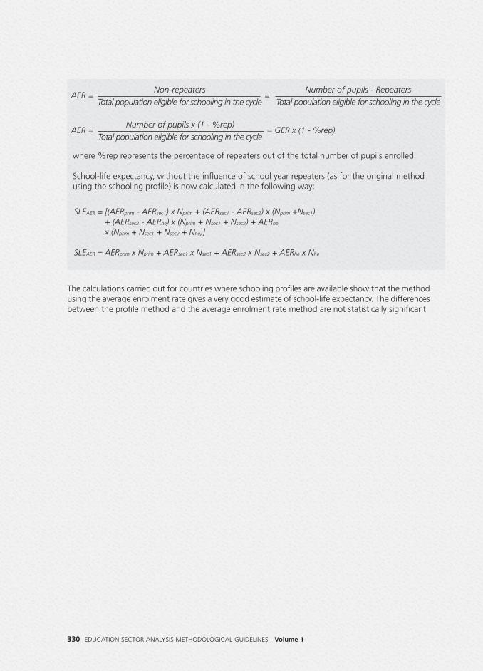
where %rep represents the percentage of repeaters out of the total number of pupils enrolled.
School-life expectancy, without the influence of school year repeaters (as for the original methodusing the schooling profile) is now calculated in the following way:
The calculations carried out for countries where schooling profiles are available show that the methodusing the average enrolment rate gives a very good estimate of school-life expectancy. The differencesbetween the profile method and the average enrolment rate method are not statistically significant.
SLEAER = [(AERprim - AERsec1) x Nprim + (AERsec1 - AERsec2) x (Nprim +Nsec1)+ (AERsec2 - AERhe) x (Nprim + Nsec1 + Nsec2) + AERhe
x (Nprim + Nsec1 + Nsec2 + Nhe)]
SLEAER = AERprim x Nprim + AERsec1 x Nsec1 + AERsec2 x Nsec2 + AERhe x Nhe
330 EDUCATION SECTOR ANALYSIS METHODOLOGICAL GUIDELINES - Volume 1
AER = Non-repeaters
Total population eligible for schooling in the cycleNumber of pupils - Repeaters
Total population eligible for schooling in the cycle
AER = = GER x (1 - %rep)Number of pupils x (1 - %rep)
Total population eligible for schooling in the cycle
=

Sector-Wide Analysis, with emphasis on Primary and Secondary Education 331
is thus a question of having a proper understanding of the indicators that are used to obtain aquantitative description of educational coverage, so that mistakes are not made when evaluating thesituation in a given country in relation to the stated objective. The objective of this section is to define certain key indicators of the coverage of an education system,and to specify how they can be interpreted. After examining theoretical examples and real situations,it appears that the rate of access into the last year of primary education (often called the completionrate) is the best indicator for measuring quantitative progress towards the Dakar objective.
1. PROBLEMS WITH USING THE AVERAGE
1.1 Gross Enrolment Ratio (GER)
For a given year, the gross primary enrolment ratio is the ratio between the numbers of pupilsenrolled in a given year and the total school-age population for this year.
The GER shows the capacity to accommodate pupils. It describes the extent to which the country iscapable of accommodating the numbers of pupils that it should be able to educate in its schools,taking account of the demographic context. Therefore, a GER of 100% means that the country hasthe physical capacity to provide education for the whole of its school-age population.
When calculating the GER, all the children enrolled in the school are taken into consideration,including newly enrolled pupils and those who have to repeat a year, regardless of whether or notthese pupils are of official school age. Because of this, a positive change in GER can be due to anincrease in simply the number of students repeating and not necessarily due to an increase in theenrolment rate of the school-age population.
ANNEX 2.3: MEASURING PROGRESS TOWARDSUNIVERSAL PRIMARY EDUCATIONSource: Abstract from Methodological Note N°1: Measuring the Progress Towards Universal Primary Schooling, Pôle de Dakar, 2004
In April 2000, during the World Education Forum in Dakar, the international community pledged itscommitment to take the necessary measures to give all children the opportunity to benefit from acomplete programme of primary education by 2015. Such an objective requires that everyone involvedhas the means to measure the progress made on a regular basis so they can target the problems moreeffectively and identify the measures that need to be taken in order to bring about improvements. It
• Definition 1
Gross enrolment ratioThe gross enrolment ratio for a particular cycle of education in a given year t can be representedby the formula:
GERt =where: GERt = gross enrolment ratio (GER) for a given year
PEt = number of pupils enrolled for a given yearSAPt = school-age population for a given year.
PEt
SAPt
AN
NEX
ES

332 EDUCATION SECTOR ANALYSIS METHODOLOGICAL GUIDELINES - Volume 1
Pupil 1 poses no problems, as after starting primary school in 1996, he/she finishes the cycle in 2001without repeating a year. He/she therefore accounts for six years in the calculation of the GER, whichcorresponds to the number of school years they have officially completed. Pupil 2, however, accountsfor nine consecutive years in the calculation of the GER because they have repeated several years from1996 to 2004. Because they are counted twice, pupil 2 and all the other school year repeaters havethe effect of artificially inflating the level of the GER.
1.2 The Net Enrolment Ratio (NER)
For a given year, the net primary enrolment ratio is the relationship between the number of pupils ofofficial school age who are enrolled and the total school-age population for this year.
The NER is an indicator of participation: it shows what proportion of the official school-agepopulation is actually enrolled in school.
The major disadvantage of this indicator is that it only accounts for the education of those childrenwho are within the official age-range for schooling, thus excluding all the children who enterthe system either after or before the official age. This can be accompanied by errors of measurement
TABLE A2.1 - What is taken into consideration for the consecutive calculations of the GER?
Pupil 1
Pupil 2
19991996 1997 1998 2000 2001 2002 2003 2004
Year 1
Year 1
Year 2
Year 1
Year 3
Year 2
Year 4
Year 3
Year 5
Year 4
Year 6
Year 5 Year 5 Year 6 Year 6
What is taken into consideration for the consecutive calculations of the GER?
Pupil 1
1997
Year 2
A2.1 - ABLETTA
1996
Year 1
What is taken into consideration for the consecutive calculations of the GER?
Year 6
200120001998 1999
Year 5Year 4Year 3
What is taken into consideration for the consecutive calculations of the GER?
Year 6
2004200320022001
2004
Pupil 2 Year 1Year 1
Year 5Year 4Year 3Year 2
Year 6Year 6Year 5Year 5
Year 6
• Definition 2
Net enrolment ratioThe net enrolment ratio for a given year t can be defined by the following formula:
NERt =PSAEt
SAPt
where: NERt = net enrolment ratio (NER) for a given yearPSAEt = number of pupils of official school age enrolled for a given yearSAPt = school-age population for a given year
The GER overestimates a country’s educational coverage
Table 1 illustrates two theoretical examples of enrolment in primary school and the impact of thesedifferent examples on the calculation of the GER over several consecutive years.
• Observation 1
GERt = x with PRt =NEt
SAPt
Rt
PEt
1
1- PRt
GER and the percentage of pupils who repeat a school yearIf NEt = the total number of newly enrolled pupils and Rt = the total number of pupils whorepeat a school year, then PEt = NEt + Rt . Consequently
being the percentage of school year repeaters for thewhole of the cycle.

Sector-Wide Analysis, with emphasis on Primary and Secondary Education 333
due to a lack of accuracy concerning the real ages of the pupils: in certain African countries, it iscommon practice to change the ages of children on the civil status register.
Table 2 illustrates the cases of three children who could attend the primary education cycle at differentages, in a country where the theoretical age for attending the cycle is 6 – 11 years.
What effects do these different ages for starting and finishing the cycle have on the calculation of the NER?
• For pupil 1, there is no problem: entering Year 1 at the official age of entry (6 years) and leavingthe cycle at 11 years of age without ever repeating a year, this pupil will therefore be included inthe calculation of the NER throughout his or her schooling.
• Pupil 2 also completes the educational cycle without interruption but starts attending schoolbefore the official age. The calculation of the NER will not take this pupil into account duringYear 1, because at the time he or she is only 5 years age (and not 6).
• The final example concerns the case of a pupil who starts school at 10 years of age (a verycommon occurrence in Africa), and also has the misfortune of having to repeat a year. He or shethus leaves the cycle five years after the official leaving age and more than two thirds of his orher education will not be accounted for in the calculation of the NER.
Therefore, the NER underestimates educational coverage: it does not take into account thewhole or a part of the schooling of individuals who enter the system too early or too late and/or whohave to repeat one or more classes, even if they eventually complete all six years of the primaryeducation cycle. In the example presented, while all three pupils successfully achieve theDakar objective, only one of them is included in the calculation of the NER throughout theentire duration of his or her schooling.
Thus, this indicator cannot be regarded as an indicator of universal primary schooling, asthe Dakar objective requires that all children complete the entire cycle of primary schoolingirrespective of their age. The children who are outside the official age of attendance shouldtherefore not be omitted.
Lastly, the GER and the NER have the disadvantage of giving an average value over the whole of thecycle, and are not suited to describing the school lives of individual pupils. However, such a descriptionappears to be of paramount importance: indeed, in addition to measuring the proportion of childrenwho start school (access), it is important to be able to measure the proportion of pupils who staythere until the end (retention). Access to this information concerning the problems of access andretention in the education system will enable planners to adapt their political approaches accordingly.
Thus, it is necessary to have recourse to a specific indicator.
TABLE A2.2 - Theoretical illustration of the extent of the age range possiblefor pupils attending the primary cycle
Pupil 1
Pupil 2
Pupil 3
85Ages 6 7 9 10 11 12 13 14 15 16
Year 1
Year 2
Year 2
Year 3
Year 3
Year 4
Year 4
Year 5
Year 5
Year 6Year 1
Year 6
Year 2 Year 2 Year 3 Year 4 Year 5 Year 6
not accounted for when calculating the NERaccounted for when calculating the NER
Key
Year 1
Pupil 3
YeararYeeaeaarYeaY 11Ye 1YY r 1r 1r 1YYYYYeYeYeYeaeaeaeararararr 1r 11111 Year 3
Theoretical illustration of the extent of the age range possibleA2.2 - ABLETTA
7
Pupil 2
Pupil 1
6Ages 5
Year 2
Year 2
Year 1
Keyaccounted for when calculating the NERnot accounted for when calculating the NER
YYYYYYYYYYYYYYYear 6
Year 6
for pupils attending the primary cycleTheoretical illustration of the extent of the age range possible
Year 2
111098
Year 1
Year 5
Year 5
Year 4
Year 4
Year 3
accounted for when calculating the NERnot accounted for when calculating the NER
Year arYeeaeaeaYe 22Y 22r 2ar r 2YeYeYeYeaeaeaeararar r r 2r 22222 Year arYeeaeaeaYeY 33Y 33Y r 3ar r 3YYYYYeYeYeYeaeaeaeararar ar 3r 3r 33333 Year arYeeaeaeaYeY 44Y 44Y r 4ar 4r 4YYYYYeYeYeYeaeaeaeararar r 4r 4r 44444 YearearYeYeaeaeaYe 55Y r 55Y r 5ar 5r 5YYYYYYeYeYeaeaeaeararar ar r 5r 55555 YeaYeeaeaeaYeaYYeYYYYYYYeYeYeeaeaeaaa
for pupils attending the primary cycleTheoretical illustration of the extent of the age range possible
1615141312
araraar 6666r 6arr 6aarararr 6r 66666
16
accounted for when calculating the NER
accounted for when calculating the NER
AN
NEX
ES

334 EDUCATION SECTOR ANALYSIS METHODOLOGICAL GUIDELINES - Volume 1
2.1 Schooling profiles
A schooling profile for a cycle of primary education is given by the series of the access rates to thedifferent classes in the cycle. This indicator is calculated in relation to one or more referencepopulations, for whom the aim is to measure their access to the different classes.
The first point of the profile is the apparent intake rate (AIR) (the ratio between the number ofnew entrants in the first year of primary education and the total population of children who are ofofficial primary school entrance age). The last point of the profile is the access rate to the last yearof the cycle: the proportion of a given cohort of children reaching the final year of primary school.It is possible to use three complementary methods of calculation to obtain different types of indicators:
• The longitudinal method makes it possible to describe the progression through school of thecohort to which the children who are currently enrolled in the last year of the cycle belong, as itprovides the access rates to each of the classes during the course of the past cycle;
• The cross section method provides information about current access rates with reference to thetotal populations of children in the age groups eligible to attend each of the classes in the cycle;
• The pseudo longitudinal method (or zigzag method) gives an illustration of the predicted accessrates for the children who have just started school, based on the current patterns of progressionbetween the classes.
2. THE NEEDS FOR CAPTURING COMPLETION
The objective of universal primary schooling requires that all children complete a full cycle of primaryeducation. Certain studies, especially those using data from household surveys, show that on average,a bare minimum of six years of schooling is essential if a person is to acquire a permanent level ofliteracy (see Figure A2.1).
FIGURE A2.1 - Cameroon – proportion of 22-44 year-olds able to read without difficulty in relationto the number of years of study completed
100908070605040302010
03 4 5 6 7 8 10 11 12 1390 1 2
Number of years of study completed
% w
ho r
ead
with
out
diff
icul
ty
to the number of years of study completed - Cameroon – proportion of 22-44 yearFIGURE A2.1
to the number of years of study completed
-olds able to read without difficulty in relation - Cameroon – proportion of 22-44 year
to the number of years of study completed
-olds able to read without difficulty in relation
0102030405060708090
100
210 3
ficul
tyea
d w
ithou
t di
f%
who
r
876543
9 13121110
Number of years of study completed
Number of years of study completed
Source: Cameroon, data from MICS 2000 survey.

Sector-Wide Analysis, with emphasis on Primary and Secondary Education 335
Whatever method is used, and thus for any of the populations considered, the profile makes it possible toview the progress through school of one or more cohorts of children. Firstly, the access rate can beascertained by measuring the intake to the primary cycle against the total population that is officially eligibleto start primary school. In addition, the subsequent access rates to the different classes in the cycle can beused to provide information about the size of the dropout rate during the course of the cycle.
Lastly, these profiles have the advantage that their measurements are not affected by pupils repeatinga year, which frees this category of indicators from the bias that the rate of repeating school yearscan introduce into measurements of school enrolment. In this case, the children’s progress throughschool is recorded in terms of years actually completed, with no account taken of repeated years.
2.2 Using the access rate in the final year as the Primary Completion Rate (PCR)
The final point of the profile can be viewed as an indicator of completion of primary education. Justas the three methods used in the calculation of a profile needs to be interpretated in three differentways, the access rates in the final year that are calculated by the three different methods are threedifferent indicators. The longitudinal method gives the completion rate of pupils who began the cyclea few years earlier, taking into account the conditions of progression between each class observed.The cross section method provides roughly the same indicator, calculated with reference to the totalpopulation that is currently of the official age for attending the final year. As for the zigzag method,it allows us to have an idea of what the completion rate for the cycle might be in several years’ time,taking account of the apparent intake rate and the current conditions of progression between eachclass.
It is certainly true that there are problems with using the access rate in the final year as a measure ofcompletion because this indicator only gives us information about the number of pupils who enrolfor the final year. It is implicitly supposed that there is very little student mortality in the final year ofprimary education. In spite of this limitation, it represents the only credible and widely available sourceof information, giving a snapshot of the enrolment at a particular moment in the final year of school.
• Definition 3
Schooling profiles A primary education cycle is considered to be of duration τ. NEj,t is the number of newly enrolledpupils in class j for year t; Pa(j),t represents the total population of the official age to attend classj, for year t.
• The longitudinal profile is given by the series of the access rates (ARj,t-τ + j)j=1,...,τ
where ARj,t-τ + j = ;
• The cross section profile is given by the series of the access rates (ARj,t )j=1,...,τ
where ARj,t = ;
• The pseudo longitudinal profile (or zigzag) is given by the series of the access rates (ARj,t )j=1,...,τ
where AR1,t = AIRt = and ARj,t = AIRt x , ∀j = 2,3...,τ.
Long
CS
ZZ
CS
Long NEj,t-τ + j
Pa(1),t-τ + 1
NEj,t
Pa(j),t
NE1,t
Pa(1),t
NEh,t
NEh-1,t-1
ZZZZ
1< h ≤ j
∏
AN
NEX
ES

2.3 Why not use the pass rates in national examinations as measures of completion?
There are several disadvantages to using this measurement. First of all, it supposes that a diploma isthe only valid outcome of an educational cycle. Thus, a pupil who does not manage to obtain theprimary school-leaving certificate could consider that he or she has not completed a full cycle ofprimary education! In addition, the results in national examinations are strongly dependent on themethods used for marking/evaluation. They cannot be regarded as an internationally comparablemeasurement of the pupils’ real achievement, as the examination is sometimes used as a means ofregulating the number of pupils who advance to the next cycle.
3. WHAT ARE THE POSSIBLE ERRORS? A THEORETICAL EXAMPLE
The objective of universal primary schooling requires that the correct indicator is chosen for measuringthe progress made towards the 2015 objective. The NER clearly appears to be out of the question, asit only focuses on the education of pupils who are of school age, and therefore omits a considerablenumber of children, even if they successfully complete a full cycle of primary education. Therefore,can the GER be used as a primary indicator of enrolment and retention? The answer is no, becausesituations which differ considerably in terms of access, retention, completion and repetition of schoolyears can give the same value for the GER.
The same GER value can be arrived at for situations that are very different in terms of access, retentionand repetition of school years.
The access rate in the final year as calculated by the cross section method is the indicatorretained within the Global Partnership for Education for the measurement of the progressmade towards universal primary schooling.
336 EDUCATION SECTOR ANALYSIS METHODOLOGICAL GUIDELINES - Volume 1
• Observation 2
GERt = xNEt
SAPt
11- PRt
An interesting comparisonGoing back to the findings of Observation 1, we arrive at:
However, NEt = NEj,t = τ x NE.,t and SAPt = Pa(j),t = τ x P.,t ,where NE.,t refers to
the average of the number of new entrants to each year of the cycle and P.,t refers to theaverage of school-age population for each year of the cycle.
We can therefore rewrite the GER in the following way:
Furthermore, if we consider that there is a reasonably regular pupil dropout rate throughout the
course of the cycle, we can write: NE.,t ≈ .
∑τ
j=1
∑τ
j=1
GERt = xNE.,t
P.,t
NE1,t + NEτ,t
2
11- PRt
▶

Sector-Wide Analysis, with emphasis on Primary and Secondary Education 337
As Observation 2 shows, the GER is greater when• the apparent intake rate is high,• the primary completion rate is high• a high proportion of pupils repeat a school year!
This is illustrated by the three theoretical cases shown in Table 3.
The first "ideal" case shows a system with no problems: 100 percent access, perfect retention and norepetition of school years. The GER is 100 percent. In the second case, the GER is also 100 percent:but while access is relatively good, there is a big problem with regard to retention, since there is aPCR of only 55 percent. The value of the GER is artificially inflated by the fact that high numbers ofpupils repeat school years. In the final case, the system is characterised by poor access and goodretention (all of the children who start school remain there until the end) but, with a disproportionatelyhigh rate of repetition, the GER is also 100 percent!
Therefore, the GER alone cannot provide an overall measure of educational coverage, as it does notreveal the problems relating to access and retention. Countries striving to achieve the Dakarobjectives, in particular universal primary schooling, which was identified as one of themillennium objectives, may find it beneficial to use the PCR rather than the GER.
Therefore, we can consider that:
Given that ≈ = AIRt , the apparent intake rate for year t,
and ≈ = PCRt = ARτ,t the access rate in the final grade of primary school
(completion rate) calculated for year t using the cross section method, we arrive at thefollowing relationship :
GERt ≈ x x12
11 - PRt
11 - PRt
NE1,t + NEτ,t
P.,t
NE1,t
P.,t
NEτ,t
P.,t
NEτ,t
Pa(τ),t
NE1,t
Pa(1),t
GERt ≈ xAIRt + PCRt
2
CS
Case 1
Case 2
Case 3
AIRGER PCR PR
100
100
100
100
95
60
100
55
60
0
25
40
TABLE A2.3 - Theoretical cases showing Apparent Intake Rate, Primary Completion Rate, Percentageof Repeaters, and Gross Enrolment Ratio
Theoretical cases showing Apparent Intake Rate, Primary Completion Rate, Percentage
Case 3
GER
Case 2
Case 1
100
100
100
A2.3 - ABLETTA of Repeaters, and Gross Enrolment Ratio
60
AIR
95
100
Theoretical cases showing Apparent Intake Rate, Primary Completion Rate, Percentage of Repeaters, and Gross Enrolment Ratio
40
PRPCR
25
0
60
55
100
Theoretical cases showing Apparent Intake Rate, Primary Completion Rate, Percentage Theoretical cases showing Apparent Intake Rate, Primary Completion Rate, Percentage
AN
NEX
ES

ANNEX 2.4: THE SCHOOLING PROFILES Source: Abstract from Methodological Note N°2: How to Elaborate and Interpret Schooling Profiles, Pôle de Dakar, 2004
In the category of educational coverage indicators, schooling profiles have the advantage of providinginformation that goes beyond a simple average figure taken over the whole of an educational cycle.These profiles make it possible to summarise the state of coverage by providing a “picture” of accessat the beginning of a cycle and retention during the course of the cycle, thus providing informationthat is fundamentally important for a precise analysis of the state of educational provision. In thefollowing sections, we propose to illustrate the concept of schooling profiles by describing the differentmethods of calculation that are possible, and how the corresponding results can be interpreted, takingaccount of the advantages and disadvantages of using different sources of data.
1. GENERAL
1.1 Definitions
A schooling profile for a particular cycle of education results from the access rates to the variousgrades in this cycle. This indicator is calculated in relation to one or more reference populations,cohorts of births for whom the aim is to measure their access to the different classes.
The first point of the profile is the apparent intake rate (AIR), defined as the ratio between thenumber of new entrants (or pupils who are not repeating a school year) in the first grade of the cycleand the population of the children who are of the official age to enter this cycle. Its calculation isinvariant, whatever method is used.
The final point of the profile is the access rate to the final grade of the cycle (often calledcompletion rate), which is the proportion of a given cohort of children reaching the final grade
All the points in between are the access rates to the different grades, which for each grade measurethe extent of the educational system’s coverage in relation to the total population of children forwhich it should be able to provide education at these different levels.
Three distinct methods can be used to construct a schooling profile. Each one produces a specificinterpretation indicator, referring to one or more different cohorts of children.
338 EDUCATION SECTOR ANALYSIS METHODOLOGICAL GUIDELINES - Volume 1
• Notations
A school cycle is considered to be of duration τ ∈ N+
The school year t-1/t is simply noted as year t.
For year t and grade j, the following can be noted: • NEj,t number of new entrants (or pupils who are not repeating); • PEj,t total number of pupils educated; • Rj,t total number of pupils who repeat a grade, defined by; PEj,t - NEj,t
• %Rj,t percentage of repeaters, defined as the ratio • a(j) theoretical age of attendance; • Pa(j),t total population of children having the theoretical age of attendance; • ARj,t access rate to the grade.
Rj,t
PEj,t

Sector-Wide Analysis, with emphasis on Primary and Secondary Education 339
Some of these methods call upon the concept of the effective promotion rate, defined for any givenyear and any given class as the ratio between the new entrants to the class in the current year andthe new entrants to the preceding class in the preceding year.
Such a rate, being based only on the new entrants from one grade to another, gives an approximationof the proportion of children in a given class who will one day reach the next one.
1.2 Why is a profile useful?
Each grade has a corresponding access rate: therefore, it is easy to give a graphical representation ofthe series of points obtained. Indeed, a chart is the clearest way of summarizing the informationcontained within a profile. As shown in Figure A2.2, the resulting representation makes it possible toview the level of schooling for each grade. Furthermore, by seeing the numbers of pupils who neverenter school and the proportion of children who, after starting school drop out before the end, onealso has access to information that is fundamentally important to the issue of access/retention.
• Definition
Schooling profile A schooling profile is defined as the series of the access rates to the different grades.(ARj,t)j=1,...,τ
• Definition
Effective promotion rate The effective promotion rate to grade j in year t (EPRj,t) is defined by: EPRj,t =
NEj,t
NEj-1,t-1
Proportion of childrenwho never enter school(Problem of access)
Dropouts before the endof the cycle(Problem of retention)
100
Apparentintake rate
Access rate inthe final grade
of the cycle
First grade of the cycle Final grade of the cycle
Situation where each pupil access to each grade
FIGURE A2.2 - Schooling profile chart
Situation wher
intake rateentAppar
100
- Schooling profile chart
e each pupil access to each gradeSituation wher
FIGURE A2.2 - Schooling profile chart
oblem of access)(Prwho never enter school
enoportion of childrPr
e each pupil access to each grade
e the endopouts beforDr
who never enter school
e the end
of the cycle
First grade of the cycle
the final gradeAccess rate in
First grade of the cycle Final grade of the cycle
etention)
Final grade of the cycle
m of rof the cycle
e the endopouts beforDr e the end
AN
NEX
ES
, ∀j = 2,..., τ

2. CHOOSING METHODS OF CALCULATION FOR EACH TYPE OF INDICATOR
Let us consider a primary cycle of six years’ duration for which the following educational statistics areavailable: new entrants by grade (pupils who are not repeaters), in thousands.
The theoretical age range for attending this cycle is 6-11 years and in addition, we have the followingdata concerning the population per age group (in thousands of children).
Taking this information into account, we can calculate three different indicators, thus allowing threedifferent questions to be answered.
2.1 What were the access rates to the different grades for pupils currently at the endof the cycle?
Such a question leads us to follow the progress through school of the cohort of children who wereof the official age to enter school six years earlier and to examine the reference population’s accessrate to each grade throughout the past cycle. For this, the cohort method (also called longitudinalmethod, see Annex 2.3) is used.
In our example the data needed for applying this method is underlined in the two tables above.
340 EDUCATION SECTOR ANALYSIS METHODOLOGICAL GUIDELINES - Volume 1
1999
2000
2001
2002
2003
2004
Years School
Grade 1 Grade 2 Grade 3 Grade 4 Grade 5 Grade 6
170
168
165
165
163
160
155190
200
185
185
180
182
175
178 173
2003 190
Grade 1
2002
2001
2000
1999 170
School Years
168
175
Grade 4Grade 3Grade 2
165
165
180185
165
163
Grade 6Grade 5Grade 4
155175
Grade 6
2004
190
200
2003 175
178182
180
185
185 155163
160
175
173178
1999
2004
Years 6 Years 7 Years 8 Years 9 Years 10 Years 11 Years
249
250 248 245 243 240 235
249
250
6 Years
2004
Years
1999
243
9 Years8 Years7 Years
245248 235240
11 Years10 Years9 Years
243
11 Years
• Definition
Cohort schooling profile (or longitudinal profile, see Annex 2.3) The cohort profile for date t is defined by the series of the access rates to the different grades inthe cycle (ARj,t-τ + j)j=1,...,τ where
ARj,t-τ + j = , ∀j = 1,..., τ
C
C NEj,t-τ + j
Pa(1),t-τ + 1
The reference population is the total population of children who were 6 years old in 1999 (P6,1999),and therefore of the official age to attend the first grade of primary school in that year, i.e. 249,000children.

Sector-Wide Analysis, with emphasis on Primary and Secondary Education 341
The apparent intake rate is calculated by dividing the total number of new entrants to grade 1 sixyears ago (NE1,1999) by the total population of the official age to attend grade 1
The following points of the profile are obtained by dividing the number of new entrants to each gradeby this same population. For example, the access rate to grade 4 in 2002 (AR4,2002) is calculated bydividing the number of new entrants to grade 4 in 2002 (NE4,2002) by the reference population.
Thus, out of the 249 000 children who should have entered grade 1 in 1999, there were only 165,000new entrants to grade 4 in 2002, i.e., a 66 percent access rate to grade 4.
Consequently, the cohort schooling profile for pupils enrolled in the final grade in 2004 is given bythe following series of access rates to the different grades:
For each grade in the primary education cycle, each point of the profile calculated in this wayrepresents the proportion of pupils in a given cohort who eventually gained access to the grade inquestion. We therefore have access to the most accurate information possible for the pupils whofinish the cycle in 2004. At this stage, one notices that each access rate is actually obtained by multiplying the intake rate bythe effective promotion rate noted in the series for each year until the particular year for which it isbeing calculated. For example, the effective promotion rate to grade 2 in 2000 (EPR2,2000) is the ratio between the newentrants to grade 2 in 2000 (168 000) and the new entrants to grade 1 in 1999 (170 000). Withreference to the apparent intake rate for the series (AIR1999), we arrive at the access rate to grade 2 in2000 as calculated by the cohort method.
There are two disadvantages associated with the cohort method. Firstly, even if the results are largelyindependent of demographic data, they are strongly dependent on the quality of enrolment data,because it is necessary to have access to enrolment statistics over a long period (six years). Secondly,the access rates calculated for the first grades of the cycle are relatively old: thus, with regard to accessas well as retention, one does not have the most up to date snapshot of the state of the school system(the apparent intake rate for a series ending in 2004 relies on enrolment and demographic data goingback to 1999!)
• Observation
Relationship between the cohort profile and the effective promotion rate
ARj,t-τ + j = = AIRt-τ + 1 x EPRh,t-τ + h,∀j = 2,...,τ= x C NEj,t-τ + j
Pa(1),t-τ + 1
NE1,t-τ + 1
Pa(1),t-τ + 1
AR1,t-τ + j = AIR1999 = =C NE1,1999
P6,1999
AR4,2002 = =C NE4,2002
P6,1999
165249
C
AR1,1999
C AR2,2000
C AR3,2001
C AR4,2002
C AR5,2003
C AR6,2004
C
170249
= 68%168249
= 67%165249
= 66%165249
= 66%163249
= 65%160249
= 64%
C
2,2000ARR2
C
1,1999AR
= 67%249168
= 68%249170
C
4,2002ARR4
C
3,2001ARR3
= 66%249165
= 66%249165
C
6,2004ARR6
C
5,2003ARR5
= 64%249160
= 65%249163
= 64%
AIR1999 x EPR2,2000 = AR2,2000 xCNE1,1999
P6,1999=NE1,2000
NE1,1999= =NE2,2000
P6,1999
170249
x 168170
= 168249
NEh,t-τ + h
NEh-1,t-τ + h-11<h≤j∏ ∏
1<h≤j
AN
NEX
ES
170249

342 EDUCATION SECTOR ANALYSIS METHODOLOGICAL GUIDELINES - Volume 1
• Definition
The cross section (or transverse) profileThe cross section schooling profile for a given year t is defined by the series of the access ratesto the different grades in the cycle (ARj,t )j=1,...,τ where:
ARj,t =
CS
CS NEj,t
Pa(j),t
Here there is not one but several reference populations, which are the total populations of children whoare officially of the age to attend each of the grades of the cycle in 2004: the population of 6 year-oldsin 2004 for attending grade 1, the population of 7 year-olds in 2004 for attending grade 2, etc.
First, we calculate the apparent intake rate for 2004. Then we divide the number of new entrants tograde 1 in 2004 (NE1,2004) i.e., 200 000 pupils, by the population of children who are theoretically ofthe age for attending grade 1 in this same year (P6,2004), i.e., 250 000 children:
The access rates to the following grades are then obtained using the same calculation formula. Forexample, the access rate to grade 4 for 2004 is calculated by comparing the number of new entrantsto grade 4 in 2004 (NE4,2004) with the population of children who are of the official age for attendinggrade 4 in this same year, i.e. the population of children who are 9 years old in 2004 (P9,2004).
For the 2004 academic year, the following cross section profile is obtained95:
In this way and for each grade, we can calculate the proportion of new entrants in relation to theentire population of children who are of the age to attend this grade (i.e., that the education systemshould be able to accommodate for this level of education). This method thus provides a snapshotof the current level of access to each grade in the cycle.
However, this method mixes cohorts of different pupils: therefore, the resulting profile does not tracethe progress through school of the same pupils. In addition, it requires the use of both enrolmentstatistics and population data. Thus, this method is used when there is a reasonable degree of
AIR2004 = AR1,2004 = =NE1,2004
P6,2004
200250
CS
AR4,2004 = =NE4,2004
P9,2004
178243
CS
AIR 2004 AR2,2004
C S AR3,2004
C S AR4,2004
C S AR5,2004
C S AR6,2004
C S
200250
= 80%185248
= 75%182245
= 74%178243
= 73%173240
= 72%160235
= 68%= 75%248185
= 80%250200
CSAR2,2004RR22004AIR
= 73%243178
= 74%245182
CSAR4,2004RR4
CSAR3,2004RR3
= 68%235160
= 72%240173
CSAR6,2004RR6
CSAR5,2004RR5
= 68%
2.2 What are the current access rates to the different grades?
The cross section (also called transverse, see annex 2.3) method allows us to answer this question.If we consider the most recent year for which enrolment and demographic data areavailable, we compare the current number of new entrants into each grade with the total populationof children who are of the theoretical age to attend that grade.
In our example, the data needed for the implementation of this method is in the highlighted cells ofthe tables above.

Sector-Wide Analysis, with emphasis on Primary and Secondary Education 343
confidence in the demographic data. If there are found to be repeated examples of projections basedon old and/or non-corrected data, we can resort to using the cross section method after correction ofthe demographic base by appropriate techniques (smoothing for example, see annex 1.1).
2.3 How do we predict the progress through school of the new entrants to the cycle?
We can use the current access rate to grade 1 and the most recent information regarding promotionto the different classes in an attempt to evaluate the future access rates to the different grades in thecycle for the population of children who are currently of the official age for starting school. A schoolingprofile can then be constructed using the pseudo cohort (or pseudo longitudinal) or zigzag method.Starting from the observation of the effective promotion rates for the two most recent academic years,we can examine what the survival rates might be like for the new entrants to the school.
In our example, the information necessary for the implementation of this method is shown by thedata in bold type in the two tables above.
The reference population is made up of children who are of the official age to enter school in themost recent school year to date i.e. the population of 6 year-olds in 2004 (P6,2004).
For the most recent year, the apparent intake rate is calculated by dividing the number of new entrantsinto grade 1 by the total reference population:
The next step is to calculate the effective promotion rates to the two school years under consideration.For example, the promotion rate to grade 4 in 2004 (noted as EPR2,2000) will be obtained by dividingthe new entrants to grade 4 in 2004 (178 000) by the number of new entrants to grade 3 in 2003(180 000). Therefore, for our example, the series of promotion rates is as follows :
Following this, each access rate is calculated by multiplying the apparent intake rate by the series ofeffective promotion rates for each grade up to the grade in question.
• Definition
The pseudo cohort (or pseudo longitudinal) or zig zag schooling profileThe pseudo cohort profile for date t is defined by the series of access rates to the different grades.
(ARj , t )j=1,...,τ where AR1,t = AIRt = and ARj,t = AIRt x ZZ ZZ ZZNE1,t
Pa(1),t
NEh,t
NEh-1,t-11<h≤j∏
AIR2004 = AR1,2004 = = 80%200250
ZZ
EPR 2,2004 EPR 3,2004 EPR 4,2004 EPR 5,2004 EPR 6,2004
185190
= 97%182185
= 98%178180
= 99%173175
= 99%160163
= 98%= 98%185182
= 97%190185
3,2004EPR 2,2004EPRPR
= 99%175173
= 99%180178
5,2004EPR4,2004EPR
= 98%163160
6,2004EPR
AIR2004 AR2,2004
ZZ ZZ ZZ ZZ ZZAR3,2004 AR4,2004 AR5,2004 AR6,2004
200250
= 80% 80%x97%= 78%
80%x97%x98%= 77%
80%x97%x98%x99% = 76%
80%x97%x98%x99%x99% = 75%
80%x97%x98%x99%x99%x98%= 74%= 77%
80%x97%x98%= 78%
80%x97%= 80%250200
3,2004ARZZ
2,2004AR2004AIR
x99%x99% = 75%80%x97%x98%
x99% = 76%80%x97%x98%
= 77%80%x97%x98%
4,2004AR3,2004
ZZZZ
x99%x98%= 74%80%x97%x98%x99%
x99%x99% = 75%80%x97%x98%
6,2004AR5,2004AR ZZZZ
x99%x98%= 74%80%x97%x98%x99%
AN
NEX
ES

The access rate to the first grade is the one that is observed for the current year. The access rate tothe second grade is the rate that might exist in one year’s time, if the conditions for progressionbetween grade 1 and grade 2 remain unchanged. By successive iterations, the access rate to grade 6is the proportion of children who will reach the end of the primary education cycle in five years’time, if the conditions of progression between the grades remain stable. This measure is therefore anestimate of the access in the final grade, taking into account the current promotion rates. The method of calculation used is identical to that used for the cohort method, except for the factthat only two consecutive academic years are used. This allows us to have a prospective view of theprogress through school of the children who have just entered the cycle, showing how the currenteducational conditions could influence the probable levels of access and retention in the future.Therefore, the access rate at the end of the primary cycle does not refer to the current situation, butrather to what could be observed in five years’ time, if the conditions for promotion remainunchanged. It should also be noted that, as for the cohort method, this method only uses demographicdata in the calculation of the first point of the profile.
3. SPECIAL REMARKS
3.1 Complementarity of the methods
Each method provides a specific indicator. Therefore, these methods are not interchangeable, asillustrated in figure A2.3.
This is the current apparent intake rate, reflecting the system’s capacity to accommodate pupils in thefirst grade in relation to the total population that it should be able to accommodate.
The access rate to last grade of the cross section profile is about the same as that obtained by thecohort method. The numerator is the same (new entrants to the last year of the cycle over the mostrecent year) whereas the reference population is slightly different: for the cohort method, the
344 EDUCATION SECTOR ANALYSIS METHODOLOGICAL GUIDELINES - Volume 1
90%
80%
70%
60%
50%Gr 1 Gr 2
80%78% 77% 76% 75%
75% 74% 73% 72%
67%68%66% 66% 65%
64%
68%
74%
Gr 3 Gr 4 Gr 5 Gr 6
Cross section
Zig Zag
Cohort
FIGURE A2.3 -Illustration of the results obtained by the three methods of calculation -Illustration of the results obtained by the three methods of calculationFIGURE A2.3 -Illustration of the results obtained by the three methods of calculation -Illustration of the results obtained by the three methods of calculation
75%
78%80%
Gr 2Gr 150%
60%
70%
80%
90%
Gr 6Gr 5Gr 4Gr 3
74%
72%73%74%
75%76%77%
Gr 6
74%
oss sectionCr
Cohort
Zig Zag
AR1,t = AR1,t CS ZZ
However, it should be noted that the apparent intake rate is exactly identical for the zigzag and crosssection methods:

Sector-Wide Analysis, with emphasis on Primary and Secondary Education 345
population of children who were of the official age to enter school 6 years previously is used, whereasthe cross section method refers to the population of children who qualify to attend the last grade ofschool in the current year. The two methods are bound to give very close results, with very littledifference between the population of 6 year-olds 6 years ago and the population of 11 year-oldstoday (apart from adjustments due to death and the balance of migration).
This is the current access rate in the final school year, noted in relation to the cohort of children whoare of the official age to attend the final class in the cycle.
3.2 Schooling profiles and survival profiles
Instead of applying the previous methods to the population of children as reference, it is possible toapply them to only those who entered school. Then, the profiles are named survival profiles insteadof schooling profiles.
ARτ,t ≈ ARτ,t C C
AN
NEX
ES
• Definition
Survival profilesA survival profile for a particular cycle is given by the series of survival rates for the different classes (SRj,t )j=1,...,τ
The first point of the survival profile is always fixed at 100 percent, as 100 percent of pupils did indeedenter school at a given time in the past! The survival rates are the other points on this profile. Theseare obtained by multiplying the series of effective promotion rates to each grade, calculated by thecohort or pseudo cohort methods.
Going back to our example, the survival rate for grade 5 in 2004 is obtained by the zig zag methodin the following way:
SR5,2004 = 100 x EPR2,2004 x EPR3,2004 x EPR4,2004 x EPR5,2004 ZZ
Although using a survival profile does not provide any information about access to a particular cycle(in reference to a cohort of births), it does, on the other hand, provide information about retention.Therefore, this indicator proves to be very useful, especially when there are doubts about the qualityof the demographic data, as it does not need demographic data at all.
• Definition
Cohort survival profile The cohort survival profile at date t is defined by the series of survival rates for the differentschool years
Pseudo cohort survival profileThe pseudo cohort survival profile at date t is defined by the series of survival rates for thedifferent school years (SRj,t-τ + j ) j=2,...,τ
(SRj,t-τ + j ) j=1,...,τ C
ZZ
SRj,t-τ + j =C NEj,t-τ + j
NE1,t-τ + 1
SRj,t =ZZ NEh,t
NEh-1,t-11<h≤j 1<h≤j ∏

346 EDUCATION SECTOR ANALYSIS METHODOLOGICAL GUIDELINES - Volume 1
CHAPTER 3 ANNEXES
ANNEX 3.1: TECHNICAL NOTE ON THE ADJUSTMENT OFTHE SHARE OF RECURRENT EXPENDITURE BY EDUCATIONLEVEL ACCORDING TO STANDARD CYCLE DURATIONS
Depending on countries, the duration of primary education usually ranges from four to eight yearsand secondary education varies from four to seven years. To compare the distribution of expenditureby level of education across countries, it is necessary to recalibrate expenditure data according to eacheducation system's structure. The recalibration is a way of estimating what the distribution ofexpenditure by level of education would be if each country had the same structure (the most commonstructure in African countries is often used, of six years of primary and seven years of secondary). Forcomparative purposes and because fully disaggregated data are not available for all countries,regrouping some subsectors is often necessary. For instance, preschool and literacy can be includedwith the primary education level, and TVET can be included with secondary education. The calibrationis thus performed on the basis of the three main levels of education: primary education, secondaryeducation and higher education.
The calibration consists of assuming proportionality between the cost of a cycle and its length.Assuming a country’s primary and secondary education cycles respectively last for Dp and Ds years,and a country spends P, S and H percent of its education budget on primary, secondary and highereducation respectively, if a country’s primary cycle is to be calibrated to a referential duration of sixyears, its expenses would be:
P6 = P x 6
Dp
S7 = S x 7Ds
Similarly, if a country’s secondary cycle is to be calibrated to a referential duration of seven years, itsexpenses would be:
Because these adjusted percentages do not add up to 100 anymore, it is necessary to perform a finalstep in the calibration. It is important to note that despite the recalibration between primary andsecondary, the share of the expenditures spent on higher education remains unchanged. Hence, P6and S7 are recalibrated using the same coefficient, in order for their sum to equal (100% - H). Thus,where P6* and S7* are the final calibrated percentages for primary and secondary their durationsshould be in line with the referential durations of six and seven years respectively:
, andP6* = P6 x 100% - HP6 + S7
S7* = S7 x 100% - HP6 + S7

AN
NEX
ES
The recalibration of the data is summarised in Table A3.1.
Primary
Duration (Years)
Share of Expenses(Non-Calibrated)
Estimated Share of Expenses for
a 6-7 Years Structure
Final Calibrated Share of Expenses
TABLE A3.1 - Methodology for Recalibration of the Share of Recurrent Expenditureby Cycle to a 6–7 Years Structure
Secondary
Higher
Total
P
S
H H H
100 % 100 %
Dp
Ds
P6+S7+H (≠100 %)
6Dp
P6 = P x 100%-HP6 + S7
P6* = P6 x
100%-HP6 + S7
S7* = S7 x7Ds
S7 = S x

348 EDUCATION SECTOR ANALYSIS METHODOLOGICAL GUIDELINES - Volume 1
ANNEX 3.2: SAMPLE QUESTIONNAIRE TO COLLECT DATAON INTERNATIONAL AID FROM DEVELOPMENT PARTNERS
Note that the following questionnaire should be adapted to national contexts.
Area Planned Amount Planned Quantities
Pedagogical Material
School Construction
Pre-Service Teacher Training
Capacity Development
Other : ...................................................
............. Textbooks
............. School Kits
............. Classrooms
............. Laboratories
............. Technical Institutes
............. Teachers
Amounts Disbursed:
2007Year 20112008 2009 2010
Amount
Planned Disbursement Calendar:
2012Year 20162013 2014 2015
Amount
Main Activities:
Pre-PrimaryLevel HigherPrimary GeneralSecondary
TVET Non-Formal
Share (%)
Questionnaire for Technical and Financial Education Partners
Partner: ..................................................................................
Please provide the following information for each education project or program you support.Name of the Project/Program: ..................................................Implementation Type (Executed by your institution, Executed by the government, Budget Support,etc.): ........................................................................................Total Amount Committed:........................................................Period:......................................................................................
Approximate Distribution of Funding Provided, by Education Level:

Sector-Wide Analysis, with emphasis on Primary and Secondary Education 349
AN
NEX
ES
Pre-Primary
Primary
Capacitybuilding
Schoolconstruction
Teachertraining
Pedagogicalmaterials
Other :
GeneralSecondary
TVET
HigherEducation
Non-Formal
Total
Level Year Amounts
2012
2013
2014
2015
2016
2012
2013
2014
2015
2016
2012
2013
2014
2015
2016
2012
2013
2014
2015
2016
2012
2013
2014
2015
2016
2012
2013
2014
2015
2016
Quantity Amounts Quantity Amounts Quantity Amounts Quantity Amounts Quantity

ANNEX 3.3 : METHODOLOGY FOR THE CONSOLIDATIONOF FINANCIAL DATA
The collection and consolidation of data related to education funding is a complex but necessary task.The analysis requires gathering the expenditure executed for the entire education system on the onehand, and to be able to reconstitute this spending for the different education levels, by type ofspending (salaries, operational costs, goods and services, transfers and so on) and by source on theother.
This data does not exist in a format that is ready to use. Indeed, many countries have three or foureducation ministries, and centralised education information systems are rare. Usually each ministryhas its own statistical service. It is also common that a given ministry covers various education levels(preschool, primary and secondary for instance) and that expenditure need to be distributed amongthese levels. Finally, there are often inconsistencies in given data according to their source.
As a result, before the analysis of education costs and funding, an important process of data collectionand consolidation must take place. This technical annex aims to understand the various steps of thisprocess to produce the indicators and financial tables required for the write-up of the chapter on costsand financing.
1. EDUCATION FUNDING FLOWS
The starting point of this process will be to understand and map out the various sources of educationfunding. In most cases the government (public resources) provides the main source of funding. It isimportant to remember to include, when they exist, not only the central level but also the decentralisedpublic institutions. Public resources are followed by private resources that may come from families(household spending) or other private entities (NGOs, faith-based organisations and so on). Finally,external funding from development partners may either be provided through the government budget(budget support) or through specific project financing.
350 EDUCATION SECTOR ANALYSIS METHODOLOGICAL GUIDELINES - Volume 1
External Funding
Public Financing: Ministry for Primary Education
+ decentralised structures
Private Financing
Households
NGOs and OthersPrimary School
FIGURE A3.1 -Illustrative Example of Funding Flows for a Primary School
-Illustrative Example of Funding Flows for a Primary School
FuundFunundinterna
gdi ggngFundingExtEx nalalExternal
FIGURE A3.1
-Illustrative Example of Funding Flows for a Primary School
M stry for Primary ucatioMinist
ist ucn dMi EP bli g:
i Eng:
decent ualisistry for P ucationd t d
M maryPrimMtdec ea isedd cttr ed+ structce esali+ ucecen ralis tru esurralised structury Educatid catio
rm y ar
ntrmar
+ decentrtry fn try fo PrimMinistry for Primary Education
Public FinanciP :inublic Financiing:ancFinanncPublic Financing:
-Illustrative Example of Funding Flows for a Primary School
rivate FinancinPriv nvate FinancinPrivate gngP gncFinancciPrivate Financing
Households
chmary SchoPrimary SchoPrimary Schooim oollPrimary School
OthersNGOs and

Sector-Wide Analysis, with emphasis on Primary and Secondary Education 351
AN
NEX
ES
TABLE A3.2 - Description of Commonly Available Cost and Funding Documents and Dataand their Respective Sources
• Administrative and financial departments of each of the education ministries, of other ministries who implement specific vocatio-nal trainings and of decentralised services• Database of the finance ministry (in some countries the budget division that consoli-dates executed/committed ministry expenditure)
• Information from development partners (See Annex 3.2 for a sample questionnaire)• International aid data consolidated by the OECD/DAC• Data from the planning ministry or the administration that monitors international aid
• Databases of household and consumption surveys, provided by their operators (often the national statistics institute)
• Finance ministry for data on government income and expenditure (table of financial operations), GDP, etc.• International Monetary Fund data
• Human resource department of each education ministry, providing data on numbers of teaching and non-teaching staff by role and status, and annual salaries• School census database and university files, providing data on teaching and non-teaching staff working in schools/universities• Ministry of finance payroll data, providing information on the monthly salaries of education sector staff• Inspection reports (start and end of school year), providing data on administrative and teaching staff collected by pedagogical divisions of education ministries
In some countries, significant vocational training is provided by ministries other than those in charge of education (for instance, nurse training may be provided by the ministry of health). It is key to include the cost and financing of such training, regardless of the country’s institutional arrangements.
It is important to compare the data from different sources and understand any differences. For instance, school databases only include staff working in schools, but not administrative staff working for decentralised services or at the central level. It is also common that ministry of finance payroll data classes administrative staff with teacher status as teaching staff.Community or temporary staff (particularly in universities) are often paid on transfer and subsidy budget lines. It is therefore necessary to estimate their payroll on the basis of data obtained from school databases and university files.
In the case of budget support, external funding is included in the government budget
1. Executed / Committed Expenditurefor each Education Ministry and decentralised structure
2. Number of Personnel and Payroll Data
3. External Funding
4. Household Spending
5. Public Finance and Macroeconomic Data
Source (According to each Country’s Institutions)
CommentsData toCollect
2. DATA SOURCES
To be able to process and consolidate the financial data, the raw data must first be obtained. Theymay be obtained from the different divisions of the education ministries (planning and statistics,

administration and finance, human resources, and pedagogy), from the budget division of the financeministry, from the ministry of planning or from national statistical institutes (See Table A3.2).
It is also sometimes possible to obtain, directly from the schools, some information on resources andexpenses (financial accounts, statistical tables from school census, etc) which allow for a documentationof the resources or subsidies perceived or mobilised locally, and of the use made of these resources.
3. PROCESSING THE EXECUTED EXPENDITURE FILE
The executed/committed expenditure file may assume different forms according to the data availablefor each country. Table A3.3 is based on the expenditure file of the Ministry of Preschool and Primary
352 EDUCATION SECTOR ANALYSIS METHODOLOGICAL GUIDELINES - Volume 1
624300441200
624203941100
624203941100
624300241200
624400345300
624204042300
624200841100
624000141100
624400542300
624100141100
Nature (ii) Budget (iii)(Thousands)
Classification (iv)
Code
Destination (i)
Title Code Title Allocated Committed Level Nature Destination
DistrictEducationOffice (Borgou)
Departmentof Educationand Cooperation
Departmentof Educationand Cooperation
DistrictEducationOffice (Atacora)
NationalInstitute forResearch inEducation
Teacher Training SchoolALLADA
Departmentof Exams
Commoncharges
Schoolcanteens
Minister'soffice
62992
6131
6499
6131
6211
6311
6499
613292
6499
6111
VariousOperationalCosts (Government)
Compensation(Government)
Compensation(Government)
GeneralSupplies(Government)
Subsidies toSchoolsand Universities(Government)
Other RecurrentTransfers(Government)
Other RecurrentTransfers(Government)
Basic Salaries(Government)
RemotenessBonus (Government)
OtherRecurrentTransfers(Government)
13,722
4,501
65,985
246,744
7,682
76,100
15,268
1,677,458
1,500,000
38,158
1,677,458
972,768
0
76,100
940
13,676
0
32,985
107,124
3,840
PS+PE
PS+PE
PS+PE
PS+PE
PS+PE
PS+PE
IST
SE
PE
PE
GS
GS
GS
GS
SUB
TS+NTS
TS
TS
TS
CAN
ADM
ADM
ADM
ADM
ADM
PS
PS
GS
DS
DS
TABLE A3.3 - Example of an Education Ministry’s Expenditure File (Abstract), Benin, 2011
Source: Benin CSR, 2012.Note: Table A3.3 presents a sub-section of the Benin 2010 Ministry of Primary Education expenditure report.

Sector-Wide Analysis, with emphasis on Primary and Secondary Education 353
AN
NEX
ES
Education of Benin for school year 2010. The procedure followed does however apply to every possibleconfiguration, whether a country has one or several education ministries.
Table A3.3 presents the raw data (in the unshaded cells) by budget line, showing: (i) the code andtitle of the destination of expenditure; (ii) the code and title of the nature of expenditure; and (iii) theinitially allocated budget and the amounts effectively committed.96 This latter information constitutesa reasonable estimation of executed expenditure.
It is also worthy of note that some expenditure may concern various teaching levels. So althoughgenerally there is no ambiguity over the final destination of spending, some budget lines cannevertheless relate to both administrative and pedagogical expenses. This is the case of local educationauthorities at the regional and provincial level.
On the basis of this data file, the aim is to categorise each budget line according to the followingsubsections, which has been performed in the shaded cells of Table A3.3 above:
PS: PreschoolPE: PrimaryPS+PE: Preschool and Primary*SE: SecondaryIST: In-service Training
TS: Teacher SalariesNTS: Non-teacher SalariesTS+NTS: All SalariesGS: Goods and ServicesLMS: Learning Materials and SuppliesCAN: CanteensSUB: Subsidies for Recurrent Costs **INV: InvestmentsSSS: Scholarships and Other Social Support
PS: Public SchoolsADM: Central AdministrationDS: Decentralised Services, including School Catchment Areas (ADM)DSS: Decentralised Services and SchoolsST: Student Teachers
Nature of Expenditure
Destination of Expenditure
Level of Education
Personnel
Salaries
Operational Costs
Goods and Services
Transfers
Equipment
Capital Expenditure
National
International
TOTAL
Primary Preschool and Primary(To Distribute)
Millions of CFAF Preschool
2,753
2,753
813
456
311
46
666
410
256
4,232
60,687
60,687
17,413
9,557
6,902
954
14,672
9,029
5,643
92,772
1,992
1,992
1,992
1,992
1,992
1,992
TABLE A3.4 - Reclassified Public Expenditure Data, Benin, 2011
Once this codification is completed, a pivot table can be used in Excel to obtain a result similar to thatpresented in Table A3.4.
Note: * Breakdown formula is to be defined for EM and EP. ** Breakdown formula to be defined between NTS, GS, LMS andCAN.

Table A3.4 is transitory in that it contains amounts still to be distributed between the education levels.This will be done with the help of a breakdown formula, as described in Box A3.1 below drawn fromthe Swaziland CSR, 2009.
354 EDUCATION SECTOR ANALYSIS METHODOLOGICAL GUIDELINES - Volume 1
BOX A3.2USE OF A BREAKDOWN FORMULA TO DISTRIBUTE ADMINISTRATIVEEXPENDITURE BY LEVEL
A breakdown formula is a set of coefficients for each level, which are applied to the multilevelspending that can be distributed among each of these levels. To illustrate this method, data fromthe Swaziland CSR, 2009 enable the use of the spending specifically pertaining to each level asthe coefficients for the breakdown of funding.
When the specific spending Si is known for each level i as well as the total multilevel spendingMS, the Ci breakdown coefficients for each level can be obtained by dividing the specific spendingSi for a given level by the total of the different levels’ specific spending (which is total spendingTS minus the multilevel spending MS):
Distribution of Administrative Expenditure by Level, Swaziland, 2009
ECCD
Primary
Lower Secondary
Upper Secondary
TVETSD (Formal)
ABET/TVETSD
Teacher Education
Higher
Other
Total
BreakdownCoefficients
(Ci)
MultilevelSpendingby Level
(MSi)
TotalSpendingby Level
(TSi)
FinalShares
(TSi/TS)
SpecificSpendingby Level
(Si)
InitialShares
(Si/TS)
0.1
526.2
374.9
138.3
28.5
7.3
32.8
243.8
(MS) 132.7
(TS) 1,484.5
0.0%
35.4%
25.3%
9.3%
1.9%
0.5%
2.2%
16.4%
8.9%
100.0%
0.0%
38.9%
27.7%
10.2%
2.1%
0.5%
2.4%
18.0%
-
100.0%
0.0
51.7
36.8
13.6
2.8
0.7
3.2
23.9
-
132.7
0.1
577.9
411.7
151.9
31.3
8.0
36.0
267.7
-
1,484.6
0.0%
38.9%
27.7%
10.2%
2.1%
0.5%
2.4%
18.0%
-
100.0%
Ci = Si
TS - MS
Ci = ,PSi
PS
The share of multilevel spending pertaining to each level i (MSi) is then equal to the breakdowncoefficient Ci applied to the multilevel spending, and the total spending attributable to the leveli is obtained by adding this share to the level’s specific spending:
When the teaching staff payrolls by level PSi are known, where PS is total payroll spending, thebreakdown coefficients will be obtained as follows:
The share of multilevel spending MSi attributable to each level i and the total spending pertainingto each level will be obtained in the same fashion:
MSi = Ci x MS, and TSi = Si + MSi
MSi = Ci x MS, and TSi = Si + MSi
Source: CSR Swaziland, 2009, and authors’ calculations.

Sector-Wide Analysis, with emphasis on Primary and Secondary Education 355
AN
NEX
ES
Finally, this process is repeated for each ministry to reach a consolidated table covering the entireeducation system, such as in Table A3.5 below.
Preschool and Primary
Preschool
Primary
Secondary and TVET
Lower Secondary
Upper Secondary
Technical 1
Technical 2
Vocational
Higher
TOTAL
Millions of CFAFSalaries
Salaries Goods andServices
Equipment Transfers ScholarshipsCapital
Expenditure TOTAL
63,440
2,753
60,687
41,225
25,690
13,049
708
1,674
103
10,646
115,312
12,005
1,253
10,752
4,873
1,489
766
748
1,771
99
2,302
19,179
1,000
46
954
1,248
761
387
28
67
4
132
2,381
7,213
311
6,902
636
217
105
249
65
5,261
13,110
233
206
27
8,169
8,402
15,337
666
14,672
640
582
16,560
98,996
5,029
93,967
48,855
28,157
14,202
1,795
3,788
271
27,093
174,944
TABLE A3.5 - Distribution of the Education Sector Recurrent Budget, by Level and Type of Expenditure,Benin, 2010
4. PROCESSING OF PAYROLL AND PERSONNEL NUMBERS
Usually, the expenditure file does not provide enough information to breakdown staff numbersaccording to their role, status and respective salaries. Very often a single block of personnel expenditureis isolated from other expenditure. This is where information obtained from the school database, startand end of school year inspection reports, human resource data and payroll data from the financeministry is useful.
This task is often complex however, in as much as some staff can work at various education levels.For instance, a secondary teacher may have upper and lower secondary classes. Furthermore, in aschool offering various levels (lower and upper secondary for example), the director and administrativestaff in general effectively work for all the levels offered. Similarly, the central service personnel of theeducation ministry work for all the levels under the ministry’s responsibility.
A methodological approach leading to a reasonable estimation of this disaggregation is thereforenecessary. Table A3.6 illustrates the result sought after processing staff number and payroll data. Theobjective is to be able to establish for each level: (i) the number of staff and their respective payrollburden; (ii) the distribution of teaching ("chalk in hand") and non-teaching staff in schools; and (iii)the distribution of central (ministry level) and decentralised administrative staff. This information islaid out in the table by column.
For each of the mentioned categories, personnel should be distributed according to their status,considering that the different types of status vary from country to country. Typically, they may include:(i) civil servants; (ii) contract staff (under central or local contracts); (iii) temporary staff; and (iv)community staff (teachers paid by families or with government subsidies). These categories are laidout in the lines of the table.

The methodology used to reach the above distribution of salary expenditure depends on the natureand comprehensiveness of available basic information. In this instance the approach is applied to thepublic sector, for which the basic required information is available. It is based on the consolidation ofpersonnel numbers by education level on the one hand, and on the elementary available informationon salaries effectively paid on the other. This approach requires the use of the following data sources:
Finance Ministries Payroll Data:• Personnel expenditure/education ministry payroll data; and• Payroll department database on monthly salaries paid to active education ministry employees.
Education Ministries:• Human resource departments’ personnel data;• School census data;• Inspection report data (start and/or end of school year); and• Data from the administrative and finance departments.
The following rules should be observed in terms of prioritizing data sources:
i. For information on teaching staff ("chalk in hand") and non-teaching staff working in schools(teachers on placement and others) it is advisable to use school census data that is usuallyprovided by the planning division of the education ministry (or its equivalent). Data can becrossed with that in inspection reports to ensure its comprehensiveness. Referential salary data
356 EDUCATION SECTOR ANALYSIS METHODOLOGICAL GUIDELINES - Volume 1
Primary
Civil Servants
Contract Staff
Central Contracts
Local Contracts
Temporary Staff
Other
Lower Secondary
Civil Servants
Contract Staff
Central Contracts
Local Contracts
Temporary Staff
Other
Upper Secondary
Etc.
Teachers TeachersNon-Teaching
Non-Teaching
Central CentralDecentralised Decentralised
Schools SchoolsAdministration Administration
Number of Staff Payroll
TABLE A3.6 - Table Template for Salary Expenditure and Staff Numbers, by Role,Status and Level

EXAMPLE A3.1 Consolidation of Teaching and Non-Teaching Staff Numbers, by Level,CAR, 2007
Sector-Wide Analysis, with emphasis on Primary and Secondary Education 357
AN
NEX
ES
Preschool
Primary (Basic 1)
Secondary
Lower
Upper
TVET
Higher (excluding ENS)
Teacher Training for Primary
Teacher Training for Secondary
Total
Teachers "Chalk in Hand"
CivilServants
TotalParentTeachers/
Volunteers
TemporaryTeachers
Total AdministrativeStaff
School Support
Staff
Non-Teaching Staff
43
2,085
399
293
96
19
162
19
14
3,111
59
2,482
0
0
0
0
0
0
0
2,541
0
0
623
197
104
17
568
17
26
1,535
102
4,567
1,022
490
200
36
730
36
40
7,187
98
848
358
113
25
73
64
73
6
1,912
17
169
76
24
7
36
140
36
15
686
115
1,017
434
137
32
109
204
109
21
2,598
TABLE A3.7 - Distribution of Teaching and Non-Teaching Staff by Status and Role,CAR, 2007
Total 3,111 2,541 1,535 7,187 1,912 686 2,598
Source: School data (DSPCS), Payroll data (ONI), Human Resource and academic inspections data.
for these staff categories should preferably be obtained from the budget department of thefinance ministry or from the education ministry’s human resource department;
(ii) For central and decentralised administrative and support staff, the best source of data is theeducation ministry’s human resource department;
(iii) Data on temporary and contract-based staff is available through school census data, universitypersonnel files and the education ministry’s human resource division. Their salary data is oftenavailable from the division of financial affairs of the education ministry and finance ministrybudget data; and
(iv) Data from the payroll department also play a crucial role in the consolidation of payroll data.
An example of this exercise, based on the Central African Republic in 2007 is offered below.
The distribution of teaching and non-teaching personnel by education level is here based on threedata sources: (i) the Division of Statistics, Planning and School Mapping (DSPCS); (ii) the HumanResources Department, and inspector reports; and (iii) the Payroll Department (ONI database).97 Theconsolidation of this data according to the above source priority rules leads to the following result.
On the basis of consolidated staff numbers, the estimation of the distribution of the payroll burdencan be carried out by level.

Processing the ONI Salary Database
The ONI file on monthly salaries paid to education ministry employees includes the following variables:Data Entry Number, Credential Number (“Matricule” in Figure A3.2), Surname (“Nom”), Name(“Prénom”), Grade, Job (“Emploi”), Gross Salary (“Brut”) and Net Salary (“Net”). Among thesevariables, mainly three will be of use in the process of consolidation of the payroll: Grade, Job andGross Salary.
The Grade category is the employee’s socioprofessional category whereas Job is the effective role orfunction. This distinction is necessary as some trained teachers are found working as administrativeassistants or head of service; as such they do not teach and should be accounted for as non-teachingstaff. Many more examples of such staff re-assignments exist.
Processing staff data involves three practical steps:
(i) Use the ONI database to create a pivot table to distribute staff and salary data according to theJob variable;
(ii) In the obtained synthesis table, qualify each Job category as Teaching (Tea), School-based Non-Teaching (Ntea) and central and decentralised services (Serv); and
(iii) Distribute each qualified Job category by education level: central administration, primary, lowersecondary, upper secondary, TVET, higher education.
Table A3.8 presents an abstract of the result of this reclassification.
358 EDUCATION SECTOR ANALYSIS METHODOLOGICAL GUIDELINES - Volume 1
FIGURE A3.2 - Screenshot of the ONI Database, CAR, 2007

Sector-Wide Analysis, with emphasis on Primary and Secondary Education 359
AN
NEX
ES
On the basis of the comprehensive version of Table A3.8, a pivot table helps to consolidate thedifferent expense categories by level. When expenses are shared across various levels (such as forlower and upper secondary and higher) a breakdown formula based on the specific payroll burdenfor each of the levels must be defined, as previously explained.
Finally, it is possible to reach a consolidated distribution of the payroll by level and type of teachingand non-teaching staff.
Finally, the total payroll amount obtained on the basis of payroll data may be slightly lower or higherthan that indicated in the budget department files (executed expenditure). In this case, an adjustmentcoefficient may be used to adjust the obtained disaggregated payroll figures to ensure that their totalmatches the budget figures that are the reference in the matter. When the difference is significant, adetailed comparative revision of both sources should ensure the identification of the gaps.
Community Development Officer
Senior Officer
Accounting Assistant
Roneo-Typist
University Lecturer Assistant
Sanitation Assistant
Administrative Attaché
Other Executive staff
Librarian
Deputy Head Teacher in Secondary
Mail Officer
Clerks
Job
1
21
1
6
49
2
240
57
4
64
9
9
112,402
1,877,890
419,834
546,556
14,940,340
186,096
25,116,111
2,207,805
393,312
12,178,200
878,264
1,000,826
Services
Teachers
Non Teachers
Services
Teachers
Services
Services
Services
Non Teachers
Non Teachers
Services
Teachers
Admin
Primary
Higher
Admin
Higher
Admin
Admin
Admin
Lower Sec./Upper Sec./Higher
Lower/Upper Secondary
Admin
TVET
Gross Salary (CFAF)Number Classification Level
TABLE A3.8 - Status and Number of Education Personnel (Abstract), by Occupation,Gross Salary and Level, CAR, 2007
Preschool
Primary
Lower Secondary
Upper Secondary
TVETTeacher Training for Primary
Teacher Training for Secondary
Higher (excluding ENS)
Central Administration
Total
Thousands of CFAF Teachers"Chalk in hand"
School-LevelSupport Staff
DecentralisedServices
CentralServices
Total
42,403
2,878,474
618,264
465,909
134,186
31,584
52,930
622,041
4,845,794
84,467
1,010,411
341,054
122,358
23,487
181,119
22,834
234,994
2,020,726
32,848
392,938
511,582
183,537
35,230
1,156,136
940,642
940,642
159,719
4,281,824
1,470,901
771,805
192,905
212,704
75,764
857,036
940,642
8,963,299
TABLE A3.9 - Consolidated Payroll (Gross Salary) Data,by Type and Level, CAR, 2007

360 EDUCATION SECTOR ANALYSIS METHODOLOGICAL GUIDELINES - Volume 1
▶ In the following menu:• Choose Linear• Check the Display Equation on chart option• Check the Display R-Squared value on chart
option• Close the window
As a result of these steps, the graph will display theregression line for the scattered values and its definingequation, as well as the value of the R² coefficient:
CHAPTER 4 ANNEXES
ANNEX 4.1: CALCULATION OF THE R² DETERMINATIONCOEFFICIENT WITH AN EXCEL-TYPE SPREADSHEET
To determine the R² coefficient on the basis of a scatter chart presenting the number of enrolledstudents and the number of teachers in each school, the following steps should be followed in theExcel spreadsheet:
▶ Right click on the scatter chart▶ In the menu that appears,
choose the Add Trendline option

Sector-Wide Analysis, with emphasis on Primary and Secondary Education 361
AN
NEX
ES
ANNEX 4.2: TEACHERS’ SOCIO-PROFESSIONAL CONTEXT:DIMENSIONS TO CONSIDERSource: Authors’ compilation based on the TTISSA guide to the analysis of the teaching issue.
Dimensions Indicators1. Professional and social context1.1 Teachers’ jobsatisfaction -Whether or notteachers liketheir job
1.2 Socialcontextin whichteachersoperate -The larger socialand organi-sationalenvironment inwhich teachersoperate, beyondthe schoolsetting
1.2.2 Stakeholders’ knowledge of the education policy frameworks and benchmarks
1.2.3 Teacher participation in social dialogue:
1.2.4 Major points of conver-gence and divergence between stakeholders regarding education issues
Proportion of teachers who would choose the same profession again
Proportion of teachers who would like to change schools
Teachers’ average number of days of absence per month
dissatisfaction
Teachers’ professional aspirations
Description of the stakeholders: Name of the organisation or body; contact details; mission and mandate; financing; membership: number and profile of members, membership criteria, membership cost; major activities; organisational and operational structure– at the national and local levels
1.1.3 Teachers’ professional ambitions
Extent of stakeholders’ awareness of: the EFA
concerning the status of teachers; World Teacher’s Day; a national education plan or program; a national policy, strategy or plan concerning for teachers
Extent to which stakeholders have beeninformed or consulted with respectto these frameworks
Whether or not the country has ratified
Existence of mechanisms/bodies for information sharing, consultation,negotiation and dispute resolutionbetween education authorities and teachers
Nature and contents of meetings/ consultations/negotiations between government and teacher unions/ associations over the past school yearAgreements reached between government and teacher unions/ associations over the past school yearNature of points of convergence and divergence (including school violence)
Government position on points of divergence
Whether or not social dialogue is used to discuss points of divergence
Anticipated resolution and outcomes
1.1.1 Levels of teachers’ job satisfaction
1.1.2 Factors contributing to or hindering satisfaction
1.2.1 Main education stakeholdersin the countryGovernment, PTAs, communities,NGOs, national education councils, develop-ment partners, religious organisations, privatesector, media, teachers’ professionalassociations, teachers’ unions
satisfaction
1. Professional and social context1.1.1 Levels of teachers’ job
their jobteachers likeWhether or notsatisfaction -1.1 Teachers’ job
1.1.1 Levels of teachers’ job 1. Professional and social context
Dimensions
Teachers’ average number of days of
change schoolsProportion of teachers who would like to
the same profession againProportion of teachers who would choose
Teachers’ average number of days of
Indicators
change schoolsProportion of teachers who would like to
the same profession againProportion of teachers who would choose
sector, media, teachers’ professionalprivatement partners, religious organisations, national education councils, developGovernment, PTAs, communities,NGOs, in the country1.2.1 Main education stakeholders
hindering satisfaction 1.1.2 Factors contributing to or
1.1.3 Teachers’ professional ambitions
and organi-The larger socialoperate -teachersin whichcontext1.2 Social
their job
sector, media, teachers’ professional
ment partners, religious organisations, -national education councils, develop
Government, PTAs, communities,NGOs,
1.2.1 Main education stakeholders
hindering satisfaction 1.1.2 Factors contributing to or
1.1.3 Teachers’ professional ambitions
structure– at the national and local levelsactivities; organisational and operational membership criteria, membership cost; major membership: number and profile of members, details; mission and mandate; financing; Name of the organisation or body; contact Description of the stakeholders:
Teachers’ professional aspirations
dissatisfaction
absence per monthTeachers’ average number of days of
membership criteria, membership cost; major membership: number and profile of members,
associations, teachers’ unions
dialogue:1.2.3 Teacher participation in social
frameworks and benchmarksof the education policy 1.2.2 Stakeholders’ knowledge
settingthe schooloperate, beyondwhich teachersenvironment insational
associations, teachers’ unions
Whether or not the country has ratified
to these frameworksinformed or consulted with respectExtent to which stakeholders have been
concerning for teachersprogram; a national policy, strategy or plan Teacher’s Day; a national education plan or concerning the status of teachers; World
Extent of stakeholders’ awareness of: the EFA
1.2.3 Teacher participation in social
frameworks and benchmarksof the education policy 1.2.2 Stakeholders’ knowledge
Whether or not the country has ratified
to these frameworksinformed or consulted with respectExtent to which stakeholders have been
concerning for teachersprogram; a national policy, strategy or plan Teacher’s Day; a national education plan or concerning the status of teachers; World
Extent of stakeholders’ awareness of: the EFA
Extent of stakeholders’ awareness of: the EFA
1.2.4 Major points of conver
Nature of points of convergence and school yearand teacher unions/ associations over the past Agreements reached between government over the past school yeargovernment and teacher unions/ associations consultations/negotiations between Nature and contents of meetings/
between education authorities and teachersnegotiation and dispute resolutioninformation sharing, consultation,Existence of mechanisms/bodies for
and teacher unions/ associations over the past
issuesstakeholders regarding education gence and divergence between 1.2.4 Major points of conver
Anticipated resolution and outcomes
discuss points of divergenceWhether or not social dialogue is used to
Government position on points of divergence
divergence (including school violence)Nature of points of convergence and
stakeholders regarding education gence and divergence between
-1.2.4 Major points of conver
Anticipated resolution and outcomes
discuss points of divergenceWhether or not social dialogue is used to
Government position on points of divergence
divergence (including school violence)Nature of points of convergence and
Government position on points of divergence

362 EDUCATION SECTOR ANALYSIS METHODOLOGICAL GUIDELINES - Volume 1
Dimensions Indicators2. “Social Dialogue in Education” Context -“All forms of information sharing, consultation and negotiation between governments, teachers and their democratically elected representatives in teachers’ organisations, and other social partners in education”
2.1 Social education stakeholders
2.1.1 Main education stakeholders
2.1.2 Roles, responsibilities and representativity of stakeholders
2.2.1 Recognition of teachers’ rights to form organisations and to bargain collectively
2.2.2 Teachers’ knowledge and teachers’ involvement in determining the main education policy frameworks
2.2.3 Perception of teachers’ involve-ment in education policy decisions
settlements in past school year
dialogue mechanisms
including rural parents’ associations; existing private schools’ principals’ associations
as perceived by organisation’s representative
activities; financing
profile of members; membership criteria; year of creation
2.2 Teachers’ participation in education policy decisions
87, 98, 151 and 154
association, collective bargaining and strikes-
Recommendations concerning the Status of Teachers
EFA goals; a national education plan or program; a national policy, strategy or plan concerning teachers
main ideas of these frameworks
informed members about these frameworks
information sharing, consultation and negotiation activities concerning these frameworks
negotiation activities and tasks of teacher representatives
teachers’ voice in education policy decisions
link between national level decisions and teachers’ preoccupations
of the impact on decisions and reforms of teachers’ unions/organisations
2.1.1 Main education stakeholders
democratically elected representatives in teachers’ organisations, and other social partners in education”
stakeholderseducation 2.1 Social
“All forms of information sharing, consultation and negotiation between governments, teachers and their 2. “Social Dialogue in Education” Context -
Dimensions
democratically elected representatives in teachers’ organisations, and other social partners in education”
private schools’ principals’ associationsincluding rural parents’ associations; existing
dialogue mechanisms
settlements in past school year2.1.1 Main education stakeholders
“All forms of information sharing, consultation and negotiation between governments, teachers and their 2. “Social Dialogue in Education” Context -
Indicators
democratically elected representatives in teachers’ organisations, and other social partners in education”
private schools’ principals’ associationsincluding rural parents’ associations; existing
dialogue mechanisms
settlements in past school year
“All forms of information sharing, consultation and negotiation between governments, teachers and their
education policy participation in 2.2 Teachers’
bargain collectivelyto form organisations and to 2.2.1 Recognition of teachers’ rights
representativity of stakeholders2.1.2 Roles, responsibilities and
87, 98, 151 and 154
year of creationprofile of members; membership criteria;
activities; financing
as perceived by organisation’s representative
bargain collectivelyto form organisations and to 2.2.1 Recognition of teachers’ rights
representativity of stakeholders2.1.2 Roles, responsibilities and
87, 98, 151 and 154
year of creationprofile of members; membership criteria;
activities; financing
as perceived by organisation’s representative
decisionseducation policy
frameworksthe main education policy teachers’ involvement in determining 2.2.2 Teachers’ knowledge and
bargain collectively
main ideas of these frameworks
concerning teachersprogram; a national policy, strategy or plan EFA goals; a national education plan or
TeachersRecommendations concerning the Status of
association, collective bargaining and strikes
the main education policy teachers’ involvement in determining 2.2.2 Teachers’ knowledge and
bargain collectively
main ideas of these frameworks
concerning teachersprogram; a national policy, strategy or plan EFA goals; a national education plan or
Recommendations concerning the Status of
-association, collective bargaining and strikes
ment in education policy decisions2.2.3 Perception of teachers’ involve
teachers’ voice in education policy decisions
representativesnegotiation activities and tasks of teacher
frameworksnegotiation activities concerning these information sharing, consultation and
informed members about these frameworks
ment in education policy decisions-2.2.3 Perception of teachers’ involve
teachers’ voice in education policy decisions
representativesnegotiation activities and tasks of teacher
frameworksnegotiation activities concerning these information sharing, consultation and
informed members about these frameworks
teachers’ unions/organisations of the impact on decisions and reforms of
teachers’ preoccupationslink between national level decisions and
teachers’ unions/organisations of the impact on decisions and reforms of
teachers’ preoccupationslink between national level decisions and

Sector-Wide Analysis, with emphasis on Primary and Secondary Education 363
AN
NEX
ES
Dimensions Indicateurs2. “Social Dialogue in Education” Context -“All forms of information sharing, consultation and negotiation between governments, teachers and their democratically elected representatives in teachers’ organisations, and other social partners in education”
2.3 Social dialogue mechanisms
2.3.1 Dispute settlement “tradition”government and teachers’ unions/associations have been settled in the past school year
according to main education stakeholders
intimidation against teacher union officials and members, and against government officials and members
2.3.2 Nature of existing social dialogue mechanisms mechanisms/bodies for information sharing,
consultation, negotiation and dispute resolution, involving education authorities, teacher unions/ organisations and, if so, other stakeholders
national), goals, stakeholders involved
issues addressed over the past school year
2.3.3 Effectiveness of existing mechanisms past school year
the mechanism
discuss major points of divergence
made according to the country context)
between government and teachers’ unions/organisations over the past school year
organisations and from main education stakeholders
on themes identified by the diagnosis (including financial constraints)
2.5.1 Technical capacity for teacher unions/ organisations to negotiate
2.4 Major points of convergence and divergence
to communicate outcomes to their members
communicate with members
2.5.3 Government’s information sharing and communication capacities
2.5 Capacity for social dialogue
structure managed by education authori-ties
concerning education policy issues
methods, channels and recipients
of information sharing and communication
communication activities concerning education policy issues
2.3.1 Dispute settlement “tradition”
democratically elected representatives in teachers’ organisations, and other social partners in education”
mechanismsdialogue 2.3 Social
“All forms of information sharing, consultation and negotiation between governments, teachers and their 2. “Social Dialogue in Education” Context -
Dimensions
democratically elected representatives in teachers’ organisations, and other social partners in education”
according to main education stakeholders
have been settled in the past school yeargovernment and teachers’ unions/associations
2.3.1 Dispute settlement “tradition”
“All forms of information sharing, consultation and negotiation between governments, teachers and their 2. “Social Dialogue in Education” Context -
Indicateurs
democratically elected representatives in teachers’ organisations, and other social partners in education”
according to main education stakeholders
have been settled in the past school yeargovernment and teachers’ unions/associations
“All forms of information sharing, consultation and negotiation between governments, teachers and their
government and teachers’ unions/associations
dialogue mechanisms2.3.2 Nature of existing social
issues addressed over the past school year
national), goals, stakeholders involved
organisations and, if so, other stakeholdersinvolving education authorities, teacher unions/ consultation, negotiation and dispute resolution, mechanisms/bodies for information sharing, dialogue mechanisms
2.3.2 Nature of existing social
membersmembers, and against government officials and intimidation against teacher union officials and
issues addressed over the past school year
national), goals, stakeholders involved
organisations and, if so, other stakeholdersinvolving education authorities, teacher unions/ consultation, negotiation and dispute resolution, mechanisms/bodies for information sharing,
membersmembers, and against government officials and intimidation against teacher union officials and
involving education authorities, teacher unions/ consultation, negotiation and dispute resolution,
members, and against government officials and intimidation against teacher union officials and
and divergence of convergence 2.4 Major points
context)made according to the country
mechanisms2.3.3 Effectiveness of existing
stakeholdersorganisations and from main education
unions/organisations over the past school yearbetween government and teachers’ made according to the country
discuss major points of divergence
the mechanism
past school year2.3.3 Effectiveness of existing
stakeholdersorganisations and from main education
unions/organisations over the past school yearbetween government and teachers’
discuss major points of divergence
the mechanism
past school year
unions/organisations over the past school year
social dialogue2.5 Capacity for
sharing and communication 2.5.3 Government’s information
membersto communicate outcomes to their
unions/ organisations to negotiate 2.5.1 Technical capacity for teacher
structure managed by education authorisharing and communication 2.5.3 Government’s information
communicate with membersto communicate outcomes to their
unions/ organisations to negotiate 2.5.1 Technical capacity for teacher
financial constraints)on themes identified by the diagnosis (including
-structure managed by education authori
communicate with members
financial constraints)on themes identified by the diagnosis (including on themes identified by the diagnosis (including
capacitiessharing and communication
education policy issuescommunication activities concerning
of information sharing and communication
methods, channels and recipients
concerning education policy issues
tiesstructure managed by education authorisharing and communication
education policy issuescommunication activities concerning
of information sharing and communication
methods, channels and recipients
concerning education policy issues
structure managed by education authori

ANNEX 4.3: SAMPLE QUESTIONNAIRE TO APPRAISETHE SOCIO-PROFESSIONAL TEACHING CONTEXT (TO BE ADAPTED TO EACH COUNTRY CONTEXT)Source: Teacher Union questionnaire used in the preparation of the Benin TTISSA report (UNESCO, Dakar 2011).
364 EDUCATION SECTOR ANALYSIS METHODOLOGICAL GUIDELINES - Volume 1
To be completed by the interviewer
Interview date: ..........................................................................................................................Name of the person interviewed: ..........................................................................................Position/role in the union: ..............................................................................................................Telephone :....................................................................................................................................e-mail : ..........................................................................................................................................Contact details of the union you represent: ...................................................................................
Part I: General Union Data
1.1- What is the full name of your union?....................................................................
1.2- Please indicate its year of creation: ....................................................................
1.3- What education levels does your union cover? (Tick the appropriate box/boxes)
Public Private
Preschool:Primary:General Secondary:TVET:Higher and university:Other :Please explain :................................................................................................................................................
1.4- Approximately how many members does your union have?...............................................
1.5- Do members have to pay a fee? (Tick the appropriate box)
If so, what is the amount of the annual fee? ............................................................What share of members effectively pay their annual fee? (Tick the appropriate box)
Over 75% 50%Between 50% and 75% Between 25% and 50%Under 25%
This survey is fully confidential. It is part of a diagnosis of the teaching issue in Benin. In particular,it aims to appraise the socio-professional context in which Beninese teachers practice. Your perspective of the situation is very important.
yes no yes no
yes no yes no
yes no yes no
yes no yes no
yes no yes no
yes no

Sector-Wide Analysis, with emphasis on Primary and Secondary Education 365
AN
NEX
ES
1.6- Who can join your union? ...................................................................................................................................................................................................................................................................................................................................................................................................................................................1.7- - Is your union affiliated to a national/regional/international federation?
(Tick the appropriate box)
If so, which one(s) (Always indicate if they are national/regional/international):...................................................................................................................................................................................................................................................................................................................................................................................................................................................
1.8- How does your union reach decisions?...................................................................................................................................................................................................................................................................................................................................................................................................................................................
1.9- What media does your union use the most to communicate with its members and shareinformation with them?
.................................................................................................................................................
.................................................................................................................................................
.................................................................................................................................................
1.10- On what occasions does your union communicate with its members? ...................................................................................................................................................................................................................................................................................................................................................................................................................................................
1.11- What objectives does your union pursue?...................................................................................................................................................................................................................................................................................................................................................................................................................................................
1.12- What other kind of issues is your union interested in? ...................................................................................................................................................................................................................................................................................................................................................................................................................................................
1.13- Do you feel that your union’s issues of interest are considered in education policies?
(Tick the appropriate box) Yes, all of themYes, some of themNo
If so, on what basis? Very often (Tick the appropriate box) Often
OccasionallyRarely
yes no

366 EDUCATION SECTOR ANALYSIS METHODOLOGICAL GUIDELINES - Volume 1
Part II: Knowledge of the Main Education Policy Frameworks and Strategy Papers
2.1- Have you heard of the Education for All objectives defined during the Dakar forum,2000? (Tick the appropriate box)
If not, go to question 2.2.
2.1.1- If so, can you mention some of the objectives or their key focus areas?a. ..........................................................................................................................................b. ..........................................................................................................................................c. ..........................................................................................................................................d. ..........................................................................................................................................
2.1.2- Do you think your union members know of or have heard of these objectives?(Tick the appropriate box)
2.1.3- If so, in what proportion?(Tick the appropriate box)
Over 75%Between 50% and 75%50%Between 25% and 50%Under 25%Don’t know
2.2- Are you aware of a national Education for All programme or of the Programme for theDevelopment of the Education Sector in Benin? (Tick the appropriate box)
If not, go to question 2.3
2.2.1- If so, which of the two ..................................................................................................
2.2.2- Was your union informed about it or consulted? (Tick the appropriate box)
If so, how? ..............................................................................................................................
2.2.3- What is your union’s position with respect to this programme?(Tick the appropriate box) Very favourable
FavourableNot very favourableUnfavourable
2.2.4- Why? ..................................................................................................................................................................................................................................................................................................2.3- Is your union aware of the ITO/UNESCO recommendations on teaching working
conditions?(Tick the appropriate box)
yes no
yes no
yes no
yes no
yes no

Sector-Wide Analysis, with emphasis on Primary and Secondary Education 367
AN
NEX
ES
If not, go to question 2.4.
2.3.1- If so, which ones? ............................................................................................................................................................................................................................................................................................................................................................................................................
2.3.2- Have you ever used them or referred to them in your negotiations with thegovernment? (Tick the appropriate box)
2.3.3- To what end? ...............................................................................................................
2.4- Do you know of the International Teachers’ Day? (Tick the appropriate box)
If not, go to question 2.5.
2.4.1- If so, does your union participate in this event?(Tick the appropriate box)
2.4.2- How? (Tick the appropriate box or boxes)
Demonstrations Organisation of seminariesParades Other
Please explain: ......................................................................................................................
2.4.3- Does your union participate in official events organised for the International Teachers’Day? (Tick the appropriate box)
If not, why? ...........................................................................................................................
2.5- Is your union consulted with respect to the elaboration of teaching policies, strategies, or action plans? (Tick the appropriate box)
If so, which ones?.....................................................................................................................
How often? (Tick the appropriate box)
Very often Often OccasionallyRarely
2.6- Is your union consulted with respect to the elaboration of the key education sector plansand programmes? (Tick the appropriate box)
If so, which ones?.....................................................................................................................
How often? (Tick the appropriate box)
Very often Often OccasionallyRarely
yes no
yes no
yes no
yes no
yes no

368 EDUCATION SECTOR ANALYSIS METHODOLOGICAL GUIDELINES - Volume 1
2.7- Do you consider that your union is involved in the elaboration and determination ofeducation policy? (Tick the appropriate box)
If so, which ones? (Tick the appropriate box)
Very often Often OccasionallyRarely
2.8- How would your union like to be involved in the elaboration and definition of educationpolicy?
.................................................................................................................................................
.................................................................................................................................................
.................................................................................................................................................
Part III: Consultation and Social Dialogue
3.1- Are you aware of the existence of a structure or institutional mechanism for consultationand social dialogue in the education sector? (Tick the appropriate box)
If not, through what mechanism does your union participate in education sector consultationand social dialogue?...................................................................................................................................................................................................................................................................................................................................................................................................................................................
3.2- Who are the key players that coordinate this mechanism? (Tick the appropriate box/boxes)
Government PTAsTeachers unions Development partnersOther unions Others
Which ones?.............................................................................................................................
3.3- Do you feel that the issues of interest to your union are sufficiently well discussed withinthis mechanism? (Tick the appropriate box)
3.4- What are the five most important points of divergence between your union and thegovernment in the negotiations that the mechanism harbors?
• Point 1 ..................................................................................................................................• Point 2 ..................................................................................................................................• Point 3 ..................................................................................................................................• Point 4 ..................................................................................................................................• Point 5 ..................................................................................................................................
yes no
yes no
yes no

Sector-Wide Analysis, with emphasis on Primary and Secondary Education 369
AN
NEX
ES
3.5- What is the government’s position on each of these points? • Point 1 ..................................................................................................................................• Point 2 ..................................................................................................................................• Point 3 ..................................................................................................................................• Point 4 ..................................................................................................................................• Point 5 ..................................................................................................................................
3.6- How are differences resolved within the mechanism? (Tick the appropriate box) Usually by consensus
Usually by voteOther
Which other.............................................................................................................................
3.7- How are you informed of the discussions held and the decisions reached within thismechanism?
.................................................................................................................................................
.................................................................................................................................................
3.8- How would you judge this mechanism, given the issues that your union is interested in?(Tick the appropriate box) Very appropriate
AppropriateNot very appropriate Inappropriate
3.9- What expectations does your union have of the existing consultation and social dialoguemechanism?
.................................................................................................................................................
.................................................................................................................................................
3.10- Are you aware of the existence of other teacher unions in your subsector?(Tick the appropriate box)
If so, how many are there approximately?
3.11- Have you established alliances with other national teacher unions?(Tick the appropriate box)
3.12- Do you meet with other teacher unions to discuss teaching issues?(Tick the appropriate box)
3.13- How would you qualify the relationship between your union and other teacher unionswith respect to the type of issues you are interested in?(Tick the appropriate box) Very close Not very close
Close Distant
3.14- How do you perceive the multiplicity of teacher unions in your subsector? ..................................................................................................................................................................................................................................................................................................
yes no
yes no
yes no

3.15- Would you favour a regrouping of teacher unions?(Tick the appropriate box)
If so, on what terms?..................................................................................................................................................................................................................................................................................................
3.16- How do you ensure that your views, claims and demands are heard?..................................................................................................................................................................................................................................................................................................
3.17- Through whom do you make your views, claims and demands known?..................................................................................................................................................................................................................................................................................................
3.18- What pressure mechanisms do you usually use when your claims are not satisfied?(Tick the appropriate box) Strikes
DemonstrationsOther
Please indicate..........................................................................................................................
3.19- Has your union participated in a strike (or strikes) over the last two school years? (Tick the appropriate box/boxes)
3.19.1- If so, how many strikes have you joined?3.19.2- How long was the shortest strike? (In days)3.19.3- How long was the longest strike (In days)3.19.4- What were the main claims? (Mention the 5 key claims).................................................................................................................................................................................................................................................................................................
3.19.5- Were these claims satisfied? (Tick the appropriate box/boxes)Yes, all of themYes, some of themNo
3.19.6- What were the five key achievements of the last strike?..................................................................................................................................................................................................................................................................................................3.20- Today, what are the three main claims of your union?a. ..........................................................................................................................................b. ..........................................................................................................................................c. ..........................................................................................................................................
370 EDUCATION SECTOR ANALYSIS METHODOLOGICAL GUIDELINES - Volume 1
yes no
yes no

Sector-Wide Analysis, with emphasis on Primary and Secondary Education 371
AN
NEX
ES
Constant
% of Repeaters
Area of Residence
Rural (Ref.)
Urban
Type of School
Government (Ref.)
Private
Community
Type of School Building
% of classrooms built with permanentor semi-permanent materials
School Feeding Programme
WFP support
Teaching Conditions
School’s PTR
Share of Students in Multi-Grade Classes
Index of Classroom Furnishing
Share of Students with a Seat/Desk in Good Condition
Number of Textbooks (Language + Math) per Student
Teachers
% of Female Teachers
Distribution of Teachers by Qualification
% with the CEPE or none
% with the BEPC (O’ Level equivalent)
% with the Baccalaureate or above
Distribution of Teachers by Status
% of Civil Servant Teachers
% of Civil servant Assistant Teachers
% of Teachers that are Community Hired
Distribution of Teachers by Age
% of Teachers under 30 years
% of Teachers between 31 and 49 years
% of Teachers over 50 years
Number of Observations (Schools)
% of the Variance Explained by Each Model
Retention Repetition CEPE SuccessRateM1 M2 M3 M4 M5
+ 0.339 ***
- 0.427 ***
-
-
-
+ 0.090 ***
+ 0.075 ***
- 0.011 ns
-
+ 0.001 ***
- 0.087 ***
+ 0.093 ***
-
+ 0.028 **
+ 0.100 **
-
- 0.001 ns
- 0.088 ***
-
- 0.030 *
- 0.428 ns
1,371
11.9
+ 0.330 ***
- 0.402 ***
-
-
-
+ 0.076 ***
+ 0.084 ***
- 0.017 ns
-
+ 0.001 ***
- 0.090 ***
+ 0.089 ***
+ 0.025 *
+ 0.075 *
-
+ 0.027 ns
- 0.007 ns
-
- 0.040 **
- 0.054 ns
11.2
+ 0.306 ***
-
-
- 0.019 *
-
- 0.080 ***
- 0.025 ***
- 0.019 **
-
-
+ 0.006 ns
- 0.016 *
+ 0.010 *
- 0.045 **
-
- 0.031 ***
- 0.074 ***
-
- 0.003 ns
- 0.018 ns
16.7
+ 0.025 ***
-
-
-
-
- 0.098 ***
- 0.021 **
- 0.024 ***
-
-
+ 0.007 ns
-
+ 0.011 *
- 0.076 ***
-
+ 0.055 ***
+ 0.036 **
-
- 0.006 ns
+ 0.017 ns
15.1
+ 0.657 ***
- 0.290 ***
-
+ 0.035 ns
-
+ 0.002 ns
+ 0.019 ns
+ 0.016 ns
0.192 ***
-
- 0.028 ns
-
+ 0.106 ***
+ 0.040 *
- 0.044 ns
-
- 0.032 ns
- 0.056 ns
-
+ 0.014 ns
- 0.037 ns
330
24.5
Rural (Ref.)
Area of Residence
% of Repeaters
Constant
- 0.402 ***
RetentionM2
+ 0.330 ***
- 0.427 ***
+ 0.339 ***M1
- 0.290 ***
CEPE SuccessRateRepetitionM5
+ 0.657 ***
-
+ 0.025 ***
-
+ 0.306 ***M4M3
CEPE SuccessRate
School Feeding Programme
or semi-permanent materials % of classrooms built with permanent
Type of School Building
Community
Private
Government (Ref.)
Type of School
Urban
Rural (Ref.)
- 0.017 ns
+ 0.084 ***
+ 0.076 ***
-
-
-
- 0.011 ns
+ 0.075 ***
+ 0.090 ***
-
-
-
+ 0.016 ns
+ 0.019 ns
+ 0.002 ns
-
+ 0.035 ns
-
- 0.024 ***
- 0.021 **
- 0.098 ***
-
-
-
- 0.019 **
- 0.025 ***
- 0.080 ***
-
- 0.019 *
-
Distribution of Teachers by Qualification
% of Female Teachers
Teachers
Number of Textbooks (Language + Math) per Student
Share of Students with a Seat/Desk in Good Condition
Index of Classroom Furnishing
Share of Students in Multi-Grade Classes
School’s PTR
Teaching Conditions
WFP support
Distribution of Teachers by Qualification
Number of Textbooks (Language + Math) per Student
Share of Students with a Seat/Desk in Good Condition
Share of Students in Multi-Grade Classes
+ 0.075 *
+ 0.025 *
+ 0.089 ***
- 0.090 ***
+ 0.001 ***
-
+ 0.100 **
+ 0.028 **
-
+ 0.093 ***
- 0.087 ***
+ 0.001 ***
-
- 0.044 ns
+ 0.040 *
+ 0.106 ***
-
- 0.028 ns
-
0.192 ***
- 0.076 ***
+ 0.011 *
-
+ 0.007 ns
-
-
- 0.045 **
+ 0.010 *
- 0.016 *
+ 0.006 ns
-
-
% of Teachers between 31 and 49 years
% of Teachers under 30 years
Distribution of Teachers by Age
% of Teachers that are Community Hired
% of Civil servant Assistant Teachers
% of Civil Servant Teachers
Distribution of Teachers by Status
% with the Baccalaureate or above
% with the BEPC (O’ Level equivalent)
% with the CEPE or none
Distribution of Teachers by Qualification
% of Teachers that are Community Hired
% with the BEPC (O’ Level equivalent)
Distribution of Teachers by Qualification
- 0.040 **
-
- 0.007 ns
+ 0.027 ns
-
- 0.030 *
-
- 0.088 ***
- 0.001 ns
-
+ 0.014 ns
-
- 0.056 ns
- 0.032 ns
-
- 0.006 ns
-
+ 0.036 **
+ 0.055 ***
-
- 0.003 ns
-
- 0.074 ***
- 0.031 ***
-
% of the Variance Explained by Each Model
Number of Observations (Schools)
% of Teachers over 50 years
% of Teachers between 31 and 49 years
% of the Variance Explained by Each Model
% of Teachers between 31 and 49 years
11.2
- 0.054 ns
- 0.040 **
11.9
1,371
- 0.428 ns
- 0.030 *
24.5
330
- 0.037 ns
+ 0.014 ns
15.1
+ 0.017 ns
- 0.006 ns
16.7
- 0.018 ns
- 0.003 ns
1,371
ANNEX 4.4: MODELISATION OF PRIMARY EDUCATIONRESULTSSource: Extract translated from World Bank, 2007d (Chad CSR).
Several models have been elaborated at the school level, with school performance being appraisedthrough three variables: retention, repetition, and the end of primary cycle exam (CEPE) success rate.

Key Findings
- There are only small differences according to whether schools are in rural or urban areas;
- Retention during the primary cycle seems to be better and repetition less frequent in private andcommunity schools than in government schools;
- The PTR is poorly associated with retention (it has no significant correlation with the frequency ofrepetition or the probability of success at the CEPE exam);
- The availability of textbooks is highly associated with the three performance dimensions; and
- School feeding is very positively associated with exam success rates.
372 EDUCATION SECTOR ANALYSIS METHODOLOGICAL GUIDELINES - Volume 1
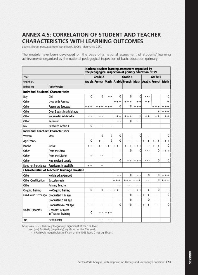
Sector-Wide Analysis, with emphasis on Primary and Secondary Education 373
Active Variable
Girl
Lives with Parents
Parents are Educated
Over 2 years in a Mahadra
Not enrolled in Mahadra
Repeater
Man
Active
From the Area
From the District
Not Involved Locally
Participates in Local Life
No Mahadra Attended
Baccalaureate
Primary Teacher
No Ongoing Training
Graduated 1 Yr ago
Graduated 2 Yrs ago
Graduated 4+ Yrs ago
9 Months or Morein Teacher Training
Headmaster
Year
Variables
Reference
Individual Students’ Characteristics
Boy
Other
Other
Other
Other
Other
No
Individual Teachers’ Characteristics
Woman
Age (Years)
Inactive
Other
Other
Other
Does not Participate Characteristics of Teachers’ Training/Education
Other
Other Qualification
Other
Ongoing Training
Graduated 3 Yrs ago
Under 9 months
No
Arabic French Math Arabic French Math Arabic French Math
Grade 2
National student learning assessment organised bythe pedagogical inspection of primary education, 1999
0
+ + +
- - -
0
-
0
+ +
+
+ +
0
- - -
0
0
+ + +
- - -
-
0
+ + +
+ + +
- -
+
0
-
- - -
- - -
- - -
+ + +
-
0
0
+ + +
- -
- - -
+ + +
- - -
0
+ + +
0
+ +
- - -
0
0
+ + +
+
0
- - -
+ + +
- - -
+ + +
- -
- - -
0
0
+ + +
0
+ + +
0
- -
- - -
+ + +
0
+ +
0
+ + +
- - -
- - -
0
0
0
0
+ +
+ + +
0
- - -
0
- - -
+ + +
0
+ + +
- - -
+ + +
- - -
+ + +
- - -
- - -
- - -
- - -
+ +
+ +
- - -
+ + +
-
- - -
- - -
0
- -
+
+ + +
0
+ + +
+ + +
+
+ +
+ + +
+ + +
0
0
0
0
0
- - -
- - -
- - -
0
+
+ + +
+ + +
+ +
0
+ + +
0
+ + +
0
+ + +
+ + +
- - -
0
- - -
0
Grade 4 Grade 6
Repeated Grade 1
Individual Students’ Characteristics
Reference
ariablesV
Year
Active Variable
the pedagogical inspection of primary education, 1999National student learning assessment organised by
Grade 2
ArabicMathFrenchArabic
the pedagogical inspection of primary education, 1999National student learning assessment organised by
MathFrenchArabicMathFrenchArabic
Grade 6Grade 4
Math
Age (Years)
Woman
Individual Teachers’ Characteristics
No
Other
Other
Other
Other
Other
Boy
Individual Students’ Characteristics
Man
Repeater
Not enrolled in Mahadra
Over 2 years in a Mahadra
Parents are Educated
Lives with Parents
Girl
Repeated Grade 1
Not enrolled in Mahadra
Over 2 years in a Mahadra
Parents are Educated
- - -
+ +
+ + +
0
0
-
+ + +
- - -
+ + +
0
-
- - -
+ + +
0
0
-
0
- - -
+ + +
0
+ + +
+ +
+ + +
+ + +
+ + +
+ +
+
+ + +
+ + +
- - -
+ +
+ +
- - -
0
- - -
0
+ + +
+ +
0
- -
0
+ + +
0
+ + +
0
0
0
- - -
+ +
0
+ + +
0
+ + +
0
+ +
+ + +
+ + +
+
0
Other
Other Qualification
Other
Characteristics of Teachers’ Training/EducationDoes not Participate
Other
Other
Other
Inactive
Age (Years)
Primary Teacher
Baccalaureate
No Mahadra Attended
Participates in Local Life
Not Involved Locally
From the District
From the Area
Active
Characteristics of Teachers’ Training/Education
No Mahadra Attended
Participates in Local Life
Not Involved Locally
- - -
+ + +
- - -
+ + ++ + +
0
+
- -
+ + +
+ + +
+ +
+
+ +
0
+ + +
+ + +
+ + +
+ + +
0
0
0
0
+ + +
+ + +
- -
0
- - -
- - -
-
+ + +
- - -
+ + +
- - -
+ + +
0
+ + +
- - -
- - -
+ + +
0
+ +
0
+ + +
- - -
- - -
+ + +
- - -
0
+
+ + +
0
+ + +
+ + +
0
+ + +
0
+ + +
No
Under 9 months
Graduated 3 Yrs ago
Ongoing Training
Headmaster
in Teacher Training9 Months or More
Graduated 4+ Yrs ago
Graduated 2 Yrs ago
Graduated 1 Yr ago
No Ongoing Training
in Teacher Training
Graduated 4+ Yrs ago
Graduated 2 Yrs ago
Graduated 1 Yr ago
No Ongoing Training
- - -
+ + +
- - -
+ + +
- - -
- -
- - -
- - -
-
0
0
- - -
0
- - -
- - -
- - -
- - -
- - -
0
+ + +
0
+ + +
+
- - -
- - -
- - -
+ + +
0
0
0
- - -
0
- - -
- -
+ + +
0
- - -
0
- - -
ANNEX 4.5: CORRELATION OF STUDENT AND TEACHERCHARACTERISTICS WITH LEARNING OUTCOMESSource: Extract translated from World Bank, 2006a (Mauritania CSR).
The models have been developed on the basis of a national assessment of students’ learningachievements organised by the national pedagogical inspection of basic education (primary).
Note: +++ (- - -) Positively (negatively) significant at the 1% level;++ (- --) Positively (negatively) significant at the 5% level;+ (- ) Positively (negatively) significant at the 10% level; 0 not significant.
AN
NEX
ES

Key Findings
- Girls face greater learning difficulties than boys, especially in math;
- The presence and education of parents is associated with better progress by students;
- Attending a Koranic school (Mahadra) is effective;
- The practice of repetition is negatively associated with school results; and
- Male teachers’ performance in ensuring their students’ progress is below that of their femalecounterparts in Grade 2 and Grade 6 Arabic and in Grade 4 French.
374 EDUCATION SECTOR ANALYSIS METHODOLOGICAL GUIDELINES - Volume 1

Sector-Wide Analysis, with emphasis on Primary and Secondary Education 375
ANNEX 4.6: CALCULATION OF SCHOOL INDICES (THE PERFORMANCE INDEX, RESOURCES INDEX AND EFFICIENCY INDEX), BASED ON THE EXAMPLE OF THE GAMBIA
The indicators included in index calculations are the same for all levels (school, district and region)with the exception of the GER which is added at the district and regional levels.
Performance Index
The table below summarises the weights and indicators used to calculate the performance index.Thresholds for each indicator are calculated based on school quintiles. The performance index is the(weighted) average of the points given to all indicators factored in the index.
TABLE A4.1 - Performance Index Calculation
1.00 point when X < 10 %0.75 points when 10 % ≤ X < 30 %0.50 points when 30 % ≤ X < 50 %0.25 points when 50 % ≤ X < 70 %0.00 points when X ≥ 70 %
1.00 point when X < 10 %0.50 point when 10 % ≤ X < 30 %0.25 point when 30 % ≤ X < 50 %0.00 point when X ≥ 50 %
1.00 point when X >33 %0.75 points when 28 % < X ≤ 33 %0.50 points when 26 % < X ≤ 28 %0.25 points when 24 % < X ≤ 26 % 0.00 points when X ≤ 24 %
1.00 point when X > 36 %0.75 points when 30 % < X ≤ 36 %0.50 points when 27 % < X ≤ 30 %0.25 points when 24 % < X ≤ 27 %0.00 points when X ≤ 24 %
1.00 point when X > 37 %0.75 points when 32 % < X ≤ 37 %0.50 points when 28 % < X ≤ 32 %0.25 points when 26 % < X ≤ 28 %0.00 points when X ≤ 26 %
1.00 point when X > 35 %0.75 points when 30 % ≤ X < 35 %0.50 points when 27 % ≤ X < 30 %0.25 points when 25 % ≤ X < 27 %0.00 points when X ≤ 25 %
1
1
1
1
1
1
Dropout Rate betweenGrade1 and Grade 6
Indicators Methodology (X= Indicator) Weight
Dropout Rate between Grade7 and Grade 9
NAT Grade 3 English (% of correct answers)
NAT Grade 3 Math (% of correct answers)
NAT Grade 5 English (% of correct answers)
NAT Grade 5 Math (% of correct answers)
Grade1 and Grade 6
ABL
Indicators
TTA
Dropout Rate between
0.50 points when 30 % 0.75 points when 10 % 1.00 point when X < 10 %
X < 50 %
Performance Index Calculation
Methodology (X= Indicator)
A4.1 - ABLE
≤0.50 points when 30 % X < 30 %≤0.75 points when 10 %
1.00 point when X < 10 %
1
Performance Index Calculation
Weight
X < 50 %X < 30 %
1.00 point when X < 10 %
0.00 points when 0.25 points when 0.50 points when 0.75 points when 1.00 point when
0.00 point when 0.25 point when 0.50 point when 1.00 point when
0.00 points when 0.25 points when 50 % 0.50 points when 30 %
NAT Grade 3 Math (%
correct answers)NAT Grade 3 English (% of
Grade7 and Grade 9Dropout Rate between
1.00 point when
24 %≤≤XX0.00 points when 26 %≤≤ 24 % < X X 0.25 points when 28 %≤≤26 % < X X0.50 points when 33 %≤≤ 28 % < X X 0.75 points when
X >33 %1.00 point when
50 % ≥ X X 0.00 point when X < 50 %≤ 30 % 0.25 point when X < 30 %≤10 % 0.50 point when
X < 10 %1.00 point when
70 %≥ X 0.00 points when X < 70 %≤0.25 points when 50 % X < 50 %≤0.50 points when 30 %
1
1
24 % 26 % 28 % 33 %
X >33 %
50 % X < 50 % X < 30 %
X < 10 %
70 %X < 70 %X < 50 %
0.50 points when 0.75 points when 1.00 point when
0.00 points when 0.25 points when 0.50 points when 0.75 points when 1.00 point when
0.00 points when 0.25 points when 0.50 points when 0.75 points when 1.00 point when
of correct answers)NAT Grade 5 Math (%
of correct answers)NAT Grade 5 English (%
of correct answers)NAT Grade 3 Math (%
X < 30 %27 % 0.50 points when X < 35 ≤≤30 % 0.75 points when
X > 35 %1.00 point when
26 %≤≤ X X 0.00 points when 28 %≤≤ 26 % < X X0.25 points when 32 %≤≤ 28 % < X X 0.50 points when 37 %≤≤ 32 % < X X0.75 points when
X > 37 %1.00 point when
24 %≤≤XX0.00 points when 27 %≤≤ 24 % < X X 0.25 points when 30 %≤≤27 % < X X0.50 points when 36 %≤≤ 30 % < X X 0.75 points when
X > 36 %1.00 point when
1
1
1
X < 30 % X < 35 %
X > 35 %
26 % 28 % 32 % 37 %
X > 37 %
24 % 27 % 30 % 36 %
X > 36 %
0.00 points when 0.25 points when 0.50 points when
25 ≤≤ XX0.00 points when X < 27 ≤≤25 % 0.25 points when X < 30 ≤≤27 % 0.50 points when
1
25 % X < 27 % X < 30 %
AN
NEX
ES

376 EDUCATION SECTOR ANALYSIS METHODOLOGICAL GUIDELINES - Volume 1
1.00 point when X < 310.75 points when 31 ≤ X < 32.50.50 points when 32.5 ≤ X < 33.50.25 points when 33.5 ≤ X < 34.50.00 points when X ≥ 34.5
1.00 point when X < 8.10.75 points when 8.1 ≤ X < 8.60.50 points when 8.6 ≤ X < 8.70.25 points when 8.7 ≤ X < 8.90.00 points when ≥ 8.9
1
4
1.00 point when X < 8.20.75 points when 8.2≤X < 8.60.50 points when 8.6≤X < 8.80.25 points when 8.8≤X < 8.90.00 points when X ≥ 8.9
1.00 point when X < 7.30.75 points when 7.3≤ X < 7.80.50 points when 7.8≤ X < 8.10.25 points when 8.1≤ X < 8.40.00 points when X ≥ 8.4
1.00 point when X< 7.40.75 points when 7.4≤X < 8.00.50 points when 8.0≤X < 8.40.25 points when 8.4≤X < 8.50.00 points when X ≥ 8.5
1.00 point when X >1100.75 points when 96 < X ≤1100.50 points when 82 < X ≤ 960.25 points when 67 < X ≤ 820.00 points when X ≤ 67
1.00 point when X > 830.75 points when 62 < X≤ 830.50 points when 49 < X≤ 620.25 points when 31 < X≤ 490.0 points when X ≤ 31
1
1
1
2
2
possible=4, Worst=36)
possible=1, Worst=9)
Economic Science score
(Primary)
(Lower Secondary)
0.75 points when 1.00 point when
0.00 points when 0.25 points when 0.50 points when 0.75 points when 1.00 point when
possible=4, Worst=36)
X < 8.68. ≤ X < 8.610.75 points when X < 8.11.00 point when
34. ≥ 34.5X 0.00 points when X < 34.33.5≤ X < 34.550.25 points when
X < 33.32.5≤ X < 33.55 0.50 points when X < 32.3 ≤ X < 32.510.75 points when
X < 311.00 point when
4
X < 8.6 X < 8.1
34.5 X < 34.5 X < 33.5 X < 32.5
0.00 points when 0.25 points when 0.50 points when 0.75 points when
0.00 points 0.25 points 0.50 points 0.75 points 1.00 point
0.00 points 0.25 points 0.50 points 0.75 points 1.00 point
possible=1, Worst=9)
8.9 ≥0.00 points when X < 8.98.7≤ X < 8.97 0.25 points when X < 8.78.6≤ X < 8.760.50 points when
X < 8.68. ≤ X < 8.61 0.75 points when
8.4≥ X when0.00 points X < 8.4≤ 8.1when0.25 points X < 8.1≤ 7.8when0.50 points
X < 7.8≤≤ 7.3when0.75 points X < 7.3when1.00 point
8.9≥ X when0.00 points X < 8.9≤ 8.8when0.25 points X < 8.8≤ 8.6when0.50 points X < 8.6≤8.2when0.75 points
X < 8.2when1.00 point
1
8.9 X < 8.9 X < 8.7 X < 8.6
1
1
8.4 X < 8.4 X < 8.1
X < 7.8 X < 7.3
8.9X < 8.9X < 8.8X < 8.6
X < 8.2
0.75 points 1.00 point
0.00 points 0.25 points 0.50 points 0.75 points 1.00 point
0.00 points 0.25 points 0.50 points 0.75 points 1.00 point
0.00 points
(Lower Secondary)
(Primary)
Economic Science score
83≤ 62 < Xwhen0.75 points X > 83when1.00 point
67≤ Xwhen0.00 points 82≤ 67 < Xwhen0.25 points 96≤82 < Xwhen0.50 points
110 ≤ 96 < Xwhen0.75 points X >110when1.00 point
8.5≥ X when0.00 points X < 8.5≤ 8.4when0.25 points X < 8.4≤ 8.0when0.50 points X < 8.0≤ 7.4when0.75 points
X< 7.4when1.00 point
8.4≥ X when0.00 points
2
1
83 X > 83
678296
110 X >110
8.5X < 8.5X < 8.4X < 8.0
X< 7.4
8.4
0.0 points
0.25 points 0.50 points 0.75 points (Lower Secondary)
31≤ Xwhen0.0 points
49≤ 31 < Xwhen0.25 points 62≤ 49 < Xwhen0.50 points 83≤ 62 < Xwhen0.75 points
2
31496283
Note: NAT: the National Assessment Test;GABECE: The Gambian Basic Education Certificate Examinations.
Resources Index
The table below summarises the weights and indicators used to compute the resources index.Thresholds for each indicator are calculated based on quintiles (schools are distributed into 5 groupsaccording to the value achieved for the indicator considered). The resources index is the (weighted)average of the points given to all indicators factored in the index.

Sector-Wide Analysis, with emphasis on Primary and Secondary Education 377
AN
NEX
ES
1.00 point when X < 180.75 points when 18 ≤ X < 250.50 points when 25 ≤ X < 310.25 points when 31 ≤ X < 370.00 points when X ≥ 37
1.00 point when X >75 %0.75 points when 60 % < X≤75 %0.50 points when 50 % < X ≤60 %0.25 points when 40 % < X ≤50 %0.00 points when X≤40 %
1.00 point when X≤10.75 points when 1 < X≤1.40.50 points when 1.4 < X≤1.90.25 points when 1.9 < X≤2.70.00 points when X>2.7
1.00 point when X≤10.75 points when 1 < X ≤1.30.50 points when 1.3 < X ≤1.70.25 points when 1.7 < X ≤2.50.00 points when X >2.5
1.00 point when X≤ 10.75 points when 1 < X ≤ 1.50.50 points when 1.5 < X ≤ 20.25 points when 2 < X ≤ 30.00 points when X > 3
1.00 point when X < 1.20.75 points when 1.2 ≤ X < 1.80.50 points when 1.8 ≤ X < 2.30.25 points when 2.3 ≤ X < 3.40.00 points when X ≥ 3.4
1 if at least one0 if none
0 points if Yes1 point if No
Mean by District of: Household WealthQuintile Divided by 5. Scale variesbetween 0 and 1
1
1
1
1
0.25
0.25
1
1
0.5
Student-Teacher Ratio
% Qualified Teachers
Number of Studentsper Textbook (Math)
Number of Studentsper Textbook (English)
Number of Students per Seat
Number of Students per Desk
Power Equipment(Electricity/Solar/Generator)
Hardship
Poverty Index (District Level)
Indicators Methodology (X= Indicator) Weight
TABLE A4.2 - Resources Index Calculation
ABL
Student-Teacher Ratio
Indicators
0.75 points when 1.00 point when
TTA
Resources Index Calculation
X < 25
Methodology (X= Indicator)
≤ 180.75 points when X < 181.00 point when
A4.2 - ABLE
Resources Index Calculation
1
Weight
per Textbook (Math) Number of Students
% Qualified Teachers
0.25 points when 1.9 < X0.50 points when 1.4 < X0.75 points when 1 < X1.00 point when X
0.00 points when 0.25 points when0.50 points when0.75 points when1.00 point when X >75 %
0.00 points when0.25 points when0.50 points when
2.7≤0.25 points when 1.9 < X1.9≤0.50 points when 1.4 < X1.4≤0.75 points when 1 < X1≤1.00 point when X
40 %≤ X0.00 points when 50 %≤40 % < X 0.25 points when60 %≤50 % < X 0.50 points when75 %≤60 % < X0.75 points when
1.00 point when X >75 %
37≥X0.00 points whenX < 37≤310.25 points whenX < 31≤250.50 points when
1
1
1
Number of Students per Desk
Number of Students per Seat
per Textbook (English) Number of Students
1.00 point when X < 1.2
0.00 points when X > 30.25 points when 2 < X0.50 points when 1.5 < X0.75 points when 1 < X1.00 point when X
0.00 points when X >2.50.25 points when 1.7 < X0.50 points when 1.3 < X0.75 points when 1 < X1.00 point when X
0.00 points when X>2.7
1.00 point when X < 1.2
0.00 points when X > 33≤0.25 points when 2 < X2≤0.50 points when 1.5 < X1.5≤0.75 points when 1 < X1≤1.00 point when X
0.00 points when X >2.52.5≤0.25 points when 1.7 < XX1.7≤0.50 points when 1.3 < XX1.3≤0.75 points when 1 < XX1≤1.00 point when X
0.00 points when X>2.7
0.25
1
Poverty Index (District Level)
Hardship
(Electricity/Solar/Generator) Power Equipment
Number of Students per Desk
Quintile Divided by 5. Scale variesMean by District of: Household Wealth
1 point if No0 points if Yes
0 if none1 if at least one
0.00 points when X 0.25 points when 2.30.50 points when 1.80.75 points when 1.21.00 point when X < 1.2
Quintile Divided by 5. Scale variesMean by District of: Household Wealth
1 point if No0 points if Yes
0 if none1 if at least one
3.4≥0.00 points when X X < 3.4≤0.25 points when 2.3X < 2.3≤0.50 points when 1.8X < 1.8≤0.75 points when 1.2
1.00 point when X < 1.2
0.5
1
1
0.25
Mean by District of: Household Wealth
between 0 and 1 Quintile Divided by 5. Scale varies
between 0 and 1 Quintile Divided by 5. Scale varies
1
Efficiency Index
To keep the efficiency index between zero and one, it is calculated as follows:
Efficiency index =Performance Index - Ressources Index + 1
2

378 EDUCATION SECTOR ANALYSIS METHODOLOGICAL GUIDELINES - Volume 1
ANNEX 4.7: COMPUTATION OF THE SCHOOL VALUE-ADDED INDICATOR
Various studies on the determinants of learning outcomes has shown that students’ initial levels andschool contexts are the most influential factors. Consequently, to truly determine what a school bringsto its students’ success, it is preferable to compute a value-added indicator. By definition, the addedvalue may be estimated as the difference between the result achieved by a school and the result thatschool was expected to achieve given its characteristics (contextual and student characteristics).
AVi = Roi - Rei
Where: - AVi is the value added by school i- Roi is the result observed for school i; and- Rei is the expected result for school i.
If the observed result is easy to obtain in as much as it is a school’s score in an assessment or exam,to propose a value for the expected result is more complex. In practice, various approaches exist butthe fairest consists of using the estimates from an econometric model that includes context variablesto predict the results schools should achieve (expected value), given the characteristics of their studentpopulation and the context they operate in.
The variables here are those the school has no influence over (students’ personal characteristics, theschool’s geographical area and so on). Thus the result obtained can vary from one school to anotheraccording to the chosen variables.

Sector-Wide Analysis, with emphasis on Primary and Secondary Education 379
AN
NEX
ES
Ministry of Basic & Secondary EducationDirectorate of Planning
Based on the information collected from the school by the CMs
SCHOOL PROFILE 2009/10 School Name :
Local Management :
Albion Government
District : Banjul School Code :School Type :
No of Students :
10002LBS663
Context-ResourcesHardship No No NoMultigrade Double Shift Electricity Yes
262262
151518M
582540
Raw Data SchoolNumber of seatsNumber of desksNumber of classroomsOf wich are permanentNumber of teachersOf which are qualifiedNumber of Maths textbooksNumber of English textbooks
Indicator School District Region GambiaNb of students per seatNb of student per desk% of permanent classroomsStudent teacher ratio% of qualified teachersNb of students per Maths textbookNb of students per English textbook
AveragePublic Schools
2.52.5
100%37M
1.21.1
2.01.9
100%28
71%2.22.2
2.72.9
100%35
70%3.63.9
3.01.6
99%18
64%3.12.9
NAT (%of Correct Answers)
LOWER BASIC EDUCATION
UPPER BASIC EDUCATION
School District Region GambiaG3 EnglishG3 MathsG5 EnglishG5 MathsDrop-out rate G1-6
AveragePublic Schools
26%29%33%27%
0%
29%34%35%30%21%
30%32%35%31%21%
27%29%30%29%43%
GABECE Scores (Core Subjects) School District Region GambiaAggregateEnglishMathsSciencesSESDrop-out rage G7 -9
AveragePublic Schools
NANANANANANA
31.57.98.57.27.83%
32.58.28.67.78.03%
33.06.37.96.87.1
25%
Performance
Performance Index Resources Index1.0
0.8
0.6
0.4
0.2
0.0School District
PublicRegionPublic
GambiaPublic
0.60 0.57 0.60
0.43
1.0
0.8
0.6
0.4
0.2
0.0School District
PublicRegionPublic
GambiaPublic
0.79 0.760.70
0.51
1.0
0.8
0.6
0.4
0.2
0.0School District
PublicRegionPublic
GambiaPublic
Efficiency IndexPerformance/Resources
0.41 0.400.45 0.46
Indices
ANNEX 4.8: SCHOOL PROFILE, BASED ON THE EXAMPLE OFTHE GAMBIA
Note: NA: Not Applicable; M: missing information

ANNEX 4.9: FLOW OF EXAM RESULT INFORMATION,CAMEROONSource: Authors’ conception based on interviews with education system stakeholders.
380 EDUCATION SECTOR ANALYSIS METHODOLOGICAL GUIDELINES - Volume 1
Need to analyse the results and havethem trickle down through each levelto help inform management practices
CentralLevel
(EducationMinistry)
RegionalDelegation
DepartmentalDelegation
Catchment AreaInspections
ExamCenters
Schools
Solid line arrows indicate current practice
Results must be fed back upto the central level to be used
in certification processes
Dotted arrows indicate tasks outstanding
Pupils are put forward ascandidates to the exam
centers
LevelCentral
o help in ement prt
anathe hrouth
anm tric h eac
Need to anthth
hato analyse the anNeed he resultNeed to results ae
o hel emennfor ractto help inf gement praagto help gementnfor practm ticevkle d h le
mamp prm tm gp i t pm cmo hel mento help inform management practicthem trickle down rough eacn thrn em tr ugh ee gdowwnowthem trickle down through each lev
analyse d hato analyse t s and haresults and alyse thyNeed to analyse the results and haveve
eseecescesDelegation
Departmental
DelegationRegional
Ministry)(Education
velevelve
t uo thces
he ust eo ntrat eo t beRes ust be fed backResults m ack ult kRes ack
certif estioncertificati ssn certifi sesatioel tolevt
orce esfica on rrn seca n p ocessocertif tio cein certification processeshe central level to be ubcentrce otlto the central level to be us
be fed bsults bmust be fed bsults must b k uRes e fed backbe fedd Results must be fed back usedsupup
sssededsed
upup
Schools
CentersExam
InspectionsCatchment Area
centerscandidates to the exam
ard asPupils are put forw
Dotted arrows indicate tasks outstanding Solid line arrows indicate current practiceDotted arrows indicate tasks outstanding Solid line arrows indicate current practiceSolid line arrows indicate current practice

Sector-Wide Analysis, with emphasis on Primary and Secondary Education 381
The estimated coefficients describe the net impact of education on earnings, all other things beingequal; the effect is for instance isolated from that of the number of years of experience of the sectorof work. Once the earnings function has been estimated, the next step will be to simulate averageincome according to the level of education.
CHAPTER 5 ANNEXES
ANNEX 5.1: METHODOLOGY FOR THE ESTIMATION OF NETINCOME, EXPECTED INCOME AND RATES OF RETURN
Earnings Functions
To estimate the rates of return of education, a standard approach consists of the use of the Mincermodel, based on the following equation:
Where, Yi* is the individual annual income (or salary), Ei the number of years of work experience, Dki = 1 if the person i has the degree Dk (or has reached the level of education k) or = 0 otherwise, Xji
is the sector of the main earning activity, and 𝒖i is a random term and is supposed to be Gaussian(normal distribution). The ƞ parameters are generated by the model itself.
In the case of Mali, by using the ELIM, 2006 data the following model is obtained. All the parametersof the model are significant at the usual level (one percent). The determination of the model is fairlygood, with an R² value close to 20 percent.
Ln(Yi*) = ƞ0 + ƞ1Ei + ƞ2Ei + ƞ3k Dki + ƞ4j Xji + 𝒖i (1)∑k=1
K2 ∑
j=1
J
Reference CoefficientVariable
Basic 1
Basic 2
General Secondary and TVET
Higher
Years of Experience
Years of Experience Squared
Man
Modern Public Sector
Modern Private Sector
Informal (Other than Agriculture)
Constant
0.0369
0.2611
0.7531
1.2991
0.0177
-0.0003
0.2384
0.7206
0.3630
0.4766
11.8583
No education
Woman
Informal Agriculture
TABLE A5.1 - Results of the Econometric Estimation (Based on Malian ELIM 2006 Data) Results of the Econometric Estimation (Based on Malian ELIM 2006 Data)
General Secondary and TVET
ariableV
Basic 2
Basic 1
A5.1 - ABLETTA Results of the Econometric Estimation (Based on Malian ELIM 2006 Data)
No education
Reference
Results of the Econometric Estimation (Based on Malian ELIM 2006 Data)
0.7531
ficientffCoe
0.2611
0.0369
Constant
Informal (Other than Agriculture)
Modern Private Sector
Modern Public Sector
Man
Years of Experience Squared
Years of Experience
Higher
General Secondary and TVET
Informal Agriculture
Woman
11.8583
0.4766
0.3630
0.7206
0.2384
-0.0003
0.0177
1.2991
0.7531
AN
NEX
ES

382 EDUCATION SECTOR ANALYSIS METHODOLOGICAL GUIDELINES - Volume 1
Experience ExperienceSquared
Man Non-AgriculturalInformal Sector
Public Sector Private Sector
19.2564 521.7487 0.4699 0.2392 0.0399 0.0710
TABLE A5.2 - Average of Explanatory Variables Other than the Number of Years of Education Average of Explanatory Variables Other than the Number of Years of Education
521.7487
ExperienceSquared
A5.2 - ABLETTA
19.2564
Experience
Average of Explanatory Variables Other than the Number of Years of Education
0.2392
Informal Sector
0.4699
Non-AgriculturalMan
Average of Explanatory Variables Other than the Number of Years of Education
0.0710
Private Sector
0.0399
Public SectorInformal Sector
Non-Agricultural
Private Sector
No Education (Ref.)
Basic 1
Basic 2
Secondary
Higher Education
12.3455
12.3455 + 0.0369
12.3455 + 0.2611
12.3455 + 0.7531
12.3455 + 1.2991
= 12.3455
= 12.3824
= 12.6066
= 13.0986
= 13.6446
TABLE A5.3 - Logarithm of Simulated Annual Income by Level of Education Logarithm of Simulated Annual Income by Level of Education
Higher Education
Secondary
Basic 2
Basic 1
No Education (Ref.)
A5.3 - ABLETTA Logarithm of Simulated Annual Income by Level of Education
12.3455 + 1.2991
12.3455 + 0.7531
12.3455 + 0.2611
12.3455 + 0.0369
Logarithm of Simulated Annual Income by Level of Education
= 13.6446
= 13.0986
= 12.6066
= 12.3824
= 12.3455
12.3455 + 1.2991
12.3455 + 0.7531
12.3455 + 0.2611
12.3455 + 0.0369
12.3455
TABLE A5.4 - Simulated Annual Income According to the Level of Education
No Education (Ref.)
Basic 1
Basic 2
Secondary
Higher Education
Simulated Income (a)
= Exp. (12.3455+ 0.4865)
= Exp. (12.3824+ 0.4865)
= Exp. (12.6066+ 0.4865)
= Exp. (13.0986+ 0.4865)
= Exp. (13.6446+ 0.4865)
373,995
388,045
485,599
794,167
1,371,000
A5.4 -
Higher Education
ABLET
Secondary
Basic 2
Basic 1
No Education (Ref.)
Simulated Annual Income According to the Level of Education
Simulated Income (a)
= Exp. (13.6446+ 0.4865)
= Exp. (13.0986+ 0.4865)
= Exp. (12.6066+ 0.4865)
= Exp. (12.3824+ 0.4865)
= Exp. (12.3455+ 0.4865)
Simulated Annual Income According to the Level of Education
Simulated Income (a)
1,371,000
794,167
485,599
388,045
373,995
= Exp. (13.6446+ 0.4865)
= Exp. (13.0986+ 0.4865)
= Exp. (12.6066+ 0.4865)
= Exp. (12.3824+ 0.4865)
= Exp. (12.3455+ 0.4865)
1,371,000
794,167
485,599
388,045
373,995
• Simulation of the Logarithm of Average Income by Level of Education and Deduction ofAverage Income by Level of Education
On the basis of the earnings model and explanatory variables estimated above, the logarithm for theaverage earnings of workers according to their level of education can be estimated, holding othervariables constant (equal to their averages). The earnings function estimated by this second model is:
Ln(Y) = 11.8583 + 0.0369 (Basic 1) + 0.2611 (Basic 2) + 0.7531 (Secondary) + 1.2991 (Higher) + 0.0177 (Years of experience)– 0.003 (Years of experience squared) + 0.2384 (Man)+ 0.4766 (Non-agriculture informal sector) + 0.7206 (Public sector)+ 0.3630 (Private sector)
The average of each of the other explanatory variables on the sample used to estimate the earningsfunction is provided in Table A5.2.
The logarithm for simulated earnings is therefore the sum of a fixed factor and a factor that variesaccording to the highest level of education attended:
Ln(Y) = 12.3455 + 0.0369 (Basic 1) + 0.2611 (Basic 2)+ 0.7531 (Secondary) + 1.2991 (Higher)
The simulated income takes the variance of the error term u of equation (1) into account in equation(4), where S represents the standard deviation of the residual of the mincer model. S2/2 is here equalto 0.4865.
(2)
(3)
Ysimulated = Exp ([Ln(Y)]simulated) x Exp ( ) (4)2s
2

Sector-Wide Analysis, with emphasis on Primary and Secondary Education 383
AN
NEX
ES
Calculation of Rates of return
On the basis of the simulated income, the rate of return of level k in comparison to the previous levelk-1 is obtained by dividing the additional income attributable to level k by the additional cost involvedin pursuing schooling at that level. This cost includes both the opportunity cost of the income lostdue to the pursuit of education, estimated as the annual income of individuals having completed thelevel k-1 and the direct cost of education at level k.
Furthermore, the estimated income to be derived from level k for an individual following level k-1should take into account the risk of not finding employment upon completion of level k.
The rate of return of level k would then be computed as:
Where πk is the employment rate (1 – the unemployment rate of recent school leavers) of individualshaving completed level k and Yk is the simulated income for individuals with level k education.
Ck is the annual cost of training;Ak is the total theoretical duration of level k;Dk is the average length of education for individuals having attained level k;Nk is the average length of education for individuals not attaining level k;Nk-1/k is the average number of additional years of education followed by individuals having attainedlevel k (compared to those having attained level k-1), computed as the difference between theaverage number of years of education held by each;
The indicators for the length of education are estimated on the basis of survey data (See Table A5.5).
Rk/k-1 = (5)πkYk -πk-1Yk-1
Nk-1/k πk-1Yk-1 + NkCk + (Ak-1-Dk-1) Ck-1
TABLE A5.5 - Employment Rate, Length of Workers’ Education and Annual Cost of Training,by Level98
No Education
Basic 1
Basic 2
Secondary
Higher Education
98.3%
96.1%
92.5%
84.3%
74.6%
373,995
388,045
485,599
794,167
1,371,000
0.0
4.2
8.1
11.4
15.5
0.0
6.0
9.0
12.0
-
4.2
2.1
2.4
3.5
0
4.2
3.8
3.4
4.1
0
5,908
7,999
25,604
33,996
0
32,113
59,288
286,388
379,481
Employment Rate, Length of Workers’ Education and Annual Cost of Training,A5.5 - ABLETTA 98by Level
Employment Rate, Length of Workers’ Education and Annual Cost of Training,
Employment Rate, Length of Workers’ Education and Annual Cost of Training,
Higher Education
Secondary
Basic 2
Basic 1
No Education
1,371,000
794,167
485,599
388,045
373,995
74.6%
84.3%
92.5%
96.1%
98.3%
3.5
2.4
2.1
4.2
-
12.0
9.0
6.0
0.0
15.5
11.4
8.1
4.2
0.0
1,371,000
794,167
485,599
388,045
373,995
379,481
286,388
59,288
32,113
33,996
25,604
7,999
5,908
0
4.1
3.4
3.8
4.2
0
379,481
286,388
59,288
32,113
0
Source : Author’s calculations on the basis of ELIM, 2006 data.

Formula (5) enables one to calculate both the social and the private returns on investment. In theestimations used here, the difference between the two is mainly due to the direct costs Ck considered.For the private rate of return, the direct cost is limited to the cost of training supported by families (asestimated in Chapter 3), whereas the social return on investment also considers the public unit costs(also estimated in Chapter 3) in addition to private costs.
Thus the rate of return of Basic 1 education (compared to having no education) can be computed inthe following way:
The expected additional annual income is equivalent to 5,284 (388,045 x 96.1%)-(373,995 x 98.3%).
The costs related to the pursuit of primary education are estimated as:• 1,558,714 of opportunity costs (373,995 x 98.3%) x 4.2;• 25,052 private costs of training [5,908 x 4.2] + [0 x (0-0)]; and• 143,393 public costs of training [32,113 x 4.2] + [0 x (0-0)].
The social rate of return for Basic 1 education is thus estimated at 0.31 percent (5,284 / (1,558,714 +25,052 + 143,393)) whereas the private rate of return is 0.33 percent (5,284 / (1,558,714 + 25,052)).
384 EDUCATION SECTOR ANALYSIS METHODOLOGICAL GUIDELINES - Volume 1

Sector-Wide Analysis, with emphasis on Primary and Secondary Education 385
AN
NEX
ES
ANNEX 5.2: THE MAIN TYPES OF SURVEY USED INLABOUR MARKET ANALYSIS
In the context of the improvement of information tools for the monitoring of poverty, many countrieshave developed broad surveys for the measurement, monitoring and evaluation of poverty. Some suchsurveys include a specific module on employment and income, which provides various measures ofthe correlation between education and work indicators (access to work, employment and income bylevel and so on). The most common surveys are described here.
Demographic Censuses usually collect information relating to homes/accommodation,sociodemographic characteristics (including age, gender, civil status), the status and area of residence,fertility, education, activities and employment. The main objective of censuses is to update thedemographic, social and economic profile of the country’s inhabitants. Collection is nation-wide andcomprehensive, and the results are available down to the smallest available geographic/administrativearea.
Household Living Condition Surveys are carried out with variable regularity, depending on thecountry. The themes covered include, among others: income, spending, health, employment,agriculture and access to basic social services. The main objective of such surveys is to monitor andevaluate households’ general living conditions and the poverty reduction programme’s impact inparticular. Surveys have nationwide coverage (on the basis of a sample) and the results arerepresentative at the regional level and by area of residence (urban/rural).
Core Welfare Indicator Questionnaire Surveys99 (or quick poverty monitoring and evaluationsurveys), cover among other themes: access to education and health, the degree of satisfaction withand the level of access of populations to basic social services, employment, nutrition, wealth andhome characteristics. CWIQs are relatively recent tools, launched in the mid-1990s, and are on trackto being carried out regularly in many countries. Such surveys have two main objectives: (i) to providevaluable household-level information to enable the elaboration and evaluation of socioeconomicdevelopment policies; and (ii) to provide a mechanism for the straightforward and regular follow-upof different socioeconomic population groups.
Demographic and Health Surveys (DHS), conducted about every five years, cover themes pertainingto education and enrolment, accommodation, health and fertility behaviours, child health(anthropometrics) and the availability of community services. In some countries they also include anemployment module. The main objective of DHS surveys is to provide information on demographicand health characteristics. Their coverage is national (on the basis of a sample) and the results areusually available by region and area of residence (urban/rural).
Multiple Indicator Cluster Surveys100 were developed to measure progress towards the goalsestablished by the World Summit for Children of 1990. These types of surveys are now common indeveloping countries. They cover issues relating to accommodation, hygiene, education, child labourand maternal and child health.
Employment Surveys provide a good knowledge of the workplace. Such surveys are key statisticaltools, providing a plethora of information on the labour market and its evolution: the share of theactive population, the number and rate of unemployed, the characteristics of workers, thecharacteristics of school leavers or work leavers and so on. They provide data on the structure of thelabour market by profession, on the activities of women and/or children, on the length of work

386 EDUCATION SECTOR ANALYSIS METHODOLOGICAL GUIDELINES - Volume 1
contracts and on unstable positions. All European Union countries are committed to carrying out anemployment survey every three months.101 Some developing countries carry out an employment surveyevery year.
1-2-3 or 1-2 Type Surveys are used in developing countries to appraise the state of the labourmarket. They owe their name to the three interlinked phases, on: (i) employment; (ii) the informalsector; and (iii) poverty. They therefore touch on the informal sector, income and consumption, inaddition to employment (current and past context, unemployment, conditions of activity). 1-2-3surveys also include a module on democracy and governance, that enables a quantified appraisal (anddisaggregated by type of institution) of governance, both from the perspective of the efficiency ofthe state administration and from that of the confidence of households in public institutions. Suchsurveys are therefore also very useful to evaluate civic and social behaviour.
Tracer Surveys (See Annex 5.4).

Sector-Wide Analysis, with emphasis on Primary and Secondary Education 387
AN
NEX
ES
ANNEX 5.3: SELECTION OF A REPRESENTATIVE SAMPLEFOR THE ANALYSIS OF THE STATUS OF EDUCATIONSYSTEM LEAVERS IN THE WORKPLACE102
SELECTION OF A SAMPLE OF ACTIVE INDIVIDUALS HAVING RECENTLY LEFTEDUCATION
The data most commonly used for such analyses are drawn from household surveys, which by natureare not conceived to provide information on education system leavers. It is however possible, on thebasis of household survey data, to build a representative sample of active individuals who recentlyfinished their education. It is common to consider individuals having left school or university in thelast ten years. To do so, a variable is computed that estimates the time spent in the workplace:Duration = age – (official school age for starting school + number of years of education)
On this basis, a sample can be selected according to the duration of an individual’s status as active. Ifthe sample composed of individuals who have been active for up to ten years is too large, the set cut-off duration can be reduced. It is however advisable to ensure that the sample obtained isrepresentative.
REPRESENTATIVITY OF THE SAMPLE OF ACTIVE INDIVIDUALS HAVING RECENTLYLEFT EDUCATION
The sample obtained above should be checked for representativity, especially if there is an interest ingeneralizing (inferring) the results of the descriptive analysis (unemployment rate, job status analysisand so on). If the sample is found to not be representative, the results should be adjusted by calibrationweighting. The procedure involves two steps: (i) the determination of the actual structure of allindividuals having recently finished their education; and (ii) the calibration weighting of the sample ofindividuals obtained according to the actual structure.
(i) Determination of the Actual Structure of Recent Education Leavers
Chapter 2 of this guide offered an approach to the construction of cross section (or transverse)schooling profiles for a given year. On the basis of this profile, and as illustrated by Table A5.6 below,the highest level attained by the enrolled individuals can be obtained.

388 EDUCATION SECTOR ANALYSIS METHODOLOGICAL GUIDELINES - Volume 1
SchoolingProfile
Highest Levelof Education Attained (%)
Education Level
No Education
Grade 1
Grade 2
Grade 3
Grade 4
Grade 5
Grade 6
Grade 1
Grade 2
Grade 3
Grade 4
Grade 5
Grade 6
Grade 7
Incomplete Primary
Complete Primary
Lower Secondary
Upper Secondary
Higher
Total
76.4
63.4
56.5
46.3
37.1
30.5
17.7
12.4
10.0
8.7
8.1
6.7
6.7
2.3
23.6 = 100 – 76.4
12.9 = 76.4 – 63.4
6.9 = 63.4 – 56.5
10.2 = 56.5 – 46.3
9.2 = 46.3 – 37.1
6.6 = 37.1 – 30.5
12.8 = 30.5-17.7
5.3 = 17.7 – 12.4
2.4 = 12.4 – 10.0
1.3 = 10.0 – 8.7
0.6 = 8.7 – 8.1
1.4 = 8.1 – 6.7
0.0 = 6.7 – 6.7
4.4 = 6.7 – 2.3
2.3
-
23.6
45.8
12.8
9.6
5.8
2.3
100.0
TABLE A5.6 - Distribution of a Pseudo Cohort of 100 Youth,by Terminal Education Level
A5.6 -
Grade 2
Education Level
ABLETTA
Grade 1
No Education
by Terminal Education Level
6.9 = 63.4 – 56.5
Profile
Distribution of a Pseudo Cohort of 100 Youth,A5.6 -
12.9 = 76.4 – 63.4
23.6 = 100 – 76.4
63.4
76.4
Grade 2
Grade 1
Schooling
Distribution of a Pseudo Cohort of 100 Youth,
23.6
of Education Attained (%)
6.9 = 63.4 – 56.5
12.9 = 76.4 – 63.4
23.6 = 100 – 76.4
Highest Level
Upper Secondary
Lower Secondary
Complete Primary
Incomplete Primary
Grade 6
Grade 5
Grade 4
Grade 3
Grade 2
Grade 1
Grade 6
Grade 5
Grade 4
Grade 3
1.3 = 10.0 – 8.7
2.4 = 12.4 – 10.0
5.3 = 17.7 – 12.4
12.8 = 30.5-17.7
6.6 = 37.1 – 30.5
9.2 = 46.3 – 37.1
10.2 = 56.5 – 46.3
6.7
8.1
8.7
10.0
12.4
17.7
30.5
37.1
46.3
56.5
Grade 6
Grade 5
Grade 4
Grade 3
Grade 2
Grade 1
Grade 6
Grade 5
Grade 4
Grade 3
5.8
9.6
12.8
45.8
0.0 = 6.7 – 6.7
1.4 = 8.1 – 6.7
0.6 = 8.7 – 8.1
1.3 = 10.0 – 8.7
2.4 = 12.4 – 10.0
5.3 = 17.7 – 12.4
12.8 = 30.5-17.7
6.6 = 37.1 – 30.5
9.2 = 46.3 – 37.1
10.2 = 56.5 – 46.3
otalTTo
Higher
Upper Secondary
Grade 7
Grade 6
2.3
6.7
6.7
Grade 7
Grade 6
100.0
2.3
5.8
-
2.3
4.4 = 6.7 – 2.3
0.0 = 6.7 – 6.7
The column for the highest level of education attained represents the distribution by level of educationleavers (the leavers’ profile by level). This profile provides the actual structure of the population ofeducation leavers for a given year.
If the analysis covers a number of years, the actual structure of the population of education leaverscan be obtained for that period through the estimation of the average schooling profile of educationleavers for each of the years considered. This average profile is the simple average of each of thepercentage distribution shares of leavers for each level. Table A5.7 provides an example of how toobtain the average schooling profile on the basis of the last five years cross section schooling profiles(See the last column of Table A5.7).
TABLE A5.7 - Determination of the Average Schooling Profile for Education Leavers, over 5 Years
No Education
Primary
Lower Secondary
Upper Secondary
Higher
Year 1 Year 2 Year 3 Year 4 Year 5 Average FiveYear Profile
20.0
50.0
20.0
7.0
3.0
17.0
45.0
25.0
9.5
3.5
17.0
40.0
28.0
11.0
4.0
16.0
40.0
30.0
9.3
4.7
14.0
39.0
32.0
10.2
4.8
16.8
42.8
27.0
9.4
4.0
Determination of the Average Schooling Profile for Education Leavers, over 5 Years
Year 2
A5.7 - ABLETTA
Year 1
Determination of the Average Schooling Profile for Education Leavers, over 5 Years
Year 4Year 3Year 2
Determination of the Average Schooling Profile for Education Leavers, over 5 Years
Average FiveYear ProfileYear 5
Average FiveYear Profile
3.0
7.0
20.0
50.0
20.0
Higher
Upper Secondary
Lower Secondary
Primary
No Education
4.7
9.3
30.0
40.0
16.0
4.0
11.0
28.0
40.0
17.0
3.5
9.5
25.0
45.0
17.0
4.0
9.4
27.0
42.8
16.8
4.8
10.2
32.0
39.0
14.0
Each item of the last column is obtained as the simple average of the shares of the same row. Forinstance, the average share of individuals without education over five years is 16.8 percent, or(20+17+17+16+14)/5. The last column represents the actual structure of the population of educationsystem leavers over the five year period considered.

Sector-Wide Analysis, with emphasis on Primary and Secondary Education 389
AN
NEX
ES
TABLE A5.8 - Average Schooling Profile of Education Leavers, over 10 Years, Sao Tomé and Principe, 2010
No Education Primary Secondary Higher Total
20.4 24.0 53.0 2.6 100.0Average Schooling Profile
Average Schooling Profile of Education Leavers, over 10 Years, Sao Tomé and Principe, 2010
20.4
No Education
A5.8 - ABLETTA
Average Schooling Profile
Average Schooling Profile of Education Leavers, over 10 Years, Sao Tomé and Principe, 2010
53.0
Secondary
24.020.4
PrimaryNo Education
Average Schooling Profile of Education Leavers, over 10 Years, Sao Tomé and Principe, 2010
100.0
otal
2.653.0
TToHigherSecondary
Average Schooling Profile of Education Leavers, over 10 Years, Sao Tomé and Principe, 2010
Source: Pôle de Dakar, 2012 (Sao Tomé et Principe CSR) and authors’ calculations.
(ii) Calibration Weighting
To reduce potential bias when the household survey data sample of individuals is not coherent withthe actual structure of education system leavers, calibration weighting is performed. The weighting isa simple procedure enabling the calibration of a sample according to one or more specific criteria. Thefollowing paragraphs demonstrate how this was done, in the case of Sao Tomé and Principe, for 2010.
Weighting of the Education Leavers’ Sample in Sao Tomé and Principe, 2010
In Sao Tomé and Principe, the average profile of education system leavers over the last ten years wasestimated as table 5.8 shows:
The sample of active individuals recently having finished their education (over the past ten years)extracted from the OIF, 2010 household survey is structured as per Table A5.9.
The structure of the survey sample of newly active individuals (TableA5.9) is clearly different to thestructure of education leavers as per the average schooling profile (Table A5.8). Calibration weightingis therefore used to remove the bias from the sample selection.
There are in fact 24 percent of primary school leavers (Table A5.8), but the sample includes 49.6percent of active individuals with primary education as highest level attended (Table A5.9). A coefficient of 24/49.6 (=0.48) should thus be applied to the data for this group of individuals. The full procedure is explained in Table A5.10.
No Education Primary Secondary Higher Total
Number 620.0
34.7
886.0
49.6
272.0
15.2
8.0
0.5
1786.0
100.0Weightin the Survey
TABLE A5.9 - Structure of Newly Active Individuals (up to 10 Years),Sao Tomé and Principe, 2010
No Education
A5.9 -
34.7
620.0Number
ABLETTA
in the SurveyWeight
Secondary
Sao Tomé and Principe, 2010
15.2
272.0
49.6
886.0
34.7
620.0
PrimaryNo Education
Structure of Newly Active Individuals (up to 10 Years),A5.9 -
otal
Structure of Newly Active Individuals (up to 10 Years),
100.0
1786.0
0.5
8.0
15.2
272.0
TToHigherSecondary
Source: Authors’ calculation on household survey data (IOF, 2010).
Weighting Coefficient 20.4/34.7=0.59 24/49.6=0.48
TABLE A5.10 - Calibration Weighting of the Survey Sample of Newly Active Individuals,Sao Tomé and Principe, 2010
No Education Primary Secondary Higher
53/15.2=3.5 2.6/0.5=5.2
Calibration Weighting of the Survey Sample of Newly Active Individuals,
20.4/34.7=0.59
No Education
Weighting Coefficient
A5.10 - ABLET Sao Tomé and Principe, 2010
24/49.6=0.48
Primary
20.4/34.7=0.59
Calibration Weighting of the Survey Sample of Newly Active Individuals,
No Education
Calibration Weighting of the Survey Sample of Newly Active Individuals,
2.6/0.5=5.2
Higher
53/15.2=3.5
Secondary
Source: Authors’ calculation on household survey data (IOF, 2010).
Practically speaking, a weighting variable is created that has a value of 0.59 when individuals have noeducation, 0.48 when they have completed primary, 3.49 when they have completed secondary and5.2 when they have higher education. All the computations of descriptive statistics are then carriedout with these weighting coefficients.

390 EDUCATION SECTOR ANALYSIS METHODOLOGICAL GUIDELINES - Volume 1
ANNEX 5.4: GRADUATE TRACER STUDIES
A tracer study, sometimes also called graduate/completer survey, is a tool to measure the relevanceand effectiveness of those terminal education/training programmes that are intended to leadgraduates/completers into employment. Hence, it is a tool mainly used for the evaluation of highereducation (HE) as well as technical and vocational education and training (TVET).
Tracer studies are management tools for planning and monitoring of HE and TVET provision (i.e. whichcourses to drop, add or change), they assist in revising curricula, and they may help monitor thedelivery of education and training. They provide information on the value of HE and TVET programmesin the labour market, and as such can also be used as a marketing tool targeting students and parents,as well as political decision-makers. As such, tracer studies enable one to conduct an externalevaluation of education and training programs, but at the same time also provide a feed-back tool tothe TVET/HE institution.
Tracer studies have been used in educational analysis for many decades. Notably in TVET, they havegained importance over recent years. Examples of more recent tracer studies include the Tracer Studyon the Employment Outcomes of Vocational Training Graduates of 2010, commissioned by theBotswana Training Authority, and the Tracer Study of TEVET and Higher Education Completers inMalawi of 2009, conducted by Pfeiffer and Chiunda on the behalf of the World Bank and GTZ as partof the CSR Malawi. The above-mentioned studies include questionnaires that can be used for furtherguidance. A good introduction into the methodologies and implementation practicalities of tracerstudies is provided by Schomburg (Center for Research on Higher Education and Work at the Universityof Kassel/Germany) in the Handbook for Graduate Tracer Studies published in 2003.
The design of a tracer study depends on the specific analytical questions, the country context and theintended scope of the analysis. Tracer studies are often used to generate initial or continuousinformation about sector-wide efficiency questions to inform HE and TVET policy-making and planningprocesses. On the other hand, it has also become more common to initiate tracer studies as aninstitutional monitoring tool conducted directly by HE/TVET institutions (consequently targeting onlygraduates from that particular learning institution).
FIGURE A5.1 - Tracer studies in higher education and TVET analysis
Tracer StudyINPUTStudy/training
conditions and delivery
Process :Teaching/training
and learning
Input :Students'/trainees'
background,experiences, motives
OUTPUT :Knowledge,
skillsmotivation,
grades
Outcome :Transition to
employment/work;service to society
FIGURE racer studies in higher education and TA5.1 - FIGURE
anco veryStu
c erudy/tr
NPUNP
dition and nditions anco yndition and daining
vld ln s a de ivition econditions and deliveryStudy/traStudy nggStudy/training
UTINPUTINPUT
TVET analysis
racer StudyT
racer studies in higher education and
UUU TO TPUTUTPOUTPUT :
erieexperie otivesme motivesen
put :
bve
cn
c ground,trai
kgk dd'/ttut :puIIn
ees'pInput In
motives,es,sexperiencesundkgbackground,
udeStuden /traits /tStuden nees'Students'/trainees'Input :
oci
esocePr s eac ing trainin ain ng
grningarningachhing/traininngand learningand learni
hand learning
g/treaching/trainingP ce
Tss :P
Tocess :Pr
gragraddm
de
O
mot ,aese
TP
atiosslldgeKnowledge
U TTPlKn ,owleK dgeowled
gradesmot tation,otiv
iilmotiv
skskillsKnowl ,dgeKnowledge
T :UOUTPUT :
service to societyemployment/work;
ransition toTOutcome :
service to societyemployment/work;
ransition toOutcome :
Source: Adapted from Schomburg, 2003.

Sector-Wide Analysis, with emphasis on Primary and Secondary Education 391
AN
NEX
ES
Usually, the core of a tracer study is comprised of a survey of graduates/completers.103 Such surveysare intended to collect data to measure external efficiency indicators, such as:
1. Employment/unemployment rates; 2. Employment outcome (formal/informal sector, public/private sector, economic sector; wage/self-
employment; whether graduates/completers are employed in the occupational field they weretrained for);
3. Income of graduates/completers;4. Duration of job search after completion of education/training;5. Promotion and income raises when in employment.
A graduate survey would usually also collect retrospective data on (individuals’ perceptions of) thequality and usefulness of the education/training received, to be used in the analysis of the quality ofinputs and the teaching/learning process.
Often, the graduate survey is complemented by an employer survey and/or a survey of teachers andinstructors to collect expert opinions about the relevance of the outputs of education and training.Employer surveys establish the satisfaction with the competence level of graduates and completers,and may also inform about skills needs and shortages. A number of design issues need to be carefullyconsidered before planning a tracer study. These include, for example:
Scope of Programmes:Tracer studies may be conducted for individual institutions or programmes, for a selected group ofcourses/programmes, or comprehensively for the entire HE and/or TVET sub-sectors in a country. Thelatter approach is often chosen if no previous tracer studies have been conducted and information onexternal efficiency is generally too weak to inform sector planning.
A comprehensive national tracer study targeting different provider systems may be conducted togenerate comparable data on different educational levels and delivery options. This may be particularlyinteresting in the TVET sector, where a broad range of rather different delivery modes usually co-exist. A tracer study may be limited to certain subjects/occupations. The 2009 tracer study in Malawi, forexample, excluded training in the health sector and teacher training on the basis that such trainingmainly targets public sector employment. Including higher education and TVET graduates/completers,as the 2009 Malawi study did, may produce useful comparative data on the two alternativeeducational streams.
Time LineAs a general rule, at least 5 cohorts of graduates should be included to obtain sufficient data for ananalysis of promotion and income development trends and capture the impact of possible reformefforts in previous years. If only one cohort is included, the tracer study will be methodologically easierand less complex, although no information on career development issues would be generated. Panelgraduate surveys have also been conducted, for instance by the University of Kassel’s Center forResearch on Higher Education and Work.
Sample SizeThe particular advantage of a tracer study is the possibility to obtain detailed labour market outcomedata across different subjects/occupations and provider systems. This requires, however, a minimumsample size in order to avoid insignificant case sizes. It is generally recommended to set the samplesize as high as possible, where it is not possible to survey the entire graduate population. The samplesize of accompanying employers’ or teachers’/instructors’ surveys is usually much smaller.

392 EDUCATION SECTOR ANALYSIS METHODOLOGICAL GUIDELINES - Volume 1
Resource RequirementsTracer studies are a complex and methodologically challenging undertaking. Particularly in developingcountries, they often target individuals that may not be approachable through electronic media. Theytherefore require considerable efforts and creativity to trace completers, often involving directlytravelling to their work places. Similar difficulties may occur with obtaining base-line data on samplecompleters. A tracer study therefore requires considerable time to be completed (not less than threemonths), and considerable financial resources. In its Handbook for Graduate Tracer Studies, theUniversity of Kassel estimates the usual duration to be one year, divided into three stages of fourmonths each, covering survey design, data collection and data analysis. Less complex studies may beaccomplished in less time.
Tracing MethodologiesTracing graduates in less developed countries is a challenge in itself, notably in the case of TVETgraduates, who are usually more scattered in the labour market and more often found in less formalemployment. Therefore, tracing methodologies have to be carefully designed in accordance with thespecific country context and pre-tested before going to scale. HE and TVET institutions are often located at central and urban locations drawing students from allover the country. Graduates often move to other places after completion of the training. Also, thegraduation often marks the start of adult life for young people with the consequence that they changeaddresses, contact data or even names. Finding the right tracing methodologies in order to obtain a reasonable response rate and to minimisebiases in the sample requires a large degree of persistence and flexibility in the methodology. Tracingmethods may include telephone interviews (if initial phone contacts are available from the educationalinstitutions), physical visits to potential employers (such as large companies, public services), visits toemployment clusters (in the informal sector) or public announcements in the media. Email tracing isanother option, more feasible in the case of higher education than TVET. The success of recentattempts to trace completers by SMS has been limited; the response rates remained low and the scopeof questions that could be administered with this methodology was rather limited.104 Often a snowballsystem, whereby one successfully traced respondent guides the researcher to a peer, may beappropriate.
Control Groups A tracer study gains significance once a control group is included, such as school leavers of generalsecondary education if the tracer study targets post-primary TVET completers. However, defining andtracing the appropriate control group and avoiding bias adds considerably to the complexity of tracerstudies.

Sector-Wide Analysis, with emphasis on Primary and Secondary Education 393
AN
NEX
ES
ANNEX 5.5: INTERVIEW CHECKLIST FOR THE QUALITATIVEANALYSIS OF EDUCATION SECTOR INSTITUTIONALSTEERING MECHANISMS FOR THE EDUCATION-TRAININGBALANCE (TO BE ADAPTED TO COUNTRY CONTEXT)
I. Review of the different mechanisms and legal and institutional frameworks established in theeducation/training sector for the steering of the education-employment balance and relatedissues;
II. Missions and activities carried out by each of the services and/or institutions of the ministry ofeducation, or under its authority;
III. Relevance of the activities and services provided by these institutions with respect to themissions’ objectives;
IV. Procedure of capitalisation of the results of the activities carried out by these institutions withinthe education sector;
V. Relationship between these institutions and other state entities responsible for the oversight ofemployment issues and the collection of relevant data, and relationships with peer institutionsin other countries;
VI. Existence of an information system within these institutions to follow-up on school leavers’ anduniversity graduates’ careers;
VII. Existence of specific tools for the implementation of missions and activities (reports, studies,surveys and so on);
VIII.Relevance of the profiles/skills of the individuals working in these institutions or responsible forthe missions and activities;
IX. Appropriateness of the financial and human resources at the disposal of these institutions;
X. Consultation framework between these services and other stakeholders and players; and
XI. Difficulties faced by these institutions.

394 EDUCATION SECTOR ANALYSIS METHODOLOGICAL GUIDELINES - Volume 1
The table offers the following insight: three countries’ gaps between the GERs of boys and girls aresubstantially less significant than for other countries: in Mauritania, Senegal and Madagascar, girls’GERs are less than 6 percentage points short of boys’ GERs. In most other countries, the difference isgenerally over 15 percentage points, and in the case of Benin, it even reaches 25 percentage points.
Gross Enrolment Rate (%)
(Girls – Boys) (Girls / Boys)
TABLE A6.1 - Gender Disparities in Primary Enrolment, Absolute Gap and GPI,10 Sub-Saharan African Countries
Benin
Burkina Faso
Côte d'Ivoire
Guinea
Madagascar
Mali
Mauritania
Niger
Senegal
Togo
Girls Boys
86.1
46.5
63.4
70.7
130.8
56.1
93.3
37.1
74.1
92.1
111.2
59.3
80.1
86.9
136.2
71.2
95.0
51.8
77.9
110.2
25.2
12.8
16.7
16.2
5.4
15.1
1.6
14.7
3.8
18.0
86.1/111.2=0.77
46.5/59.3=0.78
0.79
0.81
0.96
0.79
0.98
0.72
0.95
0.84
Gap GPI
Gender Disparities in Primary Enrolment, Absolute Gap and GPI, Gender Disparities in Primary Enrolment, Absolute Gap and GPI, Gender Disparities in Primary Enrolment, Absolute Gap and GPI, Gender Disparities in Primary Enrolment, Absolute Gap and GPI,
56.1
Gross Enrolment Rate (%)
A6.1 - ABLETTA
Girls
130.8
70.7
63.4
46.5
86.1
Mali
Madagascar
Guinea
erCôte d'Ivoi
Burkina Faso
Benin
10 Sub-Saharan African Countries
71.2
(Girls – Boys)
Gender Disparities in Primary Enrolment, Absolute Gap and GPI,
Gross Enrolment Rate (%)
Boys
136.2
86.9
80.1
59.3
111.2
56.1
130.8
70.7
63.4
46.5
86.1
Girls
10 Sub-Saharan African Countries
0.79
(Girls / Boys)
Gender Disparities in Primary Enrolment, Absolute Gap and GPI,
(Girls – Boys)GPI
0.96
0.81
0.79
46.5/59.3=0.78
86.1/111.2=0.77
15.1
5.4
16.2
16.7
12.8
25.2
Gap
0.79
0.96
0.81
0.79
46.5/59.3=0.78
86.1/111.2=0.77
92.1
74.1
37.1
93.3
ogoTTo
Senegal
Niger
Mauritania
110.2
77.9
51.8
95.0
92.1
74.1
37.1
93.3
0.84
0.95
0.72
0.98
18.0
3.8
14.7
1.6
0.84
0.95
0.72
0.98
CHAPTER 6 ANNEXES
ANNEX 6.1: CLASSIFICATION OF COUNTRIES ACCORDINGTO PRIMARY ENROLMENT GENDER DISPARITIES,COMPARING THE ABSOLUTE GAP AND THE GENDERPARITY INDEX
For the following ten francophone countries the absolute gap between the primary level grossenrolment rates for boys and girls has been computed in Table A6.1, and juxtaposed with the genderparity index.

Sector-Wide Analysis, with emphasis on Primary and Secondary Education 395
AN
NEX
ES
Furthermore, countries that are still far from reaching universal primary education (where GERs fallsubstantially short of 100 percent), systematically coincide with those where gender disparities aresignificant, as measured by the GER gap. On the other hand, the relationship is less obvious forcountries approaching UPE, some of which appear to have a low level of gender disparity (Mauritaniaand Madagascar) whereas for others the gender gap in GERs is considerable (Benin and Togo).
In Table A6.2, the countries have been ranked into lists, on the one hand according to their totalgender gap in GERs, and on the other according to the GPI. In both instances, the countries with theleast level of gender disparities are at the top of the list.
The ranking of countries where the disparities are lowest (Mauritania, Senegal and Madagascar) varylittle according to the indicator used. On the other hand, for the countries where the total gap is high,the classification changes substantially. Togo for instance, has one of the greatest absolute gaps,despite being ranked in fourth position according to the gender parity index.
The differences can be explained by the fact that in computing a ratio between the respectiveenrolment rates of boys and girls, the gender parity index normalises the gap between bothvalues, relating it to the general level of the GERs. Therefore, an absolute gap of five percentagepoints translates into a lower GPI if the GERs are low (such as is the case of Niger), than if the GERsare high (as in the case of Togo).
TABLE A6.2 - Country Classification According to Gender Disparities in Primary Enrolment,Absolute Gap and GPI, 10 Sub-Saharan African Countries
Gender Gap in GERsCountries (rankedaccording to gendergaps)
Countries (rankedaccording to genderparity index)
Mauritania
Senegal
Madagascar
Burkina Faso
Niger
Mali
Guinea
Côte d'Ivoire
Togo
Benin
1.6
3.8
5.4
12.8
14.7
15.1
16.2
16.7
18.0
25.2
Mauritania
Madagascar
Senegal
Togo
Guinea
Côte d'Ivoire
Mali
Burkina Faso
Benin
Niger
0.98
0.96
0.95
0.84
0.81
0.79
0.79
0.78
0.77
0.72
Gender Parity Index
Absolute Gap and GPI, 10 Sub-Saharan African Countries
Country Classification According to Gender Disparities in Primary Enrolment,A6.2 - ABLETTA Absolute Gap and GPI, 10 Sub-Saharan African Countries
Country Classification According to Gender Disparities in Primary Enrolment, Absolute Gap and GPI, 10 Sub-Saharan African Countries
Country Classification According to Gender Disparities in Primary Enrolment,
Guinea
gaps)according to genderCountries (ranked Gender Gap in GERs
Mali
Niger
Burkina Faso
Madagascar
Senegal
Mauritania
Mali
Gender Gap in GERs
parity index)according to genderCountries (ranked
erCôte d'Ivoi
Guinea
ogoTTo
Senegal
Madagascar
Mauritania
16.2
15.1
14.7
12.8
5.4
3.8
1.6
0.79
parity index)according to genderCountries (ranked Gender Parity Index
0.79
0.81
0.84
0.95
0.96
0.98
e
Madagascar
Gender Parity Index
Benin
ogoTTo
erCôte d'Ivoi
Niger
Benin
Burkina Faso
25.2
18.0
16.7
0.72
0.77
0.78Burkina Faso

396 EDUCATION SECTOR ANALYSIS METHODOLOGICAL GUIDELINES - Volume 1
ANNEX 6.2: THE RESPECTIVE WEIGHTS OF SCHOOLINGSTAGES IN EXPLAINING GLOBAL DISPARITIES IN THEENROLMENT OF DIFFERENT GROUPS
The analysis of disparities can also be approached through the review of the schooling careers ofdiverse groups of pupils, to identify the respective weights of certain schooling stages in explainingoverall enrolment disparities. This approach can be very helpful in terms of policy recommendations,as the enrolment situation of a given group (girls, rural children, the poor, and so on) may be morecritical at certain levels and grades, such as lower secondary enrolment, or primary progression, leadingto different conclusions.
To establish when the disparities are created, it will be necessary to reconstitute the schooling careersof different groups, focusing on the key points of their education (access, retention, transition).Different groups’ schooling careers can thus be characterised by a series of probability ratios for eachof the main stages of their education. The example used here seeks to explain the disparities betweengirls and boys in terms of completion of the upper secondary cycle.
To establish the probability of girls completing upper secondary (p(SC)G), relative to the probability of boyscompleting the cycle, the equation must be a function of probabilities of primary access (PA), primaryretention (PR), the primary to lower secondary transition (PST), lower secondary retention (LSR), the lowersecondary to upper secondary transition (UST) and upper secondary retention (USR). Thus, where G isgirl, B is boy:
By converting each of the two expressions of the equation to logarithms, a comparable equation isreached, although additive rather than multiplicative:
p(SC)G
p(SC)B= x x x x x
p(PA)G
p(PA)B
p(PR)G
p(PR)B
p(PST)G
p(PST)B
p(LSR)G
p(LSR)B
p(UST)G
p(UST)B
p(USR)G
p(USR)B
p(SC)G
p(SC)B=Log Log , or[ [x x x x x
p(PA)G
p(PA)B
p(PR)G
p(PR)B
p(PST)G
p(PST)B
p(LSR)G
p(LSR)B
p(UST)G
p(UST)B
p(USR)G
p(USR)B
p(SC)G
p(SC)B=Log Log Log+ Log+ Log+ Log+ Log+
p(PA)G
p(PA)B
p(PR)G
p(PR)B
p(PST)G
p(PST)B
p(LSR)G
p(LSR)B
p(UST)G
p(UST)B
p(USR)G
p(USR)B

Sector-Wide Analysis, with emphasis on Primary and Secondary Education 397
AN
NEX
ES
This latter formulation provides the required disaggregation. Table A6.3 presents the results obtainedin the case of Gabon.
According to the calculations, although the gender disparity in secondary completion is significant,the gap was already considerable in lower secondary (it was virtually nil in primary). Indeed, 26 percentof the gender gap in terms of secondary completion is in fact explained by the gender gap in lowersecondary retention; 31 percent is explained by disparities in the transition to upper secondary; and39 percent is due to retention in the upper secondary cycle.
However, given that this type of analysis does not have a chronological dimension; it is not possibleto conclude categorically that girls drop out of school more than boys as they progress through theirschooling careers. Indeed, the primary enrolment and secondary completion situations indicated bythe table apply to different cohorts of children. That said, the picture provided at a given point in timeof an education system’s disparities nevertheless points to likely future disparity risks, and enables theundertaking of preventive or corrective action to avoid them.
Girls (%)
Boys (%)
Ratio (Girls/Boys)
0.987
0.989
0.998
0.873
0.875
0.998
0.882
0.896
0.984
0.151
0.237
0.635
PrimaryAccess
PrimaryRetention
Primary toSecondaryTransition
LowerSecondaryRetention
Transitionto Upper
Secondary
Upper SecondaryRetention
SecondaryCompletion
Log(Ratio Girls/Boys)
Weight in Explainingthe Gap
CumulatedWeights
-0.0009
0.4%=-0.0009/-0.1975
0.4%
-0.0010
0.5%=-0.0010/-0.1975
0.9%=0.4%+0.5%
-0.0068
3.5%
4.4%
0.632
0.727
0.869
0.582
0.654
0.890
-0.0507
25.7%
30.1%
-0.0608
30.8%
60.9%
0.539
0.644
0.837
-0.0773
39.1%
100%
-0.1975
100%
TABLE A6.3 - Respective Weights of each Education Level in the Gender Gap throughout Schooling Careers,Gabon, 2004/05
Respective Weights of each Education Level in the Gender Gap throughout Schooling Careers,A6.3 - ABLETTA Gabon, 2004/05
Respective Weights of each Education Level in the Gender Gap throughout Schooling Careers, Respective Weights of each Education Level in the Gender Gap throughout Schooling Careers, Respective Weights of each Education Level in the Gender Gap throughout Schooling Careers,
Ratio (Girls/Boys)
Retention
Boys (%)
Girls (%)
0.998
0.989
0.987
0.5%=-0.00100.4%=-0.0009
-0.0009
Weight in
(Ratio Girls/Boys)Log
PrimaryAccessPrimary
Gabon, 2004/05
0.984
Retention
0.896
0.882
0.998
0.875
0.873
-0.0507
0.890
0.654
0.582
-0.0068
0.5%=-0.0010
-0.0010
SecondaryLower
TransitionSecondaryPrimary to
RetentionPrimary
0.635
Completion
0.237
0.151
-0.1975-0.0773
0.837
0.644
0.539
-0.0608
0.869
0.727
0.632
Secondary
RetentionSecondary
Upper
Secondary to UpperTransition
0.635
Completion
0.237
0.151
-0.1975
Secondary
0.4%+0.5%
0.5%=-0.0010
0.4%
/-0.19750.4%=-0.0009
WeightsCumulated
the GapExplaining
30.1%
25.7%
4.4%
3.5%
0.4%+0.5%0.9%=
/-0.19750.5%=-0.0010
100%39.1%
100%60.9%
30.8%
100%
Source: Authors’ calculations based on the Enquête Gabonaise pour l’Évaluation et le Suivi de la Pauvreté database, 2005.

398 EDUCATION SECTOR ANALYSIS METHODOLOGICAL GUIDELINES - Volume 1
ANNEX 6.3: MODELING/SIMULATION OF THE SCHOOLINGPROFILE ACCORDING TO THE SOCIOECONOMICCHARACTERISTICS OF CHILDREN
Household surveys allow deepening the analysis of disparities through simulations on certainparameters (while holding others constant). The simulations are performed with econometricregressions that estimate the net effect (all other things being equal) of each of the chosen parameterson the phenomenon under scrutiny. They also enable one to predict how the phenomenon may evolveon the basis of assumptions as to how the parameters are likely to change.
An illustration based on the Madagascar CSR is offered below. The simulations relate to disparities inthe probability of completing the primary cycle according to area of residence and household wealth,specifically for children who live more than 30 minutes away from the nearest school.
Given that the measured variable is dichotomous (children either complete primary or do not), themost appropriate prediction method is the logistical regression. This enables one to estimate theprobability of the occurrence of an event according to the value of the explanatory variables. The 5to 17 years age group is used as reference, to ensure that as many children as possible are covered bythe analysis105. The results are presented in Table A6.4.
All other things being equal, in the context of being far from school, children from the poorest twoquintiles have a 21 percent probability of completing primary, 17 percentage points lower than childrenfrom the wealthiest quintile. Similar gaps also exist between rural and urban children, the formerbeing systematically disadvantaged, whatever their household wealth.
Q1_2 Q3_4 Q5 All
Urban
Rural
All
TABLE A6.4 - Simulation of Primary Retention According to Area of Residence and Household Wealth,for Children Living More than 30 Minutes from School, Madagascar, 2005
23%
14%
21%
38%
21%
28%
48%
28%
38%
33%
17%
25%
for Children Living More than 30 Minutes from School, Madagascar, 2005
23%
Q1_2
Urban
Simulation of Primary Retention According to Area of Residence and Household Wealth,A6.4 - ABLETTA for Children Living More than 30 Minutes from School, Madagascar, 2005
38%
Q3_4
Simulation of Primary Retention According to Area of Residence and Household Wealth, for Children Living More than 30 Minutes from School, Madagascar, 2005
33%
All
48%
Simulation of Primary Retention According to Area of Residence and Household Wealth,
Q5
21%
14%All
Rural
28%
21%
25%
17%
38%
28%
Source: Madagascar CSR, 2008; data from the Priority Household Survey, 2005 (based on logistical regression models).

Sector-Wide Analysis, with emphasis on Primary and Secondary Education 399
AN
NEX
ES
ANNEX 6.4: EQUITY IN THE DISTRIBUTION OF EDUCATIONINPUTS
Absolute gaps, parity indices, scatter charts, maps, and other approaches can be used to illustrate thedisparities in the allocation of education resources (teachers, textbooks, desks, and so on) betweengeographical areas, catchment areas, or schools. Other approaches such as the variation coefficientor the correlation coefficient can also be used, and are discussed briefly here.106
THE VARIATION COEFFICIENT
The variation coefficient measures the variability of a variable around its average value. More preciselyin the case of equity in the distribution of education resources, the variation coefficient enables thestudy of the variability of resources (measured for instance by the average expenditure by pupil andby school, the pupil-teacher ratio, the average number of textbooks by student and by school, andother indicators) according to the identity or characteristics of their beneficiary (schools, inspectionacademies, regions, and so on).
The coefficient is calculated as the ratio between the standard deviation of a given indicator and theaverage value of the indicator:
Variation coefficient = , where x is an indicator measuring education resources,
and the standard deviation SDx is the square root of the variance of x:
Where perfect equity prevails, the variation coefficient will be equal to zero. Indeed, in this situation,all beneficiaries receive the same amount of resources, equal to the average amount, and the standarddeviation is therefore nil. The greater the difference between the variation coefficient and zero, thegreater the inequality. This coefficient has the advantage of being comparable between countries,regions, or any geographical division.
SDx
Averagex
SDx = (xi - x)2∑i=1
n1n√

400 EDUCATION SECTOR ANALYSIS METHODOLOGICAL GUIDELINES - Volume 1
Table A6.5 compares the pupil-teacher ratios (PTRs) for five fictitious schools in each of two regionsA and B. The variation coefficient for Region A is 0.28 (= 12.2 / 43.6), whereas the coefficient forRegion B is 0.06 (= 2.41 / 42.6), which demonstrates that the distribution of teachers among schoolsis more equitable in Region B than in Region A.
THE CORRELATION COEFFICIENT OR R²
The correlation coefficient enables the study of the intensity of the relationship between two variables.This coefficient can be useful because it can measure the link between a region’s need for resourcesand the allocation of resources received, for instance. Regions with sub-standard enrolmentperformance might be expected to receive more resources than those who do not have an enrolmentissue. The correlation coefficient will verify this, by calculating the relationship between an enrolmentindicator (such as a completion rate) and an indicator measuring the level of resources allocated.
The coefficient of correlation between two variables is calculated by dividing the covariance of thevariables by the product of their standard deviations. The coefficient ranges between -1 and 1. Thecloser it is to the extreme values of -1 and 1, the stronger the correlation between the variables. If thecoefficient is equal to -1 or 1, the two variables are perfectly correlated, meaning that the strength ofthe link between them is maximal. When negative, one of the variables is inversely related to theother, and when positive, both variables change in the same direction. A correlation coefficient ofzero indicates that the variables are completely independent, and any change in one has no impacton the other107.
TABLE A6.5 - Equity in the Pupil-Teacher Ratios (PTRs) of Schoolsin Regions A and B
A1
A2
A3
A4
A5
40
45
23
60
50
B1
B2
B3
B4
B5
40
42
47
43
41
Region A Region B
School SchoolPTR PTR
Average Average
SD SD1/5x((43.6-40)2+(43.6-45)2
+(43.6-23)2 + (43.6-60)2
+43.6-50)2)
Variation Coefficient
Variation Coefficient
= (40+45+23+60+50)/5 = 43.6
= 12.2/43.6=0.28
= (40+42+47+43+41)/5 = 42.6
= 2.41/42.6=0.06
= 12.21/5x((42.6-40)2+(42.6-42)2
+(42.6-47)2 + (42.6-43)2
+42.6-41)2)= 2.41
A6.5 -
School
ABLETTA
Region A
in Regions A and B
PTR
Equity in the Pupil-Teacher Ratios (PTRs) of SchoolsA6.5 -
School
Equity in the Pupil-Teacher Ratios (PTRs) of Schools
PTR
Region B
A5
School
A4
A3
A2
A1
SD
Average = (40+45+23+60+50)/5 = 43.6
)2+43.6-50) + (43.6-60)2+(43.6-23)
1/5x((43.6-40)
B5
PTR
B4
B3
B2
B1
50
60
23
45
40
SD
Average= (40+45+23+60+50)/5 = 43.6
School
2 + (43.6-60)2+(43.6-45)21/5x((43.6-40)
= 12.2
41
PTR
43
47
42
40
= (40+42+47+43+41)/5 = 42.6
= 2.41)2+42.6-41)
2 + (42.6-43)2+(42.6-47)2+(42.6-42)21/5x((42.6-40)
= (40+42+47+43+41)/5 = 42.6
= 2.41
= 12.2/43.6=0.28CoefficientVariation
= 12.2/43.6=0.28CoefficientVariation
= 2.41/42.6=0.06

Sector-Wide Analysis, with emphasis on Primary and Secondary Education 401
AN
NEX
ES
ANNEX 6.5: STRUCTURAL DISTRIBUTION OF PUBLICEDUCATION EXPENDITURE WHEN SCHOOLING PROFILEDATA IS UNAVAILABLE
In the example illustrated here, the Average Enrolment Rate (AER, see Annex 2.2) is used. The AER iscalculated by dividing the number of non-repeating enrolled children in the cycle by the populationof the theoretical age-group for that cycle.
As we look at the distribution of public expenditure, the enrolment ratios should exclude childrenenrolled in private schools that are not funded by public resources. Consequently, the analysis beginswith the calculation of "public" AER for each cycle. The "public" AER is calculated by multiplying theAER by (1 - %Pr) where %Pr is the proportion of non-repeaters that are enrolled in private schools.Then, the analysis continues with the calculation of the distribution of "public" individuals by terminalschooling level (column 5 in Table A6.6 below). This share, for a given cycle, is estimated by the"public" AER for that cycle minus the "public" AER for the following cycle. Thus, 67 percent of primaryaged children are enrolled in public primary (column 4), and 30 percent are enrolled in publicsecondary. Therefore, 37 percent (= 67 - 30) of children ended their schooling in primary; for 37percent of children, primary is their terminal schooling cycle. Likewise, 30 percent of the theoreticalage-group are enrolled in lower secondary, against 12 percent in upper secondary. Therefore, for 18percent (= 30 - 12), lower secondary is the terminal level.
Secondly, the analysis must determine the amount of public resources consumed by pupils, for eachcycle (column 6). This is equal to the recurrent unit cost of one year of teaching at that cycle (column2) multiplied by the number of years required to complete the cycle (column 3). So for the primarycycle that lasts six years, the public resources consumed by a pupil who completes the cycle (assumingthey do not repeat) are GF 50,292 x 6 years, or GF 301,752. For lower secondary, unit costs are GF94,308 x 4 years = GF 377,232.
The cumulated amount of public resources consumed by each terminal level is obtained by addingthe resources required for a given level to those required to reach the previous level (column 7) Thus,for a child that dropped out of school at the end of lower secondary, the government spent six yearsof primary education unit costs, or GF 301,752 (column 6), plus four years of lower secondary unitcosts, or GF 377,232. In total, 301,752 + 377,232 = GF 678,984. On the same basis, a child whoreached higher education would have consumed GF 6,569,025.
If the total population count is artificially set at 100, then 33 children (= 100 - 67) would never haveattended school (column 5). For them, the government incurred no expense (column 7). A child whocompleted their primary cycle would have cost the state GF 301,752. Consequently, for the 37members of the cohort for whom the primary level was the terminal one, the state invested a total ofGF 301,752 x 37 = 11,164,824 (column 8). The 18 members of the cohort who ended their schoolingduring lower secondary consumed 18 x GF 8,984 = GF 12,221,712 of public resources for theireducation, and so on.
To fill column 9, the share of public education resources consumed by each group (by terminaleducation level) must be computed on the basis of column 8 data. The government would thus havespent GF 11,164,824 for the group of children who finished during primary, of a total amount of GF54,297,099 (last line of column 8, equal to the sum of the resources consumed by each group). Theshare is then obtained by straightforward triangulation: 11,164,824 x 100 / 54,297,099 = 20.6

402 EDUCATION SECTOR ANALYSIS METHODOLOGICAL GUIDELINES - Volume 1
Nev
er
Enro
lled
2.
Uni
t Co
st(r
ecur
rent
publ
icex
pend
itur
epe
r st
uden
tpe
r ye
ar)
(‘000
GF)
Prim
ary
Low
erSe
cond
ary
Uppe
r Se
cond
ary
High
er
Ove
rall
13.G
ini
1. C
ycle
3.
Leng
thof
Cy
cle
Coho
rt
4.
"Pub
lic"
AER
(%
)
5.
Shar
e by
Term
inal
Cycl
e(%
)
Publ
ic R
esou
rces
6.
By
Cycl
e
7.
Cum
ulat
ed,
byTe
rmin
alCy
cle
Cum
ulat
ed P
ublic
Res
ourc
esCo
nsum
ed b
y G
roup
8.
Am
ount
(Col
. 7 x
Col.
5)(G
F)
9.
Shar
e(%
)
10.
Cum
ulat
ed
Shar
e of
Coho
rt(X
i)
11.
Cum
ulat
edSh
are
ofRe
sour
ces
(Yi)
12.
Exte
rnal
Are
as
33=
100-
67
37=
67-3
0
18=
30-1
2
00
00
00
033
301,
752
=50
,292
x 6
377,
232
=94
,308
x 4
565,
848
=18
8,61
6 x
3
5,32
4,19
3 =
1,77
4,73
1 x
3
6,56
9,02
58,
794,
593
301,
752
678,
984
=30
1,75
2+
377
,232
1,24
4,83
2=
678,
984
+56
5,84
8
6,56
9,02
5=
1,24
4,83
2+
5,32
4,19
3
11,1
64,8
24=
301,
752
x 37
12,2
21,7
12=
678,
984
x 18
11,2
03,4
88
19,7
07,0
75
54,2
97,0
99
20.6
=11
,164
,824
/54,
297,
099
22.5
20.6
36.3
100
100
100
70=
33+
37 88 97
100=
97+
3
20.6
43.1
=20
.6+
22.5
63.7
380=
(20.
6-0)
x (7
0-33
) / 2
573=
(43.
1+20
.6)
x (8
8-70
) / 2
480
246
1,67
9
50,2
92
94,3
08
188,
616
1,77
4,73
1
6 4 3 3
--67 30 12 3
3
9=12
-3
0.66
4=1
–2 x
(1,6
79/(1
00 x
100
))
TABL
E A
6.6
- Str
uctu
ral D
istr
ibut
ion
of P
ublic
Edu
catio
n Ex
pend
iture
am
ong
a Co
hort
of 1
00 P
upils
(AER
App
roac
h),
Gui
nea,
200
0 A
6.6
- A
BLE
TTA
Stru
ctur
al D
istr
ibut
ion
of P
ublic
Edu
catio
n Ex
pend
iture
am
ong
a Co
hort
of 1
00 P
upils
(AER
App
roac
h),
A6.
6 -
St
ruct
ural
Dis
trib
utio
n of
Pub
lic E
duca
tion
Expe
nditu
re a
mon
g a
Coho
rt o
f 100
Pup
ils (A
ER A
ppro
ach)
,
Stru
ctur
al D
istr
ibut
ion
of P
ublic
Edu
catio
n Ex
pend
iture
am
ong
a Co
hort
of 1
00 P
upils
(AER
App
roac
h),
A6.
6 -
Cycl
eof
Le
ngth
3.
Cyc
le.1
(‘000
GF)
per
year
)pe
r st
uden
tex
pend
itur
epu
blic
(rec
urre
ntU
nit
Cost
2.
ABL
ETTA
St
ruct
ural
Dis
trib
utio
n of
Pub
lic E
duca
tion
Expe
nditu
re a
mon
g a
Coho
rt o
f 100
Pup
ils (A
ER A
ppro
ach)
,
Cycl
eBy
6.
Publ
ic R
esou
rces
(%)
Cycl
eTe
rmin
alSh
are
by5.
(%)
AER
"P
ublic
"4.
Coho
rt
A6.
6 -
G
uine
a, 2
000
Cycl
eTe
rmin
alby
Cum
ulat
ed,
7.
Publ
ic R
esou
rces
(%)
Shar
e9.
(GF)
Col.
5)(C
ol. 7
xA
mou
nt8.
Cons
umed
by
Gro
upCu
mul
ated
Pub
lic R
esou
rces
Stru
ctur
al D
istr
ibut
ion
of P
ublic
Edu
catio
n Ex
pend
iture
am
ong
a Co
hort
of 1
00 P
upils
(AER
App
roac
h),
St
ruct
ural
Dis
trib
utio
n of
Pub
lic E
duca
tion
Expe
nditu
re a
mon
g a
Coho
rt o
f 100
Pup
ils (A
ER A
ppro
ach)
,
(%)
Shar
e9.
Cons
umed
by
Gro
upCu
mul
ated
Pub
lic R
esou
rces
(Yi)
Reso
urce
sSh
are
ofCu
mul
ated
11.
(Xi)
Coho
rtSh
are
ofCu
mul
ated
10
.Ex
tern
al A
reas
Exte
rnal
Are
as12
.
Seco
ndar
y3
Uppe
r
Seco
ndar
yLo
wer
Prim
ary
Enro
lled
Nev
er
46
188,
616
94,3
08
50,2
920
9=12
-312
188,
616
x 3
3067
565,
848
=
94,3
08 x
437
7,23
2 =
50,2
92 x
630
1,75
2 =0
18=
30-1
2
37=
67-3
0
33=
100-
67
/54,
297,
099
11,1
64,8
24
11,2
03,4
88
=67
8,98
4 x
1812
,221
,712
=30
1,75
2 x
3711
,164
,824
6,56
9,02
5
+56
5,84
8=
678,
984
1,24
4,83
2
+ 3
77,2
3230
1,75
267
8,98
4 =
301,
752
188,
616
x 3
565,
848
=
94,3
08 x
437
7,23
2 =
50,2
92 x
630
1,75
2 =
00
573=
(43.
1+20
.6)
63.7
20.6
+22
.543
.1=
20.6
9788
70=
33+
37
20.6
22.5
/54,
297,
099
11,1
64,8
2420
.6 =
330
0
480
x (8
8-70
) / 2
573=
(43.
1+20
.6)
x (7
0-33
) / 2
380=
(20.
6-0)0
13.G
ini
3
Ove
rall
High
er
0.66
4=1
–2 x
(1,6
79/(1
00 x
100
))
-
1,77
4,73
1
0.66
4=1
–2 x
(1,6
79/(1
00 x
100
))33
-10
06,
569,
025
1,77
4,73
1 x
35,
324,
193
=
54,2
97,0
99
19,7
07,0
75+
5,32
4,19
3=
1,24
4,83
26,
569,
025
8,79
4,59
36,
569,
025
1,77
4,73
1 x
35,
324,
193
=
100=
97+
310
0
100
36.3
1,67
9
246
Sour
ce: W
orld
Ban
k, 2
005d
(Gui
nea
CSR
).

Sector-Wide Analysis, with emphasis on Primary and Secondary Education 403
AN
NEX
ES
percent. Likewise, for lower secondary, the GF 12,221,712 represents 22.5 percent of the total amountof public financing (12,221,712 x 100 / 54,297,099).
Column 10 is obtained by cumulating the shares of each population group found in column 5: thecumulated share of individuals who do not receive secondary education (70 percent) is equal to thesum of the share of those who never enrolled (33 percent) and those for whom primary was theterminal level (37 percent). Those who never benefitted from upper secondary (88 percent) are thesum of the former (70 percent), and those for whom lower secondary was the terminal level (18percent).
Column 11 is reached by cumulating the shares of resources consumed by each group of children, asper column 9. Thus, the cumulated percentage of resources spent on children who never reachedupper secondary is 43.1 percent: 0 percent for those who never enrolled, 20.6 percent for those whodropped out during primary and 22.5 percent for those who dropped out during lower secondary.

404 EDUCATION SECTOR ANALYSIS METHODOLOGICAL GUIDELINES - Volume 1
Highest Level of Education AttainedSecondary
TABLE A6.7 - Share of Public Resources Consumed by each Group (%), The Gambia, 2006
Gender
Boys
Girls
Total
Never Enrolled
Area of Residence
Urban
Rural
Total
Basic 1
4.1=48.4x8.5/100
4.4
8.5
13.6=51.5x26.4/100
12.8
26.4
Basic 2
23.1=56x41.2/100
18.1
41.2
Higher
12.1=50.7x23.9/100
11.8
23.9
Total
52.9
47.1
100.0
0.0
0.0
0.0
3.3
5.2
8.5
13.3
13.1
26.4
29.2
12.0
41.2
18.3
5.6
23.9
64.0
36.0
100.0
Household Wealth
Q1
Q2
Q3
Q4
Q5
Total
0.0
0.0
0.0
0.0
0.0
0.0
1.5
1.8
1.7
1.8
1.6
8.5
2.7
5.2
5.2
6.3
7.1
26.4
1.4
4.0
6.2
8.9
20.7
41.2
0.2
1.2
1.9
3.9
16.7
23.9
5.8
12.3
15.0
20.9
46.0
100.0
0.0=44.8x0/100
0.0
0.0
Share of Public Resources Consumed by each Group (%), The Gambia, 2006
Urban
Never Enrolled
Boys
A6.7 - ABLETTA
Area of Residence
otal
Basic 1
TTo
Girls
Gender
4.1=48.4x8.5/100
0.0
0.0=44.8x0/100
0.0
0.0
Share of Public Resources Consumed by each Group (%), The Gambia, 2006
26.4
Secondary
23.1=
Highest Level of Education AttainedBasic 2
13.6=51.5x26.4/100
Basic 1
12.8
8.5
4.1=48.4x8.5/100
4.4
13.33.3
Share of Public Resources Consumed by each Group (%), The Gambia, 2006
23.9
Secondary
12.1=50.7x23.9/100
Highest Level of Education AttainedHigher
11.8
41.2
23.1=56x41.2/100
Total
18.1
64.0
52.9
18.329.2
100.0
47.1
64.0
Total
52.9
100.0
47.1
otalTTo
alr Ru
0.0
0.0
0.0
0.0
0.0
0.0
otalTTo
Q5
Q4
Q3
Q2
Q1
Household Wealth
0.0
0.0
26.4
7.1
6.3
5.2
5.2
2.7
8.5
1.6
1.8
1.7
1.8
1.5
26.4
13.1
8.5
5.2
100.0
46.0
20.9
15.0
12.3
5.8
23.9
16.7
3.9
1.9
1.2
0.2
41.2
20.7
8.9
6.2
4.0
1.4
100.0
36.0
23.9
5.6
41.2
12.0
100.0
46.0
20.9
15.0
12.3
5.8
100.0
36.0
Source: Government of The Gambia, World Bank and Pôle de Dakar, 2011 (The Gambia CSR).
ANNEX 6.6: INTERMEDIATE COMPUTATIONOF THE APPROPRIATION INDEX
The share of education expenditure consumed by boys for instance (see the last column of Table A6.7,the same as column [a] of Table 6.13), is obtained by combining two data sets: (i) the distribution ofboys aged 5 to 24 years among different education levels (provided by Table A6.8); and (ii) the shareof resources consumed by level and cycle (provided by Table A6.9).
The cells of Table A6.7 for boys are obtained by multiplying the share of resources consumed by eachlevel (provided by Table A6.9) by the value of the cell corresponding to the given level, as provided bythe first line of Table A6.8, and divided by 100. Thus, the resources consumed by boys whose terminallevel is secondary is obtained by multiplying the share of boys for whom secondary is the terminallevel (56 percent) by the share of resources devoted to individuals for whom secondary is the terminallevel (41.2 percent), and dividing by 100: 56 x 41.2 / 100 = 23.1 percent. A similar approach is usedfor each other level. The total column of the table, that is a sum of the values on the line, providesthe overall share of public resources consumed by boys (52.9 percent in our example). It can beassimilated into a weighted sum of Table A6.9, the weights being the percentages of Table A6.8. The same analytical approach can be used for the other socioeconomic groups (rural populations, thepoor, and so on).

Sector-Wide Analysis, with emphasis on Primary and Secondary Education 405
AN
NEX
ES
TABLE A6.8 - Social Distribution of Youth Aged 5-24 Years among Education Levels (%),The Gambia, 2006 (Table 6.12 in the main text)
Highest Level Attained (%)Secondary
Gender
Boys
Girls
Total
Never Enrolled
Area of Residence
Urban
Rural
Total
Basic 1 Basic 2 HigherTotal
Household Wealth
Q1
Q2
Q3
Q4
Q5
Total
44.8
55.2
100.0
27.9
72.1
100.0
26.9
21.9
21.9
17.4
11.9
100.0
48.4
51.6
100.0
38.5
61.5
100.0
17.7
21.5
20.1
21.7
18.9
100.0
51.5
48.5
100.0
50.4
49.6
100.0
10.3
19.6
19.5
23.8
26.8
100.0
56.0
44.0
100.0
70.9
29.1
100.0
3.4
9.7
15.0
21.6
50.3
100.0
50.7
49.3
100.0
76.5
23.5
100.0
0.7
5.1
8.1
16.2
69.9
100.0
48.7
51.3
100.0
37.9
62.1
100.0
19.6
20.2
20.0
20.2
20.0
100.0
The Gambia, 2006 (Table 6.12 in the main text)
Never Enrolled
Social Distribution of Youth Aged 5-24 Years among Education Levels (%),A6.8 - ABLETTA
Basic 1
The Gambia, 2006 (Table 6.12 in the main text)
Secondary
Social Distribution of Youth Aged 5-24 Years among Education Levels (%),
Highest Level Attained (%)Basic 2Basic 1
The Gambia, 2006 (Table 6.12 in the main text)
Secondary
Social Distribution of Youth Aged 5-24 Years among Education Levels (%),
HigherTotal
Total
otal
Never Enrolled
Boys
TTo
alr Ru
Urban
Area of Residence
otal
Basic 1
TTo
Girls
Gender
48.4
100.0
61.5
38.5
100.0
100.0
44.8
72.1
27.9
100.0
55.2
Household Wealth
100.0
Secondary
56.0
Basic 2Basic 1
29.1
70.9
100.0
44.0
100.0
51.5
49.6
50.4
100.0
48.5
100.0
48.4
61.5
38.5
100.0
51.6
100.0
Secondary
48.7
HigherTotal
62.1
37.9
100.0
51.3
100.0
50.7
23.5
76.5
100.0
49.3
100.0
56.0
29.1
70.9
100.0
44.0
100.0
Total
48.7
37.9
100.0
51.3
100.0
21.7
20.1
21.5
100.0
11.9
17.4
21.9
21.9
26.9
otalTTo
Q5
Q4
Q3
Q2
Q1
100.0
50.3
21.6
15.0
100.0
26.8
23.8
19.5
19.6
10.3
100.0
18.9
21.7
20.1
21.5
17.7
100.0
20.0
20.2
20.0
20.2
19.6
100.0
69.9
16.2
8.1
5.1
0.7
100.0
50.3
21.6
15.0
9.7
3.4
100.0
20.0
20.2
20.0
20.2
19.6
Source: Government of The Gambia, World Bank and Pôle de Dakar, 2011 (The Gambia CSR).
Never Enrolled
Basic 1
Basic 2
Secondary
Higher
0.0
0.4
0.8
1.0
1.1
1.3
3.9
1.6
5.1
19.8
1.9
7.1
32.2
23.9
8.5
26.4
41.2
23.9
Share of ResourcesConsumed by Level (%)
Cycle Share of ResourcesConsumed by Cycle (%)
TABLE A6.9 - Share of Resources Consumed by Level and Cycle,The Gambia, 2006 (Column 8 Of Table 6.10 in the main text)
The Gambia, 2006 (Column 8 Of Table 6.10 in the main text)
Never Enrolled
Cycle
A6.9 - ABLETTA The Gambia, 2006 (Column 8 Of Table 6.10 in the main text)
0.0
Consumed by Level (%)
Share of Resources Consumed by Level and Cycle,A6.9 -
Share of Resources
The Gambia, 2006 (Column 8 Of Table 6.10 in the main text)
Consumed by Cycle (%)
Share of Resources Consumed by Level and Cycle,
Share of Resources
Secondary
Basic 2
Basic 1
Never Enrolled
1.9
19.8
5.1
1.6
3.9
1.3
1.1
1.0
0.8
0.4
0.0
8.5
26.4
Higher
Secondary
23.9
32.2
7.1
1.9
23.9
41.2
Source: Government of The Gambia, World Bank and Pôle de Dakar, 2011 (The Gambia CSR).

406 EDUCATION SECTOR ANALYSIS METHODOLOGICAL GUIDELINES - Volume 1
NOTES
93 It is left to the reader to explore other, more detailed literature on how best to handle missing data, for exampleWooldridge, J.M. Introductory Econometrics: A Modern Approach. South-Western College Pub. 4th edition, 2009.
94 ‘Wastage’ refers to the combined effect of grade repetition and drop-out.
95 A variant of this method uses an estimate of the actual average ages of the pupils in each academic year instead of theofficial theoretical ages. This variant gives results that are very close to those calculated by the traditional method.
96 See Section 1.1 on budget procedures (planning, approval, commitment and so on).
97 The Office National de l’Informatique (ONI) is an IT service responsible for processing personnel payroll data.
98 For the calculation, one assumes that survival rate is 100% in each cycle.
99 Often referred to as CWIQ.
100 Often referred to as MICS.
101 European Regulation n° 1991/2002 made quarterly and continuous employment surveys compulsory in member statesas of 2003 and the Regulation n° 1897/2000 provides a detailed protocol for the identification of the unemployed.
102 In case it is difficult to build a sample which is representative of the active population having recently left education/training, as described in this annex, it is recommended to use the 15-29 years old age-group as ILO does whenimplementing surveys on education to work transition.
103 Usually a tracer study targets the graduates of education and training programmes. However, specifically in non-formaleducation and training, those who complete the program may not be called graduates, because they may not hold aformal or nationally recognised certificate. These are referred to as leavers or completers instead. It may also beinteresting to compare the employment performance of completers with those who attended training programmesbut dropped out prematurely in order to establish whether it is the actual qualification or the skills acquired that matterin the labour market. The Higher Education Tracer Survey conducted in Malawi in 2009 (Pheiffer and Chiunda, 2009)studied this idea, finding that graduates are better off in the labour market than those who did not complete theirstudies.
104 See for example World Bank, 2012. Baseline Survey: Labour Market Outcomes of Punjab TEVTA Graduates. DiscussionPaper Series. Report No. 52 (South Asia Human Development Sector).
105 It is based on the assumption that there are very few students enrolled in primary education after the age of 17.
106 See Chapter 4 for a complementary analysis of the allocation of public resources.
107 Note that the correlation coefficient between two variables x and y can be easily calculated with Excel or Calc, through:Formula – Insert Function – CORREL (Excel 2007).


EDUCATION SECTOR ANALYSISMETHODOLOGICAL GUIDELINES
The two volumes of the guidelines are available electronically, in English and French, at www.globalpartnership.org, www.unicef.org/educationand www.poledakar.org
ContactsMathieu Brossard, Senior Advisor, Education, UNICEF: [email protected] or Lead Economist, Human Development Program Leader, World Bank Africa Region:[email protected]
Guillaume Husson, Head, UNESCO-IIEP Pôle de Dakar: [email protected]
Blandine Ledoux, Education Economist, UNICEF: [email protected]
Margarita Focas Licht, Interim Country Support Team Lead, Global Partnership for Education: [email protected]
VOLUME 1
The purpose of these guidelines is to provide methods for comprehensive education sectoranalyses to support the preparation and monitoring of education sector plans.
They are an update of a 1999 document that has been used to support the preparation ofapproximately 70 Education Country Status Reports (CSR) in more than 40 countries.
The goal of the guidelines is to strengthen national capacities in order that Government teamscan conduct education sector analyses with progressively less external support.
They were prepared by education economists and specialists from UNESCO‘s InternationalInstitute for Educational Planning-Pôle de Dakar, UNESCO’s Dakar Office, the World Bank,UNICEF and the Global Partnership for Education secretariat.
The guidelines are divided into two volumes. The present volume features methodologies foranalysing six sector-wide thematic areas: context; access; costs and financing; quality, systemcapacity and management; external efficiency; and equity. The emphasis is on formal primaryand secondary education, with volume 2 specifically covering the other major education sub-sectors.