Education, Productivity, and Inequality - World Bank Document
463
* . S \ 'A -N 'fri ttt cc"" 'N "'cs """N c"' * *"' 'cc" N * MC.Ac qawuemuIUA4 mm-I, 0e Public Disclosure Authorized Public Disclosure Authorized Public Disclosure Authorized closure Authorized
-
Upload
khangminh22 -
Category
Documents
-
view
1 -
download
0
Transcript of Education, Productivity, and Inequality - World Bank Document
* . S
\ 'A �
-N
'fri
tttcc""
'N
"'cs �
"""N c"'
* *"' 'cc"
N
* MC.Ac�
qawuemuIUA4 ��mm-I,
0e
Pub
lic D
iscl
osur
e A
utho
rized
Pub
lic D
iscl
osur
e A
utho
rized
Pub
lic D
iscl
osur
e A
utho
rized
Pub
lic D
iscl
osur
e A
utho
rized
Education, Productivity,and Inequality

t
Education, Productivity,and Inequality
The East African Natural Experiment
John B. KnightRichard H. Sabot
Published for the World BankOxford University Press
Oxford University PressOXFORD NEW YORK TORONTO DELHI
BOMBAY CALCUTrA MADRAS KARACHI
PETALING JAYA SINGAPORE HONG KONG
TOKYO NAIROBI DAR ES SALAAM
CAPE TOWN MELBOURNE AUCKLAND
and associated companies inBERLIN IBADAN
© 1990 The International Bank forReconstruction and Development / THE WORLD BANK
1818 H Street, N.W., Washington, D.C. 20433, U.S.A.
All rights reserved. No part of this publicationmay be reproduced, stored in a retrieval system,
or transmitted in any form or by any means,electronic, mechanical, photocopying, recording,
or otherwise, without the prior permissionof Oxford University Press.
Manufactured in the United States of AmericaFirst printing July 1990
The findings, interpretations, and conclusions expressed inthis study are the results of country economic analysis or
research done by the World Bank, but they are entirely thoseof the authors and should not be attributed in any manner to
the World Bank, to its affiliated organizations, or tomembers of its Board of Executive Directors or the countries
they represent. The World Bank does not guarantee theaccuracy of the data included in this publication and accepts noresponsibility whatsoever for any consequences of their use.
Library of Congress Cataloging-in-Publication Data
Knight, John B.Education, productivity, and inequality: the East African natural
experiment / John B. Knight, Richard H. Sabot.p. cm.
Includes bibliographical references.ISBN 0-19-520804-8: $39.951. Education-Economic aspects-Kenya. 2. Education-Economic
aspects-Tanzania. 3. Education and state-Kenya. 4. Education andstate-Tanzania. 1. Sabot, R. H. 11. Title.LC67.K4K58 1990338.4'737'09678-dc20 90-30198
CIP
Foreword
IN Patterns of Development, 1950-1970 Moises Syrquin and I wrote,"In most developing countries the volume of resources devoted to educa-tion in the early 1950s was much below the optimum on almost any test.The period 1950-70 was one in which countries generally tried to catchup to some educational norm as rapidly as possible. Although the extentof this upward shift can be measured over the twenty-year period, thereis no way to determine whether this adjustment process has run itscourse. "
Since then educational expansion has continued, with the encourage-ment and assistance of the World Bank. Today developing countriesspend more than $50,000 million a year on education. The normativequestion is now more pressing. Competition for scarce resources has in-creased, as has the academic controversy about the benefits from invest-ment in education. Conventional cost-benefit assessments of these ex-penditures are open to ambiguous interpretation, are unable to refutetheoretical challenges to the human capital paradigm, and ignore the dis-tributional consequences of educational expansion.
In this book John Knight and Richard Sabot successfully employ aninnovative approach to these issues. International comparisons such asthose in Patterns of Development have established a relationship betweeneducational enrollment ratios and per capita income. Knight and Sabotfocus on two countries in East Africa with similar levels of income toisolate the consequences of different education policy regimes. Their de-sign of rich and comparable macroeconomic data sets permits a moredetailed quantitative analysis than is normally seen in international com-parisons and a deeper examination of the consequences of educationalexpansion than can be obtained from conventional cost-benefit methods.
Knight and Sabot set out the competing hypotheses clearly, along withthe means of testing them. Econometric modeling is thus used in a cre-ative and convincing way. The authors deal with virtually every problemin human capital analysis and, moreover, are willing to consider insti-tutional factors that are often ignored. They steer a fine course-acknowledging the uncertainties in the data and the constraints imposedby the modeling, yet coming to forceful conclusions. A comprehensiveoverview helps make the book accessible to the generalist as well as tothe specialist.
Although the authors are properly cautious in assessing their results,their conclusions support the hopes of those who have placed their faithin educational investment. The findings provide strong backing for the
v
Vi FOREWORD
human capital paradigm: educational expansion is shown to raise laborproductivity. The results also show that making education less scarce di-minishes inequality in access to education and in income. At the sametime, the authors challenge some of the conventional wisdom regardingeducational policy-for example, with respect to the relative returns toinvestment in primary and secondary education.
This pioneering book points the way for future work on the contribu-tion of human capital to economic development and, more generally, onthe "natural experiment" approach to economic comparisons.
Hollis CheneryHarvard University
Contents
Preface
Part I. Introduction and Overview 1
1. The Issues, the East African Natural Experiment, and theSurveys 3
The IssuesResearch Design: The Natural ExperimentThe SurveysNote
2. Overview: Findings and Implications for Policy 15
Educational Expansion and Labor ProductivityEducational Expansion, Government Policy, and the Structure
and Dispersion of PayEducational Expansion and Equality of OpportunityCost-Benefit Analysis of Secondary Education: Methodological
and Policy IssuesPolicy Implications
Part II. Educational Expansion and Labor Productivity 53
3. Earnings, Schooling, Ability, and Cognitive Skill 55
The ModelThe Appropriateness of the DataThe Expanded Human Capital Earnings FunctionThe Educational Production and Attainment Functions and
Indirect Effects on EarningsConclusionsNotes
4. Why the Returns to Experience Increase with Education 80
Earnings-Experience ProfilesCompeting HypothesesDifferences in Profiles and Social Returns to SchoolingThe Test of Competing HypothesesConclusionsNotes
vii

Viii CONTENTS
5. Education Policy and Labor Productivity: An Output AccountingExercise 98
The SettingThe Recursive Model of Cognitive Skill Acquisition and Earnings
Determination, RevisitedEducation Policy and Differences in Cognitive AchievementThe Simulation MethodologyCross-Country Policy SimulationsConclusionsNotes
Part III. Educational Expansion, Government Policy, and theStructure and Dispersion of Pay 113
6. Education, Occupation, and the Operation of the LaborMarket 115
Why Occupation Could MatterOccupational Earnings FunctionsOccupational Attainment FunctionsConclusionsNotes
7. Educational Expansion, Government Pay Policy, and WageCompression 141
The Problem and Two HypothesesGovernment Pay Policy in Kenya and TanzaniaThe Wage Distortion Hypothesis: Empirical SpecificationThe Structure of Wages in the Market and Nonmarket Sectors:
Testing the HypothesisConclusionsNotes
8. Educational Expansion, Relative Demand, and WageCompression 159
The Relative Demand Curve Hypothesis: Empirical SpecificationOccupational Production Functions in the Market and
Nonmarket SectorsThe Process of Filtering DownTesting the Relative Demand HypothesisEstimating the ElasticityConclusionsNotes
Contents ix
9. Educational Expansion and the Kuznets Effect 177
Educational Expansion and Inequality of Pay in theManufacturing Sector
Educational Expansion and Inequality of Pay in the Wage SectorConclusionsNote
Part IV. Educational Expansion and Inequality ofOpportunity 189
10. Education Policy and Intergenerational Mobility 191
A Model of the Expansion and Distribution ofEducation
Socioeconomic Background and EducationalAttainment
The Expansion and Distribution of Primary EducationThe Expansion and Distribution of Lower Secondary
EducationLevels of Intergenerational MobilityEducational Expansion and the Distribution of Post-
Form 4 EducationConclusionsNotes
11. Educational Expansion, Family Background, and Earnings 235
The ModelFamily Background and Earnings: Discrimination or
Unmeasured Human Capital?ConclusionsNotes
Part V. The Cost-Benefit Analysis of SecondaryEducation: Methodological and Policy Issues 237
12. The Returns to Cognitive Skill Acquired in School 239
The Three-Equation SystemSimulating the Rate of Return to Acquisition of Human CapitalConclusionsNotes
13. Public Sector Pay and Employment Policy and the Rate of Returnto Education 245
Conventional Estimates of the Rate of ReturnThe Sensitivity of the Rate of Return to Alternative Models of Pay
and Employment Policy
X CONTENTS
ConclusionsNotes
14. The Rate of Return on Educational Expansion 263
Simulation of Educational Expansion: Methodology andSpecification
The Rate of Return on Secondary ExpansionThe Rate of Return on Primary ExpansionConclusionsNotes
15. The Efficiency and Equity of Subsidies to SecondaryEducation 277
The Dual Secondary System in KenyaMethods and DataPrivate and Social Rates of Return to Government and Harambee
Schools and Some AdjustmentsAccess to Government Schools and Family BackgroundConclusionsNotes
Part VI. Conclusion 303
16. Lessons and Applications 305
Appendixes 311
A. The Surveys: Coverage, Sampling, Procedures, and Some CautionaryTales 313
B. Sample Questionnaire for Employees, Tanzania Survey 336
C. The Tests of Reasoning Ability and Cognitive Skill 368
D. The Simulation Approach to Decomposing Inequality 379
E. Classification of Occupations 385
E The Theory of the Occupational Production Function 392
G. The Public-Private Wage Differential: Tanzania, 1971 400
H. The Probability of Educational Attainment and Sample SelectionBias 414
I. Family Background and the Returns to Schooling 418
References 425
Index 437
Preface
THE SEARCH FOR UNIFORMITIES in the development process hasbeen a prominent feature of research on the economics of developmentover the past fifty years. Clark (1940) and Kuznets (1966) were pioneersin this effort. More recently, Chenery and Syrquin (1975) provided acomprehensive description of the structural changes that accompany thegrowth of developing countries and analyzed their relations.
Chenery and Syrquin identify the accumulation of human capital asone of ten basic processes that appear to be essential features of economicdevelopment. A positive correlation between educational enrollment ra-tios and gross national product (GNP) per capita can be observed amongcountries at a given time and within countries over time. Such a correla-tion is consistent with the view that educational expansion is a cause ofeconomic development, but it is also consistent with the reverse causa-tion: the demand for education increases with income level. The averagerelationship between enrollments and GNP per capita is thus in itself apoor guide to policy.
Our research project was designed to address two underlying ques-tions. To what degree is education an investment good that increaseslabor productivity and contributes to economic growth? To what extentdoes educational expansion yield the social advantage of reducing vari-ous dimensions of economic inequality? In pursuing these questions wechose to exploit the East African "natural experiment" in secondary edu-cation. Kenya and Tanzania are similar in GNP per capita and in manyother relevant respects, but they have differed markedly in their publicpolicy toward the provision of secondary education and thus in the edu-cational attainment of the labor force. When the relationship betweensecondary enrollment and GNP per capita is graphed, Kenya is roughlyat the level predicted for its income level, whereas Tanzania is well belowthe line.
We decided that progress toward answering our research questionscould best be made by conducting large-scale sample surveys of the labormarket to generate rigorously comparable microeconomic data sets inthe two countries. The surveys were designed to investigate the conse-quences for the labor market of the contrasting education policy regimesand thereby to assess the efficacy of the policies. The decision to limitthe scope of the inquiry to only two countries was influenced by thetradeoff noted by Chenery and Syrquin (1975, pp. 138-39): "Althoughdisaggregation of comparative analysis involves some loss of generalitybecause of the smaller number of countries having the required data
xi

Xii PREFACE
. . more detailed hypotheses can be tested and the results are more usefulin policy applications."
We have attempted to make our analysis both academically rigorousand relevant to policy and to make our results accessible not only to re-search economists but also to policymakers and readers with a generalinterest in these issues. This is reflected in the structure of the book. PartI provides a nontechnical overview of the project and a summary of itsmain findings. Parts II, III, IV, and V and the appendixes present the tech-nical analysis. The general reader may confine himself to part I or maydelve further into particular topics by reading selectively from otherparts, whereas the specialist may wish to concentrate on particular areas.We have allowed for this by making each of the parts fairly self-containedat the cost of some repetition of basic background material. The moretechnical reader may also find the overview in part I to be useful as ameans of orienting himself and of surveying the whole analysis, whichis bigger than the sum of its parts.
This book is one of two studies emanating from the same researchproject and data sets. The other volume, Education, Work, and Pay inEast Africa (by Arthur Hazlewood, Jane Armitage, Albert Berry, JohnKnight, and Richard Sabot, published by Clarendon Press) describes theeconomies and education systems of Kenya and Tanzania and containsan annotated set of cross-tabulations and other summary statistics basedon the East African surveys. The intended readership of the two booksis rather different. The companion volume to our study covers a broaderrange of topics and has considerably more descriptive material than ourbook. It will be of interest to policymakers, educationalists, and socialscientists as a statistical source book of basic information that is, in gen-eral, not otherwise available. Although comparisons are made betweenthe two countries in the introductory and concluding chapters, the statis-tical tabulations are presented separately for each country. This book,by contrast, is deliberately comparative throughout and concentrates oneconometric analysis that abstracts from the basic data.
This project has been large and complex. The research was designedin 1979 and the fieldwork and data processing phase spanned much of1980. Most of the analysis was conducted during 1981-84, and the timesince then has been devoted, although less intensively, to writing up anddisseminating the results. Over the years we have benefited from the helpof many people and organizations, and our debt of gratitude is substan-tial. We are keenly aware of how many contributors from Africa, NorthAmerica, and Great Britain-more than we can name individually-wereessential to the success of the project, although they are free of responsi-bility for the opinions expressed here and for the remaining errors.
In the first place, we thank our patrons. Grants from the ResearchCommittee of the World Bank funded the fieldwork and the initial analy-
Preface xiii
sis of the data, and the Development Research Department supportedmuch of the subsequent work. Sabot was on the staff of the DevelopmentResearch Department for much of the project, and Knight was a consul-tant. The Bank is uniquely able to identify important topics of research,gain the support of member countries for the implementation of research,and see that research findings are brought to bear on development policy.We are grateful to the Bank and in particular to Hollis Chenery, whowith vision and organizational skill shaped the research staff of the Bankinto the premier establishment of its kind and had the wisdom to allowa broad range of research initiatives to flourish. Gregory Ingram, DeanJamison, Benjamin King, Timothy King, Ardy Stoutjesdijk, and LarryWestphal are other senior Bank researchers and research administratorswho had an important influence on our inquiry. The logistic support pro-vided by the Bank's resident mission staff, in particular Haly Goris inNairobi and Anil Gore in Dar es Salaam, greatly facilitated the fieldwork.
Other bases for the researchers were the Institute of Economics andStatistics at the University of Oxford and, since September 1984, Wil-liams College. Knight is a senior member of the institute staff, and Sabotis a former staff member and regular visitor. The intellectual contribu-tions to the research made by various institute members proved invalua-ble, and we are also grateful for the institute's financial and logistic sup-port. We should like to single out for thanks Teddy Jackson, DavidHendry, and Stephen Nickell, successive directors of the institute. We aregrateful to Knight's Oxford college, St. Edmund Hall, for granting theleave that made possible his full participation in the project. WilliamsCollege, where Sabot is currently professor of economics, offered an idealintellectual environment in which to reflect on the technical analysis,draw out policy implications, and synthesize the results. We are gratefulto Gordon Winston, Steven Lewis, and Michael McPherson, successivechairmen of the Economics Department at the college, and to othersthere.
In spring of 1983 the Rockefeller Foundation and the World Banksponsored a conference on the findings of the project at the foundation'svilla in Bellagio, Italy. The key participants were senior education policy-makers from Kenya and Tanzania who agreed to meet and reflect to-gether on the economic consequences of their policies toward secondaryeducation although at the time their common border was officially closedand relations were strained. In some small way this interchange may havecontributed to the changes in education policy since adopted by the Tan-zanian government. We are grateful to the Rockefeller Foundation forhosting the conference and in particular thank Joyce Moock and KirbyDavidson of the Foundation staff.
Kenyan and Tanzanian policymakers are also to be thanked for theirrole four years earlier in obtaining government clearances and support
Xiv PREFACE
for the project. The ministries of Finance and Planning in the two coun-tries were the official backers of the project. We are grateful to HarrisMule, permanent secretary of the Kenyan ministry, and Ernest Mulokozi,principal secretary of the Tanzanian ministry, who were instrumental inobtaining the cooperation of government officials and of employers in thesample. Palmeet Singh, the director of the Central Bureau of Statisticsin Kenya, and J. Mpogolo, his counterpart in Tanzania, kindly providedthe sampling frames from which we drew our surveys. Others to whomwe are indebted include, in Kenya, R. Kagia (National ExaminationsCouncil), J. K. Maitha (principal, Kenyatta College), Francis 0. Masak-halia (permanent secretary, Ministry of Planning), J. Nkinyangi (Instituteof Development Studies, University of Nairobi), L. T. Odero (permanentsecretary, Ministry of Basic Education), and Tony Somerset (Ministry ofEducation), and in Tanzania, N. Kitomari (Ministry of Finance), R. M.Lingiwille (permanent secretary, Ministry of National Education), R.Mayaguila (Member of Parliament), Simon Mbilinyi (economic adviserto the president), G. V Mmari (University of Dar es Salaam), Joseph Ru-gumyamhato (director of Manpower Planning), and S. Tunginie (princi-pal secretary, Ministry of National Education).
The Institute of Development Studies of the University of Nairobi andthe Economic Research Bureau of the University of Dar es Salaam helpedwith the selection of roughly twenty university students in each countryas survey enumerators and provided facilities for training them and vehi-cles for transporting them to the firms at which the interviews were con-ducted. We are grateful to the late William Senga, director of the Instituteof Development Studies, and to S. Mabele, director of the Economic Re-search Bureau. Our enumerators showed great commitment to the proj-ect and demonstrated an admirable combination of good humor, flexibil-ity, willingness to work long hours-often under taxing conditions-anddiplomatic skill. As is often the case with research involving fieldworkthe enumerators, together with the 3,200 workers in our sample, whoproved so responsive, are the unsung heroes of the project.
The Educational Testing Service of Princeton, N.J., gave advice on test-ing and prepared the special tests of cognitive skill that were so importantto our research.
This project has been a team effort, and our research collaboratorswere crucial to its success. Arthur Hazlewood participated in the plan-ning of the project and in each of our visits to the field. His work onthe companion volume, of which he is the principal author, constantlyinformed and enriched our inquiry. While serving as our research assis-tants Jane Armitage and Maurice Boissiere wrote their doctoral disserta-tions at MIT and Joy de Beyer wrote hers at Oxford. We worked closelywith them on their analysis, the results of which are imbedded in several
Preface xv
of the chapters that follow. The rapport of the core team not only in-creased our productivity but also made the work a pleasure. It is difficultto imagine producing this book without our collaborators.
At times the team expanded to include other senior and junior mem-bers. Albert Berry helped administer the Tanzania survey and contributedmaterial to the companion volume. Paul Collier helped administer theKenya survey and wrote a background paper on developments in themarkets for education and labor in East Africa. Arne Bigsten also partici-pated in the administration of the Kenya survey. We turned frequentlyto Jere Behrman for technical advice and were coauthors of a methodo-logical paper with him. David Lindauer was coauthor of a backgroundpaper on the public-private wage differential in Tanzania. Alex Bowenprovided helpful research assistance. Others from whom we received val-uable comments and advice include Nancy Birdsall, Mary Jean Bowman,Jerry Hausman, Laurence Lau, Jack Maas, David Newbery, ShermanRobinson, and Nicholas Stern. The book also benefited from commentsby participants in seminars at over a dozen academic institutions atwhich we presented preliminary results and by editors and referees ofjournals in which we published material from the book. Maria Amealof the World Bank's Development Research Department and CarolineBaldwin, Gillian Coates, and Nicola Ralph of the Oxford Institute effi-ciently and cheerfully shouldered much of the secretarial burden imposedby the project. Bruce Ross-Larson provided a light editorial touch in theearly stages.
Thanks are due to the editors of the following journals for permissionto use material first published in them: American Economic Review, Eco-nomica, Economic Journal, Economics of Education Review, Journal ofDevelopment Economics, Oxford Bulletin of Economics and Statistics,and Oxford Economic Papers. Specific references are given for each chap-ter that contains such material.
Despite our best efforts, we have honored Horace's dictum: "Let yourliterary compositions be kept from the public eye for nine years at least"(Ars Poetica). Our greatest debt of gratitude throughout the period is toJanet and to Jude for their encouragement and support, without whichthe book would have taken still longer to complete. To them it is dedi-cated.

Part I
INTRODUCTIONAND OVERVIEW
CHAPTER 1
The Issues, the East AfricanNatural Experiment,
and the Surveys
As AN ECONOMY DEVELOPS, the educational system normally ex-pands. What effect does this expansion have on productivity and on thegrowth and distribution of income? The experience of Kenya and Tanza-nia may illuminate this question. These two countries, with their similarhistories and economic conditions but markedly divergent education pol-icies, constitute a "natural experiment" in which most of the relevantvariables are as controlled as is possible in a real-life situation while thevariable of interest differs. Study of the consequences of these two ap-proaches to education in East Africa offers an opportunity to test plausi-ble hypotheses about the benefits of education and related issues.
The Issues
A positive correlation between school enrollment ratios and per capitaoutput has been observed in different countries and within the samecountry over time. But correlation does not establish causation. Is educa-tion primarily an investment good that increases labor productivity andcontributes to economic growth? Or is it a consumer good that is increas-ingly demanded as incomes rise? The answer is important for governmentpolicies regarding public and private spending on education.
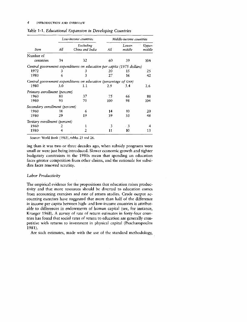
On average, governments in developing countries spend about 3 per-cent of gross national product (GNP) on education, and it has generallybeen their policy to increase this proportion. This can be seen in table1-1, which also shows the rise in enrollment ratios over two decades. Al-though these trends can often be explained by government response torent-seeking pressures for subsidized education, the usual case made forsubsidies is that the social returns to education are greater than the pri-vate returns or that private demand is constrained by imperfections inthe capital market. The issue of subsidies to education is now more press-
3
4 INTRODUCTION AND OVERVIEW
Table 1-1. Educational Expansion in Developing Countries
Low-income countries Middle-income countries
Excluding Lower- Upper-Item All China and India All middle middle
Number ofcountries 34 32 60 39 104
Central government expenditures on education per capita (1975 dollars)1972 3 3 20 15 251980 6 3 27 16 42
Central government expenditures on education (percentage of GNP)
1980 3.0 1.1 2.9 3.4 2.6
Primary enrollment (percent)1960 80 37 75 66 881980 93 70 100 98 104
Secondary enrollment (percent)1960 18 6 14 10 201980 29 19 39 33 48
Tertiary enrollment (percent)1960 2 1 3 3 41980 4 2 11 10 13
Source: World Bank (1983), tables 25 and 26.
ing than it was two or three decades ago, when subsidy programs weresmall or were just being introduced. Slower economic growth and tighterbudgetary constraints in the 1980s mean that spending on educationfaces greater competition from other claims, and the rationale for subsi-dies faces renewed scrutiny.
Labor Productivity
The empirical evidence for the propositions that education raises produc-tivity and that more resources should be diverted to education comesfrom accounting exercises and rate of return studies. Crude output ac-counting exercises have suggested that more than half of the differencein income per capita between high- and low-income countries is attribut-able to differences in endowments of human capital (see, for instance,Krueger 1968). A survey of rate of return estimates in forty-four coun-tries has found that social rates of return to education are generally com-petitive with returns to investment in physical capital (Psacharopoulos1981).
Are such estimates, made with the use of the standard methodology,
The Issues, the East African Natural Experiment, and the Surveys 5
sound guides for the allocation of public resources? An underlying as-sumption of the standard methodology is that differences in wagesamong workers of different educational levels measure the effect onworkers' productivity of human capital acquired in school (the humancapital hypothesis). Thus a large wage premium for better-educatedworkers indicates that the social rate of return to education is high. Butit can also be argued that the premium on education measures the effecton productivity of native ability or motivation-an effect that schoolspick out but do not augment (the screening hypothesis). Still another ex-planation (the credentialist hypothesis) is that the educational structureof wages is institutionally determined and that the better educated earnmore because of their higher credentials. These criticisms imply that, al-though the private return to education may indeed be high, the standardestimates of the social return on investment in education and of the con-tribution of education to growth are biased upward. In subsequent chap-ters we examine these issues with the help of new data and methods.
Income Distribution
Government subsidization of education has also been defended on thegrounds that educational expansion, by making human capital moreabundant, will reduce inequality in the distribution of pay. Perhaps three-quarters of the inequality of income in industrial countries can be ex-plained by the inequality of earnings from employment (Blinder 1974;Phelps Brown 1977). In developing countries the contribution of inequal-ity of pay to total inequality is smaller, but inequality of pay is greaterand its contribution to total inequality is increasing as wage employmentgrows.
Simple two-sector models have been widely used to explain the well-known tendency for the inequality of income first to increase and laterto decrease as economic development takes place (Kuznets 1955; Robin-son 1976). The transfer of workers from a large low-income sector toa small high-income sector is likely to increase inequality, which declinesonly when the proportion of workers in the high-income sector reachesa minimum size. This notion can also be applied to educational groupsin the wage labor market. The expansion of the educated group increasesthe proportion of educated in relation to uneducated workers, and thiscomposition effect is likely to increase inequality at first. But a counter-vailing compression effect tends to reduce inequality. Educational expan-sion has been seen to compress the educational structure of pay in indus-trial countries over the decades (Phelps Brown 1977, pp. 81-89) and hasbeen singled out as an important policy tool for narrowing pay differen-tials (Lydall 1968, pp. 254-66). In many developing countries the supply
6 INTRODUCTION AND OVERVIEW
of educated workers is growing faster in relation to wage employmentopportunities than in the industrial countries. This suggests that the com-pression effect could outweigh the composition effect.
The compression effect relies on the operation of market forces.Whether labor markets in developing countries can adjust the educa-tional structure of pay to large and rapid increases in the supply of edu-cated workers is a matter of concern. In most developing economies thepublic sector accounts for a much larger share of wage employment thanin the industrial market economies; often more than half of all wageearners work for the government and for parastatal bodies. The domi-nance of the public sector, particularly in the market for educated labor,means that it need not act as a price taker. Indeed, public sector wagesare often influenced by bureaucratic or political considerations-the for-mer associated with internal labor markets and the latter with distribu-tional, fiscal, and employment goals. Thus the educational structure ofpay in the public sector may be unresponsive to market forces, and rapideducational expansion, instead of compressing wages, may increase un-employment among the educated. In our discussion of the effects of edu-cational expansion on the inequality of pay, we distinguish compositionand compression effects and the influences exercised by market andnonmarket forces.
Intergenerational Inequality
Education policy is relevant to another dimension of inequality-the dis-tribution of income among families from one generation to the next. Onerationale for subsidizing education is the belief that the ability to payschool fees should not determine the distribution of school places. Be-cause parents who are well educated and have high incomes are betterable to afford school fees or to finance them from savings or by borrow-ing, access to education in an unsubsidized system tends to be biased infavor of their children, and socioeconomic status may be perpetuatedover generations. Many studies have found differences in educational at-tainment according to socioeconomic background; see, for instance,Coleman and others (1966) and OECD (1971) for developed countriesand Behrman and Wolfe (1984a, 1984b) and Birdsall (1985) for less de-veloped countries.
Equality of educational opportunity, which is commonly regarded asthe hallmark of a just society, can be justified on grounds of equity. Itcan also be justified on grounds of efficiency, on the premise that moreable workers can use their schooling more productively. But a combina-tion of subsidies and meritocratic selection criteria may not be enoughto ensure equality of educational opportunity. Higher-quality prepara-tory schooling, better training in the home, or other advantages may en-
The Issues, the East African Natural Experiment, and the Surveys 7
able a disproportionate number of children from families of high socio-economic status to satisfy meritocratic selection criteria. In that case,unequal access to education will persist, and those best able to meet thecosts of their children's schooling will benefit disproportionately from thesubsidies.
Subsidization of education can also promote equality in the distribu-tion of school places by increasing demand and, if the higher demandcan be effectively translated into pressures for greater public provision,generating educational expansion. If most children from high socioeco-nomic backgrounds gain access when the system is small, expansion maydisproportionately increase the access of children from less privilegedbackgrounds. And yet it may do little to increase intergenerational mobil-ity, measured in a relative sense. Children from privileged backgroundscan protect their status by taking their education a stage further. Andamong workers with the same educational attainment, those with supe-rior socioeconomic backgrounds may continue to be more successful inthe labor market as a result of discrimination or of differences in produc-tivity that stem from better schooling or better training in the home. Ourdata permit us to explore the effects of educational expansion on the in-tergenerational dimension of inequality, a topic little studied by econo-mists.
Research Design: The Natural Experiment
In experiments in the natural sciences, particular causal factors are variedin a controlled way while other exogenous factors are held constant, andthe effects are then studied. The best equivalent experiment that can bedone in the social sciences is to seek out and compare situations in whichthe factors under study vary while other conditions remain roughly thesame. Where the causal factor of interest is economywide, as in the caseof the relative abundance of human capital, the situations to be comparedshould represent either different periods or different countries. For in-stance, a comparison might be made within a country before and aftera rapid expansion of education or between two countries with differentrelative stocks of educated labor. In either case the economies to be com-pared should be as similar as possible in all other relevant respects.
A study of this kind constitutes a natural experiment because, in con-trast to controlled experiments in the physical sciences, the situationsbeing observed are the outcomes of interactions among economic agents,including government, and are beyond the researcher's control. It can betermed an experiment, as distinguished from a conventional econometricanalysis, because there are too few observations to permit the isolationof the influence of each variable by statistical means. Economists fre-quently use natural experiments as a method of argument, but usually
8 INTRODUCTION AND OVERVIEW
in an informal way. Among the more systematic cross-country studiesare Chenery and Syrquin (1975) on patterns of development and Little,Scitovsky, and Scott (1970) on industrialization policies. The methodol-ogy, however, is rarely developed with the precision that we have at-tempted in the research described in this book.
Kenya and Tanzania provide a natural experiment in secondary educa-tion. The two countries are similar in size, colonial heritage, resource en-dowment, structure of production and employment, and level of develop-ment, and their urban wage economies do not differ greatly in technicalconditions or in the intensity of physical capital. Both countries achievedindependence in the early 1960s and inherited administratively similarbut undeveloped education systems and negligible stocks of indigenouseducated manpower. Today they differ markedly in one dimension of thesupply of educated manpower: secondary schooling. It is on this differ-ence that our analysis focuses. Dissimilarities in the extent of governmentintervention in the economy, especially in government pay policies, havea bearing on our inquiry, but we were able to standardize for this dif-ference.
In both Kenya and Tanzania primary education comprises seven yearsof schooling (standards 1-7) and lower secondary education four years(forms 1-4). The two years of the much smaller upper secondary system(forms 5-6) are followed by various types of tertiary education. Unlessotherwise indicated, secondary education means lower secondary.
Primary education in both countries is nearly universal, and tertiaryenrollments are less than 1 percent of the relevant age group. But inKenya, which has a slightly smaller population than does Tanzania, thesecondary enrollment ratio was 18 percent in 1980, and in Tanzania itwas 4 percent (World Bank 1983, table 25). Although Kenya's popula-tion was about 15.9 million in mid-1980 and Tanzania's was about 18.7million (World Bank 1982, table 1), students in lower secondary schoolnumbered 410,000 in Kenya but only 67,000 in Tanzania. Kenya'ssecondary enrollment ratio is roughly at the level predicted by a cross-country comparison for countries with its national income per capita,whereas Tanzania's ratio is well below the predicted level.
This difference in secondary enrollments is attributable largely to dif-ferences in public policy regarding secondary education rather than todifferences in private demand. In both countries the government has sat-isfied only a small part of the demand for places at government secondaryschools. Places are accordingly rationed on meritocratic criteria, princi-pally performance in the nationwide primary-leaving examination. Gov-ernment secondary schools are highly subsidized in both countries, andthe rationing is partly a result of budgetary constraints. In addition, bothgovernments paid heed to early manpower planning exercises which sug-gested that the private demand for government school places, inflated as
The Issues, the East African Natural Experiment, and the Surveys 9
it is by the subsidies, is a poor guide to the socially optimal supply ofsecondary completers. East African manpower planners have repeatedlywarned that the consequences of too rapid an expansion of the secondarysystem would be a supply of overqualified workers, unemployment of theeducated, and a waste of scarce resources.
In Kenya, between 1963, the year of independence, and 1980, the yearof our survey, secondary enrollment increased by 17 percent a year, froma mere 30,000 to 410,000. In 1980, 43 percent of enrollment was inmaintained and assisted (that is, government) schools, 20 percent was inassisted harambee (self-help) schools, and 37 percent was in unassistedharambee and private schools. ("Harambee" is Kiswahili for "let's pulltogether.") The proportion of funding from public sources was 53 per-cent in the government schools, 18 percent in the assisted harambeeschools, and 0 in the remainder; the overall weighted share of publicfunding was 25 percent (Wolff 1984, table 6). The government, express-ing concern about both costs and the "school leaver problem," attemptedto restrict the growth of enrollment in government secondary schools,particularly after 1974 (Kenya, Ministry of Economic Planning 1974, pp.404-05). Harambee and private schools responded to the demand forsecondary schooling by Kenyan children who were unable to get intogovernment schools but were able to pay the higher fees, and enrollmentin these schools grew rapidly. Moreover, the burgeoning harambee move-ment had implications for the government sector. In response to politicalpressures, the government took over some harambee schools and partlysubsidized some others.
Between 1963 and 1980 secondary enrollment in Tanzania grew by 8percent a year-from only 17,000 to 67,000 (Cooksey and Ishumi 1986,table 2.4). In 1980, 58 percent of secondary students were in governmentschools. Tanzania had few community schools corresponding to theharambee system in Kenya. Public finance represented 86 percent of thetotal cost of attending government secondary school, and there was nosubsidy in private schools (Wolff 1984, table 6). The share of governmentfinance overall was 50 percent. Enrollment in government schools in-creased by only 20,000 between 1963 and 1980 and stagnated entirelyin the last five years of the period, partly because of budgetary con-straints, which were particularly tight after the decision in 1974 to moverapidly to universal primary education. Of no less importance, however,was the influence of manpower planning. The government accepted theproposition that postprimary education should not be expanded beyondthe "requirements" of the economy as gauged by existing input-outputrelationships. It also constrained the growth of the private secondary sys-tem, first by prohibiting private schools (none existed until 1965) andthen by imposing highly restrictive regulations on their establishment andoperation. The government appeared to be concerned not only about the
10 INTRODUCTION AND OVERVIEW
possibility of wasteful "overproduction" but also about the maintenanceof educational standards and about the distributional implications of asystem that catered to those who could afford to pay for education. De-spite these constraints, the private sector responded to the demands ofthose unable to enter government schools and grew beyond the limits rec-ommended by the manpower planners. In contrast to the situation inKenya, however, the private market for secondary education in Tanzaniaremained in disequilibrium.
Policies on secondary education have thus diverged sharply in the twocountries in regard both to the highly subsidized government schools(Kenya provides 4.6 places for every 1 in Tanzania) and to private schools(Kenya permits 8.3 times as many places). In 1980 Kenya's secondary en-rollment was 6.1 times that of Tanzania. By that year the diverging educa-tion policies had brought about an important difference in the educa-tional composition of the two countries' urban wage labor forces. Thisnatural experiment provided an opportunity for answering some impor-tant questions. By examining the markets for labor and education, wewere able to estimate the effects of the divergence on income and its dis-tribution and to evaluate the relative merits of Kenya's more responsiveand expansionary secondary education policy and Tanzania's more inter-ventionist and restrictive policy.
The Surveys
A single cross-section cannot be used to analyze the effect of a changein factor endowments. To conduct a comparative static analysis, at leasttwo cross-sections are needed. Comparisons over time require observa-tions that are several years apart. This could be achieved through a singlesurvey that generates retrospective data, but such data generally sufferfrom biases in sample selection and from problems of respondent recall.The remaining practical course is to analyze cross-sections from two ormore countries that differ in the factor to be studied.
To exploit the possibilities offered by the natural experiment in Kenyaand Tanzania, we had to generate new data. Those data had to be rigor-ously comparable; any possibility that an observed difference in behaviormight be in part attributable to differences in sample design or in defini-tions of variables could cast doubt on the validity of the comparisons.Although existing sets of microeconomic data could shed some light onthe issues we wished to explore, no two were rigorously comparable, andnone was specifically designed for the purpose. Our surveys containmany measures of respondent characteristics that are not availableelsewhere-at all or in sufficiently disaggregated form-or that are notavailable in the same data set with other variables essential to the analy-
The Issues, the East African Natural Experiment, and the Surveys 11
sis. The following examples illustrate the uses that can be made of ourspecially constructed data sets.
* Our measures of respondents' reasoning ability and cognitive skillprovided the basis for a simple recursive model of educational at-tainment, cognitive skill, and earnings. This model allowed us toevaluate the human capital, screening, and credentialist interpreta-tions of the link between educational attainment and earnings. Italso provided a basis for assessing, by means of output accounting,to what extent the differences in labor productivity between Kenyaand Tanzania can be attributed to differences in their education pol-icy regimes.
* Our skill-based occupational classification of respondents and ourother measures of the characteristics of respondents and their em-ployers enabled us to examine the detailed structure of wages in thepublic and private sectors. Simulations of these structures were thenused to assess how much of the difference between Kenya and Tan-zania in the wage premium to secondary education was attributableto differences in relative demand for secondary completers, howmuch to differences in public sector pay policy, and how much tothe greater supply of secondary completers in Kenya.
* The educational history and family background of each respondentmade possible a comparative cost-benefit analysis of investment inprivate and government secondary schools. This analysis allowedus to assess the consequences for efficiency and equity of govern-ment subsidies to secondary education.
Design
In designing the surveys we decided that the comparison of Kenya andTanzania should focus on the stock of economically active secondarygraduates. Because in both countries this stock is concentrated in theurban wage sector, we chose to conduct establishment surveys of urbanwage employees rather than household surveys. Several related factorsreinforced this decision. Much of the analysis pertains to behavior at theworkplace, and data on such behavior are best collected there; they arelikely to be more accurate than similar data from household surveys be-cause confirmatory information can be (and was) obtained from the em-ployer. Moreover, secondary completers are a much higher proportionof wage employees than of the urban population. The sample for anurban household survey would therefore have to be many times largerthan that for an establishment survey to obtain an equally large sampleof employees with secondary education. For this reason and because of
12 INTRODUCTION AND OVERVIEW
the greater geographic dispersion of respondents and the lack of readilyavailable sampling frames, a household survey would cost much morethan an establishment survey.
The disadvantage of an establishment survey is that it is not compre-hensive. Our sample represented the urban wage labor force and thegreat majority of secondary completers, but it did not include unem-ployed or self-employed secondary completers. It was therefore not possi-ble to analyze the effect of educational expansion on unemployment, onparticipation and earnings in self-employment, and on labor force partici-pation. These issues, although of interest in East Africa, are of relativelylow priority. Other sources indicate that the labor force participationrates of secondary completers are very high in East Africa and that theirunemployment and self-employment rates are very low.
Sample selection bias poses a potential problem for any survey ofurban wage labor. For instance, if the urban wage labor force, and there-fore our sample, is selective of the most accomplished secondary com-pleters, estimates of the effect of secondary schooling on productivitymay be biased upward. But because such a low proportion of pri-mary completers gains access to urban wage employment, selectivityamong primary completers is likely to be greater than among second-ary completers. Since our assessment of productivity benefits stemsfrom a comparison of the relative performance of these groups, any netbias is likely to be downward. The effect of such bias is to strengthenour conclusions.
The positive link between family background and educational attain-ment is at the core of our analysis of the effects of educational expansionon educational access and intergenerational mobility. Such a relationshipcould be biased upward because the mean level of educational attainmentin our sample of urban wage employees is higher than the educationalattainment of the labor force as a whole. But because the uneducatedchildren of the uneducated are underrepresented in our sample, the esti-mate of that relationship is likely to be biased downward, strengtheningour argument. More generally, it turns out that the sample selection biasinherent in our surveys does not pose serious problems of interpretation.
In sum, if a household survey were to be comprehensive, it would haveto be representative of the entire population of the country, both urbanand rural. Such a survey would be prone to greater errors in the measure-ment of key variables and would cost much more than an urban estab-lishment survey. Given the aims of our analysis and the conditions in EastAfrica, the incremental benefits of the larger undertaking would havebeen small. The expected net returns to an urban establishment sur-vey therefore far exceeded those to an urban or national householdsurvey.
The Issues, the East African Natural Experiment, and the Surveys 13
Administration
The respondents in the surveys of wage employment and education inKenya and Tanzania were randomly selected from the wage labor forcesin Nairobi and Dar es Salaam. Previous labor market survey work hadsuggested that capital cities were not unrepresentative of urban areas inrespect to relevant wage-employment characteristics. (See Sabot 1979,which compared Dar es Salaam with other towns in Tanzania.)
A sample of establishments stratified by size and sector was randomlydrawn from a frame provided by the central statistical bureau in eachcountry. In each establishment a random sample of employees was drawnfrom a complete list of employees provided by the employer. The resultwas a representative sample of urban wage employees containing nearly2,000 respondents in each country.
Teams of university students, trained and supervised by the authorsand other researchers, administered the questionnaires and tests to therespondents in 1980. The questionnaires covered respondents' demo-graphic characteristics and family background, education and traininghistories, current and previous earnings, experience in current and previ-ous jobs, links with rural areas, and own children's education. Reasoningability was assessed with Raven's Coloured Progressive Matrices. Thistest, which is widely used in developing countries, asks the respondentto match pictorial patterns, a task in which literacy and numeracy conferno advantage. The tests of literacy and numeracy were designed for thesurveys by the Educational Testing Service, Princeton, N.J., on the basisof the national school-leaving examinations, both primary and second-ary, and other guides to the content of the academic curriculum. The cur-riculum is much the same in Kenya and Tanzania, except that Kiswahiliis stressed more in Tanzania. Questions were given in both English andKiswahili so that respondents could choose the language they preferred.The sum of the scores on the literacy and numeracy tests was used asthe measure of cognitive skill.
Two other features of the sample should be noted. First, in both coun-tries respondents were from all sectors of the urban wage economy-manufacturing, services, and commerce-but a disproportionate numberwas employed in manufacturing. This oversampling, which in the aggre-gate analysis was adjusted with appropriate weights, permitted detailedcomparisons of the manufacturing sector subsamples of the 1980 surveyswith a similar survey of wage employees in manufacturing that Sabot hadconducted in Dar es Salaam in 1971 (Sabot 1979, p. 251). These compar-isons add an intertemporal dimension to the cross-country analysis of ed-ucational expansion. Second, the questionnaires were administered to allrespondents, but only a stratified subsample of respondents was given the
14 INTRODUCTION AND OVERVIEW
tests of reasoning ability and cognitive skill. The subsamples for eachcountry consisted of about 200 respondents who had left formal educa-tion after exactly completing primary school (standard 7 or 8) or second-ary school (form 4).1 The cost of administering the test was high, as wasthe risk that the expected benefits from this feature of the surveys wouldnot justify the cost. Hindsight shows that the added benefit of increasingthe size of the subsamples would have outweighed the cost.
Note
1. Standard 7 is now the final year of primary school; before 1966 it was stan-dard 8.
CHAPTER 2
Overview: Findingsand Implications for Policy
THIS CHAPTER OFFERS an overview that provides the reader with acoherent perspective on the study as a whole. Succeeding chapters makefrequent use of the same data sets to consider specific questions, each ofwhich requires a separate technical analysis. But the whole is bigger thanthe sum of the interrelated parts, and it would be difficult for readersto see the wood if they were taken immediately to inspect each tree inturn. This chapter therefore summarizes arguments and findings withoutmuch reference to sources, methods, and data, which are fully providedin the detailed analyses. Part I can stand by itself and may suffice forreaders who are not interested in the analysis and methodology. Wehope, however, that most readers are unwilling to take our interpreta-tions and conclusions on trust and are curious to know how we reachedthem. For these readers the overview is intended to whet the appetite forthe main course to come.
Parts II, III, and IV of the book examine, in order, the three issues intro-duced in chapter 1-the relationships between the expansion of second-ary education, on the one hand, and labor productivity, income distri-bution, and intergenerational mobility, on the other. Part V examinesmethodological and policy issues in the cost-benefit analysis and in thefinancing of secondary education. Part VI considers the implications ofthe findings for future research and the extent to which our East Africanresults can be generalized to other countries and situations. The appen-dixes provide details concerning the research instruments and methods.
Educational Expansion and Labor Productivity
Does educational expansion yield social benefits in the form of increasedproduction, or are the benefits only private and redistributive? We exam-ine this question by considering first the similarities between the twocountries and then the differences that arise from the natural experi-ment.
15
16 INTRODUCTION AND OVERVIEW
The Alternative Hypotheses
In cost-benefit analyses of education, the relationship between wagesand years of education is used to measure the social benefit of education.The assumption is that the education-wage relationship measures the ef-fect on labor productivity of human capital acquired in school (thehuman capital hypothesis). For this to be true, however, neither abilitynor years of schooling should have an independent influence on wages.These factors must influence earnings only indirectly, by raising the levelof skills acquired in school: they must work through the educational at-tainment function and the educational production function, which sum-marize in general terms the relationships between the inputs and outputsof the education system.
The screening hypothesis predicts that the influence of ability on pro-ductivity will be large in relation to the influence of skills acquired inschool. Taken to its extreme, the hypothesis posits that schools simplyidentify the potentially more productive and do not increase the produc-tive capacity of students. Educational attainment-as measured by yearsof schooling-"signals" workers with more ability and, because abilityraises productivity, is rewarded with higher earnings.
The loose amalgam of hypotheses generally known as credentialism isa more radical rejection of the human capital interpretation of theeducation-wage link. According to this view schools provide studentswith a credential that is personally valuable but not productive. Edu-cational qualifications are rewarded irrespective of their economicvalue. For instance, a government may determine wages and establisheducation-based hiring and payment criteria, or private employers maydiscriminate in favor of the educated because they share similar socioeco-nomic backgrounds. The implication is that the education-wage link isnot a proxy for the effects on labor productivity of skills acquired inschool or of ability but is a measure of the independent effect of yearsof schooling on earnings.
Conventional measures of the social benefit of education and the con-tribution of education to economic growth may be biased upward if thescreening or credentialist interpretations contain some truth. Our meansof adjudicating among the hypotheses is to measure all the relevant rela-tionships, not just the education-wage relationship, and our data setswere designed to make this possible. The econometric analysis reportedin chapter 3 involves the estimation of educational attainment functions(which measure the effect of ability on educational attainment), educa-tional production functions (which measure the effects of ability andyears of education on human capital acquired in school), and expandedhuman-capital wage functions (which measure the effects of ability,human capital, and years of education on earnings).
Overview: Findings and Implications for Policy 1 7
Cognitive Skill and the Educational Structure of Wages
Our measure of human capital acquired in school is the cognitive skillscore. The wage functions allowed us to weigh the relative direct influ-ences of reasoning ability, years of schooling, and cognitive skill (ourmeasure of human capital acquired in school-also termed achievement)on the structure and variance of earnings. The results show that whereasthe direct returns to reasoning ability in the labor market are small andthe returns to years of schooling are moderate, the returns to cognitiveachievement are large. They are not significantly lower among manualthan among nonmanual workers or among primary than among second-ary completers. Presumably this is so because literacy and numeracyincrease the productivity of all types of workers, manual as well asnonmanual.
To illustrate these results, simulations were conducted with the esti-mated wage functions. One such simulation shows that differences in rea-soning ability account for little of the large gap in mean wages betweenprimary and secondary completers. The direct returns to ability in thelabor market are so low that giving primary completers the ability levelsof secondary completers while keeping their cognitive skill levels constantwould increase their earnings by less than 7 percent in Kenya and by lessthan 4 percent in Tanzania. Giving primary completers four more yearsof schooling (without altering their ability or achievement) would in-crease their earnings by 19 percent in Kenya and by 13 percent in Tanza-nia. Differences in cognitive achievement between primary and secondarycompleters account for the largest proportion of the wage gap. Givingprimary completers the cognitive skill of secondary completers (withoutaltering their other characteristics) would increase their earnings by 25percent in Kenya and by 15 percent in Tanzania.
There is much variation in cognitive skill and in reasoning abilitywithin the two educational groups. Among Kenyan primary completersthe score of the bottom 10 percent on our test of reasoning ability is 11out of a possible 36, while that of the top 10 percent is 34. The rangeof cognitive skill is from 13 out of a possible 63 for the bottom 10 percentto 52 for the top 10 percent. Among Kenyan secondary completers thecorresponding ranges are 17 to 35 on the ability test and 28 to 56 onthe cognitive skill tests. In Tanzania the ranges are similarly broad. More-over, in both countries the reasoning ability and cognitive skill distribu-tions of primary and secondary completers overlap considerably.
A second set of simulations indicates that the predicted earnings of pri-mary completers of high ability are less than the predicted earnings ofless able secondary completers. In neither country is being among thebrightest of one's peers a sufficient condition for successful performancein the labor market. The results of a similar simulation with cognitive

18 INTRODUCTION AND OVERVIEW
skill are quite different; in each educational group high achievers earnmuch more than low achievers, and the predicted wage of primarycompleters who scored in the top third is nearly as high as that of second-ary completers who scored in the bottom third. In both countries, itwould seem, how much one learns in primary or secondary school hasa substantial influence on performance at work.
Cognitive Skill and the Returns to Employment Experience
A strong relationship between earnings and employment experience is al-most universal and is normally explained as the result of on-the-job ac-quisition of skills. Kenya and Tanzania follow this rule: in both countriesearnings rise steeply with employment experience. When other character-istics are standardized, a worker with ten years of experience is foundto earn a premium in relation to a labor market entrant of 57 percentin Kenya and 56 percent in Tanzania.
Our interest is in the relationship between educational attainment(years of education) and the returns to employment experience. In poorand rich countries alike, it is generally found that the higher is the levelof education, the more rapidly do earnings rise with experience. This pat-tern holds in Kenya and Tanzania. The growth rate of earnings per yearof employment experience is roughly 2 percent greater among secondarythan among primary completers in Kenya and 1.5 percent greater in Tan-zania. This is relevant to education policy because the difference in thepresent value of the lifetime earnings streams of primary and secondarycompleters is conventionally taken as a measure of the gross social bene-fits from investment in secondary schooling. The higher returns to experi-ence of secondary completers account for roughly 90 percent of this dif-ference in Kenya and for more than 100 percent in Tanzania.
The explanation offered by human capital theory for this positive in-teraction is that investments in schooling and in postschool training arecomplementary. The more education workers have received, the greateris their cognitive skill. The more cognitive skill they have acquired, themore vocational skills they will acquire over their working lives, both be-cause they are likely to devote more time to training and because theirhigher level of cognitive skill permits them to derive more from training.The greater the accumulation of vocational skills, the steeper is theearnings-experience profile.
According to proponents of screening theory, the link between invest-ments in schooling and in vocational training is simply that both are re-lated to ability. The credentialist explanation would be that the educatedhave higher returns to experience because they are more likely to have
Overview: Findings and Implications for Policy 19
white-collar jobs in which earnings rise with tenure irrespective of anyincreases in skills and productivity. Thus, how much of the private bene-fits of investment in secondary schooling should be included among thesocial benefits will depend on the choice of interpretation.
Our expanded human capital earnings functions permit a simple testof these competing explanations, as discussed in detail in chapter 4. Thehuman capital explanation predicts that the returns to experience willbe higher for workers with higher cognitive skill, even among those withthe same education. Furthermore, it implies that the higher returns to ex-perience of secondary completers are attributable to their higher cogni-tive achievement. The predictions yielded by the credentialist explanationare different. Because the returns to experience are tied to educationalcredentials by institutionally determined wage structures, secondarycompleters have the same returns to experience irrespective of their levelof cognitive skill. Since the same is held to be true of primary completers,the difference in cognitive skill between the two educational groups can-not be responsible for their difference in returns to experience. We there-fore test the hypotheses by asking two questions. First, is there a positiverelationship between cognitive skill and the returns to experience forworkers with the same education? Second, is the difference in cognitiveskill between primary and secondary completers sufficient to explain thedifference in their returns to experience?
The results of our analysis indicate, for both primary and secondarycompleters, that the returns to experience vary positively with cognitiveskill. For example, among Kenyan secondary completers with ten yearsof experience, the return to experience is 4.7 percent per year for thosewhose score on our tests of cognitive skill is at the mean of the bottomthird and 9.9 percent per year for those whose score is at the mean ofthe top third. These results also suggest that the difference between pri-mary and secondary completers in cognitive skill is responsible for theirdifferent returns to experience. We conducted simulations in which themean cognitive skill of secondary completers was reduced to that of pri-mary completers and traced the effect on their returns to experience andconsequently on the present value of earnings. As predicted by humancapital theory, a big part of the difference in the present value of earningsbetween the two educational groups in Kenya and Tanzania is attributa-ble to the influence that the higher cognitive skill of secondary completershas on the returns to experience.
We conclude that more skills of one type beget more skills of another.This supports the conventional practice of including among the social re-turns to schooling that part of the return that arises from the interactionbetween education and the returns to experience.
20 INTRODUCTION AND OVERVIEW
Cognitive Skill and the Variance in Earnings
The relative importance of the effects that reasoning ability, cognitiveskill, and years of schooling have on the dispersion of earnings can differfrom the relative importance of their effects on the wage structure. Forexample, although high levels of cognitive skill have a large positive im-pact on the earnings of the individual worker, variance in cognitive skillmay contribute little to the inequality of pay if the group of highly skilledworkers is small or if its members are evenly scattered over the earn-ings distribution. What, then, would be the effects on the inequalityof pay if, while mean earnings were held constant, the dispersionattributable to a particular characteristic such as cognitive skill wereeliminated?
Again, simulations with our estimated wage functions allow us to an-swer this question. In both countries variance in the level of reasoningability has only a small effect on variance in earnings. This is partly be-cause reasoning ability has only a small effect on a worker's pay. More-over, in neither country are the more able workers highly concentratedin the highest quintiles of the distribution; the average ability of the low-est income quintile is not much less than that of the highest quintile. Thisoccurs because a substantial proportion of primary completers of highability did not gain access to secondary school, perhaps because of therelatively poor quality of their primary schooling or home training or be-cause of the limited number of secondary places in the past.
Differences in years of schooling contribute rather more to the disper-sion of wages because of their relatively large effect on individual earn-ings and because the proportion of secondary completers in each earningsquintile rises with earnings. The contribution of years of schooling isgreater in Tanzania than in Kenya despite the higher wage premium onsecondary education in Kenya. In Tanzania the proportion of secondarycompleters rises more steeply from low-earnings to high-earnings quin-tiles. This reflects the greater scarcity of Tanzanian secondary completers;the proportion of secondary completers in relatively low-paying manu-facturing occupations is far higher in Kenya.
In Kenya cognitive skill accounts for three times more variance in earn-ings than do ability and years of schooling combined; in Tanzania theratio is two to one. Not only is cognitive skill highly rewarded, but alsothere are few highly literate and numerate workers, be they primary orsecondary completers, in the low-earnings quintiles. The predominantcontribution made by cognitive skill suggests that inequality of pay arisesprimarily from inequality of individual productivity. Thus the efficiencycost of reducing inequality may be high.
Overview: Findings and Implications for Policy 21
The Indirect Effects of Ability and Schooling on Earnings
Between two groups of employees of different reasoning ability, the moreable group has higher earnings. In Kenya and Tanzania reasoning abilityhas only a small direct influence on earnings: at any given level of school-ing or cognitive skill, the naturally more able are not much more compe-tent on the job. But ability also operates indirectly, in two ways. First,other things being equal, the more able acquire more schooling and thehigher earnings that go with it. Second, for any length of schooling, themore able are better at acquiring cognitive skill. Our estimates of educa-tional attainment functions and educational production functions mea-sure these respective mechanisms.
An analysis of the relationship between ability and earnings for differ-ent ability groups shows that the largest single reason for the higher meanwage of the more able group was that they acquired more cognitive skillin secondary school. This factor accounted for 44 percent of the differ-ence in Kenya and for 48 percent in Tanzania. Greater access to second-ary school by the more able was an important cause of their higher earn-ings; it accounted for 32 percent of the higher wage in Kenya and for45 percent in Tanzania. Most of this effect worked through human capi-tal acquisition rather than through credentialism. Reasoning ability thushas an important but indirect influence on earnings.
It was also possible to distinguish the different effects of secondaryschool attendance on earnings. The direct effect of secondary schoolingby itself-the credentialist effect-was to raise wages by 21 percent inKenya and by 12 percent in Tanzania. The indirect mechanism combinesthe isolated effect that secondary school attendance has on the level ofcognitive skill with the isolated effect of higher cognitive skill on earn-ings. Their combination implies that human capital acquisition in second-ary school raised earnings by 25 percent in Kenya and by 15 percentin Tanzania; both figures are larger than the corresponding credentialisteffect. Thus the main effect of secondary school attendance on earningsis indirect, through the development of cognitive skill.
In sum, the returns to cognitive skill are a payment for human capi-tal. Literate and numerate workers are more productive, and educationand reasoning ability are valuable to workers mainly because they allowthem to acquire skills that increase their productivity. Our analysisstrongly supports the human capital interpretation of the education-wage relationship, although not to the complete exclusion of otherinfluences. These conclusions have generally satisfied the usual statis-tical tests. That they apply to both Kenya and Tanzania increases theirrobustness.
22 INTRODUCTION AND OVERVIEW
Differences Arising from the Natural Experiment
We have argued that the economic benefits of investment in secondaryeducation are not just private; by increasing labor productivity secondaryeducation also yields social benefits. The similarity between Kenya andTanzania in the relationship between education and labor productivityposes another question: what are the consequences for labor productivityof the difference in education policy in the two countries? Or-to putthe question in a form familiar to those who have studied economists'attempts to account quantitatively for differences between countries inoutput per capita or in rates of economic growth-to what extent doesthe difference between Kenya and Tanzania in human capital endow-ments, as a result of differences in education policy, account for the ob-served gap between the two countries in the productivity of wage labor?Judging by average wages, the difference between Kenya and Tanzaniain productivity in the late 1960s was small-about 10 percent. By 1980this difference had grown to roughly 50 percent, and use of an appro-priate shadow price of foreign exchange would only increase this esti-mate.
In the late 1960s-after the Arusha Declaration of 1967 and the appli-cation of its principles to education, as enunciated in Education for Self-Reliance (Nyerere 1967a)-significant differences in education policyemerged between the two countries. In Tanzania the priority accordedto the development of postprimary education gave way to the new prior-ity of universal primary education. The difference between Kenya andTanzania in secondary enrollment rates and in the stock of secondaryschool graduates in 1980 can be traced to these changes in education pol-icies in Tanzania in the late 1960s.
DIFFERENCES IN THE QUALITY OF EDUCATION. Education for Self-Reliance involved a qualitative as well as a quantitative change in direc-tion. The curriculum was modified in Tanzania so as to change valuesand to teach vocational skills, and the outcome was that less time wasgiven to general academic skills. The two countries have differed in an-other respect: in Tanzania greater stress has been placed on the use ofKiswahili in primary school, perhaps at the cost of achievement in second-ary school, where English is the language of instruction.
Our estimated production functions indicate that secondary school at-tendance contributes substantially to cognitive skill in both Kenya andTanzania. They also allow us to compare the quality of education in thetwo countries, as measured by cognitive "output" per unit of schooling"input" (see chapter 5). The educational production functions show thatwhen inputs are standardized, cognitive skill is higher in Kenya thanin Tanzania and that it is more responsive to secondary schooling and
Overview: Findings and Implications for Policy 23
to reasoning ability. Consider, for example, someone whose reasoningability is at the mean level of the combined sample. If he attended se-condary school in Tanzania, his predicted level of cognitive achievementas measured by our tests would be 36, whereas if he attended second-ary school in Kenya, his predicted level would be 42, or 17 percenthigher.
These results suggest that Kenyan secondary schools are indeed ofhigher average quality than their Tanzanian counterparts, but they do notallow us to determine how much of this difference in quality is attributa-ble to differences in curriculum, to greater managerial efficiency inKenya, or to higher levels of such unmeasured inputs as the educationalattainment of teachers, the availability of textbooks, or the provision ofteaching facilities. Although educational spending per secondary studentis higher in Tanzania than in Kenya, a higher percentage of that spendinggoes for board and lodging. A markedly higher proportion of second-ary students in Tanzania is enrolled in boarding school because of thesmaller size of the secondary system. As the secondary system expands,economies of scale may make it possible to contain costs while raisingquality.
We have seen that the quantity and quality of secondary education aresubstantially greater in Kenya than in Tanzania. We therefore expect thecognitive skill level of the average employee to be higher in Kenya.Whereas the average scores of Kenyans and Tanzanians on the reasoningtest are essentially the same, we find that Kenyan employees are indeedmore numerate and more literate than their Tanzanian counterparts. Thecombined achievement score for Tanzania, appropriately weighted ac-cording to the proportions of primary and secondary completers in theTanzanian urban labor market, is 30, whereas for Kenyans the corre-sponding score is 42, or 40 percent higher.
EDUCATION POLICY AND LABOR PRODUCTIVITY. The results of theanalysis with the expanded human capital wage functions show thatworkers who are more literate and numerate are more productive. Tanza-nia may thus have paid a price in output forgone by restraining thegrowth of secondary education and reducing the quality of education forthe sake of other goals. We used our estimated educational productionfunctions to assess how much greater the cognitive skill of the Tanzanianlabor force would be if the quantity and quality of secondary educationwere increased to the Kenyan level, separately and in combination. Thenwe used our wage functions to assess the effect of these increases in cogni-tive skill on average wages (see chapter 5).
We found that a simultaneous increase in quantity and quality wouldincrease the cognitive skill of Tanzanians by 31 percent and their earningsby 13 percent. The increased quality of education accounted for more
24 INTRODUCTION AND OVERVIEW
than half the increases in the cognitive skill level and in earnings of thelabor force. It seems that the opportunity cost to Tanzania of constrain-ing the quantity and quality of education has been substantial. Roughly40 percent of the current difference in mean wages between the Kenyanand Tanzanian workers in our tested subsamples can be accounted forby the lower cognitive skill of the Tanzanian labor force. The divergencebetween Kenya and Tanzania in education policies appears to have beenan important factor in the divergence of mean earnings and productivityof labor in the two countries in recent years.
Educational Expansion, Government Policy, and theStructure and Dispersion of Pay
At the time of political independence in Kenya and Tanzania economi-cally active citizens with postprimary education were in extremely shortsupply. For instance, in 1962 there were only 4,700 candidates for thenational form 4 examination in Kenya and 1,900 in Tanzania. The wagepremiums that these people commanded in the labor market were sub-stantial. Wage differences associated with education were large by inter-national standards.
In the subsequent two decades the annual flow of secondary graduatesinto the labor market grew rapidly, even in Tanzania. The annual growthof nonagricultural wage employment over those decades averaged 26,000in Kenya and 7,000 in Tanzania, whereas in 1980 there were 92,000 can-didates for the form 4 examination in Kenya and 18,000 in Tanzania.As the process of ousting all but the most highly qualified expatriatescame rapidly to an end, the initially very tight labor market for secondarygraduates was progressively loosened.
Labor Markets in Kenya and Tanzania
In the theory of competitive markets, a reduction in the relative scarcityof a factor of production lowers its relative price. Whether expansion ofthe secondary system will depress the premium on secondary educationdepends on the nature of the labor market. Are there institutional factorsat work that might prevent or retard the operation of market forces? Ourultimate concern in this section is with the effect of secondary expansionin Kenya and Tanzania on the structure and dispersion of pay. Our firsttask is to explain how the labor market works in these countries. Wefocus on the roles of occupation and of public sector pay policy in thedetermination of wages.
Overview: Findings and Implications for Policy 25
OCCUPATION. The occupation of a worker is an intermediary betweenhis education and his earnings. Education, which primarily confers cogni-tive skill, is often the main determinant of occupation. Because elementsof human capital are occupation-specific, a worker's occupation has animportant influence on the vocational skills that he acquires and thereforeon his earnings. These ideas are applied to the Kenyan and Tanzaniansamples in chapter 6.
The wage in one occupation may exceed that in another because thefirst occupation inherently requires superior personal characteristics-some natural, such as ability, and some acquired, such as education andvocational skills. In exploring this idea we use the occupational produc-tion function, which, for each occupation, relates individual inputs, suchas ability, education, and employment experience, to productivity. Work-ers were divided into six broad skill-based occupational groups amongwhich the hierarchy of mean wages corresponded to our judgment aboutthe hierarchy of skill. Since there was little mobility among these groupsin the sample, assignment to a particular occupational group was likelyto be an important determinant of lifetime earnings. Estimates of occupa-tion-specific wage functions show significant differences among occu-pations with regard to education and to employment experience; thereturns to these human capital variables generally increase with thehypothesized occupational skill level.
Inasmuch as mean wages and the functional relationship between in-puts and productivity vary among occupations, workers in different oc-cupations are likely to have different mean characteristics. We thereforeestimated occupational attainment functions, in which workers' occupa-tions are explained in terms of their personal characteristics. In bothcountries the skill level of the most probable occupation rises with levelof education: a worker's educational level is a powerful determinant ofhis occupation.
We also examined the process of filtering down-the movement intolesser jobs of educated workers or of educated entrants to the labor mar-ket as a result of an increased supply of educated labor. The probabilitiesof occupational attainment were found to differ from one entry cohortto another, which suggests that the burden of filtering down falls on en-trants to the labor market rather than on incumbents. The year a workerentered wage employment is an important determinant of his occupa-tion.
Consider the most recent cohort, which entered wage employment atthe time of the surveys. The probability that a new secondary leaver willenter a semiskilled or unskilled manual job is more than two-fifths inKenya. In Tanzania the probability is less than one-fifth, and the prob-ability that such a person will enter a nonmanual job is more than
26 INTRODUCTION AND OVERVIEW
three-fifths. The probabilities of occupational attainment of new pri-mary leavers are similar in the two countries, which reflects the similar-ity of government policies for primary education. The contrast arisesfor entrants with secondary education; there is more filtering down inKenya, where secondary education expanded far more rapidly than inTanzania.
Our substantive conclusion is that skill-based occupation plays an im-portant role in the labor market in Kenya and Tanzania. In the better-paying occupations the relationship between output and inputs (labor,cognitive skill, vocational skills, and natural ability) is such that these in-puts are found in combination and yield high returns. Natural ability andaccess to education are important to occupational attainment and thusto the acquisition of vocational skills: "unto him that hath shall begiven." In a meritocratic educational and social system that providesequality of opportunity, positive interaction among the determinants ofearnings contributes to economic efficiency. Even in a meritocratic sys-tem, however, the interaction accentuates income inequality amongworkers.
Our methodological conclusion is that the role of occupation oughtexplicitly to be taken into account in analyzing the effects of educationalexpansion on the labor market. The premium on education may well bereduced primarily through the filtering down of the educated into lower-paying jobs in which their education is less productive.
GOVERNMENT PAY POLICY. Immediately after independence averagewages were substantially higher in the public than in the private sectorin Tanzania. This was partly because of the relative skill intensity of pub-lic services, but analysis of a 1971 household survey (Lindauer and Sabot1983) showed that when personal characteristics were standardized,there was a 13 percent wage premium in the public sector. This wasin accord with the government's early policy of exercising wage leader-ship and setting a good example as an employer. At independence mostmiddle- and senior-level civil service posts were held by expatriate Euro-peans whose pay was determined by labor market conditions in Europe.Localization took place rapidly over the next decade, but public sectorwages did not fully adjust to reflect the consequent decline in employeesupply price. To do away with one of the fruits of independence and tointroduce a large wage disparity between Tanzanians and their expatri-ate counterparts would have been politically untenable. Private sectorwages were more responsive to the change in labor market conditions.
The policy of equalizing pay dates from the Arusha Declaration of1967, which set Tanzania on a more egalitarian and socialist path. Thegovernment attempted to resolve, through its pay policy, the conflict be-tween the claims of equity and the reward that education could command
Overview: Findings and Implications for Policy 27
in the market. The policy of wage compression extended beyond govern-ment employment to other parts of the public sector, including the bur-geoning parastatal organizations. In principle, the egalitarian pay policyalso applied to the private sector, but it could not be enforced in practice.The effects of the public sector pay policy should be observable in the1980 survey, in which the public sector accounted for more than 60 per-cent of our sample. We refer to the public sector as the nonmarket sectorand to the private sector as the market sector because the latter is likelyto diverge less from free market conditions. We hypothesize that in 1980pay in Tanzania's nonmarket sector was less dispersed, and was lowerfor better-paid workers, than in the market sector.
The economic and political factors that led the Tanzanian governmentto exercise wage leadership also operated in Kenya in the immediatepostindependence period, and government pay policies in the two coun-tries were much the same. Since the mid-1960s the Kenyan governmenthas progressively drawn back from being a wage leader and has ex-pressed itself in favor of equalizing wages.
There is reason to question whether the government policy in factbrought about any significant departure from a market outcome for wagestructure in either the public or the private sector. There was no effectivecontrol over the private sector and public corporations, and central gov-ernment employment accounted for only a fifth of our sample. In prac-tice, the government appeared to adopt the prevailing wage rate to de-termine its wages, possibly because market forces were achieving itsdistributional goal. Our hypothesis for 1980, therefore, is that govern-ment pay policy had less influence in Kenya than in Tanzania and thatin Kenya pay in the public service and in public corporations differed lit-tle from pay in the private sector.
Educational Expansion and Wage Compression
The relationship between educational expansion and wage structure isexamined with the use of the 1980 samples and manufacturing sub-samples in both countries and a comparable 1971 survey of manufac-turing in Tanzania (see chapter 8). The manufacturing comparisons areuseful because they contain a time-series element and because the manu-facturing sector is relatively free of the effects of government pay policy,which permits analysis of the relatively unimpeded operation of marketforces.
THE MANUFACTURING SECTOR. The three manufacturing samples canbe thought of as representing three points in a time series: Tanzania 1971,Tanzania 1980, and Kenya 1980. The ratio of secondary to primaryleavers rises sharply across the three samples. By contrast, the occupa-
28 INTRODUCTION AND OVERVIEW
tional structure of the labor force is similar in all three. Given our skill-based occupational classification, this suggests that the composition ofthe demand for skills has remained much the same. Thus the relative sup-ply of secondary leavers has increased against a background of unchang-ing relative demand.
Educational expansion can compress the wage premium on educationin two ways. First, wages in the occupations that employ secondaryleavers may be reduced by competitive market forces. Second, the filter-ing down of secondary leavers into lesser jobs may reduce their averagewage in relation to that of primary leavers. The education-occupationmatrix is indeed different in the three manufacturing samples. The pro-portion of secondary leavers in nonmanual occupations was 76 percentin Tanzania 1971, 68 percent in Tanzania 1980, and a striking 26 percentin Kenya 1980. Most of the filtering down between 1971 and 1980 inTanzania was from more senior white-collar jobs into junior clerical jobs.The corresponding proportions in unskilled and semiskilled manual oc-cupations were 6 percent, 11 percent, and 52 percent. Primary leaverswere also filtering down, but at a much slower pace. The effect of theincrease in the relative supply of secondary leavers is as expected. Thestandardized wage premium earned by secondary over primary leaversfell from 80 percent in Tanzania 1971 to 52 percent in Tanzania 1980and to 26 percent in Kenya 1980.
The elasticity in the response of relative wages to relative supplies ofeducated labor implicit in the comparison between Tanzania 1971 and1980 is -1.48. It is -0.31 for Tanzania 1980 compared with Kenya1980 and -0.51 for Tanzania 1971 compared with Kenya 1980. Sincethe wage premium in Tanzania 1980 would not have entirely escaped thedepressing effect of pay policy, the first elasticity is biased upward andthe second downward. Thus the third elasticity (-0.51) is our best esti-mate. A doubling in the ratio of secondary to primary leavers employedin manufacturing would be sufficient to halve the ratio of their pay.
THE URBAN WAGE SECTOR. Considering the urban wage labor force asa whole, we find that the ratio of secondary to primary leavers in Kenya(1.17) is two-thirds higher than in Tanzania (0.69). Since the occupa-tional composition of urban wage employment is similar in the two econ-omies, these ratios imply that filtering down has proceeded further inKenya. Whereas 21 percent of secondary leavers were employed in un-skilled or semiskilled occupations in Kenya, only 5 percent were so em-ployed in Tanzania. The difference in the occupational distribution of pri-mary leavers is much less marked: the corresponding figures for primaryleavers were 41 percent in Kenya and 38 percent in Tanzania. Again wepredict a smaller wage premium for secondary leavers in Kenya. We find,however, that the standardized relative wage is higher in Kenya. The elas-

Overview: Findings and Implications for Policy 29
ticity in the response of relative wages to relative supplies implicit in thecomparison is actually positive.
The explanation for this anomaly is found in the difference in govern-ment pay policy in the two countries, the effect of which is examinedin chapter 7. Whereas in Kenya the government has not significantly al-tered the market outcome, the Tanzanian government has intervened tocompress the wage structure in the dominant public sector. In our wagefunction analysis we isolated the effect of pay policy on the educationalstructure of wages by using dummy variables for sector of ownership andallowing these variables to interact with educational attainment. It wasthen possible to simulate the premium on secondary education in themarket sector. Eliminating the pay policy increased the premium by amere 6 percent in Kenya but by 63 percent in Tanzania. This resolvedthe anomaly. The premium in Tanzania (0.64) now exceeded that inKenya (0.51), and the elasticity of relative wages with respect to relativesupplies of educated labor was negative (-0.25).
This estimate of the elasticity would be accurate only if the relative de-mand for secondary leavers were the same in both countries. For in-stance, differences in sectoral composition or technology could causeproduction in Kenya to be more skill-intensive and so raise the premiumthere. It was possible to simulate what the premium on secondary educa-tion would be in Tanzania if Tanzania had Kenya's greater relative supplyof secondary leavers or in Kenya if Kenya had Tanzania's lesser relativesupply. When we standardize both for pay policy and for relative supply,the premiums on secondary education in Kenya and Tanzania are re-markably similar; that is, the relative demand for secondary leavers ismuch the same in the two countries.
The somewhat higher elasticity estimated for the manufacturing sectorthan for the wage sector as a whole probably reflects the lower occupa-tional skill intensity of manufacturing production and the tendency ofsecondary leavers who enter manual jobs to prefer manufacturing; filter-ing down has proceeded further in manufacturing than in the wage sectoras a whole.
In sum, educational expansion can be an important means of com-pressing the wage structure in developing countries. In both Kenya andTanzania the wage structure by education was remarkably wide at thetime of independence. The structure has since been narrowed in bothcountries. Kenya achieved this outcome through its expansionary policiestoward postprimary education. The mechanism was one of filteringdown into less skilled occupations rather than of wage flexibility withinoccupations: the standardized occupational wage structure is similar inthe two countries. Tanzania restricted educational expansion and usedan egalitarian public sector pay policy to prevent scarcity rents from ac-cruing to the educated. Such segmentation of the labor market has its
30 INTRODUCTION AND OVERVIEW
drawbacks, however; it may well produce new inequities and mis-allocation of labor.
Educational Expansion and the Kuznets Effect
In making normative judgments economists are usually concerned withthe inequality of wages received by individuals rather than with the struc-ture of wages. The inequality of wages is a function not only of the wagestructure but also of the distribution of employees within that structure.Educational expansion can therefore have two effects on the inequalityof pay. The compression effect-the narrowing of the wage structure-was analyzed above. The composition effect-the changes in inequalitybrought about when educational expansion changes the educationalcomposition of the labor force-is discussed briefly here and more fullyin chapter 9.
It is widely accepted that in the process of economic development in-equality of income first increases and later decreases. The composition ef-fect has been cited to explain this phenomenon. Kuznets (1955) has ar-gued that the transfer of workers from a large traditional sector in whichmean income is low to a small modern sector in which mean income ishigh causes inequality to increase initially and to decrease later, whenthe sectors are roughly equal in size. Although Kuznets did not incorpo-rate any compression effect, and although the present study is confinedto educational groups within the urban wage sector, our analysis is inthe spirit of the broader Kuznets hypothesis.
The compression effect of educational expansion is always to reduceinequality; the composition effect may either increase or decrease ine-quality. It is therefore possible for the two effects to work against eachother, and the net outcome is then unclear. Simulation analysis usingearnings functions based on data from the three manufacturing sub-samples or the two wage sector samples makes it possible to isolate inturn the compression effect, the composition effect, and their combinednet effect.
When we examine the manufacturing subsamples, we find that thecompression effect of educational expansion, as measured by substitutingone educational composition for another, indeed reduces inequality.When Tanzania 1971 is compared with Kenya 1980, inequality as mea-sured by the variance of the natural logarithm of wages is reduced byapproximately half. As the share of secondary leavers increases from itsinitially small size, inequality increases: the composition effect is positive.But the compression effect predominates, and the combined effect is forthe variance of log wages to fall by a quarter or a third of its value. Signif-icant further expansion of the secondary leaver group (which accountsfor 42 percent of combined primary and secondary leavers in Kenya
Overview: Findings and Implications for Policy 31
1980) might well cause the composition effect to reinforce the compres-sion effect rather than work against it.
Because educational expansion reduces the wage premium less dramat-ically in the wage sector as a whole, the compression effect is weakerthere than in the manufacturing sector. But the composition effect alsoreduces inequality on account of the greater importance of secondaryleavers in employment (54 percent of the combined total in Kenya). Thecombined effect of educational expansion as it increases from theTanzanian to the Kenyan level is therefore significant; the variance of logwages falls by some 15 to 20 percent of its value.
We have shown that educational expansion can involve an importantexternality-reduced inequality of pay-that will not be taken into ac-count by private agents and possibly not even by policymakers. This ef-fect is normally ignored in conventional cost-benefit analyses of educa-tion, but it is relevant whenever government holds to an egalitarian socialwelfare function.
Educational Expansion and Equalityof Opportunity
Traditionally, because land was abundant and capital negligible, tribalcommunities in Kenya and Tanzania were economically egalitarian. Eco-nomic development, particularly in the urban modern sector, led to theaccumulation of physical and human capital, and inequality of incomeand economic opportunity increased. An important question arose: whoin these predominantly poor societies would be the lucky few to gain theeconomic prizes?
The inequalities of opportunity that stem from the inheritance ofwealth are well recognized in industrial societies. The advantages includeincome from wealth, economic gains from family connections (includingmarriage with others of similar status), and the means to invest in humancapital. There is a strong positive correlation between the educational at-tainment of children and the economic status of their parents in industrialsocieties, whether postcompulsory education is privately purchased orheavily subsidized. For instance, British higher education is almost en-tirely publicly funded, and access is on the basis of meritocratic selectioncriteria. Yet in 1980 social classes 1 and 2 (out of 5), which representfathers in professional and technical occupations, accounted for 27 per-cent of the 18-year-old population but 70 percent of those accepted byuniversities (Royal Society 1983).
This section is concerned with a dimension of inequality that is rela-tively neglected by economists-intergenerational mobility. In Kenyaand Tanzania the great shortage of educated labor after independence
32 INTRODUCTION AND OVERVIEW
created scarcity rents, and educational attainment became perhaps themost important determinant of income. It was possible that accessto education would depend on family background; that is, on the edu-cation or income of parents. Have Kenya and Tanzania been character-ized by increasing economic and social stratification as a result ofthe emergence of a self-perpetuating educated elite? The near achieve-ment of universal primary education implies that in neither country isthere now much selectivity by family background in access to the firstlevel of the educational pyramid. We therefore focus on postprimaryeducation.
Education Policy and the Distribution of Secondary Education
In which of the two secondary systems under study is the distributionof school places by family background more equal? How have the rapidexpansion of secondary enrollment in Kenya and the contrasting situa-tion in Tanzania affected the degree of intergenerational mobility and theprocess of class formation? These questions are discussed briefly here andexamined in detail in chapters 10 and 11.
DETERMINANTS OF EDUCATIONAL ACCESS. The Tanzanian governmentintroduced policies to reduce the role of family background in determin-ing access to secondary schooling, heavily subsidizing the cost of attend-ing government schools to bring secondary schooling within the financialreach of all segments of the community. It was inevitable that these subsi-dies, together with the high private returns to secondary schooling andthe small size of the secondary system, would lead to substantial excessdemand for places in government schools. As the country moved to uni-versal primary education, the promotion rate from the final year of pri-mary school to the first year of secondary school fell from 36 percentin 1961 to 19 percent in 1967 and to 7 percent in 1980. The correspond-ing promotion rate to government secondary school fell even more dra-matically, from 36 percent in 1961 to 15 percent in 1967 and to 4 per-cent in 1980 (Cooksey and Ishumi 1986, table 2.3). The figure for 1980is one of the lowest progression rates in the world. The government there-fore adopted formal meritocratic selection criteria to prevent "class collu-sion" in the rationing of the scarce places. It restricted the private sectornot only on the advice of its manpower planners but also because of itsdesire to make access to secondary education less dependent on abilityto pay.
In Kenya government secondary schools were also highly subsidized,and meritocratic criteria were used to ration scarce places. The importantpolicy differences between the two countries were that the governmentsystem grew more rapidly in Kenya and that restrictions were not im-
Overview: Findings and Implications for Policy 33
posed on the private sector, which enabled the harambee system to mush-room.
It might be expected that the greater importance of private schools inKenya would produce greater inequality in access to secondary places.This, however, overlooks the role played by the size of the system. Wehave already seen how Kenya's "failure" to curb expansion contributedto higher labor productivity and lower inequality of pay. It also contrib-uted to a more equal distribution of secondary schooling.
The hope that meritocratic selection criteria would suffice to ensurerepresentation of income groups in secondary school in proportion totheir numbers was disappointed in Tanzania. In part this was a result ofthe pressures to subvert the selection system that inevitably flowed fromthe scarcity rents associated with extreme rationing (Cooksey and Ishumi1986, section 2). Entry to government schools is regulated by a quotasystem calculated on the basis of the number of primary (standard 7)leavers in each district. Marks in the primary-leaving examination are themain criterion for filling a quota. Minimum entry requirements in termsof examination marks vary substantially from region to region. In princi-ple, the quotas help children in poor regions, but in practice, the localiza-tion of decisions is said to lead to favoritism toward the children of localadministrators and other influential people. Moreover, although thepractice is officially banned, children have been transferred "through theback door" from private to government schools in secondary forms 2 and3 (Cooksey and Ishumi 1986, pp. 16, 18).
There is a second and probably more important reason for unequalaccess to secondary school that is even less avoidable than corruption.It has been observed in many countries that children from educated back-grounds are at an advantage in academic competition. In Kenya and Tan-zania the children of more educated parents tend to be in the higher-quality primary schools. Children from educated homes also have betteropportunities to acquire cognitive skill and appropriate attitudes in thehome. This effect may be particularly powerful in Kenya and Tanzania,where education is often entirely new to a family: no less than half ofthe urban wage labor force in both countries had parents with no educa-tion at all. The children of the educated are therefore concentrated in theupper tail of the distribution of cognitive achievement at the end of pri-mary school. Accordingly, a disproportionate number of them are amongthe few who are able to clear the meritocratic hurdle into governmentsecondary school.
DIFFERENCES IN EDUCATIONAL ACCESS. We explored the determinantsof educational attainment in our samples by means of educational attain-ment functions, in which the probability of a worker's having reacheda particular level of schooling is explained in terms of various characteris-
34 INTRODUCTION AND OVERVIEW
tics, including family background (the educational attainment of his par-ents), the aggregate rate of enrollment in the school system when hewould have gone through it, race, and rural or urban location. We foundthat the distribution of secondary places by family background is highlyunequal in Tanzania. In 1960 the probability that a primary leaver wouldget into secondary school was 0.81 if one parent had at least secondaryand the other at least primary education but only 0.13 if neither parentwas educated. Fifteen years later, in 1975, these probabilities were littlechanged; they were 0.83 and 0.21, respectively.
The policy of applying academic selection criteria within a quantita-tively constrained secondary system did not have the egalitarian distribu-tional impact that had been expected. The children of Tanzania's edu-cated elite continued to claim their customary places. Children fromrelatively poor and uneducated households would have benefited dispro-portionately if the secondary system (both government and private) hadexpanded. Our survey indicated that many of these families were willingand able to pay private school fees. The frustrated demand for secondaryeducation caused by government policy was concentrated among thepoor.
The results for Tanzania are in contrast with those for Kenya. In 1960the degree of inequality of access in Kenya was similar to that then pre-vailing in Tanzania; the probability of secondary access for primaryleavers was 0.83 for children of the most educated group of parents and0.21 for children of uneducated parents. The corresponding figures for1975 were 0.89 and 0.73. Thus inequality of opportunity in Kenya nar-rowed dramatically over the fifteen years as secondary access tripled forthe children of the uneducated. A child of uneducated farmers was 3.5times more likely to attend secondary school if he was born in Kenyainstead of in Tanzania. This is another example of how intervention inthe market for education unintentionally led to an outcome in conflictwith a strongly avowed goal of the Tanzanian government.
Education Policy and Intergenerational Mobility
Today all children in Kenya have roughly the same chances of attendingprimary and secondary school, irrespective of family background. Itmight be expected, therefore, that family background would no longerinfluence performance in the labor market. We find that this is not thecase. There is a sense in which intergenerational mobility is no greaterin Kenya than in Tanzania. Occupational attainment provides an illustra-tion. In both countries family background makes for a sharp differencein the probability of attaining a high-skill, high-paying job. If both ofa worker's parents are uneducated, the probability that the worker willhave a nonmanual job is 0.22 in Kenya and 0.18 in Tanzania; if both
Overview: Findings and Implications for Policy 35
have primary education, the probabilities are 0.53 and 0.52, respectively;and if both have secondary education, the probabilities are 0.90 and0.99, respectively.
DETERMINANTS OF INTERGENERATIONAL MOBILITY. This rather sur-prising finding cannot be explained by differences in the distribution ofworkers among occupations, for the distribution is almost identical inthe two countries. The explanation is rather to be found in the influenceof family background on academic performance in secondary school andon access to tertiary education. Family background has an equally pow-erful effect on primary school performance and on access to governmentsecondary education in both countries, as was explained above. Kenyaand Tanzania differ markedly, however, in the relation of family back-ground to performance in secondary school.
The relatively small size of the Tanzanian secondary system gives riseto a very low progression rate from primary to secondary school-a mere7 percent in 1980. This means that-apart from the regional balancingeffect of quotas-only the most highly qualified primary leavers and (tothe extent that corruption occurs at the local level) the less-qualified chil-dren of the rich and powerful gain access to secondary school. The fewchildren from uneducated families-the extraordinary few-who are ad-mitted are at least as well qualified as their more privileged peers andcan compete on equal terms with them in secondary school, usually aboarding school away from home influences. Performance in the nationalform 4 examination and promotion rates to upper secondary school(forms 5 and 6) and to tertiary education are evidence of this equality.There are no substantial differences by family background either in form4 examination results or in access to form 5.
Because the secondary system is larger in Kenya, it is less selective andthe variance in entry qualifications is greater than in Tanzania. The chil-dren from uneducated families who go on to secondary school are notlimited to the few who perform outstandingly in the national primary-leaving examination. Owing to the academic advantages conferred bytheir family background, the children of educated parents perform betteron average in that examination. Not only are the children of the unedu-cated less well qualified when they enter secondary school, but this initialdisadvantage is accentuated by their concentration in the relatively low-quality harambee schools. Scores on the national form 4 examinationand rates of promotion to form 5 provide evidence that children do notcompete on equal terms in secondary school. In contrast to Tanzania, inKenya there is a strong positive relationship between the parents' educa-tion and the child's form 4 examination performance, access to form 5,and access to tertiary education.
In both countries entry to the heavily subsidized tertiary education sys-
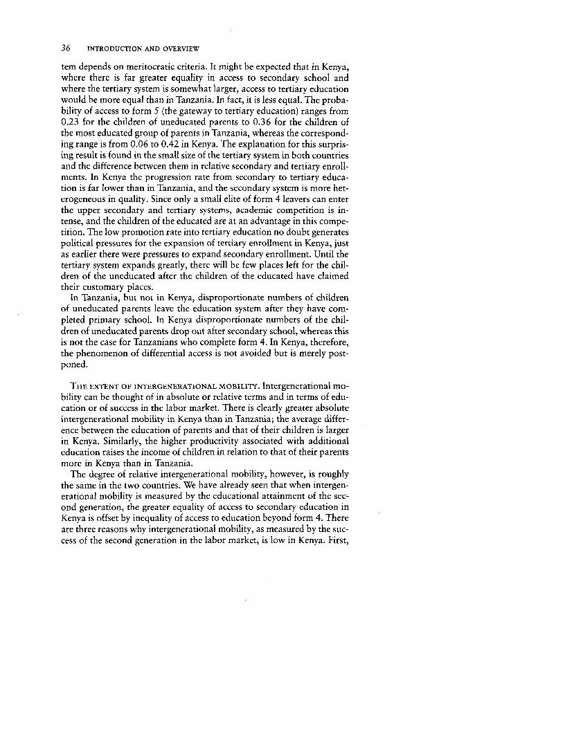
36 INTRODUCTION AND OVERVIEW
tem depends on meritocratic criteria. It might be expected that in Kenya,where there is far greater equality in access to secondary school andwhere the tertiary system is somewhat larger, access to tertiary educationwould be more equal than in Tanzania. In fact, it is less equal. The proba-bility of access to form 5 (the gateway to tertiary education) ranges from0.23 for the children of uneducated parents to 0.36 for the children ofthe most educated group of parents in Tanzania, whereas the correspond-ing range is from 0.06 to 0.42 in Kenya. The explanation for this surpris-ing result is found in the small size of the tertiary system in both countriesand the difference between them in relative secondary and tertiary enroll-ments. In Kenya the progression rate from secondary to tertiary educa-tion is far lower than in Tanzania, and the secondary system is more het-erogeneous in quality. Since only a small elite of form 4 leavers can enterthe upper secondary and tertiary systems, academic competition is in-tense, and the children of the educated are at an advantage in this compe-tition. The low promotion rate into tertiary education no doubt generatespolitical pressures for the expansion of tertiary enrollment in Kenya, justas earlier there were pressures to expand secondary enrollment. Until thetertiary system expands greatly, there will be few places left for the chil-dren of the uneducated after the children of the educated have claimedtheir customary places.
In Tanzania, but not in Kenya, disproportionate numbers of childrenof uneducated parents leave the education system after they have com-pleted primary school. In Kenya disproportionate numbers of the chil-dren of uneducated parents drop out after secondary school, whereas thisis not the case for Tanzanians who complete form 4. In Kenya, therefore,the phenomenon of differential access is not avoided but is merely post-poned.
THE EXTENT OF INTERGENERATIONAL MOBILITY. Intergenerational mo-bility can be thought of in absolute or relative terms and in terms of edu-cation or of success in the labor market. There is clearly greater absoluteintergenerational mobility in Kenya than in Tanzania; the average differ-ence between the education of parents and that of their children is largerin Kenya. Similarly, the higher productivity associated with additionaleducation raises the income of children in relation to that of their parentsmore in Kenya than in Tanzania.
The degree of relative intergenerational mobility, however, is roughlythe same in the two countries. We have already seen that when intergen-erational mobility is measured by the educational attainment of the sec-ond generation, the greater equality of access to secondary education inKenya is offset by inequality of access to education beyond form 4. Thereare three reasons why intergenerational mobility, as measured by the suc-cess of the second generation in the labor market, is low in Kenya. First,
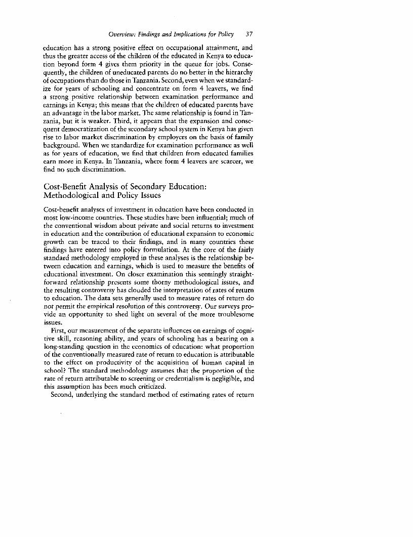
Overview: Findings and Implications for Policy 37
education has a strong positive effect on occupational attainment, andthus the greater access of the children of the educated in Kenya to educa-tion beyond form 4 gives them priority in the queue for jobs. Conse-quently, the children of uneducated parents do no better in the hierarchyof occupations than do those in Tanzania. Second, even when we standard-ize for years of schooling and concentrate on form 4 leavers, we finda strong positive relationship between examination performance andearnings in Kenya; this means that the children of educated parents havean advantage in the labor market. The same relationship is found in Tan-zania, but it is weaker. Third, it appears that the expansion and conse-quent democratization of the secondary school system in Kenya has givenrise to labor market discrimination by employers on the basis of familybackground. When we standardize for examination performance as wellas for years of education, we find that children from educated familiesearn more in Kenya. In Tanzania, where form 4 leavers are scarcer, wefind no such discrimination.
Cost-Benefit Analysis of Secondary Education:Methodological and Policy Issues
Cost-benefit analyses of investment in education have been conducted inmost low-income countries. These studies have been influential; much ofthe conventional wisdom about private and social returns to investmentin education and the contribution of educational expansion to economicgrowth can be traced to their findings, and in many countries thesefindings have entered into policy formulation. At the core of the fairlystandard methodology employed in these analyses is the relationship be-tween education and earnings, which is used to measure the benefits ofeducational investment. On closer examination this seemingly straight-forward relationship presents some thorny methodological issues, andthe resulting controversy has clouded the interpretation of rates of returnto education. The data sets generally used to measure rates of return donot permit the empirical resolution of this controversy. Our surveys pro-vide an opportunity to shed light on several of the more troublesomeissues.
First, our measurement of the separate influences on earnings of cogni-tive skill, reasoning ability, and years of schooling has a bearing on along-standing question in the economics of education: what proportionof the conventionally measured rate of return to education is attributableto the effect on productivity of the acquisition of human capital inschool? The standard methodology assumes that the proportion of therate of return attributable to screening or credentialism is negligible, andthis assumption has been much criticized.
Second, underlying the standard method of estimating rates of return
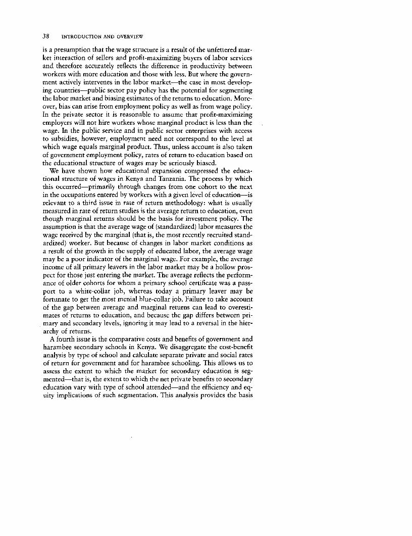
38 INTRODUCTION AND OVERVIEW
is a presumption that the wage structure is a result of the unfettered mar-ket interaction of sellers and profit-maximizing buyers of labor servicesand therefore accurately reflects the difference in productivity betweenworkers with more education and those with less. But where the govern-ment actively intervenes in the labor market-the case in most develop-ing countries-public sector pay policy has the potential for segmentingthe labor market and biasing estimates of the returns to education. More-over, bias can arise from employment policy as well as from wage policy.In the private sector it is reasonable to assume that profit-maximizingemployers will not hire workers whose marginal product is less than thewage. In the public service and in public sector enterprises with accessto subsidies, however, employment need not correspond to the level atwhich wage equals marginal product. Thus, unless account is also takenof government employment policy, rates of return to education based onthe educational structure of wages may be seriously biased.
We have shown how educational expansion compressed the educa-tional structure of wages in Kenya and Tanzania. The process by whichthis occurred-primarily through changes from one cohort to the nextin the occupations entered by workers with a given level of education-isrelevant to a third issue in rate of return methodology: what is usuallymeasured in rate of return studies is the average return to education, eventhough marginal returns should be the basis for investment policy. Theassumption is that the average wage of (standardized) labor measures thewage received by the marginal (that is, the most recently recruited stand-ardized) worker. But because of changes in labor market conditions asa result of the growth in the supply of educated labor, the average wagemay be a poor indicator of the marginal wage. For example, the averageincome of all primary leavers in the labor market may be a hollow pros-pect for those just entering the market. The average reflects the perform-ance of older cohorts for whom a primary school certificate was a pass-port to a white-collar job, whereas today a primary leaver may befortunate to get the most menial blue-collar job. Failure to take accountof the gap between average and marginal returns can lead to overesti-mates of returns to education, and because the gap differs between pri-mary and secondary levels, ignoring it may lead to a reversal in the hier-archy of returns.
A fourth issue is the comparative costs and benefits of government andharambee secondary schools in Kenya. We disaggregate the cost-benefitanalysis by type of school and calculate separate private and social ratesof return for government and for harambee schooling. This allows us toassess the extent to which the market for secondary education is seg-mented-that is, the extent to which the net private benefits to secondaryeducation vary with type of school attended-and the efficiency and eq-uity implications of such segmentation. This analysis provides the basis

Overview: Findings and Implications for Policy 39
for an evaluation of the way in which the government chooses to subsi-dize secondary education.
The Returns from Cognitive Skill Acquired in School
As was shown in the first section of this chapter, our survey evidencebears out the human capital interpretation of the education-wage rela-tionship rather than the screening or credentialist interpretation. This re-sult appears to support the standard method of estimating the social ben-efit of education. Our three-equation recursive model, however, enablesus to conduct a more precise evaluation of the standard method, of thesort first suggested by Becker (1964). The analysis is confined to Kenyabecause of the additional complications introduced by government paypolicy in Tanzania, which are difficult to isolate in the tested subsamples.We compare the social rate of return to secondary education, estimatedin the conventional way, with the return obtained by using the recursivemodel to trace the productive effects of secondary schooling (see chapter12).
The educational attainment function identifies the contributions tohuman capital acquisition that secondary schools make-through the in-teraction of ability and schooling inputs-by their selection of the moreable primary completers. The educational production function shows theeffect of secondary schooling on cognitive skill. The earnings function pre-dicts the effect of higher cognitive skill on earnings and, by implication,on productivity. These three relationships are different aspects of theproductivity-enhancing role of secondary education. The earnings func-tion also shows the direct effects on earnings of ability and credentialismand thus enables us to separate them from the human capital effects.
On the standard definition of the benefit stream, the social rate of re-turn to secondary schooling is 13 percent. When the recursive system isused and all of the effects are combined, the rate is 15 percent-not sig-nificantly different. Since the direct effects of ability are negligible, cogni-tive skill and credentialism together produce a return of 14 percent. Cog-nitive skill makes the larger contribution of the two; it raises earningsby 33 percent, whereas secondary school attendance on its own raisesearnings by 21 percent.
It is difficult to interpret the effect of cognitive skill on earnings exceptin terms of human capital acquisition. The smaller direct effect of school-ing may represent credentialism or screening by employers on the basisof education, or it may contain elements of human capital acquisitionthat are not captured by our measure. For instance, schools may impartcognitive skills other than numeracy and literacy or valuable affectivetraits such as personal motivation or discipline. Our findings thereforetend to vindicate the use of the standard methodology in Kenya.

40 INTRODUCTION AND OVERVIEW
Public Sector Pay and Employment Policyand the Return on Education
It was shown above that in Tanzania an egalitarian pay policy in thedominant public sector has compressed the wage structure by educa-tional level and reduced the premium on secondary education. This raisesthe question of whether public sector pay policy biases conventional esti-mates of the social rate of return on secondary education. Another com-plication is that since the public sector is not necessarily profit maximiz-ing, wages need not equal marginal products. To explore these issues weexamine the sensitivity of conventional estimates to alternative modelsof government pay and employment policy (see chapter 13).
Standard methods of estimation give a rate of return to secondary edu-cation of 13 percent in both countries. These results are not consistentwith our expectation of a higher return in Tanzania, where secondarycompleters are in scarcer supply. The explanation lies in the differencein public sector pay and employment policies in the two countries andin the conventional abstraction from those differences.
Rate of return estimates for the public and private sectors separatelyindicate a relatively small difference in Kenya (10 and 15 percent), whichreflects the only mildly compressive pay policy. In Tanzania public sectorpay policy gives rise to a larger difference (9 and 20 percent). Tanzaniacan maintain such a large gap because of constraints on the ability ofeducated labor to move from the large public sector to the much smallerprivate sector. Since there is no consistent evidence of a positive relation-ship between the examination performance of secondary completers andtheir employment in the private sector, the difference cannot be simplya result of the "creaming" of better workers by private employers. Asexpected, the private sector rate of return is higher in Tanzania than inKenya.
When the government intervenes to reduce pay, the wage in the publicsector may measure the marginal product of government employees (ifthe government behaves as a profit-maximizing employer), fall short ofmarginal product (if the government allocates labor optimally betweensectors but pays no more than it has to), or exceed marginal product (ifthere is overmanning in the public sector). The estimated social rate ofreturn in the economy is shown to be sensitive to the choice among theseassumptions, particularly in Tanzania.
In both countries additional knowledge of the workings of the publicsector labor market would be required to estimate definitive rates of re-turn to secondary education. Rate of return analysis should not be con-ducted mechanically but should rest on a knowledge of government ob-jectives and behavior.

Overview: Findings and Implications for Policy 41
The Relative Rates of Return to Primary and Secondary Education
Perhaps the most influential stylized fact to emerge from twenty-fiveyears of rate of return studies in dozens of developing countries concernsthe relative rates of return to primary and secondary schooling. The aver-ages of a large number of these studies indicate social rates of return of27 percent for primary education, 16 percent for secondary education,and 13 percent for tertiary education. The implication generally drawnfrom this ranking is that top priority should be given to primary educa-tion as a form of investment in human resources. A well-known but little-heeded criticism of conventional rate of return studies, however, castsdoubt on this conclusion as applied to Kenya.
In conventional rate of return studies the returns to education are mea-sured by the wage differences associated with educational differences.The assumption is that the wage difference between primary and second-ary completers measures their difference in marginal product and there-fore indicates the marginal product of education. This assumption willbe misleading if the average wages of all primary and secondarycompleters are inapplicable to those now entering the labor market.Rapid expansion of the educational system, as in Kenya, can change dra-matically the labor market conditions faced by school leavers. The supplyof educated labor has tended to outstrip wage employment in many de-veloping countries, thereby necessitating substantial adjustments in thelabor market. In particular, the education-occupation matrix tends tochange from one cohort to the next. This issue is examined in chapter14.
In the wage sector in Kenya, uneducated workers are the only oneswho have generally remained in the same (unskilled) occupations fromone cohort to the next. Two or three decades ago primary completerswere in scarce supply, and a primary school certificate was a passportto a white-collar job. Those who obtained those jobs remain in themtoday. But, owing to the rapid expansion of the education system, today'sprimary completer is fortunate to get a low-paying blue-collar job, andhis chance of obtaining a senior white-collar position, as many of hispredecessors did, is negligible.
Similarly, whereas earlier cohorts of secondary completers were en-sured access to nonmanual occupations, a rising proportion of recent co-horts have had to accept manual employment. The filtering-down proc-ess, whereby successive cohorts of workers with the same education enterless skilled jobs, was taken into account in calculating rates of return toprimary and secondary education in Kenya. In addition to average ratesof return, marginal rates of return were calculated by using the occupa-tional distribution of the most recent cohort of labor market entrants to

42 INTRODUCTION AND OVERVIEW
derive the wage difference attributable to education. In contrast, conven-tional rate of return studies inflate the wages of workers at a particulareducational level by including in the calculation the currently unattain-able occupational attainment of earlier cohorts.
In Kenya the rate of return to primary education is highly sensitive tothe distinction between average and marginal rates of return, whereas therate of return to secondary education is not. The average rate of returnto primary education, as conventionally measured, is 17 percent, and themarginal rate of return is only 12 percent. The marginal return is mark-edly lower than the average for two reasons. At the primary level substan-tial filtering down takes place and there are large differences in wagesby occupation, whereas for the uneducated there is less scope for filteringdown and wage differences by occupation are small.
The return to secondary education, by contrast, is not affected by thecorresponding adjustment: the average and marginal rates of return areboth 13 percent. Because the degree of filtering down of primary and sec-ondary completers is similar, their difference in earnings is little altered.Moving from the average to the marginal concept of the rate of returnreverses the usual hierarchy: at the margin the rate of return to secondaryeducation exceeds that to primary education.
The Kenyan analysis suggests that the conventional wisdom aboutthe hierarchy of the returns to education in Africa and elsewhere restson studies that are likely to contain a methodological error. Althoughthe average rate of return on primary schooling for a large number ofcountries may be as high as 27 percent, the marginal return is likelyto be considerably lower and may be less than the return to secondaryschooling.
The conventional assessment of educational investment priorities ac-cords the highest priority to primary education in those poor countrieswhich, unlike Kenya and Tanzania, have not achieved universal primaryeducation. The implication of our illustrative analysis for Kenya is notthat the conventional assessment is necessarily wrong: in some countrieseven the marginal rate of return to primary education may be high, andthe expansion of primary education could yield important distributionalbenefits and positive externalities. Rather, the implication is that the juryis still out.
Efficiency and Equity Implications of Subsidiesin Secondary Education
Our comparative cost-benefit analysis of government and private (ha-rambee) schools in chapter 15 is confined to Kenya because of the ab-sence of data on costs in the private sector in Tanzania. It shows that
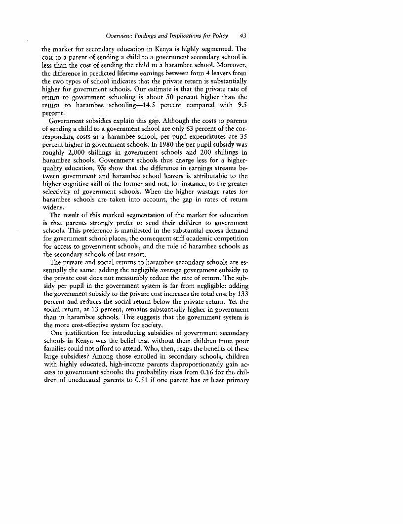
Overview: Findings and Implications for Policy 43
the market for secondary education in Kenya is highly segmented. Thecost to a parent of sending a child to a government secondary school isless than the cost of sending the child to a harambee school. Moreover,the difference in predicted lifetime earnings between form 4 leavers fromthe two types of school indicates that the private return is substantiallyhigher for government schools. Our estimate is that the private rate ofreturn to government schooling is about 50 percent higher than thereturn to harambee schooling-14.5 percent compared with 9.5percent.
Government subsidies explain this gap. Although the costs to parentsof sending a child to a government school are only 63 percent of the cor-responding costs at a harambee school, per pupil expenditures are 35percent higher in government schools. In 1980 the per pupil subsidy wasroughly 2,000 shillings in government schools and 200 shillings inharambee schools. Government schools thus charge less for a higher-quality education. We show that the difference in earnings streams be-tween government and harambee school leavers is attributable to thehigher cognitive skill of the former and not, for instance, to the greaterselectivity of government schools. When the higher wastage rates forharambee schools are taken into account, the gap in rates of returnwidens.
The result of this marked segmentation of the market for educationis that parents strongly prefer to send their children to governmentschools. This preference is manifested in the substantial excess demandfor government school places, the consequent stiff academic competitionfor access to government schools, and the role of harambee schools asthe secondary schools of last resort.
The private and social returns to harambee secondary schools are es-sentially the same: adding the negligible average government subsidy tothe private cost does not measurably reduce the rate of return. The sub-sidy per pupil in the government system is far from negligible: addingthe government subsidy to the private cost increases the total cost by 133percent and reduces the social return below the private return. Yet thesocial return, at 13 percent, remains substantially higher in governmentthan in harambee schools. This suggests that the government system isthe more cost-effective system for society.
One justification for introducing subsidies of government secondaryschools in Kenya was the belief that without them children from poorfamilies could not afford to attend. Who, then, reaps the benefits of theselarge subsidies? Among those enrolled in secondary schools, childrenwith highly educated, high-income parents disproportionately gain ac-cess to government schools: the probability rises from 0.16 for the chil-dren of uneducated parents to 0.51 if one parent has at least primary

44 INTRODUCTION AND OVERVIEW
and the other at least secondary education. The reasons, predominantlymeritocratic, have been explained above. Whatever the reasons, thosewith the greatest ability to bear the cost of their children's education arethe most likely to receive large subsidies.
Policy Implications
Tanzania's policies for secondary education were much influenced by theprinciples enunciated in Education for Self-Reliance (Nyerere 1967a), is-sued shortly after the Arusha Declaration put Tanzania on a socialistpath. The objectives of the policies included controlling the expansionof postprimary education to satisfy manpower requirements rather thanprivate demand for education, reducing elitism and the tendency forschooling to promote inequality and class formation, and preparing chil-dren better for life in socialist Tanzania.
Manpower planning involved, on the one hand, forecasting future re-quirements for educated labor and, on the other, restricting the growthof the postprimary school system. Among the policies adopted to pro-mote the egalitarian objective were the use of academic criteria, temperedby a regional quota system, for entry to secondary education, the waivingof all fees in government secondary schools, and the discouragement ofprivate schools that would offer secondary education only to those whocould afford it. To further the attitudinal and vocational objectives, polit-ical education and activities (such as cultivating farm plots) designed topromote self-reliance were introduced into the schools, the secondarycurriculum was diversified away from general academic subjects and to-ward vocational subjects, and the primary curriculum was made moreappropriate for the majority who would never enter secondary schooland would become farmers.
The education policies adopted in Tanzania have aroused interest andcomment in the international education and development community.These policies are radical not just in rhetoric but in fact: they have sad-dled Tanzania with one of the smallest secondary systems in the worldand have changed the nature of education. Some commentators have heldup Tanzania as a model. Others have been critical, perhaps because theyrecognized that government intervention frequently generates counter-vailing tendencies and side effects that can produce outcomes differentfrom those intended.
How successful have these policies been in meeting their own objec-tives and as judged by the usual economic criteria? The evidence adducedby educationalists and reviewed by Cooksey and Ishumi (1986) concern-ing the first point-the internal objectives-is discouraging. Our studyaddresses the second issue by comparing the outcomes of differing poli-
Overview: Findings and Implications for Policy 45
cies toward secondary education and assessing these policies accordingto economic criteria.
Kenya has followed a more conventional set of education policies thanhas Tanzania. Forecasts of manpower requirements have not governedthe expansion of postprimary education. At the secondary level the sup-ply of educational opportunities, both in government and in privateschools, has been more responsive to demand. The government has tole-rated the rapid growth of a private secondary system in which ability topay is necessarily a criterion for access. Unlike Tanzania, Kenya isroughly on the curve that relates the secondary enrollment ratio to na-tional income per capita in cross-country comparisons (see figure 16-1).Furthermore, primary and secondary schooling in Kenya has not strayedfar from the usual curriculum, with its stress on academic subjects.
In the foregoing sections we summarized the results of the East Africannatural experiment. In this section we shift from positive to normativeanalysis and to policy implications. We evaluate each aspect of the exper-iment by the criteria of efficiency and equity and then-since the policiesare an integrated package-overall.
Efficiency
Our research has attempted to study the relationships between educationpolicy and efficiency in greater depth and breadth than is conventionallydone. The greater depth is made possible by introducing reasoning abilityand cognitive skill as the links between education and wages. That analy-sis lends strong support to the human capital interpretation of theeducation-wage relationship. It implies that standard cost-benefit meth-ods of appraising education are valid in this crucial respect.
A corollary of this finding is that the assumptions underlying man-power planning approaches to education policy are invalid. Within oursix skill-based occupational groups we find that earnings vary by educa-tional level; indeed, in the case of form 4 leavers they vary with examina-tion performance. The cognitive skill that a worker brings to a job affectshis productivity and therefore his pay. The very different education-occupation matrices in the two countries imply that Kenyan workers, whoare better educated, are more productive in their jobs. Although expan-sion of secondary education is shown to reduce the wage premium onsecondary education and, by implication, its marginal product, the elas-ticity of substitution between workers with primary and with secondaryeducation is fairly high-well in excess of unity.
The governments of both Kenya and Tanzania have made forecasts ofmanpower requirements on the basis of fixed input coefficients for edu-cated labor. Because of political pressures for expansion, Kenyan educa-
46 INTRODUCTION AND OVERVIEW
tion policymakers have paid lip service to the forecasts, whereas theirTanzanian counterparts have taken them more seriously. Quite apartfrom the serious informational problems that have led to widely diver-gent forecasts of requirements (Cooksey and Ishumi 1986, pp. 55-58),our analysis suggests that such forecasts are fundamentally misguided.Tanzanian manpower planners have viewed the filtering down of second-ary completers into lower occupations as a waste of resources. We havedemonstrated that the process is better viewed as a deepening of humancapital.
The two countries differ not only in the quantity but also in the qualityof secondary education. Our educational production functions indicatethat the cognitive skill of workers with the same reasoning ability andyears of education is substantially higher in Kenya. This result is surpris-ing in view of the greater importance of low-cost community schools inKenya. It no doubt reflects the switch in language of instruction in Tanza-nia from Kiswahili in primary school to English in secondary school (inKenya English is used throughout) and the diversion of time from aca-demic subjects as a consequence of curriculum reform. Moreover, curric-ulum diversification has not achieved some of the economic objectivesfor which it was intended (Psacharopoulos and Loxley 1985, pp.205-09). Even if it has furthered the ideological objectives of socialismand self-reliance, that gain has been at the high cost of lower levels ofcognitive skill.
Our results strongly suggest the desirability of research into cost-effec-tive means of improving the quality of education in Tanzania. Such re-search may find that the returns to expenditure on improving quality arecomparable to or even higher than those on increasing educational quan-tity. Because of the difference in both the quantity and quality of second-ary education, the mean level of cognitive skill and therefore of labor pro-ductivity and earnings is far higher in Kenya. The difference between thetwo countries in education policy regimes appears to account for a sub-stantial proportion of their difference in the average productivity of wagelabor. Tanzania intervened in the market for education to save resourcesthat, it was perceived, would otherwise be wasted. Perversely, this inter-vention has exacted a high price in output forgone.
Furthermore, the full price has not yet been paid. The gap betweenKenya and Tanzania in the educational attainment of the labor forcewould inevitably widen even if Tanzanian policy were to change, owingto the lag between the expansion of the secondary system and the entryinto the labor market of educated workers. Looking further ahead, Ken-yans will be reaping an intergenerational benefit that Tanzanians willforgo. A markedly higher proportion of the current generation of chil-dren in Kenya has parents with secondary education. This will increase
Overview: Findings and Implications for Policy 47
the efficiency with which the children learn in school and their subse-quent performance in the labor market.
Equality
Since the governments of both Kenya and Tanzania have egalitarian ob-jectives, we examined the effects of their secondary education policies onvarious dimensions of inequality. Such effects are often ignored, inade-quately recognized, or inadequately understood in educational deci-sionmaking. The four dimensions of inequality discussed here are thestructure of wages among educational groups, the dispersion of payamong individuals, differential access to education, and the extent of in-tergenerational mobility. Each of these distributional effects has policyimplications.
The governments of both countries have expressed their desire to com-press the widely dispersed wage structure that they inherited. Our esti-mate of the response of relative wages to supplies of secondary in relationto primary completers confirmed that the expansion of secondary educa-tion is a means of achieving that objective. Although the responsivenessis not high, the degree of compression achieved in Kenya has been signifi-cant: the premium on secondary education in the market sector is about20 percent lower in Kenya than in Tanzania.
Tanzania's policy of holding back secondary enrollment meant thatscarcity rents accrued to people with secondary education. This resultmay well have been why the government intervened in the labor marketto compress the wage structure. Despite having to work against the mar-ket, the policy is effective in the dominant public sector, where govern-ment pay policy halves the premium on secondary education. Thus onepolicy intervention, in the market for education, begets another, in themarket for labor. A side effect of the latter intervention is that the labormarket is segmented by sector of ownership, which produces new inequi-ties and a misallocation of labor.
The Kenyan government, in adopting the prevailing wage rate ap-proach to public sector pay, implicitly chose to follow market forces be-cause the rapid expansion of enrollment in Kenya could be relied on toreduce the premium on secondary education. The two different policyregimes for education and the labor market have had similar results inthe size of compressive effects on the structure of wages.
Not only does the expansion of secondary education compress thewage structure by educational level, but it also reduces the inequality ofwages among individuals. This would occur even at Tanzania's low initialposition, where the compression effect is partly offset by the compositioneffect of educational expansion. On both scores-the structure and the
48 INTRODUCTION AND OVERVIEW
dispersion of wages-it would seem that the Kenyan policy of permittingthe expansion of secondary education is preferable to the Tanzanian pol-icy of containment.
One aim of universal primary education was to reduce inequality ofaccess to the education system. This has been achieved in both countries;even the children of the poor and uneducated, who once were excluded,now receive a basic education. Both governments have tried to equalizeaccess to secondary school: they heavily subsidize government secondaryschools and ration the scarce places on the basis of meritocratic criteria.In addition, one reason that Tanzania restricted private enrollment wasso that those who can afford to pay would not be at an advantage.
The extreme rationing of government secondary places in Tanzania hasgiven rise to some corruption-perhaps less than might be expected-and this has contributed to inequality of access. More important, andas in other countries, eliminating the direct effects of differences in in-come has not brought about equality of access. The academic advantagesconferred by family background mean that it is primarily the childrenof the poor and uneducated who are excluded by the quantitative restric-tions imposed by the government. Many less privileged families that arewilling and able to meet the cost of private secondary education are con-strained by policy from doing so. This is yet another example of howTanzanian government intervention has had unforeseen side effects andhas produced an outcome the opposite of that intended. Restraining thesize of the secondary system has contributed to class formation; an edu-cated elite is in the process of perpetuating itself in Tanzania.
At first, it appeared that the Kenyan policy on secondary expansionwould prove to be less egalitarian than the Tanzanian policy because ofthe greater importance of the fee-charging private sector. But in fact, thelarger size of the secondary system in Kenya has meant easier access forthe children of the poor and uneducated there than in Tanzania. Yet inter-generational mobility is not greater in Kenya; the exclusion of the chil-dren of the poor and uneducated now occurs at the tertiary level, andthis continues to order the labor market by family background. Therehas been more absolute intergenerational mobility in Kenya, where thegap between generations in education and income levels is greater thanin Tanzania. But the influence of family background on position in thesocioeconomic hierarchy remains much the same in the two countries.The widely heard claim that education is "the great equalizer" is notborne out in these countries. It is also disappointing to note that the be-havioral mechanisms at work in Kenya and Tanzania are likely to operateelsewhere.
In sum, the externalities associated with the distributional effects ofeducational expansion vary. The effects of expansion on the structureand dispersion of wages and the distribution of educational opportunities
Overview: Findings and Implications for Policy 49
are positive and reinforce efficiency arguments for expansion. The EastAfrican experiment suggests, however, that the promotion of intergenera-tional mobility cannot be used as an additional argument for the expan-sion of secondary education.
Subsidies
Government secondary schools are highly subsidized in both countries,whereas private schools are not. Although lack of data for Tanzania lim-ited our cost-benefit analysis to Kenya, the findings and their policy im-plications should also be applicable to Tanzania.
As a result of government subsidies, the market for secondary educa-tion in Kenya is highly segmented; the private returns from governmentschooling are markedly higher than those from harambee schooling. Thisimplies that government secondary places are rationed and that demandfor them is insensitive to even substantial increases in school fees. Theper pupil subsidy could therefore be reduced without reducing expendi-ture per pupil and without diminishing the quality of the education pro-vided.
The children of high-income parents, who are disproportionately rep-resented in government schools, benefit disproportionately from the sub-sidies. This suggests that an increase in school fees, tempered by a need-based scholarship scheme, would have progressive distributional effects.The regressiveness of government expenditures on secondary educationshould be considered in the light of evidence that the incidence of taxa-tion in Kenya may be regressive, as is often the case in developing coun-tries that derive a high proportion of their revenue from the taxation ofagriculture.
Our analysis suggests that the fees charged by government schoolswould have to be increased more than fourfold-to more than the costper pupil-to reduce the private rate of return to that prevailing inharambee schools. Only at such high fees would parents be indifferentin choosing between the higher-quality government system and the lower-cost harambee system. Such a reduction of the private return would notreduce the social return to government secondary education but wouldmerely shift the burden.
The revenue potential of increases in user charges is so substantial-more than 300 percent of government recurrent expenditure on second-ary education-that even a more modest increase in fees and a largescholarship program would greatly ease the constraints on the educationbudget. This is particularly important in Tanzania, where budgetary con-straints have shared the blame for the slow expansion of government sec-ondary schools and where until 1984 no fees were charged in governmentsecondary schools.
SO INTRODUCTION AND OVERVIEW
The efficiency gains from reducing subsidies in Tanzania would comefrom the opportunity to make high-yielding investments in secondaryschooling. Even in Kenya there are efficiency gains to be reaped from areduction of per pupil subsidies. If the government were to provide smallsubsidies to harambee schools to improve quality, the current gap in thesocial rates of return between the two systems could be reduced.
Overall Appraisal
We have discussed the consequences for efficiency and equity of the EastAfrican natural experiment. The overall assessment of the difference ineducation policy regimes should be clear. The Kenyan policy regime ispreferable both on grounds of efficiency and, ironically, as judged by thedistributional criteria that the Tanzanian government has emphasized.
We have reached this important conclusion with barely a reference tothe social rate of return to secondary education in either country. Whenwe calculate conventional social rates of return, we find that the return,at 13 percent in both countries, is high and is competitive with other in-vestments. This result suggests that there is a case for expanding second-ary education in both countries, but there is no indication that the ur-gency is any greater in Tanzania. Our examination of methodologicalissues in cost-benefit analysis provides some insight.
First, the usual practice of ignoring pay and employment policy in thepublic sector leads to large biases in estimates of social rates of returnto secondary education in Tanzania, where the government has aggres-sively intervened in the labor market, but to only small biases in Kenya.Second, moving from measures of average rates of return to more policy-relevant measures of marginal rates can substantially alter the level andstructure of returns. Third, when we isolated the human capital effectsof education on earnings from the screening and credentialist effects, wefound an upward bias in conventional rate of return estimates, but thebias was small.
We have used our data to examine these sources of bias, but we havenot attempted to combine the exercises and thereby to unveil the "true"rate of return to secondary education in Kenya and Tanzania. This ispartly on account of data constraints. The subsample of workers forwhom measures of ability and cognitive skill are available is not largeenough to allow us to estimate the direct effect of cognitive skill whilesimultaneously taking account of government pay and employment pol-icy and substituting the marginal for the average rate of return.
Quite independent of data constraints, however, we would be reluctantto make such an attempt. The consequences of educational expansion aremultidimensional, and the assessment of each dimension can be complex.Educational cost-benefit analysis was developed as a means of assessing
Overview: Findings and Implications for Policy Si
the consequences of expansion for productivity alone. For informing pol-icy on the expansion of secondary education, this approach is, both inconcept and in practice, clearly superior to manpower planning. Never-theless, it is seriously flawed.
The desire to generate a single number, a rate of return to educationalexpansion comparable to the rate of return for a steel mill or a port facil-ity, is understandable. The effort was of particular value in the early yearsof development economics, when some people still needed to be con-vinced that growth could be generated by, and indeed required, invest-ments in human capital as well as in physical capital. But this reductionistapproach to the assessment of educational investments, by ignoring muchof the complexity in educational and labor markets, can easily be mis-leading.
Rates of return turn out to be sensitive to several issues that are gener-ally left out of cost-benefit analysis. In some instances still more researchwould be required to determine the precise way in which an issue shouldbe resolved. For example, the impact that government employment policyhas on the returns to secondary education is ambiguous without moreinformation. Furthermore, it is not clear how to incorporate an analysisof the distributional consequences of educational expansion into the cal-culation of rates of return, and we have made no attempt to do so. Al-though our nonreductionist approach can inform education policy, itdoes not provide a basis for estimating the "true" rate of return to second-ary education. We do not wish to perpetuate the illusion of precisioncreated by oversimplification.
Our approach suggests that the Tanzanian policy regime should movecloser to that adopted by Kenya. It does not provide clear guidance asto the future rate of expansion of the Kenyan secondary system. The highsocial rate of return in Kenya suggests that secondary education thereshould be further expanded. Even at the margin, as we have measuredit, the returns are high. We have doubts, however, about this particularpolicy implication.
Most of the additional secondary completers produced by further ex-pansion of the secondary system in Kenya are likely to become self-employed farmers. It is tempting to presume that the social returns tosecondary education will not be high in agriculture; this is the sort oftrap into which manpower planners are prone to fall. To measure thesereturns and the distributional consequences of the next phase of expan-sion requires a different methodology from that applied here-a method-ology based on rural surveys and farm-level production functions. Thisis the highest research priority for future education policy in Kenya, andsignificant expansion of the government system should wait on its results.In the meantime we would not counsel that there be government restric-tions on the further expansion of privately funded education.
52 INTRODUCTION AND OVERVIEW
We are confident of the case for a substantial expansion of the second-ary system in Tanzania. The deepening of human capital will furtherboth productivity and equity. Our social rate of return analysis, basedon the market sector, merely reinforces this judgment. There is, however,one qualification concerning public sector employment policy. If the gov-ernment service and public enterprises respond to the increased supplyof educated labor by creating unnecessary white-collar jobs, the oppor-tunity presented by expansion will be wasted. The increase in labor pro-ductivity can occur only if incentives in the labor market encourage sec-ondary completers to filter down and bring their skills to bear inlower-level occupations.
Between 1980 and 1985 government secondary places in Tanzania in-creased by 10 percent, and private places were permitted to increase by29 percent. This reflects a growing recognition by the government of aneed for change; the Presidential Commission on Education has recom-mended large-scale expansion by the year 2000 (Tanzania, Ministry ofEducation 1984). It also reflects the increasing political pressure for sec-ondary expansion as the number of primary leavers has grown.
How could popular demand for secondary education have been sup-pressed so long in Tanzania while it was satisfied in Kenya? The answerappears to lie fundamentally in the difference in political systems: thegreater centralization of power in Tanzania meant that education policywas handed down from the top. Another return that Tanzania may reapfrom educational expansion is a better informed citizenry and conse-quently a greater likelihood that the benefits and opportunity costs ofgovernment initiatives will be more fully recognized and debated.
Part II
EDUCATIONAL EXPANSIONAND LABOR PRODUCTIVITY

CHAPTER 3
Earnings, Schooling, Ability,and Cognitive Skill
CONVENTIONAL ESTIMATES now available for a large number ofcountries generally indicate that the social returns to education are posi-tive, large, and competitive with returns to investment in physical capi-tal.' That such estimates are good guides for the allocation of public re-sources has, however, been questioned. The heart of the problem lies inthe interpretation of the positive relationship between workers' educationand earnings. The conventional estimates assume that the coefficient onthe education variable in the earnings function measures the effect onworkers' productivity of human capital acquired in school. But it has alsobeen hypothesized that all or part of the education coefficient representsinnate ability and motivation (the screening explanation) or the higherwages awarded to more educated workers without regard to their pro-ductivity (the credentialist explanation). If either hypothesis is correct,conventional measures of the social benefit of education have an upwardbias.2
In this chapter we attempt to distinguish the influences that cognitiveskill, native ability, and years of education have on earnings and to usethis analysis as a means of adjudicating the human capital, screening, andcredentialist hypotheses. Our two rigorously comparable micro data setsfrom Kenya and Tanzania, described in chapter 1, contain the usual vari-ables found in wage function estimates of the benefits of schooling-individual earnings, years of education, and years of employment experi-ence. In addition, they contain two variables-measures of the worker'scognitive skill and reasoning ability-that are not found in earlier studiesof developing countries and that are only rarely found in studies of theeducation-wage relationship in developed countries.3 These variables
Note: Adapted from M. Boissiere, J. B. Knight, and R. H. Sabot, 'Earnings, Schooling,Ability, and Cognitive Skills," American Economic Review 75, no. 5 (December 1985),pp. 1016-30.
55
56 EDUCATIONAL EXPANSION AND LABOR PRODUCTIVITY
allow us to estimate the direct effects on earnings of cognitive skill, abil-ity, and years of schooling. By using these inputs to estimate educationalproduction functions and educational attainment functions and by link-ing these functions with the wage function in a recursive framework, wecan also assess the various indirect effects that ability and years of school-ing have on earnings. Having data sets from two countries that are simi-lar in size, resource endowments, structure of production and employ-ment, and level of development means that we can not only subject ourresults to the usual statistical tests but can also assess their rep-licability.
Kenya and Tanzania have nearly achieved universal primary education,and university enrollments remain at less than 1 percent of the relevantage group. The important policy issues regarding mass education in EastAfrica thus arise at the secondary level, and it is the benefits of secondaryeducation that concern us here. Because the public education system inboth countries is meritocratic, years of education may provide good sig-nals of ability. The public sector is an influential employer of urbanlabor-in 1980 it accounted for 39 percent of total urban labor in Kenyaand for 61 percent in Tanzania-and institutional arrangements suggestthat educational qualifications influence access to public sector jobs andaffect entry grades and pay. The screening and credentialist explanationsof the earnings-education relationship can therefore not be dismissed.
The Model
In the conventional measurement of the social rate of return to, say, sec-ondary education, the benefit stream is estimated by means of an earningsfunction. The following is an example of an earnings function for a sam-ple of primary and secondary completers.
(3-1) In W = a + bS + cL + dL2 + u
where
In W = the log of (pretax) earnings of the individualS = a dummy variable signifying that the individual has precisely
completed secondary education; individuals who have pre-cisely completed primary education form the base subcate-gory. (Schooling is introduced as a dichotomous rather thana continuous variable for reasons of survey design, discussedin chapter 2.)
L = the number of years of employment experience of theindividual
u = an error term.
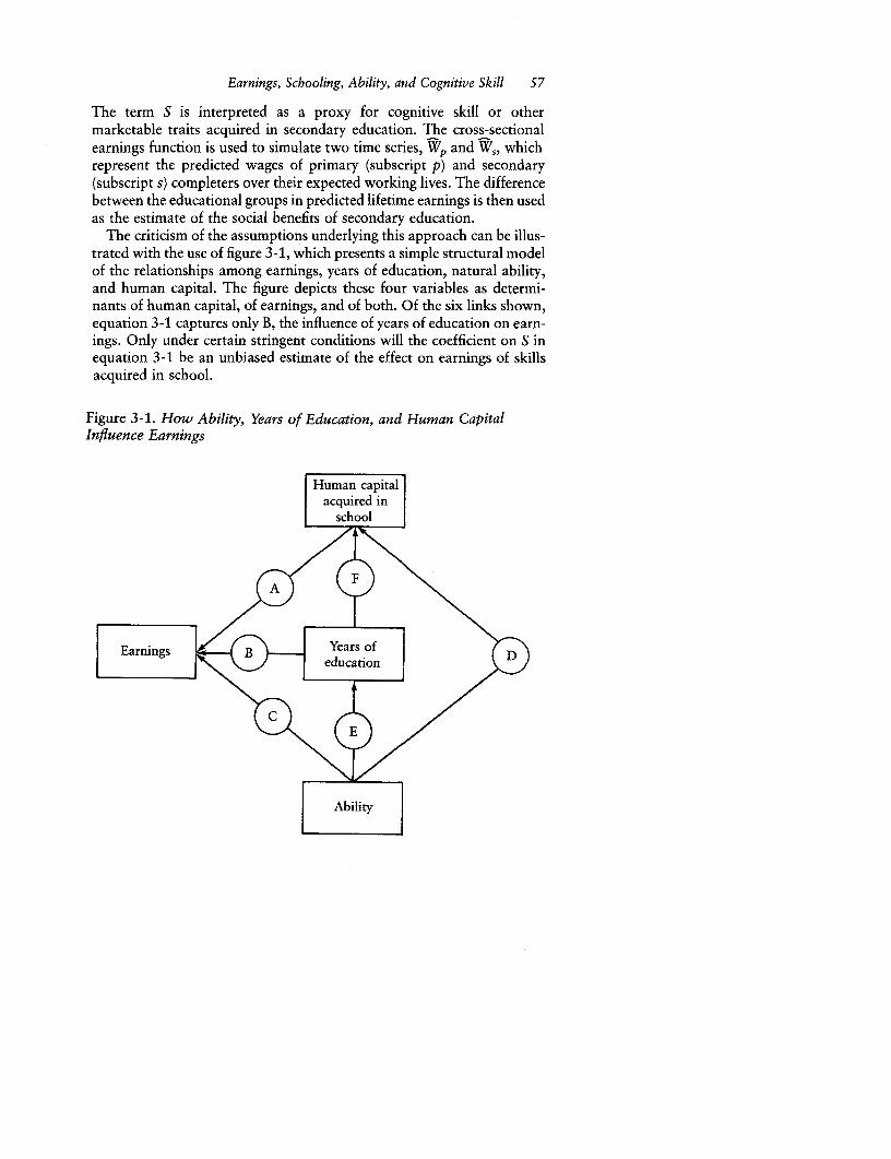
Earnings, Schooling, Ability, and Cognitive Skill 57
The term S is interpreted as a proxy for cognitive skill or othermarketable traits acquired in secondary education. The cross-sectionalearnings function is used to simulate two time series, Wp and Ws, whichrepresent the predicted wages of primary (subscript p) and secondary(subscript s) completers over their expected working lives. The differencebetween the educational groups in predicted lifetime earnings is then usedas the estimate of the social benefits of secondary education.
The criticism of the assumptions underlying this approach can be illus-trated with the use of figure 3-1, which presents a simple structural modelof the relationships among earnings, years of education, natural ability,and human capital. The figure depicts these four variables as determi-nants of human capital, of earnings, and of both. Of the six links shown,equation 3-1 captures only B, the influence of years of education on earn-ings. Only under certain stringent conditions will the coefficient on S inequation 3-1 be an unbiased estimate of the effect on earnings of skillsacquired in school.
Figure 3-1. How Ability, Years of Education, and Human CapitalInfluence Earnings
Human capitalacquired in
school
| Ability l
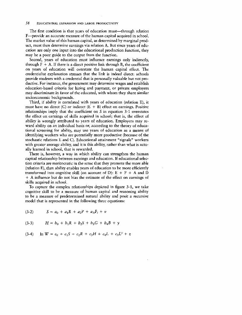
58 EDUCATIONAL EXPANSION AND LABOR PRODUCTIVITY
The first condition is that years of education must-through relationF-provide an accurate measure of the human capital acquired in school.The market value of this human capital, as determined by marginal prod-uct, must then determine earnings via relation A. But since years of edu-cation are only one input into the educational production function, theymay be a poor guide to the output from the function.
Second, years of education must influence earnings only indirectly,through F + A. If there is a direct positive link through B, the coefficienton years of education will overstate the human capital effect. Thecredentialist explanation stresses that the link is indeed direct: schoolsprovide students with a credential that is personally valuable but not pro-ductive. For instance, the government may determine wages and establisheducation-based criteria for hiring and payment, or private employersmay discriminate in favor of the educated, with whom they share similarsocioeconomic backgrounds.
Third, if ability is correlated with years of education (relation E), itmust have no direct (C) or indirect (E + B) effect on earnings. Positiverelationships imply that the coefficient on S in equation 3-1 overstatesthe effect on earnings of skills acquired in school; that is, the effect ofability is wrongly attributed to years of education. Employers may re-ward ability on an individual basis or, according to the theory of educa-tional screening for ability, may use years of education as a means ofidentifying workers who are potentially more productive (because of thestochastic relations E and C). Educational attainment "signals" workerswith greater average ability, and it is this ability, rather than what is actu-ally learned in school, that is rewarded.
There is, however, a way in which ability can strengthen the humancapital relationship between earnings and education. If educational selec-tion criteria are meritocratic in the sense that they promote the more able(relation E), then ability enables years of education to be more efficientlytransformed into cognitive skill (on account of D): E + F + A and D+ A influence but do not bias the estimate of the effect on earnings ofskills acquired in school.
To capture the complex relationships depicted in figure 3-1, we takecognitive skill to be a measure of human capital and reasoning abilityto be a measure of predetermined natural ability and posit a recursivemodel that is represented in the following three equations:
(3-2) S = ao + a1 R + a2P + a3,Fj + v
(3-3) H= bo + b,R + b2S + b3G + b4B + y
(3-4) In W = co + cIS + c2R + c3H + c 4L + csL2 + z
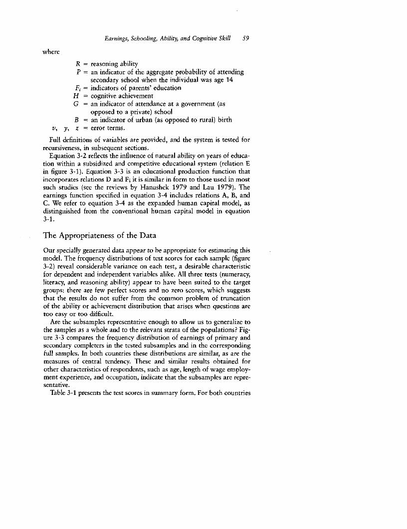
Earnings, Schooling, Ability, and Cognitive Skill 59
where
R = reasoning abilityP = an indicator of the aggregate probability of attending
secondary school when the individual was age 14Fi = indicators of parents' education
H = cognitive achievementG = an indicator of attendance at a government (as
opposed to a private) schoolB = an indicator of urban (as opposed to rural) birth
v, y, z = error terms.
Full definitions of variables are provided, and the system is tested forrecursiveness, in subsequent sections.
Equation 3-2 reflects the influence of natural ability on years of educa-tion within a subsidized and competitive educational system (relation Ein figure 3-1). Equation 3-3 is an educational production function thatincorporates relations D and F; it is similar in form to those used in mostsuch studies (see the reviews by Hanushek 1979 and Lau 1979). Theearnings function specified in equation 3-4 includes relations A, B, andC. We refer to equation 3-4 as the expanded human capital model, asdistinguished from the conventional human capital model in equation3-1.
The Appropriateness of the Data
Our specially generated data appear to be appropriate for estimating thismodel. The frequency distributions of test scores for each sample (figure3-2) reveal considerable variance on each test, a desirable characteristicfor dependent and independent variables alike. All three tests (numeracy,literacy, and reasoning ability) appear to have been suited to the targetgroups: there are few perfect scores and no zero scores, which suggeststhat the results do not suffer from the common problem of truncationof the ability or achievement distribution that arises when questions aretoo easy or too difficult.
Are the subsamples representative enough to allow us to generalize tothe samples as a whole and to the relevant strata of the populations? Fig-ure 3-3 compares the frequency distribution of earnings of primary andsecondary completers in the tested subsamples and in the correspondingfull samples. In both countries these distributions are similar, as are themeasures of central tendency. These and similar results obtained forother characteristics of respondents, such as age, length of wage employ-ment experience, and occupation, indicate that the subsamples are repre-sentative.
Table 3-1 presents the test scores in summary form. For both countries
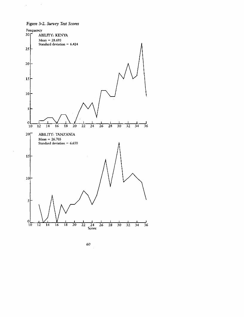
Figure 3-2. Survey Test Scores
Frequency30 ABILITY: KENYA
Mean = 28.693Standard deviation = 6.424
25 -
20 -
15 _
10 _
5-
O 1 -1-,1 10 12 14 16 18 20 22 24 26 28 30 32 34 36
20 ABILITY: TANZANIAMean = 26.703Standard deviation = 6.650
15
10
010 12 14 16 18 20 22 24 26 28 30 32 34 36
Score
60
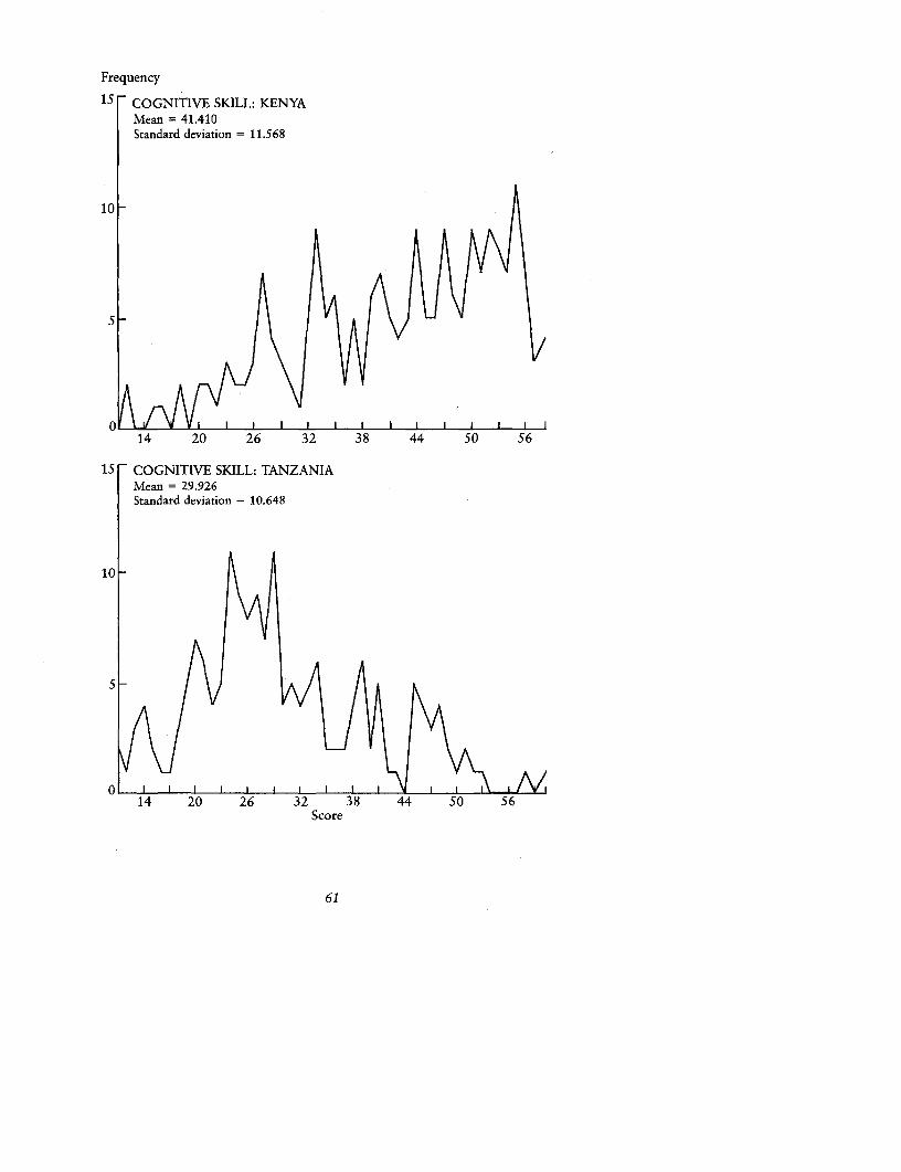
Frequency
15 COGNITIVE SKILL: KENYAMean = 41.410Standard deviation = 11.568
10
5
014 20 26 32 38 44 50 56
15 COGNITIVE SKILL: TANZANIAMean = 29.926Standard deviation = 10.648
10
5-
14 20 26 32 38 44 50 56Score
61
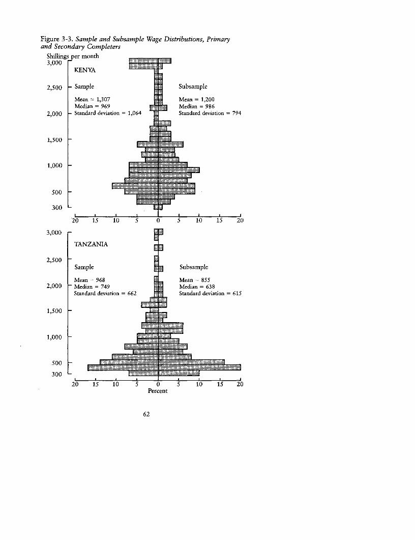
Figure 3-3. Sample and Subsample Wage Distributions, Primaryand Secondary Completers
Shillings per month3,000-
KENYA
2,500 - Sample Subsample
Mean = 1,307 Mean = 1,200Median = 969 Median = 986
2,000 - Standard deviation = 1,064 Standard deviation = 794
1,500 -
1,000 _
500
300
*20 15 10 5 0 5 10 15 20
3,000 -
TANZANIA
2,500 -Sample Subsample
Mean = 968 Mean = 8552,000 -Median = 749 Median = 638
Standard deviation = 662 Standard deviation = 615
1,500
1,000
500 . .
300 L
20 1 10 5 0 0 _5 209~
Percent
62
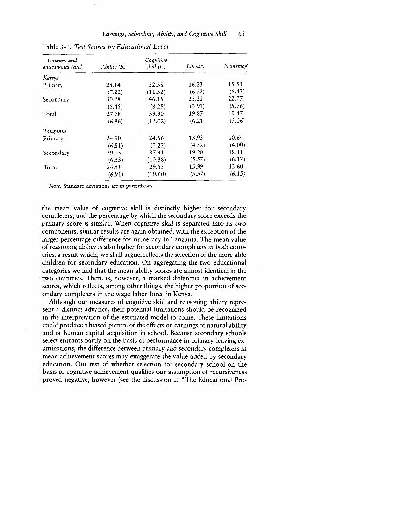
Earnings, Schooling, Ability, and Cognitive Skill 63
Table 3-1. Test Scores by Educational Level
Country and Cognitiveeducational level Ability (R) skill (H) Literacy Numeracy'
KenyaPrimary 25.14 32.38 16.23 15.51
(7.22) (11.52) (6.22) (6.43)Secondary 30.28 46.15 23.21 22.77
(5.45) (8.28) (3.91) (5.76)Total 27.78 39.90 19.87 19.47
(6.86) (12.02) (6.21) (7.06)
TanzaniaPrimary 24.90 24.56 13.93 10.64
(6.81) (7.22) (4.52) (4.00)Secondary 29.03 37.31 19.20 18.11
(6.33) (10.38) (5.57) (6.17)Total 26.51 29.55 15.99 13.60
(6.91) (10.60) (5.57) (6.15)
Note: Standard deviations are in parentheses.
the mean value of cognitive skill is distinctly higher for secondarycompleters, and the percentage by which the secondary score exceeds theprimary score is similar. When cognitive skill is separated into its twocomponents, similar results are again obtained, with the exception of thelarger percentage difference for numeracy in Tanzania. The mean valueof reasoning ability is also higher for secondary completers in both coun-tries, a result which, we shall argue, reflects the selection of the more ablechildren for secondary education. On aggregating the two educationalcategories we find that the mean ability scores are almost identical in thetwo countries. There is, however, a marked difference in achievementscores, which reflects, among other things, the higher proportion of sec-ondary completers in the wage labor force in Kenya.
Although our measures of cognitive skill and reasoning ability repre-sent a distinct advance, their potential limitations should be recognizedin the interpretation of the estimated model to come. These limitationscould produce a biased picture of the effects on earnings of natural abilityand of human capital acquisition in school. Because secondary schoolsselect entrants partly on the basis of performance in primary-leaving ex-aminations, the difference between primary and secondary completers inmean achievement scores may exaggerate the value added by secondaryeducation. Our test of whether selection for secondary school on thebasis of cognitive achievement qualifies our assumption of recursivenessproved negative, however (see the discussion in "The Educational Pro-
64 EDUCATIONAL EXPANSION AND LABOR PRODUCTIVITY
duction and Attainment Functions and Indirect Effects on Earnings,"below). Noncognitive traits, such as attitudes and interests, may also beacquired in school and may be valued in the labor market. Natural abilitymay involve not only reasoning power but also such unmeasured butmarketable qualities as drive, determination, and dynamism. Finally, theability that we measure may not be attributable entirely to heredity andhome environment: education may enhance reasoning power. But theweighted mean values of R for the subsamples are not significantly differ-ent (27.8 in Kenya and 26.5 in Tanzania), whereas those of H are signifi-cantly different (39.9 and 29.6), on account of the greater quantity andquality of secondary education in Kenya (see chapter 4). This suggeststhat R is not acquired in school.
The Expanded Human Capital Earnings Function
Estimates of the conventional human capital earnings function (equation3-1) for Kenya and Tanzania are shown in column 1 of table 3-2.4 InKenya workers are paid a premium of 4.2 percent per year of employ-ment experience, and secondary completers are paid 61 percent morethan primary completers. In Tanzania the returns to experience arehigher (5.4 percent), but because of Tanzania's vigorously imposed paypolicy, the gain from secondary education, although substantial, is lower(32 percent). The Tanzanian government has compressed the structureof wages in the dominant public sector. In the relatively unfettered pri-vate sector the premium on secondary education is higher than in thepublic sector and, indeed, higher than in Kenya. We recognize that thecompetitive market value of secondary education in Tanzania is greaterthan our estimates suggest; see chapter 6.
Do Cognitive Skill and Ability Matter?
Column 2 of table 3-2 permits a comparison of estimates of the conven-tional and expanded human capital earnings functions. In neither Kenyanor Tanzania are the estimated returns to experience affected by the in-troduction of variables that measure (cognitive) achievement and (rea-soning) ability. By contrast, the premium on secondary education de-clines by nearly two-thirds in both countries, and in Tanzania it is nolonger significantly different from zero. In neither country is the indepen-dent influence of ability on earnings either large or significant. By con-trast, in both countries the coefficient on the achievement score is posi-tive, significant, and large in relation to the coefficient on the abilityscore. This result holds when either the literacy or the numeracy scorereplaces the combined score.
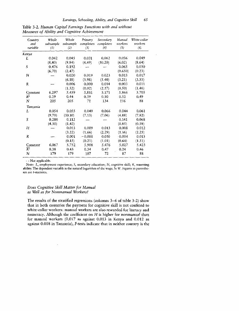
Earnings, Schooling, Ability, and Cognitive Skill 65
Table 3-2. Human Capital Earnings Functions with and withoutMeasures of Ability and Cognitive Achievement
Country Whole Whole Primary Secondary Manual White-collarand subsample subsample completers completers workers workers
variable (1) (2) (3) (4) (5) (6)
KenyaL 0.042 0.045 0.031 0.062 0.036 0.049
(8.40) (9.84) (4.49) (10.20) (6.02) (8.64)S 0.476 0.192 - - 0.065 0.030
(6.70) (2.47) (0.650) (0.23)H - 0.020 0.019 0.023 0.013 0.017
(6.18) (3.98) (5.40) (3.21) (3.55)R - 0.006 0.000 0.014 0.003 0.011
(1.32) (0.02) (2.17) (0.50) (1.46)Constant 6.297 5.459 5.811 5.171 5.866 5.705Tz 0.29 0.44 0.39 0.50 0.32 0.49N 205 205 71 134 116 88
TanzaniaL 0.054 0.055 0.049 0.066 0.044 0.061
(9.70) (10.10) (7.13) (7.06) (4.88) (7.82)S 0.280 0.112 - - 0.141 0.068
(4.30) (1.42) (0.85) (0.58)H - 0.013 0.009 0.013 0.008 0.012
(3.22) (1.66) (2.29) (1.16) (2.25)R - 0.001 -0.001 0.010 -0.004 0.013
(0.15) (0.21) (1.01) (0.64) (1.51)Constant 6.067 5.752 5.908 5.476 5.027 5.423K2 0.38 0.43 0.34 0.47 0.24 0.46N 179 179 107 72 87 88
-Not applicable.Note: L, employment experience; S, secondary education; H, cognitive skill; R, reasoning
ability. The dependent variable is the natural logarithm of the wage, In W. Figures in parenthe-ses are t-statistics.
Does Cognitive Skill Matter for Manualas Well as for Nonmanual Workers?
The results of the stratified regressions (columns 3-6 of table 3-2) showthat in both countries the payment for cognitive skill is not confined towhite-collar workers: manual workers are also rewarded for literacy andnumeracy. Although the coefficient on H is higher for nonmanual thanfor manual workers (0.017 as against 0.013 in Kenya and 0.012 asagainst 0.008 in Tanzania), F-tests indicate that in neither country is the
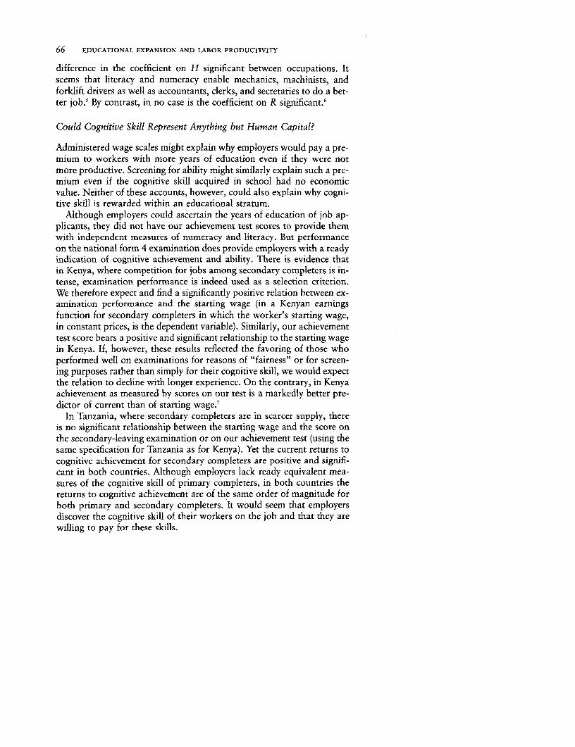
66 EDUCATIONAL EXPANSION AND LABOR PRODUCTIVITY
difference in the coefficient on H significant between occupations. Itseems that literacy and numeracy enable mechanics, machinists, andforklift drivers as well as accountants, clerks, and secretaries to do a bet-ter job.' By contrast, in no case is the coefficient on R significant.6
Could Cognitive Skill Represent Anything but Human Capital?
Administered wage scales might explain why employers would pay a pre-mium to workers with more years of education even if they were notmore productive. Screening for ability might similarly explain such a pre-mium even if the cognitive skill acquired in school had no economicvalue. Neither of these accounts, however, could also explain why cogni-tive skill is rewarded within an educational stratum.
Although employers could ascertain the years of education of job ap-plicants, they did not have our achievement test scores to provide themwith independent measures of numeracy and literacy. But performanceon the national form 4 examination does provide employers with a readyindication of cognitive achievement and ability. There is evidence thatin Kenya, where competition for jobs among secondary completers is in-tense, examination performance is indeed used as a selection criterion.We therefore expect and find a significantly positive relation between ex-amination performance and the starting wage (in a Kenyan earningsfunction for secondary completers in which the worker's starting wage,in constant prices, is the dependent variable). Similarly, our achievementtest score bears a positive and significant relationship to the starting wagein Kenya. If, however, these results reflected the favoring of those whoperformed well on examinations for reasons of "fairness" or for screen-ing purposes rather than simply for their cognitive skill, we would expectthe relation to decline with longer experience. On the contrary, in Kenyaachievement as measured by scores on our test is a markedly better pre-dictor of current than of starting wage.7
In Tanzania, where secondary completers are in scarcer supply, thereis no significant relationship between the starting wage and the score onthe secondary-leaving examination or on our achievement test (using thesame specification for Tanzania as for Kenya). Yet the current returns tocognitive achievement for secondary completers are positive and signifi-cant in both countries. Although employers lack ready equivalent mea-sures of the cognitive skill of primary completers, in both countries thereturns to cognitive achievement are of the same order of magnitude forboth primary and secondary completers. It would seem that employersdiscover the cognitive skill of their workers on the job and that they arewilling to pay for these skills.
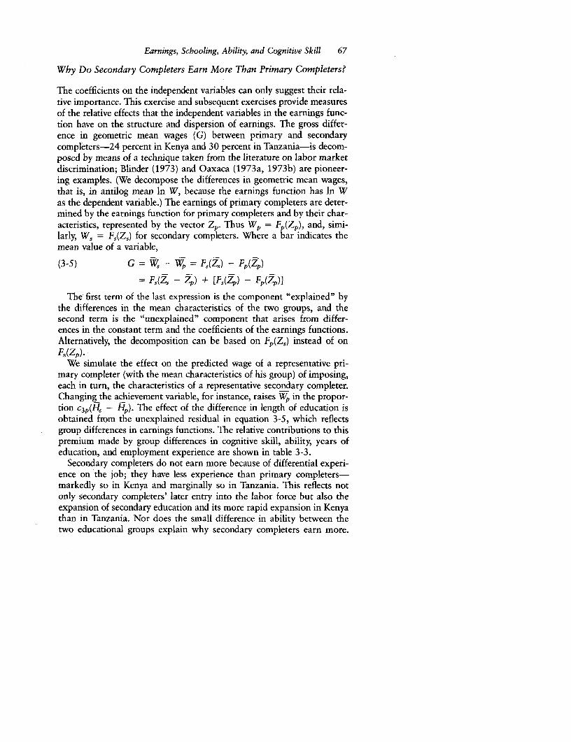
Earnings, Schooling, Ability, and Cognitive Skill 67
Why Do Secondary Completers Earn More Than Primary Completers?
The coefficients on the independent variables can only suggest their rela-tive importance. This exercise and subsequent exercises provide measuresof the relative effects that the independent variables in the earnings func-tion have on the structure and dispersion of earnings. The gross differ-ence in geometric mean wages (G) between primary and secondarycompleters-24 percent in Kenya and 30 percent in Tanzania-is decom-posed by means of a technique taken from the literature on labor marketdiscrimination; Blinder (1973) and Oaxaca (1973a, 1973b) are pioneer-ing examples. (We decompose the differences in geometric mean wages,that is, in antilog mean In W, because the earnings function has In Was the dependent variable.) The earnings of primary completers are deter-mined by the earnings function for primary completers and by their char-acteristics, represented by the vector Zp. Thus Wp = Fp(Z,), and, simi-larly, W, = F,(Z,) for secondary completers. Where a bar indicates themean value of a variable,
(3-5) G = Ws - Wp =F.,(Z) -Fp(Zp)
= Fs(Z, - Zp) + [Fs(Zp) - Fp(7)]
The first term of the last expression is the component "explained" bythe differences in the mean characteristics of the two groups, and thesecond term is the "unexplained" component that arises from differ-ences in the constant term and the coefficients of the earnings functions.Alternatively, the decomposition can be based on Fp(Z,) instead of onFs(Zp).
We simulate the effect on the predicted wage of a representative pri-mary completer (with the mean characteristics of his group) of imposing,each in turn, the characteristics of a representative secondary completer.Changing the achievement variable, for instance, raises Wp in the propor-tion c3p(H1 - Hp). The effect of the difference in length of education isobtained from the unexplained residual in equation 3-5, which reflectsgroup differences in earnings functions. The relative contributions to thispremium made by group differences in cognitive skill, ability, years ofeducation, and employment experience are shown in table 3-3.
Secondary completers do not earn more because of differential experi-ence on the job; they have less experience than primary completers-markedly so in Kenya and marginally so in Tanzania. This reflects notonly secondary completers' later entry into the labor force but also theexpansion of secondary education and its more rapid expansion in Kenyathan in Tanzania. Nor does the small difference in ability between thetwo educational groups explain why secondary completers earn more.
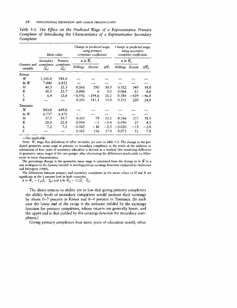
68 EDUCATIONAL EXPANSION AND LABOR PRODUCTIVITY
Table 3-3. The Effect on the Predicted Wage of a Representative PrimaryCompleter of Introducing the Characteristics of a Representative SecondaryCompleter
Change in predicted wage, Change in predicted wage,using primary using secondary
Mean value completer coefficients completer coefficients
Secondary Primary A In W, A In W,pCountry and completers completers
variable (ZI) (Z) Shillings Percent AW, Shillings Percent AWp
KenyaW 1,141.0 918.0 - - - - - -
In W 7.040 6.822 - - - - - -
H 46.3 32.3 0.266 280 30.5 0.322 349 38.0R 30.3 25.7 0.000 0 0.0 0.064 61 6.6L 6.4 12.6 - 0.192 -194.6 -21.2 -0.384 -429 -46.8S - - 0.143 141.3 15.4 0.215 220 24.0
TanzaniaW 843.0 649.0 - - - - - -
In W 6.737 6.475 - - - - - -
H 37.5 24.7 0.115 79 12.2 0.166 117 18.1R 29.0 25.0 -0.004 -3 - 0.4 0.040 27 4.1
L 7.2 7.5 -0.015 - 10 - 1.5 - 0.020 - 13 - 2.0S - - 0.165 116 17.9 0.075 51 7.8
-Not applicable.Note: W, wage. For definitions of other variables, see note to table 3-2. The change in the pre-
dicted geometric mean wage of primary or secondary completers as the result of the addition orsubtraction of four years of secondary education is derived as a residual (the remaining differencein geometric mean wages of the two groups) after eliminating the differences attributable to differ-ences in mean characteristics.
The percentage change in the geometric mean wage is caLculated from the change in In W in away analogous to the dummy variable in semilogarithmic earnings functions explained by Halvorsenand Palmquist (1980).
Tihe differences between primary and secondary completers in the mean values of H and R aresignificant at the 1 percent level in both countries._
A In W, = C,(Z,- Z,) and A In Wp = CZ(Z- Zp).
The direct returns to ability are so low that giving primary completersthe ability levels of secondary completers would increase their earningsby about 0-7 percent in Kenya and 0-4 percent in Tanzania. (In eachcase the lower end of the range is the estimate yielded by the earningsfunction for primary completers, whose returns are generally lower, andthe upper end is that yielded by the earnings function for secondary com-pleters.)
Giving primary completers four more years of education would, other
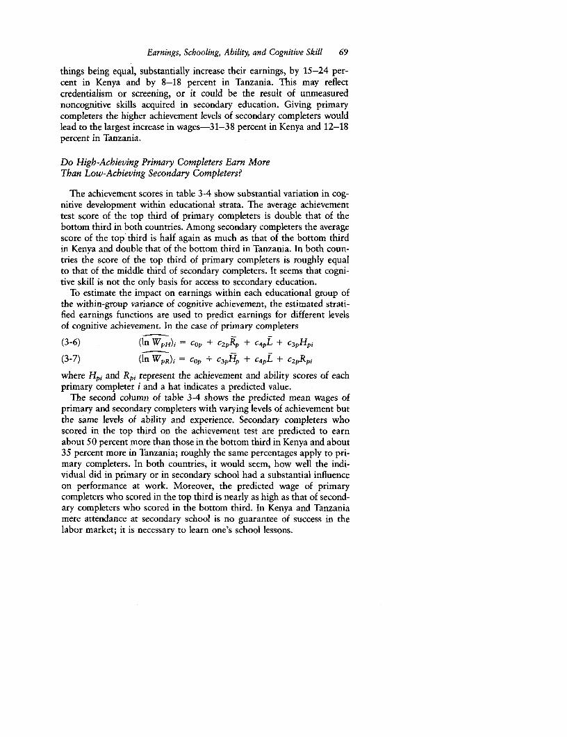
Earnings, Schooling, Ability, and Cognitive Skill 69
things being equal, substantially increase their earnings, by 15-24 per-cent in Kenya and by 8-18 percent in Tanzania. This may reflectcredentialism or screening, or it could be the result of unmeasurednoncognitive skills acquired in secondary education. Giving primarycompleters the higher achievement levels of secondary completers wouldlead to the largest increase in wages-31-38 percent in Kenya and 12-18percent in Tanzania.
Do High-Achieving Primary Completers Earn MoreThan Low-Achieving Secondary Completers?
The achievement scores in table 3-4 show substantial variation in cog-nitive development within educational strata. The average achievementtest score of the top third of primary completers is double that of thebottom third in both countries. Among secondary completers the averagescore of the top third is half again as much as that of the bottom thirdin Kenya and double that of the bottom third in Tanzania. In both coun-tries the score of the top third of primary completers is roughly equalto that of the middle third of secondary completers. It seems that cogni-tive skill is not the only basis for access to secondary education.
To estimate the impact on earnings within each educational group ofthe within-group variance of cognitive achievement, the estimated strati-fied earnings functions are used to predict earnings for different levelsof cognitive achievement. In the case of primary completers
(3-6) (In WpH)i = Cop + C2ppR + c4pL + C3pHp
(3-7) (In WPR)i = cop + c3PHP + c4PL + c2pRp,
where Hpi and Rpi represent the achievement and ability scores of eachprimary completer i and a hat indicates a predicted value.
The second column of table 3-4 shows the predicted mean wages ofprimary and secondary completers with varying levels of achievement butthe same levels of ability and experience. Secondary completers whoscored in the top third on the achievement test are predicted to earnabout 50 percent more than those in the bottom third in Kenya and about35 percent more in Tanzania; roughly the same percentages apply to pri-mary completers. In both countries, it would seem, how well the indi-vidual did in primary or in secondary school had a substantial influenceon performance at work. Moreover, the predicted wage of primarycompleters who scored in the top third is nearly as high as that of second-ary completers who scored in the bottom third. In Kenya and Tanzaniamere attendance at secondary school is no guarantee of success in thelabor market; it is necessary to learn one's school lessons.
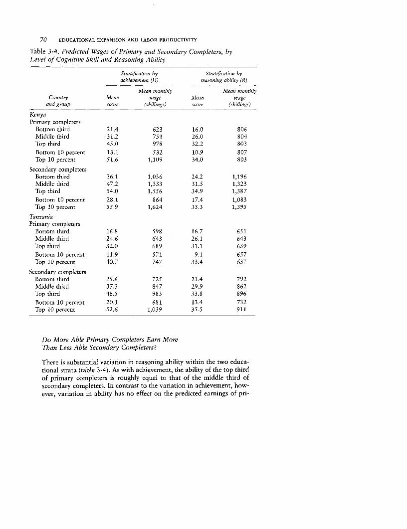
70 EDUCATIONAL EXPANSION AND LABOR PRODUCTIVITY
Table 3-4. Predicted Wages of Primary and Secondary Completers, byLevel of Cognitive Skill and Reasoning Ability
Stratification by Stratification byachievement (H) reasoning ability (R)
Mean monthly Mean monthlyCountry Mean wage Mean wage
and group score (shillings) score (shillings)
KenyaPrimary completers
Bottom third 21.4 623 16.0 806Middle third 31.2 751 26.0 804Top third 45.0 978 32.2 803
Bottom 10 percent 13.1 532 10.9 807Top 10 percent 51.6 1,109 34.0 803
Secondary completersBottom third 36.1 1,036 24.2 1,196Middle third 47.2 1,333 31.5 1,323Top third 54.0 1,556 34.9 1,387
Bottom 10 percent 28.1 864 17.4 1,083Top 10 percent 55.9 1,624 35.3 1,395
TanzaniaPrimary completers
Bottom third 16.8 598 16.7 651Middle third 24.6 643 26.1 643Top third 32.0 689 31.1 639
Bottom 10 percent 11.9 571 9.1 657Top 10 percent 40.7 747 33.4 637
Secondary completersBottom third 25.6 725 21.4 792Middle third 37.3 847 29.9 862Top third 48.5 983 33.8 896
Bottom 10 percent 20.1 681 13.4 732Top 10 percent 52.6 1,039 35.5 911
Do More Able Primary Completers Earn MoreThan Less Able Secondary Completers?
There is substantial variation in reasoning ability within the two educa-tional strata (table 3-4). As with achievement, the ability of the top thirdof primary completers is roughly equal to that of the middle third ofsecondary completers. In contrast to the variation in achievement, how-ever, variation in ability has no effect on the predicted earnings of pri-
Earnings, Schooling, Ability, and Cognitive Skill 71
mary completers and little on those of secondary completers. Moreover,whereas the ability scores of the ablest 10 percent of primary completersare more than double those of the least able 10 percent of secondarycompleters, their predicted wages are lower. In neither country is beingamong the ablest of one's peers a sufficient condition for successful per-formance in the labor market.
How Much Inequality Is Attributable to Cognitive Skill?
The effects that ability, cognitive skill, or years of education have on thedispersion of earnings may differ in relative importance from their effectson the structure of earnings. The latter effects depend only on the sizeof the coefficients in the earnings function. The former effects depend,in addition, on the distribution of characteristics among employees andon the location in the distribution of pay of employees with various char-acteristics.
To measure relative contributions to dispersion we use equation 3-4-written here as In Wi =a + I, bij Zip, where Zij is the set of independentvariables (j =1 . . . n)-to predict the earnings of each employee (W1).Each independent variable (1) is in turn set equal to its mean value, andpredicted earnings (Wij) are estimated with the use of the set of othercharacteristics possessed by each employee. Here (WT) represents thepredicted value of W for each individual (i) when his endowment of jequals that of all other individuals. The variances of Wi and Wi, arecalculated, and the contribution of Z. to the explained variance ofearnings is estimated as var(Wi) - var(Wij). The relative contribution ofeach individual variable is calculated by expressing its contribution asa percentage of Yj [var(Wi) - var(Wqi)].8 In effect, we are attempting toanswer the counterfactual question, what would be the effect on theinequality of pay if, while mean earnings were held constant, thedispersion attributable to a particular characteristic, such as cognitiveachievement, were eliminated?
The relative contribution to inequality of each independent variable inthe expanded human capital earnings function for the unstratified sampleis shown in table 3-5. The contribution of employment experience to thevariance of earnings is markedly greater in Tanzania than in Kenya. InTanzania mean experience rises monotonically, from 3.1 years in the low-est earnings quintile to 12.1 years in the highest. That is not the case inKenya, where high levels of experience are associated with low as wellas with high incomes, possibly because of the inverse correlation betweeneducation and experience: the more educated, who are more plentiful inKenya, have received preference in access to jobs over the more experi-enced but less educated. The contribution of the ability variable to thevariance of earnings is small in both countries, partly because of its negli-
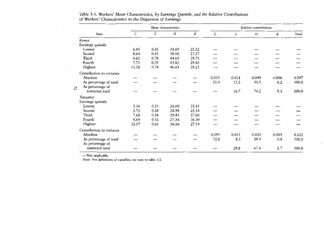
Table 3-5. Workers' Mean Characteristics, by Earnings Quintile, and the Relative Contributionsof Workers' Characteristics to the Dispersion of Earnings
Mean characteristics Relative contributions
Item EL S k L S H R Total
KenyaEarnings quintile
Lowest 6.45 0.43 31.69 25.32 - - - - -
Second 8.64 0.45 38.00 27.57 - - - - -
Third 6.62 0.78 44.60 29.71 - - - - -
Fourth 7.73 0.70 43.82 29.80 - - - - -
Highest 13.28 0.74 46.61 29.21 - - - -
Contribution to varianceAbsolute - - - - 0.031 0.011 0.049 0.006 0.097As percentage of total - - - - 32.0 11.3 50.5 6.2 100.0
- As percentage ofrestricted total - - - - - 16.7 74.2 9.1 100.0
TanzaniaEarnings quintile
Lowest 3.16 0.23 26.00 25.41 - - - - -
Second 5.73 0.38 28.98 25.14 - - - - -
Third 7.68 0.38 29.43 27.60 - - - - -
Fourth 8.69 0.32 27.56 26.10 - - - - -
Highest 12.07 0.61 36.16 27.54 - - - - -
Contribution to varianceAbsolute - - - - 0.095 0.011 0.025 0.001 0.132As percentage of total - - - - 72.0 8.3 18.9 0.8 100.0As percentage of
restricted total - - - - - 29.8 67.6 2.7 100.0
-Not applicable.Note: For definitions of variables, see note to table 3-2.
Earnings, Schooling, Ability, and Cognitive Skill 73
gible coefficient and partly because high and low earners have similarability scores. The contribution of years of education is larger, reflectingthe size of its coefficient and the tendency for the proportion with second-ary education to rise with earnings quintile. In Kenya achievement ac-counts for three-quarters of the variance in earnings explained jointly byability, education, and achievement; in Tanzania the share is two-thirds.Not only is cognitive skill highly rewarded, but there are few highly liter-ate and numerate workers, be they primary or secondary completers, inthe low-earnings quintiles.
The Educational Production and Attainment Functionsand Indirect Effects on Earnings
Having shown that length of education has a relatively small effect onearnings and ability a negligible direct influence, we now examine possi-ble indirect influences through the effects of these factors on cognitiveachievement. The simple correlations between S and H and between Rand H are strong and positive. The mean achievement scores are signifi-cantly higher for secondary than for primary completers (43 percenthigher in Kenya and 52 percent higher in Tanzania), and there is a mono-tonic relationship between ability groups and their mean levels ofachievement.
The educational production function (from equation 3-3) is presentedin table 3-6 with the use of linear and log linear specifications. In bothcountries cognitive achievement bears a highly significant positive rela-tionship to educational level and to ability. In Kenya secondary education(S) raises H by 11.75 points (linear form), or by 44 percent (log lin-ear form); similar results are obtained for Tanzania. The elasticity ofresponse of cognitive skill to reasoning ability (R) is roughly one-third in both countries. In Kenya the coefficient on G (a dummy variablethat takes a value of 1 if the secondary school attended by a secondarycompleter or the primary school attended by a primary completer wasa government school and that takes a value of 0 otherwise) is significantlypositive in the linear specification. In both countries the coefficient on B(a dummy variable that is 1 for birth in an urban area and 0 for birthin a rural area) is almost significantly negative in the linear specification.(This counterintuitive result may reflect greater selectivity in access toschooling and to the urban labor market among the rural-born, who facestiffer competition.)9
An educational attainment function (from equation 3-2) was estimatedby means of probit analysis. The results are very similar in Kenya andTanzania, respectively:
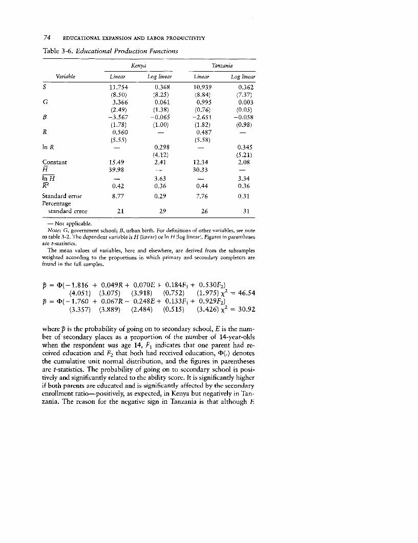
74 EDUCATIONAL EXPANSION AND LABOR PRODUCTIVITY
Table 3-6. Educational Production Functions
Kenya Tanzania
Variable Linear Log linear Linear Log linear
S 11.754 0.368 10.939 0.362(8.50) (8.25) (8.84) (7.37)
G 3.366 0.061 0.995 0.003(2.49) (1.38) (0.76) (0.05)
B -3.567 -0.065 -2.651 -0.058(1.78) (1.00) (1.82) (0.98)
R 0.560 - 0.487 -
(5.55) (5.58)In R - 0.298 - 0.345
(4.12) (5.21)Constant 15.49 2.41 12.34 2.08H 39.98 - 30.33 -InH - 3.63 - 3.34iK2 0.42 0.36 0.44 0.36
Standard error 8.77 0.29 7.76 0.31Percentage
standard error 21 29 26 31
- Not applicable.Note: G, government school; B, urban birth. For definitions of other variables, see note
to table 3-2. The dependent variable is H (linear) or In H (log linear). Figures in parenthesesare t-statistics.
The mean values of variables, here and elsewhere, are derived from the subsamplesweighted according to the proportions in which primary and secondary completers arefound in the full samples.
4p = (- 1.816 + 0.049R + 0.070E + 0.184F 1 + 0.530F 2 )(4.051) (3.075) (3.918) (0.752) (1.975) x2 = 46.54
7= '(-1.760 + 0.067R - 0.248E+ 0.133F1 + 0.929F 2 )(3.357) (3.889) (2.484) (0.515) (3.426) X2 = 30.92
where p is the probability of going on to secondary school, E is the num-ber of secondary places as a proportion of the number of 14-year-oldswhen the respondent was age 14, F1 indicates that one parent had re-ceived education and F2 that both had received education, D(.) denotesthe cumulative unit normal distribution, and the figures in parenthesesare t-statistics. The probability of going on to secondary school is posi-tively and significantly related to the ability score. It is significantly higherif both parents are educated and is significantly affected by the secondaryenrollment ratio-positively, as expected, in Kenya but negatively in Tan-zania. The reason for the negative sign in Tanzania is that although E
Earnings, Schooling, Ability, and Cognitive Skill 75
rose over time, the proportion of primary completers who went on tosecondary school actually fell. With all independent variables at theirmean values, an increase in the ability score from the mean of the bottomthird to that of the top third would raise the probability of secondaryschool attendance by 0.25 in Kenya and by 0.35 in Tanzania. Abilitytherefore has two indirect effects on earnings, not only via relation D butalso via relation E in figure 3-1.
Before combining the three functions for simulation analysis, we testwhether the estimated model is recursive-that is, whether the estimatesare consistent and not subject to simultaneous equation bias. If some un-measured characteristics, such as drive and determination, contributedto educational attainment, cognitive skill, and earnings, the error terms(v, y, and z, respectively) in equations 3-2, 3-3, and 3-4 would be corre-lated, as would educational attainment and y, educational attainmentand z, and cognitive skill and z. We apply a specification test developedby Hausman (1978) and add the predicted value of educational attain-ment (S) for each individual as an independent variable in equations 3-3and 3-4 and the predicted value of cognitive skill (H) as an independentvariable in equation 3-4. (S and H are generated with the use of equations3-2 and 3-3, respectively, plus the other exogenous variables in the three-equation system; the linear form of equation 3-3 is used.) The coefficientsare not significantly different from zero in five of the six cases and arejust significantly so in the sixth. These findings support the null hypothe-sis that the equation system is recursive."'
As a further test of recursiveness between equations 3-2 and 3-3, weestimate equation 3-3 in the linear form with the use of instrumental vari-ables and use the estimated coefficients to generate HŽ for each individualat the end of primary school (that is, with S =0). Equation 3-2 is thenestimated with H4 as an additional independent variable. The coefficienton H is not significant in either country, which suggests that simultaneityon account of selection for secondary school on the basis of cognitiveachievement is unlikely. The coefficient was actually negative, being-0.090 (standard error = 0.053) in Kenya and -0.063 (0.079) in Tanza-nia.
In table 3-7 the indirect effects of ability are measured and comparedwith the direct effects. Two ability levels are considered in each sample,corresponding to the mean values of R for the top and bottom thirds;all other characteristics of the sample are kept at their mean values.Within the three-equation system we then trace the difference in pre-dicted wages between the two ability levels that is attributable to rela-tions C, D, and E in figure 3-1. The full consequence (incorporating allthree effects) of the assumed difference in ability is to create a differencein predicted wages equal to 32 percent of the sample mean in Kenya and16 percent in Tanzania. The direct effect on earnings of differences in
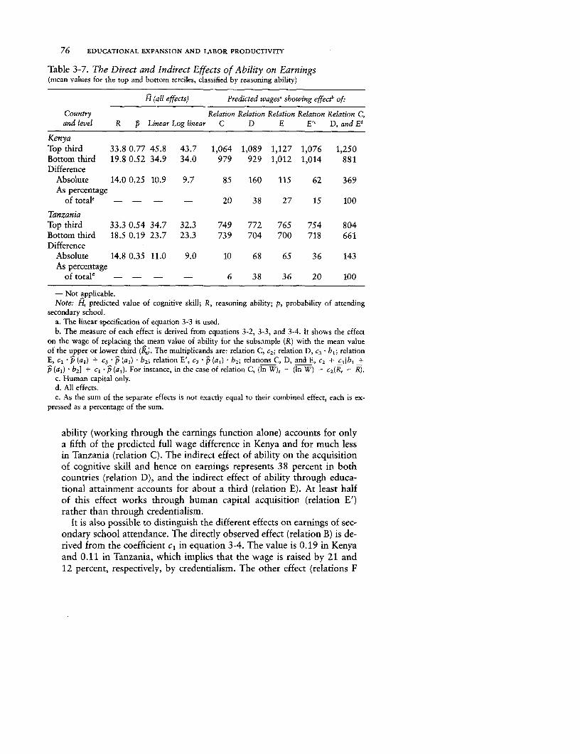
76 EDUCATIONAL EXPANSION AND LABOR PRODUCTIVITY
Table 3-7. The Direct and Indirect Effects of Ability on Earnings(mean values for the top and bottom terciles, classified by reasoning ability)
H (all effects) Predicted wages' showing effectb of.
Country Relation Relation Relation Relation Relation C,and level R p Linear Log linear C D E E" D, and Ed
KenyaTop third 33.8 0.77 45.8 43.7 1,064 1,089 1,127 1,076 1,250Bottom third 19.8 0.52 34.9 34.0 979 929 1,012 1,014 881Difference
Absolute 14.0 0.25 10.9 9.7 85 160 115 62 369As percentage
of total' - - - - 20 38 27 15 100
TanzaniaTop third 33.3 0.54 34.7 32.3 749 772 765 754 804Bottom third 18.5 0.19 23.7 23.3 739 704 700 718 661Difference
Absolute 14.8 0.35 11.0 9.0 10 68 65 36 143As percentage
of total' - - - - 6 38 36 20 100
- Not applicable.Note: H, predicted value of cognitive skill; R, reasoning ability; p, probability of attending
secondary school.a. The linear specification of equation 3-3 is used.b. The measure of each effect is derived from equations 3-2, 3-3, and 3-4. It shows the effect
on the wage of replacing the mean value of ability for the subsample (R) with the mean valueof the upper or lower third (RJ. The multiplicands are: relation C, c2; relation D, c3 * b; relationE, cl * p (a,) + C3 * p (a,) - b2; relation E', c3 * p (a,) * b2 ; relations C, D, and E, c2 + c3[b1 +p (a,) * b2] + cl * p (a,). For instance, in the case of relation C, (In W)1 - (In W) = c2 (R, - R).
c. Human capital only.d. All effects.e. As the sum of the separate effects is not exactly equal to their combined effect, each is ex-
pressed as a percentage of the sum.
ability (working through the earnings function alone) accounts for onlya fifth of the predicted full wage difference in Kenya and for much lessin Tanzania (relation C). The indirect effect of ability on the acquisitionof cognitive skill and hence on earnings represents 38 percent in bothcountries (relation D), and the indirect effect of ability through educa-tional attainment accounts for about a third (relation E). At least halfof this effect works through human capital acquisition (relation E')rather than through credentialism.
It is also possible to distinguish the different effects on earnings of sec-ondary school attendance. The directly observed effect (relation B) is de-rived from the coefficient cl in equation 3-4. The value is 0.19 in Kenyaand 0.11 in Tanzania, which implies that the wage is raised by 21 and12 percent, respectively, by credentialism. The other effect (relations F
Earnings, Schooling, Ability, and Cognitive Skill 77
and A) is derived from a combination of equations 3-3 and 3-4. The coef-ficient b2 in the former shows the effect of secondary schooling on cogni-tive skill, and the coefficient C3 in the latter shows the effect of cognitiveskill on earnings. Their product, b2 * C3 (0.22 in Kenya and 0.14 in Tanza-nia), indicates that human capital acquisition in secondary school raisesearnings by 25 and 15 percent, respectively. The human capital effect ofa secondary education thus exceeds the credentialist effect. Thus use ofthe three-equation system has shown that the indirectly measured effectsof differences in reasoning ability and in educational attainment both ex-ceed the direct effects.
Conclusions
Our survey data from Kenya and Tanzania have permitted a sharper testthan hitherto of the competing explanations-credentialism, ability,screening, or human capital-of why workers with secondary educationearn more than those without secondary education. The direct returnsto reasoning ability in the labor market are small, those to years of educa-tion are moderate, and those to literacy and numeracy-which are di-mensions of human capital-are large. The returns to cognitive achieve-ment are not significantly lower for manual than for nonmanualworkers.
The returns to cognitive skill cannot but be a payment for human capi-tal. The direct returns to years of education, however, could reflectcredentialism, screening, or human capital acquired at school or at home;that is, their interpretation is inconclusive. It appears that literate andnumerate workers are more productive and that education is valuable toworkers because it can give them skills that increase their productivity.These conclusions have generally satisfied the usual statistical tests. Theirrobustness derives no less from the fact that they all apply to both Kenyaand Tanzania.
The main effects of length of education and reasoning ability on earn-ings are indirect, as these factors operate through the development ofcognitive skill. Longer-educated or brighter workers tend to be more lit-erate and numerate. The main reason why secondary completers earnmore on average than primary completers is their higher average levelof cognitive achievement. There is substantial variation, however, in cog-nitive achievement and in reasoning ability within the two educationalgroups. Whereas primary completers of high ability earn less than lessable secondary completers, primary completers with high cognitive skillactually earn more than less skilled secondary completers. Within eacheducational group high achievers earn a great deal more than low achiev-ers. Just as cognitive achievement is the main determinant of the structure

78 EDUCATIONAL EXPANSION AND LABOR PRODUCTIVITY
of earnings, it also accounts for much of the inequality of earnings amongworkers, far more than do reasoning ability and school attendance. Be-cause inequality is primarily attributable to differences in productivitythat arise from differences in cognitive skill, the efficiency cost of reduc-ing inequality may be high.
Our analysis provides strong support for the human capital interpreta-tion of the educational structure of wages. Whether these conclusionsshould be generalized beyond Kenya and Tanzania to the many othercountries for which rates of returns have been estimated is open to ques-tion. Kenya and Tanzania have much lower incomes, and cognitive skillis in shorter supply, than in most developing countries, particularly thoseof Asia and Latin America. As economic development proceeds, thegrowth of enrollment may outstrip the growth of the economy. In thatcase the returns to cognitive achievement may decline, whereas for politi-cal and institutional reasons the returns to years of education may remainhigh.
Notes
1. See Psacharopoulos (1973, 1981) for a listing of the estimates obtained fromrate of return studies in forty-four countries.
2. See, for instance, Arrow (1973), Blaug (1976), Bowles and Gintis (1976),Riley (1979), Spence (1976), and Thurow (1975).
3. For attempts to control for ability or for cognitive achievement in studiesfor the United States, see Behrman and others (1980), Chamberlain and Griliches(1977), Griliches and Mason (1972), Olneck (1977), Taubman (1975), Taubmanand Wales (1974), and Wise (1975); see also the survey articles by Griliches(1977, 1979). In most instances the data refer to special subgroups in the popula-tion, and a clear distinction cannot be made between natural ability and cognitiveskill acquired in school.
4. The equations were also estimated with a squared experience term, butwhereas the coefficient was negative as expected, it was not significantly differentfrom zero.
5. In only one of the four cases, that of manual workers in Tanzania, is thecoefficient on achievement not significant at the 5 percent level.
6. When the samples are stratified instead by educational levels, F-tests indicateprecisely equivalent results for the achievement variable. The effect of ability onearnings remains small in comparison with the effect on achievement, and it isnot significantly different from zero in three of the four cases.
7. The substitution of In starting wage for ln current wage as the dependentvariable in column 2 of table 3-2 results in a reduction in the coefficient on Hfrom 0.020 to 0.011. That is, the percentage response of current wage to a unitincrease in H is nearly twice as great as that of starting wage.
8. For further explication of this method of decomposing inequality and a com-parison with other methods, see Behrman, Knight, and Sabot (1983).
Earnings, Schooling, Ability, and Cognitive Skill 79
9. The log-linear specification (with the continuous variables H and R in natu-ral logarithms) gave similar results but was inferior in terms of the percentagestandard error of H (29 percent in Kenya and 31 percent in Tanzania) and thesignificance of some coefficients. The ensuing simulation analysis is based on thelinear specification, but the results are not sensitive to the choice of specification.
10. The coefficients are, respectively, -1.518 (0.373), -0.058 (0.210), and-0.011 (0.748) in Kenya and 4.243 (1.430), 0.433 (2.036), and -0.011 (0.647)in Tanzania. (The figures in parentheses are t-statistics.) The possibility of simul-taneity between equations 3-2 and 3-4 in Tanzania makes the Tanzanian resultsless reliable. But the coefficient on S is significantly positive, which implies thatit is biased downward. This suggests that the bias is not attributable to simultane-ity.

CHAPTER 4
Why the Returns to ExperienceIncrease with Education
IN CHAPTER 3 WE ASSESSED the alternative hypotheses concerning thepositive relationship between education and earnings. Throughout theanalysis we standardized for employment experience; that is, we assumedthat wages increase with employment experience at the same rate forboth primary and secondary completers. In quite a few countries,however, a positive relationship between educational attainment and thereturns to employment experience has been observed with the aid ofearnings functions.' It is therefore possible that a substantial proportionof the gross returns to secondary education is accounted for by thisdifference in the returns to experience of educational groups. If thereason for the interaction between education and the returns to ex-perience were independent of human capital accumulation, we wouldhave to qualify the conclusions of chapter 3.
The tendency for the earnings-experience profile to be steeper for themore educated is open to competing explanations. Human capital theoryprovides an explanation, but so do screening and credentialism. Whichexplanation prevails is important for estimating the social returns toschooling and hence for policy. In this chapter we employ our uniquemicro data sets to measure the relationship between education and thereturns to experience and to subject the human capital interpretation ofthe relationship to a simple but persuasive test.
The following section uses earnings functions to measure the re-lationship between the educational level of employees and the slope ofthe experience-earnings profile. That relationship is shown to be stronglypositive. Subsequent sections discuss alternative models of the economicbehavior that gives rise to this relationship, present simple simulationsas a means of assessing the implications of the human capital hypothesisand the screening and credentialist hypotheses for the rate of return tosecondary schooling, specify the test used to adjudicate between thecompeting hypotheses, and present the results.
80
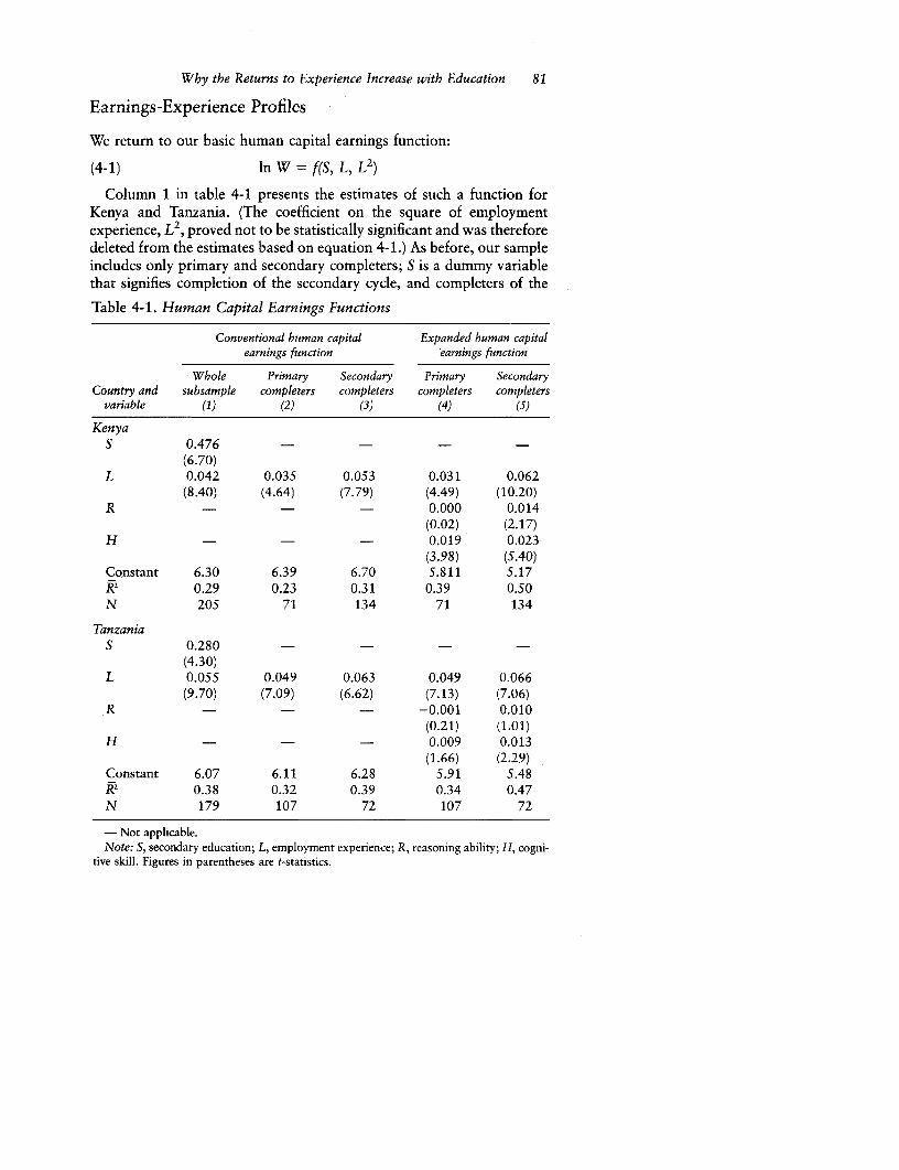
Why the Returns to Experience Increase with Education 81
Earnings-Experience Profiles
We return to our basic human capital earnings function:
(4-1) In W = f(S, L, L2)
Column 1 in table 4-1 presents the estimates of such a function forKenya and Tanzania. (The coefficient on the square of employmentexperience, L2, proved not to be statistically significant and was thereforedeleted from the estimates based on equation 4-1.) As before, our sampleincludes only primary and secondary completers; S is a dummy variablethat signifies completion of the secondary cycle, and completers of theTable 4-1. Human Capital Earnings Functions
Conventional human capital Expanded human capitalearnings function earnings function
Whole Primary Secondary Primary SecondaryCountry and subsample completers completers completers completers
variable (1) (2) (3) (4) (5)
KenyaS 0.476 - - - -
(6.70)L 0.042 0.035 0.053 0.031 0.062
(8.40) (4.64) (7.79) (4.49) (10.20)R - - - 0.000 0.014
(0.02) (2.17)H - - - 0.019 0.023
(3.98) (5.40)Constant 6.30 6.39 6.70 5.811 5.17K 0.29 0.23 0.31 0.39 0.50N 205 71 134 71 134
TanzaniaS 0.280 - - - -
(4.30)L 0.055 0.049 0.063 0.049 0.066
(9.70) (7.09) (6.62) (7.13) (7.06)R - - - -0.001 0.010
(0.21) (1.01)H - - - 0.009 0.013
(1.66) (2.29)Constant 6.07 6.11 6.28 5.91 5.48R2 0.38 0.32 0.39 0.34 0.47N 179 107 72 107 72
- Not applicable.Note: S, secondary education; L, employment experience; R, reasoning ability; H, cogni-
tive skill. Figures in parentheses are t-statistics.
82 EDUCATIONAL EXPANSION AND LABOR PRODUCTIVITY
primary cycle are the base. As expected, the coefficients on the twoindependent variables, S and L, are positive, large, and highly significantin both countries.
In columns 2 and 3 the sample is stratified to determine whether thereturns to experience vary by educational level. In Kenya the incrementto earnings per year of employment experience is 51 percent higher forsecondary than for primary completers, and in Tanzania it is 29 percenthigher. Estimation (not shown) of an interactive specification, In W =f(S, L, S * L), of the earnings function confirmed that the difference inreturns to experience between educational levels is significant at the 1percent level in Kenya and at the 10 percent level in Tanzania.
We present again the expanded human capital earnings function
(4-2) ln W = f(S, L, L2, R, H)
but in its stratified form:
(4-3) In W = f(L, L2, R, H)
Primary and secondary completers are heterogeneous in that withinboth groups there is substantial variance in reasoning ability and incognitive achievement.' The expanded earnings function can showwhether this heterogeneity matters to earnings and, if so, whether takingaccount of it alters the relationship between education and the returnsto experience. It is possible that the observed positive relationship ismerely a statistical artifact that arises from omitted variable bias.3
Columns 4 and 5 present the estimates of the expanded human capitalearnings function. (Again, the coefficient on L' proved not to bestatistically significant and was therefore deleted from the estimatesbased on equations 4-2 and 4-3.) For both countries the coefficients onthe ability variables are small and not statistically significant in theregressions for primary and for secondary completers. The coefficientson cognitive achievement are large and positive in all four cases and aresignificant at the 1 percent level in three of the four cases. The positiveassociation between educational level and the returns to experience is notdiminished by the inclusion of the ability and achievement variables.Indeed, the difference in returns to experience for primary and forsecondary completers is actually larger with this specification than withthe conventional one. Estimation (not shown) of an interactive specifica-tion, In W = f(E, L, R, H, E * L, E - R, E * H), of the expanded humancapital earnings function again confirmed the statistical significance, atthe 1 percent level in Kenya but at the 10 percent level in Tanzania, ofthe difference in returns to experience between educational groups. (Thecoefficients on the E -R and E * H terms were not significant.)
Why the Returns to Experience Increase with Education 83
Competing Hypotheses
What is the explanation for the strong positive relationship betweeneducational attainment and returns to employment experience that isobserved in Kenya and Tanzania? The following system of equations, anexpansion of the system used in chapter 3, illustrates the alternatives:
(4-4) E = ao + a1 R + a2 F + u1
(4-5) T = bo + bjR + b2F + b3H + U2
(4-6) H = co + cjE + c 2R + u 3
(4-7) V = do + d 1T + d2 R + d3 H + U4
(4-8) In W= eo + ejH + e2V + e3 Q + e4R + u5
where
H = cognitive skill acquired in schoolV = vocational and other skills acquired in postschool trainingQ = seniority on the jobE = years of schoolingR = reasoning abilityT = extent of postschool trainingF = an indicator of parents' educationu = error terms
Equations 4-4 and 4-5 are educational and training attainment func-tions, equations 4-6 and 4-7 are educational and training productionfunctions, and equation 4-8 is an earnings function. Although L is centralto our empirical analysis, it does not appear in these equations but mayact as a proxy for V or Q.
The Human Capital Explanation
Complementarity between investments in schooling and in postschooltraining can explain why the returns to experience are higher among themore educated. The linkages are as follows:
aH daT dV dV d In WaS > iH a i T > a; H >i V
The more education a worker has received, the greater will be hiscognitive skill. The more cognitive skill he has acquired, the greater willbe the vocational skills acquired in the course of his working life, bothbecause he is likely to devote more time to training and because his higherlevel of cognitive skill permits him to derive more from any given training
84 EDUCATIONAL EXPANSION AND LABOR PRODUCTIVITY
period. (Where training opportunities are rationed by meritocraticcriteria, he is more likely to be selected for training programs; where aprice rationing system is in effect, he is likely to demand more trainingbecause, owing to his greater H, the expected returns are higher.) Thegreater the accumulation of vocational skills, the steeper will be theworker's earnings-experience profile, at least initially. This is, in essence,the explanation given by Mincer (1974, p. 30): "So long as grossinvestment extends over the working life and retirement age is not earlierfor the more educated, [the postschool investment ratio for the moreeducated] is likely to exceed [the ratio for the less educated] at each age.This is the simplest interpretation of the universally observed divergence('fanning out') of age profiles of earnings."
The Screening and Self-Selection Explanations
Mincer (1974, p. 131) recognized that evidence of a positive relationshipbetween levels of investment in schooling and in postschool training "isconsistent with a notion of complementarity between the two investmentforms, but does not constitute a proof." There could be an associationbetween the two types of investment simply because they have adeterminant in common; ability could be one such determinant:
aR a R ; adV
The higher the individual's ability, the more education he is likely toreceive, either because schools apply meritocratic selection criteria orbecause the private benefits of continuing education are greater. Also, thehigher the individual's ability, the greater the skills acquired in training,because he is likely to devote more time to training (employers may selectfor training directly on the basis of ability or they may use educationalattainment to screen for ability) and because he can derive more fromany given training period. The greater are the skills acquired in training,the steeper, at least initially, is the earnings-experience profile. In this casethere will be a positive relation between education and returns toexperience even if skills acquired in school do not increase the skillsacquired in training (that is, aV/dH = 0).
Family background could be another determinant of both educationalattainment and training; for example, high-income families are betterable to afford both types of expenditure.
aS o; dV o; a n W °aF aF a >0
Why the Returns to Experience Increase with Education 85
Again, even if aV/dH = 0, there would be an association betweeneducational level and the returns to experience.
The Credentialist Explanation
This explanation, in contrast to the others, does not posit a relation-ship between skills acquired in training and earnings. It applies even ifa In W/dV = 0. The educated have higher returns to experience becausethey are more likely to be in white-collar jobs and, in the words ofPhelps Brown (1977, p. 266), "The possibility of advancing to higherpay by length of service might be regarded as one of the traditionalprivileges of the white-collared, coming down from the time when theirattainments were scarcer than they are now." This implies:
QW > ; de3 > °OQ liaE
that is, the returns to seniority are positive, and they increase witheducation irrespective of differences between educational groups in vo-cational and other skills acquired in the course of their working lives.
Differences in Profiles and Social Returns to Schooling
Human capital earnings functions estimated by means of cross-sectiondata are generally used to measure the returns to schooling. Thecoefficients on the experience variable in the equations stratified byeducational level are used to simulate two time series, W,p and Ws whichrepresent the predicted wages, over their expected working lives, ofprimary and secondary completers, respectively. For instance, in the caseof secondary completers (subscript s), from the expanded earningsfunction estimated in table 4-1,
(4-9) In W, = as + b,L + c,RS + dcH, + u,
we predict
(4-10) IniW, = a, + bsL + ?,k, + dsHR
where a hat indicates the estimated value and a bar the mean value, andsimilarly for primary completers. The difference between the educationalgroups in predicted lifetime earnings is then taken as the measure of thesocial benefit of secondary education. Figure 4-1, a stylized rendering ofour results from Kenya and Tanzania, illustrates this point.
The estimate of the social returns to education is not independent ofthe explanation for the interaction between education and returns toexperience. In attempting to measure the social benefit we therefore
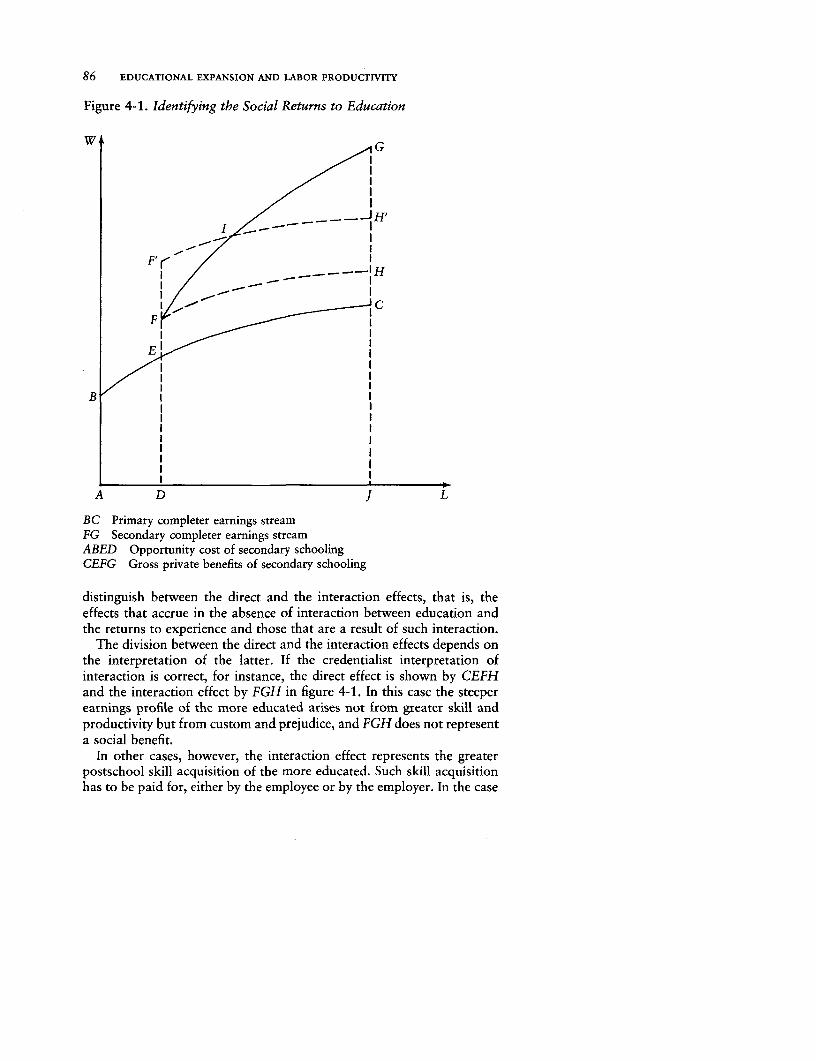
86 EDUCATIONAL EXPANSION AND LABOR PRODUCTIVITY
Figure 4-1. Identifying the Social Returns to Education
F= C
E I
I .I
A D
BC Primary completer earnings streamFG Secondary completer earnings streamABED Opportunity cost of secondary schoolingCEFG Gross private benefits of secondary schooling
distinguish between the direct and the interaction effects, that is, theeffects that accrue in the absence of interaction between education andthe returns to experience and those that are a result of such interaction.
The division between the direct and the interaction effects depends onthe interpretation of the latter. If the credentialist interpretation ofinteraction is correct, for instance, the direct effect is shown by CEFHand the interaction effect by FGH in figure 4-1. In this case the steeperearnings profile of the more educated arises not from greater skill andproductivity but from custom and prejudice, and FGH does not representa social benefit.
In other cases, however, the interaction effect represents the greaterpostschool skill acquisition of the more educated. Such skill acquisitionhas to be paid for, either by the employee or by the employer. In the case
Why the Returns to Experience Increase with Education 87
of general skills the market prediction is that it is the employee who paysand that the payment takes the form of lower initial earnings.4 In thatcase the division between the net direct and interaction effects is betweenCEF'H' minus ABED and GH'I minus FF'I. Here FF'I represents thecost of skill acquisition borne by the worker and GH'I the benefit thathe subsequently derives. In perfectly competitive markets the presentvalue of the net benefit, discounted at the appropriate rate of discount,equals zero; in imperfect markets it can be positive but may neverthelessequal the return on alternative investments such as formal education.
Both the human capital explanation of interaction and the screeningand self-selection explanations make the distinction between the directand the interaction effects discussed above. They differ, however, in theiranalysis of causation. According to the human capital interpretation theadditional education is the cause of the additional postschool skills: GH'I- FF'I is part of the social benefit of secondary schooling. On thescreening and self-selection interpretations the additional education,although a positive correlate of the postschool skill acquisition, is not thecausal factor: GH'I - FF'I is not a social benefit attributable tosecondary schooling.
In the light of this theoretical analysis we examine two empiricalquestions. First, how is the direct effect of secondary education to beexplained? Second, given that the evidence supports a human capitalinterpretation of the direct effect, is the social benefit of secondaryeducation sensitive to the interpretation of the interaction effect? We findthat the interaction effect is indeed sufficiently large in relation to thedirect effect to warrant further analysis.
The interpretation of the direct effect of secondary education in thesesamples was subjected to detailed analysis in chapter 3, and our testspointed to a human capital explanation. Support can also be found inthe results of table 4-1. From equation 4-10 the difference in predictedmean In W between secondary and primary completers (In W, - In Wp)can be decomposed, at any assumed value of L, into the contributionsof the explanatory variables-the constant term (a, - ap), employmentexperience (b5 Ls - bp Lp), reasoning ability (?, Rs - cp Rp), and cognitiveskill (dsH, - dpHp).
Table 4-2 expresses, as a proportion of the total, the difference inpredicted In earnings that is attributable to cognitive skill for those whohave no employment experience, those whose predicted earnings equaltheir actual mean values, and those whose predicted earnings equal theirmean earnings potential before postschool acquisition of skills (derivedby means of Mincer's "overtaking point"; see Mincer 1974, p. 17, anddiscussion below). Whether we assume no employment experience or theactual mean length of employment experience, cognitive skill alone
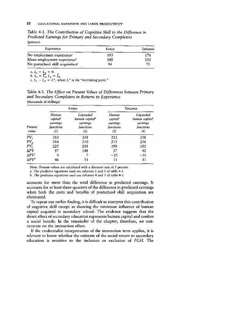
88 EDUCATIONAL EXPANSION AND LABOR PRODUCTIVITY
Table 4-2. The Contribution of Cognitive Skill to the Difference inPredicted Earnings for Primary and Secondary Completers(percent)
Experience Kenya Tanzania
No employment experience, 193 176Mean employment experience" 188 103No postschool skill acquisition' 94 75
a. L, = Lp = 0.b. L, = T5, Lp = 4.c. L, = Lp = L*, where L* is the "overtaking point."
Table 4-3. The Effect on Present Values of Differences between Primaryand Secondary Completers in Returns to Experience(thousands of shillings)
Kenya Tanzania
Human Expanded Human Expandedcapital' human capitalb capital' human capital'earnings earnings earnings earnings
Present functions functions functions functionsvalue (1) (2) (3) (4)
PVs 313 358 252 258PVp 216 210 215 216PVs 225 203 190 185APV 97 148 37 42APV' 9 7 -25 -31APV" 46 33 15 11
Note: Present values are calculated with a discount rate of 5 percent.a. The predictor equations used are columns 2 and 3 of table 4-1.b. The predictor equations used are columns 4 and 5 of table 4-1.
accounts for more than the total difference in predicted earnings. Itaccounts for at least three-quarters of the difference in predicted earningswhen both the costs and benefits of postschool skill acquisition areeliminated.
To repeat our earlier finding, it is difficult to interpret this contributionof cognitive skill except as showing the minimum influence of humancapital acquired in secondary school. The evidence suggests that thedirect effect of secondary education represents human capital and confersa social benefit. In the remainder of the chapter, therefore, we con-centrate on the interaction effect.
If the credentialist interpretation of the interaction term applies, it isrelevant to know whether the estimate of the social return to secondaryeducation is sensitive to the inclusion or exclusion of FGH. The
Why the Returns to Experience Increase with Education 89
simulations presented in table 4-3 provide the basis for an assessment.Columns 1 and 3 show the discounted present values derived by applyingthe procedure for predicting lifetime earnings described above to thestratified human capital earnings functions presented in columns 2 and3 of table 4-1. The difference in the discounted present value of earningsbetween primary and secondary completers (APV = PV, - PVp) is thestandard measure of the benefits of secondary schooling. Although APVis considerably larger in Kenya than in Tanzania, it is substantial in bothcountries when a discount rate of 5 percent is used.
The term PVs is derived by simulating the earnings stream ofsecondary completers on the assumption that they had the returns toexperience of primary completers, that is, by substituting bpLs for bsL,in the human capital equivalent of predictor equation 4-10. Thus APV'= (PVs - PVp) measures the gross benefits of secondary schooling afterthe effect of the interaction between education and the returns toexperience is subtracted (DFHJ - DECJ in figure 4-1; APV correspondsto DFGJ - ABCJ and APV' to CEFH). In both countries there is amarked difference between APV and APV' (columns 1 and 3): in Kenyathe benefit of secondary schooling (in thousands of shillings) drops from97 to 9, and in Tanzania it falls from 37 to -25.
When the expanded human capital earnings functions (which includethe ability and cognitive achievement variables) are used as predictorequations, the results are essentially the same (columns 2 and 4).(Although the present values are, of course, lower, the same pattern ofresults is obtained when a discount rate of 10 percent is used.) Estimatesof the social benefits of secondary schooling are thus highly sensitive towhether the higher returns to experience of secondary completers areinterpreted as being attributable to credentialist seniority scales.
It is also possible to examine the sensitivity of the social benefit ofsecondary education to the alternative assumptions that the interactionis caused by the additional education or is merely correlated with it.According to the human capital interpretation the full area CEFG is ameasure of the social benefit, whereas in the screening and self-selectionexplanations only CEF'H' is a social benefit attributable to the secondaryeducation. Although the rate of return may be no higher on postschoolthan on school investment, the absolute return on school investment isgreater on the human capital interpretation, provided that the rate ofreturn exceeds the rate of discount-that is, provided that the discountedpresent value of GH'I - FF'I is positive.
As an illustration of the sensitivity of present values to these differentinterpretations, we estimate, by means of Mincer's "overtaking point,"the difference in present values that is attributable to the differencebetween CEFG and CEF'H' (see Mincer 1974, p. 17). Mincer has arguedthat on certain fairly strong assumptions an estimate can be made for
90 EDUCATIONAL EXPANSION AND LABOR PRODUCTIVITY
the earnings potential of school leavers. (The potential is actual earningsplus payment for current skill acquisition minus payment received forprevious postschool skill acquisition.) The point at which the actualearnings curve, which rises with experience, overtakes the horizontalearnings potential is given by j = 1/r, where j is the overtaking year ofexperience, r is the rate of return on both school and postschoolinvestment, and it is assumed that the worker pays the same amount fortraining in each period. For any given value of r there is a value of j thatcan then be used to identify the earnings potential of both secondary andprimary completers. The difference between them is our measure ofCEF'H'. (In fact, we measure a rectangle corresponding to CEF'H',abstracting from postschool investment at both the secondary andprimary levels, rather than CEF'H' itself, abstracting from postschoolinvestment at the secondary level only.)
Our illustrative assumption about the value of r is that it equals thecombined rate of return to secondary school and to additional postschoolinvestment (as calculated from benefits CEFG and costs ABED). Anestimated r of 13 percent for Kenya and 8 percent for Tanzania impliesvalues for j of 8 years in Kenya and 12 years in Tanzania. The earningspotentials for secondary completers in Kenya and Tanzania are then12,051 and 10,603 shillings, respectively, and for primary completers,9,451 and 9,729 shillings. These earnings potential streams arediscounted to the primary-leaving point at 5 percent. The differencebetween them (APV' in table 4-3) is to be contrasted with our estimateon the human capital interpretation (APV in the table). The discountedpresent value (in thousands of shillings) of AP "' for Kenya, 46, falls wellshort of APV, 97; in Tanzania the fall is from 37 to 15. Again, thisillustrative exercise suggests that the choice between these interpretationsof interaction has a considerable effect on estimates of the social valueof secondary education.
The Test of Competing Hypotheses
Our test of the competing explanations for the interaction betweeneducation and returns to experience is a simple one. We examine, first,whether there is a positive relationship between the level of cognitive skilland the returns to experience among workers with a given level ofeducation. Second, we try to determine whether the difference incognitive skill between primary and secondary completers is sufficient toexplain their difference in returns to experience.
The human capital explanation posits complementarity betweeneducation and training. The output of schooling (cognitive skill) is aninput into the postschool skill acquisition process: workers with highercognitive skill accumulate more vocational skill, and more vocational
Why the Returns to Experience Increase with Education 91
skill generates higher earnings. This explanation yields the predictionthat even among workers with the same educational level, the returnsto experience will be higher for those with higher cognitive skill.Furthermore, it implies that the higher returns to experience of secondarycompleters are attributable to their higher cognitive achievement.
The predictions yielded by the credentialist explanation are distinctfrom the human capital predictions. Because the returns to experienceare tied by institutionally determined wage structures to the educationalcredential that the individual possesses, secondary completers have thesame returns to experience irrespective of their level of cognitive skill.Since the same is held to be true of primary completers, the differencein cognitive skill between the two groups cannot be responsible for thedifference in their returns to experience.
The screening and self-selection hypotheses also reject the propositionthat education causes training; a third factor-for example, ability orfamily background-explains why some workers have more of both.This explanation implies that differences in cognitive skill amongworkers with the same educational level do not give rise to differencesin returns to experience. Similarly, any difference in cognitive skillbetween primary and secondary completers will not cause a differencein returns to experience.
We test for a positive relationship between cognitive skill and thereturns to experience by means of the following specification of theexpanded human capital earnings function stratified by educational level:
(4-11) In W = f(L, R, H, H- L)
where H L is an interaction term that measures the returns toexperience at various levels of cognitive skill. Estimates of these equationsare presented in columns 1 and 2 of table 4-4. They can be comparedwith the equivalent results (but without the interaction term) in table 4-1.For the secondary stratum in Kenya the addition of H - L reduces thereturn to experience from 6.2 to 0.6 percent per year of experience. Theformer estimate is highly significant, the latter not at all. Amongsecondary completers in Tanzania the return to experience declines from6.6 to 0.3 percent per year and is no longer significant. At the primarylevel also, the addition of H - L causes the coefficient on experience todecline and become insignificant in both countries. The coefficient onH- L, although positive, is not significant in either country.
Since the L term is insignificant in all four cases, we reestimated theequation without it (columns 3 and 4). The H- L terms are now highlysignificant in all four cases. For both primary and secondary completersthe returns to experience vary positively with their level of cognitive skill.For example, among Kenyan secondary completers with ten years ofexperience the return to experience is 4.7 percent per year for those
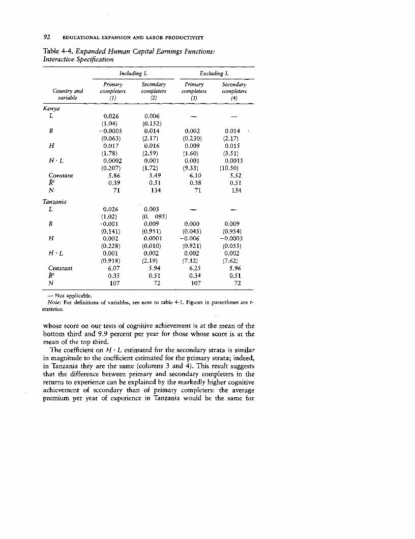
92 EDUCATIONAL EXPANSION AND LABOR PRODUCTIVITY
Table 4-4. Expanded Human Capital Earnings Functions:Interactive Specification
Including L Excluding L
Primary Secondary Primary SecondaryCountry and completers completers completers completers
variable (1) (2) (3) (4)
KenyaL 0.026 0.006 - -
(1.04) (0.152)R -0.0005 0.014 0.002 0.014
(0.063) (2.17) (0.230) (2.17)H 0.017 0.016 0.009 0.015
(1.78) (2.59) (1.60) (3.51)H L 0.0002 0.001 0.001 0.0015
(0.207) (1.72) (9.33) (10.50)Constant 5.86 5.49 6.10 5.52K2 0.39 0.51 0.38 0.51N 71 134 71 134
TanzaniaL 0.026 0.003 - -
(1.02) (0. 095)R -0.001 0.009 0.000 0.009
(0.141) (0.951) (0.045) (0.954)H 0.002 0.0001 -0.006 -0.0003
(0.228) (0.010) (0.921) (0.055)H L 0.001 0.002 0.002 0.002
(0.918) (2.19) (7.12) (7.62)Constant 6.07 5.94 6.25 5.96k2 0.35 0.51 0.34 0.51N 107 72 107 72
- Not applicable.
Note: For definitions of variables, see note to table 4-1. Figures in parentheses are t-statistics.
whose score on our tests of cognitive achievement is at the mean of thebottom third and 9.9 percent per year for those whose score is at themean of the top third.
The coefficient on H L estimated for the secondary strata is similarin magnitude to the coefficient estimated for the primary strata; indeed,in Tanzania they are the same (columns 3 and 4). This result suggeststhat the difference between primary and secondary completers in thereturns to experience can be explained by the markedly higher cognitiveachievement of secondary than of primary completers: the averagepremium per year of experience in Tanzania would be the same for

Why the Returns to Experience Increase with Education 93
primary and secondary completers who had the same employmentexperience and cognitive skill. Table 4-5 shows the effect of the differencein cognitive skill between primary and secondary completers on thepresent values of their earnings streams. The predictor equations are:
for PV,
In W,= b+ bR + 5 I- + dsH1^- L
for PVp
In Wp = ap + bpRp+ + dpHp * Lp
for PV,!
In W, = a, + bR+ + + dsHp - L,
for PVp,
In Wp = ap+ + + pHp + dpH- Lp
The difference between primary and secondary completers in presentvalue (PVS - PVp), in thousands of shillings, is 181 in Kenya and 76 inTanzania. If secondary completers had the mean cognitive skill ofprimary completers, insofar as that would influence the returns toexperience, the difference in present value (PV,' - PVS) would decline to3 in Kenya and to -38 in Tanzania; PV, - PVp is also markedly lowerthan PV, - PVp. In both Kenya and Tanzania a substantial part of thedifference in the present value of earnings between the two educationalgroups is attributable to the influence on the returns to experience of thehigher cognitive skill of secondary completers. (The same pattern ofresults is obtained, and this conclusion therefore stands, when a discountrate of 10 percent is used instead.)
A conclusion that this evidence supports a human capital explanation
Table 4-5. The Effect on Present Values of Differences in Cognitive Skillbetween Primary and Secondary Completers(thousands of shillings)
Present value Kenya Tanzania
PVs 389 290PVP 208 214PV'" 211 176
PV' 300 389PV. - PVp 181 76P1"7- PVp 92 -38P17 - PVP' 89 -99
Note: Present values are calculated with a discount rate of 5 percent. The predictor equa-tions used are columns 3 and 4 of table 4-4.

94 EDUCATIONAL EXPANSION AND LABOR PRODUCTIVITY
of the interaction must be qualified in two respects. First, it is possiblethat ability and family background enter the production function of bothcognitive and vocational skills. In this case we might find someassociation between cognitive skill and returns to experience amongworkers of the same educational level despite the absence of a causalrelationship. The evidence is consistent with the screening and self-selection explanations of interaction to the extent that the differencebetween primary and secondary completers in ability or family back-ground explains their difference in cognitive skill.
The relative contributions that secondary schooling and its possiblecorrelates make to cognitive skill acquisition can be examined by meansof an educational production function:
(4-12) H = ao + a,S + a2 R + a3 F± + a4F2 + u
where F, is a dummy variable indicating that one parent has receivededucation and F2 is a dummy variable indicating that both parents havereceived education. Equation 4-12 differs from the educational pro-duction function presented in chapter 3 principally in the addition ofthe family background variables. (The terms representing type of schoolattended and place of birth are excluded.) The difference betweenprimary and secondary completers in mean cognitive skill has threecomponents:
(4-13) HI - I = a, + Az(Rs- R) + a3 (Fl, - Flp) + i4 (F2 s - hp)
The results of this exercise are set out in table 4-6. Possession ofsecondary education accounts for 83 and 84 percent of the totaldifference in Kenya and Tanzania, respectively, and differences inreasoning ability account for only 18 and 15 percent. Although reasoningability is an important input into the educational production function,the difference in ability between primary and secondary completers isvery small in both countries. There are large differences in familybackground, but family background has only negligible positive ornegative effects on cognitive skill. (The effect is liable to be under-estimated owing to the truncation of our sample, a result of the ex-clusion of those secondary graduates who continued their schooling.Moreover, family background may have a powerful indirect effect oncognitive achievement because of its influence on the probability ofattaining secondary education; see chapter 10.) Our evidence providesmore support for the human capital interpretation of the H * L term thanfor the screening and self-selection explanations.
Elsewhere (Knight and Sabot 1981, which used the 1971 survey ofmanufacturing employees in Tanzania) we have argued that interactionbetween education and experience arose partly as a response to the rapidexpansion of education in Kenya and Tanzania. The more recent cohorts
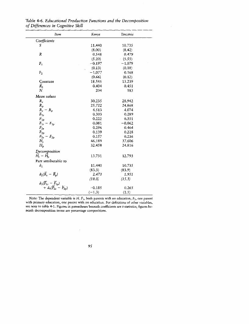
Table 4-6. Educational Production Functions and the Decompositionof Differences in Cognitive Skill
Item Kenya Tanzania
CoefficientsS 11.440 10.735
(8.00) (8.42)R 0.548 0.479
(5.20) (5.55)F5 -0.197 -1.079
(0.13) (0.18)F2 -1.077 0.168
(0.66) (0.12)Constant 18.545 13.239R2 0.404 0.451N 204 183
Mean valuesRs 30.235 28.942Rp 25.722 24.868R, -Rp 4.513 4.074F1l 0.303 0.289Flp 0.222 0.351F1 - FPp 0.081 -0.062F21 0.296 0.464
0.139 0.228F,- F2p 0.157 0.236H, 46.189 37.606lip 32.458 24.816
DecompositionH,-H p 13.731 12.793
Part attributable to11.440 10.735
(83.3) (83.9)Ii2A - Rp) 2.473 1.951
(18.0) (15.3)43(F, -Flp) _
+ a4(F2, - F2p) -0.185 0.265
Note: The dependent variable is H. Fl, both parents with no education; F2, one parentwith primary education, one parent with no education. For definitions of other variables,see note to table 4-1. Figures in parentheses beneath coefficients are t-statistics; figures be-neath decomposition terms are percentage compositions.
95

96 EDUCATIONAL EXPANSION AND LABOR PRODUCTIVITY
to enter the labor market filtered down into jobs in which their educationhad less value. Employment experience thus acted as a proxy for yearof entry into the labor market, which in turn greatly influenced occupa-tional attainment; hence the positive correlation between years of em-ployment experience and returns to education, which is equivalent to apositive correlation between years of schooling and returns to experience.The more recently entered jobs are likely to reward cognitive skill less-and thus to render the coefficient on H - L positive-when these jobs re-quire less vocational skill or less cognitive skill. We show below that fil-tering down has occurred in both countries at both educationallevels-most markedly at the secondary level in Kenya-and that the ed-ucational structure of wages has been compressed as a consequence (seechapter 7).
If the positive coefficient on H- L within educational strata arisesbecause the more recently entered jobs require less vocational skill, itrepresents the positive effect of cognitive skill on vocational skillacquisition and points to the human capital interpretation of theinteraction term. If, however, the positive coefficient arises because themore recently entered jobs require less cognitive skill, it represents adirect but differential effect of cognitive skill on earnings in differentoccupations. This interpretation provides an independent explanation forboth the positive coefficient on H * L within educational strata and thepositive interaction between experience and education across strata. Apartial test of this explanation can be made by reestimating the expandedhuman capital earnings functions (corresponding to columns 3 and 4 intable 4-4) for manual and nonmanual subsamples, thus eliminating someof the effect of filtering down. The coefficients on H * L remain positiveand significant in each case.5 This exercise suggests that the secondexplanation, which is not consistent with the human capital interpre-tation of interaction between education and experience, is unlikelyto be important.
Conclusions
We have shown that returns to employment experience vary positivelywith educational level and that this interaction accounts for a substantialpart of the returns to secondary schooling as conventionally measured.We have also shown that for workers with the same amount of education,returns to experience vary positively with level of cognitive skill and thatthe difference in cognitive skill between educational levels explains asubstantial part of their difference in returns to experience and thus ofthe returns to secondary education. These findings passed the usualstatistical tests. Their robustness is reinforced by the fact that they applyto both countries.
Why the Returns to Experience Increase with Education 97
Our results are not consistent with the credentialist interpretation ofthe interaction between education and returns to experience. They areconsistent with the screening and self-selection explanations only to theextent that the difference in ability or family background betweenprimary and secondary completers explains their difference in cognitiveskill. We have shown, however, that most of the difference in cognitiveskill between the two groups is accounted for by the difference in theiryears of schooling.
Our findings provide support for the human capital interpretation.More educated workers appear to have higher returns to experiencebecause education and training are complementary: the skills acquiredin school are determinants of training attainment and are inputs into theprocess of postschool acquisition of skills. More skills of one type begetmore skills of another. This supports the conventional practice of in-cluding among the social returns to schooling that part of the returnsthat arises from the interaction between education and returns toexperience.
Notes
1. See, for example, Blaug (1976), Knight and Sabot (1981), Layard andPsacharopoulos (1974), and Mazumdar (1981). The relationship can equally beseen as one between employment experience and the returns to education.
2. Recall that our estimates of educational production functions in which His the dependent variable indicate that the variance in achievement is in part aresult of the differences in ability among respondents. There is evidence that dif-ferences in the quality of the school attended and in training received within thehome also play a role.
3. Suppose that cognitive skill influences earnings and that, owing to rapid ex-pansion of the school system and a consequent fall in the quality of schools orof pupils, the level of cognitive skill is higher among workers with more experi-ence (who belong to earlier cohorts of school completers) than among the rela-tively inexperienced recent completers. Omission of H from the independent vari-ables in the earnings function then biases upward the coefficient on experience.If the positive relationship between H and L is stronger among secondary thanamong primary completers-perhaps reflecting different rates of educationalexpansion-the upward bias in the returns to experience is then greater in theregression estimated for the secondary stratum.
4. See, for example, Mincer (1974), ch. 1. To the extent that skills are firm-specific, however, the costs are likely to be shared between the employer and theemployee; see, for example, Becker (1964) and Oi (1962).
5. They are 0.0009 (3.69), 0.0015 (5.49), 0.0014 (3.20), and 0.0027 (3.49),respectively, for manual occupations and 0.0014 (6.01), 0.0012 (8.03), 0.0025(4.64), and 0.0019 (6.93) for nonmanual occupations. (The figures in parenthesesare t-statistics.)
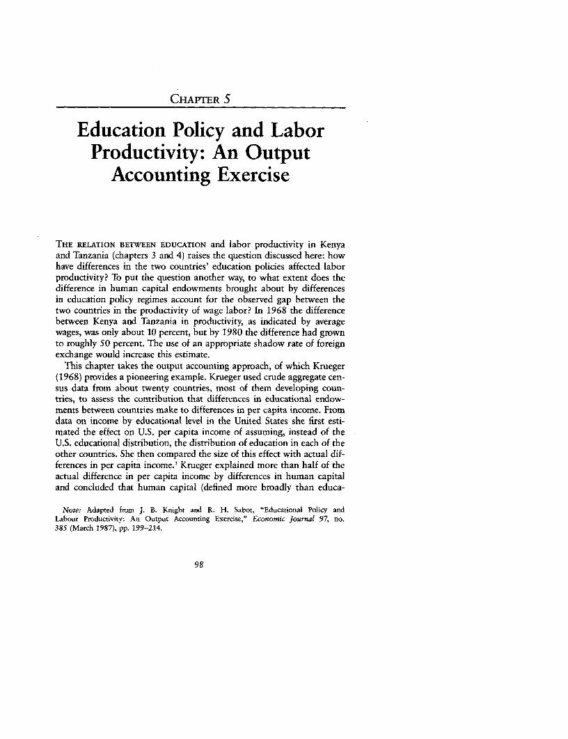
CHAPTER S
Education Policy and LaborProductivity: An Output
Accounting Exercise
THE RELATION BETWEEN EDUCATION and labor productivity in Kenyaand Tanzania (chapters 3 and 4) raises the question discussed here: howhave differences in the two countries' education policies affected laborproductivity? To put the question another way, to what extent does thedifference in human capital endowments brought about by differencesin education policy regimes account for the observed gap between thetwo countries in the productivity of wage labor? In 1968 the differencebetween Kenya and Tanzania in productivity, as indicated by averagewages, was only about 10 percent, but by 1980 the difference had grownto roughly S0 percent. The use of an appropriate shadow rate of foreignexchange would increase this estimate.
This chapter takes the output accounting approach, of which Krueger(1968) provides a pioneering example. Krueger used crude aggregate cen-sus data from about twenty countries, most of them developing coun-tries, to assess the contribution that differences in educational endow-ments between countries make to differences in per capita income. Fromdata on income by educational level in the United States she first esti-mated the effect on U.S. per capita income of assuming, instead of theU.S. educational distribution, the distribution of education in each of theother countries. She then compared the size of this effect with actual dif-ferences in per capita income.' Krueger explained more than half of theactual difference in per capita income by differences in human capitaland concluded that human capital (defined more broadly than educa-
Note: Adapted from J. B. Knight and R. H. Sabot, "Educational Policy andLabour Productivity: An Output Accounting Exercise," Economic Journal 97, no.385 (March 1987), pp. 199-214.
98
An Output Accounting Exercise 99
tional attainment) made a greater contribution than all other factorscombined. 2
Both output and growth accounting suffer from well-known draw-backs (see, for instance, the critiques in Bowman 1980 and Nelson 1981).First, failure to take account of the other determinants of income can biasestimates of the difference in income, and therefore in productivity, thatis attributable to education. Second, by assuming that the (standardized)earnings difference between educated and uneducated workers simplymeasures the productivity of education, the output and growth accoun-tants attribute causation to what may be at least in part a noncausal corre-lation. This effective equating of the marginal products of factors withtheir remuneration has led some practitioners to regard growth account-ing as no more than "a first step which cannot be relied upon to giveanswers to counterfactual questions" (Matthews, Feinstein, and Odling-Smee 1982, p. 15). Such adjustments as have been made to the earningsdifference in estimating the marginal product of education have in gen-eral simply attributed an arbitrary proportion of the difference in earn-ings to "ability" or to other correlates of education.3 Third, the simula-tions on these accounting exercises are generally conducted for timeperiods or economies that differ markedly in the relative supply of anddemand for educated labor. The differences that factor endowments andthe characteristics of production functions bring about in the structureof factor prices or in their marginal products render unreliable the an-swers to the counterfactual questions being posed.4 Krueger (1968, pp.643-44) claimed that her measure of the contribution of educationwould yield a minimum estimate, essentially because the marginal prod-uct of human capital in the United States would be relatively low if theUnited States were well endowed with human capital. This would notnecessarily be the case, however, if the U.S. economy had a greater rela-tive demand for human capital.5
Here we attempt to minimize these drawbacks by examining the natu-ral experiment afforded by Kenya and Tanzania, two countries that havehad different education policies but that are similar in relevant respectsother than the supply of educated labor. In particular, there is evidencethat the relative demand functions for different categories of educatedlabor are similar in the two economies (see chapters 6 and 7). Our datasets permit the use of earnings functions in place of mean earnings byeducational level. The measures of cognitive skill and reasoning abilitymake it possible to estimate the effects on output of country differencesnot only in the quantity of education but also (by means of educationalproduction functions) in its quality.
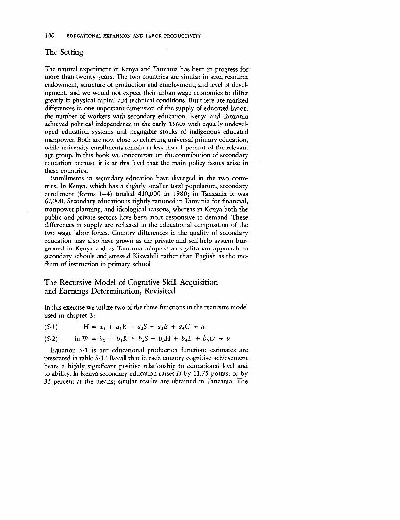
100 EDUCATIONAL EXPANSION AND LABOR PRODUCTIVITY
The Setting
The natural experiment in Kenya and Tanzania has been in progress formore than twenty years. The two countries are similar in size, resourceendowment, structure of production and employment, and level of devel-opment, and we would not expect their urban wage economies to differgreatly in physical capital and technical conditions. But there are markeddifferences in one important dimension of the supply of educated labor:the number of workers with secondary education. Kenya and Tanzaniaachieved political independence in the early 1960s with equally undevel-oped education systems and negligible stocks of indigenous educatedmanpower. Both are now close to achieving universal primary education,while university enrollments remain at less than 1 percent of the relevantage group. In this book we concentrate on the contribution of secondaryeducation because it is at this level that the main policy issues arise inthese countries.
Enrollments in secondary education have diverged in the two coun-tries. In Kenya, which has a slightly smaller total population, secondaryenrollment (forms 1-A) totaled 410,000 in 1980; in Tanzania it was67,000. Secondary education is tightly rationed in Tanzania for financial,manpower planning, and ideological reasons, whereas in Kenya both thepublic and private sectors have been more responsive to demand. Thesedifferences in supply are reflected in the educational composition of thetwo wage labor forces. Country differences in the quality of secondaryeducation may also have grown as the private and self-help system bur-geoned in Kenya and as Tanzania adopted an egalitarian approach tosecondary schools and stressed Kiswahili rather than English as the me-dium of instruction in primary school.
The Recursive Model of Cognitive Skill Acquisitionand Earnings Determination, Revisited
In this exercise we utilize two of the three functions in the recursive modelused in chapter 3:
(5-1) H = ao + ajR + a2S + a3B + a4G + u
(5-2) In W = bo + b1R + b 2S + b3H + b4L + b5L2 + v
Equation 5-1 is our educational production function; estimates arepresented in table 5s1.6 Recall that in each country cognitive achievementbears a highly significant positive relationship to educational level andto ability. In Kenya secondary education raises H by 11.75 points, or by35 percent at the means; similar results are obtained in Tanzania. The
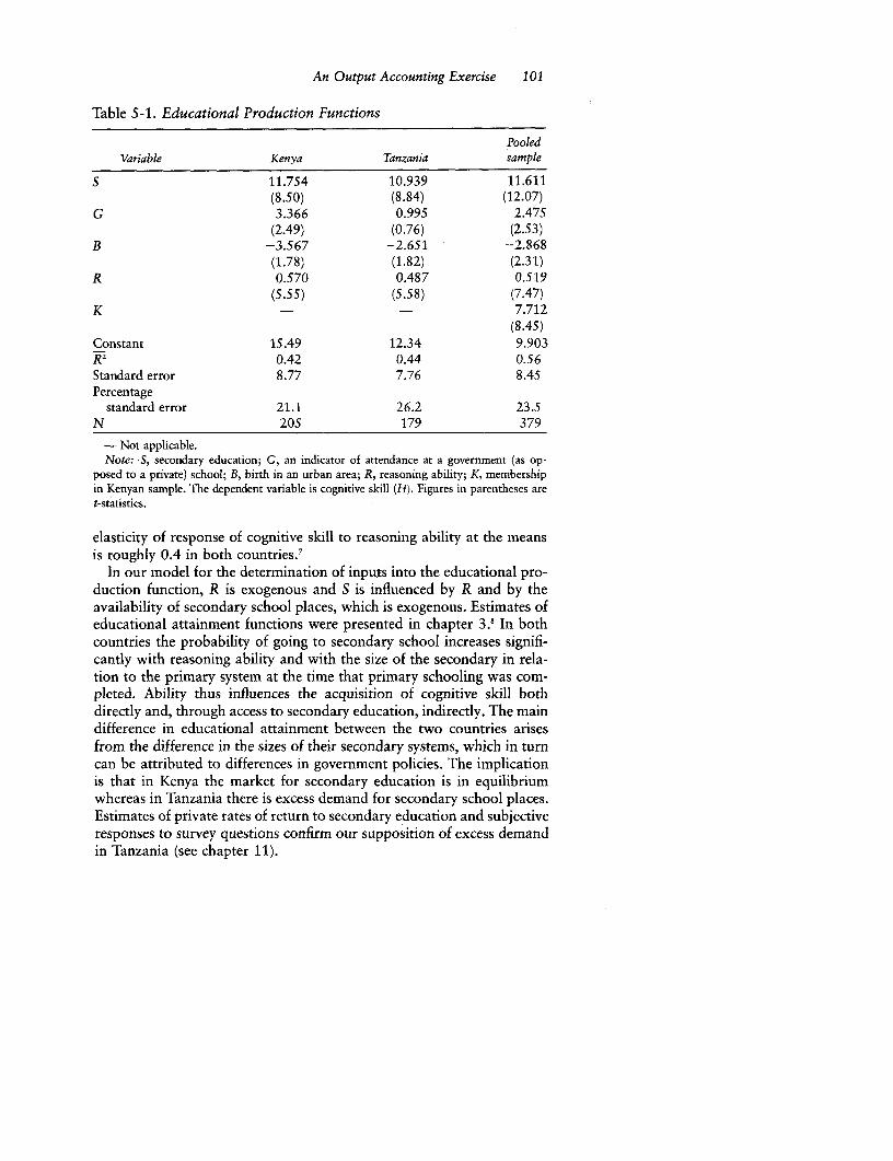
An Output Accounting Exercise 101
Table 5-1. Educational Production Functions
PooledVariable Kenya Tanzania sample
S 11.754 10.939 11.611(8.50) (8.84) (12.07)
G 3.366 0.995 2.475(2.49) (0.76) (2.53)
B -3.567 -2.651 -2.868(1.78) (1.82) (2.31)
R 0.570 0.487 0.519(5.55) (5.58) (7.47)
K - - 7.712(8.45)
Constant 15.49 12.34 9.903R2 0.42 0.44 0.56Standard error 8.77 7.76 8.45Percentage
standard error 21.1 26.2 23.5N 205 179 379
- Not applicable.Note: S, secondary education; G, an indicator of attendance at a government (as op-
posed to a private) school; B, birth in an urban area; R, reasoning ability; K, membershipin Kenyan sample. The dependent variable is cognitive skill (H). Figures in parentheses aret-statistics.
elasticity of response of cognitive skill to reasoning ability at the meansis roughly 0.4 in both countries.'
In our model for the determination of inputs into the educational pro-duction function, R is exogenous and S is influenced by R and by theavailability of secondary school places, which is exogenous. Estimates ofeducational attainment functions were presented in chapter 3.8 In bothcountries the probability of going to secondary school increases signifi-cantly with reasoning ability and with the size of the secondary in rela-tion to the primary system at the time that primary schooling was com-pleted. Ability thus influences the acquisition of cognitive skill bothdirectly and, through access to secondary education, indirectly. The maindifference in educational attainment between the two countries arisesfrom the difference in the sizes of their secondary systems, which in turncan be attributed to differences in government policies. The implicationis that in Kenya the market for secondary education is in equilibriumwhereas in Tanzania there is excess demand for secondary school places.Estimates of private rates of return to secondary education and subjectiveresponses to survey questions confirm our supposition of excess demandin Tanzania (see chapter 11).
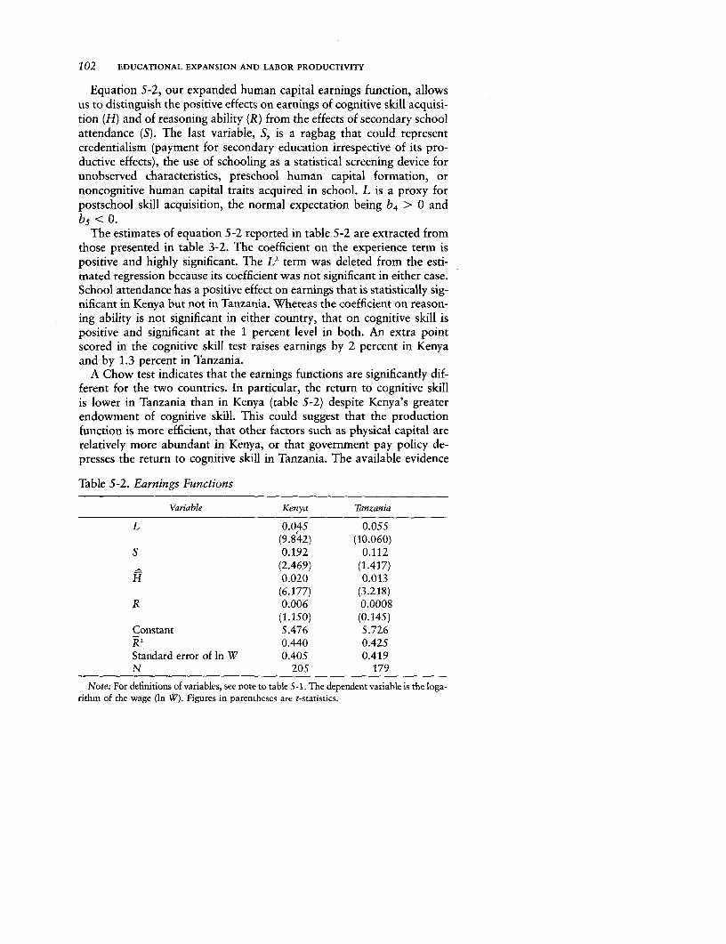
102 EDUCATIONAL EXPANSION AND LABOR PRODUCTIVITY
Equation 5-2, our expanded human capital earnings function, allowsus to distinguish the positive effects on earnings of cognitive skill acquisi-tion (H) and of reasoning ability (R) from the effects of secondary schoolattendance (S). The last variable, S, is a ragbag that could representcredentialism (payment for secondary education irrespective of its pro-ductive effects), the use of schooling as a statistical screening device forunobserved characteristics, preschool human capital formation, ornoncognitive human capital traits acquired in school. L is a proxy forpostschool skill acquisition, the normal expectation being b4 > 0 andb5 < O.
The estimates of equation 5-2 reported in table 5-2 are extracted fromthose presented in table 3-2. The coefficient on the experience term ispositive and highly significant. The LI term was deleted from the esti-mated regression because its coefficient was not significant in either case.School attendance has a positive effect on earnings that is statistically sig-nificant in Kenya but not in Tanzania. Whereas the coefficient on reason-ing ability is not significant in either country, that on cognitive skill ispositive and significant at the 1 percent level in both. An extra pointscored in the cognitive skill test raises earnings by 2 percent in Kenyaand by 1.3 percent in Tanzania.
A Chow test indicates that the earnings functions are significantly dif-ferent for the two countries. In particular, the return to cognitive skillis lower in Tanzania than in Kenya (table 5-2) despite Kenya's greaterendowment of cognitive skill. This could suggest that the productionfunction is more efficient, that other factors such as physical capital arerelatively more abundant in Kenya, or that government pay policy de-presses the return to cognitive skill in Tanzania. The available evidence
Table 5-2. Earnings Functions
Variable Kenya Tanzania
L 0.045 0.05s(9.842) (10.060)
S 0.192 0.112=2L (2.469) (1.417)H 0.020 0.013
(6.177) (3.218)R 0.006 0.0008
(1.150) (0.145)Constant 5.476 5.726k2 0.440 0.425Standard error of In W 0.405 0.419N 205 179
Note: For definitions of variables, see note to table 5-1. The dependent variable is the loga-rithm of the wage (In W). Figures in parentheses are t-statistics.

An Output Accounting Exercise 103
does not confirm these hypotheses, perhaps because of the limited num-ber of observations in the subsample. The close similarity in skill-basedoccupational composition observed in the two full samples suggests thatthe demand for cognitive skill in relation to unskilled labor is also closelysimilar in the two countries.9 Despite institutional evidence, corroboratedby evidence from the full samples, of an egalitarian pay policy in thepublic sector of Tanzania (see chapter 7), the introduction in equation5-2 of a dummy variable (P) for employment in the public sector andof a public sector-cognitive skill interaction term (P * H) does not pro-duce the hypothesized significant negative coefficient on the interactionterm that we would expect to find given the lower returns to cognitiveskill in the public sector.'"
Education Policy and Differences in Cognitive Achievement
The average level of reasoning ability (R) is much the same in the twocountries-27.8 in Kenya and 26.4 in Tanzania. The means are not sig-nificantly different even at the 10 percent level. Levels of cognitive skillare, by contrast, substantially higher in Kenya than in Tanzania; meanscores for Kenya are 23 percent higher on the literacy test and 44 percenthigher on the numeracy test. Mean cognitive skill scores (H) are 40.0in Kenya and 30.3 in Tanzania, an absolute difference of 9.7. The meansare significantly different at the 1 percent level. The regression resultsfrom the pooled sample in table 5-1 indicate that even after differencesin characteristics are standardized, the mean cognitive skill score of Ken-yans exceeds that of Tanzanians by 7.7. A Chow test, however, rejectedthe null hypothesis that the educational production functions for the twocountries are the same. This is therefore not the best estimate of the partof the difference in cognitive skill that can be attributed to differencesin educational production functions. We measure this difference bymeans of decomposition analysis.
Since the mean cognitive skill of Kenyans is determined by the educa-tional production function Hk = fk(Xk), where Xk are the mean valuesof the independent variables, the mean value that Tanzanians wouldachieve if the Kenyan production function were to apply would be fk(Xt).
The gross difference between the two countries is then decomposed asfollows:
(5-3) Hk - IH, = fk(Xk - Xt) + [fk(Xt) - 9(XD)]
or
(5-3') Ilk - =-I f(Xk - Xt) + [fk(Xk) - fI(X9k)
The first term on the right-hand side of each equation shows the com-ponent that is explained by differences in the proportion of workers with
104 EDUCATIONAL EXPANSION AND LABOR PRODUCTIVITY
secondary education and in the mean values of the other explanatory vari-ables, and the second term can be interpreted as a measure of the differ-ence in the quality of education, in the sense that output per unit of inputsis higher in one country than in the other.
As expected, country differences in the explanatory variables otherthan educational attainment contribute little to the explanation. Differ-ences in the quantity of secondary education account for 15 percent ofthe gross difference if the Kenyan educational production function is usedand for 14 percent if the Tanzanian function is used. This reflects the dif-fering proportion of secondary completers in the full sample total of pri-mary and secondary completers; S is 0.532 in Kenya and 0.414 in Tan-zania. The residual, however, accounts for no less than 75 percent whenthe Tanzanian educational production function is used or 78 percentwhen the Kenyan function is used. For given mean values of the explana-tory variables, the predicted cognitive skill score with the Kenyan educa-tional production function as predictor greatly exceeds that with theTanzanian function as predictor.
This result suggests that country differences in the quality of educationare important determinants of cognitive achievement. We equate the re-sidual with differences in quality, although we recognize that differencesin the incentive systems in the two countries could produce differencesin drive and family support that might contribute to the residual. Thelower quality of education in Tanzania could stem from divergent educa-tion policies. Teaching inputs are of the same magnitude in the two coun-tries, and cost per student is actually higher in Tanzania because a higherproportion of students is in boarding schools. Tanzania, however, hasplaced greater stress on curriculum diversification, at the cost perhaps oftime spent on general academic skills, and on Kiswahili in primaryschool, perhaps to the detriment of efficient learning in English in second-ary school.
The Simulation Methodology
The two functions can be used together in simulations to answer the fol-lowing counterfactual questions. What is the effect on the average cogni-tive skill of the Tanzanian labor force of increasing the quantity of educa-tion to the Kenyan level? What is the effect on the average cognitive skillof the Tanzanian labor force of increasing the quality of education to theKenyan level?
To answer the first question, we substitute the Kenyan for theTanzanian mean value of the secondary school dummy variable" andpredict the cognitive skill score with the use of the Tanzanian educationalproduction function:
An Output Accounting Exercise 105
(5-4) Ht = ao± + a,Rt + a2,Sk + a3 ,Tt + a4,B, + as,Gt
To answer the second question, we substitute the Kenyan for theTanzanian educational production function and predict the cognitive skillscore with the use of the Tanzanian mean values of the independent vari-ables:
(5-5) Ht = aOk + alkRt + a2kSt + a4kB, + as,G,
We can then ask, what is the effect on average earnings in Tanzaniaif first the quantity, then the quality, and then both the quantity and thequality of education in Tanzania are increased to the Kenyan level? Toanswer the question, we substitute the mean cognitive skill score associ-ated with each of these counterfactual changes in education policy foractual cognitive skill in the Tanzanian earnings function to predict theconsequent change in mean wages:
(5-6) In Wt =bo + blj,,k + b2iRt + b3pt + b4,LI
The subscript on S is either k or t, as is explained below.The assumptions implicit in these exercises are that the policy changes
do not affect the coefficients of the functions or the mean values of theother independent variables and that, as a consequence of the rationingof secondary places in Tanzania, there is an effective demand for thesimulated increases in supply.
Cross-Country Policy Simulations
Our results suggest that more literate and numerate workers are moreproductive. Tanzania has thus paid a price in output forgone by restrain-ing the growth of secondary education and reducing the quality of educa-tion for the sake of other goals. Our next exercise is to quantify this priceby simulating the effect on wages, and thus on productivity, of differ-ences between the two countries in the quantity and quality of education.
The results of our simulation exercises are presented in table 5-3. Thebase runs use the actual values of both variables and coefficients; the pre-dicted and weighted actual mean levels of cognitive skill and geometricmean levels of earnings are therefore the same. Simulation 1 shows theeffect of the change in quantity, simulation 2 the effect of the change inquality, and simulation 3 the effect of simultaneous changes in quantityand quality. The Tanzanian simulations introduce parameters fromKenya, and the Kenyan simulations introduce parameters from Tanzania.
An increase in the quantity of secondary education in Tanzania to theKenyan level would, on the basis of equations 5-1 and 5-2, increase themean cognitive skill of the labor force by 4 percent and mean earnings
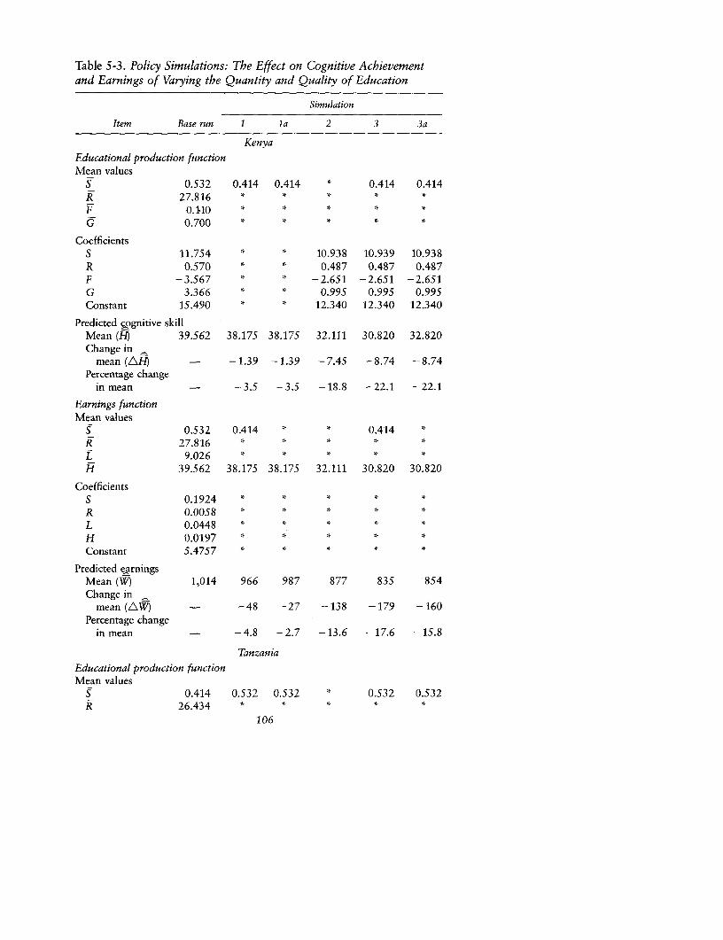
Table 5-3. Policy Simulations: The Effect on Cognitive Achievementand Earnings of Varying the Quantity and Quality of Education
Simulation
Item Base run I la 2 3 3a
Kenya
Educational production functionMean values
S 0.532 0.414 0.414 * 0.414 0.414R 27.816 * * * *
F 0.110 * * *
G 0.700 * * *
CoefficientsS 11.754 * 10.938 10.939 10.938R 0.570 * * 0.487 0.487 0.487F -3.567 * * -2.651 -2.651 -2.651G 3.366 0 * 0.995 0.99S 0.995Constant 15.490 * * 12.340 12.340 12.340
Predicted cpgnitive skillMean (H) 39.562 38.175 38.175 32.111 30.820 32.820Change in
mean (Am) - -1.39 -1.39 -7.45 -8.74 -8.74Percentage change
in mean - -3.5 -3.5 -18.8 -22.1 -22.1
Earnings functionMean values
S 0.532 0.414 * * 0.414 *
k 27.816 * * * * *
L 9.026 * * * * *
H 39.562 38.175 38.175 32.111 30.820 30.820
CoefficientsS 0.1924 * * * * *
R 0.0058 * * * *
L 0.0448 * * * * *
H 0.0197 * * * * *
Constant 5.4757 * * * * *
Predicted eqrningsMean (W) 1,014 966 987 877 835 854Change in
mean (AW) - -48 -27 -138 -179 -160Percentage change
in mean - -4.8 -2.7 -13.6 -17.6 -15.8
Tanzania
Educational production functionMean values
S 0.414 0.532 0.532 * 0.532 0.532R 26.434 * * * * *
106
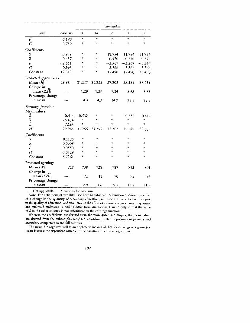
Simulation
Item Base run I la 2 3 3a
F 0.190 * * * * *
G 0.730 * * * x *
CoefficientsS 10.939 * * 11.754 11.754 11.754R 0.487 * * 0.570 0.570 0.570F -2.651 * * -3.567 - 3.567 -3.567G 0.995 * * 3.366 3.366 3.366Constant 12.340 * 15.490 15.490 15.490
Predicted cognitive skillMean (H) 29.964 31.255 31.25S 37.202 38.589 38.259Change in
mean (AR) - 1.29 1.29 7.24 8.63 8.63Percentage change
in mean - 4.3 4.3 24.2 28.8 28.8
Earnings functionMean values
S 0.414 0.532 * * 0.532 0.414R 26.434 * * * * *
L 7.163 * * * *
H 29.964 31.255 31.255 37.202 38.589 38.589
CoefficientsS 0.1125 # # # # #
R 0.0008 * * * *
L 0.0550 # # # # #
H 0.0129 * * * *
Constant 5.7261 * * * *
Predicted earningsMean (W) 717 738 728 787 812 801Change in
mean (AW) - 21 11 70 95 84Percentage change
in mean - 2.9 1.6 9.7 13.2 11.7
- Not applicable. Same as for base run.Note: For definitions of variables, see note to table S-1. Simulation 1 shows the effect
of a change in the quantity of secondary education, simulation 2 the effect of a changein the quality of education, and simulation 3 the effect of a simultaneous change in quantityand quality. Simulations la and 3a differ from simulations 1 and 3 only in that the valueof S in the other country is not substituted in the earnings function.
Whereas the coefficients are derived from the unweighted subsamples, the mean valuesare derived from the subsamples weighted according to the proportions of primary andsecondary completers in the full samples.
The mean for cognitive skill is an arithmetic mean and that for earnings is a geometricmean because the dependent variable in the earnings function is logarithmic.
107
108 EDUCATIONAL EXPANSION AND LABOR PRODUCTIVITY
by 3 percent; an increase in the quality of education would increase cog-nitive skill by 24 percent and earnings by 10 percent; and a simultaneousincrease in quantity and quality would increase cognitive skill by 29 per-cent and earnings by 13 percent.
Do these ncreases in predicted earnings-the result of assumed in-creases in H and in S-also measure the increase in the_productivityof the labor force? The effect on earnings of the rise in H can only beinterpreted as representing a productivity relationship. Although the co-efficient on S could reflect unmeasured human capital acquired in second-ary school, it might instead reflect credentialism, screening for ability, orpreschool human capital; in that case the rise in S would make no con-tribution to productivity. Simulations la and 3a differ from simulations1 and 3 only in that the value of Sgin the other country is not substitutedin the earnings function. They therefore show the lower-bound estimateof the effect on productivity of expanding secondary education in Tanza-nia to the Kenyan level. The combined effect on productivity of quantityand quality changes is 12 percent.
These simulations suggest that the opportunity costs to Tanzania ofconstraining the quantity and quality of education are substantial. Themean wage of the weighted subsample for Kenya was 41 percent higherthan that for Tanzania when converted at the official exchange rate; itwould be even higher if calculated on the basis of purchasing power par-ity. In 1971, before the effects of the divergent education policies weremanifested in the labor market, the mean urban wage in Kenya was onlyabout 10 percent higher. A third of the current difference in predictedmean wages converted at the official exchange rate (94 Kenyan to 297Tanzanian shillings) can be explained by the lower cognitive skill of theTanzanian labor force.
It is reassuring that similar results are generally obtained when the sim-ulations are conducted on the Kenyan subsample (table 5-3). The maincontrast is that an even higher proportion of the difference in predictedmean wages (60 percent) can be explained by the higher cognitive skillof Kenyan workers. Even if the use of a purchasing power parity conver-sion factor were to reduce these percentages, the difference in cognitiveskill would remain important. The use of the log linear instead of thelinear specification of the educational production function would notalter our conclusions.
As a guide to the potential gains from improving the quantity and qual-ity of education in Tanzania, these estimates may be biased in four re-spects. First, they take no account of the diminishing returns to large in-creases in the supply of cognitive skill in relation to other inputs. Inchapter 8 we use the Kenyan and Tanzanian surveys to estimate the elas-ticity of relative earnings with respect to relative educational expansion-the inverse of the elasticity of substitution between educational levels.
An Output Accounting Exercise 109
Our estimate is that if the ratio of secondary to primary completers inthe Tanzanian wage labor force were increased to the Kenyan level, theratio of the earnings of the two groups would decrease by about 12 per-cent; the predicted gain in labor productivity would be little affected bythe diminishing returns. This result squares with our finding that the re-turns to cognitive achievement are not significantly lower in the manualoccupations, which would absorb much of the additional supply of highcognitive achievers, than in the white-collar occupations, where they arenow concentrated in Tanzania (see chapter 3).
Second, the fact that access to secondary schooling is meritocratic im-plies that the expansion of secondary enrollment in Tanzania would re-duce the qualifications of entrants to the secondary system and that oursimulations overestimate the increase in productivity from educationalexpansion.
Third, the upward bias in the estimate that arises from the above con-siderations may be offset by the downward bias caused by any failureto capture in our specifications the depressing effect of pay policy on thereturns to cognitive skill in Tanzania. Although the relative supply of cog-nitive skill is greater in Kenya, the return to achievement is higher. Asa consequence, when the Kenyan instead of the Tanzanian earnings func-tion is used to measure the effect of changing the quantity and qualityof education, the change in earnings produced is more than 4 percentgreater (table 5-3).
Fourth, although it is plausible that higher cognitive skill commandshigher earnings because it raises the productivity of labor, only under therigorous assumptions required for marginal product to equal wage willthe increase in productivity equal the increase in earnings. There may bea direct proportional relationship, however, such that the change in pro-ductivity will exceed the change in the wage (if, for instance, monopolyin the product market depresses the wage below marginal product) orwill fall short of the change in the wage (if, for instance, public sectoremployment exceeds the most profitable level). We cannot thereforeclaim that the predicted absolute increase in average earnings in Tanzaniaprecisely measures the absolute increase in average labor productivity,but the percentage increases are likely to be similar.
Conclusions
The research design has been comparative-first, to establish which rela-tionships are robust; second, to explain the differences in relationshipsbetween the two countries; and third, to illuminate a particular issue onwhich policies in otherwise similar countries have differed greatly. Twofindings that are important not only because they pass the usual statisti-cal tests but also because they hold in both countries are the positive ef-
110 EDUCATIONAL EXPANSION AND LABOR PRODUCTIVITY
fect of secondary education on cognitive skill and the positive effect ofcognitive skill on earnings. The findings confirm that the relationship be-tween secondary education and earnings shows the effect that humancapital acquisition in school has on productivity at work.
The observed differences in relationships and in parameters also assistthe analysis. The difference in educational production functions permitsidentification of the effects of educational quality, and the difference inmean secondary attendance permits identification of the effects of educa-tional quantity. The recursive model, which is estimated in the same wayin the two countries, makes possible a cross-country productivity ac-counting analysis of the effects of education.
Kenya and Tanzania differ considerably in the quality of secondary andpresecondary education and in the quantity of secondary education. Thecognitive skill of workers with the same ability and school attendanceis substantially higher in Kenya than in Tanzania, as are secondary enroll-ment rates and the level of education of the labor force. Consequently,the average level of cognitive skill-and therefore the earnings and pro-ductivity of labor-is far higher in Kenya. If the quantity and quality ofeducation in Tanzania were raised to the Kenyan level, earnings wouldbe 13 percent higher. Since labor productivity is likely to rise by a similarpercentage, the economic benefits to Tanzania from pursuing such a pol-icy would be substantial. The differences between the two countries ineducation policy regimes appear to have been an important factor in theirdiverging mean earnings and labor productivity.
The difference in labor productivity attributable to the difference inpolicies for secondary education is likely to grow with time. The educa-tional composition of the labor force in 1980 did not fully reflect the di-vergence in policies that took place in the 1970s. The value of S (form4 leavers as a proportion of the total of standard 7 and form 4 leavers)for the sample as a whole was still only moderately higher in Kenya(0.53) than in Tanzania (0.41). For this reason the effect of simulatinga rise to the Kenyan level in the quantity of secondary education in Tanza-nia was modest; labor productivity rose by 3 percent. But the differencein S for the cohort that had entered the labor force within the previoussix years was more marked; S was 0.65 in Kenya and 0.38 in Tanzania.If present policies continue, the ensuing change in the educational com-position of urban wage employment will increase the difference in S andso increase the difference in labor productivity attributable to secondaryeducation.
We have given some reasons why the estimates from the simulationanalysis may be biased and why our results must therefore be regardedas suggestive rather than conclusive. Nevertheless, these results have beenobtained while avoiding some of the common drawbacks in output orgrowth accounting analyses of the contribution of education. The greater

An Output Accounting Exercise 111
similarity of the two urban wage economies and the greater comparabil-ity of our data have permitted more realistic simulation exercises thanare normally feasible in cross-country output accounting studies. Andthrough the introduction and measurement of cognitive skill as a link be-tween education and earnings it has been possible to answer questionsof causality that others have simply had to beg.
Notes
1. Another version of the same exercise was conducted by Fallon and Layard(1975) with similar data sources for a different set of twenty-three countries.They applied the estimated parameters of a three-factor, two-level constant elas-ticity of substitution (CES) production function, which distinguished crudely be-tween educated and uneducated labor, to measure the effect on per capita outputin the United States of introducing in turn the endowments of different factorsand the efficiency parameter from each of the other countries. The contributionof each factor, including human capital, was then compared with that of otherfactors and with the actual difference in per capita output.
2. Fallon and Layard found that the contribution of their index of human capi-tal was a good deal lower than Krueger's estimate and generally smaller thanthat of physical capital.
3. See, for instance, Denison (1967), pp. 82-87. Krueger (1968) made no at-tempt to separate the contribution of education from that of its likely correlates.
4. Attempts in growth accounting to allow for nonmarginal educational ex-pansion have used assumed or estimated elasticities of substitution between edu-cation and other factors to measure the effect on factor prices and factor weights(see, for instance, Dougherty 1971 and Selowsky 1971); attempts to allow forthe changing structure of factor prices have involved the use of a chain-linkedDivisia index (see, for instance, Jorgenson and Griliches 1967).
5. Fallon and Layard (1975, pp. 296-97) showed that their measure wouldoverstate the contribution of education when the comparator country had a lessefficient production function and was less well endowed in all factors than theUnited States, in the sense that the sum of all contributions would exceed theactual productivity differences to be explained.
6. A log-linear specification in which In H, In R, and In T replaced H, R, andT was also estimated but was inferior in that the percentage standard error ofH was greater (29 percent in Kenya and 31 percent in Tanzania) and the signifi-cance of some coefficients was lower. See table 3-6.
7. See chapter 3 for a discussion of the other variables included in the equa-tion. The equations were initially estimated with a variable that measured thelength of time since the respondent had left school. As this is a proxy for changein the quality of schooling over time and for gain or loss of cognitive skill afterleaving school, the sign of its coefficient cannot be predicted. In neither countrywas the coefficient significantly different from zero, and the term was thereforedeleted.
8. Recall that tests of recursiveness relating equation S-1 to equations 3-1 and

112 EDUCATIONAL EXPANSION AND LABOR PRODUCTIVITY
3-2 failed to reject the null hypothesis that the equation system is recursive.9. The criterion for occupational dassification was the level of the skills likely
to be involved in a job. See appendix G for a more detailed discussion.10. Their introduction for Tanzania has negligible effects on the explanatory
power of equation 5-2 and on the coefficients of the other variables and yieldsthe coefficients 0.036P and 0.002P * H. (The respective t-statistics are 0.158 and0.031). When interaction terms are added for all the independent variables (P 1 ,P * S, P * H, and P * L), the coefficient on P * H remains insignificant at 0.006(t-statistic 0.528).
11. The mean value is taken from the full sample, since quota sampling byeducational level was used in selecting the subsample.
Part III
EDUCATIONAL EXPANSION,
GOVERNMENT POLICY, ANDTHE STRUCTURE AND DISPERSION
OF PAY


CHAPTER 6
Education, Occupation, and theOperation of the Labor Market
OUR MAIN OBJECTIVE IN PART III is to measure the relationship betweenthe educational structure of wages and the relative supply of educatedlabor. In this chapter we throw light on the way in which the labor mar-ket operates and in particular on the role of occupation. We argue thatthe occupation of a worker is an important intermediary between his ed-ucation and his earnings. Education, which primarily represents cognitiveskill, is shown to be a powerful influence on occupational attainment.Because elements of human capital are occupation specific, the occupa-tion of a worker is an important determinant of the vocational skills thathe acquires and therefore of his earnings.
Our analysis in chapter 4 of the complementary relationships betweencognitive and vocational skills was confined to the tested subsamples,which were too small to allow the integration of occupation into theanalysis. Use of the full samples adds an additional dimension to our un-derstanding of the relationship between education and productivity andprovides a framework for analyzing the consequences of educational ex-pansion for the occupational attainment of the educated and hence fortheir earnings. Accordingly, this chapter serves as a bridge between partsII and III.
Why Occupation Could Matter
The usual practice among economists is to explain earnings in terms ofthe individual characteristics of workers, not the characteristics of thework that they perform. Occupation is treated simply as a correlate ofindividual characteristics and not as an independent influence on earn-ings. We shall argue that job-related as well as individual characteristicscan be important and that the two are likely to interact.
Note: Adapted from J. de Beyer and J. B. Knight, 'The Role of Occupation in the Deter-mination of Wages," Oxford Economic Papers 41, no. 3 (uly 1989).
115
116 EDUCATIONAL EXPANSION, GOVERNMENT POLICY, AND PAY
There are ways in which occupation itself may influence wages. First,some occupational wage differences compensate for the nonpecuniaryadvantages and disadvantages of different jobs. Second, institutional bar-riers to movement between occupations and institutional influences onwage determination may prevent or retard the equalization of wages inresponse to market forces. Third, since additional pay is needed to com-pensate for training costs incurred by workers, occupational wages differaccording to the amount of vocational skill involved in the job. The sizeof the wage differences attributable to differences in occupational skilldepends on the degree of capital market imperfection-that is, on theextent to which acquisition of skills is rationed. Fourth, the value of per-sonal characteristics such as natural ability and cognitive skill acquiredin formal education can vary among occupations, and these characteris-tics can also assist in the acquisition of vocational skills. Thus the wagein one occupation may exceed that in another because one job inherentlyrequires superior personal characteristics-some natural and some ac-quired, some observable to the researcher and some hidden.
The last three arguments require further analysis, which is providedin appendix F. A summary is sufficient here. We introduce the notion ofan occupational production function that shows an occupation-specificrelationship between inputs-such as cognitive skill, vocational skills,and natural ability-and the output of a worker. A simple form of theoccupational production function shows, for each occupation, a relation-ship between years of education and productivity. Productivity is likelyto depend positively on years of education over a certain range, but dif-ferent functions may have different positions and slopes.
The benefits of additional education differ among occupations for tworeasons. First, the cognitive skill acquired in education may simply beof more value in some occupations than in others. For instance, a work-er's cognitive skill level is more likely to affect his performance if he isa clerk or a motor mechanic than if he is a sweeper or a factory hand.Second, education may itself be an argument in the production functionof postschool human capital, and some occupations may involve greaterskill formation on the job than others.
Imperfections in the capital market work to ration education at theupper levels and raise occupational production functions for occupationsfilled by the educated. As is shown in appendix F, in competitive marketsthere is no inconsistency between the concept of the occupational pro-duction function and the Mincerian relationship between education andproductivity, which ignores occupation. It is when capital or labor mar-kets are not competitive that the occupational production function ismost useful as an analytical device.
It is plausible that there will be an occupation-specific nexus of rela-tionships among the measured variables education, formal training, em-
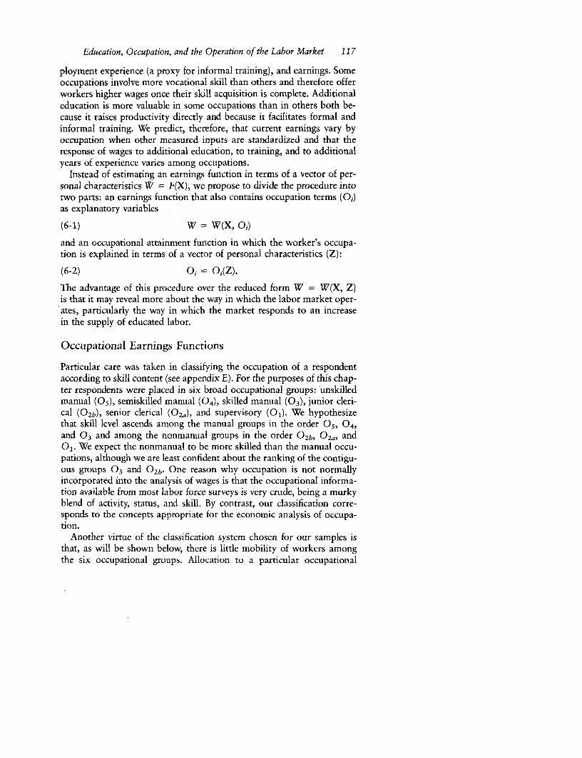
Education, Occupation, and the Operation of the Labor Market 117
ployment experience (a proxy for informal training), and earnings. Someoccupations involve more vocational skill than others and therefore offerworkers higher wages once their skill acquisition is complete. Additionaleducation is more valuable in some occupations than in others both be-cause it raises productivity directly and because it facilitates formal andinformal training. We predict, therefore, that current earnings vary byoccupation when other measured inputs are standardized and that theresponse of wages to additional education, to training, and to additionalyears of experience varies among occupations.
Instead of estimating an earnings function in terms of a vector of per-sonal characteristics W = F(X), we propose to divide the procedure intotwo parts: an earnings function that also contains occupation terms (0,)as explanatory variables
(6-1) W = W(X, 0t)
and an occupational attainment function in which the worker's occupa-tion is explained in terms of a vector of personal characteristics (Z):
(6-2) Oi = Oi(Z).
The advantage of this procedure over the reduced form W = W(X, Z)is that it may reveal more about the way in which the labor market oper-ates, particularly the way in which the market responds to an increasein the supply of educated labor.
Occupational Earnings Functions
Particular care was taken in classifying the occupation of a respondentaccording to skill content (see appendix E). For the purposes of this chap-ter respondents were placed in six broad occupational groups: unskilledmanual (°s), semiskilled manual (04), skilled manual (03), junior cleri-cal ( 0 2b), senior clerical (0 2a), and supervisory (O1). We hypothesizethat skill level ascends among the manual groups in the order 05, 04,
and 03 and among the nonmanual groups in the order 02b,
02a, and
01. We expect the nonmanual to be more skilled than the manual occu-pations, although we are least confident about the ranking of the contigu-ous groups 03 and 0
2b. One reason why occupation is not normallyincorporated into the analysis of wages is that the occupational informa-tion available from most labor force surveys is very crude, being a murkyblend of activity, status, and skill. By contrast, our classification corre-sponds to the concepts appropriate for the economic analysis of occupa-tion.
Another virtue of the classification system chosen for our samples isthat, as will be shown below, there is little mobility of workers amongthe six occupational groups. Allocation to a particular occupational
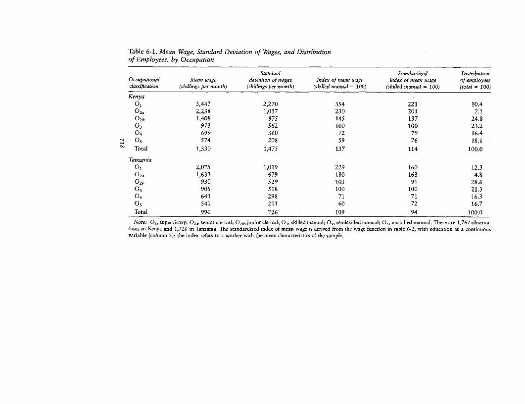
Table 6-1. Mean Wage, Standard Deviation of Wages, and Distributionof Employees, by Occupation
Standard Standardized DistributionOccupational Mean wage deviation of wages Index of mean wage index of mean wage of employeesclassification (shillings per month) (shillings per month) (skilled manual = 100) (skilled manual = 100) (total = 100)
Kenya°l 3,447 2,270 354 221 10.402a 2,238 1,017 230 201 7.10
2b 1,408 875 145 137 24.803 973 562 100 100 23.204 699 360 72 79 16.4~ 05 574 208 59 76 18.1
> Total 1,330 1,475 137 114 100.0
Tanzaniaol 2,075 1,019 229 160 12.302a 1,633 679 180 163 4.80
2b 930 529 103 91 28.603 905 518 100 100 21.304 641 298 71 71 16.3Os 541 211 60 72 16.7Total 990 726 109 94 100.0
Note: 01, supervisory; 02., senior clerical; 02b, junior clerical; 03, skilled manual; 04, semiskilled manual; 05, unskilled manual. There are 1,767 observa-tions in Kenya and 1,726 in Tanzania. The standardized index of mean wage is derived from the wage function in table 6-2, with education as a continuousvariable (column 2); the index refers to a worker with the mean characteristics of the sample.
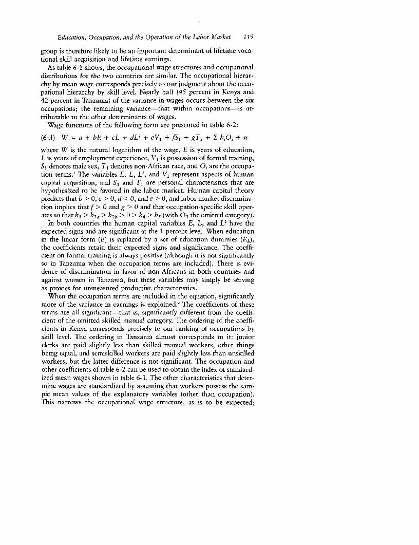
Education, Occupation, and the Operation of the Labor Market 119
group is therefore likely to be an important determinant of lifetime voca-tional skill acquisition and lifetime earnings.
As table 6-1 shows, the occupational wage structures and occupationaldistributions for the two countries are similar. The occupational hierar-chy by mean wage corresponds precisely to our judgment about the occu-pational hierarchy by skill level. Nearly half (45 percent in Kenya and42 percent in Tanzania) of the variance in wages occurs between the sixoccupations; the remaining variance-that within occupations-is at-tributable to the other determinants of wages.
Wage functions of the following form are presented in table 6-2:
(6-3) W = a + bE + cL + dL2 + eV, + fS1 + gT 1 + E hi0i + u
where W is the natural logarithm of the wage, E is years of education,L is years of employment experience, V1 is possession of formal training,S1 denotes male sex, T1 denotes non-African race, and Qi are the occupa-tion terms.' The variables E, L, L2, and V1 represent aspects of humancapital acquisition, and S, and T1 are personal characteristics that arehypothesized to be favored in the labor market. Human capital theorypredicts that b > 0, c > 0, d < 0, and e > 0, and labor market discrimina-tion implies that f > 0 and g > 0 and that occupation-specific skill oper-ates so that h1 > h2, > h2b > 0 > h4 > h5 (with 03 the omitted category).
In both countries the human capital variables E, L, and L2 have theexpected signs and are significant at the 1 percent level. When educationin the linear form (E) is replaced by a set of education dummies (Ek),the coefficients retain their expected signs and significance. The coeffi-cient on formal training is always positive (although it is not significantlyso in Tanzania when the occupation terms are included). There is evi-dence of discrimination in favor of non-Africans in both countries andagainst women in Tanzania, but these variables may simply be servingas proxies for unmeasured productive characteristics.
When the occupation terms are included in the equation, significantlymore of the variance in earnings is explained.2 The coefficients of theseterms are all significant-that is, significantly different from the coeffi-cient of the omitted skilled manual category. The ordering of the coeffi-cients in Kenya corresponds precisely to our ranking of occupations byskill level. The ordering in Tanzania almost corresponds to it: juniorclerks are paid slightly less than skilled manual workers, other thingsbeing equal, and semiskilled workers are paid slightly less than unskilledworkers, but the latter difference is not significant. The occupation andother coefficients of table 6-2 can be used to obtain the index of standard-ized mean wages shown in table 6-1. The other characteristics that deter-mine wages are standardized by assuming that workers possess the sam-ple mean values of the explanatory variables (other than occupation).This narrows the occupational wage structure, as is to be expected;
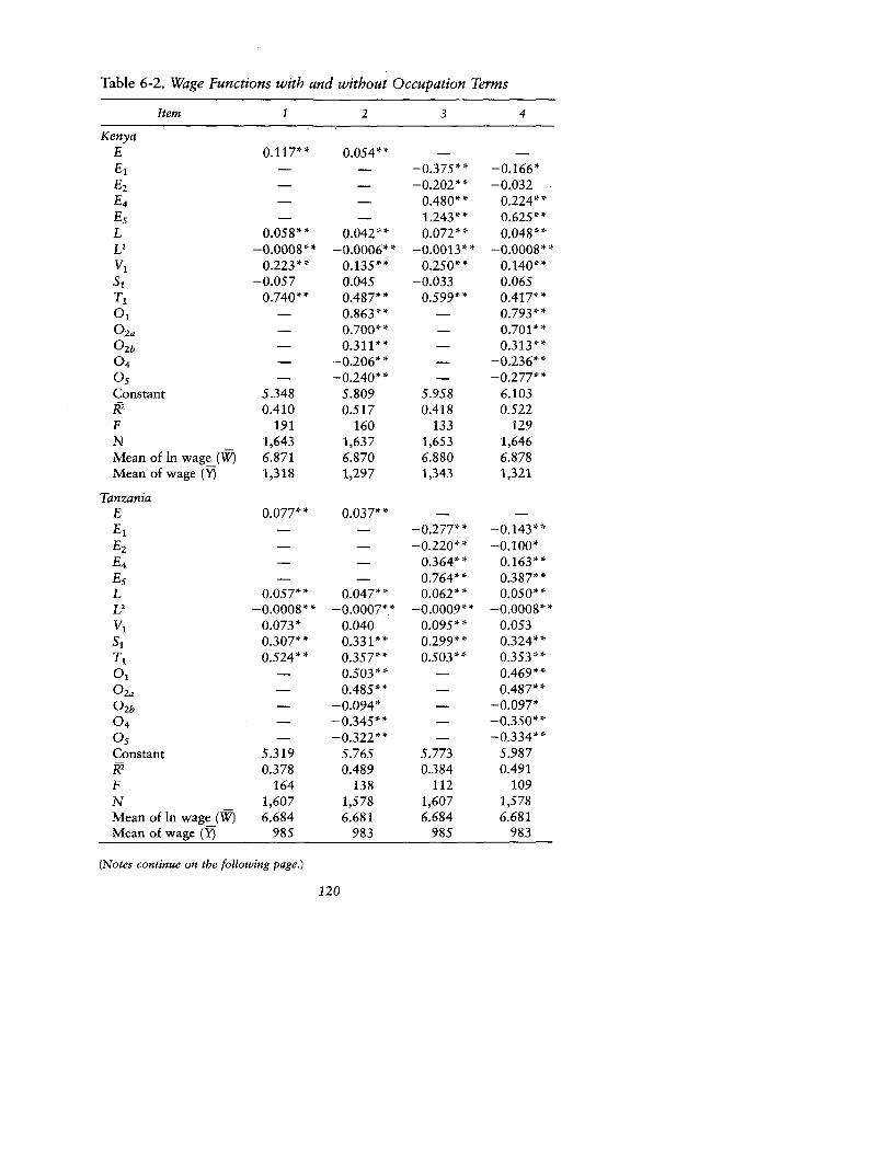
Table 6-2. Wage Functions with and without Occupation Terms
Item 1 2 3 4
KenyaE 0.117** 0.054** - -
El - - -0.375** -0.166*E2 - - -0.202** -0.032E4 - - 0.480** 0.224**Es - - 1.243* * 0.625**L 0.058** 0.042** 0.072** 0.048**L2 -0.0008** -0.0006** -0.0013** -0.0008**V1 0.223** 0.135** 0.250** 0.140**S1 -0.057 0.045 -0.033 0.065T1 0.740** 0.487** 0.599** 0.417**01 - 0.863** - 0.793**02a - 0.700** - 0.701 *0 2b - 0.311** - 0.313**04 - -0.206** - -0.236**Os - -0.240** - -0.277**Constant 5.348 5.809 5.958 6.103k2 0.410 0.517 0.418 0.522F 191 160 133 129N 1,643 1,637 1,653 1,646Mean of In wage (W) 6.871 6.870 6.880 6.878Mean of wage (Y 1,318 1,297 1,343 1,321
TanzaniaE 0.077** 0.037** - -E1 - - -0.277** -0.143**E2 - - -0.220** -0.100*E4 - - 0.364** 0.163**Es - - 0.764** 0.387**L 0.057** 0.047** 0.062** 0.050*L2 -0.0008** -0.0007** -0.0009** -0.0008**V1 0.073* 0.040 0.095** 0.053S1 0.307** 0.331** 0.299** 0.324**T, 0.524** 0.357** 0.503** 0.353**0, - 0.503** - 0.469**01, - 0.485** - 0.487*02b - -0.094* - -0.097*04 - -0.345** - -0.350**0s - -0.322** - -0.334**Constant 5.319 5.765 5.773 5.987K2 0.378 0.489 0.384 0.491F 164 138 112 109N 1,607 1,578 1,607 1,578Mean of In wage (W) 6.684 6.681 6.684 6.681Mean of wage (Y) 985 983 985 983
(Notes continue on the following page.)
120
Education, Occupation, and the Operation of the Labor Market 121
workers in the better-paying occupations tend to be better endowed withproductive characteristics.
The inclusion of the occupation terms in the wage function reducesthe coefficient on years of education by more than half and decreases thecoefficients on formal training and non-African race. This is because ofthe positive correlation between these variables and occupation orderedby skill content. The better-paying occupations tend to attract higherproportions of workers who have had more than x years of schooling,who have had formal training, and who are of non-African race. The in-clusion of occupation therefore raises the econometric problem ofmulticollinearity, but it does not necessarily bias the coefficients of theequation. Upward bias in the occupation coefficients would arise froma positive correlation between occupation and the error term in the equa-tion-for example, between occupation and unmeasured ability. Sucha correlation is indeed predicted by our model because ability is likelyto assist skill formation.
The role of occupation might therefore be exaggerated by the esti-mated coefficients, but it is implausible that occupation is simply actingas a proxy for ability. Although a correlation between education andability is widely acknowledged-and is also predicted by our model-few would argue that education therefore has no causal effect on wagesor that it has no place in the wage function. The possibility of bias isnot a reason for excluding the occupation terms, particularly if there isfurther evidence that occupation plays a role in wage determination.
The sole addition of straightforward occupation dummies to the wagefunction is consistent with only a very simple version of the occupationalproduction function, that is, one in which the coefficients on employmentexperience, on formal training, and on education in the wage functiondo not vary among occupations. It is implicit in the general model thatthere are occupational differences not only in the level of wages but alsoin the returns to education, to formal training, and to employment expe-rience.
Our first test for such interaction effects was to add to the equationwith a linear education term and with occupation terms (table 6-2, col-umn 2) a set of interaction terms, E- Oi, L Oi, and L2- °t (equationnot shown). The contribution of these interaction terms as a set provedNotes to table 6-2.
-Not applicable.* Statistically significant at the 5 percent level.* *Statistically significant at the 1 percent level.Note: E, years of education; El, no education; E2, primary standards 1-4; E4, second-
ary forms 1-4; Es, post-form 4; L, employment experience; VI, formal training; S,, malesex; TI, non-African race. Occupation variables are as defined in table 6-1. Column num-bers identify different regression specifications.
122 EDUCATIONAL EXPANSION, GOVERNMENT POLICY, AND PAY
to be statistically significant at the 1 percent level in both countries.3 Allthe coefficients on the E °i terms were significantly different from zeroin Kenya, as were three of the five in Tanzania. Since 05 was the basecategory, this showed significant differences between the returns to edu-cation in the unskilled manual and in the other occupations. The with-drawal of the E 0, terms as a set proved significant at the 1 percentlevel in both countries, as did the withdrawal of the L Oi and L2* 0,
terms as a set.4 The omission from the full equation of the L- Oi andL2 - Oi terms, one occupation at a time, had a significant effect in twoof the five cases for Kenya and in three of the five cases for Tanzania.In those occupations, therefore, the returns to experience were signifi-cantly greater than in the unskilled manual category. These tests gener-ally provided statistical support for the inclusion of interaction terms andfor our hypothesis of occupational differences in the returns to educationand to experience.
Table 6-3 reports wage functions for each occupation. The percentageof the variance in W explained by the equation is low in the unskilledmanual occupation but tends to rise with occupational skill level. Thecoefficients on the education dummy variables are generally significantand of the expected sign in the more skilled occupations. The coefficientson employment experience are all positive, and almost all are signifi-cantly so; those on the squared term are generally negative, and mostare significant. Again, the coefficients on formal training are rarely signif-icant; indeed, some are negative.5 It is notable from the mean values ofselected independent variables, also shown in table 6-3, that occupationalskill level, according to our ranking, is strongly correlated with educa-tional attainment, formal training, and race.
Do the returns to education differ among occupations, as we have pre-dicted? Figure 6-1 shows how, within each occupation, the wage varieswith educational level, other things being equal. We standardize for thedifferences in characteristics of workers both within and between occu-pations by showing the wage of a representative worker in the labor mar-ket; that is, by assuming that the worker possesses the mean values ofthe explanatory variables (other than education) for the sample as awhole. The occupational differences in wages at each educational leveltherefore correspond solely to differences in the coefficients and constantterms of the occupation-specific wage functions.
In both countries the vertical ordering of occupations again corre-sponds to that of our hypothesized skill levels. The wage is weakly re-sponsive to education in unskilled and semiskilled manual jobs but rathermore responsive in skilled manual jobs. Wages in nonmanual occupa-tions, by contrast, are extremely sensitive to educational level; it is inthese jobs that education pays off. The results for the two countries aresimilar, the main difference being that there are higher returns to educa-
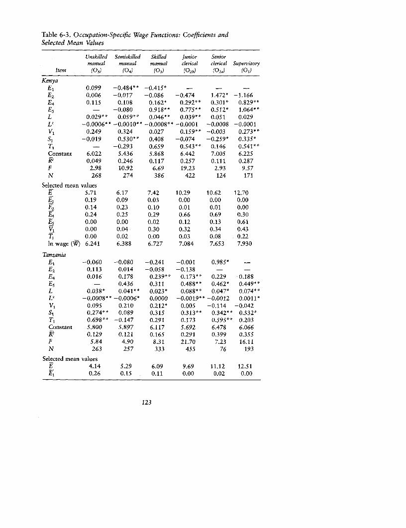
Table 6-3. Occupation-Specific Wage Functions: Coefficients andSelected Mean Values
Unskilled Semiskilled Skilled junior Seniormanual manual manual clerical clerical Supervisory
Item (05) (04) (03) (02b) (0 2 J (01)
KenyaEl 0.099 -0.484** -0.415* - - -E2 0.006 -0.017 -0.086 -0.474 1.472* -1.166E4 0.115 0.108 0.162* 0.292** 0.301* 0.829**Es - -0.080 0.918** 0.775** 0.512* 1.064**L 0.029** 0.059** 0.046** 0.039** 0.051 0.029L2 -0.0006** -0.0010** -0.0008 * -0.0001 -0.0008 -0.0001V1 0.249 0.324 0.027 0.159** -0.003 0.273**SI -0.019 0.530** 0.408 -0.074 -0.259* 0.335*T, - -0.293 0.659 0.543** 0.146 0.541**Constant 6.022 5.436 5.868 6.442 7.005 6.225R2 0.049 0.246 0.117 0.257 0.111 0.287F 2.98 10.92 6.69 19.23 2.93 9.57N 268 274 386 422 124 171
Selected mean valuesE 5.71 6.17 7.42 10.29 10.62 12.70El 0.19 0.09 0.03 0.00 0.00 0.00F2 0.14 0.23 0.10 0.01 0.01 0.00E4 0.24 0.25 0.29 0.66 0.69 0.30Es 0.00 0.00 0.02 0.12 0.13 0.61V1 0.00 0.04 0.30 0.32 0.34 0.43T, _ 0.00 0.02 0.00 0.03 0.08 0.22In wage (W) 6.241 6.388 6.727 7.084 7.653 7.930
TanzaniaE, -0.060 -0.080 -0.241 -0.001 0.985* -E2 0.113 0.014 -0.058 -0.138 - -E4 0.016 0.178 0.239** 0.173** 0.229 0.188Es - 0.436 0.311 0.488** 0.462* 0.449**L 0.038* 0.041** 0.023* 0.088** 0.047* 0.074**L 2 -0.0008** -0.0006* 0.0000 -0.0019** -0.0012 0.0011*V1 0.095 0.210 0.212* 0.005 -0.114 -0.042SI 0.274** 0.089 0.315 0.313** 0.342** 0.532*T, 0.698** -0.147 0.291 0.173 0.595** 0.203Constant 5.800 5.897 6.117 5.692 6.478 6.066k2 0.129 0.121 0.165 0.291 0.399 0.355F 5.84 4.90 8.31 21.70 7.23 16.11N 263 257 333 455 76 193
Selected mean valuesE 4.14 5.29 6.09 9.69 11.12 12.51E1 0.26 0.15 0.11 0.00 0.02 0.00
123
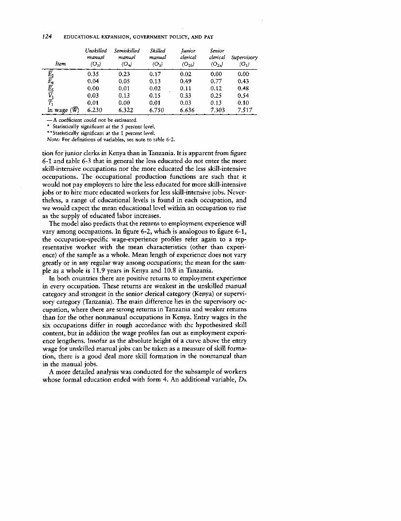
124 EDUCATIONAL EXPANSION, GOVERNMENT POLICY, AND PAY
Unskilled Semiskilled Skilled Junior Seniormanual manual manual clerical clerical Supervisory
Item (05) (04) (03) (02b) (O2)J (O)
E2 0.35 0.23 0.17 0.02 0.00 0.00F4 0.04 0.05 0.13 0.49 0.77 0.43Es 0.00 0.01 0.02 0.11 0.12 0.48VI 0.03 0.13 0.15 0.33 0.25 0.54T, 0.01 0.00 0.01 0.03 0.13 0.10In wage (W) 6.230 6.322 6.750 6.636 7.303 7.517
-A coefficient could not be estimated.* Statistically significant at the 5 percent level.**Statistically significant at the 1 percent level.Note: For definitions of variables, see note to table 6-2.
tion for junior clerks in Kenya than in Tanzania. It is apparent from figure6-1 and table 6-3 that in general the less educated do not enter the moreskill-intensive occupations nor the more educated the less skill-intensiveoccupations. The occupational production functions are such that itwould not pay employers to hire the less educated for more skill-intensivejobs or to hire more educated workers for less skill-intensive jobs. Never-theless, a range of educational levels is found in each occupation, andwe would expect the mean educational level within an occupation to riseas the supply of educated labor increases.
The model also predicts that the returns to employment experience willvary among occupations. In figure 6-2, which is analogous to figure 6-1,the occupation-specific wage-experience profiles refer again to a rep-resentative worker with the mean characteristics (other than experi-ence) of the sample as a whole. Mean length of experience does not varygreatly or in any regular way among occupations; the mean for the sam-ple as a whole is 11.9 years in Kenya and 10.8 in Tanzania.
In both countries there are positive returns to employment experiencein every occupation. These returns are weakest in the unskilled manualcategory and strongest in the senior clerical category (Kenya) or supervi-sory category (Tanzania). The main difference lies in the supervisory oc-cupation, where there are strong returns in Tanzania and weaker returnsthan for the other nonmanual occupations in Kenya. Entry wages in thesix occupations differ in rough accordance with the hypothesized skillcontent, but in addition the wage profiles fan out as employment experi-ence lengthens. Insofar as the absolute height of a curve above the entrywage for unskilled manual jobs can be taken as a measure of skill forma-tion, there is a good deal more skill formation in the nonmanual thanin the manual jobs.
A more detailed analysis was conducted for the subsample of workerswhose formal education ended with form 4. An additional variable, Dx

Figure 6-1. Occupation-Specific Wage, by Educational Level
Wage (shillings per month)3,000 KENYA 01
2,500 - 02a
2,000 -0
1,500 -
1,000 /
04
500
0 1 2 3 4 5 6 7 8 9 10 11 12 13E E2 E3 E4 E,
TANZANIA °2,500 7
1,500 _-
1,000-
son 04 O
I I I I I I I I I
r~~~ ~~ 6, E 3 10 11 12 13El 2 E3£4 EYears of education
Note: E1, no education; E2, primary standards 1-4; E3, primary standards 5-7; E4,secondary forms 1-4; E5 , post-form 4; 01, supervisory; 02., senior clerical; 0
2b, juniorclerical; 03, skilled manual; 04, semiskilled manual; 05, unskilled manual.
125

FigUre 6-2- Occupation-Specific Wage, by Imployment Expeyience.
Wage (shillingsper month)3,0 KENYA
2,500
…~~~~~~~~~~04~5,000 02a
4,500 C
4,000
4sooL 03
4= °4
3,S0o
3,0002,500/
2,500o
5002 02
1,1000 = 0~~~ 2b
o00 03
05
Years oexe 1-8 20
126

Education, Occupation, and the Operation of the Labor Market 127
(X 1 . . . 4), was added to the equation to represent the division of pass(the ranked category of scores) on the national form 4 examinations. D 4 ,
the lowest division, is omitted, and D5 indicates those who failed or didnot take the examination. Table 6-4 reports four equations for eachcountry. When occupation terms are added to the basic specification(compare columns 1 and 2), they are generally significant and have pre-cisely the expected ordering in Kenya; four have the expected signs inTanzania. Their addition as a set adds significantly to the explanatorypower of the equation.6 Again, occupation appears to be an importantdeterminant of wages.
When the division of pass in the form 4 examinations is added to thebasic specification (compare columns 1 and 3), the coefficients are signifi-cant and have the expected ordering in both countries (D1 > D2 > D3 >
0 > D5 ). The one exception is the small category D5 in Tanzania, whichis not significantly different from D 4 . In Kenya a division 1 graduateearned 130 percent more than a division 4 graduate, other things beingequal,7 and in Tanzania the difference was 68 percent. The addition ofthe DA terms as a set is highly significant.' Examination performance,which represents a combination of natural ability and cognitive skill, thusappears also to be important in determining wages. This result holds evenfor those who left school at the end of form 4; it would be strengthenedif allowance were made for the effect of examination performance on ac-cess to formal education beyond form 4.
When the variables for examination performance are added to thespecification containing occupation (compare columns 3 and 4), the Dxand Oi coefficients remain significant in Kenya, but most cease to be sig-nificant in Tanzania.9 The spread of both the Dx and Oi coefficients isreduced, especially in Tanzania, reflecting a positive correlation betweenexamination performance and occupational skill level. In Kenya goodscores affect occupational skill level partly by raising pay within occupa-tions and partly by assisting access to preferred occupations; in Tanzaniathey only assist access. The generally stronger effect of examinationperformance in Kenya probably reflects the greater abundance of second-ary (form 4) leavers in the labor market, which allows Kenyan employersto be more selective than their Tanzanian counterparts.
Occupational Attainment Functions
Even in perfectly competitive factor markets, there should be a positivecorrelation between the skill intensity of an occupation and the educationof its workers. Employers will not hire uneducated workers for a skill-intensive job in which their productivity is lower than the wage that un-educated workers can obtain in unskilled jobs. Educated workers willavoid the unskilled jobs in which their education is less productive and
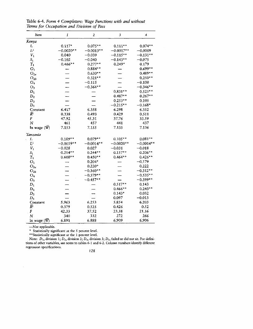
Table 6-4. Form 4 Completers: Wage Functions with and withoutTermns for Occupation and Division of Pass
Item 1 2 3 4
KenyaL 0.117* 0.075** 0.111** 0.074**L 2 -0.0020** -0.0013** -0.0017** -0.0009V1 0.040 -0.039 -0.115** -0.131**SI -0.102 -0.040 -0.143** -0.075T, 0.466** 0.277** 0.249* 0.1790l - 0.884** - 0.699**02a - 0.630** - 0.489**0
2b - 0.321** - 0.2S0**04 - -0.115 - -0.100Os - -0.364** - -0.346**D, - - 0.831** 0.525**D2 - - 0.487** 0.267**D3 - - 0.253** 0.105D5 - - -0.215** -0.168*Constant 6.417 6.358 6.298 6.352R2 0.338 0.493 0.429 0.511F 47.92 45.31 37.76 33.59N 461 457 441 437In wage (W) 7.153 7.155 7.135 7.136
TanzaniaL 0.109** 0.079** 0.105** 0.081**L 2 -0.0019** -0.0014** -0.0020** -0.0014**V1 -0.028 0.027 -0.031 -0.018S, 0.214* 0.244** 0.157** 0.206**T, 0.600** 0.450** 0.464** 0.426**0l - 0.204* - -0.17902a - 0.220* - 0.2220
2b - -0.360** - -0.312**04 - -0.579** - -0.535**O's - -0.457** - -0.399**DI - - 0.517** 0.143D,2- - 0.466** 0.243**D3 - - 0.143* 0.032D, - - 0.097 -0.013Constant 5.963 6.253 5.854 6.203k2 0.379 0.525 0.426 0.52F 42.33 37.52 23.38 21.16N 340 332 272 266In wage (w) 6.891 6.888 6.909 6.906
-Not applicable.* Statistically significant at the 5 percent level."*Statistically significant at the 1 percent level.
Note: Dl, division 1; D2, division 2; D3, division 3; Ds, failed or did not sit. For defini-tions of other variables, see notes to tables 6-1 and 6-2. Column numbers identify differentregression specifications.
128
Education, Occupation, and the Operation of the Labor Market 129
is therefore less highly rewarded. As appendix E shows, if imperfectionsin the capital and labor markets respectively permit and create occupa-tional wage differences at a given level of education, an element of jobcompetition (rather than wage competition) is introduced as workerswith the same education queue for the prized jobs. Moreover, the pres-ence of capital market imperfections, which imply that there are rentsto be gained from the acquisition of vocational skills, causes workers ofdifferent educational levels to queue for the jobs that offer higher lifetimeearnings. Such queues encourage employers to select workers on the basisof their productive characteristics (for example, level of education, exam-ination performance, and the correlate of the first two, ability) or theirsocial characteristics (such as race and sex). Thus, employers are able tominimize the costs of wage rigidity or of rental payments or to indulgea taste for discrimination.
The evidence above suggests that occupations differ in the mean valuesof some of the personal characteristics of their workers. In particular, oc-cupation, ranked according to hypothesized skill level, is positively corre-lated with mean educational attainment, receipt of formal training, race,and, in the case of form 4 leavers, examination score. These results arereadily understood in the context of our model. Formal training can beviewed as a characteristic of the occupation-that is, as a consequencerather than a cause of occupational choice. The other characteristics,however, can be hypothesized to determine occupation. They are in-cluded as explanatory variables in our occupational attainment func-tions.
Three other explanatory variables are included. Family background,measured by the educational attainment of parents, could represent ei-ther job discrimination by employers on the basis of social class or valu-able productive traits inherited or acquired from parents. Sex is likelyto show job discrimination against women. Length of employment expe-rience could represent either occupational promotion in the course of theworker's career or the state of the labor market when the worker enteredit. For instance, in the 1960s a secondary leaver entering the Kenyanlabor market could be confident of securing a white-collar job, whereasin the 1980s he was likely to enter a low-level manual job.
The importance of occupational promotion in explaining the influenceof length of experience on occupation depends on the degree of occupa-tional mobility in the sample. Our data include occupation at the endof the previous job and at the end of the first job, but since only 43 per-cent of Kenyans and 36 percent of Tanzanians had ever changed employ-ers, information on previous jobs covers only a minority of respondents.We also lack information on occupational mobility during the tenure ofthe current job. Nevertheless, the evidence that we do have is suggestive.
In Kenya, among the minority on whom we have information about
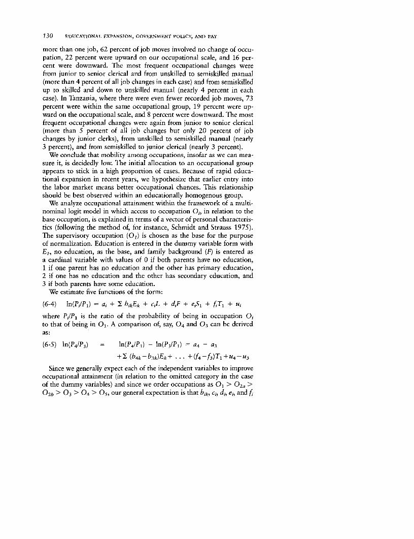
130 EDUCATIONAL EXPANSION, GOVERNMENT POLICY, AND PAY
more than one job, 62 percent of job moves involved no change of occu-pation, 22 percent were upward on our occupational scale, and 16 per-cent were downward. The most frequent occupational changes werefrom junior to senior clerical and from unskilled to semiskilled manual(more than 4 percent of all job changes in each case) and from semiskilledup to skilled and down to unskilled manual (nearly 4 percent in eachcase). In Tanzania, where there were even fewer recorded job moves, 73percent were within the same occupational group, 19 percent were up-ward on the occupational scale, and 8 percent were downward. The mostfrequent occupational changes were again from junior to senior clerical(more than 5 percent of all job changes but only 20 percent of jobchanges by junior clerks), from unskilled to semiskilled manual (nearly3 percent), and from semiskilled to junior clerical (nearly 3 percent).
We conclude that mobility among occupations, insofar as we can mea-sure it, is decidedly low. The initial allocation to an occupational groupappears to stick in a high proportion of cases. Because of rapid educa-tional expansion in recent years, we hypothesize that earlier entry intothe labor market means better occupational chances. This relationshipshould be best observed within an educationally homogenous group.
We analyze occupational attainment within the framework of a multi-nominal logit model in which access to occupation Oi, in relation to thebase occupation, is explained in terms of a vector of personal characteris-tics (following the method of, for instance, Schmidt and Strauss 1975).The supervisory occupation (01) is chosen as the base for the purposeof normalization. Education is entered in the dummy variable form withEl, no education, as the base, and family background (F) is entered asa cardinal variable with values of 0 if both parents have no education,1 if one parent has no education and the other has primary education,2 if one has no education and the other has secondary education, and3 if both parents have some education.
We estimate five functions of the form:
(6-4) ln(P,/P1) = a, + I b&kEk + ciL + d,F + e,S1 + fiT1 + ui
where P1/P1 is the ratio of the probability of being in occupation 0,to that of being in 01. A comparison of, say, 04 and 03 can be derivedas:
(6-5) ln(P4 /P3 ) = ln(P 4/P1 ) - ln(P3 /P1 ) = a4 - a3
+ X (b4k - b3k)Ek + * . . + (f4 - f3)T, + U4 -U3
Since we generally expect each of the independent variables to improveoccupational attainment (in relation to the omitted category in the caseof the dummy variables) and since we order occupations as O1 > 0 2a >
°2b > 03 > 04 > 05, our general expectation is that bik, ci, di, ei, and fi
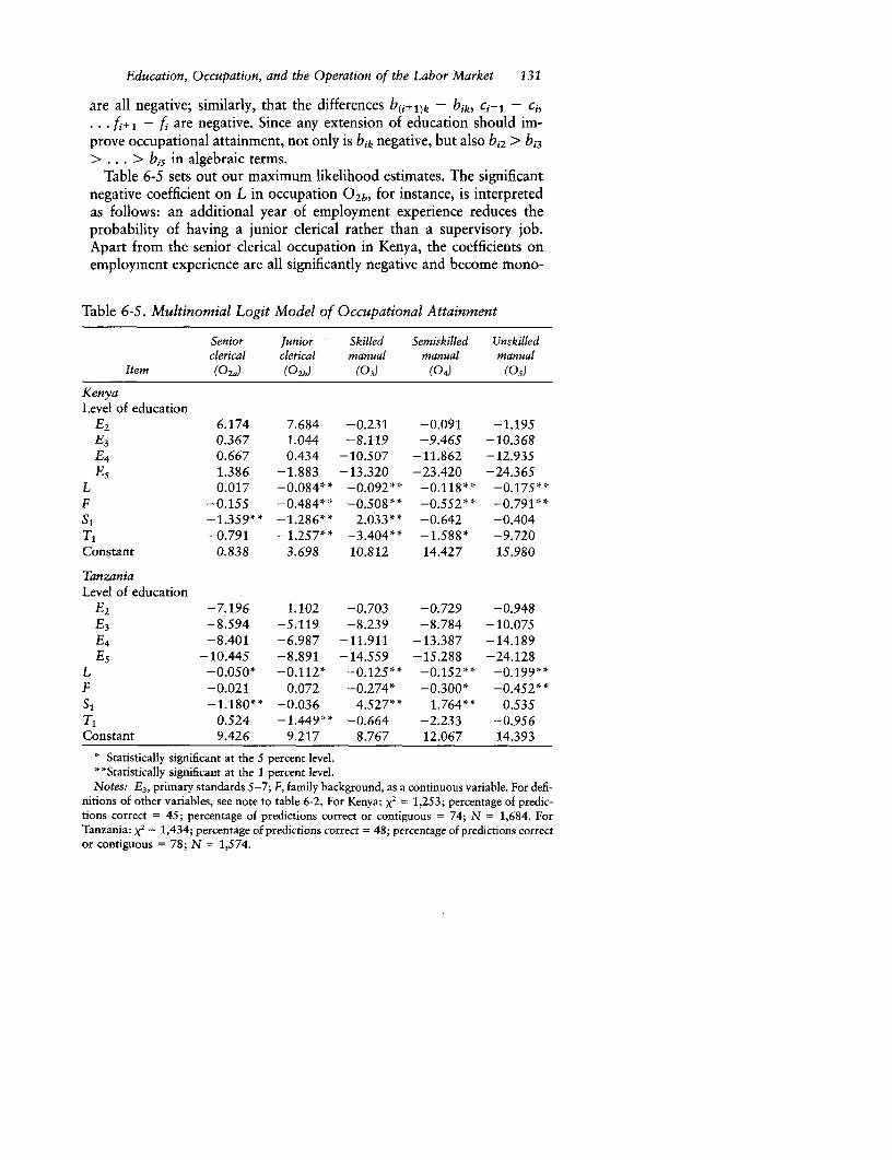
Education, Occupation, and the Operation of the Labor Market 131
are all negative; similarly, that the differences b(i+1)k - bik, ci+1 - Ci,.. . f+1 - fi are negative. Since any extension of education should im-prove occupational attainment, not only is bik negative, but also bi2 > bi3> ... > b, in algebraic terms.
Table 6-5 sets out our maximum likelihood estimates. The significantnegative coefficient on L in occupation 0 2b, for instance, is interpretedas follows: an additional year of employment experience reduces theprobability of having a junior clerical rather than a supervisory job.Apart from the senior clerical occupation in Kenya, the coefficients onemployment experience are all significantly negative and become mono-
Table 6-5. Multinomial Logit Model of Occupational Attainment
Senior Junior Skilled Semiskilled Unskilledclerical clerical manual manual manual
Item (02J (0
2b) (03) (04) (05)
KenyaLevel of education
E2 6.174 7.684 -0.231 -0.091 -1.195E3 0.367 1.044 -8.119 -9.465 -10.368E4 0.667 0.434 -10.507 -11.862 - 12.935Es 1.386 -1.883 -13.320 -23.420 -24.365
L 0.017 -0.084** -0.092** -0.118** -0.175**F -0.155 -0.484** -0.508** -0.552** -0.791**S1 -1.359** -1.286** 2.033 * * -0.642 -0.404T, -0.791 -1.257** -3.404* * - 1.588* -9.720Constant 0.838 3.698 10.812 14.427 15.980
TanzaniaLevel of education
E2 -7.196 1.102 -0.703 -0.729 -0.948E3 -8.594 -5.119 -8.239 -8.784 -10.075E4 -8.401 -6.987 -11.911 -13.387 -14.189E5 -10.445 -8.891 -14.559 -15.288 -24.128
L -0.050* -0.112* -0.125* * -0.152* * -0.199**F -0.021 0.072 -0.274* -0.300* -0.452**S, - 1.180** -0.036 4.527* * 1.764* * 0.535'Tl 0.524 -1.449** -0.664 -2.233 -0.956Constant 9.426 9.217 8.767 12.067 14.393
* Statistically significant at the 5 percent level.**Statistically significant at the 1 percent level.Notes: E3, primary standards 5-7; F, family background, as a continuous variable. For defi-
nitions of other variables, see note to table 6-2. For Kenya: x2 = 1,253; percentage of predic-tions correct = 45; percentage of predictions correct or contiguous = 74; N = 1,684. ForTanzania: x2
= 1,434; percentage of predictions correct = 48; percentage of predictions corrector contiguous = 78; N = 1,574.

132 EDUCATIONAL EXPANSION, GOVERNMENT POLICY, AND PAY
tonically more negative as occupations become less skilled; earlier entryto the labor market improves current occupational attainment. The coef-ficients on educational level (in relation to no education) are not signifi-cant, but the:- display a clear pattern. Within each occupation the coef-ficient on educational level becomes algebraically smaller as theeducational level rises, and for each educational level there is a tendencyfor the coefficient to be smaller in the less skilled occupations.'°More education reduces the probability of being in a less skilled asagainst a supervisory job, and the reduction tends to be greater the loweris the skill level of the job under consideration.
In both countries women tend to be excluded from the highest manualcategory (skilled) and the highest nonmanual category (supervisory). Thefamily background coefficients are mostly significantly negative, andtheir algebraic value tends to be directly correlated with occupationalrank; the better educated are a worker's parents, the better are hischances of being in a good job. In Kenya the coefficients on non-Africanrace are mostly significantly negative and tend to become more negativeas we move down the occupational hierarchy; being non-African im-proves a worker's occupational chances. In Tanzania the non-African co-efficients generally have the expected sign, but the results are weaker.
Both equations perform reasonably well. The chi-squared test againstthe null hypothesis that the coefficients are zero is significant at the one-in-a-million level. Moreover, the coefficients generally make good eco-nomic sense. In Kenya the model predicts the correct occupation (in thesense that the most likely occupation corresponds to the actual occupa-tion) in 45 percent of all cases and in Tanzania in 48 percent. The modelpredicts either the correct occupation or a contiguous one in our hypoth-esized occupational skill hierarchy in 74 and 78 percent of the cases, re-spectively.
Table 6-6 shows how the probability that a representative worker willbe in a particular occupation varies according to level of education andtime of entry into employment (which corresponds to years of employ-ment experience). In both countries the skill ranking of the most probableoccupation rises (apart from a couple of equalities) with level of educa-tion. In both countries the probability of being an unskilled manualworker falls monotonically and sharply as educational attainment rises,whereas the probability of being in each of the nonmanual occupationsrises almost monotonically with educational level. (The exception isthose with education beyond form 4; for them the supervisory occupa-tion dominates.) A worker's educational level is thus an important deter-minant of his occupation.
The table also permits us to examine filtering down-the movementof educated workers or of educated entrants to the labor market intolesser jobs as a result of an increased supply of educated labor. The prob-
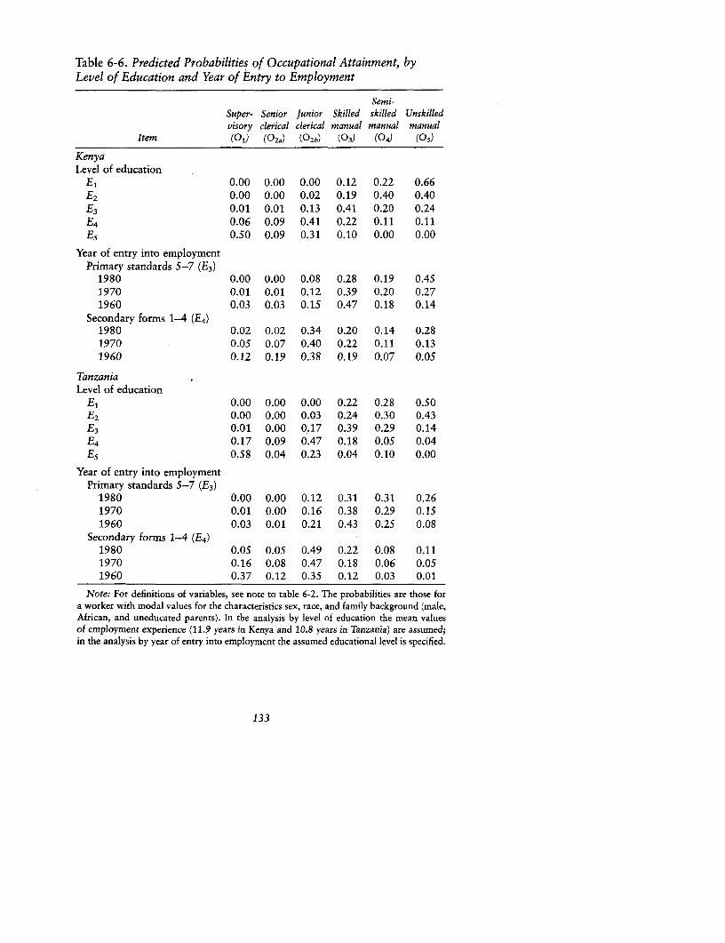
Table 6-6. Predicted Probabilities of Occupational Attainment, byLevel of Education and Year of Entry to Employment
Semi-Super- Senior Junior Skilled skilled Unskilledvisory clerical clerical manual manual manual
Itern (O1) (02a) (0
2b) (03) (04) (05)
KenyaLevel of education
E 0.00 0.00 0.00 0.12 0.22 0.66E2 0.00 0.00 0.02 0.19 0.40 0.40E3 0.01 0.01 0.13 0.41 0.20 0.24E4 0.06 0.09 0.41 0.22 0.11 0.11E5 0.50 0.09 0.31 0.10 0.00 0.00
Year of entry into employmentPrimary standards 5-7 (E3)
1980 0.00 0.00 0.08 0.28 0.19 0.451970 0.01 0.01 0.12 0.39 0.20 0.271960 0.03 0.03 0.15 0.47 0.18 0.14
Secondary forms 1-4 (E4)1980 0.02 0.02 0.34 0.20 0.14 0.281970 0.05 0.07 0.40 0.22 0.11 0.131960 0.12 0.19 0.38 0.19 0.07 0.05
Tanzania
Level of educationEl1 0.00 0.00 0.00 0.22 0.28 0.50E2 0.00 0.00 0.03 0.24 0.30 0.43F 3 0.01 0.00 0.17 0.39 0.29 0.14E4 0.17 0.09 0.47 0.18 0.05 0.04E5 0.58 0.04 0.23 0.04 0.10 0.00
Year of entry into employmentPrimary standards 5-7 (E3)
1980 0.00 0.00 0.12 0.31 0.31 0.261970 0.01 0.00 0.16 0.38 0.29 0.151960 0.03 0.01 0.21 0.43 0.25 0.08
Secondary forms 1-4 (E 4 )
1980 0.05 0.05 0.49 0.22 0.08 0.111970 0.16 0.08 0.47 0.18 0.06 0.051960 0.37 0.12 0.35 0.12 0.03 0.01
Note: For definitions of variables, see note to table 6-2. The probabilities are those fora worker with modal values for the characteristics sex, race, and family background (male,African, and uneducated parents). In the analysis by level of education the mean valuesof employment experience (11.9 years in Kenya and 10.8 years in Tanzania) are assumed;in the analysis by year of entry into employment the assumed educational level is specified.
133
134 EDUCATIONAL EXPANSION, GOVERNMENT POLICY, AND PAY
abilities of occupational attainment are shown for three different cohortsof primary and secondary leavers-those who entered the labor marketin 1960, 1970, and 1980. For primary leavers the semiskilled manual oc-cupation is pivotal in both countries; later entry decreases the probabilityof securing a better job and sharply increases the probability of enteringan unskilled job. For secondary leavers the junior clerical and skilledmanual occupations are pivotal in Kenya, whereas in Tanzania the divid-ing line is between senior and junior clerical. The fact that the probabili-ties of occupational attainment differ from one cohort to another sug-gests that the burden of filtering down falls on entrants to the labormarket rather than on incumbents. The time at which a worker enteredwage employment is an important determinant of his occupation.
Consider the most recent cohort, which entered wage employment atthe time of the surveys. The probability that a new secondary leaver willenter a semiskilled or unskilled manual job is 42 percent in Kenya butonly 19 percent in Tanzania, where the probability that such a personwill enter a nonmanual job is 61 percent. The probabilities of occupa-tional attainment of new primary leavers are similar in the two countries,which have similar government policies on primary education. The con-trast arises at the secondary level; the filtering down of entrants has pro-ceeded further in Kenya than in Tanzania, which reflects the far morerapid expansion of secondary education in Kenya.
The determinants of the occupational attainment of secondary leaversare shown in table 6-7. The equations perform well as measured by thechi-squared test and the number of bull's-eyes and near-misses, althoughhalf of their coefficients are not significantly different from zero. TheTanzanian specification had to be simplified to obtain convergence on aset of coefficients. In Kenya the discrimination variables, although notsignificant, generally show the expected pattern; the coefficients tend tobecome more negative as occupations become less skilled: parents' edu-cation and non-African race improve occupational attainment. In bothcountries the significance, sign, and pattern of the employment experi-ence coefficients are generally as expected; earlier entry into the labormarket improves occupational attainment.
Table 6-8, which is analogous to table 6-6, illustrates how the expan-sion of education has affected filtering down. The junior clerical occupa-tion is pivotal for secondary leavers; for more skilled occupations theprobability of access is lower for later entrants, whereas for less skilledoccupations the probability is higher. Although fewer than half of thecoefficients are significant (table 6-7), a pattern can be discerned that isbest illustrated by examining probabilities (table 6-8). The probability ofaccess to supervisory and senior clerical jobs improves with examinationperformance in both countries. In Kenya the chances of landing in an un-skilled or semiskilled manual job rise sharply as examination perfor-
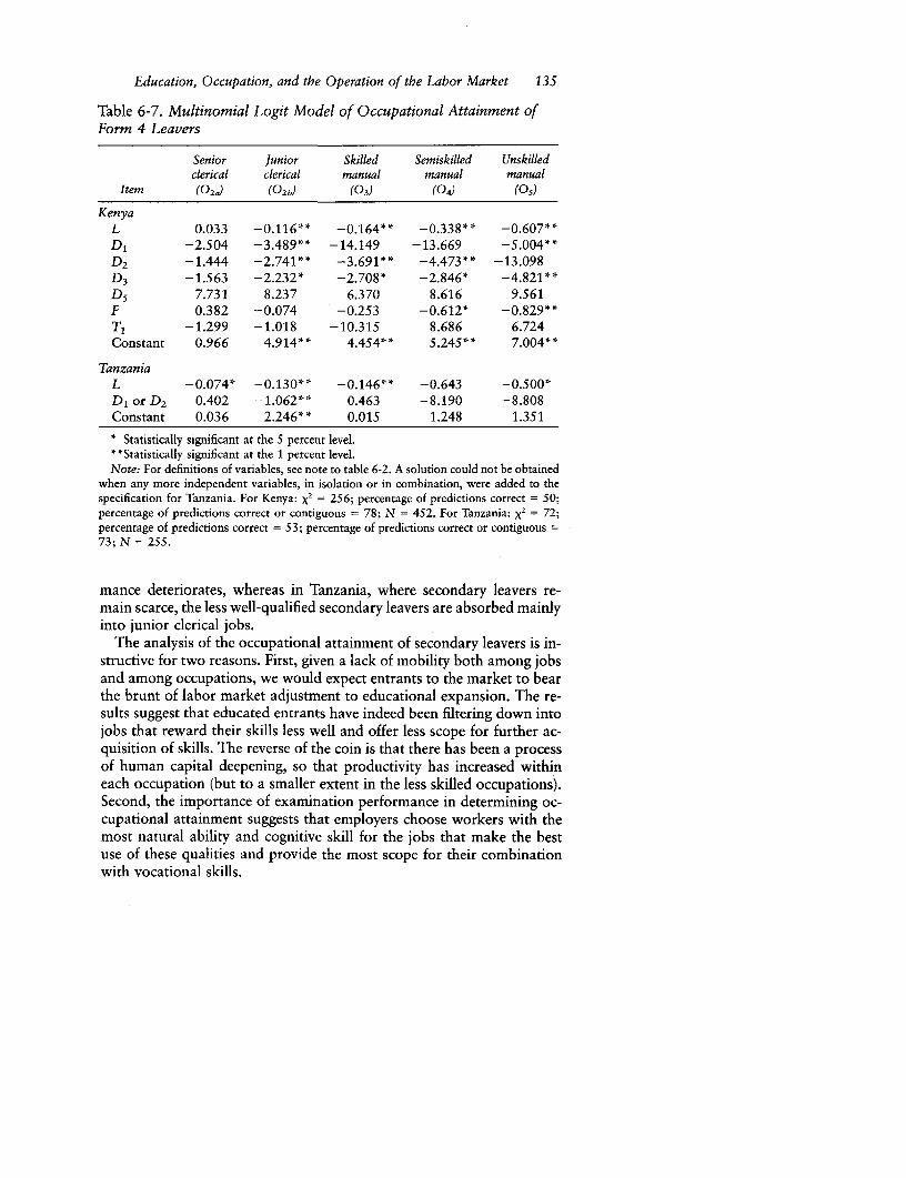
Education, Occupation, and the Operation of the Labor Market 135
Table 6-7. Multinomial Logit Model of Occupational Attainment ofForm 4 Leavers
Senior Junior Skilled Semiskilled Unskilledclerical clerical manual manual manual
Item (02.) (02b) (03) (04) (0°)
KenyaL 0.033 -0.116** -0.164** -0.338** -0.607**Di -2.504 -3.489** -14.149 -13.669 -5.004**D2 -- 1.444 -2.741 ** -3.691 ** 4.473** -13.098D3 -1.563 -2.232* -2.708* -2.846* -4.821**D 5 7.731 8.237 6.370 8.616 9.561F 0.382 -0.074 -0.253 -0.612* -0.829**T, -1.299 -1.018 -10.315 8.686 6.724Constant 0.966 4.914** 4.454** 5.245** 7.004**
TanzaniaL -0.074* -0.130** -0.146** -0.643 -0.500*DI or D2 0.402 -1.062** 0.463 -8.190 -8.808Constant 0.036 2.246** 0.015 1.248 1.351
* Statistically significant at the 5 percent level.* *Statistically significant at the 1 percent level.Note: For definitions of variables, see note to table 6-2. A solution could not be obtained
when any more independent variables, in isolation or in combination, were added to thespecification for Tanzania. For Kenya: X' = 256; percentage of predictions correct = 50;percentage of predictions correct or contiguous = 78; N = 452. For Tanzania: X2
= 72;percentage of predictions correct = 53; percentage of predictions correct or contiguous =73; N = 255.
mance deteriorates, whereas in Tanzania, where secondary leavers re-main scarce, the less well-qualified secondary leavers are absorbed mainlyinto junior clerical jobs.
The analysis of the occupational attainment of secondary leavers is in-structive for two reasons. First, given a lack of mobility both among jobsand among occupations, we would expect entrants to the market to bearthe brunt of labor market adjustment to educational expansion. The re-sults suggest that educated entrants have indeed been filtering down intojobs that reward their skills less well and offer less scope for further ac-quisition of skills. The reverse of the coin is that there has been a processof human capital deepening, so that productivity has increased withineach occupation (but to a smaller extent in the less skilled occupations).Second, the importance of examination performance in determining oc-cupational attainment suggests that employers choose workers with themost natural ability and cognitive skill for the jobs that make the bestuse of these qualities and provide the most scope for their combinationwith vocational skills.
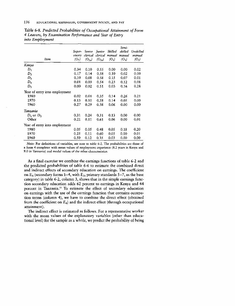
136 EDUCATIONAL EXPANSION, GOVERNMENT POLICY, AND PAY
Table 6-8. Predicted Probabilities of Occupational Attainment of Form4 Leavers, by Examination Performance and Year of Entryinto Employment
Semi-Super- Senior Junior Skilled skilled Unskilledvisory clerical clerical manual manual manual
Item (01) (02.) (0
2b) (03) (04) (0°)
KenyaD, 0.34 0.10 0.55 0.00 0.00 0.02D2 0.17 0.14 0.58 0.10 0.02 0.00D3 0.10 0.08 0.58 0.15 0.07 0.01D4 0.01 0.03 0.54 0.23 0.12 0.08D5 0.00 0.02 0.51 0.03 0.16 0.28
Year of entry into employment1980 0.02 0.01 0.35 0.14 0.26 0.211970 0.13 0.10 0.58 0.14 0.05 0.001960 0.27 0.29 0.38 0.06 0.00 0.00
TanzaniaD, or D2 0.31 0.24 0.31 0.13 0.00 0.00Other 0.21 0.11 0.61 0.06 0.00 0.01
Year of entry into employment1980 0.05 0.05 0.48 0.05 0.18 0.201970 0.25 0.11 0.60 0.05 0.00 0.011960 0.50 0.12 0.35 0.03 0.00 0.00
Note: For definitions of variables, see note to table 6-2. The probabilities are those ofa form 4 completer with mean values of employment experience (8.2 years in Kenya and9.0 in Tanzania) and modal values of the other characteristics.
As a final exercise we combine the earnings functions of table 6-2 andthe predicted probabilities of table 6-6 to estimate the combined directand indirect effects of secondary education on earnings. The coefficienton E4 (secondary forms 1-4, with E3, primary standards 5-7, as the basecategory) in table 6-2, column 3, shows that in the simple earnings func-tion secondary education adds 62 percent to earnings in Kenya and 44percent in Tanzania." To estimate the effect of secondary educationon earnings with the use of the earnings function that contains occupa-tion terms (column 4), we have to combine the direct effect (obtainedfrom the coefficient on E4) and the indirect effect (through occupationalattainment).
The indirect effect is estimated as follows. For a representative workerwith the mean values of the explanatory variables (other than educa-tional level) for the sample as a whole, we predict the probability of being

Education, Occupation, and the Operation of the Labor Market 137
in each occupation if he is a primary leaver and if he is a secondary leaver.From the sum of the occupation coefficients weighted by the predictedprobabilities for secondary leavers of being in the different occupations,we subtract the sum of the coefficients weighted by the predicted proba-bilities for primary leavers. This net term therefore shows the additionto earnings that secondary education makes by improving occupationalchances.
The coefficient on E4 is reduced by over half by the introduction ofthe occupation terms, but the indirect effect of secondary education al-most precisely makes up for this. The increase in earnings attributableto the combined direct and indirect effects is 67 percent in Kenya and49 percent in Tanzania.12 It is therefore not part of our argument thatthe effect of education on earnings is weakened by the influence of occu-pation. Rather, our argument is that the main part of that effect can arisefrom the influence of education on occupational attainment. Our abilityto decompose into its direct and indirect effects the influence that educa-tion has on earnings will be used in the analysis of the dynamic effectsof educational expansion in chapters 8 and 14.
Conclusions
Akerlof (1981) views jobs as "dam sites" not to be underutilized-thatis, not to be filled by workers whose productivity is too low. We viewjobs more as 'factories"-that is, each occupation is a production unitwith its own production function for converting inputs into outputs. Infactories that are more complex and technologically advanced than oth-ers, there is a nexus of relationships between output and the inputs oflabor, cognitive skill, vocational skills, and natural ability such that theseinputs are found in combination and yield high returns.
The East African results, which are the more impressive because oftheir replicability, are consistent with our model of the role of occupa-tion. The addition of occupation terms to the earnings function is statisti-cally significant, and their coefficients correspond to our hypothesized or-dering by skill level. When we compare occupational earnings functions,we find that the returns to the human capital variables, education andemployment experience, generally increase with hypothesized skill level.The occupation in which a worker is employed has an important effecton both the level of his pay and the responsiveness of his pay to changesin his characteristics.
The determinants of occupational attainment are education, employ-ment experience, race, sex, and family background. The findings on edu-cation suggest that, given the scarcity of education in East Africa, em-ployers prefer to recruit the most educated workers available for the jobs
138 EDUCATIONAL EXPANSION, GOVERNMENT POLICY, AND PAY
that attract scarcity rents. The results on the examination performanceof secondary leavers imply that employers do so for economic rather thansocial reasons. The role of social characteristics in occupational access,however, suggests that there is also an element of discrimination. Em-ployment experience could represent occupational promotion over thecourse of a worker's career or the state of the labor market at the timeof his entry into it. The remarkably low degree of upward occupationalmobility revealed by the surveys suggests that the initial allocation to anoccupation can govern lifetime earnings and that the date of that alloca-tion is important.
Although it would be possible to drop occupation and consider a re-duced form earnings equation that combined the determinants of occupa-tional attainment and of earnings, we gain insight by keeping the twoprocesses separate. This can be illustrated in a dynamic context. Educa-tion alters the wage by influencing both the wage within an occupationand occupational attainment. An earnings function that excludes occupa-tion will measure these combined effects. If educational expansionoccurs, its effect will be shown in a subsequent earnings function, withoccupation again excluded, as a fall in the return to education. Buteducational expansion produces a change in the education-occupationmatrix. A form 4 leaver, for instance, now becomes a factory operative,whereas previously he would have entered an office job; his education,although still valuable, is not as valuable as it would have been beforeexpansion. By introducing occupation we can better understand themechanism by which the return to education falls and, more generally,the way in which the labor market operates. This method will be em-ployed in chapters 8 and 14.
When the rate of return to skill acquisition exceeds the discount rate,access to skills raises lifetime earnings. The way in which skills are thenrationed is relevant for both efficiency and equity. The nexus of relation-ships which we have postulated and for which we have found empiricalsupport suggests that natural ability and access to formal education areimportant to occupational attainment and thus to vocational skill acqui-sition. In a meritocratic educational and social system that providesequality of opportunity, positive interaction among the determinants ofearnings contributes to economic efficiency. Even in a meritocratic sys-tem, however, the interaction accentuates income inequality amongworkers.
Our conclusions are open to at least two criticisms. First, it might beargued that in the empirical analysis occupation simply acts as a proxyfor the unmeasured personal characteristics, such as natural ability, thatinfluence wages and that it has no causal effect on wages. We accept thata positive correlation between occupation and ability, which is indeed
Education, Occupation, and the Operation of the Labor Market 139
predicted by our model, may exaggerate the role of occupation in thewage determination equation, but that does not mean that occupationhas no effect. An explanation in terms of correlation has to account forsuch correlation, and that in turn requires the occupational productionfunction model. Second, our interpretation of occupation as representingthe acquisition of occupation-specific skills can be questioned; occupa-tion might at least in part represent payments according to position ina status hierarchy (see, for instance, Lydall 1968, pp. 126-33), whichinevitably overlaps with a skill-based ordering. Yet a full explanation interms of status would have to account for the differing returns to educa-tion and experience among occupations, which are satisfactorily cap-tured in our skill-based model.
The problems of specification and interpretation mean that the resultsare suggestive rather than conclusive. We suggest that in East Africa, andquite likely elsewhere, occupation should be cast in a role on center stagerather than remain an understudy in the wings.
Notes
1. The omitted categories among the dummy variables are V2 (no formal train-ing), S2 (female sex), T2 (African race), and 03 (skilled manual occupation).
2. The F-test statistic for inclusion of the occupation terms is 72 in Kenya and70 in Tanzania, well above the critical value of 3.04 for significance at the 1 per-cent confidence level.
3. The values of F are 5.21 in Kenya and 3.31 in Tanzania, the critical valuebeing 2.04. A Vi Oi interaction term was not included in the interaction equa-tion for the reasons explained in note 5, below.
4. The values of F are 11.86 and 3.28 in Kenya and Tanzania, respectively(the critical value being 3.02), when the education interaction terms are omitted,and 3.61 and 4.13, respectively (critical value 2.32), when the experience interac-tion terms are omitted.
5. A significant positive effect may be lacking because this variable was toonarrowly defined; the relevant concept is possession of formal training, whereasthe question asked whether the current employer had provided formal training.Moreover, training courses are heterogeneous and it is difficult to convert themto full-time-equivalent training.
6. The values of F are 28.6 in Kenya and 21.0 in Tanzania, the critical valuefor significance at the 1 percent level being 3.36.
7. 100[exp(0.831) - 1] = 130. See Halvorsen and Palmquist (1980), p. 474.8. The values of F are 18.4 in Kenya and 6.8 in Tanzania, the critical value
for significance at the 1 percent level being 3.83.9. The values of F are 5.14 in Kenya and 0.33 in Tanzania, the critical value
for significance at the 1 percent level being 3.83.10. When years of education (E) is used in the occupational attainment func-

140 EDUCATIONAL EXPANSION, GOVERNMENT POLICY, AND PAY
tion instead of the dummy variables (Ek), the coefficient on E is significantly nega-tive in every case and there is a monotonic decrease in the algebraic value of thecoefficient as the hypothesized occupational skill level falls. The coefficients ofthe other independent variables are only trivially altered by the substitution.
11. 100[exp(O.480) - 1] = 62 and 100[exp(O.364) - 11 = 44.12. The difference between the two methods of 5 percentage points in each
country (67 - 62 and 49 - 44) arises because the other determinants of occupa-tional attainment also come into play owing to collinearity with educationallevel; their net effect, however, is slight.
CHAPTER 7
Educational Expansion,Government Pay Policy,and Wage Compression
THE UNDERLYING ASSUMPTION of part III is that the relative expansionof secondary education depresses the earnings premium that the marketplaces on education. Our main concern is to examine the extent to whicheducational expansion compresses the earnings structure by education-that is, the elasticity in the response of relative wages to relative supply.The relationship between wages and the supply of educated labor haslong been recognized. It was perceived to be operating powerfully innineteenth-century Britain (Mill 1848, II, p. xiv. 2), it has been held re-sponsible for the decline in average salaries in relation to wages that hasbeen taking place in Britain and the United States since the 1930s (PhelpsBrown 1977, pp. 81-89), and it has been singled out as the principalpolicy tool available for narrowing the structure of earnings (Lydall1968, pp. 254-66).
The elasticity of substitution (o() between two educational levels hasbeen the subject of study' because of its relevance not only to the conse-quences of educational expansion for economic growth but also to thechoice between the manpower requirements approach to educationalplanning and the rate of return approach. The higher is the value of a-,the greater is the potential contribution of rapid expansion to growth-and therefore the less appropriate is the manpower requirements ap-proach, with its assumption of fixed coefficients between educational andoccupational levels, and the more appropriate is the rate of return ap-proach. In fact, u is simply the reciprocal of the parameter we are seek-ing.
Part III also examines the way in which the labor market adjusts to
Note: Adapted from J. B. Knight and R. H. Sabot, "Educational Expansion, GovernmentPolicy and Wage Compression," Journal of Development Economics 26, no. 2 (August1987), pp. 201-21.
141
142 EDUCATIONAL EXPANSION, GOVERNMENT POLICY, AND PAY
educational expansion. We have already analyzed the role of occupationin the determination of wages and in market adjustment to educationalexpansion. A second issue concerns the degree of competitiveness of thelabor market and the nature and effectiveness of government pay policies.Does the additional payment for secondary education reflect the marketforces of supply of and demand for the educated, or does it reflect theinfluence that government intervention has on the wage structure? Thisanalysis should improve our understanding of the operation of labormarkets in Kenya and Tanzania. Chapter 7, which is concerned with iso-lating the effect that institutional intervention by the government has onwages, paves the way for isolating the effect of educational expansionon wages in chapter 8.
The analysis again exploits the natural experiment. In particular, weexamine the effects on relative wages of the difference in the educationalcomposition of the wage labor forces in Kenya and Tanzania caused bythe large difference in secondary enrollments. In addition to using thetwo surveys administered in 1980, we employ a similar survey of themanufacturing sector in Tanzania that was conducted by one of the au-thors in 1971. A comparison of this survey with the manufacturing sub-sets for 1980 permits time series as well as cross-country analysis. Wealso use a national urban household survey, conducted by one of the au-thors in 1971 (Sabot 1979), to assess changes in government pay policyin Tanzania during the 1970s. The three manufacturing samples, the1971 wage sector sample, and the two wage sector samples for 1980 pro-vide six data sets in all.
The Problem and Two Hypotheses
Our specific objective is to measure Th,p, the elasticity of the relative earn-ings of secondary and primary leavers with respect to the expansion ofsecondary in relation to primary leavers in the wage-labor market.
(7-1) 1P = a asY dS (ln Y)O's aS Ya(In S)
where
Y = w'/wpS = L,/Lp
wi = mean earnings of educational group i, when other personalcharacteristics are standardized
Li = number of employees with educational attainment ii = s,p
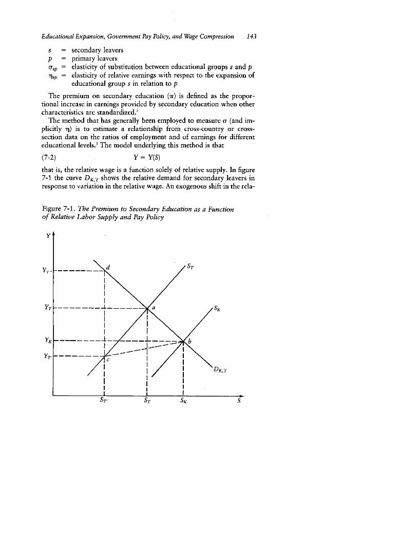
Educational Expansion, Government Pay Policy, and Wage Compression 143
s = secondary leaversp = primary leaversr-p = elasticity of substitution between educational groups s and p5p = elasticity of relative earnings with respect to the expansion of
educational group s in relation to p
The premium on secondary education (Tr) is defined as the propor-tional increase in earnings provided by secondary education when othercharacteristics are standardized.2
The method that has generally been employed to measure u (and im-plicitly q) is to estimate a relationship from cross-country or cross-section data on the ratios of employment and of earnings for differenteducational levels.3 The model underlying this method is that
(7-2) Y = Y(S)
that is, the relative wage is a function solely of relative supply. In figure7-1 the curve DK,T shows the relative demand for secondary leavers inresponse to variation in the relative wage. An exogenous shift in the rela-
Figure 7-1. The Premium to Secondary Education as a Functionof Relative Labor Supply and Pay Policy
y
YT. __ _ _ d/ST
I \II \
1ET -- X- - -/ -/-aSK
Yr : e < ~~~~~DKT/
STI ST SK _
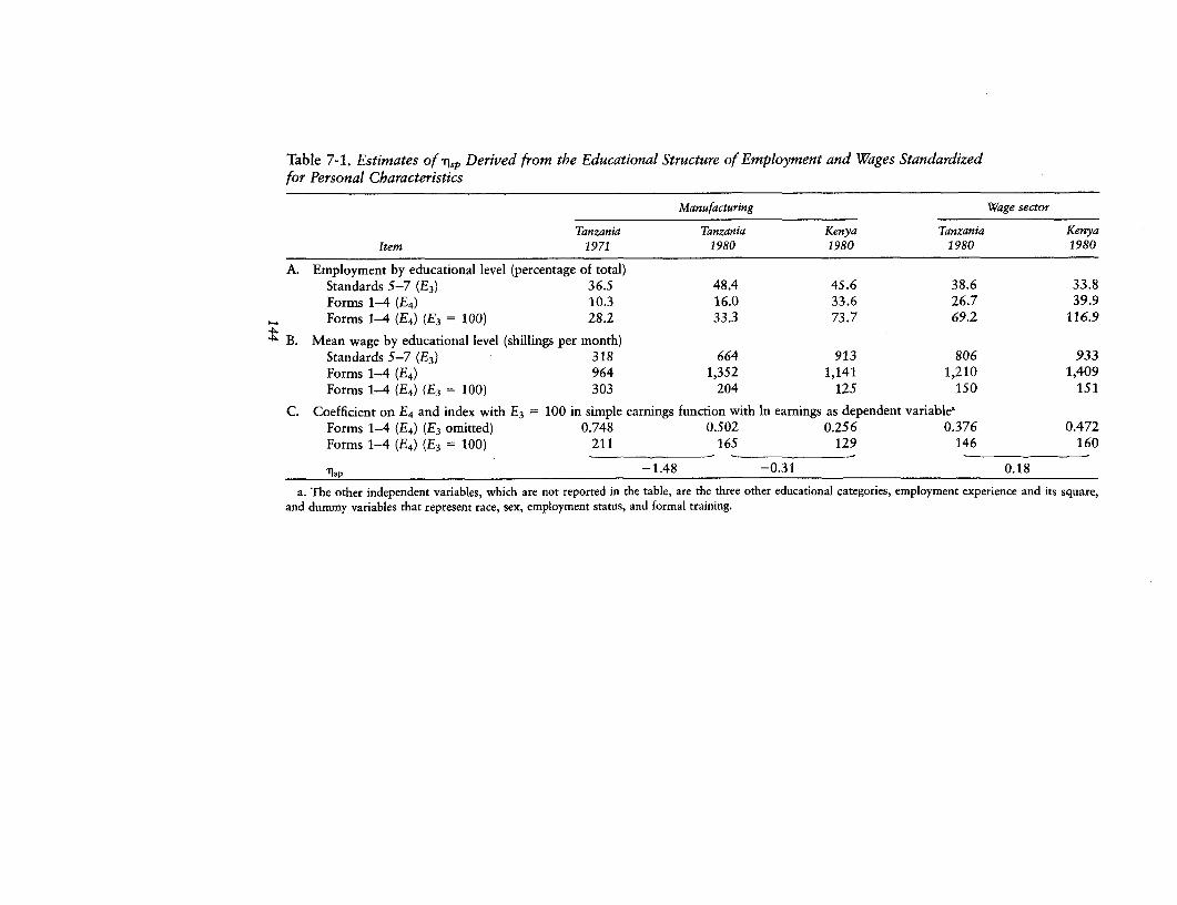
Table 7-1. Estimates of 9Sp Derived from the Educational Structure of Employment and Wages Standardizedfor Personal Characteristics
Manufacturing Wage sector
Tanzania Tanzania Kenya Tanzania KenyaItem 1971 1980 1980 1980 1980
A. Employment by educational level (percentage of total)Standards 5-7 (E3) 36.5 48.4 45.6 38.6 33.8Forms 1-4 (E4 ) 10.3 16.0 33.6 26.7 39.9Forms 1-4 (E4) (E3 = 100) 28.2 33.3 73.7 69.2 116.9
484 B. Mean wage by educational level (shillings per month)
Standards 5-7 (E3) 318 664 913 806 933Forms 1-4 (E4 ) 964 1,352 1,141 1,210 1,409Forms 1-4 (E4 ) (E3 = 100) 303 204 125 150 151
C. Coefficient on E4 and index with E3 = 100 in simple earnings function with In earnings as dependent variable,Forms 1-4 (E4 ) (E3 omitted) 0.748 0.502 0.256 0.376 0.472Forms 1-4 (E4 ) (E3 = 100) 211 165 129 146 160
-1.48 -0.31 0.18
a. The other independent variables, which are not reported in the table, are the three other educational categories, employment experience and its square,and dummy variables that represent race, sex, employment status, and formal training.
Educational Expansion, Government Pay Policy, and Wage Compression 145
tive supply curve (from ST to SK) in a competitive market reduces therelative wage from YT to YK.
Parts A and B of table 7-1 are used to derive estimates of -%, basedon the conventional method for the manufacturing sector and for thewage sector as a whole in each country. The supply of secondary in rela-tion to primary education is markedly higher in Kenya than in Tanzaniain both the wage sector as a whole and in the manufacturing sector. InTanzania's manufacturing sector relative supply is higher in 1980 thanin 1971.
The three manufacturing samples may be thought of as representingthree points in a time series: Tanzania 1971, Tanzania 1980, and Kenya1980, which is equivalent to Tanzania some years hence. The values of9p obtained for manufacturing (-2.38 between Tanzania 1971 andTanzania 1980 and -0.62 between Tanzania 1980 and Kenya 1980) havethe expected negative sign. The positive elasticity of 0.01 obtained forthe wage sector as a whole presents us with an anomaly, however. Thisassociation of a higher relative supply of secondary leavers in the laborforce with a higher relative wage might be attributable simply to differ-ences between Kenyan and Tanzanian employees in the other personalcharacteristics that influence wages.4 But when we use standardized pre-miums earned by secondary leavers, as derived from the simple earningsfunctions (part C of table 7-1), the same pattern emerges: -1.48 and-0.31 for the manufacturing sector and +0.18 for the wage sector. Theshift to the standardized premiums actually makes the estimated elastic-ity more positive.
The explanation for these anomalous results may lie in a mis-specification of the model that underlies the conventional method. Dif-ferences between two countries in institutional interventions, such asgovernment pay policies, or in relative demand functions, as well as intheir supply functions, could affect the educational structure of wages,and hence qp. Rather than Y = Y(S), the appropriate specification mightbe
(7-3) Y = Y(S, G, D)
where G is the effect that the intervention has on the premium and Drepresents differences in relative demand. Figures 7-1 and 7-2 illustratetwo alternative hypotheses.
Despite the relative scarcity of secondary leavers in Tanzania, the pre-mium on secondary education may be lower there than in Kenya becauseof the equalizing effect of government pay policy. If the impact of paypolicy is greater the higher is the position of the worker on the earningsscale, the premium to secondary education is compressed below the com-petitive level-for example, from YT to YT' in figure 7-1. As drawn, YT'
< YK. An estimate of 71p that did not eliminate the influence of pay policy
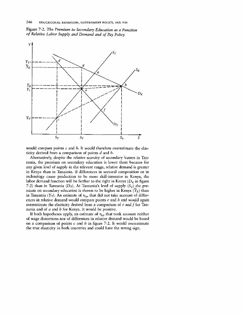
146 EDUCATIONAL EXPANSION, GOVERNMENT POLICY, AND PAY
Figure 7-2. The Premium to Secondary Education as a Functionof Relative Labor Supply and Demand and of Pay Policy
Y'
YT'
ST. ST SK
would compare points c and b. It would therefore overestimate the elas-ticity derived from a comparison of points d and b.
Alternatively, despite the relative scarcity of secondary leavers in Tan-zania, the premium on secondary education is lower there because forany given level of supply in the relevant rauge, relative demand is greaterin Kenya than in Tanzania. If differences in sectoral composition or intechnology cause production to be more skill-intensive in Kenya, thelabor demand function will be farther to the right in Kenya (DK in figure7-2) than in Tanzania (DT)- At Tanzania's level of supply (ST) the pre-mium on secondary education is shown to be higher in Kenya (YK) thanin Tanzania (YT). An estimate of Tls that did not take account of differ-ences in relative demand would compare points e and b and would againoverestimate the elasticity derived from a comparison of e and f for Tan-zania and of a and b for Kenya. It would be positive.
If both hypotheses apply, an estimate of qls, that took account neitherof wage distortions nor of differences in relative demand would be basedon a comparison of points c and b in figure 7-2. It would overestimatethe true elasticity in both countries and could have the wrong sign.
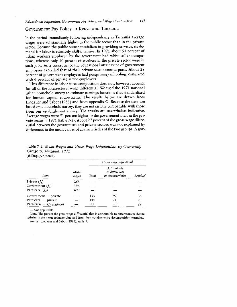
Educational Expansion, Government Pay Policy, and Wage Compression 147
Government Pay Policy in Kenya and Tanzania
In the period immediately following independence in Tanzania averagewages were substantially higher in the public sector than in the privatesector. Because the public sector specializes in providing services, its de-mand for labor is relatively skill-intensive. In 1971 about 51 percent ofurban workers employed by the government had white-collar occupa-tions, whereas only 10 percent of workers in the private sector were insuch jobs. As a consequence the educational attainment of governmentemployees exceeded that of their private sector counterparts. About 28percent of government employees had postprimary schooling, comparedwith 6 percent of private sector employees.
This difference in labor force composition does not, however, accountfor all of the intersectoral wage differential. We used the 1971 nationalurban household survey to estimate earnings functions that standardizedfor human capital endowments. The results below are drawn fromLindauer and Sabot (1983) and from appendix G. Because the data arebased on a household survey, they are not strictly comparable with thosefrom our establishment survey. The results are nevertheless indicative.Average wages were 51 percent higher in the government than in the pri-vate sector in 1971 (table 7-2). About 27 percent of the gross wage differ-ential between the government and private sectors was not explained bydifferences in the mean values of characteristics of the two groups. A gov-
Table 7-2. Mean Wages and Gross Wage Differentials, by OwnershipCategory, Tanzania, 1971(shillings per month)
Gross wage differential
AttributableMean to differences
Item wages Total in characteristics Residual
Private ( 1) 263 - - -
Government (J2) 396 - - -
Parastatal (J3) 409 - - -
Government - private - 133 97 36Parastatal - private - 144 71 73Parastatal - government - 13 -9 22
- Not applicable.Note: The part of the gross wage differential that is attributable to differences in charac-
teristics is the mean estimate obtained from the two alternative decomposition formulas.Source: Lindauer and Sabot (1983), table 7.
148 EDUCATIONAL EXPANSION, GOVERNMENT POLICY, AND PAY
ernment employee thus received about 13 percent more than he wouldhave received in the private sector.
Government pay policy provides one explanation for the public sectorpremium observed in 1971. The government's role as wage leader andits aim of raising wages were first outlined by the East African RoyalCommission in 1955. In the commission's view the migrant labor systemthat prevailed in Kenya and Tanganyika (now Tanzania) led to inefficientuse of labor both in agricultural self-employment and in wage employ-ment. A rise in wages, by encouraging the stabilization of labor, was ex-pected to end the system of circular migration and increase labor produc-tivity in both sectors. The commission's recommendation led to theintroduction of an effective minimum wage in Tanganyika in 1957. Al-though this minimum was not confined to the public sector, evasion ofthe regulation was common in the private sector. Moreover, to set anexample, the colonial government and, subsequently, the government ofindependent Tanzania tended to pay unskilled public sector employeesa wage above the legislated minimum.
At the top of the pay scale Africanization of the civil service contrib-uted to the observed sectoral segmentation of the market for wage labor.During the colonial period most high-level posts were held by Europeans,who received incomes twenty to thirty times those of African manualworkers. These high incomes were primarily determined by alternativeopportunities in the rich metropolitan countries rather than by opportu-nities in the colonial dependency. In 1961 only 26 percent of middle- andsenior-level civil service posts were held by Tanzanians. By 1971 the pro-portion had increased to 85 percent. Since the number of posts had dou-bled over the period, this implied a sevenfold increase in the number ofTanzanians in high-level government positions. The public sector wageand salary structures did not fully adjust to reflect the decline in the sup-ply price of the holders of these positions. To do away with what manypeople regarded as the fruits of independence and to introduce a largewage gap between Tanzanians and their expatriate counterparts wouldhave been politically untenable. The wage structure in the private sector(except for the large multinationals that followed the public sector leadand, after nationalization, were incorporated into that sector) was moreresponsive to the change in labor market conditions.
Tanzania's pay equalization policy dates from the Arusha Declarationof 1967, which set Tanzania on a more egalitarian and socialist path. Thebasic problem posed by the country's inadequate educational inheritancewas clearly stated by President Nyerere at that time: "The wage differen-tials in Tanzania are now out of proportion to any conceivable conceptof human equality . . . yet we cannot at present greatly reduce this gapbecause of our shortage of skilled and qualified people" (Nyerere 1967b,pp. 16-17). The government adopted two approaches to resolve this con-

Educational Expansion, Government Pay Policy, and Wage Compression 149
flict between the claims of equity and the reward that education couldcommand in the market. One approach was to discourage elitist attitudeson the part of the educated. This was attempted through, for instance,exhortation and a system of national service under which young people,on completing upper secondary and tertiary education, served the com-munity at low pay for eighteen months (Coulson 1982, pp. 181-82). Theother approach was to introduce an egalitarian government pay policy.
The policy of wage compression extended beyond government employ-ment to other parts of the public sector. After the Arusha Declarationparastatal organizations burgeoned owing to the nationalization or par-tial nationalization of large foreign companies. The Standing Committeeon Parastatal Organisations (scopo) was established in 1967 to applythe government pay policy to the parastatals. In 1968 the committee is-sued a directive that prescribed common basic scales for parastatal em-ployees, although incumbents were permitted to retain their existing paylevels. scopo undoubtedly had teeth. It laid down wage and salary scalesfor each occupation with the intention of keeping parastatal pay in linewith government pay. At the time of the 1971 survey average wages ingovernment and parastatal employment were on a par; the slight advan-tage of parastatal employees would have been larger had it not been fordifferences in mean characteristics (table 7-2). In neither sector had thenew policy of compressing wages yet been forcefully implemented. Thepassage of time and the emergence of inflation in the 1970s, however,meant that the full effects of the policy would be observable in 1980.
In principle the egalitarian pay policy applied also in the private sector.There the enforcement agency was the Permanent Labour Tribunal (PLT),
which had the power to vet and alter all collective bargaining agreementsin pursuance of government pay policy but which in practice concen-trated on regulating maximum increases in nominal pay. The governmentaccounted for 24 percent of employees in the Dar es Salaam wage labormarket and the parastatals for 38 percent (table 7-3). The private sectortail was therefore unlikely to be able to wag the public sector dog; thatis, the public sector was large enough to pursue an independent pay pol-icy for many occupations without fear of losing workers to the privatesector. We hypothesize, therefore, that in 1980 pay in the public sectorwas less dispersed and was lower for the better paid than in the privatesector.
Government policy on wages in the period immediately after indepen-dence in Kenya resembled that in Tanzania. The economic and politi-cal factors that influenced the wage leadership shown by the Kenyangovernment-the desirability of ending the system of short-term circularmigration between the countryside and the towns and the need to providetangible evidence of the fruits of independence-were much the same asin Tanzania.
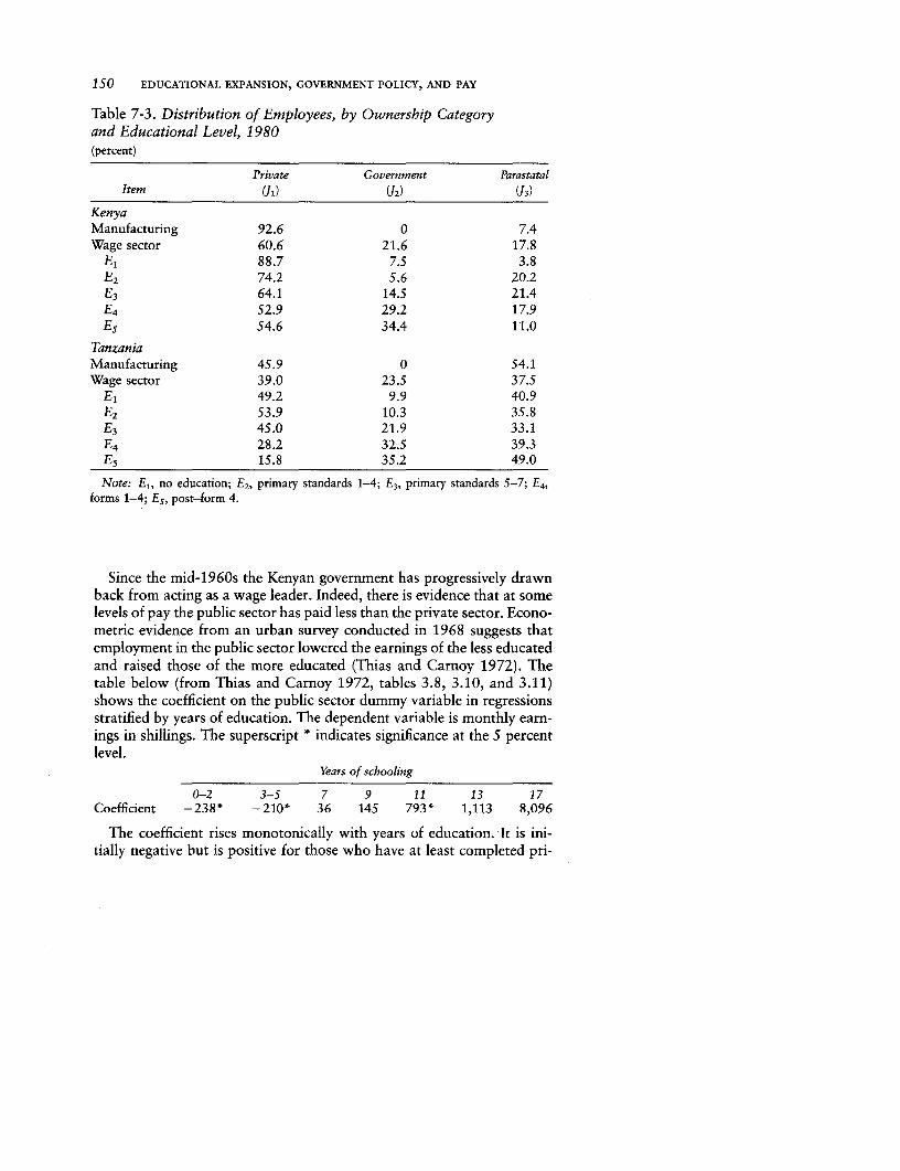
150 EDUCATIONAL EXPANSION, GOVERNMENT POLICY, AND PAY
Table 7-3. Distribution of Employees, by Ownership Categoryand Educational Level, 1980(percent)
Private Government ParastatalItem (Jfl (U2) (13)
KenyaManufacturing 92.6 0 7.4Wage sector 60.6 21.6 17.8
E, 88.7 7.5 3.8E2 74.2 5.6 20.2E3 64.1 14.5 21.4E4 52.9 29.2 17.9Es 54.6 34.4 11.0
TanzaniaManufacturing 45.9 0 54.1Wage sector 39.0 23.5 37.5
El 49.2 9.9 40.9E2 53.9 10.3 35.8E3 45.0 21.9 33.1E4 28.2 32.5 39.3E5 15.8 35.2 49.0
Note: E1 , no education; E2, primary standards 1-4; E3, primary standards 5-7; E4,forms 1-4; Es, post-form 4.
Since the mid-1960s the Kenyan government has progressively drawnback from acting as a wage leader. Indeed, there is evidence that at somelevels of pay the public sector has paid less than the private sector. Econo-metric evidence from an urban survey conducted in 1968 suggests thatemployment in the public sector lowered the earnings of the less educatedand raised those of the more educated (Thias and Carnoy 1972). Thetable below (from Thias and Carnoy 1972, tables 3.8, 3.10, and 3.11)shows the coefficient on the public sector dummy variable in regressionsstratified by years of education. The dependent variable is monthly earn-ings in shillings. The superscript * indicates significance at the 5 percentlevel.
Years of schooling
0-2 3-5 7 9 11 13 17Coefficient -238* -210* 36 145 793* 1,113 8,096
The coefficient rises monotonically with years of education. It is ini-tially negative but is positive for those who have at least completed pri-
Educational Expansion, Government Pay Policy, and Wage Compression 151
mary education. No great reliance, however, can be placed on thesefindings, since the sampling procedure for the public sector was unsatis-factory, the authors were not directly concerned with the ownership cate-gory, and the equations contained variables that could be correlated withownership category, such as firm size and sector of activity. A survey ofhigh- and middle-level manpower in 1972 found that in all but one offifteen narrowly defined occupations, average cash earnings were lowerin the public than in the private sector (Collier and Lal 1986, table 12.5).
In recent years the Kenyan government, like the Tanzanian, has ex-pressed itself in favor of equalizing wages. The Industrial Court is re-quired to vet all collective bargaining agreements and to register onlythose conforming to government guidelines that seek to restrain nominalwage increases and compress the wage structure. According to the devel-opment plan document in force at the time of our 1980 survey,
Lower-paid workers will continue to receive a relatively higher com-pensation for changes in the cost of living compared with higher-paidworkers as a means of narrowing wage differentials. These guidelineswill be applied to wages in the public as well as the private sector.(Kenya, Ministry of Economic Planning 1979, p. 41.)
There is reason to question whether in 1980 this policy in fact led toany significant departure from a market outcome for wage structure ineither the public or the private sector. Unlike Tanzania, Kenya does notcontrol pay in the public corporations, and the central government ac-counts for only 22 percent of our weighted sample of employees in Nai-robi (table 7-3). Market competition from the private sector is thereforelikely to have been felt more keenly than in Tanzania. Our interviews sug-gested that by 1980 the Kenyan government had adopted the prevailingwage rate approach to public sector wage determination; that is, publicsector pay policy compressed the wage structure no more than would themarket interaction of supply and demand. This might reflect either alesser concern with the distribution of income than in Tanzania or anawareness that the rapid increase in the relative supply of educated laborwould itself achieve the distributional goal. Our hypothesis for 1980,therefore, is that government pay policy has less influence in Kenya thanin Tanzania and that pay in the Kenyan public service and public corpo-rations differs little from pay in the private sector.
The Wage Distortion Hypothesis: Empirical Specification
We wish to test the hypothesis that pay policy has compressed the educa-tional structure of wages, and thus caused an upward bias in the estimateof 115p, in Tanzania but not in Kenya. We will simulate the wage structure
152 EDUCATIONAL EXPANSION, GOVERNMENT POLICY, AND PAY
in the absence of pay policy to estimate the shadow premium on second-ary education and so obtain a measure of -qs, that is not distorted bypay policy.
The estimates of the simple earnings functions presented in table 7-1suggest that the wage distortion hypothesis is correct. Since a far higherproportion of workers is employed in private firms in the manufacturingsector than in other sectors, a government policy that restrains public sec-tor pay could explain why in Tanzania the premium on secondary educa-tion is higher in the manufacturing sector than in the wage sector as awhole. It could also explain why, when Kenya and Tanzania are com-pared, the relationship between relative supply and the premium is "wellbehaved" in manufacturing but not in the wage sector. We can test thehypothesis more rigorously by changing the specification of our earningsfunctions from
(7-4) W = f(Ei, X)
to
(7-5) W = f(Ej, Ji, Ej * Ji, X)
whereW = log of individual earningsE; = a set of five dummy variables that signify levels of educational
attainment, with standards 5-7 (E3 ) as the base categoryX = a vector of variables that measure other personal characteris-
tics that influence earningsji = a set of dummy variables that signify the ownership category
of the firm by which the respondent is employed. The privatesector Ul) is the base category.
The coefficients on the dummy variables government J2) and para-statal (J3) show the effect on earnings of employment in the nonmarketrather than the market sector. We refer to the public sector as thenonmarket sector and to the private sector as the market sector becausethe latter is likely to diverge less from free market conditions. ('Whetherand how private sector pay diverges from the free market outcome de-pends on the employment objectives of the government and on the degreeof intersectoral mobility; see chapter 13.) The interaction terms (E, Ji)permit the effect of ownership category to vary according to the level ofeducation, thus testing the hypothesis that the pay policy is egalitarian.
In the simple earnings function based on equation 7-4, the premiumon secondary education can be derived directly as e4 , the coefficient onE4. In the function based on equation 7-5, however, there are additionalcomponents. The premium can be decomposed into (a) the componentattributable to the difference between primary and secondary leavers in

Educational Expansion, Government Pay Policy, and Wage Compression 153
access to high-paying ownership categories and (b) the component attrib-utable to the premium earned by secondary leavers within ownershipcategories.
Our method of estimating the effect of differences in the two educa-tional distributions among ownership categories is to multiply ci, the co-efficient of Ji, by the proportion of workers (pii) in the relevant ownershipcategory:
(7-6) SCiP4 -i CiP3 i = E Ci(p4i - P3i)
A similar adjustment is made for the ji * E1 interaction terms, wheredii are the relevant coefficients:
(7-7) X d4 ip4 i - d3ip3 i = 44i
because the d3 i coefficients are zero. The full premium on secondaryeducation is therefore:
(7-8) rr = e4 = e4 + Ci (i - PA + I d4i Ni
(from equation 7-4) (from equation 7-5)
Since the private sector is the base subcategory in the dummy variableanalysis, the influence of pay policy on the premium can be eliminatedsimply by setting the coefficients on Ji and Ji * E, equal to zero in the righthand side of equation 7-8. The resulting change in the premium (fromYT' to YT" in figure 7-2) provides a test of the hypothesis that the premiumin Tanzania has been depressed by government intervention on pay. Thesimulation yields an estimate of the premium (point d in figure 7-2) thatwould prevail if market forces were permitted to operate freely but sup-ply were unchanged. It is possible that the estimate will be biased becauseof the effect of the pay policy on the demand for labor in the nonmarketsector and on the supply of labor in the market sector, but the directionof bias cannot be predicted a priori (see chapter 13).
The Structure of Wages in the Market and NonmarketSectors: Testing the Hypothesis
Table 7-4 presents estimates of earnings functions for the full samples,excluding and then including the ownership and ownership-education in-teraction terms. In the simpler equations the results are generally as ex-pected. Earnings increase monotonically with educational level in bothcountries and, with primary standards 5-7 (E3) as the omitted category,all coefficients are significantly different from zero. The employment ex-perience terms are highly significant and generate the expected inverted-U-shaped earnings-experience profile. Formal training and non-Africanrace raise earnings, as do regular employment status in Kenya and male
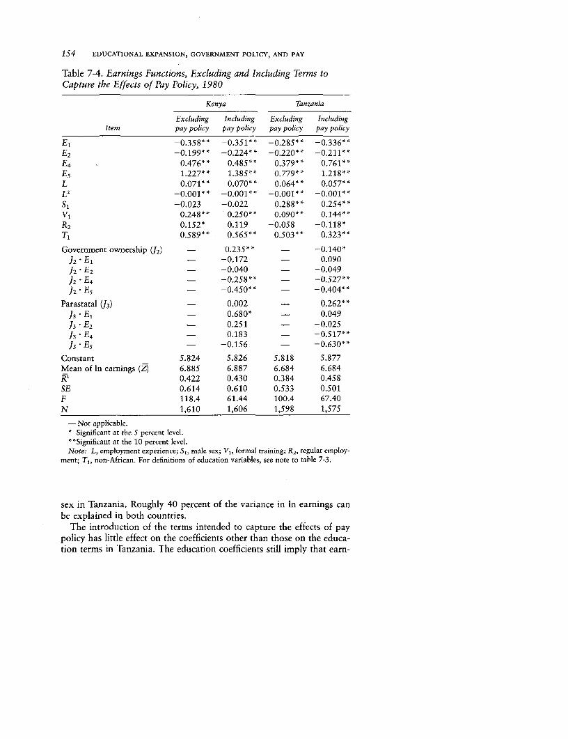
154 EDUCATIONAL EXPANSION, GOVERNMENT POLICY, AND PAY
Table 7-4. Earnings Functions, Excluding and Including Terms toCapture the Effects of Pay Policy, 1980
Kenya Tanzania
Excluding Including Excluding IncludingItem pay policy pay policy pay policy pay policy
El -0.358** -0.351** -0.285** -0.336**E2 -0.199** -0.224** -0.220** -0.211**E4 . 0.476** 0.485** 0.379* * 0.761 * *Es 1.227** 1.385** 0.779** 1.218**L 0.071** 0.070** 0.064* * 0.057* *L2- -0.001 -0 *0.00* .001** -0.001 **
S1 -0.023 -0.022 0.288* * 0.254* *V1 0.248** 0.250** 0.090** 0.144**R2 0.152* 0.119 -0.058 -0.118*T, 0.589** 0.565** 0.503** 0.323**
Government ownership J2) - 0.235** - -0.140*J2 El - -0.172 - 0.090J2 E2 - -0.040 - -0.049J2 * E4 - -0.258** - -0.527**J2 - Es - -0.450** - -0.404**
Parastatal (J3) - 0.002 - 0.262**J3 * El - 0.680* - 0.049J3 - E2 - 0.251 - -0.025J 3 *E4 - 0.183 - -0.517**J3 - Es - -0.156 - -0.630**
Constant 5.824 5.826 5.818 5.877Mean of In earnings (Z) 6.885 6.887 6.684 6.684k2 0.422 0.430 0.384 0.458SE 0.614 0.610 0.533 0.501F 118.4 61.44 100.4 67.40N 1,610 1,606 1,598 1,575
-Not applicable.Significant at the S percent level.
*Significant at the 10 percent level.Note: L, employment experience; SI, male sex; VI, formal training; R2, regular employ-
ment; T1, non-African. For definitions of education variables, see note to table 7-3.
sex in Tanzania. Roughly 40 percent of the variance in In earnings canbe explained in both countries.
The introduction of the terms intended to capture the effects of paypolicy has little effect on the coefficients other than those on the educa-tion terms in Tanzania. The education coefficients still imply that earn-

Educational Expansion, Government Pay Policy, and Wage Compression 155
ings rise monotonically with education, but they now represent that rela-tionship in the market sector, the private sector (U1) being the omittedownership category. The addition of the Ji and Ji * E. terms as a groupis significant at the 1 percent level in Tanzania but not in Kenya. In Tanza-nia the coefficients indicate that employment by government reducesearnings and that the educational structure of government and parastatalpay is more equal than that of private sector pay. The coefficients on allfour postprimary education-public sector ownership interaction terms(with JI * E3 as the base subcategory) are significantly negative.
Figure 7-3 shows the structure of wages for primary and secondaryleavers in the private sector and the public (government and parastatal)sector. The educational premiums (the standardized differences betweenIn earnings of E3 and E4 workers, as indicated by the slopes of the joininglines) were derived from the estimated equation as follows. Where e, arethe coefficients on Ep, c, on Ji, and dii on Ji * E, the premium on E4 (forms1-4) in relation to E3 (standards 5-7, the base subcategory) is
(7-9) fT = e4
in the market sector and
(7-10) T = e4 + d4i
in the nonmarket sector. On the vertical axis In earnings of E3 workersin the market sector are set equal to zero in each country. The relation-ship between the standardized In earnings of primary leavers in thenonmarket sector and those in the market sector is thus shown as theheight of the E3 observation in the nonmarket panels and is given by thevalue of ci. Both the height and the slope of the line for the nonmarketsector are calculated as weighted combinations of the government andparastatal estimates. The weights are determined by the relative impor-tance of government and parastatal employment for primary and forsecondary leavers.
As figure 7-3 shows, the premium is large in the Tanzanian market sec-tor and is much lower in the nonmarket sector. The pay policy in Tanza-nia operates against those with secondary education. It is notable thatsuch large sectoral wage differences can persist in the market. They arelikely to reflect the low labor turnover observed in our surveys and possi-ble lags in the market adjustment process. In Kenya the E * ji interactionterms display no coherent pattern, and most are insignificant. The pre-mium on secondary education is similar in the market and nonmarketsectors. In sharp contrast to Tanzania, pay policy has not compressed theeducational structure of wages.
With the use of the earnings function that contains the pay policy vari-ables, the premium on secondary education can be built up to correspondto the premium derived directly from the earnings function without the

Figure 7-3. The Premium to Secondary Education in the Market and Nonmarket Sectors, Kenya and Tanzania
KENYA TANZANIA
Market Nonmarket Market Nonmarket'rr
0.7 -
0.6-
0.5-
0.4 -
0.3-
0.2-
0.1 /
E3 E4 E3 E4 E3 E4 E3 4
Educational Expansion, Government Pay Policy, and Wage Compression 157
pay policy variables. The built-up premiums are 0.477 in Kenya and0.385 in Tanzania, and the directly estimated premiums are 0.476 and0.379, respectively. This result verifies equation 7-8. In Kenya eliminatingthe effect of pay policy (-0.009) increases the premium on secondaryeducation by a negligible 2 percent. In Tanzania the increase is muchmore substantial; eliminating the effect of pay policy (-0.382) doublesthe premium. The wage distortion hypothesis is confirmed: when the ef-fect of pay policy is eliminated, the premiums are well behaved. The pre-mium in Tanzania (0.761) exceeds that in Kenya (0.485) by 0.276.
Conclusions
In Tanzania, where the scarcity of secondary leavers places a high marketpremium on their services, the government has intervened to preventscarcity rents from accruing to the educated. Despite having to workagainst the market, the policy is effective in the public sector, which isdominant in Tanzania; government intervention halves the average pre-mium on education. A side effect of this intervention is that private sectoremployees with relatively high levels of education earn considerably morethan their public sector counterparts. Such segmentation of the labormarket by sector of ownership is not without its drawbacks, however-itmay well produce new inequities and misallocation of labor.
No such intervention was observed in the Kenyan labor market. Oureconometric results were consistent with a prevailing wage rate approachto public sector pay determination. It is possible that the Kenyan govern-ment chose to follow market forces because the rapid expansion ofsecondary enrollments in Kenya could be relied on to reduce the premiumon secondary education. It is to the measurement of this relationship thatwe turn in chapter 8.
Notes
1. The terms relative wage (Y) and premium
IT = w5w= y -1 = In w, - In wpws WI,
can normally be used interchangeably in the argument.
2. See, for instance, Bowles (1969, 1970), Dougherty (1972), Fallon andLayard (1975), the survey by Hammermesh and Grant (1979), andPsacharopoulos and Hinchliffe (1972).
3. Normally it is not possible to standardize the characteristics, such as em-ployment experience, that are known to influence earnings, and the mean earn-ings of the two educational groups are used (see Bowles 1969, pp. 42-50). Pro-

158 EDUCATIONAL EXPANSION, GOVERNMENT POLICY, AND PAY
duction function techniques have also been employed, however (see Dougherty1972).
4. For example, the employment experience of secondary leavers could begreater in relation to that of primary leavers in Kenya, so that standardizationfor experience could reduce the Kenyan premium below the Tanzanian premium.In fact the reverse is the case, which explains why the Kenyan premium rises inrelation to the Tanzanian when we substitute standardized for actual meanwages.
CHAPTER 8
Educational Expansion,Relative Demand,
and Wage Compression
OUR OBJECTIVE IN THIS CHAPTER is to measure the responsivenessof the wages of secondary and primary leavers to changes in their relativesupply (q,p). Since chapter 7 confirmed the wage distortion hypothesis,we will need to allow for the effect of government pay policy on the pre-mium to secondary education in Tanzania. We also have to take accountof differences in relative demand that could bias our estimate of Tmp. Ourfirst task, therefore, is to determine whether, despite the relative scarcityof secondary leavers in Tanzania, the premium on secondary educationis lower there because, for any given level of supply in the relevant range,relative demand is greater in Kenya than in Tanzania. In other words,is the skill intensity of production greater in Kenya-for example, be-cause of differences in sectoral composition or technology?
The Relative Demand Curve Hypothesis:Empirical Specification
We wish to test the hypothesis that the relative demand for secondaryleavers is greater in Kenya than in Tanzania and that the estimate of qpis therefore biased upward. If Kenya's relative demand curve lies aboveTanzania's (DK> DT in figure 7-2, above), we would expect that for anygiven relative supply (say, ST) the premium is greater in Kenya (YK >YT). Since relative supply is actually much greater in Kenya than in Tan-zania, to test the hypothesis we simulate a reduction of relative supplyin Kenya to Tanzania's level and predict the Kenyan premium that would
Note: Adapted from J. B. Knight and R. H. Sabot, "Educational Expansion, GovernmentPolicy and Wage Compression," Journal of Development Economics 26, no. 2 (August1987), pp. 201-21.
159

160 EDUCATIONAL EXPANSION, GOVERNMENT POLICY, AND PAY
result. We refer to this predicted premium as YK. Alternatively, we simu-late an increase of relative supply in Tanzania to Kenya's level and predictthe Tanzanian premium that would result. The test lies in the comparisonof the predicted premium of one country with the actual premium of theother. In figure 7-2, for instance, if relative supply in Tanzania is ST, thenYT (denoted by point e) should be compared with ^YK (denoted by g).If the predicted and actual premiums are the same, we cannot reject thenull hypothesis that Kenya and Tanzania have the same relative demandcurve.
To explain the method that is employed to simulate a change in therelative supply of secondary leavers, it is helpful to consider the mecha-nisms by which the premium declines in response to relative educationalexpansion. Underlying the empirical analysis below is the notion of theoccupational production function, already used in chapter 6 and ex-pounded in appendix F. Two occupational production functions, Yi andY2, are illustrated in figure 8-1. Y represents productivity and E years ofeducation; inputs of other factors are held constant. Ep and Es represent
Figure 8-1. Occupational Production Functions
YY
A~~
Y2
y~~~~~
Ep EI
Educational Expansion, Relative Demand, and Wage Compression 161
the completion of primary and secondary education, respectively. Theslopes of the functions Y, and Y2 between Ep and Es indicate the addi-tional productivity associated with secondary education in occupations1 and 2.
As secondary education expands in relation to primary education, thewage premium on secondary education falls in an economy with compet-itive labor markets, partly because wage reductions in the occupationscontaining secondary leavers depress those occupational productionfunctions. A limit to such wage reductions is imposed by the wages inoccupations that employ primary leavers and by the need to compensatefor differential acquisition of occupational skills. The premium is also re-duced, however, by the movement of people with secondary educationinto less well-paid occupations-that is, by filtering down.
If there is occupational wage stickiness owing to occupation-specifichuman capital, institutional constraints, or adjustment lags, the occupa-tional production functions will not move downward with the expansionof secondary education. Nevertheless, filtering down does occur and cancompress the educational wage structure on its own. For instance, in fig-ure 8-1 the wage of secondary leavers in occupation 1 remains at A, butthose who filter down to occupation 2 receive wage C. As the (now fewer)primary leavers continue to receive wage B but secondary leavers receivea weighted average of A and C, the premium declines. In practice, theprecise nature of filtering down depends on the degree of job security-that is, on whether less educated incumbents are displaced.
Educational expansion does not necessarily lead to greater compres-sion of the wage structure when occupational wages fall than when theydo not. This is because the occupational wage reductions tend to be offsetby the expansion of employment in these occupations. No such absorp-tion of secondary leavers can occur where wages are sticky, and the pro-cess of filtering down into less well-paid occupations therefore goesfurther.
The relative demand curve for workers with secondary education is in-fluenced by occupational structure and by the positions and slopes ofoccupational production functions. For a given relative supply, withoccupational production functions stable, the premium on secondaryeducation is derived from the weighted averages of the (standardized)occupational wages of primary and secondary leavers; the respectiveweights are the proportions of primary and secondary leavers in each oc-cupation. The relative movement of secondary leavers into jobs for whichthe wage is lower depresses the premium, as does their movement intojobs within which the premium is lower.
The first step in simulating a change in the relative supply of secondaryleavers and the consequent decline in their premium is to decompose thepremium on secondary education in our simple earnings function (the
162 EDUCATIONAL EXPANSION, GOVERNMENT POLICY, AND PAY
coefficient e4 on E4 in equation 7-4) into the component attributable tothe difference between primary and secondary leavers in access to rela-tively high-paying occupations and the component attributable to thepremium earned by secondary leavers within occupations. To effect sucha decomposition we change the specification of our earnings functionfrom equation 7-4 to:
(8-1) W = f(Ej, Ok, Ej- Ok, X)
where Ok is a set of five occupational dummy variables, with 03, skilledmanual, as the base subcategory. The coefficients of the occupation vari-ables represent the influence on earnings, after educational level is stand-ardized, of being in one occupation rather than another. In effect, theyshow the relative positions of different occupational production func-tions. The interaction terms (Ej- Ok) permit the influence of educationto vary according to occupation and, in effect, show the shapes of thedifferent occupational production functions.' The occupation and inter-action terms together permit the estimation of log linear approximationsof occupational production functions such as those illustrated in figure8-1 in the range between Ep and Es.
As explained in chapter 6 and appendix E, particular care was takenin classifying workers into occupations on the basis of ascending orderof expected skill-unskilled, semiskilled, and skilled for the manual oc-cupations and lower clerical, higher clerical, and supervisory for thenonmanual occupations-and precisely the same criteria were applied ineach country. For the reasons given in chapter 6 and appendix F, it islikely that observed differences in occupational production functions willrepresent differences in the value of cognitive and vocational skill acquisi-tion for the different occupations.
The premium on E4 in equation 7-4 can be decomposed with the useof equation 8-1 in a manner precisely analogous to the decompositionbased on equation 7-8:
(8-2) T = e4 = e4 + E ak(P4k - P3k) + 'Ff b4kP4k
(from equation 7-4) (from equation 8-1)
where
ak = the coefficients on the Ok termsbjk = the coefficients on the E - Ok termsPik = the proportion of workers at educational level j in occupation k
The second step in simulating a change in relative supply involveschanging the distributions of primary and secondary leavers across occu-pations. The effect in Tanzania of Kenya's greater relative supply can besimulated by imposing the education-occupation matrix of Kenya onTanzania. We shall therefore assume that the occupational distributions
Educational Expansion, Relative Demand, and Wage Compression 163
of primary and secondary leavers in Tanzania respectively equal those ofprimary and secondary leavers in Kenya. Similarly, simulating Tanzania'slesser relative supply in Kenya is a matter of substituting in equation 8-2estimated for Kenya the education-occupation matrix for Tanzania.Where p;k represents occupational composition in the other country, thesimulated premium is calculated from the estimated equation 8-2 as:
(8-3) IT = e4 + E ak(p4k - P3k) + I b4kP4k
The simulated premiums obtained in this way, flK and *T, are thencompared with the actual premiums, 7rK and XTT, to test the hypothesisthat relative demand is greater in Kenya than in Tanzania. The empiricaljustification for our assumptions that the education-occupation matrixof one country is indicative of the education-occupation matrix in theother and that educational expansion does not change the occupationalproduction functions will be provided below.
Occupational Production Functions in the Marketand Nonmarket Sectors
The wage distortion hypothesis having been confirmed, we go on to testthe relative demand hypothesis. We control for differences in pay policybetween Kenya and Tanzania by incorporating the specification changesof equation 7-5 and equation 8-1. The estimated equation is thus:
(8-4) W = f(E, Ji, Ej -Ji, Ok, Es °k, X)
The estimates of the regression equations in table 8-1 incorporate theownership, occupation, and interaction terms. The education and occu-pation terms have the expected signs. In Tanzania all four education vari-ables are significant, three of them at the 1 percent level; in Kenya threeare significant at the 1 percent level. Four of the five occupation variablesare significant at the 1 percent level for Tanzania, and for Kenya all fiveare significant at that level. Many of the education-occupation coeffi-cients are large in relation to the corresponding Ej terms; although feware individually significant, their introduction as a group is significant atthe 1 percent level in both countries. As was the case in table 7-5, whichomitted the occupation terms, the ownership variables are significant atthe 1 percent level for Tanzania but not for Kenya, and the education-ownership interaction terms are of the expected sign and are significantat the 1 percent level for Tanzania but not for Kenya.
As a consequence of adopting a specification that incorporates bothhypotheses simultaneously, the full decomposition of the premium (com-bining equations 7-8 and 8-2) becomes:
(8-5) IT z e 4 + } ak(P4k - P3k) + } b4kP4k + Yci(P 4 i - P3i) + X d4 ip4 i
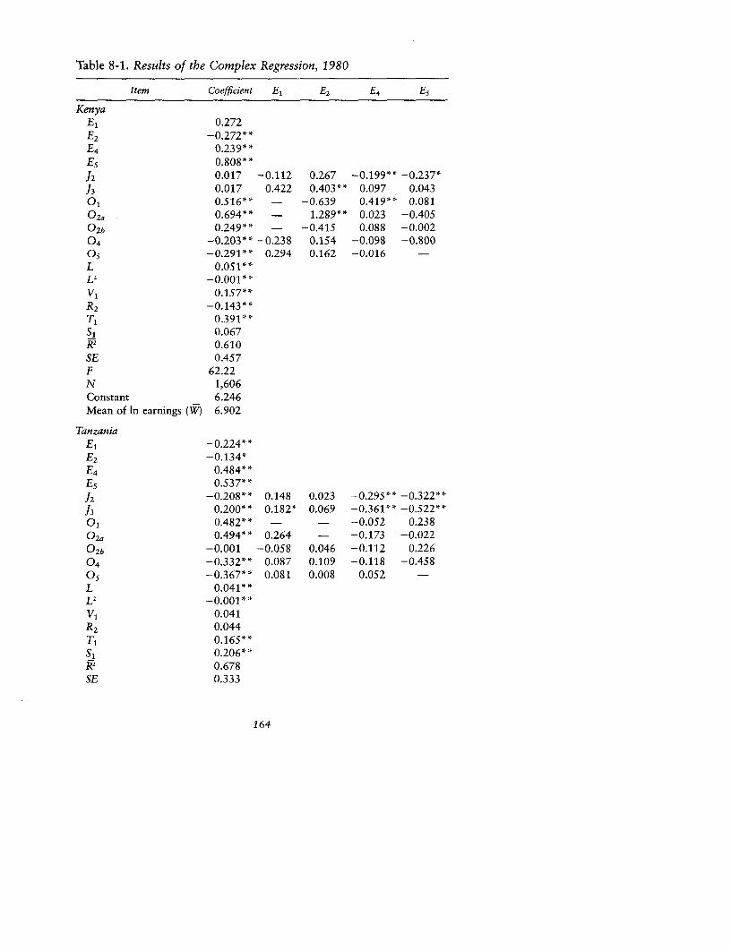
Table 8-1. Results of the Complex Regression, 1980
Item Coefficient El E2 E4 Es
KenyaEl 0.272E2 -0.272**E4 0.239**Es 0.808 * *12 0.017 -0.112 0.267 -0.199** -0.237*13 0.017 0.422 0.403** 0.097 0.043Ol 0.516** - -0.639 0.419** 0.08102a 0.694** - 1.289** 0.023 -0.4050
2b 0.249** - -0.415 0.088 -0.00204 -0.203** -0.238 0.154 -0.098 -0.80005 -0.291** 0.294 0.162 -0.016 -L 0.051**L2 - 0.001**V1 0.157**R2 -0.143**T, 0.391**S1 0.067R2 0.610SE 0.457F 62.22N 1,606Constant 6.246Mean of In earnings (W) 6.902
Tanzania
El - 0.224**E2 -0.134*E4 0.484**E5 0.537**12 -0.208** 0.148 0.023 -0.295** -0.322**13 0.200** 0.182* 0.069 -0.361** -0.522**0t 0.482** - - -0.052 0.23802a 0.494** 0.264 - -0.173 -0.0220
2b -0.001 -0.058 0.046 -0.112 0.22604 -0.332** 0.087 0.109 -0.118 -0,45805 -0.367** 0.081 0.008 0.052 -
L 0.041**L2 -0.001**V1 0.041R2 0.044T, 0.165**S1 0.206*RK 0.678SE 0.333
164
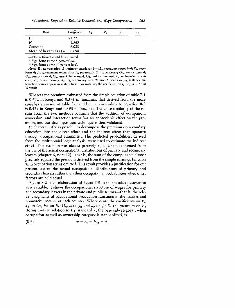
Educational Expansion, Relative Demand, and Wage Compression 165
Item Coefficient El E2 E4 Es
F 81.22N 1,563Constant 6.088Mean of In earnings (W) 6.698
-No coefficient could be estimated.* Significant at the 5 percent level.**Significant at the 10 percent level.Note: El, no education; E2, primary standards 1-4; E4, secondary forms 1-4; Es, post-
form 4; J2, government ownership; J3, parastatal; O1, supervisory; 02., senior clerical;0
2b, junior clerical; 04, semiskilled manual; 0 5, unskilled manual; L, employment experi-ence; VI, formal training; R2, regular employment; Tl, non-African race; Sl, male sex. In-teraction terms appear in matrix form. For instance, the coefficient on 12 * El is 0.148 inTanzania.
Whereas the premium estimated from the simple equation of table 7-1is 0.472 in Kenya and 0.376 in Tanzania, that derived from the morecomplex equation of table 8-1 and built up according to equation 8-5is 0.479 in Kenya and 0.393 in Tanzania. The close similarity of the re-sults from the two methods confirms that the addition of occupation,ownership, and interaction terms has no appreciable effect on the pre-mium, and our decomposition technique is thus validated.
In chapter 6 it was possible to decompose the premium on secondaryeducation into the direct effect and the indirect effect that operatesthrough occupational attainment. The predicted probabilities, derivedfrom the multinomial logit analysis, were used to estimate the indirecteffect. This estimate was almost precisely equal to that obtained fromthe use of the actual occupational distributions of primary and secondaryleavers (chapter 6, note 12)-that is, the sum of the components almostprecisely equaled the premium derived from the simple earnings functionwith occupation terms omitted. This result provides a justification for ourpresent use of the actual occupational distributions of primary andsecondary leavers rather than their occupational probabilities when otherfactors are held equal.
Figure 8-2 is an elaboration of figure 7-3 in that it adds occupationas a variable. It shows the occupational structure of wages for primaryand secondary leavers in the private and public sectors-that is, the rele-vant segments of occupational production functions in the market andnonmarket sectors of each country. Where ej are the coefficients on Ei,ak on °k, b,k on Ei - Ok, ci on Ji, and dii on ji -E, the premium on E4(forms 1-4) in relation to E3 (standard 7, the base subcategory), whenoccupation as well as ownership category is standardized, is
(8-6) iT = e4 + b4k + d4 i
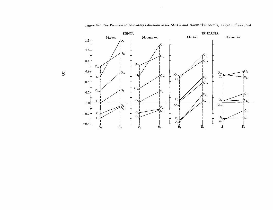
Figure 8-2. The Premium to Secondary Education in the Market and Nonmarket Sectors, Kenya and Tanzania
KENYA TANZANIAMarket Nonmarket Market Nonmarket
1.2 01
1.0 02~~~~~~~.2
0.8 02
02a 0(2I
1020.6 ~ ~ ~ ~ ~ ~ , 0 2b (,a 02a0
01 I ~~~II 03l 0, ( jf0210.4 - I I I
0 2b 03 2bI I0.2 i 03 0, 0
031 I I 0)4 0
0.0 040 0hI ~~04 102b 0bI I~ ~ 041l04I
-0.2 -04 i I04I 051 0 4 041 104
-0.4 1I I 051 OI iE3 P-F4 ' 3 E4 3LE 4
Educational Expansion, Relative Demand, and Wage Compression 167
Given that JI (private) is the base ownership subcategory, the marketsector premium is simply
(8-7) Tr = e4 + b4k
In figure 8-2 In earnings of E3 workers in 03 in the market sector ineach country are set equal to zero on the vertical axis. For example, theline 0101 for the Tanzanian market sector shows, by its height aboveE3 , the higher pay of a primary leaver in a supervisory than in a skilledmanual occupation and, by its slope, the premium accruing to secondaryeducation in the supervisory occupation. The occupational wages accru-ing to E3 workers (shown by their height above E3 ) are widely dispersedwithin a sector but are similar for the two sectors, whereas those accru-ing to E4 workers differ greatly for the two sectors. In the market sectorthe premium is large and similar in each occupation, whereas in thenonmarket sector it is much lower. The pay policy in Tanzania operatesagainst those with secondary education irrespective of occupation.
In Kenya the E, * Ji interaction terms display no coherent pattern, andmost are insignificant. Figure 8-2 shows that the slopes of the occupa-tional production functions in Kenya are similar in the market andnonmarket sectors. In both sectors the premium on secondary educationtends to increase with the hypothesized skill content of the occupation.
We can now calculate a shadow premium on secondary education inTanzania. The influence of pay policy is eliminated by subtracting fromthe estimated premium the component attributable to pay policy (the lasttwo terms of equation 8-5) to obtain the premium prevailing in the mar-ket sector. In Kenya eliminating the effect of pay policy (-0.031) in-creases the premium on secondary education by a negligible 6.5 percent.In Tanzania the increase is much more substantial; eliminating the effectof pay policy (-0.247) increases the premium on secondary educationby two-thirds. The wage distortion hypothesis is confirmed: once the ef-fect of pay policy is eliminated, the premiums are well behaved-the pre-mium in Tanzania (0.640) is greater than that in Kenya (0.510) by 0.130.
Simulation of one country's relative supply of secondary leavers in theother country entails substituting in equation 8-5 the occupational distri-butions of primary and secondary leavers in one country for those in theother. It is apparent from a comparison of the market sectors of Kenyaand Tanzania (figure 8-2) why this substitution changes the premium.The educational premium in Tanzania is larger at the three manual levels,similar at the two clerical levels, and smaller at the supervisory level,whereas in Kenya the premium is highest for the highest occupation anddecreases as occupational level decreases. The country differences in oc-cupational production functions within the market sector, however, areminor in comparison with the substantial differences among occupa-tional production functions within each country. A change of occupationmakes a big difference to one's earnings; the filtering down into lower-

Table 8-2. Distribution of All Employees and of Primary and Secondary Completers by Occupationin the Manufacturing and Wage Sectors
Manufacturing Wage sector
Tanzania 1971 Tanzania 1980 Kenya 1980 Tanzania 1980 Kenya 1980
Entered wage Entered wage Entered wage Entered wage Entered wage
employment employment employment employment employment
All Up to All Up to All Up to All Up to All Up to
Item employees 1963 1964-71 employees 1972 1973-80 employees 1972 1973-80 employees 1972 1973-80 employees 1972 1973-80
All employees0l 3.5 5.7 2.1 5.3 6.4 4.3 3.5 4.1 2.6 12.3 15.2 8.4 10.9 10.1 12.1
02a - - - 4.2 4.5 4.2 1.5 1.4 1.6 4.8 5.5 4.2 7.1 11.3 2.5
0 °2b 12.0 11.2 12.6 12.1 10.7 13.8 8.6 7.2 11.1 28.6 26.6 31.1 24.6 20.4 31.1
0 03 28.4 34.9 24.1 22.5 27.3 16.6 35.5 45.4 17.8 21.3 22.9 20.1 23.1 27.9 17.7
04 31.8 30.7 32.5 34.5 32.4 37.1 32.7 30.3 36.8 16.3 15.6 16.9 16.3 17.4 15.1
05 24.4 17.4 28.7 21.4 18.8 24.0 18.3 11.6 30.8 16.6 14.2 19.2 18.0 12.9 21.5
All nonmanual 15.5 16.9 14.7 21.6 21.6 22.3 13.6 12.7 15.3 45.7 47.3 43.7 42.6 41.8 45.7
Unskilled andsemiskilled 56.2 48.1 61.2 55.9 51.2 61.1 51.0 41.9 67.6 32.9 29.8 36.1 34.3 30.3 36.6
Form 4 completers0l 9.1 13.5 4.5 17.3 24.3 4.9 5.0 9.1 0.0 18.5 24.1 8.2 7.8 12.1 1.7
°2a- - - 12.5 16.8 4.9 3.3 5.5 0.7 13.1 13.6 11.7 12.6 19.9 2.00
2b 66.7 69.2 63.6 38.7 33.6 47.5 18.2 21.3 14.5 53.0 50.0 59.4 41.9 40.3 44.0
03 18.2 15.4 20.5 20.8 21.5 19.7 21.2 24.4 17.4 10.0 11.0 8.0 16.5 14.3 19.5
04 4.0 1.9 6.8 8.9 2.8 19.7 33.4 32.3 34.8 2.7 1.3 5.0 10.3 9.2 11.8
0s 2.0 0.0 4.5 1.8 0.9 3.3 18.9 7.3 32.6 2.7 0.0 7.8 10.9 4.1 20.9

Table 8-2. (continued)
Manufacturing Wage sector
Tanzania 1971 Tanzania 1980 Kenya 1980 Tanzania 1980 Kenya 1980
Entered wage Entered wage Entered wage Entered wage Entered wage
employment employment employment employment employment
All Up to All Up to All Up to All Up to All Up to
Item employees 1963 1964-71 employees 1972 1973-80 employees 1972 1973-80 employees 1972 1973-80 employees 1972 1973-80
All nonmanual 75.8 82.7 68.1 68.5 74.7 57.3 26.5 35.9 15.2 84.6 87.7 79.3 62.3 72.3 47.7
Unskilled andsemiskilled 6.0 1.9 11.3 10.7 3.7 23.0 52.3 39.5 67.4 5.4 1.3 12.8 21.2 11.3 32.7
Standard 7 completers> 10 3.7 7.9 1.0 1.4 1.9 0.5 2.9 3.5 1.0 3.3 4.2 1.8 3.0 3.6 1.3
02. - - - 2.0 0.2 0.5 0.2 0.3 0.0 1.1 1.4 0.5 3.4 4.5 0.00
2b 10.6 10.8 9.7 8.7 10.5 5.7 6.0 5.8 6.7 27.2 33.2 17.0 15.3 17.2 9.6
03 30.6 41.0 22.6 24.8 28.7 18.6 28.9 33.8 14.4 30.9 29.4 33.4 37.3 40.9 26.6
04 34.6 28.8 39.5 41.1 38.9 44.8 39.8 40.5 37.5 23.3 21.8 25.7 20.8 19.4 25.0
Os 20.3 11.5 27.2 22.0 17.8 28.9 22.2 16.1 40.4 14.3 10.0 21.6 20.1 14.4 37.5
All nonmanual 14.3 18.7 10.7 12.1 14.6 7.7 9.1 9.6 7.7 31.6 38.8 19.3 21.7 25.3 10.9
Unskilled andsemiskilled 54.9 40.3 66.7 63.1 56.7 73.7 62.0 56.6 77.9 37.6 31.8 47.3 40.9 33.8 62.5
- Not applicable.Note: 03, skilled manual. For definitions of other variables, see note to table 8-1.

170 EDUCATIONAL EXPANSION, GOVERNMENT POLICY, AND PAY
paying occupations of secondary leavers in relation to primary leaverscould have a substantial effect on the premium.
The Process of Filtering Down
The occupational attainment functions presented in chapter 6 showedthat the probabilities of being in a particular occupation are greatly de-pendent on two factors: the education of the worker and the year of hisentry into wage employment. We now examine the influence of these twofactors on the occupational adjustments that result from the expansionof secondary education.
The distribution of employment by occupation is shown in table 8-2.Considerable similarity can be observed in the three manufacturingsamples and between the two wage sector samples. The similarity in thedistributions of employees by occupation and the marked difference inthe distributions by education (table 7-1) imply that the education-occupation matrix is different for the two countries. As table 8-2 shows,in Tanzania's wage sector 53 percent of secondary leavers were in juniorclerical occupations and only 15 percent were manual workers, whereasin Kenya 38 percent were manual workers.
More filtering down had occurred in manufacturing; the proportionin white-collar occupations fell slightly, from 76 to 69 percent, between1971 and 1980 in Tanzania, and it was a low 27 percent in Kenya in 1980.The filtering down of secondary leavers into lower-level occupations hadthus gone further in Kenya than in Tanzania. It is apparent from the tablethat the occupational distributions of primary leavers are less dissimilarin the two countries than those of secondary leavers; indeed, in the manu-facturing sector their distributions are much the same. The rapid expan-sion of secondary education in Kenya has caused secondary leavers tofilter down the occupational scale not only in absolute terms but also inrelation to primary leavers.
Table 8-2 also suggests that the incidence of filtering down is cohortspecific. A breakdown by years since entry into wage employment showsthat the more recent cohorts did more of the filtering down into manualoccupations. For instance, in Kenya 33 percent of secondary leavers whohad entered the labor market in the previous seven years, but only 11percent of those who had entered earlier, were in unskilled or semiskilledjobs; the corresponding figures for Tanzania were 13 and 1 percent. Thedifference between cohorts was even more marked in manufacturing-67percent for the more recent cohort and 40 percent for the earlier cohortin Kenya and 23 and 4 percent in Tanzania. Tracing a cohort between1971 and 1980 by means of the Tanzanian manufacturing samples showsthat only a minor part of the cohort difference can be explained by occu-pational upward mobility with employment experience.
These cohort effects reflect the low rate of occupational mobility in

Educational Expansion, Relative Demand, and Wage Compression 171
both samples, which is the outcome of a related set of labor marketphenomena. The surveys indicated remarkably low rates of laborturnover-a change of employer once in 9.3 years on average in Kenyaand once in 16.8 years in Tanzania (the figures are the mean value ofyears of employment experience per quit). The combined result of legisla-tion, trade union pressure, and the general ethos is that incumbents enjoyconsiderable job security. Vacancies tend to be filled on the basis of edu-cational criteria; for many jobs the more educated applicants receivepreference. As might be expected from the lack of educational provisionin the past, many workers are considered undereducated for the jobs theyperform. The rapid expansion of education also helps to explain why em-ployers, when they make hiring decisions, consider the cohort differencesin education more important than the cohort differences in employmentexperience. The preference-ordering of educational levels by employers-which corresponds to our occupational classification by skill level-produces the same predictable process of filtering down in both coun-tries. It is for these reasons that we expect Kenya's education-occupationmatrix to illustrate what Tanzania's matrix would be if Tanzania pursuedthe Kenyan educational policy, and the reverse.
An assumption that underlies the simulations is that the coefficientsin the earnings function are invariant with respect to changes in the rela-tive supply of secondary leavers. The presence of occupation-specifichuman capital, as documented in chapter 6, is an important reason forexpecting resistance to the compression of the occupational wage struc-ture with educational expansion. Educational expansion does not itselfnecessarily diminish the scarcity rents to be obtained from the possessionof vocational skills. Even if workers effectively pay the entire cost of theirtraining, profit-maximizing employers may protect trained incumbentsagainst competition from untrained entrants to avoid disruption of pro-duction and to maintain worker morale. In addition, long lags in the ad-justment of the occupational wage structure to changes in relative supplyare not implausible given the importance of institutional wage-setting inKenya and Tanzania (see, for instance, House and Rempel 1978, Jackson1979, and Lindauer and Sabot 1983). Moreover, the low rates of laborturnover and the security of tenure generally enjoyed by incumbents sug-gest that competition in the wage labor market is unlikely to be strongexcept among entrants. We regard it as reasonable, therefore, to conductthe simulations on the assumption that occupational production func-tions are stable.
Testing the Relative Demand Hypothesis
We can now answer the following questions by reference to the marketsector. What would be the premium in Tanzania if education had beenexpanded or were in the future expanded so that the relative supply of
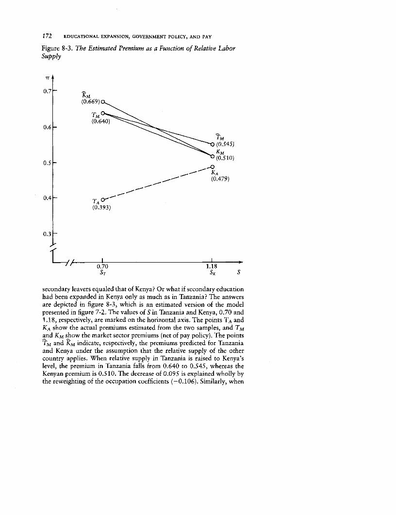
172 EDUCATIONAL EXPANSION, GOVERNMENT POLICY, AND PAY
Figure 8-3. The Estimated Premium as a Function of Relative LaborSupply
7r
0.7 -
(0.669)
TMK
0.5 (0.510)
0.6 - ~ ~ ~ ~
KA(0.479)
0.4 TA 0 -
(0.393)
0.3
0.70 1.18ST SK S
secondary leavers equaled that of Kenya? Or what if secondary educationhad been expanded in Kenya only as much as in Tanzania? The answersare depicted in figure 8-3, which is an estimated version of the modelpresented in figure 7-2. The values of S in Tanzania and Kenya, 0.70 and1.18, respectively, are marked on the horizontal axis. The points TA andKA show the actual premiums estimated from the two samples, and TMand KM show the market sector premiums (net of pay policy). The pointsTM and KM indicate, respectively, the premiums predicted for Tanzaniaand Kenya under the assumption that the relative supply of the othercountry applies. When relative supply in Tanzania is raised to Kenya'slevel, the premium in Tanzania falls from 0.640 to 0.545, whereas theKenyan premium is 0.510. The decrease of 0.095 is explained wholly bythe reweighting of the occupation coefficients (-0.106). Similarly, when

Educational Expansion, Relative Demand, and Wage Compression 173
relative supply in Kenya is lowered to Tanzania's level, the Kenyan pre-mium rises from 0.510 to 0.669, whereas the Tanzanian premium is0.640. The increase of 0.159 is attributable mainly to the reweightingof the occupation coefficients (0.098) but also to the reweighting of thecoefficients on the education-occupation terms (0.061), which reflectsthe higher premium on secondary education in the more skilled occupa-tions in Kenya.
When both pay policy and the relative supply of secondary leavers arestandardized, the two labor markets generate roughly the same premium:the difference between KM and TM is 0.035 and that between TM andkM is only 0.029. The "difference in relative demand curves" hypothesisis that, despite the relative scarcity of secondary leavers in Tanzania, thepremium is lower there because relative demand is greater in Kenya.Given the similarity of the actual and predicted premiums, we cannot re-ject the null hypothesis that Kenya and Tanzania have the same relativedemand curve. The policy differences between the two countries-Tanzania's policies on protection, trade controls, and foreign investmentare more interventionist-have not created significant differences in thestructures of their urban economies or in their use of foreign technologyand therefore in their relative demand curves.
Estimating the Elasticity
Estimating 5p (as in equation 7-1) on the basis of a comparison of TAand KA yields the anomaly of a positive elasticity that we have been at-tempting to explain. Eliminating the effect of pay policy and thereby rais-ing the Tanzanian premium from TA to TM resolves the anomaly:whether the elasticity is estimated from the Kenyan or the Tanzanianequation or from KM and TM, it will be negative. Use of the Kenyan de-mand function (comparing KM and kM) yields 'rp = -0.303; use ofthe Tanzanian demand function (comparing TM and TM) yields 9,p =-0.181; and use of the market sector premiums (comparing KM and TM)yields 1p = -0.247. These results are consistent with those for otherstudies, which-although they are sensitive to the choice of data andmethods of estimation-generally yield numerical values of 9 well belowunity.2 Educational expansion has a similar effect on the structure ofearnings, whichever demand function is used. A doubling of the ratio ofemployees with secondary education to those with primary educationwould compress the ratio of their earnings by about 25 percent. Thesevalues of jp imply a value of its reciprocal (up) well above unity andindeed greater than 3; that is, there is a fairly high degree of substitutabil-ity between educational levels.
The simulations have been conducted within the framework of stableoccupational production functions. If, after expansion of secondary edu-

174 EDUCATIONAL EXPANSION, GOVERNMENT POLICY, AND PAY
cation, the occupational wage structure in Kenya is not in equilibrium,our results may be biased. We argued above, however, that the effect ofwage stickiness on the premium could not be determined a priori: wagestickiness prevents factor substitution and so extends the filtering downprocess into less well-paid occupations. This, together with the evidencethat through standardization we could reproduce in one country the pre-mium of the other, suggests that the bias introduced by our inability toincorporate occupational wage flexibility in the simulations is only slight.
The simulation of the premium that would prevail in Tanzania wereit to adopt the education policy of Kenya was carried out on the as-sumption that the Kenyan education-occupation matrix would thenapply. This assumption is open to the criticism that the expansion ofsecondary education in Tanzania might be accompanied by developmentpolicies that would change significantly the composition of output andemployment. What would be the effect of such structural change on thedistribution of occupations and hence on the education-occupation ma-trix? What would be the consequent effect on the premium to secondaryeducation and hence on the elasticity?
We examine the sensitivity of the premium to structural change bymaking two extreme assumptions about what Tanzania will do in addi-tion to expanding secondary education to achieve the Kenyan ratio. Thefirst assumption is that Tanzania adopts an ambitious industrializationpolicy; the second is that it instead adopts a policy of far-reaching "bu-reaucratization." The assumptions imply that instead of the actual sec-toral distribution of wage employment (31 percent in manufacturing, 20percent in public services, and 49 percent in other activities in Tanzaniaand a similar distribution in Kenya) the distributions become 45, 10, and45 percent, respectively, under the industrialization policy and 15, 35,and 50 percent under bureaucratization. The effect of sectoral change onthe occupational distribution is estimated by assuming that the occupa-tional distributions within sectors remain fixed, and the effect on theeducation-occupation matrix is estimated by assuming that the occupa-tional promotions and demotions of workers that are made necessary bythe change in occupational composition are based strictly on their educa-tional qualifications. The premium on secondary education in the marketsector of Tanzania is then calculated as:
(8-8) = e4 + } ak(p4k - P3k) + 2 b4kP'4k
where p7k is the Kenyan proportion of workers with education j in occu-pation k.
The industrialization drive decreases the share of nonmanual occupa-tions in the total and increases the share of unskilled and semiskilledmanual occupations. Bureaucratization has the opposite effects. The in-dustrialization policy causes negligible filtering down of secondary
Educational Expansion, Relative Demand, and Wage Compression 175
leavers, but it depresses the proportion of primary leavers in nonmanualjobs by 5 percentage points and raises the proportion in the lesser jobsby 6 percentage points. It is for this reason that the premium on second-ary education, which falls from 0.640 to 0.545 as a result of educationalexpansion alone, decreases only to 0.571 when the industrialization pol-icy is added. The main effect of bureaucratization is to raise the propor-tion of secondary leavers in nonmanual jobs by 19 percentage points andto lower the proportion in lesser jobs by 17 points; primary leavers, bycontrast, filter down. As a result the premium decreases only from 0.640to 0.609 when bureaucratization accompanies educational expansion.The values of 9r, implied by these simulations are -0.13 with the indus-trialization policy and -0.06 with bureaucratization, instead of -0.18.
The illustrative assumptions chosen are so extreme as to be beyond therange of feasible policy options for Tanzania. Nevertheless, the simula-tions suggest that the extent of wage compression resulting from educa-tional expansion can be a function of the accompanying developmentstrategy. Although we have found no evidence that the relative demandcurves of Kenya and Tanzania are different, it is possible that a country'srelative demand curve will alter as development proceeds.
Conclusions
Because of their marked difference in the relative supply of workers withsecondary education and their broad similarities in economic structureand level of development, suggesting similarity in relative demand, Kenyaand Tanzania constitute a natural experiment. In this chapter we havemade use of the natural experiment to address a number of central ques-tions concerning education and labor market policies in developing coun-tries.
First, the governments of both countries have expressed their desire tocompress the widely dispersed wage structures that they inherited. Ourestimate of 9lp, the elasticity of the response of relative wages to suppliesof secondary in relation to primary leavers, confirmed that the expansionof postprimary education is a means of achieving that objective. Al-though the responsiveness is not high (,qsp being a third or less), the de-gree of compression achieved in Kenya has not been negligible. The pre-mium on secondary education in the market sector is about 20 percentlower in Kenya than in Tanzania for this reason and is also no doubt sig-nificantly lower than in Kenya a decade ago.
The second question concerns the efficiency with which labor marketsadjust to the rapid expansion of an education system. Because the wagesector is both relatively small and highly selective of the educated, educa-tional expansion produced a sharp increase in the educational attainmentof entrants into the wage sector. Rapid and extensive labor market ad-
176 EDUCATIONAL EXPANSION, GOVERNMENT POLICY, AND PAY
justment was required, and lags in the adjustment process may have gen-erated inefficiency. Particularly in Kenya, where expansion was morerapid, compression of the earnings structure might have gone further,and workers might have been more efficiently allocated to jobs, had thelabor market been more competitive.
Third, the analysis throws light on the central relationship between ed-ucation and productivity (which was more directly examined in part II)and on the economic criteria to be used in allocating resources to educa-tion. The low value of T1sp implies a high value (3 or more) for the elastic-ity of substitution between the two educational levels. This finding sug-gests that educational expansion produces only a gradual decline in theproductivity gain to be derived from secondary education, and it thussupports the rate of return approach rather than the manpower require-ments approach. The latter ignores the benefits, revealed in this study,from increasing the educational level within occupations. Nevertheless,the less than infinite elasticity-which reflects the filtering down of theeducated into lesser jobs as education is expanded-implies that the rateof return, as conventionally estimated, can be a misleading guide in plan-ning educational expansion. The shortfall of the social return below theprivate return, as implied by the occupation terms in the earnings func-tion, and of the marginal return below the average return, as implied bycohort-specific filtering down, are examined in chapter 14.
It may not be possible to generalize from this particular natural experi-ment, involving as it does countries in which incomes and the educationof the labor force are among the lowest in the world. But any extensionof the comparative approach to other countries must avoid the pitfallsthat our analysis has uncovered. In East Africa the conventional methodof estimating the elasticity of substitution yields grossly biased estimatesbecause of the distorting effect that government policy has on pay. Biascan also arise from differences in relative demand curves, although wefound no evidence of this in Kenya and Tanzania. If elasticities are de-rived from comparisons of countries with greater differences in the struc-ture and level of income, differences in relative demand are more likelyto be a source of bias.
Notes
1. The base category is E3* 03 (standards 5-7 x skilled manual occupation).2. Bowles (1969, ch. 3, and 1970) used cross-section analysis to estimate Twp
= -0.08. Psacharopoulos and Hinchliffe (1972), in an attempt to improve onBowles, estimated 9,p = -0.21. Fallon and Layard (1975, pp. 288-89) deriveda cross-country estimate of Thp = -0.28 (although it was -1.63 when the lesseducated category was constrained to have the same elasticity with human aswith physical capital). Dougherty (1972) used U.S. census data to obtain aggre-gated estimates of -0.05 to -0.30 for q,, for various educational categories.

CHAPTER 9
Educational Expansion and theKuznets Effect
ECONOMISTS AND ECONOMIC POLICYMAKERS show concern notonly for economic efficiency but also for equity. They would generallyagree that greater equality would be socially beneficial if it could beachieved without reducing efficiency. The diverse rationales for this beliefinclude the concept of the diminishing marginal utility of income and thenotion that the welfare of an individual depends on the income of others.There is disagreement, however, about how to weight marginal changesin these components of social welfare and how to measure the tradeoffbetween efficiency and equality. Another issue concerns the magnitudeof inequality, which is generally measured by the dispersion of individualor household incomes.
In this chapter we examine the dispersion of the main component ofthe income of urban workers, wages from employment. So far in partIII we have focused on the structure of wages-for example, on the aver-age wage of one educational group compared with that of another. Thedispersion of wages is a function both of the structure of wages and ofthe distribution of employees within that structure. Educational expan-sion can therefore have two effects on the inequality of pay. The narrow-ing of the wage structure, analyzed in chapters 7 and 8, is termed thecompression effect. The changes in inequality brought about by changesin the educational composition of the labor force are referred to as thecomposition effect. Our natural experiment allows us to examine notonly the dynamics of the wage structure but also the dynamics of wagedispersion associated with educational expansion.
The compression effect of educational expansion always works to re-duce inequality; the composition effect may increase or decrease inequal-ity. It is therefore possible for the two effects to work against each other,and the net outcome is then unclear. We wish to discover how the rapid
Note: Adapted from J. B. Knight and R. H. Sabot, "Educational Expansion and the Kuz-nets Effect," American Economic Review 73, no. 5 (December 1983), pp. 1132-36.
177
178 EDUCATIONAL EXPANSION, GOVERNMENT POLICY, AND PAY
expansion of secondary education in Kenya and Tanzania alters the in-equality of pay.
It is widely accepted that in the process of economic growth the in-equality of income first increases and later decreases. This view was firstpropounded by Kuznets (1955) and was supported empirically byAhluwalia (1976) and Ahluwalia, Carter, and Chenery (1979). It is alsowidely recognized that the inequality of pay is an important componentof total income inequality; see, for instance, Blinder (1974) and PhelpsBrown (1977). Whether the rapid expansion of education that has oc-curred in many countries has increased or decreased the inequality ofpay-thereby delaying or hastening the arrival at the point beyond whicheconomic growth is associated with a reduction of inequality-is relevantto policy.
This chapter uses a simulation methodology that is explained in gen-eral terms in appendix D. We are content here to introduce the underly-ing concepts, leaving their specific application for later in the analysis.We begin by estimating a relationship between earnings and its determi-nants. We then use those estimates to carry out simulations to examinethe effect of each determinant on the dispersion of earnings.
We can, for instance, measure the relative contribution of each inde-pendent variable to inequality by assuming that each variable in turn haszero variance. In this case the counterfactual question being posed is,what would be the impact on inequality if the dispersion attributable toeach determining characteristic were in turn eliminated? Or we can ex-amine the effect on inequality of substituting in one sample some aspectof a second sample-one or more coefficients or one or more values ordistributions of the explanatory variables. For instance, what would bethe effect on inequality if, other factors being kept equal, the gross returnto education in the second sample were applied to the first? What if theeducational composition of the second sample were found in the first?By these means the effects of educational expansion can be simulated anddecomposed.
Educational Expansion and Inequality of Payin the Manufacturing Sector
By confining our analysis to the manufacturing sector, we can base it onthree precisely comparable surveys of wage employees that were con-ducted in Tanzania in 1971 and 1980 and in Kenya in 1980. These sam-ples can be thought of as three points in a time series. Tanzania 1971has the smallest relative supply of educated workers; Kenya 1980, whichhas the highest relative supply, represents Tanzania some years hence. Wemeasure the change in wage dispersion from one survey to another and
Educational Expansion and the Kuznets Effect 179
estimate the relative contributions to that change of the composition andcompression effects of educational expansion.
The change in the educational composition of the labor force itself hasan effect on inequality. Whether it raises or lowers inequality, otherthings being equal, depends on the relative sizes, mean wages, and wagedispersions of the different educational categories. It can be shown thatin a two-group model a transfer of workers from the low-education tothe high-education (and high-wage) group raises the variance (or log vari-ance) until the high-education group reaches a certain proportion of thetotal. The precise proportion depends on the differences in the means andthe variances of the two groups. Robinson (1976, p. 438) has shown,for workers in the jth group, that where
= mean earningsp = proportion of workersaj2 = variance of earnings
j0 educated group2= uneducated groupo2= variance of earnings in the population
then inequality (as measured by o&) rises to a maximum where pi is equalto pi:
(9-1) + 12 -,~ :~2) 2
This implies that p* -1/2 as xcrj2cr. If the variance of wages of the edu-cated group exceeds that of the uneducated (crl > o2), inequality reachesa peak after more than half of the labor force has become educated. Thecondition uj>o-22 also implies that pif is larger the smaller is the differencein mean wages; that is, inequality peaks later in the process of educa-tional expansion the lower is the premium on education. If the varianceis higher for the uneducated group, however, this result is reversed.
This was the basis of Kuznets's hypothesis: the transfer of people be-tween sectors at different income levels initially increases inequality asmore people acquire high income but eventually reduces it as fewer low-income people remain. If there is more inequality in the expanding sector,the peaking of aggregate inequality is delayed.
Kuznets concentrated on the composition effect and did not incorpo-rate any resulting compression effect. Indeed, he suggested (Kuznets1955, p. 8) that the urban-rural income differentials with which he wasconcerned were likely to increase with economic development. But be-cause the competitive market prediction is that the returns to a factordecrease as its relative supply increases, we expect the coefficient on edu-cation in an earnings function to decline as education expands in relation
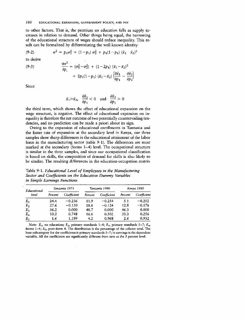
180 EDUCATIONAL EXPANSION, GOVERNMENT POLICY, AND PAY
to other factors. That is, the premium on education falls as supply in-creases in relation to demand. Other things being equal, the narrowingof the educational structure of wages should reduce inequality. This re-sult can be formalized by differentiating the well-known identity
(9-2) 22 = (1-pl) U2 + p,(p-P1) (xl-x2)2
to derive
(9-3) dp= (i-(2) + (1-2pi) (X1-X2)2
+ 2pi(1-pi) (Xl-X2) p a- )
Since
-l>, -2, d < ° and - > 0aPi ap1the third term, which shows the effect of educational expansion on thewage structure, is negative. The effect of educational expansion on in-equality is therefore the net outcome of two potentially countervailing ten-dencies, and no prediction can be made a priori about its sign.
Owing to the expansion of educational enrollments in Tanzania andthe faster rate of expansion at the secondary level in Kenya, our threesamples show sharp differences in the educational attainment of the laborforce in the manufacturing sector (table 9-1). The differences are mostmarked at the secondary (forms 1-4) level. The occupational structureis similar in the three samples, and since our occupational classificationis based on skills, the composition of demand for skills is also likely tobe similar. The resulting differences in the education-occupation matrix
Table 9-1. Educational Level of Employees in the ManufacturingSector and Coefficients on the Education Dummy Variablesin Simple Earnings Functions
Educational Tanzania 1971 Tanzania 1980 Kenya 1980
level Percent Coefficient Percent Coefficient Percent Coefficient
El 24.4 -0.236 11.9 -0.254 5.1 -0.202E2 27.6 -0.150 18.6 -0.124 12.8 -0.176E, 36.2 0.000 48.7 0.000 46.3 0.000E4 10.2 0.748 16.6 0.502 33.3 0.256E 5 1.6 1.199 4.2 0.968 2.6 0.932
Note: El, no education; E2 , primary standards 1-4; E3 , primary standards 5-7; E4,forms 1-4; E5, post-form 4. The distribution is the percentage of the column total. Thebase subcategory for the coefficients is primary standards 5-7; In earnings is the dependentvariable. All the coefficients are significantly different from zero at the 5 percent level.
Educational Expansion and the Kuznets Effect 181
are therefore likely to be attributable to differences in the relative supplyof educated labor, which is lowest in Tanzania 1971 and highest in Kenya1980.
An earnings function that includes the educational categories amongthe independent variables and log earnings as the dependent variableshows high and significant gross returns to education in all three samples(table 9-1).1 The coefficients for postprimary education (with primarystandards 5-7 as the base subcategory) are higher in Tanzania 1971 thanin Tanzania 1980 and are higher in Tanzania 1980 than in Kenya 1980.Again, the differences are most marked at the secondary (forms 1-4)level. This compression of the educational structure of wages as a conse-quence of educational expansion is consistent with the competitive mar-ket prediction.
We proceed to measure the effect of educational expansion on the in-equality of pay and the relative contributions of the compression effectand the composition effect. The method is an extension of that used byBlinder (1974) to decompose the inequality of an income distribution;it is discussed in appendix D. First, we estimate an earnings function
(9-4) W = a + E ejEj + IcjX, + u
where
W = In earningsEi = dummy variables that represent different educational
categoriesXiy = other independent variablesu = an error terma,ei, c; = parameters
The estimated earnings function is used to predict the In earnings of eachindividual worker (W) from his characteristics, and the inequality of pre-dicted earnings is then measured.
Second, we simulate the compression effect of increasing the relativesupply of educated labor. The wages of workers in each sample are pre-dicted using the education coefficients estimated for the other samplesinstead of the actual coefficients. For instance, where the subscript K de-notes the Kenya 1980 sample and the subscript Tthe Tanzania 1980 sam-ple, we predict the wages of the Kenya sample using the Tanzanian educa-tion coefficients
(9-5) WK = aK + X eiTEiK + I CjKXjK
Third, we simulate the composition effect of increasing relative supply.Instead of the actual educational composition of each sample we assumein turn the composition of the other samples. This involves reweightingthe observations. For example, where aiK represents the proportion of
182 EDUCATIONAL EXPANSION, GOVERNMENT POLICY, AND PAY
workers in each educational category Ei in the Kenya 1980 sample andOaiT the proportion in the Tanzania 1980 sample, in applying to the Kenyasample the Tanzania 1980 composition, we use the set of weights otiT/IaK.
(The weighting procedure implies that the total number of observationsis left unchanged.) In this case the simulation involves a decrease in theproportion of workers with secondary education and an increase in theproportion with primary education. The former observations are there-fore given a weight of less than unity and the latter a weight of greaterthan unity in generating the assumed distribution.
Fourth, we combine the composition effect and its consequent com-pression effect in a single simulation. The inequality of the simulatedwage distribution is measured in each case.
The index of inequality used throughout this chapter is the varianceof In earnings (that is, log variance). Other indexes that were calculatedinclude the Gini coefficient, the Theil measure, the Atkinson measure,and the coefficient of variation of the wage. The pattern of results, how-ever, is not sensitive to the choice of index, and the log variance is chosenas representative because of its use in the theory developed above.
The results of the first exercise, based on equation 9-4, indicate thatthe inequality of predicted wages is greatest in Tanzania 1971 and leastin Kenya 1980: the log variances for the three samples are 0.230, 0.128,and 0.097. Inequality is less the greater the relative supply of educatedlabor. But to what extent are these differences attributable to the com-pression effect, to the composition effect, and to differences in the sam-ples that are not related to education?
The results of the second exercise are shown in figure 9-1. Theunsimulated but predicted log variances for the three samples are circledin each panel. A line connecting points in panel A indicates the effecton the log variance for one sample when the education coefficients arealtered to those estimated for the other samples. The line marked T71,for instance, indicates the log variance when the education coefficientsof the Tanzania 1971, Tanzania 1980, and Kenya 1980 samples are ap-plied in turn to the Tanzania 1971 function. As expected, all lines in panelA slope downward; the decline in the premium on education, consideredin isolation, consistently reduces inequality.
The connecting lines in panel B show the effect of altering the educa-tional composition of a sample while the coefficients on education remainunchanged. The line labeled T71, for instance, shows how inequality var-ies as the educational compositions of the Tanzania 1980 and Kenya1980 samples are applied to the Tanzania 1971 earnings function andsample. In all but one of the six cases inequality rises with the simulatedexpansion of education.
Panel C shows the effect on the inequality of wages in each sampleof simulating both the educational composition and the accompanying
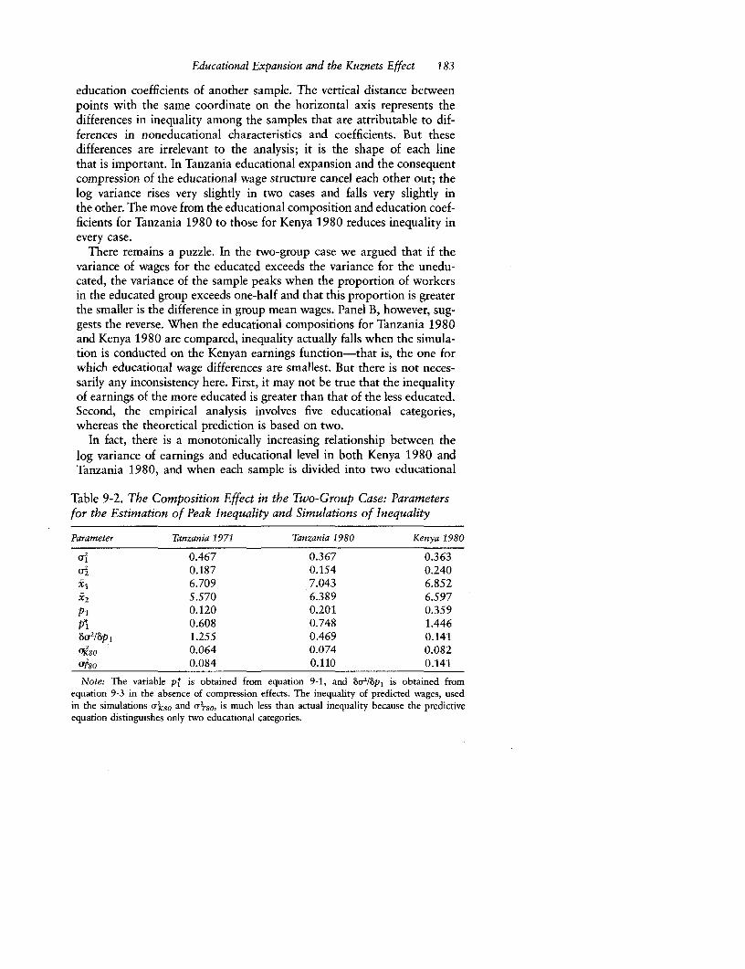
Educational Expansion and the Kuznets Effect 183
education coefficients of another sample. The vertical distance betweenpoints with the same coordinate on the horizontal axis represents thedifferences in inequality among the samples that are attributable to dif-ferences in noneducational characteristics and coefficients. But thesedifferences are irrelevant to the analysis; it is the shape of each linethat is important. In Tanzania educational expansion and the consequentcompression of the educational wage structure cancel each other out; thelog variance rises very slightly in two cases and falls very slightly inthe other. The move from the educational composition and education coef-ficients for Tanzania 1980 to those for Kenya 1980 reduces inequality inevery case.
There remains a puzzle. In the two-group case we argued that if thevariance of wages for the educated exceeds the variance for the unedu-cated, the variance of the sample peaks when the proportion of workersin the educated group exceeds one-half and that this proportion is greaterthe smaller is the difference in group mean wages. Panel B, however, sug-gests the reverse. When the educational compositions for Tanzania 1980and Kenya 1980 are compared, inequality actually falls when the simula-tion is conducted on the Kenyan earnings function-that is, the one forwhich educational wage differences are smallest. But there is not neces-sarily any inconsistency here. First, it may not be true that the inequalityof earnings of the more educated is greater than that of the less educated.Second, the empirical analysis involves five educational categories,whereas the theoretical prediction is based on two.
In fact, there is a monotonically increasing relationship between thelog variance of earnings and educational level in both Kenya 1980 andTanzania 1980, and when each sample is divided into two educational
Table 9-2. The Composition Effect in the Two-Group Case: Parametersfor the Estimation of Peak Inequality and Simulations of Inequality
Parameter Tanzania 1971 Tanzania 1980 Kenya 1980
*rj2 0.467 0.367 0.363
2X 0.187 0.154 0.240xlj 6.709 7.043 6.852x2 5.570 6.389 6.597Pi 0.120 0.201 0.359p*1 0.608 0.748 1.446bu/Ip 1 1.255 0.469 0.141060o 0.064 0.074 0.082T80 0.084 0.110 0.141
Note: The variable pi is obtained from equation 9-1, and &fM8pl is obtained fromequation 9-3 in the absence of compression effects. The inequality of predicted wages, usedin the simulations or2KS and (TTS0, is much less than actual inequality because the predictiveequation distinguishes only two educational categories.
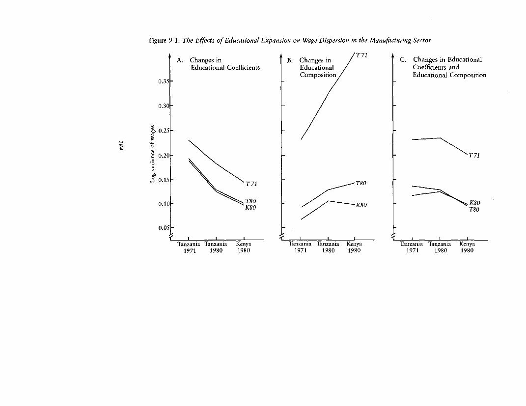
Figure 9-1. The Effects of Educational Expansion on Wage Dispersion in the Manufacturing Sector
A. Changes in B. Changes in T 71 C. Changes in EducationalEducational Coefficients Educational Coefficients and
Composition Educational Composition0.35 -
0.30 -
0.25-
0.0.20 T 71
~~ 0~~~~15 ~~T 71 T80
0.10- ~~~T80 K0K800.10 K80 ~~~~K80 T80
0.05
Tanzania Tanzania Kenya Tanzania Tanzania Kenya Tanzania Tanzania Kenya1971 1980 1980 1971 1980 1980 1971 1980 1980
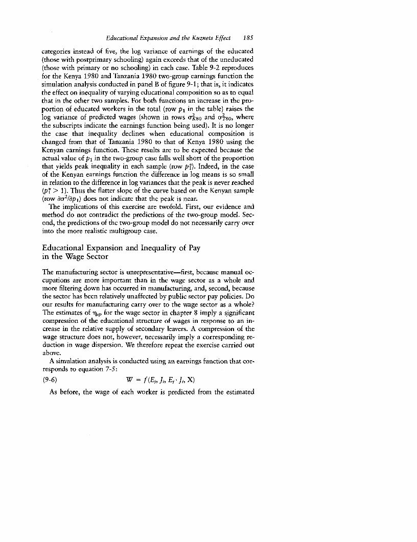
Educational Expansion and the Kuznets Effect 185
categories instead of five, the log variance of earnings of the educated(those with postprimary schooling) again exceeds that of the uneducated(those with primary or no schooling) in each case. Table 9-2 reproducesfor the Kenya 1980 and Tanzania 1980 two-group earnings function thesimulation analysis conducted in panel B of figure 9-1; that is, it indicatesthe effect on inequality of varying educational composition so as to equalthat in the other two samples. For both functions an increase in the pro-portion of educated workers in the total (row P, in the table) raises thelog variance of predicted wages (shown in rows aJ 8a and oT80 , wherethe subscripts indicate the earnings function being used). It is no longerthe case that inequality declines when educational composition ischanged from that of Tanzania 1980 to that of Kenya 1980 using theKenyan earnings function. These results are to be expected because theactual value of p, in the two-group case falls well short of the proportionthat yields peak inequality in each sample (row pi). Indeed, in the caseof the Kenyan earnings function the difference in log means is so smallin relation to the difference in log variances that the peak is never reached(pi > 1). Thus the flatter slope of the curve based on the Kenyan sample(row ar2/apj) does not indicate that the peak is near.
The implications of this exercise are twofold. First, our evidence andmethod do not contradict the predictions of the two-group model. Sec-ond, the predictions of the two-group model do not necessarily carry overinto the more realistic multigroup case.
Educational Expansion and Inequality of Payin the Wage Sector
The manufacturing sector is unrepresentative-first, because manual oc-cupations are more important than in the wage sector as a whole andmore filtering down has occurred in manufacturing, and, second, becausethe sector has been relatively unaffected by public sector pay policies. Doour results for manufacturing carry over to the wage sector as a whole?The estimates of 9,p for the wage sector in chapter 8 imply a significantcompression of the educational structure of wages in response to an in-crease in the relative supply of secondary leavers. A compression of thewage structure does not, however, necessarily imply a corresponding re-duction in wage dispersion. We therefore repeat the exercise carried outabove.
A simulation analysis is conducted using an earnings function that cor-responds to equation 7-5:
(9-6) W = f (Ep, ji, E e f ji, X)
As before, the wage of each worker is predicted from the estimated
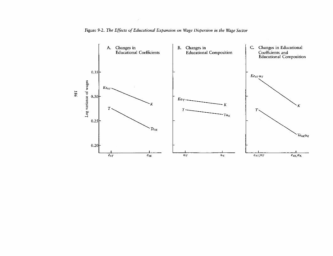
Figure 9-2. The Effects of Educational Expansion on Wage Dispersion in the Wage Sector
A. Changes in B. Changes in C. Changes in EducationalEducational Coefficients Educational Composition Coefficients and
Educational Composition
0.35Ke 4 T tT
Ke4T
00 0Q)0.30 -O~
K K K>4T T T
0.25-
Te4K
Te4KafK
0.20
e4T e4K XTOiK e4T,tT e4KCLK
Educational Expansion and the Kuznets Effect 187
equation and his set of characteristics, and the variance of In predictedearnings is then measured. When we consider the wage sector as a whole,we cannot ignore the complicating effects of pay policy in Tanzania. Inboth countries, therefore, the coefficients on the Ji and Ji * E1 terms areset equal to zero; that is, we analyze the market sector.
The compression effect of increasing relative supply from the Tan-zanian to the Kenyan level is simulated by substituting the coefficienton E4 from the Kenyan equation into the Tanzanian predictor equation.The predicted value of In earnings (W) of each secondary leaver is re-duced by the amount e4K - e4T, where e4 is the coefficient on E4, withE3 as the base category. The composition effect of increasing the relativesupply of secondary leavers is simulated by assuming the primary andsecondary educational compositions of the Kenyan sample instead of theactual Tanzanian compositions. Again, in applying the Kenyan composi-tion to the Tanzanian sample we use the set of weights XjK/otT, whereot, represents the proportion of workers in each educational category. Inthis case the simulation involves an increase in the proportion of workerswith secondary education and a decrease in the proportion with primaryeducation. We then combine the compression and composition effects ina single simulation.
Panels A, B, and C of figure 9-2 show the compression effect, the com-position effect, and their combined effect. The vertical axis measures in-equality, and the horizontal axis indicates whether standardization is onthe basis of the Kenyan or the Tanzanian value of e4, of (x, or of e4 anda. The points K and T indicate predicted inequality in the absence of paypolicy. In panel A, Ke4T and Te4K denote that in addition the coefficienton E4 (e4T, or e4K) has been substituted from the other country. The com-pression effect of educational expansion has the expected negative signin both cases. KCLT and TotK in panel B show the composition effect; in-equality declines slightly with educational expansion in both cases. Thecombined effect (panel C) is therefore to reduce inequality, primarily be-cause of the compression effect.
It is notable in panel C that whereas educational expansion by itselfreduces inequality (Te4KctK - T = 0.224 - 0.271 < 0), predicted in-equality in the market sector in Kenya is actually higher than in Tanzania(K - T = 0.281 - 0.271 > 0). The residual component of the differencebetween the countries-inequality that arises from other causes, such asa more unequal distribution of determining characteristics-works againstKenya (K Te4KcxK = 0.281 - 0.224 > 0). Nevertheless, we have shownthat education policy over the feasible range can have an important influ-ence not only on the educational structure but also on the interpersonalinequality of wages.
188 EDUCATIONAL EXPANSION, GOVERNMENT POLICY, AND PAY
A comparison of figures 9-1 and 9-2 suggests one similarity and twodifferences between the manufacturing sector and the wage sector as awhole. In Kenya and Tanzania in 1980 the size of the compression effectis roughly the same for the two sectors. The predicted log variance, how-ever, is greater in both countries for the wage sector than for the manufac-turing sector. This may be attributable in part to differences in the specifi-cations of the equation, but the main reason is likely to lie in the differentcharacteristics of the two groups of employees. The manufacturing sectorcontains a more homogeneous labor force, owing to the greater propor-tion of manual jobs. In the manufacturing sector the effect of movingfrom the Tanzania 1980 to the Kenya 1980 educational composition ispositive in one case and negative in the other, whereas in the wage sectorthis composition effect is unamibiguously negative. The difference mayreflect the higher proportion of educated workers in the wage sector thanin the manufacturing sector. The higher proportion means that the humpof the inverse-U-shaped relationship implied by equation 9-1 is morelikely to have been passed in the wage sector as a whole.
Conclusions
Is educational expansion an effective tool for reducing the inequality ofpay, or should governments that seek to reduce inequality among wageearners rely on direct labor market intervention to achieve this objective?Our results, both for the manufacturing sector and for the wage sectoras a whole after the influence of pay policy has been eliminated, suggestthat educational expansion can indeed be an effective means of reducinginequality, even without direct government intervention in the labor mar-ket. In our East African example, even when the compression and compo-sition effects of educational expansion on inequality work in opposite di-rections, the equalizing influence of the compression effect predominates.
As expected, the Kenyan pay policy makes little difference to inequalityof pay; it reduces the variance of In wages by only 0.016 to 0.265. Thisresult contrasts with the effects of pay policy in Tanzania, where the indexis 0.271 without pay policy but 0.197 with it. The reduction in inequalityattributable to pay policy (0.074) is somewhat greater than the reductionachieved by the simulated introduction of the Kenyan policy (0.047). Edu-cational expansion and pay policy in Tanzania could have equalizing ef-fects that are of roughly the same order of magnitude. A judgment onwhich policy is better must therefore depend on their other benefits andcosts.
The Kuznets effect has normally been discussed in relation to the trans-fer of population from low-income rural areas to high-income urbanareas. Such a transfer is not expected to narrow the income gap, eitherbecause of labor market imperfections or because the accumulation of
Educational Expansion and the Kuznets Effect 189
human and nonhuman capital in the urban areas tends to widen the gap.We have shown, however, that the expansion of the supply of educatedlabor in relation to the demand has a powerful compressing effect on theintraurban educational structure of wages. The composition effect of ed-ucational expansion can indeed raise intraurban inequality, but the com-pression effect outweighs it. Thus relative educational expansion reducesinequality, and since this process occurs within the relatively expandinghigh-income urban sector, it accelerates arrival at the point beyond whicheconomic growth is associated with a reduction in overall inequality.
Note
1. The other independent variables are years of wage employment experienceand its square and dummy variables that represent race, sex, employment status,and formal training.

Part IV
EDUCATIONAL EXPANSION ANDINEQUALITY OF OPPORTUNITY

CHAPTER 10
Education Policy andIntergenerational Mobility
ECONOMIC INEQUALITY has several dimensions: inequality among indi-viduals at any one time; inequality in the lifetime income of individuals;and inequality of opportunity, which perpetuates inequality from onegeneration to another. Even if current or lifetime income is unequally dis-tributed there may be perfect intergenerational mobility; in other words,the probability that a member of the next generation will be at a particu-lar position in the distribution of income may be independent of familybackground. Jencks and others (1972) take the extreme view that familybackground has little impact on economic success. But in Kenya and Tan-zania the concern has been that economic development might transformrelatively egalitarian tribal communities into a socioeconomically strati-fied society in which educated elites would perpetuate themselves fromone generation to the next.
In part III we showed that educational expansion can have a powerfuleffect on the distribution of current incomes. In this part we examine theeffect of educational expansion on the distribution of educational op-portunities and then on intergenerational mobility. Many studies havedocumented the relationship between socioeconomic background anddifferential educational attainment (see, for example, OECD 1971 andColeman and others 1966 for developed countries and Behrman andWolfe 1984a, 1984b, and Birdsall 1985 for developing countries). Few,however, have examined the effect of educational expansion on this rela-tionship.
Although it is equalization of opportunities rather than of outcomesthat is considered the hallmark of a just society (see Meade 1976), inter-generational mobility is desirable for reasons of efficiency as well as ofequity. If position in the economic hierarchy is determined by non-meritocratic criteria that favor children from particular family back-grounds, resources will be allocated inefficiently. The accepted view isthat the distribution of education significantly influences the distributionof economic opportunities; in the words of Horace Mann, "education
193

194 EDUCATIONAL EXPANSION AND INEQUALITY OF OPPORTUNITY
is the great equalizer." This beneficent view of education as a vehicle forsocial mobility has been challenged (see Bhagwati 1973 and Bowles1972, 1973). It may be that when educational opportunities for childrenfrom less privileged backgrounds are increased, children from more privi-leged backgrounds acquire still higher levels of education and therebymaintain their relative position in the socioeconomic hierarchy.
Our analysis is principally quantitative. We assess econometrically theproposition that children from privileged backgrounds tend to monopo-lize a small school system and that educational expansion disproportion-ately benefits children from less privileged backgrounds. We then exam-ine the argument that inequality of access can be reduced withoutexpansion because the relationship between family background and ac-cess can be altered even within a small system by using more meritocraticselection criteria. We also examine the relationship between the distribu-tion of secondary schooling and intergenerational mobility. Finally weassess whether greater equality in the distribution of places in the middletier of a school system increases or decreases equality in the distributionof places at the level above. Again, our analysis exploits the natural ex-periment in East Africa.
A Model of the Expansion and Distribution of Education
In this section we examine the effects of family background on the distri-bution of school places in unconstrained educational systems and in con-strained meritocratic systems. We then explore the consequences of ex-pansion for distribution in both types of system.
Education and Family Background in an Unconstrained System
If education is regarded as an investment, an individual (or his familyon his behalf) will seek education if the perceived present value (PVi) ofhis net benefits is positive (see Becker 1975). His demand function (Di)for a given level of schooling (sj) is therefore
(10-1) Disi = 1 if PVis} > 0
Di,j = 0 otherwise
and the aggregate demand function is
(10-2) Ds = X Di,
The present value of attending level s; for the individual equals dis-counted lifetime benefits less costs. Since we ignore the nonpecuniarybenefits of education, benefits are measured by earnings, which are as-
Education Policy and Intergenerational Mobility 195
sumed to be a function of the individual's stock of human capital, Ci.Therefore the benefits from lower secondary education, sl, depend onHi,,, the increment to the stock of human capital acquired in school dur-ing the course of s1 . The determinants of Hi,, are shown in the educa-tional production function:'
(10-3) Hi,, = F(Ri, Ij,1, C,s0 , Qis)
The increase (HIl) in the stock of human capital-and, consequently,in earnings-brought about by education at level si depends positivelyon four factors: Q5,, the quality of s, education; Cs, the amount ofhuman capital acquired both in and out of school before S1;
2 I,1, theamount of human capital acquired out of school during the period of s1 ;3
and R, native ability.There are several ways in which the educational level of parents can
influence the demand for education for their children and thus the com-position of enrollment. Educated parents are likely to make larger out-of-school human capital investments in their children (see Becker 1972and Leibowitz 1973). Such investments may be costless for the educated;skills may be transferred from parent to child in the course of daily inter-action without conscious effort or diversion of time from other activities.By contrast, such transfer of skills may be beyond the power of unedu-cated parents or available only in the market at a price. Moreover, theeducated live in areas in which the quality of schooling is above average,and educated parents may have higher natural ability, which their chil-dren inherit. The benefits of schooling for children of the educated arelikely to be higher because of the contributions that out-of-school in-vestments, school quality, and ability make to value added per year ofschooling.
On the cost side, educated parents generally earn more. They are there-fore better able to finance schooling from income or wealth and, givencapital market imperfections, can borrow more easily and at a lower in-terest rate. The educated tend to live and work in urban areas, wherethe costs of transport to school are lower. Because of the relative lackof employment opportunities for children in urban areas and the greatersocial stigma attached to child labor there, the opportunity cost of educa-tion may be lower for the children of the educated.
The higher benefits and lower costs of education for children of edu-cated parents imply that, other things being equal,
PVsfl > PVs1f
where a bar indicates a mean value and fe and fu indicate educated anduneducated parents, respectively. Figure 10-1, panel A, shows the distri-butions of the two groups of children according to present value of lower
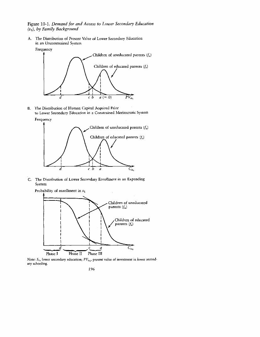
Figure 10-1. Demand for and Access to Lower Secondary Education(si), by Family Background
A. The Distribution of Present Value of Lower Secondary Educationin an Unconstrained System
Frequency
Children of uneducated parents (fu)
Children of educated parents (f,)
d c b a (= O) pVi
B. The Distribution of Human Capital Acquired Priorto Lower Secondary Education in a Constrained Meritocratic System
Frequency
Children of uneducated parents (fu)
Children of educated parents (fe)
d cb a Ciso
C. The Distribution of Lower Secondary Enrollment in an ExpandingSystem
Probability of enrollment in s,
Children of uneducatedparents (fu)
\Children of educatedparents (fe)
d __________ c a Q,
Phase I Phase II Phase IIINote: Sl, lower secondary education; PVi,,, present value of investment in lower second-ary schooling.
196
Education Policy and Intergenerational Mobility 197
secondary education (PVi,l), on the assumption that the children of edu-cated parents constitute the smaller group. The distribution by presentvalue for children of educated parents is to the right of that for childrenof uneducated parents, for the reasons noted above. Point a on the hori-zontal axis signifies a present value for si schooling of 0; that is, it demar-cates those who demand si schooling from those who do not. Theproportion of children for whom the present value of s5 schooling ispositive is higher for the children of the educated than for the childrenof the uneducated. Where market forces determine the quantity anddistribution of education, the children of the educated are thus at anadvantage.
Enrollment and Family Backgroundin a Constrained Meritocratic System
In a freely competitive market for education the equilibrium conditionis that demand is exactly satisfied; that is,
(10-4) Pis, = Dis,
where Pisj is the probability (with value 0 or 1) that the individual willattend educational level j. The aggregate probability of (that is, propor-tion in) enrollment for the relevant age group (with N*, members) is
(10-5) p N . DNiSi N,j Ns,
If school places are rationed, some individuals for whom Di,, = 1 willnevertheless not attend school.4 In this case the individual's probabilityof enrollment will depend on his probability of acceptance (irr5,) as wellas on his-demand.
(10-6) Pi,, = ,iTjDis,
The aggregate probability of enrollment is then the product of aggre-gate demand and the probability of acceptance:5
(10-7) P = Yj (7Tis, Di,)
N,,
The probability of acceptance depends on the rationing system. Wedefine the system as meritocratic if rrin, depends simply and positivelyon the human capital that the individual possesses before s1 -that is, onCi,0. We refer to this accumulated human capital as achievement. In thatcase,

198 EDUCATIONAL EXPANSION AND INEQUALITY OF OPPORTUNITY
(10-8) lrj,, = 1 if E,, 2 a,D
Wrxs, = 0 otherwise
where
E,l = the number of si places to be filled
ai = the percentile (ordered from the top) of thedistribution of human capital of s1 leaverswith Di,, = 1 in which individual i is found
For instance, if there is one s, place available for every ten applicants(E,, /D,, = 0.1), the probability of promotion to si is unity for studentsin the top 10 percent of the distribution (ai c 0.1) and zero for thosefor whom ai > 0.1.
Under a meritocratic selection criterion, whether probabilities of en-rollment differ by family background depends on whether the distribu-tions by achievement of the two groups differ. In figure 10-1, panel B,the horizontal axis is human capital acquired prior to secondary school(Ci,0). If the distribution by achievement of the children of the educatedis located to the right of that of the children of the uneducated, the proba-bility of acceptance will be greater for the former than for the latter. 7Tslf> rsilf.. Point a now signifies the achievement level necessary to ensureacceptance. The proportion of so leavers with CQ0 > W is higher amongchildren of educated parents. For this to occur, it is sufficient that edu-cated parents provide more out-of-school human capital for their chil-dren than do uneducated parents or that they send their children to betterschools. The conclusion would be strengthened if the children of edu-cated parents also inherited a higher average natural ability.
Educational Expansion at One Educational Leveland Its Effects on Distribution
Assume that in both unconstrained and constrained meritocraticschool systems the probability of attending si is greater for children ofeducated parents than for children of uneducated parents, for the reasonsenumerated above. What consequences does expansion of the aggregateenrollment ratio at educational level si have for the distribution of s,places by family background? Our measure of the inequality of accessto s, is the difference between the proportions of each group enrolledin sl, that is, Ps1f - P,,fu.
An increase in school places in a constrained meritocratic system isequivalent to reducing the achievement level required for acceptance intosl-that is, point a in panel B is moved to the left. If the original sizeof the system was small, the distributional effect need not be egalitarian.

Education Policy and Intergenerational Mobility 199
As Ps, is expanded from a small base, the distribution of places in s1 islikely to pass through various phases (panel C): inequality first increases(phase I), then decreases (phase II), and finally becomes constant (phase111). The positions and slopes of the curves in panel C are derived fromthe distributions in panel B; thus the slopes of the curves in panel C aresteepest at the modes of the distributions in panel B. The inequality ofaccess is the vertical distance between the curves in panel C.
At first, as expansion occurs,' more children of the educated than ofthe uneducated are admitted and the probability of enrollment rises moresteeply for children of educated parents than for children of uneducatedparents. That is, Ps,&f - Ps,f. increases; inequality of educational opportu-nity is exacerbated. To the left of the point at which the curves in panelsA and B cross, more children of uneducated than of educated parentsare aided by further expansion, but inequality continues to increase be-cause the educated group is smaller than the uneducated group. At pointc the slopes of the two curves in panel C are the same and inequalityis at a maximum. To the left of point c the probability of schooling forchildren of uneducated parents increases more than for children of edu-cated parents, and hence inequality begins to decrease. Phase II ends atpoint d, which corresponds to PVi,, = 0. Beyond point d (phase III), nofurther expansion in the number of places available would increase en-rollment unless measures were also taken to increase the demand for s1education (Dis,f.), which in this model is held constant. Inequality of ac-cess to s1 thus does not change.
The distribution of s1 places is likely to pass through the same threephases if an unconstrained system expands owing to, for example, an in-crease in government subsidies. The pattern might differ if expansionwere the result of a policy of subsidies that specifically benefited childrenfrom deprived backgrounds. The effect of expansion can be seen by shift-ing the distributions of PV.1 to the right in panel A. The same logic ap-plies as when point a was moved to the left.
Socioeconomic Background and Educational Attainment
The model predicts a positive relationship between socioeconomic back-ground and educational attainment. Table 10-1 shows a strong correla-tion in both countries between father's education and the level of educa-tion achieved by the employee; as father's education increases so doesthe percentage of children attaining high levels of education. For ex-ample, in Kenya 36 percent of the employees whose fathers had no educa-tion received secondary or higher education, whereas for those whose fa-thers had primary education the corresponding figure is 66 percent andfor those whose fathers had secondary or higher education it is 84 per-cent. These percentages can be seen as roughly indicating the probability,
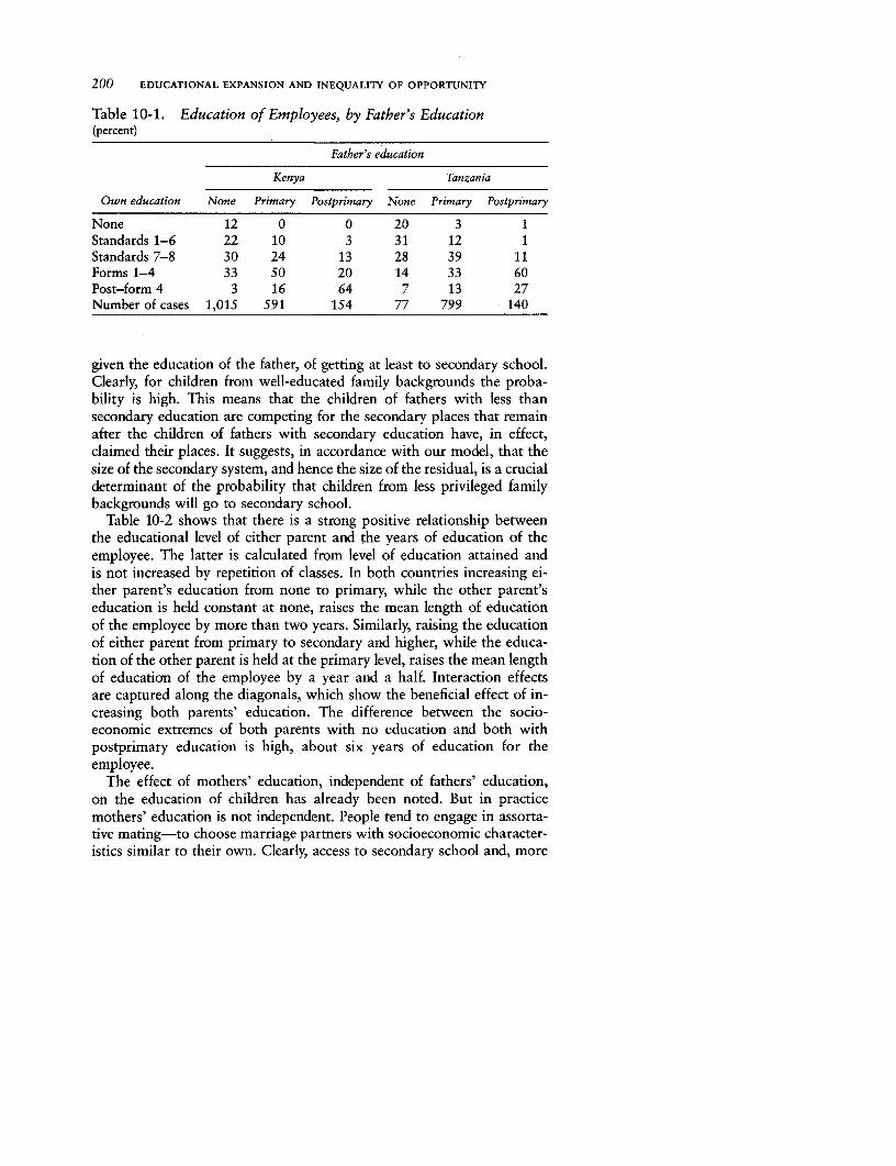
200 EDUCATIONAL EXPANSION AND INEQUALITY OF OPPORTUNITY
Table 10-1. Education of Employees, by Father's Education(percent)
Father's education
Kenya Tanzania
Own education None Primary Postprimary None Primary Postprimary
None 12 0 0 20 3 1Standards 1-6 22 10 3 31 12 1Standards 7-8 30 24 13 28 39 11Forms 1-4 33 50 20 14 33 60Post-form 4 3 16 64 7 13 27Number of cases 1,015 591 154 77 799 140
given the education of the father, of getting at least to secondary school.Clearly, for children from well-educated family backgrounds the proba-bility is high. This means that the children of fathers with less thansecondary education are competing for the secondary places that remainafter the children of fathers with secondary education have, in effect,claimed their places. It suggests, in accordance with our model, that thesize of the secondary system, and hence the size of the residual, is a crucialdeterminant of the probability that children from less privileged familybackgrounds will go to secondary school.
Table 10-2 shows that there is a strong positive relationship betweenthe educational level of either parent and the years of education of theemployee. The latter is calculated from level of education attained andis not increased by repetition of classes. In both countries increasing ei-ther parent's education from none to primary, while the other parent'seducation is held constant at none, raises the mean length of educationof the employee by more than two years. Similarly, raising the educationof either parent from primary to secondary and higher, while the educa-tion of the other parent is held at the primary level, raises the mean lengthof education of the employee by a year and a half. Interaction effectsare captured along the diagonals, which show the beneficial effect of in-creasing both parents' education. The difference between the socio-economic extremes of both parents with no education and both withpostprimary education is high, about six years of education for theemployee.
The effect of mothers' education, independent of fathers' education,on the education of children has already been noted. But in practicemothers' education is not independent. People tend to engage in assorta-tive mating-to choose marriage partners with socioeconomic character-istics similar to their own. Clearly, access to secondary school and, more

Education Policy and Intergenerational Mobility 201
Table 10-2. Employees' Mean Years of Education, by Mother'sand Father's Education
Mother's education
Kenya Tanzania
Father's education None Primary Postprimary None Primary Postprimary
None 6.9 9.3 ... 5.8 8.1 ...(959) (45) (736) (30)
Primary 9.0 10.5 12.0 8.3 9.5 11.9(317) (258) (6) (438) (345) (9)
Postprimary 11.0 12.0 13.1 8.9 11.8 11.7(55) (65) (24) (31) (98) (11)
... Zero or insignificant.Note: Figures in parentheses are numbers of cases.
generally, the degree of inequality in the distribution of educational op-portunity by socioeconomic background will be strongly affected by thepropensity of individuals to marry their educational peers.
Let us assume that the adult population is divided into two groups,the educated (E) and the uneducated (U), and that males and females aredivided equally between them. If children with two U parents have a zeroprobability of obtaining secondary education, children with one E parenta 0.5 probability, and children with two E parents a probability of 1,the distribution of secondary educational opportunities for the childrenwill depend on the mating behavior of their parents. The probabilitiesare as follows.
, Perfectly assortative mating. All the Es marry Es and all the Usmarry Us. The children of uneducated parents have a probabilityof 0 of receiving secondary education, and the children of educatedparents have a probability of 1 of receiving secondary education.
* Antiassortative mating. The Es marry Us and, since all childrenhave one parent with education, they all have a probability of 0.5of receiving secondary education.
* Random mating. Half of the U males marry U females and halfmarry E females. Similarly, half of the E males marry U femalesand half marry E females. The probabilities that the children willreceive secondary education are as follows: 0 for the 25 percentwhose parents have no education, 1 for the 25 percent with twoeducated parents, and 0.5 for the 50 percent with one educatedparent.
202 EDUCATIONAL EXPANSION AND INEQUALITY OF OPPORTUNITY
This example shows that inequality in the distribution of educationalopportunity in the next generation will be greatest if mating is perfectlyassortative. The distribution will be less unequal if mating is random andmost equal if mating is antiassortative.
In fact, the survey evidence suggests that mating behavior falls some-where between perfectly assortative and random. In the Kenyan sample95 percent of fathers who had no education had wives with no education;54 percent of fathers with primary education and 37 percent of thosewith postprimary education had wives with no education. In Tanzaniathe percentages were similar. Perfectly assortative mating is in any casenot possible because there are fewer educated women than educated men.The picture is more dramatic when we consider the mothers of respon-dents. In Kenya nearly 90 percent of the small pool (23 percent of thetotal) of women with at least primary education were married to menwith at least primary education; the tendency is no weaker in Tanzania.Thus assortative mating was constrained in the past by the limited educa-tional opportunities for girls. Greater sexual equality in access to educa-tion and the advantages of having educated parents mean that the pro-pensity of the educated to marry among themselves will reinforce theunequal distribution of educational opportunity in the next generation.
These simple cross-tabulations suggest a relationship between the edu-cation of a worker and that of his parents. They are not conclusive, how-ever, because they do not isolate the influence of parental educationwhile other determinants of educational attainment are held constant.For instance, a young worker with young parents is likely to have moreeducation than an older worker, and his parents are likely to have moreeducation than those of an older worker. Thus the relationship might besimply a result of the expansion of the education system and not of anyindependent effect of parents' education on the educational attainmentof their children. To isolate this independent effect, multivariate analysisis necessary. The probit functions that we estimate measure the indepen-dent effects of a variety of determinants of educational attainment andshow how the relationship between family background and educationalattainment has changed from one cohort of workers to the next. We aretherefore able to examine the effects of educational expansion on the dis-tribution of educational opportunities.
The Expansion and Distribution of Primary Education
In both Kenya and Tanzania the primary school system can be character-ized as nonmeritocratic, in that access is not determined by cognitiveachievement or natural ability, and unconstrained, in that before the gov-ernment commitment to universal primary education there were no legalprohibitions on local or private initiatives and regulation was not oner-
Education Policy and Intergenerational Mobility 203
ous. Thus the model predicts, for the various reasons enumerated, thatthe present value of primary education (PV,,), and hence the demand forprimary schooling and the probability of completing it, will vary posi-tively with the educational level of parents in both countries. A secondset of predictions concerns the effect of educational expansion on the dis-tribution of primary schooling. Since both Kenya and Tanzania are ap-proaching universal primary education, we would expect them to be inphase 11 of their expansion, and the model predicts that the probabilitieshave become more equal in both countries.
The probit function that we estimate measures the impact of familybackground on the probability of completing primary school and thusprovides a test of our first prediction. It also measures the interaction be-tween increases in the aggregate enrollment rate and the educational levelof parents and so tests our second prediction. Table 10-3 presents maxi-mum likelihood estimates of the parameters in the following reducedform equation:
(10-9) Prob(Y = 1) = 4'(X'P3)
where Y is a dichotomous variable that takes the value 1 where theindividual completed primary school or higher and 0 otherwise, X is avector of exogenous variables, and F(X'P) is the cumulative unit normaldistribution function. Note that the coefficients ,3 do not represent themarginal change in the probability associated with each of the inde-pendent variables, as is the case with the simple linear probabilitymodel.
The exogenous variables are:
F, = a set of four dummy variables that signify the educa-tional level of the individual's parents. In the basesubcategory (F1 ) both parents are uneducated; F2signifies one parent with no education and one withprimary education; F3 signifies both parents withprimary education or one parent with secondary edu-cation or higher and one with no education; and F4
signifies one parent with primary education and oneparent with secondary education or higher or bothparents with secondary education or higher.
P,, = the aggregate enrollment rate in standard 7 (or, be-fore 1966, 8) when the individual was 13 years old,as measured by the proportion of all 13-year-olds en-rolled in standard 7 (or, before 1966, 8) in the yearwhen the individual was 13.
P,0 - Fj = a set of interaction variables.6
B = a dummy variable that takes the value 1 if the individ-
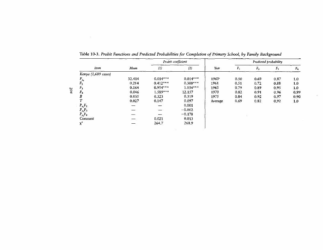
Table 10-3. Probit Functions and Predicted Probabilities for Completion of Primary School, by Family Background
Probit coefficient Predicted probability
Item Mean (1) (2) Year F, F2 F3 F4
Kenya (1,689 cases)Ps. 32.414 0.014*** 0.014*** 1960, 0.50 0.69 0.87 1.0
F2 0.214 0.412*** 0.388*** 1961 0.51 0.72 0.88 1.0
F3 0.164 O.954*** 1.034*** 1965 0.79 0.89 0.95 1.0
F4 0.046 1.589*** 12.157 1970 0.82 0.91 0.96 0.99
B 0.035 0.323 0.319 1975 0.84 0.92 0.97 0.90
T 0.027 0.147 0.097 Average 0.69 0.82 0.92 1.0
Ps0F2 - - 0.001
PJoF3 - - -0.002Ps0F4 - - -0.178
Constant - 0.021 0.013
X2 - 264.7 268.9
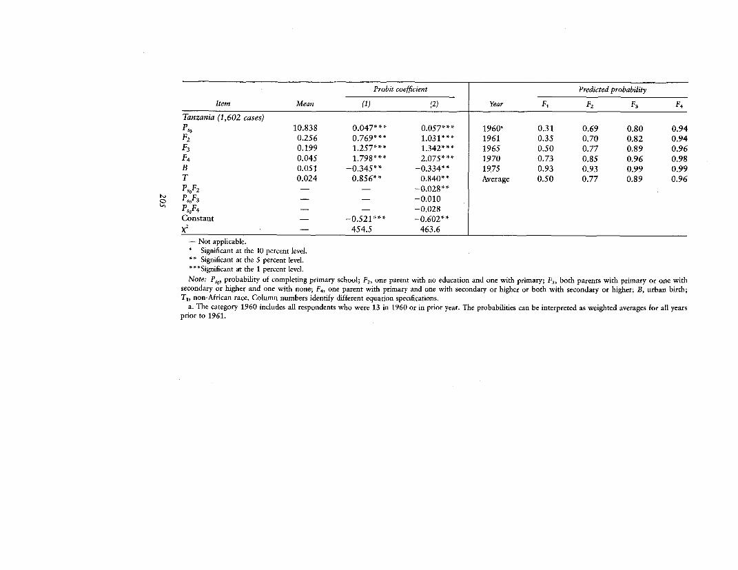
Probit coefficient Predicted probability
Item Mean (1) (2) Year F, F2 F3 F4
Tanzania (1,602 cases)Ps. 10.838 0.047*** 0.057*** 1960' 0.31 0.69 0.80 0.94F2 0.256 0.769*'* 1.031*** 1961 0.35 0.70 0.82 0.94F3 0.199 1.257*** 1.342*** 1965 0.50 0.77 0.89 0.96F4 0.045 1.798 ** 2.075*'* 1970 0.73 0.85 0.96 0.98B 0.051 -0.345** -0.334** 1975 0.93 0.93 0.99 0.99T 0.024 0.856** 0.840* * Average 0.50 0.77 0.89 0.96
PJF2 - -- -0.028**
O P50F3-0.010
>' PsoF4 - -0.028Constant - -0.521*** -0.602**
X 2 .- 454.5 463.6
-Not applicable.* Significant at the 10 percent level.
* Significant at the 5 percent level.***Significant at the 1 percent level.Note: P,O, probability of completing primary school; F2, one parent with no education and one with primary; F3, both parents with primary or one with
secondary or higher and one with none; F4, one parent with primary and one with secondary or higher or both with secondary or higher; B, urban birth;TI, non-African race. Column numbers identify different equation specifications.
a. The category 1960 includes all respondents who were 13 in 1960 or in prior year. The probabilities can be interpreted as weighted averages for all yearsprior to 1961.
206 EDUCATIONAL EXPANSION AND INEQUALITY OF OPPORTUNITY
ual was born in an urban area and 0 if the individualwas born in a rural area
T = a dummy variable that takes the value 1 if the individ-ual is non-African and 0 if the individual is African.
Table 10-3 also presents the probabilities of completing primary schoolpredicted by the estimated functions for the four family backgroundgroups.'
The first prediction of the model is clearly borne out: in both countriesthe coefficients on the family background variables increase monotoni-cally with the educational level of the parents and in column 1 are allsignificant at the 1 percent level. Five of six are significant at that levelin column 2. The average predicted probability of completing primaryschool rises from 0.69 in Kenya and 0.50 in Tanzania for children withuneducated parents (F1) to 1.0 in Kenya and 0.96 in Tanzania for chil-dren with at least one parent with secondary education (F4 ).
The second prediction is also confirmed: for children of parents withsecondary education the predicted probability of completing primaryschool remains constant at or near unity throughout the period underconsideration, whereas for children of uneducated parents the probabil-ity rises markedly. For children of uneducated parents the predictedprobability of attendance prior to 1961 was 0.50 in Kenya and 0.31 inTanzania. The probability rises to 0.84 in Kenya and 0.93 in Tanzaniain 1975. As the model led us to expect for an education system in phaseII, in both countries expansion of primary schooling more than propor-tionately benefited the children of those who are relatively low in the so-cioeconomic hierarchy.
The Expansion and Distributionof Lower Secondary Education
Kenya's lower secondary system has expanded faster than Tanzania's andis much larger. The lower secondary system in Tanzania is the moremeritocratic of the two in the sense that ability to pay determines accessin a smaller proportion of cases. In both countries performance on theprimary-leaving examination is the main determinant of access to gov-ernment secondary schools, whereas ability to pay is the main determi-nant of access to private schools. In 1976, 71 percent of form 1 studentswere enrolled in private schools in Kenya; in Tanzania the comparablefigure was 40 percent. Our surveys indicate that in both countries nearlyall primary leavers wanted at the time to continue. Inability to pay schoolfees was the main reason given for not attending secondary school inKenya, while in Tanzania insufficiently high grades was the main reason.
Education Policy and Intergenerational Mobility 207
In Tanzania there has been a marked change in the importance of thereasons for not continuing beyond primary school; financial reasons havebecome less important and failure in exams more important.
Has meritocratic selection proved an effective substitute for educa-tional expansion as a means of reducing inequality in the distribution ofschooling? Or has neither expansion nor greater meritocracy reduced in-equality?
Table 10-4 presents estimates of lower secondary probit functions forthe whole sample and the predicted probabilities of attending forms 1-4by family background. The only differences in specification betweenthese functions and those in table 10-3 are in the dependent variable andthe aggregate enrollment ratio. Yj,1 now takes the value 1 if the individ-ual attended lower secondary school and 0 otherwise. P,1 is the aggregateprobability of attending secondary school when the individual was 14years old, as measured by the proportion of all 14-year-olds enrolled inform 1 at that time.
In both Tanzania and Kenya the coefficients on the family backgroundvariables increase monotonically with parents' educational level. All aresignificant at the 1 percent level. The move toward greater meritocracyin Tanzania has not made access to lower secondary school independentof family background. The table of predicted probabilities shows that thedistribution of lower secondary opportunities is more equal in Kenyathan in Tanzania.8 The average probability that a child of the most edu-cated parents (F4) will attend lower secondary school is high-0.85 inKenya and 0.82 in Tanzania. The predicted probability for a child of un-educated parents (F1) is much lower in both countries, but in Tanzania,at 0.16, it is less than half the probability in Kenya, 0.36.
The changes in probabilities with time confirm that Kenya is clearlyin the second, increasingly egalitarian, phase of expansion of its second-ary system. Before 1961 the structure of probabilities by family back-ground was much the same in Kenya as in Tanzania; in both countriesthe predicted probability that a child of the most educated parents wouldattend lower secondary school was four or more times that for a childof uneducated parents. In 1975, roughly a decade after the two countries'policies regarding secondary schooling diverged, the structure of proba-bilities was markedly more compressed in Kenya. In both countries theprobability that a child of the most educated parents would attend lowersecondary school remained roughly constant at a high level; in Kenya thepredicted probability of attendance for a child of uneducated parents rosesharply, from 0.21 before 1961 to 0.73 in 1975. In Tanzania the proba-bility increased only from 0.13 to 0.21 during the same period.
These results suggest that Kenya's policy of allowing the enrollmentratio to increase has succeeded in reducing inequality of access to second-
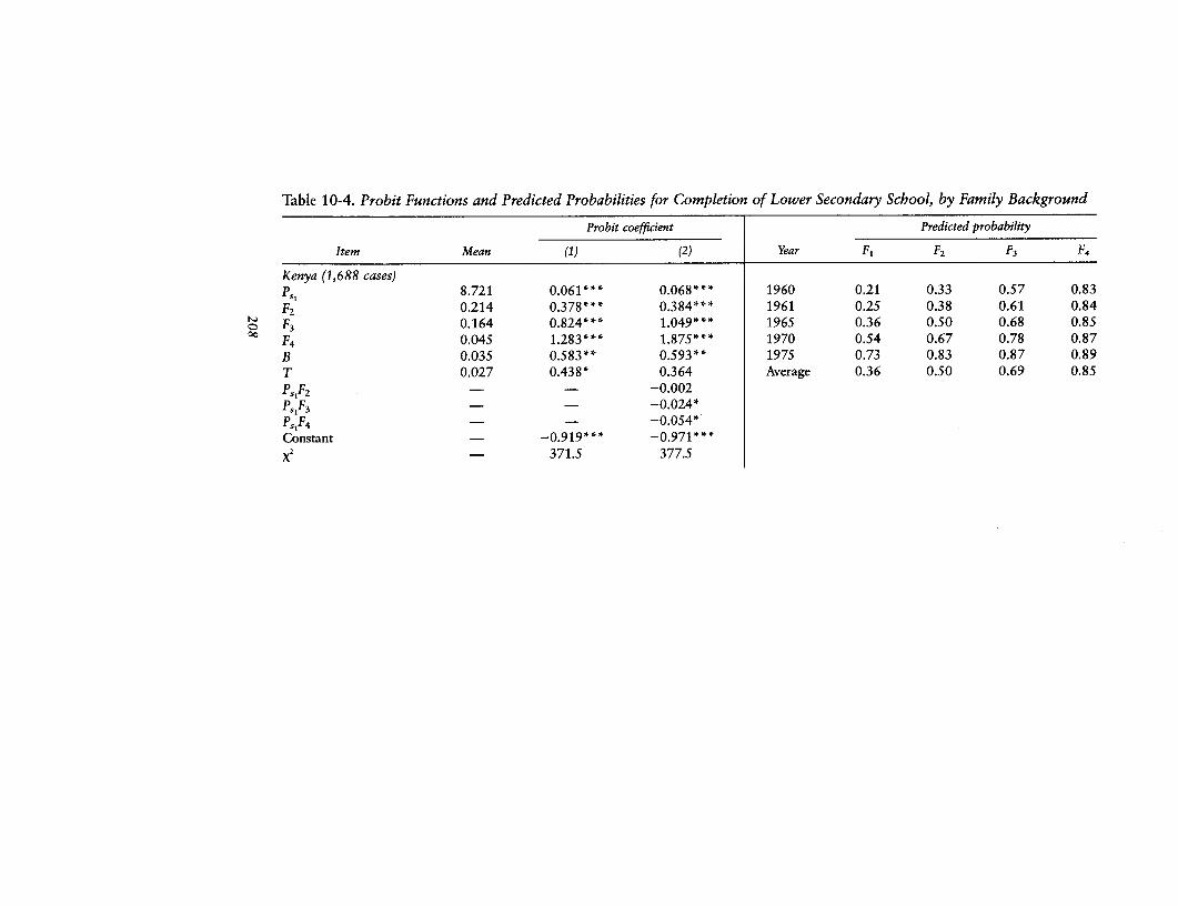
Table 10-4. Probit Functions and Predicted Probabilities for Completion of Lower Secondary School, by Family Background
Probit coefficient Predicted probability
Item Mean (1) (2) Year F, F2 F3 F4
Kenya (1,688 cases)P51 8.721 0.061 * * * 0.068*** 1960 0.21 0.33 0.57 0.83F2 0.214 0.378*** 0.384*** 1961 0.25 0.38 0.61 0.84
o F3 0.164 0.824*** 1.049*** 1965 0.36 0.50 0.68 0.85x F4 0.045 1.283*** 1.875*** 1970 0.54 0.67 0.78 0.87
B 0.035 0.583** 0.593** 1975 0.73 0.83 0.87 0.89T 0.027 0.438* 0.364 Average 0.36 0.50 0.69 0.85Ps,F2 - - -0.002
PJF3 - -- -0.024*
PJF4 - -- -0.054*
Constant - -0.919*** -0.971***
X 2 - 371.5 377.5
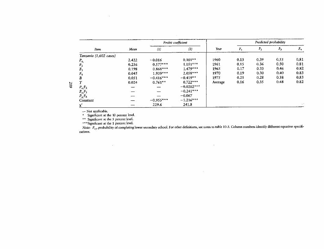
Probit coefficient Predicted probability
Item Mean (1) (2) Year F, F2 F3 F4
Tanzania (1,602 cases)P.,, 2.422 -0.016 0.101** 1960 0.13 0.39 0.55 0.81F2 0.256 0.577*** 1.051*** 1961 0.15 0.36 0.50 0.81
F3 0.198 0.868'** 1.479*'* 1965 0.17 0.33 0.46 0.82
F4 0.045 1.939*'* 2.058'** 1970 0.19 0.30 0.40 0.83
B 0.051 -0.416*** -0.419** 1975 0.21 0.28 0.38 0.83X T 0.024 0.761** 0.722*** Average 0.16 0.35 0.48 0.82
4 P,1F2 _ 0.0202***PsF3 - -- -0.241***
PsJF4 _ - -0.067
Constant - -0.955*** -1.216***X 2 - 229.6 241.8
-Not applicable.* Significant at the 10 percent level.* Significant at the 5 percent level.**Significant at the 1 percent level.
Note: P,,, probability of completing lower secondary school. For other definitions, see notes to table 10-3. Column numbers identify different equation specifi-cations.
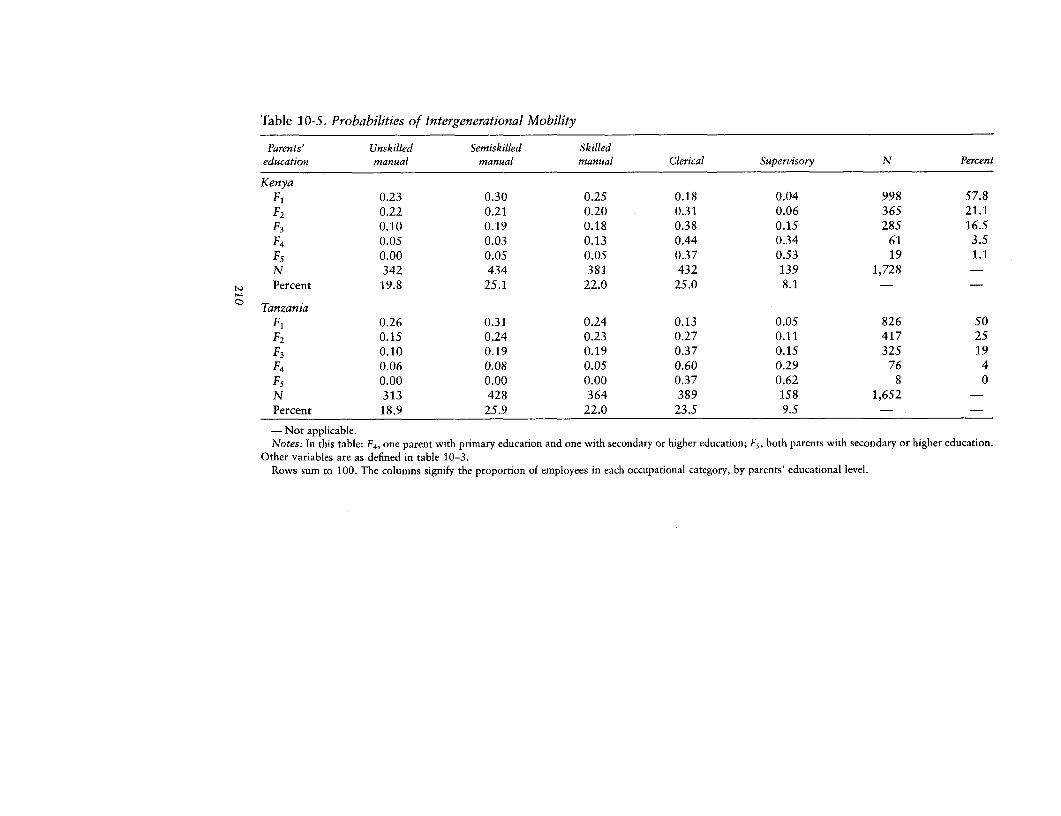
Table 10-5. Probabilities of Intergenerational Mobility
Parents' Unskilled Semiskilled Skillededucation manual manual manual Clerical Supervisory N Percent
KenyaF1 0.23 0.30 0.25 0.18 0.04 998 57.8F2 0.22 0.21 0.20 0.31 0.06 365 21.1F3 0.10 0.19 0.18 0.38 0.15 285 16.5F4 0.05 0.03 0.13 0.44 0.34 61 3.5F5 0.00 0.05 0.05 0.37 0.53 19 1.1N 342 434 381 432 139 1,728 -
v>, Percent 19.8 25.1 22.0 25.0 8.1 -
( TanzaniaF, 0.26 0.31 0.24 0.13 0.05 826 50F2 0.15 0.24 0.23 0.27 0.11 417 25F3 0.10 0.19 0.19 0.37 0.15 325 19F4 0.06 0.08 0.05 0.60 0.29 76 4F5 0.00 0.00 0.00 0.37 0.62 8 0N 313 428 364 389 158 1,652 -Percent 18.9 25.9 22.0 23.5 9.5 -
-Not applicable.Notes: In this table: F4, one parent with primary education and one with secondary or higher education; Fs, both parents with secondary or higher education.
Other variables are as defined in table 10-3.Rows sum to 100. The columns signify the proportion of employees in each occupational category, by parents' educational level.
Education Policy and Intergenerational Mobility 211
ary schooling. Tanzania's policy of restricting secondary school growthbut attempting to make access less dependent on family backgroundthrough the use of meritocratic selection criteria has been less successful.The intensely competitive meritocratic selection system appears to be aseffective in denying access to secondary school to children from poorfamilies as were fees in earlier years.9
Levels of Intergenerational Mobility
As a result of Kenya's education policies, a higher proportion of peoplefrom poor backgrounds are now receiving secondary education therethan in Tanzania. We might expect the greater equality in the distributionof lower secondary schooling in Kenya to lead to a smaller role for familybackground in determining position in the socioeconomic hierarchy thanin Tanzania. Has this in fact occurred?
Let Pii denote the probability that an individual with parents in classi is in class j. Then, assuming that the system is closed, 1i P,j = 1 forall i. Let pj(T) be the probability that the family line is in class j at timeT. Then
(10-10) pi (T + 1) = lPipT)ij
This Markov chain model of mobility rests on the assumption that theprobability that an individual will move to a position in the socioeco-nomic hierarchy-a class-different from his parents' depends only onhis parents' class and not directly on the classes of previous generations.
Table 10-5 uses our cross-sectional data on parent-child pairs to pre-sent the matrix of probabilities of intergenerational mobility for Kenyaand Tanzania.' 0 The employee's occupation indicates his economic status(expected lifetime earnings), and parents' level of education indicates hisparents' economic status. If there were perfect mobility, the row percent-ages would be similar and would be close to the overall occupational dis-tribution shown in the bottom line of the table. In fact, there is a markeddifference by family background in the probabilities of attaining high-status jobs. In both countries the probability that children will gain ac-cess to the top two categories rises monotonically with the educationallevel of their parents.
Since the overall occupational distribution in Kenya and Tanzania isalmost identical, we can roughly compare mobility in the two countriesby directly comparing the probabilities of attaining higher-status occupa-tions for the various family background groups. Kenya and Tanzaniashow striking similarities in this respect. For example, for children whoseparents had no education, the probability of getting a white-collar job(clerical, professional, or managerial) is 0.22 in Kenya and 0.18 in Tanza-nia. If both parents had primary education, the probability is 0.53 in
212 EDUCATIONAL EXPANSION AND INEQUALITY OF OPPORTUNITY
Kenya and 0.52 in Tanzania; if both parents had secondary education,the probability is 0.90 in Kenya and 0.99 in Tanzania. It appears thatalthough children from less educated households have a much higherprobability of getting secondary education in Kenya than in Tanzania,their probability of being in white-collar occupations is almost the samein both countries.
An aggregate measure confirms the impression that degrees of mobilityare similar in Kenya and Tanzania. In the following index of mobility,developed by Bartholomew (1973), movement of children to classes dif-ferent from their parents' is weighted by the distance moved and the sizeof each class in the parental generation.
(10-11) M = IfiPij Ti-jT
where fi= ni= ni
and n signifies the number in the classes of the parents' generation. Com-plete immobility-where the transition matrix is the identity matrix andhence the value of the index is equal to 0-is only possible if the propor-tions of people in the various classes remain unchanged from one genera-tion to the next. In Kenya and Tanzania the size of the classes is not thesame across generations, which implies that the value of the index in thesituation of least possible mobility, Mlm, is not equal to 0 and can differbetween Kenya and Tanzania. The magnitude of the index in the situationof perfect mobility, Mpm, will also differ between the two countries be-cause of differences in the class composition of the parental generation.
To compare intergenerational mobility in Kenya and Tanzania, westandardize the actual measure of mobility by the values for the hypothet-ical situations of perfect and least mobility." Our standardized index is
(10-12) M* = M - MimMpm - Mlm
which shows the position of M between the two extreme points as a frac-tion of the distance between them. The actual mobility measure (M) is1.331 in Kenya and 1.247 in Tanzania, whereas the standardized mobil-ity measure (M*) is 0.59 in Kenya and 0.54 in Tanzania."2 The val-ues of M* are similar in Kenya and Tanzania.
Educational Expansion and the Distributionof Post-Form 4 Education
The more equal distribution of lower secondary education in Kenya thanin Tanzania has not brought about greater intergenerational mobility. Inthis section we formalize and test the hypothesis that children from privi-
Education Policy and Intergenerational Mobility 213
leged backgrounds tend to remain one step ahead in educational attain-ment. Extensions of our model demonstrate that equalization of oppor-tunities at the lower secondary level need not equalize opportunities atthe next level-that, indeed, it may lead to greater inequality in the distri-bution of post-form 4 education.
In the second phase of the expansion of s1 outlined above, Psife - Ps,fudeclines. This equalization of opportunities at the s1 level equalizes thedemand for upper secondary, or s2 , places (on the assumption that s2 ed-ucation is highly subsidized so that Di12 = 1 for all s, completers). That is,D,& - D,2 f. falls as P51, and hence D,5 &, increases. Since
P2j= 7rs2fj st
whether reducing inequality in the demand for post-form 4 schoolingreduces inequality of enrollment depends on the changes in the probabili-ties of promotion. (If promotion to post-form 4 were random, the equali-zation of demand would clearly lead to increasing equality of enroll-ment.) In a meritocratic system the probabilities of promotion alsochange in a predictable way as the lower secondary system expands.
Consider first the situation in which the post-form 4 system remainsthe same size. As lower secondary enrollments increase, promotion rateshave to fall to adjust to the increased demand for a constant number ofS2 places. To examine the effect of this on inequality of access to s2 , wehave to examine the changing achievement levels of children from differ-ent family backgrounds both before entry to and on completion of si.Panel A of figure 10-2 shows the two family background groups distrib-uted by achievement prior to s1. When the number of s1 places is small,the achievement required for promotion to si is high (point a). A largernumber of places permits a lower minimum achievement level (for ex-ample, all those above a' are promoted).13
The distributions and means of Ci,5 f, and Cis,f. are shown for a smallsystem (panel B, point a) and for a large system (panel C, point a'). Whens1 is small, only the highest achievers among the children of uneducatedparents enter the s1 system. Their achievement prior to s1 therefore com-pares favorably with that of the children of educated parents: C0f. is notmuch less than CQOf. The expansion of s, draws into the system primarilythose children of uneducated parents who were previously excluded bytheir relatively low achievement. The expansion has little effect on theenrollment of the children of educated parents or on their mean achieve-ment prior to s1: C5 ,fe is only marginally lower than in panel B. By con-trast, C5 f. is now markedly lower.
If achievement prior to s1 is a good predictor of achievement prior tos2 (as is true if the production functions for so and s1 are similar andif out-of-school investments prior to s1 are closely correlated with suchinvestments during s1 ), the expansion of s1 , whether in a constrained or

214 EDUCATIONAL EXPANSION AND INEQUALITY OF OPPORTUNITY
Figure 10-2. The Distribution of Post-Formn 4 Education, by FamilyBackground
A. By Achievement Prior to Secondary School
Frequency
Children of uneducated parents (fu)
Children of educated parents (4)
a' a C,,O
B. If the Lower Secondary System Is SmallFrequency
Children of uneducated Children of educated parents (fe)parents (fu) N..
a Ci,f. Ci0f. b' b C,O
C. If the Lower Secondary System Is Large
Frequency
Children of uneducated parents (fu)
Children of educated parents (fe)
a' Ci,,f a C,,,f b' b Ci,,Note: C,,,, human capital acquired prior to entering lower secondary school.
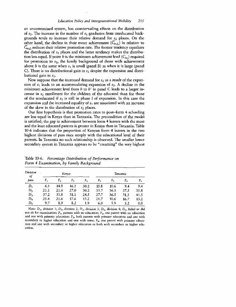
Education Policy and Intergenerational Mobility 215
an unconstrained system, has countervailing effects on the distributionof S2. The increase in the number of s, graduates from uneducated back-grounds tends to increase their relative demand for S2 places. On theother hand, the decline in their mean achievement (as,f) in relation toCQ,f, reduces their relative promotion rate. The former tendency equalizesthe distribution of s2 places and the latter tendency makes the distribu-tion less equal. If point b is the minimum achievement level (Cis,) requiredfor promotion to s2, the family background of those with achievementabove b is the same when si is small (panel B) as when it is large (panelC). There is no distributional gain in S2 despite the expansion and distri-butional gain in sl.
Now suppose that the increased demand for s2 as a result of the expan-sion of s1 leads to an accommodating expansion of S2* A decline in theminimum achievement level from b to b' in panel C leads to a larger in-crease in s2 enrollment for the children of the educated than for thoseof the uneducated if S2 is still in phase I of expansion. In this case theexpansion and the increased equality of s1 are associated with an increaseof the skew in the distribution of s2 places.
Our first hypothesis is that promotion rates to post-form 4 schoolingare less equal in Kenya than in Tanzania. The precondition of the modelis satisfied; the gap in achievement between form 4 leavers with the mostand the least educated parents is greater in Kenya than in Tanzania. Table10-6 indicates that the proportion of Kenyan form 4 leavers in the twohighest divisions of pass rises steeply with the educational level of theirparents. In Tanzania no such relationship is observed. The smaller lowersecondary system in Tanzania appears to be "creaming" the very highest
Table 10-6. Percentage Distribution of Performance onForm 4 Examination, by Family Background
Division Kenya Tanzaniaof
pass F, F2 F3 F4 F, F2 F3 F4
D,1 6.5 14.9 16.2 30.2 10.8 10.6 9.4 9.4D, 21.1 21.6 27.0 30.2 33.7 36.5 37.5 35.8D3 37.2 32.8 31.1 24.5 27.7 36.5 31.3 41.5D4 25.4 21.6 17.6 13.2 21.7 10.6 16.7 13.2D 5 9.7 8.9 8.2 1.9 6.0 5.9 5.2 0.0
Note: Dl, division l; D2 , division 2; D3 , division 3; D4 , division 4; Ds, failed or didnot sit for examination; Fl, parents with no education; F2, one parent with no educationand one with primary education; F3 , both parents with primary education and one withsecondary or higher education and one with none; F4 , one parent with primary educa-tion and one with secondary or higher education or both with secondary or higher edu-cation.
216 EDUCATIONAL EXPANSION AND INEQUALITY OF OPPORTUNITY
achievers among the children of the relatively uneducated, who thencompete on equal terms with the children of the more educated. Sincethe Kenyan lower secondary system, because of its larger size, apparentlydoes not "cream" to the same extent, children from relatively uneducatedbackgrounds tend to perform relatively poorly on the school-leaving ex-aminations. In the model a decline in the achievement of the children ofthe uneducated as s, expands results in a decline in their promotion rate,WS2 f,-
Partly because of the greater demand as a result of the faster expansionof lower secondary education in Kenya, upper secondary and higher edu-cation expanded at a faster pace there than in Tanzania. Enrollment inpost-form 4 increased in Kenya from less than 0.1 percent to 1.5 percentbetween 1961 and 1975; in Tanzania the increase from a similar basewas, less than half as large. In the model expansion of S2 from a very smallbase leads to an increase in the promotion rate of the children of the edu-cated, wrr2hf. Therefore we would expect nTs2f, - 1rr2f. to be greater in Kenyathan in Tanzania.
Table 10-7 presents estimates of probit functions for upper secondaryeducation. The dependent variable, Yi, takes the value 1 if the individualattended upper secondary school and 0 otherwise. But since the equa-tions are estimated only for respondents who attended form 4, they pre-dict promotion rates (ri) rather than the probabilities of attendance (Pi)predicted by the probit functions for primary and lower secondary educa-tion. The predicted promotion rates, by family background and overtime, are also presented in the table. The macro constraint variable isagain Ps1, the aggregate probability of attending form 1 when the individ-ual was 14 years old.
In Kenya the coefficients on the family background variables are largeand highly significant and increase monotonically with parents' educa-tional level. By contrast, Tanzania shows the same monotonic pattern,but the coefficients are smaller and not significant. The country differ-ences in predicted rates of promotion are as hypothesized. The gap inpromotion rates between the children of the most and the least educatedis much greater in Kenya than in Tanzania. In Kenya a form 4 leaver whohas a parent with secondary education is 7.0 times as likely to attendpost-form 4 schooling as a form 4 leaver with uneducated parents; inTanzania a child of the most educated parents is only 1.6 times as likelyto attend as one with uneducated parents. In Tanzania post-form 4 ex-pansion has been so slow that the rate of promotion declined between1961 and 1975 for form 4 leavers irrespective of their family back-ground, and the rate of decline has been much the same for all socioeco-nomic groups. In Kenya the predicted promotion rate has declined forform 4 leavers with uneducated parents but has increased for those witha parent with secondary education.

Education Policy and Intergenerational Mobility 217
Is the distribution of post-form 4 schooling more unequal in Kenyathan in Tanzania because of the faster expansion of upper secondary andhigher education in Kenya? Has the distribution worsened over time inKenya as a result of expansion from a small base? If, as seems likely,Kenya is still in phase 1, the expansion of s2 will have benefited primarilythe children of the educated. We use PS2F4 - PS2FI as our measure of in-equality. The percentages of groups F1 , F2, F3 , and F4 who go beyond form4 in Kenya are 2.0, 9.0, 15.0, and 43.2, respectively; in Tanzania for thesame groups they are 4.4, 7.1, 12.7, and 26.2, which implies a moreequal distribution. To assess changes over time in Kenya we divide thesample into those aged 24 and younger and those aged 25 and older. Ofthose 25 or older, the percentages going beyond form 4 are 2.1, 7.7, 14.8,and 40.8 for F1, F2 , F3, and F4. For those 24 or younger the correspond-ing percentages are 1.5, 12.9, 15.6, and 46.9. As predicted, it appearsthat the distribution of post-form 4 education is more skewed in Kenyathan in Tanzania and has become somewhat more unequal over time inKenya; the children of the educated are remaining one step ahead in edu-cational attainment.
Conclusions
Our econometric analysis of the natural experiment in Kenya and Tanza-nia points to several conclusions about the relationship between educa-tional policy, the distribution of schooling, and intergenerational mobil-ity. A small secondary system will tend to be monopolized by childrenfrom relatively privileged backgrounds, as was the case in Kenya andTanzania in the 1960s. Rapid expansion of that system, as in Kenya, willbenefit disproportionately children from less privileged backgroundswithout displacing children from more privileged backgrounds. A moveto more meritocratic selection criteria, as in Tanzania, is not an effectivesubstitute for expansion as a means of equalizing the distribution ofsecondary schooling. Children from more privileged backgrounds benefitfrom the greater out-of-school investments in human capital and fromhigher-quality primary schooling, which lead to greater skill acquisitionin primary school and superior performance on standardized secondaryentrance examinations.
Our analysis of lower secondary and post-form 4 education suggestsgeneralizations about the effect of secondary expansion on access to ter-tiary education. Kenya's experience demonstrates that despite more equalrepresentation in the pool of candidates for further education, greaterequality in the distribution of secondary places does not necessarily bringabout greater equality in the distribution of places at the next level.Secondary expansion entails a lowering of entry criteria. As a corollary,the performance on standardized examinations of children from less priv-

Table 10-7. Probit Functions and Predicted Promotion Rates into Upper Secondary School, by Family Background
Probit coefficient Predicted probability
Item Mean (1) (2) Year F, F2 F3 F4
Kenya (511 cases)p" 11.62 0.003 -0.035 1960 0.12 0.11 0.24 0.33
F2 0.262 0.472** -0.161 1965 0.08 0.14 0.24 0.39
> F3 0.283 0.726$** 0.393 1970 0.05 0.18 0.24 0.47F4 0.333 1.274$1* 0.623 1977 0.03 0.23 0.24 0.55
B 0.082 0.143 0.140 Average 0.06 0.16 0.24 0.42
T 0.050 0.660** 0.723**
P31F2 - - 0.059*PsJF3 - - 0.035
PsJF4 - _ 0.062
Constant - -1.532*** -1.171***Xi 2- 56.09 59.78
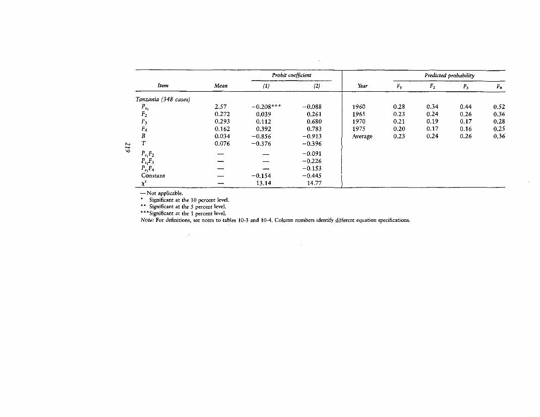
Probit coefficient Predicted probability
Item Mean (1) (2) Year F, F2 F3 F4
Tanzania (348 cases)Psl 2.57 -0.208*** -0.088 1960 0.28 0.34 0.44 0.52
F2 0.272 0.039 0.261 1965 0.23 0.24 0.26 0.36
F3 0.293 0.112 0.680 1970 0.21 0.19 0.17 0.28
F4 0.162 0.392 0.783 1975 0.20 0.17 0.16 0.25
B 0.034 -0.856 -0.913 Average 0.23 0.24 0.26 0.36
X T 0.076 -0.376 -0.396
Ps,F2 - - -0.091
P31F3 _ -0.226PsJ4 - - -0.153Constant - -0.154 -0.445
X 2 - 13.14 14.77
-Not applicable.* Significant at the 10 percent level.* * Significant at the 5 percent level.
'*Significant at the 1 percent level.Note: For definitions, see notes to tables 10-3 and 10-4. Column numbers identify different equation specifications.
220 EDUCATIONAL EXPANSION AND INEQUALIIY OF OPPORTUNITY
ileged backgrounds tends to erode in relation to the performance of chil-dren from more privileged backgrounds. The relative rate of promotioninto the tertiary system of children from less privileged backgroundstherefore declines as the secondary system expands. This tendency coun-terbalances greater equality in the composition of demand for tertiaryschooling. The distribution of places in the tertiary system may becomeless equal because an expansion of the tertiary system from a very smallbase in response to the growth of demand will initially disproportionatelybenefit the more privileged children.
Increased inequality in the distribution of places in the tertiary systemwill tend to offset the effect on intergenerational mobility of the decreasein inequality in the secondary system. Our examination of intergenera-tional mobility points to the rather pessimistic conclusion that educationpolicy need not have much impact on mobility. No matter what policyis adopted-short of actually establishing educational quotas for the var-ious family background groups and thereby possibly sacrificing allocativeefficiency-there will be a strong tendency for the elite to perpetuate theirrelative position in the socioeconomic hierarchy.
But relativity is not everything. Although the expansion of secondaryeducation in Kenya has not had the beneficial impact on intergenera-tional mobility that might have been expected, the absolute wages ofthose from less educated households are much higher in Kenya, partlybecause of the productivity gains from the expansion of the educationsystem. There may also be direct consumption benefits from a higherlevel of education. Furthermore, the parents of most students in thesecountries have had no formal education, which makes it virtually impos-sible for them to contribute to their children's acquisition of academicskills. The advantages in school performance that children from moreprivileged backgrounds gain from the higher educational level of theirparents may diminish as the educational level of the population as awhole increases.
Notes
1. For a discussion of some theoretical and empirical issues concerning educa-tional production functions see Hanushek (1979) and Lau (1979).
2. Differences among individuals in human capital acquired before s1 can affectPVi2 1. Increased human capital increases both the benefits and the opportunitycost (in earnings forgone) of s1. These influences raise and lower PVis1, respec-tively. We assume that the first influence dominates.
3. The form of the educational production function implies that out-of-schoolinvestments are complementary to formal schooling. For supporting evidence forKenya and Tanzania, see chapter 4.
Education Policy and Intergenerational Mobility 221
4. If subsidies and restrictions on supply are sufficiently marked, virtually allso leavers, irrespective of family background, will demand sl. This would be thecase, for instance, were point d to signify PVj1 j = 0.
5. When the market for s, is unconstrained, 'rnj = 1 (all i).6. Note that when the estimated equation is used to predict probabilities, inter-
actions between family background and aggregate enrollment manifest them-selves even in the absence of multiplicative terms. In contrast to a simple linearprobability equation, in the probit equation a marginal change in probability as-sociated with a given variable depends on the values of the other exogenous vari-ables:
a Prob(Y = 1) = Bkf(X'3)
aXk
where f(X'13) is the value of the normal density function at the point X'1. Themultiplicative variables are included to capture additional interactions.
7. The probability that Y = 1 is the area under the standard normal curve be-tween - ox and X'3. In table 10-3 probabilities are predicted for Africans bornoutside Nairobi; that is, we set U and T equal to 0 and P5o equal to its actualvalue in the respective years.
8. The predicted probabilities are derived from the interactive equation in bothinstances because four of the six interaction terms are significant at least at the10 percent level.
9. Conlisk (1974) has shown that reducing the random components in determi-nation of economic success may actually strengthen systematic parent-child con-nections.
10. If all observations in each cell (i, j) are drawn independently and if all fami-lies face the same matrix of transition probabilities, the observed relative frequen-cies (F,j) of children in each class for each parental class are binomially distributedabout the true probabilities.
11. To obtain Mp,,m we construct a transition matrix in which the rows are iden-tical and calculate the value of the index. For Mim we construct a transition ma-trix that represents the situation of least mobility as follows. We fill in the un-skilled category with children from the bottom parental category, F1. Since thebottom parental category is larger than the unskilled category, we fill the nextlowest occupational category with F1 children. After the bottom two occupa-tional categories have been filled with F1 children, a few remain to go into theskilled manual category. The remainder of the skilled manual category is filledwith F2 children. The F2 children left over after the skilled manual category isfilled are put into the clerical category, and so on. We use this constructed matrixto calculate Mlm.
12. M* is derived from Mi, (1.067 in Kenya and 0.983 in Tanzania) and Mpm(1.513 and 1.470, respectively).
13. Similarly, in an unconstrained system the achievement level on completionof so necessary for demand to be positive is a positive function of the private costof s1 and is hence a negative function of the size of sl.
CHAPTER 11
Educational Expansion, FamilyBackground, and Earnings
CHAPTER 10 SHOWED, rather surprisingly, that despite Kenya's muchlarger secondary system and the consequent greater equality in the distri-bution of secondary education, intergenerational mobility is not greaterthere than in Tanzania. One reason for this phenomenon is the tendencyfor the children of the educated elite to remain one rung higher on theeducational ladder. The proportion of children of the educated who con-tinue beyond lower secondary school is larger than that of children ofthe uneducated, and in Kenya the difference between the two proportionsis larger than in Tanzania.
Another possible reason for this outcome is differential labor marketperformance by family background for a given educational level. In Tan-zania, among workers whose education ended at the lower secondarylevel, there are no systematic wage differentials among family back-ground groups. In Kenya, by contrast, mean wages for form 4 leaversincrease with the educational level of the worker's parents. The differencemay be attributable to greater discrimination in the labor market on thebasis of family background in Kenya-because of less egalitarian politicalrhetoric and attitudes or as a response by elite groups to the democratiza-tion of access to lower secondary schooling. Kenyan secondary leaverswith educated parents may also be at an advantage in the labor marketbecause they tend to acquire more human capital prior to secondaryschool and to attend better schools. This phenomenon may not be as evi-dent in Tanzania, where the lower secondary system is smaller and moreuniform.
We begin our empirical analysis by comparing the extent of discrimina-tion by family background in the two countries. The conventionalmethod of measuring discrimination is to calculate the income differen-tial among the groups in question after standardizing for such proxiesfor human capital endowments as years of education and employmentexperience. The years-of-schooling variable will be an inadequate proxy
222
Educational Expansion, Family Background, and Earnings 223
for human capital acquired in school if performance in school differs byfamily background, as may be the case in Kenya. There may thereforebe a systematic upward bias in conventional estimates of discrimination.
Consider the simplest regression model. Within an educational stratumthe wage is a function of human capital endowment, Ci, and of someeffect of family background, F, that is felt through discrimination in thelabor market.
W = a + b1F + b2C
Because human capital endowments are not observed, the regressionmodel generally estimated is W = cL + bjF. The omission of an explana-tory variable causes the estimates of the coefficients to be biased unlessthe omitted variable is orthogonal to all the other variables in the model.In this example, if, as is most likely, b 2 > 0 and human capital endow-ments are positively correlated with family background, the coefficienton the latter variable will be overestimated.
It can be shown that the bias becomes larger as the correlation betweenfamily background and human capital increases and as the sample varia-tion in the excluded human capital variable becomes larger (see Hanu-shek and Jackson 1977). In the general case with several exogenous vari-ables such as years of work experience, this result holds if all thesample correlations have the same sign. The simple model in the nextsection shows that Kenya, with its larger education system, is likely toexhibit both a higher variation in human capital endowments within agiven educational group, and a higher correlation between family back-ground and human capital. Hence the upward bias of the family back-ground coefficient is likely to be larger for Kenya than for Tanzania. Inthis chapter we attempt to measure the extent of upward bias in estimatesof discrimination by family background.
The Model
The model developed here is a variant of the one in chapter 10. We positan educational production function:
(11-1) Cij = f(Ri, Ii, Qj)
The human capital endowment of individual i at the conclusion ofschooling level j, Ciq, is some (probably complex) positive function of nat-ural ability, R2; the quantity and quality of training provided in the home,Ii; and the quality of schooling, Qi. Parents' education is a proxy for thequality of parental inputs.' To facilitate the exposition we divide parentsinto two groups, educated and uneducated. Figure 11-1 is a stylized sim-plification of the true situation, in which there is more variation in the

Figure 11-1. The Distribution of Human Capital, by Family Background
A. Primary School LeaversFrequency
Children of uneducated parents (fm)
Children of educated parents (fe)
a' aB. Students in a Small Lower Secondary System
Frequency
Children of uneducatedparents (fu) Children of educated parents (fe)
Cisu Qs 0 fe'S
C. Students in a Large Lower Secondary SystemFrequency
Children of uneducated parents (f)
Children of educated parents (fe)
at CisCf ZsfeNote: Shaded areas represent lower secondary students who go on to upper secondaryschool.
224
Educational Expansion, Family Background, and Earnings 225
parental quality variable. Panel A depicts the distributions by humancapital endowment of primary leavers with educated parents, fe, and withuneducated parents, fu. The distributions reflect our presumptions thatnatural ability is distributed normally and that educated parents are thesmaller group. The distribution of primary leavers with educated parentslies to the right of the distribution of those with uneducated parents. Weassume that, as was discussed in chapter 10, educated parents makelarger out-of-school investments in their children and send their childrento higher-quality schools.2 Educated parents may have higher naturalability, which their children may inherit. This difference in ability maybe attributable to the selectivity of the school system and to assortativemating, the tendency for relatively highly educated (high-ability) men tomarry relatively highly educated (high-ability) women.
We assume that, because of large government subsidies to secondaryeducation and the consequent high private returns, there is excess de-mand for secondary places. Under meritocratic selection criteria, primaryleavers must have a higher level of endowments-as measured, for ex-ample, by primary-leaving examinations-to gain access to a smallsecondary system than to a large system. Panel B depicts the family back-ground composition for a small lower secondary system, and panel Cshows the composition for a large system. The variance of endowmentsis much higher in the large than in the small system. Moreover, becauseonly the upper tail of the distribution of children of uneducated parentsgains access in a small system, there is little difference in the mean levelof endowments between children of educated and uneducated parents.In a large system the gap between family background groups in the meanlevel of endowments is also large.
Unless there is some marked change in relative inputs or in productionfunctions, relative endowments of human capital on entry to lowersecondary school are likely to prove good predictors of relative endow-ments on completion. Under this assumption panels B and C show themean values of endowments of those form 4 leavers with educated andwith uneducated parents who do not gain access to upper secondaryschool and who therefore enter the labor market. The shaded areas inpanels B and C represent lower secondary leavers who progress to uppersecondary school. In a small system (panel B) mean human capital en-dowments are roughly the same for all form 4 leavers entering the labormarket, whether their parents are educated or uneducated. Expandingthe secondary system substantially lowers the endowments of entrantswith uneducated parents in comparison with entrants with educated par-ents.
What are the labor market implications of these changes in the market
226 EDUCATIONAL EXPANSION AND INEQUALITY OF OPPORTUNITY
for education? We assume that the following function describes howwages are determined:
(11-2) W, = f(Ci, Li, Fi)
This general function is in the spirit of Mincer's human capital wagefunction (Mincer 1974). An important difference is that our measure ofthe output of the education system, Ci, replaces years of schooling-an input into the production function3-as an independent variable.Postschool acquisition of skills is represented in the conventional way byLi, the individual's years of employment experience, and family back-ground is represented by Fij, parents' education. In contrast to Mincer'sfunction, our function, when stratified by education, permits variance inhuman capital and hence in wages among workers with a given level ofexperience.
The labor market implications of educational expansion are repre-sented by the following set of linkages:
(11-3) Lzu > 0; e/ > 0; aW'/W > 0; aWjw" > 0dz azulze 8 Ce/Cu Oz
where z denotes the supply of form 4 leavers and e and u denote educatedor uneducated parents. The first linkage indicates that an increase in thesupply of form 4 leavers as a result of expansion of the secondary systemincreases the proportion of form 4 leavers with uneducated parents inthe labor force. The second linkage indicates that as this proportion in-creases so does the ratio between the average human capital endowmentof form 4 leavers with educated parents and that of form 4 leavers withuneducated parents. Underlying the third linkage is the assumption thatthe demand for and supply of efficiency units of labor, rather than ofactual units, determine wages. Profit-maximizing employers seek to mini-mize the cost per efficiency unit of labor rather than the cost per worker.Thus, if we standardize employment experience, in equilibrium the ratioof wages is equal to the ratio of human capital endowments. As Ce/Cuincreases, so does WeIWu.
The interaction between the education and labor markets is summa-rized by the fourth linkage. An increase in the supply of form 4 leaversas a result of educational expansion induces the emergence of a wage gapbetween form 4 leavers with educated and uneducated parents. The elas-ticity of the wage gap with respect to a given increase in supply dependson the differences between family background groups in the quality ofschooling, in the quantity and quality of out-of-school investments inhuman capital, and in ability; the relative sizes of the groups; and theinitial size of the secondary system.
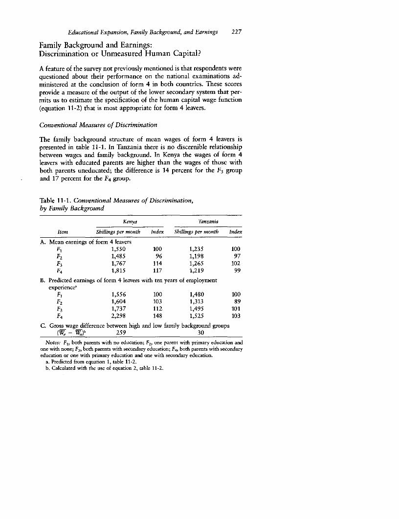
Educational Expansion, Family Background, and Earnings 227
Family Background and Earnings:Discrimination or Unmeasured Human Capital?
A feature of the survey not previously mentioned is that respondents werequestioned about their performance on the national examinations ad-ministered at the conclusion of form 4 in both countries. These scoresprovide a measure of the output of the lower secondary system that per-mits us to estimate the specification of the human capital wage function(equation 11-2) that is most appropriate for form 4 leavers.
Conventional Measures of Discrimination
The family background structure of mean wages of form 4 leavers ispresented in table 11-1. In Tanzania there is no discernible relationshipbetween wages and family background. In Kenya the wages of form 4leavers with educated parents are higher than the wages of those withboth parents uneducated; the difference is 14 percent for the F3 groupand 17 percent for the F4 group.
Table 11-1. Conventional Measures of Discrimination,by Family Background
Kenya Tanzania
Item Shillings per month Index Shillings per month Index
A. Mean earnings of form 4 leaversF1 1,550 100 1,235 100F2 1,485 96 1,198 97F3 1,767 114 1,265 102F4 1,815 117 1,219 99
B. Predicted earnings of form 4 leavers with ten years of employmentexperience,
F1 1,556 100 1,480 100F2 1,604 103 1,313 89F3 1,737 112 1,495 101F4 2,298 148 1,525 103
C. Gross wage difference between high and low family background groups(We - W.)" 259 30
Notes: F1, both parents with no education; F2, one parent with primary education andone with none; F3, both parents with secondary education; F4, both parents with secondaryeducation or one with primary education and one with secondary education.
a. Predicted from equation 1, table 11-2.b. Calculated with the use of equation 2, table 11-2.
228 EDUCATIONAL EXPANSION AND INEQUALITY OF OPPORTUNITY
Columns 1 and 2 of table 11-2 present estimates of the following func-tion for form 4 leavers:
(11-4) In W = a + bL + cL2 + dFj
This function permits us to standardize the family background struc-ture of wages for differences in employment experience among familybackground groups. In Tanzania the coefficients on Fj are small and sta-tistically insignificant, confirming the absence of a wage premium forform 4 leavers with educated parents. In Kenya, by contrast, the coeffi-cients on F3 and F4 are significant and the latter is large.
The regressions in table 11-2 are used in table 11-1 to predict thewages of form 4 leavers with ten years of employment experience butwith different family backgrounds. A comparison of mean earnings ofall form 4 leavers with the predicted earnings of those with ten years ofexperience indicates almost no change in Tanzania. In Kenya the indexfor F4 rises from 117 to 148 because form 4 leavers with uneducated par-ents have more employment experience than the form 4 leavers whoseparents have the most education. The latter group is younger, reflectingthe rarity, until recently, of marriages in which both spouses have rela-tively high educational levels.
We take the analysis of discrimination a step further and allow for dif-ferences among family background groups in the structure of wages. Thestandard technique for measuring discrimination when two groups differin their personal characteristics and in the function relating these charac-teristics to wages is to compare their actual mean wages with what theirmean wages would be if all were paid according to the same wage-function-that is, with the same constant term and the same set of coeffi-cients on the independent variables.4 Columns 3 and 5 of table 11-2 pre-sent estimates of equation 11-4 disaggregated into two groups by familybackground. These equations are used to decompose the gross wage dif-ference, G = We - W%, between form 4 leavers in the two family back-ground groups. The difference is 259 shillings in Kenya and a negligible30 shillings in Tanzania.
The gross wage difference is made up of the part explained by personalcharacteristics and the unexplained part that reflects differences in theconstant terms and coefficients of the regression equations for the edu-cated and uneducated groups. Let X be a vector of the personal charac-teristics L and L2. Then
(11-5) G = We - Wu = We - fe(Xu) + fe(Xu WuE + R
respectively, where E is the explained and R the unexplained residualpart of G. In Kenya 16 percent of G is explained by the difference inemployment experience; fully 84 percent of the gross difference is notexplained and would therefore be conventionally attributed to discrimi-
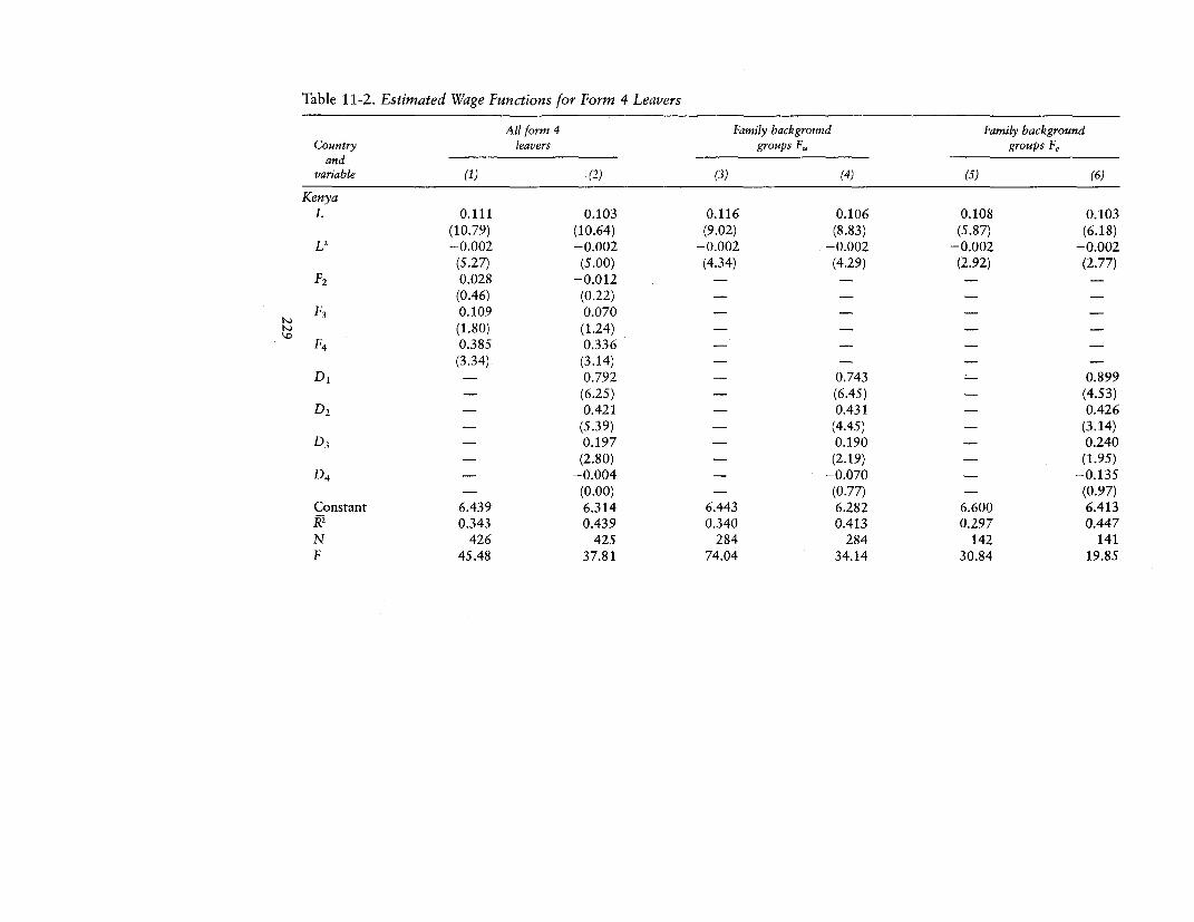
Table 11-2. Estimated Wage Functions for Form 4 Leavers
All form 4 Family background Family backgroundCountry leavers groups F. groups Fe
andvariable (1) (2) (3) (4) (5) (6)
KenyaL 0.111 0.103 0.116 0.106 0.108 0.103
(10.79) (10.64) (9.02) (8.83) (5.87) (6.18)L2 -0.002 -0.002 -0.002 -0.002 -0.002 -0.002
(5.27) (5.00) (4.34) (4.29) (2.92) (2.77)F2 0.028 -0.012
(0.46) (0.22) - - - -
F3 0.109 0.070 - - - -(1.80) (1.24) - - - -
F4 0.385 0.336 - - - -(3.34) (3.14) - - -
D, _ 0.792 - 0.743 0.899- (6.25) - (6.45) - (4.53)
D2 - 0.421 - 0.431 - 0.426- (5.39) - (4.45) - (3.14)
D3 - 0.197 - 0.190 - 0.240- (2.80) - (2.19) _ (1.95)
D4 - -0.004 - -0.070 - -0.135- (0.00) - (0.77) - (0.97)
Constant 6.439 6.314 6.443 6.282 6.600 6.413k2 0.343 0.439 0.340 0.413 0.297 0.447N 426 425 284 284 142 141F 45.48 37.81 74.04 34.14 30.84 19.85
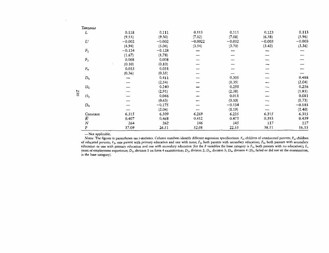
TanzaniaL 0.118 0.111 0.113 0.111 0.123 0.113
(9.55) (9.30) (7.02) (7.08) (6.38) (5.96)L2 -0.002 -0.002 -0.0022 -0.002 -0.003 -0.003
(4.94) (5.04) (3.54) (3.70) (3.42) (3.36)F2 -0.124 -0.128
(1.67) (1.78) -
F3 0.008 0.008 -
(0.10) (0.10) -
F4 0.033 0.031 -(0.36) (0.35) - - -
D I - 0.411 - 0.305 - 0.488- (2.54) - (1.35) - (2.04)
D2 - 0.240 - 0.250 - 0.2569 - (2.91) - (2.38) - (1.85)
° D3 - 0.046 - 0.011 - 0.081_ (0.63) - (0.10) - (0.73)
D 4 -0.175 - -0.134 - -0.185(2.04) - (1.19) - (1.40)
Constant 6.315 6.309 6.269 6.235 6.315 6.315k2 0.407 0.468 0.412 0.473 0.393 0.439N 264 262 146 145 117 117F 37.09 26.51 52.08 22.55 38.51 16.15
-Not applicable.Notes: The figures in parentheses are t-statistics. Column numbers identify different regression specifications. F,n children of uneducated parents; F., children
of educated parents; F2, one parent with primary education and one with none; F3, both parents with secondary education; F4, both parents with secondaryeducation or one with primary education and one with secondary education (for the F variables the base category is F,, both parents with no education); L,years of employment experience; Dl, division 1 on form 4 examination; D2, division 2; D3, division 3; D4 , division 4 (D5, failed or did not sit the examination,is the base category).
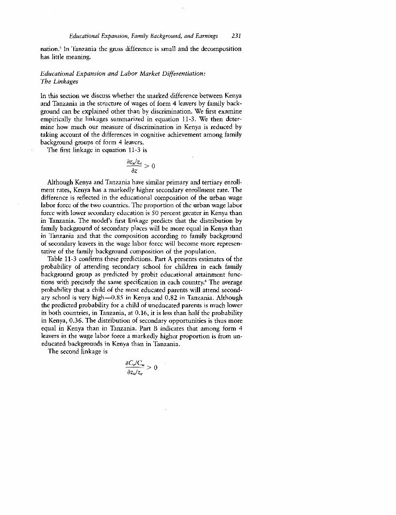
Educational Expansion, Family Background, and Earnings 231
nation.' In Tanzania the gross difference is small and the decompositionhas little meaning.
Educational Expansion and Labor Market Differentiation:The Linkages
In this section we discuss whether the marked difference between Kenyaand Tanzania in the structure of wages of form 4 leavers by family back-ground can be explained other than by discrimination. We first examineempirically the linkages summarized in equation 11-3. We then deter-mine how much our measure of discrimination in Kenya is reduced bytaking account of the differences in cognitive achievement among familybackground groups of form 4 leavers.
The first linkage in equation 11-3 is
aZuiZe > oaz
Although Kenya and Tanzania have similar primary and tertiary enroll-ment rates, Kenya has a markedly higher secondary enrollment rate. Thedifference is reflected in the educational composition of the urban wagelabor force of the two countries. The proportion of the urban wage laborforce with lower secondary education is 50 percent greater in Kenya thanin Tanzania. The model's first linkage predicts that the distribution byfamily background of secondary places will be more equal in Kenya thanin Tanzania and that the composition according to family backgroundof secondary leavers in the wage labor force will become more represen-tative of the family background composition of the population.
Table 11-3 confirms these predictions. Part A presents estimates of theprobability of attending secondary school for children in each familybackground group as predicted by probit educational attainment func-tions with precisely the same specification in each country.6 The averageprobability that a child of the most educated parents will attend second-ary school is very high-0.85 in Kenya and 0.82 in Tanzania. Althoughthe predicted probability for a child of uneducated parents is much lowerin both countries, in Tanzania, at 0.16, it is less than half the probabilityin Kenya, 0.36. The distribution of secondary opportunities is thus moreequal in Kenya than in Tanzania. Part B indicates that among form 4leavers in the wage labor force a markedly higher proportion is from un-educated backgrounds in Kenya than in Tanzania.
The second linkage is
aCe/Cu, O
azuIZe
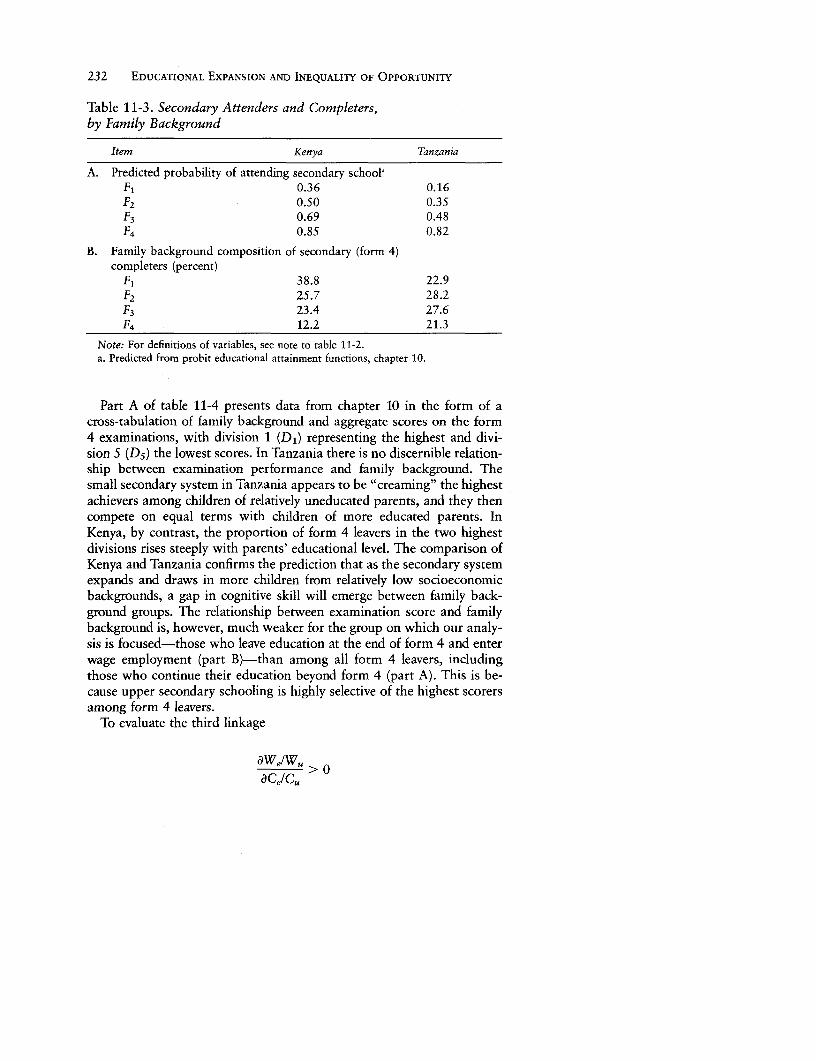
232 EDUCATIONAL EXPANSION AND INEQUALITY OF OPPORTUNITY
Table 11-3. Secondary Attenders and Completers,by Family Background
Item Kenya Tanzania
A. Predicted probability of attending secondary schoolaF1 0.36 0.16F2 0.50 0.35F3 0.69 0.48F4 0.85 0.82
B. Family background composition of secondary (form 4)completers (percent)
F1 38.8 22.9F2 25.7 28.2F3 23.4 27.6F4 12.2 21.3
Note: For definitions of variables, see note to table 11-2.a. Predicted from probit educational attainment functions, chapter 10.
Part A of table 11-4 presents data from chapter 10 in the form of across-tabulation of family background and aggregate scores on the form4 examinations, with division 1 (D1) representing the highest and divi-sion S (D5) the lowest scores. In Tanzania there is no discernible relation-ship between examination performance and family background. Thesmall secondary system in Tanzania appears to be "creaming" the highestachievers among children of relatively uneducated parents, and they thencompete on equal terms with children of more educated parents. InKenya, by contrast, the proportion of form 4 leavers in the two highestdivisions rises steeply with parents' educational level. The comparison ofKenya and Tanzania confirms the prediction that as the secondary systemexpands and draws in more children from relatively low socioeconomicbackgrounds, a gap in cognitive skill will emerge between family back-ground groups. The relationship between examination score and familybackground is, however, much weaker for the group on which our analy-sis is focused-those who leave education at the end of form 4 and enterwage employment (part B)-than among all form 4 leavers, includingthose who continue their education beyond form 4 (part A). This is be-cause upper secondary schooling is highly selective of the highest scorersamong form 4 leavers.
To evaluate the third linkage
OWeIWuelw">0
aCe/Cu

Educational Expansion, Family Background, and Earnings 233
Table 11-4. Percentage Distribution of Performance on Form 4Examination, by Family Background
Kenya Tanzania
Group D1 D, D3 D4 D, D, D2 D3 D4 D,
A. Form 4 leaversF1 6.5 21.1 37.3 25.4 9.7 10.8 33.7 27.7 21.7 6.0F2 14.9 21.6 32.8 21.6 8.9 10.6 36.5 36.5 10.6 5.9F3 16.2 27.0 31.1 17.6 8.2 9.4 37.5 31.3 16.7 5.2F4 30.2 30.2 24.5 13.2 1.9 9.4 35.8 41.5 13.2 0.0
B. Form 4 attendersF, 2.3 24.0 40.6 24.6 8.6 1.5 30.8 32.3 27.7 7.7F2 7.2 21.2 42.0 22.3 7.2 4.8 25.4 47.6 14.3 7.9F3 7.0 24.7 38.5 18.4 11.4 4.3 28.6 37.1 22.9 7.1F4 5.0 16.9 46.6 25.9 4.6 5.6 16.7 58.3 19.4 0.0
Note: For definitions of variables, see note to table 11-2.
we modify our wage function, equation 11-4, as follows:
(11-6) In W = a + bL + cL2 + dF, + eD,
where Di is a vector of examination scores with "failed" or "did notsit" (Ds) as the base. This function allows us to measure the structureby family background of the wages of form 4 leavers, with performanceon form 4 examinations standardized. We expect eDi to be positive andsignificant; that is, as human capital theory predicts, differences amongform 4 leavers in human capital endowments, as measured by examina-tion scores, will be reflected in the structure of wages.
Table 11-2 presents estimated wage functions for Kenya and Tanzaniaby family background. In both countries the fit of the function as mea-sured by R2 is somewhat improved when examination performance isadded to the equation (compare columns 1 and 2). In both countries thecoefficients on the D variables increase monotonically with examinationscore, except for the coefficient on D4 , which is small. The coefficientson D1 and D2 , the highest divisions, are positive, large, and highly signifi-cant. Table 11-5 indicates that the predicted wages of a representativeform 4 leaver are 121 percent higher in Kenya and 51 percent higher inTanzania if the person was placed in division 1 rather than in division5. Note the consistency of these findings with those in chapter 3.
How large is the bias in the measurement of discrimination that ariseswhen differences in endowments among family background groups areignored? Table 11-2 shows that in Tanzania the coefficients on the F vari-ables are not altered by the inclusion of examination performance; thesecoefficients remain small and insignificant. In Kenya, by contrast, the co-
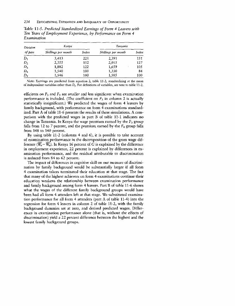
234 EDUCATIONAL EXPANSION AND INEQUALITY OF OPPORTUNITY
Table 11-S. Predicted Standardized Earnings of Form 4 Leavers withTen Years of Employment Experience, by Performance on Form 4Examination
Division Kenya Tanzania
of pass Shillings per month Index Shillings per montb Index
D, 3,413 221 2,391 151D2 2,355 152 2,015 127D3 1,882 122 1,659 105D4 1,540 100 1,330 84D5 1,546 100 1,585 100
Note: Earnings are predicted from equation 2, table 11-2, standardizing at the meanof independent variables other than D,. For definitions of variables, see note to table 11-2.
efficients on F3 and F4 are smaller and less significant when examinationperformance is included. (The coefficient on F3 in column 2 is actuallystatistically insignificant.) We predicted the wages of form 4 leavers byfamily background, with performance on form 4 examinations standard-ized. Part A of table 11-6 presents the results of these simulations. A com-parison with the predicted wages in part B of table 11-1 indicates nochange in Tanzania. In Kenya the wage premium earned by the F3 groupfalls from 12 to 7 percent, and the premium earned by the F4 group fallsfrom 148 to 140 percent.
By using table 11-2 (columns 4 and 6), it is possible to take accountof examination performance in the decomposition of the gross wage dif-ference (We - Wa). In Kenya 16 percent of G is explained by the differencein employment experience, 22 percent is explained by differences in ex-amination performance, and the residual attributable to discriminationis reduced from 84 to 62 percent.
The impact of differences in cognitive skill on our measure of discrimi-nation by family background would be substantially larger if all form4 examination takers terminated their education at that stage. The factthat many of the highest achievers on form 4 examinations continue theireducation weakens the relationship between examination performanceand family background among form 4 leavers. Part B of table 11-6 showswhat the wages of the different family background groups would havebeen had all form 4 attenders left at that stage. We substituted examina-tion performance for all form 4 attenders (part A of table 11-4) into theregression for form 4 leavers in column 2 of table 11-2, with the familybackground dummies set at zero, and derived predicted wages. Differ-ences in examination performance alone (that is, without the effects ofdiscrimination) yield a 22 percent difference between the highest and thelowest family background groups.
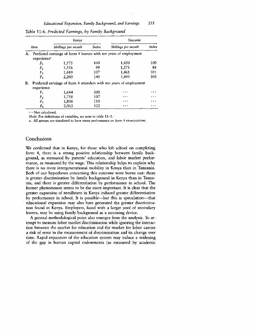
Educational Expansion, Family Background, and Earnings 235
Table 11-6. Predicted Earnings, by Family Background
Kenya Tanzania
item Shillings per month index Shillings per month index
A. Predicted earnings of form 4 leavers with ten years of employmentexperience'
F1 1,575 100 1,450 100F2 1,556 99 1,275 88F3 1,689 107 1,461 101F4 2,203 140 1,495 103
B. Predicted earnings of form 4 attenders with ten years of employmentexperience
F, 1,644 100 ... ...F2 1,758 107 ... ...F3 1,806 110 ... ...F4 2,013 122 ... ...
* Not calculated.Note: For definitions of variables, see note to table 11-2.a. All groups are simulated to have mean performance on form 4 examinations.
Conclusions
We confirmed that in Kenya, for those who left school on completingform 4, there is a strong positive relationship between family back-ground, as measured by parents' education, and labor market perfor-mance, as measured by the wage. This relationship helps to explain whythere is no more intergenerational mobility in Kenya than in Tanzania.Both of our hypotheses concerning this outcome were borne out: thereis greater discrimination by family background in Kenya than in Tanza-nia, and there is greater differentiation by performance in school. Theformer phenomenon seems to be the more important. It is clear that thegreater expansion of enrollment in Kenya induced greater differentiationby performance in school. It is possible-but this is speculation-thateducational expansion may also have generated the greater discrimina-tion found in Kenya. Employers, faced with a larger pool of secondaryleavers, may be using family background as a screening device.
A general methodological point also emerges from the analysis. To at-tempt to measure labor market discrimination while ignoring the interac-tion between the market for education and the market for labor carriesa risk of error in the measurement of discrimination and its change overtime. Rapid expansion of the education system may induce a wideningof the gap in human capital endowments (as measured by academic
236 EDUCATIONAL EXPANSION AND INEQUALITY OF OPPORTUNITY
performance) between groups from different family backgrounds. If theconventional specification of the human capital wage function is thenused to standardize the gross wage difference between the groups for dif-ferences in endowments, the residual will overestimate wage discrimina-tion. Years of schooling is too crude a proxy for economically productiveskills acquired before entering employment. The variance in human capi-tal endowments among children with the same years of schooling is large,and some of what appears to be discrimination actually reflects thepoorer academic performance of the group that is most subject to dis-crimination. Including measures of academic performance in the wagefunction reduces the residual in Kenya by roughly a quarter, althougha substantial amount of discrimination remains.
The results of this chapter should not mislead us into thinking thatfamily background has little or no influence on returns to schooling. Inappendix I we show that returns to schooling, where schooling is mea-sured by a continuous variable, increase markedly with parents' educa-tion in both countries. The findings suggest that family background af-fects earnings because out-of-school investments in human capital byeducated families complement school investments and enable the chil-dren to learn more in school and because children from educated familiesattend better schools. The results also suggest that the independent ef-fects of human capital acquired out of school and of labor market dis-crimination are of less importance.
Notes
1. For empirical evidence that observed parental schooling is an imperfectproxy for parental influences on child development, see Behrman and others(1980) and Olneck (1977) for the United States and Behrman and Wolfe (1984a,1984b) and Behrman and Wolfe (forthcoming) for Nicaragua. In our sample,however, the parental generation consists almost entirely of very poor subsistencefarmers. Thus such commonly used measures of family status as fathers' occupa-tion or income are not useful, and parents' education seems the best indicatorof differentiation among families.
2. Educated people generally live in areas where the quality of schooling isabove average. The quality of schooling appears to be an important determinantof productivity. For example, in Brazil, Behrman and Birdsall (1983) estimatedthe social return to school quality, using teachers' education as an indicator ofquality, and found it to be substantially higher than the social return to schoolquantity.
3. The wage function represented by equation 11-2 is stratified by educationallevel and therefore does not include years of education among the independentvariables as would the aggregate version. In the empirical analysis C is measuredby results on the form 4 examination.
4. See Blinder (1973), Brown, Moon, and Zoloth (1980), Malkiel and Malkiel
Educational Expansion, Family Background, and Earnings 237
(1973), and Oaxaca (1973a, 1973b). For developing countries see Behrman andWolfe (forthcoming), and Knight and Sabot (1982).
5. The corresponding decomposition in which the F3, F4 group is paid accord-ing to the Fl, F2 wage structure yields essentially the same result.
6. The function is of the following general form: Prob(Y = 1) = 'D(X'j3), whereY is a dichotomous variable that takes the value 1 if the individual attendedsecondary school or 0 if he or she did not, X is a vector of exogenous variables,including family background, and cF(X'P) is the cumulative unit normal distribu-tion function. The results are derived from the estimated equations presented inchapter 10.

Part V
THE COST-BENEFIT ANALYSIS
OF SECONDARY EDUCATION:
METHODOLOGICAL
AND POLICY ISSUES

CHAPTER 12
The Returns to Cognitive SkillAcquired in School
MANY STUDIES HAVE BEEN CONDUCTED on the educational rate of returnin both developed and developing countries. Psacharopoulos (1973,1981) has compiled such estimates from forty-four countries. Althoughthe quality of data and the sophistication of methods and interpretationsvary, a fairly standard methodology has been employed, as noted in pre-vious chapters. In chapter 3 we discussed a well-known criticism of theuse of rates of return as a criterion for government policy on educationalexpansion. It has been argued that the generally observed positive rela-tionship between educational level and earnings does not necessarilyshow the effect on productivity of human capital acquired in school.Rather, it could wholly or partially represent the influence on earningsof natural ability. Employers may reward the ability of individual work-ers, or they may use education as a statistical screening device for ability.Alternatively, the correlation may include an element of credentialism-that is, payments for education irrespective of its productive value, onaccount of social relationships or concepts of fairness. The standardmethodology simply assumes away these possibilities.
This chapter presents a methodological innovation that takes empiricalaccount of this criticism and that thus has important policy implications.We use the recursive model developed and estimated in chapter 3 to mea-sure the rate of return on education by tracing the effect of schoolingon cognitive skill and hence on earnings. The empirical analysis is basedon the Kenyan subsample for which we have data on reasoning abilityand cognitive skill. The analysis is confined to Kenya because the smallsize of our subsample prevents our taking account econometrically of thelarge impact that the Tanzanian government's pay policy has on thestructure of earnings and the returns to education. In chapter 13 we focuson the complicating effect of pay policy on rates of return, using the fullsamples.
The secondary system in Kenya is competitive-access to subsidizedplaces in government schools is based on examination performance-and
241
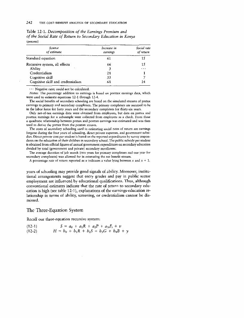
242 THE COST-BENEFIT ANALYSIS OF SECONDARY EDUCATION
Table 12-1. Decomposition of the Earnings Premium andof the Social Rate of Return to Secondary Education in Kenya(percent)
Source Increase in Social rateof estimate earnings of return
Standard equation 61 15
Recursive system, all effects 66 15Ability 3Credentialism 21 1Cognitive skill 33 7Cognitive skill and credentialism 61 14
Negative rate; could not be calculated.Notes: The percentage addition to earnings is based on posttax earnings data, which
were used to estimate equations 12-1 through 12-4.The social benefits of secondary schooling are based on the simulated streams of pretax
earnings to primary and secondary completers. The primary completers are assumed to bein the labor force for forty years and the secondary completers for thirty-six years.
Only net-of-tax earnings data were obtained from employees, but data on pretax andposttax earnings for a subsample were collected from employers as a check. From thesea quadratic relationship between pretax and posttax earnings was estimated and was thenused to derive the pretax from the posttax stream.
The costs of secondary schooling used in estimating social rates of return are earningsforgone during the four years of schooling, direct private expenses, and government subsi-dies. Direct private cost per student is based on the reported expenditures by survey respon-dents on the education of their children in secondary school. The public subsidy per studentis obtained from official figures of annual government expenditures on secondary educationdivided by total (government and private) secondary enrollment.
The average duration of job search (two years for primary completers and one year forsecondary completers) was allowed for in estimating the net benefit stream.
A percentage rate of return reported as x indicates a value lying between x and x + 1.
years of schooling may provide good signals of ability. Moreover, institu-tional arrangements suggest that entry grades and pay in public sectoremployment are influenced by educational qualifications. Thus, althoughconventional estimates indicate that the rate of return to secondary edu-cation is high (see table 12-1), explanations of the earnings-education re-lationship in terms of ability, screening, or credentialism cannot be dis-missed.
The Three-Equation System
Recall our three-equation recursive system:
(12-1) S = ao + aiR + a2 P + a3 iFi + v(12-2) H = bo + b1R + b2S + b3G + b4B + y

The Returns to Cognitive Skill Acquired in School 243
(12-3) In W = co + c 1 S + c 2 R + c 3H + c4 L + c5 L 2 + z
Equation 12-1 reflects the effect of natural ability on educational attain-ment within a subsidized and competitive education system, as well asthe influence of the size of the school system and of family background.Equation 12-2 is an educational production function in which cognitiveachievement depends on reasoning ability, educational attainment, andproxies for quality of schooling. The earnings function specified in equa-tion 12-3 includes the conventional variables, educational attainmentand employment experience, and, in addition, our measures of reasoningability and cognitive skill. The dependent variable is pretax earnings.
It is possible to interpret the coefficient on S in the earnings functionas the effect of credentialism, the coefficient on R as the effect of naturalability independent of schooling, and the coefficient on H as the effectof human capital formation. Although the R and H variables representa distinct advance in rate of return analysis, their possible limitationsshould be recalled in interpreting the results discussed below. If the rea-soning score is too narrow a measure of natural ability and the cognitiveskill score too narrow a measure of the productive traits acquired inschool, the coefficients on R and H are likely to understate the impor-tance of natural ability and human capital formation, and insofar as theseomitted elements are positively correlated with educational attainment,the coefficient on S is likely to overstate the importance of credentialism.
The educational attainment function, which is based on equation 12-1,was estimated by means of probit analysis. It is reproduced from chapter3:
(12-1') D = D(-1.816 + 0.049R + 0.070P + 0.184F1 + 0.530F2 )(4.501) (3.075) (3.918) (0.752) (1.975)
where X1 = 46.54, P is the probability of going on to secondary school,cD( - ) is the cumulative unit normal distribution, and the figures in paren-theses are t-statistics. The probability of going on to secondary schoolis positively and significantly related to the ability score, to the secondaryenrollment ratio, and to both parents' being educated.
The educational attainment ftnction is relevant insofar as the second-ary school system selects the more able and the more able acquire rela-tively more cognitive skill as a result of their secondary schooling. Thesignificant positive coefficient on R provides a justification for regardingthe difference in mean reasoning ability between secondary and primaryleavers (R, - Rp = 30.3 - 25.7 = 4.6) as a consequence of the selectionprocess for secondary school. It will be used to indicate the contributionthat the selection function of secondary schooling makes to human capi-tal acquisition.'
The educational production function, from chapter 3, is as follows:
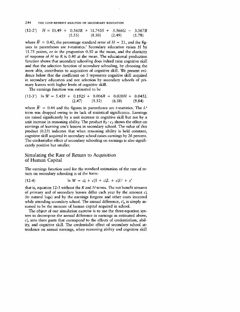
244 THE COST-BENEFIT ANALYSIS OF SECONDARY EDUCATION
(12-2') H = 15.49 + 0.560R + 11.745S + 3.366G - 3.567B(5.55) (8.50) (2.49) (1.78)
where R2 = 0.42, the percentage standard error of H = 21, and the fig-ures in parentheses are t-statistics.2 Secondary education raises H by11.75 points, or in the proportion 0.30 at the mean, and the elasticityof response of H to R is 0.40 at the mean. The educational productionfunction shows that secondary schooling does indeed raise cognitive skilland that the selection function of secondary schooling, by choosing themore able, contributes to acquisition of cognitive skill. We present evi-dence below that the coefficient on S represents cognitive skill acquiredin secondary education and not selection by secondary schools of pri-mary leavers with higher levels of cognitive skill.
The earnings function was estimated to be
(12-3') In W = 5.459 + 0.192S + 0.006R + 0.020H + 0.045L(2.47) (1.32) (6.18) (9.84)
where R2= 0.44 and the figures in parentheses are t-statistics. The L2
term was dropped owing to its lack of statistical significance. Earningsare raised significantly by a unit increase in cognitive skill but not by aunit increase in reasoning ability. The product b2 - C3 shows the effect onearnings of learning one's lessons in secondary school. The value of thisproduct (0.23) indicates that when reasoning ability is held constant,cognitive skill acquired in secondary school raises earnings by 26 percent.The credentialist effect of secondary schooling on earnings is also signifi-cantly positive but smaller.
Simulating the Rate of Return to Acquisitionof Human Capital
The earnings function used for the standard estimation of the rate of re-turn on secondary schooling is of the form:
(12-4) In W = co + cjS + c4 + csL 2 + z'
that is, equation 12-3 without the R and H terms. The net benefit streamsof primary and of secondary leavers differ each year by the amount c'(in natural logs) and by the earnings forgone and other costs incurredwhile attending secondary school. The annual difference, cj, is simply as-sumed to be the measure of human capital acquired in school.
The object of our simulation exercise is to use the three-equation sys-tem to decompose the annual difference in earnings as estimated above,cj, into three parts that correspond to the effects of credentialism, abil-ity, and cognitive skill. The credentialist effect of secondary school at-tendance on annual earnings, when reasoning ability and cognitive skill
The Returns to Cognitive Skill Acquired in School 245
are held constant, is given by cl. Because those who attend secondaryschool are more able, their annual earnings are higher by the amount c2(Rs - R.). The contribution to annual earnings of cognitive skill ac-quired in school has two components, corresponding to the selectionfunction and the educational function of secondary schooling: c3 [Ab(Rk- Rp) + b2 ]. The sum of all three effects is given by the expression:
c1 + c2 (R, - Rp) + c3[bi(R, - Rp) + b2]
This term should correspond to c' in the standard method of estimatingbenefits, based on equation 12-4.
Table 12-1 shows estimates, from the standard equation and from therecursive system, of the percentage addition to annual earnings that isattributable to secondary schooling. When the recursive system is used,the increase in earnings attributable to all the separate effects combinedis 66 percent, close to the prediction from the standard equation. Thisis also true if the standard equation, with S deleted, is estimated sepa-rately for primary and secondary leavers, which is equivalent to insertinginteraction terms between S and the experience terms in equation 12-4.Ability accounts for very little of this total, credentialism for a third, andcognitive skill for no less than half. A combination of cognitive skill andcredentialism accounts for almost all of the increase.
Table 12-1 also presents estimates of the social rate of return derivedby following the standard methodology in every respect except the de-composition of benefits. On the standard definition of the benefit stream,the return is 13 percent. When the recursive system is used and all theeffects are combined, it is 15 percent. The pattern of rates of return doesnot correspond to the pattern of increases in earnings, however, becauserates of return have a different lower bound. Owing to the initial costs,a zero gross benefit involves an infinitely negative rate of return, and asmall addition to earnings, such as that contributed by ability, involvesa large negative rate. For similar reasons the rate of return attributableto credentialism is a mere 1 percent. Only cognitive skill produces a sub-stantial positive return, 7 percent.
It would seem, therefore, that the return to secondary educationthrough acquisition of cognitive skill is quite high but is little more thanhalf that estimated according to the standard methodology. The com-bined effects of cognitive skill and credentialism, however, produce a re-turn of no less than 14 percent. Much therefore depends on the inter-pretation placed on the coefficient of secondary school attendance inequation 12-1. We have so far assumed that it represents credentialism,but secondary school attendance could plausibly be acting as a proxy foracquisition of noncognitive human capital in secondary school. In thatcase our credentialism effect would, in whole or in part, represent humancapital formation. Our estimated return from cognitive skill provides a
246 THE COST-BENEFIT ANALYSIS OF SECONDARY EDUCATION
lower bound on the return on human capital acquired in secondaryschool, that is, on the social rate of return.
Conclusions
The purpose of this chapter has not been to unveil the "true" rate of re-turn to expenditure on secondary education in Kenya. Instead, the inten-tion has been to make a methodological contribution by taking quantita-tive account of a well-known but little-heeded criticism of standard rateof return estimates. We regard the results as illustrative rather than asproviding an operational criterion.
Our labor market survey permits us to estimate the rate of return oncognitive skill acquired in secondary school within the framework of ourrecursive model, which consists of an educational attainment function,an educational production function, and an expanded earnings function.It is possible, therefore, to address the issue of how to interpret the coeffi-cient on the schooling variable in the standard earnings function ratherthan to beg the question in the usual way.
Four years of secondary schooling in Kenya, through their effect oncognitive skill, raise earnings throughout the working life by 33 percent.But the costs of secondary schooling depress the return on these benefitsto 7 percent. The direct effect of schooling on earnings and the indirecteffect through cognitive skill together account for the entire rate of returnestimated by the standard method. Since the direct effect of schoolingmight represent either credentialism or elements of human capital notcaptured by our measure, we conclude that the social rate of return maybe as high as that obtained from the standard method but could be sub-stantially lower.
If the issue with which we have been concerned here were the only crit-icism of rate of return analysis, our findings would tend to vindicate theuse of the standard methodology in Kenya. Although isolating the influ-ence of cognitive skill reduces the rate of return, that rate remains positiveand large.
Notes1. There is evidence to refute the alternative interpretation-that secondary ed-
ucation enhances reasoning ability. In Tanzania the mean value of H in theweighted sample was much lower and the difference was statistically significant,reflecting the lower proportion of Tanzanians with secondary education, whereasthe mean value of R was similar and the difference was not at all significant.
2. A log-linear specification with the continuous variables H and R in naturallogarithms was also estimated but was inferior in that the percentage standarderror of H was higher (29 percent) and the significance of some coefficients waslower.
CHAPTER 13
Public Sector Pay andEmployment Policy and theRate of Return to Education
IN THE COST-BENEFIT ANALYSIS of educational projects the presumptionis that the wage structure is the product of the unfettered market interac-tion of sellers and profit-maximizing buyers of labor services and there-fore accurately reflects the difference in productivity between more edu-cated and less educated workers. It is well-known, however, thatnonmarket forces influence wages. For example, in the United States,other things being equal, wages are higher in union than in nonunionestablishments (see Freeman and Medoff 1981, and Lewis 1963), andthere is also evidence that the educational structure of wages is morecompressed in the former, creating a difference in the returns to educa-tion (see Freeman and Medoff 1981, and Shapiro 1978). Union behaviorcan thus influence and perhaps bias conventional measures of rates ofreturn.
Wages in the public sector are set through complex administrative pro-cedures. Government pay policy can therefore segment the labor marketand influence the returns to education. This is less likely to occur where,as is often the case in high-income countries, governments adhere to theprevailing wage model of public sector pay determination, under whichthe public sector adopts the level and structure of wages in the privatesector. Government pay policy is more likely to produce labor marketsegmentation in low-income countries. First, the public sector tends tobe large; it often accounts for more than half of the wage earners in suchcountries. The importance of the public sector and, in some cases, its abil-ity to restrict the intersectoral mobility of labor reduce the need for thegovernment to act as a price taker in a competitive labor market. Second,in addition to the goal of allocative efficiency, governments in low-income countries have fiscal, employment, distributional, and politicalgoals and often use public sector pay and employment policy to try toachieve them.
247
248 THE COST-BENEFIT ANALYSIS OF SECONDARY EDUCATION
Does public sector pay policy bias conventional estimates of socialrates of return to investment in education? In practice, economists havetended to ignore this issue, even for countries in which governmentadopts an active pay policy. And when the issue has been addressed (seePsacharopoulos 1981, p. 332),' the suggested resolution-that data forthe private sector be used-may also prove unsatisfactory because it ig-nores interactions. It has long been recognized that changes in wages(and therefore in labor supply and demand) in union establishments in-fluence labor supply and demand (and therefore wages) in nonunion es-tablishments (Freeman and Medoff 1982). Similarly, the direct effects ofgovernment pay policy in the public sector are likely to have indirect ef-fects on wages in the private sector. Indeed, the indirect effects may provemore difficult to analyze in this case because of the control of labor mo-bility that governments sometimes exercise.
Public sector employment decisions introduce a further complicationinto the calculation of social rates of return. When a union alters wages,private employers adjust the level of employment so that, given the newlevel and structure of wages, profits are maximized. Although wages dif-fer between sectors, the equality of wages and marginal product is main-tained. When the government alters public sector wages, the effect on em-ployment is difficult to determine because the government does notnecessarily act as a profit maximizer. The effect that government inter-vention in the labor market has on rates of return depends not only onthe government's wage policy but also on its employment policy becausethe latter governs the relationship between wages and marginal produc-tivity in the public sector.
Kenya and Tanzania differ markedly in their public sector pay policies.Whereas the Kenyan government has adopted the prevailing wage model,the Tanzanian government has used its control over pay in the public sec-tor to equalize the distribution of wages. Government employment poli-cies also differ, as suggested by the higher share of wage employment inthe public sector in Tanzania (61 percent) than in Kenya (39 percent).We do not attempt to make definitive estimates of the rates of return forthese countries. Our more limited aim is to examine the sensitivity of con-ventional estimates to alternative models of government pay and employ-ment policy and of government control of labor mobility. We find consid-erable sensitivity, particularly in Tanzania. In the cost-benefit analysis ofeducational investment more attention must be paid to labor market poli-cies for the public sector.
Conventional Estimates of the Rate of Return
As we have noted, the supply of secondary completers in relation to thesupply of primary completers is much greater in Kenya than in Tanzania.
Public Sector Pay and Employment Policy and the Return to Education 249
In Kenya the ratio of the stock of primary completers in wage employ-ment to that of secondary completers is 1.17 to 1; in Tanzania it is 0.69to 1. The occupational structure of employment is similar in the twocountries; this and other evidence indicate that their relative demandfunctions for the two educational categories are similar (see chapter 7).Given the same relative demand functions, a competitive labor marketmodel predicts a larger wage premium on secondary education, andtherefore higher gross returns to secondary education, in the countrywith the smaller relative supply. If we assume a similar cost structure inthe two countries, we would therefore expect the rate of return to second-ary education to be higher in Tanzania than in Kenya.
This prediction, however, ignores the impact of government pay andemployment policies, which differ greatly in the two countries. After theArusha Declaration of 1967, which set Tanzania on a socialist path, thegovernment adopted a policy of compressing the wage structure in the in-terest of greater equality. Although the policy applies throughout thewage sector (and beyond), it has far more leverage in government serviceand in parastatal (nationalized and partly nationalized) bodies than inprivate firms. Pay scales in both the government and the parastatal sec-tors are administratively determined. An organ of government lays downuniform occupational pay scales for all parastatal bodies on the basis ofgovernment pay scales. Government accounts for 24 percent of employ-ees in the Tanzanian sample, and the parastatals account for 38 percent.The public sector is thus large enough to pursue an independent pay pol-icy for many occupations without fear of losing workers to the privatesector. We hypothesized, therefore, that pay in the public sector is lowerat the higher levels and lessAispersed than in the private sector and thatthe depressing effect of the pay policy on wages is more marked at thesecondary than at the primary level. This hypothesis was confirmed inchapter 7. Because of the size of the public sector in Tanzania and theegalitarian pay policy of the government, the observed structure of wagesdiffers considerably from the wages that would prevail in a competitivelabor market.
In chapter 12 the earnings streams were derived from an aggregatefunction for the subsample of primary and secondary completers that in-cluded a dummy variable for secondary education. Here we use the fullsample and obtain the earnings streams from separate functions for pri-mary and secondary completers. The following is an example.
(13-1) InW = a + bL + cL2 + Idjxx + u
These cross-sectional earnings functions are used to simulate two timeseries, WWp and Ws, that represent the predicted wages, over their expectedworking lives, of primary and secondary completers. The difference be-tween the educational groups in predicted lifetime earnings is interpreted
250 THE COST-BENEFIT ANALYSIS OF SECONDARY EDUCATION
as a measure of the difference in productivity between the two groupsthat is attributable to cognitive skill or other marketable traits acquiredin secondary education. The difference in earnings is used as the estimateof the social benefits of secondary education. In this chapter we ab-stracted from the issue that we discussed in chapter 12-the extent towhich the social benefits of secondary education are reduced because em-ployers use educational attainment to screen for natural ability or paya premium for educational credentials irrespective of the impact ofschooling on labor productivity.
Equation 13-1 is the basis for our analysis. The inclusion of the X,terms, which we discuss further below, does not alter the two predictedearnings streams, nor, therefore, the rate of return, provided that the coef-ficients d are multiplied by the mean values Xl for each educationalsubsample. The implication is that differences in Xi between primary andsecondary completers are attributable to secondary education. An advan-tage of including Xj is that when it is set equal to the mean value forprimary and secondary completers combined, the part of the benefitstream that arises from subsample differences in such characteristics asrace that are not attributable to secondary education can be eliminated.Among the Xi variables is Jk, a set of ownership category dummies, whichcaptures the effect of government pay policy in the public sector. Othercharacteristics included in the Xj vector are race, sex, formal training,employment status (casual or regular), and occupation.2 In the next sec-tion we use the Jk variables to estimate separate earnings streams, andtherefore rates of return, for workers in the public and private sectors.
We estimated equation 13-1 for primary (standard 7) completers andfor secondary (form 4) completers in both Kenya and Tanzania. As is gen-erally the case, the predicted earnings of secondary completers at comple-tion of schooling or soon thereafter exceed those of primary completers,and they rise more steeply with employment experience. The gross re-turns are similar in Kenya and Tanzania, and so are costs. Under the con-ventional method of estimation the aggregate net rate of return is 13 per-cent in both Kenya and Tanzania.3 These results are not consistent withour expectation that returns are higher in Tanzania, where secondarycompleters are in scarcer supply. The explanation may lie in the differ-ences between the two countries in public sector pay and employmentpolicies and in the convention of ignoring those differences.
A potential weakness of these establishment-based surveys for cost-benefit analysis is that the sample excludes educated workers who arenot in urban wage employment (see Psacharopoulos 1973). Like manyrate of return studies that focus exclusively on urban wage employment,our estimate of the rate of return to secondary schooling may be subjectto bias owing to differential labor market selectivity of primary and sec-
Public Sector Pay and Employment Policy and the Return to Education 251
ondary completers. Our comparison of rates of return in the public andprivate sectors, however, is less likely to be subject to this source of bias.
The Sensitivity of the Rate of Return to AlternativeModels of Pay and Employment Policy
The Competitive Labor Market Model
Figure 13-1 depicts the model of public sector pay and employment pol-icy that underlies the method of estimating the rate of return to second-ary education employed above. For heuristic purposes the model focuseson the absolute levels of productivity, wage, and employment of sec-ondary completers rather than on their levels in relation to primarycompleters.4 Assume a fixed supply of secondary completers (S), shownas the length of the horizontal axis. On the vertical axis is the wage (W)of secondary completers. The demand curve for the public sector (Dg)is measured to the right of the left-hand vertical axis, and that for theprivate sector (D.) is measured to the left of the right-hand vertical axis.Both Dg and D. are assumed to be downward sloping. If the labor mar-ket is perfectly competitive, then in equilibrium the wage equals the socialmarginal product of labor and no reallocation of secondary completersbetween sectors can increase output. Moreover, any intersectoral wagedifferential will be eroded through labor mobility. The competitive mar-ket wage (where Dp + Dg = S) is shown as W,. The issue is whetherthis model best describes intersectoral wage relations in East Africa.
Wage Reduction Models
In figure 13-2 the government, motivated by fiscal or egalitarian con-siderations, intervenes and lowers the wage in the public sector from Wcto Wg. The pay and employment outcomes of this pay policy depend onthe degree of government control over intersectoral mobility and on gov-ernment employment policy. In panel A we assume that the governmenthas complete control over the intersectoral allocation of labor and, in de-termining the level of public sector employment, behaves as a profit maxi-mizer. The government can choose how many workers to employ irre-spective of the wage it pays them. Given Wg, it chooses Dg. The supplyof labor to the private sector is thereby reduced, and the private sectorwage (W.) is raised above W,. Secondary completers in the private sectorare paid substantially more than those in the public sector.
In panel B the government also has complete control over the in-tersectoral allocation of labor. In this case, however, social efficiency
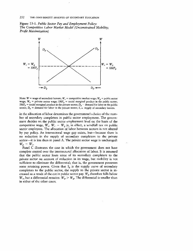
252 THE COST-BENEFIT ANALYSIS OF SECONDARY EDUCATION
Figure 13-1. Public Sector Pay and Employment Policy:The Competitive Labor Market Model (Unconstrained Mobility;Profit Maximization)
w w
Dg D
Wc = Wg W = Wp= SMPg = SMPp
__0Dg DP
Note: W = wage of secondary leavers; W, = competitive market wage; Wg = public sectorwage; Wp = private sector wage; SMP, = social marginal product in the public sector;SMPp = social marginal product in the private sector; Dg = demand for labor in the publicsector; DP = demand for labor in the private sector; S, = supply of secondary leavers.
in the allocation of labor determines the government's choice of the num-ber of secondary completers in public sector employment. The govern-ment decides on the public sector employment level on the basis of thecompetitive wage, WC. W, - Wg is, in effect, a windfall tax on publicsector employees. The allocation of labor between sectors is not alteredby pay policy. An intersectoral wage gap exists, but-because there isno reduction in the supply of secondary completers to the privatesector-it is less than in panel A. The private sector wage is unchanged:Wp = Wc.
Panel C illustrates the case in which the government does not havecomplete control over the intersectoral allocation of labor. It is assumedthat the public sector loses some of its secondary completers to theprivate sector on account of reduction in its wage, but mobility is notsufficient to eliminate the differential; that is, the government possessessome retaining power. Given that Sg is the supply curve of secondarycompleters to the public sector, the supply to the private sector is in-creased as a result of the cut in public sector pay. W. therefore falls belowWC, but a differential remains: Wp > Wg. The differential is smaller thanin either of the other cases.
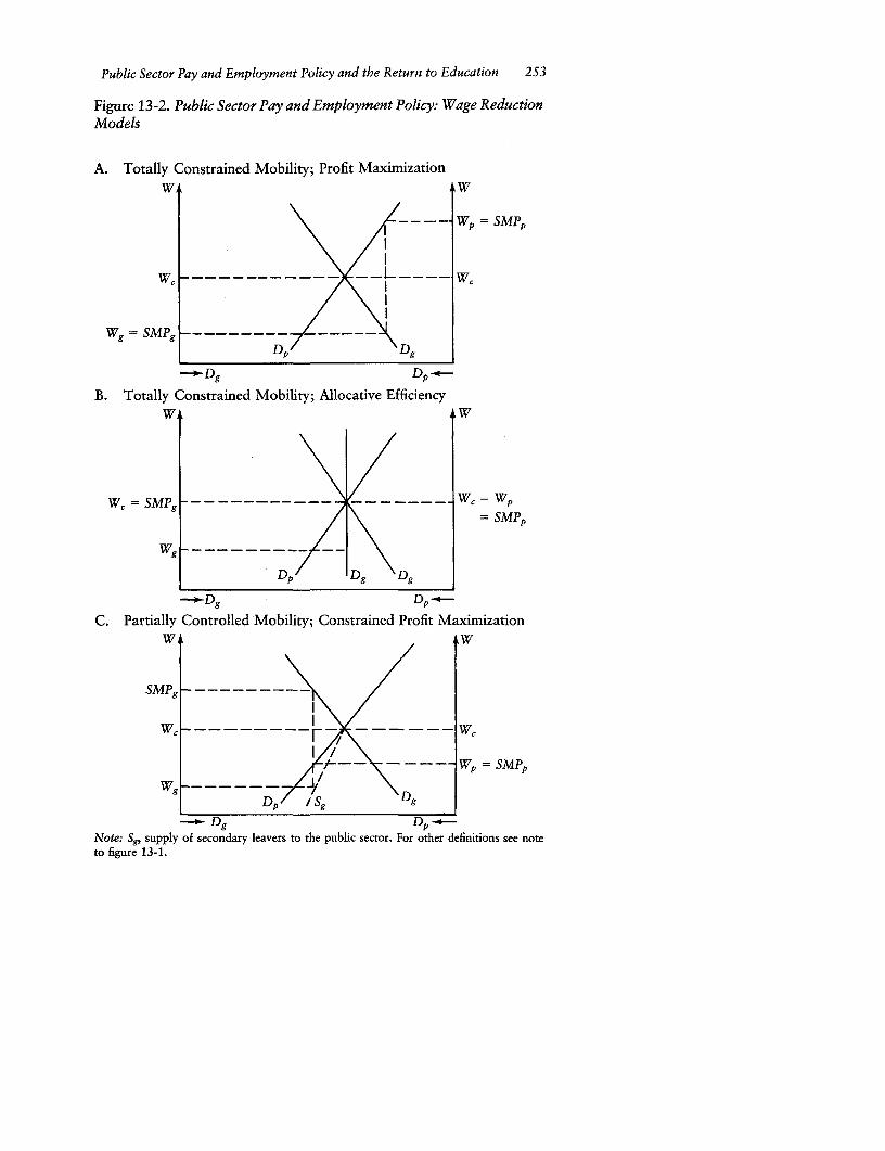
Public Sector Pay and Employment Policy and the Return to Education 253
Figure 13-2. Public Sector Pay and Employment Policy: Wage ReductionModels
A. Totally Constrained Mobility; Profit Maximizationw w
WP= SMPp
WC ______ WC
Wg = SMPg - … - -D. ~~~Dg
Dg Dp
B. Totally Constrained Mobility; Allocative Efficiencyw w
WC = SMPg…-- -…--__W, = P= smpp
Wg -
Dp Dg Dg
C. Partially Controlled Mobility; Constrained Profit Maximization
SMPg ________ S
wc /-----r------ wc
W9 ~ ~ IWg-Dp…i/;S; PDg
~ DgNote: Sg, supply of secondary leavers to the public sector. For other definitions see noteto figure 13-1.
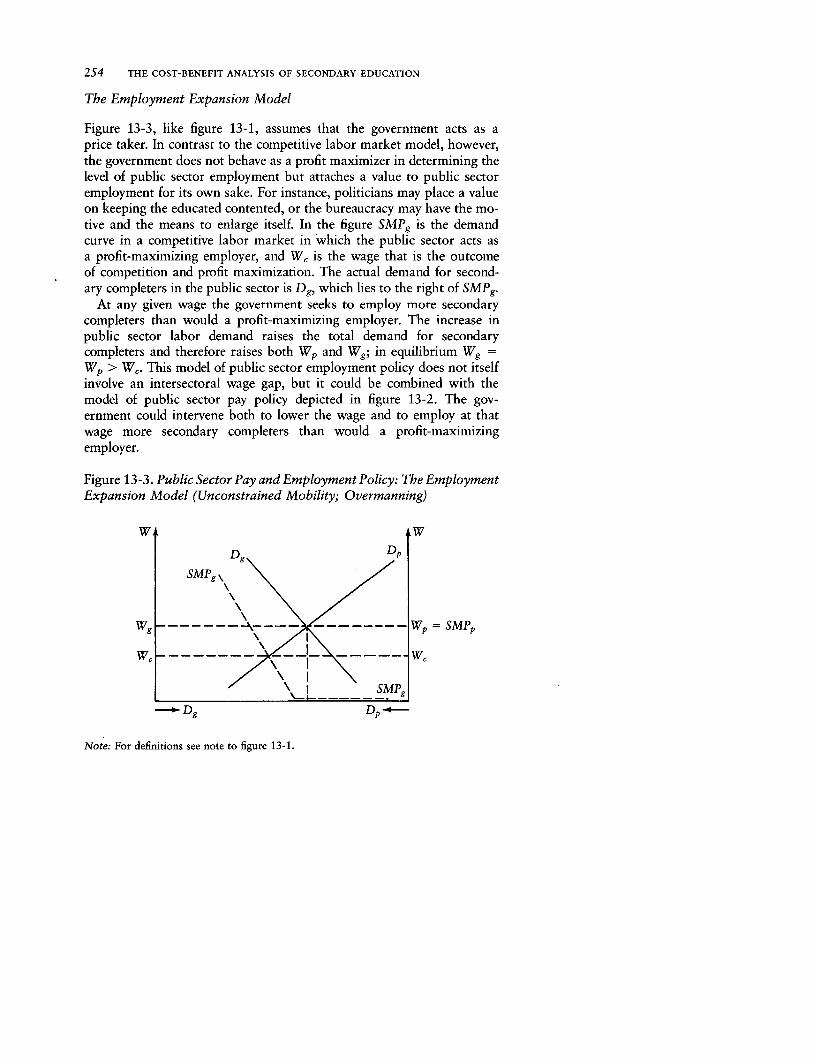
254 THE COST-BENEFIT ANALYSIS OF SECONDARY EDUCATION
The Employment Expansion Model
Figure 13-3, like figure 13-1, assumes that the government acts as aprice taker. In contrast to the competitive labor market model, however,the government does not behave as a profit maximizer in determining thelevel of public sector employment but attaches a value to public sectoremployment for its own sake. For instance, politicians may place a valueon keeping the educated contented, or the bureaucracy may have the mo-tive and the means to enlarge itself. In the figure SMPg is the demandcurve in a competitive labor market in which the public sector acts asa profit-maximizing employer, and W, is the wage that is the outcomeof competition and profit maximization. The actual demand for second-ary completers in the public sector is Dg, which lies to the right of SMPg.
At any given wage the government seeks to employ more secondarycompleters than would a profit-maximizing employer. The increase inpublic sector labor demand raises the total demand for secondarycompleters and therefore raises both Wp and Wg; in equilibrium Wg =Wp > W1. This model of public sector employment policy does not itselfinvolve an intersectoral wage gap, but it could be combined with themodel of public sector pay policy depicted in figure 13-2. The gov-ernment could intervene both to lower the wage and to employ at thatwage more secondary completers than would a profit-maximizingemployer.
Figure 13-3. Public Sector Pay and Employment Policy: The EmploymentExpansion Model (Unconstrained Mobility; Overmanning)
w w
SMPg \ \/
W.g ------ ___- …pW = MPp
-Dg Dp
Note: For definitions see note to figure 13-1.
Public Sector Pay and Employment Policy and the Return to Education 255
Rates of Return in the Public and Private Sectors
We examine whether public sector pay policy has segmented the labormarket in Kenya and Tanzania. Are the (standardized) wages of primaryand secondary completers significantly different in the two sectors? Dothe observed differences in wages lead to intersectoral differences in therate of return to secondary education? Are the observed differences inwages a consequence of labor market segmentation, or do they comeabout simply because one sector is more selective than the other aboutthe human capital endowments of its employees?
Table 13-1 presents the regressions based on equation 13-1 that areused to predict the wage streams of primary and secondary completers.Our interest here is in the dummy variables Uk) that indicate the owner-ship category (sector) of the firm by which the individual is employed.JI represents the private sector, J2 the government sector, and J3 theparastatal sector in Tanzania and the state corporation sector in Kenya.Together J2 and J3 make up the public sector. The coefficients on thesevariables indicate whether workers who in other respects have the samecharacteristics receive higher or lower wages simply because they are em-ployed in the public or in the private sector.5
In the primary completer equation for Kenya the Jk dummies are smalland are not statistically significant-that is, sector of employment has noindependent influence on the wages of primary completers. In the sec-ondary completer equation the coefficient on J3 is not significant, but thecoefficient on J2 is significant and negative; that is, other things beingequal, a secondary completer in government employment is paid less thanin the private sector. The set of four coefficients suggests that in Kenyapublic sector pay policy has a mildly compressive effect on the wage pre-mium earned by secondary completers.
In Tanzania all four coefficients on Jk are statistically significant. Atthe primary level the J2 and J3 coefficients are similar in value but of op-posite sign, suggesting that on balance employment in the public sectorhas no independent influence on earnings. At the secondary level the J2
and J3 coefficients are large and negative-that is, other things beingequal, a secondary completer earns substantially less in the public thanin the private sector. The set of four coefficients suggests that in Tanzaniapublic sector pay policy has had a substantial compressive effect on thewage premium earned by secondary completers.
We predict sector-specific earnings streams for primary and secondarycompleters as a basis for estimating separate rates of return to secondaryeducation in the public and private sectors. For secondary completers thepredicted earnings streams are given by:
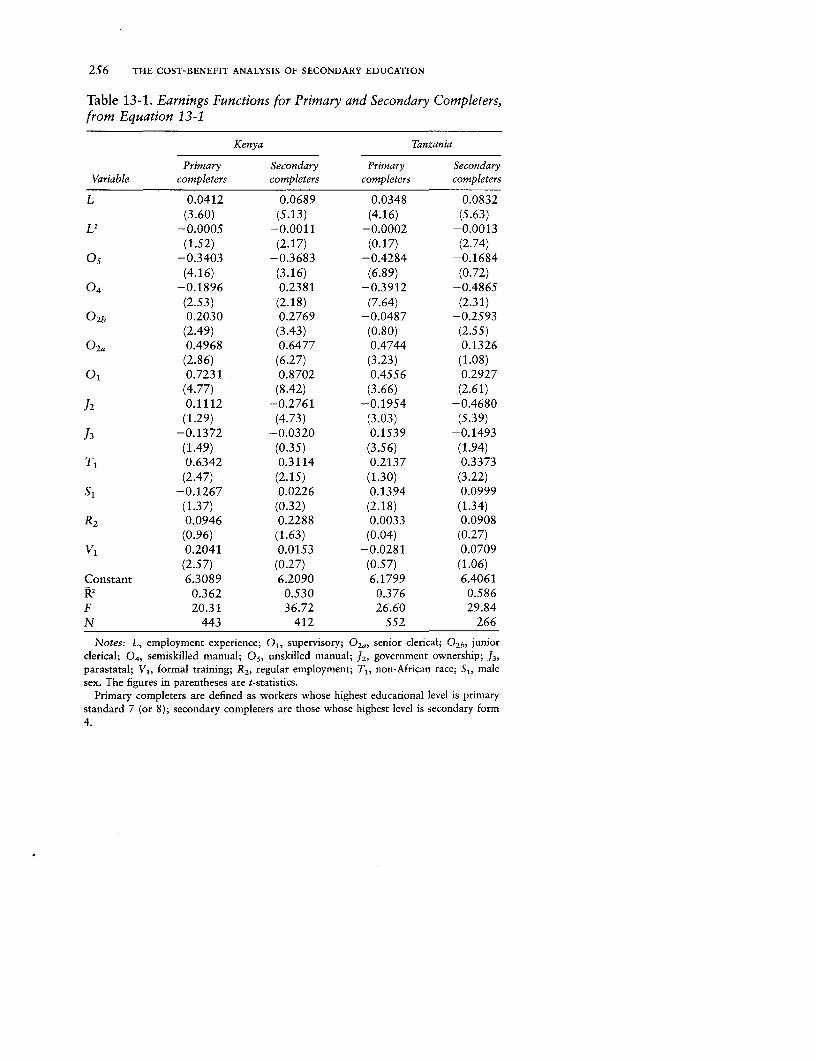
256 THE COST-BENEFIT ANALYSIS OF SECONDARY EDUCATION
Table 13-1. Earnings Functions for Primary and Secondary Completers,from Equation 13-1
Kenya Tanzania
Primary Secondary Primary SecondaryVariable completers completers completers completers
L 0.0412 0.0689 0.0348 0.0832(3.60) (5.13) (4.16) (S.63)
L2 -0.0005 -0.0011 -0.0002 -0.0013(1.52) (2.17) (0.17) (2.74)
05 -0.3403 -0.3683 -0.4284 -0.1684(4.16) (3.16) (6.89) (0.72)
04 -0.1896 0.2381 -0.3912 -0.486s(2.S3) (2.18) (7.64) (2.31)
02b 0.2030 0.2769 -0.0487 -0.2s93
(2.49) (3.43) (0.80) (2.55)02a 0.4968 0.6477 0.4744 0.1326
(2.86) (6.27) (3.23) (1.08)°0 0.7231 0.8702 0.4556 0.2927
(4.77) (8.42) (3.66) (2.61)J2 0.1112 -0.2761 -0.1954 -0.4680
(1.29) (4.73) (3.03) (5.39)
13 -0.1372 -0.0320 0.1539 -0.1493(1.49) (0.35) (3.56) (1.94)
T, 0.6342 0.3114 0.2137 0.3373(2.47) (2.15) (1.30) (3.22)
S, -0.1267 0.0226 0.1394 0.0999(1.37) (0.32) (2.18) (1.34)
R2 0.0946 0.2288 0.0033 0.0908(0.96) (1.63) (0.04) (0.27)
V1 0.2041 0.0153 -0.0281 0.0709(2.57) (0.27) (0.57) (1.06)
Constant 6.3089 6.2090 6.1799 6.4061K2 0.362 0.530 0.376 0.586F 20.31 36.72 26.60 29.84N 443 412 552 266
Notes: L, employment experience; 01, supervisory; 02a, senior clerical; 02b, junior
clerical; 04, semiskilled manual; 0 s, unskilled manual; J2, government ownership; J3,
parastatal; VI, formal training; R2 , regular employment; TI, non-African race; S,, malesex. The figures in parentheses are t-statistics.
Primary completers are defined as workers whose highest educational level is primarystandard 7 (or 8); secondary completers are those whose highest level is secondary form4.
Public Sector Pay and Employment Policy and the Return to Education 257
(13-2) lInW = a + bL + cL2 + I d1X1 + Welt
When earnings for secondary completers in the public sector are beingpredicted, J2 and J3 are set equal to one; when earnings for those in theprivate sector are being predicted, J2 and J3 are set equal to zero. A simi-lar procedure is followed for primary completers.'
In Kenya we estimate the rate of return in the private sector to be 15percent, about 2 percent higher than the rate of return as conventionallymeasured. In keeping with the moderately compressive effect of publicsector pay policy on the educational structure of wages, the rate of returnin the public sector is estimated at 10 percent, about 3 percent lower thanthe aggregate. In Tanzania, as expected, public sector pay policy givesrise to a much larger intersectoral difference in the rate of return to second-ary education. The rate of return is estimated to be 20 percent in theprivate sector and only 9 percent in the public sector.
Our presumption has been that the sectoral differences in rates of re-turn are a result of the segmentation of the labor market-that is, someworkers are paid more than others with the same human capital endow-ments simply because of their sector of employment. There is, however,an alternative explanation. We have documented elsewhere the high vari-ance in cognitive skill among workers with the same number of years ofschooling and have demonstrated that this variance is reflected in thewages paid to secondary completers; see chapter 3. It is also the case thatthe higher wages of government school completers compared with thoseof harambee school completers in Kenya can be entirely explained by thehigher average cognitive skill level of the former; see chapter 15. It is rea-sonable to hypothesize, therefore, that the higher wages paid to second-ary completers in the private sector are attributable to the "creaming"by private sector employers of the most skilled secondary completers.7
To test this hypothesis we estimate the following simple sectoral alloca-tion function for secondary completers:
(13-3) Prob( 4 = 1) = (1(X'fB)
where J4 is a dichotomous variable that takes the value 1 if the individ-ual is employed in the public sector; the vector of exogenous variablesincludes L, our measure of employment experience, which in this caseserves as a proxy for cohort of entry into the labor market; T1 is a dummyvariable indicating that the individual is non-African; and Dj is a set ofdummy variables indicating performance on the form 4 examination.The examination scores are taken to measure differences in cognitive skillamong secondary completers.
Table 13-2 presents estimates of the sectoral allocation functions andthe predicted probabilities of being in the public sector for workers withdifferent examination scores and employment experience. The coefficient

Table 13-2. Probit Sectoral Allocation Functions and Predicted Probabilities of Employment in the Public Sector forSecondary Completers
Predicted probability of publicsector employment, by length of
Probit sectoral experience and division of passallocation function Kenya Tanzania
Variable Kenya Tanzania Variable 1 year 10 years 1 year 10 years
Di -0.585 -0.783 D, 0.11 0.23 0.76 0.80(1.39) (1.10) D2 0.32 0.50 0.82 0.85
D2 0.126 -0.577 D3 0.31 0.49 0.72 0.7S(0.50) (1.11) D4 0.21 0.37 0.72 0.76
s D3 0.162 -0.918 Ds 0.27 0.44 0.93 0.9500 (0.70) (1.82)
D4 -0.194 -0.905(0.79) (1.71)
L 0.053 0.012(3.86) (0.69)
T, -1.318 -2.069(2.30) (5.58)
Constant -0.677 1.488N 409 226Scaled
deviance 511.7 220.4
Notes: DI, division 1; D2, division 2; D3, division 3; D4, division 4; D5, failed or did not sit the examination; L, employment experience; T1, non-Africanrace. Figures in parentheses are t-statistics. The probability that Y = 1 is the area under the standard normal curve between -- and X',B. Probabilities arepredicted for African secondary (form 4) completers.
Public Sector Pay and Employment Policy and the Return to Education 259
on the race variable is negative and significant in both countries, whichindicates that, other things being equal, non-Africans have a higher prob-ability than Africans of being employed in the private sector. In Kenyathe coefficient on the experience variable is positive and significant,which indicates that the probability that a secondary completer will workin the private sector has increased over time; in Tanzania the coefficientis also positive but is not significant.8
Our principal concern is with the Di variables. The table of predictedprobabilities indicates that, consistent with our alternative hypothesis, inKenya workers with the highest examination score (division 1, D1 ) havethe highest probability of working in the private sector. The coefficienton D1 is not significant, however, and for those with the next highestscores (divisions 2 and 3) the probability of being in the private sectoris lower than the probability for those with the lowest scores. We there-fore reject the hypothesis that in Kenya the intersectoral wage differentialamong secondary completers is attributable to the greater selectivity ofthe private sector. The hypothesis is also rejected for Tanzania; there isno consistent relationship between examination performance and theprobability of private sector employment, and only one of the four coeffi-cients on the examination scores is statistically significant. The probabil-ity of being in the private sector is significantly higher for a form 4 leaverin division 3 than for one who failed or did not sit the examinations.A form 4 leaver, however, has a lower probability (although not signifi-cantly so) of being in the private sector if he is in division 1 than if heis in division 3. At least in Tanzania it appears that the gap in the rateof return to secondary education between the public and private sectorsis indeed the result of the segmentation of the urban wage labor marketby government pay policy.9
The Sensitivity of the Rate of Return
Consider the implications for the social marginal product of secondarycompleters, and therefore for the social rate of return to secondary educa-tion, of the alternative models of public sector pay and employmentpolicy (table 13-3). Recall that in the competitive labor market modelW = SMP in both the private and public sectors and the intersectoralallocation of labor is efficient; that is, SMPg = SMPp. If the competitivemodel applies, the conventional method of estimating the social rate ofreturn is appropriate. The application of the conventional method to ourwage-segmented samples yields 13 percent in both countries (row 1).
In the wage reduction model depicted in figure 13-2, panel A, the gov-ernment has complete control over the intersectoral allocation of laborand behaves as a profit maximizer. Therefore the government employseducated labor up to the point at which its perceived social marginal
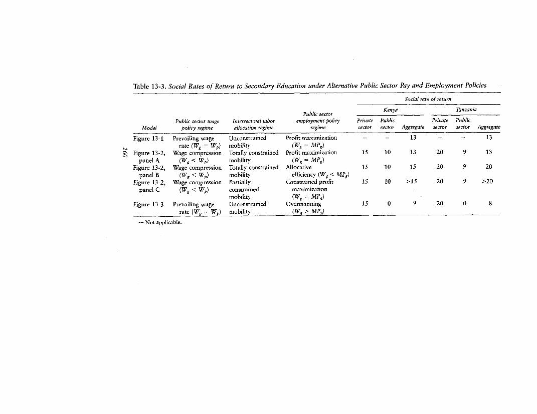
Table 13-3. Social Rates of Return to Secondary Education under Alternative Public Sector Pay and Employment Policies
Social rate of return
Public sector Kenya TanzaniaPublic sector wage Intersectoral labor employment policy Private Public Private Public
Model policy regime allocation regime regime sector sector Aggregate sector sector Aggregate
Figure 13-1 Prevailing wage Unconstrained Profit maximization - - 13 - - 13rate (Wg = Wp) mobility (Wg = MPg)
O Figure 13-2, Wage compression Totally constrained Profit maximization 15 10 13 20 9 13panel A (Wg < Wp) mobility (Wg - MPg)
Figure 13-2, Wage compression Totally constrained Allocative 15 10 15 20 9 20panel B (Wg < Wp) mobility efficiency (Wg < MPg)
Figure 13-2, Wage compression Partially Constrained profit 15 10 >15 20 9 >20panel C (Wg < WI) constrained maximization
mobility (Wg= MPg)Figure 13-3 Prevailing wage Unconstrained Overmanning 15 0 9 20 0 8
rate (Wg = Wp) mobility (W > MPg)-Not applicable.
Public Sector Pay and Employment Policy and the Return to Education 261
product equals the public sector wage (SMPg Wg). Profit maximizationalso ensures that Wp = SMPp. Thus,
Wp SMPp > WC > Wg = SMPg
In this case the social marginal product of educated labor is a weightedaverage of SMPp and SMPg. Similarly, the estimate for the aggregate so-cial rate of return is the weighted average of the rate of return in the twosectors. This rate of return is, by choice of sectoral weights, the same forthis model as for the competitive model-13 percent in both countries(row 2). Two assumptions are being made here, however: that additionalsecondary completers will be employed in the two sectors in the sameproportions as those currently employed and that the price elasticity ofthe demand for labor is the same in the two sectors. If the elasticity isgreater in the private sector, the hypothesized intervention by the govern-ment lowers the weighted average social rate of return below the rate thatwould prevail in a fully competitive market, and the reverse is true if theelasticity is greater in the public sector. Since the public sector weightfor additional secondary completers can vary between 0 and 1, theweighted average social rate of return on secondary expansion isbounded by the rates of return for the private and public sectors.
In the windfall tax case, depicted in panel B, the government is as-sumed to allocate labor optimally between the two sectors:
WC = Wp = SMPp = SMPg > Wg
The social marginal product of educated labor in the government sec-tor exceeds the wage paid by the government. The wage prevailing inthe private sector is therefore the measure of the social marginal productof educated labor. Similarly, the rate of return in the private sector indi-cates the aggregate rate of return to secondary education. This model ofpublic sector pay and employment policy resolves the anomaly in ourcomparison of rates of return in Kenya and Tanzania. If this model ap-plies, the aggregate rate of return is 20 percent in Tanzania and 15 per-cent in Kenya, where secondary completers are in relatively greater sup-ply (row 3).10
In panel C the social marginal product of educated labor in the publicsector, given by the demand curve SMPg, exceeds the wage in both sec-tors:
SMPg > WC > Wp = SMPp > Wg
The rate of return in the private sector is more appropriate than thatin the wage sector as a whole (as conventionally measured) for estimatingthe aggregate social rate of return, but even the former yields a measurethat is downward biased (row 4). The social marginal product of edu-
262 THE COST-BENEFIT ANALYSIS OF SECONDARY EDUCATION
cated labor is a weighted average of SMPp and the higher, but unob-served, SMPg.
In the final case, illustrated by figure 13-3, the government does notmaximize either public sector profits or social efficiency in the allocationof labor. The government demand curve does not reflect the social mar-ginal product in the public sector; that is, SMPg < Dg. Indeed, SMPg = Oover a range of public sector employment. In these circumstances, evenif the government adopts the prevailing wage rate model of wage deter-mination so that Wp = Wg, it is still true that SMPg < Wc. The aggregaterate of return is the weighted average of the private sector rate of returnand the zero rate depicted in the public sector. If this model applies, theaggregate rate of return, on the basis of the sectoral employment of thosein the sample, would be 8 percent in Tanzania and 9 percent in Kenya.The rate is sensitive to the relative size of the two sectors, being lowerthe larger is the public sector. The rate of return on secondary expansionwould, of course, depend on the sectoral destination of additional sec-ondary completers; it could be zero.
Which of these models apply to Kenya and Tanzania? That the Tan-zanian government's policy of compressing the wage structure in the pub-lic sector has not been thwarted by competitive forces indicates thatthe government has at least partial control over the intersectoral mobilityof labor. This must be a consequence of the dominant position of thepublic sector, which accounts for 71 percent of the employment of second-ary completers; in certain white-collar jobs the government is a virtualmonopsonist. Complete control of intersectoral mobility is implausible,however, and we suspect that figure 13-2, panel C, applies. Moreover,the pressures on the government to expand employment for equityreasons and the incentive structure-for example, cost-plus pricingdirectives-are conducive to overmanning in the public sector, as de-picted in figure 13-3.
Controls on mobility may not be the only reason for the persistenceof the wage gap. The benefits to private employers of reducing wages maynot have been sufficient to outweigh the risks of costs. Since many privateemployers are in the manufacturing sector, where labor costs are a smallproportion of total costs, wage reductions would have a small impact onprofits but might have a large impact on the morale (X-efficiency) ofworkers-a matter of particular concern in politically vulnerable non-African-owned enterprises.
Kenya more closely approximates the competitive labor market model(figure 13-1), but the moderate compression of the educational structureof wages in the public sector suggests that figure 13-2, panel C, may berelevant, and figure 13-3 may also apply to a certain extent. In bothcountries additional knowledge of the workings of the public sector labor

Public Sector Pay and Employment Policy and the Return to Education 263
market would be required to estimate definitive rates of return to second-ary education.
Conclusions
The purpose of this chapter has not been to unveil the "true" rate of re-turn to investment in secondary education in Kenya and Tanzania. In-stead, we have tried to assess whether the usual practice of ignoring pub-lic sector pay and employment policy leads to biased estimates of thesocial rates of return to education. Our conclusion is that the rankingof investment priorities may be seriously distorted by failure to take ac-count of the effects that policy-induced wage differences between thepublic and private sectors and differences between the wage and the mar-ginal productivity of labor in the public sector have on the social mar-ginal product of educated labor.
In both countries the social rate of return to secondary education issensitive to the choice among several alternative models of public sectorpay and employment policy. In Tanzania the range is at least from 8 to20 percent; in Kenya it is at least from 9 to 15 percent. The greater sensi-tivity in Tanzania is attributable to the government's highly compressivepublic sector pay policy, which has segmented the wage labor market,and to the larger size of the public sector. In Kenya pay policy has con-formed more closely to the prevailing wage model of public sector wagedetermination.
The standard method of estimation, by ignoring the issue, makes im-plicit assumptions about the underlying model of pay and employmentpolicy without recognizing or attempting to validate them. Rate of returnanalysis should not be conducted mechanically; rather, it should be basedon a knowledge of the government's objectives and behavior.
Notes
1. The argument is implicit in Psacharopoulos (1983).2. The inclusion of the occupation terms allows us to use equation 13-1 in a
separate analysis to simulate-by changing education-occupation matrices-theimpact of educational expansion on the rate of return; see chapter 14. Note againthat the inclusion of the occupation terms has no influence on the aggregate rateof return estimated in this chapter, a prediction that was empirically verified.
3. Costs include earnings forgone during schooling and job search, direct pri-vate expenses, and government subsidy. Benefits are based on pretax earnings.Only net-of-tax wage data were obtained from employees, but data on pretaxand posttax wages were collected from employers for a subsample as a check.For these quadratic (in one case) and linear (in the other, where the quadratic
264 THE COST-BENEFIT ANALYSIS OF SECONDARY EDUCATION
fit was less good) relations between pretax and posttax income were estimated,and these relations were then used to estimate the pretax wage of each employeein the full sample. The value of a percentage rate of return reported as x lies be-tween x and x + 1.
4. If the market for primary completers is not segmented by sector-that is,if sector of employment has no independent influence on the wages of primarycompleters-then the size of the wage premium paid to secondary completersin the public sector in relation to that in the private sector can be inferred froma comparison of the absolute wages of secondary completers in the two sectors.This assumption corresponds fairly well to the evidence (see below).
5. The equations presented in table 13-1 are simply stratified versions of the"working regression" presented in chapter 7.
6. Recall that for the conventional aggregate rate of return the predictor equa-tion for secondary completers included j2 and J3 for secondary completers, andsimilarly for all primary completers.
7. For a discussion of this type of sorting as an explanation of union-nonuniondifferences in wages, see Freeman and Medoff (1981).
8. The explanation for this difference between countries in the predictivepower of the cohort variable is that Kenya has a larger stock of secondary com-pleters than does Tanzania. In both countries white-collar jobs are concentratedin the public sector. Early cohorts of secondary completers are concentrated inthese jobs and therefore in the public sector. In Tanzania the education-occupation matrix has not changed nearly as much over time as in Kenya, wheresecondary completers have entered manual occupations, and therefore the privatesector, in increasingly large numbers.
9. To confirm further that the observed intersectoral wage differential for form4 leavers is not simply a result of the private sector's creaming the most skilledworkers, we entered the examination scores into the wage equations estimatedfor secondary completers. If performance on examinations and sector of employ-ment are positively correlated, we would expect the coefficients on the public sec-tor dummies to become smaller. In these regressions (not shown) the coefficientson the public sector dummies were reduced marginally in Kenya but not at allin Tanzania.
10. It must be this model, with its assumptions that the government completelycontrols labor mobility and that the sectoral allocation of labor is socially opti-mal, that underlies the suggestion by Psacharopoulos (1981) that the rate of re-turn in the private sector should determine government policies regarding invest-ment in education.
CHAPTER 14
The Rate of Returnon Educational Expansion
INVESTMENT IN EDUCATION in developing countries has been subjectedto cost-benefit analysis for the past twenty-five years or so, and rates ofreturn have been estimated for more than forty countries. Perhaps themost influential stylized fact to emerge from these studies concerns thestructure of returns to different levels of education.
In the first systematic overview of rate of return studies, Psacha-ropoulos (1973) concluded that "the most profitable educational levelin most countries is the primary one" (p. 17). A World Bank (1980) pol-icy paper on education summed up the evidence as follows: "The av-erage social rate of return is significantly higher on primary education(26.2 percent) than on secondary education (13.5 percent) and higher ed-ucation (11.2 percent)" (p. 44). Subsidization of costs implies even higheraverage private rates of return to primary education. In the most recentoverview, Psacharopoulos and Woodhall (1985) present similar figuresand conclude that "top priority should be given to primary educationas a form of investment in human resources" (p. 55). They note that "thefact that cost-benefit calculations consistently show high rates of returnto primary education ... has led to a reassessment of the economic im-portance of primary education, both within the World Bank and in otherinternational agencies" (p. 64).
It is our contention that these conclusions regarding the relative profit-ability of alternative educational investments are based on flawed esti-mates of rates of return. A methodological problem common to all thesestudies may bias substantially both the level and the structure of returns.In calculating expected benefits the assumption is made that the averagewage of standardized labor measures the wage received by the marginal(that is, the most recently recruited) standardized worker. For example,in the estimation procedure the performance in the labor market of all
Note: Adapted from J. B. Knight and R. H. Sabot, "The Rate of Return on EducationalExpansion," Economics of Education Review 6, no. 3 (1987), pp. 255-62.
26S
266 THE COST-BENEFIT ANALYSIS OF SECONDARY EDUCATION
those completing primary school in the cross section is used to generatethe expected earnings stream of new primary completers. But the per-formance of primary completers who left school a decade or two earliermay be a hollow prospect for those just entering the labor market.'
The labor market conditions faced by new entrants can change dra-matically as education expands. Many developing countries that startedwith very small educational systems chose to expand enrollments rapidlyduring the period 1960-80. Over that period enrollment rates in a groupof thirty-two low-income countries rose from 37 to 70 for primary edu-cation, from 6 to 19 for secondary education, and from 1 to 2 percentfor tertiary education, and in a group of 60 middle-income countries therates rose from 75 to 100, from 14 to 39, and from 3 to 11 percent forthe three levels, respectively (World Bank 1983, table 25). Wage employ-ment has tended to grow much more slowly than enrollments. Forinstance, nonagricultural paid employment increased, on average, by3.5 percent a year in seventeen developing countries for which statisticsare available over roughly that period (International Labour Officeyearbooks). As a result, growth in the supply of educated labor hastended to outstrip the growth of wage employment in many devel-oping countries, necessitating substantial adjustments in the labormarket.
In particular, the education-occupation matrix changes from one co-hort to the next. Consider what has happened to primary completers inKenya and Tanzania. In 1960 the primary enrollment ratio was 47 inKenya and 25 percent in Tanzania. Primary completers were in scarcesupply, and a primary school certificate was a passport to a white-collarjob. Those who obtained those jobs remain in them today. But owingto the rapid expansion of the education system-both countries hadachieved universal primary education by 1980-today's primary com-pleter is fortunate to get even the most menial blue-collar job. Never-theless, the continuing gap between self-employment income and theurban wage has provided each entry cohort with a strong incentive tosecure urban wage employment.
In 1960 secondary enrollment ratios were 2 percent in both countries.In the following two decades enrollment grew at an annual average rateof more than 16 percent in Kenya and 8 percent in Tanzania. The rapidexpansion of the secondary system, particularly in Kenya, suggests thatthe rate of return derived from cross-sectional data may be a poor guideto the rate of return on educational expansion at the margin.
In this chapter we assess whether the high rates of return on secondaryand primary education, as conventionally measured, apply also to labormarket entrants. By estimating marginal as well as average rates of returnwe attempt to measure the response of the rate of return to the declinein job prospects that accompanies the expansion of education.
The Rate of Return on Educational Expansion 267
Simulation of Educational Expansion:Methodology and Specification
We illustrate our method of estimating the marginal returns to educationby applying it to secondary education. The now familiar equation 13-1
(14-1) In W = a + bL +cL2 + X diXi + u
is the basis for the analyses in the next section and is estimated separatelyfor primary and secondary completers. The inclusion of the Xj terms doesnot alter the two estimated earnings streams-nor, therefore, the rate ofreturn-provided that the coefficients dj are multiplied by the mean val-ues Xi for each educational subsample. The implication is that differencesin Xi between primary and secondary completers are attributable to sec-ondary education. An advantage of including Xj is that when the X, termsare set equal to the mean value for primary and secondary completerscombined, the part of the benefit stream that arises from subsample dif-ferences in Xj that are not attributable to secondary education can beeliminated.
A further advantage of including Xi in equation 14-1 is that it makespossible various simulation exercises based on hypothetical values of dior of X,. In particular, the introduction of occupation variables permitsexamination of the effects on the predicted benefit stream of a simulatedexpansion of education. The estimated earnings function is therefore
(14-2) In W = a + bL + cL2 + E dX, + I ei0, + v
where 0i = occupation dummy variables and Xj = independent vari-ables.
Particular care was taken in classifying workers into occupations onthe basis of skill level (see appendix F for a discussion of the method ofclassification). In ascending order of expected skill the classifications are,for the manual occupations, unskilled (05), semiskilled (04), and skilled(0 3 -the base subcategory in the dummy variable analysis) and for thenonmanual occupations, junior clerical (0 2b), senior clerical (02A), andsupervisory (O1). There is a monotonic positive association betweenyears of education and expected occupational skill level in each sample.We saw in table 6-1 that the occupational distributions of the countrysamples are closely similar, whereas the two educational distributions aremarkedly different. This implies that the education-occupation matricesare different in the two countries. For instance, a far higher proportionof secondary completers are in manual occupations in Kenya than in Tan-zania.
In earlier chapters we discussed filtering down-the process wherebyworkers of a particular educational level enter lesser jobs or (the reverseof the coin) the educational attainment of those entering a particular oc-
268 THE COST-BENEFIT ANALYSIS OF SECONDARY EDUCATION
cupation rises. As might be expected from Kenya's larger stock of second-ary completers in relation to employment opportunities, the filteringdown of secondary completers into lower-level occupations has gone fur-ther there than in Tanzania. Moreover, the incidence of filtering downis cohort specific: the more recent cohorts of entrants into wage employ-ment did more of the filtering down into manual occupations. Tracinga cohort between 1971 and 1980 by means of the manufacturingsubsample and a comparable survey of the manufacturing sector in 1971shows that only a minor part of the cohort difference in Tanzania canbe explained by occupational upward mobility with employment experi-ence.
These cohort effects reflect the extremely low rate of occupational mo-bility observed in both samples, which is the outcome of a number ofrelated labor market phenomena. The mean values of years of employ-ment experience per quit indicate remarkably low rates of labor turnover:on average a change of employer occurs only once in 9.3 years in Kenyaand once in 16.8 years in Tanzania. As a combined result of legislation,trade union pressure, and the general ethos, incumbents enjoy consider-able job security. Vacancies, when they occur, tend to be filled on thebasis of educational criteria; for many jobs more educated applicants re-ceive preference.
Many workers are considered to be undereducated for the jobs theyperform, reflecting the limited provision of education in the past. Therapid expansion of education also helps to explain why employers con-sider the cohort differences in education more important than the cohortdifferences in employment experience. The preference ordering of educa-tional levels by employers and the preference ordering of occupations byemployees-which corresponds to our occupational classification by skilllevel-produce the same predictable process of filtering down in bothcountries.
There are three reasons for expecting occupation to influence earningsin Kenya and Tanzania: the importance of institutional wage setting, thelow rates of labor turnover, and security of tenure. The last two factorssuggest that competition in the wage labor market as a result of educa-tional expansion is unlikely to be strong except among entrants. Sincethe occupational classification is based on skill, significant coefficients onthe occupation dummy variables may represent occupation-specifichuman capital. Marketable skills of this sort would hinder the compres-sion of the occupational wage structure brought about by educationalexpansion.
The inclusion of occupation terms in equation 14-2 permits us to assessthe independent influence of occupation on earnings. Table 14-1 showsthat for primary and secondary completers the occupation coefficientsare indeed large and, with skilled manual as the base subcategory, their
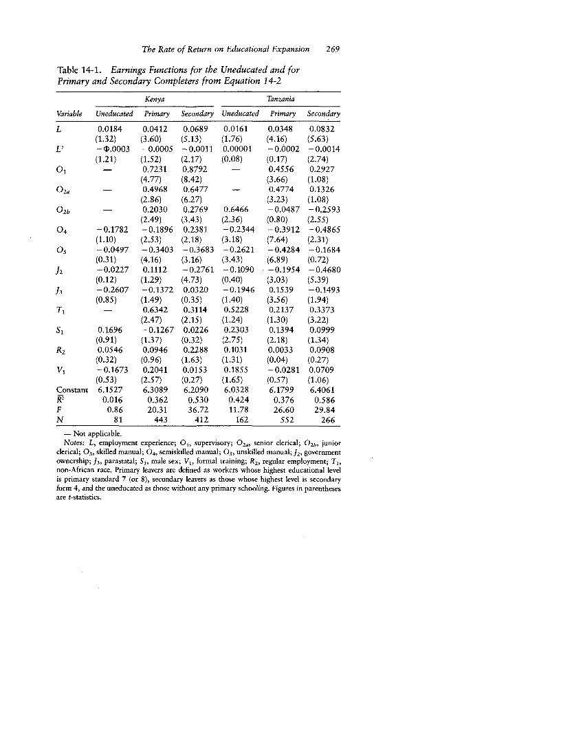
The Rate of Return on Educational Expansion 269
Table 14-1. Earnings Functions for the Uneducated and forPrimary and Secondary Completers from Equation 14-2
Kenya Tanzania
Variable Uneducated Primary Secondary Uneducated Primary Secondary
L 0.0184 0.0412 0.0689 0.0161 0.0348 0.0832(1.32) (3.60) (5.13) (1.76) (4.16) (5.63)
L2 -4 .0003 -0.0005 -0.0011 0.00001 -0.0002 -0.0014(1.21) (1.52) (2.17) (0.08) (0.17) (2.74)
O0 - 0.7231 0.8792 - 0.4556 0.2927(4.77) (8.42) (3.66) (1.08)
°2s - 0.4968 0.6477 - 0.4774 0.1326(2.86) (6.27) (3.23) (1.08)
02b - 0.2030 0.2769 0.6466 -0.0487 -0.2593
(2.49) (3.43) (2.36) (0.80) (2.55)04 -0.1782 - 0.1896 0.2381 - 0.2344 -0.3912 - 0.4865
(1.10) (2.53) (2.18) (3.18) (7.64) (2.31)Os --0.0497 - 0.3403 -0.3683 - 0.2621 -0.4284 -0.1684
(0.31) (4.16) (3.16) (3.43) (6.89) (0.72)12 -0.0227 0.1112 -0.2761 -0.1090 -0.1954 -0.4680
(0.12) (1.29) (4.73) (0.40) (3.03) (5.39)13 -0.2607 -0.1372 0.0320 - 0.1946 0.1539 -0.1493
(0.85) (1.49) (0.35) (1.40) (3.56) (1.94)T, - 0.6342 0.3114 0.5228 0.2137 0.3373
(2.47) (2.15) (1.24) (1.30) (3.22)S1 0.1696 -0.1267 0.0226 0.2303 0.1394 0.0999
(0.91) (1.37) (0.32) (2.75) (2.18) (1.34)R2 0.0546 0.0946 0.2288 0.1031. 0.0033 0.0908
(0.32) (0.96) (1.63) (1.31) (0.04) (0.27)V, -0.1673 0.2041 0.0153 0.1855 -0.0281 0.0709
(0.53) (2.57) (0.27) (1.65) (0.57) (1.06)Constant 6.1527 6.3089 6.2090 6.0328 6.1799 6.4061R2 0.016 0.362 0.530 0.424 0.376 0.586F 0.86 20.31 36.72 11.78 26.60 29.84N 81 443 412 162 552 266
- Not applicable.Notes: L, employment experience; 01, supervisory; 02-, senior clerical; 0 2b, junior
clerical; 03, skilled manual; 04, semiskilled manual; 0 5, unskilled manual; J 2 , governmentownership; 13, parastatal; SI, male sex; Vl, formal training; R2, regular employment; T1,non-African race. Primary leavers are defined as workers whose highest educational levelis primary standard 7 (or 8), secondary leavers as those whose highest level is secondaryform 4, and the uneducated as those without any primary schooling. Figures in parenthesesare t-statistics.
270 THE COST-BENEFIT ANALYSIS OF SECONDARY EDUCATION
ranking generally corresponds to the ranking of occupations by expectedskill content. In only three out of twenty cases does the coefficient notdiffer from zero at the 5 percent level of significance. The job in whicha secondary completer is employed makes a considerable difference tohis wage. For instance, in Kenya employment in the skilled manual in-stead of the junior clerical occupation, other things being equal, reducespay by 24 percent, and employment in the semiskilled instead of theskilled manual occupation reduces pay by 27 percent. The effect that fil-tering down by secondary completers has on the rate of return to second-ary education is therefore potentially important.
The effect of education on earnings is both direct and-through thechoice of occupation-indirect; education can influence a worker's wagewithin an occupation and the occupation in which he is employed. Thedifference in the earnings streams for primary and secondary completersis partly determined by their different occupational distributions. Ac-cordingly the following predictive equation, derived from equation 14-2,is used to estimate the earnings stream of secondary completers duringthirty-six years of employment (L = 1, . . . 36).
(14-3) In W = a + bL + cL2 + djXj(p,) + X ei0iO + ; fdkj
where Xj(p+ , = the mean value (proportion in the case of dummy vari-ables) of Xi in the combined sample of primary and secondary completersand °is = the proportion of secondary completers in Qi.
The earnings stream of primary completers is estimated in the sameway, except that the coefficients are those estimated from the primarycompleter sample, Oip replaces Oi,, and L = 1, . . . 40. The differencein earnings between primary and secondary completers as a result of theirdifferent distributions among the variables Oi is thus attributed to second-ary education. Whether the occupation terms are included or excludedin the specification of equation 14-1, therefore, has no effect on the esti-mated rate of return; this expectation has been empirically verified.2
The theoretical model underlying our procedure is related to the mod-els of "job competition" or "bumping," in which entrants to the labormarket compete for jobs on the basis of their educational qualifications(see, for instance, Bhagwati and Srinivasan 1977, Fields 1974, andThurow 1975). It differs from most such models, however, in permittingthe productivity and wage of workers to vary not only between jobs butalso within jobs according to education. Our model involves the conceptof the occupational production function-an occupation-specific rela-tionship between education and productivity in which productivity in-creases with education over a certain range, as discussed in chapter 7.The effect of occupation on earnings is shown by the coefficients on theoccupation dummy variables in each sample, and the effect of educationon earnings within an occupation can be derived by comparing the coeffi-
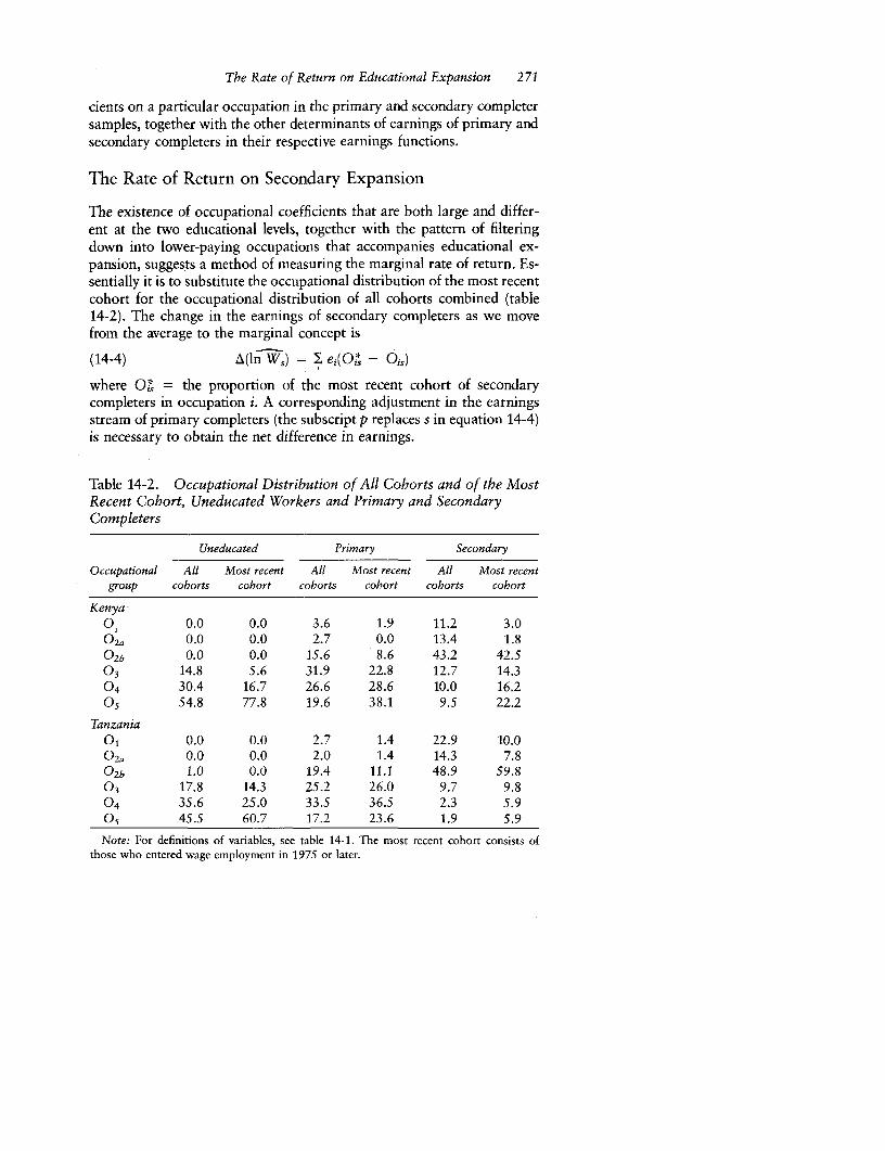
The Rate of Return on Educational Expansion 271
cients on a particular occupation in the primary and secondary completersamples, together with the other determinants of earnings of primary andsecondary completers in their respective earnings functions.
The Rate of Return on Secondary Expansion
The existence of occupational coefficients that are both large and differ-ent at the two educational levels, together with the pattern of filteringdown into lower-paying occupations that accompanies educational ex-pansion, suggests a method of measuring the marginal rate of return. Es-sentially it is to substitute the occupational distribution of the most recentcohort for the occupational distribution of all cohorts combined (table14-2). The change in the earnings of secondary completers as we movefrom the average to the marginal concept is
(14-4) A(ln W,) = I ei(OQ - Ois)
where QS' = the proportion of the most recent cohort of secondarycompleters in occupation i. A corresponding adjustment in the earningsstream of primary completers (the subscript p replaces s in equation 14-4)is necessary to obtain the net difference in earnings.
Table 14-2. Occupational Distribution of All Cohorts and of the MostRecent Cohort, Uneducated Workers and Primary and SecondaryCompleters
Uneducated Primary Secondary
Occupational All Most recent All Most recent All Most recentgroup cohorts cohort cohorts cohort cohorts cohort
Kenya0, 0.0 0.0 3.6 1.9 11.2 3.002a 0.0 0.0 2.7 0.0 13.4 1.80
2b 0.0 0.0 15.6 8.6 43.2 42.503 14.8 5.6 31.9 22.8 12.7 14.304 30.4 16.7 26.6 28.6 10.0 16.2Os 54.8 77.8 19.6 38.1 9.5 22.2
TanzaniaOr 0.0 0.0 2.7 1.4 22.9 10.002a 0.0 0.0 2.0 1.4 14.3 7.80
2b 1.0 0.0 19.4 11.1 48.9 59.803 17.8 14.3 25.2 26.0 9.7 9.804 35.6 25.0 33.5 36.5 2.3 5.90s 45.5 60.7 17.2 23.6 1.9 5.9
Note: For definitions of variables, see table 14-1. The most recent cohort consists ofthose who entered wage employment in 1975 or later.

272 THE COST-BENEFIT ANALYSIS OF SECONDARY EDUCATION
This net difference clearly represents the private benefit of secondaryschooling. If a person enters the labor market with secondary education,his wage expectation is based on the occupational distribution of similarsecondary completers, and if he enters with primary education his wageexpectation is based on the occupational distribution of similar primarycompleters. It may be argued, however, that the net difference in earningsso calculated overstates the social benefit.
Had secondary education not been provided, the posts that secondarycompleters occupy would have to be filled by primary completers, whowould be in correspondingly larger supply. On this basis the social bene-fit stream for primary completers, derived from equation 14-3, would be
(14-5) lnWp = a + bL + cL2 + X djXj(p±s) + YZ ei0i,
The only difference between this and the corresponding stream forsecondary completers is that the coefficients are those estimated for theprimary completer sample and that L = 1, . . . 40. The social benefit ofsecondary schooling is thus represented by the higher earnings of second-ary completers compared with primary completers within the occupa-tions that the former hold. The change in ln Wp as we move from measur-ing the average social benefit to measuring the marginal social benefitcorresponds precisely to equation 14-4 except that the coefficients ei areestimated from the primary completer sample; the underlying notion ofthe social benefit is retained.
It is implicit in these simulations that wages in the higher-paying occu-pations do not fall as education is expanded; that is, the coefficients inthe earnings functions are invariant with respect to changes in the relativesupply of secondary completers. Long lags in the adjustment process andinflexibility of wages are not implausible given the importance of institu-tional wage setting in Kenya and Tanzania, the low rate of labor turnover,the security of tenure enjoyed by incumbents, and the presence ofoccupation-specific human capital (see chapter 7).
Four concepts of the rate of return are reported in table 14-3. The aver-age private return-the one conventionally estimated-overstates by be-tween 1 and 3 percentage points the marginal private return derived ifwage stickiness (a stable earnings function) and filtering down are as-sumed to exist. The estimate of the marginal return is based on the occu-pational distribution of the cohort that entered wage employment during1975-80. It is somewhat lower than the average mainly because al-though both primary and secondary completers in recent cohorts had tofilter down into lesser occupations, the secondary completers filtereddown relatively further.
The average social return is considerably lower than the average pri-vate return in both countries. The difference-no less than 6-8 percent-age points-reflects our assumption that if recent investment in second-
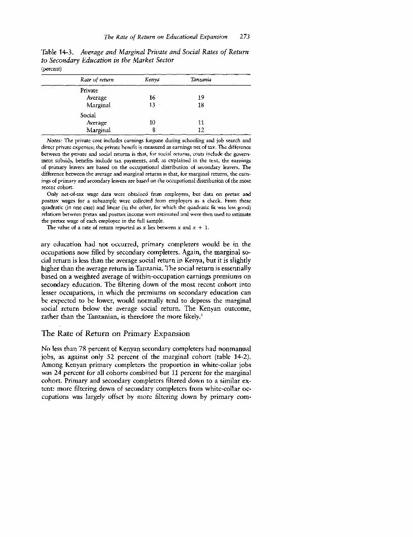
The Rate of Return on Educational Expansion 273
Table 14-3. Average and Marginal Private and Social Rates of Returnto Secondary Education in the Market Sector(percent)
Rate of return Kenya Tanzania
PrivateAverage 16 19Marginal 13 18
SocialAverage 10 11Marginal 8 12
Notes: The private cost includes earnings forgone during schooling and job search anddirect private expenses; the private benefit is measured as earnings net of tax. The differencebetween the private and social returns is that, for social returns, costs include the govern-ment subsidy, benefits include tax payments, and, as explained in the text, the earningsof primary leavers are based on the occupational distribution of secondary leavers. Thedifference between the average and marginal returns is that, for marginal returns, the earn-ings of primary and secondary leavers are based on the occupational distribution of the mostrecent cohort.
Only net-of-tax wage data were obtained from employees, but data on pretax andposttax wages for a subsample were collected from employers as a check. From thesequadratic (in one case) and linear (in the other, for which the quadratic fit was less good)relations between pretax and posttax income were estimated and were then used to estimatethe pretax wage of each employee in the full sample.
The value of a rate of return reported as x lies between x and x + 1.
ary education had not occurred, primary completers would be in theoccupations now filled by secondary completers. Again, the marginal so-cial return is less than the average social return in Kenya, but it is slightlyhigher than the average return in Tanzania. The social return is essentiallybased on a weighted average of within-occupation earnings premiums onsecondary education. The filtering down of the most recent cohort intolesser occupations, in which the premiums on secondary education canbe expected to be lower, would normally tend to depress the marginalsocial return below the average social return. The Kenyan outcome,rather than the Tanzanian, is therefore the more likely.3
The Rate of Return on Primary Expansion
No less than 78 percent of Kenyan secondary completers had nonmanualjobs, as against only 52 percent of the marginal cohort (table 14-2).Among Kenyan primary completers the proportion in white-collar jobswas 24 percent for all cohorts combined but 11 percent for the marginalcohort. Primary and secondary completers filtered down to a similar ex-tent: more filtering down of secondary completers from white-collar oc-cupations was largely offset by more filtering down by primary com-
274 THE COST-BENEFIT ANALYSIS OF SECONDARY EDUCATION
pleters from the skilled manual category. Since all of the uneducatedworkers were in manual occupations, there could be no filtering downfrom white-collar occupations for this group.
A similar pattern of filtering down is evident in Tanzania. The maindifference between the countries is that, at each educational level, boththe marginal and nonmarginal cohorts are less concentrated in the lessskilled occupations in Tanzania.
We have seen that the coefficients on the occupation terms in the equa-tions for primary and secondary completers increase monotonically withskill level (table 14-1). These results demonstrate the sensitivity of theprojected lifetime earnings stream to the occupational distribution of acohort. Filtering down can substantially depress a cohort's lifetime earn-ings.
Uneducated workers, also analyzed in table 14-1, are an exception: inKenya their occupation coefficients are small and not statistically signifi-cant, and the three white-collar occupations are empty. Even the coeffi-cient on employment experience is small and insignificant. Their equationas a whole has poor predictive power because there is relatively little vari-ance in earnings to explain. In Kenya what little change has occurredfrom one cohort to the next in the occupational distribution of unedu-cated workers will have only a limited impact on their projected lifetimeearnings stream.
Educational expansion and filtering down pose more of a threat to theexpected earnings of successive cohorts of uneducated workers in Tanza-nia than in Kenya. Uneducated workers in Tanzania are somewhat lessconcentrated at the bottom of the urban wage labor market, and a smallproportion (1 percent) is even found in the lowest of the white-collar oc-cupations. Moreover, three of the five occupational coefficients are largerthan in Kenya and are statistically significant.
To take account of filtering down and to measure the marginal rateof return to primary education, we use a method similar to that for second-ary education. We substitute for the occupational distribution of all co-horts combined the occupational distribution of the most recent cohort(table 14-2). In contrast to conventional rate of return studies, wagesof workers with primary education are not inflated by basing the calcula-tion on the (now unattainable) occupational distribution of earlier co-horts. The change in the earnings stream of primary completers, as wemove from the average to the marginal concept, is
(14-6) (1n W) = Iei(O!p- Oip)
where O* = the proportion of the most recent cohort of primarycompleters in occupation i. A corresponding adjustment in the earningsstream of uneducated workers (the subscript u replaces p in equation14-6) is necessary to obtain the net difference in earnings.
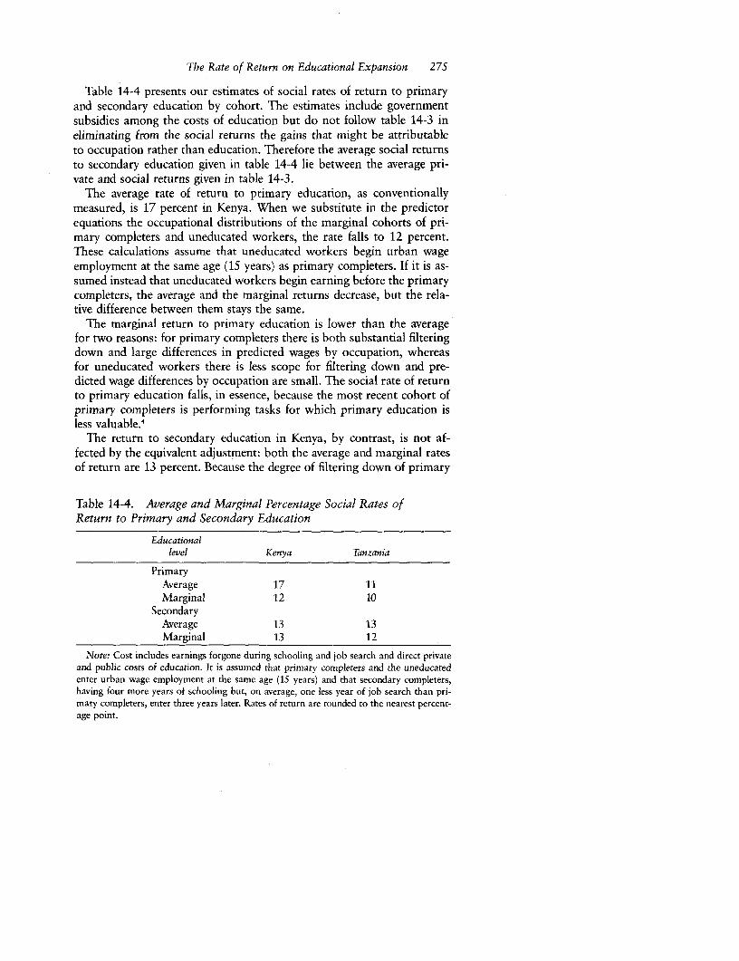
The Rate of Return on Educational Expansion 275
Table 14-4 presents our estimates of social rates of return to primaryand secondary education by cohort. The estimates include governmentsubsidies among the costs of education but do not follow table 14-3 ineliminating from the social returns the gains that might be attributableto occupation rather than education. Therefore the average social returnsto secondary education given in table 14-4 lie between the average pri-vate and social returns given in table 14-3.
The average rate of return to primary education, as conventionallymeasured, is 17 percent in Kenya. When we substitute in the predictorequations the occupational distributions of the marginal cohorts of pri-mary completers and uneducated workers, the rate falls to 12 percent.These calculations assume that uneducated workers begin urban wageemployment at the same age (15 years) as primary completers. If it is as-sumed instead that uneducated workers begin earning before the primarycompleters, the average and the marginal returns decrease, but the rela-tive difference between them stays the same.
The marginal return to primary education is lower than the averagefor two reasons: for primary completers there is both substantial filteringdown and large differences in predicted wages by occupation, whereasfor uneducated workers there is less scope for filtering down and pre-dicted wage differences by occupation are small. The social rate of returnto primary education falls, in essence, because the most recent cohort ofprimary completers is performing tasks for which primary education isless valuable.4
The return to secondary education in Kenya, by contrast, is not af-fected by the equivalent adjustment: both the average and marginal ratesof return are 13 percent. Because the degree of filtering down of primary
Table 14-4. Average and Marginal Percentage Social Rates ofReturn to Primary and Secondary Education
Educationallevel Kenya Tanzania
PrimaryAverage 17 11Marginal 12 10
SecondaryAverage 13 13Marginal 13 12
Note: Cost includes earnings forgone during schooling and job search and direct privateand public costs of education. It is assumed that primary completers and the uneducatedenter urban wage employment at the same age (15 years) and that secondary completers,having four more years of schooling but, on average, one less year of job search than pri-mary completers, enter three years later. Rates of return are rounded to the nearest percent-age point.

276 THE COST-BENEFIT ANALYSIS OF SECONDARY EDUCATION
and secondary completers is similar, the difference in expected lifetimeearnings is little affected.
The rapid expansion of primary education in Kenya might have pro-duced an increasing difference over time in the qualities of primary andsecondary completers, but our results cannot be explained in this way.First, the rate of expansion and the decline in selectivity were even greateramong secondary than among primary completers (see chapter 10). Sec-ond, those primary completers who were successful in the intensifiedcompetition for scarce and relatively high paying wage jobs were increas-ingly likely to be among the best qualified.
As is consistent with the conventional view of the hierarchy of returns,the average return to primary education is substantially higher than thatto secondary education. The marginal return to secondary education,however, exceeds that to primary education. Thus in Kenya the hierarchyis reversed.
The shift to the more appropriate marginal concept does not have asstriking an effect in Tanzania as in Kenya. There is only a slight decline,from 13 to 12 percent, in the rate of return to secondary education, a resultsimilar to that for Kenya. But the marginal rate of return to primary edu-cation, 10 percent, is only slightly lower than the average rate, 11 per-cent. In contrast to the findings for Kenya, Tanzania shows the conven-tional hierarchy of returns.
One explanation of why the marginal return differs little from the aver-age return in Tanzania is that the smaller stock of secondary completershas not filtered down to the same extent as in Kenya. Thus neither pri-mary completers nor the uneducated have felt as much competitive pres-sure in the urban wage labor market. As we have seen, a higher propor-tion of the uneducated is in skilled manual jobs than in Kenya, and afew of these workers are still to be found in junior clerical positions.
Furthermore, in contrast to Kenya, the occupation of an uneducatedTanzanian worker has a substantial impact on earnings. This implies thatthe shift to the occupational distribution of the marginal cohort reducesthe lifetime expected earnings of uneducated workers as well as of pri-mary completers, leaving the difference between them virtually un-changed. If this explanation is correct, then as the secondary system ex-pands in Tanzania, we would expect reduced variance in earnings amonguneducated workers and a widening of the gap between the average andmarginal rates of return to primary education.
This explanation is not entirely satisfactory. We would expect therapid expansion of the supply of primary completers in Tanzania to exertcompetitive pressure on the uneducated, irrespective of the pace of ex-pansion of the secondary system. The less competitive nature of theTanzanian labor market offers an alternative explanation for the greatervariance in the wages of uneducated workers in Tanzania than in Kenya.
The Rate of Return on Educational Expansion 277
A markedly higher proportion of Tanzania's urban wage labor force isemployed by the public sector, which provides greater security of tenureand is less sensitive to market pressures in wage determination. Althoughthe lags may be longer there, adjustment to the increased supply of edu-cated workers is occurring. We can expect to see less variance in thewages of uneducated workers and, as the filtering down of primarycompleters continues, a widening gap between the average and marginalrates of return to primary education.
Conclusions
The intention in this chapter has been to take account of a well-knownbut little-heeded criticism of standard rate of return estimates. Our datasets for Kenya and Tanzania have made possible a quantitative adjust-ment for this criticism. Nevertheless, we regard the results as illustrativerather than as providing an operational criterion.
In East Africa a skill-based occupational classification plays an impor-tant role in the wage structure. This can give rise to a substantial ex-cess-6-8 percentage points-of the private return over the social returnto secondary education. Some of the private benefit accrues in the formof access to high-paying occupations, with no increase in productivity.Whereas in a competitive labor market the marginal social return is thesame as the average return, the marginal return is likely to be depressedin imperfectly competitive labor markets such as those of Kenya and Tan-zania. In Kenya the marginal return to primary education in the wageemployment sector was estimated to be 5 percentage points below thecorresponding average return.
We have argued that the conventional wisdom about the hierarchy ofthe returns to education is based on studies that are likely to contain amethodological error. Although the rate of return on primary schooling,averaged over a large number of urban data sets, may be as high as 26percent, our results suggest that the marginal return may be considerablylower, and it is the marginal rate of return that is relevant for policy.
Our adjustment to the conventional method is a step in the right direc-tion. But our sample of urban wage employees, like all other such sam-ples that have been used to estimate rates of return on primary education,raises additional questions. In all but a few developing countries mostof the marginal cohort of primary completers will be entering agriculturalself-employment. The return to primary education will thus crucially de-pend on its effect on productivity in agriculture and in rural nonagricul-tural activities.
Lockheed, Jamison, and Lau (1980) have surveyed studies that use ag-ricultural production functions to measure this effect. Whereas in somecountries the derived rate of return on primary education is high, in only
278 THE COST-BENEFIT ANALYSIS OF SECONDARY EDUCATION
nineteen of thirty-seven data sets is a statistically significant effect found.The influence of education on agricultural productivity appears to de-pend on whether there is an environment that encourages the moderniza-tion of agriculture. Clearly it is dangerous to generalize about the valueof investment in primary schooling-even abstracting from questions ofquality (see Behrman and Birdsall 1983), which may itself be a functionof the expansion of the primary system.
We are not arguing that the conventional assessment of educationalpriorities, albeit based on the existing flawed rate of return studies, is nec-essarily wrong. The expansion of education can yield important distribu-tional benefits and positive externalities. Contrary to the conventionalwisdom about the hierarchy of rates of return, however, the jury is stillout.
Notes
1. The potential influence of cohort effects-in particular, changes in the sizeof cohorts as a result of population growth-on the average returns per year ofschooling has been established by Behrman and Birdsall 1988 for Brazil. The au-thors do not, however, examine the influence of cohort effects on the structureof returns to various levels of schooling.
2. To avoid the complications that arise from the equalizing government paypolicy in Tanzania (see chapter 13), all estimates are for the private sector. Inpredicting the earnings streams W,, and W,, the influence of pay policy is elimi-nated by setting to zero the coefficients on the dummy variable for ownershipcategories J2 (government) and J3 (parastatal), where Ji (private) is the base sub-category.
3. The result for Tanzania is mainly the consequence of a large positive pre-mium on secondary education in the unskilled manual occupational category.T1he coefficient on the unskilled manual dummy variable in the secondarycompleter sample, however, has a high standard error (table 13-1), and there areonly five secondary completers in that occupation.4. For the underlying theory of occupational production functions on which this
statement is based, see appendix E
CHAPTER 15
The Efficiency and Equityof Subsidies
to Secondary Education
PRACTITIONERS OF THE NEW ECONOMICS of public finance, in searchingfor sources of revenue, regard as particularly strong candidates for taxa-tion goods and services with low price elasticities of demand and highincome elasticities of demand. The elasticities imply that if these itemsare taxed, the reduction of demand (and of potential revenues) and theconsequent distortion of consumption patterns will be relatively smalland that the share of revenue accruing from taxpayers in the upper ranksof the income distribution will be relatively large. The same rule of thumbapplies to the consequences of reducing existing subsidies. In this chapterwe exploit this symmetry to show how such an assessment might be con-ducted in the education sector in Kenya.
That education expenditures should be subjected to critical scrutiny isobvious; public spending on education accounts for a sizable proportionof GDP and of public expenditure in all regions of the world. In 1970,on average, developing countries spent 4 percent of GDP and 15 percentof total public expenditure on education (Zymelman 1982). Moreover,the combination of low enrollment ratios (in comparison with thosein industrial countries), rapid population growth, and high private ratesof return to investment in education means that the demand for educa-tion (and hence pressure to increase subsidies) is high and growing.
As a consequence of the macroeconomic problems of the early 1980s,budgetary constraints on educational expenditure in developing coun-tries are tighter than in the 1950s and 1960s, when many subsidy pro-grams were put into place or were greatly expanded. Governments' share
Note: Adapted fromJane Armitage and Richard Sabot, "Efficiency and Equity Implicationsof Subsidies to Secondary Education in Kenya," The Theory of Taxation for DevelopingCountries, David Newbery and Nicholas Stern, eds. (New York: Oxford University Press,1987).
279

280 THE COST-BENEFIT ANALYSIS OF SECONDARY EDUCATION
of output grew substantially in the 1960s and 1970s, and the proportionof the budget spent on human resources increased. But today public ex-penditure is no longer growing as a percentage of GDP, and expenditureson education and health face increasing competition from other claims(Bowman and Sabot 1982).
A further reason for scrutinizing expenditures on education is thatafter twenty or thirty years of economic development the original justifi-cations for the subsidies may not apply with their original force or maynot have proved sound. One justification for subsidies is the belief thatthe distribution of school places (and therefore the rate of intergenera-tional mobility) should not be determined by ability to pay school fees.Even if the private rate of return is high, capital market imperfectionsgenerally prevent the poor from borrowing to finance expenditure on ed-ucation.
A second rationale is that the social returns to education are substan-tially higher than the private returns and that in the absence of subsidiesinvestment in education will be less than is socially optimal. The increasein the supply of human capital can compress the earnings structure andconsequently reduce inequality of pay. Education is also credited withhelping to decrease fertility and child mortality and to increase politicalawareness and participation (see Bowen and Sabot 1983; Cochrane1979). Externalities such as these, it is argued, justify subsidies.
A third reason for subsidies (and for government regulation) is thatmany parents are uneducated and may lack the background necessaryto reach informed judgments about the relative costs and benefits of high-quality and low-quality schooling. Unless the government sets standardsand subsidizes high-quality education, parents may settle for schoolingof lower quality than is socially optimal.
The public finance rule of thumb and these justifications for educa-tional subsidies suggest that an assessment of a program of educationsubsidies should include the following questions:
* Would a reduction of subsidies have a large negative impact on en-rollments, or is the price elasticity of demand sufficiently low forthat not to be the case?
* Would a reduction of subsidies have an adverse effect on the distri-bution of schooling, or, contrary to stated intentions, have the rela-tively well-to-do benefited disproportionately from the subsidiza-tion of education?
* Would a reduction of subsidy per pupil lead to a deterioration ofschool quality, or would private funds simply substitute for publicfunds, leaving expenditures per pupil on education inputs un-changed?
The Efficiency and Equity of Subsidies to Secondary Education 281
We attempt to answer these questions with regard to government sub-sidies of secondary education in Kenya. We were unable to obtain the rele-vant cost data for community and private secondary schools in Tanzania,and, moreover, the Kenyan case is more interesting because the harambeesystem of secondary schools is much larger than its equivalent in Tanza-nia. A distinction is made in the analysis between the consequences ofthe two ways of reducing subsidies to secondary education-raising feesin government schools, and leaving the growth of secondary enrollmentsto relatively unsubsidized private schools.
The Dual Secondary System in Kenya
Between 1963, the year of independence, and 1980 enrollments in thehighly subsidized government secondary system expanded rapidly, at 12percent a year. Demand grew even faster than supply. The excess demandwas satisfied by the establishment of large numbers of harambee, church,and private schools, which receive only small subsidies from the govern-ment. Since 1963 private enrollments, including those in government-assisted harambee schools, have been growing at 21 percent a year. Sec-ondary, enrollment in nongovernment schools first exceeded that ingovernment schools in 1975. In 1981, 40 percent of enrollment was ingovernment schools, about 20 percent was in assisted harambee schools,about 20 percent was in unassisted harambee schools, and the remainderwas in church or private schools. The state secondary system is clearlypreferred.' With few exceptions, harambee schools are attended by pri-mary leavers who did not qualify (on the basis of meritocratic criteria)for a government secondary education. Table 15-1 shows why.
Because subsidies are much larger in the government system than inthe harambee system (2,071 shillings per student a year, compared with227 shillings), the cost borne by parents is much smaller in the govern-ment system (1,557 shillings per student a year, as against 2,460 shillingsfor harambee schools).2 Moreover, government schools appear to behigher in quality. Total annual expenditures are roughly 1,000 shillingsper pupil higher in government than in harambee schools, and this differ-ence translates into better-educated teachers, smaller classes, more text-books, and better physical facilities. Yet harambee schools preparestudents for the same lower-secondary-leaving examinations taken bystudents in government schools; they are not attempting to offer, for ex-ample, vocational training rather than an academic education. The differ-ence in inputs is reflected in differences in outputs. Only 15 percent ofstudents in government schools drop out before reaching form 4; forharambee schools the figure is 58 percent. Similarly, 21 percent of gov-ernment school students attend upper secondary school (forms 5 and 6),which is the gateway to a higher education, compared with 1 percent for
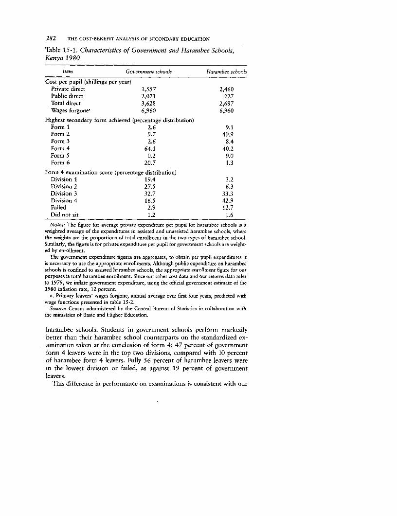
282 THE COST-BENEFIT ANALYSIS OF SECONDARY EDUCATION
Table 15-1. Characteristics of Government and Harambee Schools,Kenya 1980
Item Government schools Harambee scbools
Cost per pupil (shillings per year)Private direct 1,557 2,460Public direct 2,071 227Total direct 3,628 2,687Wages forgone' 6,960 6,960
Highest secondary form achieved (percentage distribution)Form 1 2.6 9.1Form 2 9.7 40.9Form 3 2.6 8.4Form 4 64.1 40.2Form 5 0.2 0.0Form 6 20.7 1.3
Form 4 examination score (percentage distribution)Division 1 19.4 3.2Division 2 27.5 6.3Division 3 32.7 33.3Division 4 16.5 42.9Failed 2.9 12.7Did not sit 1.2 1.6
Notes: The figure for average private expenditure per pupil for harambee schools is aweighted average of the expenditures in assisted and unassisted harambee schools, wherethe weights are the proportions of total enrollment in the two types of harambee school.Similarly, the figure is for private expenditure per pupil for government schools are weight-ed by enrollment.
The government expenditure figures are aggregates; to obtain per pupil expenditures itis necessary to use the appropriate enrollments. Although public expenditure on harambeeschools is confined to assisted harambee schools, the appropriate enrollment figure for ourpurposes is total harambee enrollment. Since our other cost data and our returns data referto 1979, we inflate government expenditure, using the official government estimate of the1980 inflation rate, 12 percent.
a. Primary leavers' wages forgone, annual average over first four years, predicted withwage functions presented in table 15-2.
Source: Census administered by the Central Bureau of Statistics in collaboration withthe ministries of Basic and Higher Education.
harambee schools. Students in government schools perform markedlybetter than their harambee school counterparts on the standardized ex-amination taken at the conclusion of form 4; 47 percent of governmentform 4 leavers were in the top two divisions, compared with 10 percentof harambee form 4 leavers. Fully 56 percent of harambee leavers werein the lowest division or failed, as against 19 percent of governmentleavers.
This difference in performance on examinations is consistent with our
The Efficiency and Equity of Subsidies to Secondary Education 283
other evidence for a difference in school quality, but it could also bepartly the result of differences in student quality, given the meritocraticselection criteria for entrance to government schools. Although we do nothave evidence on ability levels for the entire sample, we do have resultson Raven's Coloured Progressive Matrices, a test of reasoning ability, fora subsample of form 4 leavers (see chapter 3). The difference in scoresbetween harambee and government school leavers is small (the meansbeing 30.52 and 28.32, respectively) and, indeed, statistically insignif-icant. (The standard deviations are 4.85 and 7.90, respectively.) Never-theless, government school students are likely to be better qualified onentrance than harambee school students because of differences in qualityof primary schooling and in academic skills acquired at home.
The difference between government and harambee leavers in levels ofskills as measured by the examinations is, in turn, reflected in a large dif-ference between the two groups in the earnings they command in thelabor market. The predicted mean wages of workers with ten years' expe-rience, in shillings a year, are 9,273 for primary leavers, 12,518 for form4 leavers from harambee schools, and 16,897 for form 4 leavers fromgovernment schools. Predicted mean wages for secondary leavers are sub-stantially higher than predicted wages for primary leavers, but workerswho attended government secondary schools earn 23 percent more thanthose from harambee schools.3
In the parlance of cost-benefit analysis, these stylized facts suggest thatthe private costs of investing in a secondary education are lower and theprivate returns are higher for those who gain access to a government sec-ondary school than for those who must attend a harambee school. Theresulting difference in net private returns explains parents' strong prefer-ence for government schools. If, for now, we ignore the effect of individ-ual constraints on paying for secondary education when the market forsecondary education is segmented, the implication is that the subsidy perpupil in government schools can be reduced (user fees increased) withoutaffecting the demand for places in government schools or expenditure perpupil and hence without reducing school quality. A simple economicmodel of the demand for schooling predicts that in a dual school systemthere will be excess demand for places in the relatively small, highly sub-sidized segment of the system. The elasticity of effective demand in thatsegment will therefore be zero and will remain zero until fees are raisedsufficiently to equate the private net rates of return in the two segments.4
If the highly subsidized segment is also higher in quality and, hence ingross returns, the fees charged in that segment will actually have to behigher than the fees in the other segment before net rates of return areequalized.
An increase in fees in Kenyan government secondary schools wouldease budgetary constraints on education, which have tightened in the
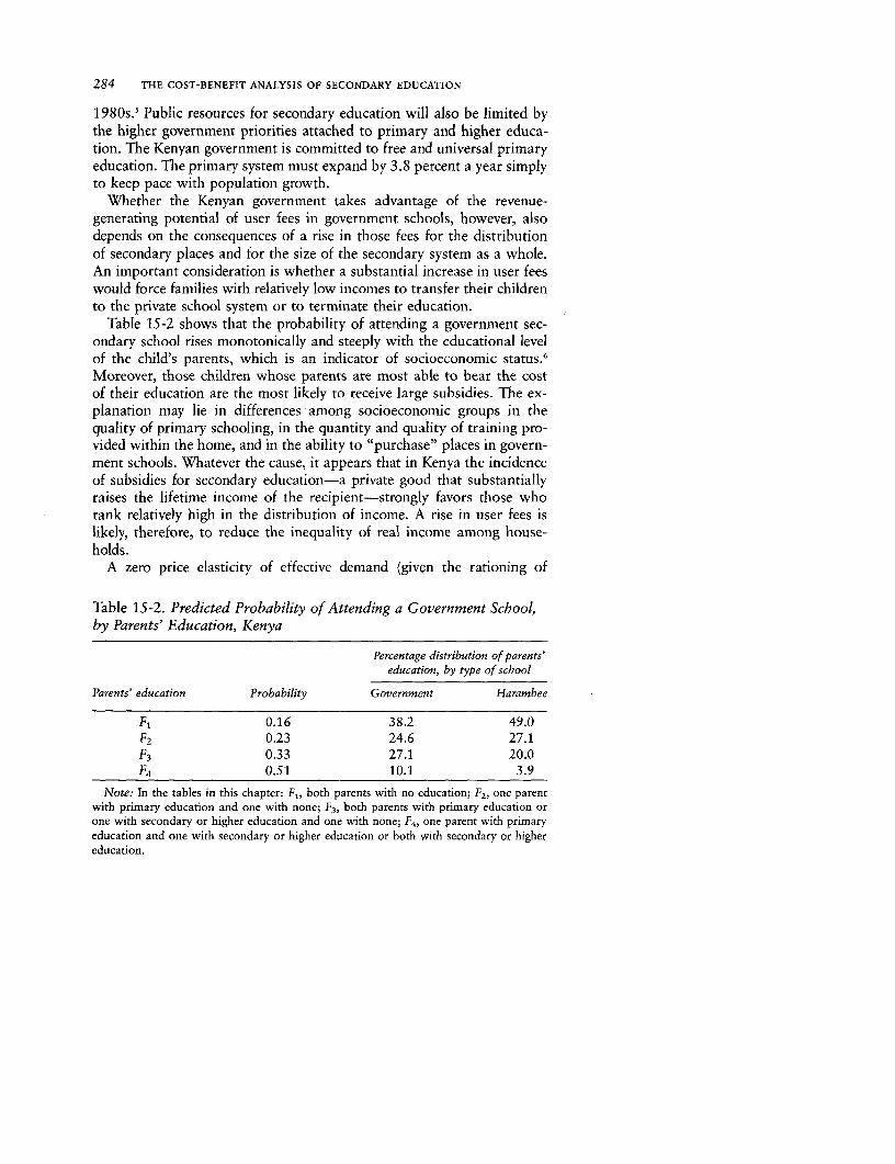
284 THE COST-BENEFIT ANALYSIS OF SECONDARY EDUCATION
1980s.5 Public resources for secondary education will also be limited bythe higher government priorities attached to primary and higher educa-tion. The Kenyan government is committed to free and universal primaryeducation. The primary system must expand by 3.8 percent a year simplyto keep pace with population growth.
Whether the Kenyan government takes advantage of the revenue-generating potential of user fees in government schools, however, alsodepends on the consequences of a rise in those fees for the distributionof secondary places and for the size of the secondary system as a whole.An important consideration is whether a substantial increase in user feeswould force families with relatively low incomes to transfer their childrento the private school system or to terminate their education.
Table 15-2 shows that the probability of attending a government sec-ondary school rises monotonically and steeply with the educational levelof the child's parents, which is an indicator of socioeconomic status.6
Moreover, those children whose parents are most able to bear the costof their education are the most likely to receive large subsidies. The ex-planation may lie in differences among socioeconomic groups in thequality of primary schooling, in the quantity and quality of training pro-vided within the home, and in the ability to "purchase" places in govern-ment schools. Whatever the cause, it appears that in Kenya the incidenceof subsidies for secondary education-a private good that substantiallyraises the lifetime income of the recipient-strongly favors those whorank relatively high in the distribution of income. A rise in user fees islikely, therefore, to reduce the inequality of real income among house-holds.
A zero price elasticity of effective demand (given the rationing of
Table 15-2. Predicted Probability of Attending a Government School,by Parents' Education, Kenya
Percentage distribution of parents'education, by type of school
Parents' education Probability Government Harambee
F1 0.16 38.2 49.0F2 0.23 24.6 27.1
F3 0.33 27.1 20.0F4 0.51 10.1 3.9
Note: In the tables in this chapter: F1 , both parents with no education; F2, one parentwith primary education and one with none; F3, both parents with primary education orone with secondary or higher education and one with none; F4, one parent with primaryeducation and one with secondary or higher education or both with secondary or highereducation.
The Efficiency and Equity of Subsidies to Secondary Education 285
places) implies that a rise in user fees will not lead to underutilizationof government schools. If some students withdraw from the governmentsystem, others from the harambee system will take their places in the pre-ferred system. But what happens to secondary enrollment as user fees areincreased depends on how many leave the government system andwhether they switch to the harambee system or leave the secondary sys-tem entirely.7 These magnitudes will depend on the composition of thegovernment system. If, at one extreme, the government system were en-tirely occupied by the children of the group with the highest educationand therefore income, a rise in fees would be unlikely to induce with-drawals. But as we have seen, in Kenya children of parents with no for-mal education, despite their low probability of attendance, still make up38 percent of the government secondary system because such a high pro-portion of parents had little or no formal education. Another 25 percentof places is filled by children with one parent with primary education.This suggests that unless the rise in school fees is discriminatory-thatis, imposed only on those "able to pay"-it may induce substantial with-drawals from the government system and perhaps from the secondarysystem entirely.
Methods and Data
Our interest is in the apparent dualism in the market for secondary edu-cation between the high-quality, high-subsidy government system and thelow-quality, low-subsidy harambee system. We therefore depart from theconventional procedure by disaggregating the benefits and costs of second-ary schooling by type of school and calculating separate rates of returnto government and to harambee schooling. When the internal private rateof return that equates the present value of these benefits to zero is calcu-lated, only the opportunity costs (wages forgone) of attending secondaryschool and the private direct costs are netted out. When the social rateof return is calculated, account must also be taken of public direct costs(subsidies). On the benefits side we disaggregate by estimating earningsfunctions that will yield Wsg and W5b, which represent the predictedwages, over their expected working lives, of government and harambeesecondary completers, respectively. The equation is
(15-1) In W = a + bL + cL' + IdiSi + IeiXi + u
where Sj are dummy variables that signify type of secondary school.8
The predictor equation for primary completers simply excludes the Siterms. Excess demand for government schooling is sufficient to establishthat the price elasticity of demand is zero. Comparison of the private rateof return to investment in government schooling, rg, with the private rate
286 THE COST-BENEFIT ANALYSIS OF SECONDARY EDUCATION
of return to harambee schooling, rg, allows us to assess the extent towhich user fees can be raised (or subsidies lowered) without inducing areduction in enrollments. On the assumption that the private rate of re-turn to government schooling is greater than that to harambee schooling(rP> rg), and that there are no financial constraints, we calculate the in-crease in direct costs required to make the two rates equal (rP= r=).
If the subsidy per pupil in secondary education is reduced by leav-ing further expansion to the low-cost, low-quality private sector, willallocative efficiency suffer? Because both the total costs and the benefitsof government schooling appear to exceed those of harambee schooling,our stylized facts did not permit even a preliminary answer to this ques-tion, which requires a comparison of the social rates of return, rg andre. The answer depends on which has the greater effect on the social ratesfor the two systems: the difference in costs or the difference in benefits.If the social rate of return to government schooling is equal to or lessthan that to harambee schooling (r-- r'), reducing the subsidy per pupilwould not reduce the economic efficiency of the school system. If the so-cial rate of return to government schooling is greater than that toharambee schooling (rg> r'), allowing the harambee system, as currentlyconstituted, to increase its share of enrollments would mean a loss in ex-pected efficiency.
The deficiencies of cost-benefit analysis as a guide to the allocationof resources between secondary schools and other types of investmentssuch as health clinics or railroads are well known, and various ad hocadjustments have been devised to correct them (Psacharopoulos 1973).Our more limited aim-comparing the social rates of return for twocomponents of the secondary system as a means of assessing the efficiencyconsequences of reducing the subsidy per pupil-is less subject to someof the biases that can be a source of concern. For example, the precisenature of the relationship between wages and the marginal product oflabor in the public sector may have a large influence on the social rateof return to secondary education but only a small effect on the relativerates of return to government and harambee schooling. Although thereis a large difference between the proportions of primary and secondarycompleters in the white-collar-intensive public sector, the difference be-tween government and harambee secondary completers in this regard isrelatively small. Wage-experience profiles derived from cross-sectionaldata are only crude approximations of earnings over the life cycle,9 butagain, the relative rate of return to government and harambee schoolsis less likely to suffer from bias on this account than is the aggregate rateof return to secondary education.
We do, however, examine empirically four issues that could have animportant bearing on relative private or social rates of return. Where ap-propriate, we devise methods for adjusting our estimates.
The Efficiency and Equity of Subsidies to Secondary Education 287
* Are the higher lifetime earnings of government school completersin comparison with those of harambee completers attributable totheir higher level of skill or to credentialism-discrimination by em-ployers on the basis of the worker's "old school tie"? We employmore refined measures of human capital-scores on the form 4examinations-to shed light on this question.
* Do government and harambee completers differ in the length oftime unemployed after leaving school, and are relative rates of re-turn sensitive to the observed differences? Measures of time devotedto job search on leaving school permit us to examine these relation-ships.
* Do relative rates of return have to be adjusted for the difference inwastage rates between government and harambee schools that wasnoted above? The answer depends on whether the returns to school-ing and the costs are linear or nonlinear functions of years ofschooling.
* How much of the difference between government and harambeecompleters in skill levels and earnings is attributable to the tendencyof children from more educated backgrounds to attend governmentschools rather than to differences in the quality of schooling? Weestimate an educational production function to isolate the effect offamily background, independent of type of school, on performanceon the school-leaving examination. We then simulate what the dif-ferences between government and harambee completers in perfor-mance and in earnings would be if the two groups did not differ infamily background.
With the exception of opportunity costs, we do not have individualdata on costs. In our rate of return calculations all government com-pleters are assumed to have paid the average current costs of govern-ment schools, and all harambee completers are assumed to have paid theaverage current costs of harambee schools. Private and public cost dataare derived from official government statistics. Our estimates of privatedirect costs-tuition and board, uniforms, books and equipment, andother school charges-and of public costs are obtained from officialsources. Our own survey is the source for the opportunity costs and forreturns to government and harambee secondary education.
Our survey has the strengths of accuracy and richness. One of its ad-vantages is that it allows the type of secondary school attended to beidentified, and hence the rates of return that are central to our analysiscan be compared. The variable for performance on form 4 examinationspermits us to test competing hypotheses regarding the cause of the differ-ence between harambee and government completers in earnings streams,which is an essential step in measuring the gap between the two types

288 THE COST-BENEFIT ANALYSIS OF SECONDARY EDUCATION
of school in gross social returns. It also permits us to estimate an educa-tional production function and to correct, if only crudely, for the biasin the measurement of the gap that arises from the selectivity of the gov-ernment system.
Our establishment-based survey-like any such survey-has a weak-ness when it is used for cost-benefit analysis: because the sample doesnot include those educated workers who are not in urban wage employ-ment, our estimate of the relative rates of return to government afidharambee schools may be subject to sample selection bias. In particular,it seems likely that a higher proportion of harambee completers than ofgovernment completers are not in urban wage employment and thatthose harambee completers who do not obtain such employment arefrom the poorest-quality schools. If those schools have below-averagecosts as well as below-average returns, our comparison need not be bi-ased. If, however, only the returns are below average, the implicationwould be that we are overestimating the returns to harambee schools inrelation to the returns to government schools.
Private and Social Rates of Return to Government andHarambee Schools and Some Adjustments
Table 15-3 presents estimates of the earnings functions used in the analy-sis. In both equations-for primary completers and for secondarycompleters-the coefficient on the experience variable is positive andhighly significant, and the coefficient on the quadratic term is negativeand highly significant. Differences between the two equations in constantterms and in the coefficients on the experience variables indicate that,as usual, the earnings profile of secondary completers lies above the curvefor primary completers and rises more steeply.
The coefficient on the harambee dummy variable in column 2 of table15-3 is negative, large, and significant. The implication is that when em-ployment experience is standardized, the earnings of harambee com-pleters are considerably (more than 21 percent) lower than those ofgovernment completers. This estimate of the standardized differential inearnings may be biased because the returns to experience are constrainedto be the same for government and harambee completers. But an F-teston an unconstrained version of the equation (not shown) did not allowus to reject the null hypothesis that the returns to experience are the samefor both groups; the F-statistic was below the critical value at the 5 per-cent level of significance.
Figure 15-1 shows the lifetime earnings streams of primary completers,government secondary (form 4) completers, and harambee secondarycompleters. The lower shaded areas represent the opportunity cost of sec-ondary schooling;") the upper shaded area represents the higher gross pri-
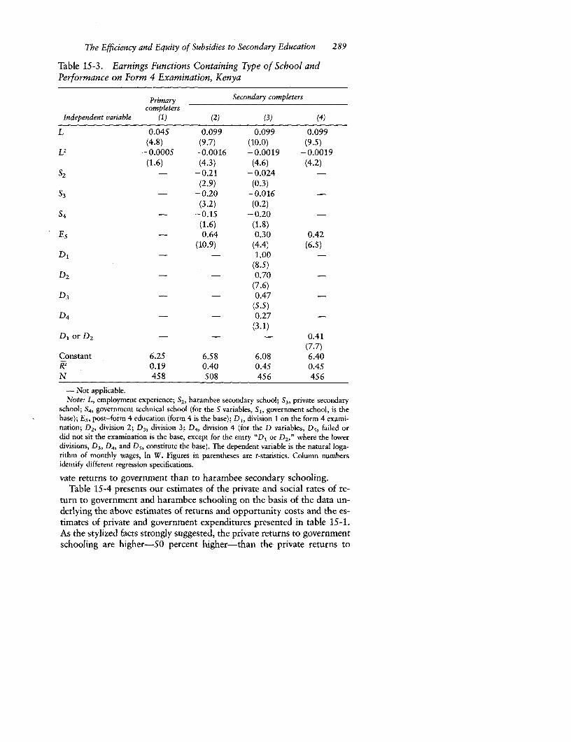
The Efficiency and Equity of Subsidies to Secondary Education 289
Table 15-3. Earnings Functions Containing Type of School andPerformance on Form 4 Examination, Kenya
Primary Secondary completerscompleters
Independent variable (1) (2) (3) (4)
L 0.045 0.099 0.099 0.099(4.8) (9.7) (10.0) (9.5)
L2 --0.0005 - 0.0016 -0.0019 - 0.0019(1.6) (4.3) (4.6) (4.2)
S2 - -0.21 -0.024(2.9) (0.3)
S3 - -0.20 -0.016(3.2) (0.2)
S4 - -0.15 -0.20 -(1.6) (1.8)
Es - 0.64 0.30 0.42(10.9) (4.4) (6.5)
D, - - 1.00 -(8.5)
D2 - - 0.70 -(7.6)
°3 - - 0.47 -(5.5)
D4 - - 0.27 _
(3.1)DV or D 2 - - - 0.41
(7.7)Constant 6.25 6.58 6.08 6.40k2 0.19 0.40 0.45 0.45N 458 S08 456 456
- Not applicable.Note: L, employment experience; S2, harambee secondary school; S3, private secondary
school; S4, government technical school (for the S variables, S,, government school, is thebase); E5 , post-form 4 education (form 4 is the base); D,, division 1 on the form 4 exami-nation; D2, division 2; D3, division 3; D4, division 4 (for the D variables, Ds, failed ordid not sit the examination is the base, except for the entry "DI or D2," where the lowerdivisions, D3, D4, and D5, constitute the base). The dependent variable is the natural loga-rithm of monthly wages, In W. Figures in parentheses are t-statistics. Column numbersidentify different regression specifications.
vate returns to government than to harambee secondary schooling.Table 15-4 presents our estimates of the private and social rates of re-
turn to government and harambee schooling on the basis of the data un-derlying the above estimates of returns and opportunity costs and the es-timates of private and government expenditures presented in table 15-1.As the stylized facts strongly suggested, the private returns to governmentschooling are higher-50 percent higher-than the private returns to
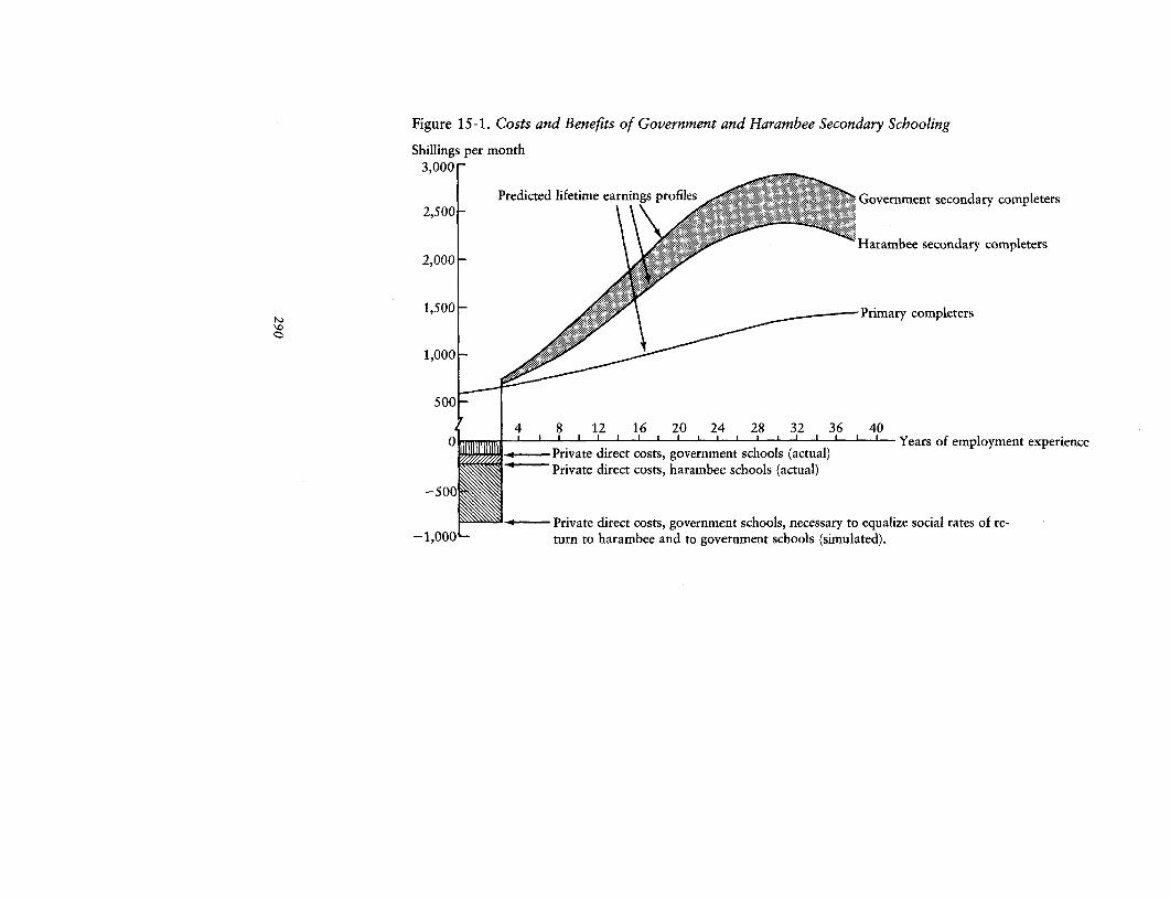
Figure 15-1. Costs and Benefits of Government and Harambee Secondary Schooling
Shillings per month3,000
2,500 - Predicted lifetime earnings profiles Government secondary completers
Harambee secondary completers
1,500 -Primary completers
1,000
4 8 12 16 20 24 28 32 36 40, III III III I I I Years of employment experience
-.-- Private direct costs, government schools (actual)*- S Private direct costs, harambee schools (actual)
-- Private direct costs, government schools, necessary to equalize social rates of re--1,000 turn to harambee and to government schools (simulated).
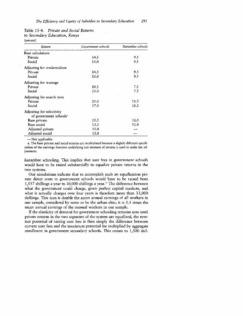
The Efficiency and Equity of Subsidies to Secondary Education 291
Table 15-4. Private and Social Returnsto Secondary Education, Kenya(percent)
Return Government scbools Harambee schools
Base calculationPrivate 14.5 9.5Social 13.0 9.5
Adjusting for credentialismPrivate 14.5 9.5Social 13.0 9.5
Adjusting for wastagePrivate 14.5 7.5Social 13.0 7.5
Adjusting for search timePrivate 21.0 11.5Social 17.0 11.5
Adjusting for selectivityof government schools'
Base private 15.5 11.0Base social 13.5 11.0Adjusted private 15.0Adjusted social 13.0
- Not applicable.a. The base private and social returns are recalculated because a slighdy different specifi-
cation of the earnings function underlying our estimate of returns is used to make the ad-justment.
harambee schooling. This implies that user fees in government schoolswould have to be raised substantially to equalize private returns in thetwo systems.
Our simulations indicate that to accomplish such an equalization pri-vate direct costs in government schools would have to be raised from1,557 shillings a year to 10,000 shillings a year."1 The difference betweenwhat the government could charge, given perfect capital markets, andwhat it actually charges over four years is therefore more than 33,000shillings. This sum is double the mean annual earnings of all workers inour sample, considered by some to be the urban elite; it is 3.5 times themean annual earnings of the manual workers in our sample.
If the elasticity of demand for government schooling remains zero untilprivate returns in the two segments of the system are equalized, the reve-nue potential of raising user fees is then simply the difference betweencurrent user fees and the maximum potential fee multiplied by aggregateenrollment in government secondary schools. This comes to 1,500 shil-
292 THE COST-BENEFIT ANALYSIS OF SECONDARY EDUCATION
lings, or more than 300 percent of government recurrent expenditureson secondary education (see Bertrand and Griffin 1983)."2 Capital marketimperfections imply that if the maximum potential user fee is charged,demand for government schooling will decline. High-cost, high-qualityprivate schools now enroll only a small proportion of secondary students,and expansion of these schools could drain revenue from the governmentsystem. Nevertheless, the revenue potential of raising school fees is likelyto be substantial.
The private and social returns to harambee secondary schooling areessentially the same. Adding the negligible government subsidies onto theprivate costs of harambee schools increases total costs by only 9.2 per-cent, which does not measurably reduce the rate of return. There is, how-ever, a gap between the private and social returns to government school-ing because the subsidy per pupil in that system is far from negligible.Adding government subsidies onto private costs increases total costs by133 percent. The result is that the social rate of return to governmentschooling is about 13 percent, whereas the private rate of return is 14.5percent.
The gap between government and harambee schools in the social rateof return is less than the gap in private returns. Nevertheless, social re-turns to investment in government schools remain substantially higherthan social returns to investment in private schools. This difference sug-gests that from the perspective of costs and benefits to the economy asa whole, not just to the individual or household, the government systemis more cost-effective; output per shilling of input is higher in governmentthan in harambee schools.13
The measured difference between the two systems in economic effi-ciency might stem from a difference in the quality of management. Alter-natively, it might reflect increasing returns in the educational productionfunction. Recall that total per pupil expenditures are substantially lowerin harambee than in government schools. The returns to the additional1,000 shillings per pupil per year spent in government schools may sub-stantially exceed average returns. Educationalists generally presume thatthe learning curve, which relates inputs (on the horizontal axis) to skillsacquired (on the vertical axis) has a logistic form; it rises rapidly at firstand then more slowly. Kenyan secondary schools may be on the steeplysloped portion of such a curve, where a small increase in inputs yieldsa disproportionately large increase in outputs (see appendix I).
One implication of this efficiency differential for the assessment of gov-ernment subsidies to secondary education is that a policy of reducing thesubsidy per pupil by allowing the relatively unsubsidized harambee sys-tem to provide a disproportionate share of new secondary places wouldentail allocative inefficiency and cause some potential output to be for-
The Efficiency and Equity of Subsidies to Secondary Education 293
gone. Because of the higher total costs of the government system, how-ever, the efficiency differential between the two systems is less than the20 percent differential in labor productivity between government andharambee completers estimated by our wage function. If, as hypothe-sized, the educational production function is characterized by increasingreturns, it may take only a small increase in the quality of harambeeschools to reduce the difference between the two systems in gross socialreturns. Narrowing the gap between the two systems in total expenditureper pupil may therefore narrow the gap in social rates of return.
Just how robust are these assessments of the economic costs and bene-fits of reducing the subsidy per pupil to secondary education in Kenya?The adjustments of our estimates of relative private and social rates ofreturn to government and harambee schooling that are summed up hereand in table 15-4 provide a basis for judgment.
Adjusting for Credentialism
To what extent does credentialism account for the higher earnings ofgovernment than of harambee school completers? To what extent is thedifference in earnings attributable to the greater skill of governmentcompleters, as indicated by their superior performance on the nationwideform 4 examination? To answer these questions we add to the wage func-tion for those who had taken the form 4 examination a set of dummyvariables, Dp, that signify the division of score on that examination. Theestimated equation is presented in table 15-3 (column 3).
We see once again that examination performance has a powerful influ-ence on earnings. The coefficients on the dummy variables increase mono-tonically and in large increments; all four are highly significant. Theequation predicts that, when other characteristics are standardized, aform 4 leaver who placed in the first division will earn more than 100percent more than a form 4 leaver who failed or did not sit the examina-tion. Most striking is that adding examination performance to the ex-planatory variables entirely eliminates the influence of type of school onearnings. A comparison of columns 2 and 3 in table 15-3 shows that thecoefficient on the harambee dummy, S2, declines from - 0.21 to - 0.024and is no longer statistically significant.
It appears that all of the difference in earnings between governmentand harambee completers is accounted for by differences in skill and thatnone is accounted for by credentialism; government and harambeecompleters with the same examination scores are predicted to earn thesame wages. Therefore no adjustment needs to be made to our estimateof the rate of return to harambee schools. The rates of return after adjust-ment for credentialism are the same as the base calculations.
294 THE COST-BENEFIT ANALYSIS OF SECONDARY EDUCATION
Adjusting for Wastage
As was seen above, the dropout rate from harambee schools (58 per-cent) is greater than that from government secondary schools (15 per-cent). Whether our estimates of rates of return have to be adjusted fordifferential wastage depends on whether gross returns to schooling area linear or an increasing function of the number of years of schooling.If the returns function is linear, no adjustment need be made; under theassumption that the cost function is also linear, the rate of return peryear of harambee school will be the same irrespective of the number ofyears completed, as will the relative rates of return to government andharambee schools."4 If, however, returns per year of harambee schoolingare lower for form 2 than for form 4 leavers, our base estimates of ratesof return to harambee schooling will be biased upward. To assesswhether the returns function is linear, we calculate the rate of return totwo years of harambee schooling by estimating a wage function for form2 harambee leavers and predicting the lifetime stream of net benefits, tak-ing into account only two years of forgone primary wages and directcosts. The result of these calculations is a rate of return (private and so-cial) of 6.5 percent, considerably less than the rate of return to four yearsof harambee schooling (9.5 percent).
To arrive at an adjusted aggregate rate of return to harambee schools,we weight the rates of return to forms 2 and 4 by the proportions wholeft harambee school at those levels. The adjusted rate of return is 7.5percent (table 15-4), which widens the gap between government andharambee schools in private and social rates of return. There is no needto adjust the returns to government school because the dropout rate isso low.
Adjusting for Search Time
No wages are earned during the time spent searching for a job on com-pletion of schooling." We did not take account of this search period whenwe predicted the lifetime earnings of school leavers and calculated thebase rates of return. Since there are large differences between harambeeand government leavers in search time, relative rates of return may bebiased by this omission. Among government form 4 leavers, 35 percentfound wage jobs immediately as against 19 percent of harambee leavers.The average time taken to find a wage job for government leavers was9.5 months, compared with 18 months for harambee leavers and 32months for primary leavers. Because primary leavers take a longer timeto find a job than do secondary leavers, the rates of return to both govern-ment and harambee schools are higher when an adjustment for searchtime is made than in the base calculation, but the returns to government
The Efficiency and Equity of Subsidies to Secondary Education 295
schools rise more.'6 Therefore the gap between government and haram-bee schools in both private and social rates of return is widened bythe adjustment.
Adjusting for Selectivity of Government Schools
We have confirmed that the difference between government andharambee leavers' wages arises from differences in cognitive skill. Howmuch of the difference in cognitive skill is attributable to the higher qual-ity of government schools and how much to the higher achievement ofgovernment school entrants at the start of secondary schooling and totheir higher ability and socioeconomic background? If, to take an ex-treme case, all of the difference in skill were attributable to the selectivityof the government system, there would be no gap between the two sys-tems in either gross private or gross social returns. Because of differencesin costs, net private returns would still be higher in the government sys-tem, but net social returns would actually be higher in the harambeesystem.
We attempt to answer this question with regard to socioeconomicbackground; we cannot answer it with regard to cognitive skill at the be-ginning of secondary school because we do not have the necessary data.We were able to show for a subsample of form 4 leavers that there isno significant difference in ability between government and harambeeschool leavers. Family background may, however, be partly serving asa proxy for differences in achievement at the start of secondary school.Table 15-5 presents probit estimates of the following simple educationalproduction function for form 4 completers:
(15-2) Prob(H = 1) = 4(X'I3)
where H is a dichotomous variable that takes the value 1 where theindividual obtained a high score (division 1 or 2) on the form 4 examina-tion. The vector of exogenous variables, X, includes F,, the family back-ground dummies; Sj, the dummies for type of school; and, to capture thecohort effect, A, the age of the worker. C1 is the cumulative-unit normaldistribution function.
The three coefficients on the family background variables are signifi-cantly positive. They indicate that the probability of attaining a highscore increases monotonically as the educational level of the student'sparents increases. Nevertheless, the coefficient on the harambee dummy(S2) is of larger absolute size and is more highly significant than the coeffi-cients on any of the family background variables. The predicted probabil-ities, also shown in the table, more clearly illustrate these findings. Inboth the government and the harambee systems there is considerable vari-
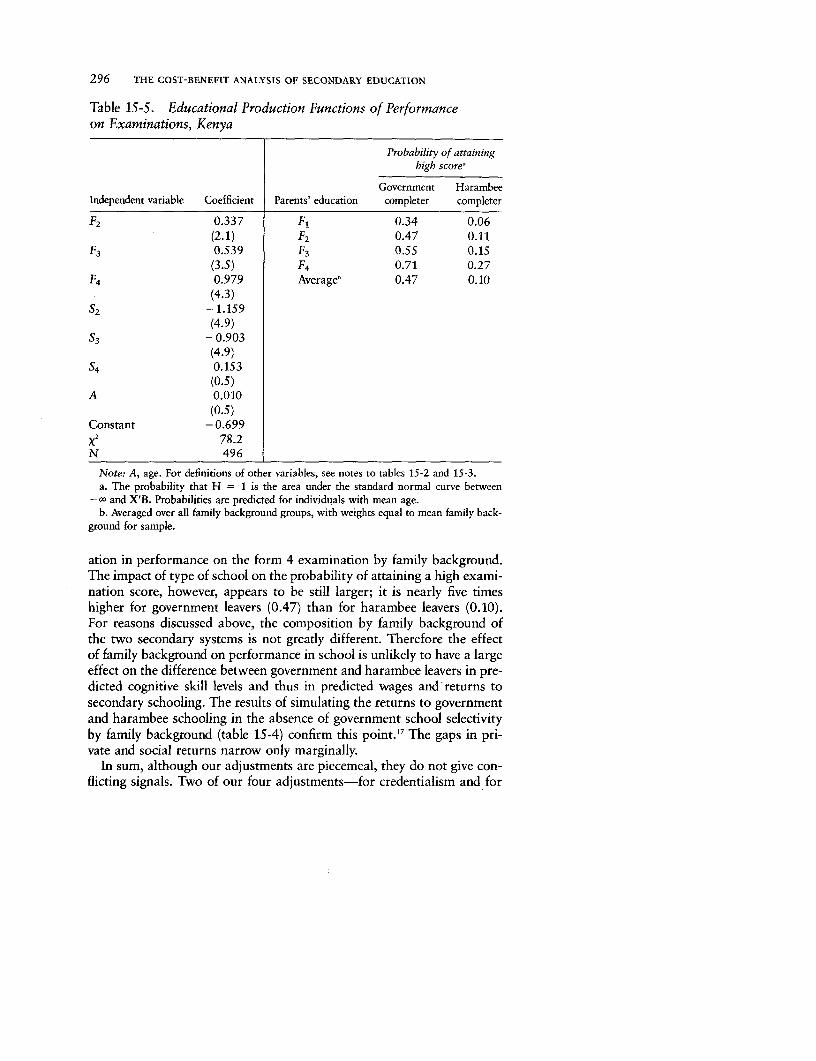
296 THE COST-BENEFIT ANALYSIS OF SECONDARY EDUCATION
Table lS-5. Educational Production Functions of Performanceon Examinations, Kenya
Probability of attaininghigh score'
Government HarambeeIndependent variable Coefficient Parents' education completer completer
F2 0.337 F, 0.34 0.06(2.1) F2 0.47 0.11
F3 0.539 F3 0.55 0.15(3.S) F4 0.71 0.27
F4 0.979 Averageb 0.47 0.10(4.3)
S2 --1.159(4.9)
S3 -0.903(4.9)
S4 0.153(0.5)
A 0.010(0.5)
Constant -0.699X 2 78.2N 496
Note: A, age. For definitions of other variables, see notes to tables 15-2 and 15-3.a. The probability that H = 1 is the area under the standard normal curve between
- - and X'B. Probabilities are predicted for individuals with mean age.b. Averaged over all family background groups, with weights equal to mean family back-
ground for sample.
ation in performance on the form 4 examination by family background.The impact of type of school on the probability of attaining a high exami-nation score, however, appears to be still larger; it is nearly five timeshigher for government leavers (0.47) than for harambee leavers (0.10).For reasons discussed above, the composition by family background ofthe two secondary systems is not greatly different. Therefore the effectof family background on performance in school is unlikely to have a largeeffect on the difference between government and harambee leavers in pre-dicted cognitive skill levels and thus in predicted wages and returns tosecondary schooling. The results of simulating the returns to governmentand harambee schooling in the absence of government school selectivityby family background (table 15-4) confirm this point."7 The gaps in pri-vate and social returns narrow only marginally.
In sum, although our adjustments are piecemeal, they do not give con-flicting signals. Two of our four adjustments-for credentialism and for
The Efficiency and Equity of Subsidies to Secondary Education 297
the selectivity of government schools-have little impact on the relativerates of return to government and harambee schooling. Both of the othertwo adjustments-for differences in length of job search and in wastagerates-widen the gap between government and harambee schools in pri-vate and social rates of return. The widening of the gap in private returnsimplies that our simulations with the base rate calculations underesti-mated the increase in user fees necessary to equalize private returns toinvestment in the two systems. It appears that 8,000 shillings a yearwould not be sufficient. The widening of the gap in social returns impliesthat allowing the harambee system to increase its share of enrollmentsentails somewhat higher efficiency costs than we had supposed.
Access to Government Schools and Family Background
To assess the effects on the distribution of school places of a reductionin the subsidy per pupil, we estimate a simple educational attainmentfunction. With the use of binomial probit we obtain maximum likelihoodestimates of the parameters in the following reduced-form equation:
(15-3) Prob(G = 1) = 'D(X'P3)
where G is a dichotomous variable that takes the value 1 if an individ-ual attended a government secondary school (and thus benefited fromgovernment subsidies) and 0 if he did not, and X is a vector of exogenousvariables. Among the exogenous variables is a set of four dummy vari-ables that signify the educational level of the individual's parents. In an-other specification of the educational attainment function, estimated onlyfor individuals whose fathers were farmers, a variable for the size ofthe farm is included among the exogenous variables. 4)(X'P) is thecumulative-unit normal distribution function."
Table 15-6 presents estimates of our probit educational attainmentfunction and the predicted probabilities of attending a government sec-ondary school, by family background group. In column I of that table,estimated for the entire sample, the coefficients on the variables forparents' education are positive and increase monotonically. All are sig-nificant. As noted in table 15-2, the predicted probabilities of reaping thelarge private benefits from subsidies to government education risesharply with parents' educational level.
Access to the government secondary system is meritocratic; selectionis based largely on performance on the primary-leaving examination. Theeducational production function in table 15-5 suggests that the educa-tional level of parents matters to performance in both high-quality (gov-ernment) and low-quality (harambee) schools."9 Although we have no di-rect evidence, there is a strong presumption that, when school qualityis standardized, the educational level of parents is also positively related
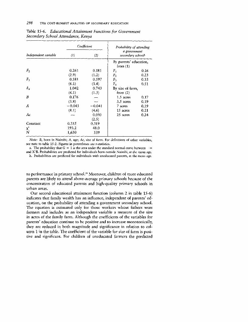
298 THE COST-BENEFIT ANALYSIS OF SECONDARY EDUCATION
Table 15-6. Educational Attainment Functions for GovernmentSecondary School Attendance, Kenya
Coefficient Probability of attendinga government
Independent variable (1) (2) secondary schoola
By parents' education,from (1)
F2 0.261 0.181 F, 0.16(2.9) (1.2) F2 0.23
F3 0.581 0.597 F3 0.33(6.1) (3.4) F4 0.51
F4 1.042 0.743 By size of farm,(6.1) (1.3) from (2)
B 0.176 - 1.5 acres 0.17(3.8) - 3.5 acres 0.19
A -0.043 -0.041 7 acres 0.19(8.1) (4.6) 15 acres 0.21
Ac - 0.010 25 acres 0.24(2.5)
Constant 0.355 0.319xw 2193.2 48.0N 1,650 539
Note: B, born in Nairobi; A, age; Ac, size of farm. For definitions of other variables,see note to table 15-2. Figures in parentheses are t-statistics.
a. The probability that G = 1 is the area under the standard normal curve between -and X'B. Probabilities are predicted for individuals born outside Nairobi, at the mean age.
b. Probabilities are predicted for individuals with uneducated parents, at the mean age.
to performance in primary school.2 " Moreover, children of more educatedparents are likely to attend above-average primary schools because of theconcentration of educated parents and high-quality primary schools inurban areas.
Our second educational attainment function (column 2 in table 15-6)indicates that family wealth has an influence, independent of parents' ed-ucation, on the probability of attending a government secondary school.The equation is estimated only for those workers whose fathers werefarmers and includes as an independent variable a measure of the sizein acres of the family farm. Although the coefficients of the variables forparents' education continue to be positive and to increase monotonically,they are reduced in both magnitude and significance in relation to col-umn 1 in the table. The coefficient of the variable for size of farm is posi-tive and significant. For children of uneducated farmers the predicted
The Efficiency and Equity of Subsidies to Secondary Education 299
probability of attending a government secondary school is about 40 per-cent higher for those from farms of 25 acres than for those from farmsof 1.5 acres. This relationship may indicate a nonmeritocratic elementin the influence of family background on access to government secondaryschooling.
The equations in table 15-6 measure the relationship between the so-cioeconomic status of the parents of the workers in our sample and theeducational attainment of the workers. To confirm that the effect of fam-ily background is not merely a historical phenomenon, we also estimatedby probit the relationship between the educational attainment of theworkers and the probability that their children would attend a govern-ment secondary school. The results (not shown) for the younger two gen-erations are qualitatively the same as those for the older two generations;the richer the family, the greater the likelihood that it will benefit fromgovernment subsidies to secondary education. Kenya is not unique in thisregard. (For evidence of similar outcomes see Hansen and Weisbrod 1969for the United States and Jallade 1974 for Colombia.) This outcome isespecially perverse since in Kenya, as in many developing countries, muchgovernment revenue comes from regressive import and excise dutiesrather than from progressive income taxes (see Fields 1975).
Conclusions
The private rate of return to investment in secondary education is mark-edly higher for children who attend government secondary schools thanfor those who attend harambee schools. This is partly because of thelower private costs of government schooling and partly because of thehigher gross returns. The latter phenomenon is the result of the higherlevel of cognitive skill of government school graduates. Moreover, thereis a positive relationship between family income and the probability ofreaping the subsidies to government schools that contribute to the differ-ence in private rates of return. These findings provide the basis for effi-ciency and equity arguments for reducing the subsidy per pupil in govern-ment schools by selectively increasing user fees.
Our simulations indicate that it would take an increase in user fees ofmore than 8,000 shillings per student a year to equalize private rates ofreturn in the two systems. The revenue potential of user fees in govern-ment schools is therefore substantial-more than 300 percent of the gov-ernment's recurrent expenditures per student for secondary education.This figure is so large partly because in the relevant range the price elas-ticity of demand for government schooling appears to be so small. It mustbe emphasized, however, that in practice the revenue potential will beless than the amount indicated because some families are not able to bor-row in formal credit markets to finance schooling. Nevertheless, a sub-
300 THE COST-BENEFIT ANALYSIS OF SECONDARY EDUCATION
stantial proportion of students in government schools is from familiesthat have the means to pay the cost of their children's education andwould be willing to do so in the absence of a highly subsidized alterna-tive. The willingness of relatively low-income families to pay high feesto send children to low-quality harambee schools that yield low privatereturns is evidence for this assertion.
Even substantial increases in user fees are unlikely to lead to un-derutilization of government schools. Nor would a reduction of thesubsidy per pupil bring about a deterioration of school quality, as pri-vate funds would simply substitute for public funds, leaving expendi-tures per pupil unchanged.
Increases in user fees may give rise to inefficient changes in the compo-sition of the student body of government schools and a reduction in thesize of the secondary system as a whole. There is some reason to believethat the students from uneducated and poor backgrounds who are forcedto withdraw from the school system because of the rise in fees will bethe most able, since students who gain access to government secondaryschools without having the advantage of educated parents are likely tobe unusually bright. If the increases in fees are uniform, relatively brightbut poor students may terminate their education and be replaced by lessable students from higher-income families who would otherwise havegone to harambee schools.
To avoid this outcome, increases in user fees could be discriminatory.A need-based scholarship program could ensure that admissions deci-sions would continue to be based solely on meritocratic criteria. Thereare problems with such a program. If the criteria for awarding scholar-ships are too loose, the scholarship program will cost too much, and ifthe criteria are too tight, the government secondary system may lose stu-dents who would qualify on meritocratic grounds. Although the difficul-ties of assessing ability to pay should not be underestimated, this systemis likely to distribute government subsidies more equitably than the cur-rent one. At present, the least needy have the highest probability of ob-taining a subsidy.
One alternative to raising school fees and providing scholarships to theneedy would be to raise fees and then provide all students with loans tofinance the private costs of a government secondary education. This ap-proach has the advantage of avoiding means tests. The disadvantage isthat a program for repayment would have to be set up and administered,but Kenya's "pay as you earn" tax system could be utilized for this pur-pose.
Reducing per student subsidies by allowing low-subsidy harambeeschools to satisfy an increasing proportion of the growing demand forsecondary schooling has been a de facto policy of the Kenyan governmentfor more than a decade. Our results suggest that, on grounds of allocative
The Efficiency and Equity of Subsidies to Secondary Education 301
efficiency, the case for this approach is actually not as strong as the casefor raising user charges in government schools. The difference betweenthe two systems in social rates of return indicates that harambee schoolsare less efficient than government schools; that is, they raise worker pro-ductivity less per shilling of total expenditure. Government regulation ofquality in harambee schools, together with small subsidies (in compari-son with those given to government schools) for quality-improving pur-poses such as buying textbooks, hiring better-trained teachers, and re-ducing teacher-student ratios, may substantially decrease this difference.If so, the efficiency costs of allowing harambee schools to satisfy an in-creasing proportion of secondary enrollments may also decline. Thiswould be the case if the difference in efficiency between the two systemswere accounted for by the higher total expenditure per pupil in govern-ment than in harambee schools and by the position of secondary schoolson that segment of the educational production function that is character-ized by increasing returns.
Notes
1. Throughout, our analysis compares government with harambee schools andexcludes other private schools. This is because of the heterogeneity of the "otherprivate" category. A few of these schools are very good and very costly; mostare poor in quality and low in cost. Thus this category would have had to befurther disaggregated, but some data essential for such a breakdown were notavailable. The omission does not pose a serious problem, since it appears thatin important respects harambee schools are representative of the larger group oflow-cost private schools.
2. The mean annual earnings of the manual workers in our sample were about9,500 shillings.
3. Predictions are made with the use of the wage functions presented in table15-3.
4. In this model, an individual demands secondary schooling, provided thatthe expected present value of the net benefit is positive, and chooses the segmentwith the higher expected present value.
S. Government guidelines call for holding expenditures on education to nomore than 30 percent of the recurrent nondefense budget. For 1981-83 the sharewas estimated at nearly 35 percent.
6. The probability is predicted at the mean age for those born outside Nairobiwith the use of the probit functions presented in table 15-6.
7. If people are capital-constrained, a rise in fees may force them to withdrawfrom the government system despite the high returns to government schooling.When fees are lower in government than in harambee schools, this will meancomplete withdrawal from the secondary system. When fees in governmentschools are raised above those in harambee schools, people who face capital con-straints may be forced to switch to the harambee system even though the privatereturns are lower.
302 THE COST-BENEFIT ANALYSIS OF SECONDARY EDUCATION
8. We also estimated a version of equation 15-1 in which the Si interact withthe other dependent variables, but we concluded, on the basis of F-tests, that thisis not a superior specification.
9. We have shown that different cohorts of school leavers have different profilesbecause of changes in the education-occupation matrix that are associated withrapid educational expansion; see chapters 7 and 14.
10. We assume that the wages of primary leavers are an accurate measure ofthe opportunity costs of secondary leavers. If entrance to secondary schools ismeritocratic, this measure of opportunity costs will be too low. Moreover, to theextent that government secondary entrants are of higher quality than harambeeentrants, the opportunity costs of the former will be still higher.
11. The 6,372-shilling difference between the total cost of schooling-3,368shillings a year-and the fee that could be charged, given perfect capital markets,would be a tax on educational expenditure.
12. This estimate ignores the general equilibrium effects of a rise in user fees.If people spend more of their income on education, they may spend less on othergoods that the government taxes-which will have a negative impact on publicrevenues-or they may spend less on goods that are subsidized-which will havea positive impact on public revenues.
13. The actual cost of public money expended is greater than the nominal costbecause of the administrative and efficiency costs of collecting public money viathe tax system. Taking account of this factor would lower the social return togovernment schools. Similarly, since harambee schools are often built and sup-ported with voluntary labor and other inputs that are not costed, the amountof private money spent on them may underestimate the resources used.
14. Strictly speaking, linearity of wages in education does not imply constancyin rate of return over education of different lengths because the length of theworking life decreases as years of education increase. This is unlikely to be quan-titatively important.
15. School leavers may obtain income from other sources during this period,but the survey does not yield estimates of such income.
16. The following procedure is adopted to take account of search time. To pre-dict the lifetime wage profile for primary leavers, we impose zero wages in thefirst two years, a third of a year's wages for the third year, and the equivalentof wages for (T - 2.7) years of experience in the Tth year. For governmentsecondary leavers wages are zero for the first four years after primary school,0.2 of a year's wages for the fifth year, and the equivalent of wages for (T -4.8) years of experience for the Tth year. For harambee leavers wages are zerofor the first five years after primary school, half of a year's wages for the sixthyear, and the equivalent of wages for (T - 5.5) years of experience for the Tthyear.
17. The simulation was conducted as follows: the equation for column 3 oftable 15-3 was reestimated after we substituted for the disaggregated set of dum-mies the more aggregated examination score variable used in the probit educa-tional production function. The scores, by type of school, that were predictedwhen family background was set at the sample mean were substituted into thewage function to predict, in turn, the respective earnings streams for the gradu-
The Efficiency and Equity of Subsidies to Secondary Education 303
ates from the two types of school. The simulation removes the part of the highercognitive achievement and earnings of government leavers that is attributable totheir more educated family background.
18. In this model the coefficients do not represent the marginal change in theprobability associated with each independent variable as they do in a simple lin-ear probability model. For heuristic reasons, therefore, the table shows the pre-dicted probabilities for various representative groups.
19. For reviews of studies that have documented such a relationship in othercountries, see Alexander and Simmons (1975) and Bridge, Judd, and Moock(1979).
20. Virtually all primary education is provided by the government; there is noequivalent of harambee schools at the primary level in Kenya.


Part VI
CONCLUSION

CHAPTER 16
Lessons and Applications
IN PART I WE SUMMARIZED our analysis and drew out its implicationsfor policy. It is not our intention to summarize the summary. We believe,however, that both the methodology and the findings of this study havebroader applications, and it is on these that we wish to reflect briefly here.In particular, we are concerned with the extent to which the results ofthis study can be generalized from Kenya and Tanzania to other develop-ing countries. We also consider how our methodological approach-thegeneration and analysis of rigorously comparable microeconomic datasets for countries that constitute natural experiments-can be applied toother country groups and can contribute to the study of the economicsof education in developing countries.
Consider a few of the general conclusions from our analysis of the EastAfrican natural experiment. First, because secondary education impartscognitive skills that increase labor productivity, investment in secondaryeducation yields a high rate of return, and its expansion contributes sub-stantially to economic growth. Second, increasing the relative abundanceof workers with secondary education compresses significantly the educa-tional structure of wages and as a result reduces the inequality of pay.Third, although the expansion of secondary education is likely to in-crease opportunities for children from poor families and thereby bothequalize the distribution of secondary places and increase the incomesof those children in comparison with the incomes of their parents, it willdo little to improve their position in the socioeconomic hierarchy.
It is possible that these findings do not apply to other developing coun-tries. The outcomes from educational expansion may be different else-where for either of two reasons.
1. Parameters may differ; that is, the underlying relationship betweeneducational expansion and outcomes may vary among countries becauseof, for example, differences in the skill intensity of production or in theculture and social structure of the societies. To illustrate, the wage com-pression associated with educational expansion might induce a counter-vailing reaction in the form of institutionalized wage structures, and thedistributional benefits of expanding secondary education that we have
307
308 CONCLUSION
identified in Kenya and Tanzania might not be realized. Where the socialreturns to education have thus been driven down but the private returns,and therefore the demand for education, have remained high, the phe-nomenon known as the "diploma disease" is said to flourish.
2. The parameters may be similar, but such variables as the size andquality of educational systems may differ. For example, Sri Lanka's percapita income lies between the incomes of Kenya and Tanzania, but itssecondary enrollment ratio exceeds 50 percent-more than twice thelevel one would expect for a country at that income level on the basisof the observed income-enrollment relation across countries and muchhigher than in either Kenya or Tanzania. If the parameters are similar,we would predict that the social returns to secondary education wouldbe much lower in Sri Lanka than in Kenya and Tanzania because of di-minishing returns to cognitive skill and perhaps because of a reductionin the quality of education as a result of rapid expansion. Examinationof the natural experiment afforded by Sri Lanka in comparison withKenya and Tanzania would allow us to assess how successive incrementsto the relative supply of secondary education beyond the range consid-ered in this book would affect productivity and equity in low-incomecountries.
Another variable that could affect the outcome of educational expan-sion is per capita income. For example, the structure of production inmiddle-income countries differs markedly from that in low-incomecountries. We would expect the skill intensity of production to rise withper capita income, and this could have implications for the consequencesof educational expansion. The per capita income of Brazil is more thanfive times that of Kenya, yet its secondary enrollment ratio in 1981 wasonly 32 percent, whereas Kenya's was 19 percent. Given similar parame-ters, we would predict that the educational structure of wages would bemuch less compressed in Brazil than in Kenya, and any greater skill inten-sity of labor demand would accentuate this effect. Similarly, we wouldexpect the productivity benefits of educational expansion to be high. Thissuggests that the findings of our analysis can be generalized from Kenyaand Tanzania to middle-income countries such as Brazil. A possible dif-ference in parameters-the large provision of vocational training by em-ployers and the government in Brazil-would qualify this prediction; theemphasis on such training may be an attempt to overcome the shortageof cognitive skill by substituting vocational skills.
Brazil lies well below the line that describes the cross-country relation-ship between per capita income and the secondary enrollment ratio (fig-ure 16-1). The Republic of Korea, which has a similar per capita income,lies well above the line; its secondary enrollment ratio in 1981 was 85percent. Yet economic growth in both countries has been impressive. Thissuggests that the relationship between skill acquisition and labor produc-
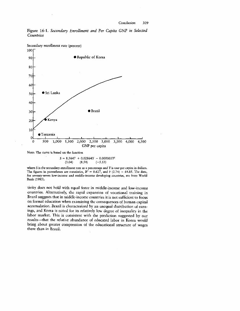
Conclusion 309
Figure 16-1. Secondary Enrollment and Per Capita GNP in SelectedCountries
Secondary enrollment rate (percent)
100 _
90 _ *Republic of Korea
80 _
70
60 _
50_ 0 Sri Lanka
40 -
30 - / * Brazil
10 _/ey
* Tanzania
0 500 1,000 1,500 2,000 2,500 3,000 3,500 4,000 4,500GNP per capita
Note: The curve is based on the function
S = 8.5647 + 0.02864Y - 0.000003Y1(3.04) (8.54) (-5.53)
where S is the secondary enrollment rate as a percentage and Y is GNP per capita in dollars.The figures in parentheses are t-statistics, R2 = 0.627, and F (2.74) = 64.85. The data,for seventy-seven low-income and middle-income developing countries, are from WorldBank (1985).
tivity does not hold with equal force in middle-income and low-incomecountries. Alternatively, the rapid expansion of vocational training inBrazil suggests that in middle-income countries it is not sufficient to focuson formal education when examining the consequences of human capitalaccumulation. Brazil is characterized by an unequal distribution of earn-ings, and Korea is noted for its relatively low degree of inequality in thelabor market. This is consistent with the prediction suggested by ourresults-that the relative abundance of educated labor in Korea wouldbring about greater compression of the educational structure of wagesthere than in Brazil.
310 CONCLUSION
Our study of Kenya and Tanzania suggests that the marked differencebetween Korea and Brazil in education policy will have little impact onintergenerational mobility. The distribution of secondary education isundoubtedly more equal in Korea, but if our model applies, children ofbetter-educated parents will be disproportionately concentrated in theupper half of the distribution of cognitive achievement on completion ofsecondary education. This in turn would give them an advantage in thecompetition for access to higher education and in the labor market,thereby preserving the position of the educated elite from one generationto the next. A qualification is in order: in Kenya and Tanzania educationis virtually the only means of access to the top of the socioeconomic hier-archy, but in Latin America and East Asia, where physical capital andfinancial wealth are more abundant and often concentrated, socioeco-nomic success may depend more on the transmission of these forms ofwealth or on the access they provide to higher education irrespective ofacademic achievement.
Although our ability to generalize our findings in East Africa may belimited, we are confident that the exploitation of other natural experi-ments would lead to sounder generalizations about the relationships be-tween education and development. The best natural experiment is onein which the comparator countries are as similar as possible in many re-spects but differ markedly in the aspects being studied. A series of naturalexperiments, illustrated in figure 16-1 by the set of countries discussedabove, would permit generalizations of the sort we are seeking. In Kenyaand Tanzania, where most postprimary leavers have been absorbed intourban wage employment, it was possible to confine the research instru-ments to the urban wage sectors. In the other countries mentioned, thesame set of questions probably requires research instruments that alsocover the urban informal sector and the rural sector.
In seeking to discover uniformities in economic behavior as they relateto education by comparing economies which differ either in income orin educational level but not in both, we would be extending a well-established mode of cross-country analysis that includes the work ofKuznets (1965) and Chenery (1979). Our comparative approach, how-ever, is much more disaggregated; our focus is more exclusively on edu-cation, and our sample contains fewer countries. Although greaterdisaggregation necessarily involves a smaller number of countries andsome loss of generality, it permits the rigorous testing of more detailedhypotheses and more direct application of results to policy.
Our small-sample comparison is in the tradition of the comparativestudies of industrialization by Balassa and others (1971), Bhagwati(1978), Krueger (1978), and Little, Scitovsky, and Scott (1970). It differsfrom such studies not only in its emphasis but also in its sources of data.The data requirements for an in-depth analysis of the relationships be-
Conclusion 311
tween human capital accumulation and labor productivity, income distri-bution, and intergenerational mobility are substantial. The only way tosatisfy these requirements is to administer specially designed sample sur-veys in each country and thus generate precisely comparable microeco-nomic data sets. This combination-the comparison of countries thatconstitute natural experiments and the rigorous analysis made possibleby survey data-may prove fruitful not only for the economics of educa-tion but also for the study of other issues in the economics of developingcountries. It has potential application wherever there is a need to exam-ine the influence of national policies by means of microeconomic dataanalysis.

I

APPENDIXES

APPENDIX A
The Surveys: Coverage,Sampling, Procedures, and
Some Cautionary Tales
OUR OBJECT IN THIS APPENDIX is to persuade the reader that our dataare reliable by explaining how the survey was designed and the informa-tion gathered. In addition, our methods may be helpful to researcherswho are considering the use of sample surveys to generate primary data.The questions that our research addressed could not have been answeredwithout generating new data sets that contained information on repre-sentative samples of individual workers. Survey design and sampling pro-cedure are rather neglected in the training of most economists; such activ-ities have too often been regarded as more within the province ofsociologists. But the quality of economic research such as ours dependscrucially on the design and implementation of the survey. The issues wewanted to explore gave us a fairly clear set of objectives for our fieldworkand data requirements. This appendix describes how, in the best eco-nomic tradition, we set about maximizing those objectives, subject to thetriple constraints of finance, researchers' time, and the logistic problemstypical of most developing countries.
There were times when we regretted our relative innocence about sur-vey work in developing countries. For those readers intrepid enough toundertake similar field-intensive research, this detailed account of our ex-periences may therefore be of particular interest. Figure A-1, whichshows the sequencing and timing of the many activities involved, maybe a useful aid in planning a survey. A realistic vision of what is entailedin fieldwork in developing countries suggests that careful planning is nec-essary but not sufficient and that a robust sense of humor is essential.
The Pre-Survey Field Trip
Within two months after securing funding for the project, the principalresearchers made a preparatory field trip, spending about eight man-
315
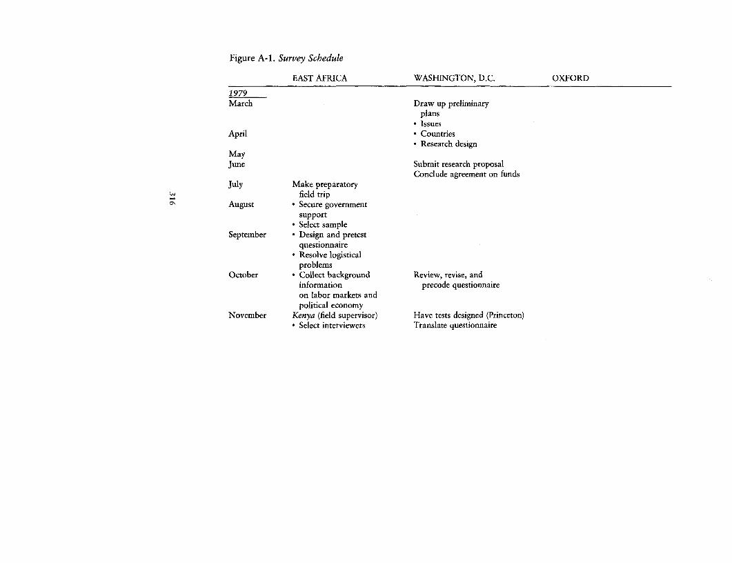
Figure A-1. Survey Schedule
EAST AFRICA WASHINGTON, D.C. OXFORD
1979March Draw up preliminary
plans* Issues
April * Countries* Research design
MayJune Submit research proposal
Conclude agreement on fundsJuly Make preparatory
field tripON August * Secure government
support* Select sample
September * Design and pretestquestionnaire
* Resolve logisticalproblems
October * Collect background Review, revise, andinformation precode questionnaireon labor markets andpolitical economy
November Kenya (field supervisor) Have tests designed (Princeton)* Select interviewers Translate questionnaire
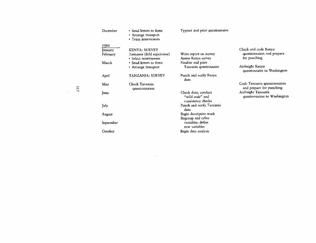
December * Send letters to firms Typeset and print questionnaire* Arrange transport* Train interviewers
1980January KENYA: SURVEY Check and code KenyaFebruary 1Tanzania (field supervisor) Write report on survey questionnaires and prepare
* Select interviewers Assess Kenya survey for punchingMarch * Send letters to firms Finalize and print
* Arrange transport Tanzania questionnaire Airfreight Kenyaquestionnaire to Washington
April TANZANIA: SURVEY Punch and verify Kenyadata
May Check Tanzania Code Tanzania questionnairesquestionnaires and prepare for punching
June Check data; conduct Airfreight Tanzania"wild code" and questionnaires to Washingtonconsistency checks
July Punch and verify Tanzaniadata
August Begin descriptive workRegroup and refine
September variables; definenew variables
October Begin data analysis
318 APPENDIX A
weeks in Kenya and about five in Tanzania. There were five main tasks:to obtain the approval and support of the two governments; to select theestablishments to be surveyed; to design and pretest the questionnaires;to resolve various logistic issues regarding the administration of the sur-veys; and to gather background information and data on labor markettrends and performance and on the political economy of educational ex-pansion and wage determination in Kenya and Tanzania.
Government support was crucial to the project. In both Kenya andTanzania research of this sort must be approved by the government. Inaddition, we expected that a government request for cooperation by theestablishments sampled would improve the response rate. The ministriesthat we decided to approach were Finance and Planning and Educationin both countries and Manpower Development in Tanzania. We includedthe ministries of Finance and Planning because of their reputation for rel-ative impartiality on educational sector issues, for efficiency, and for in-fluence on policy and because of their close relationship with the statisti-cal offices. Representatives of the World Bank in each country wrote onour behalf to the heads of the ministries of Finance and Planning-thepermanent secretary in Kenya and the principal secretary in Tanzania-and gave them brief written descriptions of the proposed research. Teammembers then met government representatives, who agreed to write let-ters of introduction to be sent to the employers whose participation wasrequired. We emphasized the potential usefulness of our research forpolicy, and it was this aspect that particularly interested the governmentofficials.
The director of the bureau of statistics in each country gave permissionfor the team to use an official list of establishments as a sampling frame.The establishments were selected on criteria that are explained below.Even with the help of official statisticians, selection was a tedious andtime-consuming task. The existing lists of establishments were not com-plete, and in some cases the information we needed to stratify our sampleby establishment size was missing.
Preparation of the questionnaire benefited from the fact that one ofthe authors (Sabot) had conducted similar research in Tanzania ten yearspreviously. In both countries the questionnaire was discussed with socialscientists and educationalists, whose knowledge of local institutions andconditions was useful. A small pilot survey led to some changes in thequestions and helped us decide on the answer categories to be used inprecoding the questionnaires.
It was essential to find someone in each country who would be on thespot for two months before the survey, during the survey itself, and forabout a month afterward. The research team could spend only a limitedtime in the field, and many planning and follow-up tasks had to be com-
The Surveys: Coverage, Sampling, and Procedures 319
pleted. In Tanzania a doctoral student who had worked for several yearsin Tanzania and who spoke Kiswahili was chosen as the principal admin-istrator. It was arranged that he be based at the Economic ResearchBureau of the University of Dar es Salaam. Our principal researcherin Kenya was a visiting academic at the Institute of DevelopmentStudies of the University of Nairobi who had spent several years con-ducting research in Kenya. This affiliation with the universities wasimportant to the success of the survey. Because of the close liaison weestablished with them, we gained a base for our operation, help in re-cruiting university students as interviewers, and, in one case, transportfacilities.
Several other practical tasks were tackled. The establishments to be vis-ited were located on large-scale maps of the cities to facilitate the compli-cated logistics of transport planning. Arrangements were made for thefleet of vehicles necessary for transporting the researchers and interview-ers during the survey.
As part of the background work on the political economy of educa-tional expansion, wage determination, and the operation of the labormarket, officials and academics were interviewed in both countries. Pub-lished data were obtained, and arrangements were made with the bureauof statistics in each country for access to data generated by other sur-veys.
Survey Coverage and Design
An establishment-based two-stage random sample survey, stratified bysector and establishment size, was carried out in the capital city of eachcountry. The Nairobi survey was done in January 1980 and the Dar esSalaam survey in April 1980.
The Sample Universe
The choice of an establishment survey rather than a household surveyrequires some explanation because of the limitations in the coverage ofdata derived in this way. In particular, workers outside formal wage em-ployment are not represented in establishment-based surveys. But the na-ture of the data to be collected made a survey of establishments ratherthan households preferable, for six main reasons.
* Most important, an establishment survey is the natural source ofdata for a project that is concerned with employment and the in-comes generated by employment. The principal concern of ourstudy was with adjustments in the labor market brought about by
320 APPENDIX A
growth in the supply of workers with secondary education in the1960s and 1970s. During this period nearly all of those withpostprimary education were absorbed into urban wage employ-ment.
* A much larger household survey would have been necessary to yieldas many as 1,700 employees.
* Interviews would have had to have been conducted at night, andmost people are more eager to interrupt their work than their din-ner. Such considerations, other economies of scale, and more readi-ly available sampling frames make establishment surveys less costlyto administer.
* Data on wages and on occupation are likely to be more accuratelycollected from an establishment-based survey than from a house-hold-based survey because confirmatory information can be ob-tained directly from the employer. The enquiry therefore does notrely solely on the recollection of the employee, and answers aremuch more easily checked and elaborated when information isbeing collected simultaneously from a number of employees withinthe same establishment.
* Characteristics of the employer are sometimes relevant variables inthe relationships under investigation and are better collected fromestablishments.
* The surveys would be comparable with a 1971 establishment-basedsurvey of about 1,000 Tanzanian wage employees in the manufac-turing sector.
Because rural workers and the urban self-employed and unemployedwere excluded from the survey, we were unable to explore the impactof education on, for example, decisions about participation in the laborforce and the probability of unemployment. But economics is alwaysabout choice, and, given our objectives, the limitations were not too con-fining.
The surveys were conducted only in the capital cities because of surveyefficiency and cost, because of the economic dominance of the capitals,and because previous labor market survey work in Tanzania had sug-gested that the capital adequately represented urban areas with respectto relevant wage employment characteristics (Sabot 1979). Sabot foundthat the relative percentage of migrants and city-born persons and theage on arrival of migrants were the same in Dar es Salaam as in the sixnext largest towns considered together. His earnings function analysisshowed that there was no substantial difference in the level and structureof wages between the capital city and the other principal towns.

The Surveys: Coverage, Sampling, and Procedures 321
The Questionnaire
CONTENT. The questionnaire, which is reproduced in appendix B, con-tains several sections on personal characteristics, family background, re-spondents' education, rural-urban links, education of children, earnings,training, employment experience in the establishment, and previous em-ployment experience. Not all sections were relevant to all workers. In ad-dition, reasoning ability and cognitive skill tests were administered to asubsample of respondents. These tests are explained and discussed in ap-pendix C.
The questions about the worker's personal characteristics were askedfirst, in accord with normal interview conventions of politeness. Theseand the questions about family background, which came next, helped putrespondents at ease and reassured them that the questions would not bedifficult. The family background questions concerned parents' education,occupation, and landholding.
Detailed information on the respondents' own education included thetype of schooling, details of certification, public examination results,postschool training, and trade tests. Perceptions of the value of educationwere elicited in the context of the workers' aspirations and intentionsconcerning their children's education. Questions on the education ofthe respondents' children (including data on costs) allowed a three-generation educational history to be put together.
It is difficult to collect accurate data on earnings. Respondents may de-liberately misrepresent their earnings-perhaps overstating them to im-press the interviewer or understating them as a precaution against incometax consequences. They may fail to understand the exact nature of theinformation that is wanted. Should gross or net earnings be reported?Should nonpecuniary benefits be included? What of income from othersources? The survey asked for the amount of the last pay packet and spe-cifically about each of the components of the remuneration package:bonus payments, overtime payments, tax and other deductions, andhousing, pension, transport, and medical benefits. As a check on consis-tency the same information was elicited from employers where it wasreadily available. Despite our care, interviewers were not always able torecord consistent figures. Some workers knew what their take-home payhad been, but others gave a gross figure. We were able to construct aconsistent net income variable afterward by using the data on deductionsand benefits and the information provided by some employers and bycomparing the answers of workers in the same establishment. The layoutof the earnings question was modified somewhat in the Tanzanian ques-tionnaire to reduce the difficulties encountered in Kenya.
Questions on employment experience in the current establishment con-
322 APPENDIX A
cerned how the job application had been made, the details of any traininggiven, changes in wages, status, and skill level, and the relationship be-tween the worker's education and the educational requirements of thejob. Details of the worker's employment history were gathered. Ques-tions were asked about the duration and nature of previous jobs, activi-ties while out of wage employment, and reasons for leaving jobs.
The occupation of the respondent was described with regard to bothcurrent and previous employment. The classification of occupation is dis-cussed in detail in appendix E.
The questions on rural links covered the size of landholdings, inputsof time and money, remittances and how they were used, and whetherrespondents planned to return to a rural area. Migrants were asked abouttheir first income and first job search in the city.
DESIGN. According to Casley and Lury (1981, p. 92), "There is nodoubt that questionnaire design is often the worst executed stage of sur-vey preparations." The questionnaire is the crucial medium by whichdata are communicated from respondents to the computer, and its designmust minimize the "noise" that can distort the process.
Our questionnaires were printed in both English and Kiswahili. Theywere translated from English into classical coastal Kiswahili by a Ki-swahili speaker in Washington, D.C., and were translated back by an-other person to check that the original sense had not been changed. Somelater adjustments had to be made to the questionnaire for Nairobi, wherea more colloquial Kiswahili tends to be spoken. Respondents couldchoose which language to use in interviews.
We attempted to phrase the questions in a clear and simple way so thatthe respondents were not in any doubt as to what was being asked. Thepilot survey conducted during the field trip was helpful in revealing andeliminating ambiguities and unfamiliar terms.
Particular care was taken with the layout and appearance of the ques-tionnaires, for the sake both of the interviewers and of data quality.Casley and Lury (1981, p. 92) are emphatic about this:
[The interviewer] is expected to produce results of a high standard inarduous conditions, and can legitimately expect that some attentionis paid to his convenience and that his working materials are of reason-able quality ... Many apparently minor, but actually important, de-tails require concern for the enumerator's convenience, and more thanrepay the time and effort taken by leading to better quality . . . data.
The questionnaires were typeset and were printed on good-qualitypaper. The result was more impressive, neater, and more easily read thana typed and duplicated copy would have been. The difference in qualityis well worth the additional cost that printing may involve, but if the print
The Surveys: Coverage, Sampling, and Procedures 323
run is large, the difference in cost is unlikely to be a consideration. Ingeneral, printing on only one side of the paper is preferable, but we de-cided to print on both sides to reduce bulk and air freight charges. Wedid not look for any false economies in layout, since we were mindfulthat "a cluttered, badly laid out appearance . . . will almost certainly leadto poor recording" (Casley and Lury 1981, p. 91). Adequate space wasallowed for writing the answers and for any additional explanatory re-marks that might prove necessary.
The questions were precoded; that is, all of the anticipated answersto each question were listed and were assigned numbers so that inter-viewers could mark the appropriate number rather than having to writeout an answer. An extra category, "other," was generally included forunanticipated answers. If this was used, the interviewer had to explainwhat it represented so that additional codes could subsequently be cre-ated where they proved relevant. Boxes for recording the coded answerwere provided to the right of each question. The layout and precodingsaved time in the preparation of the data, reduced coding errors, andminimized problems with reading interviewers' handwriting. The pre-coded categories helped to avoid vague and imprecise answers and im-proved the consistency of the data.
Sample Selection
The Sampling Frame
The sampling frame provided by the government bureau of statistics wasthe full list of establishments in each capital city, compiled for the annualEnumeration of Employees in Kenya and the annual Survey of Employ-ment and Earnings in Tanzania. In principle, all employing establish-ments with fixed addresses, in both the private and the public sectors,were covered. Very small employers were likely to be underrepresentedbecause they sometimes have no fixed address and because many aretransient and are poor correspondents. Our one amendment to the sam-pling frame was that we decided to exclude establishments that employedfewer than five people, since their small share in total urban employmentdid not warrant the significant burden that their inclusion would add tothe survey.
The most recent list of establishments in each country was for 1978.Returns submitted by establishments in the previous two years were alsoavailable. In neither case was the sampling frame complete. Exact sam-pling procedures differed between the two countries depending on theparticular problems of the incomplete sampling frames and the form inwhich information was available.
324 APPENDIX A
In Tanzania nonresponse to the 1978 employment survey by firms onthe list of establishments was a high 45 percent, which had serious impli-cations for official employment statistics. To cope with the additionalsampling problems this posed, we drew a 10 percent random sample ofall listed establishments, including the nonrespondents, to use as oursampling frame. Since we were stratifying by establishment size, we hadto know the size group for the establishments. Returns submitted in 1977or 1976 by some of the 1978 nonrespondent establishments sufficed.About half of the rest were contacted by telephone to confirm their exis-tence and size. This minimized the number of establishments that hadto be excluded from the sampling frame.
In Kenya 20 percent of listed establishments had not returned the 1978census forms and were excluded from the sampling frame. A table wasconstructed of response rates by size group of the establishments that hadreported in at least one but not all three years. Larger establishments(particularly those with over 300 employees) seemed to have a slightlylower response rate, but the relationship was weak, and correcting forit was not worthwhile. The exclusion of Kenyan nonresponders is un-likely to bias the sample to any extent. No direct information could beobtained on the size of establishments that had not responded in any ofthe three years, but the opinion of the Central Bureau of Statistics wasthat they were either very small or had ceased to operate.
The list of more than 10,000 Kenyan establishments was not stratifiedby size and did not list Nairobi establishments separately. Since the Nai-robi establishments were classified by activity only, their size distributionhad to be estimated from the national size distribution under the assump-tion that the size distribution of establishments within each activity wasthe same in Nairobi as nationally. The size distribution of establishmentswith between five and forty-nine employees was inferred in this way; ac-tual size data for establishments with more than forty-nine employeeswere taken from the Survey of Employment and Earnings list.
Drawing the Sample,
SAMPLING METHODS AND CONSTRAINTS. The sample in each countryhad to be large enough to satisfy tests of statistical significance on theinferences to be drawn from the data analysis and to yield adequate cellsizes when the sample was disaggregated into subgroups by several keyvariables simultaneously. We judged that a sample of 1,500 would beneeded to permit reliable inferences and generalizations. Both of oursamples exceed this minimum acceptable size. It seemed reasonable tointerview more people from bigger establishments but unreasonable tointerview more than sixty people in any one establishment. These con-
The Surveys: Coverage, Sampling, and Procedures 325
straints, and those of time and manpower, imposed a maximum numberof about seventy establishments and 2,000 respondents.
There were constraints on completely random selection. So thatintertemporal comparisons could be made, the Tanzanian sample in-cluded twenty-five manufacturing establishments that had been surveyedin 1971. Three firms with establishments in both countries were includedto permit detailed intercountry comparisons of the composition of thework force and the structure of wages after we controlled for differencesin products, processes, and the way in which skills are categorized. Civilservice workers-from the Central Bureau of Statistics, the Ministry ofTransport workshops, and the Ministry of Education headquarters-were included to ensure that a range of occupations was represented andthat the employees were geographically concentrated. Employees fromthese ministries were mainly clerks, manual workers, and bureaucrats,respectively. In each country workers from the headquarters andworkshops of two public utilities-the railways and the post and tele-communications corporation-were also included.
The samples were stratified on the basis of sector-that is, manu-facturing, government, and other nonmanufacturing-and, except forgovernment, on the basis of size, as measured by the number of employ-ees, both regular and casual. Stratification by ownership sector was nec-essary because pay policies differ significantly between sectors. The smallnumber of establishments in the highest size category and the importanceof government in that group made it advisable to sample government sep-arately.
The manufacturing sector was deliberately oversampled-it accountedfor about one-half of each sample-to ensure a large enough number ofmanufacturing workers for time-series comparison with the 1971 Tan-zanian data. Manufacturing was therefore sampled separately.
A two-stage random sample was drawn. Establishments were ran-domly chosen (with some exceptions in Tanzania, as explained below)at the first stage, and employees were then randomly selected within eachestablishment. Usually the firm management could supply a list of em-ployees to use as a sampling frame. Where this list grouped workers bydepartment or skill level, a rough-and-ready sort of stratification waspossible. On occasion we simply had to pick workers from the factoryfloor. We tried to avoid bias in this selection, but with perhaps ten inter-viewers waiting for us, selection procedures had to be simple and quick.An observation by Casley and Lury (1981, p. 7.8) is relevant here: "Webelieve that there has often been too much preoccupation with minorsubtleties of sample design, and that the relative weight given to practicalsurvey problems has been far too slight."
One sort of practical problem that Casley and Lury perhaps did not
326 APPENDIX A
envisage was the unexpected exposure to the elements that we experi-enced while sampling in Tanzania. The roof of the Central Bureau of Sta-tistics had been partly removed in the course of being replaced. This leftus at the mercy of the elements and necessitated occasional desperate de-fensive clutches at our piles of papers.
SAMPLING DETAILS FOR EACH COUNTRY
* Kenya. After the number of employees to be sampled from eachestablishment-size category in each sector was known, it was necessaryto decide on the number of establishments from which the respondentswould be drawn. This required decisions on the ratio of respondents toemployees within each sampled establishment-that is, on the samplingfraction. Once the sampling fractions had been decided, the establish-ments with fewer than 200 employees were drawn randomly from thealphabetical list. Random selection was ensured by the following proce-dure. The Kenyan list covered 1,100 pages. If twenty-five establishmentsof a size group were required, the first establishment listed on the twenty-second page that was of the desired size and had responded to the mostrecent official census of establishments was selected, and then the firstsuch establishment on every forty-fourth page thereafter was chosen(1,100/25 = 44). The larger establishments (more than 200 employees)were listed separately by size group. If one-sixteenth of the group wasrequired, the eighth establishment and every sixteenth establishmentthereafter were selected. If a selected establishment was a nonresponder,the next listed one was substituted.
This produced a short list from which the final sample of establish-ments was chosen. The sampling fraction dictated the number of employ-ees to be selected from each establishment. Establishments were addeduntil the desired sample size had been reached. For example, 115 workersfrom Kenyan nonmanufacturing establishments with 20-49 workerswere wanted. With a sampling fraction of 0.75, the first five of the sixshort-listed establishments provided 117 workers. In some cases the pro-posed sampling fraction would have yielded a sample rather different insize from that planned, since increments to the sample were discontinu-ous. In such cases the sampling fraction was revised to yield an actualsample equal to that desired. For establishments of S00 or more employ-ees the sample was set at 60, and so the sampling fraction was not used.
Table A-1 shows the sampling fractions and establishment samplesize-that is, the average number of respondents expected from each es-tablishment. Table A-2 shows the number of individuals and establish-ments sampled at the second stage. The three government ministries areincluded with the nonmanufacturing establishments, although they weresampled separately.
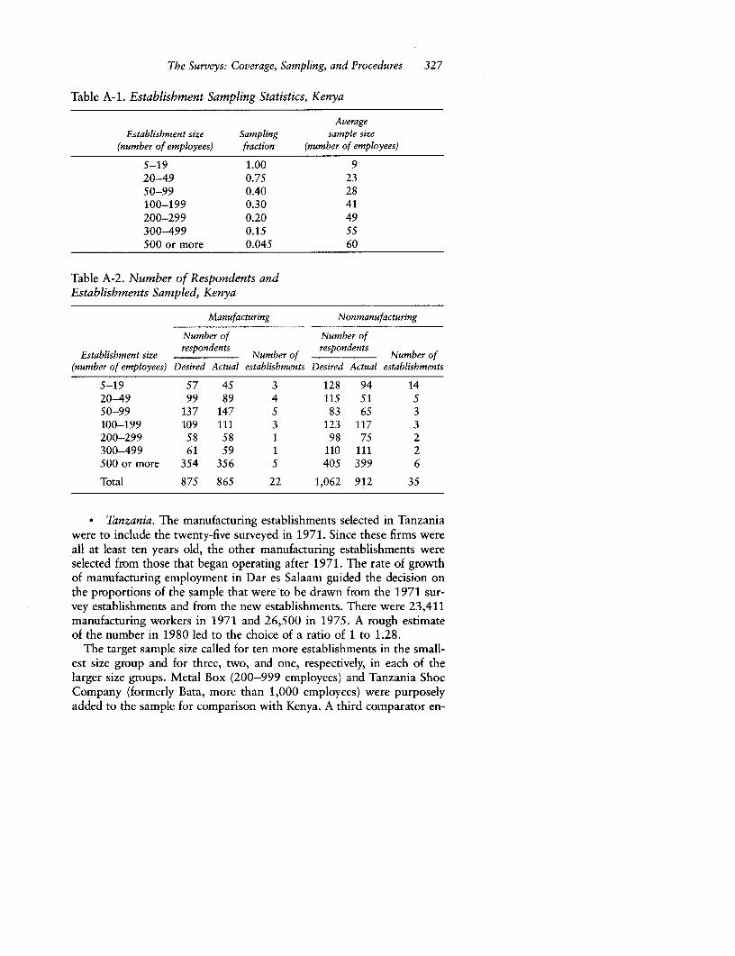
The Surveys: Coverage, Sampling, and Procedures 327
Table A-1. Establishment Sampling Statistics, Kenya
AverageEstablishment size Sampling sample size
(number of employees) fraction (number of employees)
5-19 1.00 920-49 0.75 2350-99 0.40 28100-199 0.30 41200-299 0.20 49300-499 0.15 55500 or more 0.045 60
Table A-2. Number of Respondents andEstablishments Sampled, Kenya
Manufacturing Nonmanufacturing
Number of Number ofEstablishment si .ze respondents respondents
Estabbsb___________ Number of Number of
(number of employees) Desired Actual establishments Desired Actual establishments
5-19 57 45 3 128 94 1420-49 99 89 4 115 51 550-99 137 147 5 83 65 3100-199 109 111 3 123 117 3200-299 58 58 1 98 75 2300-499 61 59 1 110 111 2500 or more 354 356 5 405 399 6
Total 875 865 22 1,062 912 35
Tanzania. The manufacturing establishments selected in Tanzaniawere to include the twenty-five surveyed in 1971. Since these firms wereall at least ten years old, the other manufacturing establishments wereselected from those that began operating after 1971. The rate of growthof manufacturing employment in Dar es Salaam guided the decision onthe proportions of the sample that were to be drawn from the 1971 sur-vey establishments and from the new establishments. There were 23,411manufacturing workers in 1971 and 26,500 in 1975. A rough estimateof the number in 1980 led to the choice of a ratio of 1 to 1.28.
The target sample size called for ten more establishments in the small-est size group and for three, two, and one, respectively, in each of thelarger size groups. Metal Box (200-999 employees) and Tanzania ShoeCompany (formerly Bata, more than 1,000 employees) were purposelyadded to the sample for comparison with Kenya. A third comparator en-
328 APPENDIX A
terprise, Tanzania Cigarette Company (formerly BAT), was one of thetwenty-five visited in 1971. This left ten establishments of 5-49 employ-ees, three of 50-199 employees, and one of 200-999 employees to besampled randomly to complete the manufacturing subsample.
The ratio of public service employees to other nonmanufacturingworkers was to be 300 to 700, corresponding to the proportions of em-ployees in the public services and nonmanufacturing enterprise sectorsrecorded in Dar es Salaam in 1976. As in Kenya, three government minis-tries and two public utilities were included. Additional establishments inthe other nonmanufacturing category were randomly drawn from thesampling frame.
In the second stage of the sampling the number of employees to be in-terviewed in each enterprise was decided. Seventy-five employees were tobe randomly sampled from each of the three government ministries, and,to generate a large enough subsample, seventy-five employees were to beinterviewed in each of the three comparator establishments. The rest ofthe employees were to be randomly sampled from the selected enterpriseswith the use of the sampling fractions shown in table A-3. The minimumand maximum conditions imply that all employees in an enterprise of 12or fewer workers would be interviewed, that an establishment with fewerthan 104 employees would provide 12 respondents, that one with be-tween 104 and 480 employees would provide one-eighth of its employees,and that those with more than 480 employees would provide 60 respon-dents.
Table A-4 shows the planned and final samples, with governmentincluded in nonmanufacturing. The large discrepancies between theplanned and actual samples in the 200-999 size groups arose becausethe Coca-Cola establishment was listed in the sampling frame as non-manufacturing but was in fact a production plant.
The actual samples (which differed a little from the final planned sam-ples of tables A-2 and A-4) consisted of 1,749 people in sixty-three estab-lishments in Tanzania and 1,777 people in fifty-seven establishments inKenya.
Table A-5 lists the establishments sampled in each country.
Conducting the Surveys
The Initial Contact with the Establishments
Once the sample had been selected, letters from the team and from thegovernment ministry were sent to the establishments (figure A-2). Theletters explained that a "study of the labor market consequences of edu-cational expansion' was being carried out by the World Bank team with
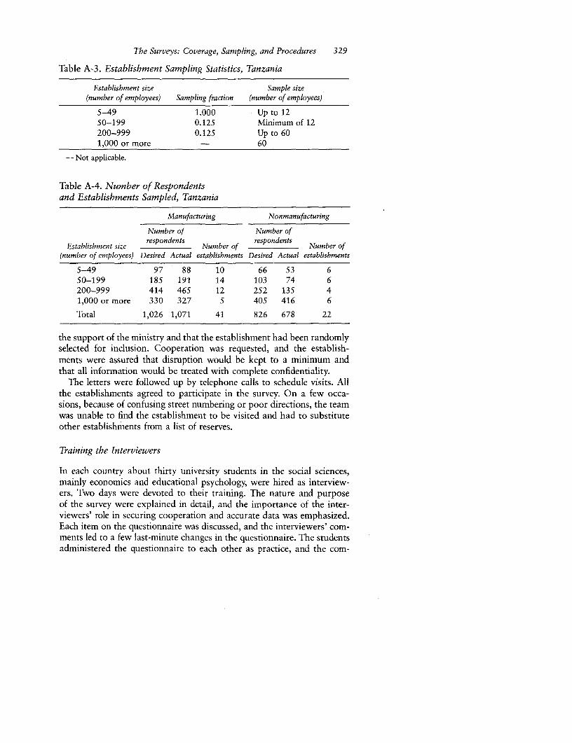
The Surveys: Coverage, Sampling, and Procedures 329
Table A-3. Establishment Sampling Statistics, Tanzania
Establishment size Sample size(number of employees) Sampling fraction (number of employees)
5-49 1.000 Up to 1250-199 0.125 Minimum of 12200-999 0.125 Up to 601,000 or more - 60
-Not applicable.
Table A-4. Number of Respondentsand Establishments Sampled, Tanzania
Manufacturing Nonmanufacturing
Number of Number ofEstablishment si'ze respondents respondents
Establgshent sizeNumber of Number of(number of employees) Desired Actual establishments Desired Actual establishments
5-49 97 88 10 66 53 650-199 185 191 14 103 74 6200-999 414 465 12 252 135 41,000 or more 330 327 S 405 416 6
Total 1,026 1,071 41 826 678 22
the support of the ministry and that the establishment had been randomlyselected for inclusion. Cooperation was requested, and the establish-ments were assured that disruption would be kept to a minimum andthat all information would be treated with complete confidentiality.
The letters were followed up by telephone calls to schedule visits. Allthe establishments agreed to participate in the survey. On a few occa-sions, because of confusing street numbering or poor directions, the teamwas unable to find the establishment to be visited and had to substituteother establishments from a list of reserves.
Training the Interviewers
In each country about thirty university students in the social sciences,mainly economics and educational psychology, were hired as interview-ers. Two days were devoted to their training. The nature and purposeof the survey were explained in detail, and the importance of the inter-viewers' role in securing cooperation and accurate data was emphasized.Each item on the questionnaire was discussed, and the interviewers' com-ments led to a few last-minute changes in the questionnaire. The studentsadministered the questionnaire to each other as practice, and the com-
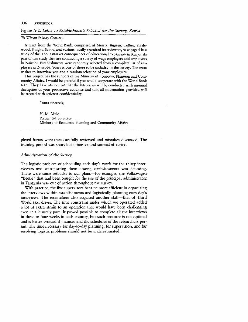
330 APPENDIX A
Figure A-2. Letter to Establishments Selected for the Survey, Kenya
To Whom It May Concern
A team from the World Bank, comprised of Messrs. Bigsten, Collier, Hazie-wood, Knight, Sabot, and various locally recruited interviewers, is engaged in astudy of the labour market consequences of educational expansion in Kenya. Aspart of this study they are conducting a survey of wage employers and employeesin Nairobi. Establishments were randomly selected from a complete list of em-ployers in Nairobi. Yours is one of those to be included in the survey. The teamwishes to interview you and a random selection of your employees.
This project has the support of the Ministry of Economic Planning and Com-munity Affairs. I would be grateful if you would cooperate with the World Bankteam. They have assured me that the interviews will be conducted with minimaldisruption of your productive activities and that all information provided willbe treated with strictest confidentiality.
Yours sincerely,
H. M. MulePermanent SecretaryMinistry of Economic Planning and Community Affairs
pleted forms were then carefully reviewed and mistakes discussed. Thetraining period was short but intensive and seemed effective.
Administration of the Survey
The logistic problem of scheduling each day's work for the thirty inter-viewers and transporting them among establishments was daunting.There were some setbacks to our plans-for example, the Volkswagen"Beetle" that had been bought for the use of the principal administratorin Tanzania was out of action throughout the survey.
With practice, the five supervisors became more efficient in organizingthe interviews within establishments and logistically planning each day'sinterviews. The researchers also acquired another skill-that of ThirdWorld taxi driver. The time constraint under which we operated addeda lot of extra strain to an operation that would have been challengingeven at a leisurely pace. It proved possible to complete all the interviewsin three to four weeks in each country, but such pressure is not optimaland is better avoided if finances and the schedules of the researchers per-mit. The time necessary for day-to-day planning, for supervision, and forresolving logistic problems should not be underestimated.
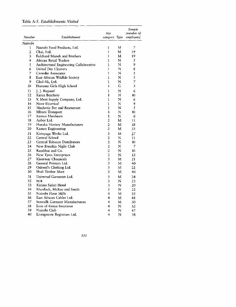
Table A-S. Establishments Visited
SampleSize (number of
Number Establishment category Type employees)
Nairobi1 Nairobi Food Products, Ltd. I M 72 Chai, Ltd. 1 M 193 Fulchard Manek and Brothers 1 M 194 African Retail Traders 1 N 55 Architectural Engineering Collaborative 1 N 96 United Dry Cleaners 1 N 87 Crowder Associates 1 N 58 East African Wildlife Society 1 N 59 Glad-Ak, Ltd. 1 N 7
10 Huruma Girls High School 1 G 3
11 J. J. Ruparel 1 N 612 Karen Butchery 1 N 1013 K Meat Supply Company, Ltd. 1 N 614 Noor Electrical 1 N 915 Macharia Bar and Restaurant 1 N 516 Mbura Transport 1 N 1017 Ramco Hardware 1 N 618 Anbee Ltd. 2 M 1119 Haraka Hosiery Manufacturers 2 M 1820 Kamco Engineering 2 M 33
21 Kirinyaga Works Ltd. 2 M 2722 Central School 2 N 1123 Central Tobacco Distributors 2 N 1024 New Rwathia Night Club 2 N 725 Rambhai and Co. 2 N 1026 New Tyres Enterprises 2 N 1327 Kleenway Chemicals 3 M 2128 General Printers Ltd. 3 M 4029 Oshwal's Clothing Ltd. 3 M 2230 Shah Timber Mart 3 M 40
31 Universal Garments Ltd. 3 M 2432 NCR 3 N 2333 Kirima Safari Hotel 3 N 2034 Murdoch, McRae and Smith 3 N 2235 Nairobi Flour Mills 4 M 3336 East African Cables Ltd. 4 M 4837 Intersilk Garment Manufacturers 4 M 3038 Lion of Kenya Insurance 4 N 3239 Nairobi Club 4 N 4740 Livingstone Registrars Ltd. 4 N 38
331
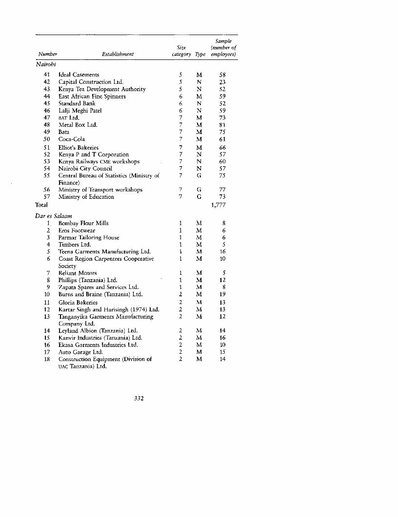
SampleSize (number of
Number Establishment category Type employees)
Nairobi
41 Ideal Casements 5 M 5842 Capital Construction Ltd. 5 N 2343 Kenya Tea Development Authority 5 N 5244 East African Fine Spinners 6 M 5945 Standard Bank 6 N 5246 Lalji Meghi Patel 6 N 5947 BAT Ltd. 7 M 7348 Metal Box Ltd. 7 M 8149 Bata 7 M 7550 Coca-Cola 7 M 61
51 Elliot's Bakeries 7 M 6652 Kenya P and T Corporation 7 N 5753 Kenya Railways CME workshops 7 N 6054 Nairobi City Council 7 N 5755 Central Bureau of Statistics (Ministry of 7 G 75
Finance)56 Ministry of Transport workshops 7 G 7757 Ministry of Education 7 G 73
Total 1,777
Dar es Salaam1 Bombay Flour Mills 1 M 82 Eros Footwear 1 M 63 Parmar Tailoring House 1 M 64 Timbers Ltd. 1 M 55 Teena Garments Manufacturing Ltd. 1 M 166 Coast Region Carpenters Cooperative 1 M 10
Society7 Reliant Motors 1 M 58 Phillips (Tanzania) Ltd. 1 M 129 Zapata Spares and Services Ltd. 1 M 8
10 Burns and Braine (Tanzania) Ltd. 2 M 19
11 Gloria Bakeries 2 M 1312 Kartar Singh and Harisingh (1974) Ltd. 2 M 1313 Tanganyika Garments Manufacturing 2 M 12
Company Ltd.14 Leyland Albion (Tanzania) Ltd. 2 M 1415 Kanvir Industries (Tanzania) Ltd. 2 M 1616 Ekasa Garments Industries Ltd. 2 M 1017 Auto Garage Ltd. 2 M 1518 Construction Equipment (Division of 2 M 14
UAC Tanzania) Ltd.
332
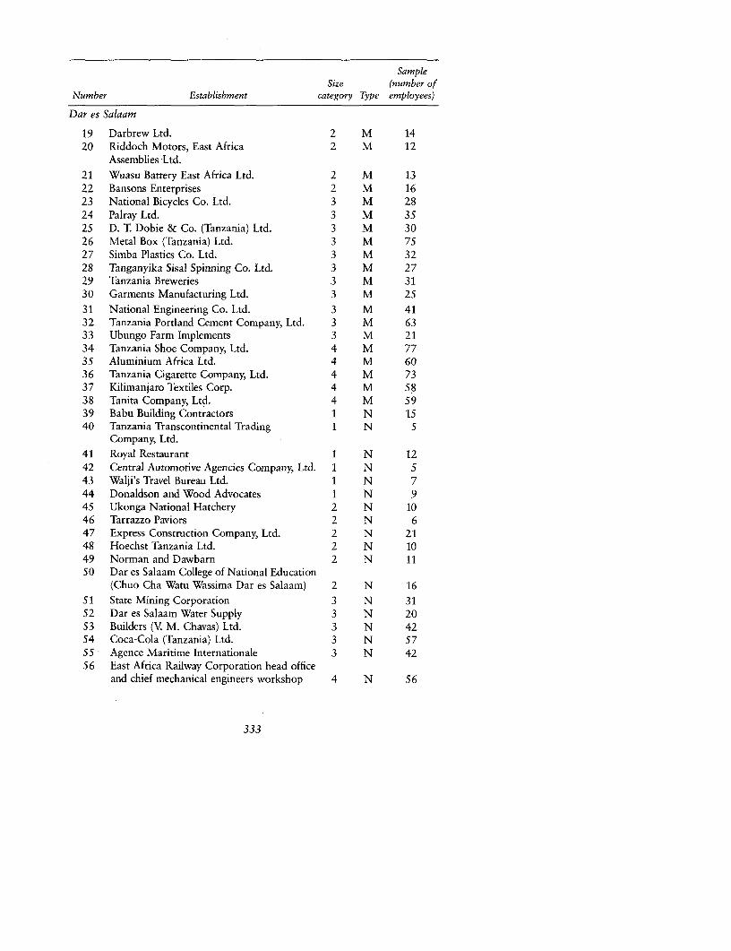
SampleSize (number of
Number Establishment category Type employees)
Dar es Salaam
19 Darbrew Ltd. 2 M 1420 Riddoch Motors, East Africa 2 M 12
Assemblies Ltd.
21 Wuasu Battery East Africa Ltd. 2 M 1322 Bansons Enterprises 2 M 1623 National Bicycles Co. Ltd. 3 M 2824 Palray Ltd. 3 M 3525 D. T. Dobie & Co. (Tanzania) Ltd. 3 M 3026 Metal Box (Tanzania) Ltd. 3 M 7527 Simba Plastics Co. Ltd. 3 M 3228 Tanganyika Sisal Spinning Co. Ltd. 3 M 2729 Tanzania Breweries 3 M 3130 Garments Manufacturing Ltd. 3 M 2531 National Engineering Co. Ltd. 3 M 4132 Tanzania Portland Cement Company, Ltd. 3 M 6333 Ubungo Farm Implements 3 M 2134 Tanzania Shoe Company, Ltd. 4 M 7735 Aluminium Africa Ltd. 4 M 6036 Tanzania Cigarette Company, Ltd. 4 M 7337 Kilimanjaro Textiles Corp. 4 M 5838 Tanita Company, Ltd. 4 M 5939 Babu Building Contractors 1 N 1540 Tanzania Transcontinental Trading 1 N 5
Company, Ltd.
41 Royal Restaurant 1 N 1242 Central Automotive Agencies Company, Ltd. 1 N 543 Walji's Travel Bureau Ltd. 1 N 744 Donaldson and Wood Advocates 1 N 945 Ukonga National Hatchery 2 N 1046 Tarrazzo Paviors 2 N 647 Express Construction Company, Ltd. 2 N 2148 Hoechst Tanzania Ltd. 2 N 1049 Norman and Dawbarn 2 N 1150 Dar es Salaam College of National Education
(Chuo Cha Watu Wassima Dar es Salaam) 2 N 1651 State Mining Corporation 3 N 3152 Dar es Salaam Water Supply 3 N 2053 Builders (V M. Chavas) Ltd. 3 N 4254 Coca-Cola (Tanzania) Ltd. 3 N 5755 Agence Maritime Internationale 3 N 4256 East Africa Railway Corporation head office
and chief mechanical engineers workshop 4 N 56
333
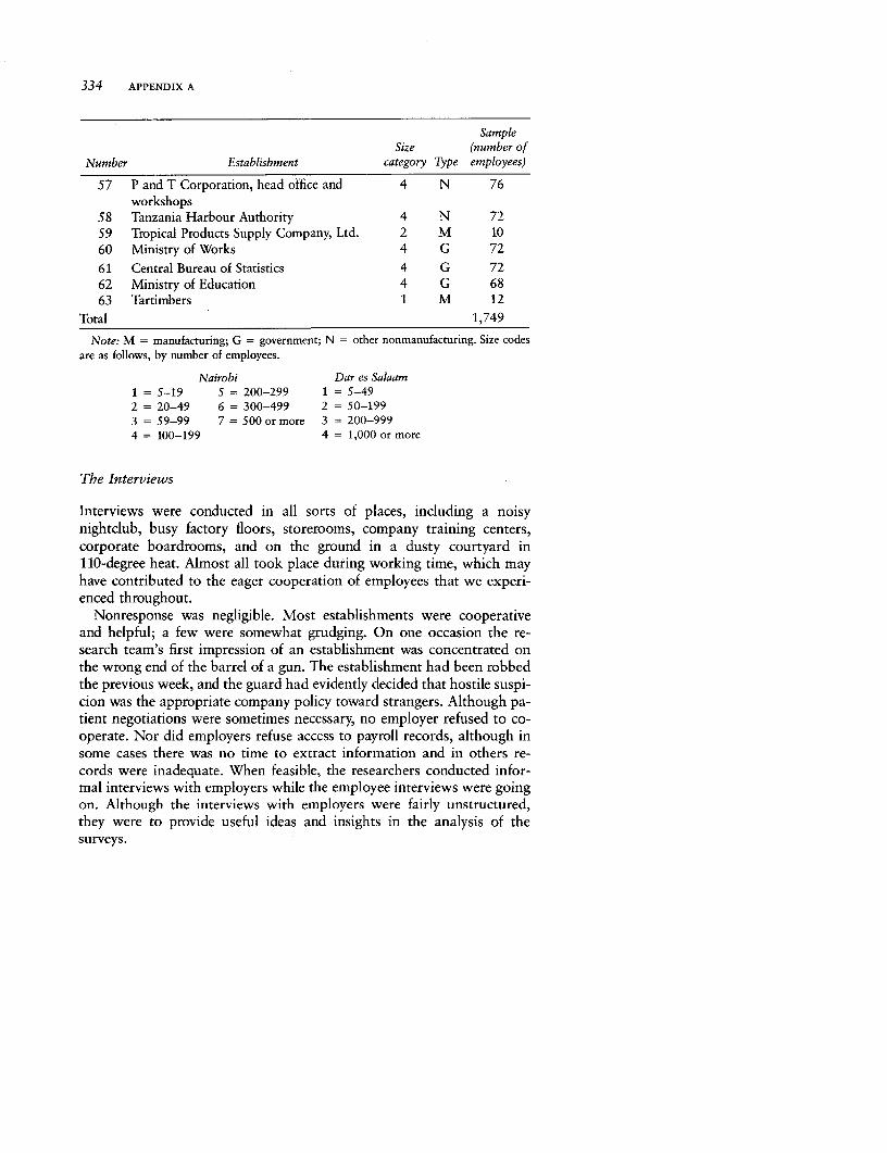
334 APPENDIX A
SampleSize (number of
Number Establishment category Type employees)
57 P and T Corporation, head office and 4 N 76workshops
58 Tanzania Harbour Authority 4 N 7259 Tropical Products Supply Company, Ltd. 2 M 1060 Ministry of Works 4 G 72
61 Central Bureau of Statistics 4 G 7262 Ministry of Education 4 G 6863 Tartimbers 1 M 12
Total 1,749
Note: M = manufacturing; G = government; N = other nonmanufacturing. Size codesare as follows, by number of employees.
Nairobi Dar es Salaam1 = 5-19 5 = 200-299 1 = 5-492 = 20-49 6 = 300-499 2 = 50-199
3 = 59-99 7 = 500 or more 3 = 200-9994 = 100-199 4 = 1,000 or more
The Interviews
Interviews were conducted in all sorts of places, including a noisynightclub, busy factory floors, storerooms, company training centers,corporate boardrooms, and on the ground in a dusty courtyard in110-degree heat. Almost all took place during working time, which mayhave contributed to the eager cooperation of employees that we experi-enced throughout.
Nonresponse was negligible. Most establishments were cooperativeand helpful; a few were somewhat grudging. On one occasion the re-search team's first impression of an establishment was concentrated onthe wrong end of the barrel of a gun. The establishment had been robbedthe previous week, and the guard had evidently decided that hostile suspi-cion was the appropriate company policy toward strangers. Although pa-tient negotiations were sometimes necessary, no employer refused to co-operate. Nor did employers refuse access to payroll records, although insome cases there was no time to extract information and in others re-cords were inadequate. When feasible, the researchers conducted infor-mal interviews with employers while the employee interviews were goingon. Although the interviews with employers were fairly unstructured,they were to provide useful ideas and insights in the analysis of thesurveys.

The Surveys: Coverage, Sampling, and Procedures 335
Workers were informed that the interviews held no possibility of per-sonal gain. The only workers who showed any reluctance to be inter-viewed were some managers. Most seemed glad for the chance to talkabout themselves. Indeed, the experience of this study (as of the classicHawthorne productivity study) is that workers are pleased to have some-one who is apparently in a position of authority take an interest in themand their opinions. The attitudinal questions, which are of dubiousanalytic value, may have served a purpose by eliciting this response.Workers who were somewhat suspicious at the start of the interviewwere, after ten minutes, generally thoroughly engaged in the processand unguarded in their responses. The reasoning ability test was viewedas a game, and the numeracy and literacy tests were accepted as achallenge.
The number of interviews completed by each enumerator per day in-creased rapidly during the first week. On the first day 130 interviews andsix sets of tests were completed, well below the average necessary to meetour targets within the allotted period. On the fifth day 240 interviewsand 45 sets of tests were completed. This marked increase in productivitywas the combined result of improvements on two learning curves. First,the increasing efficiency with which the supervisors learned to plan andorganize each day's work reduced the number of interviewers who wereidle at any time during the day. Second, the time spent on each interviewdecreased as interviewers became familiar with the questions and withthe detailed instructions concerning the alternative sets of questions tobe asked of respondents with different characteristics.
The performance of the student interviewers was impressive. Theylearned quickly and followed instructions closely. They were rarely ab-sent and were uncomplaining, whatever the circumstances. The explana-tion is not material incentives alone; they were paid the market wage,not a premium. Rather, they became engrossed in this opportunity togain on-the-job experience relevant to their course of study. They estab-lished an easy rapport with workers in a wide variety of occupations.Sometimes the questions may have contributed to this: an attractiveyoung secretary laughed when asked, "How many husbands do you havein Nairobi?"
Data Coding
From the Field to the Computer
On completion of the survey in Kenya the questionnaires were air-freighted to Oxford, where they were checked and the coding was com-pleted. The only delay between Nairobi and Oxford was caused by
336 APPENDIX A
customs officials at Heathrow, who were deeply suspicious of large boxesof printed paper, listed as having no commercial value but insured for20,000 pounds!
As Casley and Lury note, "The maxim must always be to get the data'clean' at as early a stage as possible-preferably in the field or, if notthen, immediately on receipt in the office" (1981, p. 124). In Tanzaniawe arranged for some interviewers to continue working with the princi-pal administrator after the survey, checking the questionnaires and com-pleting all the coding except for difficult items such as occupation andearnings. This was done in Oxford by two of the research team to ensureconsistency.
The coded and checked questionnaires were sent to Washington, D.C.,where the data were punched and then repunched as verification. (Withthe advent of sophisticated data entry programs, card punching is nowan outmoded technology.) The Statistical Package for the Social Sciences(spss) was chosen for its wide familiarity, easy use, clear table layout,and statistical adequacy for the more elementary analysis. Once the datawere in the computer in the file structure required by spss, a "wild code"check was carried out to ensure that the values of each variable fell withinthe range permitted by the coding scheme. Consistency checks of improb-able or impossible combinations of values on several variables were car-ried out, and extreme values of variables were checked for miscoding ormispunching. Even if these extreme numbers passed scrutiny, it was use-ful to be aware of them, since they could influence parameter estimates.Missing data were given a "missing value" code, and the affected work-ers were excluded as necessary during analysis. Since there were only afew such cases and they involved only a few variables, they did not causesignificant sample attrition.
Weighting the Samples
The samples had to be weighted to correct for the underrepresentationof nonmanufacturing compared with the actual relative sector sizes in theeconomy. The Survey of Employment and Earnings definition of the pub-lic services sector in Tanzania was more inclusive than ours. We includedonly central government ministries, whereas the official definition was"public sector community, social, and personal services." In computingthe weights to be used we had to make our demarcations of sectors con-sistent with published statistics by temporarily reclassifying a public edu-cational institution in each country as public service.
Owing to practical exigencies, the actual sample proportions of differ-ent size groups within the manufacturing and other nonmanufacturingcategories deviated somewhat from planned proportions, and a correc-tion for this was incorporated in the weights. The weights were derived
The Surveys: Coverage, Sampling, and Procedures 337
from the final sample proportion of a size-sector cell divided by its actualproportion in the population. Thus, if other nonmanufacturing establish-ments with between fifty and ninety-nine employees accounted for 15percent of total employment in Nairobi but for only 10 percent of ourNairobi sample, the weight applied to this group was 15/10 = 1.5. Ifthese "raw" weights had been applied, however, the sample size wouldhave been changed. A correction factor was computed for the weightsso that the weighted and unweighted samples would be the same size.
The Completed Data Tapes
New variables were created by aggregation, and simple cross-tabulationswere run. The first results were generated about six months after the firstinterviews. As the descriptive analysis began, we continued to watch forunfeasible or suspect variable values. Thus the first analysis and the finalchecking continued simultaneously.
Much of the data analysis used spss subprograms, but other packageswere also used. A copy of the data was transferred to the Oxford Univer-sity ICL 2988 computer, and some of the computer work was done there.The weighting procedure of spss involves some randomness. If theweighting requires that the number of cases in some stratum be in-creased-say, by 25 percent-then one-quarter of the cases in the stra-tum are randomly selected to be included twice. The Oxford and Wash-ington, D.C., data sets are therefore not necessarily exactly the same, butin no case do the (very slightly) different data sets produce other thantrivial differences in results.

APPENDIX B
Sample Questionnaire forEmployees, Tanzania Survey
THE FOLLOWING PAGES present a reduced facsimile of the employee ques-tionnaire used in Tanzania. Questions are in both English and Kiswahili.
338

Sample Questionnaire for Employees, Tanzania Survey 339
Employee Questionnaire
|REPLY CODE
Employee NumberCard number vFirm number 061
Interviewer number 1-10t
1. Personal Characteristics1. Sex: Male so
Female 2
2. Ethnic group: African 3)2)
AsianEuropeanOtherNo reply
3. Are you a citizen? Yes (,)
Wewe ni raia? No 2No reply 1 1 9 .
If no: How long have you lived in Tanzania? (years) 's-fl (N/A) 00Umeishi Tanzania kwa muda gani? (miaka)
4. How old are you? (years) (16-I,,
Umri wako ni miaka mingapi?
5. Are you: a. Never married 3,Hali ya ndoa: Hujawahi kuoa/kuolewa
b. Married 2Umeoa/umeolewa
c. Widowed 3Mjane
d. Divorced 4Mmeachana
e. Separated 5Mmetengana
f. No reply 9Hakuna jibu
6. How many people in addition to yourself do you help support(regularly in money or kind) with you rearnings?Pamoja na wewe, ni jumla ya watu wangapi ambao mahitaji yaoyanatokana na mapato yako?
Husbands or wives, fully 11
Waume au wake, yoteHusbands or wives, partly (33)
Waume au wake, kiasiChildren, fully 333.33)Watoto, yoteChildren, partly W3-25|
Watoto, kiasiOther, fully v35.30)Wengine, yoteOther, partly (03-tO)
Wengine, kiasi
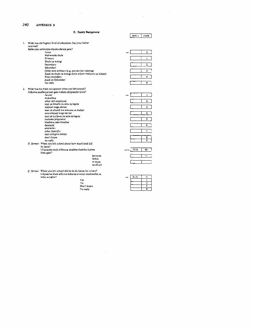
340 APPENDIX B
11. Family Background| EPY CDE|
I. What was the highest ievel of education that your fatherreceived?Baba yako amesoma mpaka daraja gani?
None |Hakwenda shulePrimaryShule ya msingiSecondary - 2SekondariOther post primary (e.g. pre-service training) 4Zaidi ya shule ya msingi (kwa mfano mafunzo ya kikazi)Post-secondary 4Zaidi ya SekondariNo reply 9
2. What was his main occupation when you left school?Alikuwa anafanya kazi gani wakati ultipoacha shule?
farmer I111|51mukulimaother self-employed I2 Lkazi ya binafsi ya aina nyinginemanual wage-earner 3zikazi ya ufundi wa mikona ya maliponon-manual wage earner 4kazi ya kulipwa ya aina nyinginebusiness proprietor 5biashara yake binafasideceased 6amefarikiother (specify) 7kazi nyingine (eleza)don't knowno reply | 9|
If farmer: When you left school about how much land didhe farm?Ulipoacha shule alikuwa analima sbamba kubwa I NYA|kiasi gani?
hectareshektaor acresau ektari
If farmer: When you left school did he do Ki barua for others?Ulipoacha shule alikuwa kibarua kwenye mashamba yawatu wengine? N/A
YesNo 2Don't know 3No reply 9
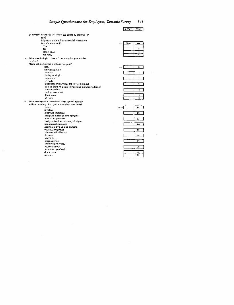
Sample Questionnaire for Employees, Tanzania Survey 341
| REPLY |CODE
If farmer: When vou left school did others do ki barua forhim?Ulipoacha shule alikuwa ameajiri vibarua wakusaidia shambani? N/A 00
YesNo2Don't know 3No reply 9
3. What was the highest level of education that your motherreceived?Mama yako amesoma mpaka daraja gani?
hakwenda shuleprimaryshule ya msingisecondary 2 |sekondariother post-primary (eg. pre-service training) 3 |zaidi ya shule ya msingi (kwa mfano mafunzo ya kikazi)post-secondary 4 1zaidi ya sekondaridon't know 5no reply 9
4. What was her main occupation when you left school?Alikuwa anafanya kazi gani wakati ulipoacha shule?
farmer 01mkulimaother self-employed 02kazi yake binafsi ya aina nyinginemanual wage-earner 03kazi ya ufundi wa mikono ya kulipwanon-manual employeekazi ya kulipwa ya aina nyinginehusiness proprietor 05biashara yake binafasideceased 06amefarikiother (specify) 07,:kazi nyingine (eleza)housewife only 10mama wa nyumbanidon't know 08no reply " 9 99

342 APPENDIX B
111. Education
| DREPLY| ODE I
I. What was the highest standard in primary school that you completed? 0
Darasa la jsu kabisa uliofikia kwenye shule ya msingi ni lipi? =
no reply I 2. Did you receive a primary leaving certificate?
Ulipata cheti cha kumalizia shule ya msingi?Yes INo 2No reply 9
If no primary schooling, proceed ro Question 4a.
3. What type of primary school was it? (If more than one, last school)Shule ya msingi uliyosoma ilikuwa ya aina gani? (Kama ni zaidi ya moja, tajauliyosoma mwishoni)
us1 N/A 0 |a. Government l I
Serikalib. Private 2
c. Mission 3lliyoendeshwa na
makanisad. No reply 9
4. Did you have any education or pre-service training afterprimary school?Baada ya kumaliza shule ya msingi uliendelea na masomo auulipata mafunzo ya kukuwezesha kupata kazi? N/A
YesNo 2No reply 9
If no: preceed to Question 4a.If yes: Which of the following types did you have? (indicate the order)
Ulipata elimu ya aina gani kati ya zifuatazo? s iN/A [00
a. Government secondary 01Sekondari ya serikali
b. Self-help secondary 02Shule ya sekondari ya kujitegemea
c. Private secondary 03Sekondari ya "private"
d. Technical secondaryShule ya sekondari
ya ufundi

Sample Questionnaire for Employees, Tanzania Survey 343
e. Teacher training (non-university) 05
Shule ya ualimuf. University 06
Chuo kikuug. Technical College | 7
Chuo cha ufundih. Trade School
Shule ya ufundii. Craft School
Shule ya kazi za mikonoj. Folk development r zl
College (specify lengthof course)
k. Government-run pre- I j
service traininginstitution (specify)Shule ya mafunzo (yavijana) kabla yakuanza kazi, inayoen-deshwa na serikali(taja)
1. Employerrun pre- 12
service trainingschool (specify)Shule ya mafunzo kablaya kuanza kazi inayo-endeshwa na mwajiri.
m. Government-run 13secretarial collegeChuo cha mafunzoya ukarani aubiashara kinachoendeshwana serikali.
n. Private secretarial ZXIII=Zcollegechu cha mafunzo ya ukaraniau biashara kinachoendeshwana watu binafsi.
o. Other (specify) 17_ |
P. No reply 99
If a, b, c or d,-formal secondary school:Which was the highest form achieved?
Ulimaliza darasa ia ngapi? s N/A 0
n 4
-H6
no reply ~~~~~~~~~9

344 APPENDIX B
| ELY|CDE|
For those who reached form 4:What were your results in the National Form 4 Examination(formerly SC or 'O' levels)?Matokeo yako ya mtihani wa darasa la 12 yalikuwa-je? 0N A O
a. Division Ib. Division 2 2c. Division 3 3d. Division 4 4e. Fail 5f. Did not sit 6g. No reply 9
What was your grade in the following subjects?Ulipata nini kwenye masomo yafuatayo? N/A |
a. MathsHesabu
b. EnglishKiingereza
C. Your best science 150 |subject (specify)Somo la sayansiulilofanya vizurikupita yote (litajeJ
d. Your practical subject (specify) 0i|Somo lako la kazi za mikono (litaje)
Which school did you attend? (the last school) oo, N/A 000Ulisoma hule gani? (uliyosoma mwishoni)
Were vou: a. a border? Si N/A Oulikowa unakaa bwenini?
b. a day pupil? _2ulikuwa unakaa nyumbani? 9
For those who reached form 6: What were your results in the National Form 6Examination (formerly HSC or 'A' level) (principal passes only)?Matokeo yako ya mtihani wa darasa la 14 yalikuwa je? 0NA O
a. no passes 8b. I passC. 2 passes 2d. 3 passes 3e. 4 or more passes 4f. did not take _g. no reply 9
What were your three best principalpasses and the grade received in each?Taja masomo kamili matatu uliyoshindavizuri kuliko mengine?
I. subject: grade: - *:2. subject: grade: -3. subject: - grade: -

Sample Questionnaire for Employees, Tanzania Survey 345
|REPLY CODE|
Which school did vou attend?(the last school) l-l N/A 000Ulisoma shule gani? (uliyosoma mwishoni) _
Were you: a. a border? , N/Aulikowa unakaa bwenini?
b. a day pupil? 2ulikuwa unakaa nyumbani? 9
For those aho attended a teacher training college (College of National Education):How long was the course? . .years.Mfunzo yalichukua muda gani?For what teaching grade did the course qualify you?Ulihitimu kuwa mwalima wa ngazi gani? ,as N/A 0
a. No qualification Ib. grade A 2C. grade B 3d. grade C. 4e. Other (specify) 5f. no reply 9
For those who attended a university:Did you obtain a degree?Ulipata shahada , N/A
yes ]no 2no reply 9
If yes: what was your highest degree?Ni ipi shahadayajuukabisauliyopata? ,,,, N/A
a. bachelorsb. masters 2c. doctorate 3d. no reply
If no: Did you obtain a diploma (specify)Ulipata diploma? (eleza) ,r, N/A 0
yesno 2no reply 9
What subjects did you study?Ulichukua miasoma gani? N/A75- )NA 0
general arts 01social sciences 02history 03languages 04geography 05engineering 06sciences 07law 08medicine 10agricualure IIarchitecture 12commerce 13other (specify) 14
no reply | 99

346 APPENDIX B
| EP |O DE|
Where did you attend university?Ulisoma chuo kikuu kipi? N/A 0
Dar 3Makerere 2Nairobielsewhere (specify) 4No reply 9
4a. What was the highest level of education that your spousereceived?Mke/Mume wako amesoma mpaka daraja gani?
none 9| | °ihakwenda shuleprimary Ishule ya msingisecondary 2sekondariother post-primary (eg. pre-service training) 3zaidi ya shule ya msingi(kama mafunzo ya kakazi)post-secondaryzaidi ya sekondariunmarried 5nakuolewa/hakuoano reply 9
Employee numberCard number 52
5. Have you attempted a craft trade test?Umewahi kujaribu mtihani wa ufundi unaotolewa na serikali?
yes MnO 2|no reply 9
If yes: What were your results?Matokeo yake yalikuwa-je? .- N/A 00Grade I Pass 00
Fail 01Did not sit 03
Grade 11 Pass 04Fail 05Did not sit 06
Grade III Pass 07Fail 08Did not sit 10
No reply
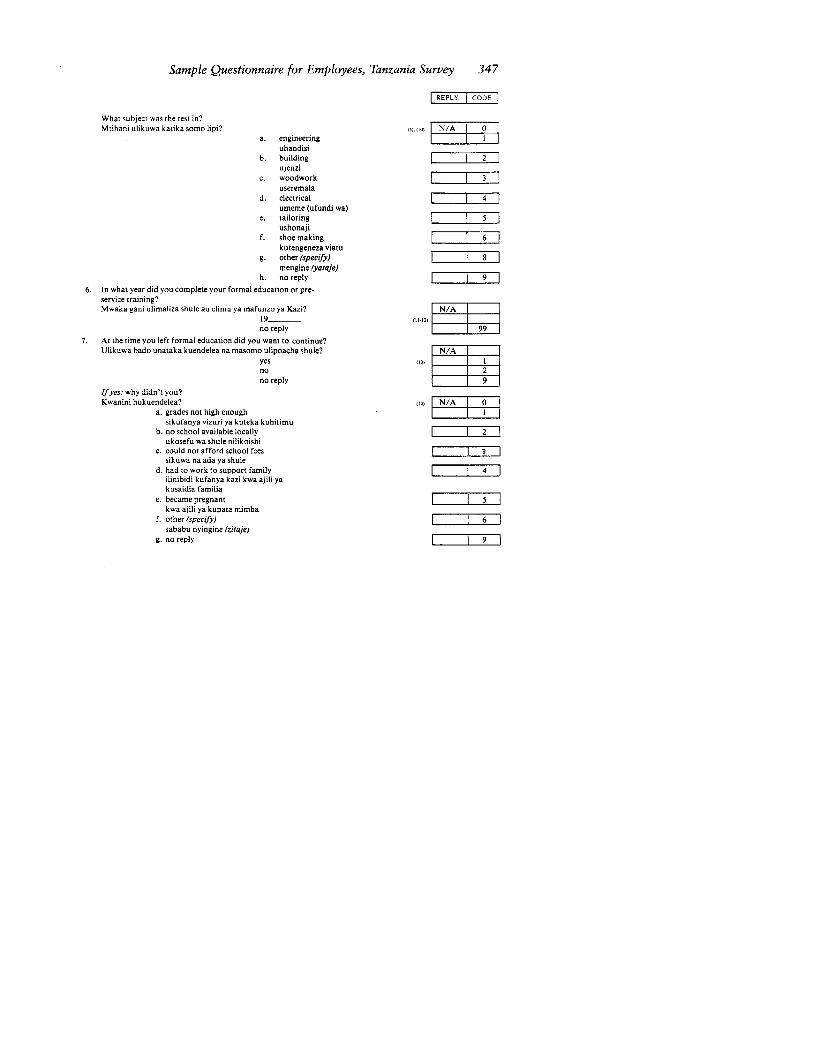
Sample Questionnaire for Employees, Tanzania Survey 347
REPLY COD
What subject was the test in?Mtihani ulikuwa katika somo lipi? u. so., N/A O
a. engineering Iuhandisi
b. building 2ujenzi
c. woodwork 3useremala
d. electrical 4umeme (ufundi wa)
e. tailoring 5|ushonaji
f. shoe making 6|kutengeneza viatu
g. other (specify) |8 |mengine (yataje)
h. no reply | |9z
6. In what year did you complete your formal education or pre-service training?Mwaka gani ulimaliza shule au elimu ya mafunzo ya Kazi? N/A
19 2)no reply _
7. At the time you left formal education did you want to continue?Ulikuwa bado unataka kuendelea na masomo ulipoacha shule? NiA
yes onono reply
If yes: why didn't you?Kwanini hukuendelea? s A N
a. grades not high enough 1 I sikufanya vizuri ya kuteka kuhitimu
b. no school available locally 2ukosefu wa shule nilikoishi
c. could not afford school feessikuwa na ada ya shule
d. had to work to support family 4ilinibidi kufanya kazi kwa ajili yakusaidia familia
e. became pregnant S T 5kwa ajili ya kupata mimba
f. other (specify) 6sababu nyingine (zitaje)
g. no reply 9
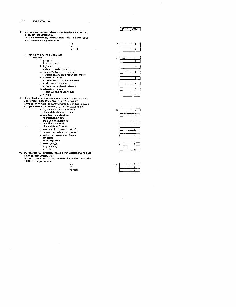
348 APPENDIX B
8. Do you want your sons to have more education than you had,if they have the opportunity?Je, kama itawezekana, unataka watobo wako wa kiume wapateelimu zaidi kuliko uliyopata wewe?
yes s,nono reply
If yes: Why? (give the main reason)Kwa nini? Is N/A 0
a. better job Lkazi nzuri zaidi
b. higher paymshahara mkubwa zaidi
c. occupation hoped for requires it 3kufuatana na mahitaji ya kazi inayonuiwa
d. position in societykufuatana na mazingara ya maisha
e. service to the communitykufuatana na mahitaji ya jumuia
f. cultural enrichment 6kuendeleza mila na utamaduni
g. no reply9. If after leaving primary school your son could not continue to
a government secondary school, what would you do?Kama baada ya kumaliza shule ya msingi mtoto wako wa kiumehakupata nafasi katika sekondari ya serikali utafanya nini?
a. pay his fees fora private school s| nitampeleka shule ya 'private'
b. send him to a craft school 2nitampeleka kwenyeshule ya kazi za mikono
c. send him out to worknitampeleka kufanya kazi
d. apprentice him (to acquire skills)nitampeleka mahali kujifunza kazi
e. get him to repeat primary leavingcertificatenitamfanya arudie
f. oLher tspecifyrvingine (eleza)
g. no reply 99a. Do you want your daughters to have more education than you had
if they have the opportunity?Je, kama ikiwezekana, unataka watoto wako wa kike wapate elimuzaidi kuliko uliyopata wewe?
yes ISnono reply j9
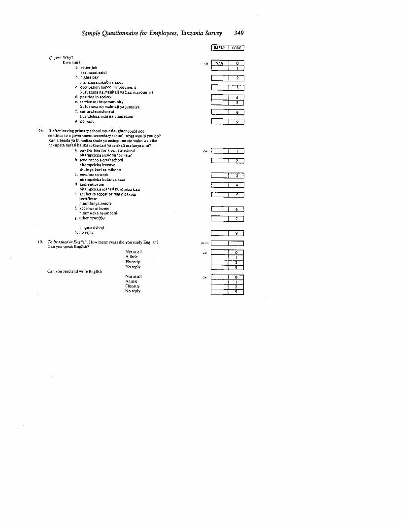
Sample Questionnaire for Employees, Tanzania Survey 349
|REPLyi CODE|
If yes: Why?Kwa nini? N/A O
a. better jobkazi nzuri zaidi
b. higher paymshahara mkubwa zaidi
C. occupation hoped for requires it 3kufuatana na mahitaji ya kazi inayonuiwa
d. position in society |_4_ |e. service u o the community _ni
kufuatana no mahitaji ya lumuiyaf. cultural enrichment 6
kuendeleza mila na utamadunig. no reply 9
9b. If after leaving primary school your daughter could notcontinue to a government secondary school, what would you do?Kama baada ya kumaliza shule ya msingi, mtoto wako wa kikehakupata nafasi katika sekondari ya serikali utafanya nini?
a. pay her fees for a private school s|
nitampeleka shule ya 'private'b. send her to a craft school 2
nitampeleka kwenyeshule ya kazi za mikono
c. sendhertowock 3nitampeleka kufanya kazi
d. apprentice her 4nitampeleka mahali kujifunza kazi
e. get her to repeat primary leaving 5certificatenitamfanya arudie
f. keep her at home 6nitamweka nyumbani
g. other (specify) 7
vingine (eleza)h. no reply . 9
10. To be asked in English. How many years did you study English? ,2,.22,Can you speak English?
Not at allA littleFluentlyNo reply
Can you read and write EnglishNot at all UO
A littleFluentlyNo reply
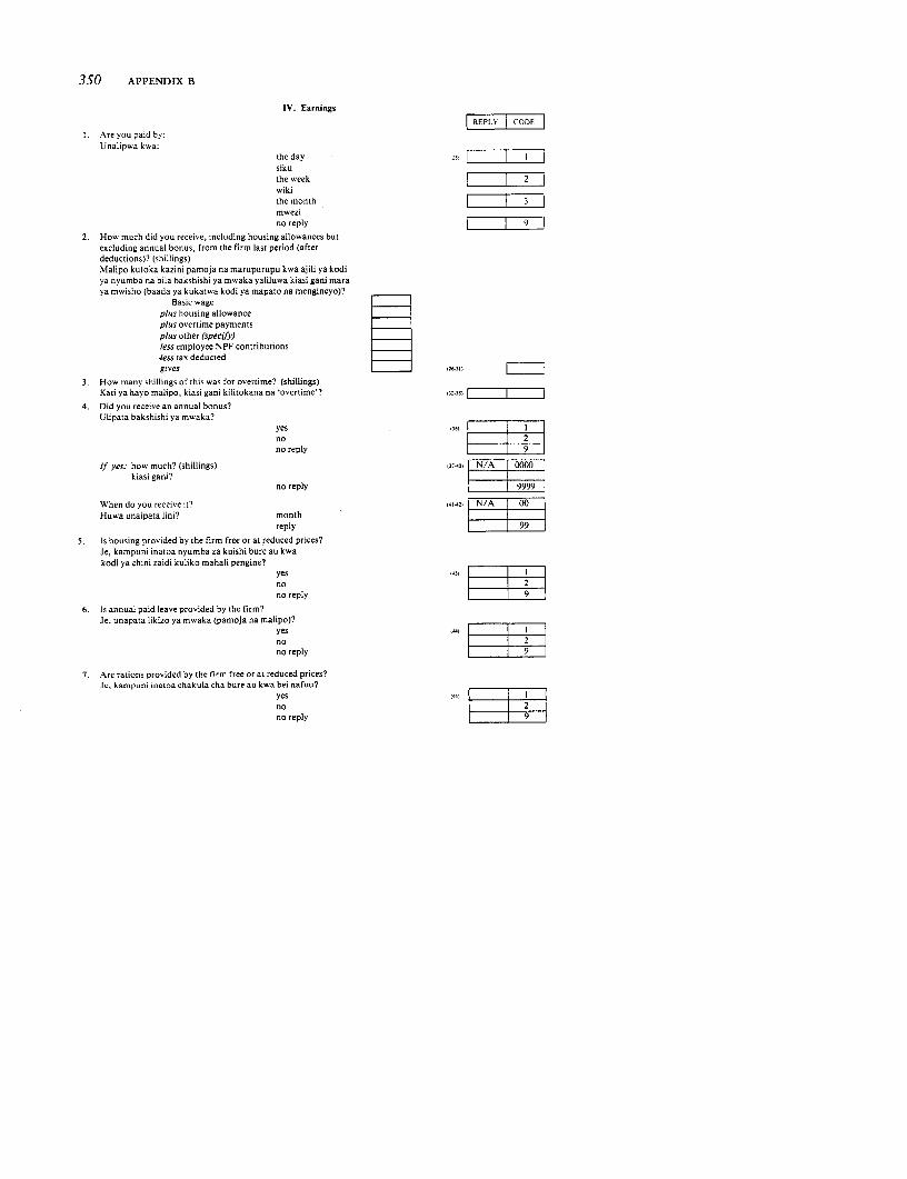
350 APPENDIX B
IV. Earnings
REPLY CODE
I. Are you paid by:Unalipwa kisa:
the day ii,
sikuthe week 2wikithe month 3mwezino reply 9
2. How much did you receive, including housing allowances butexcluding annual bonus, from the firm last period (afterdeductions)? (shillings)Malipo kutoka kazini pamoja na marupurupu kwa ajili ya kodiya nyumba na bila bakshishi ya mwaka yaliluwa kiasi gani maraya mwisho (baada ya kukatwa kodi ya mapato na mengineyo)?
Basic wageplus housing allowanceplus overtime paymentsplus other (specify)less employee NPF contributions4ess tax deductedgives n-s|
3. How many shillings of this was for overtime? (shillings)Kati ya hayo malipo, kiasi gani kilitokana na 'overtime'? si-sn I 7
4. Did you receive an annual bonus?Ulipata bakshishi ya mwaka?
yes 55
no 2no reply 1 9
If yes: how much? (shillings) -N A N/A 00|kiasi gani?
no reply 9999
When do you receive it? 'r]2l N/AHuwa unaipata lini? month
reply 99
5. Is housing provided by the firm free or at reduced prices?Je, kampuni inatoa nyumba za kuishi bure au kwakodi ya chini zaidi kuliko mahali pengine?
yes~~~~~~~~~~~~~~~~~~~~~~~~~~~~~~~~~~~~~~~~~~~2nono reply 9
6. Is annual paid leave provided by the firm?Je, unapata likizo ya mwaka (pamoja na malipo)?
yes | 2no 2no reply 9
7. Are rations provided by the firm free or at reduced prices?Se, kampuni inatoa chakula cha bure au kwa bei nafuu?
yes 1 no |2lno reply 9
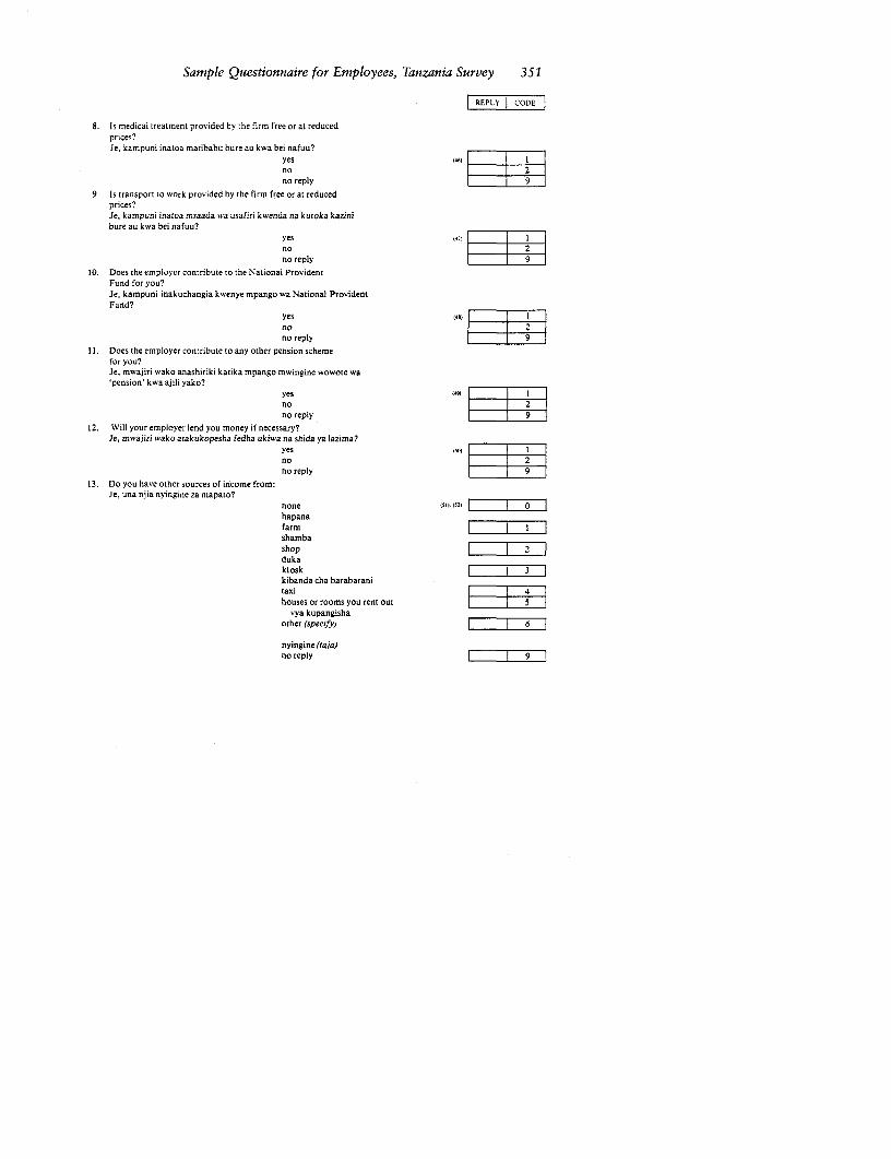
Sample Questionnaire for Employees, Tanzania Survey 351
REPLY CODE|
8. Is medical treatment provided by the firm free or at reducedprices?Je, kampuni inatoa matibabu bure au kwa bei nafuu?
yes e-no | 2no reply | 9
9. Is transport to work provided by the firm free or at reducedprices?Je, kampuni inatoa msaada wa usafiri kwenda na kutoka kazinibure au kwa bei nafuu?
yes _ _ _ _
no 2no reply 9
10. Does the employer contribute to the National ProvidentFund for you?Je, kampuni inakuchangia kwenye mpango wa National ProvidentFund?
yes 91no 2no reply 9
11. Does the employer contribute to any other pension schemefor you?Je, mwajiri wako anashiriki katika mpango mwingine wowote wapension' kwa ajili yako?
yes Ino 2no reply 9
12. Will your employer lend you money if necessary?Je, mwajiri wako atakukopesha fedha ukiwa na shida ya lazima?
yes 1etnso 2no reply L 9
13. Do you have other sources of income from:Je, una njia nyingine za mapato?
none ($5. ("5j 5O
hapanafarmshambashop 2dukakiosk 3kibanda cha barabaranitaxi 4houses or rooms you rent out |
vya kupangishaother (specify) 6
nyingine (taja)no reply 9

352 APPENDIX B
| EPY|DOE|
If yes: Roughly how much (shillings) per month? N/A 0000 Makisio ya haya mapato ni kiasi gani kwa mwezi? scl
or per dayau kwa sikuor per yearau kwa mwakano reply | 9999
V. Employment Experience in the Firm
| REPLY |CODE |
1. In what year did you join the firm? 19 -
Ni mwaka gani ulianza kazi hapa?2. Are you now a regular or casual worker?
Wewe ni mfanya kazi wa kudumu au kibarua?Regular o56Casual 92
No reply 93. If regular: Did you start in this firm as a casual worker?
Je, ulianza kazi hapa kama kibarua? aa| N/AYesINo 2No reply 9
4. If no:Would you have got your job if you had received lesseducation? 1|1|Ungeweza kuipata hii kazi kama ungekuwa na kisomocha chini ya ulichokuwa nacho?
YesNoDon't knowNo reply
If yes to question 3: When you became a regular employee, would youhave got your job if you had received less education? it N/A | 0Ulipofanywa mfanya kazi wa kudumu ungeipata hiyo kazikama ungekuwa na kisomo chini ya ulichokuwa nacho?
YesNoDon't knowNo reply
5. If casual: Would you have got your job if you had receivedless education? iv N/A 0
No INo 2Don't know 3No reply 9
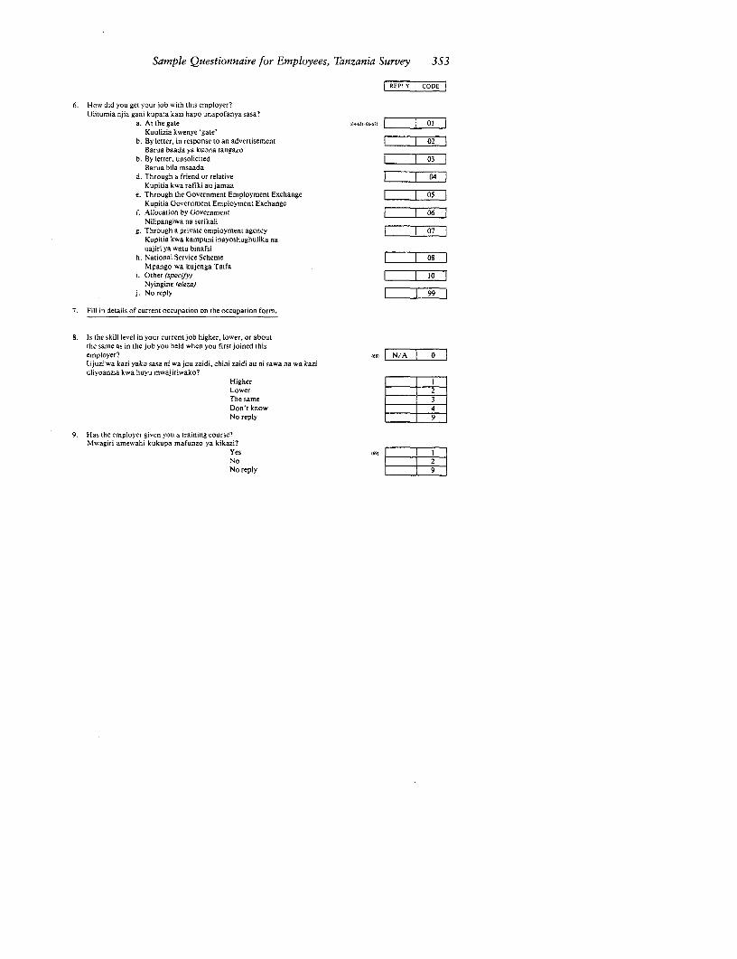
Sample Questionnaire for Employees, Tanzania Survey 353
REPLY CODE
6. How did you get your job with this employer?Uilitumia njia gani kupata kazi hapo unapofanya sasa?
a. At the gate 01Kuulizia kwenye 'gate'
b. By letter, in response to an advertisement 02Barua baada ya kuona tangazo
b. By letter, unsolicited 03Barua bila msaada
d. Through a friend or relative DrKupitia kwa rafiki au jamaa
e. Through the Government Employment Exchange 05Kupitia Government Employment Exchange
f. Allocation by Government | 6Nilipangiwa na serikali
g. Through a private employment agency 07Kupitia kwa kampuni inayoshughulika nauajiri ya watu binafsi
h. National Service Scheme 08Mpango wa kujenga Taifa
i. Other (specify) 10Nyingine feleza)
j. No reply 99
7. Fill in details of current occupation on the occupation form.
8. Is the skill level in your current job higher, lower, or aboutthe same as in the job you held when you first joined thisemployer? 08i) N/A 0
Ujuzi-wa kazi yako sasa ni wa juu zaidi, chini zaidi au ni sawa na wa kaziuliyoanzia kwa huyu mwajiriwako?
Higher ILower 2The same 3Don't know 4No reply 9
9. Has the employer given you a tTaining course?Mwagiri amewahi kukupa mafunzo ya kikazi?
YesINo i repNo reply I

354 APPENDIX B
| EL O DOE |
If yes: how many courses?mara ngapi? o N/A
No reply(If more than one, the questions relate to the main one.) 9
Was it: L iiI| N/A |Ilikuwa:
pre-servoicekabla ya kuanza kaziin-servicekama mfanya kazino reply 9
Was it:Ilikuwa: N N/A
in the firm Ikaziniin some outside institution 2mahali pengineno reply 9
How long was this course? (code in months) ,,7, N/A|Mafunzo yalichukua muda gani?
weeksor months =nLo reply _ 9
Was the course: N/A OMafunzo yalikuwa:
full-time kila sikupart-timesiku moja mojano reply 9
Did you receive full pay while attending thiscourse;Ulikuwa unalipwa mshahara wako wote ulipokuwamafunzoni? .| N/A
yesno Ino reply 9
Did you receive higher pay after completingthe course?Uliongczwa mshahara baada ya kumaliza mafunzo? N/A 0
yesno 10 1no reply 9
Employee number 14Card number F-E]

Sample Questionnaire for Employees, Tanzania Survey 355
RPLY |CODE|
10. Do you think your education qualifies you forajobata higher level than your present job?Je, kufuatana na kisoma chako unafikiri ungeweza kufanya kaziyenye madaraka zaidi kuliko uiiyo nayo sasa?
yes 6)nodon't knowno reply
If yes: Why are you in your current job?Kwa nini unafanya hii kazi ya sasa? N/A|O
a. to gain experience, or skillkupata mazoezi au uiuzi
b. too junior for higher 2job at the momentumri wangu au mudaniliokaa hapa ni mdogokuliko inavyotakiwa
c. no higher level jobsavailable 3ukosefu wa kazi yenyemadaraka zaidi
d. other (specify), 4
kwa ajili ya sababunyingine (zitaje).
e. No reply 9
11. Do you think that you could perform your present job as wellif you had not received your final stage of education?Je, unafikiri ungeweza kuifanya kazi yako ya sasa sawa na kamavile usingekuwa umefikia daraja la kisomo ulicho nacho? 1 N/
yes
no 2don't know 3no reply 9
12. Do you think you could do your present job better if you hadcompleted the next stage of education?Je, unafikiri ungeweza kuifanya kazi yako ya sasa vizuri zaidi kamaungeendelea na shule mpaka daraja la juu zaidi kuliko ulilofikia?
yes 5|
nodon't knowno reply
13. Are you a trade union member?Umejiunga na chama cha wafanya kazi?
no (lot |
yes
no reply

356 APPENDIX B
| REPt T |ODE|
14. How much were you paid (after deductions) when you firstjoined this firm? (shillings per month) 1w
Ulikuwa unalipwa kiasi gani (baada ya kukatwa kodi na mengineyo)ulipoanza kazi kwenye hii kampuni?
don't knowno reply
15. Are you actively looking for a better job in some other firm?Je, unajitahidi kutafuta kazt nzuri zaidi mahali pengine?
yes ,no |2no reply 9
VI. Previous Employment Experience
Ifnoformal education proceed to Question 3.I . Did you interrupt your formal education for a year or more?
Je, ulipokuwa unasoma shule uliwahi kuacha masomo kwa mwaka auzaidi halafu ukarudi tena kuendelea?
yes 08)nono reply 9
If yes: During that time how long did you spend doing thefollowing?Wakai huo, ulijishughulisha kwa muda gani nayafuatayo? |MONTHS| YEARS
a. worked on parent's shambakusaidia kwenye shamba la wazazi
b. worked on own shamba to
kufanya kazi kwenye shamba lakoc. non-agriculturai employment. u1s j
(eg. street vending, small businesses, etc.);kazi isiyokuwa ya kilimo (kwa mfano kukutembeza na kuuza vitu barabarani)
d. unemployed and looking for wage employment tjkushughulika kutafuta kazi ya kulipwa
e. unemployed and not looking for work ,)kukaa tu bila kufanya kazi wala kutafuta
f. employed in a wage job a.)kufanya kazi ya kulipwa
g. National ServiceKujenga Taifa
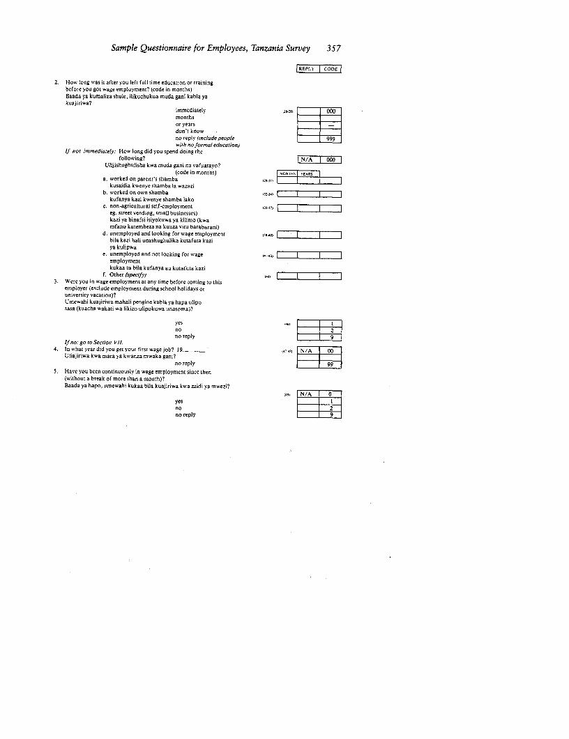
Sample Questionnaire for Employees, Tanzania Survey 357
REPLY |COOE
2. How long was it after you left full time education or trainingbefore you got wage employment? (code in months)
Baada ya kumaliza shule, ilikuchukua muda gani kabla yakuajiriwa?
immcdiately n.ts, 000
months
or years
don't know
no reply (include people
with noformal education)If nor immediately: How long did you spend doing the
following? _N/A I00(Ulijishughulisha kwa muda gani na yafuatayo?
(code in months) Ie YRS
a. worked on parent's shamba t29.3l)
kusaidia kwenye shamba la wazazib. worked on own shamba 32t,)1 _
kufanya kazi kwenye shamba lakoc. non-agricultural self-employment o,,,t)
eg. street vending, small businesses)
kazi ya binafsi isiyokuwa ya kilimo (kwa
mfano kutembeza na kuuza vitU barabarani)d. unemployed and looking for wage employment se.|
bila kazi hali unashughulika kutafuta kazi
ya kulipwae. unemployed and not looking for wage .4t.
employmentkukaa tu bila kufanya au kutafuta kazi
f. Other (specify) ujt
3. Were you in wage employment at any time before coming to thisemployer (exclude employment during school holidays oruniversity vacation)?
Umewahi kuajiriwa mahali pengine kabla ya hapa uliposasa (kuacha wakati wa likizo ulipokuwa unasoma)?
yes .9)no 2no reply 9
If no: go to Secoion VII.4. In what year did you get your first wage job? 19 cm.8) N/A 00
Uliajiriwa kwa mara ya kwanza mwaka gani?
no reply5. Have you been continuously in wage employment since then
(without a break of more than a month)?
Baada ya hapo, umewahi kukaa bila kuajiriwa kwa zaidi ya mwezi?
(39 N/A 0yes Ino 2no reply

358 APPENDIX B
6. If no: How many times have you been out of wage employment?Umekaa bila kuajiriwa mara ngapi? n boi N/A 0
number of timesno reply 9
How long in total were you out of wage employment?Kwa ujumia ni muda gani umekaa bila kuajiriwa? <irs Ni
(months)no reply 99
What did you do? (main activity) Second Mo-
Ulifanya nini? (shughuli muhimu) Tl- Tone T,e Recem, neMONTHS MONTHS MONTHS
I worked on parent's shamba
kusaidia kwenye shamba la wazazi2 worked on own shamba
kufanya kazi katika shamba langu3 non-agricultural self-employment
(eg. street vending)Kazi binafsi isiyokuwa ya cclvkilimo (kwa mfano kutembeza na ce-erkunza vitu barabarani)
4 unemployed and looking forwage employmentKushughulika kutafuta kazi yakuajiriwa
5 Unemployed and not lookingfor workKukaa bila kufanya au kutafutakazi
6 returned to educationKurudi shuleni kuendelea na masomo
7. How many previous employers have you had?Umewahi kuwa na waajiri wangapi kabla ya huyu wa sasa? N/Ai
2 23 3
4 4
6 r L68or more 8no reply 9
If none: go to Section VII.
8. (Exclude wage emploYment during school or college vacations.)What was the name of your employer in? your last jobMwajiri wako alikuwa ni nani? kazi yako ya mwisho
your first jobkazi yako ya mwanzo
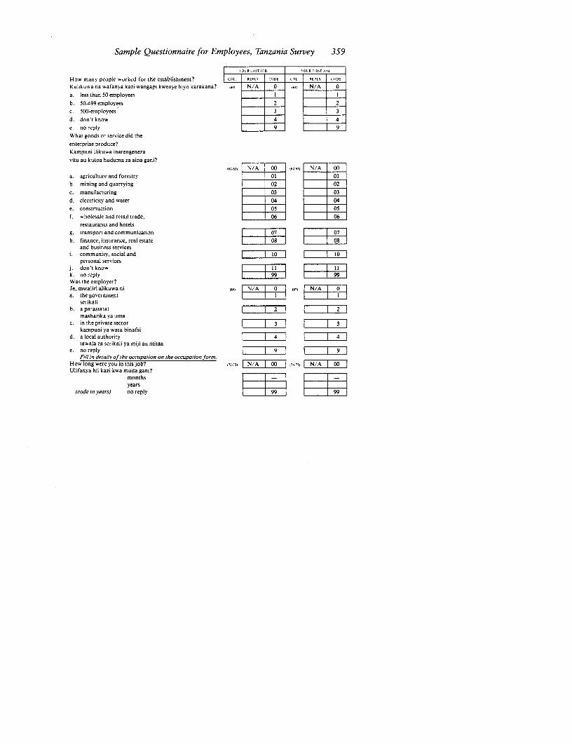
Sample Questionnaire for Employees, Tanzania Survey 359
How many people worked for the establishment? 0 REPC) CODE COL RESCI (-DE
Kulikuwa na wafanya kazi wangapi kwenye hiyo karakana? MI N/A 0 ,6 N/A 0
a. less than S0 employees I I
b. 50-499 employees 2 2
c. 500-employees 3 3
d. don't know 4 4e. no reply 99
What goods or service did the
enterprise produce?Kampuni ilikuwa inatengeneza
vitu au kutoa huduma za aina gani?
62-63 N/A 00 66 N/A 00a. agriculture and forestry 01 01
b. mining and quarrying 02 02
c. manufacturing 03 03
d. electricity and water 04 04
e. constrtuction 05 05
f. wholesale and retail trade, 06 06
restaurants and hotels
g. transport and communication 07 07h. finance, insurance, real estate |0 08
and business servicesi. community, social and 10 10
personal servicesj. don't know I =_____11k. no reply 99 99Was the employer?Je, mwajiri alikuwa ni ,66, |N -/A | N/a. the governmernt
serikalib. a parastatal | 2 r 2
masharika ya umac. in the private sector r 3 3
kampuni ya watu binafsid. a local authority 4 4
tawala za serikali ya miji au mitaae. no reply, 9 9
Fill in details oftrhe occupation on the occupationform.How long were you in this job? SC(S) N/A 00 'D'S) N/A 00Ulifanya hii kazi kwa muda gani?
monthsyears
(code in years) no reply
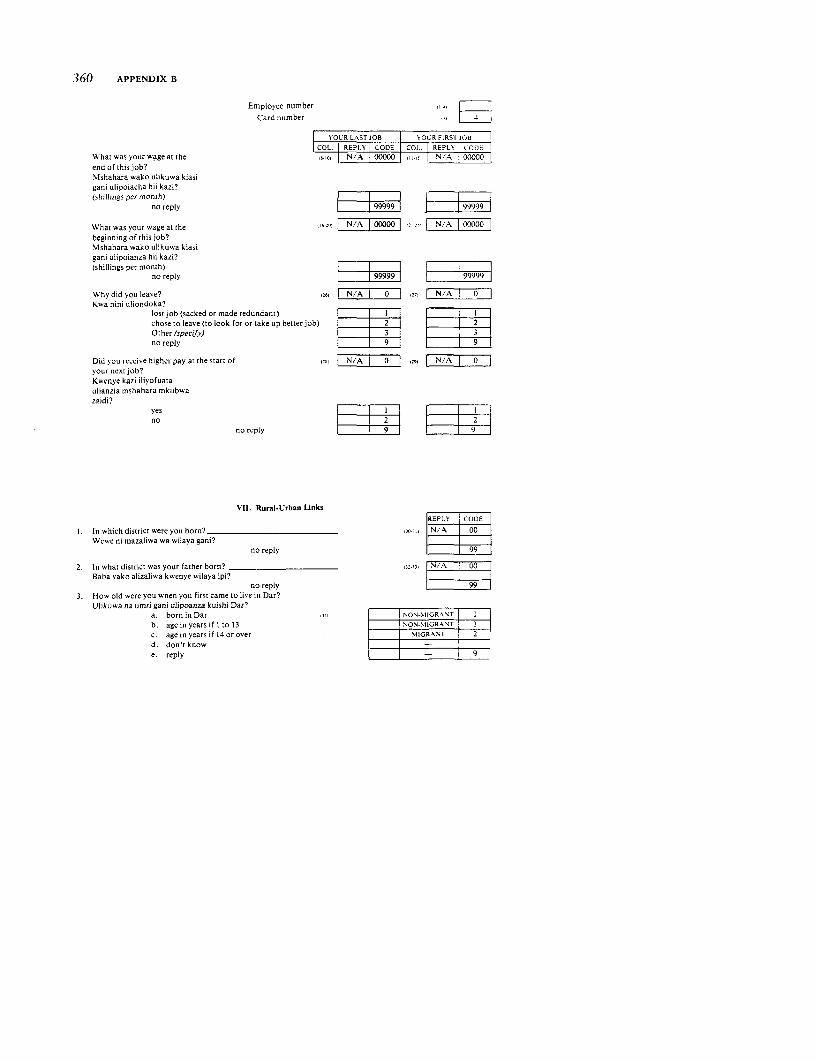
360 APPENDIX B
Employee number
Card number FYOLR LASTIOB IOUR FIRST IOB
COL. REPLY CODE COL IREPL5 LODWhat was your wage at the N/A 00000 N/A G000
end of this job?M shahara wako ulikuwa kiasigani ulipoiacha hii kazi?(shillings per month)
no reply
What was your wage at the . N/A 00000 N/A 00000
beginning of this job?Mshahara wako ulikuwa kiasigani ulipoianza hii kazi?(shillings per month) _ _ _
no reply
Why did you leave? w --- N/A 0|,, N/A 07Kwa nini uliondoka?
lost job (sacked or made redundant) Ichose to leave (to look for or take up better job) 2Other (specify) 3no reply 9 _ 9
Did you receive higher pay at the start of 18 N/A 0 |9 N/A 0your next job?Kwenye kazi iliyofuataulianzia mshahara mkubwazaidi?
yes Ino | | 2 _
no reply 9
VIl. Rural-Urban Links|REPLY ICODE
I In which district were you born? v. N/A 00Wewe ni mazaliwa wa wilaya gani?
no reply 99
2. In what district was your father born? _`__7__ ......... NiA 00 |Baba yako alizaliwa kwenye wilaya ipi?
no reply ar993n. How old were you when you first came to live in Dar?
Ulikuwa na urnri gani ulipoanza kuishi Dar?a. bornin Dar NON MI R Y\T IFIb. age in years if Ito 13 NON-\IIGRANT 21Ic. age in years if 14 or over koIGRw:Td. don' knowe. reply 9
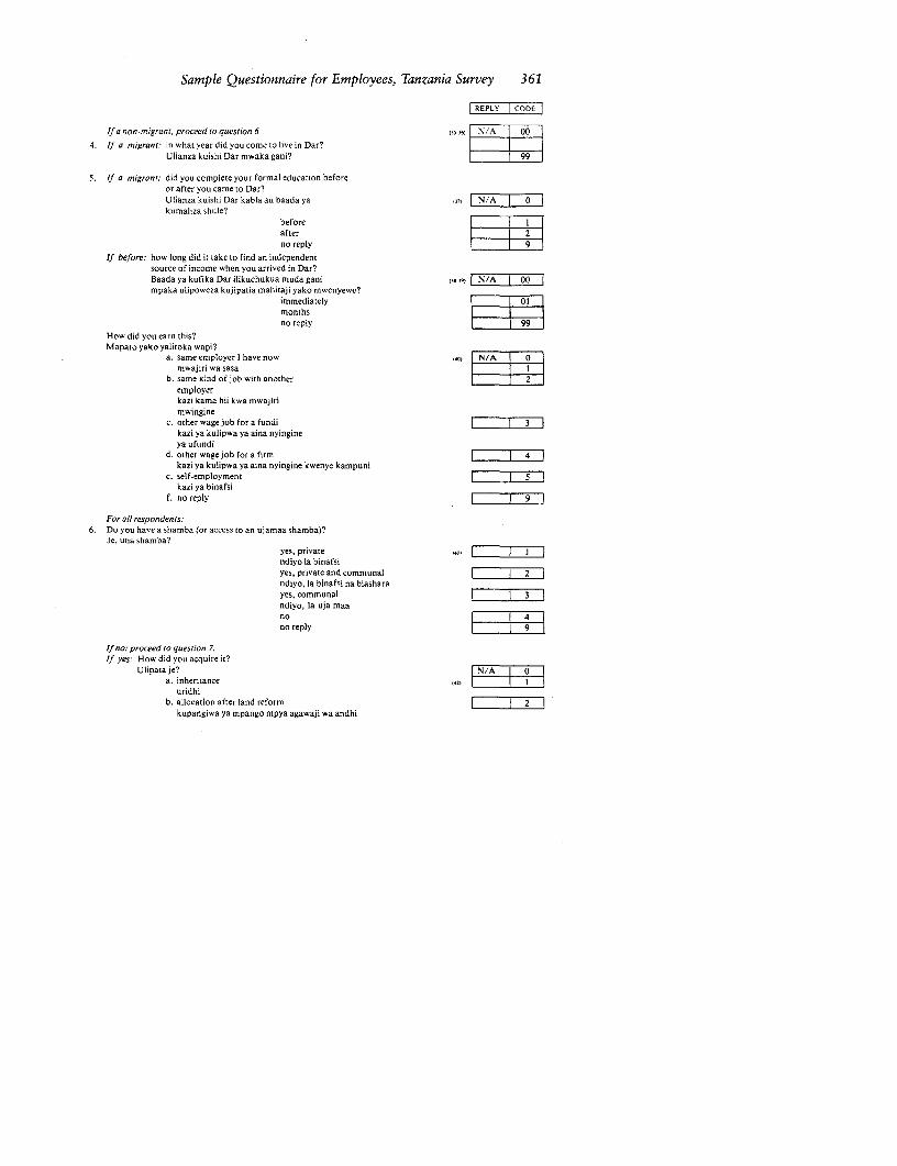
Sample Questionnaire for Employees, Tanzania Survey 361
| REPLY CODE
Ifa non-migrant, proceed to question 6 (s5-3) N!A 00
4. If a migrant: in what year did you come to live in Dar?Ulianza kuishi Dar mwaka gani? 99
5. If a migrant: did you complete your formal education beforeor after you came to Dar?Ulianza kuishi Dar kabla au baadayu s3, N/A 0akumaliza shule?
beforeafter |2no reply |9
If before: how long did it take to find an independentsource of income when you arrived in Dar?Baada ya kufika Dar ilikuchukua mudagun un| N/A 00mpaka ulipoweza kujipatia mahitaji yako mwenyewe?
immediately 01months [no reply 99
How did you earn this?Mapato yako yalitoka wapi?
a. same employer I have now ,zo N/Amwajiri wa sasa 0
b. same kind of job with anotheremployerkazi kama hii kwa mwajirimwingine
c. other wage job for a fundi |3E|kazi ya kulipwa ya aina nyingineya ufundi
d. other wage job for a firm 4kazi ya kulipwa ya aina nyingine kwenye kampuni
c. self-employment 5kazi ya binafsi
f. no reply 9
For all respondents:6. Do you have a shamba (or access to an ujamaa shamba)?
Je, una shamba?yes, private
ndiyo la binafsiyes, private and communal 2ndiyo, la binafsi na biasharayes, communal 3ndiyo, la uja maano4no reply 9
If no: proceed to question 7.If yes: How did you acquire it?
Ulipata je? N7A 8a. inheritance I42S
uridhib. allocation after land reform |2 3
kupangiwa ya mpango mpya agawaji wa andhi
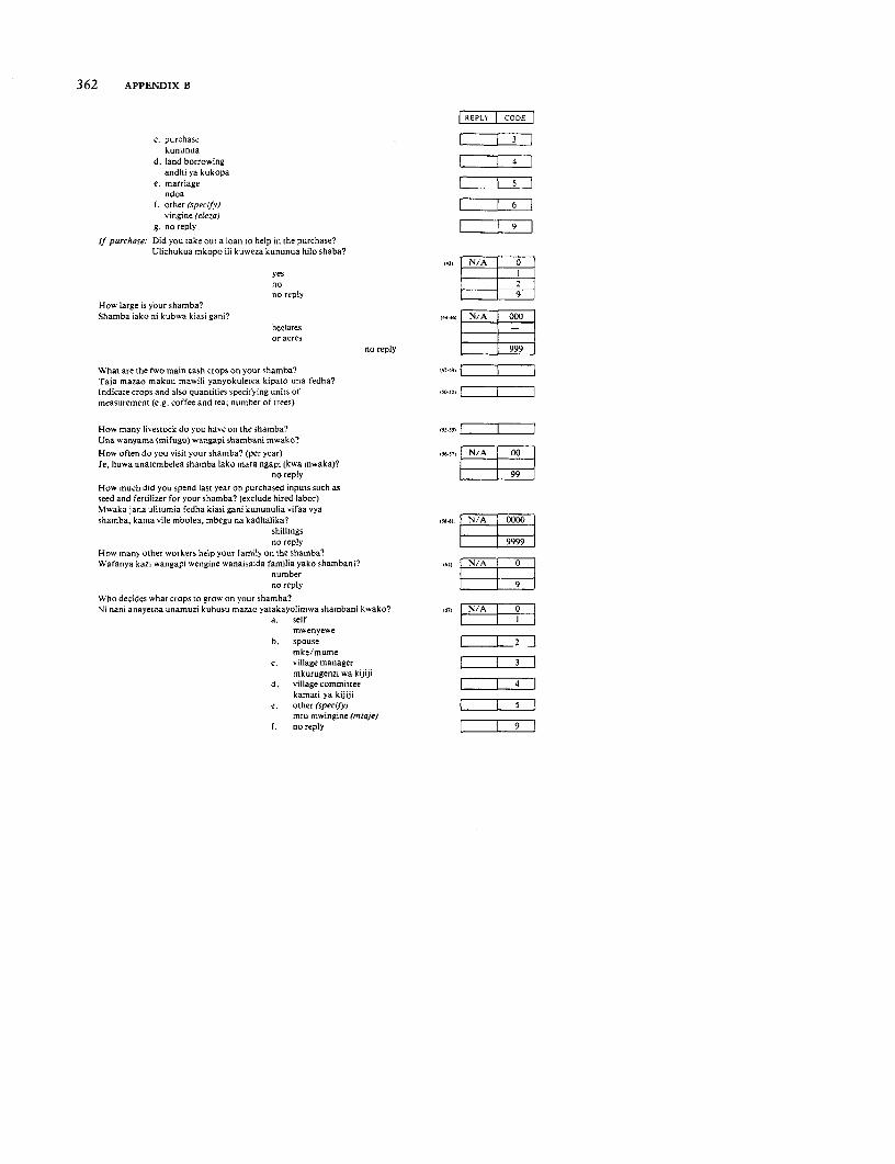
362 APPENDIX B
| EPY CDE|
c. purchase 3kununua
d. land borrowing 4andhi ya kukopa
e. marriage |ndoa
f. other (specify) | 6E|'ingine (eleza)
g. no reply 9
If purchase: Did you take out a loan to help in the purchase?Ulichukua mkopo ili kuweza kununua hilo shaba?
o -N-/A | o yes Ino 2no reply 9
How large is your shamba?Shamba iako ni kubwa kiasi gani? N/A 00
hectaresor acres
no reply
What are the two main cash crops on your shamba? W15Taja mazao makuu mawili yanyokuletea kipato una fedha?Indicate crops and also quantities specifying units of so-snmeasurement (e.g. coffee and tea; number of trees)
How many livestock do you have on the shamba? 55-55
Una wanyama (mifugo) wangapi shambani mwako?
How often do you visit your shamba? (per year) s1 N/A 00Je, huwa unatembelea shamba lako mara ngapi (kwa mwaka)?
no reply 99
How much did you spend last year on purchased inputs such asseed and fertilizer for your shamba? (exclude hired labor)Mwaka jana ulitumia fedha kiasi gani kununulia vifaa vyashamba, kama vile mbolea, mbegu na kadhalika? 0s8.6W, N/A 0000
shillingsno reply
How many other workers help your family on the shamba?Wafanya kazi wangapi wengine wanaisaida familia yako shambani? s, N/A
numberno reply
Who decides what crops to grow on your shamba?Ni nani anayetoa unamuzi kuhusu mazao yatakayolimwa shambani kwako? o N |
a. self l fImwenyewe
b. spouse Z2Tmke/mume
c village manager 3mkurugenzi wa kijiji
d. village committee 4kamati ya kijiji
e. other (specify)mtu mwingine (mteaje)
f. no reply | 9
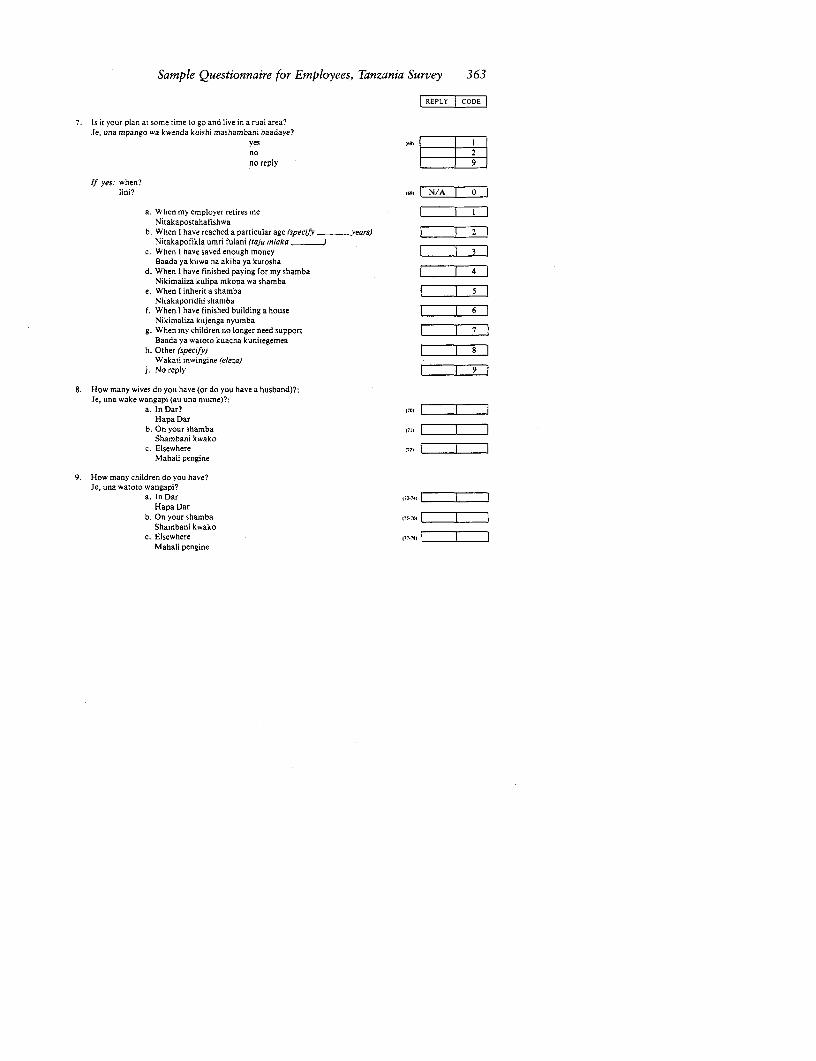
Sample Questionnaire for Employees, Tanzania Survey 363
| EPY 0 CDE|
7. Is it your plan at some time to go and live in a rual area?Je, una mpango wa kwenda kuishi mashambani baadaye?
no W 2no reply
If yes: when?lini? 9|N
a. When my employer retires me -Nitakapostahafishwa
b. When I have reached a particular age (specify _ years) 2Nitakapofikia umri fulani (taja miaka
c. When I have saved enough moneyBaada ya kuwa na akiba ya kutosha
d. When I have finished paying for my shamba 7 | 4i |Nikimaliza kulipa mkopa wa shamba
e. When I inherit a shamba 7 7 5Nitakaporidhi shamba
f. When I have finished building a houseNikimaliza kujenga nyumba
g. When my children no longer need support 7Baada ya watoto kuacha kunitegemea
h. Other (specify)Wakati mwingine (eleza)
j. No reply 9
8. How many wives do you have (or do you have a husband)?:Je, una wake wangapi (au una mume)?:
a. In Dar? ts0|
Hapa Darb. On your shamba P| j
Shambani kwakoc. Elsewhere otj
Maltali pengine
9. How many children do you have?Je, una watoto wangapi?
a. In Dar ,,,745Hapa Dar
b. On your shamba mJShambani kwako
c. Elsewhere 777i rMahali pengine

364 APPENDIX B
I REPLY I CODEO
10. To what tribe do you belong? M'9.er N/A 0OWewe ni kabila gani?
a Sukuma 01
b. Makonde 02
c. Chagga 03
d. Haya 04
e. Nyamwezi 05
f. Ha 06
g. Hehe 07
h. Gogo 08
i. Nyakyusa 09
j. Sambao 10
k. Luguru ll
1. Bena 12
m.Turu 13
n. Other (specify) 14
o. No reply 99
Employee number ri-ar
Card number r |S
11. Do you use some of your earnings to help support relatives outside Dar?Je, unatumia sehemu ya mapato yako kwa ajili ya kuwasaidia jamaa zako walio njeya Dar?
yes ,no 2no reply 9
If yes: What forms does this support take?Hua msaada ni wa aina gani?
a. remittances of money N/A 0(including school fees) [Kuwapelekea fedha(pampoja na ada ya shule)
b. purchase of goods 2Kuwanunulia vitu
c. other (specify)
Nyinsine (eieza)d. no reply 9

Sample Questionnaire for Employees, Tanzania Survey 365
R EPLY |CODE|
If remittances: 8.9) rN/A - 00how many times a year?Unapeleka fedha marangapi kwa mwaka?
no reply 99
What was the value of your O 0-,,,3 N/A | 0000last remittance (shillings)?Fedha ulizopeleka mara yamwisho zilikwa kiasi gani?
no reply
About how much does the 17-N N/Asupport you give to relativescost you a year? (shillings)Jumla ya fedha unazotumiakwa ajili ya kuwasaidiajamaa zako ni kiasi ganikwa mwaka?
no reply j999What is your help used for?Msaada wako unatumi wa kwamanufaa gani?(code asfollows:
yes=Ino =2
no reply =9) N/A 0a. education 19)
elimub. house construction or so)
improvementkujenga au kuimarisha nyumba
c. farm improvement 8)|
kuendeleza shambad. consumer goods 22)
kununulia bidhaae. food '23|
chakulaf. general purposes 12.)
matumizi ya kawaidag. other (specify) 2|)
mengine (eleza)

366 APPENDIX B
VIII. Education of ChildrenREPLY CODE|
1. How many children do you have below primary school age? r-n8j
Una watoto wangapi ambao hawajafikia umri wa kwanza shule ya misingi?How many children do you have old enough to have gone to schoolbut who never attended?Una watoto wangapi ambao wamefikia umri wakwenda shule lakini hawajawahi kwenda shule?
3. How many children do you have in formal education at present? 3.|
Kwa sasa, ni watoto wangapi wanaosoma shule?4. How many children do you have who have completed their formal slIn
education?Una watoto wangapi ambao wameshamaliza shule?
5. Consider your three eldest children aged 6 or over (if any).Fikiria watoto wako watatu wakubwa ambao wanaumri wa miaka 6 na kuendelea (kama unawo)
CHILD I CHILD2 CHILD3COL. REPLYI CODE I COL. REPLY CODE I COL. REPLY COD
N/A 0 N/A 0 N/A 0Sex: male ,3,) L 1 I4) L (33
female 22 2 2
Age: (years) (36-35 (33.31) 34.35r
don't know or not applicable | |g991 | | 9 ||Highest level of educationElimu ya juu kabisa waliyofikia
no education 3S-33 00 ss-fn 00 sv.ss 00
Standard I 01 01 01Standard 2 02 02 02Standard 3 03 03 03Standard 4 04 04 04Standard 5 05 05 05Standard 6 06 06 06Standard? 07 07 07Standard 8 08 08 08Form I 10 10 10Form 2 Ii 11 IIForm 3 12 12 12Form 4 13 13 13Form 5 14 _ 14 14Form 6 15 15 15University 16 16 16Other post- 17 17 17
secondary(specify)
Other (specify) 18 18
no reply or not applicable 99 99
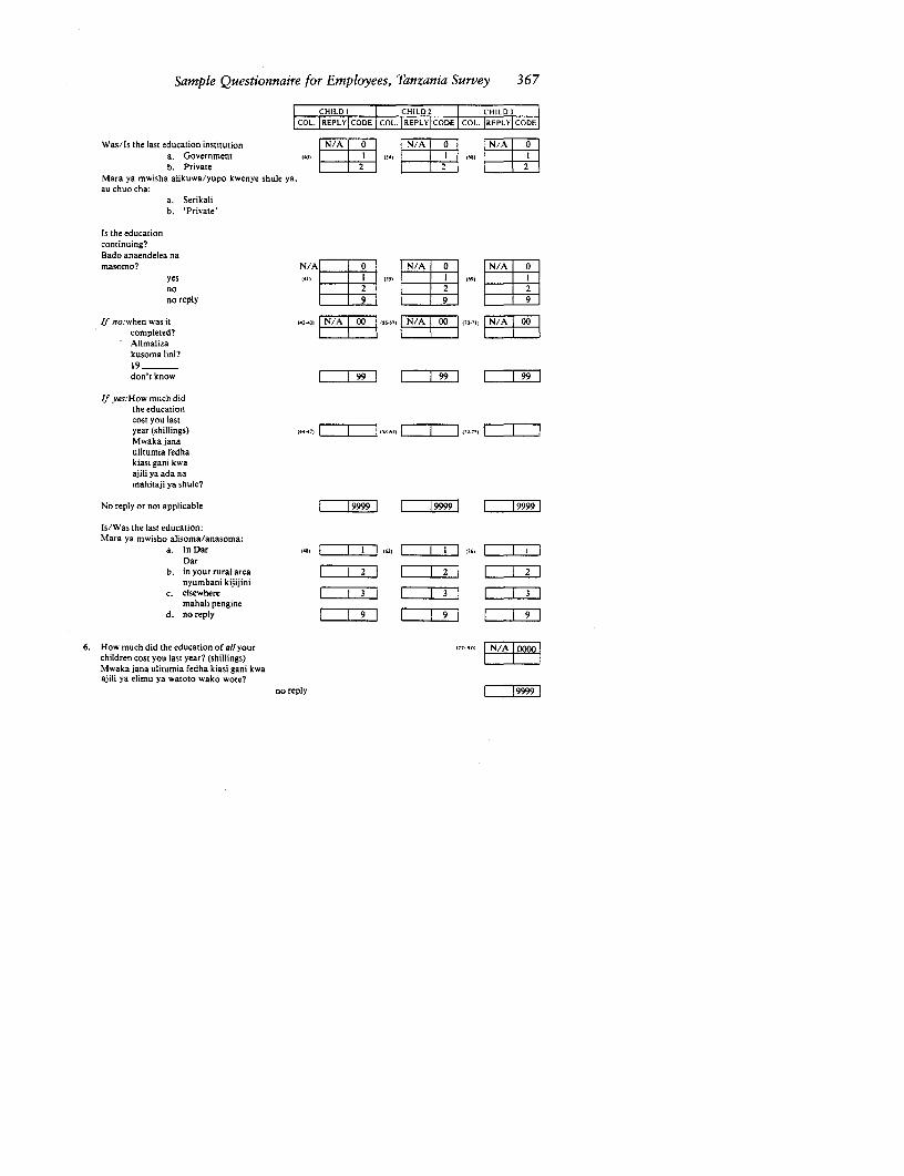
Sample Questionnaire for Employees, Tanzania Survey 367
CHILD I CHILD2 CHILD3
I COL. |REPLY|CODE I COL. I REPLY CODE I COL. IREPLY CODEJ
Was/Is the last education institution N/A 0 O N/ION/ATia. Government , 54 68) Ib. Private 2 22
Mara ya mwisha alikuwa/yupo kwenye shule ya,au chuo cha:
a. Serikalib. 'Private'
Is the educationcontinuing?Bado anaendelea namasomo? N/A 0 N/A 0 N/A 0
yes (4)) I (5) 3 1 I
no Id <2 2no reply 9 9
If no:when was it 42431 N56.,7, N/A N(0071| 0
completed? L 9 Lj.1.|Alimalizakusoma lini?19 _
don't know 99 99 99
If yes:How much didthe educationcost you lastyear (shillings) (4.7) | | -6)) | 1.75)
Mwaka janaulitumia fedhakiasi gani kwaajili ya ada namahitaji ya shule?
No reply or not applicable 9999 9999
Is/Was the last education:Mara ya mwisho alisoma/anasoma:
a. In Dar 44) |54) I (76)
Darb. in your rural area 2 |
nyumbani kijijinic. elsewhere 3 3
mahali pengined. no reply 9 9 9
6. Howmuchdidtheeducationofea/your ,7760) Nchildren cost you last year? (shillings)Mwaka jana ulitumia fedha kiasi gani kwaajili ya elimu ya watoto wako wote?
no reply 9999

368 APPENDIX B
Employee Questionnaire
REPLY I CODE_
EmployeeNumber (. j
Card number ,,,
IX. Miscellaneous1. Occupation
Current jobLast job Zn')First job (8.33)
2. Wage information obtained from employer(shillings per month)Basic wageHousing allowance 33-33
Overtime payment 333)
less Employee contribution toNPF (4Tax deducted (2.43
For those who reached Form 4 or above:
3. How did you obtain your first wage job(exclude National Service or wageemployment during school or collegevacations)?Ulipataje kazi yako ya kwanza (kuondoa kaziya kujenga taifa na pia kazi za likizoniwakati ukiwa masononi
|N/A | I. Government allocation ( I I 3
Kupangiwa na serikali2. Application 2
Maombi3. Other (specify) 3
Nyingine ftaja)4. No reply 9
Hakuna jibu
If through Government allocation:On your list of preferences, wasthis job:Kwenye arodha ya mapendekezo, kazi hiiilikuwa ya N/A 0
1. first (37)kwanza
2. second 2pili
3. third 3tatu
4. lower 4chini zaidi

Sample Questionnaire for Employees, Tanzania Survey 369
REPLY CODE
5. not your choicehaikuwa kwenye chaguo lako
6. noreply 9hakuna jibu
4. Were you bonded by Government?Ulikuwa umelazimika kwa nkatabakuitumikia serikali?
Yes r Ndiyono 2Hapana
no reply 9Hakuna jibu
If yes:Kama ndiyo:Didyou serve out your bond? LN/A 0Ulitmiza nikataba wako?Yes (49)
NdiyoNo 2HapanaNo reply 9Hakura jibu
If did not serve out bond:Kama hukutimiza nikabataIs this because: (SO|
InamaeuishaI. you are still serving I I
bado unaendelea2. transferred by government 2
ulihamishwa na serikali3. managed to move to another job 3 T --- 3
uliweza kuhahua kwenye kazi nyingine4. no reply
Hakuna jibu
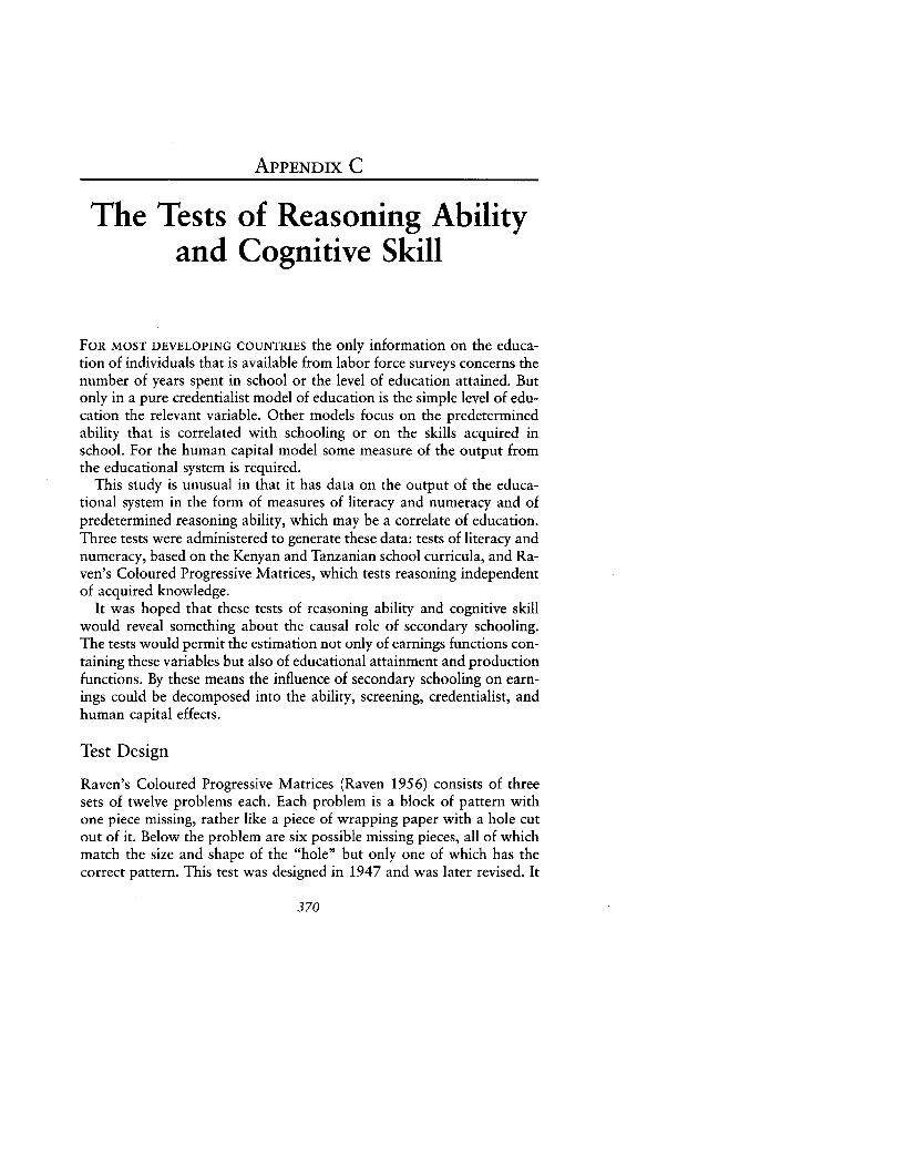
APPENDIX C
The Tests of Reasoning Abilityand Cognitive Skill
FOR MOST DEVELOPING COUNTRIES the only information on the educa-tion of individuals that is available from labor force surveys concerns thenumber of years spent in school or the level of education attained. Butonly in a pure credentialist model of education is the simple level of edu-cation the relevant variable. Other models focus on the predeterminedability that is correlated with schooling or on the skills acquired inschool. For the human capital model some measure of the output fromthe educational system is required.
This study is unusual in that it has data on the output of the educa-tional system in the form of measures of literacy and numeracy and ofpredetermined reasoning ability, which may be a correlate of education.Three tests were administered to generate these data: tests of literacy andnumeracy, based on the Kenyan and Tanzanian school curricula, and Ra-ven's Coloured Progressive Matrices, which tests reasoning independentof acquired knowledge.
It was hoped that these tests of reasoning ability and cognitive skillwould reveal something about the causal role of secondary schooling.The tests would permit the estimation not only of earnings functions con-taining these variables but also of educational attainment and productionfunctions. By these means the influence of secondary schooling on earn-ings could be decomposed into the ability, screening, credentialist, andhuman capital effects.
Test Design
Raven's Coloured Progressive Matrices (Raven 1956) consists of threesets of twelve problems each. Each problem is a block of pattern withone piece missing, rather like a piece of wrapping paper with a hole cutout of it. Below the problem are six possible missing pieces, all of whichmatch the size and shape of the "hole" but only one of which has thecorrect pattern. This test was designed in 1947 and was later revised. It
370
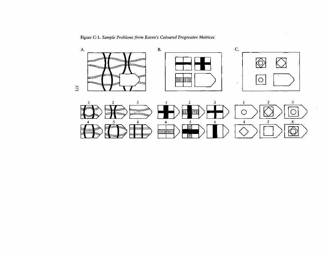
Figure C-1. Sample Problems from Raven's Coloured Progressive Matrices
A. B. C.
1 2 3 1 2 3 1 23
4 5 6 4 5 6 4 56
WD~ __ F IZD
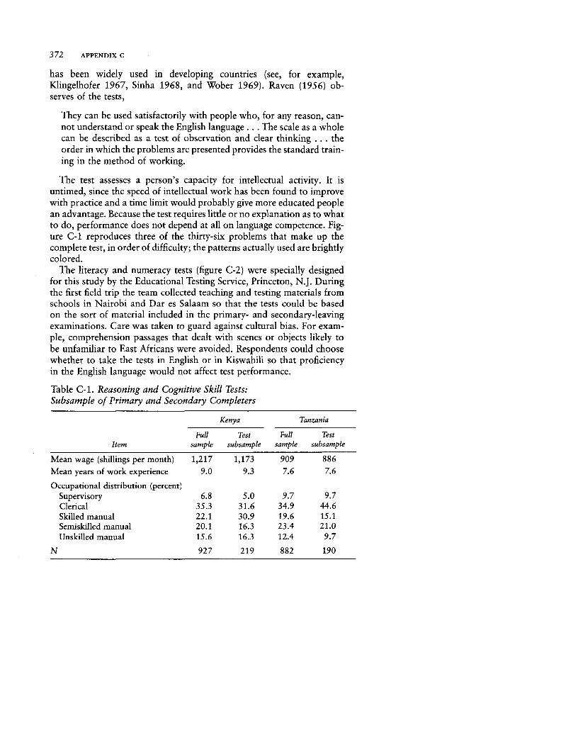
372 APPENDIX C
has been widely used in developing countries (see, for example,Klingelhofer 1967, Sinha 1968, and Wober 1969). Raven (1956) ob-serves of the tests,
They can be used satisfactorily with people who, for any reason, can-not understand or speak the English language .. . The scale as a wholecan be described as a test of observation and clear thinking ... theorder in which the problems are presented provides the standard train-ing in the method of working.
The test assesses a person's capacity for intellectual activity. It isuntimed, since the speed of intellectual work has been found to improvewith practice and a time limit would probably give more educated peoplean advantage. Because the test requires little or no explanation as to whatto do, performance does not depend at all on language competence. Fig-ure C-1 reproduces three of the thirty-six problems that make up thecomplete test, in order of difficulty; the patterns actually used are brightlycolored.
The literacy and numeracy tests (figure C-2) were specially designedfor this study by the Educational Testing Service, Princeton, N.J. Duringthe first field trip the team collected teaching and testing materials fromschools in Nairobi and Dar es Salaam so that the tests could be basedon the sort of material included in the primary- and secondary-leavingexaminations. Care was taken to guard against cultural bias. For exam-ple, comprehension passages that dealt with scenes or objects likely tobe unfamiliar to East Africans were avoided. Respondents could choosewhether to take the tests in English or in Kiswahili so that proficiencyin the English language would not affect test performance.
Table C-1. Reasoning and Cognitive Skill Tests:Subsample of Primary and Secondary Completers
Kenya Tanzania
Full Test Full TestItem sample subsample sample subsample
Mean wage (shillings per month) 1,217 1,173 909 886Mean years of work experience 9.0 9.3 7.6 7.6Occupational distribution (percent)
Supervisory 6.8 5.0 9.7 9.7Clerical 35.3 31.6 34.9 44.6Skilled manual 22.1 30.9 19.6 15.1Semiskilled manual 20.1 16.3 23.4 21.0Unskilled manual 15.6 16.3 12.4 9.7
N 927 219 882 190

Figure C-2. Selected Questions, in English and Kiswahili,from the Cognitive Skill Tests
A. Numeracy
1. 105 - 16 = ?(a) 89 (b) 91 (c) 99 (d) 111
2. There are 4 rows of chairs and 12 chairs in each row. What is the total numberof chairs?Kuna mistari 4 ya viti na kuna viti 12 katika kila mstari. Kuna jumla ya vitivingapi?(a) 12 + 4 (b) 12 - 4 (c) 12 x 4 (d) 12 . 4
3. Which of the following numbers is the largest?Kati ya tarakimu zifuatazo, ni ipi kubwa kuliko zote?(a) 0.1 (b) 0.01 (c) 0.111 (d) 0.1101
4. 1% of 400 is:1% ya 400 ni:(a) 1 (b) 4 (c) 40 (d) 400
5. The height of a man is closest to 2Urefu wa mwanamme unakaribia 2(a) millimetres (b) metres (c) kilometres (d) centimetres
6. How many square inches are there in a square foot?Katika futi ya mraba moja kuna inchi za mraba ngapi?(a) 12 (b) 36 (c) 48 (d) 144
7. Two cities are 12 kilometres apart. Each day, a bus makes 3 round trips be-tween these cities. How many kilometres does the bus travel each day?Kati ya miji miwili kuna umbali wa kilomita 12. Basi huwa linafanya safari3 za kwenda na kurudi kila siku. Kwa siku?(a) 72 (b) 36 (c) 15 (d) 4
8. A meal costs 15/00. If a 10% service charge is to be added to the bill, whatshould the total charge be?Bei ya mlo mmoja ni sh. 15/00. Kama kuna nyongeza ya 10% kwa ajili yahuduma, bili itakuwa kiasi gani kwa ujumla?(a) 15/10 (b) 16/00 (c) 16/50 (d) 25/00
9. An island has an area of about 300 square miles. The government reports thatthe western 1/3 of the island is not suitable for cultivation. How many squaremiles of this island are suitable for cultivation?Kisiwa kina enso la maili za mraba 300. Serikali imetoa repoti kwamba 1/3ya upande wa magharibi wa hicho kisiwa hanfai kwa kulimo. Je, maili zamraba ngapi zinazofaa kwa kilimo?(a) 50 (b) 100 (c) 150 (d) 200
373
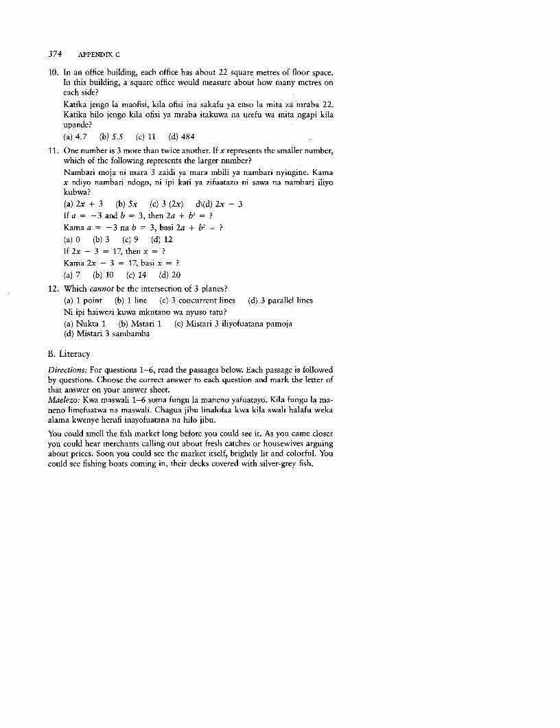
374 APPENDIX C
10. In an office building, each office has about 22 square metres of floor space.In this building, a square office would measure about how many metres oneach side?
Katika jengo la maofisi, kila ofisi ina sakafu ya enso la mita za mraba 22.Katika hilo jengo kila ofisi ya mraba itakuwa na urefu wa mita ngapi kilaupande?
(a) 4.7 (b) 5.5 (c) 11 (d) 484
11. One number is 3 more than twice another. If x represents the smaller number,which of the following represents the larger number?
Nambari moja ni mara 3 zaidi ya mara mbili ya nambari nyingine. Kamax ndiyo nambari ndogo, ni ipi kati ya zifuatazo ni sawa na nambari iliyokubwa?
(a) 2x + 3 (b) 5x (c) 3 (2x) d\(d) 2x - 3
If a = - 3 and b = 3, then 2a + b2 = ?Kama a = -3 na b = 3, basi 2a + b2 = ?
(a) 0 (b) 3 (c) 9 (d) 12
If 2x - 3 = 17, then x = ?
Kama 2x -3 = 17, basi x = ?
(a) 7 (b) 10 (c) 14 (d) 20
12. Which cannot be the intersection of 3 planes?
(a) 1 point (b) 1 line (c) 3 concurrent lines (d) 3 parallel lines
Ni ipi haiwezi kuwa mkutano wa nyuso tatu?
(a) Nukta 1 (b) Mstari 1 (c) Mistari 3 iliyofuatana pamoja(d) Mistari 3 sambamba
B. Literacy
Directions: For questions 1-6, read the passages below. Each passage is followedby questions. Choose the correct answer to each question and mark the letter ofthat answer on your answer sheet.Maelezo: Kwa maswali 1-6 soma fungu la maneno yafuatayo. Kila fungu la ma-neno limefuatwa na maswali. Chagua jibu linalofaa kwa kila swali halafu wekaalama kwenye herufi inayofuatana na hilo jibu.
You could smell the fish market long before you could see it. As you came closeryou could hear merchants calling out about fresh catches or housewives arguingabout prices. Soon you could see the market itself, brightly lit and colorful. Youcould see fishing boats coming in, their decks covered with silver-grey fish.

The Issues, the East African Natural Experiment, and the Surveys 375
1. What kind of a market is described above?
(a) A vegetable market(b) A meat market(c) A fish market(d) A fruit market
2. What could you see coming in?
(a) Tug boats(b) Rowboats(c) Fishing boats(d) Sailboats
3. What covered the decks of the boats?
(a) Rope(b) People(c) Boxes(d) Fish
Unaweza kupata harufu ya soko la samaki kabla hata hujalifikia. Ukianza kuka-ribia sokoni, unaweza kuwasikia wauza ji wakiitia samaki ambao hawajakaakwa muda tangu kuvuliwa au kina mama wakibishana juu ya bei. Pundeunaliona soko lenyewe, na lina mwangaza mkubwa na rangi nyingi. Unawezakuona mashua za kuvulia samaki zikiingia na ukumbi wake umejaa samaki warangi ya fedha.
1. Soko lililoelezewa hapo juu ni la namna gani?
(a) Soko la mboga(b) Soko la nyama(c) Soko la samaki(d) Soko la matunda
2. Uliweza kuona kitu gani kikiwasili:
(a) Meli ndogo(b) Mitumbwi(c) Mashua za kuvulia samaki(d) Mashua za matanga
3. Ukumbi wa mashua ulikuwa umejaa nini?
(a) Kamba(b) Watu(c) Maboksi(d) Samaki
The cat brushed against the old man. He did not move. He only stood, staringup at the window of the house. The party inside looked warm and friendly, butno one noticed him. The old man walked sadly on, followed by the cat.

376 APPENDIX C
4. What kind of animal was following the old man?
(a) Mouse(b) Dog(c) Cat(d) Bird
5. What was inside the house?
(a) A party(b) Some dogs(c) An old lady(d) A meeting
6. The man is described as being
(a) Old(b) Young(c) Thin(d) Small
Paka alikuwa anajigusagusa na yule baba mzee. Baba mwenyewe hakusogea, ali-simama tu huku akikodolea kwenye dirisha la nyumba. Karamu iliyokuwa ndaniilionekana kuwa nzuri na ya kikarimu, lakini hakuna mtu aliyemwona. Mzee ali-jiendea kwa unyonge akifuatwa na yule paka.
4. Huyu mzee alifuatana na mnyama wa aina gani?
(a) Panya(b) Mbwa(c) Paka(d) Ndege
S. Ndani ya nyumba kulikuwa na nini?
(a) Karamu(b) Mbwa(c) Mama mzee(d) Mkutano
6. Huyo mwanamme anasemekana kwamba ni
(a) Mzee(b) Kijana(c) Mwembamba(d) Mdogo
Directions: For questions 7-12, read the passage below. In each line, there is abox with four possible choices. Pick the choice that best completes the sentencein each numbered line. Mark the letter (a, b, c, or d) of the choice on your answersheet.
7. Sound is something we (a) hears. It comes to your(b) hearing.(c) heard.(d) hear.
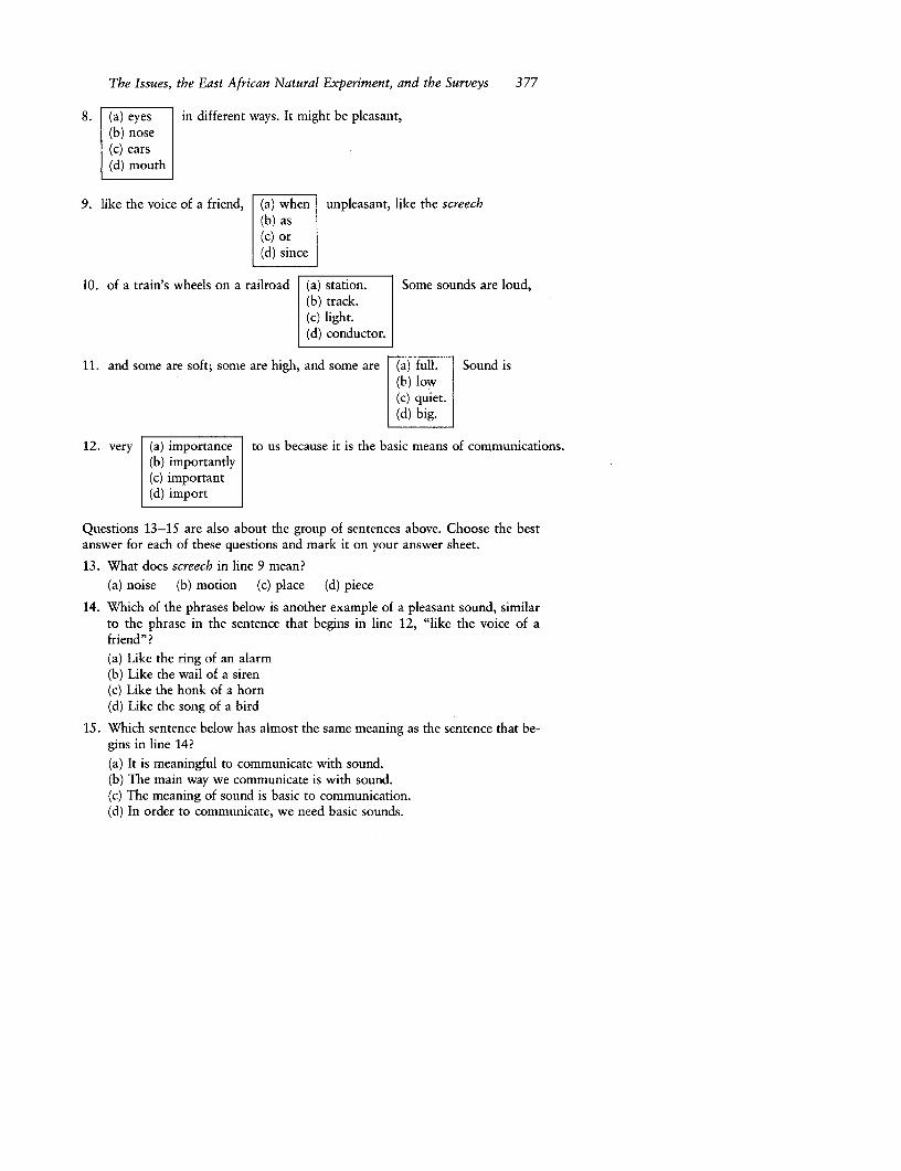
The Issues, the East African Natural Experiment, and the Surveys 377
8. (a) eyes in different ways. It might be pleasant,(b) nose(c) ears(d) mouth
9. like the voice of a friend, (a) when unpleasant, like the screech(b) as(c) or(d) since
10. of a train's wheels on a railroad (a) station. Some sounds are loud,(b) track.(c) light.(d) conductor.
11. and some are soft; some are high, and some are (a) full. Sound is(b) low(c) quiet.(d) big.
12. very (a) importance to us because it is the basic means of communications.(b) importantly(c) important(d) import
Questions 13-15 are also about the group of sentences above. Choose the bestanswer for each of these questions and mark it on your answer sheet.
13. What does screech in line 9 mean?
(a) noise (b) motion (c) place (d) piece
14. Which of the phrases below is another example of a pleasant sound, similarto the phrase in the sentence that begins in line 12, "like the voice of afriend"?
(a) Like the ring of an alarm(b) Like the wail of a siren(c) Like the honk of a horn(d) Like the song of a bird
15. Which sentence below has almost the same meaning as the sentence that be-gins in line 14?
(a) It is meaningful to communicate with sound.(b) The main way we communicate is with sound.(c) The meaning of sound is basic to communication.(d) In order to communicate, we need basic sounds.
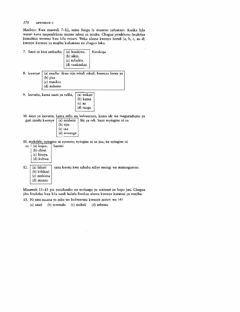
378 APPENDIX C
Maelezo: Kwa maswali 7-12, soma fungu la maneno yafuatayo. Katika kilamstari kuna mapendekezo manne ndani ya mraba. Chagua pendekezo linalofaakumalizia sentensi kwa kila mstari. Weka alama kwenye herufi (a, b, c, au d)kwenye karatasi ya majibu kufuatana na chaguo lako.
7. Sauti ni kitu ambacho (a) husikiwa. Kinakuja(b) sikia.(c) tulisikia.(d) twakisikia.
8. kwenye (a) macho tkwa njia mbali mbali. Inaweza kuwa ya(b) pua(c) masikio(d) mdomo
9. kuvutia, kama sauti ya rafiki, (a) wakati(b) kama(c) au(d) tangu
10. isiyo ya kuvutia, kama mlio wa kukwaruza, kama ule wa magurudumu yagari moshi kwenye (a) stesheni lizi ya reli. Sauti myingine ni za
(b) njia(c) taa(d) mwanga
11. makelele, nyin *ne ni nyororo; nyingine ni za juu, na nyingine niza (a) kujaa. Sautini
(b) chini.(c) kimya.(d) kubwa.
12. (a) fahari sana kwetu kwa sababu ndiyo msingi wa mazungumzo.(b) kifahari(c) muhimu(d) maana
Masawali 13-15 pia yanahusika na mafungu ya sentensi za hapo juu. Chaguajibu linalofaa kwa kila swali halafu liwekee alama kwenye karatasi ya majibu.
13. Ni nini maana ya mlio wa kukwaruza kwenye mstari wa 14?
(a) sauti (b) mwendo (c) mahali (d) sehemu
The Tests of Reasoning Ability and Cognitive Skill 379
14. Ipi kati ya misemo ifuatayo ni mfano mwingine wa sauti ya kuvutia, kamailivyosemwa kwenye sentensi inayoanzia mstari wa 11, "kama sauti ya ra-fiki"
(a) kama sauti ya kushtua(b) kama mlio wa kupaaza sauti(c) kama mlio wa honi(d) kama sauti ya ndege anapoimba
15. Ni ipi kati ya sentensi zifuatazo ina maana karibu sawa na sentensi iliyoanziamstari wa 14?
(a) Ni kitu cha maana kuzungumza na sauti.(b) Njia kuu ya kuzungumza ni kutumia sauti.(c) Maana ya sauti ni msingi wa mazungumzo.(d) Ili kuweza kuzungumza tunahitaji msingi wa sauti mbali mbali.
Reprinted by permission of Educational Testing Services, the copyright owner.Note: The questions have been renumbered, but they are in the same order as in the tests.
The difficulty of the questions increases from the beginning to the end of the tests.
The tests appear to have been well calibrated; the frequency distribu-tions of the test scores reveal considerable variance on each test, very fewperfect scores, and no zero scores. The distribution of scores on Raven'stest was similar in the two countries. This provides additional reassur-ance as to the test's validity as a measure of predetermined reasoningability, since we have no reason to expect the distribution and level ofintellectual capacity to differ between Kenya and Tanzania.
The Tested Subsample
This sort of testing is well outside the experience of most economists andto our knowledge was novel for East Africa. We did not know and couldnot predict how revealing the test results would be, nor could we be confi-dent that people would readily agree to take the tests. The history of "in-telligence tests" in Africa is not laudable, and suspicion and reluctancewould not have been surprising. For these reasons, this part of the surveywas regarded as being rather like a high-risk stock in a portfolio, withan uncertain yield and low probability attached to a high payoff. We hadto be relatively risk averse and so could not allocate a large portion ofour resources to the tests.
It was decided to limit the test to a subsample of workers that wouldbe large enough to permit statistically significant inferences and generali-zations. Because of the particular interest in the value of secondary edu-cation, testing was confined to primary and secondary completers. About100 people who had precisely completed primary school (standard 7 or8) and 100 who had precisely completed secondary school (form 4) wereselected in each country. Selection was purposive; that is, a worker who
380 APPENDIX C
was being interviewed and who fitted the educational criterion was se-lected for testing if a tester was available when the interview was com-pleted. The sample was stratified because it was considered importantto ensure adequate numbers in each educational category, and the num-ber of primary and secondary completers in the samples was not knownuntil the survey had been completed. As table C-1 shows, the subsamplesare well representative of the larger samples from which they were drawnwith respect to average wages, occupational distribution, and average ex-perience.
The tests took an hour to administer. Testing was usually done by stu-dents who were studying educational psychology. Unexpectedly, workersshowed enthusiasm for taking the tests and set to the tasks with diligenceand determined care. The success of the results and the value of the datathat they provide suggest that further work on these lines would be justi-fied, in East Africa or elsewhere. Hindsight indicates that in our research,allocation of a larger portion of our resources to the tests to obtain alarger tested subsample would have been justified.
APPENDIX D
The Simulation Approachto Decomposing Inequality
IN THIS APPENDIX we describe a simulation method which we have usedto decompose inequality of earnings (for instance, in chapter 3) or to con-duct counterfactual experiments (for instance, in chapter 9). We arguethat a simulation in which the estimated "true" relation determines thedistribution of interest is often to be preferred to a commonly used alter-native, the "comparative R2 " regression procedure.
Decompositions of measures of inequality are of interest for under-standing the sources of inequality and the impact on inequality of variousdemographic, economic, and policy changes. Several authors have advo-cated and utilized a comparative R2 regression procedure for identifyingthe relative contributions that different factors make to inequality ofincome (or of similar variables). Wise (1975, p. 359), for example,states:
An idea of the relative contribution of academic versus nonacademicvariables in the "determination" of salary may be obtained by com-paring values of R2 obtained when different groups of variables areincluded in the regression . . . A high estimate of the contribution ofacademic variables is the proportion of remaining variance explainedwhen they are added to the regression in the absence of nonacademicvariables; a low estimate is the addition to the proportions explainedwhen they are added after the nonacademic variables.
Fields and Schultz (1980, pp. 458-62) use a similar procedure to es-tablish bounds on regional and other contributions to income in-equality.
We start with the comparative R2 approach. We use In income in thisillustration because the log normal is a better approximation than the
Note: Adapted from J. R. Behrman, J. B. Knight, and R. H. Sabot, "A Simulation Alter-native to the Comparative R2 Approach to Decomposing Inequality," Oxford Bulletin ofEconomics and Statistics 45, no. 3 (August 1983), pp. 307-12.
381

382 APPENDIX D
normal for most empirical income (and related) distributions. Let thetrue relation determining In income be
n(D-1) Y= X aiX± + u
i=O
where Y is In income, Xi is a set of independent variables with Xo a con-stant, ai are unknown parameters, and u is a stochastic term distributedindependently of all Xi, with mean zero and constant variance au.
The implied variance decomposition is
n n(D-2) 2y= X a,k& + X Y aiajaxix + ±U
i=1 i1 j5'i
The R2 or coefficient of determination is the explained portion of thetotal variance:
n n(D-3) R2 = iX 2 + i j aiacxx, 1 - O 'y
R2 is weakly bounded by 0 (corrections for degrees of freedom beingignored) and 1.
Under the comparative R2 procedure the "high" estimated contribu-tion of a given variable is defined to be the coefficient of determinationobtained if only that variable is included in the estimation of relation D-1(that is, as is a priori set equal to zero for all j 0 i except j = 0), andthe "low" estimated contribution is defined to be the incremental addi-tion to the coefficient of determination if the variable of interest is addedto a specification that includes all other variables (that is, the restrictionthat ai is zero is removed):
(D-4a) "High" contribution = RI'2
(D-4b) "Low" contribution = R2- RI
where R2 is the coefficient of determination for relation D-1; Ri'2is thecoefficient of determination if only the ith variable is included; and R~',22
is the coefficient of determination if only the ith variable is excluded fromrelation D-1.
We use inverted commas around "high" and "low" because Hendryand Marshall (1983) show that the sum of the "high" contributions ofthe n right-hand variables need not exceed the sum of the "low" contri-butions. A reversal can occur if, for example, R 2 is zero yet Xi is relevantto explaining Y, given the other Xs (or, more generally, if the partial cor-relation of Xi and Y exceeds the simple correlation). Obviously this result
The Simulation Approach to Decomposing Inequality 383
raises further questions about the comparative R2 procedure.The sum of the "high" contributions is not necessarily weakly greater
than R2 , nor is the sum of the "low" contributions necessarily weaklyless than R2 , although this is usually thought to be the case for earningsfunctions. The sums are equal to each other and equal to R2 if and onlyif all the Xi variables are orthogonal. If n equals 2 (but generally onlyif n equals 2), the sum of the "high" estimate for one variable and the"low" one for the other equals R2 .
If relation D-1 is the true relation, an alternative approach is to esti-mate it directly and then to use those estimates to simulate the contribu-tion of a given variable to the inequality measure of interest by hypothe-sizing a different distribution of the Xi variable of interest (for example,zero variance). If the inequality measure of interest is variance In income,relation D-2 can be used directly once the ai and a-u have been estimated.In this case the contribution of a particular Xi to cry can be identifiedwith the sum of all terms in relation D-2 that involve the variance or co-variance of Xi.
When some other measure of inequality is employed, the estimatedrelation D-2 is used to predict the In income of each person, ^Y.Everyone's endowment of each Xi is in turn set equal to the mean valueof Xi for the sample as a whole, and the predicted In income, Yi, of eachperson is calculated with the use of the estimated function with the hypo-thetical mean value for Xi. The inequalities of ^Y and Yi are calculatedas I( and I(Vi), and the contribution of each Xi to inequality is esti-mated as I(Y) - 1(Yi).
The relative contribution of each Xi is obtained by expressing its con-tribution as a percentage of
I [I(Y) - I(YA)
In effect, the following counterfactual question is being asked: whatwould be the impact on inequality if the dispersions attributable to eachdetermining characteristic were eliminated in turn?
A second counterfactual question might be: what would be the impacton inequality if the dispersions attributable to all determining character-istics except one were eliminated in turn? W(here I(Y)D is the inequalityattributable to Xi alone, the relative contribution of Xi is I(Yi)I/, I(Y3).
The answer to the first counterfactual question is analogous to the"low" contribution in the comparative R2 approach and the answer tothe second counterfactual question is analogous to the "high" contribu-tion. In general, the answers to the two counterfactual questions do notgive the same decompositions of inequality even if the Xi are orthogonal(although in this case, as noted above, the "high" and "low" contribu-tions are the same).'
The contribution of Xi based on any of the simulations is dependent
384 APPENDIX D
in general on all parameter values, the distribution of the particular Xi,and the distributions of all other X, (through the covariances or otherinteractions). The sum of the contributions of all Xi(i = 1,.. . n) socalculated is generally not equal to R2 , even if the inequality measure ofinterest is variance In income, because of the double role of the covari-ance terms. That is, the covariance between Xi and Xi affects the contri-bution so measured of both Xi and Xi. If and only if all of the Xi areorthogonal to one another is the sum of these contributions equal to R2for the variance In income inequality measure. For other inequality mea-sures, even if the Xi are orthogonal to one another, the sum of the contri-butions of all Xi may not be R2 .
If the measure of inequality that is of interest is variance In incomeand if all of the Xi are orthogonal, the two approaches give identical de-compositions of the sources of inequality. Otherwise they may give dif-ferent decompositions. The simulation alternative seems preferable in fiverespects.
First, the usual comparative R2 approach is informative only if themeasure of inequality that is of interest is variance In income and notif other measures (for example, the Gini coefficient and Theil's inequalityindex) are of greater interest. In contrast, the simulation approach maybe used with any desired measure of inequality, and the relative contribu-tion of a variable may differ depending on which measure of inequalityis employed.
Second, the comparative R2 approach simply shows the total contribu-tion to cry made by each Xi. Even if variance In income is the inequalitymeasure of interest, at times it may be of more interest to ask what wouldhappen to uy if there were some change in the distribution of Xi otherthan the elimination of all variance in it. For example, it may be of inter-est to ask what would be the impact on variance In income of halvingthe variance in years of schooling. Such questions are straightforwardlyanswered with the simulation approach, but the comparative R2 proce-dure cannot answer them.
Third, although collinearity among the independent variables presentsa problem for both approaches-for the simulation approach the prob-lem is that less reliance can be placed on the estimated coefficients-thesimulation approach permits the establishment of confidence intervals forthe contribution of a given Xi to inequality. The variance-covariance ma-trix of parameter estimates can be used to obtain the probabilistic distri-bution of the contribution of a given Xi. In contrast, the comparative R2
does not give confidence intervals. The "high" and "low" values ob-tained in the comparative R2 procedure are not related to confidence in-tervals, although sometimes they are inappropriately discussed as thoughthey have some such relation.
Fourth, the simulation approach builds on the hypothesized structural
The Simulation Approach to Decomposing Inequality 385
relation and explicitly incorporates the dependence of a given decomposi-tion on the distributions of all parameters and of all right-hand variables.Given the assumed true structure, the decomposition estimates obtainedare based on unbiased parameter values. The comparative R2 approach,in contrast, uses parameter estimates that are biased if relation D-1 isindeed the true relation. The procedure for obtaining the "high" contri-bution, for example, uses parameter estimates that are generally biasedowing to the omission of variables from the true structural relation.Under the maintained hypothesis regarding the true relation, it is not atall clear why the implications of the particular misspecification used inthis "high" value calculation are of any particular interest.2
Fifth, in the case of the variance In income measure, the simulationalternative is easier since only one regression need be estimated insteadof 2n + 1 regressions. In the case of other measures, one regression andn simulations are required.
The simulation procedure can also be used in counterfactual experi-ments to examine the effect of hypothetical policy changes on inequality.(Recent examples for developing countries include Wolfe, Behrman, andBlau 1982 and Knight and Sabot 1983a.) For instance, it is possible tomeasure the effect on income inequality of increasing to the minimumlevel all schooling levels that are below some minimum (see Blaug,Dougherty, and Psacharopoulos 1982). Similarly, it may be of interestto examine the effect on inequality of the change in the educational com-position of the labor force or in the schooling coefficient brought aboutby a policy of educational expansion.
In chapter 9, for instance, we estimate an equation corresponding toD-1 to predict the earnings of each worker. It is then possible to calculatethe inequality of predicted earnings. We simulate the effect on the earn-ings structure of altering the relative supply of educated labor by substi-tuting the set of education coefficients of one country for those of theother and again predicting individual earnings and hence the inequalityof those earnings. Similarly, we simulate the effect on the labor forcecomposition of altering the relative supply of educated labor. The educa-tional composition of one sample is substituted for that of the other,and the inequality of predicted earnings of the reweighted sample iscalculated. A further exercise combines these two effects of educationalexpansion.
A limitation of the simulation approach should be recognized, how-ever. The counterfactual questions require that the coefficients ai beinvariant with respect to changes in the distribution of the determiningvariables Xi. Yet these coefficients might alter in response to the assumedexogenous change, as might the values of the other Xs. It is necessary,therefore, to avoid simulations if theory clearly predicts an ensuingchange in what are treated as parameters.
386 APPENDIX D
Notes
1. In general, the various Xi interact multiplicatively in inequality measures(although not in relation D-1). Therefore even if their covariances are zero, thereremains a problem of attribution for the interaction terms akin to the covariancein relation D-3, which leads to different decompositions for the twocounterfactual questions.
2. Of course, the maintained hypothesis regarding the true structure may bewrong in an infinite number of ways, and one interpretation of the "high" valuein the comparative R2 procedure is that it is the outcome if the true specificationdiffers from the assumed one in specific ways. But why focus on that particularpossibility? Relation D-1 may be misspecified in ways that lead tounderrepresenting or overrepresenting the contribution of Xi to o2.
APPENDIX E
Classification of Occupations
IN MOST LABOR FORCE SURVEYS the classification of occupations is notconceptually appropriate-it tends to be a murky blend of activity, skill,and status-and the system of classification cannot be relied on to be con-sistent from one survey to another. To avoid these faults, considerablecare was taken with the treatment of occupation in the Kenyan andTanzanian surveys. It was necessary to work from first principles, andso the skill content of the job was explicitly used as the criterion for clas-sification. To this end a specially designed occupational questionnairewas administered to the respondent by the interviewer at the appropriatestage of the main interview (figure E-1).
Information was obtained not only on the current wage job but alsoon the previous wage job and on the first wage job (if these differed).If the respondent had changed occupation during the tenure of the job,the latest information was obtained in each case. Hindsight shows that,given the importance of occupation in our analysis, it would have beenworthwhile to document changes in occupation during the tenure of eachjob. As it is, however, we have more information, and conceptually moreappropriate information, on occupation than is normally the case withlabor market surveys.
The interviewer asked not only what the job was called but also whattasks were performed. For instance, a worker who described himself asa machine operator would be asked what type of machinery was used,whether it was automatic, semiautomatic, or manual, whether it wasused for one operation only; and whether he set it himself, operated italone, or had or was an assistant. The respondent was asked about hisposition in the supervisory hierarchy. He was asked how long it hadtaken him to become fully proficient in the job and about the nature andlength of training that had been relevant to the job. The classificationof workers into occupations was precisely the same for both countries.It was done-after the interviews but before analysis of the survey data-by the researchers on the basis of a consistent set of criteria for establish-ing skill level. These criteria did not include the wage or the educationalattainment of the worker.
387
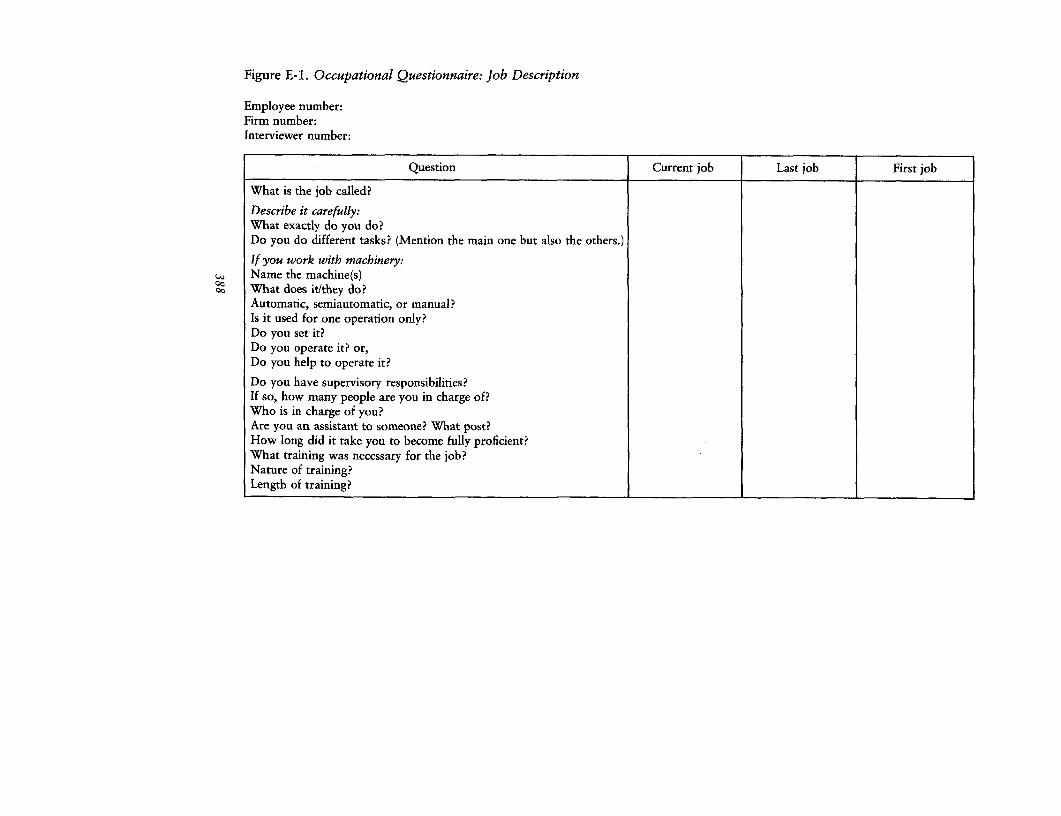
Figure E-1. Occupational Questionnaire: Job Description
Employee number:Firm number:Interviewer number:
Question Current job Last job First job
What is the job called?
Describe it carefully:What exactly do you do?Do you do different tasks? (Mention the main one but also the others.)If you work with machinery:
w Name the machine(s)oc What does it/they do?
Automatic, semiautomatic, or manual?Is it used for one operation only?Do you set it?Do you operate it? or,Do you help to operate it?
Do you have supervisory responsibilities?If so, how many people are you in charge of?Who is in charge of you?Are you an assistant to someone? What post?How long did it take you to become fully proficient?What training was necessary for the job?Nature of training?Length of training?

Classification of Occupations 389
Although finer classifications were made (table E-1, part A), respon-dents were also placed in six broad occupational groups (part B): un-skilled manual (05), semiskilled manual (04), skilled manual (03), ju-nior clerical (02b), senior clerical (O2a), and supervisory (O1). These arethe groupings that we have generally employed in the empirical analysisof occupation. A relevant trade certificate was normally decisive in plac-ing a manual worker in the skilled category. Other pointers to this cate-gory were a long period (four or more years) of training on the job;operation and setting of complicated machinery; supervision of othermachine operators; and a lengthy period (three months or more) of rele-vant full-time formal training. Indicators of semiskilled status were: norelevant trade test; two months (minimum) to four years of experienceneeded for proficiency on the job; operation of a machine or operationand setting of a simple machine; being an assistant to a skilled worker;and a short period (less than three months) of formal training. Indicatorsfor the unskilled classification were: proficiency in the job within twomonths; simple repetitive tasks; close supervision and little autonomy;and no relevant formal training. The clerical category (clerical, accounts,secretarial, and sales workers) was subdivided into senior and juniorgroups according to the levels of skill and authority involved in the job.For instance, the (smaller) senior group included clerical supervisor butnot clerk or clerical assistant; noncertified accountant and head book-keeper but not bookkeeper or assistant bookkeeper; and personal secre-tary but not typist. The category of other nonmanual workers includedtechnical and semiprofessional, managerial, administrative, and profes-sional workers.
Table E-1. Occupational Codes
A. Occupations
Manual1. Unskilled (100)
101 Laborer, general102 Laborer, factory103 Laborer, farm104 Laborer, other105 Cleaner106 Dishwasher107 Driver's mate108 Gardener109 Machine operator's assistant110 Messenger111 Porter112 Sweeper113 Watchman
(Table continues on the following page.)
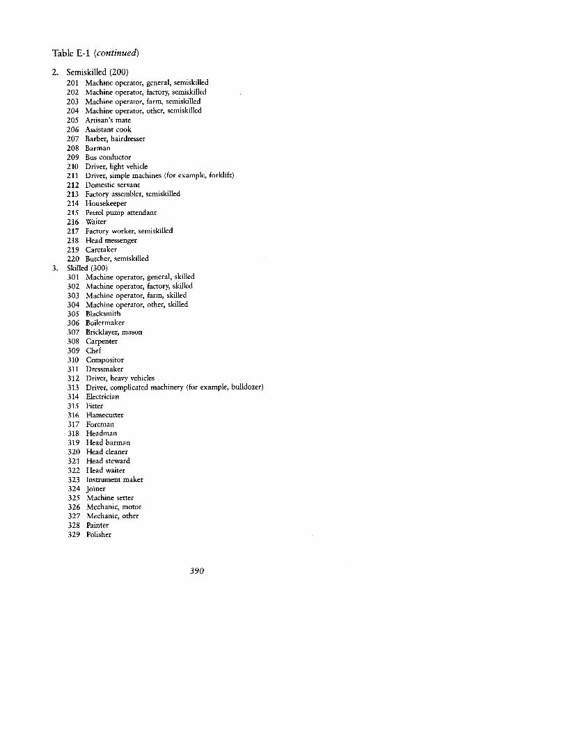
Table E-1 (continued)
2. Semiskilled (200)201 Machine operator, general, semiskilled202 Machine operator, factory, semiskilled203 Machine operator, farm, semiskilled204 Machine operator, other, semiskilled205 Artisan's mate206 Assistant cook207 Barber, hairdresser208 Barman209 Bus conductor210 Driver, light vehicle211 Driver, simple machines (for example, forklift)212 Domestic servant213 Factory assembler, semiskilled214 Housekeeper215 Petrol pump attendant216 Waiter217 Factory worker, semiskilled218 Head messenger219 Caretaker220 Butcher, semiskilled
3. Skilled (300)301 Machine operator, general, skilled302 Machine operator, factory, skilled303 Machine operator, farm, skilled304 Machine operator, other, skilled305 Blacksmith306 Boilermaker307 Bricklayer, mason308 Carpenter309 Chef310 Compositor311 Dressmaker312 Driver, heavy vehicles313 Driver, complicated machinery (for example, bulldozer)314 Electrician315 Fitter316 Flamecutter317 Foreman318 Headman319 Head barman320 Head cleaner321 Head steward322 Head waiter323 Instrument maker324 Joiner325 Machine setter326 Mechanic, motor327 Mechanic, other328 Painter329 Polisher
390
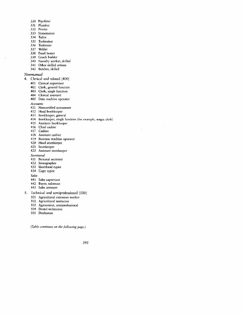
330 Pipefitter331 Plumber332 Printer333 Stonemason334 Tailor335 Toolmaker336 Toolsetter337 Welder338 Panel beater339 Coach builder340 Foundry worker, skilled341 Other skilled artisan342 Butcher, skilled
Nonmanual4. Clerical and related (400)
401 Clerical supervisor402 Clerk, general function403 Clerk, single function404 Clerical assistant405 Data machine operator
Accounts411 Noncertified accountant412 Head bookkeeper413 Bookkeeper, general414 Bookkeeper, single function (for example, wages clerk)415 Assistant bookkeeper416 Chief cashier417 Cashier418 Assistant cashier419 Business machine operator420 Head storekeeper421 Storekeeper422 Assistant storekeeper
Secretarial431 Personal secretary432 Stenographer433 Shorthand typist434 Copy typist
Sales441 Sales supervisor442 Buyer, salesman443 Sales assistant
5. Technical and semiprofessional (500)501 Agricultural extension worker502 Agricultural instructor503 Agronomist, semiprofessional504 Dental technician505 Draftsman
(Table continues on the following page.)
391

Table E-1 (continued)
506 Engineering technician507 Library assistant508 Medical assistant509 Nurse and midwife, professional510 Nurse and midwife, enrolled511 Pharmaceutical technician512 Photographer513 Physiotherapist514 Science technician515 Statistical and computing technician516 Surveyor517 Watch and clock repairer518 Clerk of works519 Other semiprofessional
6. Managerial and administrative (600)601 Government administrative officer602 Government executive officer603 General manager604 Production manager605 Specialized manager606 Farm manager607 Assistant manager
7. Professional (700)701 Accountant, professional702 Actuary703 Agronomist, professional704 Aircraft pilot, navigator705 Architect706 Auditor707 Author708 Dentist709 Doctor710 Economist711 Engineer, civil712 Engineer, chemical713 Engineer, electrical714 Engineer, mechanical715 Engineer, other716 Journalist717 jurist718 Lawyer719 Librarian720 Pharmacist721 Priest722 Quantity surveyor723 Scientist724 Statistician725 Teacher, university level726 Teacher, other postsecondary
392

727 Teacher, secondary level728 Teacher, primary level729 Teacher, preprimary level730 Teacher, special education731 Town planner732 Veterinarian733 Teacher, untrained temporary734 Computer scientist
8. Law and order (800)801 Soldier802 Sailor803 Policeman804 Warder
9. No reply (999)
B. Occupational groups and corresponding codes
Unskilled manual (Os): 101-13Semiskilled manual (04): 201-20Skilled manual (03): 301-42Junior clerical (O2b): 402-05, 413-15, 417-19, 421, 422, 432-34,
442-43Senior clerical (02a): 401, 411, 412, 416, 420, 431, 441Supervisory (O1): 501-19, 601-07, 701-34
Note: No respondents were currently in the law and order category (801-04).
393
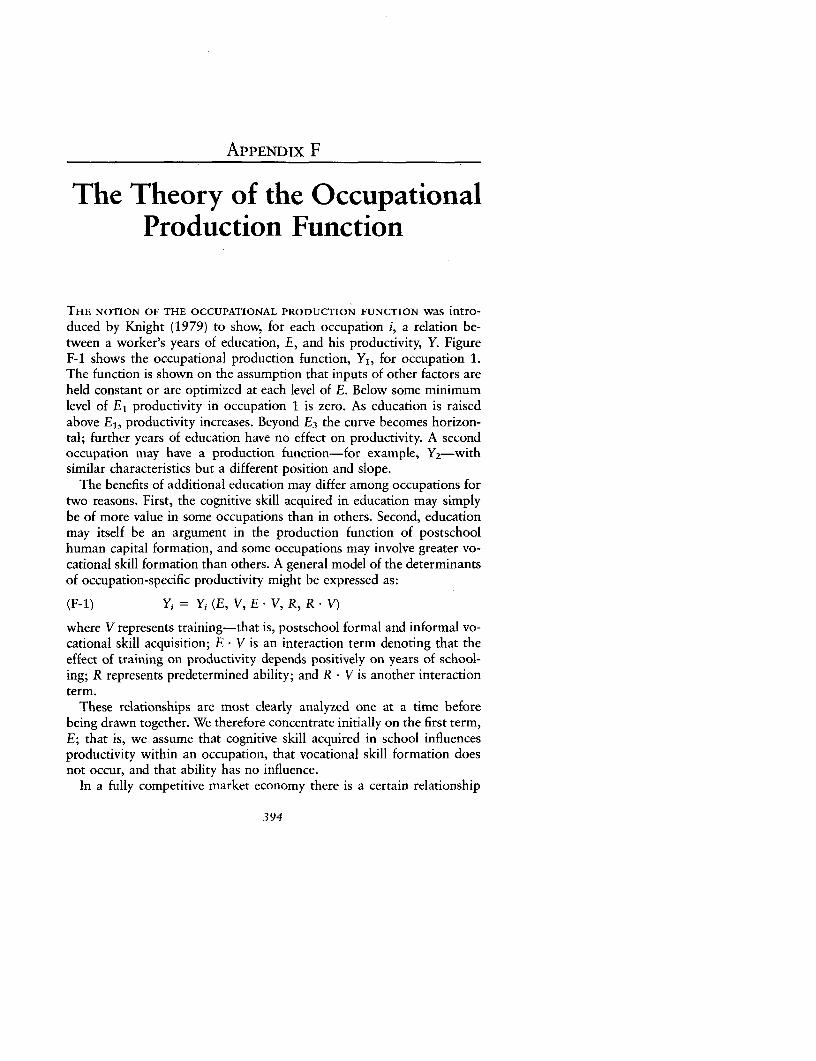
APPENDIX F
The Theory of the OccupationalProduction Function
THE NOTION OF THE OCCUPATIONAL PRODUCTION FUNCTION was intro-duced by Knight (1979) to show, for each occupation i, a relation be-tween a worker's years of education, E, and his productivity, Y. FigureF-1 shows the occupational production function, Y,, for occupation 1.The function is shown on the assumption that inputs of other factors areheld constant or are optimized at each level of E. Below some minimumlevel of El productivity in occupation 1 is zero. As education is raisedabove El, productivity increases. Beyond E 3 the curve becomes horizon-tal; further years of education have no effect on productivity. A secondoccupation may have a production function-for example, Y 2 -withsimilar characteristics but a different position and slope.
The benefits of additional education may differ among occupations fortwo reasons. First, the cognitive skill acquired in education may simplybe of more value in some occupations than in others. Second, educationmay itself be an argument in the production function of postschoolhuman capital formation, and some occupations may involve greater vo-cational skill formation than others. A general model of the determinantsof occupation-specific productivity might be expressed as:
(F-1) Yi = Yi (E, V, E V, R, R * V)
where V represents training-that is, postschool formal and informal vo-cational skill acquisition; E . V is an interaction term denoting that theeffect of training on productivity depends positively on years of school-ing; R represents predetermined ability; and R * V is another interactionterm.
These relationships are most clearly analyzed one at a time beforebeing drawn together. We therefore concentrate initially on the first term,E; that is, we assume that cognitive skill acquired in school influencesproductivity within an occupation, that vocational skill formation doesnot occur, and that ability has no influence.
In a fully competitive market economy there is a certain relationship
394

The Theory of the Occupational Production Function 395
Figure F-1. The Occupational Production Function
Productivity (Y)
B y1~~~~~I
YA
E1 E2 E3Years of education (E)
between years of education and productivity (Mincer 1974, ch. 1). Foridentical individuals there is a single semilogarithmic relationship be-tween E and Y, irrespective of occupation, that shows the combinationsof E and Y for which the rate of return on education equals the rate ofdiscount. The notion of an occupational production function is, however,perfectly consistent with competitive theory. At the point of tangency (A)between I and Y2 in figure F-1, the individual is content with the incomeassociated with education E2 in the sense that the rate of return equalshis rate of discount. He is better off, however, at (say) B on YI, whichis above 1: point B is chosen. On the assumption that all individuals haveidentical economic characteristics (that is, I, Yl, and Y2 are the same foreveryone), an inflow of persons into occupation 1 takes place and de-presses the wage. The lower wage encourages the employment of this oc-cupation in two ways, one technical and the other through the market.First, there are diminishing returns to numbers employed in an occupa-tion. Second, if manufacture of a product makes intensive use of the oc-cupation, the relative price of that product will fall. Factors are substi-tuted until the marginal product of occupation 1 falls to equal the wage.This decrease in the marginal product of the occupation shifts the entirecurve Y1 downward to Yl such that Yl touches I at C. Point C is thenew equilibrium combination of education, productivity, and wage in oc-cupation 1.
By an extension of this reasoning it can be seen that the indifferencecurve I, which is common to all individuals, forms an envelope of all oc-
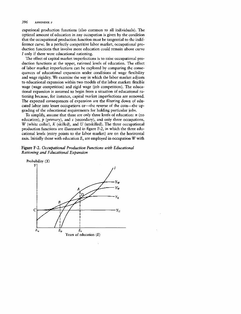
396 APPENDIX F
cupational production functions (also common to all individuals). Theoptimal amount of education in any occupation is given by the conditionthat the occupational production function must be tangential to the indif-ference curve. In a perfectly competitive labor market, occupational pro-duction functions that involve more education could remain above curveI only if there were educational rationing.
The effect of capital market imperfections is to raise occupational pro-duction functions at the upper, rationed levels of education. The effectof labor market imperfections can be explored by comparing the conse-quences of educational expansion under conditions of wage flexibilityand wage rigidity. We examine the way in which the labor market adjuststo educational expansion within two models of the labor market: flexiblewage (wage competition) and rigid wage (job competition). The educa-tional expansion is assumed to begin from a situation of educational ra-tioning because, for instance, capital market imperfections are removed.The expected consequences of expansion are the filtering down of edu-cated labor into lesser occupations or-the reverse of the coin-the up-grading of the educational requirements for holding particular jobs.
To simplify, assume that there are only three levels of education: n (noeducation), p (primary), and s (secondary), and only three occupations,W (white collar), K (skilled), and U (unskilled). The three occupationalproduction functions are illustrated in figure F-2, in which the three edu-cational levels (entry points to the labor market) are on the horizontalaxis. Initially those with education Es are employed in occupation W with
Figure F-2. Occupational Production Functions with EducationalRationing and Educational Expansion
Probability (X)
y~~~~~~~~yYl~~~~~~~~Y
A 1'V
c _~~~~~~~~~yU
En Ep EdYears of education (E)
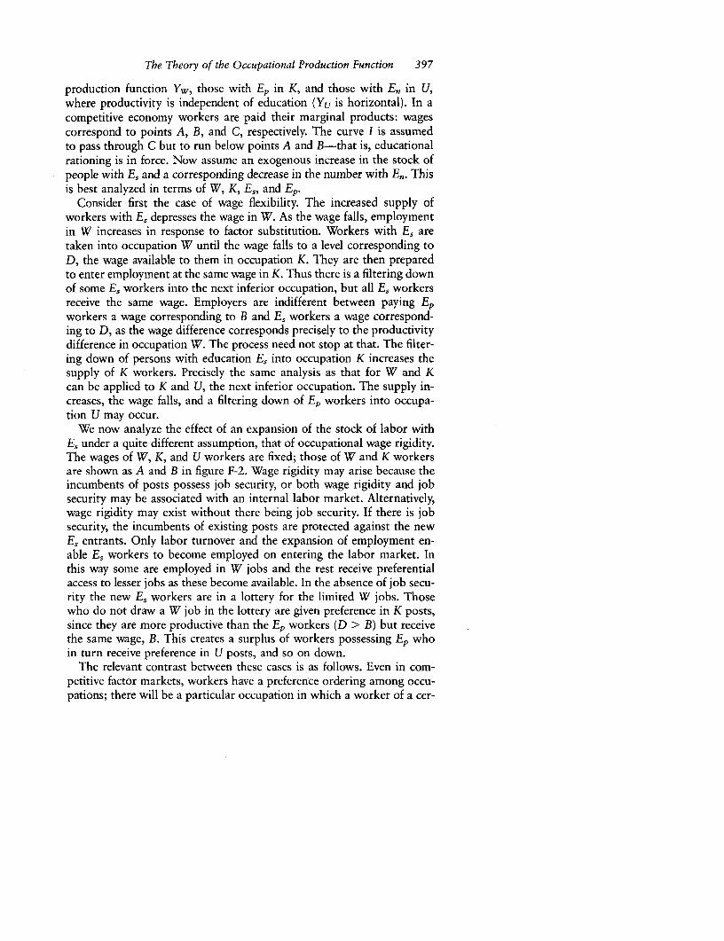
The Theory of the Occupational Production Function 397
production function Yw, those with Ep in K, and those with En in U,where productivity is independent of education (Yu is horizontal). In acompetitive economy workers are paid their marginal products: wagescorrespond to points A, B, and C, respectively. The curve I is assumedto pass through C but to run below points A and B-that is, educationalrationing is in force. Now assume an exogenous increase in the stock ofpeople with Es and a corresponding decrease in the number with En. Thisis best analyzed in terms of W, K, Es, and Ep.
Consider first the case of wage flexibility. The increased supply ofworkers with Es depresses the wage in W. As the wage falls, employmentin W increases in response to factor substitution. Workers with Es aretaken into occupation W until the wage falls to a level corresponding toD, the wage available to them in occupation K. They are then preparedto enter employment at the same wage in K. Thus there is a filtering downof some Es workers into the next inferior occupation, but all Es workersreceive the same wage. Employers are indifferent between paying Epworkers a wage corresponding to B and Es workers a wage correspond-ing to D, as the wage difference corresponds precisely to the productivitydifference in occupation W. The process need not stop at that. The filter-ing down of persons with education Es into occupation K increases thesupply of K workers. Precisely the same analysis as that for W and Kcan be applied to K and U, the next inferior occupation. The supply in-creases, the wage falls, and a filtering down of Ep workers into occupa-tion U may occur.
We now analyze the effect of an expansion of the stock of labor withEs under a quite different assumption, that of occupational wage rigidity.The wages of W, K, and U workers are fixed; those of W and K workersare shown as A and B in figure F-2. Wage rigidity may arise because theincumbents of posts possess job security, or both wage rigidity and jobsecurity may be associated with an internal labor market. Alternatively,wage rigidity may exist without there being job security. If there is jobsecurity, the incumbents of existing posts are protected against the newEs entrants. Only labor turnover and the expansion of employment en-able Es workers to become employed on entering the labor market. Inthis way some are employed in W jobs and the rest receive preferentialaccess to lesser jobs as these become available. In the absence of job secu-rity the new Es workers are in a lottery for the limited W jobs. Thosewho do not draw a W job in the lottery are given preference in K posts,since they are more productive than the Ep workers (D > B) but receivethe same wage, B. This creates a surplus of workers possessing Ep whoin turn receive preference in U posts, and so on down.
The relevant contrast between these cases is as follows. Even in com-petitive factor markets, workers have a preference ordering among occu-pations; there will be a particular occupation in which a worker of a cer-
398 APPENDIX F
tain educational attainment is more productive than in any other (figureF-1). If capital markets are imperfect but labor markets are perfect, allworkers with the same education will tend to be paid the same wage evenif they are in different occupations (figure F-2). If differences in tastesand in job satisfaction are ignored, the implication is that these workersdo not have a preference ordering among these occupations. In the rigidwage (job competition) case, by contrast, workers of the same educationcan receive different pay in different occupations and therefore have pref-erences among these occupations. Even in the flexible wage (wage compe-tition) model, employers have preferences in recruiting to occupations;competitive wages for workers of different education determine whichlevel of education is most profitable in each occupation (figure F-1). Butif wage rigidity means that the wage varies less with education withinoccupations than it does among occupations, employers have reason torecruit the most educated workers available (figure F-2).
Let us withdraw the first assumption-that the cognitive skill acquiredin education is of more value in some jobs than in others-and replaceit with the second-that education is itself an argument in the productionfunction of vocational skill formation and that some occupations involvegreater vocational skill formation than others. We thus concentrate onthe terms V and E * V in equation F-1. Assume that vocational skills aremarketable and therefore, although occupation-specific, are generalrather than firm-specific. In that case it is the employee who benefits fromand pays for the skill formation. The wage-experience profile can be ex-pected to take the normal inverted-U-shaped form: the wage falls shortof productivity during training and subsequently equals it, and produc-tivity rises in early career as skills accumulate and falls in late career asthey are lost or become obsolescent.
Let us proceed by stages, initially ignoring the interaction term E * V.Figure F-3 shows productivity (the continuous lines) against length ofemployment experience (L) for the three occupations. In the unskilledoccupation (U) there is no vocational skill formation; the wage and pro-ductivity are equal and unchanging throughout. In the skilled (K) andwhite-collar (W) occupations skill formation occurs-more in W thanin K-and the wage (the dashed lines) therefore falls short of produc-tivity during the period of employer-provided training on the job. Givencompetitive capital markets and free mobility of labor, discounted life-time earnings are independent of the amount of vocational skill acqui-sition and are the same in different occupations. Only if there are capi-tal market imperfections and therefore rationing of training are themore skilled occupations prized on account of the greater skills thatthey provide.
Consider the influence of education on vocational skill formation. As-
The Theory of the Occupational Production Function 399
Figure F-3. Vocational Skill Formation, Wages, and Productivity
Productivity (Y)
Yw~~~Y
A ~~~ ; A/ - ~~ YK
Employment experience (L)
sume initially that each occupation involves a fixed amount of vocationalskill. In that case the cognitive skill derived from education, by makingacquisition of vocational skills more efficient, simply reduces the amountof training needed to achieve the fixed amount of vocational skill. Educa-tion therefore has no effect on the productivity of a trained worker; eachoccupational production function that relates Y to E is horizontal, al-though each is at a different level of productivity. It becomes profitablefor the more educated to enter occupations that involve more vocationalskill because their training will be less costly.
Now assume that the amount of vocational skill differs within as wellas among occupations. Within an occupation the possession of educationmakes it profitable to invest in more vocational skills. Each occupationalproduction function therefore has an upward-sloping range, as in figureF-1. The educated have higher productivity both because of the amountof skill inherent in the occupations that they choose and because of theamount of training that they choose within occupations.
We now reintroduce the assumption that cognitive skill is itself valu-able in the performance of a job and more valuable in some jobs thanin others. When we bring into play all three terms-E, V, and E * V-inthe occupational production function specified in equation F-1, we findthat figure F-1 remains relevant. Given perfect capital markets, the netpresent value of vocational skills is zero. Provided that wages are re-garded as discounted lifetime income, the equilibrium tangency proper-ties of figure F-1 still hold. The current wage of trained workers, how-
400 APPENDIX F
ever, will be above the indifference curve to the extent that vocationalskills are rewarded. The higher a trained worker's educational attain-ment, the higher his wage, owing to choice both of occupation and oftraining within an occupation. Moreover, if the capital market is imper-fect and vocational training is rationed, this provides a further reasonwhy occupation can have an independent influence on wages.
It is necessary to recognize that ability also influences productivity inan occupation and that it may have a greater influence in some occupa-tions than in others. Its influence is shown by the terms R and R * V inequation F-1. The term R - V comes into play if ability, like education,alters the efficiency with which training can be converted into vocationalskills. A further complication can arise from a correlation between abilityand educational attainment. On the assumption that ability influencesthe efficiency with which schooling can be converted into cognitive skills,R and E are likely to be positively correlated in meritocratic educationalsystems. The term E should then be written as E(R) and E * V as E(R) * Vin equation F-1. As a consequence the more able have an incentive notonly to become more educated but also, since they are more educated,to enter occupations that involve more vocational skills and to acquiremore vocational skills within an occupation.
We may draw some conclusions from this analysis. Ignore for the mo-ment the fact of occupation-specific vocational skill acquisition. In thatcase, although occupational production functions are consistent withcompetitive factor markets, they would be a useful analytical tool onlyin the presence of capital and labor market imperfections. This is, ofcourse, not a serious limitation, especially in developing countries. Nowthat choice-theoretic explanations for factor market imperfections arebeing developed, economists are less reluctant to incorporate failure ortardiness of factor market clearing into their analyses (for example,Schultze 1985). Capital market inflexibility can mean that workers prizeeducation, and labor market inflexibility can mean that workers prizecertain occupations. But when occupation-specific vocational skills areincorporated into the analysis, occupation can be expected to influence(current) wages even when factor markets are competitive. Occupationalproduction functions, in their most general form, imply a nexus of rela-tionships between occupation, education, ability, cognitive skill, voca-tional skills, and productivity. Education assists vocational skill acquisi-tion, so encouraging the more educated-who are likely also to be themore able-to seek out those occupations that involve more vocationalskills and to acquire more vocational skills within occupations. Thus edu-cation raises productivity through its effect on choice of occupation andthrough its effects via cognitive and vocational skills within an occupa-tion. If capital market imperfections cause vocational skills to be ra-tioned, there is a further reason for workers to prize skill-intensive occu-
The Theory of the Occupational Production Function 401
pations. If labor market imperfections mean that there is a wage for thejob irrespective of individual productivity, the occupational productionfunction predicts that employers will prefer to employ workers with moreeducation.
APPENDIX G
The Public-Private WageDifferential: Tanzania 1971
IN THIS APPENDIX we use data from a 1971 household survey to deter-mine the pattern of wage differences across employer groups. The analy-sis provides a basis for comparing the public-private wage differential inTanzania at the beginning of the 1970s, soon after the adoption by thegovernment of a compressive pay policy, and, using establishment sur-veys, in 1980, after the policy had had ample time to take effect.
The issue of public versus private compensation has not received asmuch attention in high-income economies as, for example, wage differen-tials between union and nonunion establishments. In the United Statesthis is because the prevailing wage rate model has been used to determineand hence to explain government pay scales. The government is viewedas just another price taker that accepts a market-determined rate. In aperfectly competitive labor market, group affiliation does not influencewages. Irrespective of differences among groups of workers in goods pro-duced, in the technology or organization used to produce them, in theprofitability of such production, or in the ownership of the establish-ments in which they work, competition in the labor market will ensurethat all workers with the same personal economic characteristics andpreferences for work activity receive the same rate of pay. If public-private wage differences occur, they are generally interpreted in the com-petitive model as attributable to short-run adjustment problems or to lagsin government wage movements.
Group affiliation matters only if nonmarket forces are sufficiently pow-erful to prevent competition in the market from eroding differentialsamong homogeneous workers. The public sector holds a commanding po-sition in the labor markets of many developing countries. It is not uncom-mon to find more than half of all wage earners in the employ of the gov-
Note: Adapted from D. L. Lindauer and R. H. Sabot, "The Public/Private Wage Differ-ential in a Poor Urban Economy," Journal of Development Economics 12, nos. 1-2(February-April 1983), pp. 137-S2.
402
The Public-Private Wage Differential: Tanzania 1971 403
ernment or of parastatal enterprises. Moreover, not all governments ofdeveloping countries choose (or are in a position to choose) the prevailingwage model in setting their pay scales. Government pay policies are ofteninfluenced by distributional, fiscal, employment, or political goals. Thereis evidence, for example, that in Tanzania colonial wage and salary struc-tures, which were geared to the supply prices of Europeans, were not dis-mantled at independence because to do away with what many regardedas the fruits of independence would have been politically untenable (seeSabot 1979, p. 210). In sum, in many low-income countries the publicsector does not have the need, the desire, or even the ability to act asa wage taker.
To study the relationship of public to private wages, data for this anal-ysis were obtained from the 1971 National Urban Mobility, Employ-ment, and Income Survey of Tanzania (NUMEIST), which was conductedby Sabot. A random sample of households in Dar es Salaam and six otherurban areas was surveyed. Over 5,000 individuals, including 1,500 Afri-can male regular wage earners, were included in the sample.' Respon-dents provided information on their monthly earnings, nonwage bene-fits, education, employment history, and other personal characteristics.Roughly one-third of the sample fell into each employment category-private, government, and parastatal enterprises.2
Our first measurement is of the differences in mean wages betweengovernment and private sector employees, between parastatal and privatesector employees, and between parastatal and government employees.Both G = Wa - Wb, the absolute difference, and a = (Wa - Wb)/Wb,the relative difference, are presented; Wa represents the mean wage of thehigh-paid group. Measures of G disaggregated by occupation are alsopresented, and hypotheses are suggested to explain the public-private dif-ferences that remain. We go on to contrast ca with the value of ,3, where3 represents the average percentage by which the pay of group a exceedsthat of group b after various personal characteristics of the wage laborforce are standardized. Standardization is performed by estimating a sim-ple wage function of the general form In W = f(X), where the log ofmonthly earnings of urban wage earners is the dependent variable andX is a vector of personal characteristics. In addition to those characteris-tics generally found to be good predictors of earnings, dummy variablesfor ownership category of the worker's employer are included. The onlyother additional feature of the specification is a variable that indicateswhether the worker was employed in Dar es Salaam or in one of the sixsmaller towns included in the sample. 13 is derived from the coefficienton the ownership dummy denoting group a (the high-paid group, withgroup b as the base category) in the earnings function for the full sample(see Halvorsen and Palmquist 1980).
In an aggregate earnings function, such as this, where the coefficients
404 APPENDIX G
on the independent variables are constrained to be the same for all own-ership groups, 3 can be a misleading indicator of the magnitude of stan-dardized wage differences among ownership groups if there are markeddifferences in the wage structure among parastatals, the government, andprivate enterprises-that is, in the coefficients of separate earnings func-tions. Therefore we go on to examine the nature and degree of differencesin the structure of earnings among ownership categories. The followingstratified regressions are estimated and subjected to a series of Chowtests:
In WGO = fAXGO); In Wpr = f(Xpr); In Wpa = f(Xpa)
where Go = government, Pr = private, Pa = parastatal, and X is a vectorof independent variables that in this case exclude the ownership dum-mies. These tests do not allow us to determine whether differences amongstratified regressions are attributable to differences in slopes or in inter-cept terms. Therefore we also estimate an interactive version of our ag-gregate earnings function, that is,
(G-1) In W = a + bX + c(X * Go) + d(X Pa) + u
where a is the constant and b, c, and d are coefficients that measure, re-spectively, the impact of the independent variables on earnings in the pri-vate sector, the incremental impact of those variables for governmentworkers, and the incremental impact of those variables for workers inthe parastatal sector.
Having specified and measured as best we can the differences amongprivate, government, and parastatal establishments in the level and slopesof their earnings functions, we decompose the gross wage differences tomeasure the impact of these differences on the earnings of representativeworkers from each of the ownership categories. The representative work-ers are constructs; the characteristics of the government worker, for ex-ample, are given by the mean value for all government workers of eachof the independent variables. For each of the three representative workerswe use the stratified wage functions to predict, given their characteristics,what they would be paid in the other two ownership categories. Our pro-cedure, which is a simple form of simulation analysis, has been widelyused in the analysis of labor market discrimination in high-income coun-tries (see Blinder 1973 and Malkiel and Malkiel 1973) and is beginningto be applied in low-income countries (see Behrman and Wolfe forthcom-ing, Birdsall and Fox 1985, and Knight and Sabot 1982). In effect, wedecompose the gross wage differences among ownership categories intoE, the parts "explained" by differences in the characteristics of the laborforces among the categories, and R, the unexplained residual that reflectsdifferences in wage functions.
In explaining the method we focus on government and private sector
The Public-Private Wage Differential: Tanzania 1971 405
employees. We assume that the mean wage of government workers is de-termined by the earnings function Wa = fa (X,), where Xa are the meanvalues of a vector of characteristics. The mean wage that private sectoremployees would receive if they were paid according to the governmentwage structure is fa(X&). The gross wage difference between sectors isthen decomposed as follows:
G = Wa - Wb = [Wa - fa(Xb)] + [fa(Xb) - Wb] = E + R
A similar decomposition is obtained by substituting fb(Xa) for fa(Xb),the wage that would be received by government workers if they were paidaccording to the private sector wage structure. The procedure allows usto answer as best we can the fundamental question addressed by this ap-pendix: how much of the observed differences in mean earnings amongownership categories is attributable simply to differences in compositionand how much to various nonmarket forces that drive a wedge amongpay levels in different employer categories for workers with the samecharacteristics?
Gross and Standardized Wage Differences
Table G-1 shows that in 1971 government urban employees earned 133shillings (51 percent) more and parastatal employees 146 shillings (56percent) more than employees in privately owned establishments.3 TableG-2, however, indicates that, as is usual, labor demand is much moreskill-intensive in the government sector than in the private sector. Be-cause of these differences in composition, the government-private differ-ential for particular occupations is much less than the differential inmean earnings. Indeed, table G-l indicates that in six of eleven occupa-tional categories the earnings advantage is to private firms. If the privatesector had the occupational composition of the government, the remain-ing differential in mean earnings would be only 16 percent and wouldbe almost entirely attributable to the higher salaries of managers in thegovernment than in the private sector.
With respect to skill intensity, the parastatal sector falls between theother two, and therefore differences in occupational composition do notexplain as much of the parastatal-private as of the government-privategross wage difference. Parastatal earnings are higher in ten of the elevenoccupational categories. If the parastatal sector had the occupationalcomposition of the government, the difference in mean wages betweenthe sectors would remain a substantial 23 percent.
The observed differentials may in part represent differences in the char-acteristics of specific jobs. No occupational standardization can ever ac-count for all the variations in working conditions, security of job tenure,and risk in different work activities. Even within a competitive environ-
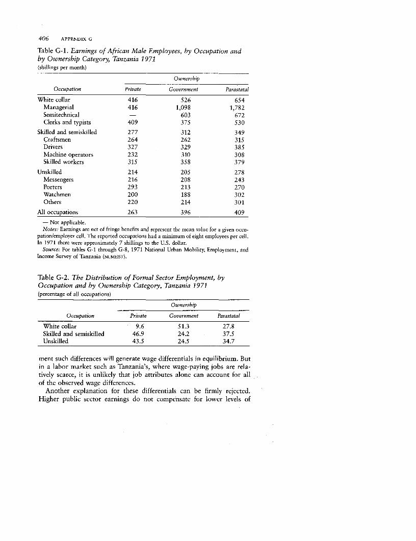
406 APPENDIX G
Table G-1. Earnings of African Male Employees, by Occupation andby Ownership Category, Tanzania 1971(shillings per month)
Ownership
Occupation Private Government Parastatal
White collar 416 526 654Managerial 416 1,098 1,782Semitechnical - 603 672Clerks and typists 409 375 530
Skilled and semiskilled 277 312 349Craftsmen 264 262 315Drivers 327 329 385Machine operators 232 310 308Skilled workers 315 358 379
Unskilled 214 205 278Messengers 216 208 243Porters 293 213 270Watchmen 200 188 302Others 220 214 301
All occupations 263 396 409
- Not applicable.Notes: Earnings are net of fringe benefits and represent the mean value for a given occu-
pation/employer cell. The reported occupations had a minimum of eight employees per cell.In 1971 there were approximately 7 shillings to the U.S. dollar.
Source: For tables G-1 through G-8, 1971 National Urban Mobility, Employment, andIncome Survey of Tanzania (NUMEIST).
Table G-2. The Distribution of Formal Sector Employment, byOccupation and by Ownership Category, Tanzania 1971(percentage of all occupations)
Ownership
Occupation Private Government Parastatal
White collar 9.6 51.3 27.8Skilled and semiskilled 46.9 24.2 37.5Unskilled 43.5 24.5 34.7
ment such differences will generate wage differentials in equilibrium. Butin a labor market such as Tanzania's, where wage-paying jobs are rela-tively scarce, it is unlikely that job attributes alone can account for allof the observed wage differences.
Another explanation for these differentials can be firmly rejected.Higher public sector earnings do not compensate for lower levels of
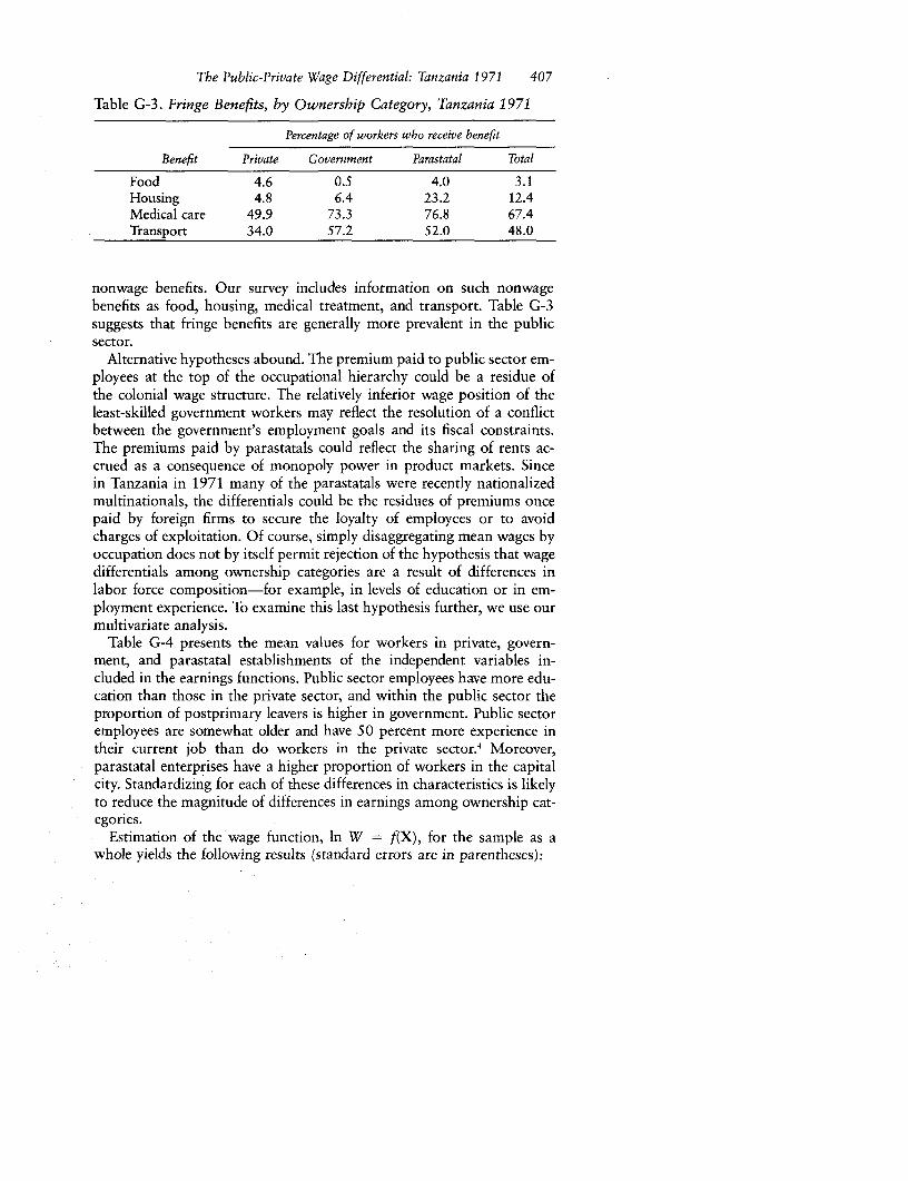
The Public-Private Wage Differential: Tanzania 1971 407
Table G-3. Fringe Benefits, by Ownership Category, Tanzania 1971
Percentage of workers who receive benefit
Benefit Private Government Parastatal Total
Food 4.6 0.5 4.0 3.1Housing 4.8 6.4 23.2 12.4Medical care 49.9 73.3 76.8 67.4Transport 34.0 57.2 52.0 48.0
nonwage benefits. Our survey includes information on such nonwagebenefits as food, housing, medical treatment, and transport. Table G-3suggests that fringe benefits are generally more prevalent in the publicsector.
Alternative hypotheses abound. The premium paid to public sector em-ployees at the top of the occupational hierarchy could be a residue ofthe colonial wage structure. The relatively inferior wage position of theleast-skilled government workers may reflect the resolution of a conflictbetween the government's employment goals and its fiscal constraints.The premiums paid by parastatals could reflect the sharing of rents ac-crued as a consequence of monopoly power in product markets. Sincein Tanzania in 1971 many of the parastatals were recently nationalizedmultinationals, the differentials could be the residues of premiums oncepaid by foreign firms to secure the loyalty of employees or to avoidcharges of exploitation. Of course, simply disaggregating mean wages byoccupation does not by itself permit rejection of the hypothesis that wagedifferentials among ownership categories are a result of differences inlabor force composition-for example, in levels of education or in em-ployment experience. To examine this last hypothesis further, we use ourmultivariate analysis.
Table G-4 presents the mean values for workers in private, govern-ment, and parastatal establishments of the independent variables in-cluded in the earnings functions. Public sector employees have more edu-cation than those in the private sector, and within the public sector theproportion of postprimary leavers is higher in government. Public sectoremployees are somewhat older and have 50 percent more experience intheir current job than do workers in the private sector.4 Moreover,parastatal enterprises have a higher proportion of workers in the capitalcity. Standardizing for each of these differences in characteristics is likelyto reduce the magnitude of differences in earnings among ownership cat-egories.
Estimation of the wage function, In W = f(X), for the sample as awhole yields the following results (standard errors are in parentheses):

408 APPENDIX G
Table G-4. Characteristics of Workers, by Ownership Category,Tanzania 1971
Ownership
Characteristic Private Government Parastatal
Education (percent)None 17.8 13.2 22.3Primary 75.9 58.1 57.8Postprimary 6.3 28.7 19.9
Age (years)Mean 29 31 32Standard deviation (8.6) (10.3) (10.1)
Employment experience (years in present job)Mean 3.9 5.8 6.2Standard deviation (5.5) (8.0) (7.8)
Location (percentage in Dar es Salaam) 60.5 57.6 71.0
Note: The data are for African male employees only.
(G-2) In W = 4.758 + 0.219E1 + 0.914E2 + 0.018L - 0.00016L 2
(0.036) (0.045) (0.003) (0.00011)
+ 0.012A + 0.138D + 0.068Go + 0.194Pa(0.002) (0.027) (0.034) (0.032)
N = 1,291, k2 = 0.365
where E1 = primary education, E2 = postprimary education, L = em-ployment experience, A = age, and D = employment in Dar es Sa-laam.
All of the coefficients except that on the squared experience variable,L2, are significant. As expected, the coefficients on education, experience,and location in Dar es Salaam are positive and substantial and, for theeducation variables, are in the usual size order. The coefficients on thegovernment and parastatal variables are significant and positive, but thegovernment coefficient is only about one-third the size of the parastatalcoefficient. Even after differences in education, employment experience,age, and location of work are standardized, therefore, government em-ployees earn a premium of 7 percent in relation to private sector employ-ees and parastatal workers a premium of 21 percent.5
These estimates of public-private differentials may be biased, however,because the dummy variables for ownership category permit differencesonly in the intercept terms of employer-specific earnings functions. In thesection that follows we consider whether there are observable differences
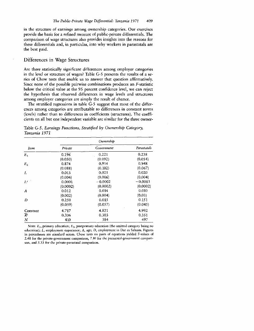
The Public-Private Wage Differential: Tanzania 1971 409
in the structure of earnings among ownership categories. Our exercisesprovide the basis for a refined measure of public-private differentials. Thecomparison of wage structures also provides insights into the reasons forthese differentials and, in particular, into why workers in parastatals arethe best paid.
Differences in Wage Structures
Are there statistically significant differences among employer categoriesin the level or structure of wages? Table G-5 presents the results of a se-ries of Chow tests that enable us to answer that question affirmatively.Since none of the possible pairwise combinations produces an F-statisticbelow the critical value at the 95 percent confidence level, we can rejectthe hypothesis that observed differences in wage levels and structuresamong employer categories are simply the result of chance.
The stratified regressions in table G-5 suggest that most of the differ-ences among categories are attributable to differences in constant terms(levels) rather than to differences in coefficients (structures). The coeffi-cients on all but one independent variable are similar for the three owner-
Table G-5. Earnings Functions, Stratified by Ownership Category,Tanzania 1971
Ownership
Item Private Government Parastatals
E, 0.196 0.221 0.238(0.050) (0.092) (0.054)
E2 0.874 0.914 0.948(0.088) (0.102) (0.067)
L 0.013 0.021 0.020(0.004) (0.006) (0.004)
L2 0.0001 -0.0002 - 0.0003(0.0002) (0.0002) (0.0002)
A 0.012 0.014 0.010(0.002) (0.004) (0.03)
D 0.250 0.015 0.151(0.039) (0.057) (0.045)
Constant 4.717 4.821 4.992R2 0.306 0.303 0.351N 410 384 497
Note: El, primary education; E2, postprimary education (the omitted category being noeducation); L, employment experience; A, age; D, employment in Dar es Salaam. Figuresin parentheses are standard errors. Chow tests on pairs of equations yielded F-values of2.48 for the private-government comparison, 7.10 for the parastatal-government compari-son, and 3.33 for the private-parastatal comparison.
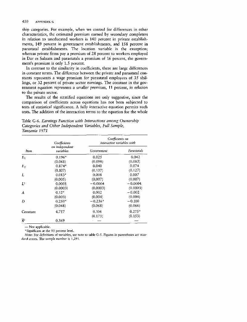
410 APPENDIX G
ship categories. For example, when we control for differences in othercharacteristics, the estimated premium earned by secondary completersin relation to uneducated workers is 140 percent in private establish-ments, 149 percent in government establishments, and 158 percent inparastatal establishments. The location variable is the exception;whereas private firms pay a premium of 28 percent to workers employedin Dar es Salaam and parastatals a premium of 16 percent, the govern-ment's premium is only 1.5 percent.
In contrast to the similarity in coefficients, there are large differencesin constant terms. The difference between the private and parastatal con-stants represents a wage premium for parastatal employees of 35 shil-lings, or 32 percent of private sector earnings. The constant in the gov-ernment equation represents a smaller premium, 11 percent, in relationto the private sector.
The results of the stratified equations are only suggestive, since thecomparison of coefficients across equations has not been subjected totests of statistical significance. A fully interactive equation permits suchtests. The addition of the interaction terms to the equation for the whole
Table G-6. Earnings Function with Interactions among OwnershipCategories and Other Independent Variables, Full Sample,Tanzania 1971
Coefficients onCoefficients interactive variables with
on independentItem variables Government Parastatals
El 0.196* 0.025 0.042(0.061) (0.098) (0.083)
E2 0.874* 0.040 0.074(0.107) (0.137) (0.127)
L 0.013* 0.008 0.007(0.005) (0.007) (0.007)
L2 0.0001 - 0.0004 - 0.0004(0.0003) (0.0003) (0.0003)
A 0.12* 0.002 - 0.002(0.003) (0.004) (0.004)
D 0.250* -0.236* -0.100(0.048) (0.068) (0.066)
Constant 4.717 0.104 0.275*(0.173) (0.153)
RK 0.369
-Not applicable.*Significant at the 95 percent level.Note: For definitions of variables, see note to table G-5. Figures in parentheses are stan-
dard errors. The sample number is 1,291.

The Public-Private Wage Differential: Tanzania 1971 411
sample is reported in table G-6, and the results confirm the impressionconveyed by the stratified equations. The premium in governmentestablishments-for example, that to primary education-is given bybEl + b(Go . El). Similarly, the premium to primary education inparastatals is given by bE1 + b(Pa * E1).
Not one of the interaction terms on primary education, postprimaryeducation, employment experience, experience squared, or age is statisti-cally significant. In these respects the wage structure in government andparastatal establishments in 1971 was similar to that in private establish-ments.
The two significant interactive terms are also notable. The premiumfor being located in Dar es Salaam was significantly less in governmentthan in the private sector and was also less in parastatals but not signifi-cantly so. The results also confirm that, irrespective of personal charac-teristics, workers in parastatals received a premium in relation to work-ers in private and government establishments. The parastatal-constantinteraction term is positive and statistically significant, whereas thegovernment-constant interaction term is positive but insignificant.6
Several alternative hypotheses for the large premium earned by work-ers in parastatals were suggested above, and the results of the interactiveequation favor one explanation in particular.
The first hypothesis is that the premium stems from differences amongownership categories in labor force composition. The large premiumearned by parastatal employees survived our best attempts to standardizefor such differences, but this does not necessarily imply that they haveno role in explaining the remaining parastatal-private differential. Ourmeasures of human capital, although comparable with those employedin other earnings functions, are still crude. Parastatals may be paying apremium to attract the very best candidates from among those of givenlevels of education and employment experience, a practice referred toas "creaming." In unskilled occupations, however, the productivity-augmenting effects of more human capital are undoubtedly much smallerthan in skilled manual, technical, or white-collar occupations. This sug-gests that the incentives for parastatals to cream would increase with oc-cupational level and that, correspondingly, the premium paid to attractthe best candidates would be larger for workers with relatively high qual-ifications.
The second hypothesis-the monopoly rent hypothesis-predicts thatthe wage premium will be higher for the more educated and more expe-rienced employees. If parastatal managers chose to distribute to employ-ees rents earned in product markets, we would expect the wage premiumto be higher among the best-qualified workers, who include within theirranks the very managers who make the distributional decisions.
Our third hypothesis is that the premium paid by parastatals is a resi-
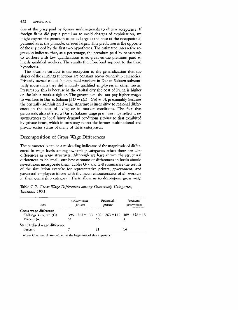
412 APPENDIX G
due of the price paid by former multinationals to obtain acceptance. Ifforeign firms did pay a premium to avoid charges of exploitation, wemight expect the premium to be as large at the base of the occupationalpyramid as at the pinnacle, or even larger. This prediction is the oppositeof those yielded by the first two hypotheses. The estimated interactive re-gression indicates that, as a percentage, the premium paid by parastatalsto workers with low qualifications is as great as the premium paid tohighly qualified workers. The results therefore lend support to the thirdhypothesis.
The location variable is the exception to the generalization that theslopes of the earnings functions are constant across ownership categories.Privately owned establishments paid workers in Dar es Salaam substan-tially more than they did similarly qualified employees in other towns.Presumably this is because in the capital city the cost of living is higheror the labor market tighter. The government did not pay higher wagesto workers in Dar es Salaam [bD - c(D * Go) 0], presumably becausethe centrally administered wage structure is insensitive to regional differ-ences in the cost of living or in market conditions. The fact thatparastatals also offered a Dar es Salaam wage premium may reflect a re-sponsiveness to local labor demand conditions similar to that exhibitedby private firms, which in turn may reflect the former multinational andprivate sector status of many of these enterprises.
Decomposition of Gross Wage Differences
The parameter ,3 can be a misleading indicator of the magnitude of differ-ences in wage levels among ownership categories when there are alsodifferences in wage structures. Although we have shown the structuraldifferences to be small, our best estimate of differences in levels shouldnevertheless incorporate them. Tables G-7 and G-8 summarize the resultsof the simulation exercise for representative private, government, andparastatal employees (those with the mean characteristics of all workersin their ownership category). These allow us to decompose gross wage
Table G-7. Gross Wage Differences among Ownership Categories,Tanzania 1971
Government- Parastatal- Parastatal-Item private private government
Gross wage differenceShillings a month (G) 396-263=133 409-263=146 409-396=13Percent (ox) 51 56 3
Standardized wage differencePercent 7 21 14Note: G, ce, and p are defined at the beginning of this appendix.
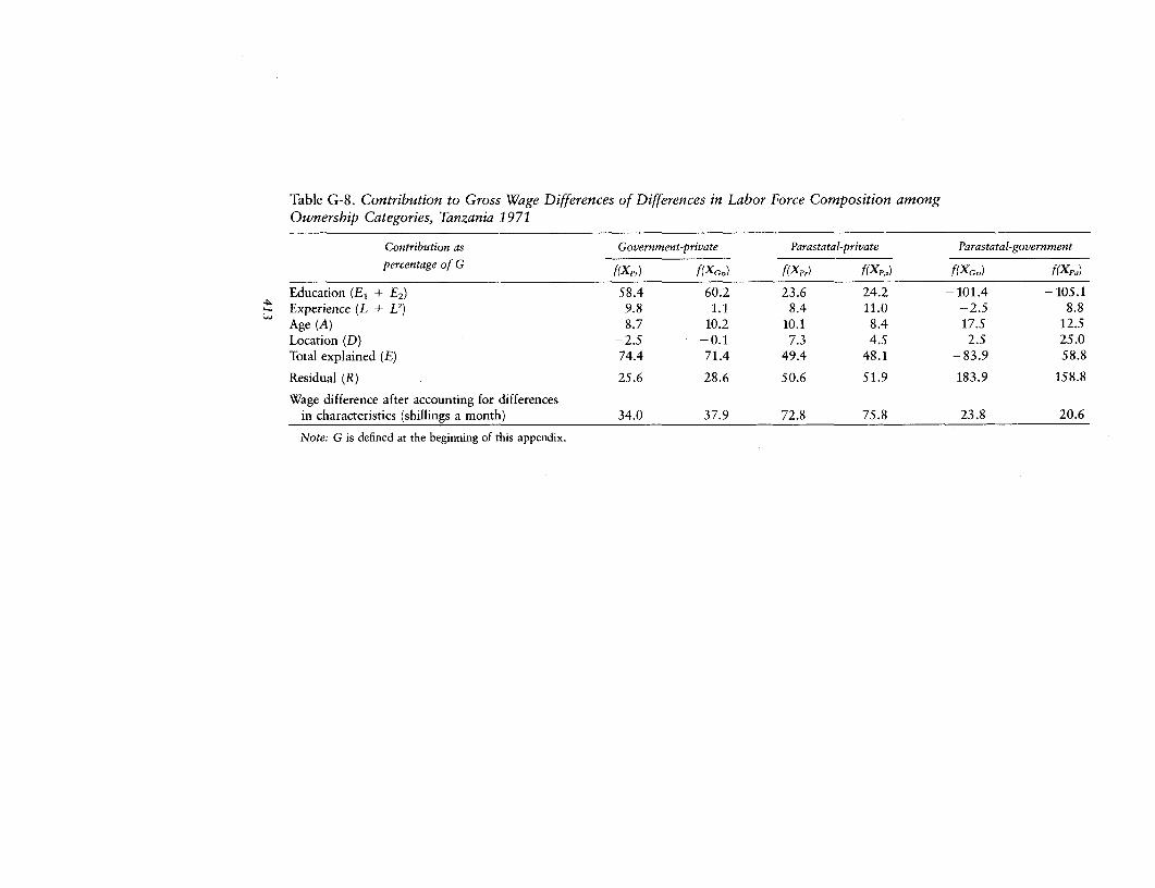
Table G-8. Contribution to Gross Wage Differences of Differences in Labor Force Composition amongOwnership Categories, Tanzania 1971
Contribution as Government-private Parastatal-private Parastatal-government
percentage of G f(XPr) f(X 0 0 ) f(XP,) f(XP.) f(XGO) f(XP.)
Education (El + E2 ) 58.4 60.2 23.6 24.2 -101.4 -105.1k Experience (L + L2) 9.8 1.1 8.4 11.0 -2.5 8.8
Age (A) 8.7 10.2 10.1 8.4 17.5 12.5Location (D) -2.5 -0.1 7.3 4.5 2.5 25.0Total explained (E) 74.4 71.4 49.4 48.1 -83.9 -58.8
Residual (R) 25.6 28.6 50.6 51.9 183.9 158.8
Wage difference after accounting for differencesin characteristics (shillings a month) 34.0 37.9 72.8 75.8 23.8 20.6
Note: G is defined at the beginning of this appendix.
414 APPENDIX G
differentials into E, the component explained by various differences incharacteristics, and R, the residual that stems from differences in earn-ings functions.
Government employees earned, on average, 51 percent more than pri-vate sector employees (table G-7), and the first two columns of table G-8indicate that differences in characteristics account for roughly 73 percentof this large differential. The much higher educational attainment of ourrepresentative government employee-a reflection of the greater white-collar intensity of labor demand in the government than in the privatesector-accounts for fully 85 percent of E. After differences in character-istics are taken into account the representative government worker earnsabout 36 shillings a month (13 percent) more than his private sectorcounterpart.
The gross wage difference in mean wages between private andparastatal employees (146 shillings, or 56 percent) is even larger than thegovernment-private difference. In this case, however, a markedly smallerproportion, roughly half, is explained by differences in characteristics.Differences in educational attainment contribute the most to E, followedin descending order of importance by the greater experience and age ofparastatal workers and their greater concentration in the capital city. Theresidual, R, which implies a difference of about 75 shillings a month, or29 percent, is the premium our representative worker earns simply forbeing a parastatal rather than a private sector employee.
Since differences in characteristics explain more of the government-private differential than of the parastatal-private differential in meanwages, we would expect differences in characteristics to explain the smalladvantage in mean wages of the "typical" parastatal worker in relationto government workers. In fact, this small advantage is greater than isexplained by differences in characteristics. The proportion of employeeswho were high-paid white-collar workers was nearly twice as high inthe government as in the parastatal sector. As a corollary, governmentworkers had a higher level of educational attainment. If government em-ployees were paid according to the parastatal wage structure, they wouldactually have earned more, on average, than parastatal employees. Thisis indicated by the negative sign of the estimated total contribution tothe gross wage difference of differences in composition, E.
Conclusion
Our analysis of public-private earnings differentials in urban Tanzaniain 1971 suggests that worker characteristics cannot account for all of thedifferences in earnings between the public and private sectors of the wageeconomy. Both government and parastatal employees were paid morethan the wage rates prevailing in the private sector. Public sector employ-
The Public-Private Wage Differential: Tanzania 1971 41S
ers did not appear to be acting simply as wage takers. The governmentpaid a modest premium, whereas parastatal workers earned 20 percentmore than private sector workers with the same characteristics. A defini-tive test of competing hypotheses was not possible owing to the crudenessof our human capital measures and our inability to control for job attri-butes and hours worked. Nonetheless, the evidence suggests that thelarge parastatal premium was a residue of the premium paid by multina-tional firms before nationalization.
Notes
1. Wage earners include employees of all firms, regardless of size.2. Private firms accounted for 31.8 percent, government for 29.7 percent, and
parastatals for 38.5 percent of all urban wage employment. These proportionscorrespond well to the distribution of employment by firm type reported in theofficial Survey of Employment and Earnings in 1971.
3. The available data are for earnings per month. In the absence of informationon hourly wage rates, we cannot reject the hypothesis that observed earnings dif-ferentials are attributable to differences in number of hours worked. We have noa priori reason, however, to expect hours worked to be related to ownership.
4. For most employees the current job is their first job, and the experience vari-able captures their total employment experience. The age variable is included tocapture the effects on earnings of prior employment experience of workers whohave had more than one job and of pure age effects.
5. Consistent and unbiased coefficients on the ownership category variablesrequire that mobility among sectors not be a function of individual earnings,other things being equal. If interemployer mobility is a function of earnings, asimultaneous model of both earnings and sector of employment would be re-quired to test for the independent effect of ownership category on wages.
6. The finding that most of the difference among ownership categories is inthe constant terms rather than in the slopes of the earnings functions is furthersupported when this equation is compared with a restricted specification in whichonly the intercept and regional parameters are entered interactively. The F-testrejects the hypothesis that the addition of the other interactive terms adds to theexplanatory power of the model.
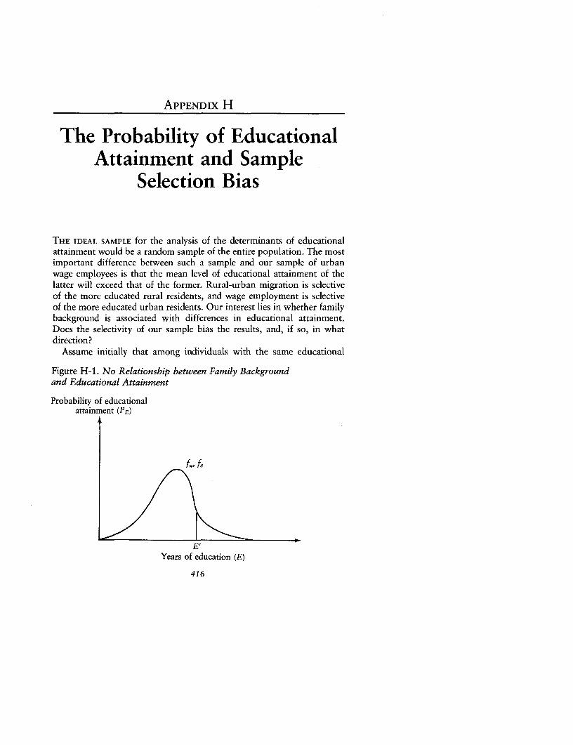
APPENDIX H
The Probability of EducationalAttainment and Sample
Selection Bias
THE IDEAL SAMPLE for the analysis of the determinants of educationalattainment would be a random sample of the entire population. The mostimportant difference between such a sample and our sample of urbanwage employees is that the mean level of educational attainment of thelatter will exceed that of the former. Rural-urban migration is selectiveof the more educated rural residents, and wage employment is selectiveof the more educated urban residents. Our interest lies in whether familybackground is associated with differences in educational attainment.Does the selectivity of our sample bias the results, and, if so, in whatdirection?
Assume initially that among individuals with the same educational
Figure H-1. No Relationship between Family Backgroundand Educational Attainment
Probability of educationalattainment (PE)
fu, fe
E'Years of education (E)
416
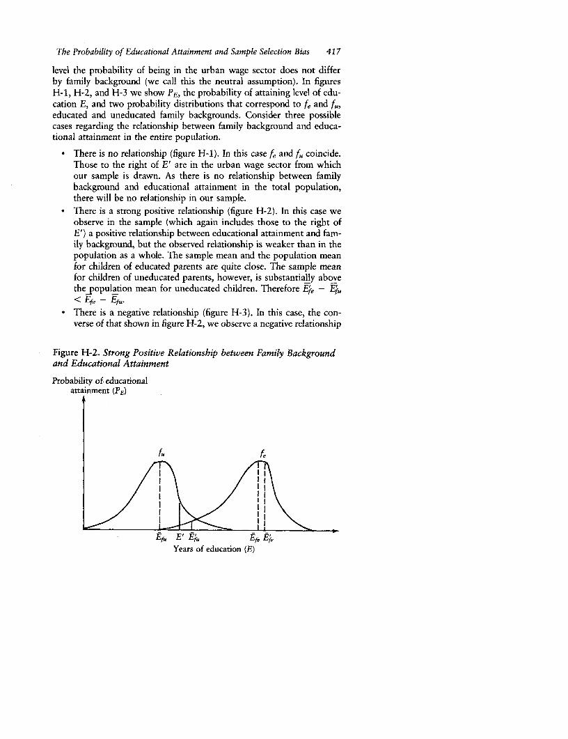
The Probability of Educational Attainment and Sample Selection Bias 417
level the probability of being in the urban wage sector does not differby family background (we call this the neutral assumption). In figuresH-1, H-2, and H-3 we show PE, the probability of attaining level of edu-cation E, and two probability distributions that correspond to fe and fu,educated and uneducated family backgrounds. Consider three possiblecases regarding the relationship between family background and educa-tional attainment in the entire population.
* There is no relationship (figure H-1). In this case fe and fu coincide.Those to the right of E' are in the urban wage sector from whichour sample is drawn. As there is no relationship between familybackground and educational attainment in the total population,there will be no relationship in our sample.
* There is a strong positive relationship (figure H-2). In this case weobserve in the sample (which again includes those to the right ofE') a positive relationship between educational attainment and fam-ily background, but the observed relationship is weaker than in thepopulation as a whole. The sample mean and the population meanfor children of educated parents are quite close. The sample meanfor children of uneducated parents, however, is substantially abovethe population mean for uneducated children. Therefore E^e - E;u< Efe - Efu.
- There is a negative relationship (figure H-3). In this case, the con-verse of that shown in figure H-2, we observe a negative relationship
Figure H-2. Strong Positive Relationship between Family Backgroundand Educational Attainment
Probability of educationalattainment (PE)
fu ~~~~~~~~fe
Ef. EtE^u EfeEfe
Years of education (E)
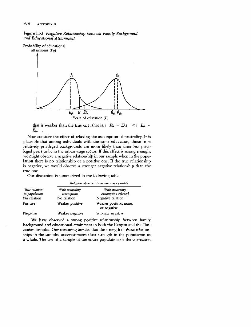
418 APPENDIX H
Figure H-3. Negative Relationship between Family Backgroundand Educational Attainment
Probability of educationalattainment (PE)
j fe fu
Years of education (E)
that is weaker than the true one; that is, i EW - EuI < I
Efu i .I i
Now consider the effect of relaxing the assumption of neutrality. It isplausible that among individuals with the same education, those fromrelatively privileged backgrounds are more likely than their less privi-leged peers to be in the urban wage sector. If this effect is strong enough,we might observe a negative relationship in our sample when in the popu-lation there is no relationship or a positive one. If the true relationshipis negative, we would observe a stronger negative relationship than thetrue one.
Our discussion is summarized in the following table.
Relation observed in urban wage sample
True relation With neutrality With neutralityin population assumption assumption relaxedNo relation No relation Negative relation
Positive Weaker positive Weaker positive, none,or negative
Negative Weaker negative Stronger negative
We have observed a strong positive relationship between familybackground and educational attainment in both the Kenyan and the Tan-zanian samples. Our reasoning implies that the strength of these relation-ships in the samples underestimates their strength in the population asa whole. The use of a sample of the entire population or the correction
The Probability of Educational Attainment and Sample Selection Bias 419
of our urban sample for bias owing to sample selectivity would only rein-force our findings. Far from weakening our sample finding of a positiverelationship between educational attainment and family background,sample selection bias implies that the finding is even stronger for the pop-ulation as a whole.
APPENDIX I
Family Background and theReturns to Schooling
IN TANZANIA WE FOUND no independent influence of family backgroundon earnings of form 4 leavers, and the relationship that we found inKenya was largely attributable to discrimination. These results shouldnot mislead us into thinking that family background has little or no influ-ence on returns to schooling. Our model suggests that the influence offamily background was not noticeable at the secondary level in Tanzaniabecause of the highly selective nature of the secondary school system,which gave access only to the upper tail of the distribution of primaryleavers from uneducated backgrounds. In Kenya the measured humancapital effect of family background was attenuated by the high rate ofpromotion to higher education of those from more educated back-grounds.
Here we switch from examining the relationship between family back-ground and earnings at a particular educational level to examining theeffect of family background on the returns to schooling for all workersin our sample. We have noted various ways in which family backgroundcan affect earnings: children of educated parents tend to receive moreout-of-school investment in human capital, which may result in theirlearning more at school; they tend to go to higher-quality schools; andthey may benefit from discrimination in the labor market.
Insofar as labor market discrimination favors the children of educatedparents, we would expect the effect on earnings to be the same irrespec-tive of the educational level of the worker. Similarly, out-of-school invest-ment, to the extent that it raises earnings directly, should do so irrespec-tive of educational level. In both cases the returns to education shouldnot be affected by family background. The returns would be raised, how-ever, if the higher-quality schooling received by children from educated
Note: Adapted from Jane Armitage and Richard H. Sabot, "Socioeconomic Backgroundand the Returns to Education in Two Low-Income Countries," Economica 54, no. 213 (Feb-ruary 1987): 103-08.
420
Family Background and the Returns to Schooling 421
backgrounds raised the value added of a year of schooling or if out-of-school investments were complementary with human capital accumula-tion in school, thus increasing the amount learned during a school year.A comparison of the returns to years of schooling among family back-ground groups should therefore serve as a pointer to the reasons for theinfluence of family background.
Empirical Results
The earnings function we estimate is of the general form:'
(1-1) W = f(Z, Fj)
where Z = a vector of human capital variables made up of S, years ofeducation, and L and L' = years of employment experience and theirsquare; F, = dummy variables that denote family background, and W= In earnings. In equation I-1 the returns to schooling are constrainedto be the same for all family background groups. We also estimate thefollowing unconstrained equation:
(1-2) W = f(Z, F,, Z -Fj)
where Z - F, are interaction terms that measure the returns to human cap-ital for workers whose parents have various levels of education in relationto returns for workers with uneducated parents.2 F-tests are conductedon equations 1-1 and 1-2 to determine whether the observed differencesare statistically significant.
Tables 1-1 and 1-2 present the estimates of the constrained and uncon-strained earnings functions, respectively. For Kenya the value of the F-statistic is 7.5 and for Tanzania it is 5.2; both exceed the critical valueof F at the 1-percent significance level. Therefore for both Kenya and Tan-zania we reject the null hypothesis that returns to human capital are inde-pendent of family background. The t-statistics pertaining to the coeffi-cients on the family background variables also suggest that theunconstrained equation is the superior specification; nearly all are highlysignificant. The education and experience variables are highly significantin both sets of equations.
In table 1-2 the average earnings premium per year of schooling forworkers with uneducated parents is the coefficient of S; for workers fromother family background groups the premium is the coefficient of S plusthe coefficient of S * F,. The results indicate that in both countries returnsto education rise sharply with the socioeconomic status of the workers'parents. In Kenya the wage premium per year of education is 8.5 percentfor workers in the F1 group (uneducated parents), 11.0 percent for work-ers in the F2 group (one parent with no education, the other with primaryeducation), and between 15.6 and 16.7 percent for workers in the top

422 APPENDIX I
Table I-1. Constrained Earnings Functions
Coefficient
Variable Kenya Tanzania
S 0.101 0.078(23.33) (25.38)
L 0.54 0.57(13.38) (14.90)
L2 -0.001 -0.001(7.44) (6.84)
F2 0.030 -0.002(0.92) (0.08)
F3 0.141 0.027
(3.78) (0.89)F4 0.360 0.036
(4.80) (0.61)Constant 5.519 5.607K2 0.354 0.431N 1,600 1,522
Note: S, secondary education; L, employment experience; F2 , one parent with primaryeducation and one with none; F3 , both parents with primary education or one with secon-dary or higher and one with none; F4 , one parent with primary education and one withsecondary or higher or both with secondary education or higher; (F1 , both parents withouteducation, is the omitted category). The dependent variable is In W. Figures in parenthesesare t-statistics.
two groups. Similarly, in Tanzania the premium is 6.7 percent for work-ers with uneducated parents, 8.6 percent for workers in the F2 category,and between 9.6 and 10.3 percent for workers with the most highly edu-cated parents.
Interpretation of Results
The educational production function describes the relationship betweenthe output of the skill acquisition process and such inputs as quantityof schooling, quality of schooling, individual ability, and out-of-schoolinvestments in human capital as proxied by family background (seeHanushek 1979 and Lau 1979). In a human capital theoretic framework,wages depend on the output of this process (the individual's stock of cog-nitive and other skills), not simply on years of schooling, which is justone of the inputs. There may be an interaction in the educational produc-tion function between out-of-school investments and formal schooling.If these two inputs are complements, the returns to schooling will in-crease with family background in the earnings function. Conversely, if
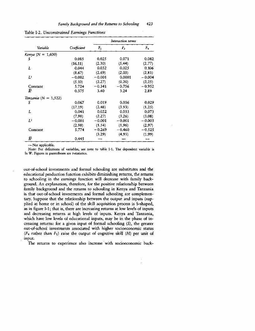
Family Background and the Returns to Schooling 423
Table 1-2. Unconstrained Earnings Functions
Interaction terms
Variable Coefficient F2 F3 F4
Kenya (N = 1,600)S 0.085 0.025 0.071 0.082
(16.11) (2.30) (5.44) (2.77)L 0.044 0.032 0.025 0.106
(8.67) (2.69) (2.03) (2.81)L2 -0.002 -0.001 0.0001 -0.004
(5.10) (2.27) (0.20) (2.25)Constant 5.724 -0.341 -0.756 -0.952KR 0.375 3.40 3.24 2.89
Tanzania (N = 1,522)S 0.067 0.019 0.036 0.029
(17.19) (2.48) (3.93) (1.25)L 0.041 0.022 0.033 0.073
(7.98) (2.27) (3.26) (3.08)L2 -0.001 -0.001 - 0.001 -0.003
(2.98) (1.54) (1.96) (2.97)Constant 5.774 -0.269 -0.460 -0.525
(3.29) (4.93) (1.99)K2 0.445 - -
--Not applicable.Note: For definitions of variables, see note to table l-l. The dependent variable is
In W. Figures in parentheses are t-statistics.
out-of-school investments and formal schooling are substitutes and theeducational production function exhibits diminishing returns, the returnsto schooling in the earnings function will decrease with family back-ground. An explanation, therefore, for the positive relationship betweenfamily background and the returns to schooling in Kenya and Tanzaniais that out-of-school investments and formal schooling are complemen-tary. Suppose that the relationship between the output and inputs (sup-plied at home or in school) of the skill acquisition process is S-shaped,as in figure I-1; that is, there are increasing returns at low levels of inputsand decreasing returns at high levels of inputs. Kenya and Tanzania,which have low levels of educational inputs, may be in the phase of in-creasing returns: for a given input of formal schooling (S), the greaterout-of-school investments associated with higher socioeconomic status(F4 rather than Fj) raise the output of cognitive skill (H) per unit ofinput.
The returns to experience also increase with socioeconomic back-
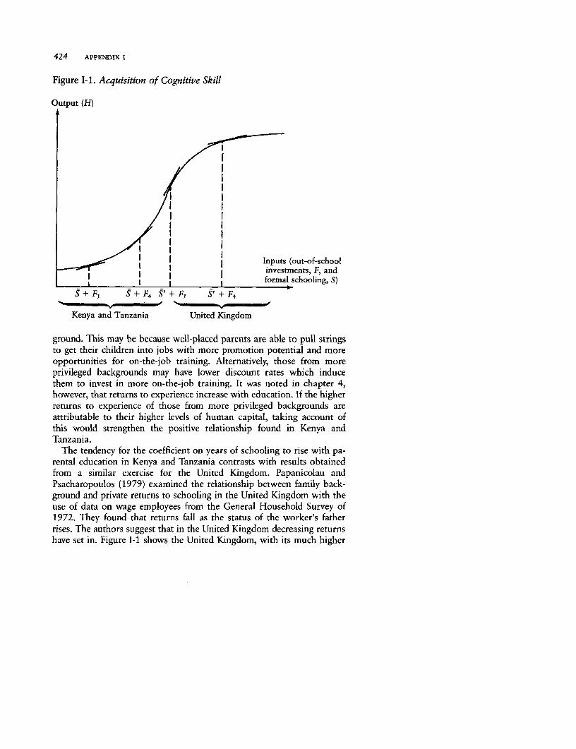
424 APPENDIX I
Figure 1-1. Acquisition of Cognitive Skill
Output (H)
Inputs (out-of-schoolinvestments, F, andformal schooling, S)
S+ F S+ F4 S' + F1 S + F4
Kenya and Tanzania United Kingdom
ground. This may be because well-placed parents are able to pull stringsto get their children into jobs with more promotion potential and moreopportunities for on-the-job training. Alternatively, those from moreprivileged backgrounds may have lower discount rates which inducethem to invest in more on-the-job training. It was noted in chapter 4,however, that returns to experience increase with education. If the higherreturns to experience of those from more privileged backgrounds areattributable to their higher levels of human capital, taking account ofthis would strengthen the positive relationship found in Kenya andTanzania.
The tendency for the coefficient on years of schooling to rise with pa-rental education in Kenya and Tanzania contrasts with results obtainedfrom a similar exercise for the United Kingdom. Papanicolau andPsacharopoulos (1979) examined the relationship between family back-ground and private returns to schooling in the United Kingdom with theuse of data on wage employees from the General Household Survey of1972. They found that returns fall as the status of the worker's fatherrises. The authors suggest that in the United Kingdom decreasing returnshave set in. Figure 1-1 shows the United Kingdom, with its much higher
Family Background and the Returns to Schooling 425
level of educational inputs per student, on the concave part of the educa-tional production function where increases in inputs reduce outputs perunit of input.
An alternative explanation for the difference between the United King-dom and Kenya and Tanzania lies in the labor market-in the wage de-termination process, rather than in the process of skill acquisition.Papanicolau and Psacharopoulos suggest that British students from privi-leged backgrounds may obtain good jobs regardless of their level of skills.In Kenya and Tanzania, where socioeconomic differentiation is a morerecent phenomenon, such a floor under the earnings of the children ofthe relatively privileged may not exist. Another explanation for the Brit-ish pattern is that ability and education are substitutes in the determina-tion of earnings and that there is a positive correlation between abilityand family background. Again, we would not expect to find the samepattern in Kenya and Tanzania, where socioeconomic differentiation isso recent.
In conclusion, the fact that in both Kenya and Tanzania the coefficienton years of schooling rises with parental education suggests that familybackground influences earnings because complementarity between out-of-school and school investments in human capital enables the childrenof the educated to learn more in school or because these children attendbetter-quality schools. It suggests that less importance is to be placedon the independent effect of human capital acquired out of school or onthe effect of labor market discrimination.
Notes
1. It is common for the earnings function to include measures of noneconomicpersonal characteristics that might nevertheless have an influence on earnings,such as race or sex. Another study using these data sets found evidence of racediscrimination but not of discrimination on the basis of sex (Armitage and Sabotforthcoming a). We therefore focus our analysis on Africans, who constitute over90 percent of the urban wage labor force in both Kenya and Tanzania, and wedo not include a dummy variable for sex.
2. The unconstrained earnings function is equivalent to estimating four regres-sions, one for each family background group. The earnings function for the basegroup (Fl = 1) is given by the first colurnn of coefficients in table 1-2. To obtainthe earnings function for the F2 category we add the coefficients in the first andsecond columns and similarly for the F3 and F4 categories.


References
Ahluwalia, Montek S. 1976. "Inequality, Poverty and Development." Journal ofDevelopment Economics 3, no. 4 (December):307-42.
Ahluwalia, Montek S., Nicholas G. Carter, and Hollis B. Chenery. 1979.'Growth and Poverty in Developing Countries." Journal of Development Eco-nomics 6, no. 3 (September):299-341.
Akerlof, George A. 1981. "Jobs as Dam Sites." Review of Economic Studies 48Uanuary):37-49.
Alexander, Leigh, and John Simmons. 1975. The Determinants of SchoolAchievement in Developing Countries: The Educational Production Function.World Bank Staff Working Paper 201. Washington, D.C.
Anderson, Lascelles. 1980. "Rates of Return to Human Capital: A Test UsingEl Salvador Data." American Economic Review, Papers and Proceedings 70,no. 2 (May):738-41.
Armitage, Jane, and Richard H. Sabot. 1987a. "Efficiency and Equity Implica-tions of Subsidies to Secondary Education in Kenya." In David Newbery andNicholas Stern, eds., The Theory of Taxation for Developing Countries. NewYork: Oxford University Press.
. 1987b. "Socioeconomic Background and the Returns to Schooling inTwo Low-Income Economies." Economica 54, no. 213 (February):103-08.
. Forthcoming a. "Discrimination in East Africa's Urban Labor Markets."In Nancy Birdsall and Richard H. Sabot, eds., Labor Market Discriminationin Developing Countries.
. Forthcoming b. "Implications of Educational Expansion for the Measure-ment of Labor Market Discrimination." In Nancy Birdsall and Richard H.Sabot, eds., Labor Market Discrimination in Developing Countries.
Arrow, K. J. 1973. "Higher Education as a Filter." Journal of Public Economics2, no. 3 (July):193-216.
Ashenfelter, Orley, and Albert Rees, eds. 1973. Discrimination in Labor Markets.Princeton, N.J.: Princeton University Press.
Atkinson, A. B. 1980. "On Intergenerational Income Mobility in Britain." Jour-nal of Post-Keynesian Economics 3, no. 2 (Winter):194-218.
Balassa, Bela, and others. 1971. The Structure of Protection in Developing Coun-tries. Baltimore, Md.: Johns Hopkins University Press.
Bartholomew, D. J. 1973. Stochastic Models for Social Processes. 2d ed. NewYork: Wiley and Sons.
Becker, Gary S. 1964. Human Capital. A Theoretical and Empirical Analysis
427
428 REFERENCES
with Special Reference to Education. Princeton, N.J.: Princeton UniversityPress.
-. 1972. Comment on S. Bowles, "Schooling and Inequality from Genera-tion to Generation." Journal of Political Economy 80, no. 3, pt. 2 (May-June):S252-55.
. 1975. "Human Capital and the Personal Distribution of Income: An An-alytical Approach." Woytinski Lecture 1967. Reprinted in Human Capital, 2ded. Chicago, Ill.: University of Chicago Press.
Behrman, Jere R., and Nancy Birdsall. 1983. "Quality of Schooling: QuantityAlone Is Misleading." American Economic Review 73, no. 5 (December):928-46.
-. 1988. "The Reward for Good Timing: Cohort Effects and EarningsFunctions for Brazilian Males." Review of Economics and Statistics 70, no.1 (February):129-35.
Behrman, J. R., and B. L. Wolfe. 1984a. "The Socioeconomic Impact of Schoolingin a Developing Country." Review of Economics and Statistics 66, no. 2(May) :296-303.
- . 1984b. "Who Is Schooled in Developing Countries? The Role of Income,Parental Schooling, Sex and Family Size." Economics of Education Review 3,no. 3:231-45.
-. Forthcoming. 'Earnings and Labor Force Participation Deter-minants in a Developing Country-Are There Sexual Differentials?" InNancy Birdsall and Richard H. Sabot, eds., Labor Market Discrimination inDeveloping Countries.
Behrman, J. R., J. B. Knight, and R. H. Sabot. 1983. "A Simulation Alternativeto the Comparative R2 Approach to Decomposing Inequality." Oxford Bulletinof Economics and Statistics 45, no. 3 (August):307-12.
Behrman, J. R., and others. 1980. Socioeconomic Success: A Study of the Effectsof Genetic Endowments, Family Environment and Schooling. Amsterdam:North-Holland.
Bertrand, Trent, and R. Griffin. 1983. "Financing Education in Kenya." CountryPolicy Department, World Bank, Washington, D.C. Processed.
Bhagwati, Jagdish N. 1973. 'Education, Class Structure and Income Equality."World Development 1, no. 5 (May):21-36.
-.1978. Foreign Trade Regimes and Economic Development. Anatomy andConsequences of Exchange Control Regimes. New York: National Bureau ofEconomic Research.
Bhagwati, Jagdish N., and T. N. Srinivasan. 1977. "Education in a Job LadderModel and the Fairness-in-Hiring Rule." Journal of Public Economics 7 (Feb-ruary) :2-22.
Birdsall, Nancy. 1985. "Public Inputs and Child Schooling in Brazil." Journalof Development Economics 18, no. 1 (May-June):67-86.
Birdsall, Nancy, and L. Fox. 1985. "Why Males Earn More: Location and Train-ing of Brazilian Schoolteachers." Economic Development and Cultural Change33, no. 3 (April):533-56.
References 429
Birdsall, Nancy, and Richard H. Sabot, eds. Forthcoming. Labor Market Dis-crimination in Developing Countries.
Birnbaum, Howard. 1976. "Career Origins, On-the-Job Training and Earnings."Southern Economic Journal 42, no. 4:587-99.
Blaug, Mark. 1974. "An Economic Analysis of Personal Earnings in Thai-land." Economic Development and Cultural Change 23, no. 1 (October):1-32.
1976. "Human Capital Theory: A Slightly Jaundiced View." Journal ofEconomic Literature 14, no. 3 (September):827-55.
Blaug, Mark, C. Dougherty, and G. Psacharopoulos. 1982. "The Distributionof Schooling and the Distribution of Earnings: Raising the School Leaving Agein 1972." Manchester School 50, no. 1 (March):24-40.
Blinder, Alan S. 1973. "Wage Discrimination: Reduced Form and Structural Esti-mates." Journal of Human Resources 8, no. 4 (Fall):436-55.
- 1974. Toward an Economic Theory of Income Distribution. Cambridge,Mass.: MIT Press.
Boissiere, Maurice, J. B. Knight, and R. H. Sabot. 1985. "Earnings, Schooling,Ability and Cognitive Skills." American Economic Review 75 (December):1016-30.
Bowen, Alex, and R. H. Sabot. 1983. "Education, Urbanization, and Family Size:Evidence from Nairobi." Development Research Department, World Bank,Washington, D.C. Processed.
Bowles, Samuel. 1969. Planning Educational Systems for Economic Growth.Cambridge, Mass.: Harvard University Press.
. 1970. "Aggregation of Labor Inputs in the Economics of Growth andPlanning: Experiments with a Two-Level CES Function." Journal of PoliticalEconomy 78, no. 1 January-February):68-81.
-. -1972. "Schooling and Inequality from Generation to Generation." Jour-nal of Political Economy 80, no. 3, pt. 2 (May-June):S219-51.
. 1973. "Understanding Unequal Opportunity." American Economic Re-view 63, no. 2 (May):346-56.
Bowles, Samuel, and Herbert Gintis. 1976. Schooling in Capitalist America. Lon-don: Routledge and Kegan Paul.
Bowman, Mary Jean. 1980. "Education and Economic Growth: An Overview."In Timothy King, ed., Education and Income. World Bank Staff Working Paper402. Washington, D.C.
Bowman, Mary Jean, and R. H. Sabot. 1982. "Human Resources in Africa: AContinent in Rapid Change." Development Research Department, WorldBank, Washington, D.C.
Bridge, R. D., C. M. Judd, and P. R. Moock. 1979. Determinants of EducationalOutcomes. Cambridge, Mass.: Ballinger.
Brown, Randall, M. Moon, and B. Zoloth. 1980. "Incorporating OccupationalAttainment in Studies of Male-Female Earnings Differentials." Jour-nal of Human Resources 15, no. 1 (Winter):3-28.
430 REFERENCES
Casley, D. J., and D. A. Lury. 1981. Data Collection in Developing Countries.Oxford, U.K.: Clarendon Press.
Chamberlain, Gary, and Zvi Griliches. 1977. "More on Brothers." In PaulTaubman, ed., Kinometrics: Determinants of Socioeconomic Success withinand between Families. Amsterdam: North-Holland.
Chenery, Hollis. 1971. Studies in Development Planning. Cambridge, Mass.:Harvard University Press.
Chenery, Hollis, ed. 1979. Structural Change and Development Policy. NewYork: Oxford University Press.
Chenery, Hollis B., and Moises Syrquin. 1975. Patterns of Development,1950-1970. New York: Oxford University Press.
Chow, G. C. 1960. "Tests of Equality between Subsets of Coefficients in TwoLinear Regressions." Econometrica 28, no. 3 (July):591-605.
Clark, Colin. 1940. The Conditions of Economic Progress. London: Macmillan.
Cochrane, Susan H. 1979. Fertility and Education: What Do We Really Know?Baltimore, Md.: Johns Hopkins University Press.
Coleman, James S., and others. 1966. Equality of Educational Opportunity.Washington, D.C.: U.S. Government Printing Office.
Collier, Paul, and Deepak Lal. 1986. Labour and Poverty in Kenya 1900-1980.Oxford, U.K.: Clarendon Press.
Conlisk, John. 1974. "Can Equalization of Opportunity Reduce Social Mobil-ity?" American Economic Review 64, no. 1 (March):80-90.
Cooksey, Brian, and Abel Ishumi. 1986. "A Critical Review of Policy and Prac-tice in Tanzanian Secondary Education since 1967." Ministry of Education,Dar es Salaam. Processed.
Coulson, Andrew. 1982. Tanzania. A Political Economy. Oxford, U.K.: Claren-don Press.
de Beyer, Joy, and J. B. Knight. 1989. "The Role of Occupation in the Determi-nation of Wages." Oxford Economic Papers, 41, no. 3 Uuly): 595-618.
Denison, Edward E 1967. Why Growth Rates Differ. Washington, D.C.: Brook-ings Institution.
Dougherty, C. R. S. 1971. "Optimal Allocation of Investment in Education." InHollis B. Chenery, ed., Studies in Development Planning. Cambridge, Mass.:Harvard University Press.
- . 1972. "Estimates of Labor Aggregation Functions." Journal of PoliticalEconomy 80, no. 6 (November):1101-19.
Fallon, P. R., and P. R. G. Layard. 1975. "Capital-Skill Complementarity, IncomeDistribution, and Output Accounting." Journal of Political Economy 83, no.2 (April):279-301.
Fields, Gary S. 1974. "The Private Demand for Education in Relation to LaborMarket Conditions in Less Developed Countries." Economic Journal 84, no.336 (December):906-25.
References 431
- 1975. "Higher Education and Income Distribution in a Less DevelopedCountry." Oxford Economic Papers 27, no. 2 (July):245-59.
. 1980. "Education and Income Distribution in Developing Countries: AReview of the Literature." In Timothy King, ed., Education and Income. WorldBank Staff Working Paper 402. Washington, D.C.
Fields, Gary S., and T. P. Schultz. 1980. "Regional Inequality and Other Sourcesof Income Variation in Colombia." Economic Development and CulturalChange 28, no. 3 (April):447-67.
Fisher, E M. 1970. "Tests of Equality between Sets of Coefficients in Two Lin-ear Regressions: An Expository Note." Econometrica 38, no. 2 (March):361-66.
Freeman, Richard B., and James L. Medoff. 1981. "The Impact of the PercentageOrganized on Union and Nonunion Wages." Review of Economics and Statis-tics 63, no. 4 (November): S61-72.
. 1981. "The Impact of Collective Bargaining: Illusion or Reality?" In J.Stieber, R. B. McKersie, and D. Q. Mills, eds., U.S. Industrial Relations1950-1980: A Critical Assessment. Madison, Wis.: Industrial Relations Re-search Association.
-1 1982. What Do Unions Do: Evidence, Interpretation, and Directions forResearch. New York: Basic Books.
Goldthorpe, John, and K. Hope. 1974. The Social Grading of Occupations: ANew Approach and Scale. Oxford, U.K.: Clarendon Press.
Griliches, Zvi. 1977. "Estimating the Returns to Schooling: Some EconometricProblems." Econometrica 45, no. 1 (January):1-22.
- . 1979. "Sibling Models and Data in Economics: Beginnings of a Survey."Journal of Political Economy 87, no. 5, pt. 2 (October):S37-64.
Griliches, Zvi, and William M. Mason. 1972. "Education, Income, and Ability."Journal of Political Economy 80, no. 3, pt. 2 (May-June):S74-103.
Halvorsen, Robert, and Raymond Palmquist. 1980. "The Interpretation ofDummy Variables in Semi-Logarithmic Equations." American Economic Re-view 70, no. 3 June):474-75.
Hammermesh, Daniel S., and James Grant. 1979. "Econometric Studies ofLabor-Labor Substitution and Their Implications for Policy." Journal ofHuman Resources 14, no. 4 (Autumn):518-42.
Hansen, W. Lee, and Burton A. Weisbrd. 1969. Benefits, Costs, and Financesof Public Higher Education. Chicago: Markham.
Hanushek, Erik A. 1979. "Conceptual and Empirical Issues in the Estimationof Educational Production Functions." Journal of Human Resources 14, no.3 (Summer):351-88.
Hanushek, Erik A., and John E. Jackson. 1977. Statistical Methods for SocialScientists. New York: Academic Press.
Hausman, J. A. 1978. "Specification Tests in Econometrics." Econometrica46, no. 6 (November):1251-71.
432 REFERENCES
Hendry, D. E, and R. C. Marshall. 1983. "On High and Low R2 Contributions."Oxford Bulletin of Economics and Statistics 45, no. 3 (August):313-16.
House, W. S., and H. Rempel. 1978. The Kenya Employment Problem: An Anal-ysis of the Formal Labour Market. Nairobi: Oxford University Press.
Jackson, Dudley. 1979. "The Disappearance of Strikes in Tanzania: Incomes Pol-icy and Industrial Democracy." Journal of Modern African Studies 17, no. 2June):219-51.
Jallade, Jean-Pierre. 1974. Public Expenditures on Education and Income Distri-bution in Colombia. Baltimore, Md.: Johns Hopkins University Press.
Jencks, Christopher, and others. 1972. Inequality: A Reassessment of the Effectof Family and Schooling in America. New York and London: Basic Books.
Jorgenson, Dale W., and Zvi Griliches. 1967. "The Explanation of ProductivityGrowth." Review of Economic Studies 34 (July):249-83.
Kenya, Ministry of Economic Planning. 1974. Development Plan, 1974-78. Nai-robi: Government Printer.
1979. Development Plan 1979-1983, Part 1. Nairobi: GovernmentPrinter.
King, Timothy, ed. 1980. Education and Income. World Bank Staff WorkingPaper 402. Washington, D.C.
Klingelhofer, E. L. 1967. "Performance of Tanzanian School Pupils on the Ra-ven's Matrices Test." Journal of Social Psychology 72 (August):205-16.
Knight, J. B. 1979. "Job Competition, Occupational Production Functions, andFiltering Down." Oxford Economic Papers 31, no. 2 (July):187-204.
Knight, J. B., and R. H. Sabot. 1981. "The Returns to Education: Increasing withExperience or Decreasing with Expansion?" Oxford Bulletin of Economicsand Statistics 43, no. 1 (February):51-71.
- . 1982. "Labor Market Discrimination in a Poor Urban Economy." Jour-nal of Development Studies 19, no. 1 (October):67-87.
- 1983a. "Educational Expansion and the Kuznets Effect." American Eco-nomic Review 73, no. 5 (December):1132-36.
- 1983b. "The Role of the Firm in Wage Determination: An African CaseStudy." Oxford Economic Papers 35, no. 1 (March):45-66.
- 1987a. 'Educational Expansion, Government Policy and Wage Com-pression." Journal of Development Economics 26, no. 2 (August):201-21.
. 1987b. "Educational Policy and Labour Productivity: An Output Ac-counting Exercise." Economic Journal 97, no. 385 (March):199-214.
. 1987c. "The Rate of Return on Educational Expansion." Economics ofEducation Review 6, no. 3:255-62.
Krueger, Anne 0. 1968. "Factor Endowments and Per Capita Income Differencesamong Countries." Economic Journal 78, no. 311 (September):641-59.
- 1978. Foreign Trade Regimes and Economic Development: Liberaliza-tion Attempts and Consequences. New York: National Bureau of EconomicResearch.
References 433
Kuznets, Simon. 1955. "Economic Growth and Income Inequality." AmericanEconomic Review 45 (March): 1-28.
. 1965. Economic Growth and Structure, Selected Essays. London:Heinemann.
. 1966. Modern Economic Growth. New Haven, Conn.: Yale UniversityPress.
Lau, Lawrence T. 1979. "Educational Production Functions." In National Acad-emy of Education, Economic Dimensions of Education. Washington, D.C.
Layard, Richard, and G. Psacharopoulos. 1974. "The Screening Hypothesis andthe Social Returns to Education." Journal of Political Economy 82 (Octo-ber):985-98.
Leibowitz, A. 1973. Comment on S. Bowles, "Understanding Unequal EconomicOpportunity," American Economic Review 63, no. 2 (May):357-58.
Lewis, H. G. 1963. Unionism and Relative Wages in the United States. Chicago,Ill.: University of Chicago Press.
Lindauer, D. L., and R. H. Sabot. 1983. "The Public/Private Wage Differentialin a Poor Urban Economy." Journal of Development Economics 12, nos. 1-2(February-April):137-52.
Little, Ian, Tibor Scitovsky, and Maurice Scott. 1970. Industry and Trade inSome Developing Countries. London: Oxford University Press.
Lockheed, Marlaine E., Jean Jamison, and Lawrence T. Lau. 1980. "Farmer Edu-cation and Farm Efficiency: A Survey." Economic Development and CulturalChange 29:37-76.
Lydall, Harold. 1968. The Structure of Earnings. Oxford, U.K.: Clarendon Press.Malkiel, Burton G., and Judith A. Malkiel. 1973. "Male-Female Pay Differentials
in Professional Employment." American Economic Review 63, no. 4 (Septem-ber):693-705.
Matthews, R. C. O., C. H. Feinstein, and J. C. Odling-Smee. 1982. British Eco-nomic Growth 1856-1973. Stanford, Calif.: Stanford University Press.
Mazumdar, Dipak. 1981. The Urban Labor Market and Income Distribution.New York: Oxford University Press.
Meade, J. E. 1976. The Just Economy. London: Allen and Unwin.Mill, J. S. 1848. Principles of Political Economy. London.Mincer, Jacob. 1974. Schooling, Experience, and Earnings. New York: National
Bureau of Economic Research.
National Academy of Education. 1979. Economic Dimensions of Education.Washington, D.C.
Nelson, Richard R. 1981. "Research on Productivity Growth and Differences."Journal of Economic Literature 19, no. 3 (September):1029-64.
Nickell, Stephen. 1982. "The Determinants of Occupational Success in Britain."Review of Economic Studies 49 (January):43-53.
Nyerere, Julius. 1967a. Education for Self-Reliance. Dar es Salaam: GovernmentPrinter.
434 REFERENCES
. 1967b. Freedom and Unity. London: Oxford University Press.OECD. 1971. "Group Disparities in Educational Participation and Achievement."
Background Reports 4 and 10. Conference on Policies for Educational Growth,Paris.
Oaxaca, Ronald. 1973a. "Male-Female Differentials in Urban Labor Markets."International Economic Review 3 (October):693-709.
-. 1973b. "Sex Discrimination in Wages." In Orley Ashenfelter and AlbertRees, eds., Discrimination in Labor Markets. Princeton, N.J.: Princeton Uni-versity Press.
Oi, Walter Y. 1962. "Labor as a Quasi-Fixed Factor." Journal of Political Econ-omy 70, no. 5, pt. 2 (October):538-55.
Olneck, M. 1977. "On the Use of Sibling Data to Estimate the Effects of FamilyBackground, Cognitive Skills and Schooling: Results from the KalamazooBrothers Study." In Paul Taubman, ed., Kinometrics: Determinants of Socio-economic Success within and between Families. Amsterdam: North-Hol-land.
Papanicolau, J., and George Psacharopoulos. 1979. "Socio-Economic Back-ground, Schooling and Monetary Rewards in the United Kingdom."Economica 46, no. 184 (November):435-39.
Phelps Brown, Henry. 1977. The Inequality of Pay. New York: Oxford Univer-sity Press.
Psacharopoulos, George. 1973. Returns to Education: An International Compar-ison. Amsterdam: Elsevier.
. 1981. "Returns to Education: An Updated International Comparison."Comparative Education 17, no. 3:321-41.
-. 1983. "Education and Private versus Public Sector Pay." Labor and Soci-ety 8 (April):123-33.
Psacharopoulos, George, and K. Hinchliffe. 1972. "Further Evidence on the Elas-ticity of Substitution among Different Types of Educated Labor." Journal ofPolitical Economy 80, no. 4 July-August):786-92.
Psacharopoulos, George, assisted by Keith Hinchliffe. 1973. Returns to Educa-tion. An International Comparison. Amsterdam: Elsevier.
Psacharopoulos, George, and William Loxley. 1985. Diversified Secondary Edu-cation and Development. Evidence from Colombia and Tanzania. Baltimore,Md.: Johns Hopkins University Press.
Psacharopoulos, George, and Maureen Woodhall. 1985. Education for Develop-ment: An Analysis of Investment Choices. New York: Oxford University Press.
Raven, J. C. 1956. Guide to the Coloured Progressive Matrices (Sets A, Ab, B).London: Lewis.
Riley, John G. 1979. "Testing the Educational Screening Hypothesis." Journalof Political Economy 87, no. 5, pt. 2 (October):S227-52.
Robinson, Sherman. 1976. "A Note on the U Hypothesis Relating Income In-equality and Economic Development.' American Economic Review 66 Uune):437-40.

References 435
Royal Society. 1983. Demographic Trends and Future University Candidates. AWorking Paper. London.
Sabot, R. H. 1979. Economic Development and Urban Migration. Tanzania1900-1971. Oxford, U.K.: Clarendon Press.
Schmidt, Peter, and Robert P. Strauss, 1975. "The Prediction of OccupationUsing Multiple Logic Models." International Economic Review 16, no. 22(June) :471-86.
Schultze, C. L. 1985. "Microeconomic Efficiency and Nominal Wage Stickiness."American Economic Review 75, no. 1 (March):1-15.
Selowsky, Marcelo. 1971. "Labor Input Substitution in the Study of Sources ofGrowth and Educational Planning." In Hollis B. Chenery, ed., Studies in De-velopment Planning. Cambridge, Mass.: Harvard University Press.
Shapiro, David. 1978. "Relative Wage Effects of Unions in the Public and PrivateSectors." Industrial and Labor Relations Review (January):193-204.
Sinha, Udai. 1968. "The Use of Raven's Progressive Matrices Test in India." In-dian Educational Review 3, no. 1 (January):118-32.
Spence, Michael. 1976. "Competition in Salaries, Credentials, and SignallingPrerequisites for Jobs." Quarterly Journal of Economics 90, no. 1 (Febru-ary) :51-74.
Stieber, Jack, R. B. McKersie, and D. Q. Mills, eds. 1981. U.S. Industrial Rela-tions 1950-1980: A Critical Assessment. Madison, Wis.: Industrial RelationsResearch Association.
Stewart, Mark B. 1983. "Racial Discrimination and Occupational Attainmentin Britain." Economic journal 93, no. 371 (September):521-41.
Tanzania, Ministry of Education. 1984. Educational System in Tanzania towardsthe Year 2000. Recommendations of the 1982 Presidential Commission on Ed-ucation as Approved by the Party and Government. Dar es Salaam: Govern-ment Printer.
Tanzania, Standing Committee on Parastatal Organizations. 1968. Directive No.3. Salary Scales in the Parastatal Sector. Dar es Salaam: Government Printer.
Taubman, Paul. 1975. Sources of Inequality of Earnings. Amsterdam: North-Holland.
Taubman, Paul, ed. 1977. Kinometrics: Determinants of Socioeconomic Successwithin and between Families. Amsterdam: North-Holland.
Taubman, Paul, and Terence Wales. 1974. Higher Education and Earnings: Col-lege as an Investment and as a Screening Device. New York: McGraw-Hill.
Thias, Hans H., and Martin Carnoy. 1972. Cost-Benefit Analysis in Education:A Case Study of Kenya. World Bank Staff Occasional Paper 14. Baltimore,Md.: Johns Hopkins University Press.
Thurow, Lester C. 1975. Generating Inequality. New York: Basic Books.
Wise, David A. 1975. "Academic Achievement and Job Performance." AmericanEconomic Review 65, no. 3 (June):350-66.
Wober, Mallory. 1969. "The Meaning of Stability of the RPM among Africans."International Journal of Psychology 4:310-24.
436 REFERENCES
Wolfe, B. L., and J. R. Behrman. 1986. "Child Quantity and Quality in a Devel-oping Country: Family Background, Endogenous Tastes and Biological SupplyFactors." Economic Development and Cultural Change 34, no. 4 July):703-20.
Wolfe, B. L., J. R. Behrman, and D. Blau. 1982. "The Impact of DemographicChanges on Income Distribution in a Developing Country." Journal of Devel-opment Economics 11, no. 3 (December):355-78.
Wolff, Laurence. 1984. Controlling the Costs of Education in Eastern Africa. AReview of Data, Issues, and Policies. World Bank Staff Working Paper 702.Washington, D.C.
World Bank. 1980. Education. Sector Policy Paper. Washington, D.C.. 1981. Accelerated Development in Sub-Saharan Africa. An Agenda for
Action. Washington, D.C.- . 1982. World Development Report 1982. New York: Oxford University
Press.1983. World Development Report 1983. New York: Oxford University
Press.- 1985. World Development Report 1985. New York: Oxford University
Press.
.1988. Education in Sub-Saharan Africa: Policies for Adjustment, Revital-ization, and Expansion. A World Bank Policy Study. Washington, D.C.
Zymelman, Manuel. 1982. "Education Expenditures in the 1970s." EducationDepartment, World Bank, Washington, D.C. Processed.
Index
Ability. See Reasoning ability 22,23, 110,242-44,246, 307;Academic curriculum. See Curriculum variations in, 46, 257; wages and,Access to education: determinants of, 17-18
32-33; differences in, 33-34; elite Coleman, James S., 6, 193groups and, 222; family and social Colonial period, 148background and, 35, 43, 225; in- Competitive labor market model, 251equality of, 196, 207-11; in Kenya, Cooksey, Brian, 4445, 48, 241, 29 7-99; primary com- Cost-benefit analysis of education, 16,pleters and, 20, 21; in Tanzania, 247, 283,285, 286; policy ap-44,48, 56; at tertiary level, 35-36 praisal and, 50-51; secondary edu-
Agriculture, 49, 278 cation and, 37-44; subsidy analysisAhluwalia, Montek S., 178 and,49Akerlof, George A., 137 Costs of schooling, 43, 48, 287; feesArusha Declaration of 1967, 22, 26, and user charges and, 49, 281, 283-
148,149,249 84, 285,291, 292,299-300,301Credentialism, 16, 18, 19, 21, 39, 50,
Balassa, Bela, 310 55, 77, 108, 241, 242, 243, 244,Bartholomew, D. J., 212 245; returns to experience and, 85,Becker, Gary S., 39 86-87, 88-89, 97; subsidies to sec-Behrman, Jere R., 6, 193 ondary education and, 293, 296Bhagwati,Jagdish N., 310 Curriculum, 13,22,44, 104Birdsall, Nancy, 6, 193Blinder, Alan S., 178 Dar es Salaam, 13, 149Brazil, 308-09, 310 Data: for estimating influence of edu-Bureaucratization, 174, 175 cation on earnings, 59-64; surveys
and generation of, 10-14, 142, 311Carter, Nicholas G., 178 Developing countries: education in, 3,Chenery, Hollis B., 8, 178, 310 5-6, 175, 266; rate of return stud-Cognitive achievement, 17,20, 310 ies and, 41Cognitive skill: discrimination by fam- Discrimination by family background,
ily background and, 234; earnings 222-23, 227-31, 233,234, 235,and, 20, 39,45, 56, 58, 63,64-66, 236. See also Family background73, 75, 77, 78, 105-08, 109, 111;earnings differences and, 20,45, Earnings: cognitive skill and, 20, 39,71-73; labor productivity and, 45, 56, 58, 63, 64-66, 71-73, 75, 77,99, 100-03, 103-04,105-08, 109, 78, 105-08, 110; data for estimat-250; occupation analysis and, 115, ing influence of education on, 59-116, 137, 162; returns to, 39, 83, 64, 77; education-related87, 88, 90,91, 92, 93,94, 96,244- differences in, 69-70, 70-71; earn-46, 308; secondary schooling and, ings-experience profile and, 80, 81-
437

438 INDEX
82; education policy and efficiency Education policy: differences in Ken-and, 45; educational attainment yan and Tanzanian, 3, 22; distribu-function and, 56, 74-75; educa- tion of secondary education and,tional expansion and, 141-46; edu- 32-34; efficiency and, 45-47, 50;cational production function and, equality and, 47-49; intergeneration-56, 58, 59, 73-74; effect of second- al mobility and, 34-37; labor pro-ary and primary schooling on, 141, ductivity and, 16, 23-24; Kenya's,142-46; family background and, 45; Tanzania's, 44-45; overall ap-227-35; human capital earnings praisal of, 50-52; secondary educa-function estimates and, 57, 58, 59, tion analysis and, 44-52; subsidies64-73; influence of education on, and, 49-50. See also Cost-benefit55-56; Kenya's secondary school analysis of education; Labor pro-system and, 293; as a measure of ductivity and education policyrate of return to education and, Efficiency: educational expansion241, 242, 243, 245, 246; model for and, 175-76; and equality, 6, 177;estimating influence of education education policy and, 45-47, 50;on, 56-59; quality of education and reducing inequality, 20; subsi-and, 105; rate of return estimates dies and, 42-44and, 268, 270, 276, 291; reasoning Elasticity of relative earnings, 143,ability and, 21, 56, 58, 59, 63, 64- 173-7565, 68, 70-71, 75, 76-77, 77-78; Elasticity of substitution between edu-of secondary and primary complet- cation levels, 141, 142, 143, 146,ers, 67-69, 78; secondary school- 176ing and lifetime, 43. See also Employment: rate of return to educa-Employment experience (returns tion and, 248, 251-63, 266, 270,to); Public sector pay policy; Public 272, 275, 277; surveys and, 13; insector pay policy effect; Wages urban public sector, 56
Earnings function. See Human capital Employment experience (returns to),earnings function estimates 257; competing hypotheses and,
East African Royal Commission, 148 83-90; credentialism and, 85, 86-Education. See Primary education; 87, 88-89, 91, 97; differences in
Secondary education; Tertiary edu- family groups and, 228; earnings-cation experience profile and, 80, 81-82;
Education for Self-Reliance, 22,44 human capital hypothesis and, 83-Educational attainment, 16,243 84, 87-88, 89, 90, 91, 93-94, 96-Educational attainment function, 16, 97; labor productivity and
39, 56, 58, 74-75,298 educational attainment and, 18-19;Educational expenditures, 3,49,279- occupation analysis and, 121, 124,
80, 283, 292, 300 131; secondary education in KenyaEducational production function, 16, and, 288; screening and self-selec-
39, 56, 58, 59, 73-74, 83, 103, tion hypothesis and, 84-85, 87, 91,104, 105,223, 243-44,288, 293 94; social returns to schooling and,
Educational subsidies. See Subsidies 85-90; test of competing hypothe-to education ses and, 90-96
Educational Testing Service, 13 English language, 22, 46, 100
Index 439
Equality: and efficiency, 6, 177; edu- Household surveys, 10-14, 142, 311cation policy and, 47-49; subsidies Human capital: accumulation, 309,and, 42X44 311; rate of return to, 244-46
Exchange rate, 108 Human capital earnings function esti-mates, 19, 57, 58, 59, 64-73, 81-
Family, costs of education and, 43 82, 85, 99,102Family background: access to second- Human capital endowment, 222,223-
ary education in Kenya and, 295, 26,236296, 297-98; cognitive skill and, Human capital hypothesis, 16, 18,94, 104; discrimination by, 222- 21, 39, 50, 55, 59, 77, 108, 241,23, 227-31,233, 234,235, 236; 243; returns to experience and, 83-earnings and, 227-35; educational 84, 87-88, 89, 90,91, 93-94, 96,attainment and, 84-85, 199-202, 97243; government schooling and,49; human capital endowment and, Income: in colonial period, 148; edu-222,223, 223-26, 236; inter- cational expansion and, 308; educa-generational mobility and, 34-35, tion and intergenerational36, 37, 193-95, 211-12; occupa- inequality in, 6-7; human capitaltion and, 34-35, 129, 130, 132, endowment and, 4; Kuznets effect134; primary education and, 200, and, 30-31; labor productivity202-06, 207; secondary education analysis and, 99; secondary educa-and, 33, 34, 35, 43,48, 49, 195, tion and, 307197, 199,200, 201,206-11,212- Income distribution, 193, 311; educa-17,220 tion and, 5-6
Fees. See Costs of schooling Industrial Court, 151Filtering down process, 161, 167-70, Inequality: in access to education 198,
174,267,268,270,274, 275 207-11; cognitive skill and earn-ings, 71-73; earnings and inter-
GNP. See Gross national product generational, 6-7; educationalGovernment pay policy. See Public expansion and pay, 177; income,
sector pay policy 30-31; of opportunity, 31-37; inGovernment schools: access to second- pay in manufacturing sector, 178-
ary schools and, 33, 241; cost of, 85; in pay in wage sector as whole,43, 49; enrollment in, 9, 10; family 185-88; reducing, 20; secondarybackground and, 49; in Kenya, schooling and, 47-49, 307281, 282,283, 284, 285,286, 287, Intergenerational inequality, 6-7,48288-97,299-300 Intergenerational mobility, 222,311;
Gross national product (GNP) and edu- access to education and familycation, 3 background and, 194-97, 197-98;
desirability of, 193-94; educationalHarambee schools (Kenya), 38,43, attainment and socioeconomic sta-
257, 281, 282, 283,285, 286, 287, tus and, 199-202, 211; educational288-97, 300, 301; enrollment in, expansion and, 198-99; education9; rate of return and, 49 policy and, 34-37; efficiency analy-
Hausman, J. A., 75 sis and, 46-47; in Kenya, 34-37;
440 INDEX
levels of, 211-12; model of expan- and nonmarket wage structure in,sion and distribution of education 153-57; occupational analysis and,and, 194-99; primary education 115-39; quality of education in,and, 202-06; secondary education 22-23; rate of return estimates for,and, 33, 34, 35,43,48, 49, 195, 266, 268,270, 272, 273, 274, 275,197, 199,200,201, 206-11,212- 276, 277, 285, 288-97, 299; rate17, 220; tertiary system and, 220 of return and government pay and
Intersectoral mobility of labor, 247, employment policies in, 247-63;262 rate of return to secondary educa-
Ishumi, Abel, 44 tion in, 40, 41-42,241-46, 285,286-87, 28 8-97, 299; relative de-
Jamison, Dean, 277 mand for secondary leavers in,Jencks, Christopher, 193 159-76; returns to employment ex-Job security, 171 perience in, 18, 19; study approach
and, 3, 8-10; study surveys and,Kenya: ability and earnings in, 20; ac- 11, 13; subsidies to education in,
cess to secondary education in, 32- 42-44; wage compression and edu-34,45, 48, 297-99; cognitive cational expansion in, 27-30; yearsachievement and, 17, 20; discrimi- of schooling and earnings in, 20nation by family background in, Kiswahili language, 22,46, 100222-23, 227-30, 233,234, 235, Korea, Republic of, 308, 309, 310236; dualism in secondary system Krueger, Anne O., 98, 99, 310in, 280,283-88; earnings-experi- Kuznets, Simon, 178, 179, 310ence profiles in, 81-82; educational Kuznets effect: educational expansionexpansion and earnings in, 141- and, 30-31; pay inequality in man-46; education and government pay ufacturing sector and, 178-85; paypolicy in, 147-53; education and inequality in wage sector as wholelabor productivity in, 23-24; educa- and,185-88tion policy in, 45-46, 50, 51, 52;education policy and intergeneratio- Labor market: competitive model fornal mobility in, 193-220; equality public sector pay and employmentin, 47-48; family background and and, 251; educational expansionearnings in, 227-35; government and, 226,235; family backgroundpay policy in, 28; human capital and, 34-35, 231-35; in Kenya andearnings function estimates in, 57, Tanzania, 24-27; rate of return esti-58, 59, 64-73, 81-82; human capi- mates and, 265-66, 268,276-77tal endowment in, 222, 223-26, Labor mobility, 247,262, 268241; inequality of pay in manufac- Labor productivity, 308-09, 311; abil-turing sector in, 178-85; inequality ity and earnings and, 21; cognitiveof pay in wage sector as whole in, skill and, 17-18, 20; demand for185-88; intergenerational mobility secondary leavers and, 176; educa-in, 34-37; labor market in, 24-27; tion and, 4-5, 18-19, 115; Educa-labor productivity analysis and, 22- tion for Self-Reliance and, 22;23, 98, 99, 100, 101-11; market hypotheses concerning educational
Index 441
benefits and, 16; in Kenya and Tan- Nyerere, Julius, 148zania, 22-23, 98, 99, 100, 101-11;study surveys and, 12 Occupation, 27-28, 103; ability and,
Laborproductivity and education pol- 116, 121, 137,138; access and,icy, 16; cognitive achievement and, 127; classification of, 117-19; cog-103-04; cognitive skill acquisition nitive skill and, 115, 116, 137; de-and earnings determination and, mand for secondary leavers and,100-03; cross-country policy simu- 162-63; education and, 115, 116,lations and, 105-09; output ac- 121-22, 124-27, 129, 130,132,counting approach and, 98-99, 134, 135, 137, 176; education and110-11; natural experiment ap- choice of, 25-26; employment ex-proach and, 100; research conclu- perience and, 121, 124, 131; fam-sions and, 23-24, 109-11; ily background and, 34-35, 129,simulation methodology and, 104- 130, 134; filtering down process05. See also Education policy and, 170; as independent influence
Labor turnover, 155, 171, 268 on earnings, 115-17; inter-Language used in school, 22,46, 100 generational mobility and, 211; per-Lau, Lawrence T., 277 sonal characteristics and, 115, 129,Lindauer, D. L., 147 138; primary schooling and, 26,Literacy, 13, 23, 59, 78, 103, 105 134, 137; promotions and, 129;Little, Ian, 8, 310 rate of return and, 267, 268-70,Lockheed, Marlaine E., 277 271,272,273-74,275,276, 277;
returns to education and, 122-24,Mann, Horace, 193-94 138, 139, 249; secondary school-Manpower requirement forecasts, 45- ing and, 130, 134, 135, 136, 137,
46 138; skill acquisition and, 138,Manufacturing, 13,28, 29, 31; filter- 139; skill content and, 117, 119,
ing down process and, 170; rate of 121, 127, 129, 132, 134; trainingreturn estimates and, 268; wage and, 116, 121, 122, 129; wagesstructure and educational expan- and, 25,116, 119-21, 122, 124,sion and, 27-28, 142, 145, 152 127,129, 138, 139
Mating behavior, 201-02 Occupational attainment, 37,96Meritocratic selection criteria, 32, 33, Occupational attainment functions,
36, 56, 58, 84, 109,225, 300; ac- 127-37,170cess and, 211; family background Occupational earnings functions, 117-and enrollment and, 197-98 27, 137, 138
Migration (rural to urban), 189-90 Occupational mobility, 129-30,135,Mincer, Jacob, 84, 87, 89 170-71,268
Occupational production functions,Nairobi, 13 137, 139,160-61,162, 163-70,Nationalization, 149 173-74Natural ability. See Reasoning ability Opportunity costs, 108, 287, 288, 289Numeracy, 13, 23, 59, 63, 78, 103, Opportunity, equality of, 31-37, 193,
105 213
442 INDEX
Output accounting approach, 98-99, Public sector employment policy. See110-11 Employment
Public sector pay policy, 6, 103, 159,Pay policy. See Public sector pay pol- 185, 187, 241; competitive labor
icy market model and rate of returnPay policy effect. See Public sector and, 251; education and, 147-53;
pay policy effect employment expansion model andPermanent Labour Tribunal (PLT), 149 rate of return and, 254; in KenyaPersonal characteristics: occupation and Tanzania, compared, 29; labor
and, 115, 129, 138; wages and, 228 market and, 26-27; rate of returnPhelps Brown, Henry, 85,178 analysis and, 247-48, 263; rate ofPrimary education: access to second- return in public sector and, 255-
ary school and, 20, 21, 32; cogni- 57; rate of return sensitivity and,tive skill and, 63; curriculum and, 259-61,262; secondary education44; earning analysis data and, 59- and, 40, 167; structure of, in Tan-64; earning model and, 56-59; zania, 64; wage reduction modelsearnings and, 17, 64-73, 78, 141, and rate of return and, 251-53. See142-46; earnings-experience pro- also Earnings; Wagesfile and, 82, 85, 87, 91, 92, 93; em- Public sector pay policy effect: analy-ployment experience and earnings sis of, 147-51; background on,and, 18, 19; enrollment in, 8, 9, 141-42; conclusions concerning,100; equality analysis and, 47-49; 157; elasticity of substitution (be-expansion and distribution of, 202- tween educational levels) and, 141,06; government pay and, 150-51, 142, 143, 146; problem of, 142-155; human capital endowment 46; testing of, 153-57. See alsoand, 225; in Kenya, 284, 285; Earnings; Wageslabor productivity and educationpolicy and, 101, 109; manufactur- Quality of education, 22-23, 46, 104,ing sector and, 27-28; occupation 105, 108, 109, 195,242, 283, 300,and, 26, 134, 137; rates of return 308to, 41-42, 43,248-49, 250, 257,265, 267, 272, 273-77; relative de- Rate of return to education: agricul-mand curve hypothesis and, 161, ture and, 278; cognitive skill and162, 163, 167, 170; in Tanzania, earnings and, 241-42; competitive22; urban wage sector and, 28 labor market model and, 251; con-
Private schools: access to, 33; enroll- ventional estimates of, 248-51; crit-ment in, 9, 10; in Kenya, 45; in icism of use of, 241; earnings asTanzania, 44, 48 measure of, 241, 242,243, 244,
Private sector: pay and employment 245; educational planning and,policies and rate of return to sec- 141; employment expansion modelondary education and, 257-73; and, 254; enrollments and employ-public sector pay policy and, 248; ment and, 266, 270,272, 275,sensitivity of rate of return and, 277; estimation procedure and,261-62 265-66,277; government objec-
Psacharopoulos, George, 241,265 tives and behavior and, 263; occu-
Index 443
pations and estimates of, 267, 268- Robinson, S., 17970, 271, 272, 273-74, 275, 276,277; policy appraisal analysis and, Sabot, Richard H., 13, 14751; primary schooling and, 41-42, Scholarships, 30043, 248-49,250, 257,265, 267, School enrollment ratios: income and,272, 273-77; in private sector, 308; labor productivity analysis257-59, 261-62; in public sector, and, 100; in Kenya and Tanzania,255-56, 259-60, 262; secondary 8-10, 22, 100; study issues and, 3;schooling and, 40, 41-42, 43, 50, university, 10051, 101, 241-46, 266, 267, 271- Scitovsky, Tibor, 8, 31073, 276, 285, 286-87, 288-97, Scott, Maurice, 8, 310299, 307; simulation of educa- Screening hypothesis, 16, 18, 39, 50,tional expansion and, 267-71; so- 55, 108, 241, 242; returns to edu-cial, 85-90, 176, 248, 250, 259, cation and, 84-85, 87263,272, 273, 275, 285, 286, 292, Secondary education: ability and,297, 301; studies of, 265, 277; 243; cognitive skill and, 63, 110;wage reduction models and, 251- cost-benefit analysis of, 37-44; cur-53 riculum and, 44; earning analysis
Raven's Coloured Progressive Matri- data and, 59-64; earning modelces, 13, 283 and, 56-59; earnings and, 17, 64-
Reasoning ability, 13, 45, 46, 223, 73, 78, 141, 142-46; earnings-ex-225, 241, 242; earnings and, 21, perience profile and, 82, 85, 87,56, 58, 59, 63, 64-65, 68, 70-71, 89, 90, 91, 92, 93, 96; education75, 76-77, 78-79; earnings and policy and, 32-34,44-52; effi-cognitive skill and, 244, 245; edu- ciency and equity of subsidies to,cational attainment and, 243; labor 42-44; employment experience andproductivity analysis and, 99, 101, earnings and, 18, 19; enrollment102; occupational analysis and, in, 8, 9, 10, 100; expansion and dis-116, 121,137,138; quality of edu- tribution of, 206-11; family back-cation and differences in, 22-23; ground and, 227, 228, 231, 232;training and, 84 fees and, 49; government pay and,
Relative demand curve hypothesis: 149, 152-53, 155, 157, 159;conclusions concerning, 175-76; human capital acquisition and,empirical specification for, 159-63; 244-45; human capital endowmentestimating elasticity and, 173-75; and family background and, 225-filtering down process and, 161, 26; income inequality and, 30; in-167-70, 170-71, 174; occupa- equality and equality and, 47-49;tional production functions and, inequality of pay and expansion of,160-61, 162, 163-70, 173-74; test- 178, 180,181, 187; intergeneratio-ing of, 171-73. See also Secondary nal mobility and, 33, 34, 35, 43,education 48, 49, 206-11, 212-17, 220; Ke-
Return to education. See Rate of re- nyan and Tanzanian policy differ-turn to education ences and, 22, 51-56; labor
Returns to experience. See Employ- productivity and education policyment experience (returns to) and, 100-01,104, 105,108,109,
444 INDEX
110; manufacturing sector and, 27- Subsidies to education, 3-4, 5, 7, 8,28; measuring effects on earnings 199, 242, 243; access to secondaryof, 141, 142-46; occupation and, education and family background25-26, 130, 134, 135, 136, 137, and, 295, 296, 297-99; budget138; primary completers and access share spent on, 279-80; dualism into, 20, 21; quality of, 22-23, 46; Kenyan system and, 281-85, 285-rate of return and government pay 88; education policy and, 49-50;and employment policies and, 247- rate of return in Kenya's secondary63; rates of return to, 40, 41-42, schools and, 285, 288-97, 299; ra-43, 50, 51, 101,242, 246, 266, tionale and justification for, 280;267, 271-73, 275,285,288-97, secondary schooling and, 32, 42-299, 307; subsidies to, 32, 42-44, 44, 225; social returns and, 275,225; subsidies to, in Kenya, 281- 285, 286, 292, 297, 301; tertiary88, 299-300; urban wage sector education and, 35-36and, 28,29 Surveys, 10-14, 142, 311
Self-employment, 12,266 Syrquin, Moises, 8Seniority, 85SES. See Socioeconomic status Tanzania: ability and earnings in, 21;Skill acquisition, 226; occupation access to secondary education in,
analysis and, 138, 139; returns to 32-34, 44, 48; cognitive achieve-experience and, 86-87, 88, 90; sec- ment and, 17, 20; discriminationondary schools in Kenya and, 283 by family background in, 222-23,
Social benefits, 16, 55, 177 227-31, 233, 234, 235, 236; earn-Social returns to education, 85-90, ings and family background in,
176, 248,250, 259,263, 272, 273, 227-35; earnings-experience pro-275,285, 286,292,297, 301. See files in, 81-82; education policyalso Rates of return to education and' intergenerational mobility in,
Socioeconomic status (SES), educa- 193-220; education and govern-tional attainment and, 193, 199- ment pay policy in, 147-53; educa-202, 211, 232; government schools tion and labor productivity and,in Kenya and, 295; intergeneration- 23-24; education policy in, 45-46;al inequality and, 6, 7 equality in, 47-48; educational ex-
Sri Lanka, 308 pansion and earnings in, 141-46;Standing Committee on Parastatal Or- government pay policy in, 26-27;
ganizations (ScoPO), 149 human capital earnings function es-Study research: conclusions concern- timates in, 57-58, 59, 64-73, 81-
ing, 307-11; design of natural ex- 82; human capital endowment in,periment approach and, 3, 7-10; 222,223-26, 236; inequality ofissues involved in, 3-7; labor pro- pay in manufacturing sector in,ductivity and natural experiment 178-85; inequality of pay in wageapproach and, 23-24, 100, 109- sector as whole in, 185-88; inter-11; natural experiment and wage generational mobility in, 34-37;structure and, 177; surveys and labor market in, 24-27; labor pro-data generation and, 10-14 ductivity analysis and, 22-23, 98,
Index 445
99, 100, 101-11; market and non- Vocational training. See Trainingmarket wage structure in, 153-57;occupational analysis and, 115-39; Wage distortion hypothesis. See Pub-policy and, 44-45, 51, 52; public lic sector pay policy effectsector urban labor in, 56; quality Wage reduction models, 251-53of education in, 22-23; rate of re- Wages: cognitive skill and, 17-18;turn estimates for, 266, 268, 272, earnings variations and, 20; educa-273, 274, 276, 277; rate of return tion-based, 58, 161, 220; educa-and government pay and employ- tion policy and efficiency and, 45;ment policies in, 247-63; rate of re- educational analysis hypothesesturn to secondary education in, 40; and, 16; educational expansionrelative demand for secondary leav- and inequality of, 30-31, 177; edu-ers in, 159-76; returns to employ- cational expansion and structurement experience in, 18, 19; study of, 27-30, 161; equality analysisapproach and, 3, 8-10; study sur- and, 47; family background and,veys and, 11, 13; subsidies to 222, 226, 227-31, 233,234, 236;education in, and, 49-50; wage government pay policy and, 26-27,compression and educational ex- 28, 29; income distribution andpansion in, 27-30; years of school- education and, 5, 6; inequality ining and wages in, 20 manufacturing sector and, 178-85;
Taxation, 49 inequality in wage sector as wholeTertiary education, 100, 149; access and, 185-88; labor productivity
to, 35-36; family background and, and education and, 5, 108, 109;220,231; rate of return estimates nonmarket forces and, 247; occupa-and, 266; subsidies to, 35-36 tion and, 25, 116, 119-21, 122,
Training, 83, 84, 85; employee pay- 124,127, 129,138, 139; primaryment for, 171; in home, 20; occupa- schooling and, 42; public sector,tion analysis and, 116, 121, 122, 247-48; rate of return estimates129; rise in earnings and, 153; and, 266, 268, 272; secondary edu-vocational, 18, 22 cation and, 307; seniority and, 85;
Turnover. See Labor turnover subsidies and, 283, 296. See alsoEarnings; Employment experience
Unemployment, 12 (returns to); Public sector pay pol-Union establishments, 248 icy; Public sector pay policy effectUniversity enrollments. See Tertiary (wage distortion hypothesis)
education Wastage, 294Urban sector: access to jobs in, 56; Wolfe, B. L., 6, 193
Kuznets effect and, 187-88; wage Women: job discrimination against,structure and educational expan- 129; SES and educational attain-sion and, 28-30, 250, 266 ment and, 200-202
Woodhall, Maureen, 265Vocational skills, 84, 90-91, 94, 96, World Bank, 265
116,135,162


-~ ~ ~ ~ ~ ~ ~~~~~~~~~~~........................................................... ....................
- ~~~~~~~~~~~~~~~~~~~~~~~~~~~~~~~~. ... ............................. .. .... .-~~~~~~~~~~~~~~~~~~~~~~~~~~~~~~~~~~~~~....................
.. .. .... .............................. . ....................... .. .. ... .. ......... ... ...........................................................................................................~~~~~~~~~~~~~~~~~~~~~~~~~~~~~~~~~~~~~~~~~~~~~~~~~~~~~~~~~~~~~~~
. ~ ~ ~ ~ ~ ~ ~~~~~~~~~~~~~~~~.. ...................................................
-~~~~~~~~~~~~~~~~~~~~~~~~~~r ......