EDUCATION CHOICES IN MEXICO:USING A STRUCTURAL MODEL AND A RANDOMIZED

EXPERIMENT TO EVALUATE PROGRESA

Orazio AttanasioCostas MeghirAna Santiago

EDePoCentre for the Evaluationof Development Policies

THE INSTITUTE FOR FISCAL STUDIES

EWP05/01

Education Choices in Mexico:Using a Structural Model and a Randomized

Experiment to evaluate Progresa.∗

Orazio Attanasio,†Costas Meghir,‡Ana Santiago§

April 2005(First version January 2001)

Abstract

In this paper we evaluate the effect of a large welfare program in rural Mexico. For such apurpose we use an evaluation sample that includes a number of villages where the program wasnot implemented for evaluation purposes. We estimate a structural model of education choicesand argue that without such a framework it is impossible to evaluate the effect of the programand, especially, possible changes to its structure. We also argue that the randomized componentof the data allows us to identify a more flexible model that is better suited to evaluate theprogram. We find that the program has a positive effect on the enrollment of children, especiallyafter primary school. We also find that an approximately revenue neutral change in the programthat would increase the grant for secondary school children while eliminating for the primaryschool children would have a substantially larger effect on enrollment of the latter, while havingminor effects on the former.

∗This paper has benefitted from valuable comments from Gary Becker, Esther Duflo, Jim Heckman,Hide Ichimura, Paul Schultz, Miguel Székely, Petra Todd and many seminar audiences. Responsibilityfor any errors is ours.

†UCL, IFS and NBER.‡UCl and IFS§UCL and Sedesol

1

1 Introduction

In 1998 the Mexican government started a remarkable new intervention in rural locali-

ties. Progresa is a program whose main aim is to improve the process of human capital

accumulation in the poorest communities by providing cash transfers conditional on spe-

cific types of behaviour in three key areas targeted by the program: nutrition, health

and education. Arguably the largest of the three components of the program was the

education one. Mothers in the poorest households in a set of targeted villages are given

grants to keep their children in school. The grants start in third grade and increase until

the ninth and they are conditional on school enrolment and attendance. Progresa was

noticeable and remarkable not only for the original design but also because, when the

program begun, the Mexican government started a rigorous evaluation of its effects.

The evaluation of Progresa is greatly helped by the existence of a high quality data set

whose collection was started at the outset of the program, between 1997 and 1998. The

officials in charge of the program identified 506 communities that qualified for the program

and started the collection of a rich longitudinal data set in these communities. Moreover,

186 of these communities where randomized out of the program with the purpose of

providing a control group that would enhance the evaluation. However, rather than being

excluded from the program all together, in the control villages the program was postponed

for about two years, during which period, four waves of the panel were collected. Within

each community in the evaluation sample, all households, both beneficiaries and non-

beneficiaries, were covered by the survey. In the control villages, it is possible to identify

the would-be beneficiaries were the program to be implemented.

The aim of this paper is to analyze the impact of monetary incentives on education

choices in rural Mexico and to address issues to do with the design of educational inter-

ventions aimed at improving educational participation. To achieve this goal we combine

the information provided by the randomized allocation of Progresa across localities with a

simple structural model of education choices. The contributions of the paper are therefore

twofold: on the one hand, we estimate the effect of PROGRESA on school enrolment and

2

predict the effect of slightly different programs; on the other, we see our approach to this

particular evaluation problem as making a methodological contribution to the evaluation

literature. We show that even when data from a randomized trial are available, the use of

a structural model is necessary if one wants to improve the design of the program using

the evaluation evidence.

By all accounts and evidence Progresa was a highly successful randomized experiment

of a major welfare programme (see Schultz, 2003). Hence the actual programme can be

evaluated by comparing mean outcomes between treatment and control villages. However,

to get more out of this exceptional experiment we need to provide a model of individual

behavior, which we could estimate exploiting the rich data set and the experimental

variation. PROGRESA effectively changes the relative price of education and child

labour. A tighly parametrized model, therefore, could be used, together with data on

wages and enrollment, to predict the effect of the program even before its implementation

This is the strategy followed, for instance by Todd and Wolpin (2003). Here we exploit the

exogeous variation induced by the randomization to estimate a more flexible specification

for our model. Critically, we do not restrict the effect of the grant to be the same as that

of wages, although from an economic point of view they both represent an opportunity

cost to schooling. The experiment allows us to test whether the grant and the wage have

the same effect.

In what follows, we estimate a dynamic structural model of education choice using

survey data colleccted to evaluate the experiment. Our model is similar to the Willis

and Rosen (1979) model where individuals base their choice on comparing the costs

and benefits of additional schooling depending on their comparative advantage. Our

estimation approach is similar to that of a much simplified version of the model by Keane

and Wolpin (1997), although their problem is a more complete study of careers. A

distinguishing feature of our model is the use of the randomised experiment and the fact

that we can allow the programme effect to differ from the effect of the wage, which is the

usual opportunity cost of education. This is potentially very important for understanding

3

the extent to which ex-ante evaluation can be helpful in predicting the effects of a planned

intervention of this sort.

A study of this sort and a better understanding of the effectiveness of such a policy is

important as deficits in the accumulation of human capital have been identified by several

commentators as one of the main reasons for the relatively modest growth performance of

Latin American economies in comparison, for instance, with some of the South East Asian

countries (see, for instance, Behrman, 1999, Behrman, Duryea and Székely, 1999,2000).

For this reason, the programme we study and similar ones have received considerable

attention in Latin America.

The rest of the paper is organized as follows. In Section 2, we present the main features

of the programme and of the evaluation survey we use. In section 3, we present some

simple results on the effectiveness of the programme based on the comparison of treatment

and control villages and discuss the limitations of this evidence. In section 4, we present a

structural dynamic model of education choices that we estimate by Maximum Likelihood.

Section 5 presents the results we obtain from the estimation and uses the model to perform

a number of policy simulations that could help to fine-tune the programme. Finally,

Section 6 concludes the paper with some thoughts about open issues and future research.

2 The PROGRESA program.

In 1997, the Mexican government started a large program to reduce poverty in rural

Mexico. The programme proposed by the Zedillo administration was innovative in that

introduced a number of incentives and conditions with which participant households had

to comply to keep receiving the programme’s benefits. When the programme was started,

the administration decided to collect a large longitudinal survey with the scope of eval-

uating the effectiveness of the program, In this section, we describe the main features of

the programme and of the evaluation survey.

4

2.1 The specifics of the PROGRESA program

PROGRESA is the Spanish acronym for ’Health, Nutrition and Education’, that are the

three main areas of the program. PROGRESA is one of the first and probably the best

known of the so-called ’conditional cash transfers’, which aim at alleviating poverty in

the short run while at the same time fostering the accumulation of human capital to

reduce it in the long run. This is achieved by transfering cash to poor households under

the condition that they engage in behaviours that are consistent with the accumulation

of human capital: the nutritional subsidy is paid to mothers that register the children

for growth and development check ups and vaccinate them as well as attend courses on

hygiene, nutrition and contracception. The education grants are paid to mothers if their

school age children attend school regularly. Interestingly such condiitonal cash transfers

have become quite popular. In 1998 the British government has piloted a similar program

targetted to children aged 16-18 (see Dearden et al 2005). The program has received

considerable attention and publicity. More recently programs similar to and insipired

by PROGRESA were imlemented in Colombia, Honduras, Nicaragua, Argentina, Brazil,

Turkey and other countries. Rawlings (2004) contains a survey of some of these programs.

Skoufias (2001) provides additional details on PROGRESA and its evaluation.

PROGRESA is first targeted at the locality level. In 1997, a number of poor commu-

nities in rural Mexico were declared eligible for the program. Roughly speaking, the two

criteria communities had to satisfy to qualify for the program were a certain degree of

poverty (as measured by what is called an ’index of marginalization’, basically the first

principal component of a certain number of village level variables routinely collected by

the government) and access to certain basic structures (schools and health centers). The

reason for the second criterion is the conditional nature of the program: without some ba-

sic structures within a certain distance, beneficiary households could not comply with the

conditions for retaining the beneficiary status (participation in vaccination and check-up

visits for the health and nutrition components and school attendance for the education

component). As a consequence of these eligibility criteria the PROGRESA communities,

5

while poor, are not the poorest in Mexico.

Within each community, then the program is targeted by proxy means testing. Once a

locality qualifies, individual households could qualify or not for the program, depending on

a single indicator, once again the first principal component of a number of variables (such

as income, house type, presence of running water, and so on). Eligibility was determined in

two steps. First, a general census of the Progresa localities measured the variables needed

to compute the indicator and each household was defined as ’poor’ or ’not-poor’ (where

’poor’ is equivalent to eligibility). Subsequently, in March 1998, an additional survey was

carried out and some households were added to the list of beneficiaries. This second set of

beneficiary households are called ’densificados’. Fortunately, the re-classification survey

was operated both in treatment and control towns.

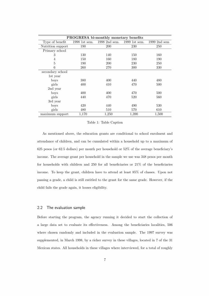
The largest component of the program is the education one. Beneficiary households

with school age children receive grants conditional on school attendance. The size of the

grant increases with the grade and, for secondary education, is slightly higher for girls

than for boys. In Table 1, we report the grant structure. All the figures are in current

pesos, and can be converted in US dollars at approximately an exchange rate of 10 pesos

per dollar. In addition to the (bi) monthly payments, beneficiaries with children in school

age receive a small annual grant for school supplies.

For logistic and budgetary reasons, the program was phased in slowly but is currently

very large. In 1998 it was started in less than 10,000 localities. However, at the end of 1999

it was implemented in more than 50,000 localities and had a budget of about US$777m

or 0.2% of Mexican GDP. At that time, about 2.6 million households, or 40% of all

rural families and one ninth of all households in Mexico, were included in the program.

Subsequently the program was further expanded and, in 2002-2003 was extended to some

urban areas.

The program represents a substantial help for the beneficiaries. The nutritional com-

ponent of 100 pesos per month (or 10 US dollars) in the second semester of 1998, corre-

sponded to 8% of the beneficiaries’ income in the evaluation sample.

6

PROGRESA bi-monthly monetary benefitsType of benefit 1998 1st sem. 1998 2nd sem. 1999 1st sem. 1999 2nd semNutrition support 190 200 230 250Primary school

3 130 140 150 1604 150 160 180 1905 190 200 230 2506 260 270 300 330

secondary school1st yearboys 380 400 440 480girls 400 410 470 500

2nd yearboys 400 400 470 500girls 440 470 520 560

3rd yearboys 420 440 490 530girls 480 510 570 610

maximum support 1,170 1,250 1,390 1,500

Table 1: Table Caption

As mentioned above, the education grants are conditional to school enrolment and

attendance of children, and can be cumulated within a household up to a maximum of

625 pesos (or 62.5 dollars) per month per household or 52% of the average beneficiary’s

income. The average grant per household in the sample we use was 348 pesos per month

for households with children and 250 for all beneficiaries or 21% of the beneficiaries

income. To keep the grant, children have to attend at least 85% of classes. Upon not

passing a grade, a child is still entitled to the grant for the same grade. However, if the

child fails the grade again, it looses eligibility.

2.2 The evaluation sample

Before starting the program, the agency running it decided to start the collection of

a large data set to evaluate its effectiveness. Among the beneficiaries localities, 506

where chosen randomly and included in the evaluation sample. The 1997 survey was

supplemented, in March 1998, by a richer survey in these villages, located in 7 of the 31

Mexican states. All households in these villages where interviewed, for a total of roughly

7

25,000 households. Using the information of the 1997 survey and that in the March 1998

survey, each household can be classified as poor or non-poor, that is, each household can

be identified as being entitled or not to the program.

One of the most interesting aspects of the evaluation sample is the fact that it contains

a randomization component. The agency running PROGRESA used the fact that, for

logistic reasons, the program could not be started everywhere simultaneously, to allocate

randomly the villages in the evaluation sample to ’treatment’ and ’control’ groups. In

particular, in 320 randomly chosen villages of the evaluation sample were assigned to the

communities where the program started early, that is in May 1998. The remaining 186

villages were assigned to the communities where the program started almost two years

later (December 1999 rather than May 1998).

An extensive survey was carried out in the evaluation sample: after the initial data

collection between the end of 1997 and the beginning of 1998, an additional 4 instruments

were collected in November 1998, March 1999, November 1999 and April 2000. Within

each village in the evaluation sample, the survey covers all the households and collects

extensive information on consumption, income, transfers and a variety of other variables.

For each household member, including each child, there is information about age, gender,

education, current labour supply, earnings, school enrolment, and health status. The

household survey is supplemented by a locality questionnaire that provides information

on prices of various commodities, average agricultural wages (both for males and females)

as well as institutions present in the village and distance of the village from the closest

primary and secondary school (in kilometers and minutes).

In what follows we make an extensive use of both the household and the locality survey.

In particular, we use the household questionnaire to get information on each child’s age,

completed last grade, school enrolment, parental background, state of residence, school

costs. We use the locality questionnaire to get information on distance from schools and

prevailing wages.

8

3 Measuring the impact of the program by comparing treatmentand control villages.

In this section, we discuss the evidence that can be obtained by comparing treatment and

control villages. The main purpose of this exercise is to show how the random allocation

of the program between treatment and control localities can be used to evaluate the effect

of the program. However, such an exercise would estimate the impact of the program as

a whole, without specifying the mechanisms through which it operates. Schultz (2003)

presents a complete set of evaluation results, which are substantially similar to those

presented here. Here our focus is on introducing some aspects of the data that are

pertinent to our model and to the sample we use to estimate it. And more importantly,

by describing the effect of the program in this sample we use to estimate our structural

model, we set the mark against which it will be fitted.

If the allocation of the program across localities is truly random and treatment and

control villages are statistically identical, comparing them provides a reliable and simple

estimate of the program’s impact. The quality of the randomization can be evaluated

by testing for the presence of significant difference in measured variables in the baseline

surveys in treatment and control villages. An extensive study of this type has been

performed by Behrman and Todd (1999). They find that, for the large majority of a very

wide set of variables, there are no statistical differences between treatment and control

villages.

Given the results in Behrman and Todd (1999), we proceed to evaluate the difference

in enrollment rates between treatment and control variables for eligible and ineligible

children. As our structural model will be estimated on boys, we report only the results

for them. The effects for girls are slightly higher but not substantially different from those

reported here for boys. As we will be interested in how the effect of the grant is affected

by age, we also report the results for different age groups. In particular, we consider

boys less than 10, boys aged 10 to 13 and older than 13. Finally we need to take into

account two possible definitions of ‘eligibility’. While, in principle, children belonging to

9

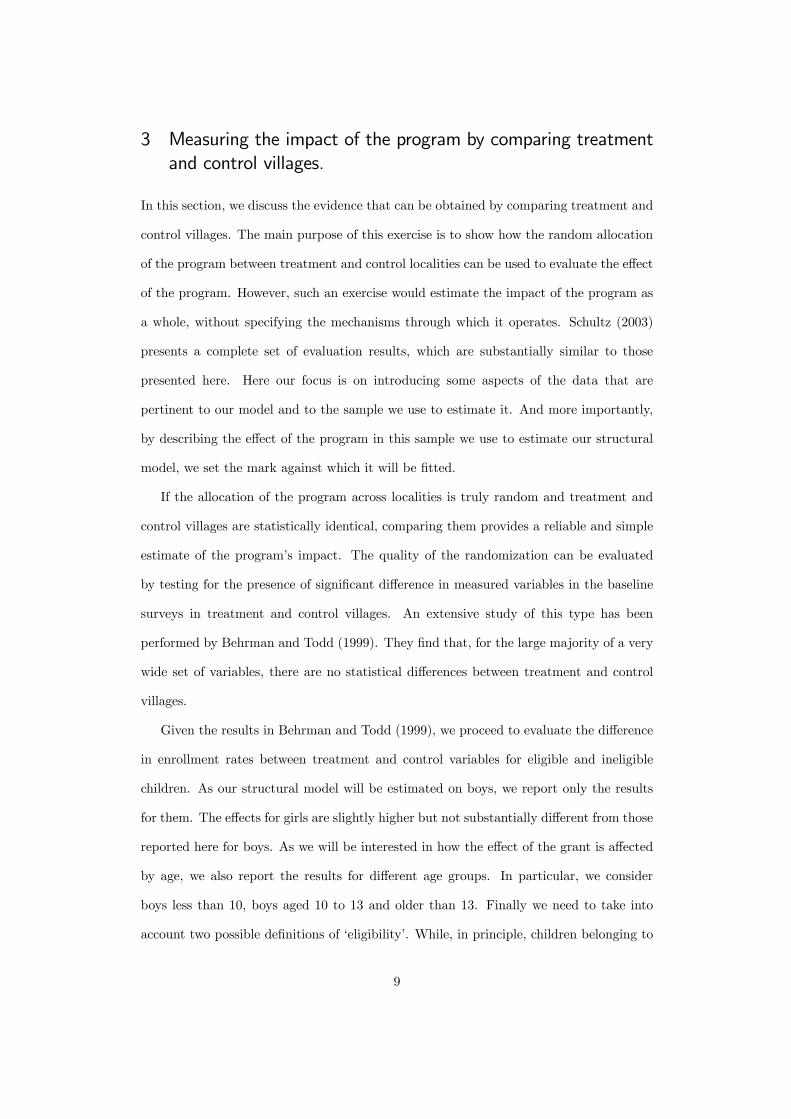
Post-program differences in educational attendancebetween treatment and control communitiesage group eligible 97 eligible 97 + 98 non eligible6-17 0.039 0.034 0.049

(0.012) (0.012) (0.021)6-9 0.008 0.003 -0.014

(0.005) (0.005) (0.009)10-13 0.037 0.032 0.030

(0.012) (0.011) (0.022)14-17 0.089 0.084 0.099

(0.033) (0.031) (0.0432)

Standard errors in parentheses are clustered at the locality level.

Table 2: Experimental Results October 1998

households that were re-defined as eligible in 1998, just before the start of the program,

should all have got the program (conditional on school attendance), it turns out that

a substantial fraction of them, probably for administrative errors, did not. In Table 2,

where we report our results, therefore, we have three columns. The first refers to the

difference in school enrolments for children who were defined as eligible in 1997. Most of

these children did get the program conditional on attendance. In the second column, we

add the children who were classified as eligible in 1998. As mentioned above, a substantial

fraction of the ‘reclassified’ children did not receive the program. The estimates in this

column should measure what in the evaluation literature is sometimes referred to as the

intention to treat . In the third column we report the difference in enrolment rates for

ineligible children.

The average treatment effect is of 0.039 points on the children belonging to the original

eligible households. The effect is concentrated among the oldest children, being not

significantly different from zero for the youngest group and almost 9% for the oldest.

These effects are slightly smaller when we consider the intent to treat estimates on the

group that includes the new eligible households, some of which, did not get the program.

The results in the third column are the most surprising, as they would indicate a

10

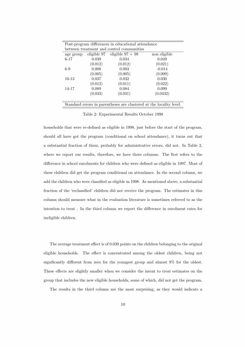
Pre-program differences in educational attendance betweentreatment and control communitiesage group eligible 97 eligible 97 + 98 ineligible6-17 0.006 0.006 0.033

(0.011) (0.011) (0.021)6-9 -0.004 -0.003 -0.003

(0.003) (0.003) (0.009)10-13 0.014 0.013 0.034

(0.012) (0.011) (0.022)14-17 0.014 0.015 0.048

(0.030) (0.028) (0.035)

Standard errors in parentheses are clustered at the locality level.

Table 3: Baseline Results August 1997

substantive effect of the program on the enrollment of ineligible children. There are two

possible alternative explanations of such a result. First, it is possible that the effect is

genuine and reflects spill-overs from eligible families to non eligible ones. The alternative

explanation, instead, would point out to pre-program differences between treatment and

control villages. Given the evidence in Behrman and Todd (1999), the latter explanation

is surprising. However, the size of the effect seems to be too large to be plausible: for

older children (aged 14-17) the effect on ineligible children would be actually larger than

for the eligible ones.

To investigate the matter further, we turn to the analysis of pre-program differences.

In Table 3 we re-do the exercise presented in Table 2 but on the baseline data collected

in August 1997, before the program started operating. From this table, it emerges that

the pre-program differences between attendance rates of eligible children in treatment

and control communities are very small indeed and never statistically different from zero.

Instead, especially for older children, we observe sizeable differences in pre-program en-

rollment rates for non- eligible children. While the estimates are not extremely precise,

and an explanation of these differences is not obvious, it is important, in evaluating the

effect of the program, to take this difference into account.

Having used the baseline to verify the existence of pre-program differences in enroll-

ment rates, we can also use it to control for them. In particular, to estimate the effect

11

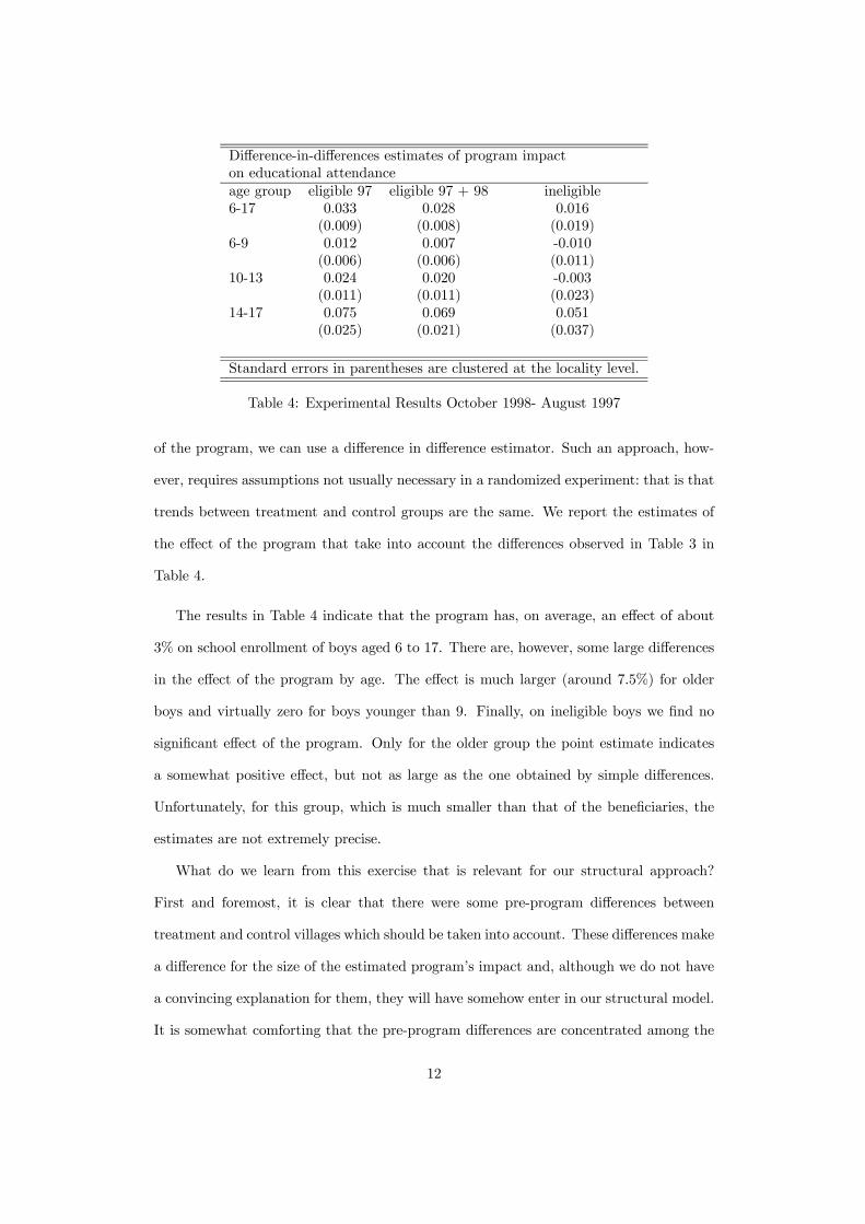
Difference-in-differences estimates of program impacton educational attendanceage group eligible 97 eligible 97 + 98 ineligible6-17 0.033 0.028 0.016

(0.009) (0.008) (0.019)6-9 0.012 0.007 -0.010

(0.006) (0.006) (0.011)10-13 0.024 0.020 -0.003

(0.011) (0.011) (0.023)14-17 0.075 0.069 0.051

(0.025) (0.021) (0.037)

Standard errors in parentheses are clustered at the locality level.

Table 4: Experimental Results October 1998- August 1997

of the program, we can use a difference in difference estimator. Such an approach, how-

ever, requires assumptions not usually necessary in a randomized experiment: that is that

trends between treatment and control groups are the same. We report the estimates of

the effect of the program that take into account the differences observed in Table 3 in

Table 4.

The results in Table 4 indicate that the program has, on average, an effect of about

3% on school enrollment of boys aged 6 to 17. There are, however, some large differences

in the effect of the program by age. The effect is much larger (around 7.5%) for older

boys and virtually zero for boys younger than 9. Finally, on ineligible boys we find no

significant effect of the program. Only for the older group the point estimate indicates

a somewhat positive effect, but not as large as the one obtained by simple differences.

Unfortunately, for this group, which is much smaller than that of the beneficiaries, the

estimates are not extremely precise.

What do we learn from this exercise that is relevant for our structural approach?

First and foremost, it is clear that there were some pre-program differences between

treatment and control villages which should be taken into account. These differences make

a difference for the size of the estimated program’s impact and, although we do not have

a convincing explanation for them, they will have somehow enter in our structural model.

It is somewhat comforting that the pre-program differences are concentrated among the

12

ineligible families. A simple strategy, therefore, would be to restrict our estimation sample

to the eligible households. We come back to these issues when we discuss the identification

of our model. Second, the effect of the program is different for different age groups. As

we will see, our model will assume that the program works by changing the relative price

of schooling relative to working. While we consider a reasonably flexible specification, it

is not completely obvious that the model should reproduce the pattern of different age

effects we see in the data, as we estimate a unique coefficient for the grant. The pattern

of results that emerges from Table 4 therefore, constitutes a useful benchmark against

which to evaluate the goodness of fit of our model.

4 The model

We use a simple dynamic school participation model. Each child, (or his/her parents)

decide whether to attend school or to work taking into account the economic incentives

involved with such choices. Parents are assumed here to act in the best interest of the

child and consequently we do not admit any interactions between children. We assume

that children have the possibility of going to school up to age 17. All formal schooling

ends by that time. In the data, almost no individuals above age 17 are in school. We

assume that children who go to school do not work and vice-versa. We also assume that

children necessarily choose one of these two options. If they decide to work they receive

a village/education/age specific wage. If they go to school, they incur a (utility) cost

(which might depend on various observable and unobservable characteristics) and, with a

certain probability, progress a grade. At 18, everybody ends formal schooling and reaps

the value of schooling investments in the form of a terminal value function that depends

on the highest grade passed. The PROGRESA grant is easily introduced as an additional

monetary reward to schooling, that would be compared to that of working.

The model we consider is dynamic for two main reasons. First, the fact that one

cannot attend regular school past age 17 means that going to school now provides the

option of completing some grades in the future: that is a six year old child who wants

13

to complete secondary education has to go to school (and pass the grade) every single

year, starting from the current. This source of dynamics becomes particularly important

when we consider the impact of the PROGRESA grants, since children,as we saw above,

are only eligible for six grades: the last three years of primary school and the first three

of secondary. Going through primary school (by age 14), therefore, also ’buys’ eligibility

for the secondary school grants. Second, we allow for state dependence: The number of

years of schooling affects the utility of attending in this period. We explicitly address the

initial conditions problem that arises from such a consideration and discuss the related

identification issues at length below. State dependence is important because it may be a

mechanism that reinforces the effect of the grant.

4.1 Instantaneous utilities from schooling and work

In each period, going to school involves instantaneous pecuniary and non-pecuniary costs,

in addition to losing the opportunity of working for a wage. The current benefits come

from the utility of attending school and possibly, as far as the parents are concerned, by

the childcare services that the school provides during the working day. As mentioned

above, the benefits are also assumed to be a function of past attendance. The costs of

attending school are the costs of buying books etc. as well as clothing items such as shoes.

There are also transport costs to the extent that the village does not have a secondary

school. For households who are entitled to Progresa and live in a treatment village, going

to school involves receiving the grade and gender specific grant.

As we are using a single cross section, we use the notation t to signify the age of

the child in the year of the survey. Variables with a subscript t may be varying with

age. Denote the utility of attending school for individual i in period t who has already

attended edit years as usit.We posit:

usit = µi + a0zit + bedit + 1(pit = 1)βpxpit + 1(sit = 1)β

sxsit + εit (1)

where zit relates to a number of taste shifter variables, including parental background,

14

age and state dummies. The variable 1(pit = 1) denotes attendance in primary school,

while the variable 1(sit = 1) denotes attendance in secondary school. xpit and x

sit represent

factors affecting the costs of attending primary school and secondary school respectively.

The term εit represents a logistic error term which is assumed independently and identi-

cally distributed over time and individuals Notice that the presence of edit introduces an

important element of dynamics we alluded to above: schooling choices affect future grades

and, therefore, the utility cost of schooling. Finally, the term µi represents unobservables

which we assume have a constant impact over time. As we discuss below, we will be

assuming that µi is a discrete random variable whose points of support and probability

distribution we estimate.

The utility of not attending school is denoted by

uwit = δwit (2)

where wit are (potential) earnings when out of school. The wage is a function (estimated

from data) of age and education attainment as well as village of residence that we discuss

below.

4.2 Uncertainty

There are two sources of uncertainty in our model. The first is an iid shock to schooling

costs, modelled by the (logistic) random term εit. Given the structure of the model, having

a logistic error in the cost of going to school is equivalent to having two extreme value

errors, one in the cost of going to school and one in the utility of work. Although the

individual knows εit in the current period,1 she does not know its value in the future.

Since future costs will affect future schooling choices, indirectly they affect current choices.

Notice that the term µi, while known (and constant) for the individual, is unobserved by

the econometrician.

The second source of uncertainty originates from the fact that the pupil may not be

1We could have introduced an additional residual term εwit in equation 2. As what matterns for thefit of the model is only the difference between the current (and future) utility of schooling and working,assuming that both εit and ε

wit were distributed as an extreme value distribution is equivalent to assuming

a single logistic residual.

15

successful in completing the grade. If a grade is not completed successfully, we assume

that the level of education does not increase. We assume that the probability of failing

to complete a grade is exogenous and does not depend on effort or on the willingness to

continue schooling. We allow however this probability to vary with the grade in question

and with the age of the individual and we assume it known to the individual.2 We

estimate the probability of failure for each grade as the ratio of individuals who are in the

same grade as the year before at a particular age. Since we know the completed grade for

those not attending school we include these in the calculation - this may be important

since failure may discourage school attendance. In the appendix we provide a Table with

our estimated probabilities of passing a grade.

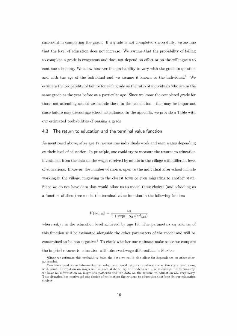
4.3 The return to education and the terminal value function

As mentioned above, after age 17, we assume individuals work and earn wages depending

on their level of education. In principle, one could try to measure the returns to education

investment from the data on the wages received by adults in the village with different level

of educations. However, the number of choices open to the individual after school include

working in the village, migrating to the closest town or even migrating to another state.

Since we do not have data that would allow us to model these choices (and schooling as

a function of these) we model the terminal value function in the following fashion:

V (edi,18) =α1

1 + exp(−α2 ∗ edi,18)

where edi,18 is the education level achieved by age 18. The parameters α1 and α2 of

this function will be estimated alongside the other parameters of the model and will be

constrained to be non-negative.3 To check whether our estimate make sense we compare

the implied returns to education with observed wage differentials in Mexico.

2Since we estimate this probability from the data we could also allow for dependence on other char-acteristics.

3We have used some information on urban and rural returns to education at the state level alongwith some information on migration in each state to try to model such a relationship. Unfortunately,we have no information on migration patterns and the data on the returns to education are very noisy.This situation has motivated our choice of estimating the returns to education that best fit our educationchoices.

16

4.4 Value functions

Since the problem is not separable overtime, schooling choices involve comparing the costs

of schooling now to its future and current benefits. The latter are intangible preferences

for attending school including the potential child care benefits that parents may enjoy.

We denote by I ∈ {0, 1} the random increment to the grade which results from

attending school at present. If successful, then I = 1, otherwise I = 0. We denote the

probability of success at age t for grade ed as pst (edit).

Thus the value of attending school for someone who has completed successfully edi

years in school and is of age t already and has characteristics zit is

V sit(edit|zit) = usit + β{pst (edit + 1)Emax

£V sit+1 (edit + 1) , V

wit+1 (edit + 1)

¤+(1− pst (edit + 1))Emax

£V sit+1 (edit) , V

wit+1 (edit)

¤}

where the expectation is taken over the possible outcomes of the random shock εit. The

value of working is similarly written as

V wit (edit|zit) = uwit + βEmax

©V sit+1 (edit) , V

wit+1 (edit)

ªThe difference between the first terms of the two equations reflects the current costs of

attending, while the difference between the second two terms reflects the future benefits

and costs of schooling. The parameter β represents the discount factor. In practice, since

we do not model savings and borrowing explicitly this will reflect liquidity constraints or

other factors that lead the households to disregard more or less the future.

Given the terminal value function described above, these equations can be used to

compute the value of school and work for each child in the sample recursively. These

formulae will be used to build the likelihood function used to estimate the parameters of

this model.

4.5 Allowing for the programme

The Progresa grant is easily introduced in our model. Since the grant is payable only

when children attend school (and therefore, according to our assumptions, do not work)

it acts as a “negative” wage. However we do not wish to impose the restriction that

17

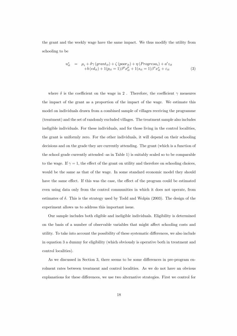
the grant and the weekly wage have the same impact. We thus modify the utility from

schooling to be

usit = µi + δγ (grantit) + ζ (poorit) + η (Progresai) + a0zit+b (edit) + 1(pit = 1)β

pxpit + 1(sit = 1)βsxsit + εit (3)

where δ is the coefficient on the wage in 2 . Therefore, the coefficient γ measures

the impact of the grant as a proportion of the impact of the wage. We estimate this

model on individuals drawn from a combined sample of villages receiving the programme

(treatment) and the set of randomly excluded villages. The treatment sample also includes

ineligible individuals. For these individuals, and for those living in the control localities,

the grant is uniformly zero. For the other individuals, it will depend on their schooling

decisions and on the grade they are currently attending. The grant (which is a function of

the school grade currently attended -as in Table 1) is suitably scaled so to be comparable

to the wage. If γ = 1, the effect of the grant on utility and therefore on schooling choices,

would be the same as that of the wage. In some standard economic model they should

have the same effect. If this was the case, the effect of the program could be estimated

even using data only from the control communities in which it does not operate, from

estimates of δ. This is the strategy used by Todd and Wolpin (2003). The design of the

experiment allows us to address this important issue.

Our sample includes both eligible and ineligible individuals. Eligibility is determined

on the basis of a number of observable variables that might affect schooling costs and

utility. To take into account the possibility of these systematic differences, we also include

in equation 3 a dummy for eligibility (which obviously is operative both in treatment and

control localities).

As we discussed in Section 3, there seems to be some differences in pre-program en-

rolment rates between treatment and control localities. As we do not have an obvious

explanations for these differences, we use two alternative strategies. First we control for

18

them by adding to the equation for the schooling utility (3) a dummy for treatment vil-

lages. Obviously such a dummy will absorb some of the exogenous variability induced

by the experiment. We discuss this issue when we tackle the identification question in

the next section. A less extreme approach, justified by the fact that most of the unex-

plained differences in pre-program enrollment is observed among non-eligible household,

we introduce a dummy for this group.

Finally, using a structural model allows us to address the issue of anticipation ef-

fects and the assumptions required for their identification. PROGRESA as well as other

randomized experiments or pilot studies create a control group by delaying the implemen-

tation of the program in some areas, rather than excluding them completely. In this case

it is possible that the control villages react to the program prior to its implementation,

depending on the degree to which they believe they will eventually receive it. A straight

comparison between treatment and control areas may then underestimate the impact of

the program. A structural model that exploits other sources of variation, such as the

variation of the grant with age may be able to estimate the extent of anticipation effects.

We investigate this with our model by examining the fit of the model under different

assumptions about when the controls are expecting to receive payment. As it turns out

we find no anticipation effects here.

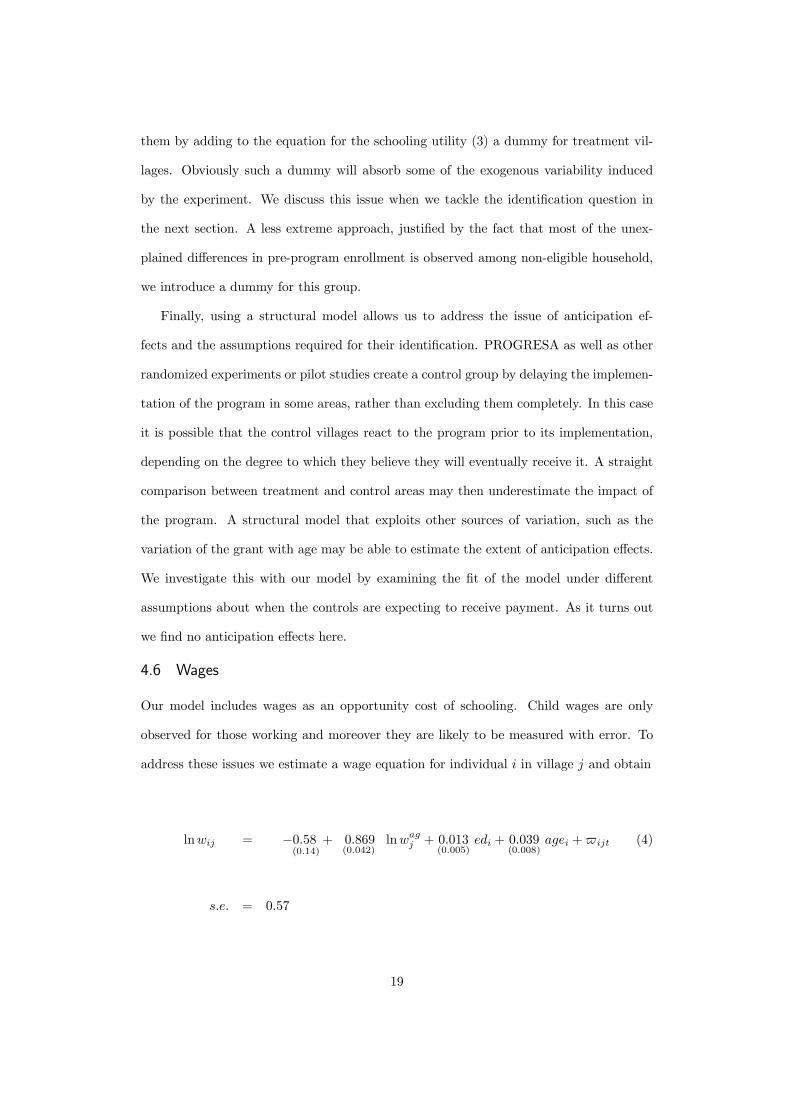
4.6 Wages

Our model includes wages as an opportunity cost of schooling. Child wages are only

observed for those working and moreover they are likely to be measured with error. To

address these issues we estimate a wage equation for individual i in village j and obtain

lnwij = −0.58(0.14)

+ 0.869(0.042)

lnwagj + 0.013

(0.005)edi + 0.039

(0.008)agei + ijt (4)

s.e. = 0.57

19

where lnwagj represents the village level log agricultural wage, edi represents the child’s

educational attainment up to that point and ijt random factors including measurement

error assumed independent of the observable characteristics. The coefficients in equation

4 were estimated separately from the rest of the model using information on the children

who work and village level information on agricultural wages. Their standard errors are

given in parentheses below the estimates. We assume that the agricultural wage reflects

the local price of human capital which provides the necessary exclusion restriction for

identifying the wage effect in the education choice model. Thus the key assumption is

that lnwagj varies across localities because of different labour demand conditions and

as such is exogenous for individual schooling choices. This is of course an important

assumption and its violation may well lead to the grant and wage effect being different.

4.7 Habits and Initial Conditions

The presence of edit in equation 1 creates an important initial conditions problem because

we do not observe the entire history of schooling for the children in the sample as we use

a single cross section. We cannot assume that the random variable µi is independent of

past school decisions as reflected in the current level of schooling edit.

To solve this problem we specify a reduced form for educational attainment up to the

current date. We model the level of schooling by an ordered probit with index function

h0iζ + ξµi where we have assumed that the same heterogeneity term µi enters the prior

decision multiplied by a loading factor ξi. The vector hi includes variables reflecting past

schooling costs such as the distance from the closest secondary schools in pre-experimental

years. Since school availability, as measured by variables such as distance, changes over

time, it can be used as an instrument in the initial conditions model that is excluded from

the subsequent (current) attendance choice, which depends on the school availability

during the experiment. Hence we can write the probability of edit = e and of child i

attending school as

P (edit = e,Attendit = 1|zit, xpit, xsit, hi, wageit, µi) =

P (Attendit = 1|zit, xpit, xsit, wageit, edit, µi)× P (edit = e|zit, xpit, xsit, hi, wage, µi)(5)

20

This will be the key component of the likelihood function presented below. The endo-

geneity of the number of passed grades (the stock of schooling) is therefore captured by

the common heterogeneity factor µi affecting both decisions The loading factor ξ governs

the covariance between the two equations. It is important to stress the role played in

identification by the variables that capture lagged availability of schools as variables that

enter the initial condition equations but not the current participation equation.

5 Identification and Estimation

5.1 Identification

In the context of our model, there are two identification issues. The first concerns the

identification of the model in the presence of habits and unobserved heterogeneity. In

the previous section we stressed that identification can as far as this aspect is concerned,

be achieved because of the presence of lagged school availability variables in the initial

condition equation.

The second issues is about the identification of the effect of the program and the

sources of variation in the data that allow us to measure such a parameter. We already

mentioned that a version of the model in which the effect of the grant can be identified

from the control sample alone without using the program data at all: If we assume

that the effect of the grant is the same (but opposite in sign) as the effect of the wage,

we can exploit variation across villages in children wages to estimate this parameter.

Here, however, we are interested in estimating a version of the model that allows these

two parameters to be different. We therefore need variation in the grant received by

individuals in our sample.

The grant available (or not) to the children in our sample varies for several reasons.

First, some individuals live in treatment villages, while others live in control villages. This

variation, given the random assignment of the program, is, by construction, exogenous

and can be used to identify the parameter of interest. However, as we discussed in Section

3, there seem to be some differences in pre-program school enrollment between treatment

21

and control villages, especially among ineligible families. We therefore might want to

allow for such (unexplained) differences in pre-programme enrollment between treatment

and control via a ’treatment’ dummy. Such a strategy sacrifices some of the variability

induced by the experiment to measure the effect of the program, although the effect of the

grant is still identified, in principle, by the fact that it varies with grade as well as by the

comparison between eligible and ineligible individuals. However we do not wish to rely on

this latter source of variation and clearly we want to put more weight on the exogenous

experimental variation. We thus introduce a dummy variable for eligibility (whether in

a treatment or control village). We then also note that the main source of pre-program

differences are due to differences in the enrolment of the ineligibles across treatment and

control villages. We therefore remove the treatment dummy an replace it with a dummy

for an ineligible household living in a treatment village. In this version of the model

the effect of the grant is identified by the comparison between eligible households in

treatment and control villages and by the age variation of the grant, over and above the

linear age effect we allow to affect preferences. Thus to summarize we present results of

three specifications: In the first we only include a dummy for eligibility (only i.e. whether

the household is poor or not); in the second we add a dummy for living in a treatment

village; in the third we remove the treatment dummy and add a dummy for treatment

village interacted with being ineligible (poor).

The discount factor in this model as well as reflecting individual time preference also

summarizes the impact of liquidity constraints, to the extent that these are important.

Thus a low discount factor may be a reflection of an inability of households to transfer

funds between periods. This would limit their behavioral response to promises of future

grants. However, since the model relates to a discrete binary choice, the actual value

of the discount factor is not identified - rather just the ratio of the discount factor to

the standard deviation of the error is identified. This ratio, which we keep refering to

as the discount factor in what follows, is identified by the variation induced in future

opportunities by the age at which the policy is introduced. It need not be lower than 1

22

but it has to be positive. In our case it turns out to be below 1.

We conclude this discussion stressing that, while functional form assumptions play a

role as in all structural models, the experimental information is key to both the estimation

of the model and the validation of the results. Without such variation we would need to

rely exclusively on wage variation and we would not have this explicitly exogenous source

of variation for the costs of schooling.

5.2 Estimation

We estimate the model by a combination of maximum likelihood and a grid search for

the discount factor.

Denote by F (·) the distribution of the iid preference shock εit, assumed logistic. As-

sume the distribution of unobservables µi is independent of all observables in the popula-

tion and approximate it by a discrete distribution withM points of support sm each with

probability pm, all of which need to be estimated (Heckman and Singer, 1984). The joint

probability of attendance and having already achieved e years of education (edit = e) can

then be written as

Pi = P (Attendit = 1, edit = e|zit, xpit, xsit, wageit) =

MXm=1

pm{F{usit + βEmax¡

V sit+1 (edit + I) , V w

it+1 (edit + I)¢

−¡uwit + βEmax

¡V sit+1 (edit) , V

wit+1 (edit)

¢ ¢|µi = sm}

×P (edit = e|zit, xpit, xsit, hi, wage, µi = sm)}

(6)

The probability of attending school conditional on µi and edit = e is given by the F (·);

the expectations inside the probability are taken over future uncertain realizations of the

shock εit and the success of passing a grade; the sum is taken over all points of support

of the distribution of unobserved heterogeneity. The expressions for the value functions

at subsequent ages are computed recursively starting from age 18 and working backwards

until the current age using the formulae in Section 4.4. The logistic assumption on the

εit allows us to derive a closed form expression for the terms in equation 6

23

The log-likelihood function is then based on this probability and takes the form

NXi=1

{Di logPi + (1−Di) log(1− Pi)} (7)

where Di = 1 denotes a school attendee in the sample of N children. To estimate the

parameters we combine maximum likelihood and a grid search for the discount factor.

Thus we maximize 7 with respect to all unknown parameters fixing the discount factor β

to many different values in increments of 0.05.

6 Estimation results

In this section, we report the results we obtain estimating different versions of the dynamic

programming model we discussed earlier. We start by presenting estimates of the basic

model and then discuss extensions and robustness checks we have performed.

In Tables 5 to 7, we present estimates of the three versions of the basic mode we

mentioned above: the first column of each table refers to the version that ignores pre-

program school enrollment between treatment and control villages, in the second column

such differences are accounted for by a ’treatment dummy’, while in the third they are

accounted for by a dummy for non-eligible treatment households. We estimate all the

versions of the model on the sample of boys older than 9. All specifications include, both in

the initial condition equation and in the cost of education equation, state dummies, whose

estimates are not reported for the sake or brevity. In addition, we have variables reflecting

parental education (the excluded groups are heads and spouses with less than completed

primary) and parents ethnicity. We also include the distance from the secondary school

as well as the cost of attending such school, which in some cases includes fees. Finally all

specifications include a dummy for eligibility (potential if in a control village- poor).

While we do not estimate the discount factor along with the other parameters of the

model, we carried out a coarse grid search in steps of 0.05 and we have found that the

value of 0.85 maximizes the likelihood.4 All our results are conditional on such a value4The value of the likelihood function increases sharply from 0.8 to 0.85, is slightly lower for 0.9 and

goes down sharply for 0.95. The results we report (for 0.85) are not very different from those obtainedwith a discount factor of 0.9.

24

As mentioned above, we allow for unobserved heterogeneity that is modelled as a

discrete variable with three points of support. The same variable enters, with different

loading factors, both the utility of going to school equation and the initial condition

equations. Such a variable, therefore, plays an important role in that it allows for a flex-

ible specification of unobserved heterogeneity and determines the degree of correlation

between the utility of schooling and completed schooling, which, by entering the equa-

tion for the current utility of schooling, introduces an important dynamic effect into the

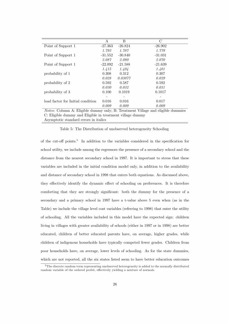
model. We therefore start reporting, in Table 5, the estimates of the points of support

of the unobserved heterogeneity terms, and that of the loading factor of the unobserved

heterogeneity terms in the initial condition equation. Three points of support seemed to

be enough to capture the observed heterogeneity in our sample. Effectively we have three

types of children, of which one is very unlikely to go to school and accounts for roughly

10% of the sample. Given that attendance rates at young ages are close to 90%, it is

likely that these are the children that have not been attending primary school and, for

some reason, would be very difficult to attract to school. Another group, which accounts

for about 30% of the sample is much more likely to be in school. The largest group,

accounting for 60% of the sample, is the middle one.

The loading factor of the unobserved heterogeneity term is positive (as expected) but

not extremely precisely estimated. This is one of the few parameters whose size depends

crucially on the value of the discount factor. Imposing, for instance, a discount factor

of 0.9 (which leads to a marginal reduction of the likelihood function) would increase

considerably the size of this parameter and make it significantly different from zero.

The initial condition edit is modeled as an ordered probit with age specific cutoff

points. The cutoff points are age specific to reflect the fact that different ages will have

very different probabilities to have completed a certain grade. Indeed, even the number

of cutoff points is age specific, to reflect the fact that relatively young children could not

have completed more than a certain grade. To save space, we do not report the estimates

25

A B CPoint of Support 1 -27.363 -26.824 -26.902

1.793 1.787 1.779Point of Support 1 -31.552 -30.840 -31.031

2.087 2.080 2.070Point of Support 1 -22.092 -21.588 -21.639

1.415 1.404 1.401probability of 1 0.308 0.312 0.307

0.028 0.03077 0.029probability of 2 0.592 0.587 0.592

0.030 0.032 0.031probability of 3 0.100 0.1019 0.1017

- - -load factor for Initial condition 0.016 0.016 0.017

0.009 0.009 0.009Notes: Column A: Eligible dummy only; B: Treatment Village and eligible dummiesC: Eligible dummy and Eligible in treatment village dummyAsymptotic standard errors in italics

Table 5: The Distribution of unobserved heterogeneity Schooling

of the cut-off points.5 In addition to the variables considered in the specification for

school utility, we include among the regressors the presence of a secondary school and the

distance from the nearest secondary school in 1997. It is important to stress that these

variables are included in the initial condition model only, in addition to the availability

and distance of secondary school in 1998 that enters both equations. As discussed above,

they effectively identify the dynamic effect of schooling on preferences. It is therefore

comforting that they are strongly significant: both the dummy for the presence of a

secondary and a primary school in 1997 have a t-value above 5 even when (as in the

Table) we include the village level cost variables (referring to 1998) that enter the utility

of schooling. All the variables included in this model have the expected sign: children

living in villages with greater availability of schools (either in 1997 or in 1998) are better

educated, children of better educated parents have, on average, higher grades, while

children of indigenous households have typically competed fewer grades. Children from

poor households have, on average, lower levels of schooling. As for the state dummies,

which are not reported, all the six states listed seem to have better education outcomes

5The discrete random term representing unobserved heterogeneity is added to the normally distributedrandom variable of the ordered probit, effectively yielding a mixture of normals.

26

A B Cpoor -0.259 -0.259 -0.259

0.023 0.026 0.026Father’s educationPrimary 0.182 0.182 0.182

0.027 0.023 0.023Secondary 0.287 0.287 0.287

0.049 0.027 0.027Preparatoria 0.588 0.588 0.588

0.023 0.049 0.049Mother’s educationPrimary 0.154 0.154 0.154

0.027 0.023 0.023Secondary 0.307 0.307 0.307

0.056 0.027 0.027Preparatoria 0.288 0.288 0.287

0.023 0.056 0.056indigenous 0.002 0.002 0.002

0.041 0.023 0.023prim97 0.257 0.257 0.257

0.024 0.054 0.054sec97 0.077 0.077 0.077

0.002 0.024 0.024Km from secondary School -0.01056 -0.011 -0.01057

0.00022 0.002 0.00177cost of attending secondary 0.00014 0.000 0.00014

0.00022 0.000 0.00022

Notes: as in Table 5. State dummies included

Table 6: Equation for Initial conditions

than Guerrero, one of the poorest states in Mexico, and particularly so Hidalgo and

Queretaro.

We now turn to the variables included in the education choice model, reported in the

top panel of Table 7. All the variables, except for the grant and the wage are expressed as

determinants of the cost of schooling, so that a positive sign on a given variable, decreases

the probability of currently attending school. The wage is expressed as a determinant

of the utility of work (so that an increase in wages decreases school attendance) and the

grant is a determinant of the utility of schooling, so that an increase in it, increases school

27

attendance. In addition, the coefficient on the grant is expressed as ratio to the coefficient

on the wage, so that a coefficient of 1 indicates that a unitary increase in the grant has

the same effect on the utility of school than an increase in the wage has on the utility of

work.

In terms of background characteristics, belonging to a household and with less edu-

cated parents leads to lower attendance. This may be a reflection of liquidity constraints

or of different costs of schooling. Perhaps surprisingly, the coefficient on poor (eligible)

households is not significantly different from zero, while that on indigenous households

indicates that, ceteris paribus, they are more likely to send their children to school. The

states that exhibit the higher costs are Queretaro and Puebla, followed by San Luis Potosi

and Michoacan, while Veracruz and Guerrero are the cheapest. The costs of attending

secondary measured in either distance (since many secondary schools are located in neigh-

boring village) or in terms of money have a significant and negative effect on attendance.

Both age and grade have a very important effect on the cost of schooling, age increasing

and grade decreasing it. The coefficient on age is the way in which the model fits the

decline in enrolment rates by age across both treatment and control villages. The effect

on the grade captures the dynamics of the model and, as we discussed, is identified by

the presence of lagged supply of school infrastructure. We find a very strong effect of

state dependence despite the fact that we include age as one of the explanatory variables.

The pre-existing level of education is a critical determinant of choice, with increased

levels of education having a substantially positive effect on further participation. This

is of course an important point since it provides an additional mechanism by which the

subsidy may increase educational participation. It also implies different effects depending

on the amount of prior educational participation.

As we discussed above, we have scant information on the returns to education, so

that we include the returns to education among the parameters to be inferred from the

differential attendance rates in school. It is therefore important to check what are the

28

A B Cwage 0.129 0.129 0.129

0.042 0.042 0.042PROGRESA Grant 2.966 2.174 2.974

1.077 0.899 1.085term 5.598 5.591 5.589

0.152 0.152 0.153term -1.146 -1.157 -1.146

0.032 0.033 0.032Poor 0.248 0.166 -0.128

0.144 0.146 0.195In PROGRESA village -0.287 -0.629

0.127 0.244Father’s Education - Default is less than primaryPrimary -0.261 -0.260 -0.263

0.113 0.112 0.113Secondary -0.582 -0.572 -0.582

0.146 0.145 0.146Preparatoria -1.233 -1.207 -1.215

0.323 0.316 0.320Mother’s Education - Default is less than primaryPrimary -0.175 -0.180 -0.172

0.117 0.115 0.116Secondary -0.430 -0.428 -0.432

0.142 0.141 0.142Preparatoria -1.520 -1.487 -1.486

0.439 0.433 0.438indigenous -0.546 -0.537 -0.536

0.133 0.131 0.132Km from secondary school 0.087 0.087 0.088

0.010 0.010 0.010cost of attending Secondary school 0.005 0.005 0.005

0.001 0.001 0.001age 3.041 3.000 3.024

0.227 0.226 0.227Prior Years of education -1.819 -1.799 -1.805

0.198 0.197 0.197

log-Likelihood -26801.110 -26798.595 -26797.383

Notes as in Table 5. Discount rate β = 0.85 State dummies included

Table 7: Parameter etimates for the Education choice model

29

returns to education implied by this model. When we compute the return to education

implied by the coefficients on the terminal value function, we obtain an estimate of 4.4%

per year, maybe a bit low in the Mexican context, but above the average return to

education observed in our villages.

Cost variables have the expected sign and are significant. For instance, an increase

in the distance from the nearest secondary school, significantly decreases the probability

of attending school. Likewise for an increase in the average cost of attending secondary

school. As several of the children in our sample are still attending primary school we also

tried to include variables reflecting the cost and availability of primary schools, but we

could not identify any significant effect.

The key parameters of the model from a policy perspective are the wage coefficient

and the coefficient of the grant itself. An increase in the wage decreases the probability

of attending school. On average, the effect of reducing the wage by 44% (which would

roughly give a reduction similar to the average grant to beneficiaries) increases the proba-

bility of attending school by 4%. This effect cannot, obviously, be inferred from the value

of the parameter alone and is obtained from the simulations of the model that we discuss

in detail below.

The value of the grant varies by treatment and control villages (where of course it is

zero) and by grade the child could be attending.6 The way we parameterize the model,

the total effect of the grant is equal to the product of the wage and the grant coefficients,

meaning that the impact of the grant is about twice that of the wage. Based on a

likelihood ratio test one strongly rejects the hypothesis that the grant coefficient is 1.7

This result is important because it suggests that the effects of the program cannot be

predicted using a model with the standard economic incentives incorporated through the

wage (see Todd and Wolpin, 2003).

The three versions of the model we present differ because of the presence, in column

6As mentioned above, in secundary school, the grant is also higher for girls than for boys. However,as we only estimate the model for the latter, we do not exploit this variation.

7Since this hypothesis is subject to normalisation the Wald test is not appropriate see Veal(

30

B and C of Table 7 of a dummy for Progresa villages (col B) and one for Progresa non

eligible. As we discussed above, these are meant to capture pre-program differences that

were identified to be present in enrolment rates despite the random assignment of the

programme. In Section 3, we showed that most of the pre-programme differences are

explained by differences among non eligible households. This evidence would justify the

specification in Column C. The specification in Column B takes a more conservative

approach and controls for the fact of living in a Progresa village. This could be too

conservative as it absorbs much of the experimental variability of the grant.

Comparing the results across specifications, we see that most coefficients do not change

much. Not surprisingly, the only coefficient that exhibits some variation is the one on

the grant. And even that does not change much between Column A and C. The size of

the coefficient on the grant, however, is somewhat reduced in column B, which, therefore,

provides a lower bound on the effect of the programme.

The model is complex and non linear. To quantify the effect of the main variables of

interest from a policy point of view, that is to assess how the grant operates and what its

effect are we now turn to the analysis of some simulations.

7 Simulations

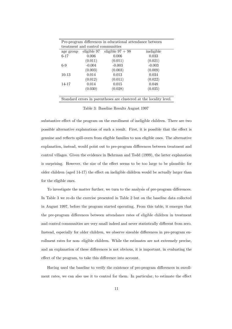
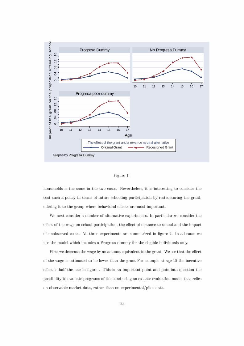
We now use the model to simulate school participation under different scenarios. The first

exercise is simply aimed at evaluating the effect of the PROGRESA grant as designed.

For such a purpose we compute, for each child in the sample, the probability of enrolment

with and without the grant. The effect is then computed averaging the differences between

these probabilities. In Figure 1, the continuous line plots these averages by age for each of

the three versions of the model estimated in Table 7. The effect of the PROGRESA grant

is very small at the youngest ages and peaks, for the three figures age 15. Perhaps not

surprisingly, the effect is smaller when we introduce a ‘treatment dummy’ in the model.

The other two models (the one without any ‘treatment dummy’ - B in the table and the one

with a ‘treatment-ineligible’ dummy -C in the table) yield similar results. Reassuringly,

31

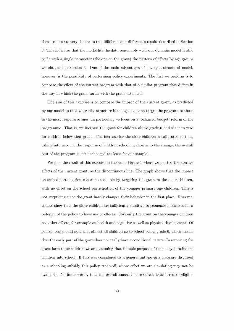
these results are very similar to the diffifference-in-differences results described in Section

3. This indicates that the model fits the data reasonably well: our dynamic model is able

to fit with a single parameter (the one on the grant) the pattern of effects by age groups

we obtained in Section 3. One of the main advantages of having a structural model,

however, is the possibility of performing policy experiments. The first we perform is to

compare the effect of the current program with that of a similar program that differs in

the way in which the grant varies with the grade attended.

The aim of this exercise is to compare the impact of the current grant, as predicted

by our model to that where the structure is changed so as to target the program to those

in the most responsive ages. In particular, we focus on a ‘balanced budget’ reform of the

programme. That is, we increase the grant for children above grade 6 and set it to zero

for children below that grade. The increase for the older children is calibrated so that,

taking into account the response of children schooling choices to the change, the overall

cost of the program is left unchanged (at least for our sample).

We plot the result of this exercise in the same Figure 1 where we plotted the average

effects of the current grant, as the discontinuous line. The graph shows that the impact

on school participation can almost double by targeting the grant to the older children,

with no effect on the school participation of the younger primary age children. This is

not surprising since the grant hardly changes their behavior in the first place. However,

it does show that the older children are sufficiently sensitive to economic incentives for a

redesign of the policy to have major effects. Obviously the grant on the younger children

has other effects, for example on health and cognitive as well as physical development. Of

course, one should note that almost all children go to school below grade 6, which means

that the early part of the grant does not really have a conditional nature. In removing the

grant form these children we are assuming that the sole purpose of the policy is to induce

children into school. If this was considered as a general anti-poverty measure disguised

as a schooling subsidy this policy trade-off, whose effect we are simulating may not be

available. Notice however, that the overall amount of resources transferred to eligible

32

0.0

4.0

8.1

2.1

60

.04

.08

.12

.16

10 11 12 13 14 15 16 17

10 11 12 13 14 15 16 17

Progresa Dummy No Progresa Dummy

Progresa poor dummy

Original Grant Redesigned GrantThe effect of the grant and a revenue neutral alternative

Impa

ct o

f th

e g

rant

on

the

pro

po

rtio

n a

tten

din

g s

ch

ool

Age

Graphs by Progresa Dummy

Figure 1:

households is the same in the two cases. Nevertheless, it is interesting to consider the

cost such a policy in terms of future schooling participation by restructuring the grant,

offering it to the group where behavioral effects are most important.

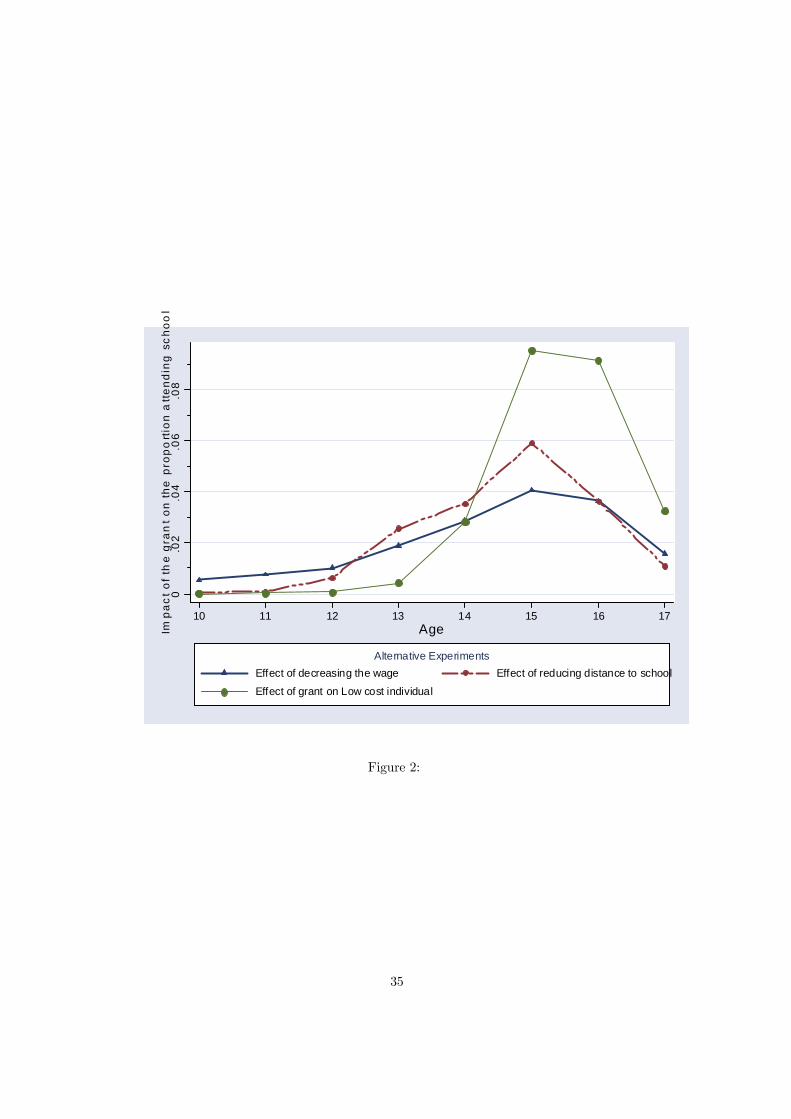
We next consider a number of alternative experiments. In particular we consider the

effect of the wage on school participation, the effect of distance to school and the impact

of unobserved costs. All three experiments are summarized in figure 2. In all cases we

use the model which includes a Progresa dummy for the eligible individuals only.

First we decrease the wage by an amount equivalent to the grant. We see that the effect

of the wage is estimated to be lower than the grant For example at age 15 the incentive

effect is half the one in figure . This is an important point and puts into question the

possibility to evaluate programs of this kind using an ex ante evaluation model that relies

on observable market data, rather than on experimental/pilot data.

33

In the next experiment we demonstrate the effects of a potential school building pro-

gram that would reduce the distance of secondary schools to no more than 3 km. We

consider this because it would constitute an alternative policy to subsidizing participation

(although we do not claim that this policy is equivalent in terms of cost or in terms of

other benefits such as better nutrition and its impact). The effect is quite substantial and

increases participation by 6 percentage points at age 15.

Finally in order to demonstrate the potential importance of targeting we show the

effects of the policy on individuals with “low cost” of schooling; i.e. we evaluate the

effect at the point of support of the unobserved heterogeneity with the highest school

participation. As shown in the graph for these individuals there is no effect of the program

before age 14. Beyond that the effects are higher than average. Conversely, for the high

cost of schooling individuals (not shown) the effects are higher than average at younger

ages and lower later.

8 Conclusions

In this paper we have evaluated the effect of a large welfare program in rural Mexico

aimed, among other things, at increasing enrolment rates among poor children. The

evaluation survey we use has an important randomization component that induces truly

exogenous variation in the enrolment into the program. After presenting some evidence

based on simple differences and differences in differences, we show that many questions

are left unanswered by this type of techniques and propose the use of a structural model.

The exogenous variation induced by the randomization is useful in estimating a relatively

flexible version of the program. The use of a coherent dynamic optimization model allows

us to address a number of important issues, such as the announcement effects induced in

control villages by the fact that the program is known to be implemented there after a

lag. Our results indicate that these effects are important and do make a difference.

The estimates we obtain are sensible and indicate that the program is quite effective

in increasing the enrolment of children at the end of their primary education. Our sim-

34

0.0

2.0

4.0

6.0

8Im

pac

t of t

he

gra

nt o

n th

e p

rop

ort

ion

att

end

ing

sc

hoo

l

10 11 12 13 14 15 16 17Age

Effect of decreasing the wage Effect of reducing distance to school

Effect of grant on Low cost individual

Alternative Experiments

Figure 2:

35

ulations also indicate, however, that the performance of the program could be improved

by back-loading the program, that is offering more resources to older children and less to

relatively younger one.

9 References

Behrman, J. (1999): “Education, Health and Demography in Latin America Around the

End of the Century: What Do We Know? What Questions Should Be Explored?”, IADB

Mimeo.

Behrman, J., Duryea, S. and M. Székely (1999):“Schoolling Investments and Aggregate

Conditions: A Household Survey-Based Approach for Latin America and teh Caribbean”,

OCE Working Paper No 407, IADB, Washington,

http://www.iadb.org/res/publications/pubfiles/pubWP-407.pdf.

Behrman, J., Duryea, S. and M. Székely (2000): “Households and Economic Growth

in Latin America and teh Caribbean”, GDN, Mimeo.

Behrman, J. and P. Todd (1999); “Randomness in the Experimental Samples of

PROGRESA (Education,Health, and Nutrition Program)”, IFPRI. dowloadable from:

http://www.ifpri.org/themes/progresa/pdf/BehrmanTodd_random.pdf .

Dearden, L. C. Emmerson, C. Frayne and C. Meghir (2005) “Can Education Subsidies

stop School Drop-outs? An evaluation of Education Maintenance Allowances in England”,

IFS discussion paper

Heckman, J.J and B. Singer (1984) “A Method for Minimizing the Impact of Distri-

butional Assumptions in Econometric Models for Duration Data”

Econometrica Vol. 52, No. 2 (Mar., 1984), pp. 271-320

Keane Michael P. and Kenneth I. Wolpin (1997) The Career Decisions of Young Men

The Journal of Political Enomy > Vol. 105, No. 3 (June 1997), pp. 473-522

Rawlings, L. (2004): “A New Approach to Social Assistance: Latin America’s Experi-

ence with Conditional Cash Transfer Programs”, World Bank Social Protection Discussion

Paper No 0416.

36

Schultz, T.P. (2003): “School Subsidies for the Poor: Evaluating the Mexican Progresa

Poverty Program” , Journal of Development Economics,

Skoufias, E. (2001): “PROGRESA and its Impacts on the Human Capital and Welfare

of Households in Rural Mexico: A Synthesis of the Results of an Evaluation by IFPRI.”,

IFPRI, dowloadable from: http://www.ifpri.org/themes/progresa/pdf/Skoufias_finalsyn.pdf

Todd , P. and K. Wolpin (2003): “Using Experimental Data to Validate a Dynamic

Behavioral Model of Child Schooling and Fertility: Assessing the Impact of a School

Subsidy Program in Mexico”, Mimeo the University of Pennsylvania

Willis R. and S. Rosen (1979) “Education and Self Selection”, Journal of Political

Economy, 87, pp S7-S36.

37