UNIT ONEINTRODUCTION

1.1.MEANING OF ECONOMIC STATISTICSStatistics: is a science that deals with the methods of collecting, organizing, and analyzing of data and interpretation of results. It is a science of decision making under uncertainty.There are 4 stages of statistics;

Collection of data, Presentation of data, Analysis and Interpretation.

Economic Statistics is an area which uses statistical methods in presenting, analyzing and interpretation of economic data.It includes those statistical methods which are frequently used in economics.

1.2.FUNCTIONS OF ECONOMIC STATISTICS It presents facts in a definite form It simplifies a mass of figures It facilitates comparison It helps in formulating and testing hypotheses It helps in prediction It helps in formulation of suitable policies

1.3.TYPES OF STATISTICAL DATA

Data are row facts about a phenomenon. Data are records of the actual state of some measurable aspect of the universe at a particular point in time. Data are not abstract; they are concrete, they are measurements or the tangible and countable features of the world. When data are processed, they generate information. There are different types of statistical data based on the reference in which they are measured.

1

A) Based on Scale of measurementBased on the scale of measurement, there are different types of data. There are four basic measurement scales: Nominal, ordinal, interval and ratio.The most accepted basis for scaling has three characteristics:

1. Numbers are ordered. One number is less than, greater than,or equal to another number.

2. Differences between numbers are ordered. The differencebetween any pair of numbers is greater than, less than, orequal to the difference between any other pair of numbers.

3. The number series has a unique origin indicated by thenumber zero.

Combination of these characteristics of order, distance, andorigin provide the following widely used classification ofmeasurement scales.

Nominal Scales: When we use nominal scale, we partition a set intocategories that are mutually exclusive and collectivelyexhaustive. The counting of members is the only possiblearithmetic operation and as a result the researcher is restrictedto the use of the mode as the measure of central tendency. If weuse numbers to identify categories, they are recognized as labelsonly and have no quantitative value. Nominal scales are the leastpowerful of the four types. They suggest no order or distancerelationship and have no arithmetic origin. Examples can berespondents’ marital status, gender, students’ Id number, etc.

Ordinal Scales: Ordinal scales include the characteristics of thenominal scale plus an indicator of order. The use of an ordinalscale implies a statement of ‘greater than’ or ‘less than’ (anequality statement is also acceptable) without stating how muchgreater or less. Thus the real difference between ranks 1 and 2may be more or less than the difference between ranks 2 and 3.The appropriate measure of central tendency for ordinal scales is

2

the median. Examples of ordinal scales include opinion orpreference scales.

Interval Scales: The interval scale has the powers of nominal andordinal scales plus one additional strength: It incorporates theconcept of equality of interval (the distance between 1 and 2equals the distance between 2 and 3). When a scale is interval,you use the arithmetic mean as the measure of central tendency.Calendar time is such a scale. For example, the elapsed timebetween 4 and 6 A.M. equals the time between 5 and 7 A.M. Onecannot say, however, 6 A.M is twice as late as 3 A.M. becausezero time is an arbitrary origin. Centigrade and Fahrenheittemperature scales are other examples of classical intervalscales.

Ratio Scales: Ratio scales incorporate all of the powers of theprevious ones plus the provision for absolute zero or origin. Theratio scale represents the actual amounts of a variable.Multiplication and division can be used with this scale but notwith the other mentioned. Money values, population counts,distances, return rates, weight, height, and area can be examplesfor ratio scales.

Summary of measurement scalesType ofscale

Characteristics Basic empirical operation

Nominal No order, distance,or origin

Determination of equality

Ordinal Order but no distanceor unique origin

Determination of greater orlesser values

Interval Both order anddistance but nounique origin

Determination of equalityof intervals or differences

Ratio Order, distance, andunique origin

Determination of equalityof ratios

3

B) Based on Time Reference

On the basis of time reference, statistical data are of fourtypes;Time Series Data: These are data collected over periods of time.Data which can take different values in different periods of timeare normally referred as time series data.Cross-Sectional Data: Data collected at a point of time from different places. Data collected at a single time are known as cross-sectional data. Pooled Data: Data collected over periods of time from different places. It is the combination of both time series and cross-sectional data.Panel Data: It is also known as longitudinal data. It is a time series data collected from the same sample over periods of time.

C) Based on the SourcesDepending on the source, the type of data collected could beprimary or secondary in nature.Primary data are those which are collected afresh and for thefirst time, and thus happen to be original in character. Itsadvantage is its relevance to the user, but it is also likely tobe expensive in time and money terms to collect. Secondary data are those which have already been collected bysomeone else and which have already been passed through thestatistical process. It is information extracted from an existingsource, probably published or held on a computer database. FromPractical point of view this type of information is collected forany purpose other than the current research objectives and is notalways up-to-date. For this reason it may not precisely meet theneeds of the secondary user. However, it is less expensive andtime-consuming to obtain. Therefore, it provides a good startingpoint and very often can help the investigator to formulate and

4

generate ideas which can later be refined further by collectingprimary data.

UNIT TWOOVERVIEW OF DATA PRESENTATION AND ANALYSIS

TECHNIQUES2.1DATA PRESENTATION TECHNIQUESData Presentation: is the process of summarizing the collected data in a meaningful and suitable form. Presentation can be done in two basic forms: Statistical tables and Statistical charts.Statistical table is the presentation of numbers in a logical arrangement with some brief explanation to show what the data representing.Statistical Charts or graphs on the other hand are pictorial devices of presenting data.

2.1.1 Presentation of Quantitative DataThe important tools for presenting quantitative data are:

1. Frequency Distribution

5

2. Histograms3. Frequency Polygons4. Cumulative Frequency Curve or Ogives.

Frequency DistributionIt is the method of arranging data in some order and counting thenumber of times each observation appears in the data set. Frequency is the number of times that each observation appears inthe data set. Important elements of frequency distribution are:

1. Class interval: it is the difference between the upper limit andthe lower limit

2. Class limit: It is the lowest and the highest values that canbe included in the class.

3. Class frequency: Is the number of observations corresponding tothe particular class.

4. Class mark: Is the midpoint of the class interval.

class mark=upper class limit+lower class limit

25. Class width: Is the size of the class.

HistogramIs a graph consisting of rectangles having:

1. Bases on horizontal axis with centers at class marks andlengths

2. Areas proportional to class frequencies.Frequency Polygon

It is a graph of frequency distribution. It facilitates comparison of two or more frequency distributions on the same graph. It can be drawn with or without histogram.Ogive CurveIt is a graph that shows the cumulative frequency less than any upper class boundary or more than any lower class boundary. Thereare two types of ogive curves; the less than ogive and more than ogive curves. In less than ogive cure we should use the upper

6

class boundaries of class in the horizontal axis and cumulative class frequencies on the vertical axis but in the case of more than ogive cure we use lower class boundaries on the horizontal axis and cumulative class frequencies on the vertical axis.

2.1.2 PRESENTATION OF QUALITATIVE DATAImportant methods of presenting qualitative data include:1. Bar charts2. Categorical distribution3. Pie-charts

Bar charts: are one sided rectangular shaped diagrams used to present qualitative data. Bar charts are drawn in such a way thatthe height of the par is proportional to the amount of a given category and the width of each bar must be equal for all bars andthe space between any two bars must be the same with the space between any other two bars. There are different types of bar graphs such as simple, sub divided and special bar graphs.Categorical Distribution: is a distribution used to present categorical data. It is the frequency distribution counter part of a categorical data. In this method of presenting data, categories should be defined in such a manner that they should bemutually exclusive and collectively exhaustive.Ex. Employees of Organization X by level of education. No Name of Employee Level of Education1 Alemu Diploma2. Yalew

Cirtificate3. Chala

Bachelor4. Toga

MSc.. .

7

. .

.60 Gebremedhin PhD

Present the data using categorical distribution.Solution: first, we have to establish the level of education intomutually exclusive and collectively exhaustive categories in sucha way that we should ensure that each employee should have only one category and does not have more than one category and there must be a category for any employee to be belonged for.

Second, we have to count the number of employees that are belonging to each category.Categorical distribution of Employees of Organization X by LOE

Education Number Certificate 5 Diploma 15 Bachelor 25 Master 12 PhD 3 Total 60

8

Pie-chart: is a type of circle used to display the percentage of total number of measurements falling into each category. It is a method of presenting data in a manner of dividing 360 degrees of a circle into a degree that is allocated to each category proportional to the share of each category in the total data.Ex. Present the data of employees of organization X by LOE using pie-chart.Solution: first, calculate the share of each category from the total data and secondly divide the circle into a degree that eachcategory should have from the circle.

Employees of Organization X by the LOEEducation Number Percentage Degree of a categoryCertificate 5 8.33 30Diploma 15 25 90Bachelor 25 41.67 150Master 12 20 72PhD 3 518Total 60 100 360

2.2 DATA ANALYTICAL TECHNIQUESREGRESSION AND CORRELATION ANALYSISVery often data are given in pairs of measurements where one variable is dependent on the other variable.Ex. Income and years of service of workers Saving and family size

9

Food consumption and weight of people University to high school level performance Etc.Regression and correlation analysis will show us how to determineboth the nature and strength of relationship between a series ofpaired observations of two or more variables. Regression dealswith the mathematical method that depicts the relationship whilecorrelation concerned with measuring and expressing the closenessof the relationship between variables.

2.2.1 Correlation AnalysisCorrelation is the degree of relationship that exists between twoor more variables. It is the measure of degree of co-variation orassociation between two or more variables. Two variables are saidto be correlated if an increase or a decrease on average in onevariable is accompanied by an average increase or decrease of theother otherwise they are not.Types of Correlation: There are different types of correlation investigated from showing the nature of relationship that variables has. Correlation may be:

Positive or negative Simple, partial or multiple Linear or non-linear

Positive or Negative CorrelationIf an increase or a decrease in one variable is accompanied bythe increase or decrease in the other changing with the samedirection of both variables, then we will have a positivecorrelation. There are many economic variables which arepositively correlated. Some examples of these include; quantitysupplied and price of a commodity, income of a consumer anddemand for a normal good, consumption and family size, saving anddisposable income, etc.If an increase or a decrease in one variable is accompanied bythe decrease or increase in the other changing with oppositedirections of both variables, we will have a negative

10

correlation. There are also several economic variables which arenegatively correlated. Some of these include; quantity demandedand price of a commodity, interest rate and investment, savingand family size, supply and price of an input, etc.Simple, Partial or Multiple CorrelationsA correlation is said to be simple if it studies or if it existsbetween two variables only. A correlation is said to partial ifit exists between two variables when all other variablesconnected to those two are kept constant and a correlation issaid to multiple if it exists between more than two variables.Simple and partial correlations can take any value positive, zeroor negative but multiple correlations cannot be negative.Linear or Non-linear Correlation: A correlation is said to belinear if a change in one variable brings on average a constantchange on the other variable. A correlation is said to be non-linear if a change in one variable brings on average a differentchange on the other variable.METHODS OF STUDYING CORRELATIONCorrelation is studied in one of the following three methods

1. The scatter diagram(Graphic method)2. Simple linear correlation coefficient3. The coefficient of rank correlation

The Scatter Diagram: It is the rectangular diagram which helps usto visualize the relationship between two phenomena. We can plotthe data by an X-Y plane starting from the minimum values of Xand Y variables. When there is a strong correlation (Eitherpositive or negative) the dots are condensed each other and asthe degree correlation decreases they become more and morescatter. If the two variables are positively correlated thescatter diagram shows that the points will be moving from leftbottom to right top. If the two variables are negativelycorrelated, the scatter diagram shows that the points will bemoving from right bottom to left top. If the two variables are

11

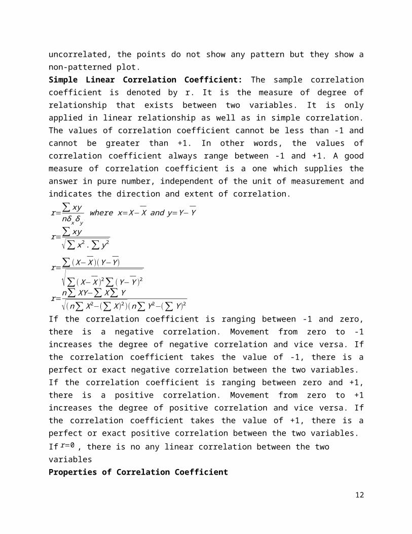
uncorrelated, the points do not show any pattern but they show anon-patterned plot.Simple Linear Correlation Coefficient: The sample correlationcoefficient is denoted by r. It is the measure of degree ofrelationship that exists between two variables. It is onlyapplied in linear relationship as well as in simple correlation.The values of correlation coefficient cannot be less than -1 andcannot be greater than +1. In other words, the values ofcorrelation coefficient always range between -1 and +1. A goodmeasure of correlation coefficient is a one which supplies theanswer in pure number, independent of the unit of measurement andindicates the direction and extent of correlation.

r=∑xynδxδy

where x=X−X__

and y=Y−Y__

r=∑xy√∑x2.∑y2

r=∑ (X−X__

)(Y−Y)__

√∑(X−X__

)2∑ (Y−Y__

)2

r=n∑ XY−∑ X∑ Y√(n∑ X2−(∑ X)2)(n∑Y2−(∑ Y)2

If the correlation coefficient is ranging between -1 and zero,there is a negative correlation. Movement from zero to -1increases the degree of negative correlation and vice versa. Ifthe correlation coefficient takes the value of -1, there is aperfect or exact negative correlation between the two variables.If the correlation coefficient is ranging between zero and +1,there is a positive correlation. Movement from zero to +1increases the degree of positive correlation and vice versa. Ifthe correlation coefficient takes the value of +1, there is aperfect or exact positive correlation between the two variables.If r=0 , there is no any linear correlation between the two variables Properties of Correlation Coefficient

12

1. The values of a correlation coefficient range between -1 and +1.

2. Correlation coefficient is symmetric. rYX=rXY3. Correlation coefficient is the geometric mean of two regression

coefficients. r=√bYX.bXY 4. Correlation coefficient has the same sign with regression

coefficients. If the two regression coefficients are positive,correlation coefficient will be positive and vice verssa.

5. Correlation coefficient is independent of change of origin andchange of scale. By change of origin we mean that adding orsubtracting any constant from the values of the variables.Independent of change of origin indicates that adding orsubtracting any constant value from the values of the twovariables does not change the correlation coefficient. By changeof scale we mean that multiplying or dividing values of the twovariables by any constant. Independent of change of scaleindicates that multiplying or dividing values of the twovariables by any constant does not change the correlationcoefficient.

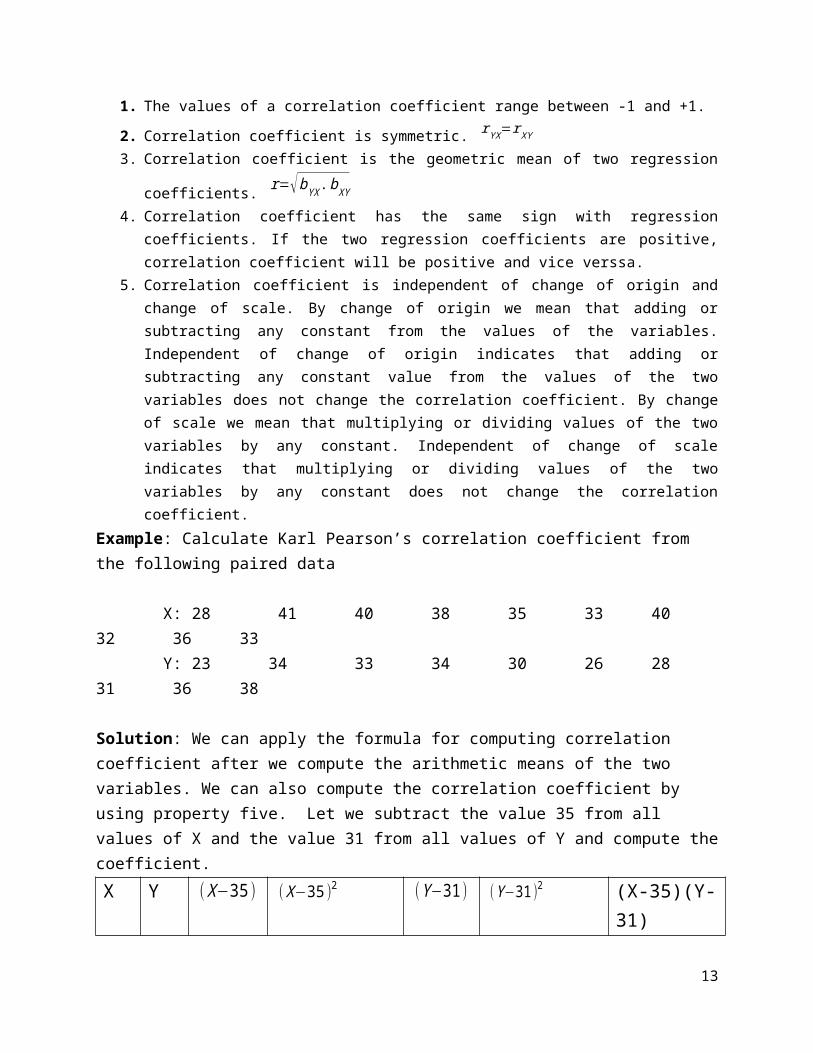
Example: Calculate Karl Pearson’s correlation coefficient from the following paired data

X: 28 41 40 38 35 33 40 32 36 33 Y: 23 34 33 34 30 26 28 31 36 38

Solution: We can apply the formula for computing correlation coefficient after we compute the arithmetic means of the two variables. We can also compute the correlation coefficient by using property five. Let we subtract the value 35 from all values of X and the value 31 from all values of Y and compute thecoefficient. X Y (X−35 ) (X−35 )2 (Y−31 ) (Y−31 )2 (X-35)(Y-

31)

13

28 23 -7 49 -8 64 5641 34 6 36 3 9 1840 33 5 25 2 4 1038 34 3 9 3 9 935 30 0 0 -1 1 033 26 -2 4 -5 25 1040 28 5 25 -3 9 -1532 31 -3 9 0 0 036 36 1 1 5 25 533 38 -2 4 7 49 -14

∑ (X−35 )2=162 ∑ (Y−31 )2=195 79

r=∑ (X−35 )(Y−31)

√∑ (X−35)2.∑ (Y−31 )2=79√162.195

r=0.44. which is averagely positive correlationRank correlation CoefficientThe Karl Pearson’s coefficient of correlation can’t be used incases where the direct quantitative measurement of phenomenonunder study is not possible. In such cases one may rank thedifferent items and apply the Spearman’s method of rankdifferences for finding out the degree of correlation. The rankcorrelation coefficient is denoted by R. Its value also ranges

from -1 to +1. R=1−

6∑Di2

n(n2−1)

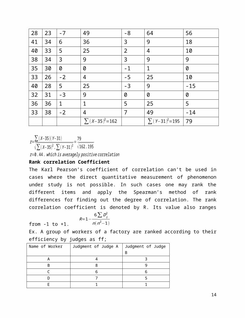
Ex. A group of workers of a factory are ranked according to theirefficiency by judges as ff;Name of Worker Judgment of Judge A Judgment of Judge

BA 4 3B 8 9C 6 6D 7 5E 1 1

14

F 3 2G 2 4H 5 7I 10 8J 9 10

Compute the rank correlation coefficient and interpret your result. Solution:Name of Worker R1 R2 Di Di

2

A 4 3 1 1B 8 9 -1 1C 6 6 0 0D 7 5 2 4E 1 1 0 0F 3 2 1 1G 2 4 -2 4H 5 7 -2 4I 10 8 -2 4J 9 10 1 1

∑Di2=20

R=1−6∑Di

2

n(n2−1)

R=1−6.2010(100−1)

R=1−120990

R=0.88

Therefore, we can interpret the result as the opinion of two judges with regard to the efficiency of workers shows greater similarity.

2.2.2 Regression AnalysisRegression describes the average relationship between variablesin a sense that the change in one or more variables brings acertain change on the other variable. A variable or group ofvariables that makes a certain cause for the change of the other

15

variable is called independent or explanatory variable. Avariable which is affected by the change of other variables iscalled dependent or explained variable. Regression describes thecause and effect relationship among variables. A regression canbe simple or multiple or it can be also linear or non-linear. Aregression is said to be linear if it studies the relationshipbetween one independent and one dependent variable while aregression is said to multiple if it studies the relationshipbetween one dependent and more than one independent variable. Acorrelation is said to be linear if the change in an independentvariable brings a constant change on the dependent variable whilea correlation is said to non-linear if the change on anindependent variable brings a non-constant change on thedependent variable. Estimating the Parameters of A functionOrdinary least Square Estimating Method (OLS): There aredifferent methods of estimating the unknown parameters of aregression function in which the ordinary least squares is themost prominent method which is frequently used by statisticiansbecause of its simplicity and having the desirable statisticalproperties that a good estimator should have to be a reliableestimator. For the matter of simplicity and scope here we willdiscuss only simple linear regression in which there are twovariables in the model (one dependent and one independentvariable) and the function is linear.Yi=β0+β1Xi+Ui . There are five elements in this function;Y, X, β0, β1 and Ui . Y, X and U are known as variables and β0 and β1 areknown as parameters. Y and X are known variables whose values arecollected from the field or from secondary sources. Sinceβ0, β1 and Ui are not observed, the above function cannot beestimated as it is. Thus, we have to get the estimators of theunobserved elements and try to estimate the parameters.Yi=b0+b1Xi+ei

16

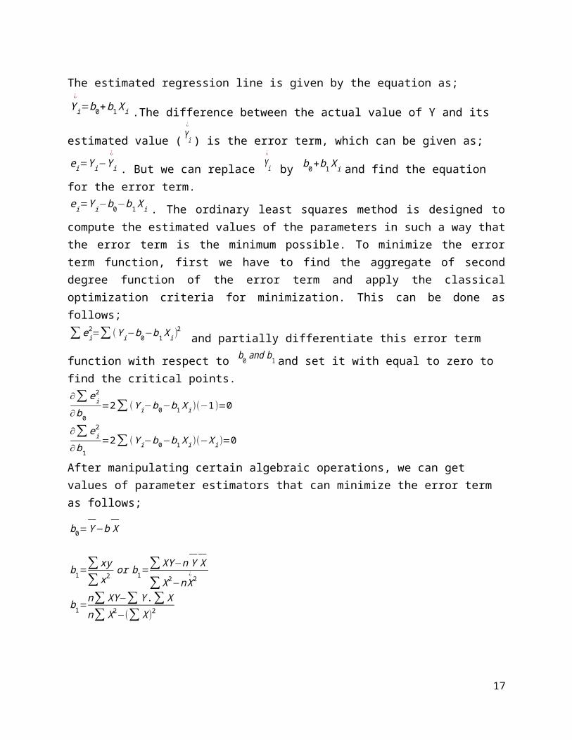
The estimated regression line is given by the equation as;

Yi¿

=b0+b1Xi .The difference between the actual value of Y and its

estimated value ( Yi¿

) is the error term, which can be given as;ei=Yi−Yi

¿

. But we can replace Yi¿

by b0+b1Xi and find the equation for the error term.ei=Yi−b0−b1Xi . The ordinary least squares method is designed tocompute the estimated values of the parameters in such a way thatthe error term is the minimum possible. To minimize the errorterm function, first we have to find the aggregate of seconddegree function of the error term and apply the classicaloptimization criteria for minimization. This can be done asfollows;∑ei

2=∑ (Yi−b0−b1Xi )2 and partially differentiate this error term

function with respect to b0 and b1 and set it with equal to zero to find the critical points.∂∑ei

2

∂b0=2∑ (Yi−b0−b1Xi )(−1)=0

∂∑ei2

∂b1=2∑ (Yi−b0−b1Xi )(−Xi)=0

After manipulating certain algebraic operations, we can get values of parameter estimators that can minimize the error term as follows;

b0=Y__

−b X__

b1=∑xy∑x2

or b1=∑XY−n Y

__X__

∑X2−nX¿2

b1=n∑ XY−∑ Y.∑ Xn∑ X2−(∑ X)2

17

It should be also noted that b1=bYX that is the regression coefficient of Y dependent on X. This regression can also be given in terms of the correlation coefficient.

bYX=r.δYδX

where r is the correlation coefficient and δY is the standard deviation of Y

and δX is the standard deviation of X

The inverse of the function Y=f(X ) which can be given asX=f=1 (Y) and its regression is known as inverse regression. The inverse regression is given asXi=c+dYi . Where c and d are parameter estimates. By the same token c and are computed as follows;

c=X__

−d Y__

d=∑ xy∑ x2

or d=∑XY−n X__Y__

∑Y2−n Y__2

=n∑ XY−∑ X.∑ Yn∑ Y2−(∑ X)2

The regression coefficient d is also known as the regression coefficient of X dependent on Y.

d=bXY=r.δXδY

Properties of Regression Coefficients1. The regression coefficients are not symmetric. That is the

value of the regression coefficient of Y dependent on X is notequal with the value of the regression coefficient of X on Y.bYX≠bXY

2. The regression coefficients must be having the same sign. Ifthe regression of Y on X is negative, then should be theregression coefficient of X on Y and vice-versa.3. If one of the regression coefficient is greater than one the

other should be less than one and vice-versa.4. Regression coefficients are independent of change of origin

but not independent of change of scale.The Coefficient of Determination

18

After we estimate the unknown parameters, we have check to whatextent the estimators are the reliable representatives of theparameters. We can test them using either t-test or z-test. Thesecond test that can help us in testing the goodness of fit isthe coefficient of determination.The coefficient of determination is the measure of theexplanatory power of the model . It measures the proportion orpercentage of the total variation of the dependent variableexplained or determined by the model. The coefficient ofdetermination is denoted by the symbol R2 .

19

UNIT FIVETIME SERIES ANALYSIS1.1 Introduction

Time series AnalysisDefinitely four types of data may be available for empirical analysis: time series, cross-section panel and pooled (combination of time series and cross section) data. A time series is a set of observations on the value that a variable takes at different times. Cross section data are data on one or more variables collected at the same point of time.

There are two major methods of analyzing time series data: Conventional and econometric methods. Econometric method of analysis can also be divided into two; frequency domain approach or spectral analysis and time domain approach. For ease of understanding, we are going to discuss the conventional method oftime series analysis.

A time series data is a set of observations taken at specified times, usually at “equal intervals”, Mathematically, a time series is defined by the values Y1,Y2, . . . Yt , thus Y is a function of time, symbolically Y=f(t). Thus, when we observe numerical data at different points of time and the set of observations is known as time series. A good example is the production of teff in each production year.

Role of Time series Analysis

20

Time series analysis is great significance in business decision making for the following reasons:

1. It helps in the understanding of post behavior by observingdata over the period of time; one can easily understand whatchanges have taken place in the past. Such exercise will beimportant in understanding and predicting the future.

2. It helps in planning future operations if the regularity ofoccurrence of any feature over a sufficient long period couldbe clearly established, then, prediction of probable futurevariations would become possible.

3. It helps in evaluating current accomplishments. Times seriesanalysis helps comparing the actual performance with that ofthe expected performance and the cause of variation isanalyzed.

4. It facilitates comparison – Different time series are oftencompared and important conclusions drawn from them.

5.2 Components of Time SeriesTime series elements are classified in to four basic types ofvariations which account for the changes in the series over aperiod of time. These four types of patterns, variations,movements are often called components or elements of timeseries. These are: 1) Secular trend 2) Seasonal variations3) Cyclical variations 4) Irregular variations In traditional or classical time series analysis, it isordinarily assumed that there is a multiplicative relationshipbetween these four components. That is, it is assumed that anyparticular value in series is the product of factors that can be

21

attributed to the various components. Symbolically, it is givenas; Y= T*S*C*I Where; T= Trend, S= Seasonal, C= Cyclical and I= Irregular If the above model is employed, the seasonal, cyclical andirregular items are not viewed as absolute amounts, but ratheras relative magnitude. 1. Secular TrendTrend is the variation of value of a variable that can beobserved in a long period of time. It is the general tendency ofthe data to grow or to decline over a long period of time. Trendis broadly divided under two heads: linear (what we going tosee) and non – linear trends. Methods of measuring Trend The following methods are used for measuring trend:1) Graphic method 2) The semi – average method 3) The method of least squares Graphic method: - This is the simplest method of studying trend.Under this method the given data are plotted on graph paper anda trend line is fitted to the data just by inspecting the graphof the series. There is no formal statistical criterion where bythe adequacy of such a line can be judged and the judgmentdepends on the discretion of the individual researcher. However,as a rough guide, the line should be drawn in such a way that itpasses between the plotted points in such a manner that thefluctuations in one direction are approximately equal to thosein the other direction and that it shows a general movement.This method is not frequently used since its approach issubjective and no statistical method is used.

Methods of semi – Averages: This method is used in such a way that the given data are divided in to two parts, preferably, with equal number of years. For example, if we are given data from 1982 to 1999, that is, over a period of 18 years, the two

22

equal parts will be first nine years, i.e., from 1982 to 1990 and from 1991 to 1999. In the case of odd number of years like 9, 13, 17, etc, two equal parts can be made simply by ignoring the middle year. For example, if the data are given for 19 yearsfrom 1981 to 1999, the two equal parts would be from 1981 to 1989 and from 1991 to 1999, the middle year 1990 would be ignored. Example: fit a trend line to the following data by the method ofsemi-averages: Year sales 1994 1021995 1051996 1141997 1101998 1081999 1162000 112

Solution: since seven years are given, the middle year should be omitted and an average of the first three years and the last three years shall be obtained. The averages of the first three years is 102+105+1143

=3213

=107 and the average of the last three years is

108+116+1123

=3363

=112

Thus, we get two points, 107 and 112, which shall be plotted corresponding to their respective middle years, i.e. 1995 and 1999. By joining these two points; we obtain the required trend line.

Y

23

Trend Line112

107 Time

1994 1995 1996 1997 1998 1999 2000

Method of least squaresThis method is most widely used in practice. When this method is applied, a trend line is fitted to the data in such a manner thatthe following two conditions are satisfied:

1) ∑ (Y−YC)=0 . The sum of deviations of the actual values of Yand the computed values of Y is zero.

2) ∑ (y−yc)2Is the least, that is, the sum of the squares of the

deviations of the actual and computed values is the leastone. The method of least squares can be used either to fit astraight line trend or a parabolic trend. The straight linetrend is represented by the equation

YC=a+bXIn order to determine the value of the constants a and b, thefollowing two normal equations are to be solved.∑Y=n.a+b∑ X∑YX=a∑ X+b∑ X2 Where n represents number of years and X isthe time period. We can measure the variable x from any point of time in originsuch as the first year. However, this calculations are very muchsimplified when the midpoint in time is taken as the originbecause in that case, the negative values in the first half ofthe series balances the positive values in the second half sothat x=0, the above two normal equations would take the form:

24

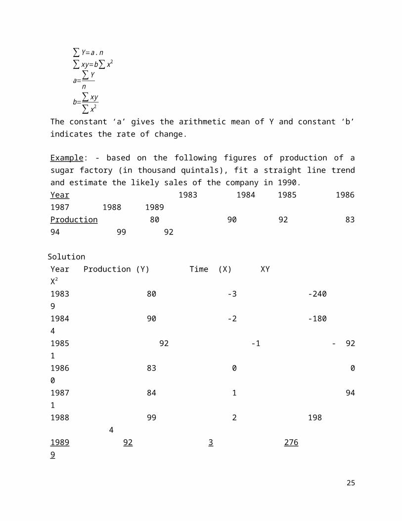
∑Y=a.n∑xy=b∑x2

a=∑Yn

b=∑xy∑x2

The constant ‘a’ gives the arithmetic mean of Y and constant ‘b’indicates the rate of change. Example: - based on the following figures of production of asugar factory (in thousand quintals), fit a straight line trendand estimate the likely sales of the company in 1990. Year 1983 1984 1985 19861987 1988 1989 Production 80 90 92 8394 99 92

Solution Year Production (Y) Time (X) XYX2 1983 80 -3 -24091984 90 -2 -18041985 92 -1 - 9211986 83 0 001987 84 1 9411988 99 2 198

41989 92 3 2769

25

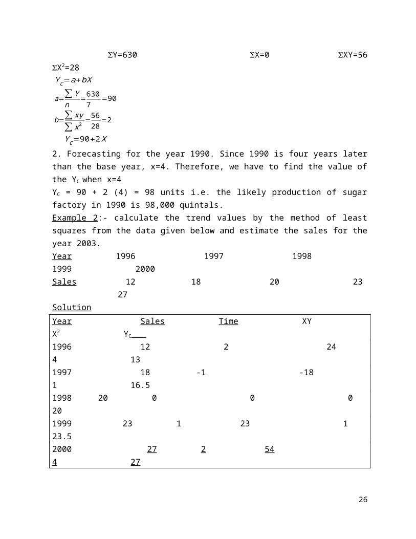
Y=630 X=0 XY=56X2=28YC=a+bX

a=∑ Yn

=6307

=90

b=∑ xy∑ x2

=5628

=2

YC=90+2X2. Forecasting for the year 1990. Since 1990 is four years laterthan the base year, x=4. Therefore, we have to find the value ofthe YC when x=4YC = 90 + 2 (4) = 98 units i.e. the likely production of sugarfactory in 1990 is 98,000 quintals. Example 2:- calculate the trend values by the method of leastsquares from the data given below and estimate the sales for theyear 2003. Year 1996 1997 1998 1999 2000 Sales 12 18 20 23

27Solution Year Sales Time XY X2 YC 1996 12 2 24 4 131997 18 -1 -18 1 16.51998 20 0 0 0 201999 23 1 23 1 23.52000 27 2 54 4 27

26

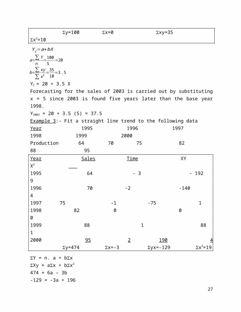
y=100 x=0 xy=35 x2=10YC=a+bX

a=∑ Yn

=1005

=20

b=∑ xy∑ x2

=3510

=3.5

YC = 20 + 3.5 XForecasting for the sales of 2003 is carried out by substitutingx = 5 since 2003 is found five years later than the base year1998.Y2003 = 20 + 3.5 (5) = 37.5Example 3:- Fit a straight line trend to the following dataYear 1995 1996 1997 1998 1999 2000Production 64 70 75 82 88 95Year Sales Time XY X2 1995 64 - 3 - 192 9 1996 70 -2 -140 4 1997 75 -1 -75 1 1998 82 0 0 0 1999 88 1 88 1 2000 95 2 190 4

y=474 x=-3 yx=-129 x2=19

Y = n. a + bxXy = ax + bx2

474 = 6a – 3b-129 = -3a + 196

27

474 = 6a – 3b-258 = -6a + 38b216 = 35 bb = 216 = 6.17 35 474 = 6a – 3 (6.17)6a = 474+18.516a = 492.51a=

492.516

=82.085

YC = 82.085 + 6.17X

Seasonal variationsSeasonal variations are periodic movements in business activitywhich occurs, regularly every year and have their origin in thenature of the year itself. It exists only when data are given ina period which is less than a year (monthly, semi-annually,quarterly, weekly, daily, etc). However, it does not exist indata which are given in annual basis or more than a year periodinternal. Nearly every type of business activity is liable toseasonal influence to a greater or lesser degree and, as such,these variations are regarded as normal phenomenon recurringevery year. Although the word ‘seasonal’ seems to imply aconnection with the season of the year, the term is meant toinclude any kind of variation which is of periodic nature andwhose repeating cycles are of relatively short duration. Thefactors that cause seasonal variations are:

1) Climate and weather conditions. The most important factorcausing seasonal variation is the climate changes in theclimate and weather conditions such as rainfall, humidity,heat, etc, act on different product and industry differently.

2) Customs, traditions and habits – Though nature is mainlyresponsible for seasonal variations in time series, customsand traditions also have their impact.

28

Measurement of seasonal variationsWhen data are expressed annually there is no seasonal variation.However, monthly or quarterly data frequently exhibit strongseasonal movements and considerable interest attaches to devisea pattern of average seasonal variation. There are severalmethods of measuring seasonal variation. However, the followingmethods are popularly used in practice: 1. Method of simple averages2. Ratio to trend method 3. Ratio to moving average method 4. Link relatives method

Method of simple averagesThis is the simplest method of obtaining a seasonal index. Thefollowing steps are necessary for computing the index:1) Average the unadjusted data by years and months or quarters

if the data are given quarterly.2) Find the totals of the data in each month, quarter or a

period in which the data are given. 3) Divide each total by the number of years for which data are

given.4) Obtain an average of monthly averages by dividing the total

of monthly averages by 12. 5) Taking the average of monthly averages as 100, compute the

percentage.

Seasonal Index for January=(Monthly average for JanuaruAverage of monthly averages

)100

Example: consumption of monthly electric power in KW hours offor street lighting in Haramaya University from 1995 – 1999. Year Jan Feb Mar Apri mayJun Jul Aug Sep Oct

29

1995 318 281 278 250 231216 223 245 269 302 1996 342 309 299 268 249236 242 262 288 3211997 367 328 320 287 269251 259 284 309 3451998 392 349 342 311 290273 282 305 328 364 1999 420 378 370 334 314296 305 330 356 396

Year Nov Dec 1995 325 347 1996 342 364 1997 367 394 1998 389 417 1999 422 452

Find out seasonal variation by the method of monthly averages?Solution: Month 1995 1996 1997 1998 1999Total Average %Jan 318 342 367 392 420 1839 367.8 116.1 Feb 281 309 328 349 378 1645 329 103.9Mar 278 299 320 342 370 1609 321.8 101.6 April 250 268 287 311

30

334 1450 290 91.6 May 231 249 269 290 314 1353 270.6 85.4Jun 216 236 251 273 296 1272 254.4 80.3July 223 242 259 282 305 1311 262.2 82.8Aug 245 262 284 305 330 1426 285.2 90.1 Sep 269 288 309 328 356 1550 310 97.9Oct 302 321 345 364 396 1728 345.6 109.Nov 325 342 367 389 422 1845 369 116.Dec 347 364 394 417 452 1974 394.8 124.7Total 19002 3800.4 1200

Average 1583.5 316.7 100

Seasonal index for January=367.8316.7

×100=116.1

Seasonal index for Februrary=329316.7

×100=103.9

Seasonal index for Julay=262.2316.7

×100=82.8

Ratio – to- Trend method This method of calculating a seasonal index in relatively simpleand yet an improvement over the method of simple averageexplained in the preceding section. The method assumes that theseasonal variation for a given month is a constant fraction of

31

the trend. It first eliminates the trend component by dividingthe original data with the trend value.

T×S×C×IT

=S×C×I

Random elements are supposed to disappear when the ratios areaveraged. A careful selection of the period of years used in thecomputation is expected to cause the influences of prosperity ordepression to offset each other and thus removes the cycle.

This method requires the following steps:1. Compute the trend values by applying the method of least

squares; 2. Divide the original data month by month by the corresponding

trend values and multiply the ratio by 100. The valuesobtained are now free from trend;

3. In order to free form irregular and cyclical movements, theirregular given for various years for January, February, etcshould be averaged and

4. The seasonal index for each month is expressed as apercentage of the average month. The sum of 12 values mustequal 1,200 or 100%. If it does not, an adjustment is made bymultiplying each index by a suitable factor (1200).This gives the final seasonal index.

Example: - find the seasonal variations by ratio to trendmethod from the data given below

Year 1 st q 2 nd q 3 rd q 4 th quarter 1996 30 40 36 34 1997 34 52 50 44 1998 40 58 54 48

32

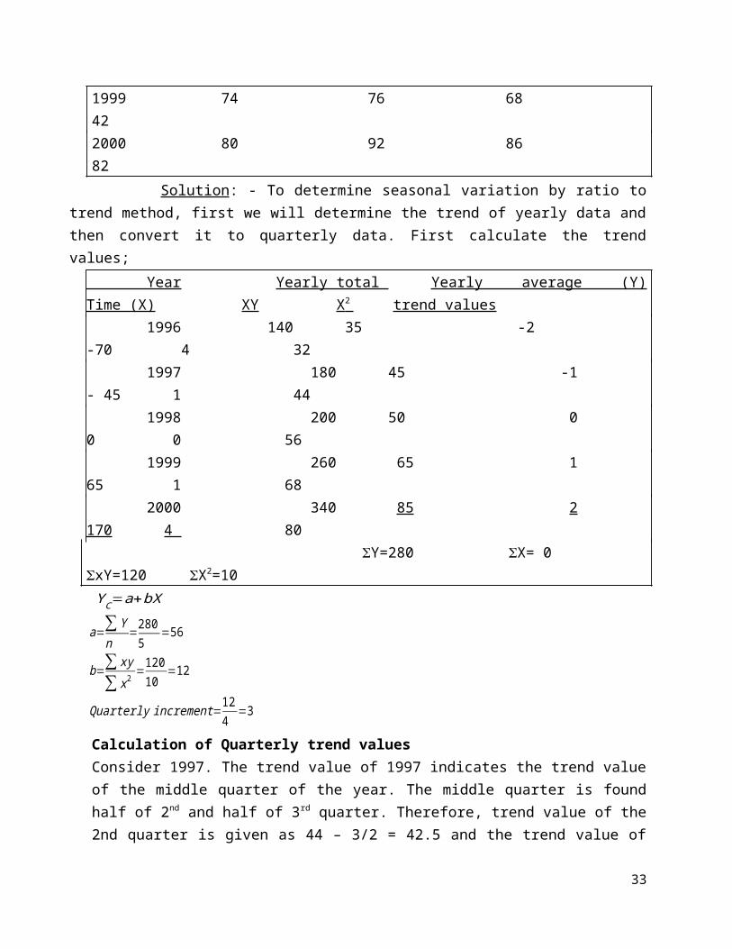
1999 74 76 68 422000 80 92 86 82

Solution: - To determine seasonal variation by ratio totrend method, first we will determine the trend of yearly data andthen convert it to quarterly data. First calculate the trendvalues; Year Yearly total Yearly average (Y)Time (X) XY X 2 trend values 1996 140 35 -2-70 4 32 1997 180 45 -1- 45 1 44 1998 200 50 00 0 56 1999 260 65 165 1 68 2000 340 85 2170 4 80 Y=280 X= 0 xY=120 X2=10 YC=a+bX a=∑ Y

n=2805

=56

b=∑ xy∑ x2

=12010

=12

Quarterly increment=124

=3

Calculation of Quarterly trend valuesConsider 1997. The trend value of 1997 indicates the trend valueof the middle quarter of the year. The middle quarter is foundhalf of 2nd and half of 3rd quarter. Therefore, trend value of the2nd quarter is given as 44 – 3/2 = 42.5 and the trend value of

33

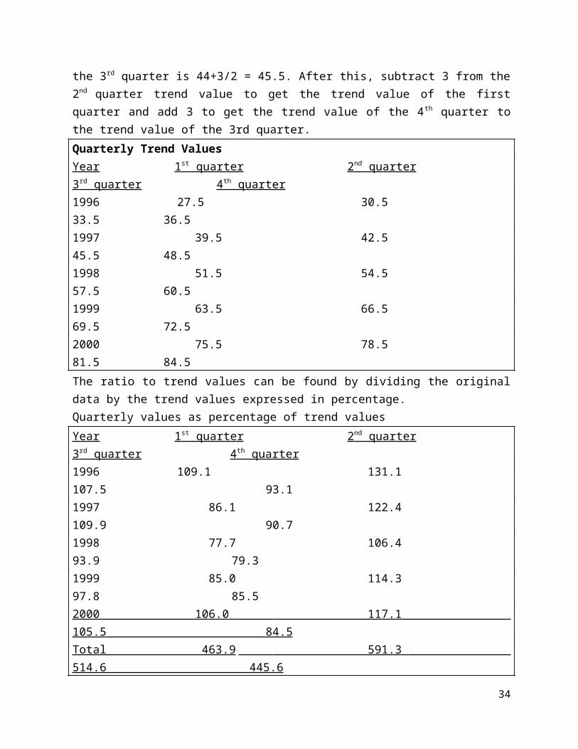
the 3rd quarter is 44+3/2 = 45.5. After this, subtract 3 from the2nd quarter trend value to get the trend value of the firstquarter and add 3 to get the trend value of the 4th quarter tothe trend value of the 3rd quarter. Quarterly Trend ValuesYear 1 st quarter 2 nd quarter 3 rd quarter 4 th quarter 1996 27.5 30.5 33.5 36.5 1997 39.5 42.5 45.5 48.5 1998 51.5 54.5 57.5 60.5 1999 63.5 66.5 69.5 72.5 2000 75.5 78.5 81.5 84.5 The ratio to trend values can be found by dividing the originaldata by the trend values expressed in percentage. Quarterly values as percentage of trend values Year 1 st quarter 2 nd quarter 3 rd quarter 4 th quarter 1996 109.1 131.1 107.5 93.1 1997 86.1 122.4 109.9 90.7 1998 77.7 106.4 93.9 79.3 1999 85.0 114.3 97.8 85.5 2000 106.0 117.1 105.5 84.5 Total 463.9 591.3 514.6 445.6

34

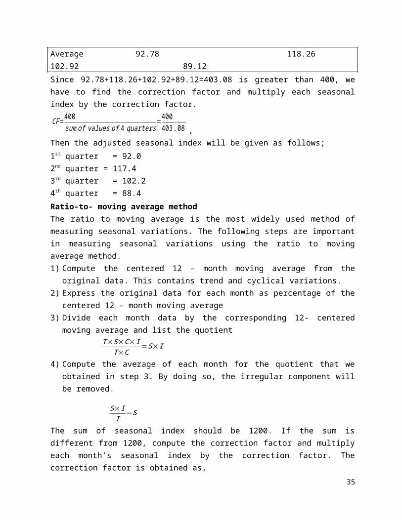
Average 92.78 118.26 102.92 89.12 Since 92.78+118.26+102.92+89.12=403.08 is greater than 400, wehave to find the correction factor and multiply each seasonalindex by the correction factor.

CF=400sum of values of 4 quarters

=400403.08 ,

Then the adjusted seasonal index will be given as follows;1st quarter = 92.02nd quarter = 117.43rd quarter = 102.24th quarter = 88.4Ratio-to- moving average methodThe ratio to moving average is the most widely used method ofmeasuring seasonal variations. The following steps are importantin measuring seasonal variations using the ratio to movingaverage method. 1) Compute the centered 12 – month moving average from the

original data. This contains trend and cyclical variations. 2) Express the original data for each month as percentage of the

centered 12 – month moving average3) Divide each month data by the corresponding 12- centered

moving average and list the quotient

T×S×C×I

T×C=S×I

4) Compute the average of each month for the quotient that weobtained in step 3. By doing so, the irregular component willbe removed.

S×II

=S

The sum of seasonal index should be 1200. If the sum isdifferent from 1200, compute the correction factor and multiplyeach month’s seasonal index by the correction factor. Thecorrection factor is obtained as,

35

CF = 1200 ______________ The total mean for 12 months

Link Relatives MethodThis is also one of the methods of measuring seasonal variations.When this method is adopted, the following steps need to be considered;1. Calculate the link relatives of seasonal figures.

LR=

Current season's figurePrevious season's figure

×100

2. Calculate the average of the link relatives for each season3. Convert the averages in to chain relatives on the base of the

last season4. Calculate the chain relatives of the first season on the base

of the last season5. For correction, the chain relative of the first season

calculated by the first method is deducted from the chain relative of the first season calculated by the second method

6. Express corrected chain relatives as percentage of their averages. These provide the required seasonal indices by the method of link relatives.

Example: Apply the method of link relatives to the following dataand calculate seasonal indicesQuarter 1998 1999 2000 2001 2002I 6.0 5.4 6.8 7.2 6.6II 6.5 7.9 6.5 5.8 7.3III 7.8 8.4 9.3 7.5 8.0IV 8.7 7.3 6.4 8.5 7.1

Solution: Calculation of Seasonal Indices by Link RelativesYear I II III IV1998 - 108.3 120.0 111.51999 62.1 146.3 106.3 86.92000 93.2 95.6 143.1 68.8

36

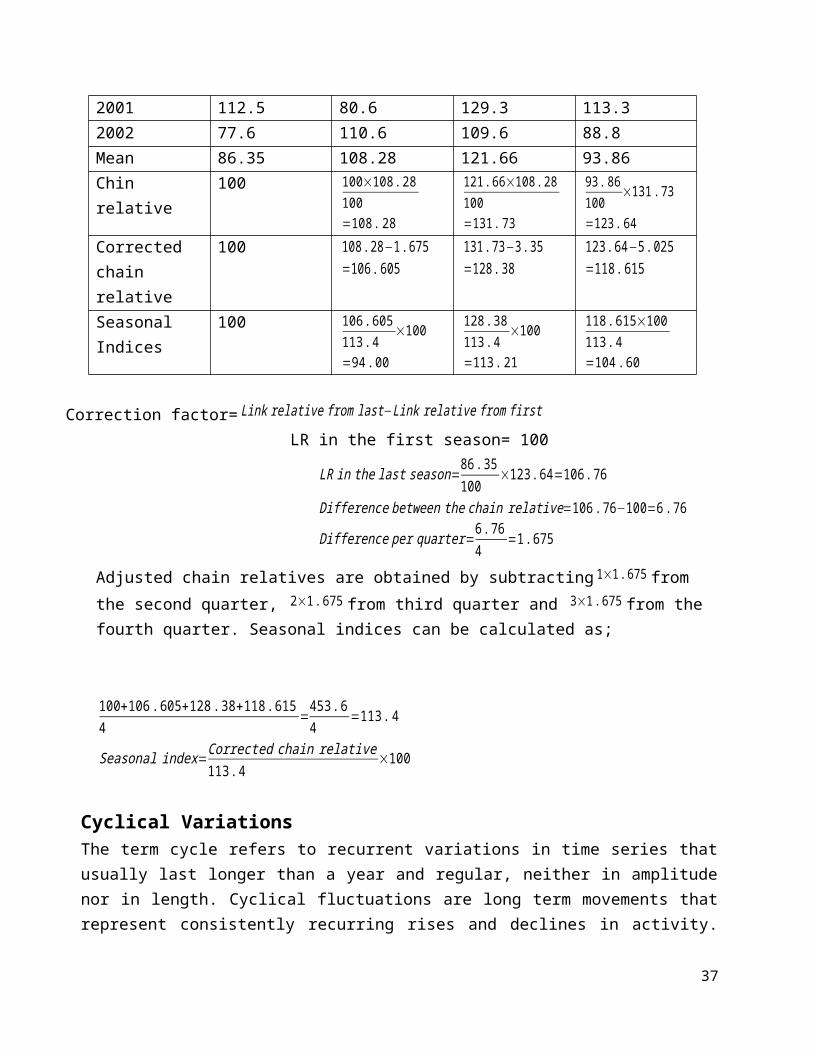
2001 112.5 80.6 129.3 113.32002 77.6 110.6 109.6 88.8Mean 86.35 108.28 121.66 93.86Chin relative

100 100×108.28100=108.28

121.66×108.28100=131.73

93.86100

×131.73

=123.64Corrected chain relative

100 108.28−1.675=106.605

131.73−3.35=128.38

123.64−5.025=118.615

Seasonal Indices

100 106.605113.4

×100

=94.00

128.38113.4

×100

=113.21

118.615×100113.4=104.60

Correction factor= Link relative from last−Link relative from first LR in the first season= 100

LR in the last season=86.35100

×123.64=106.76

Difference between the chain relative=106.76−100=6.76

Difference per quarter=6.764

=1.675

Adjusted chain relatives are obtained by subtracting 1×1.675 from the second quarter, 2×1.675 from third quarter and 3×1.675 from the fourth quarter. Seasonal indices can be calculated as;

100+106.605+128.38+118.6154 =

453.64 =113.4

Seasonal index=Corrected chain relative113.4

×100

Cyclical VariationsThe term cycle refers to recurrent variations in time series thatusually last longer than a year and regular, neither in amplitudenor in length. Cyclical fluctuations are long term movements thatrepresent consistently recurring rises and declines in activity.

37

They are resulted mainly from business cycles. A business cycleconsists of the recurrence of the up down movements of businessactivity from some sort of statistical trend. There are four welldefined periods or phases in the business cycle. These areprosperity, decline, depression and improvement. The study ofcyclical variations is extremely useful in framing suitablepolicies for stabilizing the level of business activity, i.e. foravoiding periods of booms and depressions as both are bad for theeconomy.

Measurement of Cyclical Variations Business cycles are important types of fluctuations in economicdata. Definitely, they are receiving a lot of attention ineconomic literature. Despite the importance of business cycles,they are most difficult types of fluctuations to measure. This isbecause successive cycles vary widely in timing, amplitude andpattern. Because of such reason, it is impossible to constructmeaningful typical cycle indices of curves similar to those thathave been developed for trends and seasonality. The importantmethods used for measuring cyclical variations are:

1. Residual Method2. Reference Cycle Analysis Method3. Direct Method4. Harmonic Analysis Method

Because of the frequent usage and convenience of time, only the first method is discussed. Residual Method: Among all the methods of arriving at estimates ofthe cyclical movements of time series, the residual method is mostcommonly used. This method consists of eliminating seasonal andthen trend variations to obtain the cyclical and irregularmovements.

T×S×C×IS =T×C×I

T×C×IT

=C×I

38

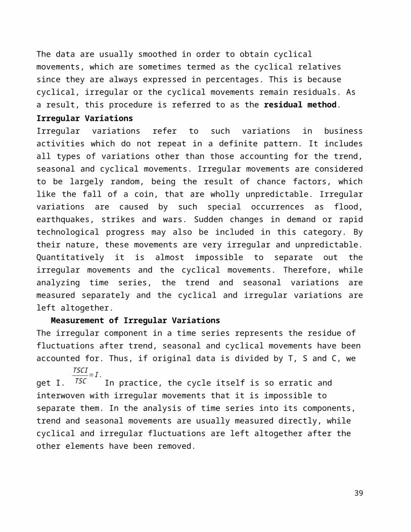
The data are usually smoothed in order to obtain cyclical movements, which are sometimes termed as the cyclical relatives since they are always expressed in percentages. This is because cyclical, irregular or the cyclical movements remain residuals. As a result, this procedure is referred to as the residual method.Irregular Variations Irregular variations refer to such variations in businessactivities which do not repeat in a definite pattern. It includesall types of variations other than those accounting for the trend,seasonal and cyclical movements. Irregular movements are consideredto be largely random, being the result of chance factors, whichlike the fall of a coin, that are wholly unpredictable. Irregularvariations are caused by such special occurrences as flood,earthquakes, strikes and wars. Sudden changes in demand or rapidtechnological progress may also be included in this category. Bytheir nature, these movements are very irregular and unpredictable.Quantitatively it is almost impossible to separate out theirregular movements and the cyclical movements. Therefore, whileanalyzing time series, the trend and seasonal variations aremeasured separately and the cyclical and irregular variations areleft altogether. Measurement of Irregular VariationsThe irregular component in a time series represents the residue of fluctuations after trend, seasonal and cyclical movements have beenaccounted for. Thus, if original data is divided by T, S and C, we

get I. TSCITSC

=I.In practice, the cycle itself is so erratic and

interwoven with irregular movements that it is impossible to separate them. In the analysis of time series into its components, trend and seasonal movements are usually measured directly, while cyclical and irregular fluctuations are left altogether after the other elements have been removed.

39

40