544 IEEE TRANSACTIONS ON AUTOMATIC CONTROL, VOL. 56, NO. 3, MARCH 2011

Edge Agreement: Graph-Theoretic PerformanceBounds and Passivity Analysis

Daniel Zelazo, Member, IEEE, and Mehran Mesbahi

Abstract—This work explores the properties of the edge variantof the graph Laplacian in the context of the edge agreementproblem. We show that the edge Laplacian, and its corre-sponding agreement protocol, provides a useful perspective on thewell-known node agreement, or the consensus algorithm. Specif-ically, the dynamics induced by the edge Laplacian facilitates abetter understanding of the role of certain subgraphs, e.g., cyclesand spanning trees, in the original agreement problem. Using theedge Laplacian, we proceed to examine graph-theoretic charac-terizations of the � and performance for the agreementprotocol. These results are subsequently applied in the contextsof optimal sensor placement for consensus-based applications.Finally, the edge Laplacian is employed to provide new insightsinto the nonlinear extension of linear agreement to agents withpassive dynamics.

Index Terms—Agreement protocol, consensus, networked dy-namic systems, passivity.

I. INTRODUCTION

C OORDINATION and control of multi-agent systems hasbecome an increasingly active area of research in the sys-

tems and control community. Applications of such systems arefar reaching and include problems such as formation flying, co-ordinated robotics, sensor fusion, and distributed computation[2]–[6], [15], [20], [21], [27], [19]. An important sub-class ofthese problems is known as the consensus, or agreement pro-tocol. In consensus problems, agents in a distributed system areable to agree on a common value of interest via a local interac-tion protocol. There is a wealth of literature on consensus prob-lems, and the reader is referred to the survey papers [23], [28],and the references therein for a more detailed treatment of thesubject.

A fundamental theme of consensus problems is the conver-gence properties of the protocol to a common value based on thestructural properties of the underlying graph. In this direction, itis well known that the second smallest eigenvalue of the graphLaplacian matrix, referred to as the algebraic connectivity of agraph [10], is a judicious measure for relating the rate of conver-gence of the protocol to the connectedness of the graph. In fact,

Manuscript received May 18, 2009; revised January 06, 2010; accepted June28, 2010. Date of publication July 08, 2010; date of current version March 09,2011. This work was supported by the National Science Foundation GrantsECS-0501606 and CMMI-0856737. Recommended by Associate Editor M.Prandini.

D. Zelazo is with the Institute for Systems Theory and Automatic Control,Universität Stuttgart, Stuttgart 70550, Germany (e-mail: daniel.zelazo@ist.uni-stuttgart.de).

M. Mesbahi is with the Department of Aeronautics and Astronautics, Univer-sity of Washington, Seattle, WA, 98195-2400, USA (e-mail: mesbahi@uw.edu).

Color versions of one or more of the figures in this paper are available onlineat http://ieeexplore.ieee.org.

Digital Object Identifier 10.1109/TAC.2010.2056730

the importance of the Laplacian spectra for convergence anal-ysis has been explored in many contexts, including random net-works [13], switching topologies [24], and noisy networks [32].

While convergence properties may arguably be the most crit-ical feature of consensus-type problems, a more control theo-retic approach to the analysis and synthesis of these systems isalso needed. Examples of such studies include a Nyquist-basedstability analysis for consensus-based feedback systems [9], agraph-centric notion of controllability in consensus problems[26], and consensus algorithms with guaranteed perfor-mance [18]. An important theme in these approaches is the de-velopment of a clear connection between certain properties ofthe underlying connection topology and the system-theoreticproperties that these networked systems exhibit.

In this work, we focus on developing a systematic frameworkfor exploring connections between the properties of the networkon one hand, and notions from systems and control on the other,in the setting of consensus problems. In this direction, we firstdevelop an edge variant of the graph Laplacian which we termthe edge Laplacian [33]. The edge Laplacian is a matrix rep-resentation of the underlying network that offers a more trans-parent understanding of how certain graph structures, such asspanning trees and cycles, relate to the algebraic properties ofthe corresponding matrix. We show that this alternative repre-sentation relates to the graph Laplacian matrix via an appro-priate similarity transformation. The importance of this matrixrepresentation has been implicitly realized in the literature [1],[8], [22], [31]; one of our contributions in this paper is to explic-itly highlight the insights that this matrix representation offersin the analysis and synthesis of multi-agent networks.

The edge Laplacian is the primary construct used to con-sider the edge agreement protocol. In consensus problems, theexchange of information is dependent on the relative informa-tion between neighboring agents. This relative information hasa natural interpretation in terms of the edges in the interconnec-tion graph, and a corresponding dynamic description of the con-sensus protocol can be written from the edge perspective. Usingthe edge agreement model, we are then able to perform a systemtheoretic analysis of the system’s performance using bothand norms. To provide a broader scope for this model,we also introduce exogenous inputs in the form of process andsensor noise. The analysis highlights the role of spanning treesand cycles and also discusses the ramification of the analysis inthe context of -regular graphs. Subsequently, the utility of theproposed framework is demonstrated via examples including

optimal sensor selection for consensus-type systems andnonlinear consensus over networks consisting of passive agents.

The organization of this paper is as follows. In Section I-A, abrief overview of our notation and a few concepts from algebraic

0018-9286/$26.00 © 2010 IEEE

ZELAZO AND MESBAHI: GRAPH-THEORETIC PERFORMANCE BOUNDS AND PASSIVITY ANALYSIS 545

graph theory are presented. These constructs are then used todevelop and introduce the edge Laplacian in Section II-A. Theedge agreement problem is then presented in Section II-C. InSection III, an and performance analysis of the agree-ment protocol is presented. Applications of the edge Laplacianfor passive networks is then given in Section IV, followed byour concluding remarks in Section V.

A. Preliminaries and Notation

The matrix-theoretic notation used in the paper is as follows:for a matrix , and denote, respectively, its rangespace and null space. Diagonal matrices will be written as

, with denoting the -th entry on the diag-onal. A matrix and/or a vector that consists of all zero entrieswill be denoted by ; whereas, “0” will simply denotes the scalarzero. Similarly, the vector denote the vector of all ones, and

The notation signifies that the func-tion is bounded from above by some constant multiple of

for large enough values of . The set of real numbers willbe denoted as , and denotes the -norm of its argument(e.g., , ), which will be used for vectors, matrices, andsystem norms. For the set , denotes its cardinality.

Graphs and the matrices associated with them will be exten-sively used in this work. The reader is referred to [11] for a de-tailed treatment of the subject and we present here only a min-imal summary of relevant constructs and results.

An undirected (simple) graph is specified by a vertex setand an edge set whose elements characterize the incidence

relation between distinct pairs of . The notation is usedto denote that node is connected to node , or equivalently,

. We make use of the incidence ma-trix, , for a graph with an arbitrary orientation, i.e., a graphwhose edges have a head (terminal node) and a tail (an initialnode). The columns of are then indexed by the edge set,and the -th row entry takes the value “1” if it is the initial nodeof the corresponding edge, “ ” if it is the terminal node, andzero otherwise. From the definition of the incidence matrix itfollows that the null space of its transpose, , containsthe agreement subspace, . More generally,for the matrix will be used to denote the subspace generatedby linear combinations of its columns. The rank of the incidencematrix depends only on and the number of its connectedcomponents [11]. The diagonal matrix of the graph con-tains the degree of each vertex on its diagonal. The adjacencymatrix, , is the symmetric matrix with zero onthe diagonal and one in the -th position if node is adjacentto node . The (graph) Laplacian of

(1.1)

is a rank deficient positive semi-definite matrix. The eigenvaluesare real and will be ordered and denoted as

.A connected graph can be written as the union of two edge-

disjoint subgraphs on the same vertex set as , whereis a spanning tree subgraph and contains the remaining

edges that necessarily complete the cycles in . Similarly, the

Fig. 1. Example of regular graphs. (a)� graph (b)� graph (c) A 4-regulargraph.

columns of the incidence matrix for the graph can always bepermuted such that can be written as

(1.2)

The cycle edges can be constructed from linear combinationsof the tree edges via a linear transformation [29], [30], as

(1.3)

where

(1.4)

Using (1.3) we obtain the following alternative representationof the incidence matrix of the graph:

(1.5)

the rows of the matrix

(1.6)

are viewed as the basis for the cut space of [11]. The matrix, on the other hand, forms a basis for the flow space.

The matrix (1.6), which will play an important rolein the present work, has a close connection with a number ofstructural properties of the underlying network. For example,the number of spanning trees in a graph, , can be deter-mined from the cut space basis [11], as

(1.7)

In order to apply the framework developed in this paper tospecific graphs, we will work with the complete graph and itsgeneralization in terms of -regular graphs, which are definedas follows. The complete graph on nodes, , is the graphwhere all possible pairs of vertices are adjacent, or equivalently,if the degree of all vertices is . Fig. 1(a) depicts , thecomplete graph on 10 nodes. When every node in a graph with

nodes has the same degree , it is called a -regulargraph. The -regular graph on nodes for is called thecycle graph, . Fig. 1(b) and (c) show, respectively, the cyclegraph and a 4-regular graph. The line graph of , denotedas , is the graph where the edges of correspond to thenodes of , and two edges in are adjacent if they sharea node in .

The edges in a graph can be given orientations, which notonly facilitate defining the incidence matrix of a graph, but alsonotions of the cut and the flow spaces of a graph. We define two

546 IEEE TRANSACTIONS ON AUTOMATIC CONTROL, VOL. 56, NO. 3, MARCH 2011

edges to be positively (negatively) adjacent if theyshare a node and point in opposite (same) directions relative tothis shared node. We denote the positive and negative adjacencyof edges as and , respectively. By conven-tion, an edge is not considered adjacent to itself.

II. THE EDGE PERSPECTIVE

In this section, we define a matrix representation of graphsthat will be used to highlight the contribution of the edges onthe evolution of the consensus protocol. This is then followedby an edge variant of the agreement protocol that we refer to asthe edge agreement protocol.

A. Edge Laplacian

We first introduce the edge Laplacian and present some graphtheoretic and algebraic interpretations of its structure. In thisvenue, we will draw parallels between the graph and edge Lapla-cians whenever possible. The edge Laplacian is defined as [33]

(2.8)

The structure of the edge Laplacian is closely related to the ad-jacency matrix of the undirected line graph of , , as

(2.9)

where for a matrix denotes its entry-wise absolute value.We note that the non-zero eigenvalues of are identicalto those of [14], and each independent cycle in corre-sponds to an eigenvalue at zero in . The notion of an inde-pendent cycle can be related algebraically to the number of in-dependent columns in . Furthermore, the null space of theedge Laplacian depends on the number of cycles in the graph.Let us elaborate on this last statement via a few definitions andobservations.

Definition 2.1: Given an incidence matrix for a directedgraph, a signed path vector is a vector correspondingto a path such that the th element of takes the value “ ” ifedge is traversed positively, “ ” if traversed negatively, and“0” if the edge is not used in the path.

Lemma 2.2: Given a path with distinct initial and terminalnodes described by a signed path vector in a graph , thevector is defined as and the th element of

takes the value “ ” if node is the initial node of the path,“ ” if it is the terminal node of the path, and “0” otherwise.

Proof: The proof follows directly from the structure of theincidence matrix and Definition 2.1.

Theorem 2.3 [11]: Given a connected graph with arbitraryorientation assigned, the null space of is spanned by allthe linearly independent signed path vectors corresponding tothe cycles in .

Proof: For any node used in a cycle, the path must enter andexit that node an equal number of times. It then follows from thestructure of the incidence matrix that when is thesigned path vector for a cycle.

Theorem 2.3 is an example of the intricate relationship be-tween the graphical and algebraic properties of a graph.

Theorem 2.4: Let and denote, respectively, theedge Laplacian and the incidence matrix of the graph . Then

(2.10)

Proof: Let ; thenand it follows that . On the other hand when

, and. Thus .

We can alternatively define the edge Laplacian in an analo-gous way to the identity (1.1). In this venue, let us define theedge adjacency matrix as

otherwise.

The edge degree matrix, , is a diagonal matrix with thenumber of nodes connected to each edge. As we do not allowself-loops, we have that . Thus, the edge Laplaciancan be equivalently defined as

(2.11)

This alternative definition can be used to further deepen theconnection between the edge Laplacian of and its line graph

. We note that the element of corresponds tothe degree of each node in the line graph of .

B. Similarity Between the Graph and Edge Laplacians

The connection between the edge and graph Laplacians canbe made explicit through the introduction of an appropriate sim-ilarity transformation. Furthermore, we find similarity transfor-mations that relate the Laplacians for connected graphs with cy-cles to graphs on spanning trees. The following theorems as-sume is a spanning tree subgraph of , and isdefined via (1.5).

Theorem 2.5: The graph Laplacian for a connected graphcontaining cycles is similar to

Proof: We define the transformation

Applying the transformation leads to thedesired result.

Theorem 2.5 provides a transparent way to separate the zeroeigenvalue of the Laplacian for a connected graph while pre-serving algebraic properties of the graph via the edge Laplacian.

Theorem 2.6: The edge Laplacian for a graph with cycles,is similar to the matrix

ZELAZO AND MESBAHI: GRAPH-THEORETIC PERFORMANCE BOUNDS AND PASSIVITY ANALYSIS 547

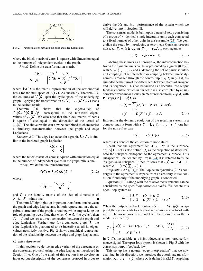
Fig. 2. Transformations between the node and edge Laplacians.

where the block-matrix of zeros is square with dimension equalto the number of independent cycles in the graph.

Proof: Define the transformation matrix

where is the matrix representation of the orthonormalbasis for the null space of . As shown by Theorem 2.3,the columns of span the cycle space of the underlyinggraph. Applying the transformation leadsto the desired result.

Theorem 2.6 shows that the eigenvalues ofcorrespond to the non-zero eigen-

values of . We also note that the block matrix of zerosis square of size equal to the dimension of the kernel of

. The above results can now be combined to characterizea similarity transformation between the graph and edgeLaplacians.

Theorem 2.7: The edge Laplacian for a graph, , is sim-ilar to the bordered graph Laplacian

where the block-matrix of zeros is square with dimension equalto the number of independent cycles in the graph minus one.

Proof: We define the transformation

(2.12)

where

and is the identity matrix of the size of dimension ofminus one.

Theorem 2.7 highlights an important transformation betweenthe graph and edge Laplacians. In both representations, the al-gebraic structure of the graph is retained while emphasizing therole of spanning trees. Note that when (no cycles), then

and we see a direct connection between the graph andedge Laplacians. Furthermore, for a connected graph , theedge Laplacian is guaranteed to be invertible as all its eigen-values are strictly positive. Fig. 2 shows a graphical representa-tion of the relationship between the edge and graph Laplacians.

C. Edge Agreement

In this section we derive an edge variant of the agreement orthe consensus protocol using the edge Laplacian introduced inSection II-A. One of the goals of this section is to develop aninput-output description of the consensus protocol in order to

derive the and performance of the system which wewill delve into in Section III.

The consensus model is built upon a general setup consistingof a group of identical single integrator units each connectedto a fixed number of other units in the ensemble [23]. We gen-eralize the setup by introducing a zero-mean Gaussian processnoise, , with , to each agent as

(2.13)

Labeling these units as 1 through , the interconnection be-tween the dynamic units can be represented by a graphwith and denoting the set of pairwise inter-unit couplings. The interaction or coupling between units’ dy-namics is realized through the control input in (2.13), as-sumed to be the sum of the differences between states of an agentand its neighbors. This can be viewed as a decentralized outputfeedback control, which in our setup is also corrupted by an un-correlated zero-mean Gaussian measurement noise, , with

, as

(2.14)

Expressing the dynamic evolution of the resulting system in acompact matrix form with , one hasfor the noise-free case

(2.15)

where denotes the collection of node states.Recall that the agreement set is the subspace

. Let us also define as the projection of statesonto the subspace orthogonal to the agreement subspace. Thissubspace will be denoted by ; in [24] it is referred to as thedisagreement subspace. It then follows that ,where .

Proposition 2.8 ([24]): The Laplacian dynamics (2.15) con-verges to the agreement subspace from an arbitrary initial con-dition if and only if the underlying graph is connected.

Equation (2.13) along with the relative measurements can beconsidered as the open-loop consensus model. We denote thisopen-loop system as

(2.16)

When the output-feedback control is ap-plied, the system leads to a generalized consensus protocol withnoise. The noisy consensus model will be referred to as themodel specified by

(2.17)

In (2.17), the variable is introduced as a monitored perfor-mance signal. The open-loop system is shown in Fig. 3 with theconsensus output-feedback law.

This set-up has a natural “edge interpretation” that we nowexamine. In this direction, we introduce the coordinate transfor-mation , where is defined in (2.12). Applying

548 IEEE TRANSACTIONS ON AUTOMATIC CONTROL, VOL. 56, NO. 3, MARCH 2011

Fig. 3. Open-loop consensus system with output feedback.

this transformation to the consensus system with noise (2.17)yields

The benefit of such a transformation is in view of thepreservation of the algebraic structure of the underlyingconnection topology through the edge Laplacian. Further-more, we note that the new state can be partitioned as

, where represents the relativestate information across the edges of a spanning tree of , and

is the mode in the subspace; the mode can beinterpreted as the “inertial state” for the entire formation. Infact, we note that this transformation separates the system intoits controllable and observable parts; that is, the mode isan unobservable mode of the system.

We can now consider a minimal realization of the system con-taining only the states for analysis. We refer to this as the

system specified by

(2.18)

The signals and are the normalized process and mea-surement noise signals. The performance variable, , con-tains information on the tree states in addition to the cycle states.Here we recall that the cycle states are linear combination of thetree states and we note that actually contains redundant in-formation. This is highlighted by recognizing that the tree statesconverging to the origin forces the cycle states to do the same.Consequently, we will consider the system with cycles as wellas a system containing only the tree states at the output, whichwe denote as

(2.19)

This distinction will subsequently be employed to quantify theeffect of cycles on the system performance. In the noise-freecase, (2.18) reduces to the edge variant of the autonomoussystem,

(2.20)

both systems (2.18) and (2.20) are referred to as the edge agree-ment protocol.

The first simple, yet important observation, relates to themeaning of agreement in the context of the edge states, leadingto an edge interpretation of Proposition 2.8.

Proposition 2.9: The edge agreement problem (2.20) con-verges to the origin for arbitrary graphs.

Proof: If the graph is connected, then we note that theagreement state is equivalent to having , as

for . In the edge setting, the agreement set, maps to the origin. The projection of the edge states onto

this set, denoted as , is consequently the norm of the edgestates; it also satisfieswith respect to the distance to the agreement subspace. For adisconnected graph with connected components, we canconclude using the results of Section II-B that each componentof the edge agreement system will converge to the origin.

From Proposition 2.8, the node dynamics over a connectedgraph converges to the agreement subspace, which implies thatthe corresponding edge dynamics converges to the origin. Animportant consequence of this result is the edge agreement willnot always correspond to the node agreement; having all the rel-ative states converge to the origin will not guarantee that eachnode state has the same value. This merely emphasizes the needto work with connected graphs. Analogous to the node agree-ment, in the edge agreement setting, the evolution of an edgestate depends on its current state and the states of its adjacentedges, i.e., those that share a node with it.

Much of the literature related to consensus problems focuseson the convergence rate of the system; a property dictated by thesecond smallest eigenvalue of the graph Laplacian. The input-output description of the consensus problem developed in thissection allows for a more general notion of performance forthese systems. We explore such ramifications next.

III. GRAPH-THEORETIC PERFORMANCE BOUNDS

In this section, we delve into the characterization of systemperformances for the agreement protocol, measured in terms ofthe and system norms, using the framework developedin Section II. In this section, we will assume that the underlyinginterconnection graph is connected; moreover, we will omit thedependency of the matrix on when it is implicit and unam-biguous. Furthermore, we introduce the shorthand notationsand in place of and .

A. Performance

We first recall that the performance of the systemcharacterizes how a (Gaussian) exogenous noise propagatesthroughout the system and effects the energy of the monitoredoutput. In the context of the agreement protocol, therefore, the

system norm can be employed to reason about how noiseon the edges of the network result in the asymptotic deviationof each node’s state from the consensus state. However, thelimiting factor for an analysis of the standard consensusmodel whose system matrix is the graph Laplacian, is that forany connected graph, the system has an unbounded normdue to the presence of the zero eigenvalue. In this section, weproceed to perform this analysis using the edge agreementprotocol.

ZELAZO AND MESBAHI: GRAPH-THEORETIC PERFORMANCE BOUNDS AND PASSIVITY ANALYSIS 549

The norm of and can be calculated as [7]

(3.21)

where is the positive-definite solution to the Lyapunovequation

(3.22)

The structure of (3.22) suggests that the solution will be depen-dent on certain properties of the graph. In fact, the solution canbe found by inspection as

(3.23)

and we arrive at the following result.Theorem 3.1: The norm of the (2.18) system is

(3.24)

On the other hand, the norm of the system (2.19) is

(3.25)

Proof: The proof follows from (3.23) and noting that, or twice the number of edges in a

spanning tree.We observe that is a linear function of the number of

edges in the graph. This has a clear practical relevance, as it indi-cates that the addition of each edge corresponds to an amplifica-tion of the noise in the consensus-type network. Let us considerthe implications of the graph-theoretic characterization of the

norm for two classes of graphs.1) Spanning Trees: The first case resulting in a simplification

of (3.24) arises when is a spanning tree. In this caseand (3.25) simplifies to

(3.26)

A direct consequence of this result is that all spanning treesresult in the same system performance. That is, the choiceof spanning tree (e.g., a path or a star) does not affect this per-formance metric. This is in contrast to results related to the rateof convergence which would favor a tree with a larger .As expected, in this scenario .

2) -Regular Graphs: Regular graphs also lead to a simplifi-cation of (3.25). In general, any connected -regular graph willcontain cycles resulting in a non-trivial expression for the ma-trix product . The norm is therefore intimately relatedto the cut space of the graph.

Denote the eigenvalues of by and note that

where is the number of spanning trees in . The quantityis recognized as a first minor of the matrix .

Fig. 4. �������������� � � for random 5-regular graphs.

Corollary 3.2: The cycle graph has spanning trees andhence

(3.27)

Thereby, the norm of the system when the underlyinggraph is the cycle graph is given as

(3.28)

Proof: Without loss of generality, we consider a di-rected path graph on nodes, with initial node andterminal node as the spanning tree subgraph . Indexthe edges as . The cycle graph is formedby adding the edge . For this graph, we have

and . It follows thatand all its first minors have value

. Combined with (3.24) yields the desired result.Corollary 3.3: The complete graph has spanning

trees, and therefore

(3.29)

Thereby, the norm of the system when the underlyinggraph is the complete graph is given as

(3.30)

Proof: Without loss of generality, we consider a star graphwith center at node and all edges are of the form

. Then the cycles in the graph are created by addingthe edges , and .It then follows that:

and all the first minors have value . Combined with (3.24)yields the desired result.

Fig. 4 depicts the sorted values of for 500randomly generated regular graphs of degree five. As this figureshows, although the degree of each node remains constant, theactual cycle structure of each graph instance varies, effecting theresulting norm of the corresponding consensus-type input-output system.

550 IEEE TRANSACTIONS ON AUTOMATIC CONTROL, VOL. 56, NO. 3, MARCH 2011

Using the above analysis, we now proceed to characterizehow the cycle structure of the graph effects the performancefor the corresponding consensus-type system. In fact, examiningthe ratio

provides an indication of how the cycles increase the norm;recall that is in general a graph containing cycles andis the spanning tree subgraph.

For example, consider the cycle graph and assume unitcovariance for both the process and measurement noises. Then,as the number of nodes increase, the ratio of the two normsbehaves as

(3.31)

indicating that for large cycles, the performance is a constantmultiple of the performance for the path graph .

In the meantime, for the complete graph we have

(3.32)

in this case, we see that the norm is amplified linearly as a func-tion of the number of vertices in the graph. It is worth men-tioning here that typical performance measures for consensusproblems, such as , would favor the complete graph overthe cycle graph. However, in terms of the performance, wesee that there is a penalty to be paid for faster convergence of-fered by the complete graph due to its cycle structure.

Alternatively, insight is also gained by considering the ratio

which highlights the effects of including cycles in the perfor-mance variable .

For the cycle graph we have

(3.33)

suggesting that the effect of including the cycle for performancedoes not vary significantly with the size of the graph.

For the complete graph, on the other hand, one has

(3.34)

suggesting that the inclusion of cycles results in perfor-mance that increases linearly as a function of vertices in thegraph.

B. Sensor Placement With Performance

Encouraged by the graph-theoretic characterization of theperformance for consensus-type systems, in this section, weproceed to consider the problem of sensor selection and place-ment for consensus-type systems. Consider, for example, a sce-nario where there are two types of sensors available for the rel-ative measurements in the open-loop consensus problem. Onesensor is high-fidelity and high cost, with associated noise co-variance of . The other sensor is a less expensive lower fidelity

sensor with covariance of . When synthesizing thetopology for the consensus problem, the designer must considerthe tradeoff between the sensor costs and the overall systemperformance.

In this direction, consider the system in (2.18) in the form

(3.35)where and are the normalized noise signals, and thematrix is a diagonal matrix with elements correspondingto the variance of the sensor on edge . We note that the mostgeneral version of this problem considers a finite set of sensorseach with an associated variance

(3.36)

where for each element there is an associated cost. The cost function has the property that

if . Using (3.21)–(3.22), in order to find the optimalplacement of these sensors, one can consider the mixed-integerprogram [17]

where represents a weighting on the performance of thesolution, and represents the maximum aggregated noise co-variance. Note that in general .

The problem is combinatorial in nature, as a discrete de-cision must be made on the placement and type of sensor in thenetwork. Although can certainly be solved by using mixed-integer programming solvers [17], certain relaxations can bemade to convexify the resulting problem. Most notably, one ap-proach involves relaxing the discrete nature of the set (3.36)into a box-type constraint as

(3.37)

The cost function can now be written as a continuous mapwhich is convex and a strictly decreasing function. The

simplest version of such a function would be the linear map,, for some . This relaxation leads to the

following modified program

As an example of the applicability of , we considered thesensor selection for the graph in Fig. 5. A random graph on 10nodes with an edge probability of 0.15 was generated. The re-sulting graph is connected and contains two independent cycles,resulting in a more general problem instance. The sensor con-straints were and . Finally, the

ZELAZO AND MESBAHI: GRAPH-THEORETIC PERFORMANCE BOUNDS AND PASSIVITY ANALYSIS 551

Fig. 5. Graph on 10 nodes with optimal sensor selection; � denotes the sensorvariance.

cost function weights were chosen as and . Solvingthen resulted in a non-trivial selection of sensors for each

edge. The sensor covariance for each edge is labeled in Fig. 5;we observe that the highest fidelity sensors tend to be concen-trated around the node of highest degree. Also, the edge withthe lowest fidelity sensor is placed in “low traffic” areas.

C. Performance

We first recall that the norm for a dynamic systemcaptures how a measurable signal with finite energy, i.e., asignal in , is amplified at the monitored output of the system.Moreover, this norm has implications for robustness, distur-bance rejection, and uncertainty management for dynamicsystems. Specifically, the norm of a linear system withtransfer-function representation can be characterized as

(3.38)

where denotes the largest singular value of the matrix . Inthe context of the agreement protocol, therefore, the systemnorm can be used to capture how disturbances and finite en-ergy exogenous signals, including reference signals, result in theasymptotic deviation of each node state from consensus. In thissection, in view of (2.18), we proceed to examine the -normfor the agreement protocol using an edge perspective.

To begin this analysis, we first write the transfer-function rep-resentation of (2.18) as

(3.39)

The transfer-function representation for is similarly de-fined from its state-space representation. Before we begin ouranalysis of the transfer-function matrix (3.39), let us providea useful result on the ordering properties of the eigenvalues ofcongruent Hermitian matrices.

Theorem 3.4 ([14]): Let be a Hermitian matrix and anonsingular square matrix. Let the eigenvalues of and bearranged in an increasing order. Then, for each ,there exists a positive real number such that

and

(3.40)

Recall now that the state matrix in (2.18) arisesfrom a similarity transformation with the graph Laplacian, asshown in (2.12). This allows us to infer that the eigenvalues

of are all positive and real, and the state matrixis diagonalizable. Therefore, we can diagonalize the systemusing a modal decomposition with transformation matrix toobtain

(3.41)

where .Consider first a variation of (3.41) where the output equation

is simplified to . The modified system has a transfermatrix representation

(3.42)

where for notational simplicity we have defined, noting that .

Proposition 3.5: For the system matrix in (3.42), onehas

(3.43)

Proof: From (3.38), we must find the singular valuesof . This is facilitated by examining the eigenvaluesof . Defining and

we have.

We note that the last identity describes as acongruence transformation of the matrix , which is in the formrequired to use Theorem 3.4. The matrix has theform

(3.44)

Denote the eigenvalues of asto highlight their dependency

on the frequency . It is now verified that for any fixedfrequency , we have .Furthermore, for any , we have for

. We thereby invoke Theorem 3.4 to con-clude that for for all .At , and hence the singular valuesof are a strictly decreasing function of . Therefore,the maximum singular value must occur at whichcorresponds to , concluding the proof.

It remains to show that introducing the output equationdoes not change the frequency at which the

supremum in (3.38) occurs.Proposition 3.6: The -norm for the system (3.41) corre-

sponds to the maximum singular value of its transfer matrix at.

Proof: It suffices to show that, where is defined in (3.42). The system

has a singular value decomposition ,with and . Consider a puresinusoidal input expressed in terms of the basis vectorsin as

552 IEEE TRANSACTIONS ON AUTOMATIC CONTROL, VOL. 56, NO. 3, MARCH 2011

where is the -th column of . We can express the output ofto the sinusoidal input as

Similarly, the matrix has a singular value decomposition, with and . As is

connected in series with , we can express the output of theoverall system as

(3.45)

where we have expressed each signal as a linear combination ofthe appropriate basis vectors, and is the -th singular value of

.For , the norm of is equiv-

alently characterized by finding the frequency that maximizes. Using (3.45), we express the output norm at a given

frequency as

where we used the property that for .As we are restricting the input to be on the unit ball, we

have that . From Proposition 3.5 we have thatfor all . Therefore, it is straightforward

to verify that the coefficients are maximized at.

Using the above observations, we now state a general resulton the -norm of the edge agreement system.

Theorem 3.7: The norms for (2.18) and (2.19),are, respectively

(3.46)

and

(3.47)

Proof: From Propositions 3.5 and 3.6, we can evaluate(3.39) at and calculate the singular values of the cor-responding matrix as

In general, is not square, so we determine the singularvalues by finding the eigenvalues of . In this di-rection, we observe that

(3.48)

We note that the second term in (3.48) is a projection matrix.Moreover, the matrix has exactly eigen-values at one, and the remaining eigenvalues at zero (with mul-tiplicity equal to the number of independent cycles). As hasfull row rank, and and are invertible matrices, we havethat both terms in (3.48) have the same null space. Therefore,the eigenvalues of can be determined fromthe first term in (3.48) which yields the desired result. For the

system, an analogous proof can used by replacing the obser-vation matrix with identity.

As in Section III-A, we provide examples on how for certainclasses of graphs the expression (3.46) can be simplified andinterpreted.

1) Spanning Trees: When the underlying graph is a spanningtree, we have that , and (3.47) reduces to

(3.49)

In the context of , we see that the choice of spanning tree isimportant, as opposed to the corresponding scenario for thenorm. In [25] and [12] it was shown that the path graph has thesmallest largest eigenvalue of the graph Laplacian, and the stargraph has the greatest largest eigenvalue. As is deter-mined by the inverse of the edge Laplacian, we conclude that thestar graph corresponds to the tree topology with minimumnorm, and the path graph with largest norm. As in the -normcase, we have .

2) -Regular Graphs: As shown in Section III-A, regulargraphs admit certain algebraic simplifications that prove usefulfor system norm calculations for the corresponding agreementprotocol. To maintain a parallel analysis with the problem,we examine the cycle graph and complete graph as special caseshere. First, we note that the only spanning tree subgraph for thecycle graph, , is the path graph, . We therefore state someresults on the path graph.

Proposition 3.8: The edge Laplacian for the path graphis the tridiagonal matrix

. . .. . .

. . . (3.50)

Proof: The structure of (3.50) follows from the edge ad-jacency definition of the edge Laplacian (2.11). This structurealso assumes an ordering of nodes and edges such that node isalways connected to node by edge .

Proposition 3.9: The inverse of the edge Laplacian for thepath graph is determined by observing that

(3.51)

Proposition 3.10: For the cycle graph with

(3.52)

ZELAZO AND MESBAHI: GRAPH-THEORETIC PERFORMANCE BOUNDS AND PASSIVITY ANALYSIS 553

Proof: For the cycle graph, it was shown in Sec-tion III-A that . It then followsthat .

Proposition 3.11: The matrix

is similar to

(3.53)

Proof: Defining the transformation matrix

yields the desired result.We note that the eigenvalues of the matrix (3.53) is

for , i.e., these eigenvalues arethe inverse of the non-zero eigenvalues of the graph Laplacianfor the cycle graph.

Corollary 3.12: The -norm of the system (2.18) whenthe underlying graph is the cycle graph is given as

(3.54)

where denotes the second smallest eigenvalue of thecycle graph Laplacian.

Proof: The proof follows from Theorem 3.7 and Proposi-tion 3.11.

Proposition 3.13: The edge Laplacian for the star graphis specified as

(3.55)

Proof: The structure of (3.55) follows from the edge ad-jacency definition of the edge Laplacian (2.11) by noting thatevery edge is adjacent to each other in the star graph. This struc-ture also assumes each edge is positively adjacent to each otheredge.

Proposition 3.14: The inverse of the edge Laplacian for thepath graph is

(3.56)

Corollary 3.15: The norm of the system when theunderlying graph is the complete graph is given as

(3.57)

The norm of the system when the underlying graph isthe complete graph is given as

(3.58)

Proof: The proof follows from propositions 3.13, 3.14, andthe fact that for the complete graph.

We conclude this section by noting that for the system(2.19), one has .

Fig. 6. Viewing edge agreement over a spanning tree as a strictly output passivesystem.

IV. EDGE LAPLACIAN AND NONLINEAR AGREEMENT

In this section, we consider the application of the edge Lapla-cian Section II-A for non-linear variations on the basic agree-ment protocol. This includes viewing the protocol in the contextof Lyapunov theory as opposed to the machinery of LaSalle’sinvariance principle [16]. We then proceed to examine the non-linear extensions of the agreement problem via the passivityframework [1]. Our contribution in this section is to streamlinethe analysis of the nonlinear consensus-type problems using theedge Laplacian.

To begin our analysis, consider the noise-free version of theedge agreement problem (2.18). Of course, an underlying as-sumption of this edge variant of the consensus problem is thelinearity of the interaction rule. A natural generalization of thismodel is to introduce non-linear passive elements in the generalsetup. As we move from a linear to non-linear model, we ex-plore how passivity theory, in conjunction with the edge Lapla-cian, can be used to analyze this extension. First, we recall thatpassivity pertains to nonlinear system of the form

(4.59)

where is locally Lipschitz and ; then (4.59) ispassive if there exists a continuously differentiable positivesemidefinite function , referred to as the storage function,such that

(4.60)

for all . If in (4.60) can be replaced by for somepositive definite function , then we call the system strictly pas-sive; in our case, since the output of the system is its state, (4.59)could also be referred to as output strictly passive.

Theorem 4.1 ([16]): Suppose that (4.59) is output strictlypassive with a radially unbounded storage function. Then theorigin is globally asymptotically stable.

To demonstrate the utility of this passivity theorem in thecontext of agreement protocol, consider the interconnection ofFig. 6(a), with an integrator in the forward path and the edgeLaplacian of a spanning tree, in the feedback path, depicting theedge agreement (2.18). Note that in this case denotes the

554 IEEE TRANSACTIONS ON AUTOMATIC CONTROL, VOL. 56, NO. 3, MARCH 2011

Fig. 7. The feedback configuration for theorem 4.3.

vector of edge states . Then, with respect to the quadraticstorage function , one has

implying that the system is strictly (output) passive with astorage function that is radially unbounded. This observation,in turn, makes the convergence analysis for the edge agreementover a spanning tree fall in the range of applicability of The-orem 4.1. Hence, as and convergence to theagreement subspace of the “node” states follows, providing analternative proof for Proposition 2.9.

The connection between the agreement protocol and The-orem 4.1 can be used to extend the basic setup of the agreementprotocol in various directions, one of which is the following.

Corollary 4.2: Suppose that for a network of inter-connected agents the edge states evolve according to

where forwhich for all when isconnected. Then the corresponding node states converge to theagreement subspace.

The above corollary suggests that many passivity-type resultsfrom nonlinear systems theory can now be applied to the agree-ment protocol in its edge context.

Corollary 4.3: Consider the feedback connectionshown in Fig. 7, where the time-invariant passive system

has a storage functionand the time invariant memory-less function is such

that for some positive definitefunction . Then the origin of the closed loop system (with

) is asymptotically stable.To illustrate the ramification of Corollary 4.3, suppose that

following the integrator block in Fig. 6, there exists a nonlinearoperator such that for some positive-definite functional ,one has . Then

(4.61)

implying that the forward path of the feedback configurationshown in Fig. 8(a) is passive with a storage function andthe function in Corollary 4.3 can be chosen as .Hence, the asymptotic stability of the origin with respect to theedge states can be implied by invoking Corollary 4.3.The more general case of this result for a connected networkis also immediate in light of the identity (1.5) implying that

, where is a spanning tree ofthe graph . This relationship suggests the loop transformationdepicted in Fig. 8, keeping in mind that passivity of the forwardpath does not change under post- and pre-multiplication by ma-trices and , and the linearity of the integrator operator al-lows an operator reordering; Corollary 4.3 can now be invokedunder this more general setting.

Fig. 8. Loop transformation between feedback connection with edge Laplacianover arbitrary connected graphs shown in (a) to one over spanning trees, shownin (b).

An example that demonstrates the utility of the above obser-vation for multi-agent systems pertains to the Kuramoto modelof -coupled oscillators interacting over the network as

(4.62)

In (4.62) the constant denotes the coupling strength betweenthe oscillators, which for the purpose of this section is assumedto be positive. The nonlinear interaction rule (4.62) can com-pactly be represented as

where and

After multiplying on both sides of the above equation,we obtain

(4.63)

which monitors the relative phases between the oscillators withfor all . In order to mold the stability anal-

ysis of the Kuramoto model (4.63) in the context of passivitytheory, we write

(4.64)

where is the edge Laplacian of a spanning tree of, and hence a positive definite matrix, or when viewed as

a dynamic system, a strictly passive element. Now we letbe a candidate storage function

for the Kuramoto model (4.64). In this case, forall nonzero (mod ), , and ,in reference to the identity (4.61) and Fig. 8(b). Using thepassivity machinery, combined with the edge Laplacian for-malism, we thus conclude that for the Kuramoto model overa connected graph, the synchronization state is asymptoticallystable.1 Finally, we note that the transformation used to arriveat (4.63) is not invertible. While an invertible transformationmay be used, as in Section II-C, the transformation employedhere facilitates the use of the presented passivity approach.

1By synchronization we refer to the case when � � � � � � � � � �����.

ZELAZO AND MESBAHI: GRAPH-THEORETIC PERFORMANCE BOUNDS AND PASSIVITY ANALYSIS 555

V. CONCLUSION

In this paper, we defined and explored the interpretation of anedge variant of the graph Laplacian in the context of the edgeagreement problem and a number of its extensions. The resultspresented in this work not only point to close connections be-tween the well-studied node agreement problem and its edgeversion, but argues that the edge formulation of the agreementproblem, lead to insights in the , and the nonlinear agree-ment problems. We also showed how the edge Laplacian high-lights the role of other features of the network, complementaryto its spectral properties, in the performance of the agreementprotocol and its extensions.

ACKNOWLEDGMENT

The authors wish to thank the reviewers for their suggestionsand A. Rahmani for his many insights and fruitful discussionson the edge Laplacian and the edge agreement protocol.

REFERENCES

[1] M. Arcak, “Passivity as a design tool for group coordination,” IEEETrans. Autom. Control, vol. 52, no. 8, pp. 1380–1390, Aug. 2007.

[2] B. Bamieh, F. Paganini, and M. Dahleh, “Distributed control of spa-tially-invariant systems,” IEEE Trans. Autom. Control, vol. 47, no. 7,pp. 1091–1107, Jul. 2002.

[3] D. P. Bertsekas and J. N. Tsitsiklis, Parallel and Distributed Compu-tation. Englewood Cliffs, NJ: Prentice-Hall, 1989.

[4] B-D Chen and S. Lall, “Dissipation inequalities for distributed sys-tems on graphs,” in Proc. IEEE Conf. Decision Control, Dec. 2003,pp. 3084–3090.

[5] J. Cortes and F. Bullo, “Coordination and geometric optimization viadistributed dynamical systems,” SIAM J. Control Optim., vol. 45, no.5, pp. 1543–1574, 2005.

[6] R. D’Andrea and G. E. Dullerud, “Distributed control design for spa-tially interconnected systems,” IEEE Trans. Autom. Control, vol. 48,no. 9, pp. 1478–1495, Sep. 2003.

[7] G. E. Dullerud and F. Paganini, A Course in Robust Control Theory.New York: Springer, 2005.

[8] D. V. Dimarogonas and K. H. Johansson, “On the stability of distance-based formation control,” in Proc. IEEE Conf. Decision Control, Dec.2008, pp. 1200–1205.

[9] J. A. Fax and R. M. Murray, “Information flow and cooperative controlof vehicle formations,” IEEE Trans. Autom. Control, vol. 49, no. 9, pp.1465–1476, Sep. 2004.

[10] M. Fiedler, “Algebraic connectivity of graphs,” Czechoslovak Math. J.,vol. 23, no. 98, pp. 298–305, 1973.

[11] C. Godsil and G. Royle, Algebraic Graph Theory. New York:Springer, 2001.

[12] I. Gutman, “The star is the tree with greatest greatest Laplacian eigen-value,” Kragujevac J. Math., vol. 24, pp. 61–65, 2002.

[13] Y. Hatano and M. Mesbahi, “Agreement over random networks,”IEEE Trans. Autom. Control, vol. 50, no. 11, pp. 1867–1872, Nov.2005.

[14] R. A. Horn and C. Johnson, Matrix Analysis. Cambridge, U.K.: Cam-bridge Univ. Press, 1985.

[15] A. Jadbabaie, J. Lin, and A. S. Morse, “Coordination of groups ofmobile autonomous agents using nearest neighbor rules,” IEEE Trans.Autom. Control, vol. 48, no. 6, pp. 988–1001, Jun. 2003.

[16] H. K. Khalil, Nonlinear Systems. Englewood Cliffs, NJ: PrenticeHall, 2001.

[17] B. Korte and J. Vygen, Combinatorial Optimization: Theory and Al-gorithms. New York: Springer, 2007.

[18] P. Lin, Y. Jia, and L. Li, “Distributed robust� consensus control indirected networks of agents with time-delaty,” Syst. Control Lett., vol.57, pp. 643–653, 2007.

[19] M. Mesbahi and M. Egerstedt, Graph Theoretic Methods in MultiagentNetworks. Princeton, NJ: Princeton Univ. Press, 2010.

[20] M. Mesbahi and F. Y. Hadaegh, “Formation flying control of mul-tiple spacecraft via graphs, matrix inequalities, and switching,” AIAAJ. Guid., Control, Dyn., vol. 24, no. 2, pp. 369–377, 2001.

[21] L. Moreau, “Stability of multiagent systems with time-dependent com-munication links,” IEEE Trans. Autom. Control, vol. 50, no. 2, pp.169–182, Feb. 2005.

[22] A. Muhammad and M. Egerstedt, “Control using higher order Lapla-cians in network topologies,” in Proc. Math. Theory Netw. Syst., Jul.2006, pp. 1024–1038.

[23] R. Olfati-Saber, J. A. Fax, and R. M. Murray, “Consensus and coop-eration in networked multi-agent systems,” Proc. IEEE, vol. 95, no. 1,pp. 215–233, Jan. 2007.

[24] R. Olfati-Saber and R. M. Murray, “Consensus problems in networks ofagents with switching topology and time-delays,” IEEE Trans. Autom.Control, vol. 49, no. 9, pp. 1520–1533, Sep. 2004.

[25] M. Petrovic and I. Gutman, “The path is the tree with smallest greatestLaplacian eigenvalue,” Kragujevac J. Math., vol. 24, pp. 67–70, 2002.

[26] A. Rahmani, M. Ji, M. Mesbahi, and M. Egerstedt, “Controllabilityof multi-agent systems from a graph theoretic perspective,” SIAM J.Control Optim., vol. 48, no. 1, pp. 162–186, 2009.

[27] W. Ren and R. W. Beard, Distributed Consensus in Multi-Vehicle Co-operative Control. London, U.K.: Springer-Verlag, 2008.

[28] W. Ren, R. W. Beard, and E. M. Atkins, “A survey of consensus prob-lems in multi-agent coordination,” in Proc. Amer. Control Conf., Jun.2005, vol. 3, pp. 1859–1864.

[29] J. Sandhu, M. Mesbahi, and T. Tsukamaki, “Cuts and flows in relativesensing and control of spatially distributed systems,” in Proc. Amer.Control Conf., Jun. 2005, pp. 73–78.

[30] J. Sandhu, M. Mesbahi, and T. Tsukamaki, “Relative sensing networks:Observability, estimation, and the control structure,” in Proc. IEEEConf. Decision Control, Dec. 2005, pp. 6400–6405.

[31] A. Tahbaz-Salehi and A. Jadbabaie, “Distributed coverage verifcationin sensor networks without location information,” in Proc. 47th IEEEConf. Decision Control, Dec. 2008, pp. 4170–4176.

[32] L. Xiao, S. Boyd, and S. Lall, “A scheme for robust distributed sensorfusion based on average consensus,” in Proc. 4h Int. Symp. Inform.Processing Sensor Networks, Apr. 2005, pp. 64–70.

[33] D. Zelazo, A. Rahmani, and M. Mesbahi, “Agreement via the edgeLaplacian,” in Proc. IEEE Conf. Decision Control, Dec. 2007, pp.2309–2314.

Daniel Zelazo (M’10) was born in Milwaukee, WI,in 1977. He received the B.Sc. and M.Eng. degreesin electrical engineering from the Massachusetts In-stitute of Technology, Cambridge, in 1999 and 2001,respectively, and the Ph.D. degree in aeronauticsand astronautics from the University of Washington,Seattle, in 2009.

In between his Master’s and Ph.D. degrees heworked at Texas Instruments, Japan, on audio com-pression algorithms. He is now a Research Associateat the Universität Stuttgart, Germany, with research

interests in networked dynamic systems, optimization, and graph theory.

Mehran Mesbahi received the Ph.D. degree from theUniversity of Southern California, Los Angeles, in1996.

He was a member of the Guidance, Navigation,and Analysis Group, Jet Propulsion Labs (JPL),from 1996 to 2000 and an Assistant Professor ofaerospace engineering and mechanics at Universityof Minnesota, Minneapolis, from 2000 to 2002. Heis currently a Professor of aeronautics and astro-nautics at the University of Washington, Seattle.His research interests are distributed and networked

aerospace systems, systems and control theory, and engineering applications ofoptimization and combinatorics.

Dr. Mesbahi received the NSF CAREER Award in 2001, the NASA SpaceAct Award in 2004, the UW Distinguished Teaching Award in 2005, and theUW College of Engineering Innovator Award for Teaching in 2008.