Economic Model Predictive Control for Spray Drying Plants
248
General rights Copyright and moral rights for the publications made accessible in the public portal are retained by the authors and/or other copyright owners and it is a condition of accessing publications that users recognise and abide by the legal requirements associated with these rights. Users may download and print one copy of any publication from the public portal for the purpose of private study or research. You may not further distribute the material or use it for any profit-making activity or commercial gain You may freely distribute the URL identifying the publication in the public portal If you believe that this document breaches copyright please contact us providing details, and we will remove access to the work immediately and investigate your claim. Downloaded from orbit.dtu.dk on: Jul 17, 2022 Economic Model Predictive Control for Spray Drying Plants Petersen, Lars Norbert Publication date: 2016 Document Version Publisher's PDF, also known as Version of record Link back to DTU Orbit Citation (APA): Petersen, L. N. (2016). Economic Model Predictive Control for Spray Drying Plants. Technical University of Denmark. DTU Compute PHD-2016 No. 403
-
Upload
khangminh22 -
Category
Documents
-
view
1 -
download
0
Transcript of Economic Model Predictive Control for Spray Drying Plants

General rights Copyright and moral rights for the publications made accessible in the public portal are retained by the authors and/or other copyright owners and it is a condition of accessing publications that users recognise and abide by the legal requirements associated with these rights.
Users may download and print one copy of any publication from the public portal for the purpose of private study or research.
You may not further distribute the material or use it for any profit-making activity or commercial gain
You may freely distribute the URL identifying the publication in the public portal If you believe that this document breaches copyright please contact us providing details, and we will remove access to the work immediately and investigate your claim.
Downloaded from orbit.dtu.dk on: Jul 17, 2022
Economic Model Predictive Control for Spray Drying Plants
Petersen, Lars Norbert
Publication date:2016
Document VersionPublisher's PDF, also known as Version of record
Link back to DTU Orbit
Citation (APA):Petersen, L. N. (2016). Economic Model Predictive Control for Spray Drying Plants. Technical University ofDenmark. DTU Compute PHD-2016 No. 403

Economic Model Predictive Controlfor Spray Drying Plants
Lars Norbert Petersen
Kongens Lyngby 2016PHD-2016-403

Technical University of DenmarkDepartment of Applied Mathematics and Computer ScienceRichard Petersens Plads, building 324,2800 Kongens Lyngby, DenmarkPhone +45 4525 [email protected]
PHD-2016-403, ISSN 0909-3192
Preface
This thesis is submitted at the Department of Applied Mathematics and Com-puter Science at the Technical University of Denmark in partial fulfillment ofthe requirements for acquiring the PhD degree in engineering. The project hasbeen funded by GEA Process Engineering A/S and Innovation Fund Denmarkunder the Industrial PhD program, project 12-128720.
The thesis deals with the development and application of new models and ModelPredictive Control (MPC) strategies to optimize the operation of four-stagespray dryers. We develop first-principle dynamic models of a four-stage spraydryer that facilitates development and comparison of control strategies. We de-velop MPCs that are tailored for the process to optimize the cost of operation bymaximizing the production rate while minimizing the energy consumption andproducing powder at given quality specifications. The proposed linear track-ing MPC with steady-state optimal targets (RTO) and the Economic NonlinearMPC (E-MPC) control strategies are compared by closed-loop simulations. Inthese simulations, the conventional PI controller serves as a benchmark for theperformance comparison. Moreover, we industrially implement and demonstratethe application of the proposed MPC with RTO for control of a full sized in-dustrial milk powder spray dryer.
The thesis consists of a summary report and a collection of nine research paperswritten during the project period October 2012 to January 2016. Seven pa-pers have been published at international peer-reviewed scientific conferences.Two journal papers are currently under review for publication in peer-reviewedscientific journals.

ii
Kgs. Lyngby, 31-January-2016
Lars Norbert Petersen

Acknowledgements
The advisors of the thesis are John B. Jørgensen, Niels K. Poulsen, Hans Hen-rik Niemann and Christer Utzen. I am thankful to my main supervisor, JohnB. Jørgensen, for his high scientific ambitions and expertise in control matters.From him I have drawn scientific knowledge, had fruitful discussions and got myguidance during the project. Thanks also goes to Niels K. Poulsen and HansHenrik Niemann for always keeping a door open when I needed their sugges-tions. I want to thank my industrial supervisor, Christer Utzen, for initiatingthis project, helping me in many technical matters and promoting the projectat GEA. Also, I would like to thank him for bringing the fun and joy into thework, both during travel and at the office. Many thanks also goes to my othercolleagues Emil Sokoler, Sabrina L. Wendt, Gianluca Frison and Emil S. Chris-tensen. In particular thanks to Rasmus Halvgaard for our hours of technicaldiscussions.
I would also like to thank Prof. James B. Rawlings for taking good care of meduring my research stay at University of Wisconsin–Madison. I would like tothank him for the valuable guidance and for co-authoring a paper.
Finally, I would like to thank my friends and family, in particular my girlfriend,Ditte Kirstine Andersen. She has been a constant support, given me love andstrength.

iv
Summary (English)
The main challenge in cost optimal operation of a spray dryer, is to maximizethe production rate while minimizing the energy consumption, keeping the resid-ual moisture content of the powder below a maximum limit and avoiding thatthe powder sticks to the chamber walls. The conventional PI control strategyis simple, but known to be insufficient at providing optimal operation in thepresence of variations in the feed and the ambient air humidity. This motivatesour investigation of Model Predictive Control (MPC) strategies.
In this thesis, we consider the development and application of new models andMPC strategies to optimize the operation of four-stage spray dryers. The modelsare first-principle dynamic models with parameters identified from dryer specificexperiments and powder properties identified from laboratory tests. A simula-tion model is used for detailed closed-loop simulations and a complexity reducedcontrol model is used for state estimation and prediction in the controllers.These models facilitate development and comparison of control strategies. Wedevelop two MPC strategies; a linear tracking MPC with a Real-Time Opti-mization layer (MPC with RTO) and an Economic Nonlinear MPC (E-MPC).We tailor these for the spray drying process to optimize the cost of operationby adjustments to the inputs of the dryer according to the present disturbancesand process constraints. Simulations show that the MPC strategies improve theprofit of operation by up to 9.69%, the production of powder by up to 9.61%,the residual moisture content by up to 3.37%, the energy efficiency by up to6.06% and the specific energy consumption is decreased by up to 6.72% whilethe produced powder is within the given quality specifications and sticky pow-der on the walls of the chamber is avoided. Thus, we are able to improve thecost of operation significantly compared to the conventional PI control strategy.

vi
The proposed MPC strategies are based on a feedback control algorithm thatexplicitly handles constrained control inputs and uses a model to predict andoptimize the future behavior of the dryer. The solution of the control problemresults in a sequence of inputs for a finite horizon, out of which only the firstinput is applied to the dryer. This procedure is repeated at each sample instantand is solved numerically in real-time. The MPC with RTO tracks a target thatoptimizes the cost of operation at steady-state. The E-MPC optimizes the costof operation directly by having this objective directly in the controller. Theneed for the RTO layer is then eliminated.
We demonstrate the industrial application of the proposed MPC with RTO tocontrol a GEA MSDTM-1250 spray dryer, which produces approximately 7500kg/hr of enriched milk powder. Compared to the conventional PI controller, ourfirst results shows that the MPC improves the profit of operation by approx-imately 228,000 e/year, the product rate by 4.44% (322 kg/hr), the residualmoisture content by 6.31% (0.166 p.p.) and decreases the specific energy con-sumption by 3.10%. The demonstrated MPC with RTO is fully integrated inthe daily operation of the spray dryer today.
Our primary objectives in the thesis are: 1) Spray dryer modeling of a small-scale four-stage spray dryer. The purpose of the models are to enable simulationsof the spray drying process at different operating points, such that the modelsfacilitate development and comparison of control strategies; 2) Development ofMPC strategies that automatically adjust the dryer to variations in the feed andthe ambient air humidity, such that the energy consumption is minimized, theresidual moisture content in the powder is controlled within the specificationsand sticky powder is avoided from building up on the dryer walls; 3) Demon-strate the industrial application of an MPC strategy to a full-scale industrialfour-stage spray dryer.
The main scientific contributions can be summarized to:
• Modeling of a four-stage spray dryer. We develop new first-principles en-gineering models for simulation of a four-stage spray dryer. These modelsenables simulations of the spray dryer at different operating points withhigh accuracy.
• Development and simulation of control strategies. We develop two controlstrategies, the MPC with RTO and the E-MPC strategy. The performanceof the controllers is studied and evaluated by simulation.
• Industrial application of MPC to a spray dryer. We demonstrate that ourproposed MPC with RTO is applicable to an industrial GEA MSDTM-1250spray dryer, that produces enriched milk powder.
Summary (Danish)
Den største udfordring i omkostningsoptimal drift af en spraytørrer er at mak-simere produktionen af pulver, samtidig med at energiforbruget minimeres, re-stfugtindholdet i pulveret holdes under en maksimumgrænse og at afsætningerpa kammervæggene undgas. Den konventionelle PI-reguleringsstrategi er enkel,men kendt for at være utilstrækkelige ved variationer i føden og den omgivendeluftfugtighed. Dette motiverer vores undersøgelse af Model Prædiktive Kontrol(MPC)-strategier.
I denne afhandling, behandler vi udviklingen af nye modeller og brugen afMPC til fire-trins-spraytørrere. Modellerne er fysik-basseret dynamiske model-ler med parametre identificeret fra spraytørrerspecifikke eksperimenter og pulveregenskaber identificeret fra laboratorieforsøg. En simuleringsmodel anvendes tildetaljerede simuleringer og en simplere reguleringsmodel bruges til tilstands-estimering og forudsigelse i regulatorerne. Tilsammen letter modellerne udvik-ling og sammenligning af reguleringsstrategier. Vi udvikler to MPC strategier;en lineær MPC med et realtids optimeringslag (MPC med RTO) og en økono-misk ulineær MPC (E-MPC). Vi skræddersyer disse til spraytørringsprocessenmed det mal at optimere driftsomkostningerne ved at justere spraytørreren tilforstyrrelser og procesbegrænsninger. Simuleringer viser, at MPC strategiernekan forbedre driftoverskudet med op til 9,69%, produktionen af pulver med op til9,61%, restfugtindholdet med op til 3,37%, energieffektiviteten med op til 6,06%og reducere det specifikke energi forbrug med op til 6,72%, mens det produceredepulver er inden for de givne kvalitetskrav og pulverafsætninger undgas. Saledeser vi i stand til at forbedre driftsomkostningerne betydeligt sammenlignet medden konventionelle PI-reguleringsstrategi.

viii
De foreslaede MPC strategier er baseret pa en algoritme til tilbagekoblingsregu-lering, som handterer begrænsningerne i styresignalerne og benytter modellernetil at forudsige og optimere det fremtidige respons af spraytørren. Resultatet afreguleringsproblemet er en sekvens af inputs over en endelig horisont, hvoraf kundet første input benyttes pa spraytørreren. Denne procedure gentages og løsesnumerisk i realtid. MPC med RTO følger en reference der optimerer driftsom-kostningerne ved stationær tilstand. E-MPC optimerer driftsomkostningerne vedat have dette mal direkte i objektivfunktionen af regulatoren. Behovet for RTOfjernes derved.
Vi demonstrerer anvendelsen af den foreslaede MPC med RTO pa en industrielGEA MSDTM -1250 spraytørre, der producerer ca. 7500 kg/time mælkepulver.Sammenlignet med den konventionelle PI-reguleringsstrategi, viser vores førsteresultater at MPC forbedrer driftsoverskuddet med ca. 1,7 mill. kr/ar, produk-tion af pulver med 4,44% (322 kg/time), restfugtindholdet med 6,31% (0,166p.p.), og det specifikke energi forbrug med 3,10%. Den demonstrerede MPCmed RTO er i dag fuldt integreret i den daglige drift af spraytørreren.
Vores primære mal i afhandlingen er: 1) Modellering af en mindre fire-trins-spraytørre. Formalet med modellerne er at lave simuleringer af spraytørrings-processen ved forskellige operationsomrader, saledes at modellerne fremmer ud-vikling og sammenligning af reguleringsstrategier; 2) Udvikling af MPC strategi-er, der automatisk justerer spraytørreren til variationer i føden og den omgivendeluftfugtighed, saledes at produktionen af pulver maksimeres mens energiforbru-get minimeres, restfugtindholdet i pulveret holdes inden for grænserne og pul-verafsætninger pa kammervæggene undgas; 3) Industriel demonstrering af enforeslaet MPC strategi pa et fuldskala industrielt fire-trins spraytørringsanlæg.
De vigtigste videnskabelige bidrag kan sammenfattes til:
• Modellering af en fire-trins-spraytørrer. Vi udvikler fysik-baserede model-ler til simulering af en fire-trins-spraytørrer. Disse modeller muliggør simu-leringer af spraytørreren ved forskellige arbejdspunkter med stor nøjagtighed.
• Udvikling og simulering af reguleringsstrategier. Vi udvikler to regule-ringsstrategier, en MPC med RTO og en E-MPC strategi. Effektivitetenaf regulatorerne undersøges og evalueres ved simulering.
• Industriel anvendelse af MPC til en spraytørrer. Vi viser, at vores fore-slaede MPC med RTO kan benyttes pa et industrielt GEA MSDTM-1250spraytørringsanlæg, der producerer beriget mælkepulver.
List of publications
International journals
The following papers were submitted for publication in international peer-reviewedjournals during the project period. They constitute the main contributions ofthe PhD project. We advice the reader to pick up on the specific details in thepapers after reading the summary report.
[A] Petersen, Lars Norbert; Poulsen, Niels Kjølstad; Niemann, Hans Henrik;Utzen, Christer; Jørgensen, John Bagterp An experimentally validatedsimulation model for a four stage spray dryer. Journal of Process Control,pp. submitted, 2016.
[B] Petersen, Lars Norbert; Poulsen, Niels Kjølstad; Niemann, Hans Hen-rik; Utzen, Christer; Jørgensen, John Bagterp Comparison of ControlStrategies for Optimization of Spray Dryer Operation Journal of ProcessControl, pp. submitted, 2016.
Peer-reviewed conferences
In addition to the papers listed above, the following peer-reviewed conferencecontributions were also published during the project period.

x
[C] Petersen, Lars Norbert; Poulsen, Niels Kjølstad; Niemann, Hans Henrik;Utzen, Christer; Jørgensen, John Bagterp A Grey-Box Model for SprayDrying Plants. 10th IFAC International Symposium on Dynamics andControl of Process Systems (DYCOPS 2013), Mumbai, pp. 559–564, 2013.
[D] Petersen, Lars Norbert; Jørgensen, John Bagterp Real-time economicoptimization for a fermentation process using Model Predictive Control.13th European Control Conference (ECC 2014), Strasbourg, pp. 1831–1836, 2014.
[E] Petersen, Lars Norbert; Poulsen, Niels Kjølstad; Niemann, Hans Henrik;Utzen, Christer; Jørgensen, John Bagterp Application of ConstrainedLinear MPC to a Spray Dryer. IEEE Multi-conference on Systems andControl (MSC 2014), Antibes, pp. 2120–2126, 2014.
[F] Petersen, Lars Norbert; Poulsen, Niels Kjølstad; Niemann, Hans Hen-rik; Utzen, Christer; Jørgensen, John Bagterp Economic Optimization ofSpray Dryer Operation using Nonlinear Model Predictive Control. 53rdIEEE Conference on Decision and Control (CDC 2014), Los Angeles, pp.6794–6800, 2014.
[G] Petersen, Lars Norbert; Jørgensen, John Bagterp; Rawlings, James B.Economic Optimization of Spray Dryer Operation using Nonlinear ModelPredictive Control with State Estimation. 9th International Symposiumon Advanced Control of Chemical Processes (ADCHEM 2015), Whistler,pp. 507–513, 2015.
[H] Petersen, Lars Norbert; Poulsen, Niels Kjølstad; Niemann, Hans Hen-rik; Utzen, Christer; Jørgensen, John Bagterp Comparison of Linear andNonlinear Model Predictive Control for Optimization of Spray Dryer Op-eration. 5th IFAC Conference on Nonlinear Model Predictive Control(NMPC 2015), Seville, pp. 218–223, 2015.
[I] Petersen, Lars Norbert; Poulsen, Niels Kjølstad; Niemann, Hans Henrik;Utzen, Christer; Jørgensen, John Bagterp Industrial Application of ModelPredictive Control to a Milk Powder Spray Drying Plant. 15th EuropeanControl Conference (ECC 2016), Aalborg, pp. accepted, 2016.

xi

xii Contents

Contents
Preface i
Acknowledgements iii
Summary (English) v
Summary (Danish) vii
List of publications ix
I Summary Report 1
1 Introduction 31.1 Megatrends in the Food Industry . . . . . . . . . . . . . . . . . . 31.2 Milk Processing Powder Plant . . . . . . . . . . . . . . . . . . . . 51.3 Spray Drying . . . . . . . . . . . . . . . . . . . . . . . . . . . . . 71.4 Model Predictive Control . . . . . . . . . . . . . . . . . . . . . . 91.5 Thesis Objective . . . . . . . . . . . . . . . . . . . . . . . . . . . 111.6 State-of-the-Art . . . . . . . . . . . . . . . . . . . . . . . . . . . . 12
1.6.1 Spray Dryer Modeling and Control . . . . . . . . . . . . . 121.6.2 Model Predictive Control . . . . . . . . . . . . . . . . . . 141.6.3 Application of MPC to an Industrial Spray Dryer . . . . . 16
1.7 Thesis Contribution . . . . . . . . . . . . . . . . . . . . . . . . . 161.8 Thesis Organization . . . . . . . . . . . . . . . . . . . . . . . . . 18
2 Four-Stage Spray Dryer Models 192.1 Equipment Setup . . . . . . . . . . . . . . . . . . . . . . . . . . . 192.2 Experimental Tests . . . . . . . . . . . . . . . . . . . . . . . . . . 23
xiv CONTENTS
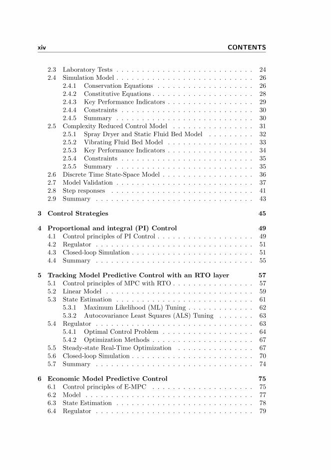
2.3 Laboratory Tests . . . . . . . . . . . . . . . . . . . . . . . . . . . 242.4 Simulation Model . . . . . . . . . . . . . . . . . . . . . . . . . . . 26
2.4.1 Conservation Equations . . . . . . . . . . . . . . . . . . . 262.4.2 Constitutive Equations . . . . . . . . . . . . . . . . . . . . 282.4.3 Key Performance Indicators . . . . . . . . . . . . . . . . . 292.4.4 Constraints . . . . . . . . . . . . . . . . . . . . . . . . . . 302.4.5 Summary . . . . . . . . . . . . . . . . . . . . . . . . . . . 30
2.5 Complexity Reduced Control Model . . . . . . . . . . . . . . . . 312.5.1 Spray Dryer and Static Fluid Bed Model . . . . . . . . . 322.5.2 Vibrating Fluid Bed Model . . . . . . . . . . . . . . . . . 332.5.3 Key Performance Indicators . . . . . . . . . . . . . . . . . 342.5.4 Constraints . . . . . . . . . . . . . . . . . . . . . . . . . . 352.5.5 Summary . . . . . . . . . . . . . . . . . . . . . . . . . . . 35
2.6 Discrete Time State-Space Model . . . . . . . . . . . . . . . . . . 362.7 Model Validation . . . . . . . . . . . . . . . . . . . . . . . . . . . 372.8 Step responses . . . . . . . . . . . . . . . . . . . . . . . . . . . . 412.9 Summary . . . . . . . . . . . . . . . . . . . . . . . . . . . . . . . 43
3 Control Strategies 45
4 Proportional and integral (PI) Control 494.1 Control principles of PI Control . . . . . . . . . . . . . . . . . . . 494.2 Regulator . . . . . . . . . . . . . . . . . . . . . . . . . . . . . . . 514.3 Closed-loop Simulation . . . . . . . . . . . . . . . . . . . . . . . . 514.4 Summary . . . . . . . . . . . . . . . . . . . . . . . . . . . . . . . 55
5 Tracking Model Predictive Control with an RTO layer 575.1 Control principles of MPC with RTO . . . . . . . . . . . . . . . . 575.2 Linear Model . . . . . . . . . . . . . . . . . . . . . . . . . . . . . 595.3 State Estimation . . . . . . . . . . . . . . . . . . . . . . . . . . . 61
5.3.1 Maximum Likelihood (ML) Tuning . . . . . . . . . . . . . 625.3.2 Autocovariance Least Squares (ALS) Tuning . . . . . . . 63
5.4 Regulator . . . . . . . . . . . . . . . . . . . . . . . . . . . . . . . 635.4.1 Optimal Control Problem . . . . . . . . . . . . . . . . . . 645.4.2 Optimization Methods . . . . . . . . . . . . . . . . . . . . 67
5.5 Steady-state Real-Time Optimization . . . . . . . . . . . . . . . 675.6 Closed-loop Simulation . . . . . . . . . . . . . . . . . . . . . . . . 705.7 Summary . . . . . . . . . . . . . . . . . . . . . . . . . . . . . . . 74
6 Economic Model Predictive Control 756.1 Control principles of E-MPC . . . . . . . . . . . . . . . . . . . . 756.2 Model . . . . . . . . . . . . . . . . . . . . . . . . . . . . . . . . . 776.3 State Estimation . . . . . . . . . . . . . . . . . . . . . . . . . . . 786.4 Regulator . . . . . . . . . . . . . . . . . . . . . . . . . . . . . . . 79
CONTENTS xv
6.4.1 Optimization Methods . . . . . . . . . . . . . . . . . . . . 816.5 Closed-loop Simulation . . . . . . . . . . . . . . . . . . . . . . . . 826.6 Summary . . . . . . . . . . . . . . . . . . . . . . . . . . . . . . . 83
7 Application of MPC to an Industrial Spray Dryer 877.1 PLC, Industrial PC and SCADA Setup . . . . . . . . . . . . . . 887.2 MPC Program . . . . . . . . . . . . . . . . . . . . . . . . . . . . 88
7.2.1 MPC Algorithm . . . . . . . . . . . . . . . . . . . . . . . 907.2.2 Add-on Module . . . . . . . . . . . . . . . . . . . . . . . . 93
7.3 XML Definition File . . . . . . . . . . . . . . . . . . . . . . . . . 947.3.1 Process Outputs, Inputs and Disturbances . . . . . . . . . 947.3.2 Model Identification . . . . . . . . . . . . . . . . . . . . . 957.3.3 Regulator and RTO Tuning . . . . . . . . . . . . . . . . . 96
7.4 Closed-loop Performance . . . . . . . . . . . . . . . . . . . . . . . 977.4.1 Experiment . . . . . . . . . . . . . . . . . . . . . . . . . . 987.4.2 Economic Benefit . . . . . . . . . . . . . . . . . . . . . . . 100
7.5 Summary . . . . . . . . . . . . . . . . . . . . . . . . . . . . . . . 101
8 Conclusions and Perspectives 1038.1 Spray Dryer Modeling . . . . . . . . . . . . . . . . . . . . . . . . 1048.2 Model Predictive Control . . . . . . . . . . . . . . . . . . . . . . 1048.3 Industrial Application of MPC . . . . . . . . . . . . . . . . . . . 1058.4 Commercial Outlook . . . . . . . . . . . . . . . . . . . . . . . . . 105
Bibliography 106
A Experiment Data 119A.1 Estimation Experiment . . . . . . . . . . . . . . . . . . . . . . . 119A.2 Validation Experiment . . . . . . . . . . . . . . . . . . . . . . . . 123
II Papers 127
A An experimentally validated simulation model for a four stagespray dryer 129
B Comparison of Control Strategies for Optimization of SprayDryer Operation 147
C A Grey-Box Model for Spray Drying Plants 165
D Real-time economic optimization for a fermentation process us-ing Model Predictive Control 173
E Application of Constrained Linear MPC to a Spray Dryer 181

xvi CONTENTS
F Economic Optimization of Spray Dryer Operation using Non-linear Model Predictive Control 191
G Economic Optimization of Spray Dryer Operation using Non-linear Model Predictive Control with State Estimation 201
H Comparison of Linear and Nonlinear Model Predictive Controlfor Optimization of Spray Dryer Operation 211
I Industrial Application of Model Predictive Control to a MilkPowder Spray Drying Plant 219
Part I
Summary Report


Chapter 1
Introduction
In this chapter we motivate the need for Model Predictive Control (MPC) forspray drying plants. First, we present the megatrends that drives the foodindustry and explain how MPC can play an important role in leveraging thefuture challenges. We briefly motivate and describe the objective of the researchproject, highlight the state-of-the-art and give an outline of the thesis.
1.1 Megatrends in the Food Industry
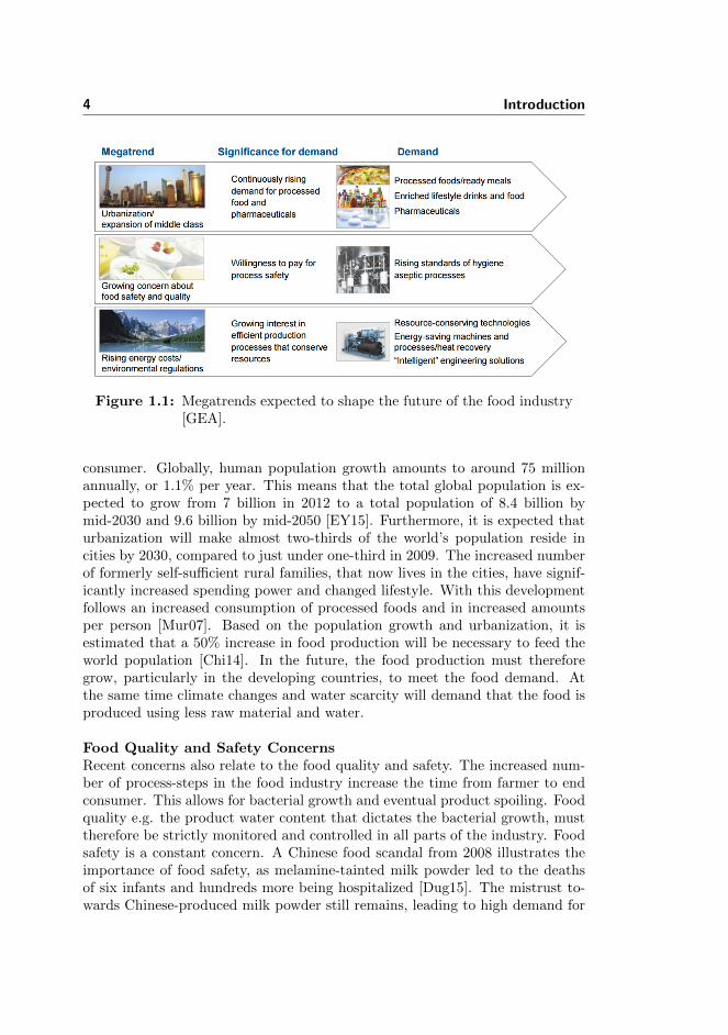
The world is currently undergoing major interrelated global changes such aspopulation growth, urbanization, climate change etc. These pose challengesthat have implications for human life and every industry all over the world.Thereby also for the food processing industry. Fig. 1.1 shows three megatrendsthat are expected in particularly to shape the future of the food industry. Theseare the urbanization and population growth, food quality and safety concernsand rising energy costs [GEA].
Urbanization and Population GrowthThe growing population and urbanization require ever increasing amounts offood to be collected, processed, shipped and stored before reaching the end
4 Introduction
Figure 1.1: Megatrends expected to shape the future of the food industry[GEA].
consumer. Globally, human population growth amounts to around 75 millionannually, or 1.1% per year. This means that the total global population is ex-pected to grow from 7 billion in 2012 to a total population of 8.4 billion bymid-2030 and 9.6 billion by mid-2050 [EY15]. Furthermore, it is expected thaturbanization will make almost two-thirds of the world’s population reside incities by 2030, compared to just under one-third in 2009. The increased numberof formerly self-sufficient rural families, that now lives in the cities, have signif-icantly increased spending power and changed lifestyle. With this developmentfollows an increased consumption of processed foods and in increased amountsper person [Mur07]. Based on the population growth and urbanization, it isestimated that a 50% increase in food production will be necessary to feed theworld population [Chi14]. In the future, the food production must thereforegrow, particularly in the developing countries, to meet the food demand. Atthe same time climate changes and water scarcity will demand that the food isproduced using less raw material and water.
Food Quality and Safety ConcernsRecent concerns also relate to the food quality and safety. The increased num-ber of process-steps in the food industry increase the time from farmer to endconsumer. This allows for bacterial growth and eventual product spoiling. Foodquality e.g. the product water content that dictates the bacterial growth, musttherefore be strictly monitored and controlled in all parts of the industry. Foodsafety is a constant concern. A Chinese food scandal from 2008 illustrates theimportance of food safety, as melamine-tainted milk powder led to the deathsof six infants and hundreds more being hospitalized [Dug15]. The mistrust to-wards Chinese-produced milk powder still remains, leading to high demand for
1.2 Milk Processing Powder Plant 5
milk buffer tank
homogenizer
centrifugal pump
cyclone
bagfilter
spray dryerevaporator
centrifugal pump
fluid bed
powder silo
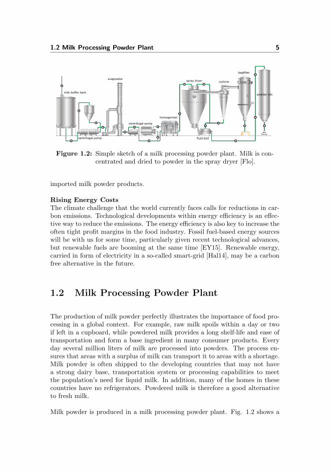
Figure 1.2: Simple sketch of a milk processing powder plant. Milk is con-centrated and dried to powder in the spray dryer [Flo].
imported milk powder products.
Rising Energy CostsThe climate challenge that the world currently faces calls for reductions in car-bon emissions. Technological developments within energy efficiency is an effec-tive way to reduce the emissions. The energy efficiency is also key to increase theoften tight profit margins in the food industry. Fossil fuel-based energy sourceswill be with us for some time, particularly given recent technological advances,but renewable fuels are booming at the same time [EY15]. Renewable energy,carried in form of electricity in a so-called smart-grid [Hal14], may be a carbonfree alternative in the future.
1.2 Milk Processing Powder Plant
The production of milk powder perfectly illustrates the importance of food pro-cessing in a global context. For example, raw milk spoils within a day or twoif left in a cupboard, while powdered milk provides a long shelf-life and ease oftransportation and form a base ingredient in many consumer products. Everyday several million liters of milk are processed into powders. The process en-sures that areas with a surplus of milk can transport it to areas with a shortage.Milk powder is often shipped to the developing countries that may not havea strong dairy base, transportation system or processing capabilities to meetthe population’s need for liquid milk. In addition, many of the homes in thesecountries have no refrigerators. Powdered milk is therefore a good alternativeto fresh milk.
Milk powder is produced in a milk processing powder plant. Fig. 1.2 shows a

6 Introduction
66,300 kg/h
SprayDryer
Falling Film Evaporator
MVR
Concentrated MilkRaw Milk Milk Powder
Evaporated Water7050 kg/hEvaporated Water
7500 kg/h at 3% water
14,550 kg/h at 50% solid
80,800 kg/h at 9% solid
1.04 MWEnergy Consumption
8.84 MWEnergy Consumption
Figure 1.3: Example of combining the MVR and the spray drying tech-nologies. The MVR technology is significantly more efficientthan the spray drying process.
schematic of a milk powder process, from standardized raw milk to final milkpowder. The production of milk powder requires large amounts of energy, partic-ularly in the spray drying process, due to the high latent heat of vaporization andthe inherent inefficiency of using hot air as the drying medium [Muj12,VdJ03].Drying processes are known to be the most energy consuming processes used inthe food industry. For example, the Dutch dairy industry required 1.4 PJ fordrying its whey and milk powder in 2007 [FASdJ10]. In order to save energy,an intermediate falling film evaporator is added to remove a large portion of thewater from the milk before it is sent to the spray dryer [VdJ03].
A Mechanical Vapor Re-compression (MVR) evaporator consumes only 55 MJ/tonevaporated water which gives an energy efficiency of above 40 (4000%). Thespray dryer consumes 4500 MJ/ton evaporated water leading to an energy ef-ficiency of 0.5 (50%). Thus, considerably lower than what can be achieved inthe MVR [FASdJ10]. Fig. 1.3 illustrates the inherent advantage of combiningan evaporator and a spray dryer. In the example, we assume that a milk pow-der plant produces 7500 kg/h of skim milk powder with 3% residual moisturecontent while receiving skim milk at 9% solids content. The product flows arethen given for the two processes assuming an intermediate milk concentrationof 50%. The energy consumption is computed according to the above efficien-cies [FASdJ10]. As can be seen, the raw milk flow intake sums to 80,800 kg/h,which is considerably more than the 7500 kg/h of final powder. Also, notice that66,300 kg/h of water is evaporated in the evaporator while only consuming 1.04MW of energy, compared to 7050 kg/h of water evaporated in the spray dryerwhile consuming 8.84 MW of energy. Thus, we seek to maximize the evaporationin the evaporator to save energy in the spray drying process. As a consequence,the evaporator should produce as high an intermediate milk concentration aspossible [FASdJ10]. However, at a certain milk concentration fouling starts in

1.3 Spray Drying 7
Figure 1.4: Skim milk powder (SMP) prices are currently at a six-yearlow. Prices provided by Clal [Cla]
the evaporator. Therefore, there is an upper limit to the amount of water thatcan be removed in the evaporator [VdJ03]. The milk powder moisture contentshould also be maximized to reduce the necessary amount of evaporation in thespray dryer [VdJ03]. The shelf-life of the powder limits the maximum moisturecontent.
Milk powder processing plants must stay profitable to form a sustainable busi-ness case. Profitability is given by the price of the produced powder minus thecost of running the process i.e. raw material and energy costs. Fig. 1.4 showsthat the milk powder price has recently fallen to a six-year low. The profit istherefore squished to a minimum, motivating the producers to maximize profitby decreasing running costs e.g. through a better utilization of the energy andraw materials.
1.3 Spray Drying
Spray drying as a concept can be tracked back to a filed patent in the 1860s.However, it took nearly 50 years for the first commercial successful dryer designto be developed and operated [Mas02]. The latest development is the four-stagespray dryer (marketed by GEA Process Engineering A/S as a Multi-Stage Dryer,
8 Introduction
MSDTM) which is widely used for production of milk powder and other foodpowders. It combines drying in four stages to increase the energy efficiency andthe product quality.
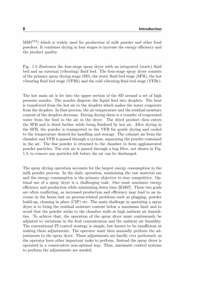
Fig. 1.5 illustrates the four-stage spray dryer with an integrated (static) fluidbed and an external (vibrating) fluid bed. The four-stage spray dryer consistsof the primary spray drying stage (SD), the static fluid bed stage (SFB), the hotvibrating fluid bed stage (VFBh) and the cold vibrating fluid bed stage (VFBc).
The hot main air is let into the upper section of the SD around a set of highpressure nozzles. The nozzles disperse the liquid feed into droplets. The heatis transferred from the hot air to the droplets which makes the water evaporatefrom the droplets. In that process, the air temperature and the residual moisturecontent of the droplets decrease. During drying there is a transfer of evaporatedwater from the feed to the air in the dryer. The dried product then entersthe SFB and is dried further while being fluidized by hot air. After drying inthe SFB, the powder is transported to the VFB for gentle drying and cooledto the temperature desired for handling and storage. The exhaust air from thechamber and VFB is passed through a cyclone, separating the powder containedin the air. The fine powder is returned to the chamber to form agglomeratedpowder particles. The exit air is passed through a bag filter, not shown in Fig.1.5, to remove any particles left before the air can be discharged.
The spray drying operation accounts for the largest energy consumption in themilk powder process. In the daily operation, minimizing the raw material useand the energy consumption is the primary objective to stay competitive. Op-timal use of a spray dryer is a challenging task. One must maximize energyefficiency and production while minimizing down time [KM07]. These two goalsare often conflicting, as increased production and efficiency may lead to an in-crease in the hours lost on process-related problems such as plugging, powderbuild-up, cleaning in place (CIP) etc. The main challenge in operating a spraydryer is to bring the residual moisture content below a maximum limit and toavoid that the powder sticks to the chamber walls at high ambient air humidi-ties. To achieve that, the operation of the spray dryer must continuously beadjusted to variations in the feed concentration and the ambient air humidity.The conventional PI control strategy is simple, but known to be insufficient atmaking these adjustments. The operator must then manually perform the ad-justments to the spray dryer. These adjustments are hardly ever performed, asthe operator have other important tasks to perform. Instead the spray dryer isoperated in a conservative non-optimal way. Thus, automatic control systemsto perform the adjustments are needed.

1.4 Model Predictive Control 9
SD
Main Air
SFB Air
Feed
Cooling
SFB
VFBh Air VFBc AirPowder
VFBh VFBc
ExhaustExit
Fines
Exhaust
Figure 1.5: Principle diagram of the four-stage spray dryerwith an integrated static fluid bed and an externalvibrating fluid bed.
1.4 Model Predictive Control
For a long time linear Model Predictive Control (MPC) has been considered thepreferred control methodology in the process industries and academia for com-plex processes. MPC provides an integrated solution for controlling processeswith multivariate and cross-coupled dynamics, time delays and constraints onboth the inputs and the states [DHN09,RAB12]. Forecasts of the disturbancesare also naturally utilized in MPC. In general, these features allows operationcloser to the process constraints which may lead to greater profits and/or betterperformance. Fig. 1.6 illustrates how optimal control can reduce the varianceof the controlled outputs, making it possible to squeeze and shift the target toa more profitable value. In spray drying, the profit significantly benefit fromreducing the variance of the residual moisture content. This makes it possibleto shift the moisture content to a slightly higher level which increase the yield,by selling more water as product, while reducing the energy consumption due toless evaporation. To illustrate the idea, we assume that MPC is able to increasethe average residual moisture content by only 0.2 p.p. at a milk powder plantthat produces 7500 kg/h of skim milk powder (from Fig. 1.3). The annual profit

10 Introduction
Figure 1.6: MPC makes it possible to squeeze and shift the residualmoisture content to a more profitable value.
increase is then
= 0.2 p.p. · 7500 kg/hr · 7200 hr/year · 2.5 e/kg
= 224, 100 e/year
The profit increase illustrates the importance of optimal control well.
MPC refers to a control algorithm that explicitly incorporates a process model,to predict the future response of the controlled process and take appropriateaction through optimization. Traditionally, MPC is designed using objectivefunctions penalizing deviations from a given target and fast movements in theinputs. Often MPC is combined with a Real-Time Optimization (RTO) layer[FCB15, Eng07, DNJN11, AO10, EH01], in a so-called two-layer structure. Theupper-level RTO system provides targets under different conditions such as feedcompositions, production rates, energy availability, feed and product prices tothe lower-level control system in order to maintain the process operation as closeas possible to the economic optimum [AG10]. The RTO layer and the MPClayer have different time scales and the RTO layer assumes that the closed-loop process will reach a steady-state. Transients, such as target transitionsand the inherent effect of disturbances, may thus lead to loss of economicalefficiency. Recent advances within process optimization focus on optimizing thehigher-level objectives, such as economics, directly in the objective function ofthe MPC, known as Economic MPC (E-MPC) [RA09, RAB12, AAR12, Gru13,Gru12]. Thus, the E-MPC eliminates the presented drawbacks. E-MPC is

1.5 Thesis Objective 11
maturing and has now been successfully applied to an increasing number ofcontinuous processes.
MPC is the natural choice to automatically optimize the operation of spraydryers, as it naturally handles the dryers multiple and cross-coupled inputs andoutputs, time delays, process constraints and feed-forward of disturbances suchas the feed concentration and the ambient air humidity. The MPC will thenallow operation closer to the process constraints which may increase profits with-out violating the process constraints. The application of MPC to spray dryerscan therefore be an effective way to support the operators in the challengingtask of optimizing the spray dryer operation.
1.5 Thesis Objective
The aim of this project is to investigate the application of MPC to optimize theoperation of four-stage spray dryers. To facilitate this goal, new models andMPC strategies for the process will be developed.
Spray Dryer ModelingOne of the key objectives is to develop first-principles dynamic models of a four-stage spray dryer. The purpose of the simulation model is to enable detailedclosed-loop simulations of the spray dryer at different operating points, suchthat the model can facilitate development and comparison of control strategies.The purpose of the control model is to provide a simpler model that can be usedfor state estimation and prediction in the controllers. We perform experimentson a GEA MSDTM-20 spray dryer to identify the model parameters and validatethe model accuracy for this dryer. Powder characteristics are identified bylaboratory tests. The models provide the key performance indicators (KPIs)such as the profit of operation, the energy consumption, the energy efficiency,the product flow rate and the stickiness of the powder in the spray dryer. Thesefeatures are important for comparison of the different control strategies.
Model Predictive ControlA key objective is to automatically adjust the dryer to variations in the feedand the ambient air humidity, such that the profit of operation is maximizedwhile the energy consumption is minimized, the residual moisture content in thepowder is controlled below the specification and sticky powder is prevented frombuilding up on the dryer walls. We do this by first developing a traditional lineartarget tracking MPC algorithm with an RTO layer for calculation of cost optimaltargets. This is the conventional approach and may perform well in many cases.Secondly, we develop an Economic Nonlinear MPC that brings economic costs

12 Introduction
directly into the objective function of the controller. The controller will thenconstantly bring the process to the most cost efficient state of operation, whileconsidering constraints of the process such as stickiness and moisture limits ofthe powder. The MPCs include a state estimator (soft-sensor) for estimationof the current state of the dryer. A second goal is therefore to investigate thedesign and tuning of this state estimator, such that missing observations arehandled well. The observations that can be missing for shorter periods are theexhaust air humidity and the residual moisture content of the powder, whichmust be handled accordingly.
Application of MPC to an Industrial Spray DryerA key objective is to demonstrate the MPC strategy on a full-scale industrialfour-stage spray dryer. In that effort, we will document the complete stan-dalone MPC solution i.e. the spray dryer setup, the MPC algorithm, the modelidentification and tuning etc. We also document the KPIs obtained during thedemonstration experiments. Our goal is that the MPC strategy will be widelyused as part of the commercial control solution.
1.6 State-of-the-Art
In this section, we provide an overview of the state-of-the-art and give somereferences to important literature in the fields that are addressed in this thesis.The collection of papers written during the project, included in Part II, alsocontain literature studies and references relevant to the specific paper.
1.6.1 Spray Dryer Modeling and Control
Mathematical modeling and control of spray dryers have been subjects of re-search for many decades. The models have traditionally been classified intostatic and dynamic models. Mathematical models of spray dryers exist as de-tailed computational fluid dynamics (CFD) models for static design orientedsimulation [CPO01, PCLA09, WDM+08a, Kie97], and as models for dynamicsimulation. The models for dynamic simulation are linear models for controldesign that are also used for closed-loop simulation [Cla88, TTA09, TIKT11]and lumped first-principles engineering models [SH08, Sha06, ZGS+88, ZPC91,PCF95, GJC+94]. The purpose of the dynamic simulation models is often tofacilitate analysis and synthesis of advanced control schemes.
Clarke [Cla88] designs a Generalized Predictive Controller (GPC) for a spray

1.6 State-of-the-Art 13
dryer and base the controller on the CARIMA model, but does not providea simulation model. Tan et al [TTA09, TIKT11] provide continuous transferfunctions of first order with a delay that they use for PI controller design as wellas closed loop simulation. They report models for spray drying of full creammilk [TTA09] as well as spray drying of whole milk and orange juice [TIKT11].
A lumped first-principles model of a single-stage spray dryer is developed in[SH08, Sha06]. Mass and energy balances describe the air temperature, themean particle size and the residual moisture content of the powder. Based onthe model PI controllers are developed to control the mean particle size and theresidual moisture content of the powder. A mathematical model based on mass,energy and momentum equations are formulated and solved in [ZGS+88]. Themodel describes the moisture content and particle size of a single spray driedpowder particle and fits the experimental data within 10-15% error. In [ZPC91]a dynamic model of a single-stage spray dryer is developed from first-principlesand is validated experimentally to assist in control simulation studies. Themodel provides the moisture content and particle size of the powder as well asthe exhaust air temperature and humidity. The inferred moisture content iscontrolled in a cascade PI configuration to mitigate the effect of disturbances.Reference [PCF95] extends the model in [ZPC91] by further developing themodel for drying of milk powder, and controls the exhaust air humidity toindirectly control the powder moisture content. A single-stage dynamic modelis developed by [GJC+94] for the simulation of the residual moisture controland air temperatures in an industrial detergent spray drying process. A linear-quadratic-Gaussian (LQG) controller for residual moisture control is reported.The moisture content for drying of milk powders in a spouted bed dryer isdescribed by a physical-mathematical model in [VFF15]. The evaporation termis estimated using a neural network and the inferred powder moisture content iscontrolled by adjusting the inlet air temperature with a PI controller. A detailedreview of the status and future of modeling and control for spray drying of dairyproducts is given in [OC05].
The above first-principles models simulate single-stage spray dryers or a spoutedbed dryer. In-line powder residual moisture sensors are often not available.Therefore, the above models are based on irregularly sampled off-line laboratorymeasurements of the residual moisture. We present models and control strate-gies for a four-stage spray dryer that is validated against in-line residual moisturemeasurements and control strategies that utilizes in-line measurements.

14 Introduction
Figure 1.7: Classification of RTO methods and their Philosophies [FCB15].
1.6.2 Model Predictive Control
The use of tracking MPC in conjunction with an RTO layer (the so-called two-layer structure) dates back to the late 1970s-1980s [Eng07, DNJN11]. Sincethen the MPC with an RTO layer has become the standard approach for imple-menting steady-state economic optimization in processes that operate aroundnominal steady-states. The RTO methods aim to reject the effect of model un-certainty on the economic performance by the use of process measurements. Asindicated by Fig. 1.7, the RTO methods divide into two classes, explicit andimplicit iterative optimization methods [FCB15,EH01]. Explicit methods utilizea model and measured disturbances for computing the optimal operating point.The explicit methods further divide into two main classes; adaptation of themodel and adaptation of the optimization problem. In model adaptation, themeasurements can be used to refine the model by updating the model parame-ters. Correction terms to the optimization problem are determined in optimiza-tion problem adaptation. No model parameter identification is performed. Thetwo methods both rely on the repeated solving of a model-based optimizationproblem. Thus, rather accurate models are needed, but the model informa-tion can be used to achieve better economic performance. Implicit methodsseek to optimize the profit of operation, without the use of a rigorous model.Well known examples of implicit methods are extremum-seeking [AK03] andself-optimizing controllers [Sko00]. Extremum-seeking methods impose smallchanges to the steady-state of the process, and a cost function gradient is esti-mated. On that basis, steps towards a lower cost are taken. The advantage isthat no model is required, but the method can be slow and requires the processto reach steady-state before a new step can be taken.
1.6 State-of-the-Art 15
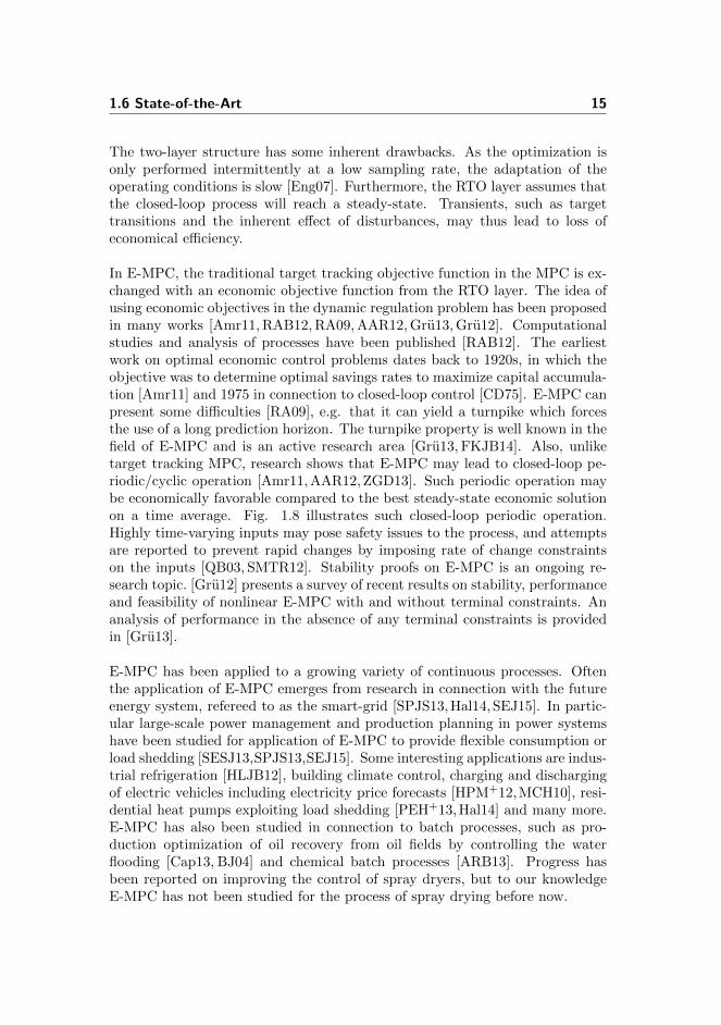
The two-layer structure has some inherent drawbacks. As the optimization isonly performed intermittently at a low sampling rate, the adaptation of theoperating conditions is slow [Eng07]. Furthermore, the RTO layer assumes thatthe closed-loop process will reach a steady-state. Transients, such as targettransitions and the inherent effect of disturbances, may thus lead to loss ofeconomical efficiency.
In E-MPC, the traditional target tracking objective function in the MPC is ex-changed with an economic objective function from the RTO layer. The idea ofusing economic objectives in the dynamic regulation problem has been proposedin many works [Amr11, RAB12, RA09, AAR12, Gru13, Gru12]. Computationalstudies and analysis of processes have been published [RAB12]. The earliestwork on optimal economic control problems dates back to 1920s, in which theobjective was to determine optimal savings rates to maximize capital accumula-tion [Amr11] and 1975 in connection to closed-loop control [CD75]. E-MPC canpresent some difficulties [RA09], e.g. that it can yield a turnpike which forcesthe use of a long prediction horizon. The turnpike property is well known in thefield of E-MPC and is an active research area [Gru13, FKJB14]. Also, unliketarget tracking MPC, research shows that E-MPC may lead to closed-loop pe-riodic/cyclic operation [Amr11, AAR12, ZGD13]. Such periodic operation maybe economically favorable compared to the best steady-state economic solutionon a time average. Fig. 1.8 illustrates such closed-loop periodic operation.Highly time-varying inputs may pose safety issues to the process, and attemptsare reported to prevent rapid changes by imposing rate of change constraintson the inputs [QB03, SMTR12]. Stability proofs on E-MPC is an ongoing re-search topic. [Gru12] presents a survey of recent results on stability, performanceand feasibility of nonlinear E-MPC with and without terminal constraints. Ananalysis of performance in the absence of any terminal constraints is providedin [Gru13].
E-MPC has been applied to a growing variety of continuous processes. Oftenthe application of E-MPC emerges from research in connection with the futureenergy system, refereed to as the smart-grid [SPJS13,Hal14,SEJ15]. In partic-ular large-scale power management and production planning in power systemshave been studied for application of E-MPC to provide flexible consumption orload shedding [SESJ13,SPJS13,SEJ15]. Some interesting applications are indus-trial refrigeration [HLJB12], building climate control, charging and dischargingof electric vehicles including electricity price forecasts [HPM+12,MCH10], resi-dential heat pumps exploiting load shedding [PEH+13,Hal14] and many more.E-MPC has also been studied in connection to batch processes, such as pro-duction optimization of oil recovery from oil fields by controlling the waterflooding [Cap13, BJ04] and chemical batch processes [ARB13]. Progress hasbeen reported on improving the control of spray dryers, but to our knowledgeE-MPC has not been studied for the process of spray drying before now.

16 Introduction
Figure 1.8: Closed-loop simulation of a system un-der periodic E-MPC [Amr11].
1.6.3 Application of MPC to an Industrial Spray Dryer
Attempts have been made to improve the industrial control of spray dryers overtime. The solutions fall mainly into two groups; the extension of the conven-tional PI control strategy and the MPC strategies with target optimization.PI control strategies are reported in patents [Nie13, SB11]. These adjust theexhaust air temperature or exhaust air humidity to maintain a stable powderresidual moisture content. [GJC+94] develop an LQG controller for residualmoisture control in an industrial detergent spray drying process. IndustrialMPCs are reported and seem to rely on empirically based step-response modelsand least-squares methods for estimation of the residual moisture content of thepowder [Vai,Roc]. [Vai] reports up to 20% increase in production capacity.
1.7 Thesis Contribution
The key contributions of this thesis are described in the following three sections.
1. Modeling of a four-stage spray dryer
We develop two first-principles engineering models of a four-stage spraydryer. The simulation and control models combines physical knowledge ofthe process with unknown parameters identified from an experiment.

1.7 Thesis Contribution 17
The novelty of the proposed models lies in three main features: 1) Themodels enable simulations of the spray dryer at different operating pointswith high accuracy and is validated against in-line measurements of thepowder residual moisture content. 2) The key performance indicators(KPIs) such as the profit of operation, the product flow rate, the energyconsumption and the energy efficiency are provided. 3) In addition, themodels offer stickiness constraints of the powder in each stage of the spraydryer.
To the author’s knowledge, there does not exist such a model that com-bines all three features for a four-stage spray dryer. These features makethe simulation model well suited for closed-loop comparison of the pro-cess economics associated to different control strategies. The complexityreduced control model, based on the simulation model, is well suited forstate estimation and predictions in the MPCs.
2. Development and simulation of control strategies
We develop and demonstrate by simulation two proposed control strate-gies and compare them against the conventional PI control strategy; thetwo strategies are based on the MPC with an RTO layer strategy andthe E-MPC strategy. The performance of the controllers are studied andevaluated according to the performance indicators above.
The novelty of the proposed MPC with RTO control strategy lies in threemain features: 1) It offers independent control of the exhaust air tem-perature, the exhaust air humidity, the SFB powder temperature and theresidual moisture content of the powder. This enables control of the spraydryer such that the stickiness of the powder and the residual moisture con-tent can be operated closer to its limits. 2) It offers significantly improvedeconomical performance and reduced energy consumption while avoidingviolation of the process constraints. 3) In addition, the state estimatoroffers a built-in method for handling missing observations as a so-calledsoft-sensor.
The novelty of the proposed E-MPC control strategy consists of the twomain features: 1) It combines the MPC and RTO layers into one E-MPCcontrol layer, such that the economical performance is constantly maxi-mized while avoiding violation of the process constraints. 2) It providesan even further improved profit of operation compared to the MPC withRTO control strategy. It also offers a state estimator that handles missingobservations.
To the author’s knowledge, there does not exist such a comprehensivestudy and evaluation of the economic benefits of using MPC with RTOas well as E-MPC for a four-stage spray dryer. Furthermore, we havenot seen any comparison of such control strategies to the conventional PIcontrol strategy.

18 Introduction
3. Application of MPC to an industrial spray dryer
We demonstrate that the proposed MPC with an RTO layer is applicableto an industrial four-stage spray dryer. The industrial dryer is a GEAMSDTM-1250 type producing enriched milk powder.
The novelty of the industrial implementation of the MPC with an RTOlayer lies in 1) The fully integrated and functioning solution, that is used inthe daily operation of the milk powder spray dryer. During the project, weparticipated in the development and installation of the in-line instrumentsfor the measurement of the exhaust air humidity and the residual moisturecontent of the powder. These provide high quality measurements andare actively used in the MPC. 2) We document in detail the installationand workings of the industrial MPC solution. 3) The performance ofthe controller is evaluated and show that the profit of operation, productflow rate and the energy efficiency are improved significantly compared toconventional PI control. This confirms the results obtained by the closed-loop simulations of the MPC with RTO control strategy.
Industrial MPC solutions exists, but to the author’s knowledge, there hasnot been published any detailed data of the performance of these nor hasthe MPC strategies been as well documented as in this work. It is ourexperience that the industrial MPC solutions seldom incorporate in-linemeasurements of the exhaust air humidity and powder residual moisturecontent.
We address these contributions in Part I, the summary report, and in Part II,the published papers.
1.8 Thesis Organization
The thesis is divided into two parts. Part I is comprised of a summary reportwhich gives an overview of the main results and contributions of the thesis. PartI is composed of the chapters 1 to 8. Chapter 1 provides an introduction and thebackground for the thesis. It presents the four-stage spray drying process and theMPC algorithm in general terms. Chapter 2 provides a short description of themodeling of the spray dryer. Chapter 3 provides an overview of the three controlstrategies considered in Chapter 4-6. Chapter 4 presents the conventional PIcontrol strategy, Chapter 5 presents the MPC with RTO control strategy andChapter 6 presents the E-MPC control strategy. Application of MPC to anindustrial spray dryer is presented in Chapter 7. Conclusions are provided inChapter 8. Part II is comprised of the research papers published and submittedduring the project period.

Chapter 2
Four-Stage Spray DryerModels
In this chapter, we describe the four-stage spray dryer and present two ex-periments conducted on the dryer and laboratory tests on the final powder.We formulate a nonlinear index-1 differential algebraic equations (DAE) modelfor simulation purposes and a simpler nonlinear ordinary differential equation(ODE) model for design of model based controllers. A linear model is alsoprovided for design of linear model based controllers. The model parametersare identified based on the experiments and we show that the models fit theexperimental data well.
The chapter is a summary of Paper A, Paper C, Paper E, and Paper G.
2.1 Equipment Setup
The four-stage spray dryer that is used in this project combines drying in fourstages to increase the energy efficiency and the product quality; spray dryingat the top of the dryer chamber (SD), drying in an integrated static bed atthe bottom of the dryer chamber (SFB) and drying in an external vibratingfluidized bed (VFB). Fig. 2.1 illustrates the working principle of the four-stage

20 Four-Stage Spray Dryer Models
SD
Main Air
SFB Air
Feed
Cooling
SFB
TSD,Yab
TSFB
Ff
Sf
Tf
VFBh Air VFBc AirPowder
VFBh VFBc
ExhaustExit
Fines
Exhaust
TVFBh TVFBc
Scd
Tsfb, Fsfb, Yamb
Tmain, Fmain, Yamb
Tvfbh, Fvfbh, Yamb Tvfbc, Fvfbc, Yamb
Sab
Figure 2.1: Principle diagram of the four-stage spray dryer withindication of the inputs, disturbances and outputs.
spray dryer as well as the inputs, disturbances and outputs. The outputs arethe exhaust and stage temperatures, TSD, TSFB, TVFBh and TVFBc, the exhaustair humidity, Yab, and the SFB and VFBc stage residual moisture content ofthe powder, Sab and Scd. The inputs are the feed flow rate, Ff, the main inletair temperature, Tmain, the SFB inlet air temperature, Tsfb and the VFBh inletair temperature, Tvfbh. The main disturbances are the ambient air humidity,Yamb, the feed solids concentration, Sf, and the feed temperature, Tf. The otherdisturbances are the main inlet air flow rate, Fmain, the SFB inlet air flow rate,Fsfb, and the VFBh inlet air flow rate, Fvfbh. The cooling of the powder isperformed with unheated ambient air in the VFBc stage at an inlet air flowrate, Fvfbc, and temperature, Tvfbc.
The experiments in this project are conducted on a small-scale industrial typeGEA MSDTM-20 spray dryer. Fig. 2.2 shows a picture of the dryer at thetest-station. The control room, the VFB, the feed tank and the feed pump arelocated on the ground floor. The SFB is located at the first floor and the spraydryer chamber is located on the first and above floors. The bag filter is the unitto the right in the picture.

2.1 Equipment Setup 21
Figure 2.2: The picture of the MSDTM-20 spray dryerseen from the ground floor.
Fig. 2.3 shows the inside of the dryer chamber, divided into an upper SDpart (left) and the lower SFB part (right). The pictures are taken after theexperiment was conducted and shows none to small signs of powder deposits onthe cone of the dryer chamber.
The dryer is fitted with an abundance of temperature sensors, pressure sensorsand air mass-flow meters. We note that all the inlet air mass-flow meters have anoffset in the readings. This offset is identified from an air humidity mass balanceof the spray dryer using measurements of the air flow rates, the feed flow rate andthe air humidity. We estimated the offset to be 5%, which we subtracted fromthe readings before these are used in the model. A combined feed mass-flow anddensity meter is fitted to the feedline. The feed solids concentration is estimated

22 Four-Stage Spray Dryer Models
(a) The SD stage with nozzle and exhaust airoutlet.
(b) The SFB at the bottom of the dryerchamber.
Figure 2.3: Picture of the SD and SFB stages. The picture is taken after theexperiments and shows none to small signs powder deposits.
from the feed density and feed temperature, as we know the density of theindividual components in the feed i.e. the solids and water. We fitted residualmoisture instruments to the SFB and VFB powder outlets and an exhaust airhumidity instrument to the exhaust air duct. We also fit vapor injectors to theinlet air streams, to control the ambient air humidity supplied to the dryer.The manipulated inputs are the reference temperature of the electric heaters onthe main, SFB and VFBh inlet air streams. The feed pump speed is controlleddirectly. All these sensors, instruments as well as actuators are connected andhandled by a single SIEMENS S7 PLC system and a WonderwareTM Intouchv10.5 SCADA system from Schneider Electric.
The experiments are based on drying of maltodextrin DE-18. Maltodextrin isa starch based polysaccharide that is used as a food additive. Maltodextrin isused because the feed can then be re-wetted and the composition is well defined.We use maltodextrin DE-18 as a substitute to milk because milk is difficult tohandle over longer periods due to natural deterioration. Stickiness and dryingproperties are sought to be comparable to milk by the selection of the DE-18type. The DE number indicates the stickiness and drying properties of themaltodextrin.
The residual moisture content is measured using two ProFossTM in-line analyzersplaced at the SFB and VFBc powder outlets. Fig. 2.4 shows the position ofthe residual moisture instruments. The SFB sensor is placed after the powderdischarge piston and the VFBc sensor is placed after the final powder outlet.The powder from the VFBc powder outlet is collected in a container.
2.2 Experimental Tests 23
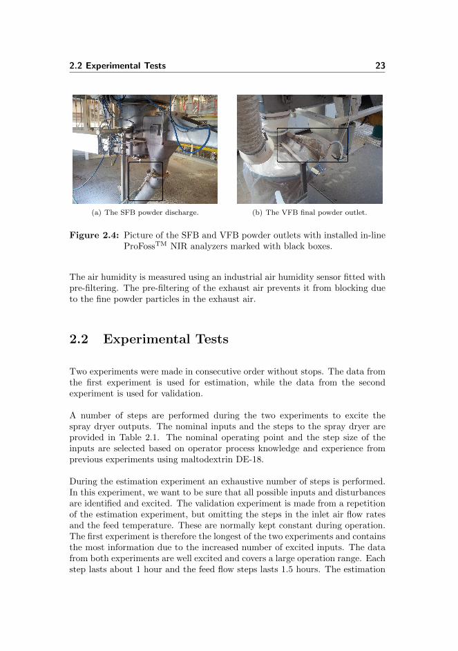
(a) The SFB powder discharge. (b) The VFB final powder outlet.
Figure 2.4: Picture of the SFB and VFB powder outlets with installed in-lineProFossTM NIR analyzers marked with black boxes.
The air humidity is measured using an industrial air humidity sensor fitted withpre-filtering. The pre-filtering of the exhaust air prevents it from blocking dueto the fine powder particles in the exhaust air.
2.2 Experimental Tests
Two experiments were made in consecutive order without stops. The data fromthe first experiment is used for estimation, while the data from the secondexperiment is used for validation.
A number of steps are performed during the two experiments to excite thespray dryer outputs. The nominal inputs and the steps to the spray dryer areprovided in Table 2.1. The nominal operating point and the step size of theinputs are selected based on operator process knowledge and experience fromprevious experiments using maltodextrin DE-18.
During the estimation experiment an exhaustive number of steps is performed.In this experiment, we want to be sure that all possible inputs and disturbancesare identified and excited. The validation experiment is made from a repetitionof the estimation experiment, but omitting the steps in the inlet air flow ratesand the feed temperature. These are normally kept constant during operation.The first experiment is therefore the longest of the two experiments and containsthe most information due to the increased number of excited inputs. The datafrom both experiments are well excited and covers a large operation range. Eachstep lasts about 1 hour and the feed flow steps lasts 1.5 hours. The estimation

24 Four-Stage Spray Dryer Models
Table 2.1: The table show the nominal inputs and the input steps that areused during the estimation and validation experiments.
Nominal Estimation Step Validation StepInput Down Up Down Up
Ff 85 kg/hr 65 kg/hr 120 kg/hr 70 kg/hr 117 kg/hrTf 50C 42C 60C - -Sf 50% 40% - 40% -
Fmain 1700 kg/h 1500 kg/h 1900 kg/h - -Tmain 170C 160C 180C 160C 180CYmain 3 g/kg - 15− 25 g/kg - 15 g/kgFsfb 470 kg/h 330 kg/h 570 kg/h - 600 kg/hTsfb 90C 80C 100C 80C 100CYsfb 3 g/kg - 15− 25 g/kg - 15 g/kgFvfbh 280 kg/h - 410 kg/h - -Tvfbh 60C - 80C - 80CYvfbh 3 g/kg - - - -Fvfbc 280 kg/h - - - -Tvfbc 35C - - - -Yvfbc 3 g/kg - - - -
experiment lasts in total 28 hours and the validation experiment lasts in total17 hours.
Appendix A reports the recorded inputs, disturbances and outputs for the esti-mation and validation experiments.
2.3 Laboratory Tests
The powder equilibrium moisture content, Xeq, is a product dependent functionthat describes the moisture content at which water cannot be evaporated fromthe powder any longer. The dynamic models, presented later, make extensiveuse of this function. We identify this function based on already dried powderin the laboratory by adsorption isotherms studies. We fit the Guggenheim-Anderson-de Boer (GAB) equation [BSM06], which has a theoretical backgroundbased on equilibrium assumptions. The GAB function has the form
Xeq =C ·K ·Xm · RH
(1−K · RH)(1−K · RH + C ·K · RH)(2.1)
in which Xm, C and K are temperature dependent Arrhenius expressions andRH is the relative humidity of the air. Fig. 2.5(a) illustrates 15 laboratory data

2.3 Laboratory Tests 25
Relative humidity, RH [%]
0 5 10 15 20 25 30 35 40 45
Re
sid
ua
l m
ois
ture
, 1
-S [
%]
1
2
3
4
5
6
7
8
T=25oC
T=50oC
T=75oC
Isotherm Sorption Curves of Maltodextrin DE-18
Data
GAB model
(a) The equilibrium moisture content.
Particle temperature, T [oC]
30 40 50 60 70 80 90 100 110
Resid
ual m
ois
ture
, 1-S
[%
]
2
3
4
5
6
7
8
9
10
Stickiness of Maltodextrin DE-18
Tg boundary
Non sticky
very sticky
sticky
(b) The stickiness boundary.
Figure 2.5: Maltodextrin DE-18 laboratory data made from adsorptionisotherm experiments. The black lines indicate fitted equations.
points and the fitted GAB function. Temperatures were fixed at T = 25C, T =50C and T = 75C with relativity humidities between RH = 4.5% and RH =40.1%. The simulation model presented in Section 2.4 uses the GAB functionfitted to the data in Fig. 2.5(a). The control model presented in Section 2.5was developed later in the project, which made it possible to conduct a secondexperiment with data points at higher temperatures. Thus, the control modeluses a different GAB function fitted to the that data (not presented here). In theliterature, models already exist for maltodextrin [WDM+08b,FOS01,PCLA09].However, these models do not fit our data well.
Stickiness of powder can be predicted using the glass transition temperature,Tg, computed by the Gordon–Taylor equation (a mass-proportion-mixing rule)as [BBH04]
Tg =Tgp + kZTgw
1 + kZ(2.2)
Tgp = 144.8C (maltodextrin DE-18) and Tgw = −137C (water) are the glasstransition temperatures, Tg, of the solid and water fractions, respectively. Z isthe dry base residual moisture content at the surface of the powder. We fit (2.2)by estimation of a single constant, k = 6.296, to data from an additional exper-iment that indicates whether the powder in Fig. 2.5(a) has turned sticky afterbeing exposed to the specific temperature and air humidity conditions [BBH04].Fig. 2.5(b) shows the experiment results and the predicted glass transition tem-perature. Powder with a temperature above Tg is sticky. The predicted glasstransition temperatures in (2.2) coincide well with the measurements.
26 Four-Stage Spray Dryer Models
Air
Powder
Stage
Air inlet
Powder inlet
Air outlet
Y
X Rw
T
T
Powder outlet
Fs, T, XFs, Tin, Xin
Fda, Tin, Yin
Fda, T, Y
Ql
Qe
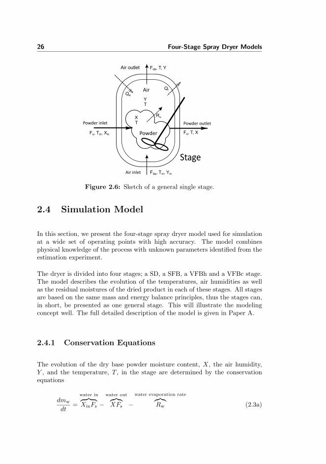
Figure 2.6: Sketch of a general single stage.
2.4 Simulation Model
In this section, we present the four-stage spray dryer model used for simulationat a wide set of operating points with high accuracy. The model combinesphysical knowledge of the process with unknown parameters identified from theestimation experiment.
The dryer is divided into four stages; a SD, a SFB, a VFBh and a VFBc stage.The model describes the evolution of the temperatures, air humidities as wellas the residual moistures of the dried product in each of these stages. All stagesare based on the same mass and energy balance principles, thus the stages can,in short, be presented as one general stage. This will illustrate the modelingconcept well. The full detailed description of the model is given in Paper A.
2.4.1 Conservation Equations
The evolution of the dry base powder moisture content, X, the air humidity,Y , and the temperature, T , in the stage are determined by the conservationequations
dmw
dt=
water in︷ ︸︸ ︷XinFs −
water out︷︸︸︷XFs −
water evaporation rate︷︸︸︷Rw (2.3a)
2.4 Simulation Model 27
dmv
dt=
vapor in inlet air︷ ︸︸ ︷YinFda −
vapor in outlet air︷ ︸︸ ︷Y Fda +
water evaporation rate︷︸︸︷Rw (2.3b)
dU
dt=
enthalpy of air flows︷ ︸︸ ︷(ha,in − ha,out)Fda +
enthalpy of powder flows︷ ︸︸ ︷(hp,in − hp,out)Fs +
enthalpy of mass exchange︷ ︸︸ ︷∆H in2out
e −heat exchange︷ ︸︸ ︷Qin2out
e −heat loss︷︸︸︷Ql
(2.3c)
where the state variables are the functions
mw = msX (2.4a)
mv = mdaY (2.4b)
U = mda(ha −RT ) +mshp +mmhm (2.4c)
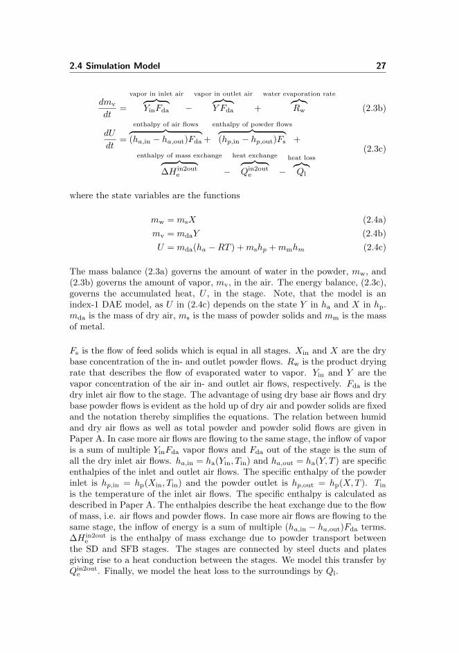
The mass balance (2.3a) governs the amount of water in the powder, mw, and(2.3b) governs the amount of vapor, mv, in the air. The energy balance, (2.3c),governs the accumulated heat, U , in the stage. Note, that the model is anindex-1 DAE model, as U in (2.4c) depends on the state Y in ha and X in hp.mda is the mass of dry air, ms is the mass of powder solids and mm is the massof metal.
Fs is the flow of feed solids which is equal in all stages. Xin and X are the drybase concentration of the in- and outlet powder flows. Rw is the product dryingrate that describes the flow of evaporated water to vapor. Yin and Y are thevapor concentration of the air in- and outlet air flows, respectively. Fda is thedry inlet air flow to the stage. The advantage of using dry base air flows and drybase powder flows is evident as the hold up of dry air and powder solids are fixedand the notation thereby simplifies the equations. The relation between humidand dry air flows as well as total powder and powder solid flows are given inPaper A. In case more air flows are flowing to the same stage, the inflow of vaporis a sum of multiple YinFda vapor flows and Fda out of the stage is the sum ofall the dry inlet air flows. ha,in = ha(Yin, Tin) and ha,out = ha(Y, T ) are specificenthalpies of the inlet and outlet air flows. The specific enthalpy of the powderinlet is hp,in = hp(Xin, Tin) and the powder outlet is hp,out = hp(X,T ). Tin
is the temperature of the inlet air flows. The specific enthalpy is calculated asdescribed in Paper A. The enthalpies describe the heat exchange due to the flowof mass, i.e. air flows and powder flows. In case more air flows are flowing to thesame stage, the inflow of energy is a sum of multiple (ha,in − ha,out)Fda terms.∆H in2out
e is the enthalpy of mass exchange due to powder transport betweenthe SD and SFB stages. The stages are connected by steel ducts and platesgiving rise to a heat conduction between the stages. We model this transfer byQin2out
e . Finally, we model the heat loss to the surroundings by Ql.

28 Four-Stage Spray Dryer Models
2.4.2 Constitutive Equations
The constitutive equations define the relations in the conservation equations.The product drying rate is governed by the thin layer equation. The thin layerequation models evaporation as a diffusion process [Lew21]
Rw = k1Dw(X −Xeq)ms (2.5)
X is the stage powder moisture content and Xeq = Xeq(T, Y )+Xadd is the equi-librium moisture content described in Section 2.3. T is the stage temperatureand Y is the stage air humidity. The free moisture content, X −Xeq, describesthe moisture content that is free to evaporate. This expression renders a lowerbound for the possible moisture removal and drives the drying process.
The diffusion term, Dw = Dw(T,X), describes the friction of evaporation anddepends on the product being dried [HAPB07, YSW01]. Dw contains an Ar-rhenius like relation to compensate for temperature dependencies and is also afunction of the residual moisture content. Consequently, we describe diffusionby
Dw(T,X) = exp
(−c1R
(1
T− 1
T0
))X
c2 +X(2.6)
where R is the ideal gas constant and T0 is the reference temperature given inPaper A. c1 and c2 are constants that must be identified.
The SFB is supplied with air from below and a proportion of the powder inthe SFB stage is therefore blown off the fluid bed and back into the SD stage.Thus, there is an exchange of heat and mass between the SD and SFB stages.We simplify the description of this phenomenon and model the heat exchangeonly, described by ∆H in2out
e . The heat transfer, due to conduction, Qin2oute ,
between these two stages is negligible. The SFB, VFBh and VFBc stages haveno continuous exchange of powder, thus we neglect ∆H in2out
e and only modelthe heat conduction between the stages, Qin2out
e .
The conductive heat loss, Ql, is modeled by
Ql = kUA(T − Tamb) (2.7)
in which Tamb denotes the ambient air temperature. kUA is a heat transfercoefficient that must be estimated.

2.4 Simulation Model 29
2.4.3 Key Performance Indicators
The key performance indicators (KPIs) in spray drying are the profit of opera-tion, p, the energy consumption, Qtot, the specific energy consumption, Qtot/Fp,the energy efficiency, η, the product residual moisture content, 1 − S, and theproduct flow rate, Fp. The profit of operation is given by the value of theproduct minus the raw material and energy costs
p(·) = ppFp − pfFf − pEQtot (2.8a)
pp is the unit value of the product, pf is the unit cost of feed material and pH isthe unit energy cost. We assume that the bulk price of skimmed milk powder(SMP) is pp = 2.5 e/kg, the feed price is pf = 0.1pp and the price of energy ispE = 12.9 e/(MWhr). Fp = Fs(1 + Xd) is the flow rate of powder out of thedryer and Ff = Fs(1 +Xf) is the feed flow rate. Xd = (1−S)/S is the moisturecontent in the VFBc stage and Xf is the moisture content in the feed on the drybase concentration.
Qtot is the total energy consumption of the dryer
Qtot = Fmain(ha,main − hamb) + Fsfb(ha,sfb − hamb)+
Fvfbh(ha,vfbh − hamb) + Fvfbc(ha,vfbc − hamb)(2.8b)
where hamb is the specific enthalpy of the air at outdoor temperature and hu-midity. The specific enthalpy is calculated as described in Paper A. The specificenergy consumption is computed as Qtot/Fp.
We adopt the definition of energy efficiency provided by [Kud12,KP10]. The en-ergy required for evaporation is relative to the total energy supplied for heatingthe air
η =λ(T0)Fs(Xf −Xd)
Qtot(2.8c)
The energy required for evaporation of the water in the feed is λ(T0)Fs(Xf−Xd).
The flow rate of powder out of the dryer is given by
Fp = Fs(1 +Xd) (2.8d)
Note that these measures can be computed without a model, as they only dependon measured outputs.

30 Four-Stage Spray Dryer Models
2.4.4 Constraints
The maximum capacity of the feed pump limits the feed flow. The inlet tem-peratures must be higher than the ambient temperature, Tamb, and the riskof scorched particles creates upper limits on the allowable inlet temperatures.Consequently, we use
0 kg/hr ≤ Ff ≤ 140 kg/hr (2.9a)
Tamb ≤ Tmain ≤ 220C (2.9b)
Tamb ≤ Tsfb ≤ 120C (2.9c)
Tamb ≤ Tvfbh ≤ 70C (2.9d)
In addition, the model includes stickiness constraints of the powder in each stageof the spray dryer. Stickiness of the powder is computed by the glass transitiontemperature given in Section 2.3. The surface moisture content, Z, in (2.2) is
Z =
0.53Xa for the SD
Xb for the SFB
Xc for the VFBh
Xd for the VFBc
(2.10)
in which the superscript a, b, c and d refers to the SD, SFB, VFBh and VFBcstages, respectively. The surface moisture content, Z, of the powder in the SDstage is subject to a correction term of 0.53. The constant is manually selectedand compensates for the crisper surface of the particles that makes the powderless sticky. We experienced none to small signs of powder deposits during theexperiments, thus 0.53 is selected to reflect this fact. The constant can onlybe exactly determined as a result of dryer specific empirical inspection of thechamber walls after deposits have actually formed [HFOS10].
2.4.5 Summary
The presented model, also provided in Paper A, describes the four-stage spraydryer as a deterministic index-1 differential algebraic equations (DAE) model.For simulation purposes, we construct a stochastic DAE model, with two piece-wise stochastic inputs, which may be represented in discrete form
xk+1 = F (xk, uk + wu,k, dk + wd,k, θ) (2.11a)
yk = hy(xk) + vk (2.11b)

2.5 Complexity Reduced Control Model 31
in which F (·) is the solution of the system of differential equations
x(tk) = xk (2.12a)
d
dtg(x(t)) = f(x(t), uk + wu,k, dk + wd,k, θ) tk ≤ t ≤ tk+1 (2.12b)
xk+1 = x(tk+1) (2.12c)
Equation (2.12) is solved efficiently by explicit singly diagonally implicit Runge-Kutta (ESDIRK) methods. We use the ESDIRK4(3) method with variablestep-size [KJTJ04, VJTS10]. The state function g(x(t)) represents hold-up ofmass and energy and f(x(t), u(t), d(t), θ) is the flux of mass and energy. Thetwo piecewise stochastic inputs, uk + wu,k and dk + wd,k, are constant for tk ≤t ≤ tk+1. The output equation, hy(xk), is corrupted by measurement noise,vk. The noises are given by the stochastic variables wu,k ∼ Niid(0, Ru), wd,k ∼Niid(0, Rd), and vk ∼ Niid(0, Rv). The covariances, (Ru , Rd, Rv), are estimatedfrom the covariances of u, d, and y, respectively. θ is the unknown parametervector that has to be estimated from data. θ is identified by minimization ofthe sum of squared simulation errors.
The measurement vector, y, the input vector, u, the disturbance vector, d, andthe state vector, x, are
y(t) = [T a T b Y a T c T d Sb Sd]T
=[TSD TSFB Yab TVFBh TVFBc Sab Scd
]T (2.13a)
u(t) = [Ff Tf Sf Fmain Tmain Ymain ...
Fsfb Tsfb Ysfb Fvfbh Tvfbh Yvfbh ...
Fvfbc Tvfbc Yvfbc]T(2.13b)
d(t) = [T abamb T cdamb]T (2.13c)
x(t) = [T a Y a Xa T b Y b Xb ...
T c Y c Xc T d Y d Xd]T(2.13d)
The superscript a, b, c and d refers to the SD, SFB, VFBh and VFBc stages,respectively.
2.5 Complexity Reduced Control Model
In this section, we present the four-stage spray dryer model that is used fordesign of the controllers i.e. in the state estimator and for prediction in thecontroller. The model provide simulations of the outputs with an emphasis

32 Four-Stage Spray Dryer Models
on the residual moisture content of the final powder and describes the datawell, while being simple due to the lumped modeling approach. Compared tothe simulation model this model contains fewer states and parameters, thussimplifying the computational demand and identification complexity. The dryeris divided into two parts; a SD and a SFB part and a VFBh and a VFBc part.The model is described in full in Paper G.
2.5.1 Spray Dryer and Static Fluid Bed Model
The evolution of the SFB powder moisture content, Xab, the SD air humidity,Yab, and the temperatures, TSD and TSFB, in the stages are determined by thelumped conservation equations
mbdXab
dt=
water in and out flows︷ ︸︸ ︷Fs(Xf −Xab) −
water evaporation rate︷︸︸︷Raw (2.14a)
madYab
dt=
vapor in and out flows︷ ︸︸ ︷(Fmain + Fsfb)(Yamb − Yab) +
vapor correction flows︷ ︸︸ ︷Fadd(Yadd − Yab) +
water evaporation rate︷︸︸︷Raw
(2.14b)
CadTSD
dt= −
heat of evaporation︷ ︸︸ ︷λRaw +
enthalpy of inlet air flows︷ ︸︸ ︷Fmainhain + Fsfbhbout + Faddhaadd
−enthalpy of outlet air flow︷ ︸︸ ︷
(Fmain + Fsfb + Fadd)haout+
enthalpy of powder flow︷ ︸︸ ︷Fs(h
pf − hpa)
−heat exchange︷︸︸︷
Qab −heat loss︷︸︸︷Qa
(2.14c)
CbdTSFB
dt=
enthalpy of air flows︷ ︸︸ ︷Fsfb(habin − habout
) +
enthalpy of powder flow︷ ︸︸ ︷Fs(h
pa − hpb)
+
heat exchange︷ ︸︸ ︷Qab −Qbc −
heat loss︷︸︸︷Qb
(2.14d)
where the constitutive equations are
haain= (cda + cvYamb)Tmain, haaout
= (cda + cvYab)TSD
habin = (cda + cvYamb)Tsfb, habout= (cda + cvYamb)TSFB
haaadd= (cda + cvYadd)Tadd, hpf = (cs + cwXf)Tf
hpa = (cs + cwXab)TSD, hpb = (cs + cwXab)TSFB
Qab = k1(TSD − TSFB) + k2Xf + k3Tf − k4
Qa = k5(TSD − Tamb), Qb = k6(TSFB − Tamb)
(2.14e)

2.5 Complexity Reduced Control Model 33
ma is the mass of dry air and mb is the mass of dry powder. Ca and Cb
are the heat capacities of the hold-up of air and powder. The mass balance(2.14a) governs the amount of water in the powder. Fs = FfSf is the flow offeed solids. Xf = (1 − Sf)/Sf is the dry base feed concentration and Tf is thefeed temperature. Raw is the product drying rate. The mass balance (2.14b)governs the amount of vapor in the air. Fmain and Fsfb are the dry base inletair flows. Yamb is the vapor concentration of the inlet air. The parameters Yadd,Fadd and Tadd are used to compensate for air leakages and un-modeled inletair flows such as nozzle cooling air. The energy balance, (2.14c) and (2.14d),governs the accumulated heat in the stages. The specific enthalpies from theair flows are, ha·, and the specific enthalpies of the powder flows are, hp·. Qab
describes the heat exchange between the SD and the SFB stages. Qbc is the heatexchange between the SFB and the VFBh stages. Qa and Qb are heat losses tothe surroundings. The heat capacities are given at the reference temperature,T0, and computed as described in Paper A.
We assume that the evaporation takes place in the SD stage only with the dryingrate determined from the powder conditions in the SFB stage. The productdrying rate is governed by the thin layer equation, describing evaporation dueto diffusion [Lew21]
Raw = k7k8
k8 + Fs
(Tf
T0
)k9
(Xab −Xeq)mb
The equilibrium moisture content, Xeq = Xeq(TSFB, Yab), describes the moisturecontent at which the water cannot be evaporated any longer and is described inSection 2.3 and in Paper G.
2.5.2 Vibrating Fluid Bed Model
The evolution of the VFB powder moisture content, Xcd, the VFB air humidity,Ycd, and the temperatures, TVFBh and TVFBc, in the stages are determined bythe lumped conservation equations
mddXcd
dt=
water in and out flows︷ ︸︸ ︷Fs(Xab −Xcd) −
water evaporation rate︷︸︸︷Rcw (2.15a)
mcdYcd
dt=
vapor in and out flows︷ ︸︸ ︷(Fvfbh + Fvfbc)(Yamb − Ycd) +
water evaporation rate︷︸︸︷Rcw (2.15b)

34 Four-Stage Spray Dryer Models
CcddTVFBh
dt= −
heat of evaporation︷ ︸︸ ︷λRcw +
enthalpy of air flows︷ ︸︸ ︷Fvfbh(hacin − hacout
)
+
enthalpy of powder flow︷ ︸︸ ︷Fs(h
pb − hpc) +
heat exchange︷︸︸︷Qbc −
heat loss︷︸︸︷Qc
(2.15c)
CcddTVFBc
dt=
enthalpy of air flows︷ ︸︸ ︷Fvfbc(hadin
− hadout) +
enthalpy of powder flow︷ ︸︸ ︷Fs(h
pc − hpd) −
heat loss︷︸︸︷Qd (2.15d)
where
hacin = (cda + cvYamb)Tvfbh, hacout= (cda + cvYcd)TVFBh
hadin= (cda + cvYamb)Tvfbc, hadout
= (cda + cvYcd)TVFBc
hpc = (cs + cwXcd)TVFBh, hpd = (cs + cwXcd)TVFBc
Qc = k11(TVFBh − Tamb), Qd = k12(TVFBc − Tamb)
Qbc = k10(TSFB − TVFBh)
(2.15e)
mc is the mass of dry air and md is the mass of dry powder. Ccd is the heatcapacity of the hold-up of air and powder in both the VFBh and VFBc stage.The mass balance (2.15a) governs the amount of water in the powder. Fs is theflow of feed solids. Xab is the dry base feed concentration of the inlet powder.Rcw is the product drying rate, that renders the flow of evaporated water tovapor. Water is assumed only to evaporate from the VFBh stage. The massbalance (2.15b) governs the amount of vapor in the air. Fvfbh and Fvfbc are thedry base inlet air flows. Yamb is the vapor concentration of the inlet air. Theenergy balance, (2.15c) and (2.15d), governs the accumulated heat in the stages.The specific enthalpies from the air flows are, ha·, and the specific enthalpies of
the powder flows are, hp·. Qbc describes the heat exchange between the SFB
and the VFBh stages. Qc and Qd are heat losses to the surroundings.
The product drying rate is governed by the thin layer equation and a constantterm
Rcw = k13(Xcd −Xeq)md − k14md
The equilibrium moisture content is Xeq = Xeq(TVFBh, Ycd)
2.5.3 Key Performance Indicators
The profit of operation is given by the value of the product minus the rawmaterial and energy costs
p(·) = ppFp − pfFf − pEQtot (2.16a)
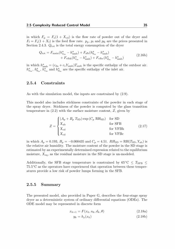
2.5 Complexity Reduced Control Model 35
in which Fp = Fs(1 + Xcd) is the flow rate of powder out of the dryer andFf = Fs(1 +Xf) is the feed flow rate. pp, pf and pE are the prices presented inSection 2.4.3. Qtot is the total energy consumption of the dryer
Qtot = Fmain(haain− haamb) + Fsfb(habin − haamb)
+ Fvfbh(hacin − haamb) + Fvfbc(hadin− haamb)
(2.16b)
in which haamb = (cda + cvYamb)Tamb is the specific enthalpy of the outdoor air.haain
, habin , hacin and hadinare the specific enthalpy of the inlet air.
2.5.4 Constraints
As with the simulation model, the inputs are constrained by (2.9).
This model also includes stickiness constraints of the powder in each stage ofthe spray dryer. Stickiness of the powder is computed by the glass transitiontemperature in (2.2) with the surface moisture content, Z, given by
Z =
(Ap +Bp TSD) exp (Cp RHSD) for SD
Xab for SFB
Xcd for VFBh
Xcd for VFBc
(2.17)
in which Ap = 0.193, Bp = −0.000435 and Cp = 4.51. RHSD = RH(TSD, Yab) isthe relative air humidity. The moisture content of the powder in the SD stage isestimated by an experimentally determined expression related to the equilibriummoisture, Xeq, as the residual moisture in the SD stage is un-modeled.
Additionally, the SFB stage temperature is constrained by 65C ≤ TSFB ≤75.5C as the operators have experienced that operation between these temper-atures provide a low risk of powder lumps forming in the SFB.
2.5.5 Summary
The presented model, also provided in Paper G, describes the four-stage spraydryer as a deterministic system of ordinary differential equations (ODEs). TheODE model may be represented in discrete form
xk+1 = F (xk, uk, dk, θ) (2.18a)
yk = hy(xk) (2.18b)

36 Four-Stage Spray Dryer Models
in which F (·) is the solution of the system of differential equations
x(tk) = xk (2.19a)
d
dtx(t) = f(x(t), uk, dk, θ) tk ≤ t ≤ tk+1 (2.19b)
xk+1 = x(tk+1) (2.19c)
Equation (2.19) is solved using the ESDIRK4(3) method with variable step-size [VJTS10]. The state x(t) represents hold-up of mass and energy andf(x(t), uk, dk, θ) is the flux of mass and energy. hy(xk) is the measurementequation. θ is the unknown parameter vector that has to be estimated fromdata. θ is identified by minimization of the sum of squared simulation errors.
The measurement and output vector, y, the input vector, u, the disturbancevector, d, and the state vector, x, are
y =[TSD TSFB Yab TVFBh TVFBc Sab Scd
]T(2.20a)
u =[Ff Tmain Tsfb Tvfbh
]T(2.20b)
d =[Sf Tf Yamb Fmain Fsfb Fvfbh Fvfbc Tamb Tvfbc
]T(2.20c)
x =[TSD TSFB Yab Xab TVFBh TVFBc Ycd Xcd
]T(2.20d)
2.6 Discrete Time State-Space Model
Linear models take many forms and may be identified directly from data or bylinearization of first-principles models. Examples of linear input-output modelsare the finite impulse response (FIR) models, autoregressive exogenous (ARX)models, autoregressive moving average exogenous (ARMAX) models, step re-sponse models, impulse response models, transfer-function models etc.
In general, all these models can be represented as linear discrete time state-spacemodels. The state-space models have the form
xk+1 = Axk +Buk + Edk + σx (2.21a)
yk = Cyxk + σy (2.21b)
in which xk is the state vector, uk is the input vector, dk is the disturbance vectorand yk is the measurement vector. (A,B,E,Cy) are the state-space matrices.σx and σy contain the constants related to the linearisation of the model, i.e.σx = xss −Axss −Buss − Edss and σy = yss − Cyxss.

2.7 Model Validation 37
In Paper B, Paper E and Paper H we identify state-space models by linearizationof the control model in Section 2.5. In Paper I we get the state-space modelfrom a transfer-function model identified solely from data to ease the requiredmodeling work, as we do not know the accuracy of the nonlinear control modelon milk products and industrial sized dryers. Discretization of the model isperformed using the matrix exponential, assuming a zero-order-hold samplingsystem.
2.7 Model Validation
In this section, we asses the quality of the deterministic simulation and controlmodels by comparing its outputs with the estimation and validation experiment.The simulation model is described in Section 2.4 and the control models aredescribed in Section 2.5 and 2.6.
Fig. 2.7 shows the outputs of the estimation experiment which is used to identifythe parameters. Fig. 2.8 shows the validation experiment. The deterministicmodel simulations are shown for each model in the same figure. The inputs anddisturbances of the two experiments are shown in Appendix A.
All three simulations show good agreement with the estimation experiment.The transients and the steady-states are well described by the models. Thesimulation model renders all the outputs well compared to the data. The stagetemperatures, T , and the air humidity in the SD stage, Y , fit the data well.The powder moisture contents, S, also fit the data well, but deviates slightly atlow residual moisture levels. The nonlinear and linear control models simulatethe stage temperatures, T , and the air humidity in the SD stage, Y , well. Thepowder residual moisture content, S, in the SFB stage do not render the samehigh accuracy as seen for the simulation model. The VFBc outlet moisturecontent fit the data well. The simulation accuracy of the SFB moisture contentis not as important as the VFBc moisture content, as it is seldom measuredand used for control anyway. The nonlinear and linear control models showalmost equal simulation abilities, except for very large steps in the ambientair humidity. This is due to the non-linearity in the model of the equilibriummoisture content.
The moisture content is in general difficult to estimate at low moisture contents,due to an increasing dependency on the equilibrium moisture content, Xeq, in(2.1). The equilibrium moisture content is estimated based on laboratory tests,which do not render the conditions in a spray dryer well. Thus, we expect somedeviation as the equilibrium moisture content becomes significant.

38 Four-Stage Spray Dryer Models
The VFBc stage is not sealed from the surrounding air, since the powder nat-urally has to be emptied from the VFBc stage. The residual moisture contentmay therefore be subject to an unknown disturbance. Note, that the communi-cation to the VFBc residual moisture sensor dropped out in the period t=16.5hours and t=18.2 hours due to a malfunction.

2.7 Model Validation 39
05
10
15
20
25
30
40
50
60
70
80
90
T [°C]
05
10
15
20
25
15
20
25
30
35
40
Y [g/kg]
Sim
ula
tion M
odel
Contr
ol M
odel
Lin
earized C
ontr
ol M
odel
05
10
15
20
25
Tim
e [
ho
urs
]
2
2.5 3
3.5 4
4.5 5
1-S [%]
Figure 2.7: Plot of the estimation experiment outputs and the simulated out-puts of each model. T and Y are the temperatures and abs. hu-midities of the air. 1− S is the residual moisture contents.

40 Four-Stage Spray Dryer Models
02
46
810
12
14
16
18
30
40
50
60
70
80
90
T [°C]
02
46
810
12
14
16
18
15
20
25
30
35
40
Y [g/kg]
Sim
ula
tio
n M
od
el
Co
ntr
ol M
od
el
Lin
ea
rize
d C
on
tro
l M
od
el
02
46
810
12
14
16
18
Tim
e [
ho
urs
]
2
2.5 3
3.5 4
4.5 5
1-S [%]
Figure 2.8: Plot of the validation experiment outputs and the simulated out-puts of each model. T and Y are the temperatures and abs. hu-midities of the air. 1− S is the residual moisture contents.

2.8 Step responses 41
0 100 200 300
-15
-10
-5
0
5
Ff +
50 k
g/h
r ste
p Temperatures, T [°C]
0 100 200 300
0
10
20Abs. Humidities, Y [g/kg]
0 100 200 300-0.7-0.1 0.5 1.1 1.7 2.3 2.9
Residual moistures, 1-S [%]
0 100 200 300
-15
-10
-5
0
5
Tm
ain
-20°C
ste
p
0 100 200 300
0
10
20
0 100 200 300-0.7-0.1 0.5 1.1 1.7 2.3 2.9
0 100 200 300
-15
-10
-5
0
5
Tsfb
-20°C
ste
p
0 100 200 300
0
10
20
0 100 200 300-0.7-0.1 0.5 1.1 1.7 2.3 2.9
0 100 200 300
Time [min]
-15
-10
-5
0
5
Tvfb
h -
20°C
ste
p
SD
SFB
VFBh
VFBc
0 100 200 300
Time [min]
0
10
20
SD
0 100 200 300
Time [min]
-0.7-0.1 0.5 1.1 1.7 2.3 2.9
SFB
VFBc
Figure 2.9: Simulated responses to several steps in the inputs.
The three simulations also show good agreement with the validation experiment.The transients and the steady-states are well described by the models. The tem-peratures and air humidity, T and Y , fit the data well during both disturbanceand input steps. The powder moisture content, S, from the simulation modelis estimated well, but some in-accuracies are present at low residual moisturecontents. As for the estimation experiment, the control models do not renderthe SFB powder moisture content well. The VFBc moisture content fits thedata well.
2.8 Step responses
Fig. 2.9 shows the step responses of the simulated outputs to the inputs. Theresponses are simulated using the simulation model of the four-stage spray dryerin Section 2.4. The control models provide similar responses. The initial offset

42 Four-Stage Spray Dryer Models
0 100 200 300
-15
-10
-5
0
5
Yam
b +
20 g
/kg s
tep Temperatures, T [°C]
0 100 200 300
0
10
20Abs. Humidities, Y [g/kg]
0 100 200 300-0.7-0.1 0.5 1.1 1.7 2.3 2.9
Residual moistures, 1-S [%]
0 100 200 300
-15
-10
-5
0
5
Sf -
15 %
ste
p
0 100 200 300
0
10
20
0 100 200 300-0.7-0.1 0.5 1.1 1.7 2.3 2.9
0 100 200 300
Time [min]
-15
-10
-5
0
5
Tf +
20°C
ste
p
SD
SFB
VFBh
VFBc
0 100 200 300
Time [min]
0
10
20
SD
0 100 200 300
Time [min]
-0.7-0.1 0.5 1.1 1.7 2.3 2.9
SFB
VFBc
Figure 2.10: Simulated responses to several steps in the selected disturbances.
in the outputs is removed and every 90 minutes the step-size of the inputs isincreased. This makes it possible to identify the effect of the non-linearities inthe model. In the first row of Fig. 2.9, a 50 kg/hr increase in the feed flowrate, Ff, is shown to have a significant effect on all outputs. When the feed flowrate increases, the temperatures decrease, the air humidity increase, and theresidual moisture content in the powder increase. The temperatures decreasebecause more water and feed need to be evaporated and heated with the sameamount of energy from the inlet air. The air humidity increase as a consequenceof the increased evaporation of water from the powder. The residual moisturecontent in the powder increase because the stage temperatures decrease andthe air humidity increase. The plots in the second, third and last row of Fig.2.9 indicate the step responses to a 20C reduction in the main hot inlet airtemperature, Tmain, the inlet air to the SFB stage, Tsfb, and the inlet air to theVFBh stage. Tmain and Tsfb both significantly affects the temperatures in theSD stage and the SFB stage. The similar effect is due to the mixing of the air inthese two stages of the four-stage spray dryer. Tmain and Tsfb hardly affects thetemperature in the VFBh stage and in the VFBc stage. Tvfbh mainly affects thetemperature in the VFBh stage of the four-stage spray dryer. Tmain and Tsfb
decrease the residual moisture of the powder at the SFB stage and the VFBcstage. Tvfbh only decreases the residual moisture content at the VFBc stage.This is as expected given the design and flows of the four-stage spray dryer.

2.9 Summary 43
Fig. 2.10 shows the step responses of the simulated outputs to the main distur-bances of the four-stage spray dryer. These disturbances vary during productionand a controller must adjust the inputs to compensate for these disturbances.The ambient air humidity, Yamb, varies due to changing weather conditions andthe feed, Sf and Tf, varies due to variations in the upstream processes. The firstrow of plots in Fig. 2.10 shows the responses to a 20 g/kg step increase in theambient air humidity, Yamb, in the SD, SFB and VFBh inlet air streams. TheVFBc inlet air is assumed dehumidified as is often the case. The ambient air hu-midity has a direct effect on the outlet air humidity in the SD stage. The stagetemperatures are only marginally affected. The ambient air humidity leads toa significant increase in the residual moisture of the powder in both the SFBstage and the VFBc stage. The second row of plots in Fig. 2.10 illustrates theresponse to step decreases in the feed solid concentration, Sf. This decreases theair temperatures in particularly the SD stage and the SFB stage, increases theSD air humidity and increases the residual moisture content of the powder. Thethird row of plots in Fig. 2.10 demonstrates that the feed temperature, Tf, hasan effect on the residual moisture of the powder. It also affects the temperatureat the SFB stage, but hardly at the other stages and has only a limited effecton the SD air humidity.
Fig. 2.9 and Fig. 2.10 do not indicate the presence of severe non-linearities.Non-linearities would show as a change in the relative step-change of the result-ing simulated outputs or a change in the time to steady-state. The figures onthe other hand clearly indicate a highly cross-coupled system model, in whichone input has an affect on several simulated outputs. We conclude, based onthe simulations and step responses, that the use of linear models can be used toaccurately simulate the outputs of the four-stage spray dryer.
2.9 Summary
In this chapter, we developed a simulation and a control model for an MSDTM-20four-stage spray dryer.
• We introduced the experimental dryer setup and presented an estimationand a validation experiment conducted on the spray dryer. The experi-ments provide the basis for identification and validation of the models withwell excited inputs and disturbances. Laboratory tests were conducted toidentify the equilibrium moisture content and stickiness of the powder.
• We presented a first-principles index-1 DAE model, based on mass andenergy balance principles, for simulation purposes. The model describes

44 Four-Stage Spray Dryer Models
the evolution of the air temperatures, the air humidity and the powdermoisture contents in each state. The model provides simulations that fitsthe validation data well.
• We developed a lumped ODE model, based on mass and energy balanceprinciples, for design of the controllers. The model describes the evolu-tion of the control relevant outputs only and fits the validation data well.Compared to the simulation model this model contains fewer states andparameters, thus simplifying the computational demand and identificationcomplexity.
• We showed that linear models of the spray dryer simulates the outputs welland that the models have strong input-output cross-couplings. A linearcontrol model is also provided based on the lumped ODE model.
• Deposits caused by stickiness of the powder is predicted in both modelsby the glass-transition temperature.
• The KPIs are computed as part of both models.

Chapter 3
Control Strategies
In the following, we briefly provide an overview of the three control strategiesthat are investigated in this thesis i.e. the conventional PI control strategy,the MPC with RTO strategy and the E-MPC strategy. In all three controlstrategies the inputs, u, are kept at their setpoints by low level PI controllers.These are not considered further in this thesis. Fig. 3.1 illustrates the workingprinciples of the high-level controllers. Fig. 3.2 illustrates the conceptual controlperformance of the controlled outputs.
Fig. 3.1(a) illustrates the single input and single output PI control strategy. ThePI controller measures and controls the spray dryer temperature, y = TSD, to thetarget, r, by manipulating the feed flow rate, u = Ff. The inlet temperatures,(Tmain, Tsfb, Tvfbh), are not manipulated in the PI control strategy. Fig. 3.2(a)illustrates that the controlled outputs in the PI control strategy have fixedconstraints for relatively long times of operation as the setpoint, r, is onlychanged manually. Furthermore, the PI control strategy has a relative largeoutput variance such that the required back-off from the constraint is largerthan for the advanced process control strategies (MPC with RTO and E-MPC).As a consequence the uncontrolled outputs, i.e. the residual moisture contentand stickiness of the powder, have a large variance and the profit of operationis as a consequence significantly decreased most of time.
Fig. 3.1(b) illustrates that the MPC with RTO is a two layer optimization
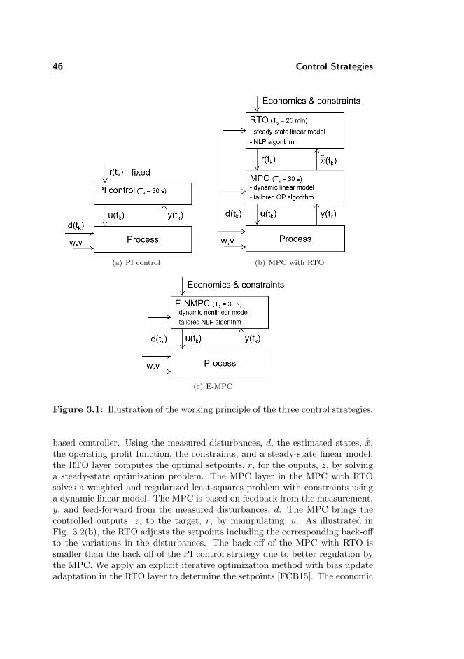
46 Control Strategies
(a) PI control (b) MPC with RTO
(c) E-MPC
Figure 3.1: Illustration of the working principle of the three control strategies.
based controller. Using the measured disturbances, d, the estimated states, ˆx,the operating profit function, the constraints, and a steady-state linear model,the RTO layer computes the optimal setpoints, r, for the ouputs, z, by solvinga steady-state optimization problem. The MPC layer in the MPC with RTOsolves a weighted and regularized least-squares problem with constraints usinga dynamic linear model. The MPC is based on feedback from the measurement,y, and feed-forward from the measured disturbances, d. The MPC brings thecontrolled outputs, z, to the target, r, by manipulating, u. As illustrated inFig. 3.2(b), the RTO adjusts the setpoints including the corresponding back-offto the variations in the disturbances. The back-off of the MPC with RTO issmaller than the back-off of the PI control strategy due to better regulation bythe MPC. We apply an explicit iterative optimization method with bias updateadaptation in the RTO layer to determine the setpoints [FCB15]. The economic

47
value of the MPC with RTO stems from the adjustment of setpoints to theactual disturbances and less back-off as a consequence of better regulation withless output variance.
Fig. 3.1(c) illustrates that the E-MPC is a one layer optimization based con-troller. Based on the measurements, y, the measured disturbances, d, the profitfunction, the constraints, and a nonlinear model, the E-MPC computes the in-puts, u, at each sample time to maximize the predicted profit of operation. Fig.3.2(c) shows that E-MPC does not compute targets directly, but maximizes op-erating profits subject to constraints. This implies that the optimal controlledoutputs corresponding to the optimal inputs, u, are adjusted and predicted ateach sample time. The back-off in E-MPC may be implemented directly or bysolving stochastic versions of E-MPC using soft constraints with penalty func-tions representing the economic cost of violating a constraint. In this thesis,we used a certainty-equivalence E-MPC and did not explicitly consider back-offfrom the constraints.
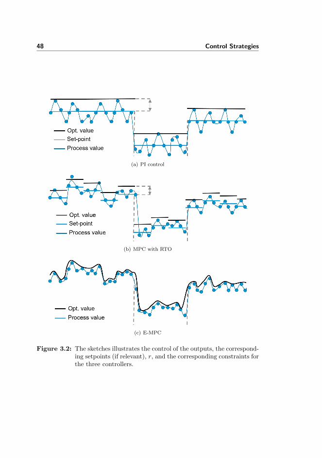
48 Control Strategies
(a) PI control
(b) MPC with RTO
(c) E-MPC
Figure 3.2: The sketches illustrates the control of the outputs, the correspond-ing setpoints (if relevant), r, and the corresponding constraints forthe three controllers.
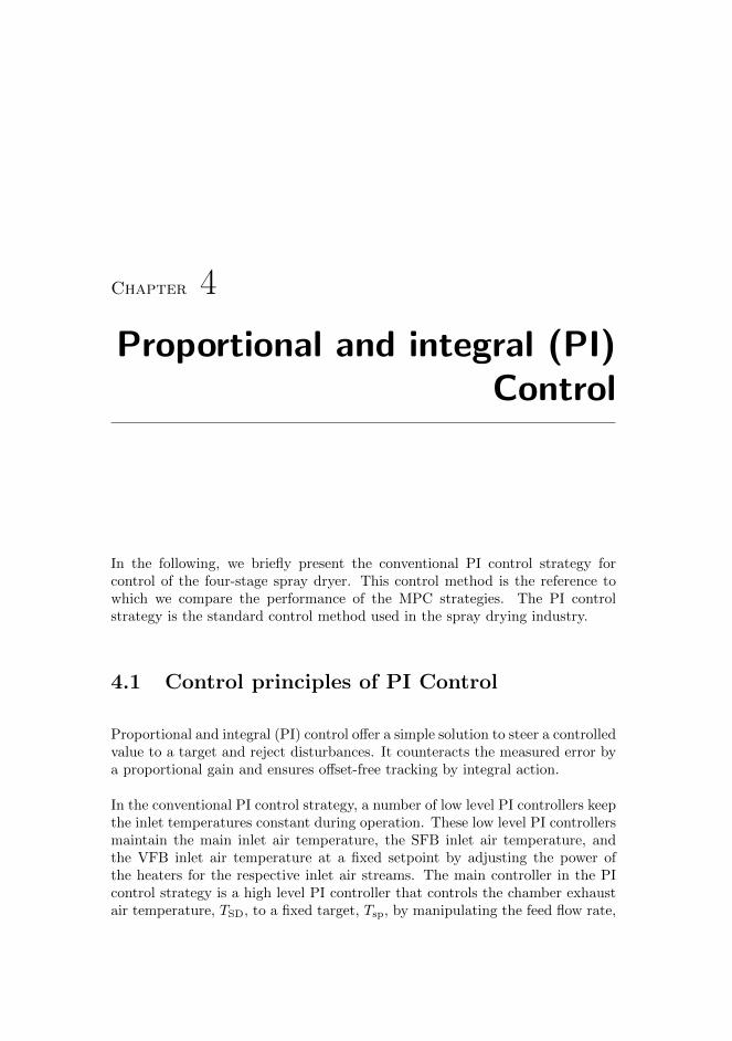
Chapter 4
Proportional and integral (PI)Control
In the following, we briefly present the conventional PI control strategy forcontrol of the four-stage spray dryer. This control method is the reference towhich we compare the performance of the MPC strategies. The PI controlstrategy is the standard control method used in the spray drying industry.
4.1 Control principles of PI Control
Proportional and integral (PI) control offer a simple solution to steer a controlledvalue to a target and reject disturbances. It counteracts the measured error bya proportional gain and ensures offset-free tracking by integral action.
In the conventional PI control strategy, a number of low level PI controllers keepthe inlet temperatures constant during operation. These low level PI controllersmaintain the main inlet air temperature, the SFB inlet air temperature, andthe VFB inlet air temperature at a fixed setpoint by adjusting the power ofthe heaters for the respective inlet air streams. The main controller in the PIcontrol strategy is a high level PI controller that controls the chamber exhaustair temperature, TSD, to a fixed target, Tsp, by manipulating the feed flow rate,
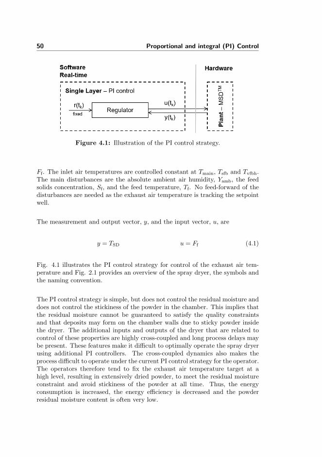
50 Proportional and integral (PI) Control
Figure 4.1: Illustration of the PI control strategy.
Ff. The inlet air temperatures are controlled constant at Tmain, Tsfb and Tvfbh.The main disturbances are the absolute ambient air humidity, Yamb, the feedsolids concentration, Sf, and the feed temperature, Tf. No feed-forward of thedisturbances are needed as the exhaust air temperature is tracking the setpointwell.
The measurement and output vector, y, and the input vector, u, are
y = TSD u = Ff (4.1)
Fig. 4.1 illustrates the PI control strategy for control of the exhaust air tem-perature and Fig. 2.1 provides an overview of the spray dryer, the symbols andthe naming convention.
The PI control strategy is simple, but does not control the residual moisture anddoes not control the stickiness of the powder in the chamber. This implies thatthe residual moisture cannot be guaranteed to satisfy the quality constraintsand that deposits may form on the chamber walls due to sticky powder insidethe dryer. The additional inputs and outputs of the dryer that are related tocontrol of these properties are highly cross-coupled and long process delays maybe present. These features make it difficult to optimally operate the spray dryerusing additional PI controllers. The cross-coupled dynamics also makes theprocess difficult to operate under the current PI control strategy for the operator.The operators therefore tend to fix the exhaust air temperature target at ahigh level, resulting in extensively dried powder, to meet the residual moistureconstraint and avoid stickiness of the powder at all time. Thus, the energyconsumption is increased, the energy efficiency is decreased and the powderresidual moisture content is often very low.

4.2 Regulator 51
Algorithm 1 PI Algorithm
Require: yk, rk, Ikek = rk − ykuk = Kcek + Ikuk = min(umax,max(umin, uk))Ik+1 = Ik + (TsKc/τc) ekreturn uk, Ik+1
4.2 Regulator
The main challenge in using PI control is tuning of the gain and integral time.We used the SIMC tuning method with good results [Sko03]. Using input-output data of the simulation model in Section 2.4, we approximate the transferfunction from Ff to TSD with the first order model
Y (s) =Kp
τps+ 1U(s) (4.2)
Kp = −0.35 C/(kg/h) and τp = 122 s. In continuous-time the PI control lawis
U(s) = Kcτcs+ 1
τcs(R(s)− Y (s)) (4.3)
Aiming for at closed-loop time constant of τcl = 50 s we get the followingPI control parameters using the SIMC tuning rule: Kc = (1/Kp)τp/τcl =−6.97 (kg/h)/C and τc = minτp, 4τcl = 122 s.
Algorithm 1 transforms the continuous-time PI controller (4.3) to a discretetime PI controller using the explicit Euler method [AH06, Arz12]. The imple-mentation outlined in Algorithm 1 provides bumpless parameter changes andhandles control signal saturation. Bumpless transfer between manual and auto-matic mode is obtained by setting I0 = u0−Kc(r0− y0) when the PI controlleris switched on to automatic mode. In the implementation we do not consideranti-windup nor setpoint weighting. For the PI control strategy we use a sampletime of Ts = 30 s, umin = 0 kg/hr and umax = 140 kg/hr.
4.3 Closed-loop Simulation
The performance of the PI control strategy has been investigated by a closed-loop simulation. The simulation model presented in Section 2.4 is used with the

52 Proportional and integral (PI) Control
0 5 10 15 2047.5
49.5
51.5
53.5
55.5
Fe
ed
c.
[%]
Sf
0 5 10 15 20 54
54.5
55
55.5
Fe
ed
T.
[oC
]
Tf
0 5 10 15 20
Time [hours]
6.5 7.5 8.5 9.5
10.511.5
Am
b.
hu
m.
[g/k
g]
Yamb
Figure 4.2: Industrially recorded disturbance scenario.
above PI controller fitted to control the exhaust air temperature, TSD, to thetarget, Tsp, using the feed flow rate, Ff.
We use an industrially recorded disturbance scenario in order to produce realisticsimulations and concluding performance measures. The three control strategiesin this thesis are compared using the same disturbance scenario shown in Fig.4.2. The feed solids concentration, Sf, the feed temperature, Tf, and the ambientair humidity, Yamb, are recorded disturbances from a larger dairy spray dryer.The feed solids concentration, Sf, have a relatively large variance where as thefeed temperature, Tf, is well controlled compared to other dryers. The ambientair humidity, Yamb, resembles the variations from a normal humid summer day.The disturbances, Fmain, Fsfb, Fvfbh, Fvfbc, Tvfbc and Tamb are constant.
Fig. 4.3 shows the measured outputs, the target and the inputs of the closed-loop simulation. The simulation shows that the PI controller is able to maintaina stable exhaust air temperature, TSD, and avoids violation of the stickiness con-straint, i.e. the glass transition temperature. Notice the mismatch between thestickiness constraint predicted by the simulation model, T SD
g , and the control
model, T SDg . By design, T SD
g , which we use for control purposes is conserva-
tively made compared to TSDg at all time. The exhaust air humidity, Yab, andthe residual moisture content, Scd, are not controlled and fluctuates accordingto the disturbances. With the conventional PI control methodology no correct-ing action is made, because the ambient air humidity, affects the air humidity,

4.3 Closed-loop Simulation 53
0 5 10 15 2057
60
63
66
69
72
75
78
81
84
87T
em
p. [o
C] TSD
TSFB
TV FBh
T SDg
T SDg
Tsp
0 5 10 15 2025
27
29
31
33
35
Abs. hum
. [g
/kg]
Yab
0 5 10 15 20
Time [hours]
33.13.23.33.43.53.63.7
Res. m
oi. [%
]
1− Scd
1− Smax
(a) Measured output variables and target.
0 5 10 15 20 90
100
110
120
130
140
Feed r
ate
[kg/h
r]
Ff
0 5 10 15 20
Time [hours]
60 70 80 90100110120130140150160170180190200
Inle
t air tem
p. [
oC
]
Tmain
Tsf b
Tvf bh
(b) Input variables.
Figure 4.3: Simulation of the PI control strategy subject to the disturbancescenario given in Fig. 4.2.

54 Proportional and integral (PI) Control
Table 4.1: Average KPIs for the PI controller.
KPIs Unit PIProduct flow rate Fp 60.95 kg/hr
Energy consumption Qtot 87.2 kW
Specific energy consum. Qtot
Fp5.16 MJ/kg
Residual moisture 1− S 3.37 %Energy efficiency η 40.2 %
Profit of operation p 123.25 e/hr
Yab and the residual moisture content, Scd, not the exhaust air temperature.Changes in the feed concentration, Sf, is better handled as the amount of waterentering the chamber directly affects the exhaust air temperature, TSD. Theexhaust air temperature is largely dictated by the evaporation rate, and thecontroller basically maintains a fixed rate of evaporation. The variations in Scd
and Yab require on average the dryer to dry the powder more than necessaryto keep the powder moisture content below the maximum limit and avoid vi-olation of the stickiness constraint at all time. The powder is therefore driedmore extensively, to meet the residual moisture limit, which increases the energyconsumption, decreases the energy efficiency and the yield of the production. Intypical industrial operation, the operators have no in-line measurement of theexhaust air humidity, Yab, and the residual moisture content, Scd. Thus, theyare running almost in blind and must back-off even further from the processconstraints. This again increases the cost of operation.
The target of the high level PI-controller, Tsp = 80C, and the low level con-trollers are selected by hand to render the best possible profit of operation. Theclosed-loop simulation in Fig. 4.3 therefore shows the most optimistic perfor-mance that may be achieved by the conventional PI control strategy.
Table 4.1 shows the key performance indicators (KPIs) of the closed-loop sim-ulation presented in Fig. 4.3. The PI controller provides on average a productflow rate at 60.95 kg/hr, an energy consumption of 87.2 kW, a specific energyconsumption of 5.16 MJ/kg, a residual moisture content in the powder of 3.37%and an energy efficiency of 40.2%. This is the benchmark for comparison of thefollowing MPC strategies.
4.4 Summary 55
4.4 Summary
In this chapter, we described the PI control strategy and performed a closed-loopsimulation for benchmark using the simulation model.
• We showed that the chamber exhaust air temperature, TSD, is controlledconstant by manipulating the feed flow rate, Ff.
• The PI control approach is simple, but insufficient for controlling the resid-ual moisture content and the powder can turn sticky inside the dryer.
• We showed that the variations in Scd and Yab requires on average the dryerto dry the powder more than necessary to satisfy the residual moisturespecifications and stickiness constraint at all time.
• The average KPIs provide the best possible performance that can beachieved by the PI control strategy. Industrial practice may be worse.

56 Proportional and integral (PI) Control
Chapter 5
Tracking Model PredictiveControl with an RTO layer
In this chapter, we present the Model Predictive Control (MPC) algorithm thatcombines a target tracking MPC and a Real-Time Optimization layer (MPCwith RTO), for control of the four-stage spray dryer. The MPC with RTOis based on the linearized control model in Section 2.6. The MPC with RTOmanipulate four inputs and control four outputs to a target. The target isadjusted by an RTO layer to provide the best steady-state economic performancewithin the given process constraints.
The chapter provides a summary of Paper B, Paper E and Paper I.
5.1 Control principles of MPC with RTO
The basic concept of MPC is to solve an optimization problem, incorporatinga dynamic model to forecast the model outputs, to produce the best controlmove at the current time. To do that, an initial state of the model must beestimated based on past recorded measurements [RM09]. The setpoint of theMPC can be manually selected or computed automatically in the RTO layer.Fig. 5.1 illustrates the components of the MPC with RTO algorithm and shows

58 Tracking Model Predictive Control with an RTO layer
the signal paths between the hardware, software and the individual softwareelements.
In the MPC with RTO control strategy we control four outputs by manipulationof four inputs. The outputs are the exhaust and SFB stage air temperatures, TSD
and TSFB, the exhaust air humidity, Yab and the VFBc stage residual moisturecontent of the powder, Scd. The inputs are the feed flow rate, Ff, the main inletair temperature, Tmain, the SFB inlet air temperature, Tsfb, and the VFBh inletair temperature, Tvfbh. The main disturbances are the ambient air humidityYamb, the feed solids concentration, Sf, and the feed temperature, Tf. Theselection of these outputs makes it possible to avoid deposits of sticky particleson the spray dryer surfaces, avoid lumps of powder to form in the SFB andcontrol the residual moisture content below and close to the maximum limit.The dryer inlet air temperatures are controlled, as opposed to controlling theinlet air flows, in order to adjust the drying of the powder without compromisingthe flow patterns of air inside the dryer and fluid beds.
The measurement vector, y, the output vector, z, the input vector, u, and themain disturbance vector, d, are
y =[TSD TSFB Yab TVFBh TVFBc Scd
]T(5.1a)
z =[TSD TSFB Yab Scd
]T(5.1b)
u =[Ff Tmain Tsfb Tvfbh
]T(5.1c)
d =[Sf Tf Yamb
]T(5.1d)
Fig. 2.1 provides an overview of the spray dryer, the symbols and the namingconvention of the outputs, inputs and disturbances.
Algorithm 2 lists the on-line computations in the MPC with RTO algorithm,consisting of a state estimator with a filter and a one-step-ahead predictor step,a regulator and an RTO layer. The sample time is Ts = 30 s. The target inthe RTO layer is computed every 25 min. At each sample, the state estimatorprovides the initial state of the dynamic model, which in combination with themodel is used in the regulator to compute the future input trajectory. The opti-mization in the regulator results in a sequence of inputs for a finite horizon (thecontrol and prediction horizon), out of which only the first input is applied tothe dryer. This procedure is repeated at each sample instant. The optimizationproblem has to be implemented efficiently and robustly, as it is repeatedly solvednumerically in real-time. The target of the target tracking MPC is computedby the RTO layer and the MPC then steers the dryer to that target. The RTOseeks to optimize the process economics while satisfying the process constraints.In this way, the MPC reduces the variance of the controlled outputs, making it

5.2 Linear Model 59
Figure 5.1: Illustration of the MPC with an RTO layer.
possible to squeeze and shift the target, computed in the RTO layer, to a moreprofitable value.
We use the so-called separation and certainty equivalence principle [Wit71,The57, Mal69] in the formulation of the MPC with RTO. This means that thestate estimation and the regulation problem can be decoupled (separated) andthat the random variables in the regulation problem can be replaced by theconditional expectations of the costs, predictions of the states, disturbances etc.Thus, the control model simplifies to a deterministic model. The key advantageis that the computational load is significantly reduced compared to for instance amean-variance approach based on Monte Carlo simulations. The repeated opti-mization procedure in the MPC provides feedback and form a closed-loop inputtrajectory. This enables the MPC to counteract model uncertainties, modelmismatch and unknown disturbances.
5.2 Linear Model
The linear model, which is used in the state estimator, the regulator and theRTO, is a linearization of the nonlinear control model with reduced complexity

60 Tracking Model Predictive Control with an RTO layer
Algorithm 2 MPC with RTO Algorithm
Require: yk, dk, ˆxk|k−1, Pk|k−1, uk−1
Filter:Compute the one-step ahead measurement predictionyk|k−1 = Cy,k ˆxk|k−1 + σy,k,Compute the filtered stateRe,k = Cy,kPk|k−1C
Ty,k +Rv,k
Kfx,k = Pk|k−1CTy,kR
−1e,k
ˆxk|k = ˆxk|k−1 + Kfx,k(yk − yk|k−1)Pk|k = Pk|k−1 − Kfx,kRe,kK
Tfx,k
RTO:rk = ρ(ˆxk|k, dk, k)Regulator:uk = µ(rk, ˆxk|k, uk−1, dk)One-step predictor:Compute the one-step ahead state, ˆxk+1|k, usingˆxk+1|k = Aˆxk|k + Buk + Edk + σx
Pk+1|k = APk|kAT + GRwGT
return uk, ˆxk+1|k, Pk+1|k
compared to the model used for simulation of the spray dryer. Section 2.5 de-scribes the nonlinear model from which the linear model presented in Section2.6 in the MPC with RTO is derived. Compared to the simulation model inSection 2.4, the nonlinear model that is used to derive the linear model of theMPC with RTO contains fewer states and parameters. This simplifies the pa-rameter estimation and identification of the model. The model parameters inthe complexity reduced model are identified from data produced by the simula-tion model as outlined in Section 2.4.5 subject to step-inputs. The complexityreduced model is linearized at steady-state and close to the operating point ofthe controller. The model could as well be identified directly from process orsimulation data and with alternative black-box models.
To achieve offset-free output estimation (and control) at steady-state, in thepresence of plant/model mismatch and/or un-modeled disturbances, the modelis augmented by integrating disturbance states [PR03, PGA15]. In Paper B,Paper E and Paper H we select pure input disturbances, i.e. Cd = 0 and Bd tosubject the energy- and the vapor mass balances to the disturbance integration.In Paper I we select pure output disturbances, i.e. Cd = I and Bd = 0.
The augmented linear control model is
xk+1 = Axk + Buk + Edk + Gwk + σx (5.2a)
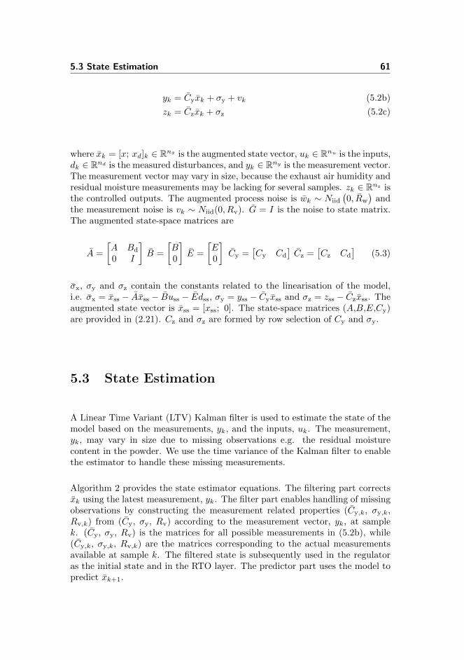
5.3 State Estimation 61
yk = Cyxk + σy + vk (5.2b)
zk = Czxk + σz (5.2c)
where xk = [x; xd]k ∈ Rnx is the augmented state vector, uk ∈ Rnu is the inputs,dk ∈ Rnd is the measured disturbances, and yk ∈ Rny is the measurement vector.The measurement vector may vary in size, because the exhaust air humidity andresidual moisture measurements may be lacking for several samples. zk ∈ Rnz isthe controlled outputs. The augmented process noise is wk ∼ Niid
(0, Rw
)and
the measurement noise is vk ∼ Niid(0, Rv). G = I is the noise to state matrix.The augmented state-space matrices are
A =
[A Bd
0 I
]B =
[B0
]E =
[E0
]Cy =
[Cy Cd
]Cz =
[Cz Cd
](5.3)
σx, σy and σz contain the constants related to the linearisation of the model,i.e. σx = xss − Axss − Buss − Edss, σy = yss − Cyxss and σz = zss − Czxss. Theaugmented state vector is xss = [xss; 0]. The state-space matrices (A,B,E,Cy)are provided in (2.21). Cz and σz are formed by row selection of Cy and σy.
5.3 State Estimation
A Linear Time Variant (LTV) Kalman filter is used to estimate the state of themodel based on the measurements, yk, and the inputs, uk. The measurement,yk, may vary in size due to missing observations e.g. the residual moisturecontent in the powder. We use the time variance of the Kalman filter to enablethe estimator to handle these missing measurements.
Algorithm 2 provides the state estimator equations. The filtering part correctsxk using the latest measurement, yk. The filter part enables handling of missingobservations by constructing the measurement related properties (Cy,k, σy,k,Rv,k) from (Cy, σy, Rv) according to the measurement vector, yk, at samplek. (Cy, σy, Rv) is the matrices for all possible measurements in (5.2b), while(Cy,k, σy,k, Rv,k) are the matrices corresponding to the actual measurementsavailable at sample k. The filtered state is subsequently used in the regulatoras the initial state and in the RTO layer. The predictor part uses the model topredict xk+1.

62 Tracking Model Predictive Control with an RTO layer
5.3.1 Maximum Likelihood (ML) Tuning
The noise variance matrices, Rw and Rv, are estimated using the MaximumLikelihood (ML) method [KMJ04, JJ07b, JJ07a]. Let θ = [θw; θv] be the di-agonal elements so Rw = diag(θw) and Rv = diag(θv). Rw and Rv, neededfor the Kalman filter computations, minimize the negative log likelihood func-tion [JJ07b,JJ07a]
VML(θ) =ln(2π)
2
N∑
k=1
ny,k +1
2
N∑
k=1
(ln[det(Re,k)] + εTkR
−1e,kεk
)(5.4)
with the innovation, εk = εk(θ) = yk − yk|k−1(θ), and its covariance, Re,k =Re,k(θ), computed by Kalman filter iterations i.e. Algorithm 2 without theregulator and RTO computations, using recorded or simulated data. The MLestimate of the variances is determined by solving the nonlinear (nonconvex)optimization problem
minθVML(θ) (5.5a)
s.t. θl ≤ θ ≤ θu (5.5b)
with the lower and upper bounds, θl and θu. Having the optimal θ = [θw; θv]provides the noise covariances, Rw = diag(θw), and Rv = diag(θv).
The model (5.2) and the estimated covariances, Rw and Rv, enables the compu-tation of the stationary state covariance, P , of the augmented system by solutionof a discrete algebraic Riccati equation. The LTV Kalman filter is initializedusing P0|−1 = P and ˆx0|−1 = xss = [xss; 0], where xss is the steady-state alsoused for linearization of the model.
Knowledge of the model (5.2), the covariances, Rw and Rv, and the measure-ment, yk, enables the filter to estimate the current states, i.e. computation ofˆxk|k. The filtered state, ˆxk|k, is used by the RTO, the regulator part of theMPC, and the one-step prediction.
The ML method is computational expensive and the solution of (5.5) may notalways converge [ORR06, RR09], but the method has shown to provide goodresults and naturally handles missing observations. The method is explored inPaper B, Paper H and Paper I and showed to estimate Rw and Rv well.
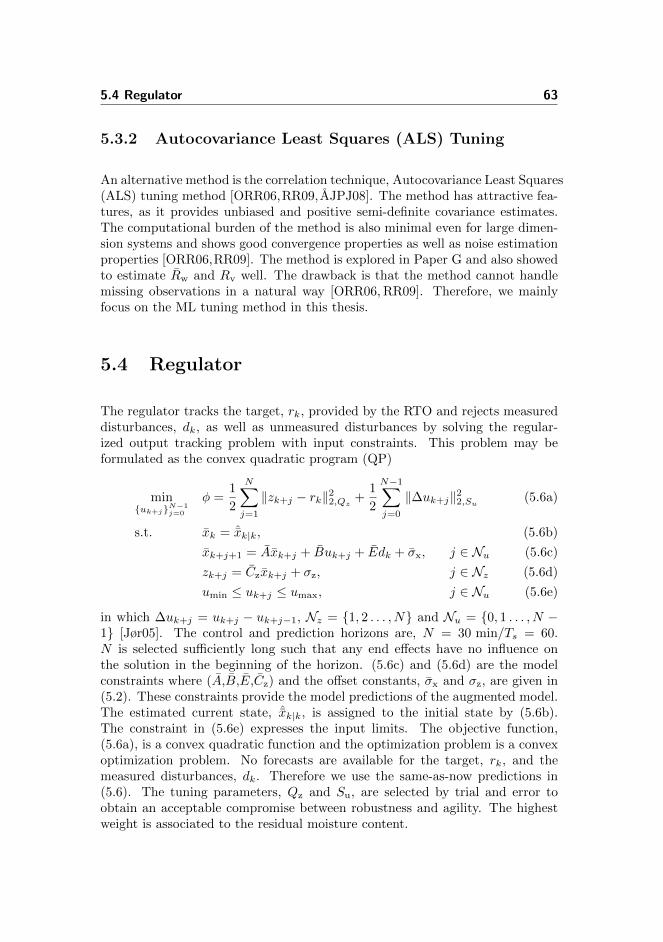
5.4 Regulator 63
5.3.2 Autocovariance Least Squares (ALS) Tuning
An alternative method is the correlation technique, Autocovariance Least Squares(ALS) tuning method [ORR06,RR09,AJPJ08]. The method has attractive fea-tures, as it provides unbiased and positive semi-definite covariance estimates.The computational burden of the method is also minimal even for large dimen-sion systems and shows good convergence properties as well as noise estimationproperties [ORR06,RR09]. The method is explored in Paper G and also showedto estimate Rw and Rv well. The drawback is that the method cannot handlemissing observations in a natural way [ORR06, RR09]. Therefore, we mainlyfocus on the ML tuning method in this thesis.
5.4 Regulator
The regulator tracks the target, rk, provided by the RTO and rejects measureddisturbances, dk, as well as unmeasured disturbances by solving the regular-ized output tracking problem with input constraints. This problem may beformulated as the convex quadratic program (QP)
minuk+jN−1
j=0
φ =1
2
N∑
j=1
‖zk+j − rk‖22,Qz+
1
2
N−1∑
j=0
‖∆uk+j‖22,Su(5.6a)
s.t. xk = ˆxk|k, (5.6b)
xk+j+1 = Axk+j + Buk+j + Edk + σx, j ∈ Nu (5.6c)
zk+j = Czxk+j + σz, j ∈ Nz (5.6d)
umin ≤ uk+j ≤ umax, j ∈ Nu (5.6e)
in which ∆uk+j = uk+j − uk+j−1, Nz = 1, 2 . . . , N and Nu = 0, 1 . . . , N −1 [Jør05]. The control and prediction horizons are, N = 30 min/Ts = 60.N is selected sufficiently long such that any end effects have no influence onthe solution in the beginning of the horizon. (5.6c) and (5.6d) are the modelconstraints where (A,B,E,Cz) and the offset constants, σx and σz, are given in(5.2). These constraints provide the model predictions of the augmented model.The estimated current state, ˆxk|k, is assigned to the initial state by (5.6b).The constraint in (5.6e) expresses the input limits. The objective function,(5.6a), is a convex quadratic function and the optimization problem is a convexoptimization problem. No forecasts are available for the target, rk, and themeasured disturbances, dk. Therefore we use the same-as-now predictions in(5.6). The tuning parameters, Qz and Su, are selected by trial and error toobtain an acceptable compromise between robustness and agility. The highestweight is associated to the residual moisture content.

64 Tracking Model Predictive Control with an RTO layer
The objective function in (5.6a) penalizes deviations from a target and includesa regularization term on the control input. One may provide targets for boththe output variables and the input variables, but such formulations require aseparate target calculator to achieve offset-free control [Raw00]. Regularizationis important to make the closed-loop trajectory of the controlled process well-behaved [PJ09,HLJB12]. The regularization term may be a linear or quadraticpenalty, where quadratic regularization favors smooth solutions [BV04]. In thisthesis we only use quadratic regularization.
5.4.1 Optimal Control Problem
The optimal control problem (OCP) in (5.6) is solved by formulating the corre-sponding boxed constrained QP with dense matrices. We use state eliminationand achieve a problem structure similar to the formulations in [Mac02, PJ09,JRH11, HPJJ10, HPJJ12]. State elimination is favorable when the number ofstates, nx, is large compared to the number of inputs, nu, and for relativelyshort prediction horizons, N [FJ13]. The number of states may be large inour problem due to the potential incorporation of large delays and the Hankelmatrix realization of the state-space matrices.
The state, xk, in (5.6) is eliminated by repeated substitution of the state pre-dictor in (5.6c) such that
xk+j = Aj xk +
j−1∑
i=0
Aj−1−iBuk+i +
j−1∑
i=0
Aj−1−iEdk +
j−1∑
i=0
Aj−1−iσx (5.7)
which by (5.6d) results in the output predictions
zk+j = CzAj xk +
j−1∑
i=0
CzAj−1−iBuk+i +
j−1∑
i=0
CzAj−1−iEdk
+
j−1∑
i=0
CzAj−1−iσx + σz
(5.8)
The integrating disturbance states are fixed during the prediction horizon. Re-call, that the augmented state vector is xk = [xk; xd,k] and the augmented

5.4 Regulator 65
system in (5.3), then the state predictor can be rewritten as
zk+j = CzAjxk +
j−1∑
i=0
CzAj−1−iBuk+i +
j−1∑
i=0
CzAj−1−iEdk
+
j−1∑
i=0
CzAj−1−i (σx +Bdxd,k) + (σz + Cdxd,k)
(5.9)
= CzAjxk +
j−1∑
i=0
Hu,iuk+i +
j−1∑
i=0
Hd,idk+
j−1∑
i=0
Hσ,i (σx +Bdxd,k) + (σz + Cdxd,k)
(5.10)
where Hu,i = CzAj−1−iB, Hd,i = CzA
j−1−iE and Hσ,i = CzAj−1−i. (5.10) is
an affine function which only depend on the initial state, xk = ˆxk|k, the input,uk+i, and the disturbance, dk.
Define the vectors Z, R, U and D as
Zk =
zk+1
zk+2
...zk+N
Rk =
rkrk...rk
Uk =
ukuk+1
...uk+N−1
Dk =
dkdk...dk
Then the predictions, (5.10), in vector-matrix notation are
Zk = Φxxk + ΓuUk + ΓdDk + ΩΣx + Σz
Using the predictions in vector-matrix notation we can write the objective func-tion as
φ =1
2
N∑
j=1
‖zk+j − rk‖2Qz+
1
2
N−1∑
j=0
‖∆uk+j‖2Su
=1
2‖Zk −Rk‖2Qz
+1
2‖Uk − Uk−1‖2Su
=1
2‖ΓuUk − (Rk + b)‖2Qz
+1
2‖ΛUk − I0uk−1‖2Su
=1
2UTk HUk + gTUk + ρ
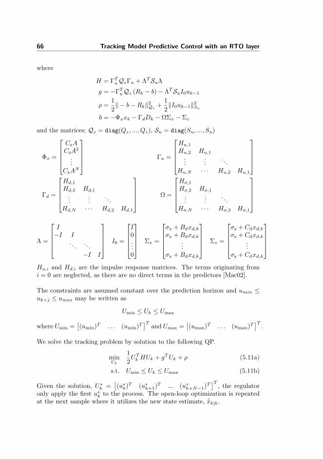
66 Tracking Model Predictive Control with an RTO layer
where
H = ΓTuQzΓu + ΛTSuΛ
g = −ΓTuQz (Rk − b)− ΛTSuI0uk−1
ρ =1
2‖ − b−Rk‖2Qz
+1
2‖I0uk−1‖2Su
b = −Φxxk − ΓdDk − ΩΣx − Σz
and the matrices; Qz = diag(Qz, ..., Qz), Su = diag(Su, ..., Su)
Φx =
CzACzA
2
...CzA
N
Γu =
Hu,1
Hu,2 Hu,1
......
. . .
Hu,N · · · Hu,2 Hu,1
Γd =
Hd,1
Hd,2 Hd,1
......
. . .
Hd,N · · · Hd,2 Hd,1
Ω =
Hσ,1
Hσ,2 Hσ,1
......
. . .
Hσ,N · · · Hσ,2 Hσ,1
Λ =
I−I I
. . .. . .
−I I
I0 =
I0...0
Σx =
σx +Bdxd,kσx +Bdxd,k
...σx +Bdxd,k
Σz =
σz + Cdxd,kσz + Cdxd,k
...σz + Cdxd,k
Hu,i and Hd,i are the impulse response matrices. The terms originating fromi = 0 are neglected, as there are no direct terms in the predictors [Mac02].
The constraints are assumed constant over the prediction horizon and umin ≤uk+j ≤ umax may be written as
Umin ≤ Uk ≤ Umax
where Umin =[(umin)T . . . (umin)T
]Tand Umax =
[(umax)T . . . (umax)T
]T.
We solve the tracking problem by solution to the following QP.
minUk
1
2UTk HUk + gTUk + ρ (5.11a)
s.t. Umin ≤ Uk ≤ Umax (5.11b)
Given the solution, U∗k =[(u∗k)T (u∗k+1)T ... (u∗k+N−1)T
]T, the regulator
only apply the first u∗k to the process. The open-loop optimization is repeatedat the next sample where it utilizes the new state estimate, ˆxk|k.

5.5 Steady-state Real-Time Optimization 67
5.4.2 Optimization Methods
Many methods exists for solving the QP related to the control problem in (5.11).The best choice of solver highly depends on the structure of the problem andthe accuracy requirements. The QP may be solved using algorithms such asactive-set methods [BB06, FKP+14, JRJ04], interior-point methods [RWR98,NW06, BV04, ESJ09, Wri97, WB10, FSD13] and first-order gradient methods[Nes09, CSZ+12, RJM09]. Active-set methods updates the working set of theactive constraints until convergence is reached. These methods can be fast whenthe working set does not change much. Interior-point methods reaches the so-lution by traversing the interior of the feasible region. Interior-point methodsproduce high-accuracy solutions using a few, but relatively computationally ex-pensive iterations. The solution is less depended on the starting point (which isalso allowed to be infeasible) and the number of active constraints. First-ordergradient methods have proven fast for large-scale distributed MPC problemswith dynamically coupled systems. These methods have slow convergence ratescompared to high order methods, but are favorable for less accurate solutionsand scales very well for large problems.
Warm starting of the solvers, i.e. re-using previous solutions, and early termi-nation, i.e. stopping the optimization algorithm at less accurate solutions, canbe used to speed up the solution time significantly [SSF+13,Sta15].
We use a primal-dual interior-point QP-solver for solution of (5.11) based onMehrotra’s predictor-corrector algorithm [NW06,BV04] tailored to the QP struc-ture [ESJ09, JRJ04]. Warm starting is used. The QP-solver reduces the com-putation time considerably compared to general purpose QP-solvers.
The solution of (5.11) is defined by the function
uk = µ(rk, ˆxk|k, uk−1, dk) (5.12)
in which uk is the first u∗k of U∗k . The function defines the on-line computationsof the regulator, provided in Algorithm 3, and used in Algorithm 2.
5.5 Steady-state Real-Time Optimization
The steady-state Real-Time Optimization (RTO) layer determines the targetthat optimizes the cost of operation subject to the process constraints and con-ditions such as feed compositions, production rates, energy availability, feed andproduct prices [FCB15,Eng07,DNJN11,AO10,AG10]. The RTO is based on the

68 Tracking Model Predictive Control with an RTO layer
Algorithm 3 Regulator Algorithm, µ(·)Require: rk, ˆxk|k, uk−1, dkCalculate g:Rk = rkNi=1 , Dk = dkN−1
i=0
[xk;xd,k] = ˆxk|kΣx = [σx +Bdxd,k; ... ;σx +Bdxd,k]Σz = [σz + Cdxd,k; ... ;σz + Cdxd,k]b = −Φxxk − ΓdDk − ΩΣx − Σzg = −ΓTuQz (Rk − b)− ΛTSuI0uk−1
Solve QP:uk= QPSolver(H,g,Umin,Umax)return uk
assumption that the process and the disturbance transients can be neglected asthe process under control will reach and maintain steady-state operation.
Various RTO methods exist for on-line optimization of the process economics.Implicit RTO methods e.g. the extremum-seeking control method, may be ap-plied. But the slow process transients and long process delays in spray dryingmay lead to a slow propagation towards the optimal residual moisture content.We apply an explicit iterative optimization method with bias update adapta-tion [FCB15] in the RTO layer, see Fig. 1.7. This method is effective as thesame linear and fixed state-space model in the MPC can be used in the RTO.The adaptation of correction terms are performed by the state estimator. Fig.5.2 illustrates how model uncertainties are mitigated by the adaption of correc-tion terms. The process profit function and the constraints are measurable fromthe outputs, inputs and disturbances of the process providing a good estimateof the optimum. Optimum mismatch will still be present due to measurementerrors and unknown disturbances, i.e. the optimum is only an estimate. Thedriving force of the RTO is then to minimize the difference between the pre-dicted and the measured profit function. The explicit method can be fast as itcan estimate the steady-state of the process from the model. The MPC withRTO two-layer structure has some inherent drawbacks. The adaptation of theoperating conditions is slow as the optimization is only performed intermittentlyat a low sampling rate [Eng07]. Furthermore, the RTO layer assumes that theclosed-loop process will reach a steady-state. Transients, such as target transi-tions and the inherent effect of disturbances, may thus lead to loss of economicalefficiency.
The RTO solves the steady-state economic optimization problem
minuss,zss,s
φss = −p(zss, uss, dk) + φs(s) (5.13a)
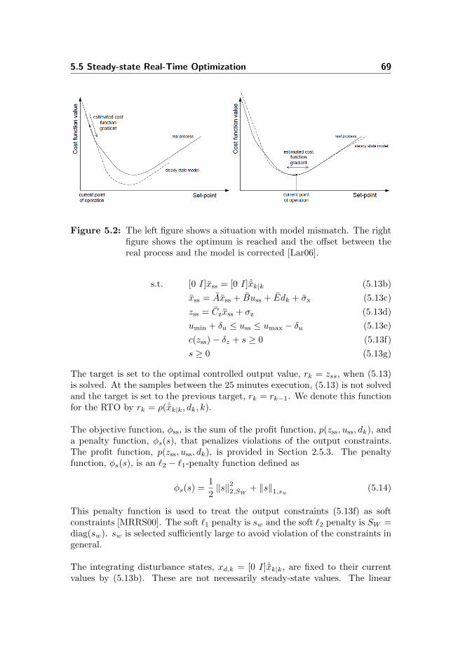
5.5 Steady-state Real-Time Optimization 69
Figure 5.2: The left figure shows a situation with model mismatch. The rightfigure shows the optimum is reached and the offset between thereal process and the model is corrected [Lar06].
s.t. [0 I]xss = [0 I]ˆxk|k (5.13b)
xss = Axss + Buss + Edk + σx (5.13c)
zss = Czxss + σz (5.13d)
umin + δu ≤ uss ≤ umax − δu (5.13e)
c(zss)− δz + s ≥ 0 (5.13f)
s ≥ 0 (5.13g)
The target is set to the optimal controlled output value, rk = zss, when (5.13)is solved. At the samples between the 25 minutes execution, (5.13) is not solvedand the target is set to the previous target, rk = rk−1. We denote this functionfor the RTO by rk = ρ(ˆxk|k, dk, k).
The objective function, φss, is the sum of the profit function, p(zss, uss, dk), anda penalty function, φs(s), that penalizes violations of the output constraints.The profit function, p(zss, uss, dk), is provided in Section 2.5.3. The penaltyfunction, φs(s), is an `2 − `1-penalty function defined as
φs(s) =1
2‖s‖22,SW
+ ‖s‖1,sw (5.14)
This penalty function is used to treat the output constraints (5.13f) as softconstraints [MRRS00]. The soft `1 penalty is sw and the soft `2 penalty is SW =diag(sw). sw is selected sufficiently large to avoid violation of the constraints ingeneral.
The integrating disturbance states, xd,k = [0 I]ˆxk|k, are fixed to their currentvalues by (5.13b). These are not necessarily steady-state values. The linear

70 Tracking Model Predictive Control with an RTO layer
model (5.2) is used in the constraints (5.13c)-(5.13d) to determine the steady-state relation between the inputs, uss, and the controlled outputs, zss. The linearmodel (5.2) is used in the RTO for the spray dryer as the nonlinear effects aremostly related to the output constraints. Note, that the model cannot and donot contain pure integrators, as the steady-state computation implies the inver-sion (I−A)−1. The nonlinear process constraints, c(zss), given in Section 2.5.4,contains the stickiness constraints of the powder and the operator defined limitson the outputs. umin and umax define the process input constraints. Togetherthese constraints provide a region in which safe operation is guaranteed. δucontains a 2.5C back-off in the input temperatures to avoid saturation and lossof controllability. δz contains a 0.05 C back-off in the stickiness constraint and0.02 % back-off in the residual moisture. δz is selected to provide constraintviolations that are similar to the E-MPC strategy.
We use a Sequential Quadratic Programming (SQP) method for solution of(5.13). The SQP method is a quasi-Newton implementation with linesearch forstep-size selection and BFGS update of the Hessian. In Paper B and H thegradients are computed by a centered finite difference method and in Paper Ithe gradients are computed analytically. We use the Matlab R© function fmincon
[Mat15] to solve the SQP. This method performs well in terms of efficiency,accuracy and percentage of successful solutions. An optimal solution is reportedby the SQP algorithm if the KKT conditions are satisfied to a relative andabsolute tolerance of 10−12. In Paper B and H we solve (5.13) with the outputsand states eliminated from the NLP. In Paper I we eliminate only the state.The problem size is relatively small, with 4 inputs and 4 outputs, thus thecomputational time difference is marginal.
The solution of (5.13) is defined by the function
rk = ψ(ˆxk|k, dk, k) (5.15)
in which ˆxk|k is the current state estimate where only the offset states are utilizedfor model corrections and dk is the measured disturbances. Algorithm 4 liststhe on-line computations of the RTO.
5.6 Closed-loop Simulation
The performance of the MPC with RTO control strategy has been investigatedby a closed-loop simulation. Fig. 5.3 shows the measured outputs, the targetsand the inputs of the closed-loop simulation. Fig. 4.2 shows the disturbances.The simulation shows that the MPC is able to control the process outputs re-lated to stickiness of the powder, TSD and Yab, the SFB stage temperature, TSFB,

5.6 Closed-loop Simulation 71
Algorithm 4 RTO Algorithm, ψ(·)Require: ˆxk|k, dk, kSolve NLP:x∗ = NLPSolver(problem(Xinit,dk,ˆxk|k))[uss,zss,s] = unpack(x∗)rk = zssreturn rk
Require: [q, ceq, cineq]=problem(x,dk,ˆxk|k)[u,z,s] = unpack(x)Compute the cost functionq = −p(z, u, dk) + 1
2sTSW s+ sT sw
Compute the equality constraintsxd,k = [0 I]ˆxk|kxss = (I −A)−1(Bu+ Edk +Bdxd,k + σx)zss = Cyxss + Cdxd,k + σz
ceq = z − zssCompute the inequality constraintscineq = [c(z) + δz + s ≥ 0; s ≥ 0;umin + δu ≤ u ≤ umax − δu]
and the residual moisture content, Scd, to their targets. The effect of the distur-bances are rejected by constant adjustments of the inputs. The targets used aregenerated by the RTO layer. These are feasible and the regulator is trackingthese targets well. It turns out, that the economics of drying are optimizedby minimizing the exhaust air temperature, TSD, in order to save energy andmaximize the exhaust air humidity, Yab, to increase the product flow rate. Thelower limit of TSD and upper limit of Yab are determined according to the stick-iness constraint of the powder. The powder moisture content, Scd, is increaseduntil it reaches its upper limit. The energy consumption is further minimizedby shifting the drying from the top of the spray dryer to the more efficient fluidbed stages. Thus, the supply of hot air to the SFB and VFB stages are favoredcompared to the SD stage. This leads to a high SFB stage temperature that iscontrolled close to its maximum temperature TSFB ≤ 75.5C.
The MPC with RTO does not operate at the maximum production rate, atall times. At time t=1 hour to t=2 hour, t=4 hour, t=5 hour, t=7.5 hoursand between t=19 hours to t=21 hours, the RTO reduces the production rate.The RTO problem (5.13) contains back-offs in the controlled inputs. The MPCwith RTO compensates for the decreased VFB inlet air temperature, Tvfbh, byincreasing the SFB inlet air temperature, Tsfb. Consequently, the SFB stagetemperature, TSFB, increases and the upper limit on the SFB stage temper-ature, TSFB ≤ 75.5 C, becomes active. When the SFB temperature limit is
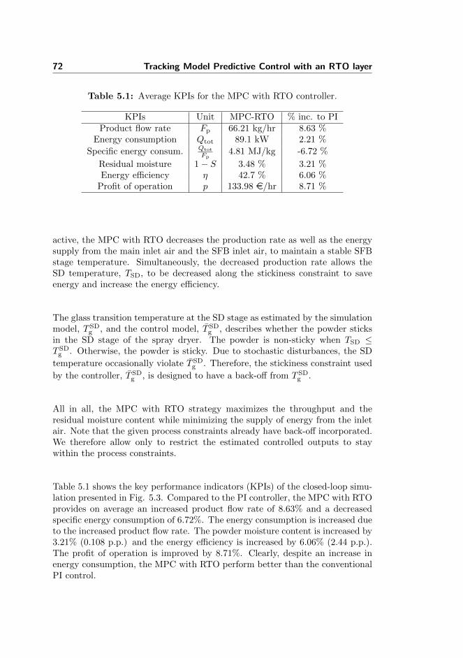
72 Tracking Model Predictive Control with an RTO layer
Table 5.1: Average KPIs for the MPC with RTO controller.
KPIs Unit MPC-RTO % inc. to PIProduct flow rate Fp 66.21 kg/hr 8.63 %
Energy consumption Qtot 89.1 kW 2.21 %
Specific energy consum. Qtot
Fp4.81 MJ/kg -6.72 %
Residual moisture 1− S 3.48 % 3.21 %Energy efficiency η 42.7 % 6.06 %
Profit of operation p 133.98 e/hr 8.71 %
active, the MPC with RTO decreases the production rate as well as the energysupply from the main inlet air and the SFB inlet air, to maintain a stable SFBstage temperature. Simultaneously, the decreased production rate allows theSD temperature, TSD, to be decreased along the stickiness constraint to saveenergy and increase the energy efficiency.
The glass transition temperature at the SD stage as estimated by the simulationmodel, T SD
g , and the control model, T SDg , describes whether the powder sticks
in the SD stage of the spray dryer. The powder is non-sticky when TSD ≤T SD
g . Otherwise, the powder is sticky. Due to stochastic disturbances, the SD
temperature occasionally violate T SDg . Therefore, the stickiness constraint used
by the controller, T SDg , is designed to have a back-off from T SD
g .
All in all, the MPC with RTO strategy maximizes the throughput and theresidual moisture content while minimizing the supply of energy from the inletair. Note that the given process constraints already have back-off incorporated.We therefore allow only to restrict the estimated controlled outputs to staywithin the process constraints.
Table 5.1 shows the key performance indicators (KPIs) of the closed-loop simu-lation presented in Fig. 5.3. Compared to the PI controller, the MPC with RTOprovides on average an increased product flow rate of 8.63% and a decreasedspecific energy consumption of 6.72%. The energy consumption is increased dueto the increased product flow rate. The powder moisture content is increased by3.21% (0.108 p.p.) and the energy efficiency is increased by 6.06% (2.44 p.p.).The profit of operation is improved by 8.71%. Clearly, despite an increase inenergy consumption, the MPC with RTO perform better than the conventionalPI control.
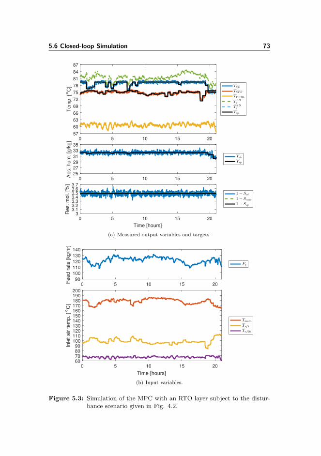
5.6 Closed-loop Simulation 73
0 5 10 15 2057
60
63
66
69
72
75
78
81
84
87T
em
p. [o
C] TSD
TSFB
TV FBh
T SDg
T SDg
Tsp
0 5 10 15 2025
27
29
31
33
35
Abs. hum
. [g
/kg]
Yab
Ysp
0 5 10 15 20
Time [hours]
33.13.23.33.43.53.63.7
Res. m
oi. [%
]
1− Scd
1− Smax
1− Ssp
(a) Measured output variables and targets.
0 5 10 15 20 90
100
110
120
130
140
Feed r
ate
[kg/h
r]
Ff
0 5 10 15 20
Time [hours]
60 70 80 90100110120130140150160170180190200
Inle
t air tem
p. [
oC
]
Tmain
Tsf b
Tvf bh
(b) Input variables.
Figure 5.3: Simulation of the MPC with an RTO layer subject to the distur-bance scenario given in Fig. 4.2.

74 Tracking Model Predictive Control with an RTO layer
5.7 Summary
In this chapter, we described the MPC with RTO control strategy and performeda closed-loop simulation.
• We described the state estimator, the regulator and the RTO layer to forma complete MPC with RTO control strategy applicable for real-time use.Tuning of the state estimator was also presented.
• We showed that the MPC with RTO provides significantly improved con-trol of the residual moisture content compared to the conventional PIcontrol and avoids that the powder sticks to the walls of the chamber.
• Compared to conventional PI control strategy, the product flow rate isimproved by 8.63%, the specific energy consumption is decreased by 6.72%,and the powder moisture content is improved by 3.21%.
• The MPC with RTO improves the profit of operation by 8.71%. Thus, theMPC with RTO control strategy perform better than the conventional PIcontrol.
Chapter 6
Economic Model PredictiveControl
In this chapter, we present the Economic Model Predictive Control (E-MPC)algorithm, utilizing a nonlinear objective, a nonlinear control model and a con-straint function from Section 2.5 for control of the four-stage spray dryer.
The chapter provides a summary of Paper B, Paper F, Paper G and Paper H.
6.1 Control principles of E-MPC
In Chapter 5 we presented the hierarchical approach to economic optimizationand control, the MPC with RTO, which is widely applied in the process indus-tries [DNJN11,AO10]. Recently, E-MPC has been found effective within processoptimization. In E-MPC the RTO layer is not required for computing targetsto the MPC, as the higher-level objective, economics, is directly implementedin the objective function of the MPC.
Fig. 6.1 illustrates the components of the E-MPC and the signal paths betweenthese and the dryer. In the E-MPC control strategy we manipulate the same

76 Economic Model Predictive Control
Figure 6.1: Illustration of the E-MPC, that combines a stateestimator and a regulator for economic optimiza-tion of the dryer operation.
four inputs as in the MPC with RTO strategy based on the same set of measuredoutputs and disturbances.
The measurement vector, y, the output vector, z, the input vector, u, and themain disturbance vector, d, are
y =[TSD TSFB Yab TVFBh TVFBc Scd
]T(6.1a)
z =[TSD TSFB Yab Scd
]T(6.1b)
u =[Ff Tmain Tsfb Tvfbh
]T(6.1c)
d =[Sf Tf Yamb
]T(6.1d)
Fig. 2.1 provides an overview of the spray dryer, the symbols and the namingconvention of the outputs, inputs and disturbances.
Algorithm 5 lists the on-line computations in the E-MPC algorithm consistingof a regulator and a state estimator. The state estimator consists of a filter anda one-step-ahead predictor step. The sample time is Ts = 30 s. As described inChapter 5, the state estimator provides the initial state of the dynamic model,which in combination with the model is used in the regulator to optimize thefuture input trajectory. The optimization in the regulator results in a sequenceof inputs for a finite horizon, out of which only the first input is applied to thedryer. This procedure is repeated at each sample instant. The repeated opti-mization procedure provides feedback and form a closed-loop input trajectory.This enables the E-MPC to counteract model uncertainties, model mismatchand unknown disturbances etc.
The discrete-time nonlinear regulator problem may be solved using single-shooting

6.2 Model 77
Algorithm 5 E-MPC Algorithm
Require: yk, dk, ˆxk|k−1, Pk|k−1, uk−1
Filter:Compute the one-step ahead measurement prediction and the output matrix
yk|k−1 = hy(ˆxk|k−1), Cy,k =dhy
dx (ˆxk|k−1)Compute the filtered stateRe,k = Cy,kPk|k−1C
Ty,k +Rv,k
Kfx,k = Pk|k−1CTy,kR
−1e,k
ˆxk|k = ˆxk|k−1 + Kfx,k(yk − yk|k−1)Pk|k = Pk|k−1 − Kfx,kRe,kK
Tfx,k
Regulator:uk = µ(ˆxk|k, uk−1, dk)One-step predictor:Compute the predicted state, ˆxk+1|k = F (ˆxk|k, uk, dk), and state sensitivity,
Ak = ∂F∂x (ˆxk|k, uk, dk) using ESDIRK
[ˆxk+1|k, Ak] = ESDIRK(tk,tk+1,ˆxk|k, uk, dk)Pk+1|k = AkPk|kATk + GRwG
T
return uk, ˆxk+1|k, Pk+1|k
(control vector parametrization) [SSBM05], multiple-shooting [BP84, CJ12] orthe simultaneous method [Bie84]. In this thesis both the single-shooting andthe multiple-shooting method are investigated. We use an efficient ODE/DAEsolver, the explicit singly diagonally implicit Runge-Kutta (ESDIRK) method,with sensitivity computation capabilities to speed up the computational time.The sensitivity capability also makes the ESDIRK method well suited for thestate estimator.
6.2 Model
The E-MPC is based on the complexity reduced nonlinear model in Section 2.5that is different from the simulation model in Section 2.4. Offset-free estimationof the measurements and offset-free control of the controlled variables at steady-state are achieved by augmenting the model. The state vector, x, is augmentedby a vector of integrated disturbance states, xd. The augmented state vectoris x = [x;xd] ∈ Rnx . The regulator and state estimator are based on theaugmented model
xk+1 = F (xk, uk, dk) + Gwk (6.2a)
yk = hy(xk) + vk (6.2b)
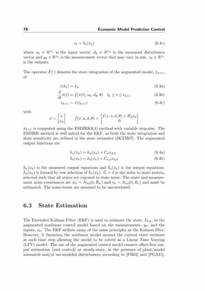
78 Economic Model Predictive Control
zk = hz(xk) (6.2c)
where uk ∈ Rnu is the input vector, dk ∈ Rnd is the measured disturbancevector and yk ∈ Rny is the measurement vector that may vary in size. zk ∈ Rnz
is the outputs.
The operator F (·) denotes the state integration of the augmented model, xk+1,of
x(tk) = xk (6.3a)
d
dtx(t) = f(x(t), uk, dk, θ) tk ≤ t ≤ tk+1 (6.3b)
xk+1 = x(tk+1) (6.3c)
with
x =
[xxd
]f(x, u, d, θ) =
[f(x, u, d, θ) +Bdxd
0
]
xk+1 is computed using the ESDIRK3(4) method with variable step-size. TheESDIRK method is well suited for the EKF, as both the state integration andstate sensitivity are utilized in the state estimator [JKTM07]. The augmentedoutput functions are
hy(xk) = hy(xk) + Cdxd,k (6.4a)
hz(xk) = hz(xk) + Cd,zxd,k (6.4b)
hy(xk) is the measured output equations and hz(xk) is the output equations.hz(xk) is formed by row selection of hy(xk). G = I is the noise to state matrix,selected such that all states are exposed to state noise. The state and measure-ment noise covariances are wk ∼ Niid(0, Rw) and vk ∼ Niid(0, Rv) and must beestimated. The noise-terms are assumed to be uncorrelated.
6.3 State Estimation
The Extended Kalman Filter (EKF) is used to estimate the state, ˆxk|k, in theaugmented nonlinear control model based on the measurements, yk, and theinputs, uk. The EKF utilizes many of the same principles as the Kalman filter.However, it linearizes the nonlinear model around the current state estimateat each time step allowing the model to be solved as a Linear Time Varying(LTV) model. The use of the augmented control model ensures offset-free out-put estimation (and control) at steady-state, in the presence of plant/modelmismatch and/or un-modeled disturbances according to [PR03] and [PGA15].

6.4 Regulator 79
In Paper B, Paper G and Paper H we select pure input disturbances, i.e. Cd = 0and Bd such that the energy- and the vapor mass balances are subject to thedisturbance integration.
Algorithm 5 provides the state estimator equations. The filtering part correctsˆxk|k, using the latest measurement, yk, after which it is used in the regulator asthe initial state. The predictor part uses the model to predict ˆxk+1|k.
Maximum Likelihood (ML) TuningThe unknown noise variances, Rw and Rv, are estimated by the MaximumLikelihood (ML) method in the same manner as described in Section 5.3. Thelikelihood function, VML(θ) in (5.5) is determined recursively by means of theEKF in Algorithm 5 without the regulator step. θ is θ = [θw; θv] and we definethe noise covariances Rw = diag(θw) and Rv = diag(θv).
6.4 Regulator
In a receding horizon manner, the inputs in the E-MPC are obtained by thesolution of the following finite dimensional discrete optimal control problem
minx,u,s
φ = φe + φs + φ∆u, (6.5a)
s.t. [xk; xd,k] = ˆxk|k, x(tk) = xk, (6.5b)
d
dtx(t) = f(x(t), uk+j , dk, θ) +Bdxd,k, t ∈ Tk (6.5c)
z(t) = hz(x(t)) + Cd,zxd,k, t ∈ Tk (6.5d)
umin ≤ uk+j ≤ umax, j ∈ Nu (6.5e)
c(z(tk+j)) + sk+j ≥ 0, j ∈ Nz (6.5f)
sk+j ≥ 0, j ∈ Nz (6.5g)
x(t) is the state vector, uk is the input vector, dk is the measured disturbancevector and sk ∈ Rns is the vector of slack variables related to the soft outputconstraints. The objective function, φ, consists of an economic term
φe = −∫ tk+T
tk
p(z(t), uk+j , dk)dt (6.6)
measuring the profit of operation, an `2 − `1 penalty term
φs =
N∑
j=1
1
2‖sk+j‖22,SW
+ ‖sk+j‖1,sw (6.7)
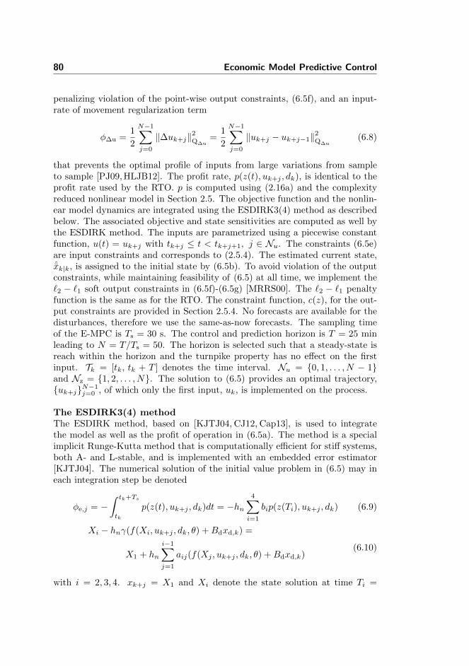
80 Economic Model Predictive Control
penalizing violation of the point-wise output constraints, (6.5f), and an input-rate of movement regularization term
φ∆u =1
2
N−1∑
j=0
‖∆uk+j‖2Q∆u=
1
2
N−1∑
j=0
‖uk+j − uk+j−1‖2Q∆u(6.8)
that prevents the optimal profile of inputs from large variations from sampleto sample [PJ09, HLJB12]. The profit rate, p(z(t), uk+j , dk), is identical to theprofit rate used by the RTO. p is computed using (2.16a) and the complexityreduced nonlinear model in Section 2.5. The objective function and the nonlin-ear model dynamics are integrated using the ESDIRK3(4) method as describedbelow. The associated objective and state sensitivities are computed as well bythe ESDIRK method. The inputs are parametrized using a piecewise constantfunction, u(t) = uk+j with tk+j ≤ t < tk+j+1, j ∈ Nu. The constraints (6.5e)are input constraints and corresponds to (2.5.4). The estimated current state,ˆxk|k, is assigned to the initial state by (6.5b). To avoid violation of the outputconstraints, while maintaining feasibility of (6.5) at all time, we implement the`2 − `1 soft output constraints in (6.5f)-(6.5g) [MRRS00]. The `2 − `1 penaltyfunction is the same as for the RTO. The constraint function, c(z), for the out-put constraints are provided in Section 2.5.4. No forecasts are available for thedisturbances, therefore we use the same-as-now forecasts. The sampling timeof the E-MPC is Ts = 30 s. The control and prediction horizon is T = 25 minleading to N = T/Ts = 50. The horizon is selected such that a steady-state isreach within the horizon and the turnpike property has no effect on the firstinput. Tk = [tk, tk + T ] denotes the time interval. Nu = 0, 1, . . . , N − 1and Nz = 1, 2, . . . , N. The solution to (6.5) provides an optimal trajectory,uk+jN−1
j=0 , of which only the first input, uk, is implemented on the process.
The ESDIRK3(4) methodThe ESDIRK method, based on [KJTJ04, CJ12, Cap13], is used to integratethe model as well as the profit of operation in (6.5a). The method is a specialimplicit Runge-Kutta method that is computationally efficient for stiff systems,both A- and L-stable, and is implemented with an embedded error estimator[KJTJ04]. The numerical solution of the initial value problem in (6.5) may ineach integration step be denoted
φe,j = −∫ tk+Ts
tk
p(z(t), uk+j , dk)dt = −hn4∑
i=1
bip(z(Ti), uk+j , dk) (6.9)
Xi − hnγ(f(Xi, uk+j , dk, θ) +Bdxd,k) =
X1 + hn
i−1∑
j=1
aij(f(Xj , uk+j , dk, θ) +Bdxd,k)(6.10)
with i = 2, 3, 4. xk+j = X1 and Xi denote the state solution at time Ti =

6.4 Regulator 81
tn + cihn for i ∈ 1, 2, 3, 4. xk+j+1 = X4 is the numerical solution at timetn + hn. a, b, c and γ are the Runge-Kutta Butcher Tableau values. Themain computational effort in the ESDIRK method is the solution of the implicitequations (6.10) using a Newton based method. The ESDIRK method alsoprovides sensitivity computation capabilities. The details of the computationof the state and stage cost sensitivities are described in [KJTJ04,CJ12,Cap13].The scheme has been implemented with variable integration step-size, hn, withan error accuracy of 10−4. Each integration step-size, hn, is chosen to be smallerthan or equal to the sample time, Ts.
6.4.1 Optimization Methods
The nonlinear optimization problem (NLP) in (6.5) may be solved using a single-shooting, a multiple-shooting or a collocation method. In Paper D, Paper F andPaper G we use the single-shooting method and in Paper B and Paper H weuse the multiple-shooting method. We found that the two methods have almostequal execution time for this E-MPC problem. The single-shooting method isadvantageous for systems with a relatively large number of states compared tothe number of inputs. The method progress towards a solution by iteratingbetween solving the model and solving a reduced size optimization problem.We speed up the computations by computing the gradients by the discrete ad-joint method, but many other methods exist. Single-shooting may be costlyif evaluation of the problem functions are costly, e.g. if an implicit discretiza-tion scheme must be applied. In addition single-shooting lacks robustness whenapplied to unstable processes [MBF04]. The multiple-shooting method is analternative and popular choice, as it requires few internal iterations and havegood stability properties. Gradients may be constructed directly from the sen-sitivities given by the ODE/DAE solver. The gradients are highly sparse whichmust be exploited. Both single-shooting and multiple-shooting methods can usestate-of-the-art ODE/DAE solvers [KJTJ04,CJ12,Cap13].
We use the multiple-shooting method with an NLP-solver from IPOPT for thesimulation study described in this chapter. IPOPT is based on an interior-pointalgorithm. Alternatively, the Matlab R© function fmincon [Mat15] can be usedfor solution of the NLP. We experience the lowest computation times using theIPOPT method.
The solution of (6.5) is defined by the function
uk = µ(ˆxk|k, uk−1, dk) (6.11)
in which uk is the first u∗k of U∗k . The function defines the on-line computationsof the regulator, provided in Algorithm 6, and used in Algorithm 5.
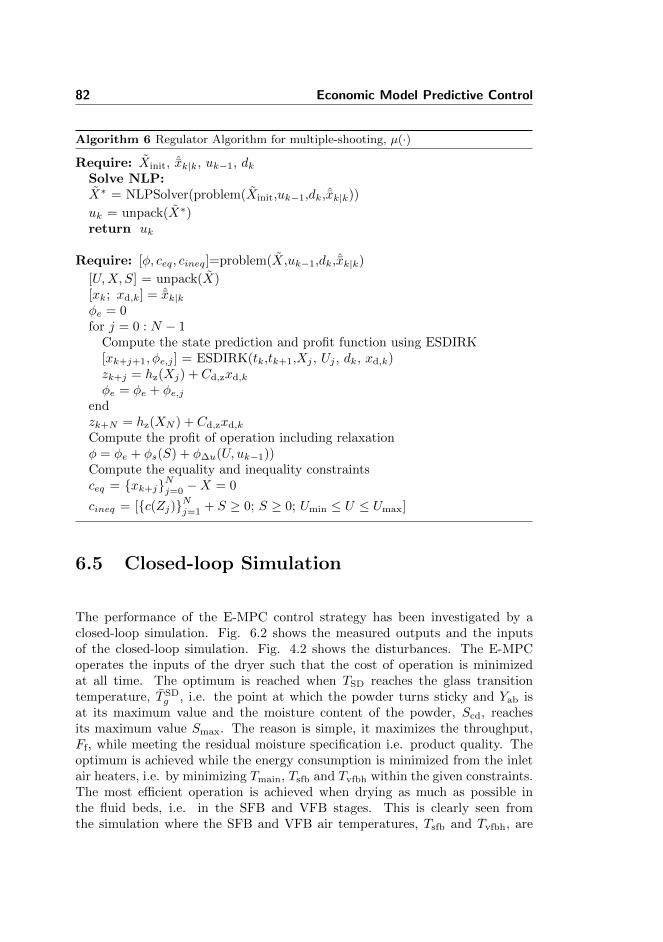
82 Economic Model Predictive Control
Algorithm 6 Regulator Algorithm for multiple-shooting, µ(·)
Require: Xinit, ˆxk|k, uk−1, dkSolve NLP:X∗ = NLPSolver(problem(Xinit,uk−1,dk,ˆxk|k))
uk = unpack(X∗)return uk
Require: [φ, ceq, cineq]=problem(X,uk−1,dk,ˆxk|k)
[U,X, S] = unpack(X)[xk; xd,k] = ˆxk|kφe = 0for j = 0 : N − 1
Compute the state prediction and profit function using ESDIRK[xk+j+1, φe,j ] = ESDIRK(tk,tk+1,Xj , Uj , dk, xd,k)zk+j = hz(Xj) + Cd,zxd,k
φe = φe + φe,jendzk+N = hz(XN ) + Cd,zxd,k
Compute the profit of operation including relaxationφ = φe + φs(S) + φ∆u(U, uk−1))Compute the equality and inequality constraintsceq = xk+jNj=0 −X = 0
cineq = [c(Zj)Nj=1 + S ≥ 0; S ≥ 0; Umin ≤ U ≤ Umax]
6.5 Closed-loop Simulation
The performance of the E-MPC control strategy has been investigated by aclosed-loop simulation. Fig. 6.2 shows the measured outputs and the inputsof the closed-loop simulation. Fig. 4.2 shows the disturbances. The E-MPCoperates the inputs of the dryer such that the cost of operation is minimizedat all time. The optimum is reached when TSD reaches the glass transitiontemperature, T SD
g , i.e. the point at which the powder turns sticky and Yab isat its maximum value and the moisture content of the powder, Scd, reachesits maximum value Smax. The reason is simple, it maximizes the throughput,Ff, while meeting the residual moisture specification i.e. product quality. Theoptimum is achieved while the energy consumption is minimized from the inletair heaters, i.e. by minimizing Tmain, Tsfb and Tvfbh within the given constraints.The most efficient operation is achieved when drying as much as possible inthe fluid beds, i.e. in the SFB and VFB stages. This is clearly seen fromthe simulation where the SFB and VFB air temperatures, Tsfb and Tvfbh, are

6.6 Summary 83
Table 6.1: Average KPIs for the E-MPC controller.
KPIs Unit E-MPC % inc. to PIProduct flow rate Fp 66.81 kg/hr 9.61 %
Energy consumption Qtot 90.4 kW 3.63 %
Specific energy consum. Qtot
Fp4.88 MJ/kg -5.44 %
Residual moisture 1− S 3.49 % 3.37 %Energy efficiency η 42.5 % 5.52 %
Profit of operation p 135.19 e/hr 9.69 %
maximized until the residual moisture reaches the upper limit. This leads to ahigh SFB stage temperature that is controlled close to its maximum temperatureTSFB ≤ 75.5C, however it does not reach it.
The simulation also shows that an increase in the ambient air humidity, Yamb,or decrease in feed solid concentration, Sf, have the same effect i.e. causing thepowder to turn more moist and sticky inside the dryer. The E-MPC compensatesin both cases by decreasing the feed rate, Ff, and the inlet air temperaturesaccordingly to maintain the optimal temperatures in the stages. Consequently,the economically most favorable conditions for the dryer is obtained at lowambient air humidity while drying a feed with a high content of solids.
Table 6.1 shows the key performance indicators (KPIs) of the closed-loop simu-lation presented in Fig. 6.2. Compared to the PI control strategy, the E-MPCprovides on average an increased product flow rate of 9.61% and a decreasedspecific energy consumption of 5.44%. The energy consumption is increased dueto the increased product flow rate. The powder moisture content is increased by3.37% (0.114 p.p.) and the energy efficiency is increased by 5.52% (2.22 p.p.).The profit of operation is improved by 9.69%. These numbers surpass both theperformance of the MPC with RTO strategy and the conventional PI controlstrategy.
6.6 Summary
In this chapter, we described the E-MPC control strategy and performed aclosed-loop simulation.
• We described the nonlinear state estimator and the nonlinear regulatorthat together forms a complete E-MPC control strategy. Tuning of thestate estimator was also considered.
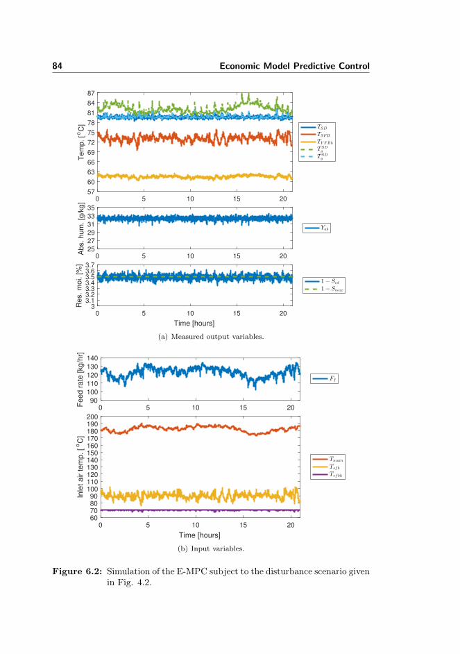
84 Economic Model Predictive Control
0 5 10 15 2057
60
63
66
69
72
75
78
81
84
87
Tem
p. [o
C] TSD
TSFB
TV FBh
T SDg
T SDg
0 5 10 15 2025
27
29
31
33
35
Abs. hum
. [g
/kg]
Yab
0 5 10 15 20
Time [hours]
33.13.23.33.43.53.63.7
Res. m
oi. [%
]
1− Scd
1− Smax
(a) Measured output variables.
0 5 10 15 20 90
100
110
120
130
140
Feed r
ate
[kg/h
r]
Ff
0 5 10 15 20
Time [hours]
60 70 80 90100110120130140150160170180190200
Inle
t air tem
p. [
oC
]
Tmain
Tsf b
Tvf bh
(b) Input variables.
Figure 6.2: Simulation of the E-MPC subject to the disturbance scenario givenin Fig. 4.2.

6.6 Summary 85
• We designed an E-MPC that controls the residual moisture content andavoids that the powder sticks to the walls of the chamber.
• Compared to the conventional PI control strategy, the product flow rateis improved by 9.61%, the specific energy consumption is decreased by5.44%, and the powder moisture content is improved by 3.37%.
• We showed by a closed-loop simulation that the E-MPC surpasses theperformance of the PI control and MPC with RTO strategies. E-MPCimproves the profit of operation by 9.69%.

86 Economic Model Predictive Control

Chapter 7
Application of MPC to anIndustrial Spray Dryer
In this chapter, we describe the application of MPC with an RTO layer to anindustrial four-stage spray dryer. We provide an industrially recorded closed-loop experiment and show that the profit of operation is improved significantlyby the application of MPC.
The chapter provides a summary of Paper I.
The spray dryer in question is a GEA Multi-Stage Dryer (MSDTM-1250) thatproduces enriched milk powder. It is one of the largest dryers installed in thedairy industry. The dryer is supplied with 169 tons/hr of air and consumes7.4 MW of energy to heat the air by combustion of natural gas. The nominalevaporation capacity is approximately 7000 kg/hr of water. The MPC solution,based on the MPC with an RTO layer, which is applied in this study, also formsthe basis of a control solution currently being commercialized and marketed asDRYCONTROLTM by GEA Process Engineering A/S.
88 Application of MPC to an Industrial Spray Dryer
7.1 PLC, Industrial PC and SCADA Setup
The dryer was erected in 2015, and is equipped with standard field instrumentsas well as the latest innovations within advanced field instruments. Fig. 7.1illustrates the communication paths between the PLC and the advanced fieldinstruments, the PLC and the industrial PC, and the PLC and the SCADAsystem. The residual moisture content is measured at the VFB powder outletand the exhaust air humidity is measured by extracting air from the exhaustair duct. The challenge from a control point of view is that these measurementsmay be unavailable for longer periods due to in-process maintenance, automati-cally detected sensor errors and slow sample frequencies. The PLC handles thecommunication between the standard field instruments, the advanced field in-struments and controls the actuators. The industrial PC, which runs our MPCalgorithm, is located in the PLC panel. The communication between the PLCand the industrial PC is performed via the OPC communication protocol, whichis a well proven industrial standard. The SCADA system handles and conveysthe operator instructions to the PLC as well as presents the current state ofthe spray dryer. Fig. 7.2 shows the SCADA system from which the operatorshandle the standard control system and the MPC solution. In the SCADA sys-tem the operator can turn the MPC solution on and off, adjust the constraintsin the recipe system and see the optimal targets which the MPC is headingtowards. The task for the operator is thus changed from defining targets for thePID controllers to defining ranges (constraints) for the manipulated variablesand targets of the MPC solution. The inputs and outputs of the MPC solutionare scaled and validated before being sent to the PLC and after being receivedfrom the PLC. Bumpless transfer is implemented to ensure a smooth transi-tion between the MPC and the conventional PI control strategy. Interlocks areimplemented to accommodate emergency shut downs.
7.2 MPC Program
The MPC program implements the MPC algorithm and the additional featuresneeded to provide a standalone MPC solution. The MPC code is compiled onlyonce to a standalone executable program using Matlab R©. The MPC programis used for all applications. The individual specification of each application ismade by configuring an XML file. The MPC program reads this XML file aspart of its initialization/start-up routine. This XML file is also referred to asthe definition file.
Fig. 7.3 shows an overview of the MPC program, which is composed of several
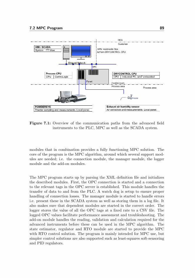
7.2 MPC Program 89
Figure 7.1: Overview of the communication paths from the advanced fieldinstruments to the PLC, MPC as well as the SCADA system.
modules that in combination provides a fully functioning MPC solution. Thecore of the program is the MPC algorithm, around which several support mod-ules are needed; i.e. the connection module, the manager module, the loggermodule and the add-on modules.
The MPC program starts up by parsing the XML definition file and initializesthe described modules. First, the OPC connection is started and a connectionto the relevant tags in the OPC server is established. This module handles thetransfer of data to and from the PLC. A watch dog is setup to ensure properhandling of connection losses. The manager module is started to handle errorsi.e. present these in the SCADA system as well as storing them in a log file. Italso makes sure that dependent modules are started in the correct order. Thelogger stores the value of all the OPC tags at a fixed rate to a CSV file. Thelogged OPC values facilitate performance assessment and troubleshooting. Theadd-on module handles the reading, validation and calculation required for theadvanced instruments before these can be used in the MPC algorithm. Thestate estimator, regulator and RTO module are started to provide the MPCwith RTO control solution. The program is mainly intended for MPC use, butsimpler control solutions are also supported such as least-squares soft-sensoringand PID regulators.

90 Application of MPC to an Industrial Spray Dryer
Figure 7.2: The SCADA system for control of the spray dryer along with theMPC faceplate.
7.2.1 MPC Algorithm
The MPC algorithm in the MPC program is based on the earlier described MPCwith an RTO layer from Chapter 5, Paper B and Paper H. The performance ofthis controller compares well to the more advanced E-MPC solution while beingsimpler to implement, proved reliable and requires a minimum of computationalpower. The MPC algorithm combines a state estimator, a regulator and an RTOlayer as presented in Algorithm 2, Fig. 5.1 in Chapter 5 and Fig. 7.3.
7.2.1.1 State Estimator Module
The state estimator module, which may also act as a standalone soft-sensor, isbased on a linear time-varying Kalman filter. The time-varying Kalman filteris used to estimate the initial state in the regulator, ˆxk|k. Offset-free outputestimation (and control) at steady-state is provided by augmenting the identifiedstate-space model with integrating output disturbances, i.e. Cd = I and Bd = 0[PR03,PGA15]. The output disturbance model is favored compared to the input

7.2 MPC Program 91
Figure 7.3: Overview of the structure in the MPC program (i.e.DRYCONTROLTM).

92 Application of MPC to an Industrial Spray Dryer
disturbances as the model errors seem to mainly show as step changes in theoutputs.
As in Section 5.2, the augmented model is
xk+1 = Axk + Buk + Edk + Gwk + σx (7.1a)
yk = Cyxk + σy + vk (7.1b)
zk = Czxk + σz (7.1c)
where xk ∈ Rnx is the augmented state vector, uk ∈ Rnu is the input vector,dk ∈ Rnd is the measured disturbance vector and yk ∈ Rny is the measurementvector that vary in size. zk ∈ Rnz is the controlled output vector. G is selectedsuch that only the integrating disturbance states are subject to state noise. wkand vk are assumed uncorrelated with wk ∼ Niid
(0, Rw
)and vk ∼ Niid(0, Rv).
The noise covariances are estimated according to Section 5.3.1.
7.2.1.2 Regulator Module
The regulator is formed as an output tracking problem with input constraints
minuk+jN−1
j=0
φ =1
2
N∑
j=1
‖zk+j − rk‖2Qz+
1
2
N−1∑
j=0
‖∆uk+j‖2Su(7.2a)
s.t. xk = ˆxk|k, (7.2b)
xk+j+1 = Axk+j + Buk+j + Edk + σx, j ∈ Nu (7.2c)
zk+j = Czxk+j + σz, j ∈ Nz (7.2d)
umin ≤ uk+j ≤ umax, j ∈ Nu (7.2e)
in which ∆uk+j = uk+j−uk+j−1 and Nz = 1, 2 . . . , N, Nu = 0, 1 . . . , N−1.N is the control and prediction horizon. The estimated current state, ˆxk|k, isassigned to the initial state by (7.2b). (7.2c) and (7.2d) are the augmented state-space constraints from (7.1). (7.2e) are the input constraints. No forecasts areavailable for the target, rk, and the measured disturbances, dk. Therefore we usethe same-as-now predictions in (7.2). The tracking problem in (7.2) is solved byformulating the corresponding convex quadratic problem as described in Section5.4.
7.2.1.3 RTO Module
The RTO layer computes the target, rk, in the regulator to achieve better eco-nomic performance. The RTO algorithm is described in details in Section 5.5.

7.2 MPC Program 93
rk is computed by
minuss,zss,s
φss = −p(zss, uss, dk) + ‖s‖22,SW(7.3a)
s.t. [0 I]xss = [0 I]ˆxk|k (7.3b)
xss = Axss + Buss + Edk + σx (7.3c)
zss = Czxss + σz (7.3d)
umin + δu ≤ uss ≤ umax − δu (7.3e)
c(zss) + s ≥ 0 (7.3f)
s ≥ 0 (7.3g)
The target is set to the optimal controlled output value, rk = zss, when (7.3) issolved. At the samples between the intervals, (7.3) is not solved and the currenttarget is maintained.
The objective function, φss, is the sum of the profit function, p(zss, uss, dk), and
a penalty function, ‖s‖22,SW, that penalizes violations of the output constraints.
The nonlinear profit function p(zss, uss, dk) is tailored to the dryer and productbeing dried as described in Paper H and Paper I. The integrating disturbancestates, xd,k = [0 I]ˆxk|k, are fixed to their current values by (7.3b). The linearmodel is used in the constraints (7.3c)-(7.3d) to determine the steady-staterelation between the inputs, uss, and the controlled outputs, zss. umin and umax
define the process input constraints. δu contains a back-off in the manipulatedvariables to maintain controllability in the regulator. The nonlinear processconstraints, c(zss), contains the stickiness constraints of the powder and theoperator defined limits on the controlled outputs. This function is tailored tothe dryer and product being dried as described in Paper H and Paper I. Togetherthese constraints provide a region in which safe operation is guaranteed. Weallowed only to constraint the controlled outputs of the Kalman filter to staywithin the stickiness constraint as the given constraints already have back-offincorporated. We use the Matlab R© function, fmincon, using the SQP methodfor solution of (7.3).
7.2.2 Add-on Module
An add-on module computes the feed solids concentration and handles the read-ing, validation and calculation required for the advanced field instruments. Thefeed concentration, Sf, is computed from measurements of the feed density andthe feed temperature. This is possible as the feed composition and the densityof the feed components are approximately known. The exhaust air humiditysensor provides a relative air humidity and a temperature measurement of the

94 Application of MPC to an Industrial Spray Dryer
extracted air from the exhaust air duct. The temperature and relative air hu-midity are used to compute the absolute air humidity, Y . The module computesthe absolute air humidity when the instrument readings are within its ranges.Otherwise the measurement is ignored. POWDEREYETM is a system for in-line powder analysis and is designed specifically for spray dryers. The systemallows producers of food and dairy powders to perform the most importantproduct quality tests (i.e. residual moisture content, poured and tapped densityof the powder and detection of scorched particles) during spray drying in a sin-gle in-line operation [DS14]. The module reads and scales the residual moisturemeasurement if no warnings are present at the instrument. If there is a warning,such as an empty sample cup, the measurement is ignored.
7.3 XML Definition File
The definition file defines the modules in the MPC program. The file identifiesthe tag names in the OPC server and defines the process inputs, outputs anddisturbances in the MPC algorithm. It contains the state-space models for eachrecipe of produced products. It specifies the control objective, i.e. targets,constraints and tuning parameters. The file also specifies the auxiliary features,such as handling of the advanced instruments. The design of this file is thedesign and modeling step of the MPC strategy. The file is formatted accordingto the XML standard, making it easy to read and parse in the program.
7.3.1 Process Outputs, Inputs and Disturbances
The controlled outputs in the MPC are the exhaust air temperature, Texh, andthe absolute exhaust air humidity, Y , to avoid deposits of sticky particles onthe spray dryer surfaces. The SFB powder temperature, Tpowder, is controlledto avoid lumps of powder to form in the SFB. The reisudal moisture content ofthe final powder, S, is controlled to keep it below and close to the maximumlimit. The inputs are the feed flow, Ff, the temperature target to the main airheater, Tmain,sp, the temperature target to the SFB air heater, Tsfb,sp, and thetemperature target to the VFB air heater, Tvfbh,sp. The inputs provide strongcontrollability of the outputs. The disturbances are the feed solids concentrationSf, the absolute ambient air humidity, Yamb, and the number of active nozzles,Nnozz, in the feed line.
The measurement and output vector, y = z, the input vector, u, and the dis-

7.3 XML Definition File 95
turbance vector, d, are
y =[Texh Y Tpowder S
]T(7.4a)
u =[Ff Tmain,sp Tsfb,sp Tvfbh,sp
]T(7.4b)
d =[Sf Yamb Nnozz
]T(7.4c)
7.3.2 Model Identification
The MPC relies on a model for estimation of the states and prediction in theregulator. The model is divided into two sub-models; an actuator model and adryer model. The approach is advantageous as it provides flexibility in tuningof the PID parameters in the actuators, as the tuning can be changed withoutthe need for identification of the full control model.
We identify a continuous-time transfer function model described by
U(s) = Ga(s)U(s) (7.5a)
Y (s) = Gm(s)U(s) +GdD(s) (7.5b)
z(tk) = y(tk) (7.5c)
in which U(s) is the inputs, U(s) is the actuated intermediate values and Z(s)is the controlled outputs. D(s) is the disturbances that affects the controlledoutputs.
Ga(s) is the actuator model, Gm(s) is the dryer model and Gd(s) is the distur-bance model. These consists of a matrix of transfer functions of the form
ga,ii(s) =Ka,ii
τa,iis+ 1e−θa,iis (7.5d)
gm,ji(s) =Km,ji
τm,jis+ 1e−θm,jis (7.5e)
gd,jk(s) =Kd,jk
τd,jks+ 1e−θd,jks (7.5f)
where i is the input, k is the disturbance and j is the output. The parametersin the above model are obtained by least-squares minimization of the residualsbetween the simulated and recorded response. Ga(s) is identified from 4 esti-mation datasets. Gm(s) and Gd(s) are identified from 10 estimation datasets.The estimation datasets were also used for validation.
Fig. 7.4 presents a dataset used for validation of the combined model in (7.5).The model response is a simulation in which no feedback from the data is im-plemented. The model fits the data well. The datasets used for identification

96 Application of MPC to an Industrial Spray Dryer
Figure 7.4: Comparison of a validation dataset (blue) and the cor-responding simulation (black) of the combined model in(7.5). The model fits the data well.
consist of both open-loop and closed-loop data. Fig. 7.5 shows the unit-stepresponses of the combined model, U(s) to Z(s). The process model in (7.5) istransformed to a discrete time state-space model, (A,B,E,Cy,Cz), using a zero-order-hold assumption on the inputs and disturbances. Thereby we can make abalanced realization from the Hankel matrix of the impulse response matrices.
The lumped control model presented in Section 2.5 and Paper G can potentiallyalso be used in the MPC and the RTO layer. Currently, the model describesdrying of maltodextrin on the smaller MSD-20 spray dryer and modificationsmust therefore be performed in order to make it fit this dryer. Instead, wedecided to use the more general black-box data driven model in (7.5).
7.3.3 Regulator and RTO Tuning
The tuning parameters in the objective function, Qz = diag([30 15 30 800]) andSu = diag([45 30 30 7.5]), are selected to achieve a good compromise between afast closed-loop response and robust performance. The highest weight is set oncontrol of the residual moisture content. The control and prediction horizon is,

7.4 Closed-loop Performance 97
Figure 7.5: Unit-step responses of the identified model in (7.5).
N = 60 min/20 s = 180. The sample rate of the MPC is 20 s. The RTO problemis solved at a sample rate of 30 s. The fast sample rate of the RTO means that asteady-state is not reached before the RTO computes a new target for the MPC.The soft constraint penalty is sW = diag([105 105 105 105]). The input andoutput constraints in the MPC and RTO layer are determined by the operatorsin the recipe handling system. The back-off in the manipulated temperatures,δu, is selected to be 5C to maintain controllability in the regulator.
7.4 Closed-loop Performance
The performance of the MPC has been validated against the conventional PIcontrol strategy in several experiments. Two of these experiments are presented
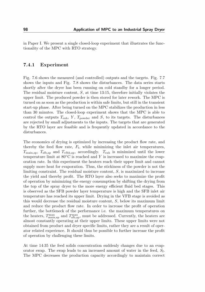
98 Application of MPC to an Industrial Spray Dryer
in Paper I. We present a single closed-loop experiment that illustrates the func-tionality of the MPC with RTO strategy.
7.4.1 Experiment
Fig. 7.6 shows the measured (and controlled) outputs and the targets. Fig. 7.7shows the inputs and Fig. 7.8 shows the disturbances. The data series startsshortly after the dryer has been running on cold standby for a longer period.The residual moisture content, S, at time 13:15, therefore initially violates theupper limit. The produced powder is then stored for later rework. The MPC isturned on as soon as the production is within safe limits, but still in the transientstart-up phase. After being turned on the MPC stabilizes the production in lessthan 30 minutes. The closed-loop experiment shows that the MPC is able tocontrol the outputs Texh, Y , Tpowder and S, to its targets. The disturbancesare rejected by small adjustments to the inputs. The targets that are generatedby the RTO layer are feasible and is frequently updated in accordance to thedisturbances.
The economics of drying is optimized by increasing the product flow rate, andthereby the feed flow rate, Ff, while minimizing the inlet air temperatures,Tmain,sp, Tsfb,sp and Tvfbh,sp, accordingly. Texh is minimized until the lowertemperature limit at 80C is reached and Y is increased to maximize the evap-oration rate. In this experiment the heaters reach their upper limit and cannotsupply more heat for evaporation. Thus, the stickiness of the powder is not thelimiting constraint. The residual moisture content, S, is maximized to increasethe yield and thereby profit. The RTO layer also seeks to maximize the profitof operation by minimizing the energy consumption by shifting the drying fromthe top of the spray dryer to the more energy efficient fluid bed stages. Thisis observed as the SFB powder layer temperature is high and the SFB inlet airtemperature has reached its upper limit. Drying in the VFB stage is avoided asthis would decrease the residual moisture content, S, below its maximum limitand reduce the product flow rate. In order to increase the profit of operationfurther, the bottleneck of the performance i.e. the maximum temperatures onthe heaters, Tmax
main,sp and Tmaxsfb,sp, must be addressed. Currently, the heaters are
almost constantly operating at their upper limits. These upper limits were notobtained from product and dryer specific limits, rather they are a result of oper-ator related experience. It should thus be possible to further increase the profitof operation by challenging these limits.
At time 14:35 the feed solids concentration suddenly changes due to an evap-orator swap. The swap leads to an increased amount of water in the feed, Sf.The MPC decreases the production capacity accordingly to maintain correct

7.4 Closed-loop Performance 99
Figure 7.6: Measured and controlled outputs. The gray-shaded area de-note PI control in action. Red dashed lines are constraints.
Figure 7.7: Input variables. Red dashed lines are constraints.
100 Application of MPC to an Industrial Spray Dryer
Figure 7.8: Measured disturbances.
residual moisture levels and prevent the powder from sticking to the chamberwalls. The varying ambient air humidity is also handled, but the maximumexhaust air humidity is never reached and no correcting action has to be made.
At 16:20 the operator observes high nozzle pressures. In an attempt to handlethe situation, the MPC is turned off by the operator. After 2 hours in conven-tional operation, the MPC is turned on again with Tmax
main,sp increased by 1Cto allow an extra nozzle to be activated. During the period with conventionaloperation, the upper limiting residual moisture content is violated.
During the experiment the MPC maintain Texh and Y within the constraints,which relate to stickiness of the powder, and the residual moisture content, S,below its maximum limit.
7.4.2 Economic Benefit
Table 7.1 shows the average key performance indicators (KPIs) of an experimentwith the conventional PI control strategy and the presented MPC experimentin Fig. 7.6. Compared to the MPC strategy, the PI control strategy provideson average a lower average product flow rate and residual moisture content inthe powder. This leads to a decreased profit of operation. On average the MPCimproves the product flow rate by 4.44% (322 kg/hr) and the residual mois-ture content by 6.31% (0.166 p.p.). The energy consumption is increased by

7.5 Summary 101
Table 7.1: Average KPI values.
KPIs Unit PI MPC % inc. to PIProduct flow rate Fp 7,177 kg/hr 7,499 kg/hr 4.44%
Energy consumption Qtot 7.40 MW 7.49 MW 1.23%
Specific energy consum. Qtot
Fp3.71 MJ/kg 3.60 MJ/kg -3.10%
Residual moisture 1− S 2.633 % 2.799 % 6.31%Energy efficiency η 63.4 % 62.6 % -1.28%
1.23%, however, more importantly the specific energy consumption is decreasedby 3.10%. The MPC decreases the energy efficiency by 1.28% (0.8 p.p.). Thisdecrease is due to a significantly higher ambient air humidity during this exper-iment compared to the PI control experiment. The powder must therefore bedried more extensively to meet the residual moisture limit, at the expense of anincreased energy consumption and decreased energy efficiency. In Paper I weshow that for a comparable experiment the energy efficiency is increased by 1p.p.
The annual profit increase from the residual moisture content improvementsequates to approx.
= 0.166 p.p. · 7400 kg/hr · 7200 hr/year · 2.5 e/kg
= 221, 112 e/year
The annual energy savings equates to approx.
= 1 p.p. · 7.40 MW · 7200 hr/year · 12.906 e/(MWhr)
= 6, 886 e/year
assuming the price of natural gas and the energy improvement achieved in PaperI. We exclude the profit related to increased production, as it may be limited byup- and down stream process capacity as well as the market demand. In total,the profit of operation is increased by approximately 228,000 e/year.
7.5 Summary
In this chapter, we described the industrial application of MPC to a Multi-StageDryer (MSDTM-1250) for drying of enriched milk powder.
• We described the implementation of a complete MPC with RTO controlstrategy applied to an industrial spray dryer.

102 Application of MPC to an Industrial Spray Dryer
• The MPC provides significantly better control of the residual moisturecontent compared to conventional PI control and avoids that the powdersticks to the walls of the chamber.
• The performance of the MPC was documented by industrial experiments.Compared to the PI control strategy, the product flow rate is improvedby 4.44% (322 kg/hr) and the residual moisture content is improved by6.31% (0.166 p.p.).
• Estimated from our experiments, the annual economic benefit from theresidual moisture content and energy improvements equates to approxi-mately 228,000 e/year. In this number we exclude the profit related toincreased production, although the increase is significant.
• The MPC program is commercialized and marketed as DRYCONTROLTM
by GEA Process Engineering A/S. The MPC developed in this projectforms an advanced control solution that can be used to improve the per-formance of several other processes over the coming years.
Chapter 8
Conclusions and Perspectives
In this thesis, we have developed and applied Model Predictive Control (MPC)strategies to optimize the operation of spray dryers. In that effort, we developedsimulation and control models of a GEA MSDTM-20 four-stage spray dryer. Themodels were used to facilitate development and comparison of two MPC strate-gies. 1) A linear MPC with a Real-Time Optimization layer (MPC with RTO)and 2) An Economic Nonlinear MPC (E-MPC) with economic costs directly inthe objective function of the controller. These were both tailored for the spraydrying process to maximize the profit of operation, by maximizing the produc-tion rate while minimizing the energy consumption. Simulations show that bothMPC strategies provide control of the dryer such that the produced powder iswithin the given quality specifications while avoiding that the powder sticks tothe walls of the chamber. We compared the performance of the conventional PIcontrol strategy to the performance of the MPC strategies by both simulationand an industrial experiment. The MPC control strategies improves the profit ofoperation by up to 9.69% in simulations and by approximately 228,000 e/yearin the industrial experiment. Thereby, we conclude that the MPC strategies canbe used to optimize the spray dryer operation compared the PI control strategy.

104 Conclusions and Perspectives
8.1 Spray Dryer Modeling
In Chapter 2, we developed a detailed first-principles dynamic model for sim-ulation of the four-stage spray dryer and a simpler lumped dynamic model fordesign of the control strategies. The models describe the evolution of the airtemperature, air humidity and the powder moisture contents in the dryer. Themodel parameters are identified from experiments conducted on the MSDTM-20four-stage spray dryer. The models fit the experimental data well in a widerange of operating points. The models also provide the key performance indica-tors (KPIs) such as the profit of operation, the energy consumption, the energyefficiency, the product flow rate and the stickiness of the powder in the spraydryer. The KPIs can be calculated directly from measurements.
Future work in this area should investigate simplification of the product dryingrate terms and heat exchange term between the SD and SFB stages in thesimulation model. Also, the models should be investigated for simulation oflarger industrial sized four-stage spray dryers, such as the MSDTM-1250, anddrying of more complex products.
8.2 Model Predictive Control
In Chapter 5 and Chapter 6, we developed and compared two MPC strategies.Both control strategies automatically adjust the dryer to variations in the feedand the ambient air humidity, to maximize the profit of operation while the en-ergy consumption is minimized, the residual moisture content in the powder iscontrolled and sticky powder is avoided. The MPC with RTO and the E-MPCboth improve the profit of operation significantly compared to the conventionalPI control strategy. By simulation we showed that the MPC with RTO im-proves the profit of operation by 8.71% and the E-MPC improves the profit ofoperation by 9.69%. Thus, the E-MPC outperforms both the PI and the MPCwith RTO control strategies. The MPC rely on a state estimator (soft-sensor)for estimation of the current state of the dryer. The tuning of these state esti-mators are important and we investigated the Maximum Likelihood (ML) andAutocovariance Least Squares (ALS) methods for automated tuning of these.We favored the ML method for its ability to handle missing observations well.
Future work in this area should be focused on speeding up the computationaltime of the E-MPC implementation, such that it can be used for real-timeimplementations. Several nonlinear MPC frameworks exists, e.g. CasADi orACADO, which could be applied.

8.3 Industrial Application of MPC 105
8.3 Industrial Application of MPC
In Chapter 7, we demonstrated that the proposed MPC with RTO is applicableto an industrial GEA MSDTM-1250 dryer producing enriched milk powder. Wedocumented the MPC setup as well as the KPIs obtained during the demon-stration experiments. The MPC solution functions well and is used in the dailyoperation. Compared to the conventional PI control strategy, the product flowrate is improved by 4.44%, the residual moisture content is improved by 6.31%(0.166 p.p.) and the specific energy consumption is decreased by 3.10%. We esti-mate that the profit of operation is increased by approximately 228,000 e/year,excluding the profit related to increased production.
Future work in this area should focus on the system identification part. Thetime available for experiments are often limited which reduces the available datafor identification. System identification may take considerably time and is thuscostly. The use of physics-based models that incorporate a priori knowledge,such as the presented control model from Chapter 5, may be beneficial to reducethe time and costs needed for identification while providing high quality models.
8.4 Commercial Outlook
The MPC with RTO control strategy is today marketed by GEA Process En-gineering A/S as DRYCONTROLTM. The MPC algorithm forms a controlpackage which is part of a general control solution platform. We hope to furtherdevelop the control package and use it to improve the performance of severalother processes in the coming years. The principle of squeeze and shift mayapply to many processes in the food industry, e.g. falling film evaporators, po-tentially leading to further energy savings and improved product quality. Theseprocesses are yet to be investigated.

106 Bibliography

Bibliography
[AAR12] D. Angeli, R. Amrit, and J. B. Rawlings. On average performanceand stability of economic model predictive control. IEEE Trans-actions on Automatic Control, 57(7):1615–1626, 2012.
[AG10] V. Adetola and M. Guay. Integration of real-time optimization andmodel predictive control. Journal of Process Control, 20(1):125–133, 2010.
[AH06] K. J. Astrom and T. Hagglund. Advanced PID control. InstrumentSociety of America, NC, USA, 2006.
[AJPJ08] B. M. Akesson, J. B. Jørgensen, N. K. Poulsen, and S. B.Jørgensen. A generalized autocovariance least–squares method forKalman filter tuning. Journal of Process Control, 18(7–8):769–779,2008.
[AK03] K. B. Ariyur and M. Krstic. Real–Time Optimization byExtremum-Seeking Control. John Wiley and Sons, NY, USA, 2003.
[Amr11] R. Amrit. Optimizing Process Economics in Model Predictive Con-trol. PhD thesis, University of Wisconsin–Madison, 2011.
[AO10] L. A. Alvarez and D. Odloak. Robust integration of real timeoptimization with linear model predictive control. Computers andChemical Engineering, 34(12):1937–1944, 2010.
[ARB13] R. Amrit, J. B. Rawlings, and L. T. Biegler. Optimizing processeconomics online using model predictive control. Computers andChemical Engineering, 58:334–343, 2013.

108 BIBLIOGRAPHY
[Arz12] K.-E. Arzen. Real-time systems – handout material provided byThe Faculty of Engineering, Lund University, 2012.
[BB06] R. A. Bartlett and L. T. Biegler. QPSchur: A dual, active–set,schur–complement method for large–scale and structured convexquadratic programming. Optimization and Engineering, 7(1):5–32, 2006.
[BBH04] P. Boonyai, B. Bhandari, and T. Howes. Stickiness measure-ment techniques for food powders: A review. Powder Technology,145(1):34–46, 2004.
[Bie84] L. T. Biegler. Solution of dynamic optimization problems by suc-cessive quadratic programming and orthogonal collocation. Com-puters and Chemical Engineering, 8(3):243–248, 1984.
[BJ04] D. R. Brouwer and J. D. Jansen. Dynamic optimization of wa-terflooding with smart wells using optimal control theory. SPEJournal, 9(4):391–402, 2004.
[BP84] H. G. Bock and K. J. Plitt. A multiple shooting algorithm fordirect solution of optimal control problems. 9th IFAC WorldCongress Budapest, pages 242–247, 1984.
[BSM06] S. Basu, U. S. Shivhare, and A. S. Mujumdar. Models for sorptionisotherms for foods: A review. Drying Technology, 24(8):917–930,2006.
[BV04] S. Boyd and L. Vandenberghe. Convex Optimization. CambridgeUniversity Press, NY, USA, 2004.
[Cap13] A. Capolei. Nonlinear Model Predictive Control for Oil ReservoirsManagement. PhD thesis, Technical University of Denmark, 2013.
[CD75] P. S. R. K. Chintapalli and J. M. Douglas. The use of economicperformance measures to synthesize optimal control systems. In-dustrial and Engineering Chemistry Fundamentals, 14(1):1–10,1975.
[Chi14] N. Chism. Future state 2030: The global megatrends shapinggovernments. KPMG International, 2014.
[CJ12] A. Capolei and J. B. Jørgensen. Solution of constrained optimalcontrol problems using multiple shooting and ESDIRK methods.American Control Conference, pages 295–300, 2012.
[Cla] Clal. Italian dairy economic consulting firm. http://www.clal.
it/en/index.php?section=confronto_smp&check=1. Accessed:2015-11-26.
BIBLIOGRAPHY 109
[Cla88] D. W. Clarke. Application of generalized predictive control toindustrial processes. Control Systems Magazine, 8(2):49–55, 1988.
[CPO01] X. D. Chen, W. Pirini, and M. Ozilgen. The reaction engineeringapproach to modelling drying of thin layer of pulped kiwifruit fleshunder conditions of small biot numbers. Chemical Engineering andProcessing: Process Intensification, 40(4):311–320, 2001.
[CSZ+12] C. Conte, T. Summers, M. N. Zeilinger, M. Morari, and C. N.Jones. Computational aspects of distributed optimization inmodel predictive control. Conference on Decision and Control,pages 6819–6824, 2012.
[DHN09] M. L. Darby, M. Harmse, and M. Nikolaou. MPC: Current practiceand challenges. Control Engineering Practice, 7(1):86–98, 2009.
[DNJN11] M. L. Darby, M. Nikolaou, J. Jones, and D. Nicholson. RTO: Anoverview and assessment of current practice. Journal of ProcessControl, 21(6):874–884, 2011.
[DS14] K. N. Dyvelkov and J. Sloth. Microencapsulation in the FoodIndustry, chapter 6, pages 57–63. Academic Press, 2014.
[Dug15] J. Duggan. China’s middle class turns to organics after food safetyscares. Guardian sustainable business, 2015.
[EH01] T. F. Edgar and D. M. Himmelblau. Optimization of ChemicalProcesses (2nd Edition). McGraw-Hill, NY, USA, 2001.
[Eng07] S. Engell. Feedback control for optimal process operation. Journalof Process Control, 17(3):203–219, 2007.
[ESJ09] K. Edlund, L. E. Sokoler, and J. B. Jørgensen. A primal-dualinterior-point linear programming algorithm for MPC. 48th Con-ference on Decision and Control, held jointly with 28th ChineseControl Conference, pages 351–356, 2009.
[EY15] EY. Megatrends 2015: Making sense of a world in motion. EMEIAMarketing Agency, pages 1–53, 2015.
[FASdJ10] M. Fox, C. Akkerman, H. Straatsma, and P. de Jong. Energyreduction by high dry matter concentration and drying. SprayDrying, NIZO food research, pages 6–8, 2010.
[FCB15] G. Francois, S. Costello, and D. Bonvin. Application of real-timeoptimization methods to energy systems in the presence of uncer-tainties and disturbances. TMC Academic Journal, 9(2):20–41,2015.

110 BIBLIOGRAPHY
[FJ13] G. Frison and J. B. Jørgensen. A fast condensing method for solu-tion of linear-quadratic control problems. Conference on Decisionand Control, pages 7715–7720, 2013.
[FKJB14] T. Faulwasser, M. Korda, C. Jones, and D. Bonvin. Turnpikeand dissipativity properties in dynamic real-time optimization andeconomic MPC. Conference on Decision and Control, pages 2734–2739, 2014.
[FKP+14] H. J. Ferreau, C. Kirches, A. Potschka, H. G. Bock, and M. Diehl.qpOASES: A parametric active–set algorithm for quadratic pro-gramming. Mathematical Programming Computation, 6(4):327–363, 2014.
[Flo] SPX Flow. Integrated dairy process – powderand butter diagram. http://www.spxflow.com/
en/industries/food-and-beverage/food-sector/
Integrated-Dairy-Process-Powder-Butter/
InteractiveSystem/. Accessed: 2015-11-19.
[FOS01] J. M. Frıas, J. C. Oliveira, and K. Schittkowski. Modeling andparameter identification of a maltodextrin DE 12 drying processin a convection oven. Applied Mathematical Modelling, 25(6):449–462, 2001.
[FSD13] J. V. Frasch, S. Sager, and M. Diehl. A parallel quadratic program-ming method for dynamic optimization problems. MathematicalProgramming Computation, pages 289–329, 2013.
[GEA] GEA. GEA at a glance. http://www.gea.com/global/en/
binaries/GEA%20at%20a%20Glance%20-%20August%202015_
tcm11-27984.pdf. Accessed: 2014-02-03.
[GJC+94] R. Govaerts, A. Johnson, R. Crezee, G. Reyman, and P. L. S.Swinkels. Control of an industrial spray-drying unit. Control En-gineering Practice, 2(1):69–85, 1994.
[Gru12] L. Grune. NMPC without terminal constraints. Conference onNonlinear Model Predictive Control, 4(1):1–13, 2012.
[Gru13] L. Grune. Economic receding horizon control without terminalconstraints. Automatica, 49(3):725–734, 2013.
[Hal14] R. Halvgaard. Model Predictive Control for Smart Energy Sys-tems. PhD thesis, Technical University of Denmark, 2014.
BIBLIOGRAPHY 111
[HAPB07] L. Hassini, S. Azzouz, R. Peczalski, and A. Belghith. Estimationof potato moisture diffusivity from convective drying kinetics withcorrection for shrinkage. Journal of Food Engineering, 79(1):47–56, 2007.
[HFOS10] S. A. Hogan, M. H. Famelart, D. J. O’Callaghan, and P. Schuck.A novel technique for determining glass-rubber transition in dairypowders. Journal of Food Engineering, 99(1):76–82, 2010.
[HLJB12] T. G. Hovgaard, L. F. S. Larsen, J. B. Jørgensen, and S. Boyd.Fast nonconvex model predictive control for commercial refriger-ation. Nonlinear Model Predictice Control Conference, 4:514–521,2012.
[HPJJ10] J. K. Huusom, N. K. Poulsen, S. B. Jørgensen, and J. B.Jørgensen. Tuning of methods for offset free MPC based on ARXmodel representations. American Control Conference, pages 2255–2360, 2010.
[HPJJ12] J. K. Huusom, N. K. Poulsen, S. B. Jørgensen, and J. B.Jørgensen. Tuning SISO offset-free model predictive control basedon ARX models. Journal of Process Control, 22(10):1997–2007,2012.
[HPM+12] R. Halvgaard, N. K. Poulsen, H. Madsen, J. B. Jørgensen,F. Marra, and D. E. M. Bondy. Electric vehicle charge planningusing economic model predictive control. International ElectricVehicle Conference, pages 1–6, 2012.
[JJ07a] J. B. Jørgensen and S. B. Jørgensen. Comparison of prediction-error–modelling criteria. American Control Conference, pages140–146, 2007.
[JJ07b] J. B. Jørgensen and S. B. Jørgensen. MPC–relevant prediction-error identification. American Control Conference, pages 128–133,2007.
[JKTM07] J. B. Jørgensen, M. R. Kristensen, P. G. Thomsen, and H. Mad-sen. A computationally efficient and robust implementation ofthe continuous–discrete extendedKalman filter. American Con-trol Conference, pages 3706–3712, 2007.
[Jør05] J. B. Jørgensen. Moving Horizon Estimation and Control. PhDthesis, Technical University of Denmark, 2005.
[JRH11] J. B. Jørgensen, J. B. Rawlings, and J. K. Huusom. Finite horizonMPC for systems in innovation form. Conference on Decision andControl, pages 1896–1903, 2011.
112 BIBLIOGRAPHY
[JRJ04] J. B. Jørgensen, J. B. Rawlings, and S. B. Jørgensen. Numericalmethods for large scale moving horizon estimation and control.International Symposium on Dynamics and Control Process Sys-tems, 2004.
[Kie97] F. Kieviet. Modelling Quality in Spray Drying. PhD thesis, Eind-hoven University of Technology, 1997.
[KJTJ04] M. R. Kristensen, J. B. Jørgensen, P. G. Thomsen, and S. B.Jørgensen. An ESDIRK method with sensitivity analysis capa-bilities. Computers and Chemical Engineering, 28(12):2695–2707,2004.
[KM07] J. Kent and J. McLeod. Spray-dryer optimization. http://www.
powderbulksolids.com/article/spray-dryer-optimization,2007. Accessed: 2016-06-09.
[KMJ04] N. R. Kristensen, H. Madsen, and S. B. Jørgensen. A method forsystematic improvement of stochastic grey-box models. Computersand Chemical Engineering, 28(8):1431–1449, 2004.
[KP10] T. Kajiyama and K. J. Park. Influence of air parameters onspray drying energy consumption. Revista Brasileira De ProdutosAgroindustriais, 12(1):45–54, 2010.
[Kud12] T. Kudra. Energy performance of convective dryers. Drying Tech-nology, 30(11–12):1190–1198, 2012.
[Lar06] L. F. S. Larsen. Model Based Control of Refrigeration Systems.PhD thesis, Aalborg University, 2006.
[Lew21] W. K. Lewis. The rate of drying of solid materials. Journal ofIndustrial and Engineering Chemistry, 13:427–432, 1921.
[Mac02] J. M. Maciejowski. Predictive Control: With Constraints. PearsonEducation. Prentice Hall, NJ, USA, 2002.
[Mal69] E. Malinvaud. First order certainty equivalence. Econometrica,37(4):706, 1969.
[Mas02] K. Masters. Spray Drying Handbook. SprayDryConsult Interna-tional ApS, Charlottenlund, Denmark, 2002.
[Mat15] MathWorks Inc. Matlab 8.6.0 (r2015b), 2015.
[MBF04] F. Martinsen, L. T. Biegler, and B. A. Foss. Application of opti-mization algorithms to nonlinear MPC. Journal of Process Con-trol, 14(8):853–865, 2004.

BIBLIOGRAPHY 113
[MCH10] Z. Ma, D. Callaway, and I. Hiskens. Decentralized charging controlfor large populations of plug-in electric vehicles: Application of thenash certainty equivalence principle. International Conference onControl Applications, pages 191–195, 2010.
[MRRS00] D. Q. Mayne, J. B. Rawlings, C. V. Rao, and P. O. M. Scokaert.Constrained model predictive control: Stability and optimality.Automatica, 36(6):789–814, 2000.
[Muj12] A. S. Mujumdar. Industrial Transfer Processes. dept. of Me-chanical Engineering, National University of Singapore, City ofSingapore, Singapore, 2012.
[Mur07] S. Murray. The world’s biggest industry. Forbes, 2007.
[Nes09] Y. Nesterov. Primal-dual subgradient methods for convex prob-lems. Mathematical Programming, 120(1):221–259, 2009.
[Nie13] P. S. Nielsen. Method of controlling a spray dryer apparatus byregulating an inlet air flow rate, and a spray dryer apparatus,2013. US Patent App. 12/520,036. URL: https://www.google.com/patents/US8402672.
[NW06] J. Nocedal and S. J. Wright. Numerical Optimization, 2nd edition.Springer, NY, USA, 2006.
[OC05] D. O’Callaghan and P. Cunningham. Modern process control tech-niques in the production of dried milk products – a review. Le Lait,85:335–342, 2005.
[ORR06] B. J. Odelson, M. R. Rajamani, and J. B. Rawlings. A new auto-covariance least-squares method for estimating noise covariances.Automatica, 42(2):303–308, 2006.
[PCF95] J. R. Perez-Correa and F. Farias. Modelling and control of a spraydryer: A simulation study. Food Control, 6(4):219–227, 1995.
[PCLA09] K. C. Patel, X. D. Chen, S. X. Q. Lin, and B. Adhikari. Acomposite reaction engineering approach to drying of aqueousdroplets containing sucrose, maltodextrin (DE6) and their mix-tures. AIChE Journal, 55(1):217–231, 2009.
[PEH+13] M. K. Petersen, K. Edlund, L. H. Hansen, J. Bendtsen, andJ. Stoustrup. A taxonomy for modeling flexibility and a computa-tionally efficient algorithm for dispatch in smart grids. AmericanControl Conference, pages 1150–1156, 2013.
114 BIBLIOGRAPHY
[PGA15] G. Pannocchia, M. Gabiccini, and A. Artoni. Offset-free MPCexplained: Novelties, subtleties, and applications. Conference onNonlinear Model Predictive Control, pages 342–351, 2015.
[PJ09] G. Prasath and J. B. Jørgensen. Soft constraints for robust MPC ofuncertain systems. International Symposium on Advanced Controlof Chemical Processes, pages 225–230, 2009.
[PR03] G. Pannocchia and J. B. Rawlings. Disturbance models for offset-free model predictive control. AIChE Journal, 49(2):426–437,2003.
[QB03] S. J. Qin and T. A. Badgwell. A survey of industrial model predic-tive control technology. Control Engineering Practice, 11(7):733–764, 2003.
[RA09] J. B. Rawlings and R. Amrit. Optimizing process economic per-formance using model predictive control. Lecture Notes in Controland Information Sciences, 384:119–138, 2009.
[RAB12] J. B. Rawlings, D. Angeli, and C. N. Bates. Fundamentals ofeconomic model predictive control. Conference on Decision andControl, pages 3851–3861, 2012.
[Raw00] J. B. Rawlings. Tutorial overview of model predictive control.IEEE Control Systems, 20(3):38–52, 2000.
[RJM09] S. Richter, C. N. Jones, and M. Morari. Real-time input-constrained MPC using fast gradient methods. 48th Conferenceon Decision and Control, held jointly with 28th Chinese ControlConference, pages 7387–7393, 2009.
[RM09] J. B. Rawlings and D. Q. Mayne. Model Predictive Control: The-ory and design. Nob Hill Pub. cop., WI, USA, 2009.
[Roc] Rockwell Automation. Advanced process con-trol for improved yield and throughput. https:
//www.rockwellautomation.com/resources/downloads/
rockwellautomation/pdf/events/automation-fair/2012/
psug/ed18-apcforimprovedyieldandthroughput_psug2012.
pdf. Accessed: 2016-06-09.
[RR09] M. R. Rajamani and J. B. Rawlings. Estimation of the disturbancestructure from data using semidefinite programming and optimalweighting. Automatica, 45(1):142–148, 2009.
[RWR98] C. V. Rao, S. J. Wright, and J. B. Rawlings. Application ofinterior-point methods to model predictive control. Journal ofOptimization Theory and Applications, 99(3):723–757, 1998.

BIBLIOGRAPHY 115
[SB11] H. Schwartzbach and A. P. Birkmire. Controlled humidity drying,2011. WO Patent App. PCT/DK2011/050,209. URL: http://www.google.com/patents/WO2011154014A1.
[SEJ15] L. E. Sokoler, K. Edlund, and J. B. Jørgensen. Application ofeconomic MPC to frequency control in a single–area power system.Conference on Decision and Control, pages 2635–2642, 2015.
[SESJ13] L. E. Sokoler, K. Edlund, L. Standardi, and J. B. Jørgensen. Adecomposition algorithm for optimal control of distributed energysystem. Innovative Smart Grid Technologies Europe, pages 1–5,2013.
[SH08] V. S. Shabde and K. A. Hoo. Optimum controller design for aspray drying process. Control Engineering Practice, 16(5):541–552, 2008.
[Sha06] V. S. Shabde. Optimal design and control of a spray drying processthat manufactures hollow micro-particles. PhD thesis, Texas TechUniversity, 2006.
[Sko00] S. Skogestad. Plantwide control: The search for the self-optimizingcontrol structure. Journal of Process Control, 10(5):487–507, 2000.
[Sko03] S. Skogestad. Simple analytic rules for model reduction and PIDcontroller tuning. Journal of Process Control, 13(4):291–309, 2003.
[SMTR12] J. Stoustrup, S. A. Meybodi, F. Tahersima, and H. Rasmussen.Economic COP optimization of a heat pump with hierarchicalmodel predictive control. Conference on Decision and Control,pages 7583–7588, 2012.
[SPJS13] L. Standardi, N. K. Poulsen, J. B. Jørgensen, and L. E. Sokoler.Computational efficiency of economic MPC for power systems op-eration. Innovative Smart Grid Technologies Europe, pages 1–5,2013.
[SSBM05] M. Schlegel, K. Stockmann, T. Binder, and W. Marquardt. Dy-namic optimization using adaptive control vector parameteriza-tion. Computers and Chemical Engineering, 29(8):1731–1751,2005.
[SSF+13] L. E. Sokoler, A. Skajaa, G. Frison, R. Halvgaard, and J. B.Jørgensen. A warm-started homogeneous and self-dual interior-point method for linear economic model predictive control. Con-ference on Decision and Control, pages 3677–3683, 2013.

116 BIBLIOGRAPHY
[Sta15] L. Standardi. Economic Model Predictive Control for Large-Scaleand Distributed Energy Systems. PhD thesis, Technical Universityof Denmark, 2015.
[The57] H. Theil. A note on certainty equivalence in dynamic planning.Econometrica, 25(2):346–349, 1957.
[TIKT11] L. W. Tan, M. N. Ibrahim, R. Kamil, and F. S. Taip. Empir-ical modeling for spray drying process of sticky and non-stickyproducts. Procedia Food Science, 1:690–697, 2011.
[TTA09] L. W. Tan, F. S. Taip, and N. A. Aziz. Simulation and controlof spray drying using nozzle atomizer spray dryer. InternationalJournal of Engineering and Technology, 9(10):1–7, 2009.
[Vai] Vaisala. +20% increase in production capacitywith zero increase in energy consumption. http:
//www.vaisala.com/VaisalaDocuments/SuccessStories/
CEN-TIA-G-Valio-Customer-Story-B211288EN-A.pdf. Ac-cessed: 2014-02-12.
[VdJ03] R. E. M. Verdurmen and P. de Jong. Optimising product qualityand process control for powdered dairy products. Dairy Process-ing: Improving Quality, pages 333–365, 2003.
[VFF15] G. N. A. Vieira, F. B. Freire, and J. T. Freire. Control of themoisture content of milk powder produced in a spouted bed dryerusing a grey–box inferential controller. Drying Technology, 33(15–16):1920–1928, 2015.
[VJTS10] C. Volcker, J. B. Jørgensen, P. G. Thomsen, and E. H. Stenby.Adaptive step size control in implicit Runge–Kutta methods forreservoir simulation. International Symposium on Dynamics andControl of Process Systems, pages 509–514, 2010.
[WB10] Y. Wang and S. P. Boyd. Fast model predictive control usingonline optimization. Transactions on Control Systems Technology,18(2), 2010.
[WDM+08a] M. W. Woo, W. R. W. Daud, A. S. Mujumdar, M. Z. M. Talib,W. Z. Hua, and S. M. Tasirin. Comparative study of droplet dryingmodels for CFD modelling. Chemical Engineering Research andDesign, 86(9):1038–1048, 2008.
[WDM+08b] M. W. Woo, W. R. W. Daud, A. S. Mujumdar, Z. Wu, M. Z. M.Talib, and S. M. Tasirin. CFD evaluation of droplet drying modelsin a spray dryer fitted with a rotary atomizer. Drying Technology,26:1180–1198, 2008.

BIBLIOGRAPHY 117
[Wit71] H. S. Witsenhausen. Separation of estimation and control fordiscrete time systems. IEEE, 59(11):1557–1566, 1971.
[Wri97] S. Wright. Applying new optimization algorithms to model predic-tive control. International Conference on Chemical Process Con-trol, pages 147–155, 1997.
[YSW01] H. Yang, N. Sakai, and M. Watanabe. Drying model with non-isotropic shrinkage deformation undergoing simultaneous heat andmass transfer. Drying Technology, 19(7):1441–1460, 2001.
[ZGD13] M. Zanon, S. Gros, and M. Diehl. A lyapunov function for pe-riodic economic optimizing model predictive control. Conferenceon Decision and Control, pages 5107–5112, 2013.
[ZGS+88] I. Zbicinski, S. Grabowski, C. Strumillo, L. Kiraly, andW. Krzanowski. Mathematical modelling of spray drying. Com-puters and Chemical Engineering, 12(2–3):209–214, 1988.
[ZPC91] C. A. Zaror and J. R. Perez-Correa. Model based control of cen-trifugal atomizer spray drying. Food Control, 2(3):170–175, 1991.

118 BIBLIOGRAPHY

Appendix A
Experiment Data
A.1 Estimation Experiment
0 5 10 15 20 25
80
100
120
Ff [
kg/h
r]
0 5 10 15 20 2540
50
60
Tf [
oC
]
0 5 10 15 20 25
Time [hours]
40
45
50
Sf [
kg/h
r]
Figure A.2: The input vector, u, for the feed inlet.

120 Experiment Data
0 5 10 15 20 25
30
40
50
60
70
80
90
T [°C
]
↓ TSD
↑ TSFB
↓ TVFBh
↓ TVFBc
0 5 10 15 20 25
20
30
40
Ya [g/k
g]
0 5 10 15 20 25
Time [hours]
2
3
4
5
1-S
[%
]
↓ 1-Sab
↑ 1-Scd
Figure A.1: The measurement vector, y.
0 5 10 15 20 25
1500
1600
1700
1800
1900
Fm
ain
[kg/h
r]
0 5 10 15 20 25
160
170
180
Tm
ain
[oC
]
0 5 10 15 20 25
Time [hours]
5
10
15
20
Ym
ain
[g/k
g]
Figure A.3: The input vector, u, for the main air inlet.

Estimation Experiment 121
0 5 10 15 20 25
400
600
Fsfb
[kg/h
r]
0 5 10 15 20 25
80
90
100
Tsfb
[oC
]
0 5 10 15 20 25
Time [hours]
5
10
15
20
Ysfb
[g/k
g]
Figure A.4: The input vector, u, for the sfb air inlet.
0 5 10 15 20 25250
300
350
400
450
Fvfb
h [kg/h
r]
0 5 10 15 20 25
60
70
80
Tvfb
h [
oC
]
0 5 10 15 20 25
Time [hours]
3
4
Yvfb
h [g/k
g]
Figure A.5: The input vector, u, for the vfbh air inlet.

122 Experiment Data
0 5 10 15 20 25
260
280
Fvfb
c [kg/h
r]
0 5 10 15 20 25
323436384042
Tvfb
c [
oC
]
0 5 10 15 20 25
Time [hours]
3
4
Yvfb
c [g/k
g]
Figure A.6: The input vector, u, for the vfbc air inlet.
0 5 10 15 20 25
Time [hours]
20
25
30
Tam
b [
oC
] ↓ Tabamb
↑ Tcdamb
Figure A.7: The disturbance vector, d.

Validation Experiment 123
A.2 Validation Experiment
0 2 4 6 8 10 12 14 16 18
30
40
50
60
70
80
90
T [°C
]
↓ TSD
↑ TSFB
↓ TVFBh
↓ TVFBc
0 2 4 6 8 10 12 14 16 1815
20
25
30
Ya [g/k
g]
0 2 4 6 8 10 12 14 16 18
Time [hours]
2
3
4
5
1-S
[%
]
↓ 1-Sab
↑ 1-Scd
Figure A.8: The measurement vector, y.
0 2 4 6 8 10 12 14 16 18
80
100
120
Ff [
kg
/hr]
0 2 4 6 8 10 12 14 16 18
51
52
53
Tf [
oC
]
0 2 4 6 8 10 12 14 16 18
Time [hours]
40
45
50
Sf [
kg
/hr]
Figure A.9: The input vector, u, for the feed inlet.

124 Experiment Data
0 2 4 6 8 10 12 14 16 18
1680
1700
1720
1740
Fm
ain
[kg
/hr]
0 2 4 6 8 10 12 14 16 18
160
170
180
Tm
ain
[oC
]
0 2 4 6 8 10 12 14 16 18
Time [hours]
5
10
15
Ym
ain
[g
/kg
]
Figure A.10: The input vector, u, for the main air inlet.
0 2 4 6 8 10 12 14 16 18
500
600
Fsfb
[kg/h
r]
0 2 4 6 8 10 12 14 16 18
80
90
100
Tsfb
[oC
]
0 2 4 6 8 10 12 14 16 18
Time [hours]
5
10
15
Ysfb
[g/k
g]
Figure A.11: The input vector, u, for the sfb air inlet.

Validation Experiment 125
0 2 4 6 8 10 12 14 16 18
275
280
285
290
Fvfb
h [
kg
/hr]
0 2 4 6 8 10 12 14 16 18
60
70
80
Tvfb
h [
oC
]
0 2 4 6 8 10 12 14 16 18
Time [hours]
2
3
4
Yvfb
h [
g/k
g]
Figure A.12: The input vector, u, for the vfbh air inlet.
0 2 4 6 8 10 12 14 16 18265
270
275
Fvfb
c [
kg
/hr]
0 2 4 6 8 10 12 14 16 18
35
40
Tvfb
c [
oC
]
0 2 4 6 8 10 12 14 16 18
Time [hours]
2
3
4
Yvfb
c [
g/k
g]
Figure A.13: The input vector, u, for the vfbc air inlet.
0 2 4 6 8 10 12 14 16 18
Time [hours]
20
25
30
Tam
b [
oC
] ↓ Tabamb
↑ Tcdamb
Figure A.14: The disturbance vector, d.

126 Experiment Data
Part II
Papers

P a p e r A
An experimentally validatedsimulation model for a four
stage spray dryer
Submitted to Journal of Process Control, 2016.

130
An experimentally validated simulation model for a four-stage spray dryer
Lars Norbert Petersena,b, Niels Kjølstad Poulsena, Hans Henrik Niemannc, Christer Utzenb, John Bagterp Jørgensena,∗
aDepartment of Applied Mathematics and Computer Science, Technical University of Denmark, DK-2800 Kgs. Lyngby, DenmarkbGEA Process Engineering A/S, DK-2860 Søborg, Denmark
cDepartment of Electrical Engineering, Technical University of Denmark, DK-2800 Kgs. Lyngby, Denmark
Abstract
In this paper, we develop a dynamic model of an industrial type medium size four-stage spray dryer. The purpose of the model isto enable simulations of the spray dryer at different operating points, such that the model facilitates development and comparisonof control strategies. The dryer is divided into four consecutive stages: a primary spray drying stage, two heated fluid bed stages,and a cooling fluid bed stage. Each of these stages in the model is assumed ideally mixed and the dynamics are described by mass-and energy balances. These balance equations are coupled with constitutive equations such as the water evaporation rate, the heattransfer rates, and an equation for the stickiness of the powder (glass transition temperature). Laboratory data is used to model theequilibrium moisture content and the glass transition temperature of the powder. The resulting mathematical model is an index-1differential algebraic equation (DAE) model with 12 states, 9 inputs, 8 disturbances, and 30 parameters. The parameters in themodel are identified from well-excited experimental data obtained from the industrial type spray dryer. The simulated outputs ofthe model are validated using independent well-excited experimental data from the same spray dryer. The simulated temperatures,humidities, and residual moistures in the spray dryer compare well to the validation data. The model also provides the profit ofoperation, the production rate, the energy consumption, and the energy efficiency. In addition, it computes stickiness of the powderin different stages of the spray dryer. These facilities make the model well suited as a simulation model for comparison of theprocess economics associated to different control strategies.
Keywords: Spray drying, Multi-stage dryer, Process simulation, Process modeling, Experimental data
1. Introduction
Spray drying is a processing technique for drying of liquidsor slurries. A spray dryer produces a free flowing powder.Spray drying is widely used in the food, chemical and pharma-ceutical industries [1]. The main purpose of drying foodstuffs isto increase the shelf life as well as to reduce cost of transport-ation over long distances. Examples of spray dried foods areinstant coffee, coffee whitener, eggs, milk, soups, baby foods,sweeteners, and cheese in powdered form [2]. Also, manypowders occur in cooking. Chemicals are often dried to formnon-dusty agglomerates that are easier to handle. These may beagrochemicals used in cultivation as well as optical brightenersused in households and many more. Pharmaceuticals are driedfor the production of tablets. Aspirin, paracetamol and vitaminsare typical examples.
In this paper, we consider a spray dryer with both an integ-rated and an external fluid bed. This is the preferred type ofdryer for production of food powders. It provides product flex-ibility and the best energy efficiency compared to other spraydryers. It is a challenge and non-trivial to operate a spray dryer
∗Corresponding authorEmail addresses: [email protected] (Lars Norbert Petersen), [email protected]
(Niels Kjølstad Poulsen), [email protected] (Hans Henrik Niemann),[email protected] (Christer Utzen), [email protected] (John BagterpJørgensen)
in an optimal way. One must maximize energy efficiency andproduction while minimizing down time [3]. These two goalsare often conflicting, as increased production and efficiencymay lead to an increase in the hours lost on process-relatedproblems such as plugging, powder build-up, cleaning in place(CIP), etc. Constantly changing external disturbances, such asthe ambient air humidity and feed composition, are the mainreason that the powder turn sticky and deposits starts to buildup on the dryer walls. The operator must perform frequent ad-justments to the spray dryer to avoid depositions. These adjust-ments are hardly ever performed, as the operator have other im-portant tasks to perform. Instead the spray dryer is operated ina conservative non-optimal way. Thus, automatic control sys-tems to perform the adjustments are needed. To facilitate devel-opment of automatic control systems, a dynamic model is desir-able to simulate the spray drying process and compare controlalgorithms in terms of economically related key performanceindicators.
1.1. Process description
Fig. 1 illustrates a modern four-stage spray dryer with anintegrated (static) fluid bed and an external (vibrating) fluidbed. The spray dryer consists of the primary spray drying stage(SD), the static fluid bed stage (SFB), the hot vibrating fluid bedstage (VFBh), and the cold vibrating fluid bed stage (VFBc).The main hot air is let into the upper section of the primary
Preprint submitted to Journal of Process Control 6th May 2016

SD
Main Air
SFB Air
VFBh Air VFBc Air
Feed
Powder
Cooling
VFBh VFBc
SFB
ExhaustExit
Fines
ExhaustTsfb, Fsfb, Ysfb
Tmain, Fmain, Ymain
Ta, Ya, Xa
Ff
Sf
Tf
Tvfbh, Fvfbh, Yvfbh Tvfbc, Fvfbc, Yvfbc
Tc,Yc,Xc Fs
Xd
Td
Td,Yd,Xd
Tb,Yb,Xb
Tabamb
Tcdamb
Figure 1: Principle diagram of the four-stage spray dryer with both an integratedfluid bed and an external fluid bed.
spray drying stage (SD) around the high pressure nozzles. Thenozzles disperse the liquid feed into droplets. The heat is trans-ferred from the hot air to the droplets. Due to this heat trans-fer, water evaporates from the droplets. In that process, the airtemperature and the residual moisture of the droplets decrease.During drying, there is a transfer of evaporated water from thedroplets to the air in the dryer. The rate of this transfer dependson the type and composition of the feed, the air temperature, theair humidity inside the dryer, and the air pressure. The driedproduct then enters the SFB and is dried further while beingfluidized by hot air. After drying in the SFB, the powder istransported to the external vibrating fluid bed (VFB) for gentledrying and cooled to the temperature desired for handling andstorage. The drying air from the chamber and VFB is passedthrough a cyclone, separating the powder contained in the air.The fine powder is returned to the chamber to form agglom-erated powder particles. The air is also passed through a bagfilter, not shown in Fig. 1, to remove any particles left beforethe air can be discharged.
1.2. Available mathematical models of spray dryers
Mathematical models of spray dryers exist as detailed com-putational fluid dynamics (CFD) models for static design ori-ented simulation [4–6], and as models for dynamic simulation.The models for dynamic simulation are linear models for con-trol design that are also used for closed-loop simulation [7–9]and lumped first-principles engineering models [10–15]. Thepurpose of the dynamic simulation models is often to facilitateanalysis and synthesis of advanced control schemes.
Clarke [7] designs a Generalized Predictive Controller (GPC)for a spray dryer and base the controller on the CARIMAmodel, but does not provide a simulation model. Tan et al [8, 9]provide continuous transfer functions of first order with a delaythat they use for controller design as well as closed loop simu-lation. They report models for spray drying of full cream milk[8] as well as spray drying of whole milk and orange juice [9].
A lumped first-principles model of a single stage spray dryeris developed in [10, 11]. Mass and energy balances describe airtemperature, the mean particle size and the residual moisturecontent of the powder. A mathematical model based on mass,energy and momentum equations are formulated and solved in[12]. The model describes the moisture content and particlesize of a single spray dried powder particle. In [13] a dy-namic model of a single stage spray dryer is developed fromfirst-principles and is validated experimentally to assist in con-trol simulation studies. The model simulates the moisture con-tent and particle size of the powder as well as the exhaust airtemperature and humidity. Reference [14] extends the modelin [13] by adding variable inlet droplet size and density of themilk powder particles. Reference [15] develops a single stagedynamic model for the simulation of the residual moisture con-trol and air temperatures in an industrial detergent spray dry-ing process. The above first-principles models simulate singlestage spray dryers. Four-stage spray dryer models are available[16, 17]. Reference [16] describes the air temperatures insidethe dryer, the final residual moisture content, and the particlesize of the produced powder. Powder residual moisture sensorsare often not available. Therefore, the above models are basedon irregularly sampled off-line laboratory measurements of theresidual moisture. Reference [17] describes a lumped first-principles model for a four-stage spray dryer that is validatedagainst in-line powder samples and describes the air temperat-ure, air humidity and residual moisture content of the powder.
1.3. Key contributionsThe novelties of the model proposed in this paper are: 1) It is
an experimentally validated dynamic model that enables simu-lation of the four-stage spray dryer at different operating points.The model is a first-principles engineering model and is dividedinto an SD, an SFB, a VFBh, and a VFBc stage. Each stagedescribes the evolution of the temperatures, the air humiditiesas well as the residual moistures of the powder. The model isvalidated against an experiment with in-line measurements ofthe residual moisture content of the powder; 2) It provides thekey performance indicators such as the profit of operation, theproduction rate, the energy consumption rate, and the energyefficiency; 3) It offers stickiness constraints of the powder ineach stage of the spray dryer.
To the authors knowledge, there does not exist such a dy-namic model for simulation of the four-stage spray dryer that isexperimentally validated, provides key economic performanceindicators, and stickiness constraints. These facilities make themodel well suited as a simulation model for comparison of theprocess economics associated to different control strategies.
1.4. OrganizationThe paper is organized as follows. Section 2 presents the
model. Identification of the model parameters is described inSection 3. Section 4 validates the model using independent ex-perimental data. Simulations with the model are performed inSection 5. Section 5 also reports the simulated stickiness con-straints and the key performance indicators. Conclusions areprovided in Section 6.
2

Powder inlet
Air outlet
Fmain, Tmain, YmainFmain+Fadd+Fsfb, Ta, Ya
Qal
ΔHa2be
Fadd, Tadd, Yadd
SD
SFB
Fsfb, Tsfb, Ysfb
Qbl
Fs, Tf, Xf
Fsfb, Tb, Yb
Air inlet
Air inlet
Fs, Ta, Xa
Powder
Air outlet
Fvfbh, Tvfbh, Yvfbh
Fvfbh,Tc, Yc
Qcl
Qc2de VFBh
VFBc
Fvfbc, Tvfbc, Yvfbc
Qdl
Fs, Tb, Xb
Powder outletFs, T
d, Xd
Air inlet
Air inlet
Fs, Tc, Xc
Air outlet
Fvfbc,Td, Yd
Qb2ce
Figure 2: Diagram of the inflows and outflows of air and powder to the stagesof the four-stage spray dryer. The diagram also shows the energy exchange.
2. The four-stage spray dryer model
In this section, we derive the four-stage spray dryer modelfrom first engineering principles [18, 19]. The dryer con-sidered in this paper is the GEA Niro Multi-Stage Dryer size20 (MSDTM-20) operating at standard conditions with a singlespray nozzle. The model and experiments are based on dryingof Maltodextrin DE-18. Maltodextrin is a starch based polysac-charide that is used as a food additive. Maltodextrin DE-18 isused because the feed can be re-wetted and the composition iswell defined.
To simplify the notation, we refer to the SD, SFB, VFBhand VFBc stages by the superscript a, b, c and d. Fig. 1 il-lustrates the spray drying process and provides the notation forthe inputs, the disturbances and the states. Fig. 2 shows a dia-gram of the mass and energy connections in the model. Thediagram illustrates the inflows and outflows of air, powder andenergy in the SD, SFB, VFBh and VFBc stages. Fig. 3 illus-trates the mass and energy flows used in the modeling of eachstage. Altogether, Fig. 1- 3 provide an overview of the symbolsand naming convention used for the mathematical model of thefour-stage spray dryer.
Mass balances for powder moisture (water in the powder) and
Air
Powder
Stage
Air inlet
Powder inlet
Air outlet
Y
X Rw
T
T
Powder outlet
Fs, T, XFs, Tin, Xin
Fda, Tin, Yin
Fda, T, Y
Ql
Qe
Figure 3: Sketch of a general single stage. The three states, X, Y and T areshown along with the inlet and outlet flows of product and air steams. Theflows are given as dry mass flows.
water in the vapor phase as well as an energy balance constitutethe conservation equations of the model for each stage of thespray dryer. The constitutive equations are the evaporation rateof water and the heat flow equations. The evaporation rate ofwater from the powder depends on two properties: the diffusioncoefficient and the equilibrium moisture. We provide modelsfor these properties.
2.1. AssumptionsTo simplify the modeling of the complex phenomena of dry-
ing we apply the following assumptions
A1 The air is an ideal gas and satisfies the ideal gas law.
A2 The hold-ups of dry air and solid powder are constant.This is a good approximation for continuous operation.
A3 The pressure in the dryer is constant and equal to the stand-ard atmospheric pressure.
A4 The stages are assumed well stirred, i.e. the temperatureof the stage air and powder are identical within each stage.
A5 The kinetic and potential energy of the powder and the airare negligible compared to the internal energy.
2.2. SD stageThe evolution of the powder moisture content, Xa, the air
humidity, Ya, and the temperature, T a, in the SD stage are de-termined by the conservation equations
dmaw
dt=
water in︷︸︸︷X f Fs −
water out︷︸︸︷XaFs −
water evaporation rate︷︸︸︷Ra
w (1a)
dmav
dt=
vapor in inlet air︷ ︸︸ ︷YmainFmain + YaddFadd + YbFsfb
−vapor in outlet air︷ ︸︸ ︷
Ya(Fmain + Fadd + Fsfb) +
water evaporation rate︷︸︸︷Ra
w
(1b)
3

dUa
dt=
enthalpy of inlet air︷ ︸︸ ︷ha,mainFmain + ha,addFadd + hb
aFsfb
−enthalpy of outlet air︷ ︸︸ ︷
haa(Fmain + Fsfb + Fadd)
+
enthalpy of powder flows︷ ︸︸ ︷(hp, f − ha
p)Fs
−enthalpy of mass exchange︷︸︸︷
∆Ha2be −
heat loss︷︸︸︷Qa
l
(1c)
where the state variables are the functions
maw = Xama
s (2a)ma
v = Yamada (2b)
Ua = mada(ha
a − RT a) + masha
p + mamha
m (2c)
The mass balance (1a) governs the amount of water in thepowder, ma
w, and (1b) governs the amount of vapor, mav , in the
air. The energy balance (1c) governs the accumulated heat,Ua, in the stage. Fs = F f S f is the flow of feed solids,X f = (1 − S f )/S f is the dry base feed concentration. Ra
w isthe evaporation rate that describes the flow of evaporated waterfrom the powder to the vapor. Ymain, Yadd and Yb are the vaporconcentration of the main air inlet, the un-modeled air sources,and the SFB stage air outlet, respectively. Fmain, Fadd and Fsfbare dry base inlet air flows to the stage from the main air inlet,un-modeled air sources, and the SFB stage air outlet, respect-ively. The relation between humid and dry air flows as wellas product flow and product/feed solid flow are given in Ap-pendix A. ha,main = ha(Ymain,Tmain), ha,add = ha(Yadd,Tadd) andhb
a = ha(Yb,T b) are specific enthalpies of the inlet air flows tothe stage. ha
a = ha(Ya,T a) is the specific enthalpy of the outletair from the stage. The specific enthalpies of the powder inletis hp, f = hp(X f ,T f ) and the powder outlet is ha
p = hp(Xa,T a).T f is the feed temperature. Tmain, Tadd and T b are temperat-ures of the inlet air flows. The specific enthalpy is calculated asdescribed in Appendix B. The enthalpies describe the heat ex-change due to the flow of mass, i.e. air flows and powder flows.ma
da = 10 kg is the mass of dry air, mas is the mass of solids and
mam is the mass of metal.The constitutive equations below defines the relations in the
conservation equations. Qal is the heat loss to the surroundings
and is modeled by
Qal = ka
UA(T a − T abamb) (3a)
in which T abamb denotes the ambient air temperature. A propor-
tion of the powder in the SFB stage is blown off the fluid bedand back into the SD stage. Thus, there is an exchange of heatand mass. We model this phenomenon in a simplified mannerconsidering the enthalpy of mass exchange only. The enthalpyof mass exchange, ∆Ha2b
e , is described by
∆Ha2be = k1(T a − T b)Fs + k2X f + k3T f − k4 (3b)
This enthalpy of mass exchange is composed of an enthalpyrelation, k1(T a − T b)Fs, where k1 is a heat capacity term, and
linear terms to compensate for the dependency on the feed com-position. We neglect the heat transfer due to conduction, Qa2b
e ,in this stage as it is small compared to ∆Ha2b
e .The product drying rate is governed by the thin layer equa-
tion. The thin layer equation models evaporation as a diffusionprocess [20]
Raw = ka
1Dw(Xa − Xeq)mas (3c)
Xa is the stage moisture content and Xeq = Xeq(T a,Ya) is theequilibrium moisture content. The free moisture content, Xa −Xeq, describes the moisture content that are free to evaporate.This expression renders a lower bound on the possible moistureremoval. The diffusion coefficient, Dw = Dw(T a, Xa), describesthe friction of evaporation and depends on the product beingdried [21, 22].
The parameters that are to be identified are ka1, kab
2 , kab3 , ka
UA,k1, k2, k3, k4, ma
m, mas , Fadd, Tadd and Yadd.
2.3. SFB stageThe evolution of the powder moisture content, Xb, the air
humidity, Yb, and the temperature, T b, in the SFB stage aredetermined by the conservation equations
dmbw
dt=
water in︷︸︸︷XaFs −
water out︷︸︸︷XbFs −
water evaporation rate︷︸︸︷Rb
w (4a)
dmbv
dt=
vapor in inlet air︷ ︸︸ ︷YsfbFsfb −
vapor in outlet air︷ ︸︸ ︷YbFsfb +
water evaporation rate︷︸︸︷Rb
w (4b)
dUb
dt=
enthalpy of air flows︷ ︸︸ ︷(ha,sfb − hb
a)Fsfb +
enthalpy of powder flows︷ ︸︸ ︷(ha
p − hbp)Fs
+
enthalpy of mass exchange︷︸︸︷∆Ha2b
e −heat exchange︷︸︸︷
Qb2ce −
heat loss︷︸︸︷Qb
l
(4c)
where the state variables are the functions
mbw = mb
s Xb (5a)
mbv = mb
daYd (5b)
Ub = mbda(hb
a − RT b) + mbshb
p + mbmhb
m (5c)
The mass balance (4a) governs the amount of water in thepowder, mb
w, and (4b) governs the amount of vapor, mbv , in the
air. The energy balance (4c) governs the accumulated heat, Ub,in the stage. Fsfb is the dry base inlet air flow and Ysfb is theair humidity of the inlet air flow. ha,sfb = ha(Ysfb,Tsfb) is thespecific enthalpy of the inlet air flow and hb
a = ha(Yb,T b) isthe specific enthalpy of the outlet air flow of the SFB stage.The specific enthalpies of the powder inlet and outlet are ha
p =
hp(Xa,T a) and hbp = hp(Xb,T b). Tsfb is the inlet air temperature.
mbda = 0.5 kg is the mass of dry air, mb
s is the mass of solids andmb
m is the mass of metal.Next we provide the constitutive equations for the SFB stage.
The term
Qb2ce = k5(T b − T c) (6a)
4

describes the heat exchange between the SFB stage and theVFBh stage. The conductive heat loss to the surroundings ismodeled as
Qbl = kb
UA(T b − T abamb) (6b)
The product drying rate is governed by
Rbw = kb
1Dw(Xb − Xeq)mbs (6c)
Xeq = Xeq(T b,Yb) is the equilibrium moisture content and Dw =
Dw(T b, Xb) is the diffusion coefficient.The parameters that are to be identified are kb
1, kbUA, k5, mb
mand mb
s .
2.4. VFBh stage
The evolution of the powder moisture content, Xc, the airhumidity, Yc, and the temperature, T c, in the VFBh stage aredetermined by the conservation equations
dmcw
dt=
water in︷︸︸︷XbFs −
water out︷︸︸︷XcFs −
water evaporation rate︷︸︸︷Rc
w (7a)
dmcv
dt=
vapor in inlet air︷ ︸︸ ︷YvfbhFvfbh −
vapor in outlet air︷ ︸︸ ︷YcFvfbh +
water evaporation rate︷︸︸︷Rc
w (7b)
dUc
dt=
enthalpy of air flows︷ ︸︸ ︷(ha,vfbh − hc
a)Fvfbh +
enthalpy of powder flows︷ ︸︸ ︷(hb
p − hcp)Fs
+
heat exchange︷ ︸︸ ︷Qb2c
e − Qc2de −
heat loss︷︸︸︷Qc
l
(7c)
where the state variables are the functions
mcw = mc
sXc (8a)
mcv = mc
daYc (8b)Uc = mc
da(hca − RT c) + mc
shcp + mc
mhcm (8c)
The mass balance (7a) governs the amount of water in thepowder, mc
w, and (7b) governs the amount of vapor, mcv, in the
air. The energy balance (7c) governs the accumulated heat, Uc,in the stage. Fvfbh is the dry base inlet air flow and Yvfbh is theair humidity of the inlet air flow. ha,vfbh = ha (Yvfbh,Tvfbh) isthe specific enthalpy of the inlet air flow and hc
a = ha (Yc,T c)is at the specific enthalpy of the outlet air flow of the VFBhstage. The specific enthalpies of the powder inlet and outlet arehb
p = hp
(Xb,T b
)and hc
p = hp (Xc,T c). Tvfbh is the inlet air tem-perature. mc
da = 0.5 kg is the mass of dry air, mcs is the mass of
solids and mcm is the mass of metal.
Next we describe the constitutive equations of the VFBhstage. The heat conductions are
Qc2de = k6(T c − T d) (9a)
Qcl = kc
UA(T c − T cdamb) (9b)
Qc2de describes the heat exchange between the VFBh stage and
the VFBc stage. Qcl is the heat loss to the surroundings in which
T cdamb is the ambient air temperature. The product drying rate is
governed by
Rcw = kc
1Dw(Xc − Xeq)mcs (9c)
Xeq = Xeq(T c,Yc) is the equilibrium moisture content and Dw =
Dw(T c, Xc) is the diffusion coefficient.The parameters that are to be identified are kc
1, kcd2 , kcd
3 , kcUA,
k6, mcm and mc
s.
2.5. VFBc stageThe evolution of the powder moisture content, Xd, the air
humidity, Yd, and the temperature, T d, in the VFBc stage aredetermined by the conservation equations
dmdw
dt=
water in︷︸︸︷XcFs −
water out︷︸︸︷XdFs −
water evaporation rate︷︸︸︷Rd
w (10a)
dmdv
dt=
vapor in inlet air︷ ︸︸ ︷YvfbcFvfbc −
vapor in outlet air︷ ︸︸ ︷YdFvfbc +
water evaporation rate︷︸︸︷Rd
w (10b)
dUd
dt=
enthalpy of air flows︷ ︸︸ ︷(ha,vfbc − hd
a)Fvfbc +
enthalpy of powder flows︷ ︸︸ ︷(hc
p − hdp)Fs
+
heat exchange︷︸︸︷Qc2d
e −heat loss︷︸︸︷
Qdl
(10c)
where the state variables are the functions
mdw = md
s Xd (11a)
mdv = md
daYd (11b)
Ud = mdda(hd
a − RT d) + mds hd
p + mdmhd
m (11c)
The mass balance (10a) governs the amount of water in thepowder, md
w, and (10b) governs the amount of vapor, mdv , in the
air. The energy balance (10c) governs the accumulated heat,Ud, in the stage. Fvfbc is the dry base inlet air flow and Yvfbc isthe air humidity of the inlet air stream. ha,vfbc = ha (Yvfbc,Tvfbc)is the specific enthalpy of the inlet air flow and hd
a = ha
(Yd,T d
)
is the specific enthalpy of the outlet air flow of the VFBcstage. The specific enthalpies of the powder inlet and outletare hc
p = hp (Xc,T c) and hdp = hp
(Xd,T d
). Tvfbc is the inlet air
temperature. mdda = 0.5 kg is the mass of dry air, md
s is the massof solids, and md
m is the mass of metal.The heat conduction and the evaporation rate are the con-
stitutive equations of the VFBc stage. The heat conduction is
Qdl = kd
UA(T d − T cdamb) (12a)
where Qdl is the heat loss to the surroundings. The product dry-
ing rate is governed by the evaporation rate
Rdw = kd
1 Dw(Xd − Xeq)mds (12b)
Xeq = Xeq(T d,Yd) is the equilibrium moisture content and Dw =
Dw(T d, Xd) is the diffusion coefficient.The parameters that are to be identified are kd
1 , kdUA, md
m andmd
s .
5
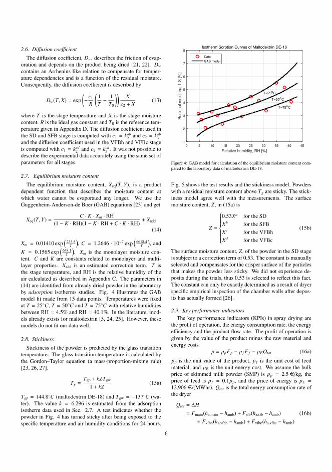
2.6. Diffusion coefficient
The diffusion coefficient, Dw, describes the friction of evap-oration and depends on the product being dried [21, 22]. Dw
contains an Arrhenius like relation to compensate for temper-ature dependencies and is a function of the residual moisture.Consequently, the diffusion coefficient is described by
Dw(T, X) = exp(−c1
R
(1T− 1
T0
))X
c2 + X(13)
where T is the stage temperature and X is the stage moisturecontent. R is the ideal gas constant and T0 is the reference tem-perature given in Appendix D. The diffusion coefficient used inthe SD and SFB stage is computed with c1 = kab
2 and c2 = kab3
and the diffusion coefficient used in the VFBh and VFBc stageis computed with c1 = kcd
2 and c2 = kcd3 . It was not possible to
describe the experimental data accurately using the same set ofparameters for all stages.
2.7. Equilibrium moisture content
The equilibrium moisture content, Xeq(T,Y), is a productdependent function that describes the moisture content atwhich water cannot be evaporated any longer. We use theGuggenheim-Anderson-de Boer (GAB) equations [23] and get
Xeq(T,Y) =C · K · Xm · RH
(1 − K · RH)(1 − K · RH + C · K · RH)+ Xadd
(14)
Xm = 0.01410 exp(
233.5T
), C = 1.2646 · 10−7 exp
(6618.4
T
), and
K = 0.1565 exp(
648.1T
). Xm is the monolayer moisture con-
tent. C and K are constants related to monolayer and multi-layer properties. Xadd is an estimated correction term. T isthe stage temperature, and RH is the relative humidity of theair calculated as described in Appendix C. The parameters in(14) are identified from already dried powder in the laboratoryby adsorption isotherms studies. Fig. 4 illustrates the GABmodel fit made from 15 data points. Temperatures were fixedat T = 25C, T = 50C and T = 75C with relative humiditiesbetween RH = 4.5% and RH = 40.1%. In the literature, mod-els already exists for maltodextrin [5, 24, 25]. However, thesemodels do not fit our data well.
2.8. Stickiness
Stickiness of the powder is predicted by the glass transitiontemperature. The glass transition temperature is calculated bythe Gordon–Taylor equation (a mass-proportion-mixing rule)[23, 26, 27].
Tg =Tgp + kZTgw
1 + kZ(15a)
Tgp = 144.8C (maltodextrin DE-18) and Tgw = −137C (wa-ter). The value k = 6.296 is estimated from the adsorptionisotherm data used in Sec. 2.7. A test indicates whether thepowder in Fig. 4 has turned sticky after being exposed to thespecific temperature and air humidity conditions for 24 hours.
Relative humidity, RH [%]
0 5 10 15 20 25 30 35 40 45
Resid
ual m
ois
ture
, 1-S
[%
]
1
2
3
4
5
6
7
8
T=25oC
T=50oC
T=75oC
Isotherm Sorption Curves of Maltodextrin DE-18
Data
GAB model
Figure 4: GAB model for calculation of the equilibrium moisture content com-pared to the laboratory data of maltodextrin DE-18.
Fig. 5 shows the test results and the stickiness model. Powderswith a residual moisture content above Tg are sticky. The stick-iness model agree well with the measurements. The surfacemoisture content, Z, in (15a) is
Z =
0.53Xa for the SDXb for the SFBXc for the VFBhXd for the VFBc
(15b)
The surface moisture content, Z, of the powder in the SD stageis subject to a correction term of 0.53. The constant is manuallyselected and compensates for the crisper surface of the particlesthat makes the powder less sticky. We did not experience de-posits during the trials, thus 0.53 is selected to reflect this fact.The constant can only be exactly determined as a result of dryerspecific empirical inspection of the chamber walls after depos-its has actually formed [26].
2.9. Key performance indicatorsThe key performance indicators (KPIs) in spray drying are
the profit of operation, the energy consumption rate, the energyefficiency and the product flow rate. The profit of operation isgiven by the value of the product minus the raw material andenergy costs
p = ppFp − p f F f − pE Qtot (16a)
pp is the unit value of the product, p f is the unit cost of feedmaterial, and pE is the unit energy cost. We assume the bulkprice of skimmed milk powder (SMP) is pp = 2.5 e/kg, theprice of feed is p f = 0.1pp, and the price of energy is pE =
12.906 e/(MWhr). Qtot is the total energy consumption rate ofthe dryer
Qtot = ∆H
= Fmain(ha,main − hamb) + Fsfb(ha,sfb − hamb)+ Fvfbh(ha,vfbh − hamb) + Fvfbc(ha,vfbc − hamb)
(16b)
6

Particle temperature, T [oC]
30 40 50 60 70 80 90 100 110
Resid
ual m
ois
ture
, 1-S
[%
]
2
3
4
5
6
7
8
9
10
Stickiness of Maltodextrin DE-18
Tg boundary
Non sticky
very sticky
sticky
Figure 5: Identification of the stickiness boundary for maltodextrin DE-18.
hamb is the specific enthalpy of the air stream at outdoor temper-ature and humidity. The energy efficiency is given by the energyrequired for evaporation relative to the total energy supplied forheating the air [28, 29]
η =λ(T0)Fs(X f − Xd)
Qtot(16c)
λ(T0)Fs(X f − Xd) is the energy required for evaporation. Theflow rate of powder out of the dryer is given by
Fdp = Fs(1 + Xd) (16d)
2.10. SummaryThe model, (1) to (14), is a deterministic system of index-1
differential algebraic (DAE) equations in the following form
ddt
g(x(t)) = f (x(t), u(t), d(t), θ) x(t0) = x0 (17a)
y(t) = h(x(t)) (17b)
The index-1 DAE model can be solved efficiently by expli-cit singly diagonally implicit Runge-Kutta (ESDIRK) meth-ods. We use the ESDIRK4(3) method with variable step-size[30, 31]. The state function g(x(t)) represents hold-up of massand energy and f (x(t), u(t), d(t), θ) is the flux of mass and en-ergy. h(x(t)) is the output equations. θ is the parameter vectorthat has to be estimated from data.
The measurement vector, y, the controlled input vector, u, thedisturbance vector, d, and the states, x, are
y(t) = [T a T b T c T d Ya S b S d]T
u(t) = [F f Tmain Tsfb Tvfbh]T
d(t) = [T f S f Fmain Fsfb Fvfbh Fvfbc Ymain ...
Ysfb Yvfbh Yvfbc Tvfbc T abamb T cd
amb]T
x(t) = [T a Ya Xa T b Yb Xb ...
T c Yc Xc T d Yd Xd]T
Figure 6: The SFB powder outlet with the in-line NIR analyser and the pistonfor powder discharge.
The parameter vector, θ, is listed in Table 1. Fig. 1 and Fig. 2provide an overview of the inputs, disturbances and states.
3. System identification
In this section, we identify the unknown parameters, θ, ofthe model in (17). Experimental tests have been designed andconducted such that all relevant parameters in the model can beidentified.
3.1. Experiment
Two experiments were made in consecutive order withoutstop. The data from the first experiment is used for estimation,while the data from the second experiment is used for valida-tion.
The nominal input to the spray dryer is a feed flow rate atF f = 85 kg/hr with a feed solids concentration of S f = 50%.The feed temperature is T f = 50C. For drying of the feed, weset the main inlet air temperature, Tmain, to 170C, the SFB inletair temperature, Tsfb, to 90C, and the VFBh inlet air temperat-ure, Tvfbh, to 60C. The cooling of the powder is performed withunheated ambient air, Tvfbc, at about 35C. The inlet air flowrates are Fmain = 1700 kg/h, Fsfb = 480 kg/h, Fvfbh = 280 kg/h,and Fvfbc = 280 kg/h. Ambient air is heated and used for dry-ing, thus the inlet air humidity is equal to the ambient air hu-midity. The ambient air humidity is measured continuously andis approximately 3 g/kg. The residual moisture contents, 1− S b
and 1− S d, are measured using two Foss Analytical ProFossTM
in-line analyzers placed at the SFB and VFBc powder outlets.Fig. 6 shows the position of the residual moisture measurementin the SFB stage and Fig. 7 shows the position of the residualmoisture measurement in the VFBc stage. We note that all theinlet air mass-flow meters have an offset in the readings. Thisoffset is identified from water and air mass balances of the spraydryer using measurements of the air flow rates and the mois-tures. We estimated the offset to be 5%, which we subtractedfrom the readings before these are used in the model.
7

Figure 7: The VFB powder outlet with the in-line NIR analyser and the collec-tion of produced powder.
A number of steps are performed in the experiments to excitethe spray dryer outputs. Appendix F describes the steps in theinputs to the spray dryer. During the first experiment, the feedflow rate, F f , is varied between 65 kg/hr and 120 kg/hr. Thefeed solid concentration, S f , is stepped from 50% to 40% andback. We tried a 60% feed solid concentration, but the sprayfrom the nozzle collapsed. This part of the data has thereforebeen cut out of the estimation experiment. The feed temper-ature, T f , is reduced to 42C, stepped to 60C and back. Theambient air humidity in the SD and SFB stages, Ymain and Ysfb,are stepped from approximately 3 g/kg to 15 g/kg and 25 g/kg intwo steps by opening a vapor nozzle in the air ducts. The maininlet air temperature, Tmain, is stepped ±10 C from 170C. TheSFB inlet air temperature, Tsfb, is stepped ±10 C from 90C.The VFBh inlet air temperature, Tvfbh, is stepped +20C from60C. The inlet air flow rates are stepped Fmain = ±200 kg/h,Fsfb = ±100 kg/h and Fvfbh = +130 kg/h from their nominalvalues. The second experiment is made from a repetition of theabove experiment program, but omitting the steps in the inletair flow rates and the feed temperature. The excitation steps arealso provided in Appendix F. The data from both experimentsare well excited and covers a large operation range. This en-sures that the model is valid in a large range of operating points.The estimation experiment lasts 28 hours and the validation ex-periment lasts 17 hours.
3.2. Method
The unknown parameter vector, θ, in the model is identifiedby minimization of the sum of squared simulation errors. Thisprocedure is performed by solving
θ = arg minθ
12
N∑
k=1
‖y(tk) − y(tk, θ)‖22 (18)
in which y(tk) is the measured output and y(tk, θ) is the simu-lated output from (17). y(tk) − y(tk, θ) is the simulation error(residual). The outputs of the model have units of comparablesize, i.e. C, g/kg and %, and we can therefore use unit-scaling.
Table 1 provides the estimated parameters, θ, the standard de-viations, σθ, and the associated 95% confidence interval. The100(1 − α)% confidence interval is calculated by
θ ± tN−p(1 − α/2)√
diag(Σθ
)(19)
in which Σθ is the estimated co-variance matrix of the estim-ated parameters, θ. N − p is the number of observations minusthe number of parameters. We compute the covariance of theestimated parameters, Σθ, from the residual mean square error,‖y − y‖22, and the Jacobian, J, of y(tk, θ) using the expression[32]
Σθ =‖y − y‖22N − p
(JT J
)−1(20)
The estimated mean and covariance, θ and Σθ, defines the dis-tribution of the parameters, i.e. θ ∼ N(θ,Σθ). Knowledge ofthis distribution enables Monte Carlo simulations that can beused to qualify and quantify the uncertainty of the responsessimulated by the model.
As is evident in Table 1, the parameters, Tadd, Yadd, kcd3 , mc
m,and kd
1 , are uncertain. The other parameters are estimated withreasonable uncertainty for engineering purposes. The followingparameters are negative: kcd
3 , k6 and kd1 . kcd
3 is a parameter, c2,in (13). As kcd
3 is very uncertain it could as well be zero suchthat (13) simplifies. Negativity of kd
1 implies that the evapora-tion rate (12b) is negative and that water condenses instead ofevaporates at the VFBc stage. This is as expected. From phys-ical reasoning negativity of k6 is problematic as it indicates heatflow (9a) from the VFBc to the VFBh; nevertheless it providesthe best fit to data.
4. Validation
In this section, we asses the quality of the model by com-paring the simulated outputs to the estimation and validationexperiment.
Fig. 8 shows the outputs of the estimation experiment whichis used to identify the parameters. Fig. 9 shows the valida-tion experiment. The simulations are shown for 15 realizationsof θ ∼ N(θ,Σθ). The simulations are performed using the fullestimated co-variance matrix, Σθ. Table 1 only provide the di-agonal elements of Σθ, i.e. σθ =
√diag(Σθ).
The simulation shows good agreement with the estimationexperiment. The transients and the steady-states are well de-scribed by the model. The stage temperatures, T a, T b, T c andT d, and the air humidity in the SD stage, Ya, fit the data well.The powder moisture contents, 1 − S b and 1 − S d, also fit thedata well. The moisture content is difficult to estimate at lowresidual moisture contents, due to an increasing dependency onthe equilibrium moisture content, Xeq, in (14). The equilibriummoisture content is estimated for data obtained from a laborat-ory experiment, which does not exactly match the conditionsin the spray dryer. Therefore, we expect some deviation, whenthe equilibrium moisture content becomes significant in the re-sidual moisture simulation. The VFBc stage is not sealed from
8
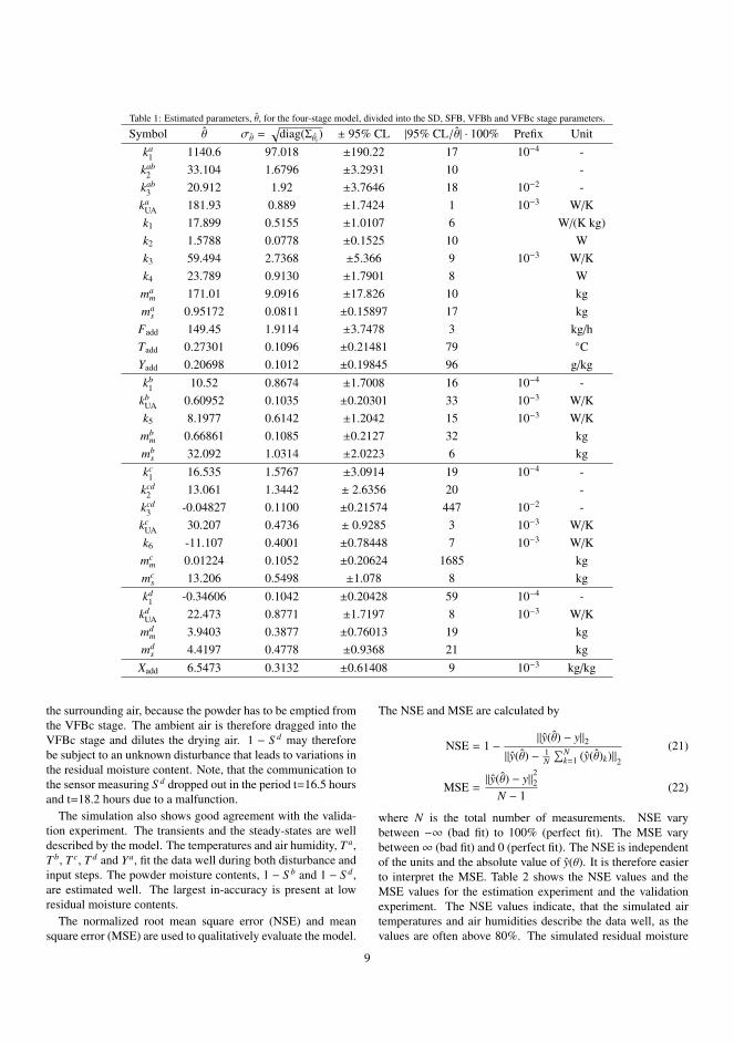
Table 1: Estimated parameters, θ, for the four-stage model, divided into the SD, SFB, VFBh and VFBc stage parameters.
Symbol θ σθ =√
diag(Σθi) ± 95% CL |95% CL/θ| · 100% Prefix Unit
ka1 1140.6 97.018 ±190.22 17 10−4 -
kab2 33.104 1.6796 ±3.2931 10 -
kab3 20.912 1.92 ±3.7646 18 10−2 -
kaUA 181.93 0.889 ±1.7424 1 10−3 W/Kk1 17.899 0.5155 ±1.0107 6 W/(K kg)k2 1.5788 0.0778 ±0.1525 10 Wk3 59.494 2.7368 ±5.366 9 10−3 W/Kk4 23.789 0.9130 ±1.7901 8 Wma
m 171.01 9.0916 ±17.826 10 kgma
s 0.95172 0.0811 ±0.15897 17 kgFadd 149.45 1.9114 ±3.7478 3 kg/hTadd 0.27301 0.1096 ±0.21481 79 CYadd 0.20698 0.1012 ±0.19845 96 g/kgkb
1 10.52 0.8674 ±1.7008 16 10−4 -kb
UA 0.60952 0.1035 ±0.20301 33 10−3 W/Kk5 8.1977 0.6142 ±1.2042 15 10−3 W/Kmb
m 0.66861 0.1085 ±0.2127 32 kgmb
s 32.092 1.0314 ±2.0223 6 kgkc
1 16.535 1.5767 ±3.0914 19 10−4 -kcd
2 13.061 1.3442 ± 2.6356 20 -kcd
3 -0.04827 0.1100 ±0.21574 447 10−2 -kc
UA 30.207 0.4736 ± 0.9285 3 10−3 W/Kk6 -11.107 0.4001 ±0.78448 7 10−3 W/Kmc
m 0.01224 0.1052 ±0.20624 1685 kgmc
s 13.206 0.5498 ±1.078 8 kgkd
1 -0.34606 0.1042 ±0.20428 59 10−4 -kd
UA 22.473 0.8771 ±1.7197 8 10−3 W/Kmd
m 3.9403 0.3877 ±0.76013 19 kgmd
s 4.4197 0.4778 ±0.9368 21 kgXadd 6.5473 0.3132 ±0.61408 9 10−3 kg/kg
the surrounding air, because the powder has to be emptied fromthe VFBc stage. The ambient air is therefore dragged into theVFBc stage and dilutes the drying air. 1 − S d may thereforebe subject to an unknown disturbance that leads to variations inthe residual moisture content. Note, that the communication tothe sensor measuring S d dropped out in the period t=16.5 hoursand t=18.2 hours due to a malfunction.
The simulation also shows good agreement with the valida-tion experiment. The transients and the steady-states are welldescribed by the model. The temperatures and air humidity, T a,T b, T c, T d and Ya, fit the data well during both disturbance andinput steps. The powder moisture contents, 1 − S b and 1 − S d,are estimated well. The largest in-accuracy is present at lowresidual moisture contents.
The normalized root mean square error (NSE) and meansquare error (MSE) are used to qualitatively evaluate the model.
The NSE and MSE are calculated by
NSE = 1 − ‖y(θ) − y‖2‖y(θ) − 1
N∑N
k=1 (y(θ)k)‖2(21)
MSE =‖y(θ) − y‖22
N − 1(22)
where N is the total number of measurements. NSE varybetween −∞ (bad fit) to 100% (perfect fit). The MSE varybetween∞ (bad fit) and 0 (perfect fit). The NSE is independentof the units and the absolute value of y(θ). It is therefore easierto interpret the MSE. Table 2 shows the NSE values and theMSE values for the estimation experiment and the validationexperiment. The NSE values indicate, that the simulated airtemperatures and air humidities describe the data well, as thevalues are often above 80%. The simulated residual moisture
9
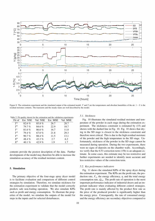
0 5 10 15 20 2530
40
50
60
70
80
90
T [°C
]
SD
SFB
VFBh
VFBc
meas.
0 5 10 15 20 25 0 5
10152025303540
Y [g/k
g]
0 5 10 15 20 25
Time [hours]
2
2.5
3
3.5
4
4.5
5
1-S
[%
]
Figure 8: The estimation experiment and the simulated output of the estimated model. T and Y are the temperatures and absolute humidities of the air. 1 − S is theresidual moisture contents. The transients and the steady-states are well described by the model.
Table 2: Fit quality shown for the estimation and the validation experiments.Fit of Est. NSE Val. NSE Est. MSE Val. MSE
T a 82.6 % 85.8 % 26.7 28.7T b 79.7 % 84.6 % 22.9 18.7T c 81.6 % 86.6 % 16.7 11.0T d 79.4 % 67.0 % 21.8 29.3Ya 90.7 % 88.4 % 11.5 13.1Xb 48.4 % 43.3 % 2.7 6.2Xd 40.1 % 42.9 % 1.9 1.7
contents provide the poorest description of the data. Furtherdevelopment of the model may therefore be able to increase thesimulation accuracy of the residual moisture content.
5. Simulation
The primary objective of the four-stage spray dryer modelis to facilitate evaluation and comparison of different controlstrategies by simulation. Therefore, we simulate stickiness forthe estimation experiment to validate that the model correctlypredicts safe non-fouling operation. We also simulate KPIssuch as profit and energy consumption. To illustrate the prop-erties of the model, we simulate the outputs of the model forsteps in the inputs and for selected disturbances.
5.1. StickinessFig. 10 illustrates the simulated residual moisture and tem-
perature of the powder in each stage during the estimation ex-periment. The stickiness constraint is estimated by (15) andshown with the dashed line in Fig. 10. Fig. 10 shows that dry-ing in the SD stage is closest to the stickiness constraint andtherefore most critical. This is due to the high residual moistureof the powder and the high temperature in the SD stage. Un-fortunately, stickiness of the powder in the SD stage cannot bemeasured during operation. During the two experiments, therewere no signs of deposits on the chamber walls. Accordingly,we verify that the 0.53 correction term (15b) is an adequate es-timate. In some cases, this estimate may be too restrictive andfurther experiments are needed to identify more accurate andless restrictive values of the correction term.
5.2. Key performance indicatorsFig. 11 shows the simulated KPIs of the spray dryer during
the estimation experiment. The KPIs are the profit rate, the pro-duction rate, Fp, the energy efficiency, η, and the total energyconsumption rate, Qtot. The profit rate of operation is the mostimportant performance indicator of industrial dryers and an im-portant indicator when evaluating different control strategies.The profit rate is mainly affected by the product flow rate asthe price of the produced powder is significantly higher thanthe energy price. Consequently, the rate of consumed energyand the energy efficiency are secondary objectives compared to
10

0 2 4 6 8 10 12 14 16 1830
40
50
60
70
80
90
T [
°C]
SD
SFB
VFBh
VFBc
meas.
0 2 4 6 8 10 12 14 16 18 0 5
10152025303540
Y [
g/k
g]
0 2 4 6 8 10 12 14 16 18
Time [hours]
2
2.5
3
3.5
4
4.5
5
1-S
[%
]
Figure 9: The validation experiment and the simulated output of the estimated model. T and Y are the temperatures and absolute humidities of the air. 1 − S is theresidual moisture contents. The simulated model outputs agree well with the measured data.
2 2.5 3 3.5 4 4.5 5 5.5
Z [%]
30
40
50
60
70
80
90
100
110
120
T [°C
]
Non-sticky
StickyBoundary
SD (red)
SFB (green)
VFBh (yellow)
VFBc (blue)
Figure 10: The simulated stickiness constraint and stickiness of the powder ineach stage during the estimation experiment.
the profit rate. It should be noted that the energy efficiency ofthis small dryer is approximately 40%, which is low comparedto industrially sized dryers that may achieve efficiencies of ap-proximately 55%. The total energy consumption rate, Qtot, isapproximately 83 kW. The energy consumption rate is mainlyaffected by adjusting the inlet air flow rates and temperaturesto the dryer. The ambient temperature and air humidity natur-ally also has an effect on the energy consumption rate. Increas-
ing ambient air temperatures decreases the energy consumptionrate.
5.3. Step responses of the inputs
Fig. 12 reports the step responses of the simulated outputsto the inputs of the four-stage spray dryer. The inputs are thefeed flow rate, Ff, the temperature in the main hot air inlet,Tmain, the temperature in the hot air inlet to the SFB, Tsfb, andthe temperature in the hot air inlet to the VFBh, Tvfbh. Theoutputs are the temperature and the air humidity in each of thefour stages of the spray dryer, as well as the measured residualmoisture of the powder in the SFB stage and the VFBc stage(the final powder product). We do not to plot the SD stage andthe VFBh stage residual moistures as they are not measurablein the four-stage spray dryer.
As is evident in the first row of Fig. 12, a 20 kg/hr increase inthe feed flow rate, Ff, has a significant effect on the temperat-ures, the air humidities, and the residual moistures in the spraydryer. When the feed flow rate increases, the temperatures de-crease, the air humidities increase, and the residual moistures inthe powder increase. The temperatures decrease because morefeed, consisting of water and solid, need to be heated and morewater is evaporated with the same amount of inlet energy. Theair humidities increase as a consequence of the increased evap-oration of water from the powder. The residual moistures ofthe powder increase because the energy supplied is unalteredand the amount of water in the feed is increased. The plots
11

0 5 10 15 20 25
60
80
100
120
0 5 10 15 20 25
3642485460
Fd p [
kg
/h]
0 5 10 15 20 25
Time [hours]
2531374349
η [
%]
0 5 10 15 20 25
75808590
Qto
t [kW
]
Figure 11: Simulated KPIs for the estimation experiment. The KPIs are theprofit rate of operation, the product flow rate, the energy efficiency, and thetotal energy consumption rate. The profit rate of operation is highly correlatedto the product flow rate.
in the second row of Fig. 12 indicate the step responses to a10C increase in the temperature of the main hot air inlet, Tmain.Tmain significantly affects the temperature in the SD stage andthe temperature in the SFB stage. It also decreases the residualmoisture of the powder at the SFB stage and the residual mois-ture at the VFBc stage. Tmain hardly affects the temperature inthe VFBh stage and the temperature in the VFBc stage. Tmainonly has a marginal effect on the air humidities. The third rowof plots in Fig. 12 shows the step responses to a 10C increaseof the temperature in the inlet air to the SFB, Tsfb. Tsfb influ-ences the temperature in the SD stage and the temperature inthe SFB stage. This is due to the mixing of the air in these twostages of the four-stage spray dryer. Tsfb has hardly any effecton the temperature in the VFBh stage and the temperature inthe VFBc stage. Similarly, Tsfb does not have any significant ef-fect on the air humidities. Increasing Tsfb decreases the powdermoisture content in the SFB stage as well as in the final productat the VFBc stage. The last row of plots in Fig. 12 illustratesthe step responses to a 10C increase in the temperature of thehot air inlet to the VFBh stage, Tvfbh. Tvfbh affects the temper-ature and the air humidity at the VFBh stage. The air humidityis increased due to the increased evaporation from the powder,resulting in a decreased powder moisture of the final product atthe VFBc stage. It does not affect any of the variables in the SDstage nor the SFB stage of the four-stage spray dryer. This isas expected given the design and flows of the four-stage spraydryer.
5.4. Step responses of the disturbances
Fig. 13 reports the step responses of the simulated outputs tothe main disturbances of the four-stage spray dryer. The maindisturbances are the ambient air humidity, Yamb, the feed solidconcentration, S f, and the feed temperature, Tf. These disturb-ances vary during production and a controller must adjust theinputs to compensate for these disturbances. The air humidity
varies due to changing weather conditions and the feed variesdue to variations in the upstream processes.
The first row of plots in Fig. 13 shows the responses to a5 g/kg step increase in the ambient air humidity. This increasesimultaneously affects all inlet air humidities, i.e. Ymain = Ysfb =
Yvfbh = Yvfbc = Yamb. The ambient air humidity has a direct ef-fect on the air humidity in all stages, but only a very small effecton the temperatures. An increased air humidity in the inlet airstreams also leads to an increase in the residual moisture of thepowder in both the SFB stage and the VFBc stage. The secondrow of plots in Fig. 13 illustrates the response to a step increasein the feed solid concentration, S f. This increases the air tem-peratures. In particular, an increase in the feed solid concentra-tion incrases the temperature in the SD stage and the temperat-ure in the SFB stage. A increase in the feed solid concentrationdecreases the SD air humidity and the residual moisture of thepowder in the SFB stage as well as in the VFBc stage. The thirdrow of plots in Fig. 13 demonstrates that the feed temperature,Tf, has an effect on the residual moisture of the powder in theSFB stage and also in the VFBc stage. It also affects the tem-perature at the SFB stage, but hardly affects the temperatures atthe other stages. The feed temperature only has a very limitedeffect on the air humidities.
6. Conclusions
In this paper, we model a medium sized GEA Niro Multi-Stage Dryer size 20 (MSDTM-20). The model is based on fourconsecutive stages; a primary spray drying stage, two heatedfluid bed stages, and a cooling fluid bed stage. In each stage,the model simulates the dynamic responses of the temperat-ures, the air humidities, and the residual moisture contents ofthe powder. Deposits caused by stickiness of the powder is pre-dicted using the glass-transition temperature. The model alsoprovides the key performance indicators including the profit ofoperation. The model is a first-principles engineering model,based on mass- and energy balances, and takes the form of anindex-1 DAE model.
The model parameters are estimated from an estimation ex-periment and validated against a validation experiment. The ex-periments were both well excited and the model fits the exper-imental data well. The model provides simulations for a broadoperating range, making it ideal as basis for development ofcontrol solutions as well as for evaluating the control perform-ance in a production rate and energy efficiency point of view.
Acknowledgement
This work was funded in part by 1) the Danish Ministryof Higher Education and Science in the industrial PhD pro-ject ”Economic Model Predictive Control for Spray DryingPlants” (12-128720); 2) GEA Process Engineering A/S, DK-2860 Søborg, Denmark; 3) EUDP 64013-0558 in the IEA An-nex for Energy Efficient Process Control.
12

-10 10 30 50 70 90 110
40
60
80
Ff +
20 k
g/h
r ste
p
Temperatures, T [°C]
-10 10 30 50 70 90 110
5
10
15
20
25
Abs. Humidities, Y [g/kg]
-10 10 30 50 70 90 1102.42.7 3
3.33.63.94.24.5
Residual moistures, 1-S [%]
-10 10 30 50 70 90 110
40
60
80
Tm
ain
+10°C
ste
p
-10 10 30 50 70 90 110
5
10
15
20
25
-10 10 30 50 70 90 1102.42.7 3
3.33.63.94.24.5
-10 10 30 50 70 90 110
40
60
80
Tsfb
+10°C
ste
p
-10 10 30 50 70 90 110
5
10
15
20
25
-10 10 30 50 70 90 1102.42.7 3
3.33.63.94.24.5
-10 10 30 50 70 90 110
Time [min]
40
60
80
Tvfb
h +
10°C
ste
p
SD
SFB
VFBh
VFBc
-10 10 30 50 70 90 110
Time [min]
5
10
15
20
25SD
SFB
VFBh
VFBc
-10 10 30 50 70 90 110
Time [min]
2.42.7 3
3.33.63.94.24.5
SFB
VFBc
Figure 12: Simulated responses to steps in the inputs. The system outputs shows the response to a step in the feed flow rate, Ff, the main inlet air temperature, Tmain,the SFB inlet air temperature, Tsfb, and the VFBh inlet air temperature, Tvfbh. The vertical line indicates when the steps are applied and this time is set to t=0.
Appendix A. Basis conversion
The solids feed flow rate, Fs, and total mass feed flow rate,F, are related by
Fs = S F F =1S
Fs (A.1)
The dry basis residual moisture content, X, and wet basis solidcontent, S , are related by
X =1 − S
SS =
11 + X
(A.2)
The dry air flow rate is determined by
Fda = F1
Y + 1F = Fda(Y + 1) (A.3)
Appendix B. Specific enthalpy
The specific enthalpy of humid air is
ha = hda + Yhv (B.1)
in which
hda = h0da + Cda(T − T0) (B.2)
hv = h0v + λ(T0) + Cv(T − T0) (B.3)
Cda is the mean heat capacity of dry air and Cv is the mean heatcapacity of vapor [33]. λ(T0) is the latent heat of evaporation.The standard enthalpies of formation, h0
da and h0v , are computed
at T0 with the phase that this product takes at T0. The specificenthalpy of feed as well as powder is
hp = hs + Xhw (B.4)
in which
hs = h0s + Cs(T − T0) (B.5)
hw = h0w + Cw(T − T0) (B.6)
Cs is the mean heat capacity of solid and Cw is the mean heatcapacity of water [33]. The mean heat capacity of maltodextrin,Cs is described in [34][pp. 87]. h0
s and h0w are the standard
enthalpies of formation. The specific enthalpy of steel is hm =
Cm(T − T0). Cm is the mean heat capacity of steel.
13

-10 10 30 50 70 90 110
40
60
80
Yam
b +
5 g
/kg s
tep
Temperatures, T [°C]
-10 10 30 50 70 90 110
5
10
15
20
25
Abs. Humidities, Y [g/kg]
-10 10 30 50 70 90 1102.42.7 3
3.33.63.94.24.5
Residual moistures, 1-S [%]
-10 10 30 50 70 90 110
40
60
80
Sf +
5 %
ste
p
-10 10 30 50 70 90 110
5
10
15
20
25
-10 10 30 50 70 90 1102.42.7 3
3.33.63.94.24.5
-10 10 30 50 70 90 110
Time [min]
40
60
80
Tf +
10°C
ste
p
SD
SFB
VFBh
VFBc
-10 10 30 50 70 90 110
Time [min]
5
10
15
20
25SD
SFB
VFBh
VFBc
-10 10 30 50 70 90 110
Time [min]
2.42.7 3
3.33.63.94.24.5
SFB
VFBc
Figure 13: Simulated responses to steps in the selected disturbances. The system outputs shows the response to a step in the ambient air humidity, Yamb, the feedsolid concentration, S f, and the feed temperature, Tf. The steps are applied after 10 minutes of operation at a steady-state. This is indicated by the vertical line inthe figures and the corresponding time is defined as t = 0.
Appendix C. Air humidity conversion
The relative air humidity is calculated by
RH =Y(
MvMda
+ Y) Pamb
Pvsat(T )(C.1)
Pvsat(T ) is the saturated vapor pressure determined by the Ant-oine equation and Pamb is the ambient total pressure. Mv andMda is the molar mass of vapor and dry air respectively. Theabsolute air humidity, Y , is calculated by
Y =Mv
Mda
RHPvsat(T )Pamb − RHPvsat(T )
(C.2)
Appendix D. Constants
The constants used in the model are listed hereR = 8.314472 · 10−3 KJ K−1mol−1, the ideal gas constant.Mv = 18.01528 · 10−3 kg mol−1, the molar mass of vapor.Mw = 18.01528 · 10−3 kg mol−1, the molar mass of water.Mda = 28.97 · 10−3 kg mol−1, the molar mass of dry air.Pamb = 101325 Pa, ambient pressureT0 = 25 + 273.15 K, reference temperature
The mean heat capacities are calculated by [33]
C· =RM
(A +
B2
T (τ + 1) +C3
T 2(τ2 + τ + 1) +DτT 2
)(D.1)
A, B, C and D for vapor, water and dry air isVapor; A = 3.470, B = 1.450·10−3, C=0, D = 0.121·105
Water; A = 8.712, B = 1.25·10−3, C = −0.18·10−6, D = 0Dry air; A = 3.355, B = 0.575·10−3, C = 0, D = −0.016·105
The mean heat capacity of Maltodextrin DE-18 and steel are
Cs = 1.5488 + 0.0019625T − 5.9399·10−6T 2 (D.2)Cm = 0.466 (D.3)
where T is in C [34][pp. 87].The standard enthalpy of formation is given by [33]
and [34][pp. 87] h0da = 0 KJ/Kg, h0
v = −0.0134 KJ/Kg,h0
w = −0.0159 KJ/Kg, h0s = 0 KJ/Kg, h0
m = 0.
The latent heat of vaporization is
λ(T ) = λre f
1 − T
α
1 − Tre f
α
β
(D.4)
in which λre f = 2257 KJ/Kg at Tre f = 100 + 273.15 K andα = 647.1 and β = 0.38 [33].
Appendix E. Steady-states
The steady-state of the model is
yss = [81.713C 73.843C 56.25C 34.491C ...
22.266g/kg 3.2717% 2.926%]T
14
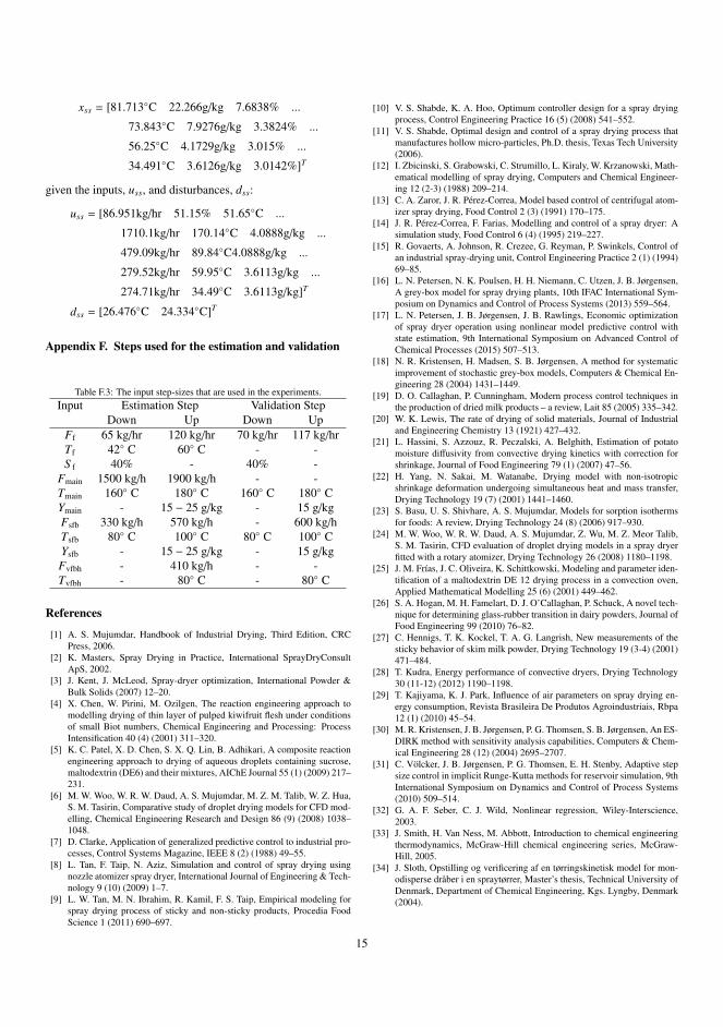
xss = [81.713C 22.266g/kg 7.6838% ...
73.843C 7.9276g/kg 3.3824% ...
56.25C 4.1729g/kg 3.015% ...
34.491C 3.6126g/kg 3.0142%]T
given the inputs, uss, and disturbances, dss:
uss = [86.951kg/hr 51.15% 51.65C ...
1710.1kg/hr 170.14C 4.0888g/kg ...
479.09kg/hr 89.84C4.0888g/kg ...
279.52kg/hr 59.95C 3.6113g/kg ...
274.71kg/hr 34.49C 3.6113g/kg]T
dss = [26.476C 24.334C]T
Appendix F. Steps used for the estimation and validation
Table F.3: The input step-sizes that are used in the experiments.Input Estimation Step Validation Step
Down Up Down UpFf 65 kg/hr 120 kg/hr 70 kg/hr 117 kg/hrTf 42 C 60 C - -S f 40% - 40% -
Fmain 1500 kg/h 1900 kg/h - -Tmain 160 C 180 C 160 C 180 CYmain - 15 − 25 g/kg - 15 g/kgFsfb 330 kg/h 570 kg/h - 600 kg/hTsfb 80 C 100 C 80 C 100 CYsfb - 15 − 25 g/kg - 15 g/kgFvfbh - 410 kg/h - -Tvfbh - 80 C - 80 C
References
[1] A. S. Mujumdar, Handbook of Industrial Drying, Third Edition, CRCPress, 2006.
[2] K. Masters, Spray Drying in Practice, International SprayDryConsultApS, 2002.
[3] J. Kent, J. McLeod, Spray-dryer optimization, International Powder &Bulk Solids (2007) 12–20.
[4] X. Chen, W. Pirini, M. Ozilgen, The reaction engineering approach tomodelling drying of thin layer of pulped kiwifruit flesh under conditionsof small Biot numbers, Chemical Engineering and Processing: ProcessIntensification 40 (4) (2001) 311–320.
[5] K. C. Patel, X. D. Chen, S. X. Q. Lin, B. Adhikari, A composite reactionengineering approach to drying of aqueous droplets containing sucrose,maltodextrin (DE6) and their mixtures, AIChE Journal 55 (1) (2009) 217–231.
[6] M. W. Woo, W. R. W. Daud, A. S. Mujumdar, M. Z. M. Talib, W. Z. Hua,S. M. Tasirin, Comparative study of droplet drying models for CFD mod-elling, Chemical Engineering Research and Design 86 (9) (2008) 1038–1048.
[7] D. Clarke, Application of generalized predictive control to industrial pro-cesses, Control Systems Magazine, IEEE 8 (2) (1988) 49–55.
[8] L. Tan, F. Taip, N. Aziz, Simulation and control of spray drying usingnozzle atomizer spray dryer, International Journal of Engineering & Tech-nology 9 (10) (2009) 1–7.
[9] L. W. Tan, M. N. Ibrahim, R. Kamil, F. S. Taip, Empirical modeling forspray drying process of sticky and non-sticky products, Procedia FoodScience 1 (2011) 690–697.
[10] V. S. Shabde, K. A. Hoo, Optimum controller design for a spray dryingprocess, Control Engineering Practice 16 (5) (2008) 541–552.
[11] V. S. Shabde, Optimal design and control of a spray drying process thatmanufactures hollow micro-particles, Ph.D. thesis, Texas Tech University(2006).
[12] I. Zbicinski, S. Grabowski, C. Strumillo, L. Kiraly, W. Krzanowski, Math-ematical modelling of spray drying, Computers and Chemical Engineer-ing 12 (2-3) (1988) 209–214.
[13] C. A. Zaror, J. R. Perez-Correa, Model based control of centrifugal atom-izer spray drying, Food Control 2 (3) (1991) 170–175.
[14] J. R. Perez-Correa, F. Farias, Modelling and control of a spray dryer: Asimulation study, Food Control 6 (4) (1995) 219–227.
[15] R. Govaerts, A. Johnson, R. Crezee, G. Reyman, P. Swinkels, Control ofan industrial spray-drying unit, Control Engineering Practice 2 (1) (1994)69–85.
[16] L. N. Petersen, N. K. Poulsen, H. H. Niemann, C. Utzen, J. B. Jørgensen,A grey-box model for spray drying plants, 10th IFAC International Sym-posium on Dynamics and Control of Process Systems (2013) 559–564.
[17] L. N. Petersen, J. B. Jørgensen, J. B. Rawlings, Economic optimizationof spray dryer operation using nonlinear model predictive control withstate estimation, 9th International Symposium on Advanced Control ofChemical Processes (2015) 507–513.
[18] N. R. Kristensen, H. Madsen, S. B. Jørgensen, A method for systematicimprovement of stochastic grey-box models, Computers & Chemical En-gineering 28 (2004) 1431–1449.
[19] D. O. Callaghan, P. Cunningham, Modern process control techniques inthe production of dried milk products – a review, Lait 85 (2005) 335–342.
[20] W. K. Lewis, The rate of drying of solid materials, Journal of Industrialand Engineering Chemistry 13 (1921) 427–432.
[21] L. Hassini, S. Azzouz, R. Peczalski, A. Belghith, Estimation of potatomoisture diffusivity from convective drying kinetics with correction forshrinkage, Journal of Food Engineering 79 (1) (2007) 47–56.
[22] H. Yang, N. Sakai, M. Watanabe, Drying model with non-isotropicshrinkage deformation undergoing simultaneous heat and mass transfer,Drying Technology 19 (7) (2001) 1441–1460.
[23] S. Basu, U. S. Shivhare, A. S. Mujumdar, Models for sorption isothermsfor foods: A review, Drying Technology 24 (8) (2006) 917–930.
[24] M. W. Woo, W. R. W. Daud, A. S. Mujumdar, Z. Wu, M. Z. Meor Talib,S. M. Tasirin, CFD evaluation of droplet drying models in a spray dryerfitted with a rotary atomizer, Drying Technology 26 (2008) 1180–1198.
[25] J. M. Frıas, J. C. Oliveira, K. Schittkowski, Modeling and parameter iden-tification of a maltodextrin DE 12 drying process in a convection oven,Applied Mathematical Modelling 25 (6) (2001) 449–462.
[26] S. A. Hogan, M. H. Famelart, D. J. O’Callaghan, P. Schuck, A novel tech-nique for determining glass-rubber transition in dairy powders, Journal ofFood Engineering 99 (2010) 76–82.
[27] C. Hennigs, T. K. Kockel, T. A. G. Langrish, New measurements of thesticky behavior of skim milk powder, Drying Technology 19 (3-4) (2001)471–484.
[28] T. Kudra, Energy performance of convective dryers, Drying Technology30 (11-12) (2012) 1190–1198.
[29] T. Kajiyama, K. J. Park, Influence of air parameters on spray drying en-ergy consumption, Revista Brasileira De Produtos Agroindustriais, Rbpa12 (1) (2010) 45–54.
[30] M. R. Kristensen, J. B. Jørgensen, P. G. Thomsen, S. B. Jørgensen, An ES-DIRK method with sensitivity analysis capabilities, Computers & Chem-ical Engineering 28 (12) (2004) 2695–2707.
[31] C. Volcker, J. B. Jørgensen, P. G. Thomsen, E. H. Stenby, Adaptive stepsize control in implicit Runge-Kutta methods for reservoir simulation, 9thInternational Symposium on Dynamics and Control of Process Systems(2010) 509–514.
[32] G. A. F. Seber, C. J. Wild, Nonlinear regression, Wiley-Interscience,2003.
[33] J. Smith, H. Van Ness, M. Abbott, Introduction to chemical engineeringthermodynamics, McGraw-Hill chemical engineering series, McGraw-Hill, 2005.
[34] J. Sloth, Opstilling og verificering af en tørringskinetisk model for mon-odisperse dråber i en spraytørrer, Master’s thesis, Technical University ofDenmark, Department of Chemical Engineering, Kgs. Lyngby, Denmark(2004).
15

146

P a p e r B
Comparison of ControlStrategies for Optimization of
Spray Dryer Operation
Submitted to Journal of Process Control, 2016.

148

Comparison of three control strategies for optimization of spray dryer operation
Lars Norbert Petersena,b, Niels Kjølstad Poulsena, Hans Henrik Niemannc, Christer Utzenb, John Bagterp Jørgensena,∗
aDepartment of Applied Mathematics and Computer Science, Technical University of Denmark, DK-2800 Kgs. Lyngby, DenmarkbGEA Process Engineering A/S, DK-2860 Søborg, Denmark
cDepartment of Electrical Engineering, Technical University of Denmark, DK-2800 Kgs. Lyngby, Denmark
Abstract
Spray drying is the preferred process to reduce the water content of many chemicals, pharmaceuticals, and foodstuffs. A significantamount of energy is used in spray drying to remove water and produce a free flowing powder product. In this paper, we presentand compare the performance of three controllers for operation of a four-stage spray dryer. The three controllers are a proportional-integral (PI) controller that is used in industrial practice for spray dryer operation, a linear model predictive controller with real-timeoptimization (MPC with RTO, MPC-RTO), and an economically optimizing nonlinear model predictive controller (E-NMPC). TheMPC with RTO is based on the same linear state space model in the MPC and the RTO layer. The E-NMPC consists of a singleoptimization layer that uses a nonlinear system of ordinary differential equations for its predictions. The PI control strategy hasa fixed target that is independent of the disturbances, while the MPC-RTO and the E-NMPC adapt the operating point to thedisturbances. The goal of spray dryer operation is to optimize the profit of operation in the presence of feed composition andambient air humidity variations; i.e. to maximize the production rate, while minimizing the energy consumption, keeping theresidual moisture content of the powder below a maximum limit, and avoiding that the powder sticks to the chamber walls. Weuse an industrially recorded disturbance scenario in order to produce realistic simulations and conclusions. The key performanceindicators such as the profit of operation, the product flow rate, the specific energy consumption, the energy efficiency, and theresidual moisture content of the produced powder are computed and compared for the three controllers. In this simulation study,we find that the economic performance of the MPC with RTO and E-NMPC is considerably improved compared to the PI controlstrategy used in industrial practice. The MPC with RTO improves the profit of operation by 8.71%, and the E-NMPC improves theprofit of operation by 9.69%. The energy efficiency is improved by 6.06% and 5.52%, respectively.
Keywords: Spray drying, Real-time optimization, Model predictive control, Economic model predictive control, PI control
1. Introduction
The four-stage spray dryer is widely used in the chemical,pharmaceutical and food industries for turning liquid productsinto free flowing powders. By combining drying in four stagesinstead of drying in a single stage, four-stage spray dryers haveincreased energy efficiency and improved product quality. In-tensified competition in industries using spray dryers requirecontinuous process innovations to reduce costs and improveproduct quality. Traditionally, spray dryers are operated using aproportional-integral (PI) control strategy with fixed targets thatare independent of disturbances such as the ambient humidityand the feed composition to the spray dryer. The PI controlstrategy is based on fixed inlet temperatures and a single-input-single-output PI-controller that manipulates the feed flowrateto control the exhaust temperature. In this paper, we demon-strate by closed-loop simulation that the key performance in-dicators of spray dryer operation using a PI control strategy
∗Corresponding authorEmail addresses: [email protected] (Lars Norbert Petersen),
[email protected] (Niels Kjølstad Poulsen), [email protected] (HansHenrik Niemann), [email protected] (Christer Utzen),[email protected] (John Bagterp Jørgensen)
can be significantly improved by using optimization based con-trollers adjusting the targets to the disturbances. We investigatetwo different economically optimizing controllers: 1) a linearmodel predictive controller with real-time optimization (MPCwith RTO, MPC-RTO), and 2) an economic nonlinear modelpredictive controller (E-NMPC).
The key product qualities in spray drying are the bulk den-sity, the particle size distribution, and the residual moisture con-tent. These product qualities affect the powder reconstitution(sinkability, solubility, dispersability and wetability) in water[1]. Changes in the residual moisture content tend to affect allthe other product qualities and have a considerably effect onthe profit of operation. It is a challenging and non-trivial task tooperate a spray dryer in an economical optimal way and simul-taneously meet the product quality specifications. In currentindustrial practice, a PI control strategy is used for operation ofthe four-stage spray dryer. This PI based control strategy keepsthe inlet and outlet temperatures constant during operation. Theapproach is simple, but in the presence of changing externaldisturbances, such as the ambient air humidity and feed com-position, the PI control strategy is insufficient. The PI controlstrategy does not maximize the production rate, it cannot guar-antee satisfaction of the residual moisture constraint, and it does
Preprint submitted to Journal of Process Control May 26, 2016

not include a stickiness constraint implying that deposits mayform due to sticky powder inside the dryer. Furthermore, the in-puts and outputs of a spray dryer are highly cross-coupled andlong process delays may be present. All these features make itdifficult to operate a spray dryer using a PI control strategy [2].
In this paper, we present an MPC-RTO as well as an E-NMPC and apply these controllers to simulate spray dryer op-eration. By closed-loop simulation, we compare the key perfor-mance indicators of the MPC strategies to the PI control strat-egy that is used in current industrial practice. The goal of spraydryer operation is to optimize the profit in the presence of feedcomposition and ambient air humidity variations; i.e. the objec-tive is to maximize the production rate, while minimizing theenergy consumption rate, keeping the residual moisture contentof the powder below a maximum limit, and avoiding that thepowder sticks to the chamber walls. The simulations are basedon a validated first-principles engineering model of a four-stagespray dryer [2] and uses an industrially recorded disturbancescenario. The MPC-RTO and the E-NMPC have previouslybeen suggested for operation of a four-stage spray dryer [3, 4].However, the study presented in the current paper represents thefirst rigorous comparison of the industrially applied PI controlstrategy to the MPC-RTO and the E-NMPC strategies using thesame disturbance scenario. The closed-loop simulations are re-alistic representations of industrial situations, as the simulationsare based on a validated model of an industrial type small scalespray dryer and an industrially recorded disturbance scenario.The MPC-RTO and E-NMPC are based on simpler models thatare not identical to the simulation model.
A PI controller is a simple method for controlling a singleprocess value to a specified target. For more complex multivari-able processes, linear tracking model predictive control (MPC)is the preferred control methodology in the process industries[5, 6]. MPC provides an integrated solution for controlling pro-cesses with multivariate and cross-coupled dynamics, time de-lays, and constraints on both the inputs and the outputs to aspecified target vector [7, 8]. Often MPC is combined with anRTO [9–12]. Together, MPC and RTO form a two-layer struc-ture. The upper-level RTO system provides targets to the lower-level control system to maintain the process operation as closeas possible to the economic optimum. The lower-level MPCsystem brings the process to the target values of the RTO sys-tem. Note that the two layer structure consisiting of an RTOand an MPC is different from the two layer MPC for offset freecontrol [13–16]. We apply an RTO, which may be categorizedas an explicit iterative optimization method with bias updateadaptation [9]. RTO methods, based on explicit iterative opti-mization, repeatedly solve a model-based optimization problemand are advantageous compared to implicit methods such as theextremum-seeking control [17, 18]. Implicit methods can beslow and require the process to reach steady-state before a newstep can be taken. The two-layer structure has some inherentdrawbacks. As the optimization is only performed intermit-tently at a lower sampling rate than the regulation, the adap-tation of the operating conditions is slow and assumes that asteady-state can be reached [10]. Recent advances within pro-cess optimization focus on optimizing economics directly in the
controller [8, 19–21]. This is known as E-NMPC. The advan-tage of E-NMPC is that it maximizes the profit of operation atall times and it takes both the steady-state and the transient eco-nomics into account. The E-NMPC eliminates the RTO layerand the drawbacks of a two-layer structure [22]. The key chal-lenges related to implementation of E-NMPC are the requiredmodel accuracy and the need for long control- and prediction-horizons to reach the turnpike solution [20]. A peculiarity ofE-NMPC is that the optimal solution is not necessarily a steady-state solution but may be a periodic solution [8, 19, 21].
Mathematical modeling and control of spray dryers havebeen a subject of research for many decades. PI control is the defacto standard control methodology in the spray drying indus-try. PI control is reported for drying of full cream milk using alaboratory scale nozzle equipped spray dryer in [23]. Drying ofwhole milk and orange juice is addressed in [24]. Shabde andHoo [25] use two PI controllers to control the mean particle sizeand the residual moisture content of the powder. The controllersare tested by simulation using a first-principles model [26, 27].Zaror and Perez-Correa [28] present a feed forward cascadecontroller to control the exhaust air temperature to indirectlymaintain constant product moisture content. Perez-Correa andFarias [29] extend [28] by controlling the humidity of the ex-haust air to indirectly maintain constant product moisture con-tent. Govaerts et al. [30] develop a linear quadratic gaussian(LQG) controller for residual moisture control in an industrialdetergent spray drying process. The above control strategiesconcern single-stage spray dryers. Petersen et al. [3, 31, 32]report linear and nonlinear MPC algorithms for control of theresidual moisture content and the stickiness of the powder ina four-stage spray dryer. Industrial MPC solutions for spraydryers exist and seem to rely on empirically based models andleast-squares methods for control of the residual moisture con-tent of the powder. Callaghan and Cunningham [33] provide athorough review on the status and future of advanced controlfor spray drying.
The paper is organized as follows. The process and thecontrollers are presented in Section 2, while Section 3 brieflypresents the simulation model. The PI, MPC with RTO, andE-NMPC control strategies are described in Section 4, Section5, and Section 6. Section 7 compares the control strategies bysimulation and the conclusions are provided in Section 8.
2. The process and the controllers
2.1. Process description
Fig. 1 illustrates a modern four-stage spray dryer with anintegrated static fluid bed and an external vibrating fluid bed.The spray dryer consists of the primary spray drying stage (SD),the static fluid bed stage (SFB), the hot vibrating fluid bed stage(VFBh), and the cold vibrating fluid bed stage (VFBc).
The hot main air is let into the upper section of the SD aroundthe high pressure nozzles. The nozzles disperse the liquid feedinto droplets. The heat is transferred from the hot air to thedroplets, which makes the water evaporate from the droplets. Inthat process the air temperature and the residual moisture of the
2
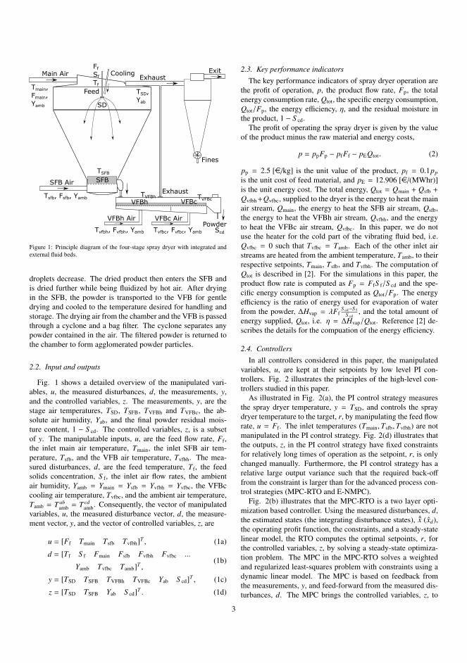
SD
Main Air
SFB Air
Feed
Cooling
SFB
TSD,Yab
TSFB
Ff
Sf
Tf
VFBh Air VFBc AirPowder
VFBh VFBc
ExhaustExit
Fines
ExhaustTVFBh TVFBc
Scd
Tsfb, Fsfb, Yamb
Tmain, Fmain, Yamb
Tvfbh, Fvfbh, Yamb Tvfbc, Fvfbc, Yamb
Figure 1: Principle diagram of the four-stage spray dryer with integrated andexternal fluid beds.
droplets decrease. The dried product then enters the SFB andis dried further while being fluidized by hot air. After dryingin the SFB, the powder is transported to the VFB for gentledrying and cooled to the temperature desired for handling andstorage. The drying air from the chamber and the VFB is passedthrough a cyclone and a bag filter. The cyclone separates anypowder contained in the air. The filtered powder is returned tothe chamber to form agglomerated powder particles.
2.2. Input and outputs
Fig. 1 shows a detailed overview of the manipulated vari-ables, u, the measured disturbances, d, the measurements, y,and the controlled variables, z. The measurements, y, are thestage air temperatures, TSD, TSFB, TVFBh and TVFBc, the ab-solute air humidity, Yab, and the final powder residual mois-ture content, 1 − S cd. The controlled variables, z, is a subsetof y. The manipulatable inputs, u, are the feed flow rate, Ff,the inlet main air temperature, Tmain, the inlet SFB air tem-perature, Tsfb, and the VFB air temperature, Tvfbh. The mea-sured disturbances, d, are the feed temperature, Tf, the feedsolids concentration, S f, the inlet air flow rates, the ambientair humidity, Yamb = Ymain = Ysfb = Yvfbh = Yvfbc, the VFBccooling air temperature, Tvfbc, and the ambient air temperature,Tamb = T ab
amb = T cdamb. Consequently, the vector of manipulated
variables, u, the measured disturbance vector, d, the measure-ment vector, y, and the vector of controlled variables, z, are
u = [Ff Tmain Tsfb Tvfbh]T , (1a)
d = [Tf S f Fmain Fsfb Fvfbh Fvfbc ...
Yamb Tvfbc Tamb]T ,(1b)
y = [TSD TSFB TVFBh TVFBc Yab S cd]T , (1c)
z = [TSD TSFB Yab S cd]T . (1d)
2.3. Key performance indicatorsThe key performance indicators of spray dryer operation are
the profit of operation, p, the product flow rate, Fp, the totalenergy consumption rate, Qtot, the specific energy consumption,Qtot/Fp, the energy efficiency, η, and the residual moisture inthe product, 1 − S cd.
The profit of operating the spray dryer is given by the valueof the product minus the raw material and energy costs,
p = ppFp − pfFf − pEQtot. (2)
pp = 2.5 [e/kg] is the unit value of the product, pf = 0.1pp
is the unit cost of feed material, and pE = 12.906 [e/(MWhr)]is the unit energy cost. The total energy, Qtot = Qmain + Qsfb +
Qvfbh +Qvfbc, supplied to the dryer is the energy to heat the mainair stream, Qmain, the energy to heat the SFB air stream, Qsfb,the energy to heat the VFBh air stream, Qvfbh, and the energyto heat the VFBc air stream, Qvfbc. In this paper, we do notuse the heater for the cold part of the vibrating fluid bed, i.e.Qvfbc = 0 such that Tvfbc = Tamb. Each of the other inlet airstreams are heated from the ambient temperature, Tamb, to theirrespective setpoints, Tmain, Tsfb, and Tvfbh. The computation ofQtot is described in [2]. For the simulations in this paper, theproduct flow rate is computed as Fp = FfS f/S cd and the spe-cific energy consumption is computed as Qtot/Fp. The energyefficiency is the ratio of energy used for evaporation of waterfrom the powder, ∆Hvap = λFf
S cd−S fS cd
, and the total amount ofenergy supplied, Qtot, i.e. η = ∆Hvap/Qtot. Reference [2] de-scribes the details for the compuation of the energy efficiency.
2.4. ControllersIn all controllers considered in this paper, the manipulated
variables, u, are kept at their setpoints by low level PI con-trollers. Fig. 2 illustrates the principles of the high-level con-trollers studied in this paper.
As illustrated in Fig. 2(a), the PI control strategy measuresthe spray dryer temperature, y = TSD, and controls the spraydryer temperature to the target, r, by manipulating the feed flowrate, u = Ff. The inlet temperatures (Tmain,Tsfb,Tvfbh) are notmanipulated in the PI control strategy. Fig. 2(d) illustrates thatthe outputs, z, in the PI control strategy have fixed constraintsfor relatively long times of operation as the setpoint, r, is onlychanged manually. Furthermore, the PI control strategy has arelative large output variance such that the required back-off
from the constraint is larger than for the advanced process con-trol strategies (MPC-RTO and E-NMPC).
Fig. 2(b) illustrates that the MPC-RTO is a two layer opti-mization based controller. Using the measured disturbances, d,the estimated states (the integrating disturbance states), ˆx (xd),the operating profit function, the constraints, and a steady-statelinear model, the RTO computes the optimal setpoints, r, forthe controlled variables, z, by solving a steady-state optimiza-tion problem. The MPC in the MPC-RTO solves a weightedand regularized least-squares problem with constraints using adynamic linear model. The MPC is based on feedback fromthe measurements, y, and feed-forward from the measured dis-turbances, d. The MPC brings the controlled variables, z, to
3

(a) PI control (b) MPC-RTO (c) E-NMPC
(d) PI control (e) MPC-RTO (f) E-NMPC
Figure 2: The diagrams (a-c) illustrates the main computations for the different controllers. The sketches (d-f) illustrates the controlled variables, z, the correspondingsetpoints (if relevant), r, and the corresponding constraints for the different controllers.
the targets, r, by manipulating u. As illustrated in Fig. 2(e),the RTO frequently adjusts the setpoints including the corre-sponding back-off to the variations in the disturbances. Theback-off of the MPC-RTO is smaller than the back-off of thePI control strategy due to better regulation by the MPC. Theeconomic value of the MPC-RTO compared to the PI controlstrategy stems from the adjustment of setpoints to the actualdisturbances and less back-off as a consequence of better regu-lation with less output variance.
Fig. 2(c) illustrates that the E-NMPC is a one layer optimiza-tion based controller. Based on the measurements, y, the mea-sured disturbances, d, the profit function, the constraints, anda nonlinear model, E-NMPC computes the manipulated vari-ables, u, at each sample time such that the predicted profit ofoperation is maximized. Fig. 2(f) shows that E-NMPC does notcompute targets, r, directly, but maximizes operating profit sub-ject to constraints. This implies that the optimal controlled vari-ables, z, corresponding to the optimal manipulated variables, u,are adjusted and predicted at each sample time. The back-off inE-NMPC may be implemented directly or by solving stochasticversions of E-NMPC using soft constraints with penalty func-tions representing the economic cost of violating a constraint.In this paper, we used a certainty-equivalence E-NMPC and didnot explicitly consider back-off from the constraints.
3. Simulation model
The simulation model is a first-principles engineering modelthat is based on mass and energy conservation laws [2]. Themodel describes drying of maltodextrin DE-18 with a high ac-
curacy in a wide range of operating points. The model may berepresented in the discrete stochastic form
xk+1 = F(xk, uk + wu,k, dk + wd,k, θ), (3a)yk = hy(xk) + vk, (3b)zk = hz(xk), (3c)
in which F is an operator representing the solution, xk+1, of thesystem of differential equations
x(tk) = xk, (4a)ddt
g(x(t)) = f (x(t), uk + wu,k, dk + wd,k, θ), tk ≤ t ≤ tk+1, (4b)
xk+1 = x(tk+1). (4c)
Equation (4) is solved using the ESDIRK4(3) method with vari-able step size [34]. hy is the measurement function and hz is theoutput function. The model (4) is a deterministic model that hastwo piecewise stochastic inputs, uk + wu,k and dk + wd,k, that areconstant for tk ≤ t ≤ tk+1. The measurement, y, is the measure-ment function, hy, corrupted by measurement noise, vk. Theprocess noise, wu,k ∼ Niid(0,Ru) and wd,k ∼ Niid(0,Rd), and themeasurement noise, vk ∼ Niid(0,Rv), are all assumed to be nor-mally distributed. The covariances, (Ru, Rd, Rv), are estimatedfrom the covariances of u, d, and y, respectively.
3.1. Constraints
The maximum capacity of the feed pump limits the feed flow.The inlet temperatures must be higher than the ambient temper-ature, Tamb. To minimize the risk of scorched particles, we also
4

apply upper limits on the allowable inlet temperatures. Conse-quently,
0 [kg/hr] ≤ Ff ≤ 140 [kg/hr], (5a)Tamb ≤ Tmain ≤ 220 [C], (5b)Tamb ≤ Tsfb ≤ 120 [C], (5c)Tamb ≤ Tvfbh ≤ 70 [C]. (5d)
These constraints are hard input constraints. To avoid de-posits of sticky particles on the spray dryer surfaces, the stagetemperatures must be below the glass transition temperatures,TSD ≤ T SD
g , TSFB ≤ T SFBg , TVFBh ≤ T VFBh
g , and TVFBc ≤T VFBc
g ≤ 45 [C]. The glass transition temperatures are de-termined in [2]. The powder moisture content must be belowa maximum limit, 1 − S cd ≤ 1 − S max = 3.5%. These con-straints should be interpreted as soft output constraints. Since,it is difficult on physical grounds to specify what the preciselimits should be, we assume that these limits already includethe back-off from the real limits.
4. Proportional-integral control
In the following, we briefly present the PI control strategy.This control method is the reference to which advanced con-trollers should be compared as it is the standard control methodused in the spray drying industry. Fig. 2(a) and Fig. 2(d) illus-trate the PI control strategy.
4.1. Control principles
PI control offers a simple and industrially accepted methodto steer a controlled value to a target and reject disturbances. Inthe conventional PI control strategy for spray dryers, a numberof low level PI controllers keep the inlet temperatures constantduring operation. These low level PI controllers maintain themain inlet air temperature, the SFB inlet air temperature, andthe VFB inlet air temperature at a fixed setpoint by adjustingthe power of the heaters for the respective inlet air streams.
The main controller in the PI control strategy is a high levelPI controller that controls the chamber exhaust air temperature,y = TSD, to a fixed target, r = Tsp, by manipulating the feedflow rate, u = Ff. The target, Tsp, of the high level PI controllerand the fixed setpoints for the low level PI controllers are se-lected such that the profit of operation is maximized, the inputconstraints are satisfied, and adequate back-off from the sticki-ness constraints is available such that deposition of particles inthe spray dryer is avoided.
4.2. Regulator tuning and discrete-time implementation
The main challenge in using PI control is tuning of the gainand integral action. We used the SIMC tuning method [35]. Us-ing input-output data of the simulation model (3), we approxi-mate the process transfer function with the first order model,
Y(s) =Kp
τps + 1U(s), (6)
Algorithm 1 PI AlgorithmRequire: yk, rk, Ik
ek = rk − yk
uk = Kcek + Ik
uk = min(umax,max(umin, uk))Ik+1 = Ik + (TsKc/τc) ek
return uk, Ik+1
Kp = −0.35 [C/(kg/h)], and τp = 122 [s]. In continuous-time,the PI control law is
E(s) = R(s) − Y(s), (7a)
U(s) = Kc
(1 +
1τcs
)E(s) (7b)
Aiming for at closed-loop time constant of τcl = 50 [s], weget the following PI control parameters using the SIMC tun-ing rule: Kc = (1/Kp)τp/τcl = −6.97 [(kg/h)/C] and τc =
minτp, 4τcl = 122 [s].Algorithm 1 transforms the continuous-time PI controller (7)
to a discrete time PI controller using the explicit Euler method[36]. The implementation outlined in Algorithm 1 providesbumpless parameter changes and handles control signal satura-tion. Bumpless transfer between manual and automatic mode isobtained by setting I0 = u0−Kce0 with e0 = r0−y0, when the PIcontroller is switched on to automatic mode. In the implemen-tation we do not consider anti-windup nor setpoint weighting.In the PI control strategy for the spray dryer, we use a sampletime of Ts = 30 [s], umin = 0 [kg/hr], and umax = 140 [kg/hr].
5. Model predictive control with real-time optimization
In the following, we briefly present the MPC-RTO. It consistsof a linear MPC and an RTO for determination of the setpointsto the linear MPC. Fig. 2(b) and Fig. 2(e) illustrate the MPC-RTO.
The linear MPC consists of a state estimator and a regulatorthat in combination based on feedback from the measurements,y, and feedforward from the measured disturbances, d, bring thecontrolled variables, z, to their targets, r. The RTO adjusts thesetargets such that the process is operated at the steady-state pro-viding the best economic performance given the process con-straint and the disturbances. The process variables (u, d, y, z)are as given in (1). The state estimator, the RTO and the regu-lator all use the same linear model.
5.1. Linear model
The linear model used in the state estimator, the RTO, and theregulator is a linearization of a nonlinear model with reducedcomplexity compared to the model used for simulation of thespray dryer. Reference [3] describes the nonlinear model fromwhich the linear model in the MPC-RTO is derived. Comparedto the simulation model [2], the nonlinear model that is used toderive the linear model of the MPC-RTO contains fewer statesand parameters. This simplifies the parameter estimation and
5

identification of the model. The model parameters in the com-plexity reduced model are identified from data produced by thesimulation model [2]. These data are generated using the nu-merical procedure outlined in Section 3. To achieve offset-freeoutput estimation (and control) at steady-state, in the presenceof plant/model mismatch and/or un-modeled disturbances, thelinear model is augmented with integrating disturbance stateson the energy balances and the vapor mass balances [15, 37].The augmented linear model is
xk+1 = Axk + Buk + Edk + Gwk + σx, (8a)yk = Cy xk + σy + vk, (8b)zk = Cz xk + σz, (8c)
where xk = [x; xd]k is the augmented state vector, uk is themanipulatable variables, dk is the measured disturbances, andyk is the measurements. zk is the vector of controlled variables.The augmented process noise is wk = [w; wd]k ∼ Niid
(0, Rw
)
and the measurement noise is vk ∼ Niid(0,Rv). The augmentedstate space matrices are
A =
[A Bd0 I
], B =
[B0
], E =
[E0
], G =
[G 00 I
], σx =
[σx0
],
Cy =[Cy 0
], Cz =
[Cz 0
], Rw =
[Rw 00 Rwd
],
where G = I is the noise to state matrix. σx, σy and σz containthe constants related to the linearization of the model, i.e. σx =
xss − Axss − Buss − Edss, σy = yss −Cyxss, and σz = zss −Czxss.
5.2. State estimator (filter and predictor)
The linear time variant (LTV) Kalman filter is used to es-timate the states. The measurement vector, yk, may vary insize as the exhaust air humidity and residual moisture measure-ments may be missing for several samples. We use the timevariance of the Kalman filter to enable the estimator to han-dle these missing measurements. The filter part of Algorithm 2handles missing observations by constructing the measurementrelated properties (Cy,k, σy,k, Rv,k) from (Cy, σy, Rv) accordingto the measurement vector, yk, at sample k. (Cy, σy, Rv) de-notes the matrices for all possible measurements in (8b), while(Cy,k, σy,k, Rv,k) denotes the matrices corresponding to the ac-tual measurements available at sample k.
Let θ = [θw; θv], Rw = diag(θw), and Rv = diag(θv). Theunknown noise covariances, Rw and Rv, needed for the Kalmanfilter computations are estimated using the maximum likelihood(ML) method [38]. The negative log likelihood function is [39,40]
VML(θ) = α +12
N∑
k=1
(ln[det(Re,k)] + εT
k R−1e,kεk
)(9)
with the innovation, εk = εk(θ) = yk − yk|k−1(θ), and its co-variance, Re,k = Re,k(θ), computed by Kalman filter iterations.α = Nny ln(π)/2 is a constant independent of θ. The ML esti-mate of the covariances is determined by solving the nonlinear
(nonconvex) optimization problem,
minθ
VML(θ), (10a)
s.t. θl ≤ θ ≤ θu, (10b)
with the lower and upper bounds, θl and θu. Having the opti-mal θ = [θw; θv] enables computation of the noise covariances,Rw = diag(θw) and Rv = diag(θv). We use the ML estima-tion method, instead of the autocovariance least squares (ALS)method [41, 42], because it can easily handle situations withmissing observations.
The model (8) and the estimated covariances, Rw and Rv, en-able the computation of the stationary state covariance, P, of theaugmented system by solution of a discrete algebraic Riccatiequation. The LTV Kalman filter is initialized using P0|−1 = Pand ˆx0|−1 = xss = [xss; 0], where xss is the steady state also usedfor linearization of the model.
Knowledge of the model (8), the covariances, Rw and Rv, andthe measurement, yk, enable the filter to estimate the currentstates, i.e. computation of ˆxk|k. The filtered state, ˆxk|k, is usedby the RTO, the regulator part of the MPC, and the one-stepprediction.
5.3. Real-time optimizationEvery 25 minutes, the RTO solves the steady-state economic
optimization problem,
minxss,uss,zss,s
φss = −p(zss, uss, dk) + ρ(s), (11a)
s.t. [0 I]xss = [0 I] ˆxk|k, (11b)xss = Axss + Buss + Edk + σx, (11c)zss = Cz xss + σz, (11d)umin + δu ≤ uss ≤ umax − δu, (11e)c(zss) − δc + s ≥ 0, (11f)s ≥ 0. (11g)
The target is set to the optimal controlled variables, rk = zss,when (11) is solved. At the samples between the 25 minutesintervals, (11) is not solved and the target is set to the previoustarget, rk = rk−1. We denote this function for the RTO by rk =
ρ( ˆxk|k, dk, rk−1, k).The objective function, φss, is the sum of the profit function,
p(zss, uss, dk), and a penalty function, ρ(s), that penalizes vio-lations of output constraints. The profit function, p(zss, uss, dk),is computed by (2). In the RTO, Qtot for the profit functionis computed using the reduced nonlinear model. The penaltyfunction, ρ(s), is an `2 − `1-penalty function defined as
ρ(s) =12‖s‖22,Qs
+ ‖s‖1,qs. (12)
This penalty function is used to treat the output constraints (11f)as soft constraints.
The integrating disturbance states, xd, are fixed to their cur-rent values by (11b). These are not necessarily steady statevalues. The linear model (8) is used in the constraints (11c)-(11d) to determine the steady state relation between the manip-ulated variables, uss, and the controlled variables, zss. The linear
6

model (8) is used in the RTO for the spray dryer as the non-linear effects are mostly related to the output constraints. Theinput constraints, umin and umax, are given in (5). δu contains a2.5 [C] back-off in the input temperatures to avoid saturationand loss of controllability. The function, c(zss), in the soft out-put constraint (11d) is described in [3]. δc contains a 0.05 [C]back-off in the stickiness constraint and a 0.02% back-off inthe residual moisture. These back-offs are selected such thatthey provide constraint violations that are similar to the PI con-trol strategy and the E-NMPC. The output constraints in (11f)are 75 [C] ≤ TSD ≤ T SD
g , 65 [C] ≤ TSFB ≤ 75.5 [C], and1 − S cd ≤ 1 − S max = 3.5%. The glass transition temperature,T SD
g , is determined as in [3].
5.4. Regulator
The regulator tracks the target, rk, provided by the RTO andrejects measured disturbances, dk, as well as unmeasured dis-turbances by solving the regularized output tracking problemwith input constraints. This problem may be formulated as theconvex quadratic program (QP),
minuk+ jN−1
j=0
φ =12
N∑
j=1
‖zk+ j − rk‖2Qz+
12
N−1∑
j=0
‖∆uk+ j‖2Q∆u, (13a)
s.t. xk = ˆxk|k, (13b)xk+ j+1 = Axk+ j + Buk+ j + Edk + σx, j ∈ Nu, (13c)zk+ j = Cz xk+ j + σz, j ∈ Nz, (13d)umin ≤ uk+ j ≤ umax, j ∈ Nu. (13e)
∆uk+ j = uk+ j−uk+ j−1,Nz = 1, 2 . . . ,N, andNu = 0, 1 . . . ,N−1. The control and prediction horizon is N = 30 min/Ts = 60.The control and prediction horizon, N, is selected sufficientlylong such that any end effects have no influence on the solutionin the beginning of the horizon. No forecasts are available forthe target, rk, and the measured disturbances, dk. Therefore weuse the same-as-now predictions in (13). The values for theinput constraints, umin and umax, are given by (5). The tuningparameters, Qz and Q∆u, are selected by trial and error suchthat an acceptable compromise between robustness and agilityis obtained. The highest weight is associated to the residualmoisture content.
The solution of (13) provides the sequence uk+ jN−1j=0 . Only
the first variable, uk, in this sequence is implemented. Thiscombined procedure is denoted uk = µ(rk, ˆxk|k, uk−1, dk).
5.5. MPC-RTO algorithm
Algorithm 2 lists the computations in the MPC-RTO algo-rithm. At every sample, the MPC-RTO assumes that the mea-surements, yk, the measured disturbances, dk, the mean and thecovariance of the one-step predicted state, ˆxk|k−1 and Pk|k−1, theprevious input, uk−1, and the previous targets, rk−1, are avail-able. Based on that, the LTV filter estimates the current aug-mented state, ˆxk|k, and its covariance, Pk|k. The RTO computesthe optimal target, rk = ρ( ˆxk|k, dk, rk−1, k), as a function of thecurrent estimated states, ˆxk|k, the measured disturbances, dk, the
Algorithm 2 MPC-RTO AlgorithmRequire: yk, dk, ˆxk|k−1, Pk|k−1, uk−1, rk−1
Filter:Compute the one-step ahead measurement predictionyk|k−1 = Cy,k ˆxk|k−1 + σy,kCompute the innovation and the filtered stateεk = yk − yk|k−1Re,k = Cy,kPk|k−1CT
y,k + Rv,k
Kfx,k = Pk|k−1CTy,kR−1
e,kˆxk|k = ˆxk|k−1 + Kfx,kεk
Pk|k = Pk|k−1 − Kfx,kRe,kKTfx,k
RTO:rk = ρ( ˆxk|k, dk, rk−1, k)Regulator:uk = µ(rk, ˆxk|k, uk−1, dk)One-step predictor:Compute the one-step ahead state and covariance predictionˆxk+1|k = A ˆxk|k + Buk + Edk + σxPk+1|k = APk|kAT + GRwGT
return uk, rk, ˆxk+1|k, Pk+1|k
previous target, rk−1, and the sample instant, k. The depen-dence on k is used to ensure that the optimization (11) is notperformed at every sample but in the case of the spray dryeronly at every 50th sample (every 25 minutes). The linear MPCuses the target, rk, computed by the RTO, the estimated aug-mented states, ˆxk|k, the previous manipulated variables, uk−1,and the measured disturbances, dk, to compute the manipulatedvariables, uk = µ(rk, ˆxk|k, uk−1, dk). This value, uk, is imple-mented on the process. To prepare the MPC-RTO for the nextsample time, the one-step prediction of the augmented statesand their covariance are computed using the predictions for lin-ear systems listed in Algorithm 2.
6. Economic nonlinear model predictive control
In the following, we briefly present the E-NMPC. E-NMPCuses the economic objective function directly in the controllayer. While the RTO in the RTO-MPC uses the economic ob-jective function for steady state optimization, the E-NMPC in-tegrates the economic objective function to capture the effectof transients on the economics. As the economic objective isincluded directly in the control layer by E-NMPC, the need forintermediate targets is eliminated. The regulator directly seeksto dynamically optimize the economic performance within thegiven process constraints. The measurements, y, the measureddisturbances, d, and the manipulated variables, u, used by thespray dryer E-NMPC are as described by (1). The E-NMPCconsists of an extended Kalman filter (EKF) for the filteringand prediction, and a dynamic optimization problem in the reg-ulator for computing the manipulated variables, uk. The EKFand the regulator in the E-NMPC use an augmented nonlinearmodel to ensure offset free control.
7
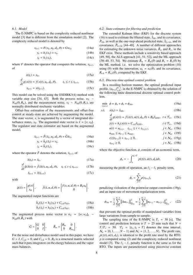
6.1. ModelThe E-NMPC is based on the complexity reduced nonlinear
model [3] that is different from the simulation model [2]. Thecomplexity reduced model is denoted by
xk+1 = F(xk, uk, dk, θ) + Gwk, (14a)yk = hy(xk) + vk, (14b)zk = hz(xk), (14c)
where F denotes the operator that computes the solution, xk+1,of
x(tk) = xk, (15a)ddt
g(x(t)) = f (x(t), uk, dk, θ), tk ≤ t ≤ tk+1, (15b)
xk+1 = x(tk+1). (15c)
This model can be solved using the ESDIRK3(4) method withvariable step size [34, 43]. Both the process noise, wk ∼Niid(0,Rw), and the measurement noise, vk ∼ Niid(0,Rv), arenormally distributed stochastic variables.
Offset-free estimation of the measurements and offset-freecontrol at steady-state are achieved by augmenting the model.The state vector, x, is augmented by a vector of integrated dis-turbance states, xd. The augmented state vector is x = [x; xd].The regulator and state estimator are based on the augmentedmodel,
xk+1 = F(xk, uk, dk, θ) + Gwk, (16a)yk = hy(xk) + vk, (16b)zk = hz(xk), (16c)
where the operator F denotes the solution, xk+1, of
x(tk) = xk, (17a)ddt
g(x(t)) = f (x(t), uk, dk, θ), tk ≤ t ≤ tk+1, (17b)
xk+1 = x(tk+1) (17c)
with
g(x) =
[g(x)xd
], f (x, u, d, θ) =
[f (x, u, d, θ) + Bdxd
0
].
The augmented output functions are
hy(xk) = hy(xk) + Cy,dxd,k, (18a)hz(xk) = hz(xk) + Cz,dxd,k. (18b)
The augmented process noise vector is wk = [w; wd]k ∼Niid(0, Rw) with
G =
[G 00 I
], Rw =
[Rw 00 Rwd
].
For the noise and disturbance model used in this paper, we haveG = I, Cy,d = 0, and Cz,d = 0. Bd is a structural matrix selectedsuch that it puts integrators on the energy balances and the vapormass balances.
6.2. State estimator for filtering and predictionThe extended Kalman filter (EKF) for the discrete system
(16) is used to estimate the filtered state, ˆxk|k, and its covariance,Pk|k, as well as the one-step-ahead predicted state, ˆxk+1|k, and itscovariance, Pk+1|k [44–48]. A number of different approachesfor estimating the unknown noise variances, Rw and Rv, in theEKF exist. These methods include a sensitivity based approach[49, 50], the ALS approach [41, 51, 52], and the ML approach[38–40, 53, 54]. We estimate Rw = Rw(θ) and Rv = Rv(θ) bythe ML method, i.e. we solve the optimization problem (10)using (9) with the innovation, εk = εk(θ), and its covariance,Re,k = Re,k(θ), computed by the EKF.
6.3. Discrete-time optimal control problemIn a receding horizon manner, the optimal predicted input
profile, uk+ jN−1j=0 , in the E-NMPC is obtained by the solution of
the following finite dimensional discrete optimal control prob-lem,
minx,u,z,s
φ = φe + φs + φ∆u, (19a)
s.t. x(tk) = xk|k, (19b)ddt
g(x(t)) = f (x(t), u(t), dk, θ) + Bd xd,k|k, t ∈ Tk, (19c)
z(t) = hz(x(t)) + Cz,d xd,k|k, t ∈ Tk, (19d)u(t) = uk+ j, tk+ j ≤ t < tk+ j+1, j ∈ Nu, (19e)umin ≤ uk+ j ≤ umax, j ∈ Nu, (19f)c(z(tk+ j)) + sk+ j ≥ 0, j ∈ Nz, (19g)sk+ j ≥ 0, j ∈ Nz, (19h)
where the objective function, φ, consists of an economic term,
φe = −∫ tk+T
tkp(z(t), u(t), dk)dt, (20)
measuring the profit of operation, an `2 − `1 penalty term,
φs =
N∑
j=1
ρ(sk+ j), (21)
penalizing violoation of the pointwise output constraints (19g),and an input-rate of movement regularization term,
φ∆u =12
N−1∑
j=0
∥∥∥∆uk+ j
∥∥∥2Q∆u
=12
N−1∑
j=0
∥∥∥uk+ j − uk+ j−1∥∥∥2
Q∆u, (22)
that prevents the optimal profile of manipulated variables fromlarge variations from sample to sample.
The sampling time of the E-NMPC is Ts = 30 [s]. Thecontrol and prediction horizon is T = 25 min such that N =
T/Ts = 50. Tk = [tk, tk + T ] denotes the time interval.Nu = 0, 1, . . . ,N − 1 and Nz = 1, 2, . . . ,N. The profit rate,p(z(t), u(t), dk), is identical to the profit rate used by the RTO.p is computed using (2) and the complexity reduced nonlinearmodel [3]. The `2 − `1 penalty function is the same as for theRTO. The inputs are parameterized using piecewise constant
8
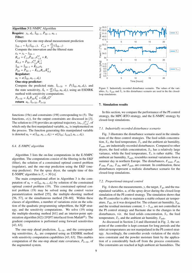
Algorithm 3 E-NMPC AlgorithmRequire: yk, dk, ˆxk|k−1, Pk|k−1, uk−1
Filter:Compute the one-step ahead measurement predictionyk|k−1 = hy( ˆxk|k−1), Cy,k =
dhy
dx ( ˆxk|k−1)Compute the innovation and the filtered stateεk = yk − yk|k−1Re,k = Cy,kPk|k−1CT
y,k + Rv
Kfx,k = Pk|k−1CTy,kR−1
e,kˆxk|k = ˆxk|k−1 + Kfx,kεk
Pk|k = Pk|k−1 − Kfx,kRe,kKTfx,k
Regulator:uk = κ( ˆxk|k, uk−1, dk)One-step predictor:Compute the predicted state, ˆxk+1|k = F( ˆxk|k, uk, dk), andthe state sensitivity, Ak = ∂F
∂x ( ˆxk|k, uk, dk), using an ESDIRKmethod with sensitivity computations.Pk+1|k = AkPk|kAT
k + GRwGT
return uk, ˆxk+1|k, Pk+1|k
functions (19e) and constraints (19f) corresponding to (5). Thefunctions, c(z), for the output constraints are discussed in [3].The solution to (19) provides an optimal trajectory, uk+ jN−1
j=0 , ofwhich only the first manipulated variable, uk, is implemented onthe process. The function generating this manipulated variableis denoted uk = κ( ˆxk|k, uk−1, dk) = κ([xk|k; xd,k|k], uk−1, dk).
6.4. E-NMPC algorithm
Algorithm 3 lists the on-line computations in the E-NMPCalgorithm. The computations consist of the filtering in the EKF(filter), the solution of a constrained optimal control problem(regulator), and the one-step prediction using the EKF (one-step predictor). For the spray dryer, the sample time of thisE-NMPC algorithm is Ts = 30 [s].
The main computational effort in Algorithm 3 is the com-putation of uk = κ( ˆxk|k, uk−1, dk) by solution of the constrainedoptimal control problem (19). This constrained optimal con-trol problem (19) may be solved using the control vectorparametrization method [55], the multiple-shooting method[56, 57], or the simultaneous method [58–60]. Within theseclasses of algorithms, a number of variations exist on the solu-tion of the quadratic programming subproblem, the SQP strat-egy, and the sensitivity computations. We solve (19) usingthe multiple-shooting method [61] and an interior-point opti-mization algorithm [62] (IPOPT interfaced from Matlab R©). Thegradient computation is performed using forward sensitivities[43, 63].
The one-step ahead prediction, ˆxk+1|k, and the correspond-ing sensitivities, Ak, are computed using an ESDIRK methodwith sensitivity computation capabilities [43, 63]. This enablescomputation of the one-step ahead state covariance, Pk+1|k, ofthe augmented system.
0 5 10 15 2047.5
49.5
51.5
53.5
55.5
Fe
ed
c.
[%]
Sf
0 5 10 15 20 54
54.5
55
55.5
Fe
ed
T.
[oC
]
Tf
0 5 10 15 20
Time [hours]
6.5 7.5 8.5 9.5
10.511.5
Am
b.
hu
m.
[g/k
g]
Yamb
Figure 3: Industrially recorded disturbance scenario. The values of the vari-ables, S f, Yamb and Tf, in this disturbance scenario are used in the the closed-loop simulations.
7. Simulation results
In this section, we compare the performance of the PI controlstrategy, the MPC-RTO strategy, and the E-NMPC strategy byclosed-loop simulations.
7.1. Industrially recorded disturbance scenario
Fig. 3 illustrates the disturbance scenario used in the simula-tions of the three control strategies. The feed solids concentra-tion, S f, the feed temperature, Tf, and the ambient air humidity,Yamb, are industrially recorded disturbances. Compared to otherdryers, the feed solids concentration, S f, has a relatively largevariance, while the feed temperature, Tf, is rather stable. Theambient air humidity, Yamb, resembles normal variations from asummer day in northern Europe. The disturbances, Fmain, Fsfb,Fvfbh, Fvfbc, Tvfbc and Tamb, are constant. In combination, thesedisturbances represent a realistic disturbance scenario for theclosed-loop simulations.
7.2. Proportional-integral control
Fig. 4 shows the measurements, y, the target, Tsp, and the ma-nipulated variables, u, of the spray dryer during the closed-loopsimulation of the PI control strategy. The simulation shows thatthe PI controller is able to maintain a stable exhaust air temper-ature, TSD, as it was designed for. The exhaust air humidity, Yab,and the residual moisture content, 1 − S cd, are not controlled inthe PI control strategy and fluctuate due to the changes in thedisturbances, viz. the feed solids concentration, S f, the feedtemperature, Tf, and the ambient air humidity, Yamb.
As discussed in Section 2.4 and illustrated in Fig. 2, the set-point of the controller is kept constant for long periods and theinlet air temperatures are not manipulated in the PI control strat-egy. Accordingly, the controller avoids violation of the sticki-ness constraint and the powder moisture limit by the applica-tion of a considerably back-off from the process constraints.The constraints are reached at high ambient air humidities. The
9

0 5 10 15 2057
60
63
66
69
72
75
78
81
84
87
Te
mp
. [o
C] TSD
TSFB
TV FBh
T SDg
T SDg
Tsp
0 5 10 15 2025
27
29
31
33
35
Ab
s.
hu
m.
[g/k
g]
Yab
0 5 10 15 20
Time [hours]
33.13.23.33.43.53.63.7
Re
s.
mo
i. [
%]
1− Scd
1− Smax
(a) The measured variables, the constraints, and the target.
0 5 10 15 20 90
100
110
120
130
140
Fe
ed
ra
te [
kg
/hr]
Ff
0 5 10 15 20
Time [hours]
60 70 80 90100110120130140150160170180190200
Inle
t a
ir t
em
p.
[oC
]
Tmain
Tsf b
Tvf bh
(b) The manipulated variables.
Figure 4: Simulation of the PI control strategy subject to the disturbance sce-nario given in Fig. 3.
stickiness constraint, i.e. the constraint related to the glass tran-sition temperature, T SD
g , is reached at t=2.5 and t=16 hours dueto high ambient air humidities. The powder moisture limit isreached at the same time points due to the high ambient air hu-midities. The controller rejects the effect of the variations in thefeed solids concentration on the exhaust air humidity, Yab, well.The residual moisture content, 1 − S cd, is affected by all threedisturbances. The PI-control strategy only partially and indi-rectly mitigates the effect of the disturbances on the residualmoisture content.
The stickiness constraint determined by the simulation modeland the control model, T SD
g and T SDg , disagree due to the sim-
plified description of this constraint in the control model. T SDg
is conservatively designed compared to T SDg such that the true
simulation constraint is not violated during operation.Due to the applied back-off, the PI control strategy makes the
0 5 10 15 2057
60
63
66
69
72
75
78
81
84
87
Te
mp
. [o
C] TSD
TSFB
TV FBh
T SDg
T SDg
Tsp
0 5 10 15 2025
27
29
31
33
35
Ab
s.
hu
m.
[g/k
g]
Yab
Ysp
0 5 10 15 20
Time [hours]
33.13.23.33.43.53.63.7
Re
s.
mo
i. [
%]
1− Scd
1− Smax
1− Ssp
(a) The measured variables, the constraints, and the targets.
0 5 10 15 20 90
100
110
120
130
140
Fe
ed
ra
te [
kg
/hr]
Ff
0 5 10 15 20
Time [hours]
60 70 80 90100110120130140150160170180190200
Inle
t a
ir t
em
p.
[oC
]
Tmain
Tsf b
Tvf bh
(b) The manipulated variables.
Figure 5: Simulation of the MPC-RTO strategy subject to the disturbance sce-nario given in Fig. 3.
dryer dry the powder more than necessary to keep the powdermoisture below the maximum limit and avoid violation of thestickiness constraint at all time. This more extensive dryingdecreases the energy efficiency and the yield, i.e. the residualmoisture content sold as product, of the production.
7.3. Model predictive control with real-time optimization
Fig. 5 shows the measurements, y, the targets, r, and the ma-nipulated variables, u, of the spray dryer during the closed-loopsimulation of the MPC-RTO strategy. The simulation showsthat the MPC-RTO strategy is able to steer the controlled vari-ables, z, to the targets, r, computed by the RTO. The controlledvariables are the variables related to the stickiness of the pow-der, TSD and Yab, the SFB stage temperature, TSFB, and theresidual moisture content, 1 − S cd. The effect of the distur-bances on the controlled variables are rejected by adjustments
10

of the manipulated variables every 30 seconds. Every 25 min-utes, the RTO updates the optimal steady state targets basedon the measurements, the economic objective, and the processconstraints.
As discussed in Section 2.4 and illustrated in Fig. 2, in com-bination the tracking ability of the MPC and the target updatesof the RTO reduce the necessary back-off from the constraintscompared to the PI control strategy. The reduced back-off re-sults in an increased profit of operation. The applied back-off isselected to render comparable constraint violations to the othercontrol strategies. As can be seen in Fig. 5(b), the MPC-RTOmanipulates Ff relatively smoothly compared to the PI con-troller (Fig. 4(b)). Making the MPC-RTO more aggressive, likethe PI controller, did not significantly reduce the variance of thecontrolled variables nor the constraint violations. We find thatthe limiting factor to reduce the applied back-off is the fixedtargets, r, that the RTO updates every 25 minutes, only.
Compared to the PI control simulation, the MPC-RTO in-creases the average product flow rate, Fp. This can be observedby inspection of the manipulated feed flow rate, Ff, in Fig. 4(b)and Fig. 5(b). As a consequence of the higher feed and produc-tion rate of the MPC-RTO, the MPC-RTO also increases theaverage energy supply from the heaters. Fig. 5(b) reveals thisby increased inlet air temperatures, Tmain, Tsfb and Tvfbh, com-pared to inlet air temperatures of the PI control strategy (Fig.4(b)). Drying in the SFB and VFB stages is more energy ef-ficient than drying in the SD stage. Therefore, the MPC-RTOseeks to maximize drying in these fluid bed stages to bring themoisture content of the powder below its maximum limit. TheRTO increases the drying in the SFB and VFB stages by select-ing an operating point that increases the inlet air temperatures,Tsfb and Tvfbh. Consider Fig. 5(b) as an example illustratingthe mechanisms of MPC-RTO. Fig. 5(b) shows how the MPC-RTO manipulates Tvfbh. The RTO selects the operating pointsuch that Tvfbh is at its upper limit except for the back-off, δu.The MPC manipulates Tvfbh around this operating point to keepthe controlled variables at their targets. At time t=1 to t=2, t=4,t=5 and t=7.5 hours and between t=19 to t=21 hours, the RTOreduces the drying capacity, Yab, as the SFB stage temperature,TSFB, reaches its upper limit at 75.5 [C]. The reduced capacityresults in a simultaneous decrease of the exhaust air tempera-ture, TSD, to reduce the energy consumption and to avoid vio-lating the stickiness constraint. In comparison to the PI-controlstrategy, the MPC-RTO increases the average residual moisturecontent and controls it to be constantly close to the upper limit.The increased residual moisture content improves the processeconomics in two ways: 1) it reduces the required heat for evap-oration and thereby reduces the energy costs; 2) it increases theproduct flow rate by including more water as part of the prod-uct. Thereby, the increased water in the product can be sold atthe price of powder.
7.4. Economic nonlinear model predictive controlFig. 6 shows a simulation of the measurements, y, and the
manipulated variables, u, of the spray dryer operated by the E-NMPC. As discussed in Section 2.4 and illustrated in Fig. 2,the manipulated variables determined by the E-NMPC strategy
0 5 10 15 2057
60
63
66
69
72
75
78
81
84
87
Te
mp
. [o
C] TSD
TSFB
TV FBh
T SDg
T SDg
0 5 10 15 2025
27
29
31
33
35
Ab
s.
hu
m.
[g/k
g]
Yab
0 5 10 15 20
Time [hours]
33.13.23.33.43.53.63.7
Re
s.
mo
i. [
%]
1− Scd
1− Smax
(a) The measured variables and the constraints.
0 5 10 15 20 90
100
110
120
130
140
Fe
ed
ra
te [
kg
/hr]
Ff
0 5 10 15 20
Time [hours]
60 70 80 90100110120130140150160170180190200
Inle
t a
ir t
em
p.
[oC
]
Tmain
Tsf b
Tvf bh
(b) The manipulated variables.
Figure 6: Simulation of the E-NMPC strategy subject to the disturbance sce-nario given in Fig. 3.
operates the dryer to maximize the predicted profit of operation.The effects of plant-model mismatch and disturbances (knownand unknown) are rejected by adjustments of the manipulatedvariables according to the feedback from measurements andmeasured disturbances, the economic objective, and the spec-ified process constraints. The dynamic optimization takes placeat each sample (30 sec) and this reduces the necessary back-off compared to the MPC-RTO strategy, where the RTO onlyexecutes every 25 min.
The E-NMPC strategy seeks to optimize the combined tran-sient and steady-state economics of the spray dryer. For thelong control and prediction horizon selected in this study, E-NMPC brings the spray dryer to an optimal steady-state pointthat is similar to the steady-state operating point selected by theRTO of the MPC-RTO. E-NMPC uses a full nonlinear model,while the RTO uses a linear model for the dynamics and the
11

same nonlinear model as the E-NMPC for the profit functionand the stickiness constraint. Thus, in both simulations, theeconomic optimum is reached when TSD reaches the point atwhich the powder turns sticky in the top of the chamber, i.e. theglass transition temperature constraint, T SD
g , and when 1 − S cd,the moisture content of the powder, reaches 1 − S max. In thisway, the product flow rate is maximized, the residual moistureis controlled to the specification, and the SFB stage tempera-ture is kept within the constraints. At the same time, the supplyof energy is minimized. As in the case of the MPC-RTO, E-NMPC exploits that the most efficient drying occurs in the fluidbeds, i.e. the SFB and VFB stages. E-NMPC increases the SFBand VFB air temperatures, Tsfb and Tvfbh, to bring the residualmoisture content just below its maximum limit.
The powder becomes moister and potentially sticky insidethe dryer, when the ambient air humidity, Yamb, increases aswell as when the feed solid concentration, S f, decreases. The E-NMPC compensates for such variations (increased air humidityand/or descreased feed solid concentration) by decreasing thefeed flow rate, Ff, and by adjusting the inlet air temperatures.In this way, E-NMPC maintains operation at the optimal pro-duction rate using the optimal heat supply.
7.5. StickinessThe glass transition temperature at the SD stage, T SD
g , deter-mines whether the powder sticks in the SD stage of the spraydryer. When the powder temperature in the SD stage, TSD,is below the glass transition temperature in the SD stage, i.e.TSD ≤ T SD
g , the powder is non-sticky. Otherwise, the powder issticky. Reference [3] provides an expression of the glass transi-tion temperature. The glass transition temperature depends onthe moisture in the powder. In the simplified, yet reasonablyaccurate, model used by the MPC-RTO and the E-NMPC, themoisture in the powder at the SD stage is a function of the tem-perature, TSD, and the air humidity, Yab. This implies that the es-timated sticky and non-sticky regions of the SD stage can be vi-sualized in a 2D-plot. Fig. 7 illustrates the stickiness constraint,T SD
g , as well as the phase portrait of the trajectories generatedby the PI control strategy, the MPC-RTO, and the E-NMPC.Due to stochastic disturbances, the trajectories produced by allthree controllers occasionally violate the stickiness constraint.Therefore, the operating point and stickiness constraint used bythe controllers are designed such that they are backed off fromthe true stickiness constraint of the process.
The PI control strategy does not control the exhaust air hu-midity, Yab, directly. In this case, Yab varies from 27.5 [g/kg]to 34 [g/kg]. Therefore, the operating point of the PI controlstrategy is selected such that the mean value of Yab is relativelyfar from the air humidity stickiness constraint. The consquenceis that the production rate is also below the production capacityof the spray dryer.
The MPC-RTO operates the air humidity, Yab, closer to theconstraint limit than the PI control strategy, as it adjusts the op-erating point every 25 minutes according to the measurementsand the measured disturbances. As is evident by Fig. 7, theMPC-RTO does not operate at the maximum air humidity, andconsequently not at the maximum production rate, at all times.
22 24 26 28 30 32
Yab
, Absolute humidity [g/kg]
55
60
65
70
75
80
85
90
TS
D,
Te
mp
era
ture
[°C
]
Non-sticky region
Sticky region
PI
MPC-RTO
E-NMPC
T SDg
Figure 7: The stickiness constraint from (11f) and (19g) constrains TSD andYab. Note, that cost optimal operation is achieved by maximizing Yab withinthe non-sticky region.
The RTO problem (11) contains back-offs in the manipulatedvariables. Due to these back-offs, the temperature of the VFBinlet air stream, Tvfbh, is on average decreased compared to thesimulation of the E-NMPC strategy (Fig. 6(a)). The MPC-RTO compensates for the decreased VFB inlet air temperature,Tvfbh, by increasing the SFB inlet air temperature, Tsfb. Con-sequently, the SFB temperature, TSFB, increases and the upperlimit on the SFB temperature, TSFB ≤ 75.5 [C], becomes ac-tive (Fig. 5(a)). When the SFB temperature limit is active, theMPC-RTO decreases the production rate as well as the energysupply from the main inlet air and the SFB inlet air, to maintaina stable SFB temperature. Simultaneously, the decreased pro-duction rate allows the SD temperature, TSD, to be decreasedalong the stickiness constraint to save energy and increase theenergy efficiency.
The E-NMPC is able to maintain a maximum air humidityand capacity at all time. In the simulation, TSD and Yab are keptconstant at the maximum exhaust air humidity. The E-NMPCis able to do so as no back-off is implemented in the constraintsof the manipulated variables and the controlled variables. If forinstance the feed solids concentration, S f, had increased further,the E-NMPC would have to decrease the capacity accordinglyand in a similarly way to the way MPC-RTO reduces capacity.
7.6. Key performance indicators
Fig. 8 illustrates the product flow rate, Fp, the specific energyconsumption, Qtot/Fp, the energy efficiency, η, and the profit ofoperation, p, for the closed-loop simulations of the three con-trol strategies. Table 1 provides the average values of the keyperformance indicators (KPIs) for the three control strategies.
Fig. 8 and Table 1 show that the performance of the PI con-trol strategy is inferior compared to the performances of theMPC-RTO and the E-NMPC. Compared to the MPC-RTO andthe E-NMPC, the PI control strategy has a lower average prod-
12

Table 1: Average KPI values.KPI % increase to PI
PI MPC-RTO E-NMPC MPC-RTO E-NMPCProduct flow rate Fp [kg/hr] 60.95 66.21 66.81 8.63% 9.61%Energy consumption rate Qtot [kW] 87.2 89.1 90.4 2.21% 3.63%Specific energy consumption Qtot
Fp[MJ/kg] 5.16 4.81 4.88 -6.72% -5.44%
Residual moisture 1 − S cd [%] 3.37 3.48 3.49 3.21% 3.37%Energy efficiency η [%] 40.2 42.7 42.5 6.06% 5.52%Profit of operation p [e/hr] 123.25 133.98 135.19 8.71% 9.69%
0 5 10 15 20
50
60
70
Fp [
kg
/hr]
PI
MPC-RTO
E-NMPC
0 5 10 15 20
4
5
6
Qto
t/Fp [
MJ/k
g]
PI
MPC-RTO
E-NMPC
0 5 10 15 20
3840424446
η [
%] PI
MPC-RTO
E-NMPC
0 5 10 15 20
Time [hours]
100
150PI
MPC-RTO
E-NMPC
Figure 8: The product flow rate, the specific energy consumption, the energyefficiency, and the profit of operation for the three control strategies.
uct flow rate, a higher specific energy consumption, a lower en-ergy efficiency, and a lower profit of operation. During most ofthe time in the simulations, the MPC-RTO and the E-NMPC in-crease both the product flow rate and the energy efficiency con-siderably. The three controllers perform equally well when theambient air humidity is high. This illustrates that the benefitsarise from the ability of the MPC-RTO and the E-NMPC to uti-lize the excess capacity available at the low ambient air humid-ity. The energy efficiency increases as the exhaust air temper-ature decreases along the stickiness constraint. Thus, the mosteconomic point of operation where Yab is maximized is not themost energy efficient point of operation. This is also revealedby Table 1. Table 1 shows that MPC-RTO provides the mostenergy efficient operation. Nevertheless, E-NMPC provides theoperation with the largest economic profit. From Table 1, itshould be noticed that the increased profit (8.71% and 9.69%) ishighly correlated with the increased production rate (8.63% and9.61%). The residual moisture content is increased by 3.21%and 3.37%, respectively. This contributes significantly to theincreased profit of operation as it corresponds to selling water atthe price of powder and using less energy for evaporation of thewater. The total energy consumption is increased for the MPC-RTO and E-NMPC strategies due to the increased productionrate. However, more importantly the specific energy consump-
tion decreases and the energy efficiency increases when usingthe MPC-RTO and the E-NMPC. MPC-RTO decreases the spe-cific energy consumption by 6.72% and increases the energyefficiency by 6.06%. E-NMPC decreases the specific energyconsumption by 5.44% and increases the energy efficiency by5.52%.
The cumulative increased profit over a year by replacingthe standard industrial PI control strategy with the MPC-RTOstrategy is (133.98 [e/hr] − 123.25 [e/hr]) · 7200 [hr/year] =
77, 000 [e/year]. Similarly, the annual cumulative profit in-crease by using the E-NMPC instead of the PI control strat-egy is (135.19 [e/hr] − 123.25 [e/hr]) · 7200 [hr/year] =
86, 000 [e/year]. Thus, the profit of operation per year is poten-tially increased considerably by both model based controllers.These numbers are for an industrial small scale spray dryerwith a production capacity around 60 kg/hr. An industrial sizedspray dryer for production of skimmed milk powder has a ca-pacity of approximately 7,500 kg/hr. Consequently, industrialsized dryers have a capacity that is more than 100 times largerthan the dryer simulated in this paper. Accordingly, the poten-tial economic benefit of replacing existing PI controls strategieswith advanced process control is significant.
8. Conclusions
In this paper, we present three control strategies for a four-stage spray dryer and compare their performance based on theproduct flow rate, the residual moisture content, the specific en-ergy consumption, the energy efficiency, and the profit of opera-tion. The industrially used PI control strategy serves as a bench-mark for the performance of the MPC-RTO and the E-NMPCcontrol strategies. Both model based controllers increase theprofit of operation by increasing the product flow rate, the resid-ual moisture content, and decreasing the specific energy con-sumption. The residual moisture content is controlled withinspecifications, and deposits of sticky powder particles on thespray dryer surfaces are avoided. For the given disturbance sce-nario, the MPC-RTO increases the profit of operation by 8.71%and the E-NMPC increases the profit of operation by 9.69%.The performance difference between the MPC-RTO and the E-NMPC is mainly due to the necessary back-off in the constraintsemployed in the RTO layer. The economic value of the MPC-RTO and E-NMPC compared to the PI control strategy stemsfrom the adjustment of the operating point of the dryer to theactual disturbances such that the spray dryer can be operatedcloser to the process constraints.
13

Acknowledgement
This work was funded in part by 1) the Danish Ministry ofHigher Education and Science in the industrial PhD project”Economic Model Predictive Control for Spray Drying Plants”(12-128720); 2) GEA Process Engineering A/S, DK-2860Søborg, Denmark; 3) EUDP 64013-0558 in the IEA Annex forEnergy Efficient Process Control.
References[1] W. P. Oliveira, C. R. F. Souza, L. E. Kurozawa, K. J. Park, Spray drying of
food and herbal producs, in: M. W. Woo, A. S. Mujumdar, W. R. W. Daud(Eds.), Spray Drying Technology, Singapore, 2010, Ch. 5, pp. 113–156.
[2] L. N. Petersen, N. K. Poulsen, H. H. Niemann, C. Utzen, J. B. Jørgensen,An experimentally validated simulation model for a four-stage spraydryer, Journal of Process Control (in review).
[3] L. N. Petersen, J. B. Jørgensen, J. B. Rawlings, Economic optimization ofspray dryer operation using nonlinear model predictive control with stateestimation, 9th Symposium on Advanced Control of Chemical Processes(2015) 507–513.
[4] L. N. Petersen, N. K. Poulsen, H. H. Niemann, C. Utzen, J. B. Jørgensen,Comparison of linear and nonlinear model predictive control for opti-mization of spray dryer operation, 5th Conference on Nonlinear ModelPredictive Control (2015) 218–223.
[5] S. J. Qin, T. A. Badgwell, A survey of industrial model predictive controltechnology, Control Engineering Practice 11 (7) (2003) 733–764.
[6] M. Bauer, I. K. Craig, Economic assessment of advanced process control– A survey and framework, Journal of Process Control 18 (1) (2008) 2–18.
[7] M. L. Darby, M. Harmse, M. Nikolaou, MPC: Current practice and chal-lenges, 7th Symposium on Advanced Control of Chemical Processes 7 (1)(2009) 86–98.
[8] J. B. Rawlings, D. Angeli, C. N. Bates, Fundamentals of economic modelpredictive control, 51st Conference on Decision and Control (2012)3851–3861.
[9] G. Francois, S. Costello, D. Bonvin, Application of real-time optimiza-tion methods to energy systems in the presence of uncertainties and dis-turbances, TMC Academic Journal 9 (2) (2015) 20–41.
[10] S. Engell, Feedback control for optimal process operation, Journal of Pro-cess Control 17 (2007) 203–219.
[11] M. L. Darby, M. Nikolaou, J. Jones, D. Nicholson, RTO: An overview andassessment of current practice, Journal of Process Control 21 (6) (2011)874–884.
[12] T. E. Marlin, A. N. Hrymak, Real-time operations optimization of con-tinuous processes, Chemical Process Control-V Conference (1996) 156–164.
[13] K. R. Muske, J. B. Rawlings, Model predictive control with linear models,AIChE Journal 39 (2) (1993) 262–287.
[14] D. E. Kassmann, T. A. Badgwell, R. B. Hawkins, Robust steady-state tar-get calculation for model predictive control, AIChE Journal 46 (5) (2000)1007–1024.
[15] G. Pannocchia, J. B. Rawlings, Disturbance models for offset-free model-predictive control, AIChE Journal 49 (2) (2003) 426–437.
[16] C. Ying, B. Joseph, Performance and stability analysis of LP-MPC andQP-MPC cascade control systems, AIChE Journal 45 (7) (1999) 1521–1534.
[17] K. B. Ariyur, M. Krstic, Real–Time Optimization by Extremum-SeekingControl, John Wiley and Sons, 2003.
[18] M. Guay, E. Moshksar, D. Dochain, A constrained extremum-seekingcontrol approach, International Journal of Robust and Nonlinear Control25 (16) (2015) 3132–3153.
[19] R. Amrit, Optimizing process economics in model predictive control,Ph.D. thesis, University of Wisconsin–Madison (2011).
[20] J. B. Rawlings, R. Amrit, Optimizing process economic performance us-ing model predictive control, Lecture Notes in Control and InformationSciences 384 (2009) 119–138.
[21] D. Angeli, R. Amrit, J. B. Rawlings, On average performance and sta-bility of economic model predictive control, IEEE Transactions on Auto-matic Control 57 (7) (2012) 1615–1626.
[22] J. B. Rawlings, D. Bonne, J. B. Jørgensen, A. N. Venkat, S. B. Jørgensen,Unreachable setpoints in model predictive control, IEEE Transactions onAutomatic Control 53 (9) (2008) 2209–2215.
[23] L. W. Tan, F. S. Taip, N. Abdul Aziz, Simulation and control of spraydrying using nozzle atomizer spray dryer, International Journal of Engi-neering & Technology 9 (10) (2009) 1–7.
[24] L. W. Tan, M. N. Ibrahim, R. Kamil, F. S. Taip, Empirical modeling forspray drying process of sticky and non-sticky products, Procedia FoodScience 1 (2011) 690–697.
[25] V. S. Shabde, K. A. Hoo, Optimum controller design for a spray dryingprocess, Control Engineering Practice 16 (5) (2008) 541–552.
[26] V. S. Shabde, K. A. Hoo, Design and operation of a spray dryer for themanufacture of hollow microparticles, Industrial & Engineering Chem-istry Research 45 (2006) 8329–8337.
[27] V. S. Shabde, Optimal design and control of a spray drying process thatmanufacture hollow micro-particles, Ph.D. thesis, Texas Tech University(2006).
[28] C. A. Zaror, J. R. Perez-Correa, Model based control of centrifugal atom-izer spray drying, Food Control 2 (3) (1991) 170–175.
[29] J. R. Perez-Correa, F. Farias, Modelling and control of a spray dryer: Asimulation study, Food Control 6 (4) (1995) 219–227.
[30] R. Govaerts, A. Johnson, R. Crezee, G. Reyman, P. L. S. Swinkels, Con-trol of an industrial spray-drying unit, Control Engineering Practice 2 (1)(1994) 69–85.
[31] L. N. Petersen, N. K. Poulsen, H. H. Niemann, C. Utzen, J. B. Jørgensen,Application of constrained linear MPC to a spray dryer, Multi-Conferenceon Systems and Control (2014) 2120–2126.
[32] L. N. Petersen, N. K. Poulsen, H. H. Niemann, C. Utzen, J. B. Jørgensen,Economic optimization of spray dryer operation using nonlinear modelpredictive control, 53rd Conference on Decision and Control (2014)6794–6800.
[33] D. O’Callaghan, P. Cunningham, Modern process control techniques inthe production of dried milk products – a review, Lait 85 (2005) 335–342.
[34] C. Volcker, J. B. Jørgensen, P. G. Thomsen, E. H. Stenby, Adaptive stepsize control in implicit runge-kutta methods for reservoir simulation, 9thInternational Symposium on Dynamics and Control of Process Systems(2010) 509–514.
[35] S. Skogestad, Simple analytic rules for model reduction and PID con-troller tuning, Journal of Process Control 13 (4) (2003) 291–309.
[36] K. J. Åstrom, T. Hagglund, Advanced PID control, Instrument Society ofAmerica, NC, USA, 2006.
[37] G. Pannocchia, M. Gabiccini, A. Artoni, Offset-free MPC explained: nov-elties, subtleties, and applications, 5th Conference on Nonlinear ModelPredictive Control (2015) 342–351.
[38] N. R. Kristensen, H. Madsen, S. B. Jørgensen, A method for systematicimprovement of stochastic grey-box models, Computers & Chemical En-gineering 28 (8) (2004) 1431–1449.
[39] J. B. Jørgensen, S. B. Jørgensen, MPC-relevant prediction-error identifi-cation, The American Control Conference (2007) 2475–2480.
[40] J. B. Jørgensen, S. B. Jørgensen, Comparison of prediction-error-modelling criteria, The American Control Conference (2007) 140–146.
[41] B. J. Odelson, M. R. Rajamani, J. B. Rawlings, A new autocovarianceleast-squares method for estimating noise covariances, Automatica 42(2006) 303–308.
[42] B. M. Åkesson, J. B. Jørgensen, N. K. Poulsen, S. B. Jørgensen, A gener-alized autocovariance least-squares method for Kalman filter tuning, Jour-nal of Process Control 18 (7) (2008) 769–779.
[43] M. R. Kristensen, J. B. Jørgensen, P. G. Thomsen, S. B. Jørgensen, An ES-DIRK method with sensitivity analysis capabilities, Computers & Chem-ical Engineering 28 (12) (2004) 2695–2707.
[44] J. B. Jørgensen, M. R. Kristensen, P. G. Thomsen, H. Madsen, A compu-tationally efficient and robust implementation of the continuous-discreteextended Kalman filter, The American Control Conference (2007) 3706–3712.
[45] J. B. Jørgensen, A critical discussion of the continuous-discrete extendedKalman filter, in: European Congress of Chemical Engineering - 6,Copenhagen, Denmark, 2007.
[46] J. B. Rawlings, D. Q. Mayne, Model Predictive Control: Theory and De-sign, Nob Hill Publishing, 2009.
[47] E. L. Haseltine, J. B. Rawlings, Critical evaluation of extended Kalmanfiltering and moving-horizon estimation, Industrial & Engineering Chem-
14
istry Research 44 (8) (2005) 2451–2460.[48] J. B. Rawlings, B. R. Bakshi, Particle filtering and moving horizon esti-
mation, Computers & Chemical Engineering 30 (10) (2006) 1529–1541.[49] J. Valappil, C. Georgakis, Systematic estimation of state noise statistics
for extended Kalman filters, AIChE Journal 46 (2) (2000) 292–308.[50] Z. K. Nagy, R. D. Braatz, Robust nonlinear model predictive control of
batch processes, AIChE Journal 49 (7) (2003) 1776–1786.[51] F. V. Lima, J. B. Rawlings, Nonlinear stochastic modeling to improve
state estimation in process monitoring and control, AIChE Journal 57 (4)(2011) 996–1007.
[52] M. A. Zagrobelny, J. B. Rawlings, Practical improvements to autocovari-ance least-squares, AIChE Journal 61 (6) (2015) 1840–1855.
[53] N. R. Kristensen, H. Madsen, S. B. Jørgensen, Parameter estimation instochastic grey-box models, Automatica 40 (2) (2004) 225–237.
[54] M. A. Zagrobelny, J. B. Rawlings, Identifying the uncertainty structureusing maximum likelihood estimation, The American Control Conference(2015) 422–427.
[55] M. Schlegel, K. Stockmann, T. Binder, W. Marquardt, Dynamic optimiza-tion using adaptive control vector parameterization, Computers & Chem-ical Engineering 29 (8) (2005) 1731–1751.
[56] H. G. Bock, K. J. Plitt, A multiple shooting algorithm for direct solutionof optimal control problems, 9th IFAC World Congress Budapest (1984)242–247.
[57] M. Diehl, H. G. Bock, J. P. Schloder, R. Findeisen, Z. Nagy, F. Allgower,Real-time optimization and nonlinear model predictive control of pro-cesses governed by differential-algebraic equations, Journal of ProcessControl 12 (4) (2002) 577–585.
[58] L. T. Biegler, Solution of dynamic optimization problems by successivequadratic programming and orthogonal collocation, Computers & Chem-ical Engineering 8 (3) (1984) 243–248.
[59] L. T. Biegler, An overview of simultaneous strategies for dynamic opti-mization, Chemical Engineering and Processing: Process Intensification46 (11) (2007) 1043–1053.
[60] L. T. Biegler, X. Yang, G. A. G. Fischer, Advances in sensitivity-basednonlinear model predictive control and dynamic real-time optimization,Journal of Process Control 30 (2015) 104–116.
[61] A. Capolei, J. B. Jørgensen, Solution of constrained optimal control prob-lems using multiple shooting and ESDIRK methods, The American Con-trol Conference (2012) 295–300.
[62] A. Wachter, L. T. Biegler, On the implementation of an interior-point filterline-search algorithm for large-scale nonlinear programming, Mathemat-ical programming 106 (1) (2006) 25–57.
[63] A. Capolei, Nonlinear Model Predictive Control for Oil Reservoirs Man-agement, Ph.D. thesis, Technical University of Denmark (2013).
15

164

P a p e r C
A Grey-Box Model for SprayDrying Plants
Published in 10th IFAC International Symposium on Dynamics and Control ofProcess Systems (DYCOPS 2013), pp. 559–564, 2013, Mumbai.

166
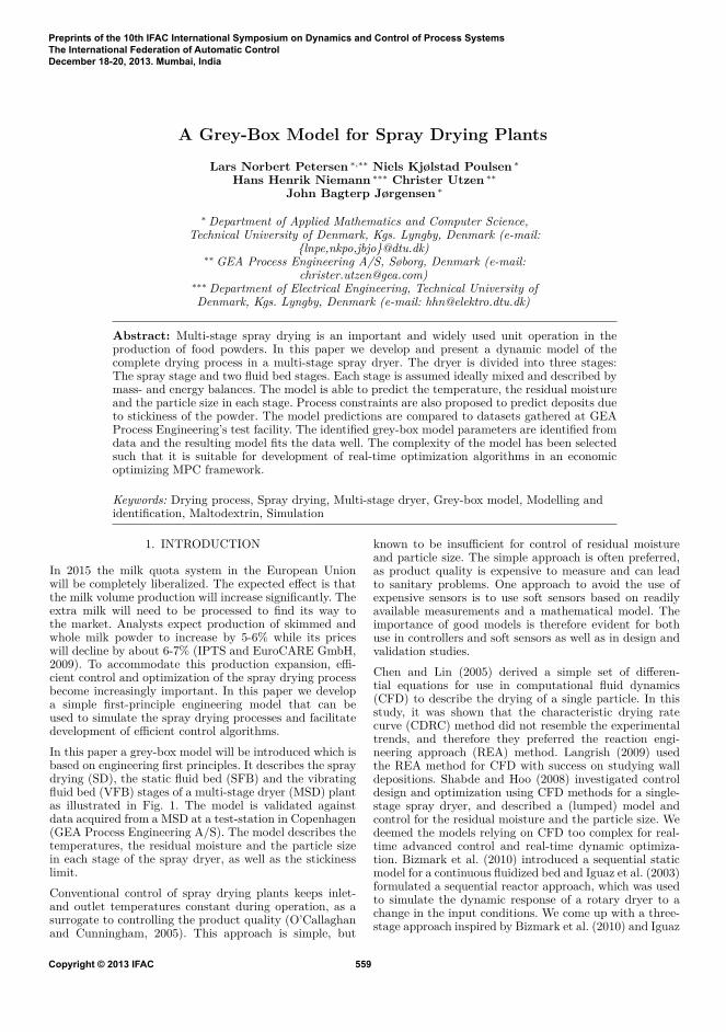
A Grey-Box Model for Spray Drying Plants
Lars Norbert Petersen ∗,∗∗ Niels Kjølstad Poulsen ∗Hans Henrik Niemann ∗∗∗ Christer Utzen ∗∗
John Bagterp Jørgensen ∗
∗Department of Applied Mathematics and Computer Science,Technical University of Denmark, Kgs. Lyngby, Denmark (e-mail:
lnpe,nkpo,[email protected])∗∗GEA Process Engineering A/S, Søborg, Denmark (e-mail:
[email protected])∗∗∗Department of Electrical Engineering, Technical University ofDenmark, Kgs. Lyngby, Denmark (e-mail: [email protected])
Abstract: Multi-stage spray drying is an important and widely used unit operation in theproduction of food powders. In this paper we develop and present a dynamic model of thecomplete drying process in a multi-stage spray dryer. The dryer is divided into three stages:The spray stage and two fluid bed stages. Each stage is assumed ideally mixed and described bymass- and energy balances. The model is able to predict the temperature, the residual moistureand the particle size in each stage. Process constraints are also proposed to predict deposits dueto stickiness of the powder. The model predictions are compared to datasets gathered at GEAProcess Engineering’s test facility. The identified grey-box model parameters are identified fromdata and the resulting model fits the data well. The complexity of the model has been selectedsuch that it is suitable for development of real-time optimization algorithms in an economicoptimizing MPC framework.
Keywords: Drying process, Spray drying, Multi-stage dryer, Grey-box model, Modelling andidentification, Maltodextrin, Simulation
1. INTRODUCTION
In 2015 the milk quota system in the European Unionwill be completely liberalized. The expected effect is thatthe milk volume production will increase significantly. Theextra milk will need to be processed to find its way tothe market. Analysts expect production of skimmed andwhole milk powder to increase by 5-6% while its priceswill decline by about 6-7% (IPTS and EuroCARE GmbH,2009). To accommodate this production expansion, effi-cient control and optimization of the spray drying processbecome increasingly important. In this paper we developa simple first-principle engineering model that can beused to simulate the spray drying processes and facilitatedevelopment of efficient control algorithms.In this paper a grey-box model will be introduced which isbased on engineering first principles. It describes the spraydrying (SD), the static fluid bed (SFB) and the vibratingfluid bed (VFB) stages of a multi-stage dryer (MSD) plantas illustrated in Fig. 1. The model is validated againstdata acquired from a MSD at a test-station in Copenhagen(GEA Process Engineering A/S). The model describes thetemperatures, the residual moisture and the particle sizein each stage of the spray dryer, as well as the stickinesslimit.Conventional control of spray drying plants keeps inlet-and outlet temperatures constant during operation, as asurrogate to controlling the product quality (O’Callaghanand Cunningham, 2005). This approach is simple, but
known to be insufficient for control of residual moistureand particle size. The simple approach is often preferred,as product quality is expensive to measure and can leadto sanitary problems. One approach to avoid the use ofexpensive sensors is to use soft sensors based on readilyavailable measurements and a mathematical model. Theimportance of good models is therefore evident for bothuse in controllers and soft sensors as well as in design andvalidation studies.Chen and Lin (2005) derived a simple set of differen-tial equations for use in computational fluid dynamics(CFD) to describe the drying of a single particle. In thisstudy, it was shown that the characteristic drying ratecurve (CDRC) method did not resemble the experimentaltrends, and therefore they preferred the reaction engi-neering approach (REA) method. Langrish (2009) usedthe REA method for CFD with success on studying walldepositions. Shabde and Hoo (2008) investigated controldesign and optimization using CFD methods for a single-stage spray dryer, and described a (lumped) model andcontrol for the residual moisture and the particle size. Wedeemed the models relying on CFD too complex for real-time advanced control and real-time dynamic optimiza-tion. Bizmark et al. (2010) introduced a sequential staticmodel for a continuous fluidized bed and Iguaz et al. (2003)formulated a sequential reactor approach, which was usedto simulate the dynamic response of a rotary dryer to achange in the input conditions. We come up with a three-stage approach inspired by Bizmark et al. (2010) and Iguaz
Preprints of the 10th IFAC International Symposium on Dynamics and Control of Process SystemsThe International Federation of Automatic ControlDecember 18-20, 2013. Mumbai, India
Copyright © 2013 IFAC 559

SD
SFB
Main Air
SFB Air
VFBh Air VFBc Air
Feed
Powder
ExhaustExit
VFB
Fines
Cooling
Fig. 1. Diagram of the multi-stage dryer. SD = spraydrying, SFB = static fluid bed and VFB = vibratingfluid bed
et al. (2003) and use constitutive equations inspired byLangrish and Kockel (2001).To our knowledge, no control oriented general dynamicmodel exist for multi-stage spray dryers. In this work sucha general model is proposed.The paper is organized as follows. In Section 2 we describethe spray drying process and in Section 3 we presentthe three-stage model. We also give constraints to theresidual moisture in order to predict wall deposits. Section4 contains a brief description of the method for parameterestimation, the estimated parameters, and a validation ofthe model to data from two experiments. Conclusions aregiven in Section 5.
2. THE SPRAY DRYING PROCESS
As illustrated in Fig. 1, spray drying is a continuous pro-cess which produces a dry powder from a liquid or a slurry.The spray dryer consists most often of a combination ofthree stages; the actual spray drying (SD), the static fluidbed (SFB) and the vibrating fluid bed (VFB). The mainpurpose of the SD stage is to reduce stickiness and foulingof the wet feed. The powder then falls to the SFB forfurther agglomeration and drying. Finally the powder istransported to the external VFB, for gentle drying andis cooled to the temperature desired for handling andstorage. Cooling air and fines from the cyclone are returnedto the SD stage near the nozzles for forced agglomeration.The main factors affecting the residual moisture in thepowder are the temperature, the relative humidity and theparticle size in the stages. Normally, the SD air temper-ature (exhaust temperature) is automatically controlledby adjusting the feed flow rate while the temperatures inthe other stages are manually controlled from the inletair temperatures set by the operator. The particle sizeis mainly affected by the nozzle pressure (i.e. feed flow,concentration and viscosity), residual moisture and theSFB inlet air flows. The particle size is often controlledby adjusting inlet air flows and the residual moisture
is controlled from the exhaust temperature. Generally,two external disturbances are present in spray drying i.e.the ambient air humidity and the feed composition. Thedisturbances both affect the residual moisture and theparticle size. Also the hold-up of powder in the SFB andVFB can vary and influences the drying.
3. MULTI-STAGE DRYER MODEL
The model structure is derived from engineering first prin-ciples and the unknown parameters are identified usinga least-squares method. This approach, called grey-boxmodeling (Ljung, 1999), combines physical knowledge withdata-based (statistical) modeling; physical knowledge pro-vides the main structure and statistical modeling providesdetails on the actual coefficients (Kristensen et al., 2004).Compared to statistical black-box models; this is advanta-geous since it allows a physical interpretation of the modeland often wide valid operation range. Utilizing mass andenergy conservation laws, also make it possible to extractotherwise unknown drying conditions inside the dryingzones.We divide the model of the dryer into three stages. TheSD, the SFB and the VFB stage. Fig. 2 shows a schematicrepresentation of the three-stage model approach, and Fig.3 describes the details of a single stage.For each of the stages, we set up two mass balances (Eq.1 and 4), one energy balance (Eq. 15) and one particlesize balance (Eq. 31) in order to fully describe the dryingconditions in each stage. In the following, the derivation ofthe equations for the stages will be treated generally andwhen necessary a specific stage is noted in the superscriptof the equation.The experiments were based on drying of maltodextrinDE-18, because milk is expensive, cannot be stored in liq-uid form and its composition is not well defined. Maltodex-trin, though, resemble the same fundamental properties asskim milk.
3.1 Powder moisture
A mass balance for water in the powder yieldsdmw
dt= Fpsin
Xin − FpsoutXout −Rwmps (1)
X is the dry basis water concentration (kg water/kg drysolid) in the powder and the flux of evaporating water isRwmps. The hold-up of dry powder is assumed constant,and thus the flow of dry powder entering and leaving is
Fpsout= Fpsin
= SinFpin(2)
The dry basis concentration of product in- and outlet flowsare
Xin = 1− SinSin
Xout = mw
mp −mw(3)
where Sin is the concentration (kg solid/kg total) and mw
is the mass of water. mp is the total mass of the powder.
3.2 Air moisture
The amount of vapour in the air is given by
IFAC DYCOPS 2013December 18-20, 2013. Mumbai, India
560

SD SFB VFB
SVFBout, D
VFBout
FVFBpout
, TVFBpoutSSD
in, DSD
in
FSDpin
, TSDpin
YSDout
FSDaout
, TSDaout
Ycoolin
Fcoolain
, Tcoolain
Ymainin
Fmainain
, Tmainain
Ysfbin
Fsfbain
, Tsfbain
FSFBaout
, TSFBaout
, YSFBaout
FSDpout
, TSDpout
, SSD
out, DSD
out
Yvfbcin
Fvfbcain
, Tvfbcain
Yvfbhin
Fvfbhain
, Tvfbhain
YVFBout
FVFBaout
, TVFBaout
FSFBpout
, TSFBpout
, SSFB
out, DSFB
out
Nozzles
Fig. 2. Princple of the sequential stage model.
dmv
dt= Fvin − Fvout +Rwmps (4)
The inlet vapour flow, Fvin, for each stage is
FSDvin= Y mainin Fmaindain
+ Y coolin F cooldain+ Y SFBout FSFBdaout
(5)FSFBvin
= Y sfbin F sfbdain(6)
FV FBvin= Y vfbhin F vfbhdain
+ Y vfbcin F vfbcdain(7)
The flow of dry air, Fdain , is given by
Fdain = 1Yin + 1Fain (8)
and the absolute humidity, Yin, of the incoming air is
Yin = Mv
Mda
RHinPvsatPin − RHinPvsat
(9)
RHin is the relative humidity and Pvsat is the saturatedvapour pressure from the Antoine equation.The hold-up of dry air is assumed constant, and thus thedry air flow out of the chamber is equal to the dry air flowinto the chamber. The flow of vapour out of the stages is
FSDvout= Y SDout (Fmaindain
+ F cooldain+ FSFBdaout
) (10)FSFBvout
= Y SFBout F sfbdain(11)
FV FBvout= Y V FBout (F vfbhdain
+ F vfbcdain) (12)
The absolute humidity of the stage air, Yout, is given by
Yout = Mda
Mv
P − PvPv
(13)
Assuming constant total chamber pressure, P , which iscontrolled by a suction fan. The vapour pressure is givenby the ideal gas law
Pv = MvRTaout
mvV(14)
Mv is the molar mass of vapour. V is the stage air volume.
3.3 Energy balance
It is assumed that in each stage the temperature of theair and the product are in equilibrium and identical. Thistemperature is defined by an energy balance
dU
dt= ∆H +Q+W (15)
Reactor
Air
Powder
Air inlet
Powder inlet
Air outlet
Qexc Qlossmv
mda
mw
ms
Rwmp
Tp
Ta
Powder outlet
Fpout, Tpout
, Sout, DoutFpin
, Tpin, Sin, Din
Fain, Tain
, Yin
Faout, Taout
, Yout
Fig. 3. Sketch of a single stage.
where W = 0 and∆H = Hain
−Haout+Hpin
−Hpout(16)
Q = −Qloss +Qexc (17)
The enthalpy of humid air isHa = Ha0 + Fda(Cda(Ta − Tref )
+ Y (λ+ Cv(Ta − Tref ))) (18)where Cda and Cv is the specific heat capacity of dry airand vapour respectively. λ is the latent heat of evaporationand Tref = 25C is the reference temperature.The enthalpy increase from inlet air in each stage is
HSDain
= Hmainain
+Hcoolain
+HSFBaout
(19)HSFBain
= Hsfbain
(20)HV FBain
= Hvfbhain
+Hvfbcain
(21)
The enthalpy of humid air leaving the stages is simplydetermined from (18). We denote the enthalpies HSD
aout,
HSFBaout
and HV FBaout
.The enthalpy of liquid feed as well as powder is
Hp = Hp0 + Fps(Cs +XCw)(Tp − Tref ) (22)where Cs and Cw is the specific heat capacity of solids andwater respectively.The heat loss is given by
IFAC DYCOPS 2013December 18-20, 2013. Mumbai, India
561

Qloss = UA(Taout − Tindoor) (23)Since the indoor temperature was not measured, we ap-proximate the indoor temperature by Tvfbc.The SD and SFB stage is subject to exchange of heat,as these are placed inside the same chamber. The heatexchange is
QSDexc = −UAexc(TSDaout− TSFBaout
) (24)QSFBexc = UAexc(TSDaout
− TSFBaout) (25)
The VFB is isolated from the other stages, and thus havezero heat exchange i.e. QV FBexc = 0.The total energy is given by
U = mpCpTpout+mdaCdaTaout
+mvCavTaout
+msteelCsteelTaout(26)
As mentioned the temperature of the air in the chamber,Taout
equals Tpout. The heat capacities are placed in
appendix A. In this we assume that the temperature of thesteel chamber changes reasonably fast compared to the airtemperature. The mass of steel is determined by assuming3 mm of steel. i.e. mSD
steel = 212.22 kg, mSFBsteel = 7.80 kg
and mV FBsteel = 8.10 kg.
3.4 Drying rate equation
The evaporation rate, Rw, is an essential part of themodel. According to Iguaz et al. (2003) it should includeequilibrium moisture content data and must be determinedexperimentally under conditions as close as possible tothose of the process. We find that the drying kineticsis best described by the lumped-parameter expression(Langrish and Kockel, 2001; Chen and Lin, 2005). Thus,the drying rate is a function of vapour density and themoisture content. The drying rate may be expressed as
Rw = K1(Xout −Xeq)(ρvsat − ρv) (27)where
ρvsat = MvPvsatRTpout
ρv = MvPvRTaout
(28)
The last term of (27), ρvsat−ρv, describes the driving forceof evaporation from the particles to the air, assuming thatthe surface of the particle is completely covered in water.To describe the friction of evaporation we introduce theterm of free moisture, Xout − Xeq. The term decreasestowards zero as the residual moisture get closer to theequilibrium moisture content. The constant K1 correctsfor un-modelled effects, such as relative speed between airand particle and other phenomena affecting drying. Thesephenomena are practically impossible to model withouttaking a CFD approach. It is, furthermore, necessary tomultiply Rw by FSDpin
/0.0241 in the SD stage in order tocorrectly render variations in the feed flow.The equilibrium moisture content, Xeq, is described by
Xeq = A
(RHaout
1−RHaout
)B ( 1Taout − 273.15
)C(29)
Xeq is a product dependent function that describe themoisture content where water cannot be extracted fromthe powder any longer. As the moisture content ap-proaches this value the friction of extracting water fromthe particles increase to infinite. In theory the moisturecontent can only be obtained by infinite residence time.
Woo et al. (2008), shows that A = 1.2098, B = 0.8535 andC = 0.5962 can be used for maltodextrin DE-18.
3.5 Particle size
The droplets can be produced by either a rotating atomizeror a nozzle. We use a nozzle and the particle size can bedescribed by
DSDin = D0 + a(FSDpin
− Fp0) + b(TSDpin− Tp0)
+ c(SSDin − S0) (30)The constants have been manually fitted to
a = 4000 b = −10.1 c = −600Fp0 = 0.021921 Tp0 = 326.35 S0 = 0.5
The sprayed droplets are subject to shrinkage duringdrying. If it is assumed that the particles are perfectlyspherical before and after the drying and only water isevaporating, we can derive a differential equation for theresulting size of the particles. For each stage we get
Dout = 1τ
((Xout + 1Xin + 1 ·
ρpin
ρpout
) 13
Din
+Kag(Fa − Fa0)−Dout) (31)Agglomeration is generally difficult to describe and wesimply add a term proportional to the air flow rate of thestage. The parameters are
τSD = 400 τSFB = 200 τV FB = 100KSDag = 100 KSFB
ag = 300 KV FBag = 200
FSDa0 = 0.49944 FSFBa0 = 0.14167 FV FBa0 = 0.18046
3.6 Stickiness
Stickiness of the produced particles is an important limi-tation to the achievable performance of the MSD. Stickyparticles form depositions on the walls of the spray dryer.Stickiness has been found to depend on product temper-ature and moisture content. Furthermore, the transitionfrom sticky to non-sticky takes place very quickly, thus wecan assume it to have binary state. We will use a mass-proportion-mixing rule, as proposed by (Hennigs et al.,2001; Hogan et al., 2010), to describe the non-sticky regioni.e. when the powder is below its glass transition temper-ature.
Tg = SoutTgp + k(1− Sout)TgwSout + k(1− Sout)
(32)
Tgp = 144.8C and Tgw = −137C for maltodextrin DE-18 and water respectively. The value k = 6.296 is estimatedfrom adsorption isotherm data.The data of the experiment is produced by studying thestickiness of the powder in an equilibrium state. Meaningthat the moisture at the surface is equal to that of thecore of the particle. This situation is not present in spraydrying, where the rapid evaporation from the surface tendto form a particle with a crisper surface than the core. Inpractice this means that Tg is higher i.e. that the powder isless sticky inside the spray dryer. To compensate for this,we form a correction term
Tmax = Tg + ∆Tadj (33)The offset depends on the design of the dryer and unknownfactors. Normally it is in the range of 10 to 60C (Hogan
IFAC DYCOPS 2013December 18-20, 2013. Mumbai, India
562
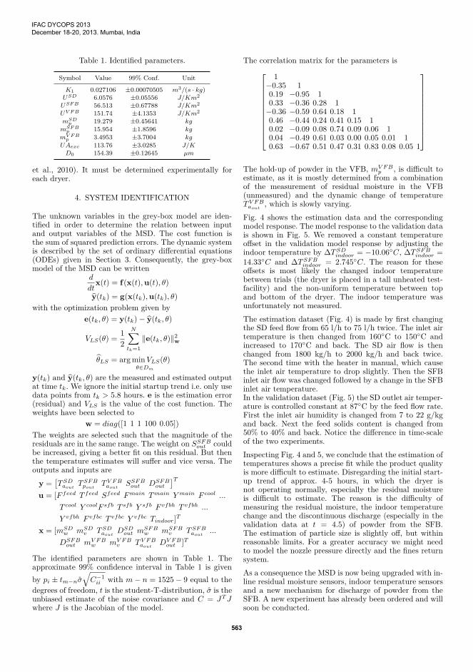
Table 1. Identified parameters.
Symbol Value 99% Conf. Unit
K1 0.027106 ±0.00070505 m3/(s · kg)USD 6.0576 ±0.05556 J/Km2
USF B 56.513 ±0.67788 J/Km2
UV F B 151.74 ±4.1353 J/Km2
mSDp 19.279 ±0.45641 kg
mSF Bp 15.954 ±1.8596 kg
mV F Bp 3.4953 ±3.7004 kg
UAexc 113.76 ±3.0285 J/KD0 154.39 ±0.12645 µm
et al., 2010). It must be determined experimentally foreach dryer.
4. SYSTEM IDENTIFICATION
The unknown variables in the grey-box model are iden-tified in order to determine the relation between inputand output variables of the MSD. The cost function isthe sum of squared prediction errors. The dynamic systemis described by the set of ordinary differential equations(ODEs) given in Section 3. Consequently, the grey-boxmodel of the MSD can be written
d
dtx(t) = f(x(t),u(t), θ)
y(tk) = g(x(tk),u(tk), θ)with the optimization problem given by
e(tk, θ) = y(tk)− y(tk, θ)
VLS(θ) = 12
N∑tk=1‖e(tk, θ)‖2
w
θLS = arg minVLS(θ)θ∈Dm
y(tk) and y(tk, θ) are the measured and estimated outputat time tk. We ignore the initial startup trend i.e. only usedata points from tk > 5.8 hours. e is the estimation error(residual) and VLS is the value of the cost function. Theweights have been selected to
w = diag([1 1 1 100 0.05])The weights are selected such that the magnitude of theresiduals are in the same range. The weight on SSFBout couldbe increased, giving a better fit on this residual. But thenthe temperature estimates will suffer and vice versa. Theoutputs and inputs are
y =[TSDaout
TSFBpoutTV FBaout
SSFBout DSFBout
]Tu = [F feed T feed Sfeed Fmain Tmain Y main F cool ...
T cool Y coolF sfb T sfb Y sfb F vfbh T vfbh ...
Y vfbh F vfbc T vfbc Y vfbc Tindoor]T
x = [mSDw mSD
v TSDaoutDSDout m
SFBw mSFB
v TSFBaout...
DSFBout mV FB
w mV FBv TV FBaout
DV FBout ]T
The identified parameters are shown in Table 1. Theapproximate 99% confidence interval in Table 1 is givenby pi ± tm−nσ
√C−1ii with m− n = 1525− 9 equal to the
degrees of freedom, t is the student-T-distribution, σ is theunbiased estimate of the noise covariance and C = JTJwhere J is the Jacobian of the model.
The correlation matrix for the parameters is
1−0.35 10.19 −0.95 10.33 −0.36 0.28 1−0.36 −0.59 0.64 0.18 10.46 −0.44 0.24 0.41 0.15 10.02 −0.09 0.08 0.74 0.09 0.06 10.04 −0.49 0.61 0.03 0.00 0.05 0.01 10.63 −0.67 0.51 0.47 0.31 0.83 0.08 0.05 1
The hold-up of powder in the VFB, mV FB
p , is difficult toestimate, as it is mostly determined from a combinationof the measurement of residual moisture in the VFB(unmeasured) and the dynamic change of temperatureTV FBaout
, which is slowly varying.Fig. 4 shows the estimation data and the correspondingmodel response. The model response to the validation datais shown in Fig. 5. We removed a constant temperatureoffset in the validation model response by adjusting theindoor temperature by ∆TSDindoor = −10.06C, ∆TSFBindoor =14.33C and ∆TSFBindoor = 2.745C. The reason for theseoffsets is most likely the changed indoor temperaturebetween trials (the dryer is placed in a tall unheated test-facility) and the non-uniform temperature between topand bottom of the dryer. The indoor temperature wasunfortunately not measured.The estimation dataset (Fig. 4) is made by first changingthe SD feed flow from 65 l/h to 75 l/h twice. The inlet airtemperature is then changed from 160C to 150C andincreased to 170C and back. The SD air flow is thenchanged from 1800 kg/h to 2000 kg/h and back twice.The second time with the heater in manual, which causethe inlet air temperature to drop slightly. Then the SFBinlet air flow was changed followed by a change in the SFBinlet air temperature.In the validation dataset (Fig. 5) the SD outlet air temper-ature is controlled constant at 87C by the feed flow rate.First the inlet air humidity is changed from 7 to 22 g/kgand back. Next the feed solids content is changed from50% to 40% and back. Notice the difference in time-scaleof the two experiments.Inspecting Fig. 4 and 5, we conclude that the estimation oftemperatures shows a precise fit while the product qualityis more difficult to estimate. Disregarding the initial start-up trend of approx. 4-5 hours, in which the dryer isnot operating normally, especially the residual moistureis difficult to estimate. The reason is the difficulty ofmeasuring the residual moisture, the indoor temperaturechange and the discontinuous discharge (especially in thevalidation data at t = 4.5) of powder from the SFB.The estimation of particle size is slightly off, but withinreasonable limits. For a greater accuracy we might needto model the nozzle pressure directly and the fines returnsystem.As a consequence the MSD is now being upgraded with in-line residual moisture sensors, indoor temperature sensorsand a new mechanism for discharge of powder from theSFB. A new experiment has already been ordered and willsoon be conducted.
IFAC DYCOPS 2013December 18-20, 2013. Mumbai, India
563

0 5 10 15 20
80
85
90
TS
Pa ou
t [°C
]
MeasuredSimulated
0 5 10 15 20687072747678
TS
FB
a out
[o C]
0 5 10 15 20384042444648
TV
FB
a out
[°C
]
0 5 10 15 200.5
1
1.5
2
2.5
1−S
SF
Bou
t [%
]
0 5 10 15 20
100
120
140
DS
FB
out
[µm
]
Time [hours]
Fig. 4. The estimation dataset. SSFBout and DSFBout are
sampled by hand resulting in a low sample frequency.
0 1 2 3 4 5 6 7 885
90
95
TS
Pa ou
t [°C
]
MeasuredSimulated
0 1 2 3 4 5 6 7 8
76
78
80
TS
FB
a out
[o C]
0 1 2 3 4 5 6 7 83840424446
TV
FB
a out
[°C
]
0 1 2 3 4 5 6 7 8
1
1.5
2
1−S
SF
Bou
t [%
]
0 1 2 3 4 5 6 7 8100
120
140
DS
FB
out
[µm
]
Time [hours]
Fig. 5. The validation dataset. The three temperatures areoffset corrected. The temperature peak (t = 3.5) isdue to change of feed tank and the peak at t = 5.5and 6.5 is due to change of nozzle.
5. CONCLUSIONS
In this paper, a mathematical model is proposed for amulti-stage spray dryer. We established a dynamic modelconsisting of three stages; the actual spray drying (SD),the static fluid bed (SFB) and the vibrating fluid bed(VFB). The stages were described by the same constitutiveequation. The model predicts the temperatures within thedryer with high accuracy. The residual moisture and theparticle size of the powder is predicted with some expecteduncertainty, due to unstable discharge of powder fromthe SFB stage and varying indoor temperature. We alsoprovided a novel prediction for stickiness of the powder, as
a function of powder temperature and residual moisture.The model is general in the sense, that it can be adjustedto describe the drying of any liquid or slurry in a multi-stage spray dryer.
REFERENCESBizmark, N., Mostoufi, N., Sotudeh-Gharebagh, R., andEhsani, H. (2010). Sequential modeling of fluidized bedpaddy dryer. Journal of Food Engineering, 101, 303–308.
Chen, X.D. and Lin, S.X.Q. (2005). Air drying of milkdroplet under constant and time-dependent conditions.AIChE J., 51, 1790–1799.
Hennigs, C., Kockel, T.K., and Langrish, T.A.G. (2001).New measurements of the sticky behavior of skim milkpowder. Drying Technology, 19, 471–484.
Hogan, S., Famelart, M., O’Callaghan, D., and Schuck,P. (2010). A novel technique for determining glass-rubber transition in dairy powders. Journal of FoodEngineering, 99, 76–82.
Iguaz, A., Esnoz, A., Martínez, G., López, A., and Vírseda,P. (2003). Mathematical modelling and simulation forthe drying process of vegetable wholesale by-productsin a rotary dryer. Journal of Food Engineering, 59, 151–160.
IPTS and EuroCARE GmbH (2009). Economic im-pact of the abolition of the milk quota regime.URL http://ec.europa.eu/agriculture/analysis/external/milkquota/ex_sum_en.pdf.
Kristensen, N.R., Madsen, H., and Jørgensen, S.B. (2004).A method for systematic improvement of stochasticgrey-box models. Computers and Chemical Engineering,28, 1431–1449.
Langrish, T.A.G. and Kockel, T.K. (2001). The assessmentof a characteristic drying curve for milk powder for usein computational fluid dynamics modelling. ChemicalEngineering Journal, 84, 69–74.
Langrish, T.A.G. (2009). Multi-scale mathematical mod-elling of spray dryers. Journal of Food Engineering, 93,218–228.
Ljung, L. (1999). System Identification: Theory for theUser (2nd Edition). Prentice Hall, Linkoping, Sweden.
O’Callaghan, D. and Cunningham, P. (2005). Modernprocess control techniques in the production of driedmilk products - a review. Lait, 85, 335–342.
Shabde, V.S. and Hoo, K.A. (2008). Optimum controllerdesign for a spray drying process. Control EngineeringPractice, 16, 541–552.
Woo, M.W., Daud, W.R.W., Mujumdar, A.S., Wu, Z.,Meor Talib, M.Z., and Tasirin, S.M. (2008). CFDevaluation of droplet drying models in a spray dryerfitted with a rotary atomizer. Drying Technology, 26,1180–1198.
Appendix A. PRODUCT RELATED CONSTANTS
The latent heat of evaporation for water is λ = 2260 KJ.The heat capacity of dry air, vapour, solid maltodextrinDE-18 and water is
Cda = 1008.6 Cv = 1883.6
Cs = 1548.8 + 1.9625T − 5.9399 · 10−3T 2
Cw = 4176.2− 0.0909T − 1.3129 · 10−3T 2
IFAC DYCOPS 2013December 18-20, 2013. Mumbai, India
564
P a p e r D
Real-time economicoptimization for a
fermentation process usingModel Predictive Control
Published in 13th European Control Conference (ECC 2014), pp. 1831–1836,2014, Strasbourg.

174
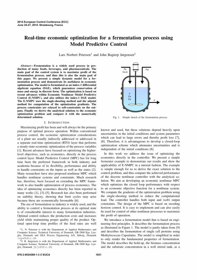
Real-time economic optimization for a fermentation process usingModel Predictive Control
Lars Norbert Petersen1 and John Bagterp Jørgensen2
Abstract— Fermentation is a widely used process in pro-duction of many foods, beverages, and pharmaceuticals. Themain goal of the control system is to maximize profit of thefermentation process, and thus this is also the main goal ofthis paper. We present a simple dynamic model for a fer-mentation process and demonstrate its usefulness in economicoptimization. The model is formulated as an index-1 differentialalgebraic equation (DAE), which guarantees conservation ofmass and energy in discrete form. The optimization is based onrecent advances within Economic Nonlinear Model PredictiveControl (E-NMPC), and also utilizes the index-1 DAE model.The E-NMPC uses the single-shooting method and the adjointmethod for computation of the optimization gradients. Theprocess constraints are relaxed to soft-constraints on the out-puts. Finally we derive the analytical solution to the economicoptimization problem and compare it with the numericallydetermined solution.
I. INTRODUCTION
Maximizing profit has been and will always be the primarypurpose of optimal process operation. Within conventionalprocess control, the economic optimization considerationsof a plant are usually indirectly addressed or addressed ina separate real-time optimization (RTO) layer that performsa steady-state economic optimization of the process variables[1]. Recent advances have focused on optimizing the higher-level objectives, such as economics, directly in the processcontrol layer. Model Predictive Control (MPC) has for longtime been the preferred framework in both industry andacademia because of its flexibility, performance and abilityto handle constraints on the inputs as well as the states [2].Many researchers have also proposed nonlinear MPC whichhandles nonlinear systems and constraints. Much researchhas, therefore, been focused on extending the MPC frame-work to also handle optimization of process economics. Theidea of optimizing economics directly has been reported inmany works [1], [3]–[5]. Research has also been performedon stability theory, showing that limit cycles may arisebecause these are economically favourable [6].
The use of fermentation in industry is widely used, and theability to control a fermentation process at its optimal stateis of considerable interest to many fermentation industries.Optimal control reduces the production costs and increasesyield while maintaining proper quality of the product. Op-timal open-loop time profiles of the feed rates are well
1L. N. Petersen is with the Department of Applied Mathematics andComputer Science, Technical University of Denmark, DK-2800 Kgs. Lyn-gby, Denmark and GEA Process Engineering A/S, Søborg, [email protected]
2J. B. Jørgensen is with the Department of Applied Mathematics andComputer Science, Technical University of Denmark, DK-2800 Kgs. Lyn-gby, Denmark [email protected]
FwFsCs,in
F
VCxCs
Fig. 1. Simple sketch of the fermentation process.
known and used, but these solutions depend heavily uponuncertainties in the initial conditions and system parameterswhich can lead to large errors and thereby profit loss [7],[8]. Therefore, it is advantageous to develop a closed-loopoptimization scheme which attenuates uncertainties and isindependent of the initial conditions [8].
In this work we address the issue of optimizing theeconomics directly in the controller. We present a simplefermenter example to demonstrate our results and show theapplicability of E-NMPC in a tutorial fashion. The exampleis simple enough for us to derive the exact solution to thecontrol problem, and thus compare the achieved performanceof the discrete nonlinear controller with the analytical so-lution. We aim at developing an economic nonlinear MPCwhich optimizes the closed loop performance with respectto an economic objective function for a nonlinear system.We compute the gradients of the optimization problem usingthe single-shooting method to reduce the computationalload. The controller handles both input and (soft) outputconstraints. The design of the MPC is based on recedinghorizon control. It is easy to implement and can also easilybe used for control of other nonlinear processes to maximizethe profit of operation.
We introduce a fermentation model that is based on engi-neering first principles. It describes the fermentation processas illustrated in Figure 1. The model is partly taken from [9]and describes the fermentation of single cell proteins usingMethylococcus Capsulatus. The model is simplified in orderto only render the fundamental properties of fermentation.The model describes the hold-up, the biomass concentrationand the substrate concentration in a well stirred tank, as a
2014 European Control Conference (ECC)June 24-27, 2014. Strasbourg, France
978-3-9524269-1-3 © EUCA 1831
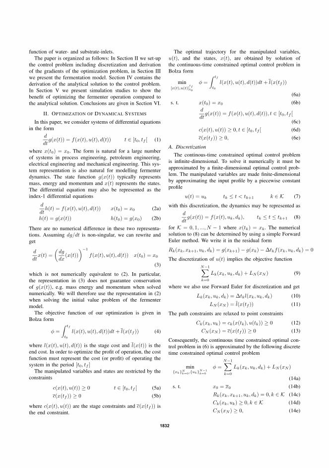
function of water- and substrate-inlets.The paper is organized as follows: In Section II we set-up
the control problem including discretization and derivationof the gradients of the optimization problem, in Section IIIwe present the fermentation model. Section IV contains thederivation of the analytical solution to the control problem.In Section V we present simulation studies to show thebenefit of optimizing the fermenter operation compared tothe analytical solution. Conclusions are given in Section VI.
II. OPTIMIZATION OF DYNAMICAL SYSTEMS
In this paper, we consider systems of differential equationsin the form
d
dtg(x(t)) = f(x(t), u(t), d(t)) t ∈ [t0, tf [ (1)
where x(t0) = x0. The form is natural for a large numberof systems in process engineering, petroleum engineering,electrical engineering and mechanical engineering. This sys-tem representation is also natural for modelling fermenterdynamics. The state function g(x(t)) typically representsmass, energy and momentum and x(t) represents the states.The differential equation may also be represented as theindex-1 differential equations
d
dth(t) = f(x(t), u(t), d(t)) x(t0) = x0 (2a)
h(t) = g(x(t)) h(t0) = g(x0) (2b)
There are no numerical difference in these two representa-tions. Assuming dg/dt is non-singular, we can rewrite andget
d
dtx(t) =
(dg
dx(x(t))
)−1f(x(t), u(t), d(t)) x(t0) = x0
(3)
which is not numerically equivalent to (2). In particular,the representation in (3) does not guarantee conservationof g(x(t)), e.g. mass energy and momentum when solvednumerically. We will therefore use the representation in (2)when solving the initial value problem of the fermentermodel.
The objective function of our optimization is given inBolza form
φ =
∫ tf
t0
l(x(t), u(t), d(t))dt+ l(x(tf )) (4)
where l(x(t), u(t), d(t)) is the stage cost and l(x(t)) is theend cost. In order to optimize the profit of operation, the costfunction must represent the cost (or profit) of operating thesystem in the period [t0, tf ]
The manipulated variables and states are restricted by theconstraints
c(x(t), u(t)) ≥ 0 t ∈ [t0, tf [ (5a)c(x(tf )) ≥ 0 (5b)
where c(x(t), u(t)) are the stage constraints and c(x(tf )) isthe end constraint.
The optimal trajectory for the manipulated variables,u(t), and the states, x(t), are obtained by solution ofthe continuous-time constrained optimal control problem inBolza form
min[x(t),u(t)]
tft0
φ =
∫ tf
t0
l(x(t), u(t), d(t))dt+ l(x(tf ))
(6a)s. t. x(t0) = x0 (6b)
d
dtg(x(t)) = f(x(t), u(t), d(t)), t ∈ [t0, tf [
(6c)c(x(t), u(t)) ≥ 0, t ∈ [t0, tf [ (6d)c(x(tf )) ≥ 0, (6e)
A. DiscretizationThe continous-time constrained optimal control problem
is infinite-dimensional. To solve it numerically it must beapproximated by a finite-dimensional optimal control prob-lem. The manipulated variables are made finite-dimensionalby approximating the input profile by a piecewise constantprofile
u(t) = uk tk ≤ t < tk+1 k ∈ K (7)
with this discretization, the dynamics may be represented asd
dtg(x(t)) = f(x(t), uk, dk), tk ≤ t ≤ tk+1 (8)
for K = 0, 1, ..., N − 1 where x(tk) = xk. The numericalsolution to (8) can be determined by using a simple ForwardEuler method. We write it in the residual form
Rk(xk, xk+1, uk, dk) = g(xk+1)− g(xk)−∆tkf(xk, uk, dk) = 0
The discretization of u(t) implies the objective functionN−1∑k=0
Lk(xk, uk, dk) + LN (xN ) (9)
where we also use Forward Euler for discretization and get
Lk(xk, uk, dk) = ∆tkl(xk, uk, dk) (10)
LN (xN ) = l(x(tf )) (11)
The path constraints are relaxed to point constraints
Ck(xk, uk) = ck(x(tk), u(tk)) ≥ 0 (12)CN (xN ) = c(x(tf )) ≥ 0 (13)
Consequently, the continuous time constrained optimal con-trol problem in (6) is approximated by the following discretetime constrained optimal control problem
minxkNk=0,ukN−1
k=0
φ =
N−1∑k=0
Lk(xk, uk, dk) + LN (xN )
(14a)s. t. x0 = x0 (14b)
Rk(xk, xk+1, uk, dk) = 0, k ∈ K (14c)Ck(xk, uk) ≥ 0, k ∈ K (14d)CN (xN ) ≥ 0, (14e)
1832

B. Single-Shooting Optimization
The discrete-time finite-dimensional optimal control prob-lem may be solved using single-shooting (control vectorparametrization) [10], multiple shooting [11], [12], or thesimultaneous method [13]. In these methods, a sequentialquadratic programming (SQP) algorithm is typically usedfor the optimization. Gradient computation is straightforwardin the simultaneous method, while either forward sensitivitycomputation or the adjoint method [14] is used by the single-shooting and the multiple-shooting methods.
We solve the optimization problem in (14) by the single-shooting method (also called vector parametrization, CVP).In this method the system dynamics (14c) are used toeliminate the state variables and express the objective andconstraint function as function of the manipulated vari-ables and initial state only. Given the manipulated inputs,ukN−1k=0 , the initial value, x0, and the requirement, that thesystem dynamics are observable, the objective function maybe expressed as
Ψ =Ψ(ukN−1k=0 ;x0)
= φ =∑N−1
k=0 Lk(xk, uk, dk) + lN (xN ) :x0 = x0,Rk(xk, xk+1, uk, dk) = 0, k ∈ K
(15)
Similarly, the constraint functions may be parametrized
χk =χk(ujkj=0;x0)
= Ck(xk, uk) :x0 = x0,Rj(xj , xj+1, uj , dj) = 0, j ∈ K
(16)
χN =χk(ujN−1j=0 ;x0)
= CN (xN ) :x0 = x0,Rj(xj , xj+1, uj , dj) = 0, j ∈ K
(17)
Using (15)-(17), the discrete time constraint optimal controlproblem may be expressed as
minukN−1
k=0
Ψ(ukN−1k=0 ;x0) (18a)
s. t. χk(ujkj=0;x0) ≥ 0, k ∈ K (18b)
χN (ujN−1j=0 ;x0) ≥ 0 (18c)
where K = 0, 1, ..., N − 1. It is a nonlinear optimizationproblem which is solved by using sequential quadratic pro-gramming (SQP). In each iteration a convex quadratic prob-lem is solved for which evaluation of Ψ, ∇Ψ, χk, χN and∇χk,∇χN of the nonlinear problem has to be determined.Ψ and χ are computed directly from (15) and (16) while∇Ψ and ∇χ is computed using the adjoint method. Thesystem states in the optimization problem are dependent onthe manipulated variables, in such a way that past changeshave an influence on all the subsequent states. This meansthat the gradients have to be determined in each iteration.The adjoint method is an efficient method for computationof these gradients.
The algorithm for the adjoint method is presented inAlgorithm 1 and 2.
Algorithm 1 Adjoint method for ∇ukΨ(ukN−1k=0 ;x0)
Solve for λN in ∇xNRN−1λN = ∇xN
LN
for k = N − 1 to 1 doCompute∇uk
Ψ = ∇ukLk −∇uk
Rkλk+1
Solve for λk in∇xk
Rk−1λk = ∇xkLk −∇xk
Rkλk+1
end forCompute∇u0
Ψ = ∇u0L0 −∇u0
R0λ1
Algorithm 2 Adjoint method for ∇ukχ(uk;x0)N−1j=0
Solve for λN in ∇xNRN−1λN = ∇xN
CN
for k = N − 1 to 1 doCompute ∇uk
χ = ∇ukCk −∇uk
Rkλk+1
Solve for λk in ∇xkRk−1λk = ∇xk
Ck −∇xkRkλk+1
end forCompute ∇u0
χ = ∇u0C0 −∇u0
R0λ1
As we use the Forward Euler method the derivativessimply become
∇xkRk = −∇xk
g(xk)− Ts∇xkf(xk, uk, dk) (19)
∇xkRk−1 = ∇xk
g(xk) (20)∇uk
Rk = −Ts∇ukf(xk, uk, dk) (21)
and the derivatives for the cost function become
∇xkLk = Ts∇xk
lk (22)∇uk
Lk = Ts∇uklk (23)
To solve the problem, we use Matlab’s fmincon withan SQP algorithm. A local optimum is reported if the KKTconditions are satisfied with relative and absolute toleranceof 10−9. A non-optimal solution is returned if the relativecost function or step size changes less than 10−9. The sampletime of the NMPC is Ts = 0.20 hours.
C. Soft Constraints
When both inputs and states are subject to constraints,the solution may become infeasible. For example whendisturbances, which cannot be rejected within the givenconstraints, hits the system. A method for dealing withinfeasibility is to introduce so-called soft-constraints. Theconstraints are softened by using slack variables with thel2 − l1 penalty function
φs =N−1∑k=0
(1
2sTk Swsk + skdiag(Sw)
)(24)
with s ≥ 0 and (14d) are relaxed to Ck(xk, uk) − sk ≥0. The optimizer will then find a solution which minimisesthe original cost function (14) while keeping the constraint
1833

TABLE IKINETIC PARAMETERS
Symbol Value Unit
γS 1.777 kg substrate/kg biomassµmax 0.37 1/hrKS 0.021 kg/m3
KI 0.38 kg/m3
violations as small as possible. The constraints can also behandled without the need for slack variables as shown in[12].
III. FERMENTATION MODEL
A mathematical model is needed for the optimal controland economic analysis of the fermentation process. The aimof this study is to provide a model of the MethylococcusCapsulatus fermentation process. The process is sketched inFigure 1
It is a model with variable volume, substrate and biomasshold-up that are governed by Haldane growth kinetics. Themodel is deliberately kept simple to illustrate key principlesof fermenter operation.
A. Constitutive Relations
The biomass growth is limited by substrate. The overallreaction mechanism is
γSS → X (25)
The cell growth model is governed by the Haldane expres-sion. The reaction rate can be written as follows
r = µCX (26)
where the specific growth rate is
µ = µmaxCS
KS + CS + C2S/KI
(27)
Consequently, the growth of biomass is only limited by thesubstrate concentration. The production rates of biomass andsubstrate are
RX = r, RS = −γsr (28)
The parameters belonging to the growth of MethylococcusCapsulatus are shown in table I.
B. Conservation equations
A mass balance for the hold-up in the fermenter isgoverned, assuming constant and identical density of all feedstreams and the fermenter content. The mass balances for thebiomass and the substrate are also governed and gives
d
dt(ρV ) = ρFs + ρFw − ρF (29a)
d
dt(V CX) = −FCX +RXV (29b)
d
dt(V CS) = FsCS,in − FCS +RSV (29c)
with V (t0) = V0, CX(t0) = CX,0 and CS(t0) = CS,0. Thestate functions in the model are the total mass, m = ρV , themass of biomass, mX = V CX , and the mass of substrate,mS = V CS . The state variables of the model are thevolume, V , the biomass concentration, CX , and the substrateconcentration, CS . The manipulated variables are the waterinlet flow rate, Fw, the substrate inlet flow rate, Fs, and theoutlet flow rate, F . When the fermenter is operated in fedbatch mode, the outlet flow rate is zero, i.e. F = 0.
C. Objective function - Profit
The profit of operating the fermenter is given as the valueof the produced biomass minus the cost of the used substrate.This profit, in the period [t0,tf ], may be expressed as
φp =
∫ tf
t0
(pXRXV − pSFSCS,in)dt (30)
The price of biomass and substrate is 3000$ and 0$ re-spectively. Often we neglect the price of the substrate, aspX pS . The end cost, l(x(tf )), is equal to zero. Optimaloperation of the fermenter seeks to maximize the profit, φp,by manipulating the fermenter inputs within the operationconstraints.
D. Constraints
The fermentation process is subject to operation restric-tions. The manipulated variables are restricted by inputconstraints
0 ≤ Fs ≤ 30 (31)0 ≤ Fw ≤ 30 (32)0 ≤ F ≤ 60 (33)
The outputs, the volume and the concentrations, are re-stricted by the output constraints
0 ≤ V ≤ 60 (34)0 ≤ CX ≤ 0.2 (35)
These are relaxed in the computations as shown in (24). Theend constraint, c(x(tf )), is equal to zero.
IV. ANALYTICAL SOLUTION
In this section, we develop an analytical solution to theoperation of the fermenter described in section III. As thefermenter is initially almost empty, we start up in fed batchmode, and when the tank is filled, it is operated in continuousmode.
We consider operation of the fermenter in a period [t0 tf ]where t0 and tf is a large number i.e. tf → ∞. In theperiod [t0 tN ] the fermenter is operated in fed batch modeand operated in continuous mode when filled in the period[tN tf ]. The profit of such an operation is, when neglectingthe cost of substrate (pX pS) for simplicity,
φp = pX
∫ tN
t0
RX(t)V (t)dt+ pX
∫ tf
tN
RX(t)V (t)dt (36)
1834

In order to maximize the production and profit, RX(t) andV (t) must be maximized in both periods. From sec. III-Awe have
R∗X = r∗ = µ(C∗S)C∗X (37)
Thus, the maximal production of biomass is obtained whenthe biomass and substrate concentrations are kept constantat their optimal values
C∗X = CX,max t ∈ [t0, tf ] (38)
C∗S = maxµ(CS) =√KIKs t ∈ [t0, tf ] (39)
In this case the production rates, RX and RS , becomeconstant values which attain their maximal values at
R∗X = r∗, R∗S = −γsr∗ (40)
such that the total profit of the biomass production (36) canbe expressed as
φp = pXR∗X(Vmax − V0) + pXR
∗XVmax(tf − tN ) (41)
A. Fed batch operation
In order to determine the optimal trajectory for the manip-ulated inputs we set up the model equations, utilizing thatthe biomass and substrate concentrations are now constant.F = 0 in fed batch mode and the density ρ is constant,which reduces the model to
V (t) = Fs(t) + Fw(t) V (t0) = V0 (42a)
V (t)C∗X = RXV (t) CX(t0) = C∗X (42b)
V (t)C∗S = FsCS,in +RSV (t) CS(t0) = C∗S (42c)
Substitution of (42a) in (42b) and (42c) yields[C∗X C∗X
C∗S − CS,in C∗S
] [Fs(t)Fw(t)
]=
[R∗XR∗S
]V (t) (43)
Solving for[Fs(t) Fw(t)
]Twe get[
Fs(t)Fw(t)
]=
[C∗
SR∗X
CS,inC∗X− R∗
S
CS,in
−R∗X(C∗
S−CS,in)CS,inC∗
X+
R∗S
CS,in
]V (t) (44)
As we have restricted Fw to be greater than zero we require
R∗X(C∗S − CS,in) ≤ R∗SC∗X ⇒ (45)CS,in ≥ C∗S + γsC
∗X (46)
As the volume in the fermenter is given by the simpledifferential equation in (29a), we can now construct thetrajectory of the states and the inputs in fed batch operation.The equation becomes
d
dtV = Fs + Fw =
R∗XC∗X
V (t) V (t0) = V0 (47)
Leading to the state evolution
V (t) = V0 exp
(R∗XC∗X
t
)(48)
and the time, tN , where the fermenter is filled, V (tN ) =Vmax
tN =C∗XR∗X
log
(Vmax
V0
)(49)
Consequently, the optimal operation of the inputs are givenby substituting (48) into (44) and the switch to continuousoperation is given in (49).
B. Continuous operation
During continuous operation, the production is optimizedby letting the state assume its optimal values
V ∗(t) = V ∗ = Vmax t ∈ [tN , tf ] (50)C∗X(t) = C∗X = CX,max t ∈ [tN , tf ] (51)
C∗S(t) = C∗S =√KIKs t ∈ [tN , tf ] (52)
Solving for[Fs(t) Fw(t) F (t)
]Tin (29) utilizing the
above we get the optimal input trajectoryF ∗s (t)F ∗w(t)F ∗(t)
=
C∗
SR∗X
CS,inC∗X− R∗
S
CS,in
−R∗X(C∗
S−CS,in)CS,inC∗
X+
R∗S
CS,in
R∗X
C∗X
V ∗ (53)
As the volume, biomass and substrate concentration in thefermenter are measured, we can now construct the optimalinputs for continuous operation.
V. RESULTS
We illustrate the applicability of the E-NMPC by consider-ing a combined simulation, in which the fermenter is startedin fed batch mode and then goes into continuous mode whenit is full. The analytical solution and simulated states, inputsand the value of the objective function to the fermenter areshown in Figure 2, 3 and 4 respectively.
A. Fed batch operation
The fermenter is started in fed batch mode. We, first ofall, notice that the controller is able to control the systemto the optimal state when comparing with the analyticalsolution. Furthermore, the volume of the fermenter increasesexponentially. The NMPC uses a simple Forward Eulermethod with constant step size for state prediction, and we,therefore, see a small offset arise in the substrate and biomassconcentrations while the volume increases. A reduced sampletime will decrease the deviation from the analytical solution.On the other hand, the deviation do not lead to a significantloss of profit. The violations of the constraints are small andby any practical means do not pose a problem.
B. Continuous operation
Continuous mode is reached when production is continuedafter the fermenter is filled. Again we note that the correctoptimal solution is found compared to the analytical solution.The before mentioned small offset in the substrate andbiomass concentrations have vanished due to the constanthold-up. Only small numerical errors on the NMPC solutionarise. These errors are due to the Forward Euler method, butare also negligible.
1835
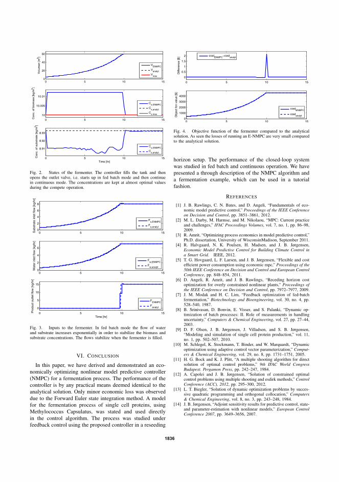
0 5 10 150
20
40
60
Vol
umen
[m3 ]
VENMPC
Vanalyt
Vmax
0 5 10 15
10
10.005
10.01
Con
c. o
f bio
mas
s [k
g/m
3 ]
Cx,ENMPC
Cx,analyt
Cx,max
0 5 10 15
8.91
8.92
8.93
Con
c. o
f sub
stra
te [k
g/m
3 ]
Time [hr]
Cs,ENMPC
Cs,analyt
Fig. 2. States of the fermenter. The controller fills the tank and thenopens the outlet valve, i.e. starts up in fed batch mode and then continuein continuous mode. The concentrations are kept at almost optimal valuesduring the compete operation.
0 5 10 150
2
4
6
8
Sub
stra
te in
let f
low
[kg/
hr]
Fs,ENMPC
Fs,analyt
0 5 10 150
2
4
6
Wat
er in
let f
low
[kg/
hr]
Fw,ENMPC
Fw,analyt
0 5 10 15
0
5
10
15
Time [hr]
Pro
duct
out
let f
low
[kg/
hr]
FENMPC
Fanalyt
Fig. 3. Inputs to the fermenter. In fed batch mode the flow of waterand substrate increases exponentially in order to stabilize the biomass andsubstrate concentrations. The flows stabilize when the fermenter is filled.
VI. CONCLUSION
In this paper, we have derived and demonstrated an eco-nomically optimizing nonlinear model predictive controller(NMPC) for a fermentation process. The performance of thecontroller is by any practical means deemed identical to theanalytical solution. Only minor economic loss was observeddue to the Forward Euler state integration method. A modelfor the fermentation process of single cell proteins, usingMethylococcus Capsulatus, was stated and used directlyin the control algorithm. The process was studied underfeedback control using the proposed controller in a reseeding
0 5 10 150
1000
2000
3000
4000
Obj
ect f
cn v
alue
[$]
costENMPC
costanalyt
0 5 10 15
0
0.5
1
1.5
2
Diff
eren
ce [$
]
cost
ENMPC−cost
analyt
Fig. 4. Objective function of the fermenter compared to the analyticalsolution. As seen the losses of running an E-NMPC are very small comparedto the analytical solution.
horizon setup. The performance of the closed-loop systemwas studied in fed batch and continuous operation. We havepresented a through description of the NMPC algorithm anda fermentation example, which can be used in a tutorialfashion.
REFERENCES
[1] J. B. Rawlings, C. N. Bates, and D. Angeli, “Fundamentals of eco-nomic model predictive control,” Proceedings of the IEEE Conferenceon Decision and Control, pp. 3851–3861, 2012.
[2] M. L. Darby, M. Harmse, and M. Nikolaou, “MPC: Current practiceand challenges,” IFAC Proceedings Volumes, vol. 7, no. 1, pp. 86–98,2009.
[3] R. Amrit, “Optimizing process economics in model predictive control,”Ph.D. dissertation, University of WisconsinMadison, September 2011.
[4] R. Halvgaard, N. K. Poulsen, H. Madsen, and J. B. Jørgensen,Economic Model Predictive Control for Building Climate Control ina Smart Grid. IEEE, 2012.
[5] T. G. Hovgaard, L. F. Larsen, and J. B. Jørgensen, “Flexible and costefficient power consumption using economic mpc,” Proceedings of the50th IEEE Conference on Decision and Control and European ControlConference, pp. 848–854, 2011.
[6] D. Angeli, R. Amrit, and J. B. Rawlings, “Receding horizon costoptimization for overly constrained nonlinear plants,” Proceedings ofthe IEEE Conference on Decision and Control, pp. 7972–7977, 2009.
[7] J. M. Modak and H. C. Lim, “Feedback optimization of fed-batchfermentation,” Biotechnology and Bioengineering, vol. 30, no. 4, pp.528–540, 1987.
[8] B. Srinivasan, D. Bonvin, E. Visser, and S. Palanki, “Dynamic op-timization of batch processes: II. Role of measurements in handlinguncertainty,” Computers & Chemical Engineering, vol. 27, pp. 27–44,2003.
[9] D. F. Olsen, J. B. Jørgensen, J. Villadsen, and S. B. Jørgensen,“Modeling and simulation of single cell protein production,” vol. 11,no. 1, pp. 502–507, 2010.
[10] M. Schlegel, K. Stockmann, T. Binder, and W. Marquardt, “Dynamicoptimization using adaptive control vector parameterization,” Comput-ers & Chemical Engineering, vol. 29, no. 8, pp. 1731–1751, 2005.
[11] H. G. Bock and K. J. Plitt, “A multiple shooting algorithm for directsolution of optimal control problems,” 9th IFAC World CongressBudapest. Pergamon Press, pp. 242–247, 1984.
[12] A. Capolei and J. B. Jørgensen, “Solution of constrained optimalcontrol problems using multiple shooting and esdirk methods,” ControlConference (ACC), 2012, pp. 295–300, 2012.
[13] L. T. Biegler, “Solution of dynamic optimization problems by succes-sive quadratic programming and orthogonal collocation,” Computers& Chemical Engineering, vol. 8, no. 3, pp. 243–248, 1984.
[14] J. B. Jørgensen, “Adjoint sensitivity results for predictive control, state-and parameter-estimation with nonlinear models,” European ControlConference 2007, pp. 3649–3656, 2007.
1836
P a p e r E
Application of ConstrainedLinear MPC to a Spray Dryer
Published in IEEE Multi-conference on Systems and Control (MSC 2014), pp.2120–2126, 2014, Antibes.

182

Application of Constrained Linear MPC to a Spray Dryer
Lars Norbert Petersen1,2, Niels Kjølstad Poulsen1, Hans Henrik Niemann3,Christer Utzen2 and John Bagterp Jørgensen1
Abstract— In this paper we develop a linear model predictivecontrol (MPC) algorithm for control of a two stage spraydryer. The states are estimated by a stationary Kalman filter.A non-linear first-principle engineering model is developed tosimulate the spray drying process. The model is validatedagainst experimental data and able to precisely predict thetemperatures, the air humidity and the residual moisture inthe dryer. The MPC controls these variables to the target andreject disturbances. Spray drying is a cost-effective methodto evaporate water from liquid foods and produces a freeflowing powder. The main challenge of spray drying is to meetthe residual moisture specification and prevent powder fromsticking to the chamber walls. By simulation we compare theperformance of the MPC against the conventional PID controlstrategy. During an industrially recorded disturbance scenario,the MPC increases the production rate by 7.9%, profit ofproduction by 8.2% and the energy efficiency by 4.1% onaverage.
I. INTRODUCTION
In 2015 the milk quota system in the European Union willbe completely liberalized. The expected effect of this liberal-ization is that the milk production increases significantly. Insome countries up to 50% in 2020 [1]. The milk productionexpansion will mainly affect the milk powder production dueto the short shelf life of dairy products. Consequently, thecapacity for production of milk powder will need to increase[1]. Industry studies show that advanced control is capableof increasing the capacity of spray dryers by up to 20% [2].Optimal control is therefore an effective way to leverage thefuture production increase.
The main objective in controlling a spray dryer is tominimize the energy consumption while bringing the residualmoisture in the powder below the specification and avoidthat the powder sticks to the chamber walls. The dryersare generally very large. These may have a feed capacityof up to 4.4 million l/day of raw milk and require 7 MW ofpower. Therefore, even small improvement in operation willhave a large impact on the profitability. The challenge is inmaintaining optimal operation since to do so the dryer mustbe constantly adjusted to variations in the feed concentrationand ambient air humidity.
Conventional PID control of spray dryers keeps inlet-and outlet temperatures constant during operation. This is asimple approach, but known to be insufficient at controlling
1 Department of Applied Mathematics and Computer Science,Technical University of Denmark, Kgs. Lyngby, Denmarklnpe,nkpo,[email protected]
2 GEA Process Engineering A/S, Søborg, [email protected]
3 Department of Electrical Engineering, Technical University of Den-mark, Kgs. Lyngby, Denmark [email protected]
SD
Main Air
SFB Air
Feed
Powder
ExhaustCooling
SFB
Tsfb, Fsfb, Yamb
Tmain, Fmain, Yamb
TSD,Y
X
TSFB
FfXfTf
Fig. 1: Illustration of the spray chamber (SD) and the staticfluid bed (SFB) stages of a two stage spray dryer. Hot airis let into the upper section of the drying chamber wherethe nozzles disperse the liquid feed. The droplets dry intopowder particles in these two stages.
the residual moisture and prevent powder from sticking tothe chamber walls [3]. The variations in residual moisture ofthe produced powder reflects that the conventional PID con-troller cannot reject disturbances such as feed concentrationvariations and air humidity variations. Still, this conventionalcontrol strategy is the de facto standard in the industry. TheMPC proposed in this paper constantly adjusts the manipu-lated variables such that the residual moisture, the exhaustair temperature and exhaust air humidity is controlled toa reference. The temperature and humidity in the dryerare closely correlated to stickiness of powder. Therefore,controlling the temperature and humidity indirectly controlsthe stickiness and deposits of the powder in the dryer.The residual moisture must be controlled to specificationsto avoid bacterial growth and preserve the milk powder.Conventional control must frequently be manually adjustedin order to avoid stickiness of the powder and produce atspecified residual moisture content.
A. Process Description
The two stage spray dryer is an energy efficient dryer andis often used for production of milk and other food powders.Fig. 1 illustrates the spray chamber (SD) and static fluid
2014 IEEE Conference on Control Applications (CCA)Part of 2014 IEEE Multi-conference on Systems and ControlOctober 8-10, 2014. Antibes, France
978-1-4799-7409-2/14/$31.00 ©2014 IEEE 2120

bed stage (SFB). The main hot air is let into the uppersection of the drying chamber (SD) around the high pressurenozzles. The nozzles disperse the liquid feed into droplets.The heat is transferred from the hot air to the droplets, anddue to this transfer water evaporates from the droplets. In thatprocess, the air temperature and the residual moisture of thedroplets decrease. The dried product then enters the staticfluid bed (SFB) where it is dried further. After drying in theSFB, the powder is transported to the external vibrating fluidbed (VFB) for gentle drying and cooled to the temperaturedesired for handling and storage. The VFB is not illustratedin Fig. 1.
B. Modelling and ControlModelling of the drying process in spray dryers varies in
complexity and purpose. First order transfer function modelsas well as first principles engineering models for controlpurposes are proposed [4], [5]. [6] proposes a dynamic modelfor a complete multi-stage dryer. A number of papers presentcontrol strategies for spray dryers. The focus varies frompressure control of the chamber pressure to MPC controlof the residual moisture based on industrial software [2].[7] provides a detailed review on the status and future ofadvanced control for spray dryers. In [5] a feed forwardapproach is made to help control the residual moisture. Set-point tracking MPC is a standard methodology for optimizingthe operation of processes and a recognised control methodin both academia and industry due to its ability to handlecoupled dynamics, time delays, constraints and feed forwardof measured disturbances [8], [9]. In this methodology theeconomics of operation is optimized in a separate real-time steady-state optimization (RTO) layer [10]. Recentadvances has shifted to combine these two layers into a singleeconomically optimizing (E-)MPC layer. [11] use nonlinear(E-)MPC for economic optimization of a two stage spraydryer.
C. ContentIn this paper we investigate the potential of optimizing
the spray drying process by linear MPC. We compare thelinear MPC to the conventional PID based control method.The MPC is composed of an optimal regulator and a stateestimator. The regulator has the structure described in [12]–[14], with the modification that we use a deterministiclinearised first principles engineering model instead of aninnovation form state space model identified from data. Themodel used for simulation is also based on the non-linearfirst principles engineering model. The proposed model isidentified and validated against two independent experimen-tal datasets provided by GEA Process Engineering A/S.
D. OrganizationThe paper is organized as follows. In Section II we
describe the model and show its accuracy by comparing itsoutput to experimental data. Section III presents the regulatorand state estimator. In Section IV we present two simulationsto validate the MPC and show the benefit of optimizing thetwo stage spray dryer. Conclusions are given in Section V.
II. SPRAY DRYER MODEL
In this section, we present the first principles engineeringmodel for a Multi-Stage Dryer type 20 (MSDTM-20), i.e. amedium-sized two stage spray dryer, made available by GEAProcess Engineering A/S. The dryer has a maximum waterevaporation capacity of approximately 125 kg/h. The data foridentification is based on drying of sugar water, maltodextrinDE-18. We use maltodextrin, because milk is difficult tohandle over longer periods due to natural deterioration andmaltodextrin DE-18 has the same drying properties as skimmilk [15].
A. Mass- and Energy Balances
The model consists of four states. The states are the spraydryer temperature, TSD, the static fluid bed temperature,TSFB , the humidity in the air of the spray dryer, Y , and themoisture in the powder, X . The lumped energy and massbalances describing the evolution of the states are
CadTSD
dt= −λRw +Hain
−Haout−Qexc −Qla (1a)
CbdTSFB
dt= Hbin −Hbout
+Qexc −Qlb (1b)
mdadY
dt= (Fmain + Fsfb)(Yamb − Y )
+ Fadd(Yadd − Y ) +Rw
(1c)
msdX
dt= Fs(Xf −X)−Rw (1d)
where
Hain = Fmain(cda + cvYamb)(Tmain − T0)+
Fadd(cda + cvYadd)(Tadd − T0)(2a)
Haout = (Fmain + Fsfb + Fadd)·(cda + cvY )(TSD − T0)
(2b)
Hbin = Fsfb(cda + cvYamb)(Tsfb − T0) (2c)Hbout = Fsfb(cda + cvYamb)(TSFB − T0) (2d)Qexc = k1(TSD − TSFB) + k2Xf + k3Tf − k4 (2e)Qla = k5(TSD − Tamb) (2f)Qlb = k6(TSFB − Tamb) (2g)Fs = FfXf/(Xf + 1) (2h)
The air and the product temperatures are assumed in equi-librium in both stages, i.e. TSD and TSFB are each identicalto the powder temperatures in the SD- and the SFB-stage,respectively. Hain
, Haout, Hbin and Hbout
are the enthalpiesof humid air in and out of the SD and the SFB stage,respectively. The reference temperature is T0 = 25C. Ca
and Cb is the heat capacity of the hold-up of air and powder.Fmain and Fsfb are dry basis inlet air flows. The parametersYadd and Fadd are used to correct for air leakage and otherun-modeled inlet air flows such as nozzle cooling air. Qexc
is the heat exchange between the SD and the SFB stages.Qla and Qlb are heat losses to the surroundings. λRw isthe heat of evaporation. We assume that the evaporationonly takes place in the SD stage. Xf is the dry base feedconcentration and Tf is the feed temperature. ms is the dry
2121

mass of powder and mda is the mass of dry air. The latentheat of vaporization, λ, and the heat capacities, cda and cv ,are calculated according to [16].
B. Drying Rate
The drying rate of the product, Rw, is an importantparameter of the model. The thin layer equation describesthe product drying rate, Rw, well [17]
Rw = Ddiff (X −Xeq)ms (3)
Ddiff is an experimentally determined constant called thedrying constant or diffusivity [18]. It may depend on boththe temperature and the moisture of the powder, but in thepresent study it is assumed constant.
The equilibrium moisture, Xeq , describes the moisturecontent at which water cannot be evaporated from the pow-der any longer. The Guggenheim-Anderson-de Boer (GAB)relation is used to describe the equilibrium moisture content[19] and is fitted to laboratory data obtained specifically frommaltodextrin to get
Xeq =C ·K ·Xm ·RH
(1−K ·RH)(1−K ·RH + C ·K ·RH)(4)
where Xm = 0.030723, C = 2.6535 · 10−7 exp(
6292.1T
)and K = 0.057882 exp
(945.16
T
). Xm, C and K are GAB
constants related to monolayer and multilayer properties.In the computation of Xeq , T = TSFB and RH =Y/(18.02/28.97 + Y ) · pc/pvapsat(T ). pc is the chamberpressure and pvapsat is the saturated vapor pressure.
C. Performance
The energy efficiency, the profit of operation and theproduct flow rate are the three key performance indicators(KPIs) for evaluation of the performance of a spray dryer.There are a number of energy efficiency indices to measurethe energy performance of a dryer. We adopt the definitiongiven by [20]
η =λFs(Xf −X)
∆H(5)
Here λFs(Xf − X) is the energy used to evaporate waterand ∆H is the total energy supplied to the dryer given by
∆H = Fmain(hain − hamb) + Fsfb(hbin − hamb) (6)
in which hamb = (cda + cvYamb)(Tamb − T0). The profitfrom operating the spray dryer is the value of the productminus the raw material and energy costs.
P = ppFs(1 +X)− pfFs(1 +Xf )− pH∆H (7)
The price of the produced powder is pp = 4.47 $/kg, theprice of feed material is pf = 0.447 $/kg, and the price ofenergy is pH = 3.4873 · 10−5 $/KJ. The prices are selectedto reflect the industrial prices of natural gas and the price ofthe powder. The flow rate of powder is Fp = Fs(1 +X).
0 2 4 6 8 10 12 14 16 18
70
80
90
T [°
C] ← T
SD
← TSFB
0 2 4 6 8 10 12 14 16 1815
20
25
30
Y [g
/kg]
MeasuredSimulated
0 2 4 6 8 10 12 14 16 18
3
4
5
X [%
t.m
.]
Time [hours]
Fig. 2: Model validation dataset. The disturbances i.e. feedconcentration and ambient air humidity are altered from t =0 to t = 4. The feed flow is altered between t = 4 and t = 8.The main inlet air temperature, the SFB inlet air temperatureand SFB air flow rate is changed between t = 8 to t = 15.
D. Parameter Estimation
The parameters, θ, in the model (1)-(4) are estimatedfrom data (not shown here) by minimizing the least squaressimulation error (not 1-step prediction error). The model isvalidated against the data in Fig. 2. Generally the model fitsthe data well. Table I provides the parameters and all param-eters are significantly identified. The mass of dry powder anddry air are determined from physical considerations and fixedto mda = 10 kg and ms = 15 kg.
The model of the dryer is a deterministic system ofordinary differential equations, i.e.
dx(t)
dt= f(x(t), u(t), d(t), θ) (8)
in which
x =[TSD TSFB Y X
]T(9)
u =[Ff Tmain Tsfb
]T(10)
d =[Fmain Fsfb Xf Tf Tamb Yamb
]T(11)
x is the state vector, u is the manipulated input vector, dis the disturbance vector and θ is the parameter vector. Themeasurement vector, y, and the controlled output vector, z,are
y =[TSD TSFB Y X
]T, z =
[TSD Y X
]TE. Stochastic Model
The deterministic system in (8) is augmented by twostochastic terms. Consequently, the state evolution and mea-surement equation of the dryer is described by
x(tk + Ts) = F (x(tk), u(tk), d(tk), θ) + w(tk) (12a)
2122
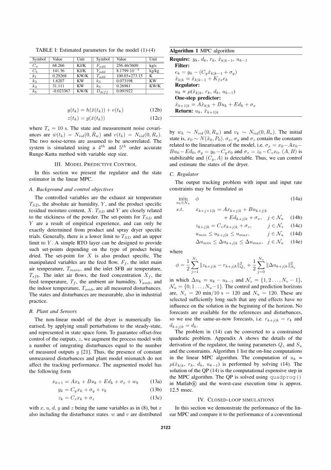
TABLE I: Estimated parameters for the model (1)-(4)
Symbol Value Unit Symbol Value UnitCa 68.266 KJ/K Fadd 256.46/3600 kg/sCb 141.36 KJ/K Yadd 8.1799·10−3 kg/kgk1 0.29268 KW/K Tadd 100.03+273.15 Kk2 1.6207 KW k3 0.073198 KWk4 31.111 KW k5 0.26981 KW/Kk6 -0.023367 KW/K Ddiff 0.091922
y(tk) = h(x(tk)) + v(tk) (12b)z(tk) = g(x(tk)) (12c)
where Ts = 10 s. The state and measurement noise covari-ances are w(tk) = Niid(0, Rw) and v(tk) = Niid(0, Rv).The two noise-terms are assumed to be uncorrelated. Thesystem is simulated using a 4th and 5th order accurateRunge-Kutta method with variable step size.
III. MODEL PREDICTIVE CONTROL
In this section we present the regulator and the stateestimator in the linear MPC.
A. Background and control objectives
The controlled variables are the exhaust air temperatureTSD, the absolute air humidity, Y , and the product specificresidual moisture content, X . TSD and Y are closely relatedto the stickiness of the powder. The set-points for TSD andY are a result of empirical experience, and can only beexactly determined from product and spray dryer specifictrials. Generally, there is a lower limit to TSD and an upperlimit to Y . A simple RTO layer can be designed to providesuch set-points depending on the type of product beingdried. The set-point for X is also product specific. Themanipulated variables are the feed flow, Ff , the inlet mainair temperature, Tmain, and the inlet SFB air temperature,Tsfb. The inlet air flows, the feed concentration Xf , thefeed temperature, Tf , the ambient air humidity, Yamb, andthe indoor temperature, Tamb, are all measured disturbances.The states and disturbances are measurable, also in industrialpractice.
B. Plant and Sensors
The non-linear model of the dryer is numerically lin-earised, by applying small perturbations to the steady-state,and represented in state space form. To guarantee offset-freecontrol of the outputs, z, we augment the process model witha number of integrating disturbances equal to the numberof measured outputs y [21]. Thus, the presence of constantunmeasured disturbances and plant model mismatch do notaffect the tracking performance. The augmented model hasthe following form
xk+1 = Axk +Buk + Edk + σx + wk (13a)yk = Cyxk + σy + vk (13b)zk = Czxk + σz (13c)
with x, u, d, y and z being the same variables as in (8), but xalso including the disturbance states. w and v are distributed
Algorithm 1 MPC algorithm
Require: yk, dk, rk, xk|k−1, uk−1Filter:ek = yk − (Cyxk|k−1 + σy)xk|k = xk|k−1 +KfxekRegulator:uk = µ(xk|k, rk, dk, uk−1)One-step predictor:xk+1|k = Axk|k +Buk + Edk + σxReturn: uk, xk+1|k
by wk ∼ Niid (0, Rw) and vk ∼ Niid(0, Rv). The initialstate is, x0 ∼ N(x0, P0). σx, σy and σz contain the constantsrelated to the linearisation of the model, i.e. σx = x0−Ax0−Bu0−Ed0, σy = y0−Cyx0 and σz = z0−Czx0. (A,B) isstabilizable and (Cy, A) is detectable. Thus, we can controland estimate the states of the dryer.
C. Regulator
The output tracking problem with input and input rateconstraints may be formulated as
minuk∈Nu
φ (14a)
s.t. xk+j+1|k = Axk+j|k +Buk+j|k
+ Edk+j|k + σx, j ∈ Nu (14b)zk+j|k = Czxk+j|k + σz, j ∈ Nz (14c)umin ≤ uk+j|k ≤ umax, j ∈ Nu (14d)∆umin ≤ ∆uk+j|k ≤ ∆umax, j ∈ Nu (14e)
where
φ =1
2
Nz∑j=1
‖zk+j|k − rk+j|k‖2Qz+
1
2
Nu∑j=0
‖∆uk+j|k‖2Su
in which ∆uk = uk − uk−1 and Nz = 1, 2 . . . , Nz − 1,Nu = 0, 1 . . . , Nu−1. The control and prediction horizonsare, Nz = 20 min/10 s = 120 and Nu = 120. These areselected sufficiently long such that any end effects have noinfluence on the solution in the beginning of the horizon. Noforecasts are available for the references and disturbances,so we use the same-as-now forecasts, i.e. rk+j|k = rk anddk+j|k = dk.
The problem in (14) can be converted to a constrainedquadratic problem. Appendix A shows the details of thederivation of the regulator, the tuning parameters Qz and Su
and the constraints. Algorithm 1 list the on-line computationsin the linear MPC algorithm. The computation of uk =µ(xk|k, rk, dk, uk−1) is performed by solving (14). Thesolution of the QP (14) is the computational expensive step inthe MPC algorithm. The QP is solved using quadprog()in Matlab R© and the worst-case execution time is approx.12.5 msec.
IV. CLOSED-LOOP SIMULATIONS
In this section we demonstrate the performance of the lin-ear MPC and compare it to the performance of a conventional
2123

0 0.5 1 1.5 2 2.5 3 3.5
818283
Tem
p. [°
C]
TSD
Ref
0 0.5 1 1.5 2 2.5 3 3.572
74
76
78
Tem
p. [°
C]
TSFB
0 0.5 1 1.5 2 2.5 3 3.5
22
24
Hum
. [g/
kg]
YRef
0 0.5 1 1.5 2 2.5 3 3.53.2
3.4
3.6
Moi
s. [%
t.m
.]
Time [hours]
XRef
(a) Measured outputs of the system. The controlled variables are shown withthe associated reference.
0 0.5 1 1.5 2 2.5 3 3.5
90
100
110
Rat
e [k
g/hr
]
Ff
0 0.5 1 1.5 2 2.5 3 3.5164166168170172
Tem
p. [o C
]
Tmain
0 0.5 1 1.5 2 2.5 3 3.5859095
100105
Tem
p. [o C
]
Time [hours]
Tsfb
(b) Manipulated inputs to the system.
Fig. 3: Closed-loop simulation showing that the MPC tracksthe set-points and rejects the unknown disturbances withoutsteady-state error.
PID controller. The stochastic system model in (12) is usedin the simulations.
A. MPC Validation
In the following the MPC will be validated againstreference- and disturbance step changes. Fig. 3a shows themeasured and controlled variables and Fig. 3b shows themanipulated variables. The ambient air humidity changesfrom 3 g/kg to 4 g/kg at t = 2.25 hours and the feedconcentration decreases from 50.6% to 45.6% at t = 2.92hours. The disturbances are treated as unknown to the MPCin this simulation. At t = 0.25 to t = 1.6 three referencesteps are introduced for each controlled variable. The exhaustair temperature and humidity, TSD and Y , change slightlyfaster than the residual moisture content, X . The MPC tracksthe references and rejects disturbances without any offset.The system is controlled to a steady-state within reasonabletime. The MPC handles the highly cross coupled system
0 10 20 30 40 50 60 7075.475.675.8
7676.276.4
Tem
p. [o C
]
TPID
SD
TMPCSD
Tmin
0 10 20 30 40 50 60 70
7172737475
Tem
p. [o C
]
TPIDSFB
TMPCSFB
0 10 20 30 40 50 60 7026
28
30
Abs
. hum
. [g/
kg]
YPID
YMPC
Ymax
0 10 20 30 40 50 60 703.8
3.9
4
4.1
Time [hours]R
es. m
oi. [
% t.
m.]
XPID
XMPC
Xmax
(a) Measured outputs of the system. The controlled variables are shown withthe associated reference.
0 10 20 30 40 50 60 7080
90
100
Fee
d ra
te [k
g/hr
]
FPIDf
FMPCf
0 10 20 30 40 50 60 70
165
170
175
Mai
n te
mp.
[o C]
TPIDmain
TMPCmain
0 10 20 30 40 50 60 70859095
100105
Time [hours]
SF
B te
mp.
[o C]
TPIDsfb
TMPCsfb
(b) Manipulated inputs to the system.
0 10 20 30 40 50 60 7059
60
61
62
Fee
d c.
[% t.
m.]
Xf
0 10 20 30 40 50 60 70
6
8
10
Am
b. h
um. [
g/kg
]
Time [hours]
Yamb
(c) Disturbance inputs to the system. The changes are used in feedforwardto the controller i.e. dk+j|k = dk .
Fig. 4: Closed-loop simulation of an industrial disturbancescenario using an MPC and the conventional PID controller.The MPC tracks the set-points and rejects the disturbances.
2124

0 10 20 30 40 50 60 70323436384042
Pro
d. r
ate
[kg/
hr]
PIDMPC
0 10 20 30 40 50 60 704748495051
Effi
cien
cy [%
]
PIDMPC
0 10 20 30 40 50 60 70100
110
120
130
Time [hours]
Pro
fit [$
/hr]
PIDMPC
Fig. 5: The production rate, the energy efficiency and theprofit of drying during the closed-loop simulation in Fig. 4.
dynamics well. The manipulated variables are kept within theinput constraints and input rate constraints. The constraintsare expected to become active occasionally as the load onthe dryer is increased, i.e. as the feed flow, Ff , and the heatinputs, Tmain and Tsfb, are increased.
B. Industrial scenario
We also perform a closed-loop simulation with a realisticdisturbance scenario from an industrial spray dryer. Therebywe can compare the achieved performance of the MPC tothe conventional PID controller. Fig. 4 shows the spray dryeroperation when controlled by the MPC and the conventionalPID controller. Fig. 5 shows the KPIs. The disturbances areknown to the MPC as these measurements are normallyavailable in industry. The disturbances are recorded at aspray dryer producing whey protein concentrate in the period8/13/2013 21:30 to 8/17/2013 04:00.
Fig. 4 shows the measured and controlled outputs, themanipulated variables and the disturbances. The simulationreveal that the proposed MPC is able to maintain a correctand constant residual moisture content, X , as well as main-taining the stickiness related variables, TSD and Y , at theirsetpoints. The MPC constantly adjusts the feed flow and inletair temperatures to maintain the controlled variables at theirset-points. An increase in the ambient air humidity increasesthe humidity in the dryer. Thus, the MPC must decreasethe feed rate i.e. production. An increase in feed waterconcentration has the same effect and is also compensatedby a decrease in the feed rate i.e. production.
The conventional PID controller maintains a constantexhaust air temperature, TSD, by manipulating the feed rate,Ff . The two inlet air temperatures are fixed. With thiscontrol methodology, no correcting action is taken whenthe ambient air humidity increases. Changes related to thefeed concentration are compensated for as the feed wateraffects the exhaust air temperature. Thus, on average thedryer need to dry the powder more than necessary to satisfythe specifications. The MPC only dries the powder to thespecified level.
Fig. 5 shows the production rate, energy efficiency andprofit of operation during the simulation. On average theMPC increases the production rate by 7.9%, the energyefficiency by 4.1% and profit of production by 8.2%. Thus,the dryer is used both more energy efficiently and increasesthe profit of operation significantly.
V. CONCLUSIONS
This paper presents a solution to the control problemof a two stage spray dryer. The controller is based on aset-point tracking MPC with output feedback. The statesused in the regulator are estimated by a Kalman filter.The regulator and the estimator is designed based on thelinearised non-linear system model. The simulations showthat the air temperature and air humidity of the outlet airfrom the dryer can be controlled to a set-point as well as theresidual moisture content in the powder. On average duringthe disturbance scenario the MPC increases the productionrate by 7.9%, the energy efficiency by 4.1% and the profitof production by 8.2%. These numbers may be even greaterin industry, as the conventional PID controller is often usedmore conservatively than presented in this paper. Thus, thedryer is used both more efficiently and increases the profitof operation significantly.
GEA Process Engineering A/S is currently implementingand testing the proposed control strategy at industrial scalespray dryers. The control methodology is generally applica-ble to other foods, chemicals and pharmaceuticals and notlimited to two-stage dryers.
REFERENCES
[1] T. Donnellan, T. Hennessy, M. Fenelon, and D. O’Callaghan, “Thepotential for scale economies in milk powder processing: an irish casestudy,” International Journal of Dairy Technology, vol. 67, no. 1, pp.129–134, 2014.
[2] Vaisala. (2014, Feb.) +20% increase in production capacitywith zero increase in energy consumption. [Online].Available: http://www.vaisala.com/Vaisala%20Documents/Success%20Stories/CEN-TIA-G-Valio-Customer-Story-B211288EN-A.pdf
[3] D. O’Callaghan and P. Cunningham, “Modern process control tech-niques in the production of dried milk products - a review,” Lait,vol. 85, pp. 335–342, 2005.
[4] L. Tan, F. Taip, and N. Aziz, “Simulation and Control of SprayDrying Using Nozzle Atomizer Spray Dryer.” International Journalof Engineering & Technology, no. 10, pp. 1–7, 2009.
[5] J. Perez-Correa and F. Fariass, “Modelling and control of a spraydryer: a simulation study,” Food Control, vol. 6, no. 4, pp. 219–227,1995.
[6] L. N. Petersen, N. K. Poulsen, H. H. Niemann, C. Utzen, and J. B.Jørgensen, “A Grey-Box Model for Spray Drying Plants,” 10th IFACInternational Symposium on Dynamics and Control of Process Systems(DYCOPS 2013), pp. 559–564, 2013.
[7] D. O. Callaghan and P. Cunningham, “Modern process control tech-niques in the production of dried milk products a review,” Lait, vol. 85,pp. 335–342, 2005.
[8] M. L. Darby, M. Harmse, and M. Nikolaou, “MPC: Current practiceand challenges,” IFAC Proceedings Volumes, vol. 7, no. 1, pp. 86–98,2009.
[9] M. Bauer and I. K. Craig, “Economic assessment of advanced processcontrol – a survey and framework,” Journal of Process Control, vol. 18,no. 1, pp. 2–18, 2008.
[10] M. R. Naysmith and P. L. Douglas, “Review of real time optimiza-tion in the chemical process industries,” Developments in ChemicalEngineering and Mineral Processing, pp. 67–87, 1995.
2125

[11] L. N. Petersen, N. K. Poulsen, H. H. Niemann, C. Utzen, andJ. B. Jørgensen, “Economic optimization of spray dryer operationusing nonlinear model predictive control,” Proceedings of the IEEEConference on Decision and Control, 2014.
[12] G. Prasath and J. B. Jørgensen, “Soft constraints for robust mpc ofuncertain systems,” International Symposium on Advanced Control ofChemical Processes, vol. 7, no. 1, pp. 225–230, 2009.
[13] J. B. Jørgensen, J. B. Rawlings, and J. K. Huusom, “Finite horizon mpcfor systems in innovation form,” Proceedings of the IEEE Conferenceon Decision and Control, pp. 1896–1903, 2011.
[14] J. K. Huusom, N. K. Poulsen, S. B. Jørgensen, and J. B. Jørgensen,“Tuning of methods for offset free mpc based on arx model represen-tations,” Proceedings of the American Control Conference, pp. 2255–2360, 2010.
[15] C. Hennigs, T. K. Kockel, and T. A. G. Langrish, “New measurementsof the sticky behavior of skim milk powder,” Drying Technology,vol. 19, no. 3-4, pp. 471–484, 2001.
[16] J. Smith, H. Van Ness, and M. Abbott, Introduction to chemicalengineering thermodynamics, ser. McGraw-Hill chemical engineeringseries. McGraw-Hill, 2005.
[17] W. K. Lewis, “The rate of drying of solid materials,” Journal ofIndustrial and Engineering Chemistry, vol. 13, pp. 427–432, 1921.
[18] F. F. G. Areed, M. S. El-Kasassy, and K. A. Mahmoud, “Design ofneuro-fuzzy controller for a rotary dryer,” International Journal ofComputer Applications, vol. 37, no. 5, p. 34, 2012.
[19] C. E. C. Perez, R. D. P. Andrade, and L. M. Roberto, “Models ofsorption isotherms for food: Uses and limitations,” Vitae, vol. 18, no. 3,pp. 325–334, 2011.
[20] C. G. J. Baker and K. A. McKenzie, “Energy consumption of industrialspray dryers,” Drying Technology, vol. 23, no. 1-2, pp. 365–386, 2005.
[21] G. Pannocchia and J. B. Rawlings, “Disturbance models for offset-freemodel-predictive control,” AIChE Journal, vol. 49, no. 2, pp. 426–437,2003.
APPENDIX
In this section we briefly describe the details of theregulator design.
A. Regulator
The tracking problem in Sec. III-C is solved by for-mulating the corresponding convex quadratic problem. Thetracking problem is similar to [12]–[14].
Define the vectors Z, R, U and D as
Z =
zk+1|kzk+2|k
...zk+Nz|k
R =
rk+1
rk+2
...rk+Nz
U =
uk|kuk+1|k
...uk+Nu|k
D =
[dk|k dk+1|k . . . dk+Nz|k
]TThen the predictions are
Z = Φxxk|k−1 + ΓuUk + ΓdDk + ΩΣx + Σz
Using the predictions in vector form we can write theobjective function as
φ =1
2
Nz∑j=1
‖zk+j|k − rk+j|k‖2Qz+
1
2
Nu∑j=0
‖∆uk+j|k‖2Su
=1
2‖Zk −Rk‖2Qz
+1
2‖ΛU − I0uk−1‖2Su
=1
2U ′kHUk + g′Uk + ρ
with
H = ΓTuQzΓu + ΛTSuΛ
g = −ΓTuQz (Rk − b)− ΛTSuI0uk−1
ρ =1
2‖ − b−Rk‖2Qz
+1
2‖I0uk−1‖2Su
where
b = −Φxxk|k − ΓdDk − ΩΣx − Σz
The constraints are assumed constant over the predictionhorizon and umin ≤ uk+j|k ≤ umax and ∆umin ≤∆uk+j|k ≤ ∆umax may be denoted
Umin ≤ Uk ≤ Umax (15)bl ≤ ΨUk ≤ bu (16)
where
bl = ∆Umin + I0uk−1, bu = ∆Umax + I0uk−1 (17)
We solve the tracking problem by solution to the followingconvex quadratic problem
minUk
1
2UTk HUk + gTUk + ρ (18a)
s.t. Umin ≤ Uk ≤ Umax (18b)bl ≤ ΨUk ≤ bu (18c)
The MPC only apply the first u∗0 of U∗k to the process. Theopen-loop optimization is repeated at the next sample whereit also utilize the new state estimate xk.
The regulator is tuned to penalize deviation in the exhaustair temperature and humidity by 10 and the residual moisturecontent the most by 500. Movements of the feed pump andinlet air temperatures are penalized, so that the feed pumpis allowed to change very fast.
Qz = diag([10 10 500
]), Su = diag(
[0.5 50 50
])
The maximum capacity of the feed pump limits the feedflow. The inlet temperatures, Tmain and Tsfb must be higherthan the ambient temperature, Tamb. Furthermore, the risk ofpowder explosions and the risk of scorched particles putsupper limits on the allowable inlet temperatures. Thus, wehave
0 kg/hr ≤Ff ≤ 200 kg/hrTamb ≤Tmain ≤ 220CTamb ≤Tsfb ≤ 120C
We do not impose input rate constraints.
2126

190

P a p e r F
Economic Optimization ofSpray Dryer Operation usingNonlinear Model Predictive
Control
Published in 53rd IEEE Conference on Decision and Control (CDC 2014), pp.6794–6800, 2014, Los Angeles.

192

Economic Optimization of Spray Dryer Operationusing Nonlinear Model Predictive Control
Lars Norbert Petersen1,2, Niels Kjølstad Poulsen1, Hans Henrik Niemann3,Christer Utzen2 and John Bagterp Jørgensen1
Abstract— In this paper we investigate an economicallyoptimizing Nonlinear Model Predictive Control (E-NMPC)for a spray drying process. By simulation we evaluate theeconomic potential of this E-NMPC compared to a conventionalPID based control strategy. Spray drying is the preferredprocess to reduce the water content for many liquid foodstuffsand produces a free flowing powder. The main challenge incontrolling the spray drying process is to meet the residualmoisture specifications and avoid that the powder sticks to thechamber walls of the spray dryer. We present a model fora spray dryer that has been validated on experimental datafrom a pilot plant. We use this model for simulation as wellas for prediction in the E-NMPC. The E-NMPC is designedwith hard input constraints and soft output constraints. Theopen-loop optimal control problem in the E-NMPC is solvedusing the single-shooting method combined with a quasi-NewtonSequential Quadratic Programming (SQP) algorithm and theadjoint method for computation of gradients. The E-NMPCimproves the cost of spray drying by 26.7% compared toconventional PI control in our simulations.
I. INTRODUCTION
The production of raw milk has increased due to theliberalization of the milk quota system in the European Union[1]. A large proportion of this milk will be dried into variestypes of food powders, due to the short shelf life of milkproducts and the increased demand for food powders inmarkets outside Europe. Consequently, a significant increasein production capacity is needed [1]. Application of advancedcontrol is potentially a cost effective way to increase theproduction capacity. An industry study reveal that advancedcontrol can increase the capacity with 20% [2]. Therefore,optimal control of the spray drying process is important.
The main challenge in controlling the spray dryer is to usea minimum of energy (hot air) to bring the residual moisturein the powder below the specification and to avoid that thepowder sticks to the chamber walls. The dryers are generallyvery large and may require up to 7 MW of energy for heatingof the inlet air flows. Therefore, it is not sufficient just tosatisfy product specifications; the energy cost of operationmust also be minimized. In addition, the operation of thespray dryer must continuously be adjusted to variations in thefeed concentration and variations in the ambient air humidity.
1 Department of Applied Mathematics and Computer Science,Technical University of Denmark, Kgs. Lyngby, Denmarklnpe,nkpo,[email protected]
2 GEA Process Engineering A/S, Søborg, [email protected]
3 Department of Electrical Engineering, Technical University of Den-mark, Kgs. Lyngby, Denmark [email protected]
SD
Main Air
SFB Air
Feed
Powder
ExhaustCooling
SFB
Tsfb, Fsfb, Yamb
Tmain, Fmain, Yamb
TSD,Y
X
TSFB
FfXfTf
Fig. 1: Principle diagram of the spray dryer. Sprayed dropletsand hot air are mixed in the top. The droplets dry into powderand ends in the SFB where the product is dried further. Thepowder exits the chamber from the SFB.
Conventional set-point based control of spray dryers keepsthe inlet and outlet temperatures constant during operation.This approach is simple, but known to be insufficient atcontrolling the residual moisture. Furthermore, the powdermay turn sticky inside the dryer during high ambient airhumidities. Thus, operators must constantly adjust the tem-perature set-points to ensure proper operation. Unfortunately,these corrections are seldom made and the dryer mustfrequently be stopped for cleaning. This motivates E-NMPCin the presence of feed and ambient air variations. E-NMPCadjusts the manipulated variables such that the residualmoisture is below its maximum, fouling of the spray dryer isavoided, and the cost of operation is minimized. E-NMPC ispotentially a step towards fully automated operation of spraydryers.
A. Process Description
We consider the spray chamber (SD) and the static fluidbed (SFB) stages of a Multi-Stage Dryer (MSDTM). Thespray dryer is an efficient dryer and is widely used inthe production of food powders. Fig. 1 illustrates the SDand SFB stages of the spray dryer. The dryer is designedsuch that the hot inlet air is let into the upper section of
53rd IEEE Conference on Decision and ControlDecember 15-17, 2014. Los Angeles, California, USA
978-1-4673-6090-6/14/$31.00 ©2014 IEEE 6794

the drying chamber around the high pressure nozzles. Thenozzles disperse the liquid feed into droplets. The heat istransferred from the hot air to the droplets, which makesthe water evaporate from the droplets. In that process, theair temperature and the residual moisture of the dropletsdecrease. The dried product then enters the SFB whereit is further dried. Next, the powder is transported to avibrating fluid bed (VFB) for gentle drying and cooled tothe temperature desired for handling and storage.
Modelling of spray dryers varies in complexity fromcomplex CFD models to simple steady-state calculations.[3] presents a first principles engineering model for controlpurposes and [4] proposes a model for a complete MSDTM
to facilitate development of advanced controllers. A simplermodel for a spray dryer is given in [5] still with a highsimulation accuracy.
B. Control and Optimization
Real-time steady-state optimization (RTO) and set-pointbased model predictive control is a standard methodologyfor optimizing process operation [6]. Recent advances withinprocess optimization focus on optimizing the higher-levelobjectives, such as economics, directly in the control layer.This is called economically optimizing NMPC (E-NMPC).Model Predictive Control (MPC) has for a long time beenthe preferred advanced control methodology in both industryand academia due to its flexibility, performance and ability tohandle constraints [7], [8]. The idea of optimizing economicsdirectly is an old idea [9], [10] that has gained significantrenewed interest [8], [11]–[13]. Steady as well as non-steadyoptimal operation may arise as a result of E-NMPC [14].
A number of papers exist, which are related to control ofspray dryers. The reported applications varies from pressurecontrol to industrial based MPC solutions for control ofthe residual moisture [2]. [3] presents a PID temperaturecontroller with feed forward for stabilization of the residualmoisture. A linear tracking MPC for a spray dryer is pre-sented in [5]. [15] provides a through review on the statusand future of advanced control for spray drying. To ourknowledge no papers about E-NMPC for spray dryers hasbeen published.
C. Content
In this paper we investigate by simulation the potentialof E-NMPC for a spray drying process. We present a simplemodel for a spray dryer and use this model to demonstrate theperformance of the E-NMPC. The model has been validatedfrom industrial data provided by GEA Process EngineeringA/S. We develop an E-NMPC which optimizes an economicobjective function using the nonlinear system model. Theoptimal control problem in the E-NMPC is solved by thesingle-shooting method using a quasi-Newton SQP algorithmand the adjoint method for the gradients. The controller han-dles both hard input constraints and soft output constraints.The NMPC algorithm is based on the computational methodsdescribed in [16], [17]. Conventional control is simulated
with a PID controller to give an estimate of the performanceimprovement by the proposed E-NMPC.
D. Organization
The paper is organized as follows. In Section II we presentthe control problem and its transcription to a computa-tionally tractable optimization problem. Section III presentsthe model of the spray dryer. In Section IV we present asimulation to show the benefit of optimizing the operation.Conclusions are given in Section V.
II. OPTIMAL CONTROL PROBLEM
In this section, we present the continuous-time constrainedoptimal control problem and its transcription to a discreteoptimal control problem. We solve the discrete optimalcontrol problem using the single-shooting method.
A. Continuous-Time Constrained Optimal Control Problem
In a receding horizon manner, the manipulated variablesin the E-NMPC considered in this paper are obtained by so-lution of the following continuous-time constrained optimalcontrol problem in Lagrange form
minx(·),u(·),s(·)
φ =
∫ tf
t0
[l(x(t), u(t), d(t)) + φ(s(t))]dt (1a)
s.t. x(t0) = x0 (1b)d
dtg(x(t)) = f(x(t), u(t), d(t)), t ∈ T (1c)
umin ≤ u(t) ≤ umax, t ∈ T (1d)c(x(t), u(t)) + s(t) ≥ 0, t ∈ T (1e)s(t) ≥ 0, t ∈ T (1f)
in which T = [t0, tf [. x(t) ∈ Rnx is the state vector,u(t) ∈ Rnu is the manipulated variables, d(t) ∈ Rnd isthe known disturbance vector, and s(t) ∈ Rns are the slackvariables related to the soft output constraints. The initialstate x(t0) = x0 and the period [t0, tf ] are fixed. At eachsample time t0 is the current time and tf is the prediction andcontrol horizon. The current state, x0, is assigned to the ini-tial state by (1b). The stage cost function, l(x(t), u(t), d(t)),represents the cost of operation, (1c) represents the processdynamics, and (1d) is hard input constraints. φ(s(t)) =12 ‖s(t)‖2,SW
+‖s(t)‖1,sW and (1e)-(1f) represent `2−`1 softoutput constraints. The system of differential equations (1c)is different from x(t) = f(x(t), u(t), d(t)). In (1c), g(x(t))represent state functions that are common in modeling pro-cess systems. In particular, we note that it is not advisablefrom a numerical point of view to use the chain rule toconvert (1c) to a system of ordinary differential equations,x(t) = f(x(t), u(t), d(t)). Rather, the numerical solutionprocedure should be tailored to the system of differentialequations (1c).
B. Transcription
The infinite-dimensional optimal control problem (1) isconverted to a numerically tractable finite-dimensional op-timal control problem by 1) parametrization of the control
6795
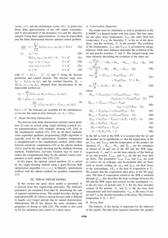
vector, u(t), and the disturbance vector, d(t), 2) point-wiseDirac delta approximation of the soft output constraints,and 3) discretization of the dynamics (1c) and the objectiveintegral. Using these approximations, (1) may be transcribedinto the finite dimensional discrete optimal control problem
minx,u,s
φ =
N−1∑k=0
Lk(xk, xk+1, uk, dk) + φ(sk) (2a)
s.t. x0 = x0 (2b)Rk(xk, xk+1, uk, dk) = 0, k ∈ N (2c)umin ≤ uk ≤ umax, k ∈ N (2d)c(xk, uk) + sk ≥ 0, k ∈ N (2e)sk ≥ 0, k ∈ N (2f)
with N = 0, 1, . . . , N − 1 and N being the discreteprediction and control horizon. The discrete stage cost,Lk = Lk(xk, uk, dk), and the residual function, Rk =Rk(xk, xk+1, uk, dk), obtained from discretization by thetrapezoidal method are
Lk =∆tk
2(l(xk, uk, dk) + l(xk+1, uk, dk)) (3)
Rk = g(xk+1)− g(xk)
− ∆tk2
(f(xk, uk, dk) + f(xk+1, uk, dk))(4)
for k ∈ N . No forecasts are available for the disturbances,so we use the same-as-now forecasts, i.e. dk = d(t0).
C. Single-Shooting Optimization
The discrete-time finite dimensional optimal control prob-lem (2) may be solved using single-shooting (control vec-tor parametrization) [18], multiple shooting [19], [20], orthe simultaneous method [21], [22]. In all these methods,some sequential quadratic programming (SQP) algorithm istypically used for the optimization. Gradient computationis straightforward in the simultaneous method, while eitherforward sensitivity computation [23] or the adjoint method[16] is used by the single-shooting and the multiple-shootingmethods. Furthermore, real-time iteration may be used toreduce the computational delay by the optimal control com-putation at each sample time [22], [24].
In this paper, the optimal control problem (2) is solvedby the single-shooting method using a quasi-Newton SQPoptimization algorithm (fmincon in Matlab’s optimizationtoolbox) and the adjoint method for gradient computation[17].
III. SPRAY DRYER MODELIn this section the spray dryer model is presented. It
is derived from first engineering principles. The unknownparameters are estimated from data by minimizing the sumof squared simulation errors. The model describes drying ofmaltodextrin DE-18, which is chosen because milk is difficultto handle over longer periods due to natural deterioration.Maltodextrin DE-18 has almost the same stickiness andproperties of drying as milk [25]. The model is also usedin [5] for simulation and control of a spray dryer.
A. Conservation EquationsThe model used for simulation as well as prediction in the
E-NMPC is a lumped model with four states. The four statesare the spray dryer temperature, TSD, the static fluid bedtemperature, TSFB , the humidity, Y , in the air of the spraydryer, and the moisture, X , in the powder. The evolutionof the temperatures, TSD and TSFB , is governed by energybalances, while mass balances determine the evolution of theair and powder moisture, Y and X . The lumped energy andmass balances describing the evolution of the states are
CadTSD
dt= −λRw +Hain −Haout −Qexc −Qla (5a)
CbdTSFB
dt= Hbin −Hbout +Qexc −Qlb (5b)
mdadY
dt= (Fmain + Fsfb)(Yamb − Y )
+ Fadd(Yadd − Y ) +Rw
(5c)
msdX
dt= Fs(Xf −X)−Rw (5d)
whereHain
= Fmain(cda + cvYamb)(Tmain − T0)+
Fadd(cda + cvYadd)(Tadd − T0)(6a)
Haout = (Fmain + Fsfb + Fadd)·(cda + cvY )(TSD − T0)
(6b)
Hbin = Fsfb(cda + cvYamb)(Tsfb − T0) (6c)Hbout = Fsfb(cda + cvYamb)(TSFB − T0) (6d)Qexc = k1(TSD − TSFB) + k2Xf + k3Tf − k4 (6e)Qla = k5(TSD − Tamb) (6f)Qlb = k6(TSFB − Tamb) (6g)Fs = FfXf/(Xf + 1) (6h)
In the SD as well as the SFB, it is assumed that the air andthe product are in equilibrium i.e. that the temperature of theair, TSD and TSFB , and the temperature of the product areidentical. Hain
, Haout, Hbin and Hbout
are the enthalpiesof humid air in and out of the SD and the SFB stage,respectively. Ca and Cb are the heat capacity of the hold-upof air and powder. Fmain and Fsfb are the dry base inletair flows. The parameters Yadd, Fadd and Tadd are usedto correct for air leakages and un-modeled inlet air flowssuch as nozzle cooling air. Qsd and Qsfb are heat lossesto the surroundings. λRw is the heat of evaporation at T0.We assume that the evaporation takes place in the SD stageonly. The heat of evaporation related to the SFB is modeledthrough Qexc, that describes the heat exchange between theSD and the SFB stages and corrects for this assumption. ms
is the dry mass of powder and X is the dry base moisturecontent of the powder. Xf and Tf is the dry base feedconcentration and feed temperature. mda is the mass of dryair and Y is the absolute humidity in the dryer. The referencetemperature is T0 = 25C.
B. Drying RateThe kinetics of the drying is important for the behavior
of the model. The thin layer equation describes the product
6796

drying rate, Rw, well [26]
Rw = Ddiff (X −Xeq)ms (7)
Ddiff is an empirical constant called the drying constantor diffusivity. It must be experimentally determined [27]. Inthe present study it is constant, but it may depend on bothtemperature and powder moisture.
The equilibrium moisture, Xeq , of the powder is a prod-uct dependent function that describes the moisture con-tent at which water cannot be evaporated any longer. TheGuggenheim-Anderson-de Boer (GAB) relation is used todescribe the equilibrium moisture [28]. The GAB relation isfitted to laboratory data obtained specifically for maltodextrinto get
Xeq =C ·K ·Xm ·RH
(1−K ·RH)(1−K ·RH + C ·K ·RH)(8)
in which Xm = 0.030723, C = 2.6535 · 10−7 exp(
6292.1T
)and K = 0.057882 exp
(945.16
T
). Xm is the monolayer mois-
ture content. C and K are constants related to monolayerand multi-layer properties. The relative humidity RH iscalculated from TSFB and Y . In the computation of Xeq
for the product drying rate, T = TSFB is used.
C. Stickiness
Stickiness of the produced particles is an important limita-tion to the achievable performance of the spray dryer. Stickyparticles form depositions on the walls of the spray dryer.Stickiness depends on product temperature and moisturecontent. We use a mass-proportion-mixing rule to describethe glass transition temperature [25], [29]
Tg =Tgp + kZTgw
1 + kZ(9)
in which Tgp = 144.8C (maltodextrin) and Tgw = −137C(water). The value k = 6.296 is estimated from adsorptionisotherm data. The obtained glass transition temperatures,TSDg and TSFB
g , are the upper limiting temperatures ofwhich deposits form on the chamber walls of the spray dryer.The moisture content of the powder is
Z =
2.2 · (Ap +Bp TSD)exp(Cp RH) for SDX for SFB
(10)
in which Ap = 0.0877, Bp = −0.00019751 and Cp =2.0498. The moisture content of the powder in the SDstage is difficult to estimate. Common practice is to use theequilibrium moisture, Xeq , as an approximation. We use anexponential function instead of the above GAB model for thispurpose, as it renders the transient residual moisture contentat low relative humidity better than (8).
TABLE I: Estimated parameters for the model (5)-(10)
Symbol Value Unit Symbol Value UnitCa 68.266 KJ/K Fadd 256.46/3600 kg/sCb 141.36 KJ/K Yadd 8.1799·10−3 kg/kgk1 0.29268 KW/K Tadd 100.03+273.15 Kk2 1.6207 KW k3 0.073198 KWk4 31.111 KW k5 0.26981 KW/Kk6 -0.023367 KW/K Ddiff 0.091922
D. Model and Parameters
The model (5)-(10) of the dryer is a deterministic systemof differential equations in the form (1c) in which
x =
TSD
TSFB
YX
u =
Ff
Tmain
Tsfb
d =
Fmain
Fsfb
Xf
TfTamb
Yamb
(11)
x is the state vector, u is the manipulated input vector,and d is the disturbance vector. The states as well as thedisturbances are measurable in industrial practice. Therefore,we do not discuss state estimation in this paper.
The parameters in the model (5)-(10) are estimated usingdata for a medium-scale spray dryer from GEA ProcessEngineering A/S. Table I provides the estimated parametersin the model. mda = 10 kg and ms = 15 kg are fixedparameters and determined from physical considerations.Generally the model fits the data well on both estimationand validation data.
E. Constraints
The maximum capacity of the feed pump limits the feedflow such that 0 kg/hr ≤ Ff ≤ 150 kg/hr. The inlettemperatures, Tmain and Tsfb must be higher than the ambienttemperature, Tamb, as the dryer can only heat but not cool.Furthermore, the risk of powder explosions and the risk ofscorched particles puts upper limits on the allowable inlettemperatures. Consequently, Tamb ≤ Tmain ≤ 180C andTamb ≤ Tsfb ≤ 120C. These constraints are hard inputconstraints of the form (1d).
To avoid depositions of sticky particles on the spray dryersurfaces, the temperatures TSD and TSFB must be below theglass transition temperatures in the SD stage, TSD ≤ TSD
g
and the SFB stage, TSFB ≤ TSFBg , respectively. The glass
transition temperature are determined by (9). Furthermore,the powder moisture must be below a maximum limit, X ≤Xmax = 4.5%, that is 4.5% for the case studies in this paper.These constraints are treated as soft output constraints in theform (2e). The soft `1 penalty is sW = 105 · [0.1; 0.1; 1.0]and the soft `2 penalty is SW = diag(sW ).
F. Objective Function - Profit and Regularization
The profit from operating the spray dryer is the value ofthe product minus the raw material and energy costs. Since
6797
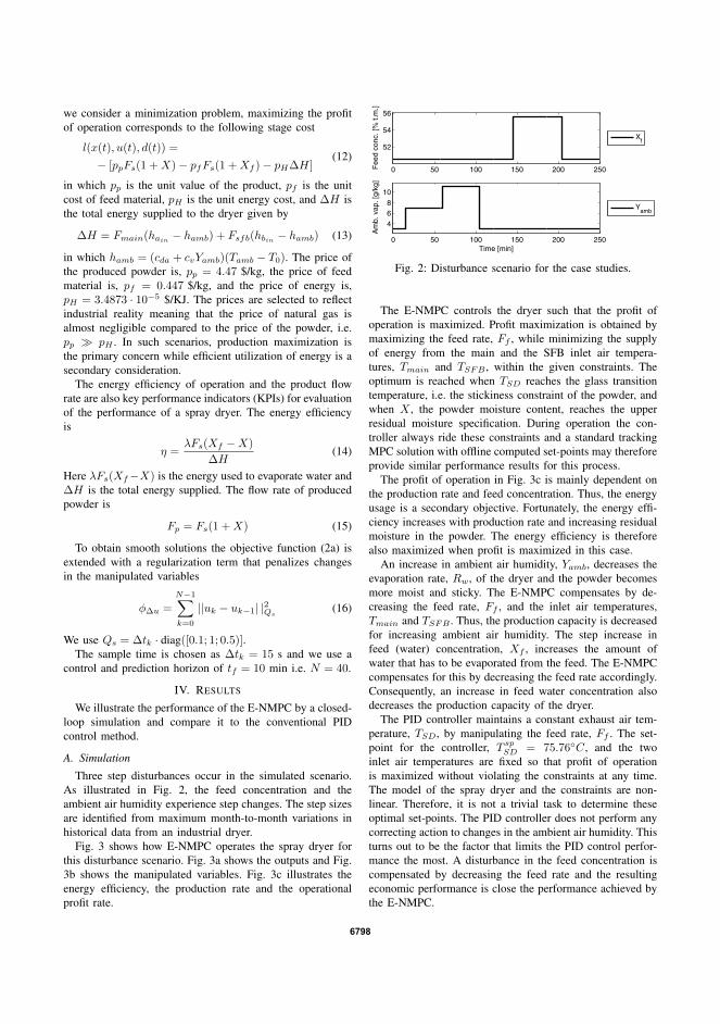
we consider a minimization problem, maximizing the profitof operation corresponds to the following stage cost
l(x(t), u(t), d(t)) =
− [ppFs(1 +X)− pfFs(1 +Xf )− pH∆H](12)
in which pp is the unit value of the product, pf is the unitcost of feed material, pH is the unit energy cost, and ∆H isthe total energy supplied to the dryer given by
∆H = Fmain(hain− hamb) + Fsfb(hbin − hamb) (13)
in which hamb = (cda + cvYamb)(Tamb − T0). The price ofthe produced powder is, pp = 4.47 $/kg, the price of feedmaterial is, pf = 0.447 $/kg, and the price of energy is,pH = 3.4873 · 10−5 $/KJ. The prices are selected to reflectindustrial reality meaning that the price of natural gas isalmost negligible compared to the price of the powder, i.e.pp pH . In such scenarios, production maximization isthe primary concern while efficient utilization of energy is asecondary consideration.
The energy efficiency of operation and the product flowrate are also key performance indicators (KPIs) for evaluationof the performance of a spray dryer. The energy efficiencyis
η =λFs(Xf −X)
∆H(14)
Here λFs(Xf−X) is the energy used to evaporate water and∆H is the total energy supplied. The flow rate of producedpowder is
Fp = Fs(1 +X) (15)
To obtain smooth solutions the objective function (2a) isextended with a regularization term that penalizes changesin the manipulated variables
φ∆u =N−1∑k=0
||uk − uk−1| |2Qs(16)
We use Qs = ∆tk · diag([0.1; 1; 0.5)].The sample time is chosen as ∆tk = 15 s and we use a
control and prediction horizon of tf = 10 min i.e. N = 40.
IV. RESULTS
We illustrate the performance of the E-NMPC by a closed-loop simulation and compare it to the conventional PIDcontrol method.
A. Simulation
Three step disturbances occur in the simulated scenario.As illustrated in Fig. 2, the feed concentration and theambient air humidity experience step changes. The step sizesare identified from maximum month-to-month variations inhistorical data from an industrial dryer.
Fig. 3 shows how E-NMPC operates the spray dryer forthis disturbance scenario. Fig. 3a shows the outputs and Fig.3b shows the manipulated variables. Fig. 3c illustrates theenergy efficiency, the production rate and the operationalprofit rate.
0 50 100 150 200 250
52
54
56
Fee
d co
nc. [
% t.
m.]
Xf
0 50 100 150 200 250
468
10
Am
b. v
ap. [
g/kg
]
Time [min]
Yamb
Fig. 2: Disturbance scenario for the case studies.
The E-NMPC controls the dryer such that the profit ofoperation is maximized. Profit maximization is obtained bymaximizing the feed rate, Ff , while minimizing the supplyof energy from the main and the SFB inlet air tempera-tures, Tmain and TSFB , within the given constraints. Theoptimum is reached when TSD reaches the glass transitiontemperature, i.e. the stickiness constraint of the powder, andwhen X , the powder moisture content, reaches the upperresidual moisture specification. During operation the con-troller always ride these constraints and a standard trackingMPC solution with offline computed set-points may thereforeprovide similar performance results for this process.
The profit of operation in Fig. 3c is mainly dependent onthe production rate and feed concentration. Thus, the energyusage is a secondary objective. Fortunately, the energy effi-ciency increases with production rate and increasing residualmoisture in the powder. The energy efficiency is thereforealso maximized when profit is maximized in this case.
An increase in ambient air humidity, Yamb, decreases theevaporation rate, Rw, of the dryer and the powder becomesmore moist and sticky. The E-NMPC compensates by de-creasing the feed rate, Ff , and the inlet air temperatures,Tmain and TSFB . Thus, the production capacity is decreasedfor increasing ambient air humidity. The step increase infeed (water) concentration, Xf , increases the amount ofwater that has to be evaporated from the feed. The E-NMPCcompensates for this by decreasing the feed rate accordingly.Consequently, an increase in feed water concentration alsodecreases the production capacity of the dryer.
The PID controller maintains a constant exhaust air tem-perature, TSD, by manipulating the feed rate, Ff . The set-point for the controller, T sp
SD = 75.76C, and the twoinlet air temperatures are fixed so that profit of operationis maximized without violating the constraints at any time.The model of the spray dryer and the constraints are non-linear. Therefore, it is not a trivial task to determine theseoptimal set-points. The PID controller does not perform anycorrecting action to changes in the ambient air humidity. Thisturns out to be the factor that limits the PID control perfor-mance the most. A disturbance in the feed concentration iscompensated by decreasing the feed rate and the resultingeconomic performance is close the performance achieved bythe E-NMPC.
6798

On average for the given disturbance scenario the E-NMPC increases the profit of operation by 26.7% comparedto the PID controller.
V. CONCLUSIONS
This paper presents an economically optimal control so-lution for a spray dryer. The controller is based on anonlinear model predictive controller with an economicobjective function (E-NMPC). The E-NMPC provides acontrol solution that constantly brings the dryer to the mostcost optimal state of operation within the given processconstraints. The residual moisture specification is controlledwithin specifications and fouling in the dryer is avoided. Acase study is used to simulate and evaluate the performanceof the E-NMPC compared to a conventional PID basedcontrol strategy. In the simulation the profit of operationis increased by 26.7%. We also find that it is not intuitiveto select the most profitable set-points for the conventionalPID control. Optimal set-points are therefore hardly neverobtained by operators in industrial practice. Accordingly,the economic benefit of E-NMPC may be even larger forindustrial spray dryers. Furthermore, a common problem inoperation of industrial spray dryers is production stops due todeposition of sticky particles on spray dryer surfaces. Suchsituations are efficiently avoided by the ability of E-NMPCto include stickiness constraints and compute control profilesthat are continuously adapted to variations in the feed andthe ambient conditions.
REFERENCES
[1] T. Donnellan, T. Hennessy, M. Fenelon, and D. O’Callaghan, “Thepotential for scale economies in milk powder processing: an irish casestudy,” International Journal of Dairy Technology, vol. 67, no. 1, pp.129–134, 2014.
[2] Vaisala, “+20% increase in production capacity withzero increase in energy consumption,” 2014. [Online].Available: http://www.vaisala.com/Vaisala\%20Documents/Success\%20Stories/CEN-TIA-G-Valio-Customer-Story-B211288EN-A.pdf
[3] J. Perez-Correa and F. Fariass, “Modelling and control of a spray dryer: A simulation study,” Food Control, vol. 6, no. 4, pp. 219–227, 1995.
[4] L. N. Petersen, N. K. Poulsen, H. H. Niemann, C. Utzen, andJ. B. Jørgensen, “A Grey-Box Model for Spray Drying Plants,” 10thIFAC International Symposium on Dynamics and Control of ProcessSystems, pp. 559–564, 2013.
[5] ——, “Application of constrained linear mpc to a spray dryer,”Proceedings of the IEEE Multi-Conference on Systems and Control,2014.
[6] M. R. Naysmith and P. L. Douglas, “Review of real time optimiza-tion in the chemical process industries,” Developments in ChemicalEngineering and Mineral Processing, pp. 67–87, 1995.
[7] M. L. Darby, M. Harmse, and M. Nikolaou, “MPC: Current practiceand challenges,” 7th IFAC International Symposium on AdvancedControl of Chemical Processes, vol. 7, no. 1, pp. 86–98, 2009.
[8] M. Bauer and I. K. Craig, “Economic assessment of advanced processcontrol – a survey and framework,” Journal of Process Control, vol. 18,no. 1, pp. 2–18, 2008.
[9] P. S. R. K. Chintapalli and J. M. Douglas, “The use of economic per-formance measures to synthesize optimal control systems,” Industrial& Engineering Chemistry Fundamentals, vol. 14, no. 1, pp. 1–10,1975.
[10] T. E. Marlin and A. N. Hrymak, “Real-time operations optimization ofcontinuous processes,” Chemical Process Control-V Conference, pp.156–164, 1996.
[11] J. B. Rawlings, C. N. Bates, and D. Angeli, “Fundamentals of eco-nomic model predictive control,” Proceedings of the IEEE Conferenceon Decision and Control, pp. 3851–3861, 2012.
0 50 100 150 200 2507576777879
Tem
p. [o C
]
TPIDSD
TPIDg,SD
TMPCSD
TMPCg,SD
0 50 100 150 200 250
60
62
64
66
Tem
p. [o C
]
TPIDSFB
TMPCSFB
0 50 100 150 200 2501820222426
Vap
. con
c. [g
/kg]
YPID
YMPC
0 50 100 150 200 2504
4.2
4.4
Time [min]W
ater
con
c. [%
t.m
.]
XPID
XMPC
(a) System outputs.
0 50 100 150 200 25050
100
150
Fee
d ra
te [k
g/hr
]
FPIDf
FMPCf
0 50 100 150 200 250150
160
170
180
Mai
n te
mp.
[o C]
TPIDmain
TMPCmain
0 50 100 150 200 250
60
80
100
120
Time [min]
SF
B te
mp.
[o C]
TPIDsfb
TMPCsfb
(b) Manipulated variables.
0 50 100 150 200 250
30
40
50
Effi
cien
cy [%
]
PIDMPC
0 50 100 150 200 250
30
40
50
60
Pro
d. r
ate
[kg/
hr]
PIDMPC
0 50 100 150 200 250
100
150
200
Pro
fit [$
/hr]
PIDMPC
(c) The operational profit rate.
Fig. 3: E-NMPC seeking to maximize profit for the distur-bance scenario given in Fig. 2. Red lines indicate constraints.
6799

[12] R. Amrit, “Optimizing process economics in model predictive control,”Ph.D. dissertation, University of Wisconsin–Madison, 2011.
[13] T. G. Hovgaard, L. F. Larsen, and J. B. Jørgensen, “Flexible and costefficient power consumption using economic mpc,” Proceedings of the50th IEEE Conference on Decision and Control and European ControlConference, pp. 848–854, 2011.
[14] D. Angeli, R. Amrit, and J. B. Rawlings, “Receding horizon costoptimization for overly constrained nonlinear plants,” Proceedings ofthe IEEE Conference on Decision and Control, pp. 7972–7977, 2009.
[15] D. O. Callaghan and P. Cunningham, “Modern process control tech-niques in the production of dried milk products – a review,” Lait,vol. 85, pp. 335–342, 2005.
[16] J. B. Jørgensen, “Adjoint sensitivity results for predictive control, state-and parameter-estimation with nonlinear models,” European ControlConference 2007, pp. 3649–3656, 2007.
[17] L. N. Petersen and J. B. Jørgensen, “Real-time economic optimizationfor a fermentation process using model predictive control,” 13thEuropean Control Conference, 2014.
[18] M. Schlegel, K. Stockmann, T. Binder, and W. Marquardt, “Dynamicoptimization using adaptive control vector parameterization,” Comput-ers & Chemical Engineering, vol. 29, no. 8, pp. 1731–1751, 2005.
[19] H. G. Bock and K. J. Plitt, “A multiple shooting algorithm for directsolution of optimal control problems,” 9th IFAC World CongressBudapest. Pergamon Press, pp. 242–247, 1984.
[20] A. Capolei and J. B. Jørgensen, “Solution of constrained optimalcontrol problems using multiple shooting and esdirk methods,” Pro-ceedings of the 2012 American Control Conference, pp. 295–300,2012.
[21] L. T. Biegler, “Solution of dynamic optimization problems by succes-sive quadratic programming and orthogonal collocation,” Computers& Chemical Engineering, vol. 8, no. 3, pp. 243–248, 1984.
[22] ——, “A survey on sensitivity-based nonlinear model predictive con-trol,” 10th IFAC International Symposium on Dynamics and Controlof Process Systems, pp. 499–510, 2013.
[23] M. R. Kristensen, J. B. Jørgensen, P. G. Thomsen, and S. B. Jørgensen,“An esdirk method with sensitivity analysis capabilities,” Computers& Chemical Engineering, vol. 28, no. 12, pp. 2695–2707, 2004.
[24] M. Diehl, H. G. Bock, and J. P. Schloder, “A real-time iteration schemefor nonlinear optimization in optimal feedback control,” SIAM Journalon Control and Optimization, vol. 43, no. 5, pp. 1714–1736, 2005.
[25] C. Hennigs, T. K. Kockel, and T. A. G. Langrish, “New measurementsof the sticky behavior of skim milk powder,” Drying Technology,vol. 19, no. 3-4, pp. 471–484, 2001.
[26] W. K. Lewis, “The rate of drying of solid materials,” Journal ofIndustrial and Engineering Chemistry, vol. 13, pp. 427–432, 1921.
[27] F. F. G. Areed, M. S. El-Kasassy, and K. A. Mahmoud, “Design ofneuro-fuzzy controller for a rotary dryer,” International Journal ofComputer Applications, vol. 37, no. 5, pp. 34–41, 2012.
[28] C. E. C. Perez, R. D. P. Andrade, and L. M. Roberto, “Models ofsorption isotherms for food: Uses and limitations,” Vitae, vol. 18, no. 3,pp. 325–334, 2011.
[29] S. Hogan, M. Famelart, D. O’Callaghan, and P. Schuck, “A noveltechnique for determining glass-rubber transition in dairy powders,”Journal of Food Engineering, vol. 99, pp. 76–82, 2010.
6800

200

P a p e r G
Economic Optimization ofSpray Dryer Operation usingNonlinear Model Predictive
Control with State Estimation
Published in 9th International Symposium on Advanced Control of ChemicalProcesses (ADCHEM 2015), pp. 507–513, 2015, Whistler.

202

ScienceDirectIFAC-PapersOnLine 48-8 (2015) 507–513
ScienceDirect
Available online at www.sciencedirect.com
2405-8963 © 2015, IFAC (International Federation of Automatic Control) Hosting by Elsevier Ltd. All rights reserved.Peer review under responsibility of International Federation of Automatic Control.10.1016/j.ifacol.2015.09.018
Lars Norbert Petersen et al. / IFAC-PapersOnLine 48-8 (2015) 507–513
© 2015, IFAC (International Federation of Automatic Control) Hosting by Elsevier Ltd. All rights reserved.
Economic Optimization of Spray DryerOperation using Nonlinear Model
Predictive Control with State Estimation
Lars Norbert Petersen ∗ John Bagterp Jørgensen ∗∗
James B. Rawlings ∗∗∗
∗ GEA Process Engineering A/S, Søborg, Denmark, (e-mail:[email protected])
∗∗ Department of Applied Mathematics and Computer Science,Technical University of Denmark, Kgs. Lyngby, Denmark, (e-mail:
[email protected])∗∗∗ Department of Chemical and Biological Engineering, University ofWisconsin-Madison, Madison, USA, (e-mail: [email protected])
Abstract:In this paper, we develop an economically optimizing Nonlinear Model Predictive Controller(E-NMPC) for a complete spray drying plant with multiple stages. In the E-NMPC the initialstate is estimated by an extended Kalman Filter (EKF) with noise covariances estimated byan autocovariance least squares method (ALS). We present a model for the spray drying plantand use this model for simulation as well as for prediction in the E-NMPC. The open-loopoptimal control problem in the E-NMPC is solved using the single-shooting method combinedwith a quasi-Newton Sequential Quadratic Programming (SQP) algorithm and the adjointmethod for computation of gradients. We evaluate the economic performance when unmeasureddisturbances are present. By simulation, we demonstrate that the E-NMPC improves the profitof spray drying by 17% compared to conventional PI control.
Keywords: Nonlinear Model Predictive Control, Optimization, Grey-box model, Spray Drying
1. INTRODUCTION
Spray drying is a processing technique for drying of liquidsor slurries into a free flowing powder. Spray drying is a keyprocess in the dairy industry (Mujumdar, 2006), wheredairy products are dried into powders to increase the shelflife as well as to reduce cost of transportation over longdistances. The quality of dairy powder is, among otherfactors, characterized by the residual moisture contentthat must be within the specification. Spray drying is byfar the most energy-intensive unit operation in the dairyindustry (IDF, 2005). Therefore, maximizing the efficiencyof the spray drying process and maintaining the correctresidual moisture level are of utmost importance.
The main challenge in controlling the spray dryer is touse a minimum of energy (hot air) to bring the residualmoisture in the powder below the specification and toavoid that the powder sticks to the walls of the chamber.This is a challenge, as the operation of the spray dryermust continuously be adjusted to variations in the feedconcentration and variations in the ambient air humidity.Application of advanced control is potentially a cost effec-tive way to reduce the energy consumption as well as toincrease the production capacity (Petersen et al., 2014b).
Conventional set-point based control of spray dryers keepsthe inlet and outlet temperatures constant during oper-ation. This approach is simple, but known to be insuffi-
cient for controlling the residual moisture. Furthermore,the powder may turn sticky inside the dryer during highambient air humidities. This motivates E-NMPC in thepresence of feed and ambient air variations. E-NMPCadjusts the manipulated variables in such a way thatthe residual moisture is below its maximum, fouling ofthe spray dryer is avoided, and the cost of operation isminimized.
1.1 Process Description
A Multi-Stage Dryer (MSDTM) consists of a spray cham-ber (SD), a static fluid bed (SFB), and two vibrating fluidbed (VFB) stages. This type of dryer is the most widelyused dryer in the production of food powders (Mujumdarand Huang, 2007). Fig. 1 illustrates the stages of the spraydryer as well as the hot air and the powder in- and outlets.The dryer is designed such that the hot inlet air is fedinto the upper section of the drying chamber around thehigh pressure nozzles. The nozzles disperse the liquid feedinto droplets. The heat is transferred from the hot airto the droplets, which makes the water evaporate fromthe droplets. In that process, the air temperature andthe residual moisture of the droplets decrease. The driedproduct then enters the SFB where it is further dried byhot air from below. Next, the powder is transported tothe VFBh and VFBc stages for gentle drying and cooledto the temperature desired for handling and storage.
9th International Symposium on Advanced Control of Chemical ProcessesJune 7-10, 2015. Whistler, British Columbia, Canada
Copyright © 2015 IFAC 507

508 Lars Norbert Petersen et al. / IFAC-PapersOnLine 48-8 (2015) 507–513
SD
Main Air
SFB Air
Feed
Cooling
SFB
Tsfb, Fsfb, Yamb
Tmain, Fmain, Yamb
TSD,Y
X
TSFB
FfXfTf
VFBh Air VFBc AirPowder
VFBh VFBc
Tvfbh, Fvfbh, Yamb Tvfbc, Fvfbc, Yamb
ExhaustExit
Fines
ExhaustTVFBh TVFBc
Fig. 1. Diagram of the spray dryer. Sprayed droplets andhot air are mixed in the top. The droplets dry intopowder and are dried further in the SFB and VFBhstages and cooled in the VFBc stage.
1.2 Modeling
Dynamic models of spray drying has recently been re-ported. Petersen et al. (2013) propose a model for a com-plete spray dryer and Petersen et al. (2014a) presents amodel for the SD and SFB stages of the spray dryer. Thelatter show good simulation accuracy. The model derivedin this paper will therefore be based on the model inPetersen et al. (2014a) and extended to also describe theVFB stages.
1.3 Control and State Estimation
The combination of real-time steady-state optimization(RTO) and set-point based model predictive control isa standard methodology for optimizing process operation(Naysmith and Douglas, 1995). Recent advances withinprocess optimization focus on optimizing the higher-levelobjectives, such as economics, directly in the control layer.This is called economically optimizing Model PredictiveControl (E-MPC). For a long time, MPC has been thepreferred advanced control methodology in the processindustries. Recently, the idea of optimizing economicsdirectly has gained significant renewed interest (Rawlingset al., 2012; Bauer and Craig, 2008). Papers relatedto control of spray dryers seldom consider an economicobjective. Petersen et al. (2014a) discuss a linear trackingMPC, while Petersen et al. (2014b) discuss an E-NMPCfor the SD and SFB stages of the spray dryer. Callaghanand Cunningham (2005) provides a thorough review on thestatus and future of advanced control for spray drying.
The model of the spray dryer is used for simulationas well as for prediction and state estimation in theNMPC. We use the well known extended continuous-discrete Kalman filter (EKF) for state estimation. Theperformance of the filter is highly dependent on goodestimation of the noise covariances, which we will estimateusing the Autocovariance Least-Squares (ALS) methoddescribed in Rajamani and Rawlings (2009).
1.4 Content & Organization
In this paper, we demonstrate that the profit of operationfor a spray drying process can be improved significantlyby application of E-NMPC based on an economicallyoptimizing controller and an EKF for state estimation.The noise covariances in the EKF are estimated by theALS method.
The paper is organized as follows. In Section 2, the modelof the spray dryer is presented. Section 3 presents the esti-mation problem and the ALS method. Section 4 presentsthe control problem and its transcription to a computa-tionally tractable optimization problem. In Section 5 wepresent a simulation to show the benefit of optimizing theoperation. Conclusions are given in Section 6.
2. SPRAY DRYER MODEL
In this section, the complete spray dryer model is pre-sented. It is derived from first engineering principles anddescribes drying of maltodextrin DE-18. We use Maltodex-trin DE-18 as a substitute to milk, because milk is difficultto handle over longer periods due to natural deterioration.
2.1 Spray Dryer and Static Fluid Bed Model
The evolution of the temperatures, TSD and TSFB, is gov-erned by energy balances, while mass balances determinethe evolution of the air and powder moisture, Yab andXab. The lumped energy and mass balances describing theevolution of the states are
CadTSD
dt= −λRaw + Fmainhain + Fsfbhbout−
(Fmain + Fsfb + Fadd)haout+
Faddhaadd+ Fs(h
pf − hp
a) −Qab −Qa
(1a)
CbdTSFB
dt= Fsfb(h
abin − ha
bout) + Fs(hpa − hp
b)+
Qab −Qbc −Qb
(1b)
madYab
dt= (Fmain + Fsfb)(Yamb − Yab)+
Fadd(Yadd − Yab) + Raw
(1c)
mbdXab
dt= Fs(Xf −Xab) −Raw (1d)
where
haain
= (cda + cvYamb)Tmain, haaout
= (cda + cvYab)TSD
habin = (cda + cvYamb)Tsfb, ha
bout = (cda + cvYamb)TSFB
haaadd
= (cda + cvYadd)Tadd, hpf = (cs + cwXf )Tf
hpa = (cs + cwXab)TSD, hp
b = (cs + cwXab)TSFB
Qab = k1(TSD − TSFB) + k2Xf + k3Tf − k4Qa = k5(TSD − Tamb), Qb = k6(TSFB − Tamb)
It is assumed that the air and the product are in equilib-rium i.e. that the temperature of the air, TSD and TSFB,and the temperature of the product are identical. ha
·and hp
· are the specific enthalpies of the humid air and
powder inlets and outlets of the SD and the SFB stages.Ca and Cb are the heat capacities of the hold-up of airand powder. The heat capacities are given at the referencetemperature, T0 = 25C. λRaw is the heat of evaporationand Qab describes the heat exchange between the SD and
IFAC ADCHEM 2015June 7-10, 2015. Whistler, BC, Canada
508
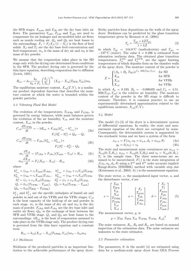
Lars Norbert Petersen et al. / IFAC-PapersOnLine 48-8 (2015) 507–513 509
SD
Main Air
SFB Air
Feed
Cooling
SFB
Tsfb, Fsfb, Yamb
Tmain, Fmain, Yamb
TSD,Y
X
TSFB
FfXfTf
VFBh Air VFBc AirPowder
VFBh VFBc
Tvfbh, Fvfbh, Yamb Tvfbc, Fvfbc, Yamb
ExhaustExit
Fines
ExhaustTVFBh TVFBc
Fig. 1. Diagram of the spray dryer. Sprayed droplets andhot air are mixed in the top. The droplets dry intopowder and are dried further in the SFB and VFBhstages and cooled in the VFBc stage.
1.2 Modeling
Dynamic models of spray drying has recently been re-ported. Petersen et al. (2013) propose a model for a com-plete spray dryer and Petersen et al. (2014a) presents amodel for the SD and SFB stages of the spray dryer. Thelatter show good simulation accuracy. The model derivedin this paper will therefore be based on the model inPetersen et al. (2014a) and extended to also describe theVFB stages.
1.3 Control and State Estimation
The combination of real-time steady-state optimization(RTO) and set-point based model predictive control isa standard methodology for optimizing process operation(Naysmith and Douglas, 1995). Recent advances withinprocess optimization focus on optimizing the higher-levelobjectives, such as economics, directly in the control layer.This is called economically optimizing Model PredictiveControl (E-MPC). For a long time, MPC has been thepreferred advanced control methodology in the processindustries. Recently, the idea of optimizing economicsdirectly has gained significant renewed interest (Rawlingset al., 2012; Bauer and Craig, 2008). Papers relatedto control of spray dryers seldom consider an economicobjective. Petersen et al. (2014a) discuss a linear trackingMPC, while Petersen et al. (2014b) discuss an E-NMPCfor the SD and SFB stages of the spray dryer. Callaghanand Cunningham (2005) provides a thorough review on thestatus and future of advanced control for spray drying.
The model of the spray dryer is used for simulationas well as for prediction and state estimation in theNMPC. We use the well known extended continuous-discrete Kalman filter (EKF) for state estimation. Theperformance of the filter is highly dependent on goodestimation of the noise covariances, which we will estimateusing the Autocovariance Least-Squares (ALS) methoddescribed in Rajamani and Rawlings (2009).
1.4 Content & Organization
In this paper, we demonstrate that the profit of operationfor a spray drying process can be improved significantlyby application of E-NMPC based on an economicallyoptimizing controller and an EKF for state estimation.The noise covariances in the EKF are estimated by theALS method.
The paper is organized as follows. In Section 2, the modelof the spray dryer is presented. Section 3 presents the esti-mation problem and the ALS method. Section 4 presentsthe control problem and its transcription to a computa-tionally tractable optimization problem. In Section 5 wepresent a simulation to show the benefit of optimizing theoperation. Conclusions are given in Section 6.
2. SPRAY DRYER MODEL
In this section, the complete spray dryer model is pre-sented. It is derived from first engineering principles anddescribes drying of maltodextrin DE-18. We use Maltodex-trin DE-18 as a substitute to milk, because milk is difficultto handle over longer periods due to natural deterioration.
2.1 Spray Dryer and Static Fluid Bed Model
The evolution of the temperatures, TSD and TSFB, is gov-erned by energy balances, while mass balances determinethe evolution of the air and powder moisture, Yab andXab. The lumped energy and mass balances describing theevolution of the states are
CadTSD
dt= −λRaw + Fmainhain + Fsfbhbout−
(Fmain + Fsfb + Fadd)haout+
Faddhaadd+ Fs(h
pf − hp
a) −Qab −Qa
(1a)
CbdTSFB
dt= Fsfb(h
abin − ha
bout) + Fs(h
pa − hp
b)+
Qab −Qbc −Qb
(1b)
madYab
dt= (Fmain + Fsfb)(Yamb − Yab)+
Fadd(Yadd − Yab) + Raw
(1c)
mbdXab
dt= Fs(Xf −Xab) −Raw (1d)
where
haain
= (cda + cvYamb)Tmain, haaout
= (cda + cvYab)TSD
habin = (cda + cvYamb)Tsfb, ha
bout = (cda + cvYamb)TSFB
haaadd
= (cda + cvYadd)Tadd, hpf = (cs + cwXf )Tf
hpa = (cs + cwXab)TSD, hp
b = (cs + cwXab)TSFB
Qab = k1(TSD − TSFB) + k2Xf + k3Tf − k4Qa = k5(TSD − Tamb), Qb = k6(TSFB − Tamb)
It is assumed that the air and the product are in equilib-rium i.e. that the temperature of the air, TSD and TSFB,and the temperature of the product are identical. ha
·and hp
· are the specific enthalpies of the humid air and
powder inlets and outlets of the SD and the SFB stages.Ca and Cb are the heat capacities of the hold-up of airand powder. The heat capacities are given at the referencetemperature, T0 = 25C. λRaw is the heat of evaporationand Qab describes the heat exchange between the SD and
IFAC ADCHEM 2015June 7-10, 2015. Whistler, BC, Canada
508
the SFB stages. Fmain and Fsfb are the dry base inlet airflows. The parameters Yadd, Fadd and Tadd are used tocompensate for air leakages and un-modeled inlet air flowssuch as nozzle cooling air. Qa and Qb are heat losses tothe surroundings. Fs = FfXf/(1 −Xf ) is the flow of feedsolids. Xf and Tf are the dry base feed concentration andfeed temperature. ma is the mass of dry air and mb is themass of dry powder.
We assume that the evaporation takes place in the SDstage only with the drying rate determined from conditionsin the SFB. The product drying rate is governed by thethin layer equation, describing evaporation due to diffusion(Lewis, 1921)
Raw = k7k8
k8 + Fs
(Tf
T0
)k9
(Xab −Xeq(TSFB, Yab))mb
The equilibrium moisture content, Xeq(T, Y ), is a nonlin-ear product dependent function that describes the mois-ture content at which the water is bounded within thepowder particles.
2.2 Vibrating Fluid Bed Model
The evolution of the temperatures, TVFBh and TVFBc, isgoverned by energy balances, while mass balances governthe evolution of the air humidity, Ycd, and the moisturecontent, Xcd, in the powder.
CcddTVFBh
dt= −λRcw + Fvfbh(h
acin − ha
cout)+
Fs(hpb − hp
c) + Qbc −Qc
(2a)
CcddTVFBc
dt= Fvfbc(h
adin
− hadout
)+
Fs(hpc − hp
d) −Qd
(2b)
mcdYcd
dt= (Fvfbh + Fvfbc)(Yamb − Ycd) + Rcw (2c)
mddXcd
dt= Fs(Xab −Xcd) −Rcw (2d)
where
hacin = (cda + cvYamb)Tvfbh, ha
cout= (cda + cvYcd)TVFBh
hadin
= (cda + cvYamb)Tvfbc, hadout
= (cda + cvYcd)TVFBc
hpc = (cs + cwXcd)TVFBh, hp
d = (cs + cwXcd)TVFBc
Qc = k11(TVFBh − Tamb), Qd = k12(TVFBc − Tamb)
Qbc = k10(TSFB − TVFBh)
ha· and hp
· are the specific enthalpies of humid air and
powder in and out of the VFBh and the VFBc stages. Ccd
is the heat capacity of the hold-up of air and powder ineach stage. mc is the mass of dry air and md is the drymass of powder. Fvfbh and Fvfbc are the dry base inlet andoutlet air flows. Qbc is the exchange of heat between theSFB and VFBh stage. Qc and Qd are heat losses to thesurroundings. λRcw is the heat of evaporation assumed totake place in the VFBh stage only. The product drying rateis governed from the thin layer equation and a constantterm
Rcw = k13(Xcd −Xeq(TVFBh, Ycd))md − k14md
2.3 Stickiness
Stickiness of the produced particles is an important lim-itation to the achievable performance of the spray dryer.
Sticky particles form depositions on the walls of the spraydryer. Stickiness can be predicted by the glass transitiontemperature given by Boonyai et al. (2004)
Tg =Tgp + kZTgw
1 + kZ(3)
in which Tgp = 144.8C (maltodextrin) and Tgw =−137C (water). The value k = 6.296 is estimated fromadsorption isotherm data. The obtained glass transitiontemperatures, TSD
g and TSFBg , are the upper limiting
temperatures of which deposits form on the chamber wallsof the spray dryer. The moisture content of the powder is
Z =
(Ap + Bp TSD)eCp RH(TSD,Yab) for SD
Xab for SFB
Xcd for VFBh
Xcd for VFBc
in which Ap = 0.193, Bp = −0.000435 and Cp = 4.51.RH(TSD, Yab) is the relative air humidity. The moisturecontent of the powder in the SD stage is difficult toestimate. Therefore, it is common practice to use anexperimentally determined approximation related to theequilibrium moisture, Xeq(T, Y ).
2.4 Model
The model (1)-(3) of the dryer is a deterministic systemof differential equations. In reality, the state and mea-surement equation of the dryer are corrupted by noise.Consequently, the deterministic system is augmented bytwo stochastic terms and we have a system of the form
xk+1 = F (xk, uk + wu,k, dk + wd,k, θ) (4a)
yk = h(xk) + vk (4b)
The state and measurement noise covariances are wu,k =Niid(0, TsRu), wd,k = Niid(0, TsRd) and vk = Niid(0, Rv).Ts is the sample time. The three noise-terms are as-sumed to be uncorrelated. F (·) is the state integration off(xk, uk, dk, θ) using a 3rd and 4th order accurate implicitRunge-Kutta (ESDIRK) method with variable step size(Kristensen et al., 2004). h(·) is the measurement equation.
The state vector, x, the manipulated input vector, u, andthe disturbance vector, d are
x =
TSD
TSFB
Yab
Xab
TVFBh
TVFBc
Ycd
Xcd
u =
Ff
Tmain
Tsfb
Tvfbh
Tvfbc
d =
Xf
Tf
Fmain
Fsfb
Fvfbh
Fvfbc
Tamb
Yamb
(5)
The measurement vector, y, is
y = [TSD TSFB Yab TVFBh TVFBc Xcd]T
(6)
The noise variances, Ru, Rd and Rv, are based on manualinspection of the estimation data. The noise variances areunknown to the state estimator.
2.5 Parameter estimation
The parameters, θ, in the model (4) are estimated usingdata for a medium-scale spray dryer from GEA Process
IFAC ADCHEM 2015June 7-10, 2015. Whistler, BC, Canada
509

510 Lars Norbert Petersen et al. / IFAC-PapersOnLine 48-8 (2015) 507–513
Table 1. Estimated param. in model (1)-(3)
Sym. Value Unit Sym. Value Unit
Ca 61.634 KJ/K Tadd 60.018 CCb 148.26 KJ/K k7 9.401·10−2 -k1 0.2725 KW/K k8 1.4887·10−2 -k2 1.5017 KW k9 8.4203 -k3 0.0605 KW/K Ccd 29.244 KW/Kk4 27.276 KW k10 9.561·10−3 KW/Kk5 0.24735 KW/K k11 22.314·10−3 KW/Kk6 -0.03198 KW/K k12 46.818·10−3 KW/KFadd 248.54 kg/hr k13 1.9963·10−3 -Yadd 9.4566 g/kg k14 13.49·10−6 -
Engineering A/S. Table 1 provides the least squares esti-mated parameters of the model. ma = 7.5 kg, mb = 15 kg,mc = 15 kg and md = 4 kg are fixed parameters and deter-mined from physical considerations. Generally the modelfits and predicts the data well both for the estimation andvalidation data, respectively.
2.6 Constraints
The maximum capacity of the feed pump limits the feedflow such that 0 kg/hr ≤ Ff ≤ 130 kg/hr. The inlet tem-peratures must be higher than the ambient temperature,Tamb, as the dryer can only heat and not cool the air.Furthermore, the risk of powder explosions and the riskof scorched particles creates upper limits on the allowableinlet temperatures. Consequently, Tamb ≤ Tmain ≤ 200C,Tamb ≤ Tsfb ≤ 120C, Tamb ≤ Tvfbh ≤ 80C and Tamb ≤Tvfbc ≤ 80C. These constraints are hard input constraintsof the form (9d).
To avoid depositions of sticky particles on the spray dryersurfaces, the temperatures TSD, TSFB, TVFBh and TVFBc
must be below the glass transition temperatures in theSD stage, TSD ≤ T SD
g , the SFB stage, TSFB ≤ T SFBg ,
the VFBh stage, TVFBh ≤ TVFBhg and the VFBc stage,
TVFBc ≤ TVFBcg ≤ 35C, respectively. The glass transition
temperatures are determined by (3). Furthermore, thepowder moisture must be below a maximum limit, Xcd ≤Xmax = 3.5%, that is 3.5% for the case study in this paper.These constraints are treated as soft output constraints inthe form (10e). The soft 1 penalty is sW = 104 · Ts ·[1 1 1 1 0.1] and the soft 2 penalty is SW = diag(sW ).
2.7 Key Performance Indicators (KPIs)
The profit from operating the spray dryer is the value ofthe product minus the raw material and energy costs
p(x(t), u(t), d(t)) = ppFs(1 + Xcd) − pfFs(1 + Xf )
− pH∆H(7)
in which pp is the unit value of the product, pf is the unitcost of feed material, pH is the unit energy cost, and ∆His the total energy supplied to the dryer. ∆H is
∆H = Fmain(haain
− haamb) + Fsfb(h
abin − ha
amb)
+ Fvfbh(hacin − ha
amb) + Fvfbc(hadin
− haamb)
in which haamb = (cda + cvYamb)Tamb. The price of, the
produced powder is pp = 4.47 $/kg, the feed material ispf = 0.447 $/kg, and the energy is pH = 34.873 $/GJ. Theprices are selected to reflect industrial reality meaning that
the price of natural gas is almost negligible compared tothe price of the powder, i.e. pp pH .
The energy efficiency of operation and the product flowrate are also key performance indicators for evaluation ofthe performance of a spray dryer. The energy efficiency is
η =λFs(Xf −Xcd)
∆HHere λFs(Xf −Xcd) is the energy used to evaporate waterand ∆H is the total energy supplied. The flow rate of theproduced powder is
Fp = Fs(1 + Xcd)
3. STATE ESTIMATION PROBLEM
In the following, we will use an extended Kalman Filter(EKF), consisting of a filtering part and a one-step predic-tor part, to estimate the states of the nonlinear stochasticsystem described in (4).
3.1 Offset-free output estimation
The regulator and state estimator are based on the aug-mented model in order to achieve offset-free output es-timation at steady-state, in the presence of plant/modelmismatch and/or un-modeled disturbances (Pannocchiaand Rawlings, 2003). We define the augmented model as
xk+1 = F (xk, uk, dk, θ) + wk (8a)
yk = h(xk) + vk (8b)
in which F is the time integral of f and h is the outputequation. x(tk) is the estimated state, d is the measureddisturbances and θ is the model parameters that bothmay differ from the true value in (4). The state andmeasurement noise covariances are wk = Niid(0, Rw) andvk = Niid(0, Rv) and estimated in Sec. 3.3 from data. Weselect pure input disturbances such that the energy- andthe vapor mass balances are subject to the disturbanceintegration.
3.2 State estimator
The EKF utilizes many of the same principles as theKalman filter. However it linearizes the non-linear modelaround the current estimate at each time step allowing thesystem to be solved as a linear time varying (LTV) system.
The estimator consists of a filtering part and a one-steppredictor part. The filtering part corrects xk|k, using thelatest measurement, yk. xk|k is used in the controller as theinitial state. The predictor part uses the model to predictxk+1|k. Assuming that the state and measurement noiseare uncorrelated, we get the filter equations
xk|k = xk|k−1 + Kfx,k(yk − h(xk|k−1))
Pk|k = Pk|k−1 −Kfx,kRe,kKfx,k
where the Kalman gains are
Re,k = CkPk|k−1CTk + Rv
Kfx,k = Pk|k−1CTkR
−1e,k
The one-step predictor is
[xk+1|k, Sx,k] = ESDIRK(xk|k−1, uk, dk, θ)
Pk+1|k = Sx,kPk|kSTx,k + GRwG
T
IFAC ADCHEM 2015June 7-10, 2015. Whistler, BC, Canada
510

Lars Norbert Petersen et al. / IFAC-PapersOnLine 48-8 (2015) 507–513 511
Table 1. Estimated param. in model (1)-(3)
Sym. Value Unit Sym. Value Unit
Ca 61.634 KJ/K Tadd 60.018 CCb 148.26 KJ/K k7 9.401·10−2 -k1 0.2725 KW/K k8 1.4887·10−2 -k2 1.5017 KW k9 8.4203 -k3 0.0605 KW/K Ccd 29.244 KW/Kk4 27.276 KW k10 9.561·10−3 KW/Kk5 0.24735 KW/K k11 22.314·10−3 KW/Kk6 -0.03198 KW/K k12 46.818·10−3 KW/KFadd 248.54 kg/hr k13 1.9963·10−3 -Yadd 9.4566 g/kg k14 13.49·10−6 -
Engineering A/S. Table 1 provides the least squares esti-mated parameters of the model. ma = 7.5 kg, mb = 15 kg,mc = 15 kg and md = 4 kg are fixed parameters and deter-mined from physical considerations. Generally the modelfits and predicts the data well both for the estimation andvalidation data, respectively.
2.6 Constraints
The maximum capacity of the feed pump limits the feedflow such that 0 kg/hr ≤ Ff ≤ 130 kg/hr. The inlet tem-peratures must be higher than the ambient temperature,Tamb, as the dryer can only heat and not cool the air.Furthermore, the risk of powder explosions and the riskof scorched particles creates upper limits on the allowableinlet temperatures. Consequently, Tamb ≤ Tmain ≤ 200C,Tamb ≤ Tsfb ≤ 120C, Tamb ≤ Tvfbh ≤ 80C and Tamb ≤Tvfbc ≤ 80C. These constraints are hard input constraintsof the form (9d).
To avoid depositions of sticky particles on the spray dryersurfaces, the temperatures TSD, TSFB, TVFBh and TVFBc
must be below the glass transition temperatures in theSD stage, TSD ≤ T SD
g , the SFB stage, TSFB ≤ T SFBg ,
the VFBh stage, TVFBh ≤ TVFBhg and the VFBc stage,
TVFBc ≤ TVFBcg ≤ 35C, respectively. The glass transition
temperatures are determined by (3). Furthermore, thepowder moisture must be below a maximum limit, Xcd ≤Xmax = 3.5%, that is 3.5% for the case study in this paper.These constraints are treated as soft output constraints inthe form (10e). The soft 1 penalty is sW = 104 · Ts ·[1 1 1 1 0.1] and the soft 2 penalty is SW = diag(sW ).
2.7 Key Performance Indicators (KPIs)
The profit from operating the spray dryer is the value ofthe product minus the raw material and energy costs
p(x(t), u(t), d(t)) = ppFs(1 + Xcd) − pfFs(1 + Xf )
− pH∆H(7)
in which pp is the unit value of the product, pf is the unitcost of feed material, pH is the unit energy cost, and ∆His the total energy supplied to the dryer. ∆H is
∆H = Fmain(haain
− haamb) + Fsfb(h
abin − ha
amb)
+ Fvfbh(hacin − ha
amb) + Fvfbc(hadin
− haamb)
in which haamb = (cda + cvYamb)Tamb. The price of, the
produced powder is pp = 4.47 $/kg, the feed material ispf = 0.447 $/kg, and the energy is pH = 34.873 $/GJ. Theprices are selected to reflect industrial reality meaning that
the price of natural gas is almost negligible compared tothe price of the powder, i.e. pp pH .
The energy efficiency of operation and the product flowrate are also key performance indicators for evaluation ofthe performance of a spray dryer. The energy efficiency is
η =λFs(Xf −Xcd)
∆HHere λFs(Xf −Xcd) is the energy used to evaporate waterand ∆H is the total energy supplied. The flow rate of theproduced powder is
Fp = Fs(1 + Xcd)
3. STATE ESTIMATION PROBLEM
In the following, we will use an extended Kalman Filter(EKF), consisting of a filtering part and a one-step predic-tor part, to estimate the states of the nonlinear stochasticsystem described in (4).
3.1 Offset-free output estimation
The regulator and state estimator are based on the aug-mented model in order to achieve offset-free output es-timation at steady-state, in the presence of plant/modelmismatch and/or un-modeled disturbances (Pannocchiaand Rawlings, 2003). We define the augmented model as
xk+1 = F (xk, uk, dk, θ) + wk (8a)
yk = h(xk) + vk (8b)
in which F is the time integral of f and h is the outputequation. x(tk) is the estimated state, d is the measureddisturbances and θ is the model parameters that bothmay differ from the true value in (4). The state andmeasurement noise covariances are wk = Niid(0, Rw) andvk = Niid(0, Rv) and estimated in Sec. 3.3 from data. Weselect pure input disturbances such that the energy- andthe vapor mass balances are subject to the disturbanceintegration.
3.2 State estimator
The EKF utilizes many of the same principles as theKalman filter. However it linearizes the non-linear modelaround the current estimate at each time step allowing thesystem to be solved as a linear time varying (LTV) system.
The estimator consists of a filtering part and a one-steppredictor part. The filtering part corrects xk|k, using thelatest measurement, yk. xk|k is used in the controller as theinitial state. The predictor part uses the model to predictxk+1|k. Assuming that the state and measurement noiseare uncorrelated, we get the filter equations
xk|k = xk|k−1 + Kfx,k(yk − h(xk|k−1))
Pk|k = Pk|k−1 −Kfx,kRe,kKfx,k
where the Kalman gains are
Re,k = CkPk|k−1CTk + Rv
Kfx,k = Pk|k−1CTkR
−1e,k
The one-step predictor is
[xk+1|k, Sx,k] = ESDIRK(xk|k−1, uk, dk, θ)
Pk+1|k = Sx,kPk|kSTx,k + GRwG
T
IFAC ADCHEM 2015June 7-10, 2015. Whistler, BC, Canada
510
In the above we have Ck = dhdx
∣∣∣xk|k−1
and G = I. The
state estimator needs a good estimate of the processand measurement noise covariances to work properly. Toachieve this we will use the ALS method.
3.3 ALS Estimator tuning
Rajamani and Rawlings (2009) describes a method forestimating the noise covariances based on data, the LTIdiscrete-time model of the augmented system and aninitial guess on the noise sources. We obtain the LTIdiscrete-time model by linearization and descretization of(8). The estimate of the states are then constructed by thestationary Kalman filter as
xk+1 = Axk|k−1 + Buk + Edk + AL(yk − Cxk|k−1)
The state estimation error then evolves as
εk+1 = (A− ALC)εk +[I −AL
] [wk
vk
]
In which A, B, E and C are the state, input, disturbanceand output LTI system matrices of (8). L is the staticKalman gain constructed from the initial guess of thenoise sources and the LTI model. (A,C) is detectable andA − ALC is stable. The innovations, Yk, are constructedby
Yk = Cεk + vk
and the auto covariance is constructed by E(YkYTk+1).
From Yk, εk+1 and the LTI model we can construct a con-strained ALS estimation problem, that enforces positivesemi-definiteness, to estimate the noise variances by
Φ = minRw,Rv
∥∥∥∥A
[(Rw)s(Rv)s
]− b
∥∥∥∥2
2
+ ρ tr(Rw)
s.t. Rw ≥ 0, Rv ≥ 0
in which A and b are constructed according to Rajamaniand Rawlings (2009). The problem is convex and canbe solved efficiently even for large datasets. We selectthe initial state noise covariance Rw = I · 10−3 andmeasurement noise Rv = I · 10−4. The data set used forthe estimation is made from an open loop simulation ofthe nonlinear system with step disturbances in Xf , Tf
and Yamb. It contains 650 data points of which the first10 points are for initialization of the Kalman Filter. Theestimated Rw and Rv in combination with the disturbancestructure render a satisfactory performance in the EKFand provides offset-free output estimation.
4. OPTIMAL CONTROL PROBLEM
In this section, we present the continuous-time constrainedoptimal control problem and its transcription to a discretetime optimal control problem. We solve the discrete opti-mal control problem using the single-shooting method.
4.1 Continuous-Time Const. Optimal Control Problem
In a receding horizon manner, the manipulated variablesin the E-NMPC considered in this paper are obtained by
the solution of the following continuous-time constrainedoptimal control problem in Lagrange form
minx(·),u(·),s(·)
φ =
∫ tf
t0
[−p(x(t), u(t), d(t)) + φ(s(t))]dt (9a)
s.t. x(t0) = x0, (9b)
dx(t)
dt= f(x(t), u(t), d(t), θ), t ∈ T (9c)
umin ≤ u(t) ≤ umax, t ∈ T (9d)
c(x(t)) + s(t) ≥ 0, t ∈ T (9e)
s(t) ≥ 0, t ∈ T (9f)
in which T = [t0, tf [. x(t) ∈ Rnx is the state vector,u(t) ∈ Rnu is the manipulated variables, d(t) ∈ Rnd is theknown disturbance vector, and s(t) ∈ Rns are the slackvariables related to the soft output constraints. The initialstate x(t0) = x0 and the period [t0, tf [ are fixed. At eachsample time t0 is the current time and tf is the predictionand control horizon. The current state, x0, is assignedto the initial state by (9b). The stage cost function,−p(x(t), u(t), d(t)), represents the cost of operation, (9c)represents the process dynamics, and (9d) is hard inputconstraints. φ(s(t)) = 1
2 ‖s(t)‖2,SW+ ‖s(t)‖1,sW and (9e)-
(9f) represent 2 − 1 soft output constraints.
4.2 Transcription
The infinite-dimensional optimal control problem (9) isconverted to a numerically tractable finite-dimensionaloptimal control problem by 1) parametrization of thecontrol vector, u(t), and the disturbance vector, d(t), 2)point-wise Dirac delta approximation of the soft outputconstraints, and 3) discretization of the dynamics (9c)and the objective integral. Using these approximations,(9) may be transcribed into the finite dimensional discreteoptimal control problem
minx,u,s
φ =N−1∑
k=0
[−Pk(xk, uk, dk) + φ(sk)] + φ∆u (10a)
s.t. x0 = x0, (10b)
Rk(xk, xk+1, uk, dk, θ) = 0, k ∈ N (10c)
umin ≤ uk ≤ umax, k ∈ N (10d)
c(xk) + sk ≥ 0, k ∈ N (10e)
sk ≥ 0, k ∈ N (10f)
with N = 0, 1, . . . , N − 1 and N being the dis-crete prediction and control horizon. The discrete stagecost, Pk(xk, uk, dk), and the residual function, Rk =Rk(xk, xk+1, uk, dk, θ) = xk+1 − F (xk, uk, dk, θ), are ob-tained using the ESDIRK3(4) method. The ESDIRK in-tegration method and the computation of the state andstage cost sensitivities are described in Kristensen et al.(2004); Capolei and Jørgensen (2012). The scheme hasbeen implemented with fixed step size using 5 intermediatesteps. No forecasts are available for the disturbances, so weuse the same-as-now forecasts, i.e. dk = d(t0).
In order to obtain smooth solutions we add the regular-ization term that penalizes changes in the manipulatedvariables
φ∆u =N−1∑
k=0
||uk − uk−1| |2Qs
We use Qs = Ts · diag([0.5; 1; 0.5; 0.5; 0.5]).
IFAC ADCHEM 2015June 7-10, 2015. Whistler, BC, Canada
511

512 Lars Norbert Petersen et al. / IFAC-PapersOnLine 48-8 (2015) 507–513
0 0.5 1 1.5 2 2.5 3 3.5 4
50515253
Fee
d c.
[%]
Xf
X0f
0 0.5 1 1.5 2 2.5 3 3.5 4
56789
Am
b. h
um. [
g/kg
]
Time [hours]
Yamb
Y0amb
Fig. 2. Disturbance scenario for the case studies.
17 18 19 20 21 22 23 24 25 26 2765
70
75
80
85
90
TS
D, T
empe
ratu
re [°
C]
Yab
, Absolute humidity [g/kg]
Model StatesEstimated States
TgSD constraint
Fig. 3. Active inequality constraint from (3) that con-strains TSD and Yab. Notice, that cost optimal oper-ation is achieved by maximizing Yab within the non-sticky region.
4.3 Single-Shooting Optimization
In this paper, the optimal control problem (10) is solvedby the single-shooting method using a quasi-Newton SQPoptimization algorithm (fmincon in Matlab’s optimizationtoolbox) and the adjoint method for gradient computation(Petersen and Jørgensen, 2014). The sample time is chosenas Ts = 30 s and we use a control and prediction horizonof tf = 35 min i.e. N = 70.
5. RESULTS
We illustrate the performance of the E-NMPC by a closed-loop simulation.
5.1 Simulation
Fig. 2 illustrates the feed concentration and the ambientair humidity disturbances considered in the simulatedscenario. These renders maximum day-to-day variations.
Fig. 4 shows E-NMPC closed-loop response operation ofthe spray dryer. Fig. 4(a) shows the outputs and Fig. 4(b)shows the manipulated variables. Fig. 4(c) illustrates theenergy efficiency, the production rate and the operationalprofit rate. Note that the operational profit rate is largelydictated by the production rate.The E-NMPC pushes thesystem to the constraints in order to maximize profit.In this example, the active constraints are the stickiness
constraint in the SD stage, T SDg , and the maximum al-
lowed residual moisture content in the powder, Xmax.An increase in ambient air humidity, Yamb, decreases theevaporation rate, Rw, of the dryer and the powder becomesmore moist and sticky. The E-NMPC compensates bydecreasing the production rate i.e. it decreases the feedrate, Ff , and the inlet air temperatures. A step increase inthe feed (water) concentration, Xf , increases the amountof water that has to be evaporated from the feed. TheE-NMPC compensates again by decreasing the produc-tion rate. Consequently, the economically most favorableconditions for the dryer is obtained at low ambient airhumidity and feeds with a high solids content. The stickytemperature, TSD
g in (3), is only a function of the statesYab and TSD. Thus, we can plot this constrain in 2D.Fig. 3 illustrates T SD
g and shows that one can form asticky and non-sticky region where cost optimal operationis achieved by maximizing Yab within the given non-stickiyregion. The stickiness constraint, T SD
g , and the residualmoisture content, Xcd, violates the constraints slightly. Aback-off strategy must therefore be implemented to avoidconstraint violation at any time.
Cost optimal operation of the plant is not guaranteedto be obtained in general by model based optimizationdue to plant and model mismatch as well as the presenceof unknown disturbances. We obtain almost exact costoptimal plant operation for the disturbance scenario inFig. 2. This is primarily due to the definition of theactive constraints, that do not depend on the unknowndisturbances, but only on the measured states TSD, Yab
and Xcd.
As illustrated in Fig. 4(c), the profit of operation dependsmainly on the production rate, the feed concentration andthe residual moisture of the final powder. The energy usageis a secondary objective. Fortunately, the energy efficiencyis maximized for a given production rate, but higherefficiencies can be achieved at the sacrifice of productioncapacity. The PI controller controls the temperature TSD
by manipulating the feed flow Ff . Thus, it does notperform any correcting action to compensate for changesin the ambient air humidity. A considerably back-off fromthe stickiness constraint must therefore be enforced leadingto reduced production and profit loss. On average, forthe given disturbance scenario, the E-NMPC increases theprofit of operation by 17% compared to the conventionalPI controller.
6. CONCLUSIONS
This paper presents an economically optimizing controlsolution for a spray dryer. The E-NMPC provides a controlsolution that constantly brings the dryer to the mostcost optimal state of operation. The residual moisture iscontrolled within specifications and deposition of stickyparticles on spray dryer surfaces are avoided. This isachieved by the ability of the E-NMPC to include stick-iness constraints and compute control profiles that arecontinuously adapted to variations in the feed and theambient conditions. On average, for the given disturbancescenario, the E-NMPC increases the profit of operation by17% compared to the conventional PI controller.
IFAC ADCHEM 2015June 7-10, 2015. Whistler, BC, Canada
512

Lars Norbert Petersen et al. / IFAC-PapersOnLine 48-8 (2015) 507–513 513
0 0.5 1 1.5 2 2.5 3 3.5 4
50515253
Fee
d c.
[%]
Xf
X0f
0 0.5 1 1.5 2 2.5 3 3.5 4
56789
Am
b. h
um. [
g/kg
]
Time [hours]
Yamb
Y0amb
Fig. 2. Disturbance scenario for the case studies.
17 18 19 20 21 22 23 24 25 26 2765
70
75
80
85
90
TS
D, T
empe
ratu
re [°
C]
Yab
, Absolute humidity [g/kg]
Model StatesEstimated States
TgSD constraint
Fig. 3. Active inequality constraint from (3) that con-strains TSD and Yab. Notice, that cost optimal oper-ation is achieved by maximizing Yab within the non-sticky region.
4.3 Single-Shooting Optimization
In this paper, the optimal control problem (10) is solvedby the single-shooting method using a quasi-Newton SQPoptimization algorithm (fmincon in Matlab’s optimizationtoolbox) and the adjoint method for gradient computation(Petersen and Jørgensen, 2014). The sample time is chosenas Ts = 30 s and we use a control and prediction horizonof tf = 35 min i.e. N = 70.
5. RESULTS
We illustrate the performance of the E-NMPC by a closed-loop simulation.
5.1 Simulation
Fig. 2 illustrates the feed concentration and the ambientair humidity disturbances considered in the simulatedscenario. These renders maximum day-to-day variations.
Fig. 4 shows E-NMPC closed-loop response operation ofthe spray dryer. Fig. 4(a) shows the outputs and Fig. 4(b)shows the manipulated variables. Fig. 4(c) illustrates theenergy efficiency, the production rate and the operationalprofit rate. Note that the operational profit rate is largelydictated by the production rate.The E-NMPC pushes thesystem to the constraints in order to maximize profit.In this example, the active constraints are the stickiness
constraint in the SD stage, T SDg , and the maximum al-
lowed residual moisture content in the powder, Xmax.An increase in ambient air humidity, Yamb, decreases theevaporation rate, Rw, of the dryer and the powder becomesmore moist and sticky. The E-NMPC compensates bydecreasing the production rate i.e. it decreases the feedrate, Ff , and the inlet air temperatures. A step increase inthe feed (water) concentration, Xf , increases the amountof water that has to be evaporated from the feed. TheE-NMPC compensates again by decreasing the produc-tion rate. Consequently, the economically most favorableconditions for the dryer is obtained at low ambient airhumidity and feeds with a high solids content. The stickytemperature, TSD
g in (3), is only a function of the statesYab and TSD. Thus, we can plot this constrain in 2D.Fig. 3 illustrates T SD
g and shows that one can form asticky and non-sticky region where cost optimal operationis achieved by maximizing Yab within the given non-stickiyregion. The stickiness constraint, T SD
g , and the residualmoisture content, Xcd, violates the constraints slightly. Aback-off strategy must therefore be implemented to avoidconstraint violation at any time.
Cost optimal operation of the plant is not guaranteedto be obtained in general by model based optimizationdue to plant and model mismatch as well as the presenceof unknown disturbances. We obtain almost exact costoptimal plant operation for the disturbance scenario inFig. 2. This is primarily due to the definition of theactive constraints, that do not depend on the unknowndisturbances, but only on the measured states TSD, Yab
and Xcd.
As illustrated in Fig. 4(c), the profit of operation dependsmainly on the production rate, the feed concentration andthe residual moisture of the final powder. The energy usageis a secondary objective. Fortunately, the energy efficiencyis maximized for a given production rate, but higherefficiencies can be achieved at the sacrifice of productioncapacity. The PI controller controls the temperature TSD
by manipulating the feed flow Ff . Thus, it does notperform any correcting action to compensate for changesin the ambient air humidity. A considerably back-off fromthe stickiness constraint must therefore be enforced leadingto reduced production and profit loss. On average, forthe given disturbance scenario, the E-NMPC increases theprofit of operation by 17% compared to the conventionalPI controller.
6. CONCLUSIONS
This paper presents an economically optimizing controlsolution for a spray dryer. The E-NMPC provides a controlsolution that constantly brings the dryer to the mostcost optimal state of operation. The residual moisture iscontrolled within specifications and deposition of stickyparticles on spray dryer surfaces are avoided. This isachieved by the ability of the E-NMPC to include stick-iness constraints and compute control profiles that arecontinuously adapted to variations in the feed and theambient conditions. On average, for the given disturbancescenario, the E-NMPC increases the profit of operation by17% compared to the conventional PI controller.
IFAC ADCHEM 2015June 7-10, 2015. Whistler, BC, Canada
512
0 0.5 1 1.5 2 2.5 3 3.5 4
30
40
50
60
70
80
Tem
p. [o C
]
TSD
TSFB
TVFBh
TVFBc
TSDg
0 0.5 1 1.5 2 2.5 3 3.5 42324252627
Abs
. hum
. [g/
kg]
Yab
0 0.5 1 1.5 2 2.5 3 3.5 4
3.45
3.5
3.55
Time [hours]
Res
. moi
. [%
]
Xcd
Xmax
(a) System outputs.
0 0.5 1 1.5 2 2.5 3 3.5 4
90
100
110
Fee
d ra
te [k
g/hr
]
Ff
0 0.5 1 1.5 2 2.5 3 3.5 4
50
100
150
200
Time [hours]
Inle
t air
tem
p. [o C
]
Tmain
Tsfb
Tvfbh
Tvfbc
(b) Manipulated variables.
0 0.5 1 1.5 2 2.5 3 3.5 4
45
50
55
Pro
d. r
ate
[kg/
hr]
Fp
0 0.5 1 1.5 2 2.5 3 3.5 4
36384042
Effi
cien
cy [%
]
η
0 0.5 1 1.5 2 2.5 3 3.5 4180
200
220
240
Time [hours]
Pro
fit [$
/hr]
p(⋅)
(c) The KPIs and operational profit rate.
Fig. 4. E-NMPC seeking to maximize profit for the dis-turbance scenario given in Fig. 2. Red lines indicateconstraints.
REFERENCES
Bauer, M. and Craig, I.K. (2008). Economic assessmentof advanced process control – a survey and framework.Journal of Process Control, 18(1), 2–18.
Boonyai, P., Bhandari, B., and Howes, T. (2004). Stick-iness measurement techniques for food powders: a re-view. Powder Technology, 145(1), 34 – 46.
Callaghan, D.O. and Cunningham, P. (2005). Modernprocess control techniques in the production of driedmilk products – a review. Lait, 85, 335–342.
Capolei, A. and Jørgensen, J.B. (2012). Solution ofconstrained optimal control problems using multipleshooting and esdirk methods. Proceedings of the 2012American Control Conference, 295–300.
IDF (2005). Energy use in dairy processing. in: Bulletin ofthe international dairy federation. International DairyFederation, 401.
Kristensen, M.R., Jørgensen, J.B., Thomsen, P.G., andJørgensen, S.B. (2004). An ESDIRK method withsensitivity analysis capabilities. Computers & ChemicalEngineering, 28(12), 2695–2707.
Lewis, W.K. (1921). The rate of drying of solid materials.Journal of Industrial and Engineering Chemistry, 13,427–432.
Mujumdar, A.S. and Huang, L.X. (2007). Global R&Dneeds in drying. Drying Technology, 25(4), 647–658.
Mujumdar, A.S. (2006). Handbook of Industrial Drying,Third Edition. CRC Press, Boca Raton, FL.
Naysmith, M.R. and Douglas, P.L. (1995). Review of realtime optimization in the chemical process industries.Developments in Chemical Engineering and MineralProcessing, 67–87.
Pannocchia, G. and Rawlings, J.B. (2003). Disturbancemodels for offset-free model-predictive control. AIChEJournal, 49(2), 426–437.
Petersen, L.N. and Jørgensen, J.B. (2014). Real-timeeconomic optimization for a fermentation process usingmodel predictive control. 13th European Control Con-ference.
Petersen, L.N., Poulsen, N.K., Niemann, H.H., Utzen, C.,and Jørgensen, J.B. (2013). A Grey-Box Model forSpray Drying Plants. 10th IFAC International Sym-posium on Dynamics and Control of Process Systems,559–564.
Petersen, L.N., Poulsen, N.K., Niemann, H.H., Utzen, C.,and Jørgensen, J.B. (2014a). Application of constrainedlinear mpc to a spray dryer. Proceedings of the IEEEMulti-Conference on Systems and Control.
Petersen, L.N., Poulsen, N.K., Niemann, H.H., Utzen, C.,and Jørgensen, J.B. (2014b). Economic optimization ofspray dryer operation using nonlinear model predictivecontrol. Proceedings of the IEEE Conference on Deci-sion and Control.
Rajamani, M.R. and Rawlings, J.B. (2009). Estimationof the disturbance structure from data using semidefi-nite programming and optimal weighting. Automatica,45(1), 142–148.
Rawlings, J.B., Bates, C.N., and Angeli, D. (2012). Funda-mentals of economic model predictive control. Proceed-ings of the IEEE Conference on Decision and Control,3851–3861.
IFAC ADCHEM 2015June 7-10, 2015. Whistler, BC, Canada
513

210

P a p e r H
Comparison of Linear andNonlinear Model PredictiveControl for Optimization of
Spray Dryer Operation
Published in 5th IFAC Conference on Nonlinear Model Predictive Control (NMPC2015), pp. 218–223, 2015, Seville.

212 P a p e r H

ScienceDirectIFAC-PapersOnLine 48-23 (2015) 218–223
Available online at www.sciencedirect.com
2405-8963 © 2015, IFAC (International Federation of Automatic Control) Hosting by Elsevier Ltd. All rights reserved.Peer review under responsibility of International Federation of Automatic Control.10.1016/j.ifacol.2015.11.286
Lars Norbert Petersen et al. / IFAC-PapersOnLine 48-23 (2015) 218–223
© 2015, IFAC (International Federation of Automatic Control) Hosting by Elsevier Ltd. All rights reserved.
Comparison of Linear and Nonlinear ModelPredictive Control for Optimization of
Spray Dryer Operation
Lars Norbert Petersen ∗,∗∗ Niels Kjølstad Poulsen ∗
Hans Henrik Niemann ∗∗∗ Christer Utzen ∗∗
John Bagterp Jørgensen ∗
∗ Department of Applied Mathematics and Computer Science,Technical University of Denmark, Kgs. Lyngby, Denmark, (e-mail:
lnpe,nkpo,[email protected])∗∗ GEA Process Engineering A/S, Søborg, Denmark, (e-mail:
[email protected])∗∗∗ Department of Electrical Engineering, Technical University ofDenmark, Kgs. Lyngby, Denmark, (e-mail: [email protected])
Abstract: In this paper, we compare the performance of an economically optimizing NonlinearModel Predictive Controller (E-NMPC) to a linear tracking Model Predictive Controller (MPC)for a spray drying plant. We find in this simulation study, that the economic performance of thetwo controllers are almost equal. We evaluate the economic performance with an industriallyrecorded disturbance scenario, where unmeasured disturbances and model mismatch are present.The state of the spray dryer, used in the E-NMPC and MPC, is estimated using Kalman Filterswith noise covariances estimated by a maximum likelihood (ML) method.
Keywords: Model Predictive Control, Optimization, Spray Drying, Simulation
1. INTRODUCTION
Spray drying is a process that turns a liquid product intoa free-flowing powder. The most efficient and dominat-ing type of spray dryer is the multi-stage dryer, whichcombines drying in several stages: Spray drying at thetop of the dryer chamber, drying in an integrated staticbed at the bottom of the chamber and drying in anexternal vibrating fluidized bed. Spray drying is a highlyenergy consuming process. The pressure of environmentalissues and demands for better product quality drives theneed for innovations within process efficiency and qualitycontrol (Govaerts et al., 1994). The key product qualitiesin spray drying are the bulk density, the particle sizedistribution and the residual moisture. Research showsthat the powder residual moisture content predominate allthe other physical parameters. Hence it is of considerableimportance to control the moisture content in the powderwhile minimizing the energy consumption.
The main challenge in controlling the spray dryer is touse a minimum of energy (hot air) to bring the residualmoisture in the powder below the specification and toavoid that the powder stick to the walls of the chamber.This is a challenge, as the operation of the spray dryermust continuously be adjusted to variations in the feedand the ambient air humidity. The conventional PIDcontrol approach is simple, but known to be insufficient atcontrolling the moisture and the powder may turn stickyinside the dryer during high ambient air humidities. Thismotivates more advanced control methods in the presenceof feed and ambient air variations.
1.1 Process Description
A multi-stage dryer (MSDTM) consist of a spray chamber(SD), a static fluid bed (SFB) and two vibrating fluidbed (VFB) stages. Fig. 1 illustrates the stages of thespray dryer as well as the hot air and the powder in- andoutlets. The hot inlet air is fed into the upper section ofthe drying chamber around the high pressure nozzles. Thenozzles disperse the liquid feed into droplets. The heat istransferred from the hot air to the droplets, which makesmost of the water evaporate. The dried product then entersthe SFB where it is further dried by hot air from below.Next, the powder is transported to the VFBh and VFBcstages for gentle drying and is cooled to the temperaturedesired for handling and storage.
1.2 Control
For a long time, linear tracking Model Predictive Control(MPC) has been the preferred advanced control method-ology in the process industries. MPC is popular for itsflexibility, performance and ability to handle constraints(Darby et al., 2009). Often MPC is combined with aneconomically optimizing RTO layer (Darby et al., 2011).Recent advances within process optimization focus on op-timizing the higher-level objectives, such as economics,directly in the control layer. A popular framework isthe economically optimizing Nonlinear Model PredictiveController (E-NMPC). The discrete-time NMPC prob-lem may be solved using single-shooting (control vec-tor parametrization), multiple shooting (Bock and Plitt,1984), or the simultaneous method. The multiple-shooting
Preprints, 5th IFAC Conference on Nonlinear Model PredictiveControlSeptember 17-20, 2015. Seville, Spain
Copyright © 2015 IFAC 218
Comparison of Linear and Nonlinear Model Predictive Control forOptimization of Spray Dryer Operation 213

Lars Norbert Petersen et al. / IFAC-PapersOnLine 48-23 (2015) 218–223 219
Comparison of Linear and Nonlinear ModelPredictive Control for Optimization of
Spray Dryer Operation
Lars Norbert Petersen ∗,∗∗ Niels Kjølstad Poulsen ∗
Hans Henrik Niemann ∗∗∗ Christer Utzen ∗∗
John Bagterp Jørgensen ∗
∗ Department of Applied Mathematics and Computer Science,Technical University of Denmark, Kgs. Lyngby, Denmark, (e-mail:
lnpe,nkpo,[email protected])∗∗ GEA Process Engineering A/S, Søborg, Denmark, (e-mail:
[email protected])∗∗∗ Department of Electrical Engineering, Technical University ofDenmark, Kgs. Lyngby, Denmark, (e-mail: [email protected])
Abstract: In this paper, we compare the performance of an economically optimizing NonlinearModel Predictive Controller (E-NMPC) to a linear tracking Model Predictive Controller (MPC)for a spray drying plant. We find in this simulation study, that the economic performance of thetwo controllers are almost equal. We evaluate the economic performance with an industriallyrecorded disturbance scenario, where unmeasured disturbances and model mismatch are present.The state of the spray dryer, used in the E-NMPC and MPC, is estimated using Kalman Filterswith noise covariances estimated by a maximum likelihood (ML) method.
Keywords: Model Predictive Control, Optimization, Spray Drying, Simulation
1. INTRODUCTION
Spray drying is a process that turns a liquid product intoa free-flowing powder. The most efficient and dominat-ing type of spray dryer is the multi-stage dryer, whichcombines drying in several stages: Spray drying at thetop of the dryer chamber, drying in an integrated staticbed at the bottom of the chamber and drying in anexternal vibrating fluidized bed. Spray drying is a highlyenergy consuming process. The pressure of environmentalissues and demands for better product quality drives theneed for innovations within process efficiency and qualitycontrol (Govaerts et al., 1994). The key product qualitiesin spray drying are the bulk density, the particle sizedistribution and the residual moisture. Research showsthat the powder residual moisture content predominate allthe other physical parameters. Hence it is of considerableimportance to control the moisture content in the powderwhile minimizing the energy consumption.
The main challenge in controlling the spray dryer is touse a minimum of energy (hot air) to bring the residualmoisture in the powder below the specification and toavoid that the powder stick to the walls of the chamber.This is a challenge, as the operation of the spray dryermust continuously be adjusted to variations in the feedand the ambient air humidity. The conventional PIDcontrol approach is simple, but known to be insufficient atcontrolling the moisture and the powder may turn stickyinside the dryer during high ambient air humidities. Thismotivates more advanced control methods in the presenceof feed and ambient air variations.
1.1 Process Description
A multi-stage dryer (MSDTM) consist of a spray chamber(SD), a static fluid bed (SFB) and two vibrating fluidbed (VFB) stages. Fig. 1 illustrates the stages of thespray dryer as well as the hot air and the powder in- andoutlets. The hot inlet air is fed into the upper section ofthe drying chamber around the high pressure nozzles. Thenozzles disperse the liquid feed into droplets. The heat istransferred from the hot air to the droplets, which makesmost of the water evaporate. The dried product then entersthe SFB where it is further dried by hot air from below.Next, the powder is transported to the VFBh and VFBcstages for gentle drying and is cooled to the temperaturedesired for handling and storage.
1.2 Control
For a long time, linear tracking Model Predictive Control(MPC) has been the preferred advanced control method-ology in the process industries. MPC is popular for itsflexibility, performance and ability to handle constraints(Darby et al., 2009). Often MPC is combined with aneconomically optimizing RTO layer (Darby et al., 2011).Recent advances within process optimization focus on op-timizing the higher-level objectives, such as economics,directly in the control layer. A popular framework isthe economically optimizing Nonlinear Model PredictiveController (E-NMPC). The discrete-time NMPC prob-lem may be solved using single-shooting (control vec-tor parametrization), multiple shooting (Bock and Plitt,1984), or the simultaneous method. The multiple-shooting
Preprints, 5th IFAC Conference on Nonlinear Model PredictiveControlSeptember 17-20, 2015. Seville, Spain
Copyright © 2015 IFAC 218
SD
Main Air
SFB Air
Feed
Cooling
SFB
Tsfb, Fsfb, Yamb
Tmain, Fmain, Yamb
TSD,Yab
Xab
TSFB
FfXfTf
VFBh Air VFBc AirPowder
VFBh VFBc
Tvfbh, Fvfbh, Yamb Tvfbc, Fvfbc, Yamb
ExhaustExit
Fines
ExhaustTVFBh TVFBc
Xcd
Fig. 1. Diagram of the spray dryer. Sprayed droplets andhot air are mixed in the top. The droplets dry intopowder and are dried further in the SFB and VFBhstages and cooled in the VFBc stage.
algorithm is a popular choice, as it has good stabilityproperties and can use state-of-the-art ODE/DAE solvers(Capolei and Jørgensen, 2012). The explicit singly di-agonally implicit Runge-Kutta (ESDIRK) method is anexample of such a DAE solver with sensitivity computationcapabilities. The method is a special implicit Runge-Kuttamethod that is computationally efficient for particularlystiff systems, both A- and L-stable, and often has anembedded error estimator (Kristensen et al., 2004a). TheESDIRK method is also well suited in combination witha continuous-discrete extended Kalman filter (EKF) forstate estimation (Jørgensen et al., 2007).
Some progress has been made towards improving thecontrol of spray dryers. Govaerts et al. (1994) reports ablack-box model combined with a cascade PID controlleras well as a physics based soft-sensor. A linear MPC andan E-NMPC for a spray dryer is presented in Petersenet al. (2014a) and Petersen et al. (2014b). Shabde and Hoo(2008) synthesizes PI controllers for control of the residualmoisture content and the particle size.
1.3 Content & Organization
The aim of this paper is to compare the applicationof E-NMPC and linear tracking MPC for a multi-stagedryer in an industrially recorded disturbance scenario. Theoptimal control problem in the E-NMPC is solved usingthe multiple-shooting method combined with an interiorpoint optimization algorithm (IPOPT). The ESDIRK3(4)method, with sensitivity capabilities, is used for stateintegration of the stiff model. The linear MPC is based onPetersen et al. (2014a) with an RTO layer for calculationof the set-points.
The paper is organized as follows. Section 2 provides a briefdescription of the spray dryer model. Section 3 presents theEKF used for state estimation and the E-NMPC optimiza-tion problem. Section 4 describes the linear tracking MPC.
In Section 5 we present a simulation to show the benefit ofoptimizing the operation and compares the performanceof the E-NMPC to the MPC. Conclusions are given inSection 6.
2. SPRAY DRYER MODEL
2.1 Model
The model, described in Petersen et al. (2015), is usedfor simulation as well as for prediction in the MPCs. Itis derived from first engineering principles and describesdrying of maltodextrin DE-18 in a small-scale industrialspray dryer. The deterministic model is augmented by twostochastic terms. We have a system of the form
xk+1 = F (xk, uk + wu,k, dk + wd,k, θ) (1a)
yk = h(xk) + vk (1b)
The state and measurement noise covariances are wu,k =Niid(0, Ru), wd,k = Niid(0, Rd) and vk = Niid(0, Rv). Thethree noise-terms are assumed to be independent and thenoise variances, Ru, Rd and Rv, are based on manualinspection of the estimation data. The noise variancesare used for simulation and are unknown to the stateestimator. F (·) is the state integration of dx(t)/dt =f(x(t), u(t), d(t), θ). h(·) is the measurement equation.θ are the model parameters. The state vector, x, themanipulated input vector, u, the disturbance vector, d,and the measurement vector, y, are
x = [TSD TSFB Yab Xab TVFBh TVFBc Ycd Xcd]T
(1c)
u = [Ff Tmain Tsfb Tvfbh Tvfbc]T
(1d)
d = [Xf Tf Fmain Fsfb Fvfbh Fvfbc Tamb Yamb]T
(1e)
y = [TSD TSFB Yab TVFBh TVFBc Xcd]T
(1f)
The controlled variables, y, are the stage air temperaturesTSD, TSFB, TVFBh and TVFBc, the absolute air humidity,Yab, and the powder residual moisture content, Xcd. Themanipulated variables, u, are the feed flow, Ff, the inletmain air temperature, Tmain, the inlet SFB air tempera-ture, Tsfb, and the VFB air temperatures, Tvfbh and Tvfbc.The disturbance variables, d, are the feed concentration,Xf, the feed temperature, Tf, and the inlet air flows rates.The ambient air temperature and the air humidity, Tamb
and Yamb.
2.2 Cost of Operation
We will judge the control performance by the profit/costof operating the spray dryer. The profit is the value of theproduct minus the raw material and energy costs
p(·) = ppFs(1 + Xcd) − pfFs(1 + Xf) − pH∆H (2)
pp is the unit value of the product, pf is the unit cost offeed material, pH is the unit energy cost, and ∆H is thetotal energy supplied to the dryer. The energy efficiencyof operation and the product flow rate are computed asdescribed in Petersen et al. (2015).
2.3 Constraints
The maximum capacity of the feed pump limits the feedflow. The inlet temperatures must be higher than the
2015 IFAC NMPCSeptember 17-20, 2015. Seville, Spain
219
214 P a p e r H

220 Lars Norbert Petersen et al. / IFAC-PapersOnLine 48-23 (2015) 218–223
ambient temperature, Tamb, and the risk scorched particlescreates upper limits on the allowable inlet temperatures.Consequently, 0 kg/hr ≤ Ff ≤ 110 kg/hr, Tamb ≤ Tmain ≤175C, Tamb ≤ Tsfb ≤ 105C, 55C ≤ Tvfbh ≤ 75C,and Tamb ≤ Tvfbc ≤ 50C. These constraints are hardinput constraints of the form (5d) and (9d). To avoiddepositions of sticky particles on the spray dryer surfaces,the stage temperatures must be below the glass transitiontemperatures, TSD ≤ T SD
g , 65 ≤ TSFB ≤ T SFBg ≤ 70,
TVFBh ≤ TVFBhg and TVFBc ≤ TVFBc
g ≤ 35C. The glasstransition temperatures are determined as in Petersenet al. (2015). The powder moisture content must be belowa maximum limit, Xcd ≤ Xmax = 3.9%. These constraintsare soft output constraints including back-off from the reallimits and is of the form (5e) and (9e).
3. NONLINEAR MODEL PREDICTIVE CONTROL
The E-NMPC control solution is a combination of a stateestimator and a regulator, as shown in Algorithm 1.
3.1 Offset-free estimation
To achieve offset-free output estimation (and control) atsteady-state, in the presence of plant/model mismatchand/or un-modeled disturbances, the system model in (1)is augmented with integrating disturbance states (Pannoc-chia and Rawlings, 2003). We select pure input distur-bances, i.e. Cd = 0 and Bd selected such that the energy-and the vapor mass balances are subject to the disturbanceintegration.
3.2 State estimator
The EKF utilizes many of the same principles as theKalman filter. However, it linearizes the non-linear modelaround the current estimate at each time step allowing thesystem to be solved as a linear time varying (LTV) system.The filter is described in Algorithm 1. The filtering partcorrects xk|k, using the latest measurement, yk, after whichit is used in the controller as the initial state. The predictorpart uses the model to predict xk+1|k.
The regulator and state estimator are based on the aug-mented model
xk+1 = F (xk, uk, dk, θ) + Gwk (3a)
yk = h(xk) + vk (3b)
in which xk is the augmented state and xk is the estimatedaugmented state. F (·) is the state integration using theESDIRK3(4) method with variable step size. G = Iis the noise to state matrix. h(·) is the measurementequation.The measured disturbances and estimated modelparameters may differ from their true value in (1) andwe denote these d(t) and θ. We select θ randomly fromθ ∼ N(θ,Σθ) where Σθ is the estimated covariance of theparameters. The state and measurement noise covariancesare wk = Niid(0, Rw) and vk = Niid(0, Rv) and must beestimated. Rw and Rv are assumed diagonal.
Estimator tuning The unknown noise variances, Rw
and Rv, are estimated using the Maximum Likelihood(ML) method (Kristensen et al., 2004b). Given the modelstructure, the optimally selected variances maximizes the
Algorithm 1 NMPC for the continuous-discrete EKF
Require: yk, dk, θ, xk|k−1, Pk|k−1, uk−1
Filter:Compute the one-step ahead measurement predictionand the output matrix
yk|k−1 = h(xk|k−1), Ck = dhdx
∣∣∣tk,xk|k−1
Compute the filtered stateRe,k = CkPk|k−1C
Tk + Rv
Kfx,k = Pk|k−1CTk R
−1e,k
xk|k = xk|k−1 + Kfx,k(yk − yk|k−1)
Pk|k = Pk|k−1 −Kfx,kRe,kKTfx,k
Regulator:uk = µ(xk|k, uk−1, dk, θ)One-step predictor:Compute the predicted state, xk+1|k, and state sensitiv-ity, Sx,k using[xk+1|k, Sx,k] = ESDIRK(tk,tk+1,xk, uk, dk, θ)
Pk+1|k = Sx,kPk|kSTx,k + GRwG
T
Return: uk, xk+1|k, Pk+1|k
likelihood function of a sequence of output measurementsYN = [yN , yN−1, ..., y1, y0]. The likelihood function isL(θ;YN ) and by conditioning on y0 and taking the nega-tive logarithm we get
− ln(L(·)) =1
2
N∑
k=1
(ln(det(Re,k|k−1)) + εTkR
−1e,k|k−1εk
)
with εk = yk − yk|k−1. The ML estimate of the variancesis then determined by solving the nonlinear optimizationproblem
[Rw, Rv] = arg minRw,Rv
− ln(L(Rw, Rv;YN |y0))
(4)
where εk and Re,k|k−1 are computed recursively by meansof the EKF i.e. Algorithm 1 without the regulator com-putation. We select the initial state noise Rw = I · 0.01,measurement noise Rv = I · 0.001, and use generated datafrom (1).
3.3 Discrete-Time Optimal Control Problem
The controlled variables are to be controlled within thegiven constraints, to maximize profit, by adjusting themanipulated variables. In a receding horizon manner, themanipulated variables in the E-NMPC are obtained by thesolution of the following finite dimensional discrete optimalcontrol problem
minx,u,s
φ =
N−1∑
k=0
[−Pk(xk, uk, dk) + φ(sk)] + φ∆u (5a)
s.t. x0 = x0, (5b)
xk+1 − F (xk, uk, dk, θ) = 0, k ∈ N (5c)
umin ≤ uk ≤ umax, k ∈ N (5d)
c(xk) + sk ≥ 0, k ∈ N (5e)
sk ≥ 0, k ∈ N (5f)
with N = 0, 1, . . . , N − 1 and N being the discreteprediction and control horizon. At each sample time, t(0)is the current time. xk ∈ Rnx is the state vector, uk ∈ Rnu
is the manipulated variables, dk ∈ Rnd is the measured
2015 IFAC NMPCSeptember 17-20, 2015. Seville, Spain
220
Comparison of Linear and Nonlinear Model Predictive Control forOptimization of Spray Dryer Operation 215
Lars Norbert Petersen et al. / IFAC-PapersOnLine 48-23 (2015) 218–223 221
ambient temperature, Tamb, and the risk scorched particlescreates upper limits on the allowable inlet temperatures.Consequently, 0 kg/hr ≤ Ff ≤ 110 kg/hr, Tamb ≤ Tmain ≤175C, Tamb ≤ Tsfb ≤ 105C, 55C ≤ Tvfbh ≤ 75C,and Tamb ≤ Tvfbc ≤ 50C. These constraints are hardinput constraints of the form (5d) and (9d). To avoiddepositions of sticky particles on the spray dryer surfaces,the stage temperatures must be below the glass transitiontemperatures, TSD ≤ T SD
g , 65 ≤ TSFB ≤ T SFBg ≤ 70,
TVFBh ≤ TVFBhg and TVFBc ≤ TVFBc
g ≤ 35C. The glasstransition temperatures are determined as in Petersenet al. (2015). The powder moisture content must be belowa maximum limit, Xcd ≤ Xmax = 3.9%. These constraintsare soft output constraints including back-off from the reallimits and is of the form (5e) and (9e).
3. NONLINEAR MODEL PREDICTIVE CONTROL
The E-NMPC control solution is a combination of a stateestimator and a regulator, as shown in Algorithm 1.
3.1 Offset-free estimation
To achieve offset-free output estimation (and control) atsteady-state, in the presence of plant/model mismatchand/or un-modeled disturbances, the system model in (1)is augmented with integrating disturbance states (Pannoc-chia and Rawlings, 2003). We select pure input distur-bances, i.e. Cd = 0 and Bd selected such that the energy-and the vapor mass balances are subject to the disturbanceintegration.
3.2 State estimator
The EKF utilizes many of the same principles as theKalman filter. However, it linearizes the non-linear modelaround the current estimate at each time step allowing thesystem to be solved as a linear time varying (LTV) system.The filter is described in Algorithm 1. The filtering partcorrects xk|k, using the latest measurement, yk, after whichit is used in the controller as the initial state. The predictorpart uses the model to predict xk+1|k.
The regulator and state estimator are based on the aug-mented model
xk+1 = F (xk, uk, dk, θ) + Gwk (3a)
yk = h(xk) + vk (3b)
in which xk is the augmented state and xk is the estimatedaugmented state. F (·) is the state integration using theESDIRK3(4) method with variable step size. G = Iis the noise to state matrix. h(·) is the measurementequation.The measured disturbances and estimated modelparameters may differ from their true value in (1) andwe denote these d(t) and θ. We select θ randomly fromθ ∼ N(θ,Σθ) where Σθ is the estimated covariance of theparameters. The state and measurement noise covariancesare wk = Niid(0, Rw) and vk = Niid(0, Rv) and must beestimated. Rw and Rv are assumed diagonal.
Estimator tuning The unknown noise variances, Rw
and Rv, are estimated using the Maximum Likelihood(ML) method (Kristensen et al., 2004b). Given the modelstructure, the optimally selected variances maximizes the
Algorithm 1 NMPC for the continuous-discrete EKF
Require: yk, dk, θ, xk|k−1, Pk|k−1, uk−1
Filter:Compute the one-step ahead measurement predictionand the output matrix
yk|k−1 = h(xk|k−1), Ck = dhdx
∣∣∣tk,xk|k−1
Compute the filtered stateRe,k = CkPk|k−1C
Tk + Rv
Kfx,k = Pk|k−1CTk R
−1e,k
xk|k = xk|k−1 + Kfx,k(yk − yk|k−1)
Pk|k = Pk|k−1 −Kfx,kRe,kKTfx,k
Regulator:uk = µ(xk|k, uk−1, dk, θ)One-step predictor:Compute the predicted state, xk+1|k, and state sensitiv-ity, Sx,k using[xk+1|k, Sx,k] = ESDIRK(tk,tk+1,xk, uk, dk, θ)
Pk+1|k = Sx,kPk|kSTx,k + GRwG
T
Return: uk, xk+1|k, Pk+1|k
likelihood function of a sequence of output measurementsYN = [yN , yN−1, ..., y1, y0]. The likelihood function isL(θ;YN ) and by conditioning on y0 and taking the nega-tive logarithm we get
− ln(L(·)) =1
2
N∑
k=1
(ln(det(Re,k|k−1)) + εTkR
−1e,k|k−1εk
)
with εk = yk − yk|k−1. The ML estimate of the variancesis then determined by solving the nonlinear optimizationproblem
[Rw, Rv] = arg minRw,Rv
− ln(L(Rw, Rv;YN |y0))
(4)
where εk and Re,k|k−1 are computed recursively by meansof the EKF i.e. Algorithm 1 without the regulator com-putation. We select the initial state noise Rw = I · 0.01,measurement noise Rv = I · 0.001, and use generated datafrom (1).
3.3 Discrete-Time Optimal Control Problem
The controlled variables are to be controlled within thegiven constraints, to maximize profit, by adjusting themanipulated variables. In a receding horizon manner, themanipulated variables in the E-NMPC are obtained by thesolution of the following finite dimensional discrete optimalcontrol problem
minx,u,s
φ =
N−1∑
k=0
[−Pk(xk, uk, dk) + φ(sk)] + φ∆u (5a)
s.t. x0 = x0, (5b)
xk+1 − F (xk, uk, dk, θ) = 0, k ∈ N (5c)
umin ≤ uk ≤ umax, k ∈ N (5d)
c(xk) + sk ≥ 0, k ∈ N (5e)
sk ≥ 0, k ∈ N (5f)
with N = 0, 1, . . . , N − 1 and N being the discreteprediction and control horizon. At each sample time, t(0)is the current time. xk ∈ Rnx is the state vector, uk ∈ Rnu
is the manipulated variables, dk ∈ Rnd is the measured
2015 IFAC NMPCSeptember 17-20, 2015. Seville, Spain
220
disturbance vector, and sk ∈ Rns is the vector of slack vari-ables related to the soft output constraints. The estimatedcurrent state, x0, is assigned to the initial state by (5b).The discrete stage cost, Pk(xk, uk, dk) in (5a), and theprocess dynamics residual function, xk+1− F (xk, uk, dk, θ)in (5c), are obtained using the ESDIRK3(4) method where
Pk(xk, uk, dk) = hn
s∑
i=1
bip(Xi, uk, dk)
F (·) = hn
i−1∑
j=1
aijf(Xj , uk, dk, θ) + hnγf(Xj , uk, dk, θ)
with xk = X1 and xk+1 = Xs. The computation ofthe state and stage cost sensitivities are described in(Kristensen et al., 2004a; Capolei and Jørgensen, 2012).The scheme has been implemented with variable stepsize with an error accuracy of 10−4. (5d) is hard inputconstraints. φ(sk) = 1
2 ‖sk‖2,SW+ ‖sk‖1,sW and (5e)-(5f)
represent 2 − 1 soft output constraints. The soft 1penalty is sW = 104 · Ts · [0.1 0.1 0.1 0.1 1.0] and the soft2 penalty is SW = diag(sW ).
In order to obtain smooth solutions, we add the regular-ization term that penalizes changes in the manipulatedvariables
φ∆u =N−1∑
k=0
||uk − uk−1| |2Qs(6)
We use Qs = Ts ·diag([0.5; 1; 0.5; 0.5; 0.5]). No forecasts areavailable for the disturbances, so we use the same-as-nowforecasts, i.e. dk = d(t0).
Multiple-Shooting Optimization The optimal controlproblem (5) is solved by the multiple-shooting methodusing an interior point method optimization algorithm(IPOPT interfaced from Matlab). The gradient computa-tion is performed using forward sensitivities as describedin Capolei (2013). The sample time is chosen as Ts = 30 sand we use a prediction horizon of 25 min i.e. N = 50.
4. LINEAR MODEL PREDICTIVE CONTROL
In the following, we present the linear tracking MPC withan RTO layer.
4.1 State estimator
The linear Kalman filter is used to estimate the states. Theregulator and state estimator are based on the linearizedmodel in (3) and we get
xk+1 = Axk + Buk + Edk + σx + wk (7a)
yk = Cyxk + σy + vk (7b)
zk = Czxk + σz (7c)
with x being the states, u being the manipulated variables,d being measured disturbances and z is the controlledvariables. σx, σy and σz contain the constants related tothe linearisation of the model, i.e. σx = x0 −Ax0 −Bu0 −Ed0, σy = y0 − Cyx0 and σz = z0 − Czx0.
4.2 Regulator
The controlled variables are the stage air temperaturesTSD and TSFB, the absolute air humidity, Yab, and the
powder residual moisture content, Xcd. The manipulatedvariables are Ff, Tmain, Tsfb and Tvfbh with Tvfbc = Tamb.
The output tracking problem with input constraints maybe formulated as
minu
φ =1
2
Nz∑
k=1
‖zk − rk‖2Qz+
1
2
Nu∑
k=0
‖∆uk‖2Su(8a)
s.t. x0 = x0, (8b)
xk+1 = Axk + Buk + Edk + σx, k ∈ Nu (8c)
zk = Czxk + σz, k ∈ Nz (8d)
umin ≤ uk ≤ umax, k ∈ Nu (8e)
in which ∆uk = uk − uk−1 and Nz = 1, 2 . . . , Nz −1, Nu = 0, 1 . . . , Nu − 1. The control and predictionhorizons are, Nu = Nz = 25 min = 50. These are selectedsufficiently long such that any end effects have no influenceon the solution in the beginning of the horizon. Noforecasts are available for the references and disturbances,so we use the same-as-now forecasts, i.e. rk = r(t0) anddk = d(t0). The tuning parameters Qz and Su are selectedto achieve fast and robust performance. The problem in(8) can be converted to a constrained quadratic problemand is solved using quadprog in Matlab.
4.3 RTO layer
The references, rk, are computed by solving the steady-state economic optimization problem
minxss,uss,s
φ = −p(xss, uss, dk) + ‖s‖2,SW(9a)
s.t. xss = Axss + Buss + Edk + σx (9b)
zss = Czxss + σz (9c)
umin ≤ uss ≤ umax (9d)
c(xss) + s ≥ 0 (9e)
s ≥ 0 (9f)
and setting rk = zss − δ. δ contains a 0.1 g/kg back-offin the air humidity and 0.01 % back-off in the residualmoisture compared to the E-NMPC, as we want the con-straints violation to be equal. The set-point is computedat a sample rate of 5 min. Plant/model mismatch and/orun-modeled disturbances are corrected for by utilizing theestimated offset parameters from the state estimator.
5. RESULTS
We illustrate the performance of the E-NMPC and thelinear MPC by two closed-loop simulations.
5.1 Simulation
Fig. 2 illustrates the disturbances considered in the simu-lated scenario. The feed concentration, Xf, the feed tem-perature, Tf, and the ambient air humidity, Yamb are in-dustrially recorded disturbances from a whey protein dairyspray dryer. We simulate an inaccuracy in the measure-ment of the disturbances and denote the measured distur-bances; Xf, Tf and Yamb. Fig. 3 illustrates the operationalprofit rate for the E-NMPC and the linear MPC. Fig. 4and Fig. 5 illustrates the outputs and the manipulatedvariables for the E-NMPC and the linear MPC describedin Sec. 3 and Sec. 4, respectively. We simulate operator
2015 IFAC NMPCSeptember 17-20, 2015. Seville, Spain
221
216 P a p e r H

222 Lars Norbert Petersen et al. / IFAC-PapersOnLine 48-23 (2015) 218–223
1 2 3 4 5
Feed c
. [%
]
55
60
Xf
Xf
1 2 3 4 5
Feed T
. [o
C]
44
46
48Tf
Tf
Time [hours]
1 2 3 4 5Am
b. hum
. [g
/kg]
6
8
10Yamb
Yamb
Fig. 2. Disturbance scenario for the case studies.
intervention between time t = 3 and t = 4 where the lowerlimit on TSFB is modify from 65to 68. We have omittedplotting the VFBc stage temperature, TVFBc, and inlet airtemperature, Tvfbc = 25C, to focus on the interestingstage temperatures.
Fig.4 shows that the E-NMPC operates the dryer suchthat the profit of operation is maximized. The optimumis reached when TSD reaches the glass transition tempera-ture, T SD
g , i.e. the point at which the powder turns stickyin the top of the chamber, TSFB reaches its lower limit at65, and when Xcd, the moisture content of the powder,reaches Xmax. The reason is simple, it’s the cheapest wayto operate while maximizing throughput and meeting theproduct specification. For the majority of the simulationtime, Xmax can not be reached. Thus, Tvfbh is minimized tomaximize Xcd. T
SDg is only a function of the air humidity,
Yab. Thus, the optimal temperature and air humidity inthe chamber are closely connected. Decreasing the airhumidity, Yab, will increase T SD
g and make the powder lesssticky.
We perform a closed-loop simulation with the linear track-ing MPC and compare the achieved performance to the E-NMPC performance. Fig. 5 shows the controlled outputs,the setpoints and the manipulated variables. The simula-tion shows that the MPC is able to maintain stable processvariables related to stickiness of the powder, TSD and Yab,at their setpoints. The residual moisture content, Xcd, cannot be controlled constant and the RTO generated setpointis fluctuating. This situation is similar to the E-NMPC.Notice, that the manipulated variables are controlled moresmoothly than with the E-NMPC. In the E-NMPC weallowed only to restrict the state estimates of the Kalmanfilters to stay within the constraints. Still, a small back-off from the constraints must be implemented to keep theconstraint violating equal for the two controllers.
The computational time for solving the optimization prob-lems in the E-NMPC and MPC are on average 35.2 sec and0.02 sec, respectively. The algorithms have not been opti-mized for speed, thus these can be decreased significantly.
Fig. 4 also shows that the noise and disturbances of the sys-tem makes both controllers violate the constraints slightly.The constraints includes back-off from the true processconstraints, and we therefore choose only to restrict thestate estimates of the Kalman filter to stay within the
Time [hours]
1 2 3 4 5
p(·
) [$
/hr]
120
140
160
NMPC
MPC
Fig. 3. Key Performance Indicator (KPI) for the E-NMPC(NMPC) and the linear MPC (MPC).
constraints. A more conservative back-off strategy can beimplemented, if required, to avoid constraint violation atany time.
Fig. 3 shows that the profit of operation mainly dependson the production rate, which again mainly depends onthe feed concentration, the ambient air humidity andthe residual moisture of the final powder. The energyusage is a secondary objective. On average, for the givendisturbance scenario, the E-NMPC increases the profit ofoperation by only 0.2% compared to the linear MPC. Theprofit loss in the MPC solution may be due to tuningdifferences and slight back-off differences in the setpoints.On average the energy efficiency is increased by 0.05% bythe E-NMPC solution. At this point we can not justifyan industrial implementation of the E-NMPC based onthe economic benefits of the controller. This will to somedegree depend on the maintenance requirements for eachof the controllers.
6. CONCLUSIONS
This paper presents two economically optimizing controlsolutions for a spray dryer. The E-NMPC and lineartracking MPC both provides control solutions that con-stantly brings the dryer to the most cost optimal stateof operation. The residual moisture is controlled withinspecifications and deposition of sticky particles on spraydryer surfaces are avoided. We show that the performanceof the E-NMPC is closely mimicked by the simpler linearMPC.
REFERENCES
Bock, H.G. and Plitt, K.J. (1984). A multiple shooting al-gorithm for direct solution of optimal control problems.9th IFAC World Congress Budapest. Pergamon Press,242–247.
Capolei, A. (2013). Nonlinear Model Predictive Controlfor Oil Reservoirs Management. Ph.D. thesis, TechnicalUniversity of Denmark.
Capolei, A. and Jørgensen, J.B. (2012). Solution ofconstrained optimal control problems using multipleshooting and ESDIRK methods. 2012 American ControlConference, 295–300.
Darby, M.L., Harmse, M., and Nikolaou, M. (2009). MPC:Current practice and challenges. 7th IFAC InternationalSymposium on Advanced Control of Chemical Processes,7(1), 86–98.
Darby, M.L., Nikolaou, M., Jones, J., and Nicholson, D.(2011). Rto: An overview and assessment of currentpractice. Journal of Process Control, 21(6), 874–884.
Govaerts, R., Johnson, A., Crezee, R., Reyman, G., andSwinkels, P. (1994). Control of an industrial spray-drying unit. Control Engineering Practice, 2(1), 69–85.
2015 IFAC NMPCSeptember 17-20, 2015. Seville, Spain
222
Comparison of Linear and Nonlinear Model Predictive Control forOptimization of Spray Dryer Operation 217

Lars Norbert Petersen et al. / IFAC-PapersOnLine 48-23 (2015) 218–223 223
1 2 3 4 5
Feed c
. [%
]
55
60
Xf
Xf
1 2 3 4 5
Feed T
. [o
C]
44
46
48Tf
Tf
Time [hours]
1 2 3 4 5Am
b. hum
. [g
/kg]
6
8
10Yamb
Yamb
Fig. 2. Disturbance scenario for the case studies.
intervention between time t = 3 and t = 4 where the lowerlimit on TSFB is modify from 65to 68. We have omittedplotting the VFBc stage temperature, TVFBc, and inlet airtemperature, Tvfbc = 25C, to focus on the interestingstage temperatures.
Fig.4 shows that the E-NMPC operates the dryer suchthat the profit of operation is maximized. The optimumis reached when TSD reaches the glass transition tempera-ture, T SD
g , i.e. the point at which the powder turns stickyin the top of the chamber, TSFB reaches its lower limit at65, and when Xcd, the moisture content of the powder,reaches Xmax. The reason is simple, it’s the cheapest wayto operate while maximizing throughput and meeting theproduct specification. For the majority of the simulationtime, Xmax can not be reached. Thus, Tvfbh is minimized tomaximize Xcd. T
SDg is only a function of the air humidity,
Yab. Thus, the optimal temperature and air humidity inthe chamber are closely connected. Decreasing the airhumidity, Yab, will increase T SD
g and make the powder lesssticky.
We perform a closed-loop simulation with the linear track-ing MPC and compare the achieved performance to the E-NMPC performance. Fig. 5 shows the controlled outputs,the setpoints and the manipulated variables. The simula-tion shows that the MPC is able to maintain stable processvariables related to stickiness of the powder, TSD and Yab,at their setpoints. The residual moisture content, Xcd, cannot be controlled constant and the RTO generated setpointis fluctuating. This situation is similar to the E-NMPC.Notice, that the manipulated variables are controlled moresmoothly than with the E-NMPC. In the E-NMPC weallowed only to restrict the state estimates of the Kalmanfilters to stay within the constraints. Still, a small back-off from the constraints must be implemented to keep theconstraint violating equal for the two controllers.
The computational time for solving the optimization prob-lems in the E-NMPC and MPC are on average 35.2 sec and0.02 sec, respectively. The algorithms have not been opti-mized for speed, thus these can be decreased significantly.
Fig. 4 also shows that the noise and disturbances of the sys-tem makes both controllers violate the constraints slightly.The constraints includes back-off from the true processconstraints, and we therefore choose only to restrict thestate estimates of the Kalman filter to stay within the
Time [hours]
1 2 3 4 5
p(·
) [$
/hr]
120
140
160
NMPC
MPC
Fig. 3. Key Performance Indicator (KPI) for the E-NMPC(NMPC) and the linear MPC (MPC).
constraints. A more conservative back-off strategy can beimplemented, if required, to avoid constraint violation atany time.
Fig. 3 shows that the profit of operation mainly dependson the production rate, which again mainly depends onthe feed concentration, the ambient air humidity andthe residual moisture of the final powder. The energyusage is a secondary objective. On average, for the givendisturbance scenario, the E-NMPC increases the profit ofoperation by only 0.2% compared to the linear MPC. Theprofit loss in the MPC solution may be due to tuningdifferences and slight back-off differences in the setpoints.On average the energy efficiency is increased by 0.05% bythe E-NMPC solution. At this point we can not justifyan industrial implementation of the E-NMPC based onthe economic benefits of the controller. This will to somedegree depend on the maintenance requirements for eachof the controllers.
6. CONCLUSIONS
This paper presents two economically optimizing controlsolutions for a spray dryer. The E-NMPC and lineartracking MPC both provides control solutions that con-stantly brings the dryer to the most cost optimal stateof operation. The residual moisture is controlled withinspecifications and deposition of sticky particles on spraydryer surfaces are avoided. We show that the performanceof the E-NMPC is closely mimicked by the simpler linearMPC.
REFERENCES
Bock, H.G. and Plitt, K.J. (1984). A multiple shooting al-gorithm for direct solution of optimal control problems.9th IFAC World Congress Budapest. Pergamon Press,242–247.
Capolei, A. (2013). Nonlinear Model Predictive Controlfor Oil Reservoirs Management. Ph.D. thesis, TechnicalUniversity of Denmark.
Capolei, A. and Jørgensen, J.B. (2012). Solution ofconstrained optimal control problems using multipleshooting and ESDIRK methods. 2012 American ControlConference, 295–300.
Darby, M.L., Harmse, M., and Nikolaou, M. (2009). MPC:Current practice and challenges. 7th IFAC InternationalSymposium on Advanced Control of Chemical Processes,7(1), 86–98.
Darby, M.L., Nikolaou, M., Jones, J., and Nicholson, D.(2011). Rto: An overview and assessment of currentpractice. Journal of Process Control, 21(6), 874–884.
Govaerts, R., Johnson, A., Crezee, R., Reyman, G., andSwinkels, P. (1994). Control of an industrial spray-drying unit. Control Engineering Practice, 2(1), 69–85.
2015 IFAC NMPCSeptember 17-20, 2015. Seville, Spain
222
1 2 3 4 5
Te
mp
. [o
C]
50
55
60
65
70
75
80
TSD
TSFB
TV FBh
T SDg
1 2 3 4 5 25
25.5
26
26.5
27Yab
Yab
Time [hours]
1 2 3 4 5
Re
s.
mo
i. [
%]
3.6
3.7
3.8
3.9
4
4.1
Xcd
Xcd
Xmax
(a) System outputs.
1 2 3 4 5Fe
ed
ra
te [
kg
/hr]
70
80
90
100
Ff
Time [hours]
1 2 3 4 5
Inle
t a
ir t
em
p.
[oC
]
50
70
90
110
130
150
170
190
Tmain
Tsfb
Tvfbh
(b) Manipulated variables.
Fig. 4. E-NMPC seeking to maximize profit for the distur-bance scenario given in Fig. 2. Dashed lines indicateconstraints. TV FBc and Tvfbc are omitted in the plot.
Jørgensen, J.B., Kristensen, M.R., Thomsen, P.G., andMadsen, H. (2007). A computationally efficient androbust implementation of the continuous-discrete ex-tended kalman filter. 26th American Control Confer-ence, 3706–3712.
Kristensen, M.R., Jørgensen, J.B., Thomsen, P.G., andJørgensen, S.B. (2004a). An ESDIRK method withsensitivity analysis capabilities. Computers & ChemicalEngineering, 28(12), 2695–2707.
Kristensen, N.R., Madsen, H., and Jørgensen, S.B.(2004b). A method for systematic improvement ofstochastic grey-box models. Computers and ChemicalEngineering, 28(8), 1431–1449.
Pannocchia, G. and Rawlings, J.B. (2003). Disturbancemodels for offset-free model-predictive control. AIChEJournal, 49(2), 426–437.
Petersen, L.N., Poulsen, Jørgensen, J.B., and Rawlings,J.B. (2015). Economic optimization of spray dryer oper-
1 2 3 4 5
Te
mp
. [o
C]
50
55
60
65
70
75
80
TSD
TSFB
TV FBh
T SDg
Tsp
1 2 3 4 5 25
25.5
26
26.5
27Yab
Yab
Ysp
Time [hours]
1 2 3 4 5
Re
s.
mo
i. [
%]
3.6
3.7
3.8
3.9
4
4.1Xcd
Xcd
Xmax
Xsp
(a) System outputs.
1 2 3 4 5Fe
ed
ra
te [
kg
/hr]
70
80
90
100
Ff
Time [hours]
1 2 3 4 5
Inle
t a
ir t
em
p.
[oC
]
50
70
90
110
130
150
170
190
Tmain
Tsfb
Tvfbh
(b) Manipulated variables.
Fig. 5. MPC for the disturbance scenario given in Fig. 2.Dashed line indicate constraints and black lines aresetpoints. TV FBc and Tvfbc are omitted in the plot.
ation using nonlinear model predictive control with stateestimation. 9th International Symposium on AdvancedControl of Chemical Processes, 507–513.
Petersen, L.N., Poulsen, N.K., Niemann, H.H., Utzen, C.,and Jørgensen, J.B. (2014a). Application of ConstrainedLinear MPC to a spray dryer. IEEE Multi-Conferenceon Systems and Control, 2120–2126.
Petersen, L.N., Poulsen, N.K., Niemann, H.H., Utzen, C.,and Jørgensen, J.B. (2014b). Economic optimization ofspray dryer operation using nonlinear model predictivecontrol. 53rd IEEE Conference on Decision and Control,6794 – 6800.
Shabde, V.S. and Hoo, K.A. (2008). Optimum controllerdesign for a spray drying process. Control EngineeringPractice, 16, 541–552.
2015 IFAC NMPCSeptember 17-20, 2015. Seville, Spain
223
218 P a p e r H
P a p e r I
Industrial Application ofModel Predictive Control to a
Milk Powder Spray DryingPlant
Submitted to 15th European Control Conference (ECC 2016), pp. accepted,2016, Aalborg.

220

Industrial Application of Model Predictive Control to a Milk PowderSpray Drying Plant
Lars Norbert Petersen1,2, Niels Kjølstad Poulsen1, Hans Henrik Niemann3,Christer Utzen2 and John Bagterp Jørgensen1
Abstract— In this paper, we present our first results from anindustrial application of model predictive control (MPC) withreal-time steady-state target optimization (RTO) for control ofan industrial spray dryer that produces enriched milk powder.The MPC algorithm is based on a continuous-time transferfunction model identified from data and states estimated by atime-varying Kalman filter. The RTO layer utilizes the samelinear model and a nonlinear economic objective functionfor calculation of the economically optimized targets. Wedemonstrate, by industrial application of the MPC, that thismethod provides significantly better control of the residualmoisture content, increases the throughput and decreases theenergy consumption compared to conventional PI-control. TheMPC operates the spray dryer closer to the residual moistureconstraint of the powder product. Thus, the same amount offeed produces more powder product by increasing the averagewater content. The value of this is 186,000 e/year. In addition,the energy savings account to 6,900 e/year.
I. INTRODUCTION
Spray drying reduces the water content of a product andproduces a free flowing powder. It is a processing technique,particularly used in the dairy industry to increase the shelf-life as well as reduce the cost of transportation. The mainchallenge in controlling the spray dryer is to use a minimumof energy (hot air) to bring the residual moisture in thepowder below the specification and to avoid powder stickingto the walls of the drying chamber. In [1] and [2] weidentified that application of advanced control is a costeffective way to
• Increase yield and lower specific energy consumption• Increase throughput while reducing the risk of fouling
or blockage due to sticky powder• Reduce waste by reduced re-work of powder
Three control concepts were investigated by simulation;conventional PI-control, MPC with RTO and economicallyoptimizing nonlinear MPC (NMPC). Based on these sim-ulations we applied the MPC with RTO to an industrialspray dryer [1]. The selected industrial spray dryer producesseveral dairy related products and is categorized as one ofthe largest dryers installed in the dairy industry. During thetrials enriched skim-milk powder was produced.
1 Department of Applied Mathematics and Computer Science,Technical University of Denmark, Kgs. Lyngby, Denmark,lnpe,nkpo,[email protected]
2 GEA Process Engineering A/S, Søborg, Denmark,[email protected]
3 Department of Electrical Engineering, Technical University of Den-mark, Kgs. Lyngby, Denmark, [email protected]
Fig. 1. Diagram of the MSDTM. Sprayed droplets are dried into powderin several stages.
A. Process Description
The MSDTM spray dryer combines spray and fluid beddrying technology to ensure the best overall drying efficiencyand product quality. Fig. 1 illustrates the stages of the spraydryer as well as the hot air and the powder in- and outlets.A set of nozzles atomize the concentrate and feed it intothe drying chamber. The drying air enters vertically throughthe air disperser at a high velocity and mixes with theatomized concentrate. At this stage, the evaporation takesplace instantaneously while the droplets pass through thedrying chamber. The air flow leads the particles to theintegrated fluid bed at the bottom of the drying chamberfor the second stage drying. Finally the powder is led toa VIBRO-FLUIDIZERTM fluid bed for final drying andcooling. A falling film evaporator is placed up stream inthe process for pre-concentration of the feed and the powderhandling system is down stream for storage and packagingof the produced powder.
For a long time, MPC has been the preferred advancedcontrol methodology in the process industries [3]. The com-bination of real-time steady-state optimization (RTO) andtarget based model predictive control (MPC) is a standardmethodology for optimizing process operation [4], [5].
Attempts have been made to improve the control of spray

Fig. 2. MPC with steady-state target optimization. The software runs onan industrial PC.
dryers. A feed forward cascade controller is presented in[6], which controls the exhaust temperature by manipulationof the feed rate to indirectly maintain constant productmoisture content. [7] extends [6] in the respect that thehumidity of the exhaust air is controlled instead of theexhaust air temperature to maintain constant product quality.[8] develop an LQG controller for residual moisture controlin an industrial detergent spray drying process. In [6]–[8]the powder moisture was analyzed off-line. Industrial MPCsolutions for spray dryers also exist and seem to rely onempirically based step-response models and least-squaresmethods for estimation of the residual moisture contentof the powder. [1] compares a linear tracking MPC withconventional PI-control by simulation and [2] studies aneconomically optimizing NMPC solution by simulation. In[9] a linear MPC is designed without an RTO layer to be usedin industrial spray drying and is validated by simulation.
In this paper, we apply an MPC with RTO to an industrialspray dryer. We describe the industrial setup and presentour first results based on industrial data. We conclude thatthe yield, energy consumption and profit of operation forthe spray drying process can be improved significantly byapplication of MPC compared to conventional PI-control.
B. Organization
The paper is organized as follows. In Section II we presentthe complete MPC with RTO algorithm. The industrialsetup is described in Section III. In Section IV we providethe results of the industrial application and compute theestimated benefits. Conclusions are given in Section V.
II. MODEL PREDICTIVE CONTROL
The MPC is constructed by combining a state estimator,a regulator and an RTO layer as illustrated in Fig. 2.
A. Plant and Sensors
The controlled variables are the exhaust air temperatureTexh, the SFB powder temperature Tpowder, the absolute
exhaust air humidity, Y , and the powder outlet residualmoisture content, X . The manipulated variables are the feedflow, Ff, the inlet main air temperatures, Tmain, the inlet SFBair temperature, Tsfb, and the VFB air temperature, Tvfbh.The disturbance variables are the feed solids concentrationSf, the absolute ambient air humidity, Yamb, and the numberof active nozzles, Nnozz.
The measurement vector, y, the manipulated input vector,u, and the disturbance vector, d, are
y =[Texh Tpowder Y X
]T(1a)
u =[Ff Tmain Tsfb Tvfbh
]T(1b)
d =[Sf Yamb Nnozz
]T(1c)
Recent developments in sensor technology have made theabsolute exhaust air humidity, Y , and the powder outletresidual moisture content, X , available in industrial practice.The sample frequency of these instruments varies up toseveral minutes and observations may also be unavailablefor longer periods which is handled in the MPC by applyinga time-varying Kalman filter.
B. Model
We identify a continuous time transfer function modeldescribed by
U(s) = Ga(s)U(s) (2a)Z(s) = Gm(s)U(s) +GdD(s) (2b)y(tk) = z(tk) (2c)
in which U(s) is the manipulated variables, U(s) is theactuated intermediate values and Z(s) is the controlledvariables. D(s) is the disturbances that only affects thecontrolled variables. Ga(s) is the actuator model, Gm(s) isthe dryer model and Gd(s) is the disturbance model. Theseconsist of a matrix of transfer functions of the form
ga,ii(s) =Ka,ii
τa,iis+ 1e−θa,iis (2d)
gm,ji(s) =Km,ji
τm,jis+ 1e−θm,jis (2e)
gd,jk(s) =Kd,jk
τd,jks+ 1e−θd,jks (2f)
where i is the input, k is the disturbance and j is the outputnumber. The parameters in the above model are obtainedby least-squares minimization of the residuals between thesimulated and recorded response. The recorded response issampled every 20 sec with the residual moisture measure-ment being updated every 3-4 minutes.
Fig. 3 shows the unit step responses of the identifiedmodel. Fig. 4 presents 1 out of the 10 datasets used forestimation of the model. The model response is a simulationin which no feedback from the data is implemented. Themodel fits the data well. The datasets consist of both open-loop step response data and closed-loop data.

Fig. 3. Unit-step responses of the identified model in (2).
Fig. 4. Comparison of 1 out of 10 estimation datasets (blue) and thecorresponding model simulation (black) of (2). The model fits the data well.
C. Offset-free estimation
The process model in (2) is transformed to a discrete timestate space model using a sample time of Ts = 20 sec and azero-order-hold assumption on the inputs and disturbances.Thereby we can make a balanced realization from theHankel matrix of the impulse response matrices. In order toachieve offset-free control at steady-state, in the presence ofplant/model mismatch and/or un-modeled disturbances, thelinear model is augmented by integrating disturbance statesaccording to the methodology proposed in [10]. We selectpure output disturbances, i.e. Cd = I and Bd = 0.
D. State estimator
The linear time-varying (LTV) Kalman filter (KF) is usedto estimate the states. The augmented model used in the state
estimator, the regulator and the RTO layer, is
xk+1 = Axk +Buk + Edk +Gwk + σx (3a)yk = Ckxk + σk + vk (3b)zk = Cxk + σ (3c)
with x being the augmented states, u being the manipulatedvariables, d being measured disturbances, y is the measure-ment variables that may change in size due to the missingobservations. z is the controlled variables. G is selected suchthat state noise is only present at the integrating disturbancestates. w and v are wk ∼ Niid (0, Rw) and vk ∼ Niid(0, Rv)in which the noise covariances must be estimated. The initialstate is, x0 ∼ N(x0, P0). σx, σ and σk are constants σx =x0−Ax0−Bu0−Ed0, σ = z0−Cx0 and σk = y0,k−Ckx0.
E. Estimator tuning
The unknown noise variances, Rw and Rv, are estimatedusing the Maximum Likelihood (ML) method [11]. Given themodel structure, the optimally selected variances maximizesthe likelihood function of a sequence of output measurementsYN = [yN , yN−1, ..., y1, y0]. The likelihood function isL(Rw, Rv;YN ) and by conditioning on y0 and taking thenegative logarithm we get
− ln(L(·)) =1
2
N∑
k=1
(ln(det(Re,k|k−1)) + εTkR
−1e,k|k−1εk
)
+ ln(2π)1
2
N∑
k=1
ny,k
with εk = yk − yk|k−1 and ny,k is the number of measure-ments. The ML estimate of the variances are then determinedby solving the nonlinear optimization problem
[Rw, Rv] = arg minRw,Rv
− ln(L(Rw, Rv;YN |y0)) (4)
where εk and Re,k|k−1 are computed recursively by meansof the KF, i.e. Algorithm 1 without the regulator and RTOcomputations, and recorded data from the plant. We selectthe initial state noise Rw = I · 0.01, measurement noiseRv = I · 0.001 and the state covariance, P0 = 10 · P ,determined by the solution to the discrete algebraic Riccatiequation (DARE)
P = APAT +GRwGT−
(APCT )(Rv + CPCT )−1(APCT )T
An alternative method for tuning of the estimator is providedin [12].

Algorithm 1 MPC with RTO AlgorithmRequire: yk, dk, xk|k−1, Pk|k−1, uk−1
Filter:Compute the one-step ahead measurement predictionyk|k−1 = Ckxk + σk,Compute the filtered stateRe,k = CkPk|k−1CTk +Rv,k
Kfx,k = Pk|k−1CTk R−1e,k
xk|k = xk|k−1 +Kfx,k(yk − yk|k−1)Pk|k = Pk|k−1 −Kfx,kRe,kK
Tfx,k
RTO:rk = ψ(xk|k, dk)Regulator:uk = µ(rk, xk|k, uk−1, dk)One-step predictor:Compute the predicted state, xk+1|k, usingxk+1|k = Axk +Buk + Edk + σxPk+1|k = APk|kAT +GRwG
T
return uk, xk+1|k, Pk+1|k
F. Regulator
The l2 output tracking problem with input constraints maybe formulated as
minUk
φ =1
2
N∑
j=1
‖zk+j − rk‖2Qz+
1
2
N−1∑
j=0
‖∆uk+j‖2Su
(5a)s.t. xk = xk|k (5b)
xk+j+1 = Axk+j +Buk+j ,
+ Edk + σx j ∈ Nu (5c)zk+j = Czxk+j + σ, j ∈ Nz (5d)umin ≤ uk+j ≤ umax, j ∈ Nu (5e)
in which ∆uk+j = uk+j −uk+j−1, Nz = 1, 2 . . . , N andNu = 0, 1 . . . , N−1 [13]. N is the control and predictionhorizon. N is selected sufficiently long to avoid any endeffects on the solution in the beginning of the horizon. Noforecasts are available for the references and disturbances,so we use the same-as-now forecasts, i.e. rk = r(t0) anddk = d(t0) is applied.
The tracking problem in (5) is solved by formulatingthe corresponding convex quadratic problem. The trackingproblem is similar to [14]–[17]. We choose to solve acondensed QP as the number of states is 55 due to the longprocess delays and the number of inputs are only 4.
Define the vectors Z, R, U and D as
Zk =
zk+1
zk+2
...zk+N
Rk =
rkrk...rk
Uk =
ukuk+1
...uk+N
Dk =
dkdk...dk
Then the predictions are
Zk = Φxxk + ΓuUk + ΓdDk + ΩΣx + Σz
Using the predictions in vector form we can write theobjective function as
φ =1
2
N∑
j=1
‖zk+j − rk‖2Qz+
1
2
N−1∑
j=0
‖∆uk+j‖2Su
=1
2‖Zk −Rk‖2Qz
+1
2‖Uk − Uk−1‖2Su
=1
2‖ΓuUk − (Rk + b)‖2Qz
+1
2‖ΛUk − I0uk−1‖2Su
=1
2UTk HUk + gTUk + ρ
with
H = ΓTuQzΓu + ΛTSuΛ
g = −ΓTuQz (Rk − b)− ΛTSuI0uk−1ρ =
1
2‖ − b−Rk‖2Qz
+1
2‖I0uk−1‖2Su
where
b = −Φxxk − ΓdDk − ΩΣx − Σz
The constraints are assumed constant over the predictionhorizon and umin ≤ uk+j ≤ umax may be denoted
Umin ≤ Uk ≤ UmaxWe solve the tracking problem by solution of the following
convex quadratic problem
minUk
1
2UTk HUk + gTUk + ρ (6a)
s.t. Umin ≤ Uk ≤ Umax (6b)
Given the solution, U∗k =[(u∗0)T (u∗1)T ... (u∗N−1)T
]T,
the regulator only apply the first u∗0 to the process. The open-loop optimization is repeated at the next sample where it alsoutilize the new state estimate xk|k. We use a tailored interiorpoint QP-solver for solution of (6), based on [18]–[20].
G. RTO
The RTO layer optimizes the reference, rk, in the regulatorto achieve better economic performance. rk is computed bysolving the steady-state economic optimization problem
minzss,uss,s
φ = −p(zss, uss, dk) + ‖s‖2SW(7a)
s.t. xss = Axss +Buss + Edk +Bdxd + σx (7b)zss = Cxss + Cdxd + σ (7c)umin + δ ≤ uss ≤ umax − δ (7d)c(zss) + s ≥ 0 (7e)s ≥ 0 (7f)
and setting rk = zss. δ contains a 5 C back-off in the ma-nipulated temperatures to maintain good control propertiesin the regulator. p(zss, uss, dk) is a nonlinear profit functionsimilar to [2]. c(zss) is the output constraints for each outputand includes stickiness constraints of the powder in the topof the dryer [2]. The model (A,B,E,C) and the state xssare the non-augmented system model. Plant/model mismatch

Fig. 5. The SCADA system for control of the spray dryer along with theMPC faceplate.
and/or un-modeled disturbances are corrected for by utilizingthe offset corrections estimated by the state estimator, xd, inthe RTO.
III. MPC IN AN INDUSTRIAL SETUP
Algorithm 1 lists the on-line computations in the MPC,consisting of a regulator, state estimator with filter and one-step-ahead predictor step and an RTO layer. The tuningparameters Qz and Su are fixed and selected to achieve fastand robust performance. The highest weight is set on controlof the residual moisture content. The control and predictionhorizon is, N = 60 min/20 s = 180. The update interval ofthe MPC is 20 sec. The long control and prediction horizonis necessary due to the process delays and slow dynamicsof the residual moisture content while the relatively fastupdate interval is necessary due to the fast temperature andair humidity dynamics. The reference, rk, is computed at asample rate of 5 min. The constraints in (6b), (7d) and (7e)renders minimum and maximum values to ensure processsafety and quality of the powder.
The MPC is implemented using MATLAB R© and compiledto a standalone executable program. The MPC interfaces tothe PLC system via an OPC connection. The inputs andoutputs to the MPC are scaled and validated. Bumplesstransfer is implemented to ensure a smooth transition be-tween the MPC and conventional PI controller. Interlocksare implemented to accommodate emergency shut down.The MPC is controlled from the SCADA system as shownin Fig. 5. The operator can turn it on or off, adjust theconstraints, and see the optimal targets which the MPC isheading towards.
IV. RESULTS
Fig. 6 and Fig. 7 illustrates the application of the MPC,referred to as MPC trial 1 and MPC trial 2.
The MPC trials in Fig. 6 and Fig. 7 show that the MPCis able to control the process variables to its targets byadjustments to the manipulated variables, even when largedisturbances constantly disturb the process. The targets arecomputed by the RTO layer and are frequently updated.
During the trials the MPC was able to maintain Texh and Yclose to the constraints that relate to stickiness of the powderand the residual moisture content, X , close to its maximumlimit. The constraints are violated particularly in the presenceof large disturbances. We only restrict the estimated outputsof the Kalman filter to stay within the process constraint. Thisis a fair restriction, as the constraints already have back-offincorporated from the true process safety constraints and toavoid process assiduous operation.
In both trial 1 and 2 the MPC handles the large dips inthe feed solids concentration well by reducing the capacityaccordingly. The dips are due to evaporator swaps upstreamin the process. The varying ambient air humidity is alsohandled, but the maximum exhaust air humidity, Ymax, wasnot reached in these trials. The bottleneck of the dryerperformance then becomes the maximum feed rate, Fmax,in Fig. 6 or the maximum temperatures on the heaters, Tmain
maxand T sfb
max in Fig. 7.The MPC in trial 2, Fig. 7, was turned off by the operator
at time 16:20 due to high nozzle pressure. Tmainmax was set
too low and thus enough energy could not be supplied to theprocess to keep the last nozzle active. After 2 hours the MPCwas turned on again with Tmain
max increased by 1C allowingthe control system to keep the extra nozzle active. In themean time, the operator violates the process constraints.
In general we see, that the RTO layer seeks to maximizethe product flow rate by maximizing the feed flow whilesupplying just the amount of energy needed to avoid that thepowder sticks to the chamber walls and the final powder stayswithin specifications. The energy consumption is furtherminimized by shifting the drying from the top of the spraydryer to the more efficient fluid bed stages. Drying in theSFB is also preferred opposed to drying in the VFB, as theenergy supplied to the SFB is better utilized.
In conventional operation, which uses a PI controller, theexhaust air temperature, Texh, is controlled stable by manipu-lation of the feed pump speed. The SFB powder temperature,Tpowder, the exhaust air humidity, Y , and the residual moisturecontent, X , are un-controlled. Thus, these vary and mayviolate the process constraints. The task of controlling theseare thus up to the operator. The plant operator have manytasks to perform and processes to control at the same time.Process optimization is thus a difficult task for the operator,as it requires constant attention to the process and insightin the spray drying process to adjust the dryer accordingly.Process economics are therefore often a secondary objective.Optimal operation with PI control is therefore hardly everobtained in practice. With the demonstrated MPC solution,optimal control of the dryer is reduced from a labor intensivetask to an automated target tracking MPC problem. The MPCtherefore makes the operation of the dryer simpler, improvesand stabilizes the powder quality and increasing the energyefficiency.
A. Benefit
Table I shows the key performance indicators (KPIs) of thetwo presented trials and a reference PI control trial. The PI

(a) System outputs.
(b) Manipulated variables.
(c) Measured disturbances.
Fig. 6. MPC trial 1 in operation. The grey-shaded area denote PI controlin action. Red lines indicate constraints.
(a) System outputs.
(b) Manipulated variables.
(c) Measured disturbances.
Fig. 7. MPC trial 2 in operation. The grey-shaded area denote PI controlin action. Red lines indicate constraints.

TABLE IAVERAGE KPI VALUES.
KPIs Unit PI MPC 1 MPC 2Product flow rate Fp [kg/hr] 7,177 7,416 7,499
Energy consumption Qtot [MW] 7.41 7.41 7.49Residual moisture X [%] 2.633 2.746 2.799Energy efficiency η [%] 63.4 64.4 62.6
controller falls out with a lower average product throughputand residual moisture content in the powder. The MPC intrial 1 improves the product flow rate by 239 kg/hr, theenergy efficiency by 1% and the residual moisture content by0.113%. This is achieved without compromising any processconstraints. The ambient air humidity is significantly higherin the MPC trial 2. The powder must therefore be dried moreextensively to meet the residual moisture limit, at the expenseof an increased energy consumption and decreased energyefficiency. The MPC in trial 2 still improves the productflow rate by 322 kg/hr and the residual moisture contentby 0.166%. The two MPC trials are both limited by theconservatively chosen tight constraints on the manipulatedvariables defined by the operators. Either the feed pumpspeed or the maximum heater temperature constrain theperformance. The gains are therefore expected to increasesignificantly as the operators get more confident in using theMPC and can agree to widen the process constraints on themanipulated variables.
The annual profit increase from the residual moisturecontent improvements equates to approx.
= 0.139% · 7, 400 kg/hr · 7, 200 hr/year · 2.5 e/kg= 185, 614 e/year
and the annual energy profit increase equates to approx.
= 1% · 7.41 MW · 7, 200 hr/year · 12.906 e/(MW/hr)= 6, 886 e/year
assuming the price of natural gas and the energy improve-ment achieved by the MPC in trial 1, where the ambient airhumidity is comparable to the PI control trial. We exclude theprofit related to increased production, as it may be limited byup- and down stream process capacity as well as the marketdemand.
V. CONCLUSIONS
We have developed a model predictive controller (MPC)and demonstrated its use on an industrial spray dryer. Theperformance of the MPC was documented by industriallyrecorded data and we showed that the MPC provided sig-nificantly better control of the residual moisture contenti.e. product quality and yield, increased the throughput andenergy efficiency compared to conventional PI control. Wefind evidence that it is difficult to control the dryer using theconventional PI controller, and optimal operation is thereforehardly never obtained by the operators. The MPC reduces thedifficult and labor intensive task of process optimization to anautomated target tracking MPC problem. The annual profit
increase by using MPC is estimated to be, 186,000 e/yearfrom the improved yield and 6,900 e/year from the energysavings.
REFERENCES
[1] L. N. Petersen, J. B. Jørgensen, and J. B. Rawlings, “Economicoptimization of spray dryer operation using nonlinear model predic-tive control with state estimation,” 9th International Symposium onAdvanced Control of Chemical Processes, pp. 507–513, 2015.
[2] L. N. Petersen, N. K. Poulsen, H. H. Niemann, C. Utzen, and J. B.Jørgensen, “Comparison of linear and nonlinear model predictive con-trol for optimization of spray dryer operation,” 5th IFAC Conferenceon Nonlinear Model Predictive Control, pp. 218–223, 2015.
[3] M. L. Darby, M. Harmse, and M. Nikolaou, “MPC: Current practiceand challenges,” 7th IFAC International Symposium on AdvancedControl of Chemical Processes, vol. 7, no. 1, pp. 86–98, 2009.
[4] M. R. Naysmith and P. L. Douglas, “Review of real time optimiza-tion in the chemical process industries,” Developments in ChemicalEngineering and Mineral Processing, pp. 67–87, 1995.
[5] T. E. Marlin and A. N. Hrymak, “Real-time operations optimization ofcontinuous processes,” Chemical Process Control-V Conference, pp.156–164, 1996.
[6] J. Perez-Correa and F. Fariass, “Model based control of centrifugalatomizer spray drying,” Food Control, vol. 2, no. 3, pp. 170–175,1991.
[7] ——, “Modelling and control of a spray dryer: a simulation study,”Food Control, vol. 6, no. 4, pp. 219–227, 1995.
[8] R. Govaerts, A. Johnson, R. Crezee, G. Reyman, and P. Swinkels,“Control of an industrial spray-drying unit,” Control EngineeringPractice, vol. 2, no. 1, pp. 69–85, 1994.
[9] L. N. Petersen, N. K. Poulsen, H. H. Niemann, C. Utzen, and J. B.Jørgensen, “Application of constrained linear MPC to a spray dryer,”The IEEE Multi-Conference on Systems and Control, 2014.
[10] G. Pannocchia and J. B. Rawlings, “Disturbance models for offset-freemodel-predictive control,” AIChE Journal, vol. 49, no. 2, pp. 426–437,2003.
[11] N. R. Kristensen, H. Madsen, and S. B. Jørgensen, “A method forsystematic improvement of stochastic grey-box models,” Computersand Chemical Engineering, vol. 28, no. 8, pp. 1431–1449, 2004.
[12] D. H. Olesen, J. K. Huusom, and J. B. Jørgensen, “A tuning procedurefor ARX-based MPC of multivariate processes,” 2013 AmericanControl Conference (ACC), pp. 1721–1726, 2013.
[13] J. B. Jørgensen, “Moving horizon estimation and control,” Ph.D.dissertation, Technical University of Denmark, 2005.
[14] G. Prasath and J. B. Jørgensen, “Soft Constraints for Robust MPC ofUncertain Systems,” International Symposium on Advanced Control ofChemical Processes, vol. 7, no. 1, pp. 225–230, 2009.
[15] J. B. Jørgensen, J. B. Rawlings, and J. K. Huusom, “Finite horizonMPC for systems in innovation form,” The IEEE Conference onDecision and Control, pp. 1896–1903, 2011.
[16] J. K. Huusom, N. K. Poulsen, S. B. Jørgensen, and J. B. Jørgensen,“Tuning of methods for offset free MPC based on ARX modelrepresentations,” The American Control Conference, pp. 2255–2360,2010.
[17] ——, “Tuning SISO offset-free model predictive control based onARX models,” Journal of Process Control, vol. 22, no. 10, pp. 1997– 2007, 2012.
[18] K. Edlund, L. E. Sokoler, and J. B. Jørgensen, “A Primal-Dual Interior-Point Linear Programming Algorithm for MPC,” 48th IEEE Confer-ence on Decision and Control and 28th Chinese Control Conference,pp. 351–356, 2009.
[19] J. B. Jørgensen, J. B. Rawlings, and S. B. Jørgensen, “Numericalmethods for large scale moving horizon estimation and control,”International Symposium on Dynamics and Control Process Systems,vol. 7, 2004.
[20] J. B. Jørgensen, G. Frison, N. F. Gade-Nielsen, and B. Damman,“Numerical Methods for Solution of the Extended Linear QuadraticControl Problem,” 4th IFAC Nonlinear Model Predictive ControlConference, pp. 187–193, 2002.

228
[This page intentionally left blank]

229
[This page intentionally left blank]