United States Office Of Air Quality Planning And Standards

Agency Research Triangle Park, NC 27711 FINAL REPORT

EPA-452/R-00-006 Environmental Protection December 2000

Air

Economic Impact Analysis of Proposed Coke Ovens NESHAP

Final Report

Economic Impact Analysis of Proposed Coke Ovens NESHAP

U.S. Environmental Protection AgencyOffice of Air Quality Planning and Standards

Innovative Strategies and Economics Group, MD-15Research Triangle Park, NC 27711

Prepared Under Contract By:

Research Triangle InstituteCenter for Economics Research

Research Triangle Park, NC 27711

December 2000

This report has been reviewed by the Emission Standards Division of the Office of Air Quality Planning and Standards of the United States Environmental Protection Agency and approved for publication. Mention of trade names or commercial products is not intended to constitute endorsement or recommendation for use. Copies of this report are available through the Library Services (MD-35), U.S. Environmental Protection Agency, Research Triangle Park, NC 27711, or from the National Technical Information Services 5285 Port Royal Road, Springfield, VA 22161.

CONTENTS

Section Page

1 Introduction . . . . . . . . . . . . . . . . . . . . . . . . . . . . . . . . . . . . . . . . . . . . . . . . . . . . 1-1

1.1 Agency Requirements for an EIA . . . . . . . . . . . . . . . . . . . . . . . . . . . . . 1-1

1.2 Overview of Coke, Iron and Steel, and Foundry Industries . . . . . . . . . . 1-2

1.3 Summary of EIA Results . . . . . . . . . . . . . . . . . . . . . . . . . . . . . . . . . . . . 1-3

1.4 Organization of this Report . . . . . . . . . . . . . . . . . . . . . . . . . . . . . . . . . . 1-5

2 Industry Profile . . . . . . . . . . . . . . . . . . . . . . . . . . . . . . . . . . . . . . . . . . . . . . . . . . 2-1

2.1 Production Overview . . . . . . . . . . . . . . . . . . . . . . . . . . . . . . . . . . . . . . . 2-12.1.1 By-Product Coke Production Process . . . . . . . . . . . . . . . . . . . . 2-22.1.2 Types of Coke . . . . . . . . . . . . . . . . . . . . . . . . . . . . . . . . . . . . . . 2-3

2.2 Industry Organization . . . . . . . . . . . . . . . . . . . . . . . . . . . . . . . . . . . . . . . 2-62.2.1 Manufacturing Plants . . . . . . . . . . . . . . . . . . . . . . . . . . . . . . . . . 2-62.2.2 Companies . . . . . . . . . . . . . . . . . . . . . . . . . . . . . . . . . . . . . . . . 2-112.2.3 Industry Trends . . . . . . . . . . . . . . . . . . . . . . . . . . . . . . . . . . . . 2-122.2.4 Markets . . . . . . . . . . . . . . . . . . . . . . . . . . . . . . . . . . . . . . . . . . 2-15

2.3 Historical Industry Data . . . . . . . . . . . . . . . . . . . . . . . . . . . . . . . . . . . . 2-162.3.1 Domestic Production . . . . . . . . . . . . . . . . . . . . . . . . . . . . . . . . 2-182.3.2 Foreign Trade . . . . . . . . . . . . . . . . . . . . . . . . . . . . . . . . . . . . . . 2-192.3.3 Market Prices . . . . . . . . . . . . . . . . . . . . . . . . . . . . . . . . . . . . . . 2-222.3.4 Future Projections . . . . . . . . . . . . . . . . . . . . . . . . . . . . . . . . . . 2-24

iii

CONTENTS (CONTINUED)

Section Page

3 Engineering Cost Analysis . . . . . . . . . . . . . . . . . . . . . . . . . . . . . . . . . . . . . . . . . 3-1

3.1 Overview of Emissions from Coke Batteries . . . . . . . . . . . . . . . . . . . . . 3-1

3.2 Approach for Estimating Compliance Costs . . . . . . . . . . . . . . . . . . . . . 3-2

3.3 Costs for MACT Performance . . . . . . . . . . . . . . . . . . . . . . . . . . . . . . . . 3-2

3.4 Costs for Model Batteries . . . . . . . . . . . . . . . . . . . . . . . . . . . . . . . . . . . 3-3

3.5 Estimates of National Engineering Costs . . . . . . . . . . . . . . . . . . . . . . . . 3-6

4 Economic Impact Analysis . . . . . . . . . . . . . . . . . . . . . . . . . . . . . . . . . . . . . . . . 4-1

4.1 EIA Data Inputs . . . . . . . . . . . . . . . . . . . . . . . . . . . . . . . . . . . . . . . . . . . 4-14.1.1 Producer Characterization . . . . . . . . . . . . . . . . . . . . . . . . . . . . . 4-14.1.2 Market Characterization . . . . . . . . . . . . . . . . . . . . . . . . . . . . . . . 4-24.1.3 Regulatory Control Costs . . . . . . . . . . . . . . . . . . . . . . . . . . . . . . 4-4

4.2 EIA Methodology Summary . . . . . . . . . . . . . . . . . . . . . . . . . . . . . . . . . 4-6

4.3 Economic Impact Results . . . . . . . . . . . . . . . . . . . . . . . . . . . . . . . . . . . . 4-84.3.1 Market-Level Impacts . . . . . . . . . . . . . . . . . . . . . . . . . . . . . . . . 4-94.3.2 Industry-Level Impacts . . . . . . . . . . . . . . . . . . . . . . . . . . . . . . . . 4-9

4.3.2.1 Changes in Profitability . . . . . . . . . . . . . . . . . . . . . . 4-124.3.2.2 Facility Closures . . . . . . . . . . . . . . . . . . . . . . . . . . . . 4-134.3.2.3 Changes in Employment . . . . . . . . . . . . . . . . . . . . . . 4-13

4.3.3 Social Cost . . . . . . . . . . . . . . . . . . . . . . . . . . . . . . . . . . . . . . . 4-15

iv

CONTENTS (CONTINUED)

Section Page

5 Small Business Impacts . . . . . . . . . . . . . . . . . . . . . . . . . . . . . . . . . . . . . . . . . . . 5-1

5.1 Identifying Small Businesses . . . . . . . . . . . . . . . . . . . . . . . . . . . . . . . . . 5-1

5.2 Screening-Level Analysis . . . . . . . . . . . . . . . . . . . . . . . . . . . . . . . . . . . 5-2

5.3 Economic Analysis . . . . . . . . . . . . . . . . . . . . . . . . . . . . . . . . . . . . . . . . 5-4

5.4 Assessment . . . . . . . . . . . . . . . . . . . . . . . . . . . . . . . . . . . . . . . . . . . . . . . 5-4

Appendices

A Economic Impact Analysis Methodology . . . . . . . . . . . . . . . . . . . . . . . . . . . . A-1

B Development of Coke Battery Cost Functions . . . . . . . . . . . . . . . . . . . . . . . . . . B-1

C Economic Estimation of the Demand Elasticity for Steel Mill Products . . . . . . C-1

D Joint Economic Impact Analysis of the Integrated Iron and SteelMACT Standard with the Coke MACT Standard . . . . . . . . . . . . . . . . . . . . . . D-1

E Foreign Imports Sensitivity Analysis . . . . . . . . . . . . . . . . . . . . . . . . . . . . . . . . . E-1

v

LIST OF FIGURES

Number Page

1-1 Summary of Interactions Between Producers and Commodities in theIron and Steel Industry . . . . . . . . . . . . . . . . . . . . . . . . . . . . . . . . . . . . . . . . . . . . 1-4

2-1 The By-Product Coke Production Process . . . . . . . . . . . . . . . . . . . . . . . . . . . . . 2-22-2 A Schematic of a By-Product Coke Battery . . . . . . . . . . . . . . . . . . . . . . . . . . . . 2-42-3 Distribution of U.S. Coke Production by Type: 1997 . . . . . . . . . . . . . . . . . . . . 2-62-4 Location of Coke Manufacturing Plants by Type of Producer: 1997 . . . . . . . . 2-92-5 Distribution of Affected U.S. Companies by Size: 1997 . . . . . . . . . . . . . . . . 2-14

4-1 Market Linkages Modeled in the Economic Impact Analysis . . . . . . . . . . . . . . 4-34-2 Market Equilibrium without and with Regulation . . . . . . . . . . . . . . . . . . . . . . . 4-7

vi

LIST OF TABLES

Number Page

2-1 Air Emissions from U.S. Coke Manufacturing Plants by Source . . . . . . . . . . . 2-52-2 Summary Data for Coke Manufacturing Plants: 1997 . . . . . . . . . . . . . . . . . . . 2-72-3 Coke Industry Summary Data by Type of Producer: 1997 . . . . . . . . . . . . . . . 2-102-4 Summary of Companies Owning Potentially Affected Coke

Manufacturing Plants: 1997 . . . . . . . . . . . . . . . . . . . . . . . . . . . . . . . . . . . . . . 2-132-5 U.S. Production, Foreign Trade, and Apparent Consumption of Coke:

1980–1997 (103 short tons) . . . . . . . . . . . . . . . . . . . . . . . . . . . . . . . . . . . . . . . 2-172-6 U.S. Production of Furnace Coke by Producer Type: 1980–1997

(103 short tons) . . . . . . . . . . . . . . . . . . . . . . . . . . . . . . . . . . . . . . . . . . . . . . . . . 2-202-7 U.S. Production of Foundry Coke by Producer Type: 1980–1997

(103 short tons) . . . . . . . . . . . . . . . . . . . . . . . . . . . . . . . . . . . . . . . . . . . . . . . . . 2-212-8 Market Prices of Coke by Type: 1990–1993 ($ per short ton) . . . . . . . . . . . . 2-23

3-1 Model Batteries . . . . . . . . . . . . . . . . . . . . . . . . . . . . . . . . . . . . . . . . . . . . . . . . . 3-43-2 MACT Compliance Cost Estimates by Model Coke Battery ($1998) . . . . . . . . 3-63-3 Number of Coke Batteries Incurring MACT Compliance Costs: 1998 . . . . . . 3-83-4 National MACT Compliance Costs by Model Coke Battery: 1998 . . . . . . . . . 3-9

4-1 Baseline Characterization of U.S. Iron and Steel Markets: 1997 . . . . . . . . . . . 4-54-2 Market-Level Impacts of the Proposed Coke MACT: 1997 . . . . . . . . . . . . . . 4-104-3 National-Level Industry Impacts of the Proposed Coke

MACT: 1997 . . . . . . . . . . . . . . . . . . . . . . . . . . . . . . . . . . . . . . . . . . . . . . . . . . 4-114-4 Distribution Impacts of the Proposed Coke MACT Across Directly Affected

Producers: 1997 . . . . . . . . . . . . . . . . . . . . . . . . . . . . . . . . . . . . . . . . . . . . . . . 4-144-5 Distribution of the Social Costs of the Proposed Coke

MACT: 1997 . . . . . . . . . . . . . . . . . . . . . . . . . . . . . . . . . . . . . . . . . . . . . . . . . . 4-16

5-1 Summary Statistics for SBREFA Screening Analysis: 1997 . . . . . . . . . . . . . . . 5-35-2 Small Business Impacts of the Proposed Coke MACT: 1997 . . . . . . . . . . . . . 5-5

vii

SECTION 1

INTRODUCTION

The U.S. Environmental Protection Agency (EPA) is developing a maximum

achievable control technology (MACT) standard to reduce hazardous air pollutants (HAPs)

from the integrated iron and steel manufacturing source categories. To support this

rulemaking, EPA’s Innovative Strategies and Economics Group (ISEG) has conducted an

economic impact analysis (EIA) to assess the potential costs of the rule. This report

documents the methods and results of this EIA. Finished steel products are primarily used as

a major input to consumer products such as automobile and appliances. In 1997, the United

States produced 105.9 million short tons of steel mill products. This National Emission

Standard for Hazardous Air Pollutants (NESHAP) (or MACT standard) addresses emissions

from pushing, quenching, and battery stacks. These proposed standards will implement

Section 112(d) of the Clean Air Act (CAA) by requiring all major sources to meet HAP

emission standards reflecting the application of the MACT. The HAPs emitted by this source

category include coke oven emissions, polycyclic organic matter, and volatile organic

compounds such as benzene and toluene.

1.1 Agency Requirements for an EIA

Congress and the Executive Office have imposed statutory and administrative

requirements for conducting economic analyses to accompany regulatory actions. Section

317 of the CAA specifically requires estimation of the cost and economic impacts for specific

regulations and standards proposed under the authority of the Act.1 ISEG’s Economic

Analysis Resource Document provides detailed guidelines and expectations for economic

1In addition, Executive Order (EO) 12866 requires a more comprehensive analysis of benefits and costs for proposed significant regulatory actions. Office of Management and Budget (OMB) guidance under EO 12866 stipulates that a full benefit-cost analysis is required only when the regulatory action has an annual effect on the economy of $100 million or more. Other statutory and administrative requirements include examination of the composition and distribution of benefits and costs. For example, the Regulatory Flexibility Act (RFA), as amended by the Small Business Regulatory Enforcement and Fairness Act of 1996 (SBREFA), requires EPA to consider the economic impacts of regulatory actions on small entities.

1-1

analyses that support MACT rulemaking (EPA, 1999). In the case of the coke MACT, these

requirements are fulfilled by examining the following:

� facility-level impacts (e.g., changes in output rates, profitability, and facility closures),

� market-level impacts (e.g., changes in market prices, domestic production, and imports),

� industry-level impacts (e.g., changes in revenue, costs, and employment), and

� societal-level impacts (e.g., estimates of the consumer burden as a result of higher prices and reduced consumption levels and changes in domestic and foreign profitability).

1.2 Overview of Coke, Iron and Steel, and Foundry Industries

In the United States, furnace and foundry coke are produced by two producing

sectors—integrated producers and merchant producers. Integrated producers are part of

integrated iron and steel mills and primarily produce furnace coke for captive use in blast

furnaces. In 1997, integrated producers accounted for approximately three-fourths of U.S.

coke capacity, and merchant producers accounted for the remaining one-fourth. Merchant

producers sell furnace and foundry coke on the open market to integrated steel producers (i.e.,

furnace coke) and iron foundries (i.e., foundry coke). Some merchant producers sell both

furnace and foundry coke, while others specialize in only one.

Figure 1-1 summarizes the interactions between source categories and markets within

the broader iron and steel industry. As shown, captive coke plants are colocated at integrated

iron and steel mills providing furnace coke for its blast furnaces, while merchant coke plants

supply the remaining demand for furnace coke at integrated iron and steel mills and supply

the entire demand for foundry coke at iron foundries. These integrated mills compete with

nonintegrated mills (i.e., mini-mills) and foreign imports in the markets for these steel

products typically consumed by the automotive, construction, and other durable goods

producers. Alternatively, iron foundries use foundry coke, pig iron, and scrap in their

ironmaking furnaces (cupolas) to produce iron castings, and steel foundries use pig iron and

scrap in their steelmaking furnaces (electric arc and electric induction) to produce steel

castings. The markets for iron and steel castings are distinct with different product

characteristics and end users.

1-2

Fore

ign

(Exp

orts

) an

d O

ther

In

dust

ries

Iron

mak

ing

Furn

aces

Non

inte

grat

ed S

teel

M

ills

(inc

ludi

ng

min

imill

s)

Fini

shin

g M

ills

Fore

ign

(Im

port

s)

Bla

st F

urna

ce

Mer

chan

t C

oke

Pla

nts

Fore

ign

(Im

port

s)

Fore

ign

(Im

port

s)

Stee

lmak

ing

Furn

ace

Fur

nace

C

oke

Pig

Iron

Scr

ap

Foun

dry

Cok

e O

ther

Cok

e

Mol

ten

Stee

l

Mar

kets

for

Fin

ishe

d St

eel P

rodu

cts

Fur

nace

C

oke M

arke

ts f

or

Iron

Cas

tings

M

arke

ts f

or S

teel

Cas

tings

Stee

lmak

ing

Fur

nace

s

Inte

grat

ed I

ron

and

Stee

l Mill

s

Scra

p

Stee

l C

astin

gsIr

on

Cas

tings

Iron

F

ound

ries

St

eel

Fou

ndri

es

Fini

shed

Ste

el P

rodu

cts

Furn

ace,

Fou

ndry

, an

d O

ther

C

oke

Mar

kets

Scra

p

Cap

tive

C

oke

Pla

nts

Figure 1-1. Summary of Interactions Between Producers and Commodities in the Iron and Steel Industry

1-3

The EIA models the specific links between these models. The analysis to support the

coke EIA focuses on four specific markets:

� furnace coke,

� foundry coke,

� steel mill products, and

� iron castings.

Changes in price and quantity in these markets are used to estimate the facility, market,

industry, and social impacts of the coke regulation.

1.3 Summary of EIA Results

The rule requires coke manufacturers to implement good management practices and

ongoing maintenance that will increase the costs of producing furnace and foundry coke at

affected facilities. The increased production costs will lead to economic impacts in the form

of small increases in market prices and decreases in domestic coke production. The impacts

of these price increases will be borne largely by integrated producers of finished steel mill

products as well as consumers of finished steel mill products and foundry products.

Nonintegrated steel mills and foreign producers of coke will earn higher profits. Key results

of the EIA for the coke MACT are as follows:

� Engineering Costs: The engineering analysis estimates annual costs for existing sources of $14.3 million.

� Sales Test: A simple “sales test,” in which the annualized compliance costs are computed as a share of sales for affected companies that own coke batteries, shows that all of these companies’ facilities are affected by less than 3 percent of sales. The cost-to-sales ratio (CSR) for the median company is 0.05 percent.

� Price and Quantity Impacts: The EIA model predicts the following:

— The market price for furnace coke is projected to increase by 1.5 percent ($1.56/short ton), and domestic furnace coke production is projected to decrease by 2.3 percent (180,000 tons/year).

1-4

The market price for foundry coke is projected to increase by 2.9 percent ($4.17/short ton),

and domestic foundry coke production is projected to decrease by 0.1 percent (1,400

tons/year).

— The market price for steel mill products is projected to increase by 0.02 percent ($0.12/short ton), and domestic production of steel mill products is projected to decrease by 0.02 percent (22,000 tons/year).

— The market price for iron castings is projected to increase by 0.04 percent ($0.35/short ton), and domestic production of iron castings is projected to decrease by 0.03 percent (3,400 tons/yr).

� Plant Closures: One furnace coke battery is projected to close.

� Small Businesses: The Agency identified three small companies that own and operate coke batteries, or 17 percent of the total. The average CSR for these firms is 1.3 percent. No small businesses are projected to have CSRs greater than 3 percent. Two small businesses are projected to have CSRs greater than 1 percent. No facilities or batteries owned by a small business are projected to close as a result of the regulation.

� Social Costs: The annual social costs are projected to be $14.0 million.

— The consumer burden as a result of higher prices and reduced consumption levels is $21.1 million annually.

— The aggregate producer profit gain is expected to increase by $7.1 million.

� The profit losses are $1.7 million annually for domestic producers.

� Foreign producer profits increase by $8.8 million due to higher prices and level of impacts.

1.4 Organization of this Report

The remainder of this report supports and details the methodology and the results of

the EIA of the coke MACT.

� Section 2 presents a profile of the coke industry.

� Section 3 describes the regulatory controls and presents engineering cost estimates for the regulation.

� Section 4 reports market-, industry-, and societal-level impacts.

1-5

� Section 5 contains the small business screening analysis.

� Appendix A describes the EIA methodology.

� Appendix B describes the development of the coke battery cost functions.

� Appendix C includes the econometric estimation of the demand elasticity for steel mill products.

� Appendix D reports the results of the joint economic impacts of the Iron and Steel and Coke MACTs.

1-6

SECTION 2

INDUSTRY PROFILE

Coke is metallurgical coal that has been baked into a charcoal-like substance that

burns more evenly and has more structural strength than coal. Coke manufacture is included

under Standard Industrial Classification (SIC) code 3312—Blast Furnaces and Steel Mills;

however, coke production is a small fraction of this industry. In 1997, the U.S. produced

23.4 million short tons of coke. Coke is primarily used as an input for producing steel in

blast furnaces at integrated iron and steel mills (i.e., furnace coke) and as an input for gray,

ductile, and malleable iron castings in cupolas at iron foundries (i.e., foundry coke).

Therefore, the demand for coke is a derived demand that is largely dependent on production

of steel from blast furnaces and iron castings.

In the remainder of this section, we provide a summary profile of the coke industry in

the United States, including the technical and economic aspects of the industry that must be

addressed in the economic impact analysis. Section 2.1 provides an overview of the

production processes and the resulting types of coke. Section 2.2 summarizes the

organization of the U.S. coke industry, including a description of U.S. manufacturing plants

and batteries, the companies that own these plants, and the markets for coke products.

Finally, Section 2.3 presents historical data on the coke industry, including U.S. production

and consumption and foreign trade.

2.1 Production Overview

This section provides an overview of the by-product coke manufacturing process and

types of coke produced in the United States. Although not discussed in this section, several

substitute technologies for by-product cokemaking have been developed in the United States

and abroad, including nonrecovery cokemaking, formcoke, and jumbo coking ovens. Of

these alternatives to by-product coke batteries, the nonrecovery method is the only substitute

in terms of current market share in the United States.

2-1

2.1.1 By-Product Coke Production Process

Cokemaking involves heating coal in the absence of air resulting in the separation of

the non-carbon elements of the coal from the product (i.e., coke). The process essentially

bakes the coal into a charcoal-like substance for use as fuel in blast furnaces at integrated iron

and steel mills and cupolas at iron foundries. Figure 2-1 summarizes the multi-step

production process for by-product cokemaking, which includes the following steps:

By-Product Recovery

Quenching

Coking and Pushing

Coal Preparation and Charging

Metallurgical Coal

Recycled Coke Oven Gas

By-Products

All Other Inputs

“Hot” Coke

Coke

All Other Inputs

Other To Blast Furnace or By-Products Foundry Cupola

Figure 2-1. The By-Product Coke Production Process

2-2

� coal preparation and charging,

� coking and pushing,

� quenching, and

� by-product recovery.

In by-product cokemaking, coal is converted to coke in long, narrow by-product coke ovens

that are constructed in groups with common side walls, called batteries (typically consisting

of 10 to 100 coke ovens).

Figure 2-2 provides a schematic of a by-product coke battery. Metallurgical coal is

pulverized and fed into the oven (or charged) through ports at the top of the oven, which are

then covered with lids. The coal undergoes destructive distillation in the oven at 1,650�F to

2,000�F for 15 to 30 hours. A slight positive back-pressure maintained on the oven prevents

air from entering the oven during the coking process. After coking, the incandescent or “hot”

coke is then pushed from the coke oven into a special railroad car and transported to a quench

tower at the end of the battery where it is cooled with water and screened to a uniform size.

During this process, raw coke oven gas is removed through an offtake system, by-products

such as benzene, toluene, and xylene are recovered, and the cleaned gas is used to underfire

the coke ovens and for fuel elsewhere in the plant.

As shown in Table 2-1, pollutants may be emitted into the atmosphere from several

sources during by-product cokemaking. For the proposed MACT standards, the sources of

environmental concern to EPA are the pushing of coke from the ovens, the quenching of

incandescent coke, and battery stacks. Coke pushing results in fugitive particulate emissions,

which may include VOCs, while coke quenching results in particulate emissions with traces

of organic compounds. EPA will focus on these three areas of emissions as HAP-emitting

source categories to be regulated.

2.1.2 Types of Coke

The particular mix of high- and low-volatile coals used and the length of time the coal

is heated (i.e., coking time) determine the type of coke produced: (1) furnace coke, which is

used in blast furnaces as part of the traditional steelmaking process, or (2) foundry coke,

which is used in the cupolas of foundries in making gray, ductile, or malleable iron castings.

2-3

Figure 2-2. A Schematic of a By-Product Coke Battery

Source: U.S. International Trade Commission. 1994. Metallurgical Coke: Baseline Analysis of the U.S.

Industry and Imports. Publication No. 2745. Washington, DC: U.S. International Trade

Commission.

Furnace coke is produced by baking a coal mix of 10 to 30 percent low-volatile coal for 16 to

18 hours at oven temperatures of 2,200�F. Most blast furnace operators prefer coke sized

between 0.75 inches and 3 inches. Alternatively, foundry coke is produced by baking a mix

of 50 percent or more low-volatile coal for 27 to 30 hours at oven temperatures of 1,800�F.

Coke size requirements in foundry cupolas are a function of the cupola diameter (usually

based on a 10:1 ratio of cupola diameter to coke size) with foundry coke ranging in size from

4 inches to 9 inches (Lankford et al., 1985). Because the longer coking times and lower

temperatures required for foundry coke are more favorable for long-term production, foundry

coke batteries typically remain in acceptable working condition longer than furnace coke

batteries (Hogan and Koelble, 1996).

Figure 2-3 shows the distribution of U.S. coke production by furnace and foundry

coke as of 1997. As shown, furnace coke accounts for the vast majority of coke produced in

2-4

Table 2-1. Air Emissions from U.S. Coke Manufacturing Plants by Emission Point

Emission Point

Oven charging and leaks from doors, lids, and offtakes1

Coke pushing, coke quenching, and battery stacks (oven underfiring)2

By-product recovery plant3

Example Pollutants

Polycyclic organic matter (e.g., benzo(a)pyrene and many others), volatile organic compounds (e.g., benzene, toluene), and particulate matter

Benzene, toluene, zylene, napthalene, and other volatile organic compounds

1A NESHAP was promulgated for these emission points in 1993—see 40 CFR Part 63, Subpart L. 2The proposed MACT standard evaluated in this economic analysis will address hazardous pollutants from these emission points and is scheduled for promulgation in 2001 in 40 CFR Part 63, Subpart CCCCC. 3A NESHAP for the by-product recovery plant was promulgated in 1989 in 40 CFR Part 61, Subpart L.

the United States. In 1997, furnace coke production was roughly 21.8 million short tons, or

93 percent of total U.S. coke production, while foundry coke production was only 1.6 million

short tons. Integrated iron and steel producers that use furnace coke in their blast furnaces

may either produce this coke on-site (i.e., captive coke producers) or purchase it on the

market from merchant coke producers. As shown in Table 2-2, almost 90 percent of U.S.

furnace coke capacity in 1995 was from captive operations at integrated steel producers

(Hogan and Koelble, 1996). Alternatively, there are no captive coke operations at U.S. iron

foundries so these producers purchase all foundry coke on the market from merchant coke

producers. In summary, captive coke production occurs at large integrated iron and steel

mills and accounts for the vast majority of domestic furnace coke production, while merchant

coke production occurs at smaller merchant plants and accounts for a small share of furnace

coke production and all of the foundry coke produced in the United States.

Co-products of the by-product coke production process are (1) coke breeze, the fine

screenings that result from the crushing of coke; and (2) “other coke,” the coke that does not

meet size requirements of steel producers that is sold as a fuel source to non-steel producers.

In addition, the by-product cokemaking process results in the recovery of some salable crude

materials such as coke oven gas, ammonia liquor, tar, and light oil. The cleaned coke oven

gas is used to underfire the coke ovens with excess gas used as fuel in other parts of the plant

2-5

U.S. Coke Production 23.4 million short tons

Furnace Coke Share 93%

Foundry Coke Share 7%

Figure 2-3. Distribution of U.S. Coke Production by Type: 1997

or sold. The remaining crude by-products may be further processed and separated into

secondary products such as anhydrous ammonia, phenol, ortho cresol, and toluene. In the

past, coke plants were a major source of these products (sometimes referred to as coal

chemicals); however, today their output is overshadowed by chemicals produced from

petroleum manufacturing (DOE, 1996).

2.2 Industry Organization

This section provides an overview of the U.S. coke industry, including the

manufacturing plants and batteries, the companies that own them, and the markets in which

they compete.

2.2.1 Manufacturing Plants

Figure 2-4 identifies the location of U.S. coke manufacturing plants by type of

producer (i.e., integrated and merchant). As shown, coke is currently manufactured at

25 plants, with 14 integrated plants and 11 merchant plants. These manufacturing plants are

located near their end-users or customers and concentrated in the north-central United States

and Alabama. Integrated and merchant manufacturing plants are characterized in the

2-6

Tab

le 2

-2.

Sum

mar

y D

ata

for

Cok

e M

anuf

actu

ring

Pla

nts:

199

7

Tot

al C

oke

Num

ber

Num

ber

Cap

acit

y C

oke

Pro

duct

ion

by T

ype

(sho

rt t

ons/

yr)

of

of C

oke

(sho

rt

Pla

nt N

ame

Loc

atio

n B

atte

ries

O

vens

to

ns/y

r)

Fur

nace

F

ound

ry

Oth

er

Tot

al

Inte

grat

ed P

rodu

cers

Acm

e St

eel

Chi

cago

, IL

2

100

500,

000

493,

552

0 19

,988

51

3,53

8

AK

Ste

el

Ash

land

, KY

2

146

1,00

0,00

0 94

2,98

6 0

0 94

2,98

6

AK

Ste

el

Mid

dlet

own,

OH

1

76

429,

901

410,

000

0 0

410,

000

Bet

hleh

em S

teel

B

urns

Har

bor,

2

164

1,87

7,00

0 1,

672,

701

0 82

,848

1,

755,

549

IN

Bet

hleh

em S

teel

L

acka

wan

na, N

Y

2 15

2 75

0,00

0 74

7,68

6 0

0 74

7,68

6

Gen

eva

Stee

l Pr

ovo,

UT

4

252

800,

000

700,

002

0 16

,320

71

6,32

2

Gul

f St

ates

Ste

el

Gad

sden

, AL

2

130

500,

000

521,

000

0 0

521,

000

LT

V S

teel

C

hica

go, I

L

1 60

61

5,00

0 59

0,25

0 0

0 59

0,25

0

LT

V S

teel

W

arre

n, O

H

1 85

54

9,00

0 54

3,15

6 0

0 54

3,15

6

Nat

iona

l Ste

el

Eco

rse,

MI

1 85

92

4,83

9 90

8,73

3 0

0 90

8,73

3

Nat

iona

l Ste

el

Gra

nite

City

, IL

2

90

601,

862

570,

654

0 0

570,

654

U.S

. Ste

el

Cla

irto

n, P

A

12

816

5,57

3,18

5 4,

854,

111

0 0

4,85

4,11

1

U.S

. Ste

el

Gar

y, I

N

4 26

8 2,

249,

860

1,81

3,48

3 0

0 1,

813,

483

Whe

elin

g-Fo

llans

bee,

WV

4

224

1,24

7,00

0 1,

249,

501

0 36

,247

1,

285,

748

Pitt

sbur

gh

Tot

al, I

nteg

rate

d Pr

oduc

ers

40

2,64

8 17

,617

,647

16

,017

,815

0

155,

403

16,1

73,2

16

(con

tinue

d)

2-7

Tab

le 2

-2.

Sum

mar

y D

ata

for

Cok

e M

anuf

actu

ring

Pla

nts:

199

7 (C

onti

nued

)

Tot

al C

oke

Num

ber

Num

ber

Cap

acit

y C

oke

Pro

duct

ion

by T

ype

(sho

rt t

ons/

yr)

of

of C

oke

(sho

rt

Pla

nt N

ame

Loc

atio

n B

atte

ries

O

vens

to

ns/y

r)

Fur

nace

F

ound

ry

Oth

er

Tot

al

Mer

chan

t Pro

duce

rs

AB

C C

oke

Tar

rant

, AL

3

132

699,

967

25,8

06

727,

720

0 75

3,52

6

Citi

zens

Gas

In

dian

apol

is, I

N

3 16

0 63

4,93

1 17

3,47

0 36

7,79

8 93

,936

63

5,20

4

Em

pire

Cok

e H

olt,

AL

2

60

162,

039

0 14

2,87

2 0

142,

872

Eri

e C

oke

Eri

e, P

A

2 58

21

4,95

1 0

122,

139

19,0

13

141,

152

Indi

ana

Har

bor

Cok

ea,b

Eas

t Chi

cago

, IN

4

268

1,30

0,00

0 0

0 0

Jew

ell C

oke

and

Coa

la V

ansa

nt, V

A

4 14

2 64

9,00

0 64

9,00

0 0

0 64

9,00

0

Kop

pers

M

ones

sen,

PA

2

56

372,

581

358,

105

0 0

358,

105

New

Bos

ton

Cok

e Po

rtsm

outh

, OH

1

70

346,

126

317,

777

0 4,

692

322,

469

She

nang

o, I

nc.

Pitt

sbur

gh, P

A

1 56

51

4,77

9 35

4,13

7 0

0 35

4,13

7

Slos

s In

dust

ries

B

irm

ingh

am, A

L

3 12

0 45

1,94

8 26

8,30

4 13

1,27

0 33

,500

43

3,07

4

Ton

awan

da

Buf

falo

, NY

1

60

268,

964

0 13

6,22

5 63

,822

20

0,04

7

Tot

al, M

erch

ant P

rodu

cers

26

1,

182

5,61

5,28

6 2,

146,

599

1,62

8,02

4 21

4,96

3 3,

989,

586

Tot

al, A

ll Pr

oduc

ers

66

3,83

0 23

,232

,933

18

,164

,414

1,

628,

024

370,

366

20,1

62,8

02

a Ope

rate

s no

nrec

over

y co

ke b

atte

ries

not

sub

ject

to th

e re

gula

tions

. b N

ewly

bui

lt co

ke o

pera

tions

com

ing

on-l

ine

duri

ng 1

998.

Sour

ces:

U

.S. E

nvir

onm

enta

l Pro

tect

ion

Age

ncy.

199

8. C

oke

Indu

stry

Res

pons

es to

Inf

orm

atio

n C

olle

ctio

n R

eque

st (

ICR

) Su

rvey

. D

atab

ase

prep

ared

for

EP

A’s

Off

ice

of A

ir Q

ualit

y P

lann

ing

and

Sta

ndar

ds.

Res

earc

h T

rian

gle

Par

k, N

C.

Ass

ocia

tion

of I

ron

and

Stee

l Eng

inee

rs (

AIS

E).

199

8. “

1998

Dir

ecto

ry o

f Ir

on a

nd S

teel

Pla

nts:

Vol

ume

1 P

lant

s an

d F

acili

ties.

” P

ittsb

urgh

, PA

: A

ISE

.

2-8

0

2-9

Figure 2-4. of Coke Manufacturing Plants by Type of Producer:

Source: U.S. Environmental Protection Agency. Coke Industry Responses to Information Collection

Request (ICR) Survey. or EPA’s Office of Air Quality Planning and Standards.

Research Triangle Park, NC.

remainder of this section using facility responses to EPA’s industry survey and industry data

sources. data for individual U.S. coke manufacturing plants,

while Table 2-3 provides summary data by type of producer.

As of 1997, there were 14 integrated plants operating 40 coke batteries with

2,648 coke ovens. at these plants was 17.6 million short tons with

production devoted entirely to furnace coke. rated plants are owned and operated

by large integrated steel companies and accounted for 80 percent of total U.S. coke

production in 1997 (all furnace coke). . Steel is the largest integrated producer, operating

Location 1997

1998.

Database prepared f

Table 2-2 presents summary

Total coke capacity

These integ

U.S

Table 2-3. Coke Industry Summary Data by Type of Producer: 1997

Integrated Producers Merchant Producers Item Total Share Total Share Total

Coke Plants (#)

Coke Batteries (#)

Total number

Average per plant

Coke Ovens (#)

Total number

Average per plant

14 56.0% 11 44.0% 25

40 60.6% 26 39.4% 66

2.86 2.36 2.64

2,648 69.1% 1,182 30.9% 3,830

189.1 107.5 153.2

Coke Capacity (short tons/yr)

Total capacity 17,617,647 75.8% 5,615,286 24.2% 23,232,933

Average per plant 1,258,403 510,481 929,317

Coke Production (short tons/yr)

Total production

Furnace 16,017,815 88.2% 2,146,599 11.8% 18,164,414

Foundry 0 0.0% 1,628,024 100.0% 1,628,024

Other 155,403 42.0% 214,963 58.0% 370,366

Total 16,173,218 80.2% 3,989,586 19.8% 20,162,804

Average per Plant

Furnace 1,144,130 195,145 726,577

Foundry 0 148,002 65,121

Other 11,100 19,542 14,815

Total 1,155,230 362,690 806,512

Sources: U.S. Environmental Protection Agency. 1998. Coke Industry Responses to Information Collection Request (ICR) Survey. Database prepared for EPA’s Office of Air Quality Planning and Standards. Research Triangle Park, NC. Association of Iron and Steel Engineers (AISE). 1998. “1998 Directory of Iron and Steel Plants: Volume 1 Plants and Facilities.” Pittsburgh, PA: AISE.

2-10

two coke manufacturing plants in Clairton, Pennsylvania and Gary, Indiana. The Clairton

facility is the largest single coke plant in the United States, accounting for roughly 24 percent

of U.S. cokemaking capacity. Together, the two U.S. Steel plants have a total of 16 coke

batteries with 1,084 coke ovens accounting for roughly 40 percent of all coke batteries and

ovens at integrated plants. As shown in Table 2-3, integrated coke plants had an average of

2.9 coke batteries, 189 coke ovens, and coke capacity of 1.26 million short tons per plant.

These plants produced an average of 1.14 million short tons of furnace coke and accounted

for 88 percent of the 18.2 million short tons of furnace coke produced in 1997.

As of 1997, there were 11 merchant plants operating 26 coke batteries with

1,182 coke ovens. Total coke capacity at these plants was 5.6 million short tons with

production split between furnace and foundry coke. Merchant coke plants are typically

owned by smaller, independent companies that rely solely on the sale of coke and coke by-

products to generate revenue. These plants accounted for 20 percent of total U.S. coke

production in 1997. Sun Coal and Coke is the largest merchant furnace producer, operating

Jewell Coke and Coal in Vansant, Virginia and newly constructed operations at Indiana

Harbor Coke in East Chicago, Illinois (both plants employ the nonrecovery cokemaking

processes). Although listed as a merchant producer, the Indiana Harbor Coke plant is co­

located with Inland Steel’s integrated plant in East Chicago, Illinois and has an agreement to

supply 1.2 million short tons of coke to Inland and sell the residual furnace coke production

(Ninneman, 1997). As shown in Table 2-3, merchant coke plants are smaller than integrated

plants with an average of 2.4 coke batteries, 108 coke ovens, and coke capacity of only

0.5 million short tons per plant. In 1997, these plants produced an average of 195,000 short

tons of furnace coke and 148,000 short tons of foundry coke per plant, accounting for

12 percent of U.S. furnace coke and 100 percent of foundry coke produced.

2.2.2 Companies

The proposed MACT will potentially affect business entities that own coke

manufacturing facilities. Facilities comprise a land site with plant and equipment that

combine inputs (raw materials, energy, labor) to produce outputs (coke). Companies that

own these facilities are legal business entities that have capacity to conduct business

transactions and make business decisions that affect the facility. The terms facility,

establishment, plant, and mill are synonymous in this analysis and refer to the physical

location where products are manufactured. Likewise, the terms company and firm are

synonymous and refer to the legal business entity that owns one or more facilities.

2-11

As shown in Table 2-4, 18 companies operated the 25 U.S. coke manufacturing plants

in 1997. These companies ranged from small, single-facility merchant coke producers to

large integrated steel producers. As shown, integrated producers are large, publicly owned

integrated steel companies including USX Corporation, Bethlehem Steel Corporation,

National Steel Corporation, LTV Corporation, and AK Steel Corporation. HMK Enterprises,

which owns Gulf States Steel, is the only integrated producer that is privately owned.

Alternatively, merchant producers are smaller, typically privately owned and operated

companies including Koppers Industries, Drummond Company (which owns ABC Coke),

McWane Incorporated (which owns Empire Coke), and Citizens Gas and Coke. These

potentially affected companies range in size from 130 to over 22,000 employees.

Companies are grouped into small and large categories using Small Business

Administration (SBA) general size standard definitions for NAICS codes. Under these

guidelines, SBA establishes 1,000 or fewer employees as the small business threshold for

Iron and Steel Mills (i.e., NAICS 331111), while coke ovens not integrated with steel mills

are classified under All Other Petroleum and Coal Products Manufacturing (i.e., NAICS

324199) with a threshold of 500. Figure 2-5 illustrates the distribution of affected U.S.

companies by size based on reported employment data. As shown, three companies (all

merchant producers), or 16.7 percent, are categorized as small, and 15 companies, or

83.3 percent, are categorized as large. As expected, the companies owning integrated coke

plants are generally larger than the companies owning merchant coke plants. None of the

nine companies owning integrated operations have fewer than 1,000 employees or are

classified as small businesses. Alternatively, three of the nine companies owning merchant

operations have fewer than 1,000 employees and are classified as small businesses.

However, not all companies owning merchant coke plants are small; for example, the Sun

Company is one of the largest companies with over 10,000 employees.

2.2.3 Industry Trends

During the 1970s and 1980s, integrated steelmakers shut down blast furnaces in

response to reduced demand for steel, thereby reducing the demand for furnace coke. During

the same period, many coke batteries were also shut down, thereby reducing the supply of

coke. During the 1990s, the improved U.S. economy has produced strong demand for steel,

and domestic coke consumption currently exceeds production. This deficit may increase

because many domestic furnace coke batteries are approaching their life expectancies and

may be shut down rather than rebuilt. However, no new coke batteries have been built and

2-12

Table 2-4. Summary of Companies Owning Potentially Affected Coke Manufacturing Plants: 1997

Legal Form of Producer Total Sales Total Small Company Name Organization Type ($106) Employment Business

Acme Metals Inc. Public Integrated 488 2,471 No

AK Steel Corporation Public Integrated 2,441 5,800 No

Aloe Holding Companya Holding company Merchant 79 435 Yes

Bethlehem Steel Corporation Public Integrated 4,631 15,600 No

Citizens Gas and Coke

Drummond Company Inc.b

Geneva Steel Company

HMK Enterprises Inc.c

Koppers Industries Inc.

LTV Corporation

McWane Inc.d

National Steel Corporation

New Boston Coke Corporation

Sun Company Inc.e

Tonawanda Coke Corporation f

USX Corporation

Walter Industries Inc.g

WHX Corporationh

Private Merchant 450 1,500 No

Private Merchant 700 2,700 No

Public Integrated 727 2,600 No

Private Integrated 530 3,000 No

Private Merchant 465 1,800 No

Public Integrated 4,446 15,500 No

Private Merchant 560 4,200 No

Public subsidiary Integrated 3,114 9,417 No

NA Merchant 35 239 Yes

Public Merchant 10,464 10,900 No

NA Merchant 23 130 Yes

Public Integrated 22,588 41,620 No

Public Merchant 1,507 7,584 No

Public Integrated 642 5,706 No a Owns Shenango Inc. b Owns ABC Coke.

Owns Gulf States Steel, Inc. d Owns Empire Coke. e Owns Indiana Harbor Coke Company and Jewell Coke and Coal Company, which are not subject to

proposed regulations. f Owns Erie Coke Corporation. g Owns Sloss Industries Corporation. h Owns Wheeling-Pittsburgh Corporation.

Source: Dun & Bradstreet. 1998. Dun’s Market Identifier Electronic Database. Dialog Corporation. Information Access Corporation. 1997. Business & Company Profile ASAP [computer file]. Foster City, CA: Information Access Corporation.

2-13

c

Small 16.7%

Large 83.3%

Figure 2-5. Distribution of Affected U.S. Companies by Size: 1997

only two coke oven batteries have been rebuilt since 1990—National Steel in Ecorse,

Michigan and Bethlehem Steel in Burns Harbor, Indiana (Agarwal et al., 1996). Most recent

investments in new cokemaking have been made in non-recovery, rather than by-product

recovery, coke batteries. In fact, LTV Steel Corporation and the U.S. Steelworkers Union are

reportedly exploring the possibility of locating a non-recovery coke facility on the site of

LTV’s current coke plant in Pittsburgh (American Metal Market, 1998). LTV closed this

coke plant at the end of 1997 because its operating and environmental performance

deteriorated to the point that it was unable to meet CAA requirements without prohibitive

investments of between $400 and $500 million (New Steel, 1997a).

Faced with the prospect of spending hundreds of millions of dollars to rebuild aging

coke batteries, many integrated steelmakers have totally abandoned their captive cokemaking

operations and now rely on outside suppliers. As of 1997, five integrated steel companies

did not produce their own coke and had to purchase this input from merchant plants, foreign

sources, or other integrated producers with coke surpluses. These integrated steel

companies—Inland Steel, Rouge Steel, USS/Kobe Steel, WCI Steel, and Weirton Steel—had

an estimated aggregate coke demand of 5.8 million short tons (Hogan and Koelble, 1996). In

2-14

addition, four other integrated producers currently have coke deficits. However, there are

few integrated producers with coke surpluses to take up the slack. Hogan and Koelble (1996)

reported that only four integrated steelmakers had coke surpluses as of 1995. This number is

now down to three with the March 1998 closing of Bethlehem Steel’s coke operations in

Bethlehem, Pennsylvania (New Steel, 1998b). These recent closures by LTV and Bethlehem

removed 2.4 million short tons, or 10.5 percent, of U.S. coke capacity (New Steel, 1998b).

Furthermore, several integrated firms have sold some or all of their coke batteries to

merchant companies, which then sell the majority of the coke they produce to the steel

company at which the battery is located. Some of these are existing coke batteries, and others

are newly rebuilt batteries, including some that use the non-recovery cokemaking process.

An example is the Indiana Harbor Coke Company’s coke batteries located at Inland Steel’s

Indiana Harbor Works in East Chicago, Indiana. Both National Steel and Bethlehem Steel

have recently sold coke batteries to DTE Energy Company (New Steel, 1998a; New Steel,

1997b). Both steel companies will continue to operate the batteries and will buy the majority

of the coke produced by the batteries from DTE at market value (National Steel, 1998).

These recent trends should have the following future impacts on the U.S. coke

industry:

� Reduce the share of furnace coke produced by integrated producers, thereby increasing reliance on merchant producers and foreign sources.

� Increase the furnace coke share of merchant production as these producers respond to expected increases in market prices for furnace coke, which also has lower production cost than foundry coke.

� Increase the volume of foreign imports of furnace and foundry coke as domestic demand continues to exceed domestic supply.

2.2.4 Markets

The U.S. coke industry has two primary product markets (i.e., furnace and foundry

coke) that are supplied by two producing sectors—integrated producers and merchant

producers. Integrated producers are part of integrated iron and steel mills and only produce

furnace coke for captive use in blast furnaces. Therefore, much of the furnace coke is

produced and consumed by the same integrated producer and never passes through a market.

However, some integrated steel producers have closed their coke batteries over the past

decade and must purchase their coke supply from merchant producers or foreign sources. In

2-15

addition, a small number of integrated steelmakers produce more furnace coke than they need

and sell their surplus to other integrated steelmakers. As of 1997, integrated producers

accounted for roughly 76 percent of U.S. coke capacity with merchant producers accounting

for the remaining 23 percent. These merchant producers sell furnace and foundry coke on the

open market to integrated steel producers (i.e., furnace coke) and iron foundries (i.e., foundry

coke). Some merchant producers sell both furnace and foundry coke, while others specialize

in only one.

Although captive consumption currently dominates the U.S. furnace coke market,

open market sales of furnace coke are increasing (USITC, 1994). Because of higher

production costs, U.S. integrated steel producers have been increasing their consumption of

furnace coke from merchant coke producers, foreign imports, and other integrated steel

producers with coke surpluses. In 1997, seven companies produced furnace coke in the

United States. Although concentration ratios indicate that the U.S. furnace market is slightly

concentrated, it is expected to be competitive at the national level after factoring in

competition from foreign imports and integrated producers with coke surpluses.

Merchant coke producers account for a small share of U.S. furnace coke production

(about 12 percent in 1997); however, they account for 100 percent of U.S. foundry coke

production. In 1997, six companies produced foundry coke in the United States. The U.S.

foundry market appears to be fairly concentrated with two companies currently accounting

for almost 68 percent of U.S. production—Drummond Company Incorporated with

45 percent and Citizens Gas and Coke with 22.6 percent. The remaining four merchant

producers each account for between 7.5 and 8.8 percent of the market. However, these

producers do not produce a differentiated product and are limited to selling only to iron

foundries, and these factors limit their ability to influence prices. In addition, the strategic

location of these manufacturers would appear to promote competition within the southeastern

and north-central United States and, perhaps, across regions given access to water

transportation. Thus, the U.S. market for foundry coke is also expected to be competitive at

the national level.

2.3 Historical Industry Data

This section presents historical and projected market data for coke products.

Table 2-5 provides the historical volumes of U.S. production, foreign trade, changes in

inventories, and apparent consumption of coke. Historical domestic data for 1980 through

1997 were obtained from the U.S. Department of Energy’s Energy Information

2-16

Table 2-5. U.S. Production, Foreign Trade, and Apparent Consumption of Coke: 1980-1997 (103 short tons)

U.S. Changes in Apparent Year Production Exports Imports Inventories Consumptiona

1980 46,132 2,071 659 3,442 41,278

1981 42,786 1,170 527 –1,903 44,046

1982 28,115 993 120 1,466 25,776

1983 25,808 665 35 –4,672 29,850

1984 30,561 1,045 582 198 29,900

1985 28,651 1,122 578 –1,163 29,270

1986 25,540 1,004 329 –487 25,352

1987 26,304 574 922 –1,012 27,664

1988 28,945 1,093 2,688 529 30,011

1989 28,045 1,085 2,311 336 28,935

1990 27,617 572 1,078 –1 28,124

1991 24,046 740 1,185 189 24,302

1992 23,410 642 2,098 –224 25,090

1993 23,182 835 2,155 –422 24,924

1994 22,686 660 3,338 –525 25,889

1995 23,749 750 3,820 366 26,453

1996 23,075 1,121 2,543 21 24,476

1997 22,115 832 3,185 3 24,465

Average Annual Growth Rates

1980–1997 –3.1% –3.5% 22.5% –5.9% –4.7%

1980–1989 –4.4% –5.3% 27.9% –10.0% –1.7%

1989–1997 –2.6% –2.9% 4.7% –12.4% –2.4%

a Apparent consumption is equal to U.S. production minus exports plus imports minus changes in inventories.

Sources: U.S. Department of Energy. “AER Database: Coke Overview, 1949-1997.” <http://tonto.eia.doe.gov/aer/aer-toc-d.cfm>. Washington, DC: Energy Information Administration. As obtained on September 14, 1998a. Hogan, William T., and Frank T. Koelble. 1996. “Steel’s Coke Deficit: 5.6 Million Tons and Growing.” New Steel 12(12):50-59. U.S. International Trade Commission. Trade Database: Version 1.7.1. <http://205.197.120.17/scripts/user_set.asp> As obtained in September 1998.

2-17

Administration (EIA) and supplemented by USITC (1994) and Hogan and Koelble (1996).

Historical data for U.S. exports and imports of coke were obtained from the U.S.

International Trade Commission’s Trade Database (USITC, 1998).

2.3.1 Domestic Production

As shown in Table 2-5, U.S. coke production has declined by 52 percent from

46.1 million short tons in 1980 to 22.1 million short tons in 1997. During this period, coke

production declined at an average annual rate of 3.1 percent, with growth from year to year

varying slightly throughout the period. The largest decline occurred between 1981 and 1982

as U.S. coke production fell from 42.8 to 28.1 million short tons. This reduction was caused

by the large-scale restructuring of the U.S. steel industry during which a large number of

integrated mills and their associated cokemaking plants were shut down. As shown in

Table 2-5, the production volume of coke remained relatively stable during the remainder of

the 1980s. U.S. coke production was almost unchanged from 28.1 million short tons in 1982

to 28 million short tons in 1989. However, during the 1990s, it has steadily declined by an

average of 2.6 percent per year. This steady reduction is associated with the closings of aging

cokemaking operations by several integrated U.S. steel producers.

Available sources do not provide a breakdown of merchant production by type of

coke. Thus, to provide U.S. production by type of coke, the Agency generated historical

estimates of the furnace coke share of merchant production. Based on limited time-series

data from Hogan and Koelble (1996) on the furnace coke share of merchant coke production,

regression analysis was employed to estimate an equation to project this share from 1980

through 1997.1 The following time trend equation was estimated using ordinary least squares

(with t-statistics shown in parentheses below coefficients):

Furnace Coke Share = –47.04 + .0238 Year (2.1)

(–39.0) (–39.3)

This equation appears to be highly predictive with an adjusted R-square value of 0.9987. The

Agency estimated U.S. furnace coke production from merchant producers by multiplying the

projected shares from Equation 1 by total merchant coke production for each year from 1980

through 1997. U.S. foundry coke production was then derived as the residual volume.

1The time-series data consisted of only three annual observations for 1979 (19 percent), 1988 (39.6 percent), and 1996 (59.6 percent).

2-18

Table 2-6 provides historical data on U.S. furnace coke production by producer type.

As shown, U.S. production of furnace coke has declined by 51 percent from 42.8 million

short tons in 1980 to 21 million short tons in 1997—an average annual reduction of

3 percent. Integrated producers have been predominant and accounted for 98 percent of U.S.

furnace coke production in 1980. This share has declined by 6.5 percent over time to

91.5 percent as of 1997. This decline is attributable to reductions in U.S. cokemaking

capacity due to plant closings at integrated producers. As a result, merchant producer’s share

has increased by four-fold from 2.1 percent in 1980 to 8.5 percent in 1997. This increase is

not only due to declines at integrated producers but also steady increases in production by

merchant producers. As shown in Table 2-6, merchant production of furnace coke has

doubled over this period from an estimated 0.9 million short tons in 1980 to 1.8 million short

tons in 1997—an average increase of almost 6 percent per year.

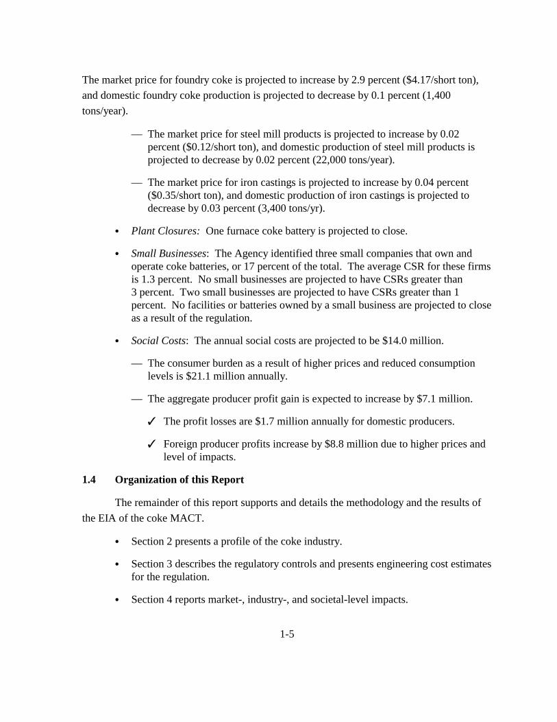
Table 2-7 provides historical data on U.S. foundry coke production at merchant

plants. Although merchant production of furnace coke has increased over time, merchant

production of foundry coke has steadily declined. As shown, U.S. production of foundry

coke has declined by two-thirds from an estimated 3.34 million short tons in 1980 to

1.11 million short tons in 1997—an average annual reduction of 3 percent. These reductions

are attributable to two factors: (1) declining demand by iron foundries, and (2) increasing

incentive to shift production toward furnace coke. During the 1980s, the demand for iron

castings declined because of the poor performance of the U.S. economy and changes in the

automotive industry (i.e., reduced demand and material substitution). As a result, one-third

of the U.S. foundries shut down operations (USITC, 1994). Reductions in demand have

continued throughout the 1990s as foundries have made technological improvements, similar

to those at blast furnaces, to reduce the amount of coke required to produce castings. In

addition, merchant producers now face increasing incentives of expected higher prices and

lower costs of producing furnace coke to meet the increasing domestic demand by integrated

steelmakers.

2.3.2 Foreign Trade

International trade has historically comprised a small portion of the U.S. coke industry

because of limitations associated with transport costs and breakage during transport.

However, trade has become increasingly important during the 1990s. Table 2-5 provides the

volume of U.S. exports and imports for coke from 1980 through 1997. As shown, the United

States has become a net importer of coke. In 1980, the volume of coke exports was

2-19

Table 2-6. U.S. Production of Furnace Coke by Producer Type: 1980-1997 (103 short tons)

Year

Integrated Producers Merchant Producers

Volume Share Volume Share Total Production

1980 41,899 97.9% 893 2.1% 42,792

1981 38,903 97.7% 912 2.3% 39,815

1982 25,374 97.3% 709 2.7% 26,083

1983 22,556 96.1% 919 3.9% 23,475

1984 26,791 95.9% 1,156 4.1% 27,947

1985 25,175 95.6% 1,148 4.4% 26,323

1986 22,251 95.0% 1,165 5.0% 23,416

1987 22,973 94.8% 1,259 5.2% 24,232

1988 25,490 94.8% 1,389 5.2% 26,879

1989 24,808 94.7% 1,378 5.3% 26,186

1990 23,892 93.7% 1,675 6.3% 25,567

1991 20,796 93.1% 1,540 6.9% 22,336

1992 20,162 92.6% 1,616 7.4% 21,778

1993 19,973 92.3% 1,673 7.7% 21,646

1994 19,444 91.7% 1,768 8.3% 21,212

1995 20,510 91.8% 1,844 8.2% 22,354

1996 19,969 91.6% 1,841 8.4% 21,810

1997 19,213 91.5% 1,790 8.5% 21,003

Average Annual Growth Rates

1980–1997 –3.2% –0.4% 5.9% 18.1% –3.0%

1980–1989 –4.5% –0.4% 6.0% 16.9% –4.3%

1989–1997 –2.8% –0.4% 3.7% 7.7% –2.5%

Source: EPA estimates.

2-20

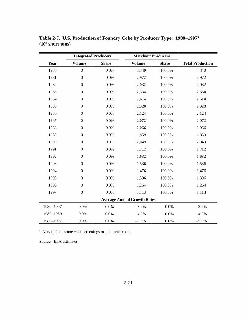
Table 2-7. U.S. Production of Foundry Coke by Producer Type: 1980–1997a

(103 short tons)

Year

Integrated Producers Merchant Producers

Volume Share Volume Share Total Production

1980 0 0.0% 3,340 100.0% 3,340

1981 0 0.0% 2,972 100.0% 2,972

1982 0 0.0% 2,032 100.0% 2,032

1983 0 0.0% 2,334 100.0% 2,334

1984 0 0.0% 2,614 100.0% 2,614

1985 0 0.0% 2,328 100.0% 2,328

1986 0 0.0% 2,124 100.0% 2,124

1987 0 0.0% 2,072 100.0% 2,072

1988 0 0.0% 2,066 100.0% 2,066

1989 0 0.0% 1,859 100.0% 1,859

1990 0 0.0% 2,049 100.0% 2,049

1991 0 0.0% 1,712 100.0% 1,712

1992 0 0.0% 1,632 100.0% 1,632

1993 0 0.0% 1,536 100.0% 1,536

1994 0 0.0% 1,476 100.0% 1,476

1995 0 0.0% 1,396 100.0% 1,396

1996 0 0.0% 1,264 100.0% 1,264

1997 0 0.0% 1,113 100.0% 1,113

Average Annual Growth Rates

1980–1997 0.0% 0.0% –3.9% 0.0% –3.9%

1980–1989 0.0% 0.0% –4.9% 0.0% –4.9%

1989–1997 0.0% 0.0% –5.9% 0.0% –5.9%

a May include some coke screenings or industrial coke.

Source: EPA estimates.

2-21

2.1 million short tons, while the volume of coke imports was only 0.7 million short tons. By

1997, coke exports had declined by almost 60 percent from 1980 to 0.8 million short tons,

and coke imports had increased by almost 400 percent to 3.2 million short tons. The decline

in coke exports resulted from reductions in coke production associated with the declining

U.S. steel industry during the 1980s. Despite the U.S. steel industry’s turnaround during the

1990s, coke exports have continued to decline as they are crowded out by increasing

domestic demand. The dramatic increase in imports has resulted from the improved U.S.

economy and increasing demand for U.S. steel products since the late 1980s. These factors

combined with previous and continued closings of U.S. coke plants have caused an aggregate

coke deficit at integrated iron and steel mills during the 1990s as domestic supply is not able

to keep pace with demand for coke.

2.3.3 Market Prices

Historical data on market prices for coke are not directly available from public

sources nor can they be derived from the sources providing market volumes. Based on

discussions with DOE’s EIA, the USITC (1994) is the only known source of recent market

prices for coke. These market prices are reported as net f.o.b. at plant and are based on

industry responses to the USITC questionnaire. According to the USITC (1994), a vast

majority of coke is sold under long-term contracts ranging from 1 to 6 years. These contracts

typically provide for semiannual or annual renegotiation so that contract prices are closely

related to open market prices. Thus, because a large share of coke is purchased through

contracts, the USITC provides prices for both contract sales and spot market sales.

Table 2-8 provides market prices by type of coke product for 1990 through 1993. As

shown, the spot market price is generally higher than the contract sales price and both seem

positively correlated over time. The table also provides a weighted average price based on

the volume sold through contracts and the spot market for each year. As shown, the weighted

average market price for furnace coke was roughly $100 per short ton in 1993 and has

declined since 1990. The market price for foundry coke is typically 50 percent higher than

for furnace coke. In 1993, the weighted average market price for foundry coke was $154 per

short ton and has slightly increased since 1990. Table 2-8 also provides the market prices for

other industrial coke and coke breeze. Industrial coke had a weighted average market price

of $113 per short ton in 1993, while coke breeze was priced at $44 per short ton.

2-22

Table 2-8. Market Prices of Coke by Type: 1990–1993a ($ per short ton)

Spot Market Sales Weighted Average Product/Year Contract Sales Price Price Price

Furnace coke

1990 $106.62 $113.87 $107.06

1991 $103.99 $111.26 $105.00

1992 $103.05 $81.55 $102.50

1993b $101.18 $71.12 $100.69

Foundry coke

1990 $149.06 $151.86 $149.82

1991 $153.55 $147.60 $151.83

1992 $152.26 $153.60 $152.58

1993b $152.90 $156.35 $153.75

Other industrial coke

1990 $119.98 $117.53 $119.21

1991 $117.07 $118.06 $117.41

1992 $115.13 $117.46 $115.25

1993b $112.08 $115.89 $112.29

Coke breeze

1990 $42.83 $69.01 $43.31

1991 $44.42 $70.67 $44.94

1992 $45.42 $59.78 $45.88

1993b $43.35 $70.38 $43.91

a Market prices are reported as net f.o.b. at plant. b Reflects prices observed for January through June 1993.

Source: U.S. International Trade Commission. 1994. Metallurgical Coke: Baseline Analysis of the U.S. Industry and Imports. Publication No. 2745. Washington, DC: USITC.

2-23

2.3.4 Future Projections

Future projections for the U.S. coke industry depend on several uncertain and

interdependent factors including trends in integrated steelmaking and iron casting,

compliance with environmental regulation, investments in or closures of domestic coke

capacity, quality and availability of imports, and economic performance of domestic

producers. For furnace coke, most analysts agree that U.S. capacity and production will

decline faster than consumption and result in continued coke shortfalls to be met by foreign

imports. Based on a survey of studies, the USITC (1994) reports that U.S. furnace coke

capacity is expected to decline by between 10 to 37 percent from 1990 through 2000, while

U.S. consumption is expected to decline by between 10 to 23 percent. During the 1990s,

furnace coke capacity at U.S. integrated producers has already declined by 27 percent from

24.2 million short tons in 1990 to 17.6 million short tons per year in 1997 (USITC, 1994;

EPA, 1998). This decline in capacity at integrated producers has been partially offset by

increases in furnace coke capacity at merchant producers from 2.7 million short tons in 1990

to roughly 4 million short tons in 1997 (USITC, 1994; EPA, 1998).

Assuming current rates of investment in existing coke batteries at integrated

producers, furnace coke production in the United States is not expected to exceed 16 million

short tons per year through 2000 (Agarwal et al., 1996). Alternatively, assuming integrated

steelmakers demand between 52 to 59 million tons per year of molten iron, furnace coke

consumption is estimated at between 18 to 22 million tons per year in 2000 (Agarwal et al.,

1996). This projected consumption level also assumes that injection of natural gas and coal

will continue to increase, thereby reducing coke rates and decreasing demand for coke by an

additional 1.2 to 2 million short tons per year. If steel demand is low (i.e., 52 to 54 million

tons per year), then coke demand will be satisfied at the current import level of 3 million tons

per year. However, if this demand is high (i.e., 56 to 59 million tons per year), then coke

imports would likely increase to 6 million tons per year. Agarwal et al. (1996) predict that

this increase in foreign imports may lead to future increases in coke prices and trigger a

scramble for coke.

For foundry coke, most analysts agree that U.S. capacity will be stable and sufficient

to meet future demands by iron foundries. The American Foundryman’s Society has

projected the demand for iron castings to be between 9 and 10.5 million short tons through

2004 (Stark, 1995). Based on casting yields of 55 percent, metal to coke ratios of 8 to 1, and

a cupola-melting share at 64 percent of total, Stark (1995) projects foundry coke demand to

2-24

range from 1.3 to 1.5 million short tons per year through 2004. As of 1997, total merchant

plant capacity was 5.6 million short tons per year with roughly 2.1 million tons for foundry

coke. Therefore, existing foundry coke capacity will exceed the projected demand and likely

cause merchant producers to increasingly rely on furnace coke to fill this excess capacity

(Stark, 1995).

2-25

SECTION 3

ENGINEERING COST ANALYSIS

Control measures implemented to comply with the MACT standard will impose

regulatory costs on coke batteries. This section presents compliance costs for typical

“model” batteries and the national estimate of compliance costs associated with the proposed

rule. These engineering costs are defined as the annual capital and operating and

maintenance costs assuming no behavioral market adjustment by producers or consumers.

For input to the EIA, engineering costs are expressed per unit of coke production and used to

shift the coke supply functions in the market model.

The proposed MACT will cover the Coke Ovens: Pushing, Quenching, and Battery

Stacks source category. It will affect all 58 by-product coke oven batteries at 23 coke plants.

The processes covered by the proposed regulation include pushing the coke from the coke

oven, quenching the incandescent coke with water in a quench tower, and maintaining the

battery stack that is the discharge point for the underfiring system. Capital, operating and

maintenance, and monitoring costs were estimated for 10 representative model batteries.

Model battery costs were linked to the existing population of coke batteries to estimate the

national costs of the regulation.

3.1 Overview of Emissions from Coke Batteries

The listed HAPs of concern in coke oven emissions include hundreds of organic

compounds formed when volatiles are thermally distilled from the coal during the coking

process. Traditionally, benzene-soluble organics and methylene chloride-soluble organics

have been used as surrogate measures of coke oven emissions. The primary constituents of

concern are polynuclear aromatic hydrocarbons (PAHs). Other constituents include benzene,

toluene, and xylene.

Coke oven emissions from pushing and quenching occur when the coal has not been

fully coked, which is called a “green” push. A green push produces a dense cloud of coke

oven emissions that is not captured and controlled by the emission control systems used for

particulate matter. Coke oven emissions from battery stacks occur when raw coke oven gas

3-1

leaks through the oven walls, enters the flues of the underfiring system, and is discharged

through the stack. Coke oven emissions from these sources are controlled by pollution

prevention activities, diagnostic procedures, and corrective actions. One component of the

control technology is the operating and maintenance of the general battery to prevent green

pushes and stack emissions.

Based on limited test data and best engineering judgment, the proposed standards are

expected to reduce coke oven emissions from pushing, quenching, and battery stacks by

about 50 percent. There is significant uncertainty in attempts to estimate emissions and

emission reductions because the emissions are fugitive in nature. For example, the emissions

from green coke during pushing and quenching are not enclosed or captured in a conveyance,

which makes accurate measurement of concentrations and flow rates very difficult.

3.2 Approach for Estimating Compliance Costs

The costs for individual batteries to achieve the MACT level of control will vary

depending on the battery condition and control equipment in place. There is uncertainty in

determining exactly what costs will be incurred by each battery. Consequently, several

model batteries were developed to represent the range of battery types and conditions to place

bounds on the probable costs. The emission control programs and equipment in place at the

best controlled batteries were investigated, and the associated costs were obtained. The costs

were then applied to the model batteries to estimate the cost necessary to comply with the

MACT level. A model battery was assigned to each actual battery based on available

emissions data, knowledge of battery condition, and engineering judgment. Errors in

underestimating and overestimating costs for individual batteries will tend to cancel when

summing these costs to estimate total nationwide costs.

3.3 Costs for MACT Performance

The MACT standard involves a routine program of systematic operating and

maintenance and oven repairs to control emissions from battery stacks and pushing. An

important element of this routine program for battery stacks is the use of continuous opacity

monitors (COMs). In addition, control of quenching emissions will require the installation of

baffles in three quench towers that do not have them.

Several plants were surveyed to obtain cost information on the technologies that

comprise the MACT standard. Basic oven repairs include spray patching, ceramic welding,

mobile gunning, silica dusting, end flue repairs, and through-wall brickwork. An annual

3-2

baseline program of oven repairs was developed from the frequency of oven repairs at USS

Clairton Works and includes spray patching, end flue repairs, and through-wall repairs.

Annual estimated costs for oven repairs range from $31,000 to $564,000 per battery.

Another element of the cost of the MACT is monitoring, which involves observing

four pushes per battery per day and bag leak detection systems for batteries that control

pushing emissions with baghouses. The average time to observe four pushes is estimated to

be about 1 hour, allowing for some delays and time for the observer to get into position. (For

batteries operated as three in a battery unit, the time may be as short as 15 to 20 minutes, and

for some foundry batteries, the observation time may be 1.5 hours or more.) Two hours per

plant are allowed for observer travel time and data reduction. For a typical inspection labor

charge of $30/hour, the inspection cost per plant per year would be

$/yr = 365 days/yr * $30/hr * [1 hr/battery * number of batteries + 2 hr/plant * 1 plant] =

$11,000 * number of batteries + $22,000.

The installed capital cost for bag leak detectors provided by vendors is $9,000 per baghouse.

Annual operating and maintenance costs are estimated to be $500/yr per detector.

3.4 Costs for Model Batteries

The model batteries are described in Table 3-1. Two groups are defined: one to

represent foundry coke by-product batteries and one to represent furnace coke by-product

batteries. These groups are further subdivided into models that represent different battery

conditions that affect emissions and the cost to improve emission control. For example,

Group A represents batteries that already achieve the MACT level of control and will not

incur significant additional expenses. Group B represents batteries that must implement a

baseline program similar to that at the MACT batteries, but they will not incur significant

capital investment. Group C represents batteries that will incur capital expenses to repair and

upgrade oven walls and end flues and, in addition, must implement a baseline program of

continuing diagnostics and repair. Group D batteries in the furnace coke group represent the

newer 6-meter batteries that are generally in a state of good repair.

3-3

Tab

le 3

-1.

Mod

el B

atte

ries

Bat

tery

co

nditi

on

Fou

ndry

By-

Pro

duct

Rec

over

y B

atte

ries

(1

2 ba

tter

ies

at 6

pla

nts)

F

urna

ce B

y-P

rodu

ct R

ecov

ery

Bat

teri

es

(46

batt

erie

s at

17

plan

ts)

1A

1B

1C

2A

2B

2C

2D

No

sign

ific

ant

cost

s fo

r pu

shin

g or

st

acks

Will

req

uire

ba

selin

e re

pair

pr

ogra

m

Will

req

uire

ba

selin

e re

pair

pr

ogra

m p

lus

2 th

roug

h-w

alls

, 10

end

flue

s, a

nd s

pray

pa

tchi

ng o

n 50

pe

rcen

t of

oven

s

No

sign

ific

ant

cost

s fo

r pu

shin

g or

st

acks

Will

req

uire

ba

selin

e re

pair

pr

ogra

m

Will

req

uire

bas

elin

e re

pair

pro

gram

plu

s 2

thro

ugh-

wal

ls, 1

0 en

d fl

ues,

and

spr

ay

patc

hing

on

50

perc

ent o

f ov

ens

No

addi

tiona

l co

sts

for

push

ing

or

stac

ks

No.

of

oven

s 41

63

77

Hei

ght (

m)

4 4

6

Cok

ing

time

27

19

18

(hrs

)

Cok

e pr

oduc

tion

(tpy

)

89,0

00

320,

000

830,

000

3-4

The cost elements associated with the model batteries are given below:

1. Model Battery Groups A and D—MACT batteries: no significant additional

repair costs.

2. Model Battery Group B—Must implement a baseline program like the one at USS

Clairton.

3. Model Battery Group C—Must implement a baseline program like the one at USS

Clairton plus additional one-time repairs and rebuilds to put them on par with the

Group B batteries: assume spray patching of 50 percent of the ovens, two

through-wall repairs, and 10 end flue repairs per battery. These repairs will be

treated as a capital cost.

4. Monitoring—all groups: Cost of COM for those batteries that do not have one

and cost of observing four pushes per day for those not already doing it, as well as

bag leak detection system for plants with baghouses. These costs will be assigned

on a battery-specific basis.

5. Quenching—Apply the cost of baffles to those plants that do not have them.

These costs will also be assigned on a battery-specific basis.

Model battery costs are summarized in Table 3-2. For the Model A batteries (batteries that

can already achieve the MACT level of control), the lower end of the range (no additional

costs) represents those batteries that already have COMs and pushing emission observers, and

the upper end of the range represents batteries that must install COMs and hire pushing

emission observers. The Model B batteries’ costs include the cost of monitoring plus the

implementation of a baseline program. The Model C batteries’ costs are based on a capital

expenditure to rebuild or upgrade ovens, plus the costs of monitoring and the baseline

program. The Model D furnace coke batteries have the same cost elements for monitoring as

the Model A group.

3-5

Table 3-2. MACT Compliance Cost Estimates by Model Coke Battery ($1998)

Total Costs ($103)

Annual Annual Total Capital Capitala Operating Annual

Foundry Coke Model Battery

Ab 0 to 46 0 to 6 0 to 42 0 to 48

B 46 6 317 323

C 2,550 241 317 558

Furnace Coke Model Battery

Ab 0 to 46 0 to 6 0 to 42 0 to 48

B 46 6 442 448

C 2,550 241 442 683

Db 0 to 46 0 to 6 0 to 42 0 to 48

a Reflects capital recovery based on a 20-year life and 7 percent interest for pushing controls and baffles and a 10-year life and 7 percent interest for monitoring equipment.

b The range includes those batteries already performing monitoring and those that do not.

3.5 Estimates of National Engineering Costs

National engineering costs were estimated by assigning model batteries to each actual

battery and then applying the model battery costs (adjusted for the number of ovens in each

actual battery). For example, batteries that have already achieved the MACT control level

are in Groups A and D, and these batteries will incur no additional control costs. However,

some of these batteries will incur monitoring costs if they do not already have a COM or if

they are not observing four pushes per day. The Group B batteries will incur costs to

implement the baseline program (at $6,100/oven per year). Group C batteries will incur the

capital cost of through-wall repairs, end flue repairs, and spray patching (at $2,500,000 +

3-6

$525 * [50% of the ovens]) plus the cost of the baseline program. All batteries without

baffles in their quench tower are assumed to install new baffles.

The costs of COMs are applied to each stack that currently does not have one. In

addition, bag leak detectors are assumed to be installed for each baghouse. In cases where a

single baghouse serves multiple batteries, the cost of the bag leak detection system ($9,000)

is distributed among the batteries.

Table 3-3 presents the cost elements of the MACT and the number of batteries for

each model battery type that will incur costs for that element. Individual battery annualized

compliance costs range from $0 to $679,000, with a mean of $243,000 and a median of

$209,000.

The aggregate capital, operating, and total national annual costs are given in Table

3-4. Total annualized engineering costs are estimated to be approximately $14.1 million per

year (1998 dollars).1 Oven repair accounts for approximately 86 percent of total annualized

costs, and monitoring accounts for the remaining 14 percent.

1Annualized costs were converted to 1997 dollars for the EIA to match the latest market data available. Total annualized costs in 1997 dollars are $14.2 million.

3-7

Tab

le 3

-3.

Num

ber

of C

oke

Bat

teri

es I

ncur

ring

MA

CT

Com

plia

nce

Cos

ts:

1998

Num

ber

of B

atte

ries

Req

uiri

ng

Num

ber

of

Bas

elin

e B

affl

es in

C

onti

nuou

s V

isib

le

Bat

teri

es

Ove

n R

epai

r Q

uenc

h O

paci

ty

Em

issi

on

Bag

Lea

k M

odel

Bat

tery

Des

crip

tion

R

epre

sent

ed

Reb

uild

s P

rogr

am

Tow

er

Mon

itor

O

bser

ver

Det

ecto

r

1A:

Fou

ndry

cok

e ba

ttery

in

3 0

0 0

3 3

3 go

od c

ondi

tion

1B:

Fou

ndry

cok

e ba

ttery

; nee

ds

10

0 10

2

7 10

8

base

line

repa

ir p

rogr

am

1C:

Fou

ndry

cok

e ba

ttery

; nee

ds

3 3

10

1 3

3 0

exte

nsiv

e ov

en r

ebui

ld a

nd

base

line

repa

ir p

rogr

am

2A:

Fur

nace

cok

e ba

ttery

in

14

0 0

0 4

14

11

good

con

ditio

n

2B:

Fur

nace

cok

e ba

ttery

; nee

ds

17

0 17

0

10

17

15

base

line

repa

ir p

rogr

am

2C:

Fur

nace

cok

e ba

ttery

; nee

ds

3 2

3 0

3 3

0 ex

tens

ive

oven

reb

uild

and

ba

selin

e re

pair

pro

gram

2D:

Fur

nace

cok

e ba

ttery

; new

er

8 0

0 0

1 6

5 6-

met

er; i

n go

od c

ondi

tion

Tot

als

58

5 40

3

3156

42

3-8

Tab

le 3

-4.

Nat

iona

l MA

CT

Com

plia

nce

Cos

ts b

y M

odel

Cok

e B

atte

ry:

1998

Tot

al A

nnua

l Cos

t ($

103 /y

r)

Mod

el B

atte

ry D

escr

ipti

on

Num

ber

of

Bat

teri

es

Ann

ual C

apit

al C

ost

($10

3 ) O

pera

ting

Cos

t ($

103 /y

r)

Ove

n R

epai

r,

Baf

fles

M

onit

orin

g

Ove

n R

epai

r,

Baf

fles

M

onit

orin

g

Ove

n R

epai

r,

Baf

fles

M

onit

orin

g

1A:

Fou

ndry

cok

e ba

ttery

in

3 $0

$9

2 $0

$6

1 $0

$7

4 go

od c

ondi

tion

1B:

Fou

ndry

cok

e ba

ttery

; 10

$1

40

$212

$2

,043

$2

62

$2,4

16

$292

ne

eds

base

line

repa

ir

prog

ram

1C:

Fou

ndry

cok

e ba

ttery

; 3

$5,3

12

$74

$732

$8

2 $1

,231

$9

3 ne

eds

exte

nsiv

e ov

en

rebu

ild a

nd b

asel

ine

repa

ir p

rogr

am

2A:

Fur

nace

cok

e ba

ttery

in

14

$0

$193

$0

$4

63

$0

$491

go

od c

ondi

tion

2B:

Fur

nace

cok

e ba

ttery

; 17

$0

$4

33

$6,7

89

$644

$6

,789

$7

06

need

s ba

selin

e re

pair

pr

ogra

m

2C:

Fur

nace

cok

e ba

ttery

; 3

$5,0

34

$111

$1

,220

$1

23

$1,6

93

$139

ne

eds

exte

nsiv

e ov

en

rebu

ild a

nd b

asel

ine

repa

ir p

rogr

am

2D:

Fur

nace

cok

e ba

ttery

; 8

0 82

0

209

0 22

0 ne

wer

6-m

eter

; in

good

co

nditi

on

Tot

als

58

10,4

86

1,19

7 10

,784

1,

844

12,1

29

2,01

5

3-9

SECTION 4

ECONOMIC IMPACT ANALYSIS

The proposed rule to control the release of HAPs from coke pushing and quenching

operations will directly (through imposition of compliance costs) or indirectly (through

changes in market prices) affect the entire U.S. iron and steel industry. Implementation of the

proposed rule will increase the costs of producing furnace and foundry coke at affected

facilities. As described in Section 3, these costs will vary across facilities and their coke

batteries depending upon their physical characteristics and baseline controls. The response

by these producers to these additional costs will determine the economic impacts of the

regulation. Specifically, the impacts will be distributed across producers and consumers of

coke, steel mill products, and iron castings through changes in prices and quantities in the

affected markets. This section presents estimates of the economic impacts of the coke

MACT using an economic model that captures the linkages between the furnace coke and

steel mill products, and foundry coke and iron castings markets.

This section describes the data and approach used to estimate the economic impacts

of this proposed rule for the baseline year of 1997. Section 4.1 presents the inputs for the

economic analysis, including characterization of producers, markets, and the costs of

compliance. Section 4.2 summarizes the conceptual approach to estimating the economic

impacts on the affected industries. A fully detailed description of the economic impact

methodology is provided in Appendix A. Lastly, Section 4.3 provides the results of the

economic impact analysis.

4.1 EIA Data Inputs

Inputs to the economic analysis are a baseline characterization of directly and

indirectly affected producers, their markets, and the estimated costs of complying with the

proposed rule.

4.1.1 Producer Characterization

As detailed in Section 2, the baseline characterization of integrated and merchant

manufacturing plants is based on the facility responses to EPA’s industry survey and industry

4-1

data sources. These plant-specific data on existing sources were supplemented with

secondary information from the 1998 Directory of Iron and Steel Plants published by the

Association of Iron and Steel Engineers and World Cokemaking Capacity published by the

International Iron and Steel Institute, as well as coke-specific cost equations as developed for

the 1993 Coke Ovens MACT (as described fully in Appendix B).

4.1.2 Market Characterization

Figure 4-1 summarizes the market interactions included in the Agency’s EIA

modeling approach. Changes in the equilibrium price and quantity due to control costs on

coke batteries were estimated simultaneously in four linked markets:

� market for furnace coke,

� market for foundry coke,

� market for steel mill products, and

� market for iron castings.

As described in Section 2, many captive coke plants supply their excess coke to the

furnace coke market. Merchant coke plants and foreign imports account for the remaining

supply to the furnace coke market. Furnace coke produced at captive coke plants and shipped

directly to integrated iron and steel mills owned by their parent companies does not directly

enter the market for furnace coke. However, compliance costs incurred by captive, or “in-

house”, furnace coke batteries indirectly affect the furnace coke market through price and

output changes in the steel mill products market.

The market demand for furnace coke is derived from integrated mills producing steel

mill products. Integrated iron and steel mills that need more coke than their captive batteries

can produce purchase furnace coke from the market. Integrated mills’ market (and captive)

demand for furnace coke depends on their production levels as influenced by the market for

steel mill products. Steel mill products are supplied by three general groups: integrated iron

and steel mills, nonintegrated steel mills (primarily mini-mills), and imports. Domestic

consumers of steel mill products and exports account for the market demand.

As described in Section 2, merchant plants are the sole suppliers of foundry coke to

the market. Based on U.S. industry production and consumption data, foreign imports of

4-2

Consumers of Steel Consumers of Mill Products Iron Castings

Merchant Coke Plants

• Finishing Mills • Steelmaking Furnace • Blast Furnace

Captive Coke Plants

Market for Foundry Coke

Imports

Imports

Exports

Integrated Iron and Steel Mills

Exports

Market for Furnace Coke

Electric Furnaces

Cupola Furnaces

Control Costs

Market for Steel

Mill Products

Nonintegrated Steel Mills (including minimills)

Market for Iron Castings

Imports

Exports

Figure 4-1. Market Linkages Modeled in the Economic Impact Analysis

4-3

foundry coke in 1997 were negligible.1 Consumers of foundry coke include foundries with

cupolas that produce iron castings, and they are modeled using aggregate market demand

curves.2

Table 4-1 provides the 1997 data on the U.S. furnace and foundry coke, steel mill

products, and iron castings markets for use in this analysis. The market price for steel mill

products was obtained from Current Industrial Reports (CIR), (U.S. DOC, 1997) and reflects

the production-weighted average across all product types. The market price for iron castings

was also obtained from CIR and reflects the production-weighted average across iron castings

(ductile, gray, and malleable). Market prices for each coke product were determined,

consistent with economic theory, by the highest-cost merchant producer. Domestic

production from affected facilities reflects the aggregate of the plant-specific data presented

in Section 2, while unaffected domestic production is derived either directly from secondary

sources or as the difference between observed total U.S. production and the aggregate

production from affected facilities. Foreign trade data were obtained from industry and

government statistical publications supplemented by survey data. Market volumes for each

product are then computed as the sum of U.S. production and foreign imports.

4.1.3 Regulatory Control Costs

As shown in Section 3, the Agency developed compliance cost estimates for model

plants that may be mapped to each of the coke manufacturing facilities affected by the

proposed rule. These estimates reflect the “most-reasonable” scenario for this industry. To

be consistent with the 1997 baseline industry characterization of the economic model, the

Agency adjusted the compliance cost estimates from 1998 dollars to 1997 dollars using the

producer price index3. These cost estimates serve as inputs to the economic

1Recent studies have indicated an increasing trend of foreign imports of foundry coke, primarily from China (USITC, 2000). Including foreign suppliers of foundry coke in the economic model would lead to smaller price changes as imports replace some domestic production. However, the U.S. ITC report indicated that lower quality of imported foundry coke and future environmental regulations being proposed in China may limit the market penetration of foreign foundry coke in the United States.

2Other coke, frequently grouped with foundry coke, is purchased as a fuel input by cement plants, chemical plants, and nonferrous smelters. However, other coke represents only 2 percent of U.S. coke production in 1997. For simplicity, supply and demand for other coke are assumed to be unaffected by the proposed coke regulation and are not included in the market model.

131.8 � 1.008

130.7 3Finished Goods 1982 = 100.

4-4

Table 4-1. Baseline Characterization of U.S. Iron and Steel Markets: 1997

Baseline

Furnace Coke

Market price ($/short ton)

Market output (103 tpy)

Domestic production

Imports

Foundry Coke

Market price ($/short ton)

Market output (103 tpy)

Domestic production

Imports

Steel Mill Products

Market price ($/short ton)

Market output (103 tpy)

Domestic production

Integrated producers

Nonintegrated steel millsa

Imports

Iron Castings

Market price ($/short ton)

Market output (103 tpy)

Domestic production

Cupola furnaces

Electric furnacesb

Imports

$107.36

11,710

7,944

3,765

$145.02

1,669

1,669

NA

$639.74

137,015

105,858

62,083

43,775

31,157

$845.55

12,314

11,483

6,695

4,789

831 a Includes mini-mills. b Includes electric arc or electric induction furnaces.

4-5

analysis and affect the operating decisions for each affected facility and thereby the markets

that are served by these facilities.

4.2 EIA Methodology Summary

In general, the EIA methodology needs to allow EPA to consider the effect of the

different regulatory alternatives. Several types of economic impact modeling approaches

have been developed to support regulatory development. These approaches can be viewed as

varying along two modeling dimensions:

� the scope of economic decision making accounted for in the model, and

� the scope of interaction between different segments of the economy.

Each of these dimensions was considered in selecting the approach used to model the

economic impact of the proposed coke regulation.

To conduct the analysis for the proposed coke regulation, the Agency used a market

modeling approach that incorporates behavioral responses in a multiple-market partial

equilibrium model. Multiple-market partial equilibrium analysis provides a manageable

approach to incorporate interactions between coke, steel mill product, and iron castings

markets into the EIA to better estimate the proposed regulation’s impact. The multiple-

market partial equilibrium approach represents an intermediate step between a simple, single-

market partial equilibrium approach and a full general equilibrium approach. The modeling

technique is to link a series of standard partial equilibrium models by specifying the

interactions between the supply and demand for products and then solving for changes in

prices and quantities across all markets simultaneously. The EIA methodology is fully

detailed in Appendix A.

The Agency’s methodology is soundly based on standard microeconomic theory

relying heavily on previous economic analyses, employs a comparative static approach, and

assumes certainty in relevant markets. For this analysis, prices and quantities are determined

in perfectly competitive markets for furnace coke, foundry coke, finished steel mill products,

and iron castings. The competitive model of price formation, as shown in Figure 4-2 (a),

posits that market prices and quantities are determined by the intersection of market supply

and demand curves. Under the baseline scenario, a market price and quantity (P, Q) are

determined by the downward-sloping market demand curve (DM) and the upward-sloping

4-6

S a S u

p+

SM

DM

p = p

qa qu Q

Affected Facilities Unaffected Facilities Market

a) Baseline Equilibrium

p�

S a S� a

p�

S u

p�

p + p = p

SM�

DM

SM

q� a qa qu q� u Q� Q

Affected Facilities Unaffected Facilities Market

b) With-Regulation Equilibrium

Figure 4-2. Market Equilibrium without and with Regulation

4-7

market supply curve (SM) that reflects the horizontal summation of the individual supply

curves of directly affected and indirectly affected facilities that produce a given product.

With the regulation, the cost of production increases for directly affected producers.

The imposition of the compliance costs is represented as an upward shift in the supply curve

for each affected facility from Sa to Sa�. As a result, the market supply curve to shift upward

to SM� as shown in Figure 4-2(b) reflecting the increased costs of production at these

facilities. In the baseline scenario without the proposed standards, the industry would

produce total output, Q, at the price, P, with affected facilities producing the amount qa and

unaffected facilities accounting for Q minus qa, or qu. At the new equilibrium with the

regulation, the market price increases from P to P� and market output (as determined from the

market demand curve, DM) declines from Q to Q�. This reduction in market output is the net

result from reductions at affected facilities and increases at unaffected facilities.

4.3 Economic Impact Results

Based on the simple analytics presented above, when faced with higher costs of coke

production, producers will attempt to mitigate the impacts by making adjustments to shift as

much of the burden on other economic agents as market conditions allow. The adjustments

available to facility operators include changing production processes, changing inputs,

changing output rates, or even closing the facility. This analysis focuses on the last two

options because they appear to be the most viable for coke manufacturing facilities, at least in

the near-term. A large segment of the furnace and foundry coke market is affected by the

regulation so we would expect upward pressure on prices as producers reduce output rates in

response to higher costs. Higher prices reduce quantity demanded and output for each market

product, leading to changes in profitability of batteries, facilities, and firms. These market

and industry adjustments will also determine the social costs of the regulation and its

distribution across stakeholders (producers and consumers).

To estimate these impacts, the economic modeling approach described in Appendix A

was operationalized in a multiple spreadsheet model. This model characterizes those

producers and consumers identified in Figure 4-1 and their behavioral responses to the

imposition of the regulatory compliance costs. These costs are expressed per ton of furnace

or foundry coke and serve as the input to the economic model, or “cost-shifters” of the

baseline supply curves at affected facilities. Given these costs, the model determines a new

equilibrium solution in a comparative static approach. The following sections provide the

Agency’s estimates of the resulting economic impacts for the proposed rule.

4-8

4.3.1 Market-Level Impacts

The increased cost of coke production due to the regulation is expected to increase the

price of coke, steel mill products, and iron castings and reduce their production and

consumption from 1997 baseline levels. As shown in Table 4-2, the regulation is projected to

increase the price of furnace coke by 1.5 percent, or $1.56 per short ton, and the price of

foundry coke by nearly 3 percent, or $4.17 per short ton. The increased captive production

costs and higher market price associated with furnace coke are projected to increase steel mill

product prices by less than 0.1 percent, or $0.12 per ton. Similarly, the higher market price of

foundry coke are projected to increase iron castings prices by less than 0.1 percent, or $0.35

per ton. As expected, directly affected output declines across all producers, while supply

from domestic and foreign producers not subject to the regulation increases. Although the

resulting net declines are slight across all products (i.e., roughly 0.1 percent decline in market

output) the change in domestic production is typically higher than 0.1 percent. This is

especially true for furnace coke where domestic production declines by 2.25 percent.

4.3.2 Industry-Level Impacts

Industry revenue, costs, and profitability change as prices and production levels adjust

to increased production costs. As shown in Table 4-3, the economic model projects that

profits for directly affected integrated iron and steel producers will decrease by $10.8 million,

or 0.8 percent. In addition, the Agency projects profit losses of $4.6 million for foundries

that produce iron casting with cupola furnaces. However, because integrated steel mills

reduce their captive production of furnace coke and purchase more through the market,

industry-level profits for U.S. merchant coke producers are expected to increase by $2.7

million, or 5.6 percent, for furnace coke. Similarly, because foundries with cupola furnaces

must continue to buy foundry coke to produce iron castings (i.e., inelastic demand), industry-

level profits for U.S. merchant coke producers are expected to increase by $3.9 million, or

5.0 percent, for foundry coke. Those domestic suppliers not subject to the regulation

experience windfall gains with non-integrated steel mills (i.e., mini-mills) increasing profits

by $5.4 million and foundries with electric furnaces increasing profits by $1.7 million.

4-9

Table 4-2. Market-Level Impacts of the Proposed Coke MACT: 1997

Changes From Baseline

Baseline Absolute Percent

Furnace Coke

Market price ($/short ton) $107.36 $1.56 1.46%

Market output (103 tpy) 11,710 –11.8 –0.10%

Domestic production 7,944 –178.7 –2.25%

Imports 3,765 166.9 4.43%

Foundry Coke

Market price ($/short ton) $145.02 $4.17 2.87%

Market output (103 tpy) 1,669 –1.4 –0.08%

Domestic production 1,669 –1.4 –0.08%

Imports NA NA NA

Steel Mill Products

Market price ($/short ton) $639.74 $0.12 0.02%

Market output (103 tpy) 137,015 –16.0 –0.01%

Domestic production 105,858 –21.9 –0.02%

Integrated producers 62,083 –30.3 –0.05%

Nonintegrated steel millsa 43,775 8.4 0.02%

Imports

Iron Castings

Market price ($/short ton)

Market output (103 tpy)

Domestic production

Cupola furnaces

Electric furnacesb

Imports

31,157 6.0 0.02%

$845.55 $0.35 0.04%

12,314 –3.1 –0.03%

11,483 –3.4 –0.03%

6,695 –5.4 –0.08%

4,789 2.0 0.04%

831 0.3 0.04 a Includes mini-mills. b Includes electric arc or electric induction furnaces.

4-10

Table 4-3. National-Level Industry Impacts of the Proposed Coke MACT: 1997

Integrated Iron and Steel Mills Total revenues ($106/yr)

Steel mill products Market coke operations

Total costs ($106/yr) Control costs

Steel production Captive coke production Market coke production

Production costs Steel production Captive coke production Market coke consumption Market coke production

Operating profits ($106/yr) Iron and steel facilities (#) Coke batteries (#) Employment (FTEs) Coke Producers (Merchant Only) Furnace

Revenues ($106/yr) Costs ($106/yr)

Control costs Production costs

Operating profits ($106/yr) Coke batteries (#) Employment (FTEs) Foundry

Revenues ($106/yr) Costs ($106/yr)

Control costs Production costs

Operating profits ($106/yr) Coke batteries (#) Employment (FTEs) Nonintegrated Steel Millsa

Operating profits ($106/yr) Cupola Furnaces

Operating profits ($106/yr) Electric Furnacesb

Operating profits ($106/yr) a Includes mini-mills.

Changes From Baseline

Baseline Absolute Percent

$40,223.9 –$10.50 –0.03% $39,716.9 –$11.80 –0.03%

$507.0 $1.29 0.26% $38,837.5 $0.25 –0.01%

$0.0 $8.43 NA $0.0 $0.00 NA $0.0 $6.29 NA $0.0 $2.14 NA

$38,837.5 –$8.17 –0.02% $36,292.9 –$18.25 –0.05%

$942.5 –$0.30 –0.03% $1,167.8 $16.11 1.38%

$434.3 –$5.74 –1.32% $1,386.4 –$10.76 –0.78%

20 0 0.00% 37 0 0.00%

67,198 –39 –0.06%

$366.5 –$10.01 –2.73% $318.5 –$12.69 –3.98%

$0.0 $2.16 NA $318.5 –$14.85 –4.66% $48.0 $2.68 5.59% 13 –1 –7.69%

840 –126 –15.00%

$273.3 $7.03 2.57% $194.2 $3.10 1.60%

$0.0 $3.30 NA $194.2 –$0.20 –0.10% $79.1 $3.93 4.96%

12 0 0.00% 2,420 0 0.00%

NA $5.4 NA

NA –$4.6 NA

NA $1.7 NA

b Includes electric arc or electric induction furnaces. c Includes iron foundries that use electric arc or electric induction furnaces.

4-11

4.3.2.1 Changes in Profitability

For integrated steel mills, operating profits decline by $10.8 million. This is the net

result of three effects:

� Net decrease in revenue ($10.5 million): Steel mill product revenue decreases as a result of reductions in output. However, these losses were mitigated by increased revenues from furnace coke supplied to the market as a result of higher prices.

� Net decrease in production costs ($8.2 million): Reduction in steel mill and market coke production costs occur as output declines. However, producers also experience increases in costs associated with the higher price of inputs (i.e., furnace coke).

� Increase in control costs ($8.4 million): The costs of captive production of furnace coke increase as a result of regulatory controls.

Industry-wide profits for merchant furnace coke producers increase by $2.7 million as

a result of the following:

� Decreases in revenue ($10 million): Reductions in output outweigh revenue increases as a result of higher market prices.

� Reduction in production costs ($14.9 million): Reduction in coke production costs occurs as output declines.

� Increased control costs ($2.2 million): The cost of producing furnace coke increases as a result of regulatory controls.

Industry-wide profits for merchant foundry coke producers increase by $3.9 million

under the regulation:

� Increase in revenue ($7.0 million): Revenue increases as a result of higher market prices with only slight reductions in output.

� Reduction in production costs ($0.2 million): Reduction in coke production costs occur as output declines.

� Increased control costs ($3.3 million): The cost of producing foundry coke increases as a result of regulatory controls.

4-12

Industry-wide profits for domestic cupola furnaces are projected to decrease by $4.6

million as the result of higher price for foundry coke–their primary input.

Lastly, domestic producers that are not subject to the regulation benefit from higher

prices without additional control costs. As mentioned above, profits increase are projected

for nonintegrated steel mills and foundries producing iron castings with electric furnaces.

Additional distributional impacts of the rule within each producer segment are not

necessarily apparent from the reported decline or increase in their aggregate operating profits.

The regulation creates both gainers and losers within each industry segment based on the

distribution of compliance costs across facilities. As shown in Table 4-4, a substantial subset

of the merchant coke facilities are projected to experience profit increases under both

alternatives (i.e., 11 furnace coke batteries, or 85 percent, and 10 foundry coke batteries, or

83 percent). However, one merchant battery is projected to cease market operations as it was

the highest-cost coke battery with the additional regulatory costs.

A majority of directly affected integrated iron and steel facilities (i.e., 15 plants, or 75

percent) are projected to become less profitable with the regulation with a total loss of $15.9

million. However, five integrated mills are projected to benefit from higher coke prices and

experience a total profit gain of $5.2 million. These integrated plants sell a significant share

of furnace coke in the market as compared to negatively affected facilities.

4.3.2.2 Facility Closures

EPA estimates one merchant battery supplying furnace coke is likely to prematurely

close as a result of the regulation. In addition, one captive battery ceases to supply the market

and only produces coke sufficient for its internal requirements for production of steel mill

products. In both cases, these batteries are the highest-cost producers of furnace coke with

the regulation.

4.3.2.3 Changes in Employment

As a result of decreased output levels, industry employment is projected to decrease

by less than 1 percent, or 165 full-time equivalents (FTEs), with the regulation. This is the

net result of employment losses for integrated iron and steel mills totaling 39 FTEs and

merchant coke plants of 126 FTEs. Although EPA projects increases in output for producers

not subject to the rule, which would likely lead to increases in employment, the Agency did

not develop quantitative estimates for this analysis.

4-13

Table 4-4. Distribution Impacts of the Proposed Coke MACT Across Directly Affected Producers: 1997

With Regulation

Integrated Iron and Steel Mills Facilities (#)

Coke production

Total (103 tpy)

Average (tons/facility)

Coke compliance costs

Total ($106/yr)

Average ($/ton)

Increased Decreased Profits Profits Closure Total

5 15 0 20

8,409 6,473 0 14,882

1,682 432 0 744

$2.72 $5.87 $0 $8.59

$0.32 $0.91 $0.00 $0.58

Change in operating profit ($106) $5.15 –$15.91 $0.00 –$10.76

Coke Plants (Merchant Only) Furnace

Batteries (#)

Production (103 tpy)

Total (103 tpy)

Average (tons/facility)

Compliance costs

Total ($106/yr)

Average ($/ton)

11 1 1 13

3,046 160 127 3,332

277 160 127 256

$1.95 $0.21 $0.21 $2.37

$0.64 $1.31 $1.66 $0.71

Change in operating profit ($106) $2.70 –$0.01 $0.00 $2.68

Foundry

Batteries (#) 10 2 0 12

Production

Total (103 tpy) 1,702 246 0 1,948

Average (tons/facility) 170 123 0 162

Compliance costs

Total ($106/yr) $2.17 $1.14 $0.00 $3.30

Average $1.27 $4.63 $0.00 $1.70

Change in operating profit ($106) $4.10 –$0.17 $0.00 $3.93

4-14

4.3.3 Social Cost

The social impact of a regulatory action is traditionally measured by the change in

economic welfare that it generates. The social costs of the proposed rule will be distributed

across consumers and producers alike. Consumers experience welfare impacts due to

changes in market prices and consumption levels associated with the rule. Producers

experience welfare impacts resulting from changes in profits corresponding with the changes

in production levels and market prices. However, it is important to emphasize that this

measure does not include benefits that occur outside the market, that is, the value of reduced

levels of air pollution with the regulation.

The national compliance cost estimates are often used as an approximation of the

social cost of the rule. The engineering analysis estimated annual costs of $14.3 million. In

this case, the burden of the regulation falls solely on the affected facilities that experience a

profit loss exactly equal to these cost estimates. Thus, the entire loss is a change in producer

surplus with no change (by assumption) in consumer surplus. This is typically referred to as

a “full-cost absorption” scenario in which all factors of production are assumed to be fixed

and firms are unable to adjust their output levels when faced with additional costs.

In contrast, the economic analysis accounts for behavioral responses by producers and

consumers to the regulation (i.e., shifting costs to other economic agents). This approach

results in a social cost estimate that differs from the engineering estimate and also provides

insights on how the regulatory burden is distributed across stakeholders. As shown in Table

4-5, the economic model estimates the total social cost of the rule to be $14.0 million. This

small difference occurs because society reallocates resources as a result of the increased cost

of coke production.

In the final product markets, higher market prices lead to consumers of steel mill

products experiencing losses of $16.8 million and consumers of iron castings experiencing

losses of $4.3 million. Although integrated iron and steel producers are able to pass on a

limited amount of cost increases to their final consumers, e.g., automotive manufactures and

construction industry, the increased costs result in a net decline in profits at integrated mills

of $10.8 million and foundries with cupola furnaces of $4.6 million.

In the coke industry, low-cost merchant producers of furnace and foundry coke

benefit at the expense of consumers and higher-cost merchant and captive coke batteries

resulting in an industry-wide increase in profits. Furnace coke profits at merchant plants

4-15

Table 4-5. Distribution of the Social Costs of the Proposed Coke MACT: 1997

Change in Consumer Surplus ($106/yr) Steel mill product consumers

Domestic

Foreign

Iron casting consumers

Domestic

Foreign

Change in Producer Surplus ($106/yr) Domestic producers

Integrated iron and steel mills

Nonintegrated steel millsa

Cupola furnaces

Electric furnacesb

Furnace coke (merchant only)

Foundry coke (merchant only)

Foreign producers

Iron and steel

Castings

Furnace coke

Social Costs of the Regulation ($106/yr)

–$21.14 –$16.81

–$16.07

–$0.74

–$4.33

–$4.07

–$0.26

$7.14 –$1.69

–$10.76

$5.37

–$4.60

$1.69

$2.68

$3.93

$8.83

$2.52

$0.29

$6.02

–$14.00 a Includes mini-mills. b Includes electric arc or electric induction furnaces.

increase in aggregate by $2.7 million, and foundry coke profits at merchant plants increase in

aggregate by $3.9 million.

Lastly, domestic producers not subject to the regulation (i.e., nonintegrated steel mills

and electric furnaces) as well as foreign producers experience unambiguous gains because

they benefit from increases in market price under both alternatives.

4-16

SECTION 5

SMALL BUSINESS IMPACTS

This regulatory action will potentially affect the economic welfare of owners of coke

batteries. These individuals may be owners/operators who directly conduct the business of

the firm or, more commonly, investors or stockholders who employ others to conduct the

business of the firm on their behalf through privately held or publicly traded corporations.

The legal and financial responsibility for compliance with a regulatory action ultimately rests

with plant managers, but the owners must bear the financial consequences of the decisions.

Although environmental regulations can affect all businesses, small businesses may have

special problems complying with such regulations.

The Regulatory Flexibility Act (RFA) of 1980 requires that special consideration be

given to small entities affected by federal regulations. The RFA was amended in 1996 by the

Small Business Regulatory Enforcement Fairness Act (SBREFA) to strengthen its analytical

and procedural requirements. Under SBREFA, the Agency must perform a regulatory

flexibility analysis for rules that will have a significant impact on a substantial number of

small entities.

This section focuses on the compliance burden of the small businesses with the coke

manufacturing industry and provides a screening analysis to determine whether this proposed

rule is likely to impose a significant impact on a substantial number of the small entities

(SISNOSE) within this industry. The screening analysis employed here is a “sales test” that

computes the annualized compliance costs as a share of sales for each company. In addition,

it provides information about the impacts on small businesses after accounting for producer

responses to the proposed rule and the resulting changes in market prices and output.

5.1 Identifying Small Businesses

The Small Business Administration (SBA) released guidelines effective October 2000

that provide small business thresholds based on NAICS codes that replace the previous

thresholds based on SIC codes. Under these new guidelines, SBA establishes 1,000 or fewer

employees as the small business threshold for Iron and Steel Mills (i.e., NAICS 331111),

5-1

while coke ovens not integrated with steel mills are classified under All Other Petroleum and

Coal Products Manufacturing (i.e., NAICS 324199) with a threshold of 500. Based on these

SBA size definitions for the affected industries and reported sales and employment data, as

described in Section 2, the Agency has identified three of the 18 companies as small

businesses (i.e., 17 percent). The following businesses were identified as small for the

purpose of this analysis:

� New Boston Coke Corporation,

� Shenango Inc. (owned by Aloe Holding Company), and

� Tonawanda Coke Corporation.

Each of these small companies owned and operated a merchant coke facility with a total of

five coke batteries, or roughly 8 percent of all the coke batteries operated in 1997.

5.2 Screening-Level Analysis

To assess the potential impact of this rule on small businesses, the Agency calculated

the share of annual compliance costs relative to baseline sales for each company. When a

company owns more than one affected facility, EPA combined the costs for each facility for

the numerator of the test ratio. Annual compliance costs include annualized capital costs and

operating and maintenance costs imposed on these companies.1 They do not include changes

in production or market adjustments.

Although small businesses represent 17 percent of the companies within the source

category, they are expected to incur only 11 percent of the total industry compliance costs of

$14.3 million (see Table 5-1). The average total annual compliance cost is projected to be

$533,000 per small company, while the average for large companies is projected to be

$840,000 per company. The mean (median) cost-to-sales ratio for small businesses is 1.3

percent (1.4 percent), with a range of 0.04 to 2.4 percent. EPA estimates that two of the three

small businesses may experience an impact greater than 1 percent of sales, but no small

1Annualized capital costs include purchased equipment costs (PEC), direct costs for installation (DCI), and indirect costs for installation (ICI) related to engineering and start up. Operating and maintenance costs include direct annual costs (DAC), such as catalysis replacement, increased utilities, and increased labor, and indirect annual costs (IAC), such as costs due to tax, overhead, insurance, and administrative burdens.

5-2

Sha

re

89%

11%

0%

All

Com

pani

es

0.28

%

0.05

%

0.00

%

2.40

%

$0.7

9

$14.

3

18

Num

ber

16

2 0

Not

e: A

ssum

es n

o m

arke

t res

pons

es (

i.e.,

pric

e an

d ou

tput

adj

ustm

ents

) by

reg

ulat

ed e

ntiti

es.

100%

Sha

re

0%

0%

Lar

ge

0.09

%

0.04

%

0.00

%

0.26

%

$0.8

4

$12.

6

Num

ber

15

15

Tab

le 5

-1.

Sum

mar

y St

atis

tics

for

SB

RE

FA

Scr

eeni

ng A

naly

sis:

199

7 0 0

Sha

re

33%

67%

0%

Smal

l

1.27

%

1.36

%

0.04

%

2.40

%

$0.5

3

$1.6

($10

6 /yr)

Num

ber

3

1 2 0

Tot

al

Ann

ual

Com

plia

nce

Cos

ts

(TA

CC

)

Com

plia

nce

cost

s ar

e �

1 to

3%

of

sale

s

Ave

rage

TA

CC

per

com

pany

($1

06 /yr)

Com

plia

nce

cost

s ar

e �

3% o

f sa

les

Com

plia

nce

cost

s ar

e <

1% o

f sa

les

Com

plia

nce

Cos

t-to

-Sal

es R

atio

s

Tot

al N

umbe

r of

Com

pani

es

Max

imum

Min

imum

Ave

rage

Med

ian

5-3

businesses will experience an impact greater than 3 percent of sales. In contrast, all of the

large companies are affected at less than 1 percent of sales.

5.3 Economic Analysis

The Agency also analyzed the economic impacts on small businesses under with-

regulation conditions expected to result from implementing the MACT. Unlike the screening

analysis, this approach examines small business impacts in light of the behavioral responses

of producers and consumers to the regulation. As shown in Table 5-2, the economic model

projects operating profits increase by $0.5 million for the furnace coke plants operated by

small businesses. For these plants, furnace coke price increases outweigh the additional costs

associated with the MACT. In contrast, the model projects operating profits decrease by $0.1

million for foundry coke plants operated by a small firm. In this case, increased foundry coke

prices mitigate the losses associated with additional control costs. No batteries (furnace or

foundry) are projected to prematurely close as a result of the additional control costs

associated with the regulation.

5.4 Assessment

Based on the Quarterly Financial Report (QFR) from the U.S. Bureau of the Census,

the average return to sales for all reporting companies within the iron and steel industry

ranged from 3.2 to 4.6 percent (U.S. Bureau of the Census, 1998).2 In addition, Dun &

Bradstreet reports the median return on sales as 3.7 percent for SIC 3312—Steel Works,

Blast Furnaces (including Coke Ovens), and Rolling Mills (Dun & Bradstreet, 1997).

Although this industry is typically characterized by average profit margins, the Agency’s

analysis indicated that none of the coke manufacturing facilities owned by small businesses

are at risk of closure because of the proposed rule. In fact, the two facilities manufacturing

furnace coke are projected to experience a slight increase in profits because of market

feedbacks related to higher costs incurred by competitors, while the one facility

manufacturing foundry coke is projected to experience a decline in profits of slightly less

than 1 percent. In summary, this analysis supports certification under the Regulatory

Flexibility Act because, while a few small firms may experience initial impacts greater than 1

percent of sales, the Agency’s economic analysis indicates no significant impacts on their

viability to continue operations and remain profitable.

2Furthermore, the QFR reports that companies within the iron and steel industry of less than $25 million in assets reported an average return to sales ranging from 6.8 to 9.8 percent.

5-4

Table 5-2. Small Business Impacts of the Proposed Coke MACT: 1997

Coke Plants (Merchant Only)

Furnace

Revenues ($106/yr)

Costs ($106/yr)

Control costs

Production costs

Operating profits ($106/yr)

Coke batteries (#)

Employment (FTEs)

Foundry

Revenues ($106/yr)

Costs ($106/yr)

Control costs

Production costs

Operating profits ($106/yr)

Coke batteries (#)

Employment (FTEs)

Total

Revenues ($106/yr)

Costs ($106/yr)

Control costs

Production costs

Operating profits ($106/yr)

Coke batteries (#)

Employment (FTEs)

Changes From Baseline

Baseline Absolute Percent

$73.0 $1.1 1.4%

$72.8 $0.5 0.7%

$0.0 $0.5 NA

$72.8 $0.0 0.0%

$0.2 $0.5 331.5%

2 0 0.0%

414 0 0.0%

$38.8 $1.1 2.8%

$27.3 $1.1 4.1%

$0.0 $1.1 NA

$27.3 $0.0 0.0%

$11.5 –$0.1 –0.5%

3 0 0.0%

260 0 0.0%

$111.8 $2.1 1.9%

$100.2 $1.6 1.6%

$0.0 $1.6 NA

$100.2 $0.0 0.0%

$11.7 $0.5 4.2%

5 0 0.0%

674 0 0.0%

5-5

REFERENCES

Agarwal, Jay, Francis Brown, David Chin, Gregory Stevens, Richard Clark, and David Smith. 1996. “The Future Supply of Coke.” New Steel 12(3):88.

Association of Iron and Steel Engineers (AISE). 1998. “1998 Directory of Iron and Steel Plants: Volume 1 Plants and Facilities.” Pittsburgh, PA: AISE.

American Metal Market. 1998. “LTV, USW Eye Coke Plant Site.” 106(37):3.

Bingham, T.H., and T.J. Fox. 1999. “Model Complexity and Scope for Policy Analysis.” Public Administration Quarterly 23(3).

Dun & Bradstreet. 1997. Industry Norms & Key Business Ratios: Desk-Top Edition 1996-97. Murray Hill, NJ: Dun & Bradstreet.

Dun & Bradstreet. 1998. Dun’s Market Identifier Electronic Database. Dialog Corporation.

Engineering and Mining Journal. 1997. “A New U.S. Trend? No Leftovers—No Problems.” 198(10):WW15.

Graham, Paul, Sally Thorpe, and Lindsay Hogan. 1999. “Non-competitive Market Behavior in the International Coking Coal Market.” Energy Economics 21:195-212.

Hogan, William T., and Frank T. Koelble. 1996. “Steel’s Coke Deficit: 5.6 Million Tons and Growing.” New Steel 12(12):50-59.

Information Access Corporation. 1997. Business & Company Profile ASAP. [computer file] Foster City, CA: Information Access Corporation.

Lankford, William T., Norman L. Samways, Robert F. Craven, and Harold E. McGannon, eds. 1985. The Making, Shaping and Treating of Steel. Pittsburgh: United States Steel, Herbick & Held.

National Steel. Web homepage. <http://www.nationalsteel.com/>. As obtained in September 1998.

New Steel. August 1997a. “LTV will Close Pittsburgh Coke Plant.”

New Steel. June 1997b. “National will Sell Ecorse Coke Battery.”

New Steel. August 10, 1998a. “ Bethlehem Sells Coke Battery.”

New Steel. January 1998b. “Bethlehem will Shut Down Coke Division.”

R-1

Ninneman, Patrick. 1997. “Less Coke and More Coal in the Blast Furnace.” New Steel 13(7):38-45.

Stark, Steven. 1995. “The Coke Industry’s Changing Face.” Foundry Management & Technology 123(5):37-41.

U.S. Bureau of the Census. 1998. Quarterly Financial Report for Manufacturing, Mining, and Trade Corporations. First Quarter, Series QFR 98-1. Washington, DC: Government Printing Office.

U.S. Department of Commerce. 1991-1997. Current Industrial Reports: Iron and Steel Castings. Washington, DC: Bureau of the Census.

U.S. Department of Energy. 1996. Coal Industry Annual 1995. Washington, DC: Energy Information Administration.

U.S. Department of Energy. “AER Database: Coke Overview, 1949-1997.” Washington, DC: Energy Information Administration. <http://tonto.eia.doe.gov/aer/ aer-toc-d.cfm>. As obtained on September 14, 1998a.

U.S. Department of Energy. 1998b. Coal Industry Annual 1997. Washington, DC: Energy Information Administration.

U.S. Department of Labor, Bureau of Labor Statistics. BLS LABSTAT Database: Employment and Earnings, SIC 33. <http://www.bls.gov>. Obtained in September 1998.

U.S. Environmental Protection Agency. 1979. Technical Approach for a Coke Production Cost Model. Prepared by Research Triangle Institute, Research Triangle Park, N.C.

U.S. Environmental Protection Agency. 1988. Benzene Emissions form Coke By-Product Recovery Plants-BackGround Information for Proposed Standards. Office of Air Quality Planning and Standards, Research Triangle Park, NC.

U.S. Environmental Protection Agency. 1991. Controlling Emissions from By-Product Coke Oven Charging, Door Leaks, and Topside Leaks: An Economic Impacts Analysis. Prepared by Research Triangle Institute, Research Triangle Park, NC.

U.S. Environmental Protection Agency. 1998. Coke Industry Responses to Information Collection Request (ICR) Survey. Database prepared for EPA’s Office of Air Quality Planning and Standards. Research Triangle Park, NC.

U.S. Environmental Protection Agency (EPA). 1999. OAQPS Economic Analysis Resource Document. Durham, NC: Innovative Strategies and Economics Group.

U.S. International Trade Commission. 1994. Metallurgical Coke: Baseline Analysis of the U.S. Industry and Imports. Publication No. 2745. Washington, DC: U.S. International Trade Commission.

R-2

U.S. International Trade Commission. Trade Database: Version 1.7.1. <http://205.197.120.17/scripts/user_set.asp> As obtained in September 1998.

U.S. International Trade Commission. July 2000. “Foundry Coke: A Review of the Industries in the United States and China.” <http://www.usitc.gov/sec/I0917W1.htm>.

R-3

APPENDIX A

ECONOMIC IMPACT ANALYSIS METHODOLOGY

This appendix provides the methodology for analyzing the economic impacts of the

proposed MACT standard for coke ovens. Implementation of this methodology provided the

economic data and supporting information that EPA requires to support its regulatory

determination. This approach is firmly rooted in microeconomic theory and the methods

developed for earlier EPA studies to operationalize this theory. The Agency employed a

computerized market model of the coke, steel mill products, and iron castings industries to

estimate the behavioral responses to the imposition of regulatory costs and, thus, the

economic impacts of the proposed standard. The market model captures the linkages

between these industries through changes in equilibrium prices and quantities. The same

model is used to evaluate the economic impact of the proposed integrated iron and steel

facilities MACT and iron foundries MACT to ensure consistency across the EIAs for these

MACT standards.

This methodology section describes the conceptual approach selected for this EIA.

For each product market included in the analysis, EPA derived facility-level supply and

demand functions that are able to account for the behavioral response and market

implications of the regulation’s costs. Finally, this appendix presents an overview of the

specific functional forms that constitute the Agency’s computerized market model.

A.1 Overview of Economic Modeling Approach

In general, the EIA methodology needs to allow EPA to consider the effect of the

different regulatory alternatives. Several types of economic impact modeling approaches

have been developed to support regulatory development. These approaches can be viewed as

varying along two modeling dimensions:

� the scope of economic decision making accounted for in the model, and

� the scope of interaction between different segments of the economy.

A-1

Each of these dimensions was considered in selecting the approach used to model the

economic impact of the proposed coke regulation. Bingham and Fox (1999) provide a useful

summary of these dimensions as they relate to modeling the outcomes of environmental

regulations.

For this analysis, prices and quantities are determined in perfectly competitive

markets for furnace coke, foundry coke, finished steel mill products, and iron castings. The

Agency analyzed the impact of the proposed regulation using a market modeling approach

that incorporates behavioral responses in a multiple-market partial equilibrium model.

Multiple-market partial equilibrium analysis accounts for the interactions between coke, steel

mill product, and iron castings markets into the EIA to better estimate the proposed

regulation’s impact. The modeling technique is to link a series of standard partial

equilibrium models by specifying the interactions between the supply and demand for

products and then solving for changes in prices and quantities across all markets

simultaneously.

Figure A-1 summarizes the market interactions included in the Agency’s EIA

modeling approach. Changes in the equilibrium price and quantity due to control costs on

coke batteries were estimated simultaneously in four linked markets:

� market for furnace coke,

� market for foundry coke,

� market for steel mill products, and

� market for iron castings.

As described in Section 2 of this EIA report, many captive coke plants supply their

excess furnace coke to the market. Merchant coke plants and foreign imports account for the

remaining supply to the furnace coke market. Furnace coke produced at captive coke plants

and shipped directly to integrated iron and steel mills owned by their parent companies does

not directly enter the market for furnace coke. However, compliance costs incurred by these

captive, or “in-house,” furnace coke batteries indirectly affect the furnace coke market

through price and output changes in the steel mill products market.

The market demand for furnace coke is derived from integrated mills producing steel

mill products. Integrated iron and steel mills that need more coke than their captive batteries

can produce will purchase furnace coke from the market. Integrated mills’ market demand

A-2

Consumers of Steel Consumers of Mill Products Iron Castings

Merchant Coke Plants

• Finishing Mills • Steelmaking Furnace • Blast Furnace

Captive Coke Plants

Market for Foundry Coke

Imports

Imports

Exports

Integrated Iron and Steel Mills

Exports

Market for Furnace Coke

Electric Furnaces

Cupola Furnaces

Control Costs Coke MACT

Market for Steel

Mill Products

Nonintegrated Steel Mills (including minimills)

Market for Iron Castings

Imports

Exports

Control Costs Iron and Steel Foundry MACT

Control Costs Integrated Iron

and Steel MACT

Figure A-1. Market Linkages Modeled in the Economic Impact Analysis

for furnace coke depends on their production levels as influenced by the market for steel mill

products. Steel mill products are supplied by three sources: integrated iron and steel mills,

nonintegrated steel mills (primarily mini-mills), and imports. Domestic consumers of steel

mill products and exports account for the market demand.

As described in Section 2 of this EIA report, in the analysis baseline of 1997,

merchant plants are the sole suppliers of foundry coke to the market. The U.S. International

Trade Commission (2000) has documented an increasing trend in foreign imports of foundry

coke from China; however, these Chinese imports represented less than 1 percent of U.S.

foundry coke consumption in 1997. Moreover, the USITC report indicates that the inferior

quality of imported foundry coke and future environmental regulations being proposed in

China may limit the market penetration in the United States. Consumers of foundry coke

include foundries with cupolas that produce iron castings that are modeled using a single,

representative demand curve.

A-3

In addition to furnace and foundry coke, merchant and captive coke plants sell a by-

product referred to as “other coke” that is purchased as a fuel input by cement plants,

chemical plants, and nonferrous smelters. Because “other coke” is a by-product and

represented only 2 percent of U.S. coke production in 1997 it is not formally characterized by

supply and demand in the market model. Revenues from this product are accounted for by

assuming its volume is a constant proportion of the total amount of coke produced by a

battery and sold at a constant price.

A.2 Conceptual Market Modeling Approach

This section examines the impact of the regulations on the production costs of coke

for affected facilities, both merchant and captive. It provides an overview of the basic

economic theory of the effect of regulations on facility production decisions and the

concomitant effect on market outcomes. Following the OAQPS Economic Analysis Resource

Document (EPA, 1999), we employed standard concepts in microeconomics to model the

supply of affected products and the impacts of the regulations on production costs and the

operating decisions. The approach relies heavily on previous economic analyses, employs a

comparative static approach, and assumes certainty in relevant markets. The three main

elements of the analysis are regulatory effects on the manufacturing facility, market

responses, and facility–market interactions. The remainder of this section describes each of

these main elements.

A.2.1 Facility-level Responses to Control Costs

Individual plant-level production decisions were modeled to develop the market

supply and demand for key industry segments in the analysis. Production decisions were

modeled as intermediate-run decisions, assuming that the plant size, equipment, and

technologies are fixed. For example, the production decision typically involves (1) whether a

firm with plant and equipment already in place purchases inputs to produce output and (2) at

what capacity utilization the plant should operate. A profit-maximizing firm will operate

existing capital as long as the market price for its output exceeds its per-unit variable

production costs, since the facility will cover not only the cost of its variable inputs but also

part of its capital costs. Thus, in the short run, a profit-maximizing firm will not pass up an

opportunity to recover even part of its fixed investment in plant and equipment.

The existence of fixed production factors gives rise to diminishing returns to those

fixed factors and, along with the terms under which variable inputs are purchased, defines the

A-4

upward-sloping form of the marginal cost (supply) curve employed for this analysis. Figure

A-2 illustrates this derivation of the supply function at an individual mill based on the

classical U-shaped cost structure. The MC curve is the marginal cost of production, which

intersects the facility’s average variable (avoidable) cost curve (AVC) and its average total

cost curve (ATC) at their respective minimum points. The supply function is that portion of

the marginal cost curve bounded by the minimum economically feasible production rate (qm)

and the technical capacity (qM). A profit-maximizing producer will select the output rate

where marginal revenue equals price, that is, at [P*, q*]. If market price falls below ATC,

then the firm’s best response is to cease production because total revenue does not cover total

costs of production.

$/q

P

AVC

ATC

MC

qm q qM q/t

Figure A-2. Product Supply Function at Facility

Now consider the effect of the proposed regulation and the associated compliance

costs. These fall into one of two categories: avoidable variable and avoidable nonvariable.

These proposed costs are characterized as avoidable because a firm can choose to cease

operation of the facility and, thus, avoid incurring the costs of compliance. The variable

control costs include the operating and maintenance costs of the controls, while the

nonvariable costs include compliance capital equipment. Figure A-3 illustrates the effect of

A-5

$/q

P m′

P m

MC

MC′

ATC�

AVC′

ATC

AVC

q m q m′ q M q/t

Figure A-3. Effect of Compliance Costs on Product Supply Function at Facility

these additional costs on the facility supply function. The facility’s AVC and MC curves

shift upward (to AVC� and MC�) by the per-unit variable compliance costs. In addition, the

nonvariable compliance costs increase total avoidable costs and, thus, the vertical distance

between ATC� and AVC�. The facility’s supply curve shifts upward with marginal costs and

the new (higher) minimum operating level (q) is determined by a new (higher) ps.

Next consider the effect of compliance costs on the derived demand for inputs at the

regulated facility. Integrated iron and steel mills are market demanders of furnace coke,

while foundries with cupola furnaces are market demanders of foundry coke. We employ

similar neoclassical analysis to that above to demonstrate the effect of the regulation on the

demand for market coke inputs, both furnace and foundry. Figure A-4 illustrates the derived

demand curve for coke inputs. Each point on the derived demand curve equals the

A-6

$/qy

1 yD

D y

q/ty

Figure A-4. Derived Demand Curve for Coke Inputs

willingness to pay for the corresponding marginal input. This is typically referred to as the

input’s value of marginal product (VMP), which is equal to the price of the output (P) less the

per-unit compliance cost (c) times the input’s “marginal physical product” (MPP), which is

the incremental output attributable to the incremental inputs. If, as assumed in this analysis,

the input-output relationship between the market coke input and the final product (steel mill

products or iron castings) is strictly fixed, then the VMP of the market coke is constant and

the derived demand curve is horizontal with the constant VMP as the vertical intercept, as

shown in Figure A-4. Ignoring any effect on the output price for now, an increase in

regulatory costs will lower the VMP of all inputs leading to a downward shift in the derived

demand in Figure A-4 from Dy to Dy1.

A.2.2 Market Effects

To evaluate the market impacts, the economic analysis assumes that prices and

quantities are determined in a competitive market (i.e., individual facilities have negligible

power over the market price and thus take the price as “given” by the market). As shown in

Figure A-5(a), under perfect competition, market prices and quantities are determined by the

intersection of market supply and demand curves. The initial baseline scenario consists of a

market price and quantity (P, Q) that is determined by the downward-sloping market demand

A-7

S a S u

p+

SM

DM

p = p

qa qu Q

Affected Facilities Unaffected Facilities Market

a) Baseline Equilibrium

p�

S a S� a

p�

S u

p�

p + p = p

SM�

DM

SM

q� a qa qu q� u Q� Q

Affected Facilities Unaffected Facilities Market

b) With-Regulation Equilibrium

Figure A-5. Market Equilibrium without and with Regulation

A-8

curve (DM) and the upward-sloping market supply curve (SM) that reflects the horizontal

summation of the individual producers’ supply curves.

Now consider the effect of the regulation on the baseline scenario as shown in Figure

A-5(b). In the baseline scenario without the proposed standards, at the projected price, P, the

industry would produce total output, Q, with affected facilities producing the amount qa and

unaffected facilities accounting for Q minus qa, or qu. The regulation raises the production

costs at affected facilities, causing their supply curves to shift upward from Sa to Sa� and the

market supply curve to shift upward to SM�. At the new with-regulation equilibrium with the

regulation, the market price increases from P to P� and market output (as determined from the

market demand curve, DM) declines from Q to Q�. This reduction in market output is the net

result from reductions at affected facilities and increases at unaffected facilities. Unaffected

facilities do not incur the increased costs due to regulation so their response to higher product

prices is to increase production. Foreign suppliers (i.e., imports), which also do not face

higher costs, will respond in the same manner as these unaffected producers.

The above description is typical of the expected market effects for final product

markets. The proposed regulation will affect the costs of producing steel mill products by

increasing the market price of furnace coke and the cost of producing captive furnace coke.

The increase in the market price and captive production costs for furnace coke result in an

upward shift in the supply functions of integrated iron and steel mills, while nonintegrated

and foreign supplier are unaffected. Additionally, the proposed regulation will affect the

costs of producing iron castings by increasing the market price of foundry coke. The increase

in market price results in an upward shift in supply functions of foundries operating cupola

furnaces, while foundries operating electric furnaces are unaffected.

However, there are additional impacts on the furnace and foundry coke markets

related to their derived demand as inputs to either the production of steel mill products or

iron castings. Figure A-6 illustrates, under perfect competition, the baseline scenario where

the market quantity and price of the final steel mill product or iron casting, Qx(Qx0, Px0), are

determined by the intersection of the market demand curve (Dx) and the market supply curve

(Sx), and the market quantity and price of furnace or foundry coke, Qy(Qy0, Py0), are

determined by the intersection of the market demand curve (Dy) and market supply curve (Sy).

Given the derived demand for coke, the demanders of coke, Qy, are the individual facilities

that purchase coke for producing their final products (i.e., integrated steel mills in the case of

furnace coke or foundries with cupola furnaces in the case of foundry coke).

A-9

$/Qx

Px1

Px0

S � x

S x

Dx

Qx1 Qx0 Qx/t

(a) Market for single steel mill product or iron casting, Qx

$/Qy S y

D y

S y

D y ′′

D y ′

D y ′′ ′

′

Py2

Py3 = Py0 Py1

Qy1 Qy3 Qy2 Qy0 Qy/t

(b) Market for coke input, Qy

Figure A-6. Market Equilibria With and Without Compliance Costs

A-10

Imposing the regulations increases the costs of producing coke and, thus, the final

product, shifting the market supply functions for both commodities upward to Sx� and Sy�, respectively. The supply shift in the final product market causes the market quantity to fall to

Qx1 and the market price to rise to Px1 in the new equilibrium. In the market for coke, the

reduced production of the final product causes a downward shift in the demand curve (Dy)

with an unambiguous reduction in coke production, but the direction of the change in market

price is determined by the relative magnitude of the demand and supply shift. If the

downward demand effect dominates, the price will fall (e.g., Py1); however, if the upward

supply effect dominates, the price will rise (e.g., Py2). Otherwise, if the effects just offset

each other, the price remains unchanged (e.g., Py3 = Py0).

A.2.3 Facility-Level Responses to Compliance Costs and New Market Prices

In evaluating the market effects, we must distinguish between the initial effect of the

regulations and the net effect after all markets have adjusted. The profit-maximizing

behavior of firms, as described above, may lead to changes in output that, when aggregated

across all producers, lead to changes in the market-clearing price and feedback on the firms to

alter their decisions. These adjustments are characterized as a simultaneous interaction of

producers, consumers, and markets. Thus, to evaluate the facility-market outcomes, the

analysis must go beyond the initial effect of the regulation and estimate the net effect after

markets have fully adjusted.

Given changes in the market prices and costs, each facility will elect to either

� continue to operate, adjusting production and input use based on new revenues and costs, or

� cease production at the facility if total revenues do not exceed total costs.

This decision can be extended to those facilities with multiple product lines or operations

(e.g., coke batteries, blast furnaces, cupolas). If product revenues are less than product-

specific costs, then these product-lines or operations may be closed.

Therefore, after accounting for the facility-market interaction, the operating decisions

at each individual facility can be derived. These operating decisions include whether to

continue to operate the facility (i.e., closure) and, if so, the optimal production level based on

compliance costs and new market prices. The approach to modeling the facility closure

decision is based on conventional microeconomic theory. This approach compares the

ATC—which includes all cost components that fall to zero when production

A-11

discontinues—to the expected post-regulatory price. Figure A-3 illustrates this comparison.

If price falls below the ATC, total revenue would be less than the total costs. In this

situation, the owner’s cost-minimizing response is to close the facility. Therefore, as long as

there is some return to the fixed factors of production— that is, some positive level of

profits— the firm is expected to continue to operate the facility.

If the firm decides to continue operations, then the facility’s decision turns to the

optimal output rate. Facility and product-line closures, of course, directly translate into

reductions in output. However, the output of facilities that continue to operate will also

change depending on the relative impact of compliance costs and higher market prices.

Increases in costs will tend to reduce producers’ output rates; however, some of this effect is

mitigated when prices are increased. If the market price increase more than offsets the

increase in unit costs, then even some affected facilities could respond by increasing their

production. Similarly, supply from unaffected domestic producers and foreign sources will

respond positively to changes in market prices.

A.3 Operational Economic Model

Implementation of the proposed MACT standard on coke plants will affect the costs

of coke production for captive and merchant plants across the United States. Responses at

the facility-level to these additional costs will collectively determine the market impacts of

the rule. Specifically, the cost of the regulation may induce some facilities to alter their

current level of production or to cease operations. These choices affect and, in turn are

affected by, the market price of each product. As described above, the Agency has employed

standard microeconomic concepts to model the supply and demand of each product and the

impacts of the regulation on production costs and the output decisions of facilities. The main

elements of the analysis are to

� characterize production of each product at the individual supplier and market levels,

� characterize the demand for each product, and

� develop the solution algorithm to determine the new with-regulation equilibrium.

The following sections provide the supply and demand specifications for each product market

as implemented in the EIA model and summarize the model’s solution algorithm. Demand

elasticities are presented in Table A-1.

A-12

Table A-1. Supply and Demand Elasticities Used in Analysis

Market Supply Elasticity Demand Elasticity

Furnace Coke

Domestic

Foreign

Foundry Coke

Domestic

Steel Mill Products

Domestic

Foreign

Iron Castings

Domestic

Foreign

Calculated Derived

3.0a –0.3a

Calculated Derived

1.0b –0.59c

1.0b –1.0b

1.0b –0.58c

1.0b –1.0b

a Graham, Thorpe, and Hogan (1999). b Assumed value.

Weighted average of product demand elasticities estimated in econometric analysis.

A.3.1 Furnace Coke Market

The market for furnace coke consists of supply from domestic coke plants, both

merchant and captive, and foreign imports and of demand from integrated steel mills and

foreign exports. The domestic supply for furnace coke is modeled as a stepwise supply

function developed from the marginal cost of production at individual furnace coke batteries.

The domestic demand is derived from iron and steel production at integrated mills as

determined through the market for steel mill products and coking rates for individual

batteries. The following section details the market supply and demand components for this

analysis.

A.3.1.1 Market Supply of Furnace Coke

The market supply for furnace coke, QSc, is the sum of coke production from

merchant facilities, excess production from captive facilities (coke produced at captive

batteries less coke consumed for internal production on steel mill products), and foreign

imports, i.e.,

A-13

c

Sc Sc ScQ Sc � qM � qI � qF (A.1)

where

Sc qM = furnace coke supply from merchant plants,

Sc qI = furnace coke supply from integrated steel mills, and

Sc qF = furnace coke supply from foreign sources (imports).

Supply from Merchant and Captive Coke Plants. The domestic supply of furnace

coke is composed of the supply from merchant and captive coke plants reflecting plant-level

production decisions for individual coke batteries. For merchant coke plants the supply is

characterized as

Sc Sc qM � � � qM(l, j ) (A.2) l j

where

Sc qM = supply of foundry coke from coke battery (j) at merchant plant (l).

Alternatively, for captive coke plants the supply is characterized as the furnace coke

production remaining after internal coke requirements are satisfied for production of final

steel mill products, i.e,

SE Sc S Ss qI � MAX � � qI(l, j ) – rI( l) qI( l) , 0 (A.3) l j

where

Sc qI(l, j) = the furnace coke production from captive battery (j) at integrated steel

mill (l);

A-14

r = the coke rate for integrated steel mill (l), which specifies the amount ofS I(l)

furnace coke input per unit of final steel mill product;1 and

q = supply of steel mill product from integrated mill (l).Ss I(l)

The MAX function in Eq. (A.3) indicates that if the total captive production of furnace coke

at an integrated mill is greater than the amount of furnace coke consumption required to

produce steel mill products, then supply to the furnace coke market will equal the difference;

otherwise, the mill’s supply to the furnace coke market will be zero (i.e., it only satisfies

internal requirements from its captive operations).

As stated above, the domestic supply of furnace coke is developed from plant-level

production decisions for individual coke batteries. For an individual coke battery the

marginal cost was assumed to be constant. Thus, merchant batteries supply 100 percent of a

battery’s capacity to the market if the battery’s marginal cost (MC) is below the market price

for furnace coke (pc), or zero if MC exceeds pc. Captive batteries first supply the furnace

coke demanded by their internal steelmaking requirements. Any excess capacity will then

supply the furnace coke market if the remaining captive battery’s MC is below the market

price.

Marginal cost curves were developed for all furnace coke batteries at merchant and

captive plants in the United States as detailed in Appendix B. Production costs for a single

battery are characterized by constant marginal cost throughout the capacity range of the

battery. This yields the inverted L-shaped supply function shown in Figure A-7(a). In this

case, marginal cost (MC) equals average variable cost (AVC) and is constant up to the

production capacity given by q. The supply function becomes vertical at q because

increasing production beyond this point is not possible. The minimum economically

achievable price level is equal to p*. Below this price level, p* is less than AVC, and the

supplier would choose to shut down rather than to continue to produce coke.

1The furnace coke rate for each integrated steel mill is taken from Hogan and Koelble (1996). The coke rate is assumed to be constant with respect to the quantity of finished steel products produced at a given mill. A constant coke rate at each integrated mill implies a constant efficiency of use at all output levels and substitution possibilities do not exist given the technology in place at integrated mills. Furthermore, the initial captive share of each integrated mill’s coke requirement is based on the baseline data from the EPA survey.

A-15

$/q

p*

q/t q

(a) Inverted L-Shaped Supply Function at Single-Battery Plant

$/q S

MC battery 1

MC battery 2

q/t q

(b) Inverted L-Shaped Supply Functions at Multibattery Plant

$/q

q

(c) Stepwise Market Supply Curve

Figure A-7. Facility-Level Supply Functions for Coke

S

AVC = MC

A-16

A stepwise supply function can be created for each facility with multiple batteries by

ordering production from least to highest MC batteries (see Figure A-7[b]). For captive coke

plants, the lowest cost batteries are assumed to supply internal demand, leaving the higher

cost battery(ies) to supply the market if MC<P for the appropriate battery(ies). Similarly, a

stepwise aggregate domestic supply function can be created by ordering production from least

to highest MC batteries (see Figure A-7(c)). Based on this characterization of domestic

supply, a decrease in demand for furnace coke would then sequentially close batteries

beginning with the highest MC battery.

ScForeign Supply of Furnace Coke. Foreign supply of furnace coke (qF ) is expressed

as

cSc qF � AF

c (p c ) F (A.4)

where

AFc

= multiplicative parameter for the foreign furnace coke supply equation, and

c F = foreign supply elasticity for furnace coke (assumed value = 1).

The multiplicative parameter (AFc) calibrates the foreign coke supply equation to replicate the

observed 1997 level of furnace coke imports based on the market price and the foreign supply

elasticity.

A.3.1.2 Market Demand for Furnace Coke

Market demand for furnace coke (QDc) is the sum of domestic demand from integrated

steel mills and foreign demand (exports), i.e.,

Dc DcQ Dc � qI � qF (A.5)

where

Dc qI = derived demand of furnace coke from integrated steel mills, and

A-17

Dc qF = foreign demand of furnace coke (exports).

Domestic Demand for Furnace Coke. Integrated steel mills use furnace coke as an

input to the production of finished steel products. Furnace coke demand is derived from the

final product supply decisions at the integrated steel mills. Once these final production

decisions of integrated producers have been made, the mill-specific coke input rate will

determine their individual coke requirements. Integrated steel mills satisfy their internal

requirements first through captive operations and second through market purchases. Thus,

the derived demand for furnace coke is the difference between total furnace coke required

and the captive capacity at integrated plants, i.e.,

Dc s Ss Sc qI � MAX � rI( l) qI( l) – � qI(l, j ) , 0 (A.6) l j

s rI(l) = the coke rate for integrated steel mill (l), which specifies the amount of

furnace coke input per unit of final steel mill product;

Ss qI(l) = supply of steel mill product from integrated mill (l); and

Sc qI(l, j) = the furnace coke production from captive battery (j) at integrated steel mill

(l).

The MAX function in Eq. (A.3) indicates that if the amount of furnace coke consumption

required by an integrated mill to produce steel mill products is greater than its total captive

production, then demand from the furnace coke market will equal the difference; otherwise,

the mill’s demand from the furnace coke market will be zero (i.e., it fully satisfies internal

requirements from its captive operations).

Increases in the price for furnace coke will increase the per-unit costs of final steel

products and thereby shift upward the integrated mill’s supply curve for steel mill products.

The shift in the supply curve decreases the market quantity of finished steel products

produced, which subsequently reduces the quantity of furnace coke consumed at integrated

mills and shifts their demand curve downward in the furnace coke market.

Foreign Demand for Furnace Coke (Exports). Foreign demand for furnace coke is

expressed as

A-18

cDc qF � BF

c (p c ) F (A.7)

where

BFc

= multiplicative demand parameter for the foreign furnace coke demand

equation, and

c F = foreign demand elasticity for furnace coke (literature estimate = –0.3).

The multiplicative demand parameter, BFc, calibrates the foreign coke demand equation to

replicate the observed 1997 level of foreign exports based on the market price and the foreign

demand elasticity.

A.3.2 Market for Steel Mill Products

The market for steel mill products consists of supply from domestic mills and foreign

imports and of demand from domestic and foreign consumers. Steel mill products are

modeled as a single commodity market. The domestic supply for steel mill products includes

production from integrated mills operating blast furnaces that require furnace coke and from

nonintegrated mills that operate electric arc furnaces that do not. The proposed rule is

expected to increase the price of furnace coke that will increase the cost of production at

integrated mills and thereby shift their supply curves upward and increase the price of steel

mill products.

A.3.2.1 Market Supply of Steel Mill Products

The market supply for steel mill products (QSs) is defined as the sum of the supply

from integrated iron and steel mills, nonintegrated mills, and foreign imports, i.e.,

Ss Ss SsQ Ss � qI � qNI � qF (A.8)

where

Ss qI = supply of steel mill products from integrated mills;

Ss qNI = supply of steel mill products from the nonintegrated steel mills; and

A-19

Ss qF = supply of steel mill products from foreign suppliers (imports).

Supply from Integrated Mills. Supply of steel mill products from integrated iron and

steel mills is the sum of individual mill production, i.e.,

Ss Ss qI � � qI(l) (A.9) l

where

Ss qI(l) = quantity of steel mill products produced at an individual integrated mill (l).

Integrated producers of steel mill products vary output as production costs change.

As described above, upward-sloping supply curves were used to model integrated mills’

responses. For this analysis, the generalized Leontief technology is assumed to characterize

the production of steel mill products at each facility. This technology is appropriate, given

the fixed-proportion material input of coke and the variable-proportion inputs of labor,

energy, and raw materials. The generalized Leontief supply function is

1

qI(l) � l � 2 ps

Ss B 1 2 (A.10)

where ps is the market price for the steel product, l and are model parameters, and l indexes

affected integrated mills. The theoretical restrictions on the model parameters that ensure

upward-sloping supply curves are l > 0 and < 0.

Figure A-8 illustrates the theoretical supply function of Eq. (A.6). As shown, the

upward-sloping supply curve is specified over a productive range with a lower bound of zero 2

that corresponds with a shutdown price equal to and an upper bound given by the 4 2

l

productive capacity of qM that is approximated by the supply parameter l. The curvature ofl

the supply function is determined by the parameter.

A-20

$/q

* p s

�2

4� 2 l

q * �i = qM q/ tl i

Figure A-8. Theoretical Supply Function for Integrated Facilities and Foundries

To specify the supply function of Eq. (A.6) for this analysis, the parameter was

computed by substituting an assumed market supply elasticity for the product ( ), the market

price of the product (p), and the production-weighted average annual production level across

mills (q) into the following equation:

� � 4q 1 ps

1 �

2 (A.11)

The parameter was calculated by incorporating market price and elasticity of supply values

into Eq. (A.11). Absent empirical or literature-based estimates, the Agency assumed the

market-level supply elasticity is equal to one (i.e., a 1 percent change in price leads to a 1

percent change in output).

The intercept of the supply function, l, approximates the productive capacity and

varies across products at each facility. This parameter does not influence the facility’s

production responsiveness to price changes as does the parameter. Thus, the parameter l is

used to calibrate the economic model so that each individual facility’s supply equation

matches its baseline production data from 1997.

A-21

Modeling the Impact of Compliance Costs. The effect of the regulation is to increase

the MC of producing furnace coke by the compliance costs. These costs include the variable

component consisting of the operating and maintenance costs and the nonvariable component

consisting of the control equipment required for the regulatory option. Regulatory control

costs will shift the supply curve upward for each affected facility by the annualized

compliance cost (operating and maintenance plus annualized capital) expressed per unit of

coke production. Computing the supply shift in this way treats compliance costs as the

conceptual equivalent of a unit tax on output. For coke facilities, the horizontal portion of its

supply curve will rise by the per-unit total compliance costs. In this case, the MC curve will

shift by this amount to allow the new higher reservation price for the coke battery to

appropriately reflect the fixed costs of compliance in the operating decision. At a multiple-

battery facility, the change in each battery’s MC may cause a reordering of the steps because

the compliance costs vary due to the technology, age, and existing controls of individual

batteries.

Compliance costs on captive furnace coke batteries will directly affect production

decisions at integrated mills, while compliance costs on merchant furnace coke batteries will

indirectly affect these decisions through the change in the market price of furnace coke. Both

of these impacts were modeled as reducing the net price integrated mills receive for finished

steel products. Returning to the integrated mill’s supply function presented in Eq. (A.10), the

mill’s production quantity with compliance costs is expressed as

where

Ss 1 qI(l) � l �

2 S (A.12) ps � rI(l) [ l cl � (1 � l ) pc ]

s rI(l) = the coke rate for integrated steel mill (l), which specifies the amount of

furnace coke input per unit of steel mill product;

l = the share of integrated steel mill l’s furnace coke provided by captive

batteries;

cl = change in per-unit cost of captive coke production at integrated steel mill l;

(1– l) = share of integrated steel mill l’s furnace coke provided by the market; and

pc = change in the market price for furnace coke.

A-22

The bracketed term in the denominator represents the increased costs due to the regulation,

i.e., both the direct and indirect effects. These costs, cl and pc, are expressed per ton of

furnace coke and weighted to reflect each integrated mill’s reliance on captive versus market

furnace coke.2 The change in the cost per ton of furnace coke due to the regulation is then

multiplied by the mill’s coke rate to obtain the change in the cost per ton of finished steel

product. The change in the cost per ton of finished steel product corresponds to the shift in

the affected facility supply curve shown in Figure A-5b.

Supply from Nonintegrated Mills. The supply of steel mill products from domestic

nonintegrated mills is specified as

q Ss NI � A s (p s )NI

s NI (A.13)

where

A s NI = multiplicative parameter for nonintegrated mill supply equation, and

s NI = the nonintegrated mill supply elasticity for finished steel products (assumed

value = 1).

Absent literature or econometric estimates of the supply elasticity, this analysis employed an

assumed value of one, which was then varied in conducting a sensitivity analysis for this

parameter. The multiplicative supply parameter is determined by backsolving Eq. (A.8),

given baseline values of the market price, supply elasticities, and quantities supplied by

nonintegrated mills and foreign mills.

Foreign Supply (Imports). The supply of steel mill products from foreign suppliers

(imports) is specified as

q Ss F � AF

s (p s ) s F (A.14)

2The captive versus market furnace coke weights are endogenous in the model because integrated mills exhaust their captive supply of coke first; hence, changes in coke consumption typically come from changes in market purchases, while captive consumption remains relatively constant.

A-23

where

AFs

= multiplicative parameter for foreign supply equation, and

s F = the foreign supply elasticity for finished steel products (assumed value = 1).

Absent literature or econometric estimates (new or existing) of the supply elasticity, this

analysis employed an assumed value of one, which was then varied in conducting a

sensitivity analysis for this parameter. The multiplicative supply parameters are determined

by backsolving Eq. (A.8), given baseline values of the market price, supply elasticity, and

level of imports.

A.3.2.2 Market Demand for Steel Mill Products

The market demand for finished steel mill products, QDs, is the sum of domestic and

foreign demand, i.e.,

Ds DsQ Ds � qD � qF (A.15)

where

Ds qD = domestic demand for finished steel mill products, and

Ds qF = foreign demand for steel mill products (exports).

Domestic Demand for Steel Mill Products. The domestic demand for finished steel

products is expressed as

sDs qD � BD

s (p s ) D (A.16)

where

BDs

= multiplicative parameter for domestic steel mill products demand equation,

and

s D = domestic demand elasticity for steel mill products (estimate = –0.59).

A-24

The multiplicative demand parameter calibrates the domestic demand equation given baseline

data on price and demand elasticity to replicate the observed 1997 level of domestic

consumption.

Foreign Demand for Steel Mill Products (Exports). Foreign demand (exports) for

finished steel products is expressed as

sDs qF � BF

s (p s ) F (A.17)

where

BFs

= multiplicative demand parameter for foreign steel mill products’ demand

equation, and

s F = foreign (export) demand elasticity for steel mill products (assumed value =

–1).

The multiplicative demand parameter calibrates the foreign demand equation given data on

price and demand elasticities to replicate the observed 1997 level of foreign exports.

A.3.3 Market for Foundry Coke

The market for furnace coke consists of supply from merchant coke plants and

demand from foundries operating cupola furnaces. The domestic supply for foundry coke is

modeled as a stepwise supply function developed from the marginal cost of production at

individual foundry coke batteries. The domestic demand is derived from iron castings

production at foundries operating cupola furnaces as determined through the market for iron

castings and coking rates for individual batteries. As described previously, the level of

imports and exports of foundry coke were negligible in 1997 and, thus, were not included in

the market model. The following section details the market supply and demand components

for this analysis.

A.3.3.1 Market Supply of Foundry Coke

The market supply of foundry coke, QSk, is composed solely of the supply from

domestic merchant plants reflecting plant-level production decisions for individual merchant

coke batteries, i.e.,

A-25

Sk SkQ Sk � qM

Merchant � � � qM(l, j ) (A.18)

l j

where

l = plants

j = batteries

Sk qM(l, j) = supply of foundry coke from coke battery (j) at merchant plant (l).

As was the case for furnace coke batteries, the marginal cost for an individual foundry coke

battery is assumed to be constant reflecting a fixed-coefficient technology. Marginal cost

curves were developed for all foundry coke batteries at merchant plants in the United States

as detailed in Appendix B.

Foundry coke production decisions are based on the same approach used to model

furnace coke production decisions. Thus, as illustrated previously in Figure A-7, the

production decision is determined by an inverted L-shaped supply curve that is perfectly

elastic to the capacity level of production and perfectly inelastic thereafter. Foundry coke

batteries will supply 100 percent of capacity if its marginal cost is less than market price;

otherwise, it will cease production. The regulatory costs shift each affected battery’s

marginal cost upward, affecting facilities’ decision to operate or shut down individual

batteries.

A.3.3.2 Market Demand for Foundry Coke

The market demand for foundry coke, QDk, is composed solely of the domestic

demand by foundries operating cupola furnaces. Therefore, the foundry coke demand is

derived from the production of iron castings from cupola furnaces. Increases in the price of

foundry coke due to the regulation will lead to decreases in production of iron castings at

foundries operating cupola furnaces. Foundries operating cupola furnaces are modeled as a

single representative supplier. Thus, the demand function for foundry coke is expressed as

follows:

Dk i SiQ Dk � qCF � rCF qCF (A.19)

A-26

where

Dk qCF = derived demand for foundry coke from domestic cupola foundries;

i rCF = the coke rate for cupola foundries, which specifies the amount of foundry

coke input per unit output; and

Si qCF = quantity of iron castings produced at domestic cupola foundries;

Changes in production at foundries using electric arc and electric induction furnaces to

produce iron castings do not affect the demand for foundry coke.

A.3.4 Market for Iron Castings

The market for iron castings consists of supply from domestic foundries and foreign

imports and of demand from domestic and foreign consumers. Iron castings are modeled as a

single commodity market. The domestic supply for iron castings includes production from

foundries operating cupola furnaces that require foundry coke and from foundries that operate

electric furnaces that do not. The proposed rule is expected to increase the price of foundry

coke that will increase the cost of production at foundries with cupola furnaces and thereby

shift their supply curves upward and increase the price of iron castings.

A.3.4.1 Market Supply of Iron Castings

The market supply for iron castings, QSi, is defined as the sum of the supply from

domestic and foreign foundries. Domestic foundries are further segmented into operations

using foundry coke (referred to as cupola foundries) and operations using electric furnaces

(referred to as electric foundries). Supply is expressed as a function of the market price for

castings:

Si Si SiQ Si � qCF � qEF � qF (A.20)

where

Si qCF = quantity of iron castings produced at domestic cupola foundries,

Si qEF = supply from domestic electric foundries, and

A-27

Si qF = supply from foreign foundries.

Domestic Cupola Foundries. The Agency used a simple supply function (Cobb

Douglas) to characterize the production of iron castings. Compliance costs on captive

foundry coke batteries will directly affect cupola foundries’ production decisions through the

change in the market price of foundry coke. This impact is modeled as reducing the net

revenue cupola foundries receive for the sales of iron castings. The aggregate cupola

foundry’s supply function is expressed as

iSi i qCF � A i

CF (p i – rCF p k ) CF (A.21)

where

A i CF = multiplicative supply parameter for cupola foundry’s supply equation,

i rCF = the coke rate for cupola foundries, which specifies the amount of foundry

coke input per unit output,

p k = change in the market price for foundry coke, and

i CF = supply elasticity for iron castings (assumed value = 1).

The multiplicative supply parameter, A i CF , is determined by backsolving Eq. (A.21), given

baseline values of the market price, supply elasticity, and quantity supplied.

Domestic Electric Furnace Foundries. The functional form of the supply curve for

domestic foundries with electric arc or induction furnaces is specified as

iSi

EF (p i ) EF (A.22)qEF � A i

where

A i EF = multiplicative parameter for electric foundries supply equation, and

A-28

i EF = electric foundries supply elasticity for iron castings (assumed value = 1).

The multiplicative supply parameter, A i EF , is determined by backsolving Eq. (A.22), given

baseline values of the market price, supply elasticity, and quantity supplied from electric

foundries.

Foreign Supply (Imports). The functional form of the foreign supply curve for iron

castings is specified as

i

qFSi � AF

i (p i ) F (A.23)

where

AFi

= multiplicative parameter for foreign iron castings supply equation, and

i F = foreign supply elasticity for iron castings (assumed value = 1).

The multiplicative supply parameter, AFi , is determined by backsolving Eq. (A.23), given

baseline values of the market price, supply elasticities, and level of imports.

A.3.4.2 Market Demand for Iron Castings

The market demand for iron castings (QDi) is the sum of domestic and foreign

demand, and it is expressed as a function of the price of iron castings:

Di DiQ Di � qD � qF (A.24)

where

Di qD = domestic demand for iron castings, and

Di qF = foreign demand (exports) for iron castings.

Domestic Demand for Iron Castings. The domestic demand for iron castings is

expressed as

A-29

iDi qD � BD

i (p i ) D (A.25)

where

B i D = multiplicative parameter for domestic iron castings’ demand equation, and

i D = domestic demand elasticity for steel mill products (estimate = –0.58).

The domestic demand elasticity for iron casting products is expected to be inelastic and

assumed to be –0.58. The multiplicative demand parameter calibrates the domestic demand

equation given baseline data on price and demand elasticity to replicate the observed 1997

level of domestic consumption.

Foreign Demand for Iron Castings. Foreign demand (exports) for iron castings is

expressed as

i

qFDi

� BFi (p i ) F (A.26)

where

BFi

= multiplicative demand parameter for foreign steel mill products’ demand

equation, and

i F = foreign (export) demand elasticity for steel mill products (assumed value =

–1).

The foreign demand elasticity for iron casting products is assumed to be –1.0, which is more

elastic than the domestic demand elasticity of –0.58. The multiplicative demand parameter

calibrates the foreign demand equation given data on price and demand elasticities to

replicate the observed 1997 level of foreign exports.

A.3.5 Post-regulatory Market Equilibrium Determination

Integrated steel mills and iron foundries with cupola furnaces must determine output

given the market prices for their finished products, which in turn determines their furnace and

A-30

foundry coke requirements. The optimal output of finished steel products at integrated mills

also depends on the cost of producing captive furnace coke and the market price of furnace

coke; whereas iron foundries with cupolas depend on only the market price of foundry coke

because they have no captive operations. Excess production of captive furnace coke at

integrated mills will spill over into the furnace coke market; whereas an excess demand will

cause the mill to demand furnace coke from the market. For merchant coke plants, the

optimal market supply of furnace and/or foundry coke will be determined by the market price

of each coke product.

Facility responses and market adjustments can be conceptualized as an interactive

feedback process. Facilities face increased costs from the regulation, which initially reduce

output. The cumulative effect of these individual changes leads to an increase in the market

price that all producers (affected and unaffected) and consumers face, which leads to further

responses by producers (affected and unaffected) as well as consumers and thus new market

prices, and so on. The new equilibrium after imposing the regulation is the result of a series

of iterations between producer and consumer responses and market adjustments until a stable

market price arises where market supply equals market demand for each product, i.e., QS =

QD.

The Agency employed a Walrasian auctioneer process to determine equilibrium price

(and output) associated with the increased production costs of coke. The auctioneer calls out

a market price for each product and evaluates the reactions by all participants (producers and

consumers), comparing total quantities supplied and demanded to determine the next price

that will guide the market closer to equilibrium (i.e., where market supply equals market

demand). Decision rules are established to ensure that the process will converge to an

equilibrium, in addition to specifying the conditions for equilibrium. The result of this

approach is a vector of prices with the proposed regulation that equilibrates supply and

demand for each product.

The algorithm for deriving the with-regulation equilibria in all markets can be

generalized to five recursive steps:

1. Impose the control costs for each affected facility, thereby affecting their supply decisions.

2. Recalculate the production decisions for coke products and both final steel mill products and iron castings across all affected facilities. The adjusted production of steel mill products from integrated steel mills and iron castings from foundries

A-31

with cupola furnaces determines the derived demand for furnace and foundry coke through the input ratios. Therefore, the domestic demand for furnace and foundry coke is simultaneously determined with the domestic supply of final steel mill products and iron castings from these suppliers. After accounting for these adjustments, recalculate the market supply of all products by aggregating across all producers, affected and unaffected.

3. Determine the new prices via a price revision rule for all product markets.

4. Recalculate the supply functions of all facilities with the new prices, resulting in a new market supply of each product, in addition to derived (domestic) demand for furnace and foundry coke. Evaluate domestic demand for final steel mill products and iron castings, as well as import supply and export demand for appropriate products given the new prices.

5. Go to Step #3, resulting in new prices for each product. Repeat until equilibrium conditions are satisfied in all markets (i.e., the ratio of supply to demand is approximately one for each and every product).

A.3.6 Economic Welfare Impacts

The economic welfare implications of the market price and output changes with the

regulation can be examined using two slightly different tactics, each giving a somewhat

different insight but the same implications: changes in the net benefits of consumers and

producers based on the price changes and changes in the total benefits and costs of these

products based on the quantity changes. This analysis focuses on the first measure—the

changes in the net benefits of consumers and producers. Figure A-9 depicts the change in

economic welfare by first measuring the change in consumer surplus and then the change in

producer surplus. In essence, the demand and supply curves previously used as predictive

devices are now being used as a valuation tool.

This method of estimating the change in economic welfare with the regulation divides

society into consumers and producers. In a market environment, consumers and producers of

the good or service derive welfare from a market transaction. The difference between the

maximum price consumers are willing to pay for a good and the price they actually pay is

referred to as “consumer surplus.” Consumer surplus is measured as the area under the

demand curve and above the price of the product. Similarly, the difference between the

minimum price producers are willing to accept for a good and the price they actually receive

is referred to as “producer surplus” or profits. Producer surplus is measured as the area above

the supply curve and below the price of the product. These areas can be thought of as

A-32

$/Q

P2

P1

S

S�

D

A

Q2 Q1 Q/t

(a) Change in Consumer Surplus with Regulation

$/Q

P2

P1

B

C

S

S�

D

Q2 Q1 Q/t

(b) Change in Producer Surplus with Regulation

$/Q

P2

P1 D

S

S�

D

Q2 Q1 Q/t

(c) Net Change in Economic Welfare with Regulation

Figure A-9. Economic Welfare Changes with Regulation: Consumer and Producer Surplus

A-33

consumers’ net benefits of consumption and producers’ net benefits of production,

respectively.

In Figure A-9, baseline equilibrium occurs at the intersection of the demand curve, D,

and supply curve, S. Price is Pl with quantity Ql. The increased cost of production with the

regulation will cause the market supply curve to shift upward to S�. The new equilibrium

price of the product is P2. With a higher price for the product, there is less consumer welfare,

all else being unchanged as real incomes are reduced. In Figure A-9(a), area A represents the

dollar value of the annual net loss in consumers’ benefits with the increased price. The

rectangular portion represents the loss in consumer surplus on the quantity still consumed,

Q2, while the triangular area represents the foregone surplus resulting from the reduced

quantity consumed, Ql–Q2.

In addition to the changes in consumer welfare, producer welfare also changes with

the regulation. With the increase in market price, producers receive higher revenues on the

quantity still purchased, Q2. In Figure A-9(b), area B represents the increase in revenues due

to this increase in price. The difference in the area under the supply curve up to the original

market price, area C, measures the loss in producer surplus, which includes the loss

associated with the quantity no longer produced. The net change in producer welfare is

represented by area B–C.

The change in economic welfare attributable to the compliance costs of the regulation

is the sum of consumer and producer surplus changes, that is, – (A) + (B–C). Figure A-9(c)

shows the net (negative) change in economic welfare associated with the regulation as area

D. However, this analysis does not include the benefits that occur outside the market (i.e.,

the value of the reduced levels of air pollution with the regulation). Including this benefit

may reduce the net cost of the regulation or even make it positive.

A-34

APPENDIX B

DEVELOPMENT OF COKE BATTERY COST FUNCTIONS

This appendix outlines EPA’s method for estimating 1997 baseline production costs

for coke batteries. The Agency used a coke production cost model developed in support of

the 1993 MACT on coke ovens. EPA’s Technical Approach for a Coke Production Cost

Model (EPA, 1979) provides a more detailed description of this model. For this analysis, the

model was updated with reported technical characteristics of coke batteries from the

Information Collection Request (ICR) survey responses and available price data. In addition,

the Agency incorporated estimates of MACT pollution abatement costs developed for the

1993 MACT on coke ovens (EPA, 1991).

B.1 Variable Costs

Coke batteries use four variable inputs during the manufacturing process—

metallurgical coal, labor, energy, and other materials/supplies. Metallurgical coal is

essentially the only raw material used in the production of coke. Labor transports and

delivers the raw materials as well as final products. Coke ovens and auxiliary equipment

consume energy and supplies during the production process and periodic maintenance and

repair of the coke batteries.

Coke production requires a fixed amount of each variable input per ton of coke, and

these inputs are not substitutable. Accordingly, the total variable cost function is linear in the

output and input prices, or, in other words, the average variable cost function is independent

of output. Therefore, the average variable cost function (expressed in dollars per short ton of

coke) can be written as

AVC = AV_CI�Pc + AV_LI�w + AV_EI�Pe + AV_OI�Po (B.1)

where AV_CI, AV_LI, AV_EI, and AV_OI are the fixed requirements per ton of coke of

metallurgical coal, labor, energy, and other material and supplies. Pc, w, Pe, and Po are the

prices of each variable input, respectively. As shown above, the contribution of each variable

input to the per-unit coke cost is equal to the average variable input (fixed requirement of the

input per ton of coke) times the price of the input. For example, the contribution of labor to

B-1

the cost per ton of coke (AV_LI) is equal to the labor requirement per ton of coke times the

price of labor (w).

The variable costs above include those costs associated with by- and co-product

recovery operations associated with the coke battery. To more accurately reflect the costs

specific to coke production, the Agency subtracted by- and co-product revenues/credits from

Eq. (B.1). By-products include tar and coke oven gas among others, while co-products

include coke breeze and other industrial coke. Following the same fixed coefficient

approach, these revenues or credits (expressed per ton of coke) are derived for each recovered

product at the coke battery by multiplying the appropriate yield (recovered product per ton of

coke) by its price or value. The variable cost components and by-/co-product credits are

identified below.

B.1.1 Metallurgical Coal (AVCI, Pc)

The ICR survey responses provided the fixed input requirement for metallurgical coal

at each battery. Based on the responses from the survey, U.S. coke producers require an

average of 1.36 tons of coal per ton of coke produced. This fixed input varies by type of

producer. Integrated, or captive, producers require an average of 1.38 tons of coal per ton of

coke produced, while merchant producers require an average of 1.31 tons of coal per ton of

coke produced. The U.S. Department of Energy (1998b) provides state-level coal price data

for metallurgical coal. For each coke battery, EPA computed the cost of coal per short ton of

coke by multiplying its input ratio times the appropriate state or regional price. As shown in

Table B-1, the average cost of metallurgical coal per ton of coke in 1997 was $66.27 for

captive producers and $63.77 for merchant producers.

B.1.2 Labor (AVLI, w)

The cost model provides an estimate of the fixed labor requirement for operation,

maintenance, and supervision labor at each battery. The Agency used these estimates to

derive the average variable labor cost for each individual battery given its technical

characteristics and the appropriate state-level wage rates obtained from the U.S. Bureau of

Labor Statistics (1998). As shown in Table B-2, average labor costs per ton of coke are

significantly lower for captive producers (e.g., $15.74 per ton of coke) relative to merchant

producers (e.g., $27.21 per ton of coke). Captive batteries are typically larger capacity

batteries and therefore require fewer person-hours per ton of coke.

B-2

Table B-1. Metallurgical Coal Costs by Producter Type: 1997 ($/ton of coke)

Captive Merchant All Coke Batteries

Number of batteries 40 18 58

Average $66.27 $63.77 $65.49

Minimum $59.25 $56.18 $56.18

Maximum $77.56 $70.34 $77.56

Table B-2. Labor Costs by Producer Type: 1997 ($/ton of coke)

Captive Merchant All Coke Batteries

Number of batteries

Average

Minimum

Maximum

40 18 58

$15.74 $27.21 $19.30

$8.62 $10.48 $8.62

$31.04 $42.04 $42.04

B.1.3 Energy (AVEI, Pe)

The cost model estimates the fixed energy requirements (i.e., electricity, steam, and

water) for each battery. These estimates are used to derive the energy costs per ton of coke

for each battery. Captive producers have a lower electricity requirement (i.e., 47.58 kWh per

ton of coke) relative to merchant producers (i.e., 50.96 kWh per ton of coke). As shown in

Table B-3, the average energy cost per ton of coke across all coke batteries is $4.36. Average

energy costs per ton of coke are lower for captive producers (e.g., $4.19 per ton of coke)

relative to merchant producers (e.g., $4.71 per ton of coke). This difference reflects lower

state/regional electricity prices in regions where captive batteries produce coke.

B-3

Table B-3. Energy Costs by Producer Type: 1997 ($/ton of coke)

Captive Merchant All Coke Batteries

Number of batteries 40 18 58

Average $4.19 $4.71 $4.36

Minimum $3.00 $3.13 $3.00

Maximum $10.59 $10.59 $10.59

B.1.4 Other Materials and Supplies (AVOI, Po)

The fixed requirements for other materials and supplies associated with the

production of coke include

� chemicals,

� maintenance materials,

� safety and clothing, and

� laboratory and miscellaneous supplies.

As shown in Table B-4, the cost model estimates the average cost for these items across all

coke batteries is $4.02 per short ton of coke, ranging from $2.73 to $6.56 per ton of coke.

These costs vary by producer type, with merchant producers averaging $4.82 per ton of coke

versus captive producers who average $3.66 per ton of coke.

B.1.5 By- and Co-product Credits

In addition to the variable cost inputs described above, by- and co-products are

associated with the manufacture of coke products. Therefore, the Agency modified Eq. (B.1)

by subtracting (1) revenues generated from the sale of by-/co-products and (2) credits

associated with using of coke oven gas as an energy input in the production process. The

following cost function adjustments were made to the engineering model to incorporate by-

and co-products into the cokemaking cost function:

B-4

Table B-4. Other Costs by Producer Type: 1997 ($/ton of coke)

Captive Merchant All Coke Batteries

Number of batteries 40 18 58

Average $3.66 $4.82 $4.02

Minimum $2.73 $2.79 $2.73

Maximum $5.70 $6.56 $6.56

� Coke breeze—ICR survey responses provided coke breeze output per ton of coke for each battery. The U.S. International Trade Commission (1994) provided data on market prices of coke breeze.

� Other industrial coke—ICR survey responses provided other industrial coke output per ton of coke for each battery. The U.S. International Trade Commission (1994) provided data on market prices of other industrial coke.

� Coke oven gas—Based on secondary sources and discussions with engineers, furnace coke producers were assumed to produce 8,500 ft3 per ton of coal, and foundry producers were assumed to produce 11,700 ft3 per ton of coal (Lankford et al., 1985; EPA, 1988).

As shown in Table B-5, the average by-/co-product credit is $16.55 per ton of coke for

captive producers and $21.31 per ton of coke for merchant producers.

B.2 MACT/LAER Pollution Abatement Costs

The 1990 Clean Air Act Amendments mandated two levels of control for emissions

from coke ovens. The first control level, referred to as MACT, specified limits for leaking

doors, lids, offtakes, and time of charge. This level of control was to be attained by 1995.

The second level of control, Lowest Achievable Emissions Rate (LAER), specified more

stringent limits for leaking doors and offtakes. Estimates of the MACT and LAER costs

associated with these controls were developed for EPA’s Controlling Emissions from By-

Product Coke Oven Charging, Door Leaks, and Topside Leaks: An Economic Impacts

B-5

Table B-5. By-/Co-Product Credits by Producer Type: 1997 ($/ton of coke)

Captive Merchant All Coke Batteries

Number of batteries 40 18 58

Average $16.55 $21.31 $18.03

Minimum $13.41 $8.83 $8.83

Maximum $30.95 $48.30 $48.30

Analysis (EPA, 1991).1 Table B-6 provides summary statistics for the projected costs

associated with each level of control. However, the Agency determined that industry actions

undertaken in the interim period to comply with the MACT limits have enabled them to also

meet the LAER limits. Therefore, only the MACT-related pollution abatement costs have

been incorporated to determine the appropriate baseline costs for the 1997 economic model.

As shown in Table B-6, the average MACT pollution abatement cost across all coke batteries

is $1.27 per short ton of coke. The projected costs for captive producers range from zero to

$2.54 per ton of coke, while projected costs for merchant producers range from zero to

$10.93 per ton of coke.

B.3 Fixed Costs

Production of coke requires the combination of variable inputs outlined above with

fixed capital equipment (e.g., coke ovens and auxiliary equipment). It also includes other

overhead and administrative expenses. For each coke battery, the average fixed costs per ton

of coke can be obtained by dividing the total fixed costs (TFC) estimated by the coke model

by total battery coke production. Therefore, the average fixed cost function (expressed in

dollars per ton of coke) can be written as

AFC = (PTI + ASE +PYOH+ PLOH)/Q (B.2)

1The Agency estimated costs for the LAER control level using two scenarios. The first (LAER-MIN) assumed all batteries will require new doors and jambs. The second (LAER-MAX) also assumed all batteries will require new doors and jambs and in addition assumed batteries with the most serious door leak problems would be rebuilt. This analysis reports cost estimates for the LAER-MIN scenario.

B-6

Table B-6. Pollution Abatement Costs by Producer Type: 1997 ($/ton of coke)

Number of batteries

MACT

Average

Minimum

Maximum

LAER

Average

Minimum

Maximum

where

Captive Merchant All Coke Batteries

40 18 58

$0.82 $2.29 $1.27

$0.00 $0.00 $0.00

$2.54 $10.93 $10.93

$1.64 $2.44 $1.88

$0.07 $0.94 $0.07

$2.63 $6.07 $6.07

� property taxes and insurance (PTI) = (0.02)�($225�Coke Capacity). This category accounts for the fixed costs associated with property taxes and insurance for the battery. The cost model estimates this component as 2 percent of capital cost. Capital costs are estimated to be $225 per annual short ton of capacity based on reported estimates of capital investment cost of a rebuilt by-product coke-making facility (USITC, 1994). As shown in Table B-7, the average PTI cost across all batteries is $4.47 per ton of coke.

� administration and sales expense (ASE) = (0.02)�($225�Coke capacity). This category accounts for the fixed costs associated with administrative and sales expenses for the coke battery. The cost model also calculates this component as 2 percent of capital cost. As shown in Table B-7, the average cost across all coke batteries for ASE is $5.02 per ton of coke.

� payroll overhead (PYOH) = (0.2)�(Total labor costs). Payroll overhead is modified as 20 percent of total labor costs. Payroll overhead is used to capture fringe benefits because wage rates obtained from the Bureau of Labor Statistics exclude fringe benefits. As shown in Table B-7, the average payroll overhead is $3.15 per ton of coke for captive producers and $5.44 per ton of coke for merchant producers, reflecting the different labor requirements by producer type.

B-7

Table B-7. Average Fixed Costs by Producer Type: 1997 ($/ton of coke)

Captive Merchant All Coke Batteries

Number of batteries

Property taxes and insurance

Average

Minimum

Maximum

Administrative and sales

expense

Average

Minimum

Maximum

Payroll overhead

Average

Minimum

Maximum

Plant overhead

Average

Minimum

Maximum

40 18 58

$4.41 $4.58 $4.47

$3.20 $3.55 $3.20

$6.78 $6.11 $6.78

$4.96 $5.16 $5.02

$3.60 $4.00 $3.60

$7.63 $6.87 $7.63

$3.15 $5.44 $3.86

$1.72 $2.10 $1.72

$6.21 $8.41 $8.41

$9.33 $17.77 $11.95

$5.38 $7.50 $5.38

$17.67 $26.95 $26.95

� plant overhead (PLOH) = (0.5)�(Total payroll + Total other expenses). The cost model computes plant overhead as 50 percent of total payroll and total other expenses by producer type. As shown in Table B-7, the average plant overhead cost is $9.33 for captive producers and $17.77 for merchant producers. As with payroll overhead, this difference reflects differences in labor requirements for captive and merchant producers.

B.5 Summary of Results

Table B-8 summarizes each cost component and aggregates them to estimate the

average total costs per ton of coke by producer type. As shown, the average total cost (ATC)

across all coke batteries is $101.72 per short ton of coke. The ATC for captive producers is

$95.99 per short ton of coke and is significantly lower than the ATC for merchant producers

B-8

Table B-8. Cost Summary by Producer Type: 1997 ($/ton of coke)

Number of batteries

Average variable costa

Average

Minimum

Maximum

MACT

Average

Minimum

Maximum

Average fixed cost

Average

Minimum

Maximum

Average total cost

Average

Minimum

Maximum

aIncludes by-/co-product credits.

Captive Merchant All Coke Batteries

40 18 58

$73.32 $79.21 $75.15

$62.09 $44.91 $44.91

$82.74 $95.43 $95.43

$0.82 $2.29 $1.27

$0.00 $0.00 $0.00

$2.54 $10.93 $10.93

$21.85 $32.96 $25.30

$15.03 $17.37 $15.03

$38.28 $46.16 $46.16

$95.99 $114.47 $101.72

$77.42 $76.97 $76.97

$119.72 $145.02 $145.02

at $114.47. This difference reflects both economies of scale and lower production costs

associated with the production of furnace coke. These differences are also consistent with

observed market prices for furnace coke $71–$114 (produced mainly by captive producers)

and for foundry coke $148–$154 (produced solely by merchant producers with some furnace

coke) (USITC, 1994). A correlation analysis of these cost estimates shows that ATC is

negatively correlated with coke battery capacity (correlation coefficient of -0.66) and

start/rebuild date (correlation coefficient of -0.36). Therefore, average total costs are lower

for larger coke batteries and those that are new or recently rebuilt. Tables B-A and B-B, at

the end of this appendix, present cost estimates for individual captive and merchant coke

batteries, respectively.

B-9

B.6 Nonrecovery Cokemaking

Several substitute technologies for by-product cokemaking have been developed in

the United States and abroad. In the United States, the nonrecovery method is the only

substitute that has a significant share of the coke market. This technology is relatively new,

and, as a result, the original coke production cost model did not include estimates for these

types of coke-making batteries. The nonrecovery process is less costly than the by-product

process because of the absence of recovery operations and a lower labor input requirement

per ton of coke. Therefore, the Agency modified the model to reflect these cost advantages in

the following manner:

� No expenses/credits associated with by- and co-product recovery.

� Reduced labor input—labor requirement estimates generated by the model were multiplied by a factor of 0.11, which represents the ratio of employment per ton of coke at merchant batteries to employment per ton of coke at nonrecovery batteries.

� Exceed current standards of pollution abatement (Engineering and Mining Journal, 1997)—MACT compliance costs were excluded.

As shown in Table B-9, the ATC for nonrecovery coke-making facilities is $71.28 per ton of

coke, which is significantly lower than the average ATC of captive and merchant producers.

These costs vary slightly across these batteries ranging from $68.49 to $72.88 per ton of

coke. Table B-C, at the end of this appendix, presents cost estimates for individual

nonrecovery cokemaking batteries.

B-10

Table B-9. Cost Summary for Nonrecovery Coke Batteries: 1997 ($/ton of coke)

Nonrecovery

Number of batteries

Metallurgical coal

Average

Minimum

Maximum

Labor

Average

Minimum

Maximum

Energy

Average

Minimum

Maximum

Other

Average

Minimum

Maximum

Average fixed cost

Average

Minimum

Maximum

Average total cost

Average

Minimum

Maximum

8

$52.03

$50.38

$53.67

$1.90

$1.31

$2.39

$5.17

$5.01

$5.38

$1.74

$1.63

$1.82

$10.45

$9.90

$10.85

$71.28

$68.49

$72.88

B-11

Tab

le B

-A.

Cos

t D

ata

Sum

mar

y fo

r C

apti

ve C

oke

Bat

teri

es:

1997

Cap

acit

y St

art/

A

VC

c M

AC

T

AF

C

AT

C

Pro

duce

r C

oke

(sho

rt

Reb

uild

($

/sho

rt

($/s

hort

($

/sho

rt

($/s

hort

F

acili

ty N

ame

Loc

atio

n T

ypea

Typ

eb to

ns/y

r)

Dat

e to

n)

ton)

to

n)

ton)

Acm

e St

eel

Chi

cago

, IL

C

1

250,

000

1979

$8

0.49

$1

.00

$20.

15

$101

.64

Acm

e St

eel

Chi

cago

, IL

C

1

250,

000

1978

$8

0.49

$1

.00

$20.

15

$101

.64

AK

Ste

el

Ash

land

, KY

C

1

634,

000

1978

$7

1.63

$1

.26

$18.

63

$91.

52

AK

Ste

el

Ash

land

, KY

C

1

366,

000

1953

$7

3.79

$1

.00

$20.

83

$95.

62

AK

Ste

el

Mid

dlet

own,

OH

C

1

429,

901

1952

$7

5.09

$1

.21

$22.

12

$98.

42

Bet

hleh

em S

teel

B

urns

Har

bor,

IN

C

1

948,

000

1972

$6

4.93

$0

.71

$17.

57

$83.

22

Bet

hleh

em S

teel

B

urns

Har

bor,

IN

C

1

929,

000

1983

$6

5.27

$0

.70

$18.

13

$84.

10

Bet

hleh

em S

teel

L

acka

wan

na, N

Y

C

1 37

5,00

0 19

62

$71.

46

$1.7

5 $2

0.40

$9

3.61

Bet

hleh

em S

teel

L

acka

wan

na, N

Y

C

1 37

5,00

0 19

52

$71.

45

$1.7

9 $2

0.22

$9

3.46

Gen

eva

Stee

l Pr

ovo,

UT

C

1

200,

000

1944

$7

7.36

$0

.26

$24.

84

$102

.46

Gen

eva

Stee

l Pr

ovo,

UT

C

1

200,

000

1944

$7

7.97

$0

.26

$26.

85

$105

.08

Gen

eva

Stee

l Pr

ovo,

UT

C

1

200,

000

1944

$7

8.24

$0

.22

$22.

85

$101

.31

Gen

eva

Stee

l Pr

ovo,

UT

C

1

200,

000

1944

$8

1.21

$0

.22

$38.

28

$119

.72

Gul

f Sta

tes S

teel

G

adsd

en, A

L

C

1 25

0,00

0 19

42

$82.

74

$1.6

8 $2

6.63

$1

11.0

5

Gul

f Sta

tes S

teel

G

adsd

en, A

L

C

1 25

0,00

0 19

65

$81.

56

$2.5

4 $1

8.77

$1

02.8

6

LT

V S

teel

C

hica

go, I

L

C

1 61

5,00

0 19

82

$69.

02

$0.3

5 $1

7.96

$8

7.33

LT

V S

teel

W

arre

n, O

H

C

1 54

9,00

0 19

79

$69.

05

$0.0

4 $2

0.79

$8

9.88

Nat

iona

l Ste

el

Eco

rse,

MI

C

1 92

4,83

9 19

92

$80.

77

$0.2

6 $1

6.56

$9

7.59

Nat

iona

l Ste

el

Gra

nite

City

, IL

C

1

300,

931

1982

$7

5.74

$0

.67

$20.

72

$97.

13

Nat

iona

l Ste

el

Gra

nite

City

, IL

C

1

300,

931

1980

$7

5.74

$0

.67

$20.

72

$97.

13

(con

tinue

d)

B-12

Tab

le B

-A.

Cos

t D

ata

Sum

mar

y fo

r C

apti

ve C

oke

Bat

teri

es:

1997

(co

ntin

ued)

Cap

acit

y St

art/

A

VC

c M

AC

T

AF

C

AT

C

Pro

duce

r C

oke

(sho

rt

Reb

uild

($

/sho

rt

($/s

hort

($

/sho

rt

($/s

hort

F

acili

ty N

ame

Loc

atio

n T

ypea

Typ

eb to

ns/y

r)

Dat

e to

n)

ton)

to

n)

ton)

USX

C

lair

ton,

PA

C

1

844,

610

1982

$6

4.94

$0

.71

$15.

28

$80.

92

USX

C

lair

ton,

PA

C

1

668,

680

1976

$6

5.89

$0

.00

$19.

72

$85.

61

USX

C

lair

ton,

PA

C

1

668,

680

1978

$6

5.89

$0

.00

$19.

72

$85.

61

USX

C

lair

ton,

PA

C

1

373,

395

1989

$6

8.36

$0

.00

$20.

96

$89.

32

USX

C

lair

ton,

PA

C

1

373,

395

1989

$6

8.36

$0

.00

$20.

96

$89.

32

USX

C

lair

ton,

PA

C

1

373,

395

1979

$6

8.36

$1

.02

$20.

96

$90.

34

USX

C

lair

ton,

PA

C

1

378,

505

1955

$7

0.52

$1

.02

$21.

96

$93.

50

USX

C

lair

ton,

PA

C

1

378,

505

1955

$7

0.52

$1

.07

$21.

96

$93.

55

USX

C

lair

ton,

PA

C

1

378,

505

1955

$7

0.52

$1

.07

$21.

96

$93.

55

USX

C

lair

ton,

PA

C

1

378,

505

1954

$7

1.75

$1

.07

$21.

69

$94.

51

USX

C

lair

ton,

PA

C

1

378,

505

1954

$7

1.75

$1

.02

$21.

69

$94.

46

USX

C

lair

ton,

PA

C

1

378,

505

1954

$7

1.75

$0

.00

$21.

69

$93.

44

USX

G

ary,

IN

C

1

827,

820

1976

$7

3.33

$0

.64

$22.

55

$96.

52

USX

G

ary,

IN

C

1

827,

820

1975

$7

4.13

$0

.64

$21.

93

$96.

70

USX

G

ary,

IN

C

1

297,

110

1954

$7

9.40

$1

.48

$23.

84

$104

.72

USX

G

ary,

IN

C

1

297,

110

1954

$7

9.68

$1

.48

$24.

98

$106

.14

Whe

elin

g-Pi

tt Fo

llans

bee,

WV

C

1

782,

000

1977

$6

2.09

$0

.30

$15.

03

$77.

42

Whe

elin

g-Pi

tt Fo

llans

bee,

WV

C

1

163,

000

1964

$7

6.53

$1

.33

$28.

51

$106

.37

Whe

elin

g-Pi

tt Fo

llans

bee,

WV

C

1

151,

000

1955

$7

7.49

$1

.09

$27.

79

$106

.37

Whe

elin

g-Pi

tt Fo

llans

bee,

WV

C

1

151,

000

1953

$7

7.49

$1

.09

$27.

79

$106

.38

a C =

Cap

tive;

M =

Mer

chan

t. b 1

= F

urna

ce; 2

= F

ound

ry; 3

= B

oth.

B-13

Tab

le B

-B.

Cos

t D

ata

Sum

mar

y fo

r M

erch

ant

Cok

e B

atte

ries

: 19

97

Cap

acit

y St

art/

A

VC

c M

AC

T

AF

C

AT

C

Pro

duce

r C

oke

(sho

rt

Reb

uild

($

/sho

rt

($/s

hort

($

/sho

rt

($/s

hort

F

acili

ty N

ame

Loc

atio

n T

ypea

Typ

eb to

ns/y

r)

Dat

e to

n)

ton)

to

n)

ton)

AB

C C

oke

Tar

rant

, AL

M

2

490,

528

1968

$7

2.41

$1

.20

$17.

37

$90.

99

AB

C C

oke

Tar

rant

, AL

M

3

112,

477

1951

$8

6.96

$2

.64

$31.

18

$117

.48

AB

C C

oke

Tar

rant

, AL

M

3

96,9

62

1941

$9

1.22

$2

.51

$34.

63

$125

.02

Citi

zens

Gas

In

dian

apol

is, I

N

M

3 38

9,11

6 19

79

$58.

28

$1.0

3 $2

0.19

$7

6.97

Citi

zens

Gas

In

dian

apol

is, I

N

M

2 12

8,97

0 19

46

$80.

97

$1.9

8 $4

1.91

$1

24.8

5

Citi

zens

Gas

In

dian

apol

is, I

N

M

2 11

6,84

5 19

41

$85.

88

$2.0

9 $4

6.16

$1

34.1

2

Em

pire

Cok

e H

olt,

AL

M

2

108,

026

1978

$9

3.33

$7

.24

$36.

59

$137

.16

Em

pire

Cok

e H

olt,

AL

M

2

54,0

13

1978

$9

5.13

$1

0.93

$3

8.96

$1

45.0

2

Eri

e C

oke

Eri

e, P

A

M

2 13

0,07

3 19

43

$76.

52

$1.7

0 $4

4.67

$1

22.8

8

Eri

e C

oke

Eri

e, P

A

M

2 84

,878

19

52

$77.

73

$1.4

5 $4

6.00

$1

25.1

8

Kop

pers

M

ones

sen,

PA

M

1

245,

815

1981

$8

7.77

$0

.12

$28.

92

$113

.16

Kop

pers

M

ones

sen,

PA

M

1

126,

766

1980

$9

9.08

$0

.35

$37.

76

$133

.55

New

Bos

ton

Port

smou

th, O

H

M

1 34

6,12

6 19

64

$83.

67

$1.3

2 $2

5.86

$1

07.0

2

She

nang

o P

ittsb

urgh

, PA

M

1

514,

779

1983

$8

4.44

$0

.00

$27.

30

$108

.16

Slos

s In

dust

ries

B

irm

ingh

am, A

L

M

3 18

4,08

6 19

59

$62.

04

$1.5

8 $2

4.69

$8

4.77

Slos

s In

dust

ries

B

irm

ingh

am, A

L

M

1 13

3,93

1 19

52

$90.

33

$1.5

8 $2

9.16

$1

17.3

5

Slos

s In

dust

ries

B

irm

ingh

am, A

L

M

1 13

3,93

1 19

56

$90.

33

$1.5

8 $2

9.16

$1

17.3

5

Ton

awan

da

Buf

falo

, NY

M

2

268,

964

1962

$4

4.91

$1

.99

$32.

30

$79.

20

a C =

Cap

tive;

M =

Mer

chan

t. b 1

= F

urna

ce; 2

= F

ound

ry; 3

= B

oth.

B-14

Tab

le B

-C.

Cos

t D

ata

Sum

mar

y fo

r N

onre

cove

ry C

oke

Bat

teri

es:

1997

Cap

acit

y St

art/

A

VC

c M

AC

T

AF

C

AT

C

Pro

duce

r C

oke

(sho

rt

Reb

uild

($

/sho

rt

($/s

hort

($

/sho

rt

($/s

hort

F

acili

ty N

ame

Loc

atio

n T

ypea

Typ

eb to

ns/y

r)

Dat

e to

n)

ton)

to

n)

ton)

Jew

ell C

oke

Van

sant

, VA

M

1

197,

000

1966

$5

8.59

$0

.00

$9.9

0 $6

8.49

and

Coa

l

Jew

ell C

oke

Van

sant

, VA

M

1

164,

000

1983

$5

9.31

$0

.00

$10.

38

$69.

69

and

Coa

l

Jew

ell C

oke

Van

sant

, VA

M

1

124,

000

1989

$5

9.98

$0

.00

$10.

85

$70.

83

and

Coa

l

Jew

ell C

oke

Van

sant

, VA

M

1

164,

000

1990

$5

9.31

$0

.00

$10.

38

$69.

69

and

Coa

l

Indi

ana

Har

bor

Eas

t Chi

cago

, IN

M

1

325,

000

1998

$6

2.36

$0

.00

$10.

52

$72.

88

Cok

e C

o

Indi

ana

Har

bor

Eas

t Chi

cago

, IN

M

1

325,

000

1998

$6

2.36

$0

.00

$10.

52

$72.

88

Cok

e C

o

Indi

ana

Har

bor

Eas

t Chi

cago

, IN

M

1

325,

000

1998

$6

2.36

$0

.00

$10.

52

$72.

88

Cok

e C

o

Indi

ana

Har

bor

Eas

t Chi

cago

, IN

M

1

325,

000

1998

$6

2.36

$0

.00

$10.

52

$72.

88

Cok

e C

o

a C =

Cap

tive;

M =

Mer

chan

t. b 1

= F

urna

ce; 2

= F

ound

ry; 3

= B

oth.

c In

clud

es b

y-/c

o-pr

oduc

t cre

dits

.

B-15

APPENDIX C

ECONOMETRIC ESTIMATION OF THE DEMAND ELASTICITY FOR STEEL MILL PRODUCTS

This appendix summarizes EPA’s estimation of the demand elasticities for steel mill

products. These estimates are based on national-level data from 1987 through 1997 as

obtained from the AISI (1990, 1992, 1997), U.S. Bureau of the Census (1988-1998, 1997,

1998), U.S. Bureau of Labor Statistics (1998), and other government sources (U.S.

Department of Energy, 1990, 1998 and U.S. Geological Survey 1987-1990, 1995-1997). The

following sections summarize the econometric procedure and present the estimates of the

demand elasticity for the following nine steel mill products:

� semi-finished products

� structural shapes and plates

� rails and track accessories

� bars

� tool steel

� pipe and tubing

� wire

� tin mill

� sheet and strip

C.1 Econometric Model

A partial equilibrium market supply/demand model is specified as a system of

interdependent equations in which the price and output of a product are simultaneously

determined by the interaction of producers and consumers in the market. In simultaneous

equation models, where variables in one equation feed back into variables in other equations,

the error terms are correlated with the endogenous variables (price and output). In this case,

C-1

single-equation ordinary least squares (OLS) estimation of individual equations will lead to

biased and inconsistent parameter estimates. Thus, simultaneous estimation of this system to

obtain elasticity estimates requires that each equation be identified through the inclusion of

exogenous variables to control for shifts in the supply and demand curves over time.

Exogenous variables influencing the demand for steel mill products include measures

of economic activity such as U.S. gross national and domestic production and the value of

construction activity, and the price of substitute products such as aluminum, plastics and

other nonferrous materials and building materials like cement/concrete (typically proxied by

the appropriate producer price indices). Exogenous variables influencing the level of supply

include measures of the change in the costs of iron and steel production caused by changes in

prices of key inputs like raw materials, fuel, and labor (typically proxied by the producer

price index for iron ore, coke, metallurgical coal, as well as the average hourly earnings for

the industry’s production workers).

The supply/demand system for a particular steel mill product over time (t) is defined

as follows:

Qtd = f(Pt,Zt) + ut (C.1)

Qts = g(Pt,Wt) + vt (C.2)

Qtd = Qt

s (C.3)

Eq. (C.1) shows quantity demanded in year t as a function of price, Pt, an array of demand

factors, Zt (e.g., measures of economic activity and substitute prices), and an error term, ut.

Eq. (C.2) represents quantity supplied in year t as a function of price and other supply factors,

Wt (e.g., input prices), and an error term, vt, while Eq. (C.3) specifies the equilibrium

condition that quantity supplied equals quantity demanded in year t, creating a system of

three equations in three variables. The interaction of the specified market forces solves this

system, generating equilibrium values for the variables Pt* and Qt

*=Qtd*=Qt

s*.

Since the objective is to generate estimates of the demand elasticities for use in the

economic model, EPA employed the two-stage least squares (2SLS) regression procedure to

estimate only the parameters of the demand equation. This 2SLS approach is preferred to the

three-stage least squares approach because the number of observations limits the degrees of

freedom for use in the estimation procedure. EPA specified the logarithm of the quantity

demanded as a linear function of the logarithm of the price so that the coefficient on the price

C-2

variable yields the estimate of the constant elasticity of demand for steel mill product. All

prices employed in the estimation process were deflated by the gross domestic product (GDP)

implicit price deflator to reflect real rather than nominal prices. The first stage of the 2SLS

procedure involves regressing the observed price against the supply and demand “shifter”

variables that are exogenous to the system. This first stage produces fitted (or predicted)

values for the price variable that are, by definition, highly correlated with the true

endogenous variable, the observed price, and uncorrelated with the error term. In the second

stage, these fitted values are then employed as observations of the right-hand side price

variable in the demand function. This fitted value is uncorrelated with the error term by

construction and thus does not incur the endogeneity bias.

C.2 Econometric Results

Table C-1 provides the results of the econometric estimation for each steel mill

product demand equation. The coefficients of the price variables represent the demand

elasticity estimates for each of the nine steel mill products. As economic theory predicts, all

of these estimates are negative, reflecting reductions in quantity demanded as price increases.

The elasticities range from –0.16 for semi-finished products to –2.17 for rails and track

accessories, with a shipments weighted average elasticity for all products of –0.59. As

shown, three of the nine elasticity estimates are significant at a 90 percent confidence level.

As expected, the estimated coefficients for the demand growth variables (GDP and

value of new construction) are all positive with the exception of the equation for steel wire

drawn products. However, this estimate is not statistically significant. The regression

coefficient results generally show that the price of aluminum, nonferrous metals’ producer

price index (PPI), and plastics’ PPI are substitutes for the majority of the steel mill products.

Prices increases for these products result in increases in quantity demand for steel mill

products. The coefficient for the primary copper PPI is negative in the wire equation

indicating that it is a complement. A price increase for this product decreases wire

consumption. Copper and steel are both used in electric appliances; therefore, this is

consistent with these results. The regressions also show a negative coefficient for the price of

aluminum in the semi-finished products equation, the nonferrous metals’ PPI in the tin mill

products equation, and the concrete products’ PPI in the structural shapes and plates equation

suggesting these products are also complement products. Although these products may be

C-3

Tab

le C

-1.

Tw

o St

age

Lea

st S

quar

es R

egre

ssio

n E

stim

atio

n of

Ste

el M

ill P

rodu

cts

Dem

and

Equ

atio

ns

Dep

ende

nt V

aria

bles

(ln

Qd )

Sem

i-St

ruct

ural

R

ails

and

fi

nish

ed

Shap

es

Tra

ck

Pip

e an

d T

in M

ill

Shee

t an

d In

depe

nden

t V

aria

bles

P

rodu

cts

and

Pla

tes

Acc

esso

ries

B

ars

Too

l Ste

el

Tub

ing

Wir

e P

rodu

cts

Stri

p

Con

stan

t 3.

42

11.2

4 1.

26

6.56

2.

06

14.4

1 22

.5

3.66

6.

14

(1.4

7)

(1.9

3)

(0.2

7)

(1.7

1)

(0.3

1)

(1.1

1)

(1.1

4)

(0.6

1)

(0.6

1)

ln(p

rice

)a –0

.16

–0.1

7 –2

.17

–0.6

6 –0

.47

–1.6

2 –0

.73

–0.2

8 –0

.65

(–1.

39)

(–0.

71)

(–1.

95)*

(–

1.17

) (–

2.02

)*

(–2.

14)*

(–

2.05

) (–

1.61

) (–

1.90

)

ln(g

dp)

1.52

1.

20

2.95

1.

61

—

—

–1.1

3 1.

41

1.92

(4.6

4)**

* (4

.00)

**

(4.9

6)**

* (6

.08)

***

(–0.

55)

(2.3

2)*

(2.5

9)**

ln(v

alue

_new

_con

stru

ct)

—

—

—

—

0.98

0.

13

—

—

—

(1.8

4)

(0.1

8)

ln(a

lum

_pri

ce)

–0.2

0 —

0.

08

0.27

0.

09

—

—

—

0.12

(–2.

75)*

* (0

.69)

(2

.67)

**

(0.5

2)

(1.1

8)

ln(P

PI_

nonf

errm

etal

s)

—

0.69

—

—

—

—

–0

.15

—

(1.6

6)

(–1.

59)

ln(P

PI_

plas

t_pa

rts_

mfg

) —

—

—

—

—

—

—

0.

39

–0.2

6

(1.2

3)

(–0.

29)

ln(P

PI_

plas

t_sh

_rd_

tube

) —

—

—

—

—

2.

09

—

—

—

(0.9

0)

ln(P

PI_

copp

er_p

rim

) —

—

—

—

—

—

–0

.50

—

—

(–2.

90)*

*

ln(P

PI_

conc

_pro

d)

—

–1.5

9 —

—

—

—

—

—

—

(–1.

25)

ln(P

PI_

plas

t_pr

od)

—

—

—

—

—

—

1.78

—

—

(2.4

6)*

Tim

e tr

end

squa

red

—

—

—

—

—

—

–0.0

02

–0.0

02

—

(–0.

54)

(–2.

37)*

(con

tinu

ed)

C-4

Tab

le C

-1.

Tw

o St

age

Lea

st S

quar

es R

egre

ssio

n E

stim

atio

n of

Ste

el M

ill P

rodu

cts

Dem

and

Equ

atio

ns (

Con

tinu

ed)

Dep

ende

nt V

aria

bles

(ln

Qd )

Sem

i-St

ruct

ural

R

ails

and

fi

nish

ed

Shap

es

Tra

ck

Pip

e an

d T

in M

ill

Shee

t an

d In

depe

nden

t V

aria

bles

P

rodu

cts

and

Pla

tes

Acc

esso

ries

B

ars

Too

l Ste

el

Tub

ing

Wir

e P

rodu

cts

Stri

p

R-S

quar

ed

0.90

0.

81

0.82

0.

84

0.44

0.

51

0.98

0.

57

0.93

Adj

uste

d R

-Squ

ared

0.

86

0.65

0.

75

0.77

0.

20

0.30

0.

96

0.14

0.

88

F v

alue

21

.44*

**

5.26

**

10.8

7***

12

.32*

**

1.85

2.

41

42.2

3***

1.

31

17.4

7***

Obs

erva

tion

s 11

10

11

11

11

11

10

11

10

Deg

rees

of

Fre

edom

7

5 7

7 7

7 4

5 5

Not

e: T

-sta

tist

ics

of p

aram

eter

est

imat

es a

re in

par

enth

esis

. T

he F

test

ana

lyze

s th

e us

eful

ness

of

the

mod

el.

Ast

eris

ks in

dica

te s

igni

fica

nce

leve

ls f

or th

ese

test

s as

foll

ows:

* =

90%

, **

= 9

5%, *

** =

99%

a Pri

ce o

f co

rres

pond

ing

stee

l mil

l pro

duct

.

Var

iabl

e D

escr

iptio

ns:

ln(g

dp)

real

gro

ss d

omes

tic

prod

uct

ln(v

alue

_new

_con

stru

ct)

real

val

ue o

f co

nstr

ucti

on p

ut in

pla

ce

ln(a

lum

_pri

ce)

real

pri

ce o

f al

umin

um

ln(P

PI_

nonf

errm

etal

s)

real

pro

duce

r pr

ice

inde

x fo

r no

nfer

rous

met

als

ln(P

PI_

plas

t_pa

rts_

mfg

) re

al p

rodu

cer

pric

e in

dex

for

plas

tic

part

s an

d co

mpo

nent

s fo

r m

anuf

actu

ring

ln(P

PI_

plas

t_sh

_rd_

tube

) re

al p

rodu

cer

pric

e in

dex

for

lam

inat

ed p

last

ic s

heet

s, r

ods,

and

tube

s

ln(P

PI_

copp

er_p

rim

) re

al p

rodu

cer

pric

e in

dex

for

prim

ary

copp

er

ln(P

PI_

conc

_pro

d)

real

pro

duce

r pr

ice

inde

x fo

r co

ncre

te p

rodu

cts

ln(P

PI_

plas

t_pr

od)

real

pro

duce

r pr

ice

inde

x fo

r pl

asti

c pr

oduc

ts

tim

e tr

end

squa

red

tim

e tr

end

squa

red

C-5

substitutes in specific applications, they are often complement products in the production of

final goods (i.e., building construction).

As a result of these econometric findings, the market model used the weighted

average demand elasticity of –0.59.

C-6

APPENDIX D

JOINT ECONOMIC IMPACT ANALYSIS OF THE INTEGRATED IRON AND STEEL MACT STANDARD WITH THE COKE MACT STANDARD

For this analysis, the Agency also considered the national-level economic impacts of

joint implementation of the Integrated Iron and Steel MACT Standard with the Coke MACT

standard. The measures of economic impacts presented in this appendix are the result of

incorporating the costs of compliance for each affected integrated iron and steel mill under

the Integrated Iron and Steel MACT into market models developed by the Agency to analyze

the economic impacts of the Coke MACT Standard. The engineering analysis estimates

annual costs for existing sources are $5.9 million under the Integrated Iron and Steel MACT

and $14.3 million under the Coke MACT. Therefore, the total national estimate for existing

sources under joint implementation are $20.2 million.

D.1 Market-Level Impacts

The increased cost of coke production due to the regulation is expected to increase the

price of coke, steel mill products, and iron castings and reduce their production and

consumption from 1997 baseline levels. As shown in Table D-1, the regulation is projected

to increase the price of furnace coke by 1.5 percent, or $1.56 per short ton, and the price of

foundry coke by nearly 3 percent, or $4.17 per short ton. The increased captive production

costs and higher market price associated with furnace coke are projected to increase steel mill

product prices by less than 0.1 percent, or $0.14 per ton. Similarly, the higher market price of

foundry coke are projected to increase iron castings prices by less than 0.1 percent, or $0.35

per ton. As expected, directly affected output declines across all producers, while supply

from domestic and foreign producers not subject to the regulation increases. Although the

resulting net declines are slight across all products (i.e., roughly 0.1 percent decline in market

output) the change in domestic production are typically higher. This is especially true for

furnace coke where domestic production declines by 2.25 percent.

D-1

Table D-1. Market-Level Impacts of the Joint Implementation of the Integrated Iron and Steel MACT with the Coke MACT: 1997

Changes From Baseline

Baseline Absolute Percent

Furnace Coke

Market price ($/short ton)

Market output (103 tpy)

Domestic production

Imports

Foundry Coke

Market price ($/short ton)

Market output (103 tpy)

Domestic production

Imports

Steel Mill Products

Market price ($/short ton)

Market output (103 tpy)

Domestic production

Integrated producers

Nonintegrated steel millsa

Imports

Iron Castings

Market price ($/short ton)

Market output (103 tpy)

Domestic production

Cupola furnaces

Electric furnacesb

Imports

$107.36 $1.56 1.46%

11,710 –11.9 –0.10%

7,944 –178.8 –2.25%

3,765 166.9 4.43%

$145.02 $4.17 2.87%

1,669 –1.4 –0.08%

1,669 –1.4 –0.08%

NA NA NA

$639.74 $0.14 0.02%

137,015 –17.6 –0.01%

105,858 –24.2 –0.02%

62,083 –33.4 –0.05%

43,775 9.2 0.02%

31,157 6.6 0.02%

$845.55 $0.35 0.04%

12,314 –3.1 –0.03%

11,483 –3.4 –0.03%

6,695 –5.4 –0.08%

4,789 2.0 0.04%

831 0.3 0.04%

a Includes mini-mills. b Includes electric arc or electric induction furnaces.

D-2

D.2 Industry-Level Impacts

Industry revenue, costs, and profitability change as prices and production levels adjust

to increased production costs. As shown in Table D-2, the economic model projects that

profits for directly affected integrated iron and steel producers will decrease by $15.9 million,

or 1.2 percent. In addition, the Agency projects profit losses of $4.6 million for foundries

that produce iron casting with cupola furnaces. However, because integrated steel mills

reduce their captive production of furnace coke and purchase more through the market,

industry-level profits for U.S. merchant coke producers are expected to increase by $2.7

million, or 5.6 percent, for furnace coke. Similarly, because foundries with cupola furnaces

must continue to buy foundry coke to produce iron castings (i.e., inelastic demand), industry-

level profits for U.S. merchant coke producers are expected to increase by $3.9 million, or

5.0 percent, for foundry coke. Those domestic suppliers not subject to the regulation

experience windfall gains with non-integrated steel mills (i.e., mini-mills) increasing profits

by $5.9 million and foundries with electric furnaces increasing profits by $1.7 million.

D.2.1 Changes in Profitability

For integrated steel mills, operating profits decline by $15.9 million. This is the net

result of three effects:

� Net decrease in revenue ($11.7 million): Steel mill product revenue decreases as a result of reductions in output. However, these losses were mitigated by increased revenues from furnace coke supplied to the market as a result of higher prices.

� Net decrease in production costs ($10.2 million): Reduction in steel mill and market coke production costs occur as output declines. However, producers also experience increases in costs associated with the higher price of inputs (i.e., furnace coke).

� Increase in control costs ($14.4 million): The costs of captive production of furnace coke increase as a result of regulatory controls.

Industry-wide profits for merchant furnace coke producers increase by $2.7 million as

a result of the following:

� Decreases in revenue ($10 million): Reductions in output outweigh revenue increases as a result of higher market prices.

D-3

Table D-2. National-Level Industry Impacts of the Joint Implementation of the Integrated Iron and Steel MACT with the Coke MACT: 1997

Integrated Iron and Steel Mills Total revenues ($106/yr)

Steel mill products Market coke operations

Total costs ($106/yr) Control costs

Steel production Captive coke production Market coke production

Production costs Steel production Captive coke production Market coke consumption Market coke production

Operating profits ($106/yr) Iron and steel facilities (#) Coke batteries (#) Employment (FTEs) Coke Producers (Merchant Only) Furnace

Revenues ($106/yr) Costs ($106/yr)

Control costs Production costs

Operating profits ($106/yr) Coke batteries (#) Employment (FTEs) Foundry

Revenues ($106/yr) Costs ($106/yr)

Control costs Production costs

Operating profits ($106/yr) Coke batteries (#) Employment (FTEs) Nonintegrated Steel Millsa

Operating profits ($106/yr) Cupola Furnaces

Operating profits ($106/yr) Electric Furnacesb

Operating profits ($106/yr)

a Includes mini-mills.

Changes From Baseline

Baseline Absolute Percent

$40,223.9 –$11.71 –0.03% $39,716.9 –$12.99 –0.03%

$507.0 $1.29 0.25% $38,837.6 $4.21 0.01%

$0.0 $14.36 NA $0.0 $5.94 NA $0.0 $6.28 NA $0.0 $2.14 NA

$38,837.6 –$10.15 –0.03% $36,292.9 –$20.09 –0.06%

$942.5 –$0.42 –0.04% $1,167.8 $16.10 1.38%

$434.3 –$5.74 –1.32% $1,386.3 –$15.92 –1.15%

20 0 0.00% 37 0 0.00%

67,198 –45 –0.07%

$366.5 –$10.01 –2.73% $318.5 –$12.69 –3.98%

$0.0 $2.16 NA $318.5 –$14.85 –4.66% $48.0 $2.68 5.59% 13 –1 –7.69%

840 –126 –15.00%

$273.3 $7.03 2.57% $194.2 $3.10 1.60%

$0.0 $3.30 NA $194.2 –$0.20 –0.10% $77.9 $3.93 4.96%

12 0 0.00% 2,420 0 0.00%

NA $5.9 NA

NA –$4.6 NA

NA $1.7 NA

b Includes electric arc or electric induction furnaces. c Includes iron foundries that use electric arc or electric induction furnaces.

D-4

� Reduction in production costs ($14.9 million): Reduction in coke production costs occurs as output declines.

� Increased control costs ($2.2 million): The cost of producing furnace coke increases as a result of regulatory controls.

Industry-wide profits for merchant foundry coke producers increase by $3.9 million

under the regulation:

� Increase in revenue ($7.0 million): Revenue increases as a result of higher market prices with only slight reductions in output.

� Reduction in production costs ($0.2 million): Reduction in coke production costs occur as output declines.

� Increased control costs ($3.3 million): The cost of producing foundry coke increases as a result of regulatory controls.

Industry-wide profits for domestic cupola furnaces are projected to decrease by $4.6

million as the result of higher price for foundry coke–their primary input.

Lastly, domestic producers that are not subject to the regulation benefit from higher

prices without additional control costs. As mentioned above, profits increase are projected

for nonintegrated steel mills and foundries producing iron castings with electric furnaces.

Additional distributional impacts of the rule within each producer segment are not

necessarily apparent from the reported decline or increase in their aggregate operating profits.

The regulation creates both gainers and losers within each industry segment based on the

distribution of compliance costs across facilities. As shown in Table D-3, a substantial

subset of the merchant coke facilities are projected to experience profit increases under both

alternatives (i.e., 11 furnace coke batteries, or 85 percent, and 10 foundry coke batteries, or

83 percent). However, one merchant battery is projected to cease market operations as it was

the highest-cost coke battery with the additional regulatory costs.

A majority of directly affected integrated iron and steel facilities (i.e., 15 plants, or 75

percent) are projected to become less profitable with the regulation with a total loss of $20.9

million. However, five integrated mills are projected to benefit from higher coke prices and

experience a total profit gain of $4.9 million. These integrated plants sell a significant share

of furnace coke in the market as compared to negatively affected facilities.

D-5

Table D-3. Distributional Impacts of the Joint Implementation of the Integrated Iron and Steel MACT with the Coke MACT: 1997

With Regulation

Increased Decreased Profits Profits Closure Total

Integrated Iron and Steel Mills Facilities (#) Steel production

Total (103 tpy) Average (tons/facility)

Steel compliance costs Total (103 tpy) Average (tons/facility)

Coke production Total (103 tpy) Average (tons/facility)

Coke compliance costs Total ($106/yr) Average ($/ton)

5 15 0 20

12,081 50,002 0 62,083 2,416 3,333 0 3,104

$0.35 $5.59 0 $5.94 $0.03 $0.11 $0.00 $0.10

8,409 6,473 0 14,882 1,682 432 0 744

$2.72 $5.87 $0 $8.59 $0.32 $0.91 $0.00 $0.58

Change in operating profit ($106) $4.94 –$20.87 $0.00 –$15.92 Coke Plants (Merchant Only) Furnace

Batteries (#) Production (103 tpy)

Total (103 tpy) Average (tons/facility)

Compliance costs Total ($106/yr) Average ($/ton)

11 1 1 13

3,046 160 127 3,332 277 160 127 256

$1.95 $0.21 $0.21 $2.37 $0.64 $1.31 $1.66 $0.71

Change in operating profit ($106) $2.70 –$0.01 $0.00 $2.68 Foundry

Batteries (#) 10 2 0 12 Production

Total (103 tpy) 1,702 246 0 1,948 Average (tons/facility) 170 123 0 162

Compliance costs Total ($106/yr) $2.17 $1.14 $0.00 $3.30 Average $1.27 $4.63 $0.00 $1.70

Change in operating profit ($106) $4.10 –$0.17 $0.00 $3.93

D-6

D.2.2 Facility Closures

EPA estimates one merchant battery supplying furnace coke is likely to prematurely

close as a result of the regulation. In addition, one captive battery ceases to supply the market

and only produces coke sufficient for its internal requirements for production of steel mill

projects. In both cases, these batteries are the highest-cost producers of furnace coke with the

regulation.

D.2.3 Changes in Employment

As a result of decreased output levels, industry employment is projected to decrease

by less than 1 percent, or 171 full-time equivalents (FTEs), with the regulation. This is the

net result of employment losses for integrated iron and steel mills totaling 45 FTEs and

merchant coke plants of 126 FTEs. Although EPA projects increases in output for producers

not subject to the rule, which would likely lead to increases in employment, the Agency did

not develop quantitative estimates for this analysis.

D.3 Social Costs

The social impact of a regulatory action is traditionally measured by the change in

economic welfare that it generates. The social costs of the proposed rule will be distributed

across consumers and producers alike. Consumers experience welfare impacts due to

changes in market prices and consumption levels associated with the rule. Producers

experience welfare impacts resulting from changes in profits corresponding with the changes

in production levels and market prices. However, it is important to emphasize that this

measure does not include benefits that occur outside the market, that is, the value of reduced

levels of air pollution with the regulation.

The national compliance cost estimates are often used as an approximation of the

social cost of the rule. The engineering analysis estimated annual costs of $20.2 million. In

this case, the burden of the regulation falls solely on the affected facilities that experience a

profit loss exactly equal to these cost estimates. Thus, the entire loss is a change in producer

surplus with no change (by assumption) in consumer surplus. This is typically referred to as

a “full-cost absorption” scenario in which all factors of production are assumed to be fixed

and firms are unable to adjust their output levels when faced with additional costs.

In contrast, the economic analysis accounts for behavioral responses by producers and

consumers to the regulation (i.e., shifting costs to other economic agents). This approach

D-7

results in a social cost estimate that differs from the engineering estimate and also provides

insights on how the regulatory burden is distributed across stakeholders. As shown in Table

D-4, the economic model estimates the total social cost of the rule to be $19.9 million. This

small difference occurs because society allocates resources as a result of the increased cost of

coke production.

In the final product markets, higher market prices lead to consumers of steel mill

products experiencing losses of $18.5 million and consumers of iron castings experiencing

losses of $4.3 million. Although integrated iron and steel producers are able to pass on a

limited amount of cost increases to their final consumers, e.g., automotive manufactures and

construction industry, the increased costs result in a net decline in profits at integrated mills

of $15.9 million and foundries with cupola furnaces of $4.6 million.

In the coke industry, low-cost merchant producers of furnace and foundry coke

benefit at the expense of consumers and higher-cost merchant and captive coke batteries

resulting in an industry-wide increase in profits. Furnace coke profits at merchant plants

increase in aggregate by $2.7 million, and foundry coke profits at merchant plants increase in

aggregate by $3.9 million.

Lastly, domestic producers not subject to the regulation (i.e., nonintegrated steel mills

and electric furnaces) as well as foreign producers experience unambiguous gains because

they benefit from increases in market price under both alternatives.

D-8

Table D-4. Distribution of the Social Costs of the Joint Implementation of the Integrated Iron and Steel MACT with the Coke MACT: 1997

Change in Consumer Surplus ($106/yr) Steel mill product consumers

Domestic

Foreign

Iron casting consumers

Domestic

Foreign

Change in Producer Surplus ($106/yr) Domestic producers

Integrated iron and steel mills

Nonintegrated steel millsa

Cupola furnaces

Electric furnacesb

Furnace coke (merchant only)

Foundry coke (merchant only)

Foreign producers

Iron and steel

Castings

Furnace coke

Social Costs of the Regulation ($106/yr)

–$22.85 –$18.51

–$17.70

–$0.82

–$4.33

–$4.07

–$0.26

$2.91 –$6.31

–$15.92

$5.91

–$4.60

$1.69

$2.68

$3.93

$9.22

$2.91

$0.34

$6.02

–$19.94

a Includes mini-mills. b Includes electric arc or electric induction furnaces.

D-9

APPENDIX E

FOREIGN IMPORTS SENSITIVITY ANALYSIS

In 1997, the baseline year of the Coke MACT EIA, Chinese imports represented

approximately 2 percent of U.S. foundry coke consumption (USITC, 2000). As a result, the

operational model developed to estimate the economic impacts of the rule on the foundry

coke market focused on domestic foundry coke production and did not explicitly model

foreign trade. However, the USITC has recently documented an increasing trend in foreign

imports of foundry coke from China. This report indicated that the ratio of imports to

consumption increased to 11.3 percent in 1999. The purpose of this appendix is to describe

our methods for modifying the economic model and investigate the sensitivity of economic

impact estimates to the inclusion of foreign trade. We find that including foreign imports of

approximately 10 percent does not significantly alter conclusions reported in this report.

E.1 Modifying the Economic Model

Our approach to investigating the influence of foreign imports on the economic

impact of the proposed regulation was to begin with the baseline year of 1997 and impose the

1999 levels of foundry coke imports. The first step in modifying the economic model was to

calculate a hypothetical quantity (short tons) of imported foundry coke. The USITC reports

that in 1999, imports were 133,000 metric tons and domestic production was 1,248,000

metric tons (see Table 2-2 of the report). Thus, the ratio of imports to domestic production

was calculated to be 10.7 percent. Multiplying this ratio by domestic production in 1997

(1,669,094 short tons) results in an import estimate of 178,593 short tons. In addition, we

adjusted the baseline level of iron castings production to account for the new foundry coke

consumption implied by the additional imports. Finally, we used a simple constant elasticity

functional form to develop a supply curve for this foreign supplier (see Eq. [A.4] in

Appendix A for a description of the similar foreign supply used for furnace coke) using a

furnace coke foreign supply elasticity of 3 based on Graham, Thorpe, and Hogan (1999).

Additional sensitivity analysis was conducted for the foreign supply elasticity using an even

more elastic value of 6.

E-1

E.2 Sensitivity Analysis Results

As shown in Table E-1, the inclusion of the Chinese imports with an import supply

elasticity of 3 does not significantly affect the Coke MACT economic impact results

presented in Section 4. The market price does not change and the change in domestic market

output decreases from –0.08 percent to –1.02 percent, an additional decrease of 15,600 short

tons. Because the change in domestic output is so small, all the decrease in output is borne

by the marginal battery.1 With the addition of foreign imports, the capacity utilization for the

marginal battery decreased to 64 percent. We assume that at 64 percent capacity utilization,

the battery will continue to operate and hence there are no closures.

Table E-1. Market-Level Impacts of the Proposed Coke MACT: 1997

Include Chinese Include Chinese Exclude Chinese Imports Imports

Foundry Coke

Market price (percent change)

Market output (percent change)

Domestic production

Imports

Closures (# batteries)

Imports = 3.0 = 6.0

2.9% 2.9% 3.9%

–0.08% –0.06% –0.09%

–0.08% –1.02% –2.8%

0 8.9% 25.8%

0 0 1

As a sensitivity test, Table E-1 also shows the impact of including Chinese imports

with an import supply elasticity of 6 (twice the empirical estimate presented in the literature).

Again, the Coke MACT economic impact results presented in Section 4 do not significantly

change. The market price now increases by 3.9 percent, as opposed to a price increase

associated with the regulation of 2.9 percent without imports. The percent change in

domestic output also decreases to 2.8 percent. The decrease in domestic output decreases the

marginal battery’s capacity utilization to 28 percent. At this utilization rate, we project that

1The marginal battery is the unit with the highest marginal cost of production. Because each coke battery is modeled as having a constant marginal cost of production, all domestic changes in output are borne by the highest cost battery until the decrease in market output is great enough to close the battery.

E-2

the battery would close and its market supply would be compensated by increased foreign

supply. The results presented Table E-1 for the supply elasticity 6 scenario incorporate the

closure of the marginal battery.

E-3

��������������������� (Please read Instructions on reverse before completing)

1. REPORT NO.

EPA-452/R-00-006 2. 3. RECIPIENT’S ACCESSION NO.

4. TITLE AND SUBTITLE

Economic Impact Analysis of Proposed Coke Ovens NESHAP

5. REPORT DATE

December 2000

6. PERFORMING ORGANIZATION CODE

7. AUTHOR(S)

Michael P. Gallaher and Brooks M. Depro, RTI 8. PERFORMING ORGANIZATION REPORT NO.

RTI Project Number 7647-012

9. PERFORMING ORGANIZATION NAME AND ADDRESS

Research Triangle Institute (RTI) Center for Economics Research, Hobbs Bldg. Research Triangle Park, NC

10. PROGRAM ELEMENT NO.

11. CONTRACT/GRANT NO.

68-D-99-024

12. SPONSORING AGENCY NAME AND ADDRESS

John Seitz, Director Office of Air Quality Planning and Standards Office of Air and Radiation U.S. Environmental Protection Agency Research Triangle Park, NC

13. TYPE OF REPORT AND PERIOD COVERED

Final

14. SPONSORING AGENCY CODE

EPA/200/04

15. SUPPLEMENTARY NOTES

16. ABSTRACT

This report evaluates the economic impacts of the proposed NESHAP for pushing and quenching operations at coke plants. to a partial equilibrium model of the U.S. iron and steel industry and projecting the market impacts for furnace and foundry coke.

17. KEY WORDS AND DOCUMENT ANALYSIS

a. DESCRIPTORS b. IDENTIFIERS/OPEN ENDED TERMS c. COSATI Field/Group

economic impacts small business impacts social costs

Air Pollution control Economic Impact Analysis Regulatory Flexibility Analysis

18. DISTRIBUTION STATEMENT

Release Unlimited

19. SECURITY CLASS (Report)

Unclassified 21. NO. OF PAGES

20. SECURITY CLASS (Page)

Unclassified 22. PRICE

27709

27711

The social costs of the rule are estimated by incorporating the expected costs of compliance

The report also provides the screening analysis for small business impacts.

��������������������������� PREVIOUS EDITION IS OBSOLETE