Ecological Condition of Coastal Ocean Waters along the U.S. Continental Shelf of the Northeastern Gulf of Mexico: 2010

NOAA Technical Memorandum NOS NCCOS 188 October 2014

NOAA Technical Memorandum NOS NCCOS 188

Ecological Condition of Coastal Ocean Waters along the U.S. Continental Shelf of Northeastern Gulf of Mexico:

2010

October 2014

U.S. Department of Commerce National Oceanic and Atmospheric Administration National Ocean Service Silver Spring, MD 20910

Ecological Condition of Coastal Ocean Waters along the U.S. Continental Shelf of Northeastern Gulf of

Mexico: 2010

October 2014

Prepared by

Cynthia Cooksey1, Jeffrey Hyland1, Michael H. Fulton1, Len Balthis1, Ed Wirth1,2, and Terry Wade3

Author Affiliations

1NOAA, National Centers for Coastal Ocean Science Center for Coastal Environmental Health and Biomolecular Research

219 Fort Johnson Road Charleston, South Carolina 29412-9110

2NOAA, National Centers for Coastal Ocean Science Center for Human Health Risk, Hollings Marine Laboratory

219 Fort Johnson Road Charleston, South Carolina 29412-9110

3Texas A&M University Geochemical and Environmental Research Group

833 Graham Road College Station, Texas 77845

ii

Preface

This document provides an assessment of ecological condition, with an emphasis on soft-bottom habitats and overlying waters, along the U.S. continental shelf in the northeastern Gulf of Mexico, from Anclote Key on the west coast of Florida to the Mississippi River Delta. Sampling was conducted in August 2010, approximately one month after the Deepwater Horizon Wellhead was capped. The project was a collaborative effort by the National Oceanic and Atmospheric Administration (NOAA)/National Centers for Coastal Ocean Science (NCCOS), the U.S. Environmental Protection Agency (EPA), and Texas A&M University (TAMU). This project is part of a series of studies, similar in protocol and design to EPA’s Environmental Monitoring and Assessment Program (EMAP) and subsequent National Coastal Assessment (NCA), which extend these prior efforts in estuaries and inland waters out to the coastal shelf, from navigable depths along the shoreline seaward to the shelf break (approximate 100 m depth contour). The appropriate citation for this report is: Cooksey, C., J. Hyland, M.H. Fulton., L. Balthis, E. Wirth, and T. Wade. 2014. Ecological Condition of Coastal Ocean Waters along the U.S. Continental Shelf of Northeastern Gulf of Mexico: 2010. NOAA Technical Memorandum NOS NCCOS 188, NOAA National Ocean Service, Charleston, SC 29412-9110. 68 pp.

Disclaimer

This publication does not constitute an endorsement of any commercial product or intend to be an opinion beyond scientific or other results obtained by the National Oceanic and Atmospheric Administration (NOAA). No reference shall be made to NOAA, or this publication furnished by NOAA, to any advertising or sales promotion which would indicate or imply that NOAA recommends or endorses any proprietary product mentioned herein, or which has as its purpose an interest to cause the advertised product to be used or purchased because of this publication.

iii

Table of Contents

Preface............................................................................................................................................ iii

List of Figures ................................................................................................................................ vi

List of Tables ............................................................................................................................... viii

List of Appendix Tables.................................................................................................................. x

Executive Summary ....................................................................................................................... xi

1.0 Introduction ............................................................................................................................... 1

2.0 Methods..................................................................................................................................... 2

2.1 Sampling Design and Field Collections ................................................................................ 2

2.2 Water Quality Analysis ......................................................................................................... 5

2.3 Sediment TOC and Grain Size Analysis ............................................................................... 5

2.4 Chemical Contaminant Analysis........................................................................................... 5

2.4.1 Sample Preparation ........................................................................................................ 5

2.4.2 Inorganic Sample Digestion and Analysis ................................................................. 6

2.4.3 Organic Extraction and Analysis ............................................................................... 6

2.5 Analysis of Potential Oil Spill Indicators ............................................................................. 8

2.6 Toxicity Analysis ................................................................................................................ 10

2.7 Benthic Community Analysis ............................................................................................. 10

2.8 Data Analysis ...................................................................................................................... 10

3.0 Results and Discussion ........................................................................................................... 16

3.1 Depth and Water Quality .................................................................................................... 16

3.1.1 Depth and General Water Characteristics: Temperature, salinity, water-column stratification, DO, pH, water clarity ...................................................................................... 16

3.2 Sediment Quality ................................................................................................................ 25

3.2.1 Grain Size and TOC ..................................................................................................... 25

3.2.2 Chemical Contaminants in Sediments ......................................................................... 27

3.2.3 Sediment Toxicity ........................................................................................................ 34

3.3 Chemical Contaminants in Fish Tissues ............................................................................. 36

3.4 Status of Benthic Communities .......................................................................................... 39

3.4.1 Taxonomic Composition .............................................................................................. 40

3.4.2 Abundance, Dominant Taxa and Diversity .................................................................. 44

3.4.4 Cluster Analysis ........................................................................................................... 49

iv

3.4.5 Non-Indigenous Species .............................................................................................. liii

3.6 Potential Linkage of Biological Condition to Stressor Impacts ......................................... liii

4.0 Acknowledgments................................................................................................................... 56

5.0 Literature Cited ....................................................................................................................... 56

v

List of Figures Figure 1. Map of Northeastern Gulf of Mexico shelf study area and station locations (green

circles). Numbers within green circles indicate station number. Red circle indicates the

location of the MC252 Macondo wellhead, also known as the Deepwater Horizon

wellhead. ............................................................................................................................. 4

Figure 2. Cumulative percentage area (solid lines) and 95% Confidence Intervals (dotted lines)

of Northeastern Gulf of Mexico shelf waters (surface and near-bottom) in relation to

depth and selected water-quality characteristics. .............................................................. 17

Figure 3. Comparison of the percentage area of the northeastern Gulf of Mexico (GOM) shelf

waters (this study), northwestern GOM shelf waters (Balthis et al. 2013), southeastern

GOM shelf waters (Cooksey et al. 2012), and GOM estuarine waters (US EPA 2012)

within specified ranges of DO. ......................................................................................... 19

Figure 4. Spatial distribution of bottom dissolved oxygen concentration in Northeastern Gulf of

Mexico continental shelf waters. ...................................................................................... 20

Figure 5. Cumulative percentage area (solid lines) and 95% Confidence Intervals (dotted lines)

of Northeastern Gulf of Mexico shelf waters (surface and near-bottom) in relation to

nurtients, chlorophyll a,and TSS concentrations. ............................................................. 23

Figure 6. Spatial distribution of surface chlorophyll a levels in Northeastern Gulf of Mexico

continental shelf waters..................................................................................................... 24

Figure 7. Percent area of Northeastern Gulf of Mexico shelf vs. percent silt-clay of sediment. .. 25

Figure 8. Comparison of the percentage area of northeastern Gulf of Mexico (GOM) shelf waters

(this study), northwestern GOM shelf waters (Balthis et al. 2013), southeastern GOM

shelf waters (Cooksey et al. 2012), and GOM estuarine waters (US EPA 2012) within

specified ranges of TOC. .................................................................................................. 26

Figure 12. Percentage area for northeastern Gulf of Mexico (GOM) shelf waters (this study),

northwestern GOM shelf waters (Balthis et al. 2013), southeastern GOM shelf waters

(Cooksey et al. 2012), and GOM estuarine waters (US EPA 2012) sediment

contamination levels, expressed as number of ERL and ERM values exceeded, within

specified ranges. ................................................................................................................ 31

Figure 13. Spatial distribution of total PAH (A) and TPH (B) concentrations in northeastern

Gulf of Mexico shelf sediments. ....................................................................................... 33

vi

Figure 14. Summary of chemical contaminant concentrations (wet weight) measured in tissues of

48 fish (from 30 coastal ocean stations) summarized by species (error bars = +1 Standard

deviation). ......................................................................................................................... 39

Figure 15. Relative percent composition of major taxonomic groups expressed as percentage of

total taxa and of abundance for northeastern Gulf of Mexico continental shelf sediment

benthic invertebrate communities. .................................................................................... 41

Figure 16. Percentage area (solid lines) and 95% Confidence Intervals (dotted lines) of

Northeastern Gulf of Mexico continental shelf benthic invertebrate infaunal species

richness (A), density (B), and H′ diversity (C). ................................................................ 45

Figure 17. Benthic community (density, richness, diversity) comparisons for northeastern Gulf of

Mexico (GOM) shelf waters (this study), northwestern GOM shelf waters (Balthis et al.

2013), southeastern GOM shelf waters (Cooksey et al. 2012), and GOM estuarine waters

(US EPA 2012). Bars represent means and lines are +1 standard deviations................. 48

Figure 18. Dendrogram resulting from clustering of benthic samples using group-average sorting

and Bray-Curtis dissimilarity. A dissimilarity level of 0.5 (horizontal line) was used to

define the two major site groups, A and B, plus C-M. ..................................................... 50

Figure 19. Map showing cluster groups for 50 Northeastern Gulf of Mexico continental shelf

stations. ............................................................................................................................. 51

vii

List of Tables Table 1. List of target contaminants analyzed in coastal-ocean sediment and tissue samples

analyzed by CCEHBR lab. ................................................................................................. 7

Table 2. Thresholds used for classifying samples relative to various environmental indicators. . 12

Table 3. ERM and ERL guidance values for near-shore and estuarine sediments (Long et al.

1995). ................................................................................................................................ 14

Table 4. Risk based EPA advisory guidelines for recreational anglers (US EPA 2000).

Concentration ranges represent the non-cancer health endpoint risk for four 8-ounce fish

meals per month. ............................................................................................................... 15

Table 5. Summary of depth and water characteristics for near-bottom (within 3-5 m of bottom)

and near-surface (0.5 – 2 m) waters from 50 Northeastern Gulf of Mexico continental

shelf sites. .......................................................................................................................... 18

Table 6. Summary of sediment characteristics from 50 Northeastern Gulf of Mexico continental

shelf sites. .......................................................................................................................... 25

Table 7. Summary of chemical contaminant concentrations in northeastern Gulf of Mexico shelf

sediments (‘N/A’ = no corresponding ERL or ERM available). ...................................... 29

Table 8. Summary of TPH and n-alkane concentrations (µg/g dry weight) in Northeastern Gulf

of Mexico shelf sediments (measured independently by TAMU-GERG and Lancaster

Labs). ................................................................................................................................ 32

Table 9. Results of Microtox solid-phase assay testing from 50 Northeastern Gulf of Mexico

continental shelf stations. .................................................................................................. 34

Table 10. Summary of chemical contaminant concentrations (wet weight) measured in tissues of

48 fish (from 30 coastal ocean stations). Concentrations are compared to human health

guidelines where available (from US EPA 2000, Table 2.7.3 here in). ‘N/A’ = no

corresponding human health guideline available. ............................................................. 37

Table 11. Summary of major taxonomic groups of benthic invertebrate infauna and

corresponding numbers of identifiable taxa in samples from Northeastern Gulf of Mexico

shelf sites. .......................................................................................................................... 41

Table 12. Mean, range and selected properties of key benthic variables from 50 Northeastern

Gulf of Mexico continental shelf sites (2 replicate 0.04-m2 grab samples per site). ........ 46

viii

Table 13. Fifty most abundant benthic taxa from 50 northeastern Gulf of Mexico continental

shelf sites (2 replicate 0.04-m2 grab samples per site). Classification: Native = native

species; Indeter = indeterminate taxon (not identified to a level that would allow

determination of origin). ................................................................................................... 47

Table 14. Total structure coefficients (TSC) from canonical discriminant analysis. Can1=first

canonical variable (57% if variability); Can2=second canonical variable (23% of

variability); Can3=third canonical variable (6% of variability); Can4=fourth canonical

variable (6% of variability). .............................................................................................. 52

ix

List of Appendix Tables

Appendix A. Locations, depths, sediment characteristics and Total Petroleum Hydrocarbons

(TPH) of 50 Northeastern Gulf of Mexico continental shelf sites sampled August 2010. 63

Appendix B. Near-surface water characteristics of 50 Northeastern Gulf of Mexico continental

shelf sites sampled August 2010. ...................................................................................... 64

Appendix C. Near-bottom water characteristics of 50 Northeastern Gulf of Mexico continental

shelf sites sampled August 2010. ...................................................................................... 65

Appendix D. Summary by station of mean ERM quotients and the number of contaminants that

exceeded corresponding ERL or ERM values (from Long et al. 1995) for 50 Northeastern

Gulf of Mexico continental shelf sites sampled August 2010. ......................................... 66

Appendix E. Summary by station of benthic macroinfauna characteristics from 50 Northeastern

Gulf of Mexico continental shelf sites sampled August 2010 (2 replicate 0.04-m2 grabs

per site). H′ derived using base 2 logarithms. (*values within lower 10th percentile of a

specific benthic variable) .................................................................................................. 67

x

Executive Summary In August 2010, the NOAA National Centers for Coastal Ocean Science (NCCOS) conducted a field survey to assess the status of the ecological condition of, and potential chemical stressor impacts in, offshore (continental shelf) waters of the northeastern Gulf of Mexico (GOM), from Ancolote Key on the west coast of Florida to the Mississippi River Delta. Sampling was completed at 50 randomly selected sites across the continental shelf, representing a total area of 70,062 km2. Field sampling followed standard methods and indicators applied in prior NOAA coastal studies as well as EPA’s Environmental Monitoring and Assessment Program (EMAP) and National Coastal Assessment (NCA). A key feature of these programs is the incorporation of a probabilistic sampling design which provides a basis for making unbiased statistical estimates of the spatial extent of condition relative to the various measured indicators and corresponding thresholds of concern, and for using this information as a means to determine how environmental conditions may be changing with time. In addition to the original project goals, both the scientific scope and general location of this project are relevant to addressing potential ecological impacts of the Deepwater Horizon (DWH) oil spill. The DWH oil spill emanated from the breached Macondo wellhead on April 20, 2010, at a water depth of 1525 m, 30 nautical miles south of the nearest station in the present study. The wellhead was capped on July 15, 2010 after releasing an estimated 4.6 million barrels of oil into the GOM. The distribution of stations that are the subject of this study includes areas that experienced large or near-continuous surface oil slicks, and provides an opportunity to evaluate potential patterns of oil exposure and any related impacts to the benthos throughout these continental shelf waters. Measurements of key bottom-water characteristics throughout the region can be summarized as follows: (1) water depths ranged from 10.0 – 100.0 m and averaged 32.5 m (water depths were not corrected to Mean Low Low Water); (2) a narrow range of euhaline salinity values from 32.8 – 36.4 PSU (overall mean of 35.3); (3) a wide range of DO concentrations from 1.6 – 6.9 mg L-1 and averaging 5.37 mg L-1; (4) typically warm temperatures ranging from 17.7 – 31.3 °C and averaging 24.7 °C; (5) a narrow range of pH levels from 7.66 – 7.95 and averaging 7.84; and (6) total suspended solids (TSS) ranging from 5.1 – 19.0 mg L-1 and averaging 8.28 mg L-1. Surface-water concentrations of total dissolved inorganic nitrogen (DIN: nitrate + nitrite + ammonium as nitrogen) were very low: ranging from 0.008 – 0.069 mg L-1 and averaging 0.013 mg L-1. Surface-water concentrations of dissolved inorganic phosphate (DIP: orthophosphate as phosphate) were also low: ranging from 0.003 – 0.027 mg L-1 and averaging 0.004 mg L-1. Chlorophyll a (Chl a) concentrations in surface waters ranged from 0 – 15.7 μg L-1 and averaged 0.85 μg L-1. Sediments throughout the northeastern Gulf survey area were relatively uncontaminated as compared to typical near-shore sediments, with all stations (representing 100% of the study area) having low levels of chemical contaminants relative to ERL and ERM Sediment Quality Guidelines (SQGs). Though some analytes occurred at concentrations above minimum detection limits, only one trace metal (arsenic) was found at moderate levels, between corresponding ERL and ERM values, and no chemicals were found in excess of the higher-threshold ERM values.

xi

Mean ERM- Quotient (ERM-Q) values across the region were variable but also low, ranging from 0.002 to 0.029 and averaging 0.006. None of the offshore sediments had mean ERM-Qs in the high range (i.e., >0.036). Two contaminant variables that serve as potential oil-spill indicators – Total Petroleum Hydrocarbons (TPH) and Total Polycyclic Aromatic Hydrocarbons (Tot PAHs) – were also found at low levels typical of background contamination in these offshore sediments, which were collected in August 2010 after the April-July 2010 Deepwater Horizon (DWH) oil spill. Total PAH concentrations ranged from non-detectable (ND) to 87 ng/g and averaged 4.88 ng/g (dry wt.). For comparison, sediment-quality bioeffect guidelines for total PAHs include mid-range ERM and lower-range ERL values of 44,792 ng/g and 4,022 ng/g respectively. TPH concentrations were also at low levels, ranging from 1.38 to 13.3 µg/g and averaging 4.55 µg/g. In contrast, TPH levels within 3 km of the DWH wellhead ranged from 103 – 5,023 µg/g (ERMA database). The present post-spill offshore survey showed no indication of DWH oil at elevated levels posing risks to benthic invertebrate infauna. The low levels of individual hydrocarbons that were present, which were below method detection limits at many stations, appeared to be of biogenic origin. Analysis of chemical contaminants in fish tissues was performed on homogenized fillets (including skin) from 48 samples of 10 fish species collected from 30 stations. Many of the measured contaminants in these samples were below corresponding method detection limits (MDL). However, 18 of the 22 inorganic trace metals that were measured, 53 of the 84 PCB congeners that were measured, and 14 of the 19 pesticides that were measured were present at detectable levels. Contaminant concentrations were found above the lower, but still below the upper, non-cancer consumption limits only for mercury (n=22). Additionally, 10 fish had measured contaminant levels above the upper non-cancer consumption limit for mercury. It is also worthwhile to note that no PAHs were detected in any fish tissues (MDLs for PAHs ranged from 3.1 to 102.9 ng/g with a mean of 14.2 ng/g). A total of 644 invertebrate infauna taxa were identified in sediment within the study area, of which 397 were identified to the species level. Polychaetes were the dominant taxa, both by percent abundance (54%) and percent taxa (36%; Figure 15, Table 11). Crustaceans were the second most dominant taxa, both by percent abundance (15%) and percent taxa (31%). Collectively, these two groups represented the majority of taxa by both the total faunal abundance and number of taxa throughout these offshore waters. Crustaceans were represented mostly by amphipods (84 identifiable taxa, 13% of the total number of taxa). Mollusca accounted for 26% of the taxa, and 16% of total faunal abundance. Echinoderms accounted for a small portion of total fauna by both percent abundance (1.5%) and percent taxa (2%). No offshore samples were devoid of benthic infauna. The 10 most abundant taxa include tubificid oligochaetes; the polychaetes Mediomastus spp., Goniadides carolinae, Prionospio cristata, Paraprionospio pinnata, Chone spp., and Scoletoma verrilli; Nemertean ribbon worms; the mollusc Caecum pulchellum; and the lancelet Branchiostoma spp. Tubificids were the most abundant group overall with a mean density of 236 m-2. The three taxa with the highest frequency of occurrence were the Tubificidae, the Nemertea, and the polychaete Spiophanes bombyx.

xii

No stations had both poor sediment and water quality accompanied by low values of biological attributes. However, one station located in the far western portion of the study region, adjacent to the Mississippi River delta, had low infaunal richness and diversity associated with low DO (1.6 mg l-1). Moreover, five additional stations in this area had one or more benthic attributes in an intermediate range (lower 10th – 50th percentile of values) accompanied by moderate levels of DO (2-5 mg/L). This area is known to experience seasonal low-DO events related to fluctuations of the Mississippi River outflow. Results of this study suggest that natural resources throughout these offshore (shelf) waters were generally (with some exceptions) in good condition based on the present sampling occasion and indicators, with lower-end values of biological attributes at many of the sites representing parts of a normal reference range controlled by natural factors (e.g., depth and grain size). Moreover, results of this post-DWH survey showed no evidence of oil in sediments at elevated levels known to pose risks to benthic infauna invertebrates based on other studies. However, given this study’s focus on offshore, shelf sediments at a distance of at least 30 nm away from the wellhead, these results do not preclude the possibility of impacts from the DWH spill on sediments deeper and more proximate to the wellhead or to near-shore sediments that may have been exposed to oil. Also, as an exception to the above general conclusions, there was evidence of hypoxic effects at stations near the Mississippi delta. In addition, there were low yet detectable levels of several classes of contaminants including metals, PCBs, PBDEs, PAHs, and pesticides in sediments throughout the region, demonstrating that such substances can make their way to the offshore environment (albeit at low levels) and thus should continue to be monitored. The present study provides an assessment of the current status of ecological condition throughout the offshore shelf region and hopefully a means for evaluating any potential changes in the future due to either natural or human influences.

xiii

1.0 Introduction The National Oceanic and Atmospheric Administration (NOAA) and the U.S. Environmental Protection Agency (EPA) both perform a broad range of research and monitoring activities to assess the status of, and potential effects of human activities on, the health of coastal ecosystems; and to promote the use of this information in protecting and restoring the Nation’s coastal resources. Authority to conduct such work is provided through several legislative mandates including the Clean Water Act (CWA) of 1977 (33 U.S.C. §§ 1251 et seq.), the National Coastal Monitoring Act (Title V of the Marine Protection, Research, and Sanctuaries Act, 33 U.S.C. §§ 2801-2805), and the National Marine Sanctuary Act of 2000. Where possible, the two agencies have sought to coordinate related activities through partnerships with states and other institutions to prevent duplications of effort and bring together complementary resources to fulfill common research and management goals. Accordingly, in August 2010, NOAA initiated a study in the northeastern Gulf of Mexico (GOM) as part of a series of collaborative efforts. The purpose of this study was to assess the status of the ecological condition of, and stressor impacts on, coastal-ocean waters of the U.S. The protocols and design of this study are similar to those used in EPA’s Environmental Monitoring and Assessment Program (EMAP) and subsequent National Coastal Assessment (NCA), both of which focused mainly on estuarine and inland waters. This study, part of a series of similar offshore studies, extends these prior efforts onto the continental shelf, from approximately one nautical mile of the shoreline seaward to the shelf break (~100-m depth contour). Where applicable, sampling has included NOAA’s National Marine Sanctuaries (NMS) to provide a basis for comparing conditions in these protected areas to surrounding non-sanctuary waters. To date such surveys have been conducted throughout the western U.S. continental shelf, from the Straits of Juan de Fuca, WA to the U.S./Mexican border (Nelson et al. 2008); shelf waters of the South Atlantic Bight (SAB) from Cape Hatteras, NC to West Palm Beach, FL (Cooksey et al. 2010); shelf waters of the mid-Atlantic Bight (MAB) from Cape Hatteras to Cape Cod, MA (Balthis et al. 2009); the continental shelf along southeastern Gulf of Mexico (Cooksey et al. 2012); and the continental shelf along the northwestern Gulf of Mexico (Balthis et al. 2013). The present study expands this work to shelf waters along the northeastern GOM, from Anclote Key on the west coast of Florida to the Mississippi River Delta (Figure 1). To address the objective of this study, NOAA-NCCOS incorporated standard methods and indicators applied in previous coastal projects including multiple measures of water quality, sediment quality, and biological condition (benthic invertebrate infauna and fish). Synoptic sampling of the various indicators provided an integrative weight-of-evidence approach to assessing ecological condition at each station and a basis for examining potential associations between presence of stressors and biological responses. Another key feature was the incorporation of a probabilistic sampling design with stations positioned randomly throughout the study area. The probabilistic sampling design provided a basis for making unbiased statistical estimates of the spatial extent of condition relative to the various measured indicators and corresponding thresholds of concern, and for using this information as a basis for determining how environmental conditions may be changing with time.

1

In addition to the original project goals, both the scientific scope and general location of this project are relevant to addressing potential ecological impacts of the Deepwater Horizon (DWH) oil spill. The DWH oil spill emanated from the breached Macondo wellhead on April 20, 2010, at a water depth of 1525 m, 30 nautical miles south of the nearest station in the present study. The wellhead was capped on July 15, 2010 after releasing an estimated 4.6 million barrels of oil into the GOM (Griffiths 2012). The distribution of stations that are the subject of this study, includes areas that experienced large or near-continuous surface oil slicks, and provided an opportunity to evaluate potential patterns of oil exposure and any related impacts to the benthos throughout these offshore shelf waters. 2.0 Methods At each station, samples were obtained for characterization of: (1) community structure and composition of benthic invertebrate macroinfauna (animals retained on a 0.5-mm sieve); (2) concentrations of chemical contaminants in sediments (metals, pesticides, PCBs, PAHs, PBDEs); (3) sediment toxicity using the Microtox assay (Microbics Corporation 1992); (4) other general habitat conditions (water depth, DO, conductivity, temperature, chlorophyll a, water-column nutrients and total suspended solids, % silt-clay versus sand content of sediment, and organic-carbon content of sediment); and (5) condition of targeted demersal fish species (contaminant body burdens and visual evidence of pathological disorders). The following section describes methods used for the collection, processing, and analysis of each of these sample types, which were adopted from the protocols developed for EPA’s National Coastal Assessment (USEPA 2001a, 2001b). 2.1 Sampling Design and Field Collections Sampling was conducted August 13 – 21, 2010 at 50 stations positioned randomly throughout shelf waters of the Northeastern Gulf of Mexico Continental Shelf, from about 1 nautical mile offshore (water depth of ~10 m) seaward to the shelf break (100 m isobath) from Mississippi Delta to Anclote Key, Florida (Figure 1). The sampling frame for positioning stations was based on a generalized random-tessellation stratified (GRTS) design (Stevens and Olsen 2004). The GRTS design represents a unified strategy for selecting spatially balanced probability-based environmental samples, in which sampling sites are evenly dispersed over the geographical extent of the sampling area (Stevens and Olsen 2004). Sampling was conducted on the NOAA ship Nancy Foster, Cruise NF-10-09-RACOW. Bottom sediments were collected at each station with a 0.04m2, Young-modified van Veen grab sampler and used for analysis of macroinvertebrate infaunal communities, concentrations of chemical contaminants, % silt-clay, organic-carbon content, and toxicity testing (Microtox). A grab sample was deemed successful when the grab unit was >75% full (with no major slumping or other signs of physical disturbance). Fine-scale sediment features such as animal burrows, fecal casts and tubes were often observed at the surface indicative of undisturbed samples. However, as with any bottom-sampling device, there remains the possibility that very fine-grained flocculent material may be disturbed or lost during sample collection. Two replicate grab samples were collected for benthic infaunal analysis. Each replicate was sieved onboard through a 0.5-mm screen and preserved in 10% buffered formalin with rose bengal stain. The

2

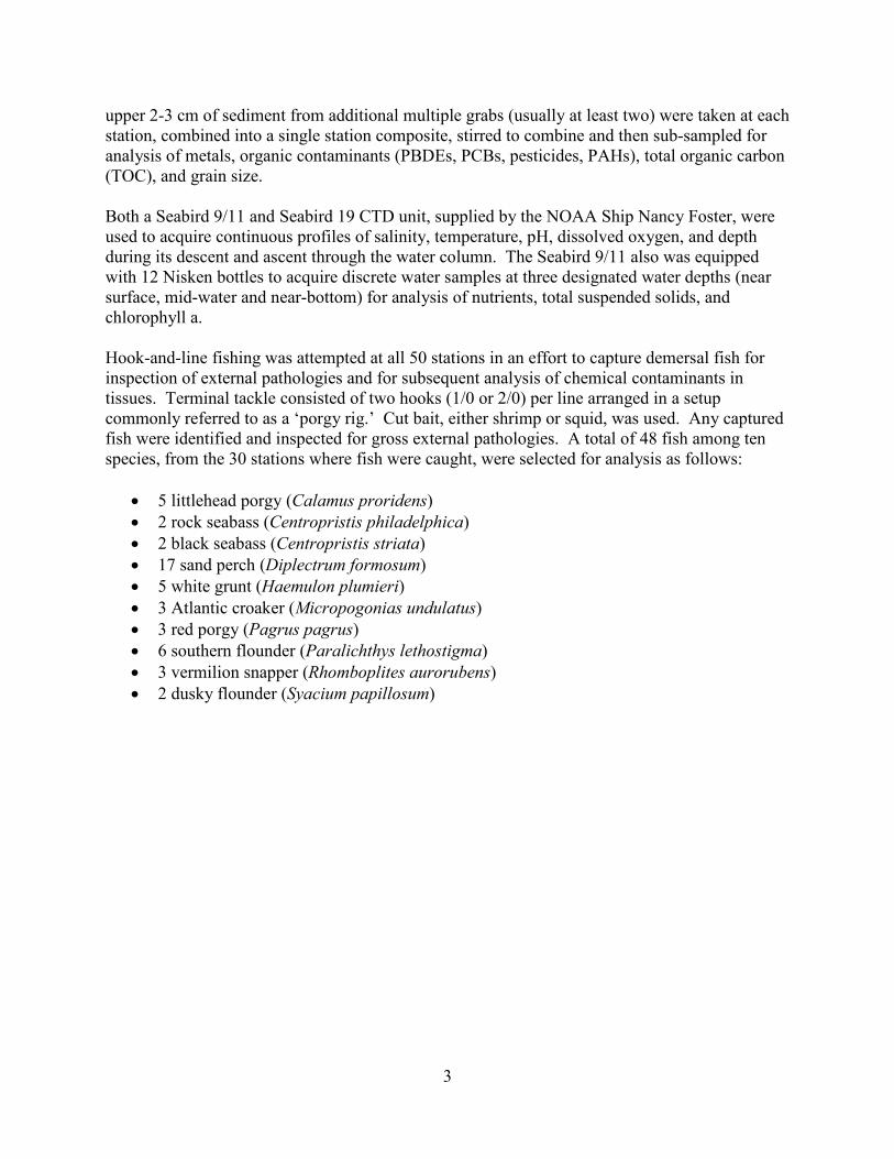
upper 2-3 cm of sediment from additional multiple grabs (usually at least two) were taken at each station, combined into a single station composite, stirred to combine and then sub-sampled for analysis of metals, organic contaminants (PBDEs, PCBs, pesticides, PAHs), total organic carbon (TOC), and grain size. Both a Seabird 9/11 and Seabird 19 CTD unit, supplied by the NOAA Ship Nancy Foster, were used to acquire continuous profiles of salinity, temperature, pH, dissolved oxygen, and depth during its descent and ascent through the water column. The Seabird 9/11 also was equipped with 12 Nisken bottles to acquire discrete water samples at three designated water depths (near surface, mid-water and near-bottom) for analysis of nutrients, total suspended solids, and chlorophyll a. Hook-and-line fishing was attempted at all 50 stations in an effort to capture demersal fish for inspection of external pathologies and for subsequent analysis of chemical contaminants in tissues. Terminal tackle consisted of two hooks (1/0 or 2/0) per line arranged in a setup commonly referred to as a ‘porgy rig.’ Cut bait, either shrimp or squid, was used. Any captured fish were identified and inspected for gross external pathologies. A total of 48 fish among ten species, from the 30 stations where fish were caught, were selected for analysis as follows:

• 5 littlehead porgy (Calamus proridens) • 2 rock seabass (Centropristis philadelphica) • 2 black seabass (Centropristis striata) • 17 sand perch (Diplectrum formosum) • 5 white grunt (Haemulon plumieri) • 3 Atlantic croaker (Micropogonias undulatus) • 3 red porgy (Pagrus pagrus) • 6 southern flounder (Paralichthys lethostigma) • 3 vermilion snapper (Rhomboplites aurorubens) • 2 dusky flounder (Syacium papillosum)

3

Figure 1. Map of Northeastern Gulf of Mexico shelf study area and station locations (green circles). Numbers within green circles indicate station number. Red circle indicates the location of the MC252 Macondo wellhead, also known as the Deepwater Horizon wellhead.

4

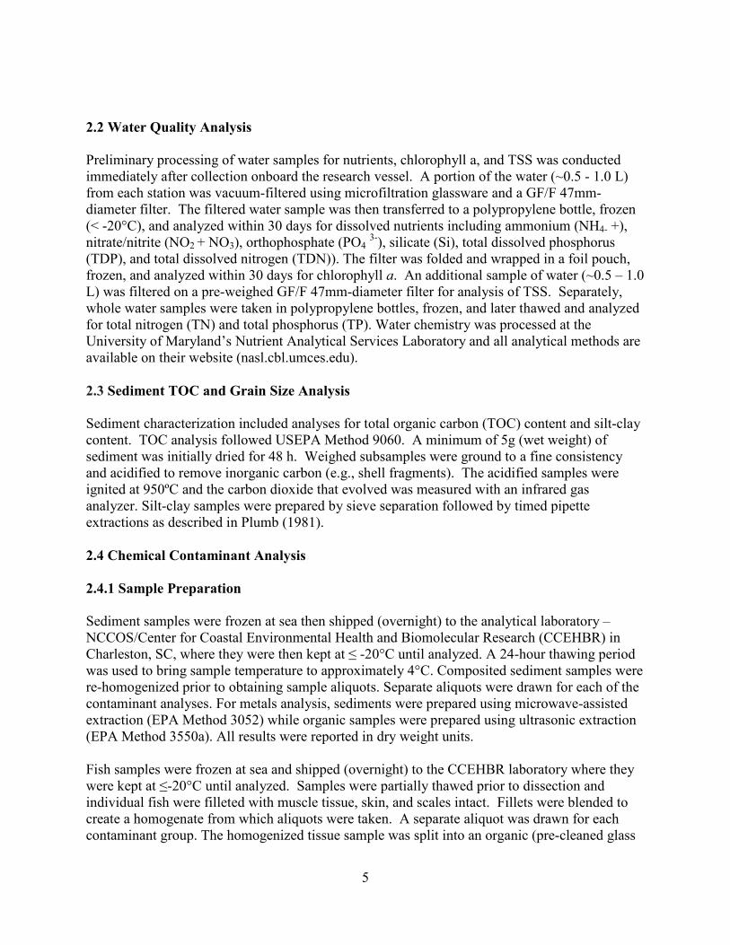
2.2 Water Quality Analysis Preliminary processing of water samples for nutrients, chlorophyll a, and TSS was conducted immediately after collection onboard the research vessel. A portion of the water (~0.5 - 1.0 L) from each station was vacuum-filtered using microfiltration glassware and a GF/F 47mm-diameter filter. The filtered water sample was then transferred to a polypropylene bottle, frozen (< -20°C), and analyzed within 30 days for dissolved nutrients including ammonium (NH4- +), nitrate/nitrite (NO2 + NO3), orthophosphate (PO4 3-), silicate (Si), total dissolved phosphorus (TDP), and total dissolved nitrogen (TDN)). The filter was folded and wrapped in a foil pouch, frozen, and analyzed within 30 days for chlorophyll a. An additional sample of water (~0.5 – 1.0 L) was filtered on a pre-weighed GF/F 47mm-diameter filter for analysis of TSS. Separately, whole water samples were taken in polypropylene bottles, frozen, and later thawed and analyzed for total nitrogen (TN) and total phosphorus (TP). Water chemistry was processed at the University of Maryland’s Nutrient Analytical Services Laboratory and all analytical methods are available on their website (nasl.cbl.umces.edu). 2.3 Sediment TOC and Grain Size Analysis Sediment characterization included analyses for total organic carbon (TOC) content and silt-clay content. TOC analysis followed USEPA Method 9060. A minimum of 5g (wet weight) of sediment was initially dried for 48 h. Weighed subsamples were ground to a fine consistency and acidified to remove inorganic carbon (e.g., shell fragments). The acidified samples were ignited at 950ºC and the carbon dioxide that evolved was measured with an infrared gas analyzer. Silt-clay samples were prepared by sieve separation followed by timed pipette extractions as described in Plumb (1981). 2.4 Chemical Contaminant Analysis 2.4.1 Sample Preparation Sediment samples were frozen at sea then shipped (overnight) to the analytical laboratory – NCCOS/Center for Coastal Environmental Health and Biomolecular Research (CCEHBR) in Charleston, SC, where they were then kept at ≤ -20°C until analyzed. A 24-hour thawing period was used to bring sample temperature to approximately 4°C. Composited sediment samples were re-homogenized prior to obtaining sample aliquots. Separate aliquots were drawn for each of the contaminant analyses. For metals analysis, sediments were prepared using microwave-assisted extraction (EPA Method 3052) while organic samples were prepared using ultrasonic extraction (EPA Method 3550a). All results were reported in dry weight units. Fish samples were frozen at sea and shipped (overnight) to the CCEHBR laboratory where they were kept at ≤-20°C until analyzed. Samples were partially thawed prior to dissection and individual fish were filleted with muscle tissue, skin, and scales intact. Fillets were blended to create a homogenate from which aliquots were taken. A separate aliquot was drawn for each contaminant group. The homogenized tissue sample was split into an organic (pre-cleaned glass

5

container) and inorganic (pre-cleaned polypropylene container) portion and stored at - 40 ºC until extraction or digestion. A percent dry-weight determination was made gravimetrically on aliquots of each of the wet sediment and tissue samples. Table 1 provides a list of all contaminants that were analyzed. 2.4.2 Inorganic Sample Digestion and Analysis Dried sediment was ground with a mortar and pestle and transferred to a 20 mL plastic screw-top container. A 0.25-g sub-sample of the ground material was transferred to a Teflon-lined digestion vessel and digested in 5 mL of concentrated Ultrex II Ultrapure nitric acid using microwave digestion. The sample was brought to a fixed volume of 50 mL with deionized water and stored in a 50-mL polypropylene centrifuge tube until instrumental analysis of Li, Be, Al, Fe, Mg, Ni, Cu, Zn, Cd, and Ag was undertaken. A second 0.25-g sub-sample was transferred to a Teflon-lined digestion vessel and digested in 5 mL of concentrated Ultrex II Ultrapure nitric acid and 1 mL of concentrated hydrofluoric acid in a microwave digestion unit. The sample was then evaporated on a hotplate at 225 °C to near dryness and 1mL of nitric acid was added. The sample was brought to a fixed volume of 50 mL with deionized water and stored in a 50-mL polypropylene centrifuge tube until instrumental analysis for V, Cr, Co, As, Sn, Sb, Ba, Tl, Pb, and U. Selenium was analyzed by hotplate digestion using a 0.25-g sub-sample and 5 mL of concentrated Ultrex II Ultrapure nitric acid. Each sample was brought to a fixed volume of 50 mL in a volumetric flask with deionized water and stored in a 50-mL polypropylene centrifuge tube until instrumental analysis. Additionally, 2-3 g of wet tissue were microwave-digested in Teflon-lined digestion vessels using 10 mL of concentrated nitric acid along with 2 mL of hydrogen peroxide. Digested samples were brought to a fixed volume with deionized water in graduated polypropylene centrifuge tubes and stored until analysis. A separate aliquot (0.5 g wet weight each for sediment and tissue) was used for mercury analysis. Mercury was analyzed on a Milestone DMA-80 Direct Mercury Analyzer. All remaining elemental analysis was performed using Inductively Coupled Plasma Mass Spectrometry (ICP-MS) except for silver, which was determined using Graphite Furnace Atomic Absorption (GFAA) spectroscopy. Data quality was controlled for by using a series of blanks, known spiked solutions, and standard reference materials including NRC MESS-3 (Marine Sediments) and NIST 1566b (freeze dried mussel tissue). 2.4.3 Organic Extraction and Analysis An aliquot (10 g sediment or 5 g tissue wet weight) was extracted with anhydrous sodium sulfate using Accelerated Solvent Extraction (ASE) in either 1:1 methylene chloride:acetone for sediments or 100% dichlormethane for tissues (Schantz 1997). Following extraction, samples were dried and cleaned using Gel Permeation Chromatography and Solid Phase Extraction to remove lipids and then solvent-exchanged into hexane for analysis. Samples were analyzed for PAHs, PBDEs, PCBs (by congener), and a suite of chlorinated pesticides using appropriate GC/MS technology. Data quality was ensured by using a series of spiked blanks, reagent blanks, and appropriate standard reference materials including NIST 1944 (sediments) and NIST 1566b (muscle tissue).

6

Table 1. List of target contaminants analyzed in coastal-ocean sediment and tissue samples analyzed by CCEHBR lab. Polycyclic Aromatic Hydrocarbons (PAHs) Polychlorinated Biphenyls (PCBs) 1-Methylnaphthalene PCB 1 (2-Chlorobiphenyl) 1-Methylphenanthrene PCB 103 (2,2',4,5',6-Pentachlorobiphenyl) 2,3,5-Trimethylnaphthalene PCB 104 (2,2',4,6,6'-Pentachlorobiphenyl) 2,6-Dimethylnaphthalene PCB 105 (2,3,3',4,4'-Pentachlorobiphenyl) 2-Methylnaphthalene PCB 106/118 Mixture Acenaphthene PCB 107/108 Mixture Acenaphthylene PCB 110 (2,3,3',4',6-Pentachlorobiphenyl) Anthracene PCB 114 (2,3,4,4',5-Pentachlorobiphenyl) Benz[a]anthracene PCB 119 (2,3',4,4',6-Pentachlorobiphenyl) Benzo[a]pyrene PCB 12 (3,4-Dichlorobiphenyl) Benzo[b]fluoranthene PCB 123 (2,3',4,4',5'-Pentachlorobiphenyl) Benzo[e]pyrene PCB 126 (3,3',4,4',5-Pentachlorobiphenyl) Benzo[g,h,i]perylene PCB 128/167 Mixture Benzo[k]fluoranthene PCB 130 (2,2',3,3',4,5'-Hexachlorobiphenyl) Biphenyl PCB 132/168 Mixture Chrysene PCB 138/163/164 Mixture Dibenz[a,h]anthracene PCB 141 (2,2',3,4,5,5'-Hexachlorobiphenyl) Dibenzothiophene PCB 146 (2,2',3,4',5,5'-Hexachlorobiphenyl) Fluoranthene PCB 149 (2,2',3,4',5',6-Hexachlorobiphenyl) Fluorene PCB 15 (4,4'-Dichlorobiphenyl) Indeno[1,2,3-c,d]pyrene PCB 151 (2,2',3,5,5',6-Hexachlorobiphenyl) Naphthalene PCB 153 (2,2',4,4',5,5'-Hexachlorobiphenyl) Perylene PCB 154 (2,2',4,4',5,6'-Hexachlorobiphenyl) Phenanthrene PCB 156 (2,3,3',4,4',5-Hexachlorobiphenyl) Pyrene PCB 157 (2,3,3',4,4',5'-Hexachlorobiphenyl) PCB 158 (2,3,3',4,4',6-Hexachlorobiphenyl) Pesticides PCB 159 (2,3,3',4,5,5'-Hexachlorobiphenyl) 2,4'-DDD PCB 165 (2,3,3',5,5',6-Hexachlorobiphenyl) 2,4'-DDE PCB 169 (3,3',4,4',5,5'-Hexachlorobiphenyl) 2,4'-DDT PCB 170/190 Mixture 4,4'-DDD PCB 172 (2,2',3,3',4,5,5'-Heptachlorobiphenyl) 4,4'-DDE PCB 174 (2,2',3,3',4,5,6'-Heptachlorobiphenyl) 4,4'-DDT PCB 177 (2,2',3,3',4,5',6'-Heptachlorobiphenyl) Aldrin PCB 18 (2,2',5-Trichlorobiphenyl) Alpha-chlordane PCB 180 (2,2',3,4,4',5,5'-Heptachlorobiphenyl) Gamma-chlordane PCB 183 (2,2',3,4,4',5',6-Heptachlorobiphenyl) Cis-nonachlor PCB 184 (2,2',3,4,4',6,6'-Heptachlorobiphenyl) Trans-Nonachlor PCB 187 (2,2',3,4',5,5',6-Heptachlorobiphenyl) Oxychlordane PCB 188 (2,2',3,4',5,6,6'-Heptachlorobiphenyl) Chlorpyrifos PCB 189 (2,3,3',4,4',5,5'-Heptachlorobiphenyl) Dieldrin PCB 193 (2,3,3',4',5,5',6-Heptachlorobiphenyl) Endosulfan I PCB 194 (2,2',3,3',4,4',5,5'-Octachlorobiphenyl) Endosulfan II PCB 195 (2,2',3,3',4,4',5,6-Octachlorobiphenyl) Endosulfan Sulfate PCB 198 (2,2',3,3',4,5,5',6-Octachlorobiphenyl) Heptachlor PCB 2 (3-Chlorobiphenyl) Heptachlor epoxide PCB 20 (2,3,3'-Trichlorobiphenyl) Hexachlorobenzene PCB 200 (IUPAC 201) alpha-Hexachlorocyclohexane (alpha-BHC) PCB 201 (IUPAC 199) beta-Hexachlorocyclohexane (beta-BHC) PCB 202 (2,2',3,3',5,5',6,6'-Octachlorobiphenyl)

7

Lindane PCB 203/196 Mixture Mirex PCB 206 (2,2',3,3',4,4',5,5',6-Nonachlorobiphenyl) PCB 207 (2,2',3,3',4,4',5,6,6'-Nonachlorobiphenyl) Metals PCB 208 (2,2',3,3',4,5,5',6,6'-Nonachlorobiphenyl) Aluminum PCB 209 (2,2',3,3',4,4',5,5',6,6'-Decachlorobiphenyl) Antimony PCB 26 (2,3',5-Trichlorobiphenyl) Arsenic PCB 28 (2,4,4'-Trichlorobiphenyl) Barium PCB 29 (2,4,5-Trichlorobiphenyl) Beryllium PCB 3 (4-Chlorobiphenyl) Cadmium PCB 31 (2,4',5-Trichlorobiphenyl) Chromium PCB 37 (3,4,4'-Trichlorobiphenyl) Cobalt PCB 44 (2,2',3,5'-Tetrachlorobiphenyl) Copper PCB 45 (2,2',3,6-Tetrachlorobiphenyl) Iron PCB 47/48 Mixture Lead PCB 49 (2,2',4,5'-Tetrachlorobiphenyl) Lithium PCB 5/8 Mixture Manganese PCB 50 (2,2',4,6-Tetrachlorobiphenyl) Mercury PCB 52 (2,2',5,5'-Tetrachlorobiphenyl) Nickel PCB 56/60 Mixture Selenium PCB 61/74 Mixture Silver PCB 63 (2,3,4',5-Tetrachlorobiphenyl) Thallium PCB 66 (2,3',4,4'-Tetrachlorobiphenyl) Tin PCB 69 (2,3',4,6-Tetrachlorobiphenyl) Uranium PCB 70/76 Mixture Vanadium PCB 77 (3,3',4,4'-Tetrachlorobiphenyl) Zinc PCB 81 (3,4,4',5-Tetrachlorobiphenyl) PCB 82 (2,2',3,3',4-Pentachlorobiphenyl) Polybrominated Diphenyl Ethers (PBDEs) PCB 84 (2,2',3,3',6-Pentachlorobiphenyl) PBDE 17 (2,2',4-Tribromodiphenyl Ether) PCB 87/115 Mixture PBDE 28 (2,4,4'-Tribromodiphenyl Ether) PCB 88 (2,2',3,4,6-Pentachlorobiphenyl) PBDE 47 (2,2',4,4'-Tetrabromodiphenyl Ether) PCB 89/90/101 Mixture PBDE 66 (2,3',4,4'-Tetrabromodiphenyl Ether) PCB 9 (2,5-Dichlorobiphenyl) PBDE 71 (2,3',4',6-Tetrabromodiphenyl Ether) PCB 92 (2,2',3,5,5'-Pentachlorobiphenyl) PBDE 85 (2,2',3,4,4'-Pentabromodiphenyl Ether) PCB 95 (2,2',3,5',6-Pentachlorobiphenyl) PBDE 99 (2,2',4,4',5-Pentabromodiphenyl Ether) PCB 99 (2,2',4,4',5-Pentachlorobiphenyl) PBDE 100 (2,2',4,4',6-Pentabromodiphenyl Ether) PBDE 138 (2,2',3,4,4',5'-Hexabromodiphenyl Ether)

PBDE 153 (2,2',4,4',5,5'-Hexabromodiphenyl Ether)

PBDE 154 (2,2',4,4',5,6'-Hexabromodiphenyl Ether)

PBDE 183 (2,2',3,4,4',5',6-Heptabromodiphenyl Ether)

PBDE 190 (2,3,3',4,4',5,6-Heptabromodiphenyl Ether)

2.5 Analysis of Potential Oil Spill Indicators In addition to the standard suite of sediment contaminant analyses performed for all regional assessment studies, an extra sediment sample was collected from each station for analysis of additional potential DWH oil-spill indicators (TPH and aliphatics, see Table 8 below). These 50 sediment samples were frozen at sea and shipped overnight to Texas A&M University/Geochemical and Environmental Research Group (TAMU/GERG) where they were

8

analyzed under the supervision of Dr. Terry Wade. At the request of the Subsurface Monitoring Unit (SMU) of the Deepwater Horizion Spill Response/Unified Area Command, these 50 sediment samples were split and half of the material was shipped overnight to Lancaster Labs for independent oil content analyses. Both TAMU/GERG and Lancaster Labs followed respective standard operating procedures for processing of these samples.

9

2.6 Toxicity Analysis Microtox® assays were conducted using the standardized solid-phase test protocols (Microbics Corporation 1992) and a Microtox® Model 500 analyzer (Strategic Diagnostics Inc., CA). In this assay, sediment was homogenized and a 7.0 – 7.1-g sediment sample was used to make a series of sediment dilutions with 3.5% NaCl diluent, which were incubated for 10 minutes at 15ºC. Luminescent bacteria (Vibrio fischeri) were then added to the test concentrations. The liquid phase was filtered from the sediment phase and bacterial post-exposure light output was measured using Microtox® Omni Software. An EC50 value (the sediment concentration that reduced light output by 50% relative to the controls) was calculated for each sample. Triplicate samples were analyzed simultaneously. Sediment samples were evaluated using criteria developed by Ringwood et al. (1997) to account for grain-size variations. 2.7 Benthic Community Analysis

Once in the laboratory, samples were transferred from formalin to 70% ethanol. Macroinfaunal invertebrates were sorted from the sample debris under a dissecting microscope and identified to the lowest practical taxon (usually species). Data were used to compute density (m-2) of total fauna (all species combined), densities of numerically dominant species (m-2), numbers of taxa, and H' diversity (Shannon and Weaver 1949) derived with base-2 logarithms. 2.8 Data Analysis A probabilistic, stratified-random sampling design was used in this study in order to provide a basis for making unbiased statistical estimates of the spatial extent (% area) of condition within the survey area, with 95% confidence intervals, based on the status of various measured ecological indicators and corresponding thresholds of interest (Table 2). A similar approach has been applied throughout EPA’s EMAP, related NCA programs, and other coastal-ocean surveys (e.g., Summers et al. 1995; Strobel et al. 1995; Hyland et al. 1996; USEPA 2004, 2006; Nelson et al. 2008; Balthis et al. 2009; Cooksey et al. 2010). Results are presented throughout this report as the percentage of survey area within specified ranges of a particular indicator. Thresholds defining such ranges (see Table 1) include, where possible, those having known biological significance (e.g., dissolved oxygen < 2 mg L-1). Additional data summaries representing key distributional properties (e.g., mean, range) and other basic data tabulations are provided as well. Data presented graphically in this report are primarily in the form of cumulative distribution functions (CDFs) and pie charts. These are useful tools for portraying the percentage of coastal area corresponding to varying levels of a given indicator across the full range of its observed values and for estimating the percentage of area falling below or above some designated threshold of interest. This can be a useful feature for management applications as well; for example, if valid thresholds can be defined for a particular indicator or suite of indicators, they could be used as ecosystem quality targets for monitoring the system and triggering any necessary management actions.

10

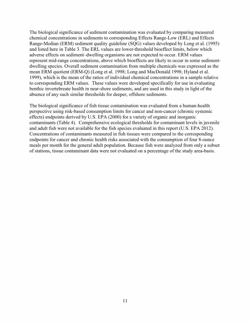
The biological significance of sediment contamination was evaluated by comparing measured chemical concentrations in sediments to corresponding Effects Range-Low (ERL) and Effects Range-Median (ERM) sediment quality guideline (SQG) values developed by Long et al. (1995) and listed here in Table 3. The ERL values are lower-threshold bioeffect limits, below which adverse effects on sediment–dwelling organisms are not expected to occur. ERM values represent mid-range concentrations, above which bioeffects are likely to occur in some sediment-dwelling species. Overall sediment contamination from multiple chemicals was expressed as the mean ERM quotient (ERM-Q) (Long et al. 1998; Long and MacDonald 1998; Hyland et al. 1999), which is the mean of the ratios of individual chemical concentrations in a sample relative to corresponding ERM values. These values were developed specifically for use in evaluating benthic invertebreate health in near-shore sediments, and are used in this study in light of the absence of any such similar thresholds for deeper, offshore sediments. The biological significance of fish tissue contamination was evaluated from a human-health perspective using risk-based consumption limits for cancer and non-cancer (chronic systemic effects) endpoints derived by U.S. EPA (2000) for a variety of organic and inorganic contaminants (Table 4). Comprehensive ecological thresholds for contaminant levels in juvenile and adult fish were not available for the fish species evaluated in this report (U.S. EPA 2012). Concentrations of contaminants measured in fish tissues were compared to the corresponding endpoints for cancer and chronic health risks associated with the consumption of four 8-ounce meals per month for the general adult population. Because fish were analyzed from only a subset of stations, tissue contaminant data were not evaluated on a percentage of the study area-basis.

11

Table 2. Thresholds used for classifying samples relative to various environmental indicators. Indicator Threshold Reference

Water Quality Salinity (psu) < 5 = Oligohaline

5 – 18 = Mesohaline >18 – 30 = Polyhaline > 30 = Euhaline

Carriker 1967

DO (mg/L) < 2 = Low (Poor)

2 – 5 = Moderate (Fair) > 5 = High (Good)

U. S. EPA 2008; Diaz and Rosenberg 1995

DIN/DIP > 16 = phosphorus limited

< 16 = nitrogen limited Geider and LaRoche 2002

ΔδT Strong Vertical Stratification: > 2 Nelson et al. 2008 Sediment Quality

Silt-Clay Content (%) > 80 = Mud 20 – 80 = Muddy Sand < 20 = Sand

U. S. EPA 2008

TOC Content (mg/g) > 50 = High (Poor)

20 – 50 = Moderate (Fair) < 20 = Low (Good)

U. S. EPA 2008

> 35 = High (Poor) Hyland et al. 2005 Overall chemical contamination

≥ 1 ERM value exceeded OR mERM-Q > 0.036 = High (Poor); ≥ 5 ERL values exceeded OR 0.013 < mERM-Q < 0.036 = Moderate (Fair); No ERMs exceeded AND < 5 ERLs exceeded AND mERM-Q < 0.013 = Low (Good)

U. S. EPA 2008; Hyland et al. 1999;

Hyland et al. 2003

12

Table 2 (continued). Indicator Threshold Reference

Individual chemical contaminant concentrations

> ERM = High probability of bioeffects < ERL = Low probability of bioeffects

Long et al. 1995

Toxicity (Microtox®) Silt-clay < 20 %: Toxic if EC50 < 0.5 %

Silt-clay > 20 %: Toxic if EC50 < 0.2 % Ringwood et al. 1997

Biological Condition

Benthic Community (potential degraded condition)

Low values of species richness, H′, and density (defined for the purpose of this analysis as the lower 10th percentile of observed values) combined with evidence of poor sediment or water quality was defined as: ≥ 1 chemical in excess of ERMs, TOC > 50 mg/g, or dissolved oxygen in near-bottom water < 2 mg/L.

Cooksey et al. 2010

Chemical Contaminants in Fish Tissues

≥ 1 chemical exceeded Human Health upper limit = High (Poor) ≥ 1 chemical within Human Health risk range = Moderate (Fair) All chemicals below Human Health lower risk limit = Low (Good)

U. S. EPA 2008

Individual chemical contaminants in fish tissues

Non-cancer (chronic systemic effects) endpoints based on consumption of four 8-ounce meals per month (general adult population). Cancer risk endpoints (1 in 100,000 risk level) based on consumption of four 8-ounce meals per month (general adult population).

U. S. EPA 2000

13

Table 3. ERM and ERL guidance values for near-shore and estuarine sediments (Long et al. 1995). Chemical ERL ERM

Metals (µg/g) Arsenic 8.2 70 Cadmium 1.2 9.6 Chromium 81 370 Copper 34 270 Lead 46.7 218 Mercury 0.15 0.71 Nickel 20.9 51.6 Silver 1 3.7 Zinc 150 410

Organics (ng/g)

Acenaphthene 16 500 Acenaphthylene 44 640 Anthracene 85.3 1100 Fluorene 19 540 2-Methylnaphthalene 70 670 Naphthalene 160 2100 Phenanthrene 240 1500 Benzo[a]anthracene 261 1600 Benzo[a]pyrene 430 1600 Chrysene 384 2800 Dibenz[a,h]Anthracene 63.4 260 Fluoranthene 600 5100 Pyrene 665 2600 Low molecular weight PAHs 552 3160 High molecular weight PAHS 1700 9600 Total PAHs 4020 44800 4,4-DDE 2.2 27 Total DDT 1.58 46.1 Total PCBs 22.7 180

14

Table 4. Risk based EPA advisory guidelines for recreational anglers (US EPA 2000). Concentration ranges represent the non-cancer health endpoint risk for four 8-ounce fish meals per month. Non-cancer

Health Endpointa Cancer

Health Endpointb

Metals (μg/g) Arsenic (inorganic)c >0.35 – 0.70 >0.0078 – 0.016 Cadmium >0.35 – 0.70 Mercury (methylmercury)d >0.12 – 0.23 Selenium >5.90 – 12.00

Organics (ng/g) Chlordane >590 – 1200 >34 – 67 Chlorpyriphos >350 – 700 DDT (total) >59 – 120 >35 – 69 Dieldrin >59 – 120 >0.73 – 1.5 Endosulfan >7000 – 14000 Heptachlor epoxide >15 – 31 >1.3 – 2.6 Hexachlorobenzene >940 – 1900 >7.3 – 15.0 Lindane >350 – 700 >9.0 – 18 Mirex >230 – 470 Toxaphene >290 – 590 >11.0 – 21 PAHs (benzo[a]pyrene) >1.6 – 3.2e PCB (total) >23 – 47 >5.9 – 12.0

a Range of concentrations for non-cancer health endpoints are based on the assumption that consumption over a lifetime of four 8-oz meals per month would not generate a health risk.

b Range of concentrations for cancer health endpoints are based on the assumption that consumption over a lifetime of four 8-oz meals per month would yield a lifetime cancer risk no greater than an acceptable risk of 1 in 100,000.

c Inorganic arsenic, the form considered toxic, estimated as 2% of total arsenic. d Because most mercury present in fish and shellfish tissue is present primarily as methylmercury and because of the relatively

high cost of analyzing for methylmercury, the conservative assumption was made that all mercury is present as methylmercury (U. S. EPA, 2000).

e A non-cancer concentration range for PAHs does not exist.

15

3.0 Results and Discussion 3.1 Depth and Water Quality 3.1.1 Depth and General Water Characteristics: Temperature, salinity, water-column stratification, DO, pH, water clarity Key bottom-water characteristics throughout the region (Figure 2, Table 5, Appendix A, B, C) can be summarized as follows: (1) water depths ranging from 10.0 – 100.0 m and averaging 32.5 m (water depths were not corrected to Mean Low Low Water); (2) a narrow range of euhaline salinity values from 32.8 – 36.4 PSU (overall mean of 35.3); (3) a wide range of DO levels from 1.6 – 6.9 mg L-1 and averaging 5.37 mg L-1; (4) typically warm temperatures ranging from 17.7 – 31.3 °C and averaging 24.7 °C; (5) a narrow range of pH levels from 7.66 – 7.95 and averaging 7.84; and (6) total suspended solids (TSS) ranging from 5.1 – 19.0 mg L-1 and averaging 8.28 mg L-1. Water-column stratification expressed as Δσt, an index of the variation between surface and bottom water densities, was calculated from temperature and salinity data. The index is the difference between the computed bottom and surface σt values, where σt is the density of a parcel of water with a given salinity and temperature relative to atmospheric pressure (Nelson et al. 2008). The Δσt index ranged from 0 to 8.9. The majority of the survey area (69%) had Δσt index values greater than 2, indicating strong vertical stratification of the water column (Table 5). The majority of the survey area (76%) had bottom-water DO levels in the high range (> 5 mg L-

1) considered as water with sufficient oxygen to sustain marine life (Figure 3). Twenty-two percent of the water samples had moderate levels of DO between 2 and 5 mg L-1 and 2% (represented by one station) had low levels of DO < 2 mg L-1. For comparison, the percentage of northeastern GOM shelf waters with low DO < 2 mg/L was less than sampling-area percentages reported for northwestern GOM shelf waters (15%, Balthis et al. 2013) and GOM estuaries (5%, US EPA 2012), though larger than that reported for southeastern GOM shelf waters (0%, Cooksey et al. 2012) (Figure 3). Shelf waters off the Louisiana coast, west of the MS delta, are known to experience annual hypoxia from spring to early fall resulting in biological “dead zones” (Rabalais et al. 2002, 2007; Turner et al. 2012). The one station with low DO below 2 mg/L and the majority of sites with intermediate DO (2-5 mg/L) in the present study were located slightly east of the MS delta, in the vicinity of Chandeleur Sound and MS Bight, where there is also a documented record of seasonal hypoxic events (Moshagianis et al. 2012).

16

Figure 2. Cumulative percentage area (solid lines) and 95% Confidence Intervals (dotted lines) of Northeastern Gulf of Mexico shelf waters (surface and near-bottom) in relation to depth and selected water-quality characteristics.

17

Table 5. Summary of depth and water characteristics for near-bottom (within 3-5 m of bottom) and near-surface (0.5 – 2 m) waters from 50 Northeastern Gulf of Mexico continental shelf sites. Near-Bottom Near-Surface Mean Range CDF

10th pctl CDF

50th pctl CDF

90th pctl Mean Range CDF

10th pctl CDF

50th pctl CDF

90th pctl Depth 32.5 10 – 100 11.9 29.0 56.0 -- -- -- -- -- Δσt 3.91 0.00 – 8.90 0.01 4.2 7.5 -- -- -- -- -- Temperature (°C) 24.7 17.7 – 31.3 19.2 24.8 30.7 30.4 29.8 – 31.4 29.8 30.3 30.9 Salinity (psu) 35.3 32.8 – 36.4 33.4 35.5 36.4 32.5 22.7 – 35.2 29.9 32.9 34.7 DO (mg/L) 5.37 1.6 – 6.9 3.91 5.50 6.42 6.04 5.11 – 6.88 5.55 6.08 6.33 pH 7.84 7.66 – 7.95 7.76 7.84 7.92 7.87 5.89 – 8.19 7.73 7.95 8.05 DIN (mg/L) 0.039 0.008 – 0.14 0.008 0.012 0.089 0.013 0.008 – 0.069 0.008 0.009 0.018 DIP (mg/L) 0.008 0.003 – 0.038 0.003 0.005 0.015 0.004 0.003 – 0.027 0.003 0.004 0.005 Chl a (µg/L) 0.99 0.56– 4.37 0.56 0.62 1.63 1.16 0.56 – 15.7 0.56 0.56 1.67 TSS (mg/L) 8.28 5.1 – 19.0 6.1 7.5 10.1 7.20 2.4 – 26.5 4.9 6.4 8.6 N/P Ratio 7.0 0.62 – 23.8 1.3 7.1 14.0 6.6 0.56 – 45.7 0.99 1.8 17.1

18

Figure 3. Comparison of the percentage area of the northeastern Gulf of Mexico (GOM) shelf waters (this study), northwestern GOM shelf waters (Balthis et al. 2013), southeastern GOM shelf waters (Cooksey et al. 2012), and GOM estuarine waters (US EPA 2012) within specified ranges of DO.

19

Figure 4. Spatial distribution of bottom dissolved oxygen concentration in Northeastern Gulf of Mexico continental shelf waters.

20

3.1.2 Nutrients and Chlorophyll a Surface-water concentrations of total dissolved inorganic nitrogen (DIN: nitrate + nitrite + ammonium as nitrogen) were very low: ranging from 0.008 – 0.069 mg L-1 and averaging 0.013 mg L-1 (Figure 5, Table 5, Appendix B). The 50th percentile of the surface-water sampling area corresponded to a DIN concentration of 0.008 mg L-1 and the 90th percentile corresponded to a DIN concentration of 0.018 mg L-1. Surface-water concentrations of dissolved inorganic phosphate (DIP: orthophosphate as phosphate) were also low: ranging from 0.003 – 0.027 mg L-1 and averaging 0.004 mg L-1 (Figure 5, Table 5). The 50th percentile of the surface-water sampling area corresponded to a DIP concentration of 0.004 mg L-1 while the 90th percentile corresponded to a DIP concentration of 0.005 mg L-1. Nutrient enrichment and associated eutrophication are ongoing concerns within the Gulf of Mexico. The Mississippi River is the largest source of nutrients into the northern Gulf of Mexico; however, most of the flow is directed to the west of the Mississippi Delta (Rabalais et al. 2007). For comparison, Balthis et al. (2013) reported higher concentrations of DIN, averaging 0.026 mg/L and ranging from 0.018 to 0.044 mg/L, for surface waters of the NW Gulf, although DIP levels (average of 0.004 mg/L and range of 0.002 to 0.011 mg/L) were similar to those reported here. Concentrations of DIN and DIP in surface waters for both the NE and NW Gulf shelf studies are higher than those reported by Cooksey et al. (2012) for SE GOM shelf waters (DIN: average of 0.002 mg/L and range of 0.002 to 0.004 mg/L; DIP: average of 0.002 mg/L and range of 0.002 to 0.003 mg/L). The ratio of DIN concentration to DIP concentration (N/P ratio) was calculated as an indicator of which of these two nutrients may be controlling primary production within the sampling region (Appendix B). A ratio above 16 is generally considered indicative of phosphorus limitation, and a ratio below 16 is considered indicative of nitrogen limitation (Geider and La Roche 2002). The N/P ratio in surface waters ranged from 0.56 to 45.7 and averaged 6.6. Eighty-eight percent of the offshore survey area had N/P ratios < 16, indicative of a nitrogen limited environment, and 12% had N/P rations > 16, indicative of a phosphorous limited environment. Nitrogen has been reported previously to be the primary limiting factor for phytoplankton growth in the northern GOM (Turner et al. 2007). Chlorophyll a (Chl a) levels in surface waters ranged from 0 – 15.7 μg L-1 and averaged 0.85 μg L-1 (Figure 5, Table 5, Appendix B). The 90th percentile corresponded to a Chl a concentration of 1.7 μg L-1. With the exception of one station, all remaining stations, representing 98% of the offshore survey area, had Chl a below the 5.0 μg L-1 threshold used to denote the beginning of the high range for estuarine waters (U.S. EPA 2004). The highest levels of Chl a (e.g., upper 10th percentile) were found along the western portion of the survey area, closest to the Mississippi River Delta (Figure 6). The amount of TSS in the water column has a direct effect on turbidity (a measure of water clarity) by causing the attenuation or scattering of light, though TSS itself is not a measure of turbidity. Generally, as TSS increases, the water becomes murkier or more turbid. Excessively high turbidity and TSS may be harmful to marine life (e.g., by reducing light penetration and photosynthesis, increasing biological oxygen demand, interfering with normal respiratory and feeding activities) and distract from the aesthetic value of a coastal area. TSS levels in both surface and bottom waters were highly variable, averaging 7.20 and 8.28 mg/L, respectively, but

21

ranging from 2.4 – 26.5 mg/L and 5.1 – 19.0 mg/L, respectively (Figure 5, Table 5). The 50th percentiles of TSS concentration within the survey area were 6.4. mg L-1 for surface-waters and 7.5 mg L-1 for bottom-waters.

22

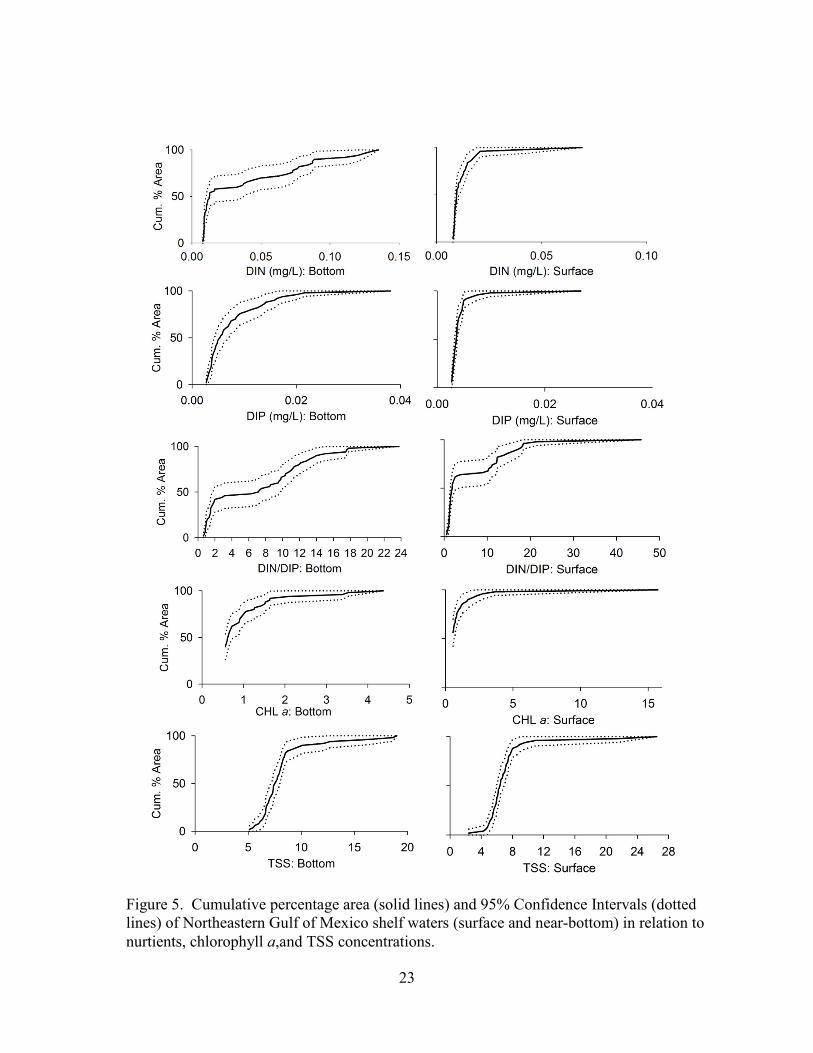
Figure 5. Cumulative percentage area (solid lines) and 95% Confidence Intervals (dotted lines) of Northeastern Gulf of Mexico shelf waters (surface and near-bottom) in relation to nurtients, chlorophyll a,and TSS concentrations.

23

Figure 6. Spatial distribution of surface chlorophyll a levels in Northeastern Gulf of Mexico continental shelf waters.

24

3.2 Sediment Quality 3.2.1 Grain Size and TOC The silt-clay content of sediments ranged from 1.5% to 78.0% and averaged 9.3% throughout the survey area (Table 6, Appendix A). None of the stations were composed of muds (> 80% silt-clay; Figure 7). Total organic carbon (TOC) content in sediments exhibited a wide range (0.3 to 31.8 mg g-1) with an average concentration of 5.3 mg g-1 (Table 6). Ninety-four percent of the survey area had relatively low TOC levels of < 20 mg g-1, six percent had moderate levels of TOC, and none of the area had high levels in excess of upper thresholds associated with a high risk of adverse effects on benthic fauna (> 50 mg g-1 cutpoint from USEPA 2008, or > 36 mg g-1 cutpoint from Hyland et al. 2005) (Figure 8). Table 6. Summary of sediment characteristics from 50 Northeastern Gulf of Mexico continental shelf sites. Mean Range CDF 10th% CDF 50th% CDF 90th% TOC (mg g-1) 5.3 0.3 – 31.8 0.6 2.9 10.2 % silt-clay 9.3 1.5 – 78.0 2.0 3.7 18.1 Mean ERM-Q 0.006 0.002 – 0.029 0.002 0.005 0.013

Figure 7. Percent area of Northeastern Gulf of Mexico shelf vs. percent silt-clay of sediment.

25

Figure 8. Comparison of the percentage area of northeastern Gulf of Mexico (GOM) shelf waters (this study), northwestern GOM shelf waters (Balthis et al. 2013), southeastern GOM shelf waters (Cooksey et al. 2012), and GOM estuarine waters (US EPA 2012) within specified ranges of TOC.

26

3.2.2 Chemical Contaminants in Sediments Effects Range-Low (ERL) and Effects Range-Median (ERM) sediment quality guideline (SQG) values for near shore and estuarine sediments from Long et al. (1995) were used to help interpret the biological significance of observed chemical contaminant levels in sediments. ERL values are lower-threshold bioeffect limits, below which adverse effects of the contaminants on sediment-dwelling organisms would not be expected to occur. In contrast, ERM values represent mid-range concentrations of chemicals above which adverse effects would be expected to occur. A list of 26 chemicals, or chemical groups, for which ERL and ERM guidelines have been developed is provided in Table 3 along with the corresponding SQG values (from Long et al. 1995). Any site with one or more chemicals that exceeded corresponding ERM values was rated as having poor sediment quality, any site with five or more chemicals between corresponding ERL and ERM values was rated as fair, and any site that had fewer than five ERLs exceeded and no ERMs exceeded was rated as good (sensu USEPA 2004). Overall sediment contamination from multiple chemicals also was expressed as the mean ERM quotient (ERM-Q) (Long et al. 1998; Long and MacDonald 1998; Hyland et al. 1999), which is the mean of the ratios of individual chemical concentrations in a sample relative to corresponding ERM values (using all chemicals in Table 3 except nickel and total PAHs). A mean ERM-Q cutpoint of 0.036, marking the beginning of the range associated with a high risk of degraded benthic condition in estuaries of the Louisianan Province (Hyland et al. 2003), was used as a guideline for evaluating sediment contaminant levels in this survey. Sediments throughout the northeastern Gulf shelf survey area were relatively uncontaminated: contaminant concentrations at all stations (100%) were in the low range with respect to the number of ERL/ERMs exceeded (Table 7, Figure 12, Appendix D). Though some analytes occurred at concentrations above minimum detection limits, only one trace metal (arsenic) was found at moderate levels, between corresponding ERL and ERM values, and no chemicals were found in excess of the higher-threshold ERM values (Table 7). Mean ERM-Q values across the study area were variable but also low, ranging from 0.002 to 0.029 and averaging 0.006 (Table 6, Appendix D). None of the offshore sediments had a mean ERM-Q in the high range (i.e., >0.036). Two contaminant variables that serve as potential oil-spill indicators – Total Petroleum Hydrocarbons (TPH) and Total Polycyclic Aromatic Hydrocarbons (Tot PAHs) – were also found at low background levels in these offshore sediments, which were collected in August 2010, after the drilling rig explosion that caused the Deepwater Horizon (DWH) oil spill. Total PAH concentrations in sediments (Table 7) ranged from non-detectable (ND) to 87 ng/g and averaged 4.88 ng/g. For comparison, sediment-quality bioeffect guidelines for total PAHs include ERM and ERL values of 44,792 ng/g and 4,022 ng/g, respectively (Long et al. 1995). Total PAH concentrations within 3 km of the DWH wellhead, coinciding with an area of deep benthic impacts (Montagna et al. 2013 a,b) ranged from 419 – 47,559 ng/g based on data from DWH Response efforts [Environmental Response Management Application (ERMA) Gulf Response website, http://gomex.erma.noaa.gov]. Sammarco et al. (2013) also found elevated hydrocarbons associated with the DWH oil spill in areas closer to shore.

27

TPH concentrations in this study (Table 8, TAMU-GERG values) were also at low levels, ranging from 1.38 – 13.3 µg/g and averaging 4.55 µg/g (Lancaster Labs values were even lower). In contrast, TPH levels within 3 km of the DWH wellhead ranged from 103 – 5,023 µg/g (ERMA database). The present post-spill offshore, shelf survey showed no indication of DWH oil at elevated levels posing risks to benthic infauna invertebrates, based on the ERL/ERM thresholds, developed for near-shore and estuarine sediments. Total PAH data reported here are based on 25 PAHs (inclusive of several alkyl homologs) typically measured within other related studies conducted in estuarine and coastal waters around the country as part of our NCCOS coastal ecosystem assessment series. However, it is important to note that the sediment samples in this study were analyzed redundantly by three different laboratories and included a much wider range of hydrocarbons that were measured, as follows: (1) the NOAA/NCCOS lab in Charleston, SC analyzed the 25 PAHs listed in Table 1, above, in a subsample from each station; (2) Texas A&M/GERG analyzed TPH and aliphatics in a separate subsample from each station; and (3) Lancaster Laboratories (LL) analyzed a more complete list of PAHs in splits of the latter subsamples, including all 34 PAHs from the OSAT Response list (OSAT 2010, Table A3) and 46 of the “NOAA 52” PAHs listed for NRDA purposes. Total PAHs, based on the 25 individual PAHs in the present report, averaged 4.9 μg/kg (ppb) and ranged from 0 – 86.8 μg/kg across the 50 stations. Similarly, total PAHs, based on the 46 individual PAHs analyzed by LL and which included an expanded list of alkylated PAHs, averaged 15.3 μg/kg and ranged from 0 – 193 μg/kg across the 50 stations (ERMA database). Both sets of numbers are extremely low and indicative of concentrations of PAHs at background contamination levels as seen in other continental shelf surveys (Nelson et al. 2008; Balthis et al. 2009; Cooksey et al. 2010). In fact, in both cases the majority of stations had undetectable to just detectable levels of total PAHs (with “U” or “J” qualifiers) – i.e., 45 and 48 of the 50 stations analyzed by NCCOS and LL, respectively.

28

Table 7. Summary of chemical contaminant concentrations in northeastern Gulf of Mexico shelf sediments (‘N/A’ = no corresponding ERL or ERM available). Concentration

> ERL < ERM Concentration

> ERM Analyte Mean Range # Stations # Stations Metals (% dry wt.)

Aluminum 0.64 0.20 – 5.13 - - Iron 0.49 0 – 31.62 - -

Trace Metals (µg/g) Antimony 0.04 0 - 1.02 - -

Arsenic 3.66 0.63 - 23.02 4 0 Barium 79.69 9.82 - 652.73 - - Beryllium 0.22 0.06 - 1.28 - - Cadmium 0.05 0 - 0.17 0 0 Chromium 11.37 3.26 - 51.24 0 0 Cobalt 1.63 0.21 - 9.8 - - Copper 1.87 0 - 11.97 0 0 Lead 3.76 1.07 - 19.9 0 0 Lithium 6.33 0.84 - 42.77 - - Manganese 76.32 4.32 - 463.91 - - Mercury 0.01 0 - 0.04 0 0 Nickel 4.57 0.53 - 19.92 0 0 Selenium 0.06 0 - 0.49 - - Silver 0 0 - 0 0 0 Thallium 0.1 0 - 0.48 - - Tin 0.4 0.16 - 1.86 - - Uranium 1.27 0.31 - 2.6 - - Vanadium 10.84 2.74 - 76.4 - - Zinc 8.99 0 - 75.02 0 0

PAHs (ng/g) Acenaphthene 0 0 - 0 0 0 Acenaphthylene 0 0 - 0 0 0 Anthracene 0 0 - 0 0 0 benz[a]anthracene 0 0 - 0 0 0 benzo[a]pyrene 0 0 - 0 0 0 benzo[b]fluoranthene 0 0 - 0 - - benzo[e]pyrene 0 0 - 0 - - Benzo[g,h,i]perylene 0 0 - 0 - - Benzo[j+k]fluoranthene 0 0 - 0 - - Biphenyl 0 0 - 0 - - Chrysene 0 0 - 0 0 0 Dibenz[a,h]Anthracene 0 0 - 0 0 0 Dibenzothiophene (Synfuel) 0 0 - 0 - - 2,6-Dimethylnaphthalene 0 0 - 0 - - Fluoranthene 0.09 0 - 4.68 0 0 Fluorene 0 0 - 0 0 0 Indeno[1,2,3-c,d]Pyrene 0 0 - 0 - - Naphthalene 0.13 0 - 6.47 0 0 2-Methylnaphthalene 0 0 - 0 0 0 1-Methylnaphthalene 0 0 - 0 - - 1-Methylphenanthrene 0 0 - 0 - - Perylene 4.66 0 - 75.66 - -

29

Concentration > ERL < ERM

Concentration > ERM

Analyte Mean Range # Stations # Stations Phenanthrene 0 0 - 0 0 0 Pyrene 0 0 - 0 0 0 1,6,7-Trimethylnaphthalene 0 0 - 0 - - Total Low Molecular Weight PAHs 0.13 0 - 6.47 0 0

Total High Molecular Weight PAHs 4.75 0 - 80.34 0 0

Total PAHs 4.88 0 - 86.81 0 0

PBDEs (ng/g) Total PBDEs 0 0 - 0.04 - -

PCBs (ng/g)1

PCB20 0 0 - 0.07 - - PCB202 0 0 - 0.08 - - PCB47/48 Mixture 0 0 - 0.02 - - PCB63 0.01 0 - 0.06 - - PCB84 0 0 - 0.04 - - PCB87/115 Mixture 0.07 0 - 0.13 - - PCB99 0 0 - 0.05 - - PCB 153 0 0 - 0.05 - - PCB 138/163/164 Mixture 0 0 - 0.04 - - PCB 12 0.01 0 - 0.41 - - Total PCBs 0.1 0 - 0.48 0 0

Pesticides (ng/g)

2,4′-DDD 0 0 - 0 - - 2,4′-DDE 0 0 - 0.03 0 0

2,4′-DDT 0 0 - 0 - - 4,4′-DDD 0 0 - 0 - - 4,4′-DDE 0 0 - 0 - - 4,4′-DDT 0 0 - 0 - - Total DDT 0 0 - 0.03 0 0 Aldrin 0 0 - 0 - - Alpha-Chlordane 0 0 - 0 - - Oxyhlordane 0 0 - 0 - - cis-Nonachlor 0 0 - 0 - - trans-Nonachlor 0 0 - 0 - - Chlorpyrifos 0 0 - 0 - - Dieldrin 0 0 - 0 - - Endosulfan I 0 0 - 0 - - Endosulfan II 0 0 - 0 - - Endosulfan Sulfate 0 0 - 0 - - Alpha-BHC 0 0 - 0 - - Beta-BHC 0 0 - 0 - - Gamma-BHC 0 0 - 0 - - Heptachlor 0 0 - 0 - - Heptachlor Epoxide 0 0 - 0 - - Hexachlorobenzene 0 0 - 0 - - Mirex 0 0 - 0 - -

1 - Only PCBs with values > MDL listed here, see Table 1 for full list of congeners tested.

30

Figure 12. Percentage area for northeastern Gulf of Mexico (GOM) shelf waters (this study), northwestern GOM shelf waters (Balthis et al. 2013), southeastern GOM shelf waters (Cooksey et al. 2012), and GOM estuarine waters (US EPA 2012) sediment contamination levels, expressed as number of ERL and ERM values exceeded, within specified ranges.

31

Table 8. Summary of TPH and n-alkane concentrations (µg/g dry weight) in Northeastern Gulf of Mexico shelf sediments (measured independently by TAMU-GERG and Lancaster Labs).

n-Alkane GERG Lab Lancaster Labs Mean Range Mean Range

Decane (n-C10) 5.86 0.2 - 21.3 16.06 0 - 220 Undecane (n-C11) 3.74 0.5 - 16 20.45 0 - 320 Dodecane (n-C12) 0.85 0.3 - 5.6 13.39 0 - 270 Tridecane (n-C13) 1.09 0 - 14.3 13.65 0 - 240 Tetradecane (n-C14) 2.98 1.1 - 11.7 83.98 0 - 940 Pentadecane (n-C15) 6.54 0.9 - 103.8 13.92 0 - 160 Heptadecane (n-C17) 27.17 0.8 - 138.1 47.76 0 - 550 Octadecane (n-C18) 1.82 0.6 - 7.2 4.12 0 - 99 Nonadecane (n-C19) 11.8 0.4 - 102.9 1.1 0 - 54 Eicosane (n-C20) 5.84 0.9 - 27.4 3.22 0 - 51 Heneicosane (n-C21) 10.75 1.2 - 24.6 5.12 0 - 46 Docosane (n-C22) 1.36 0.3 - 4 1.9 0 - 50 Tricosane (n-C23) 2.07 0.3 - 6.4 2.12 0 - 24 Tetracosane (n-C24) 1.2 0 - 4.6 3.29 0 - 49 Pentacosane (n-C25) 4.09 0 - 18.8 2.65 0 - 47 Hexacosane (n-C26) 3.91 0.2 - 21.8 4.53 0 - 47 Heptacosane (n-C27) 3.82 0 - 25.7 3.15 0 - 56 Octacosane (n-C28) 1.95 0.3 - 5.9 7.24 0 - 170 Nonacosane (n-C29) 16.12 3.8 - 58.4 14.64 0 - 89 Triacontane (n-C30) 1.13 0 - 4.3 5.09 0 - 58 Hentriacontane (n-C31) 7.68 0.6 - 32.8 4.66 0 - 66 Tritriacontane (n-C33) 3.06 0 - 12.5 0 0 - 0 Tetratriacontane (n-C34) 0.99 0 - 8.3 0 0 - 0 Pentatriacontane (n-C35) 4.21 0.3 - 20 1.11 0 - 20 TPH, Total (C9-C40) 4.55 1.38 - 13.26 0.51 0 - 8.5

32

Figure 13. Spatial distribution of total PAH (A) and TPH (B) concentrations in northeastern Gulf of Mexico shelf sediments.

A.

B.

33

3.2.3 Sediment Toxicity Sediment toxicity tests developed specifically for offshore marine applications are limited. However, the Microtox® solid-phase assay, an acute sediment toxicity test (Microbics Corporation 1992), was applied in the present study due its extensive use in estuarine sediment toxicity testing (Ringwood et al. 1997, Muller et al. 2003, Macauley et al. 2010) and the lack of a suitable offshore assay. Results, including EC50 values and corresponding silt-clay content of sediments used in the choice of evaluation cut-points, are presented in Table 9. Forty-four percent of these offshore stations would have been rated as toxic based on estuarine cutpoints (from Ringwood et al. 1997), even though they all had low levels of chemical contaminants below published bioeffect guidelines and diverse, abundant benthic invertebrate infauna assemblages. Because of this high false-positive rate, the data – though included here for reference purposes – were not used in further evaluations of resource condition for purposes of this paper. Table 9. Results of Microtox solid-phase assay testing from 50 Northeastern Gulf of Mexico continental shelf stations.

Station Mean Corr. EC50 (g/ml) Mean Corr. EC50 (%) % Silt/Clay

1 0.0036 0.3621 2.18 2 >0.1571 >15.7135 2.96 3 0.0042 0.4217 3.59 4 0.0796 7.9615 18.11 5 0.0151 1.5111 2.37 6 0.0062 0.6225 4.68 7 0.0185 1.8532 1.77 8 0.0029 0.2870 5.77 9 0.0024 0.2404 3.47

10 >0.1596 >15.96 1.53 11 0.0070 0.7036 3.66 12 0.0026 0.2559 59.56 13 0.0018 0.1815 3.57 14 0.0044 0.4368 3.23 15 0.0142 1.4173 3.83 16 0.0009 0.0944 36.90 17 0.0402 4.0247 4.39 18 0.0055 0.5518 5.48 19 0.0046 0.4643 3.15 20 0.0028 0.2827 4.10 21 0.0192 1.9192 3.71 22 0.0018 0.1799 10.15 23 0.0637 6.3664 2.60 24 0.0011 0.1142 4.48 25 0.0062 0.6170 13.73 26 0.0389 3.8858 2.46 27 >0.1607 >16.0701 1.63

34

Station Mean Corr. EC50 (g/ml) Mean Corr. EC50 (%) % Silt/Clay

28 0.0026 0.2605 7.73 29 0.0118 1.1821 3.76 30 0.0027 0.2659 23.35 31 0.0072 0.7220 3.02 32 0.0079 0.7908 12.57 33 0.0087 0.8679 3.11 34 0.0373 3.7289 2.62 35 >0.1607 >16.0722 2.06 36 0.0659 6.5857 2.24 37 0.0793 7.9344 2.94 38 0.0032 0.3234 2.87 39 0.0087 0.8744 5.89 40 0.0010 0.0956 41.56 41 0.0024 0.2404 78.00 42 0.0023 0.2337 2.04 43 0.0027 0.2703 17.18 44 0.0012 0.1158 12.10 45 0.0013 0.1314 3.88 46 0.0013 0.1275 4.77 47 0.0241 2.4135 1.98 48 0.0045 0.4494 2.54 49 0.0026 0.2577 6.42 50 0.0030 0.3046 7.81

35

3.3 Chemical Contaminants in Fish Tissues Analysis of chemical contaminants in fish tissues was performed on homogenized fillets (including skin) from 48 samples of 10 fish species collected from 30 stations (see section 2.1 for additional information). Many of the measured contaminants in these samples were below corresponding method detection limits (MDL) (Table 10). However, 18 of the 22 inorganic trace metals that were measured, 53 of the 84 PCB congeners that were measured, and 14 of the 19 pesticides that were measured were present at detectable levels. USEPA (2000) developed human health-based consumption limits for cancer and non-cancer (chronic systemic) endpoints for a variety of contaminants (Table 4). Data from the present survey are evaluated relative to the non-cancer endpoints (Table 10, sensu EPA 2012). Of the contaminants evaluated, concentrations in 22 fish tissues samples were found above the lower, but still below upper, non-cancer consumption limits for mercury. Additionally, 10 fish had mercury concentrations above the upper non-cancer consumption limit. Figure 14 provides a summary of chemical contaminant concentrations (wet weight) in tissues summarized by fish species. Of the 30 northeastern GOM shelf stations where fish were collected and analyzed for chemical contaminants, seven (23% of the 30 sites) had fish with moderate levels of tissue contaminants, between lower and upper non-cancer effect thresholds, and seven (23% of the 30 sites) had fish with high levels of tissue contaminants above the upper threshold (Table 10). It is also worthwhile to note that no PAHs were detected in any fish tissues.

36

Table 10. Summary of chemical contaminant concentrations (wet weight) measured in tissues of 48 fish (from 30 coastal ocean stations). Concentrations are compared to human health guidelines where available (from US EPA 2000, Table 2.7.3 here in). ‘N/A’ = no corresponding human health guideline available. No. of Fish Exceeding Non-Cancer

Endpoints Analyte Mean Range Lower Upper Trace Metals (µg g-1)

Aluminum (Al) 1.37 0.5 - 11.08 - - Antimony (Sb) 0.01 0 - 0.08 - - Arsenic (As) 4.00 0.2 - 11.88 - - Inorganic Arsenic 0.08 0 - 0.24 0 0 Barium (Ba) 0.05 0.01 - 0.18 - - Beryllium (Be) 0.00 0 – 0 - - Cadmium (Cd) 0.00 0 - 0.01 0 0 Chromium (Cr) 0.19 0.12 - 0.4 - - Cobalt (Co) 0.02 0.01 - 0.04 - - Copper (Cu) 0.49 0.09 - 3.67 - - Iron (Fe) 8.68 5.81 - 32.28 - - Lead (Pb) 0.01 0 - 0.24 - - Lithium (Li) 0.01 0 - 0.07 - - Manganese (Mn) 0.16 0.06 - 0.39 - - Mercury (Hg) 0.14 0.02 - 0.46 22 10 Nickel (Ni) 0.04 0.01 - 0.15 - - Selenium (Se) 0.70 0.35 - 1.38 0 0 Silver (Ag) 0.00 0 – 0 - - Thallium (Tl) 0.00 0 – 0 - - Tin (Sn) 0.00 0 - 0.01 - - Uranium (U) 0.00 0 – 0 - - Vanadium (V) 0.09 0.02 - 0.56 - - Zinc (Zn) 4.30 2.31 - 6.71 - -

PAHs (ng g-1) Total Detectable PAHs1 0.00 0 - 0 0 0

PCBs (ng g-1) Total Detectable PCBs 1.04 0 - 19.13 0 0

PBDEs (ng g-1) PBDE 100 0.01 0 - 0.14 - - PBDE 138 0.00 0 - 0 - -

PBDE 153 0.00 0 - 0 - - PBDE 154 0.00 0 - 0 - - PBDE 17 0.00 0 - 0 - - PBDE 183 0.00 0 - 0 - - PBDE 190 0.00 0 - 0 - - PBDE 28 0.00 0 - 0 - - PBDE 47 0.03 0 - 0.55 - - PBDE 66 0.00 0 - 0 - -

37

No. of Fish Exceeding Non-Cancer Endpoints

Analyte Mean Range Lower Upper PBDE 71 0.00 0 - 0 - - PBDE 85 0.00 0 - 0 - - PBDE 99 0.01 0 - 0.22 - -

Pesticides (ng g-1) 2,4'-DDD 0.00 0 - 0 - - 2,4'-DDE 0.01 0 - 0.33 - - 2,4'-DDT 0.00 0 - 0.08 - - 4,4'-DDD 0.04 0 - 0.78 - - 4,4'-DDE 0.19 0 - 3.89 - - 4,4'-DDT 0.03 0 - 1.16 - - Aldrin 0.00 0 – 0 - - alpha-BHC 0.00 0 – 0 - - Chlordane-alpha 0.01 0 - 0.23 0 0 Chlordane-gamma 0.00 0 - 0.05 - - Oxychlordane 0.01 0 - 0.11 - - cis-Nonachlor 0.01 0 - 0.19 - - trans-Nonachlor 0.04 0 - 0.42 - - Chlorpyrifos 0.00 0 – 0 0 0 Dieldrin 0.03 0 - 0.62 0 0 Endosulfan Sulfate 0.00 0 – 0 - - Endosulfan-I 0.00 0 – 0 0 0 Endosulfan-II 0.00 0 – 0 - - Endrin 0.00 0 - 0.1 - - Heptachlor 0.00 0 – 0 - - Heptachlor Epoxide 0.01 0 - 0.1 0 0 Hexachlorobenzene 0.01 0 - 0.08 0 0 Lindane 0.00 0 – 0 0 0 Mirex 0.00 0 – 0 0 0 Total Detectable DDTs 0.05 0 - 6.24 0 0

1. Cancer concentration range used, a non-cancer concentration range for PAHs does not exist.

38

Figure 14. Summary of chemical contaminant concentrations (wet weight) measured in tissues of 48 fish (from 30 coastal ocean stations) summarized by species (error bars = +1 Standard deviation).

39

3.4 Status of Benthic Communities Macroinvertebrate benthic infauna (> 0.5 mm) were sampled from two separate grab samples (0.04 m2each) at all 50 stations, resulting in a total of 100 samples. Duplicate samples were averaged for the calculation of CDFs and other analysis purposes. The resulting data were used to assess the status of benthic community characteristics (taxonomic composition, diversity, abundance, and dominant species), biogeographic patterns, incidence of non-indigenous species, and potential linkages to ecosystem stressors. 3.4.1 Taxonomic Composition A total of 644 taxa were identified across the northeastern GOM shelf, of which 397 were identified to the species level. Polychaetes were the dominant taxa, both by rawabundance (54%) and by the number of taxa represented (36%; Figure 15, Table 11). Crustaceans were the second most dominant taxa, both by raw abundance (15%) and taxa (31%). Collectively, these two groups represented the majority of taxa by both the total faunal abundance and number of taxa throughout these offshore waters. Crustaceans were represented mostly by amphipods (84 identifiable taxa, 13% of the total number of taxa). Mollusca accounted for 26% of the taxa, and 16% of total faunal abundance. Echinoderms accounted for a small portion of total fauna by both percentage abundance (1.5%) and percentage of taxa (2%). The cumulative number of taxa found in these samples (644 including 397 identified to species) is higher in comparison to other eastern U.S. continental shelf regions sampled as part of the current offshore assessment series, though similar to the SE GOM shelf. The SE GOM shelf had 646 taxa idenitifed (391 to species: Cooksey et al. 2012), while the South Atlantic Bight (SAB) had 462 taxa identified (313 to species; Cooksey et al. 2010a) and the Mid-Atlantic Bight (MAB) had only 381 taxa identified (215 to species; Balthis et al. 2009). This is a notable difference given that the size of the sampling frames for the east-coast survey areas (110,941 km2 for SAB and 103,198 km2 for MAB) were larger compared to the Gulf of Mexico shelf regions (NE GOM shelf area of 70, 061 km2, SE GOM shelf area of 85,595 km2). Both the NE and SE GOM shelves had more benthic invertebrate fauna in comparison to the NW GOM shelf – 310 total taxa, 189 identified to species, from a sampling area of 75,591 km2 (Balthis et al. 2013).

40

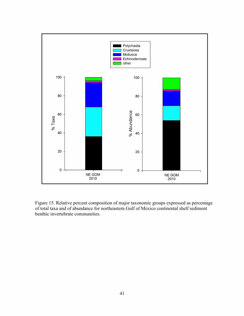
Figure 15. Relative percent composition of major taxonomic groups expressed as percentage of total taxa and of abundance for northeastern Gulf of Mexico continental shelf sediment benthic invertebrate communities.

41

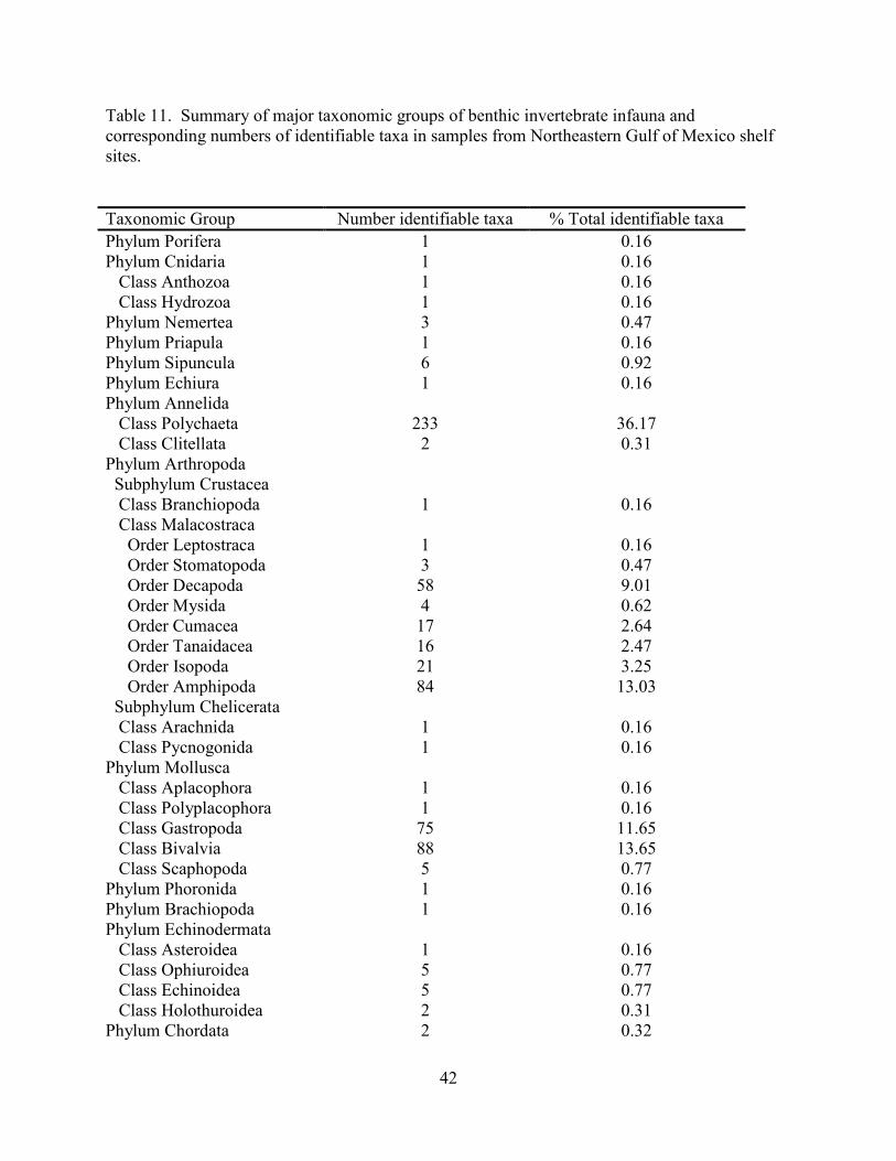
Table 11. Summary of major taxonomic groups of benthic invertebrate infauna and corresponding numbers of identifiable taxa in samples from Northeastern Gulf of Mexico shelf sites. Taxonomic Group Number identifiable taxa % Total identifiable taxa Phylum Porifera 1 0.16 Phylum Cnidaria 1 0.16 Class Anthozoa 1 0.16 Class Hydrozoa 1 0.16 Phylum Nemertea 3 0.47 Phylum Priapula 1 0.16 Phylum Sipuncula 6 0.92 Phylum Echiura 1 0.16 Phylum Annelida Class Polychaeta 233 36.17 Class Clitellata 2 0.31 Phylum Arthropoda Subphylum Crustacea Class Branchiopoda 1 0.16 Class Malacostraca Order Leptostraca 1 0.16 Order Stomatopoda 3 0.47 Order Decapoda 58 9.01 Order Mysida 4 0.62 Order Cumacea 17 2.64 Order Tanaidacea 16 2.47 Order Isopoda 21 3.25 Order Amphipoda 84 13.03 Subphylum Chelicerata Class Arachnida 1 0.16 Class Pycnogonida 1 0.16 Phylum Mollusca Class Aplacophora 1 0.16 Class Polyplacophora 1 0.16 Class Gastropoda 75 11.65 Class Bivalvia 88 13.65 Class Scaphopoda 5 0.77 Phylum Phoronida 1 0.16 Phylum Brachiopoda 1 0.16 Phylum Echinodermata Class Asteroidea 1 0.16 Class Ophiuroidea 5 0.77 Class Echinoidea 5 0.77 Class Holothuroidea 2 0.31 Phylum Chordata 2 0.32

42

Total 644 100.00

43

3.4.2 Abundance, Dominant Taxa and Diversity A total of 19,636 individual specimens were collected across the 50 stations (100 0.04 m-2 grab samples) sampled. Densities ranged from 387 to 15,375 m-2 and averaged 5,834 m-2 (Figure 16, Table 12, Appendix E). There were no offshore samples that were devoid of benthic fauna. Spatially, 10% of the shelf area had densities > 9,687 m-2 and 50% of the shelf area had densities > 5,350 m-2 (Table 12). The 50 most abundant taxa throughout the region are listed in Table 13. The 10 most abundant taxa on this list include tubificid oligochaetes; the polychaetes Mediomastus spp., Goniadides carolinae, Prionospio cristata, Paraprionospio pinnata, Chone spp., and Scoletoma verrilli; Nemertean ribbon worms; the mollusc Caecum pulchellum; and the lancelet Branchiostoma spp. Tubificids were the most abundant group overall with a mean density of 236 m-2. The three taxa with the highest frequency of occurrence were Tubificidae, Nemertea, and the polychaete Spiophanes bombyx. Species richness, expressed as the number of taxa present in a 0.04 m2 grab, was relatively high in these northeastern GOM shelf assemblages. A total of 644 taxa were identified region-wide from the 50 benthic grabs. Species richness ranged from 115 to 88 taxa grab-1 and averaged 50 taxa grab-1 (Figure 16, Table 12, Appendix E). Approximately 50% of the offshore survey area had > 57 taxa grab-1 and 10% of the area had > 71 taxa grab-1. The high species richness, plus an even distribution of species abundance within stations, resulted in high values of the diversity index H′ (log base 2) for this shelf region. Diversity values ranged from 5.32 to 6.56 grab-1 and averaged 5.32 grab-1 (Figure 16, Table 12, Appendix E). Approximately 50% of the offshore survey area had H′ > 5.4 grab-1 and 10% of the area had H′ > 6.0 grab-1. Benthic community measures (density, richness and diversity) vary notably from eastern to western regions of the Gulf of Mexico. Values for the northeastern shelf (this study) and southeastern shelf (Cooksey et al. 2012) are the most similar to one another within this region, though mean richness and density are slightly higher in the northeast than southeast. All three benthic attributes for the NW shelf (from Balthis et al. 2013) are much lower compared to the two eastern regions (Figure 17). Consistent with other historical inshore-offshore comparisons, both the NE and SE GOM offshore benthic assemblages had higher mean densities, richness, and diversity than neighboring estuaries of the region (U.S. EPA. 2012).

44

Figure 16. Percentage area (solid lines) and 95% Confidence Intervals (dotted lines) of Northeastern Gulf of Mexico continental shelf benthic invertebrate infaunal species richness (A), density (B), and H′ diversity (C).

45

Table 12. Mean, range and selected properties of key benthic variables from 50 Northeastern Gulf of Mexico continental shelf sites (2 replicate 0.04-m2 grab samples per site).

Overall Mean

Overall Range

Areal-Based Percentiles1: Frequency-Based Percentiles2 CDF 10th % CDF 50th % CDF 90th % 10th 25th 50th 75th 90th

# Taxa per grab 50 11 - 88 26 57 71 26 37 52 61 73

Density (#/m2) 5864 387 - 15375 2262 5350 9687 2337 3887 5437 7187 10575

H′ per grab 5.32 5.32 – 6.56 4.11 5.36 6.05 4.35 4.99 5.40 5.84 6.14

1 Value of response variable corresponding to the designated cumulative % area point along the y-axis of the CDF graph. 2 Corresponding lower 10th percentile, lower quartile, median, upper quartile, and upper 10th percentile of all values for each of the 3 benthic variables.

46

Table 13. Fifty most abundant benthic taxa from 50 northeastern Gulf of Mexico continental shelf sites (2 replicate 0.04-m2 grab samples per site). Classification: Native = native species; Indeter = indeterminate taxon (not identified to a level that would allow determination of origin).

Taxa Name Taxon Classification Mean

Density % Frequency of Occurrence

Tubificidae Other Indeter 236 80 Mediomastus spp. Polychaeta Indeter 159 49 Goniadides carolinae Polychaeta Native 153 33 Prionospio cristata Polychaeta Native 140 49 Paraprionospio pinnata Polychaeta Native 135 44 Nemertea Other Indeter 128 75 Caecum pulchellum Mollusca Native 125 14 Branchiostoma spp. Other Indeter 103 58 Chone spp. Polychaeta Indeter 88 53 Scoletoma verrilli Polychaeta Native 80 55 Spiophanes bombyx Polychaeta Native 74 64 Exogone lourei Polychaeta Native 72 26 Tellina spp. Mollusca Indeter 64 33 Leptochelia spp. Crustacea Indeter 60 51 Fabricinuda trilobata Polychaeta Native 60 47 Tellina listeri Mollusca Native 56 35 Apseudes olympiae Crustacea Native 55 12 Protodorvillea kefersteini Polychaeta Native 52 37 Ophiuroidea Echinodermata Indeter 49 45 Polygordius spp. Polychaeta Indeter 48 49 Cirrophorus lyra Polychaeta Native 48 32 Sphaerosyllis piriferopsis Polychaeta Native 46 25 Synelmis ewingi Polychaeta Native 44 18 Maldanidae Polychaeta Indeter 44 43 Eunice unifrons Polychaeta Native 43 41 Prionospio spp. Polychaeta Indeter 39 31 Brachiopoda Other Indeter 38 35 Litocorsa antennata Polychaeta Native 38 20 Nuculana spp. Mollusca Indeter 37 3 Ampharete finmarchica Polychaeta Native 36 36 Ceratocephale oculata Polychaeta Native 36 27 Polyplacophora Other Indeter 34 22 Paleanotus sp. A Polychaeta Indeter 31 32 Magelona pettiboneae Polychaeta Native 31 34 Aonides paucibranchiata Polychaeta Native 31 16 Crassinella lunulata Mollusca Native 30 41 Erichthonius brasiliensis Crustacea Native 30 13 Metharpinia floridana Crustacea Native 29 23 Xenanthura brevitelson Crustacea Native 28 26

47

Taxa Name Taxon Classification Mean

Density % Frequency of Occurrence

Euchone incolor Polychaeta Native 27 28 Diplodonta semiaspera Mollusca Native 26 18 Pisione sp. A Polychaeta Indeter 26 20 Caecum cubitatum Mollusca Native 26 3 Hemipodus roseus Polychaeta Native 26 24 Goniada littorea Polychaeta Native 25 21 Aricidea spp. Polychaeta Indeter 25 28 Diplodonta spp. Mollusca Indeter 25 23 Sigambra tentaculata Polychaeta Native 24 16 Aricidea philbinae Polychaeta Native 23 23 Enchytraeidae Other Indeter 22 25

Figure 17. Benthic community (density, richness, diversity) comparisons for northeastern Gulf of Mexico (GOM) shelf waters (this study), northwestern GOM shelf waters (Balthis et al. 2013), southeastern GOM shelf waters (Cooksey et al. 2012), and GOM estuarine waters (US EPA 2012). Bars represent means and lines are +1 standard deviations.

48

3.4.4 Cluster Analysis Spatial patterns in the distribution of benthic invertebrate infauna among stations were examined by hierarchical cluster analysis on double-square-root transformed data using PRIMER analytical software (Clarke and Gorley, 2001). Group-average sorting (= unweighted pair-group method; Sneath and Sokal, 1973) was used as the clustering method and Bray-Curtis dissimilarity (Bray and Curtis, 1957) was used as the resemblance measure. Results were expressed as a dendrogram in which samples were ordered into groups of increasing similarity based on resemblances of component-species abundances. Canonical discriminant analysis, performed with the CANDISC procedure in SAS (2002), also was used to determine whether the separation of the cluster groups could be explained by other measured abiotic environmental factors (sensu Green and Vascotto, 1978). Abiotic variables that were considered included depth, percent silt-clay, TOC, DO, salinity, chlorophyll a, TSS, latitude and longitude. The analysis sought to derive a reduced set of discriminant (canonical) functions that best described the separation of the pre-declared station groups based on data represented by the different abiotic environmental variables. Total structure coefficients (TSC), which are the measures of correlation between the original variables and the discriminant scores on each function, provided a measure of the relative contribution of each variable to group separation. Results of the cluster analysis are presented as a dendrogram in Figure 18. Application of a Bray-Curtis dissimilarity value of 0.5 revealed three major site groups, A, B and E, consisting of 34 of the 50 stations (Figures 18 and 19). The remaining 16 stations formed 10 smaller branches, consisting of either a single station (F, H, I, J, L), two stations (C, G, K, M) or three stations (D). While there was a great deal of spatial overlap between the cluster groups, Group B generally encompasses stations found on the more eastern portion of the sampling area, while group A is dominated by stations along the far eastern portion of the sampling area plus one station in the western portion. Group E stations were generally found within the western to middle portion of the sampling area. The 10 smaller site groups were scattered throughout the sampling region. Results of the canonical discriminant analysis showed that the first canonical function was significant (CAN 1: p < 0.0001, df = 108) and accounted for 57% of the among-group variation in abiotic variables. The second canonical function was significant (CAN 2: p < 0.0001, df = 88) and accounted for an additional 23% of the among-group variation in abiotic variables. In addition, both the third and fourth canonical functions were significant (CAN 3: p = 0.0009, df = 70; CAN 4: p=0.0126, df=54). TSCs for CAN 1 (Table 14) revealed that the strongest correlation on this function is with percent silt-clay and depth, both well-known drivers of benthic invertebrate infauna community structure and composition. TSCs for CAN2 indicated that the strongest correlation was between longitude and DO, indicating the influence of the Mississippi River outflow and related low-DO condition on the benthic invertebrate communities with increasing proximity to the MS delta area. CAN 3 highlighted a strong correlation with salinity and CAN 4 showed a strong correlation with longitude and latitude. Combined results of the discriminant analysis highlights the east-west gradient in the benthic communities across the northeastern GOM.

49

Figure 18. Dendrogram resulting from clustering of benthic samples using group-average sorting and Bray-Curtis dissimilarity. A dissimilarity level of 0.5 (horizontal line) was used to define the two major site groups, A and B, plus C-M.

50

Figure 19. Map showing cluster groups for 50 Northeastern Gulf of Mexico continental shelf stations.

51

Table 14. Total structure coefficients (TSC) from canonical discriminant analysis. Can1=first canonical variable (57% if variability); Can2=second canonical variable (23% of variability); Can3=third canonical variable (6% of variability); Can4=fourth canonical variable (6% of variability). Abiotic Variable Can1 Can2 Can3 Can4 Depth 0.802648 0.105436 0.054545 -0.382412 % Silt-Clay 0.798974 -0.387442 0.163276 0.290278 TOC 0.154788 0.223425 0.174357 0.17475 Latitude -0.021912 -0.355145 -0.26126 -0.526592 Longitude -0.301906 0.681002 -0.085936 0.601923 Salinity 0.475886 0.246883 0.647052 -0.386428 DO -0.31991 0.796807 -0.181209 0.156223 Chlorophyll a -0.311437 -0.475603 -0.479559 0.152251 TSS 0.110188 -0.242687 0.269076 0.416835

52

3.4.5 Non-Indigenous Species The spatial scale of the current survey provides a unique opportunity to examine the benthic macroinvertebrate infauna data for the occurrence of non-indigenous species throughout the northeastern GOM continental shelf. Overall, there were a total of 19,636 individual specimens distributed among 644 taxa identified from 100 grabs. Of those 644 taxa, 397 were identified to the species level. Of the 397 taxa, none was identified as non-indigenous based on a comparison with the USGS Non-indigenous Aquatic Species database (http://nas.er.usgs.gov). The northeastern GOM shelf benthos appears to be less invaded than some other coastal regions, such as the Pacific Coast — where non-indigenous species are common in estuaries and occur offshore as well, though in more limited numbers (e.g., 1.2% of the identified species in a survey of the western U.S. continental shelf; Nelson et al. 2008) — but similar to the MAB, SAB, southeastern GOM shelf, and northwestern GOM shelf where no non-indigenous species were reported (Balthis et al. 2009, Cooksey et al. 2010, Cooksey et al. 2012, Balthis et al. 2013). 3.6 Potential Linkage of Biological Condition to Stressor Impacts Multi-metric benthic invertebrate health indices are a useful tool for detecting signals of a degraded benthos (see review by Diaz et al. 2004). An important feature is the ability to combine multiple benthic invertebrate infauna community attributes (e.g., numbers of species, diversity, abundance, relative proportions of groups of species) into a single measure that maximizes the ability to distinguish between degraded versus non-degraded benthic conditions while taking into account biological variability associated with natural controlling factors (e.g. latitude, salinity, sediment particle size). While related benthic condition indices have been developed for GOM estuaries and near-coastal waters (Engle et al. 1994, Engles of Summers 1999, Tetra Tech 2011), there is currently no such index available for offshore GOM applications. In the absence of a benthic index, potential stressor impacts in offshore waters were assessed in the present study by looking for obvious linkages between reduced values of key benthic characteristics (diversity, richness, density) and synoptically measured indicators of poor sediment or water quality. To be consistent with related offshore studies where multi-metric benthic indices have been lacking (Nelson et al. 2008, Balthis et al. 2009, Cooksey et al. 2010, Cooksey et al 2012, Balthis et al. 2013), low values of benthic attributes were defined as the lower 10th percentile of observed values and evidence of poor sediment and water quality was defined using the following guidelines: ≥ 1 chemical in excess of ERMs, TOC > 50 mg g-1, and DO in near-bottom water < 2 mg L-1. No stations had both poor sediment and water quality accompanied by low values of biological attributes. However, one station located in the far western portion of the study region, adjacent to the Mississippi River delta, had low species richness and taxanomic diversity associated with low DO (1.6 mg l-1; Appendix E). Moreover, five additional stations in this area had one or more benthic attributes in an intermediate range (lower 10th – 50th percentile of values) accompanied by moderate levels of DO (2-5 mg/L). This area is known to experience seasonal low DO events related to fluctuations of the Mississippi River outflow (Moshogianis et al, 2012). Results of this study suggest that natural resources throughout the offshore (shelf) environment studied here were generally in good condition based on the present sampling occasion and the

53

indicators applied, with lower-end values of biological attributes at many of the sites representing parts of a normal reference range controlled by natural factors (e.g., depth and grain size). Moreover, results of this post-DWH survey showed no evidence of oil in sediments at elevated levels known to pose risks to benthic infauna invertebrates based on other studies. However, given this study’s focus on offshore, shelf sediments at a distance of at least 30 nm away from the wellhead, these results do not preclude the possibility of impacts from the DWH spill on sediments deeper and more proximate to the wellhead or to near-shore sediments that may have been exposed to oil. Also, as an exception to the above general conclusions, there was evidence of hypoxic effects at stations near the Mississippi delta in the vicinity of known seasonal hypoxic events. In addition, there were low yet detectable levels of several classes of contaminants including metals, PCBs, PBDEs, PAHs, and pesticides in sediments throughout the region, demonstrating that such substances are making their way to the offshore environment (albeit at low levels) and thus should continue to be monitored to help prevent growth of potential environmental risks to offshore resources and the services they provide. The present study provides an assessment of the current status of ecological condition throughout the region and hopefully a useful means for evaluating potential changes in the future due to either natural or human influences.

54

55

4.0 Acknowledgments Funding for this study was provided by the NOAA/National Ocean Service (NOS)/National Centers for Coastal Ocean Science (NCCOS)/Center for Coastal Environmental Health and Biomolecular Research (CCEHBR) to support field work, sample processing, data analysis and reporting, and related project-management activities. Field work was conducted on the NOAA Ship Nancy Foster Cruise NF-10-09-RACOW (August 13-21, 2010) by scientists from NOAA/NCCOS/CCEHBR, US. EPA/Gulf Ecology Division, and JHT Inc. Several institutions participated in the processing of samples. These included Barry Vittor and Associates (Mobile, AL) for the analysis of benthic invertebrate samples and determination of TOC in sediments; NOAA/NCCOS/CCEHBR for sediment toxicity testing, grain-size analysis, and analysis of most chemical contaminants (all but TPH) in sediments and fish tissues; Chesapeake Biological Laboratories (Solomons, MD) for analysis of nutrients and chlorophyll a in water samples; and TAMU-GERG and Lancaster Laboratories for analysis of potential DWH-related hydrocarbons in sediments. Many of the scientific protocols and concepts are adopted from prior studies conducted through partnership efforts between NOS/NCCOS and the EPA Office of Research and Development/National Health and Environmental Effects Research Laboratory (MOA-2005-003/6764 and current MOA-2011-005/8213). Resulting data are intended to support these ongoing national coastal partnership efforts. 5.0 Literature Cited Balthis WL, Hyland JL, Fulton MH, Wirth EF, Kiddon JA, Macauley J. 2009. Ecological

Condition of Coastal Ocean Waters Along the U.S. Mid-Atlantic Bight: 2006. NOAA Technical Memorandum NOS NCCOS 109, NOAA National Ocean Service, Charleston, SC 29412-9110. 63 pp.

Balthis WL, Hyland JL, Cooksey C, Fulton MH, McFall G. 2007. Long-Term Monitoring of

Ecological Conditions In Gray’s Reef National Marine Sanctuary: Comparison of Soft-Bottom Benthic Assemblages and Contaminant Levels in Sediments and Biota in Spring 2000 and 2005. NOAA Technical Memorandum NOS NCCOS 68. 29 pp. + Appendices.

Balthis WL, Hyland JL, Cooksey C, Fulton MH, Wirth EF, Cobb D, Wiley DN. 2011.

Ecological Condition of Coastal Ocean Waters within Stellwagen Bank National Marine Sanctuary: 2008. NOAA Technical Memorandum NOS NCCOS 129, NOAA National Ocean Service, Charleston, SC 29412-9110. 59 pp.

Balthis, W. L., J. L. Hyland, C. Cooksey, M. H. Fulton, E. F. Wirth. 2013. Ecological Condition

of Coastal Ocean Waters of the Western Gulf of Mexico: 2011. NOAA Technical Memorandum NOS NCCOS 171, NOAA National Ocean Service, Charleston, SC 29412-9110. 63 pp.

Bray JR, Curtis JT, 1957. An ordination of the upland forest communities of southern Wisconsin.

Ecol. Monogr,. 27: 320-349.

56

Caccia VG, Millero FJ, Palanques A. 2003. The distribution of trace metals in Florida Bay sediments. Marine Pollution Bulletin 46: 1420-1433.

Clarke KR, Gorley RN. 2001. PRIMER v5: User Manual/Tutorial. PRIMER-E Ltd, Plymouth

England. Cooksey C, Hyland J, Balthis WL, Fulton M, Scott G, Bearden D. 2004. Soft-Bottom Benthic

Assemblages and Levels of Contaminants in Sediments and Biota at Gray's Reef National Marine Sanctuary and Nearby Shelf Waters off the Coast of Georgia (2000 and 2001). NOAA Technical Memorandum NOS NCCOS 6. 55 pp.

Cooksey C, Harvey J, Harwell L, Hyland J, Summers JK. 2010a. Ecological Condition of Coastal

Ocean and Estuarine Waters of the U.S. South Atlantic Bight: 2000 – 2004. NOAA Technical Memorandum NOS NCCOS 114, NOAA National Ocean Service, Charleston, SC 29412-9110; and EPA/600/R-10/046, U.S. EPA, Office of Research and Development, National Health and Environmental Effects Research Laboratory, Gulf Ecology Division, Gulf Breeze FL, 32561. 88 pp.

Cooksey C, Hyland J, Fulton M. 2010b. Cruise Report: Regional Assessment of Ecosystem

Condition and Stressor Impacts along the Northeastern Gulf of Mexico Shelf. NOAA Technical Memorandum NOS NCCOS 121. 73 pp.

Cooksey C, Hyland J, Fulton M. 2011. Cruise Report: Regional Assessment of Ecosystem Condition

and Stressor Impacts along the Northwestern Gulf of Mexico Shelf. NOAA Technical Memorandum NOS NCCOS 140. 54 pp.

Cooksey, C., J. Hyland, M.H. Fulton., E. Wirth, L. Balthis. 2012. Ecological Condition of

Coastal Ocean Waters of the U.S. Continental Shelf off South Florida: 2007. NOAA Technical Memorandum NOS NCCOS 159, NOAA National Ocean Service, Charleston, SC 29412-9110. 68 pp.

Del Castillo CE, Coble PG, Conmy RN, Muller-Karger FE, Vanderbloemen L, Vargo GA. 2001.

Multispectral in situ measurements of organic matter and chlorophyll fluorescence in seawater: Documenting the intrusion of the Mississippi River plume in the West Florida Shelf. Limnology and Oceanography 46(7): 1836-1843.

Diaz, R. J. and R. Rosenberg. 1995. Marine benthic hypoxia: A review of its ecological effects

and the behavioural responses of benthic macrofauna. Oceanography and Marine Biology: an Annual Review 33:245-303.

Diaz, R. J., M. Solan, and R. M. Valente. 2004. A review of approaches for classifying benthic

habitats and evaluating habitat quality. Journal of Environmental Management 73:165-181.

Donahue S, Acosta A, Akins L, Ault J, Bohnsack J, Boyer J, Callahan M, Causey BD, Cox C,

Delaney J, Delgado G, Edwards K, Garrett G, Keller BD, Kellison GT, Leeworthy VR, MacLaughlin L, McClenachan L, Miller MW, Miller SL, Ritchie K, Rohmann S, Santavy

57

D, Pattengill-Semmens C, Sniffen B, Werndli S, Williams DE. 2008. The state of coral reef ecosystem of the Florida Keys. pp. 161-187. In: J.E. Waddell and A.M. Clarke (eds.), The State of Coral Reef Ecosystems of the United States and Pacific Freely Associated States: 2008. NOAA Technical Memorandum NOS NCCOS 73. NOAA/NCCOS Center for Coastal Monitoring and Assessment’s Biogeography Team. Silver Spring, MD. 569 pp.

Engle VD, Summers JK, Gaston GR. 1994. A benthic index of environmental condition of Gulf

of Mexico estuaries. Estuaries 17: 372-384. Engle, V. D. and J. K. Summers. 1999. Refinement, validation, and application of a benthic

condition index for northern Gulf of Mexico estuaries. Estuaries 22(3A):624-635. Geider RJ, La Roche J. 2002. Redfield revisited: variability of C:N:P in marine microalgae and

its biochemical basis. European Journal of Phycology 37(1):1-17. Grabe SA, Barron J. 2003. Sediment contamination, by habitat, in the Tampa Bat estuarine

system (1993-1999): PAHs, pesticides and PCBs. Environmental Monitoring and Assessment 91:105-144.

Green RH, Vascotto GL. 1978. A method for the analysis of environmental factors controlling

patterns of species composition in aquatic communities. Wat. Res., 12: 583-590. Griffiths SK (2012) Oil release from Macondo Well MC252 following the Deepwater Horizon

Accident. Environ Sci Technol 46: 5616–5622. doi: 10.1021/es204569t. Grimes CB, Turner SC. 1999. The complex life history of tilefish Lopholatilus chamaeleonticeps

and vulnerability to exploitation. American Fisheries Society Symposium 23: 17-26. Harris PJ, Wyanski DM, Powers Mikell PT. 2004. Age, growth, and reproductive biology of

blueline tilefish along the southeastern coast of the United States, 1982-1999. Transactions of the American Fisheries Society 133(5): 1190-1204.

Hetland RD, Hsueh Y, Leben RR, Niiler PP. 1999. A loop current-induced jet along the edge of

the west Florida shelf. Geophysical Research Letters 26(15):2239-2242. Hine AC, Brooks GR, Davis Jr RC, Duncan DS, Locker SD, Twichell DC, Gelfenbaum G. 2003.

The west-central Florida inner shelf and coastal system: a geologic conceptual overview and introduction to the special issue. Marine Geology 200:1-17.

Hyland JL, Balthis L, Engle VD, Long ER, Paul JF, Summers JK, et al. 2003. Incidence of stress

in benthic communities along the U.S. Atlantic and Gulf of Mexico coasts within different ranges of sediment contamination from chemical mixtures. Environmental Monitoring and Assessment 81: 149–161.

58

Hyland JL, Balthis L, Karakassis I, Magni P, Petrov A, Shine J, Vestergaard O, Warwick R. 2005. Organic carbon content of sediments as an indicator of stress in the marine benthos. Marine Ecology Progress Series 295:91-103.

Hyland JL, Herrlinger TJ, Snoots R, Ringwood AH, Van Dolah RF, Hackney CT, Nelson GA,

Rosen JS, Kokkinakis SA. 1996. Environmental quality of estuaries of the Carolinian Province: 1994. NOAA Tech. Memo. NOS ORCA 97, NOAA, Silver Spring, MD.

Hyland JL, Van Dolah RF, Snoots TR. 1999. Predicting stress in benthic communities of

southeastern U.S. estuaries in relation to chemical contamination of sediments. Envir. Toxicol. Chem. 18(11): 2557–2564.

Kannan K, Smith RG, Lee RF, Windom HL, Heitmuller PT, Macauley JM, Summers JK. 1998.

Distribution of total mercury and methyl mercury in water, sediment, and fish from South Florida estuaries. Archives of Environmental Contamination and Toxicology 34: 109-118.

Long ER, Hameedi MJ, Sloane GM, Read LB. 2002. Chemical contamination, toxicity, and

benthic community indices in sediments of the Lower Miami River and adjoining portions of Biscayne Bay, Florida. Estuaries 25(4a): 622-637.

Long ER, MacDonald DD, Smith SL, Calder FD. 1995. Incidence of adverse biological effects

within ranges of chemical concentrations in marine and estuarine sediments. Environ. Manage. 19: 81–97.

Long ER, MacDonald DD. 1998. Recommended Uses of Empirically Derived, Sediment Quality

Guidelines for Marine and Estuarine Ecosystems. Human and Ecological Risk Assessment 4: 1019-1039.

Macauley JM, Smith LM, Harwell LC, Benson WH. 2010. Sediment quality in near coastl water

of the Gulf of Mexico: Influence of Hurricane Katrina. Environmental Toxicology and Chemistry 29(7): 1403-1408.

Microbics Corporation. 1992. Microtox® Manual. A Toxicity Testing Handbook. Carlsbad, CA,

USA. Moshogianis A, Lopez J, Henkel T, Baker A, Boyd E. 2012. Recently observed seasonal hypoxia

within the Gulf of Mexico in the Chandeleur Sound of southeastern Louisiana and Mississippi Bight of coastal Mississippi. Retrieved from Lake Pontchartrain Basin Foundation website: http:// http://www.saveourlake.org/PDF-documents/our-coast/Chandeleur-2012-Hypoxia-Final.pdf

Muller DC, Bonner JS, McDonald SJ, Autenrieth RL, Donnelly KC, Lee K, Doe K, Anderson J.

2003. The use of toxicity bioassays to monitor the recovery of oiled wetland sediments. Environmental Toxicology and Chemistry 22(9): 1945-1955.

59

Nelson WG, Hyland JL, Lee II H, Cooksey CL, Lamberson JO, Cole FA, Clinton PJ. 2008. Ecological Condition of Coastal Ocean Waters along the U.S. Western Continental Shelf: 2003. EPA 620/R-08/001, U.S. EPA, Office of Research and Development, National Health and Environmental Effects Research Laboratory, Western Ecology Division, Newport OR, 97365; and NOAA Technical Memorandum NOS NCCOS 79, NOAA National Ocean Service, Charleston, SC 29412-9110. 137 p.

Office of National Marine Sanctuaries (NMS). 2011. Florida Keys National Marine Sanctuary

Condition Report 2011. U.S. Department of Commerce, National Oceanic and Atmospheric Administration, Office of National Marine Sanctuaries, Silver Spring, MD. 105 pp.

Plumb RH. 1981. Procedure for handling and chemical analysis of sediment and water samples.

Prepared for the U.S. Environmental Protection Agency/Corps of Engineers Technical Committee on Criteria for Dredge and Fill Material. Published by Environmental Laboratory, U.S. Army Waterways Experiment Station, Vicksburg, MS. Technical Report EPA/CE-81-1.

Redalje DG, Lohrenz SE, Natter MJ, Tuel MD, Kirlpatrick GJ, Mille DF, Fahnenstiel GL, Van

Dolah FM. 2008. The growth dynmaics of Karenia brevis within discrete blooms on the West Florida Shelf. Continental Shelf Research 28: 24-44.

Ringwood AH, DeLorenzo ME, Ross PE, Holland AF. 1997. Interpretation of Microtox solid-

phase toxicity tests: the effects of sediment composition. Environmental Toxicology and Chemistry 16(6): 1135-1140.

Rudnick DT, Childer DL, Boyer JN, Fontaine III TD. 1999. Phosphorus and nitrogen inputs to

Florida Bay: The importance of the Everglades watershed. Estuaries 22(2B): 398-416. Sammarco PW, Kolian SR, Warby RAF, Bouldin JL, Subra WA, Porter SA. 2013. Distribution

and concentrations of petroleum hydrocarbons associated with the BP/Deepwater Horizon Oil Spill, Gulf of Mexico. Marine Pollution Bulletin 73: 129-143.

SAS Institute, 2002. SAS OnlineDoc. Version Nine. SAS Institute Inc., Cary, North Carolina,

USA. Shannon CE, Weaver W. 1949. The Mathematical Theory of Communication. U. of Illinois

Press, Urbana, Illinois. 117 pp. Sneath PHA, Sokal RR. 1973. Numerical Taxonomy. Freeman, San Francisco, CA. Stevens Jr. DL, Olsen AR. 2004. Spatially balanced sampling of natural resources. Journal of the

American Statistical Association 99: 262-278. Strobel CJ, Buffum HW, Benyi SJ, Petrocelli EA, Reifsteck DR, Keith DJ. 1995. Statistical

summary: EMAP - Estuaries Virginian Province - 1990 to 1993. U.S. EPA National

60

Health and Environmental Effects Research Laboratory, Atlantic Ecology Division, Narragansett, R.I. EPA/620/R-94/026. 72 p. plus Appendices A–C.

Summers JK, Paul JF, Robertson A. 1995. Monitoring the ecological conditions of estuaries in

the United States. Toxicol. Environ. Chem. 49: 93-108. Tetra Tech. 2011. Benthic Index of Biological Integrity for Estuarine and Near-Coastal Waters

of the Gulf of Mexico. Report to Gulf of Mexico Alliance, Mississippi Department of Environmental Quality Contract No. MDEQ-06-ID-01TT. 123 pp.

Turner, R. E., N. N. Rabalais, and D. Justić. 2012. Predicting summer hypoxia in the northern

Gulf of Mexico: Redux. Marine Pollution Bulletin 64:319–324. U. S. EPA. 2000. Guidance for assessing chemical contaminant data for use in fish advisories,

Volume 2: Risk Assessment and fish consumption limits. U.S. Environmental Protection Agency, Office of Water, Washington, D.C. EPA/823/B-00/008.

U. S. EPA. 2001a. Environmental Monitoring and Assessment Program (EMAP): National

Coastal Assessment Quality Assurance Project Plan 2001-2004. U. S. Environmental Protection Agency, Office of Research and Development, National Health and Environmental Effects Research Laboratory, Gulf Ecology Division, Gulf Breeze, FL. EPA/620/R-01/002.

U. S. EPA. 2001b. Environmental Monitoring and Assessment Program (EMAP): National

Coastal Assessment Field Operations Manual. U.S. Environmental Protection Agency, Office of Research and Development, National Health and Environmental Effects Research Laboratory, Gulf Ecology Division, Gulf Breeze, FL EPA/620/R-01/003.

U.S. EPA. 2006. National Estuary Program Coastal Condition Report. EPA-842/B-06/001. U.S.

Environmental Protection Agency, Office of Water, Washington, D.C. 445 p. Available at: http://www.epa.gov/nccr

U.S. EPA. 2008. National Coastal Condition Report III. EPA-620/R-03/002. U.S. Environmental

Protection Agency, Office of Research and Development and Office of Water, Washington, D.C. 300 p. Available at: http://www.epa.gov/nccr/

U.S. EPA. 2012. National Coastal Condition Report IV. EPA- -842-R-10-003. U.S.

Environmental Protection Agency, Office of Research and Development and Office of Water, Washington, D.C. 368 p. Available at: http://www.epa.gov/nccr/

Vargo GA, Heil CA, Fanning KA, Dixon LK, Neely MB, Lester K, Ault D, Murasko S, Haven J,

Walsh J, Bell S. 2008. Nutrient availability in support of Karenia brevis blooms on the central West Florida Shelf: What keeps Karenia blooming? Continental Shelf Research 28: 73-98.

61

Zhang JZ, Berberian GA. 1997. Determination of dissolved silicate in estuarine and coastal waters by gas segmented continuous flow colorimetric analysis. EPA's manual "Methods for the Determination of Chemical Substances in Marine and Estuarine Environmental Matrices". EPA/600/R-97/072.

Zhang JZ, Chi J. 2002. Automated analysis of nanomolar concentrations of phosphate in natural

waters with liquid waveguide. Environmental Science & Technology 36(5):1048-1053. Zhang JZ, Ortner PB, Fischer CJ. 1997a. Determination of nitrite and nitrate in estuarine and

coastal waters by gas segmented continuous flow colorimetric analysis. EPA's Manual "Methods for the Determination of Chemical Substances in Marine and Estuarine Environmental Matrices". EPA/600/R-97/072.

Zhang JZ, Ortner PB, Fischer CJ, Moore L. 1997b. Determination of ammonia in estuarine and

coastal waters by gas segmented continuous flow colorimetric analysis. EPA's Manual "Methods for the Determination of Chemical Substances in Marine and Estuarine Environmental Matrices". EPA/600/R-97/072.

62

Appendix A. Locations, depths, sediment characteristics and Total Petroleum Hydrocarbons (TPH) of 50 Northeastern Gulf of Mexico continental shelf sites sampled August 2010.

Station Latitude (DD)

Longitude (DD)

Depth (m)

TOC (mg/g)

Silt-Clay (%)

TPH (ng/g)

01 29.49128 -83.6323 11.7 0.48 2.18 5.06 02 29.8741 -87.7521 34 0.71 2.96 5.36 03 28.51044 -83.0697 12 7.01 3.59 4.89 04 29.4979 -88.9873 18 1.42 18.11 8.23 05 29.98339 -85.7519 25 0.55 2.37 4.44 06 28.94819 -84.4843 34 1 4.68 4.93 07 29.44795 -84.941 15 0.99 1.77 4.61 08 28.70232 -84.5806 47.3 28.22 5.76 3.7 09 29.71404 -84.2935 18 2.85 3.46 4.13 10 30.18839 -87.7333 10 4.38 1.53 1.75 11 28.36118 -83.3778 23 7.93 3.66 4.34 12 29.45304 -88.4694 56 8.39 59.56 12.04 13 29.79354 -86.0503 43 14.23 3.57 3.1 14 28.774 -83.9307 30 25.36 3.23 4.03 15 29.43554 -84.4803 26 0.75 3.83 4.02 16 28.83039 -85.2364 100 4.42 36.90 5.05 17 29.80297 -88.013 36 0.74 4.39 4.6 18 29.45391 -84.1757 24 9.05 5.48 6.49 19 29.83053 -87.3382 60 0.77 3.15 4.63 20 28.54568 -83.0759 11.4 31.77 4.1 6.91 21 29.61748 -85.6565 31 0.93 3.71 4.86 22 28.66376 -84.4765 44.2 1.77 10.15 3.51 23 29.1454 -83.5158 14 0.78 2.60 3.98 24 28.83431 -84.9448 49 4.25 4.48 5.78 25 29.95691 -88.1837 32 3.11 13.72 5 26 28.98497 -83.3695 14 0.84 2.46 4.49 27 29.97831 -87.356 29 3.49 1.63 3.58 28 28.30967 -83.6573 32 4.17 7.73 4.41 29 30.18311 -85.8988 21 0.79 3.76 3.49 30 29.38904 -88.0549 81 4.64 23.35 13.26 31 29.35287 -83.5808 13.6 3.07 3.02 3.59 32 29.57762 -88.7502 17.6 1.44 12.57 9.62 33 29.56787 -87.5201 68 5.24 3.11 4.4 34 28.35372 -83.0375 12 0.47 2.62 4.08 35 29.7518 -84.4612 12 0.36 2.06 3.98 36 29.09754 -85.13 36 0.33 2.24 2.86 37 29.95572 -87.4934 32 0.74 2.94 4.64 38 28.18965 -83.3442 25.1 9.81 2.86 2.75 39 29.46679 -84.6945 25 1.11 5.89 2.17 40 28.82441 -84.7166 46 5.17 41.56 5.29 41 29.85237 -88.357 35 10.17 77.99 4.58 42 30.14833 -86.7888 39 2.27 2.04 1.38 43 29.18394 -84.1532 27 2.34 17.17 1.62 44 28.5709 -83.7738 29 4.61 12.10 1.6 45 29.35041 -85.6979 51.4 8.06 3.88 2.27 46 28.53713 -84.1252 37.6 15.37 4.77 2.72 47 29.06686 -83.4285 14 2.3 1.98 2.27 48 29.12906 -84.8782 36 6.79 2.54 1.94 49 29.44149 -87.7086 73 7.6 6.42 7.18 50 28.75888 -83.1347 12 2.06 7.81 3.65

63

Appendix B. Near-surface water characteristics of 50 Northeastern Gulf of Mexico continental shelf sites sampled August 2010. Station Temp.

°C Salinity

(psu) DO

(mg/L) pH DIN

(mg/L) DIP

(mg/L) N/P Chlorophyll a

(µg/L) TSS

(mg/L) 01 31 32.4 5.57 7.9 0.0088 0.0037 1.2 1.67 5.8 02 30.5 30.7 6.26 8 0.0693 0.0098 11 0.56 6.8 03 31.3 35.1 5.51 7.3 0.0086 0.0027 1.5 0.56 7.2 04 29.9 22.7 5.66 8.2 0.019 0.0267 2.4 15.71 26.5 05 30 32.3 6.2 8 0.0128 0.0032 17.9 0.56 5.9 06 30.4 34.1 6.11 8 0.0104 0.0028 2.4 0.56 7.8 07 29.8 33.6 6.26 7.9 0.0086 0.0028 1.4 0.56 6.5 08 30.4 32.9 6.13 8 0.0081 0.0027 1.2 0.56 7 09 30.3 33.6 5.94 7.9 0.0095 0.0047 1.2 0.56 6.5 10 30.1 30.7 5.76 8 0.0208 0.0075 12.3 2.78 6.5 11 30.6 34.7 6.15 7.9 0.0198 0.0049 18.4 0.56 10.9 12 29.9 30 6.22 8.1 0.0097 0.0037 1.7 2.35 5.4 13 29.8 32.1 6.17 8 0.0089 0.0032 1.5 0.56 6.2 14 30.2 34.4 6.09 7.9 0.0129 0.0064 8.9 0.56 7.7 15 30.2 33.8 6.12 7.9 0.0088 0.0037 1.2 0.56 9.6 16 30 33.2 6.06 8 0.0441 0.0046 45.7 0.56 6.4 17 30.7 29.7 5.84 8.1 0.0086 0.0027 1.5 0.6 5.1 18 30.1 33.7 6.06 7.9 0.0089 0.0035 10.3 0.56 6.8 19 30 31.7 6.12 8 0.0114 0.0039 10.2 0.71 6.2 20 31.3 35.1 5.11 6.4 0.0088 0.0032 1.3 0.56 7.1 21 29.8 32.7 5.55 5.9 0.0093 0.003 1.8 0.56 5.8 22 30.6 32.9 6.17 8 0.0085 0.003 1.3 0.56 7.5 23 30.6 33.8 6.47 7.9 0.0095 0.0028 1.9 0.6 5 24 30.2 32.9 6.06 8 0.0118 0.0036 12.3 0.56 7.1 25 30.7 29.8 6.39 8 0.0103 0.0047 1.4 1.57 6 26 30.7 34 6.33 7.9 0.0145 0.0043 14.7 0.63 4.6 27 30.4 30.5 6.26 8.1 0.0092 0.003 1.6 1.12 8.9 28 30.3 34.7 6.07 7.9 0.0093 0.0046 1.1 0.56 8 29 29.8 32.6 5.95 8 0.0163 0.0039 17.1 0.85 6 30 29.9 30.1 5.79 8 0.0139 0.0036 3.7 2 5 31 30.9 32.9 5.44 7 0.0135 0.0034 18.2 1.17 6 32 30 30 6.89 8.1 0.008 0.0054 0.6 3.66 21.5 33 30.4 30.9 6.28 8 0.0084 0.0029 1.3 0.81 5.6 34 31.4 35.2 6.3 7.9 0.0087 0.0033 1.3 0.56 4.8 35 30.4 32.8 5.88 7.9 0.0078 0.004 0.7 1 6.4 36 30.4 32.8 6.2 8 0.0085 0.0031 1.2 0.56 6.2 37 30.5 30.7 6.18 8 0.0104 0.0035 12.1 0.74 5.6 38 30.5 34.9 6.16 7.9 0.0078 0.0039 0.7 0.56 7.5 39 30.1 33.8 5.92 8 0.0082 0.0032 1.1 0.56 5.5 40 30.3 34 6.09 8 0.0147 0.0049 12.2 0.56 7.9 41 30.8 29.7 6.39 7.7 0.0082 0.0034 1 1 6.1 42 30.4 31.2 6.07 8.1 0.0083 0.0039 0.9 0.73 5.5 43 30.3 34 5.3 7.9 0.0096 0.003 1.8 0.56 7.4 44 30.3 34.4 6.09 7.9 0.0179 0.0037 21.6 0.56 7.5 45 30.3 31.5 6.31 8.1 0.0141 0.0048 2.6 0.56 2.4 46 31 33.4 6.07 7.9 0.0097 0.003 1.9 0.56 8.6 47 30.7 33.9 6.59 8 0.0179 0.0043 16 0.56 4.3 48 30.1 33 6.07 8 0.0098 0.0028 2.1 0.56 6.7 49 29.9 30.4 6.02 7.8 0.0112 0.0036 11.1 1.3 5.4 50 31 34.6 5.57 7.9 0.0123 0.0033 13.8 0.56 7.2

64

Appendix C. Near-bottom water characteristics of 50 Northeastern Gulf of Mexico continental shelf sites sampled August 2010. Station Temp.

°C Salinity

(psu) DO

(mg/L) pH DIN

(mg/L) DIP

(mg/L) N/P Chlorophyll a

(µg/L) TSS

(mg/L) 01 30.8 32.8 6.03 7.89 0.0163 0.0031 23.8 3.38 7.6 02 21.8 36.1 4.7 7.79 0.0113 0.0037 12.8 0.56 6.1 03 31.2 35.1 6.14 7.92 0.0086 0.0027 1.5 0.66 9.2 04 27 33.4 1.6 7.69 0.12 0.0381 6.2 1.27 6 05 24.1 35.7 5.37 7.87 0.0128 0.0064 7.3 1.02 8.5 06 22.4 36 6.59 7.92 0.0105 0.0038 1.8 0.57 10.1 07 28 34.5 5.74 7.86 0.008 0.0038 0.9 1.43 8.1 08 19.8 36.1 5.57 7.84 0.0109 0.0055 1.5 0.91 18.6 09 30.3 33.6 5.85 7.92 0.0093 0.0036 10.3 0.56 7.5 10 29 32.9 4.65 7.88 0.0324 0.0085 17.4 4.37 6.7 11 30.2 34.7 6.1 7.92 0.0089 0.0033 1.3 0.56 7.7 12 19.5 36.3 2.82 7.66 0.111 0.0216 7.5 0.56 8.7 13 20.2 36.2 5.26 7.85 0.063 0.0088 10.3 0.89 7.8 14 24.8 35.4 6.35 7.82 0.0085 0.0053 0.7 0.59 8 15 25.5 35.2 5.9 7.84 0.0089 0.0041 1.1 0.56 6.7 16 17.7 36.3 4.44 7.79 0.135 0.0174 11.4 0.56 7 17 21.5 36.1 3.91 7.76 0.073 0.0132 8.5 0.56 6.7 18 27.8 34.8 5.33 7.79 0.0086 0.004 1 0.56 7.8 19 20 36.4 5.22 7.83 0.0764 0.0083 13.2 0.56 6.9 20 31.1 35 5.99 7.91 0.0089 0.003 1.5 0.56 7.1 21 22.1 36 5.64 7.87 0.0161 0.006 3.1 0.98 6.6 22 20 36.2 5.7 7.84 0.0103 0.0049 1.4 1.51 8.3 23 30.6 33.8 6.42 7.94 0.0091 0.003 1.6 0.62 5.6 24 18.3 36.4 4.6 7.81 0.129 0.0158 14 0.56 7.9 25 25.4 35.1 4.37 7.78 0.0402 0.0125 11.9 1.25 7.2 26 30.7 35 6.3 7.94 0.0088 0.0046 0.9 0.63 5.5 27 22.6 35.9 5.24 7.86 0.0375 0.0059 9.8 0.7 8.4 28 24.9 35.6 6.67 7.88 0.0088 0.005 0.9 0.56 8.5 29 25.7 35.2 5.07 7.85 0.0129 0.0058 2 1.63 6.3 30 18.9 36.4 4.98 7.79 0.0842 0.0138 11 0.56 7.4 31 30.7 33.2 6.05 7.89 0.0088 0.0033 1.3 2.09 6.6 32 25.2 35.3 3.1 7.74 0.0887 0.0142 9.5 3.52 19 33 19.2 36.4 5.05 7.79 0.0774 0.0113 9.8 0.56 8.3 34 31.3 35.2 6.18 7.92 0.0111 0.0028 2.8 0.62 5.1 35 30.5 32.8 5.89 7.92 0.0103 0.0036 1.9 1.06 7.3 36 19.4 36.3 5.35 7.86 0.0871 0.0104 12.1 1.64 8.3 37 22.2 35.9 5.07 7.81 0.0496 0.0073 10.7 0.62 7 38 29.5 35.1 6.39 7.89 0.0078 0.0044 0.6 0.56 8 39 25 35.3 5.96 7.84 0.0085 0.0046 0.8 0.89 6.6 40 19.7 36.1 5.35 7.83 0.0496 0.0075 17.6 0.98 16.2 41 22.6 35.6 2.87 7.68 0.0729 0.02 8.6 0.72 10.1 42 19.6 36.4 5.19 7.85 0.0873 0.0093 13.6 0.56 7.4 43 26.2 35.2 6.07 7.79 0.0083 0.0039 0.9 0.9 6.7 44 26.1 35.5 6.89 7.91 0.0088 0.0043 1 0.56 7.4 45 18.2 36.3 4.44 7.83 0.124 0.0163 11.2 0.56 8.1 46 23.8 35.9 6.82 7.89 0.0105 0.0038 1.8 0.66 12.7 47 30.6 33.9 6.58 7.95 0.0128 0.0038 15 0.7 7.4 48 20.3 36.1 5.5 7.85 0.0367 0.0069 7.1 1.53 12.1 49 19.9 36.4 5.39 7.81 0.0688 0.0073 17.8 0.56 6.9 50 30.9 34.6 5.82 7.93 0.0124 0.0048 9.6 0.56 8.3

65

Appendix D. Summary by station of mean ERM quotients and the number of contaminants that exceeded corresponding ERL or ERM values (from Long et al. 1995) for 50 Northeastern Gulf of Mexico continental shelf sites sampled August 2010.

Station # of ERLs Exceeded

# of ERMs Exceeded

Mean ERM-Q

01 0 0 0.002 02 0 0 0.004 03 0 0 0.008 04 0 0 0.012 05 0 0 0.002 06 0 0 0.003 07 0 0 0.007 08 0 0 0.006 09 0 0 0.006 10 0 0 0.002 11 0 0 0.004 12 0 0 0.024 13 0 0 0.006 14 0 0 0.005 15 0 0 0.002 16 0 0 0.006 17 0 0 0.005 18 0 0 0.006 19 0 0 0.004 20 0 0 0.004 21 0 0 0.003 22 0 0 0.006 23 0 0 0.003 24 0 0 0.006 25 0 0 0.01 26 0 0 0.002 27 0 0 0.002 28 0 0 0.006 29 0 0 0.005 30 0 0 0.016 31 0 0 0.002 32 0 0 0.012 33 1 0 0.019 34 0 0 0.003 35 0 0 0.002 36 0 0 0.003 37 0 0 0.004 38 0 0 0.006 39 0 0 0.003 40 0 0 0.005 41 1 0 0.029 42 0 0 0.003 43 0 0 0.004 44 0 0 0.004 45 1 0 0.016 46 0 0 0.005 47 0 0 0.002 48 0 0 0.006 49 1 0 0.013 50 0 0 0.004

66

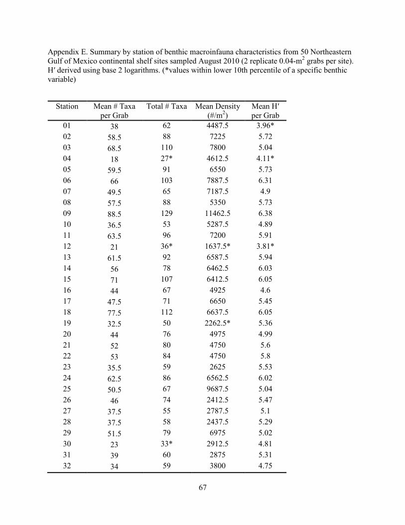
Appendix E. Summary by station of benthic macroinfauna characteristics from 50 Northeastern Gulf of Mexico continental shelf sites sampled August 2010 (2 replicate 0.04-m2 grabs per site). H′ derived using base 2 logarithms. (*values within lower 10th percentile of a specific benthic variable)

Station Mean # Taxa per Grab

Total # Taxa Mean Density (#/m2)

Mean H′ per Grab

01 38 62 4487.5 3.96* 02 58.5 88 7225 5.72 03 68.5 110 7800 5.04 04 18 27* 4612.5 4.11* 05 59.5 91 6550 5.73 06 66 103 7887.5 6.31 07 49.5 65 7187.5 4.9 08 57.5 88 5350 5.73 09 88.5 129 11462.5 6.38 10 36.5 53 5287.5 4.89 11 63.5 96 7200 5.91 12 21 36* 1637.5* 3.81* 13 61.5 92 6587.5 5.94 14 56 78 6462.5 6.03 15 71 107 6412.5 6.05 16 44 67 4925 4.6 17 47.5 71 6650 5.45 18 77.5 112 6637.5 6.05 19 32.5 50 2262.5* 5.36 20 44 76 4975 4.99 21 52 80 4750 5.6 22 53 84 4750 5.8 23 35.5 59 2625 5.53 24 62.5 86 6562.5 6.02 25 50.5 67 9687.5 5.04 26 46 74 2412.5 5.47 27 37.5 55 2787.5 5.1 28 37.5 58 2437.5 5.29 29 51.5 79 6975 5.02 30 23 33* 2912.5 4.81 31 39 60 2875 5.31 32 34 59 3800 4.75

67

33 48 78 4300 5.8 34 26 40* 1325* 4.99 35 39 65 4412.5 5.07 36 56.5 87 5025 6.22 37 53.5 78 5587.5 5.64 38 46 77 3887.5 5.28 39 70 104 11825 4.72 40 27.5 43 4937.5 3.6* 41 11.5 19* 387.5* 3.34* 42 59 91 5525 5.85 43 80 120 12387.5 6.55 44 85.5 125 15375 5.85 45 59 88 7462.5 5.1 46 62.5 101 6550 5.28 47 54 82 7312.5 6.56 48 75.5 107 14162.5 5.55 49 27.5 44 1900* 4.6 50 57.5 90 6662.5 5.58

68

United States Department of Commerce

Penny Pritzker Secretary

National Oceanic and Atmospheric Administration

Dr. Kathryn Sullivan

Administrator (Acting)

National Ocean Service

Dr. Holly Bamford Assistant Administrator