
Ecohydrology Modeling: Tools for Management
29
Provided for non-commercial research and educational use. Not for reproduction, distribution or commercial use. This chapter was originally published in Treatise on Estuarine and Coastal Science, published by Elsevier, and the attached copy is provided by Elsevier for the author's benefit and for the benefit of the author's institution, for non- commercial research and educational use including without limitation use in instruction at your institution, sending it to specific colleagues who you know, and providing a copy to your institution's administrator. All other uses, reproduction and distribution, including without limitation commercial reprints, selling or licensing copies or access, or posting on open internet sites, your personal or institution's website or repository, are prohibited. For exceptions, permission may be sought for such use through Elsevier's permissions site at: http://www.elsevier.com/locate/permissionusematerial Ben-Hamadou R, Atanasova N, and Wolanski E (2011) Ecohydrology Modeling: Tools for Management. In: Wolanski E and McLusky DS (eds.) Treatise on Estuarine and Coastal Science, Vol 10, pp. 301–328. Waltham: Academic Press. © 2011 Elsevier Inc. All rights reserved.
Transcript of Ecohydrology Modeling: Tools for Management

Provided for non-commercial research and educational use.Not for reproduction, distribution or commercial use.
This chapter was originally published in Treatise on Estuarine and CoastalScience, published by Elsevier, and the attached copy is provided by Elsevier for
the author's benefit and for the benefit of the author's institution, for non-commercial research and educational use including without limitation use in
instruction at your institution, sending it to specific colleagues who you know, andproviding a copy to your institution's administrator.
All other uses, reproduction and distribution, including without limitationcommercial reprints, selling or licensing copies or access, or posting on open
internet sites, your personal or institution's website or repository, are prohibited.For exceptions, permission may be sought for such use through Elsevier's
permissions site at:
http://www.elsevier.com/locate/permissionusematerial
Ben-Hamadou R, Atanasova N, and Wolanski E (2011) Ecohydrology Modeling:Tools for Management. In: Wolanski E and McLusky DS (eds.) Treatise on Estuarine
and Coastal Science, Vol 10, pp. 301–328. Waltham: Academic Press.
© 2011 Elsevier Inc. All rights reserved.
Author's personal copy
10.13 Ecohydrology Modeling: Tools for Management R Ben-Hamadou, Centre of Marine Sciences, University of Algarve, Faro, Portugal; International Centre for Coastal Ecohydrology, Faro, Portugal N Atanasova, Centre for Marine and Environmental Research, University of Algarve, Faro, Portugal; International Centre for Coastal Ecohydrology, Faro, Portugal E Wolanski, James Cook University, Townsville, QLD, Australia; Australian Institute of Marine Science, Townsville, QLD, Australia
© 2011 Elsevier Inc. All rights reserved.
10.13.1 Introduction 302
10.13.2 Approaches to EH Modeling 303 10.13.2.1 Knowledge-Driven Approach (Mechanistic) Models 303 10.13.2.2 Data-Driven Approach to Modeling 304 10.13.2.3 Hybrid Modeling Approach 305 10.13.2.3.1 The hybrid modeling tool LAGRAMGE: How it works? 306 10.13.3 Case Studies 308 10.13.3.1 An EH Model of the GBR 308 10.13.3.1.1 Background 308 10.13.3.1.2 The model 308 10.13.3.1.3 Management application 308 10.13.3.2 EH Model of the Guadiana Estuary Ecosystem Health 310 10.13.3.2.1 Background 310 10.13.3.2.2 The model 310 10.13.3.2.3 Management application 311 10.13.3.3 Estuarine Phytoplankton Succession Control (Bottom-Up Control) 312 10.13.3.3.1 Background 312 10.13.3.3.2 The model 312 10.13.3.3.3 Management application 315 10.13.3.4 Estuarine Phytoplankton Succession Control (Top-Down Control) 316 10.13.3.4.1 Background 316 10.13.3.4.2 The model 316 10.13.3.4.3 Management application 319 10.13.3.5 Modeling the Phytoplankton Dynamics in North Adriatic with ML Tools 319 10.13.3.5.1 Background 319 10.13.3.5.2 The model 319 10.13.3.5.3 Management applications 323 10.13.3.6 Modeling Algal Biomass in the Lagoon of Venice with ML Tools: Decision Trees, Equation Discovery, andHybrid Approach
323 10.13.3.6.1 Background 323 10.13.3.6.2 Models 324 10.13.3.6.3 Management application 325 10.13.4 Conclusion 326 References 327Glossary Empirical model An empirical or data-driven model is based on a statistical fit to data as a way to statistically identify relationships between stressor and response variables. Hybrid approach An approach for modeling that combines mechanistic with empirical approach for a mixed knowledge-driven and data-driven model. Machine learning (ML) An algorithm capable of autonomous acquisition and integration of knowledge. This capacity to learn from experience, analytical observation, and other means results in an algorithm that
Treatise on Estuarine and Coastal Science, 2011, Vol.10, 3
characterization of the scientific understanding of the
can improve its own speed or performance, that is, its efficiency and/or effectiveness. Mechanistic model Mechanistic, or theoretical, or knowledge-driven model is a mathematical
critical processes in the natural system; the only data input is in the selection of model parameters and initial and boundary conditions. Ordinary differential equation (ODE) A relation that contains functions of only one independent variable, and one or more of their derivatives with respect to that variable.
301 01-328, DOI: 10.1016/B978-0-12-374711-2.01016-0
Author's personal copy302 Ecohydrology Modeling: Tools for Management
Abstract
Models are recognized as important and necessary tools for understanding complex environmental processes. They allow us to test hypothesis in a systematic manner, predict the future behavior of ecosystems, and, thus, assist in better management of the environment. The modeling task can be addressed by various approaches. This chapter presents applications of ecohydrology models to coastal ecosystems, including various approaches that can be used model formulation. Theoretical (knowledge-driven), empirical (data-driven), and hybrid approaches to modeling are demonstrated in case studies focusing on quantifying the ecosystem health of the Guadiana Estuary in Portugal, the Lagoon of Venice in Italy, the Great Barrier Reef in Australia, and the Adriatic Sea.
10.13.1 Introduction
Coastal ecosystems are driven by complex, highly interactive, dynamic, and temporally- and spatially-distributed processes. This makes the analysis and the prediction of their responses very difficult (and uncertain), in spite of the large body of existing knowledge (Sheng and Kim, 2009). Models, on the other hand, as simplified representation of reality, can synthesize our knowledge and based on that explain the ecosystem behavior. Since a model is a simplified representation of reality, which is designed to address a specific question, scientists ought to focus only on the issue of interest, ignoring the irrelevant processes and factors and selecting temporal and spatial scales of interest. The level of complexity that simultaneously minimizes bias and variance therefore represents an optimal balance for a given modeling scenario; this is the basis for the well-known principle of parsimony (McDonald and Urban, 2010), which states that “models should be as simple as possible, but no simpler.”
There are several reasons for modeling, that is, a quantitative understanding of the system, prediction, provide information and results, and scenario-testing for management. For basic research, modeling aims to both understand in a quantitative sense how a system works and test hypotheses of structural modification impact on the ecosystem. Quantification issues will fit a model to data, allowing quantification of processes that are difficult to measure and then permit predictions by interpolating in time and space their trends and interrelations. Finally, using management tools, model predictions may be used to examine beforehand the consequences of actions.
Within this framework, ecohydrology (EH) models are developed to assist managers and policymakers to simulate ‘what-if’ scenarios. The simulations attempt to predict the future behavior of an estuary or a coastal ecosystem impacted by its watershed. Quite often in practice, the model is first calibrated using a spatial and/or temporal field data set, and then validated with another such data set; it is then used in a forecasting mode to predict the outcome of various management scenarios, such as various water-release rates from dams or water-diversion projects, the additional input of nutrients from development projects such as irrigation and urbanization, removing wetlands for land reclamation, and dredging, channelization, and other engineering structures. Quite often, the modeler has to provide an answer to governments within a very limited time and with limited budget. The common practice therefore for the modeler is to choose a model, or a hybrid of models, from a list of available models such as that provided in Volume 9 of this Treatise. The modeler then adapts the model to the local situation for the study site, keeping the model as simple as
Treatise on Estuarine and Coastal Science, 2011, Vol.10,
possible to have to juggle the least amount of independent variables. This becomes a bridge between science and engineering; nevertheless, it is a science-based model. It is a compromise between practicality and overcomplexity; indeed, some models have hundreds of independent variables, making them possibly elegant and also impractical in many field applications or scenario testing for development projects or governance issues (see a review in Wolanski (2007)). A simplified model is often selected, but later it is modified based on the inflow of new data. This model may be made simpler while sometimes more complex with the addition of more trophic levels or competing species included, which results in more independent variables to estimate.
These mechanistic or knowledge-driven models, which are based on mathematical formulations, are constructed from basic physical, chemical, and biological principles. Therefore, they are transparent and clear to the domain experts, which results in their popularity among scientists and domain experts. However, coastal ecosystems are highly dynamic and complex, making the accurate and reliable predictions of coastal processes difficult (Chau, 2006). Moreover, these predictive tools are inevitably highly specialized, limiting therefore their use for management purposes and can be manipulated only by experienced engineers who have a thorough understanding of the underlying theories. Consequently, scientists developed alternative approaches relying on the recent advancements in artificial intelligence (AI) technologies, making it possible to integrate machine-learning capabilities (e.g., data-driven approach) into ecological numerical modeling. The area of machine learning (ML) particularly provides numerous methods that were successfully applied in EH (e.g., Kompare, 1995; Kompare et al., 2001; Solomatine, 2002; Atanasova et al., 2008; Džeroski, 2009). The good property of these methods and of the data-driven methods in general is that they are capable of inducing models solely from measured data, that is, without the necessity to introduce any domain knowledge. As a result, these models do not have the descriptive power of the knowledge-driven models and are characterized as black-box models. It should be noted here that some methods from the area of ML tend to produce partly descriptive gray-box models due to their exhaustive search for patterns in data. Nevertheless, they are still induced from measured data. Table 1 presents some general characteristics of both approaches, that is, knowledge driven and data driven, their good properties, and their drawbacks.
While both approaches, knowledge driven and data driven, have positive and negative sides, as indicated in Table 1, the latest efforts are focused in their integration. The so-called hybrid approach attempts to keep the good properties and to reduce the drawbacks of both, that is, to increase the
301-328, DOI: 10.1016/B978-0-12-374711-2.01016-0
Author's personal copyEcohydrology Modeling: Tools for Management 303
Table 1 Basic properties of knowledge-driven and data-driven models
Property Mechanistic/knowledge-driven models Data-driven models
Transparency (interpretability) White box Black boxa
Data requirements Variable, can cope with less data High Domain knowledge requirement High Poor or none Coping with complex systems Difficult to construct for complex systems Suitable for any complexity Transferability to other domains Good Nontransferable Performance Poor accuracy of too complex models More accurate in predictions System analysis Very appropriate for system analysis Not appropriatea
Computational time Complex models are very time consuming Generally faster
a Some machine-learning algorithms produce gray-box model, which means that they can be partly interpreted by domain experts.
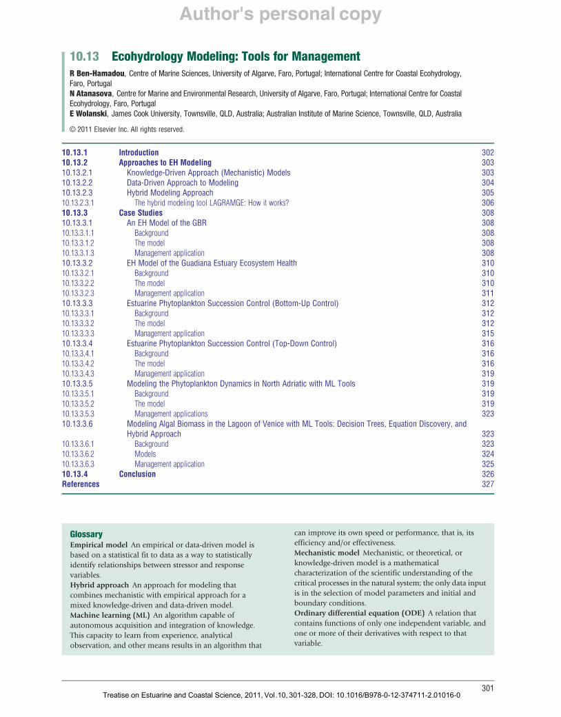
interpretability, simplicity of the model formulation procedure, and the prediction accuracy of models. Typically, this approach provides frameworks where a mechanistic model is optimized using some ML algorithms, for example, genetic algorithms (Whigham and Recknagel, 2001) or a framework where the theoretical knowledge is used to guide an ML algorithm (e.g., Todorovski, 2003; Bridewell et al., 2008). Regarding the transparency (descriptive power) and the accuracy of the models produced, this approach can be characterized between both the basic approaches, that is, data driven and knowledge driven (see Figure 1).
Since several approaches for EH modeling are available to scientists, the choice is made in accordance with the goals and available data sets. A succinct comparative analysis of these approaches is summarized in Figure 1 showing an increase of transparency from the so-called black-box models as a result of a data-driven approach in which the model is directly induced from data, to mechanistic models from a knowledge-driven approach in which the conceptual model is mainly based on processes and functions identified by experts. Contrarily, the accuracy of the obtained simulations generally tends to augment from mechanistic models to the data-driven ones. Hybrid approach usually produces models with intermediate scores of accuracy and transparency when compared to both data- or knowledge-driven approaches.
The goal of this chapter is to present the three modeling approaches through applications in estuaries and coastal EH,
Transparency
Data-driven approach
Input data
Data-driven model
Output as simulations
Hybrid appr
Hybrid approcombine
Data-drivenknowledge-d
modelingapproach
Figure 1 Comparative scheme of the three approaches for ecohydrology moTrends of their transparency and output simulations’ accuracy are represented
Treatise on Estuarine and Coastal Science, 2011, Vol.10
that is, a conceptual approach applied to the ecosystem health of the Guadiana Estuary and the Great Barrier Reef (GBR), a data-driven approach for the prediction of phytoplankton concentration in North Adriatic, and a hybrid approach for modeling algal biomass in Lagoon of Venice. Applications of these EH models for management purposes are then presented to highlight concrete incorporation of simple but not simpler models into decision-making procedure for water and environmental management in coastal areas. The chapter is organized as follows: following the first introductory section of the chapter, the next section provides a brief outlook on the methodology used in the three approaches for EH models; the Section 10.13.3 explores six appliances of these approaches through case studies across multiple settings of estuarine and coastal ecosystems, and management issues and applications are explored; the Section 10.13.4 is dedicated to a brief conclusion and discussion of the approaches and applications presented throughout the chapter.
10.13.2 Approaches to EH Modeling
10.13.2.1 Knowledge-Driven Approach (Mechanistic) Models
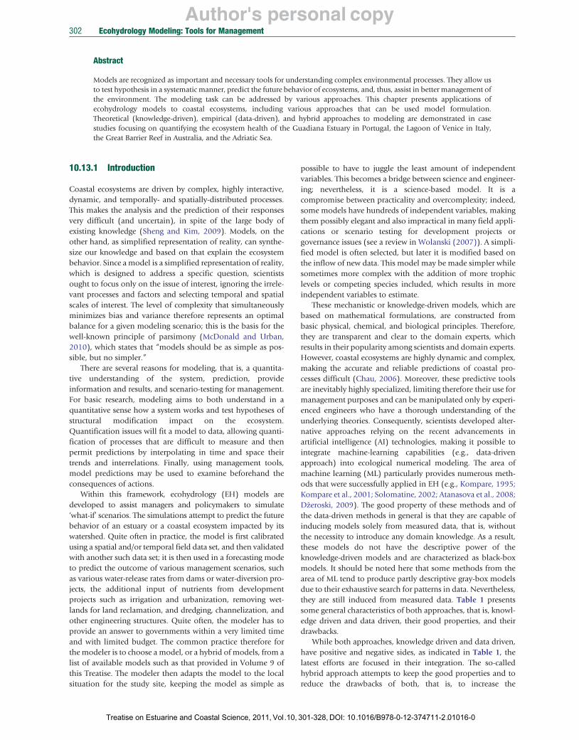
Typically, the modeling procedure within the knowledge-driven (also called theoretical) approach begins with problem identification and data collection (Figure 2(a)). Conceptual
Accuracy
oach
ach
and riven
es
Knowledge-driven approach
Conceptual model
Mathematical model
Parametrization
Input data Calibration
Good enough?
Output as simulations
deling, that is, data-driven, hybrid, and knowledge-driven approaches. respectively by red and blue curves.
, 301-328, DOI: 10.1016/B978-0-12-374711-2.01016-0
Author's personal copy
(a) Problem identification and
data collection
(b)
Selection of mathematical
expressions for the processes in the conceptual model
Calibration
Simulation of the model
Simulated data fit the measurements
Model accepted
YES YES
Mathematical model with constant
parameters
Verification OK
NO
Validation (simulation on
test data)
Simulated data fit the test data
NO
YES
NO
Evaluation (test) data set
Measured data
Conceptual model of the
system
Problem identification and
data collection
Measured data
Automated selection of best
mathematical model for given
conceptual model, i.e.,
Modelling task specification(s)
Modeling knowledge
library
Conceptual modell(s) of the
system
model that fits the
measurements best
Validation (simulation) of
the best model(s)
Evaluation (test) data set
Best model (conceptual and
mathematical)
304 Ecohydrology Modeling: Tools for Management
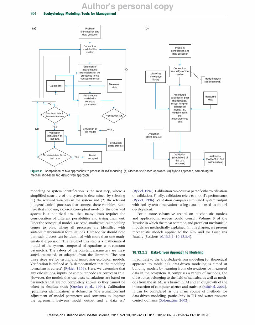
Figure 2 Comparison of two approaches to process-based modeling. (a) Mechanistic-based approach; (b) hybrid approach, combining the mechanistic-based and data-driven approach.
modeling or system identification is the next step, where a simplified structure of the system is determined by selecting (1) the relevant variables in the system and (2) the relevant bio-geochemical processes that connect these variables. Note here that choosing a correct conceptual model of the observed system is a nontrivial task that many times requires the consideration of different possibilities and trying them out. Once the conceptual model is selected, mathematical modeling comes to play, where all processes are identified with suitable mathematical formulations. Here too we should note that each process can be identified with more than one mathematical expression. The result of this step is a mathematical model of the system, composed of equations with constant parameters. The values of the constant parameters are measured, estimated, or adapted from the literature. The next three steps are for testing and improving ecological models. Verification is defined as “a demonstration that the modeling formalism is correct” (Rykiel, 1996). Here, we determine that any calculations, inputs, or computer code are correct or true. However, the models that use these calculations are based on parameters that are not completely known so they cannot be taken as absolute truth (Oreskes et al., 1994). Calibration (parameter identification) is defined as “the estimation and adjustment of model parameters and constants to improve the agreement between model output and a data set”
Treatise on Estuarine and Coastal Science, 2011, Vol.10,
(Rykiel, 1996). Calibration can occur as part of either verification or validation. Finally, validation refers to model’s performance (Rykiel, 1996). Validation compares simulated system output with real system observations using data not used in model development.
For a more exhaustive record on mechanistic models and applications, readers could consult Volume 9 of the Treatise in which the most common and prevalent mechanistic models are methodically explained. In this chapter, we present mechanistic models applied to the GBR and the Guadiana Estuary (Sections 10.13.3.1–10.13.3.4).
10.13.2.2 Data-Driven Approach to Modeling
In contrast to the knowledge-driven modeling (or theoretical approach to modeling), data-driven modeling is aimed at building models by learning from observations or measured data in the ecosystem. It comprises a variety of methods, the oldest ones belonging to the field of statistics, as well as methods from the AI. ML is a branch of AI and an outgrowth of the intersection of computer science and statistics (Mitchel, 2006). It can be considered as the main source of methods for data-driven modeling, particularly in EH and water resource control domains (Solomatine, 2002).
301-328, DOI: 10.1016/B978-0-12-374711-2.01016-0
Author's personal copy
The goal of the model Data
Learning algorithm
Model: Target = f(AT1, AT2, AT3)
AT1 AT2 AT3
1 2 3 4 5 6 7 8
Attributes (independent variables)
Target (class)
Exam ple
1.706 2.081 2.974 2.785 1.433 0.902 1.177
Simulated Target
is to minimize this
11.10 7.400 0.006 1.521
3.67 8.500 0.005 2.133 4.15 7.207 0.005 2.601 5.32 8.357 0.011 3.718 7.80 7.929 0.005 3.481 8.11 7.096 0.005 1.791 9.36 7.804 0.005 1.128
10.87 6.018 0.005 1.471
difference
Ecohydrology Modeling: Tools for Management 305
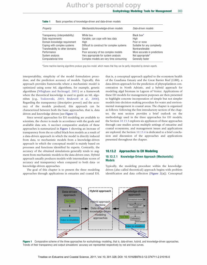
Figure 3 Data-driven modeling: inducing a model from data (examples). Adapted from Solomatine, D.P., 2002. Applications of data-driven modelling and machine learning in control of water resources. In: Mohammadian, M., Sarker, R.A., Yao, X. (Eds.), Computational Intelligence in Control. Idea Group Publishing, Hershey, PA, pp. 197–217.
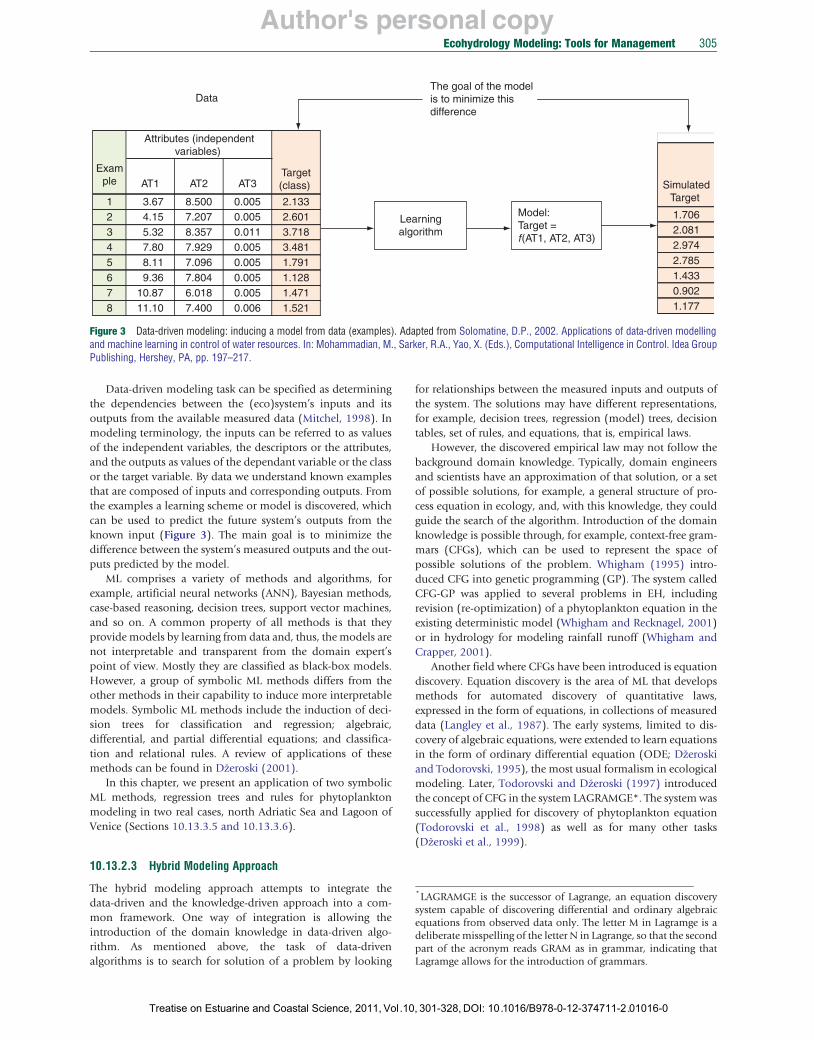
Data-driven modeling task can be specified as determining the dependencies between the (eco)system’s inputs and its outputs from the available measured data (Mitchel, 1998). In modeling terminology, the inputs can be referred to as values of the independent variables, the descriptors or the attributes, and the outputs as values of the dependant variable or the class or the target variable. By data we understand known examples that are composed of inputs and corresponding outputs. From the examples a learning scheme or model is discovered, which can be used to predict the future system’s outputs from the known input (Figure 3). The main goal is to minimize the difference between the system’s measured outputs and the outputs predicted by the model.
ML comprises a variety of methods and algorithms, for example, artificial neural networks (ANN), Bayesian methods, case-based reasoning, decision trees, support vector machines, and so on. A common property of all methods is that they provide models by learning from data and, thus, the models are not interpretable and transparent from the domain expert’s point of view. Mostly they are classified as black-box models. However, a group of symbolic ML methods differs from the other methods in their capability to induce more interpretable models. Symbolic ML methods include the induction of decision trees for classification and regression; algebraic, differential, and partial differential equations; and classification and relational rules. A review of applications of these methods can be found in Džeroski (2001).
In this chapter, we present an application of two symbolic ML methods, regression trees and rules for phytoplankton modeling in two real cases, north Adriatic Sea and Lagoon of Venice (Sections 10.13.3.5 and 10.13.3.6).
* LAGRAMGE is the successor of Lagrange, an equation discovery system capable of discovering differential and ordinary algebraic equations from observed data only. The letter M in Lagramge is a deliberate misspelling of the letter N in Lagrange, so that the second part of the acronym reads GRAM as in grammar, indicating that Lagramge allows for the introduction of grammars.
10.13.2.3 Hybrid Modeling Approach
The hybrid modeling approach attempts to integrate the data-driven and the knowledge-driven approach into a common framework. One way of integration is allowing the introduction of the domain knowledge in data-driven algorithm. As mentioned above, the task of data-driven algorithms is to search for solution of a problem by looking
Treatise on Estuarine and Coastal Science, 2011, Vol.10
for relationships between the measured inputs and outputs of the system. The solutions may have different representations, for example, decision trees, regression (model) trees, decision tables, set of rules, and equations, that is, empirical laws.
However, the discovered empirical law may not follow the background domain knowledge. Typically, domain engineers and scientists have an approximation of that solution, or a set of possible solutions, for example, a general structure of process equation in ecology, and, with this knowledge, they could guide the search of the algorithm. Introduction of the domain knowledge is possible through, for example, context-free grammars (CFGs), which can be used to represent the space of possible solutions of the problem. Whigham (1995) introduced CFG into genetic programming (GP). The system called CFG-GP was applied to several problems in EH, including revision (re-optimization) of a phytoplankton equation in the existing deterministic model (Whigham and Recknagel, 2001) or in hydrology for modeling rainfall runoff (Whigham and Crapper, 2001).
Another field where CFGs have been introduced is equation discovery. Equation discovery is the area of ML that develops methods for automated discovery of quantitative laws, expressed in the form of equations, in collections of measured data (Langley et al., 1987). The early systems, limited to discovery of algebraic equations, were extended to learn equations in the form of ordinary differential equation (ODE; Džeroski and Todorovski, 1995), the most usual formalism in ecological modeling. Later, Todorovski and Džeroski (1997) introduced the concept of CFG in the system LAGRAMGE*. The system was successfully applied for discovery of phytoplankton equation (Todorovski et al., 1998) as well as for many other tasks (Džeroski et al., 1999).
, 301-328, DOI: 10.1016/B978-0-12-374711-2.01016-0
Author's personal copy306 Ecohydrology Modeling: Tools for Management
Although CFGs have been successfully used for solving various tasks and applied to several systems, they have two major drawbacks: (1) the grammars are case specific, that is, they can be used only for the modeling task at hand and (2) the formalism of grammars is quite different to the formalisms used by domain modelers and is therefore not very popular among them. A more general representation of process-based models was proposed by Džeroski and Todorovski (2003) in the form of modeling knowledge libraries. The resulting system LAGRAMGE 2.0 allows the user to provide higher-level (generic) domain knowledge about building mathematical models of complex real-world systems. Given a specific modeling task at hand, LAGRAMGE 2.0 is capable of automatically generating a grammar of possible models (using the generic domain library) for that specific task. The generated grammar is context dependent (and not context free as in LAGRAMGE), that is, it allows the use of context-dependent constraints in the grammar specifying the space of possible equations.
Langley et al. (1997) proposed a different formalism, which uses generic processes to present the general domain modeling knowledge and specific processes to present the specific modeling task. This formalism is supported by the system inductive process modelling (IPM) (Bridewell et al., 2008), which performs a heuristic search directly through the space specified by the modeling task (without generating grammars).
Using the formalism proposed by Todorovski (2003), Atanasova et al. (2006a) elaborated a knowledge library for process-based modeling of aquatic ecosystems, and successfully applied to several domains (e.g., Atanasova et al., 2006b, 2008). The library and its application for model discovery in the Lagoon of Venice are presented in the following sections.
10.13.2.3.1 The hybrid modeling tool LAGRAMGE: How it works? For given conceptual model of an ecosystem, LAGRAMGE discovers a mathematical model, that is, structure and its parameters’ values based on (1) a knowledge library, where general modeling knowledge is encoded, (2) modeling task specification, which corresponds to a conceptual model of the system, where the user specifies important variables and processes that take place in the observed system, and, (3) time series data of the measurements of the specified variables.
After reading the modeling task specification and the measurements, LAGRAMGE performs a heuristic search through the set of candidate model structures composed following the knowledge encoded in the library. In particular, LAGRAMGE composes a list of specific mathematical model structures that can be used to model the processes specified in the task specification, that is, correspond to the given conceptual model. In the next step, LAGRAMGE processes this list of candidate models. For each candidate structure, LAGRAMGE uses nonlinear optimization methods to fit the values of the model parameters against data. Parameter values are selected that minimize the discrepancy between model simulation and observed time-series data, using mean squared error (MSE) to measure the discrepancy. The model structure with lowest discrepancy between the modeled and the observed data is selected as the best model.
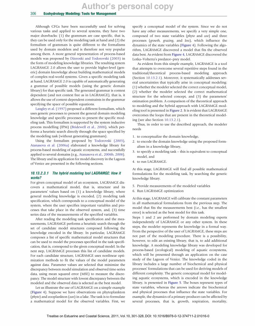
Let us illustrate the use of LAGRAMGE on a simple example (Figure 4). Suppose we have observations on phytoplankton (phyto) and zooplankton (zoo) in a lake. The task is to formulate a mathematical model for the observed variables. First, we
Treatise on Estuarine and Coastal Science, 2011, Vol.10,
specify a conceptual model of the system. Since we do not have any other measurements, we specify a very simple one, composed of two state variables (phyto and zoo) and three processes (growth, grazing, and loss), which influence the dynamics of the state variables (Figure 4). Following the algorithm, LAGRAMGE discovered a model that fits the observed data best. As evident from Figure 4, LAGRAMGE discovered the Lotka–Volterra’s predator–prey model.
As evident from this simple example, LAGRAMGE is a tool that attempts to overcome several repetitive steps found in the traditional/theoretical process-based modeling approach (Section 10.13.2.1). Moreover, it systematically addresses several uncertainties that typically arise in conceptual modeling: (1) whether the modeler selected the correct conceptual model, (2) whether the modeler selected the correct mathematical structure for the selected concept, and (3) the parameters’ estimation problem. A comparison of the theoretical approach to modeling and the hybrid approach with LAGRAMGE modeling tool is presented in Figure 2. It is evident that LAGRAMGE overcomes the loops that are present in the theoretical modeling (see also Section 10.13.2.1).
Thus, in order to use the described approach, the modeler needs
1. to conceptualize the domain knowledge, 2. to encode the domain knowledge using the proposed form
alism in a knowledge library, 3. to specify a modeling task – this is equivalent to conceptual
model, and
4. to run LAGRAMGE.
At this stage, LAGRAMGE will find all possible mathematical formulations for the modeling task, by searching the generic knowledge library.
5. Provide measurements of the modeled variables 6. Run LAGRAMGE optimization
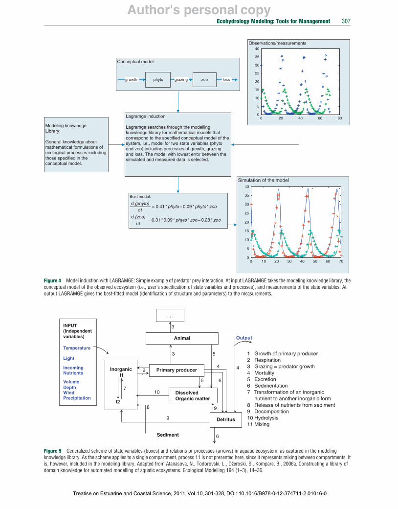
At this stage, LAGRAMGE will calibrate the constant parameters in all mathematical formulations from the previous step. The model that fits the measurements best (i.e., has the smallest error) is selected as the best model for this task. Steps 1 and 2 are performed by domain modeling experts independently of LAGRAMGE or any other system. In these steps, the modeler represents the knowledge in a formal way. From the perspective of the user of LAGRAMGE, these steps are not part of the modeling procedure. There is a possibility, however, to edit an existing library, that is, to add additional knowledge. A modeling knowledge library was developed for process-based (ecological) modeling of aquatic ecosystems, which will be presented through an application on the case study of the Lagoon of Venice. The knowledge coded in the library includes a large number of biochemical and physical processes’ formulations that can be used for deriving models of different complexity. The generic conceptual model for modeling aquatic ecosystems, which is encoded in the knowledge library, is presented in Figure 5. The boxes represent types of state variables, whereas the arrows indicate the biochemical and physical processes that influence the state variables. For example, the dynamics of a primary producer can be affected by several processes, that is, growth, respiration, mortality,
301-328, DOI: 10.1016/B978-0-12-374711-2.01016-0
Author's personal copy
Observations/measurements 40
35 Conceptual model:
30
25
growth phyto grazing zoo loss 20
15
10
5
Lagramge induction 0 0
20 40 60 80
Modeling knowledge Library:
Lagramge searches through the modelling knowledge library for mathematical models that
General knowledge about mathematical formulations of ecological processes including
correspond to the specified conceptual model of the system, i.e., model for two state variables (phyto and zoo) including processes of growth, grazing and loss. The model with lowest error between the
those specified in the simulated and measured data is selected. conceptual model.
Simulation of the model 40
35Best model:
d (phyto) 30= 0.41 * phyto − 0.09 * phyto * zoo dt
25 d (zoo)
= 0.31 * 0.09 * phyto * zoo − 0.28 * zoo 20dt
15
10
5
0 0 10 20 30 40 50 60 70
. . .
INPUT 3 (Independent variables) Animal Output
Temperature 5 1 Growth of primary producer 3
Light 2 Respiration 4 4 3 Grazing = predator growth Incoming Inorganic 2 Primary producer
Nutrients 4 Mortality I1 1 5 Excretion 6 Sedimentation
5 6Volume Depth 7
10 Dissolved 7 Transformation of an inorganic Wind Precipitation Organic matter nutrient to another inorganic form
I2 8 Release of nutrients from sediment 8 9 9 Decomposition
9 10 HydrolysisDetritus 11 Mixing
Sediment 6
Ecohydrology Modeling: Tools for Management 307
Figure 4 Model induction with LAGRAMGE: Simple example of predator prey interaction. At input LAGRAMGE takes the modeling knowledge library, the conceptual model of the observed ecosystem (i.e., user’s specification of state variables and processes), and measurements of the state variables. At output LAGRAMGE gives the best-fitted model (identification of structure and parameters) to the measurements.
Figure 5 Generalized scheme of state variables (boxes) and relations or processes (arrows) in aquatic ecosystem, as captured in the modeling knowledge library. As the scheme applies to a single compartment, process 11 is not presented here, since it represents mixing between compartments. It is, however, included in the modeling library. Adapted from Atanasova, N., Todorovski, L., Džeroski, S., Kompare, B., 2006a. Constructing a library of domain knowledge for automated modelling of aquatic ecosystems. Ecological Modelling 194 (1–3), 14–36.
Treatise on Estuarine and Coastal Science, 2011, Vol.10, 301-328, DOI: 10.1016/B978-0-12-374711-2.01016-0

Author's personal copy308 Ecohydrology Modeling: Tools for Management
excretion, sedimentation, and grazing. We refer the reader to Atanasova et al. (2006a), for more details. Part of the modeling knowledge library applied to specific case can expand or reduce, based on how many variables of each type we observe (model) in the ecosystem.
The use of the library and the hybrid modeling system LAGRAMGE is presented in Section 10.13.3.6, where the system is used for modeling of algal biomass in the Lagoon of Venice.
10.13.3 Case Studies
Modeling approaches are presented below for several case studies showing diverse hydrological and ecological conditions. A brief description of the ecosystem and the tackled problem is presented for each of the cases, followed by a detailed explanation of the modeling approach adopted. Subsequently, management applications of these EH models are presented. Focus is given to identify how EH models would answer ‘what if’ scenarios useful to managers and decision makers for a timely and science-based response to mitigation and administration actions.
10.13.3.1 An EH Model of the GBR
10.13.3.1.1 Background Australia’s GBR Reef stretches along 2600 km of the east coast of Australia from 25°S to 10°S. The study area is in the central region, comprising 261 reefs in a 400-km-long stretch of the GBR, and extending from Lizard Island in the North to the Whitsunday Islands in the South. Mean water depth between reefs is about 10–40 m, and most reefs are emergent at spring low tides. The surrounding waters receive runoff from rivers spread along the coast; river discharges are dominated by short-lived flood events during a short wet season, during which time the river plumes impact on the reefs.
10.13.3.1.2 The model An EH model of the GBR was proposed to demonstrate the need for an ecosystem-based approach to managing the GBR by regulating human activities in the adjoining river catchments (Wolanski et al., 2004; Wolanski and De’ath, 2005; Wolanski, 2007). The ecosystem of each individual reef of the GBR was assumed to be determined by corals, algae, bare space on the hard substrate, herbivorous fish, and crown-of-thorns starfish (COTS), while there were also reef-to-reef connectivity and disturbances driven by physical processes (Figure 6). The relationships for predation–prey and competition for space on the hard substrate of an individual reef were modulated by turbidity (suspended matter concentration (SSC)) and nutrients, and followed S-shaped curves (cf. eqns [1] and [2] in the subsequent section).
The physical forcings of coral reefs in this model were river floods and tropical cyclones that are natural disturbances that impact each reef differently – but in a way that could be quantified by meteorological, hydrological, and oceanographic data – and the oceanography that enables the exchange of coral larvae between reefs (i.e., the connectivity between reefs). The rate of success of recruitment of coral larvae was assumed to decrease with increasing algal cover on the hard substrate.
Treatise on Estuarine and Coastal Science, 2011, Vol.10,
Human activities in the adjoining river catchments were represented in the model by an increase in the suspended sediment and nutrient load. The coral was preyed upon by the COTS; an increase of dissolved nutrients promotes the plankton that supports the drifting COTS larvae. For scenario testing, that is, to forecast the possible future of the GBR in view of human activities, global warming was added as occasional events of increased mortality of adult corals in summer, and ocean acidification as an internal parameter slowing the growth rate of corals.
This model was applied to the GBR and successfully verified against 20 years of data on coral cover at monitored reefs as well as against data on COTS infestations since 1960 (see Chapter 12.15; Wolanski and De’ath, 2005; Wolanski, 2007).
The model predicts (Figure 7) that the biodiversity of the GBR is already measurably impacted by human activities and, if business-as-usual land-use practices continue, it may progressively degrade over a period of a few tens of years to end up with minimal coral cover. The model suggests that much-improved land-use practices will enable corals in some regions of the GBR to recover by 2050 even with global warming. However, the model suggests that if global warming proceeds unchecked at the worst-case scenario predicted by the Intergovernmental Panel on Climate Change (IPCC) scenario A2, only biological adaptation – about which no information is yet available – may prevent a collapse of the GBR’s health by the year 2100, and this collapse may also be accelerated by ocean acidification due to climate change (De’ath et al., 2009).
Thus, a simple EH model, based on a science-based framework of dominant physical and ecological processes, can provide a powerful tool to test scenarios of the impact on complex coastal ecosystems such as the GBR, of human activities on land at the local and global scales. The results of these scenarios can then be used in governance (see Chapter 12.15).
These coral reef EH models should not be seen as static; they must be expected to adapt and evolve in time as the knowledge framework improves. For instance, coral cover could be less than predicted if flood or cyclone frequency or cyclone intensity increases with climate change, and if the coral death rate in the model from bleaching from future warming events is greater than that experienced in the two GBR coral mass bleaching events that occurred in 1998 and 2002. This mortality was much less than that observed in other places such as the Seychelles in the 1998 global coral bleaching event. The model does not include biological adaptation, for which there are no data.
10.13.3.1.3 Management application The Hydrology, Oceanography, Meteorology, Ecology (HOME) model for quantifying the human impact from land use on the health of the GBR has been used to test various scenarios on (1) hindcasting the human impact so far and (2) attempting to forecast the health of the GBR in the future.
The hindcasting reconstructed the history of the GBR health in the last 100 years, roughly since European colonization in the GBR watershed. The human impact on the average coral cover in the last 30 years has been significant (Figure 7) and the predictions compare well with the field data of Bruno and Selig (2007). Hindcasting over the last century since European colonization suggests that the average coral cover has been reduced
301-328, DOI: 10.1016/B978-0-12-374711-2.01016-0

Author's personal copy
(a)
River +
Nutrients
Larval transport by water currents
cyclone
Coral reef
Global warming Individual reef ecosystem
- coral
- algae
- fish
- crown-of-thorns starfish
mud
CBA
Land River Plume
(b)
Ecohydrology Modeling: Tools for Management 309
Figure 6 A sketch of the ecohydrology model of the Great Barrier Reef. (a) Geographic setup showing how each individual coral reef (e.g., A, B, and C) is forced by different external forcings determined by location by (1) river runoff of mud and nutrients, (2) cyclones, global warming, and ocean acidification, and (3) by ocean currents that transport coral, fish, and crown-of-thorns starfish larvae, and thus generate connectivity between individual coral reefs. (b) Each reef has its own reef ecosystem that comprises adult and juvenile corals, algae, fish, and crown-of-thorns starfish. The competition between algae and coral is akin to a space war for the hard substrate. Recruitment can occur by self-seeding or by imports from other reefs. The rates are controlled by nutrients and suspended matter concentration (SSC) as a proxy for turbidity that controls light penetration and thus photosynthesis.
by about 65%. The model was also successful at reproducing the observed history of coral cover measured yearly at one reef over the last 30 years, at reproducing the observed, spatial distribution of coral cover in the central region of the GBR, as well as reproducing the history of COTS infestation over the last 30 years (Wolanski and De’ath, 2005).
The use of the HOME mode for forecasting the GBR health suggests (Figure 7) that with no change in land-use coral cover in the central region of the GBR will further decrease to that typical of a severely degraded system such as in Jamaica; this degradation will be accelerated if severe climate change occurs; that the system may partially recover by 2050 to coral cover values last experienced in the 1960s if the runoff of fine sediment and nutrients was halved from present values; even in that case the system may collapse further on in time if severe climate change occurs; this degradation will be exacerbated by ocean acidification; and the only optimistic scenario for the GBR is that where both land use and climate change are
Treatise on Estuarine and Coastal Science, 2011, Vol.10
controlled, in the former case by halving the runoff of fine sediment and nutrients from the watersheds and in the latter case by limiting atmospheric CO2 to 350 ppm. The former requires a major change in land-use practices and the latter requires global action, and each of them has profound socioeconomic implications (see Chapter 12.15). So far, the Queensland Government has legislated to start remediation measures to decrease the sediment and nutrient runoff from agriculture and grazing; however, the indications are that the farming community is not willing to follow suit willingly (see Chapter 10.04). Since globally climate change has not been addressed, the future of the GBR appears bleak. For the GBR, science is ignored whatever warming calls it makes. The same scenario may also result for US coral reefs (Richmond et al., 2007; Wolanski et al., 2009).
The situation appears more promising in several small island states of Micronesia where causes and effects from land use to coral reefs are more obvious due to the small scales
, 301-328, DOI: 10.1016/B978-0-12-374711-2.01016-0

Author's personal copy
100
80
Ave
rage
live
cor
al c
over
(%
)
Optimistic60
40
LBR + W + A
20 As is LBR + W
As is + W
0
1900 1950 2000 2050 2100 Time (years)
310 Ecohydrology Modeling: Tools for Management
Figure 7 Time-series plot of the predicted average coral cover in the central region of the Great Barrier Reef for five scenarios: (1) As is = present land use (business-as-usual); (2) As is + W = present land use plus global warming (IPCC scenario A2); (3) LBR + W = remediation of land-use activities resulting in a 50% decrease of riverine nutrients and fine sediment, plus global warming; (4) LBR + W + A = scenario (3) plus ocean acidification; (5) Optimistic = scenario (4) plus global action against climate change that results in stabilizing atmospheric CO2 to 350 ppm. (+) = Field data points from Bruno and Selig (2007). Modified from Richmond, R.H., Wolanski, E., 2011. Coral research: past efforts and future horizons. In: Dubinsky, Z and Stambler, N., (eds.) Coral Reefs: An ecosystem in Transition. Springer Science, pp. 552. ISBN: 978-94-007-0113-7.
(literally a few hundreds of meters between the watershed and the coral reef as opposed to tens of kilometers for the GBR) and where the community is smaller and more integrated and it accepts more readily the advice of their local scientists who have applied the HOME model at the local scale of a small watershed and a fringing reef. In such instances, the community is more integrated, scenario testing by scientists is more readily accepted, and land use is willingly more strictly regulated as a consensus decision (Golbuu et al., 2011).
10.13.3.2 EH Model of the Guadiana Estuary Ecosystem Health
10.13.3.2.1 Background The Guadiana River is one of the largest in the south of the Iberian Peninsula. The fluvial regime is characterized by low flows during summer and episodic runoff periods in winter with the resulting discharge of sediments into the estuary and coastal zone. The estuary is 70 km long; it has a maximum width of 550 m and the maximum depth varies between 5 and 17 m. The tidal regime of the estuary is meso-tidal, with an average amplitude of 2 m. The estuary has an important nursery function for several fish species, such as the anchovy Engraulis encrasicolus and several Sparidae, and crustacean species such as the brown shrimp Crangon crangon. Moreover, the outwelling from the estuary to the coastal area promotes the development of the food web and influences the fisheries (Chícharo et al., 2002; Erzini, 2005).
Several pollution sources exist in the Guadiana Estuary area, mainly resulting from urbanization, agriculture (fertilizers, pesticides, and herbicides), cattle breeding, and olive oil production. The freshwater flow reaching the estuary is at
Treatise on Estuarine and Coastal Science, 2011, Vol.10,
present regulated by more than 100 dams, including the Alqueva Dam whose construction was completed in 2002 and that forms the largest reservoir in Europe (Alveirinho et al., 2004).
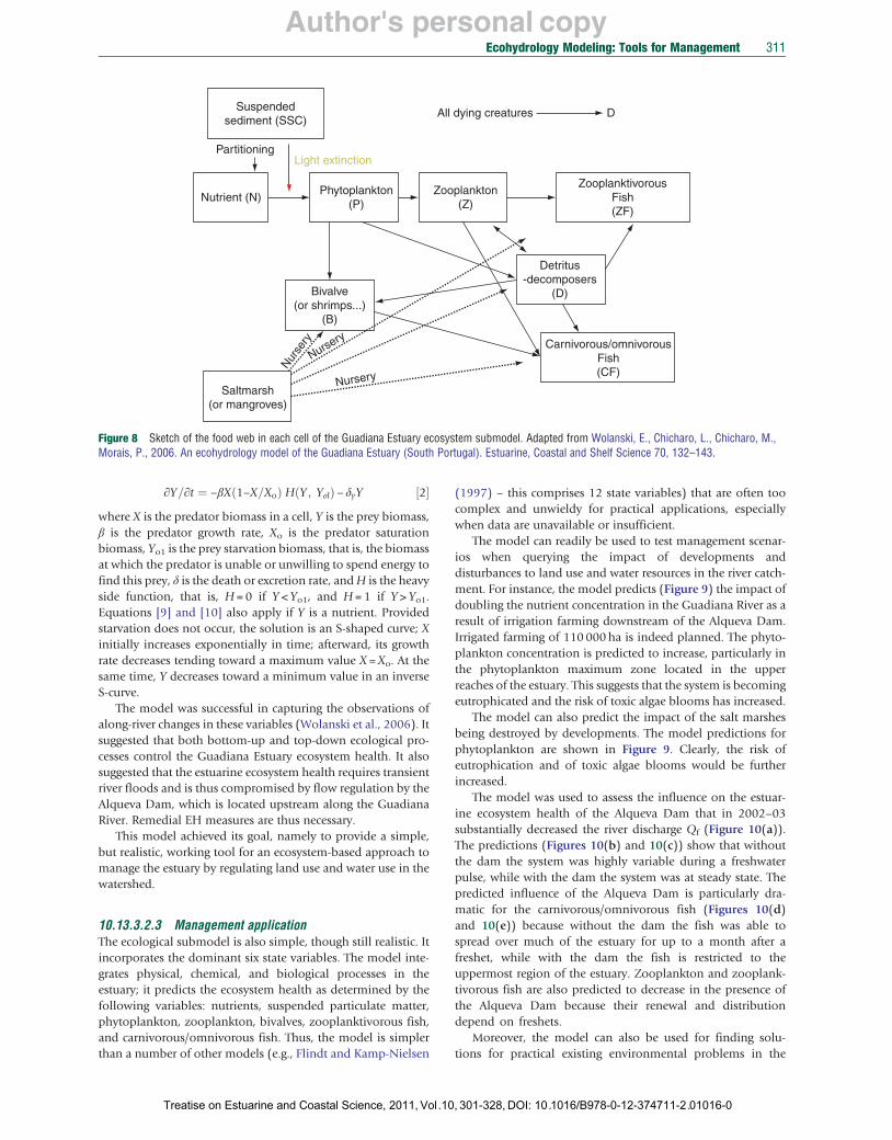
10.13.3.2.2 The model An EH model was proposed that integrates physical, chemical, and biological processes in the Guadiana Estuary during low-flow conditions and that predicts the ecosystem health as determined by the following variables: river discharge, nutrients, suspended particulate matter, phytoplankton, zooplankton, bivalves, zooplanktivorous fish, and carnivorous/ omnivorous fish (Wolanski et al., 2006). Based on field data, the modeler simplified the trophic food chain to that shown in Figure 8, which highlights the observed key role of salt marshes in the ecology of the estuary as a nursery and as a source of detrital matter, and of suspended particulate matter in providing dissolved nutrients as specified by a partitioning coefficient and in slowing down the uptake of nutrients by phytoplankton because of shading, and these nutrients in turn drive the food web. The estuary was divided into cells, and the waterborne elements of this food chain in each cell were exchanged between cells at rates determined by advection and tidal mixing. The horizontal swimming behavior of migrating species was also included. The equations for the predator–prey relationships and the competition equations were purposely kept as simple as possible to remain practical yet realistic; these equations were adapted from Kot (2001) and Brauer and Castillo-Chavez (2001):
∂X=∂t ¼ βXð1−X=XoÞ HðY ; Yo1Þ − δxX ½1� and
301-328, DOI: 10.1016/B978-0-12-374711-2.01016-0
Author's personal copy
Suspended sediment (SSC)
All dying creatures D
Phytoplankton (P)
Light extinction
Zooplankton (Z)
Nursery
Nursery
Nurse
ry
Zooplanktivorous Fish (ZF)
Nutrient (N)
Partitioning
Bivalve (or shrimps...)
(B)
Saltmarsh (or mangroves)
Detritus -decomposers
(D)
Carnivorous/omnivorous Fish (CF)
Ecohydrology Modeling: Tools for Management 311
Figure 8 Sketch of the food web in each cell of the Guadiana Estuary ecosystem submodel. Adapted from Wolanski, E., Chicharo, L., Chicharo, M., Morais, P., 2006. An ecohydrology model of the Guadiana Estuary (South Portugal). Estuarine, Coastal and Shelf Science 70, 132–143.
∂Y=∂t ¼ −βXð1−X=XoÞ HðY ; YolÞ − δyY ½2� where X is the predator biomass in a cell, Y is the prey biomass, β is the predator growth rate, Xo is the predator saturation biomass, Yo1 is the prey starvation biomass, that is, the biomass at which the predator is unable or unwilling to spend energy to find this prey, δ is the death or excretion rate, and H is the heavy side function, that is, H = 0 if Y < Yo1, and H = 1 if Y > Yo1. Equations [9] and [10] also apply if Y is a nutrient. Provided starvation does not occur, the solution is an S-shaped curve; X initially increases exponentially in time; afterward, its growth rate decreases tending toward a maximum value X = Xo. At the same time, Y decreases toward a minimum value in an inverse S-curve.
The model was successful in capturing the observations of along-river changes in these variables (Wolanski et al., 2006). It suggested that both bottom-up and top-down ecological processes control the Guadiana Estuary ecosystem health. It also suggested that the estuarine ecosystem health requires transient river floods and is thus compromised by flow regulation by the Alqueva Dam, which is located upstream along the Guadiana River. Remedial EH measures are thus necessary.
This model achieved its goal, namely to provide a simple, but realistic, working tool for an ecosystem-based approach to manage the estuary by regulating land use and water use in the watershed.
10.13.3.2.3 Management application The ecological submodel is also simple, though still realistic. It incorporates the dominant six state variables. The model integrates physical, chemical, and biological processes in the estuary; it predicts the ecosystem health as determined by the following variables: nutrients, suspended particulate matter, phytoplankton, zooplankton, bivalves, zooplanktivorous fish, and carnivorous/omnivorous fish. Thus, the model is simpler than a number of other models (e.g., Flindt and Kamp-Nielsen
Treatise on Estuarine and Coastal Science, 2011, Vol.10
(1997) – this comprises 12 state variables) that are often too complex and unwieldy for practical applications, especially when data are unavailable or insufficient.
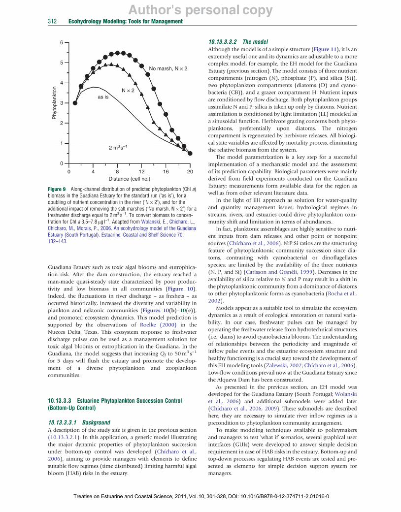
The model can readily be used to test management scenarios when querying the impact of developments and disturbances to land use and water resources in the river catchment. For instance, the model predicts (Figure 9) the impact of doubling the nutrient concentration in the Guadiana River as a result of irrigation farming downstream of the Alqueva Dam. Irrigated farming of 110 000 ha is indeed planned. The phytoplankton concentration is predicted to increase, particularly in the phytoplankton maximum zone located in the upper reaches of the estuary. This suggests that the system is becoming eutrophicated and the risk of toxic algae blooms has increased.
The model can also predict the impact of the salt marshes being destroyed by developments. The model predictions for phytoplankton are shown in Figure 9. Clearly, the risk of eutrophication and of toxic algae blooms would be further increased.
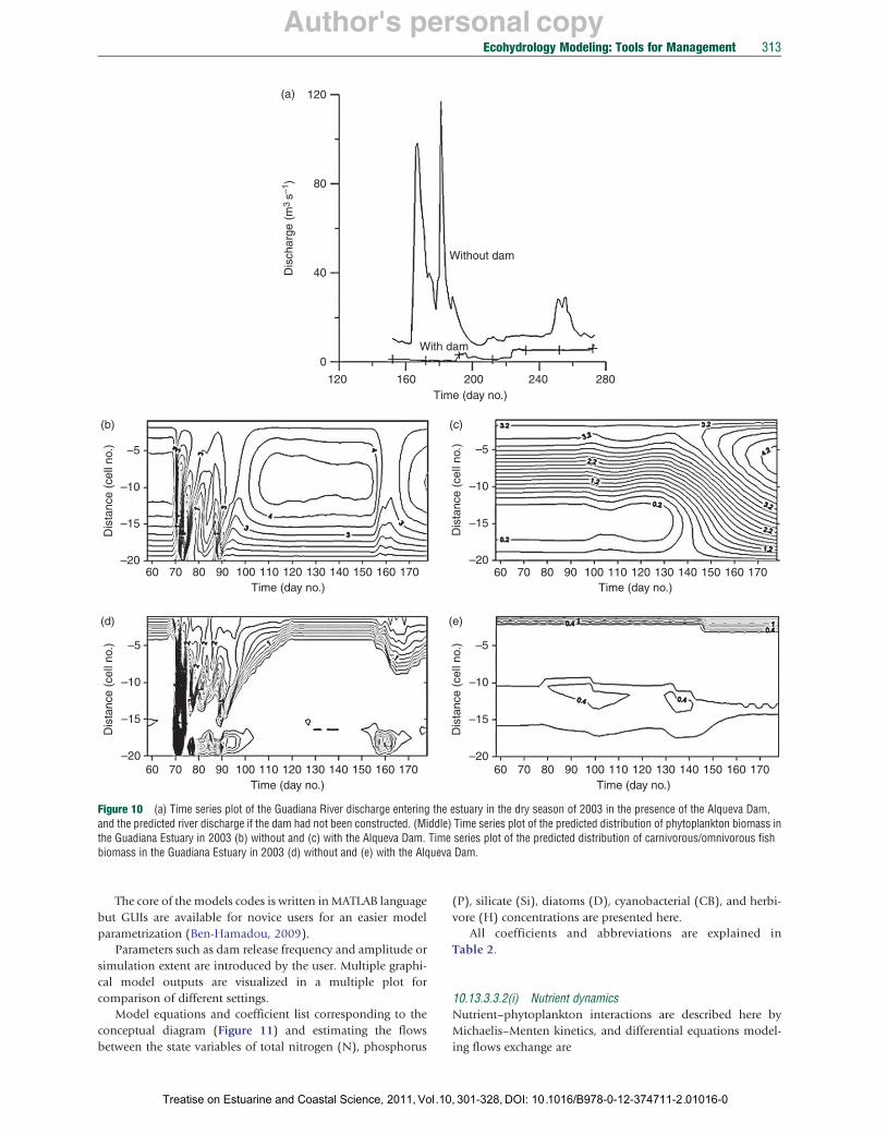
The model was used to assess the influence on the estuarine ecosystem health of the Alqueva Dam that in 2002–03 substantially decreased the river discharge Qf (Figure 10(a)). The predictions (Figures 10(b) and 10(c)) show that without the dam the system was highly variable during a freshwater pulse, while with the dam the system was at steady state. The predicted influence of the Alqueva Dam is particularly dramatic for the carnivorous/omnivorous fish (Figures 10(d) and 10(e)) because without the dam the fish was able to spread over much of the estuary for up to a month after a freshet, while with the dam the fish is restricted to the uppermost region of the estuary. Zooplankton and zooplanktivorous fish are also predicted to decrease in the presence of the Alqueva Dam because their renewal and distribution depend on freshets.
Moreover, the model can also be used for finding solutions for practical existing environmental problems in the
, 301-328, DOI: 10.1016/B978-0-12-374711-2.01016-0
Author's personal copy312 Ecohydrology Modeling: Tools for Management
Figure 9 Along-channel distribution of predicted phytoplankton (Chl a) biomass in the Guadiana Estuary for the standard run (‘as is’), for a doubling of nutrient concentration in the river (‘N � 2’), and for the additional impact of removing the salt marshes (‘No marsh, N � 2’) for a freshwater discharge equal to 2 m3 s−1. To convert biomass to concentration for Chl a 3.5–7.8 μg l−1. Adapted from Wolanski, E., Chicharo, L., Chicharo, M., Morais, P., 2006. An ecohydrology model of the Guadiana Estuary (South Portugal). Estuarine, Coastal and Shelf Science 70, 132–143.
Phy
topl
ankt
on
2
3
4
5
6
1
0
0 4 8 12 16 20 Distance (cell no.)
2 m3 s–1
as is N × 2
No marsh, N × 2
Guadiana Estuary such as toxic algal blooms and eutrophication risk. After the dam construction, the estuary reached a man-made quasi-steady state characterized by poor productivity and low biomass in all communities (Figure 10). Indeed, the fluctuations in river discharge – as freshets – as occurred historically, increased the diversity and variability in plankton and nektonic communities (Figures 10(b)–10(e)), and promoted ecosystem dynamics. This model prediction is supported by the observations of Roelke (2000) in the Nueces Delta, Texas. This ecosystem response to freshwater discharge pulses can be used as a management solution for toxic algal blooms or eutrophication in the Guadiana. In the Guadiana, the model suggests that increasing Qf to 50m3 s−1
for 5 days will flush the estuary and promote the development of a diverse phytoplankton and zooplankton communities.
10.13.3.3 Estuarine Phytoplankton Succession Control (Bottom-Up Control)
10.13.3.3.1 Background A description of the study site is given in the previous section (10.13.3.2.1). In this application, a generic model illustrating the major dynamic properties of phytoplankton succession under bottom-up control was developed (Chícharo et al., 2006), aiming to provide managers with elements to define suitable flow regimes (time distributed) limiting harmful algal bloom (HAB) risks in the estuary.
Treatise on Estuarine and Coastal Science, 2011, Vol.10,
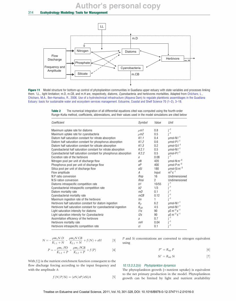
10.13.3.3.2 The model Although the model is of a simple structure (Figure 11), it is an extremely useful one and its dynamics are adjustable to a more complex model, for example, the EH model for the Guadiana Estuary (previous section). The model consists of three nutrient compartments (nitrogen (N), phosphate (P), and silica (Si)), two phytoplankton compartments (diatoms (D) and cyanobacteria (CB)), and a grazer compartment H. Nutrient inputs are conditioned by flow discharge. Both phytoplankton groups assimilate N and P; silica is taken up only by diatoms. Nutrient assimilation is conditioned by light limitation (LL) modeled as a sinusoidal function. Herbivore grazing concerns both phytoplanktons, preferentially upon diatoms. The nitrogen compartment is regenerated by herbivore releases. All biological state variables are affected by mortality process, eliminating the relative biomass from the system.
The model parametrization is a key step for a successful implementation of a mechanistic model and the assessment of its prediction capability. Biological parameters were mainly derived from field experiments conducted on the Guadiana Estuary; measurements form available data for the region as well as from other relevant literature data.
In the light of EH approach as solution for water-quality and quantity management issues, hydrological regimes in streams, rivers, and estuaries could drive phytoplankton community shift and limitation in terms of abundances.
In fact, planktonic assemblages are highly sensitive to nutrient inputs from dam releases and other point or nonpoint sources (Chícharo et al., 2006). N:P:Si ratios are the structuring feature of phytoplanktonic community succession since diatoms, contrasting with cyanobacterial or dinoflagellates species, are limited by the availability of the three nutrients (N, P, and Si) (Carlsson and Granéli, 1999). Decreases in the availability of silica relative to N and P may result in a shift in the phytoplanktonic community from a dominance of diatoms to other phytoplanktonic forms as cyanobacteria (Rocha et al., 2002).
Models appear as a suitable tool to simulate the ecosystem dynamics as a result of ecological restoration or natural variability. In our case, freshwater pulses can be managed by operating the freshwater release from hydrotechnical structures (i.e., dams) to avoid cyanobacteria blooms. The understanding of relationships between the periodicity and magnitude of inflow pulse events and the estuarine ecosystem structure and healthy functioning is a crucial step toward the development of this EH modeling tools (Zalewski, 2002; Chícharo et al., 2006). Low-flow conditions prevail now at the Guadiana Estuary since the Alqueva Dam has been constructed.
As presented in the previous section, an EH model was developed for the Guadiana Estuary (South Portugal; Wolanski et al., 2006) and additional submodels were added later (Chícharo et al., 2006, 2009). These submodels are described here; they are necessary to simulate river inflow regimes as a precondition to phytoplankton community arrangement.
To make modeling techniques available to policymakers and managers to test ‘what if’ scenarios, several graphical user interfaces (GUIs) were developed to answer simple decision requirement in case of HAB risks in the estuary. Bottom-up and top-down processes regulating HAB events are tested and presented as elements for simple decision support system for managers.
301-328, DOI: 10.1016/B978-0-12-374711-2.01016-0
Author's personal copy
(a) 120
) 80
–1 s 3
Dis
char
ge (
m
Without dam
40
With dam 0
120 160 200 240 280 Time (day no.)
(b) (c)
.)
.)
Dis
tanc
e (c
ell n
o –5
–10
–15
Dis
tanc
e (c
ell n
o –5
–10
–15
–20 –20 60 70 80 90 100 110 120 130 140 150 160 170 60 70 80 90 100 110 120 130 140 150 160 170
Time (day no.) Time (day no.)
(d) (e)
Dis
tanc
e (c
ell n
o.) –5
–10
–15
Dis
tanc
e (c
ell n
o.) –5
–10
–15
–20 –20 60 70 80 90 100 110 120 130 140 150 160 170 60 70 80 90 100 110 120 130 140 150 160 170
Time (day no.) Time (day no.)
Ecohydrology Modeling: Tools for Management 313
Figure and the predicted river discharge if the dam had not been constructed. (Middle) Time series plot of the predicted distribution of phytoplankton biomass ithe Guadiana Estuary in 2003 (b) without and (c) with the Alqueva Dam. Time series plot of the predicted distribution of carnivorous/omnivorous fish biomass in the Guadiana Estuary in 2003 (d) without and (e) with the Alqueva Dam.
10 (a) Time series plot of the Guadiana River discharge entering the estuary in the dry season of 2003 in the presence of the Alqueva Dam,n
The core of the models codes is written in MATLAB language but GUIs are available for novice users for an easier model parametrization (Ben-Hamadou, 2009).
Parameters such as dam release frequency and amplitude or simulation extent are introduced by the user. Multiple graphical model outputs are visualized in a multiple plot for comparison of different settings.
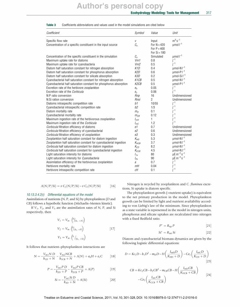
Model equations and coefficient list corresponding to the conceptual diagram (Figure 11) and estimating the flows between the state variables of total nitrogen (N), phosphorus
Treatise on Estuarine and Coastal Science, 2011, Vol.10
(P), silicate (Si), diatoms (D), cyanobacterial (CB), and herbivore (H) concentrations are presented here.
All coefficients and abbreviations are explained in Table 2.
10.13.3.3.2(i) Nutrient dynamics Nutrient–phytoplankton interactions are described here by Michaelis–Menten kinetics, and differential equations model-ing flows exchange are
, 301-328, DOI: 10.1016/B978-0-12-374711-2.01016-0
Author's personal copy
LL
Nitrogen
Phosphate
Diatoms
Cyanobacteria
Silicate
Herbivore Flow
Discharge
Frequency and Amplitude
m.D
m.CB
m.H
314 Ecohydrology Modeling: Tools for Management
Figure 11 Model structure for bottom-up control of phytoplankton communities in Guadiana upper estuary with state variables and processes linking them. ‘LL., light limitation; m.D, m.CB, and m.H are, respectively, diatoms, Cyanobacteria, and herbivores mortalities. Adapted from Chícharo, L., Chícharo, M.A., Ben-Hamadou, R., 2006. Use of a hydrotechnical infrastructure (Alqueva Dam) to regulate planktonic assemblages in the Guadiana Estuary: basis for sustainable water and ecosystem services management. Estuarine, Coastal and Shelf Science 70 (1–2), 3–18.
Table 2 The numerical integration of all differential equations cited was computed using the fourth-order Runge–Kutta method, coefficients, abbreviations, and their values used in the model simulations are cited below
Coefficient Symbol Value Unit
j−1Maximum uptake rate for diatoms ρm1 0.8 j−1Maximum uptake rate for cyanobacteria ρm2 0.5
Diatom half saturation constant for nitrate absorption K1.1 0.4 µmol-N l−1
Diatom half saturation constant for phosphorus absorption K1.2 0.6 µmol-P l−1
Diatom half saturation constant for silicate absorption K1.3 0.2 µmol-Si l−1
Cyanobacterial half saturation constant for nitrate absorption K 2.1 0.5 µmol-N l−1
Cyanobacterial half saturation constant for phosphorus absorption K 2.2 0.5 µmol-P l−1
j−1Excretion rate of the herbivore e 0.08 Nitrogen pool per unit of discharge flow eN 420 µmol-N m−3
Phosphorus pool per unit of discharge flow eP 400 µmol-P m−3
Silica pool per unit of discharge flow eSi 180 µmol-Si m−3
Flow amplitude A Input m3 s−1
N:P ratio conversion Rnp 16 Undimensioned N:Si ration conversion Rnsi 2 Undimensioned Diatoms intraspecific competition rate b1 10/55 j−1
Cyanobacterial intraspecific competition rate b2 1/3 j−1
j−1Diatom mortality rate mD 0.1 j−1Cyanobacterial mortality rate mCB 0.12 j−1Maximum ingestion rate of the herbivore Im 1
Herbivore half saturation constant for diatom ingestion KD 6.2 µmol-N l−1
Herbivore half saturation constant for cyanobacterial ingestion KCB 4.5 µmol-N l−1
Light saturation intensity for diatoms I1s 90 µEm−2 s−1
Light saturation intensity for Cyanobacteria I2s 90 µEm−2 s−1
j−1Assimilation efficiency of the herbivore a 0.7 j−1Herbivore mortality rate mH 0.04 j−1Herbivore intraspecific competition rate ci 0.1
ρm1N D ρm2N CB N ¼ − − þ f ðNÞ þ eH ½3�
K1:1 þN K2:1 þN
ρm1 PD ρm2 PCBP ¼ − − þ f ðPÞ ½4� K1:2 þ P K2:2 þ P
With f () is the nutrient enrichment function consequent to the flow discharge forcing according to the input frequency and with the amplitude A:
f ðN=P=SiÞ ¼ ðeN=eP=eSiÞA ½5�
Treatise on Estuarine and Coastal Science, 2011, Vol.10,
P and Si concentrations are converted to nitrogen equivalent using
P� ¼ Rnp P ½6� Si� ¼ Rnsi Si ½7�
10.13.3.3.2(ii) Phytoplankton dynamics The phytoplankton growth (= nutrient uptake) is equivalent to the net primary production in the model. Phytoplankton growth can be limited by light and nutrient availability
301-328, DOI: 10.1016/B978-0-12-374711-2.01016-0
Author's personal copyEcohydrology Modeling: Tools for Management 315
� �
� �
� � � �
according to von Liebig’s law of the minimum. Since phytoplankton as a state variable is represented in the model in nitrogen units, phosphorus and silicate uptakes are recalculated into nitrogen with a fixed Redfield ratio.
Diatom and cyanobacterial biomass dynamics are given by the following logistic differential equations:
D ¼ Kc1D − b1D2 − mDD −H Im D ½8�
KD þD
CB ¼ Kc2CB − b2CB2 − mCBCB −H Im CB ½9�
KCB þ CB
The growth rate Kc. for diatoms and cyanobacteria considers possible limitations first by light and second by either nitrate or phosphorus for cyanobacterial and, moreover, by silicate for diatoms following the von Liebig law of minimum:
N P Si Kc1 ¼ ρm1 lim1ðIÞ min ; ; ½10�
K1:1 þN K1:2 þ P K1:3 þ Si
N P Kc2 ¼ ρm2 lim2ðIÞ min ; ½11�
K2:1 þN K2:2 þ P
The light intensity I is a sinusoidal time function as a day mean of light irradiance:
1 2πðt−1Þ IðtÞ ¼ sin 100 þ 50 ½12�
2 140
1.5
Flow = 5 m3 s–1
Freq. = 1 days
Cyanobacteria Diatoms Herbivores
0 20 40 60
Con
cent
ratio
n (μ
g-N
l–1)
Con
cent
ratio
n (μ
g-N
l–1)
1
0.5
0
Time (days)
1.5
Flow = 40 m3 s–1
Freq. = 8 days
Cyanobacteria Diatoms Herbivores
0 20 40 60
1
0.5
0
Time (days)
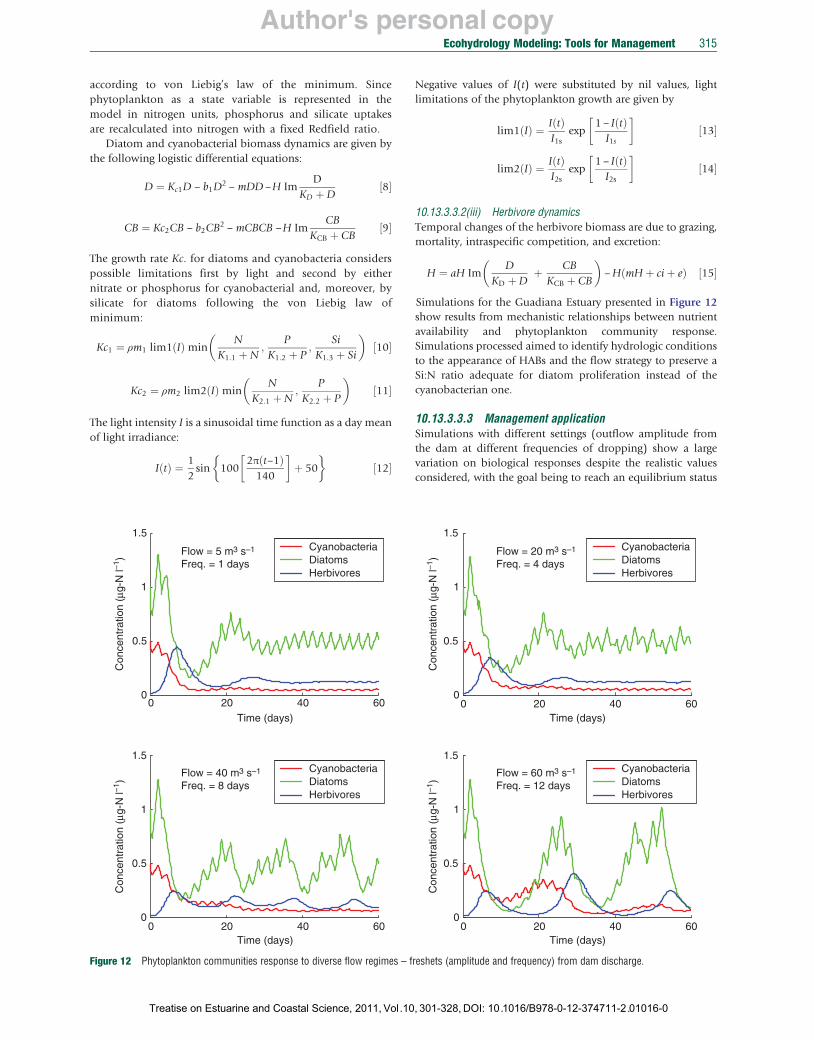
Figure 12 Phytoplankton communities response to diverse flow regimes – f
Treatise on Estuarine and Coastal Science, 2011, Vol.10
Negative values of I(t) were substituted by nil values, light limitations of the phytoplankton growth are given by
I 1 −
lim1ðIÞ ¼ ðtÞ
exp
� IðtÞ � ½13
I1s �
I1s
Iðt �I
lim2ðIÞ ¼ Þ 1 − exp
ðtÞ I2s 2s
�½14
I�
10.13.3.3.2(iii) Herbivore dynamics Temporal changes of the herbivore biomass are due to grazing, mortality, intraspecific competition, and excretion:
�D CB
H ¼ aH Im þ − H mH ci e 15KD þD KCB CB
�ð þ þ Þ ½ �þ
Simulations for the Guadiana Estuary presented in Figure 12 show results from mechanistic relationships between nutrient availability and phytoplankton community response. Simulations processed aimed to identify hydrologic conditions to the appearance of HABs and the flow strategy to preserve a Si:N ratio adequate for diatom proliferation instead of the cyanobacterian one.
10.13.3.3.3 Management application Simulations with different settings (outflow amplitude from the dam at different frequencies of dropping) show a large variation on biological responses despite the realistic values considered, with the goal being to reach an equilibrium status
1.5
Flow = 20 m3 s–1
Freq. = 4 days
Cyanobacteria Diatoms Herbivores
0 20 40 60
Con
cent
ratio
n (μ
g-N
l–1)
Con
cent
ratio
n (μ
g-N
l–1)
1
0.5
0
Time (days)
1.5
Flow = 60 m3 s–1
Freq. = 12 days
Cyanobacteria Diatoms Herbivores
0 20 40 60
1
0.5
0
Time (days)
reshets (amplitude and frequency) from dam discharge.
, 301-328, DOI: 10.1016/B978-0-12-374711-2.01016-0

Author's personal copy316 Ecohydrology Modeling: Tools for Management
in which diatoms would be clearly and constantly in higher abundances than cyanobacteria.
Two sets of runs were performed simulating for the first set multiple scenarios presenting an equal mean flow during the simulation period but with different frequency and therefore with different flow discharge amplitude. The second set is performed with different scenarios varying both frequencies and amplitudes of discharges corresponding ultimately to different mean flows.
The group of simulation (Figure 12) aimed to determine for which parameter (discharge frequency or amplitude) the phytoplankton community coexistence/competition is more sensible. We tried through these simulations to identify theoretically, within such fluctuating environments, the response of the phytoplankton community to different inflow strategies. A constant average flow per period was set (5 m3 s−1) for the four different settings of flow regimes. It appears then clearly that, more than the flow amplitude, frequency of the freshets is relevant to attain a steady state in which diatoms are continuously dominant versus cyanobacteria. These findings are pertinent for dam and water managers to limit, in spring conditions, the risk of occurrence of HAB.
10.13.3.4 Estuarine Phytoplankton Succession Control (Top-Down Control)
10.13.3.4.1 Background A description of the study site is given in the two previous sections (10.13.3.2.1 and 10.13.3.2.2). During 2006, the spatial distribution and the physiological performance of an invasive bivalve species Corbicula fluminea were investigated in the middle and upper areas of the Guadiana estuary. Benthos sampling was done with corers of 15�15 cm in intertidal areas and with a clam dredge in sub-tidal areas. The aim of the developed model is testing the efficiency of bivalve population to control microalgal blooms, as top-down control.
Diatom
Cyanoba
N
P
Si
LL
Figure 13 Conceptual model for top-down control of phytoplankton commubetween the pools. Features including multiple limiting nutrient resources (N, Pherbivorous compartment partitioned in zooplankton and Corbicula fluminea. that is, light limitation (LL) and advection, are shown with double line arrows.Mateus, C., Piló, D., Marques, R., Morais, P., Chícharo, M.A., 2009. Applicatiofunctioning of the Guadiana Estuary (South Portugal). Ecohydrology and Hydr
Treatise on Estuarine and Coastal Science, 2011, Vol.10,
10.13.3.4.2 The model To study the hypothetic positive influence of biota (i.e., bivalve clearance capabilities) in limiting HAB’s risks in estuarine ecosystems, experiments and models were developed. Modeling formulation and basis hypotheses are similar to those presented in the previous section. Herbivores are in this case subdivided into herbivorous zooplankton and Corbicula fluminea, investigating the specific top-down control of phytoplankton by C. fluminea (Figure 13).
Nutrient assimilation is conditioned by light limitation LL’, which is modeled as a sinusoidal function. Herbivore grazing and filtration affect both phytoplankton groups, with diatoms preferentially targeted by zooplankton and cyanobacteria by Corbicula. The nitrogen compartment is regenerated by herbivore releases. All biological state variables are affected by mortality, which eliminates the respective biomass from the system, excepting for Corbicula (i.e., C. fluminea biomass constant for the simulation period). While the model was not designed for predictive purposes, it still had to behave in a manner reasonable to the natural environment. Therefore, the model is based on current knowledge of ecosystem functioning, field sampling, and laboratorial experiments regarding the Guadiana lower estuary and the physiology of C. fluminea.
A graphical representation of the pools comprising the model and the interactions between the pools is shown in Figure 13.
The differential equations are presented herein and all coefficients and abbreviations are explained in the Table 3. The model is solved using an ODE based on fourth-order Runge–Kutta methods developed within the (MATLAB™) platform.
As in previous studies (Chícharo et al., 2006; Wolanski et al., 2006), advection inputs and losses for each nutrient pool represented in the model were a function of the specific flow rate (inflow divided by ecosystem volume, i.e., model box), the concentration of a specific constituent in the input source, and the concentration of a specific constituent in the simulation, and was depicted using
Zooplankton
C. fluminea
s
cteria
nities in Guadiana upper estuary with state variables and interactions , and Si), multiple phytoplankton groups (diatoms and Cyanobacteria), and All four biological pools are subject to mortality. The effects of irradiance, Adapted from Chícharo, L., Ben-Hamadou, R., Amaral, A., Range, P., n and demonstration of the ecohydrology approach for the sustainable obiology 9, 55–71.
301-328, DOI: 10.1016/B978-0-12-374711-2.01016-0
Author's personal copyEcohydrology Modeling: Tools for Management 317
Table 3 Coefficients abbreviations and values used in the model simulations are cited below
Coefficient Symbol Value Unit
Specific flow rate Concentration of a specific constituent in the input source
Concentration of the specific constituent in the simulation Maximum uptake rate for diatoms Maximum uptake rate for cyanobacteria Diatom half saturation constant for nitrogen absorption Diatom half saturation constant for phosphorus absorption Diatom half saturation constant for silicate absorption Cyanobacterial half saturation constant for nitrogen absorption Cyanobacterial half saturation constant for phosphorus absorption Excretion rate of the herbivore zooplankton Excretion rate of the Corbicula N:P ratio conversion N:Si ration conversion Diatoms intraspecific competition rate Cyanobacterial intraspecific competition rate Diatom mortality rate Cyanobacterial mortality rate Maximum ingestion rate of the herbivorous zooplankton Maximum ingestion rate of the Corbicula Corbicula filtration efficiency of diatoms Corbicula filtration efficiency of cyanobacterial Corbicula filtration efficiency of zooplankton Zooplankton half saturation constant for diatom ingestion Zooplankton half saturation constant for cyanobacterial ingestion Corbicula half saturation constant for diatom ingestion Corbicula half saturation constant for cyanobacterial ingestion Light saturation intensity for diatoms Light saturation intensity for Cyanobacteria Assimilation efficiency of the herbivorous zooplankton Herbivore mortality rate Herbivore intraspecific competition rate
v Cs
Cx Vm1 Vm2 K1D K2D K3D K1CB K2CB eh
ec Rnp Rnsi b1 b2 mD
mCB
ImH
ImC
e1 e2 e3 KHD
KHCB
KCD
KCCB
I1s I2s a mH cH
Input For N = 420 For P = 400 For Si = 180 Simulated 0.8 0.5 0.4 0.6 0.2 0.5 0.5 0.05 0.06 16 2 10/55 1/3 0.1 0.12 11.2 0.7 0.6 0.3 5.3 3.7 8.2 4.5 80 90 0.7 0.04 0.1
3 −1 m s µmol l−1
l−1 µmol j−1
j−1
l−1 µmol-N l−1 µmol-P l−1 µmol-Si l−1 µmol-N l−1 µmol-P
j−1
j−1
Undimensioned Undimensioned j−1
j−1
j−1
j−1
j−1
j−1
Undimensioned Undimensioned Undimensioned
l−1 µmol-N l−1 µmol-N l−1 µmol-N
µmol-N.l−1−2 −1 µEm s−2 −1 µEm s
j−1
j−1
j−1
½17�
� � �
� � �
� � �
A N=P=SiÞ ¼ v CsðN=P=SiÞ − v CxðN=P=SiÞð ½16�
10.13.3.4.2(i) Differential equations of the model Assimilation of nutrients (N, P, and Si) by phytoplankton (D and CB) follows a hyperbolic function (Michaelis–Menten kinetic).
If V1, V2, and V3 are the assimilation rates of N, P, and Si respectively, then
NV1 ¼ Vm ⋅ ðk1 ⋅ þNÞ
PV2 ¼ Vm ⋅ ðk2 ⋅ þPÞ ½17�
SiV3 ¼ Vm ⋅ ðk3 ⋅ þSiÞ
It follows that nutrient–phytoplankton interactions are
Vm1N D Vm2NCB N ¼ − − þ AðNÞ þ ehH þ ec C ½18�
k1D þN k1CB þN
Vm1P D Vm2P CB P ¼ − − þ AðPÞ ½19�
k2D þ P k2CB þ P
Vm1Si D Si ¼ − þ AðSiÞ ½20�
k3D þ Si
Treatise on Estuarine and Coastal Science, 2011, Vol.10
Nitrogen is recycled by zooplankton and C. fluminea excretions, Si uptake is diatom specific.
The phytoplankton growth (=nutrient uptake) is equivalent to the net primary production in the model. Phytoplankton growth can be limited by light and nutrient availability according to von Liebig’s law of the minimum. Since phytoplankton as a state variable is represented in the model in nitrogen units, phosphorus and silicate uptakes are recalculated into nitrogen with a fixed Redfield ratio.
P� ¼ Rnp P ½21� Si� ¼ Rnsi Si ½22�
Diatom and cyanobacterial biomass dynamics are given by the following logistic differential equations:
2 I D I D
D ¼ Kc1D − b1D − mDD − H
�mH
� �mC
− CeK 1HD
�þ D KCD þD
½23�
CB ¼Kc CB − b CB2 2 2 − mCBCB − H
�ImHCB
KHCB
�
þ CB
ImCCB ½24�
− Ce2
�KCCB þ CB
�
, 301-328, DOI: 10.1016/B978-0-12-374711-2.01016-0

Author's personal copy318 Ecohydrology Modeling: Tools for Management
� �
� �
� � � �
� �
� �
The growth rate Kc. for diatoms and cyanobacteria considers possible limitations first by light and second by either nitrate or phosphorus for cyanobacterial and, moreover, by silicate for diatoms following the von Liebig law of minimum:
N P Si Kc1 ¼ Vm1lim1ðIÞmin ; ; ½25�
K1D þN K2D þ P K3D þ Si
N P Kc2 ¼ Vm2lim2ðIÞ min ; ½26�
K1CB þN K2CB þ P
The light intensity I is a sinusoidal time function as a day mean of light irradiance:
1 5πðt − 6Þ IðtÞ ¼ sin 100 þ 50 ½27�
2 24
Negative values of I(t) were substituted by nil values, light limitations of the phytoplankton growth are given by
IðtÞ 1 − IðtÞ lim1ðIÞ ¼ exp ½28�
I1s I1s
IðtÞ 1−IðtÞ lim2ðIÞ ¼ exp ½29�
I2s I2s
Temporal changes of the herbivore zooplankton biomass are due to grazing, mortality (natural and predation by Corbicula), intraspecific competition, and excretion:
(a) 35 Cyanobacteria
) 30 Diatoms 3−m
yll-a
(m
g 25
20
Chl
orop
h 15
10
5
0 00 10 20 30
Time (days)
(c) 35
) 3 30
−yl
l-a (
mg
m 25
20
Chl
orop
h 15
10
5
0 00 10 20 30
Time (days)
Figure 14 Temporal evolution of diatoms and cyanobacteria (model results)(c) =80 ind m−2; (d) =100 ind m−2.
Treatise on Estuarine and Coastal Science, 2011, Vol.10,
� �
� �
� � � �
� �
D CB H ¼ aHImH þ
KHD þD KHCB þ CB
− HðmH þ cH þ ehÞ − Ce3 ImCH ½30�
KCH þH
Corbicula biomass is assimilated to be constant (mortality = growth) for the simulation period:
_C ¼ 0 ½31� Corbicula is acting as filtrating and depurating water from phytoplankton and herbivore zooplankton, its efficiency of capturing plankton cells is modeled by the ‘e’ coefficient.
The filtration by Corbicula (FC) is in the form of
ImCD ImCCB FC ¼ Ce1 þ Ce2KCD þD KCCB þ CB ImCH þ Ce3 KCH þH
½32�
Model simulations were conducted with the intent to explore synergistic processes effecting phytoplankton succession, accumulation of algal biomass, and secondary productivity, and then to determine the sensitivity of these processes to various abiotic and biotic conditions.
The model parametrization was done for spring conditions, which are favorable for phytoplankton development, with high nutrient enrichment and low light limitation. Corbicula biomass was maintained unchanged for the 30 days’ simulation period and was modulated from low abundances (10 individuals m−2) to very high (100 individuals m−2) (Figure 14).
(b) 35
) 3 30
−m 25
yll-a
(m
g
20
15
10
Chl
orop
h
5
0 00 10 20 30
Time (days)
(d) 35
) 3 30
−
25
20
yll-a
(m
g m
15
10
Chl
orop
h
5
00 0 10 20 30
Time (days)
for abundances: (a) =10 ind m−2Corbicula fluminea ; (b) =30 ind m−2;
301-328, DOI: 10.1016/B978-0-12-374711-2.01016-0

Author's personal copyEcohydrology Modeling: Tools for Management 319
10.13.3.4.3 Management application The sensitivity analysis showed a clear ability of bivalve community to restrict the total phytoplankton bloom. Results showed an increase in diatom biomass under mid–low bivalve abundances (30 individuals m−2) (Figure 14(b)), resulting from the limitation of cyanobacterial growth that allows diatoms to benefit from available nutrients, as well as from bivalve selectivity that presents higher filtration efficiencies for small-sized phytoplankton cells than for large diatoms. Therefore, the dynamics of phytoplankton groups showed a possible dominance of cyanobacterial community for lower bivalve abundances. However, the increase of bivalve abundance limits the primary productivity, preferentially through limitation of the cyanobacterial growth.
Toxic algal blooms can also be controlled by top-down approach. The model demonstrates the top-down effect caused by the alien bivalve C. fluminea on controlling phytoplankton blooms. In fact, according to our observations, C. fluminea can be mainly responsible for the lower values of chlorophyll registered in the Guadiana Estuary since the Alqueva Dam was filled, in 2002 (see Chícharo et al., 2006). Similar impacts were described for the estuary of San Francisco bay, with the alien bivalve Pomatocorbula (Cloern and Nichols, 1985) and also for the Hudson River, with the zebra mussel Dreissena (Caraco et al., 1997). In fact, filter feeders are responsible for filtering high volumes of water at high rates, as C. fluminea, and are capable of capturing substantial amounts of suspended materials, including phytoplankton (e.g., Nakamura, 2001). Thus, through active feeding on particulate organic matter, filter-feeding bivalves can control phytoplankton standing stocks, primary production, water clarity, nutrient cycling, and the nature of the food webs in the regions where they are abundant. Filter-feeding bivalves are thus expected to control processes associated with toxic algal blooms and eutrophication.
Actually, Nakamura and Kerciku (2000) described the role of a related species, C. japonica, for restoring deteriorated water bodies, in Japan. Also a recent study by Zhou et al. (2006) indicated that commercially suspension-cultured bivalves may serve as a eutrophic environment bioremediator and contribute to mitigate eutrophication pressures on coastal ecosystems subject to anthropogenic N and P loadings, However, controlling alien bivalve density is important for ensuring food availability to other planktivorous species and to sustain biodiversity.
At the Southeast area of Portugal, the increasing density of the alien clam (C. fluminea) in freshwater bodies, including the Guadiana River, and estuarine area, in the last years poses a threat to biodiversity. The results of this model provide valuable information for the managers of this protected ecosystem about the threshold densities of C. fluminea to be supported in the system for controlling water quality and ensuring sustainable biodiversity.
10.13.3.5 Modeling the Phytoplankton Dynamics in North Adriatic with ML Tools
10.13.3.5.1 Background The northern part of the Adriatic Sea, particularly its northwestern part, is one of the most productive regions in the Adriatic Sea and in the entire Mediterranean. Major reasons
Treatise on Estuarine and Coastal Science, 2011, Vol.10
are its morphology, that is, shallow water and low water exchange with the rest of the Adriatic Sea, and excessive nutrients inflow through the Po River (Degobbis and Gilmartin, 1990). Many studies and research about the phytoplankton dynamics have been undertaken, including modeling approaches, resulting in a substantial amount of knowledge about the north Adriatic (NA) ecosystem and its productivity.
In this section, we present an ML approach as an alternative to the existing conceptual modeling efforts to construct models that (1) describe and synthesize the knowledge about phytoplankton in NA and (2) predict the phytoplankton concentration in this area, from long-term measured data (Volf et al., 2011).
The data set used for learning was collected at six stations (SJ108, SJ101, SJ103, SJ105, SJ107, and RV001) on the 92-km-long transect from the Po River Delta to Rovinj, Croatia (Figure 15) by the Center for Marine Research in Rovinj, Croatia. Physical, chemical, and biological parameters presented in Table 4 were sampled throughout the water column from 1972 to 2007 at monthly intervals. Daily Po River flow data measured at Pontelagoscuro (Figure 15) from January 1966 to December 2007 were obtained from Ministero dei Lavori Pubblici, Servizio Idrografico Parma.
10.13.3.5.2 The model Two ML methods were used to construct models, that is, regression tree model was induced to describe the phytoplankton dynamics over a longer period, explain the ecosystem behavior, and identify the main triggers of change in phytoplankton concentration in NA, while rule-based regression model was induced to predict the phytoplankton concentration for some period in future given the present values of measured data.
Regression trees are one of the ML methods for numerical modeling. As it is the case with the other data-driven methods, to induce a regression tree, we need a data set to learn from and an algorithm (see also Section 10.13.2). The data can be organized as examples in a spreadsheet, where each example (each row in the spreadsheet) is composed of attributes (also called descriptors or independent variables) and class (also called outcome of the attributes values or dependent variable), having the form (AT1, AT2,…, ATn, TARGET).
Compared to the simple linear regression, which calculates one equation (one weight vector) for the entire data set, piecewise or tree-structured regression divides the data set to several subsets on which uniform class value or linear equation can be applied. The division to subsets is based on tests of the values of the input attributes, which are put as nodes in a regression tree.
Thus, regression trees are hierarchical structures composed of nodes and branches, where the internal nodes contain tests on the input attributes. Each branch of an internal test corresponds to an outcome of the test, and the predictions for the values of the target variable (the class) are stored in the leaves, which are the terminal nodes in the tree. If the leaves contain a single value for the class prediction then we are talking about simple regression trees, while if linear equation is used for prediction in the leaf we are speaking of (regression) model trees. Figure 16 illustrates the procedure of constructing regression and model trees.
Using the data set of the NA (Table 4) and the ML algorithm M5P encoded in the software package WEKA (Witten and
, 301-328, DOI: 10.1016/B978-0-12-374711-2.01016-0
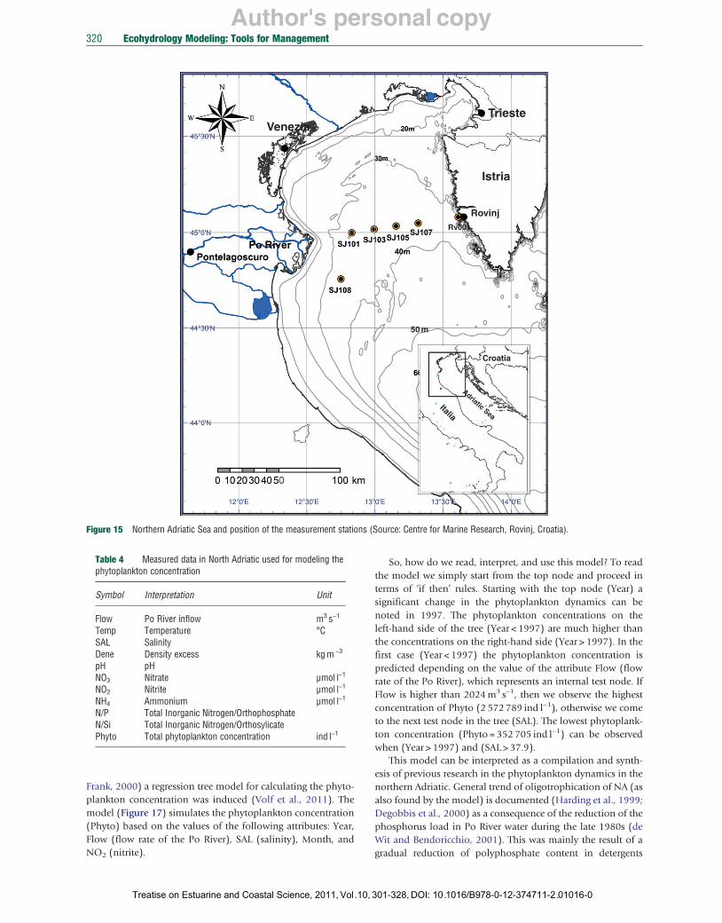
Author's personal copy
Trieste Venezia
Istria
Rovinj Rv001
50 m
Croatia
Italia
Adriatic Sea
320 Ecohydrology Modeling: Tools for Management
Figure 15 Northern Adriatic Sea and position of the measurement stations (Source: Centre for Marine Research, Rovinj, Croatia).
Table 4 Measured data in North Adriatic used for modeling the phytoplankton concentration
Symbol Interpretation Unit
Flow Po River inflow m3 s−1
Temp Temperature °C SAL Salinity Dene Density excess kg m −3
pH pH NO3 Nitrate µmol l−1
NO2 Nitrite µmol l−1
NH4 Ammonium µmol l−1
N/P Total Inorganic Nitrogen/Orthophosphate N/Si Total Inorganic Nitrogen/Orthosylicate Phyto Total phytoplankton concentration ind l−1
Frank, 2000) a regression tree model for calculating the phytoplankton concentration was induced (Volf et al., 2011). The model (Figure 17) simulates the phytoplankton concentration (Phyto) based on the values of the following attributes: Year, Flow (flow rate of the Po River), SAL (salinity), Month, and NO2 (nitrite).
Treatise on Estuarine and Coastal Science, 2011, Vol.10,
So, how do we read, interpret, and use this model? To read the model we simply start from the top node and proceed in terms of ‘if then’ rules. Starting with the top node (Year) a significant change in the phytoplankton dynamics can be noted in 1997. The phytoplankton concentrations on the left-hand side of the tree (Year < 1997) are much higher than the concentrations on the right-hand side (Year > 1997). In the first case (Year < 1997) the phytoplankton concentration is predicted depending on the value of the attribute Flow (flow rate of the Po River), which represents an internal test node. If Flow is higher than 2024 m3 s−1, then we observe the highest concentration of Phyto (2 572 789 ind l−1), otherwise we come to the next test node in the tree (SAL). The lowest phytoplankton concentration (Phyto = 352 705 ind l−1) can be observed when (Year > 1997) and (SAL > 37.9).
This model can be interpreted as a compilation and synthesis of previous research in the phytoplankton dynamics in the northern Adriatic. General trend of oligotrophication of NA (as also found by the model) is documented (Harding et al., 1999; Degobbis et al., 2000) as a consequence of the reduction of the phosphorus load in Po River water during the late 1980s (de Wit and Bendoricchio, 2001). This was mainly the result of a gradual reduction of polyphosphate content in detergents
301-328, DOI: 10.1016/B978-0-12-374711-2.01016-0
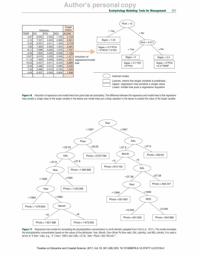
Author's personal copy
= YES
Target Attributes (class)
TEMP DO PO4 NO3 ALGAE 3.67 8.500 0.005 1.735 2.133 4.15 7.207 0.005 2.989 2.601 5.32 8.357 0.011 1.263 3.718 7.80 7.929 0.005 1.054 3.481 8.11 7.096 0.005 1.075 1.791 9.36 7.804 0.005 0.596 1.128
10.87 6.018 0.005 0.548 1.471 11.10 7.400 0.006 0.620 1.521 10.23 5.457 0.011 0.434 0.869 8.39 5.486 0.014 0.589 0.535 7.42 5.486 0.013 0.742 1.034 4.06 8.307 0.005 0.804 1.636
… … … … …
Induction of regression/model tree
PO4 < 10
Algae = 1.54 No3 < 0.011
Algae = 5
= Yes = No
= Yes = No
Algae = 3.4
Algae = 0.2*PO4 +3*NO3+1.5*DO
Algae = 0.1*DO Algae = 2*PO4 +5*PO4 +0.4*TEMP
Internal nodes
Leaves, where the target variable is predicted. Upper: regression tree predicts a single value Lower: model tree puts a regression equation
Ecohydrology Modeling: Tools for Management 321
Figure 16 Induction of regression and model trees from given data set (examples). The difference between the regression and model trees is that regreesion trees predict a single value of the target variable in the leaves and model trees put a linear equation in the leaves to predict the value of the target variable.
Year
�1997 >1997
Flow SAL
>37.9 �20 25 >20 25 �37.9
Month Photo SAL = 352 05 Photo = 2 572 789
>5 �5 � >37.8 37.8
Photo = 815 103 SAL
Year Photo = 1 082 968
>37.58 �37.58 >1992�1992
Year Photo = 458 247
Year Photo = 1 432 396
�1999 >1999
�1983 >1983 Photo = 591 000 NO2
Photo = 1 376 650 Month >0.046 �0.046
�6 >6 Photo = 591 000 Photo = 554 388
Photo = 1 921 386 Photo = 1 675 020
Figure 17 Regression tree model for simulating the phytoplankton concentration in north Adriatic (adapted from Volf et al., 2011). The model simulates the phytoplankton concentration based on the values of five attributes: Year, Month, Flow (River Po flow rate), SAL (salinity), and NO2 (nitrite). It is read in terms of ‘if then’ rules, e.g., ‘if −’ (Year > 1997) and (SAL > 37.9), 1‘then’ Phyto = 352 705 ind l .
Treatise on Estuarine and Coastal Science, 2011, Vol.10, 301-328, DOI: 10.1016/B978-0-12-374711-2.01016-0
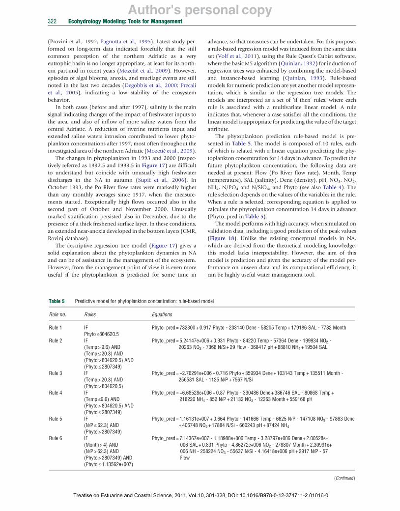
Author's personal copy322 Ecohydrology Modeling: Tools for Management
(Provini et al., 1992; Pagnotta et al., 1995). Latest study performed on long-term data indicated forcefully that the still common perception of the northern Adriatic as a very eutrophic basin is no longer appropriate, at least for its northern part and in recent years (Mozetič et al., 2009). However, episodes of algal blooms, anoxia, and mucilage events are still noted in the last two decades (Degobbis et al., 2000; Precali et al., 2005), indicating a low stability of the ecosystem behavior.
In both cases (before and after 1997), salinity is the main signal indicating changes of the impact of freshwater inputs to the area, and also of inflow of more saline waters from the central Adriatic. A reduction of riverine nutrients input and extended saline waters intrusion contributed to lower phytoplankton concentrations after 1997, most often throughout the investigated area of the northern Adriatic (Mozetič et al., 2009).
The changes in phytoplankton in 1993 and 2000 (respectively referred as 1992.5 and 1999.5 in Figure 17) are difficult to understand but coincide with unusually high freshwater discharges in the NA in autumn (Supic et al., 2006). In October 1993, the Po River flow rates were markedly higher than any monthly averages since 1917, when the measurements started. Exceptionally high flows occurred also in the second part of October and November 2000. Unusually marked stratification persisted also in December, due to the presence of a thick freshened surface layer. In these conditions, an extended near-anoxia developed in the bottom layers (CMR, Rovinj database).
The descriptive regression tree model (Figure 17) gives a solid explanation about the phytoplankton dynamics in NA and can be of assistance in the management of the ecosystem. However, from the management point of view it is even more useful if the phytoplankton is predicted for some time in
Table 5 Predictive model for phytoplankton concentration: rule-based mo
Rule no. Rules Equations
Rule 1 IF Phyto_pred = 732300 + 0.9Phyto ≤804620.5
Rule 2 IF Phyto_pred = 5.24147e+00(Temp > 9.6) AND 20263 NO3 -(Temp ≤ 20.3) AND (Phyto > 804620.5) AND (Phyto ≤ 2807349)
Rule 3 IF Phyto_pred = −2.76291e+0(Temp > 20.3) AND 256581 SAL -(Phyto > 804620.5)
Rule 4 IF Phyto_pred = −6.68528e+0(Temp ≤9.6) AND 218220 NH4
(Phyto > 804620.5) AND (Phyto ≤ 2807349)
Rule 5 IF Phyto_pred = 1.16131e+00(N/P ≤ 62.3) AND + 406748 NO2
(Phyto > 2807349) Rule 6 IF Phyto_pred = 7.14367e+00
(Month > 4) AND 006 SAL + 0.(N/P > 62.3) AND 006 NH - 258(Phyto > 2807349) AND Flow (Phyto ≤ 1.13562e+007)
Treatise on Estuarine and Coastal Science, 2011, Vol.10,
advance, so that measures can be undertaken. For this purpose, a rule-based regression model was induced from the same data set (Volf et al., 2011), using the Rule Quest’s Cubist software, where the basic M5 algorithm (Quinlan, 1992) for induction of regression trees was enhanced by combining the model-based and instance-based learning (Quinlan, 1993). Rule-based models for numeric prediction are yet another model representation, which is similar to the regression tree models. The models are interpreted as a set of ‘if then’ rules, where each rule is associated with a multivariate linear model. A rule indicates that, whenever a case satisfies all the conditions, the linear model is appropriate for predicting the value of the target attribute.
The phytoplankton prediction rule-based model is presented in Table 5. The model is composed of 10 rules, each of which is related with a linear equation predicting the phytoplankton concentration for 14 days in advance. To predict the future phytoplankton concentration, the following data are needed at present: Flow (Po River flow rate), Month, Temp (temperature), SAL (salinity), Dene (density), pH, NO3, NO2, NH4, N/PO4 and N/SiO4, and Phyto (see also Table 4). The rule selection depends on the values of the variables in the rule. When a rule is selected, corresponding equation is applied to calculate the phytoplankton concentration 14 days in advance (Phyto_pred in Table 5).
The model performs with high accuracy, when simulated on validation data, including a good prediction of the peak values (Figure 18). Unlike the existing conceptual models in NA, which are derived from the theoretical modeling knowledge, this model lacks interpretability. However, the aim of this model is prediction and given the accuracy of the model performance on unseen data and its computational efficiency, it can be highly useful water management tool.
del
17 Phyto - 233140 Dene - 58205 Temp + 179186 SAL - 7782 Month
6 + 0.931 Phyto - 84220 Temp - 57364 Dene - 199934 NO2 -7368 N/Si+ 29 Flow - 368417 pH + 88810 NH4 + 19504 SAL
06 + 0.716 Phyto + 359934 Dene + 103143 Temp + 135511 Month 1125 N/P + 7567 N/Si
06 + 0.87 Phyto - 390486 Dene + 386746 SAL - 80868 Temp + - 852 N/P + 21132 NO3 - 12263 Month + 559168 pH
7 + 0.664 Phyto - 141666 Temp - 6625 N/P - 147108 NO3 - 97863 Dene + 17884 N/Si - 660243 pH + 87424 NH4
7 - 1.18988e+006 Temp - 3.28797e+006 Dene + 2.00528e+ 831 Phyto - 4.86272e+006 NO2 - 278807 Month + 2.30991e+ 224 NO3 - 55637 N/Si - 4.16418e+006 pH + 2917 N/P - 57
(Continued )
301-328, DOI: 10.1016/B978-0-12-374711-2.01016-0
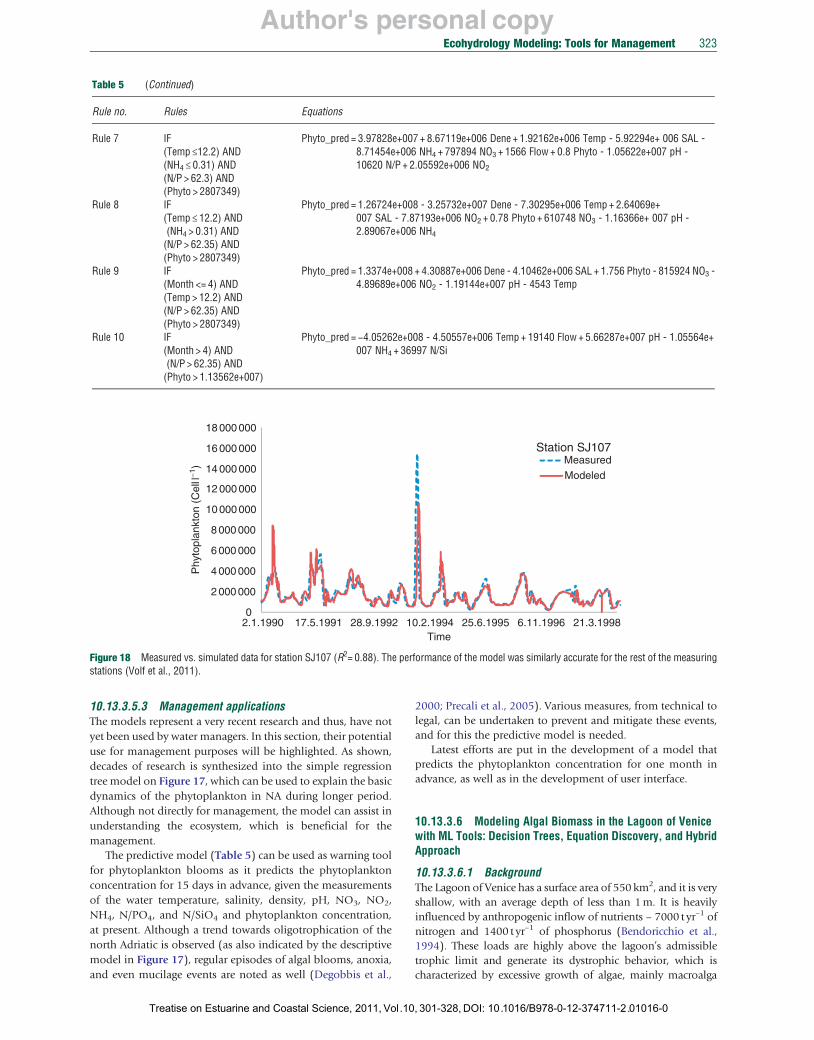
Author's personal copy
Table 5 (Continued)
Rule no. Rules Equations
Rule 7 IF Phyto_pred = 3.97828e+007 + 8.67119e+006 Dene + 1.92162e+006 Temp - 5.92294e+ 006 SAL (Temp ≤12.2) AND 8.71454e+006 NH4 + 797894 NO3 + 1566 Flow + 0.8 Phyto - 1.05622e+007 pH (NH4 ≤ 0.31) AND 10620 N/P + 2.05592e+006 NO2
(N/P > 62.3) AND (Phyto > 2807349)
Rule 8 IF Phyto_pred = 1.26724e+008 - 3.25732e+007 Dene - 7.30295e+006 Temp + 2.64069e+ (Temp ≤ 12.2) AND 007 SAL - 7.87193e+006 NO2 + 0.78 Phyto + 610748 NO3 - 1.16366e+ 007 pH (NH4 > 0.31) AND 2.89067e+006 NH4
(N/P > 62.35) AND (Phyto > 2807349)
Rule 9 IF Phyto_pred = 1.3374e+008 + 4.30887e+006 Dene - 4.10462e+006 SAL + 1.756 Phyto - 815924 NO(Month <= 4) AND 4.89689e+006 NO2 - 1.19144e+007 pH - 4543 Temp (Temp > 12.2) AND (N/P > 62.35) AND (Phyto > 2807349)
Rule 10 IF Phyto_pred = −4.05262e+008 - 4.50557e+006 Temp + 19140 Flow + 5.66287e+007 pH - 1.05564(Month > 4) AND 007 NH4 + 36997 N/Si (N/P > 62.35) AND (Phyto > 1.13562e+007)
3
e+
Ecohydrology Modeling: Tools for Management 323
18 000 000
16 000 000 Station SJ107 Measured
14 000 000 Modeled
12 000 000
10 000 000
8 000 000
6 000 000
4 000 000
2 000 000
0
Time
Phy
topl
ankt
on (
Cel
l l−1
)
2.1.1990 17.5.1991 28.9.1992 10.2.1994 25.6.1995 6.11.1996 21.3.1998
Figure 18 Measured vs. simulated data for station SJ107 (R2= 0.88). The performance of the model was similarly accurate for the rest of the measuring stations (Volf et al., 2011).
10.13.3.5.3 Management applications The models represent a very recent research and thus, have not yet been used by water managers. In this section, their potential use for management purposes will be highlighted. As shown, decades of research is synthesized into the simple regression tree model on Figure 17, which can be used to explain the basic dynamics of the phytoplankton in NA during longer period. Although not directly for management, the model can assist in understanding the ecosystem, which is beneficial for the management.
The predictive model (Table 5) can be used as warning tool for phytoplankton blooms as it predicts the phytoplankton concentration for 15 days in advance, given the measurements of the water temperature, salinity, density, pH, NO3, NO2, NH4, N/PO4, and N/SiO4 and phytoplankton concentration, at present. Although a trend towards oligotrophication of the north Adriatic is observed (as also indicated by the descriptive model in Figure 17), regular episodes of algal blooms, anoxia, and even mucilage events are noted as well (Degobbis et al.,
Treatise on Estuarine and Coastal Science, 2011, Vol.10
2000; Precali et al., 2005). Various measures, from technical to legal, can be undertaken to prevent and mitigate these events, and for this the predictive model is needed.
Latest efforts are put in the development of a model that predicts the phytoplankton concentration for one month in advance, as well as in the development of user interface.
10.13.3.6 Modeling Algal Biomass in the Lagoon of Venice with ML Tools: Decision Trees, Equation Discovery, and Hybrid Approach
10.13.3.6.1 Background The Lagoon of Venice has a surface area of 550 km2, and it is very shallow, with an average depth of less than 1 m. It is heavily influenced by anthropogenic inflow of nutrients – 7000 t yr−1 of nitrogen and 1400 t yr−1 of phosphorus (Bendoricchio et al., 1994). These loads are highly above the lagoon’s admissibletrophic limit and generate its dystrophic behavior, which is characterized by excessive growth of algae, mainly macroalga
, 301-328, DOI: 10.1016/B978-0-12-374711-2.01016-0

Author's personal copy324 Ecohydrology Modeling: Tools for Management
Ulva rigida. This alga is not (notably) grazed by any animal or zooplankton, but shades out the light by itself due to excessive growth in which all the nutrients are also depleted. An extensive research has been undertaken to understand this ecosystem and be able to predict future developments of the U. rigida growth. In this section, we present part of this research that is concerned with the development of models using various ML techniques.
We will focus on the work by Kompare and Džeroski (1995), which used regression trees to predict algal blooms and Kompare et al. (1997) which used the equation discovery system GoldHorn (Križman, 1998). More attention will be given to the hybrid approach to model development with the modeling tool LAGRAMGE (Todorovski, 2003). Todorovski and Džeroski (2006) applied the hybrid modeling system LAGRAMGE with a simple knowledge library to discover algal biomass model, while Atanasova (2005) applied a comprehensive library for ecological modeling for discovery of biomass model. Thereafte, we briefly present the applications.
All these applications used four data sets (Coffaro et al., 1993), whereby data were collected weekly for slightly more than 1 year at four different locations in the lagoon. The parameters measured were nitrogen in ammonia (nh), nitrogen in nitrate (no), phosphorus in orthophosphate (ps), dissolved oxygen DO, temperature Temp (°C), and algal biomass (biomass) (dry weight in g m−2).
In some modeling experiments, the total nitrogen concentration Ntot was used instead of ammonia and nitrate nitrogen separately, and this appears justified because Ulva can use them both without greater difference as long as ammonia is not present in toxic concentrations (Coffaro et al., 1993; Bendoricchio et al., 1994).
10.13.3.6.2 Models 10.13.3.6.2(i) Models induced by decision trees and equation discovery methods Kompare and Džeroski (1995) constructed several regression trees (for explanation of the regression tree method, the reader is referred to Section 10.13.3.5) to predict algal biomass. One of them is presented in Figure 19 (Kompare and Džeroski, 1995). The model predicts the change in biomass concentration (Bio(t + 1)-Bio(t)) that will occur after 1 week. The model indicates that nitrogen is the limiting nutrient and also the rough value of N concentration to sustain growth of around
≤ 114.01
Bio(t ) − Bio(t −1)
≤ 5.86 > 5.86
DO(t – 1) 49.3 ± 78.6
≤ 111.0 > 111.0
0.39 ± 8.33 3.21 ± 30.4
Figure 19 A regression tree for predicting the change in biomass that will ocbiomass, dissolved oxygen and nitrates at time t. The change in biomass _Bio1995. Getting more out of data: automated modeling of algal growth with machSpace Utilization. University of Hawaii, Hawaii, pp. 209–220.
Treatise on Estuarine and Coastal Science, 2011, Vol.10,
17.7 mg l−1. Although descriptive, the model did not perform with high accuracy when compared to the measured data. The accuracy was improved by applying an algorithm that, instead of single value in the leaves, calculates a regression. Severe problems in the data set were discovered during the experiments (Kompare and Džeroski, 1995), which prevented from discovery of more accurate models.
Following experiments included algal biomass equation discoveries (Kompare et al., 1997) for accurate predictions, with the system GoldHorn (Križman, 1998). Followed by some modifications in the data set, that is, introduction of two additional variables, growth, and mortality rate, GoldHorn managed to discover an accurate biomass model, which performed equally well as previously developed conceptual model composed of 11 equations. In terms of interpretability, the model can be considered as gray box, meaning that it included some descriptive elements, for example, the mortality rate. However, it was still inferred purely from field data and it did not reveal other ecological processes.
10.13.3.6.2(ii) A biomass model discovered using hybrid approach Latest experiments on this data set with ML included a model discovery using a hybrid approach with the modeling framework LAGRAMGE (see Section 10.13.2). The main goal of this approach is to use both, the efficiency of the ML methods and the theoretical modeling knowledge, so that the resulting models are simple, efficient, and transparent. Thus, by using this approach, the equations from the previous section are expected to be improved in their accuracy and interpretability. Todorovski (2003) applied the system LAGRAMGE using a simplified knowledge library and discovered models that follow the background knowledge supplied in the library and correctly predict the peaks and the crashes. However, the models contained some conceptual inconsistencies due to the library’s simplicity. To overcome these issues, a more comprehensive library was developed (Atanasova et al., 2006a) and integrated in the system LAGRAMGE.
Following the procedure of model construction with LAGRAMGE (Section 10.13.2.3), and given that steps 1 and 2 were completed, that is, the modeling knowledge library developed by Atanasova et al. (2006a) was used for this experiment,
> 114.01 Bio(t )
NO3(t )
≤ 17.68 > 17.68
– 55.5 ± 124.0 15.9 ± 311.0
LEGEND:
{Bio(t+1) – Bio(t )} ± std. dev.
cur in one week. Bio(t), DO(t) and NO3 (t) stand for the concentrations of (t) is defined as Bio(t)−Bio(t − 1). Adapted from Kompare, B., Džeroski, S., ine learning. Proceedings of the International Conference on Coastal Ocean
301-328, DOI: 10.1016/B978-0-12-374711-2.01016-0
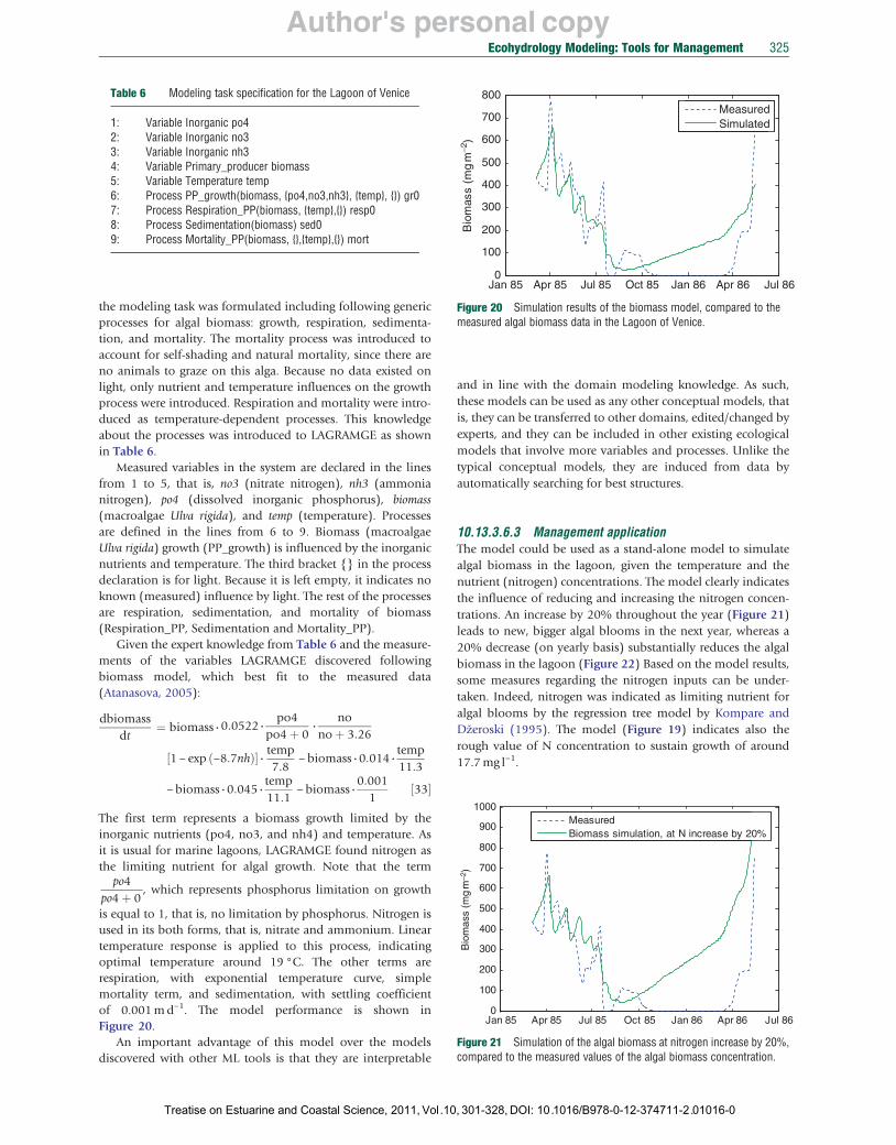
Author's personal copyEcohydrology Modeling: Tools for Management 325
Table 6 Modeling task specification for the Lagoon of Venice
1: Variable Inorganic po4 2: Variable Inorganic no3 3: Variable Inorganic nh3 4: Variable Primary_producer biomass 5: Variable Temperature temp 6: Process PP_growth(biomass, {po4,no3,nh3}, {temp}, {}) gr0 7: Process Respiration_PP(biomass, {temp},{}) resp0 8: Process Sedimentation(biomass) sed0 9: Process Mortality_PP(biomass, {},{temp},{}) mort
0
100
200
300
400
500
600
700
800
Bio
mas
s (m
g m
−2 )
Measured Simulated
Jan 85 Apr 85 Jul 85 Oct 85 Jan 86 Apr 86 Jul 86
Figure 20 Simulation results of the biomass model, compared to the measured algal biomass data in the Lagoon of Venice.
Jan 85 Apr 85 Jul 85 Oct 85 Jan 86 Apr 86 Jul 86 0
100
200
300
400
500
600
700
800
900
1000
) –2
B
iom
ass
(mg
m
Measured Biomass simulation, at N increase by 20%
Figure 21 Simulation of the algal biomass at nitrogen increase by 20%, compared to the measured values of the algal biomass concentration.
the modeling task was formulated including following generic processes for algal biomass: growth, respiration, sedimentation, and mortality. The mortality process was introduced to account for self-shading and natural mortality, since there are no animals to graze on this alga. Because no data existed on light, only nutrient and temperature influences on the growth process were introduced. Respiration and mortality were introduced as temperature-dependent processes. This knowledge about the processes was introduced to LAGRAMGE as shown in Table 6.
Measured variables in the system are declared in the lines from 1 to 5, that is, no3 (nitrate nitrogen), nh3 (ammonia nitrogen), po4 (dissolved inorganic phosphorus), biomass (macroalgae Ulva rigida), and temp (temperature). Processes are defined in the lines from 6 to 9. Biomass (macroalgae Ulva rigida) growth (PP_growth) is influenced by the inorganic nutrients and temperature. The third bracket {} in the process declaration is for light. Because it is left empty, it indicates no known (measured) influence by light. The rest of the processes are respiration, sedimentation, and mortality of biomass (Respiration_PP, Sedimentation and Mortality_PP).
Given the expert knowledge from Table 6 and the measurements of the variables LAGRAMGE discovered following biomass model, which best fit to the measured data (Atanasova, 2005):
dbiomass po4 no ¼ biomass ⋅ 0:0522 ⋅ ⋅ dt po4 þ 0 no þ 3:26
temp temp½1 − exp ð−8:7nhÞ� ⋅ − biomass ⋅ 0:014 ⋅ 7:8 11:3
temp 0:001 − biomass ⋅ 0:045 ⋅ − biomass ⋅ ½33�
11:1 1
The first term represents a biomass growth limited by the inorganic nutrients (po4, no3, and nh4) and temperature. As it is usual for marine lagoons, LAGRAMGE found nitrogen as the limiting nutrient for algal growth. Note that the term
po4 , which represents phosphorus limitation on growth
po4 þ 0 is equal to 1, that is, no limitation by phosphorus. Nitrogen is used in its both forms, that is, nitrate and ammonium. Linear temperature response is applied to this process, indicating optimal temperature around 19 °C. The other terms are respiration, with exponential temperature curve, simple mortality term, and sedimentation, with settling coefficient of 0.001md−1. The model performance is shown in Figure 20.
An important advantage of this model over the models discovered with other ML tools is that they are interpretable
Treatise on Estuarine and Coastal Science, 2011, Vol.10
and in line with the domain modeling knowledge. As such, these models can be used as any other conceptual models, that is, they can be transferred to other domains, edited/changed by experts, and they can be included in other existing ecological models that involve more variables and processes. Unlike the typical conceptual models, they are induced from data by automatically searching for best structures.
10.13.3.6.3 Management application The model could be used as a stand-alone model to simulate algal biomass in the lagoon, given the temperature and the nutrient (nitrogen) concentrations. The model clearly indicates the influence of reducing and increasing the nitrogen concentrations. An increase by 20% throughout the year (Figure 21) leads to new, bigger algal blooms in the next year, whereas a 20% decrease (on yearly basis) substantially reduces the algal biomass in the lagoon (Figure 22) Based on the model results, some measures regarding the nitrogen inputs can be undertaken. Indeed, nitrogen was indicated as limiting nutrient for algal blooms by the regression tree model by Kompare and Džeroski (1995). The model (Figure 19) indicates also the rough value of N concentration to sustain growth of around 17.7 mg l−1.
, 301-328, DOI: 10.1016/B978-0-12-374711-2.01016-0
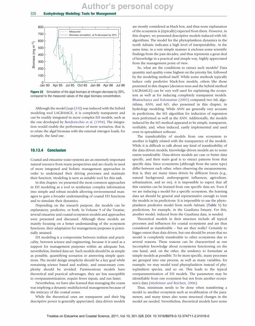
Author's personal copy326 Ecohydrology Modeling: Tools for Management
Measured Biomass simulation, at N decrease by 20%
800
Bio
mas
s (m
g m
–2)
700
600
500
400
300
200
100
0 Jan 85 Apr 85 Jul 85 Oct 85 Jan 86 Apr 86 Jul 86
Figure 22 Simulation of the algal biomass at nitrogen decrease by 20%, compared to the measured values of the algal biomass concentration.
Although the model (eqn [33]) was induced with the hybrid modeling tool LAGRAMGE, it is completely transparent and can be readily integrated in more complex EH models, such as the one developed by Bendoricchio et al. (1994). The integration would enable the performance of more scenarios, that is, to relate the algal biomass with the external nitrogen loads, for example, the land use.
10.13.4 Conclusion
Coastal and estuarine water systems are an extremely important natural resource from many perspectives and are clearly in need of more integrated and holistic management approaches in order to understand their driving processes and maintain their function. Modeling is seen as suitable tool for this task.
In this chapter, we presented the most common approaches in EH modeling as a tool to synthesize complex information into simple and robust models allowing environmental managers to gain a broader understanding of coastal EH functions and to simulate their dynamics.
Depending on the research purpose, the models can be explanatory, predictive, or both. In Volume 9 of the Treatise, several estuarine and coastal ecosystem models and approaches were presented and discussed. Although these models are mainly focusing on a better understanding of the ecosystem functions, their adaptation for management purposes is potentially attained.
EH modeling is a compromise between realism and practicality, between science and engineering, because it is used as a support for management purposes within an adequate but, nevertheless, limited data set. Such models should be as simple as possible, quantifying scenarios or answering simple questions. The model design simplicity should be a key goal while remaining science based and realistic, and unnecessary complexity should be avoided. Parsimonious models have theoretical and practical advantages, they are less susceptible to overparametrization, require fewer inputs, and run faster.
Nevertheless, we have also learned that managing the coasts was implying a dynamic multifactorial management because of the intricacy of the coastal zones.
While the theoretical ones are transparent and their big descriptive power is generally appreciated, data-driven models
Treatise on Estuarine and Coastal Science, 2011, Vol.10,
are mostly considered as black box, and thus none explanation of the ecosystem is (typically) expected from them. However, in this chapter, we presented descriptive models induced with ML algorithms. The model for the phytoplankton dynamics in the north Adriatic indicates a high level of interpretability. At the same time, in a very simple manner it encloses some scientific findings from the past decades, and thus represents a great deal of knowledge in a practical and simple way, highly appreciated from the management point of view.
So, what are the conditions to extract such models? Data quantity and quality come highest on the priority list, followed by the modeling method itself. While some methods typically induce only predictive black-box models, others like those presented in this chapter (decision trees and the hybrid method LAGRAMGE) can be very well used for explaining the ecosystem as well as for inducing completely transparent models. Bhattacharya and Solomatine (2005) compared two ML algorithms, ANN, and M5, also presented in this chapter, in hydrology modeling. While ANN are generally very accurate in predictions, the M5 algorithm for induction of regression trees performed as well as the ANN. Additionally, the models induced by the M5 method appeared to be simple, transparent, verifiable, and, when induced, easily implemented and used even in spreadsheet software.
The transferability of models from one ecosystem to another is highly related with the transparency of the models. While it is difficult to talk about any kind of transferability of the data-driven models, knowledge-driven models are to some extent transferable. Data-driven models are case or better data specific, and their main goal is to extract patterns from that specific data. Since ecosystems (although from the same type) differ between each other, when observing the measurements, that is, they are many times driven by different forces (e.g., natural background, anthropogenic influences, agriculture, urbanization, and so on), it is impossible to expect that all this varieties can be learned from one specific data set. Even if we are inducing a model for a specific ecosystem, the learning data set should be general and representative enough to trust the models in its predictions. It is impossible to use the phytoplankton predictive model from north Adriatic (Table 5) for predictions, for example, in the Guadiana Estuary. For this, another model, induced from the Guadiana data, is needed.
Theoretical models in their structure include all typical processes and influences for coastal ecosystems and are thus considered as transferable – but are they really? Certainly to bigger extent than data driven, but one should be aware that no model is completely transferable to other ecosystems due to several reasons. These reasons can be characterized as our incomplete knowledge about ecosystems functioning on the one hand, and, on the other, the tendency to formulate as simple models as possible. To be more specific, many processes are grouped into one process, as well as many variables, for example, we may model total phytoplankton instead of phytoplankton species, and so on. This leads to the typical overparametrization of EH models. The parameters may be identifiable from one ecosystem but not from another ecosystem’s data (Mieleitner and Reichert, 2006).
Thus, minimum needs to be done when transferring a model to another ecosystem such as recalibration of the parameters, and many times also some structural changes in the model are needed. Nevertheless, theoretical models have some
301-328, DOI: 10.1016/B978-0-12-374711-2.01016-0

Author's personal copyEcohydrology Modeling: Tools for Management 327
basic common structure, a result of common universal processes or functions, which is transferable to some extent.
In this sense, hybrid modeling tools are much closer to the theoretical than to the data-driven models. Moreover, they attempt to address the problems of discovery of generic model structures systematically. If appropriate interface is provided, they can represent a good modeling tool for management, since they may perform all modeling steps automatically. In the case of the modeling framework LAGRAMGE, the user only needs to specify or list (not mathematically) the variables and the processes that take place in the system. The rest of the modeling steps, that is, mathematical formulations, calibration of the parameters, simulations, and so on, are done automatically. However, one should be careful in composing the modeling task, namely, we should mention that the more background knowledge (in terms of alternative formulations of generic processes), the larger the search space, that is, number of generated models, is. This, in turn, makes a discovery of the right model more difficult, in the sense that larger quantities of good quality data are needed to identify it from the remaining candidate models. In the case of Venice Lagoon there were 3240 candidate models (Atanasova, 2005).
References
Alveirinho, J.M.A., Gonzalez, R., Ferreira, Ó., 2004. Natural versus anthropic causes in variations of sand export from river basins: an example from the Guadiana river mouth (Southwestern Iberia). Polish Geological Institute Special Papers 11, 95–102.
Atanasova, N., 2005. Preparation and Use of the Domain Expert Knowledge for Automated Modelling of Aquatic Ecosystems. Ph.D. Thesis, Faculty of Civil and Geodetic Engineering, University of Ljubljana, Ljubljana, Slovenia.
Atanasova, N., Todorovski, L., Džeroski, S., Kompare, B., 2006a. Constructing a library of domain knowledge for automated modelling of aquatic ecosystems. Ecological Modelling 194 (1–3), 14–36.
Atanasova, N., Todorovski, L., Džeroski, S., Kompare, B., 2008. Application of automated model discovery from data and expert knowledge to a real-world domain: Lake Glumsø. Ecological Modelling 212 (1–2), 92–98.
Atanasova, N., Todorovski, L., Džeroski, S., Remec-Rekar, Š., Recknagel, F., Kompare, B., 2006b. Automated modelling of a food web in lake Bled using measured data and a library of domain knowledge. Ecological Modelling 194 (1–3), 37–48.
Bendoricchio, G., Coffaro, G., De Marchi, C., 1994. A trophic model for Ulva rigida in the Lagoon of Venice. Ecological Modelling 75–76, 485–496.
Ben-Hamadou, R., 2009. Modelling estuarine ecological response to diverse hydrological patterns. Bottom-up control. Practical experiments guide for Ecohydrology. UNESCO Manuals, Faro, Portugal, 121 pp.
Bhattacharya, B., Solomatine, D.P., 2005. Neural networks and M5 model trees in modelling water level-discharge relationship. Neurocomputing 63, 381–396,
Brauer, F., Castillo-Chavez, C., 2001. Mathematical Models in Population Biology and Epidemiology. Springer, Berlin, 416 pp.
Bridewell, W., Langley, P., Todorovski, L., Dzeroski, S., 2008. Inductive process modeling. Machine Learning 71, 32.
Bruno, J.F., Selig, E.R., 2007. Regional decline of coral cover in the Indo-Pacific: timing, extent, and subregional comparisons. PLoS ONE 2 (8), e711. doi:10.1371/journal. pone.0000711.
Caraco, N.F., Cole, J.J., Raymond, P.A., Strayer, D.L., Pace, M.L., Findlay, S.E.G., Fischer, D.T., 1997. Zebra mussel invasion in a large, turbid river: phytoplankton response to increased grazing. Ecology 78, 588–602.
Carlsson, P., Granéli, E., 1999. Effects of N:P:Si ratios and zooplankton grazing on phytoplankton communities in the northern Adriatic Sea. II. Phytoplankton species composition. Aquatic Microbial Ecology 18, 55–65.
Chau, K., 2006. A review on the integration of artificial intelligence into coastal modeling. Journal of Environmental Management 80, 47–57.
Chícharo, L., Ben-Hamadou, R., Amaral, A., Range, P., Mateus, C., Piló, D., Marques, R., Morais, P., Chícharo, M.A., 2009. Application and demonstration of the ecohydrology approach for the sustainable functioning of the Guadiana Estuary (South Portugal). Ecohydrology and Hydrobiology 9, 55–71.
Treatise on Estuarine and Coastal Science, 2011, Vol.10
Chícharo, L., Chícharo, M.A., Ben-Hamadou, R., 2006. Use of a hydrotechnical infrastructure (Alqueva Dam) to regulate planktonic assemblages in the Guadiana Estuary: basis for sustainable water and ecosystem services management. Estuarine, Coastal and Shelf Science 70 (1–2), 3–18.
Chícharo, L., Chícharo, M.A., Esteves, E., Andrade, P., Morais, P., 2002. Effects of alterations in fresh water supply on the abundance and distribution of Engraulis encrasicolus in the Guadiana Estuary and adjacent coastal areas of South Portugal. Journal Ecohydrology and Hydrobiology 1, 195–200.
Cloern, J.E., Nichols, F.H., 1985. Temporal Dynamics of an Estuary: San Francisco Bay. Dr. W. Junk, Dordrecht.
Coffaro, G., Carrer, G., Bendoricchio, G., 1993. Model for Ulva Rigida growth in the Lagoon of Venice, UNESCO MURST Project: Venice Lagoon Ecosystem. University of Padova, Padova.
de Wit, M., Bendoricchio, G., 2001. Nutrient fluxes in the Po basin. Science of the Total Environment 273, 147–161.
De’ath, G., Lough, J.M., Fabricius, K.E., 2009. Declining coral calcification on the Great Barrier Reef. Science 323, 116–119.
Degobbis, D., Gilmartin, M., 1990. Nitrogen phosphorus and silicon budgets for the northern Adriatic Sea. Oceanologica Acta 13, 31–45.
Degobbis, D., Precali, R., Ivančic, I., Smodlaka, N., Fuks, D., Kveder, S., 2000. Long-term changes in the northern Adriatic ecosystem related to anthropogenic eutrophication. International Journal of Environment and Pollution 13, 495–533.
Džeroski, S., 2001. Applications of symbolic machine learning to ecological modeling. Ecological Modelling 146, 263–273.
Džeroski, S., 2009. Machine learning applications in habitat suitability modeling. In: Haupt, S.E., Pasini, A., Marzban, C. (Eds.), Artificial Intelligence Methods in the Environmental Sciences. Springer, Berlin, pp. 397–412.
Džeroski, S., Todorovski, L., 1995. Discovering dynamics: from inductive logic programming to machine discovery. Journal of Intelligent Information Systems 4, 89–108.
Džeroski, S., Todorovski, L., 2003. Learning population dynamics models from data and domain knowledge. Ecological Modelling 170 (2–3), 129–140.
Džeroski, S., Todorovski, L., Bratko, I., Kompare, B., Križman, V., 1999. Equation discovery with ecological applications. In: Fielding, A.H. (Ed.), Machine Learning Methods for Ecological Applications. Kluwer, Dordrecht, pp. 185–207.
Erzini, K., 2005. Trends in NE Atlantic landings (southern Portugal): identifying the relative importance of fisheries and environmental variables. Fisheries Oceanography 14, 195–209.
Flindt, M.R., Kamp-Nielsen, L., 1997. Modelling of an estuarine eutrophication gradient. Ecological Modelling 102, 143–153.
Golbuu, Y., Wolanski, E., Harrison, P., Richmond, R.H., Victor, S., Fabricius, K.E., 2011. Effects of land use change on characteristics and dynamics of watershed discharges in Babeldoab, Palau, Micronesia. Journal of Marine Biology (in press).
Harding, L.W., Jr., Degobbis, D., Precali, R., 1999. Production and fate of phytoplankton: annual cycles and interannual variability. In: Malone, T., Malej, A., Harding, L.W., Jr., Smodlaka, N., Turner, E. (Eds.), Ecosystems at the Land–Sea Margin: Drainage Basin to Coastal Sea. Coastal and Estuarine Studies. AGU, Washington, DC, vol. 55, pp. 131–172.
Kompare, B., 1995. The Use of Artificial Intelligence in Ecological Modelling. Ph.D. Thesis, Royal Danish School of Pharmacy, FGG, Copenhagen, Ljubljana, Slovenia.
Kompare, B., Džeroski, S., 1995. Getting more out of data: automated modelling of algal growth with machine learning. Proceedings of the International Conference on Coastal Ocean Space Utilization. University of Hawaii, Hawaii, pp. 209–220.
Kompare, B., Džeroski, S., Križman, V., 1997. Modelling the growth of algae in the Lagoon of Venice with the artificial intelligence tool GoldHorn. Proceedings of the Fourth International Conference on Water Pollution. Computational Mechanics Publications, Southampton, pp. 799–808.
Kompare, B., Todorovski, L., Džerovski, S., 2001. Modelling and prediction of phytoplankton growth with equation discovery: case study – LakeGlumsø, Denmark. Verhandlungen des Internationalen Verein Limnologie 27, 3626–3631.
Kot, M., 2001. Elements of Mathematical Ecology. Cambridge University Press, Cambridge, 464 pp.
Križman, V., 1998. Avtomatsko odkrivanje strukture modelov dinamicnih sistemov. Ph.D. Thesis, Faculty of Computer and Information Science, University of Ljubljana, Ljubljana, Slovenia (in Slovene).
Langley, P., Sanchez, J., Todorovski, L., Dzeroski, S., 1997. Inducing process models from continuous data. In: Sammut, C., Hofmann, A. (Eds.), Proceedings of the Nineteenth International Conference on Machine Learning. Morgan Kaufmann, San Mateo, CA, pp. 347–354.
Langley, P., Simon, H.A., Bradshaw, G.L., Zythow, J.M., 1987. Scientific Discovery. MIT Press, Cambridge, MA.
McDonald, C.P., Urban, N.R., 2010. Using a model selection criterion to identify appropriate complexity in aquatic biogeochemical models. Ecological Modelling 221 (3), 428–432.
, 301-328, DOI: 10.1016/B978-0-12-374711-2.01016-0
Author's personal copy328 Ecohydrology Modeling: Tools for Management
Mieleitner, J., Reichert, P., 2006. Analysis of the transferability of a biogeochemical lake model to lakes of different trophic state. Ecological Modelling 194 (1–3), 49–61.
Mitchel, T.M., 1998. Machine Learning. McGraw-Hill, New York, NY. Mitchel, T.M., 2006. The discipline of machine learning. Technical Report CMU-ML
06-108. School of Computer Science, Carnegie Mellon University. Mozetič, P., Solidoro, C., Cossarini, G., Socal, G., Precali, R., Francé, J., Bianchi, F., De
Vittor, C., Smodlaka, N., Fonda Umani, S., 2009. Recent trends towards oligotrophication of the Northern Adriatic: evidence from chlorophyll a time series. Estuaries and Coasts 33, 362–375.
Nakamura, Y., 2001. Filtration rates of the Manila clam, Ruditapes philippinarum: dependence on prey items including bacteria and picocyanobacteria. Journal of Experimental Marine Biology and Ecology 266, 181–192.
Nakamura, Y., Kerciku, F., 2000. Effects of filter-feeding bivalves on the distribution of water quality and nutrient cycling in a eutrophic coastal lagoon. Journal of Marine System 26, 209–221.
Oreskes, N., Shrader-Frechette, K., Belitz, K., 1994. Verification, validation, and confirmation of numerical models in the earth sciences. Science 263, 641–646.
Pagnotta, R., Caggiati, G., Piazza, D., Ferrari, F., 1995. Il controllo della qualitá delle acque superficiali del bacino padano. Inquinamento 1995 (4), 8–14.
Precali, R., Giani, M., Marini, M., Grilli, F., Pečar, O., Paschini, E., 2005. Mucilage events in the northern Adriatic in the period 1999–2002. Science of the Total Environment 353, 10–23.
Provini, A., Crosa, G., Marchetti, R., 1992. Nutrient export from the Po and Adige river basins over the last 20 years. In: Vollenweider, R.A., Marchetti, R., Viviani, R., (Eds.), Conference of marine coastal eutrophication, 21–24 March 1990, Bologna, Italy. Science of the Total Environment, Supplement, 291–313.
Quinlan, J.R., 1992. Learning with continuous classes. In: Adams, A., Sterling, L. (Eds.), Proc. AI’92, 5th Australian Joint Conference on Artificial Intelligence. World Scientific, Singapore, pp. 343–348.
Quinlan, J.R., 1993. Combining instance-based and model-based learning. In: Utgoff, P.E. (Ed.), Proceedings ML’93. Morgan Kaufmann, San Mateo, CA.
Richmond, R.H., Rongo, T., Golbuu, Y., Victor, S., Idechong, N., Davis, G., Kostka, W., Neth, L., Hamnett, M., Wolanski, E., 2007. Watersheds and coral reefs: conservation science, policy and implementation. BioScience 57, 598–607.
Richmond, R.H., Wolanski, E., 2011. Coral research: past efforts and future horizons. In: Dubinsky, Z., Stambler, N., (eds.) Coral Reefs: An ecosystem in Transition. Springer Science, pp. 552. ISBN: 978-94-007-0113-7.
Rocha, C., Galvão, H., Barbosa, A., 2002. Role of transient silicon limitation in the development of cyanobacteria blooms in the Guadiana Estuary, south-western Iberia. Marine Ecology Progress Series 228, 35–45.
Roelke, D.L., 2000. Copepod food quality threshold as a mechanism influencing phytoplankton succession and accumulation of biomass, and secondary productivity: a modelling study with management implications. Ecological Modelling 134, 245–274.
Rykiel, E.J., Jr., 1996. Testing ecological models: the meaning of validation. Ecological Modelling 90, 229–244.
Sheng, Y.P., Kim, T., 2009. Skill assessment of an integrated modeling system for shallow coastal and estuarine ecosystems. Journal of Marine Systems 6, 212–243.
Treatise on Estuarine and Coastal Science, 2011, Vol.10,
Solomatine, D.P., 2002. Applications of data-driven modelling and machine learning in control of water resources. In: Mohammadian, M., Sarker, R.A., Yao, X. (Eds.), Computational Intelligence in Control. Idea Group Publishing, Hershey, PA, pp. 197–217.
Supic, N., D- akovac, T., Krajcar, V., Kuzmic, M., Precali, R., 2006. Effects of excessive Po River discharges in the northern Adriatic. Fresenius Environmental Bulletin 15 (3), 193–199.
Todorovski, L., 2003. Using Domain Knowledge for Automated Modeling of Dynamic Systems with Equation Discovery. Ph.D. Thesis, Fakulteta za računalništvo in informatiko, University of Ljubljana, Ljubljana, Slovenia.
Todorovski, L., Džeroski, S., 1997. Declarative bias in equation discovery. Proceedings of the Fourteenth International Conference on Machine Learning. Morgan Kaufmann, Los Altos, CA, pp. 376–384.
Todorovski, L., Džeroski, S., 2006. Integrating knowledge-driven and data-driven approaches to modeling. Ecological Modelling 194 (1–3), 3–13.
Todorovski, L., Džeroski, S., Kompare, B., 1998. Modelling and prediction of phytoplankton growth with equation discovery. Ecological Modelling 113 (1–3), 71–81.
Volf, G., Atanasova, N., Kompare, B., Precali, R., Ožanic., 2011. Descriptive and prediction models of phytoplankton in the northern Adriatic. Ecological Modelling. DOI: 10.1016/ j.ecolmodel.2011.02.013.
Whigham, P.A., 1995. Grammatically-based genetic programming. In: Rosca, J. (Ed.), Proceedings of the Workshop on Genetic Programming: From Theory to Real-World Applications. Morgan Kaufmann, Tahoe City, CA, pp. 33–41.
Whigham, P.A., Crapper, P.F., 2001. Modelling rainfall-runoff using genetic programming. Mathematical and Computer Modelling 33 (6–7), 707–721.
Whigham, P.A., Recknagel, F., 2001. Predicting chlorophyll-a in freshwater lakes by hybridising process s-based models and genetic algorithms. Ecological Modelling 146 (1–3), 243–251.
Witten, I.H., Frank, E., 2000. Data Mining: Practical Machine Learning Tools and Techniques with Java Implementations. Morgan Kaufmann, San Francisco, CA.
Wolanski, E., 2007. Estuarine Ecohydrology. Elsevier, Amsterdam, 157 pp. Wolanski, E., Chicharo, L., Chicharo, M., Morais, P., 2006. An ecohydrology model of
the Guadiana Estuary (South Portugal). Estuarine, Coastal and Shelf Science 70, 132–143.
Wolanski, E., De’ath, G., 2005. Predicting the present and future human impact on the Great Barrier Reef. Estuarine, Coastal and Shelf Science 64, 504–508.
Wolanski, E., Martinez, J.A., Richmond, R.H., 2009. Quantifying the impact of watershed urbanization on a coral reef: Maunalua Bay, Hawaii. Estuarine, Coastal and Shelf Science 84, 259–268.
Wolanski, E., Richmond, R.H., McCook, L., 2004. A model of the effects of land-based, human activities on the health of coral reefs in the Great Barrier Reef and in Fouha Bay, Guam, Micronesia. Journal of Marine Systems 46, 133–144.
Zalewski, M., 2002. Ecohydrology – the use of ecological and hydrological processes for sustainable management of water-resources. Hydrological Sciences Bulletin 47, 823–832.
Zhou, Y., Yang, H., Liu, S., Yuan, X., Mao, Y., Zhang, T., Liu, Y., Zhang, F., 2006. Feeding on biodeposits of bivalves by the sea cucumber Stichopus japonicus Selenka (Echinidermata: Holothuroidea) and a suspension coculture of filter-feeding bivalves with deposit feeders in lantern nets from longlines. Aquaculture 256, 510–520.
301-328, DOI: 10.1016/B978-0-12-374711-2.01016-0