E cient Algorithms and Codes for k-Cardinality Assignment Problems
16
Discrete Applied Mathematics 110 (2001) 25–40 Ecient algorithms and codes for k -cardinality assignment problems Mauro Dell’Amico a , Andrea Lodi b , Silvano Martello b; ∗ a Dipartimento di Scienze e Metodi dell’Ingegneria, Universit a di Modena e Reggio Emilia, Italy b Dipartimento di Elettronica, Informatica e Sistemistica, Universit a di Bologna, Viale Risorgimento 2, 40136 Bologna, Italy Abstract Given a cost matrix W and a positive integer k , the k -cardinality assignment problem is to assign k rows to k columns so that the sum of the corresponding costs is a minimum. This generalization of the classical assignment problem is solvable in polynomial time, either by transformation to min-cost ow or through specic algorithms. We consider the algorithm re- cently proposed by Dell’Amico and Martello for the case where W is dense, and derive, for the case of sparse matrices, an ecient algorithm which includes original heuristic preprocessing techniques. The resulting code is experimentally compared with min-cost ow codes from the literature. Extensive computational tests show that the code is considerably faster, and eectively solves very large sparse and dense instances. ? 2001 Elsevier Science B.V. All rights reserved. 1. Introduction A well-known problem in telecommunications is the satellite-switched time-division multiple access (SS/TDMA) time slot assignment problem (see, e.g., [14,9]). We are given m transmitting stations and n receiving stations, interconnected by a geostationary satellite through an on-board k × k switch (k 6min(m; n)), and an integer m × n trac matrix W =[w ij ], where w ij is the time needed for the transmission from station i to station j. The problem is to determine a sequence of switching congurations which allow all transmissions to be performed in minimum total time, under the constraint that no preemption of a transmission occurs. A switching conguration is an m × n 0–1 matrix X ‘ having exactly k ones, with no two in the same row or column. Matrix X ‘ is associated with a transmission time slot of duration t ‘ =max ij {X ‘ ij w ij }. The objective is thus to determine an integer and X ‘ (‘ =1;:::;) so that ∑ ‘=1 t ‘ is a minimum. ∗ Corresponding author. Tel.: +39-051-644-3022; fax: +39-051-644-3073. E-mail addresses: [email protected] (M. Dell’Amico), [email protected] (A. Lodi), [email protected] (S. Martello). 0166-218X/01/$ - see front matter ? 2001 Elsevier Science B.V. All rights reserved. PII: S0166-218X(00)00301-2
Transcript of E cient Algorithms and Codes for k-Cardinality Assignment Problems

Discrete Applied Mathematics 110 (2001) 25–40
E�cient algorithms and codes for k-cardinality assignmentproblems
Mauro Dell’Amicoa, Andrea Lodib, Silvano Martellob; ∗aDipartimento di Scienze e Metodi dell’Ingegneria, Universit�a di Modena e Reggio Emilia, Italy
bDipartimento di Elettronica, Informatica e Sistemistica, Universit�a di Bologna, Viale Risorgimento 2,40136 Bologna, Italy
Abstract
Given a cost matrix W and a positive integer k, the k-cardinality assignment problem is toassign k rows to k columns so that the sum of the corresponding costs is a minimum. Thisgeneralization of the classical assignment problem is solvable in polynomial time, either bytransformation to min-cost -ow or through speci.c algorithms. We consider the algorithm re-cently proposed by Dell’Amico and Martello for the case where W is dense, and derive, for thecase of sparse matrices, an e�cient algorithm which includes original heuristic preprocessingtechniques. The resulting code is experimentally compared with min-cost -ow codes from theliterature. Extensive computational tests show that the code is considerably faster, and e1ectivelysolves very large sparse and dense instances. ? 2001 Elsevier Science B.V. All rights reserved.
1. Introduction
A well-known problem in telecommunications is the satellite-switched time-divisionmultiple access (SS/TDMA) time slot assignment problem (see, e.g., [14,9]). We aregiven m transmitting stations and n receiving stations, interconnected by a geostationarysatellite through an on-board k× k switch (k6min(m; n)), and an integer m× n tra)cmatrix W = [wij], where wij is the time needed for the transmission from station i tostation j. The problem is to determine a sequence of switching con.gurations whichallow all transmissions to be performed in minimum total time, under the constraintthat no preemption of a transmission occurs. A switching con+guration is an m×n 0–1matrix X ‘ having exactly k ones, with no two in the same row or column. Matrix X ‘
is associated with a transmission time slot of duration t‘=maxij{X ‘ijwij}. The objectiveis thus to determine an integer � and X ‘ (‘= 1; : : : ; �) so that
∑�‘=1 t
‘ is a minimum.
∗ Corresponding author. Tel.: +39-051-644-3022; fax: +39-051-644-3073.E-mail addresses: [email protected] (M. Dell’Amico), [email protected] (A. Lodi),
[email protected] (S. Martello).
0166-218X/01/$ - see front matter ? 2001 Elsevier Science B.V. All rights reserved.PII: S0166 -218X(00)00301 -2
26 M. Dell’Amico et al. / Discrete Applied Mathematics 110 (2001) 25–40
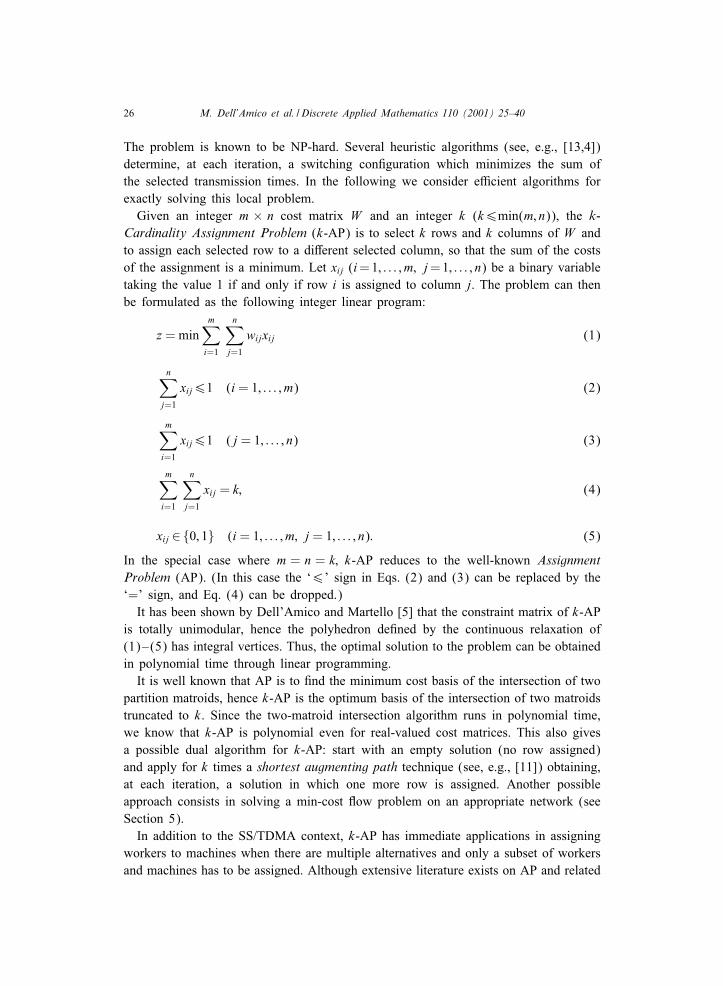
The problem is known to be NP-hard. Several heuristic algorithms (see, e.g., [13,4])determine, at each iteration, a switching con.guration which minimizes the sum ofthe selected transmission times. In the following we consider e�cient algorithms forexactly solving this local problem.Given an integer m × n cost matrix W and an integer k (k6min(m; n)), the k-
Cardinality Assignment Problem (k-AP) is to select k rows and k columns of W andto assign each selected row to a di1erent selected column, so that the sum of the costsof the assignment is a minimum. Let xij (i=1; : : : ; m; j=1; : : : ; n) be a binary variabletaking the value 1 if and only if row i is assigned to column j. The problem can thenbe formulated as the following integer linear program:
z =minm∑
i=1
n∑
j=1
wijxij (1)
n∑
j=1
xij61 (i = 1; : : : ; m) (2)
m∑
i=1
xij61 (j = 1; : : : ; n) (3)
m∑
i=1
n∑
j=1
xij = k; (4)
xij ∈{0; 1} (i = 1; : : : ; m; j = 1; : : : ; n): (5)
In the special case where m = n = k; k-AP reduces to the well-known AssignmentProblem (AP). (In this case the ‘6’ sign in Eqs. (2) and (3) can be replaced by the‘=’ sign, and Eq. (4) can be dropped.)It has been shown by Dell’Amico and Martello [5] that the constraint matrix of k-AP
is totally unimodular, hence the polyhedron de.ned by the continuous relaxation of(1)–(5) has integral vertices. Thus, the optimal solution to the problem can be obtainedin polynomial time through linear programming.It is well known that AP is to .nd the minimum cost basis of the intersection of two
partition matroids, hence k-AP is the optimum basis of the intersection of two matroidstruncated to k. Since the two-matroid intersection algorithm runs in polynomial time,we know that k-AP is polynomial even for real-valued cost matrices. This also givesa possible dual algorithm for k-AP: start with an empty solution (no row assigned)and apply for k times a shortest augmenting path technique (see, e.g., [11]) obtaining,at each iteration, a solution in which one more row is assigned. Another possibleapproach consists in solving a min-cost -ow problem on an appropriate network (seeSection 5).In addition to the SS/TDMA context, k-AP has immediate applications in assigning
workers to machines when there are multiple alternatives and only a subset of workersand machines has to be assigned. Although extensive literature exists on AP and related

M. Dell’Amico et al. / Discrete Applied Mathematics 110 (2001) 25–40 27
problems (surveys can be found, e.g., in [12,1,6]), to our knowledge the only speci.cresult on k-AP has been presented by Dell’Amico and Martello [5].The algorithm in [5] was developed for solving instances in which matrix W is
complete. In this paper, we consider the case where W is sparse, i.e., many entries areempty, or, equivalently, they have in.nite cost. The sparse case is relevant for appli-cations. Consider, e.g., the SS/TDMA time slot assignment previously discussed: it isclear that, in general, a transmitting station will not send messages to all receivingstations, so we can expect that real-world tra�c matrices are sparse.In the sparse case, the problem is more conveniently formulated through the fol-
lowing graph theory model. Let G = (U ∪ V; A) be a bipartite digraph where U ={1; : : : ; m} and V = {1; : : : ; n} are the two vertex sets and A⊆U × V is the arc set:A= {(i; j): wij ¡+∞}. Let wij be the weight of an arc (i; j)∈A. We want to selectk arcs of A such that no two arcs share a common vertex and the sum of the costs ofthe selected arcs is a minimum.In the following we assume, without loss of generality, that wij¿0 ∀(i; j)∈A. Sincek-AP does not change if we swap sets U and V , we also assume, without loss ofgenerality, that m6n.The problem in which the objective is to maximize the cost of the assignment, is
solved by k-AP if each cost whl ((h; l)∈A) is replaced by the nonnegative quantityw̃hl =max(i; j)∈A{wij} − whl.
The aim of this article is to provide a specialized algorithm, and the correspondingcomputer code, for the exact solution of k-AP.
2. Complete matrices
The main phases of the approach in [5] are a heuristic preprocessing and an exactprimal algorithm. Preprocessing .nds a partial optimal solution, determines sets ofrows and columns which must be assigned in an optimal solution and reduces the costmatrix. The partial solution is then heuristically completed, and the primal algorithmdetermines the optimum through a series of alternating paths.The preprocessing phase can be summarized as follows.Step 0: For each row i determine the .rst, second and third smallest cost in the row
(�i; �′i ; �′′i , respectively) and let c(i); c′(i); c′′(i) be the corresponding columns. For each
column j determine the .rst, second and third smallest cost in the column (�j; �′j; �′′j ,
respectively) and let r(j); r′(j); r′′(j) be the corresponding rows. Reorder the columnsof W by nondecreasing �j values, and the rows by nondecreasing �i values.
Step 1: Determine a value g16k, as high as possible, such that a partial optimalsolution in which g1 rows are assigned can be heuristically determined. This is obtainedthrough a heuristic algorithm which, for increasing values of j, assigns row r(j) tocolumn j if this row is currently unassigned; if instead row r(j) is already assigned,under certain conditions the algorithm assigns column j + 1 instead of j (and thenproceeds to column j+2) or assigns the current column j to row r′(j) instead of r(j).

28 M. Dell’Amico et al. / Discrete Applied Mathematics 110 (2001) 25–40
If g1 = k then terminate (the solution is optimal); otherwise, execute a greedy heuristicto determine an approximate solution of cardinality k and let UB1 be the correspondingvalue.Step 2: Repeat Step 1 over the transposed cost matrix. Let g2 and UB2 be the values
obtained.Step 3: UB:=min(UB1; UB2); g:=max(g1; g2).Step 4: Starting from the partial optimal solution of cardinality g, determine a set R
of rows and a set C of columns that must be selected in an optimal solution to k-AP.Compute a lower bound LB on the optimal solution value.Step 5: If UB¿LB then reduce the instance by determining pairs (i; j) for whichxij must assume the value zero.The overall time complexity of the above preprocessing phase is O(mn+ kn log n).Once Step 5 has been executed, the primal phase starts with the k × k submatrix of
W induced by the sets of rows and columns selected in the heuristic solution of valueUB, and exactly solves an AP over this matrix. Then m+n−2k iterations are performedby adding to the current submatrix one row or column of W at a time, and byre-optimizing the current solution through alternating paths on a particular digraphinduced by the submatrix.
3. Sparse matrices
In this section we discuss the most relevant features of the algorithm for the sparsecase.
3.1. Data structures
Let " be the number of entries with .nite cost. We store matrix W through a forwardstar (see Fig. 1(a)) consisting of an array, F first, of m+1 pointers, and two arrays,F head and F cost, of " elements each. The entries of row i, and the correspondingcolumns, are stored in F cost and F head, in locations F first(i); : : : ; F first(i+1)−1(with F first(1) = 1 and F first(m+ 1) = " + 1). Since the algorithm needs to scanW both by row and by column, we duplicate the information into a backward star,similarly de.ned by arrays B first (of n + 1 pointers), B tail and B cost, storingthe entries of column j, and the corresponding rows, in locations B first(j); : : : ;B first(j + 1)− 1.In the primal phase a local matrix NW is initialized to the k × k submatrix of W
obtained from preprocessing, and iteratively enlarged by addition of a row or a column.Let row(i) (resp. col(j)) denote the row (resp. column) of W corresponding to rowi (resp. column j) of NW . Matrix NW is stored through a modi.ed forward star. In thiscase we have two arrays, NF head and NF cost, of length ", and two arrays, NF firstand NF last, of m pointers each. For each row i currently in NW : (a) the elementsof the current columns, and the corresponding current column indices, are stored in

M. Dell’Amico et al. / Discrete Applied Mathematics 110 (2001) 25–40 29
Fig. 1. Data structures.
NF cost and NF head, in locations NF first(i); : : : ; NF last(i); (b) locations NF last(i) +1; : : : ; NF first(i) + L − 1 (where L = F first(row(i) + 1) − F first(row(i)) denotesthe number of elements in row row(i) of W ) are left empty for future insertions. Thebackward star for NW is similarly de.ned by arrays NB tail; NB cost; NB first and NB last.Fig. 1(b) shows the structures for a 2× 2 submatrix NW of W .
3.2. Approximate solution
All computations needed by the preprocessing of Section 2 were e�ciently imple-mented through the data structures described in the previous section, but the greedysolution of Step 1 (and 2) required a speci.c approach. Indeed, due to sparsity, in somecases a solution of cardinality k does not exist at all. Even if k-cardinality assignmentsexist, in many cases the procedure adopted for the complete case proved to be highlyine�cient in .nding one. For the same reason, a second greedy approach was neededat Step 3. These approaches are discussed in Section 3.3.In certain cases, the execution of the greedy algorithms can be replaced by the
following transformation which provides a method to determine a k-cardinality assign-ment, or to prove that no such assignment exists. Let us consider the bipartite digraphG = (U ∪ V; A) introduced in Section 1, and de.ne a digraph G′ = ({s} ∪ { Ns} ∪ U ∪V ∪ {t}; A′), where A′ = A ∪ {(s; Ns)} ∪ {( Ns; i): i∈U} ∪ {(j; t): j∈V}. Now assign unitcapacity to all arcs of A′ except (s; Ns), for which the capacity is set to k, and send themaximum -ow # from s to t. It is clear that this will either provide a k-cardinalityassignment or prove that no such assignment is possible. If #¡k, we know that no
30 M. Dell’Amico et al. / Discrete Applied Mathematics 110 (2001) 25–40
solution to k-AP exists. If # = k, the arcs of A carrying -ow provide a k-cardinalityassignment, which is suboptimal since the arc costs have been disregarded.Computational experiments proved that the above approach is only e�cient when
the instance is very sparse, i.e., |A|60:01 mn, and k ¿ 0:9 m. For di1erent cases, muchbetter performance was obtained through the following greedy approaches.
3.3. Greedy approximate solutions
We recall that at steps 1 and 2 of the preprocessing phase described in Section 2 wehave partial optimal solutions of cardinality g1 and g2, respectively. Starting from oneof these solutions, the following algorithm tries to obtain an approximate solution ofcardinality k by using the information computed at Step 0 (the .rst, second and thirdsmallest cost in each row and column). In a .rst phase (steps (a) and (b) below) wetry to compute the solution using only .rst minima. If this fails, we try using secondand third minima (step (c)). Parameter gh can be either g1 or g2.
Algorithm GREEDY(gh):
(a) Ngh:=gh;.nd the .rst unassigned row, i, such that column c(i) is unassigned and set�̃:=�i (�̃:= +∞ if no such row);.nd the .rst unassigned column, j, such that row r(j) is unassigned and set�̃:=�j (�̃:= +∞ if no such column);
(b) while Ngh ¡k and (�̃ �= +∞ or �̃ �= +∞) doNgh:= Ngh + 1;if �̃6�̃ then
assign row i to column c(i);.nd the next unassigned row, i, such that column c(i) is unassignedand set �̃:=�i (�̃:= +∞ if no such row)
elseassign column j to row r(j);.nd the next unassigned column, j, such that row r(j) is unassignedand set �̃:=�j (�̃:= +∞ if no such column)
endifendwhile;
(c) if Ngh ¡k thenexecute steps similar to (a) and (b) above, but looking, at each search,for the .rst or next row i (resp. column j) such that column c′(i) or c′′(i)(resp. row r′(j) or r′′(j)) is unassigned, and setting�̃:=�′(i) if c′(i) is unassigned, or �̃:=�′′(i) otherwise(resp. �̃:=�′(j) if r′(j) is unassigned, or �̃:=�′′(j) otherwise).
(d) if Ngh = k then UBh:= solution value else UBh:= +∞;return Ngh and UBh.
M. Dell’Amico et al. / Discrete Applied Mathematics 110 (2001) 25–40 31
Since it is possible that both Ng1 and Ng2 are less than k, Step 3 of Section 2 wasmodi.ed so as to have in any case an approximate solution of cardinality k, eitherthrough elements other than the .rst three minima, or, if this fails, through dummyelements. The resulting Step 3 is as follows.
Step 3. UB:=min(UB1; UB2); g:=max(g1; g2); Ng:=max( Ng1; Ng2);
if Ng= k then go to Step 4;for each unassigned column j do
if ∃ wij such that i is unassigned thenassign row i to column j, update UB and set Ng:= Ng+ 1;if Ng= k then go to Step 4
endif;while Ng¡k do
let i be the .rst unassigned row and j the .rst unassigned column;add to W a dummy element wij =M (a very large value);assign row i to column j, update UB and set Ng:= Ng+ 1
endwhile.
4. Implementation
The overall algorithm for sparse matrices was coded in FORTRAN 77. The approxi-mate solution of Section 3.2 was obtained using the FORTRAN implementation of theDinic [7] algorithm proposed by Goldfarb and Grigoriadis [8].The AP solution needed at the beginning of the primal phase was determined through
a modi.ed version of the Jonker and Volgenant [10] code SPJV for the sparse assign-ment problem. The original Pascal code was translated into FORTRAN and modi.edso as to: (i) handle our data structure for the current matrix NW (see Section 3.1); (ii)manage the particular case arising when the new Step 3 (see Section 3.3) adds dummyelements to the cost matrix. These elements are not explicitly inserted in the datastructure but implicitly considered by associating a -ag to the rows having .ctitiousassignment.The alternating paths needed, at each iteration of the primal phase, to re-optimize
the current solution have been determined through the classical Dijkstra algorithm,implemented with a binary heap for the node labels. Two shortest path routines werecoded: RHEAP (resp. CHEAP) starts from a given row (resp. column) and uses theforward (resp. backward) data structure of Section 3.1. Both routines implicitly considerthe possible dummy elements (see above).The overall structure of the algorithm is the following.
Algorithm SKAP:
if |A|60:01 mn and k ¿ 0:9 m thenexecute the Dinic algorithm (Section 3.2) and set LB:=− 1;if the resulting -ow is less than k then return “no solution”

32 M. Dell’Amico et al. / Discrete Applied Mathematics 110 (2001) 25–40
elseperform the sparse version of Steps 0–2 of preprocessing (Section 2);execute the new Step 3 (Section 3.3) and let UB denote the resulting value;execute the sparse version of Step 4 and let LB denote the lower bound value;if UB= LB then return the solution else reduce the instance (Step 5)
endif;initialize the data structure for matrix NW (Section 3.1);execute the modi.ed SPJV code for AP and let UB denote the solution value;if UB= LB then return the solution;for i:=1 to m− k do
add a row to NW and re-optimize by executing RHEAP;add a column to NW and re-optimize by executing CHEAP
endfor;for i:=1 to n− m do
add a column to NW and re-optimize by executing CHEAP;if the solution includes dummy elements then return “no solution”else return the solution.
4.1. Running the code
The algorithm was implemented as a FORTRAN 77 subroutine, called SKAP andavailable at http://www.or.deis.unibo.it/ORCodes/. The whole subroutine is completelyself-contained and communication with it is achieved solely through the parameter list.The subroutine can be invoked with the statement
CALL SKAP(M,N,F FIRST,F COST,F HEAD,B FIRST,B COST,B TAIL,K,OPT,Z,ROW,COL,U,V,MU,F COST2,B COST2,F HEAD2,B TAIL2)
The input parameters are
M, N = number of rows and columns (m; n);F FIRST, F COST, F HEAD = forward star data structure (see Section 3.1): thesearrays must be dimensioned at least at m+ 1; |A| and |A|, respectively;
B FIRST,B COST,B TAIL=backward star data structure (see Section 3.1): thesearrays must be dimensioned at least at n+ 1; |A| and |A|, respectively;
K = cardinality of the required solution;The output parameters are
OPT = return status: value 0 if the instance is infeasible; value 1 otherwise;Z = optimal solution value;ROW=the set of entries in the solution is {(ROW(j), j): ROW(j)¿0; j=1; : : : ;
N}: this array must be dimensioned at least at n;COL = the set of entries in the solution is {(i,COL(i)): COL(i)¿0; i=1; : : : ;M}:
this array must be dimensioned at least at m.Local arrays U, V (dimensioned at least at m and n, respectively) and scalar MU
are internally used to store the dual variables (see, Dell’Amico and Martello [5]); local
M. Dell’Amico et al. / Discrete Applied Mathematics 110 (2001) 25–40 33
arrays F COST2, F HEAD2, B COST2 and B TAIL2 are internally used to storethe restricted matrix (see Section 3.1), and must be dimensioned at least at |A|.
5. Computational experiments
Algorithm SKAP was computationally tested on a Silicon Graphics Indy R10000sc195MHz.We compared its performance with the following indirect approach. Consider digraphG′ = ({s} ∪ { Ns} ∪ U ∪ V ∪ {t}; A′) introduced in Section 3.2, and assign cost wij toeach arc (i; j)∈A, and zero cost to the remaining arcs. It is then clear that sendinga min-cost s − t -ow of value k on this network will give the optimal solution tothe corresponding k-AP. This approach was implemented by using two di1erent codesfor min-cost -ow. The .rst one is the FORTRAN code RELAXT IV of Bertsekasand Tseng, see [2], called RLXT in the sequel, and the second one is the C codeCS2 developed by Cherkassky and Goldberg, see Goldberg [3]. Parameter CRASH ofRELAXT IV was set to one, since preliminary computational experiments showed thatthis value produces much smaller computing times for our instances.Test problems were obtained by randomly generating the costs wij from the uniform
distributions [0; 102] and [0; 105]. This kind of generation is often encountered in theliterature for the evaluation of algorithms for AP.For increasing values of m and n (up to 3000) and various degrees of density (1%,
5% and 10%), 10 instances were generated and solved for di1erent values of k (rangingfrom 20
100m to 99100m�).
Density d% means that the instance was generated as follows. For each pair (i; j),we .rst generate a uniformly random value r in [0; 1): if r6d then the entry is addedto the instance by generating its value wij in the considered range; otherwise the nextpair is considered. In order to ensure consistency with the values of m and n, we thenconsider each row i and, if it has no entry, we uniformly randomly generate a columnj and a value wij. The same is .nally done for columns.Tables 1–3 show the results for sparse instances. In each block, each entry in the
.rst six lines gives the average CPU time computed over 10 random instances, whilethe last line gives the average over all k values considered. The results show that thebest of the two min-cost -ow approaches is faster than SKAP for some of the easyinstances of Table 1, while both are clearly slower for all the remaining instances.More speci.cally, for the 1% density (Table 1) RLXT is faster than SKAP in the
range [0; 102] for m and n less than 3000, while CS2 is faster than SKAP in therange [0; 105] for 5006m61000 and 10006n62000. It should be noted, however,that SKAP solves all these instances in less than one second on average, and that it isless sensitive to the cost range.For the 5% instances (Table 2), SKAP is always the fastest code. For large values ofm and n it is two–three times faster than its best competitor. This trend is con.rmedby Table 3 (10% density), where, for large instances, the CPU times of SKAP areabout one order of magnitude smaller than the others.

34 M. Dell’Amico et al. / Discrete Applied Mathematics 110 (2001) 25–40
Table 1Density 1%. Average computing times over 10 problems, Silicon Graphics INDY R10000sc seconds
Range [0; 102] Range [0; 105]
m n k100m
RLXT CS2 SKAP RLXT CS2 SKAP
20 0.018 0.029 0.005 0.031 0.038 0.00850 0.020 0.029 0.032 0.053 0.038 0.03780 0.024 0.031 0.039 0.071 0.043 0.035
250 500 90 0.023 0.030 0.039 0.067 0.042 0.03895 0.027 0.034 0.037 0.081 0.041 0.03799 0.023 0.031 0.041 0.068 0.045 0.039
Average 0.023 0.031 0.032 0.062 0.041 0.032
20 0.033 0.049 0.056 0.082 0.062 0.06350 0.054 0.056 0.061 0.155 0.064 0.06880 0.070 0.057 0.078 0.218 0.068 0.087
500 500 90 0.067 0.055 0.077 0.197 0.073 0.08895 0.076 0.058 0.073 0.165 0.074 0.07799 0.084 0.061 0.050 0.152 0.078 0.052
Average 0.064 0.056 0.066 0.162 0.070 0.073
20 0.045 0.090 0.029 0.189 0.120 0.06150 0.059 0.096 0.115 0.171 0.110 0.12680 0.075 0.095 0.118 0.227 0.125 0.141
500 1000 90 0.077 0.097 0.131 0.316 0.120 0.16495 0.072 0.100 0.182 0.364 0.122 0.20299 0.077 0.099 0.153 0.326 0.123 0.159
Average 0.068 0.096 0.121 0.266 0.120 0.142
20 0.089 0.156 0.231 0.358 0.204 0.23150 0.178 0.171 0.227 0.605 0.205 0.25680 0.200 0.181 0.294 0.987 0.219 0.351
1000 1000 90 0.199 0.188 0.271 1.109 0.232 0.32695 0.218 0.200 0.239 0.875 0.229 0.30099 0.237 0.217 0.142 0.796 0.244 0.202
Average 0.187 0.186 0.234 0.788 0.222 0.278
20 0.191 0.399 0.323 1.695 0.489 0.44850 0.196 0.430 0.446 0.911 0.489 0.47180 0.330 0.435 0.455 1.344 0.497 0.571
1000 2000 90 0.257 0.439 0.519 1.530 0.511 0.68395 0.270 0.461 0.735 1.688 0.506 0.77999 0.249 0.454 0.612 1.831 0.493 0.615
Average 0.249 0.436 0.515 1.500 0.498 0.595
20 0.477 1.015 0.905 2.485 1.190 0.91350 0.599 1.047 0.858 3.264 1.234 1.02980 0.867 1.203 1.078 7.862 1.315 1.620
2000 2000 90 0.876 1.256 1.007 6.087 1.405 1.43595 0.883 1.333 0.895 5.828 1.432 1.31299 0.900 1.427 0.503 4.274 1.547 0.893
Average 0.767 1.214 0.874 4.967 1.354 1.200

M. Dell’Amico et al. / Discrete Applied Mathematics 110 (2001) 25–40 35
Table 1 (continued)
Range [0; 102] Range [0; 105]
m n k100m
RLXT CS2 SKAP RLXT CS2 SKAP
20 0.928 1.078 0.038 7.412 1.410 1.02650 0.795 1.271 0.996 3.714 1.511 1.07780 0.613 1.307 0.983 1.723 1.490 1.262
1500 3000 90 0.754 1.370 1.112 2.656 1.560 1.67395 0.752 1.363 1.476 3.448 1.570 1.85399 0.663 1.340 1.252 2.803 1.551 1.420
Average 0.751 1.288 0.976 3.626 1.515 1.385
20 1.088 2.476 0.069 7.119 2.941 2.08350 1.431 2.743 2.012 5.509 3.220 2.38780 2.826 3.064 2.543 28.727 3.397 3.926
3000 3000 90 2.239 3.207 2.328 13.689 3.594 3.42895 2.160 3.438 1.975 14.763 3.766 3.03499 2.096 3.656 1.194 17.572 3.950 1.973
Average 1.973 3.097 1.687 14.563 3.478 2.805
Table 2Density 5%. Average computing times over 10 problems, Silicon Graphics INDY R10000sc seconds
Range [0; 102] Range [0; 105]
m n k100m
RLXT CS2 SKAP RLXT CS2 SKAP
20 0.035 0.076 0.005 0.168 0.091 0.02250 0.034 0.080 0.032 0.089 0.093 0.03980 0.040 0.082 0.042 0.080 0.107 0.051
250 500 90 0.035 0.075 0.049 0.155 0.092 0.05395 0.040 0.080 0.049 0.102 0.107 0.05799 0.043 0.077 0.043 0.072 0.093 0.049
Average 0.038 0.078 0.037 0.111 0.097 0.045
20 0.054 0.145 0.048 0.225 0.176 0.07050 0.063 0.147 0.078 0.176 0.186 0.08880 0.098 0.155 0.101 0.560 0.193 0.122
500 500 90 0.111 0.168 0.107 0.489 0.199 0.12595 0.114 0.170 0.093 0.497 0.204 0.10899 0.114 0.176 0.066 0.388 0.211 0.085
Average 0.092 0.160 0.082 0.389 0.195 0.100
20 0.176 0.358 0.016 1.376 0.450 0.09950 0.165 0.405 0.137 0.721 0.501 0.14480 0.165 0.419 0.153 0.419 0.508 0.200
500 1000 90 0.170 0.432 0.168 0.326 0.499 0.23795 0.172 0.424 0.180 0.302 0.502 0.22399 0.171 0.435 0.173 0.320 0.488 0.198
Average 0.170 0.412 0.138 0.577 0.491 0.184
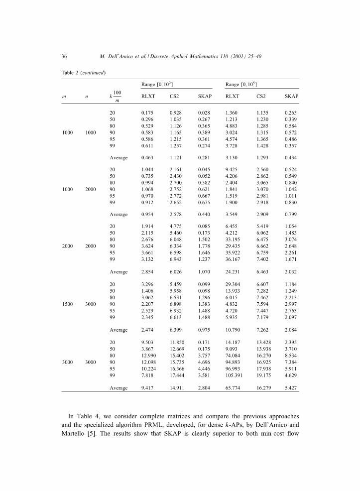
36 M. Dell’Amico et al. / Discrete Applied Mathematics 110 (2001) 25–40
Table 2 (continued)
Range [0; 102] Range [0; 105]
m n k100m
RLXT CS2 SKAP RLXT CS2 SKAP
20 0.175 0.928 0.028 1.360 1.135 0.26350 0.296 1.035 0.267 1.213 1.230 0.33980 0.529 1.126 0.365 4.883 1.285 0.584
1000 1000 90 0.583 1.165 0.389 3.024 1.315 0.57295 0.586 1.215 0.361 4.574 1.365 0.48699 0.611 1.257 0.274 3.728 1.428 0.357
Average 0.463 1.121 0.281 3.130 1.293 0.434
20 1.044 2.161 0.045 9.425 2.560 0.52450 0.735 2.430 0.052 4.206 2.862 0.54980 0.994 2.700 0.582 2.404 3.065 0.840
1000 2000 90 1.068 2.752 0.621 1.841 3.070 1.04295 0.970 2.772 0.667 1.519 2.981 1.01199 0.912 2.652 0.675 1.900 2.918 0.830
Average 0.954 2.578 0.440 3.549 2.909 0.799
20 1.914 4.775 0.085 6.455 5.419 1.05450 2.115 5.460 0.173 4.212 6.062 1.48380 2.676 6.048 1.502 33.195 6.475 3.074
2000 2000 90 3.624 6.334 1.778 29.435 6.662 2.64895 3.661 6.598 1.646 35.922 6.759 2.26199 3.132 6.943 1.237 36.167 7.402 1.671
Average 2.854 6.026 1.070 24.231 6.463 2.032
20 3.296 5.459 0.099 29.304 6.607 1.18450 1.406 5.958 0.098 13.933 7.282 1.24980 3.062 6.531 1.296 6.015 7.462 2.213
1500 3000 90 2.207 6.898 1.383 4.832 7.594 2.99795 2.529 6.932 1.488 4.720 7.447 2.76399 2.345 6.613 1.488 5.935 7.179 2.097
Average 2.474 6.399 0.975 10.790 7.262 2.084
20 9.503 11.850 0.171 14.187 13.428 2.39550 3.867 12.669 0.175 9.093 13.938 3.71080 12.990 15.402 3.757 74.084 16.270 8.534
3000 3000 90 12.098 15.735 4.696 94.893 16.925 7.38495 10.224 16.366 4.446 96.993 17.938 5.91199 7.818 17.444 3.581 105.391 19.175 4.629
Average 9.417 14.911 2.804 65.774 16.279 5.427
In Table 4, we consider complete matrices and compare the previous approachesand the specialized algorithm PRML, developed, for dense k-APs, by Dell’Amico andMartello [5]. The results show that SKAP is clearly superior to both min-cost -ow

M. Dell’Amico et al. / Discrete Applied Mathematics 110 (2001) 25–40 37
Table 3Density 10%. Average computing times over 10 problems, Silicon Graphics INDY R10000sc seconds
Range [0; 102] Range [0; 105]
m n k100m
RLXT CS2 SKAP RLXT CS2 SKAP
20 0.062 0.126 0.006 0.479 0.157 0.02750 0.062 0.140 0.044 0.243 0.172 0.04580 0.074 0.147 0.049 0.123 0.170 0.058
250 500 90 0.071 0.141 0.062 0.103 0.166 0.06995 0.065 0.144 0.061 0.105 0.170 0.06699 0.066 0.150 0.062 0.118 0.171 0.064
Average 0.067 0.141 0.047 0.195 0.168 0.055
20 0.069 0.338 0.011 0.380 0.421 0.06550 0.109 0.372 0.080 0.719 0.442 0.09880 0.180 0.380 0.129 1.194 0.450 0.183
500 500 90 0.207 0.393 0.133 1.099 0.464 0.17595 0.211 0.414 0.130 1.104 0.476 0.16699 0.219 0.423 0.097 0.794 0.478 0.124
Average 0.166 0.387 0.097 0.882 0.455 0.135
20 0.362 0.848 0.027 3.299 1.068 0.11650 0.267 0.932 0.022 1.587 1.166 0.16380 0.399 1.029 0.168 0.894 1.188 0.236
500 1000 90 0.365 1.045 0.210 0.692 1.202 0.32195 0.356 1.039 0.222 0.550 1.209 0.31399 0.347 1.030 0.237 0.488 1.167 0.259
Average 0.349 0.987 0.148 1.252 1.167 0.235
20 0.491 1.951 0.037 2.177 2.335 0.30350 0.642 2.155 0.069 2.122 2.548 0.38280 0.892 2.503 0.474 9.234 2.722 0.843
1000 1000 90 1.085 2.578 0.569 8.973 2.789 0.81795 1.218 2.546 0.546 8.413 2.869 0.76799 1.107 2.748 0.436 6.904 3.049 0.577
Average 0.906 2.414 0.355 6.304 2.719 0.615
20 1.980 4.610 0.070 25.197 5.472 0.50150 1.009 4.933 0.080 7.292 5.796 0.63980 1.898 5.400 0.583 4.349 5.962 0.996
1000 2000 90 1.840 5.559 0.760 4.198 5.948 1.63095 1.596 5.518 0.839 4.648 5.832 1.58799 1.671 5.397 0.872 3.666 5.745 1.191
Average 1.666 5.236 0.534 8.225 5.793 1.091
20 6.281 9.746 0.133 9.597 10.952 1.21650 2.105 10.495 0.149 7.715 11.145 1.67080 6.176 12.512 2.019 46.621 12.472 4.882
2000 2000 90 7.773 12.580 3.071 66.271 13.377 4.49195 8.017 13.426 2.624 49.976 13.855 3.74599 5.773 14.087 2.317 67.158 14.363 2.762
Average 6.021 12.141 1.719 41.223 12.694 3.128

38 M. Dell’Amico et al. / Discrete Applied Mathematics 110 (2001) 25–40
Table 3 (continued)
Range [0; 102] Range [0; 105]
m n k100m
RLXT CS2 SKAP RLXT CS2 SKAP
20 5.124 11.413 0.155 54.703 12.920 1.23250 3.890 12.410 0.161 20.098 13.715 1.42780 7.012 13.495 0.168 12.327 14.986 2.510
1500 3000 90 4.381 13.674 1.491 9.505 14.774 4.52995 5.027 14.092 1.880 14.312 14.470 4.39099 4.666 13.821 1.957 14.103 14.433 3.168
Average 5.017 13.151 0.969 20.841 14.216 2.876
20 27.022 24.249 0.290 18.440 26.891 2.78950 10.271 25.223 0.312 14.506 26.967 3.90780 15.036 28.650 5.850 117.946 29.787 13.780
3000 3000 90 73.373 31.067 10.134 141.552 33.177 12.53095 25.598 34.414 11.014 137.860 35.357 10.12499 19.422 34.894 7.139 158.249 36.366 7.952
Average 28.454 29.750 5.790 98.092 31.424 8.514
Table 4Complete matrices. Average computing times over 10 problems, Silicon Graphics INDY R10000sc seconds
Range [0; 102] Range [0; 105]
m n k100m
RLXT CS2 PRML SKAP RLXT CS2 PRML SKAP
20 0.263 2.323 0.029 0.032 5.838 2.577 0.043 0.06350 0.347 2.431 0.040 0.039 2.594 2.806 0.117 0.12880 0.403 2.543 0.046 0.041 2.279 2.846 0.212 0.145
250 500 90 0.482 2.585 0.049 0.052 2.678 2.905 0.297 0.17595 0.498 2.645 0.122 0.119 2.782 2.811 0.386 0.18299 0.503 2.693 0.132 0.136 2.777 2.938 0.457 0.243
Average 0.416 2.537 0.070 0.070 3.158 2.814 0.252 0.156
20 1.255 5.042 0.074 0.068 2.923 5.370 0.131 0.22150 1.224 5.197 0.083 0.076 4.087 5.549 0.295 0.27880 1.451 5.424 0.262 0.253 16.758 6.003 0.860 0.609
500 500 90 1.958 5.528 0.281 0.730 16.187 6.044 1.186 1.11695 2.732 5.876 0.292 0.775 17.136 6.631 1.318 1.06299 2.691 6.195 0.347 0.784 17.211 6.764 1.458 0.904
Average 1.885 5.544 0.223 0.448 12.384 6.060 0.875 0.698
approaches. In addition, in many cases, it is even faster than the specialized code. Thisis probably due to the new heuristic algorithm embedded in SKAP.Tables 1–4 also give information about the relative e�ciency of codes RELAXT IV
and CS2, when used on our type of instances. It is quite evident that the two codesare sensitive to the cost range: RELAXT IV is clearly faster than CS2 for the range[0; 102], while the opposite holds for the range [0; 105].

M. Dell’Amico et al. / Discrete Applied Mathematics 110 (2001) 25–40 39
Fig. 2. Density 5%, range [0; 105], rectangular instances. Average CPU time (in seconds) as a function ofthe instance size.
Fig. 3. Density 5%, range [0; 105], square instances. Average CPU time (in seconds) as a function of theinstance size.
Finally, Figs. 2 and 3 show the behavior of the average CPU time requested bySKAP, for each value of k, as a function of the instance size. We consider the caseof range [0; 105] and 5% density, separately for rectangular and square instances. Thefunctions show that SKAP has, for .xed k value, a regular behavior. There is insteadno regular dependence of the CPU times on the value of k: small values produce easyinstances, while the most di�cult instances are encountered for k around 80
100m or 90100m.

40 M. Dell’Amico et al. / Discrete Applied Mathematics 110 (2001) 25–40
Acknowledgements
This work was supported by Ministero dell’UniversitWa e della Ricerca Scienti.ca eTecnologica, and by Consiglio Nazionale delle Ricerche, Italy.
References
[1] R.K. Ahuja, T.L. Magnanti, J.B. Orlin, Network Flows, Prentice-Hall, Englewood Cli1s, NJ, 1993.[2] D.P. Bertsekas, P. Tseng, Relaxation methods for minimum cost ordinary and generalized network -ow
problems, Oper. Res. 36 (1988) 93–114.[3] A.V. Goldberg, An e�cient implementation of a scaling minimum-cost -ow algorithm, J. Algorithms
22 (1997) 1–29.[4] M. Dell’Amico, F. Ma�oli, M. Trubian, New bounds for optimum tra�c assignment in satellite
communication, Comput. Oper. Res. 25 (1998) 729–743.[5] M. Dell’Amico, S. Martello, The k-cardinality assignment problem, Discrete Appl. Math. 76 (1997)
103–121.[6] M. Dell’Amico, S. Martello, Linear assignment, in: M. Dell’Amico, F. Ma�oli, S. Martello (Eds.),
Annotated Bibliographies in Combinatorial Optimization, Wiley, Chichester, 1997, pp. 355–371.[7] E.A. Dinic, Algorithms for solution of a problem of maximum -ow in networks with power estimation,
Soviet Math. Dokl. 11 (1970) 1277–1280.[8] D. Goldfarb, M.D. Grigoriadis, A computational comparison of the Dinic and network simplex methods
for maximum -ow, in: B. Simeone, P. Toth, G. Gallo, F. Ma�oli, S. Pallottino (Eds.), FORTRANCodes for Network Optimization, Annals of Operational Research, Vol. 13, Baltzer, Basel, 1988, pp.83–103.
[9] R. Jain, J. Werth, J.C. Browne, A note on scheduling problems arising in satellite communication,J. Oper. Res. Soc. 48 (1997) 100–102.
[10] R. Jonker, T. Volgenant, A shortest augmenting path algorithm for dense and sparse linear assignmentproblems, Computing 38 (1987) 325–340.
[11] E.L. Lawler, Combinatorial Optimization: Networks and Matroids, Holt, Rinehart & Winston,New York, 1976.
[12] S. Martello, P. Toth, Linear assignment problems, in: S. Martello et al. (Eds.), Surveys in CombinatorialOptimization, Annals of Discrete Mathematics, Vol. 31, North-Holland, Amsterdam, 1987, pp. 259–282.
[13] C.A. Pomalaza-RYaez, A note on e�cient SS/TDMA assignment algorithms, IEEE Trans. Commun. 36(1988) 1078–1082.
[14] C. Prins, An overview of scheduling problems arising in satellite communications, J. Oper. Res. Soc.45 (1994) 611–623.