DYNAMICS OF LONG WATER WAVES:

WAVE-SEAFLOOR INTERACTIONS, WAVES

THROUGH A COASTAL FOREST, AND WAVE

RUNUP

A Dissertation

Presented to the Faculty of the Graduate School

of Cornell University

in Partial Fulfillment of the Requirements for the Degree of

Doctor of Philosophy

by

I-Chi Chan

August 2011

c© 2011 I-Chi Chan

ALL RIGHTS RESERVED

DYNAMICS OF LONG WATER WAVES: WAVE-SEAFLOOR INTERACTIONS,

WAVES THROUGH A COASTAL FOREST, AND WAVE RUNUP

I-Chi Chan, Ph.D.

Cornell University 2011

This dissertation studies three applied topics concerning long-wave dynamics.

Interactions between surface waves and a muddy seabed are first investigated.

Under the assumption that a seafloor can be modeled as a layer of viscoelastic

sediments, a set of depth-integrated equations is derived to describe the propa-

gation of long waves under the effects of seabed conditions. Dynamic responses

of a viscoplastic mud bed subject to a surface solitary wave are also studied.

Surface waves can be attenuated considerably due to the presence of a muddy

seabed. Features of wave-induced mud motions depend largely on the rheol-

ogy of bottom sediments. Theoretical predictions are tested against available

experimental data. A good agreement is observed.

Next, a theory is developed to study the effects of emergent coastal forests on

the propagation of long surface waves of small amplitudes. The forest is ideal-

ized by a periodic array of rigid cylinders. Parameterized models are employed

to simulate turbulence and to represent bed friction. A multi-scale analysis is

carried out to deduce the averaged equations on the wavelength-scale, with the

effective coefficients calculated by numerically solving the flow problem in a

unit cell surrounding one or several cylinders. Analytical and numerical solu-

tions for the wave attenuation are presented. Comparisons with laboratory data

show very good agreements for both periodic and transient incident waves.

Finally, the last topic concerns mainly the runup of leading tsunami waves.

Lagrangian long-wave equations are derived to help accurately track the mov-

ing shoreline. A series of numerical experiments reveals that the front-profiles

of leading tsunami waves dominate the runup processes while the back-profiles

are influential for the rundown flows. For a leading elevation wave, stronger ac-

celeration of the wave front results in higher maximum runup height. As far as

the maximum runup height is concerned, it is sufficient to consider only the ac-

celerating phase of the main tsunami wave. It is concluded that solitary wave is

not a perfect modeling wave for tsunami research. Directly applying the runup

rule of solitary wave to tsunami runup can lead to a very inaccurate estimation.

BIOGRAPHICAL SKETCH

I was born and raised in Taipei, Taiwan. Before being awarded this Doctor of

Philosophy degree, I earned my Bachelor of Engineering degree in Water Re-

sources and Environmental Engineering from Tamkang University, my Master

of Science degree in Civil Engineering from National Taiwan University, and

another Master of Science degree in Civil and Environmental Engineering from

University of Illinois at Urbana-Champaign.

iii

Dedicated to my parents, my wife, and my two sisters.

iv

TABLE OF CONTENTS

Biographical Sketch . . . . . . . . . . . . . . . . . . . . . . . . . . . . . . iiiDedication . . . . . . . . . . . . . . . . . . . . . . . . . . . . . . . . . . . ivAcknowledgements . . . . . . . . . . . . . . . . . . . . . . . . . . . . . . vTable of Contents . . . . . . . . . . . . . . . . . . . . . . . . . . . . . . . viList of Tables . . . . . . . . . . . . . . . . . . . . . . . . . . . . . . . . . . ixList of Figures . . . . . . . . . . . . . . . . . . . . . . . . . . . . . . . . . x

1 Introduction 1

2 Long water waves over a thin muddy seabed 92.1 Introduction . . . . . . . . . . . . . . . . . . . . . . . . . . . . . . . 9

2.1.1 A simplified two-layer model and assumptions . . . . . . 122.1.2 An overview of the mud rheology . . . . . . . . . . . . . . 14

2.2 A generalized model for surface waves interaction with a linearviscoelastic muddy seabed . . . . . . . . . . . . . . . . . . . . . . . 162.2.1 Depth-integrated model for weakly nonlinear and weakly

dispersive water waves . . . . . . . . . . . . . . . . . . . . 202.2.2 Model equations for mud flow motions . . . . . . . . . . . 252.2.3 Rheology model for a linear viscoelastic mud . . . . . . . . 292.2.4 Solution forms inside the muddy seabed . . . . . . . . . . 332.2.5 1HD application: evolution of wave height of a surface

solitary wave . . . . . . . . . . . . . . . . . . . . . . . . . . 442.2.6 1HD application: amplitude variation of a linear progres-

sive wave . . . . . . . . . . . . . . . . . . . . . . . . . . . . 512.2.7 Explicit solutions for 1HD periodic waves . . . . . . . . . . 552.2.8 Comparison with laboratory experiments . . . . . . . . . . 582.2.9 Summary . . . . . . . . . . . . . . . . . . . . . . . . . . . . 64

2.3 Response of a Bingham-plastic muddy seabed to a surface soli-tary wave . . . . . . . . . . . . . . . . . . . . . . . . . . . . . . . . . 652.3.1 Formulation for wave-induced mud motions inside a thin

Bingham-plastic seabed . . . . . . . . . . . . . . . . . . . . 682.3.2 Review of Mei & Liu (1987) . . . . . . . . . . . . . . . . . . 692.3.3 Solutions inside a Bingham-plastic mud . . . . . . . . . . . 732.3.4 Extension of the solution technique . . . . . . . . . . . . . 832.3.5 Numerical examples . . . . . . . . . . . . . . . . . . . . . . 842.3.6 Wave attenuation caused by a thin layer of mud . . . . . . 982.3.7 Summary . . . . . . . . . . . . . . . . . . . . . . . . . . . . 104

2.4 Conclusions . . . . . . . . . . . . . . . . . . . . . . . . . . . . . . . 104

3 Long water waves through emergent coastal forests 1063.1 Introduction . . . . . . . . . . . . . . . . . . . . . . . . . . . . . . . 1063.2 Theoretical formulation . . . . . . . . . . . . . . . . . . . . . . . . 110

vi

3.2.1 Governing equations and boundary conditions . . . . . . 1103.2.2 The linearized problem . . . . . . . . . . . . . . . . . . . . 1123.2.3 Depth-integrated equations for the constant eddy viscos-

ity model . . . . . . . . . . . . . . . . . . . . . . . . . . . . . 1123.2.4 Estimation of controlling parameters . . . . . . . . . . . . 115

3.3 Method of homogenization . . . . . . . . . . . . . . . . . . . . . . 1183.4 Macro theory for linear progressive waves . . . . . . . . . . . . . . 120

3.4.1 Homogenization . . . . . . . . . . . . . . . . . . . . . . . . 1213.4.2 Numerical solution of the micro-scale cell problem . . . . 1243.4.3 1HD application: constant water depth . . . . . . . . . . . 1253.4.4 1HD application: variable water depth . . . . . . . . . . . 1303.4.5 Experiments and numerical simulation for periodic waves 135

3.5 Macro theory for transient waves . . . . . . . . . . . . . . . . . . . 1393.5.1 Homogenization . . . . . . . . . . . . . . . . . . . . . . . . 1393.5.2 Numerical solution for the transient cell problem . . . . . 1433.5.3 Numerical model for the macro-scale solutions . . . . . . . 1463.5.4 1HD application: tsunami waves through a thick forest . . 1463.5.5 Comparison with laboratory experiments . . . . . . . . . . 154

3.6 Conclusions . . . . . . . . . . . . . . . . . . . . . . . . . . . . . . . 160

4 Long-wave modeling in the Lagrangian description 1634.1 Introduction . . . . . . . . . . . . . . . . . . . . . . . . . . . . . . . 1634.2 On the solitary wave paradigm for tsunami waves . . . . . . . . . 1654.3 Characteristics of leading tsunamis and solitary waves . . . . . . 167

4.3.1 Leading waves of the 2004 Indian Ocean tsunamis . . . . . 1674.3.2 Leading waves of the 2011 Tohoku tsunamis . . . . . . . . 171

4.4 Lagrangian long-wave equations . . . . . . . . . . . . . . . . . . . 1744.5 Numerical model and its validation . . . . . . . . . . . . . . . . . 1754.6 The role of surface profile on the tsunami runup . . . . . . . . . . 1814.7 The role of beach slope on the tsunami runup . . . . . . . . . . . . 1894.8 Discussions . . . . . . . . . . . . . . . . . . . . . . . . . . . . . . . 189

5 Concluding remarks and suggestions for future work 194

A Motions of a bi-viscous muddy seabed under a surface solitary wave 198A.1 Solutions of mud flows inside a bi-viscous seabed . . . . . . . . . 198A.2 Approximate bi-viscous model . . . . . . . . . . . . . . . . . . . . 202

B The Lagrangian long-wave equations 204B.1 Shallow water equations . . . . . . . . . . . . . . . . . . . . . . . . 204B.2 Boussinesq equations . . . . . . . . . . . . . . . . . . . . . . . . . . 207B.3 A stratified multi-layer model . . . . . . . . . . . . . . . . . . . . . 218B.4 Solid slide on a plane beach . . . . . . . . . . . . . . . . . . . . . . 219

vii

Bibliography 222

viii

LIST OF TABLES

2.1 Laboratory conditions of periodic waves over a viscoelastic mudbed by Maa & Mehta (1987, 1990). . . . . . . . . . . . . . . . . . . 63

3.1 Controlling parameters in the proposed wave-forest model: Val-ues of σ and α under different wave conditions. . . . . . . . . . . 117

3.2 Positions of wave gauges in the experiments at NTU, Singapore. 1353.3 Laboratory conditions of periodic waves experiments at NTU:

Wave periods range from 0.8 to 3.0 seconds. . . . . . . . . . . . . 1373.4 Experimental conditions of NTU study: Periodic waves with a

wide range of wave amplitudes. . . . . . . . . . . . . . . . . . . . 1393.5 Experimental conditions of NTU study: Solitary waves cases. . . 157

4.1 Solitary wave characteristics for two different scenarios. . . . . . 1714.2 Ocean bottom tsunami meters (TM1, TM2) and the GPS gauge

station (Iwate South) off the northeastern coast of Japan. . . . . . 173

ix

LIST OF FIGURES

2.1 Surface waves over a muddy seabed. . . . . . . . . . . . . . . . . 142.2 Rheology curves for viscous, elastic, and plastic behaviors. . . . . 152.3 Schematic sketch of a Maxwell element and a Kelvin-Voigt ele-

ment. . . . . . . . . . . . . . . . . . . . . . . . . . . . . . . . . . . . 162.4 Rheology curves for a Maxwell element and a Kelvin-Voigt ele-

ment. . . . . . . . . . . . . . . . . . . . . . . . . . . . . . . . . . . . 172.5 Rheology curve for a viscoplastic mud. . . . . . . . . . . . . . . . 182.6 A surface solitary wave over a viscoelastic mud: Time histories

of horizontal mud flow velocity at the water-mud interface, umi. 412.7 A surface solitary wave over a viscoelastic mud: Time histories

of bottom shear stress, τmb. . . . . . . . . . . . . . . . . . . . . . . 422.8 A surface solitary wave over a viscoelastic mud: Profiles of hor-

izontal velocity, um, inside the mud column at different phases. . 432.9 Evolution of a surface solitary wave propagating over a vis-

coelastic mud: Wave height as a function of time. . . . . . . . . . 502.10 Surface solitary wave propagates over a viscoelastic mud: Effect

of mud layer thickness on the evolution of wave height. . . . . . 512.11 A linear progressive wave over a viscoelastic mud: βi as a func-

tion of d. . . . . . . . . . . . . . . . . . . . . . . . . . . . . . . . . . 562.12 Periodic wave over a viscous mud: Comparison with Gade (1958). 602.13 Solitary wave over a viscous mud: Comparison of horizontal ve-

locity component. . . . . . . . . . . . . . . . . . . . . . . . . . . . 612.14 Viscous mud flow induced by a solitary wave: Comparison with

Park, Liu & Clark (2008). . . . . . . . . . . . . . . . . . . . . . . . 622.15 Solitary wave over a viscous mud: Interfacial displacement and

bottom shear stress . . . . . . . . . . . . . . . . . . . . . . . . . . . 632.16 Periodic waves over a viscoelastic mud: Velocity profiles. . . . . 642.17 Sketches of solitary wave induced Bingham-plastic mud flow ve-

locity: Two-layer scenario. . . . . . . . . . . . . . . . . . . . . . . . 712.18 Sketches of solitary wave induced Bingham-plastic mud flow ve-

locity: Four-layer scenario. . . . . . . . . . . . . . . . . . . . . . . 742.19 Sketches of solitary wave induced Bingham-plastic mud flow ve-

locity: Three-layer scenario. . . . . . . . . . . . . . . . . . . . . . . 772.20 Bingham-plastic mud flow solutions of 4-layer scenario (1): Yield

surfaces and interfacial velocity. . . . . . . . . . . . . . . . . . . . 852.21 Sample solutions of 4-layer scenario (2): Vertical profiles of mud

flow velocity. . . . . . . . . . . . . . . . . . . . . . . . . . . . . . . 862.22 Bingham-plastic mud flow solutions of 3-layer scenario (1): Yield

surfaces and interfacial velocity. . . . . . . . . . . . . . . . . . . . 902.23 Sample solutions of 3-layer scenario (2): Vertical profiles of mud

flow velocity. . . . . . . . . . . . . . . . . . . . . . . . . . . . . . . 91

x

2.24 Bingham-plastic mud flow solutions of 2-layer scenario (1): Yieldsurfaces and interfacial velocity. . . . . . . . . . . . . . . . . . . . 93

2.25 Sample solutions of 2-layer scenario (2): Vertical profiles of mudflow velocity. . . . . . . . . . . . . . . . . . . . . . . . . . . . . . . 94

2.26 Bingham-plastic mud problem: Comparison with the theory ofMei & Liu (1987). . . . . . . . . . . . . . . . . . . . . . . . . . . . . 95

2.27 Strain rate of at the bottom of a Bingham-plastic muddy seabed. 962.28 Effects of viscosity on the flow motion inside a Bingham-plastic,

τ0/d = 0.02. . . . . . . . . . . . . . . . . . . . . . . . . . . . . . . . 972.29 Effects of viscosity on the flow motion inside a Bingham-plastic,

τ0/d = 0.2. . . . . . . . . . . . . . . . . . . . . . . . . . . . . . . . . 982.30 Effects of physical mud layer thickness on the flow motion inside

a Bingham-plastic mud. . . . . . . . . . . . . . . . . . . . . . . . . 992.31 Energy dissipation of a surface solitary wave over a thin layer of

Bingham-plastic mud. . . . . . . . . . . . . . . . . . . . . . . . . . 102

3.1 Sketch of the wave-forest problem. . . . . . . . . . . . . . . . . . . 1103.2 Discretization of a typical unit cell and the spatial distributions

of K11(x). . . . . . . . . . . . . . . . . . . . . . . . . . . . . . . . . 1253.3 Hydraulic conductivity as a function of depth-to-wavelength ra-

tio, k0h0. . . . . . . . . . . . . . . . . . . . . . . . . . . . . . . . . . 1263.4 Periodic waves through a semi-infinite forest in a constant water

depth region: Reflection coefficient and snapshots of free-surfaceelevation. . . . . . . . . . . . . . . . . . . . . . . . . . . . . . . . . 128

3.5 Periodic waves propagating through a finite patch of forest ina constant water depth: Reflection coefficient and snapshots offree-surface elevation. . . . . . . . . . . . . . . . . . . . . . . . . . 130

3.6 Snapshots of periodic waves propagating through a forest on aplane beach. . . . . . . . . . . . . . . . . . . . . . . . . . . . . . . . 132

3.7 Periodic waves through a finite forest belt: Reflection coefficient. 1343.8 Sketch of experimental setup at NTU, Singapore. . . . . . . . . . 1363.9 Comparison between theory and experimental data: Reflection

coefficient for periodic waves. . . . . . . . . . . . . . . . . . . . . 1383.10 Reflection and transmission coefficients against amplitude-to-

depth ratio: Comparison between theory and measurements. . . 1403.11 Sample solutions of dynamic permeability, K(t). . . . . . . . . . . 1443.12 Effects of the cell geometry on the dynamic permeability. . . . . . 1453.13 Leading waves of a tsunami entering a deep forest in a constant

water depth: Theoretical and numerical solutions. . . . . . . . . . 1553.14 A transient wave packet crossing a forest: Comparison between

theory and measurements. . . . . . . . . . . . . . . . . . . . . . . 1563.15 Sample record of incident wave for solitary wave experiments at

NTU, Singapore. . . . . . . . . . . . . . . . . . . . . . . . . . . . . 158

xi

3.16 Solitary waves through a model forest of finite length (H/h0 =0.04, 0.0775): Comparison between theory and measurements. . . 159

3.17 Solitary waves through a model forest of finite length (H/h0 =0.1117, 0.1483): Comparison between theory and measurements. 160

3.18 Solitary waves through a model forest of finite width (H/h0 =0.1883): Comparison between theory and measurements. . . . . . 161

4.1 2004 Indian Ocean tsunamis: Satellite images. . . . . . . . . . . . 1694.2 2004 Indian Ocean tsunamis: Numerical simulations. . . . . . . . 1704.3 2011 Tohoku tsunamis: Locations of the gauge stations and the

epicenter of the earthquake. . . . . . . . . . . . . . . . . . . . . . . 1724.4 2011 Tohuku tsunamis: Gauge records. . . . . . . . . . . . . . . . 1734.5 Runup of surface waves on an infinite sloping beach. . . . . . . . 1784.6 Runup of a non-breaking solitary wave on a one-slope beach. . . 1794.7 Runup of a non-breaking solitary wave on a three-slope beach. . 1804.8 Effects of the horizontal length scale of the initial wave condition

on the runup and rundown. . . . . . . . . . . . . . . . . . . . . . . 1844.9 Effects of the back profile of the initial wave condition on the

runup and rundown. . . . . . . . . . . . . . . . . . . . . . . . . . . 1864.10 Effects of the preceding waves on the runup processes. . . . . . . 1884.11 Runup and drawdown of model waves on a one-slope beach. . . 1904.12 Effects of the bottom slope on the wave runup over a one-slope

beach . . . . . . . . . . . . . . . . . . . . . . . . . . . . . . . . . . . 191

A.1 Sketches of solitary wave induced bi-viscous mud flow velocity. 200A.2 Rheology curve of a bi-viscous mud. . . . . . . . . . . . . . . . . 203

xii

CHAPTER 1

INTRODUCTION

Ocean surface waves, among the best-known oceanic phenomena, perform an

essential role in sustaining life on our planet; in part these wave motions trans-

port energy across the continents and shape the coastlines. Ocean waves occur

over a tremendously broad range of wavelengths, from a few centimeters capil-

lary ripple to a tsunami spanning hundreds of kilometers. In particular, surface

gravity waves are of the greatest importance since gravity is the main restoring

force for wave motions associated with most human activities in the seas. In

the well-established linear water wave theory, to specify the wave motions one

needs to know the water depth h, wave height H , and wavelength L. While

the last two describe the physical dimensions of the wave, the first, from a cer-

tain perspective, states the property of the medium a wave travels through. As

for the seemingly undetermined wave period T , it can be calculated theoreti-

cally from the dispersion relationship, ω2 = gk tanh kh, where ω = 2π/T is the

wave frequency, g the gravitational acceleration, and k = 2π/L the wavenum-

ber. Through the theoretical analysis, it is interesting to see that as a surface

wave propagates, the active water particles pass along the wave energy by mov-

ing in circular orbits. What is more intriguing is that these circular orbital mo-

tions are only considerable within the depth no more than half the wavelength.

This influential depth, of course, can be smaller the total water depth.

Based on the relative magnitudes of water depth and wavelength, surface

waves are classified as long waves if h/L is less than 0.05. On the other hand,

for waves of h/L greater than 0.5 they are called short waves. Of course, waves

outside these two categories are given the name intermediate waves. To be more

1

precise, long waves are of large wavelengths, long periods, and low frequencies

while short waves are just the opposite. Long waves, inherently, have several

special features. For instance, the water particle trajectories of a long wave are

ellipse-like with the horizontal excursion more or less a constant throughout the

depth-wise extent, and a comparably negligible vertical component increases

linearly from the bottom to the free surface. In other words, the wave-induced

pressure is hydrostatic and the horizontal motions have only a weak depen-

dence on elevation. In addition, long waves are nondispersive, i.e. the wave

speed c is solely a function of the water depth, c =√gh. All leads to a com-

mon ground that the three-dimensional long-wave hydrodynamics can be legit-

imately approximated by some simplified models involving only two horizontal

dimensions. Let us also discuss some properties regarding short waves. Quite

differently, motions associated with short waves are strongly three-dimensional

as the trajectories of active water particles are circles with the orbital diameters

decreasing exponentially with depth. Also, the speed of short waves depends

on the wavelength, c =√gL/(2π), i.e. the so-called frequency dispersion.

Tremendous efforts have been made by scientists and engineers to study

long-wave mechanisms as these waves are more prominent in association with

many human activities in coastal marine environments. The importance of long

waves in the complex web of natural waters can be appreciated from several

perspectives. A rather intuitive explanation is that long waves travel faster than

short waves, and consequently would reach the beaches much earlier. This cor-

responds to the fact that for short waves c =√gL/(2π) <

√gh/(4π). One shall

also realize that long waves interact strongly with the seabed while the bottom

conditions have less impact on short waves. This can be understood by con-

sidering the previously discussed influential depth of the wave-induced water

2

particle motion, along with the underlying assumption on the limits of h/L that

distinguish the long and short waves. The presence of ocean floor makes the

physical process involving long waves more complicated. In part, bottom sed-

iments can be eroded and transported by wave motions while wave climates

can as well be changed simultaneously. One may also argue the significance

of long waves from the viewpoint of the amount of collective energy. As the

wavelength of a long wave is usually considerable and the corresponding wa-

ter particle motions are uniform throughout the entire water column, the energy

carried by a long wave is substantial. A good example is to consider tsunamis,

the extreme long waves which can have a wavelength of several hundred kilo-

meters in an open sea with a water depth of a few kilometers. Furthermore, long

waves lose less energy than short waves as they propagate. First, the frictional

energy loss is mainly attributed to the oscillations of water particles. Secondly,

water particles under short waves move upwards and downwards much more

rapidly as can be seen from the previously discussed particle trajectories. Com-

bining these two facts, the conclusion is drawn. Another point to argue the

importance of long waves in consideration of wave energy is that the velocity

of energy transport is the same as the wave speed of long waves. Consequently,

short waves die out fast as surface waves are sustained by energy.

The above arguments, although solely based on the linear wave theory along

with ideal conditions, support the significance of long waves in understanding

the mechanisms of ocean surface waves. Therefore, the objective of this dis-

sertation is to study the dynamics of long water waves. In particular, three

specific topics are investigated: Long water waves over a thin muddy seabed

(Chapter 2); Long water waves through emergent coastal forests (Chapter 3);

Long-wave modeling in the Lagrangian description (Chapter 4). The first topic

3

addresses the significance of seabed conditions on the long-wave propagation;

the second one investigates wave dynamics in a wave-forest system; finally, the

last essentially studies the runup of tsunami waves. Therefore, this dissertation

shall cover some fundamental, yet important, features of long water waves in

coastal marine environments. To introduce these three problems, which are to

be studied specifically in Chapter 2 to Chapter 4, an overview is provided in the

following.

Long water waves over a thin muddy seabed

Most studies of wave-seabed interactions have focused on the wave propaga-

tion over non-cohesive sediments, i.e. a sandy bed (see e.g. Liu 1973). Wave

attenuation due to percolation1 in a sandy bed tends to be relatively minor in

comparison with other dissipative mechanisms, such as bottom roughness and

wave breaking. On the other hand, it is well known that damping of ocean

waves can be considerable, if the seabed consists of cohesive sediments. Gade

(1958) reported that there is a location in the Gulf of Mexico, nicknamed the

Mud Hole, where the attenuation of surface waves due to the mud bed is so

great that fishing boats use it as an emergency harbour during severe storms.

Similar muddy seafloors have been reported in many coasts, rivers and estuar-

ies around the world (Healy, Wang & Healy 2002). Cohesive sediments, com-

monly characterized as mixtures of water and clays, are transported as aggre-

gates. In general, mud in different locales can exhibit diverse rheological prop-

erties, partly as a consequence of distinct physico-chemical compositions. Fac-

ing the rather complex dynamic behaviour of cohesive sediments, many sim-

plified constitutive models have been suggested, including the viscous fluid

1This can be observed when ocean waves propagate over a permeable seabed. Wave energyis dissipated by the porous bed due to the friction between water and solid skeleton (see Liu &Dalrymple 1984).

4

(Dalrymple & Liu 1978), viscoelastic (MacPherson 1980), viscoplastic (Mei &

Liu 1987), and poroelastic models (Yamamoto et al. 1978). Clearly, no single

model can describe the entire spectrum of the seabed responses because of the

great complexity and variety of mud rheology. Nevertheless, it is worthwhile

pursuing a deeper understanding of every model as each has its own range of

validity2, and it is the hope that one could build up a complex model closer

to the reality with the knowledge gained from this base. In the present study,

the emphasis is on muddy seafloors that can be modeled as either viscoplas-

tic or viscoelastic matter. The proposed models shall cover the basic material

behaviour of viscosity, elasticity, and plasticity. It is remarked that all these

rheological laws have been employed in the context of wave-seafloor interac-

tions (see e.g., Gade 1958; Mallard & Dalrymple 1977; Hsiao & Shemdin 1980;

Mei & Liu 1987). However, most of the past studies considered only waves of

small amplitudes, i.e. within the framework of linear periodic wave theory. It

is known that in shallow waters, where the seabed effects are expected to be

more significant, the wave nonlinearity can be considerable; a nonlinear theory

of long waves is therefore needed. In what follows, the immediate objective is

to develop a general model describing the interactions between long waves and

muddy seafloors. This problem is investigated and presented in Chapter 2.

Long water waves through emergent coastal forests

It is not surprising that coastal forests could serve as natural barriers to pro-

tect coastlines from tides, storm surges and tsunamis. Indeed, the field survey

conducted by Danielsen et al. (2005) has shown that vegetated coastal areas suf-

fered less damage from the 2004 Indian Ocean tsunamis. In the event of the 1999

Orissa Super Cyclone that struck the eastern coast of India, it was also seen that

2Wen & Liu (1998) classified the applicability of these models based on soil properties.

5

mangroves shielded the coastline and reduced the death toll (Dasa & Vincent

2009). It is indubitably comprehended that surface waves could lose a substan-

tial amount of energy when propagating through coastal forests. Based on the

field observations collected at Cocoa Creek in Australia, Massel, Furukawa &

Binkman (1999) were able to demonstrate that at low tides nearly 75% of inci-

dent wave enery, with a peak period of rougly 2 seconds, was dissipated when

waves propagated through a coastal forest of approximate 100 m in length. Of

course, a rough seabed can cause certain frictional loss. However, in a wave-

forest system the energy dissipation, as can be expected, is mainly due to the

turbulence generated through the multiple interactions between waves and the

vegetation; this most likely occurs throughout the entire water column. Labo-

ratory studies have been designed to build quantitative understanding of en-

ergy dissipation process in wetlands, and to evaluate the efficiency of coastal

trees in protecting the shore against tsunami attacks. For instance, Nepf (1999)

proposed a parameterized model to describe the turbulence for flow through

emergent vegetation. Modeling a coastal forest by an array of rigid cylinders,

Irtem et al. (2009) have demonstrated that trees planted on the sloping beach

can reduce the runup height of a model tsunami approximately by half. Built

on the established knowledge, the goal of this study is to develop a sound, yet

simple, theory describing the dynamics of long waves through coastal forests.

To make the analysis more tractable, a major simplification is adopted to model

tree trunks by a periodic array of rigid cylinders but to neglect the effects of

tree roots, branches, and leaves. Note that the typical diameter of tree trunks

is of O(0.5) m, while the characteristic wavelength of long waves can easily

reach O(100) m. The existence of these two distinct scales grants the use of the

homogenization technique, which can be viewed as a rigorous two-scale anal-

6

ysis, in developing the theoretical model for the present wave-forest problem.

The new theory is capable of dealing with both periodic waves and transient

waves, and will be tested against the available experimental data. Several nu-

merical examples are also given to illustrate some important features regarding

the wave-forest dynamics. This topic will be discussed in Chapter 3.

Long-wave modeling in the Lagrangian description

A tsunami, which is usually generated by a submarine earthquake, landslide,

or volcanic eruption, is an extremely long wave with a wavelength easily up

to several hundred kilometers. The science of tsunami waves has been studied

systematically for many decades. It is fair to say that a tremendous advance

has been achieved after the devastating 2004 Indian Ocean tsunamis shocked

the world. Nevertheless, our knowledge is still quite limited. This is evident af-

ter another earthquake-triggered destructive tsunami struck the northeastern

coast of Japan in March, 2011 and claimed thousands of lives. In studying

water wave theory, contributions can be made towards the understanding of

tsunami mechanisms by improving the prediction on the generation, propaga-

tion, and runup of tsunamis. Of course, the study of wave-structure interactions

is also important. In this study, the particular focus is on the terminal effect of

tsunami waves running up shoreline3. The capability of accurately estimating

the maximum runup height, i.e. the largest landward excursion of the waves

along the shoreline, is crucial in developing a tsunami evacuation plan. How-

ever, the problem is challenging as the moving shoreline makes the problem

domain time-varying. It is worth remembering that most of the wave-related

studies employ the Eulerian approach, which concentrates on the fluid motions

3A good reference on the modeling of tsunami generation and propagation is that of Wang(2008). For the study of wave-structure interactions, one can refer to, for example, the three-dimensional numerical model developed by Mo (2010).

7

at specific spatial locations. Several approximation techniques have been ap-

plied to address this well-known moving-boundary issue with various degrees

of success. An increasingly popular treatment is the higher order interpolation

method developed by Lynett (2002). The present study, on the other hand, ap-

proaches the problem by the use of the Lagrangian specification. The moving

shoreline becomes a fixed point as in the Lagrangian coordinates one essen-

tially follows the history of each individual particle. Thus, with no additional

numerical approximation required one can accurately and directly calculate the

time history of the shoreline movement, including the position and the velocity.

In many cases, it is desirable to have a quick assessment of tsunami inunda-

tion with only limited information. It is because of this engineering interest that

many runup formulae have been established by assuming certain idealized con-

ditions. For instance, the best-known work is that of Synolakis (1987), relating

the maximum runup height to the incident solitary wave height and the beach

slope. The performance of this so-called runup rule is very good, if indeed the

tsunamis can be scaled by solitary waves. However, Madsen, Fuhrman & Schaf-

fer (2008) cautioned that solitary waves can not be used to model tsunamis due

to the limitation of relevant geophysical scales. It is therefore important to un-

derstand the consequence if a solitary wave is still in use to model a tsunami.

In all, Chapter 4 will start from the introduction of long-wave equations in the

Lagrangian description. A Lagrangian numerical model is then developed to

study the runup of tsunami waves.

8

CHAPTER 2

LONG WATER WAVES OVER A THIN MUDDY SEABED

In this chapter, interactions between surface waves and a thin muddy seabed

made of cohesive sediments are studied by the use of a immiscible two-layer

water-mud system. Modeling the seafloor as a linear viscoelastic body, a set of

Boussinesq-type equations for long waves over a thin layer of mud is derived,

as presented in section 2.2. Wave damping rates for both periodic waves and

solitary waves are calculated using the newly developed model. In section 2.3,

the seabed is assumed to be made of Bingham-plastic mud. The dynamics of

mud flow induced by a surface solitary wave are investigated. To examine the

performance of the proposed model, theoretical predictions of mud flow veloc-

ity, bottom shear stress, vertical displacement at wave-mud interface, amplitude

attenuation, and wavenumber shift are all compared with available laboratory

measurements for the case of viscoelastic mud. As for the study of a surface

solitary wave propagating over a layer of Bingham-plastic mud, comparison

is made between the model results and field observations. Good agreements

are evident in all examples. It is concluded that a muddy seabed can attenuate

surface waves considerably.

2.1 Introduction

Understanding the interactive processes between surface water waves and

muddy seabeds is one of the intriguing research topics in the fields of coastal en-

gineering and ocean science. On one hand, as waves propagate over a seafloor

work is done by the wave-induced pressure force to excite the motion of fluid

9

mud. The associated wave energy loss can be considerable. Indeed, signifi-

cant damping of surface waves caused by a mud bottom has been reported by

numerous field observations (see e.g., Gade 1958; Wells & Coleman 1981; For-

ristall & Reece 1985; Elgar & Raubenheimer 2008). On the other hand, the wave-

induced mud motions not only affect the wave climate but also have great im-

pacts on the seabed morphology and biological activities in the benthic bound-

ary layer (Foda 1995). For instance, through the resuspension and deposition

processes transport of nutrients is enhanced as well as the remobilization of the

buried pollutants. In the long run, coastline change can also be expected (Mei

et al. 2010).

Muddy seabeds are essential cohesive sediments made up of fine particles

with a characteristic size less than 2 µm (Chou, Foda & Hunt 1991). In con-

trast to the non-cohesive deposits where particles move individually, the cohe-

sive sediments flow as aggregates. In general, mud in different locales can ex-

hibit diverse rheological properties, partly as a consequence of distinct physico-

chemical compositions (Balmforth & Craster 2001). Moreover, the rheology of

muddy seabed depends also on the wave climate and sediment concentration

(see e.g. Krone 1963; Chou, Foda & Hunt 1991). As a result, the rheology of

bottom mud could change dynamically. Owing to the difficulty in modeling

the complexity of nature, researchers have approached the problem, as the first

step, with different simplified rheology models to examine the wave-mud in-

teractions, namely the response of cohesive sediments to surface waves and the

impact of seabeds on wave propagation. The hope is that with the knowledge

gained from these basic studies, one could build up a complex model closer to

the reality. Some representative rheology models employed in the past studies

of wave-seafloor problem are: viscous fluid mud (Gade 1958; Dalrymple & Liu

10

1978), elastic bed (Mallard & Dalrymple 1977), viscoelastic model (MacPherson

1980; Piedra-Cueva 1993), and viscoplastic seabed (Mei & Liu 1987; Sakakiyama

& Bijker 1989). In fact, these simplified rheology models have been shown to fit

fairly well with specified field observations (Krone 1963; Maa & Mehta 1987;

Mei et al. 2010). Reviews on the early studies of wave-mud interactions have

been well documents by Mehta, Lee & Li (1994), Foda (1995) and Wen & Liu

(1998).

It is noted that almost all of the above mentioned studies have considered

only progressive waves of infinitesimal amplitudes. However, seabed effects

become more significant as surface waves propagate into shallow waters where

the wave nonlinearity is expected to be important as well. It is then the objective

of the present study to investigate the problem in a more general context, i.e. re-

lax the time periodicity assumption on the wave motions, and consider also the

effects of wave nonlinearity. Since it is well known that the wave system is bet-

ter described by Boussinesq equations in a shallow sea (see e.g. Peregrine 1972),

waves that are both weakly nonlinear and weakly dispersive shall be of partic-

ular interest. For the purpose of better understanding the fundamental physics

of wave-seafloor interactions, the following mud rheology models shall be con-

sidered: viscous, elastic, viscoelastic, and viscoplastic. In section 2.2, a single

model is proposed to describe the interactions between surface waves and a

muddy seabed made of Newtonian fluid, elastic mud, or linear viscoelastic ma-

terials, as it will be shown later in section 2.2.3 that these three can actually be

incorporated into a generalized viscoelastic model. In section 2.3, the dynamic

response of a viscoplastic seabed to a surface wave is discussed.

Before proceeding to the detailed analysis, an overview is first given in sec-

11

tions 2.1.1 and 2.1.2 to clarify the theoretical aspect of the present problem along

with several important assumptions.

2.1.1 A simplified two-layer model and assumptions

Inspired by the strong field evidence that surface waves can be damped out sig-

nificantly at certain locales, a phenomena which can not be explained by the

classical water wave theory where a rigid bottom is often assumed, Gade (1958)

was perhaps the first to investigate the wave-seafloor interactions both theoret-

ically and experimentally. In his study, a immiscible two-layer model, which

consists of a layer of water and a relative heavier seabed lying on a flat solid

bottom, was employed. In addition, the mud properties were assumed to be

homogeneous. Since then, this two-layer approach has been widely adopted by

other researchers (see e.g. Dalrymple & Liu 1978; Hsiao & Shemdin 1980; Mei &

Liu 1987; Piedra-Cueva 1993; Ng 2000; Mei et al. 2010 among others) due to its

simplicity and good performance when validating with laboratory experiments

and field observations.

Without any surprise, the simple two-layer approach has been challenged.

For instance, Maa & Mehta (1987, 1990) proposed a multi-layer stratified model

since the properties of mud, such as viscosity and elasticity, can also depend

on the concentration, which is essentially the mud density. To simulate nu-

merically several laboratory-scale examples, they divided the mud beds into

four distinct homogeneous viscoelastic layers, each of which has different val-

ues of viscosity and elasticity, according to the measured concentration profiles.

It is remarked that in the situation where mud density varies considerably, i.e.

12

mud properties are not vertically uniform, the multi-layer stratified model cer-

tainly outperforms the two-layer approach. However, as the vertical variation

becomes important one may also need to consider the time-varying layer thick-

ness, which is not incorporated in this stratified model. To improve the two-

layer treatment, Chou, Foda & Hunt (1991) also suggested another approach: a

multi-phase layered model. For example, the entire mud column can be dived

into three different layer (from top to bottom): viscous fluid, elastic mud, and

a solid bottom. The layer thicknesses, which are determined as part of the so-

lution, are no longer fixed. One can argue that this approach seems to be more

realistic for the field applications as the moving interfaces have been consid-

ered. Nevertheless, one can also question the appropriateness of the viscous-

elastic-solid configuration for a muddy seabed. How to assign the properties

to each sublayer, namely determine the proper rheology of each layer, remains

an issue. In addition, while locations of interfaces between different materials

change in time, whether mixing starts to play a role needs to be examined more

carefully. From another perspective, Shibayama & An (1993) have proposed to

consider the mud rheology as a function of wave forcing. More precisely, they

suggested that the fluid mud act as either viscoelastic or viscoplastic material

depending on the magnitude of the driven pressure force induced by the sur-

face waves. Their model intends to replicate the complex properties of natural

mud, although more field evidence is required to confirm the assumption that

the rheology of mud is indeed switching between viscoelasticity and viscoplas-

ticity.

As a first step to carefully examine the wave-mud interactions under a gen-

eral surface wave loading, the two-layer model will be adopted in the present

study: we shall consider an inviscid water body on top of a layer of heavier

13

mud. Schematic sketch of the wave-seafloor system is given in figure 2.1.

∇

Water

Mud

d′

h0

x′

y′

z′

ζ ′

ξ′

Figure 2.1: Surface waves over a layer of mud. h0 and d′ are the water

depth and the mud thickness, respectively. ζ ′ and ξ′ denote the

displacements at the free-surface and the water-mud interface.

x′ and y′ are the horizontal coordinates, and z′ is the vertical

axis. The mud layer is sitting on top of a solid bed.

2.1.2 An overview of the mud rheology

In addition to the two-layer assumption, the seabed will be modeled as either

a generalized linear viscoelastic material or a viscoplastic mud. To help under-

stand the complex mud rheology, figure 2.2 gives the schematic sketch of rhe-

ology curves for purely viscous, elastic, and plastic behaviors. Basically, stress

is proportional to strain rate for viscous fluid; elastic behavior shows the linear

relation between the stress and the strain; plastic material displays continuous

14

deformation after certain value of critical stress (yield stress) is achieved.

High viscous

Low viscous

Strain rate

Str

ess

(a)

More stiff

Less stiff

Strain

Str

ess

(b)

Strain rate

Str

ess

(c)

Yield stress

Figure 2.2: Schematic diagram of rheology curves for: (a) Viscous mud; (b)

Elastic mud; (c) Plastic mud.

It can be expected that a viscoelastic material exhibits both viscous and elas-

tic behaviors. Two conceptual rheology models are the Maxwell element and

the Kelvin-Voigt element, both consisting of a linear combination of an elastic

spring and a viscous damper (dashpot), as have been sketched in figure 2.3 (see

e.g., Malvern 1969). Using the information given in figures 2.2 and 2.3, the re-

sponses of these two elements under a constant stress or a fixed deformation

are illustrated in figure 2.4. This provides a qualitatively understanding of lin-

ear viscoelastic media. It is noted that the detailed constitutive equation of a

viscoelastic mud is to be discussed in section 2.2.3.

For an ideal viscoplastic mud, namely a Bingham-plastic material, the rheol-

ogy curve is demonstrated in figure 2.5. A Bingham-plastic mud behaves like a

rigid body when the magnitude of the stress is less than the yield stress (see also

figure 2.2), and flows pretty much as a viscous fluid at high stress. The detailed

analysis of waves over a viscoplastic seabed is presented in section 2.3.

15

(a) (b)

Figure 2.3: Schematic diagram of linear viscoelastic media: (a) Maxwell

element; (b) Kelvin-Voigt element. The stress is the same in

the spring and the dashpot for a Maxwell element. The spring

and the dashpot exhibit the same amount of deformation for a

Kelvin-Voigt element.

2.2 A generalized model for surface waves interaction with a

linear viscoelastic muddy seabed

Early studies on the interactions between a layer of viscoelastic mud and surface

waves relied on the introduction of a complex viscosity (see e.g., Tchen 1956;

Hsiao & Shemdin 1980; MacPherson 1980; Maa & Mehta 1990; Piedra-Cueva

1993; Zhang &Ng 2006),

νe = νm

(1 + i

Emρmω0νm

), (2.2.1)

where νm is the kinematic viscosity of mud,Em the shear modulus of elasticity of

mud, ρm the mud density, and ω0 the wave frequency. In terms of this complex

viscosity νe, the viscoelastic model shares the same governing equations with

those of Newtonian fluid-mud case and, of course, the solution forms (Tchen

1956). It is remarked that the problem of surface waves over a viscous fluid-mud

seabed has been studied extensively. Some representative references are Gade

(1958), Dalrymple & Liu (1978), and Ng (2000). Despite the breakthrough of the

complex viscosity concept, Ng & Zhang (2007) reiterated that this approach is

16

Time

Str

ess

(a)

Time

Str

ain

Maxwell

Time

Str

ain

K-V

Time

Str

ain

(b)

Time

Str

ess

Maxwell

Time

Str

ess

K-V

Figure 2.4: Viscoelastic behaviors of a Maxwell element and a Kelvin-Voigt

element: (a) Under a constant load; (b) Apply a fixed deforma-

tion.

valid only for the wave system of simple harmonic motions. By examining the

field samples taken from the eastern coast of China, Mei et al. (2010) have shown

that νm and Em in (2.2.1) are actually functions of ω0. This further confirms the

limited applicability of the complex viscosity model.

To investigate the higher harmonic components of wave motions which re-

late to the mass transport due to the muddy seabed, Ng & Zhang (2007) for-

mulated the problem in the Lagrangian coordinates without using the complex

viscosity approach commonly adopted in the Eulerian description. In fact, the

work by Ng & Zhang (2007) can be viewed as the extension of Piedra-Cueva

(1995) who has developed a Lagrangian model describing how surface waves

interact with a layer of viscous fluid mud. The conservation laws presented

by these two studies are, of course, general and valid for any surface wave

17

Yield stress

Bingham-plastic

Strain rate

Stress

Viscous

Figure 2.5: Rheology curves for viscous and viscoplastic (Bingham-plastic)

materials. The constitutive equation for a Bingham-plastic

mud is given in 2.3.164.

loadings. However, when deducing the analytical solutions both Piedra-Cueva

(1995) and Ng & Zhang (2007) considered only small amplitude waves. There-

fore, up to now analytical solution for the viscoelastic or viscous mud flow mo-

tions driven by a transient long-wave loading is still not available. This moti-

vates the present study.

The effects of a muddy seafloor on surface wave propagation become more

significant as waves enter shallow waters where the wave system is better de-

scribed by Boussinesq equations (see e.g. Peregrine 1972). It is, therefore, the

objective of this study to derive a set of Boussinesq-type depth-integrated equa-

tions for weakly nonlinear and weakly dispersive waves with the effects of a vis-

coelastic muddy seabed considered. It follows that the perturbation technique

outlined in Mei, Stiassnie & Yue (2005) for deriving common Boussinesq equa-

tions, and also in Liu & Orfila (2007) for studying the effects of water viscosity

on the evolution of shallow-water waves shall be applied. In the water-mud

18

system, an immiscible two-layer approach (Gade 1958), consisting of a water

body on top of a heavier muddy seabed modeled as a linear viscoelastic mate-

rial, is adopted. The mud viscosity is assumed to be several orders of magnitude

larger than that of water. As a result, the water layer is treated as a inviscid fluid.

Furthermore, the thickness of muddy seabed is taken to be very thin in compar-

ison with the typical wavelength of the surface waves. It is reiterated that these

assumed mud properties are in the range of field samples. For instance, during

the pilot experiment in the Gulf of Mexico Elgar & Raubenheimer (2008) ob-

served a layer of 30 cm thick yogurt-like bottom mud lying under a water body

of 5 m in depth; Holland, Vinzon & Calliari (2009) reported a muddy seabed 0.4

m thick and a viscosity 7.6× 10−3 m2s−2 offshore of the Cassino Beach, Brazil.

In the following, the mathematical model and the scalings for the motions

of long waves in the water column are first discussed. Next, a set of depth-

integrated equations is derived with a closure problem to be addressed by solv-

ing the mud flow problem beneath. After formulating the governing equations

along with the proper initial and boundary conditions for the mud motions, a

generalized rheology model for linear viscoelastic materials is then introduced

to constitute the stress-strain relation for the muddy seabed. Subsequently, so-

lutions for the motions of a thin layer of viscoelastic mud induced by a surface

wave loading are obtained. The mathematical problem is formally completed.

Using the newly derived equations, several important features, namely the bot-

tom shear stress and velocity of mud flow, and the amplitude evolution of both

linear progressive waves and solitary waves, are illustrated. Finally, the pro-

posed model is examined against the available laboratory experiments. A good

agreement is observed.

19

2.2.1 Depth-integrated model for weakly nonlinear and weakly

dispersive water waves

Consider a train of surface water waves with a characteristic wavelength L0

and wave amplitude a0 propagates in a uniform depth h0 overlying a thin layer

of bottom mud of thickness d′. The wave-seafloor system is sketched in figure

2.1. In contrast to the mud column which is made of cohesive sediments, the

water body of a constant density ρw is treated as an inviscid fluid following

the usual assumption of classical water wave theory. To ease the mathematical

manipulation, the following dimensionless variables are introduced:

(x, y) =x′

L0

, z =z′

h0

, t =t′

L0/√gh0

p =p′

ρga0

, ζ =ζ ′

a0

, u = (u, v) =(u′, v′)

ǫ√gh0

, w =w′

(ǫ/µ)√gh0

, (2.2.2)

where (x′, y′) and z′ denotes the horizontal and vertical references, respectively,

t′ the time coordinate, g the gravitational acceleration, p′ the total pressure, ζ ′

the free-surface displacement, and (u′, v′, w′) the velocity components of water

particles in (x′, y′, z′)-directions. In addition, two dimensionless parameters

ǫ =a0

h0

and µ =h0

L0

(2.2.3)

measure the relative importance of the wave nonlinearity and the frequency

dispersion, respectively, and both are considered to be small.

Consequently, the dimensionless continuity equation in the water body can

be expressed in terms of the velocity potential, Φ = Φ(x, y, z, t), as

µ2∇2Φ +∂2Φ

∂z2= 0, −1 ≤ z ≤ ǫζ, (2.2.4)

20

and the kinematic and dynamic free-surface boundary conditions are

µ2

(∂ζ

∂t+ ǫ∇Φ · ∇ζ

)=∂Φ

∂z, z = ǫζ, (2.2.5)

µ2

(∂Φ

∂t+ ζ

)+ǫ

2

[µ2 (∇Φ)2 +

(∂Φ

∂z

)2]

= 0, z = ǫζ, (2.2.6)

where ∇ ≡(∂∂x, ∂∂y

)denotes the horizontal gradients. In addition, the pressure

field can be evaluated from the Bernoulli’s equation as

p = −zǫ− 1

µ2

µ2∂Φ

∂t+ǫ

2

[µ2 (∇Φ)2 +

(∂Φ

∂z

)2]

, (2.2.7)

where the first term is the hydrostatic pressure and the rest the hydrodynamic

pressure.

The velocity potential Φ may be expended in terms of a power series in the

vertical coordinate z as (see Chapter 12.1 in Mei, Stiassnie & Yue 2005)

Φ(x, y, z, t) =∞∑

n=0

(z + 1)nφn(x, y, t). (2.2.8)

Therefore, the direct substitution of (2.2.8) into the Laplace equation, i.e. the

conservation law of mass (2.2.4), leads to a recursive relation

φn+2 = − µ2

(n+ 1)(n+ 2)∇2φn, n = 0, 1, 2, · · · . (2.2.9)

Note that

∇φ0 = ∇Φ|z=−1 = u(x, y, z = −1, t) ≡ ub (2.2.10)

and

φ1 =∂Φ

∂z

∣∣∣∣z=−1

= w(x, y,−1, t) ≡ wb (2.2.11)

represent the horizontal and vertical velocity components at the water-mud in-

terface z = −1, which are now defied as ub and wb, respectively. In the case of

a horizontal solid sea bottom, the no flux condition requires wb = 0 suggest-

ing that each φn with odd n vanishes. For the present wave-seabed problem,

21

the wave-driven mud motion leads to a non-zero wb. It is necessary to estimate

the order of magnitude of this quantity. Since in coastal waters the thickness of

mud bed, d′, is usually very small and the mud viscosity, νm, is relatively strong,

under long water waves the laminar boundary-layer thickness of mud, δ′m, can

be comparable to d′. Therefore, in this study the focus will be on the following

scenario:

d′ ∼ δ′m ∼√

νm√gh0/L0

= αL0, (2.2.12)

where

α2 =νm

L0

√gh0

(2.2.13)

is a dimensionless parameter. To give a quantitative example, let us consider a

typical case:

O(ǫ) ∼ O(µ2) ∼ 0.1, h0 ∼ 5 m, d′ ∼ 0.25 m, νm ∼ 0.01 m2 s−1, (2.2.14)

where both νm and d′ are in the range of field data reported by Mei et al. (2010).

It follows that the value of α is roughly 0.01, i.e.

O(α) ∼ O(µ4). (2.2.15)

Note that the condition (2.2.15) has also been assumed by Ng (2000), Ng &

Zhang (2007) and Mei et al. (2010) to study periodic waves over a viscous or

viscoelastic muddy seabed. Furthermore, many field observations (see e.g.,

Sheremet & Stone 2003; Winterwerp et al. 2007; Holland, Vinzon & Calliari 2009)

have supported this argument. In this study, the assumption (2.2.15) will be

adopted throughout.

It also deserves emphasis that the mud motion considered is in the laminar

flow regime. A Reynolds number can be introduced as

Rem =

(ǫ√gh0

)d′

νm=

ǫ

α2

d′

L0

, (2.2.16)

22

where α has been defined in (2.2.13). By the use of (2.2.12) and (2.2.15), we

obtain

O (Rem) = O(µ−2), (2.2.17)

which is a moderate value for the weakly dispersive waves to be discussed

herein. In fact, this statement complies with the immersible assumption: a sharp

density interface is persistent in the two-layer model, which surpasses the pos-

sible turbulence.

Through the above argument, the horizontal and vertical components of

mud flow velocity are estimated to be

O (u′m) ∼ O

(ǫ√gh0

)and O (w′

m) ∼ O(αǫ√gh0

), (2.2.18)

respectively. By virtue of matching the vertical velocity across the water-mud

interface, we obtain

O(wb) ∼ O(αµ) ∼ O(µ5). (2.2.19)

Consequently, from (2.2.8) to (2.2.11) the truncated velocity potential with an

error of O(µ6) is

Φ = (z + 1)wb + ub −µ2

2(z + 1)2∇2

ub +µ4

24(z + 1)4∇2∇2

ub +O(µ6), (2.2.20)

where (2.2.19) has been evoked as well. Under the Boussinesq assumption, i.e.

O(ǫ) ∼ O(µ2), the use of (2.2.20) into the free-surface conditions, (2.2.5) and

(2.2.6), yields

1

ǫ

∂H

∂t+∇ · (Hub)−

µ2

6∇2∇ · ub −

wbµ2

= O(µ4), (2.2.21)

and

∂ub

∂t+ ǫub · ∇ub +

1

ǫ∇H − µ2

2

∂

∂t∇∇ · ub = O(µ4), (2.2.22)

23

where

H = 1 + ǫζ (2.2.23)

denotes the total water depth. Equations (2.2.21) and (2.2.22) are the approx-

imate continuity and momentum equations in terms of H and the velocity at

the bottom of water body, (ub, wb). These vertical independent Boussinesq-type

equations can also be expressed in the form of the depth-averaged horizontal

velocity defined by

u =1

H

ǫζ∫

−1

∇Φdz = ub −µ2

6H2∇2

ub +O(µ4). (2.2.24)

Substituting the above definition into (2.2.21) and (2.2.22), we obtain

1

ǫ

∂H

∂t+∇ · (Hu)− wb

µ2= O(µ4), (2.2.25)

and

∂u

∂t+ ǫu · ∇u +

1

ǫ∇H − µ2

3∇∇ · ∂u

∂t= O(µ4). (2.2.26)

Equations (2.2.25) and (2.2.26) constitute the Boussinesq-type depth-averaged

equations in terms of the total depth, H , and the depth-averaged horizontal

velocity, u. The effects of the underlaid thin mud layer appear in the continuity

equation through a nonzero wb term and are of O(µ3). In the absence of the

muddy sea bed where the solid bottom is also frictionless, wb = 0 and the above

equations reduce to the conventional Boussinesq equations.

It is remarked that (2.2.25) and (2.2.26) are underdetermined, as three un-

knowns (ζ,u, wb) are involved. Ideally, if wb can be expressed in terms of u

and/or ζ the mathematical problem is then complete (of course, proper initial

and boundary conditions for both ζ and u are still required). Owing to the con-

tinuity of vertical velocity at the water-mud interface, wb essentially describes

24

the vertical motion of mud flow at z = −1 as well. Therefore, it sheds some in-

sight on this closure issue that the solution form of wb may be obtained from the

flow problem inside the mud layer. Details will be elaborated in the following

sections, 2.2.2 to 2.2.4.

It is beneficial to point out that actual velocity components, (u, v, w), and

pressure field, p, are realized once ζ and u are solved. The approximate velocity

is obtained, by definition, as

(u, v) = ∇Φ = u− µ2

2(z + 1)2∇∇ · u +O(µ4), (2.2.27)

and

w =∂Φ

∂z= −µ2(z + 1)2∇ · u +O(µ4). (2.2.28)

From (2.2.7), the total pressure becomes

p = −zǫ

+ ζ +µ2

2

(z2 + 2z

)+O(µ4). (2.2.29)

2.2.2 Model equations for mud flow motions

Since viscous shearing is one of the key factors affecting the mud flow motions,

we shall introduce new scalings to describe dynamics inside the muddy seabed.

For the mud flow velocity components, (u′m, v′m, w

′m), pressure, p′m, and the shear

stress tensor, τ′

m, the normalizations are as follow:

um = (um, vm) =(u′m, v

′m)

ǫ√gh0

, wm =w′m

αǫ√gh0

pm =p′m

ρmga0

, τm =τ

′

m

αǫρmgh0

, (2.2.30)

25

where ρm is the mud density and recall α defined by (2.2.13). Note that

τm =

τm,xx τm,xy τm,xz

τm, yx τm, yy τm, yz

τm, zx τm, zy τm, zz

. (2.2.31)

Recalling (2.2.12) that the mud depth d′ is assumed to be comparable to the

laminar boundary-layer thickness δ′m ∼ αL0, a new dimensionless vertical coor-

dinate is introduced:

η =z′ + d′ + h0

αL0

. (2.2.32)

The mud then occupies 0 ≤ η ≤ d in the stretched coordinate where

d =d′

αL0

+ǫµ

α

ζ ′ma0

(2.2.33)

with ζ ′m denoting the vertical displacement of the water-mud interface. By the

order of magnitude analysis on the mass conservation of both water body and

mud column, it can be shown that ζ ′m is much smaller than the free-surface

displacement, ζ ′,

O (ζ ′m/ζ′) ≈ O (d′/(d′ + h0)) ≈ O(d′/h0) ∼ O(µ3)≪ 1. (2.2.34)

The above statement has been verified by laboratory study of solitary waves

propagate over a viscous fluid-mud bed (Park, Liu & Clark 2008) and the exam-

ination of field samples of viscoelastic mud subject to a surface periodic wave

forcing (Mei et al. 2010). Following (2.2.34),

d =d′

αL0

+O(µ2). (2.2.35)

In terms of the above dimensionless variables, we can now formulate the

conservation law of mass for mud flow as

∇um +∂wm∂η

= 0, (2.2.36)

26

and the momentum equations:

∂um∂t

+ ǫ

(um · ∇um + wm

∂um∂η

)=−∇pm +

(α∇τ

HHm +

∂τHVm∂η

),

(2.2.37)

α2

[∂wm∂t

+ ǫ

(um · ∇wm + wm

∂wm∂η

)]=− ∂pm

∂η+ α

(α∇τ

V Hm +

∂τ V Vm∂η

)− α

ǫµ,

(2.2.38)

where

τHHm =

τm,xx τm,xy

τm, yx τm, yy

, τ

HVm = (τm,xz, τm, yz) , (2.2.39)

and

τV Hm = (τm, zx, τm, zy) , τ

V Vm = τm, zz. (2.2.40)

Referring again to (2.2.25) and (2.2.26), the long-wave equations that describe

the motions of water particles, leading-order solutions of (um, wm) and pm are

sufficient to satisfy the overall truncation error of O(µ4) as

wb = αµwm(x, y, η = d, t). (2.2.41)

Therefore, it is reasonable to neglect the displacement of water-mud interface in

the present study, i.e., (2.2.35) reduces to

d ≈ d′

αL0

. (2.2.42)

The significance of the above assumption is that d becomes a constant parameter

of O(1).

All in all, we shall now work on the linearization of (2.2.37),

∂um∂t

= −∇pm +∂τHVm∂η

, 0 ≤ η ≤ d. (2.2.43)

As for the vertical equation, (2.2.38), it suggests that at the leading-order pres-

sure is vertically uniform inside the mud layer, i.e.

pm = pm(x, y, t), 0 ≤ η ≤ d. (2.2.44)

27

In addition, the continuity of normal stress along the water-mud interface re-

duces to

pm(x, y, t) = γp(x, y, z = −1, t), (2.2.45)

where

γ =ρwρm

(2.2.46)

is the ratio of water density to mud density. Furthermore, the use of (2.2.26) into

(2.2.29) leads to

∇p ≈ −∂ub∂t

, z = −1 (2.2.47)

at the leading-order. The approximate problem, (2.2.43) to (2.2.47), is similar to

that of classic laminar boundary-layer theory, which is expected since d′ ∼ δ′m.

Evoking (2.2.45) and (2.2.47) into the horizontal momentum equation (2.2.43),

we obtain

∂um∂t

= γ∂ub∂t

+∂τHVm∂η

. (2.2.48)

The associated boundary conditions in the vertical coordinate are

um = 0, η = 0, (2.2.49)

τHVm = 0, η = d, (2.2.50)

which satisfy the no-slip condition and the inviscid water assumption, respec-

tively. In addition,

um = 0, t = 0 (2.2.51)

is imposed as the initial condition.

Reviewing (2.2.48) to (2.2.51), the solution of um can be obtained in terms of

ub under the circumstances that shear stress is a linear function of um, ∂um

∂ηand

their time operations. The understanding of mud rheology is therefore essential,

and will be discussed next.

28

2.2.3 Rheology model for a linear viscoelastic mud

The muddy seabed, made of cohesive sediments, is modeled as a general linear

viscoelastic body. Here, the term general signifies the fact that Newtonian flu-

ids and purely elastic media shall be recovered from the proposed viscoelastic

model as two limiting cases. In addition, the linearity refers to the direct pro-

portionality between the shear stress τ ’ and shear strain ε’ at all time (Barnes,

Hutton & Walters 1991). In other words, the effects of successive changes in

shear strain are additive. Following the study of Boltzmann (see e.g., Fabrizio

& Morro 1992; Lakes 2009), the three-dimensional constitutive equation for a

linear viscoelastic material can be expressed in a general form as

τ ′ij(x′i, t

′) =

t∫

0

Rijkl(x′i, t

′ − t′′)∂ε′kl(x

′i, t

′′)

∂t′′dt′′, i, j, k, l = 1, 2, 3, (2.2.52)

where R is the relaxation function, which describes over time under a fixed level

of strain the decreasing of stress from its peak value. Note that both ε’ and τ ’

are zero at t′ = 0. The shear-strain relation (2.2.52) can be inverted to obtain ε’

as a similar time convolution integral of C and the rate of change of τ ’, where

C denotes the creep function describing the change of strain in time subject to a

constant stress.

In practice, the rheology model (2.2.52) is difficult to apply due to the com-

plexity of R. We shall limit ourselves to a special case of homogeneous materi-

als such that the relaxation function is only a function of time. Now, recall the

common strain-displacement relationship (see e.g. Kundu & Cohen 2002),

ε′kl =1

2

(∂X ′

k

∂x′l+∂X ′

l

∂x′k

), (2.2.53)

where X’ is the displacement vector. Evoking the assumption of homogeneous

material properties and (2.2.53), the constitutive equation (2.2.52) can be recast

29

into a differential equation (Malvern 1969; Barnes, Hutton & Walters 1991),

P∑

p=0

T ′p

∂pτ ′ij∂t′p

=

Q∑

q=0

D′q

∂q

∂t′q

(∂X ′

i

∂x′j+∂X ′

j

∂x′i

), (2.2.54)

where P , T ′p , Q(= P or P + 1), and D′

q are constant coefficients to be determined

experimentally. Note that the finite order of (2.2.54) is equivalent to the lim-

ited discrete record of continuous relaxation function, R. Note also that (2.2.54)

reduces to the constitutive relation of Newtonian fluids if:

P = 0, T ′0 = 1, Q = 1, D′

0 = 0, D′1 = µv, (2.2.55)

where µv is the dynamic viscosity. Similarly, for

P = 0, T ′0 = 1, Q = 0, D′

0 = Ee, (2.2.56)

(2.2.54) recovers the case of purely elastic mediums in which Ee denotes the

shear modulus of elasticity. Therefore, both the viscous and elastic cases can be

viewed as special scenarios of the generalized linear viscoelastic problem.

Before applying the generalized viscoelastic rheology model, (2.2.54), to our

mud flow problem, we shall discuss two elementary cases, namely Maxwell’s

model and Kelvin-Voigt’s model (see e.g., Malvern 1969), for a better under-

standing of material behaviors and the associated relevance to the wave-mud

studies. Both under a phenomenological concept of a two-component Hookean

spring-and-Newtonian dashpot system, Maxwell element has a spring and a

dashpot in series whereas the Kelvin-Voigt element consists of a spring and a

dashpot in parallel (see figure 2.3). It is obviously that in Kelvin-Voigt’s model

both spring and dashpot are constrained to deform the same amount, and the

total stress is the sum of the stresses from these two parts. Alternatively, in

the design of the Maxwell element, the spring and dashpot are subjected to the

30

same stress while the total strain being the summation from both parts. There-

fore, cast in the generalized formulation, (2.2.54), these two conceptual models

are associated with the following constant coefficients:

Maxwell: P,Q = 1, T ′0 = 1, T ′

1 = µv/Ee, D′0 = 0, D′

1 = µv,

Kelvin-Voigt: P = 0, Q = 1, T ′0 = 1, D′

0 = Ee, D′1 = µv.

(2.2.57)

Recall that Ee is the elastic modulus of the Hookean spring and µv the dynamic

viscosity of the Newtonian dashpot. It is known that Maxwell’s model does

not predict creep in material accurately, and the Kelvin-Voigt element shows a

retarded elastic behavior (Malvern 1969). Despite their utility, quantitative rep-

resentation of real viscoelastic materials is not always guaranteed by these two

simple models. Through laboratory rheology tests on the estuarial mud sam-

ples1, exhibiting both viscous and elastic behaviors, Maa & Mehta (1988) have

suggested that Kelvin-Voigt element is a better selection for modeling the mud

responses. In fact, the two-parameter Kelvin-Voigt’s model has been adopted

by many researchers (see e.g., Hsiao & Shemdin 1980; MacPherson 1980; Maa

& Mehta 1990; Piedra-Cueva 1993 and others) to study the interactions between

small-amplitude surface waves and a viscoelastic seabed. A remarkable obser-

vation, first revealed by Tchen (1956), is that a mathematical problem encoun-

tered in the study of periodic waves interacting with a Kelvin-Voigt viscoelastic

medium is essentially identical to that of viscous fluid-mud case. The reasoning

is as follows. By the use of complex variables, the periodicity of wave motions

permits a new expression of a constitutive relation from (2.2.54) and (2.2.57):

τ ′ij =

(µ+ i

Ee

ω′

)(∂u′i∂x′j

+∂u′j∂x′i

), (2.2.58)

where ω′ is the wave frequency and u′i =∂X′

i

∂t′the velocity field of mud flow.

1Mud samples were taken from Cedar Key, Florida. See Maa & Mehta (1988).

31

Consequently, the introduction of a complex viscosity,

µkv = µv + iEe

ω′ , (2.2.59)

into (2.2.58) draws the conclusion suggested by Tchen (1956).

Regardless of a great appreciation for the complex viscosity approach, Ng &

Zhang (2007) have re-emphasized that this concept can only be applied to prob-

lems involving simple harmonic waves. Furthermore, examining the field mud

samples from sites along the eastern coast of China, Mei et al. (2010) reported

that, under periodic motions, the values of µv and Ee are actually functions of

ω′ when fitting the results of rheology tests to (2.2.59). Similar time-dependent

behavior of presumed constant coefficients was also observed by Jiang & Mehta

(1995) who studied the properties of viscoelastic mud samples taken from the

southwest coast of India. The above two laboratory tests both support the fact

that Kelvin-Voigt element is only an approximate rheology model for viscoelas-

tic materials, as has been mentioned. Reviewing (2.2.54) and (2.2.57), findings of

Mei et al. (2010) and Jiang & Mehta (1995) can be interpreted as the insufficient

order of the truncated constitutive equation, i.e. P and Q are not large enough

to provide the desired accuracy.

The present study does not intend to suggest a better rheology model. In-

stead, the research focuses on the interactions between long waves and a vis-

coelastic seabed where the constitutive relationship is known a priori. There-

fore, the solution methodology of mud flow motions shall be developed based

on the generalized shear stress formulation for a linear viscoelastic medium,

(2.2.54), where the problem of a Newtonian or elastic mud is also a special case

(see the discussion in (2.2.55)).

32

2.2.4 Solution forms inside the muddy seabed

We shall now discuss the solutions of the mud motions. From (2.2.39), (2.2.48)

and (2.2.54), let us first formulate the necessary components of shear stress gra-

dient in the normalized form as

N∑

p=0

Tp∂p

∂tp∂τHVm∂η

=M∑

q=0

Dq∂q

∂tq

(∂2

Xm

∂η2+ α2 ∂

∂η∇Zm

)

≈M∑

q=0

Dq∂q

∂tq

(∂2

Xm

∂η2

), (2.2.60)

where Xm = (Xm, Ym) and Zm are the horizontal and vertical displacements

of mud, respectively, and (Tp,Dq) the dimensionless coefficients. Note that the

following new normalizations have been introduced:

(Xm, Ym) =(X ′

m, Y′m)

ǫL0

, Zm =Z ′m

αǫL0

Tp =T ′p(

L0/√gh0

)p , Dq =Dq

ρmνm(L0/√gh0

)q−1

. (2.2.61)

Clearly, the relationship between τHVm and Xm is implicitly defined through

(2.2.60). By taking the Laplace transform of (2.2.60), however, an explicit expres-

sion can be deduced in terms of transformed variables, provided the necessary

initial conditions are accessible. In other words,

∂τHVm∂η

= S(s)∂2

Xm

∂η2, (2.2.62)

where () denotes the transformed function in s−domain as defined by

F(s) =

∞∫

0

e−stF(t)dt, (2.2.63)

and S = S(s) is a function of s only. Note that the actual function of S is deter-

mined by the coefficients pn and qm. For instance, as the two simplest models

33

are associated with the following dimensionless coefficients (see (2.2.57) and

(2.2.61)):

Maxwell: P,Q = 1, T0 = 1, T1 = Wi, D0 = 0, D1 = 1,

Kelvin-Voigt: P = 0, Q = 1, T0 = 1, D0 = 1/Wi, D1 = 1,(2.2.64)

we obtain

Maxwell: S =s

1 + sWi, Kelvin-Voigt: S = s+

1

Wi, (2.2.65)

where

Wi =µm/Em

L0/√gh0

(2.2.66)

is the Weissenberg number defining the ratio of the relaxation time to the pro-

cess time. It is reiterated that Em and µm are the elastic modulus and dynamic

viscosity of the viscoelastic mud, respectively.

The above discussion suggests the use of the Laplace transform to solve the

initial-boundary-value problem, (2.2.48) to (2.2.51) along with (2.2.61). As a

result, in the transformed domain the counterpart of the original problem be-

comes an ordinary differential equation:

s2Xm = γs2

Xb + S(s)∂2

Xm

∂η2, (2.2.67)

Xm = 0, η = 0, (2.2.68)

∂Xm

∂η= 0, η = d, (2.2.69)

where Xb = Xb(x, y, t) denotes the horizontal displacements of water particles

at the water-mud interface, z = −1 or η = d. By further introducing a new

variable,

X = Xm − γXb, (2.2.70)

34

the problem is now:

s2X = S(s)

∂2X

∂η2, (2.2.71)

X = −γXb, η = 0, (2.2.72)

∂X

∂η= 0, η = d. (2.2.73)

Solution can then be obtained as

X = −γXb

cosh(s (d− η) /

√S)

cosh(sd/√S) ≡ −γXbR(η, s), (2.2.74)

where the inverse Laplace transform of R can be viewed as a response function

describing the mud motions induced by the surface wave loadings. Applying

the convolution theorem, the inversion of X is

X(x, y, η, t) =

t∫

0

−γXb(x, y, t− τ)R(η, τ)dτ. (2.2.75)

The functionR(η, t), by definition, is

R(η, t) =1

2πi

c+i∞∫

c−i∞

estcosh

(s(d− η)/

√S)

cosh(sd/√S) ds, (2.2.76)

where the path of integration with respect to s is a vertical line parallel to and on

the right of the imaginary axis in the complex s-domain. In practice, the com-

plex integral in (2.2.76) can be evaluated using the Cauchy’s residue theorem2.

Afterwards, Xm = X + γXb and

um =∂Xm

∂t=∂X

∂t+ γub, ub =

∂Xb

∂t, (2.2.77)

are finally deduced in the form of ub. Subsequently, the vertical displacement is

calculated from (2.2.36) as

Zm(x, y, η, t) =

η∫

0

−∇ ·Xm(x, y, η′, t)dη′, (2.2.78)

2An example based on the two-component Kelvin-Voigt element is demonstrated shortly.

35

where the bottom boundary condition,

Zm = 0, η = 0, (2.2.79)

has been evoked. Recalling the condition (2.2.41) which states the matching of

vertical velocity at the water-mud interface, we then obtain the vertical compo-

nent of water particle velocity at the bottom of water body as

wb(x, y, t) = αµ

d∫

0

−∇ · um(x, y, η′, t)dη′. (2.2.80)

Reviewing the newly derived Boussinesq-type wave equations, (2.2.21) and

(2.2.22), the problem is now officially complete as wb has been indirectly ex-

pressed in terms of ub, i.e.

wb(x, y, t) = αµI(γ, d,ub), (2.2.81)

where the detail of function I is determined by the actual mud rheology. It is

clear from (2.2.75), (2.2.77), and (2.2.81) that derivatives involved in I are ∇ · uband ∂

∂t(∇ · ub). The same is also true for model equations (2.2.25) and (2.2.26)

since u ≈ ub at the leading-order.

Special cases: Kelvin-Voigt element, viscous fluid mud, and elastic mud

Solution technique for the mud flow problem of a generalized linear viscoelas-

tic seabed has been presented in the above. However, detailed expression of the

mud response function R(η, t), i.e. (2.2.76), still needs to be worked out once

the rheology model is specified. Without loss of generality, let us consider the

two-component Kelvin-Voigt element for the demonstration. Two representa-

tive limiting cases, namely Newtonian fluid-mud and purely elastic mud, will

also be discussed.

36

(1) Simple model for a viscoelastic mud: Kelvin-Voigt element

For the two-component Kelvin-Voigt’s model, S(s) = s+ 1/Wi as has been dis-

cussed in (2.2.65). Since the viscoelastic mud is of interest, we shall consider a

case where O (1/Wi) = O(1), which can be interpreted as both the viscous and

elastic effects are considered equally important in our analysis.

Now, substitute the expression of S into (2.2.76). Since cosh (i(n+ 1/2) π) = 0

for any given integer n, there are poles at

sn = −1

2

[(2n+ 1)π

2d

]2

1±

√

1− 4

Wi

[2d

(2n+ 1)π

]2

, n = 0, 1, 2, · · · .

(2.2.82)

By the Cauchy’s residue theorem, the inversion of R can be evaluated as

R(η, t) =∞∑

n=0

cosh(s(d− η)/

√S)

∂∂s

cosh(sd/√S) est

∣∣∣∣∣∣s=sn

=2

d

∞∑

n=0

s2n

κn (2sn − κ2n)

cosh (κn(d− η))sinh (κnd)

esnt, (2.2.83)

where

κn =sn√

sn + 1/Wi. (2.2.84)

Finally,

Xm = γXb − 2γ

d

∞∑

n=0

s2n/κn

2sn − κ2n

cosh (κn(d− η))sinh (κnd)

t∫

0

Xb(x, y, t− τ)esnτdτ . (2.2.85)

The corresponding horizontal velocity component is

um = γub + 2γ

d

∞∑

n=0

sn/κn2sn − κ2

n

cosh (κn(d− η))sinh (κnd)

t∫

0

∂ub(x, y, τ)

∂τ

[1− esn(t−τ)] dτ .

(2.2.86)

37

Recalling (2.2.78), the vertical velocity component becomes

wm = −γη∇ · ub − 2γ

d

∞∑

n=0

sn/κ2n

2sn − κ2n

1− sinh (κn(d− η))

sinh (κnd)

t∫

0

∂∇ · ub(x, y, τ)∂τ

[1− esn(t−τ)] dτ . (2.2.87)

(2) Newtonian fluid mud

If the muddy seabed is made of a viscous fluid, i.e. Em = 0 or Wi→∞, solutions

of mud flow velocity, (2.2.86) and (2.2.87), are reduced to

um = γub − 2γ

d

∞∑

n=0

sinh(√

snη)

√sn

t∫

0

∂ub(x, y, τ)

∂τ

[1− esn(t−τ)] dτ , (2.2.88)

and

wm =− γη∇ · ub

− 2γ

d

∞∑

n=0

1− cosh(√

snη)

sn

t∫

0

∂∇ · ub(x, y, τ)∂τ

[1− esn(t−τ)] dτ , (2.2.89)

where sn = − [(2n+ 1)π/ (2d)]2 is also obtained from (2.2.82). Of course, these

new solutions can also be obtained following the same procedure introduced

above with S(s) = s.

Note that solutions (2.2.88) and (2.2.89) are, in fact, identical to the results

reported by Liu & Chan (2007a) who studied only waves over a layer of vis-

cous mud and expressed the solutions in terms of complementary error func-

tion. Taking (2.2.88) for example, one can follow Tikhonov & Samarskii (1963)

to show that the series is formally interchangeable with

um = γub −γ

2√π

∞∑

n=−∞(−1)n (η + 2nd)

t∫

0

ub(x, y, τ)

(t− τ)3/2exp

[−(η + 2nd)2

4(t− τ)

]dτ.

(2.2.90)

38

Employing integration by parts, the integral in (2.2.90) becomes

2√π

η + 2nd

t∫

0

∂ub(x, y, τ)

∂τerfc

(η + 2nd√4(t− τ)

)dτ. (2.2.91)

Therefore,

um = γub − γ∞∑

n=−∞(−1)n

t∫

0

∂ub(x, y, τ)

∂τerfc

(η + 2nd√4(t− τ)

)dτ, (2.2.92)

which is exact the same as that of Liu & Chan (2007a)3.

(3) Purely elastic mud

Solutions for the case of a elastic mud can be obtained by taking proper limits

of (2.2.86) and (2.2.87) at Wi → 0. Whereas the stretched vertical coordinate η

breakdowns at α = 0 (i.e., νm = 0), we shall set an artificial viscosity as ρmνm =

EmL0/√gh0 for the sake of keeping the same vertical coordinate. Therefore, at

the elastic limit (2.2.86) reduces to

um = γub − 2γ

d

∞∑

n=0

sin (snη)

sn

t∫

0

∂ub(x, y, τ)

∂τ[1− cos (sn(t− τ))] dτ , (2.2.93)

where sn = (2n+ 1)π/(2d). Similarly, (2.2.87) becomes

wm = −γ∇ · ubη + 2γ

d

∞∑

n=0

1− cos(snη)

s2n

t∫

0

∂∇ · ub(x, τ)∂τ

[1− cos (sn(t− τ))] dτ .

(2.2.94)

Note that the above results can also be obtained by solving the elastic limit of

(2.2.67) to (2.2.69) with S = 1 directly, where the reduced equation is identical to

the wave equation and the solution is known in the literatures (see e.g. Tikhonov

& Samarskii 1963).

3See Eq. (2.2.1) in Liu & Chan (2007a). Note that in their study −d < η < 0, while in thepresent formulation 0 < η < d.

39

1HD example: a surface solitary wave loading

To illustrate the mud motions excited by surface waves, let us consider a case

of a solitary wave loading in one horizontal dimension (1HD). This example

shall also show that the current study outperforms the early studies (Gade 1958;

MacPherson 1980; Ng 2000 and others) as they considered only periodic waves.

The horizontal velocity of a water particle at the water-mud interface is assumed

to be described by the canonical solitary wave solution,

ub = sech2

(√3ǫ

2µ(x− x0 − c t)

), (2.2.95)

where c =√

1 + ǫ is the dimensionless wave celerity and x0 denotes the initial

location of the wave crest. In this section, ǫ = µ2 = 0.1 and x0 = −50 are

employed.

In order to gain some insights on the effects of both elasticity and viscos-

ity, let us examine the responses of three different types of viscoelastic mud

(Wi = 0.5, 1, 2) along with a purely elastic mud (Wi = 0) and a viscous fluid-

mud (Wi = ∞)4. Note that the two-component Kelvin-Voigt element has been

adopted as the rheology model for the viscoelastic mud. In all cases, γ = 0.85

and d = 5 are fixed. Figure 2.6 shows the time histories of horizontal veloc-

ity at the water-mud interface, umi = um|η=d. The corresponding bottom shear

stress, τmb = τm,xz|η=d, is plotted in figure 2.7. It is not surprising to observe that

both umi and τmb oscillate for the cases of elastic and viscoelastic mud. Further-

more, as the relative elasticity becomes stronger, i.e. smaller Wi, the oscillation

becomes more violent. For both viscous and viscoelastic mud, i.e. Wi > 0,

mud motions eventually vanish due to the viscous damping, although it takes

a longer time to settle down for more elastic mud. As for the case of a purely

4It is reminded that Wi, the Weissenberg number, has been defined in (2.2.66).

40

elastic mud (Wi = 0), however, it is evident that the excited mud motions do

not attenuate. Through this example, effects of both viscosity and elasticity on

the mud responses are clearly illustrated.

−5 0 5 10 15 20 25 30 35 40 45 50

−1.60

−1.20

−0.80

−0.40

0.00

0.40

0.80

1.20

1.60

umi

−(x− x0 − ct)

Wi = 0.0Wi = 0.5Wi = 1.0Wi = 2.0Wi =∞

−1 −0.5 0 0.5 10.0

0.5

1.0ub

Figure 2.6: A surface solitary wave over a viscoelastic mud: Time histo-

ries of horizontal mud flow velocity at the water-mud interface,

umi. Lower corner plots the horizontal velocity of imposed soli-

tary wave, ub. While dashed, solid and dashed-dotted lines de-

note the cases of different viscoelastic mud with Wi = 0.5, 1, 2

respectively, the gray line plots the result of a purely elastic

muddy bed (i.e. Wi = 0) and bold line represents the case

of viscous fluid-mud (Wi = ∞). In this example, x0 = −50,

ǫ = µ2 = 0.1, γ = 0.85 and d = 5.

Figure 2.8 further plots the vertical profiles of horizontal velocity inside the

mud column corresponding to the cases shown in figures 2.6 and 2.7. During the

acceleration phase of imposed solitary wave (i.e. ∂ub

∂t> 0), the velocity profiles

for different mud samples are very similar. However, as the solitary wave starts

to decelerate, these velocity profiles behave very differently depending on the

41

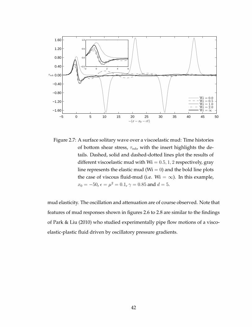
−5 0 5 10 15 20 25 30 35 40 45 50

−1.60

−1.20

−0.80

−0.40

0.00

0.40

0.80

1.20

1.60

τmb

−(x− x0 − ct)

Wi = 0.0Wi = 0.5Wi = 1.0Wi = 2.0Wi =∞

−2 0 2 4 6−0.5

0.0

0.5

1.0

Figure 2.7: A surface solitary wave over a viscoelastic mud: Time histories

of bottom shear stress, τmb, with the insert highlights the de-

tails. Dashed, solid and dashed-dotted lines plot the results of

different viscoelastic mud with Wi = 0.5, 1, 2 respectively, gray

line represents the elastic mud (Wi = 0) and the bold line plots

the case of viscous fluid-mud (i.e. Wi = ∞). In this example,

x0 = −50, ǫ = µ2 = 0.1, γ = 0.85 and d = 5.

mud elasticity. The oscillation and attenuation are of course observed. Note that

features of mud responses shown in figures 2.6 to 2.8 are similar to the findings

of Park & Liu (2010) who studied experimentally pipe flow motions of a visco-

elastic-plastic fluid driven by oscillatory pressure gradients.

42

0.000 0.125 0.2500.0

0.2

0.4

0.6

0.8

1.0θ = -1.521

η

d

um

Wi = 0.0; Wi = 0.5; Wi = 1.0; Wi = 2.0; Wi =∞

0.00 0.25 0.50 0.750.0

0.2

0.4

0.6

0.8

1.0θ = -0.634

um

−0.8 −0.4 0.0 0.30.0

0.2

0.4

0.6

0.8

1.0

θ = 1.521

um

−1.0 −0.5 0.00.0

0.2

0.4

0.6

0.8

1.0

θ = 3.456

um

−1.8 −1.2 −0.6 0.00.0

0.2

0.4

0.6

0.8

1.0

θ = 5

η

d

um

0.0 0.4 0.8 1.20.0

0.2

0.4

0.6

0.8

1.0

θ = 15

um

−0.9 −0.6 −0.3 0.0 0.30.0

0.2

0.4

0.6

0.8

1.0

θ = 25

um

−0.3 0.0 0.3 0.6 0.90.0

0.2

0.4

0.6

0.8

1.0

θ = 35

um

Figure 2.8: A surface solitary wave over a viscoelastic mud: Profiles of

horizontal velocity component, um, inside the entire mud col-

umn at several different phases, θ = −(x − x0 − ct). The up-

per four panels (θ = −1.521,−0.634, 1.521, 3.456) correspond to

ub = (+)0.25, (+)0.75, (−)0.25, (−)0.01 where (+) and (−) rep-

resent the accelerating and decelerating phases of the imposed

solitary wave, respectively. For the remaining phases, ub → 0.

All parameters are same as those in figures 2.6 and 2.7.

43

2.2.5 1HD application: evolution of wave height of a surface

solitary wave

We shall now examine the effects of muddy seabed on the surface water waves.

For simplicity, let us consider again a solitary wave in one horizontal dimension

(1HD). The solution procedure presented here follows closely the approach out-

lined in Mei, Stiassnie & Yue (2005) for studying viscous damping of solitary

waves (see also Liu & Orfila 2007).

For the 1HD problem, the conservation laws of mass and momentum can be

reduced from (2.2.25) and (2.2.26) as

∂ζ

∂t+

∂

∂x[(1 + ǫζ)u]− α

µI = O(µ4), (2.2.96)

and

∂u

∂t+ ǫu

∂u

∂x+∂ζ

∂x− µ2

3

∂3u

∂x2∂t= O(µ4), (2.2.97)

respectively. Recall the function I is defined by (2.2.81), and in this case

I = I(γ, d, u). (2.2.98)

As suggested by Mei, Stiassnie & Yue (2005), let us first introduce a moving

coordinate,

σ = x− t, (2.2.99)

and also a slow time variable,

ϕ = ǫt. (2.2.100)

The temporal and spatial derivatives then become:

∂

∂t→ − ∂

∂σ+ ǫ

∂

∂ϕ,

∂

∂x→ ∂

∂σ. (2.2.101)

44

Folding (2.2.101) into the summation of (2.2.96) and (2.2.97), we obtain

ǫ∂

∂ϕ(ζ + u) + ǫ

∂

∂σ(ζu) + ǫu

∂u

∂σ+µ2

3

∂3u

∂σ3− α

µI = O(µ4). (2.2.102)

Recall that O(α) ∼ O(µ4). Therefore, with an error of O(µ2) only the leading-

order solutions of ζ and u are required in (2.2.102).

The leading-order solution of an undisturbed solitary wave can be expressed

in terms of the newly defined coordinates as

ζ = a sech2

(√3a

2

(σ − a

2ϕ))

, (2.2.103)

where a = a(ϕ) is the dimensionless wave height. Moreover,

u = ζ (2.2.104)

is the leading-order approximation. Using (2.2.104), we obtain from (2.2.102) a

partial differential equation for ζ,

∂ζ

∂ϕ+

3

2ζ∂ζ

∂σ+

1

6

µ2

ǫ

∂3ζ

∂σ3− 1

2

α

ǫµI = O(µ2), (2.2.105)

where

I = I(γ, d, u)→ I(γ, d, ζ) (2.2.106)

is also evident.

Under the effect of a muddy seabed, the surface solitary wave is expected

to be perturbed from its original solution, i.e. (2.2.103). Let us introduce the

perturbation solution as follows (see Mei, Stiassnie & Yue 2005):

ζ =∞∑

n=0

δnζn, ζn = ζn(ρ, ξ), (2.2.107)

where

δ =α

ǫµ, ξ = δϕ =

α

µt, ρ = σ− 1

2

∫ ϕ

a(ϕ′)dϕ′ = σ− 1

2δ

∫ ξ

a(ξ′)dξ′. (2.2.108)

45

Notice that

∂

∂σ→ ∂

∂ρ,

∂

∂ϕ→ δ

∂

∂ξ− a

2

∂

∂ρ. (2.2.109)

Substituting (2.2.107) into (2.2.105) and then collecting terms at different orders,

we obtain at O(δ0):

−a2

∂ζ0∂ρ

+3

2ζ0∂ζ0∂ρ

+1

6

µ2

ǫ

∂3ζ0∂ζ3

0

= 0, (2.2.110)

and at O(δ):

∂ζ0∂ξ− a

2

∂ζ1∂ρ

+3

2

∂

∂ρ(ζ0ζ1) +

1

6

µ2

ǫ

∂3ζ1∂ζ3

0

− 1

2I0 = 0, (2.2.111)

where I0 is the leading-order of I and is a function of ζ0. Following Ott & Sudan

(1970) (see also Mei, Stiassnie & Yue 2005), (2.2.110) and (2.2.111) can be recast

as

L0ζ0 ≡∂

∂ρ

[−a

2+

3

4ζ0 +

1

6

µ2

ǫ

∂2

∂ρ2

]ζ0 = 0, (2.2.112)

and

L1ζ1 ≡∂

∂ρ

[−a

2+

3

2ζ0 +

1

6

µ2

ǫ

∂2

∂ρ2

]ζ1 = −∂ζ0

∂ξ+

1

2I0, (2.2.113)

respectively. The operators L0 and L1 satisfy

∞∫

−∞

(ζ0L1ζ1 − ζ1L0ζ0) dρ = 0, (2.2.114)

as they are adjoint operators of each other (Mei, Stiassnie & Yue 2005). There-

fore, (2.2.114) provides a solvability condition for ζ1,

∞∫

−∞

ζ0

(−∂ζ0∂ξ

+1

2I0)dρ = 0. (2.2.115)

It is remarked that this condition is actually valid for any weakly nonlinear and

weak dispersive wave loadings, as long as ζ ≈ u is legit at the leading-order.

46

Apparently, the leading-order solution, ζ0, is just the solitary wave solution

which can be re-expressed from (2.2.104) as

ζ0 = a sech2

(√3a

2ρ

), a = a(ξ). (2.2.116)

Substituting (2.2.116) into (2.2.115), we then obtain an integral equation for the

wave height, a(ξ),

∞∫

−∞

a sech2

(√3a

2ρ

)(∂ζ0∂ξ− 1

2I0)dρ = 0, (2.2.117)

where

∂ζ0∂ξ

=da

dξsech2

(√3a

2ρ

)[1−√

3a

2ρ tanh

(√3a

2ρ

)]. (2.2.118)

Since ∞∫

−∞

sech4(k) [1− k tanh(k)] dk = 1, (2.2.119)

the integral equation (2.2.117) becomes

da

dξ=

√3a

4

∞∫

−∞

sech2

(√3a

2ρ

)I0dρ. (2.2.120)

It is now necessary to discuss the detailed function of I0, which depends

on the actual mud rheology. Let us again use the two-component Kelvin-Voigt

element as an example. It is reiterated that both viscous fluid-mud and purely

elastic mud are just special cases of Kelvin-Voigt’s model (see the discussion in

section 2.2.4). Recall (2.2.41), (2.2.87) and (2.2.81), we obtain

wb = −αµγd∂u

∂x+

2

d

∞∑

n=0

sn/κ2n

2sn − κ2n

∫ t

0

∂2u(x, τ)

∂x∂τ

[1− esn(t−τ)] dτ

, (2.2.121)

and

I = −γd ∂ζ∂x− γ 2

d

∞∑

n=0

sn/κ2n

2sn − κ2n

t∫

0

∂2ζ(x, τ)

∂x∂τ

[1− esn(t−τ)] dτ , (2.2.122)

47

where the leading-order approximation of (2.2.24), (2.2.104) and (2.2.106) are

evoked. To satisfy the order of accuracy as stated in (2.2.105), (2.2.122) shall be

rewritten as

I = −γd ∂ζ∂σ

+ γ2

d

∞∑

n=0

sn/κ2n

2sn − κ2n

t∫

0

∂2ζ(x, τ)

∂σ2

[1− esn(t−τ)] dτ . (2.2.123)

It is then straightforward to obtain the leading-order term as

I0 = −γd ∂ζ0∂ρ

+ γ2

d

∞∑

n=0

sn/κ2n

2sn − κ2n

t∫

0

∂2ζ0∂ρ2

[1− esn(t−τ)] dτ . (2.2.124)

Derivatives in the above equation can be expressed explicitly as:

∂ζ0∂ρ

= −a√

3a sech2 (R) tanh (R) , (2.2.125)

∂2ζ0∂ρ2

= −3

2a2 sech4 (R) [2− cosh(2R)] , (2.2.126)

where

R =

√3a

2ρ. (2.2.127)

The substitution of the above expressions back into (2.2.124) gives

I0 = a√

3a[γd sech2(R) tanh(R)

]

+ a√

3a

t∫

0

sech4(ρ+ S) [2− cosh(ρ+ S)]M(

2S√3a

)dS, (2.2.128)

where

M(τ) = −2γ

d

∞∑

n=0

sn/κ2n

2sn − κ2n

[1− esnτ ] . (2.2.129)

Since ∞∫

−∞

sech4(k) tanh(k)dk = 0, (2.2.130)

we finally obtain from (2.2.120) and (2.2.128) an evolution equation for the wave

height of a surface solitary wave propagating over a thin layer of viscoelastic

48

mud modeled by the two-component Kelvin-Voigt element:

da

dξ=a√

3a

2

∫ ∞

−∞

∫ ∞

0

sech2(R)sech4(R + S) [2− cosh 2(R + S)]M(

2S√3a

)dSdR.

(2.2.131)

The above equation can be integrated numerically to find the time variation of

solitary wave heights for a prescribed set of wave data and mud properties.

Numerical examples

As an example, figures 2.9 and 2.10 plot a(ξ) under different values of Wi and d.

The effect of relative elasticity is first discussed by fixing γ and d while varying

Wi, as shown in figure 2.9-(a) and (b). In subplot (a) (i.e. d = 5), the wave height

tends to decay faster for the case of smaller Wi (i.e. the mud is more elastic).

However, as solitary wave propagates further (i.e. at large ξ) the attenuation

caused by mud with bigger Wi can be larger. This behavior is more obvious

if we decrease the mud layer thickness to d = 2, as shown in figure 2.9-(b).

Again, more elastic mud causes a stronger attenuation only at the beginning

stage. The complexity can be attributed to the fact that part of surface wave

energy is transfered into the mud layer as elastic energy to sustain the oscillation

motion (see figures 2.6 to 2.8 for reference). Since elastic energy is proportional

to the square of mud displacement, during the oscillation process the stored

elastic energy can be released in which a portion of energy is damped out by

the viscous mechanism while the rest recharges the surface wave motion.

In figure 2.10, the effect of mud thickness is discussed by fixing Wi but vary-

ing d. It is observed that for the case of Wi = 1 and moderate mud layer thick-

ness, the increase of d leads to remarkably faster and stronger attenuation of

solitary wave height as shown in subplot (a). However, if the mud layer thick-

49

0 2 4 6 8 100.01

0.05

0.10

0.25

0.50

0.751.00

ξ

a

(a) d = 5; Wi = 0.5, 1, 2,∞

Wi = 0.5Wi = 1.0Wi = 2.0Wi =∞

0 2 4 6 8 100.10

0.25

0.50

0.75

1.00

ξ

a

(b) d = 2; Wi = 0.5, 1, 2,∞

Wi = 0.5Wi = 1.0Wi = 2.0Wi =∞

Figure 2.9: Evolution of a surface solitary wave propagates over a vis-

coelastic mud: Wave height, a, as a function of time, ξ = (α/µ)t.

Effect of relative importance of elasticity are shown by fixing d

((a): d = 5; (b): d = 2) and varying Wi as Wi = 0.5, 1, 2,∞. In

all calculations, γ = 0.85.

ness keeps increasing, the attenuation of wave height becomes less sensitive to

d and a complex behavior, similar to that shown in figure 2.9, is displayed. Note

that, viscous damping does not grow unbounded with d as the viscous effect is

mostly contributed by the so-called boundary layer. Regarding the wave varia-

tion caused by the elastic mechanism, as discussed above the releasing of elastic

energy plays the role where the oscillation frequency of elastic motion is also a

function of d.

50

0 2 4 6 8 100.0

0.2

0.4

0.6

0.8

1.0

ξ

a

(a) Wi = 1; d = 0.5, 1, 1.5, 2

d = 0.5d = 1.0d = 1.5d = 2.0

0 2 4 6 8 100.0

0.2

0.4

0.6

0.8

1.0

ξ

a

(b) Wi = 1; d = 2.5, 5, 7.5, 10

d = 2.5d = 5.0d = 7.5d = 10

Figure 2.10: Wave height, a, as a function of time, ξ = (α/µ)t, for a surface

solitary wave propagates over a viscoelastic mud: Effect of

mud layer thickness, d. While γ = 0.85 and Wi = 1 are fixed,

d = 0.5, 1, 1.5, 2 in subplot (a) and d = 2.5, 5, 7.5, 10 in (b).

2.2.6 1HD application: amplitude variation of a linear progres-

sive wave

We can also examine the effects of bottom mud on a simple harmonic wave as

the present theory considers a general surface wave loading.

For a linear nondispersive progressive wave, the 1HD equations can be re-

duced from (2.2.96) and (2.2.97) as

∂ζ

∂t+∂u

∂x=α

µI, (2.2.132)

∂u

∂t+∂ζ

∂x= 0, (2.2.133)

which are just the linear shallow water equations with the effects of muddy

51

seabed as a forcing. Recall the moving coordinate, σ = x− t, and the slow time

variable, ξ = (α/µ)t, by evoking the leading-order approximation,

∂u

∂ξ≈ ∂ζ

∂ξ, (2.2.134)

into the summation of (2.2.132) and (2.2.133) we obtain an evolution equation

for the free-surface displacement

∂ζ

∂ξ=

1

2I. (2.2.135)

Note that in function I the spatial and temporal derivative operators should be

replaced by:

∂

∂x→ ∂

∂σ,

∂

∂t→ − ∂

∂σ. (2.2.136)

For a linear progressive wave, the displacement can be formally expressed

as

ζ = a(ξ)eiσ = [a(0)exp (iβrξ) exp (−βiξ)] eiσ, (2.2.137)

where a(ξ) is the wave amplitude. Also, βr and βi account for the wavenumber

shift and change in magnitude due to the presence of a muddy seabed, respec-

tively. In the case of a frictionless solid bottom, βr = βi = 0 and a(ξ) = a(0)

remains as a constant. For convenience, in the dimensionless manner one can

further take a(0) = 1.

Due to the periodicity of wave loadings, we can express

I(ξ, σ) = I∗(ξ)ζ. (2.2.138)

Therefore, the direct substitution of (2.2.137) and (2.2.138) into (2.2.135) leads to

βr + iβi = − i

2I∗. (2.2.139)

52

For the numerical demonstration, let us consider again the two-component

Kelvin-Voigt’s model. Following (2.2.123),

I =− γd∂ζ∂σ−

t∫

0

∂2ζ(x, τ)

∂σ2M(t− τ)dτ

= −iγd ζ + ζ

t∫

0

ei(t−τ)M(t− τ)dτ

=

−iγd+

∞∫

0

eiSM(S)dS

ζ, (2.2.140)

where the functionM has been defined in (2.2.129). Substituting (2.2.140) into

(2.2.139), we finally obtain

βr = −1

2γd+

1

2

∞∫

0

sin(S)M(S)dS, (2.2.141)

and

βi = −1

2

∞∫

0

cos(S)M(S)dS. (2.2.142)

For a purely elastic mud,M reduces to

M(τ) = −2γ

d

∞∑

n=0

[2d

(2n+ 1)π

]2 [1− cos

((2n+ 1)π

2dτ

)]. (2.2.143)

Therefore, (2.2.142) has the asymptotic result

βi = 0, (2.2.144)

while βr can be approximated as

βr = −γd2− γd

d2 − [(n+ 1/2)π]2

[2d

(2n+ 1)π

]2 [1− cos

((2n+ 1)π2

d

)]. (2.2.145)

Clearly, (2.2.144) suggests that there is zero decay for periodic waves propagat-

ing over a elastic seabed, which bas been shown by MacPherson (1980) and Mei

et al. (2010). It is reiterated that both past theories are limited to small-amplitude

53

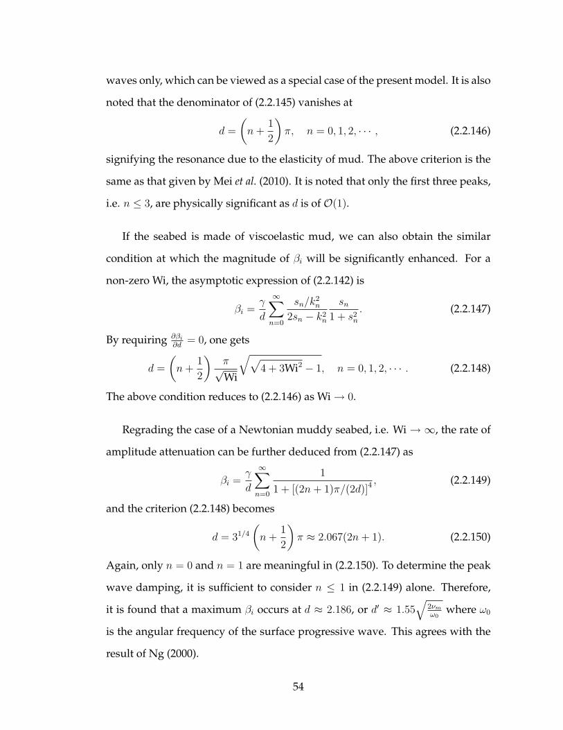
waves only, which can be viewed as a special case of the present model. It is also

noted that the denominator of (2.2.145) vanishes at

d =

(n+

1

2

)π, n = 0, 1, 2, · · · , (2.2.146)

signifying the resonance due to the elasticity of mud. The above criterion is the

same as that given by Mei et al. (2010). It is noted that only the first three peaks,

i.e. n ≤ 3, are physically significant as d is of O(1).

If the seabed is made of viscoelastic mud, we can also obtain the similar

condition at which the magnitude of βi will be significantly enhanced. For a

non-zero Wi, the asymptotic expression of (2.2.142) is

βi =γ

d

∞∑

n=0

sn/k2n

2sn − k2n

sn1 + s2

n

. (2.2.147)

By requiring ∂βi

∂d= 0, one gets

d =

(n+

1

2

)π√Wi

√√4 + 3Wi2 − 1, n = 0, 1, 2, · · · . (2.2.148)

The above condition reduces to (2.2.146) as Wi→ 0.

Regrading the case of a Newtonian muddy seabed, i.e. Wi → ∞, the rate of

amplitude attenuation can be further deduced from (2.2.147) as

βi =γ

d

∞∑

n=0

1

1 + [(2n+ 1)π/(2d)]4, (2.2.149)

and the criterion (2.2.148) becomes

d = 31/4

(n+

1

2

)π ≈ 2.067(2n+ 1). (2.2.150)

Again, only n = 0 and n = 1 are meaningful in (2.2.150). To determine the peak

wave damping, it is sufficient to consider n ≤ 1 in (2.2.149) alone. Therefore,

it is found that a maximum βi occurs at d ≈ 2.186, or d′ ≈ 1.55√

2νm

ω0

where ω0

is the angular frequency of the surface progressive wave. This agrees with the

result of Ng (2000).

54

Numerical examples

In figure 2.11, βi is plotted against d under various values of Wi and γ. Both

solutions calculated by (2.2.142) and results from MacPherson (1980) are pre-

sented. The occurrence of resonance is also compared with the prediction by

(2.2.148). As can be seen, a good agreement is evident. The oscillating feature

of βi, due largely to the presence of elasticity, is same as that demonstrated by

Mei et al. (2010). However, it is remarked that viscous damping is not responsi-

ble for the amplitude attenuation (non-zero βi) caused by a purely elastic mud

bed. Instead, wave energy transfered into the mud layer through pressure work

at the water-mud interface is stored by the muddy seabed to sustain the mud

flow motions. Furthermore, supported by the observation from figure 2.11-(b)

and the mathematical argument by Mei et al. (2010), it is realized that local max-

ima of βi, which correspond to m = 0, 1, 2, · · · in (2.2.148), decrease sequentially

as a mud layer becomes thicker (i.e. larger m). We may expect for the case of

purely elastic mud βi → 0 as d→∞, which is consistent with the conclusion by

Mallard & Dalrymple (1977).

Given that the problem of linear waves interacting with a muddy seabed has

been studied extensively, comprehensive discussions are available in the liter-

ature. Some important references are MacPherson (1980), Piedra-Cueva (1995),

Ng & Zhang (2007), and Mei et al. (2010).

2.2.7 Explicit solutions for 1HD periodic waves

For a linear progressive wave propagating over a viscoelastic seabed modeled

by a two-component Kelvin-Voigt element, explicit solution forms can actually

55

0 2 4 6 8 100.0

0.5

1.0

1.5

2.0

βi

(a) γ = 0.85 Wi = 0.5

Wi = 1.0Wi = 2.0Wi =∞Present model

0.0 0.5 1.0 1.5 2.0 2.50.00

0.25

0.50Wi =∞

0 2 4 6 8 100.0

0.5

1.0

1.5

2.0

d

βi

(b) Wi = 0.5 γ = 0.85

γ = 0.75γ = 0.65Present model

Figure 2.11: Amplitude attenuation rate (βi) for a linear progressive wave

over a viscoelastic mud: (a) Effect of relative importance of

elasticity: Wi = 0.5, 1, 2,∞; (b) Effect of mud density, γ. Sym-

bols are the solutions of present model while lines plot the

damping rate of MacPherson (1980). The insert in subplot (a)

shows the details of viscous case with the dashed line indi-

cates the value of d corresponds to the maximum βi as given

by (2.2.150). In addition, the vertical bars in (b) show the theo-

retical prediction of d values correspond to the first two peaks

of βi by (2.2.148).

56

be deduced.

Consider the free-surface displacement in the following form:

ζ(x, t) = ei(kx−t), (2.2.151)

where k is the dimensionless wavenumber. Substitute the above expression

into the momentum equation, (2.2.133), the horizontal velocity component is

obtained

u(x, t) = kei(kx−t). (2.2.152)

Furthermore, the vertical component is

w(x, z, t) = −ik2µ2zei(kx−t) + wb. (2.2.153)

Regarding the mud flow solutions, from the initial-boundary-value problem,

(2.2.48) to (2.2.50), the horizontal velocity is

um(x, η, t) = γ

[1− cosh ((d− η))

cosh (d)

]u(x, t), (2.2.154)

where

=1− i√

2

√Wi

i + Wi(2.2.155)

is a complex parameter. Accordingly,

wm(x, η, t) = −ikγ

[η − 1

sinh (d)− sinh ((d− η))cosh (d)

]u(x, t), (2.2.156)

which suggests that

I = −ik2γd

[1− tanh (d)

d

]. (2.2.157)

The dimensionless wavenumber, k, is still an unknown. By evoking the conser-

vation of mass, (2.2.132), the dispersion relation is obtained

1 = k2

1 +

α

µγd

[1− tanh (d)

d

]. (2.2.158)

57

In fact, we can further take into account the wave dispersion. Following the

continuity equation, (2.2.4), the water particle velocity components are formu-

lated as

u = [k cosh (kµ(z + 1)) +D sinh (kµ(z + 1))] ei(kx−t), (2.2.159)

w = −iµ [k sinh (kµ(z + 1)) +D cosh (kµ(z + 1))] ei(kx−t), (2.2.160)

where D is an unknown to be determined. Note that the mud flow velocity re-

mains the same, as given in (2.2.155) and (2.2.156). The continuity of the vertical

velocity at the water-mud interface yields

D = k2αγd

[1− tanh (d)

d

]. (2.2.161)

Therefore, combing the free-surface conditions, (2.2.5) and (2.2.6), we obtain the

dispersion relation

1 =k

µtanh (kµ)

1 + kαγd[1− tanh(d)

d

]coth(kµ)

1 + kαγd[1− tanh(d)

d

]tanh(kµ)

. (2.2.162)

The above solution forms agree with the results reported by Ng (2000) if the

water viscosity is ignored5. In addition, at the nondispersive limit, i.e. µ → 0,

(2.2.159), (2.2.160) and (2.2.162) reduce to (2.2.152), (2.2.153) and (2.2.158), re-

spectively.

2.2.8 Comparison with laboratory experiments

To examine the performance of the present theory, model predictions are now

compared with available laboratory measurements. In this section, three exam-

ples will be discussed: linear progressive waves over a layer of either viscous

5The water viscosity is also considered by Ng (2000), while the water body is treated as ainviscid fluid in the current study.

58

mud (Gade 1958) or viscoelastic mud (Maa & Mehta 1987, 1990), and a solitary

wave interacting with a viscous fluid-mud seabed (Park, Liu & Clark 2008). All

experiments were carried out in flat wave flumes.

The pioneering work of Gade (1958) modeled the bottom mud using sugar

water, considered as a Newtonian fluid. Experimental conditions were:

2π

ω0

= 8 s, h0 = 4 ft, νm = 5 ft2s−1, γ = 0.487,

d′√2νm/ω0

= 0, 0.28, 0.56, 0.84, 1.12, 1.40, 1.68.

Figure 2.12 plots βr and βi calculated by (2.2.141) and (2.2.141), along with the

laboratory results. A reasonable quantitative agreement is observed. Due to the

presence of the viscous mud, the amplitude of the surface wave is attenuated

while the wavelength increases. As a reminder, βr and βi represent the rates

of change of wavenumber and amplitude, respectively. It should be noted that

in the experiments, even without the mud, a remarkable wave damping is still

evident, i.e., value of βi is significant at d ≈ 0. Note that this cannot be solely

accounted for by the effect of water viscosity, as a considerable discrepancy is

also reported by Dalrymple & Liu (1978)6 whose theoretical model also includes

the water viscosity.

Park, Liu & Clark (2008) also studied the interaction between surface waves

and a viscous mud, but considered solitary waves of weak to moderate nonlin-

earity instead. In their experiments, a commercial Newtonian silicone fluid was

used as the bottom mud. Employing the particle image velocimetry (PIV), Park,

Liu & Clark (2008) reported the velocity measurements in both water body and

mud column. Experimental conditions of a specific case to be discussed are:

h0 = 10 cm, a0 = 1.9 cm, d′ = 1.7 cm, νm = 5.24× 10−3 m2s−1, γ = 0.667.

6See FIG. 2 in Dalrymple & Liu (1978).

59

0.0 0.5 1.0 1.5 2.0 2.5 3.0−0.80

−0.60

−0.40

−0.20

0.00

βr

d0.0 0.5 1.0 1.5 2.0 2.5 3.0

0.00

0.05

0.10

0.15

0.20

βi

d

Figure 2.12: Periodic wave over a viscous mud: Rates of change of dimen-

sionless wavenumber, βr, and wave amplitude, βi, as func-

tions of dimensionless mud layer thickness, d. Dots are the

laboratory measurements of Gade (1958) and lines plot the re-

sults calculated by (2.2.141) and (2.2.141), respectively.

Figure 2.13 shows the time histories of horizontal mud flow velocity, um, at

three fixed vertical levels: η/d = 0.25, 0.5, 0.75. The theoretical predictions agree

very well with the measurements. The vertical profiles of um at several different

phases are further illustrated in figure 2.14. Again, the agreement is also reason-

able. Note that panel (c) demonstrates the transition of flow reversal predicted

by the current theory. Unfortunately, the experiment did not capture this fea-

ture due to the limited sampling rate at 100 HZ, which corresponds to a phase

difference of ∆θ ≈ 0.04 with θ = −(x− x0 − ct).

In figure 2.15, records of both bottom shear stress, τmb, and the vertical dis-

placement at water-mud interface, ζm, are shown. Note that the model predicted

interfacial displacement is recovered by numerically integrating the linear ap-

proximation

∂ζm∂t

= wm, η = d. (2.2.163)

60

−1.00 −0.75 −0.50 −0.25 0.00 0.25 0.50 0.75 1.00−0.06

−0.04

−0.02

0.00

0.02

0.04

0.06

−(x− x0 − ct)

um

η

d= 0.75

η

d= 0.50

η

d= 0.25

Measurements

Figure 2.13: Solitary wave over a viscous mud: Records of horizontal mud

flow velocity, um, at three vertical levels, η/d = 0.25, 0.5, 0.75.

Lines plot the theoretical results and dots are the experimental

data of Park, Liu & Clark (2008).

The measurements are actually those of PIV products. As can be seen, theoret-

ical results agree well with the experimental data. It should be noted that ζm

is at least two orders of magnitude smaller than the free-surface displacement,

which is of O(1) in the dimensionless manner. This justifies the assumption of

negligible interfacial displacement (see the discussion in (2.2.34)).

The model validation is completed by considering a final example of peri-

odic waves over a viscoelastic muddy seabed. Here, the present solutions are

compared with the laboratory tests of Maa & Mehta (1987, 1990). It is noted

that actual estuarial mud taken from Cedar Key, Florida was used in the experi-

ments. Rheology tests have shown that the mud samples exhibited both viscous

and elastic properties. Figure 2.16 shows the comparison of horizontal velocity

component across the entire extent of water body and mud column. The cor-

61

−0.08 −0.06 −0.04 −0.02 0.00 0.02 0.04 0.06 0.080.000.250.500.751.00

(a) θ = −0.33η

d

−0.08 −0.06 −0.04 −0.02 0.00 0.02 0.04 0.06 0.080.000.250.500.751.00

(b) θ = −0.12η

d

−0.008 −0.006 −0.004 −0.002 0.000 0.002 0.004 0.006 0.0080.000.250.500.751.00

(c) θ = 0.012, 0.014, 0.016η

d

−0.08 −0.06 −0.04 −0.02 0.00 0.02 0.04 0.06 0.080.000.250.500.751.00

(d) θ = 0.09η

d

−0.08 −0.06 −0.04 −0.02 0.00 0.02 0.04 0.06 0.080.000.250.500.751.00

(e) θ = 0.33

um(x, η, t)

η

d

Figure 2.14: Mud flow induced by a surface solitary wave: Profiles of hor-

izontal velocity component, um, at several different phases,

θ = −(x − x0 − xt). Dots are the PIV products of Park,

Liu & Clark (2008) and lines show the theoretical predictions.

In panel (c), the transition of flow reversal is demonstrated,

which was not captured by the experiment due to the limited

sampling rate.

62

−1.00 −0.75 −0.50 −0.25 0.00 0.25 0.50 0.75 1.00−0.010

−0.005

0.000

0.005

0.010

ζm

−1.00 −0.75 −0.50 −0.25 0.00 0.25 0.50 0.75 1.00−1.0

−0.5

0.0

0.5

1.0

τmb

−(x− x0 − ct)

Figure 2.15: Solitary wave over a viscous mud: Time histories of interfacial

displacement, ζm, and bottom shear stress, τmb. Lines plot the

theoretical predictions and dots show the laboratory results of

Park, Liu & Clark (2008).

responding parameters are listed in Table 2.1. Notice that in both experiments,

the properties of mud, namely ρm, νm, and Em, are vertically stratified. To adopt

their data to our theory, these parameters have been depth-averaged. As can

be seen, the agreement is generally acceptable. It is clear that a sharp velocity

gradient is shown at the water-mud interface, due largely to the huge difference

in viscosities of water and mud.

Table 2.1: Experimental conditions of Maa & Mehta (1987, 1990) for periodic

waves over a viscoelastic muddy seabed.

2πω0

h0 a0 d′ ρm νm Em

(s) (cm) (cm) (cm) (g cm−3) (m2s−1) (N m2)

M&M87 1.6 19.7 1.6 16.0 2.475 0.0400 18.0

M&M90 1.2 21.1 3.4 14.6 2.400 0.0945 38.3

63

0 5 10 150

5

10

15

20

25

30

35

40

∇

(a)

Dis

tance

tobott

om

(cm

)

Horizontal velocity (cm/s)0 10 20 30

0

5

10

15

20

25

30

35

40

∇

Dis

tance

tobott

om

(cm

)

Horizontal velocity (cm/s)

(b)

Figure 2.16: Periodic waves over a viscoelastic mud: Profiles of horizontal

velocity components. Lines plot the theoretical results while

dots are experimental data of Maa & Mehta (1987) (subplot

(a)) and Maa & Mehta (1990) (subplot (b)). In addition, dashed

lines denote the free surfaces. The corresponding parameters

are given in Table 2.1.

2.2.9 Summary

A set of depth-averaged continuity and momentum equations, describing mo-

tions of surface long waves over a thin viscoelastic muddy seabed, has been

derived. The new theory is capable of modeling weakly nonlinear and weakly

dispersive waves. A generalized rheology model for a linear viscoelastic ma-

terial is adopted with both Newtonian fluid and purely elastic mud being the

limiting cases. To demonstrate, amplitude evolution of a solitary wave is in-

vestigated which shows a significant attenuation caused by the mud. The case

of linear progressive waves is also studied. It is found that the wave attenua-

tion can be enhanced remarkably by the elasticity of mud. The performance of

64

the proposed model is examined by comparing the results with the available

laboratory measurements. The overall agreement is encouraging.

2.3 Response of a Bingham-plastic muddy seabed to a surface

solitary wave

Mud in different locales can have different rheological behavior, partly as a con-

sequence of diverse chemical composition (Balmforth & Craster 2001). Examin-

ing the mud samples taken from the eastern coast of China, Mei et al. (2010) have

shown that these cohesive sediments can be modeled as a viscoelastic material.

Krone (1963) performed the viscosimetric tests on field mud samples collected

along the coasts of the United States. He reported that mud with a concentration

roughly lying between 10 to 100 g L−1 displayed both plastic and viscous-like

behavior, depending on the external forcing. This observation suggests that the

muddy seafloor can sometimes be referred as a Bingham-plastic material, in

which the constitutive equation in a simple two-dimensional case is expressed

as

µm∂u′m∂z′

=

0, |τ ′m| ≤ τ ′o

τ ′m − τ ′o sgn

(∂u′m∂z′

), |τ ′m| > τ ′o

, (2.3.164)

where τ ′o > 0 is the yield stress, and µm is the Bingham-plastic viscosity. It is

remarked that the above rheology model is the leading-order approximation as

the contribution from ∂u′m∂x′

has been ignored (see section 2.2.2 for the justifica-

tion). Detailed discussion on the validation of (2.3.164) has been documented in

Balmforth & Craster (1999). It is noted that typical values of the physical param-

eters for different Bingham-plastic muds can be found in Mei & Liu (1987). A

65

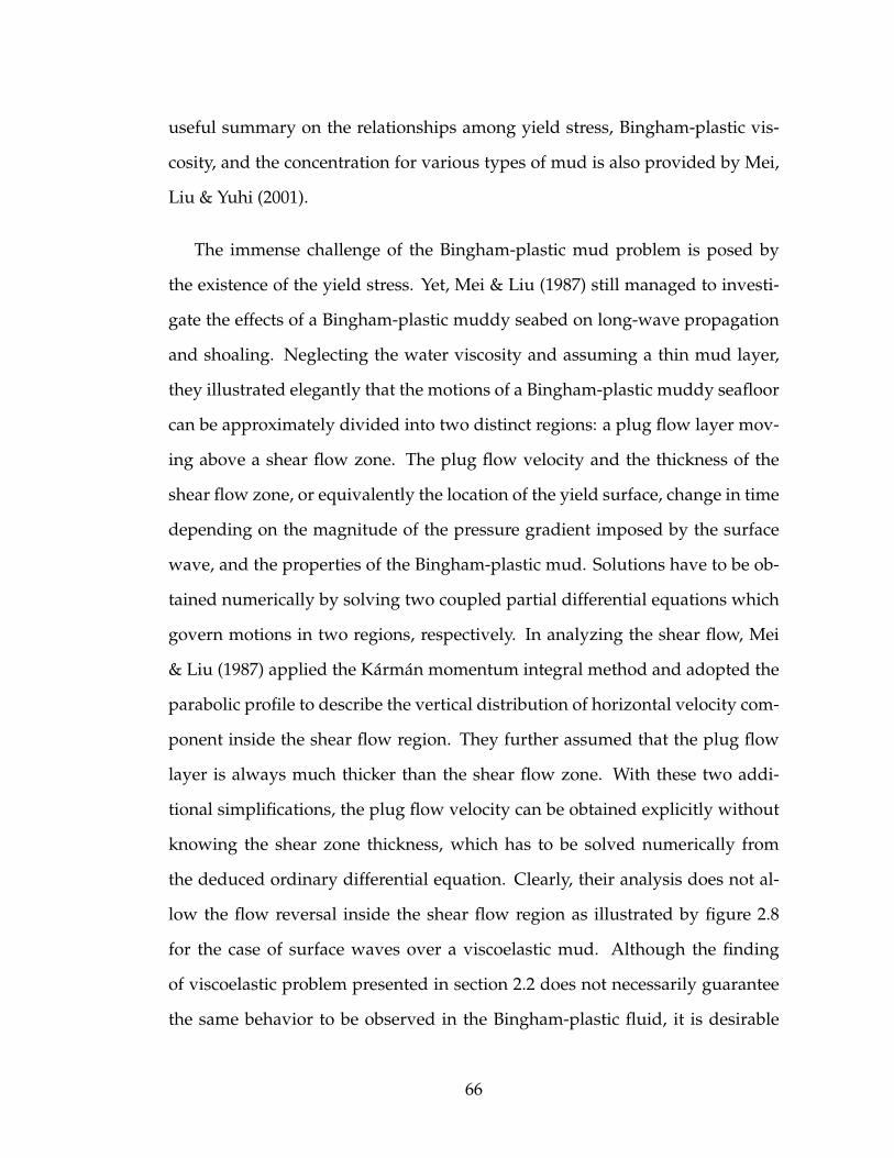
useful summary on the relationships among yield stress, Bingham-plastic vis-

cosity, and the concentration for various types of mud is also provided by Mei,

Liu & Yuhi (2001).

The immense challenge of the Bingham-plastic mud problem is posed by

the existence of the yield stress. Yet, Mei & Liu (1987) still managed to investi-

gate the effects of a Bingham-plastic muddy seabed on long-wave propagation

and shoaling. Neglecting the water viscosity and assuming a thin mud layer,

they illustrated elegantly that the motions of a Bingham-plastic muddy seafloor

can be approximately divided into two distinct regions: a plug flow layer mov-

ing above a shear flow zone. The plug flow velocity and the thickness of the

shear flow zone, or equivalently the location of the yield surface, change in time

depending on the magnitude of the pressure gradient imposed by the surface

wave, and the properties of the Bingham-plastic mud. Solutions have to be ob-

tained numerically by solving two coupled partial differential equations which

govern motions in two regions, respectively. In analyzing the shear flow, Mei

& Liu (1987) applied the Karman momentum integral method and adopted the

parabolic profile to describe the vertical distribution of horizontal velocity com-

ponent inside the shear flow region. They further assumed that the plug flow

layer is always much thicker than the shear flow zone. With these two addi-

tional simplifications, the plug flow velocity can be obtained explicitly without

knowing the shear zone thickness, which has to be solved numerically from

the deduced ordinary differential equation. Clearly, their analysis does not al-

low the flow reversal inside the shear flow region as illustrated by figure 2.8

for the case of surface waves over a viscoelastic mud. Although the finding

of viscoelastic problem presented in section 2.2 does not necessarily guarantee

the same behavior to be observed in the Bingham-plastic fluid, it is desirable

66

to analyze the shear flow region more carefully. In addition, it is anticipated

that under certain combinations of yield stress, viscosity and pressure gradient,

multiple shear flow layers (or plug flow regions) can develop.

Therefore, this section is devoted to studying the response of a Bingham-

plastic muddy seafloor subject to long water wave loadings without some of

the constrains imposed in Mei & Liu (1987). In particular, we shall relax the

following two assumptions: the parabolic shear flow velocity profile and the

negligible shear layer thickness in computing the plug flow velocity. This will

allow us to investigate the evolution of yield surfaces, and the associated ve-

locity profiles throughout the entire mud column. Since analytical solutions

are impossible for general wave loadings, we shall focus only on the free sur-

face solitary wave loading. The initial-boundary-value problem governing the

wave-induced motions inside the thin layer of Bingham-plastic mud shall be

first discussed. A brief review of the approach and assumptions of Mei & Liu

(1987) follows. Possible scenarios of mud motions, which could have up to four

layers of alternating plug flow and shear flow under a surface solitary wave,

are then illustrated. Subsequently, semi-analytical/numerical solutions are pre-

sented for the velocities inside the mud column, along with detailed discussion

on the mud flow dynamics under different physical parameters. The damping

rate for a surface solitary wave is calculated using the energy conservation law.

Using some estimated but realistic physical parameters, the predicted damp-

ing rate is compared with the field observations. Good qualitative agreement is

shown.

67

2.3.1 Formulation for wave-induced mud motions inside a thin

Bingham-plastic seabed

A thin layer of Bingham-plastic mud subject to a transient surface long-wave

loading is now studied. For simplicity, let us consider only two-dimensional

problem where the x-axis coincides with the direction of wave propagation and

the η-axis points upwards, denoting the vertical coordinate. As has been dis-

cussed comprehensively in section 2.2.2, the mud flow motions can be described

by the following linearized boundary-layer equations (see (2.2.36) and (2.2.48)):

∂um∂x

+∂wm∂η

= 0, 0 ≤ η ≤ d, (2.3.165)

∂um∂t

= γ∂ub∂t

+∂τm∂η

, 0 ≤ η ≤ d, (2.3.166)

where

−∂pm∂x

=∂ub∂t

, η = d (2.3.167)

has been evoked. In addition, from (2.2.49) and (2.2.50) the corresponding

boundary conditions in the vertical direction are

τm = 0, η = d, (2.3.168)

and

um = 0, η = 0. (2.3.169)

The idea is again to first express um in terms of ub by solving the above initial-

boundary-value problem. Afterwards,

wm(x, η, t) =

η∫

0

−∂um∂x

dη (2.3.170)

is calculated from (2.3.165) (see also (2.2.78)).

68

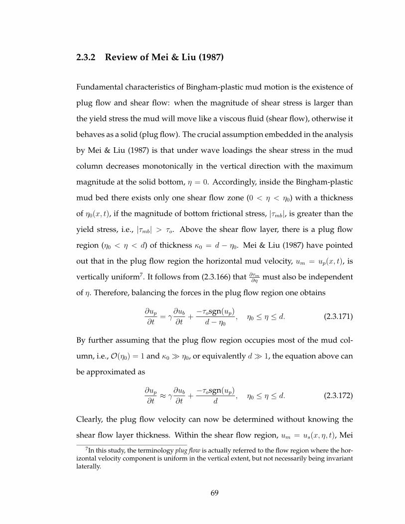
2.3.2 Review of Mei & Liu (1987)

Fundamental characteristics of Bingham-plastic mud motion is the existence of

plug flow and shear flow: when the magnitude of shear stress is larger than

the yield stress the mud will move like a viscous fluid (shear flow), otherwise it

behaves as a solid (plug flow). The crucial assumption embedded in the analysis

by Mei & Liu (1987) is that under wave loadings the shear stress in the mud

column decreases monotonically in the vertical direction with the maximum

magnitude at the solid bottom, η = 0. Accordingly, inside the Bingham-plastic

mud bed there exists only one shear flow zone (0 < η < η0) with a thickness

of η0(x, t), if the magnitude of bottom frictional stress, |τmb|, is greater than the

yield stress, i.e., |τmb| > τo. Above the shear flow layer, there is a plug flow

region (η0 < η < d) of thickness κ0 = d − η0. Mei & Liu (1987) have pointed

out that in the plug flow region the horizontal mud velocity, um = up(x, t), is

vertically uniform7. It follows from (2.3.166) that ∂τm∂η

must also be independent

of η. Therefore, balancing the forces in the plug flow region one obtains

∂up∂t

= γ∂ub∂t

+−τosgn(up)

d− η0

, η0 ≤ η ≤ d. (2.3.171)

By further assuming that the plug flow region occupies most of the mud col-

umn, i.e., O(η0) = 1 and κ0 ≫ η0, or equivalently d≫ 1, the equation above can

be approximated as

∂up∂t≈ γ

∂ub∂t

+−τosgn(up)

d, η0 ≤ η ≤ d. (2.3.172)

Clearly, the plug flow velocity can now be determined without knowing the

shear flow layer thickness. Within the shear flow region, um = us(x, η, t), Mei

7In this study, the terminology plug flow is actually referred to the flow region where the hor-izontal velocity component is uniform in the vertical extent, but not necessarily being invariantlaterally.

69

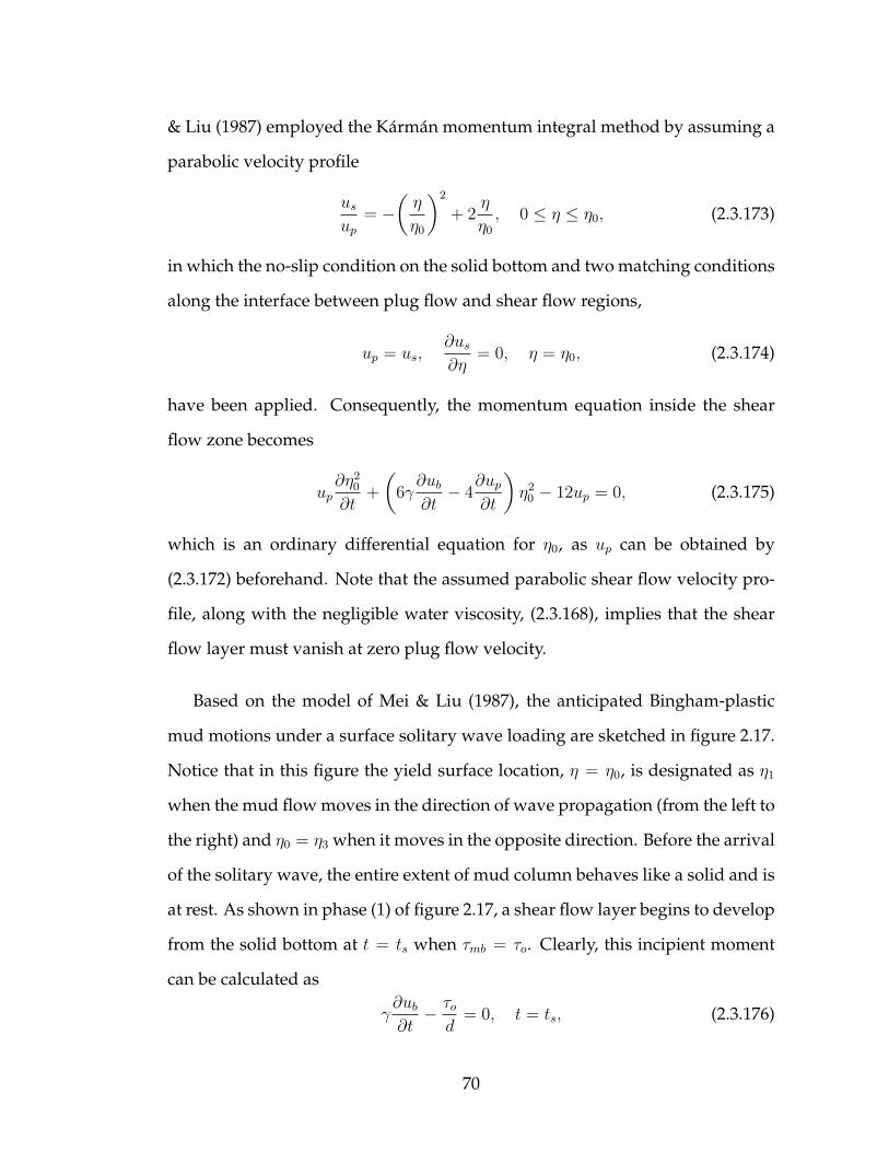
& Liu (1987) employed the Karman momentum integral method by assuming a

parabolic velocity profile

usup

= −(η

η0

)2

+ 2η

η0

, 0 ≤ η ≤ η0, (2.3.173)

in which the no-slip condition on the solid bottom and two matching conditions

along the interface between plug flow and shear flow regions,

up = us,∂us∂η

= 0, η = η0, (2.3.174)

have been applied. Consequently, the momentum equation inside the shear

flow zone becomes

up∂η2

0

∂t+

(6γ∂ub∂t− 4

∂up∂t

)η2

0 − 12up = 0, (2.3.175)

which is an ordinary differential equation for η0, as up can be obtained by

(2.3.172) beforehand. Note that the assumed parabolic shear flow velocity pro-

file, along with the negligible water viscosity, (2.3.168), implies that the shear

flow layer must vanish at zero plug flow velocity.

Based on the model of Mei & Liu (1987), the anticipated Bingham-plastic

mud motions under a surface solitary wave loading are sketched in figure 2.17.

Notice that in this figure the yield surface location, η = η0, is designated as η1

when the mud flow moves in the direction of wave propagation (from the left to

the right) and η0 = η3 when it moves in the opposite direction. Before the arrival

of the solitary wave, the entire extent of mud column behaves like a solid and is

at rest. As shown in phase (1) of figure 2.17, a shear flow layer begins to develop

from the solid bottom at t = ts when τmb = τo. Clearly, this incipient moment

can be calculated as

γ∂ub∂t− τod

= 0, t = ts, (2.3.176)

70

η = η1

(1)

t = ts

η

d

(2)

η1

(3)

η1

η1

(4)

t = t0

η3

(5)

t = t1

(6)

η3

(7)

η3

η3

(8)

t = te

Figure 2.17: Sketches of vertical profiles of horizontal velocity, um, inside

the mud bed under a surface solitary wave loading based on

the model proposed by Mei & Liu (1987) (two-layer scenario).

All dots represent the locations of yield surface (η0 = η1 for the

positive mud motion and η0 = η3 for the backward mud mo-

tion), dashed-dotted lines denote the water-mud interface and

dotted vertical lines are the zero velocity reference. A shear

flow layer develops when the bottom shear stress reaches the

yield stress at t = ts (cf. phase (1)). Both mud velocity and the

thickness of shear flow region first grow and then decrease as

shown in phases (2) to (4). The mud motion pauses at t = t0

and restarts to move backwards at t = t1 (see phases (4) and

(5)). If t1 > t0, the mud flow is intermittent (i.e., the mud is at

rest for a finite time interval t0 < t < t1), otherwise it moves

continuously. Eventually, the mud motion stops at t = te and

a cycle of mud motion under a solitary wave loading is com-

pleted. In this example, the velocity profile is always mono-

tonically increasing from zero at the bottom to the plug flow

velocity at the mud-water interface.

71

representing the balance between the driving pressure gradient, which is also

proportional to acceleration of wave motions at the water-mud interface, and

the bottom friction that is the same as the yield stress at this moment. Phases (2)

to (4) in figure 2.17 suggest that both the mud velocity and the thickness of shear

flow layer first grow and then diminish as the magnitude of the driving pressure

gradient (or acceleration of wave motions) first increases and then decreases.

Eventually, the entire mud column pauses and returns to the solid state at t = t0

(i.e., phase (4) in figure 2.17). The shear flow starts to move in the opposite

direction of the wave propagation when the reversed driving pressure gradient

yields the bottom mud again at t = t1 (see phase (5)). During the backward

mud flow motion phases, the characteristics of mud velocity and shear flow

layer thickness behave very much like those at the forward mud motion phases.

Finally, the mud flow ends at t = te as shown in phase (8). The transition times

t0, t1, and t = te are yet to be determined. Mei & Liu (1987) have suggested that

when t1 = t0 the mud flows continuously while the mud motion is intermittent

if t1 > t0 (cf. figure 2.17). For the intermittent mud flow, t1 can be calculated by

γ∂ub∂t

+τod

= 0, t = t1. (2.3.177)

The physical representation of the above equation is similar to that of (2.3.176)

except the directions of mud flow and driving pressure gradient reverse.

Although the analysis of Mei & Liu (1987) is ground breaking, the simplifica-

tions employed prevent it from being applied to more complex flow conditions.

For instance, the assumption that shear flow layer thickness is much smaller

than the total mud bed thickness, d ≫ 1, is not always applicable. Consider

a solitary wave propagating over a depth h0 = 10 m with ǫ = µ2 = 0.1. The

Bingham-plastic mud has a thickness of d′ = 0.5 m and a viscosity three orders

of magnitude greater than that of water (i.e., αL0 = 0.05 m); the dimensionless

72

mud thickness is only about d = 10. Moreover, it is well-known that for a New-

tonian boundary-layer flow under unfavorable pressure gradient, the strain rate

at the bottom can become zero and eventually a flow reversal occurs, implying

that the vertical variation of the strain rate is no longer monotonic. This fea-

ture has been demonstrated in figure 2.8 for the case of a viscoelastic mud. The

parabolic velocity profile is adequate when the driving force is always favor-

able, e.g., in gravity current or debris flow problems (Liu & Mei 1989; Huang

& Garcıa 1997). Under a transient wave loading, because of the occurrence of

unfavorable pressure gradients a multi-layer flow structure inside the Bingham-

plastic mud, i.e., alternating layers of plug and shear flow regions, can exist. Dif-

fering from the approach of Mei & Liu (1987), it is the objective of the present

study to provide a general investigation of the response of a Bingham-plastic

muddy sea bed to the surface solitary wave propagation.

2.3.3 Solutions inside a Bingham-plastic mud

Figure 2.18 illustrates the complete mud responses under a surface solitary

wave loading. During the accelerating phases of solitary wave, (1) and (2) in fig-

ure 2.18, a shear flow region develops from the solid bottom when the pressure

gradient generated bottom friction overcomes the yield stress. The correspond-

ing yield surface between the plug flow and the shear flow region is designated

as η1(x, t). As the solitary wave starts to decelerate, the unfavorable pressure

gradient creates zero strain rate at the bottom, which implies that the lower por-

tion of mud is solidified (plug flow) and a second yield surface, η2(x, t), appears;

e.g., panel (4) in figure 2.18. The corresponding time instant is denoted as t = t1.

In terms of the constitutive curve, (2.3.164), the development of the bottom plug

73

η = η1

(1)

t = ts

η

d

(2)

η1

(3)

η1

(4)

t = t0

η1

η2

(5)

η1

η2

(6)

t = ty

η1

η2 η3

(7)

η1

η2

η3

(8)

t = t1

η1 = η2

η3

(9)

η3

η3

(10)

t = te

Figure 2.18: Sketches of vertical profiles of horizontal velocity, um, inside

the mud bed under a surface solitary wave loading: Four-

layer scenario. All dots represent the locations of yield sur-

faces (η1,2,3), dashed-dotted lines denote the water-mud inter-

face and dotted lines are the zero velocity reference. The mud

is yielded at t = ts when the bottom shear stress reaches the

yield stress. During the beginning phases (1) to (3), there is

only one yield surface. In panel (4), a second plug flow region

develops from the solid bottom in response to the unfavor-

able pressure gradient and the mud plasticity at t = t0 and

the new plug flow layer grows as the strength of the unfavor-

able pressure gradient increases (cf. phase (5)). As the driving

unfavorable pressure gradient becomes stronger, the mud in

the lower plug flow region is yielded again at t = ty in (6).

The upper shear layer eventually vanishes, i.e., η1 and η2 are

merged at t = t1, and the mud motion returns to a single yield

surface (η3) structure. The whole process of mud flows ends

at t = te.

74

flow layer represents the transition during which the bottom shear stress de-

creases from the positive yield stress to the negative yield stress, τmb = −τo. As

the solitary wave keeps propagating forward, the newly developed lower plug

flow region grows and the positive (unfavorable) pressure gradient can liquefy

the bottom solid mud again when the pressure gradient overcomes the yield

stress; i.e., panels (5) and (6) in figure 2.18. The third interface between plug

flow and shear flow region is denoted as η3(x, t) and the time of its occurrence

is marked as t = ty. Consequently, a four-layer structure inside the mud column

is formed and a flow reversal occurs as shown in panel (7). The subsequent

phases show that the sandwiched shear layer vanishes, i.e., the upper two yield

surfaces, η1 and η2, merge at t = t1 in panel (8) of figure 2.18, since the driving

(positive) pressure gradient becomes fully favorable again. The sea bed con-

tinues to flow with a single yield surface structure (panel (9), figure 2.18) and

eventually the whole mud column returns to its initial resting state at t = te.

In addition to the four-layer and two-layer (also the model of Mei & Liu

1987) scenarios, a three-layer scenario is also possible and is sketched in figure

2.19. This scenario occurs only if the driving pressure gradient is not strong

enough so that the second shear flow region does not develop and the second

plug flow region builds up only until the whole mud column is solidified be-

fore the backward mud motions take place (cf. (4) to (6) in figure 2.19). With

this exception, the three-layer scenario is very similar to the four-layer scenario:

the mud is first liquefied at t = ts, a bottom plug flow region begins to develop

at t = t0, the sandwiched shear layer vanishes at t = t1 and the whole mud

motion ends at t = te. Clearly, the flow reversal does not occur in either the

three-layer or two-layer scenarios. We reiterate that the two-layer scenario, as

shown in figure 2.17, can only occur when the yield stress is so strong that dur-

75

ing the middle phases the entire mud column comes to rest without any bottom

plug flow zone develops (cf. (4) to (5) in figure 2.17). In addition, there is no

presumed shear flow velocity profile in our two-layer scenario and mud flow

has to be intermittent (i.e., no mud flow motion during t0 ≤ t ≤ t1). This is very

different from the proposal of Mei & Liu (1987).

Based on the above physical pictures, we can now formulate the mathemat-

ical model describing Bingham-plastic mud motions under a surface solitary

wave loading within the following framework:

(I) ts ≤ t ≤ t0 : A plug flow region is on top of a shear flow region with the

single yield surface, η1 (cf: (1)-(4) in figure 2.17; (1)-(3) in figures 2.18 and

2.19);

(II) t0 ≤ t ≤ t1 : There are multiple yield surfaces with alternating plug-

−shear−plug−shear flow structure (four-layer scenario: figure 2.18, (4)-

(8); three-layer scenario: figure 2.19, (4)-(6)) or no mud motion at all (two-

layer scenario: figure 2.17, (4)-(5));

(III) t1 ≤ t ≤ te : Flows return to the plug−shear flow structure with a single

yield surface, η3 (cf: (5)-(8) in figure 2.17; (8)-(10) in figure 2.18; (7)-(9) in

figure 2.19).

Notice that all the time stamps, ts, te, t0, and t1, have been illustrated and

described in figures 2.17 to 2.19. In addition, while for all scenarios ts has

a common definition (see (2.3.176)), t0 and t1 are different for two-layer or

three/four-layer scenarios. Both t0 and t1 are still parts of the solutions to be

determined with the exception that for the two-layer scenario t1 has been de-

fined in (2.3.177).

76

η = η1

(1)

t = ts

η

d

(2)

η1

(3)

η1

(4)

t = t0

η1

η2

(5)

η1

η2

(6)

t = t1

η1 = η2

(7)

η3

(8)

η3

η3

(9)

t = te

Figure 2.19: Sketches of vertical profiles of horizontal velocity, um, inside

the mud bed under a surface solitary wave loading: Three-

layer scenario. All dots represent the yield surfaces (η1,2,3),

dashed-dotted lines denote the water-mud interface and dot-

ted lines are the zero velocity reference. The mud motion is

initiated at t = ts and a second plug flow region develops

from the solid bottom when t = t0. At t = t1 the whole mud

column is solidified as the transition between positive plug

flow velocity and the backward movement (cf. phase (6)).

Thereafter, the mud bed moves backwards with a single yield

surface (η3) structure towards the ending instant, t = te. To

be consistent with the definition in section 2.3.3, here the no-

tation η3 denotes the lowest yield surface after η1 and η2 have

merged. In this example, there is no second shear flow layer

and flow reversal does not occur.

77

Despite the possibility of having different multi-layer structures, the mo-

mentum equation remains the same in each shear flow region,

∂us∂t

= γ∂ub∂t

+∂2us∂η2

, (2.3.178)

while within the plug flow layer the momentum equation becomes

∂up∂t

= γ∂ub∂t

+τpt − τpbκp

, (2.3.179)

where τpt and τpb are the shear stresses along the top and bottom of a plug flow

region, respectively and κp is the thickness of this specified layer. However, the

boundary and interfacial conditions are not the same for different flow scenar-

ios, which will be described in the following sections.

Stage (I): Initial single yield surface (η1) structure

During this initial stage (ts ≤ t ≤ t0), there is only one yield surface, η1(x, t),

and the vertical velocity gradient inside the shear flow layer is always positive,

which indicates that plug flow velocity, up1(x, t), is non-negative. Therefore, by

integrating (2.3.179) in time we obtain

up1(x, t) = γ[ub(x, t)− ub(x, ts)

]+

t∫

ts

−τo−η1

dt, η1 ≤ η ≤ d. (2.3.180)

As for the shear flow velocity, let us follow the approach presented in section

2.2 (see the mathematical treatment in (2.2.70)) to introduce a new variable

vs1 = us1 − γub. (2.3.181)

Thus, the two-point boundary-value problem (BVP) in this region can be ex-

pressed in terms of vs1 as

∂vs1∂t

=∂2vs1∂η2

, 0 ≤ η ≤ η1, (2.3.182)

78

with the initial condition

vs1 = −γub, t = ts, (2.3.183)

and the following boundary conditions

∂vs1∂η

= 0, η = η1, (2.3.184)

and

vs1 = −γub, η = 0. (2.3.185)

In addition, the continuity of mud flow velocity along the yield surface, η = η1,

needs to be satisfied. Hence, from (2.3.180) and (2.3.181) it is required that

vs1(x, η1, t) = −γub(x, ts)−t∫

ts

τod− η1

dt. (2.3.186)

The BVP, (2.3.182) to (2.3.185), is similar to that presented in section 2.2 for a

linear viscoelastic muddy seabed problem. However, the present problem has

a moving boundary, i.e., η1 = η1(x, t), which posts a mathematical difficulty

in finding an analytical solution. Nevertheless, by adopting the assumption

that the thickness of shear flow layer is slowly varying in time, η1(x, t) can be

approximated as a constant within a small time interval, ∆t. Therefore, using

the Green’s function method (Mei 1995) the solution form can be obtained as

vs1(x, η, t) =

η1∫

0

vs1(x, ξ, t∗)G(η, ξ,∆t)dξ − γ

∆t∫

0

ub(x, t∗ + t)

∂G

∂ξ(η, 0,∆t− t)dt,

(2.3.187)

where

G(η, ξ, t) =∞∑

n=−∞

(−1)n

2√πt

exp

[−(η − ξ + 2nη1)

2

4t

]− exp

[−(η + ξ + 2nη1)

2

4t

],

(2.3.188)

79

and 0 < ∆t = t − t∗ ≪ 1 in order to satisfy the slowly varying assumption,

η1 = η1(x, t) from t∗ to t. When t∗ = ts, the solution becomes

vs1(x, η, t) = γub(x, ts)∞∑

n=0

1∑

m=−1

(−1)n+m

(1− |m|

2

)erfc

[η + (2n+m)η1√

4∆t

]

− γ

2√π

∞∑

n=−∞(−1)n(η + 2nη1)

∆t∫

0

ub(x, ts + t)√(∆t− t)3

exp

[−(η + 2nη1)

2

4(∆t− t)

]dt, (2.3.189)

with η1 = η1(x, ts+∆t). Based on (2.3.189), it is possible to formulate the general

expression for vs1(x, ξ, t∗) in (2.3.187), which involves a multiple series. How-

ever, there is no obvious computational benefit for doing so since the integrals

in (2.3.187) still have to be evaluated numerically. In summary, when the proper-

ties of the Bingham-plastic mud and the velocity of water along the water-mud

interface, ub, are given, the thickness of the shear flow layer, η1, can be calcu-

lated numerically from (2.3.186). Once η1 is known, the velocities of the plug

flow and shear flow can be obtained by (2.3.180) and (2.3.187), respectively. It

is remarked that the current stage ends at t = t0. For a two-layer scenario, t0

indicates the moment that mud motion pauses from the forward motion while

in the three/four-layer scenario it represents the instant that zero shear strain

rate appears at the solid bottom (see figures 2.17 to 2.19).

Stage (II): Multiple yield surfaces structure for three/four-layer scenario

During the unfavorable pressure gradient phase, multiple yield surface struc-

ture is formed when t0 ≤ t ≤ t1. As mentioned earlier, the mud bed is stationary

during this time interval in the two-layer scenario. Referring to figure 2.18, the

maximum possible number of yield surfaces is three, therefore, the momentum

80

equations for these four layers can be formulated as

∂up1∂t

= γ∂ub∂t

+−τod− η1

, η1 ≤ η ≤ d, (2.3.190)

∂us1∂t

= γ∂ub∂t

+∂2us1∂η2

, η2 ≤ η ≤ η1, (2.3.191)

∂up2∂t

= γ∂ub∂t

+2τo

η2 − η3

, η3 ≤ η ≤ η2, (2.3.192)

∂us2∂t

= γ∂ub∂t

+∂2us2∂η2

, 0 ≤ η ≤ η3, (2.3.193)

where η1, η2 and η3 denote the yield surfaces. The associated interfacial and

boundary conditions are

up1 = us1, η = η1, (2.3.194)

∂us1∂η

= 0, η = η1 or η = η2, (2.3.195)

us1 = up2, η = η2, (2.3.196)

up2 = us2, η = η3, (2.3.197)

∂us2∂η

= 0, η = η3 and us2 = 0, η = 0. (2.3.198)

An additional yielding criterion for the second shear flow zone, 0 ≤ η ≤ η3, is

η3 = us2 = up2 = 0, t < ty, (2.3.199)

where ty is illustrated in phase (6) of figure 2.18 and can be determined by

γ∂ub∂t

+2τoη2

= 0, t = ty. (2.3.200)

It is reiterated that since η2 is still part of the unknown solutions, the above

criterion has to be checked at every time step. For the three-layer scenario, η3 is

always zero in this stage. As for the four-layer scenario, η3 > 0 when t ≥ ty. In

both scenarios, the mud motion returns to a single yield surface setup at t = t1

with η1 = η2 when the wave-induced pressure gradient becomes truly favorable

again (see (8) of figure 2.18 and (6) of figure 2.19).

81

Following the same solution method as shown in the previous section, the

plug flow velocities can be obtained as

up1(x, t) = up1(x, t0) + γ[ub(x, t)− ub(x, t0)

]+

t∫

t0

−τod− η1

dt, (2.3.201)

and

up2(x, t) = γ[ub(x, t)− ub(x, ty)

]+

t∫

ty

2τoη2 − η3

dt, t > ty. (2.3.202)

For the upper shear flow zone, solution form of BVP, (2.3.191)) with (2.3.195),

is

vs1(x, η, t) =1

2√π∆t

η1−η2∫

0

vs1(x, ξ + η2, t−∆t)G1(η, ξ)dξ, t > t0, (2.3.203)

where

G1(η, ξ) =∞∑

n=−∞

2∑

m=1

exp

[−(η + (−1)mξ + 2n(η1 − η2)

2√

∆t

)2], (2.3.204)

and vs1 = us1 − γub. Note that ∆t should be small in order to satisfy the as-

sumption of slowly varying yield surfaces. In addition, the initial condition,

vs1 = vs1(x, η, t0), has to be computed from (2.3.187). Similarly, for the second

shear flow layer, i.e., (2.3.193) with (2.3.198), we obtain

vs2(x, η, t = t∗ + ∆t) =

η3∫

0

vs2(x, ξ, t∗)G2(η, ξ,∆t)dξ

−γ∆t∫

0

ub(x, t∗ + t)

∂G2

∂ξ(η, 0,∆t− t)dt, t∗ ≥ ty, (2.3.205)

where G2(η, ξ, t) is same as G given in (2.3.188), except η1 being replaced by η3.

Recall the initial condition for this region should be

us2 = γub + vs2 = 0, t = ty. (2.3.206)

82

So far, the thicknesses of each layer remain unknown. Three interfacial con-

ditions, (2.3.194), (2.3.196) and (2.3.197), are applied to obtain these variables.

Therefore, at every instant we need to solve numerically a nonlinear system

that involves three unknowns.

Stage (III): Single yield surface (η3) structure with a negative value of plug

flow velocity

During this final period (t1 ≤ t ≤ te), the solutions are very similar to those in

stage (I). Therefore, we can easily obtain

up1(x, t) = up1(x, t1) + γ[ub(x, t)− ub(x, t1)

]+

t∫

t1

τod− η3

dt, (2.3.207)

and

vs2(x, η, t = t∗ + ∆t) =

η3∫

0

vs2(x, ξ, t∗)G2(η, ξ,∆t)dξ

−γ∫ ∆t

0

ub(x, t∗ + t)

∂G2

∂ξ(η, 0,∆t− t)dt, t∗ ≥ t1. (2.3.208)

Reminded that t1 is part of the solutions from the previous stages and the loca-

tion of yield surface, η3, can be obtained by requiring

vs2(x, η3, t) = up1(x, t1)− γub(x, t1) +

t∫

t1

τod− η3

dt. (2.3.209)

All solutions need to be carried out until up1 vanishing at t = te, which com-

pletes the process of Bingham-plastic mud response under a surface solitary

wave loading.

2.3.4 Extension of the solution technique

The above solution technique can be extended to study surface waves over an-

other yield-stress fluid-mud, namely the bi-viscous mud: a material tends to

83

resist motion at low stress, but flows readily when the yield stress is exceeded.

In other words, a bis-viscous mud has two distinct viscosities of finite values

and the viscosity is much higher when the magnitude of the applied stress is

less than the yield stress. As the solution approach for the bi-viscous problem

follows closely the methodology presented in section 2.3.3, the detailed analysis

is documented in appendix A instead.

2.3.5 Numerical examples

For illustration, numerical solutions of Bingham-plastic mud motion subject to

a surface solitary wave shall be presented. Several different scenarios will be

considered. The prescribed water velocity along the water-mud interface is as-

sumed to be the undisturbed solitary wave given as

ub(x, t) = sech2

(√3ǫ

2µ(x− x0 − c t)

). (2.3.210)

It is reiterated that x0 is the initial position of the wave crest, and c =√

1 + ǫ the

dimensionless celerity. In addition, ǫ and µ measure the wave nonlinearity and

frequency dispersion, respectively. For all cases presented here, the following

wave parameters are used

x = 0, x0 = −50, ǫ = µ2 = 0.1.

As for other physical parameters, let us consider

d = 10, γ = 0.7, α = 3× 10−3, τo = 0.2.

In terms of dimensional values:

h0 = 10 m, a0 = 1 m, λ0 = 200 m,

84

−3 −2 −1 0 1 2 3 4 5 6 7 8−1.0

−0.5

0.0

0.5

1.0

∂pm

∂x

γ = 0.7, τo = 0.2, d = 10

(1) (a) θ = -0.032(b) θ = 0.629(c) θ = 0.760(d) θ = 1.019(e) θ = 1.511(f) θ = 1.851(g) θ = 4.284

−3 −2 −1 0 1 2 3 4 5 6 7 80.00

0.25

0.50

ηj

d

(2) η1

η2

η3

−3 −2 −1 0 1 2 3 4 5 6 7 8−0.2

0.0

0.4

0.8

1.0

θ = −(x− x0 − ct)

Hori

zonta

lvel

oci

ty

(3) ub

up1

Figure 2.20: Muddy sea bed responses under a surface solitary wave load-

ing (4-layer scenario) at different phases: ⊳ (a) θ = −(x−x0−ct) = -0.032; ♦ (b) 0.629; (c) 0.760; (d) 1.019; ⊲ (e) 1.511;©(f) 1.851; (g) 4.284. (1) The pressure gradient (dashed-dotted

line indicates the yield stress, τo/(γd)); (2) Locations of yield

surfaces, ηj , j = 1, 2, 3; (3) Water-mud interfacial plug flow ve-

locity, up1 (dashed-dotted line is the water particle velocity at

the water-mud interface, ub). The corresponding velocity pro-

files are illustrated in figure 2.21. A second plug flow region

develops after phase (b) which is yielded again at (d). The

mud flow motion returns to a single yield surface (η3) struc-

ture as η1 and η2 are merged at phase (f).

85

−0.2 0.0 0.2 0.4 0.6 0.80.0

0.5

1.0(a)η

d

−1.0 −0.5 0.0 0.5 1.00.0

0.5

1.0

(a′)

η

η1

−0.2 0.0 0.2 0.4 0.6 0.80.0

0.5

1.0(b)η

d

−1.0 −0.5 0.0 0.5 1.00.0

0.5

1.0

(b′)

η

η1

−0.2 0.0 0.2 0.4 0.6 0.80.0

0.5

1.0(c)η

d

−1.0 −0.5 0.0 0.5 1.00.0

0.5

1.0

(c′)

η

η1

−0.2 0.0 0.2 0.4 0.6 0.80.0

0.5

1.0(d)η

d

−1.0 −0.5 0.0 0.5 1.00.0

0.5

1.0

(d′)

η

η1

−0.2 0.0 0.2 0.4 0.6 0.80.0

0.5

1.0(e)η

d

−1.0 −0.5 0.0 0.5 1.00.0

0.5

1.0

(e′)

η

η1

−0.2 0.0 0.2 0.4 0.6 0.80.0

0.5

1.0(f)η

d

−1.0 −0.5 0.0 0.5 1.00.0

0.5

1.0

(f′)

η

η1

−0.2 0.0 0.2 0.4 0.6 0.80.0

0.5

1.0(g)η

d

um

−1.0 −0.5 0.0 0.5 1.00.0

0.5

1.0

(g′)

η

η3

um

max|um|

Figure 2.21: Muddy sea bed responses under a surface solitary wave load-

ing (4-layer scenario) — vertical profiles of horizontal velocity

component, um, at different phases: (a) θ = −(x − x0 − ct) =

-0.032; (b) 0.629; (c) 0.760; (d) 1.019; (e) 1.511; (f) 1.851; (g)

4.284. Left panels, (a)−(g), show the velocities throughout the

entire mud column while the right panels, (a′)−(g′), are ex-

panded for 0 < η < η1 or 0 < η < η3 at the same phases. In

each plot, the dotted line represents the zero velocity reference

line. Clearly, a second plug−shear flow pair is formed from

the solid bottom during the deceleration phase of the surface

solitary wave and the flow reversal occurs (cf. phase (e)).

86

d′ = 0.95 m, ρm = 1.43 g cm−3, νm = 3× 10−3 m2 s−1, τ ′o = 8.67 N m−2,

where λ0 = 2πL0 has been defined as the effective wavelength. As mentioned

in Mei, Liu & Yuhi (2001), the properties of mud vary widely, depending on the

chemical composition, sediment concentration, salinity and other factors. For

instance, the mud found in Yunan Province, China has a viscosity three orders of

magnitude greater than that of water and the yield stress reachesO(100) N m−2.

On the other hand, Krone (1963) reported that the mud in San Francisco Bay,

USA has a viscosity which is in the same order of magnitude as the water and

the yield stress is much smaller compared to the mud observed in China. The

parameter set employed here is within the range of Provins clay data collected

by Mei & Liu (1987).

In figures 2.20-2.21 (four-layer scenario), 2.22-2.23 (three-layer scenario),

and 2.24-2.25 (two-layer scenario), the effects of the yield stress on the result-

ing mud motions are demonstrated. Three different values of yield stress,

τo = 0.2, 2.0, 4.0, are used while all other parameters remain the same. In the case

of a relatively small yield stress (τo = 0.2), i.e., figures 2.20 and 2.21, the four-

layer scenario inside the mud column results. From (2.3.167) and (2.3.176), it is

clear that the dimensionless parameter τoγd

measures the relative ease of the mud

to be mobilized under a given incident wave. As the yield stress is weak rela-

tive to the wave loading ( τoγd

= 0.029, see plate (1) in figure 2.20), the Bingham-

plastic mud is quickly liquefied and a shear flow layer starts to develop from the

solid bottom when the friction due to the yield stress is balanced by the pres-

sure force. Note that because of the viscous shear, the plug flow velocity at the

water-mud interface, up1, is not in phase with the velocity of the solitary wave

and the mud flow can move in the opposite direction of wave propagation (see

(3) in figure 2.20). During the initial period (θ < −0.032, phase (a)) both the plug

87

flow velocity, up1, and thickness of the viscous shear layer, η1/d, grow in time.

The velocity profile at the phase (θ = −0.032) of maximum plug flow velocity

is illustrated in panel (a) of figure 2.21. As the crest of solitary wave passes,

the unfavorable pressure gradient eventually slows down the forward motion

in the mud column as shown in (3) of figure 2.20. However, the corresponding

shear layer thickness, η1/d, is still increasing until the phase θ = 1.658 (see (2) in

figure 2.20). At the phase θ = 0.629 (t = t0), i.e., plate (b) of figure 2.21, the shear

strain rate vanishes at the bottom of muddy bed and the lowermost Bingham-

plastic mud returns to its plastic state (plug flow). Once the mud is solidified,

the friction between the bottom of the mud layer and solid bed prevents this

portion of mud from moving. The material plasticity resists the viscous force.

As the unfavorable pressure gradient continues to push the mud column back-

wards, the thickness of the second plug flow region (with zero velocity), η2/d,

increases and the shear flow layer thickness, (η1 − η2)/d, shrinks (cf. phases (c)

to (d) in figures 2.20 and 2.21). Since the yield stress is relatively small in this

case, as the unfavorable pressure gradient persists, the bottom plug flow region

is eventually yielded again. A new shear layer is formed at θ = 1.019 (i.e., phase

(d), t = ty) and continues to grow (see (d) to (e) in figures 2.20 and 2.21). At

this point, there are two plug flow regions (η1 < η < d; η3 < η < η2) and two

shear flow layers (η2 < η < η1; η < η3); the two plug flow regions move in the

opposite direction and flow reversal occurs (cf. (e), figure 2.21). The process

continues as the lower shear flow layer grows and the middle shear flow layer

shrinks. Finally, the sandwiched shear layer vanishes at θ = 1.851 (i.e., phase (f),

t = t1) and the mud motion returns to a single yield surface structure moving

towards the end of the event at θ = 7.833 (t = te). Notice that when the wave

crest already propagated far away, i.e., ub ≈ 0 or pressure gradient vanishes (see

88

(3) in figure 2.20), it is actually the inertia of mud drives its motion .

For the case with a larger yield stress (τo = 2.0, figures 2.22 and 2.23), it re-

quires a stronger driving pressure gradient to yield the mud and to create the

first shear flow layer (cf. plate (1) in figure 2.22). The shear flow layer thickness

is also relatively thinner than that in the previous case. During the unfavorable

(positive) pressure gradient period, for instance, phase (c), the strong plasticity

suppresses the viscous force and the pressure gradient. As a result, the bottom

solid layer (plug flow) builds up and eventually the mud motion pauses (cf.

phase (d), figure 2.23). From phase (b) to (d), i.e., stage (II): t0 ≤ t ≤ t1, there is

only one shear flow layer being sandwiched by two plug flow regions. Imme-

diately after the zero motion moment, a new shear flow layer develops from the

solid bottom and continues to grow as the positive pressure gradient increases,

see phases (e) and (f) in figures 2.22-2.23. The mud flow structure now returns

to a single yield surface structure progressing towards the end of the whole pro-

cess. We reiterate that there is no flow reversal in this case and mud flow motion

is continuous.

Figure 2.24 and 2.25 show a case where the mud has an even stronger yield

stress, i.e., τo = 4.0. The sea bed is barely liquefied and the mud flow motion

is relatively small with a single yield surface structure throughout the entire

process. Obviously, a flow reversal is impossible in this case. The mud flow

moves intermittently with no motion during −0.149 ≤ θ ≤ 0.438 (t0 ≤ t ≤ t1,

t1 given in (2.3.177)). While it has been demonstrated that the present results

can have very different features from the approach of Mei & Liu (1987) for low

yield stress situations (cf. figures 2.20-2.21 and 2.22-2.23), the solutions of this

high yield stress case (τo = 4.0) are indeed similar to those presented in Mei

89

−2.0 −1.5 −1.0 −0.5 0.0 0.5 1.0 1.5 2.0 2.5 3.0 3.5−1.0

−0.5

0.0

0.5

1.0

∂pm

∂x

γ = 0.7, τo = 2, d = 10

(1)

(a) θ = -0.218(b) θ = 0.363(c) θ = 0.430

(d) θ = 0.479(e) θ = 0.594(f) θ = 1.664

−2.0 −1.5 −1.0 −0.5 0.0 0.5 1.0 1.5 2.0 2.5 3.0 3.50.00

0.05

0.10

0.15

ηj

d

(2) η1

η2

η3

−2.0 −1.5 −1.0 −0.5 0.0 0.5 1.0 1.5 2.0 2.5 3.0 3.5−0.30

−0.15

0.00

0.15

0.30

θ = −(x− x0 − ct)

up1

(3)

Figure 2.22: Muddy sea bed responses under a surface solitary wave load-

ing (3-layer scenario) at different phases: ⊳ (a) θ = −(x−x0−ct) = -0.218; ♦ (b) 0.363; (c) 0.430; (d) 0.479; ⊲ (e) 0.594;©(f) 1.664. (1) The pressure gradient (dashed-dotted line indi-

cates the yield stress, τo/(γd)); (2) Locations of yield surfaces,

ηj , j = 1, 2, 3 ; (3) Water-mud interfacial plug flow velocity,

up1. The corresponding velocity profiles are illustrated in fig-

ure 2.23. A second plug flow region develops at phase (b) but

no flow reversal appears (i.e., at each instant the maximum

possible number of yield surface(s) is two). The entire mud

column pauses at phase (d) and immediately continues the

backward motion as a single yield surface structure.

90

−0.25 −0.15 0.00 0.15 0.250.0

0.1

0.2(a)

η

d

−1.0 −0.5 0.0 0.5 1.00.0

0.5

1.0

(a′)

η

η1

−0.25 −0.15 0.00 0.15 0.250.0

0.1

0.2(b)

η

d

−1.0 −0.5 0.0 0.5 1.00.0

0.5

1.0

(b′)

η

η1

−0.25 −0.15 0.00 0.15 0.250.0

0.1

0.2(c)

η

d

−1.0 −0.5 0.0 0.5 1.00.0

0.5

1.0

(c′)

η

η1

−0.25 −0.15 0.00 0.15 0.250.0

0.1

0.2(d)

η

d

−1.0 −0.5 0.0 0.5 1.00.0

0.5

1.0

(d′)

η

η1

−0.25 −0.15 0.00 0.15 0.250.0

0.1

0.2(e)

η

d

−1.0 −0.5 0.0 0.5 1.00.0

0.5

1.0

(e′)

η

η1

−0.25 −0.15 0.00 0.15 0.250.0

0.1

0.2(f)

η

d

um

−1.0 −0.5 0.0 0.5 1.00.0

0.5

1.0

(f′)

η

η3

um

max|um|

Figure 2.23: Muddy sea bed responses under a surface solitary wave load-

ing (3-layer scenario) — profiles of horizontal velocity compo-

nent, um, at phases: (a) θ = −(x − x0 − ct) = -0.218; (b) 0.363;

(c) 0.430; (d) 0.479; (e) 0.594; (f) 1.664. Left panels show the

velocities throughout the entire mud column while the right

ones give the corresponding details. Dotted lines indicate the

zero velocity reference. Due to a large yield stress, a plug

flow region builds up from the solid bottom and eventually

pauses the mud at the transition between forward and back-

ward mud motion (see (b) to (d)). As a result, it is impossible

for the flow reversal to develop. When the sea bed begins to

move in the opposite direction to the solitary wave propaga-

tion direction, the mud column can be described again by a

single yield surface structure.

91

& Liu (1987). Figure 2.26 shows the locations of yield surfaces and the plug

flow velocity from both studies. Two models give similar results with some

differences. The discrepancy can be mainly attributed to one of assumptions by

Mei & Liu (1987) that the shear flow layer thickness is small and negligible when

computing the plug flow velocity (see (2.3.172)). Apparently, this assumption

becomes invalid as d decreases.

Figure 2.27 shows the shear strain rate along the bottom of muddy bed (η =

0), ∂um

∂η

∣∣∣mb

, which is proportional to the bottom shear stress, τmb. In all three cases

there exists a time interval where zero velocity gradient appears along the solid

bottom, i.e., |τmb| ≤ τo. As has been discussed previously, for the large yield

stress case, τo = 4.0 (figures 2.24 and 2.25), within this period the entire mud

column is solidified and stays at rest, while for other two cases the upper portion

of mud column keeps moving. Therefore, there is no clear trend describing the

length of the zero strain rate interval as the physical processes are quite different

for the examples shown in figure 2.27. The mud movement appears to start and

end more gradually for the case of smaller yield stress, i.e., τo = 0.2. When the

yield stress is very low, the mud behaves closely to a viscous fluid. However,

it is remarked that for a purely viscous fluid mud, the zero bottom strain rate

occurs only at one moment.

The effect of Bingham-plastic viscosity on the mud flow motion has also been

investigated. Figures 2.28 and 2.29 demonstrate the plug flow velocity and lo-

cations of yield surfaces for various dimensionless mud layer thickness, d = 1,

5 and 10, with the same initiation parameter: τo/γd = 0.029, 0.29 in figures 2.28

and 2.29, respectively. Since

τoγd

=τ ′od′

1

ǫµρwg, (2.3.211)

92

−1.5 −1.0 −0.5 0.0 0.5 1.0 1.5 2.0−1.0

−0.5

0.0

0.5

1.0

∂pm

∂x

γ = 0.7, τo = 4, d = 10

(1)

(a) θ = -0.818(b) θ = -0.471(c) θ = -0.188

(d) θ = 0.784(e) θ = 1.141(f) θ = 1.413

−1.5 −1.0 −0.5 0.0 0.5 1.0 1.5 2.00.00

0.02

0.04

0.06

ηj

d

(2) η1

η3

−1.5 −1.0 −0.5 0.0 0.5 1.0 1.5 2.0−0.04

−0.02

0.00

0.02

0.04

θ = −(x− x0 − ct)

up1

(3)

Figure 2.24: Muddy sea bed responses under a surface solitary wave load-

ing (2-layer scenario) at different phases: ⊳ (a) θ = −(x−x0−ct) = -0.818; ♦ (b) -0.471; (c) -0.188; (d) 0.784; ⊲ (e) 1.141;

© (f) 1.413. (1) The pressure gradient (dashed-dotted line in-

dicates the yield stress, τo/(γd)); (2) Locations of yield sur-

faces, ηj , j = 1, 3; (3) Water-mud interfacial plug flow velocity,

up1. The corresponding velocity profiles are illustrated in fig-

ure 2.25. In this case, the shear flow region is relatively small

due to the large yield stress. The mud flow motion pauses

for a long interval before it starts to move backwards. Only

a single yield surface structure appears throughout the whole

process.

93

−0.04 −0.02 0.00 0.02 0.040.00

0.05

0.10(a)

η

d

−1.0 −0.5 0.0 0.5 1.00.0

0.5

1.0

(a′)

η

η1

−0.04 −0.02 0.00 0.02 0.040.00

0.05

0.10(b)

η

d

−1.0 −0.5 0.0 0.5 1.00.0

0.5

1.0

(b′)

η

η1

−0.04 −0.02 0.00 0.02 0.040.00

0.05

0.10(c)

η

d

−1.0 −0.5 0.0 0.5 1.00.0

0.5

1.0

(c′)

η

η1

−0.04 −0.02 0.00 0.02 0.040.00

0.05

0.10(d)

η

d

−1.0 −0.5 0.0 0.5 1.00.0

0.5

1.0

(d′)

η

η3

−0.04 −0.02 0.00 0.02 0.040.00

0.05

0.10(e)

η

d

−1.0 −0.5 0.0 0.5 1.00.0

0.5

1.0

(e′)

η

η3

−0.04 −0.02 0.00 0.02 0.040.00

0.05

0.10(f)

η

d

um

−1.0 −0.5 0.0 0.5 1.00.0

0.5

1.0

(f′)

η

η3

um

max|um|

Figure 2.25: Muddy sea bed responses under a surface solitary wave load-

ing (2-layer scenario) — profiles of horizontal velocity compo-

nent, um, at different phases: (a) θ = −(x−x0−ct) = -0.818; (b)

-0.471; (c) -0.188; (d) 0.784; (e) 1.141; (f) 1.413. Left panels, (a)-

−(f), show the velocities throughout the entire mud column

while the right panels, (a′)−(f′), are the detailed features at the

same instants. In each plot, the dotted line indicates the zero

velocity reference. The velocity profiles vary monotonically

in all phases, which is similar to those presented in Mei & Liu

(1987).

94

−1.5 −1.0 −0.5 0.0 0.5 1.0 1.5 2.00.00

0.02

0.04

0.06γ = 0.7, τo = 4, d = 10

ηj

d

M&Lη1η3

−1.5 −1.0 −0.5 0.0 0.5 1.0 1.5 2.0−0.050

−0.025

0.000

0.025

0.050

−(x− x0 − ct)

up1

Figure 2.26: Comparison of results from Mei & Liu (1987) and current

study for the case of large yield stress, τo = 4.0. The upper

panel displays the locations of yield surfaces (M&L: solid line;

Current study: dashed-dotted line = η1, dashed line = η3) and

the lower panel is the water-mud interfacial plug flow veloc-

ity.

in each figure a different value of d (= d′/(αL0), α2 ∼ νm) can be interpreted as

the results of changing viscosity (i.e., treat τ ′o, ρm and d′ as constants). Despite

the fact that the mud flow motion is initiated at the same instant with a fixed

τo(γd), it does not guarantee that the subsequent mud flow motions will be the

same. For instance, all three cases display a four-layer scenario when τo/d = 0.02

(figure 2.28) but behave differently for τo/d = 0.2 (figure 2.29). As can be seen,

low viscosity mud (bigger d) can move faster in the forward direction and the

duration of mud flow motion lasts longer. In addition, the time interval within

which the multiple yield surfaces appear tends to shorten as the viscosity in-

creases (d decreases). However, this does not imply that the single yield surface

95

−4 −2 0 2 4 6 8−0.4

−0.2

0.0

0.2

0.4

0.6γ = 0.7, d = 10

∂um

∂η

∣∣∣∣mb

−(x− x0 − ct)

τo = 0.2τo = 2.0τo = 4.0

Figure 2.27: The strain rate of various types of mud bed at the bottom. The

mud is assumed to have different yield stresses with dashed

line: τo = 0.2, solid line: τo = 2.0 and dashed-dotted line:

τo = 4.0. In all cases, γ = 0.7 and d = 10.

model of Mei & Liu (1987) is adequate when the multi-layer interval becomes

small (e.g., d = 1 in figure 2.28) as the mud flow behaves very differently, i.e.,

flow reversal occurs, within this period.

Next, the effects of actual mud layer thickness, d′, is examined. In figure

2.30, the mud column is thicker for bigger d since all other physical parameters

are kept the same (constant τo and γ are equivalent to fix τ ′o and νm). It is seen

that the thin mud layer case, d = 1, has much smaller plug flow velocity as the

relative yield stress, τo/d, is stronger. Referring to figures 2.20 to 2.25 (various

yield stress, τo), we can conclude that the mud bed thickness and strength of

yield stress show similar effects on the mud flow motion: low τo/d cases are

easier to be initiated and tend to have multi-layer mud structure, stronger plug

flow velocity and thicker shear flow region.

96

−4 −2 0 2 40.0

0.5

1.0

ηj

d

d = 1 (τo = 0.02, 4L)

−4 −2 0 4 6 80.0

0.5

1.0

−(x− x0 − ct)

d = 5 (τo = 0.1, 4L)

−4 −2 0 4 6 80.0

0.5

1.0d = 10 (τo = 0.2, 4L)

−4 −2 0 2 4 6 8

−0.2

0.0

0.2

0.4

0.6

up1

γ = 0.7, τo/d = 0.02

d = 1d = 5d = 10

Figure 2.28: Effects of viscosity on the mud flow motion with τ0/d = 0.02:

fixed τ0/d represents same τ ′o and d′; small d stands for high

viscosity mud. The upper panel shows the water-mud inter-

facial plug flow velocity, up1, with dashed line: d = 10, solid

line: 5, dashed-dotted line: 1 and dotted line the zero velocity

reference. Lower plates are the the locations of the yield sur-

faces, ηj/d, j = 1, 2, 3, with dotted line: η1, solid line: η2 and

dashed line: η3. All three cases display a four-layer scenario

and the mud is initiated at the same instant. Low viscosity

mud (bigger d) tends to have faster forward plug flow veloc-

ity and the overall mud flow duration last longer.

97

−2 0 20.0

0.3

0.6

d = 1

ηj

d

d = 1 (τo = 0.2, 2L)

−2 0 2 40.0

0.2

0.4

−(x− x0 − ct)

d = 5 (τo = 1, 3L)

−2 0 2 40.0

0.1

0.2d = 10 (τo = 2, 3L)

−2 −1 0 1 2 3 4

−0.2

−0.1

0

0.1

0.2

up1

γ = 0.7, τo/d = 0.2

d = 1d = 5d = 10

Figure 2.29: Effects of viscosity on the mud flow motion with τ0/d = 0.2: τ ′oand d′ are fixed while a small d corresponds to a high viscos-

ity mud. The upper panel shows the water-mud interfacial

plug flow velocity, up1, with dashed line: d = 10, solid line:

d = 5, dashed-dotted line: d = 1. Lower panels are the the

locations of the yield surfaces, ηj/d, j = 1, 2, 3, with dotted

line: η1, solid line: η2 and dashed line: η3. While d = 1 (high

viscosity mud) shows a two-layer scenario, the other two are

three-layer scenario.

2.3.6 Wave attenuation caused by a thin layer of mud

Estimating wave energy dissipation in the muddy seabed and the correspond-

ing wave damping rate is one of the key objectives in studying the interaction

between waves and seafloor. Referring to Dalrymple & Liu (1978) and Mei &

Liu (1987), in a moving coordinate following the wave propagation the balance

98

−2 0 20.0

0.2

0.4

0.6

d = 1

ηj

d

d = 1 (τo/d = 0.2, 2L)

−4 −2 0 2 4 60.0

0.2

0.4

0.6

−(x− x0 − ct)

d = 5 (τo/d = 0.04, 4L)

−4 −2 0 2 4 6 80.0

0.2

0.4

0.6d = 10 (τo/d = 0.02, 4L)

−4 −2 0 2 4 6 8

−0.2

0.0

0.2

0.4

0.6

up1

γ = 0.7, τo = 0.2

d = 1d = 5d = 10

Figure 2.30: Effects of physical mud layer thickness, d′, on the mud flow

motion: A fixed value of τo represents the same viscosity and

yield stress (see the normalization introduced in (2.2.30)). The

upper panel shows the water-mud interfacial plug flow ve-

locity, up1, with dashed line: d = 10, solid line: d = 5, dashed-

dotted line: d = 1 and dotted line the zero velocity reference.

Lower plates are the the locations of the yield surfaces, ηj/d,

j = 1, 2, 3, with dotted line: η1, solid line: η2 and dashed line:

η3. For a thinner sea bed, d = 1, the mud flow motion shows

a two-layer scenario while thicker mud cases are four-layer

scenario.

99

of wave energy requires

dE ′dt′

= −D′m, (2.3.212)

where E ′ and D′m represent the wave energy and the energy dissipation in the

muddy seabed, respectively. The dissipation in (2.3.212) can be calculated by

D′m =

∞∫

−∞

0∫

−d′

τ ′m∂u′m∂z′

dz′dx′. (2.3.213)

For a solitary wave, the dimensionless free-surface profile, ζ(x, t), can be ex-

pressed in the form

ζ =ζ ′

a0

= a sech2

[√3ǫa

2µ

(x− x0 −

√1 + ǫa t

)]. (2.3.214)

It is reminded that a = a′/a0 ≤ 1 is the dimensionless wave height. Therefore,

the total wave energy for a solitary wave is obtained as

E ′ = E ′p + E ′k, (2.3.215)

where

E ′p =

∞∫

−∞

1

2ρwgζ

′2dx′ =4

3√

3ρwg (a′h0)

3/2(2.3.216)

and

E ′k =

∞∫

−∞

1

2ρw(h0 + ζ ′)u′b

2dx′ = (1 + 0.8ǫa)E ′p (2.3.217)

are the potential and kinetic energies, respectively. If the wave nonlinearity is

weak, i.e., ǫ is small, we can assume E ′k ≈ E ′p. In addition, for long waves the

celerity is roughly equal to the group velocity, c′ ≈ c′g. These two approxima-

tions lead to

dE ′dt′

= c′gdE ′dx′≈ c′

dE ′dx′

. (2.3.218)

Substituting (2.3.213) and (2.3.215) to (2.3.218) into (2.3.212), we derive the evo-

lution equation of the dimensionless wave height

da

dx= −

(α√ǫ

γµ2

√3

4

)1√a

∞∫

−∞

d∫

0

τm∂um∂η

dηdx = −(α√ǫ

γµ2

√3

4

)FD√a, (2.3.219)

100

where FD, the dissipation function, represents the double-integral term and has

to be calculated numerically.

As an example, figure 2.31 plots the dissipation function FD for several dif-

ferent scenarios calculated by the current model and the theory of Mei & Liu

(1987). The parameter sets being used are same as those in figures 2.20-2.21

(four-layer scenario), 2.22-2.23 (three-layer scenario), and 2.24-2.25 (two-layer

scenario), respectively. The corresponding evolution of surface wave height is

also shown in panel (II) of the same figure. For the case of larger yield stress

(τo = 4.0, two-layer scenario), the present results fit well with those of Mei &

Liu (1987) as expected. However, the discrepancy becomes obvious as strength

of yield stress decreases. Note that it is not possible to compare the results for

τo = 0.2 (four-layer scenario) since an unbounded shear layer thickness occurs in

Mei & Liu (1987) (see their Fig. 4 for more details). In addition, in panel (I) we

observe that there is no clear relationship between the values of FD and strength

of yield stress. For a larger τo, the corresponding strain rate is weaker. However,

the product of strain rate and shear stress, which actually accounts for the en-

ergy dissipation, is not necessary smaller (i.e., FD can be larger). Referring to

panel (II), we find that the wave height can be damped out severely by the pres-

ence of Bingham-plastic mud. For instance, the case of τo = 0.2 shows that wave

height could be reduced by 50% after propagates over x′/h0 ∼ 600. Moreover, as

can be seen in panel (II) both the present solutions and those of Mei & Liu (1987)

approach asymptotic values (or equivalent to FD approaches zero in panel (I)),

which means that the attenuated surface solitary wave can no longer move the

Bingham-plastic mud for the diminished wave pressure gradient becomes too

weak to yield the mud, i.e.,∣∣∂ub

∂t

∣∣ < τoγd

. Since mud with weaker yield stress has

less ability to resist the viscous shearing than that with stronger yield stress, it

101

can eventually dissipate more wave energy.

0.00 0.25 0.50 0.75 1.000.0

0.3

0.6

0.9

1.2

1.5

a = a′/a0

FD

(I): Dissipation function, FD

τo = 0.2τo = 2τo = 4τo = 2 (ML87)τo = 4 (ML87)

0 1000 2000 30000.0

0.2

0.4

0.6

0.8

1.0(II): Dimensionless wave height, a

Distance travelled, x′/h0

a′

a0

τo = 0.2

τo = 2

τo = 4

PresentML87ER08WC81

Figure 2.31: (I): Dissipation function, FD (see (2.3.219)), for γ = 0.7, d = 10

and τo = 0.2, 2, 4. Solid lines are the current results while

dashed-dotted and dashed lines (ML87) plot the solutions of

Mei & Liu (1987). (II): Evolution of dimensionless wave height

(a = a′/a0) with respect to the dimensionless traveling dis-

tance. Solid lines represent the current model results (corre-

spond to figures 2.20 to 2.25, respectively) and dashed lines

are the solutions of Mei & Liu (1987). All symbols (WC81)

are the field observations of Wells & Coleman (1981) and the

dashed-dotted line (ER08) shows the calculation using the

measured dissipation rate at 4.5 m deep water by Elgar &

Raubenheimer (2008). A constant water depth of h0 = 10 m

is used in the present model calculations while for WC81 the

depth ranges from 7.1 to 8.7 m.

In figure 2.31 the field observations by Wells & Coleman (1981) (WC81: cir-

cles) and Elgar & Raubenheimer (2008) (ER08: dashed-dotted line) are also plot-

102

ted in panel (II). To present the data collected by Wells & Coleman (1981), the

water depth at the first station in the field experiment has been used (i.e., h1 in

their TABLE 1; h1 = 7.1− 8.7 m). As for the damping curve of Elgar & Rauben-

heimer (2008), a constant depth of 4.5 m is adopted (see their Figure 2). It is re-

minded that in the model calculations x′/ h0 = x/µ with µ =√

0.1 and h0 = 10

m. As shown in panel (II), one of model predicted wave height curves (τo = 0.2)

is close to WC81 and ER08. In fact if we increase the value of τo slightly, the

results will fit WC81 very well. However, the present model is not expected to

fully explain the field observations as the wave conditions and mud properties

in both WC81 and ER08 are incomplete. For instance, the mud in WC81 is inho-

mogeneous with density, ρm = 1.03−1.24 g cm−3, and viscosity, µm = 0.002−20

kg m−1s−1. In addition, the mud layer thickness is about half meter. Although

no yield stress data is available in Wells & Coleman (1981), it has been men-

tioned that the mud exhibited very low strength. For the mud property in Elgar

& Raubenheimer (2008), the seabed has been described as a layer of 0.3 m thick

yogurt-like mud above a harder clay bottom. The mud has a density, ρm = 1.3

g cm−3, and can resist shear. Despite the fact that the physical parameters in the

field studies and the current numerical examples are not perfectly matched, the

comparison of wave height attenuation does suggest that the muddy seabeds

mentioned in these two sites behave more closely to Bingham-plastic mud with

weaker yield stress where the model of Mei & Liu (1987) is not adequate to

describe the mud flow motion as the multi-layer scenario occurs.

103

2.3.7 Summary

Response of Bingham-plastic muddy seafloor under a surface solitary wave

loading has been investigated. A semi-analytical/numerical approach is used

to obtain solutions inside the mud bed. The present analyses suggest that lay-

ered flow structures can occur, depending on the magnitudes of yield stress and

the viscosity of the mud, the thickness of the mud bed, and the strength of the

solitary wave. Four alternating plug flow and shear flow layers are possible.

Detailed mud motions driven by a surface solitary wave have been successfully

demonstrated for the possible scenarios. Wave damping rate for the solitary

wave is also estimated and there are indications that they agree qualitatively

with available field data.

2.4 Conclusions

Considering the water-mud system as a two-layer setting, a depth-integrated

model has been developed to describe the dynamic interaction between weakly

nonlinear and weakly dispersive surface waves and a thin layer of viscoelastic

mud. Response of a Bingham-plastic seabed to a surface solitary wave is also

studied. Model predictions are examined against the available laboratory mea-

surements and field observations. The overall agreement is reasonably well.

In the present study, water viscosity is neglected. This can be improved by

installing a viscous boundary layer right above the water-mud interface. How-

ever, the correction is expected to be small due to the fact that the water viscos-

ity is much smaller than the typical viscosity of mud, as has been suggested by

104

field samples. The assumption of a flat solid bottom beneath the mud layer has

also been made in the current analysis. This certainly limits the application of

the proposed theory only to the case where bottom slope is negligible. Further

investigation is required to examine the wave-mud interaction on an inclined

beach. Finally, a true challenge comes from the assumption that thickness of

the muddy seabed is fixed in our consideration, i.e. vertical displacement at

the water-mud interface is neglected. Although this has been justified both the-

oretically and experimentally, it is still not satisfactory. Significant interfacial

movement can be expected, in particular, when a sloping bottom is considered.

For instance, Traykovski et al. (2000) reported a strong field evidence showing a

considerable interfacial waves in the wave-mud system on a roughly 1-on-150

slope. As has been pointed out by Mei et al. (2010), predicting the depth is an

immense challenge.

Of course, in the fluid dynamics problem of wave-mud interactions there

are still many physical processes being neglected in the present study, such as

resuspension and deposition of cohesive sediments. Nevertheless, supported

by the good performance of the theoretical predictions, it is fair to say that the

present model provides a better understanding on the change of wave climate

caused by the muddy seabed, and the dynamics of wave-induced mud flow.

Some of the results presented in this chapter have been published in Liu &

Chan (2007a,b) and Chan & Liu (2009).

105

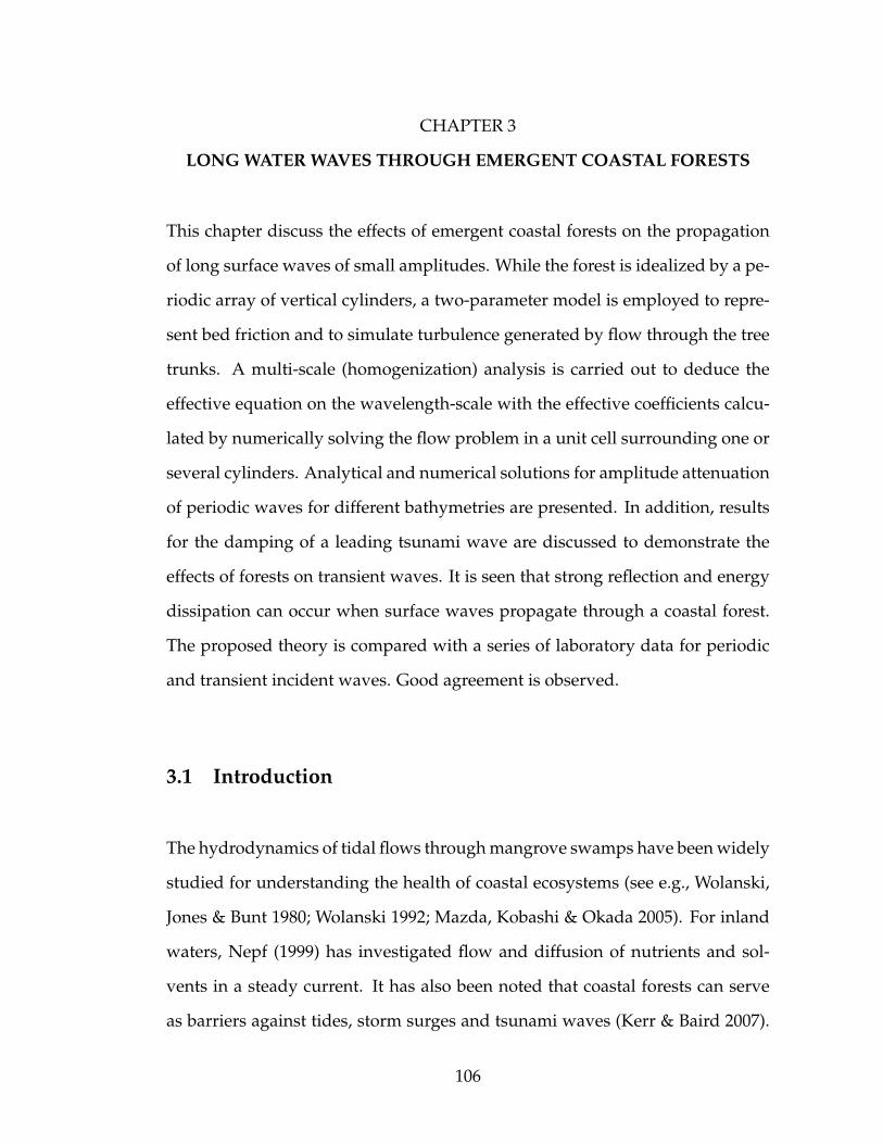
CHAPTER 3

LONG WATER WAVES THROUGH EMERGENT COASTAL FORESTS

This chapter discuss the effects of emergent coastal forests on the propagation

of long surface waves of small amplitudes. While the forest is idealized by a pe-

riodic array of vertical cylinders, a two-parameter model is employed to repre-

sent bed friction and to simulate turbulence generated by flow through the tree

trunks. A multi-scale (homogenization) analysis is carried out to deduce the

effective equation on the wavelength-scale with the effective coefficients calcu-

lated by numerically solving the flow problem in a unit cell surrounding one or

several cylinders. Analytical and numerical solutions for amplitude attenuation

of periodic waves for different bathymetries are presented. In addition, results

for the damping of a leading tsunami wave are discussed to demonstrate the

effects of forests on transient waves. It is seen that strong reflection and energy

dissipation can occur when surface waves propagate through a coastal forest.

The proposed theory is compared with a series of laboratory data for periodic

and transient incident waves. Good agreement is observed.

3.1 Introduction

The hydrodynamics of tidal flows through mangrove swamps have been widely

studied for understanding the health of coastal ecosystems (see e.g., Wolanski,

Jones & Bunt 1980; Wolanski 1992; Mazda, Kobashi & Okada 2005). For inland

waters, Nepf (1999) has investigated flow and diffusion of nutrients and sol-

vents in a steady current. It has also been noted that coastal forests can serve

as barriers against tides, storm surges and tsunami waves (Kerr & Baird 2007).

106

Historical evidence suggests that mangroves shielded the eastern coast of India

and reduced the number of deaths in the 1999 cyclone attack (Dasa & Vincent

2009). Records of the 2004 Indian Ocean tsunamis have given strong support

to the hypothesis of shore protection by mangroves and trees (Danielsen et al.

2005; Tanaka et al. 2007). Field experiments conducted in Australia and Japan

also demonstrated that during high tides only 50% of incident wave energy

is transmitted through forests over a distance of 200 m (Massel, Furukawa &

Binkman 1999). Indeed, this evidence has motivated suggestions and labora-

tory studies for planting a strip of trees along the shores. For instance, Hiraishi

& Harada (2003) have proposed the Green Belt with trees planted in water to

guard against tusnami attacks. Through a seires of experimental studies, Irtem

et al. (2009) demonstrated that trees planted on the landward side of the shore

can reduce the maximum run-up of a model tsunami by as much as 45%. Au-

gustin, Irish & Lynett (2009) and Thuy et al. (2009) have both reported laboratory

studies of wave damping by emergent cylinders along with numerical simula-

tions employing parameterized drag models.

In tidal swamps, part or most of the vegetation can be constantly immersed

in water. For effective protection against tsunamis, the needed thickness of the

green forest can be hundreds of meters. Hence an emerging plantation would

likely be a preferred option along well populated shores. It follows that the

understanding of the dissipation process of long waves through emergent veg-

etation is then essential. As can be expected, the dissipation of wave energy

is dominated by turbulence generated between the tree trunks, branches and

leaves throughout the entire sea depth, and by bed friction (Massel, Furukawa

& Binkman 1999). In general, numerical simulations shall provide the most

detailed and accurate predictions. Mo & Liu (2009), for instance, developed a

107

three-dimensional numerical model to study a solitary wave interacting with

a group of cylinders. Similarly, the large eddy simulation for open channel

flows through submerged vegetations has also been performed by Stoesser et al.

(2009). Both studies showed very good agreements when compared with lab-

oratory measurements. However, it is noted that in Stoesser et al. (2009) the

largest dimension in the computational domain is only about forty times of the

cylinder diameter. For the study by Mo & Liu (2009), about one and a half mil-

lion numerical cells are already required for the case of three cylinders. The

application to real problems can be computationally expensive. In practice, sev-

eral simplified mathematical models, all based on the common parameterized

drag force concept (e.g. Massel, Furukawa & Binkman 1999; Mazda, Kobashi &

Okada 2005; Teh et al. 2009), have been proposed to describe the most important

impact of coastal forests on surface wave propagation, namely the wave damp-

ing, without the demand of massive computation. In other words, instead of

resolving the detailed flow, effects of individual tree trunks are represented by

a bulk drag force term. The required model coefficient, i.e. the so-called drag

coefficient, is usually obtained by fitting the simulated free-surface profiles with

either laboratory measurements (e.g. Thuy et al. 2009) or field observations (e.g.

Mazda, Kobashi & Okada 2005). Although easy to implement, this kind of em-

pirical drag force model does not explain well how the detailed structure (i.e.

flow problem around tree trunks) affects the global behavior (i.e. the surface

wave transformation). One important goal of the present study is to systemati-

cally develop a theoretical model for describing the propagation and dissipation

process of long waves through emergent coastal forests. Through the substan-

tive effort of mathematical work, it is the hope to better address the effective

impact of the tree trunks than the existing drag force approach.

108

For the wave-forest problem being considered, the typical wavelength can

be of O(100) m while the diameter of tree trunks is O(0.5) m. Therefore, the

physical problem can be viewed as a micro-scale structure, i.e. the coastal trees,

subjected to a macro-scale forcing, i.e. the surface waves. The goal is then to

obtain a macro equation associated with the effective property of micro-scale

material in question. In other words, it is to find the representative macroscopic

property through multiple-scale analysis. To enable an analysis of the macro-

scale phenomenon from the micro-scale upwards, a number of simplifications

are made. The first is to consider only long waves of small amplitude so that

linearized approximation applies. The second is to model tree trunks by rigid

cylinders in a periodic array but neglect the effects of tree branches, roots, and

leaves. Turbulence generated between tree trunks is then described by the con-

stant eddy viscosity model. Finally, bottom friction is represented by a linear

law. With these simplifications, the two-scale method of homogenization is car-

ried out to derive the mean-field equations on the macro-scale. The effect of tree

trunks on the mean flows appears in macro equations through an effective hy-

draulic conductivity, which needs to be calculated from the solution of certain

initial-boundary-value problem on the micro-scale.

Several macro-scale problems will be discussed, both analytically and nu-

merically. For possible application to wind waves, the marco theory for lin-

ear progressive waves is first presented. Of interest to the protection against

tsunamis, the transient problem is then considered. Numerical examples will

be demonstrated under different incident wave conditions and coastal forest

configurations. The present theory is also examined by comparing with a se-

ries of laboratory experiments for both periodic and transient incident waves.

Comparison shows a very encouraging agreement.

109

3.2 Theoretical formulation

Consider a train of long water waves entering a thick coastal forest from the

open sea. Spanning a large horizontal area, vertical cylinders are erected in a

periodic array of uniform spacing to simulate emergent and rigid tree trunks.

An illustration of a coastal forest is provided in figure 3.1. The tree spacing ℓ

and the typical water depth h0 are assumed to be comparable. Since long waves

are considered, both ℓ and h0 are much smaller than the typical wavelength L0,

i.e., O(ℓ/L0) = O(h0/L0) ≪ 1. The variation of water depth is assumed to be

appreciable only over a distance scale comparable to a wavelength.

(a)ℓ

(b)

Figure 3.1: Problem sketch. (a) Illustration of a coastal forest. (b) Proposed

model: trees are modeled by emergent cylinders of a uniform

spacing ℓ. Only tree trunks are considered.

3.2.1 Governing equations and boundary conditions

For clarity, the horizontal and vertical quantities are separated: u = (u1, u2) and

w denote the horizontal and vertical velocity components in x = (x1, x2) and z

coordinates, respectively.

110

By the use of the eddy viscosity concept, the three-dimensional flow problem

is governed by the averaged Reynolds equations:

∂ui∂xi

+∂w

∂z= 0, i = 1, 2, (3.2.1)

∂ui∂t

+ uj∂ui∂xj

+ w∂ui∂z

= −1

ρ

∂p

∂xi+ νe

(∂2ui∂xj∂xj

+∂2ui∂z2

), i, j = 1, 2, (3.2.2)

and

∂w

∂t+ uj

∂w

∂xj+ w

∂w

∂z= −g − 1

ρ

∂p

∂z+ νe

(∂2w

∂xj∂xj+∂2w

∂z2

), j = 1, 2, (3.2.3)

where t denotes the temporal coordinate, g the gravitational acceleration, ρ the

water density, p the total pressure, and finally νe the eddy viscosity.

Several boundary conditions need to be satisfied. Along the slowly varying

seabed, z = −h(x), the no-slip condition is

ui = w = 0, z = −h(x). (3.2.4)

On the air-water interface, the kinematic boundary condition states

∂η

∂t+ ui

∂η

∂xi= w, z = η, (3.2.5)

where η depicts the free-surface displacement. The dynamic free-surface

boundary condition requires the vanishing of the normal stress

gη − p

ρ+ 2νe

∂w

∂z= 0, z = η, (3.2.6)

and of the tangential components

∂ui∂z

+∂w

∂xi= 0, z = 0. (3.2.7)

Note that the air is assumed to be free of stress and that zero atmospheric pres-

sure is also assumed. Finally, the kinematic boundary condition on the cylinder

walls, (x, z) ∈ SB , is satisfied by requiring

ui = w = 0, (x, z) ∈ SB. (3.2.8)

111

3.2.2 The linearized problem

Considering only infinitesimal waves, the above governing equations and

boundary conditions can be simplified. While the continuity equation remains

unchanged, the linearized momentum equations are obtained straightforwardly

from (3.2.2) and (3.2.3) as

∂ui∂t

= −1

ρ

∂p

∂xi+ νe

(∂2ui∂xj∂xj

+∂2ui∂z2

), i, j = 1, 2, (3.2.9)

and

∂w

∂t= −g − 1

ρ

∂p

∂z+ νe

(∂2w

∂xj∂xj+∂2w

∂z2

), j = 1, 2. (3.2.10)

Likewise, the kinematic condition on the free surface becomes

∂η

∂t= w, z = 0, (3.2.11)

and the requirements of the dynamic free-surface boundary condition reduce to

gη − p

ρ+ 2νe

∂w

∂z= 0, z = 0, (3.2.12)

∂ui∂z

+∂w

∂xi= 0, z = 0. (3.2.13)

The no-slip conditions on both the seabed and the cylinders stay the same.

3.2.3 Depth-integrated equations for the constant eddy viscos-

ity model

Let us further assume a constant eddy viscosity for the current consideration of

linear long waves through a coastal forest.

The typical tree spacing ℓ and the characteristic water depth h0 are used to

normalize the horizontal and vertical coordinates, respectively. Regarding the

112

time scale, the inverse of characteristic frequency, 1/ω, is adopted. For incom-

ing waves of a typical wave amplitude A, the scale of the dynamic pressure is

dictated as [p] = ρgA. In addition, two distinct length scales are presented as

ℓ is much smaller than the typical wavelength of long water waves, L0. As a

result, ℓ is regarded as the micro-length scale while L0 is the macro-length scale.

Employing also the common normalization for the water particle velocity, the

following dimensionless variables are introduced:

x∗i =xiℓ, z∗ =

z

h0

, t∗ = tω, h∗ =h

h0

η∗ =η

A, p∗ =

p

ρgA, ui

∗ =ui√

gh0A/h0

, w∗ =w

Aω

. (3.2.14)

The normalized conservation equations are then obtained from (3.2.1), (3.2.9)

and (3.2.10) as

∂u∗i∂x∗i

+ ǫ∂w∗

∂z∗= 0, (3.2.15)

and

ǫ∂u∗i∂t∗

= −∂p∗

∂x∗i+ ǫσ

[∂2u∗i∂x∗j∂x

∗j

+

(ℓ

h0

)2∂2u∗i∂z∗∂z∗

], (3.2.16)

∂w∗

∂t∗= −

(L0

h0

)2 [h0

A+∂p∗

∂z∗

]+ σ

[∂2w∗

∂x∗j∂x∗j

+

(ℓ

h0

)2∂2w∗

∂z∗∂z∗

]. (3.2.17)

In the above,

ǫ ≡ ℓ

L0

=ωℓ√gh0

≪ 1 (3.2.18)

defines the ratio of micro-to-macro length scales in which the characteristic

wavenumber is calculated as k0 = 1/L0. As for the turbulence parameter,

σ ≡ νe/ω

ℓ2, (3.2.19)

which can be interpreted as the square of ratio of turbulent diffusion length-

scale to tree spacing. Note that σ can take a wide range of values including

O(1) and is larger for longer waves or denser forests. It is also reminded that

ℓ/h0 = O(1).

113

From (3.2.11) to (3.2.13), the dimensionless boundary conditions on the free

surface are now

∂η∗

∂t∗= w∗, z∗ = 0, (3.2.20)

and

η∗ − p∗ + 2ǫ2σ∂w∗

∂z∗= 0, z∗ = 0, (3.2.21)

∂u∗i∂z∗

+ ǫ

(h0

ℓ

)2∂w∗

∂x∗i= 0, z∗ = 0. (3.2.22)

Denoting by a tilde the depth-averaged quantity,

F =1

h∗(x∗)

∫ 0

−h∗F dz∗, (3.2.23)

the depth-integrated continuity equation is deduced from (3.2.15) as

∂(h∗u∗i )

∂x∗i+ ǫ

∂η∗

∂t∗= 0, (3.2.24)

where the conditions (3.2.4) and (3.2.11) have been evoked. Also, it is assumed

that h = h(x) varies appreciably only over a distance of O(L0), but not over

O(ℓ).

Regarding the momentum equations, by similar depth-averaging of (3.2.16)

the vertical independent equation is

ǫ∂u∗i∂t∗

= −∂η∗

∂x∗i+ ǫσ

∂2u∗i∂x∗j∂x

∗j

+ ǫσ

h∗

(ℓ

h0

)2 [∂u∗i∂z∗

]0

−h∗. (3.2.25)

Note that the hydrostatic pressure is obtained from (3.2.17) by the use of the

long-wave assumption, i.e. h0/L0 ≪ 1. If the bottom shear is further repre-

sented by a linear term,

σ

h∗

(ℓ

h0

)2 [∂u∗i∂z∗

]

−h∗≡ αu∗i , (3.2.26)

114

we obtain from (3.2.25)

ǫ∂u∗i∂t∗

= −∂η∗

∂x∗i+ ǫσ

∂2u∗i∂x∗j∂x

∗j

− ǫαu∗i , (3.2.27)

where α can be viewed as a bottom friction parameter.

In physical units, (3.2.24) and (3.2.27) read

∂(hui)

∂xi+∂η

∂t= 0, (3.2.28)

∂ui∂t

= −g ∂η∂xi

+ νe∂2ui∂xj∂xj

− fui, (3.2.29)

where f is the common bed friction coefficient and α = f/ω. In addition, the

bottom shear stress, (3.2.26), becomes

νe

[∂ui∂z

]

−h= fhui. (3.2.30)

Both parameters νe and f (or σ and α in the dimensionless form) are given by

empirical formulae to be discussed shortly.

3.2.4 Estimation of controlling parameters

In the absence of direct measurements of turbulent momentum diffusivity in

water waves interacting with coastal forests, a reasonable compromise is to use

the empirical diffusivity for steady flows through emergent vegetation obtained

from extensive laboratory studies and field observations by Nepf and her col-

leagues (see e.g., Nepf, Sullivan & Zavistoski 1997; Nepf 1999; Tanino & Nepf

2008). In particular, results in the representative work, Nepf (1999), will be

adopted by the present study.

The collected data of Nepf (1999) are in a moderate range of Reynolds num-

ber, Red = U0d/ν = 400 − 2000, where ν is the molecular kinematic viscosity of

115

water, U0 the characteristic velocity, and d the diameter of rigid cylinders which

were used in the experiments to model stems of vegetations. Based on Fig. 10

in Nepf (1999), the turbulent diffusivity, νe, can be roughly fitted by the formula

νeU0ℓ≈ 1.86(1− n)2.06, (3.2.31)

where the range of porosity, n = 1 − π(d/2ℓ)2, of the available data is 0.945 ≤

n ≤ 0.994. Estimating U0 by the orbital velocity in open water, U0 =√gh0A/h0,

we obtain

σ ≈ 1.86(1− n)2.06 1

k0ℓ

A

h0

. (3.2.32)

It is remarked that the experimental data in Nepf (1999) are for randomly dis-

tributed cylinders arranged by using a random number generator with a dis-

placement of 0.1d. In the absence of empirical data from wave experiments for

a periodic array of cylinders, the preceding empirical relation will be adopted

even beyond the data range.

Bed friction in waves is often modeled by a formula quadratic in the local ve-

locity, but can be replaced by a linear law with the equivalent friction coefficient

(Mei 1983; Nielsen 1992),

f = fw4

3π

U0

h0

, (3.2.33)

where fw is a dimensionless friction factor in the quadratic law. Values of fw can

be estimated by an empirical formula of Swart (1974)

fw = exp[5.213κ0.194 − 5.977

], (3.2.34)

where κ = r/A with r being the bed roughness (see Nielsen 1992). Conse-

quently, by assuming U0 =√gh0A/h0 we obtain

α ≈ 0.424fw1

k0h0

A

h0

. (3.2.35)

116

It is known that fw = O(10−2) for 0 ≤ κ ≤ 0.1. For instance, fw = 0.045 corre-

sponds to a relative roughness of κ = 0.05.

Note that both σ and α depend on the wave amplitude, indicating the fact

that turbulence and bed friction are inherently nonlinear, here represented by

linear formulas. It is also obvious that effects of coastal vegetation are more sig-

nificant in stronger and longer waves as can be seen from (3.2.32) and (3.2.35).

To have some quantitative ideas, σ and α are estimated in Table 3.1 for several

different incident wave conditions and micro-scale geometry (i.e. various cylin-

der spacing ℓ and porosity n). Values of σ and α are larger for waves typical of

storm surges and tsunamis. It is remarked here that the Reynolds numbers for

these field examples are two orders of magnitude larger than those appearing

in the steady flow experiments of Nepf (1999). Despite the fact that turbulence

in steady flows interacting with cylinders is only a weak function of Reynolds

number for Red > 200 (Nepf 1999), new in-situ observations and laboratory tests

are desired to examine the applicability of (3.2.32) for oscillatory flows in field

conditions.

Table 3.1: Estimations of sample parameters. Values of σ and α are estimated

according to (3.2.32) and (3.2.35), respectively, with a constant friction

factor fw = 0.045.

h0 ℓ n 2π/ω A/h0 k0ℓ k0h0 Red σ α

2.5 (m) 1 (m) 0.80 10 (sec) 0.05 0.1269 0.317 1.25×105 0.027 0.003

2.5 (m) 1 (m) 0.85 1 (min) 0.05 0.0211 0.053 1.08×105 0.088 0.018

5.0 (m) 1 (m) 0.90 2 (min) 0.10 0.0075 0.037 2.50×105 0.217 0.051

5.0 (m) 2 (m) 0.90 10 (min) 0.05 0.0030 0.007 2.50×105 0.271 0.128

7.5 (m) 2 (m) 0.92 0.5 (hr) 0.05 0.0008 0.003 2.74×105 0.628 0.313

117

3.3 Method of homogenization

For the current problem, the primary interest is of predicting the global fea-

tures of wave propagation and dissipation through coastal forest. Therefore, it

is desirable to derive the equivalent macro-scale equations with the upscaling of

micro-scale effects. As there exists two vastly different length scales and the tree

trunks, which signifies the microstructure, are modeled by a periodic array of

cylinders, the method of homogenization based on the rigorous two-scale anal-

ysis applies (Mei 1992). The homogenization technique is a powerful mathemat-

ical tool for problems with well-separated scales to obtain macroscopic model

with effective homogenized coefficients determined by solving the associated

boundary-value problems, or initial-boundary-value problem for the unsteady

consideration, at successive smaller scales. In other words, this method serves

as a passage from microscopic description to macroscopic behavior of the sys-

tem (Bensoussan, Lions & Papanicolaou 1978) which enhances, without labori-

ous computations, the understanding of macro-scale quantities in the presence

of micro-scale variations.

The intention of this section is to give a brief introduction of the homogeniza-

tion technique, to the extent that it applies to the problem considered herein.

For the rigorous mathematical aspect of the homogenization theory and its ap-

plications, some main references are those of Bensoussan, Lions & Papanicolaou

(1978), Lions (1981), Sanchez-Palencia (1980), and Mei & Vernescu (2010).

A simple mathematical description of the homogenization method is first

118

provided. Consider a boundary-value problem in a domain Ω,

Au = f in Ω

u subject to proper conditions on boundary ∂Ω

,

where A is a linear operator. Assuming Ω is divided into equal cells of a order

of ǫ > 0 in size and the unknown solution u can be expressed by a multi-scale

series expansion

u = u0 + ǫu1 + ǫ2u2 + · · · ,

the homogenization process is to obtain and to prove that by certain averaging

limǫ→0

u = u0

A0u0 = f in Ω

u0 subject to proper conditions on boundary ∂Ω

.

In general, A is a linear partial differential operator while A0 is a integro-

differential operator.

For the current two-scale problem, the homogenization procedure can be

outlined as follows (Auriault 1991):

• Identifying the macro and micro scales. In this case, they are the wave-

length and tree spacing, respectively.

• Expressing the model equations in the dimensionless manner.

• Performing the perturbation analysis by expanding each unknown into an

infinite series in powers of the length-scale ratio, ǫ.

• Solving the resulting boundary-value or initial-boundary-value problems

at successive orders in ǫ.

• Obtaining the equivalent equations in macroscopic scale by averaging

over the microscopic scale.

119

In our analysis, microstructure is assumed to be periodic, i.e. trees are mod-

eled by a periodic array of cylinders. This strong assumption, although it can

not perfectly represent the situation in nature, provides an unique opportunity

to study the wave-forest problem more rigorously as it enables a mathematical

analysis for which the homogenization theory for periodic models has been well

established (see e.g. Bensoussan, Lions & Papanicolaou 1978). Furthermore, at

present no class of models is free of assumptions to describe the distribution

of coastal tress. The assumption of periodicity is therefore reasonable as a first

attempt to develop the theory model for the wave-forest problem. However, it

should be noted that the homogenization can actually be applied to any kind of

disordered medium. The mathematical justification involves theG-convergence

or H-convergence1. There is also a stochastic theory of homogenization (Allaire

2001). An introductory discussion is documented by Hornung (1996).

In the following sections, the macro theory for both linear progressive waves

and transient waves are developed based on the homogenization method.

3.4 Macro theory for linear progressive waves

For possible application to wind waves, let us first investigate sinusoidal waves

propagating through an emergent coastal forest. We shall work with dimen-

sionless depth-averaged quantities and equations as presented in section 3.2.3.

For brevity, tildes and asterisks, which represent depth-averaging and nondi-

mensionalization, will be omitted herein.

1G-convergence (Gamma-convergence), a notation of convergence for functionals, is used inthe proof of homogenization theory. H-convergence is the extension of G-convergence to thenon-periodic cases. Both are beyond the scope of this study and are not discussed here. For areference, see Tartar (2009).

120

For a linear progressive wave, the depth-averaged horizontal velocity and

the free-surface displacement can be expressed as

ui = ℜui(x)e−it

, η = ℜ

η(x)e−it

. (3.4.36)

Accordingly, conservation of mass, (3.2.24), can be rewritten as

−ǫηi +∂

∂xi(uih) = 0, i = 1, 2 (3.4.37)

while the momentum equation, (3.2.27), becomes

−ǫuii = − ∂η∂xi

+ ǫ

(σ

∂2ui∂xj∂xj

− αui), i, j = 1, 2. (3.4.38)

3.4.1 Homogenization

The forest region is modeled by periodic cells surrounding one or more surface-

piercing rigid cylinders. While the micro-scale motions between cylinders occur

in x coordinate, an additional macro-scale coordinate x′ = ǫx is introduced to

describe the wave motions. It is also reminded that the sea depth is assumed to

depend on x′ only, i.e., h = h(x′). Two-scale expansions are then assumed for

the dynamic unknowns:

ui = u(0)i + ǫu

(1)i + ǫ2u

(2)i + · · · , η = η(0) + ǫη(1) + ǫ2η(2) + · · · , (3.4.39)

where u(n)i = u

(n)i (x,x′) and η(n) = η(n)(x,x′) for n = 0, 1, 2, · · · . Consequently,

the perturbation problems of (3.4.37) and (3.4.38) can be organized as follows.

At O(ǫ0),

∂u(0)i

∂xi= 0, (3.4.40)

∂η(0)

∂xi= 0, (3.4.41)

121

and, at O(ǫ),

−iη(0) +∂(u

(0)i h)

∂x′i+ h

∂u(1)i

∂xi= 0, (3.4.42)

−iu(0)i = −∂η

(0)

∂x′i− ∂η(1)

∂xi+ σ

∂2u(0)i

∂xj∂xj− αu(0)

i . (3.4.43)

From (3.4.41), η(0) = η(0)(x′) is independent of x. Through the linearities of

(3.4.40) and (3.4.43), u(0)i and η(1) can be represented by

u(0)i (xk, x

′k) = −Kij(xk)

∂η(0)(x′k)

∂x′j, (3.4.44)

and

η(1) = −Aj(xk)∂η(0)(x′k)

∂x′j+ 〈η(1)〉, (3.4.45)

where coefficients Kij and Aj are periodic from cell to cell, and 〈·〉 denotes the

averaged quantity over the cell area Ω,

〈Q〉 =1

Ω

∫∫

Ωf

QdΩ (3.4.46)

with Ωf being the fluid part in the unit cell. Immediately, the cell average of A

is zero,

〈Aj〉 = 0. (3.4.47)

Note that both K and A are invariant in x′ as the local sea depth is a constant,

i.e, h = h(x′). Now, referring back to the continuity equation (3.4.40) and the

momentum equation (3.4.43), K and A must satisfy

∂Kij

∂xi= 0, x ∈ Ωf , (3.4.48)

and

σ∂2Kij

∂xk∂xk+ (i− α)K ij =

∂Aj∂xi− δij, x ∈ Ωf , (3.4.49)

where δij is the Kronecker delta. In addition, the no-slip condition on the cylin-

der walls requires

Kij = 0, x ∈ SB. (3.4.50)

122

Since η(0) is independent of micro-scale coordinates, the cell-averaged lead-

ing order velocity, 〈u(0)〉, is also of interest. Follow (3.4.44), we obtain

〈u(0)i 〉 = −〈Kij〉

∂η(0)(x′k)

∂x′j(3.4.51)

which is an extension of Darcy’s law with 〈Kij〉 denoting the spatial average

of the hydraulic conductivity tensor, Kij , over the unit cell. Both η(0) and 〈u(0)〉

describe the macro-scale wave motions with the micro-scale effects through 〈K〉.

Since 〈K〉 is the same for all x′, we shall first solve the tensorKij from the micro-

scale boundary-value-problem, (3.4.48) to (3.4.50). Afterwards, by taking the

cell average of mass conservation law at O(ǫ) and invoking the Gauss’ theorem

and periodicity, we obtain

−iη(0) +∂(〈u(0)

j 〉h)∂x′j

= 0. (3.4.52)

By further combining (3.4.51) with (3.4.52), we derive an equation for the cell-

averaged amplitude of the free-surface displacement,

iη(0) + 〈Kij〉∂

∂x′i

(h∂η(0)

∂x′j

)= 0. (3.4.53)

It is noted that the dimensionless hydraulic conductivity tensor Kij is normal-

ized by g/ω and it depends on the wave frequency through σ and α. In the

absence of forests and bottom friction, (3.4.49) gives Kij → iδij and accordingly

(3.4.51) and (3.4.53) reduce to the standard linearized equations governing in-

viscid shallow water waves.

The above perturbation analysis is very similar to that for steady flows (Ene

& Sanchez-Palencia 1975; Keller 1980) and monochromatic sound waves (Auri-

ault 1991; Mei & Vernescu 2010) through a periodic porous medium.

In the following sections, we shall first discuss the solution procedure of the

123

cell problem and then turn to the macro-scale application of linear progressive

waves propagating through a coastal forest.

3.4.2 Numerical solution of the micro-scale cell problem

The micro-scale problem, (3.4.47) to (3.4.50), is similar to that for sound waves

through a periodic porous medium (Sheng & Zhou 1988; Zhou & Sheng 1989;

Auriault 1991) and shall be solved numerically, here by the finite element

method. For this purpose the governing equations, (3.4.48) and (3.4.49), are

first rewritten in the weak form as

∫∫

Ω

∂Kij

∂xiψj dΩ = 0, (3.4.54)

and

∫∫

Ω

[(α− i)Kij +

∂Aj∂xi− δij

]φij+σ∇Kij ·∇φij dΩ = σ

∫

∂Ω

∂Kij

∂nφij ds, (3.4.55)

where ∂Ω denotes the boundary with n being its outward normal. The above

integral equations are then discretized by linear triangular elements. As an ex-

ample of a circular cylinder inside a unit square cell, figure 3.2 shows the dis-

cretization and the spatial variation of K11 for n = 0.85, σ = 0.088 and α = 0.018

which correspond to the second parameter set listed in Table 3.1. Due to cellular

symmetry, 〈Kij〉 = Kδij = (KR + iKI)δij is isotropic.

Figure 3.3 shows the normalized hydraulic conductivity,K, against the wave

frequency parameter, k0h0, for n = 0.8, 0.85, 0.9 and the following parameters:

h0 = 2.5 m, ℓ = 1 m, A/h0 = 0.05 and fw = 0.045. The imaginary part of K

vanishes as k0h0 → 0 because in a steady stream the averaged and local flows

are always in phase. While KI (the imaginary part) increases monotonically

124

n = 0.92, σ = 0.036, α = 0.020

−0.50.0

0.5−0.5 0.0 0.5

0.0

0.5

1.0

x1

Real part

x2

K11

−0.50.0

0.5−0.5 0.0 0.5

0.0

0.5

1.0

x1

Imaginary part

x2

Figure 3.2: Top: Discretization of a typical unit cell with a circular cylinder

inside a square. Bottom: Spatial distributions, K11(x). Due to

isotropy, only K11 is needed. The input parameters are listed

in the second row of Table 3.1.

with both k0h0 and n, at a fixed porosity KR (the real part) first grows then

decreases with increasing wave frequency. In physical dimensions, the real part

of the conductivity is expected to decrease monotonically from a finite value as

k0h0 increases. Since K is normalized by g/ω, value of KR approaches zero for

very long waves. It is also noted thatKR is bigger for larger n at very small k0h0.

However, the opposite is true for relatively shorter waves.

3.4.3 1HD application: constant water depth

Applications to one horizontal dimension (1HD) problems are demonstrated.

In fact, the consideration is of normal incident waves propagating into the

forest characteristized by a symmetric cellular configuration. If the bottom

125

0.0 0.1 0.2 0.30.0

0.2

0.4

0.6

0.8

1.0

k0h0

KR

n = 0.90n = 0.92n = 0.94

0.0 0.1 0.2 0.30.0

0.2

0.4

0.6

0.8

1.0

k0h0

KI

n = 0.90n = 0.92n = 0.94

Figure 3.3: Hydraulic conductivity K as a function of k0h0 for the case of

periodic waves. Left: real part, KR; Right: imaginary part, KI .The cell geometry is a circular cylinder inside a square with

n = 0.8, 0.85, 0.9, respectively. In all cases, h0 = 2.5 m, ℓ = 1 m,

A/h0 = 0.05 and fw = 0.045 are fixed. The values of σ and α are

calculated from (3.2.32) and (3.2.35) for any given n and k0h0.

bathymetry is also simple, analytical solutions are then possible which can pro-

vide useful insights on the wave-forest problem. For simplicity, uniform water

depth everywhere, i.e. h = 1, is concerned. Several different scenarios are to be

discussed.

(1) Very thick forest

Let the forest occupies the semi-infinite domain, 0 < x′ < ∞. Inside the forest,

the governing equation for η(0) can be deduced from (3.4.53) as

∂2η(0)

∂x′2+

i

Kη(0) = 0, x′ > 0. (3.4.56)

It is reminded that K = KR + iKI is the hydraulic conductivity. The solution is

η(0) = Be−x′/a (3.4.57)

126

with

a =√iK = aR + iaI =

√|K|ei( θ

2+π

4), θ = tan−1 KI

KR <π

2, (3.4.58)

and B the coefficient to be determined. From (3.4.51) and (3.4.57), the corre-

sponding velocity is also obtained:

〈u(0)〉 =1

aKBe−x′/a. (3.4.59)

Solutions (3.4.57) and (3.4.59) represent a propagating wave with decreasing

amplitude.

Regarding the open water region, x′ < 0, solutions can be expressed as

η = eix′

+Re−ix′ , (3.4.60)

u = eix′ −Re−ix′ . (3.4.61)

It is noted that in this region both the turbulence and bottom friction are ne-

glected.

Matching at x′ = 0 of the surface displacement and horizontal velocity yields

two algebraic equations for R and B, with the solutions

R =a−Ka+K , (3.4.62)

and

B =2a

a+K . (3.4.63)

Notice that |R| and |B| denote the reflection and transmitted coefficients, respec-

tively. From (3.4.58), (3.4.62), and (3.4.63), it can be readily shown that

|R|2 =

(aR −KR

)2+(aI −KI

)2

(aR +KR)2 + (aI +KI)2 ≤ 1, (3.4.64)

127

and

|B|2 =4|a|2

(aR +KR)2 + (aI +KI)2 ≥ 0. (3.4.65)

Clearly waves are damped out after a distance of x′ = O(√|K|).

For possible relevance to weak wind waves, in figure 3.4 the computed K

values shown in figure 3.3 are used to demonstrate the square of the reflection

coefficient, |R|2, and the free-surface elevations inside the forest for different

porosities and dimensionless frequency. It is evident that reflection increases

with the wave period (or wavelength) and decreases with larger porosity. The

wave amplitude is more rapidly damped for longer waves as shown in figure

3.4-(b).

0.0 0.1 0.2 0.310

−5

10−4

10−3

10−2

10−1

100

k0h0

|R|2

(a) n = 0.90

n = 0.92n = 0.94

0 2 4 6 8 10−1.0

−0.5

0.0

0.5

1.0

1.5

x′

η(0)

(b) n = 0.92 k0h0 = 0.05

k0h0 = 0.10k0h0 = 0.20

Figure 3.4: Periodic waves propagating through a semi-infinite forest in a

constant water depth region: (a) The square of the reflection

coefficient, |R|2, against the wave frequency parameter, k0h0,

for n = 0.8, 0.85, 0.9; (b) Snapshots of free-surface elevation at

the phase t = 0 for the case of n = 0.85. As can be seen, |R|2grows with increasing wavelength (i.e. smaller k0h0). In all

calculations, the input parameters are same as those used in

figure 3.3.

128

(2) A finite forest belt

Consider next a finite forest belt, 0 < x′ < L′B , where L′

B = k0LB is the ratio

of forest thickness (LB) to typical wavelength (1/k0). In the region of incidence,

x′ < 0, solutions (3.4.60) and (3.4.61) still hold. Behind the forest, x′ > L′B , the

solutions can be expressed as

η = u = Teix′

, x′ > L′B. (3.4.66)

Inside the forests, 0 < x′ < L′B, the solution of free-surface elevation is now of

the form

η(0) = Be−x′/a +Dex

′/a. (3.4.67)

Matching the displacement and velocity at both x′ = 0 and x′ = L′B, the coeffi-

cients are found to be

R =(a2 −K2)(−1 + e2L

′

B/a)

(a+K)2e2L′

B/a − (a−K)2

,

B =2a(a+K)e2L′

B/a

(a+K)2e2L′

B/a − (a−K)2

,

D =−2a(a−K)

(a+K)2e2L′

B/a − (a−K)2

,

T =4aKeL′

B(1/a−i)

(a+K)2e2L′

B/a − (a−K)2

.

(3.4.68)

Taking L′B →∞, R and B reduce to those shown in (3.4.62) and (3.4.63), respec-

tively. Consider again the cell with a single cylinder at the center, the effects of

different forest thickness and porosity are shown in figure 3.5. Values of σ and

α are calculated from (3.2.32) and (3.2.35) respectively for n = 0.8, 0.85, 0.9 with

all other parameters listed in the second row of Table 3.1. As can be seen, the

reflection coefficient, |R|, does not vary monotonically with respect to the di-

mensionless forest thickness, L′B, due to interference among multiply reflected

and transmitted waves. In addition, as L′B →∞ the values of |R| reach asymp-

totically to those for the semi-infinite forest given in (3.4.62) and are indicated

129

by triangles in figure 3.5-(a). In subplot (b), it is seen that spatial decay of the

surface waves is more rapid for greater L′B = k0LB , i.e., thicker forest relative to

the wavelength.

0 2 4 6 80.00

0.03

0.06

0.09

0.12

0.15

L′

B

|R|2

(a) α = 0.02

n = 0.90, σ = 0.057n = 0.92, σ = 0.036n = 0.94, σ = 0.020

L′

B →∞

0 2 4 6 8 10−1.0

−0.5

0.0

0.5

1.0

1.5

x′

η(0)

(b) n = 0.92 LB = 0.85

LB = 1.25LB = 4.00

Figure 3.5: Periodic waves propagating through a finite patch of forest in

a constant water depth. (a): The square of reflection coeffi-

cient, |R|2, against the dimensionless thickness of forest, L′B ;

(b): Snapshots of free-surface elevation at t = 0 for n = 0.85 and

L′B = 0.85, 1.25, 4. Lines are the results from (3.4.67) and (3.4.68)

while triangles give |R|2 of L′B → ∞ predicted by (3.4.64). In

all calculations, k0ℓ0 = 0.0211 and k0h0 = 0.053, corresponding

to the second row of Table 3.1.

3.4.4 1HD application: variable water depth

In this section, let us consider again one horizontal dimension (1HD) problems

but now with the effects of varying water depth. To seek analytical solutions,

we limit ourselves to the case where h = h(x′) varies linearly in x′ over some dis-

tance. For a general bathymetry, numerical computations of macro-scale equa-

130

tions are required.

(1) Forest on a plane beach

Consider a flat open water region connects to a beach of constant slope s covered

entirely by a forest. Accordingly, the sea depth is

h =

1, x′ < 0

1− sx′, 0 < x′ < 1/s. (3.4.69)

Over the sloping bottom, the mean wave equation, (3.4.53), becomes

iη(0) − sK∂η(0)

∂x′+ (1− sx′)K∂

2η(0)

∂x′2= 0. (3.4.70)

Assuming perfect reflection at the shore, the solution on the beach can be ex-

pressed as

η(0) =B√sJ0

(2i

sa

√1− sx′

), 0 < x′ < 1/s, (3.4.71)

where Jn(z) is the Bessel function of the first kind and B the undetermined

coefficient. Note that the parameter a is defined in (3.4.58) while the solutions

in the incidence region are given in (3.4.60) and (3.4.61). Again, the matching

conditions at x′ = 0 require

1 +R =B√sJ0

(2i

sa

)

1−R = − B√s

√aJ1

(2i

sa

) . (3.4.72)

Solving the above algebraic equations, we obtain

R =J0

(2isa

)+ aJ1

(2isa

)

J0

(2isa

)− aJ1

(2isa

) , (3.4.73)

and

B =2√s

J0

(2isa

)− aJ1

(2isa

) . (3.4.74)

131

As a check, let us consider the limiting case of no forest. Then, K → i and the

reflection coefficient becomes

R→ J0(2/s) + iJ1(2/s)

J0(2/s)− iJ1(2/s). (3.4.75)

Similarly, the coefficient B reduces to

B → 2√s

J0(2/s)− iJ1(2/s). (3.4.76)

For very small bottom slope s≪ 1, (3.4.75) and (3.4.76) recover the solutions of

Keller & Keller (1964). Figure 3.6 plots the free-surface elevation inside forests

for different n. Behaviors of these examples are similar to those of constant

water depth cases.

0 2 4 6 8 10−1.0

−0.5

0.0

0.5

1.0

1.5

x′

η(0)

n = 0.90, σ = 0.057, α = 0.02n = 0.92, σ = 0.036, α = 0.02n = 0.94, σ = 0.020, α = 0.02

Figure 3.6: Snapshots at t = 0 of periodic waves propagating through

a forest on a plane beach of slope s = 1/20. Porosities are:

n = 0.8, 0.85, 0.9 and k0h0 = 0.053. Other inputs are shown

in the second row of Table 3.1). The corresponding hydraulic

conductivity, K, is shown in figure 3.3.

132

(2): A finite forest belt on a sloping step

Now, consider the sea bed to be a plane slope in the middle region and horizon-

tal on both sides, i.e.,

h =

1, x′ < 0

1− sx′, 0 < x′ < L′B

1− sL′B, x′ > L′

B

. (3.4.77)

The forest covers the sloping part only. From (3.4.70), the solution on the slope

becomes

η(0) =1√s

BI0

(2a

s

√1− sx′

)+DK0

(2a

s

√1− sx′

), (3.4.78)

where In(z) and Kn(z) are the modified Bessel function of the first kind and

second kind, respectively. Coefficients B and D are yet to be determined. Re-

garding solutions in both open water regions, the transmitted wave in x′ > L′B

is

η = Teimx′

, u = mTeimx′

with m =1√h′B

=1√

1− sL′B

, (3.4.79)

while the free-surface elevation and horizontal velocity in the incident wave

region, x′ < 0, are again given in (3.4.60) and (3.4.61).

Matching at both x′ = 0 and x′ = L′B, the unknown coefficients can be found

as

R =c34 [(c13 − c23)c42 − (c12 − c22)c43]− c44 [(c13 − c23)c32 − (c12 − c22)c33]c34 [(c13 + c23)c42 − (c12 + c22)c43]− c44 [(c13 + c23)c32 − (c12 + c22)c33]

,

B =2(c33c44 − c34c43)

c34 [(c13 + c23)c42 − (c12 + c22)c43]− c44 [(c13 + c23)c32 − (c12 + c22)c33],

D =2(c32c44 − c34c42)

(c12 + c22)(c33c44 − c34c43)− (c13 + c23)(c32c44 − c34c42),

T =−2(c32c43 − c33c42)

c34 [(c13 + c23)c42 − (c12 + c22)c43]− c44 [(c13 + c23)c32 − (c12 + c22)c33],

(3.4.80)

133

where

c12 =1√sI0 (Z) , c13 =

1√sK0 (Z) ,

c22 = − 2i

s√s

1

ZI1 (Z) , c23 =

2i

s√s

1

ZK1 (Z) ,

c32 =1√sI0

(Z√h′B

), c33 =

1√sK0

(Z√h′B

),

c42 = − 2i

s√s

1

Z√h′B

I1

(Z√hB

), c43 =

2i

s√s

1

Z√h′B

K1

(Z√h′B

),

c34 = exp (imL′B) , c44 = m exp (imL′

B) ,

(3.4.81)

with Z = 2/(sa). Recall a and m are defined in (3.4.58) and (3.4.79), respectively.

For the case of L′B → 1/s, it can be shown that the above solutions for R and B

recover to those presented in (3.4.73) and (3.4.74).

In figure 3.7, the square of reflection coefficient, |R|2, is displayed against the

dimensionless thickness of forests, L′B . Again, |R|2 does not vary monotonically

with L′B as discussed in section 3.4.3-(2). The features are qualitatively similar

to those for a horizontal seabed.

0 2 4 6 8 100.00

0.03

0.06

0.09

0.12

0.15

|R|2

L′

B

α = 0.02

n = 0.90, σ = 0.057n = 0.92, σ = 0.036n = 0.94, σ = 0.020

L′

B →∞

Figure 3.7: Square of the reflection coefficient, |R|2, for waves through a fi-

nite forest belt of dimensionless thickness L′B on a sloping step

with a constant slope s = 1/20. Parameters used in all calcula-

tions are same as those shown in figure 3.6.

134

3.4.5 Experiments and numerical simulation for periodic waves

Mei et al. (2011) reported a laboratory study on surface waves propagating

through a model forest, which provides a great opportunity to examine the per-

formance of the present theory. For completeness, the experiments are first in-

troduced followed by the corresponding comparisons between the theoretical

predictions and measurements.

A series of laboratory experiments has been conducted in the glass-walled

wave flume (32 m long, 0.54 m wide, and 0.6 m deep) in the Hydraulics Labo-

ratory at the Nanyang Technological University, Singapore (Mei et al. 2011). At

one end, the flume is equipped with a piston-type wave maker (Wallingford,

UK) which has active wave absorbing capability. At the other end, there is an

energy absorbing beach of 1-to-7 slope to minimize the reflection. In the center

region of constant water depth, perspex cylinders of 1 cm diameter were in-

stalled as a periodic array spanning the entire width of the flume. The model

forest has a total thickness of 1.08 m and a porosity n = 0.913. Several resistance-

type wave gauges (Wallingford, UK) were employed to record time histories of

free-surface elevation. The experimental setup is sketched in figure 3.8 with the

exact positions of wave gauges listed in Table 3.2. Overall, three types of inci-

Table 3.2: Positions of wave gauges (in meters) (see figure 3.8). The origin is set at

the front edge of the model forest. In some tests records were not taken

from all gauges.

Wave type G1 G2 G3 G4 G5 G6 G7 G8

Periodic waves −3.085 −2.935 −2.685 −0.005 0.540 1.085 2.025 2.275

Transient packets — — −3.025 −0.100 0.715 — 2.260 2.660

Solitary waves — −3.205 −3.005 −0.005 0.540 1.085 1.385 —

135

≈ ≈ ≈

∇ ≈ ≈ ≈

G1 G2 G3 G4 G5 G6 G7 G8

Figure 3.8: Sketch of experimental setup at NTU (Mei et al. 2011) with sam-

ple arrangement of wave gauges (not to scale). The model for-

est has a width of 0.54 m and a thickness of 1.08 m. Wave flume

is 0.54 m wide and 0.6 m deep. The length of constant depth

part is 25 m. Gauge locations for different incident waves are

listed in Table 3.2.

dent waves were studied: periodic waves, transient wave packets and solitary

waves. Data of surface displacement were collected at a sampling rate of 100 Hz

for periodic waves and at 50 Hz for transient cases. In addition, the Reynolds

numbers in the experiments were in a moderate range of 200 to 2500 which is

close to that of Nepf (1999) (i.e. 400 < Red < 2000).

In this section, we shall only examine the periodic waves in three different

water depths: 12, 15 and 20 cm. Since long waves of accurately measurable am-

plitude are easily nonlinear in a small depth, data for relatively shorter waves

were also taken. Conditions for the first set of tests are listed in Table 3.3. Figure

3.9 compares the reflection coefficient (|R|) and transmission coefficient (|T |) ex-

tracted from the experimental data with predictions according to (3.4.68). The

quantity 1− |R|2 − |T |2 which measures the amount of wave energy dissipated

by the model forest is also shown. It is reiterated that in the present theory the

required controlling parameter σ is estimated by (3.2.32). Also, α = 0 is taken to

account for the smooth tank bottom. Despite the appearance of nonlinear sig-

nature of higher harmonics in waves of shorter periods, the agreement between

136

theoretical predictions and the measured data is generally well. Note that for

longer waves, although the parameters σ and α are larger, the ratio L′B = k0LB

is smaller since LB = 1.08 m is fixed, resulting in less attenuation hence higher

transmission. Discrepancy between theory and observation is evident for longer

waves (i.e. small k0LB) where the predicted |R| and |T | are underestimated and

overestimated, respectively. This remarkable difference is possibly attributable

to the reflection of very long waves from the sloping beach measured at roughly

9%. As |T | is around 0.8, contribution of the reflected wave off the beach can be

significant.

Table 3.3: Experimental conditions for periodic waves through a coastal forest at

NTU (Mei et al. 2011). In all cases, the forest thickness is LB = 1.08

m and porosity n = 0.913. Controlling parameter σ is estimated by

(3.2.32). See figure 3.9 for corresponding reflection and transmission

coefficients.

Period (s) h0 (m) 2A (m) 1/k0 (m) k0h0 k0LB Red σ

0.8 0.12 0.0232 0.1207 0.9940 8.9464 1049 0.0047

1.0 0.12 0.0253 0.1587 0.7560 6.8044 1144 0.0068

1.2 0.12 0.0272 0.1956 0.6135 5.5218 1230 0.0090

1.4 0.12 0.0246 0.2318 0.5177 4.6593 1112 0.0096

1.6 0.12 0.0239 0.2676 0.4485 4.0362 1081 0.0108

1.8 0.12 0.0243 0.3031 0.3959 3.5633 1099 0.0124

1.9 0.12 0.0243 0.3208 0.3741 3.3670 1099 0.0132

2.0 0.12 0.0068 0.3384 0.3546 3.1915 307 0.0039

2.5 0.12 0.0065 0.4261 0.2816 2.5344 294 0.0047

3.0 0.12 0.0050 0.5134 0.2337 2.1036 226 0.0043

To test the robustness of the present theory, the predictions of |R| and |T |

are examined against additional data for a wide range of wave amplitudes in

137

1 2 3 4 5 6 7 8 9 100.0

0.2

0.4

0.6

0.8

1.0

k0LB

|T |

|R|

1 2 3 4 5 6 7 8 9 100.0

0.2

0.4

0.6

0.8

1.0

k0LB

1−|R|2−|T|2

Figure 3.9: Left: Reflection coefficient (|R|) and transmission coefficient

(|T |) as functions of k0LB ; Right: 1− |R|2 − |T |2 vs. k0LB . Hol-

low symbols: measured data; solid symbols: predictions by

(3.4.68).

deeper water depths as detailed conditions listed in Table 3.4. For a total of 70

cases, three wave periods (Set A, B, C: 0.8, 1, 1.2 s), two water depths (0.15, 0.2

m), and wave amplitudes ranged from 1 to 4 cm are considered. Figure 3.10

shows the corresponding predictions of reflection and transmission coefficients

and the degree of dissipation, 1 − |R|2 − |T |2, by (3.4.68) along with measured

data. Again, the quantitative agreement is quite reasonable even for weakly

nonlinear waves of intermediate length.

138

Table 3.4: Experimental conditions for a wide range of wave amplitudes shown

in figure 3.10. Controlling parameter σ is estimated by (3.2.32). In all

cases, the forest thickness is LB = 1.08 m and porosity n = 0.913. The

corresponding Reynolds numbers are in the range of 490 < Red < 2520.

Set Period (s) h0 (m) 1/k0 (m) k0h0 k0LB σ/(A/h0)

0.15 0.130 1.152 8.297 0.0528A 0.8

0.20 0.141 1.415 7.642 0.0573

0.15 0.174 0.864 6.223 0.0703B 1.0

0.20 0.193 1.037 5.597 0.0782

0.15 0.215 0.696 5.014 0.0873C 1.2

0.20 0.243 0.825 4.454 0.0983

3.5 Macro theory for transient waves

Of interest to the protection against distant tsunamis, a transient wave invading

a coastal forest is now considered. Working equations are the dimensionless

depth-integrated conservation equations, (3.2.24) and (3.2.27). Again, tildes and

asterisks will be omitted for brevity.

3.5.1 Homogenization

Similar to the analysis for the periodic waves (see section 3.4.1), the dimension-

less horizontal velocity and the free-surface elevation are expressed by the two-

scale expansions as

ui = u(0)i + ǫu

(1)i + ǫ2u

(2)i + · · · , η = η(0) + ǫη(1) + ǫ2η(2) + · · · , (3.5.82)

where u(n) = u(n)(x,x′, t) and η(n) = η(n)(x,x′, t) for n = 0, 1, 2, · · · . Conse-

quently, perturbation equations can be deduced from the conservation laws of

139

0.04 0.08 0.12 0.16 0.200.00

0.25

0.50

0.75

1.00|T |

|R|

Set A

0.04 0.08 0.12 0.16 0.200.00

0.25

0.50

0.75

1.00

1−|R|2−|T|2

Set A

0.04 0.08 0.12 0.16 0.200.00

0.25

0.50

0.75

1.00|T |

|R|

Set B

0.04 0.08 0.12 0.16 0.200.00

0.25

0.50

0.75

1.00

1−|R|2−|T|2

Set B

0.04 0.08 0.12 0.16 0.200.00

0.25

0.50

0.75

1.00

A

h0

|T |

|R|

Set C

0.04 0.08 0.12 0.16 0.200.00

0.25

0.50

0.75

1.00

A

h0

1−|R|2−|T|2

Set C

Figure 3.10: Reflection (|R|) and transmission (|T |) coefficients of periodic

waves crossing a finite patch of forest in constant water depth,

as functions of amplitude-to-depth ratio (A/h0). Symbols

show the measured data while lines show the predictions by

(3.4.68). Triangles and solid lines are for h0 = 0.15 m, while

circles and dashed lines are for depth h0 = 0.2 m. See Table

3.4 for experimental conditions.

mass and momentum. At O(ǫ0),

∂u(0)i

∂xi= 0, (3.5.83)

∂η(0)

∂xi= 0, (3.5.84)

140

where the free-surface height varies only over the macro scale, η(0) = η(0)(x′, t).

At O(ǫ),

∂η(0)

∂t+∂(u

(0)i h)

∂x′i+ h

∂u(1)i

∂xi= 0, (3.5.85)

∂u(0)i

∂t= −∂η

(0)

∂x′i− ∂η(1)

∂xi+ σ

∂2u(0)i

∂xj∂xj− αu(0)

i . (3.5.86)

Due to the dynamic signature and the linearity of the above equations, the un-

knowns u(0) and η(1) can be formally represented by convolution integrals as

u(0)i (xk, x

′k, t) = −

∫ t

0

Kij(xk, t− τ)∂η(0)(x′k, τ)

∂x′jdτ, (3.5.87)

and

η(1) = −∫ t

0

Aj(xk, t− τ)∂η(0)(x′k, τ)

∂x′jdτ + 〈η(1)〉, (3.5.88)

where 〈·〉 denotes the cell average defined by (3.4.46). We shall now derive the

governing equations for K and A, i.e., construct the micro-scale cell problem. It

follows from (3.5.83) that

∂Kij

∂xi= 0, ∀x ∈ Ω. (3.5.89)

Utilizing the expressions of (3.5.87) and (3.5.88) and evoking the Leibniz rule,

the left-hand-side and the right-hand-side of (3.5.86) become

−∫ t

0

∂Kij(xk, t− τ)∂t

∂η(0)(x′k, τ)

∂x′jdτ −Kij(xk, 0+)

∂η(0)(x′k, t)

∂x′j(3.5.90)

and

−∂η(0)

∂x′i−∫ t

0

dτ∂η(0)

∂x′j

−∂Aj(xk, t− τ)

∂xi+ σ

∂2Kij(xk, t− τ)∂xk∂xk

− αKij

, (3.5.91)

respectively. Imposing the initial condition,

Kij(xk, 0+) = δij, (3.5.92)

the last term in (3.5.90) can be rewritten as

−Kij(xk, 0+)∂η(0)(x′k, t)

∂x′j= −∂η

(0)(x′k, t)

∂x′i(3.5.93)

141

which clearly cancels the first term in (3.5.91). Finally, (3.5.86) becomes∫ t

0

∂Kij

∂t

∣∣∣∣t−τ

∂η(0)

∂x′j

∣∣∣∣τ

dτ =

∫ t

0

−∂Aj∂xi

+ σ∂2Kij

∂xk∂xk− αKij

t−τ

∂η(0)

∂x′j

∣∣∣∣τ

dτ.

(3.5.94)

Hence, we obtain

∂Kij

∂t= −∂Aj

∂xi+ σ

∂2Kij

∂xk∂xk− αKij, ∀x ∈ Ω, t > 0. (3.5.95)

In addition, Kij and Aj must be Ω−periodic and satisfy

Kij = 0, x ∈ SB, (3.5.96)

and

〈Aj〉 = 0. (3.5.97)

Defined by (3.5.89), (3.5.92) and (3.5.95) to (3.5.97), the initial-boundary-value

problem in the unit cell can be solved numerically. Note that these equations,

hence their solution, are independent of the macro coordinates. Afterwards, the

cell-averaged horizontal velocity can be obtained as

〈u(0)i (xk, x

′k, t)〉 = −

∫ t

0

〈Kij(xk, t− τ)〉∂η(0)(x′k, τ)

∂x′jdτ, (3.5.98)

which is the transient Darcy’s law. By taking the cell average of (3.5.85) and

invoking Gauss’ theorem and Ω−periodicity, we obtain

∂η(0)

∂t+

∂

∂x′i

(〈u(0)

i 〉h)

= 0. (3.5.99)

Combination of (3.5.99) with (3.5.98) leads to the mean-field equation for the

free-surface displacement,

∂η(0)

∂t=

∂

∂x′i

[h(xk

′)

∫ t

0

〈Kij(xk, t− τ)〉∂η(0)(x′k, τ)

∂x′jdτ

], (3.5.100)

which can also be expressed as

∂2η(0)

∂t2=

∂

∂x′i

[h(xk

′)〈Kij(xk, 0)〉∂η(0)(x′k, t)

∂x′j

]

+∂

∂x′i

[h(xk

′)

∫ t

0

∂〈Kij(xk, t− τ)〉∂τ

∂η(0)(x′k, τ)

∂x′jdτ

],

(3.5.101)

142

displaying the dual effect of wave propagation and diffusion. Similarly, (3.5.98)

can be rewritten as

∂〈u(0)(xk, x′k, t)〉

∂t= −〈Kij(xk, 0)〉∂η

(0)(x′k, t)

∂x′j−∫ t

0

∂〈Kij(xk, t− τ)〉∂τ

∂η(0)(x′k, τ)

∂x′jdτ.

(3.5.102)

Clearly, these equations reduce to the familiar shallow water equations in the

absence of forest.

3.5.2 Numerical solution for the transient cell problem

The micro-scale cell problem forKij andAj needs be solved numerically. Again,

the finite element method is used. The initial-boundary-value problem shall be

first rewritten in the weak form. Thus, from (3.5.89),

∫∫

Ω

∂Knij

∂xiψj dΩ = 0, (3.5.103)

and from (3.5.95),

∫∫

Ω

[Knij −Kn−1

ij

∆t+∂Anj∂xi

+ αKnij

]φij + σ∇Kn

ij · ∇φij dΩ = σ

∫

∂Ω

∂Knij

∂nφij dγ,

(3.5.104)

where the superscript n denotes the n-th time step and the time derivative is

discretized by the two-point backward difference. These two integral equations

are then discretized spatially by linear triangular elements. Recall the initial and

boundary conditions are given in (3.5.92) and (3.5.96), respectively. In addition,

(3.5.97) is imposed.

As an example, a micro-scale geometry consisting of a circular cylinder in-

side a unit square is considered. A sketch of the cell configuration is shown in

the top panel of figure 3.2. Again due to micro-scale symmetry, 〈Kij〉 = Kδij is

143

isotropic. For this sample cell setting, the numerical results, as shown in figure

3.11, suggest that K can be approximated by

K(t) = K0e−bt, (3.5.105)

where K0 and b depend on the geometry of the micro-scale problem and the

controlling parameters σ and α. In particular, K0 decreases while b increases

with decreasing porosity n, hence dissipation is stronger for a denser forest.

0.0 0.1 0.2 0.3 0.4 0.5−6

−5

−4

−3

−2

−1

0

t

lnK

n = 0.85n = 0.90n = 0.95

Figure 3.11: Sample solutions of lnK(t) for a symmetric microscale config-

uration (see the top panel in figure 3.2). The corresponding

controlling parameters σ and α are calculated by (3.2.32) and

(3.2.35) respectively using n = 0.85, 0.9, 0.95 and all other pa-

rameters are listed in the third row in Table 3.1.

To examine the role of the cell geometry, in figure 3.12 the conductivities

of two different micro-scale configurations, i.e., one cylinder per cell versus

five per cell, are compared. Other parameters such as n, α, σ, and cell size

are kept the same. Note that for the same porosity, the cell with multiple

cylinders has a smaller permeability. This is qualitatively consistent with the

empirical formula of Carmen-Kozeny for steady seepage flow (Carmen 1937),

where the permeability is not only a function of porosity but also propor-

144

tional to the square of the ratio L = (total volume)/(total surface area) of a

grain. For the current circular cylindrical grains, we shall redefine it as L =

(total sectional area)/(total circumference). The ratio for the single-cylinder cell

is then L1 = d/4 with d denoting the cylinder diameter. For the five-cylinder cell,

the diameter of the four small cylinders is d/2√

2 and that of the larger cylinder

is d/√

2. Therefore, L5 = d/6√

2 = L1/3. This explains the large difference of

conductivities.

It is remarked that the use of a constant σ in figure 3.12 implies that we have

extended the empirical formula (3.2.32), which is designed for estimating σ of

single-cylinder cellular configuration, to a more general case. This of course is

not necessary true. Careful examination on the capability of (3.2.32) by future

laboratory and field studies is essential.

(C) (Cs)

0.0 0.1 0.2 0.3 0.4 0.5−10

−8

−6

−4

−2

0

t

lnK

(C)(Cs)

Figure 3.12: Effects of the cell geometry on the dynamic permeability, K:

the first two panels show two different cell configurations

while the last one compares the results of lnK. In both exam-

ples, n = 0.9, σ = 0.217 and α = 0.0051, which corresponds to

the third row in Table 3.1.

145

3.5.3 Numerical model for the macro-scale solutions

Once the dynamic conductivity 〈Kij〉 is obtained from the cell problem, the pre-

ceding macro initial-boundary-value problem (i.e., (3.5.100) along with proper

initial and boundary conditions) can be solved numerically in general. For this

purpose, an implicit finite-difference numerical model is developed. The spa-

tial derivatives are discretized by second-order difference and the time deriva-

tive approximated by the first-order backward difference, with uniform grids

being used in both temporal and spatial domains. In addition, the convolution

time integral is calculated by simple trapezoidal rule. As the model equation,

(3.5.100), is practically similar to the common linear shallow water equations

and the proposed numerical scheme is rather ordinary, the discrete differencing

equation is not presented here.

It shall be noted that hampered by the convolution integral, especially be-

ing evaluated by the low-order trapezoidal rule, the numerical calculation can

be very time consuming. Furthermore, the size of time stepping can not be

too large for the accuracy consideration. A practical approach to estimate the

required grid resolution is to perform the similar problem in the absence of for-

est and then compare the results with the existing exact solutions or numerical

simulations.

3.5.4 1HD application: tsunami waves through a thick forest

In this section, a train of leading tsunami waves entering a coastal forest is dis-

cussed. While in general the numerical results are accomplishable as described

in section 3.5.3, analytical solution of certain simplified case is valuable for pro-

146

viding useful physical understanding and validating discrete computations. To

make the problem analytically tractable, let us consider waves attack a semi-

infinite forest normally in a constant depth region. More precisely, we study

only one horizontal dimension (1HD) case with a uniform sea depth every-

where. Note that the micro-scale symmetry has also been assumed.

(1) Boundary conditions for 1HD constant depth problem

We shall first discuss the associated boundary conditions for the complete for-

mulation of the macro-scale problem.

Inside the forest, the governing equations for η(0) and 〈u(0)〉 are (3.5.100) and

(3.5.98), respectively. The initial condition in the forest is assumed to be

η(0)(x′, 0) = 0. (3.5.106)

In the open water, x′ < 0, waves can be described by

η−(x′, t) = I(t− x′) +R(t+ x′), u−(x′, t) = I(t− x′)−R(t+ x′), (3.5.107)

where I stands for incident waves and R for reflected waves. Matching the

free-surface elevation and velocity at the edge, x′ = 0, we obtain

I(t) =1

2

(η(0)(0, t)−

∫ t

0

〈Kij(x, t− τ)〉∂η(0)(x′, τ)

∂x′

∣∣∣∣x′=0

dτ

), (3.5.108)

and

R(t) =1

2

(η(0)(0, t) +

∫ t

0

〈Kij(x, t− τ)〉∂η(0)(x′, τ)

∂x′

∣∣∣∣x′=0

dτ

). (3.5.109)

Therefore, the boundary condition for η(0) at the incident edge, x′ = 0, is

η(0)(0, t)−∫ t

0

〈Kij(x, t− τ)〉∂η(0)(x′, τ)

∂x′

∣∣∣∣x′=0

dτ = 2I(t). (3.5.110)

147

If the forest is of finite extent L′B , the solution in the open water on the trans-

mission side is of the form

η+(x′, t) = u+(x′, t) = T (t− x′), L′B < x′ <∞, (3.5.111)

where T denotes the transmitted waves. Continuity of both the surface height

and horizontal velocity at x′ = L′B requires

η(0)(L′B, t) = T (t− L′

B)

−∫ t

0

〈K(x, t− τ) 〉∂η(0)(x′, τ)

∂x′

∣∣∣∣x′=L′

B

dτ = T (t− L′B)

, (3.5.112)

which implies the boundary condition

η(0)(L′B, t) +

∫ t

0

〈K(x, t− τ) 〉∂η(0)(x′, τ)

∂x′

∣∣∣∣x′=L′

B

dτ = 0. (3.5.113)

For a semi-infinite forest, i.e. L′B → ∞, the condition (3.5.113) should be re-

placed by

η(0) → 0, x′ ∼ ∞. (3.5.114)

(2) Analytical solutions

Solutions for L′B ∼ ∞ are now to be obtained by the use of Laplace transform.

For brevity, the superscripts (.)(0) and (.)′ will be omitted. Taking the Laplace

transform and applying the convolution theorem, an ordinary differential equa-

tion for the transformed free-surface displacement can be deduce from (3.5.100),

sη = K∂2η

∂x2, x > 0, (3.5.115)

where s is the transform variable and () denotes the transformed functions in

s−domain. The solution satisfying the boundary condition (3.5.110) is

η =

(2

1 +√sK

)I(s) exp

(−x√

s

K(s)

), x > 0. (3.5.116)

148

From the Laplace transforms of (3.5.108) and (3.5.109), we also obtain

R =

(1−

√sK

1 +√sK

)I. (3.5.117)

It has been shown by Kajiura (1963) (see also Mei 1983 p. 31, Eq. (1.42))

that the leading tsunami from a distant and long fault line is a propagating one-

dimensional wave train approximately expressed by Airy function with am-

plitude decaying in time as tµ−1, where µ = 2/3 if the seafloor rises or falls

vertically (line source) and µ = 1/3 if the seafloor tilts along the fault line (line

dipole). For analytical convenience, let us take

I(t) = Atµ−1 sinωt, t > 0 (3.5.118)

to model roughly the leading tsunami approaching the edge of the forest. The

Laplace transform of (3.5.118) is obtained as (see Bateman 1954 p. 152, Eq. (15))

I(s) =iA

2Γ (µ)

[1

(s+ iω)µ− 1

(s− iω)µ

], (3.5.119)

in which Γ(·) denotes the Gamma function.

Assuming (3.5.105) for K, the Laplace transform of K is then

K =

∫ ∞

0

e−stK0e−b tdt =

K0

s+ b. (3.5.120)

Consequently, the Laplace transform of the free-surface displacement in the for-

est becomes

η =iAΓ (µ)

1 +√sK0/(s+ b)

[1

(s+ iω)µ− 1

(s− iω)µ

]e−x√s(s+b)/K0 . (3.5.121)

The free-surface elevation can be obtained by inverse Laplace transform,

η =1

2πi

∫

γ

estηds, (3.5.122)

149

where γ is the path parallel to the imaginary axis in the s plane and to the right of

all singularities. It is generally difficult to obtain the inversion, (3.5.122). How-

ever, expressions at small and large time can be easily achieved, and will be

presented in the following. While the small time solution describes the onset

of tsunami waves, the large time behavior is useful for evaluating the tsunami

inundation.

(2)-I: Solution at small time

Regarding the solution at small time, the asymptotic behavior is dominated by

the inverse Laplace transform at large s (see §124, Carslaw & Jaeger 1963). For

large s, (3.5.121) becomes

η(s) ≈ CSA

2Γ (µ)

i

sµ

[(1 + i

ω

s

)−µ−(1− i

ω

s

)−µ]e−sx/

√K0

= CSA

2Γ (µ)

i

sµ

[(1− i

µω

s

)−(1 + i

µω

s

)+H.O.T .

]e−sx/

√K0

= CSA

2Γ (µ)

[2µω

sµ+1+H.O.T .

]e−sx/

√K0 , (3.5.123)

where

CS = lims→∞

2

1 +√sK0/(s+ b)

=2

1 +√K0

(3.5.124)

andH.O.T . denotes the truncated higher-order terms. Hence

η(s) ≈ CSAΓ (µ)µω

e−sx/

√K0

sµ+1

. (3.5.125)

Now, consider

G(s) =e−sx/

√K0

sµ+1, (3.5.126)

the inverse Laplace transform is

G(t) =1

2πi

∫

γ

e−s(x/√K0−t)

sµ+1ds. (3.5.127)

For x/√K0 − t > 0, a large semicircle in the right half plane is chosen as the

integration path. By Cauchy’s theorem and Jordan’s lemma, the inverse Laplace

150

transform is zero. Therefore, there is no disturbance if x/√K0 > t. For ξ =

t− x/√K0 > 0, the inverse Laplace transform is

G(t) =1

2πi

∫

Γ

esξ

sµ+1ds, (3.5.128)

which can be evaluated as (see Bateman 1954 p. 238, Eq. (1))

G(t) =ξµ

Γ(1 + µ)=

(t− x/

√K0

)µ

Γ(1 + µ). (3.5.129)

Finally, at small t we obtain

η(x, t) ≈

0, if x/√K0 > t

2

1 +√K0

Aω(t− x/

√K0

)µ, if x/

√K0 < t

, (3.5.130)

where the property Γ(1 + µ) = µΓ(µ) has been evoked. The solution suggests

that the head of tsunami enters the forest with the dimensionless speed of√K0.

SinceK0 is small when the porosity, n, is small, a dense forest slows the invasion

of an incoming tsunami.

(2)-II: Solution at large time

It is known (§126, Carslaw & Jaeger 1963) that the asymptotic behavior of η(x, t)

at large t can be found from its Laplace transform near the singular points with

the largest real part in the complex plane of s. For (3.5.121) we shall only look

at three singularities,

s = 0, s = ±iω, (3.5.131)

all of which have the same real part, 0, and neglect the contribution from the

pole at

1 +

√sK0

s+ b= 0, i.e., s = − b

1−K0

< 0 (3.5.132)

since K0 < 1. The final solution is the sum from three singularities in (3.5.131).

151

Near s = 0, the leading term of (3.5.121) is

η(x, s ≈ 0) ≈ iAΓ(µ)

[1

(iω)µ− 1

(−iω)µ

]e−x√sb/K0

= 2AΓ(µ)ω−µ sinµπ

2e−x√sb/K0 , (3.5.133)

From Bateman (1954) (see p. 245, Eq. (1)), the inverse Laplace transform for

e−√λs is

1

2√π

√λ

t3/2exp

(− λ

4t

). (3.5.134)

Thus,

[η(x, t)]0 ≈2

t3/2x√b/K0

2√π

AΓ(µ)

ωµsin

µπ

2exp

(− bx2

4K0t

), (3.5.135)

which dies out with t rapidly.

Next, consider the singularity at s = iω. Notice first that

exp(−x√s(s+ b)/K0

)≈ exp

(−x√

(iω)(iω + b)/K0

), (3.5.136)

and√

(iω)(iω + b)/K0 = ei(π/4+ψ/2)√√

ω2 + b2ω/K0, (3.5.137)

where

tanψ =ω

b. (3.5.138)

From Carslaw & Jaeger (1963) (see p. 280), the leading term of the inverse

Laplace transform is

[η(x, t)]iω ≈ −CL+

i

2

A

t1−µexp

(−xei(π/4+ψ/2)

√√ω2 + b2ω/K0

)eiωt, (3.5.139)

where

CL+ =2

1 +√sK0/(s+ b)

∣∣∣∣∣s= iω

=

(1 +

√ωK0/

√ω2 + b2ei(π/4−ψ/2)

)−1

. (3.5.140)

152

For the singularity at s = −iω, the approximate inverse Laplace transform is the

complex conjugate of (3.5.139),

[η(x, t)]−iω ≈ CL−i

2

A

t1−µexp

(−xe−i(π/4+ψ/2)

√√ω2 + b2ω/K0

)e−iωt, (3.5.141)

where

CL− =

(1 +

√ωK0/

√ω2 + b2e−i(π/4−ψ/2)

)−1

. (3.5.142)

Since contribution from s = 0 is relatively small at large time, we obtain

η ≈ [η(x, t)]iω + [η(x, t)]−iω

=2A

t1−µ(1 + δ cosψ′′) sin (ωt− ξ cosψ′)− δ sinψ′′ cos (ωt− ξ sinψ′)

1 + 2δ cosψ′′ + δ2e−ξ cosψ′

,

(3.5.143)

where

ξ = x

√√ω2 + b2

ω

K0

, δ =

√ωK0√ω2 + b2

, ψ′ =π + 2ψ

4, ψ′′ =

π − 2ψ

4

(3.5.144)

and ψ = tan−1 (ω/b) defined in (3.5.138). Solution (3.5.143) represents a spatially

damped progressive wave. The temporal attenuation follows the pattern of the

leading wave before entering the forest. For good protection, the thickness of

the forest should be greater than

O

1√√

ω2 + b2 ωK0

, (3.5.145)

which suggests that the thickness must be large for long tsunamis.

(2)-III: Comparison with numerical results

In figure 3.13, the above asymptotic solutions are compared with numerical re-

sults obtained by the method described in section 3.5.3. For illustration, the

incident wave of the form (3.5.118) with A = ω = 1 and µ = 2/3 (vertical rise

153

or fall of the seafloor) is used. The cell geometry and controlling parameters are

the same as the case of n = 0.9 displayed in figure 3.11, which correspond to the

third parameter set listed in Table 3.1. While numerical results are carried out

using (∆x,∆t) = (10−3, 10−4) for all time, analytical solutions are only given at

small and large time by (3.5.130) and (3.5.143), respectively. Figures 3.13-(a) and

-(b) show good agreement in the two limiting ranges of time. In subplot (c), the

approximation for large time according to (3.5.143) is seen to agree well with the

discrete computations at all stations, for nearly all time beyond t ≈ 5.

3.5.5 Comparison with laboratory experiments

Laboratory studies of both transient wave packets and long pulses entering a

coastal forest have also been conducted by Mei et al. (2011). The experiment

details have been described in section 3.4.5. In particular, sketch of the setup

and positions of wave gauges are displayed in figure 3.8 and Table 3.2, respec-

tively. Corresponding numerical simulations by the same algorithm described

in section 3.5.4 are performed for comparison.

Experimental data of two transient wave packets each of which consists of

a few oscillatory waves are first presented, as shown in figure 3.14. The first

packet (set I) is led by a prominent crest (elevation) and the second (set II) by

a trough (depression). In both tests, time histories of surface elevation were

recorded by five wave gauges where stations G3 and G4 were located in the re-

gion of incidence, G5 inside the forest, and two additional, G7 and G8, available

far behind the model forest (see Table 3.2 for the exact positions). Bottom fric-

tion is ignored (α = 0) in our numerical simulations. The parameter σ = 0.0085

154

0 0.001 0.002 0.003 0.004 0.005

0

0.01

0.02

0.03

0.04

η

x

(a) Snapshots of η at small time

t = 0.0025t = 0.0050

0 0.5 1 1.5−0.6

−0.3

0

0.3

0.6

η

x

(b) Snapshots of η at large time

t = 20t = 30

0 5 10 15 20 25 30−1

−0.5

0

0.5

1

1.5

η

t

(c) Histories of η at fixed locations

x = 0.1x = 0.5x = 1.0

Figure 3.13: Leading waves of a tsunami entering a deep forest in a con-

stant water depth. Snapshots of free-surface elevation are

shown in (a) for small time, and in (b) for large time. Dots are

the numerical results. Lines represent the respective asymp-

totic solutions. Time histories at different stations are com-

pared in (c) where dots are the numerical results for all time

and lines are the asymptotic solution for large time.

is again calculated from (3.2.32) by using h0 = 0.12 m, estimating the charac-

teristic wave period to be 3 seconds and taking the mean of the maximum crest

height and trough depth to be A. While (3.5.113) is imposed as the boundary

condition at the exit of the forest, records of free-surface elevation at G4 (0.1 m

from the leading edge of the forest) are used directly as the boundary value at

the incident edge. The reason for replacing the condition (3.5.110) is that inci-

dent and reflected waves cannot be easily separated as stations G3 and G4 are

155

close to the entrance of the forest. Comparison between predictions and mea-

surements at station G5 which is to the right of the forest center is shown in

figure 3.14. Spatial attenuation can be easily seen and the theory fits reasonably

well with the data for roughly the first 15 seconds of both records. After that,

reflection from the sloping beach arrived at station G5 but is not accounted for

in our simulations.

0 3 6 9 12 15 18 21 24 27−0.50

−0.25

0.00

0.25

0.50

0.75

Time (sec)

Fre

e-su

rface

elev

ati

on

(cm

)

Set I

G4 (Exp)G5 (Exp)G5 (Num)

0 3 6 9 12 15 18 21 24 27−0.50

−0.25

0.00

0.25

0.50

0.75

Time (sec)

Fre

e-su

rface

elev

ati

on

(cm

)

Set II

G4 (Exp)G5 (Exp)G5 (Num)

Figure 3.14: A transient wave packet crossing a forest. Solid and dashed

lines: experimental data at G4 and G5, respectively. Bold line:

numerical prediction at G5.

In the next set of experiments, long pulses with the profile of a soliton were

156

generated by displacing the piston wave maker as a hyperbolic tangent function

of time. Five incident waves of increasing amplitudes were tested in a constant

depth of h0 = 0.12 m, with all detailed conditions listed in Table 3.5. It is re-

marked that some cases were for moderately nonlinear waves, which does not

correspond well to the applicability of the present linear theory, due to the dif-

ficulty of accurately measuring small-amplitude long waves in a shallow depth

of 0.12 m. For each test, records of surface height were collected at six wave

Table 3.5: Experimental conditions for solitary waves crossing a 1.08 m

thick model forest with porosity n = 0.913. Records of corre-

sponding free-surface elevation are shown in figures 3.16 to 3.18.

Set h0 (m) H (cm) 1/k0 (m) k0LB Red σ

1 0.12 0.48 0.693 1.573 217 0.0056

2 0.12 0.93 0.498 2.190 420 0.0078

3 0.12 1.34 0.415 2.629 606 0.0094

4 0.12 1.78 0.360 3.030 850 0.0108

5 0.12 2.26 0.319 3.414 1022 0.0122

gauges. In reference to figure 3.8, the gauge locations are listed in Table 3.2. In

figure 3.15, the record at G2, the closest gauge station to the wave marker, is first

checked with the classical solitary wave,

η(x, t) = Hsech2[k0(x−

√g(h0 +H) t)

], k0 =

√3H

4h30

, (3.5.146)

where H is the maximum wave height and k0 the characteristic wave number

of the soliton. The agreement is essentially good, although some waviness was

found at the tail due to the finite increments of the paddle displacement driven

by a step motor. In numerical simulations, (3.5.146) is used as the incident wave

I(t) in the boundary condition (3.5.110) at G4 while (3.5.113) is imposed at the

157

exit of the forest. Also, σ is calculated by (3.2.32) and α = 0 is employed to

represent the frictionless smooth laboratory flume.

0.0 0.5 1.0 1.5 2.0 2.5 3.0 3.5 4.0−0.5

0.0

0.5

1.0

1.5

2.0

2.5

Time (sec)

Fre

e-su

rface

elev

ati

on

(cm

)

Measurementssech2()

Figure 3.15: Sample record of incident wave at station G2. In this case,

the water depth is 12 cm and wave height is 2.26 cm. The

classical solitary wave solution, (3.5.146), is also shown for

comparison.

Figures 3.16 and 3.17 compare the measured and predicted free-surface ele-

vations of two almost linear waves of solitons with H/h0 = 0.04, 0.0775 at sta-

tions G4, G5, and G6. Amplitude attenuation is evident at G5 and G6 located

at the center of the forest and near the exit edge, respectively. For larger am-

plitudes (H/h0 = 0.1117, 0.1483), the agreement is still quite good despite the

linearized theory, as seen in figure 3.17. Expectedly, the measured data show

slightly higher phase speed than the prediction and the discrepancy becomes

more significant as the wave height of incident solitary waves increases. This is

of course the effect of nonlinearity in the experiment.

Finally, records of a relatively large solitary wave of finite length (H/h0 =

158

0 1 2 3 4 5

0.0

0.5

1.0G4

Set 1: H/h0 = 0.0400

ExpNum

0 1 2 3 4 5

0.0

0.5

1.0G5

Fre

e-su

rface

elev

ati

on

(cm

)

ExpNum

0 1 2 3 4 5

0.0

0.5

1.0G6

Time (sec)

ExpNum

0 1 2 3 4 5

0.0

0.5

1.0

1.5G4

Set 2: H/h0 = 0.0775

ExpNum

0 1 2 3 4 5

0.0

0.5

1.0

1.5G5

ExpNum

0 1 2 3 4 5

0.0

0.5

1.0

1.5G6

Time (sec)

ExpNum

Figure 3.16: Comparison between model predictions (dashed lines) and

laboratory measurements (solid lines) at stations: G4, G5 and

G6. Wave heights (H) of the incident solitary waves are 0.48

cm for Set 1 and 0.93 cm for Set 2, respectively. See figure 3.8

and Table 3.2 for the positions of wave gauges.

0.1883) are shown in figure 3.18. In this test, noise from the step motor was

harder to eliminate. We use the record for 0 < t < 7.18 second at G2 as the

incident wave in (3.5.110) for simulations. This duration corresponds to the

time needed for reflection from the forest to be felt at G2, as estimated by using

the wave speed of the linearized theory. Strong spatial attenuation of the main

crest is evident. The small reflected wave is also reasonably well predicted.

159

0 1 2 3 4 5

0.0

0.5

1.0

1.5

2.0G4

Set 3: H/h0 = 0.1117

ExpNum

0 1 2 3 4 5

0.0

0.5

1.0

1.5

2.0G5

Fre

e-su

rface

elev

ati

on

(cm

)

ExpNum

0 1 2 3 4 5

0.0

0.5

1.0

1.5

2.0G6

Time (sec)

ExpNum

0 1 2 3 4 5

0.00.51.01.52.02.5

G4

Set 4: H/h0 = 0.1483

ExpNum

0 1 2 3 4 5

0.00.51.01.52.02.5

G5

ExpNum

0 1 2 3 4 5

0.00.51.01.52.02.5

G6

Time (sec)

ExpNum

Figure 3.17: Comparison of model predictions (dashed lines) with mea-

surements (solid lines) at stations G4, G5 and G6 for Set 3

(H = 1.34 cm) and Set 4 (H = 1.78 cm). The water depth

is h0 = 12 cm.

3.6 Conclusions

Starting from a set of linearized conservation equations, a micro-mechanical the-

ory of the damping of long waves by coastal forests has been developed. Mod-

eling turbulence by assuming a constant eddy viscosity and bottom friction by

a linear formula, with coefficients taken from experiments for steady flows, the

asymptotic method of homogenization (multiple scales) is employed to derive

the mean-field equations for the macro-scale motion. The effective conductivity

for the mean-field equation is obtained by numerically solving certain canoni-

cal problems in a micro-scale cell. Analytical solutions of the macro-scale prob-

160

0 2 4 6 8 10 12

0

1

2

3

Set 5: H/h0 = 0.1883

Incidnet ←−

−→ Reflected

G2

Fre

e-su

rface

elev

ati

on

(cm

)

ExpNum

0 2 4 6 8 10 12

0

1

2

3G4

Time (sec)

ExpNum

0 2 4 6 8 10 12

0

1

2

3G5

ExpNum

0 2 4 6 8 10 12

0

1

2

3G6

Time (sec)

ExpNum

Figure 3.18: Comparison between theory (dashed lines) and measure-

ments (solid lines) at selected stations: G2, G4, G5 and G6.

Wave height of the incident solitary wave is H = 2.26 cm and

the water depth is h0 = 12 cm.

lems are discussed for sinusoidal waves, which are relevant to wind waves.

Solution of the transient problem simulating the head of a tsunami is also dis-

cussed. Comparison of theoretical predictions with laboratory records of linear

and moderately nonlinear waves shows surprisingly good agreement, suggest-

ing the robustness of the current approximate theory.

In nature, the nearshore dynamics of tsunami can be highly nonlinear. The

averaging method of homogenization which enables a micro-mechanical theory

can in principle be extended for weakly nonlinear waves. The present study,

however, shows that even for moderately nonlinear waves the linearized the-

161

ory presented herein is not far off the mark, due likely to strong dissipation in

the forest. Extension to account for weak nonlinearity is worthwhile for predict-

ing mass transport and convective diffusion of particulates in coastal seas with

vegetation.

In the present theory, the controlling parameters σ and α are crucial in deter-

mining the hydraulic conductivity. The parameter σ, which is calculated based

on the experimental results of steady flow study by Nepf (1999) and models the

turbulences between tree trunks, is particularly important. Due to the lack of

reliable data and information, it is not easy to address the criticism of the di-

rect application to wave-driven turbulence. Although the comparisons of free-

surface elevation between theoretical predictions and laboratory measurements

have shown good agreements, more fundamental studies on determining σ un-

der a variety of wave conditions are needed to provide firmer basis. Two possi-

ble approaches are the direct laboratory measurements of turbulent diffusivity

and the direct numerical simulation of wave-cylinder interactions calibrated by

measured free-surface profiles and velocity data. For the later, the existing nu-

merical models, for instance the three-dimensional model of Mo & Liu (2009),

can be adopted while for the former one may extend the methodology of Nepf

(1999) to estimate the turbulent diffusivity in a wave-forest system.

Some results presented in this chapter have been documented in Mei et al.

(2011).

162

CHAPTER 4

LONG-WAVE MODELING IN THE LAGRANGIAN DESCRIPTION

This chapter essentially studies the runup and drawdown of leading tsunami

waves by the use of Lagrangian long-wave equations. The runup rule, based on

the assumption that solitary wave is the paradigm for leading tsunami waves,

has particular engineering interest as it is convenient to use. However, it has

been cautioned that solitary waves are not good representatives for tsunamis.

This issue will be investigated by carefully examining the roles of incident wave

surface profiles and beach slope on the processes of wave runup and draw-

down.

4.1 Introduction

The runup of long water waves has been investigated extensively by tsunami

research community as the reliable prediction of the wave runup is crucial to the

prevention and mitigation of tsunami hazard. Some benchmark studies are the

work of Carrier & Greenspan (1958) who solved analytical the nonlinear shal-

low water equations, and the laboratory experiment on the runup of solitary

waves by Synolakis (1987). Many numerical models, including Lynett (2002)

and Zelt (1991), have also been proven to simulate the runup process fairly

well. However, some fundamental problems still require more careful consider-

ation. For instance, solitary waves have long been used to simulate the leading

tsunami waves as they are theoretically well-understood and easy to control in

the laboratory experiments. Several runup rules have been derived based on the

solitary wave paradigm (see e.g. Synolakis 1987). Recently, Madsen, Fuhrman &

163

Schaffer (2008) raised a concern that the application of the solitary wave theory

to the runup of leading tsunami waves is incorrect since the length of solitary

wave is constrained by the wave nonlinearity and it is not the case for leading

tsunami waves. Several field observations have been found to support their

argument (see section 4.3 for more details). A brief discussion using the 2004

Indian Ocean tsunamis as an example can also be found in Segur (2007).

This chapter will discuss whether the use of solitary wave leads to any sig-

nificant effects on the prediction of tsunami runup. As the process of tsunami

runup and rundown is of particular interest, a well-known numerical challenge

is the treatment of the moving shoreline. This issue has been addressed by sev-

eral approximation techniques with various degrees of success. For instance,

the higher order interpolation method suggested by Lynett (2002) has gained

increasing popularity. An alternative to the common Eulerian approach is to

adopt the Lagrangian description, in which the moving shoreline becomes a

fixed point. Thus, no additional numerical approximation is necessary for com-

puting the runup and drawdown of the shoreline. This motivates the choice of

the Lagrangian approach in the present study.

In the following, more detailed discussions on scaling leading tsunami

waves by solitary waves are first presented. The direct evidence, based on

the field observations of the 2004 Indian Ocean tsunamis and the 2011 Tohoku

tsunamis, is provided to confirm that the leading tsunami waves can not be

characterized as solitary waves. The Lagrangian long-wave equations, i.e. the

depth-integrated equations, are introduced. A numerical method, validated by

comparing the model results with both existing analytical solutions (Carrier &

Greenspan 1958) and experimental data (Synolakis 1987; Kanoglu & Synolakis

164

1998), is then developed to study runup processes of different kinds of incident

long waves. The simulations are compared with solutions associated with soli-

tary waves in order to discuss the effects of incoming wave characteristics and

bottom topography on the runups of leading tsunami waves.

4.2 On the solitary wave paradigm for tsunami waves

Since the 1970s, most of experimental and analytical investigations on tsunami

runup and inundation processes have inherited the assumption that the leading

tsunami waves can be scaled by solitary waves (for reviews, see e.g. Madsen,

Fuhrman & Schaffer 2008; Synolakis & Kanoglu 2009). It is fair to say that this is

mainly motivated by a series of laboratory experiments by J. L. Hammack in the

1970s, as it has been demonstrated that the leading wave evolving from a sur-

face disturbance could develop into a solitary wave (see Segur 2007 for a brief

discussion). In a constant water depth, a solitary wave, which is the solution

of the Korteweg-DeVries (KdV) equation, remains a permanent waveform both

spatially and temporally. Naturally, this feature is very attractive in performing

experimental studies and in deriving theoretical solutions for tsunami research.

Indeed, several formulae have been established relating the maximum runup

height to the incident solitary wave height and the beach slope (e.g., Pedersen

& Gjevik 1983; Synolakis 1987). Although these studies provide a quick assess-

ment of tsunami inundation, the legitimacy of using solitary waves to model

leading tsunami waves has been challenged. For instant, the numerical sim-

ulation by Madsen, Fuhrman & Schaffer (2008) showed that the leading wave

evolving from an initial rectangular-shaped free-surface hump becomes a soli-

tary wave only after propagates over a very long distance. In other words, the

165

required distance to form a solitary wave is much greater than the relevant geo-

physical scale of possible tsunami propagation. This point, in fact, has been

long aware of even by the early work of J. L. Hammack (see Segur 2007). Note

also that in the classical reference of Mei, Stiassnie & Yue (2005), the range of

validity of KdV equation has been discussed which essentially addressed the

same issue.

It is clear that the direct application of the runup formulae based on soli-

tary wave to tsunami runup needs to be re-examined. As an attempt, Mad-

sen & Schaffer (2010), by adopting the solution procedure outlined in Syno-

lakis (1987)1, obtained approximate explicit solutions describing the elevations

and velocities at maximum runup and drawdown for sinusoidal waves, single

sech2-shape waves, and N -waves. A swift numerical (or semi-analytical) solu-

tion for transient waves evolving from initially static rectangular disturbances

was also demonstrated. Madsen & Schaffer (2010) greatly advanced the work

by Synolakis (1987). However, their explicit solutions are limited to waves of

symmetric surface shape propagating over a two-section bathymetry consists

of an offshore constant water depth region attached to a uniform sloping beach.

It is also worth to mention that although the analytical approach of Madsen &

Schaffer (2010), which is based on the hodograph transformation method advo-

cated by Carrier & Greenspan (1958), is very eloquent, it requires several simpli-

fications and approximations in order to carry out the explicit runup solutions.

To address issues of the so-called solitary wave paradigm for tsunami research,

the present study takes another perspectives. With no intention to develop new

runup formulae, efforts are made to investigate the effects of important param-

eters on the runup process, such as the acceleration and deceleration of inci-

1Synolakis (1987) elegantly combined the two well-known solutions of Carrier & Greenspan(1958) and Keller & Keller (1964) to study the runup of a solitary wave on a plane beach.

166

dent waves, and beach configuration. To analyze the inundation process, direct

numerical solutions are seek by solving the nonlinear shallow water (NLSW)

equations in the Lagrangian description, as have been derived in appendix B.1.

Using the Lagrangian approach, one can accurately and directly calculate the

time history of the shoreline movement, including the position and the velocity

(Shuto 1967). Furthermore, the numerical algorithm is straightforward and has

the potential in dealing with more general wave forms and beach bathymetry.

4.3 Characteristics of leading tsunamis and solitary waves

4.3.1 Leading waves of the 2004 Indian Ocean tsunamis

The 2004 Sumartra-Andaman earthquake triggered one of the most devastat-

ing natural disasters in the last few decades. The impacts of the tsunami have

been thoroughly surveyed and well documented. During the tsunami, many

dynamic features were revealed by satellite images, tourists videos, and eye-

witnessess reports (see e.g., Liu et al. 2005). One of the most important scien-

tific records during the event is the satellite altimeter data taken by TOPEX and

Jason-1 over the Bay of Bengal, providing, for the first time, snapshots of the sea

surface profiles associated with tsunami waves in an open ocean (Smith et al.

2005). In figure 4.1, the ocean surface elevations along the tracks of TOPEX and

Jason-1 are plotted. The corresponding numerical simulation obtained from a

linear shallow water equations (LSW) model by Wang & Liu (2006) is also im-

posed and agrees reasonably well with the observation. The data suggests that

the west-bound leading tsunami wave was an elevation (positive); the wave-

167

length (the horizontal distance from two adjacent crests) was in the order of

magnitude of L ∼ 250 km and the wave height (the vertical distance from crest

to trough) was around H ∼ 1 m. In addition, the initial free surface profile

across 6.63N in the Bay of Bengal (Wang & Liu 2007), as illustrated in figure

4.2, clearly indicated that H ∼ 2 m. It is remarked that in this source region

the water depth is about h ∼ 1 km. Also in figure 4.2, in the deep ocean (h ∼ 3

km) the LSW calculation showed an elevated leading wave moving towards the

west (Sri Lanka and India). Roughly speaking, the nonlinearity (H/h = 0.00067)

and frequency dispersion (h/L = 0.01) were all small. Both the satellite data and

the numerical simulation confirmed that the leading tsunami waves were small

amplitude long waves; the nonlinearity and frequency dispersion were not im-

portant as far as the leading tsunami wave propagation is concerned. Indeed,

most of the important tsunami characteristics, such as the speed and the direc-

tion of propagation as well as the leading wave height and wave period, can

be predicted reasonably well by the linear shallow water wave theory once the

earthquake source region parameters are defined. Following the initial leading

tsunami waves as shown in figure 4.2, Wang & Liu (2007) (see Fig. 9 in their pa-

per for more details) demonstrated that the wave height of the leading tsunami

waves remains low (< 1 m) in the deep water basin, while the wavelength (or

the width of the leading elevated wave form) varies between 200 km and 300

km. The evolution of the wave forms is primarily caused by the spreading of

the wave energy and the large features of bathymetry in the Bay of Bengal. As

the leading wave reaches the continental shelf adjacent to Sri Lanka, the shoal-

ing effects took place. The wave front becomes relatively steep, although the

absolute values are still rather small (∼ 1/4000). The wavelength decreases as

the leading wave approaches the shoreline. Very close to the shoreline (h ∼ 10

168

TO

PEX

Jaso

n-1

80° E 90° E 100° E 110° E

10° S

0°

10° N

20° N

−5 0 5 10 15−100

−50

0

50

100

Latitude (degree)

Rel

ati

vese

ale

vel

(cm

)

TOPEXWang & Liu

−5 0 5 10 15−100

−50

0

50

100

Latitude (degree)

Rel

ati

ve

sea

level

(cm

)

Jason-1Wang & Liu

Figure 4.1: Tsunami wave height derived from the satellite images of

TOPEX and Jason-1 by Smith et al. (2005). The left depicts the

satellite tracks while the right panels show the the relative sea

level about two hours after the earthquake. The corresponding

numerical simulation by Wang & Liu (2006) is also imposed.

m), the wave height is about 1.5 m and the wavelength is about 10 km with a

wave period of 15.69 min. Note that the typical reported wave period of the

leading waves along the eastern coast of Sri Lanka is about 15 min.

We shall now compare the time scale (wave period) and length scale (wave-

length) associated with the solitary wave2 to those of the leading waves of the

2004 Indian Ocean tsunamis. Let us consider two scenarios as illustrated in Ta-

2The characteristic wavelength is Lo = 2π/Ko and wave period To = 2π/(Koc), where Ko =√3H/(4h3) and c =

√g(h + H).

169

←−A

BCt = 0

80° E 90° E 100° E 110° E

10° S

0°

10° N

20° N

92 93 94 95 96−1

0

1

2

3

Latitude (degree)

Rel

ati

vese

ale

vel

(m)

t = 0

Cross-sectional profile along 6.63N

0 1 2 3 4 5−0.5

0

0.5

1

Rel

ati

vese

ale

vel

(m)

Location A

0 1 2 3 4 5−0.5

0

0.5

1

Rel

ati

vese

ale

vel

(m)

Location B

0 1 2 3 4 5−0.5

0

0.5

1

Time (hour)

Rel

ati

ve

sea

level

(m)

Location C

Figure 4.2: Initial leading tsunami waves (t = 0) and the time histories

of free surface elevation at three selected locations (A, B and

C). Markers in the upper left panel represent the correspond-

ing positions and the arrow denotes the west-bound propagat-

ing direction along 6.63N. Numerical calculations are those of

Wang & Liu (2007).

ble 4.1. The first scenario typifies the deep water condition, while the second

one represents a nearshore condition. The wave height and water depth in the

scenario #1 shown in Table 4.1 are in the same range as those of the leading

tsunami waves in the deep water basin of Bay of Bengal. The wavelength for

the solitary wave is about L ∼ 800 km, i.e. three times larger than those ob-

served by the satellites as shown in figure 4.1. Nevertheless, they are in the

same order of magnitude. The matching of this scenario is only a coincidence.

170

Table 4.1: Solitary wave characteristics for two different scenarios.

Scenario h (m) H (m) H/h Lo (m) h/Lo To (min)

#1 3,000 2.0 0.00067 842,978 0.0036 81.870

#2 10 1.5 0.15000 187 0.0534 0.294

Since in this deep water region both nonlinearity and frequency dispersion are

very weak, the shape of the leading wave is primarily determined by the ini-

tial free surface displacement in the source region. In the shallower water near

the coastline, the wavelength suggested by the solitary wave as shown in the

scenario #2, Lo = 187 m, is two orders of magnitude smaller than the simu-

lated and observed data (L ∼ 10 km). The corresponding wave period for the

solitary wave also under-estimates the observed value by two orders of mag-

nitude. Based on the above argument, it is clear that the runup formulae for

solitary wave can not directly be used for estimating the runup heights for a

given leading tsunami wave height.

4.3.2 Leading waves of the 2011 Tohoku tsunamis

A deadly earthquake-triggered tsunami struck Japan’s northeastern coast on

March 11, 2011. Tsunami waves were recorded by ocean bottom pressure sen-

sors (tsunami meters, TM1 and TM2) and offshore GPS buoy wave gauges (Fujii

et al. 2011). Locations of these stations as well as the epicenter of the main earth-

quake are plotted in figure 4.3. We shall examine the records at TM1, TM2,

and the closest GPS station, Iwate South, to gain some insights on the leading

tsunami waves of this particular event. These three stations are more or less

171

positioned in a line. Their locations, depths, and the distances to the shore are

listed in Table 4.2.

⋆

Tokyo

132° E 135° E 138° E 141° E 144° E

32° N

34° N

36° N

38° N

40° N

42° N

Figure 4.3: 2011 Tohoku tsunamis: Epicenter of the earthquake (marked

by the star), ocean bottom pressure sensors (tsunami meters)

(marked by the triangles: TM1 (sea-side) and TM2 (land-side)),

and the offshore GPS wave stations (circles). Information is

collected from Kanazawa & Hasegawa (1997) and Fujii et al.

(2011). The closest GPS station to the tsunami meters is Iwate

South (marked by the hollow circle).

In figure 4.4-(a), records at TM1, TM2, and Iwate South are plotted. Clearly,

the wave group was led by a small depression wave followed by a main el-

evation peak. It is interesting to see that the depression wave became more

significant at TM2. In addition, the wave form did not evolve too much over

the traveling distance of TM1 to Iwate South (around 2/3 of the wavelength).

Despite the maximum wave heights at TM1 and TM2 were both over 5 m, the

wave nonlinearities were small: H/h =0.003, 0.005 at TM1 and TM2, respec-

tively. However, at Iwate South H/h = 0.0325 which is an order of magnitude

172

Table 4.2: Ocean bottom tsunami meters (TM1, TM2) and the GPS gauge

station (Iwate South). The distances are estimated from the sta-

tions to the closest shoreline.

Station Longitude (N) Latitude (N) Depth (m) Distance (km)

TM1 142.78 39.23 1563 78.4

TM2 142.45 39.25 990 49.9

Iwate South 142.10 39.26 204 19.6

larger. In subplot (b), a solitary wave, with the same wave height as measured

at Iwate South, is imposed to compare with the observations. It is clear to see

that the solitary wave has a much smaller wave period (or wavelength) than

the leading tsunami wave. This again confirms that solitary wave paradigm for

tsunami research is questionable.

14:40 14:50 15:00 15:10 15:20 15:30−1

0

1

2

3

4

5

6

7

March 11, 2011

Surf

ace

elev

ati

on

(m)

Iwate South

TM2

TM1

(a)

14:40 14:50 15:00 15:10 15:20 15:30−1

0

1

2

3

4

5

6

7

March 11, 2011

Surf

ace

elev

ati

on

(m)

(b)Iwate South

Solitary wave

Figure 4.4: Records of surface elevations at ocean bottom sensors (TM1,

TM2) and GPS buoy gauge (Iwate South). (a) Observations;

(b) Gauge data vs. imposed solitary wave with the same wave

height.

173

4.4 Lagrangian long-wave equations

In the Lagrangian description, we essentially follow the motion of each individ-

ual fluid particle. The flow variables can be expressed as functions of the time

coordinate t′ and the independent spatial reference (a′, b′, c′), which denotes the

initial particle position in the Cartesian coordinates (x′, y′, z′).

Consider an inviscid and incompressible fluid, the continuity equation for

the three-dimensional flow can be formulated as (see e.g., Lamb 1932)

∂(x′, y′, z′)

∂(a′, b′, c′)=

∣∣∣∣∣∣∣∣∣∣

∂x′

∂a′∂x′

∂b′∂x′

∂c′

∂y′

∂a′∂y′

∂b′∂y′

∂c′

∂z′

∂a′∂z′

∂b′∂z′

∂c′

∣∣∣∣∣∣∣∣∣∣

=

∣∣∣∣∣∣∣∣∣∣

x′a′ x′b′ x′c′

y′a′ y′b′ y′c′

z′a′ z′b′ z′c′

∣∣∣∣∣∣∣∣∣∣

= 1, (4.4.1)

and the equations of motion are

∂2x′

∂t′2= −1

ρ

∂(p′, y′, z′)

∂(a′, b′, c′), (4.4.2)

∂2y′

∂t′2= −1

ρ

∂(x′, p′, z′)

∂(a′, b′, c′), (4.4.3)

∂2z′

∂t′2+ g = −1

ρ

∂(x′, y′, p′)

∂(a′, b′, c′), (4.4.4)

where g is the gravitational acceleration, ρ the fluid density, and p′ the pressure.

The above three momentum equations can also be recast as

x′a′x′t′t′ + y′a′y

′t′t′ + z′a′ (z

′t′t′ + g) = −p

′a′

ρ, (4.4.5)

x′b′x′t′t′ + y′b′y

′t′t′ + z′b′ (z

′t′t′ + g) = −p

′b′

ρ, (4.4.6)

x′c′x′t′t′ + y′c′y

′t′t′ + z′c′ (z

′t′t′ + g) = −p

′c′

ρ. (4.4.7)

It is reminded that the subscripts denote the corresponding derivatives.

Regarding the boundary conditions, the common kinematic condition sim-

ply states that the flow boundary is occupied by the same fluid particles at all

174

time. In other words, c′ = 0 always refers to the free surface while at the bottom

z′ = −h′(x′, y′, t′), c′ = −h′(a′, b′, t′ = 0), (4.4.8)

where h′ is the water depth. In addition, the dynamic free-surface condition

requires

p′ = p′air, c′ = 0 (4.4.9)

with p′air being the atmospheric pressure.

For the discussion of water waves, it is also useful to address the vorticity

field in which all three components are calculated, by definition, as

∂(x′, z′t′ , z′)

∂(a′, b′, c′)− ∂(x′, y′, y′t′)

∂(a′, b′, c′), (4.4.10)

∂(x′, y′, x′t′)

∂(a′, b′, c′)− ∂(z′t′ , y

′, z′)

∂(a′, b′, c′), (4.4.11)

∂(y′t′ , y′, z′)

∂(a′, b′, c′)− ∂(x′, x′t′ , z

′)

∂(a′, b′, c′). (4.4.12)

Since the long waves are of main concern, the goal is to derive the approx-

imate equations by vertically integrating the above conservation laws. The

derivation, which is straightforward but tedious, is documented in appendix

B.

4.5 Numerical model and its validation

Citing the long-wave equations derived in appendix B.1, the Lagrangian non-

linear shallow water (NLSW) equations in the physical variables are

[ζ + h(a+X)]

(1 +

∂X

∂a

)= h(a), (4.5.13)

175

and (1 +

∂X

∂a

)∂2X

∂t2= −g∂ζ

∂a. (4.5.14)

In the above, ζ = ζ(a, t) and X = X(a, t) are the vertical and horizontal dis-

placements of particles initially occupying the undisturbed free surface. The re-

lationship between the Lagrangian coordinate, a, and the horizontal Cartesian

coordinate, x, is

x = a+X(a, t). (4.5.15)

As a reference, the Eulerian counterpart of the NLSW equations is

∂ζ

∂t+∂ [u(h+ ζ)]

∂x= 0, (4.5.16)

∂u

∂t+ u

∂u

∂x= −g ∂ζ

∂x, (4.5.17)

where u = u(x, t) denote the horizontal velocity component.

Equations (4.5.13) and (4.5.14) are solved numerically using a second-order

finite-difference scheme, both spatially and temporally, with staggered grids. In

this study, three canonical topography configurations will be considered:

(1) Infinite uniform slope model: an infinitely long uniform sloping beach

(Carrier & Greenspan 1958).

(2) One-slope model: a slope being connected to a constant water depth region

(Synolakis 1987).

(3) Three-slope model: composite piecewise linear slopes (Kanoglu & Syno-

lakis 1998).

Despite these simplified models are far from the realistic bathymetry, they rep-

resent some important characteristics influencing the evolution of tsunamis.

For instance, the infinite uniform slope model can be used to investigate the

tsunamis generated by an initial free surface disturbance on a wide continen-

tal shelf. On the other hand, the one-slope model represents on the climbing

176

of a leading tsunami wave on beach. Therefore the incident waves are sent in

from the constant depth region. The three-slope model can be used to study

the runups of a distant tsunami where three sloping segments model the conti-

nental slope, continental shelf and the coastline, respectively. To validate the

numerical codes, simulations are tested against both analytical solutions and

experimental data. For the case of the infinite uniform slope model, numeri-

cal solutions are compared with the classical solutions of Carrier & Greenspan

(1958) and those of Carrier, Wu & Yeh (2003). Figure 4.5 shows the free sur-

face profiles at several phases and the time history of the shoreline locations

of a periodic wave. Also in the same figure, evolution of an initially static N -

shaped disturbance is illustrated. Mathematically, the first example represents a

boundary-value problem while the second case is an initial-value problem. The

present numerical results for both cases agree well with analytical solutions.

Next, numerical simulations for the case of a non-breaking solitary wave are

checked with the experimental data obtained by Synolakis (1987). A solitary

wave with wave height H first propagates on a constant water depth, h, and

then climbs on a sloping beach of hx = s = 1/19.85. The wave nonlinearity is

H/h = 0.0185. Figure 4.6 plots both the snapshots of free surface profiles and the

time histories of free surface elevation at selected locations, which demonstrates

that our numerical algorithms produce accurate solutions that agree well with

the experimental data by Synolakis (1987). In addition, the calculated shore-

line locations (the bottom panel of figure 4.6-(b)) fit reasonably with the analyti-

cally predicted elevations of maximum runup (Synolakis 1987) and drawdown

(Madsen & Schaffer 2010). Finally, the numerical model is applied to the case

where a non-breaking solitary wave propagates over bathymetry of a compos-

ite slope that was investigated experimentally by Kanoglu & Synolakis (1998).

177

0.0 0.2 0.4 0.6 0.8 1.0

−1.0

−0.5

0.0

0.5

1.0

x/L

ζ

2A

(a) Runup of a periodic wave

Free surface profiles

0 1 2 3 4

−2

−1

0

1

2

x 10−4

t/T

xs

L

Evolution of the shoreline

1 2 3 4 5

−0.04

−0.02

0.00

0.02

0.04

t/√

L/(sg)

xs

L

Evolution of the shoreline

−0.05 0.00 0.05 0.10 0.15 0.20

−0.04

−0.02

0.00

0.02

0.04

x/L

ζ

sL

(b) Evolution of a N-shpae disturbance

Free surface profiles

Figure 4.5: Validation of the numerical results (solid lines) against the an-

alytical solutions (dashed lines) for the cases of an infinite

uniform slope. (a) Runup of a periodic wave on a slope of

s = 1/10: the upper shows the snapshots of the normalized free

surface profiles, ζ/2A, with A = 0.0015 m being the incident

wave amplitude, and, the lower is the normalized inundation

depth, xs/L, where L represents the wavelength and T = 10

s is the wave period. Analytical solutions are those of Carrier

& Greenspan (1958). (b) Evolution of an initial N -shaped dis-

turbance: numerical results are compared with the analytical

solutions of Carrier, Wu & Yeh (2003) (see their equation (30)).

The present solutions agree reasonably well with the analytical

ones.

178

0 60 120 180 240−0.02

0.00

0.02

0.04(b) Time histories of free surface elevation

x/h = 19.85ζ

h

0 60 120 180 240−0.02

0.00

0.02

0.04x/h = 9.95

ζ

h

0 60 120 180 240−0.02

0.00

0.02

0.04x/h = 5.10

ζ

h

0 60 120 180 240−0.02

0.000.020.040.06

x/h = 0.25ζ

h

0 60 120 180 240−0.05

0.00

0.05

0.10Shoreline

ζ

h

t√

g/h

0 5 10 15 20−0.04

0.00

0.04

0.08(a) Snapshots of free surface profile

ζ

h

t√

g/h = 30

0 5 10 15 20−0.04

0.00

0.04

0.08

ζ

h

t√

g/h = 40

0 5 10 15 20−0.04

0.00

0.04

0.08

ζ

h

t√

g/h = 50

0 5 10 15 20−0.04

0.00

0.04

0.08

ζ

h

t√

g/h = 60

0 5 10 15 20−0.04

0.00

0.04

0.08

x/h

ζ

h

t√

g/h = 70

Figure 4.6: Runup of a non-breaking solitary wave on a one-slope beach.

Left and right panels show the the dimensionless free surface,

ζ/h, at different time instants and selected locations respec-

tively. Solid lines are the numerical solutions while dots and

the dashed lines are the experimental data of Synolakis (1987)

(except in the lowest panel the dashed lines indicate the an-

alytical prediction of maximum runup (Synolakis 1987) and

minimum drawdown (Madsen & Schaffer 2010)). In this ex-

ample, the slope is s = 1/19.85 and the wave nonlinearity is

H/h = 0.0185 with h denoting the constant water depth and H

the wave height.

179

x = 0 (wall)

x = 43.50hx = 20.32h

s1

s2

s3

∇

0 25 50 75 100 125 1500.000.020.04

ζ

h

x/h = 43.50

0 25 50 75 100 125 1500.000.020.04

ζ

h

x/h = 31.91

0 25 50 75 100 125 1500.000.020.04

ζ

h

x/h = 20.32

0 25 50 75 100 125 1500.000.020.04

ζ

h

x/h = 12.55

0 25 50 75 100 125 1500.000.020.04

ζ

h

x/h = 4.77

0 25 50 75 100 125 1500.000.020.04

ζ

h

x/h = 2.27

t/√

h/g

Figure 4.7: Comparison between the numerical solutions and the exper-

imental data for the solitary wave runup on a three-slope

beach. The uppermost panel denotes the locations of the se-

lected gauges and three linear slopes are s3 = 1/53, s2 = 1/150,

and s1 = 1/13. All dots are the data of Kanoglu & Synolakis

(1998) while the lines are the numerical results (solid lines:

with the vertical wall at the shoreline, same as the laboratory

setup; dashed lines: extended beach). The wave nonlinearity is

H/h = 0.015 and the constant water depth is h = 0.188 m.

180

The bathymetry can be described as follow: the offshore constant water depth

region is connected to three successive linear slopes, s3 = 1/53, s2 = 1/150, and

s1 = 1/13. The corresponding horizontal dimensions of each sloping segment,

from offshore edge to the shoreline are: 4.4 m, 2.9 m and 0.9 m, respectively.

A sketch of the configuration is shown in figure 4.7. While a vertical wall was

installed at the coastline in the original levee overtopping experiment (Ward

1995), an additional set of simulation is performed in which the vertical wall

was removed and the beach slope was extended so that the maximum runup

height on a composite sloping beach can be examined. The comparison be-

tween experimental data and numerical solutions at selected gauges are given

in figure 4.7. In this example, the wave nonlinearity is H/h = 0.015 and the con-

stant water depth is h = 0.188 m. The runup process is accurately simulated by

the Lagrangian model. However, the simulated reflected wave tends to move

faster than the measurements. In the same figure the numerical results for the

situation where the vertical wall at the shoreline was removed are also plotted.

Clearly because the runup onto the sloping beach, the reflected wave takes on a

different form and the arrival time of the reflected wave at an offshore station is

also significantly lagging.

4.6 The role of surface profile on the tsunami runup

In this section, the role of the surface profile of leading tsunami wave in deter-

mining the runup process is examined specifically. For a beach with an infinite

uniform slope so, three initial free surface profiles that have the same maximum

vertical displacement (wave height) but with different width are considered. All

181

of them are set to have the sech2-shape surface profiles,

ζ(x, t = 0) = Hsech2

[2π

L(x− xo)

], (4.6.18)

where H is the wave height, xo the location of the initial wave crest, and L can

be viewed as the characteristic wavelength. Note that these proposed profiles

are symmetric with respect to the crest. The reference shape is chosen as the

solitary wave whose wavelength is

L = Lo = h

√4

3

h

H. (4.6.19)

An important feature of a solitary wave is that the wave height and the wave-

length are tied. As for the other two cases, the wavelength is a free choice

which is specified as L = 2Lo and L = 3Lo, respectively. Clearly these two

non-solitary wave initial free surface disturbances spread out much wider. The

first panel in figure 4.8 plots these three sech2-shape disturbances in the dimen-

sionless form with all of them peaking at the same xo. Here, the value of xo

is selected such that these profiles are fully described inside the computational

domain. Obviously, a different choice of xo value will change the correspond-

ing runup height. However, the important information concerning the relative

runup heights among these three cases would not be affected. Finally, the pa-

rameters selected in simulations can be scaled up to geophysical scales such as:

so = 1/500, ho = 300 m, Ho = 0.02 m (Ho/ho = 6.67 × 10−5), Lo = 42.4 km

(ho/Lo = 7.08 × 10−3) and xo = 150 km. Employing our Lagrangian numeri-

cal model, the time evolution of the shoreline elevation, ζs, and the horizontal

water particle velocity at the shoreline, us, are also shown in figure 4.8. As ex-

pected, the widest initial disturbance (i.e. L = 3Lo with Lo being the character-

istic wavelength associated with a solitary wave as defined in (4.6.19)) reaches

the shoreline sooner than the other two initial disturbances. However, the nar-

rowest initial disturbance yields the largest maximum runup and drawdown

182

elevations even though it carries the least amount of water mass. By referring

to the momentum equation, (4.5.17), and the shape of the initial disturbance

profiles, it is clear that the narrower the initial disturbance (i.e. larger |ζx|) is, the

stronger the acceleration/deceleration of the runup/drawdown flows becomes.

Consequently, a higher maximum runup height results from the narrower initial

disturbance. The water particle velocities at the shoreline (the bottom panel in

4.8) also indicate that the on-offshore momentums are stronger for the narrower

initial free surface disturbance. It is also noticeable that although the initial free

surface disturbance is symmetric with respect to the crest, the runup elevations

tend to be larger than the drawdown elevations. The shoreline velocities are

stronger in the offshore direction.

Results shown in figure 4.8 strongly suggest that for an initial free surface

disturbance with a simple form like sech2-profile, the accelerating phase, ζx > 0,

is responsible for the runup process and the maximum runup elevation, and

the deceleration phase, ζx < 0, for the drawdown process and the associated

minimum drawdown elevation. Let us test further this idea by introducing the

initial disturbances that have identical wave front (i.e. acceleration phase) but

different back-profiles (deceleration phase). As illustrated in the top panel of fig-

ure 4.9, three sech2-shape initial disturbances that share a same wave front but

have different back-profiles evolve on the infinite uniform slope are discussed.

More precisely, while all three wave fronts have the same wavelength, Lf = Lo,

each initial disturbance employs different wavelength for its own back-profile:

Lb = nLo. It is reminded that Lo is defined in (4.6.19). Accordingly, the middle

and lower panels in figure 4.9 present the time history of shoreline elevation and

the water particle velocities at the shoreline. It is observed that the back-profiles

play no role in the runup process, and the maximum runup elevation remains

183

0.0 0.5 1.0 1.5 2.0 2.5 3.0 3.50

0.4

0.8

1.2x 10

−3

sox/ho

ζ0

ho

Topography configuration: infinite uniform slope

(a) t = 0, ζ0

L = Lo

2Lo

3Lo

1.5 2.0 2.5 3.0 3.5 4.0−4

0

4

8x 10

−3

sot/√

ho/g

ζs

ho

(b) shoreline, ζs

1.5 2.0 2.5 3.0 3.5 4.0−0.05

0.00

0.05

0.10

sot/√

ho/g

us√gho

(c) shoreline, us

Figure 4.8: Horizontal length scale of the initial wave condition on the

runup and rundown: the infinite uniform slope beach. (a)

Initial free surface elevation (ζ0) of three sech2-shaped distur-

bances that have different length scales, L = Lo, 2Lo, 3Lo, with

Lo being defined in (4.6.19). (b) and (c): The corresponding

shoreline elevations (ζs) and shoreline (water particle) veloci-

ties (us). In the above, so is the beach slope and ho = sLo repre-

sents the characteristic water depth.

184

the same. The deceleration history, however, determines the drawdown pro-

cess. In addition, the wider back profile (i.e., with smaller deceleration) yields

smaller maximum drawdown elevation. This is in consistent with those shown

in figure 4.8. Since the current results are obtained by solving the nonlinear shal-

low water equations, which do not include frequency dispersion, the backside

(deceleration phase) of an incoming wave can never catch up with the wave

crest due to the effects of amplitude dispersion as long as the waves do not

break, i.e., the wave speed is

c =√g(h+ ζ). (4.6.20)

It is reiterated that the leading tsunami waves are extremely long waves where

the frequency dispersion is indeed negligible and the NLSW equations are the

adequate model equations (see e.g. Wang 2008).

In short, for a given wave height the horizontal length scale of the incident

wave does have significant impacts on the runup and rundown. More specif-

ically, the wave front dominates the maximum runup height while the back-

profile plays the main role in the process of drawdown. It is remarked that the

conclusion has been drawn based on the analysis on the runup of a single wave.

However, it is well recognized that leading tsunami waves usually consist of

several waves where the first wave is not necessary the biggest (Liu et al. 2005).

This matter is now addressed by considering the following initial free surface

elevation:

ζ(x, t = 0) =3∑

i=1

Hi exp[−Ki(x− xi)2

]. (4.6.21)

Setting H1 = 0.3H3, H2 = −0.5H3, K1 = K2 = K3, x1/x3 ≈ 0.5 and x2/x3 ≈ 0.75,

a M -shaped disturbance propagating on the infinite uniform slope is demon-

strated in figure 4.10. It can be seen that the second crest is now the biggest in

185

1.0 1.5 2.0 2.5 3.0 3.5 4.00

0.4

0.8

1.2x 10

−3

sox/ho

ζ0

ho

Topography configuration: infinite uniform slope

(a) t = 0, ζ0

Lb = Lo

2Lo

3Lo

2.25 2.50 2.75 3.00 3.25 3.50 3.75−4

0

4

8x 10

−3

sot/√

ho/g

ζs

ho

(b) shoreline, ζs

2.25 2.50 2.75 3.00 3.25 3.50 3.75−0.05

0.00

0.05

0.10

sot/√

ho/g

us√gho

(c) shoreline, us

Figure 4.9: Back profile of the initial wave condition on the runup and

rundown: the infinite uniform slope beach. (a) Initial free sur-

face elevation (ζ0) of three sech2-shaped disturbances that have

the same wave front but carry the different horizontal scales,

Lb = Lo, 2Lo, 3Lo, for the back profiles. (b) and (c): The corre-

sponding shoreline elevations (ζs) and shoreline (water parti-

cle) velocities (us). Here, so is the beach slope and ho = soLo

represents the characteristic water depth.

186

the designed model input. A static soliton disturbance is also imposed in the

same plot to fit the second crests of the M -shaped disturbance. Figure 4.10 also

presents the resulting shoreline location and water particle velocity, as shown

in the middle and bottom panels. The simulations suggest that the preceding

waves have little impact on the maximum runup height and even the draw-

down process. This implies that the maximum runup height (or equivalently

the inundation depth) can be well predicted as long as the biggest incident wave

is correctly described.

Along the same line, let us now consider a leading tsunami wave, not as the

initial free surface disturbance, but as an incident wave propagating first on a

constant water depth and then climbing on a sloping beach (i.e. the one-slope

model as described in section 4.5). A scenario with a constant water depth ho =

200 m and a slope of so = 1/20 is discussed. In addition, the wave nonlinearly

of ǫ = H/h = 0.02 is chosen. This value is reasonable if one considers the

linear wave shoaling for the 2004 Indian Ocean tsunamis that had a condition

of ǫ = 0.66× 10−3 in the deep ocean of a water depth 3 ∼ 4 km (see e.g. Wang &

Liu 2006). It is noted that unlike the cases discussed previously where the initial

velocity is zero everywhere, in the present examples the initial water particle

velocity, u(x, t), is also specified in numerical simulations by adopting the long

wave theory,

u ≈ −∣∣∣∣

ζ

ζ + h

∣∣∣∣√g(h+H), (4.6.22)

where the negative sign indicates that the incoming waves travel towards

the shoreline. Considering three different initial wave forms, effects of the

length scale of the incoming waves are examined: a reference solitary wave

(L = Lo as defined in (4.6.18) and (4.6.19)); two sech2-shape profiles that have

the same wave height as the solitary wave, but with the different wavelengths

187

0.0 0.5 1.0 1.5 2.0 2.5−6

0

6

12x 10

−4

sox/ho

ζ0

ho

Topography configuration: infinite uniform slope

(a) t = 0, ζ0 Combined

Soliton

1.25 1.75 2.25 2.75 3.25 3.75−4

0

4

8x 10

−3

sot/√

ho/g

ζs

ho

(b) shoreline, ζs

1.25 1.75 2.25 2.75 3.25 3.75−0.05

0.00

0.05

0.10

sot/√

ho/g

us√gho

(c) shoreline, us

Figure 4.10: Effects of the preceding waves on the runup processes. (a) Ini-

tially static disturbances on the infinite uniform slope beach:

solid line plots the M -shaped profile given in (4.6.21); dashed

line depicts a soliton-shaped disturbance. (b) and (c): The cor-

responding shoreline elevations (ζs) and shoreline (water par-

ticle) velocities (us).

(L = 1.75Lo and 2.5Lo). The initial wave crests of these waves are all located

at xo = 100ho offshore ensuring the incoming waves are fully described in the

computational domain. The designed incident wave profiles and the result-

ing shoreline locations are shown in figure 4.11-(a). Effects of the back profile

and the preceding waves are again examined with the model inputs and result-

ing simulations shown in the cases (b) and (c) of figure 4.11. Not surprisingly,

the same behaviors are observed as those demonstrated for the infinite uniform

188

beach. It is to point out that here an additional example of Lb ≈ ∞ is discussed,

which represents an extreme case of uniform bore. As can be seen in figure 4.11-

(b), the water level eventually settles at the level that is twice the initial wave

height as the results of superposition of two opposing bores.

4.7 The role of beach slope on the tsunami runup

The above examples for the one-slope model are all limited to a specific beach

slope, i.e., hx = s = so = 1/20. We shall now examine whether the same be-

havior holds at a different bottom slope. Figure 4.12 repeats the same simu-

lations as in figure 4.11-(a) except the beach slope is now s = 1/10. Not only

does it show that the horizontal length scale effect is independent of the bot-

tom slope, a similarity also exists regarding the maximum runup height and its

occurrence time. However, the retrieving flows appear to behave differently as

the drawdown process can not be scaled in the same manner. Note that Madsen

& Schaffer (2010) derived the formulae for the maximum runup and drawdown

elevations of a single sech2-shaped wave suggesting that both elevations are in-

versely proportional to√s. It is interesting to see that in the present solutions

only the runup part shows this feature.

4.8 Discussions

The so-called runup rule, based on the study of solitary waves (e.g. Synolakis

1987), is practically used to estimate the runup of a leading tsunami wave after

the nearshore conditions, say solutions of wave heights at water depth of 50 m,

189

0 40 80 120 160 2000.000

0.005

0.010

0.015

0.020

ζ0

ho

Initial profiles: ζ0(x) = ζ(x, t = 0)

(a)

30 70 110 150 190 230−0.04

0.00

0.04

0.08

0.12

ζs

ho

Shoreline locations: ζs(t)

45 75 105 135 1650.000

0.005

0.010

0.015

0.020

ζ0

ho

(b)

75 105 135 165 195 225−0.04

0.00

0.04

0.08

0.12

ζs

ho

20 50 80 110 140−0.012

0.000

0.012

0.024

x/ho

ζ0

ho

(c)

40 70 100 130 160−0.06

0.00

0.06

0.12

t/√

ho/g

ζs

ho

L = Lo

1.75Lo

2.50Lo

Lb = Lo

1.75Lo

2.50Lo≈∞

Combined waveSolitary wave

Figure 4.11: Runup and drawdown of model waves on a one-slope beach:

(a) Effects of horizontal length scale; (b) Effects of the back

profile; (c) Effects of the preceding waves. Left panels plot

the initial free surface profiles (ζ0) while on the right are the

corresponding shoreline elevations (ζs). In (a), all three incom-

ing waves have a sech2-shaped profiles. Incident waves in (b)

share the same wave font (solitary wave) but each has a dif-

ferent backside with Lb = Lo denoting the canonical solitary

wave and Lb ≈ ∞ illustrating a uniform bore. Finally, case (c)

shows a M -shaped wave (see (4.6.21)) versus a solitary wave.

A constant slope of s = 1/20 is used for all the examples.

190

50 75 100 125 150 175−0.03

0.00

0.03

0.06

0.09

t/√

ho/g

ζs

ho

s = 1/10 L = Lo

L = 1.5Lo

L = 2.0Lo

50 100 150−0.010

−0.005

0.000

0.005

0.010

0.015

0.020

0.025

0.030

t/√

ho/g − 1/s

√s

ζs

ho

L = Lo

s = 1/10s = 1/20

50 100 150−0.010

−0.005

0.000

0.005

0.010

0.015

0.020

0.025

0.030

t/√

ho/g − 1/s

L = 1.5Lo

s = 1/10s = 1/20

50 100 150−0.010

−0.005

0.000

0.005

0.010

0.015

0.020

0.025

0.030

t/√

ho/g − 1/s

L = 2.0Lo

s = 1/10s = 1/20

Figure 4.12: Effects of the bottom slope on the wave runup over a one-

slope beach. The upper panel shows the shoreline locations

(ζs) for three different incident waves, which repeats the same

exercise as that in figure 4.11-(a) except the beach slope is now

twice steeper, s = 1/10. In the lower subplots, results from

both s = 1/20 and s = 1/10 are re-scaled with respect to√s

so as to demonstrate the effects of beach slope on the runup

heights.

191

have been calculated from a large scale numerical simulation. However, as has

been discussed previously it is now well accepted that on the geophysical scales

solitary wave is not a realistic model for leading tsunami wave. Regardless,

those laboratory and analytical studies based on the solitary paradigm are still

valuable as they not only validate the numerical models but also provide us a

clear picture of some important physics.

In this study, a Lagrangian NLSW model is established to investigate the im-

pacts of different incident wave forms and the bathymetry on the runup heights.

It is observed that the wave front profile of leading tsunami wave dominates the

runup process, while the back-profile is influential for the rundown flows and

has little impact on wave runup. This suggests that as far as the maximum

runup height is concerned, one should focus on better describing the front pro-

file of the leading tsunami waves. This, of course, involves the study on the

evolution of initial free surface disturbances, which usually caused by the earth-

quakes, into the tsunamis. Unfortunately, there exists no simple wave form as

that of solitary waves can be used to describe the leading tsunami waves. Al-

though the formation of leading waves can be formulated in terms of an inte-

gral, the numerical integration is required and the detailed information on the

initial disturbance is needed.

It is noted that the present study considered only non-breaking waves. In

many cases, leading tsunami waves indeed break in the shallow waters. It is

desirable to incorporate the wave breaking mechanism in the numerical model

proposed in section 4.5 in order to examine whether the runup features of break-

ing waves are the same as those of non-breaking waves reported in this chapter.

A natural choice for the future study would be the widely used parameterized

192

breaking scheme. This kind of wave breaking models can not perfectly describe

the breaking process but has been proven to simulate the free-surface profiles

fairly well (see e.g., Zelt 1991; Lynett 2002).

193

CHAPTER 5

CONCLUDING REMARKS AND SUGGESTIONS FOR FUTURE WORK

This dissertation is devoted to studying some important dynamics of long wa-

ter waves in coastal marine environments. Three special topics are discussed:

wave-seafloor interactions; waves through a coastal forest; runup of leading

tsunami waves.

Long water waves over a thin muddy seabed

In Chapter 2, a two-layer model is employed to study the interactions between

long waves and a muddy seabed. The mud is considered as either viscoelastic

or viscoplastic materials. A depth-integrated model is developed to describe

weakly nonlinear, and moderately dispersive long waves propagating over a

thin layer of viscoelastic mud. For the Bingham-plastic problem, responses of

seabed to a surface solitary wave are studied. It is observed that surface waves

can be attenuated considerably when propagating over a muddy seafloor. At

the same time, the structure of wave-induced mud flow can be rather com-

plicated. Theoretical predictions are examined against the available labora-

tory measurements and field observations. The overall agreement is reasonably

good.

Effects of the the water viscosity are neglected in the present study. This as-

sumption can be relaxed by installing a viscous boundary layer right above the

water-mud interface. The viscous correction, however, is expected to be small

since the water viscosity is much smaller than the typical viscosity of mud. It

is important to note that further investigation is required to examine the wave-

mud interactions on an inclined beach as currently a flat bottom is assumed.

Significant interfacial movements can be expected when a sloping bottom is

194

considered: the prediction of the time-varying mud depth is an immense chal-

lenge.

Long water waves through emergent coastal forests

In Chapter 3, a micro-mechanical theory of the damping of long waves by

coastal forests is developed. A constant eddy viscosity model and a linear bot-

tom friction formula are employed. Utilizing the homogenization technique,

the mean-field equations for the macro-scale motion is derived. The effective

conductivity for the mean-field equations is obtained by numerically solving

certain canonical problems in a micro-scale unit cell. Analytical solutions of

the macro-scale problems are discussed for long monochromatic waves. Solu-

tion of the transient problem simulating the head of a tsunami is also discussed.

Comparisons of theoretical predictions with laboratory records of linear and

moderately nonlinear waves show surprisingly good agreements, suggesting

the robustness of the current approximate theory. Through this study, it is evi-

dent that coastal forests can cause strong wave damping. Considerable reflected

waves by the trees can also be expected. The newly developed theory is capa-

ble of serving as a design guideline for planting trees to guard the shorelines

against tsunami waves.

The proposed model is, unfortunately, limited to small-amplitude waves. In

nature, the nearshore dynamics of tsunamis can be highly nonlinear. For waves

of finite amplitudes, i.e. a fully nonlinear system, the problem can be very chal-

lenging. However, the averaging method of homogenization which enables

a micro-mechanical theory can in principle be extended for weakly nonlinear

waves. Extension to account for weak nonlinearity is worthwhile for predict-

ing mass transport and convective diffusion of particulates in coastal seas with

vegetation.

195

Long-wave modeling in the Lagrangian description

In Chapter 4, Lagrangian long-wave equations are introduced to study the

runup and drawdown of water waves, with an application to examine the soli-

tary wave paradigm for leading tsunami waves. The runup rule, based on the

study of solitary waves, is practically used to estimate the runup of a leading

tsunami wave after the nearshore conditions have been calculated from a large

scale numerical simulation. However, it is now widely accepted that on the geo-

physical scales solitary wave is not a realistic model to scale leading tsunami

waves. In spite of this, the past laboratory and analytical studies based on the

solitary paradigm are still valuable as they not only provide us a clear picture of

some important physics of tsunamis but also can be used to test the robustness

of numerical models. In this study, the impacts of different incident wave forms

and the bathymetry on the processes of runup and drawdown are investigated.

Through a series of numerical experiments on the benchmark bathymetry con-

figurations, it is concluded that the front-profiles of leading tsunami waves

dominate the runup processes. On the other hand, the back-profiles have lit-

tle impact on wave runup but are influential for the drawdown flows. This

suggests that as far as the maximum runup height is concerned, it is more cru-

cial to better describe the front-profile of a leading tsunami wave. Although the

formation of leading waves can be, in theory, formulated by the integral expres-

sion, it seems that no simple wave form, as that of solitary waves, can be used

as the model tsunami wave. More careful study on the formation and evolution

of initial free-surface disturbance is therefore needed.

The Lagrangian approach is used as the toll for this study since it is a natural

way of tacking the moving shoreline without introducing additional numerical

error. Indeed, the proposed numerical model has been tested against existing

196

analytical solutions and experimental data. A satisfactory performance is ob-

served. However, the current model is only capable of simulating non-breaking

waves. It is known that leading tsunami waves often break in the shallow water

regions. Therefore, it is desirable to incorporate the wave breaking process in

order to enhance the understanding of runup and drawdown of tsunami waves.

The common parameterized wave breaking model is a good starting point for

the future study.

197

APPENDIX A

MOTIONS OF A BI-VISCOUS MUDDY SEABED UNDER A SURFACE

SOLITARY WAVE

In this appendix, the problem of a surface solitary wave over a layer of bi-

viscous mud is discussed1. The analysis is the extension of the solution tech-

nique presented in section 2.3.3 for the Bingham-plastic mud problem.

A.1 Solutions of mud flows inside a bi-viscous seabed

Let us consider again the two-dimensional problem as described in section 2.3.

The non-Newtonian rheology of a bi-viscous mud can be described by the con-

stitutive equation

τ ′m =

µm∂u′m∂z′

, |τ ′m| ≤ τ ′o

µmy∂u′m∂z′

+ τ ′o

(1− µmy

µm

)sgn

(∂u′m∂z′

), |τ ′m| > τ ′o

, (A.1.1)

where µm and µmy are two viscosities while all other parameters have been de-

fined in (2.3.164). Using the normalization suggested in section 2.3, the dimen-

sionless form of (A.1.1) is

τm =

∂um∂z

, |τm| ≤ τo

µ∂um∂z

+ τo (1− µ) sgn

(∂um∂z

), |τm| > τo

, (A.1.2)

where µ = µmy/µm is the viscosity ratio and µ < 1, i.e. the shear thinning, is

considered.

1The bi-viscous problem has been studied by Becker & Bercovici (2000) and Ng, Fu & Bai(2002). However, both studies are limited to periodic waves only.

198

Based on the concept introduced in section 2.3.3, figure A.1 illustrates the

possible mud motions excited by a surface solitary wave. As the bi-viscous

rheology responds to the unfavorable pressure induced by the surface wave,

multiple sublayers can be developed inside the mud column. In fact, figure

A.1 shows the most complicated scenario that can be expected under a solitary

wave. For the bi-viscous mud with a large yield stress, it essentially flows as

a viscous material. Therefore, we shall consider only the situation as shown in

figure A.1.

From (2.3.166) and (A.1.1), the mud motion inside each sublayer is described

by the diffusion-type equation,

∂um

∂t= γ

∂ub∂t

+ µ∂2um∂η2

, LB ≤ η ≤ LT , (A.1.3)

where µ = 1 or µ, and LB,T define the thickness of each sublayer, i.e. LT − LB .

Subject to different sublayers shown in figure A.1, the corresponding boundary

conditions are either

um = 0, η = LB = 0

∂um∂η

= A, η = LT

, (A.1.4)

or∂um∂η

= B1, η = LB

∂um∂η

= B2, η = LT

. (A.1.5)

Values of the above constants are: A = 0 or ±τo/µ; B1 = τo/µ; B2 can be either 0

or ±τo/µ. It is difficult to obtain the general solution form for the above system

as µ and LB,T all vary in time. Nevertheless, by the use of the solution tech-

nique suggested in section 2.3.3, the semi-analytical solution form for (A.1.3)

199

→

(1)

η

d

µ = 1

µ = µ

→

(2)

µ = µ

←

(3) µ = 1

µ = 1

←

(4)

µ = µ

µ = 1

←(5)

µ = µ

µ = 1

←(6)

→(7)

µ = 1

Figure A.1: Sketch of mud motions (profile of horizontal velocity compo-

nent, um) in response to a surface wave loading. Arrows in-

dicate the direction of acceleration at the topmost portion of

mud and markers are the yielding locations with dots: τm = τo

and open circle: τm = −τo. Phases (1) and (2): mud first flows

like a viscous material and then develops a two-layer struc-

ture after the bottom shear stress exceeds the yield stress. (3)

and (4): the bottom part responds to the unfavorable pressure

first, the flow reversal occurs and three sublayers are formed.

(5) and (6): as the magnitude of unfavorable pressure becomes

stronger, the bottom mud can be yield again which develops

alternating sublayers. Meanwhile, the sandwiched yielding

mud vanishes and returns to two-layer structure. (7): mud

again flows like a viscous material.

200

and (A.1.4) is

um(x, η, t) =

∫ L

0

um(x, ξ + LB, t∗)G1(η − LB, ξ,∆t)dξ

+

∫ ∆t

0

µAG1(η − LB, L,∆t− τ)dτ

+

∫ ∆t

0

γ∂ub∂τ

(x, t∗ + τ)G2(η − LB,∆t− τ)dτ, (A.1.6)

where

G1(η, ξ, t) =∞∑

n=−∞

(−1)n

2√πµt

exp

[−(η − ξ + 2nL)2

4µt

]− exp

[−(η + ξ + 2nL)2

4µt

],

(A.1.7)

and

G2(η, t) =1

2

∞∑

n=−∞

1∑

m=−1

(−1)n+m (2− |m|) erf

[η + (2n+m)L

2õt

]. (A.1.8)

For (A.1.3) and (A.1.5), the solution is

um(x, η, t) =

∫ L

0

um(x, ξ + LB, t∗)H1(η − LB, ξ,∆t)dξ

−∫ ∆t

0

µB1H1(η − LB, 0,∆t− τ)dτ

+

∫ ∆t

0

µB2H1(η − LB, L,∆t− τ)dτ

+

∫ ∆t

0

γ∂ub∂τ

(x, t∗ + τ)H2(η − LB,∆t− τ)dτ, (A.1.9)

where

H1(η, ξ, t) =∞∑

n=−∞

1

2√πµt

exp

[−(η − ξ + 2nL)2

4µt

]+ exp

[−(η + ξ + 2nL)2

4γt

],

(A.1.10)

and

H2(η, t) =1

2

∞∑

n=−∞

1∑

m=0

(−1)1+merf

[η + (2(n+m)− 1)L

2õt

]. (A.1.11)

Note that um(x, η, t∗ = 0) is the initial condition.

201

Equations (A.1.6) and (A.1.9) provide the solution form for every sublayer.

By requiring the continuation of um across two successive sublayers, a system

of nonlinear algebraic equations is obtained for solving LB,T of each sublayer.

It is reminded that the overall mud thickness is d. In addition, Lb = 0 for the

lowest sublayer and LT = d for the uppermost layer.

A.2 Approximate bi-viscous model

The main difficulty of bi-viscous problem is attributed to the nonlinear nature

of the mud rheology (see (A.1.1)). In addition to the above solution method, one

can adopt the regularized rheology approach suggested by Papanastasiou (1987).

For instance, a simple model

τm = µ∂um∂z

+ τo (1− µ) tanh

(1

τ ∗o

∂um∂z

), (A.2.12)

is proposed to approximate the rheology curve of the bi-viscous mud. In the

above, τ ∗o , the designed yield stress, is a free parameter. Comparison between

the exact constitutive equation, (A.1.1), and the regularized model with τ ∗o = τo is

demonstrated in figure A.2. As can be seen, the approximation is acceptable and

it reserves the shear thinning behavior. Although the analytical solution is still

not granted, (A.2.12) promotes a fast numerical simulation since the two-stage

constitutive equation of bi-viscous mud can now be well described by a single

smooth curve.

202

−5 −4 −3 −2 −1 1 2 3 4 5

−1.5

−1

−0.5

0.5

1

1.5

1

τ∗

o

∂um

∂z

τm

τo

Figure A.2: Solid line plots the exact rheology curve of bi-viscous mud,

(A.1.1). Dashed line is the approximate rheology model give

in (A.2.12) with τ ∗o = τo. In this example, µ = 0.1 is used.

203

APPENDIX B

THE LAGRANGIAN LONG-WAVE EQUATIONS

In this appendix, approximate long-wave equations are derived by vertically

integrating the three-dimensional conservation equations in the Lagrangian de-

scription. The nondispersive, fully nonlinear shallow water equations are first

presented, followed by the derivation of Boussinesq equations describing the

weakly nonlinear and moderately dispersive long water waves. The shallow

water equations are also extended to account for the density stratification. Fi-

nally, the application of long wave equations to study the landslide problem is

discussed.

B.1 Shallow water equations

Suggested by the studies of linear long waves in the Eulerian specification, the

following normalizations are introduced:

(x, y, a, b) =(x′, y′, a′, b′)

Lo, (z, c) =

(z′, c′)

ho, t =

t′

Lo/√gho

h =h′

ho, p =

p′

ρogho

, (B.1.1)

where ρo is the reference density, Lo and ho are the characteristic length scales in

the horizontal and vertical directions, respectively.

Consequently, the dimensionless continuity equation is deduced from (4.4.1)

as

∂(x, y, z)

∂(a, b, c)= 1, (B.1.2)

204

and the momentum equations, (4.4.5) to (4.4.7), become

xaxtt + yaytt + za(µ2ztt + 1

)= −γpa, (B.1.3)

xbxtt + ybytt + zb(µ2ztt + 1

)= −γpb, (B.1.4)

xcxtt + ycytt + zc(µ2ztt + 1

)= −γpc, (B.1.5)

where

µ =hoLo

(B.1.6)

describing the shallowness, and

γ =ρoρ. (B.1.7)

Regarding the boundary conditions, (4.4.8) and (4.4.9) are recast as

z = zdn, c = cdn, (B.1.8)

p = pup, c = cup, (B.1.9)

where

zdn = −h(x, y, t), cdn = −h(a, b, 0)

pup = pair, cup = 0. (B.1.10)

Likewise, the dimensionless vorticity components are

µ2∂(x, zt, z)

∂(a, b, c)− ∂(x, y, yt)

∂(a, b, c), (B.1.11)

∂(x, y, xt)

∂(a, b, c)− µ2∂(zt, y, z)

∂(a, b, c), (B.1.12)

∂(yt, y, z)

∂(a, b, c)− ∂(x, xt, z)

∂(a, b, c). (B.1.13)

Since µ2 ≪ 1 for long water waves, the following expansions may be em-

ployed for the flow variables:

[ · ] =∞∑

n=0

µ2n[ · ](n), [ · ] = x, y, z, and p. (B.1.14)

205

Let us now discuss the leading-order problem. At O(µ0), terms in (B.1.10) are

z(0)dn = −h(x(0), y(0), t), cdn = −h(a, b, 0)

p(0)up = p

(0)air, cup = 0

, (B.1.15)

where the assumption that ha, hb, haa, hbb, and hab are all ofO(1) has been made.

From (B.1.11) and (B.1.12), the vanish of horizontal vorticity components yields∣∣∣∣∣∣∣∣∣∣

x(0)a x

(0)b x

(0)c

y(0)a y

(0)b y

(0)c

y(0)ta y

(0)tb y

(0)tc

∣∣∣∣∣∣∣∣∣∣

=

∣∣∣∣∣∣∣∣∣∣

x(0)a x

(0)b x

(0)c

y(0)a y

(0)b y

(0)c

x(0)ta x

(0)tb x

(0)tc

∣∣∣∣∣∣∣∣∣∣

= 0, (B.1.16)

which leads to

x(0)c = y(0)

c = 0 (B.1.17)

provided

∆(0) =

∣∣∣∣∣∣∣

x(0)a x

(0)b

y(0)a y

(0)b

∣∣∣∣∣∣∣6= 0. (B.1.18)

Note that the condition (B.1.18) is automatically satisfied as physically it states

the restriction on the overlapping of fluid particles along the bottom boundary,

c = −h(a, b, 0).

By the use of (B.1.17), the continuity equation (B.1.2) becomes∣∣∣∣∣∣∣∣∣∣

x(0)a x

(0)b 0

y(0)a y

(0)b 0

z(0)a z

(0)b z

(0)c

∣∣∣∣∣∣∣∣∣∣

= 1, (B.1.19)

which gives

z(0)c =

1

∆(0). (B.1.20)

Integrating (B.1.20) and employing the bottom boundary condition stated in

(B.1.15), we obtain

z(0) =c− cdn∆(0)

+ z(0)dn . (B.1.21)

206

Substituting (B.1.17) and (B.1.20) into the c-component momentum equation

(B.1.5), the pressure field is obtained as

p(0) =cup − cγ∆(0)

+ p(0)up , (B.1.22)

where the free-surface boundary condition in (B.1.15) has been evoked.

Combining (B.1.21) and (B.1.22), we get

z(0) + γp(0) =cup − cdnγ∆(0)

+ γp(0)up + z

(0)dn . (B.1.23)

Therefore, the horizontal momentum equations, (B.1.3) and (B.1.4), become

x(0)a y

(0)a

x(0)b y

(0)b

x(0)tt

y(0)tt

= −go

ζ(0)a

ζ(0)b

, (B.1.24)

where go = 1 and

ζ(0)(a, b, t) =cup − cdn

∆(0)+ γp(0)

up + z(0)dn

=h(a, b, 0)

∆(0)− h

(x(0), y(0), t

)(B.1.25)

describing the vertical displacements of fluid particles on the free surface as

the usual zero atmospheric pressure is taken. It is remarked that (B.1.24) and

(B.1.25) are the shallow water equations in the Lagrangian description. Note

also that the model equations in the physical variables can be retrieved by set-

ting go = g.

B.2 Boussinesq equations

The previous section presented the approximate equations for very long waves

of large amplitudes. Ideally, one may extend the formulation to higher orders

207

in µ2 to include the effects of frequency dispersion. From the past experience

on the derivation of long-wave equations in the Eulerian description, this relies

on the use of the irrotationality1. Unfortunately, at higher orders, say O(µ2),

it is unclear how would the irrotational condition help understand the vertical

structure of the horizontal flow variables due to the nonlinear nature of the vor-

ticity vector in the Lagrangian expression (see (B.1.11) to (B.1.13)). Alternatively,

the weakly nonlinear and moderately dispersive long waves are considered. By

limiting the magnitude of the wave amplitude, it is observed that the irrotation-

ality leads to the relation similar to (B.1.17) at both O(µ0) and O(µ2) (the details

are to be shown shortly). This makes the derivation of the depth-integrated

approximate equations possible.

Hence, the objective is to derive the Boussinesq-type equations in the La-

grangian description, as have been well studied in the Euler specification. For

this purpose, the following normalizations are introduced:

(a, b) =(a′, b′)

Lo, c =

c′

ho, t =

t′

Lo/√gho

h =h′

ho, P =

P ′

ρogho, (X,Y ) =

(X ′, Y ′)

LoAo/ho, Z =

Z ′

Ao

. (B.2.26)

In the above, the new variables Ao and P ′ denote the characteristic wave am-

plitude and the dynamic pressure, respectively, and (X ′, Y ′, Z ′) are the corre-

sponding displacement components satisfying

(x′, y′, z′) = (a′ +X ′, b+ Y ′, c+ Z ′). (B.2.27)

As for all other notations, they have been explained in (B.1.1). The common

Boussinesq approximation is also reminded, i.e.

O(ǫ) = O(µ2)≪ 1, (B.2.28)

1One can deduce the relation between the horizontal velocity components and the verticalvelocity by requiring the irrotational condition (see e.g., Lynett 2002), or, start directly with theuse of the velocity potential as the primitive variable (see e.g., Mei, Stiassnie & Yue 2005).

208

where ǫ = Ao/ho and again µ = ho/Lo.

Following section 4.4, the dimensionless continuity equation becomes

Xa + Yb + Zc + ǫ

∂(Y, Z)

∂(b, c)+∂(Z,X)

∂(c, a)+∂(X,Y )

∂(a, b)

+ ǫ2

∂(X,Y, Z)

∂(a, b, c)= 0, (B.2.29)

while the conservation of momentum states

Xtt + (P + Z)a + ǫ

∂(P + Z, Y )

∂(a, b)+∂(P,Z)

∂(a, c)

+ ǫ2

∂(P, Y, Z)

∂(a, b, c)= 0, (B.2.30)

Ytt + (P + Z)b + ǫ

∂(X,P + Z)

∂(a, b)+∂(P,Z)

∂(b, c)

+ ǫ2

∂(X,P, Z)

∂(a, b, c)= 0, (B.2.31)

µ2Ztt + Pc −Xa − Yb + ǫ

∂(Y, P )

∂(b, c)+∂(P,X)

∂(c, a)− ∂(X,Y )

∂(a, b)

+ ǫ2

∂(X,Y, P )

∂(a, b, c)= 0.

(B.2.32)

Similarly, the dimensionless vorticity components are

µ2

(Zbt + ǫ

∂(X,Zt)

∂(a, b)+∂(Zt, Z)

∂(b, c)

+ ǫ2

∂(X,Zt, Z)

∂(a, b, c)

)

−(Yct + ǫ

∂(X,Yt)

∂(a, c)+∂(Y, Yt)

∂(b, c)

+ ǫ2

∂(X,Y, Yt)

∂(a, b, c)

),

(B.2.33)

Xct + ǫ

∂(X,Xt)

∂(a, c)+∂(Y,Xt)

∂(b, c)

+ ǫ2

∂(X,Y,Xt)

∂(a, b, c)

−µ2

(Zat + ǫ

∂(Zt, Y )

∂(a, b)+∂(Zt, Z)

∂(a, c)

+ ǫ2

∂(Zt, Y, Z)

∂(a, b, c)

),

(B.2.34)

Yat + ǫ

∂(Yt, Y )

∂(a, b)+∂(Yt, Z)

∂(a, c)

+ ǫ2

∂(Yt, Y, Z)

∂(a, b, c)

−(Xbt + ǫ

∂(X,Xt)

∂(a, b)+∂(Xt, Z)

∂(b, c)

+ ǫ2

∂(X,Xt, Z)

∂(a, b, c)

).

(B.2.35)

As for the boundary conditions, both

P = Pair, c = 0, (B.2.36)

and

ǫZ(a, b, c, t) = h(a, b, 0)− h(a+ ǫX, b+ ǫY, t), c = −h(a, b, 0) (B.2.37)

209

need to be satisfied.

For the current study, flow variables are expanded in different orders of µ as

[ · ] =∞∑

n=0

µ2n[ · ](n), [ · ] = X,Y, Z, and P. (B.2.38)

Therefore, at O(µ0) the governing equations are

X(0)a + Y

(0)b + Z(0)

c = 0, (B.2.39)

X(0)tt +

(P (0) + Z(0)

)a

= 0, (B.2.40)

Y(0)tt +

(P (0) + Z(0)

)b= 0, (B.2.41)

P (0)c −X(0)

a − Y(0)b = 0. (B.2.42)

Regarding the vorticity field, the vanish of the horizontal components leads to

(see (B.2.33) and (B.2.34))

X(0)c = Y (0)

c = 0. (B.2.43)

Likewise, the dimensionless bottom boundary condition becomes

Z(0) = −h− hincǫ

−X(0)ha − Y (0)hb, c = −hinc, (B.2.44)

where the shorthand notations h = h(a, b, t) and hinc = h(a, b, 0) have been used.

Note that ha and hb are assumed to be of O(1).

At O(µ2), the continuity equation is

X(1)a + Y

(1)b + Z(1)

c +ǫ

µ2

∂(Y (0), Z(0))

∂(b, c)+∂(Z(0), X(0))

∂(c, a)+∂(X(0), Y (0))

∂(a, b)

= 0,

(B.2.45)

and the momentum equations are

X(1)tt +

(P (1) + Z(1)

)a+

ǫ

µ2

∂(P (0) + Z(0), Y (0))

∂(a, b)+∂(P (0), Z(0))

∂(a, c)

= 0, (B.2.46)

Y(1)tt +

(P (1) + Z(1)

)b+

ǫ

µ2

∂(X(0), P (0) + Z(0))

∂(a, b)+∂(P (0), Z(0))

∂(b, c)

= 0, (B.2.47)

210

Z(0)tt +P (1)

c −X(1)a −Y

(1)b +

ǫ

µ2

∂(Y (0), P (0))

∂(b, c)+∂(P (0), X(0))

∂(c, a)− ∂(X(0), Y (0))

∂(a, b)

= 0.

(B.2.48)

From (B.2.33) and (B.2.34), the O(µ2) horizontal vorticity components yield

Z(0)bt − Y

(1)ct −

ǫ

µ2

∂(X(0), Y

(0)t )

∂(a, c)+∂(Y (0), Y

(0)t )

∂(b, c)

= 0, (B.2.49)

X(1)ct +

ǫ

µ2

∂(X(0), X

(0)t )

∂(a, c)+∂(Y (0), X

(0)t )

∂(b, c)

− Z(0)

at = 0, (B.2.50)

or by further evoking (B.2.43),

X(1)c = Z(0)

a , Y (1)c = Z

(0)b . (B.2.51)

By the use of (B.2.43), the leading-order continuity equation (B.2.39) suggests

that

Z(0)c = −

(X(0)a + Y

(0)b

)(B.2.52)

is independent of c-coordinate. Therefore,

Z(0) = −cS − T −R, (B.2.53)

where

S ≡ X(0)a + Y

(0)b

T ≡[X(0)h(a, b, t)

]a+[Y (0)h(a, b, t)

]b

R ≡(

1

ǫ− S

)h(a, b, t)− h(a, b, 0)

(B.2.54)

as the bottom condition (B.2.44) has been evoked. Note that S, T , and R are all

independent of c.

Similarly, by integrating (B.2.51) we obtain

X(1) = −c2

2Sa − c (T +R)a + F1(a, b, t), (B.2.55)

Y (1) = −c2

2Sb − c (T +R)b + F2(a, b, t), (B.2.56)

211

where both F1 and F2 are yet to be determined.

With an error of O(µ4), the horizontal displacements can be expressed as

X = X(0) + µ2X(1) +O(ǫµ2, µ4), (B.2.57)

Y = Y (0) + µ2Y (1) +O(ǫµ2, µ4). (B.2.58)

Accordingly, the displacements at an arbitrary level c = k(a, b, t) can be defined

as

X = X(0) − µ2

k2

2Sa + k(T +R)a

+ µ2F1(a, b, t) +O(ǫµ2, µ4), (B.2.59)

Y = Y (0) − µ2

k2

2Sb + k(T +R)b

+ µ2F2(a, b, t) +O(ǫµ2, µ4). (B.2.60)

Subtracting (B.2.59) from (B.2.57) and (B.2.60) from (B.2.58), (X,Y ) can be re-

expressed in terms of (X, Y ) as

X = X − µ2

c2 − k2

2Sa + (c− k)(T +R)a

+O(ǫµ2, µ4), (B.2.61)

Y = Y − µ2

c2 − k2

2Sb + (c− k)(T +R)b

+O(ǫµ2, µ4). (B.2.62)

We shall next discuss both the pressure field and the vertical displacement,

or P + Z, as they appear repeatedly in the momentum equations. Adding the

continuity equation, (B.2.29), to the c-component momentum equation, (B.2.32),

we have

µ2Ztt + (P + Z)c + ǫ

∂(Y, P + Z)

∂(b, c)+∂(P + Z,X)

∂(c, a)

+ ǫ2

∂(X,Y, P + Z)

∂(a, b, c)= 0.

(B.2.63)

At O(µ0),(P (0) + Z(0)

)c= 0, (B.2.64)

and at O(µ2),(P (1) + Z(1)

)c= −Z(0)

tt . (B.2.65)

212

Therefore, (B.2.63) reduces to

(P + Z)c = −µ2Z(0)tt +O(µ4). (B.2.66)

Since Z(0) has been given in (B.2.53), by integrating (B.2.66) with respect to c and

evoking the free-surface dynamic boundary condition, (B.2.36), we obtain

P + Z = ζ + µ2

[c2

2S + c(T +R)

]

tt

+O(µ4), (B.2.67)

where

ζ(a, b, t) ≡ Pair + Z(a, b, 0, t) (B.2.68)

with the detailed expression to be addressed in the following. Clearly, ζ is the

vertical displacement at the free surface, c = 0, if the atmospheric pressure is

taken as zero.

Now, evoking the O(µ0) results, i.e. (B.2.39) and (B.2.43), the full continuity

equation (B.2.29) reduces to

Zc = −Xa − Yb − ǫ−S2 +Q

+O(µ4), (B.2.69)

where

Q ≡ ∂(X(0), Y (0))

∂(a, b). (B.2.70)

Substituting (B.2.61) and (B.2.62) into (B.2.69), the vertical displacement on the

free surface can be formulated as

Z(a, b, 0, t) =Zb.b.c. −Xa + Yb − ǫ

(S2 −Q

)h(a, b, 0)

+ µ2

∫ 0

−h(a,b,0)

[c2 − k2

2Sa + (c− k)(T +R)a

]

a

dc

+ µ2

∫ 0

−h(a,b,0)

[c2 − k2

2Sb + (c− k)(T +R)a

]

b

dc

+O(µ4), (B.2.71)

213

where

Zb.b.c. = −h(a+ ǫX, b+ ǫY, t) + h(a, b, 0)

ǫ

∣∣∣∣c=−h(a,b,0)

(B.2.72)

is the bottom boundary condition. Performing the Taylor series expansion and

utilizing the perturbation expression of (X,Y ), i.e. (B.2.61) and (B.2.62), we get

Zb.b.c. =−h(a, b, t)− h(a, b, 0)

ǫ−Xha(a, b, t) + Y hb(a, b, t)

+ µ2

h2(a, b, 0)− k2

2Sa − (h(a, b, 0) + k) (T +R)a

ha(a, b, t)

+ µ2

h2(a, b, 0)− k2

2Sb − (h(a, b, 0) + k) (T +R)b

hb(a, b, t)

− ǫ

2M+O(µ4), (B.2.73)

where

M≡ X(0)X(0)haa(a, b, t) + Y (0)Y (0)hbb(a, b, t) + 2X(0)Y (0)hab(a, b, t). (B.2.74)

Note that hab, haa, and hbb are all of O(1). Finally, by substituting (B.2.73) into

(B.2.71) and using the Leibniz integral rule to evaluate the integrals, we obtain

ζ =Pair −h− hinc

ǫ−(Xha + Y hb

)− ǫ

2M− hinc

Xa + Yb − ǫ

(S2 −Q

)

+ µ2

[hinc

(h2inc

6− k2

2

)Sa −

(hinc2

+ k

)(T +R)a

]

a

+ µ2

[hinc

(h2inc

6− k2

2

)Sb −

(hinc2

+ k

)(T +R)b

]

b

+O(µ4). (B.2.75)

In addition, from (B.2.69) it is rapidly shown that

Z =(ζ − pair)− cXa + Yb − ǫ

(S2 −Q

)

− µ2c

[k

(1

2Sa + (T +R)a

)]

a

+

[k

(1

2Sb + (T +R)b

)]

b

+ µ2 c2

2(T +R)aa + (T +R)bb+ µ2 c

3

6Saa + Sbb+O(µ4). (B.2.76)

214

Subsequently, the pressure field is found from (B.2.67) as

P =Pair + cXa + Yb − ǫ

(S2 −Q

)

+ µ2c

[k

(1

2Sa + (T +R)a

)]

a

+

[k

(1

2Sb + (T +R)b

)]

b

+ (T +R)tt

− µ2 c2

2(T +R)aa + (T +R)bb − Stt − µ2 c

3

6Saa + Sbb

+O(µ4). (B.2.77)

The simplified vertical-independent horizontal momentum equations can

now be formulated. Substituting both (B.2.52) and (B.2.64) into the momentum

equations, (B.2.30) and (B.2.31), we obtain

Xtt + (P + Z)a − ǫX(0)a

(P (0) + Z(0)

)a+ Y (0)

a

(P (0) + Z(0)

)b

= O(µ4), (B.2.78)

and

Ytt + (P + Z)b − ǫX

(0)b

(P (0) + Z(0)

)a+ Y

(0)b

(P (0) + Z(0)

)b

= O(µ4). (B.2.79)

By the use of (B.2.61), (B.2.62) and (B.2.67), the above equations become

Xtt+µ2

[k2

2Sa + k(T +R)a

]

tt

+ ζa − ǫXaζa + Yaζb

= O(µ4), (B.2.80)

Ytt+µ2

[k2

2Sb + k(T +R)b

]

tt

+ ζb − ǫXbζa + Ybζb

= O(µ4). (B.2.81)

Note that S, T , R, Q, and M are re-defined using (X, Y ) in replacement of

(X(0), Y (0)), i.e.

S ≡ Xa + Yb

T ≡[Xh(a, b, t)

]a+[Y h(a, b, t)

]b

R ≡(

1

ǫ− S

)h(a, b, t)− h(a, b, 0)

Q ≡ ∂(X, Y )

∂(a, b)

M≡ XXhaa(a, b, t) + Y Y hbb(a, b, t) + 2XY hab(a, b, t)

, (B.2.82)

215

and, accordingly, ζ is calculated by (B.2.75) using these new (S, T ,R,Q,M).

Equations (B.2.75), (B.2.80) and (B.2.81) are the Lagrangian Boussinesq equa-

tions in terms of the vertical free-surface displacement, ζ, and the horizontal

displacements2, (X, Y ), evaluated at an arbitrary level c = k(a, b, t). Once the

above equation set is solved numerically, the actual distributions of displace-

ments (X,Y, Z) can be retrieved from (B.2.61), (B.2.62) and (B.2.76). Likewise,

the pressure field is obtained through (B.2.77).

The above long-wave equations can also be expressed in terms of cer-

tain depth-averaged quantities. For instance, one can define an averaged a-

component displacement as

X ≡1

h

∫ 0

−hXdc

=1

h

∫ 0

−h

X − µ2

(c2 − k2

2Sa + (c− k)(T +R)a

)dc+O(µ4)

=X − µ2

(h2

6− k

2

)Sa −

(h

2+ k

)(T +R)a

+O(µ4), (B.2.83)

or

X = X0 − µ2

h2

6Sa −

h

2(T +R)a

+O(µ4). (B.2.84)

Similarly, another horizontal displacement component is calculated as

Y = Y0 − µ2

h2

6Sb −

h

2(T +R)b

+O(µ4). (B.2.85)

In (B.2.84) and (B.2.85), (X0, Y0) denotes the horizontal displacements at the free

surface, c = 0, and (S, T ,R) are evaluated using (X0, Y0).

Substituting (B.2.84) and (B.2.85) into (B.2.80) and (B.2.81), the momentum

2The atmospheric pressure is taken as zero, Pair = 0.

216

equations in terms of (X,Y ) are

X tt + µ2

[h2

6Sa −

h

2(T +R)a

]

tt

+ ζa − ǫXaζa + Y aζb

= O(µ4), (B.2.86)

Y tt + µ2

[h2

6Sb −

h

2(T +R)b

]

tt

+ ζb − ǫXbζa + Y bζb

= O(µ4). (B.2.87)

It is reiterated that (S, T ,R) are now evaluated using (X,Y ) and the vertical

displacement at the free surface is deduced from (B.2.75) as

ζ =Pair −h− hinc

ǫ−(Xha + Y hb

)− ǫ

2M− hinc

Xa + Y b − ǫ

(S2 −Q

)

+ µ2

[h2inc

2

hinc3Sa − (T +R)a

]

a

+ µ2

[h2inc

2

hinc3Sb − (T +R)b

]

b

− µ2

[h2

6Sa −

h

2(T +R)a

]ha +

[h2

6Sa −

h

2(T +R)a

]

a

hinc

− µ2

[h2

6Sb −

h

2(T +R)b

]hb +

[h2

6Sb −

h

2(T +R)b

]

b

hinc

+O(µ4) (B.2.88)

with again (S, T ,R,Q,M) evaluated using (X,Y ).

In many cases, the bottom is stationary, i.e., h = h(a, b). The model equations

can then be simplified as

ζ =Pair − T − ǫ

1

2M− h

(S2 −Q

)

+ µ2

[h3

6Sa −

h2

2Ta]

a

+ µ2

[h3

6Sb −

h2

2Tb]

b

+O(µ4), (B.2.89)

and

X0tt + ζa − ǫ X0aζa + Y0aζb = O(µ4), (B.2.90)

Y0tt + ζb − ǫ X0bζa + Y0bζb = O(µ4). (B.2.91)

Note that (S, T ,Q,M) in (B.2.89) are evaluated using (X0, Y0), i.e. the horizontal

displacements at the free surface. Again, the above model equations can be

217

recast in terms of the depth-averaged quantities as

ζ =− T − ǫ

1

2M− h

(S2 −Q

)+O(µ4), (B.2.92)

and

X tt + µ2

[h2

6Sa −

h

2Ta]

tt

+ ζa − ǫXaζa + Y aζb

= O(µ4), (B.2.93)

Y tt + µ2

[h2

6Sb −

h

2Tb]

tt

+ ζb − ǫXbζa + Y bζb

= O(µ4), (B.2.94)

where the calculations of (S, T ,Q,M) are based on (X,Y ).

It is remarked that the above two sets of approximate long-wave equations,

(B.2.89) to (B.2.91) and (B.2.92) to (B.2.94), agree with those derived by Zelt

(1986).

B.3 A stratified multi-layer model

The shallow water equations presented in section B.1 can be extended to ac-

count for the density stratification by dividing the vertical extent into discrete

sub-layers of constant properties. That is, the continuous stratification is ap-

proximated by the stairway profile.

Consider a N -layer system with the uppermost one attached to the free sur-

face and the N -th layer touched the solid bottom. Through the above single-

layer analysis, the approximate long-wave equations for the n-th layer can be

rapidly formulated as (see (B.1.24) and (B.1.25))

ζ [n](a, b, t) =h[n](a, b)

∆[n]+ γ[n]p[n]

up + z[n]dn , (B.3.95)

x[n]a y

[n]a

x[n]b y

[n]b

x[n]tt

y[n]tt

= −

ζ [n]a

ζ[n]b

, (B.3.96)

218

where the superscript [n] denotes the layer index, h[n](a, b) as the initial layer

thickness, and

∆[n] =

∣∣∣∣∣∣∣

x[n]a x

[n]b

y[n]a y

[n]b

∣∣∣∣∣∣∣6= 0, γ[n] =

ρoρ[n]

. (B.3.97)

Both p[n]up and z

[n]dn are yet to be elaborated. Note also that the superscript (·)(0) has

been omitted for simplicity.

Applying the kinematic boundary condition along c = c[n]dn and the dynamic

boundary condition on c = c[n]up , i.e. (B.1.15), we obtain

z[n]dn (x, y, t) =

γ[n+1]ζ [n](x, y, t)− γ[n]ζ [n+1](x, y, t)

γ[n+1] − γ[n], n < N

−h(x, y, t), n = N

, (B.3.98)

and

p[n]up(x, y, t) =

pair, n = 1

ζ [n](x, y, t)− ζ [n−1](x, y, t)

γ[n] − γ[n−1], 1 < n

, (B.3.99)

where

(x, y) = (x[n], y[n]) = (x[n−1], y[n−1]) = (x[n+1], y[n+1]). (B.3.100)

It is reminded that a mismatch in the horizontal velocity components at the

interface between two adjacent sub-layers is expected, due to the assumption of

inviscid fluid.

B.4 Solid slide on a plane beach

The inherent advantage of the Lagrangian method can be taken to study the

tsunamis generated by landslides as this problem usually involves multiple

moving boundaries, i.e. the moving shoreline and the ground movements.

219

In this section, an idealized two-dimensional case is discussed. Let us con-

sider a solid rock with a flat bottom sliding down a plane beach. The shape

of the rock, i.e. the rock height, is describe by a given function S(ξ), where

0 < ξ < Ls with Ls denoting the length of the rock.

Motions of the solid slide

We shall first formulate the model equation for the rock motion. Let ξ-axis be

the coordinate parallel to the plane beach, from the force balance we obtain

M∂2ξ0∂t2

= Mg sin θ + Ff + Fp, (B.4.101)

where

Ff = −fLs∂ξ0∂t

(B.4.102)

models the bottom friction, and

Fp =

∫ Ls

0

ps(ξ + ξ0 − Ls, t)∂S(ξ)

∂ξdξ (B.4.103)

is the contribution from the surrounding water pressure at the top of the rock,

ps. In the above, ξ0 denotes the tip of the rock, M is the mass per unit width

of the rock, g is the gravitational acceleration, tan θ is the beach slope, f is the

friction coefficient, and finally t denotes the time variable. The corresponding

initial conditions are

ξ0 = 0,∂ξ0∂t

= U0, at t = 0, (B.4.104)

where U0 is the initial speed of the rock. Note that U0 can be determined from

the free fall motion of the solid slide:

M∂2ξ∗0∂t′2

= Mg sin θ − fLs∂ξ∗0∂t′

(B.4.105)

220

with

ξ∗0 = ξ∗I < 0,∂ξ∗0∂t′

= 0, at t′ = 0. (B.4.106)

The corresponding solution is

ξ∗0(t′) = ξ∗I +

(M

fLs

)2

g sin θ

fLsM

t′ − 1 + exp

[−fLsM

t′]

. (B.4.107)

By solving t′0 from

ξ∗0(t′ = t0) = 0, (B.4.108)

we finally obtain

U0 =∂ξ∗0∂t′

∣∣∣∣t′=t′

0

. (B.4.109)

Equations for the wave motions

Let us adopt the Lagrangian shallow water equations from section B.1 (see also

(4.5.13) and (4.5.14)):

[ζ + h(a+X, t)] (1 +Xa) = h(a, t) (B.4.110)

and

(1 +Xa)∂2X

∂t2= −g∂ζ

∂a. (B.4.111)

Note that the water depth, h, is time-varying since the rock slides down the

sloping beach. The associated pressure field can be formulated as

p(a, c, t) = −ρg c

1 +Xa

. (B.4.112)

Thus, the expression for the pressure term in (B.4.103) is

ps(ξ, t) = ρgh(a, t)

1 +Xa

, (B.4.113)

where h(a, t) depends on the shape function of the rock, S. For any given ξ, the

corresponding Lagrangian coordinate, a, can be determined, by definition, from

a+X(a, t) = x = ξ cos θ.

221

Outline for the numerical solutions

Solutions for the wave field and the rock motion can be obtained by numerically

solving (B.4.101), (B.4.110) and (B.4.111). Numerical solutions are not trivial.

A simple two-step algorithm is proposed. The first step is to obtain the new

location of the rock tip using the old wave field information, i.e., when solving

(B.4.101) the pressure field in (B.4.103) is taken at previous time-step. Next, the

wave equations, (B.4.110) and (B.4.111), are advanced in time using the newly

obtained ξ0. This algorithm has not yet been tested. In addition, a more rigorous

iterative scheme shall also be considered for the future study.

222

BIBLIOGRAPHY

ALLAIRE, G. 2001 Shape Optimization By the Homogenization Method. Springer.

AUGUSTIN, L. N., IRISH, J. L. & LYNETT, P. 2009 Laboratory and numerical

studies of wave damping by emergent and near-emergent wetland vegeta-

tion. Coast. Eng. 56, 332–340.

AURIAULT, J.-L. 1991 Dynamic behaviour of porous materials. In Transport pro-

cesses in porous media (ed. J. Bear & M. Y. Corapcioglu). pp. 471–519. Hemi-

sphere Publishing, New York.

AURIAULT, J. L. 1991 Heterogeneous medium. Is an equivalent macroscopic

description possible? Int. J. Eng. Sci. 29, 785–795.

BALMFORTH, N. J. & CRASTER, R. V. 1999 A consistent thin-layer theory for

Bingham plastics. J. Non-Newtonian Fluid Mech. 84, 65–81.

BALMFORTH, N. J. & CRASTER, R. V. 2001 Geophysical aspects of non-

Newtonian fluid mechanics. In Geomorphological Fluid Dynamics (ed. Proven-

cale, A. & Balmforth, N.). Lecture Notes in Physics, vol. 582, pp. 34–51.

Springer.

BARNES, H. A., HUTTON, J. F. & WALTERS, K. 1991 An introduction to rheology.

Elsevier Science.

BATEMAN, H. 1954 Table of Integral Transforms, Vol. 1 (ed. A. Erdrelyi). McGraw-

Hill.

BECKER, J. M. & BERCOVICI, D. 2000 Permanent bedforms in a theoretical

model of wave-sea-bed interactions. Nonlin. Processes Geophys. 7, 31–35.

223

BENSOUSSAN, A., LIONS, J.-L. & PAPANICOLAOU, G. 1978 Asymptotic Analysis

for Periodic Structures. North-Holland.

BIESEL, F. 1952 Study of wave propagation in water of gradually varying depth.

Gravity Waves. U.S. Natl. Bureau of Standards 521, 243–253.

CARMEN, P. C. 1937 Fluid flow through granular beds. Trans. Inst. Chem. Eng.

15, 15–16.

CARSLAW, H. S. & JAEGER, J. C. 1963 Operational Methods in Applied Mathemat-

ics. Dover.

CARRIER, G. & GREENSPAN, H. P. 1958 Water waves of finite amplitude on a

sloping beach. J. Fluid Mech. 4, 97–109.

CARRIER, G., WU, T. T. & YEH, H. 2003 Tsunami runup and draw-down on a

plane beach. J. Fluid Mech. 475, 79–99.

CHAN, I-C. & LIU, P. L.-F. 2009 Responses of Bingham-plastic muddy seabed

to a surface solitary wave. J. Fluid Mech. 618, 155–180.

CHOU, H.-T., FODA, M. A. & HUNT, J. R. 1991 Rheological response of cohe-

sive sediments to oscillatory forcing. In Nearshore and Estuarine Cohesive Sedi-

ment Transport (ed. A. J. Mehta). pp. 126–147. American Geophysical Union.

DALRYMPLE, R. A. & LIU, P. L.-F. 1978 Waves over soft muds: a two layer

model. J. Phys. Oceanogr. 8, 1121–1131.

DANIELSEN, F. et al. 2005 The Asian Tsunami: A Protective Role for Coastal

Vegetation. Science 310, 643.

224

DASA, S. & VINCENT, J. R. 2009 Mangroves protected villages and reduced

death toll during Indian super cyclone. Proc. Natl. Acad. Sci. USA 106, 7357–

7360.

ELGAR, S. & RAUBENHEIMER, B. 2008 Wave dissipation by muddy seafloors.

Geophys. Res. Lett. 35, L07611, doi:10.1029/2008GL033245.

ENE, H. L. & SANCHEZ-PALENCIA, E. 1975 Equations et phenomenes de sur-

face pour l’ecoulement dans un modele de milieu poreux. J. Mecanique 14,

73–108.

FABRIZIO, M. & MORRO, A. 1992 Mathematical problems in linear viscoelasticity.

SIAM.

FERNANDO, H. J. S., SAMARAWICKRAMA, S. P., BALASUBRAMANIAN, S., HET-

TIARACHCHI, S. S. L. & VOROPAYEV, S. 2008 Effects of porous barriers such

as coral reefs on coastal wave propagation. J. Hydro-environ. Res. 1, 187–194.

FODA, M. A. 1995 Sea floor dynamics. In Advances in Coastal and Ocean Engi-

neering (ed. P. L.-F. Liu). pp. 77–123. World Scientific.

FODA, M. A., HUNT, J. R. & CHOU, H.-T. 1993 A nonlinear model for the

fluidization of marine mud by waves. J. Geophy. Res. 98, 7039–7047.

FORRISTALL, G.Z. & REECE, A.M. 1985 Measurements of wave attenuation due

to a soft bottom: the SWAMP experiment. J. Geophys. Res. 90, 3367-3380.

FUJII, Y., SATAKE, K., SAKAI, S.-I., SHINOHARA, M. & KANAZAWA, T. 2011

Tsunami source of the 2011 off the Pacific coast of Tohoku, Japan earthquake.

Earth Planets Space (in press).

225

FUJIMA, K. 2007 Tsunami runup in Lagrangian description. In Tsunami and Non-

linear Waves (ed. Kundu, A). pp. 191–207. Springer.

GADE, H. G. 1958 Effects of a non-rigid, impermeable bottom on plane surface

waves in shallow water. J. Mar. Res. 16, 61–82.

HEALY, T., WANG, Y., & HEALY, H.-J. 2002 Muddy Coasts of the World: Processes,

Deposits and Function. Elsevier.

HIRAISHI, T. & HARADA, K. 2003 Greenbelt Tsunami Prevention in South-

Pacific Region. Report of the Port and Airport Research Institute 43 (2), 1–23.

HOLLAND, K. T., VINZON, S. B. & CALLIARI, L. J. 2009 A field study of coastal

dynamics on a muddy coast offshore of Cassino beach, Brazil. Cont. Shelf Res.

29, 503–514.

HORNUNG, U. 1996 Homogenization and Porous Media. Springer.

HSIAO, S. V. & SHEMDIN, O. H. 1980 Interaction of ocean waves with a soft

bottom. J. Phys. Oceanogr. 10, 605–610.

HUANG, X. & GARCIA, M. H. 1997 A perturbation solution for Bingham-plastic

mudflows. J. Hydraul. Eng. 123, 986–994.

IRTEM, E., GEDIK, N., KABDASLI, M. S. & YASA, N. E. 2009 Coastal forest

effects on tsunami run-up heights. Ocean Eng. 36, 313–320.

JIANG, F. & MEHTA, A. J. 1995 Mudbanks of the southwest coast of India. Part

IV. Mud viscoelastic priperties. J. Coast. Res. 11, 918–926.

JOHNSGARD, H. & G. PEDERSEN 1997 A numerical model for three-

dimensional run-up. Int. J. Numer. Methods Fluids 24, 913–931.

226

KAJIURA, K. 1963 The leading wave of a tsunami. Bull. Earthq. Res. 41, 525–571.

KANOGLU, U. & SYNOLAKIS, C. M. 1998 Long wave runup on piecewise linear

topographies. J. Fluid Mech. 374, 1–28.

KAPINSKI, J. 2006 On modelling of long waves in the Lagrangian and Eulerian

description. Coast. Eng. 53, 759–765.

KANAZAWA, T. & HASEGAWA, A. 1997 Ocean-bottom observatory for earth-

quakes and tsunami off Sanriku, north-east Japan using submarine cable.

Proc. Int. Works. Sci. Use Submar. Cables. 208–209.

KELLER, J. B. 1980 Darcy’s law for flow in porous media and the two-space

method. In Nonlinear Partial Differential Equations in Engineering and Applied

Science (ed. R. L. Sternberg et al.). Lecture Notes in Pure and Applied Mathe-

matics, vol. 54, pp. 429–443. Dekker, New York.

KELLER, J. B. & KELLER, H. B. 1964 Water wave run-up on a beach. ONR. Res.

Rep. Contract No. NONNR-3828(00), Department of the Navy. Washington,

D.C..

KERR, A. M. & BAIRD, A. H. 2007 Natural barriers to natural disasters. Bio-

Science 57, 102–103.

KRONE, R. B. 1963 A study of rheologic properties of estuarial sediments. Tech.

Bull. No. 7, Committee on Tidal Hydraulics, U S Army Corps of Engineers.

KUNDU, P. K. & COHEN, I. M. 2002 Fluid Mechanics. Academic Press.

LAKES, R. S. 2009 Viscoelastic materials. Cambridge University Press.

LAMB, H. 1932 Hydrodynamics. Dover.

227

LIONS, J. L. 1981 Some Methods in the Mathematical Analysis of Systems and Their

Control. Science Press.

LIU, P. L.-F. 1973 Damping of water waves over porous bed. J. Hydraul. Div.,

ASCE 99, 2263–2271.

LIU, P. L.-F. et al. 2005 Observations by the International Tsunami Survey Team

in Sri Lanka. Science 308, 1595.

LIU, P. L.-F. & CHAN, I-C. 2007a On long-wave propagation over a fluid-mud

seabed. J. Fluid Mech. 579, 467–480.

LIU, P. L.-F. & CHAN, I-C. 2007b A note on the effects of a thin visco-elastic

mud layer on small amplitude water-wave propagation. Coast. Eng. 54, 233–

247.

LIU, P. L.-F. & DALRYMPLE, R. A. 1984 The damping of gravity water-waves

due to percolation. Coast. Eng. 8, 33–49.

LIU, P. L.-F. & ORFILA, A. 2007 Viscous effects on transient long-wave propa-

gation. J. Fluid Mech. 520, 83–92 (and corrigendum 537, 2005, 443).

LIU, K.-F. & MEI, C. C. 1989 Effects of wave-induced friction on a muddy

seabed modelled as a Bingham-plastic fluid. J. Coast. Res. 5, 777–789.

LYNETT, P. J. 2002 A multi-layer approach to modeling generation, propagation,

and interaction of water waves. Ph.D. dissertation, Cornell University.

MAA, J. P.-Y. & MEHTA, A. J. 1987 Mud erosion by waves: a laboratory study.

Cont. Shelf Res. 7, 1269–1284.

MAA, J. P.-Y. & MEHTA, A. J. 1988 Soft mud properties: Voigt model. J. Waterw.

Port Coast. Ocean Eng. 114, 765–770.

228

MAA, J. P.-Y. & MEHTA, A. J. 1990 Soft mud response to water waves. J. Waterw.

Port Coast. Ocean Eng. 116, 634–650.

MACPHERSON, H. 1980 The attenuation of water waves over a non-rigid bed.

J. Fluid Mech. 97, 721–742.

MADSEN, P. A., FUHRMAN, D. R. & SCHAFFER, H. A. 2008 On the

solitary wave paradigm for tsunamis. J. Geophys. Res. 113, C12012,

doi:10.1029/2008JC004932.

MADSEN, P. A. & SCHAFFER, H. A. 2010 Analytical solutions for tsunami

runup on a plane beach: single waves, N -waves and transient waves. J. Fluid

Mech. 645, 27–57.

MALLARD, W. W. & DALRYMPLE, R. A. 1977 Water waves propagating over a

deformable bottom. Proc. Offshore Tech. Conf. OTC 2895, 141–146.

MALVERN, L. E. 1969 Introduction to the Mechanics of a Continuous Medium. Pren-

tice Hall.

MASSEL, S. R., FURUKAWA, K. & BINKMAN, R. M. 1999 Surface wave propa-

gation in mangrove forests. Fluid Dynamics Res. 24, 219–249.

MAZDA, Y., KOBASHI, D. & OKADA, S. 2005 Tidal-scale hydrodynamics within

mangrove swamps. Wetlands Ecol. Manage. 13, 647–655.

MEI, C. C. 1983 The Applied Dynamics of Ocean Surface Waves. Wiley.

MEI, C. C. 1992 Method of homogenization applied to dispersion in porous

media. Transp. Porous Med. 9, 261–274.

MEI, C. C. 1995 Mathematical Analysis in Engineering. Cambridge University

Press.

229

MEI, C. C., CHAN, I-C., LIU, P. L.-F., HUANG, Z. & ZHANG, W. 2011 Long

waves through emergent coastal vegetation. (Submitted).

MEI, C. C., KROTOV, M., HUANG, Z. & HUHE, A. 2010 Short and long waves

over a muddy seabed. J. Fluid Mech. 643, 33–58.

MEHTA, A. J., LEE, S.-C. & LI, Y. 1994 Fluid mud and water waves: a brief

review of interactive processes and simple modeling approaches. Contract

Report DRP-94-4, U.S. Army Corps of Engineers.

MEI, C. C. & LIU, K.-F. 1987 A Bingham-plastic model for a muddy seabed

under long waves. J. Geophys. Res. 92, 14581–14594.

MEI, C. C., LIU, K.-F. & YUHI, M. 2001 Mud flows - slow and fast. In Geomor-

phological Fluid Dynamics (ed. Provencale, A. & Balmforth, N.). Lecture Notes

in Physics, vol. 582, pp. 548–578. Springer.

MEI C. C., STIASSNIE, M. & YUE, D. K.-P. 2005 Theory and Applications of Ocean

Surface Waves. World Scientific.

MEI, C. C. & VERNESCU, B. 2010 Homogenization Methods for Multiscale Mechan-

ics. World Scientific.

MO, W. 2010 Numerical investigation of solitary wave interaction with group

of cylinders. Ph.D. dissertation, Cornell University.

MO, W. & LIU, P. L.-F. 2009 Three dimensional numerical simulations for non-

breaking solitary wave interacting with a group of slender vertical cylinders.

Inter. J. Nav. Archit. Oc. Engng. 57, 102–103.

NEPF, H. M. 1999 Drag, turbulence, and diffusion in flow through emergent

vegetation. Water Resour. Res. 35, 479–489.

230

NEPF, H. M., SULLIVAN, J. A. & ZAVISTOSKI, R. A. 1997 A model for diffusion

within emergent vegetation. Limnol. Oceanogr. 42, 1735–1745.

NG, C.-O. 2000 Water waves over a muddy bed: a two-layer Stokes’ boundary

layer model. Coast. Eng. 40, 221–242.

NG, C.-O., FU, S. C. & BAI, Y. C. 2002 Mass transport in a thin layer of bi-

viscous mud under surface waves. China Ocean Eng. 16, 423–436.

NG, C.-O. & ZHANG, X. 2007 Mass transport in water waves over a thin layer

of soft viscoelastic mud. J. Fluid Mech. 573, 105–130.

NIELSEN, P. 1992 Coastal Bottom Boundary Layers and Sediment Transport. World

Scientific.

OTT, E. & SUDAN, R. N. 1970 Damping of solitary waves. Phys. Fluids 13, 1432–

1434.

PAPANASTASIOU, T. C. 1987 Flows of materials with yield. J. Rheol. 31, 385–404.

PARK, Y. S., LIU, P. L.-F. & CLARK, S. J. 2008 Viscous flows in a muddy seabed

induced by a solitary wave. J. Fluid Mech. 598, 383–392.

PARK, Y. S. & LIU, P. L.-F. 2010 Oscillatory pipe flows of a yield-stress fluid. J.

Fluid Mech. 658, 211–228.

PEDERSEN, G. & GJEVIK, B. 1983 Runup of solitary waves. J. Fluid Mech. 135,

283–299.

PEREGRINE, D. H. 1972 Equations for water waves and the approximations be-

hind them. In Waves on Beaches and the Resulting Sediment Transport (ed. R. E.

Meyer). pp. 95–121. Academic.

231

PHILLIPS, O. M. 1977 Dynamics of the Upper Ocean. Cambridge University Press.

PIEDRA-CUEVA, I. 1993 On the response of a muddy bottom to surface water

waves. J. Hydraul. Eng. 31, 681–696.

PIEDRA-CUEVA, I. 1995 Drift velocity of spatially decaying waves in a two-layer

viscous system. J. Fluid Mech. 299, 217–239.

SAKAKIYAMA, T. & BIJKER, E. W. 1989 Mass transport velocity in mud layer

due to progressive waves. J. Waterw. Port Coast. Ocean Eng. 115, 614-633.

SANCHEZ-PALENCIA, E. 1980 Non-Homogeneous Media and Vibration Theory.

Springer.

SEGUR, H. 2007 Waves in shallow water, with emphasis on the tsunami of 2004.

In Tsunami and Nonlinear Waves (ed. A. Kundu). pp. 3–29. Springer.

SHENG, P. & ZHOU, M. Y. 1988 Dynamic permeability of porous media. Phy.

Rev. Lett. 61, 1951–1954.

SHEREMET, A. & STONE, G. W. 2003 Observations of nearshore wave dissipa-

tion over muddy sea beds. J. Geophys. Res. 108, 3357.

SHIBAYAMA, T. & AN, N. N. 1993 A visco-elastic-plastic model for wave-mud

interaction. Coast. Eng. Japan 36, 67-89.

SHUTO, N. 1967 Run-up of long waves on a sloping Beach. Coast. Eng. Japan 10,

23–38.

SMITH, W. H. F., SCHARROO, R., TITOV, V. V., ARCAS, D. & ARBIC, B. K. 2005

Satellite altimeters measure tsunami. Oceanography 18, 10–12.

232

STOESSER, T., SALVADOR, G. P., RODI, W. & DIPLAS. P. 2007 Large eddy sim-

ulation of turbulent flow through submerged vegetation. Transp. Porous Med.

78, 347–365.

SWART, D. H. 1974 Offshore sediment transport and equilibrium beach profiles.

Delft Hydr. Lab. Publ. No. 131.

SYNOLAKIS, C. M. 1987 The runup of solitary waves. J. Fluid Mech. 185, 523–545.

SYNOLAKIS, C. M. & KANOGLU, U. 2009 Tsunami Modeling: Development of

Benchmarked Models. In The Sea (ed. E. N. Bernard & A. R. Robinson). The

Sea: Ideas and Observations on Progress in the Study of the Seas, vol. 15,

pp. 237–294. Harvard University Press.

TANAKA, N., SASAKI, Y., MOWJOOD, M.I. M., JINADASA, K. B. S. N. & HOM-

CHUEN, S., 2007, Coastal vegetation structures and their function in tsunami

protection: experience of the recent Indian Ocean tsunami. Landscape Ecol.

Eng. 3, 33-45.

TANINO, Y. & NEPF, H. M. 2008 Lateral dispersion in random cylinder arrays

at high Reynolds number. J. Fluid Mech. 600, 339–371.

TARTAR, L. 2009 The General Theory of Homogenization: A Personalized Introduc-

tion. Springer.

TCHEN, C.-M. 1956 Interfacial waves in viscoelastic media. J. Appl. Phys. 27,

431–434.

TEH, S. Y. et al. 2009 Analytical and numerical simulation of tsunami mitigation

by mangroves in Penang, Malaysia. J. Asian Earth Sci. 36, 38–46.

233

THUY, N., TANIMOTO, K., TANAKA, N., HARADA, K. & IIMURA, K. 2009 Ef-

fect of open gap in coastal forest on tsunami run-up—investigations by ex-

periment and numerical simulation. Ocean Eng. 36, 1258–1269.

TIKHONOV, A. N. & SAMARSKII, A. A. 1963 Equations of Mathematical Physics.

Dover Publications.

TRAYKOVSKI, P., GEYER, W. R., IRISH, J. D. & LYNCH, J. F. 2000 The role of

wave-induced density-driven fluid mud flows for cross-shelf transport on the

Eel River continental shelf. Cont. Shelf Res. 20, 2113-2140.

WANG, X. 2008 Numerical modelling of surface and internal waves over shal-

low and intermediate water. Ph.D. dissertation, Cornell University.

WANG, X. & LIU, P. L.-F. 2006 An analysis of 2004 Sumatra earthquake fault

plane mechanisms and Indian Ocean tsunami. J. Hydraul. Res. 44, 147–154.

WANG, X. & LIU, P. L.-F. 2007 Numerical simulations of the 2004 Indian Ocean

Tsunamis - Coastal Effects. J. Earthq. Tsunami 1, 273–297.

WARD, D. 1995 Physical model study of Revere Beach, Massachusetts. US Army

Corps of Engineers, Waterways Experiment Station Technical Rep. CERC-95-2.

WELLS, J. T. & COLEMAN, J. M. 1981 Physical processes and fine-grained sedi-

ment dynamics, coast of Surinam, South America. J. Sed. Pet. 51, 1053–1068.

WEN, J. & LIU, P. L.-F. 1998 Effects of seafloor conditions on water wave damp-

ing. In Free Surface Flows with Viscosity (ed. P. A. Tyvand). pp. 145–178. Com-

putational Mechanics Publications.

WINTERWERP, J. C., DE GRAAFF, R. F., GROENEWEG, J. & LUIJENDIJK, A. P.

234

2007 Modelling of wave damping at Guyana mud coast. Coast. Eng. 54, 249–

261.

WOLANSKI, E., JONES, M. & BUNT, J. S. 1980 Hydrodynamics of a tidal creek-

mangrove swamp system. Aust. J. Mar. Freshwat. Res. 31, 431–450.

WOLANSKI, E. 1992 Hydrodynamics of mangrove swamps and their coastal

waters. Hydrobiologia. 247, 141–161.

YAMAMOTO, T., KONING, H. L., SELLMEIGHER, H. & HIJUM, E. V. 1978 On

the response of poro-elastic bed to water waves. J. Fluid Mech. 87, 193–206.

ZELT, J. A. 1986 Tsunamis: the response of harbours with sloping boundaries to

long wave radiation. Ph.D. thesis, California Institute of Technology.

ZELT, J. A. 1991 The run-up of nonbreaking and breaking solitary waves. Coast.

Eng. 14, 205–246.

ZHANG, X. Y. & NG, C.-O. 2006 Mud0wave interaction: a viscoelastic model.

China Ocean Eng. 20, 15–26.

ZHOU, M. Y. & SHENG, P. 1989 First-principle calculation of dynamic perme-

ability of porous media. Phy. Rev. B. 39, 12027–12039.

235