Dynamical structure of the sea off the east coastof Peninsular Malaysia

Farshid Daryabor & Azizan Abu Samah & See Hai Ooi

Received: 3 August 2013 /Accepted: 19 October 2014 /Published online: 6 November 2014# Springer-Verlag Berlin Heidelberg 2014

Abstract The regional ocean modelling system (ROMS), at aresolution of 9 km, is used to investigate the dynamics of thesea off the east coast of Peninsular Malaysia (ECPM). Themodel is configured with two, one-way nested domains. Twosimulations are performed in order to understand the dynam-ical structure of the sea off ECPM. The first simulation is acontrol run, using climatological monthly mean wind stress,surface freshwater flux, heat and observational oceanic inflowand outflow at open boundaries. The second simulation is anexperiment aimed at presenting the seasonally averaged effectof isolated forcing in the absence of wind stress. This proce-dure allows understanding of the upwelling mechanism in theabsence of wind stress forcing within the region. The modelsimulated the oceanographic features in the region reasonablywell, in particular the circulation and temperature patternsconformed to those of Simple Ocean Data Assimilation andobservations. Results show the possibility of upwelling in thesummer monsoon along the sea off ECPM. This is due to thestrong long-shore wind stress, which coincided with lower seasurface height and high baroclinic instability. The strong pos-itive horizontal transport in accordance with the positive ver-tical transport within 104.5° E and 105.5° E, at latitude 3° Nsuggests net offshore transport and the occurrence of upwell-ing. Moreover, results demonstrate that summer upwelling

rate at corresponding latitude induced by the long-shore windstress is 3×10−5 m/s larger than the vertical velocity of 0.5×10−5 m/s induced by the wind stress curl. This reflects theimportance of the long-shore wind stress for inducing thecoastal upwelling. High concentrations of phytoplankton bio-mass through the proxy of chlorophyll-a concentration and theobserved upward motion of denser water at the sea surface aredue to the upwelled nutrient-rich water.

Keywords Regional oceanmodelling system . East coast ofPeninsularMalaysia . Long-shore wind stress . Upwelling

1 Introduction

A prominent feature in the southern region of the SouthChina Sea (SSCS) is the sea off the East Coast ofPeninsular Malaysia (ECPM). It is part of the SundaShelf that connects to the Gulf of Thailand from thenorth, Karimata Strait from the south and westernBorneo from the east. The entire SSCS region is shal-low with a maximum depth of approximately 100 m;however, the depth exceeds 1,000 m towards the centralpart of the South China Sea (SCS). Circulation andhydrodynamics in the SSCS are strongly influenced bythe monsoonal winds, in conjunction with other factors,such as complex bathymetry, coastlines and the exis-tence of large islands (for instance, the Natuna Islands(Wyrtki 1961; Shaw and Chao 1994; Chao et al. 1996;Chu et al. 1999; Hu et al. 2000; Cai et al. 2007)).During the winter of the northern hemisphere, the windof the SSCS comes from the north-east; however, dur-ing the summer, the wind comes from the oppositedirection. Throughout both the monsoon seasons(Daryabor et al. 2010, 2014; Tangang et al. 2011), thewestern boundary current along the ECPM is the

Responsible Editor: Roger Proctor

F. Daryabor (*) :A. A. Samah : S. H. OoiNational Antarctic Research Center, Institute of PostgraduateStudies, University of Malaya, 50603 Kuala Lumpur, Malaysiae-mail: fdaryabor@um.edu.my

F. Daryabore-mail: farshiddaryabor@gmail.com

F. Daryabor :A. A. SamahInstitute of Ocean and Earth Sciences, Institute of PostgraduateStudies, University of Malaya, 50603 Kuala Lumpur, Malaysia

Ocean Dynamics (2015) 65:93–106DOI 10.1007/s10236-014-0787-5

prominent feature of ocean circulation. Furthermore,strong north-easterly winds blow across the SCS andinduce cyclonic surface current eddies that advect coolwater further south, resulting in a lower sea surfacetemperature (SST) in the sea off the ECPM and itssurroundings (Ooi et al. 2011; Saadon and Camerlengo1997). The north-east winds cause the cold water massto pile up against the western boundary, increasing thesea level along the sea off the ECPM and its surfacesalinity (SSS) from approximately 33 to 33.5 psu.During the summer monsoon, strong southerly coastalcurrents flow northwards along the ECPM and advectwater masses from the south, especially from the JavaSea (Qu et al. 2005; Cai et al. 2007). This conditionresults in higher SST and slightly lower SSS of 32 to32.5 psu. Long-shore winds are noted to generateEkman offshore transport that causes the shoaling ofthe coastal isotherms and isohalines, favourable for alocalized upwelling system (Ku-Kassim et al. 2001). Incontrast, the isotherms and isohalines tend to be de-pressed along the coast during the winter monsoonbecause of piled up water masses.

Many studies have shown that upwelling occurs off theVietnamese coast during the south-west monsoon season(e.g. Wyrtki 1961; Chu et al. 1999; Ho et al. 2000; Xieet al. 2003). Huang et al. (1994) presented a more than1 °C drop in SST off the Vietnamese coast. Xie et al.(2003), using a suite of new satellite measurements, dem-onstrated that the existence of upwelling off the SouthVietnam coast is influenced by strong anti-cyclonic windstress curls. Another favourable condition for coastal up-welling is the low sea surface height of South Vietnam(Ho et al. 2000). Nevertheless, the level of understandingof various hydrodynamic features in the sea off the ECPMremains relatively low. Recently, Daryabor et al. (2014)attempted to use a regional ocean model to provide abetter understanding of this region.

This paper aims to focus on the study of the dynamics,particularly the upwelling phenomena in the sea off theECPM, by using the regional ocean modelling system(ROMS). Section 2 describes the model simulation and con-figuration as well as the data sources used for validation.Section 3 presents the description and analysis of modelresults and the discussion on the large-scale flow and coastalupwelling regimes. The final section summarizes the findings.

2 Methods

2.1 Numerical model

The two-domain nested ROMS is used to simulate theseasonal dynamics of the SSCS. This model is a split-

explicit, free-surface ocean model based on theBoussinesq and hydrostatic approximations that solveincompressible primitive equations (Shchepetkin andMcWilliams 2003, 2005). Dispersion errors are reducedby using a third-order upstream-biased, dissipative ad-vection scheme, which enhances the grid resolutionaccuracy (Shchepetkin and McWilliams 1998). The splitof advection and diffusion resolve spurious diapycnalmixing in the sigma coordinates. The mixing can beattributed to the implementation of higher order diffu-sive advection schemes (Marchesiello et al. 2009). Themethod used in this nested simulation retains the lowdispersion and diffusivity capabilities of the originalscheme.

2.1.1 Model configuration

The model domains are nested through the adaptive gridrefinement in the FORTRAN package that is providedby the Institut De Recherche Pour Le Développement(refer to http://www.romsagrif.org), which uses boundaryconditions for the high-resolution domain from the low-resolution calculations. The parent–child topography isbased on ETOPO2 (see http://www.ngdc.noaa.gov),which is derived from depth soundings and satellitegravity observations (Smith and Sandwell 1997).However, the topography is smoothed to ensure thatthe maximum relative topographic gradient (r=∇h /h) isno larger than 0.2. It should be noted that for this study,the value of 0.2 is used. In this way, the pressuregradient error of the model is reduced to an acceptablelevel (Beckmann and Haidvogel 1993). The resultingreduction of the summit depth of seamounts as wellsubmarine ridges and the corresponding increase of theminimum depth in coastal regions to 4 m are notcritical for this particular study.

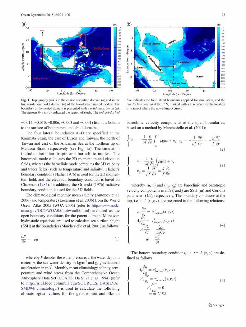
The horizontal spacing of the coarse grid is 0.5°×0.5°, withapproximately 50 km horizontal resolution and 30 vertical S-levels. The coarse model domain is from 20° S to 30° N and90° E to 140° E, encompassing the Indian and Pacific Oceans(Fig. 1a). The horizontal space of the fine grid is 0.08°×0.08°with approximately 9 km horizontal resolution and 30 verticalS-levels. The fine model domain is from 2° S to 15° N and 97°E to 117° E, encompassing Peninsular Malaysia and Borneo(Fig. 1b). Thus, the model is comprised of 99×103×30 and234×210×30 fixed grid points for parent and child domainsrespectively.

The vertical axis is resolved using 30 vertical fine-resolution S-layers (i.e. −0.951, −0.865, −0.792, −0.728,−0.674, −0.626, −0.583, −0.543, −0.506, −0.469, −0.432,−0.394, −0.354, −0.312, −0.270, −0.228, −0.188, −0.152,−0.120, −0.093, −0.072, −0.054, −0.040, −0.030, −0.022,

94 Ocean Dynamics (2015) 65:93–106

−0.015, −0.010, −0.006, −0.003 and −0.001) from the bottomto the surface of both parent and child domains.

The four lateral boundaries A–D are specified at theKarimata Strait, the east of Luzon and Taiwan, the north ofTaiwan and east of the Andaman Sea at the northern tip ofMalacca Strait, respectively (see Fig. 1a). The simulationincluded both barotropic and baroclinic modes. Thebarotropic mode calculates the 2D momentum and elevationfields, whereas the baroclinic mode computes the 3D velocityand tracer fields (such as temperature and salinity). Flather’sboundary condition (Flather 1976) is used for the 2D momen-tum field, and the elevation boundary condition is based onChapman (1985). In addition, the Orlanski (1976) radiativeboundary condition is used for the 3D fields.

The climatological monthly mean salinity (Antonov et al.2006) and temperature (Locarnini et al. 2006) from the WorldOcean Atlas 2005 (WOA 2005) (refer to http://www.nodc.noaa.gov/OC5/WOA05/pubwoa05.html) are used as theopen-boundary conditions for the parent domain. Moreover,hydrostatic equations are used to calculate sea surface height(SSH) at the boundaries (Marchesiello et al. 2001) as follows:

∂P∂z

¼ −ρg ð1Þ

whereby P denotes the water pressure; z, the water depth inmeter; ρ, the sea water density in kg/m3 and g, gravitationalacceleration in m/s2. Monthly mean climatology salinity, tem-perature and wind stress from the Comprehensive OceanAtmosphere Data Set (COADS; Da Silva et al. 1994) (referto http://iridl.ldeo.columbia.edu/SOURCES/.DASILVA/.SMD94/.climatology/) is used to calculate the followingclimatological values for the geostrophic and Ekman

baroclinic velocity components at the open boundaries,based on a method by Marchesiello et al. (2001):

u ¼ −1

ρ f∂∂y

Z−h

0

ρgdzþ ug ug ¼ −1

ρ f∂P∂y

¼ −g

f

∂ζ∂y

(

ð2Þ

v ¼ 1

ρ f∂∂x

∫0

−hρgdzþ vg

vg ¼ 1

ρ f∂P∂x

¼ g

f

∂ζ∂x

8>><>>: ð3Þ

whereby (u, v) and (ug, vg) are baroclinic and barotropicvelocity components in m/s ζ and f are SSH (m) and Coriolisparameters (1/s), respectively. The boundary conditions at thetop, i.e. z=ζ (x, y, t), are presented in the following relations:

Aν∂u∂z

¼ τ xsurface x; y; tð Þ

Aν∂v∂z

¼ τysurface x; y; tð Þ

Ac∂C∂z

¼ Qc

ρ0CP

w ¼ ∂ζ∂t

8>>>>>>>>><>>>>>>>>>:

ð4Þ

The bottom boundary conditions, i.e. z=−h (x, y) are de-fined as follows:

Aν∂u∂z

¼ τxbottom x; y; tð Þ

Aν∂v∂z

¼ τ ybottom x; y; tð Þ

Ac∂C∂z

¼ 0

w ¼ U :∇h

8>>>>>><>>>>>>:

ð5Þ

Gulf of Thailand

NNaattuunnaa IIssllaanndd

KKaarriimmaattaa SSttrraaiitt

SSuummaattrraa

BBoorrnneeoo

South China SeaAndam

anS

ea

Longitude (East-Degree)Longitude (East-Degree)

(Nor

th-D

egre

e)La

titud

e (Nor

th-D

egre

e)La

titud

e

Indian Ocean

Pacific Ocean

(a) (b)0

-20-40-60

-80

-100-200-300

-400

-500-600

-700-800

-900

-1000-2000

-3000-4000

-5000-6000

-7000-8000

0

-20

-40

-60

-80

-100

-200

-300

-400

-500-600

-700

-800

-900

-1000

-2000

-3000

-4000

-5000

-6000

98 102 106 110 114

0

4

8

12

90 100 110 120 130 140-20

-10

0

10

20

30(m)(m)

T

Luzo

nTa

iwan

A

B

C

D

Karimata

North

Fig. 1 Topography (m) is in the coarse resolution domain (a) and in thefine resolution model domain (b) of the two-domain nested models. Theboundary of the nested domain is presented with a solid black box in (a).The dashed line in (b) indicated the region of study. The red dot-dashed

line indicates the four lateral boundaries applied for simulation, and thered dot line crossed at the 3° N, marked with a T, represented the locationof transect where the upwelling occurred

Ocean Dynamics (2015) 65:93–106 95

The symbols ρ0 and C are the mean density in kg/m3 andtracers, respectively. Av and Ac are vertical eddy viscosity anddiffusivity in m2/s, respectively.U=(u,v) represents a horizon-tal velocity vector; w (m/s) is the vertical velocity component.h is the depth of the water column in meter.Qc (kg J/m

3 s) andcp (J/K) are the surface concentration flux and thermal capac-ity. τxsurface and τysurface are the x and y components of thesurface wind stress in N/m2; τxbottom and τ

ybottom are the x and y

components of the bottom stress computed based on thelogarithmic formulation given by Eqs. (6 and 7).

τ xbottom ¼ κ2uffiffiffiffiffiffiffiffiffiffiffiffiffiffiffiu2 þ v2

p

ln2 z=z0

� � ð6Þ

τ ybottom ¼ κ2vffiffiffiffiffiffiffiffiffiffiffiffiffiffiffiu2 þ v2

p

ln2 z=z0

� � ð7Þ

whereby k=0.41 is the von Karman’s constant, z and zo arethe vertical elevation and total bottom roughness length inmeter, respectively.

The computation of vertical mixing is based on the nonlo-cal K-profile parameterization (KPP) scheme (Large et al.1994). Horizontal boundary conditions are described in moredetail byMarchesiello et al. (2001). Nevertheless, the momen-tum and tracers in the northern and southern boundaries arebriefly described as follows:

∂∂y

hνmn

∂2V∂y2

� �¼ 0 ð8Þ

whereby ν is molecular viscosity and m and n are thenumber of cells in the x and y directions, respectively.Symbol V represents the momentum components/tracers.Similarly, the eastern and western boundary conditions areas follows:

∂∂x

hνmn

∂2V∂x2

� �¼ 0 ð9Þ

2.1.2 Forcing and initialization

For the monthly climatological surface wind stress, surfacefreshwater and heat fluxes from COADS ocean surface

monthly climatology are used to force the parent and childdomains. The net heat and surface freshwater flux feedback,as surface forces, is parameterized with a relaxation toCOADS climatological temperature and salinity, respectively.

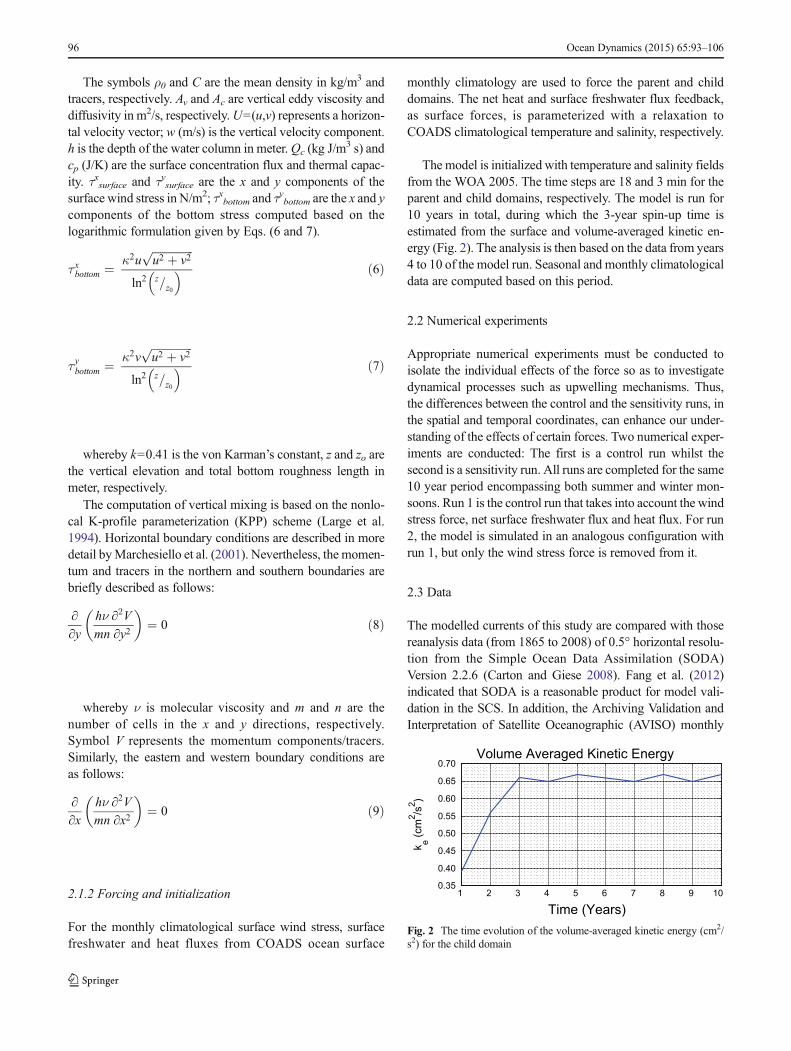
The model is initialized with temperature and salinity fieldsfrom the WOA 2005. The time steps are 18 and 3 min for theparent and child domains, respectively. The model is run for10 years in total, during which the 3-year spin-up time isestimated from the surface and volume-averaged kinetic en-ergy (Fig. 2). The analysis is then based on the data from years4 to 10 of the model run. Seasonal and monthly climatologicaldata are computed based on this period.

2.2 Numerical experiments

Appropriate numerical experiments must be conducted toisolate the individual effects of the force so as to investigatedynamical processes such as upwelling mechanisms. Thus,the differences between the control and the sensitivity runs, inthe spatial and temporal coordinates, can enhance our under-standing of the effects of certain forces. Two numerical exper-iments are conducted: The first is a control run whilst thesecond is a sensitivity run. All runs are completed for the same10 year period encompassing both summer and winter mon-soons. Run 1 is the control run that takes into account the windstress force, net surface freshwater flux and heat flux. For run2, the model is simulated in an analogous configuration withrun 1, but only the wind stress force is removed from it.

2.3 Data

The modelled currents of this study are compared with thosereanalysis data (from 1865 to 2008) of 0.5° horizontal resolu-tion from the Simple Ocean Data Assimilation (SODA)Version 2.2.6 (Carton and Giese 2008). Fang et al. (2012)indicated that SODA is a reasonable product for model vali-dation in the SCS. In addition, the Archiving Validation andInterpretation of Satellite Oceanographic (AVISO) monthly

1 2 3 4 5 6 7 8 9 100.35

0.40

0.45

0.50

0.55

0.60

0.65

0.70

Time (Years)

k e (cm

2 /s2 )

Volume Averaged Kinetic Energy

Fig. 2 The time evolution of the volume-averaged kinetic energy (cm2/s2) for the child domain

96 Ocean Dynamics (2015) 65:93–106

mean sea level anomaly—a gridded product with an approx-imate horizontal resolution of 37 km (refer to http://aviso.altimetry.fr/) for the period 2005–2012 is used for thecomparison of sea surface high anomaly (SSHA) derived fromthe model. The product is a combination of satellite-observedsea-level anomalies and the mean dynamic topography ob-tained from a study conducted by Rio and Hernandez (2004).Apart from the climatological monthly mean salinity(Antonov et al. 2006) and temperature (Locarnini et al.2006) from WOA 2005, Pathfinder 9 km SST climatologydata (Casey and Cornillon 1999) is used as a secondary SSTdataset for validation. The monthly mean productivity anddistribution of the ocean colour data for the period 2005–2012 are used as evidence for coastal upwelling. The chloro-phyll data is obtained from the Moderate Resolution ImagingSpectroradiometer (MODIS) sensor on Aqua satellite (avail-able from http://podaac.jpl.nasa.gov/dataset/MODIS_Aqua_L3_CHLA_Daily_4km_R), and the nutrients (phosphate) alsothe dissolved oxygen recommended by Garcia et al. (2006a,2006b) are extracted from the WOA 2005 (http://www.nodc.noaa.gov/OC5/WOA05/pubwoa05.html).

3 Results and discussions

3.1 Wind stress and surface circulation

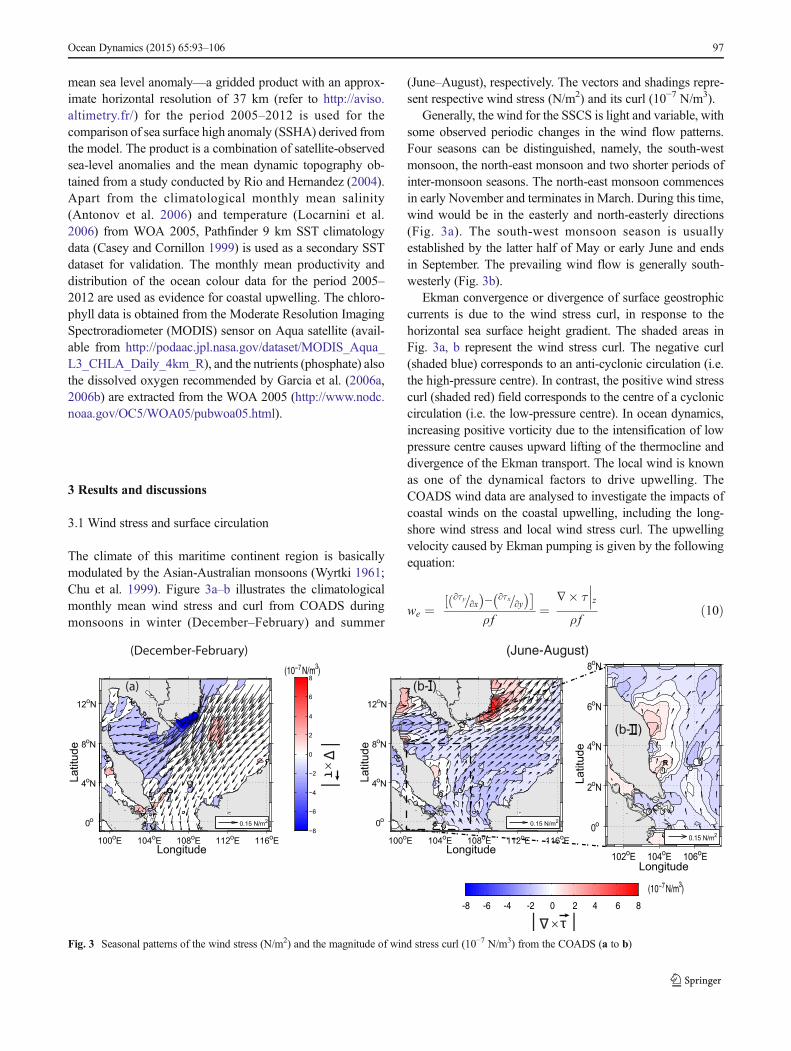
The climate of this maritime continent region is basicallymodulated by the Asian-Australian monsoons (Wyrtki 1961;Chu et al. 1999). Figure 3a–b illustrates the climatologicalmonthly mean wind stress and curl from COADS duringmonsoons in winter (December–February) and summer

(June–August), respectively. The vectors and shadings repre-sent respective wind stress (N/m2) and its curl (10−7 N/m3).

Generally, the wind for the SSCS is light and variable, withsome observed periodic changes in the wind flow patterns.Four seasons can be distinguished, namely, the south-westmonsoon, the north-east monsoon and two shorter periods ofinter-monsoon seasons. The north-east monsoon commencesin early November and terminates in March. During this time,wind would be in the easterly and north-easterly directions(Fig. 3a). The south-west monsoon season is usuallyestablished by the latter half of May or early June and endsin September. The prevailing wind flow is generally south-westerly (Fig. 3b).

Ekman convergence or divergence of surface geostrophiccurrents is due to the wind stress curl, in response to thehorizontal sea surface height gradient. The shaded areas inFig. 3a, b represent the wind stress curl. The negative curl(shaded blue) corresponds to an anti-cyclonic circulation (i.e.the high-pressure centre). In contrast, the positive wind stresscurl (shaded red) field corresponds to the centre of a cycloniccirculation (i.e. the low-pressure centre). In ocean dynamics,increasing positive vorticity due to the intensification of lowpressure centre causes upward lifting of the thermocline anddivergence of the Ekman transport. The local wind is knownas one of the dynamical factors to drive upwelling. TheCOADS wind data are analysed to investigate the impacts ofcoastal winds on the coastal upwelling, including the long-shore wind stress and local wind stress curl. The upwellingvelocity caused by Ekman pumping is given by the followingequation:

we ¼½ð∂τy=∂x

�− ∂τx=∂y

�� ρ f

¼∇� τ

zρ f

ð10Þ

100oE 104oE 108oE 112oE 116oE

0o

4oN

8oN

12oN

0.15 N/m2

(a)

(December-February)(10−7 N/m3)

−8

−6

−4

−2

0

2

4

6

8

τ

Δ×| |

Longitude

Latit

ude

100oE 104oE 108oE 112oE 116oE

0o

4oN

8oN

12oN

0.15 N/m2

Longitude

Latit

ude

102oE 104oE 106oE

0o

2oN

4oN

6oN

8oN

0.15 N/m2

-8 -6 -4 -2 0 2 4 6 8

(10−7 N/m3)

τ

Δ

×| |

Longitude

Latit

ude

(June-August)

R

(b-I)

(b-II)

Fig. 3 Seasonal patterns of the wind stress (N/m2) and the magnitude of wind stress curl (10−7 N/m3) from the COADS (a to b)

Ocean Dynamics (2015) 65:93–106 97

It is obvious that the monthly climatological wind stresscurl in the summer upwelling season should be positive withinthe corresponding area (see Fig. 3b-II the region marked withR). For this particular area, the mean wind stress curl, themean density of seawater, the Coriolis parameter and thecalculated mean average upwelling velocity caused by windstress curl are 0.37×10−7 N/m3, 10,201 kg/m3, 7.04×10−6/sand 0.5×10−5 m/s, respectively. These give a good approxi-mation to differentiate the types of upwelling in the regioneither by Ekman pumping (curl-driven upwelling) or upwell-ing induced by the long-shore wind stress (coastal upwelling).

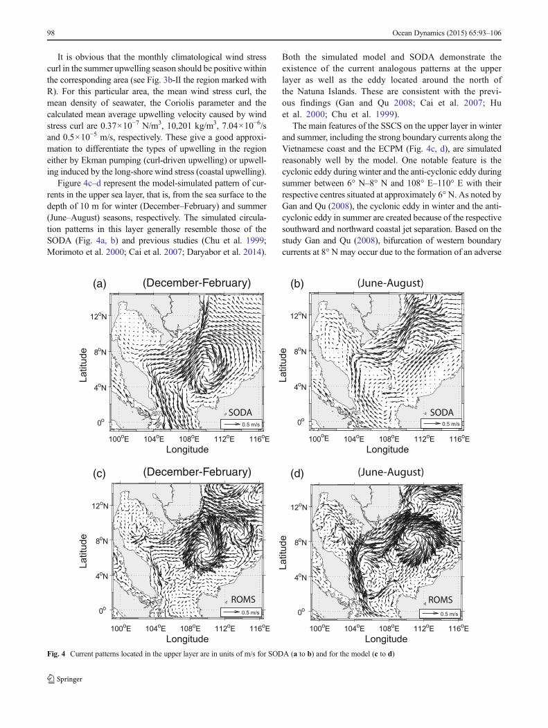
Figure 4c–d represent the model-simulated pattern of cur-rents in the upper sea layer, that is, from the sea surface to thedepth of 10 m for winter (December–February) and summer(June–August) seasons, respectively. The simulated circula-tion patterns in this layer generally resemble those of theSODA (Fig. 4a, b) and previous studies (Chu et al. 1999;Morimoto et al. 2000; Cai et al. 2007; Daryabor et al. 2014).

Both the simulated model and SODA demonstrate theexistence of the current analogous patterns at the upperlayer as well as the eddy located around the north ofthe Natuna Islands. These are consistent with the previ-ous findings (Gan and Qu 2008; Cai et al. 2007; Huet al. 2000; Chu et al. 1999).

The main features of the SSCS on the upper layer in winterand summer, including the strong boundary currents along theVietnamese coast and the ECPM (Fig. 4c, d), are simulatedreasonably well by the model. One notable feature is thecyclonic eddy during winter and the anti-cyclonic eddy duringsummer between 6° N–8° N and 108° E–110° E with theirrespective centres situated at approximately 6° N. As noted byGan and Qu (2008), the cyclonic eddy in winter and the anti-cyclonic eddy in summer are created because of the respectivesouthward and northward coastal jet separation. Based on thestudy Gan and Qu (2008), bifurcation of western boundarycurrents at 8° N may occur due to the formation of an adverse

100oE 104oE 108oE 112oE 116oE

0o

4oN

8oN

12oN

0.5 m/s

100oE 104oE 108oE 112oE 116oE

0o

4oN

8oN

12oN

0.5 m/s

100oE 104oE 108oE 112oE 116oE

0o

4oN

8oN

12oN

Longitude

Latit

ude

0.5 m/s

edutignoLedutignoL

Latit

ude

Latit

ude

100oE 104oE 108oE 112oE 116oE

0o

4oN

8oN

12oN

Longitude

Latit

ude

0.5 m/s

(b)(a)

(c) (d)

ADOSADOS

ROMS ROMS

(December-February) (June-August)

(December-February) (June-August)

Fig. 4 Current patterns located in the upper layer are in units of m/s for SODA (a to b) and for the model (c to d)

98 Ocean Dynamics (2015) 65:93–106

pressure gradient force and an adverse vorticity downstreamin the near-shore waters around the coastal region at 8° N.

An adverse pressure gradient (∂P ⁄∂x>0) occurs particular-ly for boundary layers, when the static pressure increases inthe direction of the flow. The increased fluid pressures toincreases the potential energy of the fluid, leading to a reduc-tion of kinetic energy and deceleration of the fluid. In fact, therelatively slow flow of the fluid in the inner part of theboundary layer is affected by an increase in the pressuregradient. Large enough pressure increases may cause the fluidvelocity to become zero or even reversed, causing separationof flow from the surface.

Nevertheless, during the summer monsoon, the adversepressure gradient force is balanced with the prevailing windstress. However, during the winter monsoon, the gradient isbalanced with both the wind stress and nonlinear advection(Gan and Qu 2008). Conversely, the adverse vorticity over theshelf is caused by the bottom pressure torque that is balancedby the nonlinear advection. As mentioned by Gan and Qu(2008), it is the curl of the bottom pressure across the isobathsexerted by the shelf topography on the waters. Overall, inter-action of bottom topography in the near-shore waters withwind-driven coastal currents could be the main factor incontrolling the western boundary current separation.

3.2 Sea surface temperature and salinity

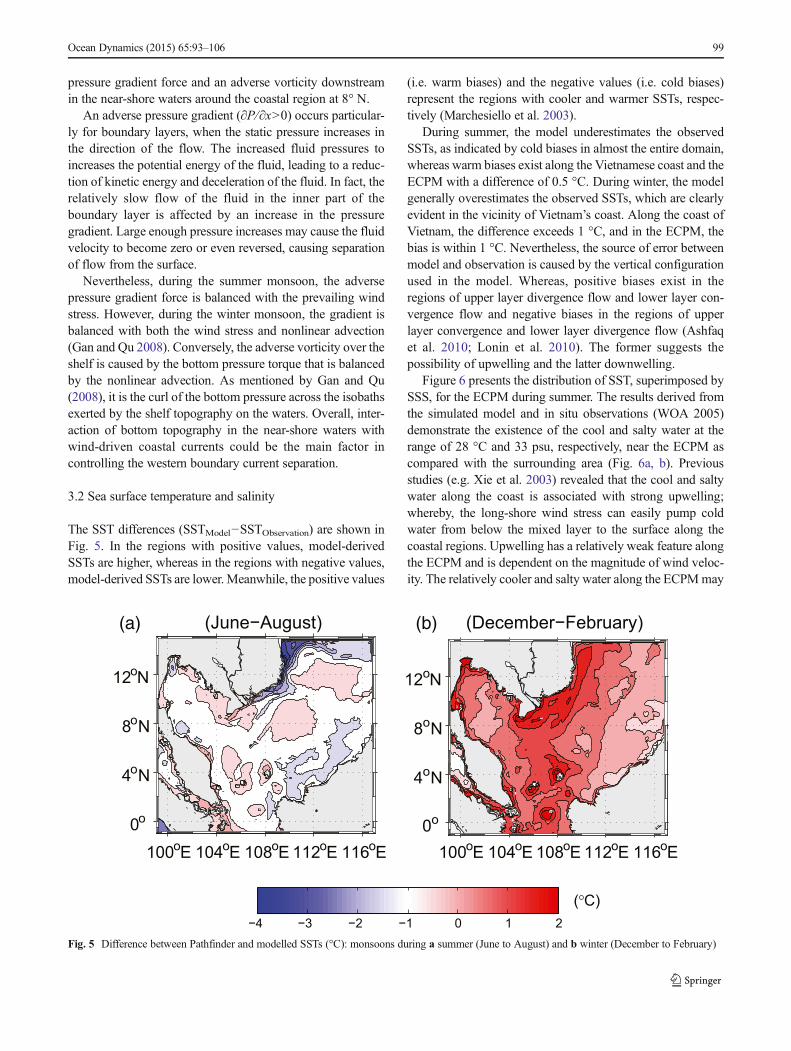
The SST differences (SSTModel−SSTObservation) are shown inFig. 5. In the regions with positive values, model-derivedSSTs are higher, whereas in the regions with negative values,model-derived SSTs are lower. Meanwhile, the positive values

(i.e. warm biases) and the negative values (i.e. cold biases)represent the regions with cooler and warmer SSTs, respec-tively (Marchesiello et al. 2003).

During summer, the model underestimates the observedSSTs, as indicated by cold biases in almost the entire domain,whereas warm biases exist along the Vietnamese coast and theECPM with a difference of 0.5 °C. During winter, the modelgenerally overestimates the observed SSTs, which are clearlyevident in the vicinity of Vietnam’s coast. Along the coast ofVietnam, the difference exceeds 1 °C, and in the ECPM, thebias is within 1 °C. Nevertheless, the source of error betweenmodel and observation is caused by the vertical configurationused in the model. Whereas, positive biases exist in theregions of upper layer divergence flow and lower layer con-vergence flow and negative biases in the regions of upperlayer convergence and lower layer divergence flow (Ashfaqet al. 2010; Lonin et al. 2010). The former suggests thepossibility of upwelling and the latter downwelling.

Figure 6 presents the distribution of SST, superimposed bySSS, for the ECPM during summer. The results derived fromthe simulated model and in situ observations (WOA 2005)demonstrate the existence of the cool and salty water at therange of 28 °C and 33 psu, respectively, near the ECPM ascompared with the surrounding area (Fig. 6a, b). Previousstudies (e.g. Xie et al. 2003) revealed that the cool and saltywater along the coast is associated with strong upwelling;whereby, the long-shore wind stress can easily pump coldwater from below the mixed layer to the surface along thecoastal regions. Upwelling has a relatively weak feature alongthe ECPM and is dependent on the magnitude of wind veloc-ity. The relatively cooler and salty water along the ECPMmay

100o 401E o 801E o 211E o 611E oE0o

4oN

8oN

12oN

(a) (June−August)

100o 401E o 801E o 211E o 611E oE 0o

4oN

8oN

12oN

(b) (December−February)

(°C)−4 −3 −2 −1 0 1 2

Fig. 5 Difference between Pathfinder and modelled SSTs (°C): monsoons during a summer (June to August) and b winter (December to February)

Ocean Dynamics (2015) 65:93–106 99

be associated with this upwelling phenomenon, particularlyalong transect T (see the location indicated in Fig. 1b).

Figure 6c displays the results of run 2 (i.e. the control runwithout wind stress). It shows the disappearance of the elon-gated cooler SST and high salinity along the ECPM, in com-parison with run 1 and in situ observations. In fact, an elon-gated yet slightly warmer SST, with lower SSS, prevailed inthe same areas. The disappearance of the elongated coolerSST and salty water indicates the absence of the coastalupwelling process. This is due to the absence of the long-shore wind stress that is required to generate offshore Ekmanflow for the upwelling process to occur. Moreover, the figuredemonstrates the disappearance of elongated dense isobaths inrun 2, due to the removal of wind stress force from the controlrun. This result reveals that the coastal upwelling in the ECPMis relatively dependent on strong wind stress, parallel to thecoastline. Nevertheless, this result indicates the importance ofwind stress in the upwelling process of the region. However,numerous factors can be involved in the upwelling, such asbottom topography, shelf circulation, eddies and islands (Caiet al. 2005, 2007; Jing et al. 2009).

3.3 Cross-shore structure

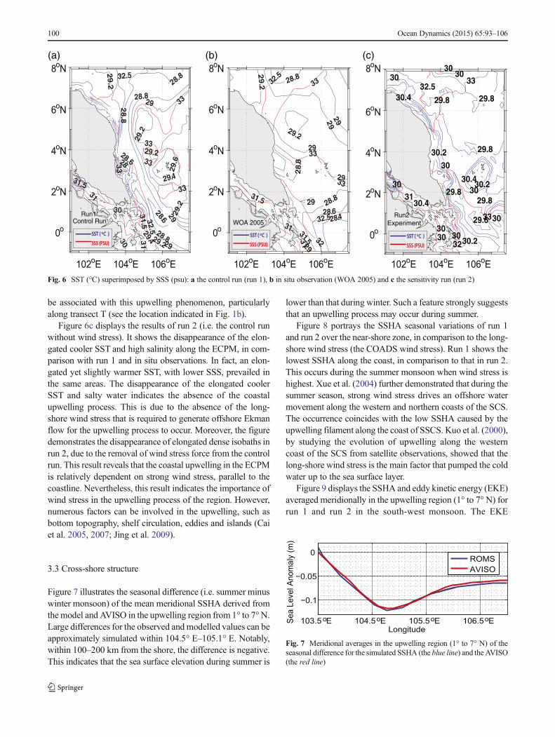
Figure 7 illustrates the seasonal difference (i.e. summer minuswinter monsoon) of the mean meridional SSHA derived fromthe model and AVISO in the upwelling region from 1° to 7° N.Large differences for the observed and modelled values can beapproximately simulated within 104.5° E–105.1° E. Notably,within 100–200 km from the shore, the difference is negative.This indicates that the sea surface elevation during summer is

lower than that during winter. Such a feature strongly suggeststhat an upwelling process may occur during summer.

Figure 8 portrays the SSHA seasonal variations of run 1and run 2 over the near-shore zone, in comparison to the long-shore wind stress (the COADS wind stress). Run 1 shows thelowest SSHA along the coast, in comparison to that in run 2.This occurs during the summer monsoon when wind stress ishighest. Xue et al. (2004) further demonstrated that during thesummer season, strong wind stress drives an offshore watermovement along the western and northern coasts of the SCS.The occurrence coincides with the low SSHA caused by theupwelling filament along the coast of SSCS. Kuo et al. (2000),by studying the evolution of upwelling along the westerncoast of the SCS from satellite observations, showed that thelong-shore wind stress is the main factor that pumped the coldwater up to the sea surface layer.

Figure 9 displays the SSHA and eddy kinetic energy (EKE)averaged meridionally in the upwelling region (1° to 7° N) forrun 1 and run 2 in the south-west monsoon. The EKE

28.428.6

28.8

28.8

28.8

29

29

29

29

29

29

29.2

29.2

31

31

31.5

31.5 32

32.5

32.5

33

33

33

WOA 2005

28.6

28.6

28.8

28.8

28.8

28.8

29

29

29

29.2

29.2

29.2

29.2

29.4

29.429

.68

30

2

30

31

31

32.5

32.5

33

33

33

33

33

Control Run

31.5

31.5

29.2

29.6

29.8

29.8

29.8

29.829.8

30

30

30

30

3030

30 30

30

30

30.2

30.2

30.2

30.4

30.4

30.4

31

32

32.533

33

102oE 104oE 106oE

0o

2oN

4oN

6oN

8oN

Experiment

SST ( C )SST ( C )o

SSS (PSU)SSS (PSU)

SST ( C )SST ( C )o

SSS (PSU)SSS (PSU)

SST ( C )SST ( C )o

SSS (PSU)SSS (PSU)

102oE 104oE 106oE 102oE 104oE 106oE

0o

2oN

4oN

6oN

8oN

0o

2oN

4oN

6oN

8oN(b)(a) (c)

Run1 Run2

Fig. 6 SST (°C) superimposed by SSS (psu): a the control run (run 1), b in situ observation (WOA 2005) and c the sensitivity run (run 2)

103.5 E 104.5 E 105.5 E 106.5 E

−0.1

−0.05

0

Longitude

Sea

Leve

l Ano

mal

y (m

)

o o o o

ROMSAVISO

Fig. 7 Meridional averages in the upwelling region (1° to 7° N) of theseasonal difference for the simulated SSHA (the blue line) and the AVISO(the red line)

100 Ocean Dynamics (2015) 65:93–106

according to the formula (Aiki and Yamagata 2006) given asfollows:

EKE ¼Z

−h

0

j������U−U�ρj2 − zρU

�����ρ

zρ���ρ −U�ρ

2

!dz ð11Þ

where U�ρ

and zρU����� ρ

zρ��� ρ are respectively, isopycnal mean and

thickness-weighted mean in density coordinates (zp≡∂z∂p is the

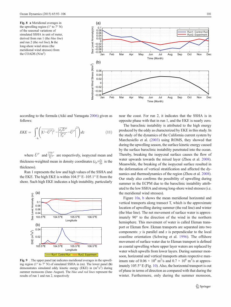
thickness).Run 1 represents the low and high values of the SSHA and

the EKE. The high EKE is within 104.5° E–105.1° E from theshore. Such high EKE indicates a high instability, particularly

near the coast. For run 2, it indicates that the SSHA is inopposite phase with that in run 1, and the EKE is nearly zero.

The baroclinic instability is attributed to the high energyproduced by the eddy as characterized by EKE in this study. Inthe study of the dynamics of the California current system byMarchesiello et al. (2003) using ROMS, they showed thatduring the upwelling season, the surface kinetic energy causedby the surface baroclinic instability penetrated into the ocean.Thereby, breaking the isopycnal surface causes the flow ofwater upwards towards the mixed layer (Zhou et al. 2008).Meanwhile, the breaking of the isopycnal surface resulted inthe deformation of vertical stratification and affected the dy-namics and thermodynamics of the region (Zhou et al. 2008).Our study also confirms the possibility of upwelling duringsummer in the ECPM due to the baroclinic instability attrib-uted to the low SSHA and strong long-shore wind stresses (i.e.the meridional wind stresses).

Figure 10a, b shows the mean meridional horizontal andvertical transports along transect T, which is the approximatelocation of upwelling during summer (the red line) and winter(the blue line). The net movement of surface water is approx-imately 90° to the direction of the wind in the northernhemisphere. This movement of water is called Ekman trans-port or Ekman flow. Ekman transports are separated into twocomponents: y is parallel and x is perpendicular to the localcoastline orientation (Schwing et al. 1996). The offshoremovement of surface water due to Ekman transport is definedas coastal upwelling where upper layer waters are replaced bywater which upwells from lower layers. During summer mon-soon, horizontal and vertical transports attain respective max-imum rate of 0.06 × 106 m2/s and 0.7 × 106 m3/s at approx-imately 105.5° E (Fig. 10). Also, the horizontal transport is outof phase in terms of direction as compared with that during thewinter. Furthermore, only during the summer monsoon,

Jan Feb Mar Apr May Jun Jul Aug Sep Oct Nov Dec−0.08−0.06−0.04−0.02

00.020.040.060.080.1

Time (Month)

Sea

Leve

l Ano

mal

y(m

)

(a)

Jan Feb Mar Apr May Jun Jul Aug Sep Oct Nov Dec−0.06−0.04−0.02

00.020.040.06

Time (Month)

(b)

Run1: Control RunRun2: Experiment

(N

/m2 )

Mer

idio

nal W

ind

Stre

ss

Fig. 8 a Meridional averages inthe upwelling region (1° to 7° N)of the seasonal variations ofsimulated SSHA in unit of meter,derived from run 1 (the blue line)and run 2 (the red line); b thelong-shore wind stress (themeridional wind stresses) fromthe COADS (N/m2)

103.5 E 104.5 E 105.5 E 106.5 E0.040.060.08

0.1

LongitudeSea

Leve

l Ano

mal

y (m

) (a)

103.5 E 104.5 E 105.5 E 106.5 E0

0.02

0.04

Longitude

EKE

(m2 /s

2 )

(b)

Run1: Control Run Run2: Experiment

o o o o

o o o o

Fig. 9 . The upper panel (a) indicates meridional averages in the upwell-ing region (1° to 7° N) of simulated SSHA in (m). The lower panel (b)demonstrates simulated eddy kinetic energy (EKE) in (m2/s2) duringsummer monsoons (June–August). The blue and red lines represent theresults of run 1 and run 2, respectively

Ocean Dynamics (2015) 65:93–106 101

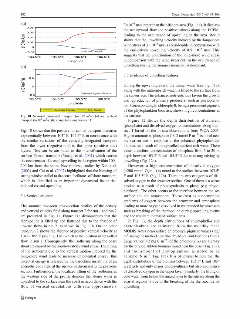
Fig. 10 shows that the positive horizontal transport increasesexponentially between 104° E–105.5° E in consonance withthe similar variations of the vertically integrated transportfrom the lower (negative rate) to the upper (positive rate)layers. This can be attributed to the intensification of thesurface Ekman transport (Yanagi et al. 2001) which causesthe occurrences of coastal upwelling in the region within 100–200 km from the shore. Nevertheless, studies by Xie et al.(2003) and Cai et al. (2007) highlighted that the blowing ofstrong winds parallel to the coast facilitates offshore transport,which is identified as an important dynamical factor thatinduced coastal upwelling.

3.4 Vertical structure

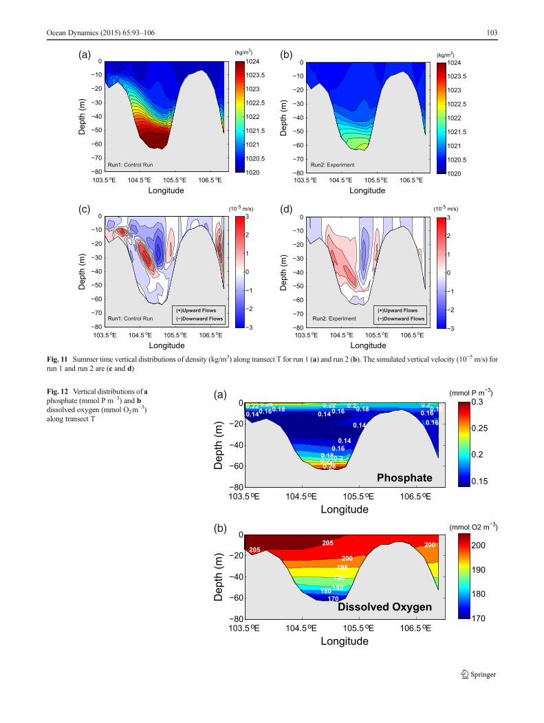
The summer monsoon cross-section profiles of the densityand vertical velocity field along transect T for run 1 and run 2are presented in Fig. 11. Figure 11a demonstrates that thethermocline is lifted up and flattened due to the absence ofupward flows in run 2, as shown in Fig. 11b. On the otherhand, run 2 shows the absence of positive vertical velocity at104°–105° E (see Fig. 11d) which is the location of upwelledflow in run 1. Consequently, the isotherms along the coastshoal are caused by the south-westerly wind stress. The liftingof the isotherms due to the vertical motion induced by thelong-shore wind leads to increase of potential energy; thispotential energy is released by the baroclinic instability of anenergetic eddy field at the surface as discussed in the previoussection. Furthermore, the localized lifting of the isotherms atthe western side of the profile denotes that dense water isupwelled to the surface near the coast in accordance with theflow of vertical circulations with rate approximately

3×10−5 m/s larger than the offshore area (Fig. 11c). It displaysthe net upward flow (or positive values) along the ECPM,leading to the occurrence of upwelling in the area. Resultshows that the upwelling velocity induced by the long-shorewind stress of 3×10−5 m/s is considerable in comparison withthe curl-driven upwelling velocity of 0.5×10−5 m/s. Thissuggests that the contribution of the long-shore wind stressin comparison with the wind stress curl in the occurrence ofupwelling during the summer monsoon is dominant.

3.5 Evidence of upwelling features

During the upwelling event, the denser water (see Fig. 11a),along with the nutrient-rich water, is lifted to the surface fromthe subsurface. The enhanced nutrients thus favour the growthand reproduction of primary producers, such as phytoplank-ton. Correspondingly, chlorophyll, being a prominent pigmentof the phytoplankton biomass, shows high concentrations atthe surface.

Figure 12 shows the depth distribution of nutrient(phosphate) and dissolved oxygen concentrations along tran-sect T based on the in situ observations from WOA 2005.Higher amounts of phosphate (>0.2 mmol Pm−3) is noted nearthe sea surface in response to the enhanced phytoplanktonbiomass as a result of the upwelled nutrient-rich water. Thereexists a uniform concentration of phosphate from 5 to 30 mdepth between 103.5° E and 105.5° E due to strong mixing byupwelling (Fig. 12a).

However, a high concentration of dissolved oxygen(>200 mmol O2m

−3) is noted at the surface between 103.5°E and 105.5° E (Fig. 12b). There are two categories of dis-solved oxygen in the seawater surface. One of them is a wasteproduct as a result of photosynthesis in plants (e.g. phyto-plankton). The other occurs at the interface between the seasurface and the atmosphere. These exist as concentrationgradients of oxygen between the seawater and atmosphereleading to more oxygen dissolved in water aided by processessuch as breaking of the thermocline during upwelling eventsand the resultant increased surface area.

In Fig. 13, the depth distributions of chlorophyll-a andphytoplankton are estimated from the monthly meanMODIS Aqua near-surface chlorophyll pigment values (mg/m3) using the method described byMorel and Berthon (1989).Large values (>2 mg C m−3) of the chlorophyll-a are a proxyfor the phytoplankton biomass found near the coast (Fig. 13a),and the amount of phytoplankton is noted to be>1 mmol N m−3 (Fig. 13b). It is of interest to note that thedepth distribution of the biomass between 103.5° E and 105°E reflects not only major photosynthesis but also abundanceof dissolved oxygen in the upper layer. Similarly, the lifting ofcold water from below the mixed layer to the surface along thecoastal regions is due to the breaking of the thermocline byupwelling.

103.5 E 104.5 E 105.5 E 106.5 E

−0.02

0

0.02

0.04

0.06

0.08

Longitude

(a)

Horizontal Transport

103.5 E 104.5 E 105.5 E 106.5 E−0.5

0

0.5

1

Longitude

(106 m

3 /s)

oo o o

o ooo

(b)

Vertically Integrated Transport

December−February June−August

(106 m

2 /s)

Fig. 10 Seasonal horizontal transport (in 106 m2/s) (a) and verticaltransport (in 106 m3/s) (b) computed along transect T

102 Ocean Dynamics (2015) 65:93–106

Dep

th (m

)

−80

−70

−60

−50

−40

−30

−20

−10

0(kg/m3)

1020

1020.5

1021

1021.5

1022

1022.5

1023

1023.5

1024(a)

Run1: Control Run

Dep

th (m

)

−80

−70

−60

−50

−40

−30

−20

−10

0(kg/m3)

1020

1020.5

1021

1021.5

1022

1022.5

1023

1023.5

1024(b)

Run2: Experiment

Longitude103.5 E 104.5 E 105.5 E 106.5 Eo ooo

Longitude103.5 E 104.5 E 105.5 E 106.5 Eo ooo

Dep

th (m

)

−80

−70

−60

−50

−40

−30

−20

−10

0(10 m/s)

−3

−2

−1

0

1

2

3

Longitude103.5 E 104.5 E 105.5 E 106.5 Eo ooo

(c)

(−)Downward Flows(+)Upward Flows

Dep

th (m

)

−80

−70

−60

−50

−40

−30

−20

−10

0

−3

−2

−1

0

1

2

3

Longitude103.5 E 104.5 E 105.5 E 106.5 Eo ooo

(10 m/s)(d)

(−)Downward Flows(+)Upward Flows

-5 -5

Run2: ExperimentRun1: Control Run

Fig. 11 Summer time vertical distributions of density (kg/m3) along transect T for run 1 (a) and run 2 (b). The simulated vertical velocity (10−5 m/s) forrun 1 and run 2 are (c and d)

Longitude

Dep

th (m

)

0.14

0.140.140.14

0.16

0.160.16 0.160.16

0.18

0.18 0.18 0.18

0.2

0.2 0.2

0.22

0.220.22 0.24

0.26

103.5 E 104.5 E 105.5 E 106.5 E−80

−60

−40

−20

0

Longitude

Dep

th (m

)

170180185

190195

200

200205205

103.5 E 104.5 E 105.5 E 106.5 E−80

−60

−40

−20

0

(mmol P m−3)

0.15

0.2

0.25

0.3

(mmol O2 m−3)

170

180

190

200

(a)

(b)

Phosphate

Dissolved Oxygen

o o o o

o o o o

Fig. 12 Vertical distributions of aphosphate (mmol P m−3) and bdissolved oxygen (mmol O2m

−3)along transect T

Ocean Dynamics (2015) 65:93–106 103

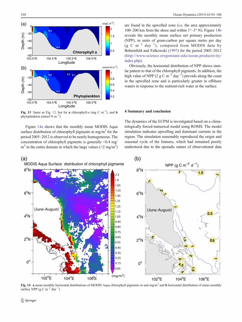
Figure 14a shows that the monthly mean MODIS Aquasurface distribution of chlorophyll pigments in mg/m3 for theperiod 2005–2012 is observed to be nearly homogeneous. Theconcentration of chlorophyll pigments is generally <0.4 mg/m3 in the entire domain in which the large values (>2 mg/m3)

are found in the upwelled zone (i.e. the area approximately100–200 km from the shore and within 1°–3° N). Figure 14breveals the monthly mean surface net primary production(NPP), in units of gram-carbon per square metre per day(g C m−2 day−1), computed from MODIS data byBehrenfeld and Falkowski (1997) for the period 2005–2012(http://www.science.oregonstate.edu/ocean.productivity/index.php).

Obviously, the horizontal distribution of NPP shows simi-lar pattern to that of the chlorophyll pigments. In addition, thehigh value of NPP (2 g C m−2 day−1) prevails along the coastin the upwelled zone and is particularly greater in offshorewaters in response to the nutrient-rich water at the surface.

4 Summary and conclusion

The dynamics of the ECPM is investigated based on a clima-tologically forced numerical model using ROMS. The modelsimulation indicates upwelling and dominant currents in theregion. The simulation reasonably reproduced the origin andseasonal cycle of the features, which had remained poorlyunderstood due to the sporadic nature of observational data

Longitude

Dep

th (m

) 0.4

0.4

103.5 E 104.5 E 105.5 E 106.5 E−80

−60

−40

−20

0

Longitude

Dep

th (m

)

0.1 0.10.2

0.2

0.3

103.5 E 104.5 E 105.5 E 106.5 E−80

−60

−40

−20

0

(mgC.m−3)

0.5

1

1.5

2

(mmol N m−3)

0.2

0.4

0.6

0.8

1

(a)

(b)

Chlorophyll a

Phytoplanktono

o o o o

o o o

Fig. 13 Same as Fig. 12, but for a chlorophyll-a (mg C m−3), and bphytoplankton (mmol N m−3)

(a)

0.05

0.15

0.25

0.35

0.45

0.55

0.65

0.75

0.85

0.95

1.05

1.15

1.25

1.35

1.45

1.55

1.65

1.9

2.3

(mg/m3)

0.5

0.5

1

1

1

1

1

1

1

1.5

1.5

1.5

2

2

2

24

4

4.5

5

5

5 102oE 104oE 106oE

0o

2oN

4oN

6oN

8oN NPP (g C m d−1)−2MODIS Aqua Surface distribution of chlorophyll pigments

(b)

102oE 104oE 106oE

0o

2oN

4oN

6oN

8oN

(June-August) (June-August)

Fig. 14 a mean monthly horizontal distributions of MODIS Aqua chlorophyll pigments in unit mg/m3 and b horizontal distribution of mean monthlysurface NPP (g C m−2 day−1)

104 Ocean Dynamics (2015) 65:93–106

in this region. This study offers a better insight into the keyfeatures of the overall current along the ECPM.

The climate of the ECPM is affected by the monsoons.During monsoons (i.e. summer and winter), the coastaljet along the east coast of Peninsular Malaysia evidentlyresults from the existence of western boundary currents. Thenorth-east monsoon (i.e. the winter monsoon) has strongnorth-easterly winds that blow across the SCS, inducing cy-clonic surface circulation that pushes cool water further south,resulting in lower SST in the ECPM. During the summermonsoon, strong coastal currents flow northwards, due tothe strong wind stress along the ECPM. This occurrenceresults in a higher SSTand slightly lower SSS over this regionas compared with those during the north-east monsoon period.The bias from the model results when compared with thesatellite results indicates a positive value along both theVietnam coast and the ECPM due to the upper layer diver-gence and lower layer convergence flows simulated by themodel. The region with high positive bias (i.e. warm bias)indicates that the waters are very cold and could have resultedfrom upwelling processes. Based on the model-derived verti-cal velocity induced by the long-shore wind stress, summermonsoon upwelling rates along the ECPM is 3×10−5 m/slarger than the vertical velocity 0.5×10−5 m/s as induced bywind stress curl. It shows the importance of the long-shorewind stress in inducing coastal upwelling. The peak upwellingseason, as derived from the model, is affected in particular bythe month of the climatological forcing. Climatological forc-ing refers to the long-shore high wind stresses, which producean average flux of approximately 0.7 × 106 m3/s. A stronghorizontal transport occurs near the coast at 3° N during thesummer season, with positive sign indicating offshore trans-port and thereby upwelling. The upwelling along the ECPMexhibits high seasonal variability with the strongest occurringduring the summer monsoon. Furthermore, results from run 1and run 2 reveal that the possible upwelling could be attribut-ed to the seasonal baroclinic instability and variations ofSSHA which are due to the simultaneous movements of thestrong long-shore currents with the EKE.

The horizontal distribution of observed chlorophyll pig-ments as a proxy for the phytoplankton biomass and NPPindicates a higher concentration of productivities near thecoast during the south-west monsoon. Furthermore, the verti-cal distribution of chlorophyll-a, phytoplankton, nutrient(phosphate), and dissolved oxygen concentration in the upperlayers are almost larger than the amounts observed in the otherlayers. This implies that the coastal upwelling is the mainfactor to facilitate the relatively high phytoplankton biomassto the sea surface.

The topographical effect is another factor that can affect theupwelling along the coast. This effect will be investigated infuture studies using a high resolution model of ~1 km bysmoothing the shelf and coastline in the alongshore direction.

Acknowledgments The authors would like to thank the anonymousreviewers for their critical review and valuable suggestions. The authorswould also like to thank Dr. Mark Freeman from the Institute of Oceanand Earth Sciences (IOES), Institute of Postgraduate Studies, Universityof Malaya. This research study is funded by the Malaysian GovernmentScience Fund Grant 14-02-03-4022. It is also strongly supported by theVice Chancellor of the University of Malaya.

References

Aiki T, Yamagata T (2006) Energetics of the layer-thickness form dragbased on an integral identity. Ocean Sci 2:161–171

Antonov JI, Locarnini RA, Boyer TP, Mishonov AV, Garcia HE (2006)World Ocean Atlas 2005, volume 2. salinity. In: Levitus S (ed)NOAA Atlas NESDIS 62. U.S. Government Printing Office,Washington, D.C, p 182

Ashfaq M, Skinner BC, Diffenbaugh SN (2010) Influence of SST biaseson future climate change projections. Clim Dynam. doi:10.1007/s00382-010-0875-2

Beckmann A, Haidvogel DB (1993) Numerical simulation of flowaround a tall isolated seamount. Part I: problem formulation andmodel accuracy. J Phys Oceanogr 23:1736–1753

Behrenfeld MJ, Falkowski PG (1997) Photosynthetic rates derived fromsatellite-based chlorophyll concentration. Limnol Oceanogr 42:1–20

Cai SQ, Su J, Long X, Wang S, Huang Q (2005) Numerical study onsummer circulation and its establishment of the upper South ChinaSea. Acta Oceanol Sin 24(1):31–38

Cai SQ, Long X,Wang S (2007) A model study of the summer SoutheastVietnam off-shore current in the Southern South China Sea. ContShelf Res 27:2357–2372

Carton JA, Giese BS (2008) A reanalysis of ocean climate using simpleocean data assimilation (SODA).MonWeather Rev 136:2999–3017

Casey KS, Cornillon P (1999) A comparison of satellite and in situ-basedsea surface temperature climatologies. J Clim 12:1848–1862

Chao SY, Shaw PT, Wu SY (1996) Deep water ventilation in the SouthChina Sea. Deep Sea Res I 43(4):445–466

Chapman CD (1985) Numerical treatment of cross-shelf open boundariesin a barotropic coastal model. J Phys Oceanogr 15:1060–1075

Chu PC, Edmons NL, Fan CW (1999) Dynamical mechanisms for theSouth China Sea seasonal circulation and thermohaline variability. JPhys Oceanogr 29:2971–2989

Da Silva AM, Young CC, Levitus S (1994) Atlas of surface marine data1994

Daryabor F, Tangang F, Juneng L (2010) Hydrodynamic and thermoha-line seasonal structures of Peninsular Malaysia’s eastern continentalshelf sea. IEGU Gen Assem Conf Abs 12:778

Daryabor F, Tangang F, Juneng L (2014) Simulation of southwest mon-soon current circulation and temperature in the east coast ofPeninsular Malaysia. Sains Malays 43(3):389–398

Fang GH, Gang W, Yue F, Wendong F (2012) A review on the SouthChina Sea western boundary current. Acta Oceanol Sin 31(5):1–10

Flather RA (1976) A tidal model of the north-west European continentalshelf. Memoires de la Societe Royale des Sciences de Liege 6:141–164

Gan J, Qu T (2008) Coastal jet separation and associated flow variabilityin the southwest South China Sea. Deep-Sea Res I 55(1):1–19

Garcia HE, Locarnini RA, Boyer TB, Antonov JI (2006a) World OceanAtlas 2005, volume 4: nutrients (phosphate, nitrate, silicate). In:Levitus S (ed) NOAA Atlas NESDIS 64. U.S. GovernmentPrinting Office, Washington, D.C, p 396

Garcia HE, Locarnini RA, Boyer TB, Antonov JI (2006b) World OceanAtlas 2005, volume 3: dissolved oxygen, apparent oxygen

Ocean Dynamics (2015) 65:93–106 105

utilization, and oxygen saturation. In: Levitus S (ed) NOAA AtlasNESDIS 63. U.S. Government PrintingOffice,Washington, D.C, p 342

Ho CR, Zheng Q, Soong YS, Kuo NJ, Hu JH (2000) Seasonal variabilityof sea surface height in the South China Sea observed with TOPEX/POSEIDON altimeter data. J Geophys Res 105(C6):13981–13990

Hu JY, Kawamura H, Hong H, Qi YQ (2000) A review on the currents inthe South China Sea: seasonal circulation, South China Sea warmcurrent and Kuroshio intrusion. J Oceanogr 56:607–624

Huang QZ, Wang WZ, Li YS, Li CW (1994) Current characteristics ofthe South China Sea. Oceanology of China Seas, edited by Di Z,Yuan-Bo L et al., pp. 39–47

Jing YZ, Qi QY, Hua LZ, Zhang H (2009) Numerical study on thesummer upwelling system in the northern continental shelf of theSouth China Sea. Cont Shelf Res 29:467–478

Ku-Kassim KY, Kawamura H, Mohd Lokman H, Sulong I, Sakaida F,Guan L (2001) The high resolution of sea surface temperature of theSouth East Asian Seas derived from AVHRR. Malaysian J RemoteSen GIS 2:1–8

KuoNJ, Zheng Q, Ho CR (2000) Satellite observation of upwelling alongthe western coast of the South China Sea. J Rem Sens Environ 74:463–470

LargeWG, McWilliams JC, Doney SC (1994) Oceanic vertical mixing: areview and a model with nonlocal boundary layer parameterization.Rev Geophys 32:363–403

Locarnini RA, Mishonov AV, Antonov JI, Boyer TP, Garcia HE (2006)World Ocean Atlas 2005, volume 1: temperature. In: Levitus S (ed)NOAA Atlas NESDIS 61. U.S. Government Printing Office,Washington, D.C, p 182

Lonin SA, Hernandez JL, Palacios DM (2010) Atmospheric eventsdisrupting coastal upwelling in the southwestern Caribbean. J.Geophys. Res 115 (C06030) (2010) http://dx.doi.org/10.1029/2008JC005100

Marchesiello P, McWilliams JC, Shchepetkin A (2001) Open boundarycondition for long-term integration of regional oceanic models.Ocean Model 3:1–21

Marchesiello P, McWilliams JC, Shchepetkin A (2003) Equilibriumstructure and dynamics of the California current system. J PhysOceanogr 33:753–783

Marchesiello P, Debreu L, Couvelard X (2009) Spurious diapycnalmixing in terrain following coordinate models: advection problemand solution. Ocean Model 26:156–169

Morel A, Berthon JF (1989) Surface pigments, algal biomass profiles, andpotential production of the euphotic layer: relationshipsreinvestigated in view of remote-sensing applications. LimnolOceanogr 34(8):1545–1562

Morimoto A, Yoshimoto K, Yanagi T (2000) Characteristics of seasurface circulation and eddy field in the South China Sea revealedby satellite altimetric data. J Oceanogr 56:331–344

Ooi SH, Samah AA, Braesicke P (2011) A case study of the BorneoVortex genesis and its interactions with the global circulation. JGeophys Res 116 (D21). doi:10.1029/2011JD015991

Orlanski I (1976) A simple boundary condition for unbounded hyperbolicflows. J Comput Phys 21:252–269

Qu T, Du Y, Strachan J, Meyers G, Slingo J (2005) Sea surface temper-ature and its variability in the Indonesian region. J Oceanogr 18(4):50–61

Rio M, Hernanadez F (2004) A mean dynamic topography com-puted over the world ocean from altimetry, in situ measure-ments and a geoid model. J Geophy Res 109 (C12). doi:10.1020/2003JC002226

Saadon MN, Camerlengo AL (1997) Response of the ocean mixed layeroff the east coast of Peninsular Malaysia during the northeast andsouthwest monsoons. Geoacta, (Argentina) (in press)

Schwing FB, Farrell MO, Steger JM, Baltz K (1996) Coastal upwellingindices, west coast of North America, 1946–1995, NOAA Tech.Memo., NOAA-TM-NMFS-SWFSC-231, pp. 144

Shaw PT, Chao SY (1994) Surface circulation in the South China Sea.Deep Sea Res I 40(11/12):1663–1683

Shchepetkin A, McWilliams JC (1998) Quasi-monotone advectionschemes based on explicit locally adaptive dissipation. MonthWeath Rev 126:1541–1580

Shchepetkin A, McWilliams JC (2003) A method for computing hori-zontal pressure gradient force in an oceanic model with a nonalignedvertical coordinate. J Geophys Res 108 (C3). doi: 10.1029/2001JC001047

Shchepetkin A, McWilliams JC (2005) The regional oceanic modelingsystem (ROMS): a split-explicit, free-surface, topography-following-coordinate oceanic model. Ocean Model 9:347–404

Smith WHF, Sandwell DT (1997) Global seafloor topography fromsatellite altimetry and ship depth soundings. Sci 277:1957–1962

Tangang F, Xia C, Qiao F, Juneng L, Shan F (2011) Seasonal circulationsin the Malay Peninsula Eastern continental shelf from a wave-tide-circulation coupled model. Ocean Dynam 61(9):1317–1328

Wyrtki K (1961) Scientific results of marine investigations of the SouthChina Sea and the Gulf of Thailand 1959–1961. Naga Rep 2:195

Xie SP, XieQ,WangDX, LiuWT (2003) Summer upwelling in the SouthChina Sea and its role in regional climate variations. J Geophys Res108 (C8). doi: 10.1029/2003JC001867

Xue H, Chai F, Pettigrew N, Xu D (2004) Kuroshio intrusion and thecirculation in the South China Sea. J Geophys Res 109 (C2). doi:10.1029/2002JC001724

Yanagi T, Sachoemar IS, Takao T, Fujiwara S (2001) Seasonal variationof stratification in the Gulf of Thailand. J Oceanogr 57:461–470

Zhou L, Murtugudde R, Jochum M (2008) Seasonal influence ofIndonesian throughflow in the Southwestern Indian Ocean. J PhysOceanogr 38:1529–1541

106 Ocean Dynamics (2015) 65:93–106