arX

iv:c

ond-

mat

/960

3173

v1 2

7 M

ar 1

996

NSF-ITP-96-15

March 26, 1996

hep-th/9603173

To the memory of R. F. Dashen 1938 − 1995

Dynamical Generation of Extended Objects ina 1 + 1 Dimensional Chiral Field Theory:

Non-Perturbative Dirac Operator ResolventAnalysis

Joshua Feinberg∗ & A. Zee

Institute for Theoretical Physics,

University of California, Santa Barbara, CA 93106, USA

∗e-mail: joshua@itp.ucsb.edu

Abstract

We analyze the 1 + 1 dimensional Nambu-Jona-Lasinio model non-

perturbatively. In addition to its simple ground state saddle points, the effective

action of this model has a rich collection of non-trivial saddle points in which the

composite fields σ(x) = 〈ψψ〉 and π(x) = 〈ψiγ5ψ〉 form static space dependent

configurations because of non-trivial dynamics. These configurations may be

viewed as one dimensional chiral bags that trap the original fermions (“quarks”)

into stable extended entities (“hadrons”). We provide explicit expressions for

the profiles of these objects and calculate their masses. Our analysis of these

saddle points is based on an explicit representation we find for the diagonal

resolvent of the Dirac operator in a {σ(x), π(x)} background which produces a

prescribed number of bound states. We analyse in detail the cases of a single as

well as two bound states. We find that bags that trap N fermions are the most

stable ones, because they release all the fermion rest mass as binding energy and

become massless. Our explicit construction of the diagonal resolvent is based

on elementary Sturm-Liouville theory and simple dimensional analysis and does

not depend on the large N approximation. These facts make it, in our view,

simpler and more direct than the calculations previously done by Shei, using

the inverse scattering method following Dashen, Hasslacher, and Neveu. Our

method of finding such non-trivial static configurations may be applied to other

1 + 1 dimensional field theories.

PACS numbers: 11.10.Lm, 11.15.Pg, 11.10.Kk, 71.27.+a

2

1 Introduction

Over the last thirty years or so, physicists have gradually learned about the behavior of

quantum field theory in the non-perturbative regime. In 1+1 dimensional spacetime,

some models are exactly soluble [1]. Another important approach involves the large

N expansion [2]. In particular, in the mid-seventies Dashen, Hasslacher, and Neveu

[3] used the inverse scattering method [4] to determine the spectrum of the Gross-

Neveu model [5]. Recently, one of us developed an alternative method, based on the

Gel’fand-Dikii equation [6], to study the same problem [7] as well as other problems

[8]. As will be explained below, we feel that this method has certain advantages over

the inverse scattering method.

In this paper we study the 1+1 dimensional Nambu-Jona-Lasinio (NJL) 1 model[9]

which is a renormalisable field theory defined by the action[5]

S =∫

d2x

N∑

a=1

ψa i∂/ψa +g2

2

(

N∑

a=1

ψa ψa

)2

−(

N∑

a=1

ψaγ5ψa

)2

(1.1)

describing N self interacting massless Dirac fermions ψa (a = 1, . . . , N). This action

is invariant under SU(N)f ⊗ U(1) ⊗ U(1)A, namely, under

ψa → Uabψb , U ∈ SU(N)f ,

ψa → eiαψa ,

and ψa → eiγ5βψa . (1.2)

We rewrite (1.1) as

S =∫

d2x

{

ψ[

i∂/ − (σ + iπγ5)]

ψ − 1

2g2(σ2 + π2)

}

(1.3)

where σ(x), π(x) are the scalar and pseudoscalar auxiliary fields, respectively 2, which

are both of mass dimension 1. These fields are singlets under SU(N)f ⊗ U(1), but1This model is also dubbed in the literature as the “Chiral Gross-Neveu Model” as well as the

“Multiflavor Thirring Model”.2From this point to the end of this paper flavor indices are suppressed. Thus iψ∂/ψ should be

understood as i

N∑

a=1

ψa∂/ψa. Similarly ψΓψ stands for

N∑

a=1

ψaΓψa, where Γ = 1, γ5.

1

transform as a vector under the axial transformation in (1.2), namely

σ + iγ5π → e−2iγ5β(σ + iγ5π) . (1.4)

Thus, the partition function associated with (1.3) is

Z =∫

DσDπDψDψ exp i∫

d2x

{

ψ[

i∂/ − (σ + iπγ5)]

ψ − 1

2g2

(

σ2 + π2)

}

(1.5)

Integrating over the grassmannian variables leads to Z =∫ DσDπ exp{iSeff [σ, π]}

where the bare effective action is

Seff [σ, π] = − 1

2g2

∫

d2x(

σ2 + π2)

− iN Tr ln[

i∂/ − (σ + iπγ5)]

(1.6)

and the trace is taken over both functional and Dirac indices.

This theory has been studied in the limit N → ∞ with Ng2 held fixed[5]. In this

limit (1.5) is governed by saddle points of (1.6) and the small fluctuations around

them. The most general saddle point condition reads

δSeff

δσ (x, t)= −σ (x, t)

g2+ iN tr

[

〈x, t| 1

i∂/ − (σ + iπγ5)|x, t〉

]

= 0

δSeff

δπ (x, t)= −π (x, t)

g2− N tr

[

γ5 〈x, t| 1

i∂/ − (σ + iπγ5)|x, t〉

]

= 0 . (1.7)

In particular, the non-perturbative vacuum of (1.1) is governed by the simplest

large N saddle points of the path integral associated with it, where the composite

scalar operator ψψ and the pseudoscalar operator iψγ5ψ develop space time indepen-

dent expectation values.

These saddle points are extrema of the effective potential Veff associated with

(1.3), namely, the value of −Seff for space-time independent σ, π configurations per

unit time per unit length. The effective potential Veff depends only on the combina-

tion ρ2 = σ2 + π2 as a result of chiral symmetry. Veff has a minimum as a function

of ρ at ρ = m 6= 0 that is fixed by the (bare) gap equation[5]

−m+ iNg2 tr∫

d2k

(2π)21

k/ −m= 0 (1.8)

2

which yields the dynamical mass

m = Λ e− π

Ng2(Λ) . (1.9)

Here Λ is an ultraviolet cutoff. The massmmust be a renormalisation group invariant.

Thus, the model is asymptotically free. We can get rid of the cutoff at the price of in-

troducing an arbitrary renormalisation scale µ. The renormalised coupling gR (µ) and

the cut-off dependent bare coupling are then related through Λ e− π

Ng2(Λ) = µ e1− π

Ng2R

(µ)

in a convention where Ng2R (m) = 1

π. Trading the dimensionless coupling g2

R for

the dynamical mass scale m represents the well known phenomenon of dimensional

transmutation.

The vacuum manifold of (1.3) is therefore a circle ρ = m in the σ, π plane, and

the equivalent vacua are parametrised by the chiral angle θ = arctanπσ. Therefore,

small fluctuations of the Dirac fields around the vacuum manifold develop dynamical3.

chiral mass m exp(iθγ5).

Note in passing that the massless fluctuations of θ along the vacuum manifold

decouple from the spectrum [10] so that the axial U(1) symmetry does not break

dynamically in this two dimensional model [11].

Non-trivial excitations of the vacuum, on the other hand, are described semiclassi-

cally by large N saddle points of the path integral over (1.1) at which σ and π develop

space-time dependent expectation values[12, 13]. These expectation values are the

space-time dependent solution of (1.7). Saddle points of this type are important also

in discussing the large order behavior[14, 15] of the 1N

expansion of the path integral

over (1.1).

Shei [16] has studied the saddle points of the NJL model by applying the inverse

scattering method following Dashen et al.[3]. These saddle points describe sectors of

(1.1) that include scattering states of the (dynamically massive) fermions in (1.1), as

well as a rich collection of bound states thereof.

These bound states result from the strong infrared interactions, which polarise the

3Note that the axial U(1) symmetry in (1.2) protects the fermions from developing a mass termto any order in perturbation theory.

3

vacuum inhomogeneously, causing the composite scalar ψψ and pseudoscalar iψγ5ψ

fileds to form finite action space-time dependent condensates. These condensates are

stable becuse of the binding energy released by the trapped fermions and therefore

cannot form without such binding. This description agrees with the general physical

picture drawn in [17]. We may regard these condensates as one dimensional chiral bags

[18, 19] that trap the original fermions (“quarks”) into stable finite action extended

entities (“hadrons”).

In this paper we develop further the method of [7, 8], applying it to the NJL model

(1.1) as an alternative to the inverse scattering investigations in [16]. We focus on

static extended configurations providing explicit expressions for the profiles of these

objects and calculate their masses. Our analysis of these static saddle points is based

on an explicit representation we find for the diagonal resolvent of the Dirac operator

in a σ(x), π(x) background which produces a prescribed number of bound states. This

explicit construction of the diagonal resolvent can actually be carried out for finite

N . It is based on elementary Sturm-Liouville theory as well as on simple dimensional

analysis. All our manipulations involve the space dependent scalar and pseudoscalar

condensates directly. In our view, these facts make the method presented here simpler

than inverse scattering calculations previously employed in this problem because we

do not need to work with the scattering data and the so called trace identities that

relate them to the space dependent condensates. Our method of finding such non-

trivial static configurations may be applied to other two dimensional field theories.

It is worth mentioning at this point that the NJL model (1.1) is completely inte-

grable for any number of flavors4 N . Its spectrum and completely factorised S matrix

were determined in a series of papers [20] by a Bethe ansatz diagonalisation of the

Hamiltonian for any number N of flavors. The large N spectrum obtained here as

well as in [16] is consistent with the exact solution of [20]. Note, however, that the

large N analysis in this paper concerns only dynamics of the interactions between

4For N = 1 a simple Fierz transformation shows that (1.1) is simply the massless Thirring model,which is a conformal quantum field theory having no mass gap. A mass gap appears dynamicallyonly for N ≥ 2.

4

fermions and extended objects. We do not address issues like scattering of one ex-

tended object on another, which is discussed in the exact analysis of [20]. Consistency

of our approximate large N results and the exact results of [20] reassures us of the

validity of our calculations.

Rather than treating non-trivial excitations as abstract vectors in Hilbert space,

which is inevitable in [20], our analysis draws almost a “mechanical” picture of how

“hadrons” arise in the NJL model. This description of “hadron” formation as a re-

sult of inhomogeneous polarisations of the vacuum due to strong infrared interactions

may have some restricted similarity to dynamics of QCD in the real world. Fur-

thermore, our resolvent method is potentially applicable for non-integrable models in

1 + 1 dimensions. In contrast, Bethe ansatz and factorisable S matrix techniques are

limited in principle to 1+1 dimensions because of the Coleman-Mandula theorem[21],

whereas large N saddle point techniques may provide powerful tools in analysis of

more realistic higher dimensional field theories[22].

If we set π(x) in (1.3) to be identically zero, we recover the Gross-Neveu model,

defined by

SGN =∫

d2x

{

ψ[

i∂/ − σ]

ψ − σ2

2g2

}

. (1.10)

In spite of their similarities, these two field theories are quite different, as is well-

known from the field theoretic literature of the seventies. The crucial difference is

that the Gross-Neveu model possesses a discrete symmetry, σ → −σ, rather than the

continuous symmetry (1.2) in the NJL model studied here. This discrete symmetry is

dynamically broken by the non-perturbative vacuum, and thus there is a kink solution

[23, 3, 7], the so-called Callan-Coleman-Gross-Zee (CCGZ) kink σ(x) = m tanh(mx),

interpolating between ±m at x = ±∞ respectively. Therefore, topology insures the

stability of these kinks.

In contrast, the NJL model, with its continuous symmetry, does not have a topo-

logically stable soliton solution. The solitons arising in the NJL model and studied

in this paper can only be stabilised by binding fermions. To stress this observation

further, we note that the spectrum of the Dirac operator of the Gross-Neveu model

5

in the backgound of a CCGZ kink has a single bound state at zero energy, and there-

fore no binding energy is released when they trap (any number of) fermions. The

stability of the kinks in the Gross-Neveu model is guaranteed by topology already.

In contrast, the stability of the extended objects studied here is not due to topology,

but to dynamics.

This paper is organised as follows: In Section 2 we prove that the static con-

denstates σ(x) and π(x) in (1.3) must be such that the resulting Dirac operator is

reflectionless. Our proof of this strong restriction on the Dirac operator involves basic

field theoretic arguments and has nothing to do with the large N approximation. We

next show in Section 3 that if we fix in advance the number of bound states in the

spectrum of the reflectionless Dirac operator, then simple dimensional analysis deter-

mines the diagonal resolvent of this operator explicitly in terms of the background

fields and their derivatives. We then construct the resolvent assuming the backround

fields support a single bound state in Subsection 4.1. We are able to determine the

profile of the background fields up to a finite number of parameters: the relative chiral

rotation of the two vacua at the two ends of the one dimensional space and the bound

state energies. In Subection 4.2 we provide partial analysis of the case of two bound

states. We stress again that our construction of these background fields has nothing

to do with the large N approximation.

In order to determine these parameters we have to impose the saddle point condi-

tion. We do so in Sections 5.1 amd 5.2. The relative chiral rotation of the asymptotic

vacua is proportional to the number of fermions trapped in the bound states, in

accordance with [24].

Some technical details are left to two appendices. In Appendix A we derive the

spatial asymptotic behavior of the static Dirac operator Green’s function. In order

to make our paper self contained we derive the Gel’fand-Dikii equation in Appendix

B.

6

2 Absence of Reflections in the Dirac Operator

With Static Background Fields

As was explained in the introduction, we are interested in static space dependent

solutions of the extremum condition on Seff . To this end we need to invert the Dirac

operator

D ≡[

i∂/ − (σ(x) + iπ(x)γ5)]

(2.1)

in a given background of static field configurations σ(x) and π(x). In particular,

we have to find the diagonal resolvent of (2.1) in that background. The extremum

condition on Seff relates this resolvent, which in principle is a complicated and gen-

erally unknown functional of σ(x), π(x) and of their derivatives, to σ(x) and π(x)

themselves. This complicated relation is the source of all difficuties that arise in any

attempt to solve the model under consideration. It turns out, however, that basic

field theoretic considerations, that are unrelated to the extremum condition, imply

that (2.1) must be reflectionless. This spectral property of (2.1) sets rather pow-

erful restrictions on the static background fields σ(x) and π(x) which are allowed

dynamically. In the next section we show how this special property of (2.1) allows

us to write explicit expressions for the resolvent in some restrictive cases, that are

interesting enough from a physical point of view.

Inverting (2.1) has nothing to do with the large N approximation, and conse-

quently our results in this section are valid for any value of N .

Here σ(x) and π(x) are our static background field configurations, for which we

assume asymptotic behavior dictated by simple physical considerations. The overall

energy deposited in any relevant static σ, π configuration must be finite. Therefore

these fields must approach constant vacuum asymptotic values, while their derivatives

vanish asymptotically. Then the axial U(1) symmetry implies that σ2 + π2 −→x→±∞

m2,

where m is the dynamically generated mass, and therefore we arrive at the asymptotic

7

boundary conditions for σ and π,

σ −→x→±∞

mcosθ± , σ′ −→x→±∞

0

π −→x→±∞

msinθ± , π′ −→x→±∞

0 (2.2)

where θ± are the asymptotic chiral alignment angles. Only the difference θ+ − θ− is

meaningful, of course, and henceforth we use the axial symmetry to set θ− = 0, such

that σ(−∞) = m and π(−∞) = 0. We also omit the subscript from θ+ and denote

it simply by θ from now on. It is in the background of such fields that we wish to

invert (2.1).

In this paper we use the Majorana representation γ0 = σ2 , γ1 = iσ3 and γ5 =

−γ0γ1 = σ1 for γ matrices. In this representation (2.1) becomes

D =

−∂x − σ −iω − iπ

iω − iπ ∂x − σ

. (2.3)

Inverting (2.3) is achieved by solving

−∂x − σ(x) −iω − iπ(x)

iω − iπ(x) ∂x − σ(x)

·

a(x, y) b(x, y)

c(x, y) d(x, y)

= −i1δ(x − y) (2.4)

for the Green’s function of (2.3) in a given background σ(x), π(x). By dimensional

analysis, we see that the quantities a, b, c and d are dimensionles.

The diagonal elements a(x, y), d(x, y) in (2.4) may be expressed in term of the

off-diagonal elements as

a(x, y) =i [∂x − σ(x)] c (x, y)

ω − π(x), d(x, y) =

i [∂x + σ(x)] b (x, y)

ω + π(x)(2.5)

which in turn satisfy the second order partial differential equations

−∂x

[

∂xb(x, y)

ω + π(x)

]

+

[

σ(x)2 + π(x)2 − σ′(x) − ω2 +σ(x)π′(x)

ω + π(x)

]

b(x, y)

ω + π(x)= δ(x− y)

−∂x

[

∂xc(x, y)

ω − π(x)

]

+

[

σ(x)2 + π(x)2 + σ′(x) − ω2 +σ(x)π′(x)

ω − π(x)

]

c(x, y)

ω − π(x)= −δ(x− y) .

(2.6)

8

Thus, b(x, y) and −c(x, y) are simply the Green’s functions of the corresponding

second order Sturm-Liouville operators in (2.6),

b(x, y) =θ (x− y) b2(x)b1(y) + θ (y − x) b2(y)b1(x)

Wb

c(x, y) = −θ (x− y) c2(x)c1(y) + θ (y − x) c2(y)c1(x)

Wc

. (2.7)

Here b1(x) and b2(x) are the Jost functions of the first equation in (2.6) and

Wb =b2(x)b

′

1(x) − b1(x)b′

2(x)

ω + π(x). (2.8)

is their Wronskian. The latter is independent of x, since b1 and b2 share a common

value of the spectral parameter ω2. Similarly, c1, c2 are the Jost functions of the

second equattion in (2.6) and Wc is their Wronskian. We leave the precise definition

of these Jost functions in terms of their spatial asymptotic behavior to Appendix

A, where we also derive the spatial asymptotic behavior of the static Dirac operator

Green’s function. Substituting (2.7) into (2.5) we obtain the appropriate expressions

for a(x, y) and d(x, y), which we do not write explicitly.5

We define the diagonal resolvent 〈x |iD−1|x 〉 symmetrically as

〈x | − iD−1|x 〉 ≡

A(x) B(x)

C(x) D(x)

=1

2lim

ǫ→0+

a(x, y) + a(y, x) b(x, y) + b(y, x)

c(x, y) + c(y, x) d(x, y) + d(y, x)

y=x+ǫ

. (2.9)

Here A(x) through D(x) stand for the entries of the diagonal resolvent, which follow-

ing (2.5) and (2.7) have the compact representation6

B(x) =b1(x)b2(x)

Wb

, D(x) =i

2

[∂x + 2σ(x)]B (x)

ω + π(x),

5It is useful however to note, that despite the ∂x operation in (2.5), neither a(x, y) nor d(x, y)contain pieces proportional to δ(x − y) . Such pieces cancel one another due to the symmetry of(2.7) under x↔ y .

6A,B,C and D are obviously functions of ω as well. For notational simplicity we suppress theirexplicit ω dependence.

9

C(x) = −c1(x)c2(x)Wc

, A(x) =i

2

[∂x − 2σ(x)]C (x)

ω − π(x). (2.10)

A simplifying observation is that the two linear operators on the left hand side of

the equations (2.6) transform one into the other under a simultaneous sign flip7 of

σ(x) and π(x). Therefore c(σ, π) = −b(−σ,−π) , and in particular

C(σ, π) = −B(−σ,−π) , (2.11)

and thus all four entries of the diagonal resolvent (2.9) may be expressed in terms of

B(x).

The spatial asymptotic behavior of (2.9) is derived in Appendix A and given by

(A.6). A more compact form of that result is

〈x | − iD−1|x 〉 −→x→±∞

1 +R (k) e2ik |x|

2k

[

iγ5π(x) − σ(x) − γ0ω]

+R (k) e2ik |x|

2γ1 sgn x (2.12)

where k =√ω2 −m2 and R(k) is the reflection coefficient of the first equation in

(2.6).

Note that for ω2 > m2, i.e., in the continuum part of the spectrum of (2.3), the

piece of the resolvent (2.12) that is proportional to R(k) oscillates persistently as a

function of x. This observation has a far reaching result that we now derive. Consider

the expectation value of fermionic vector current operator jµ in the static σ(x), π(x)

background8

〈σ(x), π(x)|jµ|σ(x), π(x)〉 = −∫ dω

2πtr

γµ

A(x) B(x)

C(x) D(x)

. (2.13)

7This is merely a reflection of the fact that coupling the fermions to πγ5 does not respect chargeconjugation invariance.

8In the following it is enough to discuss only the vector current, because the axial current jµ5

=ǫµνjν .

10

Therefore, we find from (2.12) that the asymptotic behavior of the current matrix

elements is

〈σ(x), π(x)|j0|σ(x), π(x)〉 −→x→±∞

0

and

〈σ(x), π(x)|j1|σ(x), π(x)〉 −→x→±∞

−∫

dω

2πR (k) e2ik |x| (2.14)

where we used the fact that∫

dω2π

ωkf(k) = 0 because k (ω) is an even function of ω.

Thus, an arbitrary static background σ(x) , π(x) induces fermion currents that do

not deacy as x → ±∞, unless R(k) ≡ 0. Clearly, we cannot have such currents in

our static problem and we conclude that as far as the field theory (1.3) is concerned,

the fields σ(x) , π(x) must be such that the Sturm-Liouville operators in (2.6) and

therefore the Dirac operator (2.3) are reflectionless.

The absence of reflections emerges here from basic principles of field theory, and

not merely as a large N saddle point condition, as in [3, 16]. Indeed, reflection-

lessness of (2.3) must hold whatever the value of N is. Therefore, the fact that

reflectionlessness of (2.3) appeared in [3, 16] as a saddle point condition in the inverse

scattering formalism simply indicates consistency of the large N approximation in

analysing space dependent condensations σ(x) , π(x). The absence of reflections also

restores asymptotic translational invariance. What we mean by this statement is that

if R(k) ≡ 0 then (2.12) is simply the result of inverting (2.3) in Fourier space with

constant asymptotic background (2.2), namely,

〈x | − iD−1|x 〉 =1

2√m2 − ω2

imcosθ ω +msinθ

−ω +msinθ imcosθ

(2.15)

which therefore yields the asymptotic behavior of (2.9) for properly chosen chiral

alignment angles. Note that in the absence of reflections, (2.12) attains its asymptotic

value (2.15) by simply following the asymptotic behavior of σ(x) and of π(x), which

are the exclusive sources of any asymptotic x dependence of the resolvent. This

11

expression (2.15) has cuts in the complex ω plane stemming from scattering states

of fermions of mass m. These cuts must obviously persist in A,B,C and D away

from the asymptotic region, and we make use of this fact in the next section. We

used the asymptotic matrix elements (2.13) of the vector current operator in the

background of static σ(x), π(x) to establish the absence of reflections in the static

Dirac operator. We can now make use of this result to examine its general dynamical

implications on matrix elements of other interesting operators, namely, the scalar ψψ

and pseudoscalar ψiγ5ψ density operators. Their matrix elements in the background

of σ(x), π(x) are

〈σ(x), π(x)|ψψ|σ(x), π(x)〉 = N∫

dω

2πtr 〈x |iD−1|x 〉

and

〈σ(x), π(x)|ψiγ5ψ|σ(x), π(x)〉 = N∫

dω

2πtr[

iγ5 〈x |iD−1|x 〉]

. (2.16)

Therefore, from (2.12) their asymptotic behavior is simply

〈σ(x), π(x)|ψψ|σ(x), π(x)〉 −→x→±∞

Nσ(x)∫

dω

2π

1 +R (k) e2ik |x|

k

and

〈σ(x), π(x)|ψiγ5ψ|σ(x), Nπ(x)〉 −→x→±∞

π(x)∫

dω

2π

1 +R (k) e2ik |x|

k. (2.17)

Clearly, in the absence of reflections, the asymptotic x dependence of these matrix

elements follows the profiles of σ(x) and π(x), respectively. Otherwise, if R(k) 6= 0,

these matrix elements will have further powerlike decay in x superimposed on these

profiles, which is not related directly to the typical length scales appearing in σ(x)

and in π(x). We close this section by investigating implications of (2.17) for extremal

background configurations. For such configurations the matrix element of the scalar

density is equal to σ(x)/g2 and that of the pseudoscalar density is equal to π(x)/g2.

Such background fields must obviously correspond to a reflectionless Dirac operator,

but let us for the moment entertain ourselves with the assumption that R(k) in (2.17)

is arbitrary and see how the absence of reflections appears as a saddle point condition.

Thus, for extremal configurations, as x→ ±∞, σ(x) cancels off both sides of the first

12

equation in (2.17) and π(x) cancels off both sides of the other equation. This leaves

us with a common dispersion integral

1

Ng2=∫

dω

2π

1 +R (k) e2ik |x|

k.

It turns out (see (5.21 below) that the integral over the first x independent term on the

right hand side cancels precisely the constant term on the left hand side. This is simply

a reformulation of (1.8) in Minkowski space. Therefore, the remaining x dependent

integral must vanish for any (large) |x|. It follows then, that R(k) must vanish.

Thus absence of reflections appears here as a saddle point requirement, in a rather

simple elegant manner, without ever invoking the inverse scattering transform. The

whole purpose of this section is to prove that one cannot consider static reflectionful

backgrounds to begin with, and thus the emergence of absence of reflections as a

saddle point condition is simply a successful consistency check for the validity of the

large N approximation applied to space dependent condensates.

13

3 The Diagonal Resolvent for a Fixed Number of

Bound States

The requirement that the static Dirac operator (2.3) be reflectionless is by itself quite

restrictive, since most σ(x), π(x) configurations will not lead to a reflectionless static

Dirac operator. Construction of explicit expressions for the resolvent in terms of

σ(x) , π(x) and their derivatives is a formidable task even under such severe restric-

tions on these fields. We now show how to accomplish such a construction at the

price of posing further restrictions on σ(x) and π(x) in function space. However, even

under these further restrictions the results we obtain are still quite interesting from

a physical point of view.

In the following we concentrate on the B(x) component of (2.9). The other entries

in (2.9) may be deduced from B(x) trough (2.10) and (2.11).

Our starting point here is the observation that one can derive from the represen-

tation of B(x) in (2.10) a functional identity in the form of a differential equation

relating B(x) to σ(x) and π(x) without ever knowing the explicit form of the Jost

functions b1(x) and b2(x). We leave the details of derivation to Appendix B, where

we show that the identity mentioned above is

∂x

{

1

ω + π(x)∂x

[

∂xB(x)

ω + π(x)

]}

− 4

ω + π(x)

{

∂x

[

B(x)

ω + π(x)

]} [

σ(x)2 + π(x)2 − σ′(x) − ω2 +σ(x)π′(x)

ω + π(x)

]

− 2B(x)

[ω + π(x)]2∂x

[

σ(x)2 + π(x)2 − σ′(x) +σ(x)π′(x)

ω + π(x)

]

≡ 0 (3.1)

with a similar expression for C(x) in which σ → −σ π → −π that we do not write

down explicitly.

Here we denote derivatives with respect to x either by primes or by partial deriva-

tives. This equation is a linear form of what is referred to in the mathematical

14

literature as the “Gel’fand-Dikii” identity[6]. This identity merely reflects the fact

that B(x) is the diagonal resolvent of the Strum-Liouville operator discussed above

and sets no restrictions on σ(x) and π(x).

If we were able to solve (3.1) for B(x) in a closed form for any static configuration

of σ(x), π(x), we would then be able to express 〈x |iD−1|x 〉 in terms of the latter

fields and their derivatives, and therefore to integrate (1.7) back to find an expression

for the effective action (1.6) explicitly in terms of σ(x) and π(x). Invoking at that

point Lorentz invariance of (1.6) we would then actually be able to write down the full

effective action for space-time dependent σ and π. Note moreover that in principle

such a procedure would yield an exact expression for the effective action, regardless

of what N is.

Unfortunately, deriving such an expression for B(x) is a difficult task, and thus we

set ourselves a simpler goal in this paper, by determining the desired expression for

B(x) with σ(x), π(x) restricted to a specific sectors in the space of all possible static

configurations. To specify these sectors consider the Dirac equation associated with

(2.1), Dψ = 0. For a given configuration of σ(x), π(x) (such that D is reflectionless),

this equation has n bound states at energies ω1, ..., ωn as well as scattering states.

A given sector is then defined by specifying the number of bound states the Dirac

equation has.9

As we saw above, B(x) must have a cut in the ω plane with branch points at

ω = ±m. If in addition to scattering states σ(x), π(x) support n bound states at

energies ω1, ...ωn (which must all lie in the real interval −m < ω < m)10 then the

corresponding B must contain a simple pole for each of these bound states. Therefore,

9The effect of scattering states on B(x) is rigidly fixed by spatial asymptotics, as (2.15) indicates,so only bound states are used to specify such a sector.

10The Gross-Neveu model[5, 3, 7] is a theory of Majorana (real) fermions. Therefore its spectrumis invariant under charge conjugation, i.e., it is symmetric under ω → −ω. Thus in that case thebound states are paired symmetrically around ω = 0 and B(x) is really a function of ω2. The chiralNJL model on the other hand is a theory of Dirac (complex) fermions, charge conjugation symmetryof the spectrum is broken by the π field and bound states are not paired.

15

B(x) must contain the purely ω dependent factor

1√m2 − ω2

∏nk=1(ω − ωk)

(3.2)

of mass dimension −n − 1. Any other singularity B(x) may have in the complex ω

plane cannot be directly related to the spectrum of the

Dirac operator, and therefore must involve x dependence as well. Based on our

discussion in Appendix A, the only possible combination that mixes these variables

is exp(i√ω2 −m2 x). But such a combination is ruled out as we elaborated in the

previous section, by the requirement that the Dirac operator be reflectionless. The

factor (3.2) then exhausts all allowed singularities of B(x) in the complex ω plane.

Recall further that B(x) is a dimensionless quantity, and thus the negative dimension

of the ω dependent factor (3.2) must be balanced by a polynomial of degree n+ 1 in

ω (with x dependent coefficients) of mass dimension n+ 1, namely11

B(x, ω) =Bn+1(x)ω

n+1 + ....+B1(x)ω +B0(x)√m2 − ω2

∏nk=1(ω − ωk)

. (3.3)

The mass dimension of Bk(x) (k = 0, ..., n+ 1) is n + 1 − k.

The main point here is that simple dimensional analysis in conjunction with the

prescribed analytic properties of B(x) fix its ω dependence completely, up to n + 1

unknown bound state energies, and n+ 2 unknown functions of σ(x), π(x) and their

derivatives. These functions are by no means arbitrary. They have to be such that

(3.3) and the resulting expression for C(x) are indeed the resolvents of the appropriate

Sturm-Liouville operators. These expressions for B(x) and C(x) must be therefore

subjected to the Gel’fand-Dikii identities (3.1) and the corresponding identity for

C(x).

Substituting B(x) into (3.1) we obtain an equation of the form

Q(B)n+5 (ω, x) / [ω + π(x)]4 ≡ 0 , (3.4)

11One may argue that Eq. (3.3) should be further multiplied by a dimensionless bounded functionf( ω

m). However such a function must be entire, otherwise it will changed the prescribed singularity

properties of B(x), but the only bounded entire functions are constant.

16

where Q(B)n+5 (ω, x) is a polynomial of degree n+ 5 in ω with x dependent coefficients

that are linear combinations of the functions Bk(x) and their first three derivatives.

Note that because of the linearity and homogeneity of (3.1), the purely ω depen-

dent denominator of (3.3) with its explicit dependence on the bound state energies

drops out from (3.4). This is actually the main advantage12 of working with the linear

form of the Gel’fand-Dikii identity rather than with its non-linear form (B.10)[7].

Setting to zero each of the x dependent coefficients in Q(B)n+5 we obtain an overde-

termined system of n + 6 linear differential equations in the n + 2 functions Bk(x).

Using n+2 of the equations we fix all the functions Bk(x) in terms of σ(x), π(x) and

their derivatives, up to n + 2 integration constants bk. These integration constants

are completely determined once we enforce on the resulting expression for B(x) the

asymptotic behavior (2.2) and (2.15). The integration constants bk turn out to be

polynomials in m2 and the bound state energies ωk.

At this stage we are left, independently of n, with four non-linear differential

equations in σ(x) and π(x)13. A similar analysis applies for C(x), leading to an

equation of the form Q(C)n+5 (ω, x) ≡ 0, where following (2.11) Q

(C)n+5 (ω, σ(x), π(x)) =

−Q(B)n+5 (ω,−σ(x),−π(x)) . Setting the first n + 2 coefficients in Q

(C)n+5 (ω, x) to zero

we verify that C(x) is related to B(x) as in (2.11), but that the remaining four

equations for σ(x) and π(x) are different from their counterparts associated with

B(x) as the explicit relation between Q(C)n+5 and Q

(B)n+5 suggests. We are thus left with

an overdetermined set of eight non-linear differential equations for the two functions

σ(x) and π(x). Observing that Q(C)n+5 ± Q

(B)n+5 is odd (even) in σ and π, we note that

these eight equations are equivalent to breaking each of the four remaining equations

associated with B(x) into a part even in σ and π and a part odd in σ and π and

setting each of these parts to zero separately.

Mathematical consistency of our analysis requires that the six most complicated

12The non-linear version of the Gel’fand-Dikii identity (B.8) (or (B.10)) contains further informa-tion about the normalisation of B(x), but the latter may be readily determined from the asymptoticbehavior (2.15) of B(x).

13Coefficients of the various terms in these equations are also polynomials in m2 and the boundstate energies ωk.

17

equations of the total eight be redundant relative to the remaining two equations,

because we have only two unknown functions, σ(x) and π(x). This requirement must

be fulfilled, because otherwise we are compelled to deduce that there can be no σ(x)

and π(x) configurations for which the Dirac equation Dψ = 0 has precisely n bound

states, with n = 0, 1, 2, · · ·, which is presumably an erroneous conclusion.

Therefore σ(x) and π(x) are uniquely determined from the two independent equa-

tions given the asymptotic boundary condittions (2.2) they satisfy. This leaves only

the bound state energies undetermined, but the latter cannot be determined by the

resolvent identity, which does not really care what their values are. These energies are

determined by imposing the saddle point conditions (1.7), i.e., by dynamical aspects

of the model under investigation.

In the preceding paragraphs we laid down the mathematical aspects of our anal-

ysis. We now add to these a symmetry argument which will simplify our solution

of the differential equations for σ(x) and π(x) a great deal. The two non-redundant

coupled differential equations for σ(x) and π(x) allow us to eliminate one of these

functions in terms of the other. We choose to eliminate14 π(x) in terms of σ(x),

πα(x) = Gα[σα(x)] (3.5)

where α is a global chiral alignment angle. This relation is clearly covariant under

axial rotations α → α+∆α, because σ(x) and π(x) transform as the two components

of a vector under U(1)A as (1.4) shows. We expect (3.5) to be a linear relation.

Imposing the boundary conditions (2.2) we have

π(x) = −[σ(x) −m] cotθ

2. (3.6)

In this way we reduce the problem into finding the single function σ(x). The

condition (3.6) is an external supplement to the coupled differential equations for

σ(x) and π(x) stemming from the Gel’fand-Dikii equation. We thus have to make

sure that the resulting solution for σ(x) and (3.6) are indeed solutions of these coupled

differential equations.14We prefer to eliminate π(x) in terms of σ(x) because the latter never vanishes identically.

18

We now provide the details of such calculations in the case of a single bound state,

as well as partial results concerning two bound states.

19

4 Extended Object Profiles

4.1 A single bound state

In this case (3.3) becomes

B(x) =B2(x)ω

2 +B1(x)ω +B0(x)

(ω − ω1)√m2 − ω2

(4.1)

where the single bound state energy is ω1. Then setting to zero the coefficients of ω6

through ω4 in the degree six polynomial (3.4), we find

B2(x) = b2 , B1(x) = b2π(x) + b1 and

B0(x) = b1π(x) +b22

[σ2(x) + π2(x) − σ′

(x)] + b0 (4.2)

where b2, b1 and b0 are integration constants. We then impose the asymptotic bound-

ary conditions

B(x) −→x→±∞

1

2√m2 − ω2

(ω +msinθ±)

to fix the latter,

b2 =1

2, b1 = −ω1

2, b0 = −m

2

4(4.3)

and therefore

B(x) =ω + π(x)

2√m2 − ω2

+σ2(x) + π2(x) − σ

′

(x) −m2

4 (ω − ω1)√m2 − ω2

. (4.4)

The relation (2.11) then immediately leads to

C(x) = − ω − π(x)

2√m2 − ω2

− σ2(x) + π2(x) + σ′

(x) −m2

4 (ω − ω1)√m2 − ω2

. (4.5)

Having the coefficients of ω6 through ω4 in the degree six polynomial (3.4) set to

zero, we are left with a cubic polynomial

4∂x

{[

(

m2 − π2(x) − σ2(x))

π(x) − ω1σ′(x) +

1

2π

′′

(x)]

+[

ω1

(

π2(x) + σ2(x))

− σ(x)π′

(x) + σ′

(x)π(x)]}

ω3 + · · · ≡ 0 (4.6)

20

where the (· · ·) stand for lower powers of ω. The cubic (4.6) has to be set to zero

identically, producing eight coupled differential equations in σ(x) and π(x) as we

discussed above. The simplest equation of these is obtained by setting to zero the

part of the ω3 coefficient in (4.6) that is even in σ and π, namely,

∂x

[

ω1

(

π2(x) + σ2(x))

− σ(x)π′

(x) + σ′

(x)π(x)]

= 0

which we immediately integrate into

ω1

[

π2(x) + σ2(x) −m2]

= σ(x)π′

(x) − σ′

(x)π(x) . (4.7)

Here we have used the boundary conditions (2.2) to determine the integration

constant. The next simplest equation is obtained by setting to zero the part of the

ω3 coefficient in (4.6) that is odd in σ and π, and so on.

Following our general discussion we solve the system of coupled equations (3.6)

and (4.7), which leads to

d

dx

[

1

σ(x) −m

]

− 2ω1 tanθ2

σ(x) −m=

2ω1

msinθ. (4.8)

Solving (4.8) we find

σ(x) = m− m sinθ tanθ2

1 + exp[

2ω1tanθ2· (x− x0)

]

π(x) =msinθ

1 + exp[

2ω1tanθ2· (x− x0)

] (4.9)

where we have chosen the integration constant (parametrised by x0) such that σ(x)

and π(x) would be free of poles. Note that the boundary conditions at x → +∞require

ω1 tanθ

2< 0 . (4.10)

Substituting the expressions (4.9) into (4.4) one finds that the resulting B(x) is

indeed a solution of the corresponding Gel’fand-Dikii equation (3.1), verifying the

consistency of our solution. Our results (4.9) for σ(x) and π(x) agree with those of

21

[16]. They have the profile of an extended object, a lump or a chiral “bag”, of size

of the order cot θ2/ω1 centred around an arbitrary point x0. Note that the profiles in

(4.9) satisfy

ρ2(x) = σ2(x) + π2(x) = m2 −m2 sin2 (θ/2) sech2

[

ω1tanθ

2· (x− x0)

]

. (4.11)

Thus, as expected by construction, this configuration interpolates between two differ-

ent vacua at x = ±∞. As x increases from −∞, the vacuum configuration becomes

distorted. The distortion reaches its maximum at the location of the “bag”, where

m2 − ρ2(x0) = m2 sin2 (θ/2) and then relaxes back into the other vacuum state at

x = ∞. The arbitrariness of x0 is, of course, a manifestation of translational invari-

ance.

22

4.2 Two Bound States

In this case (3.3) becomes

B(x) =B3(x)ω

3 +B2(x)ω2 + B1(x)ω +B0(x)

(ω − ω1) (ω − ω2)√m2 − ω2

(4.12)

where the bound state energies are ω1 and ω2. (Obviously, B(x) in this subsection

should not be confused with its counterpart in the previous subsection.) In this case

the polynomial (3.4) is of degree seven in ω. Following the procedure outlined in

Section 3 we find after imposing the boundary conditions (2.2) that

B(x) =ω + π(x)

2√m2 − ω2

+

[σ2(x) + π2(x) − σ′

(x) −m2][π(x) + ω − ω1 − ω2]

4 (ω − ω1) (ω − ω2)√m2 − ω2

− π′′ (x) − 2σ(x)π′ (x)

8 (ω − ω1) (ω − ω2)√m2 − ω2

. (4.13)

Then, from (2.11) we find that

C(x) = − ω − π(x)

2√m2 − ω2

−

[σ2(x) + π2(x) + σ′

(x) −m2][−π(x) + ω − ω1 − ω2]

4 (ω − ω1) (ω − ω2)√m2 − ω2

− π′′ (x) + 2σ(x)π′ (x)

8 (ω − ω1) (ω − ω2)√m2 − ω2

. (4.14)

Note that if we set ω1 +ω2 = 0 and π(x) = 0 the resolvents (4.13) and (4.14), and

therefore the whole spectrum, become invariant under ω → −ω, and we obtain the

equation appropriate to the Gross-Neveu model.

Setting to zero the coefficients of ω7 through ω4 in the degree seven polynomial

(3.4), we are left with a cubic polynomial in ω which we do not write down explic-

itly. This polynomial must vanish identically, producing eight coupled differential

23

equations in σ(x) and π(x) as we discussed above. The simplest equation of these is

obtained by setting to zero the part of the ω3 coefficient in that polynomial which

unlike the previous case, is now odd in σ and π

2∂x

{

4 (ω1 + ω2) [π2(x) + σ2(x) −m2] π(x) + 6 [π2(x) + σ2(x)] σ′(x)

+2 (2ω1ω2 −m2) σ′(x) − 2 (ω1 + ω2) π′′

(x) − σ′′′

(x)}

= 0 . (4.15)

As in the previous case, this is a complete derivative which we readily integrate into

4 (ω1 + ω2) [π2(x) + σ2(x) −m2] π(x) + 6 [π2(x) + σ2(x)] σ′(x)

+2 (2ω1ω2 −m2) σ′(x) − 2 (ω1 + ω2) π′′

(x) − σ′′′

(x) = 0 . (4.16)

Here we have used the boundary conditions (2.2) to determine the integration con-

stant. Note that (4.16) is of third order in derivatives and cubic, whereas its single

bound state counterpart (4.7) is only first order in derivatives and quadratic.

The next simplest equation is obtained by setting to zero the part of the ω3

coefficient in the cubic polynomial that is evem in σ and π,

2 ∂x{ 2 (m2 − 2ω1ω2) [π2(x) + σ2(x)] − 3 [π2(x) + σ2(x)]2 + 4(ω1 + ω2)

·[σ(x)π′(x) − σ′(x)π(x)]} + 4 [π(x)π′′′

(x) + σ(x)σ′′′

(x)] = 0 . (4.17)

and so on.

Following our general discussion we have to solve solve the system of coupled

equations (3.6) and (4.16) which is equivalent to

2 λ (ω1 + ω2) [4my2 + 2(1 + λ2)y3 − y′′]

+∂x{ 4 (m2 + ω1ω2) y + 6my2 + 2 (λ2 + 1) y3 − y′′} = 0 (4.18)

where λ = −cot(θ/2) and y(x) = σ(x) −m. We have not succeeded in solving this

non-linear ordinary differential equation in closed form.

24

5 The Saddle Point Conditions

Derivation of the explicit expressions of σ(x) and π(x) does not involve the saddle

point equations (1.7). Rather, it tells us independently of the large N approximation

that σ(x) and π(x) must have the form given in (4.9) in order for the associated

Dirac operator to be reflectionless and to have a single bound state at a prescribed

energy ω1 in addition to scattering states. Thus, for the solution (4.9) we have

yet to determine the values of ω1 and θ allowed by the saddle point condition. More

generallly, our discussion in Section III will lead us to the σ(x) and π(x) configurations

which correspond to reflectionless Dirac operators with a prescribed number of bound

states at some prescribed energies ω1, ω2, · · · in addition to scattering states. As

emphasized earlier, this result is independent of the large N limit. The allowed

values of θ, ω1, ω2, · · · must then be determined by the saddle point condition (1.7).

It is this dynamical feature that we can analyse only in the large N limit.

For static background fields the general saddle point condition (1.7) assume the

simpler form

σ(x) + Ng2∫

dω

2π[A(x) +D(x)] = 0

π(x) + iNg2∫

dω

2π[B(x) + C(x)] = 0 . (5.19)

In Subsection 5.1 we impose this condition on the explicit single bound state back-

ground we found in the previous section and calculate the mass of such “bags”. The

two bound states case is discussed in Subsection 5.2.

5.1 A single bound state

Substituting (4.4), (4.5) into the saddle point equations (5.19) we obtain15

15In the following formula we omit explicit x dependence of the fields. The number π also appearsin the formula, but only in the combination dω

2π. Therefore there is no danger of confusing the field

π(x) and the number π.

25

σ

Ng2+ i

Λ∫

−Λ

dω

2π

1

4√m2 − ω2 (ω − ω1) (ω2 − π2)

{

4σω3 + 2 (π′ − 2ω1σ)ω2

+2[

σ(

σ2 − π2 −m2)

− ω1π′ − 1

2σ′′]

ω − 2π2 (π′ − 2ω1σ)}

= 0

π

Ng2+ i

Λ∫

−Λ

dω

2π

2πω − 2ω1π − σ′

2√m2 − ω2 (ω − ω1)

= 0 . (5.20)

These equations are dispersion relations among the various x dependent parts

and ω1. Clearly, both dispersion integrals in (5.20) are logarithmically divergent in

Λ, but subtracting each of the integrals once we can get rid of these divergences.

The required subtractions are actually already built in in (5.20). In order to see this

consider the (bare) gap equation (1.8) in Minkowski space. This equation is equivalent

to the (logarithmically divergent) dispersion relation16

i

Ng2=

Λ∫

−Λ

dω

2π

1√m2 − ω2 + iǫ

. (5.21)

If we now replace each of the 1Ng2 coefficients in (5.20) by the integral on the right

hand side of (5.21) [7], the divergent parts of each pair of integrals cancel and the

equations (5.20) become

∫

C

dω

2π

π′ + ωω2−π2F (σ, π)√

m2 − ω2 (ω − ω1)= 0

∫

C

dω

2π

σ′

√m2 − ω2 (ω − ω1)

= 0 (5.22)

where

F (σ, π) = σ(σ2 + π2 −m2) − ω1π′ − 1

2σ′′ (5.23)

and C is the contour in the complex ω plane depicted in Fig.(1).

16To see this equivalence simply perform (contour) integration over spatial momentum first.

26

- m

m

1

Re

Im

c

Fig. 1: The contour C in the complex ω plane in Eq. (5.22). The continuum states appear asthe two cuts along the real axis with branch points at ±m (wiggly lines), and the bound state is thepole at ω.

The expression (5.23) is the residue of the x dependent poles at ω = ±π(x)

in the first equation in (5.22). The quantisation condition (5.22) on ω1 cannot be x

dependent. Therefore (5.23) must vanish as a consistency requirement. Substituting17

(4.9) in (5.23) we find that

F (x) =m tan2 θ

2

2sech3

[

ω1 xtanθ

2

]

[

cosθe−ω1 xtan θ2 + eω1 xtan θ

2

]

(

ω21 −m2cos2 θ

2

)

.

Thus, F (σ, π) vanishes for the configurations (4.9) provided

ω21 = m2cos2(

θ

2) (5.24)

which sets an interesting relation between the bound state energy and the chiral

alignment angle of the vacuum at x → +∞. This relation actually leaves θ the only

free parameter in the problem with respect to which we have to extremise the action.

The condition (4.10) then picks out one branch of (5.24).

We still have to determine ω1 and θ separately. Now the saddle point condition

simply boils down to the single equation

I(ω1) =∫

C

dω

2π

1√m2 − ω2 (ω − ω1)

= 0 . (5.25)

17Here we have set x0 = 0 for simplicity.

27

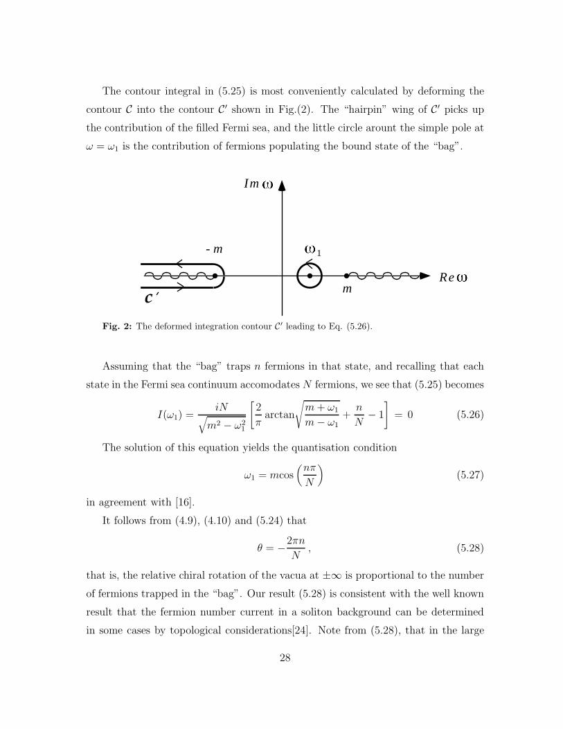
The contour integral in (5.25) is most conveniently calculated by deforming the

contour C into the contour C′ shown in Fig.(2). The “hairpin” wing of C′ picks up

the contribution of the filled Fermi sea, and the little circle arount the simple pole at

ω = ω1 is the contribution of fermions populating the bound state of the “bag”.

- m

m

1

Re

Im

c

Fig. 2: The deformed integration contour C′ leading to Eq. (5.26).

Assuming that the “bag” traps n fermions in that state, and recalling that each

state in the Fermi sea continuum accomodates N fermions, we see that (5.25) becomes

I(ω1) =iN

√

m2 − ω21

[

2

πarctan

√

m+ ω1

m− ω1+n

N− 1

]

= 0 (5.26)

The solution of this equation yields the quantisation condition

ω1 = mcos(

nπ

N

)

(5.27)

in agreement with [16].

It follows from (4.9), (4.10) and (5.24) that

θ = −2πn

N, (5.28)

that is, the relative chiral rotation of the vacua at ±∞ is proportional to the number

of fermions trapped in the “bag”. Our result (5.28) is consistent with the well known

result that the fermion number current in a soliton background can be determined

in some cases by topological considerations[24]. Note from (5.28), that in the large

28

N limit, θ (and therefore ω1) take on non-trivial values only when the number of the

trapped fermions scales as a finite fracion of N .

As we already mentioned in the introduction, stability of “bags” formed in the NJL

model are not stable because of topology. They are stabilised by releasing binding

energy of the fermions trapped in them. To see this more explicitly, we calculate now

the mass of the “bag” corresponding to (4.9),(5.27) and (5.28). The effective action

(1.6) for background fields (4.9) is an ordinary function of the chiral angle θ 18. Let

us denote this action per unit time by S(θ)/T . Then, from (2.9) and (5.21) we find

1

T

∂S

∂θ=∫

dx dω

2π

{[

iσ(x)√m2 − ω2

− (A+D)

]

∂σ(x)

∂θ

+i

[

π(x)√m2 − ω2

− (B + C)

]

∂π(x)

∂θ

}

. (5.29)

Then as in our analysis of the saddle point condition (which is simply the condition

for ∂S∂θ

= 0) we use (4.4), (4.5), (2.10) and the fact that (5.23) vanishes to find

1

T

∂S

∂θ= i

∫

dx dω

2π

∂xσ(x)∂θπ(x) − ∂xπ(x)∂θσ(x)

2 (ω − ω1)√m2 − ω2

.

Then, (3.6) leads to the factorised expression

1

T

∂S

∂θ=

i

4sin2 θ2

∞∫

−∞

dx (σ −m)σ′∫

C′

dω

2π

1

(ω − ω1)√m2 − ω2

(5.30)

where C′ is the contour in Fig.(2). The space integral is immediate and is essentially

fixed by the boundary conditions (2.2). The spectral integral is given by the left hand

side of (5.26), but with a generic ω1 given by ω1 = mcos( θ2). Here we have chosen

the particular branch of (5.24) that contains all the extremal values of ω1. Putting

everything together we finally arrive at

1

NT

∂S

∂θ=m

2

(

n

N+

θ

2π

)

sinθ

2. (5.31)

18Recall that ω1 is a function of θ and not a free parameter.

29

The zeros of (5.31) are simply the zeros of (5.26), as these two equations are one and

the same extremum condition. Integrating (5.31) with respect to θ we finally find

−1

NTmS(θ) =

(

n

N+

θ

2π

)

cosθ

2− 1

πsin

θ

2. (5.32)

Note that (5.32) is not manifestly periodic in θ because the Pauli exclusion principle

limits θ to be between 0 and 2π.

The mass of a “bag” containing n fermions in a single bound state is given by

−S/T evaluated at the appropriate chiral angle (5.28). We thus find that this mass

is simply

Mn =Nm

πsin

πn

N(5.33)

in accordance with [16, 20]. These “bags” are stable because

sinπ (n1 + n2)

N< sin

πn1

N+ sin

πn2

N(5.34)

for n1, n2 less than N , such that a “bag” with n1 +n2 fermions cannot decay into two

“bags” each containing a lower number of fermions.

Entrapment of a small number of fermions cannot distort the homogeneous vac-

uum considerably, so we expect that Mn will be roughly the mass of n free massive

fermions for n << N . As a matter of fact we used this expectation to fix the inte-

gration constant in (5.33). For n << N we have Mn ∼ nm[1 − 16

(

πnN

)2+ · · ·], so the

binding energy released

Bn ∼ nm

6

(

πn

N

)2

+ · · · (5.35)

is indeed very small. However, as the number of fermions trapped in the “bag”

approaches N , Mn vanishes and the fermions release practically all their rest mass

Nm as binding energy, to achieve maximum stability[17]. In a weakly coupled field

theory containing solitons, the mass of these extended objects is a measure of 1g2 ,

the inverse square of the coupling constant. Here we have 1g2 = N . It is amusing to

speculate that these maximally stable massless solitons may teach is something about

the strong coupling regime of the NJL model.

30

Note from (5.28), that the soliton twists all the way around as the number of

fermions approaches N . In this case ω1 → −m, and the pole the resolvent has at

ω = ω1 pinches the branchpoint ω = −m at the edge of the filled Dirac sea. One may

wonder whether this enhanced singularity is a mathematical artifact, as the bound

state simply tries to plunge into the filled Dirac sea. But this is clearly not the case.

Indeed, ω1 is occupied by N fermions (in a flavor singlet). Their common spinor wave

function must still be part of the discrete spectrum of the Dirac operator, because

the highest lying state of the sea at ω = −m is already occupied by a flavor singlet

made of N fermions, sharing a continuum spinor wave function, and therefore Pauli’s

exclusion principle protects the bound state from “dissolving” into the sea.

5.2 Two bound states

We concluded Subsection 4.2 short of an explicit solution of (4.18), namely, short of

an explicit expression for the two bound state background fields σ(x) and π(x). In

the following we make the eminently reasonable assumption that such a background

exists, and pursue our analysis of its saddle point condition as far as we can without

having its explicit form in hand.

As in the previous subsection, we substitute (4.13) and (4.14) into the saddle point

equations (5.19). We then make use of (5.21) to eliminate the ultraviolate logarithmic

divergences and to write the saddle point conditions as

∫

C′′

dω

2π

[

iσ(x)√m2 − ω2

− (A+D)

]

=

i∫

C′′

dω

2π

K + ω Lω2−π2(x)

2√m2 −m2 (ω − ω1) (ω − ω2)

rmand∫

C′′

dω

2π

[

π(x)√m2 − ω2

− (B + C)

]

=

∫

C′′

dω

2π

M + ωσ′ (x)

2√m2 −m2 (ω − ω1) (ω − ω2)

(5.36)

31

where C′′ is a contour similar to the contour C′ in Fig.(2) that encircles the additional

pole at ω2 as well, and K(x), L(x) and M(x) are given by

K(σ, π) = −σ(σ2 + π2 −m2) + (ω1 + ω2)π′ +

1

2σ′′

L(σ, π) = (ω1 + ω2)[

σ(σ2 + π2 −m2) − 1

2σ′′]

−(

σ2 + π2 −m2

2+ ω1ω2 + σ2

)

π′

+π

′′′

4and

M(σ, π) = −π(σ2 + π2 −m2) − (ω1 + ω2)π′ +

1

2π′′ . (5.37)

Note that K(σ, π) differs from −F (σ, π) in (5.23) only by the additional term

ω2π′. The expression L(σ, π) is the residue of the x dependent poles at ω = ±π(x) in

the first equation in (5.36). The quantisation conditions (5.36) on ω1 and ω2 cannot

be x dependent. Therefore L(σ, π) must vanish as a consistency requirement. As we

do not have the explicit expressions of σ(x) and π(x), we assume from now on that

L indeed vanishes. This is the only extra assumption we make. Then, assuming that

the “bag” traps n1 fermions in ω1 and n2 fermions in ω2, (5.36) boils down to the

simple conditions

I(ω1) = I(ω2) = 0 (5.38)

where I(ω) is given in (5.26). Therefore,

ω1 = m cos(

n1π

N

)

, ω2 = m cos(

n2π

N

)

(5.39)

which are identical in form to single bound state energy levels. From the general

considerations of [24] we expect that the chiral angle θ will be proportional to the

total number of fermions trapped by the “bag”, so (5.28) must read now

θ = −2π (n1 + n2)

N. (5.40)

32

The soliton mass is a function of m and of the chiral angle θ. Assuming this function

is the same as in the previous case we therefore conjecture that the mass of the two

bounnd state “bag” is simply

Mn1,n2 =Nm

πsin

π (n1 + n2)

N. (5.41)

As far as mass is concerned, such a “bag” cannot be distinguished from a single bound

state “bag” containing the same total number n1 + n2 of trapped fermions. If our

conjecture is true, then such “bags” are stable against decaying into several “bags”

with lower numbers of fermions as (5.34) shows.

33

A Appendix A

In this Appendix we provide precise definitions of the Jost functions b1 through c2 in

terms of their spatial asymptotic behavior and derive the spatial asymptotic behavior

of the static Dirac operator Green’s function.

We concentrate for the moment on the first equation in (2.6). The boundary

conditions (2.2) lead to the following simple spatial asymptotic behavior

[−∂2x +m2 − ω2] b(x) = 0

of the homogeneous part of that equation. Thus, solutions of that homogeneous

equation assume the generic asymptotic form

b(x, ω) ∼

M+eikx +N+e

−ikx , x→ +∞

M−eikx +N−e

−ikx , x→ −∞(A.1)

where

k(ω) = +√ω2 −m2 . (A.2)

On the real ω axis k(ω) is real for |ω| > m, which corresponds to scattering states of

(2.3). Bound states of (2.3) reside in the domain |ω| < m, where k(ω) = +i√m2 − ω2 =

+iκ(ω) is purely imaginary and lies in the upper half plane.

The Jost functions b1 and b2 alluded to in Section 2 form a particular pair of

linearly independnt solution of the homogeneous equation mentioned above, specified

by their asymptotic behavior. Let the asymptotic amplitudes of br(x), (r = 1, 2) in

(A.1) be Mr±, Nr±. The asymptotic form (A.1) of b1(x) has by definition M1− = 0,

and that of b2(x) has N2+ = 0. One may summarise our definitions of b1 and b2, by

saying that b1 corresponds to a one dimensional scattering situation where the source

is at +∞ emitting waves to the left (the term N1+e−ikx) and that b2 corresponds to

a one dimensional scattering situation where the source is at −∞ emitting waves to

the right (the term M2−eikx). Note also that outside the continuum, b1(x) decays to

the left while b2(x) decays to the right. With these definitions the Wronskian (2.8)

34

becomes

Wb(+∞) = −2ikM2+N1+

ω + π (+∞)= −2ik

M2−N1−

ω + π (−∞)= Wb(−∞) . (A.3)

Therefore, it follows from (2.10) and from (2.11) that the entries A,B,C, and D in

(2.9) have the asymptotic form

A(x) = − 1

2k

{

[σ(x) − ik sgnx]R(k) e2ik|x| + σ(x)}

B(x) =ω + π(x)

−2ik

[

1 +R(k) e2ik|x|]

C(x) =ω − π(x)

2ik

[

1 +R(k) e2ik|x|]

D(x) = − 1

2k

{

[σ(x) + ik sgnx]R(k) e2ik|x| + σ(x)}

(A.4)

as x→ ±∞, where

R(k) =M1+

N1+=N2−

M2−(A.5)

is the reflection coefficient of the Sturm-Liouville operator in the first equation in

(2.6). The diagonal resolvent of the Dirac operator is therefore

〈x | − iD−1|x 〉 −→x→±∞

i

2k

iσ(x) ω + π(x)

−ω + π(x) iσ(x)

+

iR (k) e2ik,|x|

2k

iσ(x) + k sgn x ω + π(x)

−ω + π(x) iσ(x) − k sgn x

. (A.6)

35

B Appendix B

Consider the Sturm-Liouville problem

−[

p(x)ψ′

(x)]′

+ [V (x) −Eρ(x)]ψ(x) = 0 , −∞ < x <∞ . (B.1)

We assume that the “metric” p(x) does not vanish anywhere and that the weight

function ρ(x) is positive everywhere. E is a complex number, called the spectral

parameter.

As in our discussion in the main text and in the previous appendix, let ψ1(x) be

the Jost function which decays as x → −∞ for values of E below the continuum

threshold. Similarly, let ψ2(x) be the Jost function which decays as x→ +∞. Then,

the Green’s function of the operator in (B.1) is

G(x, y) =θ (x− y)ψ2(x)ψ1(y) + θ (y − x)ψ2(y)ψ1(x)

W(B.2)

where

W = p(x)[

ψ2(x)ψ′

1(x) − ψ1(x)ψ′

2(x)]

(B.3)

is the (x independent) Wronskian of these two functions. Note that (B.2) decays (at a

rate dictated by the Jost functions) as either one of its argument diverges in absolute

value, holding the other one finite, as long as E does not hit one of the eigenvalues

of the Sturm-Liouville operator.

As in the main text the diagonal resolvent R(x) = G(x, x) is defined as

R(x) =1

2limǫ→0

[G(x, x+ ǫ) +G(x+ ǫ, x)] =ψ1(x)ψ2(x)

W. (B.4)

We then use (B.3) and (B.4) to show that

ψ′

1

ψ1=pR

′

+ 1

2pR,

ψ′

2

ψ2=pR

′ − 1

2pR. (B.5)

Finally, using (B.1) and (B.5) we find

36

(pR′

)′

= 2(V − Eρ)R +

(

pR′

)2 − 1

2pR(B.6)

and

[p(pR′

)′

]′

= [2p(V − Eρ)R]′

+ 2p(V −Eρ)R′

. (B.7)

Note that the non-linearity of (B.6) in R has disappeared after one more differen-

tiation with respect to x.

Multiplying (B.6) through by 2R we find

− 2pR(pR′

)′

+(

pR′)2

+ 4pR2(V − ρE) = 1 (B.8)

which is the Gel’fand-Dikii equation [6]. Eq. (B.7) is the linear form of the Gel’fand-

Dikii equation we use in the text (Eq. (3.1 .)

The quantities corresponding to the discussion of the Dirac operator in the text

are

p(x) = ρ(x) =1

ω + π(x), E = ω2

and

V (x) =1

ω + π(x)·[

σ(x)2 + π(x)2 − σ′(x) +σ(x)π′(x)

ω + π(x)

]

. (B.9)

The Gel’fand-Dikii equation (B.8) then reads

− 2B(x)

ω + π(x)∂x

[

∂xB(x)

ω + π(x)

]

+

[

∂xB(x)

ω + π(x)

]2

+

[

2B(x)

ω + π(x)

]2 [

σ(x)2 + π(x)2 − σ′(x) − ω2 +σ(x)π′(x)

ω + π(x)

]

= 1 . (B.10)

Strictly speaking, Sturm-Liouville theory requires that p(x) = ρ(x) = 1ω+π(x)

> 0 .

Our solution for π(x) turns out to be bounded, so all formulae are valid a posteriori

for large positive ω. Such a restriction on ω, though mathematically required, is

unphysical.

37

Note however, that because of the relation (2.11), we may view C(x) as a contin-

uation of B(x) to large negative ω.

An important application of the Gel’fand-Dikii identities (B.7), (B.8) is that they

generate an asymptotic expansion[6] of R in negative odd powers of√E. The explicit

ω (and therefore E) dependence of our specific p(x), ρ(x) and V (x) complicates this

expansion.

Acknowledgements We would like to thank N. Andrei for valuable discussions,

and J. Polchinski for reminding us of [24]. This work was partly supported by the

National Science Foundation under Grant No. PHY89-04035.

References

[1] For review of such model field theories see for example

R. Rajaraman, Solitons and Instantons (North-Holland, Amsterdam, 1982);

E. Abdalla, M.C.B. Abdalla and K.D. Rothe, Non-Perturbative Methods in 2

Dimensional Quantum Field Theory (World Scientific, Simgapore, 1991).

[2] A recent reprint volume of papers on the large N expansion is

E. Brezin and S. R. Wadia, The Large N Expansion in Quantum Field Theory

and Statistical Physics (World Scientific, Simgapore, 1993).

[3] R.F. Dashen, B. Hasslacher and A. Neveu, Phys. Rev. D 12,2443 (1975).

[4] L.D. Faddeev and L.A. Takhtajan, Hamiltonian Methods in the Theory of Soli-

tons (Springer Verlag, Berlin, 1987).

[5] D.J. Gross and A. Neveu, Phys. Rev. D 10, 3235 (1974).

[6] I.M. Gel’fand and L.A. Dikii, Russian Math. Surveys 30, 77 (1975).

[7] J. Feinberg, Phys. Rev. D 51, 4503 (1995).

[8] J. Feinberg, Nucl. Phys. B433, 625 (1995).

[9] Y. Nambu and G. Jona-Lasinio, Phys. Rev. 122, 345 (1961), ibid 124, 246 (1961).

38

[10] See the concluding remarks in [16] who brings an unpublished argument for

decoupling of θ due to R. Dashen, along the lines of

M.B. Halpern, Phys. Rev. D 12 1684 (1975).

See also E. Witten, Nucl. Phys. B145, 110 (1978).

[11] S. Coleman, Commun. Math. Phys. 31, 259 (1973).

[12] J.M. Cornwal, R. Jackiw, and E. Tomboulis, Phys. Rev. D 10, 2428 (1974).

[13] J. Goldstone and R. Jackiw, Phys. Rev. D 11, 1486 (1975).

[14] S. Hikami and E. Brezin, J. Phys. A (Math. Gen.) 12, 759 (1979).

[15] H.J. de Vega, Commun. Math. Phys. 70, 29 (1979);

J. Avan and H.J. de Vega, Phys. Rev. D 29, 2891 and 1904 (1984)

[16] S. Shei, Phys. Rev. D 14, 535 (1976).

[17] R. MacKenzie, F. Wilczek and A.Zee, Phys. Rev. Lett 53, 2203 (1984).

[18] T. D. Lee and G. Wick, Phys. Rev. D 9, 2291 (1974);

R. Friedberg, T.D. Lee and R. Sirlin, Phys. Rev. D 13, 2739 (1976);

R. Friedberg and T.D. Lee, Phys. Rev. D 15, 1694 (1976), ibid. 16, 1096 (1977);

A. Chodos, R. Jaffe, K. Johnson, C. Thorn, and V. Weisskopf, Phys. Rev. D 9,

3471 (1974).

[19] W. A. Bardeen, M. S. Chanowitz, S. D. Drell, M. Weinstein and T. M. Yan,

Phys. Rev. D 11, 1094 (1974);

M. Creutz, Phys. Rev. D 10, 1749 (1974).

[20] N. Andrei and J.H. Lowenstein, Phys. Rev. Lett. 43, 1698 (1979),

Phys. Lett. 90B, 106 (1980), ibid. 91B 401 (1980).

[21] S. Coleman and J. Mandula, Phys. Rev. 159, 1251 (1967).

[22] R.F. Dashen, B. Hasslacher and A. Neveu, Phys. Rev. D 10, 4130 (1974).

39

[23] C.G. Callan, S. Coleman, D.J. Gross and A. Zee, unpublished;

D.J. Gross in Methods in Field Theory , R. Balian and J. Zinn-Justin (Eds.),

Les-Houches session XXVIII 1975 (North Holland, Amsterdam, 1976);

A. Klein, Phys. Rev. D 14, 558 (1976);

See also [7] and R. Pausch, M. Thies and V. L. Dolman, Z. Phys. A 338, 441

(1991).

[24] J. Goldstone and F. Wilczek, Phys. Rev. Lett. 47, 986 (1981);

See also Eq. (4.44) of R. Aviv and A. Zee, Phys. Rev. D. 5, 2372 (1972).

40