dynamic workload balancing and scheduling in hadoop ...

DYNAMIC WORKLOAD BALANCING AND

SCHEDULING IN HADOOP MAPREDUCE WITH

SOFTWARE DEFINED NETWORKING

By

XIAOFEI HOU

Bachelor of Science in Information and Computing

Science

Northeastern University

Qinhuangdao, Hebei, China

2011

Submitted to the Faculty of the

Graduate College of the

Oklahoma State University

in partial fulfillment of

the requirements for

the Degree of

DOCTOR OF PHILOSOPHY

July, 2017

ii

DYNAMIC WORKLOAD BALANCING AND

SCHEDULING IN HADOOP MAPREDUCE WITH

SOFTWARE DEFINED NETWORKING

Dissertation Approved:

Dr. Johnson Thomas

Dissertation Adviser

Dr. Eric Chan-Tin

Dr. Christopher Crick

Dr. Weihua Sheng

iii Acknowledgements reflect the views of the author and are not endorsed by committee

members or Oklahoma State University.

ACKNOWLEDGEMENTS

Many people helped me during my PhD program, and I would like to express my sincere

gratitude to them.

Firstly, I would like to thank my advisor Dr. Johnson Thomas for his enthusiasm, his

encouragement, and his resolute dedication to the strangeness of my research. This

research has been the major driving force throughout my graduate career at Oklahoma

State University. I want to thank my committee members Dr. Eric Chan-Tin, Dr.

Christopher Crick and Dr. Weihua Sheng for their guidance and advice for my research

over these years. I would like to thank all other professors and staff in the Computer

Science Department at Oklahoma State University for their help and support.

I would like to thank my parents and my girlfriend Zhiqing Guo for their infinite love and

support during my study aboard. I would also like to thank all my friends both in China

and in the U.S.

Once again, I appreciate you all!

iv

Name: XIAOFEI HOU

Date of Degree: JULY, 2017

Title of Study: DYNAMIC WORKLOAD BALANCING AND SCHEDULING IN

HADOOP MAPREDUCE WITH SOFTWARE DEFINED

NETWORKING

Major Field: COMPUTER SCIENCE

Abstract: Hadoop offers a platform to process big data. Hadoop Distributed File System

(HDFS) and MapReduce are two components of Hadoop. Hadoop adopts HDFS which is

a distributed file system for storing data and MapReduce for processing this data for

users. Hadoop stores data based on space utilization of datanodes, without considering

the processing capability and busy level during the running time of each datanode.

Furthermore datanodes may be not homogeneous as Hadoop may run in a heterogeneous

environment. For these reasons, workload imbalances will appear and result in poor

performance. We propose a dynamic algorithm that considers space availability,

processing capability and busy level of datanodes to ensure workload balance between

different racks. Our results show that the execution time of map tasks moved will be

reduced by more than 50%. Furthermore, we propose a method in which Hadoop runs on

a Software Defined Network in order to further improve the performance by allowing fast

and adaptable data transfers between racks. By installing OpenFlow switches to replace

classical switches on a Hadoop cluster, we can modify the topology of the network

between racks in order to enlarge the bandwidth if large amounts of data need to be

transferred from one rack to another. Our results show that the execution time of map

tasks moved is significantly reduced by about 50% when employing our proposed

Hadoop cluster Bandwidth Routing algorithm. Apache YARN is the second generation of

MapReduce. YARN has three built-in schedulers: the FIFO, Fair and Capacity Scheduler.

Though these schedulers provide users different methods to allocate resources of a

Hadoop cluster to execute their MapReduce jobs, they do not guarantee that their jobs

will be executed within a specific deadline. We propose a deadline constraint scheduler

algorithm for Hadoop. This algorithm uses a statistical approach to measure the

performance of datanodes and based on this information the proposed algorithm creates

several check points to monitor the progress of a job. Based on the progress of jobs at

every checkpoint the proposed scheduler will assign them to different job queues. These

queues will have different priorities and the proportion of resources used by these queues

will depend on their priority. The results of our experiments show that the proposed

scheduler ensures that jobs will be completed within a given deadline whereas the native

schedulers cannot guarantee this. Moreover, the average job execution time in the

proposed scheduler is 56% and 15% less when compared to the Fair and EDF schedulers

respectively.

v

TABLE OF CONTENTS

Chapter Page

I. INTRODUCTION ......................................................................................................1

1.1 Big Data .............................................................................................................1

1.2 Motivation ..........................................................................................................1

1.3 The big goal ......................................................................................................1

1.4 Contributions......................................................................................................2

1.4.1 Dynamic workload balancing for Hadoop MapReduce ..............................2

1.4.2 Use software defined network in Hadoop for workload balancing ............2

1.4.3 Deadline constraint scheduler for Hadoop ..................................................3

1.5 Dissertation outline ............................................................................................3

II. REVIEW OF LITERATURE....................................................................................4

2.1 Hadoop ...............................................................................................................4

2.1.1 Hadoop Distributed File System ...............................................................5

2.1.2 MapReduce ...............................................................................................9

2.1.3 Analysis of jobs running in Hadoop .......................................................10

2.2 Software Defined Networking .........................................................................12

2.3 Workload Balancing Problem ..........................................................................14

2.4 Software Defined Networking in Hadoop .......................................................21

2.5 Hadoop scheduling algorithm ..........................................................................24

III. WORKLOAD BALANCING IN HADOOP .........................................................31

3.1 Motivation ........................................................................................................31

3.2 Dynamic Racks Workload Balancing Algorithm ............................................33

3.2.1 Overview .................................................................................................33

3.2.2 Estimation ...............................................................................................35

3.2.3 Rack selection .........................................................................................36

3.2.4 Data transfer ............................................................................................38

3.2.5 Dynamic rack workload balancing algorithm .........................................39

3.3 Simulation for Dynamic Racks Workload Balancing algorithm .....................41

3.3.1 Simulators used .......................................................................................41

3.3.2 Simulation design....................................................................................42

3.3.3 Simulation results....................................................................................42

3.4 Improvement of dynamic racks workload balancing Algorithm .....................43

vi

3.4.1 Predicting the number of tasks ................................................................44

3.4.2 Predicting remaining time of tasks .........................................................45

3.4.3 Rack selection .........................................................................................46

3.4.4 Data transfer ............................................................................................48

3.4.5 Improved Dynamic racks workload balancing algorithm .......................48

3.5 Simulation for Improved Dynamic Racks Workload Balancing algorithm.....49

3.5.1 Simulator used ........................................................................................50



3.6 Conclusion .......................................................................................................53

Chapter Page

IV. USE SDN IN HADOOP ........................................................................................54

4.1 Introduction ......................................................................................................54

4.2 Motivation ........................................................................................................54

4.3 Proposed Architecture ......................................................................................55

4.4 Hadoop cluster bandwidth routing algorithm ..................................................57

4.4.1 Problem analysis .....................................................................................57

4.4.2 New paths addition .................................................................................58

4.4.3 Algorithm to change topology by SDN ..................................................59

4.5 Simulation ........................................................................................................61

4.5.1 The simulator NS-2 .................................................................................61



4.6 Conclusions ......................................................................................................66

V. HADOOP SCHEDULING ALGORITHM ...........................................................68

5.1 Introduction ......................................................................................................68

5.2 Hadoop Scheduler ............................................................................................70

5.2.1 FIFO scheduler........................................................................................70

5.2.2 Fair scheduler ..........................................................................................70

5.2.3 Capacity scheduler ..................................................................................70

5.3 Motivation ........................................................................................................71

5.4 Datanode Capability Estimation ......................................................................72

5.5 Monitoring Job Execution................................................................................73

5.5.1 Task running time estimation..................................................................73

5.5.2 Set checkpoint .........................................................................................74

5.5.3 Monitor job execution progress ..............................................................75

5.6 Deadline constraint scheduler for Hadoop .......................................................75

5.6.1 Single job scheduling ..............................................................................75

5.6.2 Multiple jobs scheduling .........................................................................77

5.7 Experiments .....................................................................................................78

vii

5.7.1 Setup .......................................................................................................78

5.7.2 Design .....................................................................................................78

5.7.3 Results .....................................................................................................79

5.8 Conclusion .......................................................................................................83

VI. CONCLUSIONS AND FUTURE WORK ............................................................84

6.1 Main motivation of this work. .........................................................................84

6.2 Contributions....................................................................................................85

6.2.1 Dynamic workload balancing for Hadoop MapReduce ..........................86

6.2.2 Software Defined Networking in Hadoop for workload balancing ........86

6.2.3 Deadline constraint scheduler for Hadoop ..............................................86

6.3 Validation .........................................................................................................87

6.4 Results ..............................................................................................................88

6.5 Main conclusions .............................................................................................89

6.6 Future work ......................................................................................................90

REFERENCES ............................................................................................................92

viii

LIST OF TABLES

Table Page

3.1 Simulated racks and Clock velocity .....................................................................41

3.2 Simulated racks and time for one task .................................................................50

4.1 Simulated racks, switches and links.....................................................................63

4.2 Bandwidth of each link on each period of time ...................................................64

5.1 Relative capability of datanode ............................................................................73

5.2 Various Jobs Characteristics ................................................................................80

ix

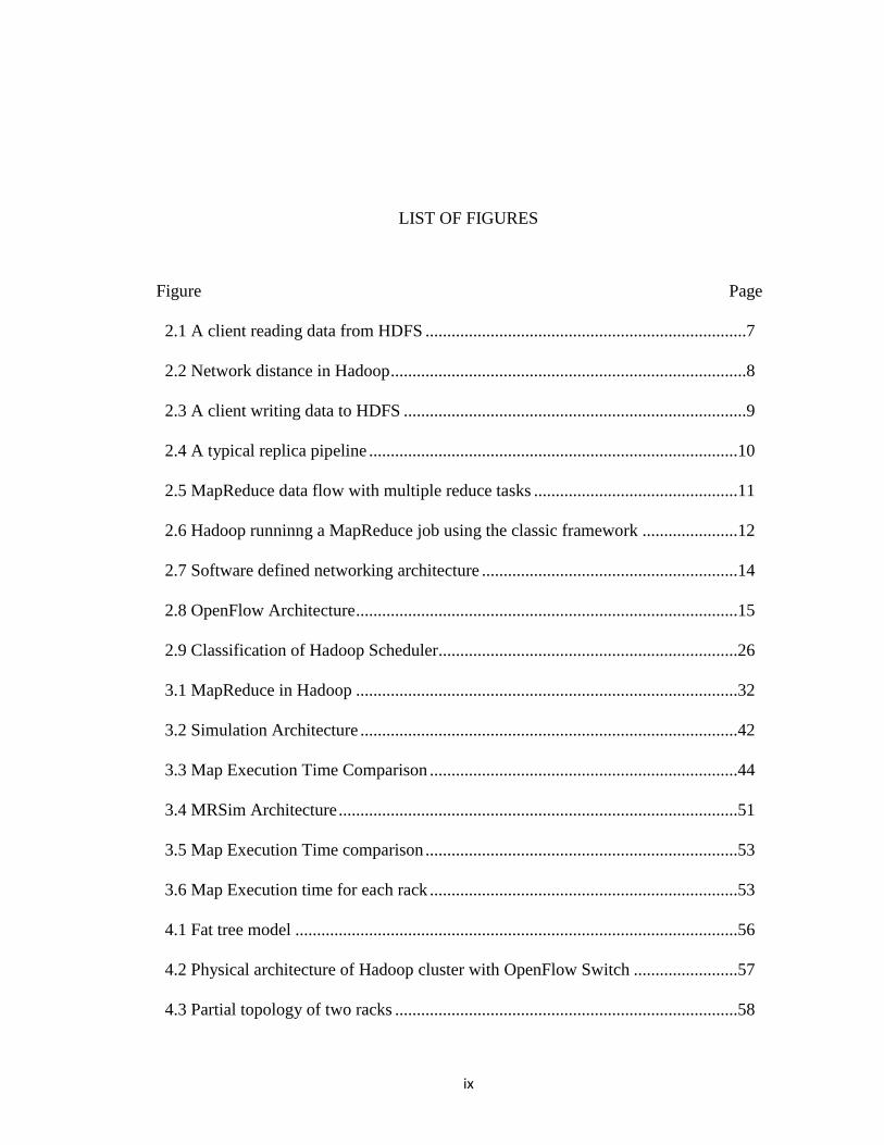
LIST OF FIGURES

Figure Page

2.1 A client reading data from HDFS ..........................................................................7

2.2 Network distance in Hadoop ..................................................................................8

2.3 A client writing data to HDFS ...............................................................................9

2.4 A typical replica pipeline .....................................................................................10

2.5 MapReduce data flow with multiple reduce tasks ...............................................11

2.6 Hadoop runninng a MapReduce job using the classic framework ......................12

2.7 Software defined networking architecture ...........................................................14

2.8 OpenFlow Architecture ........................................................................................15

2.9 Classification of Hadoop Scheduler.....................................................................26

3.1 MapReduce in Hadoop ........................................................................................32

3.2 Simulation Architecture .......................................................................................42

3.3 Map Execution Time Comparison .......................................................................44

3.4 MRSim Architecture ............................................................................................51

3.5 Map Execution Time comparison ........................................................................53

3.6 Map Execution time for each rack .......................................................................53

4.1 Fat tree model ......................................................................................................56

4.2 Physical architecture of Hadoop cluster with OpenFlow Switch ........................57

4.3 Partial topology of two racks ...............................................................................58

x

4.4 Data transferring quantity comparison.................................................................65

4.5 Data transfer time comparison .............................................................................66

4.6 Map tasks execution time comparison .................................................................67

5.1 Job execution time in Fair scheduler and deadline ..............................................81

5.2 Job execution time in EDF scheduler and deadline .............................................82

5.3 Comparison between proposed scheduler and deadline ......................................83

5.4 Comparison of average running times of MR jobs using various schedulers ......83

xi

List of publications

“Dynamic Workload Balancing for Hadoop MapReduce”, Xiaofei Hou, Ashwin Kumar T K,

Johnson P Thomas and Vijay Varadharajan, the 4th IEEE International Conference on Big Data

and Cloud Computing (BDCloud 2014)

“Privacy reserving Rack-based Dynamic Workload Balancing for Hadoop MapReduce”,

Xiaofei Hou, Doyel Pal, Ashwin Kumar T K, Johnson P Thomas and Hong Liu, the 2nd

IEEE

International Conference on Big Data Security on Cloud (BigDataSecurity 2016)

“Dynamic Deadline-constraint Scheduler for Hadoop YARN”, Xiaofei Hou, Ashwin Kumar T

K, Johnson P Thomas and Hong Liu, accepted by the 3rd

IEEE International Conference on Cloud

and Big Data Computing (CBDCom 2017)

“Cleaning Framework for BigData”, Hong Liu, Ashwin Kumar T K, Johnson P Thomas and

Xiaofei Hou, the 2nd

IEEE International Conference on Big Data Computing Service and

Applications (BigDataService2016)

“An Information Entropy Based Approach to Identify Sensitive Information in Big Data”,

Ashwin Kumar TK, Hong Liu, Johnson P Thomas and Xiaofei Hou, accepted by the 2nd

IEEE

International Conference on Big Data Security on Cloud (BigDataSecurity 2016)

List of publications under preparation

“Content Sensitivity Based Access Control Framework For Big Data”, Ashwin Kumar TK,

Xiaofei Hou, Johnson P Thomas and Hong Liu

1

CHAPTER I

INTRODUCTION

1.1 Big Data

The term “Big Data” appeared first in an academic paper in 2000 and was intended to show that huge

amounts of data were being generated every day. For example, every day, Google has over 1 billion

queries, Twitter has over 250 million tweets, Facebook has over 800 million updates and YouTube

has over 4 billion views. These just belong to social media and networks. In other areas like mobile

devices, scientific instruments and sensor technology, big data is also being generated continually.

Big data is very a large and complex data set. It is difficult for traditional databases or applications to

deal with big data because of its massive size that can be from many terabytes to petabytes. The “3Vs”

is always used to describe big data, which are Volume, Velocity and Variety, and big data is high

volume, high velocity and high variety. In addition, variability and veracity are used to show the

inconsistency and the quality of data captured from the source of big data.

Hadoop is the most popular and efficient tool to store and process big data. Hadoop uses the Hadoop

Distributed File System [1] and adopts the MapReduce model platform [2] to process big data in its

cluster.

1

1.2 Motivation

Although Hadoop is originally designed for a homogenous cluster, nodes fail and are replaced or new

nodes added to the cluster, In practice, therefore Hadoop is always working in a heterogeneous

environment. The tasks are assigned corresponding to data locality. In other words, tasks are assigned

to nodes where the data is stored. When Hadoop allocates disk space to store data, the processing

capability of datanodes is not considered. Therefore nodes which have low capabilities may be

assigned heavy tasks and nodes with high capabilities may be assigned light tasks. This leads to

workload imbalance and it adversely influences the performance of Hadoop. Currently, there doesn’t

exist a method in Hadoop to address the workload imbalance issue.

Load balancing by itself will not guarantee that a user job will complete within a certain deadline.

The current Hadoop schedulers are not able to ensure jobs submitted by users can meet their deadline

because both the Fair scheduler and Capacity scheduler ignore the jobs’ deadline. Though jobs in

Hadoop can be assigned different priorities, the jobs with the highest priority cannot be guaranteed to

be allocated enough resources to meet their deadlines. From another perspective, if the jobs with the

highest priority can meet their deadline requirements because of having enough resources, this may

negatively impact jobs with lower priority. No method exists to monitor the progress of the jobs and

prevent them from using too much resource, as this will have a negative influence on the other jobs.

1.3 The big goal

Though Hadoop is already a very popular and stable platform for distributed systems, it still has some

shortcomings in different situations and can produce complex run-time conditions. By reviewing

related literature and studying the architecture of Hadoop, we find workload balancing and scheduling

of Hadoop-MapReduce tasks as two major problems that merit further research. Performance of

Hadoop is affected by these two factors. The target of this research is to address the problems of

workload balancing and scheduling in Hadoop MapReduce and YARN. Workload balancing will

2

influence the efficiency of Hadoop and determine the execution time of jobs. Scheduling will provide

the mechanism for jobs to best utilize the resources of Hadoop. Solving these two problems will

improve the current naïve Hadoop at different levels and will improve overall performance. The new

scheduling algorithm will make the decision on how much resource to be allocated to a job based on

their execution state. Workload balancing algorithms will distribute the current allocated resources to

each rack based on performance of the racks to reduce the waiting time and total execution time.

1.4 Contributions

1.4.1 Dynamic workload balancing for Hadoop MapReduce

In our work we look at workload balancing at the rack level. This is better than considering at the

node level because balancing the workload between the racks can reduce the running time of many

tasks, which is much more efficient than reducing the running time of just one or two tasks on a

single node. A dynamic workload balancing algorithm is designed for Hadoop MapReduce in the

heterogeneous environment, which means for different racks, performance does not always match

workload which will degrade the entire performance of Hadoop. The proposed algorithm addresses

this problem by moving a task from the busiest rack to a less busy rack in order to reduce the

execution time of jobs running on the busiest rack and thereby achieve load balancing.

1.4.2 Use software defined network in Hadoop for workload balancing

Because the dynamic workload balancing algorithm requires the transfer of data between racks, when

the data is large, the cost of transferring is significant. Reducing this cost will improve the efficiency

of the dynamic workload balancing algorithm. To achieve this, we employ Software Defined

Networking (SDN) in a Hadoop cluster using a fat tree topology. When we need to transfer data

between two racks, we can increase the bandwidth between them in order to enhance the performance

of Hadoop.

3

1.4.3 Deadline constraint scheduler for Hadoop

The users of Hadoop MapReduce may have deadline requirements for their jobs. It is not possible in

the current version of Hadoop to guarantee these jobs can be completed within a specific deadline,

because the current scheduler of Hadoop does not make sure jobs with high priorities can meet their

deadline. To address this problem, we propose a deadline constraint scheduler for Hadoop, which will

monitor the progress of jobs execution. The resource allocation is based on the progress of the job to

avoid missing the deadline.

1.5 Dissertation outline

The rest of this dissertation is organized as follows. In the chapter II, a literature review of current

related work is presented. In the chapter III, the dynamic rack workload balancing algorithm and

improved version of the algorithm is explained in detail. In chapter IV, SDN and OpenFlow switches

are add to the Hadoop cluster to improve the network function. In chapter V, the deadline constraint

scheduler is proposed and discussed in detail. Chapter VI concludes the thesis.

4

CHAPTER II

REVIEW OF LITERATURE

In this chapter, recent research focusing on workload balancing, software defined networking and

scheduling problem are reviewed. For each topic, we present the research in the same and similar

areas. Moreover, we discuss and compare previous research on the same problem with our

research.

2.1 Hadoop

Doug Cutting, who is the creator of the widely used text search library Apache Lucene, and Mike

Cafarella wrote the initial version of Hadoop in 2004. In December of the following year, Hadoop

ran reliably on 20 nodes. In April 2006, a 10 GB per node sort benchmark ran on a Hadoop

cluster of 188 nodes in 47.9 hours [9]. In December of the same year, the sort benchmark ran on a

Hadoop cluster of 900 nodes in 7.8 hours. In April 2008 [9], a world record was broken by

Hadoop which became the fastest distributed system by sorting one terabyte data in 209 seconds

with 910 nodes in the cluster [9]. Just seven months later, Hadoop sorted one terabyte in 62

seconds performing better than another implementation of MapReduce of Google which needed

68 seconds to sort the same quantity of data [9]. Since then, Hadoop has been the most popular

and efficient tool to store and process big data.

Hadoop uses the Hadoop Distributed File System [1] and adopts the MapReduce model platform

[2] to process big data in its cluster and is used by Yahoo, Facebook and Amazon. The Hadoop

Distributed File System and MapReduce are the two core components of Hadoop. The Hadoop

5

Distributed File System offers reliable storage and data management while MapReduce in parallel

processes the data stored in the cluster. Hadoop divides a job into tasks and stores data as blocks,

and then allocates them to the nodes in the cluster. A Master and slave pattern is employed by

Hadoop. The distributed architecture allows Hadoop to efficiently write, read and process data.

2.1.1 Hadoop Distributed File System

The Hadoop Distribute File System (HDFS) whose original name is Nutch Distributed Filesystem

(NDFS) is an open source implementation of the architecture of Google’s distributed file system

(GFS) and written by Nutch in 2004. When a single physical node can’t provide enough storage

capacity to a dataset because of hardware constraints, we increase the number of nodes to store

the partitions of the dataset separately. The file system employed to manage the dataset across a

group of nodes is called a distributed filesystem. Distributed filesystems are more complex than

regular disk filesystems because they need to address problems like node failure in order to

ensure data availability. HDFS is a filesystem designed for files as large as hundreds of gigabytes

or terabytes.

HDFS uses a block as a storage unit that is 64 MB [1] which is much larger than a regular disk

block size of 512 bytes by default in order to decrease the cost of seeks. The files stored in HDFS

are partitioned into many blocks. The benefits of the block-based filesystem are:

1. the size of a file can be beyond the capacity of the hard disk in a single machine, because

the blocks of a file can be distributed on the hard disks of different nodes

2. because the block in HDFS is of fixed size, this simplifies the storage subsystem and

eliminates metadata concerns

3. each block in HDFS has replicas that improve fault tolerance and availability of the

system.

6

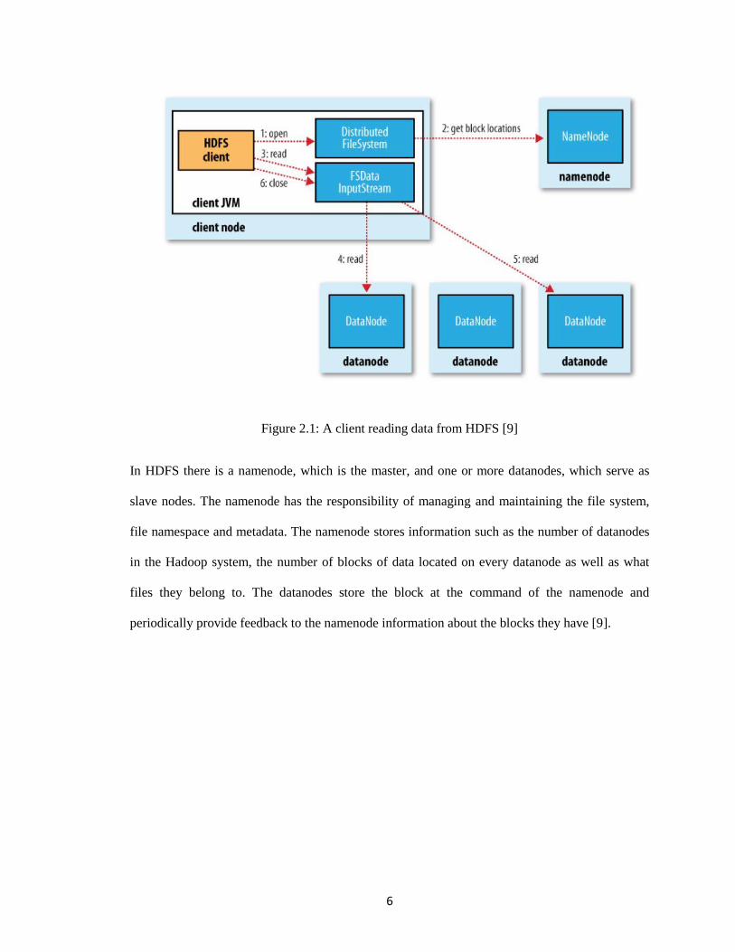
Figure 2.1: A client reading data from HDFS [9]

In HDFS there is a namenode, which is the master, and one or more datanodes, which serve as

slave nodes. The namenode has the responsibility of managing and maintaining the file system,

file namespace and metadata. The namenode stores information such as the number of datanodes

in the Hadoop system, the number of blocks of data located on every datanode as well as what

files they belong to. The datanodes store the block at the command of the namenode and

periodically provide feedback to the namenode information about the blocks they have [9].

7

Figure 2.2: Network distance in Hadoop [9]

When users want to read data from their files on Hadoop, the namenode will provide the address

of the datanodes containing the replicas of the block. Then Hadoop will sort those datanodes

based on their distance to the users; the closest datanode will be selected and if any failure occurs

during this procedure, the next closest datanode will replace the failed node. The distance defined

in Hadoop has four possibilities: 1) on the same datanode, 2) different nodes but on the same rack,

3) datanodes on different racks but in the same data center and 4) datanodes on different data

centers [9].

When one user wants to write data to Hadoop, such as creating a new file on Hadoop, the

namenode is called to create the new file in the filesystem’s namespace without any related

blocks. The namenode checks two things: firstly, that the file the user is going to create does not

exist in the current system and secondly, whether the user has the correct permissions to create

that file. After the checks have finished and passed, the new file will be recorded by the

namenode and be ready to be written. When the user writes data, the namenode will allocate new

8

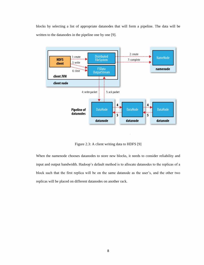
blocks by selecting a list of appropriate datanodes that will form a pipeline. The data will be

written to the datanodes in the pipeline one by one [9].

Figure 2.3: A client writing data to HDFS [9]

When the namenode chooses datanodes to store new blocks, it needs to consider reliability and

input and output bandwidth. Hadoop’s default method is to allocate datanodes to the replicas of a

block such that the first replica will be on the same datanode as the user’s, and the other two

replicas will be placed on different datanodes on another rack.

9

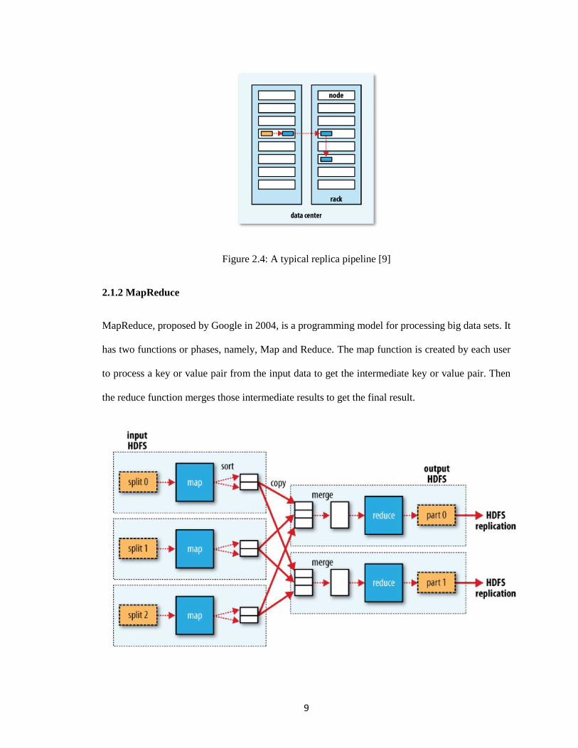
Figure 2.4: A typical replica pipeline [9]

2.1.2 MapReduce

MapReduce, proposed by Google in 2004, is a programming model for processing big data sets. It

has two functions or phases, namely, Map and Reduce. The map function is created by each user

to process a key or value pair from the input data to get the intermediate key or value pair. Then

the reduce function merges those intermediate results to get the final result.

10

Figure 2.5: MapReduce data flow with multiple reduce tasks [9]

2.1.3 Analysis of jobs running in Hadoop

When users try to submit a job to Hadoop, several steps are implemented;

1) a new job ID is generated by the jobtracker for this job,

2) the output specification of the job is checked,

3) the input split for each task of this job is computed

4) transfer the resources such as configuration file to the jobtracker’s filesystem under the

directory named after the job ID,

5) inform the jobtracker that the job is ready for processing.

The job is then initialized. The job is put into an internal queue and waits to be picked up by the

job scheduler of Hadoop. During the initialization of the job, an object is created to represent it

and encapsulates the tasks of this job, and information that keeps track of the tasks status and

execution progress is recorded. The job scheduler retrieves the input splits from the filesystem

and creates one map task for every split and some reduce tasks whose number is determined by

the property of the job. Apart from the map and reduce tasks, another two tasks are created: a job

setup task and a job cleanup task. The Tasktracker will run the job setup task before the map tasks

run and run the cleanup task after all the reduce tasks are finished.

The Tasktrackers send a heartbeat to the jobtracker to remind it whether they are available and

can accept a new task to run. If a tasktracker is ready to run a new task, the jobtracker will contact

the tasktracker through the return value of the heartbeat that will assign it a new task.

11

Figure 2.6: Hadoop running a MapReduce job using the classic framework [9]

Each tasktracker contains a certain number of slots to run map tasks and reduce tasks and the

number is based on the number of cores and how large the memory each tasktracker has. The free

map task slots will be scheduled earlier than free reduce task slots by default. When choosing a

map task to assign to the free slots, the jobtracker first considers network location of the

tasktracker, then selects a task whose input split is closest to the tasktracker. The optimal situation

is a task running on the datanode that has the input split; this is called a data-local task. If the task

has its input split on the same rack but not the same datanode, it is called a rack-local task. If the

task has its input split not on the same rack, it is a rack-off task.

12

When the task is going to be executed, the job JAR is localized by transferring it from the shared

filesystem to the filesystem of the tasktracker. A local working directory is then generated for this

task and an instance of TaskRunner is created to run the task.

After the last task of a job, the job cleanup task, is finished, the jobtracker will receive a

notification. Then it modifies the status of the job to “successful”. A message will be printed to

inform the user and the result is returned [9].

2.2 Software Defined Networking

In a traditional networking architecture, the control part and data part are separated rather than

coupled together. Software defined networking decouples those two parts and make the control

layer directly programmable. This change enables the underlying infrastructure to become

abstracted for applications and network services so that the network becomes a logical or virtual

entity from the perspective of the application and network services. In the traditional networking

architecture, devices are from different vendors and may have various protocols, but SDN

realizes a centralized management and control of networking devices from multiple vendors.

SDN has the ability to add new network capabilities and services such as not requiring

configuration of every device. SDN provides a new opportunity to users to program the network

environments [21]. In addition to abstracting the network, a lot of APIs that enable functions (like

implement common network services including routing, multicast, access control, bandwidth

management, QoS and so on) to satisfy business targets are offered by Software defined

networking.

13

Figure 2.7: Software defined networking architecture [3]

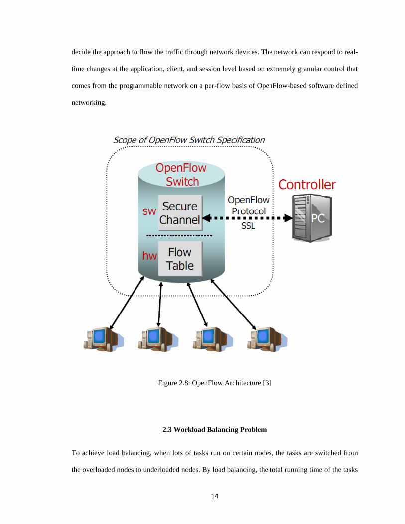
OpenFlow [3], which is the first implementation of SDN, establishes a communications interface

between the control and data forwarding layers. OpenFlow enables access to and operation of the

forwarding layer of network devices like routers and switches. An OpenFlow switch separates the

forwarding path and control function, which is the obvious distinguishing feature compared to the

classical switch. OpenFlow enables the forwarding plane of network devices to be accessible and

operated physically and virtually. The access and operation are implemented through a secure

channel that is established between the OpenFlow switch and the controller for communication.

On both sides of the interface between network infrastructure devices and the software defined

networking, the protocol of OpenFlow is employed. Software defined networking control

software can statically or dynamically program some pre-defined match rules that enables

OpenFlow to use the concept of flows to identify network traffic. OpenFlow allows the user to

14

decide the approach to flow the traffic through network devices. The network can respond to real-

time changes at the application, client, and session level based on extremely granular control that

comes from the programmable network on a per-flow basis of OpenFlow-based software defined

networking.

Figure 2.8: OpenFlow Architecture [3]

2.3 Workload Balancing Problem

To achieve load balancing, when lots of tasks run on certain nodes, the tasks are switched from

the overloaded nodes to underloaded nodes. By load balancing, the total running time of the tasks

15

will be reduced. Therefore, load balancing is essential for achieving high and efficient

performance especially in a distributed system. In recent years, significant attention and research

has been devoted to the load balancing problem. In this section, we review load balancing in

general in a cloud computing, grid environment, wireless network and then focus on load

balancing in Hadoop.

There are several existing load balancing algorithms like Round-robin, Weighted round-robin,

Least-connection, Weighted least-connection and Shortest expected delay [51].

Z. Zhang and X. Zhang [45] propose a load balancing mechanism for cloud computing. It is

based on the ant colony approach and complex network theory. They use ants’ behavior in their

mechanism to collect information from the nodes on the cloud, and then find a specific node to

run a task. But a synchronization problem exists in their mechanism, which is addressed by K.

Nishant et al in [46].

B. Radojevie et al. [47] propose an algorithm named Central Loud Balancing Decision Model

(CLBDM). This algorithm is based on session switching at the application layer, and it improves

the well-known load balancing algorithm Round Robin [48]. The CLBDM counts the connection

time between the client and the node. A threshold is set in the algorithm and if the connection

time becomes larger than it, the connection will be terminated and another node will run the task

of the original node.

J. Ni et al [49] present a virtual machine mapping policy based on multi-resource load balancing

for a private cloud. Their algorithm includes a central scheduling controller, which computes the

resource availability for a specific task and determines the task assignment, and a resource

monitor to collect the information of resource availability.

The problem of system burden caused by data duplication and redundancy is addressed by T. WU

et al. [50]. They introduce a new management architecture for data centers, which is named Index

16

Name Server (INS). The INS integrates deduplication and access point selection optimization.

The INS can be used to dynamically monitor parameters like IP information and busy level index

to keep load balancing.

X. Ren et al. [52] propose a load balancing algorithm named Exponential Smoothing forecast

based on Weighted Least-connection (ESBWLC), which improves on an existing algorithm

called weighed least connection (WLC). The WLC algorithm assigns tasks to the node with the

least number of connections. However, the capabilities of nodes are not considered. ESBWLC

addresses this issue by making the assignment based on the experience of nodes’ capabilities.

S. W et al. [53] propose an algorithm for load balancing, which combines Opportunistic Load

Balancing (OLB) [54] and Load Balancing Min-min (LBMM) [55] algorithms. The OLB is a

static load balancing algorithm, which has the issue of ignoring the execution time of the nodes

and processing tasks slowly. The proposed algorithm has a three layered architecture and divides

tasks into multiple subtasks to speed up the processing.

Active Monitoring Load Balancing (AMLB) algorithm is proposed in [56]. This algorithm will

find the VM with the least load and assign it to the request. If there is more than one satisfied VM,

the first one found will be chosen. The VM-assign load balance algorithm [57] is an improved

version of the AMLB algorithm. It will select the VM with the least load and not be assigned in

the previous request.

S. G. Domanal et al. [58] propose a local optimized load balancing approach named the modified

throttled algorithm. It is designed to distribute the incoming jobs uniformly among the servers or

virtual machines. In Throttled Load Balancer [59], when a request comes, an index table with the

list of virtual machines with their states is searched to find a VM based on availability. The

shortcoming is current load on the machine is not considered. In the modified throttled algorithm,

17

when a request comes and if it is not the first one, the search for the VM will start from the VM

next to the one already assigned in the table.

G. Soni and M. Kalra [60] propose a load balancing algorithm called the Central Load Balancer.

The balancer also uses a table with the states of every virtual machine and their priorities, which

is calculated by capability of CPU and memory. When assigning task, the VM with the highest

priority will be selected if it is not busy.

H. Chen et al. [61] propose a Load Balance Improved Min-Min Scheduling (LBIMM) algorithm.

In the traditional Min-Min algorithm [62], when several tasks already exist, the task with the

minimum size is assigned to the resource to realize the minimum completion time for all the tasks.

In LBIMM, the minimum size task from the most loaded resource is used to calculate the running

time on all the other resources. If the minimum of the running time is less than the one in

traditional Min-Min, the task will be re-assigned to the resource that generates the minimum.

The Double Threshold Energy Aware Load Balancing (DT-PALB) algorithm [63] is proposed by

J. Adhikari and S. Patil. The algorithm manages the compute nodes based on the utilization

percentage and minimizes the energy requirement by switching off the idle compute nodes at the

same time.

O. A. Rahmeh et al. [64] propose a distributed and scalable load balancing framework using

biased random sampling [65]. The Biased random sampling uses a virtual graph containing the

connectivity of servers to show their load. The algorithm in [64] has the sample walk on the

virtual graph. The sample walk starts at a specific node and moves randomly to its neighbor. The

last node in the sample walk is chosen for the load location.

A power aware load balancing algorithm named Bee-MMT is used to save energy while

maintaining load balancing in cloud computing [65] [66] [67]. The algorithm will move some

18

VMs from the overloaded hosts to maintain load balancing and move all VM from the

underloaded hosts to reduce power consumption.

Y. Lu et al. propose a load balancing algorithm for a large system called Join-Idle-Queue [68]. In

their algorithm, they first solve the problem of assigning idle processors at all the dispatchers,

then reduce the queues length in each processor.

M. Salehi et al [69] propose a load balancing algorithm in the grid environment. The algorithm

uses a new adaptive mechanism of intelligent colonies of ants, which can generate a new one if

they find themselves overloaded.

J.Galvez et al [70] propose a distributed load balancing algorithm for the wireless mesh network.

The algorithm reroutes the flows from overloaded gateways to underloaded gateways. The

algorithm considers the effects of interference, which makes itself feasible in practical scenarios.

F. Zeng and Z. Chen [71] propose a greedy algorithm named GA-LBC to solve the problem of

load balancing gateway placement. The cluster in the wireless mesh network is divided into a

load balanced part and disjointed part, where both of them satisfy QoS requirements.

Hadoop MapReduce is originally designed to run on a homogeneous cluster where nodes have the

same capacity. When employed in a heterogeneous environment, the performance of Hadoop

decreases because of the different capabilities of nodes [5] [39]. M. Zaharia et al. show that it is

impossible for Hadoop MapReduce in a heterogeneous cloud computing infrastructure like

Amazon EC2 to perform as efficiently as the homogeneous cluster. Observations from

experiments show that the homogeneity assumption of Hadoop MapReduce leads to incorrect and

often unnecessary speculative execution in heterogeneous environments [4]. Xie. J et al. find data

locality as a determining factor that influences MapReduce performance. Hadoop distributes data

to multiple nodes based on utilization of disk space, but this method to balance workload is not

19

useful in a heterogeneous node environment [7]. Workload imbalance in Hadoop MapReduce

running in a heterogeneous cluster is an obstacle to performance [40].

In [7], the authors introduce a data placement approach on a heterogeneous cluster based on the

processing capability of every datanode on Hadoop so that data movement decreases. Before

executing a user’s job, a small part of data is used to run a test in the Hadoop cluster for

measuring the different capability of nodes. They get the capability of the datanodes in Hadoop

by setting up some MapReduce application on every datanode and letting it run many times, and

select the shortest response time as the measure of computing capability after normalization.

After getting the capability of nodes, the data of the jobs will be allocated to each node

corresponding to their capability.

In [5], M. Mustafa et al. find hardware heterogeneity can result in severe performance penalties

by exposing communication or I/O bottlenecks in Hadoop MapReduce. They conquer the

bottleneck of I/O by adopting double-buffering and asynchronous I/O in MapReduce on an

asymmetric cluster. The global data streaming method and adaptive resource scheduling through

the dynamic scheduler parameterization are added to MapReduce. By using these two techniques

to overlap I/O and communication latencies, the heterogeneity problem is addressed.

In [6], C. Tian et al. observe that jobs in a large practical data center have different requirements

for resources, especially I/O and CPU. Therefore based on the I/O and CPU utilization, they

distinguish jobs into three kinds, and design a method to detect the type of workload. For

increasing the utilization rate of hardware, they develop a Triple-Queue Scheduler including a

workload prediction mechanism to improve MapReduce performance in a heterogeneous

environment. The newly arriving job will be sent to different queues after predicting the type of

workload. Resources will be allocated separately to jobs in different queues.

20

Smriti et al [41] and Y. Fan et al. [43] focus on the reduce phase in Hadoop MapReduce and

address the problem of data skew in the reduce phase. Because the reduce task with the longest

running time determines the finish time of a job in Hadoop, balancing the workload of the reducer

can improve performance. Smriti et al [41] establish a statistical model of the reducer workload

distribution and use the model to judge whether they have enough samples to meet the users’

workload balancing target. To balance the workload, they split the reduce-key that is overloaded

for one reducer into some mediumly loaded ones, and send them to multiple reducers. By this

approach, the largest workload of the reducer is minimized. Y. Fan et al. [43] find that the

number of map function output data partitions when generated by a hash function is the same as

the number of reduce tasks . The quantity of data of each reduce task is based on the partition

function only. That leads to workload imbalance because of reducers with different data loads.

The authors propose a virtual partition to split the output of the map function (the input of reduce

function) in a fine-grained manner and a workload allocation algorithm based on a continuous

virtual partition to address the performance decrease by reading disk discretely.

V. Martha et al. [42] study the case of using Hadoop MapReduce in social network analysis. They

show that workload imbalance will occur when 1) the mappers get different data for tasks of a job

and 2) slow or down nodes in the cluster run one of tasks belonging to a job. The authors employ

a properly defined cost function to determine whether a task is heavy or not based on workload. A

hierarchical MapReduce model is proposed to split the heavy task into multiple child tasks and

reassign them to other nodes in this cluster as a new job. Hierarchical MapReduce addresses some

problems such as deadlock and inheritance conflicts and speeds up the job of big dataset

execution.

In [4], the authors design an algorithm called LATE for speculative execution. Performance of

Hadoop may decrease by using the default scheduling method, and to address this problem,

LATE proposes an optimized scheduling algorithm for tasks. When LATE finds a node that

21

performs poorly on MapReduce, it runs speculative tasks on another node for that node. The

LATE algorithm maximizes the performance of Hadoop in a heterogeneous cluster by performing

speculative execution robustly. This improves the performance of Hadoop MapReduce on the

heterogeneous cluster.

In their work [4-7] [39-43] for improving the performance of Hadoop, they focus on solving the

workload imbalance in node level by using a fast node to run the task, which originally ran on a

slow node. Their method can save some time of a job execution, if the task is the last finished.

But if a job has lots of task, only reducing the time used by last task is not a big improvement. In

our work, we use a fast rack or multiple fast racks to share the tasks from the overloaded rack,

which will reduce the execution time of many tasks. The execution time of jobs will be obviously

reduced. Therefore our algorithm is more effective than theirs.

2.4 Software Defined Networking in Hadoop

SDN with its feathers of decoupling the control and forwarding planes and programmability

brings many benefits to different areas. The control panel can be unified in SDN for various kinds

of network devices [78]. Many problems such as data traffic scheduling [79], congestion control

[80], load balanced packet routing [81], energy efficient operation [82], and QoS support [83] [84]

can be solved in SDN. SDN provides a programmable network platform to implement [85],

experiment [86] for the research and innovation. M. Al-Fares et al propose a scalable, dynamic

flow scheduling system named Hedera in [79]. They use a tree architecture in their system with

Openflow switches. M. Ghobadi et al [80] propose OpenTCP, which is a TCP adaptation

framework in SDN. It mainly focuses on the data center with SDN. Aster*x, proposed in [81] is a

distributed load balancer based on SDN. It requires the network switches to be dumb, minimal

flow-based datapath and under a remote controller. ElasticTree, proposed by B. Heller et al. in

22

[82], is a network-wide power manager. It dynamically changes the links and switches based on

the traffic load in the data center. OpenFlow is used to get the information of the current network

utilization and the capability of controlling the data path. A. Ferguson et al. design an API for

applications to control SDN in [83]. They use OpenFlow controller to implement the API, which

releases the read and write authority to users. W. Jeong et al. [84] propose a QoS-aware Network

Operating System (QNOX) for SDN in order to address the issue of missing QoS function in

NOX. The QNOX mainly includes service element, control element, management element and

cognitive knowledge element. N. Melazzi et al. [86] implement an information-centric

networking solution named CONET for the OpenFlow network.

Some works using SDN for workload balancing or QoS are shown here. R. Wang et al. [87]

propose a load balancer in servers using the OpenFlow standard, which employs wildcard rules in

the switches to distribute the traffic from the clients to the servers. Plug-n-Serve, proposed by N.

Handigol in [88], is an OpenFlow based server load balancing system for unstructured networks

containingd cheap commodity hardware. It reduces the response time of web services by using

OpenFlow to monitor the state of the network and control the routes. C. Macapuna et al. [89]

propose a novel data center architecture named Switching with in-packet Bloom filters. They

discuss the risk of a single node failure happening in the controller of an OpenFlow network and

try to distribute the central controller. SIMPLE, proposed in [90] by Z.Qazi et al., is an SDN-

based policy enforcement layer. It uses the current SDN standard to simplify the middlebox-

specific traffic steering. W. Kim et al. [91] propose a network QoS control framework to address

the network convergence problem. They add a QoS API to OpenFlow such as per-flow rate-

limiter and dynamic priority assignment. S. Sharma et al. [92] propose a QoS framework using

SDN implementation such as OpenFlow and OVSDB. P. Skoldstom and B Sanchez [93] design a

system to perform virtual aggregation with a method that is able to fast divide a large number of

routes and spread them in SDN.

23

To accelerate Hadoop MapReduce and improve its performance, several various methods or

algorithms have been proposed in recent research.

Kevin C. et al. [22] study the problem of how to find the best route in a data center network and

they find the existing protocols only have a single method to forward packets which may not

satisfy the need of various applications in a data center. Topology switching given in [22]

retrocedes the control back to the individual applications in order to determine the best path of

routing data among their nodes. It normalizes the synchronized utilization of multiple routing

mechanisms in a data center, and permits applications to define multiple routing systems and

implements individualized routing tasks at a small time level.

Hadoop-A, introduced in [23] is an acceleration framework that uses some plugin components

realized in C++ to make Hadoop optimized for fast data transfer. The performance enhancements

are introduced by three methods. First, a new algorithm is employed to make reduce tasks to

implement data merging without repeating merges and disk access. Second, the shuffle, merge

and reduce phases are overlapped by a full pipeline that is designed for the reduce task. Third, an

alternative protocol is implemented in Hadoop-A to allow data transfer through Remote Direct

Memory Access along with the TCP/IP protocol adopted by general Hadoop.

In Hadoop, all the outputs of both map and reduce tasks are materialized to a local file. A simple

and elegant checkpoint and restart fault tolerance mechanism is employed in the materialization

but it likely has the risk of slowdowns or even failures at the datanodes. A modified framework

of Hadoop MapReduce is introduced in [24] by T. Condie et al. This architecture supports

processing data in pipeline between operators. In their version of Hadoop MapReduce, online

aggregation permits the clients to know the “early returns” from a job as it is being processed.

The Hadoop Online Prototype employs continuous queries as well, which allows stream

processing, and event monitoring applications can be written in MapReduce programs.

24

During the shuffle phase, which between map and reduce phases in Hadoop MapReduce, the

switches within a rack or inter racks will saturate and the bandwidth between some datanodes will

become inadequate which lead to make the computation slower than the expectation. Hadoop-

OFE, described in [25] by S. Narayan et al., demonstrates the idea of adopting the OpenFlow

switches in the Hadoop cluster in order to provide additional network bandwidth to the

overloaded network between nodes. It changes the topology of the network between nodes in

Hadoop dynamically based on different phases of processing a job in order to accelerate the speed

of Hadoop.

Their work [25] is closest to our approach, but their work only shows the idea of using the

OpenFlow switches in Hadoop to change the topology without the detail of what the architecture

in Hadoop with OpenFlow switches is, how and when to change the topology. In our work, we

present the architecture of Hadoop cluster with OpenFlow switches, which is the fat tree

architecture. We also propose an algorithm to change the topology on the fat tree architecture

Hadoop cluster. The algorithm will be deployed to accelerate the proposed workload balancing

algorithm.

2.5 Hadoop scheduling algorithm

J. Gautam et al. [44] give a classification of Hadoop scheduler based on parameters such as time,

priority, strategy and so on. The classification is shown as Figure 2.9.

25

Figure 2.9: Classification of Hadoop Scheduler [44]

Static scheduling, which schedules jobs to nodes before running jobs, tries to minimize the

overall execution time of the job. Dynamic scheduling assigns jobs to nodes while executing jobs.

The scheduling based on resource availability is designed to increase the utilization of resources

such as CPU, disk, memory to improve the total performance of Hadoop. The scheduling based

on time focuses on deadline of jobs, which means whether a job can finish before a certain time

or not, and determines how to assign resource to the job [44].

Some Hadoop or MapReduce scheduling algorithms based on data locality, resource,

performance and energy are reviewed below

M. Hammoud et al. [94] propose a practical strategy named Local-Aware Reduce Task Scheduler

(LARTS) for MapReduce. It improves MapReduce performance by finding a good data locality

and avoiding scheduling delay and skew, low system utilization and degree of parallelism. They

propose the Center-of-Gravity Reduce Scheduler (CoGRS) in [95]. The CoGRS reduces

26

MapReduce network traffic by making the reduce task locality-aware and skew-aware and

schedules every reduce task to run at the center-of-gravity node.

A. Kumar et al. [96] propose a Context Aware Scheduler for Hadoop (CASH). CASH is aware of

the heterogeneity of the Hadoop cluster and learns the context, which includes Job characteristics

and resource characteristics. The algorithm first classifies the jobs based on their requirement for

CPU and I/O and classifies the nodes based on their capabilities. Then it is based on the context

to schedule the jobs. The improved CASH is presented for the jobs with the same working set

data.

X. Zhang et al [97] propose a next-k-node scheduling (NKS) algorithm to improve the data

locality of map tasks. This algorithm schedules the map tasks with the highest probability in order

to make more map task run on the nodes with its input data.

Y. Zhao et al. [98] propose a job scheduling algorithm (TDWS) for Hadoop MapReduce based on

the Tencent Distributed Data Warehouse. The algorithm first groups the jobs based on their type

and then uses a memory-awareness mechanism to schedule the jobs in different groups.

A Self-Adaptive MapReduce scheduling algorithm (SAMR) is proposed by Q. Chen in [99].

SAMR gets the progress of tasks from historical logs and searches for tasks that need backup

tasks. It groups the slow nodes to a set dynamically in order to avoid assigning backup tasks to

the slow nodes. A similar algorithm is proposed in [100]. An Enhanced SAMR proposed by X.

Sun et al. in [101] addresses the issue of ignoring the type of jobs in [102]. In ESAMR, nodes are

divided into several clusters and the weight of each cluster is considered rather than the weight of

each node.

M. Yong et al [102] propose a resource aware scheduler for Hadoop, which monitors the resource

load on each node and schedules jobs based on their resource requirements. The algorithm

minimizes the contention of different types of resources such as CPU and I/O.

27

R. Nanduri et al. propose a job aware scheduling algorithm for MapReduce in [103]. They use

heuristics and machine learning in their algorithm. In their algorithm, when scheduling the

waiting tasks, the one that is mostly compatible in resource requirement with the running tasks

will be selected to run.

H. Mao et al. propose a load-driven task scheduler with adaptive DSC for Hadoop MapReduce in

[104]. Tasks assignment will be based on the workload of the datanodes. The scheduler contains

a dynamic slot controller, which can change the map task and reduce task slots in the datanodes.

Y. Yao et al. propose a job size-based scheduler for Hadoop in [105]. Their algorithm first learns

the information of recently finished job by a lightweight information collector. Secondly, it

allocates slots to each user. Finally, it tunes the jobs of each user.

Z. Wang et al [106] propose a scheduler strategy for heterogeneous workload-aware in Hadoop.

They also divide the jobs into two types, CPU-intensive and I/O- intensive based on historical

information. A CPU and I/O characteristic estimation strategy is presented to avoid the inference

from noise information of historical data.

J. Polo et al. [107] [108] propose a performance-driven task co-scheduler for MapReduce. The

scheduler changes the resource allocation for the jobs based on the dynamic prediction of jobs’

completion times with a specific resource.

B. Shi et al. propose a thermal and power-aware task scheduler for Hadoop in [110]. it costs a

long time for the disk to run when reading and writing large amounts of data, which will increase

both temperature and the consumption of power for cooling. The proposed scheduler minimizes

the consumption of power by selecting suitable nodes to store the data.

28

Y. Li et al. [112] propose a scheduler for MapReduce in the heterogeneous environment and a

power-aware rescheduling scheme. The power-aware rescheduling scheme considers how to save

energy in both processing jobs and storing data.

Several scheduling algorithms based on time in recent research is shown below.

In [31] [32], the authors propose a Constraint-Based Hadoop Scheduler. They use the deadline set

by users as an input parameter to a job execution cost model. This scheduler is able to provide an

immediate feedback that whether the job can be finished within the deadline or not to users and

lets the users to make a decision to reset the deadline. The scheduler will maximize the number of

jobs can run in a Hadoop cluster by making the current running job leave the maximum number

of free slots for jobs that will come in the future. The improvement of this scheduler described in

[32] adds a preemptive method that preempts the resource from jobs whose remaining time is less

than their deadline.

MOMC, a multi-objective and multi-constrained scheduling algorithm of many tasks in Hadoop

is presented in [34] by C. Voicu et al. The authors set two objectives, namely, reducing resource

contention and optimizing workload of the cluster. They consider deadline and budget as the

constraints. The MOMC algorithm is based on the best utilization of job and resources strategy. It

firstly determines whether the available resource is enough or not to complete a job in the

specified budget and deadline. If not, it will change the assignment of job and resources.

Cloud Least Laxity First (CLLF) presented in [35] is a soft real-time scheduling algorithm for the

distributed system with data locality management. This algorithm minimizes the extra-cost of

running tasks in the cloud by ranging the tasks by their laxity and locality. The algorithm firstly

sorts the jobs by laxities and provides a sorted list. Then it selects the first job in the list with the

lowest laxity and tries to search a datanode with free slots to process a task of this job. If found, it

is assigned, if not, next job is selected to search for resources to run the job.

29

A new MapReduce constraint programming based matchmaking and scheduling algorithm

(MRCP) is proposed in [36] by N Lim et al. This algorithm is able to schedule MapReduce jobs

with a deadline. Two new Hadoop schedulers are proposed as EDF-Scheduler and CP-Scheduler.

The EDF-Scheduler is designed by extending the default FIFO scheduler in Hadoop. The CP-

Scheduler is designed by incorporating the MRCP into Hadoop.

In [37], the authors propose maximal Productivity Job Scheduler by modifying the Hadoop job

scheduler to make it aware of the availability of resources. This scheduler contains a training

module in order to generate performance models, a monitoring system to measure residual

capacity of the data center, and a scheduling algorithm.

A resource and deadline-aware Hadoop job scheduler is proposed in [33]. There are three

components in this scheduler, namely, a fuzzy performance model, a resource predictor and a

scheduling optimizer. In this scheduler, the execution of a job is partitioned into multiple intervals.

The fuzzy performance model is multiple-input- single-output which means it uses the job’s input

size and resource allocation in every interval to predict execution progress. They predict resource

availability based on history information by using an Auto-Regressive Integrated Moving

Average model. The scheduling optimizer will change the number of resources assigned to every

running job based on an online receding horizon control algorithm.

The researches [31-33] [35] are close to ours. In [31] [32], the completion time is estimated by

measuring the cost of processing a unit data in a map or reduce task and the quantity of data.

However, the method is not feasible because in a heterogeneous cluster since we cannot get the

same cost of unit data for the different nodes. Authors of [33] [35] presented a better estimation

for job execution time, but their estimation is not accurate. In the work [33], they use the number

of finish tasks to determine the progress of a job. The problem of their method is the number of

finish tasks in an interval is not only based on the current resource allocation but also relative

30

with the number of initialized tasks before this interval. If just using number of finish tasks in

each interval to determine the progress, the estimated execution progress is not accurate. In our

work, we use the number of initialized tasks in each interval to monitor the progress of job

execution, which is more accurate. Based on the progress, we assign different kinds of slots to the

job with slow progress to avoid missing deadline while reducing the influence on execution of the

other jobs.

31

CHAPTER III

WORKLOAD BALANCING IN HADOOP

3.1 Motivation

When users write a file to Hadoop, the namenode will assign a group of three datanodes to users’

data. The user data will be stored as blocks. HDFS does not consider the datanode disk space

utilization when placing these blocks in the datanodes. To keep the whole HDFS cluster balanced,

a tool called balancer is employed in the cluster. A balanced HDFS cluster makes Hadoop reliable

and perform more efficiently. The balancer keeps the utilization of datanodes disk space within

range, which is the average utilization of the entire Hadoop cluster disk space plus or minus a

threshold.

32

Figure 3.1: MapReduce in Hadoop

When users want to run a task, they send a job to Hadoop. The jobtracker of Hadoop will split the

input data and find suitable tasktrackers to process it. The tasktrackers are on the datanode and

send heartbeats to the jobtracker notifying it of the status of tasks. There are a certain number of

slots owned by the tasktracker for the map and reduce tasks. So when a tasktracker has an empty

slot, it will remind the jobtracker it can be used for a new task. For the map task, the jobtracker

will assign the task to the tasktracker that is closest to the corresponding data. For the reduce task,

the jobtracker just assigns the task from the list of yet-to-be-run reduce tasks to the next ready

tasktracker.

Hence the method of block placement is based on the disk space utilization of datanodes rather

than the processing capability of datanodes. This is a major problem because when Hadoop

MapReduce chooses datanodes to process the task, it considers the location of data but not the

capability as well. Therefore workload imbalance will occur on the Hadoop cluster during run

time.

33

In a real-world cluster, Hadoop functions as a heterogeneous cluster. Hence datanodes can have

different processing capabilities and storage volume. In a large Hadoop cluster, there may be

several data centers which contain many racks of datanodes where these datanodes may have

different hardware. Moreover new datanodes can be added to the data centers at different times.

In a Hadoop cluster, the numbers of tasks running on each datanode are different where different

tasks may have different utilization of hardware. Given the above factors, irrespective of whether

the datanodes are heterogeneous or homogeneous, during different periods when tasks are

running in Hadoop, hardware utilization such as CPU and memory of datanodes will be different.

This makes the datanodes process tasks at different speeds. Each rack in a Hadoop cluster will

have different capabilities. In today’s technology, the task of assigning a job to each rack does not

take into account processing capability. This affects the performance of the cluster adversely.

The problem may be summarized as follows: There is currently no way for Hadoop to guarantee

that higher capability racks have more workload than lower capability racks. This adversely

affects the performance of not only a few datanodes, but the whole Hadoop cluster.

We propose a dynamic rack workload balancing algorithm to improve the performance of

Hadoop. Our proposed algorithm will first estimate the processing capability and the existing

workload on each rack. Based on these parameters our algorithm modifies the task allocation to

each rack in order to shorten the running time of the job which has the longest remaining time to

finish.

34

3.2 Dynamic Racks Workload Balancing Algorithm

3.2.1 Overview

To solve the above problem that exists in Hadoop, we employ a dynamic workload balancing

algorithm to modify the tasks assignment scheme to different racks. Our proposed algorithm

consists of three different steps:

Step 1: Estimate the performance of each rack. The algorithm obtains information of a Hadoop

cluster such as the processing capability of each rack and the busyness or commitment of each

rack. The performance of each rack is determined by examining the applications running on

Hadoop, that is, by scanning and analyzing the log of the jobtracker, tasktracker, datanode and

namenode. The logs of the jobtracker and tasktracker, record the start time and finish time, from

which we can get the running time of each task. The running time of each task can be used to

estimate the processing capability and the busy level of a rack

Step 2: Select the racks to schedule for running. According to the busy level of every rack, which

is measured by the recent tasks running time, we select the busiest one from all the racks to

schedule. Here we set a threshold to make sure that the busiest rack is a threshold busier than

other racks, because if the busiest rack is just a little bit busier than other racks (that is, it is less

busier by less than the threshold level), the transfer may not improve the performance of Hadoop

as there is a cost associated with the transfer. Hence we select the busiest rack and see whether its

busy level is larger than the sum of average busy level plus the threshold. If so, we schedule the

busiest rack.

Step 3: Move jobs. The next step is to find the job to move. From the log of the jobtracker, we

can know how many tasks belonging to each job are running on the busiest rack, how many of

them have finished and the time already used. Using this information we can estimate the time

35

remaining for the other tasks to finish. The job that has the longest remaining time is selected to

be moved to a node on another rack

Using parameters such as processing capability, busyness level and number of datanodes, we can

predict the running time of these tasks if run on other racks. The rack with the shortest predicted

running time is the destination rack.

The data of the partial unfinished tasks are moved to the destination rack if the destination rack

does not have a copy of the data. The destination rack will have the shortest average response

time. Within the destination rack, the data will be moved to the datanode with the shortest

response time.

3.2.2 Estimation

The first step as discussed above is to estimate the processing capability and the busy level of

datanodes as well as the racks. This is obtained by firstly, scanning the logs of all the nodes on

Hadoop to obtain information such as the running time of each task, and from it, we estimate the

capability of Hadoop.

Every datanode has its log which records the start time and finish time of the tasks running on the

datanode. The start time and finish time of a task can be obtained from the jobtracker log, for

example:

2015-03-30 11:18:10,296 INFO org. apache. hadoop. mapred. JobInProgress: Choosing data-

local task task_201502091636_0244_m_000027.

2015-03-30 11:18:25,366 INFO org. apache. hadoop. mapred. JobInProgress: Task

'attempt_201502091636_0244_m_000027_0' has completed

task_201502091636_0244_m_000027 successfully.

36

The first line is the record of the start time of the task whose ID is

201502091636_0244_m_000027. The second is the record of the finish time of that task. The

average processing time is obtained by considering all the tasks in the history. This can be used as

a measurement of the processing capability using the following formula:

𝑃 =∑ 𝑡𝑖𝑛𝑖=1

𝑛

where 𝑃 refers to processing capability, 𝑛 refers to the number of tasks running on the datanode

historically and 𝑡𝑖 refers to the time used by the 𝑖𝑡ℎ task. If there are a few tasks (n is low), and

these tasks take a long time (t is high), then P is high. Since P is the average time used by a task on

a datanode, a low P means a high performance node.

The processing capability of a rack can be calculated from the average of the processing capability

of the datanodes on this rack by the following formula:

𝑃𝑟𝑎𝑐𝑘 =∑ 𝑃𝑖𝑁𝑖=1

𝑁 (3.2)

where 𝑃𝑟𝑎𝑐𝑘 refers to the processing capability of a rack, 𝑁 refers to the number of datanodes on a

rack, and 𝑃𝑖 refers to the processing capability of the 𝑖th datanode.

As discussed above, under different workloads, even when the datanodes have the same hardware,

they will provide different performance. Therefore information of how busy the datanodes are is

estimated based on the logs. Similar to the formula above for estimating the processing capability,

we choose the most recent several tasks to compute the average running time of these tasks by the

following formula:

𝐵 =∑ 𝑡𝑖𝑘𝑖=1

𝑘 (3.3)

where 𝐵 refers to the busy level of a datanode, 𝑘 refers to the number of tasks running on the

datanode in the recent history and 𝑡𝑖 refers to the time used by the 𝑖th task.

37

The busy level of a rack can obtained from the average busy level of the datanodes on this rack

using the following formula:

𝐵𝑟𝑎𝑐𝑘 =∑ 𝐵𝑖𝑁𝑖=1

𝑁 (3.4)

where 𝐵𝑟𝑎𝑐𝑘 refers to the busy level of a rack, 𝑁 refers to the number of datanodes on a rack, and

𝐵𝑖 refers to the busy level of the 𝑖th datanode.

3.2.3 Rack selection

After we get an estimation of the processing capability and busy level of all the racks, we select

the busiest rack to schedule whose 𝐵𝑟𝑎𝑐𝑘 is the largest value, that is,

max(𝐵1, 𝐵2, … , 𝐵𝑚)

The job which has the largest remaining time from 𝐵𝑟𝑎𝑐𝑘 is scheduled and moved to another rack.

The destination rack which accepts this job is the rack which has the shortest predicted time for

running the job. This is calculated as shown below. Only some tasks of the job are transferred.

If a job is not terminated or complete, the tasks of that job will have three states: finished, running

and waiting.

The remaining running time of a job is predicted by the following formula:

𝑇𝑟𝑒𝑚𝑎𝑖𝑛𝑖𝑛𝑔 = 𝑇𝑢𝑠𝑒𝑑 ×𝑁𝑤𝑎𝑖𝑡𝑖𝑛𝑔

𝑁𝑓𝑖𝑛𝑖𝑠ℎ𝑒𝑑 (3.5)

where 𝑇𝑟𝑒𝑚𝑎𝑖𝑛𝑖𝑛𝑔refers to the predicted remaining time to finish all the tasks of a job on that

rack,𝑁𝑤𝑎𝑖𝑡𝑖𝑛𝑔

𝑁𝑓𝑖𝑛𝑖𝑠ℎ𝑒𝑑 refers to the ratio of the number of waiting tasks to finished tasks of a job, 𝑇𝑢𝑠𝑒𝑑

refers to the time elapsed from the time the first task starts to the time of the last finished task.

38

To estimate the remaining running time of a job in another rack, we use parameters such as the

processing capability, the busy level and the number of datanodes on the racks. Assume we move

some waiting tasks of a job from rack A to rack B, the estimated running time on rack B will be:

𝑇𝐵 = 𝑇𝐴 ×𝑃𝐵

𝑃𝐴×

𝐵𝐵

𝐵𝐴× (

𝑁𝐵

𝑁𝐴)2 (3.6)

where 𝑇𝐵 refers to the predicted running time of those tasks if moved to rack B, 𝑇𝐴 refers to the

predicted remaining time of those tasks running on rack A, 𝑃𝐴 and 𝑃𝐵 refer to the processing

capability of racks A and B respectively, 𝐵𝐴 and 𝐵𝐵 refer to the busy levels of racks A and B

respectively, 𝑁𝐴 and 𝑁𝐵 refer to the number of datanodes on racks A and B.

The processing capability and the busy level of a rack are the average corresponding values of the

datanodes on that rack. Hence when computing the remaining time of tasks, we get the time based

on the number of datanodes where we use the processing capability or busy level as a rack metric.

Here we use both of them, hence the square of NB/NA.

After selecting which rack to move the tasks to, we choose datanodes on this rack to run these

tasks. We generate a list of datanodes in order of processing capability multiplied by the busy

level (𝑃 × 𝐵). The nodes to be avoided are those with either a low processing capability or those

that are very busy. Hence we select the datanode whose result of 𝑃 × 𝐵 is small. If there are n

tasks to be moved, we choose the n datanodes whose 𝑃 × 𝐵values are the lowest.

To determine the amount of transferred data the selected datanodes accept from another rack, the

method we adopt is to make the amount of data transferred correspond to the ratio of 1

𝑃×𝐵 of the

selected datanodes. A large 𝑃 × 𝐵 means low performance, so a higher performance node will

have a larger 1

𝑃×𝐵. We calculate time by the average performance of a rack. Choosing datanodes

that have a higher performance than average will therefore save more time

39

3.2.4 Data transfer

Before transferring the data, we first check whether the link between two racks has enough

bandwidth to make the transfer efficient and feasible. We derive a function to compute the

appropriate amount of data to make the remaining time the least.

The bandwidth determines whether it is feasible or not to move data between two racks such that

overall performance is improved. Assume we have 𝑛 tasks to transfer and each of them is of fixed

sized (64 MB or 128 MB by default). The predicted running time difference between rack A and

rack B is:

𝑇𝐴 − 𝑇𝐵 = 𝑇𝐴 × (1 −𝑃𝐵

𝑃𝐴×

𝐵𝐵

𝐵𝐴× (

𝑁𝐵

𝑁𝐴)2) (3.7)

Determine if the following inequality holds:

𝑇𝐴−𝑇𝐵

𝑁𝑤𝑎𝑖𝑡𝑖𝑛𝑔>

𝑠𝑖𝑧𝑒𝑜𝑓𝑏𝑙𝑜𝑐𝑘

𝑏𝑎𝑛𝑑𝑤𝑖𝑑𝑡ℎ (3.8)

where 𝑁𝑤𝑎𝑖𝑡𝑖𝑛𝑔 refers to the number of waiting tasks, bandwidth refers to the bandwidth between

rack A and rack B.

If a job chosen to move has some waiting tasks on the rack, moving all the tasks is not efficient.

Instead only some of the tasks are moved because using two racks to run the job is faster than

running on only one rack.

Assume 𝑥(0 < 𝑥 < 1) where x is the number of waiting tasks to be moved. The objective is to

find the value of x that will yield the shortest times TA ,TB and Ttransfer such that:

𝑇𝐴 × (1 − 𝑥) = 𝑇𝐵 × 𝑥 + 𝑇𝑡𝑟𝑎𝑛𝑠𝑓𝑒𝑟 × 𝑥 (3.9)

where 𝑇𝐴 refers to the predicted remaining time of the tasks running on rack A, 𝑇𝐵 refers to the

predicted running time of those tasks if moved to rack B, 𝑇𝑡𝑟𝑎𝑛𝑠𝑓𝑒𝑟 refers to the time if all the

data of these tasks are moved from rack A to rack B.

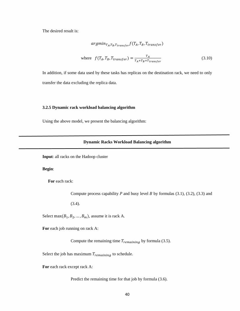
40

The desired result is:

𝑎𝑟𝑔𝑚𝑖𝑛𝑇𝐴,𝑇𝐵 ,𝑇𝑡𝑟𝑎𝑛𝑠𝑓𝑒𝑟𝑓(𝑇𝐴, 𝑇𝐵, 𝑇𝑡𝑟𝑎𝑛𝑠𝑓𝑒𝑟)

where 𝑓(𝑇𝐴, 𝑇𝐵, 𝑇𝑡𝑟𝑎𝑛𝑠𝑓𝑒𝑟) =𝑇𝐴

𝑇𝐴+𝑇𝐵+𝑇𝑡𝑟𝑎𝑛𝑠𝑓𝑒𝑟 (3.10)

In addition, if some data used by these tasks has replicas on the destination rack, we need to only

transfer the data excluding the replica data.

3.2.5 Dynamic rack workload balancing algorithm

Using the above model, we present the balancing algorithm:

Dynamic Racks Workload Balancing algorithm

Input: all racks on the Hadoop cluster

Begin:

For each rack:

Compute process capability 𝑃and busy level 𝐵 by formulas (3.1), (3.2), (3.3) and

(3.4).

Selectmax(𝐵1, 𝐵2, … , 𝐵𝑚), assume it is rack A.

For each job running on rack A:

Compute the remaining time𝑇𝑟𝑒𝑚𝑎𝑖𝑛𝑖𝑛𝑔 by formula (3.5).

Select the job has maximum 𝑇𝑟𝑒𝑚𝑎𝑖𝑛𝑖𝑛𝑔 to schedule.

For each rack except rack A:

Predict the remaining time for that job by formula (3.6).

41

Select rack has the shortest predicted remaining time.

If inequality (3.8) holds:

Get the percentage of tasks to be moved by using formula (3.10) and transfer the

data.

End;

3.3 Simulation for Dynamic Racks Workload Balancing algorithm

We simulated moving partial tasks of a job from one rack to another one in a Hadoop cluster. To

achieve this, we use “Mumak” [13] which is Apache’s Hadoop MapReduce simulator.

3.3.1 Simulators used

Apache Rumen [14] is a tool for extraction and analysis of data from Apache Hadoop. Rumen gets

information such as … from the JobHistory logs and produces the raw trace data that can be used

by simulators such as Mumak.

Apache Mumak [13] is a Hadoop MapReduce simulator. It uses the output of Rumen and some

log files of Hadoop to simulate various situations. Mumak can simulate a big Hadoop cluster and

for that the topology generated by Rumen must be configured.

The simulation architecture which is based on Apache Rumen and Apache Mumak is shown in

Fig. 3.2 below. Rumen outputs files about the cluster, that is, a file that contains the topology of

the cluster and a file that shows the record of how far the tasks of a job have been processed.

Rumen also outputs the jobs information which is shown in the Cluster Story and Job Story.

When a job from user to Hadoop is simulated, the simulation is done by the Job Story of Rumen

42

and accepted by Mumak. We can modify the topology of Hadoop cluster such as the number of

racks and the number of datanodes on each rack

Figure 3.2: Simulation Architecture [15]

3.3.2 Simulation design

We simulated a Hadoop cluster with several racks. These racks have different processing

capabilities and busy levels. In Mumak, the virtual clock represents the performance of nodes. To

achieve a heterogeneous environment the velocity of each node’s virtual clock is set to different

values to simulate their different 𝑃 × 𝐵 values.

TABLE I. Simulated racks and Clock velocity

Simulated

racks

Clock velocity

Rack1 2

Rack2 3

Rack3 4

From the above TABLE I, Rack1 has the worst performance and requires balancing. We simulate

a job with 105 tasks running on rack1 that should be moved by our algorithm.

We compared different situations when these tasks run on native Hadoop MapReduce and Hadoop

MapReduce with our algorithm.

43

3.3.3 Simulation results

In our simulation, we implemented a word counting job to run on a small Hadoop cluster. From

this we get the log files for Rumen. Rumen then generates the topology file and a json file which is

directly input to Mumak. Then we simulated this job running on a Hadoop cluster with three racks.

In this section, we explain the performance improvement of Hadoop MapReduce with our

algorithm by comparing with native Hadoop the finished time of these tasks.

We assume that 105 tasks of the word counting job on rack1 of the simulated Hadoop cluster are

waiting tasks. We use the simulated running time as the tasks of that job compared with the

remaining time if adopting our algorithm as shown in Fig. 3.3 below.

Figure 3.3: Map Execution Time Comparison

Our simulated results which compare the execution time of Native Hadoop and our proposed

balanced Hadoop, show that using our algorithm reduces the execution time by about 66%. The

execution time will be reduced by more than 50% because the rack accepting the tasks that have

been moved has better performance than the original one. Using both of them to do these tasks

more than doubles the efficiency and thereby reduce the execution time by more than 50%.

0

1000

2000

3000

4000

Native Hadoop BalancedHadoop

Exe

cuti

on

Tim

e(s

ec)

Map Execution Time Comparison

44

3.4 Improvement of dynamic racks workload balancing Algorithm

The dynamic racks workload balancing algorithm solves the imbalance by moving the over load

from the busiest racks, and this algorithm reduces the execution time of the partial jobs running

on the busiest rack. If we observe the progress of a job’s execution in different racks, we can find

the tasks belonging to a job in different racks may have different finish times. This is because the

tasks distribution of the job doesn’t match the capability of each rack. If the jobs don’t run on the

busiest rack, the dynamic racks workload balancing algorithm will not be applied to this kind of

jobs. Therefore, the dynamic racks workload balancing algorithm is not able to make the

workload balanced for all the jobs.

We propose an improved algorithm for the workload imbalance problem. The improvements in

this algorithm are 1) considering all the jobs in Hadoop and determining whether the workload on

each rack is balanced or not for every job; 2) moving overload from one rack to multiple racks

can remove the extra burden on the overloaded racks and reduce the transmission time of data.

3.4.1 Predicting the number of tasks

If a job is not terminated or complete, the tasks of that job will have three states: finished, running

and waiting.

From the logs of the jobtracker and tasktracker, we can get the number of running and finished

tasks belonging to a job on a certain rack.

For the waiting tasks, because they have not been assigned to the tasktracker, we need to predict

how many of them will be assigned to a rack.

The log of the jobtracker contains task information such as the task id and the location of input

split. When the task is to be assigned, the jobtracker first chooses a tasktracker to run this task and

the tasktracker id will be recorded to the log. The jobtracker records the type of the task such as

45

whether it is data-local task or rack-local. In a data local task the input split of the task is run on

the datanode processing this task, whereas in a rack local task the input split of a task is not run

on the datanode that processes this task but on the same rack. If this task is finished, the

jobtracker log records that the task has completed successfully. By analyzing the log of the

jobtracker, we get the probability of data-local or rack-local tasks. That is, 𝑡𝑑𝑙

𝑇 or

𝑡𝑟𝑙

𝑇 where td1 is

the number of data-local tasks, tr1 is the number of rack-local tasks and T is the total number of

tasks.

In our algorithm, we assume that all the tasks belong to either data-local or rack-local types.

In HDFS, every data block has three replicas by default. The namenode has the data block’s

location information. Hence when the jobtracker initials a job, it will get the input split location

from the namenode and record it to the log. the distribution of all the input data splits belonging

to a job is obtained from the log of the jobtracker. the number of tasks that belong to a certain job

that have the input split on a rack is also obtained from the log.

By analyzing the distribution of all the input data splits belonging to a job on a rack, the number

of tasks that will run on a rack based on data location are calculated.

𝑁𝑤𝑎𝑖𝑡𝑖𝑛𝑔 =𝑃𝑑

𝑁𝑟𝑒𝑝𝑙𝑖𝑐𝑎× (𝑁𝐴 +𝑁𝐵) +

𝑃𝑟

2× (𝑁𝐴 +

𝑁𝐵

2) (3.11)

Here 𝑁𝑤𝑎𝑖𝑡𝑖𝑛𝑔 refers to the number of tasks of a job waiting to run on the rack based on data

location. 𝑃𝑑 refers to the probability of a data-local task and 𝑃𝑟 refers to the probability of a rack-

local task from log statistics. 𝑁𝑟𝑒𝑝𝑙𝑖𝑐𝑎 refers to the number of replicas of the block in Hadoop,

which by default, is three, 𝑁𝐴 is the number of input splits of the tasks that is the first replica, 𝑁𝐵

is the number of input split of the tasks that is the second or third replica. If a datanode has the

input split of a task, the probability of that datanode running this task as a data-local type is

𝑃𝑑

𝑁𝑟𝑒𝑝𝑙𝑖𝑐𝑎 and the number of this kind of datanodes in a rack is 𝑁𝐴 +𝑁𝐵. Because one input split of

46

a task has replicas on two racks, the rack which has that input split, the probability of running this

task as rack-local type is 𝑃𝑟

2 , and the number of tasks whose input split on this rack is 𝑁𝐴 +

𝑁𝐵

2 .

3.4.2 Predicting remaining time of tasks

After predicting the number of waiting tasks that will run on a rack, the remaining time of the

tasks belonging to a job on a rack can be obtained.

First determine the time used by finished tasks on a rack, specifically the most overloaded rack.

The logs of the jobtracker and tasktracker record the start time of the first task and the finish time

of the last task. The difference of these two times provides an estimate of the performance of a

rack.

The remaining time of a job is predicted as follows:

𝑇𝑟𝑒𝑚𝑎𝑖𝑛𝑖𝑛𝑔 = 𝑁𝑤𝑎𝑖𝑡𝑖𝑛𝑔 ×𝑡

𝑓 (3.12)

where 𝑇𝑟𝑒𝑚𝑎𝑖𝑛𝑖𝑛𝑔 refers to the predicted remaining time to finish all the tasks of a job on that rack,

𝑓 refers to the number of finished tasks belonged to a job on that rack, 𝑡 refers to the time used

by these 𝑓 tasks.

The job that has the largest remaining time on the most overloaded rack will first be scheduled to

be transferred to a underloaded rack.

3.4.3 Rack selection

The optimal situation for a job is that all the map tasks running on each rack complete at the same

time. This situation requires the quantity of tasks assigned to a rack match the performance of that

rack. Task assigning has a close relation with their input split location. Therefore our method is to

change the input split location in order to reduce the map tasks finish time and maintain workload

balance.

47

The ratio 𝑡

𝑓 denotes the capability of a rack. Hence we can estimate the number of tasks to be

assigned to that rack based on its capability. This is calculated as follows:

𝑁𝑎𝑠𝑠𝑖𝑔𝑛 = 𝑁𝑡𝑜𝑡𝑎𝑙_𝑤𝑎𝑖𝑡𝑖𝑛𝑔 ×𝑓𝑘

𝑡𝑘⁄

∑ 𝑓𝑖𝑡𝑖⁄𝑛

𝑖=1

(3.13)

where𝑛 refers to the number of racks in the Hadoop cluster, 𝑖 refers to the 𝑖𝑡ℎ rack, 𝑁𝑎𝑠𝑠𝑖𝑔𝑛 refers

to the number of waiting tasks that should be assigned to the 𝑘𝑡ℎ rack, 𝑁𝑡𝑜𝑡𝑎𝑙_𝑤𝑎𝑖𝑡𝑖𝑛𝑔 refers to the

total number of waiting tasks of a job, 𝑓𝑖 refers to the amount of finished tasks belonging to a job

on the 𝑖𝑡ℎ rack, 𝑡𝑖 refers to the time used by these 𝑓𝑖 tasks. 𝑁𝑡𝑜𝑡𝑎𝑙_𝑤𝑎𝑖𝑡𝑖𝑛𝑔 is the number of total

waiting tasks of a job in the whole cluster.

We can predict the number of tasks to be assigned to a rack by eq. (3.13). For each rack, the

difference between the numbers of tasks that can run based on the capability of a rack and actual

number of tasks that will run on the rack is:

∆𝑁𝑖 = 𝑁𝑎𝑠𝑠𝑖𝑔𝑛𝑖 −𝑁𝑤𝑎𝑖𝑡𝑖𝑛𝑔

𝑖 (3.14)

where 𝑖 refers to the 𝑖𝑡ℎ rack, 𝑁𝑎𝑠𝑠𝑖𝑔𝑛𝑖 refers to the number of tasks that can be assigned to the 𝑖𝑡ℎ

rack based on the capability of this rack, 𝑁𝑤𝑎𝑖𝑡𝑖𝑛𝑔𝑖 refers to the number of tasks that are waiting

and will actually run on the 𝑖𝑡ℎ rack.

The time cost to move the task to the new rack must be considered, because the time saved by

running the task on a different rack should be larger than the transfer time. This can be measured

by determining if the following inequality holds:

𝑡𝑘𝑓𝑘⁄ −

𝑡𝑖𝑓𝑖⁄ >

𝑠𝑖𝑧𝑒𝑜𝑓𝑖𝑛𝑝𝑢𝑡𝑠𝑝𝑙𝑖𝑡

𝑏𝑎𝑛𝑑𝑤𝑖𝑑𝑡ℎ𝑘𝑖 (3.15)

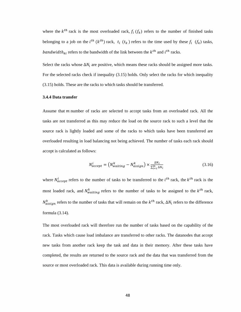
48

where the 𝑘𝑡ℎ rack is the most overloaded rack, 𝑓𝑖 (𝑓𝑘) refers to the number of finished tasks

belonging to a job on the 𝑖𝑡ℎ(𝑘𝑡ℎ) rack, 𝑡𝑖(𝑡𝑘) refers to the time used by these 𝑓𝑖 (𝑓𝑘) tasks,

𝑏𝑎𝑛𝑑𝑤𝑖𝑑𝑡ℎ𝑘𝑖 refers to the bandwidth of the link between the 𝑘𝑡ℎ and 𝑖𝑡ℎ racks.

Select the racks whose ∆𝑁𝑖 are positive, which means these racks should be assigned more tasks.

For the selected racks check if inequality (3.15) holds. Only select the racks for which inequality

(3.15) holds. These are the racks to which tasks should be transferred.

3.4.4 Data transfer

Assume that 𝑚number of racks are selected to accept tasks from an overloaded rack. All the

tasks are not transferred as this may reduce the load on the source rack to such a level that the

source rack is lightly loaded and some of the racks to which tasks have been transferred are

overloaded resulting in load balancing not being achieved. The number of tasks each rack should

accept is calculated as follows:

𝑁𝑎𝑐𝑐𝑒𝑝𝑡𝑖 = (𝑁𝑤𝑎𝑖𝑡𝑖𝑛𝑔

𝑘 −𝑁𝑎𝑠𝑠𝑖𝑔𝑛𝑘 ) ×

∆𝑁𝑖

∑ ∆𝑁𝑖𝑚𝑖=1

(3.16)

where 𝑁𝑎𝑐𝑐𝑒𝑝𝑡𝑖 refers to the number of tasks to be transferred to the 𝑖𝑡ℎ rack, the𝑘𝑡ℎ rack is the

most loaded rack, and 𝑁𝑤𝑎𝑖𝑡𝑖𝑛𝑔𝑘 refers to the number of tasks to be assigned to the 𝑘𝑡ℎ rack,

𝑁𝑎𝑠𝑠𝑖𝑔𝑛𝑘 refers to the number of tasks that will remain on the 𝑘𝑡ℎ rack, ∆𝑁𝑖 refers to the difference

formula (3.14).

The most overloaded rack will therefore run the number of tasks based on the capability of the

rack. Tasks which cause load imbalance are transferred to other racks. The datanodes that accept

new tasks from another rack keep the task and data in their memory. After these tasks have

completed, the results are returned to the source rack and the data that was transferred from the

source or most overloaded rack. This data is available during running time only.

49

3.4.5 Improved Dynamic racks workload balancing algorithm

Using the above model, the rack-based load balancing algorithm is shown below:

Improved Dynamic Racks Workload Balancing algorithm

Input: all racks on the Hadoop cluster

Begin:

For each job:

Estimate the number of waiting tasks to run on the 𝑘𝑡ℎ rack and the remaining time by eq.

(3.11), (3.12)

Based on the capability and workload of each rack, compute the number of tasks to be

assigned to each rack

Select the racks which should get more tasks based on their capability and workload

Select the racks that hold true for inequality (3.15)

Determine the number of tasks to be moved to each rack and transfer the data by eq.

(3.13), (3.14), (3.16).

End.

3.5 Simulation for Improved Dynamic Racks Workload Balancing algorithm

We simulated moving partial tasks of a job from one rack to multiple racks in a Hadoop cluster. To

achieve this, we used the “MRSim” [30] which is a Hadoop MapReduce simulator.

50

3.5.1 Simulator used

MRSim [30] simulates the Hadoop cluster and the MapReduce framework including interaction

between different nodes belonged to the cluster by using SimJava and extending the discrete event

engine. MRSim uses GridSim to simulate and establishes the network topology and simulates the

data transfer.

Figure 3.4: MRSim Architecture [30]

The MRSim [30] architecture implements the basic blocks of nodes including CPU, hard disk

driver (HDD) and Network Interface model as shown in Fig. 3.4 below. Each node is part of a

Network Topology model. In MRSim, the Jobtracker and Tasktracker process is installed on each

node. The input files for MRSim are the cluster topology file and the job specification file, which

are in Json format. The detail configuration and specification of nodes and racks is recorded in the

topology file. The number of map and reduce tasks, data distribution, algorithm description and the

job configuration arguments are recorded in the job specification file.


We simulate a Hadoop cluster with five racks and each rack contains five nodes. Each rack has

five nodes with similar capability. There is therefore a distinct difference between the capabilities

of the racks. In MRSim [8], the CPU speed represents the capability of nodes. Racks with poor

51

capability have a long time for running a task. To achieve a heterogeneous environment, the

velocity of each node’s CPU is set to different values to match their different capabilities. The

poorer capability has the lower CPU speed. From table II we observe the rack with the worst

capability is rack 5. This rack needs to transfer tasks to achieve balancing. We simulate a job with

157 tasks and 10 GB data running on all these racks. We allocate the data blocks based on the

default scheme used in the Hadoop Distributed File System.

We compare different situations when these tasks run on native Hadoop MapReduce and Hadoop

MapReduce with our algorithm.

TABLE II. Simulated racks and time for one task

Simulated racks Time for one task

Rack 1 1.8

Rack 2 7

Rack 3 12

Rack 4 19

Rack 5 22.2


In this section, the performance improvement of Hadoop MapReduce with our algorithm is shown

by comparing the completion time of these tasks on each rack and total time for the job.

157 tasks are run on the five racks of the simulated naïve Hadoop cluster and the running time of

map tasks on each rack is recorded. Then our proposed algorithm is run on the same simulated

Hadoop cluster and the 157 tasks of that job are run. the running time of map tasks on each rack

by using this algorithm is recorded twice. In the first run, the tasks on the most overloaded rack

are moved to multiple racks. In the second run, the tasks on the second most overloaded rack

which will become the most overloaded rack after first run is moved to multiple racks. The

52

comparison of the total execution time is shown in Fig. 3.5 and the comparison of the execution

time for each rack is shown in Fig. 3.6 below.

Figure 3.5: Map Execution Time comparison

Figure 3.6: Map Execution time for each rack

Our simulated results which compare the execution time of Native Hadoop and our proposed

balanced Hadoop, show that using our algorithm reduces execution time by about 55%. The

execution time is reduced by more than 50% because the racks accepting the tasks that have been

0

200

400

600

800

1000

Native Hadoop Implementproposed

algorithm once

Implementproposed

algorithm twice

Exe

cuti

on

Tim

e(t

ime

un

it)


0

100

200

300

400

500

600

700

800

900

rack 1 rack 2 rack 3 rack 4 rack 5

Exe

cuti

on

Tim

e(s

ec)

Map Execution Time Comparison on each rack

Native Hadoop

Run proposed algorithmonce

Run proposed algorithmtwice

53

moved have better capability and less workload than the original one. Using multiple racks to run

these tasks more than doubles the efficiency and thereby reduce the execution time by more than

50%.

3.6 Conclusion

Because Hadoop functions in a heterogeneous environment which means for different racks,

capability does not always match workload. This will lead to some tasks of jobs running on

overloaded racks that take a long time to finish. This degrades the entire performance of Hadoop.

The dynamic racks workload balancing algorithm proposed in this chapter addresses this problem

by moving tasks from the busiest rack to a less busy one so that the remaining time to execute the

tasks can be reduced by at least half.

The improved algorithm addresses this problem by moving tasks from the most overloaded rack

to several other racks for each job so that the remaining time to execute every job in the map

phase can be reduced by more than half.

The results of our simulations show that the finished time of these tasks decrease substantially by

adopting our algorithms compared with the original Hadoop MapReduce. In the future work, we

will consider the deadline of the job and resource availability as constraints to achieve workload

balance in Hadoop MapReduce.

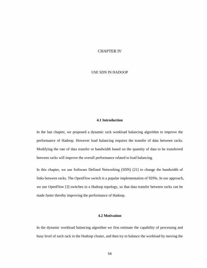
54

CHAPTER IV

USE SDN IN HADOOP

4.1 Introduction

In the last chapter, we proposed a dynamic rack workload balancing algorithm to improve the

performance of Hadoop. However load balancing requires the transfer of data between racks.

Modifying the rate of data transfer or bandwidth based on the quantity of data to be transferred

between racks will improve the overall performance related to load balancing.

In this chapter, we use Software Defined Networking (SDN) [21] to change the bandwidth of

links between racks. The OpenFlow switch is a popular implementation of SDNs. In our approach,

we use OpenFlow [3] switches in a Hadoop topology, so that data transfer between racks can be

made faster thereby improving the performance of Hadoop.

4.2 Motivation

In the dynamic workload balancing algorithm we first estimate the capability of processing and

busy level of each rack in the Hadoop cluster, and then try to balance the workload by moving the

55

tasks of some jobs and transferring the data of these tasks from the busiest rack to another rack.

When transferring the data from one rack to another, if the bandwidth increases, the time cost of

transferring will reduce, and if the quantity of data is large, time will be saved during transferring.

4.3 Proposed Architecture

In introducing software defined network within the Hadoop cluster, the OpenFlow switch

replaces the normal switch. In a large Hadoop cluster, there will be multiple racks. Each rack is

aggregated by datanodes that have the same distance to the namenode. In our proposed

architecture, we assume the datanodes on each rack are linked with a single switch and this

switch is linked with other switches in order to communicate with other racks. We treat the

switch linking every datanode as a part of the rack. This creates a tree-based architecture and

Figure 4.1 shows the topology of our architecture. The proposed architecture forms a fat-tree

topology.

The fat-tree is one kind of network architecture where the links are fatter up the tree and slimmer

lower down the tree. This is because the nodes nearer the root have larger amount of flows.

Hence these links will likely become the bottleneck of the whole network.

Figure 4.1: Fat tree model

56

Figure 4.2: Physical architecture of Hadoop cluster with OpenFlow Switch

The switches on the top of this figure can be treated as the root of the fat tree. We use multiple

switches at the different levels of the tree to implement the same function in order to enlarge the

bandwidth of links. The other OpenFlow switches we use in the Hadoop cluster can be classified

into two kinds:

Edge switch: which is linked to one or more racks directly

Intermediate switch: which is not linked to any racks directly, it only links with other switches

All the switches are connected and controlled by a SDN (OpenFlow) controller. This controller

communicates through the network with the Hadoop Namenode which is the master node of

Hadoop. The controller also communicates with the Jobtracker which controls, assigns and

schedules all the jobs from the clients that are processed by Hadoop MapReduce.

We define the default path between two racks to be the shortest path, that is, using the least

number of switches to link two racks. In the default topology of Hadoop cluster, racks use the

default path to communicate with each other.

57

4.4 Hadoop cluster bandwidth routing algorithm

4.4.1 Problem analysis

In the dynamic workload balancing we propose, if there is imbalance between racks, tasks are

moved and data transferred between two racks, for instance, from rack A to rack B. The

communications topology between rack A and rack B will fall into two kinds:

• There is one edge switch between rack A and rack B.

• There is more than one edge switch linking the two racks as shown in Figure 4.3

Figure 4.3: Partial topology of two racks

For the first situation, there is no need to do anything, that is, the data and tasks are directly

transferred.

A topology for the second case is shown in Figure 4.3. The link between rack A and edge switch

1 is link A, the link between rack B and edge switch 2 is link B, the default path between edge

switch 1 and switch 2 is link C, which may be just a simple link between two edge switches

58

directly or multiple links passing through one or more intermediate switches. The maximum

bandwidth of the default path between rack A and rack B is the weakest link in the chain, that is,

the least bandwidth of link A, link B and link C. We have two possible situations:

• If the bandwidth of link C is larger than the bandwidths of both link A and link B, there is

no change in the topology. This is because we assume that the bandwidth of the link between an

edge switch and the rack to which it is connected is fixed, that is, the bandwidth on links A and B

cannot be changed.

• If the bandwidth of link C is less than the bandwidths of both link A and link B, then link

C becomes the bottleneck of whole path. In this case, find a new path between Switch 1 and

Switch 2 and use OpenFlow to change the topology to generate the new path. Because we already

know not only the logical topology but also the physical architecture of the cluster, we can

generate new paths or links that will enlarge the bandwidth of the link between the two edge

switches.

4.4.2 New paths addition

In the above situation where ideally we want to enlarge the bandwidth, we assume bandwidth of

link C is the bottleneck, that is, the largest possible bandwidth of the path including link A, link B

and link C, but it is less the desired bandwidth which is the upper limit. When we want to add

new paths, there are two situations:

• If after all alternate paths have been considered, the bandwidth is still less than the

desired bandwidth or the upper limit T

• The available bandwidth is more than the difference between upper limit and the

bottleneck.

59

To add a new path to increase the bandwidth as needed, besides knowing the physical architecture

and logical topology, the bandwidth utilization of each path and how much bandwidth is available

at each path should be obtained.

Because the Hadoop cluster is a fat tree structure, we find the highest height ancestor of rack A

and rack B wher rack A and rack B are the leaf nodes. In the fat tree structure, one node can

contain several switches. So we can select and add switches from ancestor nodes of rack A and

rack B. The OpenFlow controller can send the packets containing the new forwarding rules to the

OpenFlow switch. The switch receives the packets and then adds the new rules to its forwarding

table. In this way, the new path is established.

From the OpenFlow controller, we can know the bandwidth utilization and availability of each

path. [10]

In practice, we will add one switch each time and recalculate the bandwidth of the links between

rack A and rack B. This procedure is complete when there is enough bandwidth or all the

switches on these ancestor nodes have been used.

4.4.3 Algorithm to change topology by SDN

After running the Dynamic Workload balancing Algorithm and determining the data to be

transferred for moving tasks between two racks, we obtain two racks for data transfer. Assume

we need transfer data from rack A to rack B.

60

Hadoop cluster Bandwidth Routing algorithm

Definition:

rackA.switch = the edge switch linked with rack A

rackB.switch = the edge switch linked with rack B

linkA = link between rackA and rackA.switch

linkB = link between rackB and rackB.switch

linkC = link between rackA .switch and rackB.switch

The nodes of the fat tree from top to bottom and from left to right are 𝑁0, 𝑁1, 𝑁2…, 𝑁0 is the root

node.

The path from root to rack A are:

( 𝑁0, 𝑁𝑖1 , 𝑁𝑖2…𝑁𝑖𝑚)

The path from root to rack B show in an array:

(𝑁0, 𝑁𝑗1 , 𝑁𝑗2…𝑁𝑗𝑛)

Input: rackA, rackB

If (rackA.switch != rackB.switch)

If (bandwidth𝑙𝑖𝑛𝑘𝐶 < min(bandwidth𝑙𝑖𝑛𝑘𝐴 , bandwidth𝑙𝑖𝑛𝑘𝐵) )

{

For 𝑘 from 1 to min(𝑚, 𝑛)

{Find last 𝑘 that: 𝑁𝑖𝑘 ==𝑁𝑗𝑘;}

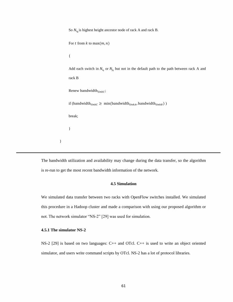
61

So 𝑁𝑖𝑘is highest height ancestor node of rack A and rack B.

For 𝑡 from 𝑘 to max(𝑚, 𝑛)

{

Add each switch in 𝑁𝑖𝑡 or 𝑁𝑗𝑡 but not in the default path to the path between rack A and

rack B

Renew bandwidth𝑙𝑖𝑛𝑘𝐶 ;

if (bandwidth𝑙𝑖𝑛𝑘𝐶 ≥ min(bandwidth𝑙𝑖𝑛𝑘𝐴 , bandwidth𝑙𝑖𝑛𝑘𝐵) )

break;

}

}

The bandwidth utilization and availability may change during the data transfer, so the algorithm

is re-run to get the most recent bandwidth information of the network.

4.5 Simulation

We simulated data transfer between two racks with OpenFlow switches installed. We simulated

this procedure in a Hadoop cluster and made a comparison with using our proposed algorithm or

not. The network simulator “NS-2” [29] was used for simulation.

4.5.1 The simulator NS-2

NS-2 [29] is based on two languages: C++ and OTcl. C++ is used to write an object oriented

simulator, and users write command scripts by OTcl. NS-2 has a lot of protocol libraries.

62

In NS-2, the network topology is first defined. The protocols and application for our simulation

are then specified in the OTcl script. The OTcl enables utilization of the objects to be compiled in

the C++ hierarchy by an OTcl linkage that generates a correspondence of OTcl object.

NS-2 simulates the discrete event and uses virtual time to set the timestamp of events in order to

record the activities in the network. Each event is an object in the C++ hierarchy that has a unique

ID.


We simulated the data transfer between two racks in a Hadoop cluster with several racks. The

Dynamic Workload Balancing Algorithm determines which two racks need to be rebalanced. The

topology of these two racks is known. Assume these two racks don’t link with the same edge

switch, which means we try to find some available bandwidth on another path to add by changing

the topology of the Hadoop cluster. The topology is shown in Figure 4.3. We set 4 nodes in the

NS-2 simulator, and three TCP links between these 4 nodes as shown in Table III.

TABLE III. Simulated racks, switches and links

NS-2 Hadoop

Node 1 Rack A

Node 2 Switch 1

Node 3 Switch 2

Node 4 Rack B

Link A Link between rack A and switch 1

Link B Link between switch 1 and switch 2

Link C Link between rack B and switch 2

63

In our simulation, we use the switches with a gigabit bandwidth on each port. Random numbers

in the range 0.1 to 1 gigabit for the bandwidth of the three links in different periods of time are

generated. The period of time is random. The time and corresponding bandwidth are shown in

Table IV.

TABLE IV. Bandwidth of each link on each period of time

Time Bandwidth of link A

Bandwidth of link C

Bandwidth of link B

16s 0.7Gb 0.5Gb 0.5Gb

19s 0.9 Gb 0.4 Gb 0.8Gb

12s 0.9 Gb 0.1 Gb 0.5 Gb

6s 0.7 Gb 0.2 Gb 0.6 Gb

15s 0.7 Gb 0.3 Gb 0.6 Gb

11s 0.9 Gb 0.3 Gb 0.8 Gb

12s 0.7 Gb 0.2 Gb 0.6 Gb

13s 0.5 Gb 0.3 Gb 0.6 Gb

16s 0.8 Gb 0.5 Gb 0.7 Gb

7s 0.9 Gb 0.1 Gb 0.9 Gb

13s 0.6 Gb 0.3 Gb 0.8 Gb

8s 0.9 Gb 0.2 Gb 0.6 Gb

13s 0.8 Gb 0.3 Gb 0.9 Gb

12s 0.7 Gb 0.3 Gb 0.9 Gb

13s 0.6 Gb 0.5 Gb 0.8 Gb

The simulation used 105 tasks. If each block in Hadoop is 64 MB and one task uses one block of

data, the total data is 6720 MB.

After changing the topology of the Hadoop cluster, that is, new paths are added so that the

bandwidth is increased. The bottleneck link’s bandwidth increases to the upper limit. For our

example, after using our proposed algorithm, the bandwidth of link C is increased to the lesser

bandwidth of link A and link B. We compared these two data transferring procedures to show the

improvement made by employing our proposed algorithm.

64


In the SDN simulation, each period of time has the same bandwidth utilization and availability.

We check the trace file to see the number of packets that are sent from node 1 and received by

node 4 (see Table III). This transfer uses the FTP protocol and each packet contains 1000 bytes of

data. By counting the number of received packets, the quantity of data that has been sent during

every period can be determined. We compare the number of packets received by the node 4

during each period of time as shown as Figure 4.4. We show the data transferring time used by

the Native Hadoop cluster and Hadoop cluster installed with OpenFlow switch in Figure 4.5.

Figure 4.4: Data transferring quantity comparison

0

2000

4000

6000

8000

10000

12000

14000

16000

18000

20000

16 19 12 6 15 11 12 13

Nu

mb

er

of

pac

kets

Time period (second)

Data Transfer Amount Comparison

Without SDN

With SDN

65

Figure 4.5: Data transfer time comparison

Our simulation compares transferring data quantity between Hadoop cluster without and with

OpenFlow switches. The results show that most of the time, the quantity of data transferred from

one rack to another increases. The comparison of total data transfer time shows that the

OpenFlow switch installed Hadoop cluster saves about 50% time by applying our proposed

Hadoop Bandwidth Routing algorithm.

In the Hadoop cluster simulation, we implemented a word counting job to run on a small Hadoop

cluster. From this we get the log files for Rumen. Rumen then generates the topology file and a

json file which is directly input to Mumak. Then we simulated this job running on a Hadoop

cluster with three racks. In this section, we explain the performance improvement of Hadoop

MapReduce with our proposed Dynamic Racks Workload Balancing algorithm by comparing the

time to finish these tasks.

0

20

40

60

80

100

120

140

160

180

200

Tran

sfe

r Ti

me

(se

con

d)

Data Transfer Time Comparison

Without SDN With SDN

66

Figure 4.6: Map tasks execution time comparison

Our simulation compares the execution time of Native Hadoop and our proposed balanced

Hadoop without and with OpenFlow switches. The results in figure 4.6 show that using our

algorithm reduces the execution time by about 23% without using OpenFlow switches and about

40% with installed OpenFlow Switches. The execution time of map tasks will be reduced by

more than 50% because the rack accepting the tasks that have been moved has better performance

than the original one. Using both of them to do these tasks more than doubles the efficiency and

thereby reduces the execution time by more than 50% if the bandwidth between the two racks is

large enough.

4.6 Conclusions

Because Hadoop functions in a heterogeneous environment which means for different racks,

performance does not always match workload. This will lead to some tasks of jobs running on

0

50

100

150

200

250

300

350

400

450

Native Hadoop Balanced Hadoop withoutSDN

Balanced Hadoop with SDN

Exe

cuti

on

Tim

e (

sec)


67

poorly performing racks that take a long time to finish. This degrades the entire performance of

Hadoop. The algorithm proposed in this chapter addresses this problem by moving the tasks from

the busiest rack to a less busy one so that we can reduce by about half the remaining time to

execute the tasks. The transfer time can be reduced by using Software Defined Network with

installed OpenFlow switches on Hadoop cluster. The results of our simulation show that the

finished time of these tasks decrease substantially by adopting our algorithm compared with the

original Hadoop MapReduce.

.

68

CHAPTER V

HADOOP SCHEDULER ALGORITHM

5.1 Introduction

Hadoop 2.X consists of three layers namely the storage, compute and application layers. The

storage layer is HDFS and compute layer is the cluster resource management system called

Apache YARN [113]. YARN supports the application layer including MapReduce, Spark, Tez

and so on. YARN has three schedulers: the FIFO, Fair and Capacity Schedulers [9]. The FIFO

scheduler executes the jobs in the queue according to the order of their submission. However, this

scheduler will not be efficient when the cluster is shared by multiple users. The Fair Scheduler

tries to allocate the same share of resources to all running jobs. The Capacity Scheduler allows

users to submit jobs with a priority. The jobs with different priority will enter different job queues.

These queues are configured to use a percentage of the clusters resources based on their priority.

These three schedulers are incapable of ensuring that all the jobs will be executed within a given

deadline. This is because these schedulers cannot estimate how much resources should be

allocated to a job to make it to finish within its deadline. Even though there are sufficient

resources in the Hadoop cluster, which is shared by many users to facilitate the job to complete

within the given deadline, there are a number of factors which might cause them to miss their

69

deadline. Some of these factors are the order of execution of jobs, proportion of resources

allocated to a job, etc.

Some researchers have tried to address this problem. A Constraint-Based Hadoop Scheduler is

proposed in [31], [32]. The deadline of a job is passed as an input to a job execution cost model.

However, this method is not practical or realistic because in a heterogeneous cluster, the tasks of

one job will require different times to finish if they execute on different data nodes. A resource

and deadline-aware Hadoop job scheduler including a fuzzy performance model, a resource

predictor and a scheduling optimizer is proposed in [33]. Nevertheless, in their method, they only

consider the number of finished tasks in each interval to determine whether the progress is

enough to guarantee the deadline to be met. However, the progress obtained by this method is not

accurate, because current finished tasks do not accurately reflect the current resource allocation

In this chapter we propose a deadline constraint scheduler for Hadoop YARN. This scheduler

first obtains the capability of the datanodes in the cluster by analyzing the job execution times

recorded in the history log. Furthermore, the scheduler monitors job execution by setting multiple

checkpoints to check the percentage of tasks that are being initialized and their progress. Then,

based on the progress of the job at every checkpoint, the scheduler changes the resource

allocation to the job to ensure that the job can be finished within its deadline. Hence unlike

previous approaches, we propose a dynamic resource allocation scheme that allocates resources

based on the deadline. The proposed scheduler consists of several queues with different priorities

and assigns the jobs to one of these queues based on its progress at every checkpoint.

We use a local Hadoop cluster and Amazon EMR to implement the proposed scheduler. We also

conduct several experiments to test the efficiency of the proposed scheduler by comparing it with

the Fair scheduler and Earliest Deadline First scheduler. The results show that the proposed

scheduler can avoid missing deadlines by allocating enough resources to the jobs based on their

need, which changes dynamically.

70

5.2 Hadoop Scheduler

5.2.1 FIFO scheduler

The FIFO scheduler is used by the Resource Manager and puts jobs into a single queue. It selects

the job from the head of the queue to execute in the cluster.

5.2.2 Fair scheduler

The Fair scheduler is developed by Facebook [34]. In the fair scheduler, each user will get a fair

share of the resources in a Hadoop cluster. A set of pools is generated for all the users and each

pool will contain its own set of resources. By default, users have their own pool with the same

resources no matter how many jobs they submit. The fair scheduler has a preemption function,

which allows the scheduler to preempt any resource from other tasks that uses more than its fair

share of resources and assign it to a pool that has not received its fair share.

5.2.3 Capacity scheduler

The Capacity scheduler is developed by Yahoo [34]. The Capacity scheduler uses several queues

to schedule jobs submitted by several users instead of resource pools as in the fair scheduler.

These queues are allocated a proportion of the resources of the Hadoop cluster and can use only

the resources allocated to them. Each queue has an allocated capacity and several queues share

resources like the fair scheduler. If a queue is empty, its resources can be used by other queues.

Inside each queue, jobs are scheduled on a FIFO basis. Jobs can have different priorities in a

queue and the higher priority job gets resources earlier. The high priority job can preempt

resources from a low priority job.

71

5.3 Motivation

The users of Hadoop MapReduce or YARN may have a deadline requirement for their jobs. To

guarantee these jobs can be finished within a specific deadline is not possible in current Hadoop,

because the current scheduler of Hadoop does not ensure each job can meet its deadline even if it

has a high priority. The difficult problem is how to allocate resources to a job with a deadline. To

address this problem, we should know resource availability in the Hadoop cluster and how much

resources are needed by the job to complete before the deadline.

Approaches to estimate the completion time of a job and allocate resources based on that

estimation in a MapReduce Scheduler have been proposed by some researchers. Several methods

have been used to estimate the completion time of the jobs running on Hadoop. The completion

time is estimated by measuring the cost of processing a unit data in a map or reduce task and the

quantity of data in [31] [32]. However, the method is not feasible because in a heterogeneous

cluster since we cannot get the same cost of unit data for the different nodes. Some algorithms

[33] [35] presented a better estimation; but before a job finishes, any method to estimate the

completion time cannot be accurate which means deadline of a job may be missed even if the

estimated completion time is before the deadline.

The method of estimating job execution progress proposed in [33] is more feasible. However, in

their method, they only consider the number of finished tasks in each interval to determine if the

progress is slow or fast and whether the deadline will be missed or not. Their estimation has a

shortcoming because the number of finished tasks cannot show the current resource allocation. To

address the deadline requirements of jobs, we propose a scheduler that both estimates datanode

capability and monitors job execution..

72

5.4 Datanode Capability Estimation

The capability of a datanode in Hadoop is determined by different kinds of hardware such as CPU,

Memory and IO device. Estimating the capability of datanodes by limiting to a certain kind of

hardware may not yield accurate results.

The method we use to estimate the capability of datanodes is by analyzing the log file of Hadoop.

From the log file, the time used by each datanode to run every task in history can be obtained.

Assume that, m number of jobs have run on the Hadoop cluster and there are n number of

datanodes on the cluster. We assume that all the tasks in a job have approximately equal

workloads. This can be represented as a time matrix..

(

𝑎11 ⋯ 𝑎1𝑚⋮ ⋱ ⋮𝑎𝑛1 ⋯ 𝑎𝑛𝑚

)

In this matrix, the element 𝑎𝑖𝑗 (1≤i≤n, 1≤j≤m) refers to the time used by the 𝑖𝑡ℎ datanode to

run a task of the 𝑗𝑡ℎ job. If the 𝑖𝑡ℎ datanode executes more than one task of the 𝑗𝑡ℎ job, we use

the average of these running times. If the 𝑖𝑡ℎ datanode does not run any tasks of the 𝑗𝑡ℎ job, set 0

to 𝑎𝑖𝑗.

The next step is to derive a ratio matrix from the time matrix above:

(𝑏11 ⋯ 𝑏1𝑚⋮ ⋱ ⋮𝑏𝑛1 ⋯ 𝑏𝑛𝑚

)

In this matrix, the element 𝑏𝑖𝑗 =𝑎𝑖𝑗

min({𝑎𝑥𝑗│1 ≤ 𝑥 ≤ 𝑛&&𝑎𝑥𝑗 ≠ 0})⁄ , shows the ratio of

the running time used by each datanode to run a task of the same job to the shortest time used for

this job.

73

Based on the second matrix, we can get the estimation of the relative capability of the 𝑖thdatanode

by the following formula:

𝐶𝑖 =∑ 𝑏𝑖𝑥𝑥𝑓𝑟𝑜𝑚1𝑡𝑜𝑚&&𝑏𝑖𝑥≠0

∑ 1𝑥𝑓𝑟𝑜𝑚1𝑡𝑜𝑚&&𝑏𝑖𝑥≠0

𝐶𝑖 is the average of the non-zero elements in the 𝑖 row of the second matrix Therefore, we get a

table of relative capabilities of a datanode.

TABLE V. Relative capability of datanode

Node Number 1 2 … 𝑛

Relative capability 𝐶1 𝐶2 … 𝐶𝑛

5.5 Monitoring Job Execution

A feasible and reliable method to make sure a job will complete before the deadline is monitoring

the execution progress of the jobs [33]. In the log of the Resource Manager, the number of

finished tasks and the number of initialized tasks are recorded, and we can use these numbers to

monitor job execution progress.

5.5.1 Task running time estimation

Firstly, let the job run in naïve Hadoop until about 10 percent of tasks are finished. Based on the

finished tasks recorded in the log, the time cost of each completed task is obtained. Assume that

𝑇𝑖 is the time cost of a completed task running on the 𝑖th datanode; if there is more than one task

running on the same datanode, take the average time of all of them. Next for every node 𝑖,

determine the ratio of 𝑇𝑖 to 𝐶𝑖. We want to use a metric to represent the time used to run a task of

this job by the datanode whose relative capacity is 1. To get this value, we first calculate the

expectation 𝐸 and standard deviation 𝑆 of the dataset of 𝑇𝑖

𝐶𝑖⁄ obtained above. According to

74

Chebyshev's theorem [38], at least 94% data is less than 𝐸 + 3𝑆. From the dataset that contains

the values of 𝑇𝑖

𝐶𝑖⁄ we get the maximum value 𝑀, the expectation 𝐸and standard deviation 𝑆.

We select min(𝐸 + 3𝑆,𝑀) as the upper limit of the time used by the datanode with relative

capability 1 to finish a task. The reason for selecting the smaller number of the two is to avoid

using a very large 𝑇𝑖

𝐶𝑖⁄ value that would be an outlier [38].

Because the tasks in Hadoop are most likely data-local type, we estimate the time cost of running

a task based on the datanodes that have the data of the job. We can know which datanodes have

the data for this job from the log of the Resource Manager. In our approach, we derive the relative

capability of these datanodes. Next, we select the smaller number of maximum and E+3S of

relative capability of those datanodes as the upper limit of relative capability.

The upper limit of the estimated running time of a task is obtained by multiplying the upper limit

of the time used by the datanode whose relative capability is 1 and the upper limit of relative

capability. 𝑇𝑢𝑝𝑝𝑒𝑟𝐿𝑖𝑚𝑖𝑡 refers to the upper limit of estimated time cost of processing a task.

5.5.2 Set checkpoint

The next step is to set checkpoints to check the task execution progress. In the above section, we

estimated the time cost to finish a task, so the checkpoint set should be used to check the number

of initialized tasks. the number of initialized tasks belonged to a job can be obtained from log of

the Resource Manager. the last checkpoint is set at the time 𝑇𝑑𝑒𝑎𝑑𝑙𝑖𝑛𝑒 − 𝑇𝑢𝑝𝑝𝑒𝑟𝐿𝑖𝑚𝑖𝑡, where 𝑇𝑑𝑒𝑎𝑑𝑙𝑖𝑛𝑒

refers to the deadline of that job. The 𝑁𝑡ℎ checkpoint is determined to be 𝑁 ∗ 𝑇𝑢𝑝𝑝𝑒𝑟𝐿𝑖𝑚𝑖𝑡 before the

deadline. If the newest checkpoint for a task is already equal to or before the current time, abandon

this checkpoint and stop setting new checkpoints.

75

5.5.3 Monitor job execution progress

After setting the checkpoint, check the number of initialized tasks belonged to that job at each

checkpoint. If 𝑝% tasks of that job haven’t been initialized, and there are 𝑁𝑐𝑝 number of

checkpoints before the deadline, then on the 𝑗𝑡ℎcheckpoint, (1 − 𝑝 + 𝑗 ×𝑝

𝑁𝑐𝑝)% tasks should be

initialized. If the percentage of initialized tasks is less than the above number at a checkpoint, it

implies the progress of the job is so slow that the deadline may be missed.

5.6 Deadline constraint scheduler for Hadoop

5.6.1 Single job scheduling

For a certain job running in Hadoop, the containers on the entire datanode can be classified into

three kinds. The containers can be: 1) on the datanodes with input split, 2) not on the datanodes

with input split, but on the rack where the input split on the same rack, 3) on a rack with no input

split. For the first kind of container, when it becomes free, it can process 1.1) a new task of this

job, or 1.2) a new task of other jobs. For the second kind of container, when it becomes free, it

can process 2.1) a data-local task whose input split is at this datanode, 2.2) a new task of this job

as a rack-local task whose input split is at the same rack but not at the same datanode, 2.3) a new

task of another job as a rack-local task. For the third kind of container, when it becomes free, it

can process 3.1) a data-local task, 3.2) a rack-local task, 3.3) an off-rack task of this job, or 3.4)

off-rack task of other jobs.

Tasks of a job running as data-local can save the cost of transferring data. Usually data

transferring between the datanodes on the same rack is faster than transferring between different

racks, that is, the cost of transferring data for rack-local task is less than off-rack task. By

considering the transferring cost of task input splits, we classify the containers at different levels

for a certain job. Level 1 contains containers on the datanode that hold data for this job;

76

containers on the datanode that do not hold data for this job, but the same rack holds the data for

this job, that is, it is a rack-local task. Level 2 contains containers on the datanode that do not hold

data for this job but the same rack holds data for this job and it is going to process a data-local

task. Level 2 also contains containers at the other racks without data of this job while it is going

to process an off-rack task. Level 3 contains the containers in the rack that do not hold data for

this job which is to be executed as a rack-local task. We will describe how to assign different

level containers to the job to be scheduled.

When monitoring the job execution progress, if the progress is slow, that is, the percentage of

initialized tasks is less than the necessary number calculated by the algorithm, to avoid missing

the job deadline, assign more containers to this job. In order to minimize the cost of data transfer

and the interference on other jobs, assign different level containers to the job in different

situations as the job progresses.

Resource Allocation Algorithm based on Job Execution

Assume that for a certain job there are 𝑁𝑐𝑝 checkpoints before its deadline and the farthest

checkpoint from deadline is the 1st checkpoint and the closest is 𝑁𝑐𝑝. For the 𝑖th (1 ≤ 𝑖 ≤ 𝑁𝑐𝑝)

checkpoint, 𝑝𝑖% tasks of this job should be initialized.

Begin:

For 𝑖 from 1 to 𝑁𝑐𝑝

If current initialized task is less than 𝑝𝑖%

Assign any free containers in level 1 to this job;

If current initialized task is less than 𝑝𝑖−1%


If current initialized task is less than 𝑝𝑖−2%


If 𝑖 = 𝑁𝑐𝑝

Assign any free containers to this job;

End;

77

5.6.2 Multiple jobs scheduling

Another problem is if execution progress of not only one but also multiple jobs became slower

than the expectation. In this case, schedule multiple jobs and assign containers to them.

When the Resource Manager (RM) assigns a container to a task, it will first choose a job from the

waiting queue and then select a task from it. This means different priorities should be assigned to

the jobs that need to be scheduled with the deadline constraint, and based on the priority

determine which job should be the first. So the method to schedule multiple jobs should be based

on their progress.

Firstly, generate some queues for the jobs with different priorities and put the jobs into queues for

scheduling. The jobs are given different priorities based on the different execution progress. The

jobs that have reached their last checkpoint should be given highest priority, and put these jobs

into a queue, Queue A. if the jobs haven’t reach their last checkpoint, classify them by the level

(1, 2 or 3) containers and put the jobs using the same level containers into the same queue, that is,

if they use containers in level 1, level 2 and level 3, put the jobs into Queue B; if the jobs use

containers only in level 1 and level 2, put them into Queue C; if the jobs use containers only in

level 1, put them into Queue D. The order of these queues in decreasing priority (from highest to

lowest) is as follows: Queue A, Queue B, Queue C, Queue D.

Secondly, for jobs in the same queue, set priorities to determine which job is at the head of the

queue. The priority is based on execution progress, that is, the job which has the largest

difference between its current progress and expected progress is put at the head of the queue. The

queue is ordered on the difference between the current progress and expected progress of a job.

Hence the last job in the queue will have the smallest difference.

78

Deadline Constraint Scheduling Algorithm

Begin:

Put the jobs that have reached their last checkpoint into Queue A;

Put the jobs that use containers in Level 1 , Level 2, Level 3 into Queue B;

Put the jobs that use containers in Level 1 and Level 2 into Queue C;

Put the jobs that only use containers in Level 1 into Queue D;

For Queue X from A to D

If (Queue X.empty()==false)

For each job in Queue X

Compute the difference between current progress and expected progress ∆p;

Return the job whose ∆p is max;

End;

5.7 Experiments

In this section the proposed scheduler is evaluated for its efficiency. The results are compared

with existing Fair scheduler and EDF scheduling algorithm, because Fair scheduler is one of the

native Hadoop YARN scheduler and EDF is a scheduler algorithm for jobs with deadlines.

5.7.1 Setup

The experiment was implemented on Amazon EMR [114]. The cluster built in Amazon EMR

[114] uses 10 m1.medium nodes with 1 name node and 9 datanodes with 1 CPU 3.75GB memory

and 410GB HDD. Hadoop 2.7.3 is installed on the EMR cluster.

5.7.2 Design

In this experiment, we compare the proposed deadline constraint scheduler with the Fair

Scheduler and Earliest Deadline First (EDF) Scheduler. In the Fair Scheduler, the root queue is

set as the only queue so all the jobs should share the resource of the cluster fairly. The EDF

79

scheduler we use is non-preemptive which will select the job in the waiting queue with the

shortest deadline to run. Because the EDF scheduler is non-preemptive, the job in the waiting

queue will wait until the job that is running in the cluster completes.

Nine jobs were submitted to the Hadoop cluster. Jobs J1-J3 are word count jobs, J4-J6 are grep

jobs and J7-J9 are terasort jobs. These jobs are submitted one by one. details about the jobs are

listed in TABLE VI.

TABLE VI. Various Jobs Characteristics

Category Label Input Size # Mapers # Reducers Deadline (miniute)

Wordcount Job 1 150GB 1200 17 500



Grep Job 4 150GB 1200 16 200

Grep Job 5 100GB 800 16 150

Grep Job 6 50GB 400 16 100

Terasort Job 7 120GB 900 16 300



5.7.3 Results

We compared the performance of Fair scheduler, EDF scheduler and the proposed deadline

constraint scheduler for these nine Jobs. We compared the completion time and deadline of all the

jobs in each scheduler. We show the average completion time of these jobs in each scheduler as

well as their deadlines. The y-axis of the four graphs below shows time in minutes.

In the experiment, we set the deadline of each job to be realistic so that all the jobs have the

possibility to finish before their deadline provided they get enough resources based on their

requirements. Although the nine jobs are submitted in the order from J1 to J9, they arrived at the

80

Hadoop cluster at almost the same time with just several seconds difference between their arrival

times.

In Figures 5.1 and 5.2, the blue bar shows the deadline, the red bar and the blue bar together

show the total execution time. Therefore the red bar shows by how much beyond the deadline it

took to execute the job. If there is no red bar, this means the job has completed execution before

the deadline. In Fig 5.3, the job execution time is represented by the dark blue bar and the

deadline is the dark blue bar plus the light blue bar. Hence the execution time is less than the

deadline in our proposed scheme.

Figure 5.1: Job execution time in Fair scheduler and the deadline

Comparing the nine jobs execution time with their deadline under the Fair Scheduler is shown in

Figure 5.1. These jobs started at almost the same time in the cluster and they should share the

resources of the cluster fairly in theory. In the experiment, the Fair Scheduling resulted in eight

out of nine jobs missing their deadline. The graph shows that only job J3 completed before its

deadline.

0

100

200

300

400

500

600

700

800

J1 J2 J3 J4 J5 J6 J7 J8 J9

Tim

e (

min

s)

Job ID

Comparison between the job execution time in Fair scheduler and the deadline

Job Excution time in FairScheduler

Deadline

81

Figure 5.2: Job execution time in EDF scheduler and the deadline

Comparing the nine jobs execution time with their deadline under the Earliest Deadline First

Scheduler is shown in Figure 5.2. The jobs in the waiting queue of this scheduler will execute in

the order of the earliest deadline and the job at the head of the waiting queue will be selected to

run in the cluster after the last running job has completed execution. Because Job J1 comes first,

it is initialized and executes firstly. The other jobs come just several seconds after J1 and wait at

the queue in order of their deadline. The results show that J1 completed before its deadline, but

the other jobs missed their deadlines. J2 almost made the deadline, but it did not.

0

100

200

300

400

500

600

J1 J2 J3 J4 J5 J6 J7 J8 J9

Tim

e (n

ims)

Job ID

Comparison between the job execution time in EDF scheduler and the deadline

Job Excution time in EDFScheduler

Deadline

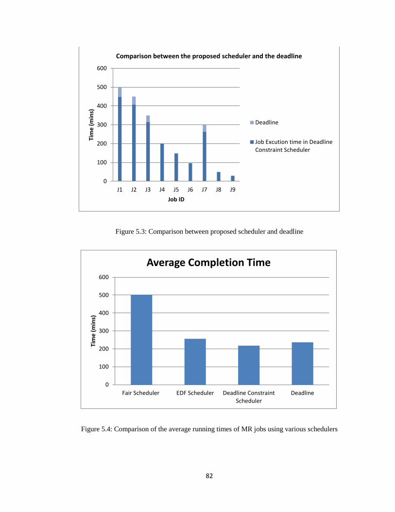
82

Figure 5.3: Comparison between proposed scheduler and deadline

Figure 5.4: Comparison of the average running times of MR jobs using various schedulers

0

100

200

300

400

500

600

J1 J2 J3 J4 J5 J6 J7 J8 J9

Tim

e (

min

s)

Job ID

Comparison between the proposed scheduler and the deadline

Deadline

Job Excution time in DeadlineConstraint Scheduler

0

100

200

300

400

500

600

Fair Scheduler EDF Scheduler Deadline ConstraintScheduler

Deadline

Tim

e (

min

s)

Average Completion Time

83

Comparing the nine jobs execution time with their deadline under the proposed Deadline

Constraint Scheduler is shown in Figure 5.3. In the experiment, each job is allocated enough

resource dynamically at different times based on their need, so no job missed the deadline. J4, J5,

J6, J8 and J9 just meet their deadline.

Figure 5.4, shows that the average completion time in the proposed scheduler is shorter compared

to the Fair scheduler and EDF scheduler. The result of the experiments showed that most of the

jobs missed their deadline under Fair scheduling and EDF scheduling, but the deadline of the

same jobs running in the same cluster under the proposed scheduler was met. The EDF scheduler

was better than the Fair scheduler.

5.8 Conclusions

In the current version of Hadoop, the schedulers cannot consider the deadline of the jobs, and

hence the native Hadoop scheduler cannot ensure that jobs will meet their deadlines. The deadline

constraint scheduler proposed in this chapter addresses this problem. The proposed scheduler sets

a checkpoint for each job based on the initialized tasks of the job to monitor the progress of job

execution, and classifies the resources at different levels. Based on the progress of job execution,

the scheduler put jobs in different queues that have different priority to use the resource. We used

a local cluster and Amazon EMR to experiment and the results show that with the proposed

scheduler all the jobs in the cluster meet their deadline if sufficient resource are available, while

the same jobs in the same cluster using Fair Scheduler and EDF Scheduler miss most of their

deadlines. Moreover, the average jobs execution time is the least in the proposed scheduler when

compared with Fair Scheduler and EDF Scheduler. Future work will look at determining the

lower bounds on resource availability to meet the deadlines.

84

CHAPTER VI

CONCLUSIONS AND FUTURE WORK

6.1 Main motivation of this work.

Hadoop is originally designed for a homogeneous cluster, however, in practice, Hadoop is always

working in a heterogeneous environment because of node failure and nodes upgrading. Hadoop

uses a distributed file system to store data. When Hadoop allocates disk space to store data, the

disk utilization rather than the processing capability of datanodes is considered. The tasks of jobs

running on Hadoop are assigned corresponding to data locality, that is, tasks are assigned to

nodes closest to its input data. Therefore nodes or racks consisting of multiple nodes which have

low capabilities may be assigned heavy tasks and nodes or racks with high capabilities may be

assigned light tasks. This problem is workload imbalance and it severely impacts the performance

of Hadoop. Currently, there doesn’t exist a method in Hadoop to address the workload imbalance

issue.

Native Hadoop schedulers are not able to guarantee users’ jobs can finish before their deadline

because the FIFO Scheduler, Fair Scheduler and Capacity Scheduler ignore the jobs’ deadline.

FIFO scheduler server the job that comes first and the Fair Scheduler allocates jobs resources

fairly. Although the Capacity Scheduler assigns jobs different priorities, the jobs with the highest

priorities cannot be guaranteed to be allocated enough resources to meet their deadlines. Another

85

problem is the priorities of jobs are assigned before the jobs start running, based on users

estimated jobs’ deadline. However it is difficult before a job starts to estimate its deadline or

completion time. There is no method in current Hadoop schedulers to monitor the progress of the

jobs. If job progress can be monitored, the completion time or required deadline can be more

accurately determined.

6.2 Contributions

6.2.1 Dynamic workload balancing for Hadoop MapReduce

While most current research focuses on solving the workload balancing problem at the node level,

in our work, we look at a workload balancing solution at the rack level. The advantage is because

balancing the workload between the racks can reduce the running time of many tasks, which is

much more efficient than reducing the running time of just one to two tasks on the single node.

We proposed two dynamic workload balancing algorithms for Hadoop MapReduce in the

heterogeneous environment to solve the workload imbalance at the rack level, since for different

racks, performance does not always match workload and this will degrade the entire performance

of Hadoop. The first proposed algorithm addresses this problem by moving the task from the

busiest rack to a less busy rack in order to reduce the execution time of jobs running on the

busiest rack and thereby achieve load balancing. The second proposed algorithm addresses this

problem by moving the task from the most overload racks to multiple other lighter loaded racks to

make all the tasks of a job on different racks to finish at the same time.

86

6.2.2 Software Defined Networking in Hadoop for workload balancing

Because the dynamic workload balancing algorithm requires the transfer of data between racks,

for the job processing big data, the cost of transferring is significant. Reducing this cost will

improve the efficiency of the dynamic workload balancing algorithm. Software Defined

Networking can change the topology of the network by program automatically. We employ some

OpenFlow switches which is one kind of implementation of Software Defined Networking in a

Hadoop cluster to construct a fat tree topology. Moreover, we proposed an algorithm to select the

paths to change the topology using the OpenFlow switch. When the workload balancing

algorithm needs to transfer data between racks, that algorithm will be called to change the

network topology in order to increase the bandwidth between racks and decrease the transfer cost.

6.2.3 Deadline constraint scheduler for Hadoop

Users may have a deadline requirement for their jobs. However, native Hadoop cannot satisfy

these deadlines because the schedulers in Hadoop do not schedule jobs based on their deadlines.

To address this problem, we proposed a deadline constraint scheduler for Hadoop. The algorithm

gets the tasks running time on each node from the log files and analyzes them to get the capability

of nodes. For the jobs running on the Hadoop cluster, the proposed algorithm use the first few

percentage of tasks in conjunction with the capability of nodes to estimate the tasks execution

time upper limit. We use the tasks execution time upper limit to monitor the job execution

progress and allocate resources based on the progress. In the scheduler, we proposed two

algorithms for allocating resources to a single job and for scheduling multiple jobs.

87

6.3 Validation

For the two dynamic workload balancing algorithms, we used two different simulators. In the

simulation of the dynamic workload balancing algorithm, we used Apache Mumak [13] and

Rumen [14] to simulate a Hadoop cluster including three racks with different processing

capabilities. A job consisting of 105 tasks ran on this cluster. During the runtime, workload

imbalance occurred and we compared different situations when these tasks run on native Hadoop

and Hadoop with our algorithm. In the simulation for the improved dynamic racks workload

balancing algorithm, we used “MRSim” to simulate a Hadoop cluster with five racks and each

rack contains five nodes. The five racks had different capabilities. We simulated a job with 157

tasks and 10 GB data running on all these racks and compared different situations when these

tasks run on native Hadoop and Hadoop with our algorithm.

For using SDN in Hadoop, we simulated data transfer between two racks with OpenFlow

switches installed by using the network simulator NS-2 [29]. In our simulation, we used switches

with a gigabit bandwidth on each port. Random numbers in the range 0.1 to 1 gigabit for the

bandwidth of the three links in different periods of time were generated. The period of time is

random. The simulation used 105 tasks. If each block in Hadoop is 64 MB and one task uses one

block of data, the total data is 6720 MB. We compared these two data transferring procedures to

show the improvement made by employing our proposed algorithm.

For the deadline-constraint scheduler for Hadoop, we implemented our algorithm in Amazon

EMR [114]. In this experiment we compared the proposed deadline constraint scheduler with the

Fair Scheduler and Earliest Deadline First (EDF) Scheduler. Nine jobs were submitted to the

88

Hadoop cluster in EMR. We compared the performance of Fair scheduler, EDF scheduler and the

proposed deadline constraint scheduler for these nine Jobs.

6.4 Results

Our simulated results of dynamic workload balancing algorithm, which compare the execution

time of Native Hadoop and our proposed balanced Hadoop, show that using our algorithm

reduces the execution time by about 66%. Our simulated results of the improved workload

balancing algorithm show that using our algorithm reduces execution time by about 55%. The

execution time will be reduced by more than 50% because the rack accepting the tasks that have

been moved has better performance than the original one. Using multiple racks to run these tasks

more than doubles the efficiency and thereby reduce the execution time by more than 50%.

The simulation of using OpenFlow switches in Hadoop cluster compared the quantity of data

transferred from one rack to another. In most of the time periods, the quantity of data transferred

from one rack to another increases if OpenFlow Switches are employed. The result shows that the

OpenFlow switch installed Hadoop cluster saves about 50% time by applying our proposed

Hadoop Bandwidth Routing algorithm.

For the experiment for deadline constraint scheduler, we compared the Fair Scheduler and EDF

Scheduler with it. In the same Hadoop cluster on EMR, we run the same jobs. Though for these

nine jobs, the cluster has enough resource to make all of them meet their deadline, but most of

jobs miss their deadline under the Fair Scheduler and EDF Scheduler, while all of them meet the

deadline under our proposed scheduler. The experiment shows that the average completion time

in the proposed scheduler is shorter compared to the Fair scheduler and EDF scheduler.

89

6.5 Main conclusions

In a Hadoop cluster, the workload of racks does not always match the capability of racks. Tasks

of the jobs running on busy or overloaded racks will take longer time to finish than on other racks.

This degrades the entire performance of Hadoop. The two proposed dynamic workload balancing

algorithms in Chapter 3 address this problem at the rack level by moving tasks from the most

overload racks to other racks in order to balance the workload between racks. Simulation results

show that by employing our proposed algorithms, for every job that causes workload imbalance

on different racks, the remaining time can be reduced by more than half in the map phase.

Our proposed workload balancing algorithms need to transfer data between racks and since

Hadoop is a platform to process big data, the cost of transfer can be very large. We use Software

Defined Networking with installed OpenFlow switches on a Hadoop cluster. With OpenFlow

switches, we can increase the bandwidth by changing the network topology in a Hadoop cluster.

In native Hadoop, there is no scheduler that uses the deadline of jobs as a criterion to schedule

jobs execution order. Therefore jobs submitted to Hadoop cannot be guaranteed to meet their

execution deadline. Our proposed deadline constraint scheduler addresses this problem by

monitoring the progress of jobs and allocates resources to job dynamically based on the progress.

From experimental results that compared our proposed scheduler, the Fair scheduler and EDF

scheduler, the proposed deadline constraint scheduler can allocate the needed resources to jobs

because the scheduler can accurately track the progress of jobs while the other schedulers do not

have this function. Hence, if sufficient resources are available, our proposed scheduler can ensure

jobs meet their deadline.

90

6.6 Future work

Our proposed workload balancing algorithms has not been implemented on a real Hadoop cluster.

It is important to validate our approach in a real cluster. The implementation of the algorithms

will have several parts:

1) log analyzer

2) workload monitor

3) tasks assignment.

The log analyzer has the function of scanning the log files of the Hadoop cluster. The information

recorded in the log file includes the jobs execution time in history, the data location of each job

and current state of jobs’ tasks. By analyzing this information, we can get the node processing

capability and busy level and the data local task and rack local task probability.

The workload monitor checks if workload imbalance occurs or not. It uses information from the

log analyzer model such as data location and the data local task and rack local task probability

and current tasks execution state to check if the finish time of map tasks of each job on different

racks have a significate difference.

The tasks assignment module will assign tasks based on information received from the workload

monitor that reflects whether workload is balanced or not. It also uses the data location

information from the log analyzer to assign the tasks to the underloaded racks with data.

Another future work related to the workload balancing algorithm is scaling the algorithm to a

large system. Currently the proposed algorithms move the data from one rack to one or more

racks where the rack we consider has some data for this job. However, in a very big cluster where

91

the data of a job may be located on some of the racks only, the algorithm only selects some

underloaded racks that have the data for the job and ignores the other racks which do not have

data for the job. Future work will involve modifications to our proposed algorithms to consider

some racks which do not have data of a job. The standard of selection should be based on the

workload of racks and the distance between overloaded racks because we need to compare the

current tasks running time and running time on other racks and the transfer cost.

92

REFERENCES

[1] K. Shvachko, H. Kuang, S. Radia, R. Chansler, "The Hadoop Distributed File System", in

Proceedings IEEE Conference on Mass Storage Systems and Technologies (MSST). 2010.

[2] J. Dean, S. Ghemawat, "MapReduce: Simplified Data Processing on Large Clusters", in

Proceedings Sixth Symposium on Operating System Design and Implementation (OSDI'04), San

Francisco, CA, December 2004.

[3] N. McKeown, T. Anderson, H. Balakrishnan, G. Parulkar, L. Peterson, J. Rexford, S. Shenker,

and J. Turner. Openflow: enabling innovation in campus networks. SIGCOMM Comput.

Commun. Rev., 38(2): pp 69–74. 2008.

[4] M.Zaharia, A.Konwinski, A.Joseph, Y.zatz, and I.Stoica. Improving mapreduce performance

in heterogeneous environments. In OSDI'08: 8th USENIX Symposium on Operating Systems

Design and Implementation, October 2008.

[5] Rafique, M. Mustafa, Benjamin Rose, Ali R. Butt, and Dimitrios S. Nikolopoulos.

"Supporting MapReduce on large-scale asymmetric multi-core clusters." ACM SIGOPS

Operating Systems Review 43, no. 2: pp. 25-34. 2009.

[6] Tian, C., Zhou, H., He, Y., & Zha, L. (2009, August). A dynamic mapreduce scheduler for

heterogeneous workloads. In Proceedings Eighth International Conference on Grid and

Cooperative Computing, GCC'09., pp. 218-224. 2009.

[7] J. Xie, S. Yin, X. Ruan, Z. Ding, Y. Tian, J. Majors, A. Manzanares, and X. Qin. Improving

MapReduce Performance through Data Placement in Heterogeneous Hadoop Clusters, In

Proceedings 19th Int'l Heterogeneity in Computing Workshop, Atlanta, Georgia, April 2010.

93

[8] Yuanquan Fan, Weiguo Wu, Haijun Cao, Huo Zhu, Xu Zhao, Wei Wei, A heterogeneity-

aware data distribution and rebalance method in Hadoop cluster, Seventh China Grid Annual

Conference, pp 176-181. 2012.

[9] T. White. Hadoop: The Definitive Guide. O'Reilly Media, Inc, 2010

[10] Z. Li, Y. Shen, B. Yao, and M. Guo. OFScheduler: a dynamic network optimizer for

MapReduce in heterogeneous cluster. International Journal of Parallel Programming, 43, no 3, pp

472-488. 2015.

[11] A. Das, C. Lumezanu, Y. Zhang, V. Singh, G. Jiang and C. Yu, "Transparent and

Flexible Network Management for Big Data Processing in the Cloud." In Proceedings ACM

Hotcloud, 2013.

[12] S. Narayan, S. Bailey, and A. Daga. Hadoop acceleration in an OpenFlow-Based cluster.

In High Performance Computing, Networking, Storage and Analysis (SCC), SC Companion: pp.

535-538. 2012.

[13] Apache Mumak (12-10-2013), https://apache.googlesource.com/- hadoopmapreduce/+/-

MAPREDUCE-233/src/contrib/mumak

[14] Apache Rumen (12-01-2013), https://hadoop.apache.org/docs/r1.2.1/rumen.html

[15] Hong Tang (12-20-2013), Using Simulation for Large-Scale Distributed System

Verification and Debugging, 2009.10 Hadoop User Group,

http://www.slideshare.net/hadoopusergroup/mumak

[16] Apache Hadoop Job Tracker (01-15-2014), https://wiki.apache.org/hadoop/JobTracker

[17] Huang Jie, Huang Bei, Huang Quicen, “A Dynamic Load Balancing Algorithm in LAN”,

In Proceedings 12th IEEE International Conference on Communication Technology (ICCT)”, pp

137-140. 2010

https://apache.googlesource.com/-%20hadoopmapreduce/+/-MAPREDUCE-233/src/contrib/mumak

https://apache.googlesource.com/-%20hadoopmapreduce/+/-MAPREDUCE-233/src/contrib/mumak

https://hadoop.apache.org/docs/r1.2.1/rumen.html

http://www.slideshare.net/hadoopusergroup/mumak

94

[18] Rohan Gandhi, Di Xie, Y. Charlie Hu, “PIKACHU: how to rebalance load in optimizing

mapreduce on heterogeneous clusters”, Proceedings 2013 USENIX conference on Annual

Technical Conference, pp 61-66. 2013

[19] Rohit Paravastu, Rozemary Scarlat, Balakrishnan Chandrasekaran, “Adaptive Load

Balancing in MapReduce using Flubber”, Department of Computer Science, Duke University

[https://www.cs.duke.edu/courses/fall12/cps216/Project/Project/projects/Adaptive_load_balancer/

adaptive-load-balancing.pdf]

[20] Kumar, T. K., Kim, J., George, K. M., & Park, N. (2014, June). Dynamic data

rebalancing in Hadoop. In Proceedings 2014 IEEE/ACIS 13th International Conference on

Computer and Information Science (ICIS), pp. 315-320. 2014

[21] Fundation, Open Networking. "Software-defined networking: The new norm for

networks." ONF White Paper. 2012.

[22] Webb, Kevin C., Alex C. Snoeren, and Kenneth Yocum. "Topology switching for data

center networks." In Proceedings Hot-ICE Workshop. 2011.

[23] Wang, Yandong, Xinyu Que, Weikuan Yu, Dror Goldenberg, and Dhiraj Sehgal.

"Hadoop acceleration through network levitated merge." In Proceedings 2011 International

Conference for High Performance Computing, Networking, Storage and Analysis, p. 57. ACM.

2011.

[24] Condie, Tyson, Neil Conway, Peter Alvaro, Joseph M. Hellerstein, Khaled Elmeleegy,

and Russell Sears. "MapReduce Online." In NSDI, vol. 10, no. 4, p. 20. 2010.

[25] Narayan, Sandhya, Stuart Bailey, Matthew Greenway, Robert Grossman, Allison Heath,

Ray Powell, and Anand Daga. "Openflow enabled hadoop over local and wide area clusters." In

High Performance Computing, Networking, Storage and Analysis (SCC), 2012 SC Companion:,

pp. 1625-1628. 2012.

95

[26] Leiserson, Charles E. "Fat-trees: universal networks for hardware-efficient

supercomputing." IEEE Transactions on Computers, vol. 100, no. 10: pp 892-901. 1985.

[27] Al-Fares, Mohammad, Alexander Loukissas, and Amin Vahdat. "A scalable, commodity

data center network architecture." In ACM SIGCOMM Computer Communication Review, vol.

38, no. 4, pp. 63-74. ACM. 2008.

[28] Lee, Chia-Wei, Kuang-Yu Hsieh, Sun-Yuan Hsieh, and Hung-Chang Hsiao. "A Dynamic

Data Placement Strategy for Hadoop in Heterogeneous Environments." Big Data Research 1: pp

14-22. 2014.

[29] Altman, Eitan, and Tania Jimenez. "NS Simulator for beginners." Synthesis Lectures on

Communication Networks 5, no. 1: 1-184. 2012.

[30] Hammoud, Suhel, Maozhen Li, Yang Liu, Nasullah Khalid Alham, and Zelong Liu.

"MRSim: A discrete event based MapReduce simulator." In Proceedings Seventh International

Conference on Fuzzy Systems and Knowledge Discovery (FSKD), vol. 6, pp. 2993-2997. 2010.

[31] Kc, Kamal, and Kemafor Anyanwu. "Scheduling hadoop jobs to meet deadlines." In

Proceedings 2010 IEEE Second International Conference on Cloud Computing Technology and

Science (CloudCom), pp. 388-392. 2010.

[32] Liu, Li, Yuan Zhou, Ming Liu, Guandong Xu, Xiwei Chen, Dangping Fan, and Qianru

Wang. "Preemptive hadoop jobs scheduling under a deadline." In Proceedings Eighth

International Conference on Semantics, Knowledge and Grids (SKG), pp. 72-79. 2012.

[33] Cheng, Dazhao, Jia Rao, Changjun Jiang, and Xiaobo Zhou. "Resource and Deadline-

Aware Job Scheduling in Dynamic Hadoop Clusters." In Proceedings 2015 IEEE International

Parallel and Distributed Processing Symposium (IPDPS), pp. 956-965. 2015.

[34] Voicu, Cristiana, Florin Pop, Ciprian Dobre, and Fatos Xhafa. "MOMC: Multi-Objective

and Multi-Constrained Scheduling Algorithm of Many Tasks in Hadoop." In Proceedings 2014

96

Ninth International Conference on P2P, Parallel, Grid, Cloud and Internet Computing (3PGCIC),

pp. 89-96. 2014.

[35] Perret, Quentin, Gabriel Charlemagne, Stelios Sotiriadis, and Nik Bessis. "A Deadline

Scheduler for Jobs in Distributed Systems." In Proceedings 27th International Conference on

Advanced Information Networking and Applications Workshops (WAINA), pp. 757-764. 2013.

[36] Lim, Norman, Shikharesh Majumdar, and Peter Ashwood-Smith. "A Constraint

Programming Based Hadoop Scheduler for Handling MapReduce Jobs with Deadlines on

Clouds." In Proceedings 6th ACM/SPEC International Conference on Performance Engineering,

pp. 111-122. ACM, 2015.

[37] Zhang, Wei, Sanguthevar Rajasekaran, Tim Wood, and Mingfa Zhu. "MIMP: deadline

and interference aware scheduling of Hadoop virtual machines." In Proceedings 14th IEEE/ACM

International Symposium on Cluster, Cloud and Grid Computing (CCGrid), pp. 394-403. 2014.

[38] Freund, Rudolph J., and William J. Wilson. "Statistical Methods" pp. 8-15, 1993.

[39] Rao, B. Thirumala, N. V. Sridevi, V. Krishna Reddy, and L. S. S. Reddy. "Performance

issues of heterogeneous Hadoop clusters in cloud computing." arXiv preprint arXiv: 1207.0894,

2012.

[40] Gao, Zhipeng, Dangpeng Liu, Yang Yang, Jingchen Zheng, and Yuwen Hao. "A load

balance algorithm based on nodes performance in Hadoop cluster." In Proceedings 16th Asia-

Pacific Network Operations and Management Symposium (APNOMS), 2014, pp. 1-4. 2014.

[41] Ramakrishnan, Smriti R., Garret Swart, and Aleksey Urmanov. "Balancing reducer skew

in MapReduce workloads using progressive sampling." In Proceedings Third ACM Symposium

on Cloud Computing, p. 16. ACM, 2012.

[42] Martha, Venkata Swamy, Weizhong Zhao, and Xiaowei Xu. "h-MapReduce: a

framework for workload balancing in MapReduce." In Proceedings 27th IEEE International

Conference on Advanced Information Networking and Applications (AINA), pp. 637-644. 2013

97

[43] Fan, Yuanquan, Weiguo Wu, Haijun Cao, Huo Zhu, Wei Wei, and Pengfei Zheng.

"LBVP: A load balance algorithm based on Virtual Partition in Hadoop cluster." In Proceedings

2012 IEEE Asia Pacific Cloud Computing Congress (APCloudCC), , pp. 37-41. 2012.

[44] Gautam, Jyoti V., Harshadkumar B. Prajapati, Vipul K. Dabhi, and Sanjay Chaudhary.

"A survey on job scheduling algorithms in Big data processing." In Proceedings 2015 IEEE

International Conference on Electrical, Computer and Communication Technologies (ICECCT),

pp. 1-11. 2015.

[45] Zhang, Zehua, and Xuejie Zhang. "A load balancing mechanism based on ant colony and

complex network theory in open cloud computing federation." In Proceedings 2nd International

Conference on Industrial Mechatronics and Automation (ICIMA), 2010 vol. 2, pp. 240-243. 2010.

[46] Nishant, Kumar, Pratik Sharma, Vishal Krishna, Chhavi Gupta, Kuwar Pratap Singh, and

Ravi Rastogi. "Load balancing of nodes in cloud using ant colony optimization." In Proceedings

14th International Conference on Computer Modelling and Simulation (UKSim), pp. 3-8. 2012.

[47] Radojević, Branko, and Mario Žagar. "Analysis of issues with load balancing algorithms

in hosted (cloud) environments." In MIPRO, 2011 Proceedings 34th International Convention, pp.

416-420. 2011.

[48] Arpaci-Dusseau, Remzi H., and Andrea C. Arpaci-Dusseau. Operating systems: Three

easy pieces. 2012.

[49] Ni, Junjie, Yuanqiang Huang, Zhongzhi Luan, Juncheng Zhang, and Depei Qian. "Virtual

machine mapping policy based on load balancing in private cloud environment." In Proceedings

2011 International Conference on Cloud and Service Computing (CSC), pp. 292-295. 2011.

[50] Wu, Tin-Yu, Wei-Tsong Lee, Yu-San Lin, Yih-Sin Lin, Hung-Lin Chan, and Jhih-Siang

Huang. "Dynamic load balancing mechanism based on cloud storage." In Proceedings Computing,

Communications and Applications Conference (ComComAp), pp. 102-106. 2012.

98

[51] Lee, Rich, and Bingchiang Jeng. "Load-balancing tactics in cloud." In Proceedings 2011

International Conference on Cyber-Enabled Distributed Computing and Knowledge Discovery

(CyberC), pp. 447-454. 2011.

[52] Ren, Xiaona, Rongheng Lin, and Hua Zou. "A dynamic load balancing strategy for cloud

computing platform based on exponential smoothing forecast." In Proceedings 2011 IEEE

International Conference on Cloud Computing and Intelligence Systems (CCIS), pp. 220-224.

2011.

[53] Wang, Shu-Ching, Kuo-Qin Yan, Wen-Pin Liao, and Shun-Sheng Wang. "Towards a

load balancing in a three-level cloud computing network." In Proceedings 2010 3rd IEEE

International Conference on, Computer Science and Information Technology (ICCSIT), vol. 1, pp.

108-113. 2010.

[54] Armstrong, Robert, Debra Hensgen, and Taylor Kidd. "The relative performance of

various mapping algorithms is independent of sizable variances in run-time predictions." In

Proceedings 1998 Seventh Heterogeneous Computing Workshop, 1998.(HCW 98), pp. 79-87.

1998.

[55] Kokilavani, T., and Dr DI George Amalarethinam. "Load balanced min-min algorithm

for static meta-task scheduling in grid computing." International Journal of Computer

Applications 20, no. 2: pp. 43-49. 2011.

[56] Mahalle, H., P. Kaveri, and Vinay Chavan. "Load Balancing on Cloud Data Centers."

International Journal of Advanced Research in Computer Science and Software Engineering 3: pp.

11-15. 2013.

[57] Domanal, Shridhar G., and G. Ram Mohana Reddy. "Optimal load balancing in cloud

computing by efficient utilization of virtual machines." In Proceedings 2014 Sixth International

Conference on, Communication Systems and Networks (COMSNETS), pp. 1-4. 2014.

99

[58] James, Jasmin, and Dr Bhupendra Verma. "Efficient VM load balancing algorithm for a

cloud computing environment." International Journal on Computer Science and Engineering

(IJCSE) 9. 2012.

[59] Domanal, Shridhar G., and G. Ram Mohana Reddy. "Load Balancing in Cloud

Computingusing Modified Throttled Algorithm." In Proceedings 2013 IEEE International

Conference on Cloud Computing in Emerging Markets (CCEM), pp. 1-5. 2013.

[60] Soni, Gaurav, and Mala Kalra. "A novel approach for load balancing in cloud data

center." In Proceedings 2014 IEEE International Advanced Computing Conference (IACC), pp.

807-812. 2014.

[61] Chen, Huankai, Frank Wang, Na Helian, and Gbola Akanmu. "User-priority guided Min-

Min scheduling algorithm for load balancing in cloud computing." In Proceedings 2013 National

Conference on Parallel Computing Technologies (PARCOMPTECH), pp. 1-8. 2013.

[62] Braun, Tracy D., Howard Jay Siegel, Noah Beck, Ladislau L. Bölöni, Muthucumaru

Maheswaran, Albert I. Reuther, James P. Robertson et al. "A comparison of eleven static

heuristics for mapping a class of independent tasks onto heterogeneous distributed computing

systems." Journal of Parallel and Distributed computing 61, no. 6: pp. 810-837. 2001.

[63] Adhikari, Jeevan, and Swapnil Patil. "Double threshold energy aware load balancing in

cloud computing." In Proceedings 2013 Fourth International Conference on Computing,

Communications and Networking Technologies (ICCCNT), pp. 1-6. 2013.

[64] Rahmeh, O. Abu, P. Johnson, and A. Taleb-Bendiab. "A dynamic biased random

sampling scheme for scalable and reliable grid networks." INFOCOMP Journal of Computer

Science 7, no. 4: pp. 1-10. 2008.

[65] Randles, Martin, David Lamb, and A. Taleb-Bendiab. "A comparative study into

distributed load balancing algorithms for cloud computing." In Proceedings 2010 IEEE 24th

100

International Conference on Advanced Information Networking and Applications Workshops

(WAINA), pp. 551-556. 2010.

[66] Kansal, Nidhi Jain, and Inderveer Chana. "Cloud load balancing techniques: a step

towards green computing." IJCSI International Journal of Computer Science Issues 9, no. 1: pp,

238-246. 2012.

[67] Ghafari, Seyed Mohssen, Mehdi Fazeli, Ahmad Patooghy, and Leila Rikhtechi. "Bee-

MMT: A load balancing method for power consumption management in cloud computing." In

Proceedings Sixth International Conference on Contemporary Computing (IC3), 2013 pp. 76-80.

2013.

[68] Lu, Yi, Qiaomin Xie, Gabriel Kliot, Alan Geller, James R. Larus, and Albert Greenberg.

"Join-Idle-Queue: A novel load balancing algorithm for dynamically scalable web services."

Performance Evaluation 68, no. 11: pp. 1056-1071. 2011.

[69] Salehi Mohsen Amini, Hossein Deldari, and Bahare Mokarram Dorri. "Balancing load in

a computational grid applying adaptive, intelligent colonies of ants." Informatica 33, no. 2. 2009.

[70] Gálvez, Juan J., Pedro M. Ruiz, and Antonio FG Skarmeta. "A distributed algorithm for

gateway load-balancing in wireless meshes networks." In Wireless Days, 2008. WD'08. 1st IFIP,

pp. 1-5. IEEE, 2008.

[71] Zeng, Feng, and Zhigang Chen. "Load balancing placement of gateways in wireless mesh

networks with QoS constraints." In Proceedings 9th International Conference for Young

Computer Scientists, 2008. ICYCS, pp. 445-450. 2008.

[72] Shahverdy, Mohammad, Misagh Behnami, and Mahmood Fathy. "A New paradigm for

load balancing in WMNs." International Journal of Computer Networks (IJCN) 3, no. 4: pp. 239-

246. 2011.

[73] Galvez, Juan J., Pedro M. Ruiz, and Antonio FG Skarmeta. "Responsive on-line gateway

load-balancing for wireless mesh networks." Ad Hoc Networks 10, no. 1: pp. 46-61. 2012.

101

[74] Kashanaki, Maryam, Zia Beheshti, and Mohammad Reza Meybodi. "A distributed

learning automata based gateway load balancing algorithm in Wireless Mesh Networks."

In Proceedings 2012 International Symposium on Instrumentation & Measurement, Sensor

Network and Automation (IMSNA), vol. 1, pp. 90-94. 2012.

[75] Choi, Hyoung-Gyu, and Seung-Jae Han. "Load balancing routing for wireless mesh

networks: An adaptive partitioning approach." In Proceedings 5th IEEE Consumer

Communications and Networking Conference,. CCNC 2008. pp. 1-5. 2008.

[76] Anh-Ngoc, L. E., K. U. M. Dong-Won, C. H. O. You-Ze, and T. O. H. Chai-Keong.

"Routing with load-balancing in multi-radio wireless mesh networks."IEICE transactions on

communications 92, no. 3: pp. 700-708. 2009.

[77] Ma, Liang, and Mieso K. Denko. "A routing metric for load-balancing in wireless mesh

networks." In Proceedings 21st International Conference on Advanced Information Networking

and Applications Workshops, 2007, AINAW'07. vol. 2, pp. 409-414. 2007.

[78] Gember, Aaron, Prathmesh Prabhu, Zainab Ghadiyali, and Aditya Akella. "Toward

software-defined middlebox networking." In Proceedings 11th ACM Workshop on Hot Topics in

Networks, pp. 7-12. ACM, 2012.

[79] Al-Fares, Mohammad, Sivasankar Radhakrishnan, Barath Raghavan, Nelson Huang, and

Amin Vahdat. "Hedera: Dynamic Flow Scheduling for Data Center Networks." In NSDI, vol. 10,

pp. 19-19. 2010.

[80] Ghobadi, Monia, Soheil Hassas Yeganeh, and Yashar Ganjali. "Rethinking end-to-end

congestion control in software-defined networks." In Proceedings 11th ACM Workshop on Hot

Topics in Networks, pp. 61-66. ACM, 2012.

[81] Handigol, Nikhil, Mario Flajslik, Srini Seetharaman, N. McKeown, and R. Johari.

"Aster* x: Load-balancing as a network primitive." In 9th GENI Engineering Conference

(Plenary), pp. 1-2. 2010.

102

[82] Heller, Brandon, Srinivasan Seetharaman, Priya Mahadevan, Yiannis Yiakoumis, Puneet

Sharma, Sujata Banerjee, and Nick McKeown. "ElasticTree: Saving Energy in Data Center

Networks." In NSDI, vol. 10, pp. 249-264. 2010.

[83] Ferguson, Andrew D., Arjun Guha, Chen Liang, Rodrigo Fonseca, and Shriram

Krishnamurthi. "Participatory networking: An API for application control of SDNs." In ACM

SIGCOMM Computer Communication Review, vol. 43, no. 4, pp. 327-338. ACM, 2013.

[84] Jeong, Kwangtae, Jinwook Kim, and Young-Tak Kim. "QoS-aware network operating

system for software defined networking with generalized OpenFlows." In Proceedings 2012 IEEE

Network Operations and Management Symposium (NOMS), pp. 1167-1174. 2012.

[85] Sharafat, Ali Reza, Saurav Das, Guru Parulkar, and Nick McKeown. "Mpls-te and mpls

vpns with openflow." In ACM SIGCOMM Computer Communication Review, vol. 41, no. 4, pp.

452-453. ACM, 2011.

[86] Melazzi, Nicola Blefari, A. Detti, G. Mazza, G. Morabito, S. Salsano, and L. Veltri. "An

openflow-based testbed for information centric networking." In Future Network & Mobile

Summit (FutureNetw), 2012, pp. 1-9. 2012.

[87] Wang, Richard, Dana Butnariu, and Jennifer Rexford. "OpenFlow-based server load

balancing gone wild". 2011.

[88] Handigol, Nikhil, Srinivasan Seetharaman, Mario Flajslik, Nick McKeown, and Ramesh

Johari. "Plug-n-Serve: Load-balancing web traffic using OpenFlow." ACM SIGCOMM Demo 4,

no. 5: p. 6. 2009.

[89] Macapuna, Carlos AB, Christian Esteve Rothenberg, and Mauricio F. Magalhaes. "In-

packet Bloom filter based data center networking with distributed OpenFlow controllers."

In Proceedings 2010 IEEE GLOBECOM Workshops (GC Workshops), pp. 584-588. 2010.

103

[90] Qazi, Zafar Ayyub, Cheng-Chun Tu, Luis Chiang, Rui Miao, Vyas Sekar, and Minlan Yu.

"SIMPLE-fying middlebox policy enforcement using SDN." In ACM SIGCOMM Computer

Communication Review, vol. 43, no. 4, pp. 27-38. ACM, 2013.

[91] Kim, Wonho, Puneet Sharma, Jeongkeun Lee, Sujata Banerjee, Jean Tourrilhes, Sung-Ju

Lee, and Praveen Yalagandula. "Automated and scalable QoS control for network

convergence." Proc. INM/WREN 10: 1-1, 2010.

[92] Sharma, Shantanu, Dimitri Staessens, Didier Colle, David Palma, Joaquim Goncalves,

Renato Figueiredo, Dan Morris, Mario Pickavet, and Piet Demeester. "Implementing quality of

service for the software defined networking enabled future internet." In Proceedings Third

European Workshop on, Software Defined Networks (EWSDN), pp. 49-54. 2014.

[93] Skoldstrom, Pontus, and Belgis Chial Sanchez. "Virtual aggregation using SDN"

In Proceedings Second European Workshop on Software Defined Networks (EWSDN), pp. 56-61.

2013.

[94] Hammoud, Mohammad, and Majd F. Sakr. "Locality-aware reduce task scheduling for

MapReduce." In Proceedings IEEE Third International Conference on Cloud Computing

Technology and Science (CloudCom), pp. 570-576. 2011.

[95] Hammoud, Mohammad, M. Suhail Rehman, and Majd F. Sakr. "Center-of-gravity reduce

task scheduling to lower mapreduce network traffic." In Proceedings IEEE 5th International

Conference on Cloud Computing (CLOUD), pp. 49-58. 2012.

[96] Kumar, K. Arun, Vamshi Krishna Konishetty, Kaladhar Voruganti, and G. V. Rao.

"CASH: Context aware scheduler for Hadoop." In Proceedings International Conference on

Advances in Computing, Communications and Informatics, pp. 52-61. ACM, 2012.

[97] Zhang, Xiaohong, Zhiyong Zhong, Shengzhong Feng, Bibo Tu, and Jianping Fan.

"Improving data locality of MapReduce by scheduling in homogeneous computing

104

environments." In Proceedings IEEE 9th International Symposium on Parallel and Distributed

Processing with Applications (ISPA), pp. 120-126. 2011.

[98] Zhao, Yanrong, Weiping Wang, Dan Meng, YongChun Lv, Shubin Zhang, and Jun Li.

"TDWS: A job scheduling algorithm based on MapReduce." In Proceeding 7th IEEE International

Conference on Networking, Architecture and Storage (NAS), pp. 313-319. 2012.

[99] Chen, Quan, Daqiang Zhang, Minyi Guo, Qianni Deng, and Song Guo. "Samr: A self-

adaptive mapreduce scheduling algorithm in heterogeneous environment." In Proceedings 10th

IEEE International Conference on Computer and Information Technology (CIT), pp. 2736-2743.

2010.

[100] Chen, Quan, Minyi Guo, Qianni Deng, Long Zheng, Song Guo, and Yao Shen. "HAT:

history-based auto-tuning MapReduce in heterogeneous environments." The Journal of

Supercomputing 64, no. 3: pp. 1038-1054. 2013.

[101] Sun, Xiaoyu, Chen He, and Ying Lu. "ESAMR: An enhanced self-adaptive MapReduce

scheduling algorithm." In Proceedings 18th IEEE International Conference on Parallel and

Distributed Systems (ICPADS), pp. 148-155. 2012.

[102] Yong, Mark, Nitin Garegrat, and Shiwali Mohan. "Towards a resource aware scheduler

in hadoop." In Proceedings 2009 IEEE International Conference on Web Services, Los Angeles,

CA, USA, pp. 102-109. 2009.

[103] Nanduri, Radheshyam, Nitesh Maheshwari, A. Reddyraja, and Vasudeva Varma. "Job

aware scheduling algorithm for mapreduce framework." In Proceedings Third IEEE International

Conference on Cloud Computing Technology and Science (CloudCom), pp. 724-729. 2011.

[104] Mao, Hong, Shengqiu Hu, Zhenzhong Zhang, Limin Xiao, and Li Ruan. "A load-driven

task scheduler with adaptive DSC for MapReduce." In Proceedings IEEE/ACM International

Conference on Green Computing and Communications (GreenCom), pp. 28-33. 2011.

105

[105] Yi Yao, Jianzhe Tai, Bo Sheng and Ningfang Mi, “LsPS: a job size-based scheduler for

efficient task assignments in Hadoop,” IEEE Transactions on Cloud Computing, pp. 1-14. 2013.

[106] Wang, Zhe, Zhengdong Zhu, Pengfei Zheng, Qiang Liu, and Xiaoshe Dong. "A New

Schedule Strategy for Heterogenous Workload-aware in Hadoop." In Proceedings 8th, ChinaGrid

Annual Conference (ChinaGrid), pp. 80-85. 2013.

[107] Polo, Jorda, Diego Carrera, Yolanda Becerra, Juana Torres, Eduard Ayguadé, Malgorzata

Steinder, and Ian Whalley. "Performance-driven task co-scheduling for mapreduce

environments." In Proceedings IEEE Network Operations and Management Symposium (NOMS),

pp. 373-380. 2010.

[108] Polo, Jorda, David Carrera, Yolanda Becerra, Vicenç Beltran, Jordi Torres, and Eduard

Ayguadé. "Performance management of accelerated mapreduce workloads in heterogeneous

clusters." In Proceedings 39th International Conference on Parallel Processing (ICPP), pp. 653-

662. 2010.

[109] Tang, Qinghui, Sandeep Kumar S. Gupta, and Georgios Varsamopoulos. "Energy-

efficient thermal-aware task scheduling for homogeneous high-performance computing data

centers: A cyber-physical approach." IEEE Transactions on Parallel and Distributed Systems, vol.

19, no. 11, pp. 1458-1472. 2008.

[110] Shi, Bing, and Ankur Srivastava. "Thermal and power-aware task scheduling for hadoop

based storage centric datacenters." In Proceedings International Green Computing Conference, pp.

73-83. 2010.

[111] Li, Zheng, Li Wang, Shangping Ren, and Gang Quan. "Temperature, Power, and

Makespan Aware Dependent Task Scheduling for Data Centers." In Proceedings 2011

IEEE/ACM International Conference on Green Computing and Communications (GreenCom), pp.

22-27. 2011.

106

[112] Li, Ying, Hongli Zhang, and Kyong Hoon Kim. "A power-aware scheduling of

mapreduce applications in the cloud." In Proceedings Ninth IEEE International Conference on

Dependable, Autonomic and Secure Computing (DASC), pp. 613-620. 2011.

[113] Vavilapalli, Vinod Kumar, Arun C. Murthy, Chris Douglas, Sharad Agarwal, Mahadev

Konar, Robert Evans, Thomas Graves et al. "Apache hadoop yarn: Yet another resource

negotiator." In Proceedings 4th annual Symposium on Cloud Computing, p. 5. ACM, 2013.

[114] Amazon, E. M. R. "Amazon elastic mapreduce.". 2012.

VITA

Xiaofei Hou

Candidate for the Degree of

Doctor of Philosophy

Thesis: DYNAMIC WORKLOAD BALANCING AND SCHEDULING IN HADOOP

MAPREDUCE WITH SOFTWARE DEFINED NETWORKING

Major Field: Computer Science

Biographical:

Education:

Completed the requirements for the Doctor of Philosophy/Education in your

major at Oklahoma State University, Stillwater, Oklahoma in July, 2017.

Completed the requirements for the Bachelor of Science/Arts in your major at

Northeastern University, Qinhuangdao, Hebei, China in June, 2011.

Experience:

Teaching Assistant from August 2011 to May 2017

Research Assistant from May-August 2015

dynamic workload balancing and scheduling in hadoop ...

Documents

Transcript of dynamic workload balancing and scheduling in hadoop ...