Dynamic recalibration of scalable fringe-projection systems for large-scale object metrology

Dynamic recalibration of scalable fringe-projectionsystems for large-scale object metrology

Viktor Hovorov, Michael Lalor, David Burton, and Francis Lilley*General Engineering Research Institute, Liverpool John Moores University, City Campus,

Room 114, James Parsons Building, Byrom Street, Liverpool L3 3AF, UK.

*Corresponding author: [email protected]

Received 13 October 2009; revised 2 February 2010; accepted 2 February 2010;posted 3 February 2010 (Doc. ID 118486); published 9 March 2010

Three-dimensional (3D) surface shape measurement is a vital component in many industrial processes.The subject has developed significantly over recent years and a number of mainly noncontact techniquesnow exist for surface measurement, exhibiting varying levels of maturity. Within the larger group of 3Dmeasurement techniques, one of the most promising approaches is provided by those methods that arebased upon fringe analysis. Current techniques mainly focus on the measurement of small and medium-scale objects, while work on the measurement of larger objects is not so well developed. One potentialsolution for the measurement of large objects that has been proposed by various researchers is the con-cept of performing multipanel measurement and the system proposed here uses this basic approach, butin a flexible form of a single moveable sensor head that would be cost effective for measuring very largeobjects. Most practical surface measurement techniques require the inclusion of a calibration stage toensure accurate measurements. In the case of fringe analysis techniques, phase-to-height calibration isrequired, which includes the use of phase-to-height models. Most existing models (both analytical andempirical) are intended to be used in a static measurement mode, which means that, typically, a singlecalibration is performed prior to multiple measurements being made using an unvarying system geome-try. However, multipanel measurement strategies do not necessarily keep the measurement systemgeometry constant and thus require dynamic recalibration. To solve the problem of dynamic recalibra-tion, we propose a class of models called hybrid models. These hybrid models inherit the basic form ofanalytical models, but their coefficients are obtained in an empirical manner. The paper also discussesissues associated with all phase-to-height models used in fringe analysis that have a quotient form, iden-tifying points of uncertainty and regions of distortion as issues affecting accuracy in phase maps pro-duced in this manner. © 2010 Optical Society of America

OCIS codes: 100.2650, 120.0280, 120.2830, 150.1488, 150.3040.

1. Introduction

The measurement of an object’s three-dimensional(3D) surface shape is a subject that constantly pro-duces a high level of scientific interest, providinginformation for scientific, industrial, medical, andother applications. Among the different potentialtechniques available for measuring 3D shape, non-contact techniques are of particular interest. A non-contact approach is applicable in a much wider rangeof scenarios when compared to traditional contact

techniques, including the measurement of fragileor dangerous objects. With recent technologicaldevelopments in the hardware available for suchmeasurement systems (including personal compu-ters, video cameras, and video projectors), fast high-resolution 3D surface height measurement has nowbecome possible at reasonable cost. A number of tech-niques have already been developed, and among themost popular of these are the so-called fringe analy-sis techniques, including Fourier fringe analysis [1,2]and phase stepping [3–6].

However, it is also true that, at the moment, onlythe measurement of small-scale and medium-scaleobjects (here we shall define a medium-scale object

0003-6935/10/081459-13$15.00/0© 2010 Optical Society of America

10 March 2010 / Vol. 49, No. 8 / APPLIED OPTICS 1459

as occupying anything up to 1m × 1m× 1m in vo-lume) has so far been well studied. Nevertheless,due to economic pressure in the manufacturing sec-tor, in recent years interest has increased in the mea-surement of large-scale objects, such as aircraftwings, ship hulls, and automotive bodies. The evolu-tion of personal computers available for scientificand industrial applications now facilitates the pro-cessing, handling, and storage of large amounts ofdata. For example, at the time of the Fourier fringeanalysis algorithm’s invention, the processing ofwhat was then a standard 512 × 512 pixel imageby that algorithm could take several hours, whilemodern computers are capable of performing thesame operation in less than a second. Thus, the mea-surement of large-scale objects at high spatial reso-lutions is now a technically possible and practicalobjective in terms of data storage and manipulation.There are two possible ways that a large object

may be measured using fringe analysis:

– by use of techniques that have already beendeveloped for medium-scale object measurement,together with an extensive increase in the sensor’sparameters, and– via the development of new techniques based

on multipanel measurement.

If we consider the first approach, there are a num-ber of limiting factors here that result in a compro-mise between maximizing the field of view of thesensor on one hand, and maximizing its spatial reso-lution in terms of pixel density and its measurementaccuracy on the other. Alternatively, the adoption ofmultipanel measurement strategies makes it possi-ble to achieve a virtually unlimited field of view,while simultaneously maintaining a constant highlevel of accuracy and resolution.

2. Multipanel Measurement

An alternative way to extend the capabilities of ex-isting noncontact techniques lies in the applicationof multipanel measurement strategies [7–10]. Theconcept of multipanel measurement involves thedivision of the object’s surface into a number ofdifferent regions or panels, which are measured in-dependently using one of the existing measurementtechniques. The partial measurements are per-formed in such a manner that there are overlappingareas between neighboring regions. A number of fea-ture points are located in these areas. It is obviousthat these points are common for both neighboringregions. By knowing the spatial coordinates of somecommon points on two images (at least three pointsare required, because three points are sufficient todefine the equation of a plane), it is possible to deter-mine the location of one image with respect to theother. Thus, the local coordinates of both imagescan be transformed into a single coordinate systemand the partial images may be combined togetherto form a single resulting image. By applying such

an approach, the spatial resolution of the whole mea-surement remains the same as that of each partialmeasurement, i.e., there is a constant pixel densityachieved across the entire measured object.

Multipanel measurements can be performedeither by using a system of several independent sen-sors or by using a single moving sensor. Theoretically,the output in both cases should be similar. The mainpurpose of the multipanel approach is to create ameasurement technique that possesses a high levelof scalability; therefore, the number of discrete pa-nels that will be measured is assumed to be large.This makes the use of a system of multiple indepen-dent sensors a very expensive option. Thus, due toeconomic and practical considerations, the use ofmoving sensor systems is most commonly found tobe the preferable option.

Several approaches exist for full-body, or multipa-nel, measurement. Asundi and Zhou [8] used a puls-ed light stripe projected upon an object turning upona rotation stage to create a full 360° pseudo-fringepattern that was analyzed via phase-stepping moiré.However, the technique is best suited to 360° mea-surement of medium-sized objects, and the require-ment for mounting the object upon a turntableprecludes the measurement of massive objects, suchas aerospace structures or ship hulls, which is themain area of interest for the sensor described here.Reich [9] describes a photogrammetric approach bywhich multiple point clouds, created by a “third-party” topometric sensor positioned at various differ-ent points of view, may be registered within a singleworld-frame coordinate system via photogrammetricbundle adjustment of marker points that have beenplaced upon the object’s surface. In comparison withthe proposed technique, Reich’s approach does notmodify the actual topometric measurement techni-que in any manner, or its associated calibration re-gime. It is, instead, an alternative approach thatregisters different point clouds produced by a topo-metric sensor system, which is based on gray-codeand phase-shift pattern projection, into a singleworld coordinate system. A change in the stand-offdistance between the topometric sensor and the ob-ject with respect to the different point-cloud acquisi-tions will produce differential magnification effectsand invalidate the registration unless interim reca-libration takes place. Schreiber and Notni [10] reportupon an interesting and powerful approach thatachieves multiple-view assembly without require-ments for placing markers upon the object’s surfaceand which self-calibrates at measurement time,rather than requiring the usual premeasurementcalibration procedure. Theirs is a hybrid fringe-projection/photogrammatery approach that uses sur-plus measurements provided by the rotation of theprojected grating by 90° to dynamically recalibrate,performed via a photogrammetry model using conco-mitant bundle adjustment of a camera and a modi-fied projector, rather than the usual two cameras.Different orientations of systems are presented, in

1460 APPLIED OPTICS / Vol. 49, No. 8 / 10 March 2010

which either the object and several cameras are ro-tated using a turntable with one or more static pro-jection systems, or the object and cameras are fixedwithin a frame and the projector is rotated. The cam-eras are, therefore, kept in a known fixed configura-tion with respect to the object. In some respects, suchas the lack of requirement for surface markers uponthe object, the approach is superior to that proposedhere; however, there are some issues regarding scal-ability in this approach. The more generic proposedtechnique would be significantly more cost effectivefor measuring very large objects, as it uses only a sin-gle moveable camera/projector pair as the sensorhead, whereas Schreiber and Notni’s method wouldrequire the use of many camera/projector sets if amassive object, such as an aircraft wing, were tobe measured. The reliance upon a rotation stage alsoraises questions about the practicability of this ap-proach for measuring very large objects.A large variety of existing surface measurement

techniques are potentially applicable for performingthe single-panel measurements in the context of amultipanel measurement system. Perhaps the mostpromising of these is the group of so-called fringeanalysis techniques, including Fourier fringe analy-sis [1,2] and phase-stepping [3–6]. These techniquesinvolve the object being illuminated by fringes, a typeof multistripe structured lighting pattern that usual-ly has a sinusoidal intensity profile. This fringe pat-tern is phase modulated by the object’s 3D surfaceshape when it is viewed from a different angle to thatof the illumination source. Fringe analysis techni-ques provide a mathematical way of calculatingphase information from the modulated fringe-pattern image that is captured by the camera. Phasevalues can be calculated at every point of the image,which means that the measurement resolution isvery high when compared to other techniques.It should be noted that fringe analysis techniques

produce an output in the form of specific fringe phaseinformation, rather than as numerical 3D distancevalues. However, it is obvious that this phase infor-mation is linked to the 3D shape information in someway. A variety of research has been carried out to findthis relationship, resulting in a wide range of exist-ing phase-to-height models. Two main classes ofphase-to-height model exist, and any model maybe grouped as being either analytical or empiricalin form. Analytical approaches mathematicallyanalyze the actual measurement system geometryin two-dimensional (2D) or 3D space to derive aphase-to-height equation. Such a derivation mayinclude different assumptions and constraints, re-sulting in different accuracies being achieved in prac-tice [11–14]. In contrast to the analytical models,empirical methods assume some generalized formof dependency between phase and 3D surface heightinformation. For instance, Lilley et al. [15] assumedthis relationship to be linear. Thus, the phase-to-height model in this case is presented in the formof a direct phase-multiplier function. The parameters

of such a function can be achieved experimentally bydetermining the unwrapped phase distribution on acalibration object with accurately preknown geome-try. The measured phase results produced as outputby the fringe analysis procedure are then fittedagainst these preknown height parameters for thecalibration object to deduce an empirically deter-mined phase-to-height relationship.

During classical static surface measurement pro-cedures, the phase-to-height calibration of the sensoris performed only once, at the beginning of the mea-surement process and prior to taking any actual mea-surements. After the calibration has taken place, thesystem is considered to be calibrated and ready toperformmeasurements, and it will remain validly ca-librated as long as the system geometry is not chan-ged in any manner. In the context of multipanelmeasurement systems, dynamic recalibration isrequired prior to the measurement of each panel,due to the possibility of any change in sensor config-uration during the sensor movement stage. No ana-lytical or empirical model currently exists that iscapable of providing a reliable solution for dynamicrecalibration. To solve this problem, we propose herea class of phase-to-height model, which we shall terma hybrid model.

3. Hybrid Phase-to-Height Models

A. Idea of Hybrid Models

One of the biggest problems associated with analyti-cal phase-to-height models, especially in the contextof multipanel measurement and moving sensor sys-tems, is the very large number of system parametersthat must be evaluated for use in the model. Thismakes the calibration process very time consuming.In some cases up to 100 images must be captured toperform a full calibration procedure. In addition,because every parameter that is obtained duringcalibration is liable to some level of error, the combi-nation of a large number of parameters in thephase-to-height equation may result in errors in thedetermination of the individual parameters accumu-lating in a manner that makes the final model unre-liable and inaccurate. This is exacerbated by the factthat typical analytical models may be very sensitiveto even very small errors in certain parameters.Sophisticated calibration algorithms, involving theuse of a number of different calibration objects,are not practically applicable to multipanel mea-surement, when multiple recalibrations would be re-quired “on-the-fly,” before the measurement of everynew panel.

On the other hand, fully empirical models do nottake into account the real complexity and nonlinear-ity of optical measurement systems. Instead, theyusually assume some simplified (e.g., linear or low-order nonlinear) dependency between the fringephase and the object’s surface height. This can resultin higher measurement errors that are not alwayspredictable. It is also the case that the extrapolation


of such empirical models beyond the volume bound-aries of the calibration experiment is of questionablevalidity, although this practice is frequently carriedout in many systems. The recalibration necessary formultipanel measurement in this case is also ques-tionable, as the presence of a calibration object is re-quired inside every panel and this is impractical inmost cases.One useful observation we can make is that,

although the different parameters used in the analy-ticalmodels are sometimes very difficult to determineaccurately, they are rarely used independently and,instead, are more frequently used in combinationwith each other, effectively forming larger “groups”of parameters. In this case, the independent determi-nation of these parameters is no longer a requirementto perform a reliable measurement. For example, ifthe parameters a1 and a2 are used only in the formof their product a1a2, we do not need to know their va-lues separately. If, by some means, we can calculatethis product a1a2, we can then pass it directly intothe phase-to-height equation. The same approach isapplicable to all other parameters.The idea of hybrid models implies the separation of

parameter combinations from analytical phase-to-height models into groups of bulk constants basedon parameter groups. It will be shown that thesebulk constants can be calculated using a relativelysimple calibration process.An example derivation of a hybrid model will be

presented that is based upon a surface measurementtechnique that was proposed by Al-Rjoub [16]. In thiscase, an advanced analytical phase-to-height modelis derived using a 3D ray-tracing approach. The raysof light, carrying fringe phase information, are tracedto their intersection with the object’s surface, andthen on to a CCD camera that images the object.By taking into account a large number of the cam-era’s and the projector’s extrinsic and intrinsic para-meters, a phase-to-height model may be derived.Equation (1) shows this height model as derivedby Al-Rjoub in [16]:

hi ¼ðmnη1xzf þ ðm2η2zf þ η1x0zf þ ð−η4 þ η2yf − η1xf Þz0 þ η4zf þ η2v0zf Þm2

ðmη1nxþm2η2yþ ððη2z0 − η2yf − η1xf þ η1x0 þ η2y0 − η3zf Þn − η2v0Þm2

×þð−u0zf z0 þ ðz2f − η1zf Þu0ÞnmÞωx þ ðz0zf − z2f ÞnmΦ

þð−u0z0 þ ðzf − η1Þu0ÞnmÞωx þ ðz0 − zf ÞnmΦ ; ð1Þ

where hi is the object surface height at a particularpoint within an image; Φ is the fringe phase regis-tered at that point; x, y are the image coordinatesof a point; and m, n, η1, η2, η3, η4, x0, y0, z0, u0, v0,xf , yf , zf , and ωx are a set of parameters describingthe camera and projector, as defined in [16]. These

parameters will not be explained here, because todo so it would be necessary to repeat the full processof deriving this model and, furthermore, one of themost useful features of the hybrid model approachas developed here is that we do not need to knowthe nature of these parameters; it is sufficient thatwe know the way that they are combined inEq. (1). Those readers who do wish to follow the de-tailed argument leading to the development of Eq. (1)are referred to Al-Rjoub’s work [11,16].

By considering Eq. (1), it can be seen that only theparameters hi,Φ, u, and v are independent variablesfor each point of any image that is captured. All otherparameters remain constant for every point of anyparticular geometric arrangement of the sensor. Ac-cording to the concept of hybrid models as describedpreviously, Eq. (1) can be rearranged to separate outthose bulk constants that describe the measurementsystem. Such a rearrangement gives us

h ¼ A1xþ A2 þ A3ΦA4xþ A5yþ A6 þ A7Φ

; ð2Þ

where h is the object surface height at some pointwithin the captured image; Φ is the fringe phaseas determined by fringe analysis at that point; x, yare the image coordinates of that point; and A1,A2, A3, A4, A5, A6, and A7 are the hybrid model bulkconstants describing the system.

The bulk constants, A1–A7, may be obtained by oneof twomethods. The first is by the combination of pre-calculated and/or directly measured parametersfrom Eq. (1), which is the traditional use of an ana-lytical model. The second method would involve sol-ving a system of simultaneous equations derived byapplying Eq. (2) to a set of points on a calibration ob-ject for which h, x, and y are known a priori. This lat-ter approach is explained below. For any arbitrarypoint of a captured image, the parameters x and yare known, as they are the image coordinates of thatpoint. If some object with a shape that is accuratelyknown in advance is measured (i.e., a calibration ob-

ject), the value of the surface height h will be knownfor that point ðx; yÞ. The value of the unwrappedfringe phaseΦ is also known, as a result of the phasemeasurement of the object. Thus, in Eq. (2) we haveseven unknowns: A1–A7. By rearranging Eq. (2), wecan obtain


A1xþ A2 þ A3Φ − hA4x − hA5y − hA6 − hA7Φ ¼ 0:

ð3Þ

The unknowns A1–A7 remain the same for all thepoints of a particular captured image. Thus, by writ-ing out the full series of points, this gives us a linearequation set and we get

k11A1 þ k21A2 þ k31A3 þ k41A4 þ k51A5 þ k61A6 þ k71A7 ¼ 0k12A1 þ k22A2 þ k32A3 þ k42A4 þ k52A5 þ k62A6 þ k72A7 ¼ 0…

k17A1 þ k27A2 þ k37A3 þ k47A4 þ k57A5 þ k67A6 þ k77A7 ¼ 0

9>>=>>;: ð4Þ

It should be noted that the equation set from Eq. (4)has an unlimited number of solutions:

Ai ¼ cA�i ; ð5Þ

whereA�i is one of the solutions, whereA�

i ≠ 0, and c issome arbitrary real number, where c ≠ 0.By substituting Eq. (5) into Eq. (2) we obtain

h ¼ cA�1 þ cA�

2 þ cA�3Φ

cA�4xþ cA�

5yþ cA�6 þ cA�

7Φ: ð6Þ

The term c can be canceled, giving

h ¼ A�1 þ A�

2 þ A�3Φ

A�4xþ A�

5yþ A�6 þ A�

7Φ: ð7Þ

Thus, the cancellation of the c term does not intro-duce any change into the result of the phase-to-height transformation. In other words, any solutionof the equation set from Eq. (4) would deliver us thesame results in terms of the phase-to-height trans-formation and the choice of any one particularsolution over another is arbitrary. However, tointroduce distinctness into the solution, we need todefine some value for c. For reasons purely of conve-nience, let us define c in the following way:

c ¼ 1A6

: ð8Þ

By substituting this into Eq. (3) we will then obtain

A1xþ A2 þ A3Φ − hA4x − hA5y − hA7Φ ¼ h: ð9Þ

As the term A6 from Eq. (3) has now been canceled,once again for the purpose of conciseness, let uschange the structure of the indexes and renamethe former term A7, which will now become the“new” A6, thus giving us

A1xþ A2 þ A3Φ − hA4x − hA5y − hA6Φ ¼ h: ð10Þ

Equation (2) in this case will have the following form:

h ¼ A1xþ A2 þ A3ΦA4xþ A5yþ 1þ A6Φ

: ð11Þ

By writing Eq. (10) for six points of an image, we canobtain

8>><>>:

k11A1 þ k21A2 þ k31A3 þ k41A4 þ k51A5 þ k61A6 ¼ h1


…


; ð12Þ

where the ki j and hi terms are simply numerical va-lues depending upon the particular points selectedon the calibration object.

The equations in Eq. (12) represent a classic linearequation set that can be solved using numerical tech-niques such as Gaussian elimination, Cramer’smethod, or Jacobian techniques. Once the equationset is solved, the bulk constants A1–A6 are known,and so Eq. (11) can be used for performing phase-to-height transformations.


Thus, the measurement system’s phase-to-heightcalibration process, using a hybrid phase-to-heightmodel, is made up of the following stages:

– phase measurement of the calibration object,– locating the points at which the calibration ob-

ject’s surface height is independently known (usuallyspecified by marked target points), and– calculating the bulk constants, which describe

the system by solving Eq. (12).

Such an approach to the calibration process hasproved to be relatively simple and practical, andhas been shown to yield high-accuracy results forthe case of a static sensor making a single field ofview measurement.However, this approach may also be implemented

to perform system recalibration in the case of a mul-tipanel measurement system, a procedure that is re-quired prior to the measurement of every new panel.This can be accomplished in the following manner.Prior to the start of the measurement process, a ca-libration object is placed in the field of view of thesensor. After this, the calibration process is per-formed as described above. At this point, the mea-surement system is calibrated and is ready toperform measurements. Then an object that is tobe measured is placed inside the field of view. A firstpanel is then measured, including a phase measure-ment and phase-to-height conversion. After this, thesensor is moved to a new position to measure a sec-ond panel. This is done in such a way that the secondpanel and the first panel have some area of overlapbetween them. Then a phase measurement of thesecond panel is performed. As a parallel process, tar-get points that are situated inside both the first andthe second panel, i.e., in the area of overlap, are lo-cated. As the system was fully calibrated when it per-formed the measurement of the first panel, at thisstage we have accurate height information from thisfirst panel, including height information for the over-lapping area. On the other hand, we also have phaseinformation for the overlapping area, achieved fromthe phase measurement of the second panel. Usingthe target points that have been located, we cannow find corresponding values for the fringe phaseand object surface height at these points. In otherwords, we can now treat the overlapping area be-tween the panels as a new “calibration object,” forwhich the equation set from Eq. (12) can be solvedand, hence, providing us with new values for the bulkconstants A1–A6 that fit the case of the geometric ar-rangement of the sensor that existed when it wasmeasuring the second panel. By means of these bulkconstant values, a phase-to-height conversion for theentire second panel can then be performed. The re-calibration process for the third and all other subse-quent panels remains exactly the same as thatpreviously described for the second panel. In eachcase, the overlap area is used as a new calibrationobject for the next panel, providing the data to up-

date the values of A1–A6 in the phase-to-height model.

B. Fundamental Problems of Phase-to-Height Models

Fringe analysis techniques allow the calculation ofphase information for every pixel of an image thathas been captured. By applying a phase-to-heightconversion procedure, 3D height information isobtained. The best scenario is the one where this con-version is possible for every pixel of an image. Unfor-tunately, the approach taken here reveals that this isnot always possible. Let us consider a hybrid modelin detail by looking at Eq. (11). It consists of twoparts: a numerator and a denominator. Let us equatethe denominator to zero and treat it as an equation inits own right:

A4xþ A5yþ 1þ A6Φ ¼ 0: ð13Þ

Equation (13), which is a linear equation of two un-knowns, x and y, can be rearranged to give us

A4xþ A5y ¼ −1 − A6Φ: ð14Þ

Now Eq. (14) effectively defines the field of solutionsfor Eq. (13). The values of A4, A5, and A6 may varywidely, virtually from −∞ to ∞, for different measure-ment systems. The value of Φ may vary from 0 to ∞,depending on the shape of the measurement object.(Negative values of phase are, of course, also possi-ble; however, as the phase measurement techniquesdeliver relative, rather than absolute, height infor-mation, it will make no difference if we add a certainconstant phase shift to change the coordinate systemin such a way that the lowest point of an object’ssurface will be associated with a zero phase value).The values of x and y are image coordinates and,therefore, are limited by the field of view of thecamera used.

It is uncommon, but possible, that, for any arbi-trary measurement system, for a given object, atsome point in the image the condition expressed inEq. (14) will be met. Fulfilment of this relationshipmakes the denominator of Eq. (11) equal to zeroand, hence,

h ¼ A1xþ A2 þ A3Φ0

→ ∞: ð15Þ

Thus, the value of height at this point will tend toinfinity. Clearly this is not physically the case and,therefore, we conclude that at such points, this mod-el, although based on rigorous ray-tracing techni-ques, experiences a singularity and provides novalid information at such a point, regardless of thevalue of the numerator. We shall term a point suchas this to be a “point of uncertainty.”

It should be noted that the existence of such pointsof uncertainty is not a particular problem of hybridmodels. Any analytical models that have a quotientform, i.e., with a denominator part in their phase-to-


height equations, are also susceptible to thisproblem.In practice, the existence of points of uncertainty

within the model is hard to predict. In most cases,the denominator of a phase-to-height equation con-tains variables representing three different factors:the configuration of the measurement system (repre-sented by Ai), the object’s shape (represented by Φ),and the object’s location inside the measurementscene (represented by x and y). Thus, for the samemeasurement system, points of uncertainty may ap-pear during the measurement of one object, but theywould not appear during the measurement of a dif-ferent object. The measurement of the same object,when it is placed in different locations within thefield of view of the sensor, may also result in the ex-istence/nonexistence of points of uncertainty. Thepresence of points of uncertainty may only be recog-nized during the actual process of performing phase-to-height conversion.As has been shown, the value of the surface height

at a point of uncertainty is undefined by the model.Let us assume that we have found that a point, B,with coordinates ðxB; yBÞ and a phase value ΦB, isa point of uncertainty, and let us consider some areaδB around that point. The values of Ai are constantfor the whole of a particular image and, therefore,will be equal for both point B and all points in thearea δB. Variables x and y are the image coordinatesand change gradually from point to point. Thus, forsome smaller values of δB, they will be approxi-mately equal to xB and yB. In the absence of surfacediscontinuities, which is commonly the case for asmall surface sample from an object being subjectedto fringe analysis, the value of the phase, Φ, alsochanges gradually from point to point. Hence, againfor small values of δB, the phase is also very likely tobe approximately equal toΦB. From this we concludethat the denominator of the phase-to-height equationfor all points in the area δB is very likely to also tendto zero:

h ¼ A1xþ A2 þ A3Φ≈ 0

→ ∞: ð16Þ

At the actual point B, the height value is indetermi-nate, as the denominator is zero. In the region δB,while the height is not technically indeterminate,it will be unreliable due to the equation’s susceptibil-ity to numerical error, which is caused by the verysmall absolute value of the denominator in this re-gion. For this reason, we shall term an area suchas δB that surrounds a point of uncertainty as a re-gion of distortion.In a similar manner to the situation for points of

uncertainty, and for the same reasons, the existenceand location of regions of distortion are not predict-able. Moreover, the size of the region of distortion isalso unpredictable. It can only be determined experi-mentally, for an object with a geometry that is knownin advance. However, such an experiment will pro-

vide us with no valuable information because, for dif-ferent objects, the size of the region of distortion maychange. Thus, perhaps the only possible way to copewith regions of distortion is to check the measure-ment result for the presence of points of uncertaintyand, if they are present, to consider the whole mea-surement to be invalid.

The situation described implies that the point ofuncertainty is situated inside the field of view of asensor and may be located mathematically. Nowlet us consider another scenario. Figure 1 showsits schematic representation. Here, C1 is the fieldof view of a particular measurement system, whichwe shall call system number one. C2 is larger fieldof view of another virtual measurement system,which we shall call system number two, and this in-herits all the parameters of the first system, exceptfor the larger field of view. Such a situation may beobtained by using a camera lens with a bigger field ofview with the same source of fringes, or by croppingan image obtained from a camera before further pro-cessing. In this case, the measurement results insidearea C1 will be exactly the same for both measure-ment systems. Now consider point B, which is a pointof uncertainty that is found inside area C2, but whichis outside area C1, and where δB is the region of dis-tortion around point B. It should be noted that,although most of the region of distortion δB is situ-ated inside area C2, part of it lies within area C1,even though no actual point of uncertainty lies with-in this area itself.

Now, in the case of system number two, with itsassociated field of view C2, point of uncertainty Bcan be located and, due to its presence, the measure-ment is therefore considered invalid. Whereas, forthe case where system number one is being used,with the associated field of view C1, there is abso-lutely no means of determining the existence of B,because it is not inside the field of view of the system.Worryingly, the region of distortion δB is still pre-sent, affecting the measurement results in this localarea, but unknown to us as users.

Fig. 1. Point of uncertainty lying outside the sensor’s field of view.


The example described shows that points of uncer-tainty may exist outside the field of view of a sensor,but still influence the measurement results therein.In this case, it is not possible to predict their appear-ance, but neither is it possible to recognize the fact oftheir presence. Thus, the result of the phase-to-height transformation may be invalid and theremay be no means of discovering this fact. It shouldbe stressed that this phenomenon is not an artifactof the hybrid model approach; it is merely that thisapproach has facilitated the discovery of this issue.Points of uncertainty can occur in any phase-to-height model that involves the use of a quotient,and that is probably the majority of all extantmodels.This kind of scenario is undesirable in any context,

but it is particularly problematic in the case of multi-panel measurement, where the results of each cur-rent partial measurement are used as the basis forevery subsequent measurement. Here, the invalidityof only a single partial measurement will result inthe invalidation of the entire measurement chainfrom that point onward.

C. Simplified Models

As the main problem lies in the possibility of the de-nominator of a phase-to-height equation becomingzero in certain circumstances, then to solve this pro-blem, we must reduce the influence of factors thatmay cause this condition. In other words, we needto reduce some terms from the denominator ofEq. (11). As was shown above, here we have threetypes of influencing factors. These are the bulk con-stants Ai, which describe the system itself, the phaseΦ, which describes the object’s shape, and the vari-ables x and y, which represent the object’s spatialcoordinates.Theoretically, the value ofΦmay vary from 0 to ∞,

depending on the object’s shape. However, for a typi-cal scenario where the measurement setup is suchthat the phase modulation index caused by the sur-face is modest, and we use Fourier transform fringeanalysis with frequency-plane shifting to eliminatethe so-called tilt or carrier signal [17], the value ofΦ is confined within a range of approximately 0 to10π rad. At the same time, the value of the image co-ordinates x and y may vary in a typical range of 0 to511 (or greater), depending on the resolution of thecamera that is used. As the appearance of pointsof uncertainty seems to be totally unpredictable,their occurrence may be seen to be purely a matterof probability. We cannot be certain of the distribu-tion and characteristics of this probability; however,it seems to be reasonable to assume that the widerthe range that a particular parameter may have,then the probability of fulfilling the relationshipshown in Eq. (14) would be correspondingly higher.Thus, as the first stage in a strategy for simplifyingthe denominator, it would seem reasonable to reducethe influence of x and y in the model, as these havethe largest range. This can be done by forcibly setting

terms A4 and A5 to be equal to zero. This changesEq. (11) in the following manner:

h ¼ A1xþ A2 þ A3Φ1þ A6Φ

: ð17Þ

We will call the model shown in Eq. (17) “simplifiedmodel number one.” The reduction described may de-crease the accuracy of the measurement, as we havemoved away from the mathematical form of the rela-tionship as predicted by ray tracing, but this is aprice we possibly need to pay to increase the system’srobustness. Experiments show that an increase in ro-bustness does indeed occur using this simplifiedmodel. However, as the model still comprises a quo-tient, there is finite, albeit smaller, possibility thatpoints of uncertainty may appear. As a way of furtherincreasing system robustness, the term Φ alsoshould be reduced in the denominator of the phase-to-height equations. This can be done by forcibly set-ting the term A6 to be equal to zero. This changes theform of Eq. (17) to become

h ¼ A1xþ A2 þ A3Φ: ð18Þ

We will call this equation “simplified model numbertwo.” The reduction described will possibly furtherdecrease the accuracy of the measurements but, inreturn, it should provide extreme robustness and atotal absence of points of uncertainty.

To evaluate the influence upon measurement accu-racy of the mathematical reductions that have beendescribed, the following facts should be taken intoaccount.

– The calibration is being performed in anempirical manner, involving the measurement of acalibration object. Thus, the calibration accuracy isgreatly dependent upon the accuracy to which thegeometry of the calibration object was origin-ally known.

– The bulk constants used in the phase-to-heightequations represent very complex combinations offactors that may have very different natures.

These facts effectively make it impossible to providean analytical prediction of the consequences of thesimplifications. The only practical way to evaluatethe different models’ performance would be to do thisempirically. The different models could be applied tothe same calibration object, which has an indepen-dently well-known geometry that has been measuredby the same measurement system under the sameconditions. Then the errors caused by the differentmodels could be calculated and compared with eachother.

To perform this comparative test, a metallic spherewas used as the measurement object in these tests.The sphere is assumed to have an ideal sphericalshape, its radius was determined independently,using a Vernier height gauge, to be 141mm, with


a conservatively estimated accuracy of �0:5mm.Prior to this independent measurement, the spheri-cal object had first been painted using matte-whitespray paint to prevent specular reflections fromthe illuminating light source. The layer of paint isnegligibly small with regard to object’s dimensionsand is assumed not to significantly change its shape.By knowing the radius of the sphere and the x and

y coordinates of the camera pixels, it is possible tocalculate the z values for this surface from the equa-tion of a sphere. Thus, the object’s 3D surface height(h≡ z), at every point of a captured image, is alsoknown independently of the measurement system,and these values may be compared with those ob-tained using the three models we have derived. Four-ier fringe analysis was used to determine the phasefield at an image resolution of 512 × 512 pixels; fromamong these pixels, a number of points were ran-domly selected for use in calibration. The calibrationfor each candidate model was then performed, usingboth the fringe phase information and the sphericalobject’s height information. Then phase-to-heightconversion was performed for the measured phaseinformation, using the phase-to-height equations ob-tained for each model. The result of such a transfor-mation is a 3D surface height image, as measured bythe optical sensor system. This image is then com-pared with the independently measured heightimage, in order to find maximum and average mea-surement errors. The procedure described was re-peated 200,000 times to select the single bestresult for each model. Such an approach, when thesame object was used for both calibration and verifi-cation purposes, allows determination of the opti-mum results that the models under examinationare capable of providing. The strategy behind em-ploying this exhaustive testing regime is to attemptto average out, and thus compensate for, phase mea-surement errors and camera calibration errors, sothat these factors do not influence the phase-to-height conversion. The main aim of this experimentwas to compare the performance of the differentphase-to-height models with each other.The following models were examined:

– a model based on a full analytical model,see Eq. (11),– simplified model number one, see Eq. (17),– simplified model number two, see Eq. (18), and– a direct phase multiplier.

Table 1 shows the results from this experiment, in-cluding the average absolute height error ratio (de-fined as ∂h=h, and given as a percentage), and theaverage relative height error (defined as the distancedeviated from the expected spherical surface in milli-meters). The data presented here is taken from thesingle best performance that each model achievedamong this exhaustive dataset.The experimental results show that the perfor-

mance of the simplified models is at least comparable

to that of the initial “full hybrid”models. Thus, basedon this large-scale trial, the use of the simplifiedmodels would not appear to cause any significant de-gradation in measurement accuracy. At the sametime, all the hybrid models tested showed signifi-cantly better accuracy than the fully empirical directphase-multiplier model commonly used in practice.

4. Error Propagation Analysis

For purposes of conciseness, from here on we shalluse the notation H to represent an entire heightdistribution Hðx; yÞ.

An obvious question arises at this point. The pri-mary calibration is performed on awell-characterizedobject, and this calibration is then used to determinethe height distribution of the first panel H1. The re-sult from this panel then forms the basis for the up-dating of the calibration. In turn, this updatedcalibration is used to determine the height distribu-tion for panel two,H2, which will then update the ca-libration again to enable us to measure panel three,and so on. The obvious question is, how do errors pro-pagate through this chain? If the method is to be suc-cessful, it is essential that error growth is notunstable, which would rapidly lead to unreliable re-sults. Furthermore, even if the error growth from pa-nel to panel is well behaved, we need to form someidea of howmany panelswe can assemble in this fash-ion before the system will require us to reestablishanother primary calibration.

These are difficult questions to answer in a generalsense. By examining the simplified hybrid model, wecan form an expression for the uncertainty inHðx; yÞ,which is caused by errors in phase and the determi-nation of the coefficients A, as follows:

ΔH ¼ffiffiffiffiffiffiffiffiffiffiffiffiffiffiffiffiffiffiffiffiffiffiffiffiffiffiffiffiffiffiffiffiffiffiffiffiffiffiffiffiffiffiffiffiffiffiffiffiffiffiffiffiffiffi�ΔA

∂H∂A

�2þ�Δφ ∂H

∂φ

�2

s: ð19Þ

Equation (19) can be rewritten as

ΔH ¼ffiffiffiffiffiffiffiffiffiffiffiffiffiffiffiffiffiffiffiffiffiffiffiffiffiffiffiffiffiffiffiffiffiffiffiffiffiffiðΔAφÞ2 þ ðΔφAÞ2

q; ð20Þ

where ΔH is the error in the determined height dis-tribution, Δφ is the error in the measured fringephase, and ΔA is the error in the coefficient arrayA1 to A6

Table 1. Measurement Errors Derived Experimentally for theDifferent Phase-to-Height Models

Model Type

Average AbsoluteHeight ErrorRatio, �%

Average RelativeHeight Error,

�mm

Full hybrid 3.13 1.252Simplified N1 2.93 1.173Simplified N2 2.46 0.982Multiplier 4.63 1.853


During the measurement-time operation of assem-bling panels, the value of A is determined as

A ¼ Hφ : ð21Þ

Thus A is determined indirectly and the error in A,ΔA, will be expressed as

ΔA ¼ffiffiffiffiffiffiffiffiffiffiffiffiffiffiffiffiffiffiffiffiffiffiffiffiffiffiffiffiffiffiffiffiffiffiffiffiffiffiffiffiffiffiffiffiffiffiffiffiffiffiffiffiffiffi�ΔH

∂A∂H

�2þ�Δφ ∂A

∂φ

�2

s; ð22Þ

yielding

ΔA ¼ffiffiffiffiffiffiffiffiffiffiffiffiffiffiffiffiffiffiffiffiffiffiffiffiffiffiffiffiffiffiffiffiffiffiffiffiffiffiffiffi�ΔH

φ

�2þ�ΔφH2

�2

sð23Þ

Let us consider the measurement process. We com-mence with the primary calibration and have a cali-bration object of height, say H0, displaying phase of,say φ0. Using Eq. (21), this would yield values for theprimary coefficient array, A0, which will be used tocalculate the height distribution of the first panelH1. The error in A0 would be

ΔA0 ¼ffiffiffiffiffiffiffiffiffiffiffiffiffiffiffiffiffiffiffiffiffiffiffiffiffiffiffiffiffiffiffiffiffiffiffiffiffiffiffiffiffiffiffiffi�ΔH0

φ0

�2þ�Δφ0

H02

�2

s: ð24Þ

Nowwe need to make some simplifying assumptions.First, let us assume that the object is perfectly flat;this would mean that φ0 is a constant. Furthermore,let us assume that Δφ0, which is the error in φ0, isalso constant. Then, according to Eq. (20), we canwrite an expression for the expected error in thefirst panel, in terms of the error in the primarycalibration, as

ΔH1 ¼ffiffiffiffiffiffiffiffiffiffiffiffiffiffiffiffiffiffiffiffiffiffiffiffiffiffiffiffiffiffiffiffiffiffiffiffiffiffiffiffiffiffiffiffiffiffiffiðΔA0φ0Þ2 þ ðΔφ0A0Þ2

q: ð25Þ

Having measured the first panel, we can now calcu-late a new coefficient matrix, A1, which will be sub-sequently used to calculate the height distribution ofthe second panel, H2. The error in A1, denoted asΔA1, will be given by

ΔA1 ¼ffiffiffiffiffiffiffiffiffiffiffiffiffiffiffiffiffiffiffiffiffiffiffiffiffiffiffiffiffiffiffiffiffiffiffiffiffiffiffiffiffiffiffiffi�ΔH1

φ0

�2þ�Δφ0

H02

�2

s: ð26Þ

In the same manner, we can progress from one panelto the next, calculating the heights ΔH2, ΔH3;…;ΔHn and the new coefficient matrix ΔA2, ΔA3;…;ΔAn, upon which we will base the determinationof the height distribution of the next panel.

To examine the behavior of these functions and,hence, study the nature of the error propagation inthis chain, we need to insert some typical values.The values we will use are taken from an actualexperiment and are given below:

H0 ¼ 10mm (i.e., the calibration object is a flatplane, with the same height everywhere),

φ0 ¼ 3:0 rads,ΔH0 ¼ 0:05H0 (i.e., 5% error), andΔφ0 ¼ 0:01φ0 (i.e., 1% error).

Fig. 2. (Color online) Plot of the surface height measurementerror ΔH calculated for 100 measured panels; whereΔH0 ¼ 0:05H0, Δφ0 ¼ 0:01φ0.

Fig. 3. Two-panel measurement of a cylinder. (a) and (b) Indivi-dual panel measurements, (c) panel stitching results without 3Dcorrection, and (d) stitching results with 3D correction.


Using these values as a typical “operating point,” wecan calculate the growth in ΔH as we progress frompanel to panel. The result of this analysis is shown inFig. 2. As can be seen from Fig. 2, the growth inΔH iswell controlled and of modest proportions. The modelpredicts that the error grows approximately linearly.It can be seen that only after 80 panels have beenadded to the chain does the error rise to a value thatis double in size to that of the primary calibration va-lue [18]. The use of the primary calibration as datumhere is, of course, entirely appropriate, as we cannotreasonably expect any panel to exceed this in termsof calibration accuracy.

5. Experimental Results

The first test object was a cylinder, representing anengineering object with few localized recognizable to-pographic features. Figures 3(a) and 3(b) show twoseparate panel measurements produced using Four-ier fringe analysis and with a dynamic recalibrationhaving taken place between the two acquisitions[18]. Figure 3(c) shows the stitched surface that re-sults from the integration of both partial panel mea-surements and Fig. 3(d) shows the final surface afterundergoing 3D correction to compensate for the dis-placement of the video camera during its movement.The second test object was a wing from a large-scale

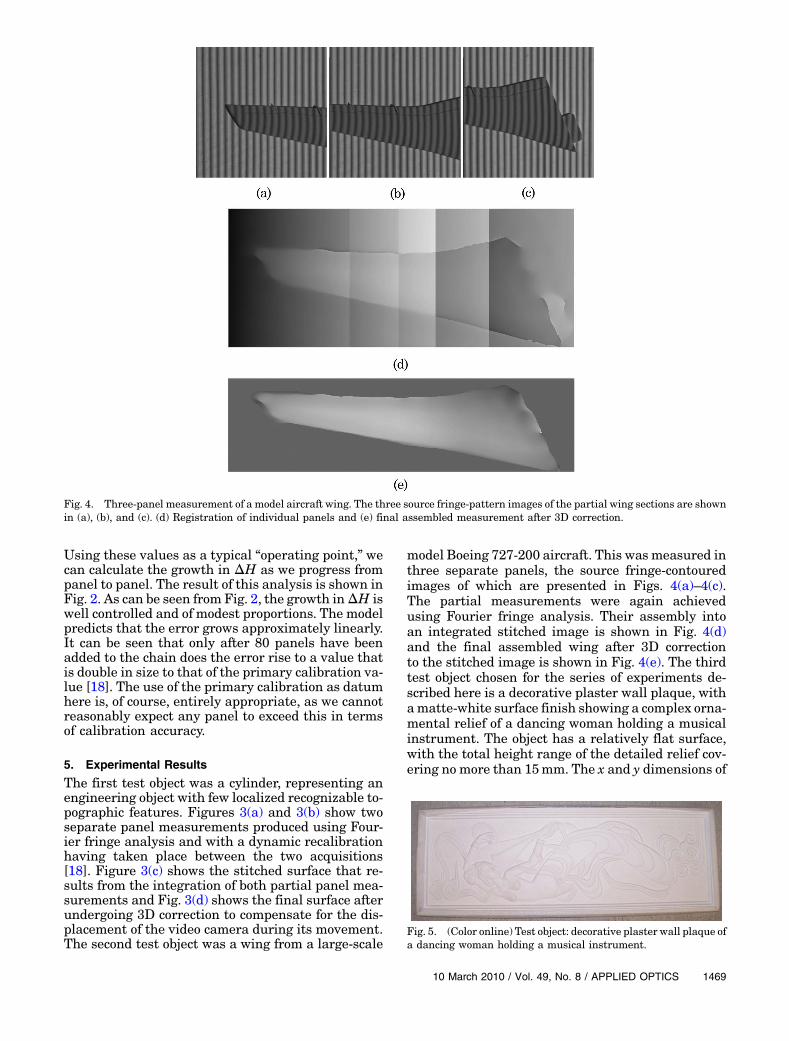
model Boeing 727-200 aircraft. This was measured inthree separate panels, the source fringe-contouredimages of which are presented in Figs. 4(a)–4(c).The partial measurements were again achievedusing Fourier fringe analysis. Their assembly intoan integrated stitched image is shown in Fig. 4(d)and the final assembled wing after 3D correctionto the stitched image is shown in Fig. 4(e). The thirdtest object chosen for the series of experiments de-scribed here is a decorative plaster wall plaque, withamatte-white surface finish showing a complex orna-mental relief of a dancing woman holding a musicalinstrument. The object has a relatively flat surface,with the total height range of the detailed relief cov-ering no more than 15mm. The x and y dimensions of

Fig. 4. Three-panel measurement of a model aircraft wing. The three source fringe-pattern images of the partial wing sections are shownin (a), (b), and (c). (d) Registration of individual panels and (e) final assembled measurement after 3D correction.

Fig. 5. (Color online) Test object: decorative plaster wall plaque ofa dancing woman holding a musical instrument.


the object are approximately 1000mm × 350mm.Figure 5 shows a general view of the test object.Because of the specific nature of the object, which

exhibits low surface height variations and the pre-sence of potential areas of shadow, the phase-stepping technique [3–6] was chosen to be the mostappropriate technique for performing the partial sin-gle-panel measurements. The rationale behind thischoice of measurement object and the specific config-uration of the measurement system used in these ex-periments was to provoke the need for multipanelmeasurement by measuring a test object that wassignificantly larger than the field of view of the opti-cal sensor, while keeping the scale of the experimentmanageable within the confines of the laboratory.This configuration is, of course, scalable, enablingthe measurement of much larger objects by employ-ing a similar strategy. The test object was measuredin two halves, each half comprising five individualpanels. Figure 6 shows the 3D measurement resultsfor the two separate halves of this object, first as 2Dgray scale (where height is scaled as intensity), asshown in Figs. 6(a) and 6(b), and, second, in 3D iso-metric form, as shown in Figs. 6(c) and 6(d).

6. Conclusions

In this paper, an approach to system phase-to-heightcalibration involving the use of hybrid models hasbeen presented. A hybrid model is a model basedon analytical equations that have been derived byanalyzing the measurement system’s geometry, butthe coefficients describing the system are obtained

in an empirical manner. Thus, hybrid models inheritthe accurate description of the measurement systemthat is provided by analytical models, along with thesimplicity of the calibration process that is providedby empirical models. They also thereby avoid one ofthe major difficulties associated with analytical mod-els, which is the accurate determination of systemparameters for use as model coefficients. When im-plemented in a multipanel measurement system,such hybrid models allow practical dynamic recali-bration to be carried out at any point in the measure-ment process.

A fundamental problem of phase-to-height modelshas been discovered as part of this research. The ma-jority of both hybrid and empirical models sufferfrom the fact that it is theoretically possible thatpoints of uncertainty and regions of distortion mightexist within any height map theymight produce. As astrategy for coping with these problems, the use of“simplified models” has been proposed in this paper.The performance of the various different models,including the “full hybrid” and “simplified hybrid”models has also been compared experimentallyand the simplified hybrid models are found to per-form well when compared to the other model types.

Finally, this paper demonstrates that it is practi-cally possible to produce such a system that incorpo-rates dynamic recalibration that is based uponhybrid phase-to-height models and that is capableof performing accurate multipanel measurement ofmedium- and large-scale objects.

Fig. 6. Multipanel measurement results for the test object. Two example surfaces are shown, each made up of five measured panels.(a) and (b) 2D gray-scale representation of height values of the two samples. (c) and (d) 3D isoplot representations of both surfaces.


References1. M. Takeda, H. Ina, and S. Kobayashi, “Fourier-transform of

fringe pattern analysis for computer-based topography andinterferometry,” J. Opt. Soc. Am. 72, 156–160 (1982).

2. X. Su andW. Chen, “Fourier transform profilometry: a review,”Opt. Lasers Eng. 35, 263–284 (2001).

3. P. Carré, “Installation et utilisation du comparateur photo-électrique et interférentiel du Bureau International des Poidset Mesures,” Metrologia 2, 13–23 (1966).

4. J. H. Bruning, D. R. Herriott, J. E. Gallagher, D. P. Rosenfeld,A. D. White, and D. J. Brangaccio, “Digital wave-front measur-ing interferometer for testing optical surfaces and lenses,”Appl. Opt. 13, 2693–2703 (1974).

5. H. P. Stahl, “Review of phase-measuring interferometry,” Proc.SPIE 1332, 704–719 (1991).

6. H. Zhang, M. J. Lalor, and D. R. Burton, “Robust, accurateseven-sample phase-shifting algorithm insensitive to non-linear phase-shift error and second-harmonic distortion: acomparative study,” Opt. Eng. 38, 1524–1533 (1999).

7. J. C. Wyant and J. Schmit, “Large field of view, high spatialresolution, surface measurements,” Int. J. Mach. Tools Manuf.38, 691–698 (1998).

8. A. Asundi and W. Zhou, “Mapping algorithm for 360 degprofilometry with time delayed integration imaging,” Opt.Eng. 38, 339–344 (1999).

9. C. Reich, “Photogrammetrical matching of point clouds for3D measurement of complex objects,” Proc. SPIE 3520,100–110 (1998).

10. W. Schreiber and G. Notni, “Theory and arrangements ofself-calibrating whole-body three-dimensional measurement

systems using fringe projection technique,” Opt. Eng. 39,159–169 (2000).

11. B. A. Rajoub, D. R. Burton, and M. J. Lalor, “A new phase-to-height model for measuring object shape using collimatedprojections of structured light,” J. Opt. A Pure Appl. Opt. 7,S368–S375 (2005).

12. B. A. Rajoub, D. R. Burton, M. J. Lalor, and S. A. Karout, “Anew model for measuring object shape using non-collimatedfringe-pattern projections,” J. Opt. A Pure Appl. Opt. 9,S66–S75 (2007).

13. G. S. Spagnolo, G. Guattari, C. Sapia, D. Ambrosini, D.Paoletti, and G. Accardo, “Three-dimensional optical profilo-metry for artwork inspection,” J. Opt. A Pure Appl. Opt. 2,353–361 (2000).

14. M. Takeda and K. Mutoh, “Fourier transform profilometry forthe automatic measurement of 3-D object shapes,” Appl. Opt.22, 3977–3982 (1983).

15. F. Lilley, M. J. Lalor, and D. R. Burton, “A robust fringeanalysis system for human body shape measurement,” Opt.Eng. 39, 187–195 (2000).

16. B. A. Al-Rjoub, “Structured light optical non-contact measur-ing techniques: system analysis and modelling,” Ph.D. disser-tation (Liverpool John Moores University, U.K., 2007).

17. D. R. Burton, A. J. Goodall, J. T. Atkinson, and M. J. Lalor,“The use of carrier frequency shifting for the elimination ofphase discontinuities in fourier transform profilometry,”Opt. Lasers Eng. 23, 245–257 (1995).

18. V. Hovorov, “A new method for the measurement of largeobjects using a moving sensor,” Ph.D. dissertation (LiverpoolJohn Moores University, U.K., 2008).


Dynamic recalibration of scalable fringe-projection systems for large-scale object metrology

Documents

Transcript of Dynamic recalibration of scalable fringe-projection systems for large-scale object metrology