Dynamic PEATSim Model: Documenting Its Use in Analyzing Global Commodity Markets

United StatesDepartment ofAgriculture

EconomicResearchService

TechnicalBulletinNumber 1933

July 2012

Dynamic PEATSim Model Documenting Its Use in Analyzing Global Commodity MarketsAgapi Somwaru and Steve Dirkse

The U.S. Department of Agriculture (USDA) prohibits discrimination in all its programs and activities on the basis of race, color, national origin, age, disability, and, where applicable, sex, marital status, familial status, parental status, religion, sexual orientation, genetic information, political beliefs, reprisal, or because all or a part of an individual's income is derived from any public assistance program. (Not all prohibited bases apply to all programs.) Persons with disabilities who require alternative means for communication of program information (Braille, large print, audiotape, etc.) should contact USDA's TARGET Center at (202) 720-2600 (voice and TDD).

To file a complaint of discrimination write to USDA, Director, Office of Civil Rights, 1400 Independence Avenue, S.W., Washington, D.C. 20250-9410 or call (800) 795-3272 (voice) or (202) 720-6382 (TDD). USDA is an equal opportunity provider and employer.

Recommended citation format for this publication:

Somwaru, Agapi, and Steve Dirkse. Dynamic PEATSIM Model: Documenting Its Use in Analyzing Global Commodity Markets, TB-1933, U.S. Department of Agriculture, Economic Research Service, July 2012.

Use of commercial and trade names does not imply approval or constitute endorsement by USDA.

ww

w.er

s.usda.gov

Visit Our Website To Learn More!

www.ers.usda.gov

United StatesDepartmentof Agriculture

www.ers.usda.gov

A Report from the Economic Research Service

Abstract

This report documents the updated version of the Partial Equilibrium Agricultural Trade Simulation (PEATSim) model developed by USDA’s Economic Research Service. PEATSim is a global model, covering 31 commodities and 27 countries/regions. The model, consistent with economic theory, provides a flexible country and commodity aggregation and accounts for cross-commodity linkages and interactions. The report includes a presentation and discussion of the structure and specific features of the revamped model, along with the theoretical underpinnings. It also documents an applica-tion of the model to illustrate its dynamic structure and to demonstrate the differential behavior.

Keywords: Partial equilibrium, dynamic, trade, multi-commodity markets, agriculture, global model

Acknowledgments

The authors thank the following individuals for their valuable insights and recommen-dations: John Dyck, William Liefert, Suchada Langley, and Danny Pick of USDA’s Economic Research Service, and three anonymous reviewers. The authors also thank John Weber and Wynnice Pointer-Napper for editorial and design assistance.

About the authors

Agapi Somwaru is a former senior economist with USDA’s Economic Research Service. Steve Dirkse is Director of Optimization with GAMS Development Corporation.

Dynamic PEATSim Model Documenting Its Use in Analyzing Global Commodity Markets

Technical Bulletin Number 1933

July 2012

Agapi Somwaru and Steve Dirkse

ii Dynamic PEATSIM Model: Documenting Its Use in Analyzing Global Commodity Markets / TB-1933

Economic Research Service/USDA

Contents

Summary. . . . . . . . . . . . . . . . . . . . . . . . . . . . . . . . . . . . . . . . . . . . . . . . . . . iii

Introduction . . . . . . . . . . . . . . . . . . . . . . . . . . . . . . . . . . . . . . . . . . . . . . . . . 1

Methodology and Data . . . . . . . . . . . . . . . . . . . . . . . . . . . . . . . . . . . . . . . . 2

Model Structure, New Features, and Modifications . . . . . . . . . . . . . . . . . 3 Geographic Scope and Flexible Country Aggregation . . . . . . . . . . . . . . . 3 Commodity Coverage . . . . . . . . . . . . . . . . . . . . . . . . . . . . . . . . . . . . . . . . 3 Sectors. . . . . . . . . . . . . . . . . . . . . . . . . . . . . . . . . . . . . . . . . . . . . . . . . . . . 4 Supply/Production. . . . . . . . . . . . . . . . . . . . . . . . . . . . . . . . . . . . . . . . . . . 5 Demand . . . . . . . . . . . . . . . . . . . . . . . . . . . . . . . . . . . . . . . . . . . . . . . . . . . 8 Prices. . . . . . . . . . . . . . . . . . . . . . . . . . . . . . . . . . . . . . . . . . . . . . . . . . . . 13 Policies . . . . . . . . . . . . . . . . . . . . . . . . . . . . . . . . . . . . . . . . . . . . . . . . . . 15 Trade and Model Closure . . . . . . . . . . . . . . . . . . . . . . . . . . . . . . . . . . . . 17 Nontraded Commodities . . . . . . . . . . . . . . . . . . . . . . . . . . . . . . . . . . . . . 18 Data Sources and Calibration . . . . . . . . . . . . . . . . . . . . . . . . . . . . . . . . . 19

Application . . . . . . . . . . . . . . . . . . . . . . . . . . . . . . . . . . . . . . . . . . . . . . . . . 21 Scenarios . . . . . . . . . . . . . . . . . . . . . . . . . . . . . . . . . . . . . . . . . . . . . . . . . 21 Results . . . . . . . . . . . . . . . . . . . . . . . . . . . . . . . . . . . . . . . . . . . . . . . . . . . 22

Conclusion. . . . . . . . . . . . . . . . . . . . . . . . . . . . . . . . . . . . . . . . . . . . . . . . . . 36

References . . . . . . . . . . . . . . . . . . . . . . . . . . . . . . . . . . . . . . . . . . . . . . . . . . 37

Appendix: Mixed Complementarity Problem . . . . . . . . . . . . . . . . . . . . . 41

iii Dynamic PEATSIM Model: Documenting Its Use in Analyzing Global Commodity Markets / TB-1933


Summary

Background

PEATSim (Partial Equilibrium Agricultural Trade Simulation) is a dynamic, partial equilibrium, mathematical-based model that enables users to reach analytical solutions to problems, given a set of parameters, data, and initial conditions. This theoretical tool developed by ERS incorporates a wide range of domestic and border policies that enables it to estimate the market and trade effects of policy changes on agricultural markets. PEATSim captures the economic behavior of agricultural producers, consumers, and markets in a global framework. It includes variables for production of crops and livestock activities, consumption, exports, imports, stocks, world prices, and domestic producer and consumer prices.

In 2010, ERS updated and modified the model extensively. The original model, static in its specification, was developed through a collaborative effort between ERS and Pennsylvania State University. This report supports requirements for documentation and information quality as specified by the U.S. Office of Management and Budget.

What Is the Contribution?

PEATSim’s innovative and flexible design enables users to analyze a variety of domestic and trade policy issues. The model is written in GAMS (General Algebraic Modeling System) using PATH, a Mixed Complementarity Problem (MCP) solver. MCP enables PEATSim to account for a discon-tinuous policy regime, such as a tariff rate quota or a trade ban. This report makes the model transparent and available to a larger audience.

In 2010, PEATSim was modified to include new features and enhanced capabilities:

•PEATSimwasaugmentedtoincorporatedifferentsetsofproductionactivities; links between upstream and downstream sectors; and interac-tions of producers, processors, and consumers at a global level.

•Unlikepreviousversions,theupdatedmodel’sdynamicspecificationandenhanced flexibility enable researchers to analyze short-term and long-term effects of domestic and border policies.

•Themodelaccountsforsimultaneousinteractionsbetweenlivestockandcrop activities and has the ability to capture and solve different sets of production activities worldwide.

•PEATSimnowincludes27countries/regions,upfrom12inthepreviousversion. The updated version also allows flexible aggregation of the coun-tries in the model to accommodate various modeling needs.

•Theupdatedmodelincludes31agriculturalcommoditiesinadditionto3 biofuel-related commodities (ethanol, biodiesel, and distillers’ dried grains with solubles).

iv Dynamic PEATSIM Model: Documenting Its Use in Analyzing Global Commodity Markets / TB-1933


•ThedatainPEATSimcalibratetoUSDA Agricultural Projections to 2019 and OECD-FAO Agricultural Outlook 2010-2019, while an innova-tive econometric method (i.e., cross entropy) equilibrates supply and use.

•PEATSimusestransparent,clearlylistedprogrammingcodes,datainputs, equations, data rules, policies, and parameters.

How Was the Study Conducted?

This report documents the latest version of PEATSim. To illustrate the model’s capabilities, we evaluate the effects on the biofuels sector of alternative macro-economic conditions and crude oil prices, taking into account biofuel produc-tion on a global scale from different feedstocks across countries.

1 Dynamic PEATSIM Model: Documenting Its Use in Analyzing Global Commodity Markets / TB-1933


Introduction

This report documents the latest version (2010) of the Dynamic Partial Equilibrium Agricultural Simulation (PEATSim) model and discusses specific modified features and structures, such as commodity/country coverage and updates of trade policies. It also presents an empirical application of the model on the global biofuels sector under alternative macroeconomic conditions and, especially, crude oil prices (testing for high/low levels).

PEATSim is a simulator in the sense that it is a mathematical-based system that attempts to find analytical solutions to problems, given a set of param-eters, data, and initial conditions. Previous versions of the PEATSim model have been used in numerous studies (see Blayney et al., 2006; Dyck et al., 2008; Langley et al., 2003, 2005, 2006; Stillman et al., 2005; Zahniser et al., 2010; Valdes et al., 2010, Meade et al., 2010; and Shane et al., 2009). For example, PEATSim was used to analyze global dairy markets, examine the effects of agricultural trade liberalization, estimate the effects of biofuels expansion on global agricultural production and trade, and analyze the impacts of biofuel mandates on worldwide grain, livestock, and oilseed sectors (see Peters et al., 2008, 2009, 2010; and Stillman et al., 2007, 2008a, 2008b).

In previous versions of the model, biofuels were represented by “stylized” biofuels activities, which do not fully capture the complexity and interaction of biofuels production patterns. An analysis of global expansion of biofuels production calls for an innovative way to incorporate these activities into the model and capture their impacts and links between upstream and down-stream activities of the biofuels “module.” For this reason, PEATSim was augmented to incorporate a module that links farm activities/sectors with downstream industries on a global basis.

The documentation of the static version of the model, the ERS/Penn State Trade model, was developed by ERS’s James Stout in collaboration with David Abler of the Pennsylvania State University (2004).1 In fall 2005, the model was revamped and extended to include the complementarity features of PATH, a state-of-the-art program (Dirkse, 1994; Dirkse and Ferris, 1994b, 1994c). In 2010, the dynamic version of the model was developed and extended to include the global biofuels module and the use of maximum entropy techniques for data consistency.

1The theoretical underpinnings for the static version of the model were developed by a modeling team, including David Abler, David Blandford, Karl Meilke, Ian Sheldon, GianCarlo Moschini, Mary Bohman, and Praveen Dixit.



Methodology and Data

PEATSim’s multiple-commodity, multiple-region structure enables it to account for simultaneous interactions between livestock and crop activities while maintaining identities such as supply and use. PEATSim covers major crops, oilseed and oilseed products, livestock, and dairy activities. It also incorporates explicit representation of each country’s domestic and trade policies pertaining to agricultural commodities. PEATSim has the ability to model different sets of production activities; links between various crops and livestock sectors both upstream (at the farm gate) and downstream (such as biofuels and dairy processing); and interactions of producers, processors, and consumers on a global level. The model’s innovative and flexible specification enables researchers to analyze a variety of domestic and trade policy issues.

PEATSim is a reduced-form model that captures the economic behavior of producers, consumers, and markets in a global framework. It includes variables for production of crops and livestock activities, consumption, exports, imports, stocks, world prices, and domestic producer and consumer prices. Commodity-based markets are modeled such that quantities and prices clear the market (Hamilton, 1994, pp. 324-327). This implies that market-clearing quantities are the sum of beginning stocks, production, and imports and equal to the sum of exports, consumption, and ending stocks. These equilibrating conditions hold at commodity levels and at world markets. The model is used to simulate “what-if” scenarios for comparison with base year(s) results. Constant elasticity functions are selected because of their ease of interpretation and well-behaved properties. They can be viewed as first-order approximations to underlying supply and demand functions (see Stout and Abler, 2004).

The PEATSim model is written in GAMS (General Algebraic Modeling System, Brooke et al., 1988) programming language using PATH, a Mixed Complementarity Problem (MCP) solver developed by Dirkse (1994a), Dirkse and Ferris (1994b), and Dirkse et al. (1994c) (see appendix). MCP enables PEATSim to generate a model with different production-consumption regimes and functional form discontinuities. Thus, PEATSim can incorporate discontinuous functional forms such as tariff-rate quotas (TRQs) and discon-tinuous demand issues created by mandates, targets, and other complicated policy instruments. MCP also allows for endogenous determination of active regimes and the consequences of regime shifts, such as the shift from an “in-quota” tariff to “over-quota” tariff. For example, PEATSim endogenously determines the TRQ price and quantity and makes the need for the arbitrary quota rent allocation obsolete.



Model Structure, New Features, and Modifications

Given the complexity of global agricultural markets, it is not easy to evaluate the implications of a growing global market for biofuels because a model would need to account for biofuel production and its links with other agricultural and nonagricultural sectors worldwide. PEATSim was exten-sively modified to include additional sectors involved in biofuels and their byproducts, including conventional ethanol and biodiesel, on a global basis, such as the AGLINK-COSIMO (OECD-FAO, 2010) and FAPRI (FAPRI, 2010) models.

The interactions of biofuel and agricultural markets are inherently multisec-toral because of the interactions between energy, farm inputs, crops, feed, food consumption, and trade. Continued long-term growth in the use of food and feed products and in the production of fuel have made it difficult to assess the impacts of such growth on the global market. For these reasons, ERS augmented and revised the model with a global biofuels module.

Theoretically, the model was modified incorporating detailed global ethanol and biodiesel markets. The new global biofuel component of PEATSim includes ethanol and biodiesel from a variety of feedstocks, such as corn, wheat, rapeseed, soybeans, sugarcane, and sugar beets, as well as down-stream production activities related to biofuels for all countries in the model.

Also, the expanded database includes biofuel production from sources other than feedstocks. For the nonfeedstock-related biofuel production processes, such as that for cellulosic ethanol, detailed technical data are unavailable. However, nonfeedstock sources, or “other” biofuels, are accounted for in PEATSim given data availability in the AGLINK-COSIMO (OECD-FAO, 2010) model and its database.

Geographic Scope and Flexible Country Aggregation

PEATSim was updated to include 27 countries/regions. The country coverage is Argentina, Australia, Bangladesh, Brazil, Canada, China, European Union (EU-27), Egypt, Indonesia, India, Iran, Japan, South Korea, Mexico, Malaysia, New Zealand, Pakistan, Philippines, Russia, Saudi Arabia, South Africa, Thailand, Turkey, Ukraine, United States, Vietnam, and the rest of the world (see fig. 1). The latest version allows flexible aggregation of the countries in the model. For example, a user can aggregate the model into fewer countries if needed.

Commodity Coverage

The model covers 31 agricultural commodities: 11 crops (rice, wheat, corn, other coarse grains, soybeans, sunflower, rapeseed, cotton, sugarcane, sugar beets, and sugar (semi-processed)); 10 oilseed, oil, and meal prod-ucts (soybeans, soybean oil, soybean meal, sunflower seed, sunflower oil, sunflower meal, rapeseed, rapeseed oil, rapeseed meal, and other oilseed oil); 4 livestock and livestock-related products (beef and veal, pork, poultry, and raw milk); and 6 dairy products (fluid milk, butter, cheese, nonfat dry milk,



whole dry milk, and other dairy products). In addition, coverage includes three biofuel commodities and byproducts (ethanol, biodiesel, and dried distillers’ grains with solubles (DDGs)).

Sectors

The model includes the crop sector, livestock and products sector, and the food processing sector. These sectors are related to each other through production processes, commodity prices, and their use of shared resources, such as land. The model includes four types of production activities: crop production (includes sugarcane and sugar beets), livestock production (includes raw milk), oilseed product production, and dairy product production.

Argentina–9%

Australia–5%

Brazil–6%

Canada–1%

EU27–50%

India–2%

Rest ofworld–10%

U.S.–17%

World biodiesel production

Argentina–0.41% Australia–0.74%

Brazil–29.82%

Canada–1.93%China–5.14%

EU27–7.08%India–2.66%

Mexico–0.08%

Rest ofworld–2.67%

U.S.49.46%

Figure 1

PEATSim countries/regions, 2009

World ethanol production



The crop sector comprises grains (rice, wheat, and corn), oilseeds, upland cotton, and sugarcane and sugar beets. “Other coarse grains” are primarily barley, sorghum, millet, and oats. Livestock sector includes beef and veal, pork, poultry, and raw milk. Sugarcane and sugar beet crops are newly intro-duced to the model, as are the complementarity conditions between sugar feedstocks (sugarcane and sugar beets) and processed/refined sugar. The revised model also includes sugar that is processed/refined, with cane and beet sugar combined into a single commodity.

Supply/Production

Crop production in the model is determined by acreage harvested and yield per harvested acre, while both acreage harvested and yield are determined endogenously. The latest version of the model is dynamic, and in an attempt to capture the relative profitability of farmers, acreage response equations are specified to reflect farmers’ perceptions of expected prices and yields. In documenting the Food and Agricultural Policy Simulator (FAPSIM), Gadson et al. (1982) wrote: “Farmers can base future yield perceptions on past or experienced yield levels or alternatively discount abnormal weather conditions in past years and base their expected yield perceptions on yields realized under normal weather conditions” (see also Westhoff et al., 1990). At planting time, acreage harvested and yields are not known. Assuming an adaptive expectations hypothesis of farmers’ perceptions, we use lagged or past acreage harvested, yields, and price to explain crop production. Following FAPSIM, the reduced form equations of acreage response and yields are specified to represent farmers’ price expectations based on past or experienced yield levels and market prices prior to planting.

Crops

Crop production, PRDi,r,t, is defined as the product of acreage harvested, AHVi,r,t, and yield, YLDi,r,t, while producer prices are allowed to adjust.

Area harvested of crop i in country r and year t is a function of area and the crop’s own producer price and producer prices of other crops, which may be complementary or competing for acreage as follows:

,, , , , |(1) , , 1 , , , 1

,(1) iji r

ni r t i r t i r t i j r t

i jAHV a AHV PPRελ

− −

= ∏

where αi,r,t|(1) is a measure that captures the past interaction between the producer price and crop area,2 AHVi,r,t-1 is lagged area of crop i, λi,r is a partial adjustment parameter, PPRi,r,t-1, is own lagged producer price, PPRj,r,t-1 is lagged producer prices of other crops j, and εi,j is cross price elas-ticities for crop area.

As explained earlier, the reduced form yield equation is then specified as a function of the ith crop’s lagged yield and lagged producer price of crop PPRi,r,t-1 as follows:

, ,, , , , |(2) , , 1 , , 1(2) i r i r

i r t i r t i r t i r tYLD a YLD PPRµ η− −=

2This modeling is appropriate when, for example, the production tech-nology is described by a Cobb-Douglas function, such as: Y(L,K) = ALbK1-b where Y represents total produc-tion, L, represents labor, K represents capital, and A represents total factor productivity, which includes effects from technology, efficiency, and scale. Given that A varies over time, we can use it as a variable to help calibrate the long-term projections.



where αi,r,t|(2) is a measure that captures the past interaction between the producer price and yield, µi,r is a partial adjustment parameter, ηi,r is the price elasticity of the yield for crop i, and PPRi,r,t-1 is own lagged producer price.

Oilseed products

As stated earlier, the model includes 10 oilseed, oil, and meal products. The “other oilseed oil” aggregate includes canola oil, flax seed oil, and tropical oils (palm oil, olive oil, coconut oil, and other oil).

Production of oilseed products i in country r at time t(PRDi,r,t) is determined by the quantity of jth oilseed crushed and by an exogenous extraction rate as follows:

, , , , , , ,(3) i r t j r t i j r ti

PRD CRU ERT= ∑

where CRUj,r,t is the crush of the associated oilseed and ERTi,j,r,t is the extraction rate assuming fixed proportion in the technology of meal and oil production. The determinants of oilseed crushing are discussed later in equa-tion 15.

Livestock products

Production of livestock product i in country at r year t, PRDi,r,t, is a function of its own producer price and the producer prices of the other livestock prod-ucts, a feed cost index for that product, and production of that product in the previous year as:

, ,, ,, , , , , ,, , 1 , , , 1(4) i j ri r i r

ni r t i r t i r ti r t i j r t

j livestockPRD PRD PPR FeCostσλ ηβ − −

∈= ∏

where βi,r,t is a measure that captures the past interaction between (1) the producer price and feed costs and (2) production, PRDi,r,t-1 is production of ith livestock product the previous year, λi,r is a partial adjustment parameter, PPRi,j,r,t is the producer price of i livestock products (own) and the producer prices of other livestock products j (cross price) in country r, σi,j,r is the price elasticity of production, FeCosti,r,t is the feed cost index for each livestock product i, and ηi,r is the elasticity of production with respect to input prices.

The feed cost index, FeCosti,r,t, is a function of feed use and feed prices and is specified as:

, , , , , , ,(5) i r t i j r t j r tj feeds

FeCost FeedUse PPR=

= ∑

where FeedUsei,j,r,t is the jth feed used in the production of livestock product i, in country r at time t, and PPRj,r,t, is the price of feed j in country r at time t. There are nine commodities in the model that can potentially be used as livestock feed: wheat, corn, other coarse grains, DDGs, and all meals (byproducts of soybeans, sunflower seeds, and rapeseeds).



Dairy products

As mentioned earlier, the model identifies six dairy products. The “other dairy products” aggregate includes ice cream, yogurt, and whey. Dairy prod-ucts are processed from raw milk, one of the four livestock products in the model. In some regions, production of one or more dairy products is zero or negligible, in which case production is set equal to zero in the model.

Production of dairy products i at year t is modeled as proportional to the total

quantity of raw milk processed , ,' ', ,

i r tprocessed milk r t

PRDPRD (because all

processed dairy products are derived from raw milk) and the price of dairy products.3 With this specification, a change in the price of one processed dairy product relative to another leads to changes in the mix of processed dairy products made from raw processed milk. The equation is as follows:

,

, ,, , , , 1, , , ,

' ', , ' ', , 1(6)

i r

i j ri r t i r ti r t j r t

processed milk r t processed milk r t j dairyproducts

PRD PRDPPRPRD PRD

λσβ −

− ∈

= ∏

where PRDi,r,t is production of the ith dairy product in country r at time t, PRD'processed milk' ,r is total production of raw processed milk,

, ,' ', ,


PRDPRD is the proportionality, which indicates that the

production of the ith dairy product varies in direct proportion with the total

production of raw processed milk, , , 1' ', , 1


PRDPRD

−−

is the

proportionality lagged one year, PPRj,r,t is the producer price of dairy product j, βi,r,t is a technology parameter that determines the production of dairy products over time, λi,r represents the rate of adjustment, and σi,j,r is the own and cross-price elasticity of supply for dairy products.

Biofuels

Production of biofuels, PRDi,r,t, is expressed as the summation of biofuels from the various feedstocks, BioPRDi,j,r,t, and production of biofuels from nonfeedstock, OthPRDi,j,r,t, as follows:

, , , , , , , ,(7) i r t i j r t i j r tj

PRD BioPRD OthBioPRD= +∑

where i indicates the type of biofuels (ethanol, biodiesel), j indicates feed-stocks, r indicates country, t indicates time, and OthBioPRDi,j,r,t denotes “other” agricultural and nonagricultural related sources, such as corn resi-dues (stover), fermentation of molasses, wheat byproducts (i.e., Australia), or forest byproducts. Note that OthBioPRDi,j,r,t, depicts biofuel production from other sources, such as corn stover, wheat straw, and sugarcane residue, driven by data availability in the database and is expressed as the summation of biofuels from other resources.

3The supply of dairy products is modeled as proportional to the total quantity of raw milk (proportionality) and the previous year's proportionality. Although dairy products and raw milk are perishable, the supply of dairy products at the first stage of processing (i.e., milk processing plants) can be subject to the longrun equilibrium specification.



The production of biofuels, both ethanol and biodiesel, from all catego-ries of feedstocks, BioPRDi,j,r,t, is an intermediate production process and depicts the interindustry technological relation of biofuels and feedstocks in each country in the model. This production process captures the technology balance of converting feedstocks to biofuels. The process is characterized by each country’s technological advances depending on the type and availability of alternative feedstocks and can be represented as follows:

, , , , , , ,(8) i j r t j r t i biofuels j r t i biofuelsBioPRD Conv Fue= ==

where i indicates type of biofuel (ethanol, biodiesel), j indicates feedstocks, r indicates country, t indicates time, Fuej,r,t|i=biofuels indicates alternative feedstocks for biofuels, and Convj,r,t|i=biofuels is the technical coefficient for converting feedstocks to biofuels. In other words, the process captures the technological interindustry relation of converting and producing biofuels from alternative feedstocks in each country in the model.

The main byproducts of corn ethanol, for example, in the case of the U.S. dry-corn milling industry, are DDGs. DDGs are a substitute for corn (as feed) and are used as a protein source for animals in feedlots, particularly finishing cattle and poultry. The production of DDGs, or PDR'DDGs', r,t, in the corn ethanol process is proportional to a technical coefficient that captures the technological relation of corn-ethanol production and DDGs. This comple-mentarity relationship between primary product (corn ethanol) and byproduct is linear and can be stated as follows:

' ', , ' ', , ' ', ,(9) DDGs r t corn r t corn r tPRD ddgsConv Fue=

where r indicates country, t indicates time, ddgsConv is the technical coeffi-cient that depicts the conversion of corn feedstocks to DDGs in the production of DDGs, and Fue'corn',r,t is corn feedstocks in the production of corn ethanol.

Sugar

Sugar production, PRD'sugar',r,t, from sugarcane and sugar beet feedstocks is defined as follows:

' ', , , , | , ,(10) sugar r t i r t i sugar i r ti

PRD sugCon Foo== ∑

where i indicates the type of sugar-producing crop, r indicates country, t indicates time, and sugConi,r,t\i=sugar denotes a technology-related concept in the sugar-processing sector determining the technological relationship between processed sugar (output) and sugarcane and sugar beets (inputs) in each country in the model. Finally, Fooi,r,t denotes sugarcane and sugar beets used (or demanded) by the refined sugar processing sector (an intermediate processing sector), where i refers to sugarcane and sugar beets for refined sugar-processing products.

Demand

The model includes various types of consumption activities, such as food, feed, and fuel demand. The model is specified to maintain consistency between consumption and its subcomponents.



Food demand

Food demand exists for all commodities in the model except raw milk and the three oilseed meals. Food demand is specified as per capita and aggre-gate. Per capita food demand PcFOOi,r,t for commodity i in country r at time t is a function of consumer price, PCNi,r,t, and per capita income in real terms, PcRGDPr,t, as follows:

, , ,, , , , , , ,(11) i j r i r

i r t i r t i r t r ti

PcFOO PCN PcRGDPσ εβ= ∏

where βi,r,t is a measure that captures the interaction between the consumer price, the per capita demand, and per capita income; σi,j,r is the own- and cross-price elasticity of demand; and εi,r denotes the income elasticity of food demand for commodity i in country r at time t.

Aggregate food demand for all commodities, FOOi,r.t, is specified as a func-tion of per capita commodity demand and population:

, , , , ,(12) i r t i r t r tFOO PcFOO POP=

where PcFOOi,r.t is per capita food demand and POPr,j denotes population in country r at time t.

Feed demand

Each region in the model has four feed demand equations, one for each of its four livestock products. As noted earlier, there are seven commodities in the model that can be used as livestock feed: wheat, corn, other coarse grains, soybean meal, sunflowerseed meal, rapeseed meal, and DDGs. In some regions, the use of a particular feed for one or more livestock products is zero or negligible, in which case feed demand is set to zero in the model.

Feed demand, FEESi,k,r,t, is specified as a function of livestock production (PRDk,r,t), feed conversion ratios (FRi,k,r,t), and feed prices (PFEi,r,t) as follows:

, , ,, , , , , , , , , , , , ,(13) i j k t

i k r t i k r t k r t i k r t i r ti feed

FEES PRD FR PFEσβ∈

= ∏

where i depicts feed category, k depicts livestock/meat category, r indicates country, t indicates time, βi,k,r,t is a measure that captures the interaction between the feed price and feed demand, PRDk,r,t depicts production of live-stock/meat, and FRi,k,r,t indicates feed used by livestock/meat category. Feed prices are depicted as PFEi,r,t, while σi,j,k,r is the own feed price elasticity of demand for i=j and the cross-price elasticity of feed demand for i≠j for meat and milk k.

Aggregate feed demand across all livestock, FEEi,r,t, is specified as the summation of feed demand by each livestock type k as follows:

, , , , ,(14) i r t i k r tk

FEE FEES= ∑



Crush

Oilseed crush, CRUi,r,t, is specified as a function of lagged crush, CRUi,r,t-1, and crush margins, MGNi,r,t, as follows:

, ,,, , , , , ,, , 1(15) i j ri r

i r t i r t i r ti r tj oilseeds

CRU CRU MGNσλβ −∈

= ∏

where i depicts oilseed category, r depicts country, t indicates time, and βi,r,t is a measure that captures the past interaction between the crush margin and crushing. In this specification, the demand for crush increases with increases in the processing/crushing margins and vice versa. In other words, as the crush margin increases, there will be a greater demand for oilseeds for crushing, resulting in a gradual rise in oilseeds prices. Conversely, when the margin starts falling, one can expect weaker demand for oilseeds and falling oilseeds prices, σi,j,r is the crush elasticity with respect to own price (i) and cross price (j) of oilseeds in country r, and λi,r is a partial adjustment parameter.

The crushing margin, MGNi,r,t, is specified as a function of the extraction rate of crush products, the prices of crush products (meal and oil), and the consumer prices for oilseeds:

, , , , ,

, ,, ,

(16) i j r t j r t

ji r t

i r t

ERT PPRMGN

PCN

∑=

where i indicates oilseed category, such as soybeans, rapeseeds, and sunflower seeds, j indicates crush products (meal and oil), r indicates country, t indicates time, ERTi,j,r,t is the extraction rate of oilseed crush (meal and oil), PPRj,r,t is the price of crush products, and PCNi,r,t is the consumer price of oilseeds.

Raw milk processing

Raw milk processing demand, CONi,r,t, for j dairy products, such as fluid milk, cheese, butter, nonfat dry milk, whole dry milk, and other dairy prod-ucts, is specified as a function of lagged raw milk demand, CONi,r,t-1, and the ratio of the value of the processed dairy product to the value of raw milk used (needed) in processing:

,,

, , , , , , , ,, , 1(17) i r

i ri r t i r t j r t j r ti r t

jCON CON PRD PPR

σλβ −

= ∑

where i indicates raw milk, j indicates dairy processed products, r indicates country, t depicts time, βi,r,t is a measure that captures the past interac-tion between processed dairy products and the demand for raw milk to be processed (as projected in the AGLINK-COSIMO (OECD and FAO model/baseline). PPRj,r,t is the producer price of processed dairy products (j = fluid milk, cheese, butter, nonfat dry milk, etc.), PCNi,r,t is the price of raw milk, λi,r is the partial adjustment parameter, and σi,r is the price elasticity of demand for raw milk in the processing of dairy products. In this specification,



PRDj,r,t depicts (over time t) demand of dairy products, while CONi,r,t depicts demand of raw milk for processing.

Biofuels-Ethanol

The demand for ethanol FUE'ethanol',r,t is specified as a function of ethanol price, PCN, the price of gasoline, pGAS, and real income, RGDP, as follows:

'' ', , ' ', , ,' ', , ' ', , ,(18) r r rethanol r t ethanol r t r tethanol r t gasoline r tFUE a PCN pGAS RGDP ϕσ ε=

where r denotes country at time t, α'ethanol',r,t is a measure that captures the interaction between the ethanol price and ethanol demand, σr is the ethanol price elasticity of demand, εr is the gasoline price elasticity of demand for ethanol, and φr is the income elasticity of demand for ethanol.

Biofuels-Biodiesel

The demand for biodiesel, FUE'biodiesel',r,t, is specified as a function of the biodiesel price, PCN, the price of diesel, pDSL, and real income, RGDP, as follows:

' ', , ' ', , ,' ', , ' ', , ,(19) r r rebiodiesel r t biodiesel r t r tbiodiesel r t diesel r tFUE a PCN pDSL RGDPηρ=

where r denotes country, t indicates time, α'biodiesel',r,t is a measure that captures the interaction between the biodiesel price and biodiesel demand, ρr is the biodiesel price elasticity of demand, er is the diesel price elasticity of demand for biodiesel, and ηr is the income elasticity of demand for biodiesel.

Biofuels-Feedstock

The demand for feedstocks, Fuej,r,t|biofuels, is an intermediate production activity and thus depends on the prices of feedstocks (upstream inputs) and biofuels (downstream outputs). The allocation (demand) of feedstocks for alternative biofuels, Fuej,r,t|biofuels, is specified as a function of the price of biofuels and the price of feedstock as follows:

, , ,, , , ,, , , ,(20) ( )i j r j re

i r t j r tj r t biofuels j r t biofuelsi biofuels

Fue PPR PCNεα=

= ∑

where i denotes biofuels (ethanol and biodiesel), j denotes feedstocks (such as corn, soybean oil, sugarcane, sugar beets, and rapeseed oil), r denotes country, t denotes time, αj,r,t|biofuels is a measure that captures the interaction between biofuel prices and the demand for feedstock for alternative fuels, PPRi,r,t denotes the producer price of biofuels i, εi,j,r is the price elasticity of demand for feedstocks in production of biofuel type/category, PCNj,r,t is the consumer price of feedstocks j, and ej,r represents the feedstock price elas-ticity of demand for biofuels.



Demand for sugarcane and sugar beets

The demand for sugarcane and/or sugar beets, FOOi,r,t\i=sugarcane / sugar-beets, is defined as follows:

, ,, , , ,' ', ,, , /(21) i r i r

i r t i r tsugar r ti r t i sugarcane sugar beetsFOO PPR PCNϕ θα= − =

where i denotes sugarcane/sugar beets, αi,r,t is a measure that captures the interaction between (1) the prices of both sugar feedstock and refined sugar and (2) the demand for sugarcane or sugar beets in country r and year t, PPR'sugar',r,t is the producer price of refined sugar, φi,r is the price elasticity of demand for sugarcane/sugar beets for the production of refined sugar, PCN is the consumer price of sugarcane/sugar beets, and θi,r represents the price elasticity of demand for sugarcane/sugar beets in country r at time t.

Other demand

Other use demand is generally small, and it is assumed to change over time by the same proportion as the change in the sum of food, fuel, feed, and crush, as follows:

, , , , , , , , , ,

, ,' ' , ,' ' , ,' ' , ,' ' , ,' '

(22) i r t i r t i r t i r t i r t

i r baseline i r baseline i r baseline i r baseline i r baseline

Oth FUE FOO FEE CRU

Oth FUE FOO FEE CRU

+ + +=

+ + +

Total

Total demand of all commodities i in country r at time t except raw milk is specified as the summation of the components food, fuel, feed, crush, and other, as follows:

, , , , , , , , , , , ,(23) i r t i r t i r t i r t i r t i r tCON FEE FOO FUE CRU OTH= + + + +

Stocks

Ending stocks for crops ESTi,r,t are specified as a function of ending stocks in the previous period and the ratio of commodity world reference prices over lagged world reference prices for crops:

, ,, ,

, , , , , , 1, , 1

(24) i r t

i r ti r t i r t i r t

i r t

PRFCEST EST

PRFC

εα −

−

=

where αi,r,t is a measure that captures that past interaction between world references prices and ending stocks for crops, i indicates commodity, r indicates country, t indicates time, PRFC denotes transmitted world price of a commodity i in country r at time t, and εi,r,t is the ending stocks price elasticity of demand. The proportionality of stocks at time “t” over stocks at time “t-1” (ESTi,r,t / ESTi,r,t-1) for a commodity depends on the proportion-ality of the transmitted world price of commodity i in country r at time “t” over price at time “t-1” (PEFCi,r,t / PRFCi,r,t-1). If this were not the case, the



demand for commercial stocks would be a function of the good’s expected price, that is, the demand for stocks would be speculative (Meilke, 1999; Gadson et al., 1982).

Prices

Domestic prices are endogenously determined in the model. World prices are in U.S. dollars, and all domestic prices and policies are expressed in local currency. Real exchange rates are treated as exogenous. In each region, domestic prices for all traded commodities (except raw milk, fluid milk, and other dairy products) depend on world prices, exchange rates, transportation costs, and country-specific policies that affect prices.

World prices

PRFi,t depicts the world reference price of commodity i, while PRFCi,r,t depicts the transmitted world price of commodity i to country r at time t. The transmitted world price to country r is defined as a function of the world reference price, PRFi,t, (see equation 40) expressed in U.S. dollars as follows:

, , , , , ,(25) i r t i r t i t r tPRFC TRANSM PRF REXR=

where TRANSMi,r,t represents a price transmission mechanism used in the model to capture the effects of world reference price on a country’s price, and REXRr,t is a real exchange rate for a tradable commodity i in country r at time t. Note that the world reference price is indexed over commodity i and time t while the transmitted world price commodity to a country is indexed over commodity i in country r at time t. Real exchange rates are exogenous in the model, while the transmission parameters are assigned or have the value of 1 for all tradable commodities.4

Domestic prices

For most region/commodity pairs, the domestic price PDOMi,r,t is defined as a weighted average of export prices, PEXi,r,t, and import prices, PIMi,r,t. The model assumes homogenous products, such that one domestic price is speci-fied as:

, , , , , , , , , ,(26) (1 )i r t i r t i r t i r t i r tPDOM PEX PIMθ θ= + −

where θi,r,t is the weight (0 ≤ θi,r,t ≤1 )and is equal to the baseline-years exports divided by the sum of baseline exports and baseline imports,

, ,, , , ,( )

i r ti r t i r t

EXPEXP IMP+

Producer prices

Producer prices, PPRi,r,t, are specified as a function of the domestic prices adjusted by producer subsidies or taxes for commodity i in country r at time t. Producer subsidies in the model can be either exogenous or endogenous

4Because of either policies (such as domestic price support or consumer subsidies) or weak market infrastruc-ture, the transmission of changes in agricultural border prices to domestic prices within countries might be incomplete (less than one). This could especially be the case for many devel-oping countries. Given that country coverage was expanded in this version of the model, particularly to include more emerging market and developing economies, future efforts will be devoted to determining more accurate price transmission parameters.



(e.g., subsidies that vary depending on the domestic price or other variables in the model):

, , , , , ,(27) i r t i r t i r tPPR PDOM TW= +

where TWi,r,t represents variable production subsidies (if any) associated with target price policies.

Consumer prices

Consumer prices, PCNi,r,t, for commodity i in country r at time t are speci-fied as a function of domestic prices adjusted by consumer subsidies (by subtracting) or taxes (by adding) as follows:

, , , , , ,(28) (1.0 )i r t i r t i r tPCN PDOM TC= ±

where TCi,r,t represents consumer subsidies/taxes. Consumer subsidies/taxes can be either exogenous or endogenous (i.e., subsidies/taxes that vary depending on other variables in the model).

Feed prices

Feed prices for feed category i in country r at time t, PFEi,r,t, are specified as a function of consumer prices (used as a proxy for the feed price at the retail level) adjusted for any difference between country/region consumer prices and the transmitted world price to the country r:

, , , , , , , , , ,(29) ( )i r t i r t i r t i r t i r tPFE PCN FeedPRFAC PRFC PCN= + −

where the feed price, FeedPRFACi,r,t, captures the difference (if any) between domestic consumer prices and world prices. Feed prices within the model can differ from domestic consumer prices by any endogenous or exogenous amount, added or subtracted, on an ad valorem or specific basis. However, as of this time, no policies have been introduced into the model for any coun-tries that could cause feed prices to deviate from domestic consumer prices. Consequently, FeedPRFACi,r,t is set equal to zero due to lack of data avail-ability, except for wheat and other coarse grains in Japan.

Import prices

Import prices, PIMi,r,t, are specified as a function of world prices adjusted for an ad valorem tariff (i.e., first tier, or in-quota rate, Tm1i,r,t, and second tier, or over-quota rate, Tm2i,r,t) and transportation costs, Transi,r,t , as follows:

, , , , , , , , , , , ,(30) (1.0 1 * 2 )i r t i r t i r t i r t i r t i r tPIM PRFC Tm Z Tm Trans= + + +

where PRFCi,r,t denotes the transmitted world price to country r of commodity i at time t while Zi,r,t relates to the TRQ. Zi,r,t is bounded with values ranging from 0 to 1 [0,1] and solves endogenously for the level where the quota operates. If the quota is not binding, it takes the value of 0;



otherwise, it takes the value of 1 (see also equation 33). Instead of “tariffica-tion” of TRQs or linear approximations, TRQs are specified as functions and are solved explicitly in the model, taking account of the discontinuity in the tariff rate using the MCP formulation.5

Export prices

Export prices, PEXi,r,t, are specified as a function of the transmitted world prices to country r, PRFCi,r,t, adjusted for export subsidies and/or taxes as follows:

, , , , , ,(31) (1.0 exp )i r t i r t i r tPEX Sub PRFC= +

where i denotes commodity, r denotes country, t denotes time, PRFCi,r,t denotes the transmitted world price to country r, and exp Subi,r,t denotes ad valorem export subsidies or taxes. Note that the transmitted world price to a country r depends on the world reference price (see equation 25).

Producer price for nontraded commodities

The domestic prices for nontradable commodities (raw milk, fluid milk, other dairy products, sugarcane, and sugar beets) are determined by domestic supply-demand equilibria, or the material balance equation holds:

, , , , 1 , , , ,(32) 0i r t i r t i r t i r tPRD EST CON EST−+ − − =

where i denotes nontraded commodity, and r denotes country at time t.

Policies

The core set of policies includes both specific and ad valorem import and export taxes/subsidies, TRQs, and producer and consumer subsidies. In addi-tion, the model includes other policies that constitute important aspects of agricultural policy in particular countries.

In particular, for the United States, the model includes loan rates with marketing loan benefits for crops and export subsidies for dairy products. For the EU, the model includes export subsidies and production quotas for raw milk and sugar. For Canada, the model includes production quotas for milk that target producer prices.

Tariff-rate quotas

A TRQ is a policy in which imports are subject to one (low) tariff below a specified quantity of imports and a second higher tariff on imports in excess of this limit. To model a TRQ directly, we use complementarity to capture this switching from one regime to another.

There are two issues in modeling TRQs: how to model a switch from one regime to another and how to handle the boundary case where imports are exactly at the quota limit. In the latter case, we have a range of possible supply

5The MCP formulation allows in the absence of TRQs the actual applied tariff rates to be used. The model uses actual applied tariff rates rather than World Trade Organization bound rates whenever such data are available. For most of the agricultural products imported by the United States, Canada, and Mexico, tariffs under the North American Free Trade Agreement (NAFTA) are more important than Most Favored Nation tariffs because more agricultural imports are from within NAFTA than outside NAFTA.



prices whose bounds are determined by the below- and above-quota tariffs. The model determines a supply price in this range such that markets clear.

Our TRQ policy for an imported commodity i in country r at time t is defined by a lower (tier 1) tariff, Tm1i,r,t, an upper (tier 2) tariff, Tm2i,r,t, a TRQ quota limit, Tarqtai,r,t, and the import quantity qi,r,t (aka IMPi,r,t). Note that the over-quota tariff is the sum Tm1i,r,t + Tm2i,r,t, and both Tm1i,r,t and Tm2i,r,t are positive—if not, we have one regime (i.e., a normal tariff). If we intro-duce a variable Zi,r,t in [0,1] complementarity to a function:

( ), , , , , , , ,(33) : = 0 1i r t i r t i r t i r tF Tarqta q Z• − ⊥ ≤ ≤

then by definition (see appendix), below-quota imports imply that Zi,r,t = 0. To see this, observe that below-quota imports imply that Fi,r,t > 0, so by defi-nition, Zi,r,t must be at its lower bound. Similarly, above-quota imports imply that Zi,r,t = 1. At-quota imports imply that Fi,r,t = 0, so that Zi,r,t is allowed to float between 0 and 1. Note that in this specification, Fi,r,t is perpendicular to Zi,r,t even though Fi,r,t does not depend on Zi,r,t.

Given this behavior for Zi,r,t, we can write the function determining the supply price for this import as in equation 30 or:

PIMi,r,t = PFRCi,r,t (1.0 + Tm1i,r,t + Zi,r,t * Tm2i,r,t) + Transi,r,t

where we would have used only Tm (or tariff rate) for a “simple” tariff case. With this, we get the (tier 1) tariff Tm1i,r,t below the quota, the (tier 2) tariff Tm1i,r,t+ Tm2i,r,t above the quota, and the possibility to choose any value in between these two when we are at the quota. The at-quota behavior allows the model to choose Zi,r,t in [0,1] so that the supply price is equal to the demand price at equilibrium.

Variable production subsidies

In the presence of variable production subsidies for certain agricultural commodities, producers receive government payments when the domestic price falls below a certain level known as the target price. The payment amount is equal to some fixed percentage of the price shortfall. We assume that the payment is zero when the domestic price is at or above the target price. To implement these subsidies, we introduce a price wedge TWi,r,t (vari-able production subsidy) equal to the maximum of and a percentage of the price shortfall. To compute, we utilize the complementarity framework as follows:

( ), , , , , , , , , , 0i r t i r t i r t i r t i r t(34) TW PtargetFac Ptarget PDOM TW≥ − ⊥ ≥

where Ptargeti,r,t is the target price, PtargetFaci,r,t is the percentage, and PDOMi,r,t is the domestic price for a commodity i in country r at time t. Complementarity implies that TWi,r,t takes on the desired maximum (max) value:

( ), , , , , , , ,max 0,i r t i r t i r t i r t(35) TW PtargetFac Ptarget PDOM = −



Production quotas

The model incorporates production quotas for policies that limit produc-tion by placing explicit upper bounds on the quantity produced. When such a quota for a commodity is binding, the producer price for that commodity in the production equation (called the area harvested equation in the case of crops) is adjusted endogenously by adjustment factor (ShadSlki,r,t).

6

Complementarity allows this endogenous adjustment factor ShadSlki,r,t to be nonzero only if production is at the quota level for a commodity i in country r at time t. To implement this, we replace the producer price PPRi,r,t in production equations with the adjusted price and set:

, , , , , ,(36) 0i r t i r t i r tProdLim PRD ShadSlk≥ ⊥ ≥

Price supports

In the absence of price supports, we have at equilibrium that the producer price PPRi,r,t is equal to the domestic price PDOMi,r,t. Note that the consumer price in the absence of policy-distorted taxes and or subsidies is equal to the domestic price. If the government has a price support policy (i.e., it pays producers the shortfall between the producer price and the announced support price), then the equality will not hold when the price drops below the support price. In this case, the producer sets output at a level consistent with the higher support price and the consumer sets demand/consumption consistent with the lower consumer price to clear the market. This happens when we set a lower bound on the producer price and equate producer and consumer prices as follows:

, , , , , , , ,(37) _i r t i r t i r t i r tPPR PDOM PPR PPR Support≥ ⊥ ≥

Trade and Model Closure

Global net trade in each commodity must be zero for international markets to clear. The model is nonspatial in the sense that a region’s imports and exports are not distinguished by their source or destination, respectively. It is a gross trade model that accounts for total exports and total imports of each commodity in every region. This is accomplished in most cases by distin-guishing gross exports and gross imports as follows: the smaller of the two (exports or imports) in a region is governed by a behavior equation that is consistent with historical trade, while the larger of two (exports or imports) adjusts to clear global agricultural markets. For the nontraded commodities, supply and demand in each region must be equal. The revamped model was extended and includes a separate module to handle bilateral trade flows.

Internationally traded commodities

The model balances supply and demand for each tradable commodity i in region r at time t as follows:

, , , , , , 1 , , , ,(38) i r t i r t i r t i r t i r tNET PRD EST CON EST−= + − −

6In the previous (static) version of the model (ERS/Penn State Trade model), when a quota for a commodity was binding, the producer price for that commodity in the production equation (called the area harvested equation in the case of crops) was replaced by an endogenous shadow price that was assumed to be equal to marginal cost. In that specification, the shadow price was equal to the producer price when the quota was not binding. In the latest version of PEATSim, when a quota for a commodity is binding, the producer price for that commodity in the produc-tion equation (called the area harvested equation in the case of crops) is adjusted endogenously by an adjustment factor (ShadSlki,r,t ). Complementarity allows this endogenous adjustment factor to be nonzero only if production is at the quota level. The complementarity condi-tion holds for current production. Note that the adjustment factor is not the shadow price.



where PRDi,r,t is production, ESTi,r,t-1 is lagged ending stocks (or beginning stocks for time t), CONi,r,t is consumption, and ESTi,r,t is ending stocks.

Equilibrium conditions for world markets require that the sum of exports, EXPi,r,t, be equal to the sum of imports, IMPi,r,t, across regions for tradable commodity i in region r and year t:

, , , ,(39) i r t i r tr r

EXP IMP=∑ ∑

and under the complementarity condition, the world price, PFRi,r,t is the equilibrating variable in the world balance equation, or

, , , , , ,(40) 0i r t i r t i r tr r

EXP IMP PRF= ⊥ ≥∑ ∑

Trade

For any tradable commodity i in region r and time t, one of the export/import pairs is specified as a function of price while the other is left relatively free to allow the market to clear. In the description that follows, we consider the case where export quantities are determined as a function of export price and imports float to clear the market. The case where the roles are reversed is treated similarly.

The complementarity conditions determining the import and export quanti-ties when ,

, , , ,i r

i r t i r tPEXεα is positive are:

,

,

, , , , , , , , , ,

, , , , , , , , , ,

, , , , , , ,

(41) 0

(42) 0

(43)

i r

i r

i r t i r t i r t i r t i r t

i r t i r t i r t i r t i r t

i r t i r t i r t i

EXP PEX Neterr EXP

PEX Neterr NET Neterr

IMP EXP NET IMP

ε

ε

α

α

≥ + ⊥ ≥

+ ≥ ⊥ ≥

≥ − ⊥ , 0r t ≥

where αi,r,t represents a technology-related attribute, PEXi,r,t is the price of export-bounded commodity, εi,r is an export elasticity, and Neterri,r,t is an endog-enous variable used as a correction factor to ensure that EXPi,r,t ≥ NETi,r,t. When

,, , , ,

i ri r t i r tPEXεα is not positive, we use these conditions:

, , , , , ,(44) 0i r t i r t i r tEXP NET EXP≥ ⊥ ≥

, , , , , , , ,(45) 0i r t i r t i r t i r tIMP EXP NET IMP≥ − ⊥ ≥

Import quantity, in this case, is the equilibrating variable.

Nontraded Commodities

For commodity i in region r at time t that is not traded internationally, domestic supply must be equal to domestic demand (i.e., NETi,j,t must be zero):

, ,(46) 0, ,i j tNET for i j nontraded commodities= ∈



Data Sources and Calibration

Currently, the model utilizes the domestic USDA baseline, the Country-Commodity Linked System, and the AGLINK-COSIMO model of OECD and FAO. The Linked System joins ERS foreign country models and is used to perform the first rounds of projections for the international baseline. PEATSim uses the AGLINK-COSIMO database for all dairy products, sugar, sugarcane and sugar beets, and biofuels. The data in PEATSim calibrate to USDA Agricultural Projections to 2019 and 2019 AGLINK-COSIMO (OECD-FAO, 2010) projections.

We develop a suite of programs in GAMS for accessing, calibrating, and performing consistency tests: (1) the OECD AGLINK baseline database, and (2) the USDA Baseline with the Linked System’s foreign country models in conjunction with the AGLINK databases. This involves reading the databases from various formats and platforms (i.e., Microsoft Excel and Microsoft Access) into GAMS and, using an Information-Theoretic estima-tion procedure (cross entropy), we estimate a new set of information (or data in a general context) close to the prior (or available data). In other words, the objective of this approach, which aims to use all available information, is to minimize the entropy between the probabilities that are consistent with the information in the data and the priors (see Judge et al., 1985; Golan et al., 1996; and Golan, 2002). In PEATSim, we ensure the basic identities of supply equal use (material balanced):

Σ(Production, Imports, Beginning Stocks)= Σ(Consumption, Exports, Beginning Stocks)

and similarly,

Consumption=Σ(of sub-consumption component)=Σ(Food, Feed, Fuel, Crush, Other)

This way, we ensure the base data clear the markets and, hence, the model’s price solutions are consistent with market-clearing conditions. We develop an approach in GAMS for calibrating the rest of the world as a region along with the specific countries and the world, while maintaining the integrity of the U.S. baseline, by the use of maximum-entropy econometrics (though without using a penalty approach). Maximum entropy econometrics provides a procedure for economic and statistical models that may be nonregular in the sense that they are ill-posed or underdetermined and the data are partial or incomplete (Golan et al., 1996; and Golan, 2002). By using the maximum entropy formalisms and techniques used in the physical sciences, we are able to recover informa-tion about economic systems such as the USDA Baseline. Since entropy is a measure of uncertainty for a single random variable, we use entropy economet-rics as a measure of uniformity (Golan and Gzyl, 2003).

Values for elasticities and other parameters in the model are drawn from studies; reviews of the literature; other trade models, such as Abler (2001), Dyck (1988), Hahn (1996), Hertel et al. (1989), Huang (1993), and Regmi (2001); and other models, such as European Simulation Model (ESIM), ERS Baseline Projections Model, FAPSIM, and the IMPACT Model – International Food Policy Research Institute. In the past, certain models’



elasticities that account/depend on the base data were derived in spread-sheets. At present, we developed a process that integrates the derivation of these elasticities in GAMS. This way, the elasticities are revised/updated when the model is calibrated to different base years.

We also are in the process of updating trade policies using the World Integrated Trade Solution (WITS), a software developed by the World Bank in close collaboration with various international organizations, including United Nations Conference on Trade and Development (UNCTAD), International Trade Center (ITC), United Nations Statistical Division (UNSD), and the World Trade Organization. WITS gives access to major international trade, tariff, and nontariff data (http://wits.worldbank.org/wits).



Application

The global biofuels sector is growing rapidly, and the expansion of biofuel production is changing agricultural markets worldwide. The revamped version of PEATSim includes a biofuels-feedstock module that allows an indepth examination of the effects of global biofuels expansion on agricul-tural production and trade, accounting for links between relevant upstream (inputs) and downstream (outputs) industries. Our empirical application examines the impact of alternative petroleum prices and macroeconomic conditions on the demand for biofuels and their feedstocks on global agricul-tural markets.

As different countries use different feedstock sources for the production of biofuels, the challenge is to capture and properly model both the demand for biofuels and the supply response specific to each country. A “stylized” representation of biofuels production would fail to capture the complexity and interaction of biofuel/feedstock production. For this reason, it is impor-tant that each country’s production of biofuels be explicitly represented in the model to consistently account for links between biofuels and feedstock needed/used and their interaction with other sectors. This calls for an inno-vative way to capture the impacts of biofuels expansion from the producer level all the way to the global agricultural markets and trade. We focus on accessing variability of the simulation under alternative levels of real gross domestic product (GDP) and prices of crude oil in the long run.

The expansion of biofuel production and consumption is not limited to the United States. For example, over the last several decades, production of crop-based biofuels increased in Brazil as it used sugarcane as a feedstock to produce ethanol and then used ethanol on a large scale to fuel vehicles. The EU has used rapeseed oil to produce biodiesel for fuel use in relatively large quantities over the last decade. Government policies are also influencing biofuel industries in Canada, Argentina, China, countries of the former Soviet Union, India, and Indonesia. A number of developed and developing coun-tries have instituted programs to promote biofuel production and consumption and have set targets for increasing the use of biofuels.

Scenarios

We consider alternative scenarios that focus on the variability of ethanol and biodiesel production worldwide under various crude petroleum price levels and macroeconomic conditions in the long run. In particular, we utilize the long-term 30-year projections for the United States from the Information Handling Services (IHS) Global Insights as posted on www.ihsglobalinsight.com. Following Global Insights, we adopt three projections characterized by different long-term outlooks: optimistic, pessimistic, and the “middle” projection, or baseline. According to Global Insights, under the optimistic projection, economic growth proceeds smoothly but more rapidly than under the baseline. Under the pessimistic projection, economic growth proceeds smoothly but more slowly than under the baseline. The assumptions on the long-term optimistic and pessimistic projections form a bandwidth around the baseline. For this reason, the baseline’s results are omitted. We adopt the same assumptions of economic growth for all countries in the model.



In the long term, scarcity of energy supplies and/or sources tends to bid energy prices up, while new technologies tend to hold them down. In the end, according to Global Insights projections, these two forces are more likely to balance out, and real crude oil prices are projected to remain flat over the baseline projection, especially over the long-term forecast period. For each of the macroeconomic scenarios, we consider three alternative crude petroleum prices: low ($70/barrel), medium ($90/barrel), and high ($120/barrel). A crude oil price outcome higher than the baseline projection could result from stronger demand growth (perhaps notably in China) and/or weaker supply. Although crude oil prices and growth tend to move together, a crude oil price outcome lower than the baseline projection could result from higher effi-ciency standards, recession, and/or better supply prospects (http://myinsight.ihsglobalinsight.com/servlet/cats?filterID=876&serviceID=1784&typeID=4410&pageContent=report).

The macroeconomic conditions and the price of crude oil are exogenous to the model, and the scenario analyses account for demand and supply responses for both upstream and downstream sectors/industries and their interdependence on the global modeling framework. Given the structure of the model, producers and consumers are allowed to respond to these exog-enous changes by making adjustments that affect world prices and production of each commodity as well as prices and production for each country/region, but the impacts vary among sectors and countries/regions. In turn, these price and production changes that are generated by links between, for example, producers and consumers or between imports and exports depict new long-term solutions.

We employ the “bootstrap” technique (see Efron and Tibshirani, 1994; Varian, 1996) in assessing the variability of the scenario results generated by exogenous variables in the model. In particular, we draw 5,000 bootstrap samplings of real gross domestic product for each macroeconomic projection and 5,000 bootstrap samplings of crude oil prices for each alternative crude oil petroleum price (high, medium, and low). The model is solved 5 times 5,000 (or 25,000 simula-tions were performed in all), and estimates of the mean, variability, and confi-dence intervals of the simulations outcomes are obtained.

Since the purpose of this report is to illustrate how PEATSim can be used for scenario analyses, only selective model results are reported. The source of variability also illustrates the purpose, since many other sources of vari-ability, such as yield and exchange rate, are not considered.

Results

Overall, the model simulations show that the price of crude petroleum oil, leaving other factors unchanged, has a larger effect on feedstock use for biofuel production than do long-term macroeconomic projections of the world’s economy (tables 1-6 and figures 2-5). Biofuel production from various feedstocks is affected more by alternative crude oil prices than by alternative economic conditions.



Table 1

Global ethanol production (in million metric tons) from various feedstocks, under alternative macroeconomic projections and crude oil prices, 2010-49

Optimistic projection Pessimistic projection

MeanStandard deviation

Lowerbound

Upperbound


Lowerbound

Upperbound

High oil price High oil price

EU27 Corn 2.320 0.201 2.260 2.369 2.275 0.190 2.222 2.326

Wheat 0.681 0.299 0.602 0.751 0.744 0.274 0.676 0.808

Sugar beets 1.802 0.190 1.754 1.852 1.793 0.193 1.747 1.844

China Corn 1.375 0.258 1.307 1.440 1.383 0.247 1.329 1.441

Argentina Sugarcane 0.562 0.118 0.531 0.593 0.531 0.096 0.506 0.555

Brazil Sugarcane 43.470 7.530 41.334 45.720 40.716 5.879 38.976 42.492

U.S. Corn 50.732 3.065 49.783 51.477 49.881 2.977 49.048 50.619

Canada Wheat 0.166 0.070 0.146 0.188 0.184 0.064 0.165 0.200

Corn 0.705 0.044 0.692 0.718 0.693 0.044 0.678 0.705

India Sugarcane 0.237 0.050 0.220 0.252 0.224 0.041 0.212 0.236

Medium oil price Medium oil price

EU27 Corn 1.947 0.132 1.914 1.979 1.906 0.115 1.875 1.933

Wheat 0.685 0.299 0.606 0.764 0.755 0.278 0.682 0.827

Sugar beets 1.563 0.157 1.521 1.601 1.548 0.163 1.509 1.592

China Corn 1.160 0.216 1.096 1.206 1.153 0.216 1.095 1.204



U.S. Corn 42.814 1.500 42.407 43.186 41.990 1.364 41.611 42.315

Canada Wheat 0.168 0.070 0.146 0.189 0.185 0.065 0.167 0.206

Corn 0.595 0.025 0.588 0.603 0.582 0.027 0.574 0.591

India Sugarcane 0.198 0.041 0.186 0.210 0.186 0.033 0.176 0.196

Low oil price Low oil price

EU27 Corn 1.057 0.117 1.029 1.091 1.016 0.121 0.988 1.055

Wheat 0.704 0.309 0.626 0.784 0.776 0.286 0.704 0.842

Sugar beets 0.923 0.171 0.882 0.976 0.901 0.183 0.860 0.949

China Corn 0.633 0.188 0.589 0.685 0.615 0.194 0.569 0.671



U.S. Corn 23.559 2.772 22.888 24.423 22.760 2.775 22.073 23.578

Canada Wheat 0.172 0.072 0.151 0.191 0.191 0.066 0.170 0.208

Corn 0.328 0.049 0.315 0.347 0.317 0.054 0.302 0.337

India Sugarcane 0.107 0.024 0.100 0.114 0.098 0.018 0.094 0.104



Table 2

Global biodiesel production (in million metric tons) from various feedstocks, under alternative macroeconomic projections and crude oil prices, 2010-49

Optimistic projection Pessimistic projection


Lowerbound

Upperbound


Lowerbound

Upperbound

High oil price High oil price

EU27 Rapeseed oil 5.611 0.417 5.492 5.717 5.615 0.409 5.493 5.715

Other oil 0.426 0.118 0.395 0.456 0.427 0.119 0.397 0.456

Soybean oil 0.465 0.118 0.437 0.496 0.465 0.118 0.437 0.495

Argentina Soybean oil 1.909 0.200 1.859 1.963 1.909 0.199 1.859 1.959

Brazil Soybean oil 1.027 0.234 0.956 1.098 1.027 0.234 0.967 1.096

U.S. Soybean oil 2.656 0.221 2.588 2.711 2.656 0.223 2.587 2.709

Canada Rapeseed oil 0.055 0.018 0.049 0.060 0.055 0.018 0.049 0.059

India Rapeseed oil 0.146 0.025 0.139 0.155 0.146 0.025 0.139 0.153

Medium oil price Medium oil price

EU27 Rapeseed oil 4.461 0.214 4.399 4.512 4.480 0.201 4.423 4.535

Other oil 0.342 0.095 0.317 0.365 0.357 0.087 0.334 0.379

Soybean oil 0.390 0.108 0.361 0.414 0.415 0.099 0.389 0.443



U.S. Soybean oil 2.110 0.111 2.077 2.136 2.113 0.108 2.076 2.141



Low oil price Low oil price

EU27 Rapeseed oil 1.746 0.457 1.634 1.901 1.749 0.471 1.635 1.893

Other oil 0.148 0.072 0.129 0.167 0.152 0.072 0.134 0.171

Soybean oil 0.188 0.097 0.163 0.214 0.199 0.094 0.176 0.224



U.S. Soybean oil 0.849 0.176 0.806 0.909 0.847 0.176 0.804 0.899





Table 3

Global ethanol production (in million metric tons) from various feedstocks, optimistic projection

High oil price Medium oil price Low oil price




2010-19

EU27 Corn 2.319 0.209 1.950 0.128 1.058 0.122

Wheat 0.683 0.300 0.685 0.303 0.705 0.314

Sugar beets 1.805 0.190 1.561 0.157 0.924 0.184

China Corn 1.386 0.261 1.157 0.215 0.634 0.195

Argentina Sugarcane 0.562 0.118 0.493 0.102 0.293 0.065

Brazil Sugarcane 43.528 7.638 37.448 6.338 22.087 3.771

U.S. Corn 50.721 3.328 42.828 1.571 23.594 3.042

Canada Wheat 0.165 0.070 0.168 0.071 0.173 0.073

Corn 0.705 0.045 0.596 0.025 0.328 0.055

India Sugarcane 0.238 0.049 0.198 0.042 0.107 0.024

2020-29

EU27 Corn 2.323 0.206 1.951 0.127 1.058 0.124

Wheat 0.690 0.305 0.689 0.302 0.709 0.308

Sugar beets 1.796 0.191 1.561 0.157 0.928 0.189

China Corn 1.378 0.261 1.162 0.218 0.632 0.190



U.S. Corn 50.720 3.345 42.813 1.626 23.639 3.180

Canada Wheat 0.166 0.070 0.168 0.071 0.173 0.073

Corn 0.705 0.044 0.595 0.025 0.328 0.055

India Sugarcane 0.237 0.049 0.199 0.042 0.107 0.024

2030-39

EU27 Corn 2.323 0.203 1.949 0.134 1.056 0.123

Wheat 0.673 0.299 0.685 0.302 0.707 0.309

Sugar beets 1.800 0.191 1.563 0.157 0.925 0.188

China Corn 1.375 0.256 1.154 0.214 0.635 0.197



U.S. Corn 50.734 3.281 42.812 1.612 23.576 3.023

Canada Wheat 0.166 0.070 0.167 0.071 0.174 0.073

Corn 0.704 0.046 0.595 0.025 0.327 0.055

India Sugarcane 0.238 0.049 0.199 0.040 0.107 0.024

2040-49

EU27 Corn 2.319 0.207 1.948 0.131 1.057 0.124

Wheat 0.675 0.300 0.679 0.299 0.706 0.313

Sugar beets 1.804 0.192 1.563 0.157 0.924 0.186

China Corn 1.377 0.257 1.153 0.212 0.629 0.193



U.S. Corn 50.759 3.225 42.807 1.621 23.554 2.995

Canada Wheat 0.166 0.071 0.169 0.071 0.172 0.073

Corn 0.706 0.045 0.595 0.025 0.327 0.053

India Sugarcane 0.237 0.050 0.197 0.042 0.107 0.024



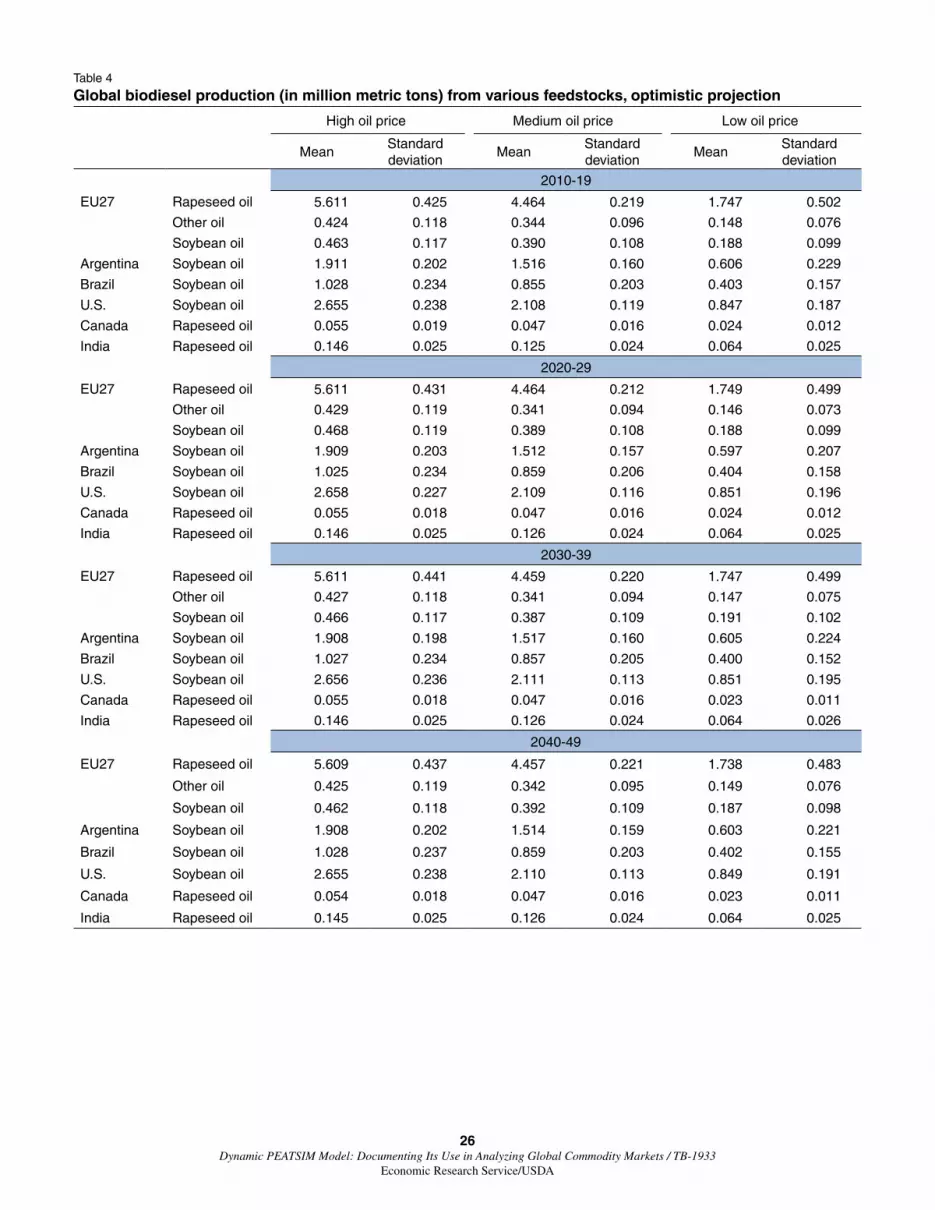
Table 4

Global biodiesel production (in million metric tons) from various feedstocks, optimistic projection





2010-19

EU27 Rapeseed oil 5.611 0.425 4.464 0.219 1.747 0.502

Other oil 0.424 0.118 0.344 0.096 0.148 0.076

Soybean oil 0.463 0.117 0.390 0.108 0.188 0.099

Argentina Soybean oil 1.911 0.202 1.516 0.160 0.606 0.229

Brazil Soybean oil 1.028 0.234 0.855 0.203 0.403 0.157

U.S. Soybean oil 2.655 0.238 2.108 0.119 0.847 0.187

Canada Rapeseed oil 0.055 0.019 0.047 0.016 0.024 0.012

India Rapeseed oil 0.146 0.025 0.125 0.024 0.064 0.025

2020-29

EU27 Rapeseed oil 5.611 0.431 4.464 0.212 1.749 0.499

Other oil 0.429 0.119 0.341 0.094 0.146 0.073

Soybean oil 0.468 0.119 0.389 0.108 0.188 0.099



U.S. Soybean oil 2.658 0.227 2.109 0.116 0.851 0.196



2030-39

EU27 Rapeseed oil 5.611 0.441 4.459 0.220 1.747 0.499

Other oil 0.427 0.118 0.341 0.094 0.147 0.075

Soybean oil 0.466 0.117 0.387 0.109 0.191 0.102



U.S. Soybean oil 2.656 0.236 2.111 0.113 0.851 0.195



2040-49

EU27 Rapeseed oil 5.609 0.437 4.457 0.221 1.738 0.483

Other oil 0.425 0.119 0.342 0.095 0.149 0.076

Soybean oil 0.462 0.118 0.392 0.109 0.187 0.098



U.S. Soybean oil 2.655 0.238 2.110 0.113 0.849 0.191





Table 5

Global ethanol production (in million metric tons) from various feedstocks, pessimistic projection





2010-19

EU27 Corn 2.274 0.194 1.903 0.119 1.018 0.131

Wheat 0.750 0.277 0.752 0.278 0.773 0.282

Sugar beets 1.790 0.192 1.549 0.162 0.903 0.191

China Corn 1.385 0.251 1.152 0.217 0.614 0.199



U.S. Corn 49.868 3.208 41.971 1.505 22.792 3.119

Canada Wheat 0.183 0.064 0.186 0.064 0.190 0.067

Corn 0.692 0.044 0.582 0.027 0.315 0.057

India Sugarcane 0.224 0.042 0.187 0.034 0.099 0.018

2020-29

EU27 Corn 2.277 0.196 1.905 0.120 1.022 0.139

Wheat 0.749 0.274 0.752 0.275 0.774 0.286

Sugar beets 1.790 0.192 1.548 0.164 0.903 0.199

China Corn 1.377 0.245 1.145 0.216 0.617 0.205



U.S. Corn 49.879 3.123 41.993 1.438 22.794 3.146

Canada Wheat 0.183 0.063 0.184 0.064 0.190 0.066

Corn 0.693 0.044 0.582 0.027 0.317 0.059

India Sugarcane 0.224 0.041 0.187 0.033 0.098 0.018

2030-39

EU27 Corn 2.276 0.194 1.905 0.121 1.020 0.136

Wheat 0.746 0.277 0.758 0.281 0.776 0.289

Sugar beets 1.797 0.194 1.545 0.162 0.899 0.188

China Corn 1.379 0.247 1.151 0.216 0.609 0.192



U.S. Corn 49.925 3.089 41.972 1.483 22.769 3.118

Canada Wheat 0.182 0.063 0.185 0.066 0.190 0.066

Corn 0.693 0.045 0.582 0.027 0.316 0.059

India Sugarcane 0.223 0.041 0.186 0.034 0.099 0.019

2040-49

EU27 Corn 2.277 0.200 1.906 0.118 1.017 0.127

Wheat 0.742 0.276 0.750 0.279 0.775 0.283

Sugar beets 1.790 0.191 1.544 0.164 0.902 0.192

China Corn 1.387 0.248 1.154 0.219 0.612 0.196



U.S. Corn 49.957 3.031 42.007 1.410 22.796 3.123

Canada Wheat 0.184 0.064 0.184 0.064 0.191 0.067

Corn 0.692 0.045 0.582 0.027 0.316 0.059

India Sugarcane 0.224 0.040 0.186 0.033 0.099 0.018



Table 6

Global biodiesel production (in million metric tons) from various feedstocks, pessimistic projection





2010-19

EU27 Rapeseed oil 5.606 0.435 4.483 0.207 1.735 0.484

Other oil 0.427 0.119 0.357 0.087 0.150 0.071

Soybean oil 0.464 0.118 0.415 0.099 0.200 0.097



U.S. Soybean oil 2.663 0.221 2.111 0.119 0.848 0.191



2020-29

EU27 Rapeseed oil 5.609 0.429 4.483 0.207 1.739 0.490

Other oil 0.426 0.118 0.355 0.086 0.151 0.071

Soybean oil 0.465 0.118 0.414 0.098 0.200 0.096



U.S. Soybean oil 2.657 0.233 2.111 0.118 0.852 0.200



2030-39

EU27 Rapeseed oil 5.615 0.431 4.479 0.207 1.760 0.536

Other oil 0.427 0.118 0.357 0.087 0.152 0.074

Soybean oil 0.465 0.118 0.417 0.099 0.200 0.097



U.S. Soybean oil 2.658 0.233 2.111 0.121 0.846 0.189



2040-49

EU27 Rapeseed oil 5.619 0.426 4.486 0.201 1.745 0.500

Other oil 0.425 0.117 0.357 0.087 0.152 0.075

Soybean oil 0.464 0.118 0.415 0.100 0.198 0.093



U.S. Soybean oil 2.654 0.237 2.115 0.113 0.845 0.187





The Global Perspective: Alternative Macroeconomic Conditions Versus Crude Oil Prices

Under alternative prices of crude oil, the demand for feedstock for the production of biofuels varies considerably. Figures 2 through 5 and tables 1 and 2 capture the demand/consumption of feedstock (mean, variance, and confidence intervals) for the production of ethanol and biodiesel under high, medium, and low crude oil prices and alternative long-term macroeconomic projections at the global level (comparing left and right panels).

The long-term macroeconomic conditions under alternative economic growth perspectives have a rather small impact on the demand of feedstock used for the production of ethanol, both at the mean and variance (figs. 2 and 3 and table 1). Unlike the effect of economic growth projections (i.e., optimistic vs. pessimistic), the level of the crude oil price significantly affected demand (both the mean and variance) for the relevant feedstocks in the production of ethanol. Interestingly, the effect of crude oil prices on feedstock demand is not symmetric. In this sense, the mean values of feedstock demand under high and medium crude oil prices are not quite the same as feedstock demand under low crude oil prices. On the other hand, the variability measured by the standard deviation of the feedstock demand in the case of medium and low crude oil prices is much smaller than in the case of the higher crude oil prices (fig. 3 and table 1).

At the mean, the feedstock demand/consumption for biodiesel production is much smaller than the demand of feedstock for the production of ethanol worldwide (figs. 4 and 5, table 2). Again, the impact of long-term macroeco-nomic projections, such as optimistic vs. pessimistic, on global demand for feedstock for biodiesel production is small compared with the impact of crude oil prices. The variability measured by the standard deviation of the demand for feedstock is larger for the case of high crude oil prices and almost the same for the medium and low crude oil prices. Under the pessimistic outlook projection, the variability of global demand of feedstock is smaller than under the optimistic outlook projection (fig. 5 and table 2). The 90-percent confi-dence interval of the mean measured by the lower and upper bound indicates the probability that the confidence interval contains the true population mean.

In sum, crude oil prices have a larger effect on the demand for feedstock for ethanol and biodiesel production than macroeconomic growth projections. At the global level, both the mean and variance are affected considerably by the level of crude oil, but the effect is asymmetric. The variability depends on feedstock demand and is different for the demand/consumption of feed-stock for ethanol than for biodiesel. Note that we do not conduct any formal testing on the causal relationship of crude oil prices and the first and second moments (mean and variance) of the distribution of the feedstock produc-tions. Such an effort is beyond of the scope of this report.

The Country Perspective: Diverge Variability of Production of Feedstock for Ethanol

A variety of feedstock is used for the production of ethanol worldwide. Tables 3 and 4 present the model results (mean and standard deviation) of feedstock demand for the production of ethanol by country under alternative



Figure 2

Global ethanol production (mean) under alternative crude oil prices and macroeconomic projections

2010 15 20 25 30 35 40 4597.5

98.0

98.5

99.0

99.5

100.0

100.5

101.0

2010 15 20 25 30 35 40 4586.2

86.4

86.6

86.8

87.0

87.2

87.4

87.6

2010 15 20 25 30 35 40 4549.0

49.2

49.4

49.6

49.8

50.0

50.2

50.4

High crude oil price, pessimistic projectionMil. metric tons

Medium crude oil price, pessimistic projectionMil. metric tons

Low crude oil price, pessimistic projectionMil. metric tons

High crude oil price, optimistic projectionMil. metric tons

Medium crude oil price, optimistic projectionMil. metric tons

Low crude oil price, optimistic projectionMil. metric tons

2010 15 20 25 30 35 40 45

97.297.497.697.898.098.298.498.698.899.099.299.4

2010 15 20 25 30 35 40 45

82.6

82.8

83.0

83.2

83.4

83.6

83.8

84.0

84.2

84.4

2010 15 20 25 30 35 40 45

46.4

46.6

46.8

47.0

47.2

47.4

47.6

47.8



Figure 3

Global ethanol production variability (standard deviation) under alternative crude oil prices and macroeconomic projections

High crude oil price, standard deviationMil. metric tons

Medium crude oil price, standard deviationMil. metric tons

Low crude oil price, standard deviationMil. metric tons

2010 15 20 25 30 35 40 450.70

0.90

1.10

1.30

1.50

Optimistic projection

Pessimistic projection

2010 15 20 25 30 35 40 450.50

0.70

0.90

1.10

2010 15 20 25 30 35 40 450.50

0.60

0.70

0.80

0.90







Figure 4

Global biodiesel production (mean) under alternative crude oil prices and macroeconomic projections

High crude oil price, pessimistic projectionMil. metric tons

Medium crude oil price, pessimistic projectionMil. metric tons

Low crude oil price, pessimistic projectionMil. metric tons

High crude oil price, optimistic projectionMil. metric tons

Medium crude oil price, optimistic projectionMil. metric tons

Low crude oil price, optimistic projectionMil. metric tons

2010 15 20 25 30 35 40 4512.22

12.24

12.26

12.28

12.30

12.32

12.34

12.36

12.38

2010 15 20 25 30 35 40 459.74

9.76

9.78

9.80

9.82

9.84

9.86

9.88

9.90

9.92

2010 15 20 25 30 35 40 453.90

3.92

3.94

3.96

3.98

4.00

4.02

4.04

4.06

4.08

2010 15 20 25 30 35 40 4512.18

12.20

12.22

12.24

12.26

12.28

12.30

12.32

12.34

12.36

2010 15 20 25 30 35 40 459.98

10.00

10.02

10.04

10.06

10.08

10.10

10.12

10.14

2010 15 20 25 30 35 40 454.00

4.02

4.04

4.06

4.08

4.10

4.12

4.14

4.16



Figure 5

Global biodiesel production variability (standard deviation) under alternative crude oil prices and macroeconomic projections

High crude oil price, standard deviationMil. metric tons

Medium crude oil price, standard deviationMil. metric tons

Low crude oil price, standard deviationMil. metric tons





2010 15 20 25 30 35 40 450.150

0.155

0.160

0.165

0.170

0.175

0.180

0.185

0.190

2010 15 20 25 30 35 40 450.090

0.095

0.100

0.105

0.110

0.115

0.120

0.125

2010 15 20 25 30 35 40 450.1300.1350.1400.1450.1500.1550.1600.1650.1700.175





macroeconomic conditions and crude oil prices. Again, the results clearly indicate that at the country level, the price of crude oil has a much larger effect on feedstock demand/production, both at the mean and standard devia-tion, than the long-term macroeconomic projections/conditions. Furthermore, the price of crude oil affects the demand for feedstock for ethanol asymmetri-cally while the variability of feedstock in the production of ethanol depends considerably on the type of the feedstock.

For example, under the high crude oil price scenario, Brazil’s sugarcane feedstock demand (at the mean) is 15 percentage points higher than under the medium crude oil price (scenario). The demand/production of feedstock (at the mean) for ethanol in all countries in the model exhibits the same pattern as that in Brazil (tables 3 and 4). In other words, the higher the crude oil price, the larger the demand/production of feedstock for ethanol.

Under the low crude oil price scenario, Brazil’s sugarcane feedstock demand (at the mean) is about 40 percentage points lower than under medium prices during the period under study (2010-49) (tables 3 and 4). The model results indicate that under the low vs. medium crude oil price scenario, the demand/produc-tion of sugarcane (India and Argentina), sugar beets (EU), and corn (United States, Canada, and the EU) follow the same pattern as that of Brazil over the long-term 40-year projections. However, under the low crude oil price level, the feedstock demand/production for ethanol from corn in China and wheat from Canada and the EU is only 11 percentage points different than that under medium price level (tables 3 and 4). Furthermore, the production/demand for feedstock (at the mean) for ethanol follows the similar pattern under the alter-native long-term scenarios (optimistic vs. pessimistic projection).

In conducting the scenarios, we treat all commodities and/or countries simi-larly under the same specifications of the long-term projections (www.ihsglo-balinsight.com). Note that by only employing the bootstrapping technique, we are able to access the variability of the simulation results and derive esti-mates of the underlying statistics (mean, standard deviation, and confidence intervals) as the outcomes of simulated scenarios completely lack any statis-tical property. Since the bootstrapping procedure is distribution independent, it provides us with an indirect method to assess the distributional proper-ties of the underlying outcomes/sample. Using the bootstrapping technique along with simulation matters as the outcomes are associated with stochastic properties that also matter. A Monte-Carlo type of stochastic simulation that accounts for cross-commodity correlations would greatly enhance the proce-dure. However, such a simulation is beyond the scope of this report.

The variability of feedstock production depends on the kind of feedstock used for the production of ethanol. Under the optimistic projection, Brazil’s sugar-cane variability (standard deviation) is higher under high crude oil prices than under medium or low crude prices. In this sense, it is almost 20 percentage points higher when under high vs. medium prices and 40 percentage points lower under low vs. medium crude oil prices. U.S. corn, EU sugar beets, and China corn feedstock demand/production variability (standard deviation) is much larger under high and low crude oil prices than under medium crude oil prices. The use of bootstrapping indicates that if there are policies in place in a certain country that are targeting certain levels of production of ethanol, which



is associated with certain levels of feedstock production, the level and the vari-ability of the relevant feedstock must be considered.

Under the pessimistic projection and for all levels of crude oil prices, vari-ability follows the same pattern as that of the optimistic projection but at a smaller magnitude (tables 3 and 4).

The Country Perspective: Diverge Variability of Production of Feedstock for Biodiesel

Overall feedstock demand/production for biodiesel is much smaller than feedstock demand/production for ethanol. The simulation results again indi-cate that crude oil prices have a much larger asymmetric effect on feedstock demand (mean and standard deviation) for the production of biodiesel than do the long-term macroeconomic projections/conditions.

The EU is the largest biodiesel producer followed by the United States, Argentina, and Brazil. While the EU uses a variety of feedstocks for the production of biodiesel, the United States, Argentina, and Brazil use soybean oil (tables 5 and 6). In the case of the EU, rapeseed oil feedstock demand (at the mean) is 25 percentage points higher than under medium crude oil prices (high vs. medium crude oil price) and declines by 60 percentage points under low crude oil prices (low versus medium crude oil price). For the United States, the price of crude oil affects the demand for soybean oil for the production of biodiesel (at the mean) considerably, but its fluctua-tion increases when crude oil prices decline. The same is observed with Argentina’s and Brazil’s soybean production and India’s rapeseed production for biodiesel (tables 5 and 6).



Conclusion

This report documents the latest version of the PEATSim model and illus-trates global biofuel production/demand under various crude oil prices and economic growth (macroeconomic conditions) scenarios.

PEATSim is a partial equilibrium, multiple-commodity, multiple-region dynamic model of agricultural policy and trade for policy analysis and reforms on a multilateral and bilateral basis.

Policy specification is treated on a policy-by-policy basis rather than being aggregated and introduced as price “wedges,” as is done in several Computable General Equilibrium models.

The partial equilibrium approach allows the use of commodity-specific elas-ticity specifications. These features can reflect own- and cross-price elastici-ties much better than could ever be achieved in a general equilibrium model that has far less flexibility in the assignment of parameters that determine the production/consumption response of each particular commodity. The specifi-cation of PEATSim is consistent with economic theory due to the imposition of symmetry and homogeneity conditions on elasticity assignments in the model wherever appropriate.

The report also examines an application of the model to illustrate its dynamic structure and to demonstrate the differential behavior of global commodity markets. In particular, the application examines the impact of macroeconomic conditions and crude oil prices on the feedstock demand for ethanol and biodiesel. Based on a comparison of the outcomes of alterna-tive scenarios, the application finds that unlike macroeconomic conditions, crude oil prices have a profound effect on feedstock demand for ethanol and biodiesel production. At the global level, both the mean and variance are affected considerably by the level of crude oil prices, but the effect is asym-metric. Overall, the scenario simulations show that the effects on feedstock demand/production for biodiesel are much smaller than those on demand/production of feedstock for ethanol.



References

Abler, D., D. Blandford, M. Bohman, P. Dixit, and J. Stout. “Development of and Initial Results from the ERS/Penn State WTO Model,” International Agricultural Trade Research Consortium Meeting, Washington, DC, May 18-20, 2001, Supported by Cooperative Agreement No. 43-3AEK-8-80117 between USDA, Economic Research Service and Penn State University.

Blayney, D., M. Gehlhar, C. Bolling, K. Jones, S. Langley, M.A. Normile, and A. Somwaru. U.S. Dairy at Global Crossroads, Economic Research Report No. 28, U.S. Department of Agriculture, Economic Research Service, November 2006, www.ers.usda.gov/publications/err28/

Brooke, A., D. Kendrick, and A. Meeraus. GAMS-General Algebraic Modeling System, A User’s Guide, The Scientific Press, 1988.

Dirkse, S. Robust Solution of Mixed Complementarity Problems, A Thesis Submitted in Partial Fulfillment of the Requirements for the Degree of Doctor of Philosophy, Computer Sciences, University of Wisconsin, Madison, 1994.

Dirkse, S., and M. Ferris. “The PATH Solver: A Non-Monotone Stabilization Scheme for Mixed Complementarity Problems,” Optimization Methods and Software, 1994.

Dirkse, S., M. Ferris, P. Preckel, and T. Rutherford. “The GAMS Callable Program Library for Variational and Complementarity Solvers,” Working Paper, Computer Science Department, University of Wisconsin, 1994.

Dyck, J., M. Gehlhar, B. Meade, A. Regmi, R. Seeley, A. Somwaru, and R. Stillman. “ERS Tariff Line Model, PEATSim, GTAP: Complementary Tools for US-Korea Trade Analysis,” International Agricultural Trade Research Consortium (IATRC), Summer Symposium Meeting, Seoul, Korea, June 30-July 1, 2008.

Dyck, J. Demand for Meats in Japan: A Review and an Update of Elasticity Estimates, U.S. Department of Agriculture, Economic Research Service, Staff Report No. AGES 880525, 1988.

Efron, B., and Tibshirani, R.J. An Introduction to the Bootstrap, Boca Raton, FL: CRC Press, 1994.

Food and Agricultural Policy Research Institute (FAPRI). FAPRI U.S. and World Agricultural Outlook, Iowa State University and the University of Missouri, Columbia, 2010.

Gadson, K., J.M. Price, and L. Salathe. Food and Agricultural Policy Simulator (FAPSIM): Structural Equations and Variable Definitions, Staff Report No. AGES 820506, May 1982.

Golan, A. “Information and Entropy Econometrics—Editor’s View,” Journal of Econometrics, 107, 2002: 1-15.



Golan, A., and H. Gzyl, “Priors and Information-Theoretic Estimation,” American Statistical Association Proceedings, 2003.

Golan, A., G. Judge, and D. Miller. Maximum Entropy Econometrics, Robust Estimation With Limited Data, San Francisco: John Wiley & Sons, 1996.

Hahn, W.F. An Annotated Bibliography of Recent Elasticity and Flexibility Estimates for Meat and Livestock, U.S. Department of Agriculture, Economic Research Service, Staff Report No. AGES 9611, 1996.

Hamilton, J. Time Series Analysis. Princeton, NJ: Princeton University Press, 1994.

Hertel, T.W., V.E. Ball, K.S. Huang, and M.E. Tsigas. Computing General Equilibrium Farm Level Demand Elasticities for Agricultural Commodities, AES Research Bulletin No. 988, Purdue University, 1989.

Huang, K.S. U.S. Demand for Food: A Complete System of Quantity Effects on Prices, U.S. Department of Agriculture, Economic Research Service, Technical Bulletin No. 1795, 1993.

Judge, G.G., R.C. Hill, W.E. Griffiths, H. Lütkepohl, and T.C. Lee. The Theory and Practice of Econometrics, San Francisco: John Wiley & Sons, 1985.

Langley, S., D. Blayney, J. Stout, A. Somwaru, M.A. Normile, J. Miller, and R. Stillman. “Trade Liberalization in International Dairy Markets,” American Agricultural Economics Association Meeting, Montreal, July 27-30, 2003.

Langley, S., A. Somwaru, M.A. Normile. “A Trade Liberalization in International Dairy Markets,” International Agricultural Trade Research Consortium, June 19-21, Seville, Spain, 2005.

Langley, S., A. Somwaru, and M.A. Normile. Trade Liberalization in International Dairy Markets, Economic Research Report No. 16, U.S. Department of Agriculture, Economic Research Service, 2006, www.ers.usda.gov/publications/err16/

Meade, B., C. Arriola, and A. Somwaru. “Argentina’s Biofuel Production and Trade Impacts,” AEDA Congress, Buenos Aires, Asociación de Economía para el Desarrollo de la Argentina (AEDA), September 20-21, 2010.

Meilke, K. “A Proposed Framework for an International Multicommodity Trade Model,” Working Paper, Department of Agricultural Economics and Business, University of Guelph, January 1999.

Morath, T., and I. Sheldon. “The Economics of Modeling Tariff-Rate Quotas,” Economic Research Service and Ohio State University, Working Paper, February 1999.

Moschini, G. “Specification of the Demand Structure of National Models and Welfare Calculations,” Working Paper, Iowa State University, 1999.



Organisation for Economic Co-Operation Development and the Food and Agriculture Organization of the United Nations (OECD-FAO), Agricultural Outlook 2010-2019, June 2010.

Peters, M., A. Somwaru, R. Stillman, J. Hansen, D. Kelch, and R. Seeley. “Modeling Biofuels: Global Production and Trade Implications,” International Agricultural Trade Research Consortium (IATRC) Annual General Meeting Scottsdale, AZ, December 7-9, 2008.

Peters, M., A. Somwaru, J. Hansen, R. Seeley, and S. Dirkse. “Modeling Biofuels Expansion in a Changing Global Environment,” International Association of Agricultural Economics Conference, Beijing, China, August 16-22, 2009.

Peters, M., R. Stillman, and A. Somwaru. “Bio-Fuels Expansion in a Changing Economic Environment: A Global Modeling Perspective,” in Ball, E.V., Fanfani, R., Gutierrez, L. (eds.), The Economic Impact of Public Support to Agriculture, New York: Springer, 2010.

Regmi, A. (ed). Changing Structure of Global Food Consumption and Trade, Agriculture and Trade Report No. WRS No. 01-1, U.S. Department of Agriculture, Economic Research Service, 2001, www.ers.usda.gov/publications/wrs011/

Shane, M., W. Liefert, M. Morehart, M. Peters, J. Dillard, D. Torgerson, and W. Edmondson. The 2008/2009 World Economic Crisis—What It Means for U.S. Agriculture, E-Outlook No. WRS-09-02, U.S. Department of Agriculture, Economic Research Service, 2009, www.ers.usda.gov/publications/wrs0902/

Stillman, R., S. Langley, A. Somwaru, and M.A. Normile. “PEATSim: Analyzing the Dairy Market,” International Agricultural Trade Research Consortium (IATRC), San Diego, CA, December 5, 2005.

Stillman, R., J. Hansen, R. Seeley, D. Kelch, A. Somwaru, and E. Young. “Analyzing the Impacts of Biofuel Mandates on World-Wide Grain, Livestock, and Oilseed Sectors,” Domestic and Trade Impacts of U.S. Farm Policy: Future Directions and Challenges, Washington, DC, November 15-16, 2007.

Stillman, R., A. Somwaru, M. Peters, E. Young, and S. Dirkse. “Bio-Fuels: Impact on the World Grain, Livestock, and Oilseed Sectors,” American Agricultural Economics Association Annual Meeting, Orlando, FL, July 27-29, 2008a.

Stillman, R., A. Somwaru, M. Peters, E. Young, and S. Dirkse. “Biofuels and Trade: World Agricultural Market Impacts,” GTAP Conference, Helsinki, Finland, June 12-14, 2008b.

Stout, J., and D. Abler. ERS/Penn State Trade Model Documentation, August 2003, Updated Version, October 2004.



U.S. Department of Agriculture, Office of the Chief Economist, World Agricultural Outlook Board. USDA Agricultural Projections to 2019, Long-Term Projections Report OCE-2011-1, February 2010.

Valdes, C., C. Arriola, A. Somwaru, and J. Gasques. “Brazil’s Climate Adaptation Policies: Impacts on Agriculture,” International Agricultural Trade Research Consortium, Stuttgart, Germany, June 27-29, 2010.

Varian, H. Computational Economics and Finance: Modeling and Analysis with Mathematica, New York: Springer-Verlag, May 1996.

Westhoff, P., R. Baur, D. Stephens, and W. Meyers. FAPRI U.S. Crops Model Documentation, Technical Report 90-TR17, Center for Agricultural and Rural Development, Iowa State University, 1990.

Zahniser, S., C. Arriola, and A. Somwaru. “The European Union’s Framework for Climate Change Adaptation: Implications of Agriculture’s Adaptation through Sustained Yield Growth,” International Agricultural Trade Research Consortium, Stuttgart, Germany, June 27-29, 2010.



Appendix: Mixed Complementarity Problem

Complementarity problems are used extensively in economics because the concept of complementarity is intimately linked with the notion of system equilibrium. The balance of supply and demand in economics is often described by a complementary relationship between price and excess supply. In this case, the complementarity condition requires that the excess supply of a commodity must be zero if its price is positive, and the price of the commodity must be zero if there is positive excess supply.

Nonlinear complementarity problems, NCP( F ), seek to find an x ∈ ℜn given a nonlinear function defined as F: ℜn → ℜn, such that

NCP( F ): 0 ≤ x ⊥ F ( x ) ≥ 0

where the perpendicular notation “⊥” indicates that in addition to the above inequalities, the equation xTF (x) = 0 also holds. This equation can be stated as:

0 ≤ x, F ( x ) ≥ 0, xiFi( x ) =0, i =1,2,…,n

In other words, complementarity implies that for each variable, either the variable or its complement (i.e., either xi or Fi ( x )) must be zero for each i =1,2,…,n.

Complementarity problems of this form are associated with the Karush-Kuhn-Tucker conditions of a constrained nonlinear program as follows:

minimize θ( x )

subject to g( x ) ≤ 0, x ≥ 0

where θ: ℜn → ℜ is a continuously differentiable real-valued function and g: ℜn → ℜm is a continuously differentiable vector-valued function.

The NCP( F ) can be generalized by the introduction of (possibly infinite) lower and upper bounds on the variable x. This results in the MCP( F,L,U )defined as follows:

given F: ℜn → ℜn and bounds L,U where , and n nL U∈ℜ − ∞ ∈ℜ + ∞

find:

x ∈ [L,U]

s.t. ∀ i, one of the following conditions holds:

i) Fi( x ) =0

ii) Fi( x ) >0 and xi = Li

iii) Fi( x ) <0 and xi = Ui.

The NCP( F ) is a special case of MCP( F,L,U ) obtained by setting L = 0 and U = −∞.



Another special case occurs if we set L = −∞ and U = +∞; then alternatives (ii) and (iii) above are impossible and we have Fi( x ) = 0 (i.e., a smooth system of nonlinear equations). This concept is applied to discontinuous functions in PEATSim, such as production quotas, tariff-rate quotas, and discontinuous demand issues created by mandates or targets.

Dynamic PEATSim Model: Documenting Its Use in Analyzing Global Commodity Markets

Documents

Transcript of Dynamic PEATSim Model: Documenting Its Use in Analyzing Global Commodity Markets