Chapter 9

DRIVING FORCES FOR CHANGES IN LAND USE

Johan Brons, Ruerd Ruben, Mohammed Toure and Boukary Ouedraogo

Abstract: In this chapter we apply a multivariate regression model to assess the effects of agro-climatic and socio-economic factors on land use and crop yields in Mali and Burkina Faso. We use 1965-1990 time-series data at national level on climate, prices, input use, infrastructure, and population density to explain land use and crop yields. The results show that infrastructure development and credit availability have, in particular, been stimuli which have enhanced cotton yields and expanded the cotton area. Farmers managed to increase cotton production against lower output prices mainly because costs were reduced by better crop management practices. Cereal and groundnut production benefited from spin-off effects at farm level, such as the availability of animal traction, fertiliser residual effects and improved market outlets. These findings confirm the importance of supportive agricultural policies that facilitate the optimal use of inputs and access to new technologies. Moreover, a sound production environment can offset the effects of adverse and deteriorating climate conditions. Further enhancement of food crop production will require additional public investments in infrastructure, markets and technological development.

1. INTRODUCTION

Changes in land use and resource allocation are caused by the interaction between a wide range of agro-climatic and socio-economic factors that influence regional ad farm-household options for crop choice, input use, labour allocation and marketing. In this chapter, we analyze the driving forces behind changes in land use and resource allocation in sub-Saharan Africa, considering the variable and changing agricultural production environment in which farmers face uncertainty about short-term and medium-term production conditions. Therefore, attention is given to (i) the analysis of the determining factors for

83

A.J. Dietz et al. (eds.),The Impact of Climate Change on Drylands: With a Focus on West-Africa, 83–96.© 2004 Kluwer Academic Publishers. Printed in the Netherlands.

84 Chapter 9

resource use in agricultural production, (ii) the impact of population pressure and technical change on land use and factor intensity and iii) the differential response to rainfall variability for specific cropping activities.

Opportunities

(climate and

technology)

Public

investment

Households’

resource use

Markets

• Product prices

• Factor prices

Output

(primaryproduction

Private

investment

Production

function

Direct effects

Technology trend

Infrastructure

“pressure”

factors

“pressure”

factors

System

effects

Policy effectsAgro-climatic effects

Policy effects

Figure 9.1. Major interactions between agro-climatic opportunities and agricultural output.

The adjustment of resource management strategies is considered to be highly dependent on prevailing conditions of factor and commodity markets. Favourable output prices offer incentives for intensification, but market and institutional constraints frequently limit farmers’ capacities to mobilise the required resources for agricultural intensification. Figure 9.1 (adapted from Binswanger et al., 1993) illustrates the relationships among agro-climatic endowments, public and private investment, prices and agricultural output. Public investment (in infrastructure) and farmers’ investments (input use) can partly offset adverse weather or market conditions (Rosegrant et al., 1998). In addition, technological change tends to reduce production costs. These relationships interdependently and simultaneously determine supply response in terms of the adjustments in cultivated area and yield level. If climate and market conditions are favourable, synergy effects can occur when public and private investments reinforce farmers’ welfare.

The assessment of the impact of climatic variability on land use and food production enables the subsequent identification of different pathways and livelihood strategies for portfolio choice in West African drylands (see Chapter 16). Making use of farm-household village-level data, specific socio-economic and biophysical factors can be identified that influence decisions regarding choice of livelihood options, labour allocation and input use.

The analysis regarding temporal variability in land use at a regional scale in West Africa focuses on Mali and Burkina Faso, paying attention to the interaction of agro-climatic and socio-economic factors

9. DRIVING FORCES FOR CHANGES IN LAND USE 85

influencing farmers' supply response during the last three decades (Brons et al., 1999). Different analyses are performed making use of statistical data obtained from national agencies (CMDT in Mali; ENSA and INERA in Burkina Faso), local research centres (CEDRES in Burkina Faso, IER in Mali) and from international organisations (FAO, World Bank, ICRISAT-SH). Analytical procedures are based on the statistical analysis of time series on rainfall variability (drought risk) and yields, and multiple regression to identify factors influencing area and yield response.

2. DRIVING FORCES OF CHANGES IN LAND USE IN WEST AFRICA

Variability in agricultural land use is related to natural processes and socio-economic forces. The relative importance of climate and demographic change, market development and the availability of productive and social infrastructure for adjustments in land use during a period of 25 years (1966-1990) has been analysed for Burkina Faso and Mali. Figures 9.2 – 9.4 provide an overview of the changes in land use, yields and production in cereal and cash crops in both countries and their relationship with rainfall patterns. As expected, cereal yields show more sensitivity to rainfall variability compared to cash crops. Moreover, short-term variations in crop yields are associated with rainfall, but long-term trends in yields generally improved.

Supply response models for changes in crop area and yields are applied to disentangle different patterns of agricultural development. The models rely on the Nerlovian supply response analysis technique, making use of multiple regression procedures. Harvested areas per rural inhabitant and crop yields (cereals, cotton, and groundnuts) are used as dependent variables. The Nerlovian supply response model compares different determinants as if they directly influence agricultural supply (Nerlove, 1958; Askari & Cummings, 1976; Sadoulet & de Janvry, 1995).

Despite its limited capacity to analyse features of simultaneity of determinants and long-term supply dynamics (Nerlove, 1979; Oyejide, 1990), the Nerlovian supply response model can be considered a standard approach to assessing supply response mechanisms and related policy issues (Rao, 1989; Fosu et al., 1997). The basic Nerlovian supply response equation is as follows:

Q = α0 + α1 Qt-1 + α2 Pt-1 + α3 Zt + vt

where Q represents production, P are prices, Z are structural (non-price) characteristics and t is time. The specification includes lagged variables that indicate a response to earlier events.

86 Chapter 9

Figure 9.2. Area of cereals, cotton and groundnut (ha/inhabitant) for Burkina Faso and Mali.

The models are estimated on the basis of time-series data from FAO and World Bank. Climate data are from the Agrometeorological Group FAO-SDRN, NOAA and AGRHYMET. The data covers the period 1966-1990.

This model can be used to examine agricultural sector responses to changes in the agro-ecological and socio-economic environment. These responses can be specified in terms of adjustment of cultivated area per rural inhabitant (i.e. extensive growth) and crop yields (i.e. intensive growth). Extensive growth is usually associated with expansion of the agrarian frontier into less fertile lands, declining fallow periods and decreasing soil fertility. Intensive growth refers to yield enhancement by crop management practices that use more labour and capital per area unit. Extensive growth and intensive growth are not necessarily mutually exclusive.

9. DRIVING FORCES FOR CHANGES IN LAND USE 87

Figure 9.3. Rainfall and yield of major crops for Burkina Faso and Mali (1966 - 1990).

Figure 9.4. Total cereal production and rainfall for Burkina Faso and Mali (1966-1990).

Available time-series data at national level allows the use of proxies for the following explanatory variable categories: i) climate; ii) crop prices; iii) technical input-output relations; iv) infrastructure; and v) an

88 Chapter 9

autonomous technology. These factors are not truly exogenous but may be mutually related to each other. Production opportunities attract both public and private investments and induce farmers to invest in crop production. These supply determinants can reinforce each other either in space (i.e. within a specific region) or in specific sectors (i.e. within the cotton sector). In contrast, negative driving forces such as erratic and low precipitation and a weak infrastructure discourage agricultural investments.

To examine producers’ responses to climate variability, two separate regression equations are specified for area and yield adjustments (Table 9.1). The first regression follows the Nerlovian supply response model in which the harvested area is a function of farmers’ expectations and observations with respect to price and non price variables. Farmers’ expectations concerning climate are included with a one-year lagged specification of yield, rainfall and temperature. Price expectations are taken into account by the previous year’s sorghum and groundnut prices and the actual year’s price of cotton (the price of cotton is announced before planting). Productive and social infrastructure is specified by tractor availability and cattle density (numbers rural inhabitant-1), credit supply (FCFA rural inhabitant-1), road density (km road km-2 arable land), and government expenses (FCFA capita-1). Population density (inhabitants km-2 arable land) reflects an autonomous trend variable. Finally, a lagged specification of the dependent variable accounts for the possibility of a time-lag in the adjustment of crop area.

In the second regression equation, crop yield is a function of climate conditions during the actual year (rainfall and temperature), price expectations, factor availability, productive and social infrastructure, and an autonomous trend variable. In addition to the area response model, proxies are introduced for factor availability of labour (persons ha-1),fertilisers (kg ha-1), tractors and cattle (number ha-1). A proxy for land use patterns is the share of cereals on the total harvested area. Infrastructure indicators are credit supply, road density and government expenses.

It is expected that climatic stress has an adverse effect on both crop area and yield, hence coefficients for rainfall and crop yield are expected to be positive, while the temperature coefficient is expected to be negative. Producers are supposed to respond positively to price increases, reflected by a positive price elasticity for the own crop and a negative elasticity for competing crop prices. However, commodity prices may have a limited or ambiguous effect on area and yield of food crops, since only 15% of the cereal output is marketed (Lecaillon et al., 1987). In addition, illustrative examples of perverse supply reactions to increasing prices are known, particularly for subsistence food crops (Fosu et al.,1997). Factor availability, infrastructure development as well as the trend estimator (changes in population density) are expected to have a positive effect on land use intensity and yield. Improved market access (i.e roads

9. DRIVING FORCES FOR CHANGES IN LAND USE 89

and means of transport) leading to reduced transportation costs can significantly enhance crop production (Heerink et al., 1997).

Table 9.1.Supply response model for crop area and yield: variables in double log

regression equations

Category Area response model Yield response model (unit) Dependent variable Crop area

(ha person-1)1)Crop yield (kg ha-1)

Explanatory variables

- Adjustment coefficient

Crop area t-12) (ha person-1)

- Climate Crop yield t-1

Rainfall t-1

Temperature t-1

RainfallTemperature

(kg ha-1)(mm yr-1)(0C)

- Price expectations Sorghum price t-1

Cotton price Groundnut price t-1

Sorghum price t-1

Cotton price Groundnut price t-1

(FCFA kg-1) 3)

(FCFA kg-1)(FCFA kg-1)

- Factor availability Labour availability Cereal share of harvested area Fertiliser availability Tractor availability Cattle availability

(persons ha-1)(%)(kg ha-1)(numbers ha-1)(numbers ha-1)

- Infrastructure development

Tractor availability Cattle density Credit supply Road density Government expenses

Credit supply Road density Government expenses

(numbers person-1)(numbers person-1)(FCFA person-1)(km km-2)4)

(FCFA person-1)5)

- Trend estimator Population density Population density (persons km-2) Notes: 1) unless otherwise stated, persons refer to rural inhabitants; 2) the subscript t-1

denotes that the variable is one-year lagged specified; 3) prices are real prices (deflated by GDP index: 1987 = 100); 4) per km2 of arable land; 5) FCFA per inhabitant for the total population.

The development of price and non-price variables is depicted in Figure 9.5 and 9.6 (annex). Real cereal prices increased only slightly until 1984, while cotton prices declined dramatically during this period (Lecaillon et al., 1987). In Burkina Faso, cotton prices improved in relative terms in the mid 1980s. Over the whole period, however, the ratio cotton-sorghum price declined, basically due to the stronger tendency towards market liberalization in cereal markets. The availability of physical and social infrastructure and material inputs (tractors, fertilizers) shows a positive tendency in both countries. Tractor density and credit supply are substantially higher in Mali, but credit supply stagnated in the 1980s and even declined in Mali after 1984. Cattle density decreased in Mali after the drought years of 1971/72 and 1981/82.

90 Chapter 9

Figure 9.5. Official prices of major crops (FCFA/kg) and ratio cotton - sorghum price for Burkina Faso and Mali (1966 - 1990).

3. RESULTS

The model estimates for area response in Mali and Burkina Faso provide most consistent results for cash crops (cotton, groundnuts) but are less conclusive for food crops (see Table 9.2). The area adjustment coefficient for cotton is 0.63 and 0.69 respectively (significant at a 1% level for Burkina Faso and at 10% for Mali). For cereals and groundnuts, the model does not show a significant time-lag in area adjustment (g = 1) for Burkina Faso. For Mali, the cereal area adjustment coefficient is 0.52 (significant at a 5% level) and the groundnut area adjustment coefficient is 0.24 (significant at 1%). The cotton area equation shows a negative own price response for Burkina Faso (significant) as well as for Mali (not significant). This might indicate that the marginal costs of production have decreased and have permitted farmers to produce at lower prices. The own price elasticity of cereals is negative in Burkina Faso (not significant) and positive for Mali (significant at a 10% level). The positive own price elasticity for groundnuts for both countries is not significant. The substitution of groundnut for cotton in Mali was positively influenced by cotton prices. Climate variability does not appear to have much effect on harvested area, except for the lagged cotton yield specification for Mali. A positive coefficient indicates that farmers expand the cotton area in response to a good harvest in the

9. DRIVING FORCES FOR CHANGES IN LAND USE 91

previous year. For Burkina Faso, the coefficients of cattle density and road density are highly positive and significant. For Mali, the population density coefficient is positive and significant, indicating a trend of production increase that is not captured with the other variables.

Figure 9.6. Productive and social infrastructure indicators for Burkina Faso and Mali (1966 - 1990).

92 Chapter 9

Table 9.2. – Summary of outcomes of the reduced equations for area response. Burkina Faso Mali

Cereals Cotton Groundnut Cereals Cotton GroundnutArea adjustment coefficient

1.00 +0.63 *** (3.84)

+0.78 ns (1.51)

+0.52 ** (2.94)

+0.69 * (1.73

+0.24***(5.74)

Climate Yield lagged

+0.19 *** (4.42)

Own price -0.347** (-2.43)

-0.59 ** (-2.21)

-0.07 ns (-0.39)

+0.21 ns (1.55)

-0.44 ns (-1.40)

0.42 ns (0.98)

Cross Price Cotton

+0.89 ** (1.87)

Infrastructure Cattle density

Road density

+2.17 *** (6.44)+0.37 *** (4.40)

Populationdensity

+1.28 *** (2.06)

Adjusted r-Squared

0.31 0.94 0.156 0.342 0.77 0.70

F-Statistics 6.20*** 70.83*** 3.12* 6.96*** 26.57*** 19.16*** LM F-statistic 1.58 0.13 0.54 0.00 0.23 0.10 Notes: 1) *** = 1% significance level; ** = 5% significance level; * = 10% significance

level; 2) ns = not significant at a 10% level; 3) t-values are presented between parentheses; 4) an intercept is allowed for all equations.

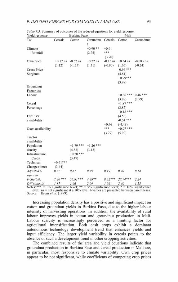
The results of the yield response equation indicate that groundnuts in Burkina Faso and cereals in Mali are particularly responsive to the selected climate variables (Table 9.3). Coefficients of prices of the own crop are not significant in any of the equations. However, coefficients of competing crop prices are significant at a 10% level in the case of cotton and groundnut in the equation for Mali. Higher sorghum prices seem to increase competition for inputs, while higher groundnut prices enhance cotton yields. Important effects on yields are found for the variables related to input use. Credit supply is particularly relevant for improving cotton yields in Burkina Faso, and tractor availability stimulated cereals and cotton yields in Mali. In the latter case, the substitution of oxen by tractors had a significant positive yield effect. Cotton yields in Mali are also very sensitive to fertilizer use.

9. DRIVING FORCES FOR CHANGES IN LAND USE 93

Table 9.3. Summary of outcomes of the reduced equations for yield response. Yield response Burkina Faso MaliTo: Cereals Cotton Groundnu

tCereals Cotton Groundnut

Climate Rainfall

+0.90 ** (2.25)

+0.91*** (3.70)

Own price +0.17 ns (1.12)

-0.52 ns (-1.25)

+0.22 ns (1.31)

-0.15 ns(-0.90)

+0.34 ns (1.66)

-0.083 ns (-0.24)

Cross Price Sorghum

Groundnut

-0.96 *** (4.81)+0.99***(3.98)

Factor useLabour

CerealPercentage

Fertiliseravailability

Oxen availability

Tractoravailability

+0.46***(3.79)

+0.66 ***(3.88)+1.87 ***(3.87)+0.18 ***(4.56)-0.54 *** (-4.49)+0.97 ***(5.92)

0.46 *** (1.99)

Populationdensity

+1.79 *** (4.32)

+1.26 *** (3.12)

Infrastructure Credit

+0.20 *** (3.47)

TechnicalChange (time)

+0.61*** (3.44)

Adjusted r-

squared

0.37 0.87 0.39 0.49 0.90 0.14

F-Statistic 7.40 *** 55.91*** 4.49** 8.32*** 27.74*** 2.24

DW statistic 1.87 1.66 2.09 1.56 2.40 1.53Notes: *** = 1% significance level; ** = 5% significance level; * = 10% significance

level; ns = not significant at a 10% level; t-values are presented between parentheses. Source: Brons et al. (1999).

Increasing population density has a positive and significant impact on cotton and groundnut yields in Burkina Faso, due to the higher labour intensity of harvesting operations. In addition, the availability of rural labour improves yields in cotton and groundnut production in Mali. Labour scarcity is increasingly perceived as a limiting factor for agricultural intensification. Both cash crops exhibit a dominant autonomous technology development trend that enhances yields and input efficiency. The larger yield variability in cereals points to the absence of such a development trend in other cropping activities.

The combined results of the area and yield equations indicate that groundnut production in Burkina Faso and cereal production in Mali are, in particular, most responsive to climate variability. Own crop prices appear to be not significant, while coefficients of competing crop prices

94 Chapter 9

are significant at a 10% level only in the case of cotton and groundnut in the equation for Mali. Usual cross-price elasticities are registered for competing crops. Most input variables have the expected sign (except for oxen, due to the substitution by tractors) and are especially significant for cotton in Mali. Population density is a positive and significant factor in the case of cotton and groundnut for Burkina Faso. Moreover, the presence of a dominant autonomous technology development trend for these cash crops is confirmed. Due to large yield variability, such a trend is absent in other crops. Finally, infrastructure indicators are found to have a significant coefficient for credit supply in the cotton yield equation for Burkina Faso.

The findings also indicate that particularly variations in cotton area as well as yield are induced by infrastructure development, factor availability and an autonomous trend variable (related to population growth). Expansion of production has been realised in Mali as well as in Burkina Faso despite lower real prices of cotton. Farmers have been able to offset these negative determinants with an important reduction of production costs (crop variety choice, traction, fertiliser and insecticide application) that permitted them to produce against lower prices. In addition, technological progress might have neutralised the effects of climate deterioration, explaining the relative limited incidence of rainfall and temperature variables. The production of crops grown with traditional technologies (cereals and groundnut) is less responsive to changes in climatic, technical and socio-economic conditions. The results confirm that long-term changes in the quality of infrastructure, crop management practices and assets might have been at least as important than short-term variability in prices and climate for explaining variability in yields and cultivated area.

4. CONCLUSIONS

The importance of climate variability between the years as a determinant of crop choice is generally considered to reflect a rather indirect relationship. Prolonged periods of drought might, however, influence the availability of resources like seed material. Decisions on cultivated areas are clearly influenced by rainfall expectations (especially the timing of the start of the growing season), but other factors – like the availability of labour and traction – tend to be of greater importance. The role of prices and price expectations is difficult to register since marketing channels for staple crops were still highly institutionalised in the period under study. Consequently, price uncertainty was rather limited and input availability was determined on a contractual base.

Considering differences between agro-ecological zones, we can conclude that land availability and rainfall are most important factors for explaining yield differences especially in the more arid (northern) zone,

9. DRIVING FORCES FOR CHANGES IN LAND USE 95

while land and manure and fertiliser applications are more important for yields in the central and southern zones. Variations between villages and farmers may, however, be more important. Regions with rather similar rainfall levels, but with very different land use patterns show specific levels of adaptation by the local population while very different yield levels are achieved. In addition, relatively stable incomes are achieved during years with very different rainfall regimes, by making use of technological development based on local resources (mechanisation with limited land availability, non-input based land management change, etc.).

Crop choice, land use and input intensity are related to rainfall regimes and land endowments over the long term. While rainfall plays a prominent role in explaining variability of (cereal) yields and production, it is far less important as an underlying factor for differences in income, since a variety of other factors play an intermediate role. Aggregate production data suggests that mainly infrastructure development (roads and extension and credit institutions) stimulated the increase of cotton production, in particular, both through yield enhancement and area expansion. Since the input – output price ratio for cotton production deteriorated, the production increase was only made possible through a reduction in the production costs (crop management improvements such as variety development, fertiliser application, insect control, and mechanisation) and horizontal expansion (more farmers adopting similar technologies). Cereal production (in particular maize and rice) and groundnut cultivation benefited from spin-off effects at farm level (fertiliser residues, mechanisation, better market structure, etc.). Yet, the production of these crops also expanded mainly in a horizontal direction with more farmers cultivating larger areas.

As expected, climate variability proved to be particularly relevant for explaining differences in yield levels. Given the long time period, technological change and adjustments in market linkages (due to infrastructure investments) may have had a significant influence on improvements in yields. The consistent increase in crop yields throughout the whole period – maintained even under adverse weather conditions – points to the fact that farmers can adjust factor use as a compensatory device. This is especially the case with cash crops that register relatively higher supply response compared to food crops (perhaps with the exception of maize cultivated in rotation with cotton). Efforts to enhance agricultural yields should thus rely on an adequate mixture of public incentives and private investment (see Chapter 21).

It should be noted, however, that instead of average rainfall other variables, like the timing of rainfall, the first days of rainfall in relation to the rest of the agricultural year, or the moment when enough rainfall has fallen for the soil to be workable (depending on the soil) may be more important for explaining differences in yield levels. Local rainfall and yield data mostly show limited direct correlation (see also Chapter 7) and methodological problems (e.g. interpretation of the rainfall data for areas

96 Chapter 9

in between stations, yield measurement procedures, soil quality differences) strongly constrain the registration of such linear relationships.

A comparison of the supply response models for the different crops confirms the importance of supportive agricultural policies that facilitate optimal use of inputs and access to the innovations generated by technological progress. The reduction of production costs allows farmers to produce at lower prices. Particularly in the long term, technological progress supported by adequate infrastructure development is a more effective policy device than instruments of agricultural product pricing. Moreover, a sound production infrastructure can offset the negative effects of adverse risk-prone production conditions. Long term public investments do have a positive impact on agricultural production. However, these efforts tend to be strongly biased in favour of the cotton sector. Enhancement of the performance of food crops grown without modern technologies will thus require additional public investments in infrastructure, markets and technological development.