Draft NIST CSWP, Combination Frequency Differencing

NIST CYBERSECURITY WHITE PAPER (DRAFT) CSRC.NIST.GOV

Combination Frequency Differencing 1

2

3

4

D R Kuhn 5 M S Raunak 6 Computer Security Division 7 Information Technology Laboratory 8 9 R N Kacker 10 Applied and Computational Mathematics Division 11 Information Technology Laboratory 12 13

14

15

16

December 6, 2021 17

18

This publication is available free of charge from: 19 https://doi.org/10.6028/NIST.CSWP.12062021-draft 20

21

NIST CYBERSECURITY WHITE PAPER (DRAFT) COMBINATION FREQUENCY DIFFERENCING DECEMBER 6, 2021

Abstract 22 This paper introduces a new method related to combinatorial testing and measurement, 23 combination frequency differencing (CFD), and illustrates the use of CFD in machine learning 24 applications. Combinatorial coverage measures have been defined and applied to a wide range 25 of problems, including fault location and for evaluating the adequacy of test inputs and input 26 space models. More recently, methods applying coverage measures have been used in 27 applications of artificial intelligence and machine learning, for explainability and for analyzing 28 aspects of transfer learning. These methods have been developed using measures that depend on 29 the inclusion or absence of t-tuples of values in inputs, training data, and test cases. In this paper, 30 we extend these combinatorial coverage measures to include the frequency of occurrence of 31 combinations. Combination frequency differencing is particularly suited to AI/ML applications, 32 where training data sets used in learning systems are dependent on the prevalence of various 33 attributes of elements of class and non-class sets. We illustrate the use of this method by 34 applying it to analyzing physically unclonable functions (PUFs) for bit combinations that 35 disproportionately influences PUF response values, and in turn provides indication of the PUF 36 potentially being more vulnerable to model-building attacks. Additionally, it is shown that 37 combination frequency differences provide a simple but effective algorithm for classification 38 problems. 39

Keywords 40 combinatorial coverage; combination frequency difference; combinatorial testing; physical unclonable 41 function (PUF); unclonable. 42

Acknowledgments 43 The authors are very grateful to Charles Prado of INMETRO Brazil for data used in the PUF analysis and 44 to Sandip Kundu and Vinay Patil for helpful discussion. The authors also plan to continue working with 45 INMETRO to apply and develop these ideas for practical application to PUFs. 46

Disclaimer 47 Any mention of commercial products or reference to commercial organizations is for information only; it 48 does not imply recommendation or endorsement by NIST, nor does it imply that the products mentioned 49 are necessarily the best available for the purpose. 50

Additional Information 51 For additional information on NIST’s Cybersecurity programs, projects and publications, visit the 52 Computer Security Resource Center. Information on other efforts at NIST and in the Information 53 Technology Laboratory (ITL) is also available. 54

Public Comment Period: December 6, 2021 through February 7, 2022 55 National Institute of Standards and Technology 56

Attn: Computer Security Division, Information Technology Laboratory 57 100 Bureau Drive (Mail Stop 8930) Gaithersburg, MD 20899-8930 58

Email: [email protected] 59

All comments are subject to release under the Freedom of Information Act (FOIA). 60

https://csrc.nist.gov/

https://www.nist.gov/

https://www.nist.gov/itl

https://www.nist.gov/itl

mailto:[email protected]


4

1 Introduction 61

Methods and tools for measuring combinatorial coverage were initially developed to analyze the degree to which 62 test sets included t-way combinations of values (for some specified level of t) [1][2][4] and have since been 63 studied extensively in the realm of system and software testing [7][8][9][10][11]. Combinatorial coverage 64 measures have been defined and applied to a wide range of problems, specifically for fault location and for 65 evaluating the adequacy of test inputs and input space models. More recently, coverage measures have been used 66 for explainability in artificial intelligence and machine learning [24][28] and for analyzing aspects of transfer 67 learning [27]. These methods have been developed using measures that depend on the inclusion or absence of t-68 tuples of values in inputs and test cases. For software testing, primarily for deterministic systems where the 69 presence of a particular combination always triggers a specified error, it is relevant whether a t-tuple of values 70 is present in test inputs, but the number of occurrences of a particular t-tuple of values is generally not relevant 71 to testing. Multiple occurrences are only redundant and do not add value. These measures can also be applied in 72 artificial intelligence and machine learning (AI/ML) systems. 73

For many aspects of assurance of autonomous systems and machine learning, this type combinatorial coverage 74 measure is valuable and possibly essential, since the correct and safe behavior of many AI systems is dependent 75 on the training inputs. Conventional structural coverage measures are not applicable to such black box behavior. 76 Consequently, it is essential to evaluate the degree to which possible combinations of input attribute values have 77 been included in training and test sets for AI and autonomy. (Attributes in a machine learning setting correspond 78 to parameters in a test effort; they are the inputs to the system.) If the system has not been shown to function 79 correctly for an input combination that may be encountered in use, then assurance is inadequate. However, for 80 some questions in machine learning, consider the frequency (or rate) of occurrence of t-tuples of values in input 81 and how two different sets may compare or differ in combinatorial coverage. 82

This paper applies combinatorial coverage measures from [13], which include the frequency of occurrence of 83 combinations, in an approach referred to as combination frequency differencing (CFD). This method is 84 particularly suited to AI/ML applications, where training data sets used in learning systems are dependent on the 85 prevalence of various attributes of elements of class and non-class sets. This paper illustrates the use of this 86 method by applying it to analyzing physical unclonable functions (PUFs) for potential weaknesses in design and 87 showing how it can be extended to develop a simple but effective classification algorithm. 88

2 Combinatorial Coverage and Combination Frequency Differences 89

This section reviews the basic measures of combinatorial coverage and applications of these measures 90 in Section 2.1. This idea is extended to measures that include the frequency of occurrence of 91 combinations in Section 2.2. These measures can then be applied to the analysis of PUFs. 92

2.1 Basic Combinatorial Coverage and Coverage Difference Measures 93

Combinatorial methods offer an approach to coverage measurement that provides a measure directly related to 94 fault detection. A series of studies have shown that most software bugs and failures are caused by one or two 95 parameters and progressively fewer by three or more [19][20][21][22][5][6]. This finding means that testing 96 parameter combinations can provide more efficient fault detection than conventional methods. This section, 97 derived from [13], reviews the concept of measuring the combinatorial coverage of an input space [1][2][4] for 98 use in testing or in other applications where it is important to ensure the inclusion of combinations of input 99 parameter values. 100


5

a b c d 1 0 0 0 0 2 0 1 1 0 3 1 0 0 1 4 0 1 1 1

Figure 1. Example test array for a system with four binary components 101

Combinatorial coverage measurement concepts can be illustrated using the example in Figure 1, which shows a 102 test array that contains 19 of a possible set of 24 2-tuples of values. To facilitate discussion, it is helpful to 103 establish terminology for two related but distinct concepts: 104

• t-way combination: a set of t parameters or variables. For example, using the parameters in Figure 1, 105 (b,d) is a 2-way combination, (a,c) is a different 2-way combination, and (a,c,d) is a 3-way combination. 106

• t-tuple of values: a combination for which the parameters have specific values. (Note: in the original 107 definition from [1], this is referred to as a variable-value combination.) For example, (b=0, d=0) is one 108 t-tuple of values, and (b=1, d=0) is a different t-tuple of values for the same 2-way parameter 109 combination. 110

A simple combinatorial coverage of t-way combinations, 𝑆𝑆𝑡𝑡, is the fraction of possible t-tuples of values included 111 in a test array from a domain 𝐷𝐷𝑡𝑡 that may include constraints. With no constraints, where v is the number of 112 values and k is the number of parameters, the size of the domain is 𝑣𝑣𝑡𝑡 �𝑘𝑘𝑡𝑡� but may be smaller with constraints. 113 For a set of t-tuples of values 𝐴𝐴𝑡𝑡 in a test array, 114

𝑆𝑆𝑡𝑡 =|𝐴𝐴𝑡𝑡||𝐷𝐷𝑡𝑡|

115

Example: Figure 1 contains 19 different 2-way combinations out of a possible domain of 22 �42�, = 24 t-tuples 116

of values, so 𝑆𝑆𝑡𝑡 = 19/24 = 0.79. 117

Combinatorial coverage differences have been applied to several problem domains. Initially, this approach was 118 used in fault identification, specifically to determine the particular combination(s) of parameter values that would 119 trigger a fault. Another example problem where there is a need to distinguish one class of elements from another 120 is anomaly-based intrusion detection, which seeks to determine if a particular exchange of packets represents an 121 attempted network intrusion. Thus, it is useful to generalize the approach to find combinations that are present 122 in one class or set and absent or rare in another, as well as to distinguish one set from another. 123

For fault location, if 𝐴𝐴𝑡𝑡 = the set of t-tuples of values from passing tests and 𝐵𝐵𝑡𝑡 = the set of t-tuples of values 124 from failing tests, then the set difference 𝐵𝐵𝑡𝑡\𝐴𝐴𝑡𝑡 is of interest. These are the combinations in failing tests but not 125 in passing tests, and thus, those that triggered a failure are contained in this set difference [26]. 126

Example: If test #2 from Figure 1 is a failing test, then 𝐵𝐵𝑡𝑡\𝐴𝐴𝑡𝑡 = {bc = 10, cd = 10} is to be investigated to 127 identify failing combinations because the four other 2-way t-tuples of values in test #2 are also contained in the 128 passing tests #1, #3, #4, which are set 𝐴𝐴𝑡𝑡. 129

For transfer learning, if 𝐴𝐴𝑡𝑡 = the set of t-way t-tuples of values from a source set of class instances and 𝐵𝐵𝑡𝑡 = the 130


6

set of t-tuples of values from a target set of instances, then the size of the set difference 𝐵𝐵𝑡𝑡\𝐴𝐴𝑡𝑡 as a fraction of 131 the target set size is of interest as a metric of how similar the source is to the target set [27]. This set difference 132 of t-tuples of values is:

|𝐵𝐵𝑡𝑡\𝐴𝐴𝑡𝑡||𝐵𝐵𝑡𝑡|

133

2.2 Distinguishing Combinations 134

For many machine learning applications, the goal is to develop a model that distinguishes members of one class 135 from another using attributes that identify them, such as distinguishing dogs from cats using attributes like size, 136 ear shape, or hair texture. This publication will refer to sets being distinguished as either Class or Non-class sets. 137 The terms Class and Non-class are used as generic terms for sets of objects that can be distinguished based on 138 some attributes or properties. In a machine learning context, these sets may refer to concepts that are to be 139 learned, such as distinguishing one animal species from others. In earlier applications, set differences of t-tuples 140 of values have been used to identify the causes of failures [4][5]. In both cases, the process is the same – set 141 differencing is used to identify combinations that occur in the class set that do not occur, or are rare, in the non-142 class set. If this difference is computed on t-tuples of values in failed tests versus passed tests, then the difference 143 contains t-tuples of values that have triggered the failure (in a deterministic system). In machine learning, the 144 difference represents properties or attributes that occur in the class (e.g., a particular animal species) that do not 145 occur, or are rare, in the non-class examples (other species). Note that this is simply a generalized version of the 146 original fault location problem, where the class whose distinguishing features are to be identified is the set of 147 failing tests, and the features to be found are the combinations that lead to a test resulting in a failure. 148

The combinatorial coverage measures described in the previous section – as applied in fault location, 149 explainability, and transfer learning – are based on the presence or absence of t-tuples of values in input files for 150 testing or machine learning training. That is, a combination is counted as covered if it occurs once or multiple 151 times in the input file, and this measure is appropriate in the applications discussed. For these applications, it is 152 important to determine if a t-tuple of values has been included, but the number of times it occurs is less important. 153 For testing, multiple occurrences of a combination mean some duplication of effort but do not affect the 154 requirement for ensuring that all t-way combinations have been covered. In transfer learning evaluation, the 155 same type of requirement holds – assurance that states and environments, as represented by t-tuples of values of 156 the input model, are handled correctly. If it can be shown that the ML model produces the right prediction or 157 classification for a t-tuple of values, multiple occurrences of the combination are not needed. (This does not 158 consider the effect of input sequences; other measures are appropriate for sequence coverage.) 159

In other types of evaluations related to machine learning, it will be important to consider the number or frequency 160 of occurrence of t-way t-tuples of values to determine the degree to which an attribute is associated with a 161 particular class. If a particular combination of attribute values is seen in a high proportion of class members but 162 not in non-class members, then it may be a reasonable indicator for distinguishing instances or at least for 163 narrowing the range of possibilities for class identification. For example, many dog breeds may have a long tail, 164 and many may have a curled tail, but a much smaller number of breeds have both attributes. Thus, it is important 165 to have a measure that considers the quantity of instances with t-tuples of values in class and non-class instances. 166

This paper will abbreviate Ct and Nt as C and N, where interaction level t is clear or is not needed for discussion. 167 The following discussion defines a t-way combination ct as a distinguishing combination for the class C if it is 168 present in a class instance of class set C and absent in non-class instances N, or if it is more common in C than 169 N as determined by a threshold value. Two ways to identify distinguishing combinations are suggested below, 170 and others are clearly possible. The key point is to use combinations of attribute values that are strongly 171 associated with one class but not with others based on the frequency or rate of occurrence in one class as 172 compared with others. 173


7

At least two possible ways to define the strength of association of a t-tuple of values with a class can be 174 considered. These are defined and presented below as CFD1 and CFD2. (In a previous publication, only CFD1 175 was given as the definition of this strength of association [13].) The threshold T in definition CFD1 determines 176 if a t-tuple of values ct is common in set Ct and rare in set Nt and, thus, distinguishes one set from the other. 177 Specifically, the definition below identifies t-tuples of values for which one can say “x is T times more common 178 in C than it is in N” – an intuitive way to identify t-tuples of values that are associated closely with the class C. 179 Note that the phrase “T times more common” suggests that T will normally be 1 or greater. For definition CFD2, 180 U designates the threshold value. T may be any positive number, and U ranges from 0.0 to 1.0. Notice that these 181 definitions produce the same result for inclusion or exclusion in the set of distinguishing combinations when 182 𝑇𝑇 = 1

1−𝑈𝑈 , or 𝑈𝑈 = 𝑇𝑇−1

𝑇𝑇. For example, if T = 4 or U = 0.75, then for pairs [(f(xt, Ct) ; f(xt, Nt)], [.81; .2], and [.79; 183

.2], the first will be found to be distinguishing, and the second will not. 184

CFD1 Definition: A combination xt is distinguishing for a class 𝐶𝐶 ⇔ 𝑓𝑓(𝑥𝑥𝑖𝑖 ,𝐶𝐶𝑡𝑡) > 𝑇𝑇 × 𝑓𝑓(𝑥𝑥𝑖𝑖 ,𝑁𝑁𝑡𝑡), where 𝑓𝑓(𝑥𝑥𝑖𝑖 ,𝑌𝑌𝑡𝑡) 185 = frequency of t-tuple of values x in set of t-tuples of values Y. The frequency f is the number of times a t-tuple 186 of values appears in rows of the class over the number of rows for the class. 187

CFD2 Definition: A combination xt is distinguishing for a class 𝐶𝐶 ⇔ 𝑓𝑓(𝑥𝑥𝑖𝑖,𝐶𝐶𝑡𝑡)− 𝑓𝑓(𝑥𝑥𝑖𝑖,𝑁𝑁𝑡𝑡)𝑓𝑓(𝑥𝑥𝑖𝑖,𝐶𝐶𝑡𝑡) > 𝑈𝑈, where 𝑓𝑓(𝑥𝑥𝑖𝑖 ,𝑌𝑌𝑡𝑡) = 188

frequency of t-tuple of values x in set of t-tuples of values Y. Note that, in this case, the threshold U ranges from 189 0.0 to 1.0. The frequency f is the number of times a t-tuple of values appears in rows of the class over the number 190 of rows for the class. 191

The choice of CFD1 or CFD2 as a definition may depend on which is more intuitive for the application. 192 Specifying T = 1 or U = 0 means that a combination is selected as distinguishing whenever it occurs at a higher 193 frequency in C than N, no matter how small the difference in frequency. 194

2.3 Combination Frequency Difference Measures 195

The frequency (or rate) of occurrence refers to the number of times a t-tuple of values is present per number of 196 rows in the file or array. Therefore, the combination frequency difference, for a t-tuple of values x in two arrays 197 of instances of two different classes can be defined as the difference between the fraction of occurrences in one 198 array and the second. That is, using the symbols defined below, CFD = FCx - FNx, where 199

R = number of rows of challenge-response file 200 RC = rows of class instances; for PUFs, RC = R1 (i.e., where challenges produce a 1 response) 201 RN = rows of non-class instances; for PUFs, RN = R0 202 k = number of columns or attributes, excluding class or response variable; for PUFs, k = 64 203 v = number of values for attributes; for PUFs, v = 2 as the attributes correspond to bits 204 MCx = number of occurrences of a particular t-tuple of values x in C 205 MNx = number of occurrences of a particular t-tuple of values x in N 206 FCx = MCx/RC = fraction of occurrences of a t-tuple of values in C 207 FNx = MNx/RN = fraction of occurrences of a t-tuple of values in N 208

The frequency difference values can be graphed, where the height on the Y axis shows the difference FCx - FNx 209 for every t-tuple of values x. The X axis is indexed by 𝑣𝑣𝑡𝑡 �𝑘𝑘𝑡𝑡�, points for t-way combinations. Thus, for each t-210 way combination, there are vt possible values or settings of the t attributes or variables in the combination. For 211 example, 2-way t-tuples of values are displayed in the order given by: i,j for i in 0 ≤ i < k-1 for j in i+1 ≤ j < k. 212 Thus, there are k-1 iterations of the inner loop on j for each attribute i, and for each 2-way combination, the 213


8

graph displays the fraction of occurrences of each set of v2 t-tuples of values on the X axis at 214 𝑣𝑣2�(𝑘𝑘 − 1)𝑖𝑖 + 𝑗𝑗 − 1� through 𝑣𝑣2�(𝑘𝑘 − 1)𝑖𝑖 + 𝑗𝑗 − 1� + 𝑣𝑣2-1. For each of these 2-way combinations x, FCx - 215 FNx for four t-tuples of values are displayed for the four possible value settings 00, 01, 10, 11. Thus, in Figure 216 2, the difference in coverage for C and N for i =1, j = 4 will be found on the horizontal axis at x = 32..35. 217 218

219

Figure 2. Example combinatorial frequency difference for two classes of 6 binary variables 220

For example, with n = 6 numbered 0..5, 2-way combinations will be indexed on the Y axis as (0,1,00), 221 (0,1,01),…, (4,5,11), for a total of 22 �6

2�, = 60 X-axis points, numbered 0..59. For each of these, the Y-axis 222 shows the difference in frequency of occurrence between C and N, normalized for the size of sets C and N. For 223 example, if the value 01 for attribute combination i=1, j=4 occurs 40 times in a C file of 100 rows and 60 times 224 in an N file of 120 rows, then the Y axis value for i,j = 1,4 for value 01 is (40/100) – (60/120) = -0.1. The analysis 225 of PUFs described in this paper can use these quantities to identify bits related to internal structure. 226

3 Application to Physical Unclonable Functions 227

A physical unclonable function, or PUF, may be regarded as a physical implementation of a black box function 228 that produces a response r for a given challenge string of bits c, that is, r = f(c). The unit response is binary and 229 can be represented as 0 or 1. A series of PUFs can be put together to produce a larger response sequence. As the 230 name suggests, PUFs are designed using physical hardware devices. These functions utilize unique properties of 231 the physical elements within the hardware, such as the small variation in propagation delays between identical 232 circuit gates or small threshold mismatches in a transistor feedback loop due to process variation. These physical 233 characteristics are difficult to reproduce in the hardware, which is what makes them physically unclonable. Using 234 such physical characteristics, PUFs can be utilized to combat insecure storage, hardware counterfeiting, and 235 other security problems. 236

An ideal PUF should be stable over time, unique in its existence, easy to evaluate, and difficult or impossible to 237 predict. Thus, it should not be possible to generate a function that has the same behavior or produces the same 238 output as the PUF for challenge inputs. In this sense, the PUF function is “unclonable.” It should also be 239 infeasible to determine components of the PUF that influence the output of the PUF, such that a 0 or 1 value in 240 some positions of the input string makes a 0 or 1 output more likely for the output r. 241

The primary use of PUFs is related to authentication. In a simple use case, the physical system is subjected to 242


9

one or more challenges during manufacturing, and the responses to these challenges are recorded. Later, if one 243 of those recorded challenges is repeated and if the expected response is received, then the device is authenticated. 244

Depending on the strength of their implementation and consequent scalability, PUFs are categorized into two 245 levels – weak and strong. Weak PUFs have a limited number of challenge-response pairs (CRPs) that can be 246 generated from a single device, while strong PUFs can generate a much larger set of CRPs. One of the key 247 requirements for a strong PUF design is that it should not be possible to infer information about the internal 248 structure by observing inputs and outputs [16]. Many authors have shown that machine learning models can be 249 constructed to predict the output of PUFs for a given input string (i.e., “breaking” the PUF by defeating its 250 authentication function). Vulnerability to breaking through machine learning attacks can vary significantly with 251 PUF design, and one of the challenges in developing PUFs is to identify potential weaknesses before constructing 252 the PUF. 253

Table 1 shows ML prediction results for the five PUF designs discussed in this paper and for 10 ML algorithms 254 available through the Weka machine learning tool package [17]. Note that ZeroR is a baseline, where predictions 255 are simply the proportion of 0 or 1 results for the challenge/response pairs in the training set. The other algorithms 256 were selected to provide a representative sample of popular ML algorithms of different types. AdaBoost is an 257 adaptive ensemble algorithm that uses a phased sequence of basic decision tree algorithms, improving on 258 prediction results with each phase. Bayes Net and Naïve Bayes are based on Bayesian statistical concepts. 259 Decision Table is a majority classifier based on a nearest neighbor algorithm. J48 and Random Forest are based 260 on decision trees. Stochastic gradient descent minimizes a loss function that is a weighted linear combination of 261 the attributes, and logistic regression uses weighted attributes in a regression function. JRip is a propositional 262 logic-based rule learning algorithm. Although there is a wide range of results for different algorithms, it is clear 263 that DB1 – the arbiter design – is much more vulnerable to ML attacks, where two algorithms are able to predict 264 the response to challenges with near perfect accuracy. Even the best two PUF implementations (DB3 and DB4) 265 are not fully resistant to revealing some bias in their responses. Note that their averages are all considerably 266 above the baseline ZeroR, which simply guesses in proportion to 0 or 1 responses in challenge-response pairs. 267

Table 1. ML Prediction results for five PUF designs 268

Ada Boost

BayesNet Decision Table

J48/C45 JRip Logistic Naïve Bayes

Random Forest

Stoc Grad Descent

ZeroR Average accuracy

combined diff 2-way

DB1 77.1 96.2 75.6 72.1 77.2 99.7 96.2 87.2 99.3 55.0 86.7 0.489

DB2 54.8 54.9 76.7 68.1 75.2 54.9 54.9 71.9 52.4 55.6 62.6 0.309

DB3 50.7 50.1 71.0 63.9 67.2 50.3 50.1 62.6 50.2 50.1 57.3 0.248

DB4 57.5 56.5 58.8 54.6 60.7 56.4 56.5 55.3 54.6 50.6 56.8 0.216

NN00 64.1 64.8 62.1 59.1 64.8 64.8 64.8 65.4 62.6 50.5 63.6 0.383

This section shows how combination frequency differences of PUF input data can be used to determine a good 269 deal of information about the design and internal structure of a PUF. This is achieved by measuring the difference 270 between occurrences of t-way combinations associated with a 0 response as compared with a 1 response. Ideally, 271 there should be little difference, except for random variances. As shown below, however, these differences vary 272 considerably and align with the differences in predictability using machine learning. Although this work is only 273 preliminary, this information may be useful in identifying design deficiencies and making PUFs more resistant 274 to breakthrough machine learning. 275

Comparing the accuracy of ML predictions in Table 1 with the graphs in Figures 3 through 7, it is immediately 276 apparent that there is a relationship between the “noisiness” of the graphs and the success of ML algorithms in 277 predicting or breaking the PUF. The arbiter PUF, DB1 (Figure 3), response has a very noisy graph with 278


10

differences for nearly every 2-way combination of bits ranging from about 0.10 to 0.25. For this PUF, ML 279 algorithms predict the response with up to 99.7 % accuracy. For the PUF most resistant to ML predictions, DB4 280 (Figure 6), the graph shows small frequency differences with nearly all under 0.05 and up to a few around 0.10. 281 The others fall within the range between DB1 and DB4 for both frequency differences and prediction accuracy, 282 which is a metric for the potential of breaking the PUF. Maximum frequency differences for DB3 are around 283 0.12, for DB2 about 0.15, and for the neural net PUF around 0.19 – roughly consistent with the rankings of best, 284 worst, and average for prediction accuracy and, hence, vulnerability to ML attacks. See the last column of Table 285 1, which shows the range for 2-way frequency differences above and below the center line, or max(|𝑓𝑓(𝑥𝑥𝑖𝑖 ,𝐶𝐶𝑡𝑡) −286 𝑓𝑓(𝑥𝑥𝑖𝑖 ,𝑁𝑁𝑡𝑡)|) + max(|𝑓𝑓(𝑥𝑥𝑖𝑖 ,𝑁𝑁𝑡𝑡) − 𝑓𝑓(𝑥𝑥𝑖𝑖 ,𝐶𝐶𝑡𝑡)|). 287

There are two major types of hardware implementation of PUFs: memory-based and delay-based. A typical 288 memory-based PUF is the SRAM PUF. Delay-based PUFs include arbiter PUFs, the pseudo-linear feedback 289 shift register PUF, and the ring oscillator (RO) PUF. 290

3.1 Arbiter PUF (DB1) 291

The main idea of an arbiter PUF is to create a digital race for signals through two paths within a chip and to have 292 an arbiter circuit that decides which signal has won the race. The two paths are designed identically. However, 293 the manufacturing process usually introduces a very slight longer delay in one of the paths from the other. Given 294 a particular challenge, the arbiter PUF will therefore produce an output dictated by the physical characteristics 295 of that unique hardware implementation. During an arbiter PUF design, one has to make sure that the delays 296 between the two paths are not too close to each other. Otherwise, the output will be dictated by noise in the signal 297 rather than the delay uniquely introduced through the manufacturing variation. 298

299

Figure 3. Basic operations of an arbiter PUF 300

As Figure 3 shows, each gate or switch-block introduces a delay for one of the outputs, which accumulates over 301 the blocks. This gives rise to the opportunity of building what is typically known as model-based attacks (also 302 known as model building attacks or model learning attacks). The idea is that one can build a mathematical model 303 of the PUF which, after observing several CRP queries, will be able to predict the response for a given challenge 304 with a high level of accuracy. With the proliferation of machine learning algorithms, this type of model building 305


11

or model learning has become easier to implement. To make model building attacks more difficult on basic 306 arbiter PUFs, non-linearity is introduced into the delay lines of the designed circuit. For example, in case of feed-307 forward arbiter PUFs, some challenge bits are not set by the user. Rather, they are connected to the outputs of 308 the intermediate arbiters evaluating the race at some intermediate point the circuit. This technique, however, 309 increases the noise in the output of the arbiter PUF. Although initial results with feed-forward arbiter PUFs were 310 shown to be resistant to model-building or model-learning attacks, more sophisticated learning models were able 311 to break them [17]. 312

By simply analyzing combination frequency differences (CFD) within a subset of the challenge-response pairs 313 (CRPs) and without knowing anything about the type or design of the circuitry, one can predict which arbiter 314 PUF design is likely to be more vulnerable to model-building attacks. 315

Figure 3(a) shows 2-way frequency differences for a 64-bit PUF, DB1, an early arbiter design with delays placed 316 randomly in the hardware. With 64 bits, there are 22 �64

2 � = 8064 2-way differences indexed. Differences range 317 from a low of -0.23881 to a high of 0.25108 for a range of 0.48990. Note that differences are given as difference 318 FCx - FNx., so negative values are cases where non-class t-tuples of values exceed class t-tuples of values. 319

320

Figure 3(a). 2-way frequency differences for a 64 bit arbiter PUF 321

Figure 3(b) shows 3-way frequency differences for the same PUF. Note that variance, minimum, and 322 maximum differences are smaller than those for 2-way combinations. The X axis indexes 23 �64

3 �, = 333,312 323 combinations. 324

325

Figure 3(b). 3-way frequency differences for a 64 bit arbiter PUF 326

3.2 8-bit Shift Register PUF (DB2) 327

Shift register PUF is another delay-based PUF implementation, where a series of linear feedback shift registers 328


12

(LFSR) are put together to capture the unique delays associated with a physical implementation. Researchers 329 have proposed pseudo-LFSR-based physically unclonable functions, known as PL-PUF, which are usually small 330 in size, efficient in producing authentication ID for devices, and easy to modify to adjust the challenge-response 331 pairs when needed [29]. 332

This section examines the security of a shift register-based PUF against a model-based attack using combinatorial 333 frequency difference analysis. Frequency differences for an 8-bit shift register type of PUF are shown in Figure 334 4(a) (2-way) and Figure 4(b) (3-way). Note that the variance is much smaller – 0.00017 compared to 0.0521 for 335 2-way combinations of DB1 inputs. There is much more uniformity in the response of DB2 to 2-way and 3-way 336 combinations of input bits, and as expected, this makes it much more difficult for ML to derive a model for the 337 PUF that can successfully reproduce its response to inputs. 338

339

Figure 4(a). 2-way frequency differences for an 8-bit shift register PUF 340

341

Figure 4(b). 3-way frequency differences for an 8-bit shift register PUF 342

However, Figure 3(a) also shows a small number of spikes in the combination frequency chart. Combinations 343 producing these spikes are shown in Table 2, which shows 2-way bit combinations where the frequency 344 difference exceeds 3σ. Combinations of almost all bits with bit 56 result in a spike that exceeds 3σ (others have 345 spikes that are slightly below this value but still clearly different from the other combinations). The appearance 346 of spikes compresses towards the right end of the graph because combinations are indexed in a loop computation: 347 i,j,b: for i in 0 ≤ i <63 for j in i+1 ≤ j < 64 for b in {00,01,10,11}, similarly for 3-way combination indexes. 348

349

350


13

Table 2. 2-way combinations with greatest frequency differences in Figure 4(a) 351

bits = values bits = values bits = values bits = values

( 0,56) = (1,0) (11,56) = (0,0) (26,56) = (1,1) (41,56) = (0,1)

( 0,56) = (0,1) (12,56) = (1,0) (26,56) = (0,0) (42,56) = (1,1)

( 1,56) = (1,0) (12,56) = (0,1) (31,56) = (1,1) (42,56) = (0,0)

( 1,56) = (0,1) (14,56) = (1,1) (31,56) = (0,0) (51,56) = (1,1)

( 3,56) = (1,1) (14,56) = (0,0) (32,56) = (1,1) (51,56) = (0,0)

( 3,56) = (0,0) (15,56) = (1,0) (37,56) = (1,1) (52,56) = (1,0)

( 4,56) = (1,0) (15,56) = (0,1) (37,56) = (0,0) (52,56) = (0,1)

( 6,56) = (1,0) (16,56) = (0,1) (38,56) = (1,1) (53,56) = (1,1)

( 6,56) = (0,1) (17,56) = (1,0) (38,56) = (0,0) (53,56) = (0,0)

( 8,56) = (1,1) (17,56) = (0,1) (40,56) = (1,0) (54,56) = (1,1)

( 8,56) = (0,0) (25,56) = (1,1) (40,56) = (0,1) (54,56) = (0,0)

(11,56) = (1,1) (25,56) = (0,0) (41,56) = (1,0)

A potential explanation can be developed for the pattern of spikes in combinations that include bit 56 by noting 352 that 8 is an even divisor of 56. PUFs accumulate differences as steps progress, so bit 56 occurs at the final stage 353 before the last 8-bit shift register. In a design situation, the next step would be to analyze the hardware 354 components to determine why this irregularity was occurring. 355

3.3 32-bit Shift Register PUF (DB3) 356

This section shows the results of the analysis performed on a 32-bit shift register PUF. As the name suggests, a 357 32-bit shift register PUF is designed the same as an 8-bit shift register, where the circuitry is four times longer. 358 The added circuitry increases the complexity of the PUF and, thus, likely makes it a little less susceptible to 359 model-building attacks. 360

The results of applying the analyses are shown in Figures 5(a) and 5(b). 361

362

Figure 5(a). 2-way frequency differences for a 32-bit shift register PUF 363


14

364

Figure 5(b). 3-way frequency differences for a 32-bit shift register PUF 365

3.4 Uniform distribution PUF (DB4) 366

Figure 6 shows results for a PUF with the most uniform distribution of all studied here. This PUF has the greatest 367 resistance to machine learning attacks, which are able to predict responses only somewhat better than chance 368 (see Table 1). In this case, the variations used in producing PUF responses accumulate uniformly with slight 369 frequency differences for t-tuples of bits that include either bit 61 or 62. (Compression of the spikes towards the 370 right side of the graph occurs because of the loop computation, as explained in Section 3.2.) 371

372

Figure 6(a). 2-way frequency differences for a uniform distribution PUF 373

374

375

Figure 6(b). 3-way frequency differences for a uniform distribution PUF 376

377


15

3.5 Neural Net PUF 378

Researchers have pointed out the vulnerabilities of arbiter and other types of PUFs, especially against model-379 building attacks [30]. To thwart the model-learning attack, researchers proposed both a simple neural network 380 (NN) [31] as well as recurrent neural network (RNN)-based PUFs [32]. These new models are specifically 381 designed for high resistance to model-building attacks achieved by introducing non-linearity between the 382 challenge-response pairs. The physical implementation uses current-mirrors to construct the PUF. The basic idea 383 is to propagate a current through two identical chains of non-linear current mirrors. In the case of RNN-based 384 PUF, the circuitry feeds back the challenge bits into the PUF. [32] 385

386

Figure 7(a). 2-way frequency differences for a neural net PUF 387

388

389

Figure 7(b). 3-way frequency differences for a neural net PUF 390

4 Extension to Machine Learning 391

A distinguishing combination has been defined as one present in a class instance of class set C and absent in 392 non-class instances N, or if it is more strongly associated with C than N, as determined by a threshold value. As 393 the name suggests, a distinguishing combination is one that differentiates one type or class of instance from 394 others. Thus, it is natural to consider if these combinations can be used directly in machine learning problems 395 for predicting class membership from instance attributes. If an instance contains many t-tuples of values that are 396 associated with a particular class but not with other classes, then it is likely to be a member of the class with 397 which the t-tuples of values are strongly associated. This section shows that initial results suggest this approach 398 works quite well in many cases. No ML algorithm is best for all problems, and the CFD approach to classification 399 performs better than other ML algorithms for some problems and less well for others. This section reviews some 400 of these empirical results and suggests future work to characterize the conditions under which CFD machine 401


16

learning will be advantageous. 402

Given a set of distinguishing combinations, a simple algorithm for classification seems natural: if an instance 403 has more attribute combinations that are associated with a class C than another class, then assign it to C, and if 404 there are fewer combinations associated with C than another class, then assign it to the other class. (For 405 simplicity, only two classes are considered here, but the method can be extended to multiple classes by 406 considering each one as “C” in turn). If the C and N combinations are equally present, then the result is 407 undermined. As the saying goes, “if it looks like a duck and walks like a duck and quacks like a duck (a 3-way 408 combination), it’s probably a duck!” 409

CFD algorithm: 410

dist_c = {distinguishing combinations for instances in class C} 411 dist_n = {distinguishing combinations for instances not in class C} 412 413

dc = sum(1 for t-way combinations xi in row if xi in dist_c) 414 dn = sum(1 for t-way combinations xi in row if xi in dist_n) 415 if dc > dn: predict C 416 if dn > dc: predict N 417 if dc == dn: indeterminate 418

A number of possible alternatives to the basic algorithm can be conceived. Perhaps the most obvious is to weigh 419 the presence of distinguishing combinations in instances, shown below as CFDw. Using a weight of |FCx – FNx|, 420 the CFDw algorithm has been compared with the basic CFD for several examples. Comparisons of the weighted 421 method with the basic method are shown in the following sections along with frequency difference graphs. 422 Accuracy scores for CFD and CFDw are relatively close, and there is no clear winner between these two 423 variations. 424

CFDw algorithm: 425

dc = sum(weight(xi) for t-way combinations xi in row if xi in dist_c) 426 dn = sum(weight(xi) for t-way combinations xi in row if xi in dist_n) 427 if dc > dn: predict C 428 if dn > dc: predict N 429 if dc == dn: indeterminate 430

Using this approach on the PUF data presented in the previous section produces results that are relatively 431 comparable to the ML algorithms shown in Table 1 for 10,000 rows using 4-way combinations shown in Table 432 3. 433

Table 3. Comparison of CFD accuracy with average, best, worst from Table 1 434

CFD Avg, Table 1 Best, Table 1 Worst, Table 1

DB1 .953 86.7 .997 (logistic) .721 (J48)

DB2 .547 62.6 .767 (dec tbl) .524 (SGD)

DB3 .520 57.3 .710 (dec tbl) .501 (Bayesnet)

DB4 .546 56.8 .607 (JRip) .546 (SGD)

NN00 .621 63.6 .654 (Rand Forest) .591 (J48)


17

As previously discussed, PUFs are designed to be “unclonable” (i.e., difficult to replicate, including through 435 strategies such as machine learning). In most ML applications, the classes of interest are in nature or may be 436 industrial products not designed to be resistant to modeling. This difference is also immediately apparent in the 437 graphs in Appendix A, which show much wider variation for these “natural” or practical datasets. An example 438 is shown in Figure 8 below (mushroom data set from Appendix): 439

440

441

Figure 8. Frequency difference graph for 2-way and 3-way differences, mushroom example 442

As shown in this graph and others in Appendix A, there is a much wider variation in frequency differences – up 443 to roughly 75 % or more. The much smaller variation for PUFs is likely due to the fact that they are designed to 444 be difficult to clone or replicate. The wider range of frequency differences in these natural examples make the 445 CFD approach more effective, using the differences to distinguish between classes. On these applications, CFD 446 class prediction does quite well, as shown in Table 4. Accuracy scores in the column labeled “CFD4 @ T” are 447 the average of 10 random assignments of the total number of rows given by “n rows” split into 66 % training 448 and 34 % test for the threshold of T shown using 4-way combinations. 449

Table 4. Comparison of CFD accuracy with other ML algorithms 450

Dataset n row n col n class n non CFD4 @ T Ada Baye DecTbl J48 JRip Log NB Rand SGD ZR

Bcanc 286 9 68 218 [email protected] .759 .766 .745 .769 .720 .752 .752 .745 .766 .762

Coupon 12684 25 7210 5474 [email protected] .644 .663 .688 .718 .725 .693 .663 .757 .684 .569

Credit 1000 20 37 963 .991 @ 5.1 .963 .950 .962 .963 .957 .958 .949 .963 .963 .963

Diab 768 8 367 401 [email protected] .698 .723 .709 .694 .692 .728 .723 .674 .715 .522

Heart2 47786 21 23893 23893 [email protected] .745 .741 .745 .757 .754 .767 .741 .753 .762 .500

Mush 5644 22 2156 3488 1.00 @ 1.0 .963 .985 1.00 1.00 1.00 1.00 .974 1.00 1.00 .618

Soyb 684 31 133 551 .986 @ 15.0 .991 .968 .988 .981 .972 .975 .929 .983 .845


18

It is important to note that a small number of threshold values have been tried. Further experimentation with 451 threshold values and characterization of their applicability will be the subject of future research. An additional 452 issue to be investigated is the possibility of overfitting. Two of the sample machine learning data sets have less 453 than 10 attributes. Using 4-way combinations to test for membership in class or non-class sets may have a 454 potential for overfitting because a 4-way combination could include roughly half of the attributes available for 455 classifying an instance. The other data sets were chosen with more than 20 attributes to reduce the possibility of 456 overfitting. A detailed investigation of this issue will be the subject of future research. 457

5 Conclusions 458

This paper presents a method for measuring and visualizing differences in the frequency or rate of occurrence of 459 t-way combinations for two data sets. This measure, combination frequency differencing (CFD), has potential 460 use in a variety of applications. Initially applied to challenge-response pairs for physical unclonable functions of 461 PUFs, CFD was shown to provide the ability to identify combinations of bits in the challenge that are more or 462 less strongly associated with particular output values of 0 or 1. The level of difference appears to correlate with 463 the effectiveness of machine learning attacks on PUFs. In future research, the authors hope to develop ways to 464 trace these strongly non-uniform bit combination associations to the hardware components that produce them. 465 This ability might be useful in the design and development of PUFs to identify design weaknesses and correct 466 them before production. 467

It was also shown that the basic idea behind CFD can be extended to produce a new type of machine learning 468 algorithm. CFD identifies and measures differences between two data sets using attribute value combinations, 469 and this approach lends itself naturally to identifying instances in classification problems. An instance that is 470 very similar to others of a particular class is likely to be a member of that class. This paper shows that the 471 accuracy of this CFD approach to classification problems is comparable to the accuracy of well-known 472 algorithms across a variety of problem types. Further research is planned to investigate developing this method 473 into a practical approach for classification problems. In previous work, the authors have used the concept of 474 unique or distinguishing combinations for explainability in AI/ML systems [23][28], so there may be effective 475 methods for combining the CFD method for classification with explainability. 476


19

References 477

[1] Kuhn, D. R., Mendoza, I. D., Kacker, R. N., & Lei, Y. (2013, March). Combinatorial coverage measurement concepts 478 and applications. In 2013 IEEE Sixth International Conference on Software Testing, Verification and Validation 479 Workshops (pp. 352-361). IEEE. 480

[2] Mendoza, I. D., Kuhn, D. R., Kacker, R. N., & Lei, Y. (2013, October). CCM: A tool for measuring combinatorial 481 coverage of system state space. In 2013 ACM/IEEE International Symposium on Empirical Software Engineering and 482 Measurement (pp. 291-291). IEEE. 483

[3] Kuhn, D.R., Kacker, R.N. and Lei, Y., 2010. Practical combinatorial testing. NIST special Publication, 800(142), 484 p.142. 485

[4] Kuhn, D. R., Kacker, R. N., & Lei, Y. (2015). Combinatorial coverage as an aspect of test quality. CrossTalk, 28(2), 486 19-23. 487

[5] Z. Ratliff, R.Kuhn, R. Kacker, Y.Lei, K. Trivedi, The Relationship Between Software Bug Type and Number of Factors 488 Involved in Failures, submitted to International Workshop Combinatorial Testing, 2016. 489

[6] Li, X., Gao, R., Wong, W.E., Yang, C. and Li, D., Applying combinatorial testing in industrial settings. In 2016 IEEE 490 Intl Conf on Software Quality, Reliability and Security (QRS) (pp. 53-60). 491

[7] Fifo, M., Enoiu, E., & Afzal, W. (2019, April). On measuring combinatorial coverage of manually created test cases 492 for industrial software. In 2019 IEEE International Conference on Software Testing, Verification and Validation 493 Workshops (ICSTW) (pp. 264-267). IEEE. 494

[8] Smith, R., Jarman, D., Bellows, J., Kuhn, R., Kacker, R., & Simos, D. (2019, April). Measuring Combinatorial 495 Coverage at Adobe. In 2019 IEEE International Conference on Software Testing, Verification and Validation 496 Workshops (ICSTW) (pp. 194-197). IEEE. 497

[9] Mayo, Q., Michaels, R., & Bryce, R. (2014, March). Test suite reduction by combinatorial-based coverage of event 498 sequences. In 2014 IEEE Seventh International Conference on Software Testing, Verification and Validation 499 Workshops(pp. 128-132). IEEE. 500

[10] Morgan, J. (2018). Combinatorial testing: an approach to systems and software testing based on covering 501 arrays. Analytic Methods in Systems and Software Testing, 131-158. 502

[11] Ozcan, M. (2017, March). Applications of practical combinatorial testing methods at siemens industry inc., building 503 technologies division. In 2017 IEEE International Conference on Software Testing, Verification and Validation 504 Workshops (ICSTW) (pp. 208-215). IEEE. 505

[12] Chandrasekaran, J., Lei, Y., Kacker, R., & Kuhn, D. R. (2021, April). A Combinatorial Approach to Explaining Image 506 Classifiers. In 2021 IEEE International Conference on Software Testing, Verification and Validation Workshops 507 (ICSTW) (pp. 35-43). IEEE. 508

[13] Kuhn, R., Raunak, M. S., & Kacker, R. (2021). Combinatorial Coverage Difference Measurement (Draft). National 509 Institute of Standards and Technology. 510

[14] Vijayakumar, A., Patil, V. C., Prado, C. B., & Kundu, S. (2016, May). Machine learning resistant strong PUF: Possible 511 or a pipe dream? In 2016 IEEE international symposium on hardware oriented security and trust (HOST) (pp. 19-24). 512 IEEE. 513

[15] Ghandehari, L. S., Chandrasekaran, J., Lei, Y., Kacker, R., & Kuhn, D. R. (2015, April). BEN: A Combinatorial 514 Testing-based Fault Localization Tool. In Software Testing, Verification and Validation Workshops (ICSTW), 2015 515 IEEE Eighth International Conference on (pp. 1-4). IEEE. 516

[16] Herder, C., Yu, M. D., Koushanfar, F., & Devadas, S. (2014). Physical unclonable functions and applications: A 517 tutorial. Proceedings of the IEEE, 102(8), 1126-1141. 518

[17] Witten, I. H., & Frank, E. (2002). Data mining: practical machine learning tools and techniques with Java 519 implementations. Acm Sigmod Record, 31(1), 76-77. 520

[18] Majzoobi, M., Koushanfar, F., Potkonjak, M.: Testing techniques for hardware security. In: Test Conference, 2008. 521 ITC 2008. IEEE International, pp. 1{10 (2008) 522

[19] D.R. Kuhn, D.R. Wallace, A.M. Gallo, Jr., Software Fault Interactions and Implications for Software Testing, IEEE 523 Transactions on Software Engineering, vol. 30, no. 6, June 2004, pp. 418-421. Comment: Investigates interaction level 524 required to trigger faults in a large distributed database system. 525

[20] D.R. Kuhn and M.J. Reilly, An Investigation of the Applicability of Design of Experiments to Software Testing, 27th 526 Annual NASA Goddard/IEEE Software Engineering Workshop (SEW ’02), Greenbelt, Maryland, December 5-6, 2002, 527 pp. 91-95 528


20

[21] D. R. Kuhn, V. Okun, Pseudo-exhaustive Testing for Software, 30th Annual IEEE/NASA Software Engineering 529 Workshop (SEW-30), Columbia, Maryland, April 24-28, 2006, pp. 153-158 530

[22] Cotroneo, D., Pietrantuono, R., Russo, S., & Trivedi, K. (2016). How do bugs surface? A comprehensive study on the 531 characteristics of software bugs manifestation. J.Systems and Software, 113, 27-43. 532

[23] R. Kuhn, R. Kacker, An Application of Combinatorial Methods for Explainability in Artificial Intelligence and Machine 533 Learning. NIST Cybersecurity Whitepaper, May 22, 2019. 534

[24] DR Kuhn, R Kacker, Y Lei, D Simos, "Combinatorial Methods for Explainable AI", Intl Workshop on Combinatorial 535 Testing, Porto, Portugal, March 23-27, 2020. 536

[25] Simos, D. E., Kleine, K., Voyiatzis, A. G., Kuhn, R., & Kacker, R. (2016, August). Tls cipher suites recommendations: 537 A combinatorial coverage measurement approach. In 2016 IEEE International Conference on Software Quality, 538 Reliability and Security (QRS) (pp. 69-73). IEEE. 539

[26] Laleh Sh Ghandehari, Yu Lei, Raghu Kacker, Richard Kuhn, Tao Xie, and David Kung. A combinatorial testing-based 540 approach to fault localization. IEEE Transactions on Software Engineering, 46(6):616–645, 2018. 541

[27] Lanus, E., Freeman, L. J., Kuhn, D. R., & Kacker, R. N. (2021, April). Combinatorial Testing Metrics for Machine 542 Learning. In 2021 IEEE International Conference on Software Testing, Verification and Validation Workshops 543 (ICSTW) (pp. 81-84). IEEE. 544

[28] Kampel, L., Simos, D. E., Kuhn, D. R., & Kacker, R. N. (2021). An exploration of combinatorial testing-based 545 approaches to fault localization for explainable AI. Annals of Mathematics and Artificial Intelligence, 1-14. 546

[29] Y. Hori, H. Kang, T. Katashita and A. Satoh, Pseudo-LFSR PUF: A Compact, Efficient and Reliable Physical 547 Unclonable Function, 2011 International Conference on Reconfigurable Computing and FPGAs, 2011, pp. 223-228, 548 doi: 10.1109/ReConFig.2011.72. 549

[30] U. Ruhrmair, F. Sehnke, J. Solter, G. Dror, S. Devadas, and J. Schmidhuber, Modeling Attacks on Physical Unclonable 550 Functions. 2010. Proc. of the 17th ACM Conference on Computer and Communications. Security (CCS ‘10) ACM. 237-551 249. https://doi.org/10.1145/1866307.1866335 552

[31] R. Kumar and W. Burleson. 2014. On design of a highly secure PUF based on non-linear current mirrors. In 2014 IEEE 553 International Symposium on HardwareOriented Security and Trust (HOST). 38ś43. https://doi.org/10.1109/HST.2014. 554 6855565 555

[32] Shah, Nimesh, et al. "A 0.16 pj/bit recurrent neural network based PUF for enhanced machine learning attack resistance." 556 Proceedings of the 24th Asia and South Pacific Design Automation Conference. 2019. 557

558

559

560


21

Appendix A—Difference Graphs of Classification Problems 561

This section presents examples of typical machine learning classification problems taken from the UCI 562 Machine Learning Repository (https://archive.ics.uci.edu/ml) or from Kaggle (https://www.kaggle.com). Each 563 example includes the data source, associated publication, and results from the tools described in this paper. 564

Bcanc - https://archive.ics.uci.edu/ml/datasets/Breast+Cancer 565

Michalski,R.S., Mozetic,I., Hong,J., & Lavrac,N. (1986). The Multi-Purpose Incremental Learning System 566 AQ15 and its Testing Application to Three Medical Domains. Proceedings of the Fifth National Conference 567 on Artificial Intelligence, 1041-1045, Philadelphia, PA: Morgan Kaufmann. 568

569

Figure 9. Breast cancer data frequency differences. 570

CFD results: 571 == confusion matrix 4-way == 572 | C | N <- predicted 573 C | 75 | 0 574 N | 3 | 21 575 ===================== 576 Accuracy: 0.970 577 578

CFDw results: 579 == confusion matrix 4-way == 580 | C | N <- predicted 581 C | 24 | 0 582 N | 2 | 73 583 ===================== 584 Accuracy: 0.980 585 ============================ 586

587

https://archive.ics.uci.edu/ml

https://www.kaggle.com/

https://archive.ics.uci.edu/ml/datasets/Breast+Cancer


22

Coupon - https://www.kaggle.com/mathurinache/invehicle-coupon-recommendation 588

Wang, Tong, Cynthia Rudin, Finale Doshi-Velez, Yimin Liu, Erica Klampfl, and Perry MacNeille. 'A 589 Bayesian framework for learning rule sets for interpretable classification.' The Journal of Machine Learning 590 Research 18, no. 1 (2017): 2357-2393. 591

592

Figure 10. Coupon data frequency differences. 593

== confusion matrix 4-way == 594 | C | N <- predicted 595 C | 1931 | 521 596 N | 661 | 1201 597 ===================== 598 Accuracy: 0.726 599 ============================ 600

601

602

https://www.kaggle.com/mathurinache/invehicle-coupon-recommendation


23

Credit - https://archive.ics.uci.edu/ml/citation_policy.html 603 Dua, D. and Graff, C. (2019). UCI Machine Learning Repository [http://archive.ics.uci.edu/ml]. Irvine, CA: University of 604 California, School of Information and Computer Science. 605 606 607

608

Figure 11. German credit check data frequency differences. 609

== confusion matrix 4-way == 610 | C | N <- predicted 611 C | 10 | 3 612 N | 0 | 328 613 ===================== 614 Accuracy: 0.991 615 ============================ 616 617 618 CFDw results: 619 == confusion matrix 4-way == 620 | C | N <- predicted 621 C | 293 | 35 622 N | 0 | 13 623 ===================== 624 Accuracy: 0.897 625 ============================ 626

627


24

Diab - https://archive.ics.uci.edu/ml/datasets/diabetes 628

Smith, J.W., Everhart, J.E., Dickson, W.C., Knowler, W.C., Johannes, R.S. (1988). Using the ADAP learning 629 algorithm to forecast the onset of diabetes mellitus. Proceedings of the Symposium on Computer Applications 630 and Medical Care (pp. 261--265). IEEE. 631

632

Figure 12. Diabetes data frequency differences. 633

CFD results: 634 == confusion matrix 4-way == 635 | C | N <- predicted 636 C | 124 | 1 637 N | 1 | 136 638 ===================== 639 Accuracy: 0.992 640 641 CFDw results: 642 == confusion matrix 4-way == 643 | C | N <- predicted 644 C | 125 | 0 645 N | 1 | 136 646 ===================== 647 Accuracy: 0.996 648 ============================ 649

650

https://archive.ics.uci.edu/ml/datasets/diabetes


25

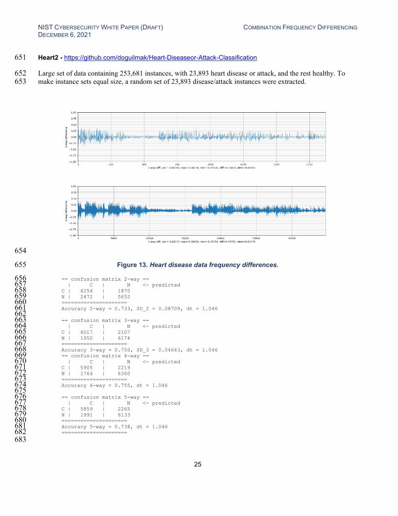
Heart2 - https://github.com/doguilmak/Heart-Diseaseor-Attack-Classification 651

Large set of data containing 253,681 instances, with 23,893 heart disease or attack, and the rest healthy. To 652 make instance sets equal size, a random set of 23,893 disease/attack instances were extracted. 653

654

Figure 13. Heart disease data frequency differences. 655

== confusion matrix 2-way == 656 | C | N <- predicted 657 C | 6254 | 1870 658 N | 2472 | 5652 659 ===================== 660 Accuracy 2-way = 0.733, SD_2 = 0.08709, dt = 1.046 661 662 == confusion matrix 3-way == 663 | C | N <- predicted 664 C | 6017 | 2107 665 N | 1950 | 6174 666 ===================== 667 Accuracy 3-way = 0.750, SD_3 = 0.04643, dt = 1.046 668 == confusion matrix 4-way == 669 | C | N <- predicted 670 C | 5905 | 2219 671 N | 1764 | 6360 672 ===================== 673 Accuracy 4-way = 0.755, dt = 1.046 674 675 == confusion matrix 5-way == 676 | C | N <- predicted 677 C | 5859 | 2265 678 N | 1991 | 6133 679 ===================== 680 Accuracy 5-way = 0.738, dt = 1.046 681 ===================== 682

683

https://github.com/doguilmak/Heart-Diseaseor-Attack-Classification


26

Mush - https://archive.ics.uci.edu/ml/datasets/Mushroom 684

Schlimmer, J.S. (1987). Concept Acquisition Through Representational Adjustment (Technical Report 87-19). 685 Doctoral dissertation, Department of Information and Computer Science, University of California, Irvine. 686

687

Figure 14. Edible mushroom data frequency differences. 688



705

706

https://archive.ics.uci.edu/ml/datasets/Mushroom


27

Soyb - https://archive.ics.uci.edu/ml/datasets/Soybean+%28Large%29 707

R.S. Michalski and R.L. Chilausky. "Learning by Being Told and Learning from Examples: An Experimental 708 Comparison of the Two Methods of Knowledge Acquisition in the Context of Developing an Expert System 709 for Soybean Disease Diagnosis", International Journal of Policy Analysis and Information Systems, Vol. 4, 710 No. 2, 1980. 711

712

Figure 15. Soybean disease data frequency differences. 713



730

https://archive.ics.uci.edu/ml/datasets/Soybean+%28Large%29

Draft NIST CSWP, Combination Frequency Differencing

Documents

Transcript of Draft NIST CSWP, Combination Frequency Differencing