Downtown Miami Urban Redevelopment and Sea Wall Infrastructure – Comprehensive Economic Analysis for Resilience and Community Impacts

Triple Bottom Line Cost Benefit Analysis – Economic Contributions to Green Infrastructure/Low Impact Development and Raised/Living Sea Wall Investments to Downtown Miami and First Miami Presbyterian Church

FINAL Prepared by Impact Infrastructure

February, 2019

Outline

Executive Summary 4 Why Now? 4 Project Overview 4 High Level Results 5 Main Takeaways & Discussion 7

Project Overview 9 The Challenge 9 Project Structure 10 Type of Analyses 11

Triple Bottom Line Cost Benefit Analysis 11 Economic Impact Analysis 11

Design Alternatives 13 Design Alternative 1: 7ft Sea Wall (Figure 2) 13 Design Alternative 2: 7ft Sea Wall with Living Shoreline 15

Levels of Assessment: 17 Downtown-Level Assessment 17 First Miami Presbyterian Church (FMPC) Site Level Analysis 17

Impacts Being Valued 21 TBL-CBA 21 EIA 22

Results at Miami Downtown Level 23 TBL-CBA Results of Two Sea Wall Types 23

Summary of Costs and Benefits 23 Coastal Flood Risk Results 24

Overview 24 Building Damage (Structure and Contents) 28 Vehicles 31 Emergency Shelter Costs 34 Total Flood Impact 36

Ecosystem Services 39 Cost of Sea Wall Types 41

Economic Impact Assessment (EIA) Results of Two Sea Wall Types 42

Results at First Miami Presbyterian Church (FMPC) Level 43

1

TBL-CBA Results of FMPC Site 43

Summary of Costs & Benefits of the FMPC Site (Upland Redevelopment & Sea Wall Types) 43 Coastal Flood Risk Benefits of the Two Sea Walls 46

Building Damage (Structure and Contents) 46 Vehicle Damage 47 Emergency Shelter Costs 48 Total Flood Impact 49

Ecosystem Services from Living Shoreline Features 51 Costs 51

Cost of Sea Wall Types 51 Cost of Upland Redevelopment 52

Economic Impact Assessment (EIA) Results of FMPC 53

Flood Insurance Considerations 54

Discussion: Qualitative Impacts and Caveats 56

Appendix A: Methodology 58 Impact Infrastructure 58 TBL-CBA Methodologies and Inputs 58

TBL-CBA Framework 58 Base Case and Design Case 59 Valuation Methodologies and Inputs 59 Financial Impacts 59

Capital Expenditures 59 Operations and Maintenance Costs 60 Replacement Costs and Residual Value 61

Social Impacts 62 Property Value 62 Recreation Value 63 Heat Island Effect 64 Education Value 65 Public Health 66 Flood Risk from the FMPC Upland Redevelopment 67

Environmental Impacts 68 Ecosystem Services from Living Shoreline of Mangroves and Seagrasses 68 Water Quality 73 Carbon Reduction by Vegetation 73 Air Pollution Reduction by Vegetation 74

2

Coastal Flood Risk Methodologies 76

Conceptual model 76 Spatial data model 81

Geographic boundary 81 Spatial resolution 83 Temporal resolution 83

Sea level rise projections 83 10-year storm 84

Mathematical model 84 Flood Model Justification 84 Structure and Logic Diagram 85 Flood Model Parameters in COAST 89

Sea Level Rise Projections 89 Computed Storm Event 89

Monetized Flood Risk Outputs 90 Structural and contents damage 90 Vehicle damage 90

Shelter costs 90 Economic Impact Analysis Methodologies 91

Appendix B: References 92

3

1. Executive Summary

1.1. Why Now? The City of Miami faces various natural hazards, including sea level rise (SLR) and storm surges, urban heat island, and stormwater quality, which are expected to worsen as the climate continues to change. The market value for downtown properties is roughly $39bn – representing more than 50% of the City’s taxable property value. As a result, damage to properties, infrastructure, and people could have significant fiscal and social consequences, therefore it is important to show the full cost of a business-as-usual/do-nothing approach versus investing in resiliency measures.

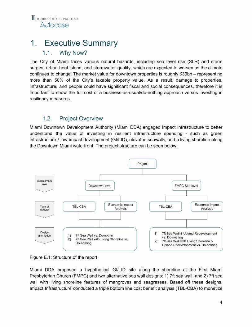
1.2. Project Overview Miami Downtown Development Authority (Miami DDA) engaged Impact Infrastructure to better understand the value of investing in resilient infrastructure spending - such as green infrastructure / low impact development (GI/LID), elevated seawalls, and a living shoreline along the Downtown Miami waterfront. The project structure can be seen below.

Figure E.1: Structure of the report Miami DDA proposed a hypothetical GI/LID site along the shoreline at the First Miami Presbyterian Church (FMPC) and two alternative sea wall designs: 1) 7ft sea wall, and 2) 7ft sea wall with living shoreline features of mangroves and seagrasses. Based off these designs, Impact Infrastructure conducted a triple bottom line cost benefit analysis (TBL-CBA) to monetize

4

the financial, social, and environmental broader co-benefits of the proposed FMPC upland site with the two sea wall options. Impact Infrastructure also conducted a TBL-CBA at the downtown Miami level of the two sea wall options to specifically assess coastal flooding risk. In addition to a TBL-CBA, the team conducted an Economic Impact Assessment (EIA) to estimate the contribution to economic growth and employment from the two sea wall types at both the FMPC site level and the downtown Miami level.

1.3. High Level Results

Figure E.2: Summary of Results TBL-CBA of First Miami Presbyterian Church (FMPC) Results indicate that, over a 40-year period, the triple bottom line net present value (TBL-NPV) of the FMPC site with 7ft sea wall and upland redevelopment could be $4.2 million (m) while the FMPC site with living sea wall features would return about 10% higher TBL-NPV of $4.6m. TBL-CBA of Downtown Miami

● TBL-NPV ○ For the Downtown level analysis, the TBL-NPV for the 7ft sea wall is estimated to

be $338m compared to that of the 7ft sea wall with living shoreline, which has TBL-NPV of $455m (more than 30% greater). Both designs offer large benefit cost ratios, with $6.1 and $5.2 in benefits being created for every $1 invested. See Table E.1 for a summary of the results.

5

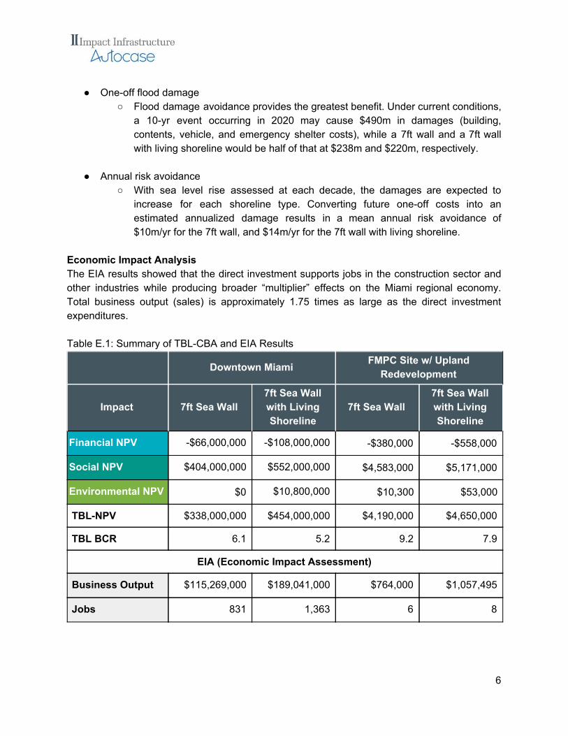
● One-off flood damage ○ Flood damage avoidance provides the greatest benefit. Under current conditions,

a 10-yr event occurring in 2020 may cause $490m in damages (building, contents, vehicle, and emergency shelter costs), while a 7ft wall and a 7ft wall with living shoreline would be half of that at $238m and $220m, respectively.

● Annual risk avoidance

○ With sea level rise assessed at each decade, the damages are expected to increase for each shoreline type. Converting future one-off costs into an estimated annualized damage results in a mean annual risk avoidance of $10m/yr for the 7ft wall, and $14m/yr for the 7ft wall with living shoreline.

Economic Impact Analysis The EIA results showed that the direct investment supports jobs in the construction sector and other industries while producing broader “multiplier” effects on the Miami regional economy. Total business output (sales) is approximately 1.75 times as large as the direct investment expenditures. Table E.1: Summary of TBL-CBA and EIA Results

Downtown Miami FMPC Site w/ Upland Redevelopment

Impact 7ft Sea Wall 7ft Sea Wall with Living Shoreline

7ft Sea Wall 7ft Sea Wall with Living Shoreline

Financial NPV -$66,000,000 -$108,000,000 -$380,000 -$558,000

Social NPV $404,000,000 $552,000,000 $4,583,000 $5,171,000

Environmental NPV $0 $10,800,000 $10,300 $53,000

TBL-NPV $338,000,000 $454,000,000 $4,190,000 $4,650,000

TBL BCR 6.1 5.2 9.2 7.9

EIA (Economic Impact Assessment)

Business Output $115,269,000 $189,041,000 $764,000 $1,057,495

Jobs 831 1,363 6 8

6

1.4. Main Takeaways & Discussion

Spend Money to Save Money Despite the significant initial capital outlay for investing in resilience infrastructure, the returns can be expected to yield $5-$6 for every $1 spent, with the avoided flood damage being the largest value creator. In terms of flood damage, the cost of doing nothing is expected to cost $37m/yr, while investing in a 7ft wall is expected to reduce that to $27m/yr, and adding a living shoreline is expected to reduce that further still to $23m/yr. Over 50 years, this is expected to save $404m and $552m, respectively.

Figure E.3: Present Value of Annualized Total Cost from a 10-yr Storm with Sea Level Rise The results of this study illustrate the value that living features like mangroves and seagrasses contribute to mitigating against flood risk as well as providing co-benefits. This analysis provides an illustrative example of the potential benefits of implementing two different sea wall designs as well as GI attributes to support Miami DDA’s efforts in resilience investments. Insurance Considerations This study discusses the insurance considerations related to the implementation of a 7ft sea wall or 7ft sea wall with living shoreline in Downtown Miami. The City of Miami is currently rated as a Class 7 and eligible property owners in Special Flood Hazard Areas (SFHAs) receive a discount of 15% on their flood insurance premiums under the Community Rating System (CRS) under Federal Emergency Management Agency’s (FEMA) National Flood Insurance Program (NFIP). If FEMA officials and other industry experts considered a 7ft seawall or 7ft seawall with 1

living shoreline in Downtown Miami as a flood mitigation activity that could provide enough

1 FEMA. 2018. COMMUNITY RATING SYSTEM. https://www.fema.gov/media-library-data/1523648898907-09056f549d51efc72fe60bf4999e904a/20_crs_508_apr2018.pdf

7

credits to push the City of Miami to a Class 6 (a 20% discount to eligible properties in SFHAs), the City of Miami could receive an additional 5% discount that could lower eligible properties’ insurance premiums. 2

To provide Miami DDA with an illustrative example of this potential value, Impact Infrastructure used FEMA Policy & Claim Statistics for Flood Insurance data of the written premium in-force for the City of Miami as of September 30 2018 combined the assumption that all properties that pay FEMA NFIP premiums are in SFHAs and eligible for the CRS discount. Applying a 5% discount 3

to written premiums in-force for the City of Miami for illustrative purposes only, it is estimated that a potential incremental discount could have a present value of approximately $21 million over 40-years.

2 FEMA. 2017. National Flood Insurance Program Community Rating System Coordinator’s Guide. https://www.fema.gov/media-library-data/1493905477815-d794671adeed5beab6a6304d8ba0b207/633300_2017_CRS_Coordinators_Manual_508.pdf 3 FEMA. 2019. Policy Statistics. https://bsa.nfipstat.fema.gov/reports/1011.htm

8

2. Project Overview 2.1. The Challenge

The City of Miami faces various natural hazards, which are expected to worsen as the climate continues to change. Resilience infrastructure and resilience policy development can be seen from an economist’s point of view as an insurance policy that can either prevent a natural hazard from becoming a natural disaster, or aid in faster recovery after an event has struck. The market value for downtown properties is roughly $39bn – representing more than 50% of the City’s taxable property value. Damage to properties, infrastructure, and people could have significant consequences, and thus it is important to show the full cost of a do-nothing approach versus alternative investments. Miami Downtown Development Authority’s (Miami DDA) mission is to grow, strengthen, and promote the economic health and vitality of Downtown Miami. As part of the 2025 Downtown Miami Master Plan, a specific objective is “Complete the Baywalk & Riverwalk”. Furthermore, to help bolster Downtown Miami’s resiliency, Miami DDA created the Resilience Task Force to better prepare Downtown for climate change and extreme storm events as well as review options for reinforcing Miami’s waterfront. To support this, the Miami DDA, in partnership with the City of Miami Resiliency Office and The Nature Conservancy (TNC), would like to better understand the value of investing in GI/LID along the Miami waterfront. The agency engaged Impact Infrastructure to conduct a triple bottom line cost benefit analysis (TBL-CBA) to monetize the holistic value to the community in Miami of potential resiliency efforts. By quantifying, in monetary terms, the full lifecycle costs, as well as the broader social and environmental impacts of green infrastructure such as avoided flood risk, recreation, urban heat island reduction, water quality improvements, among other benefits, this report will illustrate the public and private return on resilience investment.

9

2.2. Project Structure This report is structured according to Figure 1 below. Both a TBL-CBA and an EIA were conducted, evaluating two design alternatives (7ft sea wall and 7ft sea wall with living features) at both the Downtown Miami (Downtown-level) and First Miami Presbyterian Church upland redevelopment site (FMPC- site level).

Figure 1: Structure of the report

10

2.3. Type of Analyses Across each level of assessment, and for each design alternative, both a TBL-CBA and an EIA are conducted to show the full suite of financial, social, and environmental costs and benefits of the proposed design alternatives.

2.3.1. Triple Bottom Line Cost Benefit Analysis TBL-CBA is a systematic, evidence-based economic business case framework that uses best practice Life Cycle Cost Analysis and Cost Benefit Analysis (CBA) techniques to quantify and attribute monetary values to the Triple Bottom Line (TBL) impacts resulting from an investment. TBL-CBA expands the traditional financial reporting framework (such as capital, and operations and maintenance costs) to also consider social and environmental performance. TBL-CBA provides an objective, transparent, and defensible economic business case approach to assess the costs and benefits pertaining to the project being analyzed. The underlying cost-benefit analysis approach is an industry standard decision-support methodology and is widely used in federal grants. Furthermore, it is a requirement for federal departments when proposing policy changes. It aims to quantify, in monetary terms, as many of the costs and benefits of a project as possible and converts them all into a present day dollar value. In CBA, a “base case” (the existing conditions) is compared to one or more alternatives (which have some significant improvement compared to the base case). The analysis evaluates incremental differences between the base case and each alternative. The importance of CBA for decision makers is that its results provide a quantitative measure of a project’s worthiness.The analysis involves a comprehensive account of project benefits and costs over the entire project life cycle and a “side-by-side” comparison of net benefits for alternative investments. The cost-benefit framework offers an opportunity to recognize and include in the evaluation all social and economic impacts in an objective manner.

2.3.2. Economic Impact Analysis An Economic Impact Analysis (EIA) is a widely used analysis that estimates the short-term direct and indirect economic impacts on value added (GDP) and jobs localized in the region where a project is taking place and is based on government estimated economic activity multipliers of the cost of construction and development. EIA can be used to quantify the economic activity and jobs produced from a specific project. Key economic impact metrics are defined as:

● Output: The direct and total business sales (output) of businesses in Miami-Dade County – the broadest measure of economic activity.

11

● Value-Added: Value-added represents the incremental value added by business activity

(largely represented by wages and profits) while excluding the purchase of input goods as part of the production process.

● Earnings: The wages earned by workers at impacted industries (construction and supporting).

● Jobs: The employment impact by industry.

12

2.4. Design Alternatives This project compares the impacts of the base case to two design alternatives for sea walls, providing results that are incremental and relative. The base case is the do-nothing – or “as is” scenario – while the design scenario reflects possible future policy measures.

2.4.1. Design Alternative 1: 7ft Sea Wall (Figure 2) Design alternative 1 is a traditional sea wall in design, but is raised 2 feet higher from 5ft to 7ft (NAVD).

Figure 2: Example of Traditional 7ft Sea Wall

13

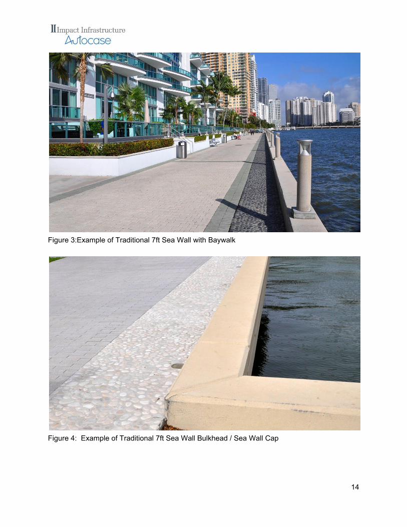
Figure 3:Example of Traditional 7ft Sea Wall with Baywalk

Figure 4: Example of Traditional 7ft Sea Wall Bulkhead / Sea Wall Cap

14

2.4.2. Design Alternative 2: 7ft Sea Wall with Living Shoreline

Design alternative 2 is a 7 feet sea wall with a living shoreline comprising of red mangrove (Rhizophora mangle) and saltmeadow cordgrass (Spartina patens), and rip rap (Figure 3) that extends 12 feet.

Figure 5: Example of 7ft Sea Wall with Living Shoreline

Figure 6: Example of Living Shoreline with Mangroves and Rip-Rap

15

Figure 7: Example of Living Shoreline with Mangroves and Rip-Rap

16

2.5. Levels of Assessment: This report is split into two levels of assessment:

1. The downtown-level (44,000 feet of shoreline – or 8.3 miles) looking at a large section of the Downtown Miami shoreline between SW 26th Rd in the south to NE 36th St in the north, as well as up the Miami River east of the I-95.

2. A site-specific level, which assesses a ~175 feet piece of shoreline at the First Miami Presbyterian Church (609 Brickell Avenue) with a GI/LID upland redevelopment site.

2.5.1. Downtown-Level Assessment TBL-CBA The downtown Miami analysis is an assessment of the triple bottom line costs and benefits – including avoided coastal flooding damage from a 10-yr storm – at the municipal level for two sea wall options (along 44,000 feet of shoreline – or 8.3 miles):

1. Increasing the 44,000 feet of shoreline and Baywalk from a 5ft (NAVD) sea wall to a 7ft sea wall

2. Increasing the 44,000 feet of shoreline and Baywalk from a 5ft sea wall to a 7ft sea wall with a 12 feet deep living shoreline comprising of red mangroves and cordgrasses in the waterway adjacent to the 7ft wall for wave attenuation.

EIA An Economic Impact Assessment of the two sea wall options is conducted for 44,000 feet of shoreline and Baywalk. The economic impact analysis is focused on the one-time construction spending (capital expenditures) to construct the following options.

1. Downtown Miami shore with a seven foot sea wall 2. Downtown Miami shore with a seven foot sea wall and living shoreline

2.5.2. First Miami Presbyterian Church (FMPC) Site Level Analysis First Miami Presbyterian Church is located at 609 Brickell Avenue and situated on Biscayne Bay near the Miami River. It is a three-acre property that has a two-story historic building, which currently serves as a church, daycare, and school. Currently, the property allows for untreated stormwater to runoff straight in to Biscayne Bay, and it has been identified by the Miami DDA as a hypothetical demonstration project to illustrate the benefits of resilience infrastructure investment in green infrastructure / low impact development (GI/LID). Theses terms are used interchangeably in this report where both terms generally refer to cost-effective and resilience practices that manage wet weather impacts using natural or human-made systems. 4

4 https://www.epa.gov/green-infrastructure/what-green-infrastructure

17

Figure 8: Location of the FMPC Upland Redevelopment Site The hypothetical FMPC upland redevelopment site consists of approximately 0.24-acres (herein referred to as, “upland site design” or “upland redevelopment”) of features GI/LID to replace the currently unmanaged shoreline area. The GI/LID side would not replace any parking lot area of the FMPC. GI/LID design features in the upland site design include interlocking porous concrete pavers, a rain garden of groundcovers and ornamental grasses, shrubs, trees, and other site amenities including shade umbrella covered tables, park benches, litter receptacles, light posts, and bike racks. Table 1 describes the FMPC upland redevelopment site GI/LID and amenities features.

U.S. EPA. 2009. Managing Stormwater with Low Impact Development Practices: Addressing Barriers to LID. https://www3.epa.gov/region1/npdes/stormwater/assets/pdfs/AddressingBarrier2LID.pdf

18

Table 1: FMPC Upland Site Redevelopment Features

Type Unit

Interlocking Porous Concrete Pavers 4095 sq-ft

Rain Garden of Groundcover and Ornamental Grasses 569 sq-ft

Shrubs 3438 sq-ft

Trees 38

4-Backed Seat Table 4

2-Seat backed Table 2

Stay Backed Bench 6

Shade Umbrella 6

Litter Receptacles 2

Bike Racks 4

Light Posts 4

The 7ft sea wall and living shoreline option was designed to include approximately 0.05-acres of red mangrove (Rhizophora mangle) and saltmeadow cordgrass (Spartina patens) on a vegetated slope above the high-water line in the waterway adjacent to the elevation of the Baywalk and FMPC upland site. The hypothetical FMPC upland and sea wall project would form a vital connection to the Baywalk both north and south of the site for recreational users, as well as provide numerous broader social and environmental benefits -- from avoided water quality issues, carbon sequestration, urban heat island impacts, flood risk reductions, to others. The outputs of the TBL-CBA of the FMPC upland site and sea wall options would contribute a common language - dollars - the costs and benefits of this hypothetical design that Miami DDA and its partners can communicate with to their stakeholders. TBL-CBA An assessment of the triple bottom line costs and benefits of two hypothetical design options located at the First Miami Presbyterian Church (175 feet of shoreline)

a. Raising the shoreline from a 5 ft sea wall to a 7ft sea wall, and include a GI/LID upland redevelopment.

b. Raising the shoreline from a 5ft sea wall to a 7ft sea wall with a living shoreline (12 ft deep), and include a GI/LID upland redevelopment.

19

EIA An Economic Impact Analysis of the two design alternatives for the 175 feet stretch of Baywalk is conducted. The economic impact analysis is focused on the one-time construction spending (capital expenditures) to construct the following two options:

1. FMPC site upland GI/LID construction with a seven foot sea wall. 2. FMPC site upland GI/LID construction with a seven foot sea wall plus a living shoreline

adjacent to the sea wall.

20

2.6. Impacts Being Valued The impacts assessed in each of the two assessment levels are outlined in the table below.

2.6.1. TBL-CBA Table 2: TBL-CBA Impacts Evaluated by Assessment Level

Category Impact Downtown Miami + Sea Walls

FMPC + Sea Walls+Upland

Financial Capital Expenditure ✔ ✔

Financial Operations and Maintenance ✔ ✔

Financial Replacement Cost ✔ ✔

Financial Residual Value ✗ ✔

Social Coastal Flood Risk ✔ ✔

Social Upland Flood Risk ✗ ✔

Social Property Value ✗ ✔

Social Recreational Value ✗ ✔

Social Urban Heat Island Effects ✗ ✔

Social Education ✗ ✔

Social Public Health ✗ ✔

Environmental Living Shoreline ✗

✔ (only with the

7ft+living shoreline option)

Environmental Water Quality ✗ ✔

Environmental Air Pollution Reduced by Vegetation ✗ ✔

Environmental Carbon Reduction by Vegetation ✗ ✔

For the coastal flood risk, each of the two analyses assesses the avoided damage to buildings, vehicles, and emergency shelter from a 10-yr storm event for the two sea wall typologies (7ft 5

sea wall and 7ft sea wall with living shoreline), as compared to the current 5ft sea wall across five SLR scenarios, which are identified in the table below.

5 A 10-yr storm event is a storm that has a 10% chance of occurring in any given year.

21

Table 3: Sea Level Rise Projections using USACE High 6

Year SLR (inches)

2020 6

2030 10

2040 15

2050 20

2060 26

Autocase conducted a Triple Bottom Line-Cost Benefit Analysis (TBL-CBA) to determine the net present value of financial, social and environmental costs and benefits associated with the alternative scenarios over a 41-year time horizon (1 year construction, 40 years of operation) using a 3.5% real discount rate for Fiscal Year 2018.

2.6.2. EIA For each level of analysis the EIA assesses direct capital expenditure (direct capex), business output, value added, wages/earnings, and employment. Multipliers for Miami-Dade County were sourced from the U.S Bureau of Economic Analysis. Table 4: EIA Impacts assessed in Each Analysis Level

Impact Downtown Miami (two sea wall alternatives)

FMPC (two sea wall alternatives & upland

redevelopment)

Direct CapEx ✔ ✔

Business Output (i.e. Sales) ✔ ✔

Value Added ✔ ✔

Wages / Earnings ✔ ✔

Employment (i.e. Jobs) ✔ ✔

6 Unified Sea Level Rise Projection Southeast Florida: http://www.southeastfloridaclimatecompact.org/wp-content/uploads/2015/10/2015-Compact-Unified-Sea-Level-Rise-Projection.pdf

22

3. Results at Miami Downtown Level

3.1. TBL-CBA Results of Two Sea Wall Types 3.1.1. Summary of Costs and Benefits

High level results indicate a significantly positive TBL-NPV for both sea wall alternatives - suggesting that resilience investment generates positive use of public funds. At the Downtown Miami level, increasing the elevation of the sea wall from 5ft to 7ft along 8.3 miles of shoreline would cost roughly $66 million (m), but would yield upwards of $404m in coastal flood risk protection over 40 years from a 10-yr storm event, resulting in a TBL-NPV of $338m. Assessing the triple bottom line benefit cost ratio, for every $1 invested, the project yields an expected $6.10 in benefit. If Downtown Miami were to include a living shoreline in addition to raising the height of the sea wall to 7ft, this would cost in the range of $108m across 8.3 miles of shoreline. However, this living shoreline provides ecosystem services equivalent to $10.8m over 40 years, as well as attenuating coastal flood risk, which generates roughly $552m in present value. This alternative yields a TBL-NPV of $455m over 40 years - a significant positive return. Assessing the triple bottom line benefit cost ratio, for every $1 invested, this yields an expected $5.20 in benefit. The 7ft wall has a lower TBL-NPV than the 7ft wall with living shoreline but yields a larger “bang for the buck” given the higher triple bottom line benefit cost ratio (TBL-BCR). There is a tradeoff to be made, but ultimately, both alternatives suggest they are sound investments. Moreover, the broader social benefits that may be unquantifiable (such as sense of place, cultural identity, peace of mind etc.) should be also considered to support decision-making. Table 5: Summary of TBL-CBA Results for Two Sea Wall Types at the Downtown Level

Impact Cost/Benefit

Present Value of 7ft Wall ($)

Present Value of 7ft Wall & Living Shoreline ($)

Financial Capital Expenditures -$66,000,000 -$108,000,000

Social Coastal Flood Risk Mitigated $404,000,000 $552,000,000

Environmental Ecosystem Services $0 $10,800,000

Triple Bottom Line NPV $338,000,000 $455,000,000

TBL Benefit Cost Ratio 6.1 5.2

23

3.1.2. Coastal Flood Risk Results

Overview Firstly, it is important to note that the following results are conceptual and to be used for high level project planning and funding. Given the Hydrology and Hydraulic (H&H) modeling has not been conducted, detailed flood depth grids were unavailable to be used as inputs in to the economic loss estimation tool. As a result, Impact Infrastructure relied on the in-built storm model within the economic loss estimation tool, COAST (Coastal Adaptation to Sea Level Rise Tool). COAST lent itself well to this analysis, as it did not require an H&H model in order to generate risk results; using a Digital Elevation Model (DEM), land parcel boundaries, property values, and information regarding storm exceedance, COAST enabled the team to estimate flood depth at the parcel level and combine it with depth-damage curves to monetize that the risk that is found in the subsequent sections. The COAST approach assesses costs and benefits of adaptations to SLR scenarios by incorporating a variety of existing tools and datasets, including the U.S. Army Corps of Engineers' depth-damage functions; NOAA's Sea, Lake, and Overland Surges from Hurricanes (SLOSH) model; and other flood methods, as well as projected SLR scenarios over time, property values, and infrastructure costs, into a comprehensive GIS-based picture of potential economic damage. Under the current shoreline conditions, 274 parcels of the 4,732 parcels (5.8%) in downtown area of Miami (equating to 6.5m sq ft of land area – or 8.1% of total land) is exposed to a 10-yr storm event if it were to occur in 2020. As sea levels rise as time goes on, the number increases if the storm were to occur in 2030 to 296 parcels and 7.0m sq ft (6.3% of parcels and 8.7% of total land), 370 parcels and 8.3m sq ft in 2040 (7.8% of parcels and 10.3% of total land), 404 parcels and 8.9m sq ft in 2050 (8.55% and 11.1%), and 440 parcels and 9.4m sq ft in 2060 (9.3% and 11.7%). If a 7ft sea wall were to replace the current 5ft policy in Downtown Miami, the number of parcels exposed in 2020 would drop to 196 i.e. 4.6m sq ft of land (4.1% of all parcels and 5.7% of land) – a saving of 78 parcels, or 1.9m sq ft of land. However, we can see from the graphs in Figures 5 and 6 that by 2060, the 7ft wall no longer avoids land or parcels from being exposed. This is most likely due to the fact that seas are projected to have risen too much by 2060 for a wall to make any meaningful difference. Furthermore, given an expected 40-yr useful life of a seawall, a new strategy is likely to be put in place by this time. The 7ft wall with living shoreline performs similarly to the 7ft wall from 2020 to 2030, but shows improvement in 2040 by avoiding 55 parcels equating to 2 million sq ft of land (1.2% of all parcels and 2.5% of total land) versus the current policy, whereas the 7ft wall by itself only prevents exposure to 34 parcels (1.1m sq ft). Similarly to the 7ft wall, the benefits of the 7ft wall with living shoreline are muted by 2060.

24

Figure 9: Land Impacted from a 10-yr Storm (sq ft)

Figure 10: Number of Parcels Impacted by a 10-yr Storm

25

It is important to assess the geographic extent of flooding in the downtown region. Figure 6 above illustrates the parcels that would be impacted from a 10-yr storm – and the year in which those parcels would first be impacted (given sea level rise) – for each sea wall scenario. To interpret this image, a parcel that is red would be impacted in 2020, where as parcel that is blue would not be impacted until 2060. Under the current shoreline, we can see that a significant portion of the downtown area is already exposed to a 10-yr event in 2020. Unsurprisingly, parcels closer to the shoreline and the Miami River are exposed at earlier periods, while parcels more inland start to be impacted in future decades once sea level rise increases. With a 7ft sea wall, despite many parcels still being impacted in 2020, we can start to see that parcels which were once impacted in 2020 now are protected in that year, but are still impacted in future years. This trend of delaying exposure from a 10-yr event is even more visible under the 7ft wall with living shoreline scenario.

26

Figure 11: Parcels Affected by Flooding, and the Year in Which those Parcels are Impacted for Each Sea Wall Type.

27

Building Damage (Structure and Contents) COAST outputs estimate the potential future structural and building contents damage that could be inflicted to the downtown area from a 10-yr event is significant. Figure 8 below shows the future cost (i.e. not discounted) of structural damage and contents damage of a one-off 10-yr event happening in that year for each sea wall scenario. We can see that in 2020, under current shoreline conditions, a 10-yr event may cause $437m in structural and contents damage, while a 7ft wall and a 7ft wall with living shoreline would be half of that at $212m and $196m, respectively. With sea level rise assessed at each decade, the damages increase for each shoreline type, but the living shoreline performs better than the 7ft sea wall due to the wave attenuation. Again, by 2060 all three sea wall types converge to around $1billion (bn) in combined damages, because sea levels have risen considerably that even 7ft wall and living shoreline is not enough to prevent exposure.

Figure 12: Structural and Contents Damage from a 10-yr Storm the Year in Which the Storm Occurs Figure 9 below illustrates the present value of building damages. Because we are assessing values upwards of 40 years in to the future, the $1bn of damages in 2060 has a present value of $245m (2018 dollars) due to discounting. Discounting future values represents the time value of money and enables us to assess future values in present dollars. Although this is a significant drop in scale, it does not change the overall results that highlight the fact that both the 7ft wall and 7ft wall with living shoreline provides substantial risk avoidance.

28

Figure 13: Present Value of Structural and Contents Damage from a 10-yr Storm the Year in Which the Storm Occurs It is useful to look at the present value of the avoided building damage from a 10-yr event by comparing the current 5ft wall to the two alternative scenarios (7ft wall and 7ft wall with living shoreline). Figure 10 below shows that the 7ft wall provides $210m in avoided risk if a 10-yr storm were to occur in 2020, $168m in 2030, $39m in 2040, $33m in 2050, and $0m in 2060. A similar pattern is visible for the 7ft wall with living shoreline: the present value of protection is $225m if a 10-yr event were to strike in 2020, $178m in 2030, $142m in 2040, $64m in 2050, and still providing some protection in 2060 at $5m.

29

Figure 14: Present Value of Avoided Structural and Contents Damage from a 10-yr Storm the Year in Which the Storm Occurs Converting these one-off damages in the year in which they occur into an expected annualized damage provides an idea of the risk in any year from a 10-yr event. A 10-yr event is a storm that has a 10% chance of occuring in any given year. Taking the mean discounted value of damages in each period between 2020-2060, we find that Miami has $33m/yr risk from a 10-yr event under the current sea wall, a $24m/yr with a 7ft wall, and $20m with a 7ft wall with a living shoreline. This results in a mean annual risk avoidance to building damage of $9.0m/yr for the 7ft wall, and $12.3m/yr for the 7ft wall with living shoreline. Given that the future damages are based on a snapshot of today’s land use, these results may underestimate the true value that could be avoided, since the analysis does not factor in future land use changes or development built to accommodate a growing population.

30

Figure 15: Present Value of Mean estimated Annualized Building Damage from a 10-yr Storm

Figure 16: Present Value of mean Annualized Avoided Building Damage from 7ft sea wall and 7ft sea wall and living shoreline.

Vehicles Vehicle damage and the cost of these damages is an important factor to consider when assessing a storm event. This analysis finds that a one-off event in 2020 could cause $8.9m damage costs to cars under the current shoreline, whereas it would be lower with a 7ft wall and 7ft wall and living shoreline of $4.5m and $4.3m, respectively. With increasing sea levels, these damages are likely to increase for each sea wall type, with the 7ft wall and living shoreline performing best until 2060 when the damage is roughly equal for all sea wall types at $36m.

31

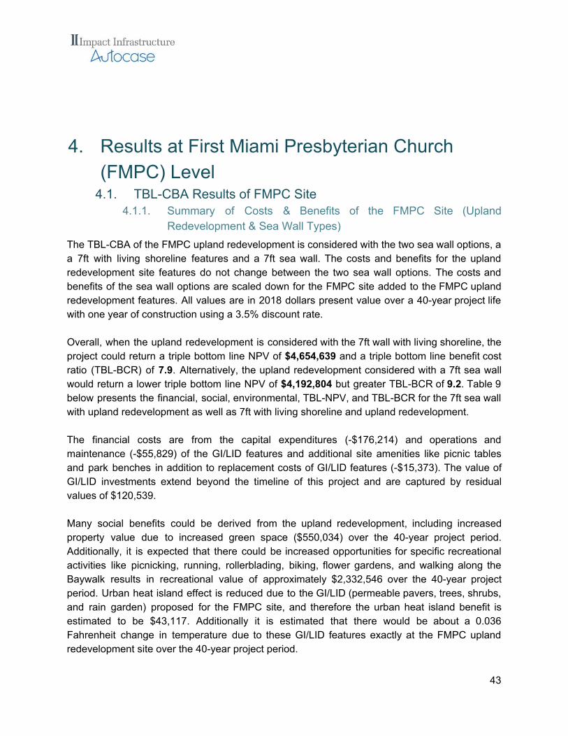
Figure 17: Vehicle Damage from a 10-yr Storm the Year in Which the Storm Occurs Converting these one-off damages in to a present value and finding the difference between the current shoreline, and the 7ft wall and 7ft wall with living shoreline shows the value of avoided risk. We can see that the 7ft wall and 7ft wall with living shoreline avoid roughly $4m in vehicle damages in 2020, but the 7ft wall with living shoreline performs better through 2030-2050 ($5.1m, $3.2m, and $3.1m) versus the 7ft wall ($3.4m, $0.6m, and $1.2m). At 2060, there is no difference in the present value of avoided vehicle damage from a 10-yr storm between the sea wall designs.

32

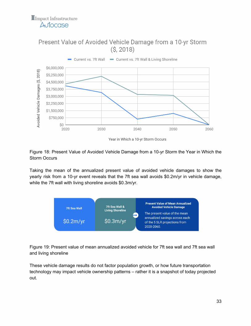
Figure 18: Present Value of Avoided Vehicle Damage from a 10-yr Storm the Year in Which the Storm Occurs Taking the mean of the annualized present value of avoided vehicle damages to show the yearly risk from a 10-yr event reveals that the 7ft sea wall avoids $0.2m/yr in vehicle damage, while the 7ft wall with living shoreline avoids $0.3m/yr.

Figure 19: Present value of mean annualized avoided vehicle for 7ft sea wall and 7ft sea wall and living shoreline These vehicle damage results do not factor population growth, or how future transportation technology may impact vehicle ownership patterns – rather it is a snapshot of today projected out.

33

Emergency Shelter Costs Being able to shelter those people affected by flooding is a public cost that should be considered in a flood risk analysis. This report finds that costs associated with emergency shelter is much lower than for building damage or vehicle. A 10-yr storm occurring in 2020 is estimated to cost almost $0.19m for emergency shelter under the current shoreline, whereas a 7ft wall and a 7ft wall with living shoreline would be roughly half that at $0.1m and $0.09m, respectively. The 7ft wall and 7ft wall with living shoreline continues to protect, with the living shoreline scenario adding additional protection compared to the 7ft wall in 2040 and 2050.

Figure 20: Cost of Emergency Shelter from a 10-yr Storm the Year in Which the Storm Occurs Converting the above into a present value, and finding the difference between the current shoreline and the two alternative scenarios reveals that the avoided costs in 2020 and 2030 are equal, at around $80,000 and $60,000, respectively. In 2040 and 2050, the 7ft wall with living shoreline avoids more costs ($40,000 and $20,000) than the 7ft wall alone ($20,000 and $10,000).

34

Figure 21: Present Value of Avoided Emergency Shelter Cost from a 10-yr Storm the Year in Which the Storm Occurs Taking the mean of the annualized present value of avoided shelter costs to show the yearly avoided risk from a 10-yr event reveals that the 7ft sea wall avoids $3,400/yr in emergency shelter costs, while the 7ft wall with living shoreline avoids $4,000/yr.

Figure 22: Present Value of Mean Annualized Avoided Shelter Costs These results do not factor in population growth projections through to 2060 - rather they are a snapshot of today. Nevertheless, we don't know where population will be growing within the city – especially if development slows in high risk areas; therefore even if population were to grow over time, the number of people needing emergency shelter may not increase with those projections.

35

Total Flood Impact Looking at vehicle and building damage and shelter costs, we see that in 2020, under current conditions, a 10-yr event may cause $490m in structural and contents damage, while a 7ft wall and a 7ft wall with living shoreline would be half of that at $238m and $220m, respectively. With sea level rise assessed at each decade, the damages increase for each shoreline type, but the living shoreline performs better than the 7ft sea wall due to the wave attenuation, which performs better than the current conditions. By 2060 all three sea wall types converge to around $1.2bn in combined damages, because sea levels are projected to have risen considerably that even 7ft wall and living shoreline is not enough to prevent exposure.

Figure 23: Total Cost from a 10-yr Storm the Year in Which the Storm Occurs It is useful to look at the present value of the avoided building damage from a 10-yr event by comparing the current 5ft wall to the two alternative scenarios (7ft wall and 7ft wall with living shoreline). Figure 20 and 21 below show that the 7ft wall provides $235m in avoided risk if a 10-yr storm were to occur in 2020, $188m in 2030, $44m in 2040, $38m in 2050, and $0.3m in 2060. A similar pattern is visible for the 7ft wall with living shoreline: the present value of protection is $252m if a 10-yr event were to strike in 2020, $201m in 2030, $159m in 2040, $74m in 2050, and still providing some protection in 2060 at $5m.

36

Figure 24: Avoided damage in each year due to 7ft sea wall (blue) and 7ft with living shoreline (green)

Figure 25: Present Value of Total Avoided Cost from a 10-yr Storm the Year in Which the Storm Occurs

37

Converting these one-off damages into an expected annualized damage provides an idea of the risk in any year from a 10-yr event. A 10-yr event is a storm that has a 10% chance of occuring in any given year. Taking the mean value of damages from 2020-2060, we find that Miami has $37m/yr risk from a 10-yr event under the current sea wall, a $27m/yr with a 7ft wall, and $23m with a 7ft wall with a living shoreline. This results in a mean annual risk avoidance of $10m/yr for the 7ft wall, and $14m/yr for the 7ft wall with living shoreline.

Figure 26: Present Value of Annualized Total Cost from a 10-yr Storm Under Each Sea Wall

Figure 27: Present Value of Annualized Total Avoided Cost from a 10-yr Storm

38

3.1.3. Ecosystem Services

The living shoreline features of the 7ft sea wall plus living shoreline design includes red mangrove (Rhizophora mangle) and saltmeadow cordgrass (Spartina patens). Saltmeadow cordgrass is a species of marsh grass native to Florida and the Atlantic Coast. Mangroves and cordgrasses have provisioning, regulating, cultural, and supporting functions to species and ecosystems as illustrated in Table 6 below. Table 6: Ecosystem Services of Mangroves and Cordgrasses 7

Ecosystem Service Mangroves Cordgrasses Provisioning

Food and raw materials ✔ ✔

Medicinal resources ✔ ✔

Genetic resources ✔ ✔

Regulating Services

Flood, storm, and erosion regulation ✔ ✔

Carbon sequestration ✔ ✔

Cultural Services

Tourism and recreation ✔ ✔ and ✗

History, culture, traditions ✔ ✔

Science, knowledge, education ✔ ✔

Supporting Services

Primary production ✔ ✔

Nutrient cycling ✔ ✔

Species and ecosystem protection ✔ ✔ Mangroves serve as natural barriers for shoreline protection; they attenuate destructive wave energy and reduce the impact of storm surges. The intricate root system of mangroves also 8

makes these forests attractive to fish and other organisms seeking food and shelter from

7 Adapted from: Waite, R., et al. 2014. Coastal Capital: Ecosystem Valuation for Decision Making in the Caribbean. Washington, DC: World Resources Institute. https://www.wri.org/sites/default/files/coastal_capital_ecosystem_valuation_caribbean_guidebook_online.pdf Barbier et al. (2011) 8 Narayan, S., Beck, M.W., Wilson, P., Thomas, C., Guerrero, A., Shepard, C., Reguero, B.G., Franco, G., Ingram, C.J., Trespalacios, D. 2016. Coastal Wetlands and Flood Damage Reduction: Using Risk Industry-based Models to Assess Natural Defenses in the Northeastern USA. Lloyd’s Tercentenary Research Foundation, London.

39

predators. Along the southeast Florida coast, mangroves provide critical nursery and foraging 9

habitat for marine aquatic and water bird species. Mangroves have also been found to filter 10

nitrogen, phosphorous, and heavy metals - all commonly found in wastewater and stormwater. 11

Both mangroves and cordgrasses have the provisioning service to sequester carbon. , , 12 13 14

Impact Infrastructure conducted an in-depth literature review of the value of ecosystem services provided by mangroves. A study by Salem and Mercer (2012) estimates value of ecosystem services that mangrove forests contribute through a meta-analysis. This analysis uses the values of recreation and tourism, non-use values, carbon sequestration, and water and waste filtration from Salem and Mercer (2012) combined with the estimation methodology for living shoreline acreage that is described in Appendix A. The ecosystem benefits derived from mangroves are illustrated in Table 7 below. The total value for the 7ft sea wall with living shoreline for the Downtown level analysis could be approximately $10,800,000 over the lifetime (40 years) of the project. This estimate includes about $7,900,000 from recreation and tourism, $150,000 from carbon sequestration, $2,300,000 from non-use values, and approximately $500,000 from water and waste filtration services. See Appendix A for more information on the method applied for ecosystem services valuation of mangroves and seagrasses at the Downtown level analysis. The 7ft sea wall without living features has $0 living shoreline benefits because of its lack of natural living features to contribute tourism and recreation, carbon sequestration, non-use, or water filtration services.

9 National Oceanic and Atmospheric Administration. 2018. What is a "mangrove" forest? https://oceanservice.noaa.gov/facts/mangroves.html 10 Lorenz, J. 2013. Southeast Florida Coastal Marine Ecosystem - Shoreline Habitat: Mangroves. http://www.aoml.noaa.gov/ocd/ocdweb/docs/MARES/MARES_SEFC_ICEM__20131001_Appendix_Mangroves.pdf 11 Lorenz, J. 2013. Southeast Florida Coastal Marine Ecosystem - Shoreline Habitat: Mangroves. http://www.aoml.noaa.gov/ocd/ocdweb/docs/MARES/MARES_SEFC_ICEM__20131001_Appendix_Mangroves.pdf 12 Arkema, K., D. Fisher, K. Wyatt. 2017. Economic valuation of ecosystem services in Bahamian marine protected areas. Prepared for BREEF by The Natural Capital Project, Stanford University. 13 Edward B. Barbier Sally D. Hacker Chris Kennedy Evamaria W. Koch Adrian C. Stier Brian R. Silliman. 2011. The value of estuarine and coastal ecosystem services. Ecological Monographs 81(2): 169-193. 14 Gail L. Chmura Shimon C. Anisfeld Donald R. Cahoon James C. Lynch. 2003. Global carbon sequestration in tidal, saline wetland soils. Global Biogeochemical Cycles 17(3).

40

Table 7: Value of Ecosystem Services for the 7ft seawall with living shoreline (present value, 2018 dollars)

Ecosystem Service Present Value 95% Confidence Interval

Recreation & Tourism $7,893,536 $413,924 to $21,019,385

Carbon sequestration $151,453 $17,795 to $343,372

Non-use $2,277,210 $485,174 to $4,362,575

Water and waste filtration $496,599 $191,482 to $776,879

Total value $10,818,798 $1,108,375 to $26,502,211

3.1.4. Cost of Sea Wall Types The capital expenditure of a traditional sea wall is roughly $1,500 per linear foot , and the cost 15

of living shoreline can range from $1,000 to $5,000 per linear foot . TNC provided cost 16

estimates for the additional living shoreline at $960/lf (which includes rock, fill, red mangrove, spartina, and bedding stone and sand). Given that the length of shoreline being assessed in downtown Miami is ~44,000 feet: Cost of traditional 7ft high sea wall:

● $66m i.e. $1,500/lf 7ft high sea wall with living shoreline:

● $108m i.e. $2,460/lf ($1,500 for 7’ wall + $960 for mangroves etc.) This analysis assumes that a sea wall would have a useful life of around 40 years, and given the analysis is 40 years, replacement costs did not need to be considered.

15 Peng, B.; Song, J. A Case Study of Preliminary Cost-Benefit Analysis of Building Levees to Mitigate the Joint Effects of Sea Level Rise and Storm Surge. Water 2018, 10, 169. 16 NOAA Fisheries. 2017. Understanding Living Shorelines.https://www.fisheries.noaa.gov/insight/understanding-living-shorelines#how-much-do-living-shorelines-cost

41

3.2. Economic Impact Assessment (EIA) Results of Two Sea Wall Types

Looking at the assessment as a whole, the direct capital expenditure from the upfront cost of each sea wall option at the Downtown level supports jobs in the construction sector and other supporting industries while producing broader “multiplier” effects on the Miami regional economy. As shown in Table 8 below, the total business output (sales) is approximately 1.75 times larger than the direct capital expenditures, as the construction-related activity creates demand for a wide variety of input goods and services, and the earned wages can be re-spent in the regional economy. Table 8: EIA Results for Downtown Miami of Sea Wall Alternatives

Impact Downtown: 7ft Sea Wall Downtown Miami: 7ft Wall with Living Shoreline

Direct Capital Expenditure $66,000,000 $108,000,000

Business Output (i.e. sales) $115,269,000 $189,041,000

Value Added $68,369,000 $112,126,000

Wages / Earnings $37,811,000 $62,011,000

Employment (i.e. jobs) 831 1,363

Downtown Miami 7ft Sea Wall: The seven foot sea wall along about 8.3 miles of downtown Miami is estimated to stimulate $66 million in construction activity. This direct spending would lead to over $115 million of business output, $68.4 million of value-added, $37.8 million in earned wages, and about 830 jobs in construction and supporting industries. Downtown Miami 7ft Sea Wall with Living Shoreline: This scenario is the highest cost with the addition of the living shoreline leading to direct construction spending of $108 million. Total economic impacts of this major investment would include $189 million in total business output, around $112 million in value added, $62 million in wages, and 1,363 jobs.

42

4. Results at First Miami Presbyterian Church (FMPC) Level

4.1. TBL-CBA Results of FMPC Site 4.1.1. Summary of Costs & Benefits of the FMPC Site (Upland

Redevelopment & Sea Wall Types) The TBL-CBA of the FMPC upland redevelopment is considered with the two sea wall options, a a 7ft with living shoreline features and a 7ft sea wall. The costs and benefits for the upland redevelopment site features do not change between the two sea wall options. The costs and benefits of the sea wall options are scaled down for the FMPC site added to the FMPC upland redevelopment features. All values are in 2018 dollars present value over a 40-year project life with one year of construction using a 3.5% discount rate. Overall, when the upland redevelopment is considered with the 7ft wall with living shoreline, the project could return a triple bottom line NPV of $4,654,639 and a triple bottom line benefit cost ratio (TBL-BCR) of 7.9. Alternatively, the upland redevelopment considered with a 7ft sea wall would return a lower triple bottom line NPV of $4,192,804 but greater TBL-BCR of 9.2. Table 9 below presents the financial, social, environmental, TBL-NPV, and TBL-BCR for the 7ft sea wall with upland redevelopment as well as 7ft with living shoreline and upland redevelopment. The financial costs are from the capital expenditures (-$176,214) and operations and maintenance (-$55,829) of the GI/LID features and additional site amenities like picnic tables and park benches in addition to replacement costs of GI/LID features (-$15,373). The value of GI/LID investments extend beyond the timeline of this project and are captured by residual values of $120,539. Many social benefits could be derived from the upland redevelopment, including increased property value due to increased green space ($550,034) over the 40-year project period. Additionally, it is expected that there could be increased opportunities for specific recreational activities like picnicking, running, rollerblading, biking, flower gardens, and walking along the Baywalk results in recreational value of approximately $2,332,546 over the 40-year project period. Urban heat island effect is reduced due to the GI/LID (permeable pavers, trees, shrubs, and rain garden) proposed for the FMPC site, and therefore the urban heat island benefit is estimated to be $43,117. Additionally it is estimated that there would be about a 0.036 Fahrenheit change in temperature due to these GI/LID features exactly at the FMPC upland redevelopment site over the 40-year project period.

43

Due to the proposed implementation of GI/LID, the flood risk reduction value from the site could be $35,960 over the 40-year project period. Assuming some students will use the upland site for education, there could be an education benefit of $1,540 and a small public health benefit of $216 over the project period. The environmental benefits of the upland redevelopment site include the value of water quality benefits amount to $6,764 over the 40-year project period. Air pollution and carbon emissions from green features could be $2,469 and $1,035 respectively. The upland redevelopment site reduces carbon emissions by 31 U.S. tons (about 28 metric tonnes) of CO2e, which is equivalent to taking 6 typical gasoline passenger cars off the road for one year. 17

When the upland redevelopment is combined with the 7ft sea wall an additional -$263,000 in capital expenditures are incurred with an additional $1,608,000 in flood risk reduction benefits over the 40-year project period. Overall, for the upland redevelopment with the 7ft sea wall, financial NPV is -$388,877, social NPV is $4,571,413 and environmental NPV of $10,268 for a triple bottom line of $4,192,804 over the 40-year project period with a TBL-BCR of 9.2. Alternatively, when the upland redevelopment is combined with the 7ft wall with living shoreline, -$431,000 in capital expenditures are incurred with $2,196,000 in flood risk reductions, and an additional ecosystem service value of $42,835 from the living shoreline over the 40-year project period. This living shoreline value incorporates values from four types of ecosystem service: recreation and tourism, nonuse, water filtration, and carbon sequestration benefits. 18

The financial NPV for the upland redevelopment and 7ft sea wall and living shoreline amounts to -$557,877, social NPV is $5,159,413, and environmental NPV is $53,103 to give a triple bottom line NPV of $4,654,639 and a TBL-BCR of 7.9. Comparatively, the 7ft sea wall does have smaller flood risk reduction benefits than that of the 7ft sea wall with living shoreline. The 7ft sea wall derives $0 from ecosystem service benefits as it does not have the living shoreline aspect. The 7ft sea wall with a living shoreline derives benefits from the living features that help mitigate flood damage impacts and contribute ecosystem services such as recreation and tourism, nonuse, water filtration, and carbon sequestration benefits.

17 Based on U.S. EPA estimates for a typical passenger car that drives about 22.0 miles per gallon and drives around 11,500 miles per year. U.S. EPA. 2018. Greenhouse Gas Emissions from a Typical Passenger Vehicle. https://www.epa.gov/greenvehicles/greenhouse-gas-emissions-typical-passenger-vehicle 18 For more information please see the Ecosystem Services from Living Shoreline Features section as well as the Methodology section on Living Shoreline Benefits from Mangroves and Seagrass.

44

Table 9: TBL-NPV of 7ft Seawalls with the FMPC Site compared to the 5ft ( 95% Confidence Interval, 2018 dollars)

Impact Cost/Benefit 7ft Wall with Upland Site 7ft Wall with Living Shoreline and Upland Site

Financial Capital Expenditures Upland -$176,214 (-$228,257 to -$130,381)

Financial Capital Expenditures Sea Wall -$262,000 -$431,000

Financial Operations and Maintenance -$55,829 (-$77,611 to -$38,497)

Financial Residual Value of GI $120,539 ($48,352 to $217,084)

Financial Replacement Costs -$15,373 (-$22,600 to -$10,091)

Social Property Value $550,034 ($547,358 to $552,798)

Social Recreational Value $2,332,546 ($1,894,903 to $3,497,324)

Social Heat Island Effect $43,117

Social Education $1,540 ($246 to $3,906)

Social Public Health $216 ($126 to $296)

Social Flood Risk from Upland $35,960

Social Coastal Flood Risk Mitigated $1,608,000 $2,196,000

Environmental Living Shoreline $0 $42,835 ($4,012 to$105,581)

Environmental Water Quality $6,764 ($1,121 to $13,864)

Environmental Air Pollution Reduced by Vegetation $2,469 ($1,456 to $3,487)

Environmental Carbon Reduction by Vegetation $1,035 ($425 to $1,845)

Financial NPV -$388,877 (-$542,116 to -$223,885)

-$557,8777 (-$711,116 to -$392,885)

Social NPV $4,571,413 ($4,129,710 to $5,741,401)

$5,159,413 ($4,717,710 to $6,329,401)

Environmental NPV $10,268 ($8,645 to $12,096)

$53,103 ($12,657 to $117,677)

Triple Bottom Line NPV $4,192,804 ($3,596,239 to $5,529,612)

$4,654,639 ($4,019,251 to $6,054,193)

Triple Bottom Line BCR 9.2 7.9

45

4.1.2. Coastal Flood Risk Benefits of the Two Sea Walls The following flood impacts are derived from undertaking a city-wide assessment (results and details of which can be found in previous sections), and scaling it down from the downtown shoreline (roughly 44,000 ft) to a stretch of shoreline to 175 feet in length, which is the length of waterfront at the First Miami Presbyterian Church site. As a result, the following results are not to be assumed as the actual realized flood impacts if the sea wall investments were to be made. Again, impacts measured include building damage, vehicle damage, and emergency shelter costs.

Building Damage (Structure and Contents) The figure below illustrates the potential avoided structural and contents damage to buildings from a 10-yr storm for each sea level rise projection (indicated by the year in which a storm occurs). We can see that in 2020 a 7ft wall avoids $89,000 in damages, while a 7ft wall with living shoreline avoids $95,000. As sea levels rise, both shoreline scenarios avoid damages, with the living shoreline performing better than the 7ft sea wall due to the wave attenuation. By 2060 both sea wall types no longer prevent damage because sea levels have risen considerably that even 7ft wall and living shoreline is not enough to prevent exposure.

Figure 28: Avoided Structural and Contents Damage from a 10-yr Storm the Year in Which the Storm Occurs

46

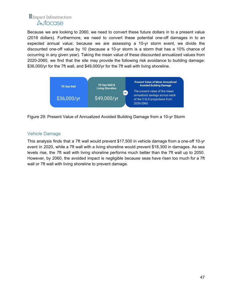
Because we are looking to 2060, we need to convert these future dollars in to a present value (2018 dollars). Furthermore, we need to convert these potential one-off damages in to an expected annual value; because we are assessing a 10-yr storm event, we divide the discounted one-off value by 10 (because a 10-yr storm is a storm that has a 10% chance of occurring in any given year). Taking the mean value of these discounted annualized values from 2020-2060, we find that the site may provide the following risk avoidance to building damage: $36,000/yr for the 7ft wall, and $49,000/yr for the 7ft wall with living shoreline.

Figure 29: Present Value of Annualized Avoided Building Damage from a 10-yr Storm

Vehicle Damage This analysis finds that a 7ft wall would prevent $17,500 in vehicle damage from a one-off 10-yr event in 2020, while a 7ft wall with a living shoreline would prevent $18,300 in damages. As sea levels rise, the 7ft wall with living shoreline performs much better than the 7ft wall up to 2050. However, by 2060, the avoided impact is negligible because seas have risen too much for a 7ft wall or 7ft wall with living shoreline to prevent damage.

47

Figure 30: Avoided Vehicle Damage from a 10-yr Storm the Year in Which the Storm Occurs Converting these one-off costs into an annualized risk in 2018 dollars generates the following results: a 7ft wall avoids $740/yr in vehicle damage, while a 7ft wall with living shoreline prevents $1,250/yr.

Figure 31: Present Value of Annualized Avoided Vehicle Damage from a 10-yr Storm

Emergency Shelter Costs A 7ft wall at the FMPC site would avoid roughly $330 in emergency shelter costs from a 10-yr storm occurring in 2020, while a 7ft wall with a living shoreline would avoid $360. Both sea wall types continue to provide savings to 2050, with the living shoreline providing greater benefits. By 2060, both sea wall types no longer perform any meaningful flood prevention.

48

Figure 32: Avoided Emergency Shelter Costs from a 10-yr Storm the Year in Which the Storm Occurs Converting these one-off costs into an annualized risk in 2018 dollars generates the following results: a 7ft wall avoids $14/yr in emergency shelter costs, while a 7ft wall with living shoreline prevents $16/yr.

Figure 33: Present Value of Annualized Avoided Emergency Shelter Costs from a 10-yr Storm

Total Flood Impact Combining the avoided building damage (structure and contents), avoided vehicle damage, and avoided emergency shelter, we can see that both sea wall types perform better than the existing sea wall.

49

Figure 34: Total Avoided Costs from a 10-yr Storm the Year in Which the Storm Occurs Converting these one-off costs into an annualized risk in 2018 dollars generates the following results: a 7ft wall avoids $40,200/yr in total costs, while a 7ft wall with living shoreline prevents $54,900/yr.

Figure 35: Present Value of Annualized Total Avoided Costs from a 10-yr Storm

50

4.1.3. Ecosystem Services from Living Shoreline Features

At the FMPC site level ecosystem benefits are only attributed to the 7ft sea wall with living shoreline of approximately $43,000 present value over the life of the project with risk ranges of approximately $4,000 to $105,600. Table 10 below illustrates the value of the proposed mangroves and cordgrasses area for recreation and tourism, carbon sequestration, non-use values, water and waste filtration, and the total value over the project. The total value of ecosystem services at the FMPC site for the 7ft sea wall with living shoreline is comprised of approximately $31,000 from recreation and tourism, less than $1,000 for carbon sequestration, $8,800 for non-use values, and about $2,000 for water and waste filtration. See Appendix A for more information on the method applied for ecosystem services valuation of mangroves and seagrasses at the FMPC site level. The 7ft sea wall without living features has $0 living shoreline benefits because of its lack of natural living features to contribute tourism and recreation, carbon sequestration, non-use or water filtration services. Table 10: Value of Ecosystem Services for FMPC Upland Site (Present Value, 2018 dollars)

Ecosystem Service Present Value 95% Confidence Interval

Recreation & Tourism $31,395 $1,646 to $83,598

Carbon sequestration $603 $73 to $1,368

Non-use $8,857 $1,551 to $17,613

Water and waste filtration $1,980 $742 to $3,002

Total value $42,835 $4,012 to $105,581

4.1.4. Costs

Cost of Sea Wall Types The cost of a traditional sea wall is roughly $1,500 per linear foot , and the cost of living 19

shoreline ranges from $1,000 to $5,000 per linear foot . TNC provided cost estimates for a 20

living shoreline at the FMPC of $168,256 (which includes rock, fill, red mangrove, spartina, and bedding stone and sand, as well as a 30% contingency). Given that the length of shoreline at the First Presbyterian Church Site is ~175 feet:

19 Peng, B.; Song, J. A Case Study of Preliminary Cost-Benefit Analysis of Building Levees to Mitigate the Joint Effects of Sea Level Rise and Storm Surge. Water 2018, 10, 169. 20 NOAA Fisheries. 2017. Understanding Living Shorelines.https://www.fisheries.noaa.gov/insight/understanding-living-shorelines#how-much-do-living-shorelines-cost

51

Cost of traditional 7ft high sea wall:

● $262,000 7ft high sea wall with living shoreline:

● $431,000 ($2,460/lf = $1,500/lf for 7’ wall + $960/lf for living shoreline) This analysis assumes that a sea wall would have a useful life of around 40 years, and given the analysis is 40 years, replacement costs did not need to be factored into this report.

Cost of Upland Redevelopment Financial costs of FMPC upland redevelopment include capital expenditures are from capital expenditures (-$176,214) and operations and maintenance (-$55,829) of the GI/LID features (i.e. ICPCs, trees, shrubs, rain garden) and additional site amenities like picnic tables and park benches in addition to replacement costs of GI features (-$15,373).

52

4.2. Economic Impact Assessment (EIA) Results of FMPC

Looking at the EIA assessment results as a whole for the FMPC site, the capital expenditure supports jobs in the construction sector and other industries while producing broader “multiplier” effects on the Miami regional economy. As shown in the table below, the total business output (sales) is approximately 1.75 times as large as the direct investment expenditures as the construction-related activity creates demand for a wide variety of input goods and services, and the earned wages can be re-spent back in the regional economy. Table 11: EIA Results for FMPC Site

Impact 7ft Wall & Upland Redevelopment

7ft Wall with Living Shoreline & Upland

Redevelopment

Direct Cap Expenditure $437,494 $605,494

Business Output (i.e. sales) $764,083 $1,057,495

Value Added $453,200 $627,23

Wages / Earnings $250,640 $346,888

Employment (i.e. jobs) 6 8

FMPC Upland Redevelopment Site with 7ft Sea Wall: The sea wall and site construction at the FMPC site is estimated to be almost $440,000 which would lead to a total business output impact of about $765,000; $453,000 of value-added; $250,000 in new wages for local workers; and approximately six jobs. FMPC Upland Redevelopment Site with 7ft Sea Wall and Living Shoreline: Adding the living shoreline to the sea wall at the church site is projected to cost a total of $605,000, which would lead to a total business output impact of about $1.1 million along with $627,000 of value-added, $347,000 in new wages for local workers; and approximately 8 jobs.

53

5. Flood Insurance Considerations Flood insurance is provided to individuals through FEMA’s National Flood Insurance Program via local insurance providers. Private insurers provide additional insurance for properties that are valued at more than FEMA’s maximum structural and content coverage. A property’s insurance premium is determined by several factors including the flood zone it resides in, assessed property and contents value, building type (e.g. condo, single dwelling), building attributes (e.g. building elevation, basement, crawlspace), building date, and base flood elevation. The deductible is determined in conjunction with the premium rate and other factors. 21

A primary trigger that determines premiums is the flood zone. Most of Downtown Miami is located within FEMA Special Flood Hazard Areas (SFHAs) Flood Zone AE, AH, VE, or X. 22

Properties in these flood zones are required to obtain flood insurance in order to secure funding so the effects of a property’s premium rate is notable. Flood Zone VE has the most risk as it corresponds to a 1% annual chance coastal floodplain that has additional hazards associated with storm waves. Flood Zone AE is less severe and rated for floodplains with a 1% annual chance of flooding. Zone AH is rated for 1% annual chance shallow flooding (usually areas of ponding) while X flood zones have limited risk of 0.02% to 1% shallow flooding. The impacts 23

on insurance premiums from building a 7ft sea wall or 7ft with living shoreline would be from how these seawalls would change the triggers of premium rates mentioned above. For example, if a seawall contributed to a change in the flood zone from a VE to AE zone on the flood insurance rate map (FIRM) , then properties in that flood zone could receive reduced premiums 24

if properties/communities follow through with FEMA NFIP protocols and requirements. The process for FEMA to make revisions to its FIRM may be done through several ways including letter of map change (LOMC), letter of map revision, letter of map amendments, or others. 25

The FMPC upland redevelopment site is currently within an AE flood zone, which is not the most severe coastal hazard zone. Therefore the site could need additional flood mitigation infrastructure like increasing first floor elevations, combined with implementing a sea wall in order to mitigate flooding risk enough to change its flood zone classification, and thus secure a lower rate.

21 FEMA. 2018. FEMA NFIP Flood Insurance Manual - Appendix J: Rate Tables. https://www.fema.gov/media-library-data/1538670910296-81423feb161c06426ac157a409123f3d/app-j_rate_tables_508_oct2018.pdf 22 Miami-Dade County. Flood Zones. https://mdc.maps.arcgis.com/apps/webappviewer/index.html?id=685a1c5e03c947d9a786df7b4ddb79d3 23 FEMA. 2016. Mandatory Purchase of NFIP Coverage. https://www.fema.gov/faq-details/Mandatory-Purchase-of-NFIP-Coverage/ 24 FEMA. 2015. Flood Insurance Rate Map. https://www.fema.gov/faq-details/Flood-Insurance-Rate-Map 25 FEMA. 2018. Flood Map Revision Processes. https://www.fema.gov/flood-map-revision-processes#4

54

This project will not conclude any flood zone changes due to the sea wall given the lack of the fundamental project-specific evidence and peer-reviewed confirmation from industry experts like engineering, actuaries or insurance underwriters, flood plain manager, or hydrologists of the impact of the downtown sea wall on properties’ insurance fee triggers like flood zones. Currently eligible properties in Miami receive a discount of 15% in SFHAs on their flood insurance premiums under the Community Rating System (CRS) because the City of Miami is rated as a Class 7. The CRS program recognizes and encourages community floodplain 26

management activities that exceed the minimum NFIP standards. If FEMA officials and other industry experts considered a 7ft seawall or 7ft seawall with living shoreline in Downtown Miami as an flood mitigation activity that could give enough credits to push the City of Miami to a Class 6 (a 20% discount to eligible properties in SFHAs), the City of Miami could receive an additional 5% discount that could lower eligible properties’ insurance premiums. 27

To provide Miami DDA with an illustrative example of this potential value, Impact Infrastructure used FEMA Policy & Claim Statistics for Flood Insurance data of the written premium in-force for the City of Miami as of September 30 2018 combined the assumption that all properties that pay FEMA NFIP premiums are in a SFHA and eligible for the CRS discount. Applying a 5% 28

discount to written premiums in-force for the City of Miami for illustrative purposes only, it is estimated that a potential incremental discount could have a present value of approximately $21 million over 40-years. As stated in preceding content, the missing link to enable the robust and property-specific monetization of flood insurance fee impacts was the lack of fundamental project-specific evidence and peer-reviewed confirmation by industry experts of the impact of the Downtown sea wall on properties’ insurance fee triggers (e.g. flood zone, base flood elevation, CRS Class). Impact Infrastructure attempted to determine the impact of a 7ft seawall and 7ft with living shoreline seawall on these triggers through peer-reviewed literature and stakeholder engagement, such as reaching out to flood insurance underwriters in the City of Miami, an insurance research institution, FEMA, City of Miami flood plain manager and CRS coordinator. Yet these experts were unable to confirm how the hypothetical downtown sea wall considered in this project would impact these insurance triggers without project-specific evidence. Without this essential evidence, Impact Infrastructure could not robustly provide an estimate of the economic value of reduced flood insurance fees (e.g. premiums, deductibles, coverage).

26 FEMA. 2018. COMMUNITY RATING SYSTEM. https://www.fema.gov/media-library-data/1523648898907-09056f549d51efc72fe60bf4999e904a/20_crs_508_apr2018.pdf 27 FEMA. 2017. National Flood Insurance Program Community Rating System Coordinator’s Guide. https://www.fema.gov/media-library-data/1493905477815-d794671adeed5beab6a6304d8ba0b207/633300_2017_CRS_Coordinators_Manual_508.pdf 28 FEMA. 2019. Policy Statistics. https://bsa.nfipstat.fema.gov/reports/1011.htm

55

6. Discussion: Qualitative Impacts and Caveats The value of resiliency spans a huge variety of financial, social, and environmental impacts. This report has attempted to capture a significant number of these in order to approximate a true value of resiliency investment. However, there are undoubtedly some impacts that are not captured because: 1) they can be monetized but were not included due to data limitations, or 2) can not be reasonably and defensibly monetized. Impacts that theoretically can be monetized but were left out due to data limitations include, but are not limited to: insurance premiums, transportation delays, flood-related casualties, flood debris damage, and critical infrastructure damage. Mangroves serve as natural barriers for shoreline protection; they attenuate destructive wave energy and reduce the impact of storm surges. This effect of mangroves could improve the 29

useful life of seawalls. Regarding damage due to casualties and critical infrastructure, the COAST model does not provide outputs that can be used to formulate values. As has already been mentioned, because H&H modeling had not been conducted for the site in question, FEMA’s HAZUS tool was not able to be used, which prevented the team from being able to generate a broader set of flood damage valuation metrics. Nevertheless, since the project focuses on a 10-yr event, rather than a more severe storm, the impact to casualties is not likely to be a significant gap in the analysis. Furthermore, relatively forward thinking planning policies in the City of Miami limits the importance of monetizing damage to critical infrastructure due to the fact it has been designed in such a way that it limits the risk from storm events i.e. not placing it underground. It is worth noting that this analysis only assesses reduced flooding risk from 10-yr storm event; assessing the full spectrum of flood events (25, 50, 100, & 500-yr) would offer a fuller picture of the flood impacts under each scenario. However, it may be the case that stronger storms are too powerful for the 7ft wall or 7ft wall with living shoreline to generate any meaningful risk reduction benefits versus the current 5ft scenario. Furthermore, the analysis takes a snapshot of the current land use, population, and property values etc. This means that factors such as future additional housing stock and population

29 Narayan, S., Beck, M.W., Wilson, P., Thomas, C., Guerrero, A., Shepard, C., Reguero, B.G., Franco, G., Ingram, C.J., Trespalacios, D. 2016. Coastal Wetlands and Flood Damage Reduction: Using Risk Industry-based Models to Assess Natural Defenses in the Northeastern USA. Lloyd’s Tercentenary Research Foundation, London.

56

growth, as well as how transportation technology may affect vehicle usage and car numbers are not accounted for. Therefore, it may be possible these results underestimate the potential true cost. However, we can’t be sure where population or development will be growing within the city, and it is possible that development in high risk areas will slow - especially as new information regarding sea level rise comes to light, so even if population were to grow over time, the number of people, parcels, and cars directly impacted may not increase with those projections.

57

7. Appendix A: Methodology

7.1. Impact Infrastructure Impact Infrastructure’s team of professionals across North America have developed best-practice cost-benefit analysis approaches and tools and have been involved in all facets of infrastructure development. The firm has worked with corporations and all levels of government to support decision making, project prioritization, and stakeholder outreach. Our primary goal is to create a standardized suite of business case analysis tools to promote the development of more sustainable and resilient communities. The company’s economics professionals conduct rigorous economic assessments to help decision makers prioritize worthy but competing projects for funding based on maximum economic, environmental and community benefits. We have also built the market-leading cloud-based automated economic analysis software, Autocase, with modules for evaluating buildings and GI/LID. In aggregate, our team’s track record of conducting economic assessments to inform decision making spans roughly $50 Billion of projects. Impact Infrastructure is also an Institute for Sustainable Infrastructure (ISI) Charter Member, an Envision Qualified Company, and a 100 Resilient Cities (Rockefeller Foundation) Platform Partner. This appendix describes the detailed methodologies for the Autocase software impacts, as well as the exogenous models that were created, including flood risk.

7.2. TBL-CBA Methodologies and Inputs 7.2.1. TBL-CBA Framework

This project was conducted using a Triple Bottom Line Cost Benefit Analysis (TBL-CBA) framework. TBL-CBA provides an objective, transparent, and defensible business case framework to assess investments. The analysis broadens traditional financial analysis to incorporate and value social and environmental factors within an expanded CBA framework. The intent of these analyses is to determine the net social and environmental benefits (net benefits means costs minus benefits), in addition to the lifecycle financial costs and avoided costs that arise from projects. Cost benefit analysis (CBA) is a conceptual framework that quantifies in monetary terms as many of the costs and benefits of a project as possible and converting them all into a present day dollar value. In CBA, a “base case” (the existing conditions) is compared to one or more alternatives (which have some significant improvement compared to the base case). The analysis evaluates incremental differences between the base case and the alternative.

58

For this analysis, the TBL-CBA was conducted for a 41-year study period with 40 operating years and one year of construction period beginning in January 2019. Costs and benefits are discounted at 3.5% to present value, assuming a base year of 2018 and using 2018 US dollars.

7.2.2. Base Case and Design Case The TBL-CBA of the hypothetical FMPC upland site is conducted relative to a base case. The hypothetical FMPC upland site is the design alternative and the base case is the current site conditions of unmanaged shoreline.

7.2.3. Valuation Methodologies and Inputs The following section provides detailed methodology descriptions for each of the costs and benefits examined. For this assessment, Autocase for Sites and external modelling were used to value:

● Capital expenditures; ● Operations and maintenance costs; ● Replacement costs and residual value; ● Property value; ● Recreation value; ● Heat island effect; ● Education value; ● Public health; ● Flood risk from the FMPC Upland Redevelopment; ● Living shoreline benefits; ● Water quality; ● Carbon reduction by vegetation; and ● Air pollution reduction by vegetation.

7.2.4. Financial Impacts

Capital Expenditures Capital expenditure estimates for interlocking porous concrete pavers (IPCPs), rain garden, trees, and shrubs. The costs for IPCPs, rain garden, and shrubs are based on estimates from Autocase for Sites default data ($ per sq ft) and their associated risk ranges. Per unit costs are 30

then combined with the estimated area of plantings to derive total capital expenditure costs. Capital costs for trees are based on a per tree cost.

30 Sources used in the cost estimation of design features IPCPs, rain garden, trees, and shrubs are varied and include: CNT Fact Sheet, CNT Methodology, WERF 2009, Orange County BMP, Toronto Regional Conservancy, University of Toronto, EPA (1999), OptiTOOL, EPA Charles River Authority, CRWA, BMP Western Washington.

59

For rain garden feature, the area of plantings was derived from the number of plants and on centre (O.C.) planting specifications that was detailed in the site design provided by Miami DDA. The rain garden would include a mix of Purple Muhly Grass (Muhlenbergia capillaris), Swamp Lily (Crinum americanum), Coontie (Zamia pumila), Butterfly Weed (Asclepias tuberosa), and Moon Vine (Ipomoea pes-capre), for a total area of 569 sq-ft. Other site amenities are picnic tables, park benches, shade umbrellas, litter receptacles, bike racks, and lighting posts as specified in the hypothetical site design provided by Miami DDA. Per item costs are based on costing information from Landscape Forms . Per item costs for 31

lighting poles are based on estimates from Florida Department of Transportation. Cost ranges 32

for site amenities are based on AACE International’s Cost Estimate Classification System, allowing costs to be 30% below budget up to 50% above budget. 33

Table A.1: FMPC Upland Site Amenities

Type # Unit Cost

(2018 dollars)

35 Collection: 4-Seat Backed Tables 4 $3,315

35 Collection: 2-Seat Backed Tables 2 $2,955

35 Collection: Stay Backed Bench with Arms and Two Dividers 6 $2,710

Umbrella with Surface Mount Stand 6 $3,950

35 Collection: Pitch Side-Opening Litter Receptacle 2 $1,475

35 Collection: Loop Bike Rack 4 $375

Light Posts 4 $14,337

Operations and Maintenance Costs Operations and maintenance (O&M) costs are those that occur yearly throughout the life of the project. Values are discounted to produce a present value of the costs. O&M costs for IPCPs, rain garden, trees, shrubs are based on estimates from Autocase for Sites default data ($ per sq ft). 34

31 Landscape Forms. 2018. 2018 End of the Year Pricebook, https://pricebook.landscapeforms.com/Print-Page.aspx?cp=true&cmp=207;657;656;655;225;226;228;227;639;640;638;302;208;658;659;660;189;185;198;188;211;&pb=53&curr=USD 32 Florida Department of Transportation - District Six. 2013. Lighting Justification Report. www.fdotmiamidade.com/pde-projects/pdf.../3650-Lighting_Justification_Report.pdf 33 AACE International. (December 2012). Cost Estimate Classification System - As Applied for the Building and General Construction Industries. AACE International Recommended Practice No. 56R-08. 34 Sources used in the cost estimation of design features IPCPs, rain garden, trees, and shrubs are varied and include: CNT Fact Sheet, CNT Methodology, WERF 2009, Orange County BMP, Toronto Regional

60

O&M costs for the other site amenities (i.e. picnic tables, park benches, shade umbrellas, litter receptacles, bike racks, and light posts) were derived using the 2017 city park data from the Trust for Public Lands. The per acre operation spending estimate of $241 in 2018 dollars was 35

estimated using total spending on Miami parks, total miami park acres, and the share of per acre spending attributed to operation. Operation spending is defined by the Trust for Public Lands as, “year-in, year-out work such as landscape and tree maintenance, facility maintenance, trash removal, recreational programming, planning, administration, policing, lighting, marketing, etc." This provides a rough estimate for additional O&M spending that could be attributable to the amenity features (e.g. park benches, litter receptacles) in the hypothetical upland redevelopment site design.

Replacement Costs and Residual Value All elements of an infrastructure project need to be replaced at some point. All feature types have different lifespans, as well as different costs of replacement at the end of their operating lives. Autocase quantifies these costs as the lifetime “Replacement Costs” of each feature. Replacement costs for features are estimated whenever the expected operating duration of the project exceeds the lifespan of a feature. Replacement costs are then combined with the expected lifespans of each feature type and the operating life of the project to quantify the expected total replacement costs. When a project’s operating life comes to an end, assets can still have an implicit residual value. Depending on the remaining useful life of the asset for each alternative, at the end of the study period, some site elements have a “residual value”. The residual value was calculated by determining the assets’ useful lives remaining at the end of the period and determining an appropriate value of the asset based on its remaining useful life. Autocase estimates this residual value by assuming straight-line depreciation in the value of the design features. This value is then discounted into present value terms. For the FMPC design, it is estimated that replacement costs IPCPs, rain garden, trees, and shrubs could be approximately $15,373 with risk ranges between $22,600 to $10,091. Residual value of the site features - IPCPs, rain garden, trees, and shrubs - could be $120,539 with risk ranges of $48,352 to $217,084. Replacement costs or residual values were not calculated for the other site amenities - picnic tables, park benches, litter receptacles, bike racks, or lighting posts. It is assumed these would have the same lifetime as the project of 40 years.

Conservancy, University of Toronto, EPA (1999), OptiTOOL, EPA Charles River Authority, CRWA, BMP Western Washington. 35 The Trust for Public Lands. 2017. City Park Facts. https://www.tpl.org/sites/default/files/files_upload/CityParkFacts_2017.4_7_17.FIN_.LO_.pdf

61

7.2.5. Social Impacts

Property Value High quality landscape design will improve the aesthetic quality of the surrounding area, creating a more desirable neighborhood. The literature tells us that it is highly likely that property values – not only adjacent to the low impact development (LID) – but beyond, will increase as a result. To estimate this impact, we use a US EPA meta-analysis of 35 hedonic property valuation studies on the benefits of general open space and low impact development (Mazzotta, Besedin, & Speers, 2014). Autocase estimates the percent change in a home’s value for an observed percent change in the amount of open green space, while factoring in other influencing characteristics, such as existing house prices (at the zip code-level for USA), existing green space within 500m, the the distance of the property from the LID, and whether there are recreational facilities, among others. Our model is based on literature that suggests properties within 0.15 mile of the LID will be impacted to a greater extent than properties 0.15-0.3 miles from the LID. Based on the literature, we assume that properties more than 0.3 miles from the LID amenity will not be affected, which is consistent with the distance people are generally willing to walk for local amenities. Once the percentage increase in property value is calculated for the two distance bands (within 0.15 miles and 0.15-0.3 miles), we convert the total increase in value to an “annual rental equivalence” i.e. a yearly benefit, since we do not know what year the property will be sold. Essentially this estimates the yearly increase in rent that would be gained, if this property were to be rented out, since the price of a home can be thought of or represented as the sum of the discounted future annual rental-equivalent values of living in that home. The model multiplies this yearly increase in value of a property by the number of properties in each distance band (within 0.15 miles and 0.15-0.3 miles) to calculate the total yearly benefits for all properties within 0.3 miles of the LID. These yearly benefits are then discounted according to the time horizon of the project to create a present value of the benefits. The model assumes a property value in the base year of $403,142 and defaults the number of properties in each band given property density data (600 within 0.15 miles and 1,367 within 0.15 miles and 0.15-0.3 miles). The estimated increase in property value that could occur due to this project can be estimated at $550,034 in present value with risk ranges of $547,358 to $552,798 over the 40-year project period.

62

Recreation Value The hypothetical FMPC upland site could add amenity value to current users of the site. It is expected that the additional site amenities including the 4-seat and 2-seat backed tables, park benches, litter receptacles, bike racks, and lighting posts will be beneficial for recreational opportunities. Use values can be assigned to the various recreational amenities offered by the environment. Although the protection of public space and the provision of recreational amenities are typically not priced, they nevertheless have significant value to society, and economists have developed sophisticated analytical techniques to derive monetary values for these types of goods. Using a methodology developed by the US Army Corps of Engineers and combined with an activity specific direct use value model developed by The Trust for Public Land’s Center for City Park Excellence, based on willingness-to-pay values for specific recreational opportunities, the recreational benefit of the hypothetical FMPC upland site is monetized. The model incorporates low and high risk ranges into the analysis, which is important because the valuation of how much people are willing to pay for a recreational experience can be uncertain. Given daily pedestrian counts from the current FMPC provided by Miami DDA of 2018 pedestrians per day, an annual user count was derived to be 736,570 pedestrians per year. Impact Infrastructure made the following assumptions in order to estimate the potential value of recreation for the hypothetical FMPC upland site. It is estimated that there are several parks within 3 miles and a few within 1.5 miles travel with the same amenities as those proposed for the FMPC upland site. This is based on Miami-Dade’s community services mapping tool of nearby city and county parks and bike trails as well as the site design from Miami DDA was developed based on downtown baywalk area development requirements. Furthermore, given 36

the hypothetical design features of the FMPC upland site, it is assumed to have the following recreational activity uses as indicated below in Table A.2. Additionally, it is assumed that current pedestrians that walk along the unmanaged shoreline would use the additional amenities featured in the hypothetical FMPC upland site. The recreational value could be $2,332,546 with risk ranges of $1,894,903 to $3,497,324 over the 40-year project period. This is representative of the additional amenity value to current pedestrians of the site and does not estimate the incremental value of potential new users due to the site.

36 Miami-Dade County. 2017. Community Services. https://gisweb.miamidade.gov/communityservices/

63

Table A.2: FMPC Upland Site Recreational Characteristics

Category of Recreation Yes/No

Playground No

Picnic/Bench-sitting Yes

Walking on Trails Yes

Walking Dog in Park Yes

Birdwatching/Nature Yes

Running Yes

Rollerblading Yes

Biking Yes

Skateboarding No

Waterbody used for Water Activities Yes

Tennis No

Team Sports No

Flower Gardens Yes

Golf Courses No

Community Gardening No

Festival or Performances No

Visiting Historical Sites No

Visiting Arts & Crafts Fairs No

Heat Island Effect The Urban Heat Island (UHI) effect compromises human health and discomfort by causing respiratory difficulties, exhaustion, heat stroke, and heat-related mortality. Green infrastructure and light-colored surfaces can reduce the severity of extreme heat events by creating shade and reducing the amount of heat absorbed by traditional pavement and rooftops. Even a small cooling effect can be sufficient to reduce heat stress-related fatalities during extreme heat wave events. This cooling effect is monitored in terms of a temperature change on a monthly basis. Various studies have estimated that trees, shrubs, and other vegetation within sites can reduce temperatures by 5 °F when compared to outside non-green space. At larger scales, variation

64

between non-green city centers and rural areas has been shown to be as high as 9 °F during the day and up to 22 °F during the night. Besides vegetation, the level of surface albedo can determine the change in temperature. Albedo measures the level of heat reflectivity of a surface. To quantify heat risk mitigated, the first step is to determine reduced temperatures in the area as a result of increased vegetation in the project. Climate change is accounted for by using U.S. monthly forecasted temperature data from sources such as the Canadian Centre for Climate Modelling and Analysis (CCCMA). Forecasted temperature is calculated on the basis of future carbon concentration assumptions, more commonly known as Representative Concentration Pathways (RCPs). The model provides the option of choosing either RCP 4.5 or RCP 8.5 to provide two possible climate futures. Greenhouse Gas (GHG) emissions in RCP 4.5 peak around 2040, and in RCP 8.5, GHG emissions continue to increase throughout the 21st century. The reduction in temperature is then used to determine avoided death over the life of the project. The reduction in the average annual mortality rate is dependent on the difference in surface temperature before and after the FMPC Upland Site mean daily maximum temperature predictions based on CCCMA, the local mortality rate (state-level), and the local (city-level) temperature threshold at which the impacts of heat on mortality can be detected (referred to as the Minimum Mortality Temperature, or MMT). Finally, the Value of Statistical Life, is used to quantify the benefit of reduced heat mortality rates. Permeable pavers, trees, shrubs, and rain garden in the hypothetical FMPC Upland Redevelopment Site design positively impacts urban heat island effect reductions, which are estimated to be $43,117 present value over the 40-year life of the project. Additionally, it is estimated that there would be about a 0.036 Fahrenheit change in temperature over the 40-year life of the project due to these GI/LID features exactly at the FMPC upland redevelopment site.

Education Value GI/LID investments often offer a unique opportunity to promote eco-literacy and environmental education for children and adults alike. Ultimately, we use the cost of educating a child to monetize the educational benefits of the upland redevelopment site at the FMPC, with the assumption that education within the classroom is equivalent to education at the project site. We multiply the estimated number of student hours spent on-site by the cost of educating a student per hour to give us the educational value for the time students spend at the project site. We calculate the hourly cost of educating a student by dividing each state’s total per-student spending by the number of hours each student attends in school. Multiplying the cost of one student-hour by the estimated number of student-hours spent at the project site (e.g. a class of 30 students spending 2 hours on-site equals 60 student-hours) enables us to determine the

65

educational value associated with the project. Given that an estimate of student-hours expected for the hypothetical upland redevelopment was unobtainable, the default in Autocase for Sites was used as a rough estimate. This default is based on estimates of educational use hours for parks calculated using school survey information from the county of Sonoma, California. Schools and school districts reported the number of hours their students spent at parks in the county for educational purposes. These reported hours were used to calculate total annual educational hours spent at each park, and then per acre averages were estimated. Using the total GI/LID of the upland redevelopment of FMPC (approximately 0.2-acres) and this default, an educational benefit of $1,540 with risk ranges between $246 to $3,906 was estimated for the hypothetical site over the 40-year project period. 37 38 39

Public Health GI/LID, parks, and greener streets are more attractive for exercise. The economic benefits of improved health from engaging in regular physical activity can be valued as the prevented – or avoided – reduction in productivity that results from that activity. Lost economic output from people being out of work or not engaged while at work represents the social cost in this model. In order to determine this value, we need to estimate 1) the amount of time adults spend at the park exercising, and 2) the cost per minute – in terms of lost productivity – of not exercising. By multiplying the two, we find the avoided cost due to engaging in physical activity. To estimate the cost per minute of inactivity (or avoided cost of a minute’s activity), we use a study that showed the lost productivity (absenteeism i.e. being away from work, and presenteeism i.e. not being able to work well even when you are present at work) in percentage terms of inactivity. Multiplying these productivity losses by the GDP per capita, we can establish the annual per person cost of lost productivity from inactivity. Given that the CDC states there are 7,800 minutes (150 minutes a week) of exercise needed in a year to avoid lost productivity, we work out the per-minute avoided cost of activity by dividing the cost of lost productivity by 7,800. Multiplying the per-minute avoided cost of activity by the estimated number of minutes on the park gives us an estimate of the avoided productivity losses due to inactivity that can be attributed to the park.

37 NCES. (2008). Schools and Staffing Survey: Average number of hours in the school day and average number of days in the school year for public schools, by state: 2007–08. Retrieved from https://nces.ed.gov/surveys/sass/tables/sass0708_035_s1s.asp 38 U.S. Census Bureau. (2014). 2014 Public Elementary–Secondary Education Finance Data. Retrieved from https://www.census.gov/data/tables/2014/econ/school-finances/secondary-education-finance.html 39 Sonoma County Education Survey” (2016) Sonoma County Office of Education, Sonoma CA. California Department of Education.

66

It is assumed the number of visitors to the park is the same amount of recreational users, amounting to 2,018 daily users or 736,570 annual users. The amount of time spent at the park is estimated as approximately 1 minute as visitors could walk the linear distance of the shoreline (175 ft) at a pace of 3 miles per hr. The estimated present value of public health benefits for the hypothetical FMPC upland site could be $216 with risk ranges between $126 to $296 over the lifetime of the project.

Flood Risk from the FMPC Upland Redevelopment Flood risk is quantified by estimating the percent flood risk mitigated as a result of the project design. As climate change has progressed and rainfall events in some regions have become more extreme, flood risk has become an important consideration in infrastructure development. Autocase quantifies the value of reduced flood risk due to a smaller volume of runoff from the project’s property during storm events. Runoff can be reduced by increased green acreage, stormwater storage capacity, stormwater drainage capacity, or reducing the surface area covered by impervious land. Flood risk is quantified in Autocase by estimating the percent flood risk mitigated in the city because of the project design. The components to this methodology are explained as follows:

1. The first is estimating the total flood risk damage in any given year. 1. Flood risk is estimated based on historical property value and historical flood

damage in each state in the United States. 2. The second component to the flood risk methodology is determining the flood risk

mitigated because of the project. 1. This uses historical rainfall data from over 6,000 weather stations across the

United States and Canada, enabling location-specific rainfall data to estimate the rainfall amounts in large storm events each year. Precipitation trends from climate change predictions are also incorporated into the modeling.

2. Estimated flood risk mitigated by the design is equal to the change in retention and infiltration capacity beyond the site’s base capacity, divided by the approximate city-wide flood volume in storm events.

3. The overall flood risk mitigated each year is calculated by multiplying total city property value by the flood risk mitigated.

Although the value at risk increases linearly when compared with storm repeat rate, this actually implies that risk increases exponentially as rainfall depth goes up. This is due to the fact that rainfall levels off as the storm repeat rate goes up. In other words, going from a 10-year storm to a 40-year storm may double rainfall depth from 2.5 inches to 5 inches, but that same doubling from 5 inches to 10 inches may be extremely improbable, even in a 10,000-year storm. In short, for each extra 0.1 inches of rainfall, flood damage is exponentially costlier.

67

The Autocase flood risk methodology is a dynamic simulation, meaning that for every year in each iteration of the simulation, it produces different risk values. For example, flood risk mitigated due to a decrease of impervious surfaces might be zero for most years. However, in some years there may be rainfall events that are extraordinarily large, at which point there could be massive flooding and the value of reduced flooding due to higher infiltration rates on the site may have value. This is reflected in the Autocase methodology, as there is an element of randomness applied to the rainfall estimates for each year. This means that Autocase’s analysis is a better reflection of reality than assuming constant maximum storm strength each year or simply estimating reduced damage value from synthetic design storms, such as 10-, 20-, 50-, and 100-year storms. The inputs for the FMPC upland site include TR-55 stormwater model, soil type, and 24-hr design storm. The preferred stormwater model, TR-55, uses the Curve Number method to characterize a site based on land use cover and soil type. Soil Type B is the dominant soil on the project site, which means it is a silt loam or loam that is moderately deep to deep, moderately well drained to well drained with moderately fine to moderately coarse textures. The 24-hr design storm of 10.08 inches is the amount of runoff that the site must be able to handle over a 24-hr period. The benefit of flood risk reduction that could be attributed to the hypothetical FMPC upland redevelopment site could be $35,960 present value over the 40-year life of the project. 40

7.2.6. Environmental Impacts

Ecosystem Services from Living Shoreline of Mangroves and Seagrasses Ecosystem goods and services can be valued using the total economic value (TEV) approach. TEV categorizes ecosystem services into use and non-use values. The use values are further subdivided into direct use, indirect use, and optional value. Non-use value has three components: altruism, bequest, and existence values (TEEB, 2010). Direct use values of 41

40 Hanson, L. S. & R. Vogel (2008). The Probability Distribution of Daily Rainfall in the United States. Retrieved from http://engineering.tufts.edu/cee/people/vogel/documents/DailyRainfall.pdf Nowak, D. J. & E. J. Greenfield (2012). Tree and Impervious Cover Change in U.S. Cities. Retrieved from http://www.itreetools.org/Canopy/resources/Tree_and_Impervious_Cover_change_in_US_Cities_Nowak_Greenfield.pdf Pielke, Jr., R.A., M.W. Downton, & J.Z. Barnard Miller (2002). Flood Damage in the United States, 1926-2000: A Reanalysis of National Weather Service Estimates. Retrieved from http://www.flooddamagedata.org/flooddamagedata.pdf 41 TEEB. 2010. The Economics of Ecosystems and Biodiversity Ecological and Economic Foundations: Chapter 5: The economics of valuing ecosystem services and biodiversity. Edited by Pushpam Kumar. Earthscan, London and Washington http://africa.teebweb.org/wp-content/uploads/2013/04/D0-Chapter-5-The-economics-of-valuing-ecosystem-services-and-biodiversity.pdf

68

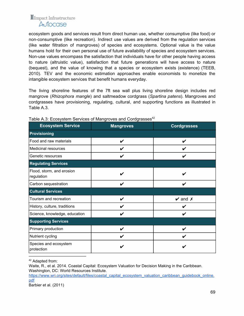
ecosystem goods and services result from direct human use, whether consumptive (like food) or non-consumptive (like recreation). Indirect use values are derived from the regulation services (like water filtration of mangroves) of species and ecosystems. Optional value is the value humans hold for their own personal use of future availability of species and ecosystem services. Non-use values encompass the satisfaction that individuals have for other people having access to nature (altruistic value), satisfaction that future generations will have access to nature (bequest), and the value of knowing that a species or ecosystem exists (existence) (TEEB, 2010). TEV and the economic estimation approaches enable economists to monetize the intangible ecosystem services that benefit humans everyday. The living shoreline features of the 7ft sea wall plus living shoreline design includes red mangrove (Rhizophora mangle) and saltmeadow cordgrass (Spartina patens). Mangroves and cordgrasses have provisioning, regulating, cultural, and supporting functions as illustrated in Table A.3. Table A.3: Ecosystem Services of Mangroves and Cordgrasses 42

Ecosystem Service Mangroves Cordgrasses Provisioning

Food and raw materials ✔ ✔

Medicinal resources ✔ ✔

Genetic resources ✔ ✔

Regulating Services

Flood, storm, and erosion regulation ✔ ✔

Carbon sequestration ✔ ✔

Cultural Services

Tourism and recreation ✔ ✔ and ✗

History, culture, traditions ✔ ✔

Science, knowledge, education ✔ ✔

Supporting Services

Primary production ✔ ✔

Nutrient cycling ✔ ✔

Species and ecosystem protection ✔ ✔

42 Adapted from: Waite, R., et al. 2014. Coastal Capital: Ecosystem Valuation for Decision Making in the Caribbean. Washington, DC: World Resources Institute. https://www.wri.org/sites/default/files/coastal_capital_ecosystem_valuation_caribbean_guidebook_online.pdf Barbier et al. (2011)

69

Literature sources suggest that there is conflicting evidence of the recreational or tourism cultural services of seagrasses. , , , For this analysis, we exclude cordgrasses from the area 43 44 45 46

used to derive recreational and tourism ecosystem benefits. Mangroves serve as natural barriers for shoreline protection, they attenuate destructive wave energy and reduce the impact of storm surges. The intricate root system of mangroves also 47

makes these underwater forests attractive to fish and other organisms seeking food and shelter from predators. Along the southeast Florida coast, mangroves provide critical nursery and 48

foraging habitat for marine aquatic and water bird species. Mangroves have also been found 49

to filter nitrogen, phosphorous, and heavy metals - all commonly found in wastewater and stormwater. Both mangroves and cordgrasses have the provisioning service to sequester 50

carbon. , , Table A.3 above illustrates the multitude of ecosystem services mangroves and 51 52 53

cordgrasses can provide.

43 Barbier et al (2011) 44 Padilla, J. Analysis of Coastal and Marine Resources: A Contribution to the Philippines Country Environmental Analysis; World Bank: Washington, DC, USA, 2008; p. 57. http://siteresources.worldbank.org/INTPHILIPPINES/Resources/JosePadillaPHICEACoastalandMarineSectorReportOct2008.pdf 45 Waite, R., et al. 2014. Coastal Capital: Ecosystem Valuation for Decision Making in the Caribbean. Washington, DC: World Resources Institute. https://www.wri.org/sites/default/files/coastal_capital_ecosystem_valuation_caribbean_guidebook_online.pdf 46 UNEP. 2006. Marine and coastal ecosystems and human well-being: A synthesis report based on the findings of the Millennium Ecosystem Assessment. UNEP. 76 http://wedocs.unep.org/bitstream/handle/20.500.11822/18066/unep_2006_marine_and_coastal.pdf?sequence=1&isAllowed=y 47 Narayan, S., Beck, M.W., Wilson, P., Thomas, C., Guerrero, A., Shepard, C., Reguero, B.G., Franco, G., Ingram, C.J., Trespalacios, D. 2016. Coastal Wetlands and Flood Damage Reduction: Using Risk Industry-based Models to Assess Natural Defenses in the Northeastern USA. Lloyd’s Tercentenary Research Foundation, London. 48 National Oceanic and Atmospheric Administration. 2018. What is a "mangrove" forest? https://oceanservice.noaa.gov/facts/mangroves.html 49 Lorenz, J. 2013. Southeast Florida Coastal Marine Ecosystem - Shoreline Habitat: Mangroves. http://www.aoml.noaa.gov/ocd/ocdweb/docs/MARES/MARES_SEFC_ICEM__20131001_Appendix_Mangroves.pdf 50 Lorenz, J. 2013. Southeast Florida Coastal Marine Ecosystem - Shoreline Habitat: Mangroves. http://www.aoml.noaa.gov/ocd/ocdweb/docs/MARES/MARES_SEFC_ICEM__20131001_Appendix_Mangroves.pdf 51 Arkema, K., D. Fisher, K. Wyatt. 2017. Economic valuation of ecosystem services in Bahamian marine protected areas. Prepared for BREEF by The Natural Capital Project, Stanford University. 52 Edward B. Barbier Sally D. Hacker Chris Kennedy Evamaria W. Koch Adrian C. Stier Brian R. Silliman. 2011. The value of estuarine and coastal ecosystem services. Ecological Monographs 81(2): 169-193. 53 Gail L. Chmura Shimon C. Anisfeld Donald R. Cahoon James C. Lynch. 2003. Global carbon sequestration in tidal, saline wetland soils. Global Biogeochemical Cycles 17(3).

70

The value of ecosystem services that mangrove forests contribute has been estimated by Salem and Mercer (2012) through a meta-analysis regression. Salem and Mercer (2012) 54

synthesize the mangrove ecosystem valuation literature from 44 studies that monetize the value of mangroves. The authors also standardize studies’ values by using country gross domestic product (GDP) deflators and purchasing power parity (PPP) conversion factors to convert all values to US dollars. Meta-analyses are advantageous as they overcome selection bias and subjectivity of the economist in selecting a “good-fit” value for use in benefit transfer; a meta-analysis provides a statistical framework that incorporates evidence from the entire literature in a way that enables superior summarization and interpretation (Salem and Mercer 2012). Table A.4 below indicates select ecosystem services and their estimated values by Salem and Mercer (2012). Ecosystem service values from mangroves that were not applicable in the Miami context have been filtered out (i.e. timber harvest, traditional uses). The four ecosystem services from mangroves below are applicable to Miami for the following reasons. Recreation and tourism values for mangroves are applicable for this project as mangroves provide nursery habitat for aquatic species that are recreationally caught in the Biscayne Bay area. Carbon 55

sequestration by mangroves is expected to occur in the Miami area. Nonuse values capture by the study encompass bequest values for mangroves, which is transferable to the Miami context as well as existence values for loggerhead sea turtles, which can be found in Biscayne National Park. 56

Additionally, water and waste purification services of mangroves are transferable to the Miami context as during storm events, if stormwater overflows into Biscayne Bay, then mangroves ability to filter stormwater concentrations would be of benefit. Water and waste filtration values within the meta-analysis are mostly based on avoided cost (e.g. abatement cost, avoided cost of mitigation, etc) valuation studies. This valuation method typically estimates the water or waste filtration capacity (e.g. amount of pollutants in effluents removed by the mangroves) and applies the cost of treating such waste or water at local facilities to determine an avoided cost of treatment. Given the lack of Miami-specific data for stormwater filtration services by site specific mangroves at the study area, and given the overall applicability of Salem and Mercer (2012), the authors provide robust water and waste filtration values for this study, as attested in preceding paragraphs.

54 Salem, M. & D. Evan Mercer. 2012. The Economic Value of Mangroves: A Meta-Analysis. Sustainability 4: 359-383. doi:10.3390/su4030359 55 Biscayne Bay Aquatic Preserves and Florida Department of Environmental Protection Coastal and Aquatic Managed Areas. 2013. Biscayne Bay Aquatic Preserve Management Plan. pg. 201 - 204. http://publicfiles.dep.state.fl.us/cama/plans/aquatic/Biscayne-Bay-AP-Management-Plan.pdf 56 National Park Service. 2017. A summary about the Loggerhead Turtle's biology and conservation status. https://www.nps.gov/bisc/learn/nature/species-focus-loggerhead-sea-turtles.htm

71

Table A.4: Mangrove Ecosystem Service Values (2018 dollars per ha per year) (Salem and Mercer 2012)

Ecosystem Service Mean Min Max

Recreation & Tourism $42,285 $2 $565,668

Carbon sequestration $1,078 $44 $4,755

Non-use $19,369 $4 $56,567

Water and waste filtration $5,294 $14 $8,227

Total $68,026 $64 $635,217

The value of the living shoreline can be estimated by taking the area of red mangroves (Rhizophora mangle) and saltmeadow cordgrasses (Spartina patens) and applying a benefit transfer approach using the estimates above from Salem and Mercer (2012) to determine the non-flood benefits of the living shoreline. It is assumed that the living shoreline would be offset 5 ft from the seawall and extend 12 ft into the water from the offset. The living shoreline at the FMPC upland site would be the length of the shoreline 175 ft. Given the living shoreline would be 12 ft deep, the total area of living shoreline would be 2,100 sq-ft. It was estimated that there would be 58 red mangroves to be planted at 5 ft on centre (O.C.) and 244 saltmeadow cordgrasses to be planted at 2 ft on centre (O.C.). Assuming a triangle planting pattern, the total area of mangroves would be 1,255 sq-ft and 845 sq-ft of cordgrasses for a total of 2,100 sq-ft of mangroves and cordgrasses. The living shoreline benefit for the FMPC living shoreline is derived using the total area of both mangrove and seagrass for all ecosystem values (i.e. carbon sequestration, non-use, water and waste purification) but not tourism and recreation. Only the area of mangroves is used for tourism and recreation valuation as literature suggests cordgrasses may not provide that service, excluding the cordgrasses area in the recreation and tourism value calculation is a conservative approach to estimating the value of the living shoreline features. The area of mangroves and cordgrasses for the FMPC living shoreline is combined with each ecosystem service value per area and summed for across all four services: recreation and tourism, carbon sequestration, non-use, and water and waste purification. The total value of mangrove ecosystem services is adjusted for risk with a risk range to derive the total value of living shoreline benefits for the FMPC living shoreline. The value of living shoreline mangroves and cordgrasses would be $42,835 with risk ranges between $4,012 to $105,581 at the FMPC site level. For the Downtown-level analysis, the factor of total shoreline length for the sea wall (44,000 ft) to FMPC upland site shoreline (175 ft) is applied to the FMPC living shoreline value to derive the total value of living shoreline features for the Downtown-level analysis. The value of living

72

shoreline mangroves and cordgrasses could be $10,818,798 with risk ranges between $1,108,375 to $26,502,211. Both FMPC site and municipal-level analysis could overestimate the benefits of mangroves as the area considered includes that of both mangroves and cordgrasses, which cordgrasses may not provide the exact same value as mangroves but is included in this estimate to represent some kind of value for the services provided by cordgrasses.

Water Quality In addition to managing run off, the site provides water quality benefits in the form of pollutant load reductions (total suspended solids, phosphorus, and nitrogen and fecal coliform). Increased acres of vegetation, including forest or wetlands, can positively influence the water quality in a local area. In addition, using GI/LID for stormwater management can reduce the stormwater volume that must be managed by grey infrastructure, reducing the frequency and volume of overflowing sewer systems in large storm events. This leads to improved water quality in local waters. An avoided cost of treatment is approach is applied for this analysis. Autocase values changes in pollutant loadings by estimating the changes in pollutant loads compared to a base case and then applying a social cost of water pollutants to these values. The estimated water quality benefit from the increased GI/LID at the FMPC upland redevelopment site could be $6,764 present value over the lifetime of the project. 57

Carbon Reduction by Vegetation Newly planted trees, shrubs, grasses, and plants can sequester carbon from the atmosphere, reducing the impacts of climate change. Additionally, growing trees, shrubs, grasses, and plants can act as carbon ‘sinks’, absorbing carbon dioxide from the air and incorporating it into their stems or trunks, branches, and roots, as well as into the soil. As with air pollution, plant life often requires maintenance which emits carbon into the atmosphere (“lawn mower effect”) yet carbon sequestration ability more than offsets maintenance emissions. Avoided CO2 emissions, as well as increased CO2 sequestration, are benefits of investing in GI/LID development. Autocase quantifies the carbon sequestration rate for all design features available in the software, given the existing literature on carbon sequestration. It will then value this reduction in carbon emissions by applying the social cost of carbon to the change in total tonnes of avoided CO2e emissions due to the project.

57 Hernandez-Sancho, F., Laminzana-Diallo, B., Mateo-Sagasta, J., & Qadir, M. (2015). Economic Valuation of Wastewater - The cost of action and the cost of no action. Retrieved from http://unep.org/gpa/Documents/GWI/Wastewater Evaluation Report Mail.pdf

73

The social cost of carbon used in this assessment follows the guidance from the Interagency Working Group on Social Cost of Carbon and is valued at $41 per U.S. ton (or $44.80 per tonne) in 2018 with a total reduction in CO2e of 31 U.S. tons (about 28 metric tonnes). This quantitative reduction in carbon emissions is equivalent to taking 6 typical passenger cars off the road for one year. It is estimated that one typical gasoline passenger car emits 4.6 tonnes per year by driving around 11,500 miles per year with a fuel efficiency of 22.0 miles per gallon. 58

The additional 38 trees, 75 (or 3,439 sq-ft) shrubs, and rain garden (569 sq-ft) that are in the hypothetical FMPC site design along the Baywalk could provide carbon sequestration benefits. It is noted that the carbon sequestration potential of green features of the upland redevelopment site are offset by the conversion of unmanaged shoreline to permeable pavers. The carbon stored and sequestered is valued by multiplying by the social cost of carbon. Carbon that could be stored and sequestered could provide a benefit of $1,035 in present value terms over the life of the project with risk ranges of $425 to $1,845. , , , , , 59 60 61 62 63 64

Air Pollution Reduction by Vegetation Criteria Air Contaminants (CACs) are air pollutants emitted by combustion engines, which affect the health of people immediately in their vicinity. Air pollution (or CACs, is removed from the air by trees and shrubs. As the trees on site grow throughout the life of the project their canopies grow and capture air pollutants at an increasing rate. The air pollutants that could be reduced given the hypothetical FMPC upland redevelopment site design include carbon monoxide (CO), sulphur dioxide (SO2), NO2, ozone (O3), and particulate matter smaller than 2.5 micrometers (PM2.5). The air pollution is valued by multiplying by the social cost of each pollutant ranges from $28 per U.S. ton for CO to $338,000 per U.S. ton for PM2.5. Air pollution reductions could provide a benefit of $2,469 over the life of

58 Based on U.S. EPA estimates for a typical gasoline passenger car that drives around 11,500 miles per year with a fuel efficiency of 22.0 miles per gallon. U.S. EPA. 2018. Greenhouse Gas Emissions from a Typical Passenger Vehicle. https://www.epa.gov/greenvehicles/greenhouse-gas-emissions-typical-passenger-vehicle 59 Interagency Working Group on Social Cost of Carbon. (2013). Technical update on the social cost of carbon for regulatory impact analysis-under executive order 12866. Interagency Working Group on Social Cost of Carbon, United States Government. 60 Nordhaus, W. D. (2011). Estimates of the social cost of carbon: background and results from the RICE-2011 model. 61 Stern, N. (2006). What is the economics of climate change? WORLD ECONOMICS-HENLEY ON THAMES-,7(2), 1. 62 U.S. Energy Information Administration. (2011). Voluntary Reporting of Greenhouse Gases Program. US Department of Energy, Energy Information Administration. 63 U.S. Environmental Protection Agency. (2013). eGRID 2012 Files. Retrieved from: http://www.epa.gov/cleanenergy/energy-resources/egrid/index.html 64 U.S. Environmental Protection Agency. (2014). Emission Factors for Greenhouse Gas Inventories. (April), 1-5.

74

the project $1,456 to $3,487. Table A.5 illustrates the unit costs of air pollutions assessed in the TBL-CBA for FMPC upland redevelopment site. , , , , , , , 65 66 67 68 69 70 71

Table A.5: Air Pollution Social Costs

Type Unit Cost ($2018 per U.S. ton)

CO $28

SO2 $43,697

NO2 $7,393

PM2.5 $338,213

O3 $1,308

65 Cai, H., Wang, M., Elgowainy, A., & Han, J. (2012). Updated greenhouse gas and criteria air pollutant emission factors and their probability distribution functions for electricity generating units. 66 European Commission. (2005). Damages per tonne emission of EU25 Member State (excluding Cyprus) and surrounding seas March 2005. (March). 67 Mike Holland, P. W. (2002). Benefits Table Database: Estimates of the Marginal External costs of air pollution in Europe. 68 Friedrich, R., Rabl, A., & Spadaro, J. V. (2001). Quantifying the costs of air pollution: the ExternE project of the EC. Pollution Atmospherique, 77-104. 69 Matthews, H. S., & Lave, L. B. (2000). Applications of environmental valuation for determining externality costs. Environmental Science & Technology, 34(8), 1390-1395. 70 McPherson, G. E., Nowak, D. J., & Rowntree, R. A. (1994). Chicago's urban forest ecosystem: results of the Chicago Urban Forest Climate Project. 71 Muller, N. Z., & Mendelsohn, R. O. (2010). Weighing the value of a ton of pollution. Regulation, 33(2), 20.

75

7.3. Coastal Flood Risk Methodologies The following sections outline the detailed methodology for estimating coastal flood risk avoidance.

7.3.1. Conceptual model

Figure A.1: Conceptual Methodology for Coastal Flood Risk The conceptual model is summarized in the figure above, but essentially Miami DDA wanted to assess the flood risk of a 10-yr storm event for various SLR projections under three sea wall scenarios:

1. Current 5ft sea wall a. This is the current protection around the shoreline.

2. 7ft Sea Wall a. This is the same as the 5ft wall except it would involve raising the current

protection from 5ft to 7ft NAVD across the entire shoreline. 3. 7ft sea wall & living shoreline

a. Not only would this involve increasing the sea wall height from 5ft to 7ft, this type of sea wall would consist of mangroves, grasses, and rip-rap.

76

Current 5ft sea wall

Figure A.2: Example of Traditional 5ft Sea Wall 7ft Sea Wall

Figure A.3: Example of Traditional 7ft Sea Wall

77

Figure A.4: Example of Traditional 7ft Sea Wall with Baywalk

Figure A.5: Example of Traditional 7ft Sea Wall Bulkhead / Sea Wall Cap

78

7ft sea wall & living shoreline

Figure A.6: Example of 7ft Sea Wall with Living Shoreline

Figure A.7: Example of Living Shoreline with Mangroves and Rip-Rap

79

Figure A.8: Example of Living Shoreline with Mangroves and Rip-Rap The figure below illustrates the high-level methodology of how the results are created. There are three main steps in the methodology:

1. Data collection; a. The outermost circle represents data collection. Environmental, social,

geopolitical, and economic data is collected. The data, their source, and format they come in are displayed in the surrounding tables.

2. Data processing; a. Different processing and mathematical operations and techniques will be applied

to these data in COAST and GIS software. These manipulations are illustrated in the inner ring. This process was iterated for the five SLR projections, as well as for each sea wall type.

3. Generating results. a. Data collection and modeling generate the results seen in the center. These

results will be produced for the city as a whole for each SLR scenario and sea wall type.

i. The impacts considered in this analysis include: 1. Structural and contents damage;

80

2. Vehicle damage; 3. Shelter costs; 4. Land area; and 5. Parcels impacts

Figure A.9: High-Level Coastal Flood Risk Methodology

7.3.2. Spatial data model

Geographic boundary The report focuses on the impacts of flooding to the downtown area of the City of Miami, FL. The exact boundary is shown in Figure A.11, which is illustrated by the white parcel boundaries.

81

Figure A.10: City of Miami, FL

Figure A.11: Study Area of Concern (Outlined in Thick Black)

82

Spatial resolution The spatial resolution - or granularity - is outlined in the table below. Table A.6: Spatial Resolution for the Coastal Flood Model

Metric Spatial resolution Interpretation

Flood model 5ft x 5ft

The digital elevation model used as the input in to the COAST flood model gives the elevation for each 5 sq ft area of land.

Economic model Parcel & City The output from COAST gives the depth and damage for each parcel, and the results will be scaled up to the City level.

Temporal resolution This report’s time horizon is from 2020-2060. It does not go beyond 2060 due to the fact that the standard life of a sea wall is typically 40 years.

Sea level rise projections

This report assesses the impact of a 10-yr storm at five separate sea level rise projections from 2020 to 2060 - the details of which can be seen in the table below. Table A.7: Sea Level Rise Projections from 2020-2060

Year SLR (inches above 1992 level)

2020 6

2030 10

2040 15

2050 20

2060 26

Note: Sea Level Rise figures are in inches above 1992 sea levels The Unified Sea Level Rise Projection: Southeast Florida (2015) using the USACE high estimate were used, which predict 6 inches sea level rise for Miami by around 2020, 10 inches

83

by around 2030, 15 inches by around 2040, 20 inches by around 2050, and 26 inches by around 2060. It must be noted, however that there is debate among scientists on the timings of SLR, and this report is not the outlet for such considerations, yet Miami has already seen over 3 inches since 1992 levels.

10-year storm

This report assesses the impact of a 10-year storm event on top of predicted sea level rise. However, what do we actually mean when referring to a 10-year storm? A 10-year storm does not mean a storm that happens every 10 years. Instead, it is a storm that has a 10% chance of happening in any year.

7.3.3. Mathematical model

Flood Model Justification The COAST software was chosen to model the flooding depths that were fed in to the 72

economic loss calculations. The team considered other tools like FEMA’s HAZUS MH model, but despite HAZUS being a FEMA product for hazard loss estimation, and the fact it assesses more intangible impacts than COAST (e.g. casualties, debris etc.) there were limiting factors that prevented its use.

1. Firstly, HAZUS uses a less granular DEM of 33 ft x 33 ft, whereas the team used a 5ft x 5ft DEM - thus allowing for greater precision.

2. HAZUS does not lend itself well to the type of ‘what if?’ scenarios used in this report (i.e. 7ft wall versus a 7ft wall with living shoreline as compared to the current shoreline) unless the H&H modeling has already been completed so as to use the flood depth grids as inputs. Since the H&H modeling had not been done, the team would have had to replace the in-built DEM 11 times - five times to account for the current shoreline under each sea level rise scenario (2020-2060), and then an additional six times to account for a 7ft wall to replace the current shoreline on top of five sea level rise changes.

3. COAST has the ability to specify specific sea level rise projections within the tool, so when you specify a year in the future that the 10-yr storm will hit, it automatically knows the corresponding sea level rise.

4. HAZUS relies on out-dated default data regarding valuation i.e. from the early 2000s, whereas COAST enables you to upload recent valuations easily on a parcel-by-parcel basis.

5. HAZUS conducts analysis at the census block level, whereas COAST gives you the ability to assess impacts at the parcel level.

72 http://www.bluemarblegeo.com/products/COAST.php

84

Despite each model having different benefits compared to the other, ultimately, due to the fact that H&H had not been completed, COAST made the most sense to use over HAZUS as it is better suited to scenario analyses.

Structure and Logic Diagram Figure A.14 illustrates the mathematical model used to generate the results. The main steps in the model are as follows:

1. Inputting the DEM in to COAST, along with SLR projections and exceedance information regarding wave and surge heights for a 10-yr storm, will generate a flooding depth across the region of interest.

2. By overlaying data regarding property characteristics, such as value, location, size, number of units etc., COAST is able to assign each parcel a flood depth for each SLR projection.

3. Using USACE depth-damage functions for structures, contents, and vehicles (Figure A.12), we can generate a damage estimate for each parcel, given the depth of flooding.

Figure A.12: Depth-Damage Functions for Structure, Contents, and Vehicles (USACE)

4. By summing up the damage cost for all affected parcels, we can estimate a city-wide damage for each SLR projection.

5. Iterations were then performed for each sea wall type.

85

a. In order to mimic the 7ft sea wall alternatives, the team manipulated the DEM

using a raster editor to assign coastal pixels a value of 7ft instead of their old value. The result of this process can be seen below in Figure A.13.

Figure A.13: A snapshot of converting the 5ft current shoreline to a 7ft wall. Note: This was done for 44,000 feet of downtown shoreline, including up part of the Miami River east of the I-95.

b. To mimic the living shoreline, the team researched how mangroves and rip rap typically attenuate wave height and storm surge.

i. There is no definitive answer to how mangroves will affect wave height or surge height , however, the best research available showed that wave 73

73 Krauss et al. (2009), using observations during Hurricanes Katrina (2004) and Wilma (2005), showed that intact mangrove wetlands can reduce surge heights by up to 9.4 cm/km inland. Using a numerical model Zhang et al. (2012) showed that mangrove wetlands are more effective at reducing surge heights for fast moving storms (~40km/hr) and that surge reduction varies non-linearly with wetland size. Relative to mangroves, there is much less knowledge about the capacity or value of marshes and other temperate coastal wetlands for reducing flood heights and damages. Loder et al. (2009a) simulated an idealized salt marsh to show that flood heights are reduced by higher bottom friction from vegetation and greater wetland continuity. In a recent field study, Stark et al. (2015) measured surge attenuation rates from 5 cm/km to 70 cm/km in a large tidal marsh.

86

height is reduced 13% - 66% for every 100m of mangrove . Given the 74

living shoreline we are considering is 12’ out to shore, but does include other aspects such as riprap, the team chose 13% wave attenuation.

ii. The result of this 13% reduction in wave height on the computed storm event can be seen in more detail in the section that follows.

74 Spalding M., McIvor A, Tonneijck FH, Tol S and van Eijk P (2014) Mangroves for coastal defence. Guidelines for coastal managers & policy makers. Published by Wetlands International and The Nature Conservancy. http://www.nature.org/media/oceansandcoasts/mangroves-for-coastal-defence.pdf

87

Figure A.14: Mathematical Model for Coastal Flood Risk

88

Flood Model Parameters in COAST

Sea Level Rise Projections

The following projections were taken from the Unified Sea Level Rise Projection: Southeast Florida (2015) using the USACE High estimate. Table A.8: Sea Level Rise Projections from 2020-2060

Year SLR (inches) SLR (ft) SLR (m)

2020 6 0.49 0.15

2030 10 0.82 0.25

2040 15 1.25 0.38

2050 20 1.67 0.51

2060 26 2.17 0.66

Note: Sea level rise figures are above the 1992 mean sea level

Computed Storm Event

The following table outlines the inputs used in COAST for each year analyzed to estimate a 10-yr storm event (i.e. storm surge, waves, and SLR). Table A.9: Computed Storm Events for a 10-yr Storm with and without Mangroves

Year Computed Storm Event i.e. Surge + Waves + SLR (ft):

Without Mangroves

Computed Storm Event i.e. Surge + Waves + SLR (ft):

With Mangroves (reducing wave height by 13%)

2020 5.54 5.45

2030 5.87 5.77

2040 6.30 6.20

2050 6.74 6.64

2060 7.22 7.12

89

Monetized Flood Risk Outputs

Structural and contents damage

Once COAST generated the depth of flooding for each scenario (SLR and sea wall type), the assessed value provided by Miami DDA was combined with the relevant USACE depth-damage curves.

● For structural and contents damage, the following depth-damage function was used: 'RES1-3SNB', which is for the building type “Three or more floors, no basement”. The relationship between depth and damage can be seen visually in a previous section.

Vehicle damage

The parcel information contained number of units for each parcel. To estimate the number of cars impacted under each scenario, the team assumed that for every two units that are impacted by flooding, one car is impacted - since there is roughly 1.2 cars per household in Miami . This assumption is made because it is possible that people would move their cars from 75

at-risk zones given a warning. To calculate vehicle damage, the depth-damage function developed by FEMA’s HAZUS was used, which can be seen visually in the Coastal Flood Risk Results section. This was combined with the above estimate for the number of cars impacted, as well as with an average cost of a second-hand car at $19,400 to reflect replacement cost. 76

Shelter costs To estimate the cost of emergency shelter, the following assumptions were considered:

● The average nightly cost per unit of emergency shelter needed is $41/night. ○ This is taken from a HUD report that had data on monthly homeless program

emergency shelter costs per household for Jacksonville at $962/mo (2006 dollars) . 77

● The average number of nights needed for emergency shelter from a 10-yr storm event is assumed to be 1.5 nights i.e. some people affected by flooding may not need to leave their house overnight, while some of those affected may need to stay in temporary accommodation for an extended period of time while the water recedes or while their home is damaged.

75 http://www.governing.com/gov-data/car-ownership-numbers-of-vehicles-by-city-map.html 76 Kelly Blue Book (average December price) and Edmunds (average Q3 prices) via https://roadloans.com/blog/average-car-price 77 U.S. Department of Housing and Urban Development Office of Policy Development and Research https://www.huduser.gov/publications/pdf/costs_homeless.pdf

90

7.4. Economic Impact Analysis Methodologies An Economic Impact Analysis (EIA) is a widely used analysis that estimates the short-term direct and indirect economic impacts on value added (GDP) and jobs localized in the region where a project is taking place and is based on economic activity multipliers of the cost of construction and development. EIA can be used to quantify the economic activity and jobs produced from a specific project. The capital expenditures to build the sea walls, living shore line and other physical site improvements generate direct spending on construction industries and broader impacts to the Miami-Dade County economy. Using the U.S. Bureau of Economic Analysis (BEA) RIMS II economic impact model , we’re able to estimate the direct and total economic impacts 78

(including multiplier effects) of this reinvestment.The RIMS II economic impact model was customized and regionalized to Miami-Dade County in Florida. Key economic impact metrics are defined as:

● Output: The direct and total business sales (output) of businesses in Miami-Dade County – the broadest measure of economic activity.

● Value-Added: Value-added represents the incremental value added by business activity (largely represented by wages and profits) while excluding the purchase of input goods as part of the production process.

● Earnings: The wages earned by workers at impacted industries (construction and supporting).

● Jobs: The employment impact by industry. Regional Input-Output Modeling System (RIMS II) multipliers provide a measure of the effects of local demand shocks on total gross output, value added, earnings, and employment. The multipliers (estimated by the Bureau of Economic Analysis) are used by investors, planners, and elected officials to objectively assess the potential economic impacts of various projects. The impacts are customized to Miami-Dade County as that is the lowest level of geographic granularity can be achieved. It gives the best estimate of how direct construction spending for the project alternatives results in increased economic activity (including direct, indirect and induced effects) in Miami-Dade County across all industry sectors. The methodology used to calculate the economic impact analysis is described as follows. The employment multiplier calculates the expected number of new jobs created for every $1 million spent on the project during the construction phase. To determine the expected value added impact on the economy from the project, we multiply the value of capital expenditure to the

78 For more information, see: https://apps.bea.gov/regional/rims/rimsii/

91

multiplier. This analysis calculates what the project is expected to generate in terms of new jobs and value added in the state due to the construction of a new sea wall

8. Appendix B: References AACE International. (2012). Cost Estimate Classification System - As Applied for the Building and General Construction Industries. AACE International Recommended Practice No. 56R-08. ArcGIS. Miami-Dade County. Flood Zones. https://mdc.maps.arcgis.com/apps/webappviewer/index.html?id=685a1c5e03c947d9a786df7b4ddb79d3 Arkema, K., D. Fisher, K. Wyatt. (2017). Economic valuation of ecosystem services in Bahamian marine Biscayne Bay Aquatic Preserves and Florida Department of Environmental Protection Coastal and Aquatic Managed Areas. (2013). Biscayne Bay Aquatic Preserve Management Plan. pg. 201 - 204. Cai, H., Wang, M., Elgowainy, A., & Han, J. (2012). Updated greenhouse gas and criteria air pollutant Cost of Carbon, United States Government. Edward B. Barbier, Sally D. Hacker, Chris Kennedy, Evamaria W. Koch, Adrian C. Stier, Brian R. Silliman. (2011) The value of estuarine and coastal ecosystem services. Ecological Monographs 81(2): 169-193. Energy Information Administration. (2011). Voluntary Reporting of Greenhouse Gases Program. US Department of Energy, Energy Information Administration. Environmental Protection Agency. (2009). Managing Stormwater with Low Impact Development Practices: Addressing Barriers to LID. Retrieved from:https://www3.epa.gov/region1/npdes/stormwater/assets/pdfs/AddressingBarrier2LID.pdf Environmental Protection Agency. (2013). eGRID 2012 Files. Retrieved from:http://www.epa.gov/cleanenergy/energy-resources/egrid/index.html Environmental Protection Agency. (2014). Emission Factors for Greenhouse Gas Inventories. (April), 1-5. Environmental Protection Agency. (2018). Greenhouse Gas Emissions from a Typical Passenger Vehicle. Retrieved from: https://www.epa.gov/greenvehicles/greenhouse-gas-emissions-typical-passenger-vehicle Environmental Protection Agency. What is Green Infrastructure? Retrieved from: https://www.epa.gov/green-infrastructure/what-green-infrastructure European Commission. (2005). Damages per tonne emission of EU25 Member State (excluding Cyprus) and surrounding seas March 2005. Florida Department of Transportation - District Six. (2013). Lighting Justification Report. Retrieved from: www.fdotmiamidade.com/pde-projects/pdf.../3650-Lighting_Justification_Report.pdf Friedrich, R., Rabl, A., & Spadaro, J. V. (2001). Quantifying the costs of air pollution: the ExternE project of the EC. Pollution Atmospherique, 77-104.

92

G., Ingram, C.J., Trespalacios, D. (2016). Coastal Wetlands and Flood Damage Reduction: Using Risk Gail L. ChmuraShimon C. AnisfeldDonald R. Cahoon James C. Lynch. (2003). Global carbon sequestration in tidal, saline wetland soils. Global Biogeochemical Cycles 17(3). Hanson, L. S. & R. Vogel (2008). The Probability Distribution of Daily Rainfall in the United States. Retrieved from: http://engineering.tufts.edu/cee/people/vogel/documents/DailyRainfall.pdf Hernandez-Sancho, F., Laminzana-Diallo, B., Mateo-Sagasta, J., & Qadir, M. (2015). Economic Valuation of Wastewater - The cost of action and the cost of no action. Retrieved from http://unep.org/gpa/Documents/GWI/Wastewater Evaluation Report Mail.pdf Interagency Working Group on Social Cost of Carbon. (2013). Technical update on the social cost of carbon for regulatory impact analysis-under executive order 12866. Kelly Blue Book (average December price) and Edmunds (average Q3 prices) via https://roadloans.com/blog/average-car-price Landscape Forms. (2018). 2018 End of the Year Pricebook. Retrieved from: https://pricebook.landscapeforms.com/Print-Page.aspx?cp=true&cmp=207;657;656;655;225;226;228;227;639;640;638;302;208;658;659;660;189;185;198;188;211;&pb=53&curr=USD Lorenz, J. (2013). Southeast Florida Coastal Marine Ecosystem - Shoreline Habitat: Mangroves. Retrieved from: http://www.aoml.noaa.gov/ocd/ocdweb/docs/MARES/MARES_SEFC_ICEM__20131001_Appendix_Mangroves.pdf Matthews, H. S., & Lave, L. B. (2000). Applications of environmental valuation for determining externality costs. Environmental Science & Technology, 34(8), 1390-1395. McPherson, G. E., Nowak, D. J., & Rowntree, R. A. (1994). Chicago's urban forest ecosystem: results of the Chicago Urban Forest Climate Project. Miami-Dade County. (2017). Community Services. https://gisweb.miamidade.gov/communityservices/ Mike Holland, P. W. (2002). Benefits Table Database: Estimates of the Marginal External costs of air pollution in Europe. Muller, N. Z., & Mendelsohn, R. O. (2010). Weighing the value of a ton of pollution. Regulation, 33(2), 20. Narayan, S., Beck, M.W., Wilson, P., Thomas, C., Guerrero, A., Shepard, C., Reguero, B.G., Franco, G., Ingram, C.J., Trespalacios, D. 2016. Coastal Wetlands and Flood Damage Reduction: Using Risk Industry-based Models to Assess Natural Defenses in the Northeastern USA. Lloyd’s Tercentenary Research Foundation, London. National Center for Education Statistics - NCES. (2008). Schools and Staffing Survey: Average number of hours in the school day and average number of days in the school year for public schools, by state: 2007–08. Retrieved from: https://nces.ed.gov/surveys/sass/tables/sass0708_035_s1s.asp National Marine Fisheries Service - NOAA Fisheries. (2017). Understanding Living Shorelines. Retrieved from:

93

https://www.fisheries.noaa.gov/insight/understanding-living-shorelines#how-much-do-living-shorelines-cost National Oceanic and Atmospheric Administration. (2018). What is a "mangrove" forest? Retrieved from: https://oceanservice.noaa.gov/facts/mangroves.html National Park Service. (2017). A summary about the Loggerhead Turtle's biology and conservation status. Retrieved from: https://www.nps.gov/bisc/learn/nature/species-focus-loggerhead-sea-turtles.htm Nordhaus, W. D. (2011). Estimates of the social cost of carbon: background and results from the RICE-2011 model. Nowak, D. J. & E. J. Greenfield (2012). Tree and Impervious Cover Change in U.S. Cities. Retrieved from: http://www.itreetools.org/Canopy/resources/Tree_and_Impervious_Cover_change_in_US_Cities_Nowak_Greenfield.pdf Padilla, J. Analysis of Coastal and Marine Resources: A Contribution to the Philippines Country Environmental Analysis; World Bank: Washington, DC, USA, 2008; p. 57. http://siteresources.worldbank.org/INTPHILIPPINES/Resources/JosePadillaPHICEACoastalandMarineSectorReportOct2008.pdf Peng, B.; Song (2018). J. A Case Study of Preliminary Cost-Benefit Analysis of Building Levees to Mitigate the Joint Effects of Sea Level Rise and Storm Surge. Water 2018, 10, 169. Pielke, Jr., R.A., M.W. Downton, & J.Z. Barnard Miller (2002). Flood Damage in the United States, 1926-2000: A Reanalysis of National Weather Service Estimates. Retrieved from: http://www.flooddamagedata.org/flooddamagedata.pdf Salem, M. & D. Evan Mercer. (2012). The Economic Value of Mangroves: A Meta-Analysis. Sustainability 4: 359-383. doi:10.3390/su4030359 Sea Level Rise Work Group. (2015). Unified Sea Level Rise Projection Southeast Florida: http://www.southeastfloridaclimatecompact.org/wp-content/uploads/2015/10/2015-Compact-Unified-Sea-Level-Rise-Projection.pdf Sonoma County Education Survey. (2016). Sonoma County Office of Education, Sonoma CA. California Department of Education. Spalding M., McIvor A, Tonneijck FH, Tol S and van Eijk P (2014) Mangroves for coastal defence. Guidelines for coastal managers & policy makers. Published by Wetlands International and The Nature Conservancy. Retrieved from: http://www.nature.org/media/oceansandcoasts/mangroves-for-coastal-defence.pdf Stern, N. (2006). What is the economics of climate change? WORLD ECONOMICS-HENLEY ON THAMES-,7(2), 1. The Economics of Ecosystems and Biodiversity (TEEB). (2010). The Economics of Ecosystems and Biodiversity Ecological and Economic Foundations: Chapter 5: The economics of valuing ecosystem services and biodiversity. Edited by Pushpam Kumar. Earthscan, London and Washington The Federal Emergency Management Agency - FEMA. (2015). Flood Insurance Rate Map. Retrieved from: https://www.fema.gov/faq-details/Flood-Insurance-Rate-Map

94

The Federal Emergency Management Agency - FEMA. (2016). Mandatory Purchase of NFIP Coverage. Retrieved from: https://www.fema.gov/faq-details/Mandatory-Purchase-of-NFIP-Coverage/ The Federal Emergency Management Agency - FEMA. (2017). National Flood Insurance Program Community Rating System Coordinator’s Guide. Retrieved from: https://www.fema.gov/media-library-data/1493905477815-d794671adeed5beab6a6304d8ba0b207/633300_2017_CRS_Coordinators_Manual_508.pdf The Federal Emergency Management Agency - FEMA. (2018). Community Rating System. Retrieved from: https://www.fema.gov/media-library-data/1523648898907-09056f549d51efc72fe60bf4999e904a/20_crs_508_apr2018.pdf The Federal Emergency Management Agency - FEMA. (2018). Flood Map Revision Processes. Retrieved from: https://www.fema.gov/flood-map-revision-processes#4 The Federal Emergency Management Agency - FEMA. (2018). NFIP Flood Insurance Manual - Appendix J: Rate Tables. Retrieved from: https://www.fema.gov/media-library-data/1538670910296-81423feb161c06426ac157a409123f3d/app-j_rate_tables_508_oct2018.pdf The Federal Emergency Management Agency - FEMA. (2019). Policy Statistics. Retrieved from: https://bsa.nfipstat.fema.gov/reports/1011.htm The Trust for Public Lands. (2017). City Park Facts. Retrieved from: https://www.tpl.org/sites/default/files/files_upload/CityParkFacts_2017.4_7_17.FIN_.LO_.pdf U.S. Census Bureau. (2014). 2014 Public Elementary–Secondary Education Finance Data. Retrieved from: https://www.census.gov/data/tables/2014/econ/school-finances/secondary-education-finance.html U.S. Department of Housing and Urban Development Office of Policy Development and Research https://www.huduser.gov/publications/pdf/costs_homeless.pdf United Nations Environment Programme - UNEP. (2006). Marine and coastal ecosystems and human well-being: A synthesis report based on the findings of the Millennium Ecosystem Assessment. UNEP. 76 Retrieved from: http://wedocs.unep.org/bitstream/handle/20.500.11822/18066/unep_2006_marine_and_coastal.pdf?sequence=1&isAllowed=y Waite, R., et al. (2014). Coastal Capital: Ecosystem Valuation for Decision Making in the Caribbean. Washington, DC: World Resources Institute. Retrieved from: https://www.wri.org/sites/default/files/coastal_capital_ecosystem_valuation_caribbean_guidebook_online.pdf

95