Does Owning Your Home Make You Happier? Impact Evidence from Latin America?

Inder J. Ruprah

Inter-American Development Bank Office of Evaluation and Oversight Working Paper: OVE/WP-02/10 May, 2010

Electronic version: http://www.iadb.org/ove/DefaultNoCache.aspx?Action=WUCPublications@ImpactEvaluations Inter-American Development Bank Washington, D.C.

Office of Evaluation and Oversight, OVE Does Owning your Home Make you Happier? Impact Evidence from Latin America

Inder J. Ruprah*

* This study was prepared by Inder J. Ruprah, from the Office of Evaluation and Oversight of the Inter-American Development Bank.

The author would like to thank Pavel Luengas (Oxford University) and Camilo Pecha of the IDB for their inputs. The findings and interpretations of the author do not necessarily represent the views of the Inter-American Development Bank. The usual disclaimer applies. Correspondence to: Inder J. Ruprah, email: inderr@iadb.org Office of Evaluation and Oversight, Inter-American Development Bank, 1300 New York Ave. NW, Washington DC 2005 

ABSTRACT

In this paper we present evidence that homeowners are happier than non-homeowners and it is homeownership that causes the difference in happiness. The data used is for seventeen Latin American countries obtained from the LatinBarometer surveys. The association between homeownership and happiness is measured by an ordered logit regression with a comprehensive set of socio-demographic control variable with errors clustered at year and country. Happiness and ownership are positively and statistically significantly related. Causality is determined through nonparametric impact measure via the propensity score matching technique. Homeownership causes increased happiness. The impact result is robust to the problem of hidden bias. The impact conclusion also holds in a meta-impact approach where impacts are calculated for each country separately. Owning your home makes you happier, at least in Latin America.

1

INTRODUCTION

This paper presents evidence on whether home ownership increases happiness. The question is explored through regression and impact techniques for seventeen Latin American countries using data from the Latinbarometer surveys. 1

Happiness has entered into mainstream economic research agenda as many individual’s economic decisions are aimed at maximizing well-being (the terms well-being, life satisfaction and happiness are used interchangeably in the literature). Self-reported subjective measures like happiness, as argued by Kahneman and Krueger (2006), enable a more direct welfare analysis than traditional analysis. Hence, well-being analysis provides information for policy analysis and policy makers who need a better understanding of the individual’s choice behaviour in order to better design policies aimed at improving welfare, see Frey and Stultzer (2002).

The question regarding homeownership and happiness has a particular relevance for housing policy in Latin America for a number of reasons. First, most countries have public housing programs that are almost all exclusively designed to increase owner occupancy rates rather than financing housing solutions, for example, through rent subsidies. Second, as far as we know, there has not been any systematic empirical research on this relation for Latin American countries hence our paper contributes to filling this lacuna. Further, most of the existing research attempts to determine if there is a positive relation between happiness and ownership but does not attempt to determine causality; if a happier person buys a house or owning a house makes you happier. We use nonparametric impact estimation technique that mimics random assignment of homeownership to determine the direction of causality between happiness and homeownership.

The structure of the paper is as the following: We first briefly review the literature on the relation between homeownership and happiness. In the

1 The countries are Argentina (ARG), Bolivia (BOL), Brazil (BRA), Chile (CHL), Colombia (COL), Costs Rica (CRI), Ecuador (ECU), Guatemala (GUT), Honduras (HON), Mexico (MEX), Nicaragua (NIC), Panama (PAN), Peru (PER), Paraguay (PAR), El Salvador (SLV), Uruguay (URG), and Venezuela (VEN). The data includes the years 2000, 2001, 2003-2007.

2

following section we set out our research agenda, i.e., discuss the data and methodology. In the penultimate section we present our findings for the logit equation and the impact calculations. The final section contains a discussion of the findings.

LITERATURE REVIEW

There is an assumption that owning a house would increase the person’s life satisfaction, an assertion based on many claimed channels of influence. Roe et al, (2001) groups them into three sets: self-esteem, net wealth, and self- efficacy.

One line of argument is that buying a home is an important rite-of-passage that symbolizes that a person has achieved a certain status in the community or personal goal that should increase life satisfaction. Underlying this relation is that homeownership leads to higher levels of self esteem hence life satisfaction. Self-esteem is influenced by how the person is viewed by others; homeowners are given higher social status hence are likely to internalize this status in the form of higher self-esteem. Self-esteem may increase if individuals see themselves as compared to others hence if they see themselves doing better than others they are likely to have higher self esteem.

Another line of causality is that the accumulation of wealth represented by the net value of house may increase life satisfaction of homeowners. The two mechanisms through which this occurs are: (i) households equity is built up as any mortgage is repaid; and (ii) households reap any house price increase. This holds particularly for low-income households as housing equity can make up the majority of all of their net wealth (Boehm and Schlottmann, 2008). Another economic argument, particularly relevant for countries and households with little access to credit, is that homeownership leads to increased access to credit.

The third line invokes self-efficacy, i.e. individual’s belief that he is in command of life events rather being subject to other’s whims, may also account for a positive association between ownership and life satisfaction. Unlike renters who would not reap the benefits of expenditures on maintaining and improving a house to their taste, homeowners therefore would have greater satisfaction than renters. In addition, homeowners are not dependent on landlords concerning rents.

3

However, homeownership experiences maybe negative. Homeownership might be expected to decrease satisfaction if there are problems with the house and the owners do not have sufficient income to maintain the house, a decline in the neighbourhood or if the value of the house depreciates or are unable to meet mortgage payments. Homeowners, particularly lower income households, may have less control over their lives as ownership may tie them to declining areas where jobs are dwindling.

A review of the empirical happiness literature reveals that homeownership is variable included in many studies on happiness as one of the domains influencing happiness, see for example Van Praag, Frijeters and Ferrer-i-Carbonell (2003), but is rarely the main topic of these studies.

The empirical literature focusing on homeownership and life satisfaction, see Rohe et al (2001) and Dietz and Haurin (2003) for a survey of studies, is scant and is ambiguous regarding the relation between life satisfaction and home ownership. Typically the studies estimate the correlation between homeownership and life satisfaction. Rossi and Weber (1996), using cross-section data for the USA, found a weak support for the positive link between happiness and homeownership. Bucchianeri (2009), also using cross section data for the USA, in contrast found that “unadjusted difference … conform to the conventional wisdom that homeowners on average report to be more satisfied with their lives…” but “ once the analyses adjusts for the basic demographic variables … there is little evidence that home owners are happier” p11. Studies using quasi-experimental impact methods are rarer. An example is a study by Rohe and Stegman (1994) that compared low- income homeowners who recently acquired a house in Baltimore, USA, through subsidies and a comparison group of low-income renters. After a year homeowners reported a significant differential of life satisfaction with respect to renters. This holds also after three years, see Rohe and Basolo (1997)

However, Rohe et al (2001) lamented at the quality of the studies and recommend: “Future research needs to do a better job controlling for potentially confounding variables. … Homeownership is strongly correlated with income, education, age in the life cycle, martial status, and race, the presence of children and employment tenure and security. However, many studies fail to control for one or more of these variables.” For determining the direction of causality they argue that: “Future research needs to do a better job of addressing self-selection bias. The self-selection

4

of people into ownership and rental occupancy represents a significant threat to the validity of most of the research done on the impact of homeownership making it impossible to determine the casual direction of any relation found.” We attempt to meet both challenges.

RESEARCH STRATEGY: DATA AND METHODOLOGY

The date used in this paper is from LatinoBarometro, a public opinion survey applied to roughly 19,000 households each year, in 18 different countries in Latina America. We use two estimation methods: an ordered logit regression to determine the association between ownership and happiness and an impact- propensity score calculation to determine causality between happiness and ownership.

Data

LatinBarometer annual surveys have a sample of about 1,000 interviews per country. Information about life satisfaction is available from 1997 onwards other than for 1998 and 2002. The survey was not carried out in 1999. The Dominican Republic was included only from 2005 onwards hence is excluded from our data as is the data for 1997. Thus our data base includes 17 countries for 7 years with a sample of 147,446 subjects where 108,656 are homeowners and 38,205 are non-homeowners.

The information on life satisfaction comes from the following question in the survey: “Would you say that you are : (a) very satisfied; (b) fairly satisfied; (c) not very satisfied; and (d) not at all satisfied? The responses to the life satisfaction question are assigned the integers 1 to 4 for each category from least to more life satisfaction. This gives a four ordered categorical dependent variable. The control variables used are discussed below.

Using data from LatinoBarometro for 2007, Chart 1 below shows homeownership at each country level. Chart 2 shows the unadjusted percentage point difference between homeowners and non-homeowners of their self-reported life satisfaction. Homeowners more often reform a higher level of life satisfaction than non-homeowners. In particular homeowners are less likely to report lower levels of categories of not at all and not very satisfied and more likely to report being “satisfied” or “very satisfied” relative to non-homeowners.

Chart 1 Homeownership Rates

(%, in 2008)

Chart 2 Happiness Difference Between

Homeowners and Non-homeowners

50.0% 60.0% 70.0% 80.0% 90.0% 100.0%

GTMURYBOLCOLHND

ESLVECU

MEXCHLCRI

BRAPER

VENPANARGNICPRY

Very satisfied

SatisfiedNotvery

Not atall

6%

5%

4%

3%

2%

1%

0%

-1%

-2%

-3%

-4%

Method

In order to address the selection issues discussed above, we use two methods: (i) an ordered logit regression with errors clustered at country and year level using a set of covariates of socio-demographic characteristics of the household and (ii) a non-parametric impact calculation using single difference propensity score-nearest neighbourhood matching techniques.2

The ordered logit regression’s dependent variable is the four ordered life satisfaction variable. To address issues of selection we include a large set of covariates: homeownership status, ages of household head and its square, gender of household head, his or hers’ level of education, martial status, employment status, the interviewer’s assessment of the economic situation of the household, and the size of the city in which the dwelling is located. The regression also includes gross domestic product per capita (in purchasing power constant US$) of the country in which the household

5

2 See Caliendo et al (2005) for a discussion of the different algorithms. In this paper we report only a specific exercise although different algorithms were used. No substantial difference in the results was observed.

lives. Economic situation variables are included as proxies for household income, as household income is not available in the surveys. The economic situation of the household is the interviewer’s opinion of whether the household is in one of the following categories: very good, good, regular, bad and very bad. There are a number of variables that the survey does not capture. Perhaps the most important missing covariates are: whether the house is fully paid for or the household is paying a mortgage, the quality of the house, and the characteristics of the neighbourhood in which it is located.

The ordered logit approach would not be adequate, however, if there are problems in the overlap between homeowner and non-homeowners (see Imbens, 2004 and Imbens et all, 2009). In order to address this limitation, we use propensity-score matching method to select only observations which satisfy this overlap condition. This method balances the distribution of observed covariates between the treatment group (homeowners) and a comparison group (non-homeowners) based on similarity of their predicted probabilities of having a given treatment, i.e. their propensity score. The differences in the mean values of the outcomes are then attributable to the treatment.3 Specifically, two groups are constructed: households that own their house (denoted Di=1 for household i) and households that do not own their house (Di=0). Homeowners are matched to non-homeowners on the basis of their propensity score, P(xi):

P(xi) = Prob(Di=1│xi)

Where xi is the vector of control variables and P(xi) is obtained from the predicted values from a standard logit participation equation using the vector xi. Using the estimated propensity scores matched pairs are constructed based on how close the scores are across the two samples. Specifically we use nearest neighbour with replacement.

The mean impact of homeownership on happiness, ∆H, is calculated from:

∑ ∑∈ ∈

⎟⎟⎞

⎜⎜⎛

−=ΔNi Jj

jkikk yJ

yN

H 11

⎠⎝ i

6

3 This assertion holds only if: (i) the Di’s are independent over all i and (ii) conditional independence holds, i.e. outcomes are independent of participation given x then outcomes are independent of P(xi), in which case they would be the same as if they had been assigned randomly.

7

Where ∆Hk is the difference in the happiness category k of the household head attributable to homeownership, yik is the k happiness category of the ith non-homeowner matched to the jth homeowner, N is the total number of homeowners, J is the total number of matched non-homeowners.

RESULTS

Unadjusted data shows that level of happiness is higher for homeowners relative to non homeowners. In this section we provide evidence that this assertion remains valid when the relation is controlled for by a set of covariates. An estimated ordered logit, with an extensive list of control variables, reveals that owning a house is associated with higher happiness. Further, using comparison group of non-homeowners the impact calculations shows that owning a house causes increased happiness.

Correlation

All of the estimated coefficients and their statistical significance of the logit regression are given in Table 1.

Table 1 Ordered Logit Regression Results

Variables Coeff. P-value Variables Coeff. P-valueln (GDP per capita, Constant USD PPP) 0.92** [0.013] country==ARG -0.75*** [0.000]Declaration of housing ownership 0.07*** [0.000] country==BOL -0.01 [0.967]Age -0.02*** [0.000] country==BRA -0.65*** [0.000]Age squared 0.00*** [0.000] country==CHL -0.88*** [0.000]Male 0.02** [0.024] country==COL 0.22 [0.246]Education country==CRI -0.02 [0.792]

No education (reference) country==ECU -0.44*** [0.007]Primary 0.01 [0.535] country==GTM 0.56* [0.081]Secondary 0.03** [0.028] country==HND 0.86** [0.035]Tertiary 0.08*** [0.001] country==MEX -0.49*** [0.000]

Marital status country==NIC 0.89* [0.099]Married 0.05*** [0.000] country==PAN -0.20** [0.028]Single (reference) country==PER -0.57*** [0.000]Widower, Divorced 0.03*** [0.004] country==PRY 0.24 [0.491]

Employment country==SLV 0.13 [0.602]Wage_earners 0.03*** [0.004] country==URY -0.60*** [0.000]Self-employment.Professional and Owners 0 [0.888] country==VEN (reference)Self-employment.Agriculture and Informal -0.03*** [0.006] Year=1997 (dropped)Unemployed -0.21*** [0.000] Year=2000 (reference)Inactive (reference) Year=2001 0.77*** [0.000]

Interviewer assesment of economic situation Year=2003 1.01*** [0.000]Very good 0.41*** [0.000] Year=2004 0.70*** [0.000]Good 0.27*** [0.000] Year=2005 0.77*** [0.000]Regular 0.19*** [0.000] Year=2006 0.80*** [0.000]Bad 0.09*** [0.005] Year=2007 0.68*** [0.000]Very bad (reference) Observations 127,498

Size of the city Adjusted R-squar 0.07 20,000 habs. or less 0.08*** [0.000] Log pseudolikelih -150588.9320,001 - 100,000 0.05*** [0.001]100,001 or more (reference)

The coefficient for homeownership, of 0.07, is both positive and statistically significant at the 1% level. This result holds despite controlling for the socio-demographic features of the household. Although not of central concern for this paper, as can be seen the following variables are significantly correlated with happiness: age of household head and its square, gender of household head (female is the reference), his or her’s level of education (no education is the reference), martial status (single is the reference), employment status (inactive is the reference), and the interviewer’s assessment of the economic situation of the household, and the size of the city in which the dwelling is located (with the largest city size used as the reference) and gross domestic product per capita (in

8

purchasing power constant US$) of the country in which the household lives.

The predicated probabilities, using the results presented in Table 1 are given in Table 2. As can be seen homeownership decreases the probability of the two unhappy categories and increases the probability of the two happy categories.

Table 2 Predicated Probabilities

Happiness categoryYes No Δ% Chance

Not satisfied 5% 6% -13.6% [-0.0097, -0.0054]Not very satisfied 27% 29% -6.4% [-0.0190, -0.0179]Fairly satisfied 41% 41% 0.6% [ 0.0016, 0.0034]Very satisfied 27% 25% 9.3% [ 0.0173, 0.0296]

Declared to own the dwelling 95% Confidence Interval for Change

Impact

The estimated impact of homeownership on happiness depends critically on the success of creating a relevant comparison group. Therefore, a number of procedures are used to test the adequacy of the comparison group. We use the following:

For individual covariates tests consist of a simple inspection of average values of the covariates between treated and comparison group before and after matching plus a t-test with the null hypothesis that the means of the covariates for the treated and comparison group are individually equal. With p-values greater than 0.05 the null cannot be rejected at 5%, see Table 3.A below.

For the entire distribution of propensity score tests consist of a chart of the distribution of propensity score after matching compared to the chart of propensity score before matching. As can be seen in Table 3.B after matching the distributions appear to be the same which was not the case before matching this is confirmed by the formal Kolmogorov-Smirov, K-S, test, which has the null that the treated and comparison group propensity score distributions are equal (see Table 3.C). The P-value in the row denoted as “Combined K-S” the p-value is unity that indicates that the null hypotheses—the two distributions of the propensity scores are equal—cannot be rejected. Note that the application of the matching

9

technique reduced the original sample of 147,446 subjects to 62,932 subjects where 24,727 are homeowners and 38,205 are the matched non-homeowners (see Table 3.D).

Table 3 Participation Equation and Balancing Tests

A. Regression results and balancing tests

for mean values of covariates.

B. Balancing tests of the propensity score

distribution.

Variable Part. Eq.

Coefficient Sample Treated Controlt p>t Bal. Y

Age 0.009*** Unmatched 40.21 36.11 42.97 0.000 N[0.003] Matched 38.56 38.83 -1.91 0.056 Y

Male 0.166*** Unmatched 0.50 0.46 11.65 0.000 N[0.000] Matched 0.49 0.49 -0.09 0.929 Y

Primary -0.100*** Unmatched 0.34 0.39 -16.88 0.000 N[0.000] Matched 0.36 0.36 0.10 0.922 Y

Secondary -0.141*** Unmatched 0.30 0.27 11.64 0.000 N[0.000] Matched 0.30 0.30 0.00 0.996 Y

Tertiary -0.192*** Unmatched 0.09 0.06 18.41 0.000 N[0.000] Matched 0.07 0.07 1.34 0.180 Y

Married -0.421*** Unmatched 0.56 0.62 -17.94 0.000 N[0.000] Matched 0.57 0.57 1.71 0.088 Y

Widower, Divorced -0.446*** Unmatched 0.11 0.11 3.65 0.000 N[0.000] Matched 0.11 0.11 -0.44 0.662 Y

Wage_earners -0.337*** Unmatched 0.24 0.28 -14.18 0.000 N[0.000] Matched 0.25 0.26 -0.35 0.726 Y

Self-employment.Professional and Owners -0.175*** Unmatched 0.09 0.07 13.25 0.000 N

[0.000] Matched 0.08 0.08 0.72 0.469 YSelf-employment.Agriculture and Informal -0.133*** Unmatched 0.22 0.25 -11.16 0.000 N

[0.000] Matched 0.23 0.23 -0.68 0.494 YUnemployed -0.156*** Unmatched 0.06 0.07 -8.03 0.000 N

[0.000] Matched 0.06 0.06 -0.30 0.764 YWealth index (0-6) 0.427*** Unmatched 3.27 2.42 84.77 0.000 N

[0.000] Matched 3.03 2.97 3.87 0.000 N

/N

0

0.5

1

1.5

2

2.5

3

3.5

4

0.12

0.18

0.23

0.28

0.34

0.39

0.45

0.50

0.56

0.61

0.66

0.72

0.77

0.83

0.88

0.94

0.99

Den

sity

Score

Propensity Score Before Matching

Owners

Non-owners

0

10000

20000

30000

40000

50000

60000

70000

80000

90000

0.22

0.26

0.31

0.36

0.41

0.46

0.50

0.55

0.60

0.65

0.70

0.74

0.79

0.84

0.89

0.94

0.98

Den

sity

Score

Propensity Score After MatchingNN 6, Caliper(0.0000020)

Owners Non-owners

10

C. The K-S Test D. Sample Size Before and After

Matching

MatchedD P-value Corrected

Control: 0.02 0.98Treated: (0.04) 0.92Combined K-S: 0.04 1.00 1.00

Total OwnersNon-

OwnersSample 147,446 108,656 38,790

Matched Sample 62,932 24,727 38,205

Observations (Households)

The estimated impact of homeownership on happiness is shown in Chart 3. The Chart shows the average treatment of the treated, ATT with dark columns indicating statistical significance at the five percent level. Clearly very satisfied and satisfied (although this category of happiness is not statistically significant at the 5% level) increase while not very satisfied and not at all satisfied fall. Repeating the exercise for two categories satisfied (very satisfied plus satisfied) and unsatisfied (not very satisfied plus not at all satisfied) there is an increase in the former and a reduction in the latter. Owning your home makes you happier and not owning your house makes you unhappier. Note in this case of two happiness categories the results have to be opposite and symmetrical. However, percentages differ because percentages are taken over different bases, i.e., there are different numbers of persons in each category. Both are shown for heuristic reasons.

11

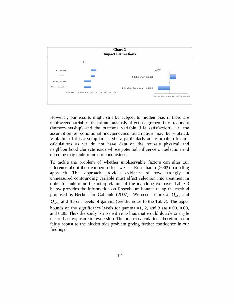
Chart 3 Impact Estimations

-5% -4% -3% -2% -1% 0% 1% 2% 3% 4% 5%

1 Not at all satisfied

2 Not very satisfied

3 Satisfied

4 Very satisfied

ATT

-4% -3% -2% -1% 0% 1% 2% 3% 4% 5%

Not at all satisfied or not very satisfied

Satisfied or very satisfied

ATT

However, our results might still be subject to hidden bias if there are unobserved variables that simultaneously affect assignment into treatment (homeownership) and the outcome variable (life satisfaction), i.e. the assumption of conditional independence assumption may be violated. Violation of this assumption maybe a particularly acute problem for our calculations as we do not have data on the house’s physical and neighbourhood characteristics whose potential influence on selection and outcome may undermine our conclusions.

To tackle the problem of whether unobservable factors can alter our inference about the treatment effect we use Rosenbaum (2002) bounding approach. This approach provides evidence of how strongly an unmeasured confounding variable must affect selection into treatment in order to undermine the interpretation of the matching exercise. Table 3 below provides the information on Rosenbaum bounds using the method proposed by Becker and Caliendo (2007). We need to look at Q and

at different levels of gamma (see the notes to the Table). The upper bounds on the significance levels for gamma =1, 2, and 3 are 0.00, 0.00, and 0.00. Thus the study is insensitive to bias that would double or triple the odds of exposure to ownership. The impact calculations therefore seem fairly robust to the hidden bias problem giving further confidence in our findings.

+mh

−mhQ

12

Table 4 Rosenbaum Bounds For Very Satisfied plus Satisfied)

Where: Gamma : odds of differential assignment due to unobserved factors; Q_mh+ : Mantel-Haenszel statistic (assumption: over-estimation of treatment effect); Q_mh- : Mantel-Haenszel statistic (assumption: under-estimation of treatment effect); p_mh+ : significance level (assumption: over-estimation of treatment effect); p_mh- : significance level (assumption: under-estimation of treatment effect)

Gamma Q_mh+ Q_mh- p_mh+ p_mh-1.0 7.46 7.46 0.00 0.002.0 40.47 25.15 0.00 0.003.0 60.71 44.64 0.00 0.00

However, the distribution of owners and renters by country in the matched sample may be important given that there is a systematic difference in happiness levels by country as indicated by the coefficients of countries in Table 1. Thus it is important to guarantee that the findings above have not arisen from the country composition of the sample obtained in the matching exercise used. To check whether the results are sensitive to country composition we repeated the matching exercise by country for the year 2008.

The meta-evaluation is presented in the forest Chart 4. In the Chart the horizontal line is the scale measuring the treatment effect, the vertical line in the middle is where the treatment and comparison groups have the same mean level; there is no difference between the two. Towards the left of the line is a negative impact and towards the right is a positive effect. For each country the level estimation is represented by a square at the point estimate and a horizontal line gives its confidence level at the 5%. The pooled analysis is shown with a diamond shape where the widest bit in the middle is located at the point estimate (drawn also as a dotted vertical line) and the horizontal width of the diamond is the confidence interval, at 95% level. Confidence levels are also given numerically in the penultimate column in the charts. If the confidence interval crosses the line of no effect this implies that there is no statistically significant difference in homeownership and renting on happiness. The ultimate column is the weight, using the random method, given to each country’s level impact

13

estimation. Note it is strictly not necessary, as mentioned previously, to present both effect sizes as they have to be symmetrical and opposite, hence only the estimations for satisfied and very satisfied is shown.

Chart 4 Impact Estimated for the Combined Satisfied and Very Satisfied Category

The conclusion that owning your home makes you happier and not owning your house makes you unhappier are robust to repeating the estimation at individual country level and estimating the meta-impact coefficient. However, it is not a valid statement for each country. The influence of individual countries estimations on the general conclusion is shown in the following Charts 5 in which the dots are the each country’s point estimates and the horizontal lines are the 95% confidence intervals, the vertical line is the meta-impact calculation.

14

15

Chart 5 Sensitivity to Country Level Results for the Satisfied and Very Satisfied Category

DISCUSSION

This paper examined whether homeownership increased happiness in seventeen Latin American countries. We found that owning your house makes you happier.

We found that unadjusted data shows that homeowners are more satisfied with life than non-homeowners. This conclusion is robust when the relation is examined through regressions using a relatively large set of control variables in which the coefficient for homeownership is found to be positive and statistically significant.

Further, it is homeownership that causes the increased happiness not the other way round. This conclusion is based on comparing the mean level of happiness of homeowners with the mean level of happiness of a comparison group of non-homeowners where the comparison group was constructed using propensity score approach that mimics a random assignment of homeownership. The impact results are fairly robust to the

16

possible influences of non-observables that may undermine our conclusions and to carrying out the exercise by country. The results hold in a meta-impact approach that uses impact calculations at individual country level. However, our results remain a black box as our data did not allow us to measure the mechanism, i.e., the causality chain, through which homeownership could increase happiness like the links of increased self-esteem, self-efficacy and net wealth.

Nonetheless, the homeownership-happiness relation and direction of causality could account for the fact that Latin American countries’ housing programs are essentially directed at increasing homeownerships rather than providing housing solutions for example through subsidized rents. Politicians know that ribbon cutting ceremonies have higher political returns.

REFERENCES

Belsky E. and A. Calder “Credit Matters: Low-income Asset Building Challenges in Dual Financial System”, BABC 04-1, Joint Center for Housing Studies, Harvard University, February 2002.

Boehm, Thomas and Alan Schlottmann (2008). “Wealth Accumulation and Homeownership: Evidence for Low-Income Households,” Cityscape, Vol. 10, No. 2, pp. 225-256.

Bucchianeri, G. W. “The American Dream or the American Delusion? The Private and External Benefits of Homeownership”, Working Paper, The Wharton School of Business. 2009

Becker, S.,, and M. Caliendo, “ mhbounds- Senstivity Analysis for Average Treatment Effects”, IZA DP No. 2542, January 2007.

Caliendo M., and S. Kopeinig “Some Practical Guidance for the Implementation of Propensity Score Matching”, Discussion Paper 485, DIW Berlin, April 2005.

Dietz R. and D. Haurin “The social and private micro-level consequences of homeownership”, Journal of Urban Economics 54 (2003) 401-450, 2003.

Frey, Bruno S. and Alois Stutzer, “What Can Economists Learn From Happiness

Research?”, Journal of Economic Literature, 40, 2002, pp. 402-435.

Imbens, Guido. (2004). Nonparametric estimation of average treatment effects under erogeneity: A review. Review of Econometrics and Statistics 86, 1–29.

Imbens, Guido, Oscar Mitnik et al. 2009. “Dealing with limited overlap in estimation of average treatment effects.” Biometrika 96(1):187

Kahneman and A. Krueger “Developments in the Measurement of Subjective Well-Being”, Journal of Economic Perspectives, Vol. 20, Nu.1, Winter 2006, pp 3-24.

Rosenbaum, P. R. Observation Studies. 2nd Edition New York: Springer, 2002.

W.M. Rohe, M.A. Stegman, The impacts of homeownership on the self esteem, perceived control and life satisfaction of low-income people, Journal of the American Planning Association 60 (1994) 173–184.

W.M. Rohe, V. Basolo, “Long-term effects of homeownership on the self-perceptions and social interactions of low-income persons” , Environment and Behaviour, 29 (1997) 793–819.

Rohe W., S.Van Zandt and G. McCarthy, “The Social Benefits of Home Ownership: A Critical Assessment of the Research”, Working Paper 01.12, October 2001. Joint Center for Housing Studies, Harvard University.

Rossi P.H. and Weber E. (1996) “The Social Benefits of Homeownership: Empirical Evidence from National Surveys”. Housing Policy Debate, 7(1) 1-35.

Van Praag, Frijters, and Ferrer-Carbonell (2003) “The Anatomy of Subjective Well-being”. Journal of Economic Behaviour and Organization, 51, 29-49.

Inter-American Development BankWashington, D.C.