Dodd 2006 Amphibian ecology and conservation A handbook of techniques
245
Amphibian Ecology and Conservation A Handbook of Techniques Edited by C. Kenneth Dodd, Jr 1
-
Upload
independent -
Category
Documents
-
view
1 -
download
0
Transcript of Dodd 2006 Amphibian ecology and conservation A handbook of techniques
Amphibian Ecology and Conservation
A Handbook of Techniques
Edited by
C. Kenneth Dodd, Jr
1
00_Dodd_Prelims.indd iii00_Dodd_Prelims.indd iii 8/19/2009 3:18:46 PM8/19/2009 3:18:46 PM

Techniques in Ecology and Conservation Series
Series Editor: William J. Sutherland
Bird Ecology and Conservation: A Handbook of TechniquesWilliam J. Sutherland, Ian Newton, and Rhys E. Green
Conservation Education and Outreach TechniquesSusan K. Jacobson, Mallory D. McDuff, and Martha C. Monroe
Forest Ecology and Conservation: A Handbook of TechniquesAdrian C. Newton
Habitat Management for Conservation: A Handbook of TechniquesMalcolm Ausden
Conservation and Sustainable Use: A Handbook of TechniquesE.J. Milner-Gulland and J. Marcus Rowcliffe
Invasive Species Management: A Handbook of TechniquesMick N. Clout and Peter A. Williams
Amphibian Ecology and Conservation: A Handbook of TechniquesC. Kenneth Dodd, Jr
00_Dodd_Prelims.indd ii00_Dodd_Prelims.indd ii 8/19/2009 3:18:45 PM8/19/2009 3:18:45 PM
Preface
As this volume is completed, more than 6400 amphibian species have been recognized, with new taxa being described nearly every day. The last few dec-ades have seen an explosion in systematic research, particularly in the tropics. Long-recognized centers of diversity have been explored using increasingly sophisticated sampling techniques, yielding many new taxa. At the same time, new centers of speciation, such as Sri Lanka and the Western Ghats of India, have been discovered, while molecular techniques have yielded previously unsuspected diversity within some well-known taxa, such as the plethodontid salamanders of southeastern North America and the green toad (Bufo viridis) complex of Eurasia. For amphibian systematists, these are exciting times.
Unfortunately, amphibians are now at greater peril than at any time in recent geologic history, a situation chronicled in two recent data-rich books (Lannoo 2005; Stuart et al. 2008). Habitats are being lost at alarming rates because of expanding human populations and generally favorable economic conditions fostering development; emerging infectious diseases, particularly amphibian chytrid fungus (Batrachochytrium dendrobatidis), threaten worldwide impacts; non-indigenous species proliferate, affecting amphibians and their habitats; and amphibians, with their permeable skins, diverse life histories, and often biphasic life cycles requiring both terrestrial and aquatic habitats, are being saturated by a host of lethal and sublethal toxic substances. New threats, such as the effects of global climate change, further imperil amphibians, especially those with limited distributions and dispersal capabilities. Fully one-third of all amphib-ians are now considered threatened (Stuart et al. 2004), and 168 species have become extinct within the last two decades. Clearly, these are treacherous times for many frogs, salamanders, and caecilians.
Amphibians are, quite frankly, engaging animals. Despite Linnaeus’ early characterization of amphibians in the context of “Terrible are thy works, O God”, biologists have come to appreciate that their diverse life histories and shear numbers offer a wealth of material for research on basic ecological princi-ples, such as trophic interactions, phenotypic plasticity, predator–prey interac-tions, community structure, mate choice and recognition, water balance, and many others. In response to threats, conservation biologists have probed these and other questions in hopes of understanding amphibian biology in order to prevent declines and extinctions. The basic and applied themes of biology merge
00_Dodd_Prelims.indd v00_Dodd_Prelims.indd v 8/19/2009 3:18:46 PM8/19/2009 3:18:46 PM
vi | Preface
in these disciplines: understanding ecology leads to conservation options (see Gascon et al. 2007), and conservation-based research leads to a better appreci-ation of ecological principles.
To say that there are a great many techniques available in ecological and conservation-based research on amphibians is an understatement. The pages of journals such as Herpetological Review and Applied Herpetology contain tech-niques papers with every issue. Specialized books, such Heyer et al. (1994), Henle and Veith (1997), and Gent and Gibson (1998), offer additional summar-ies that are as applicable today as when they were published. No one volume can include all techniques. The current volume is meant not to supplant these earlier works, but to supplement them and add new areas not previously summarized, such as occupancy modeling, landscape ecology, genetics, telemetry, and dis-ease biosecurity. Our objectives have been to delineate important new develop-ments, to give an idea as to what the techniques tell or do not tell a researcher, to focus attention on biases and data inference, and to get readers to appreciate sampling as an integral part of their science, rather than just a means of captur-ing animals. The techniques used will set the boundaries within which results can or should be interpreted.
As noted earlier, amphibian systematics is a fl ourishing fi eld, with many new opportunities made available by combining large datasets using molecular and morphological data with powerful computer analysis. The phylogeny of amphibians is undergoing increasingly sophisticated analysis. Some analyses, such as those of Frost et al. (2006), suggest relationships that differ substantially from “traditional” concepts. If accepted, extensive nomenclatural changes will be warranted. Although Frost et al. (2006) have advocated substantive changes in nomenclature, many of which will likely be accepted with further study, other amphibian biologists disagree with automatically accepting every change pro-posed by these authors. In this book, I have decided to retain the older nomen-clature rather than make a taxonomic decision each time a name is mentioned. The intended audience of this volume (biologists starting their careers in ecology and conservation) likely will be more familiar with the older generic names of Bufo, Rana, and Hyla, and initially may be confused by the unfamiliar replace-ment names. Readers should be aware, however, that names such as Lithobates (� Rana, in part), Anaxyrus (� Bufo, in part), and others currently unfamiliar may soon be more commonplace.
I wish to thank the following for taking their valuable time to review manu-scripts and offer suggestions for improving this volume: James Austin, Larissa Bailey, Bruce Bury, Dan Cogalniceanu, Sarah Converse, Steve Corn, Rafael Ernst, Alisa Gallant, Marian Griffey, Kerry Griffi s-Kyle, Richard Griffi ths,
00_Dodd_Prelims.indd vi00_Dodd_Prelims.indd vi 8/19/2009 3:18:46 PM8/19/2009 3:18:46 PM
Preface | vii
Margaret Gunzburger, Tibor Hartel, Robert Jehle, Steve Johnson, Y.-C. Kam, Sarah Kupferberg, Frank Lemckert, Harvey Lillywhite, John Maerz, Joseph Mitchell, Clinton Moore, Erin Muths, James Petranka, Benedikt Schmidt, Ulrich Sinsch, Kevin Smith, Lora Smith, Joseph Travis, Susan Walls, and Matthew Whiles. I greatly appreciate the support from Ian Sherman and Helen Eaton at Oxford University Press and editorial help from freelance copy-editor Nik Prowse, and thank series editor, Bill Sutherland, for inviting me to edit the amphibian volume. This volume is dedicated to all the biologists who take up the challenge of amphibian ecology and conservation.
C. Kenneth Dodd, Jr
References
Frost, D. R., Grant, T., Faivovich, J., Bain, R. H., Haas, A., Haddad, C. F. B., de Sá, R. O., Channing, A.,Wilkinson, M., Donnellan, S. C. et al. (2006). The amphibian tree of life. Bulletin of the American Museum of Natural History, 297, 1–370.
Gascon, C., Collins, J. P., Moore, R. D., Church, D. R., McKay, J. E., and Mendelson, III, J. R. (eds) (2007). Amphibian Conservation Action Plan. IUCN/SSC Amphibian Specialist Group, Gland and Cambridge.
Gent, T. and Gibson, S. (eds) (1998). Herpetofauna Worker’s Manual. Joint Nature Conservation Committee, Peterborough.
Henle, K. and Veith, M. (eds) (1997). Naturschutzrelevante Methoden der Feldherpetologie. Mertensiella 7.
Heyer, W. R., Donnelly, M. A., McDiarmid, R. W., Hayek, L.-A., and Foster, M. S. (eds). (1994). Measuring and Monitoring Biological Diversity. Standard Methods for Amphibians. Smithsonian Institution Press, Washington DC.
Lannoo, M. J. (ed) (2005). Amphibian Decline. The Conservation Status of United States Species. University of California Press, Berkeley, CA.
Stuart, S., Chanson, J. S., Cox, N. A., Young, B. E., Rodrigues, A. S. L., Fishman, D. L., and Waller, R. W. (2004). Status and trends of amphibian declines and extinctions worldwide. Science, 306, 1783–6.
Stuart, S., Hoffman, M., Chanson, J. S., Cox, N. A., Berridge, R. J., Ramani, P., and Young, B. E. (eds) (2008). Threatened Amphibians of the World. Lynx Edicions, Barcelona; IUCN, Gland; Conservation International, Arlington, VA.
00_Dodd_Prelims.indd vii00_Dodd_Prelims.indd vii 8/19/2009 3:18:46 PM8/19/2009 3:18:46 PM

Contents
List of contributors xxv
Part 1 Introduction 1
1 Amphibian diversity and life history 3Martha L. Crump
1.1 Introduction 31.2 Amphibian species richness and distribution 31.3 Amphibian lifestyles and life history diversity 5
1.3.1 Caecilians 61.3.1.1 Aquatic 71.3.1.2 Combination aquatic and terrestrial 71.3.1.3 Terrestrial and/or fossorial 7
1.3.2 Salamanders 71.3.2.1 Aquatic 8
1.3.2.2 Combination of aquatic and terrestrial 81.3.2.3 Terrestrial 91.3.2.4 Fossorial 101.3.2.5 Arboreal 10
1.3.3 Anurans 101.3.3.1 Aquatic/aquatic 101.3.3.2 Terrestrial/aquatic 111.3.3.3 Arboreal/aquatic 131.3.3.4 Fossorial/aquatic 141.3.3.5 Terrestrial/non-aquatic 141.3.3.6 Arboreal/non-aquatic 141.3.3.7 Fossorial/non-aquatic 15
1.4 Amphibian declines and why they matter 151.4.1 Economics 161.4.2 Ecosystem function 161.4.3 Esthetics 171.4.4 Ethics 17
1.5 References 17
2 Setting objectives in fi eld studies 21Dan Cogalniceanu and Claude Miaud
2.1 Basic concepts for a good start 21
00_Dodd_Prelims.indd ix00_Dodd_Prelims.indd ix 8/19/2009 3:18:46 PM8/19/2009 3:18:46 PM
Paul
Resaltado
Paul
Resaltado
x | Contents
2.2 Steps required for a successful study 242.2.1 Temporal and spatial scales 242.2.2 Choosing the model species 252.2.3 Pilot/desk study 262.2.4 Elaborate a conceptual model 262.2.5 The SMART approach 272.2.6 Applying the SMART approach to plan an
amphibian inventory 282.2.7 Experimental versus fi eld studies 292.2.8 Methods for sampling, data storage, and analysis 29
2.3 Trade-offs and pitfalls 302.4 Ethical issues 312.5 Acknowledgments 322.6 References 32
Part 2 Larvae 37
3 Morphology of amphibian larvae 39Roy W. McDiarmid and Ronald Altig
3.1 Background 393.2 Larval caecilians 40
3.2.1 Morphology and ontogeny 403.2.2 Coloration 423.2.3 Diversity 42
3.3 Larval and larviform salamanders 423.3.1 Morphology and ontogeny 423.3.2 Coloration 443.3.3 Diversity 44
3.4 Anuran tadpoles 453.4.1 Morphology and ontogeny 453.4.2 Coloration 493.4.3 Diversity 49
3.5 Summary 503.6 References 51
4 Larval sampling 55David K. Skelly and Jonathan L. Richardson
4.1 Introduction 554.1.1 Why sample larvae? 554.1.2 Target responses 564.1.3 Timing 574.1.4 Sampling effort 57
4.2 Sampling techniques 584.2.1 Box/pipe sampler 58
00_Dodd_Prelims.indd x00_Dodd_Prelims.indd x 8/19/2009 3:18:46 PM8/19/2009 3:18:46 PM

Contents | xi
4.2.1.1 Description 584.2.1.2 Application 604.2.1.3 Considerations 60
4.2.2 Dip net 604.2.2.1 Description 604.2.2.2 Application 614.2.2.3 Considerations 61
4.2.3 Seine 614.2.3.1 Description 614.2.3.2 Application 624.2.3.3 Considerations 62
4.2.4 Leaf litterbags 624.2.4.1 Description 624.2.4.2 Application 634.2.4.3 Considerations 63
4.2.5 Trapping 644.2.5.1 Description 644.2.5.2 Application 644.2.5.3 Considerations 64
4.2.6 Mark–recapture 654.2.6.1 Description 654.2.6.2 Application 664.2.6.3 Considerations 66
4.3 Other techniques 664.3.1 Bottom net 674.3.2 Electroshocking 674.3.3 Visual encounter survey 67
4.4 Conclusions 674.5 Acknowledgments 684.6 References 68
5 Dietary assessments of larval amphibians 71Matt R. Whiles and Ronald Altig
5.1 Background 715.2 Larval caecilians and salamanders 725.3 Anuran tadpoles 725.4 Assessing food sources and diets 73
5.4.1 Category I: preparatory studies 735.4.2 Category II: gut contents 745.4.3 Procedures: anurans and small predators 745.4.4 Processing and analysis of gut contents 75
5.5 Category III: assimilatory diet 785.5.1 Stable-isotope analysis 785.5.2 Procedures 805.5.3 Fatty acid analyses 81
00_Dodd_Prelims.indd xi00_Dodd_Prelims.indd xi 8/19/2009 3:18:46 PM8/19/2009 3:18:46 PM
xii | Contents
5.6 Summary 825.7 References 83
6 Aquatic mesocosms 87Raymond D. Semlitsch and Michelle D. Boone
6.1 Introduction 876.2 Historical background 886.3 Why use mesocosms? 906.4 Types of mesocosm 936.5 Setting up mesocosms 956.6 Common experimental designs 966.7 Case studies 98
6.7.1 Community ecology 986.7.2 Evolutionary ecology 996.7.3 Ecotoxicology 1006.7.4 Land use and management 100
6.8 Conclusion 1016.9 References 102
7 Water-quality criteria for amphibians 105Donald W. Sparling
7.1 Introduction 1057.2 Dissolved oxygen 1057.3 Temperature 1087.4 pH 1107.5 Conductivity, hardness, and salinity 1127.6 Total and dissolved organic carbon 1137.7 Pollutants 114
7.7.1 Fertilizers and nitrogenous compounds 1147.7.2 Pesticides 1147.7.3 Metals 1157.7.4 Organic pollutants and halogenated hydrocarbons 1157.7.5 Pharmaceuticals 116
7.8 Summary and conclusions 1167.9 References 117
Part 3 Juveniles and adults 121
8 Measuring and marking post-metamorphic amphibians 123John W. Ferner
8.1 Introduction 1238.2 Toe-clipping 125
00_Dodd_Prelims.indd xii00_Dodd_Prelims.indd xii 8/19/2009 3:18:47 PM8/19/2009 3:18:47 PM
Paul
Resaltado

Contents | xiii
8.2.1 Anurans 125 8.2.2 Salamanders 129 8.2.3 Ethical issues related to toe-clipping of amphibians 129
8.3 Branding 130 8.3.1 Anurans 130 8.3.2 Salamanders 131
8.4 Tagging and banding 131 8.4.1 Anurans 131 8.4.2 Salamanders 133 8.4.3 Caecilians 133
8.5 Trailing devices 1338.6 Pattern mapping 134
8.6.1 Anurans 134 8.6.2 Salamanders 135
8.7 Passive integrated transponder (PIT) tags 136 8.7.1 Anurans 137 8.7.2 Salamanders 137 8.7.3 Caecilians 137
8.8 Taking measurements 1388.9 Recommendations 1388.10 References 139
9 Egg mass and nest counts 143Peter W. C. Paton and Reid N. Harris
9.1 Background: using egg mass and nest counts to monitor populations 143
9.2 Oviposition strategies 1449.3 Egg-mass counts 1459.4 Amphibian nests and nest counts 1479.5 Clutch characteristics 1509.6 Spatial distribution of eggs 1529.7 Breeding phenology 1529.8 Number of surveys needed 1539.9 Estimating egg-mass detection probabilities 1549.10 Variation in counts among observers 1549.11 Marking eggs 1559.12 Situations in which nest counts are not practical 155
9.12.1 Nest destruction 155 9.12.2 Desertion of attendant 155
9.13 How to count eggs in a nest 1569.14 Estimating hatching success 1569.15 Analysis of egg-mass count data 1579.16 Summary 1579.17 References 158
00_Dodd_Prelims.indd xiii00_Dodd_Prelims.indd xiii 8/19/2009 3:18:47 PM8/19/2009 3:18:47 PM

xiv | Contents
10 Dietary assessments of adult amphibians 167Mirco Solé and Dennis Rödder
10.1 Introduction 16710.1.1 Adult anurans 16710.1.2 Adult caudata 16810.1.3 Adult gymnophiona 169
10.2 Methods to obtain prey items: historical overview 16910.2.1 Stomach fl ushing: materials 17010.2.2 When should sampling be conducted? 17110.2.3 How to perform the fl ush 171
10.3 Data analysis 17210.3.1 Measuring prey availability and electivity 17410.3.2 Comparing trophic niche structure 17610.3.3 Fatty acid and stable-isotope analyses 17710.3.4 Further biochemical analyses 178
10.4 General considerations 17810.4.1 Ontogenetic changes 17910.4.2 Seasonal changes 179
10.5 Conclusions 18010.6 Acknowledgments 18010.7 References 180
11 Movement patterns and radiotelemetry 185Dale M. Madison, Valorie R. Titus, and Victor S. Lamoureux
11.1 Introduction 18511.2 Equipment 186
11.2.1 Receivers and antennas 18611.2.2 Transmitters 186
11.2.2.1 External transmitters 18711.2.2.2 Internal transmitters 188
11.3 Surgical techniques 18911.3.1 Surgery 18911.3.2 Recovery and healing 191
11.4 Tracking procedures 19111.4.1 Animal release 19111.4.2 Locating signal source 19211.4.3 Data collection 193
11.5 Analysis of movement data 19311.6 Validation of telemetry procedures 197
11.6.1 Internal condition and mass 19711.6.2 Movements 19811.6.3 Reproduction 19811.6.4 Injury and survivorship 199
00_Dodd_Prelims.indd xiv00_Dodd_Prelims.indd xiv 8/19/2009 3:18:47 PM8/19/2009 3:18:47 PM
Paul
Resaltado
Contents | xv
11.7 Conclusions 19911.8 References 200
12 Field enclosures and terrestrial cages 203Elizabeth B. Harper, Joseph H.K. Pechmann, and James W. Petranka
12.1 Introduction: amphibians in the terrestrial environment 20312.2 What are the purposes of terrestrial enclosures? 20412.3 Defi ning the research question 205
12.3.1 Questions related to habitat types 20512.3.2 Questions with treatments that can be assigned
within enclosures 20712.4 Constructing enclosures 208
12.4.1 Location of enclosures 20812.4.2 Size and number of enclosures 20912.4.3 Building enclosures that minimize escapes and
trespasses 21612.4.4 “Standardizing” conditions among enclosures 218
12.5 Study species 21812.5.1 Choice of species 21812.5.2 Source and age of animals 219
12.6 Census techniques 21912.6.1 Individual marks 21912.6.2 Methods of capture 22012.6.3 Frequency of censuses 220
12.7 Response metrics 22112.7.1 Vital rates: survival, growth, age at reproductive
maturity, fecundity 22112.7.2 Physiological responses 22212.7.3 Behavioral responses 222
12.8 Thinking outside the box 22312.9 References 223
Part 4 Amphibian populations 227
13 Drift fences, coverboards, and other traps 229John D. Willson and J. Whitfi eld Gibbons
13.1 Introduction 22913.2 Drift fences, funnel traps, and other passive
capture methods 22913.2.1 What are passive traps? 22913.2.2 How are passive traps constructed, aligned,
and monitored? 231
00_Dodd_Prelims.indd xv00_Dodd_Prelims.indd xv 8/19/2009 3:18:47 PM8/19/2009 3:18:47 PM
Paul
Resaltado
Paul
Resaltado

xvi | Contents
13.2.3 What can passive traps tell you? What can they not tell you? 235
13.3 Coverboards and other traps that require active capture 23613.3.1 What are coverboards and other active traps? 23613.3.2 How are active traps constructed, aligned, and
monitored? 23713.3.3 What can active traps tell you? What can they
not tell you? 24013.4 References 241
14 Area-based surveys 247David M. Marsh and Lillian M.B. Haywood
14.1 Introduction: what are area-based surveys? 24714.1.2 Why use area-based surveys? 247
14.2 Kinds of area-based survey 24914.3 Specifi c examples of area-based surveys 249
14.3.1 Leaf-litter plots 24914.3.2 Natural-cover surveys for terrestrial salamanders 25014.3.3 Nocturnal transects 25114.3.4 Quadrats for stream amphibians 25214.3.5 Soil quadrats for caecilians 252
14.4 Modifi cations 25314.4.1 Distance sampling 25314.4.2 Adaptive cluster sampling 253
14.5 Design issues: choice of sampling unit 25414.5.1 Design issues: how many replicates? 25514.5.2 Reducing variation among replicates 25514.5.3 How many times to survey each replicate? 256
14.6 An example of study design 25714.7 Assumptions of area-based surveys 25914.8 Summary and recommendations 26014.9 References 260
15 Rapid assessments of amphibian diversity 263James R. Vonesh, Joseph C. Mitchell, Kim Howell, and Andrew J. Crawford
15.1 Background: rapid assessment of amphibian diversity 26315.1.1 When is an RA needed? 264
15.2 Planning an RA 26515.2.1 Developing objectives 26515.2.2 Costs and funding 26615.2.3 Team selection and training 26615.2.4 Permits 267
00_Dodd_Prelims.indd xvi00_Dodd_Prelims.indd xvi 8/19/2009 3:18:47 PM8/19/2009 3:18:47 PM
Paul
Resaltado
Contents | xvii
15.2.5 Data management 26715.2.6 Developing the sampling plan 268
15.2.6.1 Selecting sampling sites 26815.2.6.2 Selecting sampling time 27015.2.6.3 Selecting sampling techniques 270
15.2.6.3.1 Visual encounter surveys (VESs) 27015.2.6.3.2 Assumptions and limitations of VESs 272
15.2.6.4 Determining what data to collect 27315.2.6.5 Field logistics 274
15.3 In the fi eld 27415.4 Compiling data and interpreting results 27415.5 Recommendations and reporting 27515.6 Summary 27515.7 References 276
16 Auditory monitoring of anuran populations 281Michael E. Dorcas, Steven J. Price, Susan C. Walls, and William J. Barichivich
16.1 Introduction 28116.2 MCS 281
16.2.1 History and current status of MCS 28216.2.2 Study objectives: what can MCS tell us? 28316.2.3 Survey design 28316.2.4 Other survey-design issues to consider:
the effi ciency of MCS 28416.2.5 Limitations of MCS data 287
16.3 ARS 28816.3.1 Sources for ARS 28916.3.2 Construction, deployment, and retrieval of data 28916.3.3 Monitoring environmental data 29216.3.4 Answering questions using ARS 29216.3.5 Limitation of ARS 294
16.4 Conclusions 29416.5 Acknowledgments 29516.6 References 295
17 Measuring habitat 299Kimberly J. Babbitt, Jessica S. Veysey, and George W. Tanner
17.1 Introduction 29917.2 Habitat selection 29917.3 Spatial and temporal scale 30017.4 Approaches for examining habitat selection 30017.5 Determining availability 301
00_Dodd_Prelims.indd xvii00_Dodd_Prelims.indd xvii 8/19/2009 3:18:47 PM8/19/2009 3:18:47 PM
Paul
Resaltado
xviii | Contents
17.6 What to measure 30217.7 Weather variables 30217.8 Aquatic habitat 30417.9 Physical habitat variables 30417.10 Chemical variables 30717.11 Measuring vegetation 309
17.11.1 Tree (overstory) measurements 31017.11.2 Shrub (midstory) measurements 31217.11.3 Ground (understory) measurements 313
17.12 Edaphic features 31417.13 Conclusion 31417.14 References 315
Part 5 Amphibian communities 319
18 Diversity and similarity 321C. Kenneth Dodd, Jr
18.1 Introduction 32118.2 Data transformation 32218.3 Species diversity 323
18.3.1 Sampling considerations 32318.3.2 Species richness 32418.3.3 Species accumulation curves 32518.3.4 Heterogeneity 32718.3.5 Evenness and dominance 329
18.4 Similarity 32918.5 Software 33118.6 Summary 33418.7 References 334
19 Landscape ecology and GIS methods 339Viorel D. Popescu and James P. Gibbs
19.1 Introduction 33919.1.1 Relevance of landscape ecology to amphibian
biology and conservation 33919.1.2 Defi ning a “landscape” from an amphibian’s
perspective 34119.1.3 GIS 342
19.2 Applications of spatial data for amphibian conservation 34619.2.1 Multiscale predictors of species occurrence and
abundance 34619.2.2 Landscape thresholds 347
19.2.3 Connectivity/isolation in amphibian populations 349
00_Dodd_Prelims.indd xviii00_Dodd_Prelims.indd xviii 8/19/2009 3:18:47 PM8/19/2009 3:18:47 PM
Contents | xix
19.2.4 Landscape permeability 35119.2.5 Landscape genetics 352
19.3 Spatial statistics 35319.4 Limitations and future directions 35419.5 References 356
Part 6 Physiological ecology and genetics 361
20 Physiological ecology: fi eld methods and perspective 363Harvey B. Lillywhite
20.1 Introduction 36320.1.1 Important features of amphibians 364
20.2 Heat exchange, body temperature, and thermoregulation 36520.2.1 Thermal acclimation of physiological function 36520.2.2 Early methods in fi eld studies of amphibian
thermal relations 36620.2.3 Precautions for temperature measurements 36720.2.4 Telemetry 371
20.3 Water relations 37220.3.1 Cutaneous water exchange: terrestrial environments 37220.3.2 Cutaneous water exchange: aquatic environments 374
20.4 Measuring water exchange 37420.5 Energetics 37520.6 Modeling amphibian–environment interactions 376
20.6.1 Mathematical models 37620.6.2 Physical models 377
20.7 Other issues and future research directions 37920.8 References 382
21 Models in fi eld studies of temperature and moisture 387Jodi J. L. Rowley and Ross A. Alford
21.1 Introduction 38721.1.1 The importance of understanding the temperature
and moisture environments of amphibians 38721.1.2 Physical models of amphibians 389
21.2 Field models for investigating temperature and moisture 39021.2.1 Models with zero resistance to EWL 39021.2.2 A system of models that allows for variable EWL 39021.2.2.1 Rationale 390
21.2.2.2 Model design and construction 391
00_Dodd_Prelims.indd xix00_Dodd_Prelims.indd xix 8/19/2009 3:18:48 PM8/19/2009 3:18:48 PM
Paul
Resaltado
xx | Contents
21.2.2.3 Example of model construction and
validation in the laboratory 39221.2.2.4 Field validation of use of models to
characterize available temperatures 39521.2.2.5 The importance of matching the spectral
properties of models to living animals 39921.2.2.6 Models as indicators of relative moisture
availability of microenvironments 39921.3 Summary and future developments 40221.4 References 403
22 Genetics in fi eld ecology and conservation 407Trevor J. C. Beebee
22.1 Background: the importance of genetics in ecology and conservation 407
22.2 Molecular methods for investigating amphibian populations 40822.2.1 Laboratory facilities 40822.2.2 Sampling 40922.2.3 DNA extraction 409
22.2.3.1 Proteinase K/phenol/chloroform method 41022.2.3.2 Kit-based DNA extraction 41022.2.3.3 Chelex method 41022.2.3.4 FTA cards 41022.2.3.5 Summary of DNA-extraction methods 410
22.2.4 Quantifying DNA recoveries 41122.2.5 The basis of PCR analysis 41122.2.6 Choice of analytical methods 412
22.2.6.1 Mitochondrial DNA (mtDNA) 41222.2.6.2 Random amplifi cation of polymorphic
DNA (RAPD) and amplifi ed fragment
length polymorphism (AFLP) analyses 41322.2.6.2.1 RAPD analysis 41322.2.6.2.2 AFLP analysis 41422.2.6.2.3 Microsatellite analysis 414
22.3 Analysis of genetic data 41722.3.1 Cryptic species or life-stage identifi cation 41722.3.2 Genetic diversity, inbreeding, and bottlenecks 41722.3.3 Identifi cation of barriers to movement 41922.3.4 Defi ning populations and population size 42022.3.5 Historical issues 42122.3.6 Behavior and sexual selection 423
22.4 Future developments 42322.5 References 425
00_Dodd_Prelims.indd xx00_Dodd_Prelims.indd xx 8/19/2009 3:18:48 PM8/19/2009 3:18:48 PM
Contents | xxi
Part 7 Monitoring, status, and trends 429
23 Selection of species and sampling areas: the importance to inference 431Paul Stephen Corn
23.1 Introduction 43123.2 Sampling 43323.3 Study sites and consequences of convenience sampling 43523.4 Abundance and inference 43923.5 Conclusions 44223.6 Acknowledgments 44323.7 References 443
24 Capture–mark–recapture, removal sampling, and occupancy models 447Larissa L. Bailey and James D. Nichols
24.1 Introduction 44724.2 Estimating amphibian population size and vital rates 448
24.2.1 Marking: tag type and subsequent encounter 44824.2.2 Capture–mark–recapture 44924.2.3 Removal sampling 455
24.3 Estimating amphibian occupancy and vital rates 45524.3.1 Occupancy estimation 45624.3.2 Estimation of occupancy vital rates:
extinction and colonization 45724.4 Summary and general recommendations 45824.5 Disclaimer 45924.6 References 459
25 Quantifying abundance: counts, detection probabilities, and estimates 465Benedikt R. Schmidt and Jérôme Pellet
25.1 Background: imperfect detection in amphibian ecology and conservation 465
25.2 Imperfect detection 46625.2.1 Counts underestimate abundance 46725.2.2 Per-visit and cumulative detection probabilities 46825.2.3 Temporal and spatial variation in
detection probabilities 46925.3 Components of imperfect detection 47025.4 How to deal with imperfect detection 471
00_Dodd_Prelims.indd xxi00_Dodd_Prelims.indd xxi 8/19/2009 3:18:48 PM8/19/2009 3:18:48 PM
Paul
Resaltado
Paul
Resaltado

xxii | Contents
25.4.1 Estimation of abundance 47125.4.2 Other approaches to dealing with
imperfect detection 47325.5 Designing a sampling protocol 47625.6 Software 47625.7 Outlook 47725.8 References 477
26 Disease monitoring and biosecurity 481D. Earl Green, Matthew J. Gray, and Debra L. Miller
26.1 Introduction 48126.2 Amphibian diseases of concern 482
26.2.1 Infectious diseases 48226.2.2 Parasitic diseases 48726.2.3 Toxins 487
26.3 Disease monitoring: detection and diagnosis 48726.3.1 Disease surveillance 48726.3.2 Sample size 49026.3.3 Sample collection and shipment 49026.3.4 Diagnostics 494
26.4 Biosecurity: preventing disease transmission 49726.4.1 Human and animal safety 49726.4.2 Washing and disinfecting equipment 49826.4.3 Movement of animals and disease management 499
26.5 Conclusions 50026.6 References 501
27 Conservation and management 507C. Kenneth Dodd, Jr
27.1 Introduction 50727.1.1 Statutory protection 50827.1.2 Protecting habitats 508
27.2 Managing amphibian populations 50927.3 Wetland breeding sites 510
27.3.1 Wetland integrity and hydroperiod 51027.3.2 Wetland creation and restoration 51227.3.3 Core habitat and buffer zones 51427.3.4 Vegetation structure, composition, and
canopy cover 51627.3.5 Water quality 516
27.4 Terrestrial habitats 51727.4.1 Contiguous habitats and edge effects 51727.4.2 Silviculture 517
00_Dodd_Prelims.indd xxii00_Dodd_Prelims.indd xxii 8/19/2009 3:18:48 PM8/19/2009 3:18:48 PM
Paul
Resaltado

Contents | xxiii
27.4.3 Restoring degraded lands 51827.5 Migratory and dispersal routes 519
27.5.1 Corridors between habitat fragments 51927.5.2 Crossing transportation corridors 519
27.6 Intensive manipulation of individuals 52127.6.1 Captive breeding 52127.6.2 Relocation, repatriation, translocation (RRT) 52127.6.3 Disease and biosecurity 522
27.7 Conclusion 52327.8 References 523
Index 529
00_Dodd_Prelims.indd xxiii00_Dodd_Prelims.indd xxiii 8/19/2009 3:18:48 PM8/19/2009 3:18:48 PM
Contributors
Ross A. Alford School of Marine and Tropical Biology, James Cook University, Townsville, Queensland 4811, Australia. E-mail: [email protected] Altig Department of Biological Sciences, Mississippi State University, Mississippi State, Mississippi 39762-5759, USA. E-mail: [email protected] J. Babbitt Department of Natural Resources and the Environment, University of New Hampshire, Durham, NH 03824, USA. E-mail: [email protected] L. Bailey Department of Fish, Wildlife and Conservation Biology, Colorado State University, Fort Collins, CO 80523, USA. E-mail: [email protected] J. Barichivich Florida Integrated Science Center, US Geological Survey, 7920 NW 71st Street, Gainesville, FL 32653, USA. E-mail: [email protected] J. C. Beebee School of Life Sciences, University of Sussex, Falmer, Brighton BN1 9QG, UK. E-mail: [email protected] D. Boone Department of Zoology, 212 Pearson Hall, Miami University, Oxford, Ohio 45056, USA. E-mail: [email protected] J. Crawford Smithsonian Tropical Research Institute, Apartado Postal 0843-03092, Balboa, Ancón, Republic of Panama. E-mail: [email protected] Cogalniceanu University Ovidius Constant‚a, Faculty of Natural Sciences, Bvd. Mamaia 124, Constant‚a, Romania. E-mail: [email protected] Stephen Corn U.S. Geological Survey, Aldo Leopold Wilderness Research Institute, 790 E. Beckwith Ave., Missoula, MT 59801, USA. E-mail: [email protected] L. Crump Department of Biological Sciences, Northern Arizona University, Flagstaff, Arizona 86011, USA. E-mail: marty.crump@ nau.eduC. Kenneth Dodd, Jr Department of Wildlife Ecology and Conservation, University of Florida, Gainesville, FL 32611, USA. E-mail: [email protected] E. Dorcas Department of Biology, Davidson College, Davidson, NC 28035, USA. E-mail: [email protected] W. Ferner Department of Biology, Thomas More College, Crestview Hills, Kentucky 41017, USA. E-mail: [email protected]. Whitfi eld Gibbons Savannah River Ecology Laboratory, P.O. Drawer E, Aiken, South Carolina 29802, USA. E-mail: [email protected] P. Gibbs Department of Environmental and Forest Biology, State University of New York, Syracuse, NY 13210, USA. E-mail: [email protected] J. Gray Center for Wildlife Health, Department of Forestry, Wildlife and Fisheries, University of Tennessee, 274 Ellington Plant Sciences Building, Knoxville, TN 37996, USA. E-mail: [email protected]
00_Dodd_Prelims.indd xxv00_Dodd_Prelims.indd xxv 8/19/2009 3:18:48 PM8/19/2009 3:18:48 PM
xxvi | Contributors
D. Earl Green U.S. Geological Survey, National Wildlife Health Center, 6006 Schroeder Drive, Madison, WI 53711, USA. E-mail: [email protected] B. Harper State University of New York, College of Environmental Sciences and Forestry, 1 Forestry Drive, Syracuse, New York 13210, USA. E-mail: [email protected] N. Harris Department of Biology, James Madison University, Harrisonburg, Virginia 22807, USA. E-mail: [email protected] M. B. Haywood Department of Biology, Washington and Lee University, Lexington, VA 24450, USA. E-mail: [email protected] Howell Department of Zoology and Wildlife Conservation, PO Box 35064, University of Dar es Salaam, Dar es Salaam, Tanzania. E-mail: [email protected] S. Lamoureux Binghamton University, PO Box 6000, Binghamton, New York 13902, USA. E-mail: [email protected] B. Lillywhite Department of Zoology, University of Florida, Gainesville, FL 32611, USA. E-mail: [email protected] .eduDale M. Madison Binghamton University, PO Box 6000, Binghamton, New York 13902, USA. E-mail: [email protected] M. Marsh Department of Biology, Washington and Lee University, Lexington, VA 24450, USA. E-mail: [email protected] W. McDiarmid Patuxent Wildlife Research Center, US Geological Survey, National Museum of Natural History, Washington DC 20036, USA. E-mail: [email protected] Miaud Laboratoire d’ Alpine UMR CNRS 5553, Université de Savoie, 73376 Le Bourget-du-Lac, France. E-mail: [email protected] L. Miller Veterinary Diagnostic and Investigational Laboratory, The University of Georgia, College of Veterinary Medicine, 43 Brighton Road, Tifton, GA 31793, USA. E-mail: [email protected] C. Mitchell Mitchell Ecological Research Service, LLC, PO Box 5638, Gainesville, FL 32627–5638, USA. E-mail: [email protected] D. Nichols U.S. Geological Survey, Patuxent Wildlife Research Center, 12100 Beech Forest Road, Laurel, MD 20708, USA. E-mail: [email protected] W. C. Paton Department of Natural Resources, University of Rhode Island, Kingston, Rhode Island 02881, USA. E-mail: [email protected] H. K. Pechmann Department of Biology, 132 Natural Sciences Building, Western Carolina University, Cullowhee, North Carolina 28723, USA. E-mail: [email protected]érôme Pellet A. Mailbach Sàrl, CP 99, Ch. de la Poya 10, CH-1610 Oron-la-Ville, Switzerland. E-mail : [email protected] W. Petranka Department of Biology, University of North Carolina at Asheville, Asheville, North Carolina 28804, USA. E-mail: [email protected]
00_Dodd_Prelims.indd xxvi00_Dodd_Prelims.indd xxvi 8/19/2009 3:18:48 PM8/19/2009 3:18:48 PM
Contributors | xxvii
Viorel D. Popescu Department of Wildlife Ecology, University of Maine, Orono, ME 04469, USA. E-mail: [email protected] J. Price Department of Biology, Wake Forest University, Winston-Salem, NC 27109, USA. E-mail: [email protected] L. Richardson School of Forestry and Environmental Studies, Yale University, 370 Prospect Street, New Haven, Connecticut 06511, USA. E-mail: [email protected] Rödder Zoological Research Museum Alexander Koenig, Adenauerallee 160, D-53113, Bonn, Germany and Faculty of Geography/Geosciences, Trier University, Wissenschaftspark Trier-Petrisberg, Am Wissenschaftspark 25–27, D-54286 Trier, Germany. E-mail: [email protected] J. L. Rowley School of Marine and Tropical Biology, James Cook University, Townsville, Queensland 4811, Australia. E-mail: [email protected] R. Schmidt Zoologisches Institut, Universität Zürich, Winterthurerstrasse 190, CH-8057 Zürich, Switzerland. E-mail: [email protected] D. Semlitsch Division of Biological Sciences, 105 Tucker Hall, University of Missouri, Columbia, Missouri 65211, USA. E-mail: [email protected] K. Skelly School of Forestry and Environmental Studies, Yale University, 370 Prospect Street, New Haven, Connecticut 06511, USA. E-mail: [email protected] Solé Department of Biology, Universidade Estadual de Santa Cruz, Rodovia Ilhéus – Itabuna, km 16, Ilhéus, Bahia, Brazil. E-mail: [email protected] W. Sparling Cooperative Wildlife Research Laboratory, Life Science II, MS6504, Southern Illinois University, Carbondale, Illinois 62901, USA. E-mail: [email protected] W. Tanner Department of Wildlife Ecology and Conservation, University of Florida, Gainesville, FL 32611, USA. E-mail: tannerg@ufl .eduValorie R. Titus Binghamton University, PO Box 6000, Binghamton, New York 13902, USA. E-mail: [email protected] S. Veysey Department of Natural Resources and the Environment, University of New Hampshire, Durham, NH 03824, USA. E-mail: [email protected] R. Vonesh Department of Biology, Virginia Commonwealth University, 1000 West Cary Street, Richmond, VA 23284, USA. E-mail: [email protected] C. Walls Florida Integrated Science Center, US Geological Survey, 7920 NW 71st Street, Gainesville, FL 32653, USA. E-mail: [email protected] R. Whiles Department of Zoology and Center for Ecology, Southern Illinois University, Carbondale, Illinois 62901-6501, USA. E-mail: [email protected] D. Willson Savannah River Ecology Laboratory, P.O. Drawer E, Aiken, South Carolina 29802, USA. E-mail: [email protected]
00_Dodd_Prelims.indd xxvii00_Dodd_Prelims.indd xxvii 8/19/2009 3:18:48 PM8/19/2009 3:18:48 PM
1Amphibian diversity and life history
Martha L. Crump
When the fi rst crossopterygian crawled out of the rich Devonian waters and cast the fi rst envious vertebrate gaze at the terrestrial world, a boundless empire awaited colon-ization. Although the change from an ungainly lobe-fi nned locomotion to a terrestrial walking gait . . . was agonizingly slow, generations succeeded generations, archotypes [sic] gave way to new evolutionary experiments, and the land became the home for the fi rst quadrupeds—the amphibians.
William E. Duellman (1970)
1.1 Introduction
Over the past 350 million years, amphibian descendents of lobe-fi nned fi shes have radiated into most habitats on Earth. In doing so, they have acquired spec-tacular and sometimes bizarre physiological, morphological, behavioral, and ecological attributes that mold their innovative life histories. Amphibians have highly permeable skin, which makes them both vulnerable to losing water and able to absorb water. Their eggs, covered with jelly capsules rather than hard shells, lose water rapidly. For these reasons, amphibians require relatively moist environments.
Many sampling techniques have been developed in North America or Europe where most amphibians exhibit the complex life cycle of aquatic eggs, aquatic larvae, and metamorphosis into terrestrial adults that return to water to breed. Not all amphib-ians fi t this stereotype. The spectacular diversity of amphibian life histories provides a focus for studying their natural history, as well as presents a challenge since researchers must ensure that fi eld methods are appropriate for the target species.
1.2 Amphibian species richness and distribution
Scientists have named approximately 1.75 million species of living organisms (Groom et al. 2006). About 72% of all named animals are insects; about 5% are vertebrates. Approximately 0.5% of all animal species—6347 species (see AmphibiaWeb; http://amphibiaweb.org)—belong to the class Amphibia. The
01_Dodd_Chap01.indd 301_Dodd_Chap01.indd 3 8/19/2009 3:22:41 PM8/19/2009 3:22:41 PM
4 | Amphibian ecology and conservation
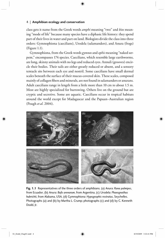
class gets it name from the Greek words amphi meaning “two” and bios mean-ing “mode of life” because many species have a diphasic life history: they spend part of their lives in water and part on land. Biologists divide the class into three orders: Gymnophiona (caecilians), Urodela (salamanders), and Anura (frogs) (Figure 1.1).
Gymnophiona, from the Greek words gymnos and ophis meaning “naked ser-pent,” encompasses 174 species. Caecilians, which resemble large earthworms, are long, skinny animals with no legs and reduced eyes. Annuli (grooves) encir-cle their bodies. Their tails are either greatly reduced or absent, and a sensory tentacle sits between each eye and nostril. Some caecilians have small dermal scales beneath the surface of their mucus-covered skin. These scales, composed mainly of collagen fi bers and minerals, are not found in salamanders or anurans. Adult caecilians range in length from a little more than 10 cm to about 1.5 m. Most are highly specialized for burrowing. Others live on the ground but are cryptic and secretive. Some are aquatic. Caecilians occur in tropical habitats around the world except for Madagascar and the Papuan–Australian region (Pough et al. 2004).
(a) (b)
(c) (d)
Fig. 1.1 Representatives of the three orders of amphibians. (a) Anura: Rana palmipes, from Ecuador, (b) Anura: Bufo arenarum, from Argentina, (c) Urodela: Phaeognathus hubrichti, from Alabama, USA, (d) Gymnophiona: Hypogeophis rostratus, Seychelles. Photographs (a) and (b) by Martha L. Crump; photographs (c) and (d) by C. Kenneth Dodd, Jr.
01_Dodd_Chap01.indd 401_Dodd_Chap01.indd 4 8/19/2009 3:22:41 PM8/19/2009 3:22:41 PM
1 Amphibian diversity and life history | 5
Five hundred and seventy-one species belong to Urodela, from the Greek words uro and delos meaning “tail evident.” All salamanders have tails, and adults have elongate bodies. Most have front and back legs of about the same length; the limbs of a few aquatic species are greatly reduced or absent. Salamanders are completely aquatic, terrestrial, combined aquatic and terrestrial, fossor-ial, or arboreal. Adults range in size from about 30 mm to nearly 2 m. Most salamander species occur in eastern and western North America and temper-ate Eurasia, although plethodontids have radiated extensively in Central and South America. There are no salamanders in sub-Saharan Africa, Australasia, Australia, or much of tropical Asia, and they are missing from most islands (Pough et al. 2004).
Frogs, which include toads, make up the order Anura from the Greek words an and oura, meaning “without tail.” Although tadpoles have tails, adults do not. Anurans live in the water, on the ground, underground, and in the trees. Most have long, strong back legs well suited for jumping. Males of most species call to attract females for mating. Adults of the 5602 recognized species range in size from about 13 mm to 30 cm. Anurans live almost everywhere except where restricted by cold temperatures or extremely dry conditions, and except for many oceanic islands (Pough et al. 2004).
Duellman identifi ed 43 areas worldwide with exceptionally high numbers of amphibian species, endemic species (those found nowhere else), or both (Duellman 1999). Nineteen of these high diversity areas are in the western hemi-sphere; the others are in Eurasia, Africa, and the Papuan–Australian region. The neotropical region houses 54% of the world’s amphibian species.
Amphibians live in nearly every habitat except for open oceans, most oceanic islands, polar regions, and some extremely dry deserts (Wells 2007). These restrictions are imposed on them because of their highly permeable skin that loses water, and because they are ectothermic: the energy needed to raise their body temperatures comes from the sun. Thus, amphibians become inactive at low temperatures. These characteristics, however, work to their advantage as well. In dry areas and those with seasonal rainfall, amphibians absorb water through their skin by contacting moist soil. Their low metabolic rates translate into low energy requirements and allow them to estivate, often underground, during unfavorable conditions.
1.3 Amphibian lifestyles and life history diversity
Textbooks, management guides, and monitoring manuals, especially those ori-ginating in Europe and North America, often give an oversimplifi ed impression
01_Dodd_Chap01.indd 501_Dodd_Chap01.indd 5 8/19/2009 3:22:46 PM8/19/2009 3:22:46 PM
6 | Amphibian ecology and conservation
of amphibian life histories. In fact, amphibian life histories are often complex, and many are still poorly understood. Not all species have an aquatic larval stage and a terrestrial adult stage.
Reproductive mode, a central aspect of amphibian life history, refers to the site of egg deposition, egg and clutch characteristics, type and duration of embryonic and larval development, and type of parental care if any (Duellman and Trueb 1986). Many amphibians are not tied to aquatic habitats for repro-duction. Instead, they reproduce on land, underground, or in trees, even in the temperate zones. The following brief discussion of selected lifestyles and life histories reveals that similar behaviors have evolved in diverse taxonomic groups and geographical areas: amphibian “experiments” toward greater inde-pendence from standing or fl owing water and perhaps from lower predation pressure as well.
Readers wishing more information concerning amphibian life histories should consult Duellman (2007) and Wells (2007). For reviews of reproduct-ive modes, see Salthe (1969), Salthe and Duellman (1973), Wake (1982, 1992), Haddad and Prado (2005), and Duellman (2007). For reviews of parental care see Crump (1995, 1996).
1.3.1 Caecilians
Caecilian lifestyles include aquatic, combined aquatic and terrestrial, terrestrial, and fossorial. Fully aquatic caecilians generally have compressed bodies with well-developed dorsal fi ns on the posterior portion. Fossorial species generally have blunt heads, used for pushing and compacting the soil while burrowing.
Although details of reproductive biology are unknown for many species, cae-cilians display two basic modes: oviparous (egg-laying) and viviparous (bear-ing live young) (Wake 1977, 1992). Oviparous caecilians lay eggs on land. In some species the eggs hatch into larvae that wriggle to water. Caecilian larvae exhibit less dramatic metamorphosis than do salamanders or frogs. They hatch almost fully developed, and the larval period is short. The eggs of some ovip-arous species undergo direct development. That is, development occurs within the egg capsule; there is no free-living larval stage. Some oviparous females stay with their eggs, which probably protects them from predators and from drying out. Viviparity evolved independently several times in caecilians. Females retain eggs in their oviducts until development is complete (Wake 1993; Wilkinson and Nussbaum 1998). After the developing young exhaust their yolk reserves, they scrape lipid-rich secretions from their mothers’ oviductal epithelium with their fetal teeth. Gestation lasts for many months, and the newborn are large relative to their mothers.
01_Dodd_Chap01.indd 601_Dodd_Chap01.indd 6 8/19/2009 3:22:46 PM8/19/2009 3:22:46 PM
1 Amphibian diversity and life history | 7
1.3.1.1 Aquatic
All species in the South American family Typhlonectidae are either fully aquatic or semi-aquatic. Some in the latter group spend the day in burrows they con-struct next to water, then emerge at night to feed in shallow water. All typhlonec-tids are assumed to be viviparous. Soon after the young are born, they shed their gills and quickly acquire adult morphology.
1.3.1.2 Combination aquatic and terrestrial
Caecilians of the two most primitive families—Ichthyophiidae and Rhinotrematidae—all appear to have complex life cycles encompassing both water and land. As far as is known, ichthyophiids from southeastern Asia lay their eggs in burrows or under vegetation at the edge of water. The female coils around her eggs. The hatchling larvae wriggle to water. Rhinotrematids from South America likewise appear to be oviparous, and free-living aquatic lar-vae have been found for some species. Although egg-laying sites are unknown, females presumably oviposit on land near water and the larvae make their way to water. The developmental mode is not known for uraeotyphlids, from southern India, but presumably they also lay eggs on land and have aquatic larvae. Some species of the large, widespread family Caeciliidae also oviposit on land and have free-living aquatic larvae.
1.3.1.3 Terrestrial and/or fossorial
Many caecilians burrow underground, although some forage at night on the ground surface. Some terrestrial and fossorial caeciliids from South America, Africa, India, and the Seychelles lay direct-developing eggs. In some of these, females have been found coiled around their eggs. Some terrestrial and fossor-ial caeciliids are viviparous. All members of the family Scolecomorphidae from Africa are terrestrial. One is viviparous; in the other fi ve species the mode is unknown.
1.3.2 Salamanders
Salamander lifestyles include fully aquatic, combined aquatic and terrestrial, terrestrial, arboreal, and fossorial. Body shapes of aquatic salamanders range from the slender and eel-like sirenids and amphiumids to the fl attened and robust cryptobranchids. Many permanently aquatic species retain external gills as adults. Most arboreal salamanders are small and have extensively webbed feet; some have prehensile tails. Burrowing salamanders generally have long slender bodies and tails, reduced limbs and feet, and small body size.
01_Dodd_Chap01.indd 701_Dodd_Chap01.indd 7 8/19/2009 3:22:47 PM8/19/2009 3:22:47 PM
8 | Amphibian ecology and conservation
As a group salamanders exhibit diverse reproductive modes. Some salaman-ders go through a complex life cycle with aquatic larvae and metamorphosis. Others are paedomorphic: they become sexually mature and reproduce while retaining juvenile characteristics. Still others have direct-developing eggs or give birth to live young.
1.3.2.1 Aquatic
Some aquatic salamanders lay eggs in still or slowly fl owing water. Siren and Pseudobranchus from southeastern USA and northeastern Mexico live in swamps, lakes, marshes, and sluggish streams, where they attach their eggs to vegetation. The larvae develop into eel-like paedomorphic adults: they lack eyelids, have external gills, and their skin resembles larval skin. When their habitat dries out, sirenids secrete a mucous cocoon and burrow into the mud where they estivate until conditions improve. The Mexican axolotl (Ambystoma mexicanum) is per-manently aquatic and paedomorphic. Its larvae fail to metamorphose fully, and the gonads mature in the larval body form.
Proteus anguinus, from southeastern Europe, lives in subterranean lakes and streams of limestone caves where it lays aquatic eggs that hatch into aquatic lar-vae. Females attend their eggs. In North America, Typhlomolge and Haideotriton also live in cave waters and lay aquatic eggs that hatch into aquatic larvae. All these species are paedomorphic.
Some aquatic salamanders oviposit in fl owing water of cold streams. Male hellbenders (Cryptobranchus alleganiensis) from eastern North America con-struct nests under rocks. More than one female might lay her strings of eggs in the nest. The male guards the eggs through their early stages. Likewise, male Andrias japonicus from Japan and male Andrias davidianus from central China guard their nests. In all three cryptobranchid species, aquatic larvae undergo incomplete metamorphosis. The adults retain certain larval features such as lid-less eyes and the absence of a tongue pad.
1.3.2.2 Combination of aquatic and terrestrial
In Eurasia, many salamandrids (e.g. Triturus) live on land but lay their eggs in ponds, lakes, or streams. Likewise, most Asian hynobiids are terrestrial as adults but migrate to aquatic sites to lay aquatic eggs that hatch into aquatic larvae. The same is true for many North American terrestrial salamanders. Tiger salaman-ders (Ambystoma tigrinum) and spotted salamanders (Ambystoma maculatum) migrate to breeding ponds in the spring. Once the aquatic larvae metamorphose and leave the water, they return to their aqueous beginnings only during breed-ing season.
01_Dodd_Chap01.indd 801_Dodd_Chap01.indd 8 8/19/2009 3:22:47 PM8/19/2009 3:22:47 PM
1 Amphibian diversity and life history | 9
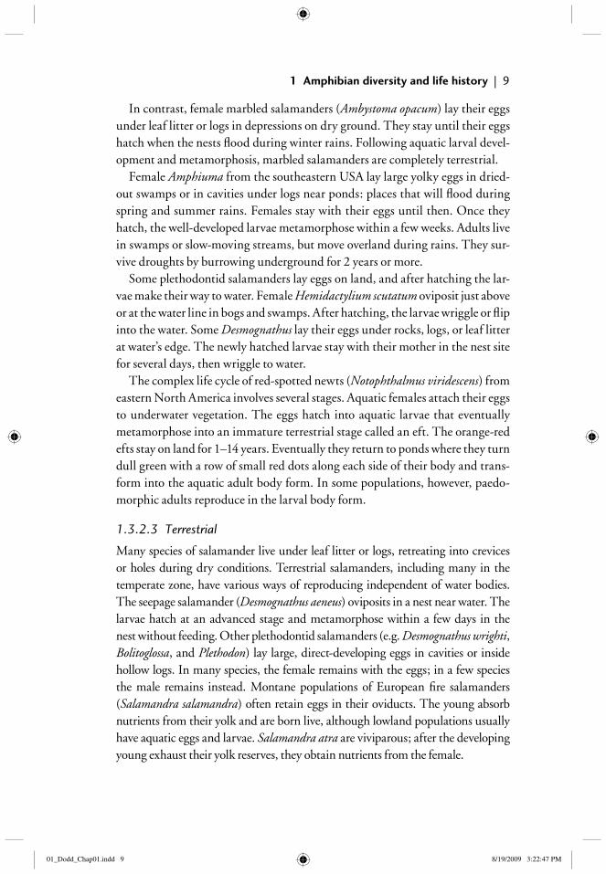
In contrast, female marbled salamanders (Ambystoma opacum) lay their eggs under leaf litter or logs in depressions on dry ground. They stay until their eggs hatch when the nests fl ood during winter rains. Following aquatic larval devel-opment and metamorphosis, marbled salamanders are completely terrestrial.
Female Amphiuma from the southeastern USA lay large yolky eggs in dried-out swamps or in cavities under logs near ponds: places that will fl ood during spring and summer rains. Females stay with their eggs until then. Once they hatch, the well-developed larvae metamorphose within a few weeks. Adults live in swamps or slow-moving streams, but move overland during rains. They sur-vive droughts by burrowing underground for 2 years or more.
Some plethodontid salamanders lay eggs on land, and after hatching the lar-vae make their way to water. Female Hemidactylium scutatum oviposit just above or at the water line in bogs and swamps. After hatching, the larvae wriggle or fl ip into the water. Some Desmognathus lay their eggs under rocks, logs, or leaf litter at water’s edge. The newly hatched larvae stay with their mother in the nest site for several days, then wriggle to water.
The complex life cycle of red-spotted newts (Notophthalmus viridescens) from eastern North America involves several stages. Aquatic females attach their eggs to underwater vegetation. The eggs hatch into aquatic larvae that eventually metamorphose into an immature terrestrial stage called an eft. The orange-red efts stay on land for 1–14 years. Eventually they return to ponds where they turn dull green with a row of small red dots along each side of their body and trans-form into the aquatic adult body form. In some populations, however, paedo-morphic adults reproduce in the larval body form.
1.3.2.3 Terrestrial
Many species of salamander live under leaf litter or logs, retreating into crevices or holes during dry conditions. Terrestrial salamanders, including many in the temperate zone, have various ways of reproducing independent of water bodies. The seepage salamander (Desmognathus aeneus) oviposits in a nest near water. The larvae hatch at an advanced stage and metamorphose within a few days in the nest without feeding. Other plethodontid salamanders (e.g. Desmognathus wrighti, Bolitoglossa, and Plethodon) lay large, direct-developing eggs in cavities or inside hollow logs. In many species, the female remains with the eggs; in a few species the male remains instead. Montane populations of European fi re salamanders (Salamandra salamandra) often retain eggs in their oviducts. The young absorb nutrients from their yolk and are born live, although lowland populations usually have aquatic eggs and larvae. Salamandra atra are viviparous; after the developing young exhaust their yolk reserves, they obtain nutrients from the female.
01_Dodd_Chap01.indd 901_Dodd_Chap01.indd 9 8/19/2009 3:22:47 PM8/19/2009 3:22:47 PM
10 | Amphibian ecology and conservation
1.3.2.4 Fossorial
Most Oedipina, fossorial or semi-fossorial plethodontid salamanders ranging from Mexico to northern South America, lay direct-developing eggs under-ground. Some fossorial plethodontids (e.g. Lineatriton lineola) attend their direct-developing eggs.
1.3.2.5 Arboreal
Neotropical arboreal plethodontids (e.g. Bolitoglossa and Nototriton) lay their eggs under mats of mosses and liverworts on tree branches and in bromeliads. The eggs undergo direct development, and some female Bolitoglossa attend their eggs. Aneides lugubris from western North America lays direct-developing eggs as high as 10 m above the ground.
1.3.3 Anurans
Anuran lifestyles include purely aquatic, aquatic and terrestrial, terrestrial, arbor-eal, and fossorial. A frog with relatively short hind legs is most likely a terrestrial hopper or fossorial species. One with long hind legs is likely to be aquatic, arbor-eal, or a jumping terrestrial species. Aquatic anurans tend to have their eyes on the top of their heads rather than at the sides, and they often have fully webbed feet. Some have fl attened bodies. Arboreal frogs generally have expanded pads on the ends of their toes. Many fossorial species have small heads with pointed snouts and depressed bodies. Some have spadelike tubercles on their hind feet used for burrowing.
Anurans have evolved remarkably diverse life histories, from aquatic eggs to viviparity. In between those extremes, frogs from numerous families on many continents lay their eggs out of water yet have aquatic larvae. In the section head-ings below, the fi rst designation refers to post-metamorphic stages, the second to egg and/or larval stages.
1.3.3.1 Aquatic/aquatic
Many aquatic frogs lay eggs that hatch into tadpoles. African clawed frogs (Xenopus) attach their eggs to submerged vegetation in standing water. The South American paradox frog (Pseudis paradoxa) oviposits among vegetation in shallow water of ponds and lakes. Aquatic larvae grow to 25 cm—the largest of any frog—then they metamorphose into relatively small juveniles. Tailed frogs (Ascaphus truei) from northwestern USA and adjacent Canada live in cold, torrential streams where they lay eggs under rocks. In some areas larvae require several years to metamorphose.
01_Dodd_Chap01.indd 1001_Dodd_Chap01.indd 10 8/19/2009 3:22:47 PM8/19/2009 3:22:47 PM
1 Amphibian diversity and life history | 11
Some fully aquatic anurans brood their young. Female South American Pipa carry eggs embedded in their backs. In some species of Pipa the eggs hatch into tadpoles. In others they undergo direct development. Female Australian gastric-brooding frogs (Rheobatrachus) swallowed their late-stage eggs or early-stage larvae, and the tadpoles absorbed yolk reserves while developing in their mothers’ stomachs. No Rheobatrachus have been seen since the 1980s; both species are assumed extinct.
1.3.3.2 Terrestrial/aquatic
Terrestrial anurans from many families lay aquatic eggs, and the aquatic larvae metamorphose into terrestrial juveniles. Species that oviposit in standing water produce clutches in compact masses (some ranids), fl oating rafts on the water surface (some ranids), strings (most Bufo and some pelobatids), scattered indi-vidually or in small packets on the bottom substrate (Bombina and Discoglossus), attached individually or in small groups onto submerged plants (some species of Pseudacris, Acris, Hyla, and Spea), or as a fi lm on the water surface (some microhylids).
Some anurans breed in moderately fast streams or mountain torrents. Female Atelopus from Central and South America lay their eggs in strings attached to rocks. The larvae have ventral sucker-like discs that allow them to adhere to rocks while feeding. Tadpoles of bufonid stream-breeding Ansonia from Asia and Werneria from Africa have similar suckers. Other stream-adapted frogs, such as many ranids, lay large eggs in compact masses attached to rocks in areas where the current is slow and the eggs are less likely to be swept away.
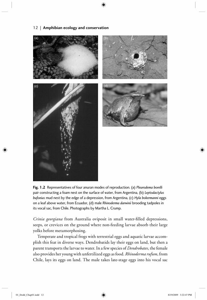
Some terrestrial anurans produce foam nests in which their eggs are sus-pended. Male Leptodactylus, Physalaemus, and Pleurodema from Central and South America kick their hind legs during amplexus, whipping the females’ eggs and mucus and their sperm and mucus into foamy masses (Figure 1.2a). The outermost layer of foam dries quickly and provides some protection against desiccation and predation. Some foam-nesters produce their nests on the water surface, others in cavities or holes next to ponds. Leptodactylus bufonius con-structs mud nests at the margin of temporary ponds and deposits its foam nests inside (Figure 1.2b). The eggs hatch into tadpoles that remain in the nests until rains dissolve the nests and fl ood the area. Some Australian myobatrachids also construct foam nests on the water surface.
Some terrestrial frogs oviposit in very small bodies of water on land. Brazilian Bufo castaneoticus lay their eggs in water-fi lled fruit capsules of the Brazil nut tree, and the tadpoles feed on detritus. Eupsophus from Chile and
01_Dodd_Chap01.indd 1101_Dodd_Chap01.indd 11 8/19/2009 3:22:47 PM8/19/2009 3:22:47 PM
12 | Amphibian ecology and conservation
(a) (b)
(c) (d)
Fig. 1.2 Representatives of four anuran modes of reproduction. (a) Pleurodema borelli pair constructing a foam nest on the surface of water, from Argentina, (b) Leptodactylus bufonius mud nest by the edge of a depression, from Argentina, (c) Hyla bokermanni eggs on a leaf above water, from Ecuador, (d) male Rhinoderma darwinii brooding tadpoles in its vocal sac, from Chile. Photographs by Martha L. Crump.
Crinia georgiana from Australia oviposit in small water-fi lled depressions, seeps, or crevices on the ground where non-feeding larvae absorb their large yolks before metamorphosing.
Temperate and tropical frogs with terrestrial eggs and aquatic larvae accom-plish this feat in diverse ways. Dendrobatids lay their eggs on land, but then a parent transports the larvae to water. In a few species of Dendrobates, the female also provides her young with unfertilized eggs as food. Rhinoderma rufum, from Chile, lays its eggs on land. The male takes late-stage eggs into his vocal sac
01_Dodd_Chap01.indd 1201_Dodd_Chap01.indd 12 8/19/2009 3:22:47 PM8/19/2009 3:22:47 PM
1 Amphibian diversity and life history | 13
where they hatch, then transports the larvae to water. In Europe, male midwife toads (Alytes) carry their eggs wrapped around their hind legs. Eventually they hop to ponds where the eggs hatch into aquatic larvae.
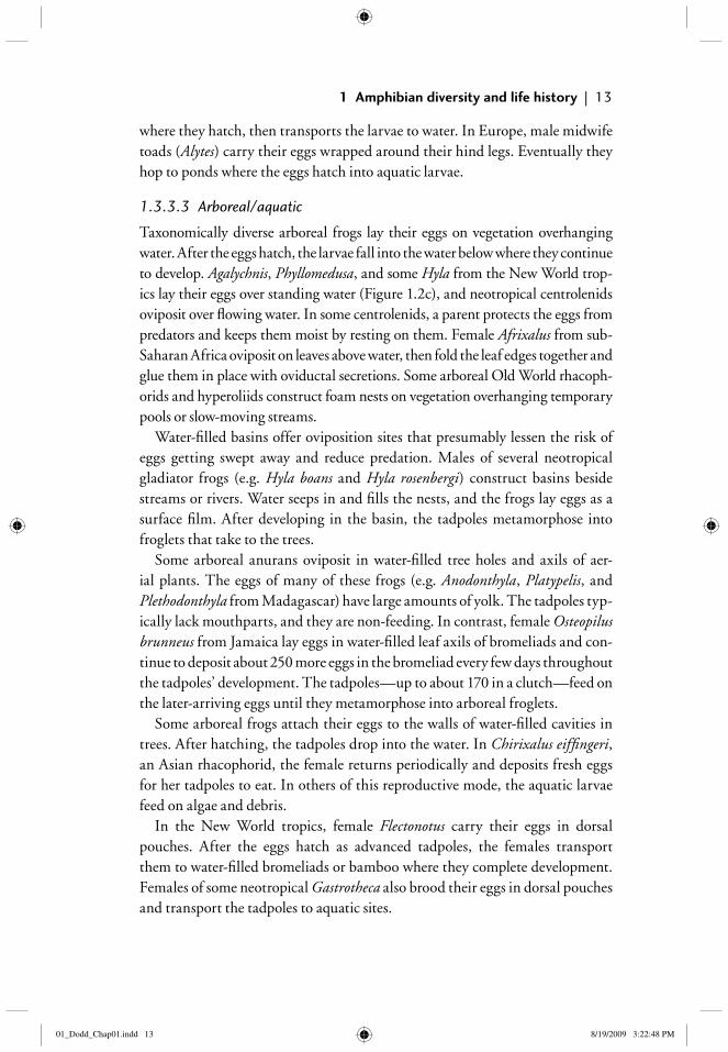
1.3.3.3 Arboreal/aquatic
Taxonomically diverse arboreal frogs lay their eggs on vegetation overhanging water. After the eggs hatch, the larvae fall into the water below where they continue to develop. Agalychnis, Phyllomedusa, and some Hyla from the New World trop-ics lay their eggs over standing water (Figure 1.2c), and neotropical centrolenids oviposit over fl owing water. In some centrolenids, a parent protects the eggs from predators and keeps them moist by resting on them. Female Afrixalus from sub-Saharan Africa oviposit on leaves above water, then fold the leaf edges together and glue them in place with oviductal secretions. Some arboreal Old World rhacoph-orids and hyperoliids construct foam nests on vegetation overhanging temporary pools or slow-moving streams.
Water-fi lled basins offer oviposition sites that presumably lessen the risk of eggs getting swept away and reduce predation. Males of several neotropical gladiator frogs (e.g. Hyla boans and Hyla rosenbergi) construct basins beside streams or rivers. Water seeps in and fi lls the nests, and the frogs lay eggs as a surface fi lm. After developing in the basin, the tadpoles metamorphose into froglets that take to the trees.
Some arboreal anurans oviposit in water-fi lled tree holes and axils of aer-ial plants. The eggs of many of these frogs (e.g. Anodonthyla, Platypelis, and Plethodonthyla from Madagascar) have large amounts of yolk. The tadpoles typ-ically lack mouthparts, and they are non-feeding. In contrast, female Osteopilus brunneus from Jamaica lay eggs in water-fi lled leaf axils of bromeliads and con-tinue to deposit about 250 more eggs in the bromeliad every few days throughout the tadpoles’ development. The tadpoles—up to about 170 in a clutch—feed on the later-arriving eggs until they metamorphose into arboreal froglets.
Some arboreal frogs attach their eggs to the walls of water-fi lled cavities in trees. After hatching, the tadpoles drop into the water. In Chirixalus eiffi ngeri, an Asian rhacophorid, the female returns periodically and deposits fresh eggs for her tadpoles to eat. In others of this reproductive mode, the aquatic larvae feed on algae and debris.
In the New World tropics, female Flectonotus carry their eggs in dorsal pouches. After the eggs hatch as advanced tadpoles, the females transport them to water-fi lled bromeliads or bamboo where they complete development. Females of some neotropical Gastrotheca also brood their eggs in dorsal pouches and transport the tadpoles to aquatic sites.
01_Dodd_Chap01.indd 1301_Dodd_Chap01.indd 13 8/19/2009 3:22:48 PM8/19/2009 3:22:48 PM
14 | Amphibian ecology and conservation
1.3.3.4 Fossorial/aquatic
Scaphiopus and Spea, North American spadefoot toads, spend much of their lives underground but emerge following heavy rains and lay their eggs in newly formed ponds. The tadpoles develop quickly, which increases the probability of metamorphosing before the ponds dry. Rhinophrynus dorsalis, from south-ern Texas to Costa Rica, likewise lives underground and emerges after the fi rst heavy rains to breed in temporary ponds. Female Hemisis marmoratum from Africa lay their eggs in subterranean chambers and stay with their eggs until after they hatch. At that point, the female digs a tunnel into adjacent water for the tadpoles.
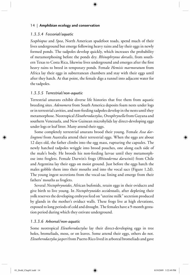
1.3.3.5 Terrestrial/non-aquatic
Terrestrial anurans exhibit diverse life histories that free them from aquatic breeding sites. Adenomera from South America deposits foam nests under logs or in terrestrial cavities, and non-feeding tadpoles develop in the nests until they metamorphose. Neotropical Eleutherodactylus, Oreophrynella from Guyana and southern Venezuela, and New Guinean microhylids lay direct-developing eggs under logs or leaf litter. Many attend their eggs.
Some completely terrestrial anurans brood their young. Female Assa dar-lingtoni from Australia attend their terrestrial eggs. When the eggs are about 12 days old, the father climbs into the egg mass, rupturing the capsules. The newly hatched tadpoles wriggle into brood pouches, one along each side of the male’s body. He broods his non-feeding larvae until they metamorph-ose into froglets. Female Darwin’s frogs (Rhinoderma darwinii) from Chile and Argentina lay their eggs on moist ground. Just before the eggs hatch the males gobble them into their mouths and into the vocal sacs (Figure 1.2d). The young ingest secretions from the vocal-sac lining and emerge from their fathers’ mouths as froglets.
Several Nectophrynoides, African bufonids, retain eggs in their oviducts and give birth to live young. In Nectophrynoides occidentalis, after depleting their yolk reserves the developing embryos feed on “uterine milk” secretion produced by glands in the mother’s oviduct walls. These frogs live at high elevations, exposed to long periods of cold and drought. The females have a 9-month gesta-tion period during which they estivate underground.
1.3.3.6 Arboreal/non-aquatic
Some neotropical Eleutherodactylus lay their direct-developing eggs in tree holes, bromeliads, moss, or on leaves. Some attend their eggs, others do not. Eleutherodactylus jasperi from Puerto Rico lived in arboreal bromeliads and gave
01_Dodd_Chap01.indd 1401_Dodd_Chap01.indd 14 8/19/2009 3:22:49 PM8/19/2009 3:22:49 PM
1 Amphibian diversity and life history | 15
birth to live young. The direct-developing eggs were retained in the oviducts, and nutrition came entirely from the embryo’s yolk reserves. This species has not been seen since 1981 and is assumed extinct.
Female Cryptobatrachus, Stefania, and Hemiphractus, neotropical hylids, carry their direct-developing eggs exposed on their backs, secured by mucous gland secretions. Females of some Gastrotheca brood direct-developing eggs in dorsal pouches that protect the developing embryos from predators and des-iccation and also function in gaseous exchange between the females and their embryos.
1.3.3.7 Fossorial/non-aquatic
The burrowing microhylid Synapturanus salseri from Colombia lays its eggs in burrows just below the root mat on the forest fl oor. Non-feeding tadpoles hatch at an advanced stage and absorb their yolk reserves. The Brazilian bur-rowing leptodactylid Cycloramphus stejnegeri likewise oviposits in underground nests and has non-feeding tadpoles. Other fossorial anurans, such as Geocrinia and Arenophryne (Australian myobatrachids), Callulops (New Guinean micro-hylids), and Breviceps (African microhylids), lay direct-developing eggs in underground burrows. Female Breviceps stay with their eggs and presumably keep them moist.
1.4 Amphibian declines and why they matter
The world is experiencing a “biodiversity crisis”: rapid and accelerating loss of species and habitat (Ehrlich and Ehrlich 1981; Myers 1990; Raven 1990; Wilson 1992). Amphibians are part of this overall loss. Populations of amphibians are declining and disappearing worldwide at an increasing rate as compared to pre-1980 decades, even from protected areas (Blaustein and Wake 1990; Phillips 1994; Stuart et al. 2004). During the late 1980s and early 1990s, many declines seemed mysterious because there was no obvious cause. Skeptics argued that declines might be simply natural population fl uctuations. Since the late 1980s, scientists worldwide have focused on determining the extent of declines and identifying the causes. We now know these declines are real.
The International Union for the Conservation of Nature (IUCN) assesses the status of species on a global scale and maintains and updates a catalog of taxa that face a high risk of global extinction: the IUCN Red List of Threatened Species. The 2008 update lists 30% of described amphibians as threatened with extinction (IUCN 2008). Since 1500, at least 39 species of amphibians have become extinct.
01_Dodd_Chap01.indd 1501_Dodd_Chap01.indd 15 8/19/2009 3:22:49 PM8/19/2009 3:22:49 PM
16 | Amphibian ecology and conservation
Scientists have hypothesized six major threats to amphibians: habitat modi-fi cation and destruction, commercial over-exploitation, introduced species, environmental contaminants, global climate change, and emerging infectious diseases, especially the chytrid fungus Batrachochytrium dendrobatidis (Collins and Storfer 2003). Most agree the primary threat is habitat modifi cation and destruction. For the past 100 years, human population growth has been expo-nential and has occurred largely in areas with the highest amphibian species richness: the tropics and subtropics (Gallant et al. 2007). As a result, these land-scapes are being heavily modifi ed to support agriculture and other human activ-ities. The chytrid fungus also is exerting a major impact in many areas and on many species (Smith et al. 2006). Thus far the chytrid has caused the decline or extinction of about 200 species of frog (Skerratt et al. 2007). Many factors make the chytrid a signifi cant concern, including its wide distribution in both the New and Old Worlds, its rapid spread and high virulence, and the fact that it infects a broad diversity of host species (Daszak et al. 1999).
Why should we care if we lose amphibians? It is for the same basic reasons we should care if other animals and plants disappear: economics, ecosystem func-tion, esthetics, and ethics (Noss and Cooperrider 1994; Groom et al. 2006).
1.4.1 Economics
Selfi shly, we should care if we lose amphibians because we use them for our own benefi t, including for food and as pets. We use literally tonnes of frogs each year in medical research and teaching. We have isolated novel chemical compounds from granular glands of anuran skin and have used these compounds to develop new drugs.
1.4.2 Ecosystem function
Amphibians play a key role in energy fl ow and nutrient cycling because they serve as both predator and prey. By eating huge quantities of algae, tadpoles reduce the rate of natural eutrophication, the over-enrichment of water with nutrients, which leads to excessive algal growth and oxygen depletion. Most adult amphibians eat insects and other arthropods. As ectotherms, amphib-ians are effi cient at converting food into growth and reproduction. Unlike endothermic birds and mammals that generate heat metabolically, amphib ians expend relatively little energy to maintain themselves. Birds and mammals use up to 98% of their ingested energy to maintain their body temperatures, leaving as little as 2% to be converted to new animal tissue: food for preda-tors. In contrast, amphibians convert about 50% of their energy gained from food into new tissue, which is transferred to the next level in the food chain
01_Dodd_Chap01.indd 1601_Dodd_Chap01.indd 16 8/19/2009 3:22:49 PM8/19/2009 3:22:49 PM
1 Amphibian diversity and life history | 17
(Pough et al. 2004). If amphibians disappeared, would the world be overrun with housefl ies, mosquitoes, and crop-eating insect pests? Would their preda-tors go extinct?
1.4.3 Esthetics
Imagine the silence of rainy spring evenings without the lively croaking of male frogs. The monotonous roads without spring migrations of salamanders. People worldwide consider frogs to be good luck because of their association with rain. Amphibians provide inspiration for our artistic endeavors, from literature to music and the visual arts.
1.4.4 Ethics
Every species is a unique product of evolution. In 1982 the United Nations General Assembly adopted the World Charter for Nature, which states: “Every form of life is unique, warranting respect regardless of its worth to man, and, to accord other organisms such recognition, man must be guided by a moral code of action” (Noss and Cooperrider 1994). More than 100 nations signed the charter. Like all other living species, amphibians have intrinsic value and a right to exist.
Amphibians, amazing descendants of terrestrial pioneers, are fi ghting for their lives in a world greatly modifi ed by humans.
1.5 References
Blaustein, A. R. and Wake, D. B. (1990). Declining amphibian populations: a global phe-nomenon? Trends in Ecology and Evolution, 5, 203–4.
Collins, J. P. and Storfer, A. (2003). Global amphibian declines: sorting the hypotheses. Diversity and Distributions, 9, 89–98.
Crump, M. L. (1995). Parental care. In H. Heatwole and B. K. Sullivan (eds), Amphibian Biology, vol. 2: Social Behaviour, pp. 518–67. Surrey Beatty and Sons, Chipping Norton, NSW.
Crump, M. L. (1996). Parental care among the Amphibia. In J. S. Rosenblatt and C. T. Snowdon (eds), Advances in the Study of Behavior, vol. 25: Parental Care: Evolution, Mechanisms, and Adaptive Signifi cance, pp. 109–44. Academic Press, New York.
Daszak, P., Berger, L., Cunningham, A. A., Hyatt, A. D., Green, D. E., and Speare, R. (1999). Emerging infectious diseases and amphibian population declines. Emerging Infectious Diseases, 5, 735–48.
Duellman, W. E. (1970). The Hylid Frogs of Middle America, vol. 1. Monograph of the Museum of Natural History, Number 1. University of Kansas, Lawrence, KA.
Duellman, W. E. (1999). Global distribution of amphibians: patterns, conservation, and future challenges. In W. E. Duellman (ed.), Patterns of Distribution of Amphibians: a Global Perspective, pp. 1–30. John Hopkins University Press, Baltimore, MD.
01_Dodd_Chap01.indd 1701_Dodd_Chap01.indd 17 8/19/2009 3:22:49 PM8/19/2009 3:22:49 PM
18 | Amphibian ecology and conservation
Duellman, W. E. (2007). Amphibian life histories: their utilization in phylogeny and clas-sifi cation. In H. Heatwole and M. J. Tyler (eds), Amphibian Biology, vol. 7. Systematics, pp. 2843–92. Surrey Beatty and Sons, Chipping Norton, NSW.
Duellman, W. E. and Trueb, L. (1986). Biology of Amphibians. McGraw-Hill, NewYork.Ehrlich, P. R. and Ehrlich, A. H. (1981). Extinction: The Causes and Consequences of the
Disappearance of Species. Random House, New York.Gallant, A. L., Klaver, R. W., Casper, G. S., and Lannoo, M. J. (2007). Global rates of
habitat loss and implications for amphibian conservation. Copeia, 2007, 967–79.Groom, M., Meffe, G. K., and Carroll, C. R. (2006). Principles of Conservation Biology,
3rd edn. Sinauer Associates, Sunderland, MA.Haddad, C. F. B. and Prado, C. P. A. (2005). Reproductive modes in frogs and their unex-
pected diversity in the Atlantic Forest of Brazil. BioScience, 55, 207–17.IUCN (International Union for the Conservation of Nature) (2008). Red List of
Threatened Species. IUCN, Gland. http://www.iucn.org/themes/ssc/redlist.htm.Myers, N. (1990). Mass extinctions: what can the past tell us about the present and the
future? Global and Planetary Change, 82, 175–85.Noss, R. F. and Cooperrider, A. Y. (1994). Saving Nature’s Legacy: Protecting and Restoring
Biodiversity. Island Press, Washington DC.Phillips, K. (1994). Tracking the Vanishing Frogs: an Ecological Mystery. St. Martin’s Press,
New York.Pough, F. H., Andrews, R. M., Cadle, J. E., Crump, M. L., Savitzky, A. H., and Wells, K. D.
(2004). Herpetology, 3rd edn. Prentice Hall, Upper Saddle River, NJ.Raven, P. H. (1990). The politics of preserving biodiversity. BioScience, 40, 769–74.Salthe, S. N. (1969). Reproductive modes and the number and sizes of ova in the urodeles.
American Midland Naturalist, 81. 467–90.Salthe, S. N. and Duellman, W. E. (1973). Quantitative constraints associated with
reproductive mode in anurans. In J. L. Vial (ed.), Evolutionary Biology of the Anurans, pp. 229–49. University of Missouri Press, Columbia, MO.
Skerratt, L. F., Berger, L., Speare, R., Cashins, S., McDonald, K. R., Phillott, A. D., Hines, H. B., and Kenyon, N. (2007). Spread of chytridiomycosis has caused the rapid global decline and extinction of frogs. EcoHealth, 4, 125–34.
Smith, K. F., Sax, D. F., and Lafferty, K. D. (2006). Evidence for the role of infectious disease in species extinction and endangerment. Conservation Biology, 20, 1349–57.
Stuart, S. N., Chanson, J. S., Cox, N. A., Young, B. E., Rodrigues, A. S.L., Fischman, D. L., and Waller, W. (2004). Status and trends of amphibian declines and extinctions world-wide. Science, 302, 1783–6.
Wake, M. H. (1977). The reproductive biology of caecilians: an evolutionary perspec-tive. In D. H. Taylor and S. I. Guttman (eds), The Reproductive Biology of Amphibians, pp. 73–101. Plenum, New York.
Wake, M. H. (1982). Diversity within a framework of constraints. Amphibian repro-ductive modes. In D. Mossakowski and G. Roth (eds), Environmental Adaptation and Evolution, pp. 87–106. Gustav Fischer, New York.
Wake, M. H. (1992). Reproduction in caecilians. In W. C. Hamlett (ed.), Reproductive Biology of South American Vertebrates, pp. 112–20. Springer-Verlag, New York.
01_Dodd_Chap01.indd 1801_Dodd_Chap01.indd 18 8/19/2009 3:22:49 PM8/19/2009 3:22:49 PM

1 Amphibian diversity and life history | 19
Wake, M. H. (1993). Evolution of oviductal gestation in amphibians. Journal of Experimental Zoology, 266, 394–413.
Wells, K. D. (2007). The Ecology and Behavior of Amphibians. University of Chicago Press, Chicago, IL.
Wilkinson, M. and Nussbaum, R. A. (1998). Caecilian viviparity and amniote origins. Journal of Natural History, 32, 1403–9.
Wilson, E. O. (1992). The Diversity of Life. The Belknap Press of Harvard University Press, Cambridge, MA.
01_Dodd_Chap01.indd 1901_Dodd_Chap01.indd 19 8/19/2009 3:22:49 PM8/19/2009 3:22:49 PM

01_Dodd_Chap01.indd 2001_Dodd_Chap01.indd 20 8/19/2009 3:22:49 PM8/19/2009 3:22:49 PM
2Setting objectives in fi eld studies
Dan Cogalniceanu and Claude Miaud
2.1 Basic concepts for a good start
Considerable fi nancial and human resources may be wasted due to poor research design and implementation. In addition, poor planning can result in taking non-repeatable or unreliable data that are of no or limited use, and leads to the paradox of “data-rich, information-poor.” Rigorous study planning and the def-inition of clear and realistic goals can help avoid wasted effort. Before undertak-ing fi eld studies, biologists fi rst must defi ne their objectives and then assess the availability of resources necessary to accomplish them. This is a key stage, and any uncertainty or vagueness at this point could prove detrimental to the success and usefulness of the study.
There are two different approaches in scientifi c investigation: inductive and deductive methods. The inductive or exploratory method relies on gathering data without fi rst identifying hypotheses to be tested; results may then be explained based on the data gathered. However, science involves more than accumulating data and then searching for patterns. A useful study must start with an obser-vation that identifi es a problem or question to be resolved. The observation should have biological signifi cance and be based on current evolutionary theory (Wolff and Krebs 2008). For example, amphibian populations are declining: what are the causes? Two related species hybridize on just a narrow contact zone: why? Habitats are fragmented by human activity: what effects does this have on population persistence, and why (e.g. dispersal abilities, food resources, popula-tion demography, genetics, susceptibility to predators, and human activities)?
As science is an activity focused on understanding natural processes and, espe-cially in modern times, in devising solutions to problems, the hypothesis-based deductive method was developed (James and McCulloch 1985). An hypothesis is a statement related to an observation which may be true, but for which proof has not yet been found. The function of the hypothesis is to direct the search
02_Dodd_Chap02.indd 2102_Dodd_Chap02.indd 21 8/19/2009 3:23:46 PM8/19/2009 3:23:46 PM
22 | Amphibian ecology and conservation
for order among facts. Fieldwork then serves to test one’s hypothesis, thereby scientifi cally demonstrating correlation, causation, or the absence thereof. The hypothesis must of necessity regard some facts as more signifi cant than others, based on the researcher’s previous experience, familiarity with the literature, and individual interpretation.
As scientifi c knowledge is rarely complete, any list of potential alternative hypotheses is also unlikely to be complete. Therefore, alternative hypotheses for the particular problem or question being considered must also be formulated. Thus, it is necessary to conduct research with both the hypothesis and alter-native hypothesis in mind, as more than one cause may be contributing to any single effect (Wolff and Krebs 2008). For example, Jaeger (1972) used enclos-ures to test the mechanism of interspecifi c competition between two species of plethodontid salamanders, hypothesizing that it resulted from either differential exploitation of food resources or through interference. Both primary and alter-native hypotheses are formulated and tested so that researchers can determine which explanations best fi t the results obtained. Unsupported hypotheses can be rejected, but even the most parsimonious hypothesis may not be fully accepted because there still may be underlying explanations as yet untested (Senar 2004). Repeated experimentation involving alternative hypotheses eventually allows researchers to gain a measure of confi dence in the validity of empirically sup-ported hypotheses (Jaeger and Halliday 1998). Both hypotheses and data are essential for credible science since, as Krebs (1999) concluded, hypotheses with-out data are not very useful, and data without hypotheses are useful only for an inductive approach.
Ecology is an empirical science that requires data from the “real” world, and a fi eld study is a tool which can ultimately lead to the acceptance or rejec-tion of an hypothesis. After repeated experimentation and validation, data and information from many fi eld studies are synthesized and organized into concepts of how nature functions. These concepts are the result of the integra-tion between what scientists think they know (based on previous research and observation) and newly acquired data (Ford 2000). Asking the right question is important, because the type of question asked and the particular techniques and methods used in hypothesis-driven research strongly infl uence what is discovered and the direction of future research. During the course of this feedback process, scientists come to a better understanding of the phenomena they study (Figure 2.1).
Scientists present what they want to accomplish during a fi eld study in terms of goals and objectives. A goal is a statement that explains what the study is designed to accomplish. It is usually a broad and general statement, inclusive of
02_Dodd_Chap02.indd 2202_Dodd_Chap02.indd 22 8/19/2009 3:23:46 PM8/19/2009 3:23:46 PM
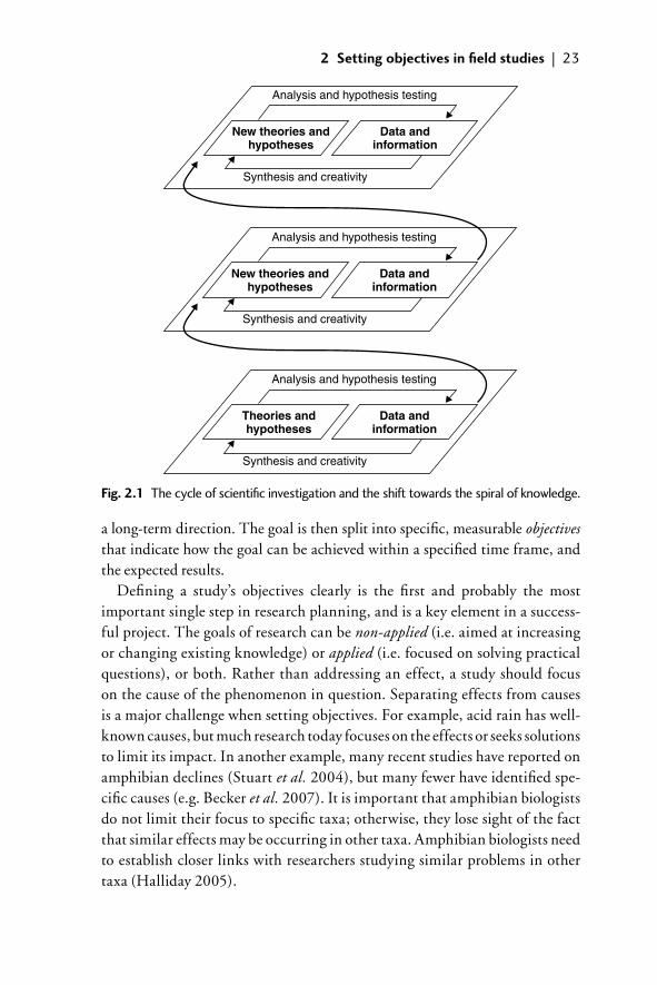
2 Setting objectives in fi eld studies | 23
a long-term direction. The goal is then split into specifi c, measurable objectives that indicate how the goal can be achieved within a specifi ed time frame, and the expected results.
Defi ning a study’s objectives clearly is the fi rst and probably the most important single step in research planning, and is a key element in a success-ful project. The goals of research can be non-applied (i.e. aimed at increasing or changing existing knowledge) or applied (i.e. focused on solving practical questions), or both. Rather than addressing an effect, a study should focus on the cause of the phenomenon in question. Separating effects from causes is a major challenge when setting objectives. For example, acid rain has well-known causes, but much research today focuses on the effects or seeks solutions to limit its impact. In another example, many recent studies have reported on amphibian declines (Stuart et al. 2004), but many fewer have identifi ed spe-cifi c causes (e.g. Becker et al. 2007). It is important that amphibian biologists do not limit their focus to specifi c taxa; otherwise, they lose sight of the fact that similar effects may be occurring in other taxa. Amphibian biologists need to establish closer links with researchers studying similar problems in other taxa (Halliday 2005).
Analysis and hypothesis testing
Synthesis and creativity
New theories andhypotheses
Data andinformation
Analysis and hypothesis testing
Synthesis and creativity
New theories andhypotheses
Data andinformation
Analysis and hypothesis testing
Synthesis and creativity
Theories andhypotheses
Data andinformation
Fig. 2.1 The cycle of scientifi c investigation and the shift towards the spiral of knowledge.
02_Dodd_Chap02.indd 2302_Dodd_Chap02.indd 23 8/19/2009 3:23:46 PM8/19/2009 3:23:46 PM
24 | Amphibian ecology and conservation
Ideally, the cycle of scientifi c investigation should proceed from data and infor-mation gathering and analysis, to quantifying knowledge, and to conceptual understanding. A logical, stepwise approach of scientifi c inquiry (Lehner 1996) should be followed: (1) perceive that a problem/question exists; (2) formulate a possible explanation (i.e. devise an hypothesis); (3) formulate alternative hypoth-eses; (4) identify the best approach to test the hypothesis (i.e. theoretical models, experiments, or fi eld observations); (5) collect and analyze data; (6) support or reject the hypothesis; and (7) understand the meaning and implications of the results. The original hypothesis can then be modifi ed, experiments repeated and, with time, conceptual understanding attained.
2.2 Steps required for a successful study
Ecological systems are large and complex and, at times, unpredictable. The more complex the system, the more uncertainties arise. Data are most often obtained within the parameters of a limited number of samples, restricted time, or specifi c area, and then applied to larger scales. By carefully framing the hypothesis and deciding the most practical, meaningful, and objective method of study, degree of error can be minimized (Hayek 1994). The following section presents some of the most important issues that must be considered when planning a fi eld study.
2.2.1 Temporal and spatial scales
The issue of scale has three components (Schneider 2001): (1) pressing problems in ecology often exist within timescales of decades or centuries, and cover large areas; (2) most data can be gathered directly for only short periods of time and over small areas; (3) patterns measured at small scales do not necessarily hold true at larger scales; nor do processes observed at smaller scales necessarily exist at larger ones. Thus, an inappropriate scale limits the inference of the results.
Spatial and temporal scales can be classifi ed as gradient, interval, discrete, and continuous (Bernstein and Goldfarb 1995). Setting temporal and spatial scales involves defi ning their boundaries and helps to answer three practical questions: where, for how long, and how often? Selecting the appropriate scale is diffi cult because of environmental heterogeneity in both time and space. Amphibian populations and communities also vary widely throughout time and space, since they are infl uenced by a multitude of environmental variables (Meyer et al. 1998; Pechmann et al. 1991; Pellet et al. 2006).
Temporal scales are rarely discussed explicitly, but they are often assumed to span years rather than generations. Many time-dependent phenomena such as extinction, predator–prey interactions, competition, and succession reveal
02_Dodd_Chap02.indd 2402_Dodd_Chap02.indd 24 8/19/2009 3:23:47 PM8/19/2009 3:23:47 PM
2 Setting objectives in fi eld studies | 25
important insights if considered on a generational scale (Frankham and Brook 2004). The current distribution and abundance of animal species inhabiting an area is the result, in part, of the impact of geological processes (e.g. plate tecton-ics, orogenesis, sea-level changes, major catastrophes), ecological processes (e.g. competition, predation, climate), life-history traits (e.g. dispersal), and recent human impacts (e.g. changes in vegetation and habitat structure, overexploi-tation, introduction of nonindigenous species). For example, in the Northern Hemisphere the Pleistocene–Holocene post-glacial recolonizations of species and human activities (e.g. habitat destruction and alteration) are the two major factors shaping the current distribution of amphibians. Objectives of a time-scale component of a study plan should include such factors as short-term (less than one generation), intermediate (more than one to a few generations), and long-term (many generations, and inclusive of a large spatial scale and monitor-ing activities).
Spatial scales and objectives are strongly interconnected. Selection of a study site includes such factors as the complexity of local macro- and microhabitats and, at large spatial scales, biogeographical provinces and landscapes (Morrison 2002). Of great importance to the overall study plan are the criteria for describ-ing vegetation, whether gross (e.g. foliage height, diversity), physiognomy (phys-ical structure), or fl oristic (plant taxonomic description). The relative usefulness of structural or fl oristic measures depends on the spatial scale of the analysis. For example, whereas most studies do not require a detailed description of plant taxa, species lists might be essential for characterizing microhabitat and trophic (resource) availability.
The importance of choosing the correct scale can be exemplifi ed by a study assessing population fl uctuations within a particular species: the fi rst step would be to understand the distribution of the species in order to thoroughly sample all areas, rather than by biasing results by sampling in only one small portion of the range. In another example, a study of the movement patterns of a species may focus on individual distributional patterns, daily or weekly movements, sea-sonal migrations related to reproduction or dispersal, or on region-wide range shifts through years or decades.
2.2.2 Choosing the model species
Many amphibian species have restricted distributions and complex habitat requirements. Some amphibian populations, especially among temperate pond-breeding species, are maintained by episodic reproduction that occurs in a spor-adic and unpredictable manner (Alford and Richards 1999). If a number of different species is available for study, selecting an experimental species should
02_Dodd_Chap02.indd 2502_Dodd_Chap02.indd 25 8/19/2009 3:23:47 PM8/19/2009 3:23:47 PM
26 | Amphibian ecology and conservation
be based on an understanding of its life history (i.e. feeding, habitat use, disper-sal abilities, reproduction, behavior, predators, phylogeography, population gen-etics) and its suitability in resolving the particular question being asked (Wolff and Krebs 2008). For example, a species with low detectability is not a good choice for a mark–recapture study since it will require a considerable sampling effort and entail potential capture bias (Weir et al. 2005). The role of keystone species (e.g. Eleutherodactylus bransfordii in Costa Rican forests), umbrella spe-cies (e.g. Rana sylvatica in the Milwaukee river basin), or fl agship species (e.g. Salamandra lanzai in the Western Alps) can also be considered. Rare or threat-ened species are often selected because of conservation applications, but research on them could incur potential risks due to ethical considerations. Researchers should avoid choosing a rare or threatened species if common or less vulnerable surrogate species can be selected.
2.2.3 Pilot/desk study
A preliminary pilot study usually helps to develop and test realistic and achiev-able objectives, and avoids later shortcomings and failures. Usually a pilot study is carried out on short temporal and small spatial scales, and allows the testing of conceptual models and methods. What might seem simple during offi ce plan-ning might prove completely different or unworkable in the fi eld. Even a simple review of the literature can prove helpful in avoiding mistakes, however.
2.2.4 Elaborate a conceptual model
A conceptual model (e.g. a simple box diagram showing components and link-ages) is a simplifi ed model of the system to be studied. There are no ideal methods to employ; instead, a multitude of models are available to choose from with various degrees of complexity. Conceptual models are helpful in that they can be used to select the variables to be measured that might be considered import-ant to the study. Since professionals with diverse backgrounds have different philosophies or approaches to using models, it is recommended that each team member contribute knowledge of and/or expertise with various models, then develop an integrated study model from which to work (Maher et al. 1994).
After model development, many of the design questions become more obvi-ous. A model need not embrace all components of the system; it needs only to be adequate for the scope of the investigation. There is always a possible risk that the conceptual model is inappropriate or over-simplifi ed; thus, a slightly more complex model may need to be developed. Adopting a more complex model focuses researchers on collecting additional data that might prove important, despite the extra costs involved with sampling and measurements. In other
02_Dodd_Chap02.indd 2602_Dodd_Chap02.indd 26 8/19/2009 3:23:47 PM8/19/2009 3:23:47 PM

2 Setting objectives in fi eld studies | 27
words, it might be better to collect more data than appears necessary at fi rst, than to discover later that some important parameter was omitted. A pilot study helps to avoid under- or over-collecting data. Although conceptual models help researchers identify what to measure, the timing of studies is determined by the natural history of the species of interest.
2.2.5 The SMART approach
Specifi c objectives allow for greater chances of conducting a successful research project. SMART stands for specifi c, measurable, attainable, relevant, and time (Piotrow et al. 1997), an approach used in project writing that also helps in for-mulating specifi c and measurable objectives within study plans. SMART helps devise objectives that are clear and concise, indicates what is to be achieved, addresses only attainable results, indicates when each stage will be completed, and is not encumbered by idealistic aspirations.
• S: The specifi c part of an objective defi nes what will be done and where it will occur. When setting objectives, ask simple questions that can be answered, and avoid ambiguities, the use of buzzwords or jargon (e.g. “cutting-edge”), and pompous phrasing.
• M: Measurable is an attribute of an activity or its results. The source of and mechanism for collecting measurable data are identifi ed, and collec-tion of these data is determined feasible. If the objective of the study is to document trends (i.e. an increase or decrease of one or more measurable variables), then a baseline is required to act as a reference point (e.g. habi-tat availability, characteristics and use; amphibian community structure; population size). If a baseline is not yet available then it will be useful to fi rst have it established.
• A: Attainable refers to the probability of conducting the proposed activ-ities within the established time frame with the available resources and sup-port. It also includes the external factors critical to success. Doing research today, for example, can become diffi cult due, in part, to increasing admin-istrative restrictions (Prathapan et al. 2008). Other external factors include unforeseen costs, shifts in exchange rates, obtaining collecting and access permits, changes in legislation, and political, security, and health (both human and animal) issues. In coping with external factors, a risk analysis is useful because it allows for planning alternative strategies.
• R: Some useful measures for the relevance of the study’s objectives are the utility and value of the results for practical purpose (e.g. management of protected areas, better conservation measures, and ecological restoration). It
02_Dodd_Chap02.indd 2702_Dodd_Chap02.indd 27 8/19/2009 3:23:47 PM8/19/2009 3:23:47 PM
28 | Amphibian ecology and conservation
may be diffi cult to determine how relevant the objective may be, especially since the true relevance may not be apparent until the study is completed (e.g. if a drought were to affect a long-term study of amphibian breeding). Perhaps an easy way to evaluate the relevance is to answer the “so what” question, thus avoiding undertaking studies of limited or no interest.
• T: Finally, the time required to complete the project will depend on the parameters discussed above.
2.2.6 Applying the SMART approach to plan an amphibian inventory
In the following example, the SMART approach is used as the basis for setting up an inventory of amphibian species in a national park or reserve.
• Specifi c: determine whether to inventory all amphibian species, or only those of special interest, such as rare, threatened, or endemic species. Set the spatial limits of the study, such as the administrative boundary of the park or reserve, or specifi c habitats of interest (e.g. temporary ponds; roads in areas which bisect amphibian dispersal corridors; high elevations con-taining unique habitats or species richness, such as cloud forests).
• Measurable: select parameters to be measured (e.g. presence/not detected, relative abundance, density, sex or life stage, percentage of area occupied), select methods appropriate for each species (especially taking detection probabilities into account), and decide habitat parameters (e.g. tempera-ture, humidity, vegetative cover, characteristics of aquatic habitats).
• Attainable: identify resources and available support (e.g. funding, work force) and administrative considerations (e.g. collecting and access per-mits, training staff for fi eld data collection, animal care and use require-ments, security issues).
• Relevance: provide concise statements as to the importance of the research, and whether it has practical applications. The relevance of the proposed research is particularly important in fi eld studies, especially if it will aid in the management of protected areas and species conservation. Utility also assists in determining research approaches. For example, incorpor-ating measures of abundance with detection probabilities, in addition to occupancy models, is much more informative in determining status than occupancy models alone.
• Time: the research schedule (planning, fi eldwork, data analysis, report and publication preparation) should be clearly stated based on the previ-ously outlined parameters and limiting factors.
02_Dodd_Chap02.indd 2802_Dodd_Chap02.indd 28 8/19/2009 3:23:47 PM8/19/2009 3:23:47 PM
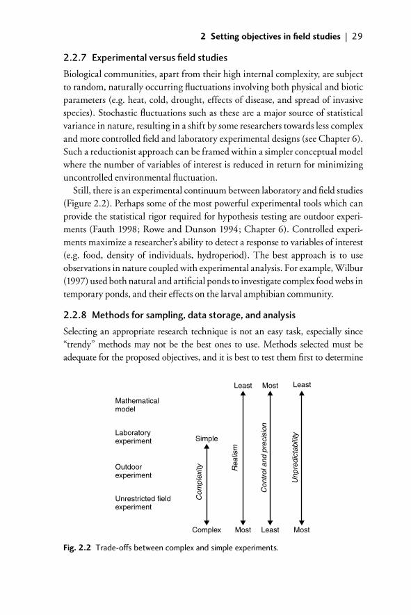
2 Setting objectives in fi eld studies | 29
2.2.7 Experimental versus fi eld studies
Biological communities, apart from their high internal complexity, are subject to random, naturally occurring fl uctuations involving both physical and biotic parameters (e.g. heat, cold, drought, effects of disease, and spread of invasive species). Stochastic fl uctuations such as these are a major source of statistical variance in nature, resulting in a shift by some researchers towards less complex and more controlled fi eld and laboratory experimental designs (see Chapter 6). Such a reductionist approach can be framed within a simpler conceptual model where the number of variables of interest is reduced in return for minimizing uncontrolled environmental fl uctuation.
Still, there is an experimental continuum between laboratory and fi eld studies (Figure 2.2). Perhaps some of the most powerful experimental tools which can provide the statistical rigor required for hypothesis testing are outdoor experi-ments (Fauth 1998; Rowe and Dunson 1994; Chapter 6). Controlled experi-ments maximize a researcher’s ability to detect a response to variables of interest (e.g. food, density of individuals, hydroperiod). The best approach is to use observations in nature coupled with experimental analysis. For example, Wilbur (1997) used both natural and artifi cial ponds to investigate complex food webs in temporary ponds, and their effects on the larval amphibian community.
2.2.8 Methods for sampling, data storage, and analysis
Selecting an appropriate research technique is not an easy task, especially since “trendy” methods may not be the best ones to use. Methods selected must be adequate for the proposed objectives, and it is best to test them fi rst to determine
Mathematicalmodel
Laboratoryexperiment
Outdoorexperiment
Unrestricted fieldexperiment
Simple
Complex Most
Most
MostLeast
Least Least
Com
plex
ity Rea
lism
Con
trol
and
pre
cisi
on
Unp
redi
ctab
ility
Fig. 2.2 Trade-offs between complex and simple experiments.
02_Dodd_Chap02.indd 2902_Dodd_Chap02.indd 29 8/19/2009 3:23:47 PM8/19/2009 3:23:47 PM
30 | Amphibian ecology and conservation
effi ciency and effectiveness. Researchers should adopt complimentary models, applicable and relevant methods, and an altogether SMART use of study plans, resources, and results. The most important elements in any study plan are accurate and precise methods that meet the objectives of the study. A cost-benefi t analysis can prove helpful in the fi nal selection of the methods (Arntzen et al. 1995, 2004).
The sampling design should be both effi cient (a better use of sampling effort in obtaining results) and simple (easily comprehended and easily implemented) (Scott and Köhl 1993). Statistical analyses often have biases or limitations in ecological studies (Krebs 1999; Pollock et al. 2002). Statistical signifi cance may not be the equivalent of biological signifi cance. Focusing too much on statistical issues may prove deceptive or lead to inaccurate conclusions. One way to min-imize the potential of error is to incorporate power analysis into study designs (Yoccoz 1991). Statistical power refers to the ability of a test to correctly reject a null hypothesis, and is frequently evaluated in the context of the sample size required to detect an effect of a given magnitude (Michener 2000).
When using probability statistics, it is possible to make two kinds of error: a researcher may claim there is a difference when one does not exist, or can fail to detect a difference when one does exist (Underwood 1997). The fi rst type of error is estimated by the traditional probability value (��0.05) associated with statistical tests. If a researcher rejects the null hypothesis at this level, then there is still a 5% chance that he/she is in error.
The second type of error is more diffi cult to estimate because it depends on the sample size, the magnitude of effect, and sample variability. Researchers are likely to correctly reject a null hypothesis with larger sample sizes, larger effect sizes, or less variable samples. Alternatively, a higher critical value may be selected (e.g. ��0.1) as an indication of statistical signifi cance.
Statistical power is a measure of the proportion of time that a researcher would correctly reject the null hypothesis if an experiment could be repeated an infi nite number of times; statistical power is usually estimated by computer simulation. The goal of a power analysis is to defi ne a level of confi dence in the research results; it can also be used in determining trends and in setting optimal sample size. A discussion of power analysis is available through StatSoft (www.statsoft.com/textbook/stpowan.html).
2.3 Trade-offs and pitfalls
There are several pitfalls that can and should be avoided when establishing object-ives in fi eld studies (Bardwell 1991). The most common ones are: (1) addressing the wrong problem; (2) stating the problem in a way that no solution is possible;
02_Dodd_Chap02.indd 3002_Dodd_Chap02.indd 30 8/19/2009 3:23:48 PM8/19/2009 3:23:48 PM
2 Setting objectives in fi eld studies | 31
(3) prematurely accepting a solution as the only possible answer; and (4) using data and information that are either incorrect (e.g. inaccurate information in the scientifi c literature) or irrelevant. There are several additional pitfalls that may be avoided by careful planning and a thorough understanding of the questions to be asked (Tucker et al. 2005). Four of the most frequent are listed below.
1) The statistical framework might be inadequate, since many techniques developed in the context of controlled experimentation are sometimes incorrectly applied to fi eld data, resulting in an inappropriate use of the null hypothesis (Johnson 1999).
2) Researchers and technicians might differ in their skills, use non- comparable methods, or have different personal goals. Training prior to the start of fi eld collection of data and a comparison of each person’s abilities helps to min-imize these problems.
3) Methods may be changed during a study. This could lead to an incompati-bility of data sets and limit the interpretation of results.
4) The locations of permanent sample sites are not properly recorded so that different areas are subsequently revisited or sampled.
When designing fi eldwork, researchers need to be aware of potential options and trade-offs, and try to balance them (Hairston 1989). Examples include: (1) complexity versus simplicity (e.g. choices ranging from theoretical models to fi eld experiments), (2) confi dence in results versus general application (e.g. high confi dence can be achieved at short temporal and small spatial scales and with relatively simple goals and conceptual models, but the results will be of limited value), and (3) replication versus sophistication of experimental design, recog-nizing that it is impossible to simultaneously maximize precision, realism, and generality (Levins 1968).
2.4 Ethical issues
While ecological fi eld studies have generated a wealth of useful and important data, the environmental impacts of these studies have rarely been quantifi ed. A basic assumption is that the relative benefi ts of research outweigh the potential short-term costs to the study animals or habitats (Farnsworth and Rosovsky 1993). Even the simple act of observation, however, may affect the behavior of the study organisms. Repeatedly visiting different sites during fi eldwork can have negative impacts, either by spreading or introducing nonindigenous species (Whinam et al. 2005) or diseases, such as amphibian chytrid fungus (Garner et al. 2005), or by microhabitat alteration (e.g. turning logs). Preventive
02_Dodd_Chap02.indd 3102_Dodd_Chap02.indd 31 8/19/2009 3:23:48 PM8/19/2009 3:23:48 PM
32 | Amphibian ecology and conservation
measures, such as equipment disinfection (Chapter 26) and routine checks for unwanted “passengers” (e.g. seeds) are now widely used (ARG-UK 2008).
Controversies continue regarding the negative effects of some common tech-niques. For example, toe-clipping, historically one of the most widely used mark-ing techniques, has recently received much criticism (Chapter 8; May 2004; McCarthy and Parris 2004). Critics, however, have not provided much evalu-ation of the impacts of alternative procedures. Apart from dorsal or ventral pat-tern mapping by photography or computer imaging, which are non-invasive, all other marking techniques have disadvantages (Phillott et al. 2007). The effects of toe-clipping vary among species, and therefore must be assessed accordingly. Other marking methods for amphibians are available, although they are not as economic or as easy to use, but which have fewer risks (Chapter 8; Ferner 2007). Toe-clipping also may be prohibited by regulatory constraints; information on regulations is best obtained and evaluated during the planning stage. Thus, there may be a trade-off between the risks associated with methodology and the know-ledge to be gained, even when the species may be benefi ted (Funk et al. 2005).
Field studies often involve years of hard work. In the end, the results may provide few insights compared to the amount of effort to acquire them, unless careful planning precedes the initiation of research activities. Careful planning optimizes researcher effort and helps ensure that the data recorded will be stat-istically accurate, with benefi cial results in advancing knowledge of amphibian ecology and conservation biology.
2.5 Acknowledgments
Cristina Vâlcu, Tibor Hartel, Marian Griffey, and Ken Dodd provided helpful comments on previous versions of this chapter.
2.6 References
Alford, R.A. and Richards, S.J. (1999). Global amphibian declines: a problem in applied ecology. Annual Review of Ecology and Systematics, 30, 133–65.
ARG-UK (Amphibian and Reptile Groups of the UK) (2008). Amphibian Disease Precautions: a Guide for UK Fieldworkers. ARG-UK Advice Note 4, pp. 1–5. www.arg-uk.org.uk/Downloads/ARGUKAdviceNote4.pdf.
Arntzen, J. W., Oldham, R. S., and Latham, D. M. (1995). Cost effective drift fences for toads and newts. Amphibia-Reptilia, 16, 137–45.
Arntzen, J. W., Goudie, I. B., Halley, J.J., and Jehle, R. (2004). Cost comparison of marking techniques in long-term population studies: PIT-tags versus pattern maps. Amphibia-Reptilia, 25, 305–15.
02_Dodd_Chap02.indd 3202_Dodd_Chap02.indd 32 8/19/2009 3:23:48 PM8/19/2009 3:23:48 PM
2 Setting objectives in fi eld studies | 33
Bardwell, L. V. (1991). Problem-framing: a perspective of environmental problem solv-ing. Environmental Management, 15, 603–12.
Becker, C. G., Fonseca, C. R., Haddad, C. F. B., Batista, R. F., and Prado, P. I. (2007). Habitat split and the global decline of amphibians. Science, 318, 1775–7.
Bernstein, B. B., and Goldfarb, L. (1995). A conceptual tool for generating and evaluating ecological hypotheses. BioScience, 45, 32–9.
Farnsworth, E. J., and Rosovsky, J. (1993). The ethics of ecological fi eld experimentation. Conservation Biology, 7, 463–72.
Fauth, J. E. (1998). Investigating geographic variation in interspecifi c interactions using common garden experiments. In W. J. Resetaridis Jr and J. Bernardo (eds), Experimental Ecology, Issues and Perspectives, pp. 394–415. Oxford University Press, New York.
Ferner, J. W. (2007). A Review of Marking and Individual Recognition Techniques for Amphibians and Reptiles. Herpetological circular no. 35. Society for the Study of Amphibians and Reptiles, Salt Lake City, UT.
Ford, E. D. (2000). Scientifi c Method for Ecological Research. Cambridge University Press, Cambridge.
Frankham, R. and Brook, B. W. (2004). The importance of time scale in conservation biology and ecology. Annales Zoologici Fennici, 41, 459–63.
Funk, W. C., Donnelly, M. A., and Lips, K. R. (2005). Alternative views of amphibian toe-clipping. Nature, 433, 193.
Garner T. W. J., Walker, S., Bosch, J., Hyatt, A.D., Cunningham, A.A., and Fisher, M.C. (2005). Chytrid fungus in Europe. Emerging Infectious Diseases, 11, 1639–41.
Hairston, N. G. (1989). Hard choices in ecological experimentation. Herpetologica, 45, 119–22.
Halliday, T. (2005). Diverse phenomena infl uencing amphibian population declines. In M. Lannoo (ed.), Amphibian Declines: the Conservation Status of United States Species, pp. 3–6. University of California Press, Berkeley, CA.
Hayek, L. A. (1994). Research design for quantitative amphibian studies. In W. R. Heyer, M. A. Donnelly, R. W. McDiarmid, L. A. Hayek, and M. Foster (eds), Measuring and Monitoring Biological Diversity. Standard Methods for Amphibians, pp. 21–39. Smithsonian Institution Press, Washington.
Jaeger, R. G. (1972). Food as a limited resource in competition between two species of terrestrial salamanders. Ecology, 53, 535–46.
Jaeger, R. G. and Halliday, T. R. (1998). On confi rmatory versus exploratory research. Herpetologica, 54 (supplement), 64–6.
James, F. C. and McCulloch, C. E. (1985). Data analysis and the design of experiments in ornithology. In R. F. Johnston (ed.), Current Ornithology, vol. 2, pp. 1–63. Plenum Press, New York.
Johnson, D. H. (1999). The insignifi cance of statistical signifi cance testing. Journal of Wildlife Management, 63, 763–72.
Krebs, C. J. (1999). Ecological Methodology, 2nd edn. Benjamin/Cummings, Menlo Park, CA.Lehner, P. N. (1996). Handbook of Ethological Methods, 2nd edn. Cambridge University
Press, Cambridge.Levins, R. (1968). Evolution in Changing Environments. Princeton University Press,
Princeton, NJ.
02_Dodd_Chap02.indd 3302_Dodd_Chap02.indd 33 8/19/2009 3:23:48 PM8/19/2009 3:23:48 PM
34 | Amphibian ecology and conservation
Maher, W. A., Cullen, P. W., and Norris, R. H. (1994). Framework for designing sam-pling programs. Environmental Monitoring and Assessment, 30, 139–62.
May, R. M. (2004). Ethics and amphibians. Nature, 431, 403.McCarthy, M. A. and Parris, K. M. (2004). Clarifying the effect of toe clipping on frogs
with Bayesian statistics. Journal of Applied Ecology, 41, 780–6.Meyer A. H., Schmidt, B.R., and Grossenbacher, K. (1998). Analysis of three amphibian
populations with quarter-century long time-series. Proceedings of the Royal Society of London Series B Biological Sciences 265, 523–8.
Michener, W. K. (2000). Research design: translating ideas to data. In W. K. Michener and J. W. Brunt (eds), Ecological Data: Design, Management and Processing, pp. 1–24. Blackwell Science, Oxford.
Morrison, M. L. (2002). Wildlife Restoration. Techniques for Habitat Analysis and Animal Monitoring. Society for Ecological Restoration. Island Press, Washington DC.
Pechmann, J.H.K., Scott, D.E., Semlitsch, R.D., Caldwell, J.P., Vitt, L.J., and Gibbons, J.W. (1991). Declining amphibian populations: the problem of separating human impacts from natural fl uctuations. Science, 253, 892–5.
Pellet J., Schmidt, B.R., Fivaz, F., Perrin, N., and Grossenbacher, K. (2006). Density, cli-mate and varying return points: an analysis of long-term population fl uctuations in the threatened European tree frog. Oecologia, 149, 65–71.
Phillott, AD, Skerratt, L. F., McDonald, K. R., Lemckert, F. L., Hines, H. B., Clarke, J. M., Alford, R. A., and Speare, R. (2007). Toe-clipping as an acceptable method of identifying individual anurans in mark recapture studies. Herpetological Review, 38, 305–8.
Piotrow, P. T., Kincaid, D. L., Rimon, J. G., and Rinehart W. (1997). Health Communication: Lessons from Family Planning and Reproductive Health. Johns Hopkins School of Public Health, Center for Communication Programs. Praeger Publishers, Westport, CT.
Pollock, K. H., Nichols, J. D., Simons, T. R., Farnsworth, G. L., Bailey, L. L., and Sauer J. R. (2002). Large scale wildlife monitoring studies: statistical methods for design and analysis. Environmetrics, 13, 105–19.
Prathapan, K. D., Rajan, P. D., Narendran, T. C., Viraktamath, A. C., Aravind, N. A., and Poorani, J. (2008). Death sentence on taxonomy in India. Current Science, 94, 170–1.
Rowe, C. L. and Dunson, W. A. (1994). The value of simulated pond communities in mesocosms for studies of amphibian ecology and ecotoxicology. Journal of Herpetology, 28, 346–56.
Schneider, D. C. (2001). The rise of the concept of scale in ecology. BioScience, 51, 545–53.
Scott, C. T. and Köhl, M. (1993). A method of comparing sampling design alternatives for extensive inventories. Mitteilungen der Eidgengessischen Anstalt fuer Wald, Schneeund Landschaft, Birmensdorf, 69, 1–62.
Senar, J. C. (2004). Mucho mas que plumas. Monografi es del Museu de Ciències Naturals 2. Museu de Ciències Naturals i l’Institut Botànic de Barcelona, Barcelona.
Stuart, S. N., Chanson, J. S., Cox, N. A., Young, B. E., Rodrigues, A. S. L., Fischman, D. L., and Waller, W. (2004). Status and trends of amphibian declines and extinctions world-wide. Science, 306, 1783–5.
02_Dodd_Chap02.indd 3402_Dodd_Chap02.indd 34 8/19/2009 3:23:48 PM8/19/2009 3:23:48 PM

2 Setting objectives in fi eld studies | 35
Tucker, G., Bubb, P., de Heer, M., Miles, L., Lawrence, A., Bajracharya, S.B., Nepal, R.C., Sherchan, R., and Chapagain, N. R. (2005). Guidelines for Biodiversity Assessment and Monitoring for Protected Areas. KMTNC, Kathmandu, Nepal.
Underwood, A. J. (1997). Experiments in Ecology. Their Logical Design and Interpretation Using Analysis of Variance. Cambridge University Press, Cambridge.
Weir, L. A., Royle, A., Nanjappa, P., and Jung, R. E. (2005). Modeling anuran detection and site occupancy on North American Amphibian Monitoring Program (NAAMP) routes in Maryland. Journal of Herpetology, 39, 627–39.
Whinam, J., Chilcott, N., and Bergstrom, D. M. (2005). Subantarctic hitchhikers: expe-ditioners as vectors for the introduction of alien organisms. Biological Conservation, 121, 207–19.
Wilbur, H. M. (1997). Experimental ecology of food webs: complex systems in temporary ponds. Ecology, 78, 2279–2302.
Wolff, J. O. and Krebs, C. J. (2008). Hypothesis testing and the scientifi c method revis-ited. Acta Zoologica Sinica, 54, 383–6.
Yoccoz, N. G. (1991). Use, overuse and misuse of signifi cance tests in evolutionary biol-ogy and ecology. Bulletin of the Ecological Society of America, 72, 106–11.
02_Dodd_Chap02.indd 3502_Dodd_Chap02.indd 35 8/19/2009 3:23:48 PM8/19/2009 3:23:48 PM
6Aquatic mesocosms
Raymond D. Semlitsch and Michelle D. Boone
6.1 Introduction
We have often told our students that any experiment can be easily criticized for lack of realism because all experiments, whether in the laboratory or fi eld, by design are contrived by humans and are not natural. However, in spite of such criticism the more challenging issue is coming up with new venues or innova-tive designs to answer important ecological or conservation questions and to balance trade-offs. As amphibian ecology has become more experimental, we have been confronted with numerous trade-offs concerning the choice of venue, design, realism, and replication. Each choice is often coupled with benefi ts as well as limitations. As in many rapidly developing fi elds, criticism is an expected and healthy process that pushes investigators to think about their choices and develop solutions. The use of mesocosms in studies of aquatic ecology across an array of taxonomic groups has been central in that debate (e.g. Kimball and Levin, 1985; Carpenter 1996; Schindler 1998). Within the fi eld of amphibian biology, a number of reviews also have stimulated a healthy discussion on the use of experiments (Hairston 1989a, 1989b), and in particular, use of mesocosms (e.g. Jaeger and Walls 1989; Rowe and Dunson 1994; Skelly and Kiesecker 2001; Skelly 2002).
The purpose of our chapter is to provide background on the use of aquatic mesocosms in ecological and conservation studies of amphibians. We describe the history, various types, set-ups, and designs and present selected case studies to emphasize their versatility. We also provide examples and comments on limi-tations of the technique and strengths of inference that come with the results. Our goal is to provide readers with an effective technique to answer a range of ecological and conservation questions.
Dodd_Ch06.indd 87Dodd_Ch06.indd 87 4/17/2009 7:31:06 PM4/17/2009 7:31:06 PM
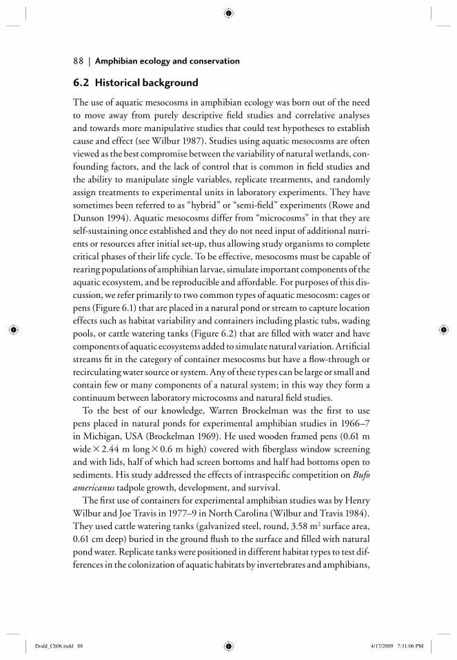
88 | Amphibian ecology and conservation
6.2 Historical background
The use of aquatic mesocosms in amphibian ecology was born out of the need to move away from purely descriptive fi eld studies and correlative analyses and towards more manipulative studies that could test hypotheses to establish cause and effect (see Wilbur 1987). Studies using aquatic mesocosms are often viewed as the best compromise between the variability of natural wetlands, con-founding factors, and the lack of control that is common in fi eld studies and the ability to manipulate single variables, replicate treatments, and randomly assign treatments to experimental units in laboratory experiments. They have sometimes been referred to as “hybrid” or “semi-fi eld” experiments (Rowe and Dunson 1994). Aquatic mesocosms differ from “microcosms” in that they are self- sustaining once established and they do not need input of additional nutri-ents or resources after initial set-up, thus allowing study organisms to complete critical phases of their life cycle. To be effective, mesocosms must be capable of rearing populations of amphibian larvae, simulate important components of the aquatic ecosystem, and be reproducible and affordable. For purposes of this dis-cussion, we refer primarily to two common types of aquatic mesocosm: cages or pens (Figure 6.1) that are placed in a natural pond or stream to capture location effects such as habitat variability and containers including plastic tubs, wading pools, or cattle watering tanks (Figure 6.2) that are fi lled with water and have components of aquatic ecosystems added to simulate natural variation. Artifi cial streams fi t in the category of container mesocosms but have a fl ow-through or recirculating water source or system. Any of these types can be large or small and contain few or many components of a natural system; in this way they form a continuum between laboratory microcosms and natural fi eld studies.
To the best of our knowledge, Warren Brockelman was the fi rst to use pens placed in natural ponds for experimental amphibian studies in 1966–7 in Michigan, USA (Brockelman 1969). He used wooden framed pens (0.61 m wide 3 2.44 m long 3 0.6 m high) covered with fi berglass window screening and with lids, half of which had screen bottoms and half had bottoms open to sediments. His study addressed the effects of intraspecifi c competition on Bufo americanus tadpole growth, development, and survival.
The fi rst use of containers for experimental amphibian studies was by Henry Wilbur and Joe Travis in 1977–9 in North Carolina (Wilbur and Travis 1984). They used cattle watering tanks (galvanized steel, round, 3.58 m2 surface area, 0.61 cm deep) buried in the ground fl ush to the surface and fi lled with natural pond water. Replicate tanks were positioned in different habitat types to test dif-ferences in the colonization of aquatic habitats by invertebrates and amphibians,
Dodd_Ch06.indd 88Dodd_Ch06.indd 88 4/17/2009 7:31:06 PM4/17/2009 7:31:06 PM
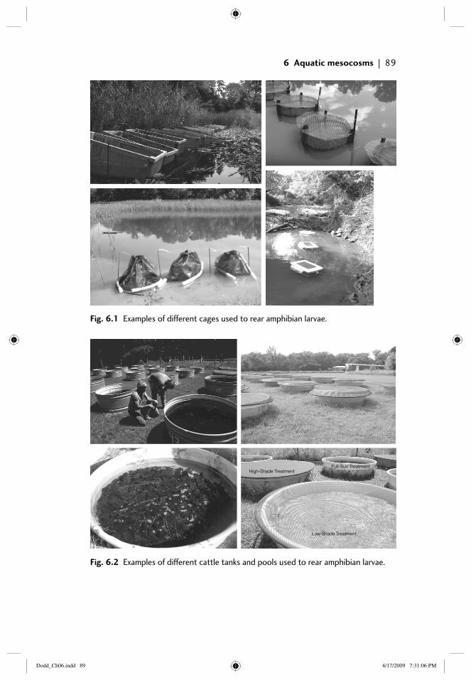
6 Aquatic mesocosms | 89
High-Shade TreatmentFull-Sun Treatment
Low-Shade Treatment
Fig. 6.1 Examples of different cages used to rear amphibian larvae.
Fig. 6.2 Examples of different cattle tanks and pools used to rear amphibian larvae.
Dodd_Ch06.indd 89Dodd_Ch06.indd 89 4/17/2009 7:31:06 PM4/17/2009 7:31:06 PM
90 | Amphibian ecology and conservation
and the formation of community structure. In 1980, one of Henry Wilbur’s graduate students, Peter Morin, subsequently developed a more effi cient and novel venue for experiments using cattle tanks to manipulate factors important to community regulation (Morin 1981). He placed cattle tanks (epoxy-coated galvanized steel, round, 1.52 m diameter, 1000 L) in a fi eld, above ground, so that they could be fi lled, manipulated, and easily drained to initiate new experi-ments each year. Each tank was fi lled with tap water and then each received an equal amount of dried litter collected from the edge of a natural pond (550 g) and Purina Trout Chow (50 g) for substrate and a source of nutrients. Equal amounts of inoculum of plankton derived from pooled plankton collections from eight natural ponds were added to each tank to initiate a diverse food web and prey base for larvae. This latter approach of using cattle tanks as aquatic mesocosms that could be renewed for each question and study has been critical in the advancement experimental amphibian ecology.
6.3 Why use mesocosms?
Studies in nature and in the laboratory allow researchers to answer important questions, but both have limitations (Diamond 1986). While laboratory stud-ies allow us to maximize control and manipulate factors so that cause–effect relationships can be established, the laboratory lacks realism and complexity, reducing its application in the real world. In contrast, fi eld studies offer realism and can encompass the complexity of natural food webs, but it can be diffi cult to distinguish cause–effect relationships and there can be high levels of vari-ation among replicates. Mesocosms are the middle ground. Proponents argue that mesocosms offer the best of both worlds: control, the ability to determine cause–effect relationships, natural food webs, and realism (Wilbur 1987; Rowe and Dunson 1994; Drake et al. 1996; Boone and James 2005). Critics, however, contend that mesocosms offer little gain over laboratory studies in that they are still artifi cial and may have limited application to the real world, yet they require more work and time, and they have greater variation among replicates than laboratory studies (Carpenter 1996; Skelly 2002). Certainly, mesocosms would not be mistaken for natural ponds, but they incorporate many natural elements that allow them to mimic some but not all of the processes occurring in larger natural ponds or lakes (Schindler 1998).
There are a number of reasons why mesocosms can be a useful technique in your research program. First, mesocosms allow you to incorporate some compo-nents of natural systems into your experiments—the changes in season, photo-period, temperature, and habitat that animals experience in nature—something
Dodd_Ch06.indd 90Dodd_Ch06.indd 90 4/17/2009 7:31:11 PM4/17/2009 7:31:11 PM
6 Aquatic mesocosms | 91
that you typically cannot alter in the laboratory. Secondly, if you have evaluated a mechanism within or between organism(s), or developed a theoretical model, then a logical next step is to see if your predictions hold in a more complex and nat-ural environment; mesocosm studies are a logical next step. Thirdly, if you want to evaluate single factors in isolation, a mesocosm may be ideal. Fourthly, manipula-tions in mesocosms can help you eliminate less important factors and fi nd system drivers, so that you can design a better, more effi cient large-scale fi eld study.
If you need a short-term answer to a basic experimental question, then a labora-tory experiment can offer an expedient answer: can trematodes infect limb buds? What concentration of an insecticide is lethal to tadpoles or zooplankton? Do overwintered bullfrog tadpoles prey upon recently hatched tadpoles? If your ques-tion is site- or habitat-specifi c or requires a vast area to encompass the entire ecosys-tem, then fi eld experiments may be the best way to go: can ponds in city parks and golf courses support native fauna? What effects do forest-management practices have on amphibian communities? Studies in mesocosms provide a useful surro-gate for the fi eld and allow us to evaluate single and multiple factors that may be important at a larger scale, which allows us to better design larger fi eld studies and provides insight into the system: do changes in food webs from eutrophication cause increases in number of trematodes and in the number of infected amphib-ians? Does a sublethal pesticide used on golf courses cause changes in aquatic community dynamics? Although mesocosms are often referred to as a “black box,” suggesting that the mechanisms underlying the outcome are not clear, additional studies can be done to discern mechanisms by behavioral observations, periodic sampling of covariates (e.g. temperature, primary production, dissolved carbon), or with a paired laboratory study (e.g. prey palatability).
Mesocosms are useful in addressing a variety of questions in ecology, evolu-tion, behavior, and conservation (see case studies below). We surveyed the litera-ture from 2004 to 2007 through the Ecological Society of America (including the journals Ecology, Ecological Applications, Frontiers in Ecology and Evolution, and Ecological Monographs), Oecologia, Evolution, Animal Behavior, and Behavior by searching the terms “amphibian” or “frog” or “salamander” and then select-ing all studies that used mesocosms. A total of 30 articles using mesocosms or enclosures were found only in the journals Oecologia or of the Ecological Society of America. The studies addressed a range of questions in ecology (e.g. species interactions, population biology, community structure), evolution (e.g. pheno-typic plasticity), behavior (e.g. oviposition selection), and conservation (e.g. effects of pathogens, habitat fragmentation, pesticides). Whereas mesocosms have been historically used for basic questions of ecology and evolution, they are becoming more frequently used in the fi eld of conservation and have enormous
Dodd_Ch06.indd 91Dodd_Ch06.indd 91 4/17/2009 7:31:11 PM4/17/2009 7:31:11 PM
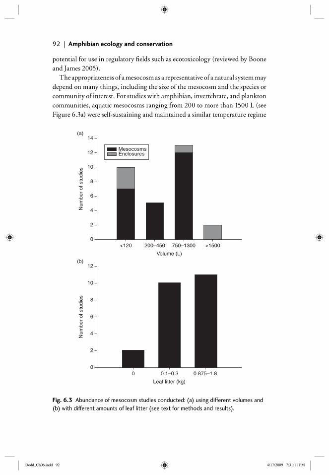
92 | Amphibian ecology and conservation
potential for use in regulatory fi elds such as ecotoxicology (reviewed by Boone and James 2005).
The appropriateness of a mesocosm as a representative of a natural system may depend on many things, including the size of the mesocosm and the species or community of interest. For studies with amphibian, invertebrate, and plankton communities, aquatic mesocosms ranging from 200 to more than 1500 L (see Figure 6.3a) were self-sustaining and maintained a similar temperature regime
0<120 200–450 750–1300 >1500
2
4
6
Num
ber
of s
tudi
es
8
10
12
14(a)
Volume (L)
MesocosmsEnclosures
00 0.1–0.3 0.875–1.8
2
4
6
Num
ber
of s
tudi
es 8
10
12(b)
Leaf litter (kg)
Fig. 6.3 Abundance of mesocosm studies conducted: (a) using different volumes and (b) with different amounts of leaf litter (see text for methods and results).
Dodd_Ch06.indd 92Dodd_Ch06.indd 92 4/17/2009 7:31:11 PM4/17/2009 7:31:11 PM
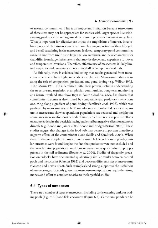
6 Aquatic mesocosms | 93
to natural communities. This is an important limitation because mesocosms of these sizes may not be appropriate for studies with larger species like wide- ranging predatory fi sh or larger-scale ecosystem processes like nutrient cycling. What is important for effective use is that the amphibians of interest, inverte-brate prey, and plankton resources can complete major portions of their life cycle and be self-sustaining in the mesocosm. Isolated, temporary pond communities range in size from tire ruts to large shallow wetlands, and have characteristics that differ from larger lake systems that may be deeper and experience turnover and temperature inversions. Therefore, effective use of mesocosms is likely lim-ited to species and processes that occur in shallow, temporary wetlands.
Additionally, there is evidence indicating that results generated from meso-cosm experiments have high predictability to the fi eld. Mesocosm studies evalu-ating the role of competition, predation, and pond drying (e.g. Wilbur 1972, 1987; Morin 1981, 1983; Semlitsch 1987) have proven useful in understanding the structure and regulation of amphibian communities. Long-term monitoring at a natural wetland (Rainbow Bay) in South Carolina, USA, has shown that community structure is determined by competitive and predatory interactions occurring along a gradient of pond drying (Semlitsch et al. 1996), which was predicted by mesocosm research. Manipulations with sublethal pesticide expos-ure in mesocosms show zooplankton populations are reduced and periphyton abundance increases for short periods of time, which can result in positive effects on tadpoles despite the pesticide having sublethal but negative effects on tadpoles directly (e.g. Boone and James 2003; Boone and Bridges-Britton 2006). These studies suggest that changes in the food web may be more important than direct negative effects of the contaminant alone (Mills and Semlitsch 2004). When these studies were replicated under more natural fi eld conditions in ponds, simi-lar outcomes were found despite the fact that predators were not excluded and that zooplankton populations could have recovered more quickly due to ephippia present in the soil sediments (Boone et al. 2004). Studies of dragonfl y preda-tion on tadpoles have documented qualitatively similar results between natural pools and mesocosms (Gascon 1992) and between different sizes of mesocosms (Gascon and Travis 1992). Such examples lend strong support to the usefulness of mesocosms, particularly given that mesocosm manipulations require less time, money, and effort to conduct, relative to the large fi eld studies.
6.4 Types of mesocosm
There are a number of types of mesocosm, including cattle watering tanks or wad-ing pools (Figure 6.1) and fi eld enclosures (Figure 6.2). Cattle tank ponds can be
Dodd_Ch06.indd 93Dodd_Ch06.indd 93 4/17/2009 7:31:11 PM4/17/2009 7:31:11 PM
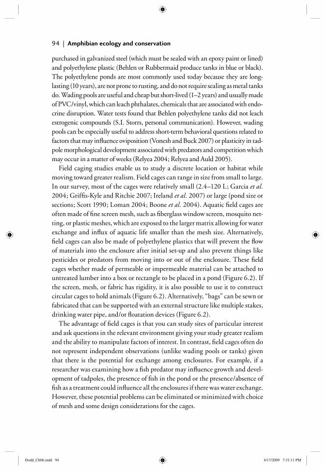
94 | Amphibian ecology and conservation
purchased in galvanized steel (which must be sealed with an epoxy paint or lined) and polyethylene plastic (Behlen or Rubbermaid produce tanks in blue or black). The polyethylene ponds are most commonly used today because they are long-lasting (10 years), are not prone to rusting, and do not require sealing as metal tanks do. Wading pools are useful and cheap but short-lived (1–2 years) and usually made of PVC/vinyl, which can leach phthalates, chemicals that are associated with endo-crine disruption. Water tests found that Behlen polyethylene tanks did not leach estrogenic compounds (S.I. Storrs, personal communication). However, wading pools can be especially useful to address short-term behavioral questions related to factors that may infl uence oviposition (Vonesh and Buck 2007) or plasticity in tad-pole morphological development associated with predators and competition which may occur in a matter of weeks (Relyea 2004; Relyea and Auld 2005).
Field caging studies enable us to study a discrete location or habitat while moving toward greater realism. Field cages can range in size from small to large. In our survey, most of the cages were relatively small (2.4–120 L; Garcia et al. 2004; Griffi s-Kyle and Ritchie 2007; Ireland et al. 2007) or large (pond size or sections; Scott 1990; Loman 2004; Boone et al. 2004). Aquatic fi eld cages are often made of fi ne screen mesh, such as fi berglass window screen, mosquito net-ting, or plastic meshes, which are exposed to the larger matrix allowing for water exchange and infl ux of aquatic life smaller than the mesh size. Alternatively, fi eld cages can also be made of polyethylene plastics that will prevent the fl ow of materials into the enclosure after initial set-up and also prevent things like pesticides or predators from moving into or out of the enclosure. These fi eld cages whether made of permeable or impermeable material can be attached to untreated lumber into a box or rectangle to be placed in a pond (Figure 6.2). If the screen, mesh, or fabric has rigidity, it is also possible to use it to construct circular cages to hold animals (Figure 6.2). Alternatively, “bags” can be sewn or fabricated that can be supported with an external structure like multiple stakes, drinking water pipe, and/or fl oatation devices (Figure 6.2).
The advantage of fi eld cages is that you can study sites of particular interest and ask questions in the relevant environment giving your study greater realism and the ability to manipulate factors of interest. In contrast, fi eld cages often do not represent independent observations (unlike wading pools or tanks) given that there is the potential for exchange among enclosures. For example, if a researcher was examining how a fi sh predator may infl uence growth and devel-opment of tadpoles, the presence of fi sh in the pond or the presence/absence of fi sh as a treatment could infl uence all the enclosures if there was water exchange. However, these potential problems can be eliminated or minimized with choice of mesh and some design considerations for the cages.
Dodd_Ch06.indd 94Dodd_Ch06.indd 94 4/17/2009 7:31:11 PM4/17/2009 7:31:11 PM
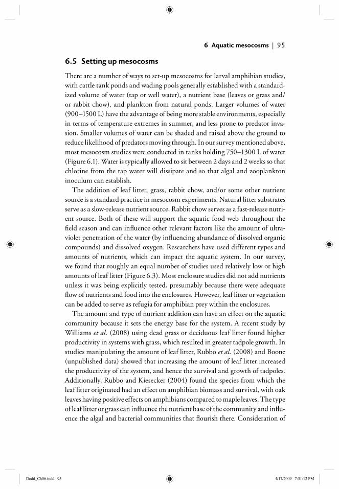
6 Aquatic mesocosms | 95
6.5 Setting up mesocosms
There are a number of ways to set-up mesocosms for larval amphibian studies, with cattle tank ponds and wading pools generally established with a standard-ized volume of water (tap or well water), a nutrient base (leaves or grass and/or rabbit chow), and plankton from natural ponds. Larger volumes of water (900–1500 L) have the advantage of being more stable environments, especially in terms of temperature extremes in summer, and less prone to predator inva-sion. Smaller volumes of water can be shaded and raised above the ground to reduce likelihood of predators moving through. In our survey mentioned above, most mesocosm studies were conducted in tanks holding 750–1300 L of water (Figure 6.1). Water is typically allowed to sit between 2 days and 2 weeks so that chlorine from the tap water will dissipate and so that algal and zooplankton inoculum can establish.
The addition of leaf litter, grass, rabbit chow, and/or some other nutrient source is a standard practice in mesocosm experiments. Natural litter substrates serve as a slow-release nutrient source. Rabbit chow serves as a fast-release nutri-ent source. Both of these will support the aquatic food web throughout the fi eld season and can infl uence other relevant factors like the amount of ultra-violet penetration of the water (by infl uencing abundance of dissolved organic compounds) and dissolved oxygen. Researchers have used different types and amounts of nutrients, which can impact the aquatic system. In our survey, we found that roughly an equal number of studies used relatively low or high amounts of leaf litter (Figure 6.3). Most enclosure studies did not add nutrients unless it was being explicitly tested, presumably because there were adequate fl ow of nutrients and food into the enclosures. However, leaf litter or vegetation can be added to serve as refugia for amphibian prey within the enclosures.
The amount and type of nutrient addition can have an effect on the aquatic community because it sets the energy base for the system. A recent study by Williams et al. (2008) using dead grass or deciduous leaf litter found higher productivity in systems with grass, which resulted in greater tadpole growth. In studies manipulating the amount of leaf litter, Rubbo et al. (2008) and Boone (unpublished data) showed that increasing the amount of leaf litter increased the productivity of the system, and hence the survival and growth of tadpoles. Additionally, Rubbo and Kiesecker (2004) found the species from which the leaf litter originated had an effect on amphibian biomass and survival, with oak leaves having positive effects on amphibians compared to maple leaves. The type of leaf litter or grass can infl uence the nutrient base of the community and infl u-ence the algal and bacterial communities that fl ourish there. Consideration of
Dodd_Ch06.indd 95Dodd_Ch06.indd 95 4/17/2009 7:31:12 PM4/17/2009 7:31:12 PM
96 | Amphibian ecology and conservation
the type of natural system you are attempting to represent (e.g. forested pond, grassy pond, or marsh) is the best guide to selecting the appropriate nutrient base to add.
It is important to establish the primary components of an aquatic food web in mesocosm tanks in order for them to be self-sustaining. A complex community of both phyto- and zooplankton is critical to help balance nutrient exchange, bacterial growth, and nitrogenous waste production as well as serve as a food source for amphibian larvae. Temporary wetlands are often an ideal source of inoculum for mesocosms because there will be fewer insect predators and no fi sh. All inoculum added to mesocosms should be strained to eliminate detri-mental insect or fi sh larvae, and eggs or larvae of non-target amphibian species. Several additions over time and from varying natural ponds will help ensure adequate diversity and complexity.
6.6 Common experimental designs
Establishing cause–effect relationships is the hallmark of mesocosm approaches and allows complex multifactorial designs. Designs using pools or tanks allow clear tests of each factor independently. Mesocosm studies allow researchers to address how incremental changes in a treatment level impact the study organ-ism and how different treatments may interact with one another. This level of manipulation would be diffi cult to achieve under most fi eld conditions, but is a critical tool for understanding how amphibian populations and communities function.
Replicate tanks or pools are physically separate pond communities that can be established with standardized procedures but diverge if treatment differences occur. Each tank represents an independent replicate and experimental unit. Cages located within ponds are typically not independent from one another; therefore, the question of interest will determine how these fi eld experiments are replicated. If you are interested in how a particular type of habitat infl uences an amphibian community, then you should replicate at the level of pond-habitat type. For instance, to examine whether amphibians can survive larval develop-ment in golf course ponds, Boone et al. (2008) used multiple golf course and reference ponds with replicate cages both within and between ponds. Using a single golf course and reference pond with replicate enclosures within each pond would not have clarifi ed whether golf-course management affected larval amphibians; instead, it would only confi rm that the two ponds are different for some reason; perhaps due to golf course management, historically differ-ent abiotic and biotic factors present in the pond, or chance. Replicate cages in
Dodd_Ch06.indd 96Dodd_Ch06.indd 96 4/17/2009 7:31:12 PM4/17/2009 7:31:12 PM
6 Aquatic mesocosms | 97
the latter case would constitute “pseudoreplicates” (Hurlbert 1984) and would increase the probability of making a type I error or determining there is a sig-nifi cant difference related to treatment when there is not. However, if you are interested in how overwintered bullfrog tadpoles may infl uence the amphibian community, then manipulating bullfrog abundance in replicate cages in a single pond would be acceptable. Replication in fi eld cage studies requires replicating at the level of your question and factor of infl uence (e.g. golf course), which will likely be at separate locations. Replication is also necessary within ponds to determine variation among specifi c cage locations (e.g. aspect, slope, or shading along a shoreline). Split-plot or nested designs are especially useful in studies using cages in ponds and may allow the testing of hypotheses not testable with less sophisticated designs (Gunzburger 2007).
The number of replicates you should use is also an important consideration. Typically there is a trade-off between the number of replicates and the total size of the study related to logistical and fi nancial constraints. However, the more divergent your replicates, the greater the variation within your treatments, and the less your ability to detect signifi cant differences between treatments. Therefore, consideration of the level of variation inherent in your replicates will infl uence the number of replicates that you need. While laboratory studies fre-quently have fi ve or more replicates because of the ease of replication, mesocosm tank studies will often be limited to three to fi ve replicates (Boone and James 2005), which is typically suffi cient to detect signifi cant differences in behavior, morphology, development, and survival. You can estimate a priori how many replicates you should use by determining your desired statistical power (1−�; a power of 0.8 or greater is desirable) based on your � criteria and the effect size (size of the difference). Using a statistical program like SAS (Proc Power) or using online calculators (e.g. www.math.yorku.ca/SCS/ Online/power/) you can determine the ideal number of replicates to use based on the system you are studying.
The random assignment of treatments is one of the most critical steps of all true experiments and should be applied to mesocosm studies. Randomizing your treatments is extremely important to avoid confounding variation among replicate tanks or cages with variation among treatments. You can use a random number chart or a random number generator in SAS (Proc Plan). Treatments may be randomly assigned across all tanks (completely random design) or cages, or they may be blocked so that experimental units are grouped along a known gradient that may cause variation (e.g. shading) not relevant to the experimental question and which can be removed statistically (randomized complete block).
Dodd_Ch06.indd 97Dodd_Ch06.indd 97 4/17/2009 7:31:12 PM4/17/2009 7:31:12 PM
98 | Amphibian ecology and conservation
6.7 Case studies
6.7.1 Community ecology
The study of community ecology has had a long history of experimental studies to help disentangle the complex interactions among species. Morin (1981) used three species of anuran tadpoles (Scaphiopus holbrookii, Pseudacris crucifer, and Bufo terrestris) as competitors and adult newts (Notophthalmus viridescens) as a predator to address the role of interspecifi c competition. Tadpoles were reared together from hatching to metamorphosis in 16 cattle tanks (epoxy-coated gal-vanized steel, 1.52 m diameter, 1000 L) at constant initial densities in all tanks. Newts were added in four densities (none, two, four, and eight per tank) to vary the intensity of predation and replicated four times each. The results showed that in the absence of newt predators Scaphiopus (62%) and Bufo (33%) meta-morphs were relatively abundant, followed by Pseudacris (5%). However, in the presence of a high density of newts, Pseudacris (68%) metamorphs were most abundant followed by Scaphiopus (20%) and Bufo (12%). The rarity of Pseudacris in tanks without newts was best explained by intense interspecifi c competition with Scaphiopus and Bufo. The increased survival and larger body mass of Pseudacris in tanks with newts was best explained by release from inter-specifi c competition due to newt predation on the preferred prey of Scaphiopus and Bufo tadpoles. Morin suggested that newts acted as a ‘keystone’ predator to prevent exclusion of competitively inferior species by reducing the survival and density of competitively superior species. These results demonstrate that predation and competition could interact to produce deterministic patterns of community structure in amphibians.
In a subsequent experiment, Wilbur (1987) tested the interaction effects of competition, predation, and disturbance on the structure of a similar aquatic amphibian community. He used four species of anuran tadpoles (Rana sphe-nocephala, S. holbrookii, P. crucifer, and B. terrestris) as competitors and adult newts (Notophthalmus viridescens) as a predator. Tadpoles of the four species were reared together in 36 cattle tanks (epoxy-coated galvanized steel, 1.52 m diameter, 1000 L) at a constant high or low density. Four newts were added to half the tanks and ponds were drained at three rates; either 50 days, 100 days, or control tanks kept at 50 cm deep. All 12 treatment combinations were repli-cated in three spatial blocks to account for physical differences across a fi eld were tanks were positioned. The results showed that Scaphiopus was least sensitive to intraspecifi c density, metamorphosed quickly in fast-drying tanks, and was the competitive dominant in tanks without newt predators, but suffered highest predation from newts. Rana was most successful at low density but could not
Dodd_Ch06.indd 98Dodd_Ch06.indd 98 4/17/2009 7:31:12 PM4/17/2009 7:31:12 PM
6 Aquatic mesocosms | 99
grow fast enough to metamorphose in fast-drying tanks and suffered high pre-dation by newts. Bufo were very sensitive to high density and produced few met-amorphs without newt predators. This effect was reversed by newts selectively preying on Scaphiopus and Rana tadpoles, especially in rapidly drying tanks. Pseudacris performed poorly in all slow-drying tanks but showed moderate suc-cess in high-density tanks where newts had removed most competitors. The overall conclusion of this study was that all three factors interacted with each other and with species’ life history to determine community structure. Further, it suggested that competition dominates simple habitats of short duration and predation becomes increasingly important in ponds with longer hydroperiods that permit the establishment of diverse predators. Both of the studies described above were infl uential in focusing attention on the complex interactions of pre-dation, competition, and pond drying in aquatic communities rather than his-torical single-factor arguments.
6.7.2 Evolutionary ecology
The “common-garden” experimental approach to evolutionary studies has been important for clarifying genetic and environmental interactions by measuring genotype performance in a simplifi ed controlled environment (Clausen et al. 1947). Parris et al. (1999) examined the larval performance of hybrid and par-ental genotypes of the southern and plains leopard frog (Rana sphenocephala and Rana blairi) in a common-garden approach using cattle tanks. They estab-lished 56 experimental populations in cattle tanks (polyethylene, round, 1.83 m diameter) by adding 960 L of tap water, 1.0 kg of deciduous leaf litter, and mul-tiple additions of plankton from natural ponds. Six genotypes of hatchling tad-poles were added to tanks at a low (20 per tank) or high (60 per tank) density to simulate a competitive gradient. The 12 treatment combinations were replicated either three or fi ve times in the 56 tanks (Parris et al. 1999). Survival was the same among all genotypes, but decreased with increasing density. Body mass at metamorphosis was the same among genotypes, but decreased with increas-ing density. Tadpoles of R. sphenocephala had the shortest larval period while the other parental species R. blairi had the longest larval period. Ponds with hybrid genotypes produced a greater proportion of metamorphs than those with R. blairi tadpoles but a smaller proportion than ponds with R. sphenocephala tadpoles. Their results demonstrate equal or increased larval performance of hybrids relative to parental genotypes in cattle tank environments. Studies such as the one described above are critical for determining whether or not natural hybridization could potentially lead to the production of recombinant geno-types possessing novel adaptations.
Dodd_Ch06.indd 99Dodd_Ch06.indd 99 4/17/2009 7:31:12 PM4/17/2009 7:31:12 PM
100 | Amphibian ecology and conservation
6.7.3 Ecotoxicology
The fi eld of toxicology historically has taken a reductionist approach by using single species and chemical testing in the laboratory. However, there is growing effort to develop multispecies, community, and ecosystem-level experimental approaches that better mimic real-world problems (Kimball and Levin 1985; Rowe and Dunson 1994; Boone and James 2005; Semlitsch and Bridges 2005). A model study by Boone et al. (2007) examined the role that chemical con-tamination, competition, and predation play singly and in combination in an aquatic amphibian community. They established replicate aquatic communities in 64 polyethylene cattle tanks (round, 1.85 m diameter, 0.6 cm height, 1480 L volume) by adding 1000 L of tap water, 1.0 kg of leaf litter, plankton from nat-ural ponds, 60 Bufo americanus tadpoles, 30 R. sphenocephala tadpoles, and 10 Ambystoma maculatum salamander larvae to each. Four factors were manipulated and replicated four times in a fully factorial design: no or two bluegill sunfi sh, no or six overwintered bullfrog tadpoles, 0 or 2.5 mg/L carbaryl (an insecticide), and 0 or 10 mg/L ammonium nitrate fertilizer. The results showed that bluegills had the largest impact on the community by eliminating B. americanus and A. maculatum and reducing the abundance of R. sphenocephala. Chemical contam-inants had the second strongest effect on the community with the insecticide reducing A. maculatum abundance by 50% and increasing the mass of anurans (R. sphenocephala and B. americanus) at metamorphosis; the fertilizer positively infl uenced time and mass at metamorphosis for both anuran and salamander larvae. Presence of overwintered bullfrog tadpoles reduced mass and increased time to metamorphosis of the anurans. Although both bluegill and overwin-tered bullfrog tadpoles had negative effects on the amphibian community, they performed better in the presence of one another and in contaminated ponds. These results indicate that predicting complex interactions from single-factor effects may not be straightforward. Further, the research supports the hypoth-esis that combinations of factors can contribute to population declines.
6.7.4 Land use and management
Only recently have ecologists begun to use mesocosms to address questions con-cerning human land use and habitat fragmentation. Hocking and Semlitsch (2007) tested the effects of timber harvest on oviposition-site selection by gray treefrogs (Hyla versicolor) in four experimental forest treatments. Five plastic wading pools (1.5 m diameter, 30 cm deep) were placed above ground in each of the four forest treatments: (1) a clear-cut with high coarse woody debris (CWD), (2) a clear-cut with low CWD, (3) a partial cut with 50% canopy removal,
Dodd_Ch06.indd 100Dodd_Ch06.indd 100 4/17/2009 7:31:12 PM4/17/2009 7:31:12 PM
6 Aquatic mesocosms | 101
and (4) a control. The fi ve pools were placed at three distances from the nat-ural breeding pond in each treatment (see Figure 1 in Hocking and Semlitsch 2007): one pool at 10 m, two pools at 64 m, and two pools at 115 m from a natural breeding pond. The four forest treatments were positioned around three replicate natural breeding ponds for a total of 60 wading pools. Pools fi lled naturally with rainwater by April. Following the fi rst oviposition event, all pools were checked every 24–48 h for treefrog eggs. Eggs were removed and counted. The results indicated that treefrogs laid signifi cantly more eggs in the clear-cuts (low-CWD 77 185 eggs; high-CWD 51 990 eggs) than in either the partial (13 553 eggs) or the control (14 068 eggs) treatments. Further, the interaction of forest � isolation treatment showed that oviposition in both clear-cut treatments decreased with increasing isolation whereas oviposition was the same at all levels of isolation in the partial and control treatments. Hocking and Semlitsch (2007) suggested that the strong preference for open-canopy pools likely benefi ts the larval stage because of higher-quality food and warmer water temperatures but that isolation of breeding pools beyond 50–100 m can inhibit oviposition by female treefrogs. They also add that the possible benefi ts to one stage (tadpoles) might be diminished by the risk of desiccation to the terrestrial juvenile stage after metamorphosis. Thus, mesocosms can be used to address land-use questions beyond the boundary of aquatic ecosystems.
6.8 Conclusion
Although we are both advocates for the use of mesocosms in amphibian ecology and conservation, we also agree that a pluralistic approach to any question is likely necessary for complete understanding. The use of laboratory experiments to understand mechanisms as well as fi eld studies to anchor mesocosm results back to the real world are critical. The use of cattle watering tanks, wading pools, and cages is a powerful technique in any researcher’s toolbox. The choice of mesocosm should refl ect knowledge of the natural history of the species and system being studied. If used properly, at the correct scale for the questions one is asking, many questions can be clearly answered and results can have strong inferences back to natural systems. However, we caution readers that neither type of mesocosm described here can address all ecological and conservation questions alone. One has only to read Schindler (1998) to realize that most large-scale ecosystem processes cannot be replicated in cattle tanks or cages. But, for many population- and community-level studies of amphibians, meso-cosms offer an excellent approach.
Dodd_Ch06.indd 101Dodd_Ch06.indd 101 4/17/2009 7:31:12 PM4/17/2009 7:31:12 PM
102 | Amphibian ecology and conservation
6.9 References
Boone, M. D. and Bridges-Britton, C. M. (2006). Examining multiple sublethal con-taminants on the gray treefrog, Hyla versicolor: effects of an insecticide, herbicide, and fertilizer. Environmental Contamination and Chemistry, 25, 3261–5.
Boone, M. D. and James, S. M. (2003). Interactions of an insecticide, herbicide, and natural stressors in amphibian community mesocosms. Ecological Applications, 13, 829–41.
Boone, M. D. and James, S. M. (2005). Use of aquatic and terrestrial mesocosms in eco-toxicology. Applied Herpetology, 2, 231–57.
Boone, M. D., Semlitsch, R. D., Fairchild, J. F., and Rothermel, B. B. (2004). Effects of an insecticide on amphibians in large-scale experimental ponds. Ecological Applications, 14, 685–91.
Boone, M. D., Semlitsch, R. D., Little, E. E., and Doyle, M. C. (2007). Multiple stressors in amphibian communities: interactive effects of chemical contamination, bullfrog tadpoles, and bluegill sunfi sh. Ecological Applications, 17, 291–301.
Boone, M. D., Semlitsch, R. D., and Mosby, C. (2008). Suitability of golf course ponds for amphibian metamorphosis when bullfrogs are removed. Conservation Biology, 22, 172–9.
Brockelman, W. Y. (1969). An analysis of density effects and predation in Bufo americanus tadpoles. Ecology, 50, 632–43.
Carpenter, S. R. (1996). Microcosm experiments have limited relevance for community and ecosystem ecology. Ecology, 77, 677–80.
Clausen, J., Keck, D. D., and Hiesey, W. M. (1947). Heredity of geographically and eco-logically isolated races. American Naturalist, 81, 114–33.
Diamond, J. (1986). Overview: laboratory experiments, fi eld experiments, and natural experiments. In J. Diamond and T. Case (eds), Community Ecology, pp. 3–22. Harper and Row Publishers, New York.
Drake, J. A., Huxel, G. R., and Hewitt, C. L. (1996). Microcosms as models for generat-ing and testing community theory. Ecology, 77, 670–7.
Garcia, T. S., Stacy, J., and Sih, A. (2004). Larval salamander response to UV radiation and predation risk: color change and microhabitat use. Ecological Applications, 14, 1055–64.
Gascon, C. (1992). Aquatic predators and tadpole prey in central Amazonia: fi eld data and experimental manipulations. Ecology, 73, 971–80.
Gascon, C. and Travis, J. (1992). Does the spatial scale of experimentation matter? A test with tadpoles and dragonfl ies. Ecology, 73, 2237–43.
Griffi s-Kyle, K. L. and Ritchie, M. E. (2007). Amphibian survival, growth, and devel-opment in response to mineral nitrogen exposure and predator cues in the fi eld: An experimental approach. Oecologia, 152, 633–42.
Gunzburger, M. S. (2007). Habitat segregation in two sister taxa of hylid treefrogs. Herpetologica, 63, 301–10.
Hairston, Sr, N. G. (1989a). Hard choices in ecological experimentation. Herpetologica, 45, 119–22.
Hairston, Sr, N. G. (1989b). Ecological Experiments. Cambridge University Press, Cambridge.
Dodd_Ch06.indd 102Dodd_Ch06.indd 102 4/17/2009 7:31:12 PM4/17/2009 7:31:12 PM
6 Aquatic mesocosms | 103
Hocking, D. J. and Semlitsch, R. D. (2007). Effects of timber harvest on breeding-site selection by gray treefrogs (Hyla versicolor). Biological Conservation, 138, 506–13.
Hurlbert, S. H. (1984). Pseudoreplication and the design of ecological fi eld experiment. Ecological Monographs, 54, 187–211.
Ireland, D. H., Wirsing, A. J., and Murray, D. L. (2007). Phenotypically plastic responses of green frog embryos to confl icting predation risk. Oecologia, 152, 162–8.
Jaeger, R. G. and Walls, S. C. (1989). On salamander guilds and ecological methodology. Herpetologica, 45, 111–19.
Kimball, K. D. and Levin, S. A. (1985). Limitations of laboratory bioassays: the need for ecosystem-level testing. Bioscience, 35, 165–71.
Loman, J. (2004). Density regulation in tadpoles of Rana temporaria: a full pond fi eld experiment. Ecology, 85, 1611–18.
Mills, N. E. and Semlitsch, R. D. (2004). Competition and predation mediate indirect effects of an insecticide on southern leopard frogs. Ecological Applications, 14, 1041–54.
Morin, P. J. (1981). Predatory salamanders reverse the outcome of competition among three species of anuran tadpoles. Science, 212, 1284–6.
Morin, P. J. (1983). Predation, competition, and the composition of larval anuran guilds. Ecological Monographs, 53, 119–38.
Parris, M. J., Semlitsch, R. D., and Sage, R. D. (1999). Experimental analysis of the evolutionary potential of hybridization in leopard frogs (Anura: Ranidae). Journal of Evolutionary Biology, 12, 662–71.
Relyea, R. A. (2004). Fine-tuned phenotypes: tadpole plasticity under 16 combinations of predators and competitors. Ecology, 85, 172–9.
Relyea, R. A. and Auld, J. R. (2005). Predator- and competitor-induced plasticity: how changes in foraging morphology affect phenotypic trade-offs. Ecology, 86, 1723–9.
Rowe, C. L. and Dunson, W. A. (1994). The value of simulated pond communities in mesocosms for studies of amphibian ecology and ecotoxicology. Journal of Herpetology, 28, 346–56.
Rubbo, M. J., Belden, L. K., and Kiesecker, J. M. (2008). Differential responses of aquatic consumers to variations in leaf-litter inputs. Hydrobiologia, 605, 37–44.
Rubbo, M. J. and Kiesecker, J. M. (2004). Leaf litter composition and community struc-ture: translating regional species changes into local dynamics. Ecology, 85, 2519–25.
Schindler, D. W. (1998). Replication versus realism: the need for ecosystem-scale experi-ments. Ecosystems, 1, 323–34.
Scott, D. E. (1990). Effects of larval density in Ambystoma opacum: an experiment in large-scale fi eld enclosures. Ecology, 71, 296–306.
Semlitsch, R. D. (1987). Relationship of pond drying to the reproductive success of the salamander Ambystoma talpoideum. Copeia, 1987, 61–9.
Semlitsch, R. D. and Bridges, C. M. (2005). Amphibian ecotoxicology. In M. Lannoo (ed.), Amphibian Declines: the Conservation Status of United States Species, pp. 241–3. University of California Press, Berkeley, CA.
Semlitsch, R. D., Scott, D. E., Pechmann, J. H. K., and Gibbons, J. W. (1996). Structure and dynamics of an amphibian community: evidence from a 16-year study of a nat-ural pond. In M. L. Cody and J. A. Smallwood (eds), Long-term Studies of Vertebrate Communities, pp. 217–48. Academic Press, San Diego, CA.
Dodd_Ch06.indd 103Dodd_Ch06.indd 103 4/17/2009 7:31:12 PM4/17/2009 7:31:12 PM

104 | Amphibian ecology and conservation
Skelly, D. K. (2002). Experimental venue and estimation of interaction strength. Ecology, 83, 2097–2101.
Skelly, D. K. and Kiesecker, J. M. (2001). Venue and outcome in ecological experiments: manipulations of larval anurans. Oikos, 94, 198–208.
Vonesh, J. R. and Buck, J. C. (2007). Pesticide alters oviposition site selection in gray treefrogs. Oecologia, 154, 219–26.
Wilbur, H. M. (1972). Competition, predation, and the structure of the Ambystoma-Rana sylvatica community. Ecology, 53, 3–20.
Wilbur, H. M. (1987). Regulation in complex systems: experimental temporary pond communities. Ecology, 68, 1437–52.
Wilbur, H. M. and Travis, J. (1984). An experimental approach to understanding pattern in natural communities. In D. R. Strong, Jr, D. Simberloff, L. G. Abele, and A. B. Thistle (eds), Ecological Communities: Conceptual Issues and the Evidence, pp. 113–22. Princeton University Press, Princeton, NJ.
Williams, B. K., Rittenhouse, T. A. G., and Semlitsch, R. D. (2008). Leaf litter input medi-ates tadpole performance across forest canopy treatments. Oecologia, 155, 377–86.
Dodd_Ch06.indd 104Dodd_Ch06.indd 104 4/17/2009 7:31:13 PM4/17/2009 7:31:13 PM
10Dietary assessments of adult amphibians
Mirco Solé and Dennis Rödder
10.1 Introduction
Dietary information is essential to understand amphibian life history, popu-lation fl uctuations, and the impact of habitat modifi cation, and to develop conservation strategies (Anderson 1991). In ecology, trophic relationships represent a functional connection between different taxa and are a key subject in many aut- and synecological studies. Studies on diets are essen-tial for assessments of energy fl ow and food webs in ecological communi-ties. Variables involved in an animal’s diet are seldom obvious and include behavioral, physiological, and morphological features of both predator and prey (Simon and Toft 1991). Therefore, dietary information from locally imperilled species is a necessary component in designing management and conservation programs.
Traditionally, amphibians are described as generalist predators feeding mainly on arthropods, but mollusks, annelids, and even small vertebrates are also frequently consumed. Amphibians are able to distinguish between different prey types allowing for different degrees of feeding specialization (Freed 1982). Dietary specialization is often associated with morphological, physiological, and behavioral characteristics that facilitate location, identifi -cation, capture, ingestion, and digestion of prey items. Feeding dynamics can vary considerably between species, but differences between the three major amphibian lineages and between species feeding on land and in water become obvious. Therefore, the feeding mechanisms and dietary specialties of the dif-ferent groups are discussed separately (for amphibian larvae see Chapter 5).
10.1.1 Adult anurans
Anurans are carnivores and their main diet consists of arthropods. Parts of plants or fruits are accidentally consumed with other food items by adult
10_Dodd_Chap10.indd 16710_Dodd_Chap10.indd 167 8/19/2009 3:32:09 PM8/19/2009 3:32:09 PM
168 | Amphibian ecology and conservation
amphibians, although exceptions have been documented, such as the hylid frog Xenohyla truncata (Silva and Britto-Pereira 2006). In most anurans, prey capture is enhanced by the use of projectile tongues fi xed at the anterior part of the mouth. The posterior part is commonly free, and the whole tongue can be thrust out in order to capture prey items. Among anurans, the family of the predominately aquatic Pipidae lack tongues and uses suction feeding. The species are characterized by broad elements of the hyobranchial skeleton, especially the ceratohyals and ceratobranchials. Sokol (1969) observed that the small pipid Hymenochirus boettgeri depressed its hyobranchium prior to mandibular depression, so that maximum suction is achieved as soon as the mouth is opened. The larger pipid genera Pipa in South America and Xenopus in Africa augment buccal suction by stuffi ng their prey into their mouth with their forelimbs.
Differences in feeding behavior among frogs with different diets have been observed, encompassing a continuum between sit-and-wait and opportunistic search strategies. The composition of the diet can refl ect the feeding strat-egy to some degree. Whereas sit-and-wait foragers commonly consume larger, mobile prey and only a few food items per time unit, opportunistic searchers consume greater numbers of smaller food items. These behavioral patterns are also refl ected in morphological properties of the species. Emerson (1985) found a relationship between the skull shapes of frogs and their diet, whereby frogs that eat relatively small, slow prey have relatively long jaws and an asym-metrical feeding cycle; time to capture prey is less than the time to bring prey into the mouth. On the other hand, snail-eating frogs have lower jaws with a relatively long distance from the insertion point of the adductor muscle to the jaw articulations. Two main diet patterns in anurans were identifi ed by Toft (1980a, 1981, 1985). They comprise “ant specialists” eating slow-moving, strongly chitinized arthropods such as ants, termites, and mites, and “non-ant specialists” eating generally more variable and less chitinous arthropods (e.g. spiders and grasshoppers).
10.1.2 Adult caudata
Terrestrial salamanders typically feed by capturing their prey with a large, moist, sticky tongue. Although predominately carnivorous, several species of the genus Siren include larger plant parts in their diet (Duellman and Trueb 1994). Some neotropical salamanders exhibit lower prey diversity than most temperate-zone terrestrial and aquatic species, a difference that might be explained by the dis-proportionately high contribution of ants in the diets of the neotropical species (Anderson and Mathis 1999).
10_Dodd_Chap10.indd 16810_Dodd_Chap10.indd 168 8/19/2009 3:32:10 PM8/19/2009 3:32:10 PM
10 Dietary assessments of adult amphibians | 169
10.1.3 Adult gymnophiona
Despite being widely distributed in the tropics, only few dietary studies have been performed on caecilians (O’ Reilly 2000). Most dietary studies of terres-trial and aquatic caecilians suggest that they are generalized carnivores. Kupfer et al. (2005) studied the diet of both larval and adult Ichthyophis cf. kohtaoensis from Thailand. The larvae feed exclusively on aquatic invertebrates, preferring benthic prey. The adults consume mostly soil invertebrates such as earthworms, ants, and termites. Ontogenetic dietary shifts and the trophic position of caecil-ians are more similar to salamanders than frogs with biphasic life cycles.
10.2 Methods to obtain prey items: historical overview
Most accounts of amphibian feeding are anecdotal and involve only a few taxa. As a result, much is unknown about prey selection and foraging strategies. The diet of amphibians has commonly been studied by sacrifi cing the ani-mals and dissecting their stomachs. Technically, this is the easiest method and, when applied to series of preserved specimens housed in museum collections, ethically justifi ed. Prey items can be obtained in good condition, facilitating identifi cation and measurements. Today, the euthanasia of large samples of study animals for dietary analyses is ethically questionable because alternative methods are available. One of these alternative methods is stomach fl ushing. It avoids killing large number of animals, and has been used in herpetological studies since the 1970s. For example, Fraser (1976) used this method to study salamander diets, and it was used in later studies of both frogs and reptiles (Legler 1977; Legler and Sullivan 1979). Most researchers anesthetize the ani-mals prior to stomach fl ushing, but this occasionally has resulted in mortality (Joly 1987). Despite early attempts at alternative study methods, most dietary studies continued to rely upon freshly killed specimens, probably because the description of stomach-fl ushing techniques proved rather inadequate and diffi -cult to replicate. Solé et al. (2005) published a protocol clearly explaining which materials were needed, and which steps had to be followed to achieve successful stomach fl ushing. Their protocol has since been used in dietary research on different anurans (e.g. Miranda et al. 2006; Mahan and Johnson 2007; Solé and Pelz 2007; Wang et al. 2008). Wu et al. (2007) compared data on stomach dissection with those obtained by stomach fl ushing to assess dietary diversity, and found no signifi cant differences, tending to validate the fl ushing method. They stated that “our study indicates that the result of stomach fl ush is accurate
10_Dodd_Chap10.indd 16910_Dodd_Chap10.indd 169 8/19/2009 3:32:10 PM8/19/2009 3:32:10 PM
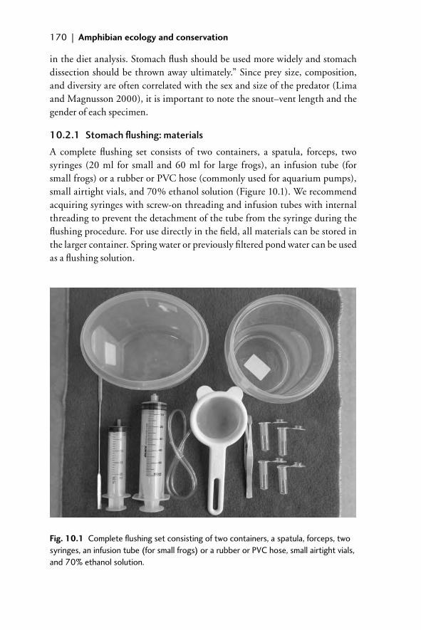
170 | Amphibian ecology and conservation
in the diet analysis. Stomach fl ush should be used more widely and stomach dissection should be thrown away ultimately.” Since prey size, composition, and diversity are often correlated with the sex and size of the predator (Lima and Magnusson 2000), it is important to note the snout–vent length and the gender of each specimen.
10.2.1 Stomach fl ushing: materials
A complete fl ushing set consists of two containers, a spatula, forceps, two syringes (20 ml for small and 60 ml for large frogs), an infusion tube (for small frogs) or a rubber or PVC hose (commonly used for aquarium pumps), small airtight vials, and 70% ethanol solution (Figure 10.1). We recommend acquiring syringes with screw-on threading and infusion tubes with internal threading to prevent the detachment of the tube from the syringe during the fl ushing procedure. For use directly in the fi eld, all materials can be stored in the larger container. Spring water or previously fi ltered pond water can be used as a fl ushing solution.
Fig. 10.1 Complete fl ushing set consisting of two containers, a spatula, forceps, two syringes, an infusion tube (for small frogs) or a rubber or PVC hose, small airtight vials, and 70% ethanol solution.
10_Dodd_Chap10.indd 17010_Dodd_Chap10.indd 170 8/19/2009 3:32:10 PM8/19/2009 3:32:10 PM
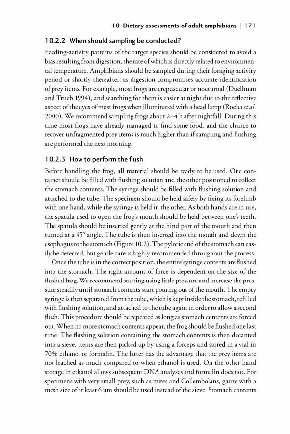
10 Dietary assessments of adult amphibians | 171
10.2.2 When should sampling be conducted?
Feeding-activity patterns of the target species should be considered to avoid a bias resulting from digestion, the rate of which is directly related to environmen-tal temperature. Amphibians should be sampled during their foraging activity period or shortly thereafter, as digestion compromises accurate identifi cation of prey items. For example, most frogs are crepuscular or nocturnal (Duellman and Trueb 1994), and searching for them is easier at night due to the refl ective aspect of the eyes of most frogs when illuminated with a head lamp (Rocha et al. 2000). We recommend sampling frogs about 2–4 h after nightfall. During this time most frogs have already managed to fi nd some food, and the chance to recover unfragmented prey items is much higher than if sampling and fl ushing are performed the next morning.
10.2.3 How to perform the fl ush
Before handling the frog, all material should be ready to be used. One con-tainer should be fi lled with fl ushing solution and the other positioned to collect the stomach contents. The syringe should be fi lled with fl ushing solution and attached to the tube. The specimen should be held safely by fi xing its forelimb with one hand, while the syringe is held in the other. As both hands are in use, the spatula used to open the frog’s mouth should be held between one’s teeth. The spatula should be inserted gently at the hind part of the mouth and then turned at a 45° angle. The tube is then inserted into the mouth and down the esophagus to the stomach (Figure 10.2). The pyloric end of the stomach can eas-ily be detected, but gentle care is highly recommended throughout the process.
Once the tube is in the correct position, the entire syringe contents are fl ushed into the stomach. The right amount of force is dependent on the size of the fl ushed frog. We recommend starting using little pressure and increase the pres-sure steadily until stomach contents start pouring out of the mouth. The empty syringe is then separated from the tube, which is kept inside the stomach, refi lled with fl ushing solution, and attached to the tube again in order to allow a second fl ush. This procedure should be repeated as long as stomach contents are forced out. When no more stomach contents appear, the frog should be fl ushed one last time. The fl ushing solution containing the stomach contents is then decanted into a sieve. Items are then picked up by using a forceps and stored in a vial in 70% ethanol or formalin. The latter has the advantage that the prey items are not leached as much compared to when ethanol is used. On the other hand storage in ethanol allows subsequent DNA analyses and formalin does not. For specimens with very small prey, such as mites and Collembolans, gauze with a mesh size of at least 6 µm should be used instead of the sieve. Stomach contents
10_Dodd_Chap10.indd 17110_Dodd_Chap10.indd 171 8/19/2009 3:32:14 PM8/19/2009 3:32:14 PM
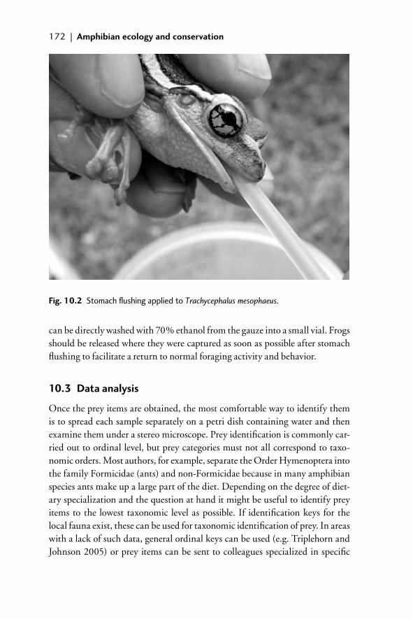
172 | Amphibian ecology and conservation
can be directly washed with 70% ethanol from the gauze into a small vial. Frogs should be released where they were captured as soon as possible after stomach fl ushing to facilitate a return to normal foraging activity and behavior.
10.3 Data analysis
Once the prey items are obtained, the most comfortable way to identify them is to spread each sample separately on a petri dish containing water and then examine them under a stereo microscope. Prey identifi cation is commonly car-ried out to ordinal level, but prey categories must not all correspond to taxo-nomic orders. Most authors, for example, separate the Order Hymenoptera into the family Formicidae (ants) and non-Formicidae because in many amphibian species ants make up a large part of the diet. Depending on the degree of diet-ary specialization and the question at hand it might be useful to identify prey items to the lowest taxonomic level as possible. If identifi cation keys for the local fauna exist, these can be used for taxonomic identifi cation of prey. In areas with a lack of such data, general ordinal keys can be used (e.g. Triplehorn and Johnson 2005) or prey items can be sent to colleagues specialized in specifi c
Fig. 10.2 Stomach fl ushing applied to Trachycephalus mesophaeus.
10_Dodd_Chap10.indd 17210_Dodd_Chap10.indd 172 8/19/2009 3:32:14 PM8/19/2009 3:32:14 PM
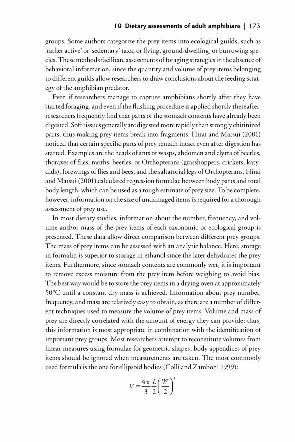
10 Dietary assessments of adult amphibians | 173
groups. Some authors categorize the prey items into ecological guilds, such as ‘rather active’ or ‘sedentary’ taxa, or fl ying, ground-dwelling, or burrowing spe-cies. These methods facilitate assessments of foraging strategies in the absence of behavioral information, since the quantity and volume of prey items belonging to different guilds allow researchers to draw conclusions about the feeding strat-egy of the amphibian predator.
Even if researchers manage to capture amphibians shortly after they have started foraging, and even if the fl ushing procedure is applied shortly thereafter, researchers frequently fi nd that parts of the stomach contents have already been digested. Soft tissues generally are digested more rapidly than strongly chitinized parts, thus making prey items break into fragments. Hirai and Matsui (2001) noticed that certain specifi c parts of prey remain intact even after digestion has started. Examples are the heads of ants or wasps, abdomen and elytra of beetles, thoraxes of fl ies, moths, beetles, or Orthopterans (grasshoppers, crickets, katy-dids), forewings of fl ies and bees, and the saltatorial legs of Orthopterans. Hirai and Matsui (2001) calculated regression formulae between body parts and total body length, which can be used as a rough estimate of prey size. To be complete, however, information on the size of undamaged items is required for a thorough assessment of prey use.
In most dietary studies, information about the number, frequency, and vol-ume and/or mass of the prey items of each taxonomic or ecological group is presented. These data allow direct comparison between different prey groups. The mass of prey items can be assessed with an analytic balance. Here, storage in formalin is superior to storage in ethanol since the later dehydrates the prey items. Furthermore, since stomach contents are commonly wet, it is important to remove excess moisture from the prey item before weighing to avoid bias. The best way would be to store the prey items in a drying oven at approximately 50°C until a constant dry mass is achieved. Information about prey number, frequency, and mass are relatively easy to obtain, as there are a number of differ-ent techniques used to measure the volume of prey items. Volume and mass of prey are directly correlated with the amount of energy they can provide; thus, this information is most appropriate in combination with the identifi cation of important prey groups. Most researchers attempt to reconstitute volumes from linear measures using formulae for geometric shapes; body appendices of prey items should be ignored when measurements are taken. The most commonly used formula is the one for ellipsoid bodies (Colli and Zamboni 1999):
VL W
��4
3 2 2
2
10_Dodd_Chap10.indd 17310_Dodd_Chap10.indd 173 8/19/2009 3:32:19 PM8/19/2009 3:32:19 PM
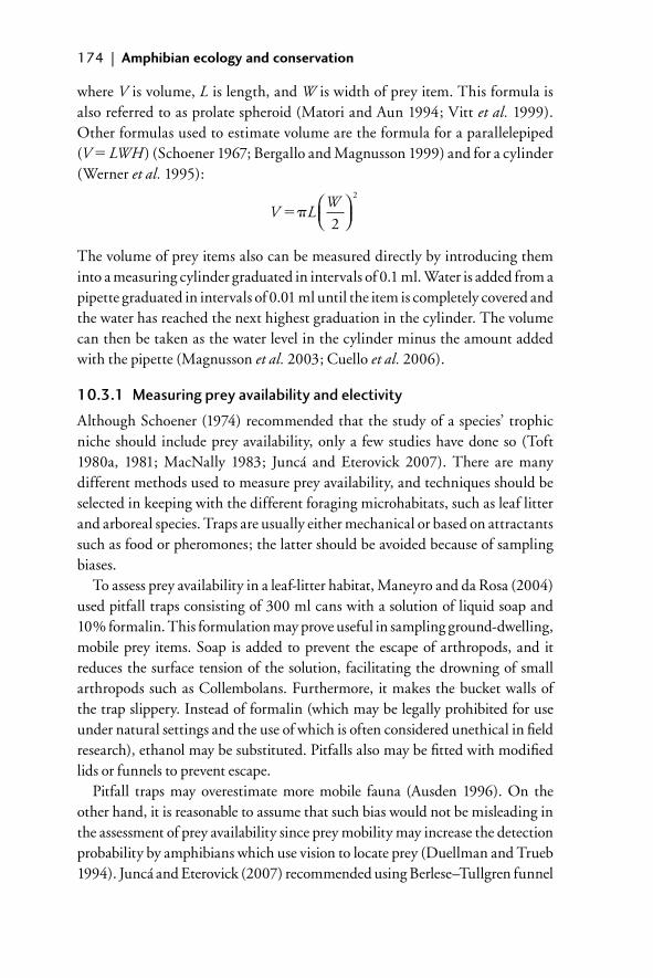
174 | Amphibian ecology and conservation
where V is volume, L is length, and W is width of prey item. This formula is also referred to as prolate spheroid (Matori and Aun 1994; Vitt et al. 1999). Other formulas used to estimate volume are the formula for a parallelepiped (V � LWH) (Schoener 1967; Bergallo and Magnusson 1999) and for a cylinder (Werner et al. 1995):
V LW
��2
2
The volume of prey items also can be measured directly by introducing them into a measuring cylinder graduated in intervals of 0.1 ml. Water is added from a pipette graduated in intervals of 0.01 ml until the item is completely covered and the water has reached the next highest graduation in the cylinder. The volume can then be taken as the water level in the cylinder minus the amount added with the pipette (Magnusson et al. 2003; Cuello et al. 2006).
10.3.1 Measuring prey availability and electivity
Although Schoener (1974) recommended that the study of a species’ trophic niche should include prey availability, only a few studies have done so (Toft 1980a, 1981; MacNally 1983; Juncá and Eterovick 2007). There are many different methods used to measure prey availability, and techniques should be selected in keeping with the different foraging microhabitats, such as leaf litter and arboreal species. Traps are usually either mechanical or based on attractants such as food or pheromones; the latter should be avoided because of sampling biases.
To assess prey availability in a leaf-litter habitat, Maneyro and da Rosa (2004) used pitfall traps consisting of 300 ml cans with a solution of liquid soap and 10% formalin. This formulation may prove useful in sampling ground-dwelling, mobile prey items. Soap is added to prevent the escape of arthropods, and it reduces the surface tension of the solution, facilitating the drowning of small arthropods such as Collembolans. Furthermore, it makes the bucket walls of the trap slippery. Instead of formalin (which may be legally prohibited for use under natural settings and the use of which is often considered unethical in fi eld research), ethanol may be substituted. Pitfalls also may be fi tted with modifi ed lids or funnels to prevent escape.
Pitfall traps may overestimate more mobile fauna (Ausden 1996). On the other hand, it is reasonable to assume that such bias would not be misleading in the assessment of prey availability since prey mobility may increase the detection probability by amphibians which use vision to locate prey (Duellman and Trueb 1994). Juncá and Eterovick (2007) recommended using Berlese–Tullgren funnel
10_Dodd_Chap10.indd 17410_Dodd_Chap10.indd 174 8/19/2009 3:32:19 PM8/19/2009 3:32:19 PM
10 Dietary assessments of adult amphibians | 175
traps (Brower et al. 1998) in addition to pitfall traps and combining the results. These traps sample sedentary taxa in addition to mobile fauna. Both methods underestimate fl ying prey items.
In grassy or herbaceous habitats, the composition and abundance of prey items can be estimated along transects using linear sweeps with insect nets. Each sweep sample should be transferred into a Berlese–Tullgren trap for at least 30 min to separate prey items from litter (leaves, seeds, sticks). Properly conducted, this method can provide a comprehensive assessment of inverte-brate availability. It should be noted that highly mobile fl ying insects such as Odonates (dragonfl ies) might be underrepresented. Furthermore, the time and temperature at which the sweeps are conducted can have a strong infl uence on the result depending on the activity periods of the insects.
Arboreal habitat can be sampled most easily using fogging techniques. Applying insecticides through fogging is widely used in pest control, and a wide range of commercial fogging machines is available. Fumigated insects falling from tree canopies are collected on plastic sheets laid out on the ground or by plastic trays or aluminum funnels (for a short review, see Adis et al. 1998). Insecticide fogging has become established as a standard technique since the 1980s for assessing arthropod diversity, especially in tropical forest canopies (Adis et al. 1998). A variety of “knockdown” insecticides have been tested, but natural pyrethrum is now established as a standard as it allows for collection of live specimens and its biodegradability facilitates application in ecologically sen-sitive habitats. Adis et al. (1998) suggested recommendations to standardize fog-ging procedures. When applying fogging procedures, researchers must consider that the entire vertical habitat that is sampled may overestimate the prey avail-able to amphibians, which inhabit only parts of the vertical habitat structure.
Aquatic habitats can be sampled using a fi ne mashed net, such as the D-frame kick net or surber stream-bottom sampler. The D-frame kick net is either cone- or bag-shaped for the capture of organisms and commonly used by lying the spine of the net fi rmly on the ground and hauling it a specifi c number of times along a specifi c distance. This type of net is easy to transport and can be used in a variety of habitat types. However, the D-frame kick net must have a defi ned or delimited area that is sampled/kicked in order to compare results obtained from different sites or samples. Cao et al. (2005) investigated the performance and comparability between surber and D-frame kick-net samples and found that subsamples with the same number of individuals were highly and consistently comparable between sampling devices. Rocky stream habitats are best sampled by two persons. One collector should place a fi ne mashed net so that its bottom lies on the ground. Another collector should turn over as many rocks as possible
10_Dodd_Chap10.indd 17510_Dodd_Chap10.indd 175 8/19/2009 3:32:19 PM8/19/2009 3:32:19 PM
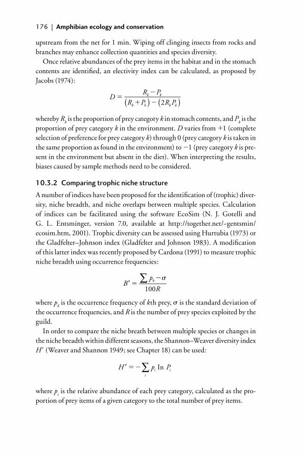
176 | Amphibian ecology and conservation
upstream from the net for 1 min. Wiping off clinging insects from rocks and branches may enhance collection quantities and species diversity.
Once relative abundances of the prey items in the habitat and in the stomach contents are identifi ed, an electivity index can be calculated, as proposed by Jacobs (1974):
DR P
R P R Pk k
k k k k
��
� �( ) ( )2
whereby Rk is the proportion of prey category k in stomach contents, and P
k is the
proportion of prey category k in the environment. D varies from �1 (complete selection of preference for prey category k) through 0 (prey category k is taken in the same proportion as found in the environment) to �1 (prey category k is pre-sent in the environment but absent in the diet). When interpreting the results, biases caused by sample methods need to be considered.
10.3.2 Comparing trophic niche structure
A number of indices have been proposed for the identifi cation of (trophic) diver-sity, niche breadth, and niche overlaps between multiple species. Calculation of indices can be facilitated using the software EcoSim (N. J. Gotelli and G. L. Entsminger, version 7.0, available at http://together.net/~gentsmin/ecosim.htm, 2001). Trophic diversity can be assessed using Hurtubia (1973) or the Gladfelter–Johnson index (Gladfelter and Johnson 1983). A modifi cation of this latter index was recently proposed by Cardona (1991) to measure trophic niche breadth using occurrence frequencies:
′ ∑Bp
Rk
���
100
where pk is the occurrence frequency of kth prey, � is the standard deviation of
the occurrence frequencies, and R is the number of prey species exploited by the guild.
In order to compare the niche breath between multiple species or changes in the niche breadth within different seasons, the Shannon–Weaver diversity index H� (Weaver and Shannon 1949; see Chapter 18) can be used:
′ ∑H p Pi ii
�� In
where pi is the relative abundance of each prey category, calculated as the pro-
portion of prey items of a given category to the total number of prey items.
10_Dodd_Chap10.indd 17610_Dodd_Chap10.indd 176 8/19/2009 3:32:19 PM8/19/2009 3:32:19 PM

10 Dietary assessments of adult amphibians | 177
The index of relative importance (IRI) is a measure that reduces bias in descriptions of animal dietary data. Introduced by Pianka et al. (1971) and Pianka (1973), it is mainly used currently to describe the diet of fi sh:
IRI PO PI PVt t t t� �( )( )where PO
t is the percentage of occurrence (100 � number of stomachs containing
t item/total number of stomachs), PIt is the percentage of individuals (100 � total
number of individuals of t in all stomachs/total number of individuals of all taxa in all stomachs), and PV
t is the percentage of volume (100 � total volume of indi-
viduals of t in all stomachs/total volume of all taxa in all stomachs). Hart et al. (2002) suggested that IRI should be applicable to a wide range of taxa. To calcu-late the trophic niche breadth, the index of Simpson (1949) can be used:
Bpi
�1
2∑where B is Simpson’s index, p
i is the fraction of items in the food category i, and
the range is 1 to n.To compare various diets with a different number of food categories, the
standardized Simpson’s index (BS) form as proposed by Hulbert (1978) can be used:
BSBn
��
�
1
1
Here, n is the number of food categories and the index ranges from 0 to 1.Overlap in trophic niches between two species can be assessed with an index
proposed by May and MacArthur (1972) as modifi ed by Pianka (1974):
OP P
P Pjk
ij iki
n
iji
n
iki
n�
∑
∑ ∑2 2
Here, Ojk is niche overlap and p
ij and p
ik represent the proportions of the ith
resource used by the jth and kth species.
10.3.3 Fatty acid and stable-isotope analyses
Analyses of isotopic composition and fatty acid profi les of tissues can provide reliable information on diets and trophic status because they refl ect assimilation
10_Dodd_Chap10.indd 17710_Dodd_Chap10.indd 177 8/19/2009 3:32:19 PM8/19/2009 3:32:19 PM
178 | Amphibian ecology and conservation
over long periods of time. Isotope signatures—that is, ratios of heavier (e.g. 15N and 14C) and lighter (14N and 13C) isotopes—of consumers are generally similar to those of their food and can thus provide insights into food-web struc-ture. Fatty acids are essential energy storage lipids in consumers that cannot be readily synthesized and must be obtained from their food. Differences in fatty acid composition among available food types are refl ected in fatty acid compositions in consumers; therefore, profi les can be good indicators of diets. For both techniques, tissue samples (or in the case of small individuals or food items, the whole organism) are simply collected and preserved in a manner that does not alter isotopic or fatty acid composition, depending on the analyses to be performed, and then sent to an analytical laboratory for analyses (for a more detailed description of these techniques see Chapter 5).
10.3.4 Further biochemical analyses
Some frog species in the neotropics and Madagascar secrete alkaloids for protec-tion against predators. These so-called poison frogs do not produce the alkal-oids, but instead obtain them from their insect-rich diet (Daly et al. 1994). While the diet of neotropical poison frogs is well studied (Daly et al. 1994, 2002), data on the Malagasy frogs was only provided recently by Clark et al. (2005). These authors extracted alkaloid samples from both Malagasy frogs and their food. Alkaloid fractions can be extracted and isolated from skin samples using methanol (one part skin/two parts methanol) (Daly et al. 1992). Possible methods for biochemical analyses comprise gas chromatography in conjunc-tion with mass spectrometry and infrared spectroscopy to identify alkaloids (for detailed descriptions see Daly et al. 1992, 1993, 1994). They found that Malagasy frogs, like the neotropical species, acquire their alkaloids from the ants they prey upon. Thirteen of the 16 alkaloids detected in the Malagasy frogs also exist in insects and frogs in the neotropics. As neither the ants nor the frogs in these two regions are closely related, these authors suggested that the evolution of acquisition mechanisms for alkaloids in these ant species was likely responsible for the subsequent convergent evolution of the frogs that preyed on them. The researchers also found nicotine, a plant alkaloid, in one Malagasy frog species, suggesting a possible plant–ant–frog toxin food chain.
10.4 General considerations
Samples should be taken randomly throughout the habitat of the target spe-cies in order to avoid bias, such as the predominance of ants which would be expected if all samples were obtained next to an ant hill. Furthermore, sample
10_Dodd_Chap10.indd 17810_Dodd_Chap10.indd 178 8/19/2009 3:32:19 PM8/19/2009 3:32:19 PM
10 Dietary assessments of adult amphibians | 179
sizes are an important issue for dietary analyses. Considering that diet may vary between the sexes, adequate samples from both genders should be obtained. When working with stomach contents, researchers should be aware that they will probably not get a picture of what prey items the focal species feeds upon, but rather a picture of the items that are hard to digest. Frogs are capable of digesting prey rapidly: Blanchard’s cricket frogs (Acris crepitans blanchardi) fed dyed Drosophila (fruit fl ies) and killed 7 h later had no trace of prey remain-ing in their stomachs (Johnson and Christiansen 1976). In another study with A. crepitans immediately preserved frogs had a mean of seven prey items per stomach, whereas frogs preserved 6 h after capture revealed 3.6 prey items per stomach (Caldwell 1996). In a preliminary study with 20 Physalaemus lisei, frogs were fed three different prey categories (Oligochaeta, Curculionid beetles, and Aranea) at the same time, and four frogs were stomach-fl ushed every 4 h. Oligochaeta (worms) could not be detected after 4 h, whereas the pronotum of spiders was still undigested after 8 h and the beetle elytra were still present after 12 h (M. Solé, unpublished results). In conclusion, researchers will underesti-mate the prey categories that basically consist of soft tissue (worms, mollusks, and fl y larvae) and overestimate those with strongly keratinized bodies (ants and beetles). One way in which biologists can mediate this problem is to carefully choose the sampling period according to the feeding period of each species.
10.4.1 Ontogenetic changes
Diet composition of amphibians may change during ontogeny, since larger indi-viduals may be able to eat larger prey items, which signifi cantly increases the var-iety of available prey types. However, Lima (1998) found changes in types and sizes of prey that were caused other than by a simple passive effect of selection for larger prey with growth of the frogs. Foraging modes and microhabitat use may also change during ontogeny, which can affect the composition of available prey items (Lima and Magnusson 2000). To assess ontogenetic changes in the com-position of the diet, different snout–vent size classes of the target species can be compared. The best visualization provides a cluster analysis based on the relative frequency of the different prey categories. Data must be normally distributed to meet the assumptions of the statistical test (Zar 1999). If the data do not meet the required statistical assumptions, they can be transformed (see Chapter 18).
10.4.2 Seasonal changes
Availability and diversity of prey items can change between different seasons (Houston 1973). Although there are many records concerning feeding habits in amphibians, few include seasonal patterns. In Amazonian Peru, Toft (1980b)
10_Dodd_Chap10.indd 17910_Dodd_Chap10.indd 179 8/19/2009 3:32:20 PM8/19/2009 3:32:20 PM
180 | Amphibian ecology and conservation
observed a decrease in arthropod biomass and in frog abundance in the dry season. However, she argued that frog species and their arthropod prey may respond differently to seasonal changes, since the principal feeding patterns of the litter anurans studied did not appear to change seasonally. Yilmaz and Kutrup (2006) analyzed seasonal changes in the diet of the European common frog, Rana ridibunda, and found changes in prey diversity between July (62 prey categories) and August (38). The highest mean prey number was observed in July. The mean prey size also changed during the year: frogs were more likely to consume large prey items in June than in the other months. These results suggested that the monthly variation in diet composition of this species was correlated with prey availability. Finally, large sample sizes are important when studying seasonal dietary changes.
10.5 Conclusions
Dietary information is pivotal for successful development of conservation strat-egies on species level and the understanding of ecosystem function. Unfortunately, this kind of information is not available for the vast majority of taxa and is often incomplete. Seasonal variations, ontogenetic shifts, and relationships between site-specifi c prey availability, presence of potential competitors, and diet compos-ition are commonly not addressed. Future studies should focus on these issues. In the light of global amphibian declines an Amphibian Conservation Action Plan was formulated by the International Union for Conservation of Nature to prevent further biodiversity loss and captive breeding programmes are being developed for the most threatened species (Gascon et al. 2007). Such approaches depend crucially on autecological knowledge such as information on the diet of the target species. Here, every kind of information can be valuable.
10.6 Acknowledgments
We are grateful to Ken Dodd, Marian Griffey, and Matt Whiles for helpful com-ments on the manuscript and to Klaus Riede for fruitful discussions concerning quantitative insect sampling methods and help with the literature. The work of DR was funded by the Graduiertenförderung des Landes Nordrhein-Westfalen.
10.7 References
Adis, J., Basset, Y., Floren, A., Hammond, P. M., and Linsenmair, K. E. (1998). Canopy fog-ging on an overstorey tree- recommendations for standardization. Ecotropica, 4, 93–7.
10_Dodd_Chap10.indd 18010_Dodd_Chap10.indd 180 8/19/2009 3:32:20 PM8/19/2009 3:32:20 PM
10 Dietary assessments of adult amphibians | 181
Anderson, M. T. and Mathis, A. (1999). Diets of two sympatric Neotropical salaman-ders, Bolitoglossa mexicana and B. rufescens, with notes on reproduction for B. rufescens. Journal of Herpetology, 33, 601–7.
Anderson, S. H. (1991). Managing our Wildlife Resources. Merrill Publishing Co., Columbus, OH.
Ausden, M. (1996). Invertebrates. In W. J. Sutherland (ed.), Ecological Census Techniques, pp. 139–77. Cambridge University Press, Cambridge.
Bergallo, H. G. and Magnusson, W. E. (1999). Effects of climate and food availability on four rodent species in southeastern Brazil. Journal of Mammalogy, 80, 472–86.
Brower, J. E., Zar, J. H., and von Ende, C. N. (1998). Field and Laboratory Methods for General Ecology. WCB McGraw-Hill, Boston, MA.
Caldwell, J. P. (1996). The evolution of myrmecophagy and its correlates in poison frogs (family Dendrobatidae). Journal of Zoology, London, 240, 75–101.
Cao, Y., Hawkins, C. P., and Storey, A. W. (2005). A method for measuring compar-ability of different sampling methods used in biological surveys: implications for data integration and synthesis. Freshwater Biology, 50, 1105–15.
Cardona, L. (1991). Measurement of trophic niche breadth using occurrence frequencies. Journal of Fish Biology, 39, 901–3.
Clark, V. C., Raxworthy, C. J., Rakotomalala, V., Sierwald, P., and Fisher, B. L. (2005). Convergent evolution of chemical defense in poison frogs and arthropod prey between Madagascar and the Neotropics. Proceedings of the National Academy of Sciences USA, 102, 11617–22.
Colli, G. R. and Zamboni, D. S. (1999). Ecology of the worm-lizard Amphisbaena alba in the Cerrado of central Brazil. Copeia, 1999, 733–42.
Cuello, M. E., Bello, T. M., Kun, M., and Ubeda, C. A. (2006). Feeding habits and their implications for the conservation of endangered semiaquatic frog Atelognathus patagonicus (Anura, Neobatrachia) in a northwestern Patagonian pond. Phyllomedusa, 5, 67–76.
Daly, J. W., Secunda, S. I., Garraffo, H. M., Spande, T. F., Wisnieski, A., Nishihira, C., and Cover Jr, J. F. (1992). Variability in alkaloid profi les in Neotropical poison frogs (Dendrobatidae). Toxicon, 30, 887–98.
Daly, J. W., Garraffo, H. M., and Spande, T. F. (1993). Amphibian alkaloids. In G. A. Cordell (ed.), The Alkaloids, vol. 43, pp. 185–288. Academic Press, San Diego, CA.
Daly, J. W., Garraffo, H. M., Spande, T. F., Jaramillo, C., and Rand, A. S. (1994). Dietary source for skin alkaloids of poison frogs (Dendrobatidae)? Journal of Chemical Ecology, 20, 943–55.
Daly, J. W., Kaneko, T., Wilham, J., Garraffo, H. M., Spande, T. F., Espinosa, A., and Donnelly, M. (2002). Bioactive alkaloids of frog skin: combinatorial bioprospect-ing reveals that pumiliotoxins have an arthropod source. Proceedings of the National Academy of Sciences USA, 99, 13996–14001.
Duellman, W. E. and Trueb, L. (1994). Biology of Amphibians. John Hopkins University Press, Baltimore, MD.
Emerson, S. B. (1985). Skull shape in frogs—correlations with diet. Herpetologica, 41, 177–88.Fraser, D. F. (1976). Coexistence of salamanders in the genus Plethodon, a variation of the
Santa Rosalia theme. Ecology, 57, 238–51.
10_Dodd_Chap10.indd 18110_Dodd_Chap10.indd 181 8/19/2009 3:32:20 PM8/19/2009 3:32:20 PM
182 | Amphibian ecology and conservation
Freed, A. N. (1982). A treefrog’s menu: selection for an evening’s meal. Oecologia, 53, 20–6.
Gascon, C., Collins, J. P., Moore, R. D., Church, D. R., McKay, J. E., and Mendelson III, J. R. (2007). Amphibian Conservation Action Plan - Proceedings: IUCN/SSC Amphibian Conservation Summit 2005. IUCN, Gland.
Gladfelter, W. B. and Johnson, W. S. (1983). Feeding niche separation in a guild of trop-ical reef fi sh (Holocentridae). Ecology, 64, 552–63.
Hart, R. K., Calver, M. C., and Dickman, C. R. (2002). The index of relative import-ance: an alternative approach to reducing bias in descriptive studies of animal diets. Wildlife Research, 29, 415–21.
Hirai, T. and Matsui, M. (2001). Attempts to estimate the original size of partly digested prey recovered from stomachs of Japanese anurans. Herpetological Review, 32, 14–16.
Houston, W. W. K. (1973). The food of the common frog, Rana temporaria, on high moorland in northern England. Journal of Zoology, 171, 153–65.
Hulbert, S. H. (1978). The measurement of niche overlap and some relatives. Ecology, 59, 67–77.
Hurtubia, J. (1973). Trophic diversity measurement in sympatric predatory species. Journal of Ecology, 549, 885–90.
Jacobs, J. (1974). Quantitative measurement of food selection: a modifi cation of the for-age ration and Ivlev’s electivity index. Oecologia, 14, 413–17.
Johnson, B. K. and Christiansen, J. L. (1976). The food and food habits of Blanchard’s cricket frog, Acris crepitans blanchardi (Amphibia, Anura, Hylidae), in Iowa. Journal of Herpetology, 10, 63–74.
Joly, P. (1987). Le regime alimentaire des amphibiens: methods d’etude. Alytes, 6, 11–17.Juncá, F. A. and Eterovick, P. C. (2007). Feeding ecology of two sympatric species of
Aromobatidae, Allobates marchesianus and Anomaloglossus stepheni, in Central Amazon. Journal of Herpetology, 41, 301–8.
Kupfer, A., Nabhitabhata, J., and Himstedt, W. (2005). From water into soil: trophic ecology of a caecilian amphibian (Genus Ichthyophis). Acta Oecologica, 28, 95–105.
Legler, J. M. (1977). Stomach fl ushing: a technique for chelonian dietary studies. Herpetologica, 33, 281–4.
Legler, J. M. and Sullivan, L. J. (1979). The application of stomach-fl ushing to lizards and anurans. Herpetologica, 35, 107–10.
Lima, A. P. (1998). The effects of size on the diets of six sympatric species of postmeta-morphic litter anurans in central Amazonia. Journal of Herpetology, 32, 392–9.
Lima, A. P. and Magnusson, W. E. (2000). Does foraging activity change with ontogeny? An assessment for six sympatric species of postmetamorphic litter anurans in Central Amazonia. Journal of Herpetology, 34, 192–200.
MacNally, R. (1983). Trophic relationships of two sympatric species of Ranidella (Anura). Herpetologica, 39, 130–40.
Magnusson, W. E., Lima, A. P., Silva, W. A., and Araújo, M. C. (2003). Use of geomet-ric forms to estimate volume of invertebrates in ecological studies of dietary overlap. Copeia, 2003, 13–19.
Mahan, R. D. and Johnson, J. R. (2007). Diet of the gray treefrog (Hyla versicolor) in rela-tion to foraging site location. Journal of Herpetology, 41, 16–23.
10_Dodd_Chap10.indd 18210_Dodd_Chap10.indd 182 8/19/2009 3:32:20 PM8/19/2009 3:32:20 PM
10 Dietary assessments of adult amphibians | 183
Maneyro, R. and da Rosa, I. (2004). Temporal and spatial changes in the diet of Hyla pulchella (Anura, Hylidae) in southern Uruguay. Phyllomedusa, 3, 101–13.
Matori, R. and Aun, L. (1994). Aspects of the ecology of a population of Tropidurus spinu-losus. Amphibia-Reptilia, 15, 317–26.
May, R. M. and MacArthur, R. H. (1972). Niche overlap as a function of environmental variability. Proceedings of the National Academy of Sciences USA, 69, 1109–13.
Miranda, T., Ebner, M., Solé, M., and Kwet, A. (2006). Spatial, seasonal and intrapopu-lational variation in the diet of Pseudis cardosoi (Anura: Hylidae) from the Araucária Plateau of Rio Grande do Sul, Brazil. South American Journal of Herpetology, 1, 121–30.
O’Reilly, J. C. (2000). Feeding in caecilians. In K. Schwenk (ed.), Feeding, Form, Function and Evolution in Tetrapod Vertebrates. Academic Press, New York.
Pianka, E. R. (1973). The structure of lizard communities. Annual Review of Ecology and Systematics, 4, 53–74.
Pianka, E. R. (1974). Niche overlap and diffuse competition. Proceedings of the National Academy of Sciences USA, 71, 2141–5.
Pianka, E. R., Oliphant, M. S., and Iverson, Z. L. (1971). Food habits of albacore bluefi n, tuna and bonito in Califorina waters. California Department of Fish and Game Bulletin, 152, 1–350.
Rocha, C. F. D., Van Sluys, M., Alves, M. A. S., Bergallo, H. G., and Vrcibradic, D. (2000). Activity of leaf-litter frogs: when should frogs be sampled? Journal of Herpetology, 34, 285–7.
Schoener, T. W. (1967). The ecological signifi cance of sexual dimorphism in size in the lizard Anolis conspersus. Science, 155, 474–7.
Schoener, T. W. (1974). The compression hypothesis and temporal resource partitioning. Proceedings of the National Academy of Sciences USA, 71, 4169–72.
Silva, H. R. and Britto-Pereira, M. C. (2006). How much fruit do fruit-eating frogs eat? An investigation on the diet of Xenohyla truncata (Lissamphibia: Anura: Hylidae). Journal of Zoology, 270, 692–8.
Simon, M. P. and Toft, C. A. (1991). Diet specialization in small vertebrates: mite-eating in frogs. Oikos, 61, 263–78.
Simpson, E. H. (1949). Measurement of diversity. Nature, 163, 688.Sokol, O. M. (1969). Feeding in the pipid frog Hymenochirus boettergi (Tornier).
Herpetologica, 25, 9–24.Solé, M. and Pelz, B. (2007). Do male tree frogs feed during the breeding season? Stomach
fl ushing of fi ve syntopic hylid species in Rio Grande do Sul, Brazil. Journal of Natural History, 41, 2757–63.
Solé, M., Beckmann, O., Pelz, B., Kwet, A., and Engels, W. (2005). Stomach-fl ushing for diet analysis in anurans: an improved protocol evaluated in a case study in Araucaria forests, southern Brazil. Studies on Neotropical Fauna and Environment, 40, 23–8.
Toft, C. A. (1980a). Feeding ecology of thirteen syntopic species of anurans in a seasonal tropical environment. Oecologia, 45, 131–41.
Toft, C. A. (1980b). Seasonal variation in populations of Panamanian litter frogs and their prey: a comparison of wetter and drier sites. Oecologia, 47, 34–8.
Toft, C. A. (1981). Feeding ecology of Panamanian litter anurans: patterns in diet and foraging mode. Journal of Herpetology, 15, 139–44.
10_Dodd_Chap10.indd 18310_Dodd_Chap10.indd 183 8/19/2009 3:32:20 PM8/19/2009 3:32:20 PM
184 | Amphibian ecology and conservation
Toft, C. A. (1985). Resource partitioning in amphibians and reptiles. Copeia, 1985, 1–21.
Triplehorn, C. A. and Johnson, N. F. (2005). Borror and Delong’s Introduction to the Study of Insects, 7th edn. Thomson Brooks/Cole, Belmont, CA.
Vitt, L. J., Zani, P. A., and Espósito, M. C. (1999). Ecological differences in tropical sympatric skinks (Mabouya macrorhyncha and Mabouya agilis) in southeastern Brazil. Journal of Herpetology, 30, 60–7.
Wang, Y. P., Zhang, P., and Li, Y. (2008). Diet composition of post-metamorphic bull-frogs (Rana catesbeiana) in the Zhoushan archipelago, Zhejiang Province, China. Frontiers of Biology in China, 3, 219–26.
Weaver, W. and Shannon, C. E. (1949). The Mathematical Theory of Communication. University of Illinois, Urbana, IL.
Werner, E. E., Wellborn, G. A., and McPeek, M. A. (1995). Diet composition in post-metamorphic bullfrogs and green frogs: implications for interspecifi c predation and competition. Journal of Herpetology, 29, 600–7.
Wu, Z. J., Li, Y. M., and Wang, Y. P. (2007). A comparison of stomach fl ush and stomach dissection in diet analysis of four frog species. Acta Zoologica Sinica, 53, 364–72.
Yilmaz, Z. C. and Kutrup, B. (2006). Seasonal changes in the diet of Rana ridibunda Pallas, 1771 (Anura: Ranidae) from the Gorele River, Giresun, Turkey. In M. Vences, J. Köhler, T. Ziegler, and W. Böhme (eds), Herpetologia Bonnensis II. Proceedings of the 13th Congress of the Societas Europaea Herpetologica, pp. 201–4. Bonn, Germany.
Zar, J. H. (1999). Biostatistical Analysis. Prentice-Hall, Englewood Cliffs, NJ.
10_Dodd_Chap10.indd 18410_Dodd_Chap10.indd 184 8/19/2009 3:32:20 PM8/19/2009 3:32:20 PM
12Field enclosures and terrestrial cages
Elizabeth B. Harper, Joseph H.K. Pechmann, and
James W. Petranka
12.1 Introduction: amphibians in the terrestrial environment
Amphibians exhibit many life-history patterns and occur in biomes ranging from deserts and grasslands to boreal and tropical forests (Chapter 1). Most species have complex life cycles with a free-living aquatic larval stage and a non-gilled post-metamorphic stage. Of the more than 6000 extant species that have been described, almost all use terrestrial habitats during some or all of their life cycle. Common terrestrial specializations include arboreal, fossorial, surface-dwelling, and riparian species (Chapter 1).
The aquatic larval stage, if present, is typically much shorter than the post-metamorphic stage. The juveniles and adults of most species live in semi-aquatic or terrestrial habitats. Despite these facts, researchers have conducted surprisingly few studies on the terrestrial ecology of amphibians, especially pond-breeding amphibians (Pechmann 1995). Even some of the most basic questions—such as the extent to which population regulation occurs during the aquatic and terres-trial stages of the life cycle—are poorly resolved because of a shortage of infor-mation on density dependence during the terrestrial stages.
Conservation biologists have identifi ed factors that are contributing to the global declines of amphibians (e.g. environmental pollutants, forest fragmen-tation, urbanization, and road construction), but the relative extent to which these are affecting the aquatic and terrestrial stages is often uncertain (Biek et al. 2002). Widespread gaps in knowledge about the terrestrial ecology of amphib-ians continue to hamper our ability to develop effective conservation strategies for the hundreds of species that are in long-term decline. Experiments using fi eld enclosures can help resolve critical issues concerning the terrestrial ecology of amphibians and the ability of animals to tolerate environmental stressors.
Dodd_Ch12.indd 203Dodd_Ch12.indd 203 4/17/2009 7:40:28 PM4/17/2009 7:40:28 PM
204 | Amphibian ecology and conservation
Given that the use of enclosures is often expensive and time-consuming, why should a researcher use them? Enclosures allow researchers to expose animals to experimental treatments that test explicit hypotheses and to recapture animals to measure response variables. More importantly, fi eld experiments maximize realism relative to laboratory or mesocosm studies and provide the strong-est inferences as to whether the factors under investigation operate in nature (Hairston 1989; Morin 1998; Boone and James 2005).
When designing enclosure experiments, researchers must balance trade-offs in experimental design because it is impossible to simultaneously maximize realism, precision, and generality (Hairston 1989). Precision is maximized by creating replicates of experimental treatments that are as similar as possible to one another. Generality, which is the ability to extrapolate to a broad area or to a number of conditions, is maximized by placing replicate enclosures in as many locations or conditions as possible. In general, experimental designs that maximize generality compromise precision (and visa versa), and designs that maximize realism also compromise precision.
Optimally balancing these trade-offs depends on the questions that are being addressed. For example, a researcher who wishes to address how density affects the growth of juvenile amphibians may elect to maximize precision and reduce experimental error by placing enclosures at one site and in close proximity to one another (Altwegg 2003). In contrast, a researcher who wishes to determine the rate at which air-borne agricultural pesticides are accumulating in amphibians in a nearby mountain range may want to establish test sites at numerous loca-tions to maximize generality.
In the sections that follow we provide examples of how terrestrial enclosures have been used to address questions about the ecology and conservation biology of amphibians. We also provide information on cage designs, add cautionary notes about experimental artifacts, and discuss trade-offs that should be consid-ered when designing experiments.
12.2 What are the purposes of terrestrial enclosures?
Terrestrial enclosures have been used by amphibian ecologists for four general purposes, as follows.
1) To confi ne amphibians so that they can be subjected to an experimen-tal treatment. The treatment can be the characteristics of the area itself (e.g. forested or non-forested; Chazal and Niewiarowski 1998; Todd and Rothermel 2006), or one applied by the researcher (e.g. population density;
Dodd_Ch12.indd 204Dodd_Ch12.indd 204 4/17/2009 7:40:28 PM4/17/2009 7:40:28 PM
12 Field enclosures and terrestrial cages | 205
Pechmann 1995; Harper and Semlitsch 2007). Enclosures allow these experiments to be conducted under realistic conditions in the fi eld on organisms that could otherwise migrate from their assigned treatment.
2) To facilitate recapture of amphibians subjected to experimental treat-ments before they were placed in the enclosures, for example investigating the post-metamorphic carryover effects of larval exposure to pesticides (Boone 2005). In this case, enclosures permit evaluation of treatment effects under natural climatic conditions and diets, and perhaps under natural competition and predation regimes, depending on the type and size of the enclosures.
3) To facilitate recapture of dispersing or migrating amphibians to measure habitat choice and movement distances (Rothermel and Semlitsch 2002; Croshaw and Scott 2006). Enclosures in this case consist of walled corri-dors. Although these topics can also be addressed by tracking unenclosed individuals (Chapter 11), enclosures allow large groups of animals to be followed and recaptured. Enclosures can also confi ne choices and move-ments to particular habitats. For example, Croshaw and Scott (2006) examined the elevations marbled salamanders chose for nesting in enclos-ures in which the amount of cover was equalized across elevations.
4) To estimate terrestrial densities of amphibians (Regosin et al. 2003a, 2005). Enclosing an area containing naturally occurring amphibians limits their movement and can improve the accuracy of density estimates obtained by removal sampling or mark–recapture.
12.3 Defi ning the research question
The fi rst step in designing an effective experiment using terrestrial enclosures is to clearly defi ne the research question. This is essential in deciding: (1) which species to use, (2) the location, size, and number of enclosures, (3) methods of pen construction, (4) the number of amphibians per enclosure, (5) the fre-quency and methods of recapturing individuals, (6) the duration of the experi-ment, (7) the response metrics, and (8) how the data will be analyzed. The majority of research questions fall into two general categories: questions with habitat types as the experimental treatment and questions with treatments that can be randomly assigned to enclosures or to individuals within them.
12.3.1 Questions related to habitat types
If the research question examines the effects of specifi c habitat types, then the treatment consists of the conditions inside each enclosure and the surrounding
Dodd_Ch12.indd 205Dodd_Ch12.indd 205 4/17/2009 7:40:28 PM4/17/2009 7:40:28 PM
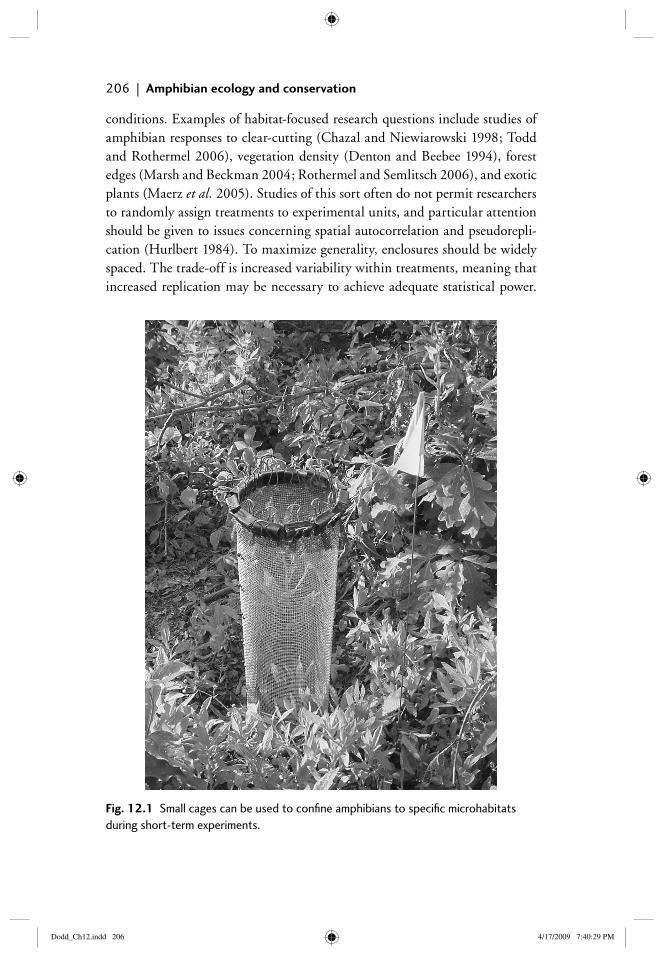
206 | Amphibian ecology and conservation
conditions. Examples of habitat-focused research questions include studies of amphibian responses to clear-cutting (Chazal and Niewiarowski 1998; Todd and Rothermel 2006), vegetation density (Denton and Beebee 1994), forest edges (Marsh and Beckman 2004; Rothermel and Semlitsch 2006), and exotic plants (Maerz et al. 2005). Studies of this sort often do not permit researchers to randomly assign treatments to experimental units, and particular attention should be given to issues concerning spatial autocorrelation and pseudorepli-cation (Hurlbert 1984). To maximize generality, enclosures should be widely spaced. The trade-off is increased variability within treatments, meaning that increased replication may be necessary to achieve adequate statistical power.
Fig. 12.1 Small cages can be used to confi ne amphibians to specifi c microhabitats during short-term experiments.
Dodd_Ch12.indd 206Dodd_Ch12.indd 206 4/17/2009 7:40:29 PM4/17/2009 7:40:29 PM
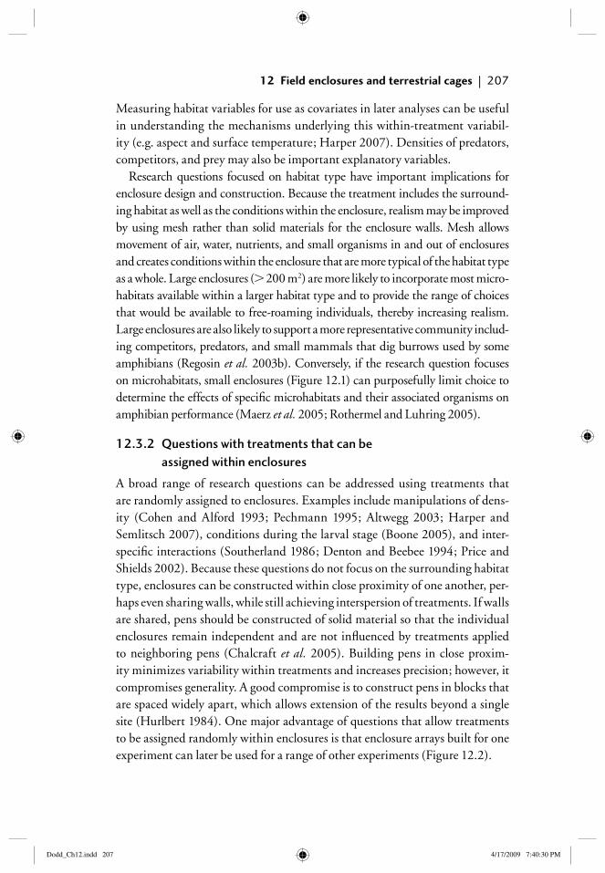
12 Field enclosures and terrestrial cages | 207
Measuring habitat variables for use as covariates in later analyses can be useful in understanding the mechanisms underlying this within-treatment variabil-ity (e.g. aspect and surface temperature; Harper 2007). Densities of predators, competitors, and prey may also be important explanatory variables.
Research questions focused on habitat type have important implications for enclosure design and construction. Because the treatment includes the surround-ing habitat as well as the conditions within the enclosure, realism may be improved by using mesh rather than solid materials for the enclosure walls. Mesh allows movement of air, water, nutrients, and small organisms in and out of enclosures and creates conditions within the enclosure that are more typical of the habitat type as a whole. Large enclosures (� 200 m2) are more likely to incorporate most micro-habitats available within a larger habitat type and to provide the range of choices that would be available to free-roaming individuals, thereby increasing realism. Large enclosures are also likely to support a more representative community includ-ing competitors, predators, and small mammals that dig burrows used by some amphibians (Regosin et al. 2003b). Conversely, if the research question focuses on microhabitats, small enclosures (Figure 12.1) can purposefully limit choice to determine the effects of specifi c microhabitats and their associated organisms on amphibian performance (Maerz et al. 2005; Rothermel and Luhring 2005).
12.3.2 Questions with treatments that can be assigned within enclosures
A broad range of research questions can be addressed using treatments that are randomly assigned to enclosures. Examples include manipulations of dens-ity (Cohen and Alford 1993; Pechmann 1995; Altwegg 2003; Harper and Semlitsch 2007), conditions during the larval stage (Boone 2005), and inter-specifi c interactions (Southerland 1986; Denton and Beebee 1994; Price and Shields 2002). Because these questions do not focus on the surrounding habitat type, enclosures can be constructed within close proximity of one another, per-haps even sharing walls, while still achieving interspersion of treatments. If walls are shared, pens should be constructed of solid material so that the individual enclosures remain independent and are not infl uenced by treatments applied to neighboring pens (Chalcraft et al. 2005). Building pens in close proxim-ity minimizes variability within treatments and increases precision; however, it compromises generality. A good compromise is to construct pens in blocks that are spaced widely apart, which allows extension of the results beyond a single site (Hurlbert 1984). One major advantage of questions that allow treatments to be assigned randomly within enclosures is that enclosure arrays built for one experiment can later be used for a range of other experiments (Figure 12.2).
Dodd_Ch12.indd 207Dodd_Ch12.indd 207 4/17/2009 7:40:30 PM4/17/2009 7:40:30 PM
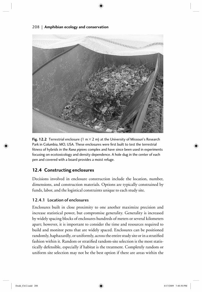
208 | Amphibian ecology and conservation
12.4 Constructing enclosures
Decisions involved in enclosure construction include the location, number, dimensions, and construction materials. Options are typically constrained by funds, labor, and the logistical constraints unique to each study site.
12.4.1 Location of enclosures
Enclosures built in close proximity to one another maximize precision and increase statistical power, but compromise generality. Generality is increased by widely spacing blocks of enclosures hundreds of meters or several kilometers apart; however, it is important to consider the time and resources required to build and monitor pens that are widely spaced. Enclosures can be positioned randomly, haphazardly, or uniformly, across the entire study site or in a stratifi ed fashion within it. Random or stratifi ed random-site selection is the most statis-tically defensible, especially if habitat is the treatment. Completely random or uniform site selection may not be the best option if there are areas within the
Fig. 12.2 Terrestrial enclosure (1 m � 2 m) at the University of Missouri’s Research Park in Columbia, MO, USA. These enclosures were fi rst built to test the terrestrial fi tness of hybrids in the Rana pipiens complex and have since been used in experiments focusing on ecotoxicology and density dependence. A hole dug in the center of each pen and covered with a board provides a moist refuge.
Dodd_Ch12.indd 208Dodd_Ch12.indd 208 4/17/2009 7:40:30 PM4/17/2009 7:40:30 PM
12 Field enclosures and terrestrial cages | 209
habitat that amphibians avoid or areas where it is impossible to build suitable pens. If the study animals prefer specifi c microhabitats, then stratifi ed designs that place all or a disproportionately large number of pens in preferred habitats may be desirable. Areas that expose amphibians to high temperatures due to lack of canopy cover or aspect can result in high mortality (Harper 2007), as can lack of moisture, burrows, or cover objects (Rothermel and Luhring 2005). In some studies these factors may be part of the treatments, while in others they may be sources of experimental error that reduce statistical power. Haphazard place-ment of enclosures may be ideal for ensuring that pens are located in areas where installation is feasible and habitats seem suitable, but it often compromises gen-erality and may introduce bias.
12.4.2 Size and number of enclosures
Limited resources explain the inverse relationship between the number and size of enclosures used in experiments and the prevalence of small (� 10 m2) enclo-sures (Table 12.1). Striking the right balance between the number and size of enclosures depends largely on the research question and the duration of the experiment. In general, it is best to fi rst determine the size of enclosure that best suits the research question and then ascertain the number of enclosures that can feasibly be built, stocked, and monitored given the circumstances. Then decide whether this number of enclosures is adequate to answer the research question without a high probability of type II error (i.e. failing to reject a null hypothesis when the alternate is true), preferably by doing a statistical power analysis. Keep in mind that some enclosures may be lost to falling trees or other misfortunes, especially during long-term experiments.
Small pens compromise realism because they rarely encompass the home range and associated microhabitats that are used by amphibians. They may also exclude or restrict the movements of competitors, predators, and prey more than large pens. This can result in large variation in the organisms included in replicate pens. Cage effects, including unnatural behaviors resulting from confi nement, are expected to be more prevalent in small enclosures because the available behavioral options, including habitat selection and predator avoid-ance, are limited.
Some amphibian species migrate over 1 km among over-wintering habitats, breeding habitats, and summer foraging areas, and the area of habitat used can vary dramatically depending on life-history stage and time of year (Beebee 1996). Experiments using these species can still achieve a reasonable level of realism if the duration of the experiment is limited; for example, to the juven-ile stage or to the summer foraging period. Realism can also be improved by
Dodd_Ch12.indd 209Dodd_Ch12.indd 209 4/17/2009 7:40:31 PM4/17/2009 7:40:31 PM
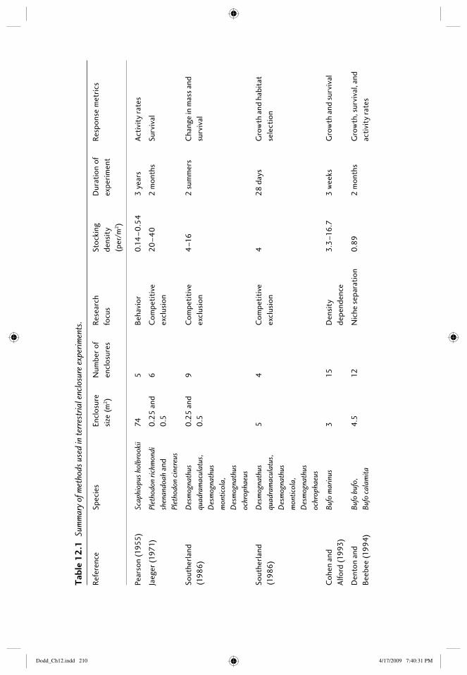
Tab
le 1
2.1
Sum
mar
y of
met
hods
use
d in
terr
estr
ial e
nclo
sure
exp
erim
ents
.
Refe
renc
eSp
ecie
sEn
clos
ure
size
(m
2)
Num
ber o
f en
clos
ures
Rese
arch
fo
cus
Stoc
king
de
nsit
y (p
er/m
2)
Dur
atio
n of
ex
perim
ent
Resp
onse
met
rics
Pear
son
(195
5)
Scap
hiop
us h
olbr
ooki
i74
5Be
havi
or0
.14
–0
.54
3 y
ears
Acti
vity
rate
s
Jaeg
er (1
971)
Plet
hodo
n ric
hmon
di
shen
ando
ah a
nd
Plet
hodo
n ci
nere
us
0.2
5 a
nd
0.5
6C
ompe
titi
ve
excl
usio
n20
–4
02
mon
ths
Surv
ival
Sout
herla
nd
(198
6)
Des
mog
nath
us
quad
ram
acul
atus
, D
esm
ogna
thus
m
ontic
ola,
D
esm
ogna
thus
oc
hrop
haeu
s
0.2
5 a
nd
0.5
9
Com
peti
tive
ex
clus
ion
4–1
62
sum
mer
sC
hang
e in
mas
s an
d su
rviv
al
Sout
herla
nd
(198
6)
Des
mog
nath
us
quad
ram
acul
atus
, D
esm
ogna
thus
m
ontic
ola,
D
esm
ogna
thus
oc
hrop
haeu
s
54
Com
peti
tive
ex
clus
ion
428
day
sG
row
th a
nd h
abit
at
sele
ctio
n
Coh
en a
nd
Alfo
rd (1
993)
Bufo
mar
inus
315
Den
sity
de
pend
ence
3.3
–16
.73
wee
ksG
row
th a
nd s
urvi
val
Den
ton
and
Beeb
ee (1
994)
Bufo
buf
o,
Bufo
cal
amita
4.5
12N
iche
sep
arat
ion
0.8
92
mon
ths
Gro
wth
, sur
viva
l, an
d ac
tivi
ty ra
tes
Dodd_Ch12.indd 210Dodd_Ch12.indd 210 4/17/2009 7:40:31 PM4/17/2009 7:40:31 PM
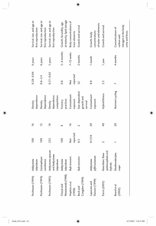
Pech
man
n (1
994)
Amby
stom
a ta
lpoi
deum
100
16D
ensi
ty
depe
nden
ce0
.28
–0
.84
6 y
ears
Surv
ival
, siz
e, a
nd a
ge a
t fi r
st re
prod
ucti
on
Pech
man
n (1
994)
Gas
trop
hryn
e ca
rolin
ensis
100
12D
ensi
ty
depe
nden
ce0
.6–2
.46
yea
rsSu
rviv
al, s
ize,
and
age
at
fi rst
repr
oduc
tion
Pech
man
n (1
995
)Am
byst
oma
opac
um
and
Amby
stom
a ta
lpoi
deum
225
18D
ensi
ty
depe
nden
ce,
com
peti
tion
0.3
1–0
.62
5 y
ears
Surv
ival
, siz
e, a
nd a
ge a
t fi r
st re
prod
ucti
on
Cha
zal a
nd
Nie
wia
rows
ki (1
998)
Amby
stom
a ta
lpoi
deum
100
8Fo
rest
ry
prac
tice
s0
.85
–6
mon
ths
Gro
wth
, fec
undi
ty, a
ge
at m
atur
ity,
lipi
d st
orag
e
Hop
kins
et a
l. (1
998)
Bufo
terr
estr
isN
ot
repo
rted
16C
onta
min
ant
expo
sure
Not
re
port
ed7–
12 w
eeks
Body
con
cent
rati
ons
of
trac
e el
emen
ts
Beck
and
C
ongd
on (1
999)
Bufo
terr
estr
is0
.52
Size
-dep
ende
nt
grow
th a
nd
surv
ival
522
mon
ths
Gro
wth
and
sur
viva
l
Lapo
sata
and
D
unso
n (1
999)
Amby
stom
a je
ffers
onia
num
0.1
134
20C
onta
min
ant
expo
sure
8.8
1 m
onth
Gro
wth
, bod
y co
ncen
trat
ions
of
wat
er a
nd e
lem
ents
Parr
is (2
001
)Ra
na b
lairi
, Ran
a sp
ehno
ceph
ala
and
hybr
ids
24
8H
ybrid
fi tn
ess
3.5
1 y
ear
Gro
wth
and
sur
viva
l
Bear
d et
al.
(20
02)
Eleu
ther
odac
tylu
s co
qui
120
Nut
rient
cyc
ling
74
mon
ths
Con
cent
rati
ons
of
carb
on a
nd
nitr
ogen
in th
e bo
dy
urin
e an
d fe
ces
Dodd_Ch12.indd 211Dodd_Ch12.indd 211 4/17/2009 7:40:31 PM4/17/2009 7:40:31 PM
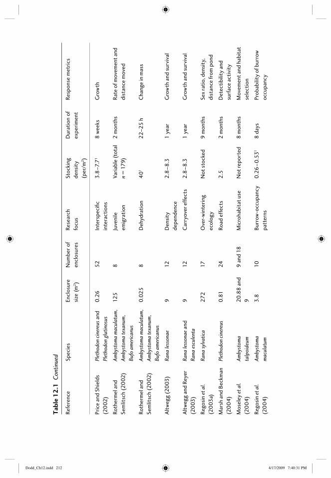
Pric
e an
d Sh
ield
s (2
002
)Pl
etho
don
cine
reus
and
Pl
etho
don
glut
inos
us0
.26
52In
ters
peci
fi c
inte
ract
ions
3.8
–7.7
18
wee
ksG
row
th
Roth
erm
el a
nd
Sem
litsc
h (2
002
)Am
byst
oma
mac
ulat
um,
Amby
stom
a te
xanu
m,
Bufo
am
eric
anus
125
8Ju
veni
le
emig
rati
onVa
riabl
e (t
otal
n
� 1
79)
2 m
onth
sRa
te o
f mov
emen
t and
di
stan
ce m
oved
Roth
erm
el a
nd
Sem
litsc
h (2
002
)Am
byst
oma
mac
ulat
um,
Amby
stom
a te
xanu
m,
Bufo
am
eric
anus
0.0
258
Deh
ydra
tion
401
22–
25 h
Cha
nge
in m
ass
Alt
weg
g (2
003
)Ra
na le
sson
ae9
12D
ensi
ty
depe
nden
ce2
.8–
8.3
1 y
ear
Gro
wth
and
sur
viva
l
Alt
weg
g an
d Re
yer
(20
03)
Rana
less
onae
and
Ra
na e
scul
enta
912
Car
ryov
er e
ffec
ts2
.8–
8.3
1 y
ear
Gro
wth
and
sur
viva
l
Rego
sin
et a
l. (2
003
a)Ra
na sy
lvatic
a27
217
Ove
r-w
inte
ring
ecol
ogy
Not
sto
cked
9 m
onth
sSe
x ra
tio,
den
sity
, di
stan
ce fr
om p
ond
Mar
sh a
nd B
eckm
an
(20
04)
Plet
hodo
n ci
nere
us0
.81
24Ro
ad e
ffec
ts2
.52
mon
ths
Det
ecti
bilit
y an
d su
rfac
e ac
tivi
ty
Mos
eley
et a
l. (2
00
4)Am
byst
oma
talp
oide
um20
.88
and
9
9 a
nd 1
8M
icro
habi
tat u
seN
ot re
port
ed8
mon
ths
Mov
emen
t and
hab
itat
se
lect
ion
Rego
sin
et a
l. (2
00
4)Am
byst
oma
mac
ulat
um3.
810
Burr
ow-o
ccup
ancy
pa
tter
ns0
.26
–0
.531
8 d
ays
Prob
abili
ty o
f bur
row
oc
cupa
ncy
Tab
le 1
2.1
Con
tinue
d
Refe
renc
eSp
ecie
sEn
clos
ure
size
(m
2)
Num
ber o
f en
clos
ures
Rese
arch
fo
cus
Stoc
king
de
nsit
y (p
er/m
2)
Dur
atio
n of
ex
perim
ent
Resp
onse
met
rics
Dodd_Ch12.indd 212Dodd_Ch12.indd 212 4/17/2009 7:40:31 PM4/17/2009 7:40:31 PM
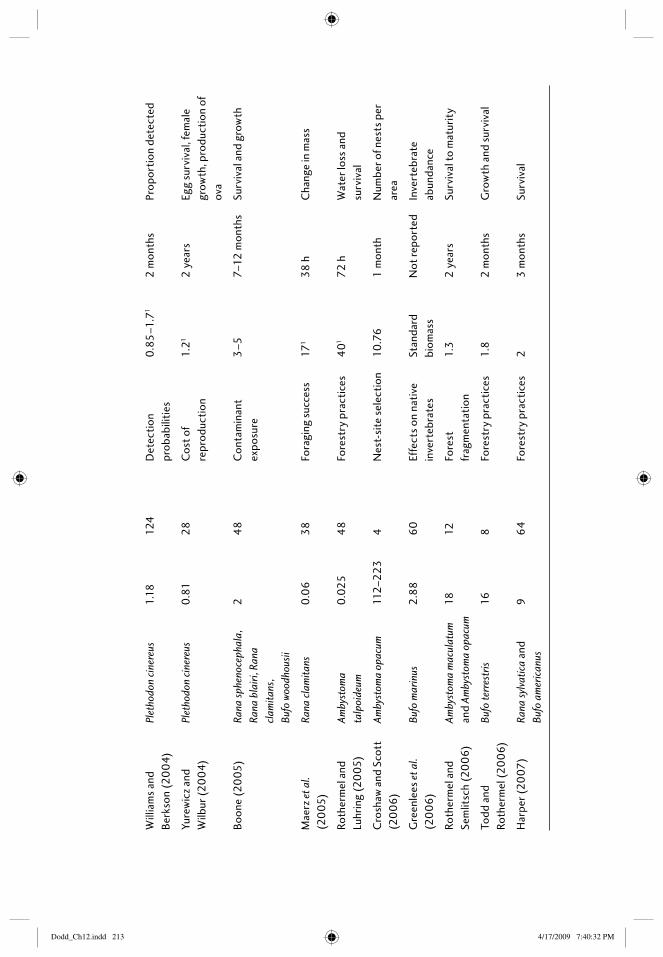
Will
iam
s an
d Be
rkso
n (2
00
4)Pl
etho
don
cine
reus
1.18
124
Det
ecti
on
prob
abili
ties
0.8
5–1
.71
2 m
onth
sPr
opor
tion
det
ecte
d
Yure
wic
z an
d W
ilbur
(20
04)
Plet
hodo
n ci
nere
us0
.81
28C
ost o
f re
prod
ucti
on1.
212
yea
rsEg
g su
rviv
al, f
emal
e gr
owth
, pro
duct
ion
of
ova
Boon
e (2
005
)Ra
na sp
heno
ceph
ala,
Ra
na b
lairi
, Ran
a cl
amita
ns,
Bufo
woo
dhou
sii
24
8C
onta
min
ant
expo
sure
3–5
7–12
mon
ths
Surv
ival
and
gro
wth
Mae
rz e
t al.
(20
05)
Rana
cla
mita
ns0
.06
38Fo
ragi
ng s
ucce
ss17
138
hC
hang
e in
mas
s
Roth
erm
el a
nd
Luhr
ing
(20
05)
Amby
stom
a ta
lpoi
deum
0.0
254
8Fo
rest
ry p
ract
ices
401
72
hW
ater
loss
and
su
rviv
al
Cro
shaw
and
Sco
tt
(20
06
)Am
byst
oma
opac
um11
2–2
23
4N
est-
site
sel
ecti
on10
.76
1 m
onth
Num
ber o
f nes
ts p
er
area
Gre
enle
es e
t al.
(20
06
)Bu
fo m
arin
us2
.88
60
Effe
cts
on n
ativ
e in
vert
ebra
tes
Stan
dard
bi
omas
sN
ot re
port
edIn
vert
ebra
te
abun
danc
e
Roth
erm
el a
nd
Sem
litsc
h (2
00
6)
Amby
stom
a m
acul
atum
an
d Am
byst
oma
opac
um18
12Fo
rest
fr
agm
enta
tion
1.3
2 y
ears
Surv
ival
to m
atur
ity
Todd
and
Ro
ther
mel
(20
06
)Bu
fo te
rres
tris
168
Fore
stry
pra
ctic
es1.
82
mon
ths
Gro
wth
and
sur
viva
l
Har
per (
2007
)Ra
na sy
lvatic
a an
d Bu
fo a
mer
ican
us9
64
Fore
stry
pra
ctic
es2
3 m
onth
sSu
rviv
al
Dodd_Ch12.indd 213Dodd_Ch12.indd 213 4/17/2009 7:40:32 PM4/17/2009 7:40:32 PM
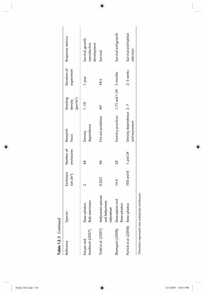
Har
per a
nd
Sem
litsc
h (2
007
)Ra
na sy
lvatic
a,
Bufo
am
eric
anus
24
8D
ensi
ty
depe
nden
ce1–
101
yea
rSu
rviv
al, g
row
th,
repr
oduc
tive
de
velo
pmen
t
Todd
et a
l. (2
007
)Am
byst
oma
opac
um
and
Amby
stom
a ta
lpoi
deum
0.0
2596
Fire
ant
pre
dati
on4
014
8 h
Surv
ival
Blom
quis
t (20
08)
Rana
pip
iens
and
Ra
na sy
lvatic
a14
.428
Fore
stry
pra
ctic
es1.
73
and
1.3
93
mon
ths
Surv
ival
and
gro
wth
Part
ick
et a
l. (2
00
8)Ra
na sy
lvatic
a10
0 a
nd 8
1 a
nd 2
4D
ensi
ty d
epen
denc
e an
d m
ovem
ent
2–7
2–3
wee
ksSu
rviv
al a
nd h
abit
at
sele
ctio
n
1 D
ensi
ties
rep
rese
nt o
ne a
nim
al p
er e
nclo
sure
.
Tab
le 1
2.1
Con
tinue
d
Refe
renc
eSp
ecie
sEn
clos
ure
size
(m
2)
Num
ber o
f en
clos
ures
Rese
arch
fo
cus
Stoc
king
de
nsit
y (p
er/m
2)
Dur
atio
n of
ex
perim
ent
Resp
onse
met
rics
Dodd_Ch12.indd 214Dodd_Ch12.indd 214 4/17/2009 7:40:32 PM4/17/2009 7:40:32 PM
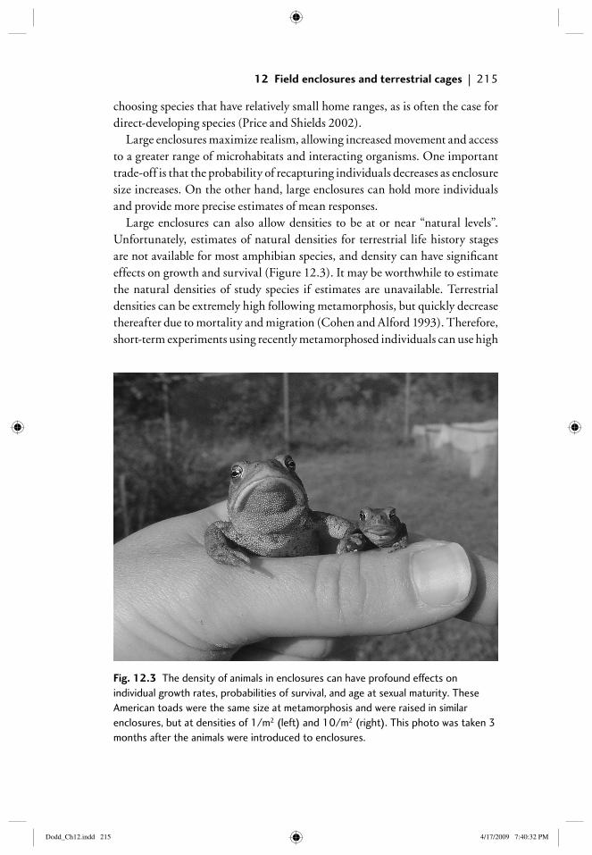
12 Field enclosures and terrestrial cages | 215
choosing species that have relatively small home ranges, as is often the case for direct-developing species (Price and Shields 2002).
Large enclosures maximize realism, allowing increased movement and access to a greater range of microhabitats and interacting organisms. One important trade-off is that the probability of recapturing individuals decreases as enclosure size increases. On the other hand, large enclosures can hold more individuals and provide more precise estimates of mean responses.
Large enclosures can also allow densities to be at or near “natural levels”. Unfortunately, estimates of natural densities for terrestrial life history stages are not available for most amphibian species, and density can have signifi cant effects on growth and survival (Figure 12.3). It may be worthwhile to estimate the natural densities of study species if estimates are unavailable. Terrestrial densities can be extremely high following metamorphosis, but quickly decrease thereafter due to mortality and migration (Cohen and Alford 1993). Therefore, short-term experiments using recently metamorphosed individuals can use high
Fig. 12.3 The density of animals in enclosures can have profound effects on individual growth rates, probabilities of survival, and age at sexual maturity. These American toads were the same size at metamorphosis and were raised in similar enclosures, but at densities of 1/m2 (left) and 10/m2 (right). This photo was taken 3 months after the animals were introduced to enclosures.
Dodd_Ch12.indd 215Dodd_Ch12.indd 215 4/17/2009 7:40:32 PM4/17/2009 7:40:32 PM
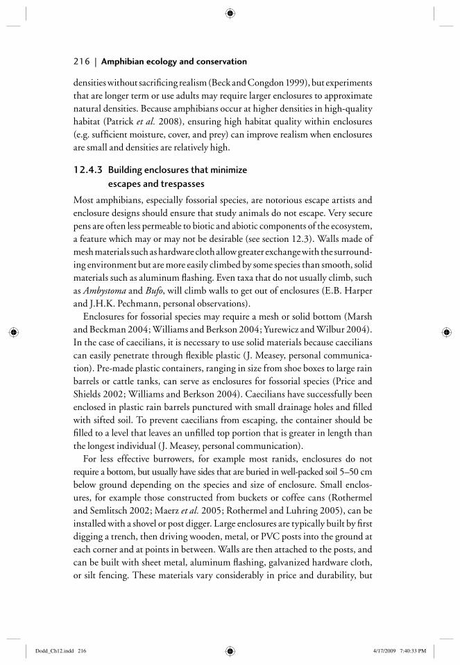
216 | Amphibian ecology and conservation
densities without sacrifi cing realism (Beck and Congdon 1999), but experiments that are longer term or use adults may require larger enclosures to approximate natural densities. Because amphibians occur at higher densities in high-quality habitat (Patrick et al. 2008), ensuring high habitat quality within enclosures (e.g. suffi cient moisture, cover, and prey) can improve realism when enclosures are small and densities are relatively high.
12.4.3 Building enclosures that minimize escapes and trespasses
Most amphibians, especially fossorial species, are notorious escape artists and enclosure designs should ensure that study animals do not escape. Very secure pens are often less permeable to biotic and abiotic components of the ecosystem, a feature which may or may not be desirable (see section 12.3). Walls made of mesh materials such as hardware cloth allow greater exchange with the surround-ing environment but are more easily climbed by some species than smooth, solid materials such as aluminum fl ashing. Even taxa that do not usually climb, such as Ambystoma and Bufo, will climb walls to get out of enclosures (E.B. Harper and J.H.K. Pechmann, personal observations).
Enclosures for fossorial species may require a mesh or solid bottom (Marsh and Beckman 2004; Williams and Berkson 2004; Yurewicz and Wilbur 2004). In the case of caecilians, it is necessary to use solid materials because caecilians can easily penetrate through fl exible plastic (J. Measey, personal communica-tion). Pre-made plastic containers, ranging in size from shoe boxes to large rain barrels or cattle tanks, can serve as enclosures for fossorial species (Price and Shields 2002; Williams and Berkson 2004). Caecilians have successfully been enclosed in plastic rain barrels punctured with small drainage holes and fi lled with sifted soil. To prevent caecilians from escaping, the container should be fi lled to a level that leaves an unfi lled top portion that is greater in length than the longest individual (J. Measey, personal communication).
For less effective burrowers, for example most ranids, enclosures do not require a bottom, but usually have sides that are buried in well-packed soil 5–50 cm below ground depending on the species and size of enclosure. Small enclos-ures, for example those constructed from buckets or coffee cans (Rothermel and Semlitsch 2002; Maerz et al. 2005; Rothermel and Luhring 2005), can be installed with a shovel or post digger. Large enclosures are typically built by fi rst digging a trench, then driving wooden, metal, or PVC posts into the ground at each corner and at points in between. Walls are then attached to the posts, and can be built with sheet metal, aluminum fl ashing, galvanized hardware cloth, or silt fencing. These materials vary considerably in price and durability, but
Dodd_Ch12.indd 216Dodd_Ch12.indd 216 4/17/2009 7:40:33 PM4/17/2009 7:40:33 PM
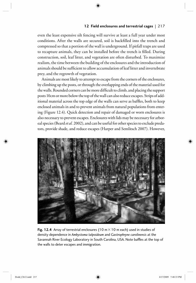
12 Field enclosures and terrestrial cages | 217
even the least expensive silt fencing will survive at least a full year under most conditions. After the walls are secured, soil is backfi lled into the trench and compressed so that a portion of the wall is underground. If pitfall traps are used to recapture animals, they can be installed before the trench is fi lled. During construction, soil, leaf litter, and vegetation are often disturbed. To maximize realism, the time between the building of the enclosures and the introduction of animals should be suffi cient to allow accumulation of leaf litter and invertebrate prey, and the regrowth of vegetation.
Animals are most likely to attempt to escape from the corners of the enclosures, by climbing up the posts, or through the overlapping ends of the material used for the walls. Rounded corners can be more diffi cult to climb, and placing the support posts 10cm or more below the top of the wall can also reduce escapes. Strips of add-itional material across the top edge of the walls can serve as baffl es, both to keep enclosed animals in and to prevent animals from natural populations from enter-ing (Figure 12.4). Quick detection and repair of damaged or worn enclosures is also necessary to prevent escapes. Enclosures with lids may be necessary for arbor-eal species (Beard et al. 2002), and can be useful for other species to exclude preda-tors, provide shade, and reduce escapes (Harper and Semlitsch 2007). However,
Fig. 12.4 Array of terrestrial enclosures (10 m � 10 m each) used in studies of density dependence in Ambystoma talpoideum and Gastrophryne carolinensis at the Savannah River Ecology Laboratory in South Carolina, USA. Note baffl es at the top of the walls to deter escapes and immigration.
Dodd_Ch12.indd 217Dodd_Ch12.indd 217 4/17/2009 7:40:33 PM4/17/2009 7:40:33 PM
218 | Amphibian ecology and conservation
lids typically infl uence light, temperature, rainfall, litterfall, and movement of prey, which can hinder realism and may confound the treatment.
12.4.4 “Standardizing” conditions among enclosures
One advantage of terrestrial enclosures is that they can expose animals to the range of conditions found within a study area, such as the densities of prey, competitors, and predators, as well as variation in leaf-litter depth, vegetation, and solar radiation. Unfortunately, this variability decreases statistical power by contributing to experimental error. One option to reduce this “noise” is to standardize conditions within enclosures. For example, quantities of leaf litter and woody debris can be equalized (Harper 2007). Devices that provide wet refuges, such as a pit with moist leaf litter, a bowl of water, or a covering object, can reduce the risk of desiccation (Greenlees et al. 2006), and reduce variation in survival within treatments, especially if amphibians must be released into enclos ures during dry periods when they would not normally be active. Predators including snakes may have to be removed, especially from small pens, because of the diffi culty of equalizing predation across enclosures without excessive mor-tality. Competition can also be standardized by removing competitors or by introducing an equal number to all enclosures. Standardization comes at the cost of reduced realism, and it is important to consider how this may comprom-ise the interpretation of the results. This is especially important when biotic and abiotic factors comprise the treatments.
12.5 Study species
The choice of study species is an important consideration when designing enclosure experiments. It must be possible to confi ne the species under realis-tic conditions and densities and to have access to enough animals to design an experiment with high statistical power.
12.5.1 Choice of species
Terrestrial enclosures are most appropriate for species that are primarily terrestrial after metamorphosis. For species that are both aquatic and terrestrial (e.g. Rana clamitans and Desmognathus monticola), short-term terrestrial enclosure experi-ments that coincide with normal habitat use can be informative (Maerz et al. 2005). Enclosures that encompass both aquatic and terrestrial habitats can also be used (Southerland 1986). For arboreal species, enclosures must be completely covered to prevent escape, which decreases realism. Effective jumpers, such as Acris, are diffi cult to keep in enclosures without very high walls or covers.
Dodd_Ch12.indd 218Dodd_Ch12.indd 218 4/17/2009 7:40:35 PM4/17/2009 7:40:35 PM
12 Field enclosures and terrestrial cages | 219
12.5.2 Source and age of animals
Animals can be wild-caught or raised from eggs in captivity (e.g. in artifi cial ponds). Both methods have advantages and disadvantages in terms of logis-tics, experimental design, and conservation. Using wild-caught animals is often necessary for studies of adult amphibians when raising individuals to adulthood is unfeasible due to constraints of time, space, and/or expense. Research on the ecology of adult amphibians is important because amphibian populations are especially sensitive to changes in adult vital rates (Biek et al. 2002); for this same reason, however, the effects on wild populations should be carefully con-sidered before adults are removed. Raising individuals through metamorphosis in outdoor tanks or experimental ponds is often the best method for studies of juvenile pond-breeders for several reasons. First, large numbers of individuals can be produced with minimal effects on wild populations. Survival to meta-morphosis in predator-free aquatic enclosures and tanks often exceeds 50–80% compared with fewer than 5–10% in many wild populations (Petranka and Sih 1986). Secondly, the conditions experienced by larvae can be controlled, thereby maximizing precision. Experimental ponds can also be used in con-junction with terrestrial enclosures to study carryover effects by manipulating conditions during the larval period and observing their effects on terrestrial life-history stages (Pechmann 1994; Altwegg and Reyer 2003; Boone 2005). When collecting eggs for future experimental populations, one should consider the genetic make-up in the context of the experiment. In some instances it may be prudent to select eggs from multiple populations or from multiple clutches within a population so the results are more representative of the species or popu-lation of interest.
12.6 Census techniques
For most enclosure studies, gathering data requires recapturing amphibians during and/or at the end of the study. Gathering data at regular intervals rather than waiting until the end of the experiment is often a wise strategy because mortality can be higher than expected. Multiple census intervals are also useful in estimating capture probabilities, which are often necessary to calculate esti-mates of survival (Chapter 24).
12.6.1 Individual marks
Individually marking animals before they are released into enclosures allows monitoring of individual growth rates, estimation of capture probabilities, and analysis of factors such as initial mass or time to metamorphosis (Beck
Dodd_Ch12.indd 219Dodd_Ch12.indd 219 4/17/2009 7:40:35 PM4/17/2009 7:40:35 PM
220 | Amphibian ecology and conservation
and Congdon 1999). There are many techniques that can be used to identify individuals, including toe-clipping, visible implant elastomer, passive integra-tive transponder tags (PIT tags), and photographing unique dorsal patterns (Chapter 8). Group marks may be necessary when it is impractical to mark all individuals. In general, the marking technique chosen should strive to minimize the increased probability of mortality and stress to the animals while maximiz-ing the probability of successful identifi cation.
12.6.2 Methods of capture
The most common methods of recapturing amphibians in enclosures are hand capture, pitfall traps, and coverboards (Chapter 13). A combination of methods can be used to maximize capture probability. Hand captures work well for ani-mals that are active on the surface or that jump when the leaf litter is disturbed. However, this method can result in biased data if animals are easier to see and catch in some treatments than others. Pitfall traps (Chapter 13) may provide a more standardized method for recapturing amphibians and are especially useful for fossorial species like ambystomatid salamanders that are not easily captured by hand (Pechmann 1995). Traps can be covered or fi lled with leaf litter when not in use and opened on rainy nights when the animals are most likely to be active. A wet sponge in the bottom of the traps can reduce desiccation risks, although only sponges that are free of chemicals should be used. Cover objects such as rotting logs or boards can also be placed in enclosures as a method for recapturing animals (Chapter 13) as long as their addition does not con-found the effects of the treatment. Similarly, burrows can be created within enclosures to provide retreats where animals can predictably be found (Regosin et al. 2004). For caecilians and other truly fossorial amphibians that are rarely active on the surface, it may be necessary to do a single census at the end of the experiment by removing and thoroughly sifting through the soil and leaf lit-ter. Radiotransmitters or harmonic radar tags (Moseley et al. 2004) can make study animals easier to relocate, but the equipment may affect behavior and expense can be an issue. Animals marked with PIT tags can be detected up to 13 cm underground (Blomquist et al. 2008). Pond-breeding amphibians can be censused along the enclosure walls during breeding migrations by pitfall traps, funnel traps, or hand capture as they attempt to migrate out of the enclosure to fi nd a breeding pond (Pechmann 1995; Regosin et al. 2003b).
12.6.3 Frequency of censuses
Because enclosure experiments usually require an initially large input of time, labor, and resources, it is worthwhile in longer-term experiments to collect data
Dodd_Ch12.indd 220Dodd_Ch12.indd 220 4/17/2009 7:40:35 PM4/17/2009 7:40:35 PM
12 Field enclosures and terrestrial cages | 221
early and often to ensure that useful data are gathered even if natural disas-ters or unexpectedly high mortality occur before the end of the experiment. Frequent censuses also improve estimates of capture probability and survival (Chapter 25). However, it is important to consider that handling animals too frequently can affect survival and induce unnecessary stress. The optimal fre-quency of censuses for estimating capture probability and survival also depends on the statistical methods that will be used. Some methods require equal time between sampling intervals or a minimum number of sample periods. Other statistical methods rely on multiple consecutive samples spaced at regular inter-vals (e.g. 3 days of sampling every 2 weeks). These methods are discussed in greater detail in Chapter 25. It is important to become familiar with these stat-istical methods prior to gathering the data to ensure that the frequency and methods used in the censuses maximize statistical power.
12.7 Response metrics
Experiments conducted in enclosures can use a wide range of response vari-ables to describe the effects of experimental treatments on amphibians. Vital rates, including growth and survival, are among the most commonly used met-rics (Table 12.1), but more subtle effects can be quantifi ed with physiological measurements such as lipid content (Chazal and Niewiarowski 1998) or stress-hormone concentrations (Cooperman et al. 2004). Behavioral observations, including habitat selection, can also yield useful response metrics (Patrick et al. 2008). Data that quantify conditions within enclosures can provide covariates for analyses or can be used to provide metrics describing the role of amphibians in the ecosystem, for example in nutrient cycling (Beard et al. 2002) or reducing prey densities (Greenlees et al. 2006). In most enclosure experiments the enclos-ure is the experimental unit, so for any response metric that is based on the indi-vidual (e.g. mass), means per enclosure (or the equivalent) should be used in the analysis (Pechmann 1995). Proportions can also be used (e.g. percentage survival or the percentage that selected a given habitat type; Patrick et al. 2008).
12.7.1 Vital rates: survival, growth, age at reproductive maturity, fecundity
Survival can be surprisingly diffi cult to measure in all but very small enclos-ures. The minimum number known alive (MNKA) can be used as a proxy for survival (Rothermel and Semlitsch 2006), but does not allow the estimation of error, resulting from undetected individuals. Because capture probabilities are rarely 100%, capture–mark–recapture models can be useful for estimating
Dodd_Ch12.indd 221Dodd_Ch12.indd 221 4/17/2009 7:40:35 PM4/17/2009 7:40:35 PM
222 | Amphibian ecology and conservation
survival (Altwegg 2003; Chapter 24). However, when capture probabilities are low, there is a large amount of error associated with these estimates. Methods for incorporating errors from mark–recapture estimates into other statistical analyses of multiple experimental populations, such as analysis of variance, have received limited attention. Survival estimates can be improved by using an end-point associated with breeding migrations, such as fi rst reproduction, because migrations increase the likelihood of capture (Pechmann 1995; Regosin et al. 2003b).
Growth is usually measured as change in mass or length over time. Some researchers prefer measuring snout–vent length, often with additional measure-ments including head width or tibia length (Altwegg and Reyer 2003), because mass is prone to short-term fl uctuations.
Reproductive maturity can be determined by dissection, candling, or exter-nal signs of maturity such as nuptial pads or a swollen cloaca (Pechmann 1995; Rothermel and Semlitsch 2006; Harper and Semlitsch 2007). Age at repro-ductive maturity or the proportion of individuals that have reached maturity at the conclusion of the experiment are demographically important response met-rics. Although fecundity is a component of individual fi tness and population growth, clutch size has not typically been used as a response metric for enclosure experiments (but see Yurewicz and Wilbur 2004).
12.7.2 Physiological responses
Response metrics that quantify physiological responses are especially useful when the effects of experimental treatments are likely to be sublethal. Many of the methods used to quantify physiological responses require that animals be killed, so it is necessary to gather these data at the end of the experiment, or by removing a subset of animals at points during the experiment. Lipids stored in the body or in eggs can be measured and used as indicators of body condition and parental investment (Chazal and Niewiarowski 1998). Whole-body con-centrations of elements such as arsenic, selenium, and vanadium can indicate bioaccumulation of contaminants (Hopkins et al. 1998; Laposata and Dunson 1999). Heightened concentrations of corticosterone circulating in the blood indicate a stress response, and can be determined using non-lethal methods (Cooperman et al. 2004).
12.7.3 Behavioral responses
Measures of behavioral responses in enclosure experiments have typically focused on movement and habitat selection. Movement has been quantifi ed as activity rate (Pearson 1955; Rothermel and Semlitsch 2002; Marsh and Beckman 2004;
Dodd_Ch12.indd 222Dodd_Ch12.indd 222 4/17/2009 7:40:35 PM4/17/2009 7:40:35 PM
12 Field enclosures and terrestrial cages | 223
Moseley et al. 2004) and distance moved (Rothermel and Semlitsch 2002). Studies of habitat selection typically quantify the proportion of individuals that select a particular habitat type (Southerland 1986; Moseley et al. 2004; Patrick et al. 2008). Regosin et al. (2004) used probability of burrow occupancy as a response metric.
12.8 Thinking outside the box
Amphibian studies using terrestrial enclosures and cages have so far focused on a relatively narrow range of species and experimental designs. However, there is great scope for creativity in the use of these techniques. Some of the most exciting and least studied aspects of amphibian ecology can be studied using terrestrial enclosures. For example, a study by Beard et al. (2002) used cages as “exclosures” to document the effects of both the presence and absence of a terrestrial frog on nutrient cycling. Creative techniques for answering complex amphibian research questions have also involved using enclosures in conjunc-tion with other experimental techniques (Marsh and Beckman 2004; Todd and Rothermel 2006) or conducting multiple enclosure experiments at a range of spatial and temporal scales (Patrick et al. 2008).
Although most amphibian enclosure experiments have been conducted in temperate regions, there is enormous potential for the use of enclosures in trop-ical ecosystems. Many tropical amphibians may actually be far better suited for enclosure experiments than their temperate counterparts. Leaf-litter species such as the neotropical Eleutherodactylus, Arthroleptis of Africa, or many of the Asian microhylids, occur at remarkably high densities and are unlikely to have large home ranges. Well-designed enclosures can also be used to gain a better understanding of the ecology of caecilians, for which few data are currently available.
12.9 References
Altwegg, R. (2003). Multistage density dependence in an amphibian. Oecologia, 136, 46–50.
Altwegg, R. and Reyer, H.-U. (2003). Patterns of natural selection on size at metamor-phosis in water frogs. Evolution, 57, 872–82.
Beard, K. H., Vogt, K. A., and Kulmatiski, A. (2002). Top-down effects of a terrestrial frog on forest nutrient dynamics. Oecologia, 133, 583–93.
Beck, C. W. and Congdon, J. D. (1999). Effects of individual variation in age and size at metamorphosis on growth and survivorship of southern toad (Bufo terrestris) meta-morphs. Canadian Journal of Zoology, 77, 944–51.
Dodd_Ch12.indd 223Dodd_Ch12.indd 223 4/17/2009 7:40:35 PM4/17/2009 7:40:35 PM
224 | Amphibian ecology and conservation
Beebee, T. J. C. (1996). Ecology and Conservation of Amphibians. Chapman & Hall, London.
Biek, R., Funk, W. C., Maxell, B. A., and Mills, L. S. (2002). What is missing in amphib-ian decline research: insights from ecological sensitivity analysis. Conservation Biology, 16, 728–34.
Blomquist, S. M. (2008). Relative Fitness and Behavioral Compensation of Amphibians in a Managed Forest. PhD dissertation, University of Maine, Orono, ME.
Blomquist, S. M., Zydlewski, J. D., and Hunter, M. L. (2008). Effi cacy of PIT tags for tracking the terrestrial anurans Rana pipiens and Rana sylvatica. Herpetological Review, 39, 174–9.
Boone, M. D. (2005). Juvenile frogs compensate for small metamorph size with terrestrial growth: overcoming the effects of larval density and insecticide exposure. Journal of Herpetology, 39, 416–23.
Boone, M. D. and James, S. M. (2005). Aquatic and terrestrial mesocosms in amphibian ecotoxicology. Applied Herpetology, 2, 231–57.
Chalcraft, D. R., Binckley, C. A., and Resetarits Jr, W. J. (2005). Experimental venue and estimation of interaction strength: comment. Ecology, 86, 1061–7.
Chazal, A. C. and Niewiarowski, P. H. (1998). Responses of mole salamanders to clear-cutting: using fi eld experiments in forest management. Ecological Applications, 8, 1133–43.
Cohen, M. P. and Alford, R. A. (1993). Growth, survival and activity patterns of recently metamorphosed Bufo marinus. Wildlife Research, 20, 1–13.
Cooperman, M. D., Reed, J. M., and Romero, L. M. (2004). The effects of terrestrial and breeding densities on corticosterone and testosterone levels in spotted salamanders, Ambystoma maculatum. Canadian Journal of Zoology, 82, 1795–1803.
Croshaw, D. A. and Scott, D. E. (2006). Marbled salamanders (Ambystoma opacum) choose low elevation nest sites when cover availability is controlled. Amphibia-Reptilia, 27, 359–64.
Denton, J. S. and Beebee, T. J.C. (1994). The basis of niche separation during terrestrial life between two species of toad (Bufo bufo and Bufo calamita): competition or special-isation? Oecologia, 97, 390–8.
Greenlees, M. J., Brown, G. P., Webb, J. K., Phillips, B. L., and Shine, R. (2006). Effects of an invasive anuran [the cane toad (Bufo marinus)] on the invertebrate fauna of a trop-ical Australian fl oodplain. Animal Conservation, 9, 431–8.
Hairston Sr, N. G. (1989). Ecological Experiments: Purpose, Design, and Execution. Cambridge University Press, Cambridge.
Harper, E. B.H. (2007). The Population Dynamics and Conservation of Pond-breeding Amphibians. PhD dissertation, University of Missouri, Columbia, MO.
Harper, E. B. and Semlitsch, R. D., (2007). Density dependence in the terrestrial life his-tory stage of two anurans. Oecologia, 153, 879–89.
Hopkins, W. A., Mendonca, M. T., Rowe, C. L., and Congdon, J. D., (1998). Elevated trace element concentrations in southern toads, Bufo terrestris, exposed to coal combus-tion waste. Archives of Environmental Contamination and Toxicology, 35, 325–9.
Hurlbert, S. H. (1984). Pseudoreplication and the design of ecological fi eld experiments. Ecological Monographs, 54, 187–211.
Dodd_Ch12.indd 224Dodd_Ch12.indd 224 4/17/2009 7:40:35 PM4/17/2009 7:40:35 PM
12 Field enclosures and terrestrial cages | 225
Jaeger, R.G. (1971). Competitive exclusion as a factor infl uencing the distributions of two species of terrestrial salamanders. Ecology, 52, 632–7.
Laposata, M. M. and Dunson, W. A. (1999). Enclosure design for ecotoxicological stud-ies of terrestrial salamanders. Herpetological Review, 30, 28–30.
Maerz, J. C., Blossey, B., and Nuzzo, V. (2005). Green frogs show reduced foraging success in habitats invaded by Japanese knotweed. Biodiversity and Conservation, 14, 2901–11.
Marsh, D. M. and Beckman, N. G. (2004). Effects of forest roads on the abundance and activity of terrestrial salamanders. Ecological Applications, 14, 1882–91.
Morin, P. J. (1998). Realism, precision, and generality in experimental tests of ecological theory. In W. J. Resetarits and J. Bernardo (eds), Issues and Perspectives in Experimental Ecology, pp. 50–70. Oxford University Press, Oxford.
Moseley, K. R., Castleberry, S. B., and Ford, W. M. (2004). Coarse woody debris and pine litter manipulation effects on movement and microhabitat use of Ambystoma talpoi-deum in a Pinus taeda stand. Forest Ecology and Management, 191, 387–96.
Parris, M. J. (2001). Hybridization in leopard frogs (Rana pipiens complex): terrestrial performance of newly metamorphosed hybrid and parental genotypes in fi eld enclos-ures. Canadian Journal of Zoology, 79, 1552–8.
Patrick, D. A., Harper, E. B., Hunter Jr, M. L., and Calhoun, A. J. K. (2008). Terrestrial habitat selection and strong density-dependent mortality in recently metamorphosed amphibians. Ecology, 89, 2563–74.
Pearson, P. G. (1955). Population ecology of the spadefoot toad, Scaphiopus h. holbrooki (Harlan). Ecological Monographs, 25, 233–67.
Pechmann, J. H. K. (1994). Population Regulation in Complex Life Cycles: Aquatic and Terrestrial Density-dependence in Pond-breeding Amphibians. PhD dissertation, Duke University, Durham, NC.
Pechmann, J. H. K. (1995). Use of large fi eld enclosures to study the terrestrial ecology of pond-breeding amphibians. Herpetologica, 51, 434–50.
Petranka, J. W. and Sih, A. (1986). Environmental instability, competition and density-dependent growth and survivorship of a stream-dwelling salamander. Ecology, 67, 729–36.
Price, J. E. and Shields, J. A.S. (2002). Size-dependent interactions between two terrestrial amphibians, Plethodon cinereus and Plethodon glutinosus. Herpetologica, 58, 141–55.
Regosin, J. V., Windmiller, B. S., and Reed, J. M. (2003a). Terrestrial habitat use and win-ter densities of the Wood Frog (Rana sylvatica). Journal of Herpetology, 37, 390–4.
Regosin, J. V., Windmiller, B. S., and Reed, J. M. (2003b). Infl uence of abundance of small-mammal burrows and conspecifi cs on the density and distribution of spot-ted sala manders (Ambystoma maculatum) in terrestrial habitats. Canadian Journal of Zoology, 81, 596–605.
Regosin, J. V., Windmiller, B. S., and Reed, J. M. (2004). Effects of conspecifi cs on the burrow occupancy behaviour of spotted salamanders. Copeia, 2004, 152–8.
Regosin, J. V., Windmiller, B. S., Homan, R. N., and Reed, J. M. (2005). Variation in terrestrial habitat use by four poolbreeding amphibian species. Journal of Wildlife Management, 69, 1481–93.
Dodd_Ch12.indd 225Dodd_Ch12.indd 225 4/17/2009 7:40:35 PM4/17/2009 7:40:35 PM
226 | Amphibian ecology and conservation
Rothermel, B. B. and Semlitsch, R. D. (2002). An experimental investigation of land-scape resistance of forest versus old-fi eld habitats to emigrating juvenile amphibians. Conservation Biology, 16, 1324–32.
Rothermel, B. B. and Luhring, T. M. (2005). Burrow availability and desiccation risk of mole salamanders (Ambystoma talpoideum) in harvested versus unharvested forest stands. Journal of Herpetology, 39, 619–26.
Rothermel, B. B. and Semlitsch, R. D. (2006). Consequences of forest fragmentation for juvenile survival in spotted (Ambystoma maculatum) and marbled (Ambystoma opacum) salamanders. Canadian Journal of Zoology, 84, 797–807.
Southerland, M. T. (1986). Coexistence of three congeneric salamanders: the importance of habitat and body size. Ecology, 67, 721–8.
Todd, B. and Rothermel, B. B. (2006). Assessing quality of clearcut habitats for amphib-ians: effects on abundances versus vital rates in the southern toad (Bufo terrestris). Biological Conservation, 133, 178–85.
Todd, B. D., Rothermel, B. B., Reed, R. N., Luhring, T. M., Schlatter, K., Trenkamp, L., and Gibbons, J. W. (2007). Habitat alteration increases invasive fi re and abundance to the detriment of amphibians and reptiles. Biological Invasions, 10, 539–46.
Williams, A. K. and Berkson, J. (2004). Reducing false absences in survey data: detection probabilities of red-backed salamanders. Journal of Wildlife Management, 68, 418–28.
Yurewicz, K. L. and Wilbur, H. M. (2004). Resource availability and costs of reproduc-tion in the salamander Plethodon cinereus. Copeia, 2004, 28–36.
Dodd_Ch12.indd 226Dodd_Ch12.indd 226 4/17/2009 7:40:36 PM4/17/2009 7:40:36 PM
13Drift fences, coverboards, and other traps
John D. Willson and J. Whitfi eld Gibbons
13.1 Introduction
Many of the simplest yet most highly productive sampling methods in her-petological fi eld research use some type of trap or attraction device to increase capture rates or target secretive species. These techniques fall into two general categories: those that actually trap animals, accumulating captures on their own over time (passive traps) and those that attract animals but require an observer to actively capture them at the moment of the census (active traps). The most popular examples of these two trap categories are drift fences (generally with pitfall and/or funnel traps) and coverboards, respectively. Both of these methods are inherently simple concepts, and their description and explanation need not be made complex or complicated. Both techniques are usually best modifi ed by the investigator who can use common sense to focus on the needs of a particular project that involves capturing animals in a fi eld situation. However, we provide a general discussion of some of the fundamental issues that investigators who use these techniques must face, with particular emphasis on how choice of cap-ture method and sampling design infl uence interpretation of capture data.
13.2 Drift fences, funnel traps, and other passive capture methods
13.2.1 What are passive traps?
Passive capture methods are designed to restrain animals that enter the trap of their own accord, accumulating captures that are then assessed upon regular cen-suses by the observer. Passive traps are among the more intensive methods for sam-pling amphibians in terms of time and effort, but often yield higher capture rates and more standardized samples than opportunistic or visual searches. Perhaps
13_Dodd_Chap13.indd 22913_Dodd_Chap13.indd 229 8/19/2009 2:48:58 PM8/19/2009 2:48:58 PM
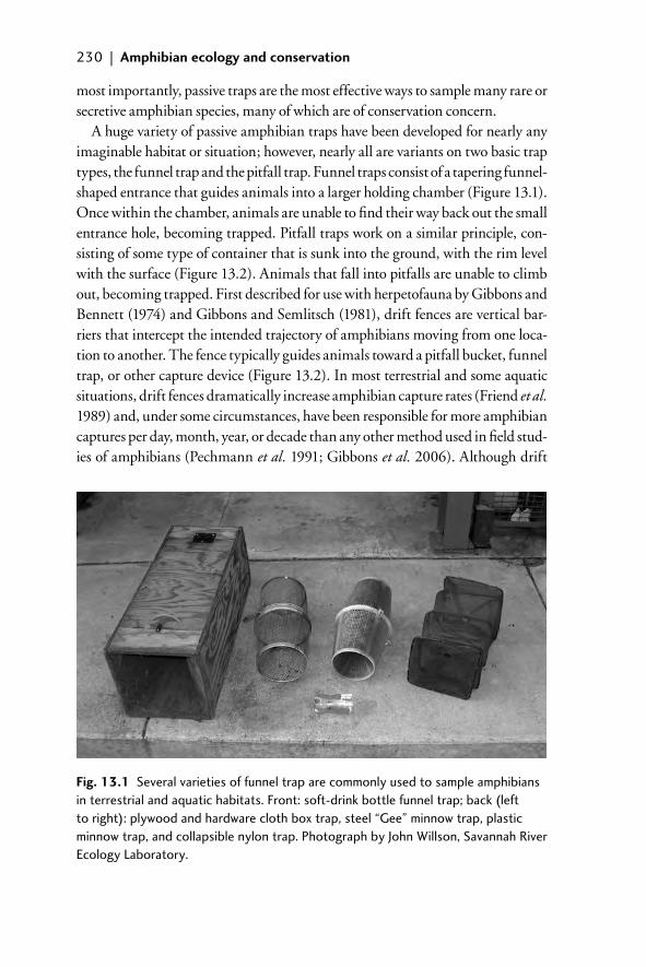
230 | Amphibian ecology and conservation
most importantly, passive traps are the most effective ways to sample many rare or secretive amphibian species, many of which are of conservation concern.
A huge variety of passive amphibian traps have been developed for nearly any imaginable habitat or situation; however, nearly all are variants on two basic trap types, the funnel trap and the pitfall trap. Funnel traps consist of a tapering funnel-shaped entrance that guides animals into a larger holding chamber (Figure 13.1). Once within the chamber, animals are unable to fi nd their way back out the small entrance hole, becoming trapped. Pitfall traps work on a similar principle, con-sisting of some type of container that is sunk into the ground, with the rim level with the surface (Figure 13.2). Animals that fall into pitfalls are unable to climb out, becoming trapped. First described for use with herpetofauna by Gibbons and Bennett (1974) and Gibbons and Semlitsch (1981), drift fences are vertical bar-riers that intercept the intended trajectory of amphibians moving from one loca-tion to another. The fence typically guides animals toward a pitfall bucket, funnel trap, or other capture device (Figure 13.2). In most terrestrial and some aquatic situations, drift fences dramatically increase amphibian capture rates (Friend et al. 1989) and, under some circumstances, have been responsible for more amphibian captures per day, month, year, or decade than any other method used in fi eld stud-ies of amphibians (Pechmann et al. 1991; Gibbons et al. 2006). Although drift
Fig. 13.1 Several varieties of funnel trap are commonly used to sample amphibians in terrestrial and aquatic habitats. Front: soft-drink bottle funnel trap; back (left to right): plywood and hardware cloth box trap, steel “Gee” minnow trap, plastic minnow trap, and collapsible nylon trap. Photograph by John Willson, Savannah River Ecology Laboratory.
13_Dodd_Chap13.indd 23013_Dodd_Chap13.indd 230 8/19/2009 2:48:59 PM8/19/2009 2:48:59 PM
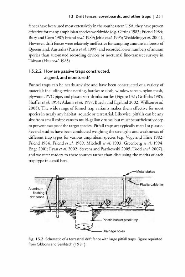
13 Drift fences, coverboards, and other traps | 231
fences have been used most extensively in the southeastern USA, they have proven effective for many amphibian species worldwide (e.g. Gittins 1983; Friend 1984; Bury and Corn 1987; Friend et al. 1989; Jehle et al. 1995; Weddeling et al. 2004). However, drift fences were relatively ineffective for sampling anurans in forests of Queensland, Australia (Parris et al. 1999) and recorded lower numbers of anuran species than automated recording devices or nocturnal line-transect surveys in Taiwan (Hsu et al. 1985).
13.2.2 How are passive traps constructed, aligned, and monitored?
Funnel traps can be nearly any size and have been constructed of a variety of materials including twine netting, hardware cloth, window screen, nylon mesh, plywood, PVC pipe, and plastic soft-drinks bottles (Figure 13.1; Griffi ths 1985; Shaffer et al. 1994; Adams et al. 1997; Buech and Egeland 2002; Willson et al. 2005). The wide range of funnel trap variants makes them effective for most species in nearly any habitat, aquatic or terrestrial. Likewise, pitfalls can be any size from small coffee cans to multi-gallon drums, but must be suffi ciently deep to prevent escape of the target species. Pitfall traps are typically metal or plastic. Several studies have been conducted weighing the strengths and weaknesses of different trap types for various amphibian species (e.g. Vogt and Hine 1982; Friend 1984; Friend et al. 1989; Mitchell et al. 1993; Greenberg et al. 1994; Enge 2001; Ryan et al. 2002; Stevens and Paszkowski 2005; Todd et al. 2007), and we refer readers to these sources rather than discussing the merits of each trap type in detail here.
Fig. 13.2 Schematic of a terrestrial drift fence with large pitfall traps. Figure reprinted from Gibbons and Semlitsch (1981).
Aluminum-flashing
drift fence
Plastic bucket pitfall trap
Drainage holes
Plastic cable ties
Metal stakes
13_Dodd_Chap13.indd 23113_Dodd_Chap13.indd 231 8/19/2009 2:49:05 PM8/19/2009 2:49:05 PM
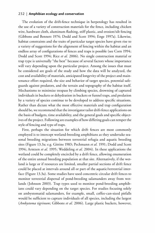
232 | Amphibian ecology and conservation
The evolution of the drift-fence technique in herpetology has resulted in the use of a variety of construction materials for the fence, including chicken wire, hardware cloth, aluminum fl ashing, stiff plastic, and erosion/silt fencing (Gibbons and Bennett 1974; Dodd and Scott 1994; Enge 1997a). Likewise, habitat constraints and the traits of particular target species have given rise to a variety of suggestions for the alignment of fencing within the habitat and an endless array of confi gurations of fences and traps is possible (see Corn 1994; Dodd and Scott 1994; Rice et al. 2006). No single construction material or trap type is universally “the best” because of several factors whose importance will vary depending upon the particular project. Among the issues that must be considered are goals of the study and how the data will be analyzed, the cost and availability of materials, anticipated longevity of the project and main-tenance effort required, the size and behavior of target species, potential safe-guards against predators, and the terrain and topography of the habitat itself. Mechanisms to minimize trespass by climbing species, drowning of captured individuals in buckets or dehydration in buckets or funnel traps, and predation by a variety of species continue to be developed to address specifi c situations. Rather than dictate what the most effective materials and trap confi guration should be, we recommend that the investigator tailor drift-fence applications on the basis of budgets, time availability, and the general goals and specifi c object-ives of the project. Following are examples of how differing goals can temper the style of fencing and type of traps.
First, perhaps the situation for which drift fences are most commonly employed is to intercept wetland-breeding amphibians as they undertake sea-sonal breeding migrations between terrestrial refugia and aquatic breeding sites (Figure 13.3a; e.g. Gittins 1983; Pechmann et al. 1991; Dodd and Scott 1994; Arntzen et al. 1995; Weddeling et al. 2004). In these applications the wetland could be completely encircled by a drift fence, allowing enumeration of the entire annual breeding population at that site. Alternatively, if the wet-land is large or if resources are limited, smaller partial sections of drift fence could be placed at intervals around all or part of the aquatic/terrestrial inter-face (Figure 13.3a). Some studies have used concentric circular drift fences to monitor terrestrial dispersal of pond-breeding salamanders away from wet-lands (Johnson 2003). Trap types used to monitor pond-breeding amphib-ians could vary depending on the target species. For studies focusing solely on ambystomatid salamanders, for example, small, coffee-can-sized pitfalls would be suffi cient to capture individuals of all species, including the largest (Ambystoma tigrinum; Gibbons et al. 2006). Large plastic buckets, however,
13_Dodd_Chap13.indd 23213_Dodd_Chap13.indd 232 8/19/2009 2:49:06 PM8/19/2009 2:49:06 PM
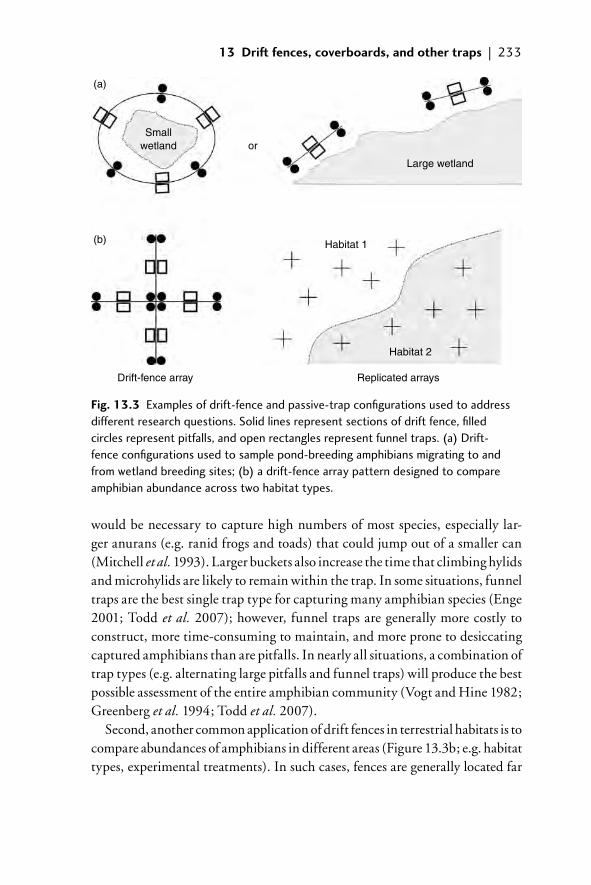
13 Drift fences, coverboards, and other traps | 233
would be necessary to capture high numbers of most species, especially lar-ger anurans (e.g. ranid frogs and toads) that could jump out of a smaller can (Mitchell et al. 1993). Larger buckets also increase the time that climbing hylids and microhylids are likely to remain within the trap. In some situations, funnel traps are the best single trap type for capturing many amphibian species (Enge 2001; Todd et al. 2007); however, funnel traps are generally more costly to construct, more time-consuming to maintain, and more prone to desiccating captured amphibians than are pitfalls. In nearly all situations, a combination of trap types (e.g. alternating large pitfalls and funnel traps) will produce the best possible assessment of the entire amphibian community (Vogt and Hine 1982; Greenberg et al. 1994; Todd et al. 2007).
Second, another common application of drift fences in terrestrial habitats is to compare abundances of amphibians in different areas (Figure 13.3b; e.g. habitat types, experimental treatments). In such cases, fences are generally located far
(a)
(b)
Drift-fence array Replicated arrays
Habitat 2
Habitat 1
Large wetland
Smallwetland or
Fig. 13.3 Examples of drift-fence and passive-trap confi gurations used to address different research questions. Solid lines represent sections of drift fence, fi lled circles represent pitfalls, and open rectangles represent funnel traps. (a) Drift-fence confi gurations used to sample pond-breeding amphibians migrating to and from wetland breeding sites; (b) a drift-fence array pattern designed to compare amphibian abundance across two habitat types.
13_Dodd_Chap13.indd 23313_Dodd_Chap13.indd 233 8/19/2009 2:49:06 PM8/19/2009 2:49:06 PM
234 | Amphibian ecology and conservation
from any obvious breeding wetland, hibernaculum, or other habitat focal point. For such applications, drift fences are often constructed in cross- or X-shaped arrays with a central trap and traps placed along each section of the fence (see Corn 1994). Because the goal of this type of study is generally to test hypoth-eses about amphibian abundance between areas, each array makes a convenient sampling unit for statistical comparisons. In this case, care should be taken to ensure that arrays are comparable (same length of fencing, number of traps, etc.) and that arrays are located randomly or systematically across the treatments or habitats.
Finally, passive traps can be used for quantitative sampling of aquatic amphibians that are not easily captured by other methods. For this applica-tion, a variety of aquatic funnel traps can be effective, with the size of the trap being dictated by the size of the target species. For small species or life stages, small funnel traps made from plastic soft-drinks bottles would suffi ce (e.g. Griffi ths 1985; Willson and Dorcas 2003), while targeting larger spe-cies such at the giant salamanders, Siren and Amphiuma, would require lar-ger traps such as commercially available minnow or crawfi sh traps (Johnson and Barichivich 2004; Willson et al. 2005). In most cases, aquatic traps should be set in water shallow enough to allow captured animals access to air and care should be taken to monitor fl uctuations in water level that could submerge traps. Specifi c microhabitats where traps are set will vary by spe-cies, but heavily vegetated shallow areas are often preferable. Capture rates may also be increased by setting aquatic traps along natural barriers such as submerged logs or the shoreline or by the use of aquatic drift fences to direct amphibians into traps (Enge 1997b; Willson and Dorcas 2004; Palis et al. 2007). Finally, as in the previous example, traps may be set in any number of spatial confi gurations. Often a simple linear transect along a shoreline is suffi cient. However, if the goal of the study is to compare captures stat-istically across different treatments (habitats, wetlands, etc.) standardized arrays of traps can be set that will serve as the sampling units in statistical comparisons.
Passive traps restrain captured animals, so frequent (generally at least daily) monitoring of traps is necessary to avoid mortality of captured animals. During hot or dry periods it is often advisable to provide access to moisture (e.g. a water bowl or damp sponge) within traps to avoid desiccation of captured animals. Finally, natural amphibian predators such as mid-sized mammals, birds, and large snakes often learn to target drift fences, and predator-control measures (raised covers for pitfalls, live-trapping and removal, or wide-width steel mesh trap covers, etc.) may be necessary to avoid undue predation.
13_Dodd_Chap13.indd 23413_Dodd_Chap13.indd 234 8/19/2009 2:49:07 PM8/19/2009 2:49:07 PM
13 Drift fences, coverboards, and other traps | 235
13.2.3 What can passive traps tell you? What can they not tell you?
Passive traps, especially when used in conjunction with drift fences, have proved highly effective for determining the distribution and abundance of amphib-ians both spatially and temporally. Many examples exist in which drift-fence captures revealed the presence of species that were rare or not even known to be present in an area, as well as providing a comparative assessment of annual and seasonal activity among species. Drift fences have also been used to capture large numbers of specifi c life stages of study species for laboratory experiments. The application of drift fences to a conservation effort was aptly demonstrated by Aresco (2005), who used silt fencing to create a barrier to prevent amphibians and reptiles from crossing a busy highway. Despite considerable hand-waving about the statistical approaches that could and should be applied to drift-fence data, as long as an investigator is aware of potential biases in the effectiveness of the fence and what is being revealed, the technique remains one that unques-tionably can reveal natural history information about amphibians that may be unobtainable or unlikely to be discovered in any other way.
Generally, amphibians are only captured in passive traps when they are actively moving through the area where traps are deployed. Thus, the number of amphibians captured (often expressed as a rate, such as captures per trap per night) is ultimately a function of three major factors: (1) the density of animals within the area sampled, (2) the activity (movement) levels of those animals, and (3) the probability that an individual animal encountering a trap will be captured and not escape. Although trap capture rates can be extremely inform-ative, consideration of all three factors is critical to interpreting capture data.
In situations where the population density of amphibians can be assumed to be relatively constant (e.g. within a single population over a fairly short time), most of the variation in capture rates can be assumed to be due to shifts in activity. Thus, drift fences have been instrumental in allowing investigators to identify seasonality and orientation of amphibian breeding migrations and environmen-tal correlates of migratory activity (e.g. Semlitsch 1985; Semlitsch and Pechmann 1985; Phillips and Sexton 1989; Todd and Winne 2006). Likewise, when trap captures are pooled over relatively long intervals (e.g. seasons or years), thus minimizing short-term variation in activity due to environmental conditions, long-term shifts in abundance or activity can be assessed (e.g. Jehle et al. 1995). Ideally, studies wishing to use trap capture rates as abundance indices should test the assumption of equal catchability through mark–recapture, occupancy modeling, or similar methods (Chapter 24; Mazerolle et al. 2007). Additionally, marking captured animals allows the researcher to distinguish between novel
13_Dodd_Chap13.indd 23513_Dodd_Chap13.indd 235 8/19/2009 2:49:07 PM8/19/2009 2:49:07 PM
236 | Amphibian ecology and conservation
individuals and recaptures, improving census counts by eliminating multiple counts of the same individual animal (Weddeling et al. 2004).
Although it is often tempting to attempt interspecifi c comparisons of abun-dance using capture-rate data, such comparisons are nearly always tenuous, given that species often differ in seasonal timing of activity levels and vary in their susceptibility to being captured by a particular trap type. For example, some species, such as many hylid and microhylid frogs, are adept at climbing out of buckets and over fences, whereas even small pitfalls are highly effective for capturing many salamanders and terrestrial anurans (Friend et al. 1989; Dodd 1991; Enge 2001; Todd et al. 2007). Thus, it would clearly be inappropriate to conclude that because more salamanders were captured in drift fences, they were actually more abundant than treefrogs within the habitat. Some conserva-tive interspecifi c comparisons of abundance are possible, however, given careful consideration of potential biases. For example, if a wetland were to be completely surrounded by a drift fence with large pitfalls for an entire breeding season, it would probably be safe to compare total annual breeding population sizes of ambystomatid salamander species using that wetland. However, Arntzen et al. (1995) demonstrated that even for relatively small terrestrial species (Bufo bufo and Triturus cristatus), drift-fence effi ciencies (proportion of breeding popula-tion captured) were often low and varied between species.
13.3 Coverboards and other traps that require active capture
13.3.1 What are coverboards and other active traps?
Unlike passive traps such as funnel traps or pitfalls, some so-called traps do not actually restrain or capture animals, but instead concentrate free-ranging amphibians to facilitate their capture by an active observer (usually by hand). For example, a herpetologist may lay down boards or other artifi cial cover objects that attract amphibians and allow them to be captured without disturb-ing natural cover such as logs, rocks, or vegetation. Such active traps generally operate on the principle of creating optimal microhabitats for the target species, attracting animals that can then be collected more easily than would otherwise be possible.
Because many amphibians are partially or exclusively fossorial for much of their lives and most prefer moist habitats, coverboards and other artifi cial cover objects are the most widely used active traps for amphibians. Coverboards sim-ply consist of sections of cover material, most commonly wood or metal, which
13_Dodd_Chap13.indd 23613_Dodd_Chap13.indd 236 8/19/2009 2:49:07 PM8/19/2009 2:49:07 PM
13 Drift fences, coverboards, and other traps | 237
are placed on the ground in habitats preferred by target species. Coverboards act in the same way as natural-cover objects, trapping moisture and providing refugia for a variety of amphibian species. Amphibians are captured when an observer gently lifts the cover object and collects any animals observed hiding beneath. Because coverboards generally create moist subterranean microhabi-tats, this technique is most frequently used for amphibian species that prefer such habitats and include most terrestrial salamander species and some of the more fossorial anurans such as toads (e.g. Bufo and Scaphiopus) and microhylid frogs (e.g. Gastrophryne).
Other active capture methods have been developed, many for specifi c species or situations. One example is the use of PVC pipes for collecting hylid treefrogs (Moulton et al. 1996; Boughton et al. 2000). Pipes are placed vertically within the habitat, creating a moist arboreal microclimate favored by treefrogs for diur-nal refugia. Pittman et al. (2008) used an extensive grid of PVC refugia within a wetland and surrounding upland habitats to document seasonal activity patterns, habitat use, and site fi delity in a North Carolina population of gray treefrogs (Hyla chrysoscelis). Additional examples of active traps include leaf-litter bags to aid in capture of aquatic salamanders and their larvae (Pauley and Little 1998; Waldron et al. 2003) and artifi cial pools to assess breeding activity of various anuran species (Resetarits and Wilbur 1991; Gascon 1994).
13.3.2 How are active traps constructed, aligned, and monitored?
Coverboards may be constructed from nearly any material and the most suit-able material likely varies depending on the target species, research budget, habitat, and other characteristics of the study site (e.g. proximity to roads, terrain). For most amphibians, wooden boards are probably the best all-round option as they create moist conditions preferred by many species. Indeed, wood coverboards have been used in studies of a variety of woodland and stream-dwelling salamander species (Figure 13.4; Degraaf and Yamasaki 1992; Fellers and Drost 1994; Houze and Chandler 2002; Moore 2005; Luhring and Young 2006). Moore (2005) suggested using boards cut in situ from native trees for studying redback salamanders (Plethodon cinereus), providing a cost-effective coverboard option that can be used in habitats that are diffi cult to traverse. Although coverboards consisting of roofi ng tin or other metals are frequently used in reptile studies, these materials heat quickly and create conditions too hot and dry for amphibians in most situations. Indeed, Grant et al. (1992) found that amphibian captures in South Carolina were highest under plywood coverboards, while reptiles preferred tin. As most amphibian species are small,
13_Dodd_Chap13.indd 23713_Dodd_Chap13.indd 237 8/19/2009 2:49:07 PM8/19/2009 2:49:07 PM
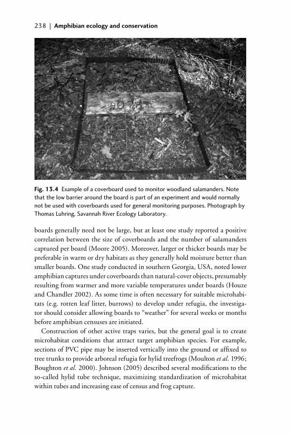
238 | Amphibian ecology and conservation
boards generally need not be large, but at least one study reported a positive correlation between the size of coverboards and the number of salamanders captured per board (Moore 2005). Moreover, larger or thicker boards may be preferable in warm or dry habitats as they generally hold moisture better than smaller boards. One study conducted in southern Georgia, USA, noted lower amphibian captures under coverboards than natural-cover objects, presumably resulting from warmer and more variable temperatures under boards (Houze and Chandler 2002). As some time is often necessary for suitable microhabi-tats (e.g. rotten leaf litter, burrows) to develop under refugia, the investiga-tor should consider allowing boards to “weather” for several weeks or months before amphibian censuses are initiated.
Construction of other active traps varies, but the general goal is to create microhabitat conditions that attract target amphibian species. For example, sections of PVC pipe may be inserted vertically into the ground or affi xed to tree trunks to provide arboreal refugia for hylid treefrogs (Moulton et al. 1996; Boughton et al. 2000). Johnson (2005) described several modifi cations to the so-called hylid tube technique, maximizing standardization of microhabitat within tubes and increasing ease of census and frog capture.
Fig. 13.4 Example of a coverboard used to monitor woodland salamanders. Note that the low barrier around the board is part of an experiment and would normally not be used with coverboards used for general monitoring purposes. Photograph by Thomas Luhring, Savannah River Ecology Laboratory.
13_Dodd_Chap13.indd 23813_Dodd_Chap13.indd 238 8/19/2009 2:49:07 PM8/19/2009 2:49:07 PM
13 Drift fences, coverboards, and other traps | 239
As uses of coverboards and other active traps vary, so will the designs for their placement. In general active traps should be placed in habitats that are favorable for amphibians, including well-shaded areas with abundant moisture. For spe-cies that breed in aquatic habitats, breeding sites may be the most appropriate places to maximize captures. For example, an obvious location to deploy PVC tubes for hylid frogs would be around the periphery of wetland breeding sites.
The spatial distribution of active traps also depends on the goals of the study. For simple amphibian inventories (documenting species presence) or collecting individuals for use in the laboratory, placing devices haphazardly in the most optimal habitats is the most cost-effective method. For studies where statistical comparisons are to be made, replicated sampling units must be designated. In general, because captures per individual trap are low, arrays of several boards or other traps are usually designated as the sampling unit. An array can consist of any arbitrary number of traps, generally arranged in a systematic pattern (e.g. a grid or transect). Replicate arrays are then placed systematically or randomly within treatments. Ideally, a power analysis can be used to determine the num-ber of arrays (sample size) that is needed to obtain suffi cient statistical power for the analysis.
For example, a researcher might wish to compare salamander abundance across three forest types within a relatively small geographical area. Having determined that salamanders are generally fairly common (say, an average of one salamander found per fi ve coverboards checked), an array of 10 cover-boards, spaced 5 m apart in a linear transect, might be determined as the sam-pling unit. Geographic Information Systems (GIS) technology could then be used to generate randomized locations for fi ve arrays to be placed within each of the three habitat types. Thus, the total number of boards to be used would be 150 (10 boards/array � 5 arrays per habitat treatment � 3 habitats) and the sample size would be fi ve per treatment.
Unlike passive traps, active traps can be monitored on nearly any tem-poral schedule, and the timing of censuses will refl ect the question of inter-est. Generally, as animals may remain within the same refuge for extended periods, allowing some time (e.g. a few days or a week) between censuses may minimize repeated counts of the same individual animal. Alternatively, ani-mals may avoid boards that are disturbed too frequently; one study noted that salamander captures under coverboards that were checked daily were reduced compared to boards that were censused on longer time intervals (1 or 3 weeks; Marsh and Goicochea 2003). Similarly, when designing a monitoring scheme, care should be taken to make samples as repeatable as possible. This typic-ally means that environmental conditions should be as comparable as possible
13_Dodd_Chap13.indd 23913_Dodd_Chap13.indd 239 8/19/2009 2:49:16 PM8/19/2009 2:49:16 PM
240 | Amphibian ecology and conservation
between samples, and many researchers set up environmental criteria for deter-mining census times based on the biology of the study animal. For example, coverboard arrays might be checked once-weekly at 7–9 am on days without precipitation or only on nights with a temperature greater than 15°C and at least 1 cm of rain.
13.3.3 What can active traps tell you? What can they not tell you?
Coverboards and other active traps have several advantages as sampling methods for amphibians. First, in many cases, these are among the best methods for col-leting large numbers of target species and can be the only ways to collect highly fossorial species or those that do not form breeding aggregations. Moreover, unlike passive traps, which require high-intensity monitoring on a daily basis to avoid mortality of captured animals, active traps can be monitored on a low-intensity or periodic basis because animals are not restrained and are not prone to accidental mortality or unnaturally high levels of predation. Also, because active traps generally concentrate animals into a highly searchable area (e.g. under a board, or in a PVC tube), these methods minimize the effects of obser-ver bias, which can be substantial in other active capture methods such as visual searches. Finally, because artifi cial refugia are standardized for size and material, they create more repeatable microhabitats than natural-cover objects, yielding more standardized measures of abundance, and can be censused with minimal disturbance to the habitat (Heyer et al. 1994).
Because active traps yield high capture rates of target species, they can be use-ful for assessing patterns of abundance over time or space (e.g. population trends over time or variation in abundance across habitats). Generally, studies designed to investigate these types of questions compare capture rates among arrays of traps placed in different locations (e.g. two habitat types) or capture rates within an array or set of arrays over time. In these types of studies, the dependent vari-able is generally an index of relative abundance, typically the number of animals captured over some unit of time and effort (e.g. captures per array per census). However, as with any abundance index, data collected using these methods may be biased in a variety of ways, all of which must be considered when interpreting capture data.
The key assumption when comparing indices of relative abundance is that the capture probability of an individual animal is the same across arrays or time intervals. Thus, differences in capture rate among arrays refl ect true differences in population density between sampling units. Although this assumption may be met in some situations, it is relatively easy to imagine situations where this
13_Dodd_Chap13.indd 24013_Dodd_Chap13.indd 240 8/19/2009 2:49:16 PM8/19/2009 2:49:16 PM
13 Drift fences, coverboards, and other traps | 241
premise is violated. Perhaps the most obvious case where the equal catchability assumption is violated is when comparing capture rates among species, as noted for the drift-fence method. It is often the case, regardless of the sampling method, that some species are highly catchable, while others are seldom encountered. Thus, it is generally unreasonable to assume that simply because one species is captured more frequently than another, that it is truly more abundant. Likewise, differences in catchability across time are critical to consider in temporal com-parisons and the potential for activity patterns to infl uence catchability must be considered when interpreting capture rates. For example, in warm climates, salamanders often retreat deep underground during the summer and are seldom captured using any method. In this case, low capture rates of salamanders in the summer are best explained by seasonal differences in catchability rather than by changes in actual abundance within the landscape. A growing body of literature uses mark–recapture or occupancy modeling to incorporate detection probabil-ity (catchability) in interpretations of amphibian abundance data (Chapter 24; Mazerolle et al. 2007). Ideally, any researcher wishing to use abundance indices as indicators of population size or density should consider using these methods to test the equal catchability assumption.
A fi nal consideration when using active traps is the potential for use of these methods to actually improve the overall quality of the habitat for target spe-cies. For example, if one of the factors limiting population size in an amphibian species is availability of suitable refugia, adding boards, hylid tubes, or other artifi cial refugia to the habitat may permit an increase in population density. Although such a situation would probably be favorable in studies designed to conserve at-risk amphibian species, it is worth remembering that population densities estimated in areas with abundant artifi cial refugia may not necessarily be representative of those in unaltered habitats. To our knowledge the poten-tial for artifi cial refugia to improve habitat quality for amphibians has not been addressed experimentally and warrants future investigation.
13.4 References
Adams, M. J., Richter, K. O., and Leonard, W. P. (1997). Surveying and monitoring amphibians using aquatic funnel traps. In D. H. Olson, W. P. Leonard, and R. B. Bury (eds), Sampling Amphibians in Lentic Habitats, Northwest Fauna, no. 4, pp. 47–54. Society for Northwestern Vertebrate Biology, Olympia, WA.
Aresco, M. J. (2005). Mitigation measures to reduce highway mortality of turtles and other herpetofauna at a north Florida lake. Journal of Wildlife Management, 69, 549–60.
Arntzen, J. W., Oldham, R. S., and Latham, D. M. (1995). Cost effective drift fences for toads and newts. Amphibia-Reptilia, 16, 137–45.
13_Dodd_Chap13.indd 24113_Dodd_Chap13.indd 241 8/19/2009 2:49:16 PM8/19/2009 2:49:16 PM
242 | Amphibian ecology and conservation
Boughton, R. G., Staiger, J., and Franz, R. (2000). Use of PVC pipe refugia as a sampling technique for hylid treefrogs. American Midland Naturalist, 144, 168–77.
Buech, R. R. and Egeland, L. M. (2002). Effi cacy of three funnel traps for capturing amphibian larvae in seasonal forest ponds. Herpetological Review, 33, 182–5.
Bury, R. B. and Corn, P. S. (1987). Evaluation of pitfall trapping in northwestern forests: trap arrays with drift fences. Journal of Wildlife Management, 51, 112–19.
Corn, P. S. (1994). Straight-line drift fences and pitfall traps. In W. R. Heyer, M. A. Donnelly, R. W. McDiarmid, and L. C. Hayek (eds), Measuring and Monitoring Biological Diversity. Standard Methods for Amphibians, pp. 109–17. Smithsonian Institution Press, Washington DC.
Degraaf, R. M. and Yamasaki, M. (1992). A nondestructive technique to monitor the relative abundance of terrestrial salamanders. Wildlife Society Bulletin, 20, 260–4.
Dodd, Jr, C. K. (1991). Drift fence-associated sampling bias of amphibians at a Florida sandhills temporary pond. Journal of Herpetology, 25, 296–301.
Dodd, Jr, C. K. and Scott, D. E. (1994). Drift fences encircling breeding sites. In W. R. Heyer, M. A. Donnelly, R. W. McDiarmid, and L. C. Hayek (eds), Measuring and Monitoring Biological Diversity. Standard Methods for Amphibians, pp. 125–30. Smithsonian Institution Press, Washington DC.
Enge, K. M. (1997a). Use of silt fencing and funnel traps for drift fences. Herpetological Review, 28, 30–1.
Enge, K. M. (1997b). A Standardized Protocol for Drift-fence Surveys. Technical report no. 14. Florida Game and Fresh Water Fish Commission, Tallahassee, FL.
Enge, K. M. (2001). The pitfalls of pitfall traps. Journal of Herpetology, 35, 467–78.Fellers, G. M. and Drost, C. A. (1994). Sampling with artifi cial cover. In W. R. Heyer,
M. A. Donnelly, R. W. McDiarmid, and L. C. Hayek (eds), Measuring and Monitoring Biological Diversity. Standard Methods for Amphibians, pp. 146–50. Smithsonian Institution Press, Washington DC.
Friend, G. R. (1984). Relative effi ciency of two pitfall-drift fence systems for sampling small vertebrates. Australian Zoologist, 21, 423–34.
Friend, G. R., Smith, G. T., Mitchell, D. S., and Dickman, C. R. (1989). Infl uence of pit-fall and drift fence design on capture rates of small vertebrates in semi-arid habitats of western Australia. Australian Wildlife Research, 16, 1–10.
Gascon, C. (1994). Sampling with artifi cial pools. In W. R. Heyer, M. A. Donnelly, R. W. McDiarmid, and L. C. Hayek (eds), Measuring and Monitoring Biological Diversity. Standard Methods for Amphibians, pp. 144–6. Smithsonian Institution Press, Washington DC.
Gibbons, J. W. and Bennett, D. H. (1974). Determination of anuran terrestrial activity patterns by a drift fence method. Copeia 1974, 236–43.
Gibbons, J. W. and Semlitsch, R. D. (1981). Terrestrial drift fences with pitfall traps: an effective technique for quantitative sampling of animal populations. Brimleyana, 7, 1–16.
Gibbons, J. W., Winne, C. T., Scott, D. E., Willson, J. D., Glaudas, X., Andrews, K. M., Todd, B. D., Fedewa, L. A., Wilkinson, L., Tsaliagos, R. N. et al. (2006). Remarkable amphibian biomass and abundance in an isolated wetland: Implications for wetland conservation. Conservation Biology, 20, 1457–65.
13_Dodd_Chap13.indd 24213_Dodd_Chap13.indd 242 8/19/2009 2:49:17 PM8/19/2009 2:49:17 PM
13 Drift fences, coverboards, and other traps | 243
Gittins, S. P. (1983). The breeding migration of the common toad (Bufo bufo) to a pond in mid-Wales. Journal of Zoology, London, 199, 555–62.
Grant, B. W., Tucker, A. D., Lovich, J. E., Mills, A. M., Dixon, P. M., and Gibbons, J. W. (1992). The use of coverboards in estimating patterns of reptile and amphibian bio-diversity. In D. R. McCullough, and R. H. Barrett (eds), Wildlife 2001, pp. 379–403. Elsevier Science, London.
Greenberg, C. H., Neary, D. G., and Harris, L. D. (1994). A comparison of herpetofaunal sampling effectiveness of pitfall, single-ended, and double-ended funnel traps used with drift fences. Journal of Herpetology, 28, 319–24.
Griffi ths, R. A. (1985). A simple funnel trap for studying newt populations and an evalu-ation of trap behavior in smooth and palmate newts, Triturus vulgaris and Triturus helveticus. Herpetological Journal, 1, 5–10.
Heyer, W. R., Donnelly, M. A., McDiarmid, R. W., and Hayek, L. C. (eds) (1994). Measuring and Monitoring Biological Diversity. Standard Methods for Amphibians, Smithsonian Institution Press, Washington DC.
Houze, C. M. and Chandler, C. R. (2002). Evaluation of coverboards for sampling terres-trial salamanders in south Georgia. Journal of Herpetology, 36, 75–81.
Hsu, M. Y., Kam, Y. C., and Fellers, G. M. (2005). Effectiveness of amphibian monitor-ing techniques in a Taiwanese subtropical forest. Herpetological Journal, 15, 73–9.
Jehle, R., Hodl, W., and Thonke, A. (1995). Structure and dynamics of central European amphibian populations: a comparison between Triturus dobrogicus (Amphibia, Urodela) and Pleobates fuscus (Amphibia, Anura). Australian Journal of Ecology, 20, 362–6.
Johnson, J. R. (2005). A novel arboreal pipe-trap designed to capture the gray treefrog (Hyla versicolor). Herpetological Review, 36, 274–7.
Johnson, S. A. (2003). Orientation and migration distances of a pond-breeding salaman-der (Notophthalmus perstriatus, Salamandridae). Alytes, 21, 3–22.
Johnson, S. A. and Barichivich, W. J. (2004). A simple technique for trapping Siren lac-ertina, Amphiuma means, and other aquatic vertebrates. Journal of Freshwater Ecology, 19, 263–9.
Luhring, T. M. and Young, C. A. (2006). Innovative techniques for sampling stream-inhabiting salamanders. Herpetological Review, 37, 181–3.
Marsh, D. M. and Goicochea, M. A. (2003). Monitoring terrestrial salamanders: biases caused by intense sampling and choice of cover objects. Journal of Herpetology, 37, 460–6.
Mazerolle, M. J., Bailey, L. L., Kendall, W. L., Royle, J. A., Converse, S. J., and Nichols, J. D. (2007). Making great leaps in herpetology: accounting for detectability in fi eld studies. Journal of Herpetology, 41, 672–89.
Mitchell, J. C., Erdle, S. Y., and Pagels, J. F. (1993). Evaluation of capture techniques for amphibian, reptile, and small mammal communities in saturated forested wetlands. Wetlands, 13, 130–6.
Moore, J. D. (2005). Use of native wood as a new coverboard type for monitoring red-backed salamanders. Herpetological Review, 36, 268–71.
Moulton, C. A., Fleming, W. J., and Nerney, B. R. (1996). The use of PVC pipes to cap-ture hylid frogs. Herpetological Review, 27, 186–7.
13_Dodd_Chap13.indd 24313_Dodd_Chap13.indd 243 8/19/2009 2:49:17 PM8/19/2009 2:49:17 PM
244 | Amphibian ecology and conservation
Palis, J. G., Adams, S. M., and Peterson, M. J. (2007). Evaluation of two types of commercially-made aquatic funnel traps for capturing ranid frogs. Herpetological Review, 38, 166–7.
Parris, K. M., Norton, T. W., and Cunningham, R. B. (1999). A comparison of tech-niques for sampling amphibians in the forests of south-east Queensland, Australia. Herpetologica, 55, 271–83.
Pauley, T. K. and Little, M. (1998). A new technique to monitor larval and juvenile sala-manders in stream habitats. Banisteria, 12, 32–6.
Pechmann, J. H. K., Scott, D. E., Semlitsch, R. D., Caldwell, J. P., Vitt, L. J., and Gibbons, J. W. (1991). Declining amphibian populations: the problem of separating human impacts from natural fl uctuations. Science, 253, 892–5.
Phillips, C. A. and Sexton, O. J. (1989). Orientation and sexual differences during breeding migrations of the spotted salamander, Ambystoma maculatum. Copeia, 1989, 17–22.
Pittman, S. E., Jendrek, A. L., Price, S. J., and Dorcas, M. E. (2008). Habitat selection and site fi delity of Cope’s gray treefrog (Hyla chrysoscelis) at the aquatic-terrestrial eco-tone. Journal of Herpetology, 42, 378–85.
Resetarits, W. J. and Wilbur, H. M. (1991). Calling site choice by Hyla chrysoscelis: effects of predators, competitors, and oviposition sites. Ecology, 72, 778–86.
Rice, A. N., Rice, K. G., Waddle, J. H., and Mazzotti, F. J. (2006). A portable non-invasive trapping array for sampling amphibians and reptiles. Herpetological Review, 37, 429–30.
Ryan, T. J., Philippi, T., Leiden, Y. A., Dorcas, M. E., Wigley, T. B., and Gibbons, J. W. (2002). Monitoring herpetofauna in a managed forest landscape: effects of habitat types and census techniques. Forest Ecology and Management, 167, 83–90.
Semlitsch, R. D. (1985). Analysis of climatic factors infl uencing migrations of the sala-mander Ambystoma talpoideum. Copeia, 1985, 477–89.
Semlitsch, R. D. and Pechmann, J. H.K. (1985). Diel patterns of migratory activity for several species of pond-breeding salamanders. Copeia, 1985, 86–91.
Shaffer, H. B., Alford, R. A., Woodward, B. D., Richards, S. J., Altig, R. G., and Gascon, C. (1994). Quantitative sampling of amphibian larvae. In W. R. Heyer, M. A. Donnelly, R. W. McDiarmid, and L. C. Hayek (eds), Measuring and Monitoring Biological Diversity. Standard Methods for Amphibians, pp. 130–41. Smithsonian Institution Press, Washington DC.
Stevens, C. E. and Paszkowski, C. A. (2005). A comparison of two pitfall trap designs in sampling boreal anurans. Herpetological Review, 36, 147–9.
Todd, B. D. and Winne, C. T. (2006). Ontogenetic and interspecifi c variation in timing of movement and responses to climatic factors during migrations by pond-breeding amphibians. Canadian Journal of Zoology, 84, 715–22.
Todd, B. D., Winne, C. T., Willson, J. D., and Gibbons, J. W. (2007). Getting the drift: examining the effects of timing, trap type, and taxon on herpetofaunal drift fence sur-veys. American Midland Naturalist, 158, 292–305.
Vogt, R. C. and Hine, R. L. (1982). Evaluation of techniques for assessment of amphibian and reptile populations in Wisconsin. In N. J. Scott, Jr (ed.). Herpetological Communities, pp. 201–17. Wildlife Research Report 13. United States Fish and Wildlife Service, Washington DC.
13_Dodd_Chap13.indd 24413_Dodd_Chap13.indd 244 8/19/2009 2:49:17 PM8/19/2009 2:49:17 PM

13 Drift fences, coverboards, and other traps | 245
Waldron, J. L., Dodd, Jr, C. K., and Corser, J. D. (2003). Leaf litterbags: factors affecting capture of stream-dwelling salamanders. Applied Herpetology, 1, 23–6.
Weddeling, K., Hachtel, M., Sander, U., and Tarkhnishvili, D. (2004). Bias in estimation of newt population size: a fi eld study at fi ve ponds using drift fences, pitfalls, and funnel traps. Herpetological Journal, 14, 1–7.
Willson, J. D. and Dorcas, M. E. (2003). Quantitative sampling of stream salamanders: comparison of dipnetting and funnel trapping techniques. Herpetological Review, 34, 128–30.
Willson, J. D. and Dorcas, M. E. (2004). A comparison of aquatic drift fences with traditional funnel trapping as a quantitative method for sampling amphibians. Herpetological Review, 35, 148–50.
Willson, J. D., Winne, C. T., and Fedewa, L. A. (2005). Unveiling escape and capture rates of aquatic snakes and salamanders (Siren spp. and Amphiuma means) in commer-cial funnel traps. Journal of Freshwater Ecology, 20, 397–403.
13_Dodd_Chap13.indd 24513_Dodd_Chap13.indd 245 8/19/2009 2:49:17 PM8/19/2009 2:49:17 PM
15Rapid assessments of amphibian diversity
James R. Vonesh, Joseph C. Mitchell, Kim Howell, and
Andrew J. Crawford
15.1 Background: rapid assessment of amphibian diversity
More than 6400 amphibian species are known worldwide, with more than 50 new species being described in just the fi rst half of 2008 (AmphibiaWeb 2008). Many of these species are threatened or declining and more than 150 may have recently become extinct (IUCN 2006). Such rates of species loss are far greater than the historic background extinction rate for amphibians (e.g. McCallum 2007; Roelants et al. 2007). Amphibians play diverse roles in natural ecosys-tems, and their decline may cause other species to become threatened or may undermine aspects of ecosystem function (Matthews et al. 2002; Whiles et al. 2006). Anthropogenic habitat loss and degradation, disease, introduced species, and pollution or combinations of these factors are at the root of most declines. As awareness of declines has increased, conservation groups, governments, and land managers have become more interested in protecting amphibian diversity. However, the lack of accurate data on amphibian distributions, particularly for tropical regions where diversity and declines are concentrated (IUCN 2006), is often a roadblock to effective conservation and management. Ideally, lack of information on the amphibian fauna for a particular area would result in a thor-ough inventory. Unfortunately, this is usually not realistic. Exhaustive inven-tories are costly and may take decades to compile (e.g. Timm 1994). Given the urgency of the current global biodiversity crisis, fi nite resources, and dynamic socio-economic environments with respect to conservation, an approach for rapidly gathering preliminary data on biodiversity is sometimes required.
Rapid biodiversity-assessment methods were developed in response to this need. A Rapid Assessment (RA) is an accelerated, targeted, and fl exible bio-diversity survey, often focusing on species associated with particular vegetation
15_Dodd_Chap15.indd 26315_Dodd_Chap15.indd 263 8/19/2009 3:16:12 PM8/19/2009 3:16:12 PM
264 | Amphibian ecology and conservation
types or topographical features (Sayre et al. 2000). RAs consist of planning, fi eld sampling, and analytical and writing stages, and are implemented by teams of biologists and resource managers with expertise in the region and taxonomic group(s) of interest. Most RAs aim to be completed, from planning to report, in less than a year. Although a variety of RA strategies have been proposed, two of the better documented are the Rapid Ecological Assessment method-ology developed by the Nature Conservancy (Sayre et al. 2000) and the Rapid Assessment Program methodology developed by Conservation International (Roberts 1991; www.conservation.org). RA approaches share a number of fea-tures in common (modifi ed from Sayre et al. 2000).
• Speed. Reducing project duration reduces costs and delivers results to decision- makers quickly.
• Careful initial planning and training. Effective planning saves time and money and increases the consistency of the information gathered.
• Use of mapping technologies. The use of Geographic Information Systems (GIS), remote sensing, and global positioning systems (GPS) can greatly facilitate planning, sampling design, and geo-referencing of data.
• Careful scientifi c documentation. Selecting classifi cation, sampling, and surveying methods that are most effective for the habitat, season, and taxa being sampled can maximize assessment effectiveness.
• Capacity-building and partnerships. Developing collaborative relationships among conservation, government, and academic partners in host countries and internationally helps ensure that information generated will have a local impact.
An RA is not an exhaustive faunal inventory, monitoring program, environ-mental impact assessment, or management plan, nor does it seek to elucidate species interactions or ecological processes, although an RA could serve as an important prelude to any of these activities. Instead, an RA is a conservation planning tool that can provide an effi cient initial characterization of diversity in areas for which relatively little is known (Sayre et al. 2000). Here we describe in brief the steps involved in RA and discuss sampling methodologies likely to be effective for assessing amphibian diversity. Due to the integrative nature of RA, we often refer the reader to other chapters in this volume that cover material important to the topic.
15.1.1 When is an RA needed?
Determining whether an RA approach is called for depends on how much is already known about the area of interest and the urgency to obtain additional
15_Dodd_Chap15.indd 26415_Dodd_Chap15.indd 264 8/19/2009 3:16:12 PM8/19/2009 3:16:12 PM
15 Rapid assessments of amphibian diversity | 265
information. The best candidate sites are those that are only marginally sur-veyed and are highly threatened (Sayre and Roca 2000). It is in these cases that data resulting from an RA, though typically limited in scope, can have import-ant implications for decision-making.
For example, the Atewa Range Forest Reserve of Ghana contains some of the last remaining upland evergreen forest in the country and is home to endemic plant and insect species (McCullough et al. 2007). In 2006, Conservation International initiated a Rapid Assessment Program of amphibians (and other taxa) within the Atewa Range Forest Reserve in response to proposed mineral exploration in the reserve. Sampling sites were selected in areas suspected to sup-port high biodiversity that also had large mineral deposits (McCullough et al. 2007). Field surveys were conducted over just 18 days at the beginning of the rainy season. Nearly one-third of the 32 amphibian species observed were listed as threatened on the IUCN Red List. One species was considered Critically Endangered (Kouamé et al. 2007). Based in part on the amphibian assessment results, the authors recommended that Atewa Range Forest Reserve be elevated to national park status and that mineral exploitation be prohibited (Kouamé et al. 2007; McCullough et al. 2007).
15.2 Planning an RA
When an RA is indicated, the next steps involve planning and preparation. Because RAs may involve government and non-government participants from multiple regions, are often conducted in remote, logistically challenging fi eld localities, and investigate unknown or poorly described faunas, substantial advanced planning is necessary for success.
15.2.1 Developing objectives
Establishing clear and realistic objectives is the most important step of the plan-ning process, as the objectives become the yardstick for subsequent activities and resource allocation (Hayek 1994; Sayre and Roca 2000). Often amphibian assessments will be conducted as part of a larger project involving specialized teams looking at a variety of taxonomic groups, and objectives will need to be coordinated (e.g. Kouamé et al. 2007). The objectives should defi ne the tem-poral, spatial, and taxonomic scope of the project, and in doing so determine the sampling methods and intensity required. For example, the objective might be to provide a preliminary species list of stream-associated taxa from a particular watershed based on snapshot sampling of several sites during the rainy season. Or perhaps the goal is to provide an initial inventory of all amphibian species
15_Dodd_Chap15.indd 26515_Dodd_Chap15.indd 265 8/19/2009 3:16:12 PM8/19/2009 3:16:12 PM
266 | Amphibian ecology and conservation
within an area of conservation interest based on sampling effort spread over multiple seasons. Ideally, one’s objectives are focused, realistic, and quantifi able (Chapter 2). Initial effort in reviewing and refi ning objectives is always worth the investment.
15.2.2 Costs and funding
Consideration of the costs and time necessary to successfully complete an RA is important and the decision on whether or not to proceed with an RA is often affected by fi nancial and time investments. Costs will depend upon the scope of the objectives and logistics of fi eld implementation, and can include sal-ary expenditures, fi eld equipment and supplies, landscape imagery purchases, international and in-country travel expenses, collecting and research permits, training expenses, contracts, laboratory equipment, museum supplies, software, digital storage media, and publication costs (Sayre and Roca 2000). Advanced consideration of these costs allows careful evaluation of trade-offs in the use of fi nite resources. For example, the use of satellite images, aerial photographs, or aerial videography to identify and map different habitat types and topographical features can greatly facilitate selection of sampling localities and is a key feature of some RA approaches (e.g. Rapid Ecological Assessment; Sayre et al. 2000). However, acquisition and processing of remote imagery can be very expensive, putting it beyond the scope of projects with more limited resources. Similarly, additional fi eld sampling across seasons may increase the number of species observed, but also increases costs associated with returning to the site or main-taining a team in the fi eld. Once costs have been estimated and a short project proposal developed, potential fi nancial supporters can be approached. Options for securing fi nancial support include development banks, governments, devel-opment agencies, conservation organizations, foundations, corporations, mili-tary landowners, and private individuals (Sayre et al. 2000).
15.2.3 Team selection and training
Depending upon the scope of the project, RA teams range from a few to many people, and may include senior scientists, students, technicians, fi eld assist-ants, guides, rangers, data managers, cartographers, and administrators from multiple collaborating institutions (Sayre and Roca 2000; McCullough et al. 2007). For larger teams, an initial planning workshop is advisable, with the goal of developing a work plan that clearly identifi es the roles and responsibilities of participating organizations and individuals. An example outline for a planning workshop and an example working plan for Rapid Ecological Assessment is given in Sayre and Roca (2000). International collaborations are recommended,
15_Dodd_Chap15.indd 26615_Dodd_Chap15.indd 266 8/19/2009 3:16:12 PM8/19/2009 3:16:12 PM
15 Rapid assessments of amphibian diversity | 267
whenever possible. Foreigners planning an RA should collaborate with local scientists to increase the chances of a successful project, and to make lasting contributions to the host country. Nationals planning an RA should consider involving foreign experts in important methodologies or taxonomic groups, especially from neighboring countries with related faunas.
A training workshop specifi cally for fi eld personnel can also be an import-ant tool, by providing training related to animal identifi cation, fi eld sampling techniques and data collection, use of GPS for geolocation, mapping and navi-gation, and safety protocols. All team members in charge of data collection should have at least a basic appreciation of the sampling design and statistical analyses planned (Magnusson and Mourão 2004; Chapter 18). In addition, amphibian pathogens and parasites can be carried between habitats on hands, footwear, or fi eld equipment, and could be spread to new localities. Thus, it is important that initial training for those involved in RA include how to minimize the spread of disease and parasites between study sites (Declining Amphibians Population Task Force (DAPTF) code of practice, Chapter 26; Aguirre and Lampo 2006). Typically, this training occurs at the study area at the commencement of fi eldwork. An overview of basic qualifi cations for fi eld biologists, training tips, project supervision, and quality assurance are given in Fellers and Freel (1995).
15.2.4 Permits
Conducting an RA may require permits from local, regional, national, and inter-national governing agencies. Most national governments, and many state and local governments, require permits to study amphibians within their boundaries and public lands. Many protected areas (e.g. national parks) require additional permission. National agencies and international treaties (e.g. Convention on International Trade in Endangered Species of Wild Fauna and Flora (CITES), U.S. Fish and Wildlife Service, Convention on Biological Diversity) also regu-late export and import of specimens and tissue samples. There is considerable variation among regions in permit fees and the times required to process and receive permits, ranging from weeks to well over a year. Thus, the permitting process should be initiated well in advance of the planned fi eldwork.
15.2.5 Data management
Although short in duration, RA projects can produce large amounts of data of different types, include quantitative data that can be represented as numbers, qualitative data that are not easily represented in numerical form, spatial data that are linked to geographic coordinates, metadata documentation that accompanies
15_Dodd_Chap15.indd 26715_Dodd_Chap15.indd 267 8/19/2009 3:16:12 PM8/19/2009 3:16:12 PM
268 | Amphibian ecology and conservation
other data sets, and images or video or audio clips. Data management is the process that helps ensure that diverse data sets can be effi ciently collected, integrated and analyzed, and archived so that they can be easily retrieved in the future (Gotelli and Ellison 2004). Planning for good data management begins early in project development by making a table of the types of data to be produced in the fi eld; for example habitat variables (Chapter 17), conditions, counts, specimens, and other media such as photos, audio (Chapter 16), or video. This information can be used to design protocols (e.g. fi eld forms, labels, code numbers) for collection and management of disparate types of data. Once data are being generated it is important to review data in the fi eld, and verify that team members are using iden-tical protocols. Data should be transcribed regularly and transferred to a database as soon as possible. If a portable computer is brought to the fi eld, raw data should still be maintained on paper in case of damage to the computer. Widely used software for data management include Microsoft Access and the non-proprietary OpenOffi ce BASE. Protocols need to be established for reviewing, cleaning, and backing up data on a regular basis. Museum specimen data should be stored in a manner compliant with the Distributed Generic Information Retrieval (DiGIR) protocols, such as the database management software, Specify (http://www.specifysoftware.org).
15.2.6 Developing the sampling plan
The sampling plan is a document that identifi es areas to be sampled during fi eld work, the time that each area is to be sampled, the sampling techniques to be used and designate the individuals or teams responsible for conducting the fi eld work. The sampling plan lays out the strategy for obtaining data that are repre-sentative of the target area of interest (Sayre 2000).
15.2.6.1 Selecting sampling sites
RA, at its most basic level, involves the collection and characterization of taxo-nomic and spatial information about biodiversity (Sayre et al. 2000). Although identifying sampling localities is one of the fi rst steps in developing a sampling plan for any RA, protocols differ in their emphasis of initial landscape charac-terization. In some cases, sampling sites may be identifi ed based upon perceived high biodiversity potential (e.g. perhaps as indicated by previous sampling of other taxa), specifi c conservation threats, or access logistics (e.g. Kouamé et al. 2007). In other cases, sites may be selected to capture clines in important abiotic features (e.g. elevation, rainfall, vegetation) that may determine the boundaries of particu-lar amphibian assemblages (e.g. Menegon and Salvidio 2005). Some projects use remote sensing imagery to visually identify specifi c habitats of interest prior to
15_Dodd_Chap15.indd 26815_Dodd_Chap15.indd 268 8/19/2009 3:16:12 PM8/19/2009 3:16:12 PM
15 Rapid assessments of amphibian diversity | 269
sampling. Finally, GIS (Chapter 19) coupled with ecological niche modeling pro-vide a new tool for remotely identifying potential habitat for species of concern or biodiversity hotspots in general (e.g. Raxworthy et al. 2003; Pawar et al. 2007).
Development and accessibility of new mapping technologies over the past two decades have had important impacts on the way RAs are conducted. Spatial tech-nologies, including GIS, remote sensing, and GPS are commonly used in defi n-ing project scope and establishing sampling localities. The Rapid Ecological Assessment approach developed by Conservation International places strong emphasis on using satellite and aerial imagery to classify landscapes of interest into vegetation or land-use cover categories (Sayre et al. 2000). Sampling sites are spread across these vegetation categories to establish the framework within which fi eld sampling is conducted and to facilitate linkages between fi ne-scale sampling by fi eld teams with landscape-level assessment of biodiversity (Nagendra and Gadgil 1999; Sayre et al. 2000). Sayre et al. (2000) provide a detailed example of how natural-colour and colour-infrared satellite and aerial fl y-over imagery were used to develop an initial landscape characterization of Parque Nacional del Este, Dominican Republic, which was subsequently used to identify specifi c sampling sites and generate detailed site maps. While the utility of remote sensing imagery when planning an RA is readily apparent, costs can be considerable. Commercial satellite imagery may cost US$3000–5000 per scene and an aerial photo acqui-sition mission may cost between $20 000 and 120 000 (Sayre et al. 2000). For projects with limited resources, Google Earth™ maps integrate data from satel-lite imagery, aerial photography, and a GIS 3D globe to provide resolution of at least 15 m for most terrestrial areas.
We draw a distinction between the ways sampling sites are determined in most RA studies compared to traditional ecological inventory methods. Traditional ecological inventories emphasized objective fi eld sampling based on rand-omized selection of replicated samples and substantial effort may be given to issues such as defi ning sampling coverage and determining detection probabil-ities (e.g. Buckland et al. 1993; 2001, 2004; Heyer et al. 1994; Williams et al. 2002). This emphasis on randomization, replication, and estimating detection functions greatly increases the kinds of inferences that can be made. However, for many RAs, sampling may be opportunistic, or determined by issues such as logistics, access, effi ciency, and a priori perceptions of areas likely to be high-est in diversity or under the greatest threat. Although replicate units may be sampled in some cases, the resulting data may not be rigorously applied to all questions of interest to the ecologist or biogeographer (Sayre 2000). As a result, the results from many RAs are best viewed as qualitative or semi-quantitative (e.g. Kouamé et al. 2007).
15_Dodd_Chap15.indd 26915_Dodd_Chap15.indd 269 8/19/2009 3:16:12 PM8/19/2009 3:16:12 PM
270 | Amphibian ecology and conservation
15.2.6.2 Selecting sampling time
Scheduling sampling times will depend on latitude, elevation, seasonal patterns of rainfall, and knowledge of species breeding phenology. For example, in Kibale National Park, Uganda, pond-breeding Hyperolius reed frogs are most active and breed during the two rainy seasons (Vonesh 2000). In contrast, Leptopelis treefrogs breed during the dry seasons (J.R. Vonesh, unpublished results). Successfully sampling both of these taxa might require fi eldwork during wet and dry seasons. However, when resources limit sampling to a single season, more amphibians are likely to be sampled during wet months.
15.2.6.3 Selecting sampling techniques
A variety of techniques can be used to assess amphibian diversity, including drift fences, pitfall traps, and cover boards (Chapter 13; Menegon and Salvidio 2005), quadrat sampling (aquatic: Chapter 4; terrestrial: Chapter 14), call sur-veys (Chapter 16), road and trail censuses (Pearman et al. 1995; Rödel and Ernst 2004), aquatic sweep-net sampling (Chapter 4), bottle or minnow traps, and visual surveys (e.g. Crump and Scott 1994). References on amphibian sampling include Campbell and Christman (1982), Corn and Bury (1990), Heyer et al. (1994), Olson et al. (1997), Lips et al. (2001), Howell (2002), Rueda-Almonacid et al. (2006), and Williams et al. (2002).
Selecting the sampling methodologies for an RA requires careful thought. Above all an RA must be rapid, yet our objective of a complete species list would suggest that we employ multiple techniques because techniques differ in the set of species they sample successfully. Often the strengths of different techniques are readily apparent, for example litter quadrat sampling will be more effective at sampling direct-developing species than visual encounter surveys (VESs) around aquatic habitats (Vonesh 2000, 2001a, 2001b; J.R. Vonesh, unpublished results). In other cases the trade-offs among techniques are more subtle and may change seasonally (K. Howell, unpublished results). Techniques also vary in terms of cost, effort, and other logistical requirements. Drift-fence arrays can be effect-ive at sampling amphibians in a variety of situations (Chapter 13; K. Howell, unpublished results) but they are relatively expensive and labor-intensive to set up and maintain. Therefore, each potential fi eld method should be evaluated for its relative capture success, speed, bias, and the extent to which it can facilitate the objectives of the RA (e.g. see Chapter 6, Table 4 in Heyer et al. 1994).
15.2.6.3.1 Visual encounter surveys (VESs)
VESs involves fi eld personnel searching the focal habitat systematically for a known period of time. The clock is stopped when not actively searching
15_Dodd_Chap15.indd 27015_Dodd_Chap15.indd 270 8/19/2009 3:16:12 PM8/19/2009 3:16:12 PM
15 Rapid assessments of amphibian diversity | 271
(e.g. animals are being processed). The number of animals observed can then be expressed in terms of animals observed per area (or distance) per person searching, or per unit time per person. VES is an effective technique for build-ing species lists rapidly (Crump and Scott, 1994; Rodda et al. 2007), requires little equipment (e.g. minimally a headlamp and field notebook), and can be implemented in a variety of habitat types. For these reasons it is perhaps the most widely employed sampling method in RA of amphibian diversity, so we provide a brief overview of the method here. For additional information see Crump and Scott (1994), Corn and Bury (1990), Campbell and Christman (1982), Rödel and Ernst (2004), and Rueda-Almonacid et al. (2006).
There is considerable variation among past studies in how VES is conducted. In some instances (e.g. Mitchell 2006; Kouamé et al. 2007) experienced her-petologists selectively search areas and microhabitats determined most likely to yield amphibians. This approach has the benefi t of potentially yielding more animals and species per effort than randomized sampling approaches. However, it is most subject to variation in the skill levels of the fi eld personnel and is lim-ited in its ability to generalize about relative abundances and habitat associations because (micro-)habitats are searched in a biased manner. Alternatively, an area may be searched via VES using a randomized-walk design (Crump and Scott 1994). In this case, prior to going to the fi eld site the researcher generates a ran-dom sequence of compass headings as well as a random distance to be searched along each heading. A starting heading and distance is selected at random and fi eld personnel simply work through the list of headings and distances, search-ing for animals, for a specifi ed time. Since the path to be sampled is determined randomly, this approach has the advantage that replicated random walks from different areas could be compared statistically. However, it is important to appre-ciate that differences in the observed number of animals among sites may be as much due to differences in detection among sites as much as differences in true abundance. If the sampling design requires greater effort per area, VES can be conducted using a quadrat design (Crump and Scott 1994). In this case, quad-rats of a known area are established and each is then sampled systematically by searching parallel transects across the plot (e.g. Hairston 1980; Aichinger 1987; Donnelly 1989). Crump and Scott (1994) recommend plot sizes of 10 m � 10 m or 25 m � 25 m, depending upon amphibian densities. To statistically compare areas of interest (e.g. different habitats) plots must be replicated and randomly located within areas to be compared (e.g. using GPS coordinates or a trail grid system). Finally, transect designs are often used in coordination with VES for sampling across habitat gradients that may affect amphibian diversity and abun-dance (e.g. moisture, elevation). Although these considerations may determine
15_Dodd_Chap15.indd 27115_Dodd_Chap15.indd 271 8/19/2009 3:16:12 PM8/19/2009 3:16:12 PM
272 | Amphibian ecology and conservation
transect direction, distances to be sampled and starting points are best deter-mined a priori and multiple randomly located replicate transects will be needed if areas are to be compared statistically.
It is also important to determine and carefully defi ne the intensity of fi eld sampling in advance. Crump and Scott (1994) suggest three levels of sampling intensity for sampling amphibians. The least intensive surveys are counts of animals that are active on the surface (Hairston 1980; Vonesh 2000). This approach is minimally invasive and thus is suitable for search areas with sensi-tive faunas and also requires the least amount of time, increasing the amount of area that can be covered. Intermediate-level searches count exposed ani-mals but also turn over surface cover objects (note that cover objects must be returned to their original position to minimize disturbance). This level of VES can yield species often overlooked by low-intensity VES because of their secretive and semi-fossorial life histories (e.g. many salamanders and caecilians). When the most complete inventory possible is desired, all pos-sible microhabitats are searched; surface objects are turned, decaying logs are torn apart, the leaf litter is systematically raked, epiphytes and tree holes are searched (Crump and Scott 1994), and aquatic habitats are searched for adults and larvae (Chapter 4). Such intensity requires considerable labor per unit area and causes the greatest disturbance to the habitat but may be more effect-ive at sampling some rare species.
15.2.6.3.2 Assumptions and limitations of VESs
The analysis of VES data is based on the following assumptions: (1) all individu-als are equally detectable; (2) individuals are recorded once during a survey; and (3) there are no observer-related biases in sampling (Crump and Scott 1994). In most instances, one or more of these assumptions will be violated. Amphibians of different species, sizes, or life stages are generally not equally conspicuous. Even the probability of detecting the same individual may vary due to temporal (e.g. diel, seasonal) variation in behavior (Bailey et al. 2004; Schmidt 2005). Similarly, differences in observer experience can often result in differences in detection. Thus, the assumption of equal detection probability across time, space, and individuals is unlikely to hold for most amphibian taxa or studies (Mazerolle et al. 2007). This has important implications for simple count-based methods like VES. Consider that the expected number of individuals or taxa counted (C) in a survey area is E(C) � PN, where P is the probably of detection and N is the true number in the population (Williams et al. 2002). Without an estimate of P, for any count of animals sampled, there is an infi nite number of possible true population sizes. Mazerolle et al. (2007) and Schmidt (2004, 2005) provide
15_Dodd_Chap15.indd 27215_Dodd_Chap15.indd 272 8/19/2009 3:16:13 PM8/19/2009 3:16:13 PM
15 Rapid assessments of amphibian diversity | 273
lucid reviews of these issues and specifi cally focus on their application to her-petological studies. Given these limitations, VES is best viewed as a qualitative or semi- quantitative approach and should be used only when qualitative results are acceptable (e.g. threatened species were observed; Kouamé et al. 2007). VES may be a suitable sampling approach given the objectives of many RA projects. However, when resources and objectives allow, other more powerful study designs (e.g. distance sampling methods; Thomas et al. 2002; Funk et al. 2003; Fogarty and Viletta 2001; Viletta and Fogarty 2005) should be considered.
15.2.6.4 Determining what data to collect
Generating lists of observed species is usually the principle type of data-collection method used during an RA. In some cases, animals encountered in the fi eld may be identifi ed in the fi eld. In other cases, it may not be possible to identify all species, requiring that specimens be held temporarily for identifi cation (e.g. to consult a key) before being released at the site of collection, or it may be necessary to preserve voucher specimens that can be identifi ed by taxonomic specialists (Jacobs and Heyer 1994; McDiarmid 1994). Voucher specimens are what ultim-ately defi ne the identity and distribution of any amphibian species. Depending on collecting permits obtained, a series of one or more voucher specimens per sex, life stage, and species should be collected during any give RA, especially for remote geographic locations, and deposited in a recognized natural history museum. Voucher specimens allow independent researchers to confi rm speci-men identifi cation at a later date, a very important consideration given the highly unstable state of amphibian taxonomy. The systematic value of a voucher speci-men increases as more ancillary data are included.
Depending upon the project’s goals, it may be important to collect add-itional data for animals observed or collected. GPS can be used to provide a geo- reference for each sample. Basic size measurements (snout–vent length, mass), sex, reproductive status based on secondary sexual characteristics, notes or photographs indicating coloration, and basic activity (e.g. calling, resting, mov-ing, etc.) may be recorded. Tissue samples for DNA analyses may be obtained from a toe clip, liver sample, or a buccal swab preserved in 95% ethanol or other buffer (Seutin et al. 1991; Gonser and Collura 1996; Goldberg et al. 2003). The benefi ts of integrating RA data with the DNA barcode of life campaign are potentially enormous but so far have been under-utilized (Vences et al. 2005; Fouquet et al. 2007; Ficetola et al. 2008; Smith et al. 2008). Additional types of sample, such as skin swabs, may be required for disease detection (Chapter 26). It is also important to record environmental characteristics, such as weather conditions, lunar cycle, and vegetation or habitat characteristics (Chapter 17).
15_Dodd_Chap15.indd 27315_Dodd_Chap15.indd 273 8/19/2009 3:16:13 PM8/19/2009 3:16:13 PM
274 | Amphibian ecology and conservation
However, collecting additional data on individuals is time-consuming and thus additional data on individuals may involve trading-off the amount of area that can be searched. Field forms are useful to remind the fi eld team what data are to be collected and can help ensure consistency of data collection among team members. Crump and Scott (1994) provide an example data sheet for VES that includes some basic individual-level data. If designed with foresight, forms can also expedite data entry.
15.2.6.5 Field logistics
Poorly organized trips typically result in poor-quality data collection. Careful advance planning for the transportation of the team, sampling equipment, and basic supplies will be required, particularly for large teams and remote localities. Logistics also includes coordinating the safety of the team. Injuries and illness in remote locations can be dangerous and hinder project progress. In advance of fi eldwork the fi eld team should prepare a well-stocked medical kit, review vaccines and allergies of each participant, and plan for various possible medical emergencies that could arise.
15.3 In the fi eld
After the planning and preparation has been completed, the team goes to the fi eld and begins sampling in the manner indicated by the sampling plan. Situations will naturally arise that prevent the sampling protocols from being followed exactly. RAs are intended to be fl exible enough to allow fi eld teams to respond to unforeseen roadblocks as they arise. The fi eld team should keep the primary objectives of the project in mind if they are required to alter plans in the fi eld (Young et al. 2000).
15.4 Compiling data and interpreting results
Producing information that is useful to conservation biologists, land managers, and policy-makers requires skillful synthesis of the large volume of fi eld data generated. If data-management strategies were developed and the data and metadata have been entered into the database, work can now focus on ana-lysis and interpretation. RA data summaries typically focus on species lists (Kouamé et al. 2007). Species lists may be organized to highlight species sampled in different primary sampling localities, particular habitat types (e.g. stream, pond, litter), points along environmental gradients (e.g. eleva-tion; Menegon and Salvidio 2005), indicator taxa (e.g. disturbance-tolerant
15_Dodd_Chap15.indd 27415_Dodd_Chap15.indd 274 8/19/2009 3:16:13 PM8/19/2009 3:16:13 PM
15 Rapid assessments of amphibian diversity | 275
versus -intolerant; Kerr et al. 2000), endemicity or conservation status (e.g. IUCN Red List status). The best summary approach will depend on the goals of the RA. Because sampling effort often varies among sites and may have relied to some degree on opportunistic sampling, it is often diffi cult to make direct comparisons between species lists among sites across or even within RA studies. In some cases, species accumulation or rarefaction curves can be used to show how rapidly the number of species sampled at a specifi c site or habitat increased with sampling effort (e.g. Chapter 18; Gotelli and Colwell 2001; Magurran 2003) to facilitate comparison at a given sampling effort. Similarly, in some cases it may be possible to use total diversity estimators to extrapolate from incidence sampling data to estimate the total number of amphibian species at a site (e.g. Chapter 18; Chao et al. 2005). When using VES data, however, investigators should clearly defi ne their sampling unit and be aware how their choice could infl uence the diversity analyses.
15.5 Recommendations and reporting
Because RAs are typically motivated from a conservation or management per-spective, recommendations will focus on how the information generated in the RA can be used to maintain long-term faunal diversity of the study sites. However, recommendations should be fi rmly based on the study results, not on preconceived ideas about the sites importance, and should consider the target audience and their ability to follow through on the recommendations. Little benefi t comes from recommendations for which the target audience has no ability to implement (Young et al. 2000). Ways in which RA results are typically used to guide decision-making include providing direction for future land acquisition, identifying monitoring needs, establishing priorities for future research, suggestions for how to zone for multiple use, and for identifying poten-tial threats to species of interest (Young et al. 2000).
15.6 Summary
Rapid assessment is an approach that can be useful for conservation planning because it can provide an effi cient preliminary characterization of the amphibian fauna. However, because the methods are often qualitative or semi- quantitative, the RA approach is of most value when the fauna of the study areas is unknown and when even qualitative information is needed urgently to help decision-making. When resources, time, and project objectives allow, researchers should consider more quantitative approaches.
15_Dodd_Chap15.indd 27515_Dodd_Chap15.indd 275 8/19/2009 3:16:13 PM8/19/2009 3:16:13 PM
276 | Amphibian ecology and conservation
15.7 References
Aguirre, A. A. and Lampo, M. (2006). Protocolo de bioseguridad y cuarentena para preve-nir la transmisión de enfermedades en anfi bios. In A. Angulo, J. V. Rueda-Almonacid, J. V. Rodríguez-Mahecha, and E. La Marca (eds), Técnicas de Inventario y Monitoreo para los Anfi bios de la Región Tropical Andina, pp. 73–92. Conservación Internacional, Bogotá.
Aichinger, M. (1987). Annual activity patterns of anurans of anurans in a seasonal Neotropical environment. Oecologia, 71, 583–92.
AmphibiaWeb (2008). Information on Amphibian Biology and Conservation. AmphibiaWeb, Berkeley, CA. http://amphibiaweb.org.
Bailey, L. L., Simons, T. R., and Pollock, K. H. (2004). Estimating site occupancy and species detection probability parameters for terrestrial salamanders. Ecological Applications, 14, 692–702.
Buckland, S. T., Anderson, D. R., Burnham, K. P., and Laake, J. L. (1993). Distance Sampling: Estimating Abundance of Biological Populations. Chapman and Hall, London.
Buckland, S. T., Anderson, D. R., Burnham, K. P., Laake, J. L., Borchers, D. L., and Thomas, L. (2001). Introduction to Distance Sampling: Estimating Abundance of Biological Populations. Oxford University Press, New York.
Buckland, S. T., Anderson, D. R., Burnham, K. P., Laake, J. L., Borchers, D., and Thomas, L. (2004). Advanced Distance Sampling: Estimating Abundance of Biological Populations. Oxford University Press, Oxford.
Campbell, H. W. and Christman, S. P. (1982). Field techniques for herpetofaunal com-munity analysis. In N. J. Scott, Jr (ed.), Herpetofaunal Communities, pp. 193–200.Wildlife Research Report 13. U.S. Department of the Interior, Fish and Wildlife Service, Washington DC.
Chao, A., Chazdon, R. L., Colwell, R. K., and Shen, T.-J. (2005). A new statistical approach for assessing similarity of species composition with incidence and abundance data. Ecology Letters, 8, 148–59.
Corn, P. S. and Bury, R. B. (1990). Sampling Methods for Terrestrial Amphibians and Reptiles. General Technical Report, PNW-GTR-256. U.S. Forest Service, Fort Collins, CO.
Crump, M. L. and Scott, Jr, N. J. (1994). Visual encounter surveys. In W. R. Heyer, M. A. Donnelly, R. W. McDiarmid, L. A. C. Hayek, and M. S. Foster (eds), Measuring and Monitoring Biological Diversity, Standard Methods for Amphibians, pp. 84–92. Smithsonian Institution Press, Washington DC.
Donnelly, M. A. (1989). Demographic effects of reproductive resource supplementation in a territorial frog, Dendrobates pumilio. Ecological Monographs, 59, 207–21.
Fellers, G. M. and Freel, K. L. (1995). A standardized protocol for surveying aquatic amphib-ians. Technical Report NPS/WRUC/NRTR-95-01. U.S. National Park Service, Davis, CA.
Ficetola, G. F., Miaud, C., Pompanon, F., and Taberlet, P. (2008). Species detection using environmental DNA from water samples. Biology Letters, 4, 423–5.
Fogarty, J. H. and Vilella, F. J. (2001). Evaluating methodologies to survey Eleutherodactylus frogs in montane forests of Puerto Rico. Wildlife Society Bulletin, 29, 948–55.
15_Dodd_Chap15.indd 27615_Dodd_Chap15.indd 276 8/19/2009 3:16:13 PM8/19/2009 3:16:13 PM
15 Rapid assessments of amphibian diversity | 277
Fouquet, A., Gilles, A., Vences, M., Marty, C., Blanc, M., and Gemmell, N. J. (2007). Underestimation of species richness in Neotropical frogs revealed by mtDNA analyses. PLoS ONE, 2, e1109.
Funk, W., Almeida-Reinoso, D., Nogales-Sornosa, F., and Bustamante, M. (2003). Monitoring population trends of Eleutherodactylus frogs. Journal of Herpetology, 37, 245–56.
Goldberg, C. S., Kaplan, M. E., and Schwalbe, C. R. (2003). From the frog’s mouth: buccal swabs for collection of DNA from amphibians. Herpetological Review, 34, 220–1.
Gonser, R. A. and Collura, R. V. (1996). Waste not, want not: toe-clips as a source of DNA. Journal of Herpetology, 30, 445–7.
Gotelli, N. J. and Colwell, R. K. (2001). Quantifying biodiversity: procedures and pitfalls in the measurement and comparison of species richness. Ecology Letters, 4, 379–91.
Gotelli. N. J. and Ellison, A. M. (2004). Chapter 8: Managing and curating data. A Primer of Ecological Statistics, pp. 207–36. Sinauer Associates, Sunderland, MA.
Hairston, N. G. (1980). The experimental test of an analysis of fi eld distributions: Competition in terrestrial salamanders. Ecology, 61, 817–26.
Hayek, L.-A. (1994). Research design for quantitative amphibian studies. In W. R. Heyer, M. A. Donnelly, R. W. McDiarmid, L. A. C. Hayek, and M. S. Foster (eds), Measuring and Monitoring Biological Diversity, Standard Methods for Amphibians, pp. 21–38. Smithsonian Institution Press, Washington DC.
Heyer, W. R., Donnelly, M. A., McDiarmid, R. W., Hayek, L. A. C., and Foster, M. S. (eds) (1994). Measuring and Monitoring Biological Diversity, Standard Methods for Amphibians. Smithsonian Institution Press, Washington DC.
Howell, K. M. (2002). Amphibians and reptiles: Herptiles. In G. Davies, (ed.), African Forest Biodiversity, pp. 17–44. Earthwatch, London.
IUCN, Conservation International, and NatureServe (2006). Global Amphibian Assessment. http://globalamphibians.org.
Jacobs, J. F. and Heyer, W. R. (1994). Collecting tissue for biochemical analysis. In W. R. Heyer, M. A. Donnelly, R. W. McDiarmid, L. A. C. Hayek, and M. S. Foster (eds), Measuring and Monitoring Biological Diversity, Standard Methods for Amphibians, pp. 103–7. Smithsonian Institution Press, Washington DC.
Kerr, J. T., Sugar, A., and Packer, L. (2000). Indicator taxa, rapid biodiversity assessment, and nestedness in an endangered ecosystem. Conservation Biology, 14, 1726–34.
Kouamé, N. G., Bonteng, C. O., and Rödel, M.-O. (2007). A rapid survey of the amphib-ians from Atewa Range Forest Reserve, Eastern Region, Ghana. In J. McCullough, L. E. Alonso, P. Naskrescki, H. E. Wright, and Y. Osei-Owusu (eds), A Rapid Biological Assessement of the Atewa Range Forest Reserve, Eastern Ghana. RAP Bulletin of Biological Assessment 47, pp. 76–83. Conservation International, University of Chicago Press, Chicago, IL.
Lips, K. R., Reaser, J. K., Young, B. E., and Ibáñez, R. (2001). Amphibian monitoring in Latin America: a protocol manual/Monitoreo de Anfi bios en América Latina: Manual de protocolos. SSAR Herpetological Circular no. 30.
Magnusson, W. E. and Mourão, G. (2004). Statistics without Math. Sinauer Associates, Sunderland, MA.
15_Dodd_Chap15.indd 27715_Dodd_Chap15.indd 277 8/19/2009 3:16:13 PM8/19/2009 3:16:13 PM
278 | Amphibian ecology and conservation
Magurran, A. E. (2003). Measuring Biological Diversity. Blackwell Publishing, Oxford.Matthews, K. R., Knapp, R. A., and Pope, K. L. (2002). Garter snake distributions in
high-elevation aquatic ecosystems: is there a link with declining amphibian popula-tions and non-native trout introductions? Journal of Herpetology, 36, 16–22.
Mazerolle, M. J., Bailey, L. L., Kendall, W. L., Royle, J. A., Converse, S. J., and Nichols, J. D. (2007). Making great leaps forward: Accounting for detectability in herpetological fi eld studies. Journal of Herpetology, 41, 672–89.
McCallum, M. L. (2007). Amphibian declines or extinction? Current declines dwarf background extinction rate. Journal of Herpetology, 41, 483–91.
McCullough, J., Alonso, L. E., Naskrecki, P., Wright, H. E., and Osei-Owusu, Y. (eds) (2007). A Rapid Biological Assessment of the Atewa Range Forest Reserve, Eastern Ghana. RAP Bulletin of Biological Assessment 47, 1–191. Conservation International, Arlington, VA.
McDiarmid, R. W. (1994). Preparing amphibians as scientifi c specimens. In W. R. Heyer, M. A. Donnelly, R. W. McDiarmid, L. A. C. Hayek, and M. S. Foster (eds), Measuring and Monitoring Biological Diversity, Standard Methods for Amphibians, pp. 103–7. Smithsonian Institution Press, Washington DC.
Menegon, M. and Salvidio, S. (2005). Amphibian and reptile diversity in the southern Udzungwa Scarp Forest Reserve, south-eastern Tanzania. In B. A. Huber, B. J. Sinclair, and K.-H. Lampe (eds), African Biodiversity. Molecules, Organisms, Ecosystems, pp. 205–12. Springer, New York.
Mitchell, J. C. (2006). Inventory of Amphibians and Reptiles of Fredericksburg and Spotsylvania National Historic Battlefi eld. Technical Report/NERCHAL/NRTR-200600/000. U.S. National Park Service, Fredericksburg, VA.
Nagendra, H. and Gadgil, M. (1999). Biodiversity assessment at multiple scales: linking remotely sensed data with fi eld information. Proceedings National Academy of Sciences USA, 96, 9154–8.
Olson, D. H., Leonard, W. P. and Bury, R. B. (eds) (1997). Sampling Amphibians in Lentic Habitats: Methods and Approaches for the Pacifi c Northwest: Northwest Fauna No. 4. Society for Northwestern Vertebrate Biology, Olympia, WA.
Pawar, S., Koo, M. S., Kelley, C., Ahmed, M. F., Chaudhuri, S., and Sarkar, S. (2007). Conservation assessment and prioritization of areas in Northeast India: priorities for amphibians and reptiles. Biological Conservation, 136, 346–61.
Pearman, P. B., Velasco, A. M., and Lopez, A. (1995). Tropical amphibian monitoring: a comparison of methods for detecting inter-site variation in species composition. Herpetologica, 51, 325–37.
Raxworthy, C. J., Martinez-Meyer, E., Nussbaum, R. A., Schneider, G. E., Ortega-Huerta, M. A., and Peterson, A. T. (2003). Predicting distributions of known and unknown reptile species in Madagascar. Nature, 426, 837–41.
Roberts, L. (1991). Ranking the rainforests. Science, 251, 1559–60.Rodda, G. H., Campbell, E.W, Fritts, T. H., and Clark, C. S. (2007). The predictive
power of visual searching. Herpetological Review, 36, 259–64.Rödel, M.-O. and Ernst, R. (2004). Measuring and monitoring amphibian diversity in
tropical forests. I. An evaluation of methods with recommendations for standardiza-tion. Ecotropica, 10, 1–14.
15_Dodd_Chap15.indd 27815_Dodd_Chap15.indd 278 8/19/2009 3:16:13 PM8/19/2009 3:16:13 PM
15 Rapid assessments of amphibian diversity | 279
Roelants, K., Gower, D. J., Wilkinson, M., Loader, S. P., Biju, S. D., Guillaume, K., Moriau, L., and Bossuyt, F. (2007). Global patterns of diversifi cation in the history of modern amphibians. Proceedings of the National Academy of Sciences USA, 104, 887–92.
Rueda-Almonacid, J. V., Castro, F., and Cortez, C. (2006). Técnicas para el inventario y muestreo de anfi bios: Una compilación. In A. Angulo, J. V. Rueda-Almonacid, J. V. Rodríguez-Mahecha, and E. La Marca (eds), Técnicas de Inventario y Monitoreo para los Anfi bios de la Región Tropical Andina, pp. 135–71. Conservación Internacional, Bogotá.
Sayre, R. (2000). Overview: Rapid Ecological Assessment after ten years. In R. Sayre, E. Roca, G. Sedaghatkish, B. Young, S. Keel, R. L. Roca, and S. Sheppard (eds), Nature in Focus Rapid Ecological Assessment, pp. 1–18. Island Press, Washington DC.
Sayre, R. and Roca E. (2000). Careful planning: a key to success. In R. Sayre, E. Roca, G. Sedaghatkish, B. Young, S. Keel, R. L. Roca, and S. Sheppard (eds), Nature in Focus Rapid Ecological Assessment, pp. 33–44. Island Press, Washington DC.
Sayre, R., Roca, E., Sedaghatkish, G., Young, B., Keel, S., Roca, R. L., and Sheppard S. (eds) (2000). Nature in Focus: Rapid Ecological Assessment. Island Press, Washington DC.
Schmidt, B. (2004). Declining amphibian populations: the pitfalls of count data in the study of diversity, distributions, dynamics, and demography. Herpetological Journal, 14, 167–74.
Schmidt, B. (2005). Monitoring the distribution of pond breeding amphibians when spe-cies are detected imperfectly. Aquatic Conservation: Marine and Freshwater Ecosystems, 15, 681–92.
Seutin, G., White, B. N., and Boag, P. T. (1991). Preservation of avian blood and tissue samples for DNA analyses. Canadian Journal of Zoology, 69, 82–90.
Smith, M. A., Poyarkov, Jr, N. A., and Hebert, P. D. N. (2008). CO1 DNA barcod-ing amphibians: take the chance, meet the challenge. Molecular Ecology Resources, 8, 235–46.
Thomas, L., Buckland, S. T., Burnham, K. P., Anderson, D. R., Laake, J. L., Borchers, D. L., and Strindberg, S. (2002). Distance sampling. In A. H. El-Shaarawi and W. W. Piegorsch (eds), Encyclopedia of Environmetrics, vol. 1, pp. 544–52. John Wiley & Sons, Chichester.
Timm, R. M. (1994). The mammal fauna. In L. A. McDade, K. S. Bawa, H. A. Hespenheide, and G. S. Hartshorn (eds), LaSelva: Ecology and Natural History of a Neotropical Rainforest, pp. 229–37. University of Chicago Press, Chicago, IL.
Vences, M., Thomas, M., Bonett, R. M., and Vieites, D. R. (2005). Deciphering amphibian diversity through DNA barcoding: chances and challenges. Philosophical Transactions of the Royal Society of London Series B Biological Sciences, 360, 1859–68.
Vilella, F. and Fogarty, J. (2005). Diversity and abundance of forest frogs (Anura: Leptodactylidae) before and after Hurricane Georges in the Cordillera Central of Puerto Rico. Caribbean Journal of Science, 41,157–62.
Vonesh, J. R. (2000). Dipteran predation on the arboreal eggs of four Hyperolius frog spe-cies in western Uganda. Copeia, 2000, 560–6.
Vonesh, J. R. (2001a). Patterns of richness and abundance in a tropical African leaf-litter herpetofauna. Biotropica, 33, 502–10.
15_Dodd_Chap15.indd 27915_Dodd_Chap15.indd 279 8/19/2009 3:16:13 PM8/19/2009 3:16:13 PM

280 | Amphibian ecology and conservation
Vonesh, J. R. (2001b). Natural history and biogeography of the amphibians and reptiles of Kibale National Park, Uganda. Contemporary Herpetology. http://www.nhm.ac.uk/hosted_sites/ch/.
Whiles, M. R., Lips, K. R., Pringle, C. M., Kilham, S. S., Bixby, R. J., Brenes, R., Connelly, S., Colon-Gaud, J. C., Hunte-Brown, M., Huryn, A. D. et al. (2006). The effects of amphibian population declines on the structure and function of Neotropical stream ecosystems. Frontiers in Ecology and the Environment, 4, 27–34.
Williams, B. K., Nichols, J. D., and Conroy, M. J. (2002). Analysis and Management of Animal Populations. Academic Press, New York.
Young, B., Sedaghatkish, G., and Roca, R. (2000). Fauna surveys. In R. Sayre, E. Roca, G. Sedaghatkish, B. Young, S. Keel, R. L. Roca, and S. Sheppard (eds), Nature in Focus Rapid Ecological Assessment. pp. 93–117. Island Press,Washington DC.
15_Dodd_Chap15.indd 28015_Dodd_Chap15.indd 280 8/19/2009 3:16:13 PM8/19/2009 3:16:13 PM
16Auditory monitoring of anuran populations
Michael E. Dorcas, Steven J. Price, Susan C. Walls, and
William J. Barichivich
16.1 Introduction
Because anurans rely on vocalization for most communication, detection of species-specifi c calls provides relatively effi cient mechanisms for studying and evaluating the status of anuran populations. Consequently, most amphibian monitoring programs focus on anurans and use call detection as their sole or pri-mary monitoring technique. The overall goal of these programs is to determine and monitor the status of populations over time. Some monitoring programs may actually attempt some form of quantifi cation of anuran population size or density, but this is often diffi cult when using only calling data. In this chapter we describe approaches for monitoring anuran populations based solely on auditory techniques. These approaches include manual calling surveys (MCS), automated recording systems (ARS), or some combination of the two. MCS can be used by researchers to monitor multiple amphibian populations, often over large spatial scales. ARS can be used by researchers interested in intensively monitoring popu-lations of anurans at a single or a few locations. In this chapter, we describe both approaches and the potential costs and benefi ts of each. We also explain how data resulting from ARS can be used to optimize manual survey protocol and to interpret data resulting from MCS. Our goal is to provide an overview of these techniques and questions that can be addressed using them.
16.2 MCS
Generally, MCS simply involve observers listening to the vocalizations of male frogs and recording all species detected for the duration of the survey or for a given area. In many surveys, observers also score abundance of each species
16_Dodd_Chap16.indd 28116_Dodd_Chap16.indd 281 8/19/2009 3:14:59 PM8/19/2009 3:14:59 PM
282 | Amphibian ecology and conservation
heard vocalizing. Researchers have long used MCS to conduct inventories of anurans in a given area. For example, Wright and Wright (1949) understood the importance of MCS when they stated that “If one knows the frog notes, he can in one night do more work on frog distribution than he might other-wise do in years.” However, only within the last 30 years, when concerns of declining amphibian populations prompted the development of formal moni-toring programs, have MCS been widely used for large-scale investigations of anuran popu lations. The widespread use of MCS for monitoring anurans has led numerous investigations into survey protocol, study design, and effi ciency as a technique to detect anurans.
16.2.1 History and current status of MCS
Many historic and recent small-scale investigations have used MCS to detect anurans for ecological, behavioral, and conservation-related investigations (i.e. Martof 1953; Blair 1961; Woolbright 1985; Knutson et al. 1999). In this chapter, we emphasize MCS approaches that have specifi c objectives to monitor the pro-portion of sites where a given anuran species is observed, accounting for the poten-tial effects of imperfect detection and other biases (site and sampling covariates such as habitat type and weather conditions). This metric is known as occupancy (MacKenzie et al. 2002, 2006).
Most MCS programs use surveys in which observers listen to anuran vocaliza-tions at several points along a roadside transect or at designated sampling loca-tions. Since the early 1980s, the use of roadside surveys to detect calling anurans has become used widely by many local and regional environmental monitoring programs. At least fi ve Canadian provinces and 28 US states conduct, or have conducted, roadside surveys for calling anurans (Weir and Mossman 2005). If similar protocols are used, MCS data collected at the local or regional level (e.g. state or province) can be incorporated into a centralized database allowing for the evaluation of anuran populations at the national level. Two US programs initi-ated by the Department of Interior’s US Geological Survey, the North American Amphibian Monitoring Program (NAAMP; www.pwrc.usgs.gov/naamp/; Weir and Mossman 2005), and the Amphibian Research and Monitoring Initiative (ARMI; http://armi.usgs.gov/), are good examples of this. Many US Geological Survey scientists use both MCS and ARS (see section 16.3) to meet their moni-toring objectives, primarily on federal lands. Additional examples of North American MCS include the Marsh Monitoring Program in the Great Lakes region (Weeber and Vallianatos 2000), Ontario Backyard Frog Survey (de Solla et al. 2005), and FrogWatch USA (Inkley 2006). MCS are also used to monitor trends in anuran populations in Australia (Australia Frog Census; Walker 2002),
16_Dodd_Chap16.indd 28216_Dodd_Chap16.indd 282 8/19/2009 3:14:59 PM8/19/2009 3:14:59 PM
16 Auditory monitoring of anurans | 283
as well as some European (e.g. Anthony 2002; Pellet and Schmidt 2005; Schmidt 2005; Scott et al. 2008), and Central American countries (e.g. Kaiser 2008).
16.2.2 Study objectives: what can MCS tell us?
The objective of any contemporary MCS is typically to conduct an inventory of an area of interest to determine the status of anurans in that region and/or to monitor populations and communities, over time, to address how species are responding to habitat change, climatic variation, or some other ecological or management issue. An objective of many monitoring programs, including those using MCS that are rapidly gaining recognition, is that of determining site occu-pancy (Marsh and Trenham 2008).
16.2.3 Survey design
Establishment of sampling sites is a critical component of all monitoring pro-grams for which it is essential that sites are sampled according to a probabilistic scheme, so that statistical inference may be extrapolated to a defi ned area of interest. According to the NAAMP protocol (Weir and Mossman 2005), sur-veys are conducted along routes that generally are established along roads, dikes, waterways, or other points of access. Routes consist of 10 stops that are either placed at least 0.8 km apart or are stratifi ed by habitat. Although NAAMP is often used as a template for designing MCS, roads are not typically established in a randomized fashion, thus illustrating one of the weaknesses of the NAAMP approach. One compromise for conducting road surveys and meeting this cri-terion is to, for example, randomly select stops along a given route that are at least 0.8 km apart. In this modifi cation the area of inference would be limited to the route, rather than to a larger area of interest (e.g. a large protected area). Determining the number of routes and their associated sites/stops is another critical element if the resulting data are destined for occupancy analysis. The number of sites to be sampled varies depending upon the distribution and nat-ural history of the anuran species being monitored, the question of interest, and other factors. But, generally speaking, a good rule of thumb in determining the number of sites to sample is usually as many as possible, typically at least 50, assuming that sites are sampled for a minimum of four seasons (see Figure 7.3 of MacKenzie et al. 2006).
MCS are usually conducted at night, starting one-half hour after sunset, and are completed by 01:00 h. For many anuran species, especially those in temperate regions, peak calling does occur within this sampling time. Bowers et al. (1998) found that the majority of species in their surveys ended peak calling at midnight. To minimize the potential effect of anthropogenic noise (see section 16.2.4),
16_Dodd_Chap16.indd 28316_Dodd_Chap16.indd 283 8/19/2009 3:14:59 PM8/19/2009 3:14:59 PM
284 | Amphibian ecology and conservation
researchers typically allow 1 min between arriving at each site and beginning the chorus survey. All anuran species heard in a specifi ed time frame (usually 5 min, but see section 16.2.4) are recorded; each calling anuran species is given a score, known as an amphibian calling index (ACI), ranging from 1 to 3, where 1 means distinct calls of individuals that can be counted and have no overlapping calls, 2 means calls of individuals that can be distinguished but have some overlap-ping calls, and 3 means a full chorus, with calls of individuals indistinguishable. Generally, MCS should not be conducted during heavy rain, high wind, or other inclement weather that could affect the detection of calling anurans. At each site, air temperature, relative humidity, barometric pressure, wind speed, and other variables are often measured immediately after recording call data to be used as sample covariates in occupancy analysis. These covariates can be used to help explain variation in site occupancy or detection probabilites.
In regions where anurans vocalize in a somewhat predictable manner, many MCS, such as NAAMP, recommend sampling each stop along a roadside route during a specifi ed sampling period, such as during early spring, late spring, and summer. The NAAMP protocol recommends a single survey, based on conveni-ence to volunteer observers, despite studies that have shown that signifi cant vari-ation in calling behavior does occur within the specifi ed sampling periods (e.g. Todd et al. 2003; Gooch et al. 2006; Kirlin et al. 2006). For example, Gooch et al. (2006) conducted three MCS during the NAAMP-specifi ed “summer” sampling period in the western Piedmont region of North Carolina, USA, and found that detection probabilities increased for some species (e.g. Acris crepitans, Rana catesbeiana) and decreased for other species (e.g. Rana clamitans) from survey 1 to survey 3 (Figure 16.1). Variation in calling behavior with prescribed sampling periods may cause the observer to not detect a species if single sampling occasions are employed. At least two surveys are required to calculate detection probabilities (preferably a minimum of three; J. Nichols, personal communi-cation) during a sampling period (see MacKenzie et al. 2002 and Table 6.1 of MacKenzie et al. 2006 for more details).
16.2.4 Other survey-design issues to consider: the effi ciency of MCS
The widespread use of MCS has led to numerous investigations that focus on the effi ciency of MCS to detect anurans. In fact, few if any amphibian survey methodologies have been scrutinized to the extent of MCS. A central issue in all wildlife-monitoring programs, including MCS, is that of imperfect detection (MacKenzie et al. 2002, 2006). For example, even during the peak breeding season for a given anuran species, calling does not occur each night; variations
16_Dodd_Chap16.indd 28416_Dodd_Chap16.indd 284 8/19/2009 3:14:59 PM8/19/2009 3:14:59 PM
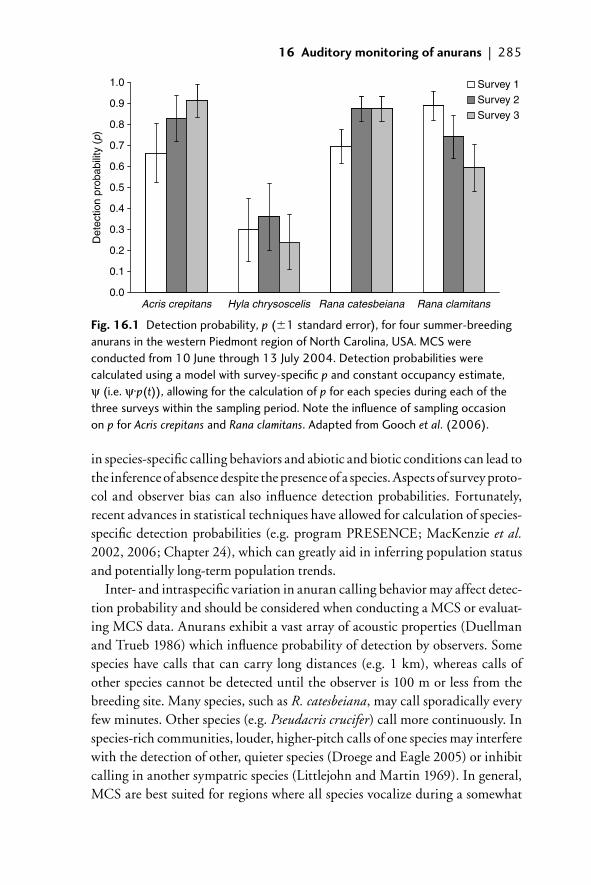
16 Auditory monitoring of anurans | 285
in species-specifi c calling behaviors and abiotic and biotic conditions can lead to the inference of absence despite the presence of a species. Aspects of survey proto-col and observer bias can also infl uence detection probabilities. Fortunately, recent advances in statistical techniques have allowed for calculation of species-specifi c detection probabilities (e.g. program PRESENCE; MacKenzie et al. 2002, 2006; Chapter 24), which can greatly aid in inferring population status and potentially long-term population trends.
Inter- and intraspecifi c variation in anuran calling behavior may affect detec-tion probability and should be considered when conducting a MCS or evaluat-ing MCS data. Anurans exhibit a vast array of acoustic properties (Duellman and Trueb 1986) which infl uence probability of detection by observers. Some species have calls that can carry long distances (e.g. 1 km), whereas calls of other species cannot be detected until the observer is 100 m or less from the breeding site. Many species, such as R. catesbeiana, may call sporadically every few minutes. Other species (e.g. Pseudacris crucifer) call more continuously. In species-rich communities, louder, higher-pitch calls of one species may interfere with the detection of other, quieter species (Droege and Eagle 2005) or inhibit calling in another sympatric species (Littlejohn and Martin 1969). In general, MCS are best suited for regions where all species vocalize during a somewhat
Survey 1
Survey 2
Survey 3
Det
ectio
n pr
obab
ility
(p)
0.0
0.1
0.2
0.3
0.4
0.5
0.6
0.7
0.8
0.9
1.0
Acris crepitans Hyla chrysoscelis Rana catesbeiana Rana clamitans
Fig. 16.1 Detection probability, p (�1 standard error), for four summer-breeding anurans in the western Piedmont region of North Carolina, USA. MCS were conducted from 10 June through 13 July 2004. Detection probabilities were calculated using a model with survey-specifi c p and constant occupancy estimate, ψ (i.e. ψ·p(t)), allowing for the calculation of p for each species during each of the three surveys within the sampling period. Note the infl uence of sampling occasion on p for Acris crepitans and Rana clamitans. Adapted from Gooch et al. (2006).
16_Dodd_Chap16.indd 28516_Dodd_Chap16.indd 285 8/19/2009 3:14:59 PM8/19/2009 3:14:59 PM
286 | Amphibian ecology and conservation
predictable breeding season. Species that breed in response to localized heavy rains (e.g. Spea and Scaphiopus), call quietly or not at all (e.g. Ascaphus truei), call infrequently (e.g. Rana capito), or have relatively short breeding (i.e. vocal-izing) seasons (e.g. Rana sylvatica) should not be monitored exclusively by MCS. Droege and Eagle (2005) suggest that MCS are suitable for detecting and infer-ring population trends for approximately 55 of the 103 anuran species in North America.
Abiotic factors also infl uence calling behavior in many anuran species (Blair, 1961) and thus infl uence detection probability via MCS. Because anurans are ectotherms, air temperature has been shown to infl uence calling, especially for species that vocalize during winter and early spring (e.g. Todd et al., 2003; Weir et al. 2005; Kirlin et al. 2006). Weir et al. (2005) found that air tempera-ture explained calling variation in eight of 10 species studied; however, fi ve species displayed preference for particular temperatures, indicating an optimal temperature for detection. Additionally, Pellet and Schmidt (2005) found that air temperature was a predictor of calling in Hyla arborea in Switzerland, with greater detections during warm temperatures. For winter-breeding species in temperate zones, calling behavior may be more sporadic and limited to day-light or early evening hours when temperatures are moderate (Todd et al. 2003; Kirlin et al. 2006; Saenz et al. 2006).
Abiotic factors other than air temperature have also been shown to infl u-ence anuran calling. For example, Oseen and Wassersug (2002) suggested that water temperature was the overall most important predictor of calling behav-ior of some Canadian anurans. Precipitation can also infl uence calling because many species are known to call more intensely after periods of heavy rain (Blair 1961; Oseen and Wassersug 2002). However, heavy rainfall during MCS is not recommended as it may obfuscate anuran vocalizations and decrease prob-ability of detection. Other factors, such as wind speed (Weir et al. 2005; Oseen and Wassersug 2002; Johnson and Batie 2001), humidity of air (Oseen and Wassersug 2002), barometric pressure (Oseen and Wassersug 2002), and moonlight (Weir et al. 2005), may also infl uence anuran detection probabil-ity. However, anuran species respond differently to abiotic factors (Saenz et al. 2006). Knowledge of the relationship between anuran breeding strategies and abiotic factors prior to conducting MCS may allow for increased effi ciency and/or detection.
Anthropogenic noise also likely impacts anuran detection probability. Most calling anurans will respond to anthropogenic noise disturbance. For this rea-son, some MCS programs recommend that after arriving at a stop the obser-ver must wait for a few minutes prior to conducting the survey. However, few
16_Dodd_Chap16.indd 28616_Dodd_Chap16.indd 286 8/19/2009 3:14:59 PM8/19/2009 3:14:59 PM
16 Auditory monitoring of anurans | 287
studies have been conducted on the effects of noise on anuran calling behavior. Weir et al. (2005) found that only three of 10 species decreased calling behavior due to increased traffi c. Regardless, anthropogenic noise can affect the obser-ver’s ability to detect frogs and should be recorded during MCS. Additionally, anthropogenic noise can also reduce a species proclivity to call, thus lowering its detectability (Sun and Narins 2005; C. Steelman, personal communication)
Several studies have investigated the effects of survey length on anuran detec-tion. The majority of MCS range from 3 to 10 min per stop. Pierce and Gutzwiller (2004) found that 15 min was required to detect 90% of all species known to be present, whereas Shirose et al. (1997) found that 3 min surveys were adequate to detect most species. Gooch et al. (2006) found that 94% of summer-breeding anurans in the North Carolina Piedmont region were detected within the fi rst 5 min of the MCS and detection probabilities were slightly higher as observers spent longer listening (3 min compared to 10 min). However, these and other investigations highlight that some species may go undetected even if surveys are extended up to an hour. The length of survey should be determined based on the specifi c objectives of the MCS; however, for detecting long-term population trends for most species, 3–5 min appears to be adequate.
Variation among observers can also substantially infl uence the quality of MCS data. Some large-scale MCS (e.g. NAAMP) rely heavily on volunteers, who may vary in experience and/or hearing ability. As a result, observers may not detect all species present, include species not present, or incorrectly identify vocalizations, resulting in fl awed assessments of anuran populations (Lotz and Allen 2007). Weir et al. (2005) found that volunteer experience may infl uence species detection. However, studies by Genet and Sargent (2003), Shirose et al. (1997), and Lotz and Allen (2007) suggest that even relatively inexperienced volunteers were reliable in their abilities to determine species, yet estimating abundance categories often differed among observers. Pierce and Gutzwiller (2007) showed 79% agreement among nine observers conducting MCS in cen-tral Texas, USA, and stressed the importance of accounting for interobserver variation in data analysis. NAAMP currently requires all volunteers to pass an online anuran call test (available at www.pwrc.usgs.gov/frogquiz/) prior to con-ducting MCS. In general, training of volunteers will likely increase the prob-ability of ensuring quality data.
16.2.5 Limitations of MCS data
MCS are excellent tools for monitoring changes in anuran occupancy or for inventorying which species occur in an area. At a given site, however, these surveys only yield qualitative data on abundance as obtained through the use of
16_Dodd_Chap16.indd 28716_Dodd_Chap16.indd 287 8/19/2009 3:15:00 PM8/19/2009 3:15:00 PM
288 | Amphibian ecology and conservation
the ACI (section 16.2.3). These types of abundance data are of limited utility in assessing population densities. However, Nelson and Graves (2004) compared population estimates (via mark–recapture) of male R. clamitans with ACI col-lected at the same sites and found abundance to be correlated positively with ACI. In contrast, Corn et al. (2000) found that another measure of call fre-quency failed to refl ect “a relatively large population” of Bufo woodhousii and only weakly distinguished among different-sized populations of Pseudacris maculata. The need to be able to use indices of relative abundance, such as the calling index, in occupancy models has been conceptualized and is currently an active area of research (Royle and Nichols 2003; Dorazio 2007).
Because call surveys are based upon the vocalizations of adult male anurans, they do not provide complete information on population structure; that is, non-calling females and subadults are not assessed by this method (Stevens and Paszkowski 2004). Similarly, this method is not useful for other non-calling amphibians, such as salamanders and caecilians. The males of many species of anurans will vocalize in contexts not necessarily related to breeding; moreover, the MCS does not consider the presence of egg masses, tadpoles, or metamorph-osing juveniles in the population. Thus, the MCS provides no information about whether there was successful reproduction at a given site. Depending on the questions of interest in a given study, the MCS is therefore most useful when used in conjunction with other survey methods, such as visual encoun-ter surveys and the use of traps or dipnets to assess the larval component of the population.
16.3 ARS
In addition to MCS, automated systems (ARS) can be used to detect anuran vocalizations and can be useful in monitoring many anuran populations (Peterson and Dorcas 1994). Typically, ARS (or so-called frogloggers) are used to collect data intensively at a single or a few locations, whereas MCS provide more superfi cial data but for a larger number of sites. ARS can be used to survey for anuran species in places diffi cult to access for MCS and can be left in the fi eld for extended periods of time, thus increasing the probability of detecting a given species. ARS may be the only practical way to reliably detect species that have very short or unpredictable breeding seasons, such as R. capito. ARS minimize disturbance to calling anurans and provide a permanent sampling record that can be evaluated by multiple experts if required (Mohr and Dorcas 1999; Todd et al. 2003). When combined with information on environmental variation, data from ARS can be incorporated into models that can be used to optimize
16_Dodd_Chap16.indd 28816_Dodd_Chap16.indd 288 8/19/2009 3:15:00 PM8/19/2009 3:15:00 PM
16 Auditory monitoring of anurans | 289
monitoring programs based on MCS (Bridges and Dorcas 2000; Oseen and Wassersug 2002).
16.3.1 Sources for ARS
At the time Peterson and Dorcas (1994) published on building and using ARS, there were few options for their procurement. Although not specifi cally intended for anuran monitoring, the Cornell Laboratory of Ornithology builds robust ARS units that have been used in a wide variety of tasks ranging from the detection of ivory- billed woodpeckers (Campephilus principalis) to monitoring whales around the world’s oceans. Bedford Technical (www.frogloggers.com) and Wildlife Acoustics (www.wildlifeacoustics.com) have both produced ARS systems with a variety of options that make them attractive for monitoring frogs. Although their software has not been tested on anuran vocalizations, both Cornell Lab of Ornithology and Wildlife Acoustics produce products, Raven and Song Scope respectively, which may prove useful in automated call detection.
16.3.2 Construction, deployment, and retrieval of data
Although sources for ARS now exist, some biologists may still choose to build their own. This may be a logistical hurdle for some investigators; however, con-struction of an ARS can have the added benefi t of familiarizing the user with the inner workings of their equipment. Construction of an ARS generally requires combining several simpler components: a recorder, timer/controller, micro-phone, power supply, and housing (Peterson and Dorcas 1994; Barichivich 2003). If the investigator is not familiar with electronics, we recommend work-ing with someone skilled in building electrical devices.
The core component of an ARS is the recorder. Devices that have been suc-cessfully used include analog cassette and various digital (e.g. MPEG-1 Audio Layer 3, or MP3) recorders. Selection of a recorder is dependent on the required recording quality, capacity, and budget. Recordings produced on inexpensive analog cassette recorders are suffi cient for manual listening, but higher sam-pling rates and frequency responses may be required in some circumstances. Additionally, storage capacity can usually be greatly increased when using digital recordings.
In most cases, researchers choose to make recordings at specifi c times of day (e.g. dusk) and on set intervals rather than continuously. Some recording devices (e.g. PDAs and digital voice recorders) have built-in timers or clocks. The add-ition of a timer/controller allows programming of the desired recording schedule. A wide variety of devices, from mechanical (K. Wharton, personal communica-tion) to computer microprocessors (Acevedo and Villanueva-Rivera 2006), have
16_Dodd_Chap16.indd 28916_Dodd_Chap16.indd 289 8/19/2009 3:15:00 PM8/19/2009 3:15:00 PM
290 | Amphibian ecology and conservation
been used for this purpose. Timers generally work in one of two ways: controlling the function of the recorder or interrupting the power supply to the recorder. In addition to time-based triggers, environmental triggers can be used to activate an ARS. For example, to detect explosive breeders like Spea or Scaphiopus, a tipping-bucket rain gauge with a reed valve could be used so a rainfall event would trip an ARS into service.
The choice of microphones is a crucial decision, as recordings will only be as good as the microphone, regardless of the recording device. At least nine types of microphone are available but condenser or dynamic varieties are those most commonly used. Unlike dynamic microphones, condenser microphones require a power supply. Condenser microphone power sources are often small (e.g. a single AA battery) and may not be suffi cient if the ARS is deployed for extended periods of time without maintenance. This issue can be addressed by using the timer/controller to control the microphone as well as the recorder. Another con-sideration in selecting a microphone is the directional or acceptance cone. Cones can range from a 360° circle around the microphone (omnidirectional) to just a few degrees in front of the microphone (unidirectional or shotgun). To capture the vocalizations of species that call while partially or completely submerged (e.g. Rana sevosa or Rana subaquavocalis), a hydrophone would be more appro-priate to use than a microphone (Platz 1993).
The fi nal considerations of building an ARS are power supply and pro-tection. Rechargeable batteries generally provide the best option for most researchers. Cost, power, size, and weight should be considered when selecting batteries. In environments with suffi cient sunlight, rechargeable batteries can be supplemented by a solar panel and can generally operate without interrup-tion. With the exception of the microphone, all components of an ARS should be fi rmly mounted inside a protective case. The case should provide adequate environmental protection and be large enough to hold all the components, yet small enough to be reasonably portable for ease of fi eld deployment. For most fi eld deployments, waterproof boxes (e.g. Otter or Pelican brands) work well, but less costly options exist. These include surplus ammunition cans, polyethylene coolers, plastic tool boxes, and plastic watertight marine boxes. Consideration should be given to the environment in which the ARS will be deployed. In areas frequented by people, the ARS can be locked, hidden, or even buried. Animals, such as raccoons and bears, may damage equipment and thus more rugged cases might be needed in some situations (Corn et al. 2000). Microphones should also be protected by a windscreen to reduce wind noise, along with a cover to shield the windscreen and microphone from the environment.
16_Dodd_Chap16.indd 29016_Dodd_Chap16.indd 290 8/19/2009 3:15:00 PM8/19/2009 3:15:00 PM
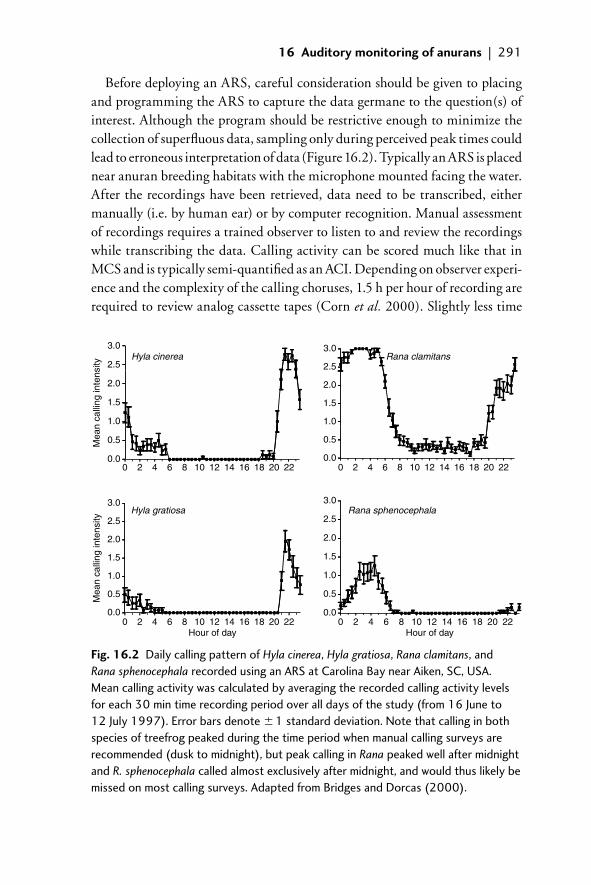
16 Auditory monitoring of anurans | 291
Before deploying an ARS, careful consideration should be given to placing and programming the ARS to capture the data germane to the question(s) of interest. Although the program should be restrictive enough to minimize the collection of superfl uous data, sampling only during perceived peak times could lead to erroneous interpretation of data (Figure 16.2). Typically an ARS is placed near anuran breeding habitats with the microphone mounted facing the water. After the recordings have been retrieved, data need to be transcribed, either manually (i.e. by human ear) or by computer recognition. Manual assessment of recordings requires a trained observer to listen to and review the recordings while transcribing the data. Calling activity can be scored much like that in MCS and is typically semi-quantifi ed as an ACI. Depending on observer experi-ence and the complexity of the calling choruses, 1.5 h per hour of recording are required to review analog cassette tapes (Corn et al. 2000). Slightly less time
Fig. 16.2 Daily calling pattern of Hyla cinerea, Hyla gratiosa, Rana clamitans, and Rana sphenocephala recorded using an ARS at Carolina Bay near Aiken, SC, USA. Mean calling activity was calculated by averaging the recorded calling activity levels for each 30 min time recording period over all days of the study (from 16 June to 12 July 1997). Error bars denote � 1 standard deviation. Note that calling in both species of treefrog peaked during the time period when manual calling surveys are recommended (dusk to midnight), but peak calling in Rana peaked well after midnight and R. sphenocephala called almost exclusively after midnight, and would thus likely be missed on most calling surveys. Adapted from Bridges and Dorcas (2000).
Hyla cinerea Rana clamitans
Hyla gratiosa Rana sphenocephala
0.0
0.5
1.0
1.5
2.0
2.5
3.0
8 10 12 14 16 18 20 226420
Mea
n ca
lling
inte
nsity
0.0
0.5
1.0
1.5
2.0
2.5
3.0
0.0
0.5
1.0
1.5
2.0
2.5
3.0
0.0
0.5
1.0
1.5
2.0
2.5
3.0
Mea
n ca
lling
inte
nsity
Hour of day
8 10 12 14 16 18 20 226420 8 10 12 14 16 18 20 226420
8 10 12 14 16 18 20 226420Hour of day
16_Dodd_Chap16.indd 29116_Dodd_Chap16.indd 291 8/19/2009 3:15:00 PM8/19/2009 3:15:00 PM
292 | Amphibian ecology and conservation
is usually required to review digital recordings. While in its infancy, computer recognition of high-quality recordings shows great promise for decreasing the time, and cost, of manually listening to ARS recordings and potentially increas-ing the accuracy of call recognition. Though not an automated process, one study showed that in a mixed-species chorus, including the acoustically domin-ant coqui (Eleutherodactylus coqui), several species were omitted or signifi cantly underrepresented using only a manual data review (Villanueva-Rivera 2007). By adding a simple visual analysis of the spectrograms of digital call recordings using Adobe Audition, the calls of the less acoustically dominant species were no longer eclipsed (Villanueva-Rivera 2007). Research on birds demonstrates the potentially signifi cant time savings when using computer recognition software. In 12 h, Agranat (2007) scanned more than 250 h of fi eld recordings for bird vocalizations using Song Scope software. This process allowed a human obser-ver to review 1552 potential calls of the cerulean warbler (Dendrocia cerulea) in under 1 h.
16.3.3 Monitoring environmental data
Automatically monitoring environmental data, while simultaneously monitor-ing anuran calling activity using ARS, can allow interpretation of how envir-onmental variation affects calling activity (Dorcas and Foltz 1991; Peterson and Dorcas 1992, 1994; Saenz et al. 2006) and detection probability. Typically, investigators use dataloggers to monitor variables such as air and water tempera-tures, relative humidity, solar radiation, precipitation, wind speed, and baromet-ric pressure. Numerous types of dataloggers of varying quality and capabilities are available (e.g. Onset Computer Corp., Pocasset, MA, USA; Campbell Scientifi c, Logan, UT, USA). Like ARS, some investigators fi nd dataloggers to be particularly challenging to learn to use. However, recent advances in software interfaces for nearly all dataloggers make learning to use them simple enough for even novice researchers.
16.3.4 Answering questions using ARS
ARS can be used by researchers to address basic questions such as whether a spe-cies is present at a given location or to conduct more detailed investigations of factors affecting calling activity and population fl uctuations (Corn and Muths 2002; Todd et al. 2003). Generally, investigators using ARS for monitoring purposes are simply interested in detecting whether a species is present. As such, many ARS systems can be set to only come on and record at certain times of the day when a particular species is most likely to vocalize (e.g. dusk until midnight), thus minimizing the number of recordings that must be evaluated. However,
16_Dodd_Chap16.indd 29216_Dodd_Chap16.indd 292 8/19/2009 3:15:00 PM8/19/2009 3:15:00 PM
16 Auditory monitoring of anurans | 293
one must be careful not to assume that anurans call primarily during times trad-itionally recognized as peak calling periods (Bridges and Dorcas 2000).
In some cases, researchers use ARS to attempt to detect a species that is either rare or has very unpredictable calling patterns. Anurans such as Spea and Scaphiopus that generally only call under certain conditions (i.e. during or after heavy rains) may be particularly hard to detect using MCS and ARS may offer the best opportunity to detect their populations. For some extremely rare species (e.g. R. sevosa) detecting every known population is important for proper man-agement and thus, increasing detectability of populations using ARS can play a vital role in conservation efforts.
Because ARS can collect data at regular and precise intervals, mathematical models can be developed that allow prediction of when and under what condi-tions species are likely to call, thus providing data that can be used to optimize MCS. Typically, data collected simultaneously with anuran calling data, such as temperature, precipitation, wind speed, and time of day, are used as independ-ent variables in a logistic regression to predict the optimal conditions to conduct MCS (i.e. the times when detectability is maximized; Oseen and Wassersug 2002). Anurans may respond differently to environmental variables across their ranges, and thus development of models should be done for particular regions as needed. Such models were developed for three species of winter-breeding anurans (Pseudacris crucifer, Pseudacris feriarum, and Rana sphenocephala) in the western Piedmont region of North Carolina (Steelman and Dorcas, in press). Models showed that for P. crucifer day of year, time, precipitation, and water temperature positively infl uenced calling and air temperature negatively infl u-enced calling; for P. feriarum time, precipitation, air temperature, and water temperature positively infl uenced calling, and day of year negatively infl uenced calling; for R. sphenocephala day of year, time, precipitation, and air temperature positively infl uenced calling, and higher water temperature negatively infl u-enced calling. The models described for the winter-breeding species above were tested using previously collected data from MCS along with spot measurements of environmental data (Kirlin et al. 2006). Models accurately predicted whether a species was calling approximately 70% of the time.
In addition to using models to predict the best times and conditions to manu-ally sample anurans, ARS can be used to interpret data collected previously, assuming suffi cient environmental data are collected at the time of the surveys. Fortunately, nearly all existing MCS programs require collection of at least some environmental data. To do this, an investigator would insert the spot measure-ments of environmental variables collected by volunteers at the time the surveys were conducted into the model equation for each species of interest to generate a
16_Dodd_Chap16.indd 29316_Dodd_Chap16.indd 293 8/19/2009 3:15:00 PM8/19/2009 3:15:00 PM
294 | Amphibian ecology and conservation
likelihood of calling (e.g. ranging from 0 to 1). Calling likelihoods can then be used to interpret previously collected calling survey results. If a species was not heard at a particular location but the model indicates a high likelihood of calling if it was present (e.g. 0.9), then the investigator can have a higher confi dence in concluding that the species was not present, rather than it simply not vocalizing and being undetectable.
16.3.5 Limitation of ARS
Despite the advantages of using ARS, there are some disadvantages when com-pared to surveys based on MCS (Corn et al. 2000; Penman et al. 2005). For many investigators, ARS can be expensive compared to volunteer-based MCS. Additionally, ARS can typically only be deployed at one or a few sites, thus decreasing the number of anuran populations that can be monitored. This can have major implications for statistical analyses of data when each site is a rep-licate. The possibility of wildlife damage, vandalism, or theft of equipment is another issue that may limit investigators’ ability to use ARS in some localities (e.g. Corn et al. 2000). Although ARS can be hidden relatively easily, one of us (M.E.D.) has had equipment stolen even in remote locations. Some investiga-tors fi nd using automated systems particularly challenging, especially if they consider themselves technologically challenged. However, we have found that nearly anyone can be taught to use automated systems effectively and for those that are apprehensive about doing so we suggest initial consultations with a biologist experienced with the equipment being used.
16.4 Conclusions
Auditory monitoring of anuran populations, either by MCS or by ARS, is a use-ful tool for assessing the status and trends of populations, as well as the responses of populations and communities to environmental and anthropogenic change. The use of auditory monitoring has increased tremendously since the realiza-tion that amphibian populations are undergoing global population declines, and has become a standard approach to monitoring in many state, national, and international programs. Auditory monitoring has limitations in that (1) its utility in estimating abundance is restricted, (2) this method provides little information about the complete structure of a population (i.e. the status of non-calling adult females and subadults) or about whether a given popula-tion has experienced successful reproduction, and (3) this method cannot be used on non-calling amphibians, such as salamanders and caecilians. The two means by which auditory monitoring may be conducted (manual or automated) differ in their relative costs and benefi ts, and the appropriate approach for a
16_Dodd_Chap16.indd 29416_Dodd_Chap16.indd 294 8/19/2009 3:15:00 PM8/19/2009 3:15:00 PM
16 Auditory monitoring of anurans | 295
given study ultimately depends on the study objectives and resources available. Nevertheless, MCS can provide vital information on changes in occupancy states of various sites, which can be overlaid with environmental data to assess potential causes of change in occupancy for a given species or community. Data from ARS can be used to optimize the effectiveness of MCS or interpret data based on MCS. As such, auditory monitoring has great utility in assessing the extent of declines of anuran amphibians, a topic of heightened concern in ecol-ogy and conservation biology.
16.5 Acknowledgments
We thank P. Stephen Corn, Erin Muths, and Charlotte K. Steelman for com-ments that improved the manuscript. Manuscript preparation was partially sup-ported by the Department of Biology at Davidson College, Duke Power, and National Science Foundation grant (DEB-0347326) to M.E.D and the U.S. Geological Survey’s Amphibian Research and Monitoring Initiative to SCW and WJB. The use of trade or product names does not imply endorsement by US government agencies.
16.6 References
Acevedo, M. A. and Villanueva-Rivera, L. J. (2006). Using automated digital recording systems as effective tools for the monitoring of birds and amphibians. Wildlife Society Bulletin, 34, 211–14.
Agranat, I. D. (2007). Automatic Detection of Cerulean Warblers Using Autonomous Recording Units and Song Scope Bioacoustics Software. www.wildlifeacoustics.com/
Anthony, B. P. (2002). Results of the fi rst batrachian survey in Europe using road call counts. Alytes, 20, 55–66.
Barichivich, W. J. (2003). Appendix IV: Guidelines for building and operating remote fi eld recorders. In C. K. Dodd, Jr, Monitoring Amphibians in Great Smoky Mountains National Park, pp. 87–96. U.S. Geological Survey Circular no. 1258. U.S. Geological Survey, Tallahassee, FL.
Blair, W. F. (1961). Calling and spawning seasons in a mixed population of anurans. Ecology, 42, 99–110.
Bowers, D. G., Anderson, D. E., and Euliss, Jr, N. H. (1998). Anurans as indicator of wetland condition in the Prairie Pothole Region of North Dakota: an environmen-tal monitoring and assessment program pilot project. In M. Lannoo (ed.), Status and Conservation of Midwestern Amphibians, pp. 369–78. University of Iowa Press, Iowa City, IO.
Bridges, A. S. and Dorcas, M. E. (2000). Temporal variation in anuran calling behavior: implications for surveys and monitoring programs. Copeia, 2000, 587–92.
Corn, P. S. and Muths, E. (2002). Variable breeding phenology affects the exposure of amphibian embryos to ultraviolet radiation. Ecology, 83, 2958–63.
16_Dodd_Chap16.indd 29516_Dodd_Chap16.indd 295 8/19/2009 3:15:00 PM8/19/2009 3:15:00 PM
296 | Amphibian ecology and conservation
Corn, P. S., Muths, E., and Iko, W. M. (2000). A comparison in Colorado of three methods to monitor breeding amphibians. Northwestern Naturalist, 81, 22–30.
de Solla, S. R., Shirose, L. J., Fernie, K. J., Barrett, G. C., Brousseau, C. S., and Bishop, C. A. (2005). Effect of sampling effort and species detectability on volunteer based anuran moni-toring programs. Biological Conservation, 121, 585–94.
Dorazio, R. M. (2007). On the choice of statistical models for estimating occurrence and extinction from animal surveys. Ecology, 88, 2773–82.
Dorcas, M. E. and Foltz, K. D. (1991). Environmental effects on anuran advertisement calling. American Zoologist, 31, 3111A.
Droege, S. and Eagle, P. (2005). Evaluating calling surveys. In M. Lannoo (ed.), Amphibian Declines: The Conservation Status of United States Species, pp. 314–19. University of California Press, Berkeley, CA.
Duellman, W. E. and Trueb, L. (1986). Biology of Amphibians. McGraw-Hill Publishing Company, New York.
Genet, K. S. and Sargent, L. G. ( 2003). Evaluation of methods and data quality from a volunteer-based amphibian call survey. Wildlife Society Bulletin, 31, 703–14.
Gooch, M. M., Heupel, A. H., Price, S. J., and Dorcas, M. E. (2006). The effects of survey protocol on detection probabilities and site occupancy estimates of summer breeding anurans. Applied Herpetology, 3, 129–42.
Inkley, D. B. (2006). Final report assessment of utility of Frogwatch USA data 1998–2005. www.nwf.org/frogwatchUSA/FinalRptFW-ScienceAssess.pdf. National Wildlife Federation for U.S. Geological Survey, Washington DC.
Johnson, D. H. and Batie, R. D. (2001). Surveys of calling amphibians in North Dakota. The Prairie Naturalist, 33, 227–47.
Kaiser, K. (2008). Evaluation of a long-term amphibian monitoring protocol in Central America. Journal of Herpetology, 42, 104–10.
Kirlin, M., Gooch, M. M., Price, S. J., and Dorcas, M. E. (2006). Predictors of winter anuran calling activity in the North Carolina Piedmont. Journal of the North Carolina Academy of Science, 122, 10–18.
Knutson, M. G., Sauer, J. R., Olsen, D. A., Mossman, M. J., Hemesath, L. M., and Lannoo, M. J. (1999). Effects of landscape composition and wetland fragmentation on frog and toad abundance and species richness in Iowa and Wisconsin, U.S.A. Conservation Biology, 13, 1437–46.
Littlejohn, M. J. and Martin, M. M. (1969). Acoustic interaction between two species of leptodactylid frog. Animal Behaviour, 17, 785–91.
Lotz, A. and Allen, C. R. (2007). Observer bias in anuran call surveys. Journal of Wildlife Management, 71, 675–9.
MacKenzie, D. L., Nichols, J. D., Lachman, G. B., Droege, S., Royle, J. A., and Langtimm, C. A. (2002). Estimating site occupancy rates when detection probabilities are less than one. Ecology, 83, 2248–55.
MacKenzie, D. I., Nichols, J. D., Royle, J. A., Pollock, K. H., Bailey, L. L., and Hines, J. E. (2006). Occupancy Estimation and Modeling: Inferring Patterns and Dynamics of Species Occurrence. Academic Press, San Diego, CA.
Marsh, D. M. and Trenham, P. C. (2008). Current trends in plant and animal population monitoring. Conservation Biology, 22, 647–55.
16_Dodd_Chap16.indd 29616_Dodd_Chap16.indd 296 8/19/2009 3:15:01 PM8/19/2009 3:15:01 PM
16 Auditory monitoring of anurans | 297
Martof, B. S. (1953). Territoriality in the green frog, Rana clamitans. Ecology, 34, 165–74.Mohr, J. R. and Dorcas, M. E. (1999). A comparison of anuran calling patterns at two
Carolina bays in South Carolina. Journal of the Elisha Mitchell Scientifi c Society, 115, 63–70.
Nelson, G. L. and Graves, B. M. (2004). Anuran population monitoring: comparison of the North American Amphibian Monitoring Program’s calling index with Mark-Recapture estimates for Rana clamitans. Journal of Herpetology, 38, 355–9.
Oseen, K. L. and Wassersug, R. J. (2002). Environmental factors infl uencing calling in sympatric anurans. Oecologia, 133, 616–25.
Pellet, J. and Schmidt, B. R. (2005). Monitoring distributions using call surveys: esti-mating site occupancy, detection probabilities and inferring absence. Biological Conservation, 123, 27–35.
Penman, T. D., Lemckert, F. L., and Mahony, M. J. (2005). A cost-benefi t analysis of automated call recorders. Applied Herpetology, 2, 389–400.
Peterson, C. R. and Dorcas, M. E. (1992). The use of automated data acquisition techniques in monitoring amphibian and reptile populations. In D. McCullough and R. Barrett (eds), Wildlife 2001: Populations, pp. 369–78. Elsevier Applied Science, London.
Peterson, C. R. and Dorcas, M. E. (1994). Automated data acquisition. In W. Heyer, R. McDairmid, M. Donnelly, and L. Hayek (eds), Measuring and Monitoring Biological Diversity. Standard Methods for Amphibians, pp. 47–57. Smithsonian Institution Press, Washington DC.
Pierce, B. A. and Gutzwiller, K. J. (2004). Auditory sampling of frogs: detection effi -ciency in relation to survey duration. Journal of Herpetology, 38, 495–500.
Pierce, B. A. and Gutzwiller, K. J. (2007). Interobserver variation in frog call surveys. Journal of Herpetology, 41, 424–9.
Platz, J. E. (1993). Rana subaquavocalis, a remarkable new species of Leopard Frog (Rana pipiens complex) from southeastern Arizona that calls under water. Journal of Herpetology, 27, 154–62.
Royle, J. A. and Nichols, J. D. (2003). Estimating abundance from repeated presence-absence data or point counts. Ecology, 84, 777–90.
Saenz, D., Fitzgerald, L. A., Baum, K. A., and Conner, R. N. (2006). Abiotic correl-ates of anuran calling phenology: the importance of rain, temperature and season. Herpetological Monographs, 20, 64–82.
Schmidt, B. R. (2005). Monitoring the distribution of pond-breeding amphibians when species are detected imperfectly. Aquatic Conservation: Marine and Freshwater Ecosystems, 15, 681–92.
Scott, W. A., Pithart, D., and Adamson, J. K. (2008). Long-term United Kingdom trends in the breeding phenology of the common frog, Rana temporaria. Journal of Herpetology, 42, 89–96.
Shirose, L. J., Bishop, C. A., Green, D. M., MacDonald, C. J., Brooks, R. J., and Helferty, N. J. (1997). Validation tests of an amphibian call count survey technique in Ontario, Canada. Herpetologica, 53, 312–20.
Steelman, C. K. and Dorcas, M. E. (in press). Anuran calling survey optimization: developing and testing predictive models of anuran calling activity. Journal of Herpetology.
16_Dodd_Chap16.indd 29716_Dodd_Chap16.indd 297 8/19/2009 3:15:01 PM8/19/2009 3:15:01 PM
298 | Amphibian ecology and conservation
Stevens, C. E. and Paszakowski, C. A. (2004). Using chorus-size ranks from call sur-veys to estimate reproductive activity of the wood frog (Rana sylvatica). Journal of Herpetology, 38, 404–10.
Sun, J. W. C. and Narins, P. M. (2005). Anthropogenic sounds differentially affect amphibian call rate. Biological Conservation, 121, 419–27.
Todd, M. J., Cocklin, R. R., and Dorcas, M. E. (2003). Temporal and spatial variation in anuran calling activity in the western Piedmont of North Carolina. Journal of the North Carolina Academy of Science, 119, 103–10.
Villanueva-Rivera, L. J. (2007). Digital recorders increase detection of Eleutherodactylus frogs. Herpetological Review, 38, 59–63.
Walker, S. J. (2002). Frog Census 2001: Community monitoring of water quality and habitat condition in South Australia using frogs as indicators. Environment Protection Authority, Adelaide.
Weeber, R. C. and Vallitanios, M. (2000). The Marsh Monitoring Program 1995–1999: Monitoring Great Lakes wetlands and their amphibian and bird inhabitants. www.bsc-eoc.org/mmpreport.html. Bird Studies Canada with the U.S. Environmental Protection Agency, Ontario.
Weir, L. A. and Mossman, M. J. (2005). North American amphibian monitoring pro-gram (NAAMP). In M. Lannoo (ed.), Amphibian Declines: The Conservation Status of United States Species, pp. 307–13. University of California Press, Berkeley, CA.
Weir, L. A., Royle, J. A., Nanjappa, P., and Jung, R. E. (2005). Modeling anuran detection and site occupancy on North American Amphibian Monitoring Program (NAAMP) routes in Maryland. Journal of Herpetology, 39, 627–39.
Woolbright, L. L. (1985). Patterns of nocturnal movement and calling by the tropical frog, Eleutherodactylus coqui. Herpetologica, 41, 1–9.
Wright, A. H. and Wright, A. A. (1949). Handbook of Frogs and Toads of the United States and Canada. 3rd edn. Comstock Publishing Associates, Ithaca, NY.
16_Dodd_Chap16.indd 29816_Dodd_Chap16.indd 298 8/19/2009 3:15:01 PM8/19/2009 3:15:01 PM
21.1 Introduction
21 Models in field studies of
temperature and moisture
Jodi J. L. Rowley and Ross A. Alford
21.1.1 The importance of understanding the temperature
and moisture environments of amphibians
In ectothermic organisms, variation in body temperature directly affects fac
tors such as rates of energy acquisition, growth, and reproduction (Shoemaker
and McClanahan 1975; McClanahan 1978). Temperature also exerts a strong
influence on ecological interactions such as predator- prey and host- pathogen
interactions, and changes in temperature can completely reverse the outcome
of such interactions at both the individual and population levels (Elliot et al.
2002; Woodhams et al. 2003). Although the body temperature of terrestrial
ectotherms is broadly correlated with environmental temperature, the actual
body temperatures of many species can differ considerably from macro environ
mental temperatures due to species-specific behavior, physiology, morphology,
and microenvironment use. As a result, ectotherms exposed to identical mac
roenvironmental conditions can experience very different body temperatures
(Kennedy 1997).
The physiology and ecology of amphibians, and their thermal relations,
are also strongly influenced by moisture. The degree of evaporative water loss
(EWL) varies considerably within and among species (Shoemaker and Nagy
1977; Wygoda 1984; Buttemer et al. 1996; Young et al. 2005), and individuals
of many species are able to adjust their rates of water loss over relatively short
periods of time (Withers et al. 1982; Wygoda 1989a; Withers 1995; Tracy et al.
2008). The moisture and thermal environments, and interactions between them,
can constrain the performance of amphibians (Snyder and Hammerson 1993;
388 I Amphibian ecology and conservation
Tracy et al. 1993). However, the actual temperature and humidity experienced
by an amphibian can differ dramatically within a range of available macroen
vironmental conditions, depending on microenvironment use (Schwarzkopf
and Alford 1996; Seebacher and Alford 2002; Rowley and Alford 2007a). To
understand how the environment is experienced by amphibians in the field,
both the thermal and moisture environments must be characterized as they are
experienced by amphibians.
Understanding the thermal and water relations of amphibians in the field
is important not only for understanding their biology, but also for conserva
tion. Recent declines in amphibian populations around the world have been
attributed in part to the epidemic disease amphibian chytridiomycosis (Lips
et al. 2006). Changes in thermoregulatory opportunities available to rainforest
frogs may have contributed to their widespread declines in association with the
disease (Pounds et al. 2006). Laboratory experiments have shown that elevated
body temperatures, as can be produced by basking, can cure amphibians of the
disease (Woodhams et al. 2003).
Global warming is also likely to have a large impact on many species, with
macro environmental modeling suggesting that the distributions of many
ectothermic species will be dramatically altered (Thomas et al. 2004). This
approach is limited by the fact that the present distributions of many species
may not reflect their fundamental climatic requirements (Parmesan et al.
2005). Understanding those requirements may aid in refining such predictions
(Kennedy 1997; Parmesan eta!' 2005).
There are two complementary approaches to collecting field data on tem
perature and water relations. The first is to sample living animals. This can
involve single measurements from individuals (e.g. Snyder and Hammerson
1993; Navas 1996), or intensive monitoring via mark- recapture or tracking
(e.g. Schwarzkopf and Alford 1996; Seebacher and Alford 2002). Sampling
living animals typically results in a relatively small number of measurements
per unit of investigator effort. In addition, it often requires attaching tags to
animals or repeatedly handling them, both of which may alter normal behavior.
The second approach is to place physical models that mimic the thermal and
hydric properties of animals in the field. Because the thermal and hydric states
of many models can be monitored simultaneously, a large number of microenv
ironments can be sampled intensively. The best approach is probably a com
bination of techniques. Living animals provide information on behavior and
microhabitat use, which is used to inform the design of studies using models and
to compare with their results. Models are used to collect large volumes of data
21 Models in temperature and moisture studies I 389
that can provide an integrated picture of how the environment should affect
animals across space and time. Sampling ofliving animals is covered elsewhere
in this volume; here we focus on the collection and interpretation of data using
physical models.
21 .1.2 Physical models of amphibians
Physical thermal models mimic the thermal properties of a particular ani
mal in steady state, thereby producing an approximation of body tempera
ture, which is often referred to as the operative environmental temperature,
although the original definition of operative environmental temperature
requires that it be measured using a model with no thermal inertia (Bakken
and Gates 1975). Relatively simple physical models made of substances such
as hollow or water-filled copper casts or even tubes can be used to mimic the
thermal properties of many reptiles (reviewed by Dzialowski 2005), and their
use has led to a detailed understanding of many aspects of reptilian thermal
biology (Dzialowski 2005).
Although such models are suitable for species with low and constant rates
of EWL, the higher and often variable rates of EWL that occur in many
amphibians complicate the design of physical models for these animals and
the interpretation of data collected using them. Many amphibians have cuta
neous resistances to EWL of zero or near zero, although it is increasingly clear
that many anurans, particularly arboreal frogs, can have substantially higher
levels of resistance (Wygoda 1984; Buttemer et al. 1996; Young et al. 2005).
This is caused by mucus or lipid secretions (Shoemaker and McClanahan 1975;
McClanahan 1978; Christian and Parry 1997) or possibly by physical barriers
of dermal iridophores (Schmuck et al. 1988; Kobelt and Linsenmair 1992). In
such species, cutaneous resistance to EWL may at times be more than 100 times
greater than that of 'typical' ranid and bufonid frogs (Buttemer 1990; Buttemer
and Thomas 2003), with the skin of some frogs being as resistant to water loss
as that of terrestrial reptiles (McClanahan and Shoemaker 1987; Shoemaker
et al. 1987). In many species, levels of skin resistance are variable, depending on
the current physiological state and behavior of the individual (Toledo and Jared
1993; Lillywhite 2006; Tracy et al. 2008). The difficulty of accurately incorpor
ating the effects of EWL has hindered the use of physical models in amphibian
thermal biology (Bartelt and Peterson 2005). In species with variable resistance
to EWL, measurements of thermal and water relations need to encompass the
range of states possible for a given set of environmental conditions. In this chap
ter, we describe the use of models to measure this range of states directly.
390 I Amphibian ecology and conservation
21.2 Field models for investigating
temperature and moisture
21 .2.1 Models with zero resistance to EWL
To allow EWL to occur, physical models of amphibians for use in the field
have been constructed as hollow copper tubes covered in wet fabric (Bradford
1984; Bartelt and Peterson 2005), periodically or continuously re-wetted plaster
(O'Connor and Tracy 1987; Tracy et al. 2007), dead or immobilized amphibians
(Wygoda 1989a, 1989b; Seebacher and Alford 2002), wet sponges (Hasegawa
et al. 2005), or agar casts of animals (Schwarzkopf and Alford 1996; Navas
and Araujo 2000). Most of these models lose water as free water surfaces, and
can therefore only be used to model the body temperatures of amphibians with
zero cutaneous resistance to EWL. The rates of EWL of sponge models can be
adjusted by controlling the moisture content of the sponges (Hasegawa et al.
2005), which may make them preferable for species with constant skin resist
ances greater than zero. Modified agar models (Navas et al. 2002) may also be
used to mimic constant higher skin resistance. Some types of models can also
provide data on rates of evaporative water loss, and therefore of the potential for
water stress, in the locations where they are deployed (Schwarzkopf and Alford
1996; Bartelt and Peterson 2005; Tracy et al. 2007). However, many species
have variable skin resistance to EWL (Toledo and Jared 1993; Lillywhite 2006;
Tracy et al. 2008). Models with zero resistance will significantly underestimate
body temperature for such amphibians at many times, while models with fixed
resistances above zero will overestimate them. No single model can therefore be
used alone to accurately characterize the ranges of body temperatures available
to many amphibians in the field.
21 .2.2 A system of models that allows for variable EWL
21.2.2.1 Rationale
Instead of a single body temperature for any combination of environmental
temperature, relative humidity, wind speed, and solar irradiance, the body tem
peratures available to an amphibian with variable cutaneous resistance, or one
with unknown resistance, can be characterized as falling within an envelope
the upper and lower boundaries of which are formed by the temperatures that
would be experienced by animals with zero and very high skin resistance.
To define the upper and lower boundaries of body temperatures available
to amphibians occupying any microenvironment, it is possible to use pairs
of models that are identical except that one has zero resistance to evaporative
21 Models in temperature and moisture studies I 391
water loss (a permeable model) and the other (an impermeable model) has
either near-complete resistance or resistance equivalent to the highest known
for the species of interest, if good data on this exist. Although we developed and
have implemented this technique using agar models, it could be adapted to use
with models of other types. If the upper boundary of skin resistance for a spe
cies is known, the technique we suggest could be modified by designing models
similar to those we use, but with resistance that matches the species of interest.
One way to do this has been suggested by Hasegawa et al. (2005); manipulat
ing the water content of sponge models can vary their rates of EWL. Another
technique would be to apply an impermeable coating in patches distributed
over the body or concentrated in particular regions with lower EWL, and cali
brate the resulting models against living animals (Navas et al. 2002).
A pair of permeable and impermeable models should always have equilib
rium temperatures that indicate the lower and upper limits, respectively, of body
temperature available to a frog at thermal equilibrium in any location. Placing
pairs of models in a wide range of activity and retreat sites known to be used by
a species will provide data that set boundaries on the body temperatures that
can be experienced by that species in the habitat being sampled. If models with
zero and near-complete resistance to EWL are used, this is true even if the range
of skin resistance exhibited by the species is unknown, since the models span
the possible extremes. Using pairs of models ensures that the measured range
encompasses the range available to any individual of a species with variable skin
resistance, regardless of its present state.
21.2.2.2 Model design and construction
Models of frogs in the water-conserving posture are constructed of 3% agar.
Most frogs remain in the water-conserving posture during daylight hours, when
temperature relationships are of most interest. Agar loses water as a free surface
(equivalent to a cutaneous resistance of 0; Spotila and Berman 1976). The agar
models are produced in latex molds, which themselves are made from plaster
casts produced in alginate impressions taken from anesthetized or preserved
frogs. To prevent water exchange with the substrate, the ventral surfaces of all
models are coated with an impermeable plastic (PLASTI DIP®, clear, PLASTI
DIP International, Blaine, MN, USA), which is intended for coating tool han
dles and other surfaces. In this condition, models should simulate the thermal
performance of frogs with zero resistance to EWL in their dorsal skin (Spotila
and Berman 1976), and with their ventral surfaces in contact with a dry, imper
meable substrate. Leaving the ventral surface uncoated would allow water
exchange with the substrate, but it is unlikely that this would occur in a manner
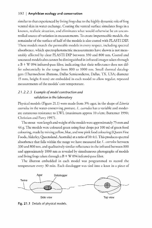
392 I Amphibian ecology and conservation
similar to that experienced by living frogs due to the highly dynamic role of frog
ventral skin in water exchange. Coating the ventral surface simulates frogs in a
known, realistic situation, and eliminates what would otherwise be an uncon
trolled source of variation in measurements. To create impermeable models, the
remainder of the surface of half of the models is also coated with PLASTI DIP.
These models match the permeable models in every respect, including spectral
absorbence, which spectrophotometric measurements have shown is not meas
urably affected by clear PLASTI DIP between 330 and 800 nm. Coated and
uncoated models also cannot be distinguished in infrared images taken through
a B + W 094 infrared-pass filter, indicating that their reflectance does not dif
fer substantially in the range from 800 to 1000 nm. Small thermal datalog
gers (Thermochron iButtons, Dallas Semicondictor, Dallas, TX, USA; diameter
15 mm, height 6 mm) are embedded in each model to allow regular, repeated
measurements of the models' core temperature.
21.2.2.3 Example of model construction and
validation in the laboratory
Physical models (Figure 21.1) were made from 3% agar, in the shape of Litoria caerulea in the water-conserving posture. L. caerulea has a variable and moder
ate cutaneous resistance to EWL (maximum approx 10 s/cm; Buttemer 1990;
Christian and Parry 1997).
The snout-vent length and weight of the models were approximately 75 mm and
44 g. The models were coloured green using four drops per 100 ml of green food
colouring, made by mixing yellow, blue, and rose pink food colouring (Queen Fine
Foods, Alderley, Queensland, Australia) at a ratio of 10:4: 1. This produces spectral
absorbence that falls within the range we have measured for L. caerulea between
330 and 800 nm, and qualitatively similar reflectance in the infrared between 800
and approximately 1000 nm as revealed by simultaneous photographs of models
and living frogs taken through a B + W 094 infrared-pass filter.
The iButton embedded in each model was programmed to record the
temperature every 30 min. Each datalogger was tied into a knot in a piece of
Agar Datalogger
Side view Top view
Fig. 21.1 Details of physical models.
21 Models in temperature and moisture studies I 393
twine, which was pegged at each end of the mold as the agar set, so that the
datalogger was suspended in the centre of the model (Figure 21.1). The free
twine remaining at each end of the models could be used to attach them to
surfaces either by using tape over the twine or by tying the twine around fea
tures such as branches and roots. We set up three opaque, white, plastic con
tainers (60 cm X 40 cm X 40 cm), each with a small water bowl in the center
and a metal fly-screen lid. The containers were housed in a constant tempera
ture room, which maintained ambient temperature between 19.5 and 21.SOC. Relative humidity fluctuated between 64 and 96% (mean 74%). A 150 Wheat
lamp was provided at one end of each container and was illuminated between
0930 and 2130 h to create a temperature gradient simulating the normal range
of temperatures available to this species. We ran four temporal replicates of the
experiment, creating a total of 12 sets of measurements of frog and model tem
peratures for comparison. Each replicate ran for 3 days.
At the start of each replicate, models were placed in each container in pairs,
with one permeable and one impermeable model. The pairs were located so
they spanned the range of thermal and light environments available in the con
tainers. Twelve adult L. caerulea (11 males and one female) were captured near
Townsville, Queensland, Australia. They ranged from 74.1 to 91.8 mm snout
vent length and 26 to 65 g body mass. Prior to experiments, they were main
tained in smaller containers at ambient temperature in the constant-temperature
room in which the experiments were carried out. Each frog was used in a single
run of the experiment.
We recorded the body temperatures offrogs five times per day (0900, 1l00,
1300,1500, and 1700 h) over the 3 days of each temporal replicate, producing 15
measurements for each individual. The first time (0900 h) was chosen because
at that time the frogs had not had access to any source of extra heat for almost
12 h, and their body temperatures should have been similar to those that would
be measured during nocturnal readings in the field. Each temporal replicate was
set up at least 60 min before the first temperature reading was taken, allowing
models and frogs to reach a thermal steady state. At each reading, cloacal tem
peratures were measured using a small, chromel-alumel K-type thermocouple
(diameter"" 1 mm) with the tip coated in plastic, attached to a digital therm
ometer (Small Pocket Thermometer model 90000, Industrial Automation,
Joondalup, Western Australia). During temperature measurement, each frog
was held by a single leg only. When temperatures were taken, the posture and
location of the individual was noted; this information was later used to deter
mine whether individuals had changed location, and to select the pair of models
that should represent the upper and lower boundaries of the thermal envelope
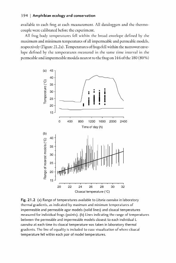
394 I Amphibian ecology and conservation
available to each frog at each measurement. All dataloggers and the thermo
couple were calibrated before the experiment.
All frog body temperatures fell within the broad envelope defined by the
maximum and minimum temperatures of all impermeable and permeable models,
respectively (Figure 21.2a). Temperatures offrogs fell within the narrower enve
lope defined by the temperatures measured in the same time interval in the
permeable and impermeable models nearest to the frog on 144 of the 180 (80%)
(a) 45
40
2: 35 OJ :; . · . · til 30 • I I CD n. I I E 25 OJ l- I • 20
15
0 400 800 1200 1600 2000 2400
Time of day (h)
(b)
2: 40
(fJ
35 (jj ""0 0 E 30 Ui OJ Co 25 OJ c "0 OJ 20 OJ c ell a:
15
20 22 24 26 28 30 32 Cloacal temperature (OC)
Fig. 21.2 (a) Range of temperatures available to Litoria caerulea in laboratory
thermal gradients, as indicated by maximum and minimum temperatures of
impermeable and permeable agar models (solid lines) and cloacal temperatures
measured for individual frogs (points). (b) Lines indicating the range of temperatures
between the permeable and impermeable models closest to each individual L.
caerulea at each time its cloacal temperature was taken in laboratory thermal
gradients. The line of equality is included to ease visualization of where cloacal
temperature fell within each pair of model temperatures.
21 Models in temperature and moisture studies I 395
occasions on which we measured frog temperatures (Figure 21.2b). As expected,
permeable models were cooler than frog body temperatures, while imperme
able models were warmer than frog body temperatures. For III of our observa
tions, frogs had changed their location since the last observation, or were being
observed for the first time. On 28 of the 36 (77.8 %) occasions when frog cloacal
temperatures were outside the envelope defined by the nearest models, frogs
had changed their location since the time of the last observation or were being
observed for the first time, and therefore might not have equilibrated thermally.
The association between changing location and being ou tside the thermal enve
lope was statistically significant (Fisher's Exact Test, two-tailed, P = 0.034). No
cloacal temperature was more than 2.6°C below or 1.2°C above the boundaries
of the envelope as defined by the nearest pair of models, and all were well within
the extremes defined by all models.
21.2.2.4 Field validation of use of models to characterize available temperatures
We tracked 27 Litoria lesueuri using radiotelemetry and harmonic radar in the
warm/wet season (19- 21 March 2005) and the cool/dry season (5- 13 August
2005) in Frenchman Creek, near Babinda, Queensland, Australia (1r20'S, 14S055'E; 20- 100 m above sea level; Rowley and Alford 2007a). Weather
conditions during both tracking periods varied considerably with respect to
ambient temperature, humidity, solar radiation, wind speed, and rainfall. Body
temperatures were recorded once during the day (between 1200 and 1600 h)
and once at night (between 1900 and 0700 h) by holding a Raytek ST80 Pro
Plus Non-contact thermometer approximately 5 cm away from the frog and
aiming at the lower dorsal area, between the thigh and point of transmitter
attachment. We have demonstrated that the temperatures we measure in this
manner accurately reflect the skin and cloacal temperatures of frogs (Rowley
and Alford 2007b). During the tracking period, we placed pairs of permeable
and impermeable models, constructed as previously described, in sites previ
ously used as diurnal retreat sites by the tracked L.lesueuri (on bare ground, leaf
litter, in vegetation, and on gravel, in exposed and sheltered positions; Rowley
and Alford 2007c; Figure 21.3). Fifteen pairs of models were deployed during
the warm/wet season, and eight pairs during the cool/dry season. The embed
ded iButtons recorded temperatures of the models every 30 min.
Models were left in the field and weighed every 24 h until at least one per
meable model had lost 50% of its original weight. Although these models were
reduced in size, they were within the range of body sizes of L. lesueuri, retained
their basic shape, and were still 94% water, and thus continued to lose water at a
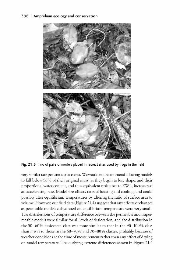
396 I Amphibian ecology and conservation
Fig. 21 .3 Two of pairs of models placed in retreat sites used by frogs in the field
very similar rate per unit surface area. We would not recommend allowing models
to fall below 50% of their original mass, as they begin to lose shape, and their
proportional water content, and thus equivalent resistance to EWL, increases at
an accelerating rate. Model size affects rates of heating and cooling, and could
possibly alter equilibrium temperatures by altering the ratio of surface area to
volume. However, our field data (Figure 21.4) suggest that any effects of changes
as permeable models dehydrated on equilibrium temperature were very small.
The distributions of temperature difference between the permeable and imper
meable models were similar for all levels of desiccation, and the distribution in
the 50- 60% desiccated class was more similar to that in the 90- 100% class
than it was to those in the 60-70% and 70-80% classes, probably because of
weather conditions at the time of measurement rather than any effect of drying
on model temperature. The outlying extreme differences shown in Figure 21.4
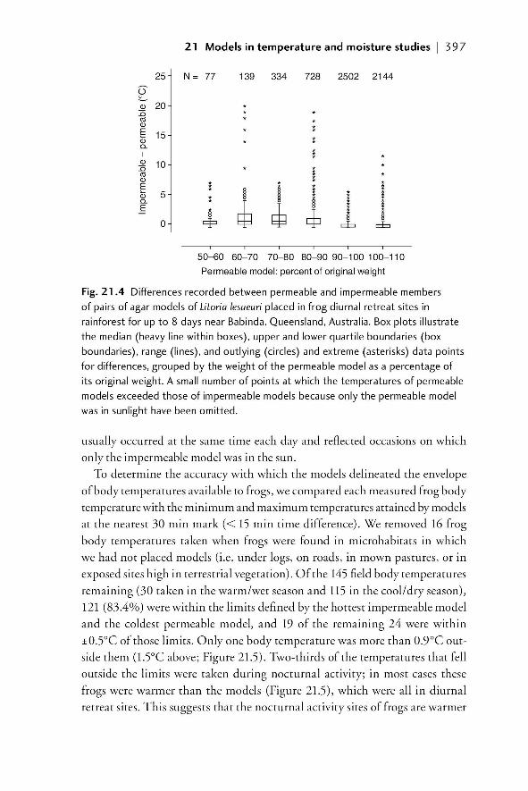
21 Models in temperature and moisture studies I 397
25 N= 77 139 334 728 2502 2144
~ OJ 20 :0 ell OJ E 15 Qj 0-I
OJ 10 :0 i ell OJ
* E ~ ~ I I Qj 5 i 0-
~ E 8 ~ ¢ 8 8 0 c:p c::b c::b
50-60 60-70 70-80 80-9090-100100-110 Permeable model: percent of original weight
Fig. 21.4 Differences recorded between permeable and impermeable members
of pairs of agar models of Litoria lesueuri placed in frog diurnal retreat sites in rainforest for up to 8 days near Babinda, Queensland, Australia. Box plots illustrate
the median (heavy line within boxes), upper and lower quartile boundaries (box boundaries), range (lines), and outlying (circles) and extreme (asterisks) data points for differences, grouped by the weight of the permeable model as a percentage of its original weight. A small number of points at which the temperatures of permeable models exceeded those of impermeable models because only the permeable model was in sunlight have been omitted.
usually occurred at the same time each day and reflected occasions on which
only the impermeable model was in the sun.
To determine the accuracy with which the models delineated the envelope
of body temperatures available to frogs, we compared each measured frog body
temperature with the minimum and maximum temperatures attained by models
at the nearest 30 min mark « 15 min time difference). We removed 16 frog
body temperatures taken when frogs were found in microhabitats in which
we had not placed models (i.e. under logs, on roads, in mown pastures, or in
exposed sites high in terrestrial vegetation). Of the 145 field body temperatures
remaining (30 taken in the warm/wet season and ll5 in the cool/dry season),
121 (83.4%) were within the limits defined by the hottest impermeable model
and the coldest permeable model, and 19 of the remaining 24 were within
±O.SOC of those limits. Only one body temperature was more than 0.9°C out
side them (lSC above; Figure 21.5). Two-thirds of the temperatures that fell
outside the limits were taken during nocturnal activity; in most cases these
frogs were warmer than the models (Figure 21.5), which were all in diurnal
retreat sites. This suggests that the nocturnal activity sites of frogs are warmer
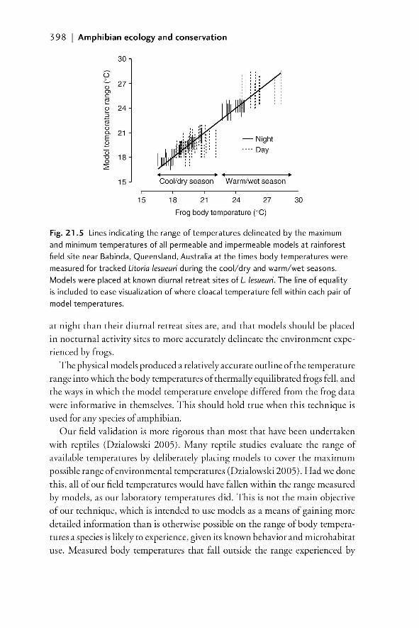
398 I Amphibian ecology and conservation
30
~ 27 OJ Ol C
~ ~ 24 OJ
co Qj D- 21 E 2 Cii
18 ""0 0 ~
15
15
-Night · ... Day
• • +1------------+ Cool/dry season Warm/wet season
18 21 24 27
Frog body temperature (0C)
30
Fig. 21.5 Lines indicating the range of temperatures delineated by the maximum and minimum temperatures of all permeable and impermeable models at rainforest field site near Babinda, Queensland, Australia at the times body temperatures were
measured for tracked Litoria lesueuri during the cool/dry and warm/wet seasons. Models were placed at known diurnal retreat sites of L lesueuri. The line of equality is included to ease visualization of where cloacal temperature fell within each pair of model temperatures.
at night than their diurnal retreat sites are, and that models should be placed
in nocturnal activity sites to more accurately delineate the environment expe
rienced by frogs.
The physical models produced a relatively accurate outline of the temperature
range into which the body temperatures of thermally equilibrated frogs fell, and
the ways in which the model temperature envelope differed from the frog data
were informative in themselves. This should hold true when this technique is
used for any species of amphibian.
Our field validation is more rigorous than most that have been undertaken
with reptiles (Dzialowski 2005). Many reptile studies evaluate the range of
available temperatures by deliberately placing models to cover the maximum
possible range of environmental temperatures (Dzialowski 2005). Had we done
this, all of our field temperatures would have fallen within the range measured
by models, as our laboratory temperatures did. This is not the main objective
of our technique, which is intended to use models as a means of gaining more
detailed information than is otherwise possible on the range of body tempera
tures a species is likely to experience, given its known behavior and microhabitat
use. Measured body temperatures that fall outside the range experienced by
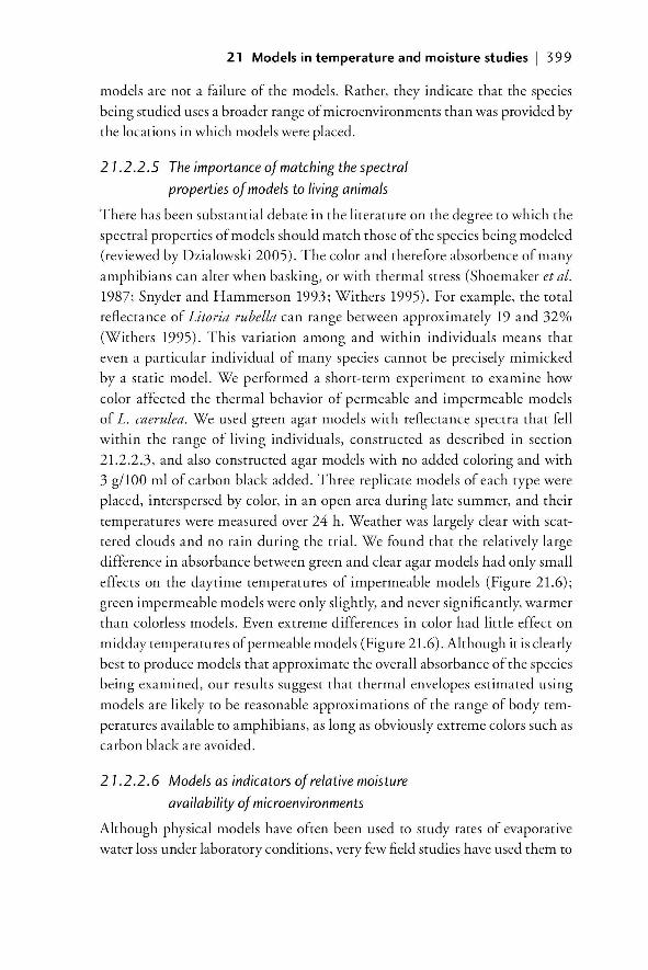
21 Models in temperature and moisture studies I 399
models are not a failure of the models. Rather, they indicate that the species
being studied uses a broader range of micro environments than was provided by
the locations in which models were placed.
21.2.2.5 The importance of matching the spectral
properties of models to living animals
There has been substantial debate in the literature on the degree to which the
spectral properties of models should match those of the species being modeled
(reviewed by Dzialowski 2005). The color and therefore absorbence of many
amphibians can alter when basking, or with thermal stress (Shoemaker et al.
1987; Snyder and Hammerson 1993; Withers 1995). For example, the total
reflectance of Litoria rubella can range between approximately 19 and 32%
(Withers 1995). This variation among and within individuals means that
even a particular individual of many species cannot be precisely mimicked
by a static model. We performed a short-term experiment to examine how
color affected the thermal behavior of permeable and impermeable models
of L. caerulea. We used green agar models with reflectance spectra that fell
within the range of living individuals, constructed as described in section
2l.2.2.3, and also constructed agar models with no added coloring and with
3 g/lOO ml of carbon black added. Three replicate models of each type were
placed, interspersed by color, in an open area during late summer, and their
temperatures were measured over 24 h. Weather was largely clear with scat
tered clouds and no rain during the trial. We found that the relatively large
difference in absorbance between green and clear agar models had only small
effects on the daytime temperatures of impermeable models (Figure 2l.6);
green impermeable models were only slightly, and never significantly, warmer
than colorless models. Even extreme differences in color had little effect on
midday temperatures of permeable models (Figure 2l.6). Although it is clearly
best to produce models that approximate the overall absorbance of the species
being examined, our results suggest that thermal envelopes estimated using
models are likely to be reasonable approximations of the range of body tem
peratures available to amphibians, as long as obviously extreme colors such as
carbon black are avoided.
21.2.2.6 Models as indicators of relative moisture
availability of microenvironments
Although physical models have often been used to study rates of evaporative
water loss under laboratory conditions, very few field studies have used them to
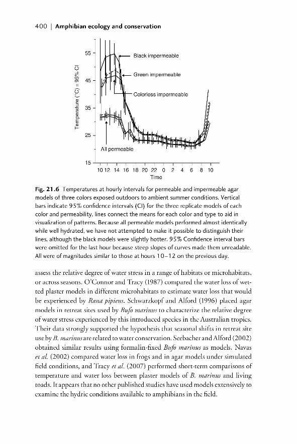
400 I Amphibian ecology and conservation
55
0 :? 0 L{)
45 (j)
+1
~ OJ :;
35 co Qj D-E OJ I-
25
Black impermeable
, +-- Green impermeable
Colorless impermeable
10 12 14 16 18 20 22 0 2 4 6 8 1 0 Time
Fig. 21.6 Temperatures at hourly intervals for permeable and impermeable agar
models of three colors exposed outdoors to ambient summer conditions. Vertical
bars indicate 95% confidence intervals (CI) for the three replicate models of each
color and permeability, lines connect the means for each color and type to aid in
visualization of patterns. Because all permeable models performed almost identically
while well hydrated, we have not attempted to make it possible to distinguish their
lines, although the black models were slightly hotter. 95% Confidence interval bars
were omitted for the last hour because steep slopes of curves made them unreadable.
All were of magnitudes similar to those at hours 1 0- 12 on the previous day.
assess the relative degree of water stress in a range of habitats or microhabitats,
or across seasons. O'Connor and Tracy (1987) compared the water loss of wet
ted plaster models in different microhabitats to estimate water loss that would
be experienced by Rana pipiens. Schwarzkopf and Alford (1996) placed agar
models in retreat sites used by Bufo marinus to characterize the relative degree
of water stress experienced by this introduced species in the Australian tropics.
Their data strongly supported the hypothesis that seasonal shifts in retreat site
use by B. marinus are related to water conservation. Seebacher and Alford (2002)
obtained similar results using formalin-fixed Bufo marin us as models. Navas
et al. (2002) compared water loss in frogs and in agar models under simulated
field conditions, and Tracy et al. (2007) performed short-term comparisons of
temperature and water loss between plaster models of B. marinus and living
toads. It appears that no other published studies have used models extensively to
examine the hydric conditions available to amphibians in the field.
21 Models in temperature and moisture studies I 401
Wet season 1.1 1.0 0 ~ e ~ 0.9 ~ (fJ
~ co- 0.8 .r:: -Ol .r:: ._ 0.7 OlOJ ·iii ;: 0.6 ;:<ii 0.5 (jj :-e
""0 c o .-Eo Dry season OJ c 1.1
- 0 ~ ~ e 8 ~
..0 .- 1.0 0 ~ ~ cot::: ~ OJ 0 0.9 E Q. 0
~ 0 0.8 OJ ~ CLQ. 0.7
0.6 0.5
0 2 4 6 8
Days since model placement
Fig. 21.7 Relative water loss by permeable agar models placed in diurnal retreat
sites of Litoria lesueuri in rainforest near Babinda, Queensland, Australia. There was
substantial cloud cover and rainfall during the winter, nominally dry season, sampling
period (top), while the summer, nominally wet season, sampling period (bottom)
was unusually dry. In both seasons, some retreat sites provided very low rates of
evaporative water loss while some led to higher rates; in the summer, one of the
models reached 50% water loss on day 4, causing data collection to cease.
Data collected using models to examine the envelope of thermal conditions
available to amphibians can also be used to delineate an envelope of relative degrees
of water stress. When agar models are used, the simplest approach is to weigh
models daily to document cumulative change in water content. If automatically
rehydrated models of other types, such as those developed by Bartelt and Peterson
(2005) or Tracy et al. (2007) are used, cumulative water lost from reservoirs can be
recorded manually or monitored automatically. Figure 21.7 presents data collected
from the models of L. lesueuri placed in the field near Babinda, Queensland, as
described in section 2l.2.2.4. These data demonstrate that although the rainforest
where the data were collected experiences annual wet and dry seasons, short-term
weather patterns can result in greater opportunity for water stress in the wet sea
son than in the dry season; this is probably compounded by the fact that the wet
season occurs in the summer months, in which diurnal temperatures can be up
to lOoe higher than in the winter dry season. They also indicate that the diurnal
retreat sites that were monitored presented a wide range of potential levels of water
stress. This is likely to affect the frogs' behavior and metabolism, and is also likely
to affect their interactions with the amphibian chytrid fungus, which may repro
duce more slowly on hosts with relatively dry skin surfaces (Pounds et al. 2006).
402 I Amphibian ecology and conservation
21.3 Summary and future developments
Models are useful for delineating the range of body temperatures and degrees of
moisture stress available to amphibians in the field. Because numerous models
can be placed in known retreat and activity sites, and temperatures and water
loss can be recorded in models at frequent intervals, they can rapidly provide
a detailed picture of the envelope of temperatures and moisture available to a
species, without requiring that individuals be handled or otherwise disturbed.
If a species is known to have zero resistance to EWL, permeable models should
be sufficient to characterize its thermal and hydric environment. However, for
species that have higher and usually variable levels of resistance to EWL, pairs
of models should be employed to delineate the boundaries of the thermal enve
lope available.
Pairs of models cannot predict the exact body temperatures of specific indi
vidual frogs. Rates of EWL can fluctuate considerably over even short periods
in individual frogs (McClanahan 1978; Withers et al. 1982; Wygoda 1989a;
Withers 1995; Barbeau and Lillywhite 2005; Tracy et al. 2008). Although many
frogs alter EWL with respect to temperature or humidity in a moderately pre
dictable manner (Withers et al. 1982; Wygoda 1989a; Buttemer and Thomas
2003), in others, EWL fluctuates unpredictably (Barbeau and Lillywhite 2005).
Because rates of EWL are so variable, measuring the limits of the envelope of
body temperatures available to a species in a given microenvironment is likely to
be more ecologically relevant to population-level questions for most species than
precise measurements for particular individuals can be.
The physical models we have described are easy to construct in large numbers,
and are also relatively inexpensive to produce, features that are highly desirable,
since to truly characterize the range of conditions available to animals in the
field it is necessary to sample a large number of locations (Dzialowski 2005).
Our models are also compact and self-contained, and can therefore be placed
in the exact shelter sites used by the study species without altering their struc
ture, which might prove difficult with models of other designs (e.g. Bartelt and
Peterson 2005; Tracy et al. 2007).
Using data obtained from models in the field in conjunction with the detailed
knowledge of temporal patterns of microhabitat use made possible by advances
in tracking technology, it will be possible to develop pictures of temporal pat
terns of body temperature experienced by frogs that are as detailed as those
that have been available for some time for many reptiles. Variation in relative
rates of water loss among sites and through time can also be determined. The
knowledge that can be gained using models is likely to be increasingly useful
21 Models in temperature and moisture studies I 403
in understanding the effects of climate change on amphibians. The majority
of predictive models forecast a near-term global temperature rise of 1.5-4.SOC (Thomas et al. 2004), and these estimates have been used in predicting species
responses (Thomas et al. 2004) despite their questionable relevance to micro
environmental conditions or body temperature (Kennedy 1997). Detailed
species-specific data, as can be obtained using models, will therefore be essen
tial for accurately predicting responses and designing management plans. This
approach is also likely to be of use in developing more sophisticated models of
energy use and growth within individuals, and thus of population dynamics,
and in understanding the factors affecting host-pathogen interactions in nature
(e.g. Woodhams eta!' 2003).
21.4 References
Bakken, G. S. and Gates, D. M. (1975). Heat-transfer analysis of animals: some implica
tions for field ecology, physiology, and evolution. In D. M. Gates and R. B. Schmer!
(eds), Perspectives in Biophysical Ecology, pp. 255-90. Springer, New York. Barbeau, T. R. and Lillywhite, H. B. (2005). Body wiping behaviors associated with
cutaneous lipids in hylid tree frogs of Florida. journal 0/ Experimental Biology, 208,
2147-56. Bartelt, P. E. and Peterson, C. R. (2005). Physically modeling operative temperatures and
evaporation rates in amphibians. journal o/Thermal Biology, 30, 93-102. Bradford, D. F. (19S4). Temperature modulation in a high-elevation amphibian, Rana
muscosa. Copeia, 1984, 966-76. Buttemer, W. A. (1990). Effect of temperature on evaporative water loss of the Australian
tree frogs Litoria caerulea and Litoria chloris. Physiological Zoology, 63, 1043-57. Buttemer, W. A. and Thomas, C. (2003). Influence of temperature on evaporative water
loss and cutaneous resistance ro water vapour diffusion in the orange-thighed frog
(Lito ria xanthomera). Australian journal o/Zoology, 51, Ill-IS. Buttemer, W. A., van der Wielen, M., Dain, S., and Christy, M. (1996). Cutaneous
properties of the Green and Golden Bell Frog Litoria aurea. Australian Z oologist, 30,
134-S. Christian, K. A. and Parry, D. (1997). Reduced rates of water loss and chemical properties
of skin secretions of the frogs Litoria caerulea and Cyclorana australis. Australian journal
o/Z oology, 45, 13-20. Dzialowski, E. M. (2005). Use of operative temperature and standard operative tempera
ture models in thermal biology. journal o/Thermal Biology, 30, 317-34. Elliot, S. L., Blanford, S., and Thomas, M. B. (2002). Host-pathogen interactions in
a varying environment: temperature, behavioural fever and fitness. Proceedings 0/ the
Royal Society o/London Series B Biological Sciences, 269, 1599-1607. Hasegawa, M., Suzuki, Y, and Wada, S. (2005). Design and performance of a wet sponge
model for amphibian thermal biology. Current Herpetology, 24, 27-32.
404 I Amphibian ecology and conservation
Kennedy, A.D. (1997). Bridging the gap between general circulation model (GCM) out
put and biological microenvironments. International journal 0/ Biometeorology, 40,
119-22.
Kobelt, F. and Linsenmair, K. E. (1992). Adaptations of the reed frog Hyperolius viridifia
vus (Amphibia: Anuta: Hyperoliidae) to its arid environment. journal o/Comparative
Physiology B, 162,314-26.
Lillywhite, H. B. (2006). Water relations of tetrapod integument. journal o/Experimental
Biology, 209, 202-26.
Lips, K. R., Brem, F., Brenes, R., Reeve,]. D., Alford, R. A., Voyles,]., Carey, c., Livo, L., Pessier, A. P., and Collins,]. P. (2006). Emerging infectious disease and the loss ofbio
diversity in a Neotropical amphibian community. Proceedings o/the NationalAcademy
o/Sciences USA, 103, 3165-70. McClanahan, L. L. (1978). Skin lipids, water loss, and energy metabolism in a South
American tree frog (Phyllomedusa sauvagei). Physiological Z oology, 51, 179-87. McClanahan, L. L. and Shoemaker, V. H. (1987). Behavior and thermal relations of the
arboreal frog Phyllomedusa sauvagei. National Geographic Research, 3, 11-21. Navas, C. A. (1996). Implications of microhabitat selection and patterns of activity on the
thermal ecology of high elevation neotropical anurans. Oecologia, 108 ,617-26.
Navas, C. A. and Araujo, C. (2000). The use of agar models to study amphibian thermal
ecology. journal o/Herpetology, 34, 330-4. Navas, C. A., Jared, c., and Antoniazzi, M. M. (2002). Water economy in the casque
headed tree-frog Corythomantis greeningi (Hylidae): role of behaviour, skin, and skull
skin co-ossification. journal o/Zoology, 257,525-32. O'Connor, M. P. and Tracy, C. R. (1987). Thermal and hydric relations ofleopard frogs
in the field. American Zoologist, 27, 118A.
Parmesan, c., Gaines, S., Gonzalez, L., Kaufman, D. M., Kingsolver,]., Peterson, A. T., and Sagarin, R. (2005). Empirical perspectives on species borders: from traditional
biogeography to global change. Oikos, 108, 58-75. Pounds, ].A. , Bustamante, M. R., Coloma, L. A., Consuegra, ]. A., Fogden, M. P. L.,
Foster, P. N., La Marca, E., Masters, K. L., Merino-Viteri, A., Puschendorf, R. et al.
(2006). Widespread amphibian extinctions from epidemic disease driven by global
warming. Nature, 439, 161 -7.
Rowley,].]. L. and Alford, R. A. (2007a). Movement patterns and habitat use of rainforest stream frogs in northern Queensland, Australia: implications for extinction vulner
ability. Wildlift Research, 34, 371-8. Rowley,].]. L. and Alford, R. A. (2007b). Non-contact infrared thermometers can accur
ately measure amphibian body temperatures. Herpetological Review, 38, 308-11. Rowley, ]. ]. L. and Alford, R. A. (2007c). Behaviour of Australian rainforest stream
frogs may affect the transmission of chytridiomycosis. Diseases 0/ Aquatic Organisms,
77,1-9.
Schmuck, R., Kobelt, F., and Linsenmair, K. E. (1988). Adaptations of the reed frog
Hyperolius viridifiavus (Amphibia, Anura, Hyperoliidae) to its arid environment:
V. Iridophores and nitrogen metabolism. journal 0/ Comparative Physiology B, 158,
537-46.
21 Models in temperature and moisture studies I 405
Schwarzkopf, L. and Alford, R. A. (1996). Desiccation and shelter-site use in a trop
ical amphibian: comparing toads with physical models. Functional Ecology, 10, 193-200.
Seebacher, F. and Alford, R. A. (2002). Shelter microhabitats determine body temperature
and dehydration rates of a terrestrial amphibian (Bufo marinus).journal of Herpetology, 36,69-75.
Shoemaker, V. H. and McClanahan, L. L. (1975). Evaporative water loss, nitrogen excre
tion and osmoregulation in phyllomedusine frogs. journal of Comparative Physiology, 100,331-45.
Shoemaker, V. H. and Nagy, K. A. (1977). Osmoregulation in amphibians and reptiles.
Annual Review of Physiology, 39, 449-71. Shoemaker, V. H., McClanahan, L. L., Withers, P. c., Hillman, S. S. , and Drewes, R. C.
(1987). Thermoregulatory response to heat in the waterprooHrogs Phyllomedusa and
Chiromantis. Physiological Zoology, 60, 365-72. Snyder, G. K. and Hammerson, G. A. (1993). Interrelationships between water econ
omy and thermoregulation in the canyon tree frog Hyla arenicolor. journal of Thermal Biology, 25, 321-9.
Spotila,]. R. and Berman, E. N. (1976). Determination of skin resistance and the role of
the skin in controlling water loss in amphibians and reptiles. Comparative Biochemistry and Physiology, 55A, 407-11.
Thomas, C. D., Cameron, A., Green, R. E., Bakkenes, M., Beaumont, L. J.,
Collingham, Y. c., Erasmus, B. F. N., de Siquera, M. F., Grainger, A., Hannah, L. etal. (2004). Extinction risk from climate change. Nature, 427, 145-8.
Toledo, R. C. and Jared, c. (1993). Cutaneous adaptations to water balance in amphib
ians. Comparative Biochemistry and Physiology, 105A, 593-608. Tracy, C. R., Christian, K. A., O'Connor, M. P., and Tracy, C. R. (1993). Behavioral
thermoregulation by Bufo americanus: the importance of the hydric environment.
Herpetologica, 49, 375-82. Tracy, C. R., Betts, G., Tracy, C. R., and Christian, K. A. (2007). Plaster models to
measure operative temperatures and evaporative water loss of amphibians. journal of Herpetology, 41,597-603.
Tracy, C. R. , Christian, K. A., Betts, G., and Tracy, C. R. (2008). Body temperature
and resistance to evaporative water loss in tropical Australian frogs. Comparative Biochemistry and Physiology, 150A, 102-8.
Withers, P. C. (1995). Evaporative water loss and colour change in the Australian desert
tree frog Lito ria rubella (Amphibia: Hylidae). Records of the WesternAustralianMuseum, 17,277-8J.
Withers, P. c., Hillman, S. S., Drewes, R. c., and Sokol, o. M. (1982). Water loss and
nitrogen excretion in Sharp-nosed Reed frogs (Hyperoliusnasutus: Anura, Hyperoliidae).
journal of Experimental Biology, 97,335-43. Woodhams, D. C.,Alford, R. A., and Marantelli, G. (2003). Emergingdiseaseofamphib
ians cured by elevated body temperature. Diseases of Aquatic Organisms, 55, 65-7. Wygoda, M. L. (1984). Lowcutaneous evaporative water loss in arboreal frogs. Physiological
Zoology, 57, 329-37.

406 I Amphibian ecology and conservation
Wygoda, M. L. (J989a). Body temperature in arboreal and non arboreal anuran amphib
ians: differential effects of a small change in water vapour density. journal of Thermal Biology, 14,239-42.
Wygoda, M. L. (J 989b). A comparative study of heating rates in arboreal and nonarboreal
frogs. journal of Herpetology, 23, 141 - 5. Young, ]. E., Christian, K. A., Donnellan, S., and Tracy, C. R. (2005). Comparative
analysis of cutaneous evaporative water loss in frogs demonstrates correlation with eco
logical habits. Physiological and Biochemical Zoology, 78, 847- 56.
23Selection of species and sampling
areas: the importance to inference
Paul Stephen Corn
23.1 Introduction
Inductive inference, the process of drawing general conclusions from specifi c observations, is fundamental to the scientifi c method. Platt (1964) termed conclusions obtained through rigorous application of the scientifi c method as “strong inference” and noted the following basic steps: generating alterna-tive hypotheses; devising experiments, the results of which will exclude one or more hypotheses; conducting the experiment to get a “clean result”; and repeating the process with revision based on the information obtained. Every student is exposed to these basics in introductory courses, and a consider-able proportion of a modern graduate education in the sciences is devoted to acquiring the analytic (statistical) skills necessary to apply the scientifi c method. Not even considering the fi eld of mathematical statistics or applied statistics in disciplines such as social sciences, library shelves groan under the weight of texts on applied statistics, ranging from introductory (Hayek and Buzas 1997) to advanced (Williams et al. 2002), for conducting research in ecology, and new works are published every year. Much effort is currently devoted to the mechanisms of analysis and the issues involved in choosing among statistical methods; specifi cally, traditional hypothesis testing versus information-theoretic or Bayesian approaches (Hobbs and Hilborn 2006). This chapter does not address these topics, but instead discusses some of the issues related to selection of study sites and species necessary to obtain a “clean result.” Regardless of the method of analysis, successful inference relies on correctly designed data collection, meaning that the observations represent the population of interest. As Anderson (2008, p. 7) puts it, valid
23_Dodd_Chap23.indd 43123_Dodd_Chap23.indd 431 8/19/2009 3:07:30 PM8/19/2009 3:07:30 PM
432 | Amphibian ecology and conservation
inference requires, “some type of probabilistic sampling of the well-defi ned population.”
Experimental design and sampling are well-developed topics in applied stat-istics. There are numerous books available (see Anderson 2001 for a sample of representative works), and many universities offer their graduate students spe-cifi c courses in these areas. Most biologists have had the requisite education and are familiar with and employ statistically valid designs. However, good study designs are not universal. Anderson (2008, p. 143) stated:
. . . there is no excuse for collecting data that are fundamentally fl awed. Still, I see data collected from convenience sampling where any valid inductive inference is precluded. In some cases the population of interest is not even defi ned.
Convenience sampling is a broad term that describes non-random study-site selection (Hayek 1994; Anderson 2001). Inadequate design and sampling is often justifi ed on logistical grounds, or, to put it more crudely, that it is unreal-istic to satisfy the demands of a statistician, who is usually offi ce-bound in an ivory tower. As a fi eld biologist and not a statistician, I sometimes fi nd myself sympathetic to such rationalizations. However, the solution is not to politely thank the statistician and then go ahead and sample as originally planned (see the fi rst phrase in the Anderson quote above). Instead, more planning is neces-sary. Either a means must be devised for obtaining a valid sample, or the pro-ject’s objectives should be revised so that a population can be defi ned that will allow a valid sample, or, in extreme cases, the project might need to be abandoned.
In this chapter, I provide a brief overview of sampling design, but this is a large, complex topic and it is impossible to do more than scratch the surface here. For more thorough instruction and discussion, including statistics spe-cifi c to different designs, consult one of the many texts that have been writ-ten for that purpose (e.g. Cochran 1977; Thompson 1992; Hayek and Buzas 1997; Williams et al. 2002). The US Geological Survey (www.pwrc.usgs.gov/monmanual/) and National Park Service (http://science.nature.nps.gov/im/monitor/) also have extensive and very useful web-based resources to aid in study design for inventory and monitoring studies. Following this introduction to sampling, I will discuss issues related to selection of study sites and effects of estimating abundance on inference. This discussion will use a few selected cases to illustrate problems that can arise from either poor study design or inter-pretation of results that cannot be supported by the design. These ex amples include issues arising from both selection of study sites and collection and ana-lysis of data from individual species, and describe some of the methods that can be used to minimize bias.
23_Dodd_Chap23.indd 43223_Dodd_Chap23.indd 432 8/19/2009 3:07:30 PM8/19/2009 3:07:30 PM
23 Selection of species and sampling areas | 433
23.2 Sampling
In all but a tiny number of exceptional cases, it is impossible to survey every possible habitat or catch every individual in a population. Therefore, inference depends on statistics generated from a subset of individuals or habitats drawn from the population. Ideally, a sample has three qualities (Williams et al. 2002): it comprises separate individual units, and these share the same underlying dis-tribution and are statistically independent. These criteria are more diffi cult to satisfy in inventory and monitoring studies than in a carefully designed experi-ment, but a good study design should try to come as close as possible.
Before a sample can be taken, the sampling units must be defi ned and be available for selection. Sample units can be individual animals, artifi cially bounded areas (quadrats), or natural habitat features, such as ponds, streams, or drainage basins. For population studies, where the individual is the sam-ple unit, the availability for selection is often assumed, but this assumption is tested when the data are analyzed. For inventory or monitoring studies, site delineation and selection has become easier with the increasing availability of tools such as satellite imagery and Geographic Information Systems (GIS) software. A good example is the study by Kroll et al. (2008), which took advan-tage of detailed GIS data layers to select stream reaches for sampling. However, detailed GIS coverage exists mainly where there is an economic use for the data (e.g. the commercial forests surrounding the streams studied by Kroll et al. 2008), and even when GIS data are available the amphibian habitats may be poorly described. Temporary wetlands are notoriously underrepresented in aquatic data layers, and studies of lentic-breeding amphibians often will have more success in defi ning sampling units if areas are used instead of specifi c habitats, for example, 1 km2 blocks (Johannson et al. 2006) or drainage basins (Corn et al. 2005).
The most basic form of probabilistic sampling is a simple random sample. All the available sample units are put into a metaphorical hat (the mechanics of choosing a sample now usually involve a computer) and the desired num-ber of units are selected in random order. The number of sample units should be suffi cient to estimate parameters of interest with suffi cient precision, but samples that are too large should be avoided. Determining the desired sample size requires knowing the variability of the parameter to be estimated, the mag-nitude of the effect to detect (e.g. a 10% difference or a 5% annual trend), and the strength of the inference. The formula for determining sample size depends on the sampling scheme. Hayak and Buzas (1997) and Williams et al. (2002) describe the details for determining sample size.
23_Dodd_Chap23.indd 43323_Dodd_Chap23.indd 433 8/19/2009 3:07:30 PM8/19/2009 3:07:30 PM
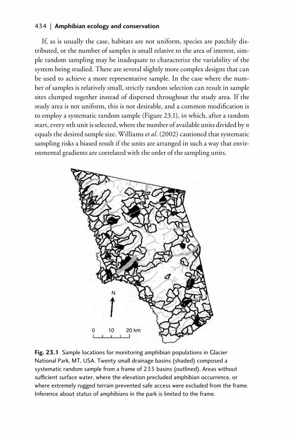
434 | Amphibian ecology and conservation
If, as is usually the case, habitats are not uniform, species are patchily dis-tributed, or the number of samples is small relative to the area of interest, sim-ple random sampling may be inadequate to characterize the variability of the system being studied. There are several slightly more complex designs that can be used to achieve a more representative sample. In the case where the num-ber of samples is relatively small, strictly random selection can result in sample sites clumped together instead of dispersed throughout the study area. If the study area is not uniform, this is not desirable, and a common modifi cation is to employ a systematic random sample (Figure 23.1), in which, after a random start, every nth unit is selected, where the number of available units divided by n equals the desired sample size. Williams et al. (2002) cautioned that systematic sampling risks a biased result if the units are arranged in such a way that envir-onmental gradients are correlated with the order of the sampling units.
0 10 20 km
N
Fig. 23.1 Sample locations for monitoring amphibian populations in Glacier National Park, MT, USA. Twenty small drainage basins (shaded) composed a systematic random sample from a frame of 235 basins (outlined). Areas without suffi cient surface water, where the elevation precluded amphibian occurrence, or where extremely rugged terrain prevented safe access were excluded from the frame. Inference about status of amphibians in the park is limited to the frame.
23_Dodd_Chap23.indd 43423_Dodd_Chap23.indd 434 8/19/2009 3:07:30 PM8/19/2009 3:07:30 PM
23 Selection of species and sampling areas | 435
If a study area is not homogenous and differences within the area can be described (e.g. altitudinal gradients, different types of wetlands, differences in ability to access potential sample units) then a stratifi ed design is usually pref-erable to a simple random or systematic random sample. Once the strata and sampling units within them are delineated, then simple or systematic random samples can be drawn from each stratum. The formulas for calculating various statistics vary among sampling designs. See Williams et al. (2002) for a concise description of these. For long-term monitoring studies, strata should be based on features that are not expected to change signifi cantly during the course of the study. For example, strata based on geological differences would be preferable to strata based on vegetative land cover.
This section is not a comprehensive treatment of sampling design. Advanced schemes, such as adaptive sampling (Thompson 1992; Williams et al. 2002), are beyond the scope of this chapter, but may be necessary or desirable in many cases. Sources listed above should be consulted when beginning the design of any study.
Any valid sampling design must incorporate replication of sample units. A study that compared toad populations in only two ponds could only describe the dif-ferences in abundance between the two ponds. Tests of hypotheses of the causes of the differences are not appropriate because there is no replication (Underwood 1998). Most inventory or monitoring studies include numerous sample units, but care must be taken to ensure that external factors are dealt with in the design stage (e.g. through stratifi cation). If variation among sample units can be attributed to something other than random processes, then the study would suffer from pseu-doreplication (Hurlbert 1984). Large fi eld studies are vulnerable to temporal pseu-doreplication (sample units vary in some systematic fashion over time), because it is seldom possible to visit all sample units simultaneously. This is a particular problem for studies of amphibians. For example, surveys that use breeding activ-ity are affected by the changing composition of breeding choruses over time, both among and within species, and external factors, such as weather, that infl uence behavior of individuals. Studies that focus on larval stages must deal with growth and development and changes in abundance that may infl uence detection. It is always a good practice to minimize the time span of fi eld surveys where possible.
23.3 Study sites and consequences of convenience sampling
If study sites or sample units are not selected using a probalistic design, the result is a convenience sample. The motivations for convenience sampling are several,
23_Dodd_Chap23.indd 43523_Dodd_Chap23.indd 435 8/19/2009 3:07:31 PM8/19/2009 3:07:31 PM
436 | Amphibian ecology and conservation
but common reasons are to choose study sites that are most accessible, or where the target species are most abundant. The latter case poses particular problems for analysis of trends in abundance, because there may be a built-in bias for detecting declining populations (Alford and Richards 1999; but see Green 2003).
The effects of convenience sampling on inference can be subtle. Results of ecological experiments are often interpreted to demonstrate the generality of effects or even causality, but experiments by themselves are insuffi cient to explain complex ecological phenomena; such an effort requires integrating observation and theory with experimentation (Werner 1998). Broad inference is limited when experiments, even those that are internally well designed, are conducted at locations that are convenient for the researcher. The results may be useful for investigating possible mechanisms, but cannot be generalized without making the unsupportable assumption that the study sites are an unbiased represen-tation of the habitats in question. For example, Blaustein et al. (1994) found that ambient ultraviolet-b (UV-B) radiation caused higher mortality of amphib-ian embryos than when embryos were shielded from UV-B at four lakes in the Cascade Mountains in Oregon, USA. This and subsequent research formed the basis of a theory of how climate change, UV-B, and pathogens might play a sig-nifi cant role in global amphibian declines (Kiesecker et al. 2001; Pounds 2001; Blaustein and Kiesecker 2002). The issue of amphibian declines and UV-B has been controversial with a large literature that I will not delve into here. Relevant to this chapter, the sites used for the UV-B studies were not chosen with respect to the potential for exposure to UV-B, but were a convenience sample. The pri-mary study site turned out to have water much more transparent to UV-B trans-mission than most amphibian breeding habitats in the Pacifi c Northwest (Palen et al. 2002), severely restricting the generality of the proposed hypothesis.
Convenience sampling is almost always done without any intention to prod-uce a biased result. The water chemistry and UV-B transmission at the study sites in the Oregon UV-B studies were not known beforehand. These sites were known to the researchers to have suitable amphibian populations and included locations where long-term studies had been conducted. Similarly, Corn and Bury’s (1989) study of the effects of logging on stream amphibians in western Oregon did not include conscious bias in selection of streams to be sampled, but it was none-the-less based on a convenience sample. In this study, Bruce Bury and I identifi ed likely sample locations on topographic maps beforehand, but the decision to sample was made in the fi eld after inspecting each stream. We attempted to select typical streams and sample reaches based on our know-ledge of the characteristics of headwater streams in the region. However, we did not begin with a well-defi ned population of streams, and we did not apply
23_Dodd_Chap23.indd 43623_Dodd_Chap23.indd 436 8/19/2009 3:07:31 PM8/19/2009 3:07:31 PM
23 Selection of species and sampling areas | 437
any probabilistic sampling. As stated by Hayek and Buzas (1997, p. 113), “If the basis for inclusion in a sample is judgment, regardless of how expert, we will not have a reproducible measure of our fi eld study’s usefulness.” Corn and Bury (1989) found strong differences in abundance and diversity of amphibians between streams in logged and unlogged forest. The paper was an early infl u-ence on what has become a spate of research on stream amphibians and forest management in the Pacifi c Northwest. Although the original results are largely supported by subsequent work (Olson et al. 2007), the convenience sampling design employed limits the scope of the conclusions and Corn and Bury (1989) should be viewed as hypothesis-generating work rather than a defi nitive demon-stration of differences between streams in managed and unmanaged forests.
Cautions about convenience sampling apply equally to the sample frame, the pool from which the sample is drawn, as to individual study sites. Study areas, meaning the regions containing the sample frames, are almost never chosen at random. Study areas may be defi ned by a relevant management question (e.g. what is the status of amphibians in a National Park?), or they might be contain habitats or species of interest, yet be located conveniently near a researcher’s institution. Probabilistic methods can be used properly to select study sites, but if the frame is defi ned by convenience, then inference is restricted to the study area and the generality of the results may be limited. Two recent studies, con-ducted less than 200 km apart in Switzerland, illustrate this point. Pellet et al. (2004) found that urbanization and roads had a strong negative infl uence on presence of European treefrogs (Hyla arborea). Conversely, Van Buskirk (2005) found only weak support for landscape variables (including urbanization) to explain occurrence and abundance of treefrogs. Both studies were well designed, and although different methods of analysis were used (logistic regression versus information theoretic analysis) the different conclusions likely resulted from intrinsic differences between the study areas.
The North American Amphibian Monitoring Program (NAAMP; Weir and Mossman 2005), patterned after the North American Breeding Bird Survey (BBS; Peterjohn et al. 1995), also suffers from a sampling frame defi ned by con-venience. NAAMP conducts manual calling surveys of breeding amphibians on prescribed road routes. Species are identifi ed by their breeding calls, and data are collected mainly by volunteers. Survey routes are generated through a random process, but the goal of the program is to monitor trends in amphib-ian populations throughout the region where routes are conducted (Weir and Mossman 2005). Reliance on roadside observations limits the inference to those areas accessed by roads, or requires investigators to make an additional, untested assumption that the roadside amphibian population experiences the
23_Dodd_Chap23.indd 43723_Dodd_Chap23.indd 437 8/19/2009 3:07:32 PM8/19/2009 3:07:32 PM
438 | Amphibian ecology and conservation
same trends in abundance as those found in populations away from roads. The biases that potentially undermine this assumption can be related to both habitat and the observations themselves (Peterjohn et al. 1995). In Chapter 16 in this volume Dorcas et al. discuss assumptions about auditory observations. Habitat assumptions require that roadside wetlands refl ect the same conditions found at wetlands away from roads, and that habitat condition changes over time in the same direction and at a similar pace alongside and away from roads. These assumptions are more likely to be violated than satisfi ed. For example, Keller and Scallan (1999) found that land cover types were similar near and away from BBS routes in Maryland and Ohio, but that in Maryland, urbanization was proceeding at a more rapid pace along roads. If urbanization is associated largely with existing road networks, then roadside habitats may diverge from distant habitats more rapidly in Maryland than in Ohio.
A more immediate and concrete difference between wetlands near and dis-tant from roads (and also a difference between amphibians and birds) is that roads, especially paved roads with higher volumes of traffi c, are a signifi -cant source of mortality of adult amphibians moving in and out of breeding ponds. Studies in North America and Europe have found negative relation-ships between traffi c intensity and amphibian mortality and breeding activity (Fahrig et al. 1995), habitat occupancy (Pellet et al. 2004), and species richness and abundance (Eigenbrod et al. 2008). Similarly in New York, Karraker et al. (2008) found a twofold increase in density of egg masses of two amphibian spe-cies away from roads compared to roadside ponds. This may have been more an indirect road effect than from direct mortality. Demographic models showed signifi cant negative effects on these species in roadside ponds resulting from the application of salt for de-icing (Karraker et al. 2008). Road de-icers epitomize a confounding variable contributing to differences that would be very diffi cult to model in analyses of NAAMP data. Application of de-icers varies among geographic regions, states, road types, and chemistry from year to year, and the data quantifying application are likely to be extremely diffi cult to obtain. The assumption that roadside habitats are equivalent to habitats away from roads is not supported by research to date.
The road studies illustrate the point that concerns about convenience sam-pling also apply to choosing variables for explaining patterns or trend. Data may be readily available in GIS data layers (e.g. road density), but less available data (e.g. traffi c intensity, de-icer application) may be more important for generating well-supported models. Anderson (2008) emphasizes that considerable effort should be devoted to generating hypotheses before data are collected; this obvi-ously applies to selection of the variables that make up the candidate models.
23_Dodd_Chap23.indd 43823_Dodd_Chap23.indd 438 8/19/2009 3:07:32 PM8/19/2009 3:07:32 PM
23 Selection of species and sampling areas | 439
23.4 Abundance and inference
Issues of inference regarding species typically arise when deciding how to quan-tify abundance or the related estimate of habitat occupancy. These are import-ant and somewhat controversial topics, and other chapters deal with estimating occupancy (Chapter 24) and abundance (Chapter 25) in detail. In this section, I focus on how uncertainty about numbers affects inference.
Studies often use an index, either simple counts of individuals observed or counts converted to relative abundance, to represent the abundance of a species (Hayek and Buzas 1997), and many standard fi eld methods (e.g. in this volume or Heyer et al. 1994) are designed to obtain counts. However, inference about trends over time or differences among habitats requires that there is no trend in the detection probability (the relationship between the index and the true abundance). Bart et al. (2004) contended that this was a reasonable assumption for bird studies. Anderson (2001) regarded this as unlikely, and recently put it even more strongly (Anderson 2008, p. 20): “. . . the evidence is conclusive that they [index values] represent an amateur, unthinking approach and is not scientifi c” and “. . . index values are not data, they are just numbers.” This viewpoint is not universal. Reliable estimation of detection probability may be diffi cult in many situations (Johnson 2008), and variation in detection probability, par-ticularly among individuals, may result in unreliable estimates of abundance (Link 2003). Nevertheless, evidence from amphibian studies tends to support the idea that use of indices should be avoided, because estimates incorporat-ing detection are more closely correlated to actual abundance than are counts (Schmidt 2004).
Welsh and Droege (2001) advocated use of count data from surveys of plethodontid salamanders to monitor forest condition and biological diversity. Terrestrial salamanders are associated with habitat features that are often dis-rupted by activities such as logging, and counts of salamanders in several studies sampled by a variety of techniques show relatively consistent numbers from year to year (Welsh and Droege 2001). Low inter-annual variation increases ability to detect trends. However, at any given time, the majority of Plethodon in a popula-tion are subterranean and unavailable to be captured (Bailey et al. 2004a), and counts of terrestrial plethodontids vary considerably among years, habitats, and sampling methods, violating many of the assumptions required for use of indi-ces in monitoring (Hyde and Simons 2001; Dodd and Dorazio 2004). More critically, temporary immigration between surface and subterranean habitats varies among sampling occasions, so that the proportion of the population avail-able to be sampled is not constant. Additionally, capture– recapture studies on
23_Dodd_Chap23.indd 43923_Dodd_Chap23.indd 439 8/19/2009 3:07:32 PM8/19/2009 3:07:32 PM
440 | Amphibian ecology and conservation
plethodontids have found low detection probabilities, often less than 0.05 (Jung et al. 2000; Welsh and Droege 2001; Dodd and Dorazio 2004). Low capture probabilities are not a problem if they are relatively uniform among habitats and observers (Welsh and Droege 2001), but there is considerable reason to doubt that this is true. Detection probabilities of plethodontids varied from 0.06 to 0.41 among years (Dodd and Dorazio 2004), and.between 0.01 and 0.58 among sampling occasions in one model evaluated by Bailey et al. (2004a). Low detection magnifi es any bias due to variation among observers, habitats, or years. For example, an increase in detection from 0.50 to 0.55 would result in a 10% increase in numbers of animals observed, but an increase from 0.06 to 0.38 would result in 6.5 times as many observations in the second count. This could produce a result similar to that illustrated in Schmidt (2004, fi gure 1), where counts were similar among years, but capture probability varied, with the result that counts did not refl ect a large increase in actual abundance.
Concerns about use of count data apply more broadly than to just terrestrial salamanders. Johannson et al. (2006) used uncorrected counts of common frog (Rana temporaria) egg masses as an index to population size, and concluded that population size declined with increasing latitude and smaller populations had less genetic variability. Johannson et al. conceded that egg mass counts likely underestimated true abundance of breeding females but contended it was an unbiased index, because sampling was the same at all study sites. However, counts often fail to detect all egg masses present in a pond for a variety of rea-sons, such as differences in habitat complexity, weather conditions that might affect visibility, or variation in ability among observers. Grant et al. (2005) found detection probabilities of ranid egg masses to vary between 0.78 and 1.0. Variation in detection introduces uncertainty into conclusions about popula-tion size; this uncertainty is magnifi ed if detection varies in a systematic manner across a study area.
Count data are incorporated into many indices of species diversity (Hayek and Buzas 1997), but calculation of these indices for amphibian assemblages are not appropriate, unless unbiased estimates of abundance are used instead of the raw counts. It has long been known that number of captures varies among sampling methods, so that a diversity index that included counts of species made using different techniques (for example, pitfall traps for one species and time-constrained searches for another) would not be valid (Corn 1994). Hyde and Simons (2001) demonstrated sampling effi ciency varied among methods, but also among habitat types for some species of plethodontids when the same method was employed. Interpretations of diversity indices suffer from the same problems as interpretations about abundance.
23_Dodd_Chap23.indd 44023_Dodd_Chap23.indd 440 8/19/2009 3:07:32 PM8/19/2009 3:07:32 PM
23 Selection of species and sampling areas | 441
The uncertainties about count data, the expense of obtaining unbiased estimates of population size, and high amount of year-to-year variation in abundance of many amphibian species prompted Green (1997) to suggest that tracking the changes in the occurrence of a species across the landscape—that is, whether or not a species occupied a given patch of habitat—was a more effi cient way to monitor status and trend of amphibians. Such presence/absence (or, more accurately, detected/not detected) data used to be considered inferior to or less scientifi c than count data (MacKenzie et al. 2003). In part, this is because surveys to detect presence are typically at a reduced level of effort than surveys that include counts, and in most situations it is impossible to prove absence even with great effort. False negatives, or failures to detect species that are actually present, introduce bias that underestimates occupancy and can lead to errors in interpretation, such as incorrectly identifying the infl uence of habitat variables on occurrence (Mazerolle et al. 2005; Hossack and Corn 2007).
Occupancy estimation (MacKenzie et al. 2006; see also Chapter 24 in this volume) has been implemented in a variety of studies of amphibians, including effects of disturbance (e.g. Mazerolle et al. 2005; Hossack and Corn 2007), in addition to more general monitoring efforts (e.g. Corn et al. 2005; Schmidt 2005). Occupancy analysis has been recommended in the US Geological Survey’s Amphibian Research and Monitoring Initiative (Muths et al. 2005), mainly through surveys for tadpoles or egg masses to indicate breeding popula-tions. Tadpoles typically have high detection probabilities (Brown et al. 2007; Hossack and Corn 2007), which increases the precision of estimated occupancy. Occupancy analysis also shows promise as a means for monitoring terrestrial salamanders. Detection probabilities for occurrence of plethodontids on small plots were much higher than capture–recapture studies have found for detec-tion of individual salamanders, and estimated occupancy was much less variable among years compared to estimated abundance (Bailey et al. 2004b).
Occupancy analysis may not be the best choice in all situations. It includes assumptions about the relationship between occurrence on the landscape and abundance of a species (Royle and Nichols 2003), although combining occu-pancy and count data is topic of active development (Royle et al. 2005; see also Chapter 24). Occupancy analysis can be diffi cult to implement in habitats that are not discrete, for example extensive wetlands. It also may not be possible to obtain reliable estimates of occupancy for rare species with low detection probabilities (Bailey et al. 2004b). A reservation about use of occupancy for detecting trends in salamanders is that local populations must go extinct or be recolonized for change to be observed. This may be a common occurrence for
23_Dodd_Chap23.indd 44123_Dodd_Chap23.indd 441 8/19/2009 3:07:32 PM8/19/2009 3:07:32 PM
442 | Amphibian ecology and conservation
pond-breeding amphibians (Green 1997), but it is less likely that populations of terrestrial salamanders undergo the same dynamics.
One fi nal note of caution: research can be well designed, but the resulting data and analysis can still be undermined if the investigators do not pay suf-fi cient attention to the biology of the organisms they are studying. Kroll et al. (2008) recently conducted a study on stream amphibians that employed a rigor-ous statistically valid design for sample selection, estimated occupancy among streams for several species, and analyzed effects on detection and occupancy using information-theoretic methods. One of their fi ndings was that detection of coastal tailed frogs (Ascaphus truei) declined as the fi eld season progressed. This was likely a consequence of the timing of sampling, which was conducted from 19 July to 6 October. Although in parts of the Pacifi c Northwest, tadpoles of A. truei require 2 or more years to reach metamorphosis, many of the streams examined by Kroll et al. are in a region where tadpoles metamorphose in less than 1 year, beginning as early as late June (Bury and Adams 1999). During the time when Kroll et al. were sampling, only adult frogs or hatchling tadpoles (which tend to remain clustered for several weeks under rocks near the nest site) would have been present in many streams. Both of these life stages are less observable than older tadpoles. Reduced detection probability results in positive bias in the occupancy estimate. Studies that employ occupancy analysis should be designed so that detection does not vary among sample units in a systematic manner.
23.5 Conclusions
The path to strong inference leads through good study design that incorporates probabilistic sampling from a well-defi ned population. Inventory and, especially, monitoring studies stray from this path when scientifi c rigor is sacrifi ced to logis-tic constraints and convenience in data collection. Tension often exists between the fi eld biologist and the consulting statistician regarding the requirements of good study design and the logistical realities of data collection. Having been on the fi eld biologist’s side of the argument, I can testify that the attitude summa-rized by “Yes, we realize valid sample selection is important, and it would be nice, but we have to collect data from the real world”, is fairly common. Constraints in site selection can be incorporated into study design, such as by stratifying based on accessibility, and the resulting analysis can test hypotheses about whether populations that are easily accessible differ from those that are not.
The perils of convenience sampling also apply to choice of life stage to study or explanatory variables to incorporate in a model. The easiest life stage to study
23_Dodd_Chap23.indd 44223_Dodd_Chap23.indd 442 8/19/2009 3:07:32 PM8/19/2009 3:07:32 PM
23 Selection of species and sampling areas | 443
may not be the same one that is most sensitive to external factors, and variables should not be included in a model simply because the data are available. There is no “magic bullet” for sampling amphibians. No single technique encompasses the variety of life histories of amphibians or the habitats in which they can be found. Occupancy analysis provides a useful tool for avoiding the pitfalls of using simple count data or the logistic diffi culties of obtaining unbiased esti-mates of abundance, but it is not a panacea. Ultimately, the design that allows the strongest inference will be one that avoids convenience sampling and min-imizes untested assumptions when the data are analyzed.
23.6 Acknowledgments
I thank Larissa Bailey, Blake Hossack, Benedikt Schmidt, and Susan Walls for suggestions that greatly improved the manuscript.
23.7 References
Alford, R. A. and Richards, S. J. (1999). Global amphibian declines: a problem in applied ecology. Annual Review of Ecology and Systematics, 30, 130–65.
Anderson, D. R. (2001). The need to get the basics right in wildlife fi eld studies. Wildlife Society Bulletin, 29, 1294–7.
Anderson, D. R. (2008). Model Based Inference in the Life Sciences: a Primer on Evidence. Springer, New York.
Bailey, L. L., Simons, T. R., and Pollock, K. H. (2004a). Estimating detection probabil-ity parameters for plethodon salamanders using the robust capture–recapture design. Journal of Wildlife Management, 68, 1–13.
Bailey, L. L., Simons, T. R., and Pollock, K. H. (2004b). Estimating site occupancy and species detection probability parameters for terrestrial salamanders. Ecological Applications, 14, 692–702.
Bart, J., Droege, S., Geissler, P., Peterjohn, B., and Ralph, C. J. (2004). Density estima-tion in wildlife surveys. Wildlife Society Bulletin, 32, 1242–7.
Blaustein, A. R. and Kiesecker, J. M. (2002). Complexity in conservation: lessons from the global decline of amphibian populations. Ecology Letters, 5, 597–608.
Blaustein, A. R., Hoffman, P. D., Hokit, D. G., Kiesecker, J. M., Walls, S. C., and Hays, J. B. (1994). UV repair and resistance to solar UV-B in amphibian eggs: a link to population declines? Proceedings of the National Academy of Sciences USA, 91, 1791–5.
Brown, G. W., Scroggie, M. P., Smith, M. J., and Steane, D. (2007). An evaluation of methods for assessing the population status of the threatened alpine tree frog Litoria verreauxii alpina in southeastern Australia. Copeia, 2007, 765–70.
Bury, R. B. and Adams, M. J. (1999). Variation in age at metamorphosis across a latitu-dinal gradient for the tailed frog, Ascaphus truei. Herpetologica, 55, 283–91.
Cochran, W. G. (1977). Sampling Techniques, 3rd edn. John Wiley & Sons, New York.
23_Dodd_Chap23.indd 44323_Dodd_Chap23.indd 443 8/19/2009 3:07:32 PM8/19/2009 3:07:32 PM
444 | Amphibian ecology and conservation
Corn, P. S. (1994). Straight-line drift fences and pitfall traps. In W. R. Heyer, M. A. Donnelly, R. W. McDiarmid, L.-A. C. Hayek, and M. S. Foster (eds), Measuring and Monitoring Biological Diversity: Standard Methods for Amphibians, pp. 109–17. Smithsonian Institution Press, Washington DC.
Corn, P. S. and Bury, R. B. (1989). Logging in western Oregon: responses of headwater habitats and stream amphibians. Forest Ecology and Management, 29, 39–57.
Corn, P. S., Hossack, B. R., Muths, E., Patla, D. A., Peterson, C. R., and Gallant, A. L. (2005). Status of amphibians on the Continental Divide: surveys on a transect from Montana to Colorado, USA. Alytes, 22, 85–94.
Dodd, Jr, C. K. and Dorazio, R. M. (2004). Using counts to simultaneously estimate abundance and detection probabilities in a salamander community. Herpetologica, 60, 468–78.
Eigenbrod, F., Hecnar, S. J., and Fahrig, L. (2008). The relative effects of road traffi c and forest cover on anuran populations. Biological Conservation, 141, 35–46.
Fahrig, L., Pedlar, J. H., Pope, S. E., Taylor, P. D., and Wegner, J. F. (1995). Effect of road traffi c on amphibian density. Biological Conservation, 73, 177–82.
Grant, E. M., Jung, R. E., Nichols, J. D. and Hines, J. E. (2005). Double-observer approach to estimating egg mass abundance of pool-breeding amphibians. Wetland Ecology and Management, 13, 305–20.
Green, D. M. (1997). Perspectives on amphibian population declines: defi ning the prob-lem and searching for answers. In D. M. Green (ed.), Amphibians in Decline: Canadian Studies of a Global Problem. Herpetological Conservation, vol. 1, pp. 291–308. Society for the Study of Amphibians and Reptiles, St. Louis, MO.
Green, D. M. (2003). The ecology of extinction: population fl uctuation and decline in amphibians. Biological Conservation, 111, 331–43.
Hayek, L.-A. C. (1994). Research design for quantitative amphibian studies. In W. R. Heyer, M. A. Donnelly, R. W. McDiarmid, L.-A. C. Hayek, and M. S. Foster (eds), Measuring and Monitoring Biological Diversity: Standard Methods for Amphibians, pp. 21–39. Smithsonian Institution Press, Washington DC.
Hayek, L.-A. C. and Buzas, M. A. (1997). Surveying Natural Populations. Columbia University Press, New York.
Heyer, W. R., Donnelly, M. A., McDiarmid, R. W., Hayek, L.-A. C., and Foster, M. S. (eds), (1994). Measuring and Monitoring Biological Diversity: Standard Methods for Amphibians. Smithsonian Institution Press, Washington DC.
Hobbs, N. T. and Hilborn, R. (2006). Alternatives to statistical hypothesis testing in ecology: a guide to self teaching. Ecological Applications, 16, 5–19.
Hossack, B. R. and Corn, P. S. (2007). Responses of pond-breeding amphibians to wildfi re: short-term patterns in occupancy and colonization. Ecological Applications, 17, 1403–10.
Hurlbert, S. N. (1984). Pseudoreplication and the design of ecological fi eld experiments. Ecological Monographs, 54, 187–211.
Hyde, E. J. and Simons, T. R. (2001). Sampling plethodontid salamanders: sources of variability. Journal of Wildlife Management, 65, 624–32.
Johannson, M., Primmer, C. R., and Merilä, U. (2006). History vs. current demography: explaining the genetic population structure of the common frog (Rana temporaria). Molecular Ecology, 15, 975–83.
23_Dodd_Chap23.indd 44423_Dodd_Chap23.indd 444 8/19/2009 3:07:32 PM8/19/2009 3:07:32 PM
23 Selection of species and sampling areas | 445
Johnson, D. H. (2008). In defense of indices: the case of bird surveys. Journal of Wildlife Management, 72, 857–68.
Jung, R. E., Droege, S., Sauer, J. R., and Landy, R. B. (2000). Evaluation of terrestrial and streamside salamander monitoring techniques at Shenandoah National Park. Environmental Monitoring and Assessment, 63, 65–79.
Karraker, N. E., Gibbs, J. P., and Vonesh, J. R. (2008). Impacts of road deicing salt on the demography of vernal pool-breeding amphibians. Ecological Applications, 18, 724–34.
Keller, C. M. E. and Scallan, J. T. (1999). Potential roadside biases due to habitat changes along Breeding Bird Survey routes. The Condor, 101, 50–7.
Kiesecker, J. M., Blaustein, A. R., and Belden, L. K. (2001). Complex causes of amphib-ian population declines. Nature, 410, 681–4.
Kroll, A. J., Risenhoover, K., McBride T., Beach E., Kernohan B. J., Light, J., and Bach, J. (2008). Factors infl uencing stream occupancy and detection probability parameters of stream-associated amphibians in commercial forests of Oregon and Washington, USA. Forest Ecology and Management, 255, 3726–35.
Link, W. A. (2003). Nonidentifi ability of population size from capture-recapture data with heterogeneous detection probabilities. Biometrica, 59, 1123–30.
MacKenzie, D. I., Nichols, J. D., Hines, J. E., Knutson, M. G., and Franklin, A. B. (2003). Estimating site occupancy, colonization, and local extinction when a species is detected imperfectly. Ecology, 84, 2200–7.
MacKenzie, D. I., Nichols, J. D., Royle, J. A., Pollock, K. H., Bailey, L. L., and Hines, J. E. (2006). Occupancy Estimation and Modeling: Inferring Patterns and Dynamics of Species Occurrence. Academic Press, Burlington, MA.
Mazerolle, M. J., Desrochers, A., and Rochefort, L. (2005). Landscape characteris-tics infl uence pond occupancy by frogs after accounting for detectability. Ecological Applications, 15, 824–34.
Muths E., Jung, R. E., Bailey, L. L., Adams, M. J., Corn, P. S., Dodd, Jr, C. K., Fellers, G. M., Sadinski, W. J., Schwalbe, C. R., Walls, S. C. et al. (2005). The U.S. Department of Interior’s Amphibian Research and Monitoring Initiative: a successful start to a national program. Applied Herpetology, 2, 355–71.
Olson, D. H., Anderson, P. D., Frissell, C. A., Welsh, Jr, H. H., and Bradford, D. F. (2007). Biodiversity management approaches for stream–riparian areas: perspectives for Pacifi c Northwest headwater forests, microclimates, and amphibians. Forest Ecology and Management, 246, 81–107.
Palen, W. J., Schindler, D. E., Adams, M. J., Pearl, C. A., Bury, R. B., and Diamond, S. A. (2002). Optical characteristics of natural waters protect amphibians from UV-B in the U. S. Pacifi c Northwest. Ecology, 83, 2951–7.
Pellet, J., Guisan, A., and Perrin, N. (2004). A concentric analysis of the impact of urban-ization on the threatened European tree frog in an agricultural landscape. Conservation Biology, 18, 1599–1606.
Peterjohn, B. G., Sauer, J. R., and Robbins, C. S. (1995). Population trends from the North American Breeding Bird Survey. In T. E. Martin and D. M. Finch (eds), Ecology and Management of Neotropical Migrants, pp. 3–39. Oxford University Press, New York.
Platt, J. R. (1964). Strong inference. Science, 146, 347–53.Pounds, J. A. (2001). Climate and amphibian declines. Nature, 410, 639–40.
23_Dodd_Chap23.indd 44523_Dodd_Chap23.indd 445 8/19/2009 3:07:32 PM8/19/2009 3:07:32 PM
446 | Amphibian ecology and conservation
Royle, J. A. and Nichols, J. D. (2003). Estimating abundance from repeated presence–absence data or point counts. Ecology, 84, 777–90.
Royle, J. A., Nichols, J. D., and Kéry, M. (2005). Modelling occurrence and abundance of species when detection is imperfect. Oikos, 110, 353–9.
Schmidt, B. R. (2004). Declining amphibian populations: the pitfalls of count data in the study of diversity, distributions, dynamics, and demography. Herpetological Journal, 14, 167–74.
Schmidt, B. R. (2005). Monitoring the distribution of pond-breeding amphibians when species are detected imperfectly. Aquatic Conservation: Marine and Freshwater Ecosystems, 15, 681–92.
Thompson, S. K. (1992). Sampling. John Wiley & Sons, New York.Underwood, A. J. (1998). Design, implementation, and analysis of ecological and envir-
onmental experiments. In W. J. Resetarits, Jr. and J. Bernardo (eds), Experimental Ecology: Issues and Perspectives, pp. 325–49. Oxford University Press, New York.
Van Buskirk, J. (2005). Local and landscape infl uence on amphibian occurrence and abundance. Ecology, 86, 1936–47.
Weir, L. A. and Mossman, M. J. (2005). North American Amphibian Monitoring Program (NAAMP). In M. Lannoo (ed.), Amphibian Declines: The Conservation Status of United States Species, pp. 307–13. University of California Press, Berkeley, CA.
Welsh, Jr, H. H. and Droege, S. (2001). A case for using plethodontid salamanders for monitoring biodiversity and ecosystem integrity of North American forests. Conservation Biology, 15, 558–69.
Werner, E. E. (1998). Ecological experiments and a research program in community ecology. In W. J. Resetarits, Jr and J. Bernardo (eds), Experimental Ecology: Issues and Perspectives, pp. 3–26. Oxford University Press, New York.
Williams, B. K., Nichols, J. D., and Conroy M. J. (2002). Analysis and Management of Animal Populations. Academic Press, San Diego, CA.
23_Dodd_Chap23.indd 44623_Dodd_Chap23.indd 446 8/19/2009 3:07:32 PM8/19/2009 3:07:32 PM
25Quantifying abundance: counts,
detection probabilities, and estimates
Benedikt R. Schmidt and Jérôme Pellet
25.1 Background: imperfect detection in amphibian ecology and conservation
Understanding temporal and spatial variation in distribution and abundance has been, and will remain, a central goal in amphibian ecology and conser-vation. Even though these two quantities, distribution and abundance, are so fundamental, we usually cannot observe them directly in the fi eld. We rarely observe all individuals, all populations, or all species in an area of interest. Imperfect detection is the rule rather than the exception and is a characteristic that all fi eld studies share.
Imperfect detection is a trivial fact and herpetologists are often aware of it. For example, Hairston and Wiley (1993) attributed all fl uctuations in sala-mander counts to variation in weather conditions (salamanders tend to remain underground during cold weather) and motivation of students (a class of highly motivated students found an exceptionally high number of salamanders). This implies that salamander detection was imperfect and, equally important, vari-able among years (Hyde and Simons 2001).
Nevertheless, imperfect detection is all too often ignored when estimating abundance or when temporal and spatial trends are analysed. In this chapter we pinpoint patterns and the consequences of imperfect detection and show how to deal with it in general (Chapter 24 introduces many of the estimators required to deal with imperfect detection). We focus on the effects of imperfect detection on population abundance estimation but we call attention to the fact that imperfect detection also affects other ecological quantities, such as distribution and species richness (e.g. Schmidt 2004; Royle and Dorazio 2006; Mazerolle et al. 2007). We focus on how the issue of imperfect detection should be incorporated into the
25_Dodd_Chap25.indd 46525_Dodd_Chap25.indd 465 8/19/2009 3:05:49 PM8/19/2009 3:05:49 PM
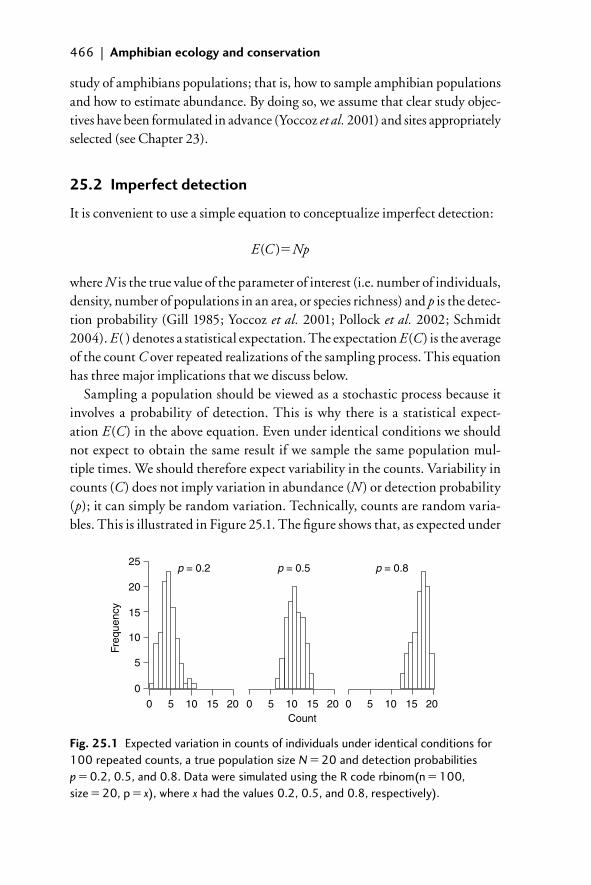
466 | Amphibian ecology and conservation
study of amphibians populations; that is, how to sample amphibian populations and how to estimate abundance. By doing so, we assume that clear study objec-tives have been formulated in advance (Yoccoz et al. 2001) and sites appropriately selected (see Chapter 23).
25.2 Imperfect detection
It is convenient to use a simple equation to conceptualize imperfect detection:
E C Np( )�
where N is the true value of the parameter of interest (i.e. number of individuals, density, number of populations in an area, or species richness) and p is the detec-tion probability (Gill 1985; Yoccoz et al. 2001; Pollock et al. 2002; Schmidt 2004). E( ) denotes a statistical expectation. The expectation E(C) is the average of the count C over repeated realizations of the sampling process. This equation has three major implications that we discuss below.
Sampling a population should be viewed as a stochastic process because it involves a probability of detection. This is why there is a statistical expect-ation E(C) in the above equation. Even under identical conditions we should not expect to obtain the same result if we sample the same population mul-tiple times. We should therefore expect variability in the counts. Variability in counts (C) does not imply variation in abundance (N ) or detection probability (p); it can simply be random variation. Technically, counts are random varia-bles. This is illustrated in Figure 25.1. The fi gure shows that, as expected under
25
20
Freq
uenc
y
15
10
5
00 5 10 15 20 0 5 10
Count
p = 0.2 p = 0.5 p = 0.8
15 20 0 5 10 15 20
Fig. 25.1 Expected variation in counts of individuals under identical conditions for 100 repeated counts, a true population size N � 20 and detection probabilities p � 0.2, 0.5, and 0.8. Data were simulated using the R code rbinom(n � 100, size � 20, p � x), where x had the values 0.2, 0.5, and 0.8, respectively).
25_Dodd_Chap25.indd 46625_Dodd_Chap25.indd 466 8/19/2009 3:05:50 PM8/19/2009 3:05:50 PM
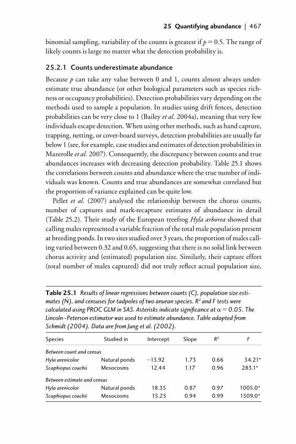
25 Quantifying abundance | 467
binomial sampling, variability of the counts is greatest if p � 0.5. The range of likely counts is large no matter what the detection probability is.
25.2.1 Counts underestimate abundance
Because p can take any value between 0 and 1, counts almost always under-estimate true abundance (or other biological parameters such as species rich-ness or occupancy probabilities). Detection probabilities vary depending on the methods used to sample a population. In studies using drift fences, detection probabilities can be very close to 1 (Bailey et al. 2004a), meaning that very few individuals escape detection. When using other methods, such as hand capture, trapping, netting, or cover-board surveys, detection probabilities are usually far below 1 (see, for example, case studies and estimates of detection probabilities in Mazerolle et al. 2007). Consequently, the discrepancy between counts and true abundances increases with decreasing detection probability. Table 25.1 shows the correlations between counts and abundance where the true number of indi-viduals was known. Counts and true abundances are somewhat correlated but the proportion of variance explained can be quite low.
Pellet et al. (2007) analysed the relationship between the chorus counts, number of captures and mark-recapture estimates of abundance in detail (Table 25.2). Their study of the European treefrog Hyla arborea showed that calling males represented a variable fraction of the total male population present at breeding ponds. In two sites studied over 3 years, the proportion of males call-ing varied between 0.32 and 0.65, suggesting that there is no solid link between chorus activity and (estimated) population size. Similarly, their capture effort (total number of males captured) did not truly refl ect actual population size,
Table 25.1 Results of linear regressions between counts (C), population size esti-mates (N), and censuses for tadpoles of two anuran species. R2 and F tests were calculated using PROC GLM in SAS. Asterisks indicate signifi cance at � � 0.05. The Lincoln–Peterson estimator was used to estimate abundance. Table adapted from Schmidt (2004). Data are from Jung et al. (2002).
Species Studied in Intercept Slope R2 F
Between count and census Hyla arenicolor Natural ponds �13.92 1.73 0.66 34.21*Scaphiopus couchii Mesocosms 12.44 1.17 0.96 283.1*
Between estimate and census Hyla arenicolor Natural ponds 18.35 0.87 0.97 1005.0* Scaphiopus couchii Mesocosms 15.25 0.94 0.99 1509.0*
25_Dodd_Chap25.indd 46725_Dodd_Chap25.indd 467 8/19/2009 3:05:50 PM8/19/2009 3:05:50 PM
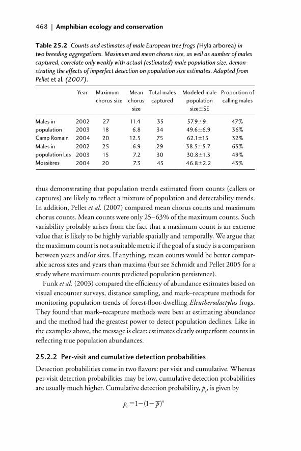
468 | Amphibian ecology and conservation
thus demonstrating that population trends estimated from counts (callers or captures) are likely to refl ect a mixture of population and detectability trends. In addition, Pellet et al. (2007) compared mean chorus counts and maximum chorus counts. Mean counts were only 25–63% of the maximum counts. Such variability probably arises from the fact that a maximum count is an extreme value that is likely to be highly variable spatially and temporally. We argue that the maximum count is not a suitable metric if the goal of a study is a comparison between years and/or sites. If anything, mean counts would be better compar-able across sites and years than maxima (but see Schmidt and Pellet 2005 for a study where maximum counts predicted population persistence).
Funk et al. (2003) compared the effi ciency of abundance estimates based on visual encounter surveys, distance sampling, and mark–recapture methods for monitoring population trends of forest-fl oor-dwelling Eleutherodactylus frogs. They found that mark–recapture methods were best at estimating abundance and the method had the greatest power to detect population declines. Like in the examples above, the message is clear: estimates clearly outperform counts in refl ecting true population abundances.
25.2.2 Per-visit and cumulative detection probabilities
Detection probabilities come in two fl avors: per visit and cumulative. Whereas per-visit detection probabilities may be low, cumulative detection probabilities are usually much higher. Cumulative detection probability, p
c, is given by
p pcn� � �1 1( )
Table 25.2 Counts and estimates of male European tree frogs (Hyla arborea) in two breeding aggregations. Maximum and mean chorus size, as well as number of males captured, correlate only weakly with actual (estimated) male population size, demon-strating the effects of imperfect detection on population size estimates. Adapted from Pellet et al. (2007).
Year Maximum chorus size
Mean chorus
size
Total males captured
Modeled male population
size�SE
Proportion of calling males
Males in population Camp Romain
2002 27 11.4 35 57.9�9 47%2003 18 6.8 34 49.6�6.9 36%2004 20 12.5 75 62.1�15 32%
Males in population Les Mossières
2002 25 6.9 29 38.5�5.7 65%2003 15 7.2 30 30.8�1.3 49%2004 20 7.3 45 46.8�2.2 43%
25_Dodd_Chap25.indd 46825_Dodd_Chap25.indd 468 8/19/2009 3:05:50 PM8/19/2009 3:05:50 PM
25 Quantifying abundance | 469
where p_ is the average per-visit detection probability and n is the number of
visits or capture events. Per-visit (i.e. per day) detection probabilities of the frog Colostethus stepheni in the study of Funk and Mills (2003) ranged from 0 to 1 with a mean of 0.58 (W.C. Funk, personal communication). Because Funk and Mills (2003) had six capture events during a short time period when the popu-lation did not change, the cumulative capture probabilities were greater than 0.987. This implies that Funk and Mills (2003) achieved an almost complete census of the frogs and suggests that multiple capture events are an obvious way to deal with imperfect detection because cumulative detection probabilities can be quite high.
25.2.3 Temporal and spatial variation in detection probabilities
Counts of animals are usually made to assess temporal or spatial variation in population size. Such comparisons are only valid if E(p) remains constant in time or space; however, this is hardly ever the case (MacKenzie and Kendall 2002), even under strictly standardized methods. If p varies temporally and/or spatially then variation in p and N are confounded. In the form of an equation, this may be expressed as
E T C C N p N p( ) / /� �1 2 1 1 2 2
Spatial or temporal variation in pi can lead to the detection of spurious temporal
or spatial trends E(T ). The contrary may also be true: one may miss true pat-terns in abundance or (under- or) overestimate the effects of variables that are thought to explain variation in abundance (Mazerolle et al. 2005). Obviously, the absolute values of p matter. If p is high, then bias will be low. If p is low, how-ever, then most variation in C is likely due to variation in p. For example, if p var-ies between 80 and 90%, then variation in C will be relatively small. However, if a low p varies by the same absolute amount, say between 10 and 20%, then variation in C will be relatively greater.
Temporal and spatial variation is the rule rather than the exception. Tacitly, Hairston and Wiley (1993) attributed variation in salamander counts entirely to variation in detection probability. In the study of Funk and Mills (2003), p varied from 0 to 1 depending on prevailing weather conditions (W.C. Funk, personal communication). Daily means (across sites) ranged from 0.43 to 0.75 and different sites had different means (across days) ranging from 0.43 to 0.90 (W.C. Funk, per-sonal communication). Most variation in detection probabilities of the European treefrog H. arborea in the study of Pellet et al. (2007) was between sites whereas Schmidt et al. (2007) found that detection probabilities of Salamandra salamandra were low in autumn and high in spring. Bailey et al. (2004a) used a drift fence to
25_Dodd_Chap25.indd 46925_Dodd_Chap25.indd 469 8/19/2009 3:05:50 PM8/19/2009 3:05:50 PM
470 | Amphibian ecology and conservation
capture salamanders (Ambystoma tigrinum) on their way to and from the pond. Detection probabilities were high in most years (greater than 90%) but inexplicably lower in one year (76%). Although detection probabilities of egg masses of Rana sylvatica and Ambystoma maculatum were generally high (usually � 80%), Grant et al. (2005) documented substantial spatial and temporal variation in detection probabilities that could bias estimates of population trends based on unadjusted counts.
25.3 Components of imperfect detection
There are many reasons why detection is imperfect and it makes sense to decom-pose detection probabilities into its components (Pollock et al. 2004; Nichols et al. 2008):
E C Npe( )�
where e is exposure to sampling (also referred to as availability for sampling). In this equation, p should best be called detection probability given exposure. Nichols et al. (2008) describe how detection probability and exposure to sam-pling can be further decomposed. Detection probability (p) and exposure to sampling (e) are easy to distinguish at the conceptual level. In practice, the dis-tinction may not always be obvious.
Under different names, exposure to sampling is a well-known phenomenon of mark–recapture studies dealing with survival estimation. The two cases are transients and temporary emigrants (Williams et al. 2002). Transients are animals that show up only once in the study area and then leave. Temporary emigrants are animals that leave the study area temporarily during the sam-pling period and then return (e.g. animals that skip a breeding season). In other words, these animals are only partly exposed to sampling and this can cause negative bias in survival estimates.
Incomplete exposure to sampling also affects abundance estimation (Kendall 1999; Bailey et al. 2004b; Royle and Dorazio 2006). Non-exposure to sam-pling can result from both biological and methodological reasons. Biological reasons include brooding salamanders that are underground and not at the sur-face during the time of survey or frogs that do not breed in a particular year and hence do not migrate to the study site which may be a breeding site (e.g. pond). Another biological reason may be that only a proportion of all males present at a pond may be calling at a particular time. This would explain why there is a difference between mean and maximum chorus counts (Pellet et al. 2007). Methodological reasons may play a part when funnel or minnow traps
25_Dodd_Chap25.indd 47025_Dodd_Chap25.indd 470 8/19/2009 3:05:51 PM8/19/2009 3:05:51 PM
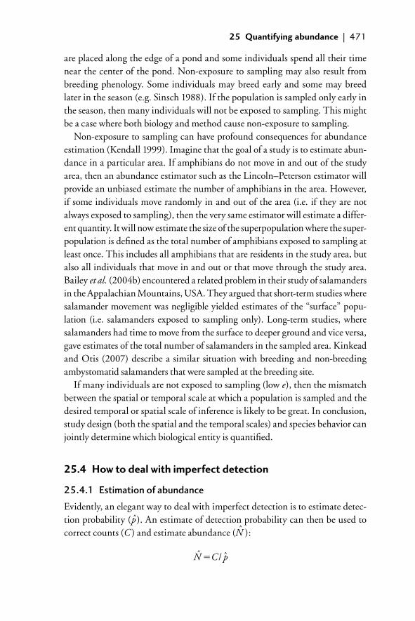
25 Quantifying abundance | 471
are placed along the edge of a pond and some individuals spend all their time near the center of the pond. Non-exposure to sampling may also result from breeding phenology. Some individuals may breed early and some may breed later in the season (e.g. Sinsch 1988). If the population is sampled only early in the season, then many individuals will not be exposed to sampling. This might be a case where both biology and method cause non-exposure to sampling.
Non-exposure to sampling can have profound consequences for abundance estimation (Kendall 1999). Imagine that the goal of a study is to estimate abun-dance in a particular area. If amphibians do not move in and out of the study area, then an abundance estimator such as the Lincoln–Peterson estimator will provide an unbiased estimate the number of amphibians in the area. However, if some individuals move randomly in and out of the area (i.e. if they are not always exposed to sampling), then the very same estimator will estimate a differ-ent quantity. It will now estimate the size of the superpopulation where the super-population is defi ned as the total number of amphibians exposed to sampling at least once. This includes all amphibians that are residents in the study area, but also all individuals that move in and out or that move through the study area. Bailey et al. (2004b) encountered a related problem in their study of salamanders in the Appalachian Mountains, USA. They argued that short-term studies where salamander movement was negligible yielded estimates of the “surface” popu-lation (i.e. salamanders exposed to sampling only). Long-term studies, where salamanders had time to move from the surface to deeper ground and vice versa, gave estimates of the total number of salamanders in the sampled area. Kinkead and Otis (2007) describe a similar situation with breeding and non-breeding ambystomatid salamanders that were sampled at the breeding site.
If many individuals are not exposed to sampling (low e), then the mismatch between the spatial or temporal scale at which a population is sampled and the desired temporal or spatial scale of inference is likely to be great. In conclusion, study design (both the spatial and the temporal scales) and species behavior can jointly determine which biological entity is quantifi ed.
25.4 How to deal with imperfect detection
25.4.1 Estimation of abundance
Evidently, an elegant way to deal with imperfect detection is to estimate detec-tion probability (p). An estimate of detection probability can then be used to correct counts (C ) and estimate abundance (N ):
ˆ / ˆN C p�
25_Dodd_Chap25.indd 47125_Dodd_Chap25.indd 471 8/19/2009 3:05:51 PM8/19/2009 3:05:51 PM
472 | Amphibian ecology and conservation
This equation is the conceptual basis for all kinds of abundance estimators, be they mark–recapture, distance sampling, point count, removal, or other meth-ods (Williams et al. 2002; Mazerolle et al. 2007; see also Chapter 24 in this volume). When non-exposure to sampling is a problem, then N can only be estimated if one knows the fraction of the population that is exposed to sam-pling as well as the probability of detecting exposed individuals, populations, or species:
ˆ / ˆ ˆN C pe�
The best tool to estimate abundance in the presence of non-exposure to sam-pling is the robust design (see Williams et al. 2002) which has been successfully used with plethodontid and ambystomatid salamanders (Bailey et al. 2004b; Kinkead and Otis 2007). The robust design allows estimating both abundance and non-exposure (known as temporary emigration in this particular case). In the previously cited case of the European treefrog (H. arborea), the robust design also allowed demonstrating that annual male temporary emigration was negligible (i.e. that males rarely skipped breeding seasons; Pellet et al. 2007). In contrast, Bailey et al. (2004a) showed that temporary emigration in A. tigrinum was substantial.
Other approaches to dealing with non-exposure were described by Royle and Dorazio (2006) and Condit et al. (2007). Royle and Dorazio (2006) describe a method for point counts that allows dealing with non-exposure to sampling that arises from a mismatch between the scale at which data was collected and the desired scale of inference. They describe a case where quadrats have only been partially searched (in that study, only a fraction of the area of 1 km2 quad-rats was surveyed). Their method works if there is a suitable covariate (such as transect length) that can statistically link the exposed population to the true population.
Condit et al. (2007) developed a method for estimating the size of a popula-tion when individuals are asynchronously present. Their method may be par-ticularly relevant for pond-breeding amphibians where the breeding season of the population is longer than the breeding season of an individual (e.g. in the natterjack toad Bufo calamita and the European treefrog H. arborea; Sinsch 1988; Friedl and Klump 2005).
Methods to estimate abundance are not without problems. Detection prob-abilities can be low. This will have the effect that confi dence intervals can be very wide (Williams et al. 2002). It is possible to make confi dence intervals shrink with more effort or better capture techniques. That is, researchers should either use better methods that increase per-visit detection probabilities or
25_Dodd_Chap25.indd 47225_Dodd_Chap25.indd 472 8/19/2009 3:05:51 PM8/19/2009 3:05:51 PM
25 Quantifying abundance | 473
increase the number of repeat visits such that cumulative detection probabilities are increased. However, standard errors and confi dence intervals are not a nuis-ance. Rather, they are an advantage of estimation methods. Standard errors and confi dence intervals are a measure of uncertainty that allow an assessment of the estimates’ reliability. Consequently, we view wide confi dence intervals as an honest statement whether a particular estimate is or is not particularly reliable and useful. Wide confi dence intervals are no reason to discard mark–recapture estimates and to prefer the simple counts (C; e.g. Alford and Richards 1999). There is also uncertainty associated with counts (because detection probability p is unknown) but it is not explicit and is, in fact, unknowable.
Heterogeneity in detection probabilities among individuals can be a problem in mark–recapture studies (Link 2003). Heterogeneity usually leads to nega-tive bias in abundance estimates and in the worst case it may not be possible to identify a best model that should be used for inference. We believe that amphib-ian ecologists and conservationists should attempt to minimize detection prob-ability heterogeneity among individuals by adopting methods that account for variation in detectability among individuals (i.e. grouping individuals into homogeneous sets by sexes, colour morphs, age classes).
25.4.2 Other approaches to dealing with imperfect detection
Amphibian ecologists have dealt with imperfect detection in many ways. Some authors simply did not analyse data from species where detection was uncertain and variable. For example, Pechmann et al. (1991) analysed data from ambysto-matid salamanders that are unlikely to trespass a drift fence but they did not analyse data from treefrogs that could easily trespass a drift fence.
The most common objection to the use of methods that allow estimating population sizes and detection probabilities instead of counts is that they are demanding in terms of money, human resources, and statistical knowledge. This argument was not true in the detailed study of Funk et al. (2003) where different methods were compared. We discard this argument because every con-servation action based on counts is likely to be biased to the point where they will be ineffi cient or, worse, counterproductive (Yoccoz et al. 2001). Moreover, it will be impossible to evaluate the success of actions taken because no data will be available to detect population trends accurately, and to adapt management actions accordingly.
Some authors have expressed the view that there is no need to estimate detec-tion probabilities and to adjust counts accordingly (i.e. estimate abundance). One argument put forward in the context of long-term monitoring programs is that variability in detection probability does not matter as long as there is no
25_Dodd_Chap25.indd 47325_Dodd_Chap25.indd 473 8/19/2009 3:05:51 PM8/19/2009 3:05:51 PM
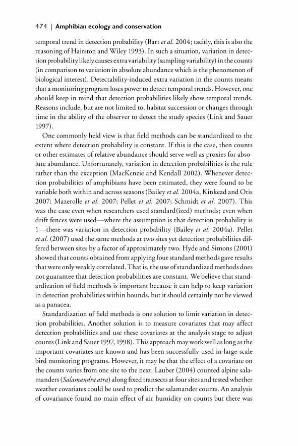
474 | Amphibian ecology and conservation
temporal trend in detection probability (Bart et al. 2004; tacitly, this is also the reasoning of Hairston and Wiley 1993). In such a situation, variation in detec-tion probability likely causes extra variability (sampling variability) in the counts (in comparison to variation in absolute abundance which is the phenomenon of biological interest). Detectability-induced extra variation in the counts means that a monitoring program loses power to detect temporal trends. However, one should keep in mind that detection probabilities likely show temporal trends. Reasons include, but are not limited to, habitat succession or changes through time in the ability of the observer to detect the study species (Link and Sauer 1997).
One commonly held view is that fi eld methods can be standardized to the extent where detection probability is constant. If this is the case, then counts or other estimates of relative abundance should serve well as proxies for abso-lute abundance. Unfortunately, variation in detection probabilities is the rule rather than the exception (MacKenzie and Kendall 2002). Whenever detec-tion probabilities of amphibians have been estimated, they were found to be variable both within and across seasons (Bailey et al. 2004a, Kinkead and Otis 2007; Mazerolle et al. 2007; Pellet et al. 2007; Schmidt et al. 2007). This was the case even when researchers used standard(ized) methods; even when drift fences were used—where the assumption is that detection probability is 1—there was variation in detection probability (Bailey et al. 2004a). Pellet et al. (2007) used the same methods at two sites yet detection probabilities dif-fered between sites by a factor of approximately two. Hyde and Simons (2001) showed that counts obtained from applying four standard methods gave results that were only weakly correlated. That is, the use of standardized methods does not guarantee that detection probabilities are constant. We believe that stand-ardization of fi eld methods is important because it can help to keep variation in detection probabilities within bounds, but it should certainly not be viewed as a panacea.
Standardization of fi eld methods is one solution to limit variation in detec-tion probabilities. Another solution is to measure covariates that may affect detection probabilities and use these covariates at the analysis stage to adjust counts (Link and Sauer 1997, 1998). This approach may work well as long as the important covariates are known and has been successfully used in large-scale bird monitoring programs. However, it may be that the effect of a covariate on the counts varies from one site to the next. Lauber (2004) counted alpine sala-manders (Salamandra atra) along fi xed transects at four sites and tested whether weather covariates could be used to predict the salamander counts. An analysis of covariance found no main effect of air humidity on counts but there was
25_Dodd_Chap25.indd 47425_Dodd_Chap25.indd 474 8/19/2009 3:05:51 PM8/19/2009 3:05:51 PM
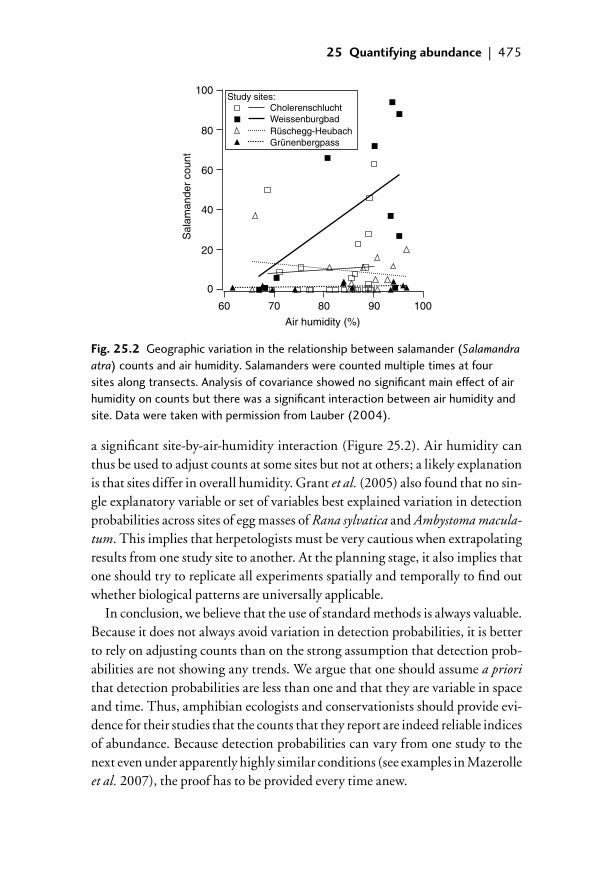
25 Quantifying abundance | 475
a signifi cant site-by-air-humidity interaction (Figure 25.2). Air humidity can thus be used to adjust counts at some sites but not at others; a likely explanation is that sites differ in overall humidity. Grant et al. (2005) also found that no sin-gle explanatory variable or set of variables best explained variation in detection probabilities across sites of egg masses of Rana sylvatica and Ambystoma macula-tum. This implies that herpetologists must be very cautious when extrapolating results from one study site to another. At the planning stage, it also implies that one should try to replicate all experiments spatially and temporally to fi nd out whether biological patterns are universally applicable.
In conclusion, we believe that the use of standard methods is always valuable. Because it does not always avoid variation in detection probabilities, it is better to rely on adjusting counts than on the strong assumption that detection prob-abilities are not showing any trends. We argue that one should assume a priori that detection probabilities are less than one and that they are variable in space and time. Thus, amphibian ecologists and conservationists should provide evi-dence for their studies that the counts that they report are indeed reliable indices of abundance. Because detection probabilities can vary from one study to the next even under apparently highly similar conditions (see examples in Mazerolle et al. 2007), the proof has to be provided every time anew.
60
Study sites:CholerenschluchtWeissenburgbadRüschegg-HeubachGrünenbergpass
100
80
60
40
Sal
aman
der
coun
t
20
0
70 80 90 100
Air humidity (%)
Fig. 25.2 Geographic variation in the relationship between salamander (Salamandra atra) counts and air humidity. Salamanders were counted multiple times at four sites along transects. Analysis of covariance showed no signifi cant main effect of air humidity on counts but there was a signifi cant interaction between air humidity and site. Data were taken with permission from Lauber (2004).
25_Dodd_Chap25.indd 47525_Dodd_Chap25.indd 475 8/19/2009 3:05:51 PM8/19/2009 3:05:51 PM
476 | Amphibian ecology and conservation
25.5 Designing a sampling protocol
The adequate design of a sampling protocol is a fundamental aspect of research, whether it be on individuals, populations, or species. Once the research or monitoring question addressed has been explicitly formalized (Yoccoz et al. 2001) and sites were appropriately selected (see Chapter 23 in this volume), it is essential that aspects of imperfect detection are incorpo-rated into the design. To do so, the procedures of data collection and data analysis must be identifi ed in advance. Having a sound knowledge of your study species’ ecology will be instrumental in determining which biological quantity (e.g. above-ground population size, breeders, super-population) your estimator will represent.
Importantly, one must be fully aware that detection probability (p) is not only a species trait (see examples in Mazerolle et al. 2007); it also depends on methods, observers, year, site, and a myriad of other factors. Because p (and exposure to sampling, e) are both variable in space and time, one can-not apply values obtained in one study to another. For these reasons we rec-ommend that detection probability is explicitly integrated in all amphibian study protocols. Non-exposure to sampling is often hard to deal with at the analysis stage (except when using the robust design). We therefore recom-mend that researchers carefully plan a study such that all animals are exposed to sampling.
25.6 Software
There are many computer programs freely available to estimate population abundance while incorporating detection probability. The most versatile and widely used of them is program MARK (White and Burnham 1999). This software, available at www.phidot.org/, allows the analysis of a wide range of capture–recapture-based data sets. Every new version incorporates the latest development in capture–recapture and thus allows the user to choose from a wide range of models the one that will fi t its data best. As the name implies, DISTANCE (www.ruwpa.st and.ac.uk/ distance/) is the software tool that allows one to design and analyse distance sampling surveys. More recent devel-opments have been integrated in statistical software such as R and WinBugs. These tools have the inconvenience of being less user-friendly than the previously listed programs, which benefi t from a graphical user interface. There is soft-ware that can be used when planning a mark–recapture study (Devineau et al. 2006; Zucchini et al. 2007).
25_Dodd_Chap25.indd 47625_Dodd_Chap25.indd 476 8/19/2009 3:05:51 PM8/19/2009 3:05:51 PM
25 Quantifying abundance | 477
25.7 Outlook
Imperfect detection is the feature that the vast majority of all amphibian surveys have in common. Complete censuses where all amphibians that are present at the study site are captured are not impossible, but require a lot of work (drift fences: Bailey et al. 2004a; many capture events: Funk and Mills 2003; Pellet et al. 2007). We argue that detection probabilities can be low and highly variable among years and/or sites. While counts that are not adjusted for imperfect detec-tion can certainly indicate negative population trends (Laurance et al. 1996), variability in imperfect detection can seriously bias inference from surveys. Amphibian ecologists and conservationists should therefore estimate detection probabilities as the best tool to calibrate a survey and use robust methods for abundance estimation (Williams et al. 2002; Chapter 24). Unfortunately, the use of such methods is not yet widespread (Alford and Richards 1999).
The number of methods available for estimation of abundance that account for imperfect detection has increased tremendously in the recent past. Existing methods are constantly being refi ned, while new methods are being developed (e.g. Royle 2004; Royle and Dorazio 2006). Still, all methods need to be used with care as sampling design, the behavior of the species, and the estimator used all determine which biological quantity is being estimated. Notwithstanding, the quality of inference from methods that adjust for imperfect detection will be stronger than inference from any other kind of method.
In the future, we ought to be able to estimate abundance with a precision and freedom from bias that was not achievable in the past. We should now be able to determine which factors infl uence abundance rather than study patterns of an inseparable combination of abundance, detectability, and exposure to sam-pling (such as counts). This will help us gain new insights into fundamental and applied aspects of amphibian ecology and conservation.
25.8 References
Alford, R. A. and Richards, S. J. (1999). Global amphibian declines: a problem in applied ecology. Annual Reviews of Ecology and Systematics, 30, 133–65.
Bailey, L. L., Kendall, W. L., Church D. R., and Wilbur, H. M. (2004a). Estimating survival and breeding probability for pond-breeding amphibians: a modifi ed robust design. Ecology, 85, 2456–66.
Bailey, L. L., Simons, T. R., and Pollock, K. H. (2004b) Comparing population size esti-mators for plethodontid salamanders. Journal of Herpetology, 38, 370–80.
Bart, J., Droege, S., Geissler, P., Peterjohn, B., and Ralph, C. J. (2004). Density estima-tion in wildlife surveys. Wildlife Society Bulletin, 32, 1242–7.
25_Dodd_Chap25.indd 47725_Dodd_Chap25.indd 477 8/19/2009 3:05:52 PM8/19/2009 3:05:52 PM
478 | Amphibian ecology and conservation
Condit, R., Le Boeuf, B. J., Morris, P. A., and Sylvan, M. (2007). Estimating population size in asynchronous aggregations: A Bayesian approach and test with elephant seal censuses. Marine Mammal Science, 23, 834–55.
Devineau, O., Choquet, R., and Lebreton, J. D. (2006). Planning capture-recapture stud-ies: straightforward precision, bias, and power calculations. Wildlife Society Bulletin, 34, 1028–35.
Friedl, T. W. P. and Klump, G. M. (2005). Sexual selection in the lek-breeding European treefrog: body size, chorus attendance, random mating and good genes. Animal Behaviour, 70, 1141–54.
Funk, W. C. and Mills, L. S. (2003). Potential causes of population declines in forest frag-ments in an Amazonian frog. Biological Conservation, 111, 205–14.
Funk, W. C., Almeida-Reinoso, D., Nogales-Sornosa, F., and Bustamante, M. R. (2003). Monitoring population trends of Eleutherodactylus frogs. Journal of Herpetology, 37, 245–56.
Gill, D. E. (1985). Interpreting breeding patterns from census data: a solution to the Husting dilemma. Ecology, 66, 344–54.
Grant, E. H. C., Jung, R. E., Nichols, J. D., and Hines, J. E. (2005). Double-observer approach to estimating egg mass abundance of pool-breeding amphibians. Wetlands Ecology and Management, 13, 305–20.
Hairston, Sr, N. G. and Wiley, R. H. (1993). No decline in salamander (Amphibia: Caudata) populations: a twenty-year study in the southern Appalachians. Brimleyana, 18, 59–64.
Hyde, E. J. and Simons, T. R. (2001). Sampling plethodontid salamanders: sources of variability. Journal of Wildlife Management, 65, 624–32.
Jung, R. E., Dayton, G. H., Williamson, S. J., Sauer, J. R., and Droege, S. (2002). An evaluation of population index and estimation techniques for tadpoles in desert pools. Journal of Herpetology, 36, 465–72.
Kendall W. L. (1999). Robustness of closed capture-recapture methods to violations of the closure assumption. Ecology, 80, 2517–25.
Kinkead, K. E. and Otis, D. L. (2007). Estimating superpopulation size and annual prob-ability of breeding for pond breeding salamanders. Herpetologica, 63, 151–62.
Lauber, A. (2004). Methodenevaluation zum Monitoring der Alpensalamanderpopulation. Diploma thesis, Eidgenössische Technische Hochschule Zürich (ETHZ), Zürich.
Laurance, W. F., McDonald, K. R., and Speare, R. (1996). Epidemic disease and the cata-strophic decline of Australian rain forest frogs. Conservation Biology, 10, 406–13.
Link, W. A. (2003). Nonidentifi ability of population size from capture-recapture data with heterogeneous detection probabilities. Biometrics, 59, 1123–30.
Link, W. A. and Sauer, J. R. (1997). Estimation of population trajectories from count data. Biometrics, 53, 488–97.
Link, W. A. and Sauer J. R. (1998). Estimating population change from count data: Application to the North American Breeding Bird Survey. Ecological Applications, 8, 258–68.
MacKenzie, D. I. and Kendall, W. L. (2002). How should detection probability be incor-porated into estimates of relative abundance? Ecology, 83, 2387–93.
Mazerolle, M. J., Desrochers, A., and Rochefort, L. (2005). Landscape characteris-tics infl uence pond occupancy by frogs after accounting for detectability. Ecological Applications, 15, 824–34.
25_Dodd_Chap25.indd 47825_Dodd_Chap25.indd 478 8/19/2009 3:05:52 PM8/19/2009 3:05:52 PM
25 Quantifying abundance | 479
Mazerolle, M. J., Bailey, L. L., Kendall, W. L., Royle, J. A., Converse, S. J., and Nichols, J. D. (2007). Making great leaps forward: accounting for detectability in herpetological fi eld studies. Journal of Herpetology, 41, 672–89.
Nichols, J. D., Thomas, L., and Conn, P. B. (2008). Inferences about landbird abun-dance from count data: recent advances and future directions. In D. L. Thomson, E. G. Cooch, G. Evan, and M. J. Conroy (eds), Modeling Demographic Processes in Marked Populations, pp. 203–38. Springer Science�Business Media, New York.
Pechmann, J. H. K., Scott, D. E., Semlitsch, R. D., Caldwell, J. P., Vitt, L. J., and Gibbons, J. W. (1991). Declining amphibian populations: the problem of separating human impacts from natural fl uctuations. Science, 253, 892–5.
Pellet, J., Helfer, V., and Yannic, G. (2007). Estimating population size in the European tree frog (Hyla arborea) using individual recognition and chorus counts. Amphibia-Reptilia, 28, 287–94.
Pollock, K. H., Nichols, J. D., Simons, T. R., Farnsworth, G. L., Bailey, L. L., and Sauer, J. R. (2002). Large scale wildlife monitoring studies: statistical methods for design and analysis. Environmetrics, 13, 105–19.
Pollock, K. H., Marsh, H., Bailey, L. L., Farnsworth, G. L., Simons, T. R., and Alldredge, M. W. (2004). Separating components of detection probability in abun-dance estimation: an overview with diverse examples. In W. L. Thompson (ed.), Sampling Rare or Elusive Species, pp. 43–58. Island Press, Washington DC.
Royle, J. A. (2004). N-mixture models for estimating population size from spatially rep-licated counts. Biometrics, 60, 108–15.
Royle, J. A. and Dorazio, R. M. (2006). Hierarchical models of animal abundance and occurrence. Journal of Agricultural, Biological, and Environmental Statistics, 11, 249–63.
Schmidt, B. R. (2004). Declining amphibian populations: the pitfalls of count data in the study of diversity, distributions, dynamics and demography. Herpetological Journal, 14, 167–74.
Schmidt, B. R. and Pellet, J. (2005). Relative importance of population processes and habitat characteristics in determining site occupancy of two anurans. Journal of Wildlife Management, 69, 884–93.
Schmidt, B. R., Schaub, M., and Steinfartz, S. (2007). Apparent survival of the sala-mander Salamandra salamandra is low because of high migratory activity. Frontiers in Zoology, 4, e19.
Sinsch, U. (1988). Temporal spacing of breeding activity in the natterjack toad, Bufo calamita. Oecologia, 76, 399–407.
White, G. C. and Burnham, K. P. (1999). Program MARK: survival estimation from populations of marked animals. Bird Study, 46, 120–38.
Williams, B. K., Nichols, J. D., and Conroy, M. J. (2002). Analysis and Management of Animal Populations. Academic Press, San Diego, CA.
Yoccoz, N. G., Nichols, J. D., and Boulinier, T. (2001). Monitoring of biological diversity in space and time. Trends in Ecology and Evolution, 16, 446–53.
Zucchini, W., Borchers, D. L., Erdelmeier, M., Rexstad, E., and Bishop, J. (2007). WiSP 1.2.4. Institut für Statistik und Ökonometrie, Georg-August-Universität Göttingen, Göttingen.
25_Dodd_Chap25.indd 47925_Dodd_Chap25.indd 479 8/19/2009 3:05:52 PM8/19/2009 3:05:52 PM
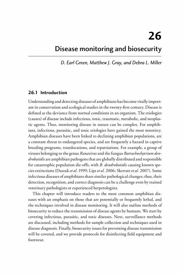
26Disease monitoring and biosecurity
D. Earl Green, Matthew J. Gray, and Debra L. Miller
26.1 Introduction
Understanding and detecting diseases of amphibians has become vitally import-ant in conservation and ecological studies in the twenty-fi rst century. Disease is defi ned as the deviance from normal conditions in an organism. The etiologies (causes) of disease include infectious, toxic, traumatic, metabolic, and neoplas-tic agents. Thus, monitoring disease in nature can be complex. For amphib-ians, infectious, parasitic, and toxic etiologies have gained the most notoriety. Amphibian diseases have been linked to declining amphibian populations, are a constant threat to endangered species, and are frequently a hazard in captive breeding programs, translocations, and repatriations. For example, a group of viruses belonging to the genus Ranavirus and the fungus Batrachochytrium den-drobatidis are amphibian pathogens that are globally distributed and responsible for catastrophic population die-offs, with B. dendrobatidis causing known spe-cies extinctions (Daszak et al. 1999; Lips et al. 2006; Skerratt et al. 2007). Some infectious diseases of amphibians share similar pathological changes; thus, their detection, recognition, and correct diagnosis can be a challenge even by trained veterinary pathologists or experienced herpetologists.
This chapter will introduce readers to the most common amphibian dis-eases with an emphasis on those that are potentially or frequently lethal, and the techniques involved in disease monitoring. It will also outline methods of biosecurity to reduce the transmission of disease agents by humans. We start by covering infectious, parasitic, and toxic diseases. Next, surveillance methods are discussed, including methods for sample collection and techniques used in disease diagnosis. Finally, biosecurity issues for preventing disease transmission will be covered, and we provide protocols for disinfecting fi eld equipment and footwear.
26_Dodd_Chap26.indd 48126_Dodd_Chap26.indd 481 8/19/2009 3:04:36 PM8/19/2009 3:04:36 PM
482 | Amphibian ecology and conservation
26.2 Amphibian diseases of concern
Amphibians are susceptible to a variety of pathogens, including internal and external parasites, viruses, bacteria, and fungi. Each of the three major life stages of amphibians (embryos, larvae, and adults) has a distinct suite of diseases, with some overlap between life stages. Aquatic amphibian embryos and larvae share many diseases with fi sh, whereas post-metamorphic stages often share few infec-tious diseases with earlier life stages. For detailed information on the amphibian diseases, we recommend that readers consult recent reviews (e.g. Converse and Green 2005a, 2005b; Green and Converse 2005a, 2005b) and the veterinary literature (e.g. Wright and Whitaker 2001).
26.2.1 Infectious diseases
Major infectious diseases for each amphibian life stage are summarized in Tables 26.1–26.3. Many viruses have been reported in amphibians, and include Ranavirus, herpesvirus, and adenovirus (Converse and Green 2005a, 2005b; Green and Converse 2005a, 2005b). Of these, Ranavirus has been the most sig-nifi cant contributor to population declines, resulting in signifi cant morbidity and mass mortality (Daszak et al. 1999; Green et al. 2002; Cunningham et al. 2007). In North America, ranaviruses are responsible for the majority of cata-strophic die-offs in ambystomid salamanders and late-stage anuran larvae, with the number of reported cases each year exceeding all other pathogens by three to four times (Green et al. 2002; Muths et al. 2006). Although many die-offs have been with common species, declines in several species of conservation concern (e.g. Rana muscosa, Rana aurora, Bufo boreas, and Ambystoma tigrinum steb-binsi) have been reported (Jancovich et al. 1997; Converse and Green 2005a). There is evidence that ranaviruses may function as a novel or endemic pathogen, with the former likely associated with the movement of infected amphibians by humans (Storfer et al. 2007). Anthropogenic stressors also may facilitate emer-gence (Forson and Storfer 2006; Gray et al. 2007a). Additionally, subclinically infected individuals (i.e. those that do not appear sick) may serve as reservoirs for more susceptible amphibian species (Brunner et al. 2004).
Likewise, numerous bacteria have been cultured from anurans (Mauel et al. 2002). Of these, Mycobacterium lifl andii, a mycolactone-producing myco-bacteria, is of concern because it is closely related to the human pathogen Mycobacterium ulcerans (Yip et al. 2007), which causes severe skin lesions in humans. Nevertheless, Aeromonas hydrophila remains the most recognized bac-terial pathogen in amphibians because of its association with red-leg disease
26_Dodd_Chap26.indd 48226_Dodd_Chap26.indd 482 8/19/2009 3:04:37 PM8/19/2009 3:04:37 PM
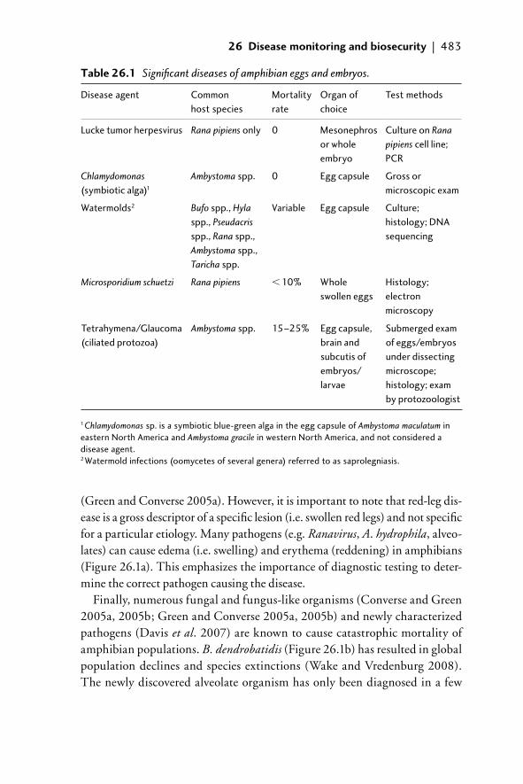
26 Disease monitoring and biosecurity | 483
Table 26.1 Signifi cant diseases of amphibian eggs and embryos.
Disease agent Common host species
Mortality rate
Organ of choice
Test methods
Lucke tumor herpesvirus Rana pipiens only 0 Mesonephros or whole embryo
Culture on Rana pipiens cell line; PCR
Chlamydomonas (symbiotic alga)1
Ambystoma spp. 0 Egg capsule Gross or microscopic exam
Watermolds2 Bufo spp., Hyla spp., Pseudacris spp., Rana spp., Ambystoma spp., Taricha spp.
Variable Egg capsule Culture; histology; DNA sequencing
Microsporidium schuetzi Rana pipiens 10% Whole swollen eggs
Histology; electron microscopy
Tetrahymena/Glaucoma (ciliated protozoa)
Ambystoma spp. 15–25% Egg capsule, brain and subcutis of embryos/larvae
Submerged exam of eggs/embryos under dissecting microscope; histology; exam by protozoologist
1 Chlamydomonas sp. is a symbiotic blue-green alga in the egg capsule of Ambystoma maculatum in eastern North America and Ambystoma gracile in western North America, and not considered a disease agent.2 Watermold infections (oomycetes of several genera) referred to as saprolegniasis.
(Green and Converse 2005a). However, it is important to note that red-leg dis-ease is a gross descriptor of a specifi c lesion (i.e. swollen red legs) and not specifi c for a particular etiology. Many pathogens (e.g. Ranavirus, A. hydrophila, alveo-lates) can cause edema (i.e. swelling) and erythema (reddening) in amphibians (Figure 26.1a). This emphasizes the importance of diagnostic testing to deter-mine the correct pathogen causing the disease.
Finally, numerous fungal and fungus-like organisms (Converse and Green 2005a, 2005b; Green and Converse 2005a, 2005b) and newly characterized pathogens (Davis et al. 2007) are known to cause catastrophic mortality of amphibian populations. B. dendrobatidis (Figure 26.1b) has resulted in global population declines and species extinctions (Wake and Vredenburg 2008). The newly discovered alveolate organism has only been diagnosed in a few
26_Dodd_Chap26.indd 48326_Dodd_Chap26.indd 483 8/19/2009 3:04:37 PM8/19/2009 3:04:37 PM
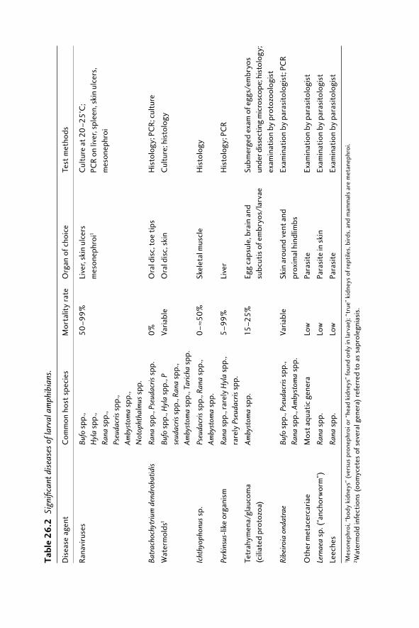
Tab
le 2
6.2
Sig
nifi c
ant d
isea
ses o
f lar
val a
mph
ibia
ns.
Dis
ease
age
ntC
omm
on h
ost
spec
ies
Mor
talit
y ra
teO
rgan
of c
hoic
eTe
st m
etho
ds
Rana
viru
ses
Bufo
spp
.,H
yla
spp.
,Ra
na s
pp.,
Pseu
dacr
is sp
p.,
Amby
stom
a sp
p.,
Not
opht
halm
us s
pp.
50–9
9%
Live
r, sk
in u
lcer
sm
eson
ephr
oi1
Cul
ture
at 2
0–2
5°C
;PC
R on
live
r, sp
leen
, ski
n ul
cers
, m
eson
ephr
oi
Batr
acho
chyt
rium
den
drob
atid
isRa
na s
pp.,
Pseu
dacr
is sp
p.0
%O
ral d
isc,
toe
tips
His
tolo
gy; P
CR;
cul
ture
Wat
erm
olds
1Bu
fo s
pp.,
Hyl
a sp
p., P
seud
acris
spp
., Ra
na s
pp.,
Amby
stom
a sp
p., T
aric
ha s
pp.
Varia
ble
Ora
l dis
c, s
kin
Cul
ture
; his
tolo
gy
Icht
hyop
honu
s sp.
Pseu
dacr
is sp
p., R
ana
spp.
, Am
byst
oma
spp.
0–
≈50
%Sk
elet
al m
uscl
eH
isto
logy
Perk
insu
s-lik
e or
gani
smRa
na s
pp.,
rare
ly H
yla
spp.
, ra
rely
Pse
udac
ris s
pp.
5–9
9%
Live
rH
isto
logy
; PC
R
Tetr
ahym
ena/
glau
com
a (c
iliat
ed p
roto
zoa)
Amby
stom
a sp
p.15
–25%
Egg
caps
ule,
bra
in a
nd
subc
utis
of e
mbr
yos/
larv
aeSu
bmer
ged
exam
of e
ggs/
embr
yos
unde
r diss
ectin
g m
icro
scop
e; h
istol
ogy;
ex
amin
atio
n by
pro
tozo
olog
ist
Ribe
iroia
ond
atra
eBu
fo s
pp.,
Pseu
dacr
is sp
p.,
Rana
spp
., Am
byst
oma
spp.
Varia
ble
Skin
aro
und
vent
and
pr
oxim
al h
indl
imbs
Exam
inat
ion
by p
aras
itolo
gist
; PC
R
Oth
er m
etac
erca
riae
Mos
t aqu
atic
gen
era
Low
Para
site
Exam
inat
ion
by p
aras
itolo
gist
Lern
aea
sp. (
“anc
horw
orm
”)Ra
na s
pp.
Low
Para
site
in s
kin
Exam
inat
ion
by p
aras
itolo
gist
Leec
hes
Rana
spp
.Lo
wPa
rasi
teEx
amin
atio
n by
par
asito
logi
st
1 Mes
onep
hroi
, “bo
dy k
idne
ys”
(ver
sus
pron
ephr
oi o
r “he
ad k
idne
ys”
foun
d on
ly in
larv
ae);
“tru
e” k
idne
ys o
f rep
tile
s, b
irds,
and
mam
mal
s ar
e m
etan
ephr
oi.
2W
ater
mol
d in
fect
ions
(oo
myc
etes
of s
ever
al g
ener
a) r
efer
red
to a
s sa
prol
egni
asis
.
26_Dodd_Chap26.indd 48426_Dodd_Chap26.indd 484 8/19/2009 3:04:37 PM8/19/2009 3:04:37 PM
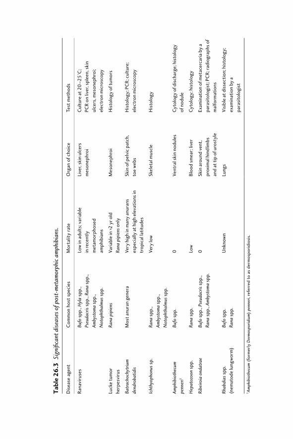
Tab
le 2
6.3
Sig
nifi c
ant d
isea
ses o
f pos
t-m
etam
orph
ic a
mph
ibia
ns.
Dis
ease
age
ntC
omm
on h
ost
spec
ies
Mor
talit
y ra
teO
rgan
of c
hoic
eTe
st m
etho
ds
Rana
viru
ses
Bufo
spp
., H
yla
spp.
, Ps
euda
cris
spp.
, Ran
a sp
p.,
Amby
stom
a sp
p.,
Not
opht
halm
us s
pp.
Low
in a
dult
s; v
aria
ble
in re
cent
ly
met
amor
phos
ed
amph
ibia
ns
Live
r, sk
in u
lcer
sm
eson
ephr
oiC
ultu
re a
t 20
–25°
C;
PCR
on li
ver,
sple
en, s
kin
ulce
rs, m
eson
ephr
oi;
elec
tron
mic
rosc
opy
Luck
e tu
mor
he
rpes
viru
sRa
na p
ipie
nsVa
riabl
e in
>2 y
r old
Ra
na p
ipie
ns o
nly
Mes
onep
hroi
His
tolo
gy o
f tum
ors
Batr
acho
chyt
rium
de
ndro
batid
isM
ost a
nura
n ge
nera
Very
hig
h in
man
y an
uran
s es
peci
ally
at h
igh
elev
atio
ns in
tr
opic
al la
titu
des
Skin
of p
elvi
c pa
tch,
to
e w
ebs
His
tolo
gy; P
CR;
cul
ture
; el
ectr
on m
icro
scop
y
Icht
hyop
honu
s sp.
Rana
spp
., Am
byst
oma
spp.
, N
otop
htha
lmus
spp
.
Very
low
Skel
etal
mus
cle
His
tolo
gy
Amph
ibio
thec
um
penn
eri1
Bufo
spp
.0
Vent
ral s
kin
nodu
les
Cyt
olog
y of
dis
char
ge; h
isto
logy
of
nod
ule
Hep
atoz
oon
spp.
Rana
spp
.Lo
wBl
ood
smea
r; li
ver
Cyt
olog
y; h
isto
logy
Ribe
iroia
ond
atra
eBu
fo s
pp.,
Pseu
dacr
is sp
p.,
Rana
spp
., Am
byst
oma
spp.
0Sk
in a
roun
d ve
nt,
prox
imal
hin
dlim
bs
and
at ti
p of
uro
styl
e
Exam
inat
ion
of m
etac
erca
ria b
y a
para
sito
logi
st; P
CR;
radi
ogra
phs
of
mal
form
atio
ns
Rhab
dias
spp
. (n
emat
ode
lung
wor
m)
Bufo
spp
.Ra
na s
pp.
Unk
now
nLu
ngs
Visi
ble
at d
isse
ctio
n; h
isto
logy
; ex
amin
atio
n by
a
para
sito
logi
st
1Am
phib
ioth
ecum
(fo
rmer
ly D
erm
ospo
ridiu
m)
penn
eri,
refe
rred
to
as d
erm
ospo
ridi
osis
.
26_Dodd_Chap26.indd 48526_Dodd_Chap26.indd 485 8/19/2009 3:04:37 PM8/19/2009 3:04:37 PM
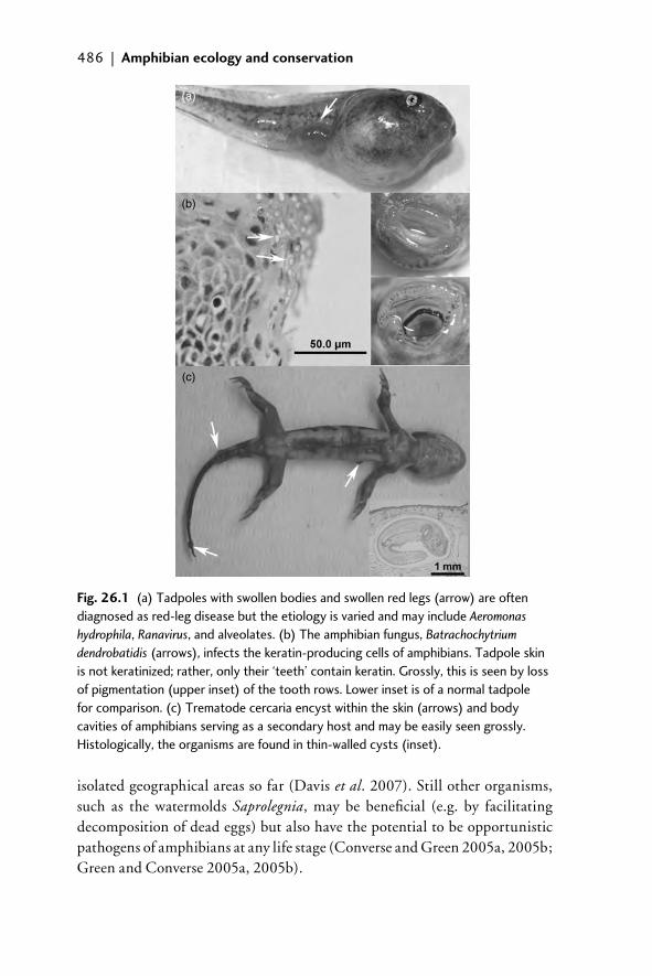
486 | Amphibian ecology and conservation
isolated geographical areas so far (Davis et al. 2007). Still other organisms, such as the watermolds Saprolegnia, may be benefi cial (e.g. by facilitating decomposition of dead eggs) but also have the potential to be opportunistic pathogens of amphibians at any life stage (Converse and Green 2005a, 2005b; Green and Converse 2005a, 2005b).
(a)
(b)
(c)
Fig. 26.1 (a) Tadpoles with swollen bodies and swollen red legs (arrow) are often diagnosed as red-leg disease but the etiology is varied and may include Aeromonas hydrophila, Ranavirus, and alveolates. (b) The amphibian fungus, Batrachochytrium dendrobatidis (arrows), infects the keratin-producing cells of amphibians. Tadpole skin is not keratinized; rather, only their ‘teeth’ contain keratin. Grossly, this is seen by loss of pigmentation (upper inset) of the tooth rows. Lower inset is of a normal tadpole for comparison. (c) Trematode cercaria encyst within the skin (arrows) and body cavities of amphibians serving as a secondary host and may be easily seen grossly. Histologically, the organisms are found in thin-walled cysts (inset).
26_Dodd_Chap26.indd 48626_Dodd_Chap26.indd 486 8/19/2009 3:04:37 PM8/19/2009 3:04:37 PM
26 Disease monitoring and biosecurity | 487
26.2.2 Parasitic diseases
As with any species, parasites are commonly found on and in amphibians (Figure 26.1c). External parasites include leaches, anchorworms, and mites, whereas internal parasites include various trematodes, cestodes, nematodes, and protozoa (Converse and Green 2005a, 2005b; Green and Converse 2005b; Wright and Whitaker 2001). Many species of helminthes (trematodes, ces-todes, nematodes) have been documented in amphibians, and often they are considered incidental (Miller et al. 2004), but their presence may be an indi-cator of stress or aquatic food-web restructuring related to human land use (Johnson and Lunde 2005; Gray et al. 2007b). Likewise, many protozoans (e.g. myxozoa) are often considered incidental fi ndings but their numbers may increase when amphibians are stressed, and they may potentially contribute to morbidity.
26.2.3 Toxins
Contaminants in the environment may kill larvae or post-metamorphs (Relyea 2005, 2009), and may have non-lethal impacts including reducing growth, impacting metamorphosis, disrupting gonadal development and secondary sex characteristics, or causing musculoskeletal, skin, and visceral malformations (Boone and Bridges 2003; Davidson et al. 2007; Ouellet et al. 1997; Storrs and Semlitsch 2008). Often these changes are not detected by external exami-nations until metamorphosis is complete or until the animals attain a size for reproduction. Amphibians are often considered sentinels or bio-indicators of environmental quality because they are sensitive to toxins and many species have the potential to be exposed to stressors in aquatic and terrestrial systems due to their typical biphasic life cycle (Blaustein and Wake 1995).
26.3 Disease monitoring: detection and diagnosis
26.3.1 Disease surveillance
Recently, the World Animal Health Organization (the OIE; www.oie.int/eng/en_index.htm) included two amphibian diseases (chytridiomycosis and rana-viral disease) on their listing of reportable diseases. The OIE listing provides the impetus for disease surveillance and required testing of amphibians prior to transport among states or between nations. The need for required testing of amphibians for pathogens has been expressed by several researchers (Gray et al. 2007a; Griffi ths and Pavajeau 2008; Picco and Collins 2008). Historically, pre- transport pathogen testing and health certifi cation for amphibians has
26_Dodd_Chap26.indd 48726_Dodd_Chap26.indd 487 8/19/2009 3:04:41 PM8/19/2009 3:04:41 PM
488 | Amphibian ecology and conservation
been essentially non-existent, unlike for domestic livestock and pets and some wild mammals (e.g. cervids). The OIE has established guidelines for surveillance and requirements necessary for countries to declare Ranavirus- free status (www.oie.int/eng/norms/fcode/en_chapitre_2.4.2.htm#rubrique_ranavirus) and B. dendrobatidis-free status (www.oie.int/eng/normes/fcode/en_chapitre_2.4.1.htm#rubrique_batrachochytrium_dendrobatidis). The OIE-approved methods for conducting surveillance and diagnosis of infection are in development. In the meantime, guidelines from the 2006 OIE Manual of Diagnostic Tests for Aquatic Animals (www.oie.int/ eng/normes/fmanual/A_summry.htm) and from the fi sheries industry (USFWS and AFS-FHS 2005) can be helpful for general monitoring of amphibian population health. In gen-eral, the criteria of a population health assessment should include (1) determin-ation of the status and trends of amphibian pathogens, (2) determination of the risk of disease for threatened or endangered amphibians, (3) investigation of unexplained population declines, (4) evaluation of populations following a morbidity or mortality event, (5) detection of pathogens in non-indigenous spe-cies, (6) evaluation of a site or population prior to translocation, (7) evaluation of sympatric amphibians prior to release of captive-raised animals, and (8) the potential for amphibians and their diseases to “piggy back” with fi sh translocation.
Disease testing should not focus on one pathogen. For surveillance programs, we recommend that animals are tested for infection by at least the OIE patho-gens: ranaviruses and B. dendrobatidis. For diagnosis of morbid or dead individ-uals, we encourage a full diagnostic work-up (i.e. necropsy, histology, bacterial culture, virus testing, and parasite testing) to attempt to identify all etiologic agents. It is important to note that simultaneous infection by multiple patho-gens is possible. Further, histological examination of organs often is required to determine which of the pathogens identifi ed are causing the changes responsible for the diseased state (Miller et al. 2008, 2009). Histological examination is also important in discovering introduced pathogens or pathogens that have not been described previously (Longcore et al. 1999; Davis et al. 2007).
Population health assessments can include non-lethal or lethal collection of tissue samples from individual amphibians (Greer and Collins 2007), and col-lection of environmental samples (e.g. water, soil; Walker et al. 2007). Ideally, we recommend that tissue samples are collected from all species in a community and from pre- and post-metamorphic life stages. Amphibian species differ in sus-ceptibility to pathogens, and some age classes may serve as a reservoir (e.g. larval for B. dendrobatidis and adults for Ranavirus; Daszak et al. 1999; Brunner et al. 2004; Schock et al. 2008). Further, some infectious diseases become evident only after the post-metamorph has overwintered (e.g. Lucke tumor herpesvirus, Amphibiothecum (formerly Dermosporidium) penneri). The lack of gross signs
26_Dodd_Chap26.indd 48826_Dodd_Chap26.indd 488 8/19/2009 3:04:41 PM8/19/2009 3:04:41 PM
26 Disease monitoring and biosecurity | 489
of disease also does not imply healthy populations. We and others have found tadpoles with no signs of illness but that are infected with ranaviruses (Gray et al. 2007a; Harp and Petranka 2006; Miller et al. 2009). Laboratory studies have demonstrated that amphibian pathogen infection and mortality rates frequently track each other (e.g. Brunner et al. 2007); thus, high prevalence in a population could signal that a die-off is imminent.
In some cases, it may not be possible to collect suffi cient tissue for dis-ease testing. For example, small amphibians (e.g. Bufo larvae) may not have adequate tissue for tests, especially for toxicological analysis. Also, non-lethal testing may be required because a species is listed as a conservation concern. We found that testing for Ranavirus from tail clips results in about 20% false-negatives (D. L. Miller and M. J. Gray, unpublished results). In cases when a small amount of tissue is collected, multiple individuals within a species could be pooled to acquire suffi cient tissue for testing. If contaminants are suspected as the cause of a die-off, we also recommend collecting and testing water and sediment at the amphibian breeding site.
Monitoring for malformations can be challenging, because typically mal-formed individuals have low survival. Although amphibian malformations have been documented for many years (Rostand, 1958), an increase in mal-formation rates occurred in the late twentieth century (Johnson and Lunde 2005). Generally, malformation studies have targeted recently metamorphosed amphibians (Meteyer et al. 2000), because metamorphs with prominent abnor-malities are quickly removed from the population by predation or starvation. Additionally, the bony skeleton of metamorphosed amphibians is more con-ducive for radiographically visualizing deformities compared to the cartilagin-ous skeleton of larvae. However, monitoring of larval abnormalities is needed because it is likely that some abnormalities prevent metamorphosis, thus are not detected in post-metamorphic cohorts.
Finally, comprehensive disease surveillance should include captive amphib-ians in zoological and ranaculture facilities, because disease transmission can occur between captive and free-ranging populations. Maintenance of health in zoological facilities is especially important for rare species or in captive breeding populations intended for release. High densities in ranaculture facil-ities, pet shops, and stores that sell amphibians (e.g. Ambystoma tigrinum) for fi shing bait can be cauldrons for disease transmission and pathogen evolution (Picco and Collins 2008). Ranaviruses isolated from ranaculture facilities and bait shops appear to be more virulent than wild strains (Majji et al. 2006; Storfer et al. 2007). This emphasizes the importance for disease monitoring at facilities with captive amphibians. In the event of a die-off in a captive facil-ity, freshly dead animals should be submitted for diagnostic evaluation. Live
26_Dodd_Chap26.indd 48926_Dodd_Chap26.indd 489 8/19/2009 3:04:41 PM8/19/2009 3:04:41 PM
490 | Amphibian ecology and conservation
animals that are infected should be euthanized or treated if a treatment exists (discussed in section 26.4.3), and facilities decontaminated with bleach or an equivalent disinfectant (discussed in section 26.4.2).
26.3.2 Sample size
Determination of statistically appropriate sample sizes for amphibian disease surveillance remains in its infancy. Although not established for amphibians, health assessment of fi sh is based on the minimum assumed pathogen preva-lence level (APPL). The commonly used APPLs in aquatic health investiga-tions are 2, 5, and 10% (Lavilla-Pitogo and de la Pena 2004; USFWS and AFS-FHS 2005). The APPL is used with an estimate of amphibian population size to determine the number of individuals that should be tested to have 95% confi dence in pathogen detection. If it is assumed that APPL is 10%, required sample size ranges from 20 to 30 depending on the size of the amphibian popu-lation (Table 26.4). Required sample size increases with decreasing APPL (Table 26.4). Unpublished fi ndings of the US Geological Survey National Wildlife Health Center suggest that APPL for ranaviruses, B. dendrobatidis, and alveolates is 10% or less (Table 26.5). In Tennessee, USA, health moni-toring of two common anuran species inhabiting farm ponds revealed 29% prevalence for Ranavirus, 0% for B. dendrobatidis and alveolates, and 43% for parasites (Miller et al., 2009). Ranavirus prevalence in plethodontid salaman-ders in the southern Appalachian Mountains can range from 3 to 81% depend-ing on the watershed (M. J. Gray and D. L. Miller, unpublished results). Thus, we recommend that biologists determine required sample sizes for amphibian disease monitoring using either 5 or 10% APPL (Table 26.4).
26.3.3 Sample collection and shipment
Sample collection may include whole live animals, dead animals, sections of tissues, swabs of lesions or orifi ces, environmental samples, or sympatric spe-cies. It is important to wear disposable gloves when handling amphibians and to change gloves between animals. This is necessary to prevent disease transmis-sion between amphibians and to protect biologists from zoonotic diseases (dis-cussed in section 26.4). Gutleb et al. (2001) and Cashins et al. (2008) reported that disposable gloves (especially latex gloves) may be toxic to amphibian larvae. Therefore, when handling amphibians, biologists and researchers should use disposable vinyl gloves that have been rinsed with distilled or sterilized water (Cashins et al. 2008).
Mortality events involving all amphibian species should be investigated, even if it is not part of a disease surveillance program. There is a paucity of information
26_Dodd_Chap26.indd 49026_Dodd_Chap26.indd 490 8/19/2009 3:04:41 PM8/19/2009 3:04:41 PM
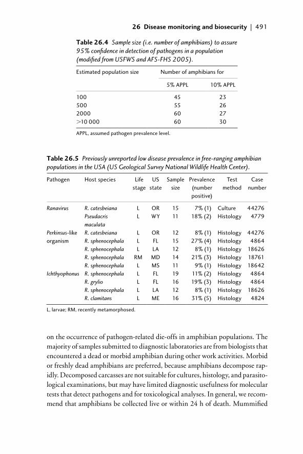
26 Disease monitoring and biosecurity | 491
Table 26.4 Sample size (i.e. number of amphibians) to assure 95% confi dence in detection of pathogens in a population (modifi ed from USFWS and AFS-FHS 2005).
Estimated population size Number of amphibians for
5% APPL 10% APPL
100 45 23500 55 262000 60 27�10 000 60 30
APPL, assumed pathogen prevalence level.
Table 26.5 Previously unreported low disease prevalence in free-ranging amphibian populations in the USA (US Geological Survey National Wildlife Health Center).
Pathogen Host species Life stage
US state
Sample size
Prevalence (number positive)
Test method
Case number
Ranavirus R. catesbeiana L OR 15 7% (1) Culture 44276Pseudacris maculata
L WY 11 18% (2) Histology 4779
Perkinsus-like organism
R. catesbeiana L OR 12 8% (1) Histology 44276R. sphenocephala L FL 15 27% (4) Histology 4864R. sphenocephala L LA 12 8% (1) Histology 18626R. sphenocephala RM MD 14 21% (3) Histology 18761R. sphenocephala L MS 11 9% (1) Histology 18642
Ichthyophonus R. sphenocephala L FL 19 11% (2) Histology 4864R. grylio L FL 16 19% (3) Histology 4864R. sphenocephala L LA 12 8% (1) Histology 18626R. clamitans L ME 16 31% (5) Histology 4824
L, larvae; RM, recently metamorphosed.
on the occurrence of pathogen-related die-offs in amphibian populations. The majority of samples submitted to diagnostic laboratories are from biologists that encountered a dead or morbid amphibian during other work activities. Morbid or freshly dead amphibians are preferred, because amphibians decompose rap-idly. Decomposed carcasses are not suitable for cultures, histology, and parasito-logical examinations, but may have limited diagnostic usefulness for molecular tests that detect pathogens and for toxicological analyses. In general, we recom-mend that amphibians be collected live or within 24 h of death. Mummifi ed
26_Dodd_Chap26.indd 49126_Dodd_Chap26.indd 491 8/19/2009 3:04:41 PM8/19/2009 3:04:41 PM
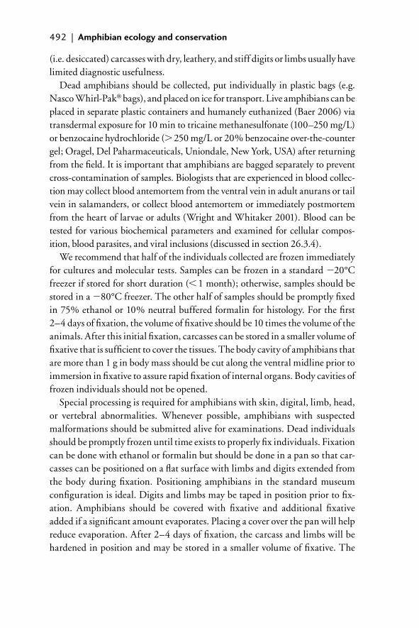
492 | Amphibian ecology and conservation
(i.e. desiccated) carcasses with dry, leathery, and stiff digits or limbs usually have limited diagnostic usefulness.
Dead amphibians should be collected, put individually in plastic bags (e.g. Nasco Whirl-Pak® bags), and placed on ice for transport. Live amphibians can be placed in separate plastic containers and humanely euthanized (Baer 2006) via transdermal exposure for 10 min to tricaine methanesulfonate (100–250 mg/L) or benzocaine hydrochloride (� 250 mg/L or 20% benzocaine over-the-counter gel; Oragel, Del Paharmaceuticals, Uniondale, New York, USA) after returning from the fi eld. It is important that amphibians are bagged separately to prevent cross-contamination of samples. Biologists that are experienced in blood collec-tion may collect blood antemortem from the ventral vein in adult anurans or tail vein in salamanders, or collect blood antemortem or immediately postmortem from the heart of larvae or adults (Wright and Whitaker 2001). Blood can be tested for various biochemical parameters and examined for cellular compos-ition, blood parasites, and viral inclusions (discussed in section 26.3.4).
We recommend that half of the individuals collected are frozen immediately for cultures and molecular tests. Samples can be frozen in a standard �20°C freezer if stored for short duration ( 1 month); otherwise, samples should be stored in a �80°C freezer. The other half of samples should be promptly fi xed in 75% ethanol or 10% neutral buffered formalin for histology. For the fi rst 2–4 days of fi xation, the volume of fi xative should be 10 times the volume of the animals. After this initial fi xation, carcasses can be stored in a smaller volume of fi xative that is suffi cient to cover the tissues. The body cavity of amphibians that are more than 1 g in body mass should be cut along the ventral midline prior to immersion in fi xative to assure rapid fi xation of internal organs. Body cavities of frozen individuals should not be opened.
Special processing is required for amphibians with skin, digital, limb, head, or vertebral abnormalities. Whenever possible, amphibians with suspected malformations should be submitted alive for examinations. Dead individuals should be promptly frozen until time exists to properly fi x individuals. Fixation can be done with ethanol or formalin but should be done in a pan so that car-casses can be positioned on a fl at surface with limbs and digits extended from the body during fi xation. Positioning amphibians in the standard museum confi guration is ideal. Digits and limbs may be taped in position prior to fi x-ation. Amphibians should be covered with fi xative and additional fi xative added if a signifi cant amount evaporates. Placing a cover over the pan will help reduce evaporation. After 2–4 days of fi xation, the carcass and limbs will be hardened in position and may be stored in a smaller volume of fi xative. The
26_Dodd_Chap26.indd 49226_Dodd_Chap26.indd 492 8/19/2009 3:04:41 PM8/19/2009 3:04:41 PM
26 Disease monitoring and biosecurity | 493
positioning described above is necessary for radiographic examination of the malformation.
Given that it often is not possible to obtain collection permits for threat-ened amphibians, alternative sampling may be necessary. Two alternatives are (1) capture–release studies and (2) collection of “sentinel” sympatric amphibian species. Capture–release studies can be used to collect swabs of external tissues, blood, or fecal samples. Swabs appear to be a reliable tech-nique to test for B. dendrobatidis (Kriger et al. 2006); however for ranaviruses, false-positive and -negative test results are greater than for tail clips and both of these non-lethal techniques have more false results than testing internal organs (D. L. Miller and M. J. Gray, unpublished results). Swabs are typ-ically performed in the oral then cloacal regions, and the swab stored in its packaging container or a microcentrifuge tube. Swabs should be put on ice and frozen similar to tissues. An accepted protocol for swabbing amphibians for B. dendrobatidis testing using PCR (discussed in section 26.3.4) has been reported by Brem et al. (2007) and can be found at www.amphibianark.org/chytrid.htm. Briefl y, the amphibian should be gently but fi rmly swabbed in a sweeping motion fi ve times at each of the following fi ve locations (for a total of 25 times): rear feet (toe webbing), inner thighs, and ventral abdomen. Occasionally, modifi cations to this technique are necessary for salamanders (Brem et al. 2007). Swabs for B. dendrobatidis testing by PCR may be stored in 70% ethanol. Collecting common sympatric species for health assessment can provide insight into the presence of amphibian pathogens at a site, but does not allow for direct health assessment of the species of concern, which may differ in susceptibility.
Shipment of live, freshly dead, or frozen specimens must be via an overnight courier and according to the specifi c courier guidelines. For fi xed specimens, overnight shipment is unnecessary. General guidelines for shipment include tri-ple packaging and labeling each layer of packaging with a waterproof writing utensil. Commonly, the fi rst package layer is a specimen in a Whirl-Pak® bag. The second layer is a larger sealable plastic bag in which multiple specimens are placed. If the fi rst package layer contains liquid (e.g. ethanol), paper towel should be added to the second package to absorb any liquid if a spill occurs. The third package typically is a padded box or shipping cooler. For frozen specimens, adequate ice packs or dry ice should be added around the secondary package. It is vital that the package contains a detailed list of all contents, a description of requested services, and the contact information of the shipper. The tracking information should be provided to the recipient prior to package arrival.
26_Dodd_Chap26.indd 49326_Dodd_Chap26.indd 493 8/19/2009 3:04:41 PM8/19/2009 3:04:41 PM
494 | Amphibian ecology and conservation
26.3.4 Diagnostics
Several tools are available for diagnosing amphibian diseases but generally require some level of specialized expertise to perform. Commonly used diagnos-tic tools include necropsy, histology, cytology, bacterial culture, virus isolation, fecal fl oatation, electron microscopy, molecular modalities, and radiology. Most of these tests can be performed on samples collected from dead or live amphib-ians. Fresh or frozen tissues can be used for most tests, and are necessary for virus isolation. Frozen tissues are not appropriate for histology or cytology; rather, preserved tissues are used. Although formalin-fi xed specimens are preferred for histological examination, ethanol-fi xed specimens may also be used. Blood can be used for cell counts to assess immune function and to look for inclusion bod-ies that can be diagnostic for certain pathogens. Blood also may be tested for the presence of antibody response to various diseases. Examples of laboratories that currently test for amphibian diseases in Australia, New Zealand, Europe, and the USA include Australian Animal Health Laboratories (AAHL), Geelong, Victoria, Australia (www.csiro.au/places/aahl.html), Gribbles Veterinary Pathology, Australia and New Zealand (www.gribblesvets.com/), Exomed, Berlin, Germany (www.exomed.de/), Hohenheim University (R. Marschang), Stuttgart, Germany, Wildlife Epidemiology, Zoological Society of London (ZSL), London, UK, The University of Georgia Veterinary Diagnostic and Investigational Laboratory, Tifton, GA, USA (www.vet.uga.edu/dlab/tifton/index.php), University of Florida (J. Wellehan), College of Veterinary Medicine, Gainesville, FL, USA, and National Wildlife Health Center, Madison, WI, USA (www.nwhc.usgs.gov/).
There are advantages and disadvantages to the various tests available (Table 26.6). Necropsy allows for identifi cation and documentation of exter-nal and internal gross changes. Histological and cytological examination allows for identifi cation of changes at the cellular level and is generally neces-sary to document disease versus infection. Virus isolation is the process of culturing a virus which is necessary to determine the presence of live virus and to perform some molecular tests used in identifying viral species (e.g. sodium dodecyl sulphate/polyacrylamide-gel electrophoresis (SDS/PAGE) and restriction fragment length polymorphism (RFLP)). One caveat is that some viruses are diffi cult to culture, thus infection cannot be ruled out based solely on negative isolation results. Electron microscopy is used for identify-ing key features of parasites or other infectious agents (e.g. B. dendrobatidis, Ranavirus, herpesvirus), documenting intracellular changes or changes to the cellular surface, and confi rmation of cultured virus. Electron microscopy can be performed on fresh, fi xed, or paraffi n-embedded tissues. Radiology allows
26_Dodd_Chap26.indd 49426_Dodd_Chap26.indd 494 8/19/2009 3:04:41 PM8/19/2009 3:04:41 PM
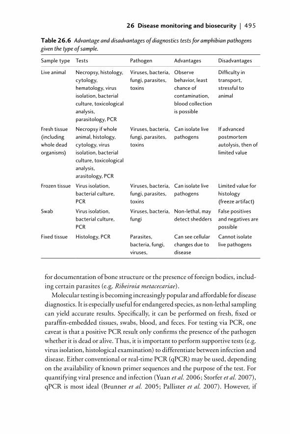
26 Disease monitoring and biosecurity | 495
for documentation of bone structure or the presence of foreign bodies, includ-ing certain parasites (e.g. Ribeiroia metacecariae).
Molecular testing is becoming increasingly popular and affordable for disease diagnostics. It is especially useful for endangered species, as non-lethal sampling can yield accurate results. Specifi cally, it can be performed on fresh, fi xed or paraffi n-embedded tissues, swabs, blood, and feces. For testing via PCR, one caveat is that a positive PCR result only confi rms the presence of the pathogen whether it is dead or alive. Thus, it is important to perform supportive tests (e.g. virus isolation, histological examination) to differentiate between infection and disease. Either conventional or real-time PCR (qPCR) may be used, depending on the availability of known primer sequences and the purpose of the test. For quantifying viral presence and infection (Yuan et al. 2006; Storfer et al. 2007), qPCR is most ideal (Brunner et al. 2005; Pallister et al. 2007). However, if
Table 26.6 Advantage and disadvantages of diagnostics tests for amphibian pathogens given the type of sample.
Sample type Tests Pathogen Advantages Disadvantages
Live animal Necropsy, histology, cytology, hematology, virus isolation, bacterial culture, toxicological analysis, parasitology, PCR
Viruses, bacteria, fungi, parasites, toxins
Observe behavior, least chance of contamination, blood collection is possible
Diffi culty in transport, stressful to animal
Fresh tissue (including whole dead organisms)
Necropsy if whole animal, histology, cytology, virus isolation, bacterial culture, toxicological analysis, arasitology, PCR
Viruses, bacteria, fungi, parasites, toxins
Can isolate live pathogens
If advanced postmortem autolysis, then of limited value
Frozen tissue Virus isolation, bacterial culture, PCR
Viruses, bacteria, fungi, parasites, toxins
Can isolate live pathogens
Limited value for histology (freeze artifact)
Swab Virus isolation, bacterial culture, PCR
Viruses, bacteria, fungi
Non-lethal, may detect shedders
False positives and negatives are possible
Fixed tissue Histology, PCR Parasites, bacteria, fungi, viruses,
Can see cellular changes due to disease
Cannot isolate live pathogens
26_Dodd_Chap26.indd 49526_Dodd_Chap26.indd 495 8/19/2009 3:04:41 PM8/19/2009 3:04:41 PM
496 | Amphibian ecology and conservation
sequencing is desired, which is often necessary to identify the species of a patho-gen, conventional PCR is necessary.
There are three standard methods for characterizing amphibian malforma-tions: (1) dissection, (2) radiography, and (3) clearing and staining. Dissection of a carcass is tedious, as it usually requires careful removal of muscles from limbs, head, and axial skeleton. Dermestid beetles (Dermestes maculatus) might be used to remove muscles and soft tissues from an amphibian carcass, but re-assembly of bones of vertebrae, limbs and digits can be very challenging and time-consuming. Radiography is the preferred diagnostic method for investi-gating and documenting abnormalities of the skeleton (Meteyer et al. 2000). A major limitation of radiography is that cartilage is invisible; hence, detection of abnormalities of cartilage is not possible. Instead, the clearing-and-staining method commonly used in teratological studies of embryos is recommended when both cartilage and bone need to be examined (Kimmel and Trammell 1981; Schotthoefer et al. 2003). This method involves “clearing” the skin, mus-cles, and viscera by immersion in potassium hydroxide. The bones are stained red with Alizarin Red, and cartilage is stained blue using Alcian Blue stain. Clearing and staining is the preferred method to evaluate larval amphibian skel-etal abnormalities.
Regardless of the diagnostic tests employed, interpretation of the test results must be done with caution and knowledge of the amphibian patho-gen that is being tested (Table 26.6). The type of sample must be consid-ered when targeting a pathogen. For example, infection of Ranavirus is best diagnosed from internal organs otherwise environmental contamination (e.g. water or soil) cannot be ruled out. Nonetheless, documentation of ranavi-ruses from skin surfaces does provide evidence of environmental exposure. In contrast, B. dendrobatidis is commonly tested from skin surfaces in adults or mouth parts in larvae, because this pathogen infects only keratinized tis-sue (Kriger et al. 2006; Skerratt et al. 2008). However, histology is generally required to distinguish between B. dendrobatidis exposure and infection when gross lesions are not observed. In contrast, some pathogens (e.g. alveolates, Ichthyophonus spp., Ribeiroia ondatrae) may not be identifi able from external swab preparations and often specialized techniques are required (e.g. clearing or radiography for R. ondatrae). In addition, one must keep in mind that there is a difference between malformations and deformities. Malformations are those abnormalities that arise during growth and development (organogen-esis) in which the organ or structure fails to form normally. A deformity is an abnormality that naturally occurs to a normal organ or structure, such as an
26_Dodd_Chap26.indd 49626_Dodd_Chap26.indd 496 8/19/2009 3:04:42 PM8/19/2009 3:04:42 PM
26 Disease monitoring and biosecurity | 497
amputation or wound. It is often diffi cult to determine, even in radiographs, whether an abnormality is a malformation or a deformity.
26.4 Biosecurity: preventing disease transmission
Lethal infectious diseases of amphibians may be endemic and emerge in response to stressors, whether anthropogenic or natural (Carey et al. 2003). Disease emer-gence also may occur through geographical transport of pathogens (Jancovich et al. 2005; Storfer et al. 2007). Ranaviruses, B. dendrobatidis, the alveolate organism, and Ichthyophonus spp. are well established in many regions of the world; however, it is likely that some amphibian species have never been exposed to these agents. Further, in areas with multiple endemic pathogen strains or species (e.g. ranaviruses), slight variations in genetic coding can increase viru-lence (Williams et al. 2005). Thus, an endemic strain may function as a novel pathogen to amphibian populations outside the region where the pathogen evolved. This may be especially true with amphibian pathogens given the lim-ited mobility of their host. Hence, prevention of the spread of endemic diseases to naïve populations or species remains a high conservation priority. Health examinations of amphibian populations and good biosecurity methods need to be employed because often little is known about the life cycles of infectious diseases, modes of transmission, and the persistence of the pathogen within and outside the amphibian host.
Preventing mechanical transmission of pathogens and contaminants from one location to another by equipment, supplies and people is the purpose of biosecurity. Biosecurity involves three equally important aspects: (1) safety of the humans and animals in the area, (2) decontamination or disinfection of fi eld equipment, and (3) restriction on transporting amphibians among watersheds.
26.4.1 Human and animal safety
Whenever sampling amphibians for disease, the priority must be personal safety and health. For standard monitoring, biologists should wear gloves and water-proof footwear that can be easily disinfected (e.g. rubber boots). If a die-off is observed, it is important to note whether other vertebrates (e.g. birds, fi sh) are dead or appear morbid. If so, there is a greater chance the animal deaths are due to toxins, which may present a signifi cant human health risk. In cases with a multiple wildlife taxa die-off, fi eld personnel should leave the site immediately without collecting specimens and notify the nearest public health department and wildlife agency. Persons leaving a multiple-taxa mortality site should wash
26_Dodd_Chap26.indd 49726_Dodd_Chap26.indd 497 8/19/2009 3:04:42 PM8/19/2009 3:04:42 PM
498 | Amphibian ecology and conservation
and disinfect boots, waders, nets, and fi eld equipment and change clothes before entering a vehicle and leaving the site (discussed in section 26.4.2).
Few infectious diseases of amphibians are contagious to humans. Potential zoonotic diseases that may be carried by amphibians include certain Salmonella spp., Yersinia spp., Chlamydophila spp. (formerly Chlamydia)), and some tox-in-producing mycobacteria (e.g. Mycobacterium lifl andii) that can cause skin ulceration. In addition, Gray et al. (2007c) demonstrated that Rana catesbe-iana metamorphs were suitable hosts for the human pathogen Escherichia coli O157:H7. We also demonstrated recently that tadpoles could maintain this pathogen in aquatic mesocosms (M. J. Gray and D. L. Miller, unpublished results). Thus, disposable gloves should be worn whenever handling amphib-ians, and hands washed thoroughly with soap and warm water after removing gloves. In the fi eld, hands can be soaked in a 2% clorhexidine solution for 1 min or disposable antibacterial wipes used. Avoid exposure of surface water to soaps and disinfectants, as they may negatively affect local fl ora and fauna. Clothing that becomes stained with feces or skin secretions should be removed as soon as possible and washed in color-safe bleach.
The skin secretions of many amphibians contain potent irritants and toxins. For example, newts (Salamandridae), toads (Bufonidae), and poison-dart frogs (Dendrobatidae) exude toxic skin secretions. Skin secretions of certain newts (e.g. Taricha) may cause temporary blindness lasting several hours if the secretions get into the eyes. The parotoid gland secretions of giant toads (Bufo marinus), if ingested, can rapidly cause heart malfunction in humans and animals. When handling toads, it is best to avoid touching the parotoid glands. After handling amphibians, avoid touching your eyes or mouth prior to washing hands.
26.4.2 Washing and disinfecting equipment
Cleaning equipment and waders is recommended when leaving any amphibian breeding site, whether it is known that pathogens are present or not (see also www.nwhc.usgs.gov/). Cleaning is a three-step process: (1) washing with a soap or detergent, (2) rinsing thoroughly with clean water, and (3) disinfecting of the objects via a chemical disinfectant. Common soaps or detergents are not disin-fectants but are useful in removing sediments and vegetation. Biodegradable soaps should be used in the fi eld and not discarded into surface waters, as many are toxic to amphibians, fi sh, and invertebrates. Chemical disinfectants need to remain in contact with cleaned and rinsed surfaces for several minutes to kill microorganisms.
Common disinfectants used are chlorhexidine and sodium hypochlorite (bleach). Bleach is often preferred because it is cost effective, easily obtained,
26_Dodd_Chap26.indd 49826_Dodd_Chap26.indd 498 8/19/2009 3:04:42 PM8/19/2009 3:04:42 PM
26 Disease monitoring and biosecurity | 499
and effective against most bacteria and many viruses. The US Fish and Wildlife Service and American Fisheries Society – Fish Health Section (USFWS and AFS-FHS) (2005) recommend 10 min of exposure of a 0.05% bleach solution (i.e. 28.4 g of 6.15% sodium hypochlorite in 3.8 L of clean water) for disinfection of fi eld equipment and surfaces for B. dendrobatidis, and, although not conclu-sive, a 0.5% solution (i.e. 312 g of 6.15% sodium hypochlorite per 3.8 L of water) is recommended to destroy myxosporeans. However, bleach is not very effective at inactivating Ranavirus, and requires at least a 3% concentration (Bryan et al. 2009). It should be noted that this concentration can be toxic to amphibians. In contrast, chlorhexidine used at a dosage that is safe for amphibians (0.75% for a 1 min exposure) has been shown to inactivate Ranavirus (Bryan et al. 2009). Further, it is important to keep in mind that the shelf-life of bleach solutions is infl uenced by exposure to light, air, and organic material, and solutions should be discarded after 5–7 days. After disinfection, equipment may be allowed to air dry or rinsed with fresh, clean water. Alternatively, if carrying large quantities of water is not possible because multiple fi elds sites are to be visited, surface water from the subsequent site (i.e. where the equipment will be used next) can serve as the rinse water. If mountain systems with stream watersheds are sampled, we rec-ommend that researchers begin sampling at higher elevations and work towards lower sites. If a disease agent is present at higher elevations, it is likely to be at lower elevations due to downstream transmission. Hence, if accidental transmis-sion occurs during travel on fomites, it is less likely to be a novel introduction.
26.4.3 Movement of animals and disease management
Introducing captive-raised or moving wild amphibians into new locations may be necessary because of population declines or extirpations. It is important to understand the initial cause of the die-off to ensure the factor no longer exists. In the case of diseases, environmental testing for the etiologic agent should be done before reintroductions or translocations. For pathogens, existing amphib-ian species also should be tested to ensure they are not functioning as a reservoir. It hinders conservation efforts to release species with high susceptibility if the pathogen remains at a site. Simultaneously, testing of the source population should be performed prior to reintroduction to avoid introduction of pathogens into the wild. Non-lethal testing as described previously generally can be used. Alternatively, in the case of translocations, lethal testing of common closely related resident species from the donor environment can provide some assurance that the target species is not infected.
Amphibians (dead or alive) from a mortality site should be considered con-tagious specimens. Morbid animals and carcasses should not be released or
26_Dodd_Chap26.indd 49926_Dodd_Chap26.indd 499 8/19/2009 3:04:42 PM8/19/2009 3:04:42 PM
500 | Amphibian ecology and conservation
discarded at the same or other sites because this may facilitate the spread or persistence of infectious diseases. Dead amphibians that are not used for testing should be placed in double-layered plastic trash bags and disposed by burial or incineration. Removal of carcasses is a good strategy to help thwart the spread of infectious diseases.
While some serious infectious diseases of amphibians (e.g. B. dendrobatidis, nematode lungworms (Rhabdias spp.)) are readily treated and eliminated from captive populations, some important infectious diseases have no known treatments (e.g. ranaviruses, alveolates) or no practical treatment in the wild. Treatment of any disease varies by the pathogen involved as well as the host. Some pathogens are resistant to many treatments (e.g. antibiotic-resistant bac-teria) and some hosts may be sensitive to a particular treatment (e.g. Methylene Blue may be toxic to tadpoles at concentrations over 2 mg/ml). Generally, it is best to contact a veterinarian with experience in amphibians for proper treatment of disease. However, some treatments (i.e. elevated temperature for B. dendroba-tidis or dermosporidium, sea salt or Methylene Blue for Saprolegnia, chlorhexi-dine for bacteria and Ranavirus) may be attempted by the non- veterinarian and treatment guidelines can be found in Wright and Whitaker (2001) and Poole (2008). As a general rule, treatment for disease is only applicable to captive environments; however, it can be a valuable conservation tool for amphibians slated for release.
In the event that animals destined for release test positive for a treatable dis-ease, the animal and any others that may have been exposed should be treated. Following treatment, a minimum of two negative test results with 1 month between tests should be obtained. If the animal does not test negative, the treat-ment should be repeated. Only animals that test negative should be released into the wild. In addition, if one animal in a group of 10 housed together tests posi-tive for a pathogen, all of the animals should be treated, regardless of individual test results. Current guidelines for treatment and release have been established by the Association of Zoos and Aquariums (Poole 2008). Testing at the appro-priate life stage for the host and disease agent is important.
26.5 Conclusions
Amphibians are declining globally and emerging infectious diseases are one of the causes. Natural resource agencies and conservation organizations should consider establishing amphibian disease surveillance programs that moni-tor populations for at least the two pathogens linked to catastrophic die-offs: Ranavirus and B. dendrobatidis. Further, the OIE has listed these pathogens as
26_Dodd_Chap26.indd 50026_Dodd_Chap26.indd 500 8/19/2009 3:04:42 PM8/19/2009 3:04:42 PM
26 Disease monitoring and biosecurity | 501
notifi able diseases, mandating that Ranavirus- and B. dendrobatidis-free status be verifi ed prior to movement of amphibians for commerce. Herein, we have provided guidance on collection, storing, and shipping protocol of amphibians to diagnostic laboratories for disease testing. We encourage readers to use the Internet to locate a wildlife diagnostic laboratory in your area.
Given that pathogens can cause signifi cant mortality that have trickle-down effects on ecosystem processes (Whiles et al. 2006), biologists must be prudent to decontaminate fi eld equipment and footwear when moving among amphib-ian breeding sites. We also recommend that natural resource agencies consider implementing wildlife laws that prevent the use of amphibians as fi shing bait. Transmission of Ranavirus in western North America has been attributed to the movement and sale of A. tigrinum larvae (Storfer et al. 2007; Picco and Collins 2008). We also encourage natural resource agencies to develop public educational brochures on the threat of amphibian diseases and the benefi ts of decontaminating recreational gear when leaving watersheds. Finally, prudent land stewardship undoubtedly reduces the likelihood of disease emergence by decreasing the effect of anthropogenic stressors. We encourage support of exist-ing or development of new conservation programs that help landowners estab-lish undisturbed buffers around amphibian breeding sites.
26.6 References
Baer, C. K. (2006). Guidelines for Euthanasia of Nondomestic Animals. American Association of Zoo Veterinarians, Yulee, FL.
Blaustein, A. R. and Wake, D. B. (1995). The puzzle of declining amphibian populations. Scientifi c American, 272, 52–7.
Boone, M. D. and Bridges, C. M. (2003). Effects of carbaryl on green frog (Rana clami-tans) tadpoles: timing of exposure versus multiple exposures. Environmental Toxicology and Chemistry, 22, 2695–2702.
Brem, F., Mendelson, III, J. R., and Lips, K. R. (2007). Field-Sampling Protocol for Batrachochytrium dendrobatidis from Living Amphibians, using Alcohol Preserved Swabs, version 1.0 (18 July 2007). www.amphibianark.org/pdf/Field%20sampling%20protocol%20for%20amphibian%20chytrid%20fungi%201.0.pdf. Conservation International, Arlington, VA.
Brunner, J. L., Schock, D. M., Davidson, E. W., and Collins, J. P. (2004). Intraspecifi c reser-voirs: complex life history and the persistence of a lethal ranavirus. Ecology, 85, 560–6.
Brunner, J. L., Richards, K., and Collins, J. P. (2005). Dose and host characteristics infl u-ence virulence of ranavirus infections. Oecologia, 144, 399–406.
Brunner, J. L., Schock, D. M., and Collins, J. P. (2007). Transmission dynamics of the amphib-ian ranavirus Ambystoma tigrinum virus. Diseases of Aquatic Organisms, 77, 87–95.
Bryan, L. K., Baldwin, C. A., Gray, M. J., and Miller, D. L. (2009). Effi cacy of select disinfectants at inactivating Ranavirus. Diseases of Aquatic Organisms, 84, 89–94.
26_Dodd_Chap26.indd 50126_Dodd_Chap26.indd 501 8/19/2009 3:04:42 PM8/19/2009 3:04:42 PM
502 | Amphibian ecology and conservation
Carey, C., Bradford, D. F., Brunner, J. L., Collins, J. P., Davidson, E. W., Longcore, J. E., Ouellet, M., Pessier, A. P., and Schock, D. M. (2003). Biotic factors in amphibian declines. In G. Linder, S. K. Krest, and D. W. Sparling (eds), Amphibian Declines: an Integrated Analysis of Multiple StressorEffects, pp. 153–208. Society of Environmental Toxicology and Chemistry, Pensacola, FL.
Cashins, S. D., Alford, R. A., and Skerratt, L. F. (2008). Lethal effect of latex, nitrile, and vinyl gloves on tadpoles. Herpetological Review, 39, 298–301.
Converse, K. A. and Green, D. E. (2005a). Diseases of tadpoles. In S. K. Majumdar, J. Huffman, F. J. Brenner, and A. I. Panah (eds), Wildlife Diseases: Landscape Epidemiology, Spatial Distribution, and Utilization of Remote Sensing Technology, pp. 72–88. Pennsylvania Academy of Science, Easton, PA.
Converse, K. A. and Green, D. E. (2005b). Diseases of salamanders. In S. K. Majumdar, J. Huffman, F. J. Brenner, and A. I. Panah (eds), Wildlife Diseases: Landscape Epidemiology, Spatial Distribution, and Utilization of Remote Sensing Technology, pp. 118–30. Pennsylvania Academy of Science, Easton, PA.
Cunningham, A. A., Hyatt, A. D., Russell, P., and Bennett, P. M. (2007). Experimental transmission of a ranavirus disease of common toads (Bufo bufo) to common frogs (Rana temporaria). Epidemiology and Infection, 135, 1213–16.
Daszak, P., Berger, L., Cunningham, A. A., Hyatt, A. D., Green, D. E., and Speare, R. (1999). Emerging infectious diseases and amphibian population declined. Emerging Infectious Diseases, 5, 735–48.
Davidson, C., Benard, M. F., Shaffer, H. B., Parker, J. M., O’Leary, C., Conlon, J. M., and Rollins-Smith, L. A. (2007). Effects of chytrid and carbaryl exposure on survival, growth and skin peptide defenses in foothill yellow-legged frogs. Environmental Science and Technology, 41, 1771–6.
Davis, A. K., Yabsley, M. J., Keel, M. K., and Maerz, J. C. (2007). Discovery of a novel alveolate pathogen affecting southern leopard frogs in Georgia: description of the dis-ease and host effects. EcoHealth, 4, 310–17.
Forson, D. D. and Storfer, A. (2006). Atrazine increases ranavirus susceptibility in the tiger salamander, Ambystoma tigrinum. Ecological Applications, 16, 2325–32.
Gray, M. J., Miller, D. L., Schmutzer, A. C., and Baldwin, C. A. (2007a). Frog virus 3 prevalence in tadpole populations inhabiting cattle-access and non-access wetlands in Tennessee, U.S.A. Diseases of Aquatic Organisms, 77, 97–103.
Gray, M. J., Smith, L. M., Miller, D. L., and Bursey, C. R. (2007b). Infl uence of agricul-tural land use on trematode occurrence in southern Great Plains amphibians, U.S.A. Herpetological Conservation and Biology, 2, 23–8.
Gray, M. J., Rajeev, S., Miller, D. L., Schmutzer, A. C., Burton, E. C., Rogers, E. D., and Hickling, G. J. (2007c). Preliminary evidence that American bullfrogs (Rana cat-esbeiana) are suitable hosts for Escherichia coli O157:H7. Applied and Environmental Microbiology, 73, 4066–8.
Green, D. E. and Converse, K. A. (2005a). Diseases of amphibian eggs. In S. K. Majumdar, J. Huffman, F. J. Brenner, and A. I. Panah (eds), Wildlife Diseases: Landscape Epidemiology, Spatial Distribution, and Utilization of Remote Sensing Technology, pp. 62–71. Pennsylvania Academy of Science, Easton, PA.
26_Dodd_Chap26.indd 50226_Dodd_Chap26.indd 502 8/19/2009 3:04:42 PM8/19/2009 3:04:42 PM
26 Disease monitoring and biosecurity | 503
Green, D. E. and Converse, K. A. (2005b). Diseases of frogs & toads. In S. K. Majumdar, J. Huffman, F. J. Brenner, and A. I. Panah (eds), Wildlife Diseases: Landscape Epidemiology, Spatial Distribution, and Utilization of Remote Sensing Technology, pp. 89–117. Pennsylvania Academy of Science, Easton, PA.
Green, D. E., Converse, K. A., and Schrader, A. K. (2002). Epizootiology of sixty-four amphibian morbidity and mortality events in the USA, 1996–2001. Annals of the New York Academy of Sciences, 969, 323–39.
Greer, A. L. and Collins, J. P. (2007). Sensitivity of a diagnostic test for amphibian ranavi-nus varies with sampling protocol. Journal of Wildlife Diseases, 43, 525–32.
Griffi ths, R. A. and Pavajeau, L. (2008). Captive breeding, reintroduction, and the con-servation of amphibians. Conservation Biology, 22, 852–61.
Gutleb, A. G., Bronkhorst, M., van den Berg, J. H. J., and Murk, A. J. (2001). Latex laboratory gloves-an unexpected pitfall in amphibian toxicology assays with tadpoles. Environmental Toxicology and Pharmacology, 10, 119–21.
Harp, E. M. and Petranka, J. W. (2006). Ranavirus in wood frogs (Rana sylvatica): poten-tial sources of transmission within and between ponds. Journal of Wildlife Diseases, 42, 307–18.
Jancovich, J. K., Davidson, E. W., Morado, J. F., Jacobs, B. L., and Collins, J. P. (1997). Isolation of a lethal virus from the endangered tiger salamander Ambystoma tigrinum stebbinsi. Diseases of Aquatic Organisms, 31, 161–7.
Jancovich, J. K., Davidson, E. W., Parameswaran, N., Mao, J., Chinchar, V. G., Collins, J. P., Jacobs, B. L., and Storfer, A. (2005). Evidence of emergence of an amphibian iridoviral disease because of human-enhanced spread. Molecular Ecology, 14, 213–24.
Johnson, P. T. J. and Lunde, K. B. (2005). Parasite infection and limb malformation: a growing problem in amphibian conservation. In M. Lannoo (ed.), Amphibian Declines: the Conservation Status of United States Species, pp. 124–38, University of California Press, Berkeley, CA.
Kimmel, C. A. and Trammell, C. (1981). A rapid procedure for routine double staining of cartilage and bone in fetal and adult animals. Stain Technology, 56, 271–3.
Kriger, K. M., Hines, H. B., Hyatt, A. D., Boyle, D. G., and Hero, J.-M. (2006). Techniques for detecting chytridiomycosis in wild frogs: comparing histology with real-time Taqman PCR. Diseases of Aquatic Organisms, 71, 141–8.
Lavilla-Pitogo, C. R. and de la Pena, L. D. (2004). Diseases in Farmed Mud Crabs Scylla spp.: Diagnosis, Prevention, and Control. SEAFDEC Aquaculture Department, Iloilo, Philippines.
Lips, K. R., Brem, F., Brenes, R., Reeve, J. D., Alford, R. A., Voyles, J., Carey, C., Livo, L., Pessier, A. P., and Collins, J. P. (2006). Emerging infectious disease and the loss of bio-diversity in a neotropical amphibian community. Proceedings of the National Academy of Sciences USA, 103, 3165–70.
Longcore, J. E., Pessier, A. P., and Nichols, D. K. (1999). Batrochochytrium dendrobatidis gen.et sp. nov., a chytrid pathogenic to amphibians. Mycologia, 91, 219–27.
Majji, S., LaPatra, S., Long, S. M., Sample, R., Bryan, L., Sinning, A., and Chinchar, V. G. (2006). Rana catesbeiana virus Z (RCV-Z): a novel pathogenic ranavirus. Diseases of Aquatic Organisms, 73, 1–11.
26_Dodd_Chap26.indd 50326_Dodd_Chap26.indd 503 8/19/2009 3:04:43 PM8/19/2009 3:04:43 PM
504 | Amphibian ecology and conservation
Mauel, M. J., Miller, D. L., Frazier, K., and Hines, II, M. E. (2002). Bacterial pathogens isolated from cultured bullfrogs (Rana catesbeiana). Journal of Veterinary Diagnostic Investigation, 14, 431–3.
Meteyer, C. U., Loeffl er, I. K., Fallon, J. F., Converse, K. A., Green, E., Helgen, J. C., Kersten, S., Levey, R., Eaton-Poole, L., and Burkhart, J. G. (2000). Hind limb malfor-mations in free-living northern leopard frogs (Rana pipiens) from Maine, Minnesota, and Vermont suggest multiple etiologies. Teratology, 62, 151–71.
Miller, D. L., Bursey, C. R., Gray, M. J., and Smith, L. M. (2004). Metacercariae of Clinostomum attenuatum in Ambystoma tigrinum mavortium, Bufo cognatus and Spea multiplicata from west Texas. Journal of Helmithology, 78, 373–6.
Miller, D. L., Rajeev, D., Brookins, M., Cook, J., Whittington, L., and Baldwin, C. A. (2008). Concurrent infection with Ranavirus, Batrachochytrium dendrobatidis, and Aeromonas in a captive anuran colony. Journal of Zoo and Wildlife Medicine, 39, 445–9.
Miller, D. L., Gray, M. J., Rajeev, S., Schmutzer, A. C., Burton, E. C., Merrill, A. and Baldwin, C. (2009). Pathological fi ndings in larval and juvenile anurans inhabiting farm ponds in Tennessee, U. S.A. Journal of Wildlife Diseases, 45, 314–24.
Muths, E., Gallant, A. L., Campbell, E. H. C., Battaglin, W. A., Green, D. E., Staiger, J. S., Walls, S. C., Gunzburger, M. S., and Kearney, R. F. (2006). The Amphibian Research and Monitoring Initiative (ARMI): 5-year report. U.S. Geological Survey Scientifi c Investigations Report 5224. U.S. Geological Survey, Reston, VA.
Ouellet, M., Bonin, J., Rodrigue, J., DesGranges, J. L., and Lair, S. (1997). Hindlimb deformities (ectromelia, ectrodactyly) in free-living anurans from agricultural habitats. Journal of Wildlife Diseases, 33, 95–104.
Pallister, J., Gould, A., Harrison, D., Hyatt, A., Jancovich, J., and Heine, H. (2007). Development of real-time PCR assays for the detection and differentiation of Australian and European ranaviruses. Journal of Fish Diseases, 30, 427–38.
Picco, A. M. and Collins, J. P. (2008). Amphibian commerce as a likely source of patho-gen pollution. Conservation Biology, 22, 1582–9.
Poole, V. A. (2008). Amphibian Husbandry Resource Guide, edn 1.1. Association of Zoos and Aquarium’s Amphibian Taxon Advisory Group, Yulee, FL.
Relyea, R. A. (2005). The lethal impact of Roundup on aquatic and terrestrial amphib-ians. Ecological Applications, 15, 1118–24.
Relyea, R. A. (2009). A cocktail of contaminants: how mixtures of pesticides at low con-centrations affect aquatic communities. Oecologia, 159, 363–76.
Rostand. J. (1958). Les Anomalies des Amphibiens Anoures. Sedes, Paris.Schock, D. M., Bollinger, T. K., Chinchar, V. G., Jancovich, J. K., and Collins, J. P.
(2008). Experimental evidence that amphibian ranaviruses are multi-host pathogens. Copeia, 2008, 133–43.
Schotthoefer, A. M., Koehler, A. V., Meteyer, C. U., and Cole, R. A. (2003). Infl uence of Ribeiroia ondatrae (Trematoda: Digenea) infection on limb development and survival of Northern leopard frogs (Rana pipiens): Effects of host-stage and parasite exposure level. Canadian Journal of Zoology, 81, 1144–53.
Skerratt, L. F., Berger, L., Speare, R., Cashins, S., McDonald, K. R., Phillott, A. D., Hines, H. B., and Kenyon, N. (2007). Spread of chytridiomycosis has caused the rapid global decline and extinction of frogs. EcoHealth, 4, 125–34.
26_Dodd_Chap26.indd 50426_Dodd_Chap26.indd 504 8/19/2009 3:04:43 PM8/19/2009 3:04:43 PM
26 Disease monitoring and biosecurity | 505
Skerratt, L. F., Berger, L., Hines, H. B., McDonald, K. R., Mendez, D., and Speare, R. (2008). Survey protocol for detecting chytridiomycosis in all Australian frog popula-tions. Diseases of Aquatic Organisms 80, 85–94.
Storfer, A., Alfaro, M. E., Ridenhour, B. J., Jancovich, J. K., Mech, S. G., Parris, M. J., and Collins, J. P. (2007). Phylogenetic concordance analysis shows an emerging pathogen is novel and endemic. Ecology Letters, 10, 1075–83.
Storrs, S. I. and Semlitsch, R. D. (2008). Variation in somatic and ovarian develop-ment: predicting susceptibility of amphibians to estrogenic contaminants. General and Comparative Endocrinology, 156, 524–30.
USFWS and AFS-FHS (US Fish and Wildlife Service and American Fisheries Society – Fish Health Section) (2005). AFS-FHS Blue Book: suggested procedures for the detection and identifi cation of certain fi nfi sh and shellfi sh pathogens, 2005 edition. American Fisheries Society – Fish Health Section, Bethesda, MD.
Wake, D. B. and Vredenburg, V. T. (2008). Are we in the midst of the sixth mass extinc-tion? A view from the world of amphibians. Proceedings of the National Academy of Sciences USA, 105, 11466–73.
Walker, S. F., Salas, M. D., Jenkins, D., Garner, T. W.J., Cunningham, A. A., Hyatt, A. D., Bosch, J., and Fisher, M. C. (2007). Environmental detection of Batrachochytrium den-drobatidis in a temperate climate. Diseases of Aquatic Organisms, 77, 105–12.
Whiles, M. R., Lips, K. R., Pringle, C. M., Kilham, S. S., Bixby, R. J., Brenes, R., Connelly, S., Colon-Gaud, J. C., Hunte-Brown, M., Huryn, A. D., Montgomery, C., and Peterson, S. (2006). The effects of amphibian population declines on the struc-ture and function of Neotropical stream ecosystems. Frontiers in Ecology and the Environment, 4, 27–34.
Williams, T., Barbosa-Solomieu, V., and Chinchar, V. G. (2005). A decade of advances in iridovirus research. In K. Maramorosch and A. Shatkin (eds), Advances in Virus Research, vol. 65, pp. 173–248. Academic Press, New York.
Wright, K. M. and Whitaker, B. R. (2001). Amphibian Medicine and Captive Husbandry. Krieger Publishing, Malabar, FL.
Yip, M. J., Porter, J. L., Fyfe, J. A. M., Lavender, C. J., Portaels, F., Rhodes, M., Kator, H., Colorni, A., Jenkin, G. A., and Stinear, T. (2007). Evolution of Mycobacterium ulcerans and other mycolactone-producing mycobacteria from a common Mycobacterium mari-num progenitor. Journal of Bacteriology, 189, 2021–9.
Yuan, J. S., Reed, A., Chen, F., and Stewart, Jr, C. N. (2006). Statistical analysis of real-time PCR data. BMC Bioinformatics, 7, 85–97.
26_Dodd_Chap26.indd 50526_Dodd_Chap26.indd 505 8/19/2009 3:04:43 PM8/19/2009 3:04:43 PM