Do Criminal Politicians Deliver? - eScholarship.org
281
UCLA UCLA Electronic Theses and Dissertations Title Do Criminal Politicians Deliver?: Evidence from India’s Employment Guarantee and Hindu Holidays Permalink https://escholarship.org/uc/item/8911504b Author Murray, Galen Publication Date 2020 Peer reviewed|Thesis/dissertation eScholarship.org Powered by the California Digital Library University of California
-
Upload
khangminh22 -
Category
Documents
-
view
1 -
download
0
Transcript of Do Criminal Politicians Deliver? - eScholarship.org

UCLAUCLA Electronic Theses and Dissertations
TitleDo Criminal Politicians Deliver?: Evidence from India’s Employment Guarantee and Hindu Holidays
Permalinkhttps://escholarship.org/uc/item/8911504b
AuthorMurray, Galen
Publication Date2020 Peer reviewed|Thesis/dissertation
eScholarship.org Powered by the California Digital LibraryUniversity of California

UNIVERSITY OF CALIFORNIA
Los Angeles
Do Criminal Politicians Deliver?:
Evidence from India’s Employment Guarantee
and Hindu Holidays
A dissertation submitted in partial satisfaction
of the requirements for the degree
Doctor of Philosophy in Political Science
by
Galen Patrick Murray
2020

c© Copyright by
Galen Patrick Murray
2020

ABSTRACT OF THE DISSERTATION
Do Criminal Politicians Deliver?:
Evidence from India’s Employment Guarantee
and Hindu Holidays
by
Galen Patrick Murray
Doctor of Philosophy in Political Science
University of California, Los Angeles, 2020
Professor Daniel Posner, Chair
In India, politicians facing criminal charges are routinely elected at higher rates. In this dis-
sertation, I investigate three primary questions to better understand criminal politicians’ electoral
success and performance in office: 1) Do criminal politicians deliver superior access to social wel-
fare programs relative to clean politicians? 2) Do criminal politicians target benefits to co-partisans
at higher rates than clean politicians? 3) Do voters reward criminal politicians for delivering more
constituency service than clean politicians? On the one hand, powerful dons may be less responsive
to voters’ needs, banking on clout to keep voters in line. On the other hand, previous literature and
my fieldwork suggest a more Machiavellian strategy, where criminal politicians use both violence
and deep pockets to distribute resources to voters.
I present two key arguments to explain criminal politicians’ distributive advantages. First, I
contend that criminal politicians core assets of money, muscle and networks make them particularly
suited to both deliver more state benefits and target co-partisans. Second, I identify a trade-off that
candidates face between accruing enough capital to fund campaigns and remaining rooted in the
constituency to provide personalized service to voters. I argue that criminals’ muscle-power allows
ii

them to sidestep this trade-off and optimize on both dimensions. Muscle enables criminals to
establish lucrative protection rackets in their home constituencies. In effect, protection rackets turn
muscle into money. To protect this money, criminals invest in networks for delivering resources
to voters. Constituent service networks help criminal politicians maintain political power, which
proves useful for protecting their illegal enterprises.
To measure criminal politicians’ in-office performance, I focus on how India’s state legislators
influence the delivery of the world’s largest public works program, India’s National Rural Em-
ployment Guarantee Scheme (NREGS). Specifically, to determine if criminal politicians translate
their assets of money, muscle and networks into superior social welfare delivery, I construct and
combine three original datasets. First, to measure criminality, I scraped self-disclosed affidavits
listing 87,000 candidates’ criminal charges. The dataset details the criminal histories, wealth, and
electoral results of all state legislative candidates in India between 2003 and 2017 (N = 87,000).
To measure criminal politicians’ benefit distribution, I combine the candidate dataset with origi-
nal data on the geo-locations of over 20 million NREGS local public works projects. Finally, to
determine if criminal politicians are more likely to target resources to co-partisans, I map the geo-
tagged NREGS projects to over 400,000 polling stations. Methodologically, I use causal inference
and machine learning techniques to analyze this data and strengthen the validity of my estimates.
Overall, I find that criminal politicians deliver more NREGS benefits in safe seats, though
not necessarily in competitive constituencies. Second, I find suggestive evidence that criminal
politicians target welfare benefits to co-partisans at higher rates relative to clean politicians. By
remaining embedded in the constituency, I argue that criminals are better positioned to identify,
and then meet, supporters needs. Finally, and perhaps unsurprisingly, I find criminals’ core advan-
tage derives from their capacity for violence. Both qualitative and quantitative evidence speak to
criminal muscle as a necessary input for improved constituency service and benefit delivery. Em-
pirically, I find that criminals with violent charges are associated with increased NREGS delivery.
Whereas, non-violent criminals are not.
iii
The dissertation of Galen Patrick Murray is approved.
Jennifer Bussell
Miriam Golden
Michael Ross
Daniel Posner, Committee Chair
University of California, Los Angeles
2020
iv

For my mother, Sharon.
v
Contents
1 Introduction 1
1.1 Setting the Stage . . . . . . . . . . . . . . . . . . . . . . . . . . . . . . . . . . . 1
1.1.1 Focus on India’s National Rural Employment Guarantee Scheme . . . . . . 4
1.2 The Argument . . . . . . . . . . . . . . . . . . . . . . . . . . . . . . . . . . . . . 5
1.2.1 Money . . . . . . . . . . . . . . . . . . . . . . . . . . . . . . . . . . . . 7
1.2.2 Muscle . . . . . . . . . . . . . . . . . . . . . . . . . . . . . . . . . . . . 8
1.2.3 Networks . . . . . . . . . . . . . . . . . . . . . . . . . . . . . . . . . . . 9
1.3 Research Design and Chapter Overviews . . . . . . . . . . . . . . . . . . . . . . . 12
1.3.1 Chapter 2: Do Criminals Deliver NREGS? . . . . . . . . . . . . . . . . . 12
1.3.2 Chapter 3: Do Criminals Target Co-partisans? . . . . . . . . . . . . . . . . 14
1.3.3 Chapter 4: Do Criminals Deliver Constituency Service? . . . . . . . . . . 17
1.4 Why NREGS and MLAs? . . . . . . . . . . . . . . . . . . . . . . . . . . . . . . 18
1.4.1 NREGS Background and Political Interference . . . . . . . . . . . . . . . 19
1.5 Contributions . . . . . . . . . . . . . . . . . . . . . . . . . . . . . . . . . . . . . 21
2 Do Criminal Politicians Deliver? Evidence from NREGS 25
2.1 Introduction . . . . . . . . . . . . . . . . . . . . . . . . . . . . . . . . . . . . . . 25
2.2 Criminal Politicians and Service Delivery in India . . . . . . . . . . . . . . . . . . 29
2.3 Research Design . . . . . . . . . . . . . . . . . . . . . . . . . . . . . . . . . . . 31
2.3.1 Population and Sampling Frame . . . . . . . . . . . . . . . . . . . . . . . 33
vi

2.3.2 NREGS Background and Data . . . . . . . . . . . . . . . . . . . . . . . . 34
2.4 RDD Validity . . . . . . . . . . . . . . . . . . . . . . . . . . . . . . . . . . . . . 42
2.4.1 Balance Tests and Controls . . . . . . . . . . . . . . . . . . . . . . . . . . 46
2.5 Results . . . . . . . . . . . . . . . . . . . . . . . . . . . . . . . . . . . . . . . . . 49
2.5.1 Main Results Without Controls . . . . . . . . . . . . . . . . . . . . . . . . 49
2.5.2 Main Results With Controls . . . . . . . . . . . . . . . . . . . . . . . . . 54
2.5.3 Sensitivity Analysis . . . . . . . . . . . . . . . . . . . . . . . . . . . . . 56
2.5.4 Serious Criminals Analysis . . . . . . . . . . . . . . . . . . . . . . . . . . 59
2.6 Corruption . . . . . . . . . . . . . . . . . . . . . . . . . . . . . . . . . . . . . . . 61
2.7 Conclusion . . . . . . . . . . . . . . . . . . . . . . . . . . . . . . . . . . . . . . 67
Appendices 70
2.A Controls . . . . . . . . . . . . . . . . . . . . . . . . . . . . . . . . . . . . . . . . 70
2.B Sensitivity Analysis for Models Including All Charges . . . . . . . . . . . . . . . 70
2.B.1 Varying Bandwidth Selectors . . . . . . . . . . . . . . . . . . . . . . . . . 70
2.B.2 Varying Local Polynomial Order . . . . . . . . . . . . . . . . . . . . . . . 72
2.B.3 Varying Global/Parametric Polynomials . . . . . . . . . . . . . . . . . . . 76
2.C Serious Charges . . . . . . . . . . . . . . . . . . . . . . . . . . . . . . . . . . . . 77
2.C.1 Serious Charges Balance Tests . . . . . . . . . . . . . . . . . . . . . . . . 77
2.C.2 Serious Chrages Varying Polynomials for Non-parametric models . . . . . 80
2.C.3 Serious Charges Bandwidth Sensitivity . . . . . . . . . . . . . . . . . . . 83
2.C.4 Serious Charges Placebo Tests . . . . . . . . . . . . . . . . . . . . . . . . 84
2.D State-Years in RD Sample . . . . . . . . . . . . . . . . . . . . . . . . . . . . . . 85
2.E Maps . . . . . . . . . . . . . . . . . . . . . . . . . . . . . . . . . . . . . . . . . 86
2.F Unlogged Estimates . . . . . . . . . . . . . . . . . . . . . . . . . . . . . . . . . . 87
2.G Variation in NREGS Outcomes by State and MLA type . . . . . . . . . . . . . . . 88
2.H Estimates from Various R Packages . . . . . . . . . . . . . . . . . . . . . . . . . 93
vii

2.I Estimates from Varying Bandwith Sizes . . . . . . . . . . . . . . . . . . . . . . . 94
2.J Estimates from Varying Local Polynomials . . . . . . . . . . . . . . . . . . . . . 96
2.K Placebo Tests . . . . . . . . . . . . . . . . . . . . . . . . . . . . . . . . . . . . . 100
2.L Financial Years . . . . . . . . . . . . . . . . . . . . . . . . . . . . . . . . . . . . 102
2.M Wages and Employment per Project . . . . . . . . . . . . . . . . . . . . . . . . . 104
3 Criminal Crosshairs: Do Criminal Politicians Target Co-partisans? 107
3.1 Introduction . . . . . . . . . . . . . . . . . . . . . . . . . . . . . . . . . . . . . . 107
3.1.1 Primary Results . . . . . . . . . . . . . . . . . . . . . . . . . . . . . . . . 110
3.1.2 Mechanisms Investigation . . . . . . . . . . . . . . . . . . . . . . . . . . 111
3.1.3 Overview of Empirical Strategy . . . . . . . . . . . . . . . . . . . . . . . 112
3.2 Context: NREGS Targeting and Criminal Politicians in India . . . . . . . . . . . . 114
3.2.1 MLAs and NREGS Targeting . . . . . . . . . . . . . . . . . . . . . . . . 114
3.2.2 Criminal Politicians and NREGS Targeting . . . . . . . . . . . . . . . . . 116
3.3 Data Construction . . . . . . . . . . . . . . . . . . . . . . . . . . . . . . . . . . . 123
3.3.1 Primary Outcomes . . . . . . . . . . . . . . . . . . . . . . . . . . . . . . 123
3.3.2 Measuring Political Support . . . . . . . . . . . . . . . . . . . . . . . . . 124
3.3.3 Identifying Criminality: Constructing the Candidates Dataset . . . . . . . . 126
3.3.4 Control Variables . . . . . . . . . . . . . . . . . . . . . . . . . . . . . . . 127
3.3.5 Summary Statistics . . . . . . . . . . . . . . . . . . . . . . . . . . . . . . 128
3.4 Descriptive and Graphical Analysis . . . . . . . . . . . . . . . . . . . . . . . . . 129
3.4.1 Political Competition in State Assembly Elections . . . . . . . . . . . . . 129
3.4.2 Political Competition and Criminality . . . . . . . . . . . . . . . . . . . . 131
3.5 Empirical Estimation . . . . . . . . . . . . . . . . . . . . . . . . . . . . . . . . . 133
3.5.1 Kernel Regularized Least Squares . . . . . . . . . . . . . . . . . . . . . . 137
3.6 Results . . . . . . . . . . . . . . . . . . . . . . . . . . . . . . . . . . . . . . . . . 139
3.6.1 Criminal Politicians and NREGS Targeting Results . . . . . . . . . . . . . 142
viii

3.7 Discussion . . . . . . . . . . . . . . . . . . . . . . . . . . . . . . . . . . . . . . . 145
3.7.1 Money . . . . . . . . . . . . . . . . . . . . . . . . . . . . . . . . . . . . 145
3.7.2 Muscle . . . . . . . . . . . . . . . . . . . . . . . . . . . . . . . . . . . . 148
3.7.3 Networks: Contractor Raj? . . . . . . . . . . . . . . . . . . . . . . . . . . 151
3.7.4 Assembly Constituency Political Competition . . . . . . . . . . . . . . . . 154
3.7.5 Comparing Model Predictions on Test Data . . . . . . . . . . . . . . . . . 159
3.8 Conclusion . . . . . . . . . . . . . . . . . . . . . . . . . . . . . . . . . . . . . . 159
Appendices 163
3.A Coding Ruling and Opposition Parties . . . . . . . . . . . . . . . . . . . . . . . . 163
3.B NREGS Projects . . . . . . . . . . . . . . . . . . . . . . . . . . . . . . . . . . . 165
3.C Data Matching and Merging . . . . . . . . . . . . . . . . . . . . . . . . . . . . . 166
3.C.1 Match Rates for TCPD Candidate Results and ADR Criminal Charges . . . 166
3.D Political Competition . . . . . . . . . . . . . . . . . . . . . . . . . . . . . . . . . 167
3.D.1 Graphical Analysis of Political Competition and NREGS Distribution . . . 167
3.D.2 Urban and Rural Polling Stations . . . . . . . . . . . . . . . . . . . . . . 171
3.D.3 Rural Polling Stations Only . . . . . . . . . . . . . . . . . . . . . . . . . 175
3.E Multiverse Analysis . . . . . . . . . . . . . . . . . . . . . . . . . . . . . . . . . . 178
3.F Supplemental Results . . . . . . . . . . . . . . . . . . . . . . . . . . . . . . . . . 180
3.F.1 KRLS . . . . . . . . . . . . . . . . . . . . . . . . . . . . . . . . . . . . . 180
3.F.2 Muscle Mechanism Test . . . . . . . . . . . . . . . . . . . . . . . . . . . 182
3.F.3 Networks Mechanism Test . . . . . . . . . . . . . . . . . . . . . . . . . . 185
3.F.4 Assembly Constituency Political Competition . . . . . . . . . . . . . . . . 189
4 Wedding Service: Do Criminal Politicians Deliver Constituency Service? 196
4.1 Introduction . . . . . . . . . . . . . . . . . . . . . . . . . . . . . . . . . . . . . . 196
4.1.1 The Role of Constituency Service in Winning Elections . . . . . . . . . . . 197
ix
4.1.2 The Role of Money in Winning Elections . . . . . . . . . . . . . . . . . . 199
4.2 Criminals in the Constituency . . . . . . . . . . . . . . . . . . . . . . . . . . . . 200
4.2.1 Criminal Politicians and Local Wealth Generation . . . . . . . . . . . . . 200
4.2.2 Criminal Politicians and Constituency Service . . . . . . . . . . . . . . . . 203
4.3 Measuring Constituency Service . . . . . . . . . . . . . . . . . . . . . . . . . . . 205
4.3.1 Measurement Challenges . . . . . . . . . . . . . . . . . . . . . . . . . . . 205
4.3.2 Measuring Constituency Service with Wedding Supply Shocks . . . . . . . 206
4.3.3 Drawbacks to Focusing on Weddings . . . . . . . . . . . . . . . . . . . . 208
4.3.4 Weddings as Constituency Service . . . . . . . . . . . . . . . . . . . . . . 210
4.3.5 Chaturmas as a Natural Experiment . . . . . . . . . . . . . . . . . . . . . 212
4.4 Identification Strategy . . . . . . . . . . . . . . . . . . . . . . . . . . . . . . . . . 214
4.5 Data . . . . . . . . . . . . . . . . . . . . . . . . . . . . . . . . . . . . . . . . . . 218
4.5.1 Election and Campaign Timing . . . . . . . . . . . . . . . . . . . . . . . 218
4.5.2 Identifying Chaturmas and Wedding Season . . . . . . . . . . . . . . . . . 222
4.5.3 Covariates . . . . . . . . . . . . . . . . . . . . . . . . . . . . . . . . . . . 223
4.5.4 Balance Checks . . . . . . . . . . . . . . . . . . . . . . . . . . . . . . . . 223
4.6 Results . . . . . . . . . . . . . . . . . . . . . . . . . . . . . . . . . . . . . . . . . 224
4.7 Discussion . . . . . . . . . . . . . . . . . . . . . . . . . . . . . . . . . . . . . . . 227
4.7.1 Strategic Politicians and Parties . . . . . . . . . . . . . . . . . . . . . . . 228
4.7.2 Coterminous Confounders . . . . . . . . . . . . . . . . . . . . . . . . . . 229
4.7.3 General Equilibrium Effects . . . . . . . . . . . . . . . . . . . . . . . . . 231
4.8 Conclusion . . . . . . . . . . . . . . . . . . . . . . . . . . . . . . . . . . . . . . 232
Appendices 234
4.A Balance Checks . . . . . . . . . . . . . . . . . . . . . . . . . . . . . . . . . . . . 234
4.B Aggregate State Level Analysis . . . . . . . . . . . . . . . . . . . . . . . . . . . . 235
4.C Post Treatment Bias . . . . . . . . . . . . . . . . . . . . . . . . . . . . . . . . . . 237
x
5 Conclusion 238
5.1 Overview . . . . . . . . . . . . . . . . . . . . . . . . . . . . . . . . . . . . . . . 238
5.2 Summary of Findings . . . . . . . . . . . . . . . . . . . . . . . . . . . . . . . . . 240
5.3 Limitations and Measurement Challenges . . . . . . . . . . . . . . . . . . . . . . 242
5.3.1 Measuring Constituency Service . . . . . . . . . . . . . . . . . . . . . . . 243
5.3.2 Measuring the Latent Concept of Criminality . . . . . . . . . . . . . . . . 244
5.4 Implications for Future Research . . . . . . . . . . . . . . . . . . . . . . . . . . . 246
xi
List of Figures
2.1 NREGS Outcomes by Criminal Status of MLA . . . . . . . . . . . . . . . . . . . 41
2.2 Check for Sorting of Bare Criminal Winners . . . . . . . . . . . . . . . . . . . . . 44
2.3 McCrary Test for Sorting . . . . . . . . . . . . . . . . . . . . . . . . . . . . . . . 45
2.4 Balance of Candidate Characteristics . . . . . . . . . . . . . . . . . . . . . . . . . 47
2.5 Balance of Constituency Characteristics . . . . . . . . . . . . . . . . . . . . . . . 48
2.6 Main RD Plots - Baseline Specification . . . . . . . . . . . . . . . . . . . . . . . 51
2.7 Main RD Plots - Controls and Fixed Effects . . . . . . . . . . . . . . . . . . . . . 57
2.8 Sensitivity Analysis - LATE for Varying Bandwidths . . . . . . . . . . . . . . . . 58
2.9 Placebo Tests - LATE for Varying Cutpoints- Baseline with Fixed Effects and
RDRobust data driven BWS . . . . . . . . . . . . . . . . . . . . . . . . . . . . . 60
2.C.1 Candidate characteristics Balance Tests for Serious Charges . . . . . . . . . . . . 78
2.C.2 Constituency Balance Tests for Serious Charges . . . . . . . . . . . . . . . . . . . 79
2.C.3 Serious Charges Sensitivity Analysis - LATE for Varying Bandwidths- Baseline
with Fixed Effects and RDRobust data driven BWS . . . . . . . . . . . . . . . . . 83
2.C.4 Serious Charges Placebo Tests - LATE for Varying Cutpoints- Baseline with Fixed
Effects and RDRobust data driven BWS . . . . . . . . . . . . . . . . . . . . . . . 84
2.E.1 Variation in Pay across Bihar Assembly Constituencies . . . . . . . . . . . . . . . 86
2.G.1Variation in Workdays by State and Criminal status of MLA . . . . . . . . . . . . 89
2.G.2Variation in Pay by State and Criminal status of MLA . . . . . . . . . . . . . . . . 90
2.G.3Variation in Materials Expenditure by State and Criminal status of MLA . . . . . . 91
xii
2.G.4Varation in Projects completed by State and Criminal status of MLA . . . . . . . . 92
2.I.1 Sensitivity Analysis - LATE for Varying Bandwidths- Baseline with FE and rddtools 94
2.I.2 Sensitivity Analysis - LATE for Varying Bandwidths - Baseline with RDRobust
data driven BWS . . . . . . . . . . . . . . . . . . . . . . . . . . . . . . . . . . . 95
2.K.1Placebo Tests - LATE for Varying Cutpoints- Baseline with FE and rddtools . . . . 100
2.K.2Placebo Tests - LATE for Varying Cutpoints- Baseline with RDRobust data driven
BWS . . . . . . . . . . . . . . . . . . . . . . . . . . . . . . . . . . . . . . . . . . 101
3.4.1 Polling Station Political Competition by State- Rural Sample . . . . . . . . . . . . 131
3.4.2 Polling Station Political Competition by Criminality- Rural Sample . . . . . . . . 132
3.5.1 Specification Curve: NREGS Pay . . . . . . . . . . . . . . . . . . . . . . . . . . 136
3.6.1 KRLS Marginal Effect Estimates on NREGS Outcomes . . . . . . . . . . . . . . . 141
3.6.2 First Differences of Criminality moderated by Polling Station Political Competition 144
3.7.1 First Differences of Criminality moderated by Wealth . . . . . . . . . . . . . . . . 147
3.7.2 Slope Estimates for Candidate Covariates (NREGS Projects) . . . . . . . . . . . . 152
3.7.3 Marginal Effect of Criminality on NREGS by Assembly Constituency Margin of
Victory . . . . . . . . . . . . . . . . . . . . . . . . . . . . . . . . . . . . . . . . 155
3.7.4 Targeting in Competitive and Safe Constituencies . . . . . . . . . . . . . . . . . . 158
3.C.1 Candidate Results and Criminal Records Match Rates for State Elections . . . . . . 167
3.D.1NREGS vs. Political Competition . . . . . . . . . . . . . . . . . . . . . . . . . . 168
3.D.2NREGS vs. Political Competition by Criminality . . . . . . . . . . . . . . . . . . 170
3.D.3Full Sample: Density of Polling Station Margin by State . . . . . . . . . . . . . . 172
3.D.4Full Sample: Density of Polling Station Vote Share by State . . . . . . . . . . . . 172
3.D.5Full Sample: Density of Polling Station Votes Totals by State . . . . . . . . . . . . 173
3.D.6Density of Polling Station Margin of Victory by Criminality: Full Sample . . . . . 173
3.D.7Density of Polling Station Vote Share by Criminality: Full Sample . . . . . . . . . 174
3.D.8Density of Polling Station Total Votes by Criminality: Full Sample . . . . . . . . . 174
xiii
3.D.9Statewide Variation in Polling Station Political Competition- Rural polling stations 176
3.D.10Distribution of Polling Station Political Comp. by Criminal status of MLA . . . . . 177
3.E.1 Summary of Coefficient Estimates for Criminality based on different model choices 178
3.E.2 Variance Decomposition of Model Estimates . . . . . . . . . . . . . . . . . . . . . 179
3.F.1 Slope Estimates for Census Covariates (NREGS Projects) . . . . . . . . . . . . . . 185
3.F.2 Slope Estimates for Constituency Covariates (NREGS Projects) . . . . . . . . . . 186
3.F.3 Marginal Effects of Criminality moderated by Polling Station Political Competi-
tion (OLS Estimates) . . . . . . . . . . . . . . . . . . . . . . . . . . . . . . . . . 187
3.F.4 Blue lines are the predicted effects of Criminal MLAs. Red lines are predicted ef-
fects of Clean MLAs. Standard errors are clustered at the Assembly-Constituency-
Election Level. . . . . . . . . . . . . . . . . . . . . . . . . . . . . . . . . . . . . 188
3.F.5 Slope Estimates for Constituency Covariates (NREGS Projects) . . . . . . . . . . 192
4.5.1 Distribution of State Election Campaigns . . . . . . . . . . . . . . . . . . . . . . 221
4.6.1 Vote Shares by Criminality and Campaign Timing . . . . . . . . . . . . . . . . . . 226
4.A.1Balance Check . . . . . . . . . . . . . . . . . . . . . . . . . . . . . . . . . . . . 234
xiv

List of Tables
2.1 Mixed Election Observations for Varying Bandwidths . . . . . . . . . . . . . . . . 34
2.2 Balance across Candidate Characteristics . . . . . . . . . . . . . . . . . . . . . . 47
2.3 Balance across Constituency Characteristics . . . . . . . . . . . . . . . . . . . . . 48
2.4 Main RD Estimates of Criminal Accusations on NREGS Outcomes . . . . . . . . 50
2.5 RD Estimates of Criminal Accusations on NREGS Outcomes- Including Covariates 55
2.6 RD Estimates for Serious Charges . . . . . . . . . . . . . . . . . . . . . . . . . . 62
2.7 RD Estimates for NREGS Corruption . . . . . . . . . . . . . . . . . . . . . . . . 66
2.A.1Variables for Balance Checks . . . . . . . . . . . . . . . . . . . . . . . . . . . . . 70
2.B.1 Varying Bandwidth Selectors - All Charges, Including Covariates . . . . . . . . . . 71
2.B.2 Local Polynomials Varying Order - Non Parametric . . . . . . . . . . . . . . . . . 72
2.B.3 Local Polynomials Varying Order - Non Parametric . . . . . . . . . . . . . . . . . 73
2.B.4 Local Polynomials Varying Order - Non Parametric . . . . . . . . . . . . . . . . . 74
2.B.5 Local Polynomials Varying Order - Non Parametric . . . . . . . . . . . . . . . . . 75
2.B.6 AIC for Parametric Polynomials (Baseline Spec, NO controls NO FE) . . . . . . . 76
2.C.1 Candidate Balance Tests for Serious Charges . . . . . . . . . . . . . . . . . . . . 77
2.C.2 Constituency Balance Tests for Serious Charges . . . . . . . . . . . . . . . . . . . 80
2.C.3 Serious Charges- Local Polynomials Varying Order - Non Parametric . . . . . . . 81
2.C.4 Serious Charges- Local Polynomials Varying Order - Non Parametric . . . . . . . 81
2.C.5 Serious Charges- Local Polynomials Varying Order - Non Parametric . . . . . . . 82
2.C.6 Serious Charges- Local Polynomials Varying Order - Non Parametric . . . . . . . 82
xv

2.D.1State Legislative Elections in RD Sample . . . . . . . . . . . . . . . . . . . . . . 85
2.F.1 RD Robust . . . . . . . . . . . . . . . . . . . . . . . . . . . . . . . . . . . . . . 87
2.H.1RD Package . . . . . . . . . . . . . . . . . . . . . . . . . . . . . . . . . . . . . . 93
2.H.2RDD Tools . . . . . . . . . . . . . . . . . . . . . . . . . . . . . . . . . . . . . . 94
2.J.1 Local Polynomials Varying Order - Non Parametric . . . . . . . . . . . . . . . . . 96
2.J.2 Local Polynomials Varying Order - Non Parametric . . . . . . . . . . . . . . . . . 97
2.J.3 Local Polynomials Varying Order - Non Parametric . . . . . . . . . . . . . . . . . 98
2.J.4 Local Polynomials Varying Order - Non Parametric . . . . . . . . . . . . . . . . . 99
2.L.1 Financial Years: RD Robust . . . . . . . . . . . . . . . . . . . . . . . . . . . . . 102
2.L.2 Financial Years - RD Robust . . . . . . . . . . . . . . . . . . . . . . . . . . . . . 103
2.L.3 Financial Years - Unlogged - RD Robust . . . . . . . . . . . . . . . . . . . . . . . 104
2.M.1Serious Charges Log Pay and Work per Project . . . . . . . . . . . . . . . . . . . 106
3.3.1 Summary Statistics: Rural Polling Stations Only . . . . . . . . . . . . . . . . . . . 129
3.4.1 Quartiles of Polling Station Margin of Victory by Criminal Status of MLA . . . . . 131
3.6.1 KRLS: Serious Criminal . . . . . . . . . . . . . . . . . . . . . . . . . . . . . . . 139
3.7.1 Muscle Mechanism Test: Comparing Violent and Non-Violent Criminals . . . . . . 150
3.7.2 KRLS: Train vs. Test . . . . . . . . . . . . . . . . . . . . . . . . . . . . . . . . . 160
3.A.1Party Coalitions for State Legislatures in Sample . . . . . . . . . . . . . . . . . . 164
3.B.1 NREGS Project Types and Project Codes . . . . . . . . . . . . . . . . . . . . . . 165
3.C.1 Match Rates for Candidate Results and Criminal Charges . . . . . . . . . . . . . . 166
3.D.1Polling Station Political Competition: Full Sample . . . . . . . . . . . . . . . . . 171
3.D.2Assembly Constituency Political Competition: Full Sample . . . . . . . . . . . . . 171
3.F.1 KRLS: Serious Criminal . . . . . . . . . . . . . . . . . . . . . . . . . . . . . . . 181
3.F.2 OLS: Violent Criminal . . . . . . . . . . . . . . . . . . . . . . . . . . . . . . . . 183
3.F.3 OLS: Non Violent Criminal . . . . . . . . . . . . . . . . . . . . . . . . . . . . . . 184
xvi
4.6.1 Serious Criminal x Chaturmas Treatment . . . . . . . . . . . . . . . . . . . . . . 228
4.7.1 Robustness Checks . . . . . . . . . . . . . . . . . . . . . . . . . . . . . . . . . . 230
4.7.2 Controlling for Rain Shocks . . . . . . . . . . . . . . . . . . . . . . . . . . . . . 230
4.B.1 State Election Regression Results . . . . . . . . . . . . . . . . . . . . . . . . . . 235
4.C.1 OLS- Serious Criminal . . . . . . . . . . . . . . . . . . . . . . . . . . . . . . . . 237
xvii

ACKNOWLEDGMENTS
This dissertation would not have been possible without the help and support of many people.
First, I would like to thank all of my committee members. Dan Posner, has been an excellent
advisor. Dan was always asking me to think bigger and my dissertation is so much better for all
his kind encouragement. Dan’s clarity of scholarship is something I still aspire to. I thank him for
helping to push my thinking and logical deduction.
I would not have landed on this topic if it had not been for the support and encouragement of
Miriam Golden. Miriam’s distributive politics class was where I first latched on to this literature.
Her early advising is the reason I ended up in India one summer at the beginning of graduate
school. Miriam’s willingness to allow her students to take risks, and soak and poke along the way,
brought me to studying criminal politicians. I thank her for encouraging my early scholarship, at a
time when I was unsure of where the project would ever end up.
Michael Ross was always a warm light around Bunche. I’ll always remember Michael for his
ability to clarify and explain large comparative politics literatures to me as a hapless first year.
Michael’s ability to pick out and compliment the best part of each article we discussed in Introduc-
tion to Comparative Politics showed what a generous scholar he is, a trait that I truly admire.
I thank Jennifer Bussell for inspiring my research with her incredibly comprehensive scholar-
ship. Jennifer’s books were constant companions in the writing process and pushed me to think
about how expansive a book project could truly be.
Next, I would like to thank all the people who made my fieldwork abroad possible. I owe an
incredible debt of gratitude to Akhilesh Kumar. His research assistance and intricate knowledge of
Bihari politics is a primary reason I was able to study this topic in the first place. Any qualitative
insights contained in this dissertation most likely belong to Akhilesh. I also thank the innumerable
interview subjects whose kindness and willingness to sit down and talk politics with a kid from
California was incredibly generous. Thank you to Dr. Shaibal Gupta and the staff at ADRI for
connecting me to the research community in Patna. Pratima Singh and her family provided a
xviii
lovely home away from home in Patna. Thank you to Professor Gilles Verniers for providing
support and taking the time to speak with me in Delhi. Finally thank you to Ronald Abraham and
the researchers at IDinsight for providing a welcoming place to relieve some stress from conducting
research abroad.
Of course the dissertation would not have been possible without all my fellow grads and Bunche
aficionados whose laughter was encouraging, scholarship inspiring and friendship immeasurable.
I would particularly like to thank the members of the breakfast club: Andrea Vilan, George Ofosu,
Sarah Brierley and Mauricio Velazquez. The BC helped so much in the early stages of this project.
In addition, their kind words and encouragement both in and out of Bunche will always be cher-
ished. Fabricio Fialho was a better friend and roommate than a dude could ask for. Aaron Rudkin
and Luke Sonnet were very generous with their methodological support and technical expertise.
Finally, I owe so much to my friends and love ones. Eddie and Forrest Hoffman have been
mainstays in my life and provided a welcome connection to my life back in Santa Cruz. To my
dad, Chris, I thank you for your kind support in your own way. I could not have done this without
out you. My sister Leanne stepped up for our family in so many ways while I was dragged away by
the dissertation. I owe you a huge debt of gratitude. You inspire me everyday little sis. Thank you
Melissa, without your love, patience and support, I don’t know if I would have ever finished. Our
long walks and silly shared moments were always rejuvenating when the dissertation had become
a slog. I love you always.
I dedicate this dissertation to my mom, Sharon. Her love is what gave me the encouragement
to take a chance on a PhD in the first place. Her memory is what kept me going even when I was
struggling to see the end.
xix

VITA
Education:
2009 B.A. Political Science, University of California, Berkeley
2009 B.A. Film, University of California, Berkeley
Publications:
2020 “Vested interests: Examining the political obstacles to
power sector reform in twenty Indian states.” (with Cheng,
C. Y., Lee, Y. J., Noh, Y., Urpelainen, J., & Van Horn, J.)
2020. Energy Research & Social Science, 70, 101766.
Employment:
2020- Senior Manager of Econometrics, Bliss Point Media
2010-2011 Paralegal, R.A. Miller Associates
xx

Chapter 1
Introduction
1.1 Setting the Stage
One muggy summer afternoon in 2017, Arun Yadav sat at the head of a long table outside his
palatial estate. The state legislator from Sandesh constituency in Bihar, India was surrounded
by aides and local politicians. Scores of rupees spilled from his pockets. A line of constituents
sprawled across his lawn and onto the street, patiently waiting for an audience. With a whirl of
action, one of Arun’s aides emerged from inside the house carrying a large plastic sack stuffed
with cash. The line of constituents slowly moved past Arun, who broke off a handful of notes for
each attendee. Even children received a small cash transfer from the powerful politician. A few
constituents paused for longer conversations with Arun, while his right hand man wrote down their
names, requests and monetary grants in a notebook. This display was somewhat shocking as I had
recently come from an interview that fingered Arun for “managing” the murder of six scheduled
caste persons.1 However, Arun’s violent reputation is well known in Sandesh. When standing for
election in 2015, Arun was under indictment for kidnapping and murder charges. Alarmingly, his
violent actions likely surpass his extensive rap sheet.2
1Interview August 2017. Further details are omitted due to the sensitive subject nature. Throughout the dissertation,I take cautions to not identify interview subjects or locations. For the same reason I did not record interview subjects.
2In 2010, when Arun Yadav first ran for the stage legislature, his criminal charges included: 1 charge related toKidnapping or abducting in order to murder (IPC Section-364), 1 charge related to Murder (IPC Section-302), 1 chargerelated to Voluntarily causing hurt by dangerous weapons or means (IPC Section-324), 1 charge related to Attempt tomurder (IPC Section-307), and other lesser charges.
1

Despite Arun’s violent pedigree, the Member of the Legislative Assembly (MLA) is extremely
popular. His weekly janata darbars (“people’s court”) are well attended. His notebook is filled
with names and payments for pricier constituent requests dating back months. Arun lavishes the
constituency with proceeds obtained from his illegal sand mining operation. In brief, Arun is
widely loved within his constituency. In particular, constituents revere the mafioso for his ability to
deliver infrastructure projects where previous politicians have failed. For example, prior to being
elected, Arun commissioned the retrofitting of a local bridge that improved connectivity for 25
villages (representing a sizable number of voters).3 Originally built in 1962, the small bridge was
constantly being washed out during the rainy season. Despite decades of requests, no politician
had heeded these citizens’ appeals before Arun did so. To paraphrase a rough translation from
one interview “everyone knows the bridge was needed, but Arun was the first to act.” In scores
of interviews, Arun was lauded for his “social work,” “living in the village,” and demonstrating
his locals ties.4 In 2015, Arun again ran for office, beating out his local BJP rival, and the sitting
MLA, Sanjay Tiger. Almost unfailingly, voters described Sanjay Tiger as an “honest man,” who is
focused on development. However, in the same breath, some accused him of focusing too heavily
on roads for urban and peri-urban areas, spending too much time in Patna (the state capital) and not
engaging in the same degree of face-to-face constituency service as Arun.5 The race for the MLA
seat was fierce, with Arun Yadav winning by just over 25,000 votes. Perhaps not coincidentally,
Arun’s margin of victory was similar in size to the population served by his bridge retrofit. In other
words, Arun may have quite literally paved his own path to victory.
The differences between Arun Yadav and Sanjay Tiger speak to the heart of the political ques-
tions this dissertation addresses. Most notably, Arun Yadav and Sanjay Tiger employ contrasting
governance strategies. Arun remains rooted in village life, an ear firmly to the ground, listening to
3Interview, August 2017.4Of course Arun had his detractors as well. Though, interestingly, these sentiments did not always fall along party
lines.5Interviews, August 2017.
2

constituents problems and then demonstrating the capacity to solve them “then and there.”6 Con-
versely, some voters admonished Sanjay Tiger for spending too much time in the capital of Patna-
even if there was a recognition that his efforts were in the service of engaging party leaders to spur
development in Sandesh. In essence, Sanjay Tiger faced a conundrum between politicking in Patna
for pork or fighting Arun on his own turf. Despite his reputation as an honest politician, or perhaps
because of it, many ultimately labeled him as ineffectual and disconnected from Sandesh.
Criminal politicians7 are hardly confined to struggling states such as Bihar. Rather, they are
a mainstay of Indian politics (Vaishnav, 2017). To help understand criminals’ political success,
I construct a dataset that includes over 87,000 candidates and 10,000 state legislative elections.
Between 2003 and 2017, I find that 18% of MLA candidates faced criminal charges, including
5% who faced violent charges ranging from assault to murder. Among winning candidates, these
percentages nearly double. Overall, 32% of victorious MLAs have a criminal record, with nearly
one-third facing violent charges.8 In effect, violent criminality is predictive of electoral success.
To put it starkly, 929 MLAs were charged with violent crimes in the 14 year period I study.
In this dissertation, I investigate three primary questions to better understand criminal politi-
cians’ electoral success and performance in office: 1) Do criminal politicians deliver superior
access to social welfare programs relative to clean politicians? 2) Do criminal politicians target
benefits to co-partisans at higher rates than clean politicians? 3) Do voters reward criminal politi-
cians for delivering more constituency service than clean politicians? On the one hand, powerful
dons may be less responsive to voters’ needs, banking on clout to keep voters in line. On the other
hand, previous literature and my fieldwork suggest a more Machiavellian strategy, where criminal
politicians traffic in both fear and love (Hansen, 2005; Vaishnav, 2017). As Arun Yadav’s rise
6Interview August 27th, 2017. “Then and there” is a direct quote in English from the interview subject. Theinterviewee emphasized Arun Yadav’s ability to resolve disputes and distribute justice with great alacrity.
7Throughout this dissertation I use the terms criminal politicians, charged politicians, and accused politiciansinterchangeably. “Charged” politicians is technically more accurate since politicians convicted of crimes can not standfor election. I follow previous literature and use the canonical term of “criminal” politician interchangeably withcharged for brevity and variety.
8Nine percent of winning MLAs face some type of violent charge. Violent charges include assault, sexual assault,armed robbery and charges related to homicide. I detail the coding of violent charges in Chapter 3.
3

to power illustrates, criminal politicians bring more than guns and money to the table. Equally
important, I argue, is the ability to translate those resources into durable, political networks. In
particular, I explore how criminal politicians’ resources of money, muscle and political networks
help them to serve voters and retain political power.
1.1.1 Focus on India’s National Rural Employment Guarantee Scheme
Criminal politicians’ nefarious deeds and political killings capture newspaper headlines and inspire
Bollywood baddies.9 However, criminal politicians’ in-office behavior arguably matters more for
voters’ everyday lives and remains understudied. In India, politicians’ mediate access to some of
the largest social welfare programs in the world (Kruks-Wisner, 2018; Bussell, 2019). Understand-
ing why politicians place barriers for some citizens, while easing access for others, is central to
improving program outcomes for those who depend on public assistance.
Governments around the world deploy social assistance to protect and provide for vulnerable
populations (Shahidi et al., 2019). Social welfare programs improve livelihoods, increase income,
help purchase groceries and serve as a crucial safety net during economic downturns. These pro-
grams matter far more than their immediate benefits. In addition to economic relief, government
assistance programs boost mental and physical well-being (O’Campo et al., 2015).
To measure criminal politicians’ in-office performance, I focus on how MLAs influence the dis-
tribution of the world’s largest public works program, India’s National Rural Employment Guar-
antee Scheme (NREGS; World Bank, 2015).10 All rural Indian households are eligible for 100
days of guaranteed employment under the program, which covers 65% of Indian citizens (approx-
imately 11.5% of the world’s population; Wong, 2020). By providing on-demand employment,
NREGS helps protect against income shocks and smooths consumption. At its height, NREGS
employed more than 48 million individuals in a single year to work on local infrastructure projects
9For example, the film Dabaang centers around a vigilante policeman and his encounters with a corrupt politi-cian. Vaishnav (2012) notes a reciprocal relationship between the screen and politics, with many politicians stylingthemselves after Bollywood “hero-villains.”
10NREGS employed a quarter billion people during it’s first six years (Dey and Sen, 2017; Jenkins and Manor,2017).
4
(Sukhtankar et al., 2016). Thus, NREGS employment simultaneously improves village assets.
Given NREGS’s scale, slight improvements in program performance can result in enormous ben-
efits. For example, Banerjee et al. (2016) have demonstrated that an e-payment reform reduced
program outlays by 19%, saving the government approximately 0.1% of India’s GDP.
In 2005, the National Rural Employment Guarantee Act enshrined every Indian citizen’s right
to work. The rights based and demand-driven program was designed to put program access firmly
in the hands of citizens, while limiting the control of bureaucrats and politicians. Despite the rights
based framework, rationing, corruption, leakage and political interference remain (Sukhtankar
et al., 2016; Gulzar and Pasquale, 2017; Niehaus and Sukhtankar, 2013). In Section 1.4 I fur-
ther elaborate on NREGS’s institutional structure and how politicians manage program access.
First, I discuss the resources in criminal politicians’ arsenals that may enable the manipulation of
social welfare programs such as NREGS, and the delivery of constituency service that matters to
voters.
1.2 The Argument
Criminal politicians routinely win elections in India (Aidt et al., 2011; Vaishnav, 2017). Why?
I contend that, given a context where access to state benefits are heavily mediated by politicians
and middlemen, politicians need to prove their capacity to solve constituents’ problems and get
work done prior to taking office. At the same time, politicians require deep pockets both to contest
expensive elections and provide constituency service. In other words, money and constituency
service are fundamental inputs for winning elections. I argue that politicians may find it difficult
to optimize on both these dimensions at the same time. In order to provide routine, face-to-face
constituency service politicians need to spend a large portion of their time in the constituency.
Politicians rooted in the village, however, may find it difficult to accumulate enough wealth to fund
expensive campaigns and win elections. Conversely, if politicians pursue wealth in India’s major
cities, they may lose connections with local political networks and under-provide constituency
5

service. Put simply, politicians face a trade-off between wealth generation and personalized con-
stituency service provision. This trade-off may be especially stark in rural constituencies with
fewer opportunities for making money.
I argue that criminal politicians are particularly capable of solving this wealth-generation ver-
sus constituency-service conundrum. Criminals can employ violence to muscle in on whatever
economic game happens to be in town. In essence, criminals set up protection rackets, squeezing
wealth out of the constituency that is otherwise inaccessible to clean politicians. For example, dur-
ing my fieldwork in Bihar, I found that criminal politicians’ protection rackets often targeted state
owned monopolies or government contracts. Once criminals take over the local, illegal economy
they are well positioned to both continue accumulating wealth and provide constituency service.
By maintaining political power, criminals can protect their lucrative illegal enterprises from the
state and other brigands. Therefore, criminals face strong incentives to redistribute wealth to local
communities- both to maintain the loyalty of the local populace and to continue winning elections.
Conversely, if clean candidates are locked out of the local economy, they may be forced else-
where to find campaign funding. Wealthy, clean candidates may be more likely to accrue their
fortunes in state capitals or abroad. This limits their ability to remain deeply embedded in the
local community. For example, RK Sinha, one of Bihar’s richest politicians, made his money by
creating an international personal security service. Extremely wealthy politicians like Sinha, who
lack the local leader bonafides, tend to end up in the Rajya Sabha (India’s upper house of Parlia-
ment) (Vaishnav, 2012). Rajya Sabha members are selected by sitting MPs and do not need to
face hotly contested elections. Instead, these politicians act as major party benefactors (Vaishnav
2017). Clean candidates that remain in the village, on the other hand, may lack the necessary
funds to enhance their popularity through constituent service or even obtain a party ticket in the
first place.
A core part of the dissertation explores the role that money, muscle and networks can play in
facilitating criminal politicians delivery of state benefits and constituency service. I focus on how
6

money, muscle and networks can theoretically aid criminal politicians in both delivering social
welfare benefits and effectively target benefits to co-partisans. I outline the properties of each asset
in greater depth below.
1.2.1 Money
“Small criminals with a few crores flowing would go on to become a sarpanch or gram
pradhan or block pramukh. Beyond ten crores, he would run for MLA.”
- Vikram Singh, former director general of UP police cited in Vaishnav (2017)
Money is useful for contesting increasingly expensive elections, greasing the wheels of bu-
reaucracy and creating economic inter-dependencies between voters and politicians. Campaigns
are costly, with wealthier politicians gaining a slight advantage at the polls (Dutta and Gupta,
2014). For these reasons, Indian political parties prefer self-financed candidates (Vaishnav 2017).
In part, these costs stem from electoral expenditures on food, liquor, and cash for votes (Björk-
man, 2014; Björkman and Witsoe, 2019; Sukhtankar and Vaishnav, 2014). For example, Sanjay
Singh an aspiring independent MLA candidate in Bihar, and large landholder, was well known for
operating an open kitchen in the run up to the elections. Anyone who stopped by was welcome to
share a meal, day or night (fieldwork interview, July 2017). To defray campaign costs, large liquid
assets are almost an electoral prerequisite. To be clear, these funds are not necessarily in service of
garden variety, quid-pro-quo clientelism. Instead, generous and grandiose displays of wealth sig-
nal a candidates’ credibility and potential to deliver goods for voters in the future (Auerbach et al.,
2020; Björkman, 2014). Once, in-office, criminal politicians’ cash can help provide direct benefit
transfers to voters or finance bribes necessary to unlock state resources. For example, sometimes
bureaucrats demand up front payments from local politicians before allowing NREGS projects to
break ground (Marcesse, 2018).
7
1.2.2 Muscle
“The more murders you commit the higher office you can aspire to. One murder equals
Mukhiya. Five murders equals MLA. Seven murders and up equals MP” - Paraphrased
quotation from interview with village president in Bihar.
Criminal politicians’ capacity for violence reinforces their foundation for constituency service
and targeting supporters. For example, criminal politicians can physically intimidate bureaucrats
to bring them to heel. In addition, muscle-power translates to effective contract enforcement and
service delivery on the ground for supporters.
Arun Yadav, the aforementioned criminal MLA from Sandesh, Bihar, provides one window
into this muscular brand of politics. Arun blasted his way into Bihari politics, establishing himself
as a power-player by ruthlessly taking over the local sand syndicate. His notoriety garnered the
attention of RJD king maker Lalu Yadav who handed him the MLA ticket for Sandesh. Arun’s vio-
lent nature and quick temper is hardly a secret across the constituency. For example, one well-tread
story claimed Arun ordered (or was otherwise directly involved) in the murder of six Scheduled
Caste persons. While Arun did not pull the trigger, it was intimated that he “managed” the murders
(fieldwork 2017). Subsequently, Arun leveraged his political and bureaucratic contacts to escape
any criminal proceedings. In this case, his close connections with party-leader Lalu Prasad and the
District Magistrate meant the police“managed” the situation and made it disappear.
Arun’s deadly power makes his word law in Sandesh. In turn, Arun leverages his violent
reputation to settle disputes and deal with a recalcitrant bureaucracy, substituting for an indifferent
state. For example, two neighbors were involved in a heated dispute over property boundaries.
Arun Yadav helped the parties- one Rajput and the other a member of Scheduled Caste from
the village next door- reach a compromise. The scheduled caste villager claimed that his Rajput
neighbor encroached on his land to such an extent that he could no longer access his front door.
He demanded ten extra feet in the disputed area but Arun Yadav settled on three feet- noting that
8

three feet is more than sufficient space for leaving one’s house. With this simple statement, the
dispute was resolved and both parties accepted Arun’s decision. Despite scheduled castes making
up a substantial portion of the RJD support base, in this instance Arun ruled in favor of the forward
caste Rajputs. In essence, the compromise represented a political overture to the forward castes,
and Rajputs specifically, with concerns towards the next election. Arun (a Yadav) reached across
typical caste lines for electoral incentives in an attempt to move beyond his traditional support
base. In addition to serving as the constituencies’ de facto surveyor, Arun has a stranglehold on
the bureaucracy. When meeting with Arun he emphasized how bureaucrats were at his beck and
call, picking up a rose gold iPhone to demonstrate that his decree was just a phone call away, and
assuring me that bureaucrats “never refused” his demands.11 In short, Arun’s authority is enforced
at the barrel of a gun. Leveraging fear and intimidation allows criminal politicians to exploit
extralegal measures to aid supporters and court new voters.
1.2.3 Networks
“You must be my lifeline in the village” - Times of India Reporter regarding voters
views on effective politicians.
Voters may rely on prior demonstrations of constituency and personal problem solving as a
strong indicator of candidates’ likely behavior in office. In order to build up local popularity
candidates can invest in constituency service, which requires access to money and dense, local
networks. Further, to reach a broad swath of voters candidates’ networks should consist of contacts
among local bureaucrats, leaders and politicians.
To put a finer point on the argument, criminality aids networks in three primary ways. First,
criminality places an emphasis on trust and loyalty that may be more readily provided by family,
kinship and locality ties rather than relying on caste (Michelutti, 2019). The illicit nature of illegal
economies may therefore strengthen network bonds beyond concerns of caste based voting. For
11I give additional examples when describing Arun’s power in Chapters 3 and 4.
9

example, Arun Yadav campaigned hard to have his relative installed as the Block Pramukh, a key
local political position, in order to strengthen his grip over village politics in a core sand extraction
area (sand mining representing the cornerstone of his illegal enterprise).12 Arun went to great
lengths to ensure victory, paying for a dummy candidate from the majority Rajput caste to split
the Rajput vote and make sure his Yadav relative won the election. By installing his relative as
the Block Pramukh, Arun was able to strengthen the direct bond between himself and a key lower
level politician that he depends on both for votes and control over his sand mining operations. At
the same time, as the president of the Panchayat Samiitti, a strong Pramukh controls a majority of
block resources (fieldwork interviews July 2017).
Second, criminality fosters political networks by aligning the economic incentives of politi-
cians, bureaucrats and voters. Criminal networks generate employment and kickbacks that bind
voters, bureaucrats and local politicians to the criminal boss. Sand mining is by far the largest
economic activity in Arun Yadav’s constituency of Sandesh. As the major economic activity in the
area it generates employment for voters and kickbacks to bureaucrats and politicians. A village
president in Sandesh explained that his village favored Arun Yadav due to the economic benefits
from sand trucking. In order to access the river, the sand syndicates’ trucks would pay a toll to
cross villagers’ land. As compensation, households could make between Rs 140-200+ per truck
load (Interview 2017). Police and the District Magistrate were well aware of this illegal sand ex-
traction and corrupt counterparts in the business (Interview 2017).13 In essence, these networks
produce a self reinforcing equilibrium where locals are dependent on the criminal MLA for eco-
nomic benefits and the MLA requires the votes, silence and compliance of villages to secure their
illegal enterprise. In other words, the networks are bound by a reciprocal need for protection
between patrons and clients.
Third, by dominating the local illegal economy, criminals can remain rooted in their com-
12The Pramukh is a block level politician responsible for development and oversees the Panchayat Samitti council.13For similar anecdotes outside of Bihar consider an investigation of the Sand and Oil mafia in North India which re-
vealed that “the highest single cost component in this business consists of the ‘protection’ fees. It is this extorted moneythat goes to feed ‘the big mafia’ coffers and directly and indirectly sustains local political machines.”(Michelutti, 2019)
10
munity. In turn, this facilitates the development of politicians local bonafides via investments in
face-to-face network building. Beyond the provision of patronage, criminal politicians are seen
as “sons of the soil’ (Vaishnav 2017). They speak the local language, address the local people,
and perhaps most importantly, take the time to sit with voters and connect.14 Put differently, to
strengthen network ties, politicians must demonstrate more than munificence during campaigns.
Importantly, developing deep-rooted and reciprocal networks requires personal investments over a
prolonged period. Voters may discount politicians who parachute in to give handouts and attend
rallies. As one reporter put it, voters rightly question, “how much money can [they] give me for
life?” Whereas, “sharing meals together shows I’m close to you, I’m dear to you.”
Ritualized, routine and repeated connection with local voters, builds a networks’ connective
tissue over time. In turn, criminal politicians can call on this personal vote to help protect them
from authorities, win a party nomination and eventually an election (Times of India Reporter Inter-
view in Patna, 2018). This resonates with recent revisions in the clientelism literature emphasizing
politicians doling out benefits to build credibility and bolster their reputations (Hicken and Nathan,
2020). In essence, delivering services to constituents can buy candidates a seat at the electoral table
and voters have come to expect it. Those who fail in this core area of service work hardly stand a
chance come election time (Bussell (2019), fieldwork).15 Here, criminal politicians who dominate
local economies have an advantage in cultivating deep-rooted and durable networks. Control over
the local illegal economy enables criminal politicians to repeatedly invest in reciprocal protection
networks while also aligning voters economic incentives with their own.
14Arun Yadav is particularly proud of his local bonafides. He brags about speaking only Bhojpuri in legislative ses-sions despite hardly any of the other legislators being able to understand him. Needless to say this is more parochiallyperformative than helpful in passing legislation.
15Interviewees consistently emphasized the importance of social work and village connectivity as core assets ofsuccessful politicians. They also highlighted, caste, party and money as important aspects of successful MLAs, butsocial work was a near universal requirement. This “social work,” consists of face-to-face meetings, repeated villagevisits, empathizing with voters problems and then having the power to solve them.
11

1.3 Research Design and Chapter Overviews
To determine if criminal politicians translate their assets of money, muscle and networks into su-
perior social welfare delivery, I construct and combine three original datasets.16 To measure crim-
inality, I scraped self-disclosed affidavits listing 87,000 candidates’ criminal charges. Specifically,
the dataset details the criminal histories, wealth, and electoral results of all state legislative can-
didates in India between 2003 and 2017 (N = 87,000). To measure criminal politicians’ in-office
performance, I combine the candidate dataset with original data on the geo-locations of over 20
million NREGS local public works projects.
1.3.1 Chapter 2: Do Criminals Deliver NREGS?
In Chapter 2, I leverage this data to compare the constituency-wide distribution of NREGS benefits
between criminal and clean MLAs. Using project geo-coordinates I map all 20 million NREGS
infrastructure works to state assembly constituencies. Each project contains information on the
number of workdays generated, wages paid and total cost. In this first empirical chapter, I ask if
criminal politicians improve or hinder the provision of India’s National Rural Employment Guar-
antee Scheme overall? NREGS provides guaranteed jobs for local infrastructure improvement
(e.g. roads and irrigation) and represents a huge portion of government spending.17 Given its size,
politicians are keen to exert control over NREGS distribution. Recent survey evidence suggests
that voters think criminal politicians can “get things done” and are willing to vote for criminals if
it means increased benefits (Vaishnav 2015).
However, simply comparing NREGS delivery between criminal and clean constituencies would
likely result in a biased estimate of the effect of MLA criminality on NREGS outcomes. For exam-
ple, if there is a greater supply of criminal candidates in areas with poor functioning bureaucracies,
16I provide greater detail on dataset construction and sources in Chapters 2 and 3. These chapters and their appen-dices explain the multiple sub-sources comprising each of the three primary datasets and the merging process.
17In some states NREGS funds are 20 times the size of state legislators personal development funds (Gulzaar andPasquale 2017).
12

a straightforward comparison might underestimate the effect of criminal governance on NREGS
provision. On the other hand, if criminals buy their way into safe seats- with high performing
local bureaucracies- this would upwardly bias the effect of criminality. To overcome potential con-
founding and endogeneity concerns I employ a regression discontinuity design. This estimation
strategy compares NREGS outcomes in constituencies with “knife-edge” races between criminal
and clean candidates. In other words, the “assignment” of criminal politicians to a constituency
can be considered “as-if-random,” allowing for a precise causal estimate of the impact of crim-
inality on NREGS delivery in legislative constituencies. Overall, I find that criminal politicians
complete 34% fewer NREGS infrastructure projects during their terms. However, the estimates
for wages, employment and project funds are imprecise and results remain inconclusive. In short,
these findings point to differential distributional strategies based on politicians’ criminality.
Second, I consider an alternative argument that perhaps criminal politicians deliver more cor-
ruption captured by village elites. In turn, village politicians could reward MLAs with political
support and/or a share of the rents. To measure corruption I construct a novel, qualitatively in-
formed measure of NREGS projects that facilitate graft. A common method to extract rents from
NREGS projects is for local politicians and bureaucrats to overstate the amount of work or ma-
terial expenditures and pocket the difference. Auditors and project engineers are required to sign
off on the total amount of work completed for each project. However, some NREGS projects are
more susceptible to this type of fraud. For example, some projects are more durable and visible
(e.g. pucca roads) whereas some projects present problems for measuring the total amount of work
conducted (e.g. extending a water catchement pond). This creates variation in engineers ability
to verify the true amount of work completed on a project. I leverage this variation to test whether
criminal constituencies authorize projects more amenable to corruption. However, at least for the
RD sample where political competition is high, I find no evidence that constituencies governed by
criminal politicians are more likely to engage in graft prone NREGS projects.
These negative and null results for both overall delivery and corruption beg the question of
13
what else can explain criminal politicians’ popularity?
1.3.2 Chapter 3: Do Criminals Target Co-partisans?
In Chapter 3, I investigate one potential alternative explanation. Namely, that criminal politicians
are better at targeting NREGS benefits to co-partisans. Put differently, while in Chapter 2 I do
not find evidence that criminal politicians increase the size of the NREGS pie, they may more effi-
ciently distribute slices to supporters. Previous qualitative studies suggest that criminal politicians’
comparative advantage rests on protecting and providing for their own communities (Vaishnav,
2017; Hansen, 2005; Berenschot, 2011b; Michelutti, 2019). If criminals do not deliver benefits in
the aggregate, perhaps they prioritize their in-group. Since MLAs require only a bare plurality of
votes to win, targeting supporters could provide one efficient path to victory.
In this empirical chapter, I build on the clientelism literature to investigate whether criminal or
clean Members of the Legislative Assembly (MLAs) reward local voting strongholds with NREGS
resources. In fact, a burgeoning literature on criminal politicians in India analyzes the welfare
and in-office effects of constituencies governed by criminal politicians (Chemin (2012), Prakash
et al. (2019), Asher and Novosad (2016)). This chapter moves beyond comparisons of criminals’
aggregate welfare effects across constituencies to consider micro-targeting within constituencies.
Specifically, I map the location of millions of NREGS projects to micro-pockets of political sup-
port, estimated from the results of over 120,000 polling stations. By matching NREGS projects to
polling station returns, I precisely compare whether criminal or clean politicians are more efficient
in rewarding their supporters. Not only is NREGS a vital anti-poverty program, but state legislators
control several influential distribution levers. Thus, I provide a quantitative test that hews closely
to the theoretical expectations of why criminal politicians are viewed as effective governors, in a
setting where they can demonstrate this power.
To the best of my knowledge, my polling station results and locations data is the most compre-
hensive collection of polling station geo-data for India’s legislative assemblies.18 In total, I include
18Raphael Susewind maintains an incredible data repository on polling station geo-data in India. How-
14
six Indian states and nine state elections.19. The polling station dataset covers 494 million citizens
(36% of India’s population).20
Theoretically, given criminal politicians’ close communal ties, they should be better situated
to understand, and then meet, constituents needs. I find a positive association between criminal-
ity and NREGS provisions- both for benefit delivery to villages overall, and the targeting of core
support villages. In competitive polling stations, I find that criminals are associated with deliv-
ering 25% more NREGS resources relative to clean MLAs. However, this increases to 33% for
polling stations that strongly support the incumbent MLA, suggesting superior targeting on behalf
of criminals.
In the second half of this chapter, I attempt to unpack the mechanism explaining the associ-
ation between criminality and NREGS delivery. In particular, I test whether criminal politicians
resources of money, muscle and networks can explain improved delivery. I find the most support
for the muscle and networks resources. Criminals superior NREGS delivery is concentrated among
violent politicians, suggesting muscle is an important characteristic. Second, I note that increased
targeting is consistent with the networks hypothesis where criminal politicians are able to identify
co-partisans, understand and then meet their needs. On the other hand, results are inconsistent
with the money mechanism. Using politicians’ reported assets, I compare NREGS benefit deliv-
ery across the range of MLAs’ wealth. Overall, improved NREGS delivery is driven by poorer
criminal politicians.
To be fair, these findings are based only on correlations. However, I do undertake several
methodological safeguards to minimize specification bias. First, I map projects and polling stations
ever, most of Dr. Susewind’s polling station geo-data is for national parliamentary elections. Formore information see Dr. Susewind’s github repository https://github.com/raphael-susewind/india-religion-politics. To create the polling stations dataset, I scrape, extract and match results fromoriginal Form 20 data archived by the Election Commission of India. I detail this process in Chapter 3.
19I have comprehensive polling station location and results data for Assam, Himachal Pradesh, Kerala, Tamil Nadu,Uttar Pradesh, West Bengal
20The complete polling station dataset includes over 400,000 polling stations. However, I break this data intotraining and test samples to see if results hold for unseen data. Thus, the core analysis of this chapter is conducted onthe 120,000 polling station sub-sample in the training dataset.
15

to census villages, which allows me to adjust for demographic and development differences at an
extremely local level. Simple differences in NREGS demand should not explain why criminals
target co-partisans at higher rates. Second, I use Kernel Regularized Least Squares to regularize
estimates while allowing the model to flexibly fit the data, reducing the chances of misspecification
likely to occur under OLS. Third, given the large dataset, I split my sample into training and test
sets leaving one half of the data untouched. In essence this allows me to perform a self replication.
I find that criminals continue to target co-partisans at higher rates when re-estimating the model
on unseen holdout data. Nevertheless, I can still not definitively rule out that some unobserved
confounder may be driving the result.
Still, this analysis is useful for addressing some of the theoretical and analytical shortcomings
in the regression discontinuity design. First, RD designs only identify a local average treatment
effect. In my case, that means I estimate the causal effect of criminality only in highly competitive
constituencies featuring an electable criminal and electable clean candidate. Therefore, my find-
ings from the regression discontinuity in Chapter 2 may not generalize to safe seats, where criminal
politicians rule the roost. One way to reconcile the discrepancy between the negative RD estimates
and the positive association between criminality and NREGS delivery in the targeting chapter, is
that this positive association is driven by criminals in safe seats. Though of course, differences in
the sample of constituencies between the two chapters could also lead to divergent results.
Second, extremely competitive elections (which the RD analysis requires) conflict with qual-
itative descriptions of how criminal politicians deliver resources. The canonical representation of
criminal politicians describes a don, supplanting the state, and ruling their own fiefdom (Vaishnav,
2012, 2017). In fact, criminal politicians are regularly accused of murdering opposition candi-
dates and party-workers (Vaishnav, 2017). In other words, the setting where criminal politicians
are thought to provide for voters is entirely absent from the RD analysis, which is constrained to
highly competitive elections. In this chapter, I complement the regression discontinuity analysis
by providing insights for safe seats where we might expect, and I find, criminal politicians to be
16
more effective.
1.3.3 Chapter 4: Do Criminals Deliver Constituency Service?
Do criminal politicians deliver benefits outside of government sanctioned welfare programs? And,
if so, is this really what drives criminals electoral success? NREGS (while vastly important) is just
one program among an array of potential resources under politicians’ control. In Chapter 4, I ask if
criminal politicians provide alternative forms of constituency service outside of formal government
channels.
My final chapter provides an alternative explanation for criminal candidates’ continued suc-
cess. Based on 12 months of qualitative fieldwork (interviews with criminal and non-criminal
politicians, local elites, voters and party-workers), I argue that criminal politicians cultivate supe-
rior communal bonafides by investing in personalized constituency service. This “social work,” (as
it was referred to by many interviewees) consists of face-to-face meetings, repeated village visits,
empathizing with voters’ problems and then having the power to solve them. I argue that criminal
politicians are better positioned to invest in these forms of social work because they dominate the
local, illegal and legal economy through coercive force. In turn, criminals can remain rooted in the
community while still acquiring the necessary capital to credibly contest elections. One way politi-
cians signal their communal credentials is by routinely showing up at weddings, often providing
large cash gifts and enhancing the status of the wedding celebration (fieldwork and Rao (2001)).
Here, cash acts not as an instrument for vote buying but as a continuing lubricant of pre-existing
social ties (Bjorkman 2014). Conversely, voters may discount the generosity of helicopter drops
from candidates who primarily show up during campaigns, reasoning these politicians will be un-
available after votes are tallied. Thus, I expect criminal politicians to be electorally rewarded when
given ample opportunities to remind voters of their continued communal ties.
As a proxy test for this argument, I exploit variation in the demand for weddings based on
the Hindu wedding calendar. The Hindu religious period of Chaturmas runs roughly from July
to October. Very few Hindu weddings take place at this time as it is devoted to austerity, fasting
17

and penance (Gupte, 1994). Since the timing of state elections is unrelated to the Hindu wedding
calendar, campaigns running from July to October realize an exogenous decrease in the demand for
candidates to pay dowry expenses and attend weddings. On the other hand, elections that take place
during Hindu wedding season should provide more opportunities for candidates to demonstrate
their community bonafides. With more wedding ceremonies, criminals can consistently remind
voters of their strong community ties and deep pockets. I find that criminal politicians are less
likely to win when elections coincide with Chaturmas relative to elections held during “wedding
season.”
1.4 Why NREGS and MLAs?
Before presenting my chapters, I provide additional motivation for selecting NREGS as my pri-
mary dependent variable and background information on how the program operates. NREGS
provides a useful setting to test criminal politicians distributive strategies for several reasons. First,
the program can be politicized and manipulated by Members of the Legislative Assembly. De-
spite ostensibly being a demand driven program, there is consistent evidence of NREGS rationing
(Sukhtankar et al., 2016), with the degree of rationing varying across states (Imbert and Papp,
2011). NREGS has been found to be highly politicized with resources distributed via partisan
channels (Dunning and Nilekani (2013), Dasgupta (2016), Das (2015)).
Second, NREGS provides granular and geotagged administrative project data, enabling a sys-
tematic comparison of targeting by state legislators within constituencies, across India. Leveraging
the geo-locations of individual NREGS projects I map program benefits to polling stations mea-
sures of political support. In turn, this aligns NREGS benefits with the relevant political unit
MLAs would exert effort to target (i.e. the polling station and attendant villages). Previous studies
of criminal politicians could not examine differential targeting due to outcomes measured at the
constituency level.
Finally, NREGS is a valuable program in and of itself, which makes it both politically and
18
practically important. NREGA “serves more people than an other anti-poverty program in the
world” (Manor 2014). At the programs peak in 2010, total government outlays reached over 250
billion rupees per year, or about 0.33% of India’s GDP (Sukhtankar et al., 2016). To put it mildly,
NREGS is a massive welfare program relative to both development initiatives around the world
and other programs in India. Voters also care deeply about the programs benefits. Voters list
employment and development near the top of their concerns in public opinion surveys (Lokniti
2014). Similarly, NREGS size makes it a crucial funding vehicle for both village and state level
politicians. NREGS represents 80-95% of Gram Panchayat spending and thus is a key development
and political tool for village presidents (Dey and Sen, 2017).21 Constituency-wide spending far
outpaces even MLAs’ personal development funds (MLALADs) (Gulzar and Pasquale, 2017). At
the same time, MLAs attempt to grab control of NREGS fundings both to cash in and maintain
control over village politicinas (Jenkins and Manor, 2017).
The fiscal incentives for both voters and politicians are clear. Given its sheer size and political
importance, NREGA serves as a crucial point of service for politicians to bolster their reputations
as critical problem solvers and engage in partisan targeting. In short, NREGS serves as a backdrop
to systematically test a “most-likely” scenario of criminal MLAs delivering state resources to their
supporters.
1.4.1 NREGS Background and Political Interference
In 2005 the Indian parliament passed the National Rural Employment Guarantee Act (NREGA).
The act guaranteed 100 days of manual labor employment, to all rural households, at a state man-
dated minimum wage. The scheme (NREGS) officially began in February 2006, initially rolling
out to 200 of the most underserved districts in India, with the remaining rural districts covered by
2008 (Dey and Sen, 2017; Sukhtankar et al., 2016). NREGS employs laborers to build village-level
assets, including irrigation canals, dirt roads, water catchments, ponds and even latrines.
After obtaining a job-card, any rural household is eligible for yearly allotment of 100 days of
21Village presidents are sometimes referred to as Mukhiyas or Pradhans, depending on the state.
19

employment. Ostensibly, villages hold “all-hands,” gram-panchayat meetings to generate lists of
preferred NREGS projects and laborers interested in employment under the scheme. In reality,
political considerations and lack of fund disbursement from the central government induce supply-
side constraints (Imbert and Papp, 2011; Jenkins and Manor, 2017; Gulzar and Pasquale, 2017;
Sukhtankar et al., 2016).22 Villages preferred projects are passed up the Indian bureaucratic chain
for approval. Once a project is greenlit by the block, district and state bureaucracy, 60 percent of
project funds are legally required to be paid to laborers. Material expenditures are capped at 40%
of the allocated budget, in part to reduce rents from leaking out to contractors and local elites.
While rural employment is the primary goal of NREGS, a second aim is the creation of village
infrastructure. In this sense NREGS projects are best thought of as local public works that also
enable individual targeting via project employment. In some circumstances, infrastructure benefits
may accrue primarily to local elites since projects can be placed close to their households (?). Still,
all else equal, improving local irrigation or roads is more likely to aid households in the village
where the asset is located rather than villages farther away (Andrew Harris and Posner, 2019).
Despite being demand driven, rationing of project funds and employment leaves space for
politicians to mediate NREGS access (Dutta et al., 2014; Dunning and Nilekani, 2013). Typi-
cally, rural citizens levy employment claims via local village politicians, though they may also
demand access directly from MLAs (Bussell, 2019). Village level institutions remained largely
neutered until the large influx of cash made available by NREGA. With 50-90% of NREGA funds
funneled through local panchayat councils, NREGA greatly empowered village level politicians
(Manor, 2013) Given this devolution of power, local village presidents became increasingly im-
portant to NREGA access and implementation because of the huge amount of funding now under
their purview.23
22The central government guarantees all labor payments but only pays for 75% of material costs, with states con-tributing the remaining funds.
23Local village council presidents hold both formal and informal power over the distribution of NREGA benefits.Indeed, (Jeong et al., 2018) leverage close village elections to show that village presidents control over NREGSdistribution results in greate wages and employment allocated to president’s relatives.
20

Nevertheless, despite NREGS funding and implementation shifting to the village, MLAs can
intervene to control program outcomes. First, MLAs sit on the block council, a middle tier of the
Indian administration. Blocks bureaucrats have veto power over project approval, making the block
the first hurdle in getting NREGS off the ground (Jenkins and Manor 2017). Informally, MLAs
may pressure block development officers responsible for project approval to fast-track funding
for their preferred projects (Marcesse, 2018). Village politicians may therefore require the aid of
MLAs to get their NREGS project off the ground. Finally, MLAs serve as a key intermediary
between citizens and the state facilitating access to development programs like NREGS (Kruks-
Wisner (2012), Bussell (2019)). By focusing on NREGS and MLAs I am able to compare delivery
of state resources for a program where MLAs control several influential levers, voters care deeply
about outcomes and the consequences of controlling program funds can be instrumental for re-
elections.
1.5 Contributions
In addition to original data collection and inferences, this dissertation contributes to literatures
on criminal politicians, clientelism and distributive politics. My dissertation builds most directly
from Vaishnav’s (2012, 2017) seminal work on criminal politicians in India. Vaishnav and Hansen
(2005) highlight money and muscle as core resources at criminal politicians’ disposal.24 Previous
studies have theorized that criminal politicians are elected because they act as safety nets and
redistribute resources to their supporters (Vaishnav 2012, Vaishnav 2017, Hansen 2005, Berenschot
(2011b)). While bringing rich qualitative evidence to this questions, these studies fail to ascertain
if criminal politicians are systematically better at connecting supporters with core state resources.25
24Vaishnav’s argument draws inspiration from several other qualitative works including but not limited to Witsoe(2012), Berenschott (2011), and Michelutti (2014).
25In addition, I add to Vaishnav’s scholarship in several key ways. Vaishnav’s (2012, 2017) quantitative studiesfocus on candidate selection and parties’ preferences for criminal politicians. In other words, Vaishnav emphasizesthe role of criminal politicians’ prior to election. Whereas, I investigate post-election outcomes and how money andmuscle aid criminal politicians while governing in office. Second my argument stresses the importance of the sourceand use of candidate wealth beyond buying party tickets and financing expensive electoral campaigns (Vaishnav 2017).I argue, money and muscle serve as critical inputs into developing durable and deep-rooted political networks that are
21
Alternatively, studies that attempt to quantify the causal effect of criminality on welfare look only
at constituency wide outcomes and typically consider broad measures of welfare or public goods
(Chemin (2012), Prakash et al. (2019), Chapter 2). These RDD studies thus fail to consider whether
criminal politicians are better at redistributing resources to their in-group, which the qualitative
literature suggests is criminal politicians true comparative advantage. Secondly, these quantitative
studies focus on broad measures of welfare or public road provision that MLAs may lack fine
control over. In other words, their is a misalignment between the qualitatively generated theory of
criminals connecting core supporters to resources and the quantitative tests to date.
To overcome these challenges, I develop a granular dataset that enables a direct comparison
between how criminal and clean politicians reward their supporters with access to one of India’s
largest anti-poverty programs. In addition, I take seriously the theoretical predictions of criminal
politicians advantage in money and muscle. I provide direct quantitative tests investigating how
each mechanism may independently aid in delivering state resources to voters.
More broadly, my work is indebted and connected to the distributive politics’ literature. Politi-
cal scientists have continuously argued over the determinants of politicians’ distributive strategies
(Kitschelt and Wilkinson, 2007; Posner, 2005). Do politicians target co-ethnics or co-partisans?
Do they condition benefits on political support, or distribute goods in a non-contingent manner to
bolster their reputation (Bussell, 2019; Hicken and Nathan, 2020)? In Golden and Min’s (2013)
taxonomy my dissertation speaks most directly to studies on government responsiveness and pat-
terns of political favoritism. Broadly, I contribute to this distributive politics literature illustrat-
ing how candidates’ background characteristics and personal resources can influence clientelistic
strategies. Not all candidates are created equal. In other words, the ability to engage in strate-
gic clientelism may depend on politicians ex-ante characteristics and could explain variation in
programmatic performance within the same institutional setting. While previous studies have em-
core to criminal politicians’ electoral success. While discussion of how criminals provide constituency service is notabsent from Vaishnav’s work, how networks operate and quantitative tests of criminals’ personal resources are novelto my dissertation.
22

phasized politicians’ demographics such as gender (e.g. Chattopadhyay and Duflo, 2004; Brollo
and Troiano, 2016) or caste (Dunning and Nilekani, 2013; Gulzar et al., 2020), I expand the pool
of candidate characteristics to consider how personal resources- such as a politicians’ source of
wealth- can alter patterns of clientelistic distribution.
More narrowly within the distributive politics literature, I add to the growing analysis of
NREGS. In particular I consider how clientelism and partisan targeting may influence program
delivery. Several studies have found that politicians target NREGS to co-partisans (Dunning and
Nilekani (2013), Dasgupta (2016), Das (2015)). However, even within the same ruling party and
same institutional contexts MLAs bring different assets that alter their personal targeting calculus.
For example, politicians must have the ability to identify supporters and influence the bureaucracy
where their supporters are located (e.g. targeting depends on pre-existing networks). This expands
on prior work that considers how partisan alignment of MLAs with the ruling party (Das and
Maiorano (2019b), Dasgupta (2016)) or individuals with village presidents (Jeong et al. (2018),
Das (2015)) increase access to NREGS benefits. Here, I focus on MLAs as a conduit that links
both state level party strategies and village level decisions of allocation. At the same time, using
original data on polling station results, I am able drill down analyzing how individual characteris-
tics of MLAs influence targeting within constituencies.
My results add to emerging research that higher-level politicians are more likely to target local
group benefits (Busell 2019), especially when co-partisans are geographically concentrated, mini-
mizing spillover (Andrew Harris and Posner, 2019). In these environments targeting returns more
bang for your buck, by maximizing partisans reached while minimizing leakage to opposition vot-
ers. Since NREGS project function as village public goods with limited spillover, it is more likely
that MLAs would exert effort in targeting projects to core areas based on partisan alignments,
where returns could be larger and partisanship more observable (polling stations release results).
Whereas, (Busell 2019) finds MLAs and MPs do not condition individual constituency service on
partisanship (e.g. helping constituents access job cards or gain employment via NREGA). In part,
23

because individual partisanship is unobservable (Bussell 2019, Schneider (2019)) and it may be
more effective to burnish a reputation as an effective problem solver. Similarly, targeting parti-
sans is more likely when they are geographically concentrated so that politicians efforts does not
spillover to opposition supporters (Andrew Harris and Posner, 2019).
These contributions are made possible by combining original geo-data on both NREGS out-
comes and polling station results. Previous studies focused on NREGS distribution have been
limited to survey measures of individual targeting (?Dasgupta, 2016), do not measure partisanship
(Niehaus and Sukhtankar (2013), Jeong et al. (2018)) or aggregate to a higher level of government
(e.g. constituency Das and Maiorano (2019); or block Gupta and Mukhopadhyay (2016), Gulzar
and Pasquale (2017)). I improve upon the NREGS targeting literature by mapping the desired
political benefit to a relevant level of political support for MLAs. Second, most NREGS studies
focused on targeting are limited to a single state. However, heterogeneity in program outcomes is
a fundamental fact of NREGA distribution (Imbert and Papp 2011, Sukhtankar et al. (2016)).26
In short, my dissertation represents the first study of how criminally accused politicians fare
in relaying social welfare benefits to their constituents and helps clarify a puzzling and troubling
trend in Indian politics. At the same time, I contribute to our understanding of clientelism, the
delivery of anti-poverty programs, and why violent politicians win elections.
26Studies of NREGS partisan targeting have found limited evidence of targeting in Andhra Pradesh (Das and Maio-rano (2019), Sheahan et al. (2016)) but consistent evidence of partisan preference in Rajasthan and West Bengal (Das,2015).
24
Chapter 2
Do Criminal Politicians Deliver? Evidence from NREGS
2.1 Introduction
Despite high levels of inter-party competition, criminals routinely win elections across India. In
fact, several scholars have demonstrated that criminal candidates are actually “rewarded” by voters
for their checkered past (Aidt et al. 2011, Vaishnav 2012, Dutta and Gupta 2014).1 Over the past
decades, India has witnessed a rise in criminal politicians at both the national and state level. More
than 40 percent of current Members of Parliament faced criminal charges during the 2019 elections,
up from 24 percent in 2004 (ADR, 2019). The problem is particularly acute in several Indian states.
In 2010, 58% of Bihar’s Members of the Legislative Assembly (MLAs) faced criminal charges,
with 34% of these charges considered “serious” (e.g. murder, kidnapping, extortion, theft-related,
etc.). In short, this troubling trend cuts across party and state lines, continuing to corrode Indian
politics (Vaishnav 2017).
Why do voters elect politicians with a criminal record? One common explanation cites crim-
inals’ ruthless ability to solve voters’ everyday problems. Recent survey evidence suggests that
voters think criminal politicians “can get things done” and are willing to vote for candidates facing
criminal charges if it means increased benefits (Vaishnav, 2015).2 Similarly, qualitative accounts
1Vaishnav (2012) finds that politicians facing criminal charges are elected at higher rates to the Lok Sabha (thelower house of India’s national parliament) and state legislatures, relative to candidates with no criminal history.
2The literature on corrupt politicians raises a similar “trade-off” argument, claiming that voters may be willingto ignore self-dealing if politicians are capable of delivering public or private goods (Boas et al., 2019; Winters and
25

across India, claim voters view criminal politicians as effective strongmen capable of delivering
state resources where others have failed (Witsoe, 2013; Martin and Michelutti, 2017; Berenschot,
2011a,b; Vaishnav, 2017).
When politicians and middlemen heavily mediate access to state benefits, candidates often
need to prove their capacity to solve constituent problems and get work done before taking office
(Kruks-Wisner, 2015; Berenschot, 2015). If criminals are uniquely suited to substitute for the state,
then this may explain their sustained and increasing success. For example, Pappu Yadav, a mafioso
MP from Bihar, raided health clinics demanding doctors lower fees for his constituents (Jha, 2014).
Nearby, Anant Singh, affectionately referred to as “Chotte Sarkar” (or Little Government), runs a
parallel state from his own deep pockets (Tewary, 2019).
Are criminal politicians merely misunderstood robin hoods? Do they systematically deliver
more resources to their constituents? In this paper, I test whether criminal politicians help or hin-
der the delivery of India’s National Rural Employment Guarantee Scheme (NREGS). NREGS is
the world’s largest workfare program, guaranteeing 100 days of paid labor to all rural Indian house-
holds. At its peak, the program employed upwards of 50 million people per year, generating over
$US 6 billion in central government expenditures (Gulzar and Pasquale 2017). In addition to em-
ployment generation, NREGS aims to improve village infrastructure (e.g., roads and irrigation). To
date, over 30 million local infrastructure projects have been completed under the scheme. Given
NREGS size, politicians are keen to exert control over distribution (Maiorono 2014, Marcesse
2018). At the same time, citizens care deeply about employment and demand access to the pro-
gram from politicians (Marcesse 2018). Thus, if criminal politicians connect constituents to state
resources, NREGS provides a viable and valuable conduit. In short, if voters elect criminally ac-
cused candidates because they can “get things done,” then we might expect discrepancies between
charged and clean candidates in the implementation and execution of one of India’s largest social
welfare programs.
Weitz-Shapiro, 2013).
26

Using a regression discontinuity design, I estimate the causal impact of electing a criminally
accused politician on the distribution of NREGS projects and program employment. I find that
constituencies governed by criminal politicians complete 34% fewer local infrastructure projects.
On average, this translates to nearly 475 fewer roads, irrigation improvements, or other works
implemented during a criminal politicians’ tenure. A back of the envelope calculation suggests that
these missing projects would have resulted in an additional 29 million rupees in wage payments
across criminal constituencies.3 Similarly, I find adverse effects of criminality on employment
and material expenditures. However, these estimates are more imprecisely measured and model
dependent. Beyond the welfare loss, this finding illustrates how politicians’ personal backgrounds
can shape public service delivery and challenges prevailing explanations that criminal politicians
are elected because they “get things done.”
Second, I test an alternative explanation of criminal candidates’ popularity. Namely, that crim-
inal politicians facilitate corruption, enriching local elites in exchange for votes. I find no evidence
that constituencies run by criminal politicians engage in significantly more NREGS corruption.
To test this alternative channel, I develop a qualitatively informed measure of corruption based on
interviews with contractors and bureaucrats engaged in NREGS malfeasance. The key insight is
that specific projects are more amenable to corruption. However, constituencies run by criminal
politicians are not more likely to undertake corruptible projects. While I estimate negative effects
of criminality on other, potential indicators of fraud, such as excess expenditures on labor and
materials, these results are imprecise and inconclusive. Overall, I find little evidence that criminal
politicians facilitate more corruption than clean politicians.
To determine if criminal politicians deliver, I draw on several originally collected administra-
tive datasets. In order to run for office, candidates for Members of the Legislative Assembly must
3The back of the envelope calculation is based on average project wage payments of 61,538 Rs x 475 projects= 29,230,895 Rs. Average project wages are calculated using the training sub-sample of projects from Chatper 3.In addition, I am not able to precisely estimate a causal effect of criminality on lost wages. Therefore it is possiblethat criminal MLAs do not reduce wages compared to clean politicians. However, as the back of the envelope cal-culation suggests, if criminals’ completed projects at the same rate as clean politicians, wage payments in criminalconstituencies would be much higher.
27

submit affidavits containing personal details. I leverage these disclosures to assemble the criminal
histories, wealth, and identifying characteristics of all Members of the Legislative Assembly in
India from 2003-2016. Using probabilistic record linkage, I match the affidavit data to electoral
results. In turn, the linked datasets allow the identification of bare criminal winners and losers
necessary to estimate the regression discontinuity. Finally, to measure criminal politicians’ per-
formance in delivering state resources, I combine the candidate dataset with original data on the
geo-locations of over 20 million local public works projects from the National Rural Employment
Guarantee Scheme.
Using NREGS data provides several advantages over previous work. First, it allows a closer
alignment between measurement and theory. Given that NREGS is a program voters care about and
politicians’ control, this paper represents a direct test of whether criminals deliver superior access
to state resources. Previous studies using a similar regression discontinuity design, report criminal
politicians reduce overall economic development (Chemin 2012, Prakash et al. 2016). However,
these investigations lack a direct link between what voters expect Members of the Legislative
Assembly to influence and outcomes measured.
Theoretically, if voters judge politicians on their ability to mediate access to state resources,
then it is necessary to examine distributional differences of vital social services between criminal
and clean politicians. In some respects, NREGS represents an ideal test of criminal politicians’
ability to deliver state resources. The program is visible, manipulable, and provides a source of
credit claiming for politicians (Muralidharan et al., 2016; Gulzar and Pasquale, 2017; Banerjee
et al., 2016). NREGS also represents a large pot of cash that politicians can potentially con-
trol in their constituency. For example, in Andhra Pradesh, NREGS expenditures are up to 20
times greater than Members of the Legislative Assembly personal development funds (Gulzar and
Pasquale 2017). What’s more, voters consistently rank employment among their top concerns
(CSDS, 2018).
Additionally, NREGS offers several empirical benefits. The program reports universal, micro-
28
level administrative data on both payment and project completion, across India. In fact, it is one
of the only programs where standardized outcomes can be precisely mapped to political con-
stituencies across every Indian state. Studies of distributive politics in India often suffer from a
mismatch between programs administered in bureaucratic districts and areas represented by politi-
cians (Golden and Min, 2013). I use newly released, granular, geotagged data on NREGS projects
to bypass the mismatch between administrative data and political boundaries. The geolocations al-
low me to map local public works projects to MLA constituencies, facilitating a direct comparison
between criminal and clean politicians in the delivery of a core anti-poverty program.
To buttress my results, I subject the analysis to several stress tests. Criminal politicians con-
sistently complete fewer NREGS projects across various specifications, functional forms and al-
ternative bandwidths.4 Secondly, I restrict the definition of criminality to serious charges. These
charges are harder to fabricate and carry severe sentences, which should strengthen the alignment
between charges and latent criminal ability (Vaishnav 2015). When examining serious charges,
the deleterious effects of criminality tend to increase, or at least, remain consistent with the initial
results. This robustness check increases confidence that criminal charges are measuring the desired
traits of criminality. Finally, I conduct a series of placebo tests. As is common in the RD literature,
I test placebo cutoffs far from the threshold of bare criminal winners and losers. I do not find a
significant difference in the number of NREGS projects completed at these placebo cutoffs. In
sum, I find little to suggest that criminal politicians are better at delivering a crucial government
program for their constituents.
2.2 Criminal Politicians and Service Delivery in India
Several qualitative works have noted that criminal politicians possess several tools that make them
uniquely suited (relative to non-criminal politicians) to deliver targeted benefits and win elections.
Largely, these advantages can be grouped under Money, Muscle, and Networks. Put simply, money
4see Appendix 2.B for sensitivity Analysis.
29

helps charged candidates contest increasingly expensive campaigns and develop a block of loyal
voters via direct transfers. Muscle is multifaceted in its applications. On the one hand, muscle
imbues criminal politicians with both the ability and reputation of being able to “get things done.”
Criminal politicians can use this muscle power to intimidate bureaucrats into diverting benefit
flows to their voting blocks or protect their favored constituents from extortion at the hands of the
bureaucracy, police or other criminal cadres (Martin and Michelutti, 2017). On the other, muscle
can be used to intimidate these same voters and suppress turnout (Witsoe, 2012; Vaishnav, 2017).
Finally, money and muscle are hardly sufficient without networks of organized, loyal subordinates
who can act as political brokers and vote mobilizers, projecting criminals’ money and muscle-
power across electoral constituencies (Berenschot 2012).
Similarly, the lack of programmatic service delivery may aid the election of accused candidates.
Vaishnav (2017) points to charged politicians’ ability to act as “community warriors” protecting
parochial communities’ interests, especially when local ethnic divisions are salient. When (legal)
economic opportunities are limited, and the rule of law is unequally applied, criminal candidates
may gain advantages in funding and local network building that serve as critical inputs to benefit
delivery. In this setting, criminally charged candidates may be ideally suited to meet constituent
needs via targeted service delivery.
On the other hand, recent empirical evidence finds that the election of criminally charged can-
didates leads to negative outcomes for the constituency. This paper is most similar to work by
previous scholars that found criminal politicians reduce monthly per capita expenditure among
scheduled castes, scheduled tribes or other backward classes (Chemin 2012)5 and lower overall
economic activity (Prakash et al. 2016). Criminally charged politicians may also be less interested
5Chemin finds that electing a criminal MLA or MP lowers expenditure of this marginalized groups by 19 percent.However, constituencies do not map perfectly into districts the level at which per capita expenditure is measuredat in National Sample Surveys. Thus, it is possible that the results in Chemin 2012 are subject to an ecologicalfallacy. Secondly, outcomes on expenditure are measured in 2005, and criminal status is measured using electionresults from 2004 . Given that the National Sample Survey asks respondents to recall consumption 6 months prior forsome measures, it could be that politicians have little impact early in their term or may not have taken office whenexpenditure was measured.
30

or capable of interfacing with the legislature and bureaucracy in order to procure state resources.
For example, Members of Parliament facing serious criminal charges are less likely to attend leg-
islative sessions relative to those not facing serious charges (Sircar, 2018b).6
How do we reconcile these adverse aggregate outcomes with voters’ willingness to elect crim-
inal politicians and survey evidence indicating that citizens favor criminally accused candidates if
they deliver benefits (Vaishnav 2015)? One possibility may be that criminal politicians engage in
more strategic clientelism, looking to solve local citizens’ problems in order to claim credit and
strengthen clientelistic relationships. Given that access to state resources can require the mediation
of local politicians,7 we might expect that criminally accused politicians focus their efforts on tar-
geted programs like India’s National Rural Employment Guarantee (NREGS), even if these same
politicians harm overall welfare in their constituency. In fact, Gulzar and Pasquale (2017) finds
improved NREGS provision when MLAs can claim credit for their efforts.
However, my findings suggest that criminal politicians do not deliver by improving benefit de-
livery, at least when it comes to NREGS. In this sense, my results are more consistent with the
literature that finds deleterious effects of criminal politicians. I add to this literature by studying
NREGS implementation, a program that politicians can manipulate, and voters expect them to
deliver. In this way, I provide a concrete test of whether or not criminal politicians connect con-
stituents to state resources, which the qualitative literature suggests undergirds criminal politicians’
electoral success.
2.3 Research Design
Constituencies that elect criminally charged politicians may differ in observable and unobservable
ways from constituencies that elect clean candidates. The criminal status of an MLA may, there-
6One MLA I interviewed speaks only Bhojpuri (the only language he knows) in state legislative sessions. Mostother politicians do not speak this regional language. While legislative sessions are supposed to be carried out in Hindi,the use of the local language provided further evidence of the MLAs’ community bonafides. However, to paraphraseone interviewee, “how can he get anything done in the legislature?” (Authors’ interviews).
7For evidence see Kruks-Wisner (2015), Witsoe (2012), and Berenschot (2011)
31
fore, be endogenous to benefit delivery.8 In this paper, I use a regression discontinuity design to
determine the causal effect of electing a criminally charged candidate on NREGS benefit deliv-
ery, in state legislative assembly constituencies, between 2004 and 2016. This estimation strategy
compares the delivery of India’s National Rural Employment Guarantee Scheme (NREGS) ben-
efits in close elections. That is, I compare constituencies where criminal candidates just barely
won, to those where criminal candidates just barely lost, when facing a clean counterpart. As
long as legislative assembly candidates are not capable of precisely controlling final vote tallies,
the assignment of criminal politicians to a constituency can be considered “as-if-random,” at the
threshold where the winning candidate changes discontinuously from uncharged to charged. In
turn, this allows for a causal estimate of the impact of criminal accusations on NREGS delivery.
To clarify, the regression discontinuity sample compares elections in which one of the top two
candidates faced criminal charges while the other candidate was clean. Under this scenario, the
margin of victory between criminal and clean candidates (i.e., the forcing variable) determinis-
tically assigns treatment to a given assembly constituency. Treated assembly constituencies are
those where the margin of a criminal candidate’s victory is greater than 0. Control constituencies
are those where a criminal candidate loses to a clean candidate (i.e., the criminal candidate’s mar-
gin of victory is less than 0) (Prakash et al. 2016). Subsequently, I compare differences in the
provision of NREGS benefits between constituencies assigned to treatment and control.
Formally, treated constituencies are determined by the assignment variable Criminal Margin
of Victory (CMV), which discontinuously changes from 0 to 1 as CMV crosses the 0 threshold.
CMV subtracts a clean candidates’ vote share from their criminally accused challenger. Following
Prakash et al. 2016, in the baseline specification I estimate the causal effect of criminal accusations
8For example, variation in historical colonial institutions could influence the current rule of law, provision of publicgoods, and the salience of caste relations (Banerjee and Iyer, 2005; Iyer, 2010). The British outsourced colonial ruleand tax collection to landed Zamindar classes in some regions and maintained direct control in others. Thus, criminalscould flourish where weak institutions in the past led to current deficiencies in the rule of law. These same regions maysuffer from a lack of institutional capacity to provide public goods and development resources, causing politicians tofocus on the delivery of individualized benefits. Alternatively, criminal politicians could potentially self-select intoconstituencies with better benefit delivery, paying parties for the privilege of running in these districts.
32

using a local linear regression that estimates the discontinuity at the CMV threshold:
NREGSi,s,t = αs + βt + τCriminali,s,t + f(CMVi,s,t) + ei,s,t
∀CMVi,s,t ∈ (0− h, 0 + h)
(2.1)
Where αs is the state-level fixed effect and βt is the election-year fixed effect. τCriminali,s,t
is the treatment indicator, f(CMVi,s,t) is the forcing variable and ei,s,t represents the error term.
h is the bandwidth for close elections around the cut point of 0. In most specifications NREGS
outcomes are measured over a politicians’ entire term in office, allowing for a short lag immediately
after elections.
2.3.1 Population and Sampling Frame
To estimate this equation I combine data from four datasets across India. There are a total of 4,033
legislative assembly constituencies in India.9 In 2003 the Supreme Court ruled that all parliamen-
tary and legislative candidates would submit sworn affidavits detailing their assets, education and
pending criminal chargers. Candidates need only submit charges that had been registered at least 6
months prior to election and where a judge has taken cognizance of the case. In other words accu-
sations represent more than mere mud flinging but indicate that judicial proceedings are underway.
Below, I discuss further attempts to address potential politically motivated charges. To compare ac-
cused and non-accused MLAs, I consider all state assembly elections between 2004 and 2016. The
full dataset includes 4,654 state assembly constituencies and a total of 83,028 candidates compet-
ing across 10,222 elections.10 The RD design compares constituencies where criminally accused
candidates barely won to those where the accused candidate barely lost. Therefore, I only consider
“mixed” races, where one of the top two candidates faced criminal charges and the other had a
clean record. Restricting the analysis to mixed races reduces the sample to 3,149 elections (6,304
9There were 4,120 Members of the Legislative MLA constituencies created by the 1976 delimitation, this wasreapportioned to 4,033 in the 2008 delimitation.
10The dataset begins prior to the 2008 delimitation and therefore includes constituencies both before and after the2008 delimitation.
33

candidates).11 Overall, the full RD sample considers 31% of the elections in the entire dataset.12
Since the causal effect of “criminality” is identified when the “criminal” treatment discontinuously
changes at the 0% threshold for a criminal candidates’ margin of victory, I further restrict the sam-
ple to consider only “close” elections. Table 2.1 presents the number of mixed elections that fall
within a given bandwidth of competition.13
Table 2.1: Mixed Election Observations for Varying Bandwidths
Bandwidth Election Obs.RD Sample 3149Close +/- 10% 1754Close +/- 5% 969Close +/- 1 % 199
2.3.2 NREGS Background and Data
Employment guarantees have a long history in India.14 The current incarnation of NREGS, en-
acted in 2005, guarantees rural households 100 days of paid labor per year. Overall, NREGS em-
ploys around “50 million households annually” and is the largest workfare program in the world
(accounting for about 0.3-0.4 percent of India’s GDP) (Mookherjee, 2014). While NREGS is a
universal program, laborers are paid the state minimum wage, leading to self-targeting of poorer
households. In addition to employment, a secondary goal of the scheme is the creation of village-
level infrastructure assets. Projects include road construction, irrigation improvement, and other
local public works (mostly concerning water management) (Sukhtankar 2016). While the central
government finances NREGS, states are responsible for administration and delivery of funds to
beneficiaries. Initial seed money is released from the center to states based on demand from the11347 elections are dropped because I was unable to match the affidavit for either the winner or runner-up, or the
election was uncontested.12However, this only equates to about 7.5 percent of the total candidates, considering MLA elections typically
include more than two candidates.13The total number of observations may vary depending on the outcome analyzed. For example averaging NREGS
provision over the MLAs entire term versus year over year growth. In most specifications I use the CCT data-drivenapproach to select an optimal bandwidth (explained below).
14For example, the Employment Guarantee Scheme, an early predecessor to NREGS began in 1972 (Puri et al.,2016).
34

previous fiscal year. To release the next set of funds, the state must demonstrate demand in the form
of requested workdays uploaded to the central governments’ electronic reporting system (Banerjee
et al. 2014). Within states, request for workdays and project funding flow-up the administrative
hierarchy (Gram Panchayat → Block → District → State) and funds flow back down (State →
District→ Block→ Gram Panchayat). Gram Panchayats (village-level governing bodies) are re-
sponsible for village-level implementation (Banerjee et al. 2014). Finally, funds are released into a
bank account or local post office for last mile collection by beneficiaries. Fund leakage can occur
at any part of this flow. Similarly, politicians may attempt to influence allocation decisions by
pressuring bureaucrats at multiple points in the administrative chain.
Ten years after implementation, there remains substantial variation in NREGS quality and ac-
cess (Sukhtankar 2016). Despite the universal guarantee, certain states are considered “star per-
formers,”15 while others lag behind (e.g. poorer states like Bihar, Uttar Pradesh and Jharkhand).
Undoubtedly, some of the state-level variation in implementation results from differences in de-
mand for NREGS employment. However, poorer states, are actually some of the worst imple-
menters, failing to provide requested work (Dutta, 2012). Unmet demand tends to cluster among
these poorer states, exactly where demand is highest. Partially, this reflects low bureaucratic and
fiscal capacity. At the same time, numerous studies document high levels of leakages (Imbert and
Papp 2011, Muralidharan et al. 2016, Niehaus and Sukhtankar 2013, Banerjee et al. 2014).16
Mounting empirical evidence suggests NREGS is hardly programmatic in its application but in-
stead serves political ends (Dasgupta 2106, Gulzar and Pasquale 2017).17
How do politicians interfere in this ostensibly demand driven, universal program operated by
the bureaucracy? Politicians (particularly MLAs) often act as intermediaries solving everyday
problems for their constituents (Kruks-Wisner 2015, Witsoe 2012 and 2013, Berenschot 2011).
15Andhra Pradesh, Chhattisgarh, Himachal Pradesh, Madhya Pradesh, Tamil Nadu, Rajasthan, and Uttarakhand(Imbert and Papp, 2015).
16Despite these problems studies have found large, aggregate benefits to the NREGS rollout (e.g. see Mookherjee2014 and Sukhtankar 2016 for reviews).
17For constituency level variation in NREGS pay in Bihar see map in Appendix 2.E.
35

MLAs manipulate state resources via their control over bureaucrats’ employment prospects. In
India, politicians ability to transfer state employees to desirable or undesirable postings effectively
undermines bureaucratic independence (Iyer and Mani 2012). In turn, this allows politicians to
influence resource allocation and development outcomes (Wade, 1985). In fact, senior Indian Ad-
ministrative Serivce bureaucrats who are placed in their home states are seen as more corrupt and
subordinate to political masters (Xu et al., 2018). This nexus between bureaucrats and politicians
can be mutually beneficial and opens doors for manipulation of programs like NREGS. For ex-
ample, when bureaucrats fall under the jurisdiction of a single politician NREGS benefit delivery
improves. Gulzar and Pasquale (2017) interpret this as evidence that when politicians can in-
ternalize the benefits to service delivery (i.e. credit claim) they pressure bureaucrats to improve
the programs’ performance. Similarly, constituencies aligned with the state ruling party (which
controls the NREGS faucet) receive increased wages, workdays and project approvals (Dasgupta,
2016). More nefariously, politicians may also engage in rent-seeking in league with bureaucrats
(Dreze, 2011). Recent technological reforms that enable fund transfers to bypass bureaucratic
middlemen reduce NREGS corruption (Banerjee et al. 2014, Muralidharan et al. 2016).
In short, Members of the Legislative Assembly have both the wherewithal and incentives to
manipulate NREGS distribution. Given that there is room for political interference in NREGS, I
argue that politician type can alter the delivery of this universal program. If, as Vaishnav (2017) and
others argue, criminal politicians are better situated to provide service delivery then their election
should result in a net increase of NREGS benefits within their constituencies. However, if electing
charged politicians reduces NREGS benefits this would be more in line with the findings of Chemin
(2012) and Prakash et al. (2016) that politicians with criminal backgrounds harm constituency
welfare.
NREGS Outcomes
The NREGS dataset includes observations on project implementation, work days and costs for all
of India from 2006 to 2017, spanning the range of the elections dataset. Table 2.D.1 in appendix
36

2.D summarizes the state-election years included in my analysis.
I collected original data on the provision of NREGS jobs, payment and projects from http://
bhuvan.nrsc.gov.in/governance/mgnrega_phase2.php. The NREGS data con-
tains information on over 20,000,000 completed projects between 2006 and 2017. Using geo-
coordinates of NREGS project locations I assign the projects to the nearest polling station, map-
ping them into either a bare criminal winner or bare criminal loser constituency. Specifically, I test
the causal effect of electing a criminally accused candidate on the following outcomes:
• Workdays: The total number of NREGS work person days summed over every project in a
constituency-year.
• Pay: Total unskilled labor expenditure summed over every project in a constituency-year.
• Materials: Total materials expenditure summed over every project in a constituency-year.
• Projects Completed: The sum total of NREGS projects completed during the MLA’s constituency-
term.
NREGS outcomes are summed over the MLA’s constituency-term (generally 5 years). While
constituencies are roughly similar in size, I test for imbalance in the number of votes cast to proxy
for population and program demand between treatment and control constituencies.18 The RD
should balance on constituencies characteristics but I include these as controls in certain specifica-
tions.
Previous scholars investigating NREGS outcomes relied on administrative data detailing wages
and employment down to the village level. There are a few reasons to prefer the geotagged project
data used in this paper. First, since it is linked to physical assets (including digital pictures and
project location) the geotagged data are less likely to be subject to over-reporting. Several studies
have found that NREGS administrative data overestimates wage and employment creation when18For a full list of controls see Table 2.A.1 in Appendix 2.A. In chapter 3, I match projects to village census controls
for a subset of states to better adjust for program demand.
37

compared to survey estimates of these outcomes (Imbert and Papp 2007, Niehaus and Sukhan-
tankar 2012). Second, geotagging the projects requires local officials to assess, map and sign off
on completed NREGS projects. Thus, geotagging acts as a partial post completion audit on project
creation. However it does not completely alleviate the possibility that labor costs or employment
are inflated for a given project but should greatly decrease the probability that the project is missing
entirely.
In addition, the sheer size and granular details of the projects dataset allows me to conduct
an India-wide analysis. This massive data helps on two fronts. First, it maximizes the number
of close elections in my sample. Second, it addresses heterogeneity in NREGS outcomes across
states. Several “star implementing states” are responsible for most of the positive program impacts
across India (Sukhtankar 2016). Typically, NREGS studies are much smaller in scope: confined to
a single state, a shorter time-period, or analyzed at very high levels of aggregation (e.g. districts).19
For example, Niehaus and Sukhtankar’s (2012) seminal study on NREGS corruption relies on
results from 110,000 work-spell observations, spanning six months in Orissa and Andhra Pradesh.
Ravi and Engler (2015) definitive work on NREGS impacts- while laudable for its fine-grained
panel-data from 1,064 households- is confined to just 200 villages in Andhra Pradesh over two
years. Results from studies analyzing a single state are difficult to generalize. This is doubly true
when considering variation in program implementation quality (Sukhtankar 2016).20
There is one drawback to using the geotagged data. The creation of the geotagged NREGS
project database is a brand new initiative and currently only includes completed projects. In other
words, I do not observe ongoing projects that will only be added to the database during the sec-
ond phase of geotagging and miss some completed projects still being added. Overall, I observe
19One notable exception is Gulzar and Pasquale (2017) which uses different administrative data to conduct anIndia-wide analysis of principal-agent problems between MLAs and block bureaucrats for NREGS delivery. However,this study only penetrates down to the block level, which is still too highly aggregated to precisely measure politicaltargeting in NREGS. Blocks represent 35 villages, on average (Dunning and Nilekani 2013). To measure politicaltargeting in chapter 3, I use precise geo-coordinates to map NREGS projects to villages and polling station results.
20NREGS studies tend to focus on Andhra Pradesh, one of the aforementioned “star-implementing” states, due toAndhra Pradesh’s ready-made administrative data and better implementation.
38

roughly 83% of all geotagged projects (20 out of 24 million) and 63% of all completed NREGS
projects (20 out of 32 million). There are a further 11 million ongoing projects for a total of 43.8
million projects created since the inception of NREGS. Thus, I capture roughly 46% of all projects
(ongoing + completed) (MoRD, 2017). Effects should therefore be interpreted as conditional on
completed NREGS projects.21 However, since the assignment of a criminally charged politician is
discontinuous at the threshold, criminal status should be orthogonal to reporting and geotagging of
NREGS project creation. In other words, overestimation of project benefits or the type of missing
projects should not be correlated with the criminal status of the MLA.
Still, I can not simply claim projects are completely missing at random. As noted above, there
are two sources of missingness. Each source accounts for about half of the missing projects in the
dataset. First, some completed projects still require geo-tagging. This bureaucratic hurdle should
not be correlated with constituencies barely won or barely lost by criminals. Incomplete projects,
on the other hand, present a thornier issue. For example, if criminals are better at timing their
NREGS distribution to ramp up right before elections, then missingness would be positively corre-
lated with criminality for ongoing election terms. I include 23 state elections where legislators had
not finished their entire five year term by 2017- the last year I collected NREGS data. These later
electoral terms will have more incomplete projects and more future projects yet to break ground.
In other words, if criminal politicians back-load NREGS distribution during their electoral terms,
then incomplete projects from later state elections are more likely to be missing from criminal
constituencies. In turn, this may penalize criminal politicians for failing to deliver NREGS early
in their tenures.
One analytical solution to this problem would be to drop unfinished electoral terms. However,
since project data is aggregated to the constituency-level in this chapter, causal estimates are al-
ready noisy. Dropping state elections would make this problem worse. In other words, there is
21To alleviate this concern in future work, I plan to re-run the analysis with the complete village level data on wagesand employment. This will help serve as a check on discrepancies between the project-level administrative data andvillage-level administrative data.
39
a bias-variance tradeoff. It is not obvious to me that minimizing an unknown bias by dropping
elections is the best path forward in this case. Second, the bulk of the data are from electoral terms
that finished prior to 2017. Forty-nine out of 72 state-election terms (68%) finished before 2017.
With more than 75% of all projects completed in less than 400 days, incomplete projects are less
problematic in these finalized electoral terms. The evidence is, therefore, weighted heavily towards
MLAs who have finished their entire electoral term. Third, it is not necessarily the case that voters
are myopic and only consider projects and employment generated right before elections. For these
reasons, I retain all state elections in the analysis.
Defining Criminality
I use affidavit data I scrapped from the Association for Democratic Reform22 to code criminality
after matching affidavits to election outcomes by candidates names.23 Politicians convicted of
crimes are not allowed to hold office. However, politicians can contest elections while cases are
pending trial. Some cases remain on the dockets for decades. Once in office, criminally charged
politicians can use their new found power to postpone court dates. Candidates are only required
to report charges where there is sufficient evidence for a judge to have deemed the case worthy
of proceeding to trial (similar to an indictment in the U.S.) (Vaishnav 2012). This helps assuage,
though not completely remove, concerns about politically motivated indictments. Additionally,
to help alleviate concerns that criminal charges are politically motivated, I restrict some of my
analysis to only “serious” charges. Briefly, serious charges are those that carry at least a 2 year
prison sentence if convicted or are a non-bailable offense. Often these charges are associated with
violence such as murder, attempted murder, rape, or committing grievous physical harm.24
In the baseline specification, I include all criminal accusations. Subsequently I restrict some
analyses to just serious charges, in part to alleviate concerns of conflating non-criminal and “crim-
22http://myneta.info/23Candidates are further matched by state, constituency, election year and age.24I code serious charges based on the crime committed as described by the associated Indian Penal Code (IPC)
that accompanies each charge sheet. In follow up work I check the sensitivity results to alternate codings of seriouscharges.
40
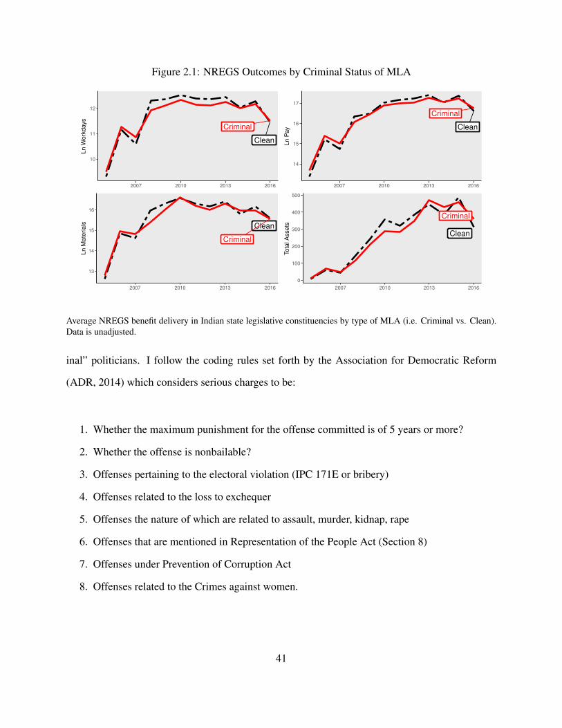
Figure 2.1: NREGS Outcomes by Criminal Status of MLA
Clean
Criminal
10
11
12
2007 2010 2013 2016
Ln W
ork
days
Clean
Criminal
14
15
16
17
2007 2010 2013 2016
Ln P
ay
Clean
Criminal
13
14
15
16
2007 2010 2013 2016
Ln M
ate
rials
Clean
Criminal
0
100
200
300
400
500
2007 2010 2013 2016Tota
l A
ssets
Average NREGS benefit delivery in Indian state legislative constituencies by type of MLA (i.e. Criminal vs. Clean).Data is unadjusted.
inal” politicians. I follow the coding rules set forth by the Association for Democratic Reform
(ADR, 2014) which considers serious charges to be:
1. Whether the maximum punishment for the offense committed is of 5 years or more?
2. Whether the offense is nonbailable?
3. Offenses pertaining to the electoral violation (IPC 171E or bribery)
4. Offenses related to the loss to exchequer
5. Offenses the nature of which are related to assault, murder, kidnap, rape
6. Offenses that are mentioned in Representation of the People Act (Section 8)
7. Offenses under Prevention of Corruption Act
8. Offenses related to the Crimes against women.
41

Despite NREGS’s ostensibly universal guarantee, the program is known for wide variation in
performance and implementation (Sukhtankar 2016).25 Figure 2.1 compares NREGS outcomes
averaged over criminal and clean constituencies, for all of India. In general, there is no discernible
gap between average NREGS delivery in criminal and clean constituencies. In other words, the
raw, unadjusted data does not suggest that criminal politicians are noticeably better (or worse)
at implementing NREGS. Across both employment (Workdays and Pay in top panel) and local
infrastructure measures (Material Expenditures and Projects Completed, bottom panel), the trends
in criminal and clean constituencies are highly similar. If anything, criminal politicians slightly
underperform in NREGS delivery.
The lack of discernible difference between charged and clean politicians could be spurious. For
example, clean politicians may typically win elections in monsoon affected areas with higher de-
mand for seasonal NREGS employment. Or criminal politicians may flourish where state capacity
is weak and NREGS implementation poor. To estimate the causal effect of electing a criminally
charged candidate on NREGS outcomes, I turn now to the RD analysis.
2.4 RDD Validity
The RD literature suggests several strategies and diagnostic tests to validate the regression dis-
continuity design. First, I consider the possibility that criminally accused candidates are capable
of sorting around the threshold. In other words, criminal candidates may be particularly suited to
first noticing they are in a tight race and then propelling themselves to bare victories. This would
invalidate the assumption of quasi-random treatment assignment around the threshold. In fact, it
could be criminal candidates’ superior access to money, muscle and networks that enable them to
win close races. For example, criminal candidates tend to be wealthier (Vaishnav 2017) and may
marshal these extra resources during the campaign to convince late deciders and push themselves
to bare victories. Similarly, criminals may have stronger ties to local communities, which could
25For comparisons of state-level variation in NREGS outcomes between criminal and clean constituencies see Ap-pendix 2.G.
42
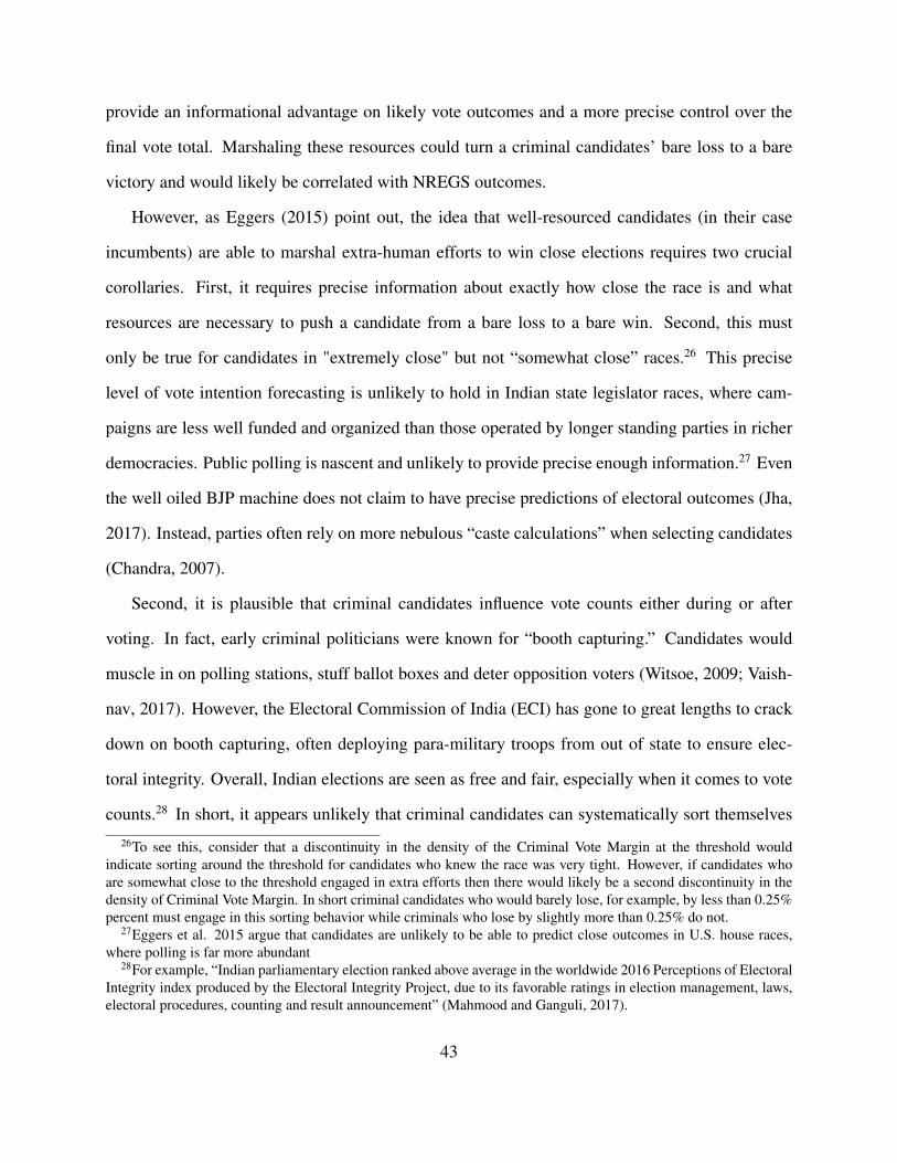
provide an informational advantage on likely vote outcomes and a more precise control over the
final vote total. Marshaling these resources could turn a criminal candidates’ bare loss to a bare
victory and would likely be correlated with NREGS outcomes.
However, as Eggers (2015) point out, the idea that well-resourced candidates (in their case
incumbents) are able to marshal extra-human efforts to win close elections requires two crucial
corollaries. First, it requires precise information about exactly how close the race is and what
resources are necessary to push a candidate from a bare loss to a bare win. Second, this must
only be true for candidates in "extremely close" but not “somewhat close” races.26 This precise
level of vote intention forecasting is unlikely to hold in Indian state legislator races, where cam-
paigns are less well funded and organized than those operated by longer standing parties in richer
democracies. Public polling is nascent and unlikely to provide precise enough information.27 Even
the well oiled BJP machine does not claim to have precise predictions of electoral outcomes (Jha,
2017). Instead, parties often rely on more nebulous “caste calculations” when selecting candidates
(Chandra, 2007).
Second, it is plausible that criminal candidates influence vote counts either during or after
voting. In fact, early criminal politicians were known for “booth capturing.” Candidates would
muscle in on polling stations, stuff ballot boxes and deter opposition voters (Witsoe, 2009; Vaish-
nav, 2017). However, the Electoral Commission of India (ECI) has gone to great lengths to crack
down on booth capturing, often deploying para-military troops from out of state to ensure elec-
toral integrity. Overall, Indian elections are seen as free and fair, especially when it comes to vote
counts.28 In short, it appears unlikely that criminal candidates can systematically sort themselves
26To see this, consider that a discontinuity in the density of the Criminal Vote Margin at the threshold wouldindicate sorting around the threshold for candidates who knew the race was very tight. However, if candidates whoare somewhat close to the threshold engaged in extra efforts then there would likely be a second discontinuity in thedensity of Criminal Vote Margin. In short criminal candidates who would barely lose, for example, by less than 0.25%percent must engage in this sorting behavior while criminals who lose by slightly more than 0.25% do not.
27Eggers et al. 2015 argue that candidates are unlikely to be able to predict close outcomes in U.S. house races,where polling is far more abundant
28For example, “Indian parliamentary election ranked above average in the worldwide 2016 Perceptions of ElectoralIntegrity index produced by the Electoral Integrity Project, due to its favorable ratings in election management, laws,electoral procedures, counting and result announcement” (Mahmood and Ganguli, 2017).
43

into the category of bare winners.
Beyond these theoretical considerations, I directly test for candidate sorting by inspecting the
density of the forcing variable (Criminal Vote Margin, see figure 2.2). If criminal politicians are
indeed sorting into the bare winning column this should create a noticeable discontinuity at the
cut-point. In other words, there will be more criminal candidates just to the right of the 0 threshold
than just to the left. Figure 2.2 provides a visual check by plotting the density of Criminal Vote
Margin. It is not indicative of criminal candidate sorting at the threshold.
Figure 2.2: Check for Sorting of Bare Criminal Winners
0.00
0.01
0.02
0.03
−40 0 40
Criminal Vote Margin
de
nsity
Visual Inspection of Forcing Variable Continuity
CVM subtracts clean candidates vote share from criminal candidates vote share for a given constituency-election.Negative values indicate the percentage that criminally accused candidates lost by to a clean winner. Positive valuesindicate the percentage that criminally accused candidates won by against a clean loser.
44

More formally, I conduct a McCrary test for sorting at the threshold (see figure 2.3). The test is
inconsistent with the hypothesis that criminal candidates are more likely to win in close elections
(p-value = 0.58).29
Figure 2.3: McCrary Test for Sorting
−30 −20 −10 0 10 20 30
0.0
00.0
10.0
20.0
30.0
4
The estimated log difference in heights at the threshold is 0.042 (s.e. 0.075) which equates to a p-value of 0.58 and isnot consistent with sorting around the threshold.
29Eggers et al. 2015 and Prakash et al. 2016 also fail to find evidence of MLA sorting in India.
45

2.4.1 Balance Tests and Controls
A second implication of the regression discontinuity design is that if treatment assignment is quasi-
random at the threshold, then treatment and control groups should be balanced on observable and
unobservable characteristics. Treated constituencies that elect a bare criminal winner should look
similar to control constituencies that barely elect clean candidates. Similarly, winning criminals
should look like winning clean candidates around the threshold, with the only discrepancy being
their criminal status.30 Overall, treatment and control units seem relatively well balanced across
both constituency and candidate characteristics (see Figures 2.4 & 2.5 and Tables 2.2 & 2.3).
However, bare criminal winners are less likely to be a member of a national party.31 I control
for this imbalance (along with the other covariates) in my models. Finally, candidates are not
imbalanced on National Party membership when the analysis is restricted to just serious charges
(see Appendix Figure 2.C.1 and Table 2.C.1).32
30The regression discontinuity design should balance treatment and control constituencies, but does not guaranteethat bare criminal winners are similar on average to clean candidates who just beat out criminals. While acknowledgingthis limitation, I note that several other papers employ similar designs (e.g. for RDs comparing candidates’ gender inthe U.S., Brazil and India see Ferreira and Gyourko (2014); Brollo and Troiano (2016); Brown (2017), respectively;for RD comparisons of candidates’ criminality in India see Chemin (2012); Prakash et al. (2019); Nanda and Pareek(2016)) and that this does not mean that treatment and control units will be unbalanced on other covariates.
31While this could arise due to chance, I will use the remaining variables listed in Appendix 2.A Table 2.A.1 toadjudicate if there is indeed evidence of imbalance between treated and control candidates.
32If criminal politicians are less likely to be members of national party this could be problematic if this means theyare also less likely to be members of the INC or aligned with the ruling party (both of which are associated with theprovision of NREGS). I test these possibilities in my forthcoming section on heterogeneous treatment effects.
46
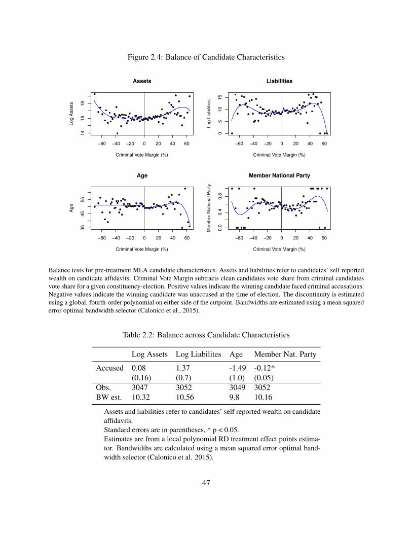
Figure 2.4: Balance of Candidate Characteristics
−60 −40 −20 0 20 40 60
14
16
18
Assets
Criminal Vote Margin (%)
Lo
g A
sse
ts
−60 −40 −20 0 20 40 60
05
10
15
Liabilities
Criminal Vote Margin (%)
Log
Lia
bili
ties
−60 −40 −20 0 20 40 60
35
45
55
Age
Criminal Vote Margin (%)
Ag
e
−60 −40 −20 0 20 40 60
0.0
0.4
0.8
Member National Party
Criminal Vote Margin (%)
Mem
ber
National P
art
y
Balance tests for pre-treatment MLA candidate characteristics. Assets and liabilities refer to candidates’ self reportedwealth on candidate affidavits. Criminal Vote Margin subtracts clean candidates vote share from criminal candidatesvote share for a given constituency-election. Positive values indicate the winning candidate faced criminal accusations.Negative values indicate the winning candidate was unaccused at the time of election. The discontinuity is estimatedusing a global, fourth-order polynomial on either side of the cutpoint. Bandwidths are estimated using a mean squarederror optimal bandwidth selector (Calonico et al., 2015).
Table 2.2: Balance across Candidate Characteristics
Log Assets Log Liabilites Age Member Nat. Party
Accused 0.08 1.37 -1.49 -0.12*(0.16) (0.7) (1.0) (0.05)
Obs. 3047 3052 3049 3052BW est. 10.32 10.56 9.8 10.16
Assets and liabilities refer to candidates’ self reported wealth on candidateaffidavits.Standard errors are in parentheses, * p < 0.05.Estimates are from a local polynomial RD treatment effect points estima-tor. Bandwidths are calculated using a mean squared error optimal band-width selector (Calonico et al. 2015).
47

Figure 2.5: Balance of Constituency Characteristics
−60 −40 −20 0 20 40 60
0.0
0.4
0.8
SC/ST Reserved Constituency
Criminal Vote Margin (%)
Sh
are
Re
se
rve
d C
on
stitu
en
cy
−60 −40 −20 0 20 40 60
50
00
0
Votes Cast
Criminal Vote Margin (%)
Vo
tes C
ast
Balance tests for pre-treatment MLA constituency characteristics. Criminal Vote Margin subtracts clean candidatesvote share from criminal candidates vote share for a given constituency-election. Positive values indicate the winningcandidate faced criminal accusations. Negative values indicate the winning candidate was unaccused at the time ofelection. The discontinuity is estimated using a global, fourth order polynomials on either side of the cutpoint. Thebandwidth is estimate using a mean squared error optimal bandwidth selector (Calonico et al. 2015).
Table 2.3: Balance across Constituency Characteristics
Reserved Const. Votes cast
Accused -0.046 1386(0.026) (4103)
Obs. 3052 3052BW est. 11.343 9.466
Standard errors are in parentheses, * p <0.05.Estimates are from a local polynomialRD treatment effect points estimator.Bandwidths are calculated using a meansquared error optimal bandwidth selector(Calonico et al. 2015).
48
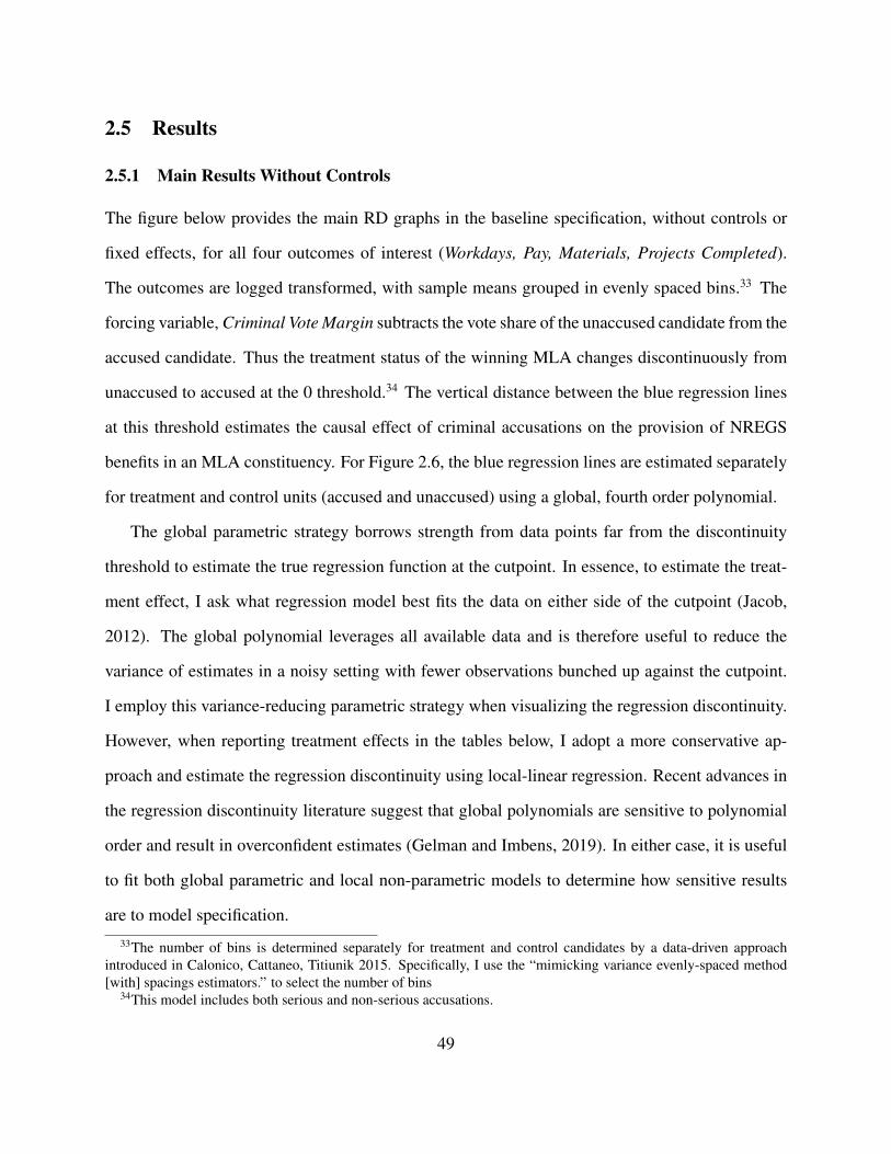
2.5 Results
2.5.1 Main Results Without Controls
The figure below provides the main RD graphs in the baseline specification, without controls or
fixed effects, for all four outcomes of interest (Workdays, Pay, Materials, Projects Completed).
The outcomes are logged transformed, with sample means grouped in evenly spaced bins.33 The
forcing variable, Criminal Vote Margin subtracts the vote share of the unaccused candidate from the
accused candidate. Thus the treatment status of the winning MLA changes discontinuously from
unaccused to accused at the 0 threshold.34 The vertical distance between the blue regression lines
at this threshold estimates the causal effect of criminal accusations on the provision of NREGS
benefits in an MLA constituency. For Figure 2.6, the blue regression lines are estimated separately
for treatment and control units (accused and unaccused) using a global, fourth order polynomial.
The global parametric strategy borrows strength from data points far from the discontinuity
threshold to estimate the true regression function at the cutpoint. In essence, to estimate the treat-
ment effect, I ask what regression model best fits the data on either side of the cutpoint (Jacob,
2012). The global polynomial leverages all available data and is therefore useful to reduce the
variance of estimates in a noisy setting with fewer observations bunched up against the cutpoint.
I employ this variance-reducing parametric strategy when visualizing the regression discontinuity.
However, when reporting treatment effects in the tables below, I adopt a more conservative ap-
proach and estimate the regression discontinuity using local-linear regression. Recent advances in
the regression discontinuity literature suggest that global polynomials are sensitive to polynomial
order and result in overconfident estimates (Gelman and Imbens, 2019). In either case, it is useful
to fit both global parametric and local non-parametric models to determine how sensitive results
are to model specification.
33The number of bins is determined separately for treatment and control candidates by a data-driven approachintroduced in Calonico, Cattaneo, Titiunik 2015. Specifically, I use the “mimicking variance evenly-spaced method[with] spacings estimators.” to select the number of bins
34This model includes both serious and non-serious accusations.
49

There seems to be some visual evidence of discontinuity. In fact, criminally accused candidates
show a reduction in the number of workdays, total pay, material expenditure, and completion of
NREGS projects at the threshold. However, these negative discontinuities seem to be small relative
to the general variability in NREGS provision as estimated by the wide dispersion of binned sample
means in the scatterplot. Given the lack of a strong visual discontinuity relative to the large overall
variation in NREGS benefits across the sample, further investigation is required. In table 2.4, I
explore the results more formally using local polynomial regressions to estimate the causal effect
of criminal accusations. Below, I investigate the sensitivity of these initial results to alternative
specifications, bandwidth size and selectors, and the inclusion of covariates.
Table 2.4: Main RD Estimates of Criminal Accusations on NREGS Outcomes
Log Workdays Log Pay Log Materials LogProjectsCompleted
Conventional −0.36 −0.25 −0.74 −0.42∗(0.25) (0.27) (0.44) (0.21)
Bias-Corrected −0.39 −0.27 −0.86 −0.48∗(0.25) (0.27) (0.44) (0.21)
Robust −0.39 −0.27 −0.86 −0.48∗(0.29) (0.31) (0.51) (0.24)
Num. obs. 2679 2678 2670 2679Eff. Num. obs. Left 874 917 854 831Eff. Num. obs. Right 930 966 912 868Eff. Num. obs. Left BC 1144 1165 1157 1133Eff. Num. obs. Right BC 1227 1250 1249 1220BW (h) 12.95 13.76 12.58 11.86BW Bias Corr. (b) 22.30 23.77 23.67 21.70Order (p) 1 1 1 1Order Bias Corr. (q) 2 2 2 2Model Non-parametric Local Polynomials∗∗∗p < 0.001, ∗∗p < 0.01, ∗p < 0.05
BW represents the bandwidth chosen by the CCT algorithm that minimizes Mean Squared Error. The number of ob-servations represents those in the entire sample, while Effective Number is the number of observations included insidethe bandwidth (with BC indicating effective number of observations for bias corrected estimates). Local polynomialsare estimated separately for each side of the threshold. The Bias Corrected estimates try to measure and remove thebias introduced by the polynomial estimation of the true regression function (Cattaneo et al. 2018). BW Bias Corr.gives the bandwidth for the bias corrected estimate which also changes given the new bias corrected estimate. Orderand Order Bias Corr. provide the polynomial order for the regression on either side of the threshold.
50
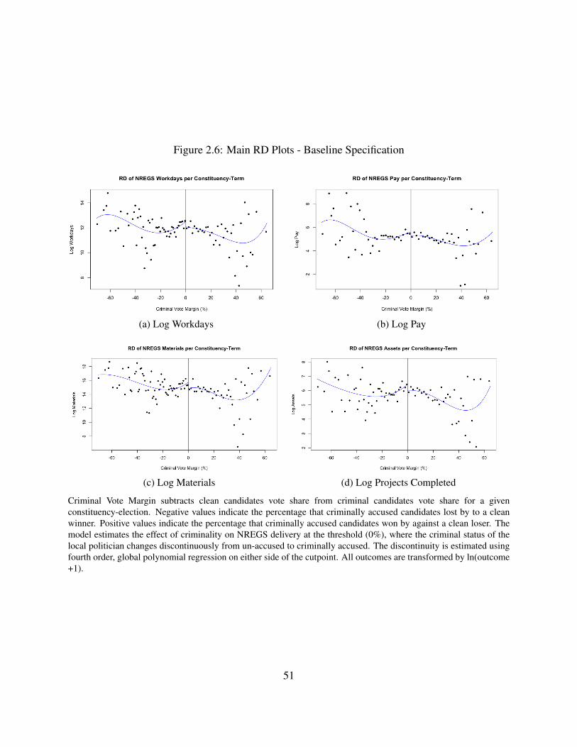
Figure 2.6: Main RD Plots - Baseline Specification
(a) Log Workdays (b) Log Pay
(c) Log Materials (d) Log Projects Completed
Criminal Vote Margin subtracts clean candidates vote share from criminal candidates vote share for a givenconstituency-election. Negative values indicate the percentage that criminally accused candidates lost by to a cleanwinner. Positive values indicate the percentage that criminally accused candidates won by against a clean loser. Themodel estimates the effect of criminality on NREGS delivery at the threshold (0%), where the criminal status of thelocal politician changes discontinuously from un-accused to criminally accused. The discontinuity is estimated usingfourth order, global polynomial regression on either side of the cutpoint. All outcomes are transformed by ln(outcome+1).
51
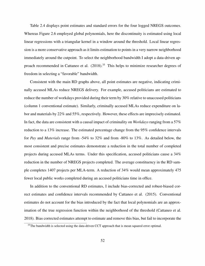
Table 2.4 displays point estimates and standard errors for the four logged NREGS outcomes.
Whereas Figure 2.6 employed global polynomials, here the discontinuity is estimated using local
linear regressions with a triangular kernel in a window around the threshold. Local linear regres-
sion is a more conservative approach as it limits estimation to points in a very narrow neighborhood
immediately around the cutpoint. To select the neighborhood bandwidth I adopt a data-driven ap-
proach recommended in Cattaneo et al. (2018).35 This helps to minimize researcher degrees of
freedom in selecting a “favorable” bandwidth.
Consistent with the main RD graphs above, all point estimates are negative, indicating crimi-
nally accused MLAs reduce NREGS delivery. For example, accused politicians are estimated to
reduce the number of workdays provided during their term by 30% relative to unaccused politicians
(column 1 conventional estimate). Similarly, criminally accused MLAs reduce expenditure on la-
bor and materials by 22% and 55%, respectively. However, these effects are imprecisely estimated.
In fact, the data are consistent with a causal impact of criminality on Workdays ranging from a 57%
reduction to a 13% increase. The estimated percentage change from the 95% confidence intervals
for Pay and Materials range from -54% to 32% and from -80% to 13%. As detailed below, the
most consistent and precise estimates demonstrate a reduction in the total number of completed
projects during accused MLAs terms. Under this specification, accused politicians cause a 34%
reduction in the number of NREGS projects completed. The average constituency in the RD sam-
ple completes 1407 projects per MLA-term. A reduction of 34% would mean approximately 475
fewer local public works completed during an accused politicians time in office.
In addition to the conventional RD estimates, I include bias-corrected and robust-biased cor-
rect estimates and confidence intervals recommended by Cattaneo et al. (2015). Conventional
estimates do not account for the bias introduced by the fact that local polynomials are an approx-
imation of the true regression function within the neighborhood of the threshold (Cattaneo et al.
2018). Bias corrected estimates attempt to estimate and remove this bias, but fail to incorporate the
35The bandwidth is selected using the data-driven CCT approach that is mean squared error optimal.
52

variability from estimating this bias into their confidence intervals, resulting in confidence inter-
vals that are too small. The robust bias-corrected methods account for this variability and include
larger confidence intervals with better coverage properties (Cattaneo et.al. 2018). It is encourag-
ing however that the point estimates do not change dramatically despite the bias correction and
alternative bandwidth selection. Moreover, the Projects Completed outcome retains conventional
levels of statistical significance throughout, even though standard errors increase in size under the
robust correction for confidence intervals.
At the very least, accused politicians complete fewer NREGS projects during their term. This
is worrying given that the construction of local public works is a primary goal and justification
for the massive investment in NREGS. NREGS projects such as improved irrigation, roads or the
construction of school walls, also provide a public benefit that can last well beyond the short term
project investment and employment. The lack of a clear visual discontinuity (at least relative to the
overall variation in NREGS outcomes) combined with the imprecisely estimated effects of criminal
accusations suggests the need for reducing sampling variance of the estimates. There are two ways
to improve the precision of RD estimates. First, using a global, parametric approach to estimate
the discontinuity by including all observations (even those far from the threshold). However, this
results in a bias-variance tradeoff as observations far from the threshold may have undue impact on
the estimated treatment effect. Second the inclusion of covariates that are predictive of outcomes.
Including controls can reduce variance while not biasing the RD design. Estimated treatment
effects should not change after the inclusion of these covariates. This follows from the fact that
assignment to treatment is independent of observable and unobservable covariates so including
additional candidate characteristics in the local linear regression should only reduce the sampling
variability of the estimate but not alter the estimate itself (Lee and Lemieux, 2010).
In the remainder of this section, I explore how discontinuity estimates change under alterna-
tive specifications and after including adjustors. In the appendices I include additional sensitivity
analyses.
53

2.5.2 Main Results With Controls
In the following specifications I include baseline controls and fixed effects for state and election-
year. There is well documented variation in NREGS provision by state and time period. Some
states have delivered a high level of NREGS benefits (e.g. Andhra Pradesh, MP, Rajasthan, and
Chhatisgarh), while others remain chronic underperformers (Bihar, Jharkhand, Orissa and Uttar
Pradesh) (Imbert and Papp 2011). Secondly, Modi’s BJP led government has focused on techno-
logical solutions to curb leakage, with the program generally improving over time (Banerjee et al.
2014).
Table 2.5 makes this comparison explicit by successively adding controls and fixed effects
for State and Election-Year to each outcome. The first column for each outcome is the baseline
(same model as in table 2.4). The second column adds in controls (for now, just the number of
votes cast per constituency to proxy for NREGS demand). The third column includes controls and
fixed effects for state and election-year. Following Lee and Lemieux (2010) the outcomes in the
fixed effects models are residuals from a linear regression of the log of NREGS Benefit on state
and election year. The residuals are then used in the RD model to estimate the treatment effect
of criminally charged MLAs on NREGS provision. While controlling for the number of votes
cast did not noticeably reduce the variance of the estimates, including fixed effects for state and
year did improve precision. After including fixed effects, constituencies that elect a criminally
charged MLA witness a 59% reduction in materials expenditure, on average (significant at the
95% level). At the same time accused MLAs cause a 40% reduction in the number of completed
projects. Overall, the point estimates remain consistently negative and quantitatively similar after
the inclusion of covariates.
The main RD graphs (figure 2.7) for the residuals also show a reduction in sampling variance
consistent with State and Election-Year being informative predictions of the delivery of NREGS
benefits. They also seem to indicate a greater visual discontinuity. For the rest of the paper I
continue with specifications that include controls and fixed effects while including results without
54

Tabl
e2.
5:R
DE
stim
ates
ofC
rim
inal
Acc
usat
ions
onN
RE
GS
Out
com
es-I
nclu
ding
Cov
aria
tes
Log
Wor
kday
sL
ogPa
yL
ogM
ater
ials
Log
Proj
ects
Com
plet
ed
Con
vent
iona
l−0.36−0.36−0.41−0.25−0.25−0.33−0.74
−0.74
−0.84
∗−0.42
∗−0.43
∗−0.48
∗∗
(0.25)
(0.25)
(0.21)
(0.27)
(0.26)
(0.24)
(0.44)
(0.44)
(0.35)
(0.21)
(0.21)
(0.16)
Bia
s-C
orre
cted
−0.39−0.39−0.39−0.27−0.29−0.31−0.86
−0.86
−0.89
∗−0.48
∗−0.50
∗−0.51
∗∗
(0.25)
(0.25)
(0.21)
(0.27)
(0.26)
(0.24)
(0.44)
(0.44)
(0.35)
(0.21)
(0.21)
(0.16)
Rob
ust
−0.39−0.39−0.39−0.27−0.29−0.31−0.86
−0.86
−0.89
∗−0.48
∗−0.50
∗−0.51
∗∗
(0.29)
(0.29)
(0.25)
(0.31)
(0.31)
(0.29)
(0.51)
(0.51)
(0.41)
(0.24)
(0.23)
(0.19)
Num
.obs
.26
7926
7926
7926
7826
7826
7826
7026
7026
7026
7926
7926
79E
ff.N
obs.
Lef
t87
487
681
591
792
678
685
484
875
783
183
175
5E
ff.N
obs.
Rig
ht93
093
484
396
697
980
891
290
077
286
886
976
6E
ff.N
obs.
LB
C.
1144
114
1063
116
1177
1034
1157
1147
.00
1011
1133
1179
1017
Eff
.Nob
s.R
BC
.12
2712
3011
3812
5012
7211
0112
4912
3710
7312
2012
7310
72B
W(h
)12
.95
1311
.44
13.7
614
.08
10.8
612
.58
12.4
510
.28
11.8
611
.87
10.0
6B
WB
C(b
)22
.30
22.6
318
.48
23.7
725
.08
17.5
823
.67
23.0
516
.83
21.7
025
.21
16.7
8O
rder
(p)
11
11
11
11
11
11
Ord
erB
C(q
)2
22
22
22
22
22
2C
ontr
ols
NO
YE
SY
ES
NO
YE
SY
ES
NO
YE
SY
ES
NO
YE
SY
ES
FEN
ON
OY
ES
NO
NO
YE
SN
ON
OY
ES
NO
NO
YE
S∗∗
∗p<
0.001
,∗∗p<
0.01
,∗p<
0.05
For
the
mod
els
incl
udin
gfix
edef
fect
s,ou
tcom
esar
eth
ere
sidu
als
afte
rco
ntro
lling
for
stat
ean
del
ectio
nye
ar.
BW
repr
esen
tsth
eba
ndw
idth
chos
enby
the
CC
Tal
gori
thm
that
min
imiz
esM
ean
Squa
red
Err
or.
The
num
ber
ofob
serv
atio
nsre
pres
ents
thos
ein
the
entir
esa
mpl
e,w
hile
Eff
ectiv
enu
mbe
ris
the
num
ber
ofob
serv
atio
nsin
clud
edin
side
the
band
wid
th.
Loc
alpo
lyno
mia
lsar
ees
timat
edse
para
tely
for
each
side
ofth
eth
resh
old.
The
Bia
sC
orre
cted
estim
ates
try
tom
easu
rean
dre
mov
eth
ebi
asin
trod
uced
byth
epo
lyno
mia
lest
imat
ion
ofth
etr
uere
gres
sion
func
tion
(Cat
tane
oet
al.2
018)
.BW
BC
.giv
esth
eba
ndw
idth
fort
hebi
asco
rrec
ted
estim
ate
whi
chal
soch
ange
sgi
ven
the
new
bias
corr
ecte
des
timat
e.O
rder
and
Ord
erB
C.p
rovi
deth
epo
lyno
mia
lord
erfo
rthe
regr
essi
onon
eith
ersi
deof
the
thre
shol
d.
55

covariates in the appendix.
2.5.3 Sensitivity Analysis
Varying Bandwidth Selections
I test the sensitivity of my results using a variety of models and bandwidth specifications. To
recover the treatment effect I compare the average outcomes from “close” elections on either side of
the cutoff. Regression discontinuity results are sensitive to which elections are considered “close"
(i.e. to bandwidth size). Narrow bandwidths can be noisy since they include fewer observations.
Wider bandwidths stabilize estimates, but may bias results by including elections further from the
cut-point.36 Figure 2.8 plots the local average treatment effects (LATE) for the NREGS outcomes
at various bandwidth sizes. The estimates appear stable across a wide variety of bandwidth choices.
The reduction in the completion of NREGS projects (8(d)) remains significant across bandwidth
choices too.
Secondly, the RD literature recommends several different bandwidth selection methods. Table
2.B.1 in appendix 2.B re-estimates the fixed effect models with different bandwidth selectors.
Columns 1 (CCT) and 2 (CCT 2014) are the original specification using the data-driven bandwidth
selector that optimizes MSE. Column 3 uses cross-validation to estimate the optimal bandwidth
size for the baseline specification. In addition, I test the sensitivity of results to bandwidths selected
by the Imbens and Kalyanaraman (2012) algorithm (Column 4).
Varying Functional Forms
Next, I estimate treatment effects for a variety of functional forms. Gelman and Imbens (2019)
recommend the use of local linear or quadratic polynomials instead of controlling higher order
polynomials. Their results indicate that higher order polynomials can given large weight to ob-
servations far from the cut-point, are highly sensitive to the degree of the polynomial and produce
36That is, there is a bias/variance tradeoff to bandwidth selection. In short, researchers want to include enoughobservations in bins to reduce noise but not so many that you are nor longer comparing observations at the thresholdwhere treatment is randomized.
56
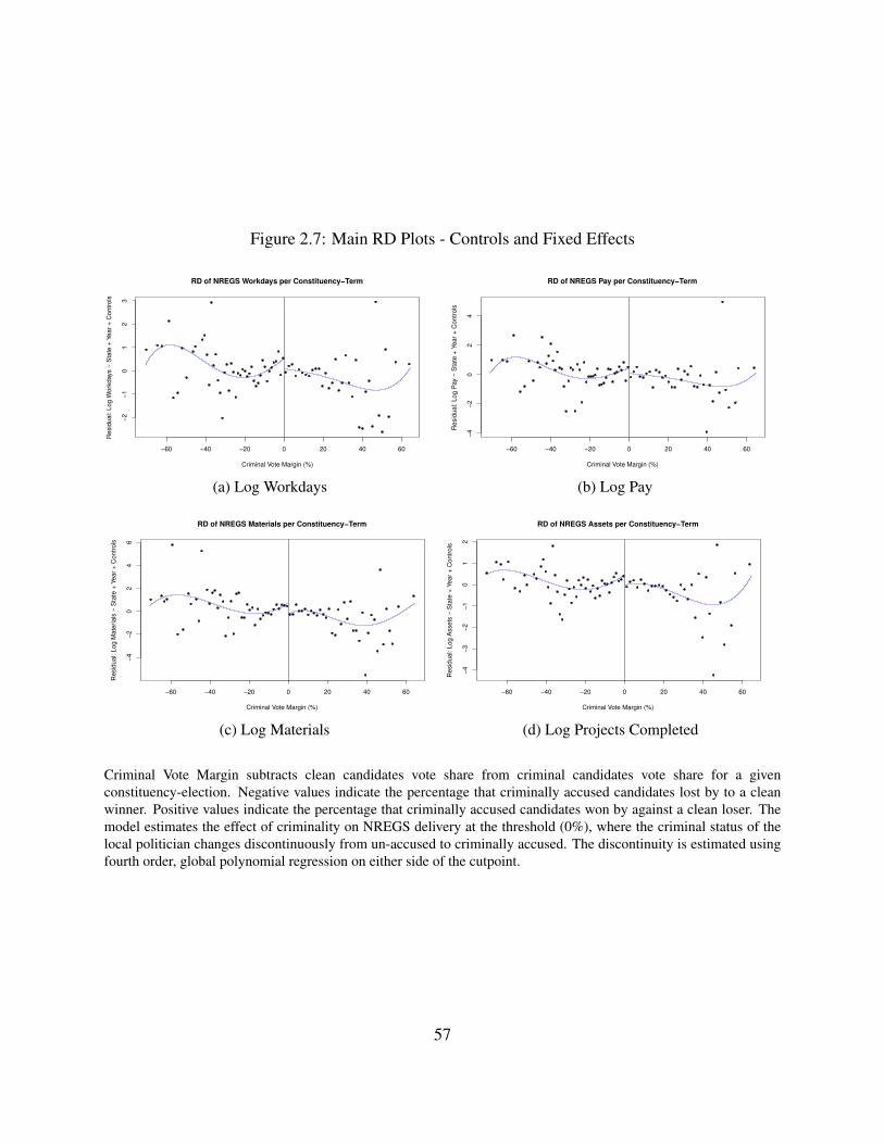
Figure 2.7: Main RD Plots - Controls and Fixed Effects
−60 −40 −20 0 20 40 60
−2
−1
01
23
RD of NREGS Workdays per Constituency−Term
Criminal Vote Margin (%)
Resid
ual: L
og W
ork
days ~
Sta
te +
Year
+ C
ontr
ols
(a) Log Workdays
−60 −40 −20 0 20 40 60
−4
−2
02
4
RD of NREGS Pay per Constituency−Term
Criminal Vote Margin (%)
Resid
ual: L
og P
ay ~
Sta
te +
Year
+ C
ontr
ols
(b) Log Pay
−60 −40 −20 0 20 40 60
−4
−2
02
46
RD of NREGS Materials per Constituency−Term
Criminal Vote Margin (%)
Resid
ual: L
og M
ate
rials
~ S
tate
+ Y
ear
+ C
ontr
ols
(c) Log Materials
−60 −40 −20 0 20 40 60
−4
−3
−2
−1
01
2
RD of NREGS Assets per Constituency−Term
Criminal Vote Margin (%)
Resid
ual: L
og A
ssets
~ S
tate
+ Y
ear
+ C
ontr
ols
(d) Log Projects Completed
Criminal Vote Margin subtracts clean candidates vote share from criminal candidates vote share for a givenconstituency-election. Negative values indicate the percentage that criminally accused candidates lost by to a cleanwinner. Positive values indicate the percentage that criminally accused candidates won by against a clean loser. Themodel estimates the effect of criminality on NREGS delivery at the threshold (0%), where the criminal status of thelocal politician changes discontinuously from un-accused to criminally accused. The discontinuity is estimated usingfourth order, global polynomial regression on either side of the cutpoint.
57

Figure 2.8: Sensitivity Analysis - LATE for Varying Bandwidths
(a) Log Workdays (b) Log Pay
(c) Log Materials (d) Log Projects Completed
Note that RD estimates are non-parametric linear polynomials from the RDDTools package using the data-drivenbandwidth selector from the RDRobust package. This leads to slightly different standard errors than those calculatedunder the RDrobust package (e.g. see Tables above). However the point estimates remain the same.
58

confidence intervals that are too small. To this end, I report results for a variety of local poly-
nomials running from 1st-6th degree for each NREGS outcome (see tables in Appendix 2.B.2).
Encouragingly, the Projects Completed outcome remains statistically significant across all polyno-
mial choices though the estimate varies.
Placebo Tests
Finally, I conduct a number of placebo tests, including checking for discontinuities at other values
of the forcing variable (Criminal Vote Margin). There should not be a discontinuity when com-
paring constituency outcomes in narrow windows at different values of CVM (see figure 2.9). The
estimates for the placebo cutpoints are not entirely stable. For example, for the Projects Completed
outcome there is a significant effect around a cutpoint of -9. Ideally, the placebo plots should look
more like that of Materials, with insignificant effects everywhere except at the threshold of 0.
2.5.4 Serious Criminals Analysis
I now turn to the results for the subset of MLAs accused of serious crimes. To reiterate, I expect
effects to be stronger when analyzing serious charges. Including all charges potentially conflates
“criminal” politicians with those falsely accused by political rivals or who incur charges in the
course of political activism (Jaffrelot and Verniers, 2014). In turn, this increase in measurement
error may muddy the effect of criminal charges on NREGS provision. Moreover, serious charges
correspond more directly to underlying criminal traits, such as the propensity for violence.37 If
these latent criminal traits help candidates’ win elections, perhaps despite an inability to perform
in office, then we might expect stronger, negative effects when examining politicians facing only
serious charges.
Specifications for the regression models analyzing serious charges remain the same as above
(i.e. for all charges). Treatment effects compare constituency results from close races where a
candidate facing a serious charge ran against a candidate who did not face a serious charge (i.e. the
37In future work I specifically inspect only violence related charges.
59

Figure 2.9: Placebo Tests - LATE for Varying Cutpoints- Baseline with Fixed Effects and RDRo-bust data driven BWS
(a) Log Workdays (b) Log Pay
(c) Log Materials (d) Log Projects Completed
Note that RD estimates are non-parametric linear polynomials from the RDDTools package using the data-drivenbandwidth selector from the RDRobust package. This leads to slightly different standard errors than those calculatedunder the RDrobust package (e.g. Tables above). However the point estimates remain the same.
60
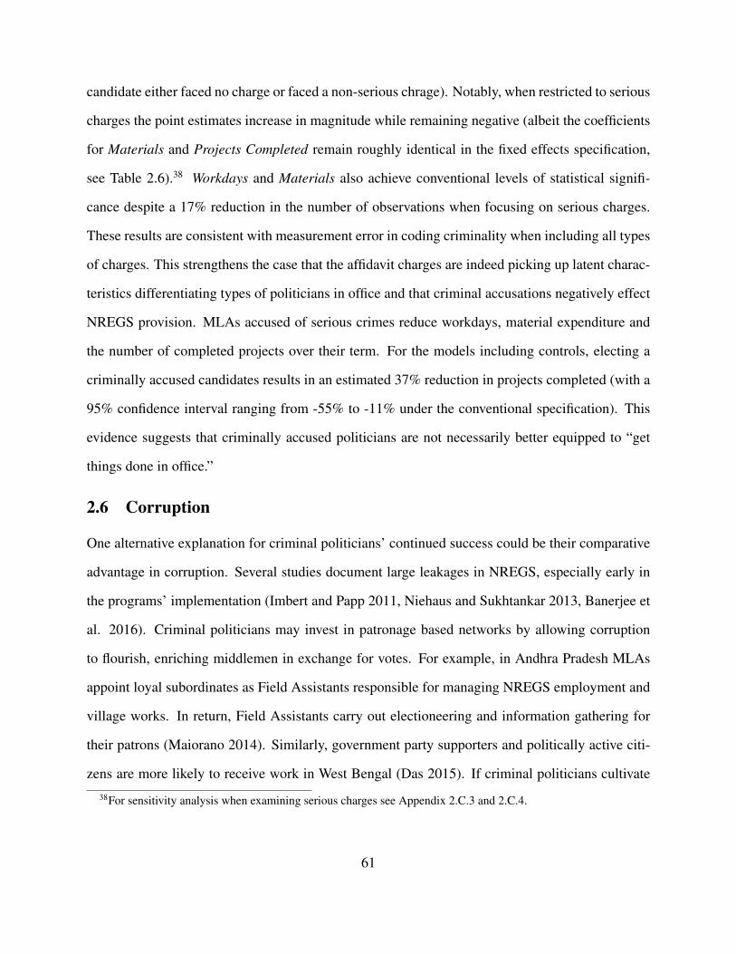
candidate either faced no charge or faced a non-serious chrage). Notably, when restricted to serious
charges the point estimates increase in magnitude while remaining negative (albeit the coefficients
for Materials and Projects Completed remain roughly identical in the fixed effects specification,
see Table 2.6).38 Workdays and Materials also achieve conventional levels of statistical signifi-
cance despite a 17% reduction in the number of observations when focusing on serious charges.
These results are consistent with measurement error in coding criminality when including all types
of charges. This strengthens the case that the affidavit charges are indeed picking up latent charac-
teristics differentiating types of politicians in office and that criminal accusations negatively effect
NREGS provision. MLAs accused of serious crimes reduce workdays, material expenditure and
the number of completed projects over their term. For the models including controls, electing a
criminally accused candidates results in an estimated 37% reduction in projects completed (with a
95% confidence interval ranging from -55% to -11% under the conventional specification). This
evidence suggests that criminally accused politicians are not necessarily better equipped to “get
things done in office.”
2.6 Corruption
One alternative explanation for criminal politicians’ continued success could be their comparative
advantage in corruption. Several studies document large leakages in NREGS, especially early in
the programs’ implementation (Imbert and Papp 2011, Niehaus and Sukhtankar 2013, Banerjee et
al. 2016). Criminal politicians may invest in patronage based networks by allowing corruption
to flourish, enriching middlemen in exchange for votes. For example, in Andhra Pradesh MLAs
appoint loyal subordinates as Field Assistants responsible for managing NREGS employment and
village works. In return, Field Assistants carry out electioneering and information gathering for
their patrons (Maiorano 2014). Similarly, government party supporters and politically active citi-
zens are more likely to receive work in West Bengal (Das 2015). If criminal politicians cultivate
38For sensitivity analysis when examining serious charges see Appendix 2.C.3 and 2.C.4.
61

Table 2.6: RD Estimates for Serious Charges
Log Workdays Log Pay Log Materials Log Projects Completed
Conventional −0.49∗ −0.38 −0.82∗ −0.46∗∗(0.22) (0.25) (0.40) (0.17)
Bias-Corrected −0.50∗ −0.39 −0.87∗ −0.51∗∗(0.22) (0.25) (0.40) (0.17)
Robust −0.50 −0.39 −0.87 −0.51∗(0.26) (0.30) (0.49) (0.20)
Num. obs. 2216 2214 2212 2216Eff. N obs. Left 678 636 642 596Eff. N obs. Right 702 645 655 600Eff. N obs. Left BC 876 831 832 809Eff. N obs. Right BC 967 902 906 870BW 11.33 10.13 10.39 9.16BW Bias Corr. 18.87 16.79 16.93 15.73Order 1 1 1 1Order Bias Corr. 2 2 2 2Controls YES YES YES YESFE YES YES YES YES∗∗∗p < 0.001, ∗∗p < 0.01, ∗p < 0.05
For the models including fixed effects, outcomes are the residuals after controlling for state and election year. BWrepresents the bandwidth chosen by the CCT algorithm that minimizes Mean Squared Error. The number of observa-tions represents those in the entire sample, while Effective number is the number of observations included inside thebandwidth. Local polynomials are estimated separately for each side of the threshold. The Bias Corrected estimatestry to measure and remove the bias introduced by the polynomial estimation of the true regression function (Cattaneoet al. 2018). BW Bias Corr. gives the bandwidth for the bias corrected estimate which also changes given the new biascorrected estimate. Order and Order Bias Corr. provide the polynomial order for the regression on either side of thethreshold.
62

superior networks and influence over the bureaucracy, they may be more adept at delivering cor-
rupt rents. I construct several measures of corruption but do not find that criminal politicians
systematically engage in more malfeasance.
Typically, investigations of NREGS corruption focus on over-reporting by officials, such as ex-
cess wages, workers or material expenditures (Niehaus and Sukhtankar 2013, Gulzar and Pasquale
2018).39 To test for corruption, I construct two measures of over-reporting, based on excess wage
payments and material overages.
First, I investigate corruption by comparing wages paid per workdays between criminal and
clean constituencies. Excess wage payment would be consistent with corruption, though not defini-
tive on its own.40 I estimate the discontinuity in wages per workdays for criminal and clean con-
stituencies in Table 2.7 column 1. These models are net state and election-term fixed effects since
States set minimum NREGS wage rates. Any difference between criminal and clean constituen-
cies should, therefore, not simply result from different wage rates across states or time. I do not
find significant differential wage payments between criminal and clean constituencies (Table 2.7
Column 1). Pay per workday (column 1) is imprecisely estimated and consistent with both large
positive and negative effects of criminality, though the data is not sufficient to differentiate the
effect from zero.
Second, I check if criminal constituencies exhibit higher material expenditures on NREGS
projects. Ostensibly, material expenditures are capped at 40% of project costs. Excess material
expenditures could indicate rents that are shared between politicians and contractors responsible
for providing the materials. For instance, Maiorono (2014) notes that MLAs push for higher ma-
terial expenditures to reward crony contractors supplying NREGS projects. Under the regression
39Niehaus and Sukhtankar (2013) compare administrative NREGS expenditures to self-reported wages from surveysof NREGS labor and find substantial evidence of over-reporting of days worked in Orissa and Andhra Pradesh. Gulzarand Pasquale (2018) measure over-reporting by analyzing administrative data for discrepancies between wages paidunder NREGS and deposits to laborers accounts.
40Ideally I would be able to observe the true number of days worked by actual laborers on NREGS projects, withexcess wages indicative of corruption. However, since I only observe the reported number of workdays, I insteadcheck for an overabundance of wage payments for a given number of workdays.
63
discontinuity design, criminality should be independent of project type or size near the threshold.
In other words, differences in material expenditures around the threshold should not simply re-
sult from different project demands across constituencies. Column 2 in Table 2.7 shows that, if
anything, criminal constituencies spend less on NREGS materials. The coefficient on criminal-
ity suggests a 40% reduction in material expenditures, though the data is consistent with criminal
constituencies spending 2% to 63% less on NREGS materials. Voters could conceivably reward
criminal politicians for limiting contractor corruption in NREGS materials. However, given that
this is an indirect measure of material embezzlement, a lack of corroborating evidence in other
measures of corruption and the model dependence of this result (i.e., not significant under the
bias-correction estimate) I do not put much weight on this result as indicative of criminals curbing
corruption. In short, I find suggestive evidence that criminal constituencies complete less materi-
ally intensive projects.
At best, administrative measures of over-reporting provide only indirect observations of cor-
ruption. Simply following the NREGS paper trail for fund disbursal says nothing about whose
pockets ultimately get lined. As an alternative, I construct a qualitatively informed measure of
corruption based on interviews in Bihar, India. Auditors and contractors involved in NREGS cor-
ruption identified certain types of NREGS projects as more amenable to corruption.41 For example,
contractors noted that “soilworks” e.g. (pond creation, water preservation) were preferred to roads
or brick canal building. Soilworks provide two main advantages over other projects. First, it is
easier to hide the amount of corruption in soil based projects compared to more visually verifiable
projects like roads. Or, as it was relayed to me, once you put the shovel into the ground the first foot
of soil looks exactly like the 10th. Thus, it is easier to exaggerate the amount of work completed
on pond deepening and other soil based projects. Second, soil structures are more susceptible to
heavy rains making post-completion audits difficult.42 I leverage this information to create a ty-
41Contractors want to control both the placement and type of the project. By controlling the project location con-tractors ensure that “their guys” i.e. loyal workers and pliable politicians are involved in the scheme in areas wherethey have connections and clout.
42These sentiments were echoed by bureaucrats involved in project monitoring in Jharkhand, a neighboring state.
64

pology of NREGS projects by their susceptibility to corruption. As a first cut, I divide NREGS
projects based on their broad category type into soil and non-soil related projects. I use the broad
category type as these labels are standardized across all states.43
While I do find consistent evidence that criminal politicians’ constituencies complete fewer
“corruptible” projects (column 3), this seems to be an artifact of criminal constituencies completing
fewer NREGS projects overall. When assessing the proportion of corruptible projects (column 4),
I find a fairly precisely estimated zero. At most, the data is consistent with criminal constituencies
completing 4% more corruptible projects (95% confidence interval of -0.04 to 0.04). In sum, I do
not find any evidence that criminal politicians engage in excess corruption though more precise
measures of corruption are necessary to rule out this pathway.
The bureaucrat also mentioned that the timing of projects could indicate corruption as a large uptick in projects duringthe agricultural season when demand for NREGS work is low is a red flag for auditors.
43In future work, I plan a more fine grained analysis by using individual project names, which requires transliterationand training a classifier for the millions of projects.
65

Table 2.7: RD Estimates for NREGS Corruption
Pay per Log Material Log Corrupt Proportion CorruptWorkday Expend. per Project Projects Projects
Conventional −95.64 −0.50∗ −0.52∗∗∗ 0.00(122.38) (0.24) (0.16) (0.02)
Bias-Corrected −94.62 −0.55∗ −0.54∗∗∗ 0.00(122.38) (0.24) (0.16) (0.02)
Robust −94.62 −0.55 −0.54∗∗ 0.00(141.72) (0.28) (0.18) (0.02)
Num. obs. 2639.00 2669.00 2678.00 2675.00BW (h) 6.49 10.30 11.44 10.98BW Bias Corr. (b) 13.88 17.13 18.82 18.30Order (p) 1.00 1.00 1.00 1.00Order Bias Corr. (q) 2.00 2.00 2.00 2.00Controls YES YES YES YESFE YES YES YES YES∗∗∗p < 0.001, ∗∗p < 0.01, ∗p < 0.05
For the models including fixed effects, outcomes are the residuals after controlling for state and election year. BWrepresents the bandwidth chosen by the CCT algorithm that minimizes Mean Squared Error. The number of observa-tions represents those in the entire sample, while Effective number is the number of observations included inside thebandwidth. Local polynomials are estimated separately for each side of the threshold. The Bias Corrected estimatestry to measure and remove the bias introduced by the polynomial estimation of the true regression function (Cattaneoet al. 2018). BW Bias Corr. gives the bandwidth for the bias corrected estimate which also changes given the new biascorrected estimate. Order and Order Bias Corr. provide the polynomial order for the regression on either side of thethreshold.
66

2.7 Conclusion
I find that criminally accused MLAs cause a reduction in the number of local NREGS projects
completed during their time in office. This result is consistent across a broad range of model spec-
ifications and bandwidth selections. However, the lack of a clear visual discontinuity in the main
RD graph and imprecise estimates for other outcomes, tempers these findings. When considering
only serious charges, constituencies with accused politicians witness a reduction in employment
and material expenditure in addition to completing fewer projects. The creation of local public
infrastructure is one of the primary goals of NREGS and an increased emphasis under the BJP
government. Thus, accused MLAs reduction in project completion demonstrates the importance
of considering how politicians’ backgrounds may translate to their (under)performance in office.
Overall, the results for Workdays, Pay, Materials, remain imprecisely estimated and inconclu-
sive. While point estimates are consistently negative for these outcomes, standard errors are often
large. I only reach conventional levels of statistical significance in some models (e.g. when com-
paring serious criminals to clean politicians). While fewer completed projects may result from an
accused MLAs general underperfomance in NREGS provision (i.e., reduction in employment and
expenditure) the imprecise estimates for other outcomes fail to rule out alternative interpretations.
For example, it could be that I am looking for the keys under the lamp-post. While NREGS pro-
vides a clean, standardized measure of politician performance, there are myriad other programs
and problems that criminal politicians could solve.
In short, NREGS is only one development program among a bundle of benefits distributed by
the Indian government. I am therefore cautious in drawing broad conclusions regarding criminal
politicians’ distributive strategy based on a solitary (though important) government program (Kra-
mon and Posner, 2013). Recently, NREGS has increased transparency and accountability initia-
tives (Banerjee et al. 2017). With this heightened scrutiny, perhaps criminal politicians focus their
efforts elsewhere? For example, MLAs have access to local area development funds (MLALADs).
67
MLALADs can be used at state legislators’ discretion to fund whatever development projects they
see fit. However, the amount of NREGS funds flowing through a constituency can be 20 times
greater than the amount available under MLALADs (Gulzar and Pasquale 2017). In addition,
NREGS can be more precisely targeted to a larger number of constituents than large public works
constructed using MLALADs. Therefore, it seems less likely that MLAs would ignore politicizing
NREGS entirely.
Why then are criminal politicians routinely elected in India? I find little evidence that they fa-
cilitate rent extraction or benefit delivery. Still, I can not rule out that charged politicians are more
effective at targeting NREGS delivery to their core supporters or that they provide other services
outside of NREGS (e.g., protection, adjudication or direct cash transfers). Criminal politicians
are often thought of as constituent problem-solvers substituting for a dysfunctional state (Vaishnav
2017). Voters may care more intensely about MLAs providing personalized constituency service
(Bussell 2019). In turn, MLAs may more easily claim credit from personal service acts relative to
manipulating programs that pass through multiple bureaucratic and government tiers. For example,
during fieldwork, I witnessed criminal politicians ply voters with personal cash transfers to pay for
school fees, weddings or economic shocks. Similarly, criminals’ may derive their comparative
advantage from mediating disputes, resolving issues with the police, and enforcing contracts. In
effect, criminals may serve as judge, jury and executioner, enforcing their decisions at the barrel
of a gun. All in all, I can not rule out that criminal politicians substitute other, unmeasured ben-
efits, for poor NREGS performance. However, in Chapters 3 and 4 I do explore two alternative
explanations for criminal politicians’ success.
First, in Chapter 3, I investigate if criminals locally rooted networks allow them to more easily
target NREGS to co-partisans. MLAs do not need to win every vote in their constituency. By
efficiently targeting NREGS, criminals can cultivate a stable of core supporters needed to win a
bare plurality. I find some evidence that criminals are associated with superior NREGS targeting.
Second, I consider whether criminal politicians provide extra services to voters that fall outside
68

of government programs. In Chapter 4, I provide some suggestive evidence that voters reward
criminal politicians who leverage their local roots to deliver personalized constituency service.
69

Appendix
2.A Controls
Table 2.A.1: Variables for Balance Checks
Dataset Constituency CharacteristicsElections Lagged DV
Number of Registered VotersVotes CastAlignment with Party in PowerReservation Status of Constituency (Scheduled Caste/Tribe)
Dataset Candidate CharacteristicsAffidavits Wealth (self reported Assets)
Liabilities (self reported)EducationAgeMember of National PartyMember of Congress PartyCasteIncumbent
2.B Sensitivity Analysis for Models Including All Charges
Given that regression discontinuity estimates are sensitive to bandwidth choice and model specifi-
cation, I include multiple alternative modeling choices in the following appendices. I consistently
estimate negative effects of criminality on completed projects.
2.B.1 Varying Bandwidth Selectors
70
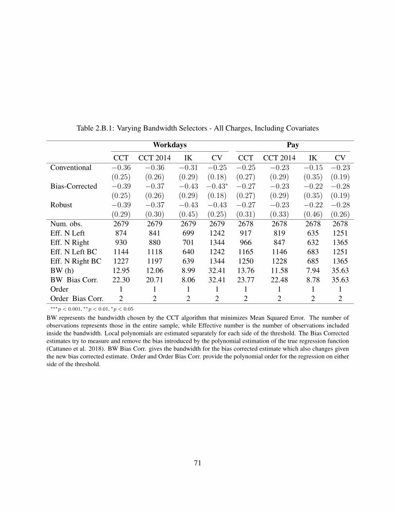
Table 2.B.1: Varying Bandwidth Selectors - All Charges, Including Covariates
Workdays Pay
CCT CCT 2014 IK CV CCT CCT 2014 IK CVConventional −0.36 −0.36 −0.31 −0.25 −0.25 −0.23 −0.15 −0.23
(0.25) (0.26) (0.29) (0.18) (0.27) (0.29) (0.35) (0.19)Bias-Corrected −0.39 −0.37 −0.43 −0.43∗ −0.27 −0.23 −0.22 −0.28
(0.25) (0.26) (0.29) (0.18) (0.27) (0.29) (0.35) (0.19)Robust −0.39 −0.37 −0.43 −0.43 −0.27 −0.23 −0.22 −0.28
(0.29) (0.30) (0.45) (0.25) (0.31) (0.33) (0.46) (0.26)Num. obs. 2679 2679 2679 2679 2678 2678 2678 2678Eff. N Left 874 841 699 1242 917 819 635 1251Eff. N Right 930 880 701 1344 966 847 632 1365Eff. N Left BC 1144 1118 640 1242 1165 1146 683 1251Eff. N Right BC 1227 1197 639 1344 1250 1228 685 1365BW (h) 12.95 12.06 8.99 32.41 13.76 11.58 7.94 35.63BW Bias Corr. 22.30 20.71 8.06 32.41 23.77 22.48 8.78 35.63Order 1 1 1 1 1 1 1 1Order Bias Corr. 2 2 2 2 2 2 2 2∗∗∗p < 0.001, ∗∗p < 0.01, ∗p < 0.05
BW represents the bandwidth chosen by the CCT algorithm that minimizes Mean Squared Error. The number ofobservations represents those in the entire sample, while Effective number is the number of observations includedinside the bandwidth. Local polynomials are estimated separately for each side of the threshold. The Bias Correctedestimates try to measure and remove the bias introduced by the polynomial estimation of the true regression function(Cattaneo et al. 2018). BW Bias Corr. gives the bandwidth for the bias corrected estimate which also changes giventhe new bias corrected estimate. Order and Order Bias Corr. provide the polynomial order for the regression on eitherside of the threshold.
71

2.B.2 Varying Local Polynomial Order
Table 2.B.2: Local Polynomials Varying Order - Non Parametric
Log Workdays
Polynomial Order = 1 2 3 4 5 6Conventional −0.41 −0.37 −0.39 −0.40 −0.36 −0.31
(0.21) (0.26) (0.32) (0.35) (0.42) (0.47)Bias-Corrected −0.39 −0.33 −0.42 −0.43 −0.34 −0.28
(0.21) (0.26) (0.32) (0.35) (0.42) (0.47)Robust −0.39 −0.33 −0.42 −0.43 −0.34 −0.28
(0.25) (0.29) (0.35) (0.37) (0.44) (0.49)Num. obs. 2679 2679 2679 2679 2679 2679Eff. N Left 812 1006 1061 1169 1151 1175Eff. N Right 842 1058 1138 1263 1237 1271Eff. N Left BC 1061 1165 1167 1236 1207 1223Eff. N Right BC 1138 1254 1255 1336 1301 1321BW 11.40 16.28 18.46 24.16 22.89 24.77BW Bias Corr. 18.46 23.91 23.98 31.02 27.91 29.53Order 1 2 3 4 5 6Order Bias Corr. 2 3 4 5 6 7Controls YES YES YES YES YES YESFE YES YES YES YES YES YES∗∗∗p < 0.001, ∗∗p < 0.01, ∗p < 0.05
BW represents the bandwidth chosen by the CCT algorithm that minimizes Mean Squared Error. The number ofobservations represents those in the entire sample, while Effective number is the number of observations includedinside the bandwidth. Local polynomials are estimated separately for each side of the threshold. The Bias Correctedestimates try to measure and remove the bias introduced by the polynomial estimation of the true regression function(Cattaneo et al. 2018). BW Bias Corr. gives the bandwidth for the bias corrected estimate which also changes giventhe new bias corrected estimate. Order and Order Bias Corr. provide the polynomial order for the regression on eitherside of the threshold.
72

Table 2.B.3: Local Polynomials Varying Order - Non Parametric
Log Pay
Polynomial Order = 1 2 3 4 5 6Conventional −0.33 −0.32 −0.35 −0.40 −0.48 −0.46
(0.24) (0.30) (0.35) (0.38) (0.46) (0.51)Bias-Corrected −0.31 −0.30 −0.40 −0.45 −0.48 −0.45
(0.24) (0.30) (0.35) (0.38) (0.46) (0.51)Robust −0.31 −0.30 −0.40 −0.45 −0.48 −0.45
(0.29) (0.34) (0.38) (0.41) (0.48) (0.54)Num. obs. 2678 2678 2678 2678 2678 2678Eff. N Left 783 964 1059 1163 1145 1165Eff. N Right 804 1011 1135 1249 1228 1252Eff. N Left BC 1033 1118 1170 1235 1201 1210Eff. N Right BC 1098 1196 1263 1332 1290 1303BW 10.79 15.06 18.38 23.59 22.41 23.84BW Bias Corr. 17.54 20.69 24.26 30.83 27.19 28.17Order 1 2 3 4 5 6Order Bias Corr. 2 3 4 5 6 7Controls YES YES YES YES YES YESFE YES YES YES YES YES YES∗∗∗p < 0.001, ∗∗p < 0.01, ∗p < 0.05
BW represents the bandwidth chosen by the CCT algorithm that minimizes Mean Squared Error. The number ofobservations represents those in the entire sample, while Effective number is the number of observations includedinside the bandwidth. Local polynomials are estimated separately for each side of the threshold. The Bias Correctedestimates try to measure and remove the bias introduced by the polynomial estimation of the true regression function(Cattaneo et al. 2018). BW Bias Corr. gives the bandwidth for the bias corrected estimate which also changes giventhe new bias corrected estimate. Order and Order Bias Corr. provide the polynomial order for the regression on eitherside of the threshold.
73

Table 2.B.4: Local Polynomials Varying Order - Non Parametric
Log Materials
Polynomial Order = 1 2 3 4 5 6Conventional −0.83∗ −0.88∗ −0.91 −0.94 −0.92 −0.83
(0.35) (0.42) (0.52) (0.59) (0.68) (0.76)Bias-Corrected −0.88∗ −0.85∗ −0.94 −0.97 −0.90 −0.82
(0.35) (0.42) (0.52) (0.59) (0.68) (0.76)Robust −0.88∗ −0.85 −0.94 −0.97 −0.90 −0.82
(0.41) (0.48) (0.57) (0.63) (0.72) (0.79)Num. obs. 2670 2670 2670 2670 2670 2670Eff. N Left 760 977 1042 1124 1138 1161Eff. N Right 772 1031 1120 1218 1227 1259Eff. N Left BC 1011 1126 1152 1197 1196 1209Eff. N Right BC 1072 1220 1244 1297 1296 1311BW 10.32 15.64 17.93 21.59 22.37 24.12BW Bias Corr. 16.81 21.75 23.34 27.55 27.53 28.79Order 1 2 3 4 5 6Order Bias Corr. 2 3 4 5 6 7Controls YES YES YES YES YES YESFE YES YES YES YES YES YES∗∗∗p < 0.001, ∗∗p < 0.01, ∗p < 0.05
BW represents the bandwidth chosen by the CCT algorithm that minimizes Mean Squared Error. The number ofobservations represents those in the entire sample, while Effective number is the number of observations includedinside the bandwidth. Local polynomials are estimated separately for each side of the threshold. The Bias Correctedestimates try to measure and remove the bias introduced by the polynomial estimation of the true regression function(Cattaneo et al. 2018). BW Bias Corr. gives the bandwidth for the bias corrected estimate which also changes giventhe new bias corrected estimate. Order and Order Bias Corr. provide the polynomial order for the regression on eitherside of the threshold.
74

Table 2.B.5: Local Polynomials Varying Order - Non Parametric
Log Projects Completed
Polynomial Order = 1 2 3 4 5 6Conventional −0.48∗∗ −0.52∗∗ −0.53∗ −0.56∗ −0.58∗ −0.69∗
(0.16) (0.20) (0.22) (0.25) (0.28) (0.32)Bias-Corrected −0.51∗∗ −0.53∗∗ −0.56∗ −0.59∗ −0.60∗ −0.71∗
(0.16) (0.20) (0.22) (0.25) (0.28) (0.32)Robust −0.51∗∗ −0.53∗ −0.56∗ −0.59∗ −0.60∗ −0.71∗
(0.18) (0.22) (0.24) (0.26) (0.29) (0.33)Num. obs. 2679 2679 2679 2679 2679 2679Eff. N Left 757 912 1041 1133 1170 1159Eff. N Right 767 966 1112 1222 1264 1247Eff. N Left BC 1017 1068 1163 1219 1234 1215Eff. N Right BC 1074 1141 1250 1312 1332 1310BW 10.12 13.69 17.72 21.79 24.25 23.37BW Bias Corr. 16.83 18.64 23.60 28.97 30.61 28.49Order 1 2 3 4 5 6Order Bias Corr. 2 3 4 5 6 7Controls YES YES YES YES YES YESFE YES YES YES YES YES YES∗∗∗p < 0.001, ∗∗p < 0.01, ∗p < 0.05
BW represents the bandwidth chosen by the CCT algorithm that minimizes Mean Squared Error. The number ofobservations represents those in the entire sample, while Effective number is the number of observations includedinside the bandwidth. Local polynomials are estimated separately for each side of the threshold. The Bias Correctedestimates try to measure and remove the bias introduced by the polynomial estimation of the true regression function(Cattaneo et al. 2018). BW Bias Corr. gives the bandwidth for the bias corrected estimate which also changes giventhe new bias corrected estimate. Order and Order Bias Corr. provide the polynomial order for the regression on eitherside of the threshold.
75

2.B.3 Varying Global/Parametric Polynomials
Table 2.B.6: AIC for Parametric Polynomials (Baseline Spec, NO controls NO FE)
PolynomialOrder Log Workdays Log Pay Log Materials Log Projects Completed
1 13156.58 13620.36 16096.14 12074.932 13150.93 13617.84 16094.36 12076.553 13153.17 13621.30 16094.28 12077.004 13156.95 13624.58 16098.26 12080.255 13160.90 13628.51 16102.21 12082.416 13164.14 13631.16 16105.28 12081.77
76
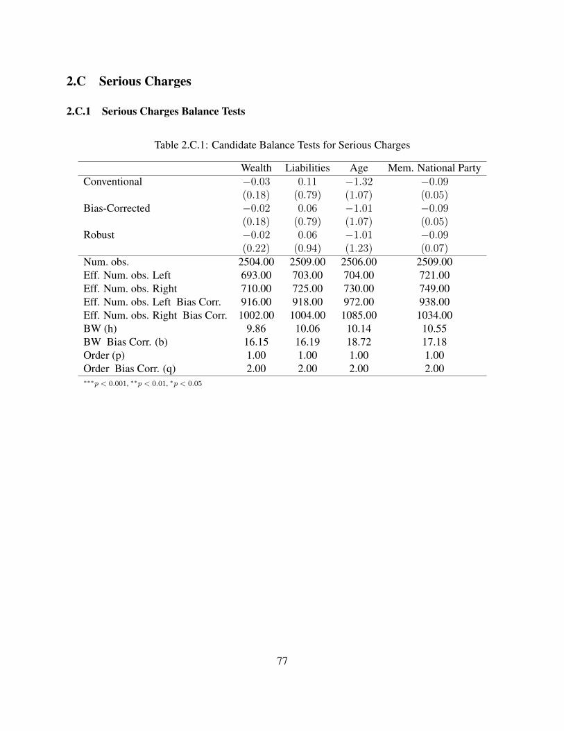
2.C Serious Charges
2.C.1 Serious Charges Balance Tests
Table 2.C.1: Candidate Balance Tests for Serious Charges
Wealth Liabilities Age Mem. National PartyConventional −0.03 0.11 −1.32 −0.09
(0.18) (0.79) (1.07) (0.05)Bias-Corrected −0.02 0.06 −1.01 −0.09
(0.18) (0.79) (1.07) (0.05)Robust −0.02 0.06 −1.01 −0.09
(0.22) (0.94) (1.23) (0.07)Num. obs. 2504.00 2509.00 2506.00 2509.00Eff. Num. obs. Left 693.00 703.00 704.00 721.00Eff. Num. obs. Right 710.00 725.00 730.00 749.00Eff. Num. obs. Left Bias Corr. 916.00 918.00 972.00 938.00Eff. Num. obs. Right Bias Corr. 1002.00 1004.00 1085.00 1034.00BW (h) 9.86 10.06 10.14 10.55BW Bias Corr. (b) 16.15 16.19 18.72 17.18Order (p) 1.00 1.00 1.00 1.00Order Bias Corr. (q) 2.00 2.00 2.00 2.00∗∗∗p < 0.001, ∗∗p < 0.01, ∗p < 0.05
77

Figure 2.C.1: Candidate characteristics Balance Tests for Serious Charges
−60 −40 −20 0 20 40 60
15
17
19
Assets
Criminal Vote Margin (%)
Log
Asse
ts
−60 −40 −20 0 20 40 60
05
10
15
Liabilities
Criminal Vote Margin (%)
Lo
g L
iab
ilities
−60 −40 −20 0 20 40 60
35
45
55
Age
Criminal Vote Margin (%)
Age
−60 −40 −20 0 20 40 60
0.0
0.4
0.8
Member National Party
Criminal Vote Margin (%)
Mem
ber
Na
tion
al P
art
y
78

Figure 2.C.2: Constituency Balance Tests for Serious Charges
−60 −40 −20 0 20 40 60
0.0
0.4
0.8
SC/ST Reserved Constituency
Criminal Vote Margin (%)
Sh
are
Reserv
ed
Con
stitu
en
cy
−60 −40 −20 0 20 40 60
50
00
0
Votes Cast
Criminal Vote Margin (%)
Vote
s C
ast
79

Table 2.C.2: Constituency Balance Tests for Serious Charges
Votes Cast ReservedConventional −638.56 −0.04
(4356.79) (0.03)Bias-Corrected −739.75 −0.04
(4356.79) (0.03)Robust −739.75 −0.04
(5114.37) (0.04)Num. obs. 2509.00 2509.00Eff. Num. obs. Left 661.00 687.00Eff. Num. obs. Right 677.00 702.00Eff. Num. obs. Left Bias Corr. 892.00 921.00Eff. Num. obs. Right Bias Corr. 975.00 1009.00BW (h) 9.21 9.73BW Bias Corr. (b) 15.42 16.33Order (p) 1.00 1.00Order Bias Corr. (q) 2.00 2.00∗∗∗p < 0.001, ∗∗p < 0.01, ∗p < 0.05
2.C.2 Serious Chrages Varying Polynomials for Non-parametric models
80
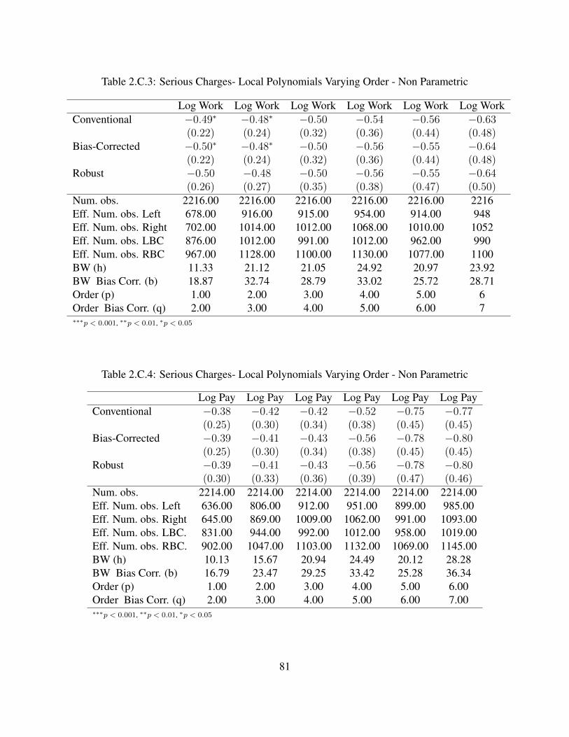
Table 2.C.3: Serious Charges- Local Polynomials Varying Order - Non Parametric
Log Work Log Work Log Work Log Work Log Work Log WorkConventional −0.49∗ −0.48∗ −0.50 −0.54 −0.56 −0.63
(0.22) (0.24) (0.32) (0.36) (0.44) (0.48)Bias-Corrected −0.50∗ −0.48∗ −0.50 −0.56 −0.55 −0.64
(0.22) (0.24) (0.32) (0.36) (0.44) (0.48)Robust −0.50 −0.48 −0.50 −0.56 −0.55 −0.64
(0.26) (0.27) (0.35) (0.38) (0.47) (0.50)Num. obs. 2216.00 2216.00 2216.00 2216.00 2216.00 2216Eff. Num. obs. Left 678.00 916.00 915.00 954.00 914.00 948Eff. Num. obs. Right 702.00 1014.00 1012.00 1068.00 1010.00 1052Eff. Num. obs. LBC 876.00 1012.00 991.00 1012.00 962.00 990Eff. Num. obs. RBC 967.00 1128.00 1100.00 1130.00 1077.00 1100BW (h) 11.33 21.12 21.05 24.92 20.97 23.92BW Bias Corr. (b) 18.87 32.74 28.79 33.02 25.72 28.71Order (p) 1.00 2.00 3.00 4.00 5.00 6Order Bias Corr. (q) 2.00 3.00 4.00 5.00 6.00 7∗∗∗p < 0.001, ∗∗p < 0.01, ∗p < 0.05
Table 2.C.4: Serious Charges- Local Polynomials Varying Order - Non Parametric
Log Pay Log Pay Log Pay Log Pay Log Pay Log PayConventional −0.38 −0.42 −0.42 −0.52 −0.75 −0.77
(0.25) (0.30) (0.34) (0.38) (0.45) (0.45)Bias-Corrected −0.39 −0.41 −0.43 −0.56 −0.78 −0.80
(0.25) (0.30) (0.34) (0.38) (0.45) (0.45)Robust −0.39 −0.41 −0.43 −0.56 −0.78 −0.80
(0.30) (0.33) (0.36) (0.39) (0.47) (0.46)Num. obs. 2214.00 2214.00 2214.00 2214.00 2214.00 2214.00Eff. Num. obs. Left 636.00 806.00 912.00 951.00 899.00 985.00Eff. Num. obs. Right 645.00 869.00 1009.00 1062.00 991.00 1093.00Eff. Num. obs. LBC. 831.00 944.00 992.00 1012.00 958.00 1019.00Eff. Num. obs. RBC. 902.00 1047.00 1103.00 1132.00 1069.00 1145.00BW (h) 10.13 15.67 20.94 24.49 20.12 28.28BW Bias Corr. (b) 16.79 23.47 29.25 33.42 25.28 36.34Order (p) 1.00 2.00 3.00 4.00 5.00 6.00Order Bias Corr. (q) 2.00 3.00 4.00 5.00 6.00 7.00∗∗∗p < 0.001, ∗∗p < 0.01, ∗p < 0.05
81

Table 2.C.5: Serious Charges- Local Polynomials Varying Order - Non Parametric
Log Materials Log Mats. Log Mats Log Mats Log Mats Log MatsConventional −0.82∗ −0.89 −0.94 −0.91 −1.21 −1.20
(0.40) (0.47) (0.65) (0.67) (0.90) (0.90)Bias-Corrected −0.87∗ −0.85 −1.00 −0.94 −1.28 −1.24
(0.40) (0.47) (0.65) (0.67) (0.90) (0.90)Robust −0.87 −0.85 −1.00 −0.94 −1.28 −1.24
(0.49) (0.54) (0.72) (0.72) (0.96) (0.94)Num. obs. 2212.00 2212.00 2212.00 2212.00 2212.00 2212Eff. Num. obs. Left 642.00 849.00 846.00 967.00 912.00 991Eff. Num. obs. Right 655.00 935.00 928.00 1080.00 1021.00 1108Eff. Num. obs. LBC 832.00 956.00 925.00 1009.00 956.00 1015Eff. Num. obs. RBC 906.00 1071.00 1031.00 1133.00 1072.00 1145BW (h) 10.39 17.71 17.60 26.35 21.42 29.60BW Bias Corr. (b) 16.93 25.36 22.23 33.42 25.45 35.73Order (p) 1.00 2.00 3.00 4.00 5.00 6Order Bias Corr. (q) 2.00 3.00 4.00 5.00 6.00 7∗∗∗p < 0.001, ∗∗p < 0.01, ∗p < 0.05
Table 2.C.6: Serious Charges- Local Polynomials Varying Order - Non Parametric
Log Projects Log Proj. Log Proj. Log Proj. Log Proj. Log Proj.Conventional −0.46∗∗ −0.53∗∗ −0.55∗ −0.59∗ −0.65∗ −0.70∗
(0.17) (0.20) (0.24) (0.27) (0.31) (0.32)Bias-Corrected −0.51∗∗ −0.54∗∗ −0.57∗ −0.61∗ −0.67∗ −0.73∗
(0.17) (0.20) (0.24) (0.27) (0.31) (0.32)Robust −0.51∗ −0.54∗ −0.57∗ −0.61∗ −0.67∗ −0.73∗
(0.20) (0.23) (0.27) (0.28) (0.33) (0.33)Num. obs. 2216.00 2216.00 2216.00 2216.00 2216.00 2216Eff. Num. obs. Left 596.00 777.00 833.00 920.00 916.00 983Eff. Num. obs. Right 600.00 836.00 905.00 1023.00 1013.00 1093Eff. Num. obs. LBC 809.00 909.00 933.00 988.00 970.00 1020Eff. Num. obs. RBC 870.00 1004.00 1035.00 1096.00 1078.00 1146BW (h) 9.16 14.64 16.88 21.68 21.11 28.01BW Bias Corr. (b) 15.73 20.57 22.57 28.37 26.21 36.18Order (p) 1.00 2.00 3.00 4.00 5.00 6Order Bias Corr. (q) 2.00 3.00 4.00 5.00 6.00 7∗∗∗p < 0.001, ∗∗p < 0.01, ∗p < 0.05
82

2.C.3 Serious Charges Bandwidth Sensitivity
Figure 2.C.3: Serious Charges Sensitivity Analysis - LATE for Varying Bandwidths- Baseline withFixed Effects and RDRobust data driven BWS
(a) Log Workdays (b) Log Pay
(c) Log Materials (d) Log Projects Completed
Note that RD estimates are non-parametric linear polynomials from the RDDTools package using the data-drivenbandwidth selector from the RDRobust package. This leads to slightly different standard errors than those calculatedunder the RDrobust package (e.g. Tables above). However the point estimates remain the same.
83

2.C.4 Serious Charges Placebo Tests
Figure 2.C.4: Serious Charges Placebo Tests - LATE for Varying Cutpoints- Baseline with FixedEffects and RDRobust data driven BWS
(a) Log Workdays (b) Log Pay
(c) Log Materials (d) Log Projects Completed
Note that RD estimates are non-parametric linear polynomials from the RDDTools package using the data-drivenbandwidth selector from the RDRobust package. This leads to slightly different standard errors than those calculatedunder the RDrobust package (e.g. Tables above). However the point estimates remain the same.
84

2.D State-Years in RD Sample
Table 2.D.1: State Legislative Elections in RD Sample
State # Constituencies Election Year1 andhra pradesh 169 2009, 20142 arunachal pradesh 12 2004, 2009, 20143 assam 64 2006, 2011, 20164 bihar 273 2005, 2010, 20155 chhattisgarh 38 2008, 20136 delhi 88 2008, 2013, 20157 goa 23 2007, 20128 gujarat 104 2007, 20129 haryana 73 2005, 2009, 2014
10 himachal pradesh 49 2007, 201211 jammu kashmir 15 2008, 201412 jharkhand 96 2005, 2009, 201413 karnataka 131 2008, 201314 kerala 202 2006, 2011, 201615 madhya pradesh 126 2008, 201316 maharashtra 384 2004, 2009, 201417 manipur 5 2007, 201218 meghalaya 5 2008, 201319 mizoram 6 2008, 201320 nagaland 3 2008, 201321 odisha 138 2004, 2009, 201422 puducherry 29 2006, 2011, 201623 punjab 66 2007, 201224 rajasthan 90 2008, 201325 sikkim 14 2009, 201426 tamil nadu 237 2006, 2011, 201627 tripura 16 2008, 201328 uttar pradesh 338 2007, 201229 uttarakhand 35 2007, 201230 west bengal 324 2006, 2011, 2016
85
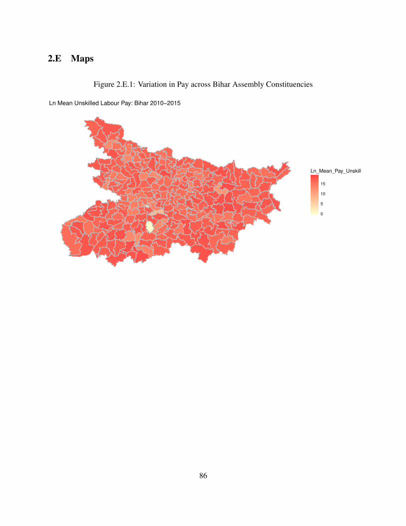
2.E Maps
Figure 2.E.1: Variation in Pay across Bihar Assembly Constituencies
0
5
10
15
Ln_Mean_Pay_Unskill
Ln Mean Unskilled Labour Pay: Bihar 2010−2015
86

2.F Unlogged Estimates
Table 2.F.1: RD Robust
Workdays Pay Materials Projects Comp.Conventional −241463.62 −11542589.81 −6656203.51 −360.47
(135792.14) (13349696.42) (6042734.37) (221.94)Bias-Corrected −270744.86∗ −11293911.30 −6828284.92 −402.32
(135792.14) (13349696.42) (6042734.37) (221.94)Robust −270744.86 −11293911.30 −6828284.92 −402.32
(159048.89) (15729776.77) (7039976.62) (264.23)Num. obs. 2679.00 2678.00 2670.00 2679.00Eff. Num. obs. Left 734.00 767.00 844.00 828.00Eff. Num. obs. Right 739.00 775.00 890.00 862.00Eff. Num. obs. LBC 1001.00 1012.00 1103.00 1080.00Eff. Num. obs. RBC 1053.00 1065.00 1181.00 1159.00BW (h) 9.66 10.36 12.28 11.79BW Bias Corr. (b) 16.07 16.66 20.33 19.26Order (p) 1.00 1.00 1.00 1.00Order Bias Corr. (q) 2.00 2.00 2.00 2.00∗∗∗p < 0.001, ∗∗p < 0.01, ∗p < 0.05
BW represents the bandwidth chosen by the CCT algorithm that minimizes Mean Squared Error. The number ofobservations represents those in the entire sample, while Effective number is the number of observations includedinside the bandwidth. Local polynomials are estimated separately for each side of the threshold. The Bias Correctedestimates try to measure and remove the bias introduced by the polynomial estimation of the true regression function(Cattaneo et al. 2018). BW Bias Corr. gives the bandwidth for the bias corrected estimate which also changes giventhe new bias corrected estimate. Order and Order Bias Corr. provide the polynomial order for the regression on eitherside of the threshold.
87

2.G Variation in NREGS Outcomes by State and MLA type
I replicate state level variation in NREGS performance in Figures 1 through 4. These plots ag-
gregate each NREGS outcome to the state-level, depending on if the sitting MLA in a given con-
stituency faced one or more criminal charges (blue dashed line) or was uncharged (red solid line).
Consistent with other studies, the plots show a general increase over time in program expenditures
and project completion (Sukhtankar 2016). Interestingly in the raw data, clean politicians (red
line) consistently outperform charged politicians (blue line) in NREGS delivery.44 There are a few
notable exceptions to this overall trend. Constituencies that elect criminally charged politicians
seem to fare as well, if not better, in Bihar, Jharkhand, Uttar Pradesh, Maharashtra and Kerala.
The first three states are known for their NREGS underperformance and abundance of criminally
charged politicians. However, Kerala is somewhat of the odd state out, having the highest human
development of any Indian state.
44This data is for the entire sample and is not restricted to mixed elections a la the RD sample. I also include allcharges and do not restrict the definition of a charge to those of only a serious nature.
88

Figure 2.G.1: Variation in Workdays by State and Criminal status of MLA
TRIPURA UTTAR PRADESH UTTARAKHAND WEST BENGAL
ODISHA PUDUCHERRY PUNJAB RAJASTHAN SIKKIM TAMIL NADU
MADHYA PRADESH MAHARASHTRA MANIPUR MEGHALAYA MIZORAM NAGALAND
GUJARAT HARYANA HIMACHAL PRADESH JHARKHAND KARNATAKA KERALA
ANDHRA PRADESH ARUNACHAL PRADESH ASSAM BIHAR CHHATTISGARH GOA
20
04
20
07
20
10
20
13
20
16
20
04
20
07
20
10
20
13
20
16
20
04
20
07
20
10
20
13
20
16
20
04
20
07
20
10
20
13
20
16
20
04
20
07
20
10
20
13
20
16
20
04
20
07
20
10
20
13
20
16
05
101520
05
101520
05
101520
05
101520
05
101520
Year
Ln W
ork
days +
1
Charged 0 1
In order to highlight the disparity between accused and unaccused politicians these plots do not divide outcomes bypopulation. As such, populous states like Bihar and Uttar Pradesh seem to perform better than they would on a percapita basis. The logarithmic scale also flattens variation between states.
89
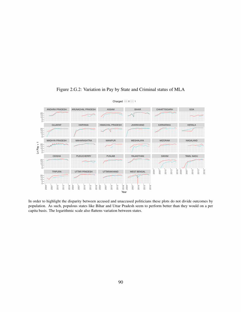
Figure 2.G.2: Variation in Pay by State and Criminal status of MLA
TRIPURA UTTAR PRADESH UTTARAKHAND WEST BENGAL
ODISHA PUDUCHERRY PUNJAB RAJASTHAN SIKKIM TAMIL NADU
MADHYA PRADESH MAHARASHTRA MANIPUR MEGHALAYA MIZORAM NAGALAND
GUJARAT HARYANA HIMACHAL PRADESH JHARKHAND KARNATAKA KERALA
ANDHRA PRADESH ARUNACHAL PRADESH ASSAM BIHAR CHHATTISGARH GOA
20
04
20
07
20
10
20
13
20
16
20
04
20
07
20
10
20
13
20
16
20
04
20
07
20
10
20
13
20
16
20
04
20
07
20
10
20
13
20
16
20
04
20
07
20
10
20
13
20
16
20
04
20
07
20
10
20
13
20
16
05
101520
05
101520
05
101520
05
101520
05
101520
Year
Ln P
ay +
1
Charged 0 1
In order to highlight the disparity between accused and unaccused politicians these plots do not divide outcomes bypopulation. As such, populous states like Bihar and Uttar Pradesh seem to perform better than they would on a percapita basis. The logarithmic scale also flattens variation between states.
90
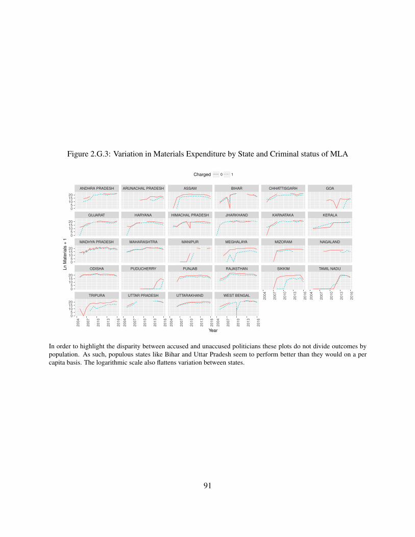
Figure 2.G.3: Variation in Materials Expenditure by State and Criminal status of MLA
TRIPURA UTTAR PRADESH UTTARAKHAND WEST BENGAL
ODISHA PUDUCHERRY PUNJAB RAJASTHAN SIKKIM TAMIL NADU
MADHYA PRADESH MAHARASHTRA MANIPUR MEGHALAYA MIZORAM NAGALAND
GUJARAT HARYANA HIMACHAL PRADESH JHARKHAND KARNATAKA KERALA
ANDHRA PRADESH ARUNACHAL PRADESH ASSAM BIHAR CHHATTISGARH GOA
20
04
20
07
20
10
20
13
20
16
20
04
20
07
20
10
20
13
20
16
20
04
20
07
20
10
20
13
20
16
20
04
20
07
20
10
20
13
20
16
20
04
20
07
20
10
20
13
20
16
20
04
20
07
20
10
20
13
20
16
05
101520
05
101520
05
101520
05
101520
05
101520
Year
Ln M
ate
rials
+ 1
Charged 0 1
In order to highlight the disparity between accused and unaccused politicians these plots do not divide outcomes bypopulation. As such, populous states like Bihar and Uttar Pradesh seem to perform better than they would on a percapita basis. The logarithmic scale also flattens variation between states.
91

Figure 2.G.4: Varation in Projects completed by State and Criminal status of MLA
TRIPURA UTTAR PRADESH UTTARAKHAND WEST BENGAL
ODISHA PUDUCHERRY PUNJAB RAJASTHAN SIKKIM TAMIL NADU
MADHYA PRADESH MAHARASHTRA MANIPUR MEGHALAYA MIZORAM NAGALAND
GUJARAT HARYANA HIMACHAL PRADESH JHARKHAND KARNATAKA KERALA
ANDHRA PRADESH ARUNACHAL PRADESH ASSAM BIHAR CHHATTISGARH GOA
20
04
20
07
20
10
20
13
20
16
20
04
20
07
20
10
20
13
20
16
20
04
20
07
20
10
20
13
20
16
20
04
20
07
20
10
20
13
20
16
20
04
20
07
20
10
20
13
20
16
20
04
20
07
20
10
20
13
20
16
2.55.07.5
10.012.5
2.55.07.5
10.012.5
2.55.07.5
10.012.5
2.55.07.5
10.012.5
2.55.07.5
10.012.5
Year
Ln A
ssets
+ 1
Charged 0 1
In order to highlight the disparity between accused and unaccused politicians these plots do not divide outcomes bypopulation. As such, populous states like Bihar and Uttar Pradesh seem to perform better than they would on a percapita basis. The logarithmic scale also flattens variation between states.
92

2.H Estimates from Various R Packages
Table 2.H.1: RD Package
Log Workdays Log Pay Log Materials Log Projects CompletedLATE −0.40 −0.42 −0.95 −0.63
(0.40) (0.48) (0.73) (0.35)Half-BW −0.40 −0.36 −0.50 −0.76
(0.57) (0.71) (1.05) (0.47)Double-BW −0.32 −0.15 −0.71 −0.35
(0.30) (0.36) (0.51) (0.26)Obs LATE 769.00 679.00 790.00 611.00Obs Half-BW 402.00 353.00 424.00 311.00Obs Doulbe-BW 1411.00 1250.00 1441.00 1135.00BW LATE 4.54 3.91 4.72 3.49BW Half-BW 2.27 1.95 2.36 1.75BW Doulbe-BW 9.07 7.82 9.44 6.99∗∗∗p < 0.001, ∗∗p < 0.01, ∗p < 0.05
BW represents the bandwidth chosen by the CCT algorithm that minimizes Mean Squared Error. The number ofobservations represents those in the entire sample, while Effective number is the number of observations includedinside the bandwidth. Local polynomials are estimated separately for each side of the threshold. The Bias Correctedestimates try to measure and remove the bias introduced by the polynomial estimation of the true regression function(Cattaneo et al. 2018). BW Bias Corr. gives the bandwidth for the bias corrected estimate which also changes giventhe new bias corrected estimate. Order and Order Bias Corr. provide the polynomial order for the regression on eitherside of the threshold.
93

Table 2.H.2: RDD Tools
Log Workdays Log Pay Log Materials Log Projects CompletedEstimate −0.01 −0.03 −0.06 −0.01
(0.17) (0.18) (0.29) (0.13)No. Obs 2679.00 2678.00 2670.00 2679.00Order 1.00 1.00 1.00 1.00∗∗∗p < 0.001, ∗∗p < 0.01, ∗p < 0.05
BW represents the bandwidth chosen by the CCT algorithm that minimizes Mean Squared Error. The number ofobservations represents those in the entire sample, while Effective number is the number of observations includedinside the bandwidth. Local polynomials are estimated separately for each side of the threshold. The Bias Correctedestimates try to measure and remove the bias introduced by the polynomial estimation of the true regression function(Cattaneo et al. 2018). BW Bias Corr. gives the bandwidth for the bias corrected estimate which also changes giventhe new bias corrected estimate. Order and Order Bias Corr. provide the polynomial order for the regression on eitherside of the threshold.
2.I Estimates from Varying Bandwith Sizes
Figure 2.I.1: Sensitivity Analysis - LATE for Varying Bandwidths- Baseline with FE and rddtools
(a) Log Workdays (b) Log Pay
(c) Log Materials (d) Log Projects Completed
94

Figure 2.I.2: Sensitivity Analysis - LATE for Varying Bandwidths - Baseline with RDRobust datadriven BWS
(a) Log Workdays (b) Log Pay
(c) Log Materials (d) Log Projects Completed
Note that RD estimates are non-parametric linear polynomials from the RDDTools package using the data-drivenbandwidth selector from the RDRobust package. This leads to slightly different standard errors than those calculatedunder the RDrobust package (e.g. Tables above). However the point estimates remain the same.
95
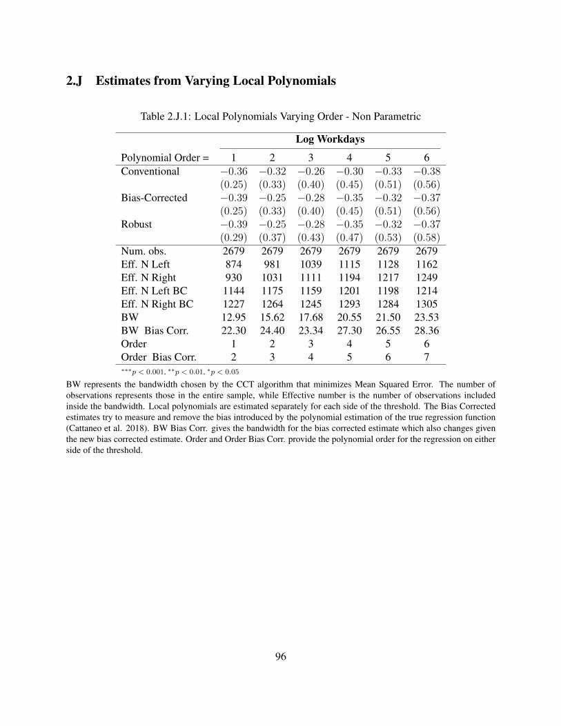
2.J Estimates from Varying Local Polynomials
Table 2.J.1: Local Polynomials Varying Order - Non Parametric
Log Workdays
Polynomial Order = 1 2 3 4 5 6Conventional −0.36 −0.32 −0.26 −0.30 −0.33 −0.38
(0.25) (0.33) (0.40) (0.45) (0.51) (0.56)Bias-Corrected −0.39 −0.25 −0.28 −0.35 −0.32 −0.37
(0.25) (0.33) (0.40) (0.45) (0.51) (0.56)Robust −0.39 −0.25 −0.28 −0.35 −0.32 −0.37
(0.29) (0.37) (0.43) (0.47) (0.53) (0.58)Num. obs. 2679 2679 2679 2679 2679 2679Eff. N Left 874 981 1039 1115 1128 1162Eff. N Right 930 1031 1111 1194 1217 1249Eff. N Left BC 1144 1175 1159 1201 1198 1214Eff. N Right BC 1227 1264 1245 1293 1284 1305BW 12.95 15.62 17.68 20.55 21.50 23.53BW Bias Corr. 22.30 24.40 23.34 27.30 26.55 28.36Order 1 2 3 4 5 6Order Bias Corr. 2 3 4 5 6 7∗∗∗p < 0.001, ∗∗p < 0.01, ∗p < 0.05
BW represents the bandwidth chosen by the CCT algorithm that minimizes Mean Squared Error. The number ofobservations represents those in the entire sample, while Effective number is the number of observations includedinside the bandwidth. Local polynomials are estimated separately for each side of the threshold. The Bias Correctedestimates try to measure and remove the bias introduced by the polynomial estimation of the true regression function(Cattaneo et al. 2018). BW Bias Corr. gives the bandwidth for the bias corrected estimate which also changes giventhe new bias corrected estimate. Order and Order Bias Corr. provide the polynomial order for the regression on eitherside of the threshold.
96

Table 2.J.2: Local Polynomials Varying Order - Non Parametric
Log Pay
Polynomial Order = 1 2 3 4 5 6Conventional −0.25 −0.17 −0.18 −0.26 −0.45 −0.53
(0.27) (0.38) (0.44) (0.49) (0.57) (0.64)Bias-Corrected −0.27 −0.11 −0.23 −0.33 −0.47 −0.53
(0.27) (0.38) (0.44) (0.49) (0.57) (0.64)Robust −0.27 −0.11 −0.23 −0.33 −0.47 −0.53
(0.31) (0.42) (0.48) (0.52) (0.61) (0.68)Num. obs. 2678 2678 2678 2678 2678 2678Eff. Num. obs. Left 917 959 1049 1139 1127 1156Eff. Num. obs. Right 966 1007 1120 1225 1215 1241Eff. N Left BC 1165 1128 1164 1221 1190 1206Eff. N Right BC 1250 1216 1249 1316 1282 1297BW (h) 13.76 14.95 17.92 22.05 21.44 23.23BW Bias Corr. 23.77 21.48 23.64 29.27 26.11 27.58Order 1 2 3 4 5 6Order Bias Corr. 2 3 4 5 6 7∗∗∗p < 0.001, ∗∗p < 0.01, ∗p < 0.05
97
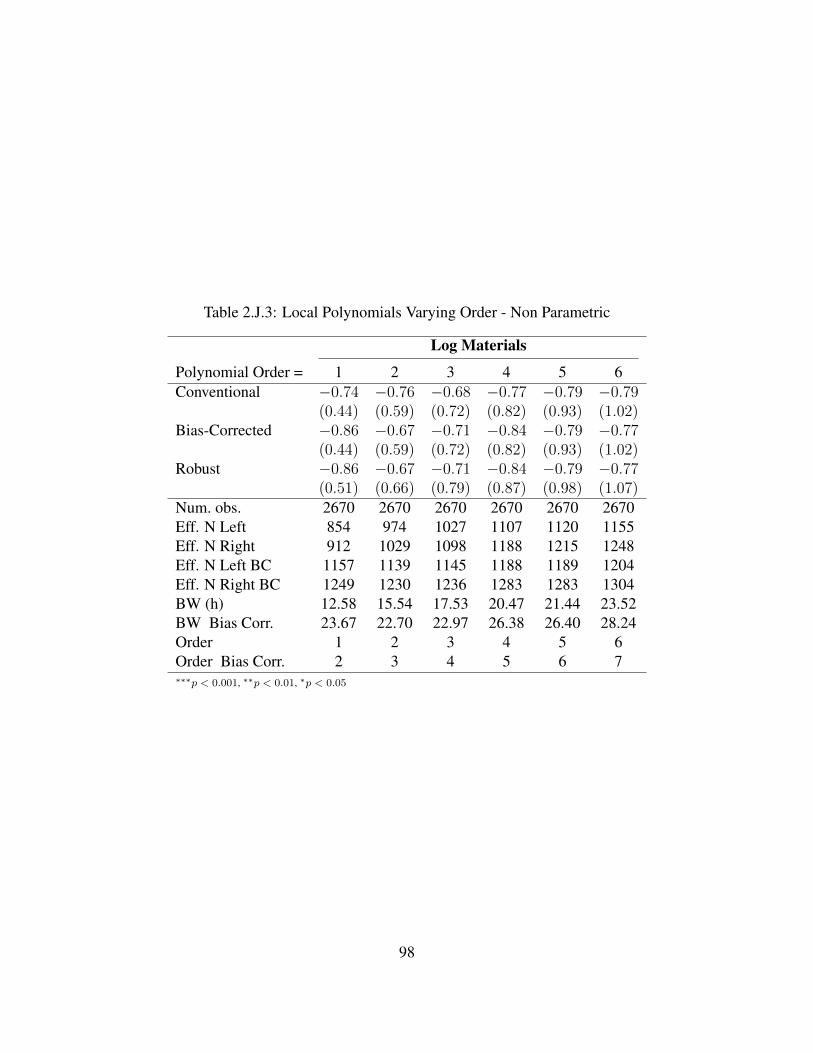
Table 2.J.3: Local Polynomials Varying Order - Non Parametric
Log Materials
Polynomial Order = 1 2 3 4 5 6Conventional −0.74 −0.76 −0.68 −0.77 −0.79 −0.79
(0.44) (0.59) (0.72) (0.82) (0.93) (1.02)Bias-Corrected −0.86 −0.67 −0.71 −0.84 −0.79 −0.77
(0.44) (0.59) (0.72) (0.82) (0.93) (1.02)Robust −0.86 −0.67 −0.71 −0.84 −0.79 −0.77
(0.51) (0.66) (0.79) (0.87) (0.98) (1.07)Num. obs. 2670 2670 2670 2670 2670 2670Eff. N Left 854 974 1027 1107 1120 1155Eff. N Right 912 1029 1098 1188 1215 1248Eff. N Left BC 1157 1139 1145 1188 1189 1204Eff. N Right BC 1249 1230 1236 1283 1283 1304BW (h) 12.58 15.54 17.53 20.47 21.44 23.52BW Bias Corr. 23.67 22.70 22.97 26.38 26.40 28.24Order 1 2 3 4 5 6Order Bias Corr. 2 3 4 5 6 7∗∗∗p < 0.001, ∗∗p < 0.01, ∗p < 0.05
98
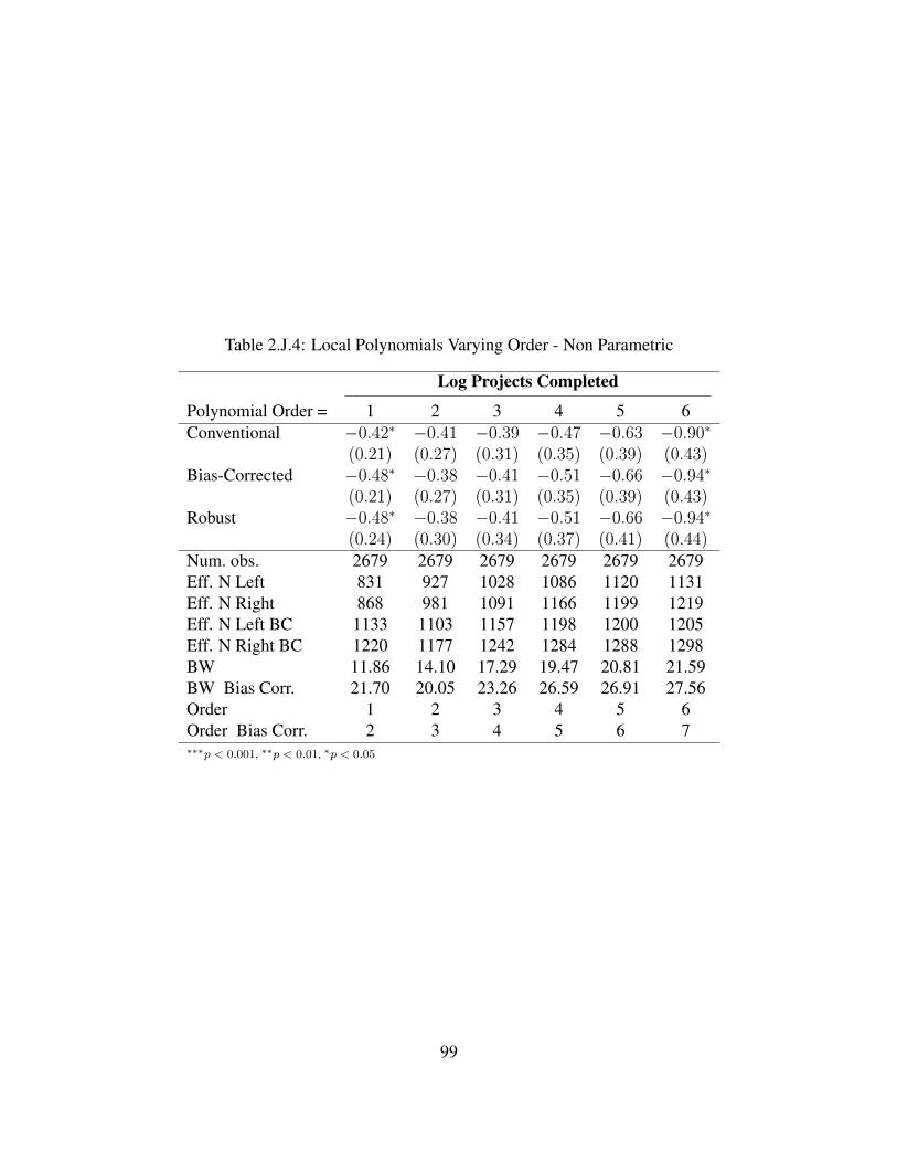
Table 2.J.4: Local Polynomials Varying Order - Non Parametric
Log Projects Completed
Polynomial Order = 1 2 3 4 5 6Conventional −0.42∗ −0.41 −0.39 −0.47 −0.63 −0.90∗
(0.21) (0.27) (0.31) (0.35) (0.39) (0.43)Bias-Corrected −0.48∗ −0.38 −0.41 −0.51 −0.66 −0.94∗
(0.21) (0.27) (0.31) (0.35) (0.39) (0.43)Robust −0.48∗ −0.38 −0.41 −0.51 −0.66 −0.94∗
(0.24) (0.30) (0.34) (0.37) (0.41) (0.44)Num. obs. 2679 2679 2679 2679 2679 2679Eff. N Left 831 927 1028 1086 1120 1131Eff. N Right 868 981 1091 1166 1199 1219Eff. N Left BC 1133 1103 1157 1198 1200 1205Eff. N Right BC 1220 1177 1242 1284 1288 1298BW 11.86 14.10 17.29 19.47 20.81 21.59BW Bias Corr. 21.70 20.05 23.26 26.59 26.91 27.56Order 1 2 3 4 5 6Order Bias Corr. 2 3 4 5 6 7∗∗∗p < 0.001, ∗∗p < 0.01, ∗p < 0.05
99

2.K Placebo Tests
Figure 2.K.1: Placebo Tests - LATE for Varying Cutpoints- Baseline with FE and rddtools
(a) Log Workdays (b) Log Pay
(c) Log Materials (d) Log Projects Completed
100
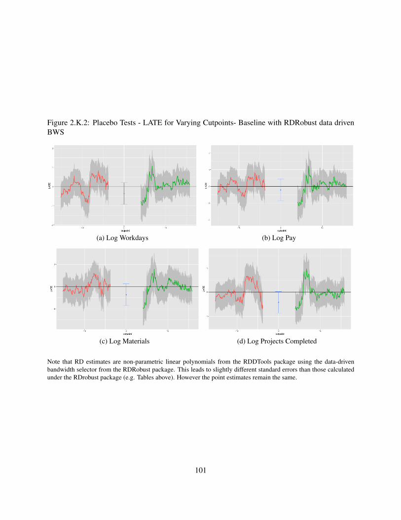
Figure 2.K.2: Placebo Tests - LATE for Varying Cutpoints- Baseline with RDRobust data drivenBWS
(a) Log Workdays (b) Log Pay
(c) Log Materials (d) Log Projects Completed
Note that RD estimates are non-parametric linear polynomials from the RDDTools package using the data-drivenbandwidth selector from the RDRobust package. This leads to slightly different standard errors than those calculatedunder the RDrobust package (e.g. Tables above). However the point estimates remain the same.
101
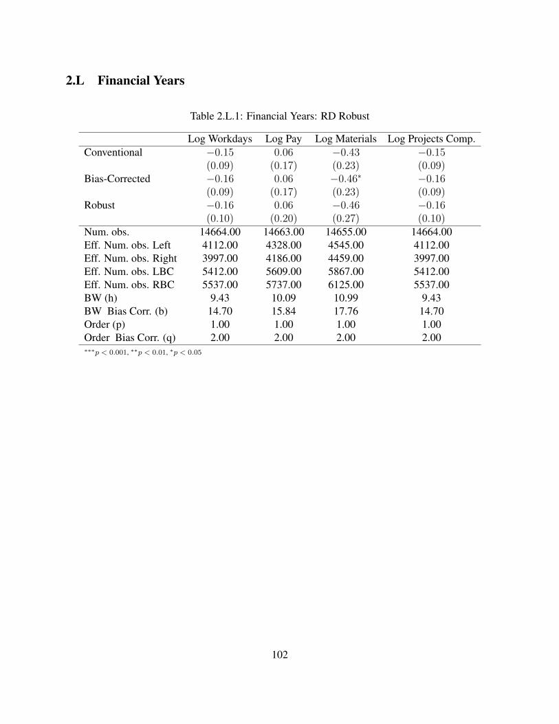
2.L Financial Years
Table 2.L.1: Financial Years: RD Robust
Log Workdays Log Pay Log Materials Log Projects Comp.Conventional −0.15 0.06 −0.43 −0.15
(0.09) (0.17) (0.23) (0.09)Bias-Corrected −0.16 0.06 −0.46∗ −0.16
(0.09) (0.17) (0.23) (0.09)Robust −0.16 0.06 −0.46 −0.16
(0.10) (0.20) (0.27) (0.10)Num. obs. 14664.00 14663.00 14655.00 14664.00Eff. Num. obs. Left 4112.00 4328.00 4545.00 4112.00Eff. Num. obs. Right 3997.00 4186.00 4459.00 3997.00Eff. Num. obs. LBC 5412.00 5609.00 5867.00 5412.00Eff. Num. obs. RBC 5537.00 5737.00 6125.00 5537.00BW (h) 9.43 10.09 10.99 9.43BW Bias Corr. (b) 14.70 15.84 17.76 14.70Order (p) 1.00 1.00 1.00 1.00Order Bias Corr. (q) 2.00 2.00 2.00 2.00∗∗∗p < 0.001, ∗∗p < 0.01, ∗p < 0.05
102

Tabl
e2.
L.2
:Fin
anci
alY
ears
-RD
Rob
ust
Log
Wor
kday
sL
ogPa
yL
ogM
ater
ials
Log
Proj
ects
Com
p.
Con
vent
iona
l−0.07−0.07−0.05
0.06
0.06
0.03
−0.43
−0.43−0.36−0.15−0.15−0.19
∗
(0.12)
(0.13)
(0.13)
(0.17)
(0.17)
(0.17)
(0.23)
(0.23)
(0.23)
(0.09)
(0.09)
(0.09)
Bia
s-C
orre
cted
−0.07−0.06−0.05
0.06
0.07
0.02
−0.46
∗−0.45−0.39−0.16−0.17−0.20
∗
(0.12)
(0.13)
(0.13)
(0.17)
(0.17)
(0.17)
(0.23)
(0.23)
(0.23)
(0.09)
(0.09)
(0.09)
Rob
ust
−0.07−0.06−0.05
0.06
0.07
0.02
−0.46
−0.45−0.39−0.16−0.17−0.20
∗
(0.15)
(0.15)
(0.15)
(0.20)
(0.20)
(0.20)
(0.27)
(0.28)
(0.28)
(0.10)
(0.10)
(0.10)
Num
.obs
.14
664
1466
414
664
1466
314
663
1466
314
655
1465
514
655
1466
414
664
1466
4E
ff.o
bs.L
eft
4562
4431
4392
4328
4326
4328
4545
4412
4306
4112
4104
4233
Eff
.obs
.Rig
ht44
9143
3342
4241
8641
7741
8644
5943
0541
7739
9739
6740
85E
ff.o
bs.L
BC
5901
5764
5688
5609
5575
5575
5867
5683
5547
5412
5374
5550
Eff
.obs
.RB
C61
5859
3558
4657
3757
0257
0261
2558
4556
7555
3755
1856
76B
W11
.08
10.5
910
.38
10.0
910
.02
10.0
610
.99
10.4
810
9.43
9.32
9.78
BW
Bia
sC
orr.
17.8
917
.13
16.4
715
.84
15.7
215
.71
17.7
616
.50
15.5
314
.70
14.5
715
.52
Ord
er1
11
11
11
11
11
1O
rder
Bia
sC
orr.
22
22
22
22
22
22
∗∗∗p<
0.001
,∗∗p<
0.01
,∗p<
0.05
103
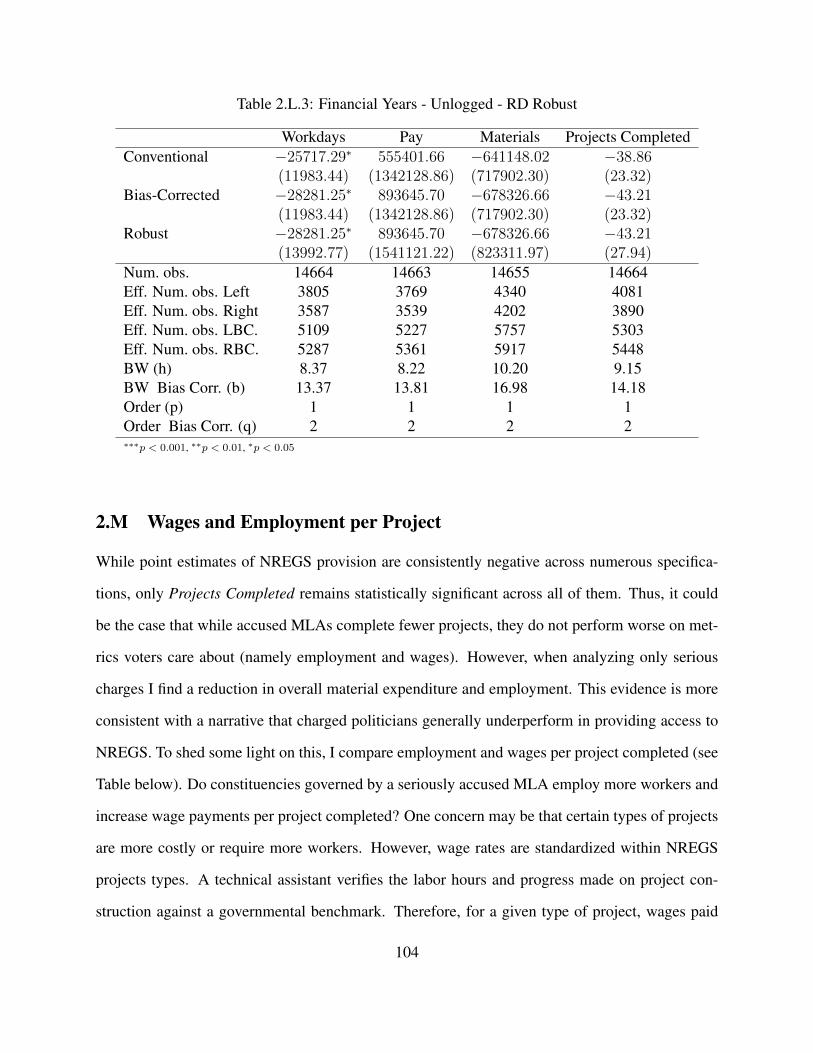
Table 2.L.3: Financial Years - Unlogged - RD Robust
Workdays Pay Materials Projects CompletedConventional −25717.29∗ 555401.66 −641148.02 −38.86
(11983.44) (1342128.86) (717902.30) (23.32)Bias-Corrected −28281.25∗ 893645.70 −678326.66 −43.21
(11983.44) (1342128.86) (717902.30) (23.32)Robust −28281.25∗ 893645.70 −678326.66 −43.21
(13992.77) (1541121.22) (823311.97) (27.94)Num. obs. 14664 14663 14655 14664Eff. Num. obs. Left 3805 3769 4340 4081Eff. Num. obs. Right 3587 3539 4202 3890Eff. Num. obs. LBC. 5109 5227 5757 5303Eff. Num. obs. RBC. 5287 5361 5917 5448BW (h) 8.37 8.22 10.20 9.15BW Bias Corr. (b) 13.37 13.81 16.98 14.18Order (p) 1 1 1 1Order Bias Corr. (q) 2 2 2 2∗∗∗p < 0.001, ∗∗p < 0.01, ∗p < 0.05
2.M Wages and Employment per Project
While point estimates of NREGS provision are consistently negative across numerous specifica-
tions, only Projects Completed remains statistically significant across all of them. Thus, it could
be the case that while accused MLAs complete fewer projects, they do not perform worse on met-
rics voters care about (namely employment and wages). However, when analyzing only serious
charges I find a reduction in overall material expenditure and employment. This evidence is more
consistent with a narrative that charged politicians generally underperform in providing access to
NREGS. To shed some light on this, I compare employment and wages per project completed (see
Table below). Do constituencies governed by a seriously accused MLA employ more workers and
increase wage payments per project completed? One concern may be that certain types of projects
are more costly or require more workers. However, wage rates are standardized within NREGS
projects types. A technical assistant verifies the labor hours and progress made on project con-
struction against a governmental benchmark. Therefore, for a given type of project, wages paid
104

per day and the number of workers needed should be similar.45
The table below demonstrates that projects completed in seriously accused constituencies wit-
ness higher levels of employment and pay per project. Since I do not observe actual hours worked
or if wages reach NREGS laborers, I can not adjudicate between whether this indicates improved
worker outcomes or increased leakage. In other words, more workdays and higher labor expendi-
tures could represent over-reporting or ghost-workers, with the excess rents captured by bureau-
crats and/or politicians. An alternative explanation could be that constituencies governed by a
seriously accused MLA happen to engage in more expensive or difficult projects. However, under
the regression discontinuity design project type should not systematically vary with the criminal
status of the MLA.46 Finally, the results are only statistically significant in the model adding fixed
effects and controls. However, this does not result from a reduction in standard errors but instead a
dramatic increase in the size of point estimates. The large jump in coefficient size and simultaneous
increase in standard errors, after adding controls, are indicative of model misspecification. Given
these caveats, I take the results of this analysis as minimally suggestive and exploratory for now.
I investigate alternative, qualitatively informed, measures of NREGS corruption in the subsequent
section.45While this is the formal vetting process, as noted above the ground level experience of NREGS can diverge
dramatically from the formal process.46I plan to test this more formally by checking for balance across project types in accused and unaccused constituen-
cies.
105

Table 2.M.1: Serious Charges Log Pay and Work per Project
LnWorkdaysLnProject
LnPayLnProject
Conventional 0.01 0.28∗ 0.18 0.59∗
(0.14) (0.12) (0.18) (0.23)Bias-Corrected 0.04 0.31∗ 0.24 0.66∗∗
(0.14) (0.12) (0.18) (0.23)Robust 0.04 0.31∗ 0.24 0.66∗
(0.16) (0.14) (0.20) (0.26)Num. obs. 2221 2216 2219 2214Eff. Num. obs. Left 591 583 602 584Eff. Num. obs. Right 595 590 606 591Eff. Num. obs. Left Bias Corr. 834 826 877 830Eff. Num. obs. Right Bias Corr. 906 894 970 899BW (h) 8.96 8.89 9.28 8.91BW Bias Corr. (b) 16.74 16.49 18.94 16.72Order (p) 1 1 1 1Order Bias Corr. (q) 2 2 2 2∗∗∗p < 0.001, ∗∗p < 0.01, ∗p < 0.05
For the models including fixed effects, outcomes are the residuals after controlling for state and election year. BWrepresents the bandwidth chosen by the CCT algorithm that minimizes Mean Squared Error. The number of observa-tions represents those in the entire sample, while Effective number is the number of observations included inside thebandwidth. Local polynomials are estimated separately for each side of the threshold. The Bias Corrected estimatestry to measure and remove the bias introduced by the polynomial estimation of the true regression function (Cattaneoet al. 2018). BW Bias Corr. gives the bandwidth for the bias corrected estimate which also changes given the new biascorrected estimate. Order and Order Bias Corr. provide the polynomial order for the regression on either side of thethreshold.
106

Chapter 3
Criminal Crosshairs: Do Criminal Politicians Target
Co-partisans?
3.1 Introduction
One explanation for criminal politicians’ continued electability is their ability to connect voters
to services. Voter surveys and informal interviews suggest that criminal politicians are elected
because “they get things done” (Vaishnav, 2017). However, what it means to “get things done,”
remains bundled, nebulous and empirically unverified. Generally, getting things done refers to con-
stituency service and benefit delivery (Vaishnav (2017), author’s interview). As Michelutti (2014)
puts it, criminal politician’s core competencies are to “protect and provide” (Michelutti, 2014).
By combining violence with generous service delivery, criminals leverage their Machiavellian at-
tributes to “defend and represent the community” (Hansen, 2005). To take one example, consider
Pappu Yadav a well known and well liked criminal Member of Parliament from Bihar. Pappu uses
his home in Delhi to house over 100 migrants from Bihar, often making grand, public displays of
his own generosity.1 As an MLA in Bihar, Pappu mobilized muscular and political networks to
pressure public servants from doctors to District Magistrates to provide for his constituents.2 In this
1Papu has decades of accolades detailing how he turned muscle into constituency service.Interview with reporterin Patna, Bihar. Author’s interviews.
2Interview with reporter in Patna.
107
chapter, I look specifically at criminal politicians’ ability to deliver government benefits to their
supporters.3 Are criminal politicians the robin hoods of Bollywood legend, protecting constituents
from an ineffective and indifferent bureaucracy?
On balance, the empirical evidence suggests criminals do not “get things done” by improving
general welfare or economic development (Chemin, 2012; Prakash et al., 2019).4 In the previous
chapter, I find little evidence that criminal politicians’ prowess extends to government service
delivery. If anything, criminal politicians under-provide state resources and are linked to increased
rent extraction (Chapter 2; Asher and Novosad, 2016). Why then are criminals consistently referred
to as effective politicians, when the empirical record finds perverse impacts post-election? One
oversight of empirical tests to date is that they measure performance at the aggregate constituency-
level, while MLAs compete in single member districts. Perhaps criminals’ comparative advantage
rests on targeting core voters who push them to plurality. In other words, criminal MLAs do not
need to appease every constituent. Instead, developing a core base of supporters can be sufficient-
alongside party and caste votes- to consistently win elections. Do criminal politicians privilege
their own?
I take up this question using granular geotagged data on India’s National Rural Employment
Guarantee Scheme. By matching the delivery of NREGS projects and benefits to polling stations
I can adjudicate if criminal Members of the Legislative Assembly are better at delivering to core
supporters relative to clean politicians.
NREGS provides a useful setting to analyze whether criminal MLAs deliver state resources
to their supporters. First, despite ostensibly being a demand driven program, there is consistent
evidence of NREGS rationing (Sukhtankar et al., 2016), with the degree of rationing varying across
states (Imbert and Papp, 2011). Second, NREGS is highly politicized with resources distributed
3I leave testing criminal politicians’ provision of constituency service outside of government benefits for chapter4.
4For a qualitative example, consider a BJP party-worker in Bihar noting that the local MP was far more connectedthan the local criminal MLA and could bring larger infrastructure projects to his village like a recently installedtransformer. Arun Yadav, the criminal MLA did not have this kind of clout.
108

via partisan channels (Dunning and Nilekani, 2013; Dasgupta, 2016; Das, 2015). Third, the Indian
government pushed digitization and transparency initiatives resulting in granular, geotagged data
across the sub-continent. Finally, Members of the Legislative Assembly serve as linchpins in the
allocation of projects and access to program benefits. In short, NREGS provides a platform for
comparing precise targeting within a program MLAs can manipulate.
If targeting occurs on the basis of partisan ties, it’s feasible that criminal politicians are better
equipped to efficiently target state resources. For instance, Vaishnav (2017) finds that parties are
more likely to field criminal politicians in constituencies where ethnic divisions are salient and
therefore a criminal politicians’ capacity to protect and provide may carry more weight. Drawing
on previous literature and fieldwork, I identify and systematically test three unique assets that
could explain criminal politicians’ targeting advantage: Money, Muscle and Networks. Criminal
politicians tend to be wealthier, on average, and may leverage these assets to bribe bureaucrats or
otherwise push NREGS resources to their supporters. Second, criminals’ reputation for violence
can secure fealty from bureaucrats and brokers facilitating access to NREGS resources. By kicking
a sclerotic bureaucracy into gear and minimizing local leakage, criminals can efficiently maximize
their targeting efforts. Finally, I argue that criminal politicians’ dominance over the local, illegal
and legal economy creates dense political networks. By remaining rooted in local communities
instead of seeking fortunes in urban areas, criminal politicians nurture networks of economic and
political dependence. Theoretically, given these close communal ties, criminal politicians should
be better situated to understand- and then meet- supporters’ needs.
This chapter provides a critical test of criminal politicians as “community warriors” (Vaishnav,
2017). As Vaishnav recounts, criminal politicians are seen as parochial protectors providing for
their own in-groups. In turn, the community warrior hypothesis suggests that criminal politicians
may not deliver better governance overall, but are particularly effective in bringing particularistic
goods to their fiefdoms. To translate, criminal politicians should be more effective at targeting co-
partisans. Previous studies focused on constituency wide results of consumption (Chemin, 2012),
109

economic development (Prakash et al., 2019), or broad public goods (Prakash et al., 2019). Al-
ternatively, by considering within constituency targeting of a key anti-poverty program this study
directly tests qualitative theories of criminal politicians as sons of the soil providing for their com-
munities.
By aligning data and theory I overcome several shortcomings of prior studies. First, if criminal
politicians are parochial protectors this suggests testing distributional consequences and not aggre-
gate governance outcomes. Second, co-partisan targeting aligns with MLAs re-election incentives.
Members of the Legislative Assembly are elected in single-member districts in highly competitive
elections5 requiring a bare plurality. Within this institutional framework, targeting state resources
to a core stable of supporters may be an efficient path to victory, rather than undertaking broad de-
velopment work for the constituency at large. Third, mapping micro-level NREGS data to polling
station results measures outcomes and political support at the appropriate unit of analysis, the vil-
lage. NREGS is a program that voters care about and MLAs can influence by targeting villages.
Whereas, constituency wide development indicators are noisy measurements of MLAs political
effort and effective governance.
3.1.1 Primary Results
Overall, criminal MLAs increase the total provision of NREGS projects, employment and wages to
a typical polling station. In addition, I find evidence that criminals are better at targeting NREGS
to core supporters. At competitive polling stations, Criminal MLAs are predicted to deliver 2.8
more NREGS projects than clean politicians (a 25% increase compared to typical polling stations).
However, in core areas where an MLA wins the polling station by more than 25%, Criminals are
expected to deliver 3.6 more projects, on average (a 33% increase compared to typical polling
stations). In other words, while criminal politicians are expected to deliver more NREGS resources
independent of political competition, they outperform clean politicians by greater margins in core
areas of support.
5Average margin of victory in my sample is 7%
110
This evidence is consistent with criminal MLAs targeting core areas where supporters are read-
ily identifiable and and geographically concentrated- reducing the chance of benefits spilling over
to opposition voters. Recently, Bussell (2019) argues that local, group-based goods increase the
likelihood of targeting since the marginal returns to political effort are larger relative to help-
ing individuals. Similarly, Andrew Harris and Posner (2019) argue that in order to minimize
spillovers, politicians target goods when supporters are geographically separated from opposi-
tion voters. Given MLAs imperfect control over who is employed on an individual project, they
may be more likely to allocate effort to projects located in villages with near universal support. In
these villages, both project and employment benefits are likely to accrue to supporters, maximizing
benefits to partisans and minimizing spillover to non-partisans.
3.1.2 Mechanisms Investigation
To understand why criminal politicians may be associated with an increase in NREGS delivery, I
investigate three mechanism-driven hypotheses (money, muscle and networks). Using data on the
personal assets of each MLA, I test if wealthy criminal politicians drive the delivery and targeting
of NREGS benefits. However, I find a precisely estimated null association between wealth and
NREGS targeting. Moreover, criminal politicians advantage in delivering NREGS is decreasing
in wealth. In other words, criminal politicians’ deep pockets do not explain their predicted positive
NREGS performance. Second, to test the muscle hypothesis, I disaggregate criminality based
on the nature of politicians’ charges. Criminals’ facing violent charges systematically predict
improved NREGS delivery. In sum, money may by you a seat at the electoral table, but to get
things done, muscle matters.
I find additional support for the networks hypothesis. Core villages ruled by criminals dispro-
portionately benefit form increased NREGS projects and expenditures. Superior NREGS targeting
in core areas, perhaps somewhat tautologically, is consistent with identifiable and efficient sup-
porter networks. To understand who benefits most from these extra resources, I drill down one step
further and tease apart supporter networks. Leveraging granular information on individual NREGS
111

projects I shed light on whether excess funds flow primarily to voters or local contractors. On one
hand, MLAs may target voters directly with larger projects that increase employment and wage
payments. On the other, MLAs may maximize a projects material expenses to increase the avail-
able rents for local politicians and contractors (Das and Maiorano, 2019a).6 In exchange, brokers
can reward MLAs with votes and/or kickbacks.7
As noted in the primary results, more total NREGS resources are allocated to core villages.
However, on a per project basis, NREGS spending does not differ based on polling station political
support nor by the criminal status of the MLA. NREGS projects are fundamentally similar on ob-
servable funding dimensions across criminal and clean constituencies. That is, criminal politicians
do not disproportionately reward core villages by allocating larger, or more expensive, projects in
these areas. Projects located in core villages do not employ more voters or pay out larger wages.
Nor do core projects reward brokers by increasing material expenditures. Criminals simply award
more projects to core areas than clean politicians.
3.1.3 Overview of Empirical Strategy
To increase external validity and explore heterogeneity in NREGS targeting, I include six Indian
states and nine state elections.8 My analysis is constrained to the six states where I can identify
6This strategy is inspired by Das and Maiorano (2019) who find little evidence of partisan targeting of wages, butincreased material costs for projects in core areas. However, their analysis does not align the relevant political unit(villages) MLAs would target with NREGS spending. Instead, Das and Maiorano (2019) analyze constituency-leveloutcomes and thus focus on whether the Indian National Party’s party-wide strategy targets swing or core constituen-cies across the state. Das and Maiorano (2019) is also limited to Andhra Pradesh, generally seen as one of the betterfunctioning states where political influence may be curtailed since citizens know their rights and social audits are moreroutinely employed. Most NREGS study suffer from a similar ecological fallacy. At the other end of the spectrum,studies that use survey data at the individual-level tend to focus on co-partisan ties between village politicians andNREGS recipients. And, thus do not account for the role that MLAs play in altering NREGS distribution prior tofunding reaching the village. My study overcomes these problems by directly mapping individual NREGS projects tovillages that MLAs would consider as the relevant political unit for targeting.
7Graft has increasingly turned towards the material expenses on NREGS projects since wages are paid directlytowards workers bank accounts (Jenkins and Manor, 2017). Hiring local contractors to provide the materials is alsoone way to reward local elites in the MLAs’ network. In return, MLAs may receive campaign financing in the run upto elections (Sukhtankar and Vaishnav, 2014; Das and Maiorano, 2019a; Jenkins and Manor, 2017). Targeting brokershas the added appeal of easing the monitoring problem of this clientelistic exchange, assuming brokers are effectivein delivering votes.
8See Table 3.A.1 in Appendix 3.A.
112

polling station geo-locations (Assam, Himachal Pradesh, Kerala, Tamil Nadu, Uttar Pradesh, West
Bengal). Despite this limitation, my sample covers over 400,000 polling stations and 494 million
citizens (36% of India’s population).9 Overall, my “convenience” sample still captures heterogene-
ity in wealth, public goods provision, geography, NREGS outcomes and political predictors. For
example, Kerala and Tamil Nadu rank above the median in GDP per capita whereas Uttar Pradesh
and Assam rank near the bottom. Forty-six percent of Uttar Pradesh MLAs faced declared criminal
cases, whereas only 11% of Assams’ politicians reported charges. Furthermore, I capture political
and regional variation across the sample. During the study period from 2007 to 2017, the national
BJP party gained strongholds in the northeastern states of Uttar Pradesh and Assam. Whereas re-
gional parties dominated politics in Tamil Nadu and West Bengal to the South and West. At the
same time, all MLAs compete in single member district plurality elections. Thus, I can explore
variation in targeting under consistent electoral rules.
Given the likely confounding between political support and allocation of NREGS projects, I
undertake several methodological precautions to minimize misspecification and researcher degrees
of freedom. First, I map polling stations and NREGS projects to census village shapefiles. This
allows me to adjust for demographic predictors of NREGS demand. NREGS guarantees a lo-
cal minimum wage for hard manual labor, which encourages self-targeting. Program demand is
strongest among households that are poorer, less educated or members of marginalized scheduled
caste and scheduled tribes (Dutta et al., 2014). Second, I demonstrate that OLS results predict-
ing partisan targeting of NREGS are highly sensitive to model choices. Using a “multi-verse”10
approach, I test for partisan targeting by criminal MLAs across 288 different OLS models. De-
pending on model choices, the data are consistent with both large positive and negative effects of
criminality on NREGS provision. Point estimates range from a 1% to 280% increase in NREGS
wages provided in criminal constituencies relative to clean constituencies. To address this model
9Polling station results are dropped for urban areas as NREGS is only allocated to rural villages. I discuss pollingstation data construction in further detail in the data description and Appendix 3.D.
10i.e. Analyzing variation across alternative reasonable data coding and modeling choices (see Steegen et al. (2016)for a detailed description of multi-verse analysis).
113
dependency, I adopt a machine learning approach, testing predictions on a random sample of, un-
seen holdout data. In effect, I run a self replication on new data and compare the machine learning
models’ predictive power for NREGS delivery after including or excluding the variable indicating
MLAs’ criminal status.11 Specifically, I use Kernel Regularized Least Squares on the randomly
selected training and testing data. KRLS is helpful as it regularizes coefficients, reducing overfit-
ting while still allowing for a flexible model not constrained to standard assumptions of linearity.
Given that my main hypothesis is an interaction between the criminal status of the MLA and the
co-partisanship of a polling station, KRLS represents a natural choice for data driven detection of
interactions while providing interpretable results (Hainmueller and Hazlett, 2014).
3.2 Context: NREGS Targeting and Criminal Politicians in India
3.2.1 MLAs and NREGS Targeting
Before examining criminals’ unique targeting advantages, I first outline how MLAs of all stripes
can intervene in NREGS disbursal. Members of the Legislative Assembly hold both formal and
informal levers of control over NREGS fund flows. MLAs can use these powers to bend the
bureaucracy to their desires.
First, and most formally, MLAs sit on the the block council.12 The block council both approves
the NREGS labor budget and monitors project implementation (MoRD 2019).13 14
11This allows an estimate of how well the model generalizes to new, unseen data (i.e. the generalization error,(Cranmer and Desmarais, 2017). If the model fits poorly on the testing data this indicates likely misspecificationor that the model may be missing some crucial part of the data generating process. In addition machine learninghelps minimize overfitting that could occur if I only considered how well the model performed on training data (as iscommon in the literature).
12The block is the middle tier in India’s bureaucracy and government, in-between larger districts and lower-levelvillages.
13NREGS projects and labor requests originate in village meetings. Gram-panchayats submit their villages’ pri-oritized project list to an NREGA Block Programme Officer for scrutiny and technical certification. Block Pro-gramme Officers consolidate all village pancahayat project requests into a single block plan (MoRD 2014). Seehttps://nrega.nic.in/Circular_Archive/archive/Roles_responsibilites.pdf. After allprojects in the block plan are certified by the technical department, the plan is forwarded to the block council for finalapproval. The approved block plan is subsequently passed up the bureaucratic ladder to the district, which bundlesblock plans into an overarching district plan for state certification. Only after each tier of the bureaucratic hierarchyapproves the bundled project plans does money flow back down the bureaucratic chain.
14https://nrega.nic.in/Netnrega/WriteReaddata/Circulars/2390Annual_Master_
114

MLAs block council seat and subsequent relationships with block bureaucrats provides one en-
try point into controlling NREGS outcomes. Despite the block representing a middle tier in India’s
bureaucracy and governance, blocks and block bureaucrats hold immense power over the approval
of NREGS projects and therefore the disbursal of program funding (Jenkins and Manor 2017).15
For instance, Block Development Officers (BDOs)16 act as “veto players” whose signature is re-
quired before engineers and other officials can begin work on NREGS projects. BDOs and other
block bureaucrats are ultimately responsible for measuring, auditing, certifying and disbursing
project funds (Jenkins and Manor, 2017).17
Thus, BDOs occupy a sweet spot- close enough to the village to interact with individual project
backers but powerful enough to veto any project before it can even get off the ground.18 For
example, one of the villages I visited during fieldwork in August of 2018, dug several irrigation
canals using NREGS funding. The projects in this village were “managed” by a middleman.19
In order to initiate these projects the middleman developed a close working relationship with the
BDO to ensure funding requests were quickly approved.
Circular_2019-20.pdf15Or as Maiorano (2014) puts it “There is little the state government can do to block/release funds to specific
[blocks]. MLAs can influence the allocation of funds within their constituencies, though.”16Technically, Block Programme Officers are the bureaucratic point person for NREGS projects, with a rank equal to
that of BDOs. However, Programme Officer positions can be left unfilled with duties falling to the Block DevelopmentOfficer. In either case, the BDO is ultimately responsible for all development work within the block. I use the termsinterchangeably here.
17With these far reaching powers, the BDO role can be extremely remunerative. During my fieldwork I met with alocal Block Development Officer who had initially taken the position due to its immense control over NREGS imple-mentation and the rents accompanying that power. However, during his tenure NREGS switched funding mechanisms,bypassing blocks and depositing payments directly into laborers bank accounts (Banerjee et al., 2016). This made itmore difficult to skim wage payments and demand kickbacks. At the time of the interview, the BDO was consideringresigning due to the position’s paltry salary when not subsidized by NREGS rents. Still, it would be remiss to lay allthe blame for corruption and leakage at the feet of block bureaucrats. BDOs face political pressure from MLAs andhigh-ranking bureaucrats. At the same time, block offices are under-resourced and understaffed, making it difficult tocarry out their multitude of responsibilities (Dasgupta and Kapur, 2020).
18Block bureaucrats also face minimal accountability constraints. Block level politicians are relatively weak con-sidering that higher level politicians like the MLA sit on the block council. At the same time, most of NREGAstransparency initiatives are focused on village level politicians (Jenkins and Manor, 2017).
19Middlemen and contractors are formally outlawed under NREGA. However there is qualitative evidence thatmiddlemen continued to operate and extract rents from the program, especially early on in NREGA implementation.Contractors pull is thought to have waned over time due to increased transparency measures and technological changesthat distributed wage payments directly to workers bank accounts (Banerjee et al., 2016) I leave out any identifyinginformation.
115

MLAs that are capable of controlling block level bureaucrats secure a key chokepoint in redi-
recting projects towards their preferred voters. In this sense, an MLAs’ informal powers of persua-
sion are perhaps more important for controlling NREGS distribution relative to their seat on the
block council. MLAs can pressure block bureaucrats primarily through two mechanisms: 1) threat-
ening transfers, and 2) direct confrontation. First, MLAs can credibly threaten to transfer BDOs,
derailing their careers and livelihoods (Iyer and Mani, 2012). Bussell (2015) documents that 86%
of MLAs claim to have the power to transfer lower level bureaucrats (much higher than the self-
reported transfer powers of block council presidents or other lower level politicians). Similarly,
Bussell (2015) reports that BDOs have an average tenure of just 22 months, indicating frequent
transfers.20 However, transfers are no simple matter. They require the involvement of higher level
politicians and bureaucrats, and tend to be employed more as a tool of last resort (Interview Patna,
2017). Instead, an MLA may lean on a series of increasingly muscular tactics to bend the bu-
reaucracy to their will. Below, I outline how criminals leverage muscle (as well as money and
networks) to control the bureaucracy and distribute resources to their preferred targets.
3.2.2 Criminal Politicians and NREGS Targeting
Are criminals better equipped to target supporters? I argue that criminals’ arsenals of money, mus-
cle and networks helps them to control the bureaucracy, identify supporters, and target resources.21
While these three resources are self-reinforcing to some degree, I consider how each independently
aids in targeting NREGS. Overall, I expect criminal politicians to deliver more NREGS resources,
especially to their core supporters. For further discussions on criminal politicians attributes, see
20A ward member I interviewed recalled the multitude of block transfers over the past five years. Though theward member cautioned that MLAs may value bureaucratic competence over loyalty since development work couldtranslate directly to votes (author’s interviews 2017).
21Vaishnav (2017) and Hansen (2005) emphasize money and muscle as core ingredients in criminals’ electoral suc-cess. These resources were consistently mentioned in my own field interviews (2017, 2018). In addition, I highlight asuperior access to networks rooted in criminal politicians illegal economies that create networks of dependencies be-tween voters, bureaucrats, politicians and the criminal enterprise. At the same time, lucrative illegal economies createenough wealth to contest elections, while allowing the politicians to remain rooted in the community strengtheningtheir community and network bonafides. In Chapter 4 I emphasize how the nature of the illegal economy enablespoliticians to remain rooted in communities in order to buttress their reputations as effective problems solvers overtime.
116
the argument laid out in Chapter 1.
Money
Is money the root of criminals’ political power? Criminal enterprises present one viable revenue
stream for cash strapped parties. Indeed, criminal politicians are wealthier on average, according
to self-reported net-worth (Vaishnav, 2017). For my sample, serious criminal politicians report
being about 27% wealthier than clean politicians, on average.22 In Tamil Nadu, Jharkhand and
Bihar, rents from illegal mining activities run by criminal syndicates wind their way into party
coffers (Singh and Harriss-White, 2019; Jeyaranjan, 2019).23 In turn, these funds are used for vote
buying, campaign expenditures or other party outlays Jeyaranjan (2019).
Once in power, criminal politicians can flex their financial muscles to solve constituent prob-
lems and deliver resources like NREGS. In particular, money can turn on the NREGS tap by lu-
bricating intransigent bureaucrats (Maiorano, 2014). For instance, local politicians are sometimes
required to pay bribes and incur travel expenses to visit block bureaucrats before NREGS projects
are approved (Maiorano, 2014; Jenkins and Manor, 2017). Secondly, the very nature of criminal
enterprises often necessitates establishing contacts within the bureaucracy. For aspiring MLAs in-
volved in illegal enterprises like sand mining, “ the highest single cost component... consists of
‘protection’ fees” paid to bureaucrats and the police to ensure the smooth operation (Michelutti,
2019). This money, paid to political protectors or party coffers “directly and indirectly sustains
local political machines” (Michelutti, 2019).
Criminal politicians’ liquid assets can bind bureaucrats to them, cultivate a reputation as an
effective fixer, and pay or forgo bribes to ensure service delivery. If criminal politicians’ primary
advantage in NREGS delivery is due to their superior access to money I would expect targeting
to be concentrated among wealthier criminal politicians. On the other hand, access to cash may
shelter politicians from the demands to deliver services. Instead of complementing service deliv-
22Criminal politicians have average assets of 26,171,352 Rs. Whereas clean politicians average 20,622,816 Rs.23In order to protect their rents, Vaishnav (2017) demonstrates how criminals’ vertically integrated into politics
forgoing their role as middlemen and vote fixers for political patron.
117

ery, money may substitute for it. Under this scenario, wealthier politicians would perform worse
on delivering NREGS overall. I test this hypothesis using data on MLAs assets reported from
candidate affidavits. As outlined below, I compare NREGS targeting between criminal and clean
politicians at different levels of wealth.
Muscle
Criminal politicians’ violent nature underpins their ability to target supporters. Bureaucrats and
brokers are well aware of the violent deeds and political killings orchestrated by local mafiosos.
Refusing a request from a local Don may entail consequences beyond career concerns and transfer
threats. To add descriptive meat to the theoretical bones of why muscle matters, I provide examples
from two criminal politicians in Bihar. In particular, I detail how their muscle-power translates to
effective service delivery on the ground for supporters.
Mohammed Shahabuddin is one of the more prominent criminal politicians in India (Vaishnav
2017). After winning two state legislative elections in the 1990s, Shahabuddin subsequently se-
cured a Member of Parliament seat in the Siwan constituency of Bihar in 1996.24. At the time,
Shahabuddin was a well known “muscleman” facing over 30 criminal charges “[including] alle-
gations of murder, kidnapping and possessing illegal arms and explosives etc.”25 Still, it would
sell Shahabuddin short to paint him as a one-dimensional gangster. Heeding Machiavelli’s advice
to be both feared and loved, Shahabuddin orchestrated a parallel state (Vaishnav 2017). Akin to
Arun Yadav, Shahabuddin would hold his own jantar durbar to redress grievances, resolve land
disputes and lean on bureaucrats to improve service delivery (Vaishnav 2017; fieldwork interview
with former MLA; India Today 2016).26 For instance, Shahabuddin demanded that doctors charge
no more than 100 Rs for clinic visits (interview with former MLA). As Vaishnav (2017 notes)24https://www.hindustantimes.com/india/shahabuddin/story-cPcnLvjzZj8jjLaKhW89AM.
html25https://web.archive.org/web/20030429101015/http://www.pucl.org/reports/
Bihar/2001/shahabuddin.htm26https://www.indiatoday.in/fyi/story/mohammad-shahabuddin-criminal-record\
-bihar-siwan-all-you-need-to-know-340582-2016-09-12
118

“the MP’s ‘phone call to any government officer... was a non-negotiable order.”’ A former two
time MLA noted that Shahabuddin “provided justice, where justice was extremely slow.” In other
words, where courts and police had failed, Shahabuddin stepped in, translating muscle-power into
effective governance for his supporters.
Similarly, Pappu Yadav, a Bihari MLA from the 1990s to early 2000s, employed muscular
tactics to bring bureaucrats to heel. Pappu Yadav has a rap sheet nearly as long as Shahabuddin’s,
at one point serving a life sentence for the murder of his political opponent, from which he was
eventually acquitted (Vaishnav 2017). Almost immediately after his release, Pappu issued a dictat
ordering government health workers to lower fees. He burst into local clinics in Saharasa “to detect
anomalies”’ and intimidate doctors.27 In Siwan, Pappu often held shows of strength, organizing
rallies to pressure the District Magistrate (a high level bureaucrat). In fact, Pappu had enough pull
to force the District Magistrate or doctor to pay attention to poorer segments of his constituency
(Interview with reporter in Patna 2018, Vaishnav 2017).
I test the extent to which muscle matters for targeting by comparing the distribution of NREGS
between violent and non-violent criminal politicians. Violent criminals are coded based on whether
they face a charge for a violent crime (discussed further in the Data section). In sum, Money and
Muscle strengthen voters perceptions that MLAs have the ability to hold up their end of the deal
and deliver on core resources. Voters may see their vote as an investment in a social security
net, supporting politicians as a way to mitigate risk (Vaishnav 2017). However, voters need to
have some confidence that candidates can actually deliver on their promises to bring local goods
back to the village. Money, muscle and the accompanying reputation can strengthen a candidate’s
credibility in the eyes of voters.
27https://www.thehansindia.com/posts/index/National/2014-09-19/Mafia-MP-Pappu-Yadav-fixes-fees-of-doctors/108253
119

Networks
Criminality fosters political network development in several ways. First, the illegal nature of crim-
inal enterprises requires weaving bonds of trust between MLAs, lower-level politicians and the
bureaucracy. The desire for silence and loyalty means criminal networks tend to rely on familial
ties, which may be stronger than networks predicated on caste (Michelutti, 2019). The threat of
violence also prevents political networks from fraying. Fearing violent repercussions, lower-level
actors may be less likely to break ranks and flea to another political patron. At the same time,
village politicians may initially lend support to local dons they deem credible in delivering clien-
telistic goods. NREGS provides a ripe opportunity for MLAs to demonstrate their clout and pull
voters into their network. For example, Jenkins and Manor describe how the delivery of votes by a
village politician was conditioned on the prior delivery of NREGS projects.
“Part of the bargain was that the [MLA] would have to demonstrate his ability to fulfill
his commitment by leaning on block authorities to bring jobs to the hamlet in the the
months before the election. Because the BJP, the candidate’s party, was at the time
in control of the state government, this was theoretically within his power. However,
no jobs appeared within the stipulated timeframe. The local Bhil community, through
their broker, informed the candidate’s operatives that they would not be voting for the
BJP...” (Jenkins and Manor (2017) p. 77)
Second, criminality strengthens political networks by enriching politicians, bureaucrats and
voters. For example, in Sandesh, illegal sand mining represents the dominate economic activ-
ity. Sand mining provides kickbacks to bureaucrats and employment for voters (e.g. via jobs in
excavation and transportation). The economic fate of many in Sandesh is directly tied to the con-
tinued success of Arun Yadav and his natural resource extraction empire. In turn, Arun Yadav can
leverage these increased contacts and control over the bureacuracy to deliver state resources.
Finally, by extracting wealth from rural areas where industry is absent, criminals solve the
120

problem of generating enough money to contest elections, while simultaneously remaining con-
nected to the local community. For instance, protection rackets and illegal mining can be far more
remunerative than agriculture. Moreover, once criminals have a stranglehold on the illegal econ-
omy they often expand to dominate the legal economy. This allows criminals to invest both time
and money in strengthening network bonds through repeated demonstrations of local bonafides.
For example, voters know that Arun Yadav is available any time if they need help accessing job
cards for NREGS (Interview 2017).
By understanding voters concerns and then having the capacity to solve them, criminals polit-
ical networks may be primed as efficient targeting machines. In other words, criminal politicians
may be more effective at targeting partisans and translating infrastructure projects to votes. I test
the networks hypothesis using polling station results. Put simply, I compare the distribution of
NREGS funds and projects in criminal and clean constituencies to co-partisan polling stations.28
Do MLAs target brokers or voters?
Further, qualitative and quantitative evidence is divided over how political networks precisely op-
erate. Do MLAs target local elites or voters themselves? To shed light on if brokers or voters
disproportionately profit in core villages, I leverage granular information on funding patterns from
individual NREGS projects. In particular, I am interested in comparing if criminal politicians struc-
ture their networks differently. Is there evidence indicating that criminals funnel NREGS resources
to local elites or voters at different rates than clean politicians?
Following, (Das and Maiorano, 2019a) I tease apart MLAs targeting networks noting that
NREGS wages accrue directly to voters whereas material expenditures can reward local elites
28To be clear, networks do not facilitate the distribution of NREGS to core supporters under all conditions. WhileNREGS can promote employment and wages for India’s poorest segments it may alienate large land holders or otheremployers of casual village labor as it bids up the local reservation wage rate. Thus MLAs who derive support fromthese local elites may be wary of forcing the scheme without compensating local elites in some way. Which incentivewins out, depends on if votes from program generation are greater than votes generated by maintaining and greasingrelationships with local elites. NREGS targeting is thus dependent on who is in the MLAs support network. If MLAsrely on local landholders and farmers then NREGS is an ineffectual form of patronage as this undermines landholderprofits. To partially address these concerns, I adjust for agricultural measures at the village level using census data.
121

(Das and Maiorano, 2019a).29 This leads to two distinct sub-hypotheses for the network hypothe-
sis. First, if projects in core areas tend to employ more workers and pay higher wages, this would
suggest that MLAs targeting efforts are concentrated on voters. That is voters are the ones who
directly benefit from the increase in employment and wages, allowing politicians to claim credit
for NREGS distribution. To be clear, I do not directly observe whose pockets NREGS funds even-
tually line. However, since wage payments are direct deposited in workers’ bank accounts, all else
equal, increased employment rewards voters.
Second, if projects in core areas report increased material expenditures this would be consistent
with a strategy of MLAs rewarding co-partisan local elites. After NREGS wage payments con-
verted to direct deposits, graft has increasingly targeted material expenditures (Jenkins and Manor
(2017), fieldwork 2018). Therefore, material expenditures are likely to reward village politicians,
with MLAs targeting local elites in exchange for vote banks and/or kickbacks. One way politi-
cians can skim rents from NREGS material funds is by colluding with contractors.30 Recent work
in India suggests that politicians privilege firms and contractors they share close connections with
(Lehne et al., 2018; Sukhtankar, 2012). Additionally, politicians may skim rents by over-invoicing
a projects material budget (Das and Maiorano, 2019a). For example, a BJP partyworker explained
one scam leading to the collapse of a massive water tank on the same day the tank was inaugurated.
The contracting firm supplied cheap cement while reporting inflated invoices. In turn, contractors,
officials and politicians skimmed excess funds from the material budget.31
29Das and Maiorano (2019) employ a similar strategy and find little evidence of partisan targeting of wages, butincreased material costs for projects in core areas. However, the analysis does not align the relevant political unitMLAs would target with NREGS spending. Most NREGS study suffer from this ecological fallacy. I move beyondDas and Mairoano by more precisely measuring targeting using polling station results. In short my study overcomes theecological inference problem by directly mapping individual NREGS projects to the relevant political unit of villagesthat MLAs would target. Das and Mairoano analyze the entire constituency focusing on whether the Indian NationalCongress targets swing or core constituencies across the state. Das and Maiorano (2019) is also limited to AndhraPradesh generally seen as one of the better functioning states where political influence may be curtailed via increasedcitizen knowledge of program benefits and routine social audits. Second studies that use individual survey data onNREGS tend to focus on co-partisan ties between village politicians and NREGS recipients. Thus, these studies donot account for the role that MLAs play in altering NREGS distribution prior to funding reaching the village.
30See previous chapter for further examples of corruption in NREGS expenditures.31This water tank was not built with NREGA funding but money from a similar scheme started by Bihar’s Chief
Minister Nitish Kumar. Nitish Kumar had emphasized bringing water connection to every village so there was a focus
122

If politicians act purely strategically to reward supporters, I would expect more expensive
projects that increase employment and wage payments in core-areas. On the other hand, if MLAs
look to reward local elites in exchange for votes or kickbacks, I would expect projects in core areas
to have greater material expenditures.32 I then test if these tendencies differ between criminal and
clean politicians.
In sum, criminals’ assets of money, muscle and networks aid in targeting state resources to
supporters. Money is useful for greasing the wheels of the bureaucracy. Muscular politicians can
physically threaten bureaucrats and brokers, adding weight to their demands. Networks indicate
that politicians are both more attune to constituent needs and have contacts in the bureaucracy who
can rectify voters issues.
3.3 Data Construction
To determine if criminal politicians more effectively target NREGS, I combine three main datasets:
NREGS outcomes, polling station results, and MLAs criminality and characteristics. Each of these
datasets is comprised of multiple sources. I document the data construction in the following section
with additional information in the appendices. The construction of this dataset is particularly
useful for investigating whether criminal politicians “get things done” by aligning the delivery of a
resource voters care about and politicians can manipulate with a measure of voter political support.
3.3.1 Primary Outcomes
To measure the distribution of NREGS projects, funds and employment I collect original data
on the location and details of over 20 million NREGS projects from India’s Ministry of Rural
Development.33 These data provide the geographic location (latitude and longitude) for NREGS
projects across all states from 2007 to 2017. Each individual NREGS project record includes
on building water tanks at this time. Officials would procure shoddy materials and pocket the difference.32Hiring local contractors to provide the materials is also one way to reward local elites in the MLAs network.
With the contracting firm making campaign donations in the run up to elections (Vaishnav and Sukhtankar, Das andMaiorano, Jenkins and Manor, fieldwork).
33Data available here: https://bhuvan-app2.nrsc.gov.in/mgnrega/mgnrega_phase2.php
123

longitude and latitude coordinates, the project start and end date, funding distributions by the fiscal
years and project details (e.g. name, type and an image of the asset). While the NREGS dataset
covers all of India, in this chapter I limit my analysis to states where I can obtain polling stations
location data. Overall, I observe 3,538,247 projects across nine state elections.34 Table 3.A.1 in
Appendix 3.A lists the state elections included in my sample.
From the NREGS data I construct four primary outcomes. Workdays are the total number
of labor person-days spent constructing the NREGS asset. Pay are the total wages paid out to a
laborers on the project. Materials are the total material expenditures incurred by the project. I also
count the total number of NREGS projects located at a polling station or village: Projects. Project
funds and labor are measured by the fiscal-year. Seventy-five percent of projects are completed
in under a year. For projects that span more than one fiscal year, I aggregate the outcomes across
years to the project-level. In other words, NREGS outcomes measure the total workdays, pay
and materials for each project.35 Further, to measure partisan targeting, I assign each project to a
polling station. Subsequently, I aggregate project outcomes over their assigned polling station for
a given MLA’s term (generally five years). For my primary models, the final unit-of-analysis is
thus the polling-station-election-term.
3.3.2 Measuring Political Support
I collect original data on polling station results for all MLA candidates at 409,147 polling stations
from the Indian state election commissions’ Form 20s.36 Form 20s include polling station results,
polling station ID and candidates name and party.
To identify polling station locations I scrapped longitude and latitude coordinates from the
34As detailed in the empirical section I split my sample into training and testing data. The training data includes1,777,811 NREGS projects.
35Details on this process and assigning projects to electoral cycles are provided in Appendix ??.36To the best of my knowledge, this is the most comprehensive collection of polling station data for state legislative
elections in India. Susewind (2020) provides comprehensive polling station returns for MPs and some state elections.Bussell (2019) uses Susewind’s polling station data for legislative elections in Karnataka. When polling station results,names or locations were unavailable from state election websites I accessed this data via internet archive. Data sourcesare available from the author upon request.
124
Election Commission of India’s polling station locator in 2016.37 The polling station location data
includes the polling station name and ID. However, polling station ids are election specific and the
Election Commission updates the polling station locator as new state and general elections occur.
The Election Commission does not identify which election year the polling stations represent,
making it nearly impossible to match by polling station ID.38 Given this limitation, I fuzzy match
polling station locations to polling station results by name, within constituencies.39 In effect, to
obtain the final polling station dataset, I link polling station results to polling station locations
by polling station name.40 In sum, obtaining a complete set of polling station results, names and
locations for elections between 2007 and 2017, restricts my sample to nine state elections.
Subsequently, I combine the finalized polling station dataset with the NREGS datset using geo-
cooridnates. To measure if MLAs target core areas I map NREGS projects to the nearest polling
station by longitude and latitude. Following the Election Commission of India’s voting mandates,
for my preferred models, I select a 2 kilometer catchment area around polling stations. Projects
that are further than two kilometers from every polling station remain unassigned. I adopt this
conservative approach to ensure that NREGS benefits match voters political support as closely
as possible. The two kilometer radius is motivated by how India’s election administrators assign
polling stations to villages. First, the Election Commission of India mandates that “no voter should
ordinarily travel more than 2 kms” (ECI 2006). Thus, polling stations correspond closely to vil-
lages. Second, each village with more than 300 electors and a suitable building is required to have
its own polling station (ECI 2006). The maximum number of electors per polling booth is capped
at 1500 (ECI 2008). On average, 1300 people live in a given village (Indian Census 2011). Un-
37I am indebted to Aaron Rudkin for help in scraping polling station location data from http://psleci.nic.in/Default.aspx.
38The most reasonable assumption is that location data refers to the most recent election for each state when Icollected the data in 2016. However, as some elections occurred in 2016 it is not clear if locations are for the upcomingor previous elections. Also, some states most recent elections were the national parliamentary elections of 2014. Whichhave different polling station ID numbering.
39Further details can be found in Appendix ??.40Where available, I collected polling station names from state election commission website and matched these to
polling station results by polling station ID.
125
less the village is tiny or lacks a suitable building there should be a one to one matching between
villages and polling stations. In turn, there should be high correspondence between polling sta-
tion results and an MLAs true level of support for citizens served by any NREGS project within
the 2km radius. Moreover, NREGS serves rural residents, reducing concerns that polling stations
tightly overlap as they do in urban settings. In any case, I assign projects to their nearest polling
station, noting that voters are assigned to the nearest polling station in their village as well.
Finally, to include census controls, I map NREGS projects and polling stations to 2001 village
census shapefiles. Thus, polling stations and their assigned projects are matched to village demo-
graphics for the villages that they serve. Thus for most analyses, I can include village controls,
polling stations results and the assigned NREGS projects outcomes.41 The census data is also use-
ful for identifying and removing urban polling stations. Since NREGS is only available in rural
areas I drop all urban polling stations. To identify urban polling stations, I leverage two pieces of
information. Polling stations with NREGS projects within two kilometers are by definition located
in rural areas where the program operates. However, polling stations without NREGS projects
within two kilometers pose a challenge. On one hand, these polling stations may be in rural areas
but simply failed to receive a project during that electoral cycle. On the other, these polling sta-
tions may actually be in urban areas and therefore ineligible to receive NREGS funding. To avoid
conflating targeting with urban vs. rural voting patterns, I use the 2001 census coding of rural and
urban areas to identify urban polling stations.
3.3.3 Identifying Criminality: Constructing the Candidates Dataset
The primary hypothesis compares differential rates of targeting between criminal and clean MLAs.
Data on MLA candidate characteristics, party affiliation and constituency results is taken from
41Note, that I do not aggregate NREGS outcomes to 2001 village shapefiles, since these village boundaries couldchange over time. Instead , I use the village data as a proxy for development and NREGS demand at given pollingstation election term. In other words, projects are still assigned to polling stations and I merge in village demographicand development data from 2001 census to proxy for demand.
126

the Trivedi Center for Political Data’s Lok Dhaba database.42 The TCPD database provides the
most comprehensive and linked coverage of Indian elections, forming the universe of candidates
in my analysis. To identify criminal MLAs I supplement the TCPD data with candidate affi-
davits scrapped from the Association for Democratic Reform.43 I code MLAs as criminal if their
signed affidavit lists any serious charge.44 To combine the comprehensive elections database with
the criminal affidavits, I fuzzy match candidates within constituency by name, party and age.45
Overall, I match 100% of the candidates in the criminal charges dataset and 74% of all possible
candidates from the universe of candidates in the TCPD database (see Appendix 3.C.1 for further
discussion on these points).46 While a higher match rate would be ideal, for this chapter, I am only
interested in winning MLAs who can control the distribution of NREGS and so do not need to
match every candidate. Among winning MLAs, I match 99% to their criminal affidavits.
Finally, to test if criminals engage in more partisan targeting, I match the winners from the
MLA affidavit dataset to polling station results by candidate name and party. Overall, I link 99%
of winning MLAs to their criminal histories and polling station performance for the nine state elec-
tions analyzed below. In sum, the final dataset consists of 1,763 victorious MLAs (their charac-
teristics, demographics, criminal charges and wealth) how they performed across 409,147 polling
stations and more than 3.5 million NREGS projects generated during their electoral term.
3.3.4 Control Variables
Primary controls variables are taken from the 2001 Indian census abstract. One important con-
founder is worker demand for the NREGS program. It could be the case that criminals tend to
42The database maintained by Ashoka University can be accessed here: http://lokdhaba.ashoka.edu.in/
43All MLA candidates are required to submit signed affidavits detailing any criminal charges, the candidate’s assetsand education level. ADR digitizes these candidate affidavits, which I scrapped and cleaned from here: http://myneta.info/.
44See previous chapter for definition of serious charges.45Parties will often run dummy candidates with similar names to their main challenger to siphon votes from com-
petitors. Some candidates also have common names. This makes it difficult to uniquely identify candidates withcommon names even within constituencies. By matching on party and age, I am able to uniquely identify candidatesfrom both databases.
46Most of the non matches result from small time, independent candidates who receive less than 2% of the vote.
127

operate in less developed areas where NREGS demand is likely high. To attempt to adjust for
NREGS demand I use data from the 2001 census. There are over 150 variables in the Indian socio-
economic census. Following Gulzar et al. (2020) I create indices that are likely to be predictive
of NREGS demand. Demand tends to be highest among women, SC/ST and marginal agricultural
laborers (Dutta et al., 2014). Using village level data from the 2001 Indian census I adjust for a
villages number of women, SC/ST and seasonal agricultural laborers, among other factors that are
predictive of program demand. The complete list of indices can be found in Gulzar et al. (2020).
Second, since prior literature highlights the importance of political alignment with the ruling
party in receiving NREGS funds, I code MLAs as members of the ruling coalition or opposition.
Lacking a definitive source on ruling parties and coalitions in state legislatures, I construct my
own from primary sources. A detailed description of coalition coding and sources is available in
Appendix 3.A, Table 3.A.1.
3.3.5 Summary Statistics
Summary Statistics are calculated using only the training data sample to keep information from the
testing data leaking into the analysis. I randomly sample 50% of the dataset, conditioning on MLA
criminality to include in the training data.47 The final training dataset- consisting of NREGS out-
comes, polling station results, MLAs criminal affidavits and 2001 census controls- covers 120,141
polling stations. Mirroring the rest of Indian politics, political competition at polling stations is
quite intense. Rural polling stations show a high level of political competition, with an average
margin of victory of 5% or 31 votes for victorious MLAs (see table 3.3.1).
47Further, summary statistics are provided for only rural polling stations in table 3.3.1. For the full sample oftraining data see Appendix 3.D.
128
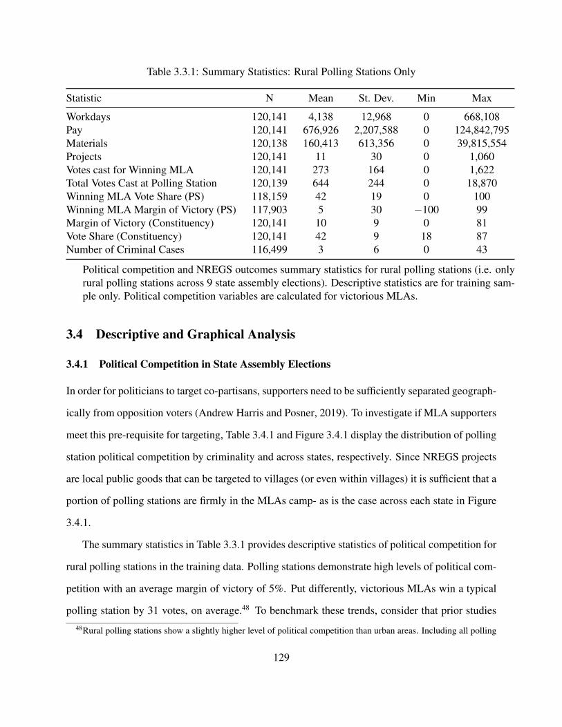
Table 3.3.1: Summary Statistics: Rural Polling Stations Only
Statistic N Mean St. Dev. Min Max
Workdays 120,141 4,138 12,968 0 668,108Pay 120,141 676,926 2,207,588 0 124,842,795Materials 120,138 160,413 613,356 0 39,815,554Projects 120,141 11 30 0 1,060Votes cast for Winning MLA 120,141 273 164 0 1,622Total Votes Cast at Polling Station 120,139 644 244 0 18,870Winning MLA Vote Share (PS) 118,159 42 19 0 100Winning MLA Margin of Victory (PS) 117,903 5 30 −100 99Margin of Victory (Constituency) 120,141 10 9 0 81Vote Share (Constituency) 120,141 42 9 18 87Number of Criminal Cases 116,499 3 6 0 43
Political competition and NREGS outcomes summary statistics for rural polling stations (i.e. onlyrural polling stations across 9 state assembly elections). Descriptive statistics are for training sam-ple only. Political competition variables are calculated for victorious MLAs.
3.4 Descriptive and Graphical Analysis
3.4.1 Political Competition in State Assembly Elections
In order for politicians to target co-partisans, supporters need to be sufficiently separated geograph-
ically from opposition voters (Andrew Harris and Posner, 2019). To investigate if MLA supporters
meet this pre-requisite for targeting, Table 3.4.1 and Figure 3.4.1 display the distribution of polling
station political competition by criminality and across states, respectively. Since NREGS projects
are local public goods that can be targeted to villages (or even within villages) it is sufficient that a
portion of polling stations are firmly in the MLAs camp- as is the case across each state in Figure
3.4.1.
The summary statistics in Table 3.3.1 provides descriptive statistics of political competition for
rural polling stations in the training data. Polling stations demonstrate high levels of political com-
petition with an average margin of victory of 5%. Put differently, victorious MLAs win a typical
polling station by 31 votes, on average.48 To benchmark these trends, consider that prior studies48Rural polling stations show a slightly higher level of political competition than urban areas. Including all polling
129

view assembly constituencies with +/- 10% margin of victory as “swing constituencies” (Vaishnav,
2012; Das and Maiorano, 2019a). For comparison, from 2004-2014 victorious Members of Parlia-
ment won by an average margin of victory between 10 and 20% (Auerbach, 2015). Similarly, Min
(2012) finds an average margin of victory of 14.5% for all legislative assembly elections between
1991 and 2003. For a more direct comparison, in the training sample I find that MLAs have an av-
erage margin of victory of 11% across assembly constituencies.49 Taken together, polling stations
display high levels of political competition, even for the notoriously competitive Indian political
landscape.50
Still, victorious MLAs win about 25 percent of polling stations by more than a 25 percent mar-
gin (see Table 3.4.1). In other words, there is a substantial subset of core villages providing ample
opportunities for NREGS targeting with minimal leakage. On average, assembly constituencies
have about 138 rural polling stations. Thus, for a typical constituency, there are roughly 35 polling
stations where the winning MLA dominates the local landscape.
Finally, focusing on the average masks variation in polling station political competition across
states. Figure 3.4.1 compares the distributions of margin of victory across Indian states, illumi-
nating variation in micro-level political competition.51 All else equal, states with greater spread
exhibit less political competition. States with probability mass concentrated around 0 exhibit rela-
tively higher levels of political competition (e.g. West Bengal). Assam and Uttar Pradesh show a
greater spread of political competition indicating relatively more core and opposition strongholds.
In these states, targeting programs to core villages should be relatively easier given the separation
of core and support polling stations (see Andrew Harris and Posner (2019)). On the other hand
states like West Bengal and Kerala exhibit relatively higher degrees of political competition with
stations (i.e. urban and rural) the average margin of victory is 7% or 45 votes. For reference and the full sample ofpolling station political competition see Table 3.D.1 in Appendix 3.D
49See Table 3.D.2 in 3.D.50To be fair, this is somewhat of an artificial comparison, given that winning candidates can’t lose constituencies but
can lose polling stations. Moreover, it does not account for the distribution of polling station results which I discussbelow.
51For distributions of alternative measures of political competition by state see Appendix 3.D, Figure 3.D.9.
130

polling stations margin of victory clustered more tightly around zero. Interestingly, Tamil Nadu
shows strong areas of opposition support in 2011 but not 2016.52
Figure 3.4.1: Polling Station Political Competition by State- Rural Sample
assam 2016
assam 2011
uttar pradesh 2012
tamil nadu 2011
himachal pradesh 2012
kerala 2011
tamil nadu 2016
kerala 2016
west bengal 2011
−100 −50 0 50 100
Margin of Victory: Polling Station
Den
sity
State_Election_Yearassam 2016assam 2011uttar pradesh 2012tamil nadu 2011himachal pradesh 2012kerala 2011tamil nadu 2016kerala 2016west bengal 2011
Political Competition by State Assembly Election
States sorted by the standard deviation of the polling station margin of victory
3.4.2 Political Competition and Criminality
Table 3.4.1: Quartiles of Polling Station Margin of Victory by Criminal Status of MLA
Criminality Q1 Median Mean Q3 Std. Dev.1 Clean -9.12 7.86 7.12 24.52 28.522 Criminal -10.44 7.33 6.49 24.83 28.98
Do criminals blow away the competition? Figure 3.4.2 illustrates the distribution of polling
station margin of victory comparing criminal to clean politicians.53 Overall, the distributions of
political competition between criminal and clean appear visually very similar. Given the large sam-
52Assam has similar spikes of opposition strongholds in both elections, see vote share in Figure 3.D.9a of Appendix3.D.
53For full sample including urban polling stations and alternative measures of political competition, see Appendix3.D.3.
131
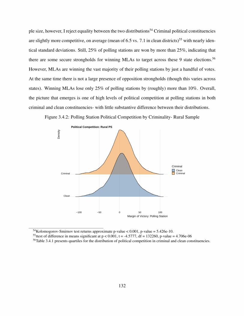
ple size, however, I reject equality between the two distributions54 Criminal political constituencies
are slightly more competitive, on average (mean of 6.5 vs. 7.1 in clean districts)55 with nearly iden-
tical standard deviations. Still, 25% of polling stations are won by more than 25%, indicating that
there are some secure strongholds for winning MLAs to target across these 9 state elections.56
However, MLAs are winning the vast majority of their polling stations by just a handful of votes.
At the same time there is not a large presence of opposition strongholds (though this varies across
states). Winning MLAs lose only 25% of polling stations by (roughly) more than 10%. Overall,
the picture that emerges is one of high levels of political competition at polling stations in both
criminal and clean constituencies- with little substantive difference between their distributions.
Figure 3.4.2: Polling Station Political Competition by Criminality- Rural Sample
Clean
Criminal
−100 −50 0 50 100
Margin of Victory: Polling Station
Den
sity
CriminalCleanCriminal
Political Competition: Rural PS
54Kolomogorov-Smirnov test returns approximate p-value < 0.001, p-value = 5.426e-10.55ttest of difference in means significant at p < 0.001, t = -4.5777, df = 132260, p-value = 4.706e-0656Table 3.4.1 presents quartiles for the distribution of political competition in criminal and clean constituencies.
132

3.5 Empirical Estimation
In light of the graphical analysis, I now build up to more complex models which consider that
criminal politicians likely operate in different political contexts and constituencies compared to
clean politicians. To more systematically investigate the relationship between criminal status and
targeting I turn first to OLS models that attempt to adjust for confounders between criminality and
NREGS distribution. After reporting OLS results, I motivate the use of Kernel Regularized Least
Squares as a way to relax OLS assumptions.
To estimate the relationship between criminality and targeting using OLS, I assign all NREGS
projects to their nearest polling stations, subject to a maximum distance of two kilometers. Projects
further away than two kilometers I do not consider as serving villagers voting at that polling station.
The unit of analysis is the polling station-election term. Put simply, I count the number of projects
targeted to a polling station catchment area and aggregate NREGS wages and employment days
within these same locales. I model NREGS outcomes as a function of the interaction between
incumbent margin of victory at an individual polling station and MLA criminality, controlling for
village level demand, MLA characteristics and constituency political predictors. Controls include:
• Census village indices
– Indexes proxy for village NREGS demand.
– Demand tends to be highest among women, SC/ST and marginal agricultural laborers
(Dutta et al., 2014).
– For example, using village level data from the 2001 Indian census I adjust for a villages
number of women, SC/ST and seasonal agricultural laborers among other factors that
are predictive of program demand.
– For the full list of census controls and index construction see (Gulzar et al., 2020).
• MLA personal and political characteristics:
133

– Age, Sex, Assets, Liabilities57
– INC: Indicator for whether MLA belongs to the Indian National Congress58
– Opposition: indicator for whether MLA belong to the opposition or ruling party coali-
tion.
• Constituency Measures of Political Competition:
– Assembly constituency margin of victory (%)59
– Assembly constituency turnout (%)
My preferred OLS model can be represented as:
NREGSb,t = α + β1V oteshareb,t + β2Criminalb,t + β3Criminalb,t ∗ V oteshareb,t+X+ StateElectiont + eb,t
(3.1)
Where subscript b refers to a polling booth and t refers to the election term and X is the bat-
tery of aforementioned controls. If criminal politicians deliver more NREGS benefits to their core
supporters relative to clean politicians, then I would expect a positive coefficient on the interaction
term. If criminal politicians simply deliver more NREGS benefits overall but do not necessarily
target co-partisans, then β2Criminal should be positive. Standard errors are clustered at the as-
sembly constituency level. I included state election cycle fixed effects to capture variation across
states and over time in NREGS program implementation (Sukhtankar et al., 2016). NREGS out-
comes of labor expenditures (Pay), workdays (Workdays), and material expenditures (Materials)
57Assets and liabilities are taken from candidate self-reported affidavits dataset. I log these skewed income variables.58(Gulzar and Pasquale, 2017) indicate that, at least initially, voters affiliated NREGS with the INC. Congress
created the program and congress party members lobbied hard to claim credit for its success Dasgupta (2016). Toadjust for these party effects, I use an indicator for whether or not the MLA is a member of the Indian NationalCongress
59It could be the case that incentives for targeting are only present in competitive MLA races. Safe seats on the otherhand may not illicit targeting efforts from MLAs who feel they can maintain their incumbency without increasingefforts to target political resources.
134

are logged transformed. The count of projects (Projects) assigned to a polling station remain un-
transformed.
Given researcher degrees of freedom in choosing outcomes, controls, interactions, coding,
among a myriad of other researcher specific decisions, the number of possibly analyses can quickly
balloon, leading to overconfidence in results (Simmons et al., 2011). To investigate how outcomes
depend on data, specification and model choices I take a multiverse approach (Steegen et al., 2016).
Put simply, there are many reasonable and defensible coding, cleaning and modeling decisions. For
example, measuring polling station political competition as vote share or total votes may more pre-
cisely capture the idea that politicians target where their supporters are more numerous. However,
if politicians care about minimizing spillovers then margin of victory may be the more precise
measure of the underlying latent concept of political competition. Second, demand for NREGS
is likely to be non-linear in demographics and may include interactions between inter-sectional
identities (e.g. women from scheduled castes). But which interactions to include? Or, what is
the best threshold for declaring matches and non-matches in polling station or candidate names
that minimizes false positives and false negatives? Instead of simply moving a handful of alterna-
tive analyses to robustnesss and sensitivity appendices, I explicitly compare how results hinge on
analytic choices.
To be clear, I am still providing only a brief tour of the modeling sausage factory. But I hope
by bringing this choice set of defensible decisions to the forefront of the analysis I can embrace
uncertainty and avoid over-hyping results dependent on an arbitrarily selected model.
Figure 3.5.1 estimates the association between criminality and NREGS pay for 288 different
OLS models. These models vary how the dependent variable is measured (i.e. any criminal charge
or only serious charges), adjustors included, interactions between criminality and political compe-
tition and the type of standard error estimator used.60 Overall, the takeaway message is that the is
wide variation in effect estimates based on researcher degrees of freedom. Depending on the type
60See table notes in Figure 3.5.1 for model and data permutations.
135
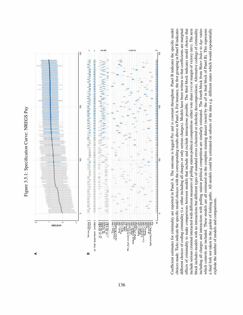
Figu
re3.
5.1:
Spec
ifica
tion
Cur
ve:N
RE
GS
Pay
Coe
ffici
ente
stim
ates
for
crim
inal
ityar
ere
port
edin
Pane
lA.T
heou
tcom
eis
logg
edPa
yan
dis
cons
tant
thro
ugho
ut.
Pane
lBin
dica
tes
the
spec
ific
mod
elch
oice
sm
ade.
Tick
sin
dica
teth
esp
ecifi
cm
odel
choi
ces
with
the
corr
espo
ndin
gre
sults
abov
ein
Pane
lA.F
orin
stan
ce,t
hefir
stgr
oupi
ngin
Pane
lBin
dica
tes
diff
eren
tcho
ices
ofco
ding
crim
inal
ity(i
.e.e
ither
incl
udin
gal
lcha
rges
oron
lyse
riou
sch
arge
s).M
odel
sha
vebe
enw
ritte
nso
that
coef
ficie
nts
are
mar
gina
lef
fect
sof
crim
inal
ityto
mak
eco
mpa
riso
nsbe
twee
nm
odel
sth
atin
clud
ean
dex
clud
ein
tera
ctio
nspo
ssib
le.
The
thir
dbl
ock
indi
cate
sm
odel
choi
ces
that
incl
ude
seri
ous
crim
inal
inte
ract
edw
ithdi
ffer
entm
easu
res
ofpo
lling
stat
ion
polit
ical
com
petit
ion-
eith
ervo
tesh
are
(vs)
orm
argi
nof
vict
ory
(mv)
.The
next
bloc
kin
clud
esm
odel
sw
ithno
inte
ract
ions
butd
iffer
entt
ypes
ofst
anda
rder
rors
(clu
ster
edor
chol
esky
decc
ompo
sitio
n).A
ltern
ativ
eco
ding
sof
crim
inal
ityin
clud
ing
allc
harg
esan
din
tera
ctio
nsw
ithpo
lling
stat
ion
polit
ical
com
petit
ion
are
sim
ilarl
yes
timat
ed.
The
four
thbl
ock
from
Wat
erIn
dex
toA
geva
ries
whi
chco
ntro
lsar
ein
clud
ed.
The
sem
odel
sar
eal
lest
imat
edon
the
com
plet
etr
aini
ngda
tase
t(no
ted
byth
eal
lin
final
bloc
kof
Pane
lB).
Thi
sre
pres
ents
afin
alfo
rkno
ttak
enin
the
gard
enof
fork
ing
path
s.A
llm
odel
sco
uld
bees
timat
edon
subs
ets
ofth
eda
tae.
g.di
ffer
ents
tate
sw
hich
wou
ldex
pone
ntia
llyex
plod
eth
enu
mbe
rofm
odel
san
dco
mpa
riso
ns.
136
of model, measurement of criminality and controls included, estimated coefficients for Criminality
can range from 0.01 to 1.03 (i.e. for the unlogged coefficients these estimates range from 1% to
280%) increase in NREGS pay when switching the criminal status of the MLA. For some mod-
els, the data are even consistent with negative associations between criminality and NREGS pay.
Figures 3.E.1 and 3.E.2 in Appendix 3.E further explore what drives these variations in effect
estimates. Overall, difference in estimates are driven by model choices (e.g. whether the model
includes interactions) and residual variance. Including different adjustors matters relatively less
in explaining effect variation (see Figure 3.E.2). Given the unexplained residual variance, model
dependence and the likely non-linear interplay between independent variables and variance in OLS
estimates, I try alternative strategies to tie my hands in model specification. In particular, Kernel
Regularized Least Squares provides one path to more agnostic modeling.
3.5.1 Kernel Regularized Least Squares
KRLS, combined with sample splitting, provides a number of advantages over defaulting to a
preferred OLS specification accompanied by robustness checks. First, KRLS is agnostic about
functional form (i.e. how features combine to predict NREGS outcomes). Where OLS assumes ad-
ditivity and linearity, KRLS allows for a flexible functional form search (Hainmueller and Hazlett,
2014). In turn, this reduces the likelihood of misspecification bias resulting from strict OLS as-
sumptions. This is particularly helpful given that my primary hypothesis is an interaction between
criminality and political competition. It is unlikely that the only interaction between predictors is
those that I explicitly theorize. With dozens of predictors specification searches for the “correct”
interactions among all potential interactions quickly explode. I deploy two methodological shields
to guard against model misspecification. First, I rerun models using KRLS to allow a more ag-
nostic approach to choosing the model’s functional form. KRLS also regularizes predictors which
penalizes large or overly complex models. Second, I set aside half the polling station observations
to test model predictions. The hold out set allows a comparison of model performance and can
help adjudicate if criminality is predictive of NREGS delivery on unseen data- in effect, acting as
137

type of self-replication.
However, allowing KRLS to flexibly fit the data can lead to overfitting (i.e. fitting noise in
the training data leading to poor prediction on new data). In other words, the flexible function
while reducing misspecification bias can lead to greater variance in estimates, in a classic bias-
variance tradeoff. KRLS regularizes coefficients by penalizing model complexity leading to better
predictions on test data (Hainmueller and Hazlett, 2014). Regularization is particularly useful
in this setting given the large amount of data and wide variation in NREGS outcomes. If the
criminal status of MLAs is not predictive of NREGS provision the coefficient on criminality should
be shrunk towards zero. In all cases I build exploratory models on the training data and test
their accuracy on the test set. Thus, I can check if the model findings in the training set capture
systematic relationships between political predictors and NREGS outcomes of interest on unseen
data.
Finally, KRLS allows for interpretable estimates and easily communicated quantities of interest
(Hainmueller and Hazlett, 2014). While other machine learning models (e.g. Random Forrest) can
flexibly fit data and regularize estimates, communicating results and conducting hypothesis tests
proves more difficult. KRLS reports pointwise marginal effects and error bounds similar to OLS.
In addition, KRLS reports marginal effects for each data point, aiding exploration of heterogeneous
effects and interactions. KRLS is flexible (avoiding OLS assumptions leading to misspecification
bias), regularized (avoiding overfitting) and interpretable (reporting communicable results).61 At
the same time, KRLS is not a magic bullet and does nothing to alleviate omitted variable bias.
Model estimates are only as useful as the data they flexibly fit. Even with the rich set of covariates
there are still possible unobserved confounding between the criminal status of MLAs and NREGS
delivery (e.g. bureaucratic capacity). I therefore do not make causal claims when discussing
reported “effects” below. Having motivated the advantages of KRLS I turn now to reporting results.
61These advantages come at computational cost. I overcome KRLS’ slow computing using brute force via AmazonWeb Services cloud computing.
138
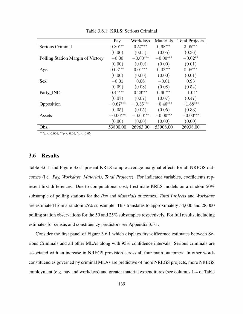
Table 3.6.1: KRLS: Serious Criminal
Pay Workdays Materials Total ProjectsSerious Criminal 0.80∗∗∗ 0.57∗∗∗ 0.68∗∗∗ 3.05∗∗∗
(0.06) (0.05) (0.05) (0.36)Polling Station Margin of Victory −0.00 −0.00∗∗∗ −0.00∗∗∗ −0.02∗∗
(0.00) (0.00) (0.00) (0.01)Age 0.03∗∗∗ 0.01∗∗∗ 0.02∗∗∗ 0.08∗∗∗
(0.00) (0.00) (0.00) (0.01)Sex −0.01 0.06 −0.01 0.93
(0.09) (0.08) (0.08) (0.54)Party_INC 0.44∗∗∗ 0.29∗∗∗ 0.60∗∗∗ −1.04∗
(0.07) (0.07) (0.07) (0.47)Opposition −0.67∗∗∗ −0.35∗∗∗ −0.46∗∗∗ −1.88∗∗∗
(0.05) (0.05) (0.05) (0.33)Assets −0.00∗∗∗ −0.00∗∗∗ −0.00∗∗∗ −0.00∗∗∗
(0.00) (0.00) (0.00) (0.00)Obs. 53800.00 26963.00 53908.00 26938.00∗∗∗p < 0.001, ∗∗p < 0.01, ∗p < 0.05
3.6 Results
Table 3.6.1 and Figure 3.6.1 present KRLS sample-average marginal effects for all NREGS out-
comes (i.e. Pay, Workdays, Materials, Total Projects). For indicator variables, coefficients rep-
resent first differences. Due to computational cost, I estimate KRLS models on a random 50%
subsample of polling stations for the Pay and Materials outcomes. Total Projects and Workdays
are estimated from a random 25% subsample. This translates to approximately 54,000 and 28,000
polling station observations for the 50 and 25% subsamples respectively. For full results, including
estimates for census and constituency predictors see Appendix 3.F.1.
Consider the first panel of Figure 3.6.1 which displays first-difference estimates between Se-
rious Criminals and all other MLAs along with 95% confidence intervals. Serious criminals are
associated with an increase in NREGS provision across all four main outcomes. In other words
constituencies governed by criminal MLAs are predictive of more NREGS projects, more NREGS
employment (e.g. pay and workdays) and greater material expenditures (see columns 1-4 of Table
139

3.6.1). On average, serious criminals are associated with delivering 3 more NREGS projects to
each polling station during their electoral term. At the same time, serious criminals increase pay,
employment and material expenditures relative to clean politicians. Interestingly, polling station
political competition shows a precisely estimated zero correlation with NREGS provision (top row
second panel of Figure 3.6.1). In other words, there is no evidence that MLAs target NREGS
resources to core villages. The lack of targeting when considering both types of MLAs together,
is consistent with previous work by (Das and Maiorano, 2019a).62 Still, it could be that there are
differential targeting rates between criminal and clean politicians that net out when combined.
Other personal candidate characteristics show precisely estimated null associations with NREGS
delivery. An MLAs Wealth, Age and Sex are not predictive of NREGS provision. However,
party politics are predictive of NREGS delivery. Consistent with previous findings by Gulzar
and Pasquale (2017) and Dasgupta (2016) Indian National Congress’ MLAs are associated with
increased NREGS provision relative to other parties’ politicians. Recall that the INC developed
and implemented NREGS with voters seeing the scheme as a “Congress program.” On the other
hand, opposition MLAs are less likely to deliver NREGS resources (a la findings from (Bohlken,
2018) regarding MPLADS).
62However Das and Maiorano (2019a) find increased targeting of material expenditures as a reward for local con-tractors in Andhra Pradesh. I examine this alternative explanation in more detail in the discussion below, but note thatI find no evidence of greater material expenditures for core polling stations. Nor do NREGS projects increase mate-rial expenditures as a percentage of overall project costs in areas that support the MLA (Das and Maiorano (2019a)’spreferred measure of rewarding contractors).
140
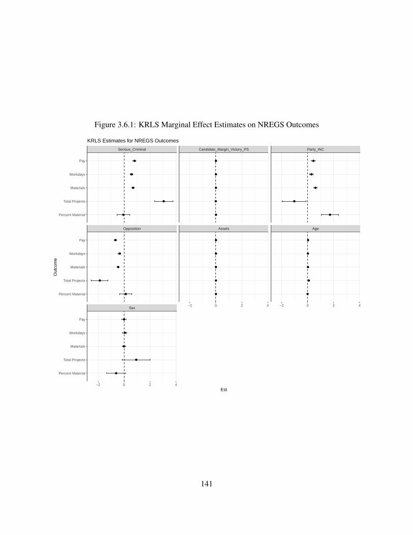
Figure 3.6.1: KRLS Marginal Effect Estimates on NREGS Outcomes
Sex
Opposition Assets Age
Serious_Criminal Candidate_Margin_Victory_PS Party_INC
−2 0 2 4
−2 0 2 4 −2 0 2 4
Percent Material
Total Projects
Materials
Workdays
Pay
Percent Material
Total Projects
Materials
Workdays
Pay
Percent Material
Total Projects
Materials
Workdays
Pay
Est
Out
com
e
KRLS Estimates for NREGS Outcomes
141
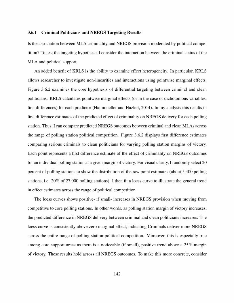
3.6.1 Criminal Politicians and NREGS Targeting Results
Is the association between MLA criminality and NREGS provision moderated by political compe-
tition? To test the targeting hypothesis I consider the interaction between the criminal status of the
MLA and political support.
An added benefit of KRLS is the ability to examine effect heterogeneity. In particular, KRLS
allows researcher to investigate non-linearities and interactions using pointwise marginal effects.
Figure 3.6.2 examines the core hypothesis of differential targeting between criminal and clean
politicians. KRLS calculates pointwise marginal effects (or in the case of dichotomous variables,
first differences) for each predictor (Hainmueller and Hazlett, 2014). In my analysis this results in
first difference estimates of the predicted effect of criminality on NREGS delivery for each polling
station. Thus, I can compare predicted NREGS outcomes between criminal and clean MLAs across
the range of polling station political competition. Figure 3.6.2 displays first difference estimates
comparing serious criminals to clean politicians for varying polling station margins of victory.
Each point represents a first difference estimate of the effect of criminality on NREGS outcomes
for an individual polling station at a given margin of victory. For visual clarity, I randomly select 20
percent of polling stations to show the distribution of the raw point estimates (about 5,400 polling
stations, i.e. 20% of 27,000 polling stations). I then fit a loess curve to illustrate the general trend
in effect estimates across the range of political competition.
The loess curves shows positive- if small- increases in NREGS provision when moving from
competitive to core polling stations. In other words, as polling station margin of victory increases,
the predicted difference in NREGS delivery between criminal and clean politicians increases. The
loess curve is consistently above zero marginal effect, indicating Criminals deliver more NREGS
across the entire range of polling station political competition. Moreover, this is especially true
among core support areas as there is a noticeable (if small), positive trend above a 25% margin
of victory. These results hold across all NREGS outcomes. To make this more concrete, consider
142
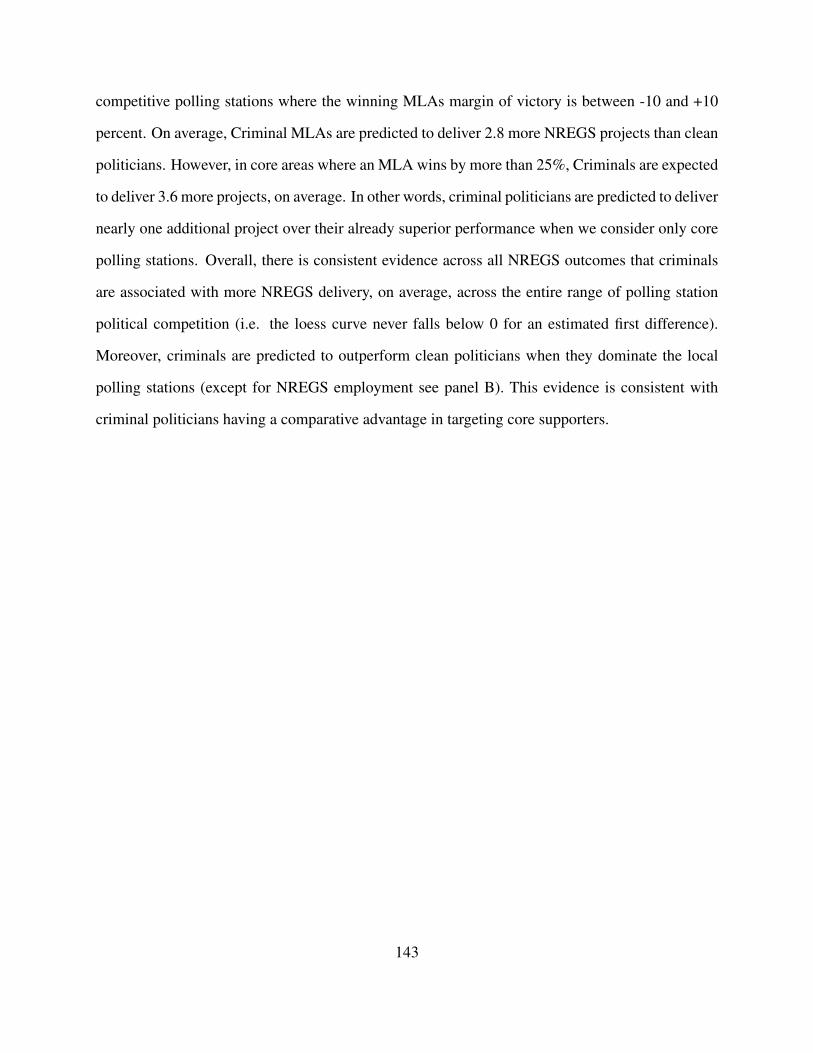
competitive polling stations where the winning MLAs margin of victory is between -10 and +10
percent. On average, Criminal MLAs are predicted to deliver 2.8 more NREGS projects than clean
politicians. However, in core areas where an MLA wins by more than 25%, Criminals are expected
to deliver 3.6 more projects, on average. In other words, criminal politicians are predicted to deliver
nearly one additional project over their already superior performance when we consider only core
polling stations. Overall, there is consistent evidence across all NREGS outcomes that criminals
are associated with more NREGS delivery, on average, across the entire range of polling station
political competition (i.e. the loess curve never falls below 0 for an estimated first difference).
Moreover, criminals are predicted to outperform clean politicians when they dominate the local
polling stations (except for NREGS employment see panel B). This evidence is consistent with
criminal politicians having a comparative advantage in targeting core supporters.
143

Figure 3.6.2: First Differences of Criminality moderated by Polling Station Political Competition
(a) Pay
0
1
2
−100 −50 0 50 100Margin_Victory
Se
rio
us_
Cri
min
al_
Ma
rgin
al_
Effe
ct
(b) Workdays
−0.5
0.0
0.5
1.0
1.5
−100 −50 0 50 100Margin_Victory
Se
rio
us_
Cri
min
al_
Ma
rgin
al_
Effe
ct
(c) Total Projects
−5
0
5
−100 −50 0 50 100Margin_Victory
Se
rio
us_
Cri
min
al_
Ma
rgin
al_
Effe
ct
(d) Material Expenditure
−1
0
1
2
−100 −50 0 50 100Margin_Victory
Ser
ious
_Crim
inal
_Mar
gina
l_E
ffect
The x-axis in all figures represents polling station margin of victory. In other words, moving from left to right ismoving from opposition to core polling stations. The y-axis represents First Differences for the serious criminalindicator. Each point estimate represents the first difference for an individual polling station estimate. Points above 0(i.e. the vast majority) indicate that criminal politicians are estimated to be associated with superior NREGS deliveryat that polling station. The loess curves sloping upward indicate that serious criminals outperform clean candidatesby greater margins in core polling stations (i.e. where criminals have a larger margin of victory). These trends areindicative of superior targeting on behalf of criminal politicians.
144

3.7 Discussion
In this section, I consider if criminal politicians advantages in money, muscle and networks may
explain their positive association with delivering more NREGS resources. In addition, I break
apart supporter networks, to investigate if increased NREGS benefits flow primarily to voters or
local contractors. By comparing individual NREGS projects in core and opposition areas, I test if
differential spending is funneled to voters via increased wages or to local contractors via material
expenditures. Third, I consider whether results depend on constituency-wide political competition.
Finally, I demonstrate that the main results hold when testing KRLS models on an unseen holdout
sample of polling stations.
3.7.1 Money
Do criminal politicians liquid assets drive superior NREGS delivery? Criminal politicians tend to
be wealthier on average (Dutta and Gupta, 2014). Money may grease the wheels of bureaucracy,
enabling NREGS funds to flow (Maiorano, 2014). Marcesse (2018) finds that local politicians
are sometimes required to pay bribes out of pocket before NREGS projects are approved. Alter-
natively, money may enmesh voters in networks of dependence, enabling NREGS to flow down
pre-existing channels. While the previous models controlled for politicians’ assets and liabilities,
Figure 3.7.1 explicitly examines the wealth mechanism. I leverage KRLS pointwise estimates to
examine heterogeneity in the effect of criminality by the level of politician wealth. Figure 3.7.1
plots the pointwise first differences of criminality by MLAs logged wealth. Each point represents
the predicted effect of criminality on NREGS resource delivery to a polling station. If criminal
MLAs superior NREGS performance is driven by wealth, I would expect an increase in the effect
of criminality moving across the wealth spectrum (x-axis). However across all NREGS outcomes,
the first difference effect of Criminality on NREGS is decreasing in criminals’ wealth. In other
words, while wealthy criminals still perform slightly better than wealthy but clean MLAs, the
biggest difference in predicted NREGS performance is among poorer politicians. In short, the as-
145

sociation between criminal MLAs and improved NREGS delivery is driven by poorer politicians.
This does not mean that wealth is unimportant to political survival or resource delivery. For
example, politicians may substitute cash payments for targeting effort. Instead of delivering state
resources, wealthy MLAs may rely on superior campaign spending or personalized constituent
service to carry them to victory. However, the overall effect of wealth on NREGS delivery is a
precisely estimated zero (see Total Projects in Table 3.6.1). Whereas, a substitution hypothesis
would predict a strong negative effect of wealth on NREGS delivery as poorer politicians compete
with the only tool in their toolbox.
In sum, the evidence is inconsistent with the money hypothesis. Wealth may still enable crim-
inal’s to solve other constituent problems (e.g. paying for weddings, temples or school fees as
witnessed at Arun Yadav’s janata durbar). However, I find no evidence that access to liquid funds
is associated with criminal MLAs predicted improved delivery of NREGS resources.
146
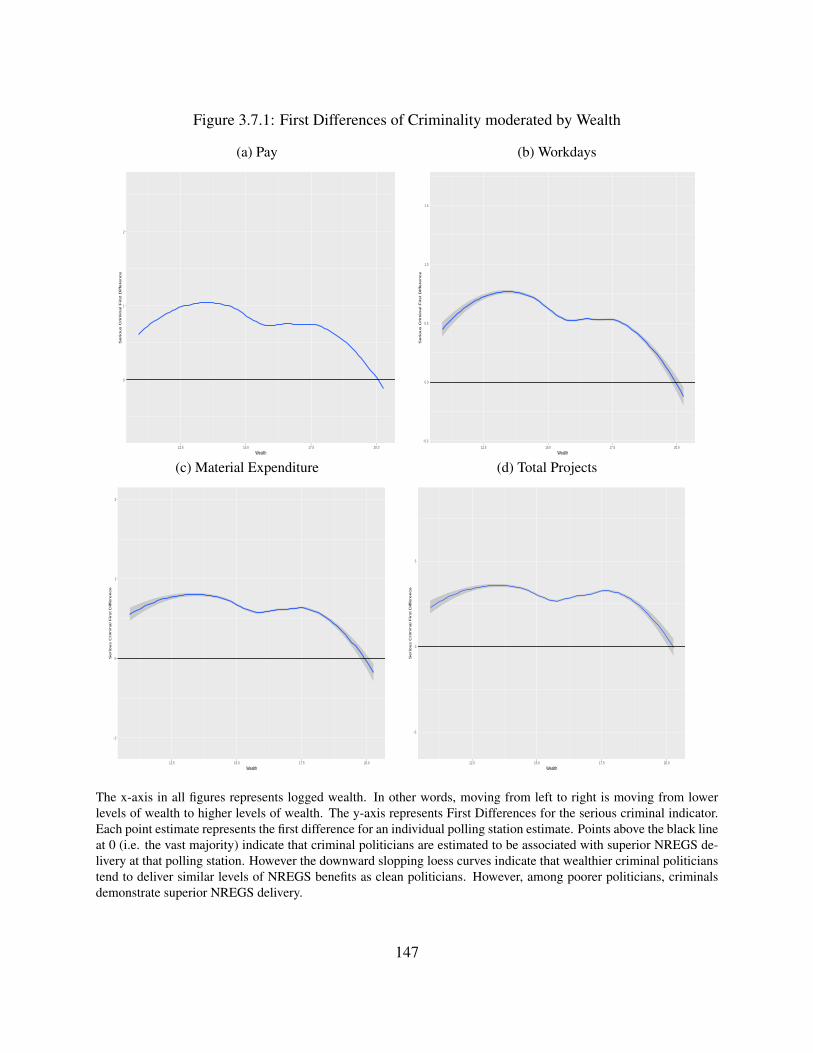
Figure 3.7.1: First Differences of Criminality moderated by Wealth
(a) Pay
0
1
2
12.5 15.0 17.5 20.0Wealth
Se
rio
us C
rim
ina
l F
irst D
iffe
ren
ce
(b) Workdays
−0.5
0.0
0.5
1.0
1.5
12.5 15.0 17.5 20.0Wealth
Se
rio
us C
rim
ina
l F
irst D
iffe
ren
ce
(c) Material Expenditure
−1
0
1
2
12.5 15.0 17.5 20.0Wealth
Se
rio
us C
rim
ina
l F
irst D
iffe
ren
ce
(d) Total Projects
−5
0
5
12.5 15.0 17.5 20.0Wealth
Se
rio
us C
rim
ina
l F
irst D
iffe
ren
ce
The x-axis in all figures represents logged wealth. In other words, moving from left to right is moving from lowerlevels of wealth to higher levels of wealth. The y-axis represents First Differences for the serious criminal indicator.Each point estimate represents the first difference for an individual polling station estimate. Points above the black lineat 0 (i.e. the vast majority) indicate that criminal politicians are estimated to be associated with superior NREGS de-livery at that polling station. However the downward slopping loess curves indicate that wealthier criminal politicianstend to deliver similar levels of NREGS benefits as clean politicians. However, among poorer politicians, criminalsdemonstrate superior NREGS delivery.
147

3.7.2 Muscle
Criminal politicians with a capacity for violence can credibly threaten bureaucrats to redirect re-
sources towards their political needs. Given that MLAs violent reputations may precede them,
sometimes a simple phone call will suffice to bend the bureaucracy to a politician’s will (Vaish-
nav (2017), fieldwork 2017). In short, criminals supply of muscle could improve their ability to
target resources like NREGS. To test the Muscle hypothesis, I use the Indian Penal Code to iden-
tify MLAs charged with violent crimes. I define violent charges as those being both serious in
nature (i.e. max sentence of at least two years and non-bailable) and demonstrating a capacity
for violence.63 Types of violent crime include charges associated with murder, attempted murder,
homicide, assault (including sexual assault), rape, kidnapping, armed robbery, extortion and ar-
son.64 For example, I code IPC section 324 “Voluntarily causing hurt by dangerous weapons or
means” as indicative of a violent criminal politician. However, IPC section 323 “Punishment for
voluntarily causing hurt” is coded as non-violent. The maximum punishment for violating IPC 323
is one year and the offense is bailable. Therefore I do not code it as “serious crime.” Following
Vaishnav (2012) I do not code charges related to rioting as violent. Even though these types of
charges may demonstrate a capacity for violence, political opponents may try to trump up charges
against politicians holding rallies. Therefore, these politically motivated charges are less likely to
capture the underlying latent concept of a “Violent Criminal Politician.”
Table 3.7.1 compares OLS results for Violent (Panel A) and Non-Violent (Panel B) crimi-
nals.65 Non-violent criminals are all MLAs facing a serious charge not coded as violent. Column 1
shows the marginal effect of criminality on NREGS pay for rural polling stations. The previously
63Indian Penal Code descriptions are taken from https://www.latestlaws.com/. My coding is similar tothe Association for Democratic Reforms definition of violent crimes (myneta.org) and follows inspiration from (Asherand Novosad, 2016)
64There are 144 unique IPC charges in my training data sample, 36 of which (25%) I code as violent. The IndianPenal Code is divided into chapters with most of the violent charges pertaining to Chapter 16 “Of Offenses Affectingthe Human Body.”
65I use OLS instead of KRLS to explore this mechanism due to computational cost constraints in rerunning KRLSmodels after recoding criminality twice for both Violent and Non-violent charges. For full results, including controlvariable coefficients see Tables and coefficient plots in Appendix 3.F.2
148

discussed result that criminal politicians are associated with increased NREGS delivery is driven
entirely by violent criminals (see bold coefficients in Panel A compared to bold coefficients in
Panel B). Violent criminal politicians have a consistent, positive association with NREGS delivery
regardless of the outcome analyzed (see columns 1-4). The difference in coefficients between Vio-
lent and Non-violent criminals is statistically significant across all four outcomes. The models also
include an interaction between violent criminality and polling station margin of victory to test for
differential targeting (see third row of Panel A and B for interaction coefficients). Neither Violent
nor Non-Violent MLAs show an increased proclivity to target core polling stations. While OLS
may not pick up the subtle non-linearities found in prior KRLS models, the results still indicate the
strong positive association between criminality and NREGS outcomes is attributable to politicians
charged with Violent crimes. In sum, the data is more consistent with the Muscle hypothesis, that
criminals violent nature is associated with improved resource delivery. In other words, money is
fungible but muscle matters.
149

Table 3.7.1: Muscle Mechanism Test: Comparing Violent and Non-Violent Criminals
Panel A: Violent Criminals
Pay Materials Workdays Total ProjectsViolent Criminal 1.15∗∗∗ 0.96∗∗ 0.77∗∗∗ 3.79∗∗
(0.34) (0.29) (0.22) (1.16)Margin of Victory −0.00 0.00 −0.00 0.01
(0.00) (0.00) (0.00) (0.00)Violent Criminal x MoV −0.00 −0.00 0.00 0.01
(0.00) (0.00) (0.00) (0.01)Controls Yes Yes Yes YesObs. 107894.00 107891.00 107894.00 107894.00Adj. R-Squared 0.08 0.06 0.08 0.04
Panel B: Non-Violent Criminals
Pay Materials Workdays Total ProjectsNon-Violent Criminal −0.30 −0.31 −0.19 −0.24
(0.45) (0.38) (0.28) (1.56)Margin of Victory −0.00 −0.00 −0.00 0.01
(0.00) (0.00) (0.00) (0.00)Non-Violent Criminal x MoV 0.01 0.01 0.01 0.00
(0.01) (0.01) (0.00) (0.02)Controls Yes Yes Yes YesObs. 107894.00 107891.00 107894.00 107894.00Adj. R-Squared 0.08 0.06 0.08 0.04∗∗∗p < 0.001, ∗∗p < 0.01, ∗p < 0.05 Standard errors in parentheses are clustered by Assembly Constituency.
Standard errors in parentheses are clustered by Assembly Constituency.
150

3.7.3 Networks: Contractor Raj?
The KRLS results from section 3.6 show that criminals have a proclivity to target core polling sta-
tions with NREGS resources. Who benefits from additional NREGS funding? On one hand, more
wages and workdays will likely benefit voters who labor on NREGS projects. On the other, rents
from material expenditures likely accrue to local contractors and politicians (Das and Maiorano
(2019a), fieldwork). Do MLAs reward local elite or voters in their networks? To investigate this
question, I conduct a project-level analysis. That is, instead of aggregating NREGS projects up to
the polling station, I compare individual projects in core and opposition areas. Specifically, I ask
if NREGS projects assigned to supporter polling stations are fundamentally different than projects
assigned to opposition polling stations?
In this setup, the logic is that criminal politicians prioritize projects in their core areas funneling
greater payments and employment to their supporters. In part, the project level analysis recognizes
that placement of NREGS projects is endogenous to local demand for employment. Some villages
will simply desire more NREGS projects. Still, politicians might be able to influence the money
that flows to individual projects by pressuring block level bureaucrats to fast track certain projects
and district officials to release more money to criminals’ core areas. Second, a project level analysis
can provide some suggestive insights into criminal politicians’ proclivity to channel extra resources
towards voters or local elites. If projects allocated to core-areas fundamentally benefited voters I
would expect these projects to have higher levels of employment and wages. On the other hand
if networks in core-areas facilitate a “contractor-raj,” where rents accrue to local elites, I would
expect greater material expenditures and a higher percentage of total project expenditures allocated
towards materials.
To investigate if MLAs prioritize voters in core polling stations I compare labor expenditures
(Pay) and employment (Workdays) generated per project. Conversely, if MLAs privilege local
elites, I would expect greater material expenditures on projects. I use Material Expenditures and
151
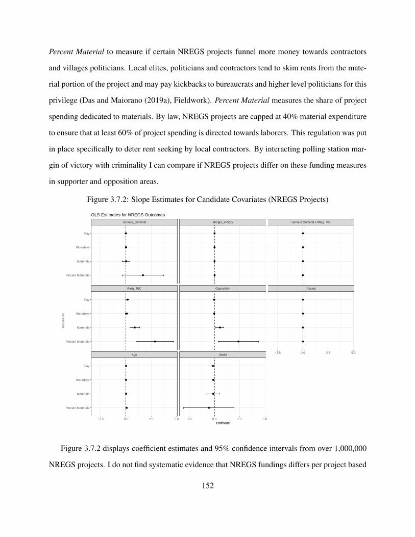
Percent Material to measure if certain NREGS projects funnel more money towards contractors
and villages politicians. Local elites, politicians and contractors tend to skim rents from the mate-
rial portion of the project and may pay kickbacks to bureaucrats and higher level politicians for this
privilege (Das and Maiorano (2019a), Fieldwork). Percent Material measures the share of project
spending dedicated to materials. By law, NREGS projects are capped at 40% material expenditure
to ensure that at least 60% of project spending is directed towards laborers. This regulation was put
in place specifically to deter rent seeking by local contractors. By interacting polling station mar-
gin of victory with criminality I can compare if NREGS projects differ on these funding measures
in supporter and opposition areas.
Figure 3.7.2: Slope Estimates for Candidate Covariates (NREGS Projects)
Age SexM
Party_INC Opposition Assets
Serious_Criminal Margin_Victory Serious Criminal x Marg. Vic.
−2.5 0.0 2.5 5.0 −2.5 0.0 2.5 5.0
−2.5 0.0 2.5 5.0
Percent Materials
Materials
Workdays
Pay
Percent Materials
Materials
Workdays
Pay
Percent Materials
Materials
Workdays
Pay
estimate
outc
ome
OLS Estimates for NREGS Outcomes
Figure 3.7.2 displays coefficient estimates and 95% confidence intervals from over 1,000,000
NREGS projects. I do not find systematic evidence that NREGS fundings differs per project based
152

on the criminality of the MLA, polling station political competition nor their interaction (see Fig-
ure 3.7.2 top row).66 In fact, criminality, polling station margin of victory, and their interaction are
all precisely estimated zeros for both labor and material spending (see top row of panels in Figure
3.7.2). Projects are essentially the same on funding dimensions in criminal and clean constituen-
cies. Likewise polling station political competition has no effect on altering project funding or
employment. In other words, while I can not definitively partial out whether local elites or voters
gain the most from any individual project, NREGS projects in core-areas are qualitatively similar
to those in opposition areas.67 Projects in core polling stations are not more expensive (see Pay
and Materials outcomes in Figure 3.7.2). Nor do they privilege contractors by increasing the share
of material expenditure (see Percent Material outcome in Figure 3.7.2).
In sum, NREGS projects are remarkably consistent across candidate characteristics and po-
litical competition. Larger, more expensive and more graft prone projects are not specifically
allocated to core support areas. Recall from the main results that criminal constituencies see an
overall increase in the number of projects and NREGS benefits, with these gains concentrated in
core polling stations. It does not seem to be the case that "better" projects are located in criminal
support areas at the expense of opposition or swing areas. Instead, criminals are associated with
increased NREGS delivery, allocating more projects and thus more funds to all types of polling
stations relative to clean politicians. Simply put, criminal politicians just deliver more NREGS
funding.
66For full results, including controls, see coefficient plots in Appendix 3.F.3. For predicted effects of the interactionbetween criminality and polling station margin of victory for project-level outcomes see figures in the same Appendix.
67It is possible that contractors are able to extract more from projects located in core-areas but if so this is not afunction of the project observables.
153

3.7.4 Assembly Constituency Political Competition
Do the results depend on how tight the MLA race is? It could be the case that incentives for target-
ing are only present when competition is fierce and MLAs fear losing their seats. In settings of high
political competition, incumbents may use every tool in their toolbox to ensure victory. Whereas
in safe seats, MLAs do not feel pressured to extend extra effort to target supporters. Qualitative
fieldwork and quantitative evidence suggests that MLAs must address constituent concerns and
provide personalized service if they want a seat at the electoral table and will be quickly rebuked
if they fail to make these overtures (see Bussell (2019)). However, in competitive constituencies
MLAs may feel added pressure to make every effort in rewarding previous supporters to keep those
voters in their stable and turning out. In other words, does stronger evidence for targeting emerge
when looking at competitive constituencies where incentives for targeting increase?
In Figures 3.7.3 and 3.7.4, I compare results between competitive and safe seats. While prior
models controlled for assembly constituency political competition (either using margin of victory
or effective number of parties), here I explicitly explore whether evidence of NREGS targerting
differs across safe and contested constituencies. Specifically, Figure 3.7.3 plots the predicted point-
wise first differences for Criminality against Assembly Constituency margin of victory for NREGS
Pay. Moving from left to right across the x-axis is moving from competitive to safe seats, compar-
ing the predicted polling station effect of criminality on NREGS labor expenditures. The positive
LOESS trend (cyan line) predicts that criminals outperform clean MLAs by an even wider margin
in safe seats. While criminals are predicted to deliver more NREGS resources across the entire
spectrum of Assembly Constituency political competition, on average, this advantage is expected
to increase in safer seats. In fact almost all of the individual pointwise first differences predict a
positive effect of criminality when the Assembly Constituency margin of victory is greater than
20%.
Second, I compare differential polling station targeting in competitive and safe constituencies
154

Figure 3.7.3: Marginal Effect of Criminality on NREGS by Assembly Constituency Margin ofVictory
0
1
2
0 20 40 60 80
Margin of Victory (Assembly Constituency)
Ser
ious
Crim
inal
Firs
t Diff
eren
ce
155
(Figure 3.7.4 parts A and B, respectively). I consider all constituencies where the margin of victory
is less than 10% to be competitive, and those greater than 10% to be safe. Subsequently, I break
apart each type of constituency to investigate targeting by polling station political competition.
Thus, I can compare targeting trends in competitive and safe constituencies. Each figure plots the
pointwise predicted effects of criminality against polling station margin of victory. In other words,
these graphs compare if there is more evidence for differential targeting between criminal and
clean politicians in competitive versus safe constituencies. For now, I focus on a single NREGS
outcome, Pay. The overall trends in predicted effects are similar for competitive and safe assembly
constituencies. Interestingly, the predicted effects of criminality are much larger, on average, for
safe constituencies (part B) relative to competitive constituencies, across the spectrum of polling
station competition. Put simply, while criminals are expected to deliver more NREGS wages,
on average, the predicted difference between criminal and clean MLAs is much greater in safe
seats. This result is consistent with the finding from Figure 3.7.3, that criminals are predicted to
perform especially well in safe constituencies. Second, the targeting trends are similar in both safe
and competitive seats. Criminals predicted advantage in delivering wages increases when moving
from toss-up polling stations to core areas of support. Albeit, there is also an upward trend for
opposition polling stations.
Disaggregating the analysis by Assembly Constituency competition can also help reconcile
the findings in this chapter with those from the regression discontinuity analysis. Recall that the
regression discontinuity found either imprecise or negative effects of criminality on NREGS de-
livery. Whereas, in this chapter Criminal MLAs are associated with increased access to NREGS
funds. However, this positive effect of criminality is driven primarily by safe seats. Whereas,
the regression discontinuity is constrained to compare extremely close elections by design. In
other words, the RDD estimates the local average treatment effect of criminality to be negative.
But when considering safe seats far away from the RD threshold, criminal politicians’ apparent
advantages materialize.
156

One potential explanation to reconcile these findings is that in competitive seats all types of
candidates are incentivized to deliver. Any benefits of a criminals’ type are washed out, either by
the selection of similarly effective clean competitors or because parties focus efforts on these close
battlegrounds. At the same time, political competition is endogenous to the effectivenes of MLAs
in office. In other words, the relationship could be reversed with criminals winning votes exactly
in the constituencies where they are most effective at delivering NREGS resources and meeting
voters needs. While my analysis considers prospective targeting, rewarding voters for votes in the
prior election, these time trends are difficult to untangle with observational data. Further research
is required to ascertain if the “effect” of criminal politicians is consistently moderated by political
competition. In appendix 3.F.4 I provide some suggestive evidence that clean politicians drop off
in their targeting efforts more rapidly as the safety of their seat increases. However, the predicted
interaction effects of criminality and assembly constituency margin of victory are not significantly
different across politician type.
157
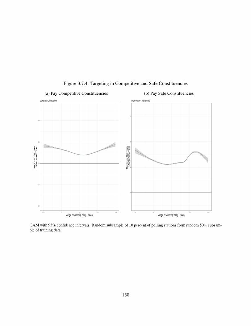
Figure 3.7.4: Targeting in Competitive and Safe Constituencies
(a) Pay Competitive Constituencies
−1.0
−0.5
0.0
0.5
1.0
−100 −50 0 50 100
Margin of Victory (Polling Station)
Se
rio
us C
rim
ina
l M
arg
ina
lEffe
ct
Competitive Constituencies
(b) Pay Safe Constituencies
0
1
2
3
−100 −50 0 50 100
Margin of Victory (Polling Station)
Se
rio
us C
rim
ina
l M
arg
ina
lEffe
ct
Uncompetitive Constituencies
GAM with 95% confidence intervals. Random subsample of 10 percent of polling stations from random 50% subsam-ple of training data.
158

3.7.5 Comparing Model Predictions on Test Data
I turn now to comparing the out of sample predictive power of KRLS models. Specifically, I com-
pare models with and without a variable for Serious Criminality. I fit the models on the training
data and then predict NREGS pay outcomes for the testing dataset. The holdout test set randomly
samples 50% of the constituencies from the overall dataset (i.e. the 50% of constituencies not
included in the training data). If criminal politicians are a strong driver of NREGS delivery, then
models including the serious criminal variable should perform better. However, I find nearly identi-
cal predictive accuracy, regardless of whether the Serious Criminal variable is withheld. I estimate
a 6.64 root mean squared error for each model (i.e. a measure of how far off the model predic-
tion of NREGS pay is from the actual value of NREGS pay for a given polling station). Overall,
including the Serious Criminal does not improve the models out of sample predictions. Which
is understandable, since the other variables in the model include demographic and development
measures which are known to be highly predictive of demand for a minimum wage employment
program like NREGS. MLA criminality likely explains little additional variation in light of these
other controls.
Second, I check if the result showing increased delivery for criminal politicians replicates for
the testing data. Indeed the positive and significant coefficient on criminality is reproduced in the
test sample (see Table 3.5, column 2). However, the effect of criminality does attenuate by about
half for the holdout testing data. By replicating these baseline results, I help reduce uncertainty
that the relationship between criminality and NREGS provision is a spurious artifact of the training
sample.
3.8 Conclusion
One core explanation of criminal politician’s electoral success is that they deliver for their own
communities. Party leaders may view muscular politicians and caste defenders as strong candi-
dates in constituencies dominated by parochial concerns (Vasihnav 2017). If criminal politicians’
159
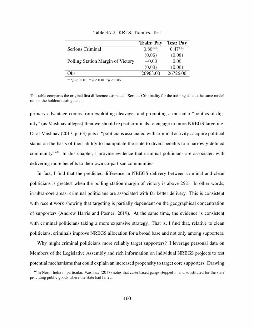
Table 3.7.2: KRLS: Train vs. Test
Train: Pay Test: PaySerious Criminal 0.80∗∗∗ 0.47∗∗∗
(0.06) (0.08)Polling Station Margin of Victory −0.00 0.00
(0.00) (0.00)Obs. 26963.00 26726.00∗∗∗p < 0.001, ∗∗p < 0.01, ∗p < 0.05
This table compares the original first difference estimate of Serious Criminality for the training data to the same modelrun on the holdout testing data
primary advantage comes from exploiting cleavages and promoting a muscular “politics of dig-
nity” (as Vaishnav alleges) then we should expect criminals to engage in more NREGS targeting.
Or as Vaishnav (2017, p. 63) puts it “politicians associated with criminal activity...acquire political
status on the basis of their ability to manipulate the state to divert benefits to a narrowly defined
community.”68 In this chapter, I provide evidence that criminal politicians are associated with
delivering more benefits to their own co-partisan communities.
In fact, I find that the predicted difference in NREGS delivery between criminal and clean
politicians is greatest when the polling station margin of victory is above 25%. In other words,
in ultra-core areas, criminal politicians are associated with far better delivery. This is consistent
with recent work showing that targeting is partially dependent on the geographical concentration
of supporters (Andrew Harris and Posner, 2019). At the same time, the evidence is consistent
with criminal politicians taking a more expansive strategy. That is, I find that, relative to clean
politicians, criminals improve NREGS allocation for a broad base and not only among supporters.
Why might criminal politicians more reliably target supporters? I leverage personal data on
Members of the Legislative Assembly and rich information on individual NREGS projects to test
potential mechanisms that could explain an increased propensity to target core supporters. Drawing
68In North India in particular, Vaishnav (2017) notes that caste based gangs stepped in and substituted for the stateproviding public goods where the state had failed.
160

on previous literature and fieldwork, I identify and systematically test three unique assets that could
explain criminal politicians targeting advantage: Money, Muscle and Networks. I find the most
evidence for the Muscle channel, with tentative support for the networks hypothesis. Conversely,
the data is not consistent with the Money hypothesis where wealthy criminals deliver better NREGS
outcomes.
Finally, I ask if results differ based on how tight the overall MLA race is? I split my sample into
competitive and safe assembly constituencies to determine if incentives for targeting co-partisans
are stronger when the overall race narrows. Criminals’ superior NREGS provision is driven by safe
constituencies. This finding provides one potential reconciliation for the negative and null effects
of criminality found in the regression discontinuity chapter. Simply put, the RDD design only
considers extremely competitive races, where the margin of victory is close to zero.69 Whereas, in
this chapter, I find the strongest, positive impacts of criminality on NREGS provision in safe seats-
far away from the regression discontinuity threshold of zero margin of victory.
In addition to the core findings, I provide the first descriptive evidence of polling station compe-
tition for MLAs in six Indian states. I find that India’s notoriously competitive elections replicate
at the very local level, with an average margin of victory of 7% or less than 25 votes. Though
this masks variation across states. Overall, this indicates that some states have greater political
polarization at the micro-level and may be more amenable to politicians discerning and targeting
supporters.
Finally, I use several methods to improve predictions and limit model misspecification while
using observational data. In observational settings one default may be to model outcomes and
conduct robustness tests to check specification sensitivity. However, I show that even for relatively
few alternative specification decisions the number of potential models explodes and results can
69To be clear, this chapter looks at only a subsample of states, but the finding is consistent with a moderating resultof political competition across both chapters. For instance, it could be the case that in close races, clean politiciansface strong incentives to increase NREGS provision so any innate benefit to criminality is trumped by extra effortfrom clean MLAs. Also, technically speaking, in some models the RDD draws strength from every constituency race,increasing weight for races close to the threshold.
161

vary widely. As data becomes more readily available and computational costs decrease, sample
splitting and machine learning models present one fruitful way forward. By testing models on
holdout data we can increase our confidence that results are more reliable and likely to replicate.
162
Appendix
3.A Coding Ruling and Opposition Parties
163

Tabl
e3.
A.1
:Par
tyC
oalit
ions
forS
tate
Leg
isla
ture
sin
Sam
ple
Stat
eE
lect
ion
Year
Rul
ing
Coa
litio
nO
ppos
ition
Oth
er
Ass
am20
11IN
CA
GP,
AIU
DF,
BJP
,A
ITC
,IN
DB
OPF
Ass
am20
16N
DA
:BJP
,BO
PF,A
GP
AIU
DF,
INC
IND
Him
acha
lPr
ades
h20
12IN
CB
JPH
LP,
IND
Ker
ala
2011
UD
F:IN
C,
MU
L,
SJD
,K
EC
(J),
KE
C(M
),K
EC
(B),
KR
SP
LD
F:C
PM,C
PI,J
D(S
),N
CP,
RSP
IND
Ker
ala
2016
LD
F:C
PI,C
PM,N
CP,
NSC
,K
EC
(B),
JD(S
),C
(S)
UD
F:IN
C,I
UM
L,K
EC
(M),
CM
PKSC
,KE
C(J
)N
DA
:B
JPTa
mil
Nad
u20
11A
IAD
MK
,D
MD
K,
CPI
,C
PM,
MA
MA
K,
PT,
AIF
B,
AID
MK
DM
K,I
NC
,PM
KIN
D
Tam
ilN
adu
2016
AD
MK
IUM
L,I
NC
,DM
KIN
DU
ttarP
rade
sh20
12SP
BSP
,IN
C,
SP,
RL
D,
PEC
P,B
JP,I
EM
C,N
CP,
QE
D,I
ND
Wes
tBen
gal
2011
AIT
C,I
NC
,SU
CI
CPI
M,
CPI
,R
SPI,
AIF
B,
RC
P,SP
,DSP
(P),
BB
C,W
PIG
OJA
M,
IND
Thi
sta
ble
only
incl
udes
part
ies
that
won
ase
atin
anas
sem
bly
elec
tion.
Idi
dno
tcod
epa
rtie
sth
atfa
iled
tow
in.
Inde
pend
entC
andi
date
sar
eco
nsid
ered
asth
eop
posi
tion
exce
ptw
hen
Ico
uld
find
defin
itive
evid
ence
that
thes
eca
ndid
ates
cont
este
das
part
ofth
eru
ling
allia
nce
(e.g
.in
Ker
ala)
.Coa
litio
npa
rtne
rsar
ein
clus
ive
ofbo
thpr
e-el
ectio
npa
rtne
rsan
dpa
rtne
rsin
gove
rnm
enta
sit
was
diffi
cult
tofin
dev
iden
ceof
the
late
r.
164
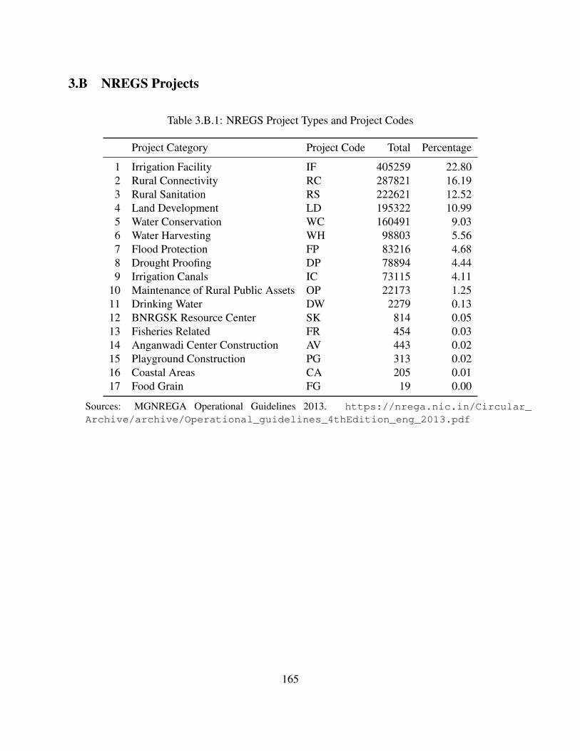
3.B NREGS Projects
Table 3.B.1: NREGS Project Types and Project Codes
Project Category Project Code Total Percentage
1 Irrigation Facility IF 405259 22.802 Rural Connectivity RC 287821 16.193 Rural Sanitation RS 222621 12.524 Land Development LD 195322 10.995 Water Conservation WC 160491 9.036 Water Harvesting WH 98803 5.567 Flood Protection FP 83216 4.688 Drought Proofing DP 78894 4.449 Irrigation Canals IC 73115 4.11
10 Maintenance of Rural Public Assets OP 22173 1.2511 Drinking Water DW 2279 0.1312 BNRGSK Resource Center SK 814 0.0513 Fisheries Related FR 454 0.0314 Anganwadi Center Construction AV 443 0.0215 Playground Construction PG 313 0.0216 Coastal Areas CA 205 0.0117 Food Grain FG 19 0.00
Sources: MGNREGA Operational Guidelines 2013. https://nrega.nic.in/Circular_Archive/archive/Operational_guidelines_4thEdition_eng_2013.pdf
165
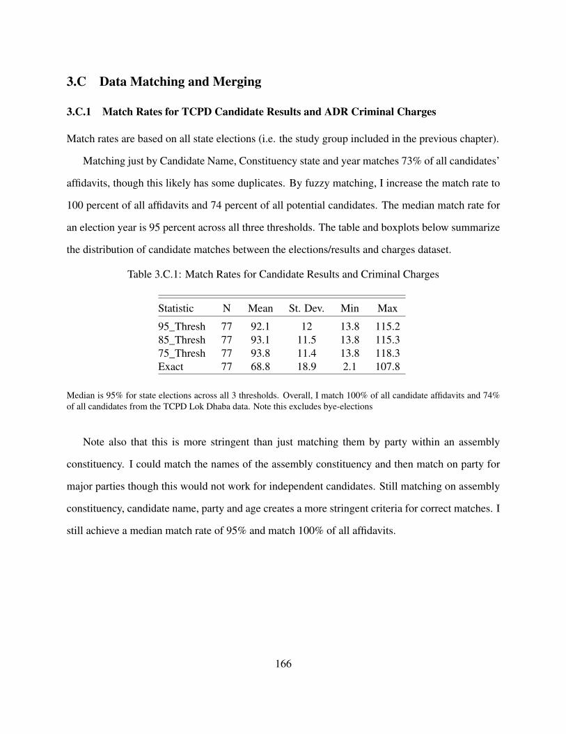
3.C Data Matching and Merging
3.C.1 Match Rates for TCPD Candidate Results and ADR Criminal Charges
Match rates are based on all state elections (i.e. the study group included in the previous chapter).
Matching just by Candidate Name, Constituency state and year matches 73% of all candidates’
affidavits, though this likely has some duplicates. By fuzzy matching, I increase the match rate to
100 percent of all affidavits and 74 percent of all potential candidates. The median match rate for
an election year is 95 percent across all three thresholds. The table and boxplots below summarize
the distribution of candidate matches between the elections/results and charges dataset.
Table 3.C.1: Match Rates for Candidate Results and Criminal Charges
Statistic N Mean St. Dev. Min Max
95_Thresh 77 92.1 12 13.8 115.285_Thresh 77 93.1 11.5 13.8 115.375_Thresh 77 93.8 11.4 13.8 118.3Exact 77 68.8 18.9 2.1 107.8
Median is 95% for state elections across all 3 thresholds. Overall, I match 100% of all candidate affidavits and 74%of all candidates from the TCPD Lok Dhaba data. Note this excludes bye-elections
Note also that this is more stringent than just matching them by party within an assembly
constituency. I could match the names of the assembly constituency and then match on party for
major parties though this would not work for independent candidates. Still matching on assembly
constituency, candidate name, party and age creates a more stringent criteria for correct matches. I
still achieve a median match rate of 95% and match 100% of all affidavits.
166

Figure 3.C.1: Candidate Results and Criminal Records Match Rates for State Elections
0
30
60
90
120
75_Thresh 85_Thresh 95_Thresh Exact
Threshold
Mat
ch_R
ate
Median is 95% for state elections across all 3 thresholds. Overall, I match 100% of all candidate affidavits and 74%of all candidates. Note this excludes bye-elections
3.D Political Competition
3.D.1 Graphical Analysis of Political Competition and NREGS Distribution
Here I display the raw data comparing the distributions of NREGS outcomes by polling station
competition and criminal status of the MLA. Figure 3.D.1 below plots NREGS outcomes (log(pay),
log(workdays), log(materials), total projects) against the range of polling station political competi-
tion. The loess smoother represents the trend of NREGS provision across varying levels of polling
station political competition for all 120,141 rural polling stations. I randomly sample 5,000 polling
stations to give a sense of the raw data distribution. However, trend lines are fit to the entire train-
ing dataset. Each point indicates an individual polling station and the total NREGS resources
distributed during an MLAs’ five year electoral term. In general the distribution of NREGS re-
sources shows some evidence of targeting swing polling stations (though the main takeaway is that
the trends appear flat across the range of political competition). Second there is perhaps a slight
167
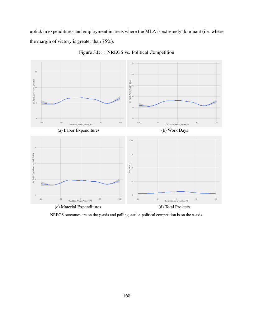
uptick in expenditures and employment in areas where the MLA is extremely dominant (i.e. where
the margin of victory is greater than 75%).
Figure 3.D.1: NREGS vs. Political Competition
0
5
10
15
−100 −50 0 50 100Candidate_Margin_Victory_PS
Ln_T
otal
_Exp
endi
ture
_Uns
kille
d
(a) Labor Expenditures
0.0
2.5
5.0
7.5
10.0
12.5
−100 −50 0 50 100Candidate_Margin_Victory_PS
Ln_T
otal
_Wor
k_P
erso
n_D
ays
(b) Work Days
0
5
10
15
−100 −50 0 50 100Candidate_Margin_Victory_PS
Ln_T
otal
_Exp
endi
ture
_Mat
eria
l_S
kille
d
(c) Material Expenditures
0
50
100
150
200
−100 −50 0 50 100Candidate_Margin_Victory_PS
Tota
l_P
roje
cts
(d) Total Projects
NREGS outcomes are on the y-axis and polling station political competition is on the x-axis.
168

Breaking out the same graphs by criminal status of the MLA reproduces the same overall pat-
tern for both types of politicians (Figure 3.D.2). There is perhaps a slight tendency towards favor-
ing swing polling stations. There is no strong visual pattern of co-partisan targeting, though again
perhaps a slight uptick in NREGS resources flowing to areas where the MLA is most dominant.
Overall, the loess curves show fairly flat trends for expenditures and employment across polling
station competition, with a slight uptick above 75%. Interestingly, criminal MLAs are associated
with higher rates of pay and workdays across the entire range of polling station political competi-
tion. In other words, criminal politicians are associated with delivering more NREGS employment
regardless of the local level of political competition. Criminals deliver more total projects overall
as well. Finally, for material expenditures (Figure 4c) there is a discernible separation at extreme
levels of support, with criminal politicians associated with greater material expenditures. Deliver-
ing more material expenditures to core areas would be consistent with rewarding local elites rather
than voters (Das and Maiorano (2019a)).
Obviously, this visual investigation is preliminary and I do not want to over-interpret poten-
tially random fluctuations, even with the large number of observations. For example, replicating
the graphs for each state individually shows little difference between criminal and clean constituen-
cies in the distribution of NREGS resources (see figures in Appendix ??). Likewise, no state shows
dramatic evidence of co-partisan targeting. Instead, the difference in criminal constituencies re-
ceiving more NREGS resources is only visually apparent after aggregating across states. To more
systematically adjust for potential confounders across political constituencies and types I turn now
to modeling the distribution of NREGS resources.
169

Figure 3.D.2: NREGS vs. Political Competition by Criminality
(a) Labor Expenditures (b) Work Days
(c) Material Expenditures (d) Total Projects
NREGS outcomes are on the y-axis and polling station political competition is on the x-axis. The orange line is theloess smooth of NREGS distribution across polling station competition in criminally governed constituencies. Theblue line displays the loess smooth for clean governed constituencies.
170

3.D.2 Urban and Rural Polling Stations
Table 3.D.1: Polling Station Political Competition: Full Sample
Statistic N Mean St. Dev. Min Max
PollingStation_Vote_Percent 203,327 44.5 17.8 0.0 100.0Candidate_Margin_Victory_PS 202,974 6.9 28.5 −100.0 99.4Votes_PS 205,431 292.8 160.6 0.0 5,194.0Total_Votes_perPS 205,429 652.4 237.9 0.0 18,870.0
Political competition summary statistics for polling stations across full sample (i.e.rural and urban polling stations in 9 state assembly elections). Descriptive Statisticsare for the training sample only.
Table 3.D.2: Assembly Constituency Political Competition: Full Sample
Statistic N Mean St. Dev. Min Max
Margin_Percentage 872 11.1 9.7 0.04 81.4Vote_Share_Percentage 872 45.6 9.3 18.5 87.4
Political competition summary statistics for assembly constituen-cies across full sample (i.e. rural and urban polling stations in 9state assembly elections). Descriptive Statistics are for the train-ing sample only.
171
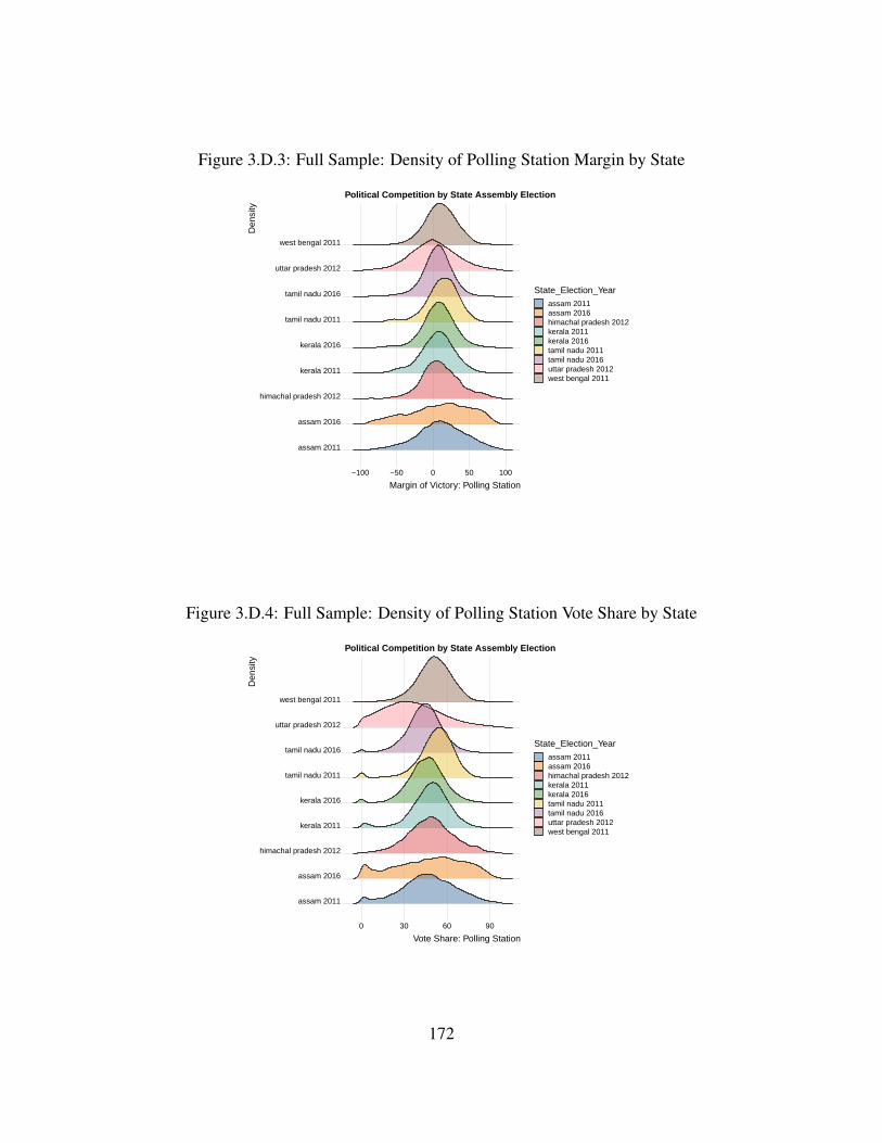
Figure 3.D.3: Full Sample: Density of Polling Station Margin by State
assam 2011
assam 2016
himachal pradesh 2012
kerala 2011
kerala 2016
tamil nadu 2011
tamil nadu 2016
uttar pradesh 2012
west bengal 2011
−100 −50 0 50 100
Margin of Victory: Polling Station
Den
sity
State_Election_Yearassam 2011assam 2016himachal pradesh 2012kerala 2011kerala 2016tamil nadu 2011tamil nadu 2016uttar pradesh 2012west bengal 2011
Political Competition by State Assembly Election
Figure 3.D.4: Full Sample: Density of Polling Station Vote Share by State
assam 2011
assam 2016
himachal pradesh 2012
kerala 2011
kerala 2016
tamil nadu 2011
tamil nadu 2016
uttar pradesh 2012
west bengal 2011
0 30 60 90
Vote Share: Polling Station
Den
sity
State_Election_Yearassam 2011assam 2016himachal pradesh 2012kerala 2011kerala 2016tamil nadu 2011tamil nadu 2016uttar pradesh 2012west bengal 2011
Political Competition by State Assembly Election
172
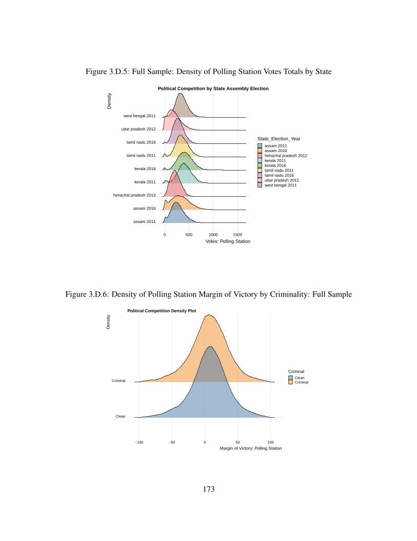
Figure 3.D.5: Full Sample: Density of Polling Station Votes Totals by State
assam 2011
assam 2016
himachal pradesh 2012
kerala 2011
kerala 2016
tamil nadu 2011
tamil nadu 2016
uttar pradesh 2012
west bengal 2011
0 500 1000 1500
Votes: Polling Station
Den
sity
State_Election_Yearassam 2011assam 2016himachal pradesh 2012kerala 2011kerala 2016tamil nadu 2011tamil nadu 2016uttar pradesh 2012west bengal 2011
Political Competition by State Assembly Election
Figure 3.D.6: Density of Polling Station Margin of Victory by Criminality: Full Sample
Clean
Criminal
−100 −50 0 50 100
Margin of Victory: Polling Station
Den
sity
CriminalCleanCriminal
Political Competition Density Plot
173
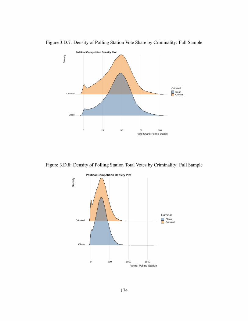
Figure 3.D.7: Density of Polling Station Vote Share by Criminality: Full Sample
Clean
Criminal
0 25 50 75 100
Vote Share: Polling Station
Den
sity
CriminalCleanCriminal
Political Competition Density Plot
Figure 3.D.8: Density of Polling Station Total Votes by Criminality: Full Sample
Clean
Criminal
0 500 1000 1500
Votes: Polling Station
Den
sity
CriminalCleanCriminal
Political Competition Density Plot
174

3.D.3 Rural Polling Stations Only
175
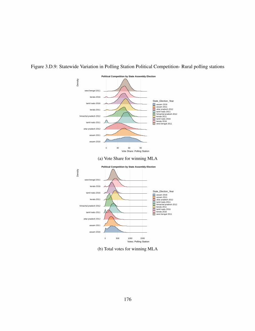
Figure 3.D.9: Statewide Variation in Polling Station Political Competition- Rural polling stations
assam 2016
assam 2011
uttar pradesh 2012
tamil nadu 2011
himachal pradesh 2012
kerala 2011
tamil nadu 2016
kerala 2016
west bengal 2011
0 30 60 90
Vote Share: Polling Station
Den
sity
State_Election_Yearassam 2016assam 2011uttar pradesh 2012tamil nadu 2011himachal pradesh 2012kerala 2011tamil nadu 2016kerala 2016west bengal 2011
Political Competition by State Assembly Election
(a) Vote Share for winning MLA
assam 2016
assam 2011
uttar pradesh 2012
tamil nadu 2011
himachal pradesh 2012
kerala 2011
tamil nadu 2016
kerala 2016
west bengal 2011
0 500 1000 1500
Votes: Polling Station
Den
sity
State_Election_Yearassam 2016assam 2011uttar pradesh 2012tamil nadu 2011himachal pradesh 2012kerala 2011tamil nadu 2016kerala 2016west bengal 2011
Political Competition by State Assembly Election
(b) Total votes for winning MLA
176
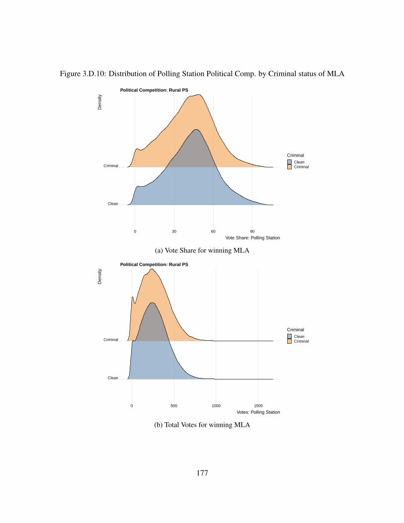
Figure 3.D.10: Distribution of Polling Station Political Comp. by Criminal status of MLA
Clean
Criminal
0 30 60 90
Vote Share: Polling Station
Den
sity
CriminalCleanCriminal
Political Competition: Rural PS
(a) Vote Share for winning MLA
Clean
Criminal
0 500 1000 1500
Votes: Polling Station
Den
sity
CriminalCleanCriminal
Political Competition: Rural PS
(b) Total Votes for winning MLA
177

3.E Multiverse Analysis
Figure 3.E.1: Summary of Coefficient Estimates for Criminality based on different model choices
controlsm
odelsubsets
xy
0.00 0.25 0.50 0.75 1.00
AgeAgricultural_Worker_Index
all covariatesAssets
Banking_IndexCommunication_Index
Education_IndexIncome_Index
Irrigation_IndexLiabilities
Margin_PercentageMedical_Facilities_Index
Minority_Indexno covariates
Non_Agricultural_Worker_IndexOppositionParty_INCPop_Index
Power_IndexRoad_Index
SexTurnout_Percentage
Vulnerability_IndexWater_Index
c_mv_interactionc_vs_interaction
lm_choleskylm_clustered
sc_mv_interactionsc_vs_interaction
all
CriminalSerious_Criminal
Ln_Total_Expenditure_Unskilled
estimate
valu
e
178

Figure 3.E.2: Variance Decomposition of Model Estimates
0
10
20
30
40
controls model Residual x
prop
ortio
n of
var
ianc
e
179

3.F Supplemental Results
3.F.1 KRLS
Income_Index Irrigation_Index Turnout_Percentage Margin_Percentage
Communication_Index Banking_Index Road_Index Power_Index
Non_Agricultural_Worker_Index Education_Index Medical_Facilities_Index Water_Index
Pop_Index Vulnerability_Index Minority_Index Agricultural_Worker_Index
−40 0 40 80 −40 0 40 80 −40 0 40 80 −40 0 40 80
Percent Material
Total Projects
Materials
Workdays
Pay
Percent Material
Total Projects
Materials
Workdays
Pay
Percent Material
Total Projects
Materials
Workdays
Pay
Percent Material
Total Projects
Materials
Workdays
Pay
Est
Out
com
e
KRLS Estimates for NREGS Outcomes
180

Table 3.F.1: KRLS: Serious Criminal
Pay Workdays Materials Total Projects Percent MaterialSerious Criminal 0.80∗∗∗ 0.57∗∗∗ 0.68∗∗∗ 3.05∗∗∗ −0.06
(0.06) (0.05) (0.05) (0.36) (0.25)Political Competition (PS) −0.00 −0.00∗∗∗ −0.00∗∗∗ −0.02∗∗ 0.00
(0.00) (0.00) (0.00) (0.01) (0.00)Age 0.03∗∗∗ 0.01∗∗∗ 0.02∗∗∗ 0.08∗∗∗ −0.01
(0.00) (0.00) (0.00) (0.01) (0.01)Sex −0.01 0.06 −0.01 0.93 −0.62
(0.09) (0.08) (0.08) (0.54) (0.37)Party INC 0.44∗∗∗ 0.29∗∗∗ 0.60∗∗∗ −1.04∗ 1.71∗∗∗
(0.07) (0.07) (0.07) (0.47) (0.33)Opposition −0.67∗∗∗ −0.35∗∗∗ −0.46∗∗∗ −1.88∗∗∗ 0.13
(0.05) (0.05) (0.05) (0.33) (0.24)Assets −0.00∗∗∗ −0.00∗∗∗ −0.00∗∗∗ −0.00∗∗∗ −0.00
(0.00) (0.00) (0.00) (0.00) (0.00)Liabilities −0.00∗∗∗ −0.00∗ −0.00∗∗∗ −0.00∗∗ −0.00
(0.00) (0.00) (0.00) (0.00) (0.00)Pop_Index −0.51 −0.99 −1.77 23.98 −20.00∗∗∗
(2.41) (2.17) (2.15) (14.76) (5.76)Vulnerability_Index −5.08 0.46 −4.21 75.05∗∗∗ −3.11
(3.12) (2.74) (2.72) (18.71) (8.96)Minority_Index 0.25∗∗∗ 0.07 0.17∗∗∗ 0.79∗∗ −0.01
(0.05) (0.05) (0.04) (0.31) (0.15)Agricultural_Worker −4.34∗∗ −0.19 −3.84∗∗ 4.01 −13.81∗
(1.67) (1.50) (1.49) (10.45) (6.42)Non_Agricultural_Worker −6.38∗ −10.74∗∗∗ −11.34∗∗∗ 14.18 −21.39∗
(3.20) (2.79) (2.80) (19.77) (9.64)Education_Index −0.05 −0.04 −0.08 −0.64 −0.32
(0.07) (0.07) (0.07) (0.46) (0.25)Medical_Facilities_Index 0.66∗∗∗ 0.47∗∗∗ 0.60∗∗∗ 2.84∗∗∗ −0.13
(0.09) (0.08) (0.08) (0.55) (0.27)Water_Index −0.24∗∗∗ −0.07 −0.46∗∗∗ −1.92∗∗∗ −1.55∗∗∗
(0.06) (0.05) (0.05) (0.36) (0.19)Communication_Index −0.14∗ −0.04 −0.05 0.01 −0.25
(0.07) (0.06) (0.06) (0.42) (0.21)Banking_Index −0.15∗∗ −0.08 −0.06 −0.12 0.12
(0.05) (0.04) (0.04) (0.30) (0.19)Road_Index 0.01 −0.02 −0.05 0.76∗∗ −0.67∗∗∗
(0.04) (0.04) (0.04) (0.28) (0.13)Power_Index −0.89∗∗∗ −0.61∗∗∗ −0.71∗∗∗ −1.90∗∗∗ −0.53∗∗
(0.04) (0.04) (0.04) (0.26) (0.17)Income_Index 0.19∗∗∗ 0.10∗∗∗ 0.21∗∗∗ 2.00∗∗∗ −0.08
(0.03) (0.02) (0.03) (0.31) (0.05)Irrigation_Index −0.57∗∗∗ −0.05 −0.46∗∗∗ 0.35 −1.10∗∗
(0.12) (0.12) (0.11) (0.69) (0.36)Turnout_Percentage −0.06∗∗∗ −0.04∗∗∗ −0.04∗∗∗ 0.05∗∗ −0.05∗∗∗
(0.00) (0.00) (0.00) (0.02) (0.01)Margin_Percentage −0.04∗∗∗ 0.04∗∗
(0.00) (0.02)ENOP −0.10∗∗∗ −0.13∗∗∗ −1.22∗∗∗
(0.03) (0.02) (0.18)Obs. 53800.00 26963.00 53908.00 26938.00 50840.00∗∗∗p < 0.001, ∗∗p < 0.01, ∗p < 0.05
181

3.F.2 Muscle Mechanism Test
Non_Violent_Criminal Non−Violent Criminal x Marg. Vic.
Violent_Criminal Violent Criminal x Marg. Vic.
−2 0 2 4 6 −2 0 2 4 6
Total Projects
Materials
Workdays
Pay
Total Projects
Materials
Workdays
Pay
estimate
outc
ome
OLS Estimates for Violent and Non−Violent Criminals
182

Table 3.F.2: OLS: Violent Criminal
Pay Materials Workdays Total Projects(Intercept) 12.46∗∗∗ 8.72∗∗∗ 7.46∗∗∗ 2.19
(1.09) (0.92) (0.69) (3.85)Violent Criminal 1.15∗∗∗ 0.96∗∗ 0.77∗∗∗ 3.79∗∗
(0.34) (0.29) (0.22) (1.16)Political Competition (PS) −0.00 0.00 −0.00 0.01
(0.00) (0.00) (0.00) (0.00)Age 0.04∗∗ 0.03∗∗ 0.02∗∗ 0.12∗∗
(0.01) (0.01) (0.01) (0.04)SexM −0.45 −0.34 −0.31 −0.15
(0.48) (0.42) (0.30) (1.48)Party_INC 0.49 0.67∗ 0.23 −2.18
(0.35) (0.32) (0.22) (1.58)Opposition −0.53 −0.61∗ −0.39∗ −2.06∗
(0.29) (0.24) (0.18) (0.97)Assets −0.00 −0.00 −0.00 −0.00
(0.00) (0.00) (0.00) (0.00)Liabilities −0.00 −0.00 −0.00 −0.00
(0.00) (0.00) (0.00) (0.00)Pop_Index 16.02∗∗∗ 10.49∗∗∗ 9.77∗∗∗ 13.25
(3.24) (3.07) (2.05) (18.81)Vulnerability_Index −13.42∗∗∗ −9.22∗∗∗ −8.25∗∗∗ −20.31
(2.70) (2.61) (1.74) (14.98)Minority_Index 0.06 0.03 0.04 0.08
(0.06) (0.07) (0.04) (0.43)Agricultural_Worker_Index −0.02 −0.90 0.14 8.05
(1.15) (0.94) (0.74) (5.58)Non_Agricultural_Worker_Index −1.66 −1.71 −0.83 14.13
(1.35) (1.20) (0.87) (7.31)Education_Index −0.22∗∗ −0.16∗ −0.16∗∗ −0.99
(0.08) (0.08) (0.05) (0.58)Medical_Facilities_Index 0.16 0.16 0.11 0.58
(0.10) (0.08) (0.06) (0.46)Water_Index −1.43∗∗∗ −1.48∗∗∗ −0.93∗∗∗ −6.01∗∗∗
(0.22) (0.18) (0.14) (0.82)Communication_Index 0.43∗∗ 0.24 0.25∗∗ 1.03
(0.13) (0.13) (0.09) (0.71)Banking_Index −0.21∗ −0.06 −0.12∗ 0.42
(0.09) (0.07) (0.06) (0.39)Road_Index 1.24∗∗∗ 0.66∗∗∗ 0.77∗∗∗ 4.24∗∗∗
(0.16) (0.12) (0.10) (0.62)Power_Index −0.85∗∗∗ −0.54∗∗∗ −0.53∗∗∗ −1.04
(0.16) (0.13) (0.10) (0.61)Income_Index 0.02 0.02 0.01 0.01
(0.01) (0.01) (0.01) (0.05)Irrigation_Index −0.01 −0.00 −0.01 −0.09
(0.09) (0.08) (0.06) (0.43)Turnout_Percentage −0.10∗∗∗ −0.06∗∗∗ −0.06∗∗∗ 0.10∗
(0.01) (0.01) (0.01) (0.04)Margin_Percentage −0.05∗∗ −0.04∗∗ −0.04∗∗∗ −0.26∗∗∗
(0.02) (0.01) (0.01) (0.05)Violent_Criminal:Candidate_Margin_Victory_PS −0.00 −0.00 0.00 0.01
(0.00) (0.00) (0.00) (0.01)Obs. 107894.00 107891.00 107894.00 107894.00Adj. R-Squared 0.08 0.06 0.08 0.04∗∗∗p < 0.001, ∗∗p < 0.01, ∗p < 0.05
183

Table 3.F.3: OLS: Non Violent Criminal
Pay Materials Workdays Total Projects(Intercept) 13.35∗∗∗ 9.46∗∗∗ 8.05∗∗∗ 4.95
(1.07) (0.91) (0.67) (3.74)Non Violent Criminal −0.30 −0.31 −0.19 −0.24
(0.45) (0.38) (0.28) (1.56)Political Competition (PS) −0.00 −0.00 −0.00 0.01
(0.00) (0.00) (0.00) (0.00)Age 0.03∗∗ 0.02∗ 0.02∗∗ 0.10∗
(0.01) (0.01) (0.01) (0.04)SexM −0.18 −0.11 −0.13 0.69
(0.47) (0.42) (0.30) (1.46)Party_INC 0.40 0.59 0.17 −2.48
(0.35) (0.32) (0.22) (1.59)Opposition −0.65∗ −0.71∗∗ −0.47∗ −2.48∗∗
(0.29) (0.24) (0.18) (0.96)Assets −0.00 −0.00 −0.00 −0.00
(0.00) (0.00) (0.00) (0.00)Liabilities −0.00 −0.00 −0.00 −0.00
(0.00) (0.00) (0.00) (0.00)Pop_Index 16.81∗∗∗ 11.11∗∗∗ 10.29∗∗∗ 15.83
(3.25) (3.04) (2.06) (18.66)Vulnerability_Index −14.09∗∗∗ −9.76∗∗∗ −8.70∗∗∗ −22.62
(2.71) (2.60) (1.74) (14.89)Minority_Index 0.06 0.03 0.04 0.06
(0.06) (0.07) (0.04) (0.43)Agricultural_Worker_Index 0.16 −0.75 0.26 8.60
(1.18) (0.96) (0.76) (5.72)Non_Agricultural_Worker_Index −1.64 −1.69 −0.82 14.25
(1.41) (1.21) (0.91) (7.39)Education_Index −0.23∗∗ −0.17∗ −0.16∗∗ −1.02
(0.08) (0.08) (0.05) (0.58)Medical_Facilities_Index 0.17 0.17∗ 0.12 0.62
(0.11) (0.08) (0.07) (0.46)Water_Index −1.52∗∗∗ −1.56∗∗∗ −0.99∗∗∗ −6.32∗∗∗
(0.22) (0.18) (0.14) (0.83)Communication_Index 0.42∗∗ 0.23 0.25∗∗ 1.01
(0.13) (0.13) (0.09) (0.72)Banking_Index −0.22∗ −0.07 −0.12∗ 0.39
(0.09) (0.07) (0.06) (0.39)Road_Index 1.25∗∗∗ 0.67∗∗∗ 0.78∗∗∗ 4.27∗∗∗
(0.16) (0.12) (0.10) (0.63)Power_Index −0.80∗∗∗ −0.50∗∗∗ −0.49∗∗∗ −0.87
(0.16) (0.13) (0.10) (0.61)Income_Index 0.02 0.02 0.01 0.01
(0.01) (0.01) (0.01) (0.05)Irrigation_Index −0.02 −0.00 −0.01 −0.11
(0.09) (0.08) (0.05) (0.43)Turnout_Percentage −0.10∗∗∗ −0.07∗∗∗ −0.06∗∗∗ 0.08
(0.01) (0.01) (0.01) (0.04)Margin_Percentage −0.05∗∗ −0.04∗∗ −0.04∗∗∗ −0.26∗∗∗
(0.02) (0.01) (0.01) (0.05)Non_Violent_Criminal:Candidate_Margin_Victory_PS 0.01 0.01 0.01 0.00
(0.01) (0.01) (0.00) (0.02)Obs. 107894.00 107891.00 107894.00 107894.00Adj. R-Squared 0.08 0.06 0.08 0.04∗∗∗p < 0.001, ∗∗p < 0.01, ∗p < 0.05
184

3.F.3 Networks Mechanism Test
Figure 3.F.1: Slope Estimates for Census Covariates (NREGS Projects)
Income_Index Irrigation_Index
Communication_Index Banking_Index Road_Index Power_Index
Non_Agricultural_Worker_Index Education_Index Medical_Facilities_Index Water_Index
Pop_Index Vulnerability_Index Minority_Index Agricultural_Worker_Index
−20 −10 0 10 20 −20 −10 0 10 20
−20 −10 0 10 20 −20 −10 0 10 20
Percent Materials
Materials
Workdays
Pay
Percent Materials
Materials
Workdays
Pay
Percent Materials
Materials
Workdays
Pay
Percent Materials
Materials
Workdays
Pay
estimate
outc
ome
OLS Estimates for NREGS Outcomes
185

Figure 3.F.2: Slope Estimates for Constituency Covariates (NREGS Projects)
Turnout_Percentage ENOP
−2 −1 0 1 −2 −1 0 1
Percent Materials
Materials
Workdays
Pay
estimate
outc
ome
OLS Estimates for NREGS Outcomes
186

Figure 3.F.3: Marginal Effects of Criminality moderated by Polling Station Political Competition(OLS Estimates)
8.7
8.9
9.1
−100 −50 0 50 100Candidate_Margin_Victory_PS
Ln_E
xpen
ditu
re_U
nski
lled
Serious_Criminal
0
1
Predicted values of Ln_Expenditure_Unskilled
(a) Project Labor Expenditure
4.1
4.2
4.3
4.4
−100 −50 0 50 100Candidate_Margin_Victory_PS
Ln_W
ork_
Per
son_
Day
s
Serious_Criminal
0
1
Predicted values of Ln_Work_Person_Days
(b) Project Workdays
Blue lines are the predicted effects of Criminal MLAs. Red lines are predicted effects of Clean MLAs. Standard errorsare clustered at the Assembly-Constituency-Election Level.
187

Figure 3.F.4: Blue lines are the predicted effects of Criminal MLAs. Red lines are predicted effectsof Clean MLAs. Standard errors are clustered at the Assembly-Constituency-Election Level.
1.0
1.5
2.0
2.5
−100 −50 0 50 100Candidate_Margin_Victory_PS
Ln_E
xpen
ditu
re_M
ater
ial_
Ski
lled
Serious_Criminal
0
1
Predicted values of Ln_Expenditure_Material_Skilled
(a) Material Expenditure
2.5
5.0
7.5
10.0
−100 −50 0 50 100Candidate_Margin_Victory_PS
Per
cent
_Mat
eria
l_E
xpen
ditu
re
Serious_Criminal
0
1
Predicted values of Percent_Material_Expenditure
(b) Project share of Material Expenditure
Test
188

Clean
Criminal
0.0
2.5
5.0
7.5
10.0
0 20 40 60Margin_Percentage
Ln_T
otal
_Exp
endi
ture
_Uns
kille
dPredicted values of Ln_Total_Expenditure_Unskilled
3.F.4 Assembly Constituency Political Competition
189

Clean
Criminal
0.0
2.5
5.0
7.5
10.0
0 20 40 60Margin_Percentage
Ln_T
otal
_Wor
k_P
erso
n_D
ays
Predicted values of Ln_Total_Work_Person_Days
190
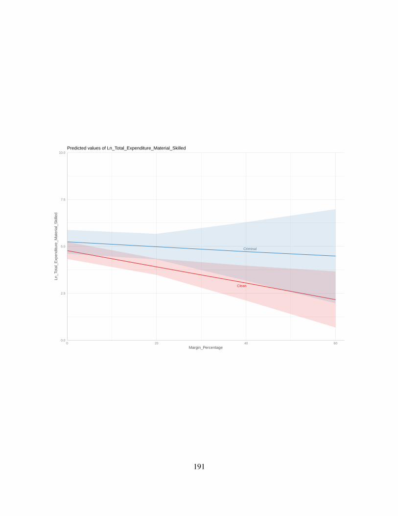
Clean
Criminal
0.0
2.5
5.0
7.5
10.0
0 20 40 60Margin_Percentage
Ln_T
otal
_Exp
endi
ture
_Mat
eria
l_S
kille
d
Predicted values of Ln_Total_Expenditure_Material_Skilled
191

Figure 3.F.5: Slope Estimates for Constituency Covariates (NREGS Projects)
−0.02
−0.01
0.00
0.01
0.02
0 20 40 60 80
Assembly Constituency Margin of Victory
Pol
ling
Sta
tion
Mar
gin
of V
icto
ry
Mar
gina
l Effe
ct
192

Age SexM
Serious Criminal x Marg. Vic. PS Party_INC Opposition Assets
Serious_Criminal Margin Victory AC Serious Criminal x Marg. Vic. AC Margin Victory PS
−5.0 −2.5 0.0 2.5 5.0 −5.0 −2.5 0.0 2.5 5.0
−5.0 −2.5 0.0 2.5 5.0 −5.0 −2.5 0.0 2.5 5.0
Total Projects
Materials
Workdays
Pay
Total Projects
Materials
Workdays
Pay
Total Projects
Materials
Workdays
Pay
estimate
outc
ome
OLS Estimates for NREGS Outcomes
193
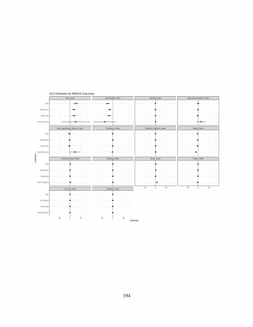
Income_Index Irrigation_Index
Communication_Index Banking_Index Road_Index Power_Index
Non_Agricultural_Worker_Index Education_Index Medical_Facilities_Index Water_Index
Pop_Index Vulnerability_Index Minority_Index Agricultural_Worker_Index
−30 0 30 −30 0 30
−30 0 30 −30 0 30
Total Projects
Materials
Workdays
Pay
Total Projects
Materials
Workdays
Pay
Total Projects
Materials
Workdays
Pay
Total Projects
Materials
Workdays
Pay
estimate
outc
ome
OLS Estimates for NREGS Outcomes
194

Turnout_Percentage
−0.1 0.0 0.1
Total Projects
Materials
Workdays
Pay
estimate
outc
ome
OLS Estimates for NREGS Outcomes
195
Chapter 4
Wedding Service: Do Criminal Politicians Deliver Con-
stituency Service?
4.1 Introduction
Do criminal politicians deliver benefits outside of government programs? The previous chapters
found mixed evidence regarding criminals’ ability to distribute NREGS. In part, this discrepancy
may be explained by heterogeneous effects depending on the level of constituency political compe-
tition, with criminals under providing in close races but over providing in safe seats. Still, criminal
politicians retain a predictable advantage at the polls (Aidt et al., 2011; Vaishnav, 2017; Sircar,
2018a). Perhaps criminal politicians’ electoral intangibles derive from services outside of govern-
ment funded welfare programs. While NREGS is an important program, it represents only one
benefit in the eco-system of resources at politicians’ disposal. Criminal politicians’ distributive
strategy may focus on other channels. In particular, previous literature highlights the importance
of constituency service for MLAs (Bussell, 2019; Kruks-Wisner, 2018). Further, qualitative evi-
dence suggests that criminals engage heavily in solving everyday problems, patronizing temples
and attending community events (Berenschot, 2011a; Vaishnav, 2017).
In this chapter, I argue that MLA candidates face a tradeoff between spending time conducting
constituency service in villages, and accumulating wealth in cities. Both constituency service and
196
wealth accumulation are vital for winning elections. Yet, candidates may find it difficult to optimize
across these two dimensions at the same time. This may be especially true in rural and peri-urban
constituencies with less dynamic economies that limit wealth generation. I argue that criminal
politicians are uniquely suited to solving this fundamental problem. By leveraging their muscle-
power, criminals can extort wealth from the local economy that is inaccessible to clean candidates.
In turn, this provides criminals with the funds necessary to credibly contest elections and the time
necessary to conduct constituency service. Conversely, candidates who try to accumulate wealth
outside the constituency may fail to provide sufficient constituency service and subsequently be
discounted by voters.
Before discussing challenges in systematically measuring constituency service and my identi-
fication strategy, I first lay out each part of this argument in detail.
4.1.1 The Role of Constituency Service in Winning Elections
Voters expect politicians to provide constituency service (Auerbach, 2019; Bussell, 2019; Pili-
avsky, 2014; Vaishnav et al., 2019). MLAs report receiving requests from thousands of constituents
“on days when they are in their home constituecies” (Bussell, 2019 p. 53, emphasis added). Face-
to-face constituency service of this magnitude is time consuming. Bussell (2019) finds that MLAs
spend one-fifth of their time meeting with citizens, which is a greater share of time than they at-
tribute to policy or office work. Similarly, many interviewees during my fieldwork argued that
engaging in “social-work” can make or break candidates’ campaigns. For example, one mukhiya
(village president) I interviewed claimed that the most important trait MLAs must possess is a
demonstrated respect for voters. The best way for politicians to demonstrate this respect he said is
“by making themselves available.” The same mukhiya went on to elaborate that Arun Yadav (the
local criminal MLA from Sandesh) is seen as an effective and available leader while Sanjay Tiger
(the losing “honest” candidate for the Sandesh MLA seat in 2015) fails to embody either of these
traits. Arun Yadav, famously can be reached by phone anytime, day or night. Candidates who base
themselves in cities and state capitals will have fewer opportunities to engage in this work. Given
197

voters expectations for constituency service, absentee politicians may suffer am electoral penalty.
Can politicians split the difference? That is, can they spend some time in cities and visit the
constituency when they can? Perhaps substituting face-to-face service with an unlimited cell plan
to field requests from afar? Indeed, some politicians prefer to live in state capitals for reasons
beyond wealth generation (e.g. to access better services and schools, or simply to be closer to
their office and legislative work). To take one example, Sanjay Tiger often made his home base
in Patna, Bihar’s capital. Sandesh is only 60km outside of Patna making this seem like a viable
strategy. Yet, bumpy roads and traffic jams make the trip regularly take over 2-3 hours one way.1
Even periodic travel to far flung constituencies can be difficult, especially if you are trying to visit
multiple villages. Secondly, state legislators represent hundreds of thousands of voters. Not all
of their requests can be handled over the phone (e.g. attending weddings, paying respects to the
deceased, or intervening immediately to obtain a hospital bed). If politicians make infrequent trips
back home, their absence- and the resultant backlog of requests- will surely be noticed. Trying to
provide constituency service infrequently and from afar is unlikely to be a winning strategy with
voters.
I argue that, to win elections, candidates need to demonstrate some form of constituent problem
solving before ever holding office- which likely requires long-term and repeated relationship build-
ing. When politicians prove they are repeatedly “available” and capable of solving constituents
problems, voters may interpret this as a strong indicator of a candidate’s likely behavior in office.
At a minimum, effective constituency service requires candidates to posses an abundance of time
to spend in their home district.
At the same time, economic opportunities in villages can be limited, at least relative to more
dynamic Indian cities. A candidate who spends all their time in villages sitting down, speaking
with constituents, may find it hard to develop the necessary capital to credibly contest elections.
That is, candidates can face a trade-off between boning up on constituency service bonafides and
1This can easily stretch to longer travel times if you need to reach a remote part of the constituency or visit multiplevillages.
198
developing a sufficient pot of money to buy a party ticket and fund campaigns.
4.1.2 The Role of Money in Winning Elections
Wealth is practically a pre-requisite for contesting expensive MLA elections. Several forces in In-
dian politics push towards self-financing candidates. First, party tickets represent the most viable
path toward winning elections. Parties prefer deep-pocketed candidates who can help finance cam-
paigns across the party ticket (Vaishnav, 2017). All else equal, parties tend to nominate wealthier
individuals. Second, party power is highly centralized in India. Lower-level legislators have lit-
tle say over party policy positions. Party centralization reduces incentives for firms or lobbyists to
pour money into individual MLA campaigns. Instead, politicians must fend for themselves (Sircar,
2018a).
While wealthier candidates are more likely to win in India, debate continues over how cash
actually helps candidates (Vaishnav 2017, Bjorkman 2014, Sircar 2018). Does cash directly buy
votes or do wealthy candidates buy party tickets in safe seat constituencies? In either case, the
costs of entering the electoral arena are substantial.
It is difficult to pin down the precise amount of campaign spending. Formal spending is capped
for MLA elections in the range of about $30,000 to $45,000 (Bussell, 2018). However, anecdotal
evidence suggests that actual outlays are much larger. Estimates of true campaign spending often
eclipse 10 times the legal limit (Chauchard, 2018).2 Nevertheless, politicians likely spend more
on constituency service over their five years in office and in reputation building activities prior to
being elected (as compared to campaigns which last a matter of weeks). For example Arun Yadav
claimed to have donated up to 20 million rupees (about $270,000 USD) in less than two years
after his election.3 These funds went towards everything from weddings and funerals, to temple
construction and small cash payments.4 Using cash in this manner facilitates relationship building,
2In a particularly extreme example, the AIADMK in Tamil Nadu lavished 50-75,000 potential swing voters withwith 1,000 INR each (Jeyaranjan, 2019).
3Albeit, this boast should be taken with a heaping dose of salt as Arun also claimed to be a great wrestler beforepromptly being thrown on his backside by a local youth.
4Arun claimed that he bequeaths larger amounts to about 40-60 constituents every week and showed me the ledger
199

demonstrates candidates’ generosity, highlights financial connections and proves their ability to get
things done. For example, Bjorkman (2014) argues that during a municipal election in Mumbai,
cash gifts served not to buy votes but instead fostered trust in on-going relationships between voters
and politicians. In short, money helps build critical political networks before campaigns begin, and
maintains these networks after votes are tallied.
Money, therefore, serves a dual purpose. On one hand, money is necessary to gain the atten-
tion of party big-wigs and win a party ticket. On the other, cash serves as a crucial input into
constituency service networks. Thus, to effectively engage in constituency service politicians must
have an abundance of both time and money. This is precisely where I argue the tradeoff binds.
Candidates who opt to seek fortunes far from the constituency risk losing ties with local political
networks. To be both deep-pocketed and ever-present in the constituency requires finding a way
to accumulate wealth within the district. However, at least in some constituencies, opportunities to
raise enough capital to fund a campaign may be few and far between.
4.2 Criminals in the Constituency
The fundamental problem candidates face is making money while remaining rooted in the con-
stituency. I argue that criminals solve this problem by using coercive force to take over the local
illegal and legal economy. Politicians chasing money in major metropolises may be limited in their
ability to develop a ground game. Whereas, criminal politicians can more easily expropriate wealth
directly from the constituency. While some voters surely hold the expropriation I describe below
against criminal politicians, criminals lavish redistribution machines mitigate this blowback.
4.2.1 Criminal Politicians and Local Wealth Generation
Criminals’ coercive power provides an advantage in solving the wealth-accumulation vs. constituency-
service tradeoff. By leveraging their muscle, criminals can establish protection rackets and squeeze
wealth out of the local economy that is otherwise inaccessible to clean candidates. Protection
he keeps as proof.
200
rackets are central to how mafias make money around the world. When the state lacks a complete
monopoly on violence and fails to provide core, muscle-backed services, such as protecting prop-
erty rights, contract enforcement and dispute adjudication, criminals may step in to fill this void
(Gambetta, 1996). During my fieldwork, natural resource extraction and protection rackets were
commonly cited occupations for criminal politicians in Bihar.
Criminal politicians’ protection driven funding advantage may be especially large in rural or
peri-urban economies where fewer legitimate opportunities for wealth generation exist. Despite
massive economic growth over the past few decades, nearly half of India’s workforce remains em-
ployed in agriculture. Yet, agriculture accounted for only 17.5% of India’s overall GDP in 2016
(Deshpande, 2017). This represents a large economic shift from over 50% of GDP in the 1950s.
India’s rural economy continues to diversify with a rising share of manufacturing and more rural
workers employed in non-farm activities. However, these non-farm activities consist of occupa-
tions in handicrafts, transportation and small shops (World Bank, 2017). As one independent MLA
candidate opined while gesturing across wide open agricultural fields “can you show me any in-
dustry in Bihar that has created 1,000 jobs? Show me the industry” (fieldwork 2017). Instead,
wealth is concentrated among large landholders, those with access to government contracts and
illegal enterprises. Often, the largest funds flowing through the constituency are from state owned
monopolies and state development initiatives. I argue that criminals can access this pot of money
through coercive force. Whereas, everyday entrepreneurs can not.
Consider the following examples that speak to how protection rackets confer a natural advan-
tage to criminal politicians for delivering constituency service while still accumulating wealth.
When the State’s monopoly over violence is incomplete criminals can hone in on these opportu-
nities by establishing protection rackets and illegal enterprises. For example, Anant Singh- one of
Bihar’s most notorious criminal politicians- derived most of his wealth from providing protection
for the National Thermal Power Plant Corporation (NTPC). A three time MLA from Mokoma,
Anant Singh was an established criminal, with an extensive rap sheet but little money. When
201

the power plant broke ground in this still heavily agricultural constituency, the NTPC became the
biggest economic player in the area by far. The power plant was one of only two such power
stations in the state. However, the power plant was susceptible to extortion from local brigands,
especially during construction. In exchange for protection money, Anany Singh stepped in and
dealt with the smaller crooks to allow construction to continue unimpeded (fieldwork 2018).
State monopolies over natural resources provide another opportunity for criminals to expro-
priate wealth. In the 1980s, much of India witnessed a real estate development boom (Jeyaranjan,
2019). This led to increased demand for sand, a core ingredient in concrete construction. Lucrative
sand extraction cartels popped up in response to the sky rocketing demand for the natural resource.
In Tamil Nadu, seeing the potential for rents, politicians swooped in “investing their own resources,
they co-opted local politicians as junior partners in sand ventures. ” (Jeyaranjan, 2019). No bid
contracts were provided to cartel loyalists and money flowed primarily to state politicians but also
to local politicians and bureaucrats in charge of oversight in the form of kickbacks. Maintaining
control over the sand cartels thus required maintaining political power.
A similar story characterizes the rise to power of Arun Yadav in Sandesh, Bihar. Arun is a high-
level player in Bihar’s “Sand Mafia.” The MLA is one of 5-6 members heading the so-called sand
syndicate. Illegal sand mining was already a massive enterprise before Arun arrived in Sandesh.
However, Arun leveraged superior fire power to grab control of this racket. As Arun’s bank account
grew, he caught the eye of Lalu Yadav, the former Chief Minister of Bihar and political kingmaker.
Lalu tapped Arun for the RJD ticket leading to Arun’s eventual MLA victory. Once in power,
Arun expanded his empire beyond illegal sand mining. Like other MLAs, he is known to skim
rents from government contracts, especially in the road and construction sectors. Arun Yadav does
not so much substitute for the state, as insert himself directly in to it. Arun now comports himself
more as a legitimate businessman. He owns a milk production factory with over 600 head of cattle,
huge tracts of land, and other local businesses. Though illegal sand mining is by far his greatest
asset. Arun dominates nearly every facet of the Sandesh economy (fieldwork 2017 and 2018).
202

More systematically, Asher and Novosad (2016) find that exogenous shocks to the price of
mining minerals cause an increase in the election of criminal politicians. Moreover, when mineral
prices spike, politicians in office are charged with more crimes.
4.2.2 Criminal Politicians and Constituency Service
Once criminals are deeply embedded in the local economy they can supercharge their constituency
service provision and local network creation. As Vaishnav (2017) notes, criminals first contested
elections as a way to vertically integrate their personal power with their political power. In other
words, criminals sought a way to stop merely being the muscle for some political patron who
reaped all the in-office benefits from criminals cracking skulls. In a similar vein, I argue that
criminals engage in politics as a way to vertically integrate the protection of their lucrative illegal
enterprises. Criminals have several incentives to engage in constituency service even though they
may be the dominant economic and political player in the area. First, as in the case of illegal sand
mining, criminal enterprises may be heavily dependent on local labor. Plying constituents with
services helps keep the whole operation running smoothly. Second, by assimilating into the State,
criminals neutralize (at least in part) their greatest threat and violence competitor: the State itself.
Therefore, providing constituency service to win elections becomes a key strategy in maintaining
criminals’ economic and political power.
Establishing trusted political networks with voters is far from a single-shot game. Networks
require routine investments in local communities over time. Blessed with both time and money,
embedded criminals can engage in repeated constituency service in order to protect their own
empires. In an ethnographic exploration of North Indian Sand and Oil mafias, Michelutti (2019)
explains the importance of mafiosos “invest[ing] locally in strengthening their political careers
and/or the ones of emerging local leaders as strategies to cultivate immunity. The prerogative is to
keep their residential ‘territory’ secure.” In other words, criminal politicians remain rooted in their
local communities both to keep watch over their lucrative enterprises and to cultivate relationships,
with politicians, bureaucrats and locals to protect these assets.
203

To reiterate the argument presented in Chapter 1, criminality fosters political networks via
three channels. First, criminal enterprises have a ready-made core network of co-conspirators
(often family members) and a business fundamentally centered on trust. Second, the criminal
enterprise helps align the economic incentives of politicians, bureaucrats and voters with that of
the criminals. For example, in the case of the thermal power plant, politicians saw their massive
infrastructure project come to fruition, bureaucrats and construction workers stop getting harassed
on the job, and voters received improved power supply. All it cost was some protection money
paid to Anant Singh. Third, as outlined above, criminals’ muscle-power allows them to solve the
tradeoff between wealth generation and spending time with the community.
In sum, to build reputable constituency service networks, politicians must demonstrate more
than munificence during campaigns. Repeated demonstrations of empathy within villagers across
the constituency are instrumental in building community ties. Criminals expropriative enterprises
generate the wealth necessary to fund service networks, but also provide the time to strengthen
network bonds. For example, criminal politicians like Pappu Yadav in Bihar, sit down to eat with
voters, sharing their pain and problems. By sharing meals politicians demonstrate their social
connections instead of just standing aloof from crowds at rallies (Interview with reporter, Patna
2018).5 Ritualized, routine and repeated connections with local voters, builds a networks’ con-
nective tissue over time. In turn, criminal politicians can call on this personal vote to help protect
them from authorities, win a party nomination and eventually an election (Interview with reporter
in Patna, 2018). This qualitative evidence resonates with recent revisions in the clientelism liter-
ature emphasizing politicians doling out benefits in an effort to build credibility and bolster their
reputations (Hicken and Nathan, 2020). In essence, delivering services to constituents can buy
candidates a seat at the electoral table and voters have come to expect it. Those who fail in this
5To paraphrase one reporter (from an interview in 2018) regarding relations between MLAs and voters, “sharingmeals together shows I’m close to you, I’m dear to you.” By showing concern and “connectedness” to local peoplepoliticians can raise the status of a household or village. Connected politicians extend support to all types of house-holds, regardless of caste or standing. The reporter went on to say “dalits may not have plastic chairs or even wateror cup of tea, but these [criminal] politicians still sit with them and share their concerns, connecting with all types oflocal people.”
204

core area of service work may hardly stand a chance come election time Bussell (2019). Here,
criminal politicians who dominate local economies have an advantage in cultivating deep-rooted
and durable networks. Control over the local illegal economy enables criminal politicians to re-
peatedly invest in reciprocal protection networks while also aligning voters’ economic incentives
with their own.
By combining local wealth generation with deep, embedded networks, criminals can increase
the likelihood of winning office. Having laid out the theoretical expectations, I now turn to mea-
surement issues in judging whether criminal candidates actually engage in more constituency ser-
vice than clean candidates.
4.3 Measuring Constituency Service
4.3.1 Measurement Challenges
Do criminal politicians engage in more constituency service? And if so, do they reap greater
electoral rewards as a result? Observational and survey data analyzing this causal pathway fall short
on two fronts. First, there is a fundamental dearth of data regarding how candidates spend time and
treasure (Vaishnav et al., 2019). In particular, there is a lack of data on candidates backgrounds,
biographies and historical time use, especially for aspiring politicians. We know little about the
degree of constituency investment candidates engage in over time, especially prior to being elected
to office. Similarly, given the accusations of black money in political campaigns, details on precise
spending and campaign operations remains a black box for Indian MLA candidates.6
Previous scholars have made great strides to fill these gaps. In particular, Bussell (2019) pro-
vides a comprehensive, multi-method study of constituency service in the Indian sub-continent.
Combining survey experiments, micro-observational data and rich qualitative analysis Bussell
identifies which citizens politicians are likely to serve and the conditions that lead to claim making.
6See Kapur and Vaishnav (2018). In particular, Bussell (2018) provides survey evidence on variation in sourcesof campaign financial support and gift giving across levels of Indian government and perceptions of which type ofcampaigns are fueled by “black money.”
205

Still, quantitative evidence of constituency service focuses on elected politicians. If, as I argue, the
primary value in communal investment derives from repeated and routine problem solving over
time, the evidence to date elides whether victorious candidates engage in more of this behavior
prior to gaining office. At the same time, the evidence base is typically cross-sectional, failing to
consider how historical investments evolve over time. Thus, we can not identify variation in candi-
dates’ ability to provide communal investments and whether voters reward these skills as opposed
to influxes of campaign cash.
The second and arguably thornier challenge is estimating causal effects when the relationship
between candidate wealth, constituency service and electoral fate is likely endogenous. Wealth-
ier candidates are more likely to spend lavishly in their communities but also more likely to be
appointed to safe seats. Similarly, popular politicians are more likely to be invited to communal
events and coveted by political parties. Two notable studies attempt to identify the causal effects of
increased cash on politicians electoral fortunes. Sukhtankar and Vaishnav (2014) leverages shocks
to cement prices as construction companies act as a primary source of campaign cash. Similarly,
Asher and Novosad (2016) exploits price shocks to local mining deposits to show that additional
mineral revenues causes an increase in the number of criminal politicians elected to office. How-
ever, they can not determine if this increase results from additional campaign finance for criminal
candidates or from close associations between candidates and mining firms. Finally, while survey
experiments manipulate aspects of voter (Bussell 2019) or candidate characteristics (Chauchard,
2016) they do not directly manipulate the provision of constituency service, let alone match this to
observable election results.
4.3.2 Measuring Constituency Service with Wedding Supply Shocks
I address these challenges by focusing on a single form of constituency service- weddings. By
narrowing the scope of my investigation, I bypass some of the difficulties in measuring and ac-
counting for the various forms of constituency service that MLAs perform (though this strategy
does have its drawbacks as I discuss below). In part, I focus on weddings as they form a core
206

component of constituency service. One of the major social expenditures that candidates can make
directly to individual constituents is to pay for marriage expenses, which can cost several times
families’ annual income (Bloch et al., 2004). For example, MLA Arun Yadav noted that he sees
an uptick in requests and cash outlays during wedding season. By attending weddings, politicians
can provide generous gifts, enhance the status of the local community, and extend their network
during a large, centralized gathering of constituents. In this sense, weddings are uniquely conse-
quential in their economic and cultural importance relative to other types of constituency service.
I elaborate further on the role of weddings in constituency service in the next section. Finally, I
am able to approximate a natural experiment by leveraging a shock to the supply of weddings that
occur during campaigns.
To overcome the aforementioned endogeneity challenges, I exploit the timing of the Hindu
religious period of Chaturmas in relation to state legislative elections. I explain my identification
strategy in greater depth in Section 4.4. Briefly, Chaturmas causes a large, negative shock in the
number of weddings held during the four months when Vishnu is asleep and Hindus observe a
more subdued and somber period. Elections that fall during Chaturmas, therefore, experience a
negative, exogenous shock to demand for campaign spending and services that target wedding
ceremonies. Election dates are arguably orthogonal to the Hindu wedding calendar. The Election
Commission of India (ECI) determines the precise election and campaign schedule. Additionally,
auspicious marriage days and wedding season vary year-over-year according to the Hindu luni-
solar calendar. The primary structural break that delineates wedding season from non-wedding
season is Chaturmas (which roughly runs from July to November) (Gupte, 1994). During this
period there are very few Hindu weddings as it is a time of austerity, fasting and penance. I
leverage this quasi-random shock as a discouragement for candidates to engage in one traditional
form of constituency service during campaigns.
To clarify, my qualitative argument stresses criminal politicians’ long-term and repeated in-
vestment in constituency service as the important point of differentiation. Still, there are reasons
207
to believe that candidates who have previously invested in local communities should fare better
from an uptick in wedding spending before elections. The communal importance and public na-
ture of weddings offers candidates a chance to cement social ties and status within the community
(Bloch et al., 2004; Rao, 2001). Politicians are also routinely expected to pay marriage expenses
(fieldwork and Rao 2001). Voters may discount candidates who splash cash during the campaign
only, thinking this candidate will not return after the election. In this case, the returns to paying for
weddings may be higher for candidates who have proven themselves to be “sons of the soil” via
longstanding ties and investment in the community. Therefore, paying for and attending weddings
will provide a greater marginal vote return to candidates consistently investing in local political
networks.
In an ideal experiment, I could randomly assign some candidates to increase constituency ser-
vice, leaving others to serve as a valid counterfactual for how voters punish the absence of these
efforts. Lacking these conditions, I leverage a shock to constituency service opportunities that
coincides with campaigns. While I can not precisely manipulate access to constituency service,
the religious period of Chaturmas does induce natural variation in the supply of weddings (a core
form of constituency service) that occur during MLA campaigns. I exploit this natural shock to the
opportunity for constituency investment, at a critical time, when acts of service may carry more
weight in the mind of voters.
4.3.3 Drawbacks to Focusing on Weddings
Despite the potentially exogenous variation in constituency service created by Chaturmas, there
are some drawbacks to my singular focus on weddings. First, this strategy fails to capture the full
variety of constituency service and will miss other important channels of community investment
that politicians engage in. The total basket of constituency service, and how the components of
that basket varies across candidates and over time, presents a fruitful avenue for future research.
Another concern is that politicians may just substitute towards other forms of constituency ser-
vice during Chaturmas. For example, candidates may take their wedding investments and inject
208
them into rallies. While rallies are not strictly a traditional form of constituency service outside
campaign season, candidates often hand out food and other gifts to entice voters to show up. It’s
plausible that when faced with a dearth of weddings, candidates reinvest in rallies.
There are a few reasons to believe that simply putting money and time towards rallies (or other
forms of constituency service) would not necessarily return the same bang for politicians’ service
buck. To be fair, I can not definitively rule out that criminal politicians’ channel extra resources
of time and money to other forms of constituency service. Still, strict substitution away from
weddings may be difficult. First, weddings are a unique event in the type of crowd that they draw.
Voters that may not necessarily show up to candidates’ other events, will show up to their friends’
wedding. For example, rallies tend to draw supporters. Whereas, weddings are more likely to draw
a cross-section of society, including swing and opposition voters. In this sense, weddings serve as
a type of free advertisement for voters who might not otherwise have a way to update their beliefs
about the candidate.
Second weddings are a large public gathering that may provide the most efficient use of candi-
dates’ time during campaigns. Money may be more easily injected into other campaign expenses.
However, outside of rallies, it is difficult to consider a form of constituency service that provides
the same efficient use of candidates’ time when reaching out to voters. Weddings provide a large,
centralized pool of voters, the candidate is given a seat of honor, and candidates can demonstrate
their generosity via gifts. Still, I can not empirically rule out that candidates are able to substitute
fully towards other acts of service during Chaturmas.
In addition to aiding the identification strategy, concentrating on weddings is useful for the cen-
tral role they play in constituency service. To further motivate the focus on one part of politicians’
service eco-system, I lay out the importance of weddings both in communal life, and specifically
as a form of constituency service.
209
4.3.4 Weddings as Constituency Service
Attending and paying for wedding expenses are cornerstones of politicians’ constituency service.
Weddings enable candidates to demonstrate their standing in the community and provide generous
gifts. Constituency service, writ broadly, acts as a core tool in politicians’ community representa-
tion (Bussell 2019). Still, within the wide array of service acts, weddings standout as a particularly
fundamental ingredient. One Member of Parliament from Karnataka noted the electoral benefits
associated with wedding attendance:
“At weddings of our constituents or well-wishers, I can meet 1,000 to 2,000 people at
one place. I attend at least 10-12 marriages a day and to save time, sometimes I go in
the afternoon when all the rituals are over. My presence there is more important...The
fear of losing the goodwill of voters makes us attend all these events...” - BJP MP P C
Mohan (Ataulla, 2016)
Similarly, an independent MP candidate in Rajasthan offered “to pay for 2,100 weddings to win
votes” (Campbell, 2014). Arguing that he was a “son of the soil, born and brought up here and...
engaged in such activities for many years”’ (Campbell, 2014). Albeit, these weddings were to be
held after the election to skirt charges of illegal vote-buying. Other scholars have noted the trade-
off candidates can face between legislative duties and constituency service, particularly wedding
attendance (Jensenius and Suryanarayan, 2017). Put differently, not only are weddings important
communal events, certain politicians may be more capable and credible at investing in these op-
portunities. Candidates can face a tradeoff in time and treasure of investing in weddings versus
pursuing other political goals. For example, voters may assign credit to politicians for personal
constituency service via wedding attendance and gift giving. Whereas, efforts put towards devel-
opment work may prove difficult for credit claiming. An interview between Francesca Jensenius
and a prominent politician puts these points succinctly:
210

“On his desk there were piles and piles of thick envelopes. Following my gaze, he
smiled and told me that these were weddings invitations, enough of them for him to
attend several weddings every day. He said that even if he worked to improve roads or
water, people did not credit him for it. On the other hand, if he came to their wedding
or came to show respect when someone in the family had passed away, then he would
be guaranteed their vote for a long time to come. In fact, he was convinced that if he
attended weddings and did nothing else during his whole period in office that would
ensure him re-election.” - Jensenius (2011)
Weddings take on an outsize importance in generating communal bonds and serving as con-
spicuous displays of social status. Voters prize the attendance of elites to further enhance their own
families standing within the local community.7 For example, Rao (2001) argues that “publicly ob-
servable celebrations have two functions: they provide a space for maintaining social reputations
and webs of obligation, and they serve as arenas for status enhancing competitions.” In fact, enter-
prising wedding planners are known to print separate VIP invitations with political leaders photos
to entice honored guests to come (Ataulla, 2016).
While voters clamor for the attendance of notable political figures in order to raise the salience
and status of their own wedding, politicians efforts are expected to go beyond merely showing
up (Times of India 2016). Large monetary gifts from high profile attendees are practically a pre-
requisite for weddings that can cost multiple times some families’ annual income (Bloch et al.,
2004).8 Thus, deep pocketed and connected candidates conceivably have more to gain by investing
in weddings.
7For a peculiarly American example consider Hillary Clinton’s attendance at Donald Trump’s wedding where sheclaimed “that her presence was the gift” (Times of India 2016).
8For example, “former chief minister HD Kumaraswamy and MLA BZA Zameer Ahmed Khan are known to footthe wedding expenditure of poor people” (Times of India 2016).
211
4.3.5 Chaturmas as a Natural Experiment
Given weddings central role in constituency service, do candidates attend fewer weddings outside
of wedding season? To ensure the greatest difference between treatment and control campaigns,
I focus on Chaturmas which severely curtails the supply of weddings for four months each year.
During this time, politicians who thrive on providing constituency service lose a large opportu-
nity to invest in communal bonds and differentiate themselves from other contenders. Typically
the Hindu luni-solar calendar period of Chaturmas corresponds to late June through early Novem-
ber. The 11th day of Ashadh (the fourth month of the Hindu lunisolar calendar) signals when
Vishnu goes to sleep and the the start of Chaturmas. At this time, there are no auspicious wedding
days until Vishnu reawakens on the 11th day of Kartik (which roughly corresponds to October or
November) (Agarwal, 2017).
While weddings form just one part of constituency service, the Chaturmas shock to wedding
supply is sizable. For instance, the price of gold is known to fluctuate with the Indian wedding
season (Menon, 2020). Gold is the main luxury in both elaborate wedding displays and dowry gifts
(Menon, 2020). The gold worn by a bride quite literally serves as a status signal, with wedding
expenses eclipsing up to six times a rural family’s annual income (Bloch et al., 2004; McKenzie,
2015). In total, “India accounts for roughly a third of global gold demand, with half of that being
spent on jewelry” for weddings (Garner, 2016). With up to 20 million weddings held annually,
India’s gold laden brides cause prices to spike. Commodity analysts routinely note the bull run
on gold that occurs around the end of Chaturmas in anticipation of the upcoming wedding season
(Wood and Wachman, 2010; Garner, 2016; Menon, 2020; Ghosal, 2015). Moreover, gold prices
vary in response to the number of auspicious wedding days on the Hindu calendar (Jadhav, 2019;
McKenzie, 2015).
The number of weddings held in a constituency in a given month is mechanically related to
Chaturmas. While I can not definitively show which politicians alter their behavior in wedding
212
attendance or constituency service, fluctuations in the price of gold speak to the magnitude of
the wedding supply shock that occurs during these four months. In turn, I anticipate politicians’
wedding attendance to be much higher during wedding season- with larger electoral rewards for
politicians whose personalized constituency service forms the backbone of their appeal.9 Chatur-
mas, therefore, provides a unique opportunity to study a quasi-random shock to the number of
wedding celebrations held during campaigns and the accompanying opportunity for constituency
service.
In sum, I argue that candidates view wedding attendance as integral to their election chances.
Second, Chaturmas provides a negative shock to the supply of weddings. Putting the pieces to-
gether, campaigns that coincide with Chaturmas will have fewer weddings and social network
opportunities than otherwise similar campaigns held during wedding season. If we think of can-
didates attending wedding ceremonies as the treatment, wedding season is the encouragement for
this treatment (or discouragement in the case of Chaturmas). In other words, I observe intent-to-
treat effects. To be clear, I do not think voters evaluate candidates’ constituency service records
solely on wedding attendance during campaigns. Instead, to the extent that voters are myopic,
the dearth of weddings in the four months leading up to elections will harm candidates whose
bread and butter is constituency service more than candidates whose strengths lie elsewhere. In
other words, criminal politicians (who I argue are more likely to invest in long-term constituency
service networks) will suffer a greater electoral blow. As discussed in the data section below,
there are two distinct clusters of elections pre and post Chaturmas. Therefore, in the run-up to the
post-Chaturmas elections, candidates will face a four month wedding drought and reduced oppor-
tunities to nurture networks. Even if Chaturmas does not completely overlap with the campaign
window, candidates who stand to gain the most from wedding attendance will miss out on a golden
opportunity.
9For example, one reporter claimed that Karnataka’s politicians “Be it a member of Parliament or the legislature-or one even in the making - attending a minimum of five weddings a day during the marriage season is a given.Blessing newlyweds, offering condolences at funerals and gracing house warming functions or other rituals in theirconstituencies are must-dos for Karnataka’s elected representatives.”
213
4.4 Identification Strategy
Is campaign timing relative to Chaturmas “quasi-random?” The fundamental identification as-
sumption is that the timing of elections relative to Chaturmas is quasi-random. In other words,
whether a campaign is run during Chaturmas or wedding season is orthogonal to candidates’ po-
tential election outcomes. Elections held during Chaturmas should, therefore, be otherwise similar
to elections held during wedding season.
Several electoral institutional features make the haphazard assignment of campaigns to Chatur-
mas more plausible. Under the 1951 Representation of the People Act, the Election Commission
of India, an independent, federal body, determines the exact election dates and preceding campaign
schedule. The ECI’s mandate requires elections to be completed before the end of the current leg-
islative sessions’ five year term. Given that deadline, the ECI has some leeway in determining the
precise election schedule and preceding campaign window. A typical ECI press release outlining
the election schedule illustrates the quasi-random factors influencing election timing. In partic-
ular, the ECI prepares the election schedule “after taking into consideration all relevant aspects
like the climatic conditions, academic calendars, festivals, prevailing law and order situation in the
State, availability of Central Police Forces, time needed for movement, transportation and timely
deployment of forces, and assessment of other ground realities” (ECI, 2013).
Second, larger states require multiple election phases, further altering the campaign season
even among states that hold elections in the same month. Campaign windows can prove particu-
larly lengthy in populous states, depending on the availability and logistics of moving independent
police forces to bolster election safety (Khalil et al., 2019). Finally, the timing of Chaturmas itself
varies from year to year based on the Hindu luni-solar calendar.
One particular concern could be that certain states happen to fall on the Chaturmas election
cycle, holding elections every five years without any variation in treatment status. If this were the
case, my strategy might identify only state specific differences in election outcomes, rather than
214

a treatment effect of election timing per se. However, the leeway in ECI assigning election dates,
year-over-year changes in Chaturmas timing, and idiosyncratic perturbations to states’ electoral
schedules, provide quasi-random overlap between campaigns and Chatrumas- even within states’
election cycles.
Do Candidates and Parties Self-Select into Treatment?
In order for the ignorability of the Chaturmas treatment assignment assumption to hold, candidates
must not self-select into election schedules. At first blush, self-selection of candidates into wedding
or Chaturmas election windows may seem likely. For example, if candidates know they are going to
take an electoral hit they may decide to not run, biding their time for a better opportunity. However,
elections operate on five year cycles making it likely that candidates will face the same treatment
status after wasting a half-decade. Second, party tickets- which represent the best path towards
electoral victory- are controlled by party elites and notoriously competitive. There is no indication
that parties consider Chaturmas in allocating nominations, though parties may do so indirectly by
factoring in a candidates’ popularity at the time of elections. Instead, parties prioritize candidates’
wealth and caste considerations when handing out nominations (Vaishnav, 2017).
Governing parties that routinely call early elections represent a far greater potential for selec-
tion bias. If parties strategically select election timings, it could be that early elections are called
when incumbents feel they can win comfortably. In this case, parties choose their electoral win-
dow for reasons unrelated to Chaturmas and the dearth of weddings. Since Chaturmas represents
only 1/3 of the year, strategic early elections could lead to higher margins of victory during wed-
ding season and an artificial correlation between my hypothesized treatment effect and election
outcomes.10 Studies of political budget and business cycles in parliamentary democracies have
to grapple with the endogeneity inherent in parties setting the election schedule. For example, in
India, Khemani (2004) finds that 34% of state legislative elections between 1960 and 1992 were
10Though it is not immediately clear to me why this would disproportionately effect criminal as compared to cleancandidates.
215

called in the middle of the legislative session. However, the prevalence of early elections in Indian
states seems to be a relic of the Congress era. In my sample, only 2 out of 74 state legislative
elections (less than 3%) were called early by the ruling party or coalition.
Even in the case of “early elections” the exact timing is not precisely controlled by parties and
occurs generally for reasons orthogonal to Chaturmas. In late 2013, the BJP fell just short of a ma-
jority seat-share and failed to form a government. The upstart Aam Aadmi Party formed a coalition
government alongside Congress ruling for a short-lived 49 days. After failing to table a preferred
anti-corruption bill, Arvind Kejriwal the Aam Aadmi Party leader resigned, and Delhi entered into
a period of President’s rule by the federal government (Jain, 2014). Early elections were subse-
quently held in 2015. A more canonical example of strategic early elections occurred in 2009 in
Haryana. The Haryana assembly elections were called four months early. The ruling Congress
party wanted to capitalize on their strong showing in the Lok Sabha parliamentary elections five
months prior, where they won 9 out of 10 seats (Kumar, 2019). Still, even in the rare cases where
elections are called early based on estimations of popularity signals, it would not necessarily mean
this strategy differentially favors criminal over clean candidates.11
One further case bolsters the idiosyncratic nature of state election timings and how states may
switch their treatment status. In 2005, the Bihar legislative elections resulted in an hung assembly.
After failing to form a coalition government, the Prime Minister imposed President’s Rule until
fresh elections were held in November that same year. With that fractured election, Bihar shifted
its campaign cycle from February to October with the subsequent 2010 and 2015 elections falling
during Chaturmas. These idiosyncratic outcomes lend plausibility to the as-if random assignment
of elections and undermine the narrative that MLAs can choose their fate.
In short, election timing with respect to the Chaturmas window is plausibly exogenous across
states. To clarify, states that hold campaigns during Chaturmas should be otherwise similar to
states that hold campaigns outside of Chaturmas, except for the timing of the campaign and the re-
11As a robustness check, I re-run the main specifications after dropping these early election states
216
sultant negative shock to community events. To operationalize this test, I compare changes in vote
share and win probabilities for criminal and clean politicians between campaigns that occur during
Chaturmas or wedding season. This analysis will recover the causal effect of Chaturmas on vote
share under the identifying assumption that state elections held during Chaturmas are otherwise
similar to state elections held during wedding season, except for the timing of the election.
There are two primary shortcomings to this identification strategy. First, Chaturmas serves
as a proxy for the true treatment I care about: MLAs local investment over time, especially as
signaled via wedding attendance. To recap the primary theoretical argument, criminal politicians
local wealth generation allows them to perform long standing community investments which vot-
ers reward. While voters may care about the long-term nature of these investments, I am unable
to measure these inputs. Instead, I argue that Chaturmas will reduce a campaigns salience of con-
stituency service, undermining politicians who rely on conspicuously displaying their community
bonafides. Campaigns held during Chaturmas are, therefore, a proxy (at best) for the larger the-
oretical argument that longstanding community investment drives criminal politicians’ electoral
advantage. Put differently, the analysis can be thought of as an intent-to-treat effect where Chatur-
mas acts as a discouragement to the wedding attendance treatment. In this case, where I do not
directly measure or vary wedding attendance (let alone overall constituency service), comparing
vote share in Chaturmas and wedding season elections recovers only an intent-to-treat effect. As
noted above, there are qualitative reasons to believe that criminals would both avail themselves of
these communal opportunities and be disproportionately rewarded for this investment. However, I
am unable to show that this is systematically true.
Second, any unmeasured confounders that are coterminous with Chaturmas would bias estima-
tion. Most obviously, Chaturmas coincides with monsoon season in several states. I discuss threats
to identification in more detail in the discussion section. For now, any causal interpretation would
rest entirely on the plausibility of the ignorability assumption and accounting for time-varying con-
founders. For this reason, I consider my analysis as an exploration of a potential natural experiment
217
without claiming confirmatory causal results.
4.5 Data
To contrast how criminal and clean state legislators perform during Chaturmas compared to wed-
ding season I combine two primary sources of information. First, the candidate dataset- detailed
in Chapters 2 and 3- identifies serious criminals and electoral performance. The primary outcomes
of interest are candidate vote-share (Vote Share) and an indicator for whether or not the candidate
won the election (Winner). In the main specifications, I interact the Chaturmas treatment with can-
didate’s criminality. Thus, I can compare if criminal candidates suffer a greater electoral penalty
during Chaturmas elections as compared to clean politicians. Second, to allocate state elections to
treatment and control conditions, I collect new data on campaign windows. More specifically, this
requires identifying both campaign windows and Chaturmas windows to determine if they coincide
and the percentage of overlap.
4.5.1 Election and Campaign Timing
There is no definitive dataset on election dates for state legislatures let alone campaign time-frames.
The Trivedi Center for Political Data houses the most authoritative source on Indian state legislative
elections. However, the TCPD dataset lists the month votes were counted, but not when ballots
were cast or candidates hit the campaign trail. This can lead to large discrepancies between the
TCPD’s “election month” and when candidates actually campaign. This divergence is especially
troublesome for large states, where voting is staggered across constituencies resulting in over a
month between the TCDPs election date and when the first ballot was actually cast. To identify
plausible campaign windows, I collect data from the Election Commission of India’s Press Notes
which outline election schedules and sets key election dates.12 The Election Commission of India
determines the exact election dates and thus dictates the campaign schedule. I code “the date of
issue” of the ECI press notification as the start of the campaign window.
12The ECI’s election schedule Press Notes are available at https://eci.gov.in/files/category/11-press-releases/.
218

The campaign window officially starts immediately upon the release of the Press Note from the
ECI. After release of the Press Note, campaigns are subject to the ECI’s Model Code of Conduct
and candidates begin to file their nomination papers. The Model Code of Conduct regulates cam-
paign and government activities. For example, the ruling government is forbidden from staring
new welfare programs or transferring civil servants. Similarly, the ECI heightens its observation of
campaign spending and illegal electioneering activities like vote-buying. A natural alternative for
the campaign start date would be the last day to file candidate nomination papers, which finalizes
the list of candidates. However, I prefer the date of press notification issue for two reasons. First,
party efforts begin prior to the notification period (e.g. parties identify candidates, PR firms and
coalition partners) with “spending [intensifying] once the ECI fixes polling dates and candidates
file their nomination papers” (Collins, 2018). Second, most major candidates and incumbents will
anticipate receiving party tickets and may increase community investments prior to filing their
nomination paperwork.13
I use the final day of polling to mark the end of the campaign window. In populous states,
assembly elections are held in multiple phases to accommodate voters, logistics and ensure safe
elections. Even if voting has finished in one part of the state, campaigns are allowed to continue
for constituencies that have yet to go to the polls. For this reason, I consider the campaign period
as extending from the date of the ECI press notification until the final day of voting.14 In sum,
I construct campaign time frames for 74 state legislative elections. Based on these starting and
ending definitions, the typical campaign window lasts 55 days. Figure 4.5.1 plots the annual dis-
tribution of campaign weeks, with the shaded portion indicating the average Chaturmas start and
13The distribution of state legislative elections by week shows a generally bimodal pattern, with a group of stateelections coming before Chaturmas, and a second group after Chaturmas (see Figure 4.5.1). Thus adjusting the cam-paign start date by one or two weeks (i.e. by using the nomination deadline vs. the press issue date) does not make amaterial difference in the state elections assigned to treatment and control.
14Future work could leverage this staggered roll-out within states to more precisely align overlaps of constituencylevel campaigns and Chaturmas dates. Allowing for variation within state will drastically increase sample size. On theother hand, these micro-lags in polling dates within the same month will produce a smaller shock in wedding supplyrelative to state elections that are held during the four month absence of weddings incurred under Chaturmas. For adesign that exploits staggered, within-state election timing see (Khalil et al., 2019).
219

ending period between 2005 and 2016. Broadly speaking, state legislative elections are temporally
bimodal, with one group of state elections occurring after Chaturmas and one before. I exploit this
variation to construct the wedding shock during campaigns.
One other point of interest from Figure 4.5.1 is the dearth of elections in the summer. Due
to the monsoon season few elections are held between June and September. This is likely in part
due to the resulting logistical complications for moving security troops to ensure free and fair
elections. This is potentially concerning as it illustrates that monsoon season is highly correlated
with Chaturmas. I elaborate on the problems created by the fact that there is a strong correlation
between monsoon season and Chaturmas in the discussion section. My primary strategy to address
this issue is to adjust for rain shocks. I elaborate further in the discussion.
220

Figure 4.5.1: Distribution of State Election Campaigns
Chaturmas
0
10
20
30
40
50
Feb Apr Jun Aug Oct DecMonth
Cam
paig
n W
eeks
Cou
nt
This figure displays the distribution of campaign weeks across the year, for state elections between 2005 and 2016.The shaded area indicates Chaturmas. Start and end dates for the Chaturmas represent the average start and end datesbetween 2005 and 2016. State elections appear to be bimodally dsitributed with one grouping of campaigns occurringearly in the year and one towards the end.
221
4.5.2 Identifying Chaturmas and Wedding Season
Chaturamas typically runs from July to November, depending on the Hindu luni-solar calendar.
On average, Chaturmas lasts 122 days, or just over 4 months. Chaturmas start and end dates are
scrapped from drikpanchang.com which provides historical Hindu calendars. I construct the
treatment indicator by combining the Chaturmas and campaign windows. To be fair, the binary
coding of Chaturmas coarsens the treatment effect of the supply of weddings that co-occur with
campaigns. A more granular treatment measure would be to count the number of auspicious Hindu
wedding days during campaigns. However, there is no definitive list of auspicious dates and “even
Hindu sages had different viewpoints on some of the elements considered while selecting auspi-
cious marriage dates” (Drik Panchang).
In fact, the exact start and length of Hindu “wedding season,” is somewhat arbitrary. Wedding
Season generally occurs soon after Chaturmas and extends several months into the following year.
For example, December is a popular wedding month in India. In this case, campaigns that start
in November but move into December would water down any treatment effect from Chaturmas.
Unfortunately, without a reliable way to code wedding season or auspicious wedding dates, I rely
instead on the well defined Chaturmas period. Chaturmas start and end dates are dictated by the
days when Vishnu enters and then arises from a four month slumber. These days are constant on the
Hindu lunisolar calendar and only vary on the Gregorian calendar from year to year. In addition,
I code the percentage of overlapping campaign and Chaturmas days. This continuous treatment
variable should help avoid the contamination that occurs for campaigns that blur between the end of
Chaturmas and the start of a broadly defined “wedding season.” Combining the candidate dataset
with the timing of campaigns and Chaturmas allows me to compare the relative performance of
criminal and clean candidates when elections coincide with Chaturmas versus wedding season.
222
4.5.3 Covariates
While Chaturmas and wedding season elections should be otherwise similar, given the aggregated
level of treatment, I include controls to increase precision. In particular, I include constituency
and candidate adjustors from the candidates dataset. Candidate controls include sex, age, personal
wealth, and whether the candidate is a member of a major party or running as an independent.
Constituency-Election controls include turnout, whether the constituency is reserved for Sched-
uled Caste or Scheduled Tribe candidates, the number of electors and the number of candidates.
Still, including adjustors presents a tradeoff in increasing precision versus inducing bias from con-
ditioning on post-treatment variables (Kern and Hainmueller, 2009). In particular, turnout and the
number of candidates are variables that could be influenced by the Chaturmas treatment as they
occur after the ECI sets the election dates. As a robustness check, I report results with and without
adjustment.
4.5.4 Balance Checks
Overall, there are 82,567 candidates running across 10,072 assembly-constituency elections. Of
the 74 state legislative elections in the study group, 29 are assigned to treatment and 45 to control,
based on their campaign timing relative to Chaturmas. While there is debate over the usefulness
and interpretation of balance tests in experimental research, Dunning (2012) recommends includ-
ing balance tests for natural experiments where the researcher does not control the assignment
mechanism. Balance checks serve as one possible insight into as-if random assignment for natural
experiments. I report balance checks between treatment and control state elections in Appendix
4.A. The coefficient estimates and 95% confidence intervals in Figure 4.A.1 are from indepen-
dent linear models where treatment (i.e. being assigned to a Chaturmas election) is regressed
on constituency, electoral and candidate characteristics. Elections where campaigns overlap with
Chaturmas are not significantly more populous (as measured by the number of electors). Nor do
they have higher turnout or more candidates running. Crucially, wealthy and criminal candidates
223
are not significantly more likely to run during wedding season. If criminals were more likely to
run during wedding season this could indicate selection into treatment. This helps to lend some
credence- and one empirical check- that elections held during Chaturmas and wedding season are
otherwise similar, and treatment assignment is as-if random. The one substantive difference in
the balance tests is that more independent candidates run during Chaturmas. I control for can-
didate type (i.e. whether they are affiliated with a party or not) along with the other predictors
in the balance tests in an attempt to adjust for imbalance between treatment and control electoral
conditions.
4.6 Results
Do criminal politicians suffer an electoral penalty during Chaturmas? As an initial inspection,
Figure 4.6.1a displays how vote share changes across election dates, relative to Chaturmas. I fit
local regression smoothers to candidates vote share by criminality based on the week the state
election was held (i.e. the week of the last day to cast a ballot in the state). The grey shaded
area indicates the typical beginning and end dates for Chaturmas. Elections that occur during or
after Chaturmas show a decrease in vote share relative to elections that take place during wedding
season. However, this downturn is appreciably larger for criminal candidates. Thus, this visual
evidence is consistent with criminals paying a larger penalty for campaigns held during Chaturmas
relative to wedding season. Figure 4.6.1b provides an alternative view of these trends. Here, I plot
the number of days from the close of an election campaign, relative to the start of Chaturmas, for
that year. Again, campaigns that take place during wedding season show increased vote shares for
criminal and clean candidates. Whereas, campaigns that end after Chaturmas, show a steep decline
in vote share for criminal candidates.
One other point to note about Figure 4.6.1a is the relatively large increase in criminal vote
share that occurs right before the start of Chaturmas. At the risk of over-interpreting trendlines,
this evidence is actually consistent with my Chaturmas treatment effect argument. Elections that
224

occur right before the start of Chaturmas have undergone the entirety of wedding season. Hence,
candidates in these elections have had more weddings with which to demonstrate their routine
community investment. Whereas, elections in January (with the campaign starting eight weeks
prior) land right at the tail-end of Chaturmas when the lack of wedding attendance is fresh in
voters’ minds. Therefore this uptick is consistent with criminals as community warriors faring
better after having the opportunity to demonstrate community investment over a longer period of
time. Data listing the exact dates of auspicious wedding days could help investigate this trend in
future work.
While the quasi random assignment of elections balances elections characteristics in expecta-
tion, it is still possible (especially for this small draw of 74 elections) that an increase in the number
of candidates contesting these elections or drops in turnout may explain part of the dip in vote-share
percentage. To adjust for potential confounders and imbalance, I explore models predicting vote
share and margin of victory by interacting criminality with the Chaturmas treatment.
Column 1 of Table 4.6.1 interacts the Chaturmas treatment with candidates’ criminality to
predict vote shares. Here, the treatment is simply if at least one day of a candidate’s campaign
overlaps with the Chaturmas window. Standard errors are clustered at the state-level (i.e. the
level of treatment assignment).15 Chaturmas is associated with a decline in vote shares for both
clean and serious criminal candidates. However, the decrease in vote share relative to wedding
season is steeper (more negative) for serious criminal candidates. Serious criminals experience a
nearly 6 percentage point decrease in vote share (from an average of 21% in elections held during
wedding season to 15% when campaigns overlap with Chaturmas).16 Moreover, this is nearly 2.5
percentage points more than the decrease expected for clean candidates between wedding season
and Chaturmas. However, the disproportionate decrease for criminal candidates is only significant
15For results aggregated to the state election level see Appendix 4.B. Results have similar signs and magnitudesthough remain statistically insignificant.
16These calculations are taken from the table displaying the full marginal effects of Chaturmas in Appendix ??.This decrease for serious criminals is statistically significant at the 5% level.
225

Figure 4.6.1: Vote Shares by Criminality and Campaign Timing
(a) Candidate Vote Share vs. Election Timing
Criminal
Clean
0
5
10
15
20
25
10 20 30 40 50Election Week
Vot
e S
hare
(%
)
(b) Candidate Vote Share for Campaigns Ending Before vs. After Chaturmas
Criminal
Clean
Campaign Ends
Before Chaturmas
Campaign Ends
After Chaturmas
0
10
20
30
−100 0 100Days from Start of Chaturmas
Vot
e S
hare
(%
)
(a) plots the local regression smooth of candidate vote share by criminality across election weeks for state legislativeelections between 2005 and 2016. Election weeks are based on the week where the last date of voting occurred in agiven state election. The figure illustrates how vote share changes as a function of the week of the year when an electionfinished, broken out by the criminality of the candidate. The shaded portion of the graph indicates the typical time-frame for Chaturmas. The exact Chaturmas start and end dates are based on the average start and end dates between2005 and 2016. (b) portrays the same information but reorients the graph to compare vote shares in campaigns thatend after Chaturmas to those that end before Chaturmas. The zero point indicates the start of Chaturmas for a givenyear. I use a local regression smoother to trace the change in vote shares by criminality based on the number of days acampaign ended prior to, or after, the beginning of Chaturmas. Vote shares see a noticeable dip for criminal candidatesin elections that occur after Chaturmas relative to those at the beginning of the year.
226

at conventional levels after candidate and constituency controls are included (see column 2).17
To increase the validity of as-if random assignment, I include both candidate and electoral
constituency controls in columns 2 and 4. For example, candidates’ wealth could be a potential
confounder. Wealthier candidates are known both to perform better at the ballot box and the have
a greater disposal to splurge on community social events such as a wedding. After adjusting for
wealth and other candidate characteristics, Criminality still positively predicts vote-share and gets
an added bounce during wedding season. Some of those adjustors could conceivably be considered
post-treatment with the timing of election affecting how many candidates run or party allocation
of tickets. For results with just pre-treatment candidate characteristics see Appendix 4.C.
Columns 3 and 4 report estimates from linear probability models after changing the dependent
variable to an indicator for the winning MLA candidate.18 Substantively speaking, the results are
broadly the same as those for models with vote share as the dependent variable. Serious criminal
candidates are 7 percentage points less likely to win an MLA seat when campaigns run during
Chaturmas as opposed to wedding season. Which is a further 3 percentage point decline over that
experienced by clean candidates. Albeit, the difference in slopes is not statistically significant at
conventional levels. In sum, results are consistent with criminals performing worse in elections
held outside of wedding season. Though this decrease is not large enough to statistically differen-
tiate from the simultaneous decrease for clean candidates in all models.
4.7 Discussion
This identification strategy faces two primary challenges. First, I do not directly observe wedding
attendance by candidates, let alone differential attendance across elections based on candidate
criminality. In an absolute best case scenario, I identify the causal effect of holding a campaign
17This is somewhat to be expected given that precisely estimating interaction effects can require at least 16 timesthe sample size as identifying main effects (Gelman, 2018)
18I prefer linear probability models in this setting as opposed to logit to ease interpretation. At the same time,predicted probabilities do not fall outside of the 0,1 interval and I use heteroskedasticity-consistent standard errors.Thus, I address the main concerns about using the linear probability model in place of logistic regression.
227

Table 4.6.1: Serious Criminal x Chaturmas Treatment
Vote Share Vote Share Winner WinnerSerious Criminal 9.08∗∗∗ 6.15∗∗∗ 0.11∗∗∗ 0.08∗∗∗
(0.99) (0.78) (0.01) (0.01)Chaturmas −3.16∗ −1.88∗ −0.04∗ −0.02∗
(1.51) (0.84) (0.02) (0.01)Serious Criminal x Chaturmas −2.44 −2.33∗ −0.03 −0.03
(1.33) (1.09) (0.02) (0.02)Controls No Yes No YesN obs. 82,564 80,793 82,567 80,796N clusters 74 74 74 74∗∗∗p < 0.001, ∗∗p < 0.01, ∗p < 0.05
Controls adjust for both constituency and candidate characteristics. Candidate controls include age, gender, log(wealth+ 1) and whether the candidate ran as an independent or on a party ticket. Constituency controls include the numberof electors, whether the constituency is reserved for SC/ST, turnout (%), and number of candidates. Standard errorsare clustered at the state-election level.
during Chaturmas versus wedding season on vote share. In other words, I measure an intent -
to-treat effect, where Chatrumas serves as a discouragement. However, I fail to observe actual
wedding attendance. I can not rule out politicians responding strategically and substituting other
forms of constituency service, undermining inference for the primary mechanism I am interested in
testing. Second, I am unable to adjust precisely for some confounders that regularly co-occur with
Chaturmas. I discuss both limitations in turn. For now, I consider my analysis as an exploratory
investigation. In addition, this chapter lays the groundwork for an identification strategy that could
be more plausible given additional data collection or alternative research questions.
4.7.1 Strategic Politicians and Parties
Without measuring actual candidate behavior, it is possible that MLA candidates simply substi-
tute other forms of constituency service for wedding attendance during Chaturmas. Still, it is
not obvious that handing out cash or attending temple services are easily interchangeable with
wedding attendance. Weddings are unique both from an economic and cultural standpoint. Eco-
nomically speaking, weddings are a particularly burdensome expense. Dowries can cost twice
228

the brides’ family annual income, with total wedding expenses routinely sending families deep
into debt (Menon, 2020; Bloch et al., 2004). Politicians play an integral part in raising the sta-
tus of local households by attending services while simultaneously strengthening personal bonds
and accruing cultural cache. The economic expense and status signaling associated with weddings
underscore their central importance in village life (Rao, 2001). Therefore, it may be difficult for
politicians to find a second-order substitute of similar economic and cultural significance where
they can efficiently meet many constituents. On the other hand, weddings’ represent just one mode
of community investment and I can not precisely identify whether weddings outweigh the basket
of other local opportunities that politicians could shift their time and money towards. Future data
collection on how MLAs spend their time (especially during campaigns), the type and amount
of community investments they engage in, would be illuminating in this regard. Combining data
on community investments with the exogenous wedding season shock would more closely ap-
proximate an encouragement design to identify the effect of community investments on election
outcomes.
Secondly, it is possible that parties act strategically in the aggregate, giving tickets to different
types of candidates depending on their electability at the start of campaign season. I find this
strategic response to be less plausible given the previous discussion on the limited number of early
elections called during this period. Still, I re-run the analysis after dropping the early election
results for Delhi in 2015 and Haryana in 2009. Re-running the analysis with only elections that
reach their full term does not substantively alter the results, with a slightly larger negative effect
estimated for criminal politicians during Chaturmas (see columns 3 and 4 of Table 4.7.1).
4.7.2 Coterminous Confounders
The biggest threat to identification plausibly comes from events that occur on the same annual
cycle as Chaturmas. In this case, I could not disentangle the effect of wedding season from another
event that happens at the same regular interval. Monsoon season is perhaps the most obvious
cyclic confounder. While it seems unlikely that voters would disproportionately punish criminal
229

Table 4.7.1: Robustness Checks
Percentage Overlap Dropping Early ElectionsVote Share Winner Vote Share Winner
Serious Criminal 5.95∗∗∗ 0.08∗∗∗ 6.12∗∗∗ 0.08∗∗∗
(0.68) (0.01) (0.79) (0.01)Chaturmas −1.82 −0.02 −1.86∗ −0.02∗
(1.01) (0.01) (0.85) (0.01)Serious Criminal x Chaturmas −2.47∗ −0.03 −2.36∗ −0.03
(1.18) (0.02) (1.11) (0.02)Controls Yes Yes Yes YesN obs. 80,793 80,796 78,958 78,961N clusters 74 74 72 72∗∗∗p < 0.001, ∗∗p < 0.01, ∗p < 0.05
The treatment in columns 1 and 2 is the percentage of campaign days that overlap with Chaturmas. Columns 3 and4 use the baseline treatment indicator for at least one day of the campaign overlapping Chaturmas but drop the twostate elections that were called early and may indicate strategic selection of campaign timing. Controls adjust for bothconstituency and candidate characteristics. Candidate controls include age, gender, log(wealth + 1) and whether thecandidate ran as an independent or on a party ticket. Constituency controls include the number of electors, whetherthe constituency is reserved for SC/ST, turnout (%), and number of candidates. Standard errors are clustered at thestate-election level.
Table 4.7.2: Controlling for Rain Shocks
Vote Share WinnerSerious Criminal 6.65∗∗∗ 0.08∗∗∗
(0.86) (0.01)Chaturmas −1.33 −0.02
(0.91) (0.01)Serious Criminal x Chaturmas −2.86∗ −0.04
(1.14) (0.02)Controls Yes YesN clusters 74 74∗∗∗p < 0.001, ∗∗p < 0.01, ∗p < 0.05
Controls are the same as in Table 2 with the addition of the rain shock variable. Standard errors are clustered at thestate-election level.
230

candidates for weather events, in times of economic pain voters may turn to criminals for a safety
net. That is, voters are more willing to make the tradeoff between a criminals miscreant deeds and
their ability to ensure against the worst case economic outcomes, upwardly biasing the Chaturmas
treatment effect. The timing of monsoons and states exposure to weather events varies across the
country, which raises the possibility of adjusting for weather and agricultural confounding.
In table 3, I adjust for rainfall shocks using mean deviations from monthly state rainfall aver-
ages over the entire study period. Unfortunately the rain data is somewhat imprecise as it spans
multiple smaller states. Still, it is encouraging that results are similar to the baseline specification
and even significant in the case of vote share. However, lacking precise data on rain, I do not
consider this potential confounder well adjusted for. I leave more precise monsoon measurement
for future research.
Another way to partially mitigate the threat of contemporaneous shocks (outside of just mon-
soon season) is to exploit variation in campaign length and yearly changes in Chaturmas start and
end dates. Even states that hold elections during the same month experience variation in the extent
of campaign exposure to the Chaturmas window. Table 4.7.1 columns 1 and 2 repeat the base-
line specification replacing the indicator for Chaturmas with the percentage a campaign days that
overlap with Chaturmas.19
This measure is imperfect since small variations in overlap with Chatrumas is a weak shock
to wedding supply. If voters are retrospectively myopic they may care less about a few days of
missed weddings relative to the fresh memory of candidates’ absent during an extended Chaturmas
period.20 Results are substantively similar using this alternative treatment coding.
4.7.3 General Equilibrium Effects
Do candidates attend the same weddings? One additional concern might be that city based candi-
dates respond to constituency service types by shadowing and showing up at the same event. Or,
19Alternatively, one could exploit staggered election phases in large states or special by-elections that occur through-out the year- a strategy employed by (Baskaran et al., 2015).
20See Khemani (2001) for a discussion of under what circumstances Indian voters may act myopically.
231
similarly, that all candidates are invited and to the same weddings. Under this scenario, would the
effect of Chaturmas net out to zero? Given hundreds of thousands of constituents and the com-
pressed wedding season, candidates likely have some choice in the weddings they could attend.
Still, there are better reasons why the wedding effect would not necessarily cancel out with politi-
cians attending the same events. First, my argument is that criminal politicians are able to unlock
the wedding vote bump due to their historical constituency investments. Voters discount politi-
cians who only show up during the campaign. If anything, this mirroring strategy may serve to
discredit the campaign opportunist. Voters would likely draw comparisons between the candidate
they routinely see and the one who only shows up when an election is on the line.
4.8 Conclusion
Drawing on 12 months of fieldwork, I argue that criminal politicians are uniquely suited to opti-
mizing both constituency service delivery and wealth generation, within their home constituency.
Criminals muscle-in on local economic activity and set up protection rackets. By extracting wealth
from rural areas where industry is absent, criminals solve the problem of generating enough money
to contest elections, while simultaneously remaining connected to the local community. For in-
stance, protection rackets and illegal mining can be far more remunerative than even large agri-
cultural landholdings. Moreover, once criminals have a stranglehold on the illegal economy they
often expand to dominate the legal economy. This allows criminals to invest both time and money
in strengthening network bonds through repeated demonstrations of local bonafides. For example,
Arun Yadav routinely contributes to local temples, often paying for renovations. By re-investing
in the community over time, criminals can ensure the continued compliance of local populations
and strengthen political networks. Voters know who has repeatedly shown up at communal events
and been available in their own time of need.
Given the difficulty in observing all forms of constituency service, to induce variation in con-
stituency service delivery, I leverage a plausible exogenous shock to the number of weddings that
232
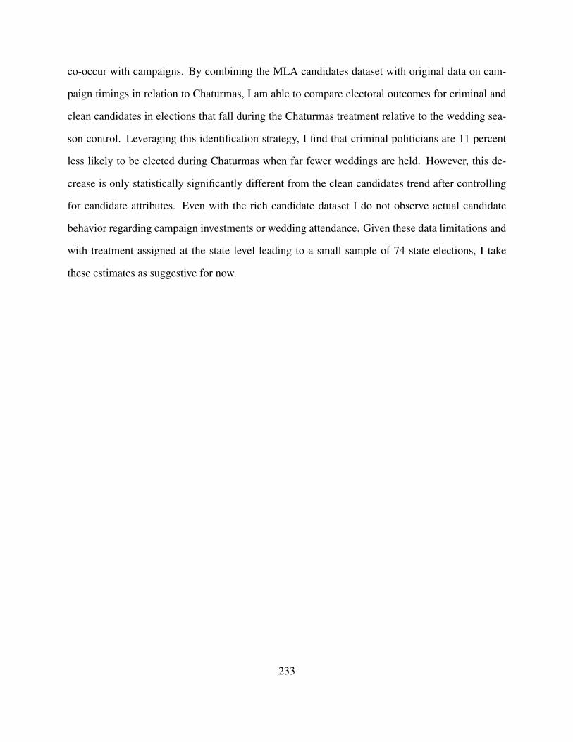
co-occur with campaigns. By combining the MLA candidates dataset with original data on cam-
paign timings in relation to Chaturmas, I am able to compare electoral outcomes for criminal and
clean candidates in elections that fall during the Chaturmas treatment relative to the wedding sea-
son control. Leveraging this identification strategy, I find that criminal politicians are 11 percent
less likely to be elected during Chaturmas when far fewer weddings are held. However, this de-
crease is only statistically significantly different from the clean candidates trend after controlling
for candidate attributes. Even with the rich candidate dataset I do not observe actual candidate
behavior regarding campaign investments or wedding attendance. Given these data limitations and
with treatment assigned at the state level leading to a small sample of 74 state elections, I take
these estimates as suggestive for now.
233
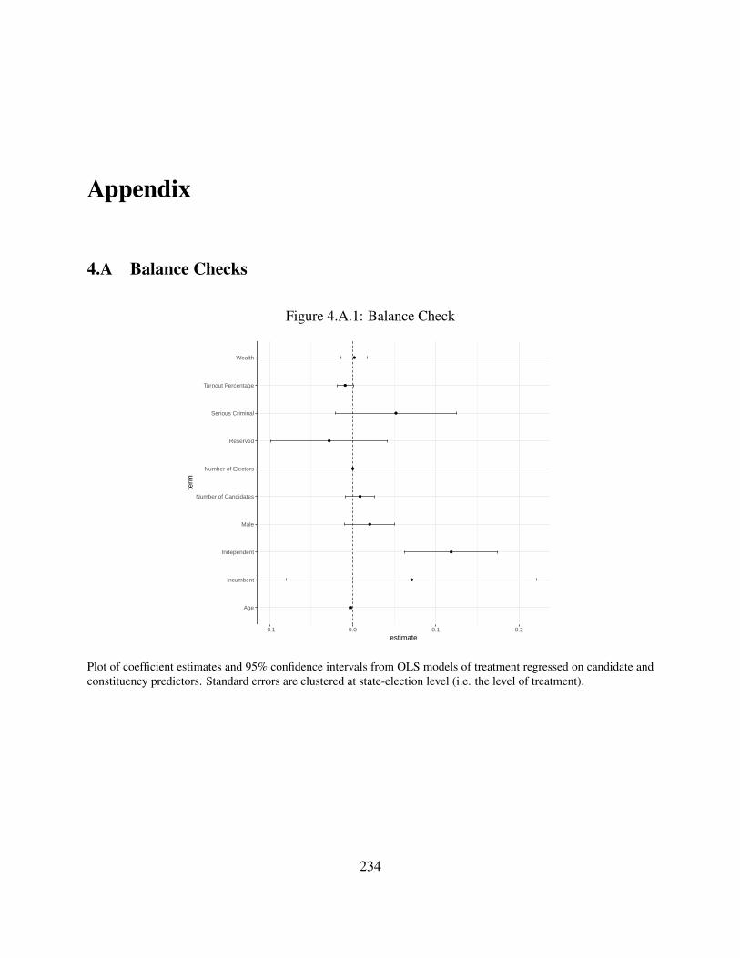
Appendix
4.A Balance Checks
Figure 4.A.1: Balance Check
Age
Incumbent
Independent
Male
Number of Candidates
Number of Electors
Reserved
Serious Criminal
Turnout Percentage
Wealth
−0.1 0.0 0.1 0.2estimate
term
Plot of coefficient estimates and 95% confidence intervals from OLS models of treatment regressed on candidate andconstituency predictors. Standard errors are clustered at state-election level (i.e. the level of treatment).
234

4.B Aggregate State Level Analysis
Table 4.B.1: State Election Regression Results
Dependent Variable:
State Election Mean Vote Share by Criminality
Serious Criminal 7.00∗∗∗
(2.32)
Chaturmas −5.59∗∗
(2.62)
Serious Criminal x Chaturmas −0.49(3.71)
Constant 19.04∗∗∗
(1.64)
Observations 148R2 0.14Adjusted R2 0.13Residual Std. Error 11.01 (df = 144)F Statistic 8.02∗∗∗ (df = 3; 144)
Note: ∗p<0.1; ∗∗p<0.05; ∗∗∗p<0.01
The dependent variable is the average vote share in the state election for serious criminals and clean candidates. Seriouscriminals are more likely to win elections and see a 6 percentage point decrease in vote share during Chaturmas.However this difference is not significantly distinguishable from clean candidate trends at conventional levels.
235
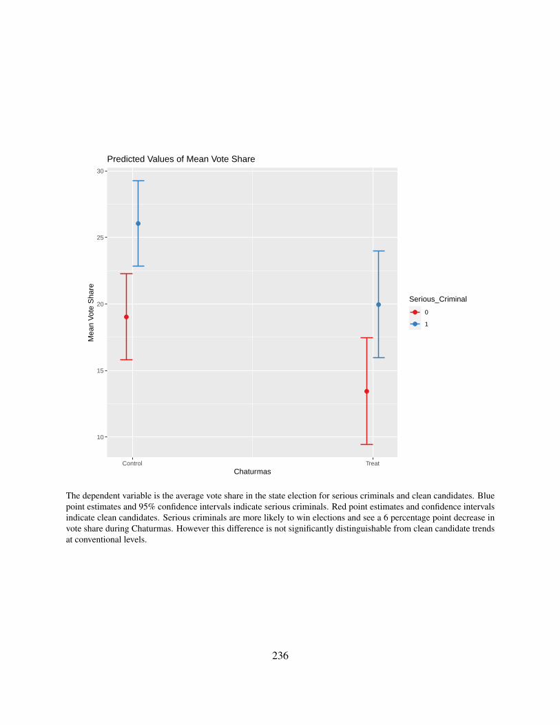
10
15
20
25
30
Control TreatChaturmas
Mea
n V
ote
Sha
re
Serious_Criminal
0
1
Predicted Values of Mean Vote Share
The dependent variable is the average vote share in the state election for serious criminals and clean candidates. Bluepoint estimates and 95% confidence intervals indicate serious criminals. Red point estimates and confidence intervalsindicate clean candidates. Serious criminals are more likely to win elections and see a 6 percentage point decrease invote share during Chaturmas. However this difference is not significantly distinguishable from clean candidate trendsat conventional levels.
236
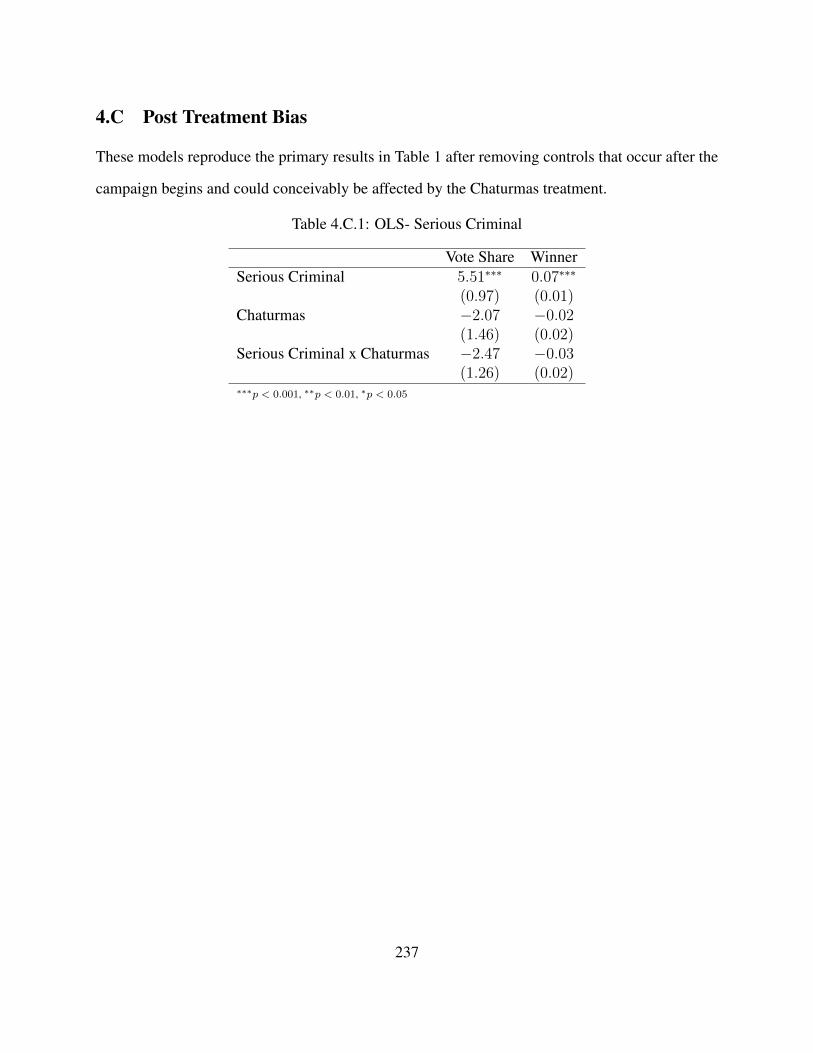
4.C Post Treatment Bias
These models reproduce the primary results in Table 1 after removing controls that occur after the
campaign begins and could conceivably be affected by the Chaturmas treatment.
Table 4.C.1: OLS- Serious Criminal
Vote Share WinnerSerious Criminal 5.51∗∗∗ 0.07∗∗∗
(0.97) (0.01)Chaturmas −2.07 −0.02
(1.46) (0.02)Serious Criminal x Chaturmas −2.47 −0.03
(1.26) (0.02)∗∗∗p < 0.001, ∗∗p < 0.01, ∗p < 0.05
237
Chapter 5
Conclusion
5.1 Overview
In this dissertation I investigate the conditions under which criminal politicians distribute resources
to their constituents. In turn, I ask whether superior state resource distribution or constituency ser-
vice can explain criminals’ enduring electoral success? In other words, what do criminal politicians
deliver to voters? If anything? To gain traction on these questions, I focus on one of India’s key
anti-poverty initiatives and the worlds’ largest public works program. Access to NREGS is en-
shrined in a fundamental human right to work. However, demand for the program exceeds supply.
As I write, NREGS has been pushed to the brink as employment demand soars during the coron-
avirus pandemic. Voters across India turn to politicians for help in interfacing with the bureaucracy
to access these benefits.
In addition to NREGS importance in the aggregate, there are theoretical reasons why I focus
on the employment program. As described throughout the preceding chapters, NREGS benefits
are highly desirable, politically manipulable and precisely measurable. NREGS represents a large
flow of government funds reaching a wide variety of voters. Inherently, the size and availability
of program benefits catch the eye of voters and politicians alike. At the same time, previous
research documents how politicians can intervene to redirect benefits towards their own political
goals (Gulzar and Pasquale, 2017; Dasgupta, 2016; Marcesse, 2018). Finally, NREGS provides
238

fine grained, administrative geo-data across India. Put simply NREGS serves as a “most likely
scenario,” for an empirical test of whether or not criminal politicians intervene to redistribute
resources towards their supporters.
In this dissertation, I present two key arguments. First, I contend that criminal politicians core
assets of money, muscle and networks make them particularly suited to both deliver more state ben-
efits and redirect fund flows towards co-partisans. Importantly, NREGS allows for a critical test of
the theory that criminal politicians are community warriors, protecting and providing for their “in-
group.” Previous quantitative treatments of criminal politicians have focused solely on aggregate
constituency outcomes. Leveraging NREGS geo-data I directly test if criminal politicians engage
in differential targeting, within constituencies.
Second, I identify a trade-off that candidates face between accruing enough capital to fund
campaigns and remaining rooted in the constituency to provide personalized service to voters. I
argue that criminals’ muscle-power allows them to sidestep this tradeoff and optimize on both
dimensions. Muscle enables criminals to establish lucrative protection rackets in their home con-
stituencies. In effect, protection rackets turn muscle into money. To protect this money, criminals
invest in networks. Constituent service networks help criminal politicians maintain political power,
which is useful for protecting their illegal enterprises.
To understand if criminal politicians deliver social welfare benefits and constituency service, I
combine granular and exhaustive data on NREGS outcomes, polling station results and candidate
affidavits. I use causal inference and machine learning designs to analyze this data and strengthen
the validity of my estimates. While some of my findings conflict, two primary patterns emerge
from the empirical analyses.
First, I provide new evidence that criminal politicians are associated with increased targeting
of state resources to co-partisans. This hews closely to criminals’ theoretical advantages stem-
ming from their deep communal roots. By remaining embedded in the constituency, I argue that
criminals are better positioned to identify, and then meet, supporters needs. Second, and perhaps
239

unsurprisingly, I find criminals’ core advantages in providing for constituents derives from their
capacity for violence. Both qualitative and quantitative evidence speak to criminal muscle as a
necessary input for both improved constituency service and benefit delivery. Quantitatively, I find
that criminals with violent charges are associated with increased NREGS delivery. Whereas, non-
violent criminals are not. In addition, drawing on in-depth fieldwork, I highlight the role of muscle
in solving the constituency-service vs. wealth-generation trade-off.
5.2 Summary of Findings
In Chapter 2, I leverage state of the art causal inference techniques to estimate the impact of crimi-
nality on NREGS delivery. Relative to clean politicians, criminals underperform in the provision of
NREGS, completing 475 fewer projects during their tenure. However, results remain inconclusive
regarding whether criminals deliver NREGS wages and employment. Therefore, I can not rule out
the possibility that criminal politicians may perform better on the primary dimensions that voters
care about. Still, the cleanest causal estimate identifies a negative effect of criminal politicians on
NREGS project delivery.
In this chapter, I construct a novel, qualitatively informed measure of corruption. Leveraging
rich NREGS project data, I identify projects that are more susceptible to corruption based on how
easy graft is to hide from engineering audits. I do not find that constituencies governed by criminal
politicians are more likely to engage in graft-prone projects. This rules out a primary alternative
explanation for the continued success of criminal politicians. Namely, that criminals deliver rents
to lower level politicians in exchange for votes.
Lacking a smoking gun from the regression discontinuity analysis, in Chapter 3, I test whether
criminal politicians are more efficient at targeting NREGS to co-partisans. I argue that if money
and muscle help criminals deliver NREGS benefits, networks help them identify supporters and
then meet their needs (e.g. providing access to NREGS job cards). Combining NREGS project
geo-data with an original geo-dataset on polling stations results, I map NREGS benefits directly
240
to micro pockets of political support. In this chapter, I find that criminal politicians both deliver
NREGS benefits overall and demonstrate superior targeting relative to clean politicians. Secondly,
I conduct a mechanisms investigation to understand if money, muscle or networks are responsi-
ble for superior NREGS delivery. I find the most support for the muscle mechanism. Criminal
politicians facing violent charges deliver at higher rates than non-violent criminals.
To increase the validity of these results, I apply a machine learning approach and replicate the
analysis on unseen holdout data. In the testing replication, I find that criminals still deliver more
NREGS wages overall. Though, the effect of criminality attenuates by about half relative to the
training data estimates.
How then do we think about reconciling the divergent NREGS delivery findings between the
regression discontinuity and micro-targeting analyses? To investigate one potential path to unify
these results, I disaggregate the micro-targeting analysis into competitive and safe constituencies.
I find that superior NREGS delivery is primarily driven by criminals in safe seats. Recall that
the regression discontinuity only compares criminal and clean candidates in competitive, coin-flip
races. Therefore, heterogeneous effects based on the level of constituency political competition,
provide one way to to reconcile these findings. At the risk of post-hoc theorizing, it could be the
case that parties and candidates face stronger incentives to ensure smooth NREGS delivery in very
tight races to ensure another seat in the legislature. This additional effort and party support may
swamp any baseline advantage for criminal politicians.
However, political competition is not the only factor changing across these two analyses. In the
targeting chapter, my sample is constrained to states for which I have polling stations results. Thus
the analyses differ on both the degree of competition and geography. Moreover, in the targeting
chapter I do not attempt to identify a causal effect. I can not rule out that the positive association
between criminality and NREGS provision is the result of biased estimation.
Finally, in Chapter 4 I flip the question around to ask if voters reward criminal politicians
for providing superior constituency service. This chapter recognizes that my prior analyses were
241

limited by only analyzing a single distributive program. I discuss this limitation in greater detail in
the next section. To partially alleviate my reliance on NREGS, in this chapter, I focus on criminal
politicians provision of constituency service. My analysis exploits a plausibly exogenous shock to
the opportunity for candidates to invest in constituency service during their campaigns. During the
Hindu holiday period of Chaturmas, there are no auspicious wedding days, reducing the supply
of a key form of constituency service. Campaigns that coincide with Chaturmas will not provide
candidates the same opportunity to show up and pay for weddings. I argue that this exogenous
shock should be particularly painful for criminal candidates who can demonstrate superior local
bonafides at these events. I find that, relative to clean politicians, criminal politicians suffer a
greater electoral penalty when elections are held during Chaturmas. However, this difference is
only statistically significant for some models.
5.3 Limitations and Measurement Challenges
One limitation of this dissertation is that I focus on a single social welfare program (NREGS).
However, the reality is that India runs a vast welfare state and politicians can optimize over a
bevy of resources at their distributive disposal. In Chapter 4, I attempt to address this deficiency
by examining the role that criminal politicians play in delivering constituency service that falls
outside of NREGS. However, by focusing solely on weddings, I only add one small piece of
the constituency service puzzle to my analysis. As Bussell (2019) notes, constituency service is
often missing entirely from studies on distributive politics which tend to focus on social assistance
programs or government fund flows. During my fieldwork, I found constituency service to be one
of the main ways that criminal politicians curry favor with voters. However, constituency service
presents difficulties from a measurement and causal identification perspective. I elaborate on these
challenges and my attempts to address them in the subsequent section.
242
5.3.1 Measuring Constituency Service
There are several measurement challenges to identifying the impact of constituency service on
electoral outcomes and whether criminal politicians are more likely to engage in these tactics.
Bussell (2019) provides the most up to date, India-wide analysis of politicians’ constituency ser-
vice. Still, there is a lack of data on the historical evolution of constituency service, how spending
changes over time and what candidates prioritize during campaigns. We know even less about
MLA candidates who fail to win, raising questions about survivorship bias.
One important way that politicians can provide constituency service is via small cash transfers
to constituents. Cash can solve a variety of small requests on demand. Several studies have utilized
candidate affidavit data to investigate the role wealth plays in determining electability (Vaishnav,
2017; Sircar, 2018a). While the candidate affidavits dataset is a rich resource it falls short on
actually identifying how wealth matters. First, data on candidates’ personal assets are a stock not
a flow. This elides how candidates’ spending habits change over time and whether this variation
drives a response from voters. Second, the assets data says nothing about how candidates alter
their cash distribution strategies during campaigns. In other words, the affidavits data only allows
comparisons across candidates and not within candidates.
Ultimately, given the amount of black money funding campaigns, the true level of election
spending is likely unobservable (Kapur and Vaishnav, 2018). While campaign spending is limited
by law, it is well known (and sometimes documented) that candidates spend above and beyond
the paltry ceiling placed on election spending. In my own fieldwork, there were multiple rumors
that one candidate was arrested during a campaign when trying to flee authorities with a heavy
suitcase full of cash. Second, Bussell (2019) conducts a detailed survey of election spending. Can-
didates admit to spending more than campaign limits with the amount increasing. Still, despite this
expansive and exhaustive data collection effort, Bussell’s analysis unfortunately can not identify
individual candidate spending. An actual accounting of election spending is perhaps impossible
243

to collect via surveys. For respondents, accurately accounting for their own campaign spending
habits could be tantamount to admitting to a felony.
To circumvent these measurement challenges, I exploit a novel natural experiment that induces
variation in the supply of weddings. Weddings are a bundled form of constituency service since
they consist of candidates donating both time and money to the event. However, like my singu-
lar focus on NREGS, constituency service is ultimately far broader than the one form I identify.
One potential solution, for future research, would be to combine detailed administrative data on a
distributive program (like NREGS) with survey evidence regarding the broader ecosystem of dis-
tributive resources available to politicians. For example, in this dissertation, I leverage the granular
NREGS data and detailed politicians’ affidavits to conduct a mechanism-based investigation of the
specific criminal assets driving NREGS performance. While this micro-level work is revealing, my
investigative spotlight is firmly fixed on only one program. Therefore, I leave open the possibility
that criminals exhibit heterogeneous effects across a basket of distributive goods and constituency
services. To not completely elide this limitation, my prior would be that criminals would perform
better, on average, across this basket of distributive goods. As I have argued throughout the dis-
sertation, criminals’ assets of money, muscle and networks are useful for solving a variety of voter
requests.
5.3.2 Measuring the Latent Concept of Criminality
One additional measurement issue requires attention. I use criminal charges to identify “criminal”
politicians. While an obvious choice, charges are only a proxy for the underlying, latent concept of
criminality. Some candidates are accused of only minor issues and should not be lumped in with
the Arun Yadavs and Anant Singhs of the world. On the other end of the spectrum, some powerful
dons may escape police scrutiny entirely. This misclassification is not overly detrimental to my
analysis- since measurement error should attenuate the effects of criminality. Moreover, the more
common occurrence seems to be that criminal politicians are slapped with charges for the crimes
they commit but then have the power to delay court dates indefinitely (Vaishnav, 2012). Instead,
244

these data problems speak to the larger issue of trying to capture latent criminality. Really what
I am interested in measuring is the capacity for violence and, to some extent, candidates’ ability
to engage in extortion rings and protection rackets. Raw criminal power is a difficult concept to
capture empirically.
Consider a more pernicious case that fell out of my fieldwork in Bihar. The politician Vijay
Krishna exhibits all the characteristics of a canonical criminal MLA. He is deeply embedded in
local villages and viewed as a strong and capable leader who provides for his constituents. In
fact, Vijay Krishna is even serving time in jail for a serious criminal charge. However, the voters
I interviewed were adamant that Vijay Krishna, while a capable leader, was not a strongman in
the same sense as Arun Yadav. Vijay incurred his charge while covering up a murder that his son
committed. While Vijay was present at the time of the murder, everyone was adamant that he
had no role in the actual killing. Instead, in an effort to save his son, he covered up the murder
by having the body dumped in the Ganges. While not a model citizen, Vijay does not exude the
qualities of criminal politicians that I have described previously.
This is not an easy measurement issue to solve. No matter how I recode charges, Vijay Krishna
would look every bit as much like the murderous Arun Yadav. While this may just be an edge
case, it speaks to larger issues within both the affidavit data and the conceptualization of criminal
politicians. One potential solution to better capture the latent concept of criminality would be
a deeper dive and data collection effort on the sources of politicians’ wealth, their connections
to local firms and identification of protection rackets. This would enable me to identify if there is
systematic differences between charged and uncharged politicians in how they fund political efforts
and engage in constituency service. Local reporters are very knowledgeable about who the power
players are in their area. Reporters’ local knowledge could be leveraged to construct a measure of
criminality that more closely aligns with the latent concept.
245

5.4 Implications for Future Research
One common recommendation for reducing political interference in state resource distribution is to
professionalize the bureaucracy and push for programmatic distribution (Stokes et al., 2013). When
applied to criminal politics in India, on its face, this strategy may seem like a useful lever for rooting
out criminal politicians. If citizens can depend on the impartial bureaucracy for state resources,
instead of politicians, then criminals’ electoral appeal would disappear. However, one implication
of my research is that simply improving the programmatic delivery of social welfare programs
seems unlikely to curtail criminal politicians’ distributive power. Insulating and professionalizing
the bureaucracy may reduce criminals appeal to a degree. However, in Chapter 4 I argue that
criminal politicians are perfectly capable of delivering constituency service that falls outside of
formal state programs. In fact it may be a more fundamental break down in state capacity that
allows criminal politicians to accrue political power via protection rackets in the first place. In
turn, I argue that criminals leverage this power to make themselves economically and politically
indispensable to a plurality of the constituency. Alternative options suggested by my research
would be to either root out protection rackets, or at least, address how state owned monopolies can
attract these rackets with the added consequence that criminals may eventually entangle themselves
in the state directly.
Regarding the broader distributive politics literature, my research suggests continued efforts
on identifying variation over time in how politicians provide constituency service, especially prior
to taking office. This could be an important ground clearing data exercise in order to better un-
derstand how challengers successfully defeat incumbents without access to state resources. In this
dissertation I have argued that politicians have different inherent capabilities for resource distribu-
tion. I add to the pool of important characteristics that can shape politicians distributive strategy. In
particular, I argue for understanding how the source of politicians’ wealth can influence incentives
and capabilities for engaging in constituency service. Identifying how muscle-power is systemat-
246

ically transformed into wealth generation and redistribution is a criminally underrated avenue for
future research.
247

Bibliography
Press Note: Schedule for the General Elections to the Legislative Assembly of Karnataka – Re-garding. Technical report, Election Commission of India, 2013.
ADR. Criteria for Categorization of Serious Criminal Cases. Technical report, Association forDemocratic Reform, 2014.
ADR. Lok Sabha Elections 2019 Analysis of Criminal Background, Financial, Education, Genderand other details of Winners. Technical report, Association for Democratic Reform, 2019. URLhttps://adrindia.org/.
Pravin Agarwal. 17 Facts about Chaturmas (July to October) which no oneknows!, 2017. URL https://www.speakingtree.in/allslides/lesser-known-facts-about-chaturmas-july-to-october.
T. S. Aidt, M. A. Golden, and D. Tiwari. Incumbents and Criminals in the Indian National Legisla-ture, 2011. URL https://www.repository.cam.ac.uk/handle/1810/242058.
J. Andrew Harris and Daniel N. Posner. (Under What Conditions) Do Politicians Reward TheirSupporters? Evidence from Kenya’s Constituencies Development Fund. American Political Sci-ence Review, 113(1):123–139, feb 2019. ISSN 15375943. doi: 10.1017/S0003055418000709.URL https://doi.org/10.1017/S0003055418000709.
Sam Asher and Paul Novosad. Dirty Politics: Mining Booms and Politician Behavior in India.SSRN Electronic Journal, jul 2016. doi: 10.2139/ssrn.2812315. URL https://papers.ssrn.com/abstract=2812315.
Naheed Ataulla. Politicians attend weddings, funerals with eye on votes, may 2016.
Adam Auerbach, Jennifer Bussell, Simon Chauchard, Francesca Jensenius, Gareth Nellis, MarkSchneider, Neelanjan Sircar, Pavithra Suryanarayan, Tariq Thachil, Rahul Verma, and AdamZiegfeld. Rethinking India and the Study of Electoral Politics in the Developing World *. Tech-nical report, 2020. URL https://vaishnavmilan.files.wordpress.com/2020/05/rethinking-india-working-paper.pdf.
Adam Michael Auerbach. India’s urban constituencies revisited. Contemporary SouthAsia, 0(2):136–150, 2015. ISSN 0958-4935. doi: 10.1080/09584935.2015.1028026.URL https://www.tandfonline.com/action/journalInformation?journalCode=ccsa20.
248

AM Auerbach. Demanding Development: The Politics of Public Goods Provision in India’s UrbanSlums. Cambridge University Press, 2019.
Abhijit Banerjee and Lakshmi Iyer. History, institutions, and economic performance: the legacy ofcolonial land tenure systems in India. The American Economic Review, 95(4):1190–1213, 2005.
Abhijit Banerjee, Esther Duflo, Clement Imbert, Santhosh Mathew, and Rohini Pande. E-governance, Accountability, and Leakage in Public Programs: Experimental Evidence from a Fi-nancial Management Reform in India. Technical report, National Bureau of Economic Research,Cambridge, MA, nov 2016. URL http://www.nber.org/papers/w22803.pdf.
T Baskaran, B Min, and Y Uppal. Election cycles and electricity provision: Evidence froma quasi-experiment with Indian special elections. Journal of Public Economics, pages64–73, 2015. URL https://www.sciencedirect.com/science/article/pii/S0047272715000547.
Ward Berenschot. The Spatial Distribution of Riots: Patronage and the Instigation of CommunalViolence in Gujarat, India. World Development, 39(2):221–230, feb 2011a. ISSN 0305750X.doi: 10.1016/j.worlddev.2009.11.029.
Ward Berenschot. On the usefulness of goondas in Indian politics: ’Moneypower’ and ’mus-clepower’ in a Gujarati locality. South Asia: Journal of South Asia Studies, 34(2):255–275, aug 2011b. ISSN 00856401. doi: 10.1080/00856401.2011.582669. URL https://www.tandfonline.com/doi/abs/10.1080/00856401.2011.582669.
Ward Berenschot. Clientelism, Trust Networks, and India’s Identity Politics: Conveying Closenessin Gujarat. Asian Studies, 47(1):24–43, 2015.
L Björkman and J Witsoe. Money and Votes: Following Flows through Mumbai and Bihar. In De-vesh Kapur and Milan Vaishnav, editors, Costs of Democracy: Political Finance in India. 2019.URL https://oxford.universitypressscholarship.com/downloadpdf/10.1093/oso/9780199487271.001.0001/oso-9780199487271-chapter-6.pdf.
Lisa Björkman. "You can’t buy a vote": Meanings of money in a Mumbai election. AmericanEthnologist, 41(4):617–634, nov 2014. ISSN 15481425. doi: 10.1111/amet.12101.
Francis Bloch, Vijayendra Rao, and Sonalde Desai. Wedding Celebrations as ConspicuousConsumption Signaling Social Status in Rural India. Technical report, 2004. URL http://jhr.uwpress.org/content/XXXIX/3/675.short.
Taylor Boas, Daniel F. Hidalgo, and Marcus Andre Melo. Norms versus action: Why voters fail tosanction malfeasance in Brazil. American Journal of Political Science, 63(2):385–400, 2019.
Anjali Thomas Bohlken. Targeting Ordinary Voters or Political Elites? Why Pork Is DistributedAlong Partisan Lines in India. American Journal of Political Science, 62(4):796–812, oct 2018.
249

ISSN 00925853. doi: 10.1111/ajps.12374. URL http://doi.wiley.com/10.1111/ajps.12374.
F Brollo and U Troiano. What happens when a woman wins an election? Evidence from closeraces in Brazil. Journal of Development Economics, 122:28–45, 2016. URL https://www.sciencedirect.com/science/article/pii/S0304387816300244.
Ryan Brown. Competition and the Progression of Women’s Political Participation. 2017.
Jennifer Bussell. Whose Money, Whose Influence? Multilevel Politics and Campaign Finance inIndia. In K. Devesh and M. Vaishnav, editors, Costs of Democracy, pages 232–272. OxfordUniversity Press, aug 2018. doi: 10.1093/oso/9780199487271.003.0008.
Jennifer Bussell. Clients and constituents: political responsiveness in patronage democracies.Oxford University Press, 2019. doi: 10.1080/14662043.2020.1733266.
S. Calonico, M. D. Cattaneo, and R. Titiunik. rdrobust: An R package for robust nonparametricinference in regression discontinuity designs. R Journal, 7:38–51, 2015.
Charlie Campbell. India Elections: Rajasthan Candidate Offers to Fund2,100 Weddings. Time, apr 2014. URL https://time.com/62957/indian-election-2100-weddings-makhan-lal-meena/.
Kanchan Chandra. Why ethnic parties succeed: Patronage and ethnic head counts in India. Cam-bridge University Press, 2007.
Raghabendra Chattopadhyay and Esther Duflo. Women as policy makers: Evidence from a ran-domized policy experiment in India, sep 2004. ISSN 00129682.
Simon Chauchard. Unpacking Ethnic Preferences. Comparative Political Studies, 49(2):253–284,feb 2016. ISSN 0010-4140. doi: 10.1177/0010414015609356. URL http://journals.sagepub.com/doi/10.1177/0010414015609356.
Simon Chauchard. What Costs So Much in Indian Elections. In Costs of Democracy: PoliticalFinance in India, pages 201–231. 2018.
Matthieu Chemin. Welfare effects of criminal politicians: A discontinuity-based approach. Journalof Law and Economics, 55(3):667–690, jul 2012. ISSN 00222186. doi: 10.1086/664574.
Michael A. Collins. Navigating Fiscal Constraints. In Costs of Democracy, pages 119–152. OxfordUniversity Press, aug 2018. doi: 10.1093/oso/9780199487271.003.0005.
Skyler J. Cranmer and Bruce A. Desmarais. What can we learn from predictive modeling? PoliticalAnalysis, 25(2):145–166, apr 2017. ISSN 14764989. doi: 10.1017/pan.2017.3.
CSDS. CSDS Mood of the Nation Survey, 2018: ’Jobs the biggest problem, have become harderto get, jan 2018. URL https://indianexpress.com/.
250
Upasak Das. Does political activism and affiliation affect allocation of benefits in the rural employ-ment guarantee program: Evidence from West Bengal, India. World Development, 67:202–217,mar 2015. ISSN 0305750X. doi: 10.1016/j.worlddev.2014.10.009.
Upasak Das and Diego Maiorano. Post-clientelistic initiatives in a patronage democracy: Thedistributive politics of India’s MGNREGA. World Development, 117:239–252, may 2019a.ISSN 18735991. doi: 10.1016/j.worlddev.2019.01.011.
Upasak Das and Diego Maiorano. Post-clientelistic initiatives in a patronage democracy: Thedistributive politics of India’s MGNREGA. World Development, 117:239–252, may 2019b.ISSN 18735991. doi: 10.1016/j.worlddev.2019.01.011.
Aditya Dasgupta. Strategically greasing the wheels The political economy of India’s rural em-ployment guarantee Strategically Greasing the Wheels: the Political Economy of India’s Ru-ral Employment Guarantee. Technical report, 2016. URL http://www.theigc.org/wp-content/uploads/2016/08/Dasgupta-2016-Working-Paper.pdf.
Aditya Dasgupta and Devesh Kapur. The Political Economy of Bureaucratic Overload: Evidencefrom Rural Development Officials in India. American Political Science Review, 114(4):1316–1334, 2020. ISSN 15375943. doi: 10.1017/S0003055420000477. URL https://doi.org/10.1017/S0003055420000477.
Tanvi Deshpande. State of Agriculture in India. Technical report, PRS In-dia, 2017. URL https://www.prsindia.org/sites/default/files/parliament_or_policy_pdfs/StateofAgricultureinIndia.pdf.
Subhasish Dey and Kunal Sen. Is Partisan Alignment Electorally Rewarding? Evidence fromVillage Council Elections in India. SSRN Electronic Journal, jun 2017. ISSN 1556-5068. doi:10.2139/ssrn.2835536. URL https://papers.ssrn.com/abstract=2835536.
Jean Dreze. NREGA: Dismantling the contractor raj, 2011.
Drik Panchang. Online Panchang, Panchangam and Hindu Calendar for the world. URL https://www.drikpanchang.com/.
Thad Dunning. Natural experiments in the social sciences: A design-based approach. CambridgeUniversity Press, jan 2012. ISBN 9781139084444. doi: 10.1017/CBO9781139084444.URL /core/books/natural-experiments-in-the-social-sciences/96A64CBDC2A2952DC1C68AF77DE675AF.
Thad Dunning and Janhavi Nilekani. Ethnic quotas and political mobilization: Caste, parties, anddistribution in Indian village councils. American Political Science Review, 107(1):35–56, 2013.ISSN 15375943. doi: 10.1017/S0003055412000573. URL https://doi.org/10.1017/S0003055412000573.
251
B Dutta and P Gupta. How Indian Voters Respond to Candidates with Criminal Charges: Evidencefrom the 2009 Lok Sabha Elections. Economic and Political Weekly, 2014. URL https://www.jstor.org/stable/24479421.
Puja Dutta. Does India’s employment guarantee scheme guarantee employment? Economic andPolitical Weekly, pages 55–64, 2012.
Puja Dutta, Rinku Murgai, Martin Ravallion, and Dominique van de Walle. Right to Work?:Assessing India’s Employment Guarantee Scheme in Bihar. The World Bank, feb 2014. doi:10.1596/978-1-4648-0130-3.
Andrew C. Eggers. On the validity of the regression discontinuity design for estimating electoraleffects: New evidence from over 40,000 close races. American Journal of Political Science, 59(1):259–274, 2015.
Fernando Ferreira and Joseph Gyourko. Does gender matter for political leadership? The case ofUS mayors. Journal of Public Economics, 112(2014):24–39, 2014.
Diego Gambetta. The Sicilian Mafia: The Business of Private Protection. Harvard UniversityPress, 1996.
Carley Garner. Indian Wedding Season Is a Golden Opportunity - RealMoney, sep2016. URL https://realmoney.thestreet.com/articles/09/14/2016/indian-wedding-season-golden-opportunity.
Andrew Gelman. You need 16 times the sample size to estimate an interaction than to estimate amain effect « Statistical Modeling, Causal Inference, and Social Science, 2018. URL https://statmodeling.stat.columbia.edu/.
Andrew Gelman and Guido Imbens. Why high-order polynomials should not be used in regressiondiscontinuity designs. Journal of Business & Economic Statistics, 2019.
Sutanuka Ghosal. Expect a 10 per cent rise in gold demand this wedding season, mar 2015.
Miriam Golden and Brian Min. Distributive Politics Around the World. Annual Review of PoliticalScience, 16, 2013.
S Gulzar and BJ Pasquale. Politicians, Bureaucrats, and Development: Evidence from India. Amer-ican Political Science Review, 111(01):162–183, 2017. URL https://www.cambridge.org/core/journals/american-political-science-review/article/politicians-bureaucrats-and-development-evidence-from-india/130F6270702BDE2449BA4902C0FA1804.
Saad Gulzar, Nicholas Haas, and Benjamin Pasquale. Does Political Affirmative Action Work,and for Whom? Theory and Evidence on India’s Scheduled Areas. mar 2020. URL https://escholarship.org/uc/item/3f54527z.
252

Bhanu Gupta and Abhiroop Mukhopadhyay. Local funds and political competition: Evidencefrom the National Rural Employment Guarantee Scheme in India. European Journal of PoliticalEconomy, 41:14–30, jan 2016. ISSN 01762680. doi: 10.1016/j.ejpoleco.2015.10.009.
BA Gupte. Hindu holidays and ceremonials: with dissertations on origin, folklore and sym-bols. 1994. URL https://books.google.com/books?hl=en&lr=&id=_FSWKWzNSagC&oi=fnd&pg=PR41&dq=hindu+holidays+gupte+1994&ots=oKn-CCr3oH&sig=OMh26-KCi-2_NMLJI0J5GV-lq00.
Jens Hainmueller and Chad Hazlett. Kernel regularized least squares: Reducing misspecificationbias with a flexible and interpretable machine learning approach. Political Analysis, 22(2):143–168, 2014. ISSN 14764989. doi: 10.1093/pan/mpt019.
Thomas Bloom Hansen. Sovereigns beyond the state: on legality and authority in urban India.In Sovereign Bodies: Citizens, Migrants, and States in the Postcolonial World, pages 169–191.Princeton University Press, 2005.
Allen Hicken and Noah L. Nathan. Clientelism’s Red Herrings: Dead Ends and New Directions inthe Study of Nonprogrammatic Politics. Annual Review of Political Science, 23(1):1–18, may2020. ISSN 1094-2939. doi: 10.1146/annurev-polisci-050718-032657.
Guido Imbens and Karthik Kalyanaraman. Optimal bandwidth choice for the regression disconti-nuity estimator. The Review of Economic Studies, 79(3):933–959, 2012.
Clément Imbert and John Papp. Estimating Leakages in India’s Employment Guarantee UsingHousehold Survey Data. In Battle for Employment Guarantee. Oxford University Press, NewDelhi, 2011. URL http://nrega.nic.in.
Clement Imbert and John Papp. Labor market effects of social programs: Evidence from India’semployment guarantee. American Economic Journal: Applied Economics, 7(2):233–63, 2015.
Lakshmi Iyer. Direct versus indirect colonial rule in India: Long-term consequences. The Reviewof Economics and Statistics, 92(4):693–713, 2010.
Lakshmi Iyer and Anandi Mani. TRAVELING AGENTS: POLITICAL CHANGE AND BU-REAUCRATIC TURNOVER IN INDIA. MIT Press, 94(3):723–739, 2012. doi: 10.1162/REST_a_00183. URL https://www.mitpressjournals.org/doi/abs/10.1162/REST_a_00183.
Robin Jacob. A practical guide to regression discontinuity. Technical report, MDRC, 2012.
Rajendra Jadhav. Weddings, lower prices could lift Indian gold demand in June quar-ter: WGC | Reuters, may 2019. URL https://br.reuters.com/article/india-gold-demand-idINKCN1S805O.
Christophe Jaffrelot and Gilles Verniers. Indian Elections : Reaching the End of the DemocraticTether. Esprit, pages 75–87, 2014.
253
Bharti Jain. President’s rule imposed in Delhi: President’s rule imposed in Delhi | Delhi News -Times of India, feb 2014. URL https://timesofindia.indiatimes.com/city/delhi/Presidents-rule-imposed-in-Delhi/articleshow/30558345.cms.
Rob Jenkins and James Manor. Politics and the right to work: India’s national rural employmentguarantee act. 2017. doi: 10.1080/09584935.2018.1507711.
Francesca R Jensenius and Pavithra Suryanarayan. Party candidate linkages and Anti-IncumbencyVoting: Evidence from the Indian States. pages 1–29, 2017.
Francesca Refsum Jensenius. Power and influence in India: Bosses, Lords and Captains. Forumfor Development Studies, 38(3):391–398, nov 2011. ISSN 0803-9410. doi: 10.1080/08039410.2011.619683.
Dahyeon Jeong, Ajay Shenoy, Laura Zimmermann, and Amos Hall. Are transparency and account-ability enough? Open corruption and why it exists. 2018. URL https://www.econstor.eu/handle/10419/197762.
J. Jeyaranjan. Sand and the politics of plunder in Tamil Nadu, India. In The Wild East, pages92–114. UCL Press, sep 2019. doi: 10.2307/j.ctvfrxr41.11.
Giridhar Jha. Who is Pappu Yadav to fix our fees, ask Bihar doctors, sep 2014.
Prashant Jha. How the BJP Wins: Inside India’s Greatest Election Machine. Juggernaut, 2017.
Devesh Kapur and Milan Vaishnav. Costs of Democracy. Oxford University Press, aug 2018. doi:10.1093/oso/9780199487271.001.0001.
HL Kern and J Hainmueller. Opium for the masses: How foreign media can stabilize authoritar-ian regimes. Political Analysis, pages 377–399, 2009. URL https://www.jstor.org/stable/25791984.
Umair Khalil, Sulagna Mookerjee, and Ryan Tierney. Social interactions in voting behavior: Ev-idence from india. Journal of Economic Behavior and Organization, 163:158–171, jul 2019.ISSN 01672681. doi: 10.1016/j.jebo.2019.04.024.
Stuti Khemani. Decentralization and Accountability: Are Voters More Vigilant in Local thanin National Elections? Policy Research Working Papers. The World Bank, feb 2001. doi:10.1596/1813-9450-2557. URL http://elibrary.worldbank.org/doi/book/10.1596/1813-9450-2557.
Stuti Khemani. Political cycles in a developing economy: Effect of elections in the Indian States.Journal of Development Economics, 73(1):125–154, feb 2004. ISSN 03043878. doi: 10.1016/j.jdeveco.2003.01.002.
Herbert Kitschelt and Steven Wilkinson. Patrons, Clients, and Policies: patterns of democraticaccountability and political competition. 2007.
254
Eric Kramon and Daniel N. Posner. Who benefits from distributive politics? How the outcome onestudies affects the answer one gets. Perspectives on Politics, pages 461–474, 2013.
Gabrielle Kruks-Wisner. Navigating the State: Citizenship practice and the pursuit ofservices in Rural India." Present at the Harvard South Asia Institute. 2015. URLhttp://southasiainstitute.harvard.edu/website/wp-content/%0Duploads/2013/07/GKW_SAI-working-paper_2015.pdf.
Gabrielle Kruks-Wisner. The pursuit of social welfare: Citizen claim-making in rural India. WorldPolitics, 70(1):122–163, jan 2018. ISSN 10863338. doi: 10.1017/S0043887117000193. URLhttps://doi.org/10.1017/S0043887117000193.
Gabrielle K. Kruks-Wisner. Making Claims: Citizenship and Service Delivery in Rural India.SSRN Electronic Journal, jan 2012. ISSN 1556-5068. doi: 10.2139/ssrn.1945333. URLhttps://papers.ssrn.com/abstract=1945333.
ASHUTOSH Kumar. Assembly Elections 2009 in Haryana: Exploring the Verdict. Economicand Political Weekly, pages 19–21, 2019. URL https://www.jstor.org/stable/25663962.
David S. Lee and Thomas Lemieux. Regression discontinuity designs in economics. Journal ofEconomic Literature, 48(2):281–355, 2010.
Jonathan Lehne, Jacob N. Shapiro, and Oliver Vanden Eynde. Building connections: Politicalcorruption and road construction in India. Journal of Development Economics, 131:62–78, mar2018. ISSN 03043878. doi: 10.1016/j.jdeveco.2017.10.009.
Zaad Mahmood and Rahul Ganguli. The Performance of Indian States in Electoral Integrity.Technical report, 2017.
Diego Maiorano. The politics of the Mahatma Gandhi national rural employment guarantee act inAndhra Pradesh. World Development, 58:95–105, jun 2014. ISSN 0305750X. doi: 10.1016/j.worlddev.2014.01.006.
James Manor. When Local Government Strikes It Rich Strikes It Rich. 2013. ISBN9789186725129.
Thibaud Marcesse. Public Policy Reform and Informal Institutions: The Political Articulationof the Demand for Work in Rural India. World Development, 103:284–296, mar 2018. ISSN18735991. doi: 10.1016/j.worlddev.2017.10.024.
Nicolas Martin and Lucia Michelutti. Protection Rackets and Party Machines. Asian Journal ofSocial Science, 45(6):693–723, 2017.
Sheena McKenzie. What does every Indian wedding need? Gold (and lots ofit) - CNN, 2015. URL https://edition.cnn.com/2015/08/20/business/indian-wedding-gold-jewelery-prices/index.html.
255

Seetha Menon. The effect of marital endowments on domestic violence in India. Journal ofDevelopment Economics, 143:102389, mar 2020. ISSN 03043878. doi: 10.1016/j.jdeveco.2019.102389.
L Michelutti. The inter-state criminal life of sand and oil in North India. In The Wild East: CriminalPolitical Economies in South Asia, page 168. 2019. URL https://books.google.com/books?hl=en&lr=&id=8i26DwAAQBAJ&oi=fnd&pg=PA168&dq=The+inter-state+criminal+life+of+sand+and+oil+in+North+India&ots=hfYw10tXkt&sig=lpUepjX6e_itGDnRh_Mqik6KxKQ.
Lucia Michelutti. Kingship without kings in Northern India. In Patronage as Politics in SouthAsia, pages 283–302. Cambridge University Press, jan 2014. ISBN 9781107296930. doi: 10.1017/CBO9781107296930.014.
Brian Min. Estimating the Effects of Quotas Across India using Satellite Imagery. 2012.
Dilip Mookherjee. MNREGA: populist leaky bucket or anti-poverty success? Technical report,2014.
MoRD. MGNREGA Performance Review Committee (PRC). Technical report, 2017.
Karthik Muralidharan, Niehaus, Paul, and Sandip Sukhtankar. Building state capacity: Evidencefrom biometric smartcards in India. The American Economic Review, 106(10):2895–2929, 2016.
Vikram K. Nanda and Ankur Pareek. Do Criminal Politicians Affect Firm Investment and Value?Evidence from a Regression Discontinuity Approach. 2016.
Paul Niehaus and Sandip Sukhtankar. Corruption dynamics: The golden goose effect. AmericanEconomic Journal: Economic Policy, 5(4):230–269, nov 2013. ISSN 19457731. doi: 10.1257/pol.5.4.230.
Patricia O’Campo, Agnes Molnar, Edwin Ng, Emilie Renahy, Christiane Mitchell, Ketan Shankar-dass, Alexander St. John, Clare Bambra, and Carles Muntaner. Social welfare matters: A realistreview of when, how, and why unemployment insurance impacts poverty and health. SocialScience and Medicine, 132:88–94, may 2015. ISSN 18735347. doi: 10.1016/j.socscimed.2015.03.025.
A Piliavsky. Patronage as politics in South Asia. 2014. URL https://books.google.com/books?hl=en&lr=&id=Nw6MBgAAQBAJ&oi=fnd&pg=PP1&ots=8DVIFj18fG&sig=ntnSgwiM5dLRS7KoQBkwGBWKzXk.
Daniel N. Posner. Institutions and Ethnic Politics in Africa. Cambridge University Press, 2005.
Nishith Prakash, Marc Rockmore, and Yogesh Uppal. Do criminally accused politicians affecteconomic outcomes? Evidence from India. Journal of Development Economics, 141:102370,nov 2019. ISSN 03043878. doi: 10.1016/j.jdeveco.2019.102370.
256

Jyotsna Puri, Vijit Singh Chahar, and Hugh Waddington. Examining the evidence on the effective-ness of India’s rural employment guarantee act. 2016.
Vijayendra Rao. Celebrations as Social Investments: Festival Expenditures, Unit Price Variationand Social Status in Rural India. Journal of Development Studies, 38(1):71–97, 2001. ISSN00220388. doi: 10.1080/713601102. URL https://www.tandfonline.com/doi/abs/10.1080/713601102.
Shamika Ravi and Monika Engler. Workfare as an effective way to fight poverty: The case ofIndia’s NREGS. World Development, 67:57–71, 2015.
Mark Schneider. Do local leaders know their voters? A test of guessability in India. ElectoralStudies, 61:102049, oct 2019. ISSN 02613794. doi: 10.1016/j.electstud.2019.102049.
Faraz V. Shahidi, Chantel Ramraj, Odmaa Sod-Erdene, Vincent Hildebrand, and Arju-mand Siddiqi. The impact of social assistance programs on population health: Asystematic review of research in high-income countries. BMC Public Health, 19(1):1–11, jan 2019. ISSN 14712458. doi: 10.1186/s12889-018-6337-1. URL https://link.springer.com/articles/10.1186/s12889-018-6337-1https://link.springer.com/article/10.1186/s12889-018-6337-1.
Megan Sheahan, Yanyan Liu, Christopher B. Barrett, and Sudha Narayanan. Preferential Re-source Spending under an Employment Guarantee: The Political Economy of MGNREGSin Andhra Pradesh. Policy Research Working Papers. The World Bank, sep 2016. doi:10.1596/1813-9450-7818. URL http://elibrary.worldbank.org/doi/book/10.1596/1813-9450-7818.
Joseph P. Simmons, Leif D. Nelson, and Uri Simonsohn. False-positive psychology: Undisclosedflexibility in data collection and analysis allows presenting anything as significant. Psychologi-cal Science, 22(11):1359–1366, nov 2011. ISSN 14679280. doi: 10.1177/0956797611417632.URL http://journals.sagepub.com/doi/10.1177/0956797611417632.
Nigel Singh and Barbara Harriss-White. The criminal economics and politics of black coal inJharkhand, 2014. In The Wild East, pages 35–67. UCL Press, sep 2019. doi: 10.2307/j.ctvfrxr41.9.
Neelanjan Sircar. Money in Elections. In D. Kapur and M. Vaishnav, editors, Costs of Democracy,pages 36–73. Oxford University Press, aug 2018a. doi: 10.1093/oso/9780199487271.003.0003.
Neelanjan Sircar. Education ups attendance of MPs, criminal history lowers it, 2018b.
Sara Steegen, Francis Tuerlinckx, Andrew Gelman, and Wolf Vanpaemel. Increasing Trans-parency Through a Multiverse Analysis. Perspectives on Psychological Science, 11(5):702–712,sep 2016. ISSN 17456924. doi: 10.1177/1745691616658637. URL http://journals.sagepub.com/doi/10.1177/1745691616658637.
257
Susan Stokes, Thad Dunning, Marcelo Nazareno, and Valeria Brusco. Brokers, Voters, and Clien-telism: The Puzzle Of Distributive Politics. Cambridge Studies in Comparative Politics, 2013.
Sandip Sukhtankar. Sweetening the deal? Political connections and sugar mills in India. AmericanEconomic Journal: Applied Economics, 4(3):43–63, jul 2012. ISSN 19457782. doi: 10.1257/app.4.3.43.
Sandip Sukhtankar and Milan Vaishnav. Corruption in India: Bridging Academic Evidence andPolicy Options. Technical report, 2014. URL www.ncaer.org.
Sandip Sukhtankar, Michael Kaiser, Kevin Li, Frances Lu, and Katherine Mcavoy. India’s NationalRural Employment Guarantee Scheme: What Do We Really Know about the World’s LargestWorkfare Program? Technical report, 2016.
Amarnath Tewary. Independent Bihar MLA Anant Singh goes missing from his Patna house, aug2019.
M Vaishnav. The Merits of Money and" Muscle": Essays on Criminality, Elections and Democracyin India. PhD thesis, 2012. URL https://academiccommons.columbia.edu/doi/10.7916/D832030W.
Milan Vaishnav. Understanding the Indian Voter. Technical report, Carnegie Endowment forInternational Peace, 2015.
Milan Vaishnav. When crime pays: Money and muscle in Indian politics. Yale University Press,2017.
Milan Vaishnav, Saksham Khosla, Aidan Milliff, and Rachel Osnos. Digital India? an emailexperiment with Indian legislators. India Review, 18(3):243–263, may 2019. ISSN 1473-6489.doi: 10.1080/14736489.2019.1616259. URL https://www.tandfonline.com/doi/full/10.1080/14736489.2019.1616259.
Robert Wade. The market for public office: Why the Indian state is not better at development.World Development, 13(4):467–497, apr 1985. ISSN 0305750X. doi: 10.1016/0305-750X(85)90052-X.
Matthew S. Winters and Rebecca Weitz-Shapiro. Lacking information or condoning corruption:When do voters support corrupt politicians? Comparitive Politics, 45(4):418–436, 2013.
Jeffrey Witsoe. Territorial democracy: Caste, dominance and electoral practice in postcolonialIndia. PoLAR: Political and Legal Anthropology Review, 31(1):64–83, 2009.
Jeffrey Witsoe. Everyday corruption and the political mediation of the Indian state: An ethno-graphic exploration of brokers in Bihar. Economic and Political Weekly, pages 47–54, 2012.
Jeffrey Witsoe. Democracy against Development: Lower-Caste Politics and Political Modernity inPostcolonial India, Witsoe. The University of Chicago Press, 2013. URL https://press.uchicago.edu/ucp/books/book/chicago/D/bo16552144.html.
258

Wendy N Wong. Optimal Monitoring and Bureaucrat Adjustments. Technical report, 2020.
Z. Wood and R. Wachman. Every Indian wedding adds to demand in world’s biggest jewellerymarket | Business | The Guardian, oct 2010. URL https://www.theguardian.com/business/2010/oct/10/indian-jewellery-market.
World Bank. The State of Social Safety Nets 2015. The World Bank, jun 2015. doi: 10.1596/978-1-4648-0543-1. URL https://openknowledge.worldbank.org/handle/10986/22101.
World Bank. Growing the Rural Nonfarm Economy to Alleviate Poverty. Technical report,2017. URL http://ieg.worldbankgroup.org/sites/default/files/Data/Evaluation/files/RuralNonFarm.pdf.
Guo Xu, Marianne Bertrand, and Robin Burgess. Social Proximity and Bureaucrat Performance:Evidence from India. 2018.
259