Dividend Discount Model (DDM) : A study based on select ...

Dividend Discount Model (DDM) : A study based on

select companies from India. Soumya V

1, Binu P Paul

2

Christ Institute of Management, Christ Trust, Lavasa.

Christ Institute of Management, Christ Trust, Lavasa. [email protected]

[email protected]

Abstract— Knowledge about the intrinsic value of stock will help the investors to make the right decision – whether to go long, short

or hold a particular stock at a particular time. Researchers have come up with different methods for finding out the intrinsic value of

common stock. One of the methods is ‘Dividend Discount Model’ (DDM), also known as Gordon growth model (GGM), which was

proposed by Myron J. Gordon in 1960s. The model uses the basic principle of time value of money and portrays the value of a

common stock as the present value of all its expected future dividends. Many studies have been conducted to test the relevance and

reliability of the DDM model which showed mixed results. While reviewing the literature, the authors of this paper came across

studies testing the applicability of DDM in selected stocks of Nairobi and Ghana Stock Exchange but could not find studies with

respect to Indian Companies. This study is aimed to check the applicability of DDM in the valuation of top 5 dividend paying

companies in National Stock Exchange (NSE), India. To check the accuracy of predictions, different Absolute Percentage Error

(APE) measures were used and the result showed that the GGM model has low prediction accuracy in the case of some companies,

whereas for other companies, there are considerable differences. But when the actual and predicted share prices of all the selected

companies were clubbed into one to represent the data of a fictitious company, the result showed that GGM tend to reflect actual

share prices.

Keywords— Stock Valuation, Dividend Discount Model, India, NSE, Gordon Growth Model

I. INTRODUCTION

Valuation of companies and stocks is one area which has attracted the interests of researchers, academicians, business houses,

investors as well as government and policy makers across the world. An investor is keen to know the intrinsic value of a stock

which will help him/her to make the right financial decision. There are different techniques of calculating the intrinsic value of

common stock. The techniques of equity valuation could be broadly classified in to three broad categories viz., Balance Sheet

Techniques, Discounted Cash Flow Techniques and Relative Valuation Techniques. (Chandra, 2017)[1]

A. Balance Sheet Techniques

The methods of stock valuation under Balance Sheet techniques include Book Value approach, Liquidation Value Approach

and Replacement Cost Approach. Under Book value approach, the value of a stock is found out by dividing the sum total of the

book value of the net worth of a company by the number of equity shares outstanding on a particular day. Net worth is

calculated either by using the formula Total Assets – Outside Liabilities or by taking the total funds available to equity share

holders which includes the paid up equity capital and reserves and surplus. The biggest disadvantage of this method is that,

book value, being historical in nature, rarely reflects the real economic value of the business. Also, it does not portray the future

earnings power and growth potential of a business. In Liquidation value method, the value per share is found out using the

formula (Value realized by liquidating the assets of the firm – Amount payable to outsiders and preference shareholders) /

Number of equity shares. Just like book value method, this method too does not reflect the earnings power and growth potential

of a business. Also, it is difficult to estimate the realizable value while liquidating the assets of a business and those values too

may not reflect the current real worth of the assets of the business. This method is more suitable for a company or a firm which

goes in to liquidation and not for stable or growing firms. While making investing decisions, investors may not be interested in

investing in ‘dying’ firms or firms which are in the verge of liquidation. In replacement cost method, value of a share is found

out using the cost involved in replacing the net assets (Assets – Liabilities) instead of taking either the book value or liquidation

values. Even though this method is more realistic than book value and liquidation methods of stock valuation, this too does not

reflect the future earnings power and growth potential of a business. [1]

B. Discounted Cash Flow Techniques

CIKITUSI JOURNAL FOR MULTIDISCIPLINARY RESEARCH

Volume 6, Issue 3, March 2019

ISSN NO: 0975-6876

http://cikitusi.com/70

Discounted Cash Flow techniques are the most popular techniques of stock valuation as these take in to consideration the basic

premise of time value of money. Here, value of a share is found out by taking the present value of all future cash flows. Unlike

Balance Sheet techniques, Discounted cash flow techniques consider the future earnings and growth potential of a business

while valuing the shares. This technique is further classified in to two – Dividend Discount Model (DDM) and Free Cash Flow

(FCF) Model.

In Dividend Discount Model, the value of a share is equal to the present value of all its expected future dividends plus the

present value of the expected sale price when the shares are sold. DDMs normally assume that all the future dividend payments

are made annually and the first dividend is received one year after the shares are bought. DDMs are of two categories viz.,

Single – Period Valuation Model which assumes that the shares will be held only for a single period normally for one year and

the more realistic and complex Multi-Period Valuation Model which considers all the future streams of dividends and the final

sale price of the share. Multi – Period Valuation model is further categorized in to Zero Growth Model, Constant Growth Model

(Gordon Growth Model), Two Stage growth model, three stage growth model and H Model. Single period valuation model, just

like the name suggests, has much limited practical significance especially for long term investors. Zero Growth model assumes

that a firm will pay a constant dividend per share every year and will not grow at all which is a rarity [1]. The investors expect

their investments to grow in the future and therefore, a model which considers the future growth potential has more practical

relevance than a model which does not consider growth at all.

Gordon’s model assumes that the growth rate of the firm will be stable in perpetuity. In other words, this model is applicable for

steady firms who are capable of paying dividends at a steady rate forever. Two stage growth model is an extension of GGM

which assumes an extraordinary growth for a firm for a finite number of years and a normal growth in perpetuity thereafter. H

Model is similar to two stage growth model but instead of having a sharp shift from one growth rate to another, this model

assumes a linear decline in supernormal growth rate to arrive at a normal growth rate for a firm in 2H years [1]. In Three stage

growth model, there are three stages of growth for a firm: an initial period of high growth, a second period of declining growth

and a third period of stable growth. [2]

Free Cash Flow Model of equity valuation involves valuing the firms based on the present value of all its expected future free

cash flows. Free Cash Flow is the cash flow which is freely available to the investors of funds after meeting the long term and

working capital investment requirements of a firm. Thus FCF = NOPAT – Net Investment. The enterprise value is found out by

discounting the free cash flows at the firm’s overall cost of capital and equity value is arrived at by deducting the preference

value and debt value from the enterprise value. Value of an equity share as per FCF model is simply the equity value divided by

the number of outstanding equity shares [1].The major limitation of FCF model is the complexity in arriving at the Free Cash

Flows.

C. Relative Valuation Techniques

In relative valuation, a company is valued on the basis of the performance of comparable companies. Different multiples like

Price-Earnings Ratio, Price-Book Value Ratio, Price – Sales Ratio, EV-EBITDA ratio, EV – Book Value ratio, EV-Sales ratio

etc are used in this technique. An appropriate multiple of a comparable company is calculated and the same is for valuing the

subject company’s stock with appropriate modifications required [3]. The major drawback of this method is in identifying the

comparable companies as it may be difficult to find out companies which are completely comparable.

II. GORDON GROWTH MODEL (GGM)

Gordon Growth Model (GGM) was proposed by Myron J. Gordon in 1960s. It portrays the value of a common stock as the

present value of all its expected future dividends. The model uses three variables viz., expected dividend, growth rate and cost

of capital to determine the value of stock on a particular date. The following formula is used to find out the value of a stock.

Value of the stock (Po) = D0 * (1+g) or D1

Ke – g Ke – g

Where in, D0 stands for current dividend, g stands for growth rate, Ke stands for Cost of equity and D1 stands for expected

dividend for the next period.

GGM, the simplest among the valuation models, is suitable for firms in a steady state with dividends having a sustainable stable

growth rate in perpetuity [2]. While estimating the value of a share, identifying the growth rate is a crucial component. While

fixing the growth rates, three important points could be kept in mind by an analyst. Firstly, if the expectation about inflation in

the long term is high, it is better to keep a high growth rate. Secondly, since company is only a part of the economy, normally



ISSN NO: 0975-6876


the growth rate of the company will be less than the economy. Thirdly, even if a firm is expected to have an above-stable

growth for a few years, that growth rate cannot be more than 1 – 2 % above the growth rate of the economy. Also, while

estimating the growth rate, an analyst could assume that the earnings may also be expected to grow at the same rate for a steady

firm having a stable growth rate and an average growth rate could be taken instead of year on year change in growth rate.

An appropriate discount rate needs to be used while estimating the present value of expected future dividends. Cost of Equity

(Ke) could be employed as the rate for discounting the future dividends [4]. To calculate Cost of Equity, Capital Asset Pricing

Model (CAPM) could be adopted. Cost of Equity is nothing but the expected returns of the investors when they invest in an

equity stock of a company. The formula to calculate Ke as per CAPM model is as follows:

Ke = Rf + β*(Rm – Rf) , where Rf stands for Risk Free rate, β is the beta of the investment and Rm is the expected return of the

market.

The rate on government securities preferably, long term, can be taken as the risk free rate[2] and the duration of the risk free

asset (government security here), can be matched up with the duration of the cash flows in the analysis. Beta could be estimated

either using historical data on market prices or using fundamental characteristics of investment or using accounting data. In

historical beta calculation method, a company’s historical returns could be regressed against the historical returns on the market

index for calculating beta. While taking the return interval for estimating betas, weekly or monthly returns could be taken as it

reduces the chances of non-trading biases. While choosing the market index for beta estimation, the standard practice is to take

the index of the market in which the company’s stock trades.

Mwangi [5] tested the theoretical values of dividend as per GGM with that of actual values of Safaricom Limited, a leading

communications company in Kenya for the period 2008- 2017. Since the company is leveraged, the author used Ko to drive Ke,

which is an important variable for GGM. A Paired sample t test was done to check whether there is any difference and the study

concluded that GGM is not applicable for estimating the stock price of Safaricom Ltd and the model is more suitable for

matured companies with steady dividend growth rather than young companies with less predictable dividend patterns. Ana &

Saša [6] studied the reliability of DDM especially the stable growth model in the valuation of stocks in European Equity Market

for the period 2010-2013 due to the influence of global financial crisis. Out of a firm level data of 4788 publicly traded

companies of European Equity market, a sample of 199 companies was used in the study which compared the estimated and

actual values of stocks and the statistical difference is tested using the tests of equality (equality of average value and variance).

Since the data time series did not have normal distribution, the authors used two non-parametric tests viz., Wilcoxon Signed-

Rank test and Kruskal–Wallis test for testing. The result showed that GGM is a reliable measure of stock price valuation. Gacus

& Hinlo [7] studied the reliability of constant growth dividend discount model in valuation of 19 companies traded in Philippine

Stock Exchange. The different variables used in this study are DPS, EPS, ROE and stock prices of these selected companies

from the year 2012 to 2016. The reliability of the model in predicting the stock prices in comparison with the actual stock

prices is checked using Symmetric Median Absolute Percentage Error (sMdAPE) and tested using Wilcoxon Signed Rank Test.

(testing is done by finding the difference between actual and predicted prices and seeing whether the difference is significant).

The study found that out of 19 companies, the predicted values of 4 companies were significantly different to the actual values

while for the remaining 15 companies (sMdAPE values less than 30%), there was no statistical median difference between

predicted and actual values. The paper concluded that DDM is reliable tool for predicting the prices of 15 stocks in PSE.

Acheampong & Agalega [8] examined whether the predicted stock prices of 5 banks traded in Ghana Stock Exchange match

their actual prices for the period 2006-2010. Growth rate is taken as 5.15% which is the average GDP growth rate of Ghana

from 1999 to 2008. Base year for D0 is taken as 2006. CAPM is used to find out Ke. Risk Free rate is taken as the T Bill rate of

Government of Ghana, market return is taken from the monthly Data Bankstock Index (DSI) of Ghana stock Exchange and Beta

is calculated by regressing the monthly returns of the selected companies’ stocks with the market return. A paired t test was

done to check whether there is difference between actual prices and predicted prices based on Gordon’s growth Model. The test

result rejected the null hypothesis and concluded that the stock predictions using Gordon Growth model and the actual prices of

the selected stocks were indeed different. Charumathi & Suraj [9] studied the reliability of DDM in valuation of 14 bank stocks

in BSE for the periods 2001-02 to 2010-11. They collected market prices and dividends for the selected stocks and calculated

the correlation coefficient between stock returns and dividend yields. CAPM method was used to estimate cost of equity which

is used in valuation of stock using DDM. Growth rate is found out using the formula g = b*r. The study predicted the stock

values using DDM and compared the values with actual market values. T test was done for testing the differences and the study

rejected the null hypothesis and concluded that DDM is not a reliable model for predicting the stock values for bank stocks in

BSE. The authors state that the non-reliability could be attributed to the stock market (BSE here) inefficiency, inappropriate

discounting factors, information differentials and measurement problems.

GGM, on account of its simplicity, is generally used by companies which are stable, normally, the blue chip companies [10].

Since these companies are well established and have steady cash flows, they generally pay consistent dividends. Dividend is the

only cash flow which the equity investors consistently receive from a company which adds to the popularity of this model in

equity valuation.



ISSN NO: 0975-6876


III. OBJECTIVES OF THE STUDY

The objective of the study is to test the applicability of Gordon Growth Model on the valuation of selected dividend paying

stocks in National Stock Exchange (NSE), India. The objectives undertaken could be enlisted as follows:

Estimate the variables required to predict the stock prices of selected dividend paying companies using GGM

Predict the stock prices of selected companies using GGM

Test whether there is significant difference between actual prices and predicted prices of the selected dividend paying

companies.

IV. METHODOLGY, RESULTS & DISCUSSION

This study uses the data of 5 dividend paying companies of India chosen from the data of top dividend paying stocks in India as

per Nifty Trading Academy[11] and tries to predict the stock prices from 2009 to 2018. The companies are Hindustan

Petroleum Corporation Ltd (HPCL), Indian Oil Corporation Ltd (IOC), Power Finance Corporation Ltd (PFC), Reliance

Industries Ltd (RIL) and National Aluminium Company Ltd (NALCO). Vedanta Ltd, though stands at the top in terms of

dividend payment, does not show consistency and is excluded from the study. Since dividend details of the years 2009 and 2010

are not available for Coal India, the same too is excluded from the study. Dividend details of the selected companies are taken

from the website ‘moneycontrol.com’ [12] and the historical stock price details are taken from ‘Yahoo Finance’[13]. The period

for this study is from 2009 to 2018. The steady growth rate is taken at 7% (rounded off) which is derived from the average GDP

growth rate of the Indian economy (taken from the World Bank data) [14] for the years 2009-2018.

This study employed cost of equity (Ke) as the discount rate for calculating present value of expected future dividends. CAPM

formula is used to calculate Ke. The variables required to calculate Ke are Rf, Rm and Beta. Rf is found out for all the 10 years

by taking the average of the risk free rates of 10 years previous to each year under analysis. The rates are taken from the website

‘Investing.com’[16]. Market returns (Rm) is taken as the average of the market returns of 10 previous years corresponding to

each year under analysis. The average market returns (Rm) and risk free rates (Rf) for all the years used in this study are as

follows:

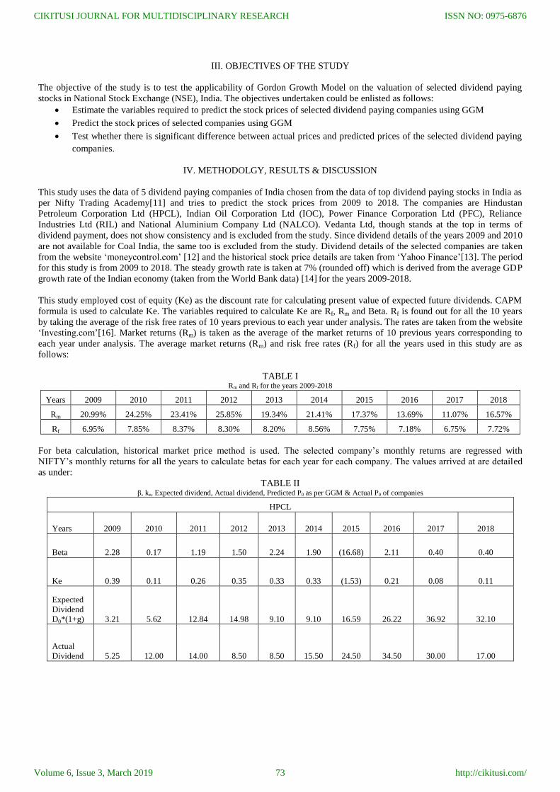
TABLE I Rm and Rf for the years 2009-2018

Years 2009 2010 2011 2012 2013 2014 2015 2016 2017 2018

Rm 20.99% 24.25% 23.41% 25.85% 19.34% 21.41% 17.37% 13.69% 11.07% 16.57%

Rf 6.95% 7.85% 8.37% 8.30% 8.20% 8.56% 7.75% 7.18% 6.75% 7.72%

For beta calculation, historical market price method is used. The selected company’s monthly returns are regressed with

NIFTY’s monthly returns for all the years to calculate betas for each year for each company. The values arrived at are detailed

as under:

TABLE II β, ke, Expected dividend, Actual dividend, Predicted P0 as per GGM & Actual P0 of companies

HPCL

Years 2009 2010 2011 2012 2013 2014 2015 2016 2017 2018

Beta 2.28 0.17 1.19 1.50 2.24 1.90 (16.68) 2.11 0.40 0.40

Ke 0.39 0.11 0.26 0.35 0.33 0.33 (1.53) 0.21 0.08 0.11

Expected

Dividend

D0*(1+g) 3.21 5.62 12.84 14.98 9.10 9.10 16.59 26.22 36.92 32.10

Actual

Dividend 5.25 12.00 14.00 8.50 8.50 15.50 24.50 34.50 30.00 17.00



ISSN NO: 0975-6876


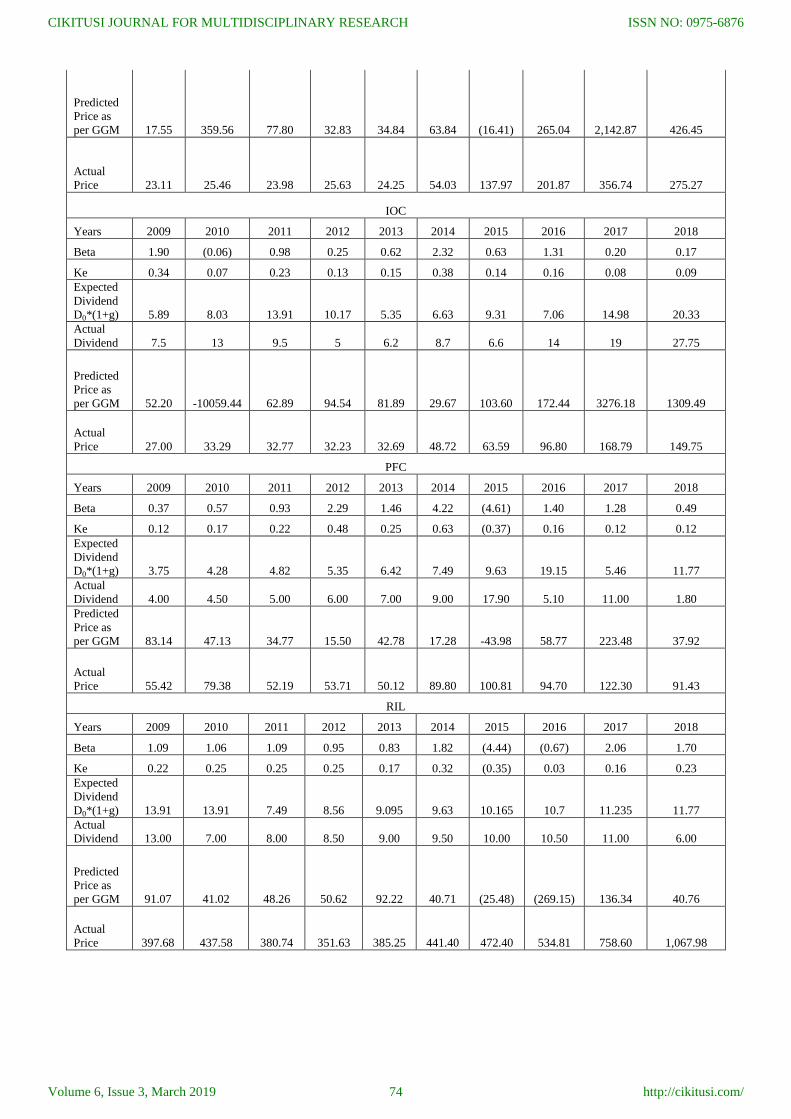
Predicted

Price as

per GGM 17.55 359.56 77.80 32.83 34.84 63.84 (16.41) 265.04 2,142.87 426.45

Actual

Price 23.11 25.46 23.98 25.63 24.25 54.03 137.97 201.87 356.74 275.27

IOC

Years 2009 2010 2011 2012 2013 2014 2015 2016 2017 2018

Beta 1.90 (0.06) 0.98 0.25 0.62 2.32 0.63 1.31 0.20 0.17

Ke 0.34 0.07 0.23 0.13 0.15 0.38 0.14 0.16 0.08 0.09

Expected

Dividend

D0*(1+g) 5.89 8.03 13.91 10.17 5.35 6.63 9.31 7.06 14.98 20.33

Actual

Dividend 7.5 13 9.5 5 6.2 8.7 6.6 14 19 27.75

Predicted

Price as

per GGM 52.20 -10059.44 62.89 94.54 81.89 29.67 103.60 172.44 3276.18 1309.49

Actual

Price 27.00 33.29 32.77 32.23 32.69 48.72 63.59 96.80 168.79 149.75

PFC

Years 2009 2010 2011 2012 2013 2014 2015 2016 2017 2018

Beta 0.37 0.57 0.93 2.29 1.46 4.22 (4.61) 1.40 1.28 0.49

Ke 0.12 0.17 0.22 0.48 0.25 0.63 (0.37) 0.16 0.12 0.12

Expected

Dividend

D0*(1+g) 3.75 4.28 4.82 5.35 6.42 7.49 9.63 19.15 5.46 11.77

Actual

Dividend 4.00 4.50 5.00 6.00 7.00 9.00 17.90 5.10 11.00 1.80

Predicted

Price as

per GGM 83.14 47.13 34.77 15.50 42.78 17.28 -43.98 58.77 223.48 37.92

Actual

Price 55.42 79.38 52.19 53.71 50.12 89.80 100.81 94.70 122.30 91.43

RIL

Years 2009 2010 2011 2012 2013 2014 2015 2016 2017 2018

Beta 1.09 1.06 1.09 0.95 0.83 1.82 (4.44) (0.67) 2.06 1.70

Ke 0.22 0.25 0.25 0.25 0.17 0.32 (0.35) 0.03 0.16 0.23

Expected

Dividend

D0*(1+g) 13.91 13.91 7.49 8.56 9.095 9.63 10.165 10.7 11.235 11.77

Actual

Dividend 13.00 7.00 8.00 8.50 9.00 9.50 10.00 10.50 11.00 6.00

Predicted

Price as

per GGM 91.07 41.02 48.26 50.62 92.22 40.71 (25.48) (269.15) 136.34 40.76

Actual

Price 397.68 437.58 380.74 351.63 385.25 441.40 472.40 534.81 758.60 1,067.98



ISSN NO: 0975-6876


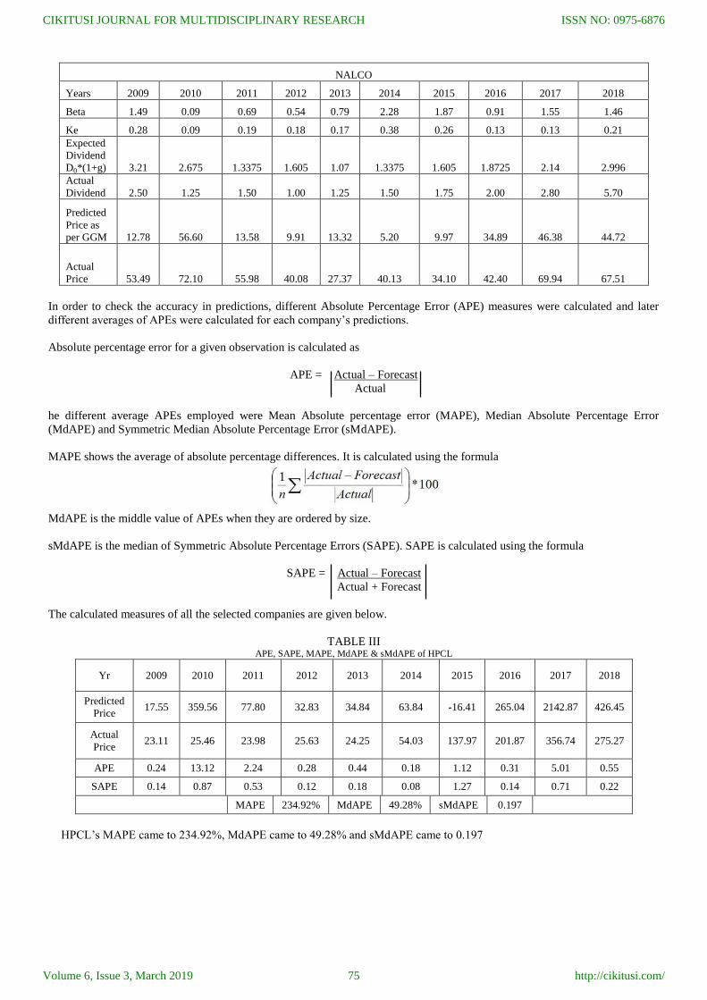
NALCO

Years 2009 2010 2011 2012 2013 2014 2015 2016 2017 2018

Beta 1.49 0.09 0.69 0.54 0.79 2.28 1.87 0.91 1.55 1.46

Ke 0.28 0.09 0.19 0.18 0.17 0.38 0.26 0.13 0.13 0.21

Expected

Dividend

D0*(1+g) 3.21 2.675 1.3375 1.605 1.07 1.3375 1.605 1.8725 2.14 2.996

Actual

Dividend 2.50 1.25 1.50 1.00 1.25 1.50 1.75 2.00 2.80 5.70

Predicted

Price as

per GGM 12.78 56.60 13.58 9.91 13.32 5.20 9.97 34.89 46.38 44.72

Actual

Price 53.49 72.10 55.98 40.08 27.37 40.13 34.10 42.40 69.94 67.51

In order to check the accuracy in predictions, different Absolute Percentage Error (APE) measures were calculated and later

different averages of APEs were calculated for each company’s predictions.

Absolute percentage error for a given observation is calculated as

APE = Actual – Forecast

Actual

he different average APEs employed were Mean Absolute percentage error (MAPE), Median Absolute Percentage Error

(MdAPE) and Symmetric Median Absolute Percentage Error (sMdAPE).

MAPE shows the average of absolute percentage differences. It is calculated using the formula

MdAPE is the middle value of APEs when they are ordered by size.

sMdAPE is the median of Symmetric Absolute Percentage Errors (SAPE). SAPE is calculated using the formula

SAPE = Actual – Forecast

Actual + Forecast

The calculated measures of all the selected companies are given below.

TABLE III APE, SAPE, MAPE, MdAPE & sMdAPE of HPCL

Yr 2009 2010 2011 2012 2013 2014 2015 2016 2017 2018

Predicted

Price 17.55 359.56 77.80 32.83 34.84 63.84 -16.41 265.04 2142.87 426.45

Actual

Price 23.11 25.46 23.98 25.63 24.25 54.03 137.97 201.87 356.74 275.27

APE 0.24 13.12 2.24 0.28 0.44 0.18 1.12 0.31 5.01 0.55

SAPE 0.14 0.87 0.53 0.12 0.18 0.08 1.27 0.14 0.71 0.22

MAPE 234.92% MdAPE 49.28% sMdAPE 0.197

HPCL’s MAPE came to 234.92%, MdAPE came to 49.28% and sMdAPE came to 0.197



ISSN NO: 0975-6876


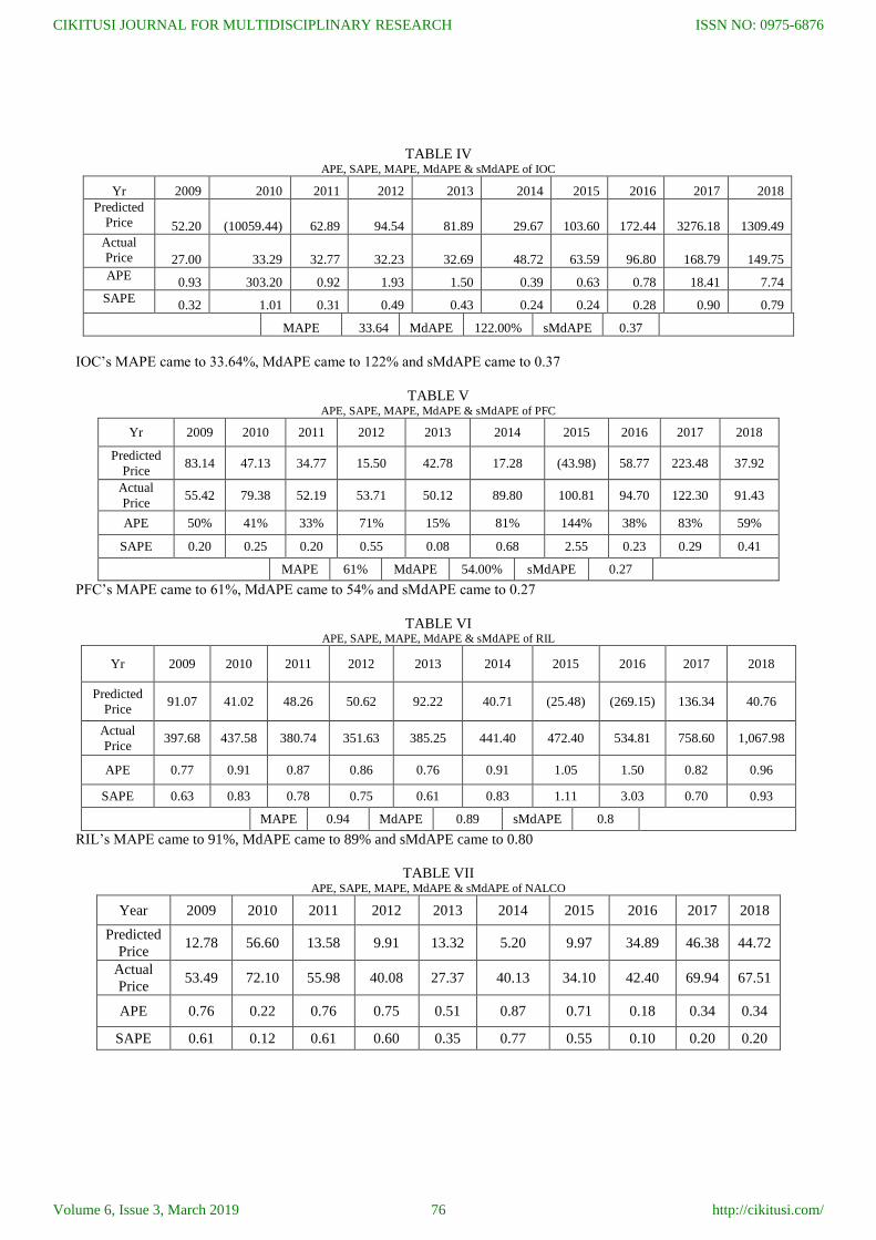
TABLE IV APE, SAPE, MAPE, MdAPE & sMdAPE of IOC

Yr 2009 2010 2011 2012 2013 2014 2015 2016 2017 2018

Predicted

Price 52.20 (10059.44) 62.89 94.54 81.89 29.67 103.60 172.44 3276.18 1309.49

Actual

Price 27.00 33.29 32.77 32.23 32.69 48.72 63.59 96.80 168.79 149.75

APE 0.93 303.20 0.92 1.93 1.50 0.39 0.63 0.78 18.41 7.74

SAPE 0.32 1.01 0.31 0.49 0.43 0.24 0.24 0.28 0.90 0.79

MAPE 33.64 MdAPE 122.00% sMdAPE 0.37

IOC’s MAPE came to 33.64%, MdAPE came to 122% and sMdAPE came to 0.37

TABLE V APE, SAPE, MAPE, MdAPE & sMdAPE of PFC

Yr 2009 2010 2011 2012 2013 2014 2015 2016 2017 2018

Predicted

Price 83.14 47.13 34.77 15.50 42.78 17.28 (43.98) 58.77 223.48 37.92

Actual

Price 55.42 79.38 52.19 53.71 50.12 89.80 100.81 94.70 122.30 91.43

APE 50% 41% 33% 71% 15% 81% 144% 38% 83% 59%

SAPE 0.20 0.25 0.20 0.55 0.08 0.68 2.55 0.23 0.29 0.41

MAPE 61% MdAPE 54.00% sMdAPE 0.27

PFC’s MAPE came to 61%, MdAPE came to 54% and sMdAPE came to 0.27

TABLE VI APE, SAPE, MAPE, MdAPE & sMdAPE of RIL

Yr 2009 2010 2011 2012 2013 2014 2015 2016 2017 2018

Predicted

Price 91.07 41.02 48.26 50.62 92.22 40.71 (25.48) (269.15) 136.34 40.76

Actual

Price 397.68 437.58 380.74 351.63 385.25 441.40 472.40 534.81 758.60 1,067.98

APE 0.77 0.91 0.87 0.86 0.76 0.91 1.05 1.50 0.82 0.96

SAPE 0.63 0.83 0.78 0.75 0.61 0.83 1.11 3.03 0.70 0.93

MAPE 0.94 MdAPE 0.89 sMdAPE 0.8

RIL’s MAPE came to 91%, MdAPE came to 89% and sMdAPE came to 0.80

TABLE VII APE, SAPE, MAPE, MdAPE & sMdAPE of NALCO

Year 2009 2010 2011 2012 2013 2014 2015 2016 2017 2018

Predicted

Price 12.78 56.60 13.58 9.91 13.32 5.20 9.97 34.89 46.38 44.72

Actual

Price 53.49 72.10 55.98 40.08 27.37 40.13 34.10 42.40 69.94 67.51

APE 0.76 0.22 0.76 0.75 0.51 0.87 0.71 0.18 0.34 0.34

SAPE 0.61 0.12 0.61 0.60 0.35 0.77 0.55 0.10 0.20 0.20



ISSN NO: 0975-6876


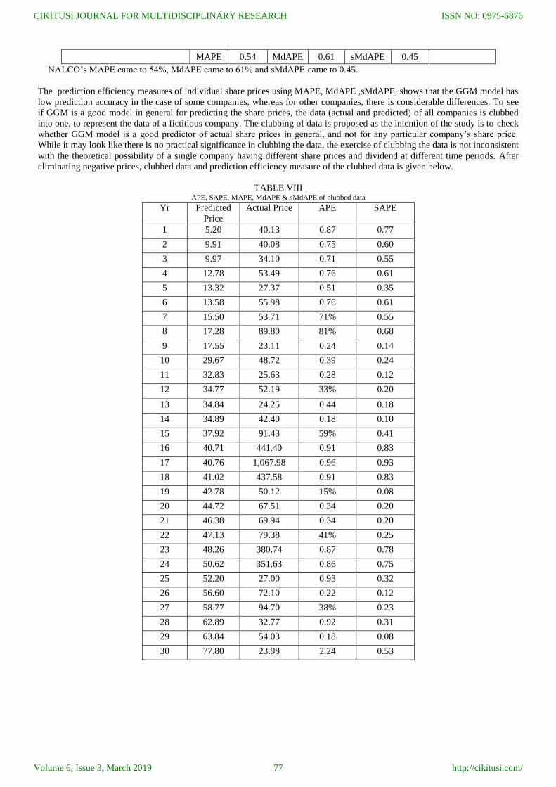
MAPE 0.54 MdAPE 0.61 sMdAPE 0.45

NALCO’s MAPE came to 54%, MdAPE came to 61% and sMdAPE came to 0.45.

The prediction efficiency measures of individual share prices using MAPE, MdAPE ,sMdAPE, shows that the GGM model has

low prediction accuracy in the case of some companies, whereas for other companies, there is considerable differences. To see

if GGM is a good model in general for predicting the share prices, the data (actual and predicted) of all companies is clubbed

into one, to represent the data of a fictitious company. The clubbing of data is proposed as the intention of the study is to check

whether GGM model is a good predictor of actual share prices in general, and not for any particular company’s share price.

While it may look like there is no practical significance in clubbing the data, the exercise of clubbing the data is not inconsistent

with the theoretical possibility of a single company having different share prices and dividend at different time periods. After

eliminating negative prices, clubbed data and prediction efficiency measure of the clubbed data is given below.

TABLE VIII APE, SAPE, MAPE, MdAPE & sMdAPE of clubbed data

Yr Predicted

Price

Actual Price APE SAPE

1 5.20 40.13 0.87 0.77

2 9.91 40.08 0.75 0.60

3 9.97 34.10 0.71 0.55

4 12.78 53.49 0.76 0.61

5 13.32 27.37 0.51 0.35

6 13.58 55.98 0.76 0.61

7 15.50 53.71 71% 0.55

8 17.28 89.80 81% 0.68

9 17.55 23.11 0.24 0.14

10 29.67 48.72 0.39 0.24

11 32.83 25.63 0.28 0.12

12 34.77 52.19 33% 0.20

13 34.84 24.25 0.44 0.18

14 34.89 42.40 0.18 0.10

15 37.92 91.43 59% 0.41

16 40.71 441.40 0.91 0.83

17 40.76 1,067.98 0.96 0.93

18 41.02 437.58 0.91 0.83

19 42.78 50.12 15% 0.08

20 44.72 67.51 0.34 0.20

21 46.38 69.94 0.34 0.20

22 47.13 79.38 41% 0.25

23 48.26 380.74 0.87 0.78

24 50.62 351.63 0.86 0.75

25 52.20 27.00 0.93 0.32

26 56.60 72.10 0.22 0.12

27 58.77 94.70 38% 0.23

28 62.89 32.77 0.92 0.31

29 63.84 54.03 0.18 0.08

30 77.80 23.98 2.24 0.53



ISSN NO: 0975-6876


31 81.89 32.69 1.50 0.43

32 83.14 55.42 50% 0.20

33 91.07 397.68 0.77 0.63

34 92.22 385.25 0.76 0.61

35 94.54 32.23 1.93 0.49

36 103.60 63.59 0.63 0.24

37 136.34 758.60 0.82 0.70

38 172.44 96.80 0.78 0.28

39 223.48 122.30 83% 0.29

40 265.04 201.87 0.31 0.14

41 359.56 25.46 13.12 0.87

42 426.45 275.27 0.55 0.22

43 1309.49 149.75 7.74 0.79

44 2142.87 356.74 5.01 0.71

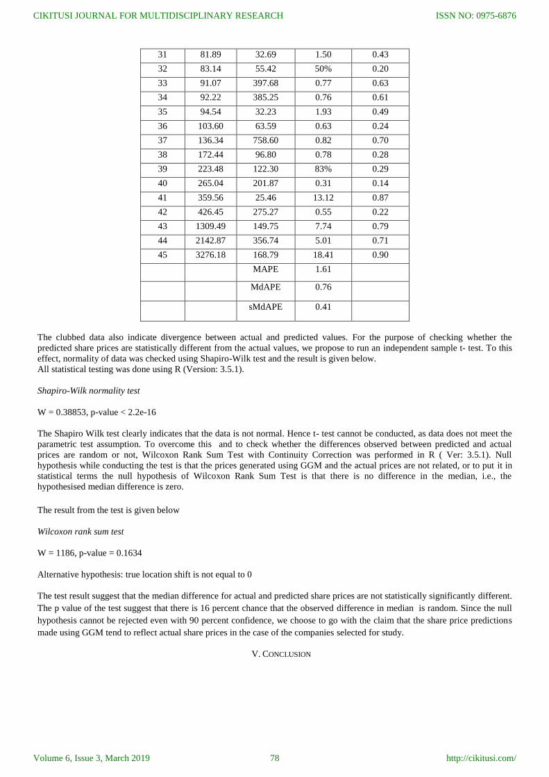
45 3276.18 168.79 18.41 0.90

MAPE 1.61

MdAPE 0.76

sMdAPE 0.41

The clubbed data also indicate divergence between actual and predicted values. For the purpose of checking whether the

predicted share prices are statistically different from the actual values, we propose to run an independent sample t- test. To this

effect, normality of data was checked using Shapiro-Wilk test and the result is given below.

All statistical testing was done using R (Version: 3.5.1).

Shapiro-Wilk normality test

W = 0.38853, p-value < 2.2e-16

The Shapiro Wilk test clearly indicates that the data is not normal. Hence t- test cannot be conducted, as data does not meet the

parametric test assumption. To overcome this and to check whether the differences observed between predicted and actual

prices are random or not, Wilcoxon Rank Sum Test with Continuity Correction was performed in R ( Ver: 3.5.1). Null

hypothesis while conducting the test is that the prices generated using GGM and the actual prices are not related, or to put it in

statistical terms the null hypothesis of Wilcoxon Rank Sum Test is that there is no difference in the median, i.e., the

hypothesised median difference is zero.

The result from the test is given below

Wilcoxon rank sum test

W = 1186, p-value = 0.1634

Alternative hypothesis: true location shift is not equal to 0

The test result suggest that the median difference for actual and predicted share prices are not statistically significantly different.

The p value of the test suggest that there is 16 percent chance that the observed difference in median is random. Since the null

hypothesis cannot be rejected even with 90 percent confidence, we choose to go with the claim that the share price predictions

made using GGM tend to reflect actual share prices in the case of the companies selected for study.

V. CONCLUSION



ISSN NO: 0975-6876


The test result from the present study lend support to GGM as a method of estimating stock prices . While there are many

factors that have an impact on share price, expected dividend and their present value is certainly a logical factor that can

influence the prices. The study has focused only on the five highest dividend paying companies for a ten year period. Choice of

different companies or same companies but different time periods could possibly give different results. For future studies the

researchers wish to expand the current list of companies and time period in future research to check whether GGM predictions

are statistically consistent.

REFERENCES

[1] Chandra, P. "Equity Valuation." In Investment Analysis and Portfolio Management, 5th ed., 13.4 to 13.16. Chennai, India: McGraw Hill Education (India)

Private Limited, 2017. [2] Damodaran, A. "Estimating Risk Parameters." n.d. http://people.stern.nyu.edu/adamodar/pdfiles/papers/beta.pdf.

[3] Chandra, P. "Relative Valuation." In Corporate Valuation and Value Creation, 3rd ed. New Delhi, India: McGraw-Hill Education (India) Private Limited,

2011. [4] Corelli, A. "Dividend-Based Valuation." Inside Company Valuation, 2017, 15-27. doi:10.1007/978-3-319-53783-2_2.

[5] Mwangi, W. M. "Testing the Gordon’s growth model." Research Journal of Finance and Accounting 8, no. 14 (2017).

[6] Ana, M., and P. Saša. "Towards and effective financial management: Relevance of Dividend Discount Model in stock price valuation." Economic Analysis 48 (2015), 39-53. http://ebooks.ien.bg.ac.rs/335/1/2015_1-23.pdf.

[7] Gacus, R. B., and J. E. Hinlo. "The Reliability of Constant Growth Dividend Discount Model (DDM) in Valuation of Philippine Common Stocks."

International Journal of Economics & Management Sciences 07, no. 01 (2018). doi:10.4172/2162-6359.1000487. [8] Acheampong, P., and E. Agalega. "Examining the dividend growth model for stock valuation: Evidence from selected stock on the Ghana stock

exchange." Research Journal of Finance and Accounting 4, no. 8 (2013).

[9] Charumathi, B., and E. S. Suraj. "The reliability of dividend discount model in valuation of bank stocks at the Bombay Stock exchange." International Journal of Research in Commerce & Management 5, no. 3 (2014), 39-44. http://ijrcm.org.in/article_info.php?article_id=4350.

[10] Chen, J. "Multistage Dividend Discount Model." Last modified April 21, 2018. https://www.investopedia.com/terms/m/multistageddm.asp.

[11] Nifty Trading Academy (www.niftytradingacademy.com). "Highest Dividend Paying Stocks in India - Best & Top Stocks List by NTA??" Last modified December 7, 2018. https://www.niftytradingacademy.com/best-dividend-paying-stocks-in-india/.

[12] "Stock/Share Market Investment, Live BSE/NSE Sensex & Nifty, Mutual Funds, Commodity Market, Finance Portfolio Investment/Management,

Startup news India, Financial News - Moneycontrol." Accessed February 18, 2019. http://moneycontrol.com. [13] "Yahoo Finance - Business finance, stock market, quotes, news." Accessed February 18, 2019. https://in.finance.yahoo.com/.

[14] "GDP growth (annual %) | Data." Accessed February 19, 2019.

https://data.worldbank.org/indicator/NY.GDP.MKTP.KD.ZG?end=2017&locations=IN&start=2009&year_high_desc=false. [15] "GDP of India: growth rate until 2022 | Statista." Accessed February 19, 2019. https://www.statista.com/statistics/263617/gross-domestic-product-gdp-

growth-rate-in-india/.

[16] "India 10-Year Bond Historical Data - Investing.com India." Accessed February 19, 2019. https://in.investing.com/rates-bonds/india-10-year-bond-yield-historical-data.

[17] Chen, J. "Dividend Discount Model - DDM." Last modified November 21, 2003. https://www.investopedia.com/terms/d/ddm.asp.

[18] "Calculating stock beta using Excel." Video file. July 14, 2012. https://www.youtube.com/watch?v=zlClflcSrM8. [19] Cornell, B. "Using Dividend Discount Models to Estimate Expected Returns." The Journal of Investing 24, no. 1 (2015), 48-51.

doi:10.3905/joi.2015.24.1.048.

[20] Damodaran, A. pages.stern.nyu.edu/~adamodar/pdfiles/valn2ed. [21] "Dividend Growth Rate - Definition, How to Calculate, Example." n.d. https://corporatefinanceinstitute.com/resources/knowledge/finance/dividend-

growth-rate/.

[22] Lemke, T. "For blue-chip firms, use this straightforward way to price a stock." Last modified July 23, 2018. https://www.thebalance.com/how-to-use-the-dividend-discount-model-to-value-a-stock-4172616.

[23] "Nifty Annual Returns – Historical Analysis (Updated 2019-2020)." Last modified January 6, 2018. https://stableinvestor.com/2018/01/nifty-annual-

yearly-returns-historical.html. [24] "Welcome to Forecast Pro - Software for sales forecasting, inventory planning, demand planning, S&OP and collaborative planning." n.d.

https://www.forecastpro.com/Trends/forecasting101August2011.html.

[25] "MdAPE - Median Absolute Percentage Error." Accessed February 24, 2019. http://www.spiderfinancial.com/support/documentation/numxl/reference-manual/forecasting-performance/mdape.



ISSN NO: 0975-6876


Dividend Discount Model (DDM) : A study based on select ...

Documents

Transcript of Dividend Discount Model (DDM) : A study based on select ...