CECW-EH-Y

EngineerManual

1110-2-1415

Department of the ArmyU.S. Army Corps of Engineers

Washington, DC 20314-1000

EM 1110-2-1415

5 March 1993

Engineering and Design

HYDROLOGIC FREQUENCY ANALYSIS

Distribution Restriction StatementApproved for public release; distribution is unlimited.

DEPARTMENT OF THE ARMY U.S. Army Corps of Engineers Washington. D.C. 20314-1000

CECW-EH- 1’

Engineer Manual No. IllO-Z-1415

EM 1110-2-1415

5 March 1993

Engineering and Design HYDROLOGIC FREQUENCY ANALYSIS

1. m. This manual provides guidance and procedures for frequency analysis of: flood flows, low flows, precipitation. water surface elevation, and flood damage.

9 . . -. Appk&&& This manual applies to major subordinate commands, districts. and laboratories having responsibility for the design of civil works projects.

3. u. Frequency estimates of hydrologic. climatic and economic data are required for the planning, design and evaluation of flood control and navigation projects. The text illustrates many of the statistical techniques appropriate for hydrologic problems by example. The basic theory is usually not provided, but references are provided for those who wish to research the techniques in more detail.

FOR THE COMMANDER:

WILLIAM D. BROk’N Colonel, Corps of Engineers Chief of Staff

DEPARTMENT OF THE ARMY U.S. Army Corps of Engineers Washington, D.C. 20314-1000

CECW-EH-Y

Engineer Manual No. 1110-2-1415

Engineering and Design HYDROLOGIC FREQUENCY ANALYSIS

Table of Contents

Subject Paragraph Page

CHAPTER

CHAPTER

CHAPTER

CHAPTER

1 INTRODUCTION Purpose and Scope .................... References .......................... Definitions .......................... Need for Hydrologic Frequency Estimates ... Need for Professional Judgement .........

2 FREQUENCY ANALYSIS Definition ........................... Duration Curves ...................... Selection of Data for Frequency Analysis ... Graphical Frequency Analysis ............ Analytical Frequency Analysis ...........

3 FLOOD FREQUENCY ANALYSIS Introduction ......................... Log-Pearson Type III Distribution ........ Weighted Skew Coefficient .............. Expected Probability ................... Risk .............................. Conditional Probability Adjustment ....... Two-Station Comparison ................ Flood Volumes ....................... Effects of Flood Control Works on

Flood Frequencies .................... Effects of Urbanization ................

4 LOW-FLOW FREQUENCY ANALYSIS Uses .............................. Interpretation ........................ Application Problems ..................

EM 1110-2-1415

5 March 1993

l-l 1-2 l-3 1-4 1-5

I-1 I-1 1-l 1-l l-2

2-1 2-l 2-2 2-3 2-3 2-6 2-4 2-10 2-5 2-12

3-l 3-l 3-2 3-l 3-3 3-6 3-4 3-7 3-5 3-10 3-6 3-11 3-7 3-13 3-8 3-18

3-9 3-22 3-10 3-28

4-l 4-l 4-2 4-1 4-3 4-l

i

EM 1110-2-1415 5 Mar 93

Subject Paragraph Page

CHAPTER 5

CHAPTER 6

PRECIPITATION FREQUENCY ANALYSlS General Procedures . . . . . . . . . . . . . . . . . . . . Available Regional Information . . . . . . . . . . Derivation of Flood-Frequency Relations

from Precipitation . . . . . . . . . . . . . . . . . . .

STAGE(ELEVATION)-FREQUENCY ANALYSIS Uses . . . . . . . . . . . . . . . . . . . . . . . . . . . . . . Stage Data . . . . . . . . . . . . . . . . . . . . . . . . . . . Frequency Distribution . . . . . . . . . . . . . . . . . Expected Probability . . . . . . . . . . . . . . . . . . .

CHAPTER 7 DAMAGE-FREQUENCY RELATIONSHIPS Introduction . . . . . . . . . . . . . . . . . . . . . . . . . Computation of Expected Annual Damage . . Equivalent Annual Damage . . . . . . . . . . . . . .

CHAPTER 8 STATISTICAL RELIABILITY CRITERIA Objective . . . . . . . . . . . . . . . . . . . . . . . . . . . Reliability of Frequency Statistics . . . . . . . . . Reliability of Frequency Curves . . . . . . . . . .

5-I 5-l 5-2 5-2

5-3 5-2

6-l 6-1 6-2 6-l 6-3 6-2 6-4 6-2

7-l 7-1 7-2 7-l 7-3 7-3

8-1 8-l 8-2 8-l 8-3 8-1

CHAPTER 9 REGRESSION ANALYSIS AND APPLICATION TO REGIONAL

CHAPTER 10

CHAPTER 11

STUDIES Nature and Application ................. Calculation of Regression Equations ....... The CorrelationCoefficient and Standard Error ........

Simple L’ink’Regression Example .......................

Factors Responsible of Nondetermination ... Multiple Linear Regression Example ....... Partial Correlation ..................... Verification of Regression Results ........ Regression by Graphical Techniques ....... Practical Guidelines ................... Regional Frequency Analysis ............

ANALYSIS OF MIXED POPULATIONS Definition ........................... Procedure ........................... Cautions ............................

FREQUENCY OF COINCIDENT FLOWS Introduction . . . . . . . . . . . . . . . . . . . . . . . . . A Procedure for Coincident Frequency Analysis

9-l 9-2

9-3 9-3 9-4 9-4 9-5 9-7 9-6 9-8 9-7 9-8 9-8 9-10 9-9 9-10 9-10 9-10 9-11 9-11

10-l 10-2 10-3

11-l 11-2

9-l 9-l

10-l 10-l 10-2

11-l 11-l

ii

Subject

CHAPTER I2

APPENDIX A

APPENDIX B

APPENDIX C

APPENDIX D

APPENDIX E

APPENDIX F

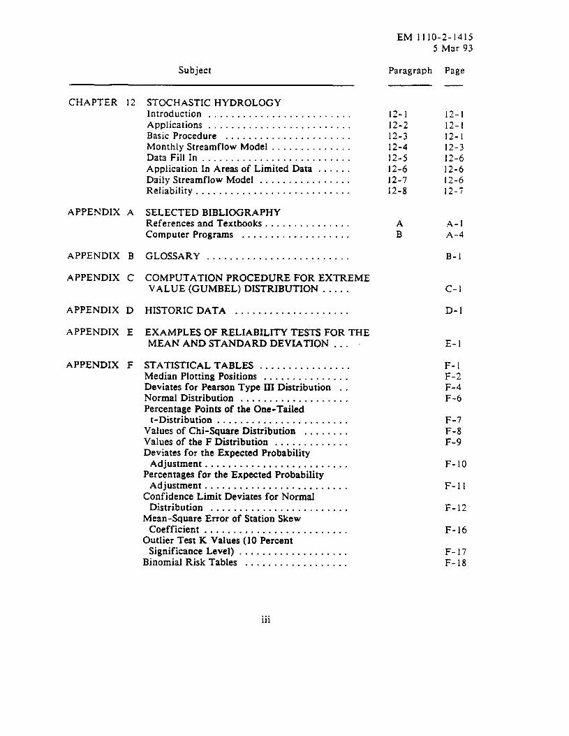
STOCHASTIC HYDROLOGY Introduction ......................... Applications ......................... Basic Procedure ...................... Monthly Streamflow Model .............. Data Fill In .......................... Application In Areas of Limited Data ...... Daily Streamflow Model ................ Reliability ...........................

SELECTED BIBLIOGRAPHY References and Textbooks ............... Computer Programs ...................

GLOSSARY .........................

COMPUTATION PROCEDURE FOR EXTREME VALUE (GUMBEL) DISTRIBUTION .....

HISTORIC DATA ....................

EXAMPLES OF RELIABILITY TESTS FOR THE MEAN AND STANDARD DEVIATION ...

STATISTICAL TABLES ................ Median Plotting Positions ............... Deviates for Pearson Type III Distribution . . Normal Distribution ................... Percentage Points of the One-Tailed

t-Distribution ....................... Values of Chi-Square Distribution ........ Values of the F Distribution ............. Deviates for the Expected Probability

Adjustment ......................... Percentages for the Expected Probability

Adjustment ......................... Confidence Limit Deviates for Normal

Distribution ........................ Mean-Square Error of Station Skew

Coefficient ......................... Outlier Test K Values (10 Percent

Significance Level) ................... Binomial Risk Tables ..................

EM 1110-2-1415 5 Mar 93

Paragraph Page

12-l 12-l 12-2 12-l 12-3 12-I 12-4 12-3 12-5 12-6 12-6 12-6 12-7 12-6 12-8 12-7

A A-l B A-4

B-l

C-l

D-l

E-l

F-l F-2 F-4 F-6

F-7 F-8 F-9

F-10

F-11

F-12

F-16

F-17 F-18

. . . 111

EM 1110-2-1415 5 Mar 93

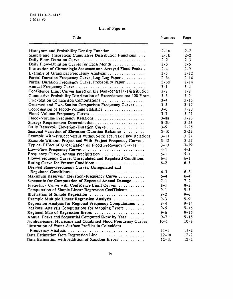
List of Figures

Title

Histogram and Probability Density Function .............. Sample and Theoretical Cumulative Distribution Functions ... Daily Flow-Duration Curve ........................... Daily Flow-Duration Curves for Each Month .............. Illustration of Chronologic Sequence and Arrayed Flood Peaks . Example of Graphical Frequency Analysis ................ Partial Duration Frequency Curve, Log-Log Paper .......... Partial Duration Frequency Curve, Probability Paper ........ Annual Frequency Curve ............................. Confidence Limit Curves based on the Non-central t-Distribution Cumulative Probability Distribution of Exceedances per 100 Years Two-Station Comparison Computations .................. Observed and Two-Station Comparison Frequency Curves .... Coordination of Flood-Volume Statistics ................. Flood-Volume Frequency Curves ....................... Flood-Volume Frequency Relations ..................... Storage Requirement Determination ..................... Daily Reservoir Elevation-Duration Curve ................ Seasonal Variation of Elevation-Duration Relations ......... Example With-Project versus Without-Project Peak Flow Relations Example Without-Project and With-Project Frequency Curves . Typical Effect of Urbanization on Flood Frequency Curves ... Low-Flow Frequency Curves .......................... Frequency Curve, Annual Precipitation .................. Flow-Frequency Curve, Unregulated and Regulated Conditions Rating Curve for Present Conditions .................... Derived Stage-Frequency Curves, Unregulated and

Regulated Conditions ............................... Maximum Reservoir Elevation-Frequency Curve ........... Schematic for Computation of Expected Annual Damage ..... Frequency Curve with Confidence Limit Curves ........... Computation of Simple Linear Regression Coefficients ...... Illustration of Simple Regression ....................... Example Multiple Linear Regression Analysis ............. Regression Analysis for Regional Frequency Computations ... Regional Analysis Computations for Mapping Errors ........ Regional Map of Regression Errors ..................... Annual Peaks and Sequential Computed Skew by Year ....... Nonhurricane, Hurricane and Combined Flood Frequency Curves Illustration of Water-Surface Profiles in Coincident

Frequency Analysis ................................ Data Estimation from Regression Line ................... Data Estimation with Addition of Random Errors ..........

Number Page

2-la 2-2 2-lb 2-2 2-2 2-3 2-3 2-5 2-4 2-9 2-5 2-12 2-6a 2-14 2-6b 2- 14 3-l 3-4 3-2 3-8 3-3 3-9 3-4 3-16 3-5 3-17 3-6 3-20 3-7 3-21 3-8a 3-23 3-8b 3-23 3-9 3-25 3-10 3-25 3-11 3-27 3-12 3-27 3-13 3-29 4-l 4-3 5-1 5-l 6-1 6-1 6-2 6-3

6-3 6-3 6-4 6-4 7-l 7-2 8-l 8-2 9-l 9-5 9-2 9-6 9-3 9-9 9-4 9-14 9-5 9-15 9-6 9-15 9-7 9-18 10-I 10-3

11-l 11-2 12-la 12-2 l2-lb 12-2

iv

EM 1110-2-1415 5 Mar 93

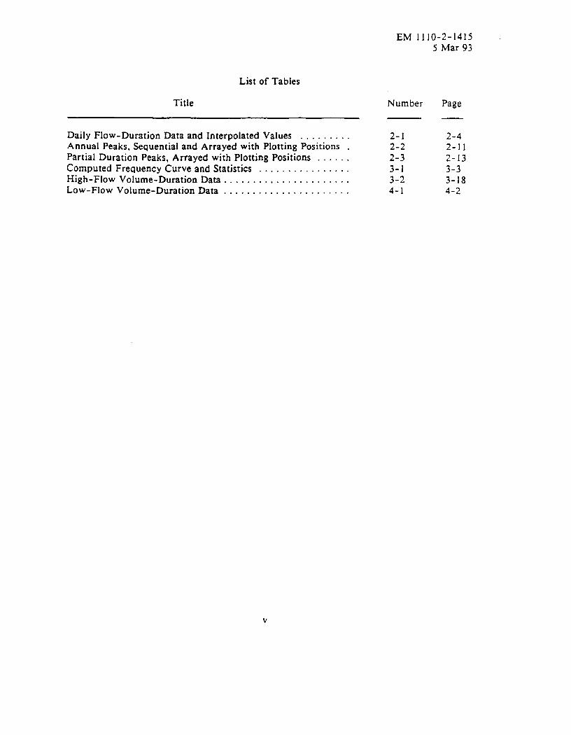
List of Tables

Title Number Page

Daily Flow-Duration Data and Interpolated Values ......... 2-1 2-4 Annual Peaks, Sequential and Arrayed with Plotting Positions . 2-2 2-11 Partial Duration Peaks, Arrayed with Plotting Positions ...... 2-3 2-13 Computed Frequency Curve and Statistics ................ 3-l 3-3 High-Flow Volume-Duration Data ...................... 3-2 3-18 Low-Flow Volume-Duration Data ...................... 4-l 4-2

V

EM 1110-2-1415 5 Mar 93

ENGINEERING AND DESIGN HYDROLOGIC FREQUENCY ANALYSIS

CHAPTER 1

INTRODUCTION

I- 1. Purpose and SCOD~. This manual provides guidance in applying statistical principles to the analysis of hydrologic data for Corps of Engineers Civil Works activities. The text illustrates, by example, many of the statistical techniques appropriate for hydrologic problems. The basic theory is usually not provided, but references are provided for those who wish to research the techniques in more detail.

l-2. References. The techniques described herein are taken principally from “Guidelines for Determining Flood Flow Frequency” (46)‘, “Statistical Methods in Hydrology” (l), and “Hydrologic Frequency Analysis” (41). References cited in the text and a selected bibliography of literature pertaining to frequency analysis techniques are contained in Appendix A.

l-3. Definitions. Appendix B contains a list of definitions of terms common to hydrologic frequency analysis and symbols used in this manual.

l-4. Need for Hvdrolonic Freauencv Estimates.

a. ADDlications. Frequency estimates of hydrologic, climatic and economic data are required for the planning, design and evaluation of water management plans. These plans may consist of combinations of structural measures such as reservoirs, levees, channels, pumping plants, hydroelectric power plants, etc., and nonstructural measures such as flood proofing, zoning, insurance programs, water use priorities, etc. The data to be analyzed could be streamflows, precipitation amounts, sediment loads, river stages, lake stages, storm surge levels, flood damage, water demands, etc. The probability estimates from these data are used in evaluating the economic, social and environmental effects of the proposed management action.

b. Objective. The objective of frequency analysis in a hydrologic context is to infer the probability that various size events will be exceeded or not exceeded from a given sample of recorded events. Two basic problems exist for most hydrologic applications. First the sample is usually small, by statistical standards, resulting in uncertainty as to the true probability. And secondly, a single theoretical frequency distribution does not always fit a particular data-type equally well in all applications. This manual provides guidance in fitting frequency distributions and construction of confidence limits. Techniques are presented which can possibly reduce the errors caused by small sample sizes. Also, some types of data are noted which usually do not fit any theoretical distributions.

c. General Guidance. Frequency analysis should not be done without consideration of the primary application of the results. The application will have a bearing on the type of analysis (annual series or partial duration series), number of stations to be included,

’ Numbered references refer to Appendix A, Selected Bibliography.

l-l

EM 11 IO-2 1415 5 Mar 93

whether regulated frequency curves will be needed, etc. A frequency study should be well coordinated with the hydrologist, the planner and the economist.

l-5. Need for Professional Judnment. It is not possible to define a set of procedures that can be rigidly applied to each frequency determination. There may be applications where more complex joint or conditional frequency methods, that were considered beyond the scope of this guidance, will be required. Statistical analyses alone will not resolve all frequency problems. The user of these techniques must insure proper application and interpretation has been made. The judgment of a professional experienced in hydrologic analysis should always be used in concert with these techniques.

l-2

EM 1110-2-1415 5 Mar 93

CHAPTER 2

FREQUENCY ANALYSIS

2- 1. Definition.

a. Freaue cy (to enable infer&es?%

of the statistical techniques that are applied to hydrologic data made about particular attributes of the data) can be labeled

with the term “frequency analysis” techniques. The term “frequency” usually connotes a count (number) of events of a certain magnitude. To have a perspective of the importance of the count, the total number of events (sample size) must also be known. Sometimes the number of events within a specified time is used to give meaning to the count, e.g., two daily flows were this low in 43 years. The probability of a certain magnitude event recurring again in the future, if the variable describing the events is continuous, (as are most hydrologic variables), is near zero. Therefore, it is necessary to establish class intervals (arbitrary subdivisions of the range) and define the frequency as the number of events that occur within a class interval. A pictorial display of the frequencies within each class interval is called a histogram (also known as a frequency polygon).

b. Relative Freauency . Another means of representing the frequency is to compute the relative frequency. The relative frequency is simply the number of events in the class interval divided by the total number of events:

f. 1

= ni/N (2-l)

where:

f i = relative frequency of events in class interval i

ni = number of events in interval i

N - total number of events

A graph of the relative frequency values is called a frequency distribution or histogram, Figure 2-la. As the number of observations approaches infinity and the class interval size approaches zero, the enveloping line of the frequency distribution will approach a smooth curve. This curve is termed the probability density function (Figure 2-la).

c w In hydrologic studies, the probability of some magnitude being’exceeded (or no: exceeded) is usually the primary interest. Presentation of the data in this form is accomplished by accumulating the probability (area) under the probability density function. This curve is termed the cumulative distribution function. In most statistical texts, the area is accumulated from the smallest event to the largest. The accumulated area then represents non-exceedance probability or percentage (Figure 2- 1 b). It is more common in hydrologic studies to accumulate the area from the largest event to the smallest. Area accumulated in this manner represents exceedance probability or percentage.

2-l

EM 1110-2 1415 5 Mar 93

J I p; ia

1

0

Potomac Riror at Point of Rocka, MD

” ‘. : ”

:.

4 1.. 1.. 1.a 8.6 0

Logarithm of Annual Peakm

Figure 2- la. Histogram and Probability Density Function.

Potonmc River 8t Point of Rock, MD

5 2 b b = a B e a

0.4 . 0.8 . . 0 1

1 ..4 4.. *.a 6.8 0

Logarithm of Annud Peaka

Figure 2- I b. Sample and Theoretical Cumulative Distribution Functions.

2-2

EM 1110-2-1415 5 Mar 93

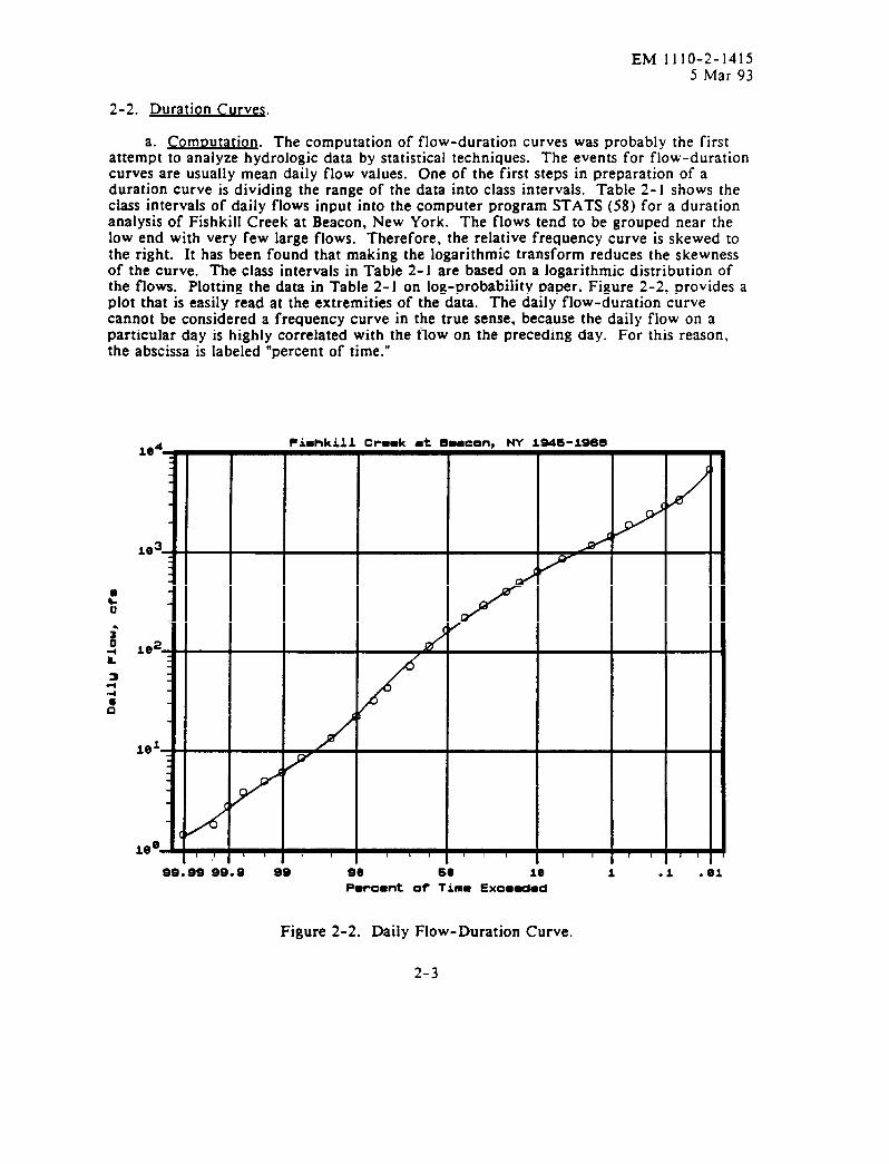
2-2. Duration Curves.

a. Comoutation. The computation of flow-duration curves was probably the first attempt to analyze hydrologic data by statistical techniques. The events for flow-duration curves are usually mean daily flow values. One of the first steps in preparation of a duration curve is dividing the range of the data into class intervals. Table 2-l shows the class intervals of daily flows input into the computer program STATS (58) for a duration analysis of Fishkill Creek at Beacon, New York. The flows tend to be grouped near the low end with very few large flows. Therefore, the relative frequency curve is skewed to the right. It has been found that making the logarithmic transform reduces the skewness of the curve. The class intervals in Table 2-1 are based on a logarithmic distribution of the flows. Plotting the data in Table 2-1 on log-probability paper, Figure 2-2, provides a plot that is easily read at the extremities of the data. The daily flow-duration curve cannot be considered a frequency curve in the true sense, because the daily flow on a particular day is highly correlated with the flow on the preceding day. For this reason, the abscissa is labeled “percent of time.”

99.99 99.8 99 se 68 10 1 .l .e1 Percent of Time Excmmdrd

Figure 2-2. Daily Flow-Duration Curve.

2-3

EM 1110-2 1415 5 Mar 93

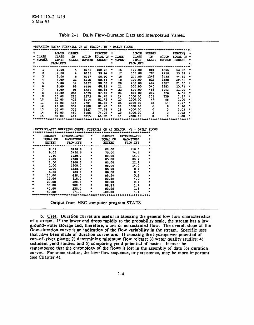
Table 2-1. Daily Flow-Duration Data and Interpolated Values.

-DURATION DATA- FISHKILL CR AT BEACON, NY - DAILY FLOWS *.*.**.....*..***.******....*..*...**...*.**.**..**..******.***..*.**.*********.***.*** l

Lmm NUMBER PERCENT l LOWER Numm PERCENT l

l CLAPS

Es ACCLM EQUAL OR l cuss

c&s NumER MCEED CLASS IN ACCUM EOUAL OR l

l NUtBER l NUHBER LMIT CLASS NIJWER EXCEED + . FLCW.CFS l

FLW,CFS l

.------------------------------------------*------------------------------------------*

. 1 1.00 5 6766 100.00 l 16 100.00 668 5606 63.95 l

. 2 2.00 4 6761 99.94 l 17 150.00 763 4710 53.62 l

l 3 3.00 6757 SQ.90 l 16 200.00 1246 3935 44.09 l

. 4 4.00 228 6749 99.61 l 19 300.00 622 2669 30.68 l

l 5 5.00 37 6727 99.56 l 20 400.00 464 1667 21.30 l

l 6 6.00 66 6690 99.13 l 21 500.00 350 1363 15.76 l

l 7 8.00 95 6624 96.36 l 22 600.00 465 1043 11.90 l

l 8 10.00 25b 6529 97.30 l 23 600.00 239 570 6.59 l

l

. 1: 15.00 261 6275 94.40 l 24 1000.00 251 339 3.67 l

20.00 423 6014 91.42 l 25 1500.00 47 66 1.00 l

l 11 30.00 405 7591 86.60 l 26 2000.00 32 41 0.47 l

l 12 40.00 359 7166 61.96 l 27 3000.00 6 9 0.10 l

. 13 50.00 332 6027 77.06 l 20 4000.00 0 3 0.03 l

l 14 60.00 480 6495 74.09 l 29 6000.00 3 3 0.03 l

l 15 80.00 409 6015 66.62 l 30 7000.00 0 0 0.00 l

. . ..**.***************....***..*******.*****...****************************************

-INTERPOLATED DURATION CURVE- FISBKILL CR AT BEACON, NY - DAILY FLOWS ***.**.*.*********.************.****.*.*****.*********.*****.**** l PmcENT INTmwoLtrED l 1NTmLATED l

l EQUAL OR MAGNITUDE l MAGNITUDE l

l mKEED FLCW,CFS l EXCEED FLOW.CFS l

*-------------------------------*-------------------------------*

l 0.01 6970.0 l 60.00 118.0 l

l 0.05 3b60.0 l 70.00 74.5 l

l 0.10 3020.0 l 60.00 54.7 l

l 0.20 2530.0 l 65.00 33.4 l

l 0.50 1960.0 l 90.00 22.7 l

l 1.00 1500.0 l 95.00 14.0 l

l 2.00 1230.0 l 98.00 0.8 l

* 5.00 903.0 l 99.00 6.3 l

t 10.00 656.0 l 99.50 5.2 l

l 15.00 516.0 l 99.60 4.0 l

* 20.00 420.0 l 99.90 2.9 l

l 30.00 306.0 l 99.95 1.9 l

l 40.00 230.0 l 99.99 1.5 l

* 50.00 171.0 l 100.00 1.1 l

*********.********~****.**.*.******.********************.*******

Output from HEC computer program STATS.

b. u. Duration curves are useful in assessing the general low flow characteristics of a stream. If the lower end drops rapidly to the probability scale, the stream has a low ground-water storage and, therefore, a low or no sustained flow. The overall slope of the flow-duration curve is an indication of the flow variability in the stream. Specific uses that have been made of duration curves are: 1) assessing the hydropower potential of run-of-river plants; 2) determining minimum flow release; 3) water quality studies; 4) sediment yield studies; and 5) comparing yield potential of basins. It must be remembered that the chronology of the flows is lost in the assembly of data for duration curves. For some studies, the low-flow sequence, or persistence, may be more important (see Chapter 4).

2-4

EM 1110-2-1415 5 Mar 93

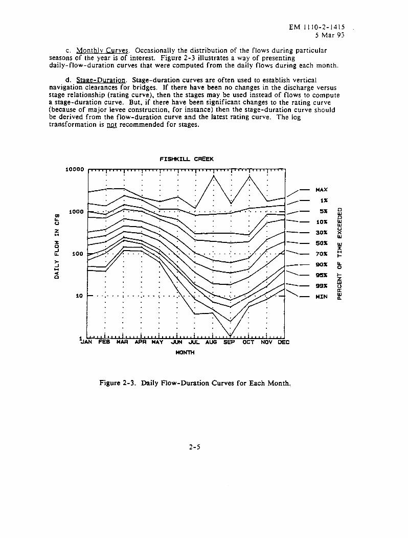
c. Monthlv Curves. Occasionally the distribution of the flows during particular seasons of the year is of interest. Figure 2-3 illustrates a way of presenting daily-flow-duration curves that were computed from the daily flows during each month.

d. Stage-Duration. Stage-duration curves are often used to establish vertical navigation clearances for bridges. If there have been no changes in the discharge versus stage relationship (rating curve), then the stages may be used instead of flows to compute a stage-duration curve. But, if there have been significant changes to the rating curve (because of major levee construction, for instance) then the stage-duration curve should be derived from the flow-duration curve and the latest rating curve. The log transformation is m recommended for stages.

FISHKIU CREEK

10000

1000 E E

8 ii 100

5 c( d

10

9 L ‘JAN FEB MAR APR MAY JUN JUL AUG SEP OCT NOV OEC

MONTH

MAX

IX

5%

10%

30%

50%

70%

90%

95%

99%

MIN

Figure 2-3. Daily Flow-Duration Curves for Each Month.

2-5

EM JIlO-2-1415 5 Mar 93

e. Future Probabilities. A duration curve is usually based on a fairly large sample size. For instance, Figure 2-2 is based on 8766 daily values (Table 2-l). Even though the observed data can be used to make inferences about future probabilities, conclusions drawn from information at the extremities can be misleading. The data indicate there is a zero percent chance of exceeding 6970 cfs, however, it is known that there is a finite probability of experiencing a larger flow. And similarly, there is some chance of experiencing a lower flow than the recorded 1 .I cfs. Therefore, some other means is needed for computing the probabilities of infrequent future events. Section 2-4 describes the procedure for assigning probabilities to independent events.

2-3. Selection of Data for Freauencv Analysis.

a. S le i n 5s. The primary question to be asked before selection of data for a frequency study is: how will the frequency estimates be used? If the frequency curve is to be used for estimating damage that is related to the peak flow in a stream, maximum peak flows should be selected from the record. If the damage is best related to a longer duration of flow, the mean flow for several days’ duration may be appropriate. For example, a reservoir’s behavior may be related to the 3-day or IO-day rain flood volume or to the seasonal snowmelt volume. Occasionally, it is necessary to select a related variable in lieu of the one desired. For example, where mean-daily flow records are more complete than the records of peak flows, it may be more desirable to derive a frequency curve of mean-daily flows and then, from the computed curve, derive a peak-flow curve by means of an empirical relation between mean daily flows and peak flows. All reasonably independent values should be selected, but only the annual maximum events should be selected when the application of analytical procedures discussed in Chapter 3 is contemplated.

b. Uniformity of Data.

(1) Bm. Data selected for a frequency study must measure the same aspect of each event (such as peak flow, mean-daily flow, or flood volume for a specified duration), and each event must result from a uniform set of hydrologic and operational factors. For example, it would be improper to combine items from old records that are reported as peak flows but are in fact only daily readings, with newer records where the instantaneous peak was actually measured. Similarly, care should be exercised when there has been significant change in upstream storage regulation during the period of record to avoid combining unlike events into a single series. In such a case, the entire record should be adjusted to a uniform condition (see Sections 2-3f and 3-9). Data should always be screened for errors. Errors have been noted in published reports of annual flood peaks. And, errors have been found in the computer files of annual flood peaks. The transfer of data to either paper or a computer file always increases the probability that errors have been accidentally introduced.

(2) ms. Hydrologic factors and relationships during a general winter rain flood are usually quite different from those during a spring snowmelt flood or during a local summer cloudburst flood, Where two or more types of floods are distinct and do not occur predominately in mutual combinations, they should not be combined into a single series for frequency analysis. It is usually more reliable in such cases to segregate the data in accordance with type and to combine only the final curves, if necessary. In the Sierra Nevada region of California and Nevada, frequency studies are made separately for rain floods which occur principally during the months of November through March,

2-6

EM 1110-2-1415 5 Mar 93

and for snowmelt floods, which occur during the months of April through July. Flows for each of these two seasons are segregated strictly by cause - those predominantly caused by snowmelt and those predominantly caused by rain. In desert regions, summer thunderstorms should be excluded from frequency studies of winter rain flood or spring snowmelt floods and should be considered separately. Along the Atlantic and Gulf Coasts, it is often desirable to segregate hurricane floods from nonhurricane events. Chapter 10 describes how to combine the separate frequency curves into one relation.

c. Location Differences. Where data recorded at two different locations are to be combined for construction of a single frequency curve, the data should be adjusted as necessary to a single location, usually the location of the longer record. The differences in drainage area, precipitation and, where appropriate, channel characteristics between the two locations must be taken into account. When the stream-gage location is different from the project location, the frequency curve can be constructed for the stream-gage location and subsequently adjusted to the project location.

d. Estimating Missing Even& Occasionally a runoff record may be interrupted by a period of one or more years. If the interruption is caused by destruction of the gaging station by a large flood, failure to fill in the record for that flood would result in a biased data set and should be avoided. However, if the cause of the interruption is known to be independent of flow magnitude, the record should be treated as a broken record as discussed in Section 3-2b. In cases where no runoff records are available on the stream concerned, it is usually best to estimate the frequency curve as a whole using regional generalizations, discussed in Chapter 9, instead of attempting to estimate a complete series of individual events. Where a longer or more complete record at a nearby station exists, it can be used to extend the effective length of record at a location by adjusting frequency statistics (Section 3-7) or estimating missing events through correlation (Chapter 12).

e. Climatic Cycles. Some hydrologic records suggest regular cyclic variations in precipitation and runoff potential, and many attempts have been made to demonstrate that precipitation or streamflows evidence variations that are in phase with various cycles, particularly the well established I l-year sunspot cycle. There is no doubt that long-duration cycles or irregular climatic changes are associated with general changes of land masses and seas and with local changes in lakes and swamps. Also, large areas that have been known to be fertile in the past are now arid deserts, and large temperate regions have been covered with glaciers one or more times. Although the existence of climatic changes is not questioned, their effect is ordinarily neglected, because the long-term climatic changes have generally insignificant effect during the period concerned in water development projections, and short-term climatic changes tend to be self-compensating. For these reasons, and because of the difficulty in differentiating between stochastic (random) and systematic changes, the effect of natural cycles or trends during the analysis period is usually neglected in hydrologic frequency studies.

f. Eff f ect R lationg.

(I) Hydrologic frequency estimates are often used for some purpose relating to planning, design or operation of water resources control measures (structural and nonstructural). The anticipated effects of these measures in changing the rate and volume of flow is assessed by comparing the without project frequency curve with the corresponding with project frequency curve. Also, projects that have existed in the past have affected the rates and volumes of flows, and the recorded values must be adjusted to reflect uniform conditions in order that the frequency analysis will conform to the basic

2-7

EM 1110-2-1415 5 Mar 93

assumption of homogeneity. In order to meet the assumptions associated with analytical frequency analysis techniques, the flows must be essentially unregulated by manmade storage or diversion structures. Consequently, wherever practicable, recorded runoff values should be adjusted to natural (unimpaired) conditions before an analytical frequency analysis is made. In cases where the impairment results from a multitude of relatively small improvements that have not changed appreciably during the period of record, it is possible that analytical frequency analysis techniques can be applied. The adjustment to natural conditions may be unnecessary and. because of the amount of work involved, not cost effective.

(2) One approach to determining a frequency curve of regulated or modified runoff consists of routing all of the observed flood events under conditions of proposed or anticipated development. Then a relationship is developed between the modified and the natural flows, deriving an average or dependable relationship. A frequency curve of modified flows is derived from this relationship and the frequency curve of natural flows. In order to determine frequencies of runoff for extreme floods, routings of multiples of the largest floods of record or multiples of a large hypothetical flood can be used. Techniques of estimating project effects are outlined in Chapter 3-09d.

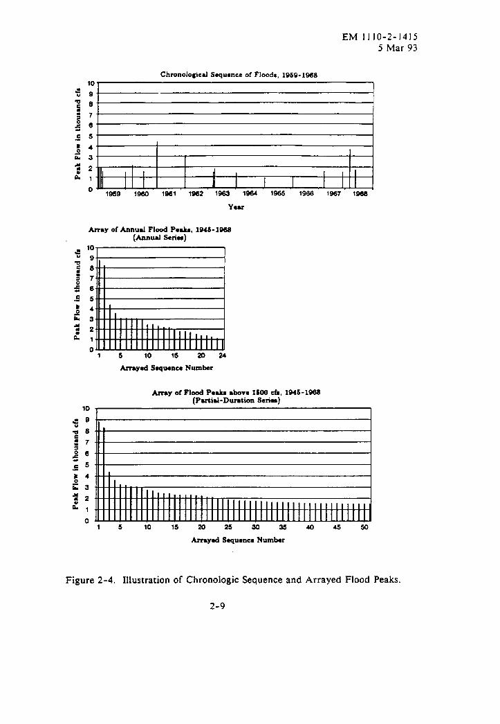
An ual Se ‘es Versus Partial Du at ion Seria There are two basic types of frequtncy c:rves uf:ed to estimate flood rdamage. A curve of annual maximum events is ordinarily used when the primary interest lies in the larger events or when the second largest event in any year is of little concern in the analysis. The partial-duration curve represents the frequency of all independent events of interest, regardless of whether two or more occurred in the same year. This type of curve is sometimes used in economic analysis, where there is considerable damage associated with the second largest and third largest floods that occurred in some of the years. Caution must be exercised in selecting events because they must be both hydrologically and economically independent. The selected series type should be established early in the study in coordination with the planner and/or economist. The time interval between flood events must be sufficient for recovery from the earlier flood. Otherwise damage from the later flood would not be as large as computed. When both the frequency curve of annual floods and the partial-duration curve are used, care must be exercised to assure that the two are consistent. A graphic demonstration of the relation between a chronologic record, an annual-event curve and a partial-duration curve is shown on Figure 2-4.

h. Presentation of Data and Results of Freauencv AnalvsiS. When frequency curves are presented for technical review, adequate information should be included to permit an independent review of the data, assumptions and analysis procedures. The text should indicate clearly the scope of the studies and include a brief description of the procedure used, including appropriate references. A summary of the basic data consisting of a chronological tabulation of values used and indicating sources of data and any adjustments should be included. The frequency data should also be presented in graphical form, ordinarily on probability paper, along with the adopted frequency curves. Confidence limit curves should also be included for analytically-derived frequency curves to illustrate the relative value of the frequency relationships. A map of the gage locations and tables of the adopted statistics should also be included.

2-8

EM 1110-2-1415 5 Mar 93

Chronological Sequence of Floods, 1959-1868

d ”

9

I”

9 8

7

6

5

4

3

2

1

0 1959 IQ60 IQ61 lQ62 1963 1964 1966 1966 1967 1966

Amy of Annual Flood Peakr, lQ46-1968 (Annual Seriee)

10) I 9 8

7

6

5

4 4

3 3

2 2

1 1

0 0 1 1 5 5 10 10 15 15 20 24 20 24

10

a Q ;a 5 7 ; e 6

85 84

%3 a t 2 Ll

0

Arrayed Sequence Number

Amy of Flood Pe&e dove IIXJO da. 1945-1968 (Partial-Duration Serb)

1 5 10 15 20 25 30 35 40 45 60

Amyed Sequence Number

Figure 2-4. Illustration of Chronologic Sequence and Arrayed Flood Peaks.

2-9

EM 1110-2-1415 5 Mar 93

2-4. Graohical Freauencv Analvsis.

a. Advantaaes and Limitations. Every set of frequency data should be plotted graphically, even though the frequency curves are obtained analytically. It is important to visually compare the observed data with the derived curve. The graphical method of frequency-curve determination can be used for any type of frequency study, but analytical methods ha\+: certain advantages when they are applicable. The principal advantages of graphical methods are that they are generally applicable, that the derived curve can be easily visualized, and that the observed data can be readily compared with the computed results. However, graphical methods of frequency analysis are generally less consistent than analytical methods as different individuals would draw different curves. Also, graphical procedures do not provide means for evaluating the reiiability of the estimates. Comparison of the adopted curve with plotted points is not an index of reliability, but it is often erroneously assumed to be, thus implying a much greater reliability than is actually attained. For these reasons, graphical methods should be limited to those data types where analytical methods are known not to be generally applicable. That is, where frequency curves are too irregular to compute analytically, for example, stream or reservoir stages and regulated flows. Graphical procedures should always be to visually check the analytical computations.

b. Selection and Arraneement of Peak Flow Data. General principles in the selection of frequency data are discussed in Section 2-3. Data used in the construction of frequency curves of peak flow consist of the maximum instantaneous flow for each year of record (for annual-event curve) or all of the independent events that exceed a selected base value (for partial-duration curve). This base value must be smaller than any flood flow that is of importance in the analysis, and should also be low enough so that the total number of floods in excess of the base equals or exceeds the number of years of record. Table 2-2 is a tabulation of the annual peak flow data with dates of occurrence, the data arrayed in the order of magnitude, and the corresponding plotting positions.

C. Plot&-&&&. Median plotting positions are tabulated in Table F- 1. In ordinary hydrologic frequency work, N is taken as the number of years of record rather than the number of events, so that percent chance exceedance can be thought of as the number of events per hundred years. For arrays larger than 100. the plotting position, P,, of the largest event is obtained by use of the following equation:

P, = 100 (1 - (.5)1/N) (2-2a)

The plotting position for the smallest event (P P )

and all the other plotting positions are is the complement (1 -P,) of this value,

interpo ated linearly between these two. The median plotting positions can be approximated by

P, - lOO(m -.3)/(N +.4) (2-2b)

where m is the order number of the event.

For partial-duration curves, particularly where there are more events than years (N), plotting positions that indicate more than one event per year can also be obtained using

2-10

EM 1110-2-1415 5 Mar 93

Table 2-2. Annual Peaks, Sequential and Arrayed with Plotting Positions.

-PLOTTING POSITIONS-FISEKILL CREEK AT BEACON, N.Y. **.............................................................. . . . . . FnNTS ANN.YZED......*...........ORDERED EVENTS..........* . . WATER I-EEDIAU l

l tBN DAY YEAR FLCU,CFS l RANK YEAR FLoW,CFS PLOT WS l

t--------------------------.-----------------------------------*

l 3 5 1945 l 12 27 1945 . 3 15 1947 . 3 16 1946 l 1 1 1949 l 3 8 1950 l 4 1 1951 . 3 12 1952 . 1 25 1953 . 9 13 1954 4 8 20 1955 l 10 16 1955 . 4 10 1957 l 12 21 1957 . 2 11 1959 l 4 6 1960 . 2 26 1961 . 3 13 1962 . 3 28 1963 . 1 26 1964 l 2 9 1965 . 2 15 1966 . 3 30 1967 . 3 19 1966

2290. l

1470. l

2220. l

2970. l

3020. l

1210. l

2490. l

3170. l

3220. l

1760. l

8800. l

8280. l

1310. l

2500. l

1960. l

2140. l

4340. l

3060. + 1700. l

1380. l

980. l

1040. l

1560. l

3630. l

1 1955 8800. 2.87 l

2 1956 6260. 6.97 l

3 1961 4340. 11.07 l

4 1968 3630. 15.16 l

5 1953 3220. 19.26 l

6 1952 3170. 23.36 * 7 1962 3060. 27.46 l

8 1949 3020. 31.56 l

9 1948 2970. 35.66 l

10 1956 2500. 39.75 l

11 1951 2490. 43.85 l

12 1945 2290. 47.95 l

13 1947 2220. 52.05 l

14 1960 2140. 56.15 * 15 1959 1960. 60.25 l

16 1963 1760. 64.34 l

17 1954 1760. 66.44 l

16 1967 1580. 72.54 l

19 1946 1470. 76.64 l

20 1964 1380. 00.74 l

9: 1957 1310. 64.84 l

1950 1210. 88.93 l

23 1966 1040. 93.03 l

24 1965 980. 97.13 l

. . . . . . . . ..*.........*..*........................................

Output from HEC computer program HECWRC.

Equation 2-2b. This is simply an approximate method used in the absence of knowledge of the total number of events in the complete set of which the partial-duration data constitute a subset.

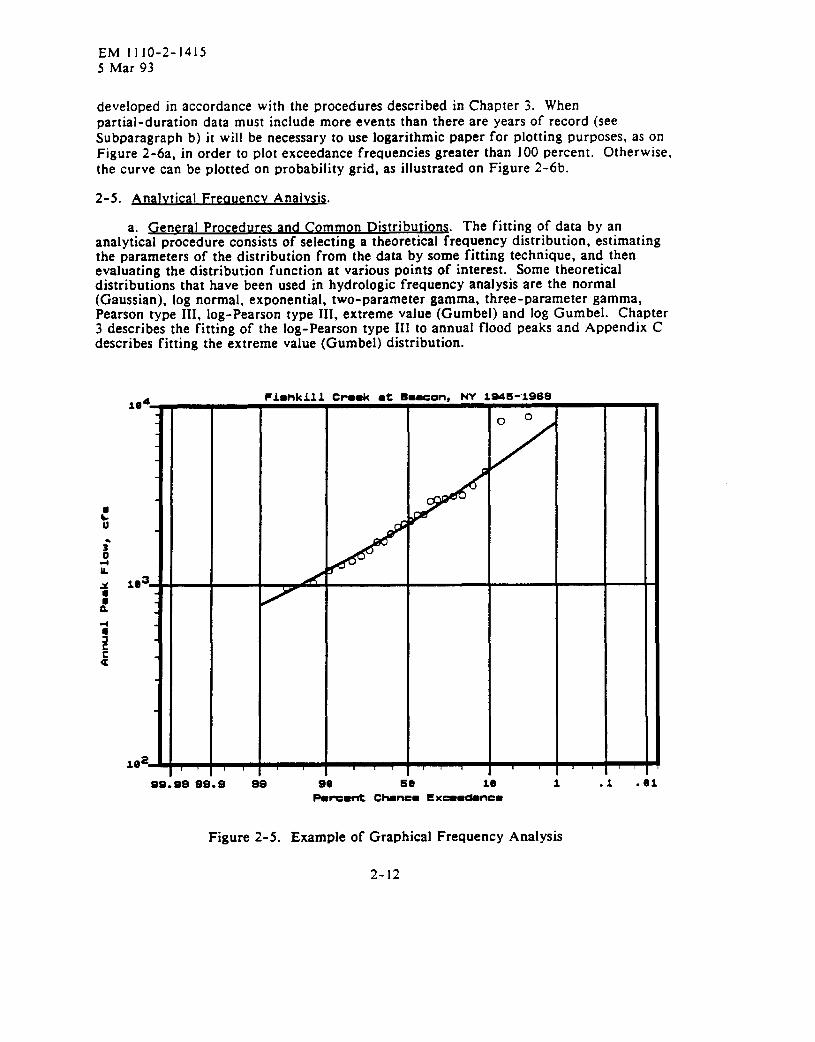
d. Plottintz Grids. The plotting grid recommended for annual flood flow events is the logarithmic normal grid developed by Allen Hazen (ref 13) and designed such that a logarithmic normal frequency distribution will be represented by a straight line, Figure 2-5. The plotting grid used for stage frequencies is often the arithmetic normal grid. The plotting grids may contain a horizontal scale of exceedance probability, exceedance frequency, or percent chance exceedance. Percent chance exceedance (or nonexceedance) is the recommended terminology.

e. ExamDIe Plottim! of Annual-Event Freauencv Curve. Figure 2-5 shows the plotting of a frequency curve of the annual peak flows tabulated in Table 2-2. A smooth curve should be drawn through the plotted points. Unless computed by analytical frequency procedures, the frequency curve should be drawn as close to a straight line as possible on the chosen probability graph paper. The data plotted on Figure 2-5 shows a tendency to curve upward, therefore, a slightly curved line was drawn as a best fit line.

f. Exam le Plo tin s The partial-duration curve corresponding to the partial-duration data in Table 2-3 is shown of Figure 2-6a. This curve has been drawn through the plotted points, except that it was made to conform with the annual-event curve in the upper portion of the curve. The annual-event curve was

2-11

EM 1110-2-1415 5 Mar 93

developed in accordance with the procedures described in Chapter 3. When partial-duration data must include more events than there are years of record (see Subparagraph b) it will be necessary to use logarithmic paper for plotting purposes, as on Figure 2-6a, in order to plot exceedance frequencies greater than 100 percent. Otherwise, the curve can be plotted on probability grid, as illustrated on Figure 2-6b.

2-5. Analvtical Freauencv Analvsis.

a. General Procedures and Common Distributions. The fitting of data by an analytical procedure consists of selecting a theoretical frequency distribution, estimating the parameters of the distribution from the data by some fitting technique, and then evaluating the distribution function at various points of interest. Some theoretical distributions that have been used in hydrologic frequency analysis are the normal (Gaussian), log normal, exponential, two-parameter gamma, three-parameter gamma, Pearson type III, log-Pearson type III, extreme value (Gumbel) and log Gumbel. Chapter 3 describes the fitting of the log-Pearson type III to annual flood peaks and Appendix C describes fitting the extreme value (Gumbei) distribution.

f 4 B 4 IL % 10 3.

d 4 : E a

10?

ss;ss 9s

Cimhkill

I I

0 E

I I

I

3-e.k l t I

I , I

I

meon, NY 46-‘1966

10 1 .l .81 Pehmnt Chnom Exwrdmncr

Figure 2-5. Example of Graphical Frequency Analysis

2-12

EM 1110-2-1415 5 Mar 93

Table 2-3. Partial Duration Peaks, Arrayed with Plotting Positions.

FISEKILL CREEK AT BEACON. . . . . . . . . . . . . . . . . . . . . . . . . . . . . . . . . . . . . . . . . . . . . . . . . . ORDERED EnNTS..........' . WATER MEDIAN l

. NANKYEAN FLcw.cFs PLOT PCS l

g-----------------------------------g

.

.

.

.

.

.

.

.

.

.

.

.

.

.

.

.

.

.

.

.

.

.

.

.

.

.

1 2 3

: 6 7 8 9 10 11 12 13 14 15 16 17 18 19 20 21 22 23 24 25

1955 8800. 1956 8280. 1961 4340. 1968 3630. 1953 3220. 1952 3170. 1962 3060. 1949 3020. 1946 2970. 1948 2750. 1949 2700. 1958 2500. 1951 2490. 1952 2460. 1945 2290. 1953 2290. 1958 2290. 1953 2280. 1948 2220. 1951 2210. 1960 2140. 1953 2080. 1959 1960. 1959 1920. 1958 1900.

2.07 l

6.97 l

11.07 l

15.16 l

19.26 l

23.36 l

27.46 l

31.56 l

35.66 l

39.75 l

43.85 l

47.95 l

52.05 l

56.15 l

60.25 l

64.34 l

'66.44 l

72.54 l

76.64 l

80.74 l

04.04 l

88.93 l

93.03 * 97.13 * 101.23 l

.

. . . . . . . . . . . . . . . . . . . . . . . . . . . . . . . . . . . . .

NY -- PEAK.5 ABOVE 1500 CFS . . . . . . . . . . . . . . . . . . . . . . . . . . . . . . . . . . . . . . . . . . . . . . . . . ORDERED EVENTS.........." . WATER KEDIAN * . NANKYEAN FLoW,CFS PLOT WS l

g-----------------------------------*

.

.

.

.

.

.

.

.

.

.

.

.

.

.

.

.

.

.

.

.

.

.

.

.

.

.

26 27 20 29 30 31 32 33 34 35 36 37 39 39 40 41 42 43 44 45 46 47 40 49 50 51

1952 1820. 105.33 1945 1780. 109.43 1963 1760. 113.52 1956 1770. 117.62 1954 1760. 121.72 1952 1730. 125.62 1968 1720. 129.92 1955 1660. 134.02 1958 1650. 136.11 1958 1650. 142.21 1953 1630. 146.31 1960 1610. 150.41 1956 1600. 154.51 1956 1590. 158.61 1956 1580. 162.70 1967 1580. 166.60 1951 1560. 170.90 1959 1560. 175.00 1955 1550. 179.10 1951 1540. 183.20 1968 1530. 167.30 1960 1520. 191.39 1956 1520. 195.49 1952 1520. 199.59 1948 1510. 203.69

l

l

l

l

.

.

.

.

.

l

.

.

l

.

l

l

*

.

l

l

.

.

.

.

.

. 1963 1510. 207.79 . . . . . . . . . ..**.......*................

b. AdvantageS. Determining the frequency distribution of data by the use of analytical techniques has several advantages. The use of an established procedure for fitting a selected distribution would result in consistent frequency estimates from the same data set by different persons. Error distributions have been developed for some of the theoretical distributions that enable computing the degree of reliability of the frequency estimates (see Chapter 8). Another advantage is that it is possible to regionalize the parameter estimates which allows making frequency estimates at ungaged locations (see Chapter 9).

c. Disadvantaees. The theoretical fitting of some data can result in very poor frequency estimates. For example, stage-frequency curves of annual maximum stages are shaped by the channel and valley characteristics, backwater conditions, etc. Another example is the flow-frequency curve below a reservoir. The shape of this frequency curve would depend not only on the inflow but the capacities, operation criteria, etc. Therefore, graphical techniques must be used where analytical techniques provide poor frequency estimates.

2-13

EM 1110-2-1415 5 Mar 93

I

.

i 1r* M L

::

h

mr of 2HOtm pwr lwnerrd YW'rrt-9

Figure 2-6a. Partial Duration Frequency Curve, Log-Log Paper

99.99 99.9 9s SO 60 18 1 .1 . .l mr of 2Wrlt.~ pn lalneme Y9m-9

Figure 2-6b. Partial Duration Frequency Curve, Probability Paper.

2-14

EM 1110-2-1415 5 Mar 93

CHAPTER 3

FLOOD FREQUENCY ANALYSIS

3-I. Introduction.

The procedures that federal agencies are to follow when computing a frequency curve of annual flood peaks have been published in Guidelines for Determining Flood Flow Frequency, Bulletin 17B (46). As stated in Bulletin 17B, “Flood events . . . do not fit any one specific known statistical distribution.” Therefore, it must be recognized that occasionally, the recommended techniques may not provide a reasonable fit to the data. When it is necessary to use a procedure that departs from Bulletin 17B, the procedure should be fundamentally sound and the steps of the procedure documented in the report along with the frequency curves.

This report contains most aspects of Bulletin 17B, but in an abbreviated form. Various aspects of the procedures are described in an attempt to clarify the computational steps. The intent herein is to provide guidance for use with Bulletin 17B. The step by step procedures to compute a flood peak frequency curve are contained in Appendix 12 of Bulletin 17B and are not repeated herein.

3-2. Lon-Pearson TVDe 111 Distribution.

a. General. The analytical frequency procedure recommended for annual maximum streamflows is the logarithmic Pearson type III distribution. This distribution requires three parameters for complete mathematical specification. The parameters are: the mean, or first moment, (estimated by the sample mean, X); the variance, or second moment, (estimated by the sample variance, S*); the skew, or third moment, (estimated by the sample skew, G). Since the distribution is a logarithmic distribution, all parameters are estimated from logarithms of the observations, rather than from the observations themselves. The Pearson type III distribution is particularly useful for hydrologic investigations because the third parameter, the skew, permits the fitting of non-normal samples to the distribution. When the skew is zero the log-Pearson type III distribution becomes a two-parameter distribution that is identical to the logarithmic normal (often called log-normal) distribution.

b. Fitting the Distribution.

(1) The log-Pearson type III distribution is fitted to a data set by calculating the sample mean, variance, and skew from the following equations:

P Z7- N

(3-l)

2 1x2 1 (xx)* S z-c

N-l N-l (3-2a)

3-l

EM 1110-2-1415 5 Mar 93

1 X2 - (1 X)*/N 0

N-l

WC x3) G=

N(C (X-y)3) 5

(N- I)(N-2)S3 (N- l)(N-2)S3

N*(c X3) - 3N(l X)(1 X2) + 2(cX)3 m

N(N- l)(N-2)S3

(3-2b)

(3-3a)

(3-3b)

in which:

ST = mean logarithm

X = logarithm of the magnitude of the annual event

N = number of events in the data set

S2 - unbiased estimate of the variance of logarithms

X = X-z, the deviation of the logarithm of a’ single event from the mean logarithm

G= unbiased estimate of the skew coefficient of logarithms

The precision of the computed values is more sensitive to the number of significant digits when Equations 3-2b and 3-3b are used.

(2) In terms of the frequency curve itself, the mean represents the general magnitude or average ordinate of the curve, the square root of the variance (the standard deviation, S) represents the slope of the curve, and the skew represents the degree of curvature. Computation of the unadjusted frequency curve is accomplished by computing values for the logarithms of the streamflow corresponding to selected values of percent chance exceedance. A reasonable set of values and the results are shown in Table 3- 1. The number of values needed to define the curve depends on the degree of curvature (i.e., the skew). For a skew value of zero, only two points would be needed, while for larger skew values all of the values in the table would ordinarily be needed.

(3) The logarithms of the event magnitudes corresponding to each of the selected percent chance exceedance values are computed by the following equation:

IogQ = ?t+KS (3-4)

where ‘jT and S are defined as in Equations 3-1 and 3-2 and where

3-2

EM 1110-2-1415 5 Mar 93

log Q = logarithm of the flow (or other variable) corresponding to a specified value of percent chance exceedance

K = Pearson type III deviate that is a function of the percent chance exceedance and the skew coefficient.

c. ExamDie Computation.

(I) As shown iL the following example, Equation 3-4 is solved by using the computed values of X and S and obtaining from Appendix V-3 the value of K corresponding to the adopted skew, G, andthe selected percent chance exceedance (P). An example computation for P=l.O, where X, S and G are taken from Table 3-1, is:

log Q = 3.3684 + 2.8236 (.2456)

= 4.0619

Q - 11500 cfs

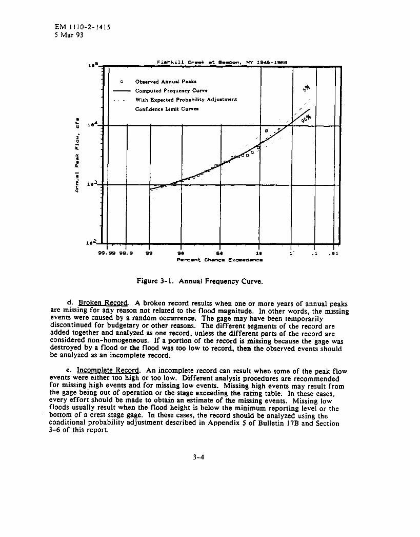
(2) It has been shown (36) that a frequency curve computed in this manner is biased in relation to average future expectation because of uncertainty as to the true mean and standard deviation. The effect of this bias for the normal distribution can be eliminated by an adjustment termed the expected D- adiustment that accounts for the actual sample size. This adjustment is discussed in more detail in Section 3-4. Table 3-l and Figure 3-l shows the derived frequency curve along with the expected probability adjusted curves and the 5 and 95 percent confidence limit curves.

2 TI - isti

-FRXQUENCY CURVE- 01-3735 FISEKILL CREEK AT BEACON, NEW YORK . . . ..**.....***....**.*...***.*..**..*.****.*.........*....**... . . . . . . . ..FLW.CPB........* PERCEET l . ..CONFIDENCE LIMITS....* .

nPEcTED l CEANCE l .

l CCMWTED PROBABILITY l EKEEDANCE * 0.05 LIMIT 0.95 LIMIT * .------------------------.------------.------------------------. . 19200. 28300. l 0.2 l 39100. 12300. * . 14500. 19000. l 0.5 l 26900. 9740. l

. 11500. 14100. * 1.0 l 20100. 8080. l

. 9110. 10500. l 2.0 l 14800. 6640. l

. 7100. 7820. l 4.0 l 10800. 5380. l

. 4960. 5210. l 10.0 l 6850. 3950. l

. 3650. 3740. l 20.0 l 4710. 2990. l

. 2190. 2190. l 50.0 * 2650. 1790. l

. 1440. 1420. l 80.0 l 1760. 1110. *

. 1200. 1170. l 90.0 l 1490. 804. l

. 1040. 1010. * 95.0 * 1320. 746. *

. 641. 791. l 99.0 l 1100. 568. l

48.

. FREQUENCY CURVE STATISTICS l STATISTICS BASED ON l

t--------------------------------.-----------------------------.

* mANLoGARIlm 3.3604 l HISTORIC EVENTS 0 l

* STANDARD DEVIATION 0.2456 l Ena OUTLIEXS 0 * l comuIEDsKEw 0.7300 l mouTLIERS 0 l

l GENERALIZEDSKEW 0.6000 l ZERO OR MISSING 0 l

l ADOPTED SKEW 0.7000 l SYSTEHATIC EVENTS 24 l

. . . . . . . . . . . . . . . . . . . . . . . . . . . . . . . . . . . . . . . . . . . . . . . . . . . . . . . . . . . . . . . .

3-3

EM 1110-2-1415 5 Mar 93

: led-- 0 s ii P z : 0 4 Y C 6

re3- -

Fishhill Crrrk rt Or&on, HY !

0 Obeened Annual Peakr

- Computed Frequency Curve

- With Expected Probability Adjurtment

Confidence Limit Curwe

98 60 _- l8

PIrrrnt Chrncr Excrrdmcr

/

7 = I ,

I‘ .I .01

Figure 3- 1. Annual Frequency Curve.

d. Broken Rem . A broken record results when one or more years of annual peaks are missing for any reason not related to the flood magnitude. In other words, the missing events were caused by a random occurrence. The gage may have been temporarily discontinued for budgetary or other reasons. The different segments of the record are added together and analyzed as one record, unless the different parts of the record are considered non-homogeneous. If a portion of the record is missing because the gage was destroyed by a flood or the flood was too low to record, then the observed events should be analyzed as an incomplete record.

e. InCOmDlete Record. An incomplete record can result when some of the peak flow

events were either too high or too low. Different analysis procedures are recommended for missing high events and for missing low events. Missing high events may result from the gage being out of operation or the stage exceeding the rating table. In these cases, every effort should be made to obtain an estimate of the missing events. Missing low floods usually result when the flood height is below the minimum reporting level or the

. bottom of a crest stage gage. In these cases, the record should be analyzed using the conditional probability adjustment described in Appendix 5 of Bulletin 17B and Section 3-6 of this report.

3-4

EM 1110-2-1415 5 Mar 93

f. Zero-flood years. Some of the gaging stations in arid regions record no flow for the entire year. A zero flood peak precludes the normal statistical analysis because the logarithm of zero is minus infinity. In this case the record should be analyzed usinn the conditional probability adjustment described in Appendix 5 of Bulletin 17-B and Section 3-6 of this report.

g. Outliers.

depart (1) Guidance. The Bulletin 17B (46) defines outliers as “data points which significantly from the trend of the remaining data.” The sequence of steps for testing for high and low outliers is dependent upon the skew coefficient and the treatment of high outliers differs from that of low outliers. When the computed (station) skew coefficient is greater than +0.4, the high-outlier test is applied first and the adjustment for any high outliers and/or historic information is made before testing for low outliers. When the skew coefficient is less than -0.4, the low-outlier test is applied first and the adjustment for any low outlier(s) is made before testing for high outliers and adjusting for any historic information. When the skew coefficient is between -0.4 and +0.4, both the high- and low-outlier tests are made to the systematic record (minus any zero flood events) before any adjustments are made.

(2) bation. The following equation is used to screen for outliers:

J7, = X + K,S (3-5)

where:

X0 = outlier threshold in log units

ST = mean logarithm (may have been adjusted for high or low outliers, and/or historical information depending on skew coefficient)

S= standard deviation (may be adjusted value)

K, = K value from Appendix 4 of Bulletin 17B or Appendix F, Table 11 of this report. Use plus value for high-outlier threshold and minus value for low-outlier threshold

N= Sample size (may be historic period (H) if historically adjusted statistics are used)

(3) Hiah Outliers. Flood peaks that are above the upper threshold are treated as high outliers. The one or more values that are determined to be high outliers are weighted by the historical adjustment equations. Therefore, for any flood peak(s) to be weighted as high outlier(s), either historical information must be available or the probable occurrence of the event(s) estimated based on flood information at nearby sites. If it is not possible to obtain any information that weights the high outlier(s) over a longer period than that of the systematic record, then the outlier(s) should be retained as part of the systematic record.

3-5

EM 1110-2-1415 5 Mar 93

(4) La. Flood peaks that are below the low threshold value are treated as low outliers. Low outliers are deleted from the record and the frequency curve computed by the conditional probability adjustment (Section 3-6). If there are one or more values very near, but above the threshold value, it may be desirable to test the sensitivity of the results by considering the value(s) as low outlier(s).

h. Historic Events and Historical Information.

(1) Definitions. Historic events are large flood peaks that occurred outside of the systematic record. Historical information is knowledge that some flood peak, either systematic or historic, was the largest event over a period longer than that of the systematic record. It is historical information that allows a high outlier to be weighted over a longer period than that of the systematic record.

(2) Eauations. The adjustment equations are applied to historic events and high outliers at the same time. It is important that the lowest historic peak be a fairly large peak, because every peak in the systematic record that is equal to or larger than the lowest historic peak must be treated as a high outlier. Also a basic assumption in the adjusting equations is that no peaks higher than the lowest historic event or high outlier occurred during the unobserved part of the historical period. Appendix D in this manual is a reprint of Appendix 6 from Bulletin 17B and contains the equations for adjusting for historic events and/or historical information.

3-3. Weiahted Skew Coefficient.

a. General. It can be demonstrated, either through the theory of sampling distributions or by sampling experiments, that the skew coefficient computed from a small sample is highly unreliable. That is, the skew coefficient computed from a small sample may depart significantly from the true skew coefficient of the population from which the sample was drawn. Consequently, the skew coefficient must be compared with other representative data. A more reliable estimate of the skew coefficient of annual flood peaks can be obtained by studying the skew characteristics of all available streamflow records in a fairly large region and weighting the computed skew coefficient with a generalized skew coefficient. (Chapter 9 provides guidelines for determining generalized skew coefficients.)

b. Weinhtine Eauation. Bulletin 17B recommends the following weighting equation:

G, = MSEE(G) + MSE,(@

(3-6) MSE; + MSE,

where:

Gbl = weighted skew coefficient

G = computed (station) skew

c = generalized skew

MSEi = mean-square error of generalized skew

MSE, = mean-square error of computed (station) skew

3-6

EM 1110-2-1415 5 Mar 93

c. Mean Sauare Error.

(1) The mean-square error of the computed skew coefficient for log-Pearson type III random variables has been obtained by sampling experiments. Equation 6 in Bulletin 17B provides an approximate value for the mean-square error of the computed (station) skew coefficient:

MSE, = 10CA-BCLog~~W~~)l~

= 10A+B/NB

(3-7a)

(3-7b)

A = -0.33 + 0.08 IGl if IGlf 0.90

= -0.52 + 0.30 IGI if IGl > 0.90

B = 0.94 - 0.26 IGI if IGlz SO

= 0.55 if IGl > 1.50

where:

IQ = absolute value of the computed skew

N = record length in years

Appendix F- 10 provides a table of mean-square error for several record lengths and skew coefficients based on Equation 3-7a.

(2) The mean-square error (MSE) for the generalized skew will be dependent on the accuracy of the method used to develop generalized skew relations. For an isoline map, the MSE would be the average of the squared differences between the computed (station) skew coefficients and the isoline values. For a prediction equation, the square of the standard error of estimate would approximate the MSE. And, if an arithmetic mean of the stations in a region were adopted, the square of the standard deviation (variance) would approximate the MSE.

3-4. Exoected Probability.

a. The computation of a frequency curve by the use of the sample statistics, as an estimate of the distribution parameters, provides an estimate of the true frequency curve. (Chapter 8 discusses the reliability and the distribution of the computed statistics.) The fact of not knowing the location of the true frequency curve is termed uncertainty. For the normal distribution, the sampling errors for the mean are defined by the t distribution and the sampling errors for the variance are defined by the chi-squared distribution. These two error distributions are combined in the formation of the non-central t distribution. The non-central t-distribution can be used to construct curves that, with a specified confidence (probability), encompass the true frequency curve. Figure 3-2 shows

3-7

EM 1110-2-1415 5 Mar 93

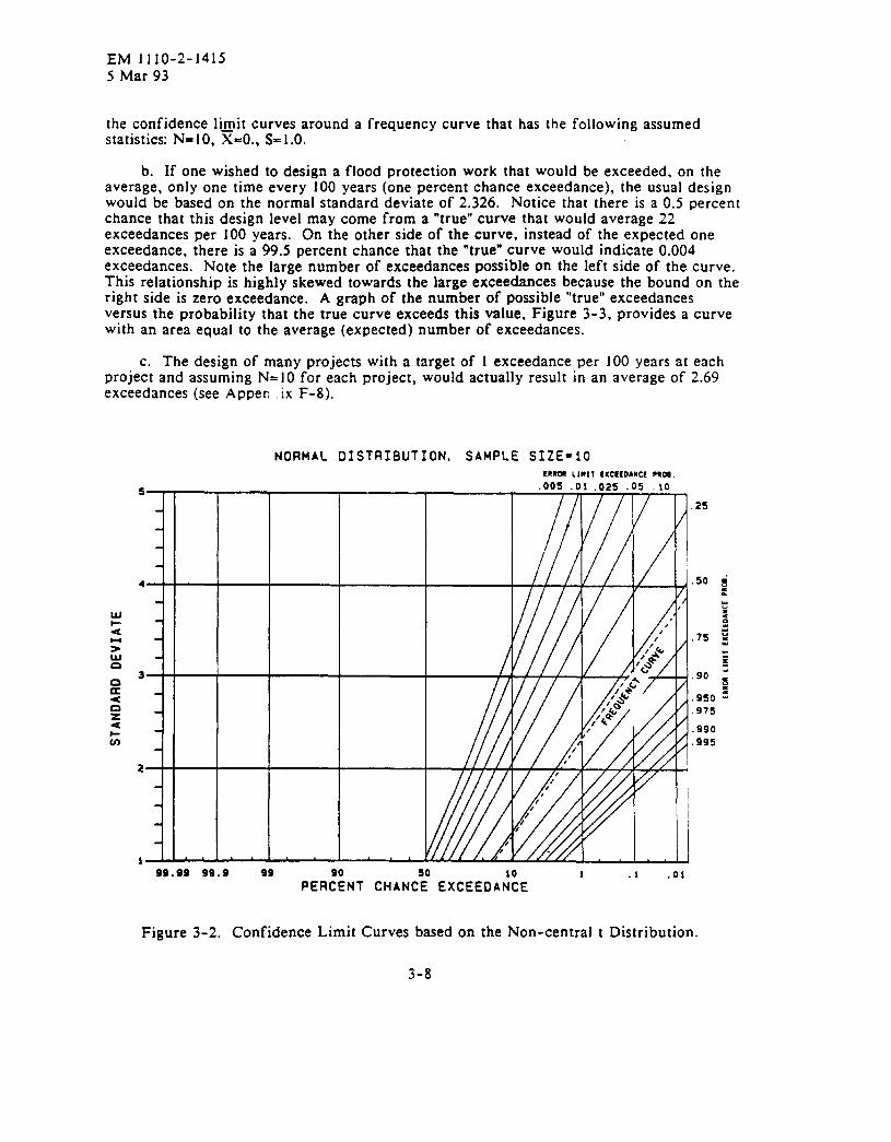
the confidence li_mit curves around a frequency curve that has the following assumed statistics: N= IO, X=0., S= 1 .O.

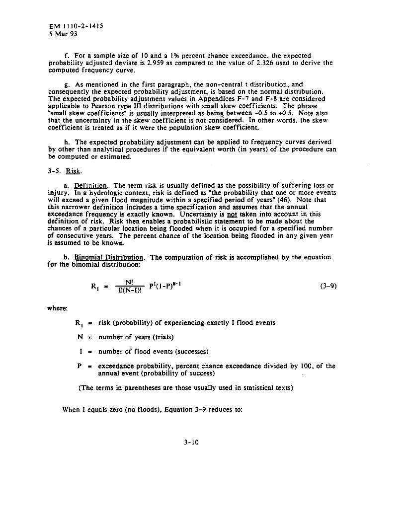
b. If one wished to design a flood protection work that would be exceeded, on the average, only one time every 100 years (one percent chance exceedance), the usual design would be based on the normal standard deviate of 2.326. Notice that there is a 0.5 percent chance that this design level may come from a “true” curve that would average 22 exceedances per 100 years. On the other side of the curve, instead of the expected one exceedance, there is a 99.5 percent chance that the “true” curve would indicate 0.004 exceedances. Note the large number of exceedances possible on the left side of the curve. This relationship is highly skewed towards the large exceedances because the bound on the right side is zero exceedance. A graph of the number of possible “true” exceedances versus the probability that the true curve exceeds this value, Figure 3-3, provides a curve with an area equal to the average (expected) number of exceedances.

c. The design of many projects with a target of 1 exceedance per 100 years at each project and assuming N-IO for each project, would actually result in an average of 2.69 exceedances (see Apperi .ix F-8).

NORMAL OISTRIBUTION, SAMPLE SIZE-10 ERROX LIMIT EXCEEDAYCL l XDO.

5 .25

4 .50 d L z 9 B

.75 ;

= 5

3 .90 a’

,950 - 2

,975

,990 .995

2

1 90.99 99.9 99

P&NT CHIN&! EXCEED& 1 .l .Ol

Figure 3-2. Confidence Limit Curves based on the Non-central t Distribution.

3-8

EM 1110-2-1415 5 Mar 93

TARGET Of 1 LXCEEDAYCE PER 100 EVENTS

AN0 USED ON SAMPLE SIZE OF 10 EVEYlS

Figure 3-3. Cumulative Probability Distribution of Exceedances per 100 Years.

d. There are two methods that can be used to correct (expected probability adjustment) for this bias. The first method, as described above, entails plotting the curve at the “expected” number of exceedances rather that at the target value, drawing the new curve and then reading the adjusted design level. Appendix F-8 provides the percentages for the expected probability adjustment.

e. The second method is more direct because an adjusted deviate (K value) is used in Equation 3-4 that makes the expected probability adjustment for a given percent chance exceedance. Appendix F-7 contains the deviates for the expected probability adjustment. These values may be derived from the t-distribution by the following equation:

K P,N = t [tN+l PI” (3-8) P,N-1

where:

P = exceedance probability (percent chance exceedance divided by 100)

N= sample size

K- expected probability adjusted deviate

t = Student’s t-statistic from one-tailed distribution

3-9

EM 1110-2-1415 5 Mar 93

f. For a sample size of 10 and a 1% percent chance exceedance, the expected probability adjusted deviate is 2.959 as compared to the value of 2.326 used to derive the computed frequency curve.

g. As mentioned in the first paragraph, the non-central t distribution, and consequently the expected probability adjustment, is based on the normal distribution. The expected probability adjustment values in Appendices F-7 and F-8 are considered applicable to Pearson type III distributions with small skew coefficients. The phrase “small skew coefficients” is usually interpreted as being between -0.5 to +0.5. Note also that the uncertainty in the skew coefficient is not considered. In other words, the skew coefficient is treated as if it were the population skew coefficient.

h. The expected probability adjustment can be applied to frequency curves derived by other than analytical procedures if the equivalent worth (in years) of the procedure can be computed or estimated.

3-5. &j&.

a. Definition. The term risk is usually defined as the possibility of suffering loss or injury. In a hydrologic context, risk is defined as “the probability that one or more events will exceed a given flood magnitude within a specified period of years” (46). Note that this narrower definition includes a time specification and assumes that the annual exceedance frequency is exactly known. Uncertainty is m taken into account in this definition of risk. Risk then enables a probabilistic statement to be made about the chances of a particular location being flooded when it is occupied for a specified number of consecutive years. The percent chance of the location being flooded in any given year is assumed to be known.

b. Binomial Distributioq. The computation of risk is accomplished by the equation for the binomial distribution:

R, s N!

I!(N-I)! P’(l-P)N-* U-9)

where:

RI = risk (probability) of experiencing exactly I flood events

N= number of years (trials)

I = number of flood events (successes)

P = exceedance probability, percent chance exceedance divided by 100, of the annual event (probability of success)

(The terms in parentheses are those usually used in statistical texts)

When I equals zero (no floods), Equation 3-9 reduces to:

3-10

EM 1110-2-1415 5 Mar 93

RO = (1-P)” (3-10a)

and the probability of experiencing one or more floods is easily computed by taking the complement of the probability of no floods:

R (1 or more)

= 1-(1-P)” (3-lob)

c. Aoolication.

(1) Risk is an important concept to convey to those who are or will be protected by flood control works. The knowledge of risk alerts those occupying the flood plain to the fact that even with the protection works, there could be a significant probability of being flooded during their lifetime. As an example, if one were to build a new house with the ground floor at the 1% chance flood level, there is a fair (about one in four) chance that the house will be flooded before the payments are completed, over the 30-year mortgage life. Using Equation 3- lob:

R (1 or more)

= 1-(1-.01)3a

= l-.9930

= l-.74

= .26 or 26% chance .

(2) Appendix F-12 provides a table for risk as a function of percent chance exceedance, period length and number of exceedances. This table could also be used to check the validity of a derived frequency curve. As an example, if a frequency curve is determined such that 3 observed events have exceeded the derived 1% chance exceedance level during the 50 years of record, then there would be reason to question the derived frequency curve. From Appendix F-12, the probability of this occurring is 0.0122 or about 1%. It is possible for the situation to occur, but the probability of occurring is very low. This computation just raises questions about the validity of the derived curve and indicates that other validation checks may be warranted before adopting the derived curve.

3-6. Conditional Probabilitv Adiustment. The conditional probability adjustment is made when flood peaks have either been deleted or are not available below a specified truncation level. This adjustment will be applied when there are zero flood years, an incomplete record or low outliers. As stated in Appendix 5 of Bulletin 17B, this procedure is not appropriate when 25 percent or more of the events are truncated. The computation steps in the conditional probability adjustment are as follows:

1. Compute the estimated probability <F> that an annual peak will exceed the truncation level:

F = N/n (3-l la)

3-11

EM 1110-2 1415 5 Mar 93

where N is the number of peaks above the truncation level and n is the total number of years of record. If the statistics reflect the adjustments for historic information, then the appropriate equation is

H - WL F= (3-l lb)

H

where H is the length of historic period, W is the systematic record weight and L is the number of peaks truncated.

2. The computed frequency curve is actually a conditional frequency curve. Given that the flow exceeds the truncation level, the exceedance frequency for that flow can be estimated. The conditional exceedance frequencies are converted to annual frequencies by the probability computed in Step 1:.

P = FPd (3-12)

where P is the annual percent chance exceedance and P, is the conditional percent chance exceedance.

3. Interpolate either graphically or mathematically to obtain the discharge values (Qt.,) for 1, 10 and 50 percent chance exceedances.

4. Estimate log-Pearson type III statistics that will fit the upper portion of the adjusted curve with the following equations:

Gs = -2.50 + 3.12 log (Q,/Q,,,)

(3- 13)

log (Q,dQso)

ss = log (Q,/Qso)

(3-14)

Kl-K50

Xs = log (Qso) - KS, S, (3-15)

where G,, S, and z are the synthetic skew coefficient, standard deviation and mean, respectively; 6,. Q and K

sg are the Pearson Type ’ f

and Qso the discharges determined in Step 3; and K II deviates for percent change exceedances of 1 and 30

an skew coefficient G,.

3-12

EM 1110-2-1415 5 Mar 93

5. Combine the synthetic skew coefficient with the generalized skew by use of Equation 3-6 to obtain the weighted skew.

6. Develop the computed frequency curve with the synthetic statistics and compare it with the plotted observed flood peaks.

3-7. Two-Station Comoarison.

a. Purnose.

(I) In most cases of frequency studies of runoff or precipitation there are locations in the region where records have been obtained over a long period. The additional period of record at such a nearby station is useful for extending the record at a short record station provided there is reasonable correlation between recorded values at the two locations.

(2) It is possible, by regression or other techniques, to estimate from concurrent records at nearby locations the magnitude of individual missing events at a station. However, the use of regression analysis produces estimates with a smaller variance than that exhibited by recorded data. While this may not be a serious problem if only one or two events must be estimated to “fill in” or complete an otherwise unbroken record of several years, it can be a significant problem if it becomes necessary to estimate more than a few events. Consequently, in frequency studies, missing events should not be freely estimated by regression analysis.

(3) The procedure for adjusting the statistics at a short-record station involves three steps: (I) computing the degree of correlation between the two stations, (2) using the computed degree of correlation and the statistics of the longer record station to compute an adjusted set of statistics for the shorter-record station, and (3) computing an equivalent “length of record” that approximately reflects the “worth” of the adjusted statistics of the short-record station. The longer record station selected for the adjustment procedure should be in a hydrologically similar area and, if possible, have a drainage area size similar to that of the short-record station.

b. Cm. The degree of correlation is reflected in the correlation coefficient R2 as computed through use of the following equation:

R2 3: [BY - (~~VN12

[B2 - (fW2/Nl rp* - (~)2/Nl

where:

R2 = the determination coefficient

Y = the value at the short-record station

X = the concurrent value at the long-record station

N = the number of years of concurrent record

(3-16)

3-13

EM 1110-2 1415 5 Mar 93

For most studies involving streamflow values, it is appropriate to use the logarithms of the values in the equations in this section.

c. Adiustment of Mean. The following equation is used to adjust the mean of a short-record station on the basis of a nearby longer-record station:

T = T, + (X3 - %,I R (s,,/S,,) (3-17)

where:

T = the adjusted mean at the short-record station

P, = the mean for the concurrent record at the short-record station

J7, = the mean for the complete record at the longer-record station

K, = the mean for the concurrent record at the longer-record station

R= the correlation coefficient

S Yl

= the standard deviation for the concurrent record at the short-record station

S Xl

= the standard deviation for the concurrent record at the longer-record station

AI1 of the above parameters may be derived from the logarithms of the data where appropriate, e.g., for annual flood peaks. The criterion for determining if the variance of the adjusted mean will likely be less than the variance of the concurrent record is:

R* > l/(N, - 2) (3-18)

where N, equals the number of years of concurrent record. If R2 is less than the criterion, Equation 3- 17 should not be applied. In this case just use the computed mean at the short-record station or check another nearby long-record station. See Appendix 7 of Bulletin l7B for procedures to compare the variance of the adjusted mean against the variance of the entire short-record period.

d. Adiustment of Standard Deviation. The following equation can be used to adjust the standard deviation:

s,z = Sy: + cS:- $1 R *(S,;/S,~ (approximate)

3-14

EM 1110-2-1415 5 Mar 93

where:

SY = the adjusted standard deviation at the short-record station

S Yl

= the standard deviation for the period of concurrent record at the short-record station

SX = the standard deviation for the complete record at the base station

= the standard deviation for the period of concurrent record at the base station

= the determination coefficient

All of the above parameters may be derived from the logarithms of the data where appropriate, e.g., for annual flood peaks. This equation provides approximate results compared to Equation 3- 19 in Appendix 7 of Bulletin 17B, but in most cases the difference in the results does not justify the additional computations.

e. Adiustment of Skew coefficient. There is no equation to adjust the skew coefficient that is comparable to the above equations. When adjusting the statistics of annual flood peaks either a weighted or a generalized skew coefficient may be used depending on the record length.

f. mRecord The final step in adjusting the statistics is the computation of the “equivalent record length” which is defined as the period of time which would be required to establish unadjusted statistics that are as reliable (in a statistical sense) as the adjusted values. Thus, the equivalent length of record is an indirect indication of the reliability of the adjusted values of Y and S,. The equivalent record length for the adjusted mean is computed from the following equation:

NY = NY,

1 - W, - N,,)/N,] [R2 - (1 - R2VW,, - 3)l

(3-20)

where:

NY = the equivalent length of record of the mean at the short-record station

Ny1 = the number of years of concurrent record at the two stations

N, = the number of years of record at the longer-record station

R= the adjusted correlation coefficient

Figure 3-4 shows the data and computations for a two-station comparison for a short record station with 21 events and a long record station with 60 systematic events. It can be seen that the adjustment of the frequency statistics provides an increased reliability in the mean equivalent to having an additional 17 years of record at the short-record station.

3-15

EM 1110-2-1415 5 Mar 93

-r--- - Iear flow

I Chettooge 1ellul.h River River

1915 1917 1918 1919 1920 1921 1922 1923 192L 1925 1924 1927 1928 1929 1940 1941 1942 1943 1944 1945 1946 1947 1948 1949 1950 1951 1952 1953 19SL 19% 1956 1957 1958 1959 1960 1961 1962 1963 1964 1945 1966 1967 196a I969 1970 I971 I972 1973 1974 I975 1974 I977 I978 I979 I980 I981 I982 1983 I984 I965

12400 14000 5900

14000 8200 4100 4200 5300 9200 3900 4200 3400

20100 11400 29000. 7530 6870 4870 3840 2930 4450 6440 12400 13900 4740 5220

13400 4020 4230 5820 5820 5620 5420

2% 7310 9660 5420 9880

27200 13400 15400 5620 14700 3480 3290 7440

19400 4400 6340 18500 13000 7850

14800 lD900 4120 5000 7910 4810 4740

7440 5140 2800 3100 2470 2010 976 2160 8500 4660 2410 4530 3580 4090 4240 2880 1400 19bD 3260 2000 1010

-4 YOC

rota1 Concurrent concurrent ,-e-e- I

^..“. - -_-__------_---_-____ ______

systematic Events 40 21 39 21

Wistofic Period I 71 0 0 0

Log *em 13.1844 3.9310 3.8450 3.L794

Standard Deviation (0.2322 0.24713 0.2140 0.2409

Computed I 0.5075 0.1588 0.7340 -0.0811

Skew Cenerelised - Adopted , - -0.1000

cm:

Slope: b = 0.?90495 Correletion Coefficient: R =0.811351 (See Figure P-00

From equrtions 19, 21, end 22:

I1 = 3.4794 * 0.?90495 (3.M6b l 3.9310)

Y, = 3.4445

$1 2 = t(0.2322)2 - ~0.2678)21(0.11114)2~0.2b09/0.2b?8~2

9 (0.2b09~2

f 1 = 0.23M

"I( = 1 - ?=+ ,o.::a3 - ' ;,0:63 = 38

i, = 0.0 NSEi = 0.302 Ii n -0.0811 MSES = 0.142

% = (0.302)(-0.0111) l (0.0142)(0.0)

. l .

c, = -0.055 =* -0.1

FREOUEYCY CURVE, TALLULAH RIVER NEAR CLAYTON, GA

. . . . ..FLDM.CFS........ PERCENT ..COYFIDENCE LIMITS.. EXPECTED CNANCE

CDMPUTED PROBAIILITY EXCEEDANCE .os LIMIT -95 LIMIT

127Do 142OD 10900 11900

:: 18100 9580 15400 8410

9590 10300 8350 8800

i-8 13400 7540

s:o 11300 4480

4740 4990 8810 5550

Efi! 44aD 5710 20.0 10.0 7040 5370 4480 3780 2810 2610 SO.0 3260 2420 1760 1740 80.0 2060 1450 1370 1340 90.0 1440 1060 1110 1070 95.0 1340 847 745 406 99.0 957 524

.-.. l Nistorjc inforution, peek Largest since 1~).

Figure 3-4. Two-Station Comparison Computations.

3-16

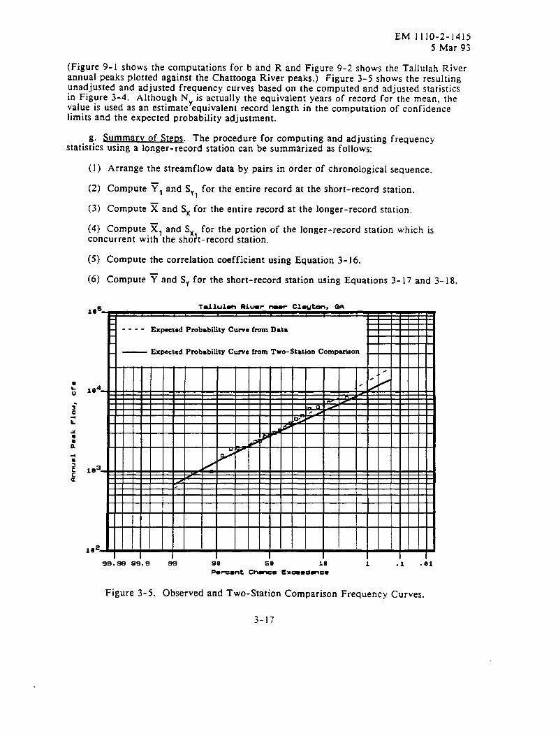
EM I I lO-2-1415 5 Mar 93

(Figure 9-1 shows the computations for b and R and Figure 9-2 shows the Tallulah River annual peaks plotted against the Chattooga River peaks.) Figure 3-5 shows the resulting unadjusted and adjusted frequency curves based on the computed and adjusted statistics in Figure 3-4. Although N is actually the equivalent years of record for the mean, the value is used as an estimateYequivalent record length in the computation of confidence limits and the expected probability adjustment.

g. Summarv of Stem. The procedure for computing and adjusting frequency statistics using a longer-record station can be summarized as follows:

(1) Arrange the streamflow data by pairs in order of chronological sequence.

(2) Compute y, and S,, for the entire record at the short-record station.

(3) Compute % and S, for the entire record at the longer-record station.

(4) Compute %, and S, for the portion of the longer-record station which is concurrent with the shojt-record station.

(5) Compute the correlation coefficient using Equation 3- 16.

(6) Compute y and S, for the short-record station using Equations 3- 17 and 3- 18.

---- Expected Probability Curve from Data

- Exwctcd Probability Cunc from Two-Station Comrwiaon

1e4

103.

it?=- liiiiilii I I I Hill I I I III Hlll siss 9s’.s 9s 9-0 se 1-e

Pmrcmnt Chmer Erardmcr

i .i .ir

Figure 3-5. Observed and Two-Station Comparison Frequency Curves.

3-17

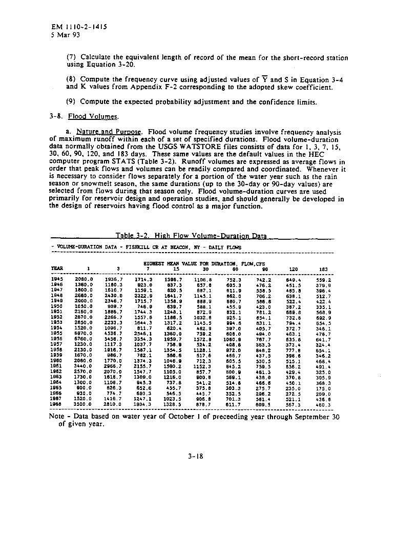
EM 1110-2-1415 5 Mar 93

3-8.

(7) Calculate the equivalent length of record of the mean for the short-record station using Equation 3-20.

(8) Compute the frequency curve using adjusted values of y and S in Equation 3-4 and K values from Appendix F-2 corresponding to the adopted skew coefficient.

(9) Compute the expected probability adjustment and the confidence limits.

Flood Volumes.

a. Nature and Purpose. Flood volume frequency studies involve frequency analysis of maximum runoff within each of a set of specified durations. Flood volume-duration data normally obtained from the USGS WATSTORE files consists of data for 1, 3, 7, 15, 30, 60, 90, 120, and 183 days. These same values are the default values in the HEC computer program STATS (Table 3-2). Runoff volumes are expressed as average flows in order that peak flows and volumes can be readily compared and coordinated. Whenever it is necessary to consider flows separately for a portion of the water year such as the rain season or snowmelt season, the same durations (up to the 30-day or 90-day values) are selected from flows during that season only. Flood volume-duration curves are used primarily for reservoir design and operation studies, and should generally be developed in the design of reservoirs having flood control as a major function.

Table 3-2. Hinh Flow Volume-Duration Data

- VOLUME-DURATION DATA - FISIiKILL CR AT BEACON, NY - DAILY FLOWS -----------------------------------------------------------------------------------------------

TEAR BIGHi? bEAN VALUE FOR DURATION, FL0w.CF.S

1 3 7 15 30 60 90 120 183 ----------------------------------------------------------------------------------------------- 1945 2080.0 1936.7 1714.3 1398.7 1106.8 752.3 742.2 649.4 559.2 1946 1360.0 1160.3 923.0 837.3 657.0 605.3 476.2 451.5 379.9 1947 1800.0 1616.7 1159.1 820.5 687.1 611.9 558.5 405.6 396.4 1948 2660.0 2430.0 2322.9 1641.7 1145.1 162.0 706.2 636.1 512.7 1949 2900.0 2346.7 1715.7 13S8.9 88B.S 680.7 586.6 522.4 422.4 1950 1oso. 0 909.7 746.9 639.7 568.1 455.9 423.0 307.2 335.1 1951 2160.0 1886.7 1744.3 1248.1 872.9 632.1 781.2 669.6 560.9 1952 2670.0 2266.7 1557.6 1186.5 1032.6 925.1 654.1 732.6 692.9 1953 2850.0 2233.3 1644.3 1317.2 1145.5 994.6 631.1 794.4 654.5 1954 1520.0 1096.7 811.7 620.4 462.9 397.0 405.7 372.7 346.1 1955 6970.0 4536.7 2546.1 1360.0 759.2 608.0 494.0 463.1 470.7 1956 6760.0 5456.7 3354.3 19s9-7 1572.8 1080.9 767.7 635.8 641.7 1957 1230.0 1117.3 1037.7 756.9 524.2 408.8 363.3 373.4 324.4 1958 2130.0 1916.7 lS87.1 1354.s 1128.1 972.0 848.2 777.0 654.1 1959 1670.0 986.7 782.1 566.6 517.6 466.7 437.5 396.6 346.2 1960 2080.0 1770.0 1374.3 1046.9 712.3 605.5 530.5 515.1 460.4 1961 3440.0 2966.7 2155.7 lS90.2 1152.3 645.2 759.5 656.2 491.4 1962 2570.0 2070.0 1547.7 llos.o 857.7 600.9 461.3 429.4 325.0 1963 1730.0 1616.7 1309.0 1216.0 900.6 569.1 430.0 370.8 305.9 1964 1300.0 1106.7 945.3 737.8 541.2 514.8 486.6 450.1 380.3 1965 900.0 826.3 652.6 455.7 375.8 303.3 275.7 235.0 175.0 1966 930.0 774.7 6Q3.3 S46.5 445.7 352.5 296.2 272.5 209.0 1967 1520.0 1416.7 1247.1 1023.5 906.6 701.3 581.4 521.1 436.8 1968 3500.0 2810.0 1934.3 1328.5 876.7 611.7 609.5 567.3 460.3 -----------------------------------------------------------------------------------------------

Note - Data based on water year of October I of preceeding year through September 30 of given year.

3-18

EM 1110-2-1415 5 Mar 93

b. Data for Comorehensive Series. Data to be used for a comprehensive flood volume-duration frequency study should be selected from nearly complete water year records. Unless overriding reasons exist, the durations in Table 3-2 should be used in order to assure consistency among various studies for comparison purposes. Maximum flood events should be selected only for those years when recorder gages existed or when the maximum events can be estimated by other means. Where a minor portion of a water year’s record is missing, the longer-duration flood volumes for that year can often be estimated adequately. If upstream regulation or diversion is known to have an effect, care should be exercised to assure that the period selected is the one when flows would have been maximum under the specified (usually natural) conditions.

c. Statistics for Comorehensive Series.

(I) The probability distribution recommended for flood volume-duration frequency computations is the log-Pearson type III distribution; the same as that used for annual flood peaks. In practice, only the first two moments, mean and standard deviations are based on station data. As discussed in Section 3-3, the skew coefficient should not be based solely on the station record, but should be weighted with information from regional studies. To insure that the frequency curves for each duration are consistent, and especially to prevent the curves from crossing, it is desirable to coordinate the variation in standard deviation and skew with that of the mean. This can be done graphically as shown in Figure 3-6. For a given skew coefficient, there is a maximum and minimum allowable slope for the standard deviation-versus-mean relation which prevents the curves from crossing within the established limits. For instance, to keep the curves from crossing within 99.99 and .Ol percent chance exceedances with a skew of O., the slope must not exceed .269, nor be less than -.269, respectively. The value of this slope constraint is found by stating that the value of one curve (XA for curve A) must equal or exceed the value for a second curve (Xa for curve B) at the desired exceedance frequency. Each of these values can be found by substitution into Equation 3-4 (the K for zero skew and 99.99 percent chance exceedance is -3.719):

x, L x,

Tz, + (-3.719) s, z TI, + (-3.719) sa

3.719 (Se - S,) 2 Za - TT,

(S* - S,)

(ST, - q

2 0.269

where:

X* = Value of frequency curve A at 99.99 percent chance exceedance

Xr3 = Value of frequency curve B at 99.99 percent chance exceedance

Ti, = Mean of frequency curve A

Yi, = Mean of frequency curve B

% = Standard deviation of frequency curve A

sil = Standard deviation of frequency curve B

3-19

EM 1110-2-1415 5 Mar 93

0.W

ci 0.26

4

B

5 z 0.20

ci

3

5 0.15

0.10

2.4 2.6 2.6 3.0 3.2 3.4

Mean of Lo(laibhm (Z,

0.6 -

2.4 2.6 2.6 3.0 3.2

MesIn of Logartthns (X,

Figure 3-6. Coordination of Flood-Volume Statistics.

3-20

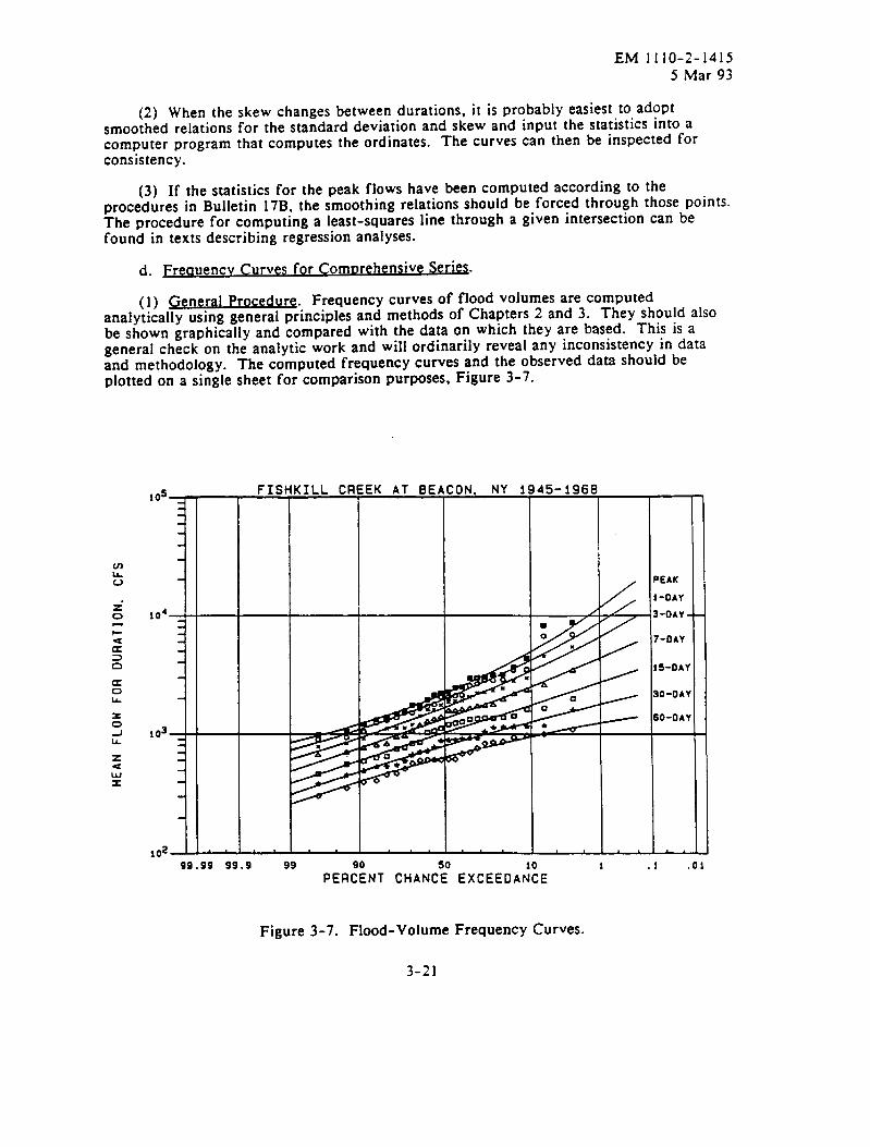
EM 1110-2-1415 5 Mar 93

(2) When the skew changes between durations, it is probably easiest to adopt smoothed relations for the standard deviation and skew and input the statistics into a computer program that computes the ordinates. The curves can then be inspected for consistency.

(3) If the statistics for the peak flows have been computed according to the procedures in Bulletin l7B, the smoothing relations should be forced through those points. The procedure for computing a least-squares line through a given intersection can be found in texts describing regression analyses.

d. Freauencv Curves for ComDrehensive Series.

(1) Ge e al p ocedu e Frequency curves of flood volumes are computed analytically :si’ng g&era1 brinciples and methods of Chapters 2 and 3. They should also be shown graphically and compared with the data on which they are based. This is a general check on the analytic work and will ordinarily reveal any inconsistency in data and methodology. The computed frequency curves and the observed data should be plotted on a single sheet for comparison purposes, Figure 3-7.

07 L 0

z M c u 5 n

E LL

z A IA z I2 I

Figure 3-7. Flood-Volume Frequency Curves.

3-21

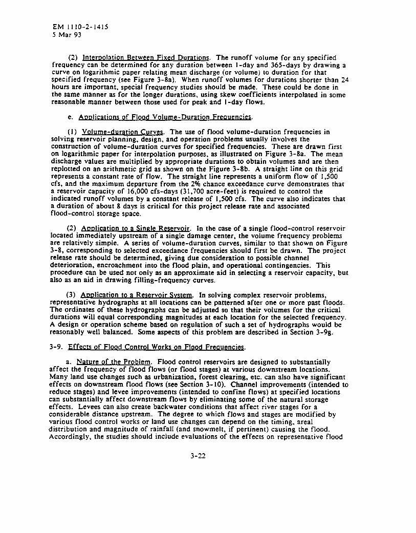
EM 1110-2-1415 5 Mar 93

(2) c Durations. The runoff volume for any specified frequency can be determined for any duration between l-day and 365-days by drawing a curve on logarithmic paper relating mean discharge (or volume) to duration for that specified frequency (see Figure 3-&la). When runoff volumes for durations shorter than 24 hours are important, special frequency studies should be made. These could be done in the same manner as for the longer durations, using skew coefficients interpolated in some reasonable manner between those used for peak and l-day flows.

e. ADDliCatiOnS of Flood Volume-Duration Freauencies.

(1) Volume-duration Curves. The use of flood volume-duration frequencies in solving reservoir planning, design, and operation problems usually involves the construction of volume-duration curves for specified frequencies. These are drawn first on logarithmic paper for interpolation purposes, as illustrated on Figure 3-8a. The mean discharge values are multiplied by appropriate durations to obtain volumes and are then replotted on an arithmetic grid as shown on the Figure 3-8b. A straight line on this grid represents a constant rate of flow. The straight line represents a uniform flow of 1,500 cfs, and the maximum departure from the 2% chance exceedance curve demonstrates that a reservoir capacity of 16,000 cfs-days (31,700 acre-feet) is required to control the indicated runoff volumes by a constant release of 1,500 cfs. The curve also indicates that a duration of about 8 days is critical for this project release rate and associated flood-control storage space.

(2) Abblication to a Single Reservoir. In the case of a single flood-control reservoir located immediately upstream of a single damage center, the volume frequency problems are relatively simple. A series of volume-duration curves, similar to that shown on Figure 3-8, corresponding to selected exceedance frequencies should first be drawn. The project release rate should be determined, giving due consideration to possible channel deterioration, encroachment into the flood plain, and operational contingencies. This procedure can be used not only as an approximate aid in selecting a reservoir capacity, but also as an aid in drawing filling-frequency curves.

(3) ADDlication to a Reservoir Svstem. In solving complex reservoir problems, representative hydrographs at all locations can be patterned after one or more past floods. The ordinates of these hydrographs can be adjusted so that their volumes for the critical durations will equal corresponding magnitudes at each location for the selected frequency. A design or operation scheme based on regulation of such a set of hydrographs would be reasonably well balanced. Some aspects of this problem are described in Section 3-9g.

3-9. Effects of Flood Control Works on Flood Freauencies.

a. Nature. Flood control reservoirs are designed to substantially affect the frequency of flood flows (or flood stages) at various downstream locations. Many land use changes such as urbanization, forest clearing, etc. can also have significant effects on downstream flood flows (see Section 3-10). Channel improvements (intended to reduce stages) and levee improvements (intended to confine flows) at specified locations can substantially affect downstream flows by eliminating some of the natural storage effects. Levees can also create backwater conditions that affect river stages for a considerable distance upstream. The degree to which flows and stages are modified by various flood control works or land use changes can depend on the timing, areal distribution and magnitude of rainfall (and snowmelt, if pertinent) causing the flood. Accordingly, the studies should include evaluations of the effects on representative flood

3-22

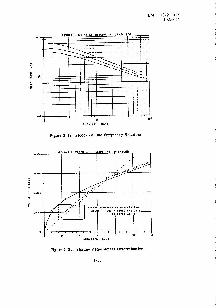
w

w

;:

I

g

e.

;

.g

0

2

-

t

;:

Fi

z 3

e.

E

E

VOLU

ME,

CFS-

DAYS

01*

-z:

0 . :

-it

z;

or-

-::

I :

,A:

xi:

001

mm

: “.

I*

. In

* _n

.

-4

-a-.

z:

m

i;;

z x t 4.

lo

=I

7

I z g

n L.

F 2 w

b 2 ? oc

E

3 0 n a P fi z Y P

E

g’

(n

MEAN

FL

OW.

CFS

_

--.L. .-,-l-L

b -..

I t 1-I

i I

-

I I

5 I

1 !z

“7

SCM

I :-

P

a-

wul

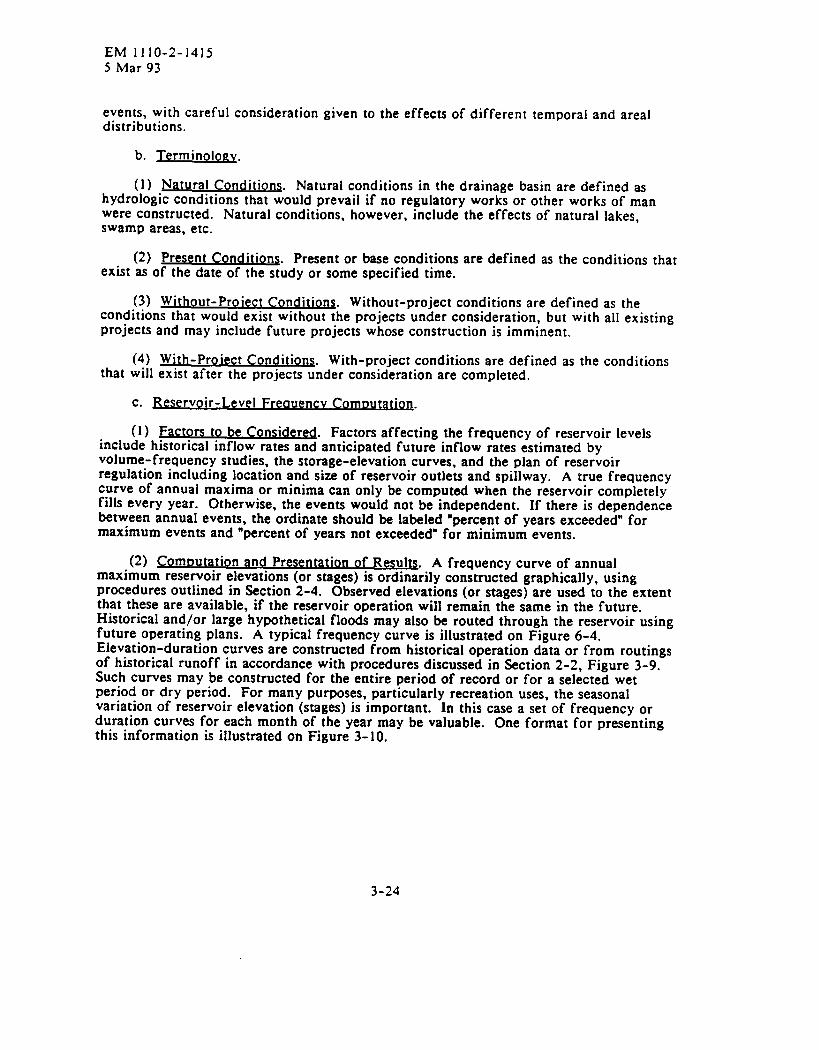
EM 1110-2-1415 5 Mar 93

events, with careful consideration given to the effects of different temporal and area1 distributions.

b. Terminology.

(1) Natural Conditions. Natural conditions in the drainage basin are defined as hydrologic conditions that would prevail if no regulatory works or other works of man were constructed. Natural conditions, however, include the effects of natural lakes, swamp areas, etc.

(2) Present Conditions. Present or base conditions are defined as the conditions that exist as of the date of the study or some specified time.

(3) Without-Proiect Conditions. Without-project conditions are defined as the conditions that would exist without the projects under consideration, but with all existing projects and may include future projects whose construction is imminent.

(4) With-Proiect Conditions. With-project conditions are defined as the conditions that will exist after the projects under consideration are completed.

c. J? rv ir- Qa.Level+reauencv.

(1) Factors to be Considered. Factors affecting the frequency of reservoir levels include historical inflow rates and anticipated future inflow rates estimated by volume-frequency studies, the storage-elevation curves, and the plan of reservoir regulation including location and size of reservoir outlets and spillway. A true frequency curve of annual maxima or minima can only be computed when the reservoir completely fills every year. Otherwise, the events would not be independent. If there is dependence between annual events, the ordinate should be labeled “percent of years exceeded” for maximum events and “percent of years not exceeded” for minimum events.

(2) Combutation and Presentation of Results. A frequency curve of annual maximum reservoir elevations (or stages) is ordinarily constructed graphically, using procedures outlined in Section 2-4. Observed elevations (or stages) are used to the extent that these are available, if the reservoir operation will remain the same in the future. Historical and/or large hypothetical floods may also be routed through the reservoir using future operating plans. A typical frequency curve is illustrated on Figure 6-4. Elevation-duration curves are constructed from historical operation data or from routings of historical runoff in accordance with procedures discussed in Section 2-2, Figure 3-9. Such curves may be constructed for the entire period of record or for a selected wet period or dry period. For many purposes, particularly recreation uses, the seasonal variation of reservoir elevation (stages) is important. In this case a set of frequency or duration curves for each month of the year may be valuable. One format for presenting this information is illustrated on Figure 3-10.

3-24

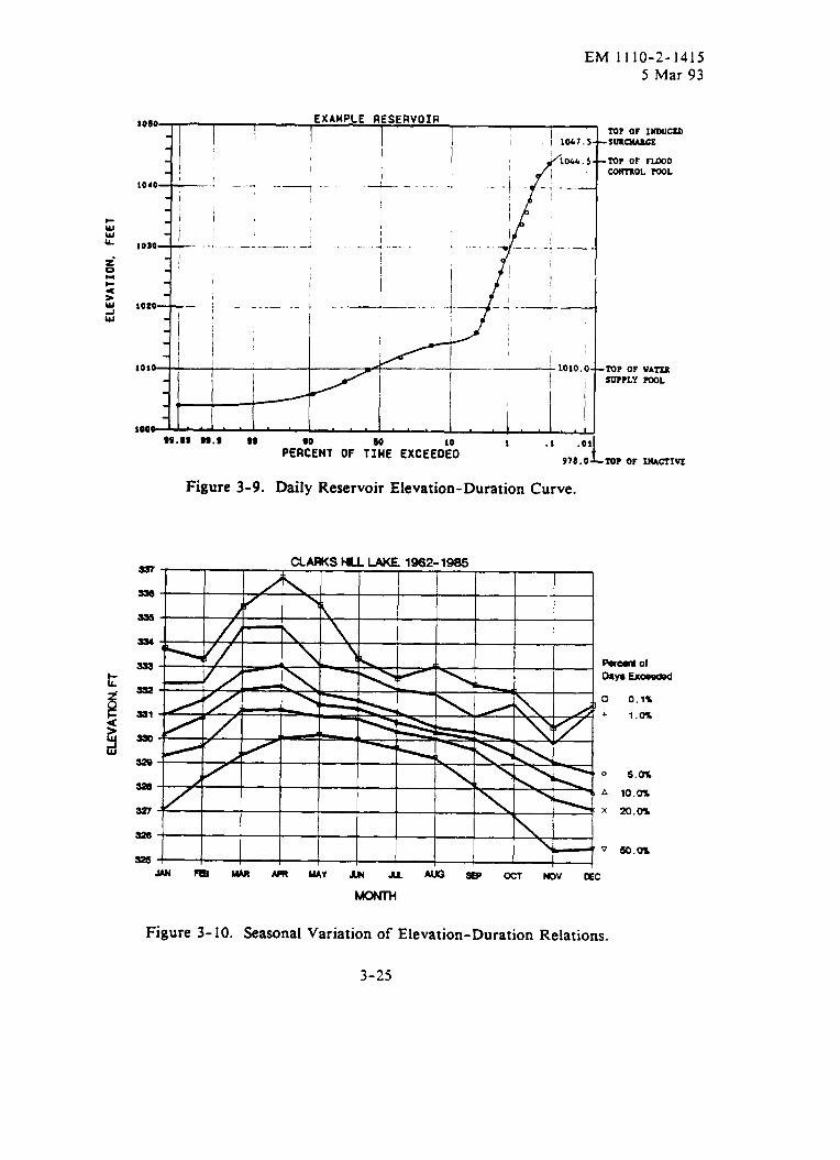
EM 1110-2-1415 5 Mar 93

1010 EXAMPLE RESERVOIR

L L 1030 i- i :: 2 z id

IO20 -

i i 1 lOi0 '

i lolo.:

_f ..- -_-___ A

1000 m.0 n.a as

P&NT OF fIWWE EXCEEC& 1 .I .Ol

976.0

.+ ..-.

Figure 3-9. Daily Reservoir Elevation-Duration Curve.

I 1

-TOP OF FIDOD CONTROL moL

-fo? OF VAT6R su?rLY PWL

-m? OF INACIIVE

PorcuM of Oaya Exceeded

Figure 3- 10. Seasonal Variation of Elevation-Duration Relations.

3-25

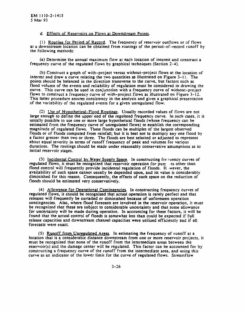
EM 1110-2-1415 5 Mar 93

d. Fffects of Reservoirs on Flows at Downstream Points.

(1) Routine for Period of Record. The frequency of reservoir outflows or of flows at a downstream location can be obtained from routings of the period-of-record runoff by the following methods:

(a) Determine the annual maximum flow at each location of interest and construct a frequency curve of the regulated flows by graphical techniques (Section 2-4).

(b) Construct a graph of with-project versus without-project flows at the location of interest and draw a curve relating the two quantities as illustrated on Figure 3-l 1. The points should be balanced in the direction transverse to the curve, but factors such as flood volume of the events and reliability of regulation must be considered in drawing the curve. This curve can be used in conjunction with a frequency curve of without-project flows to construct a frequency curve of with-project flows as illustrated on Figure 3-12. This latter procedure assures consistency in the analysis and gives a graphical presentation of the variability of the regulated events for a given unregulated flow.

(2) Use of Hvoothetical-Flood Routinns Usually recorded values of flows are not large enough to define the upper end of the regulated frequency curve. In such cases, it is usually possible to use one or more large hypothetical floods (whose frequency can be estimated from the frequency curve of unregulated flows) to establish the corresponding magnitude of regulated flows. These floods can be multiples of the largest observed floods or of floods computed from rainfall; but it is best not to multiply any one flood by a factor greater than two or three. The floods are best selected or adjusted to represent about equal severity in terms of runoff frequency of peak and volumes for various durations. The routings should be made under reasonably conservative assumptions as to initial reservoir stages.

(3) Incidental Control bv Water SUDD~V Soace. In constructing fre:uency curves of regulated flows, it must be recognized that reservoir operation for purr .es other than flood control will frequently provide incidental regulation of floods. Ii .wever, the availability of such space cannot usually be depended upon, and its value is considerably diminished for this reason. Consequently, the effects of such space on the reduction of floods should be estimated very conservatively.

(4) All w n da. In constructing frequency curves of r regulated flows, it should be recognized that actual operation is rarely perfect and that releases will frequently be curtailed or diminished because of unforeseen operation contingencies. Also, where flood forecasts are involved in the reservoir operation, it must be recognized that these are subject to considerable uncertainty and that some allowance for uncertainty will be made during operation. In accounting for these factors, it will be found that the actual control of floods is somewhat less than could be expected if full release capacities and downstream channel capacities were utilized efficiently and if all forecasts were exact.

(5) Runoff from Unreaulated Area& In estimating the frequency of runoff at a location that is a considerable distance downstream from one or more reservoir projects, it must be recognized that none of the runoff from the intermediate areas between the reservoir(s) and the damage center will be regulated. This factor can be accounted for by constructing a frequency curve of the runoff from the intermediate area, and using this curve as an indicator of the lower limit for the curve of regulated flows. Streamflow

3-26

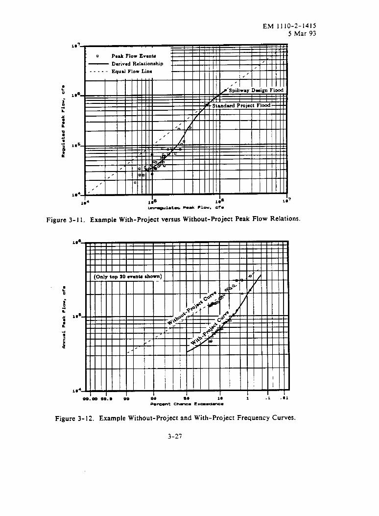
EM 1110-5

-2-1415Mar 93

10

10

10

101 ‘s ‘s ‘7

104 10 10 10

hmulat-o P--k Flou, cfs

Figure 3-11. Example With-Project versus Without-Project Peak F1OWRelations.

1o4-S9. SS 99.9 S“s 9“9 60

P,mmt Chmcm

Figure 3-12. Example Without-Project and

10 1 .1 .ilE xmwd-m

With-Project Frequency Curves.

3-27

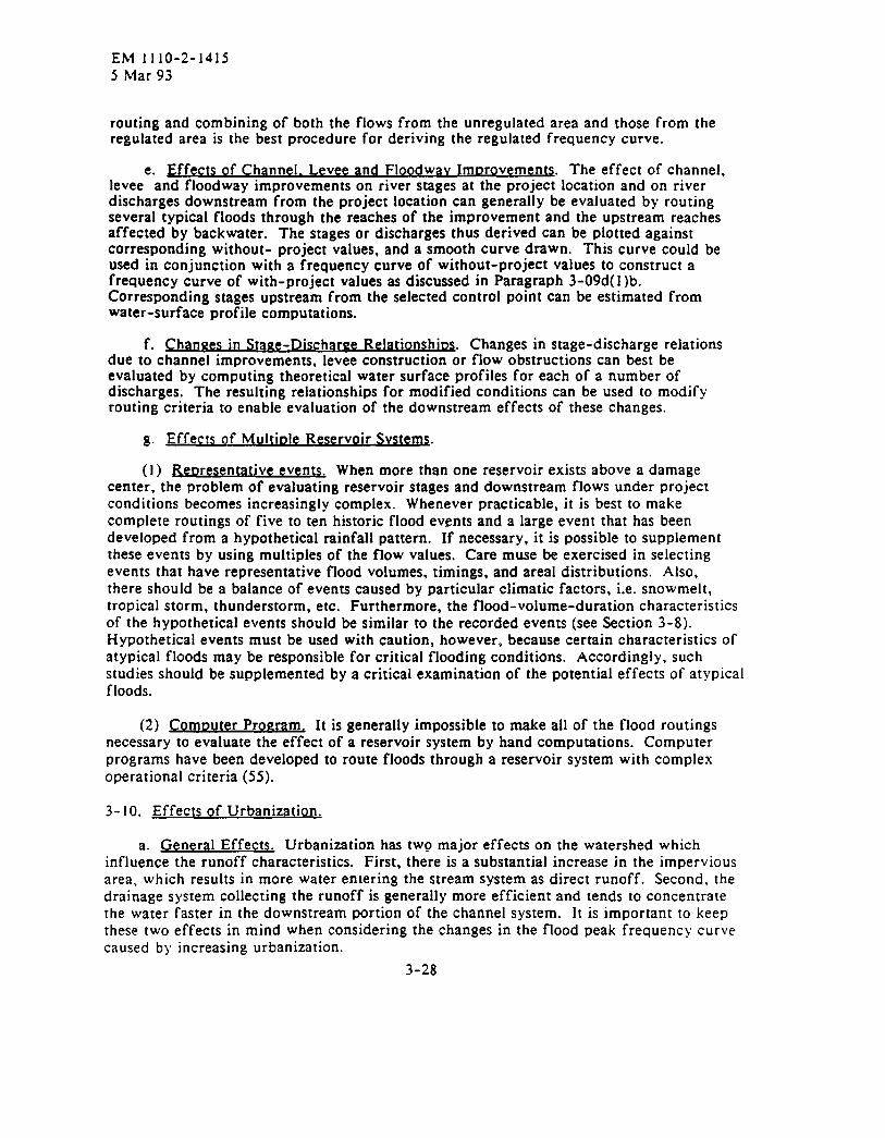
EM 1110-2-14155 Mar 93

routing and combining of both the flows from the unregulated area and those from theregulated area is the best procedure for deriving the regulated frequency curve.

Effects of Channel. Le ee and Floodwav ImDrovemen&. The effect of channel,Ieveee-and floodway improvem~nts on river stages at the project location and on riverdischarges downstream from the project location can generally be evaluated by routingseveral typical floods through the reaches of the improvement and the upstream reachesaffected by backwater. The stages or discharges thus derived can be plotted againstcorresponding without- project values, and a smooth curve drawn. This curve could beused in conjunction with a frequency curve of without-project values to construct afrequency curve of with-project values as discussed in Paragraph 3-09d( 1)b.Corresponding stages upstream from the selected control point can be estimated fromwater-surface profile computations.

f. han in~ ionsh~. Changes in stage-discharge relationsdue to channel improvements, levee construction or flow obstructions can best beevaluated by computing theoretical water surface profiles for each of a number ofdischarges. The resulting relationships for modified conditions can be used to modifyrotlting criteria to enable evaluation of the downstream effects of these changes.

g. Effects of Mu ltiDle Rese rvoir Svste~.

(I) Ret)resentative events. When more than one reservoir exists above a damagecenter, the problem of evaluating reservoir stages and downstream flows under projectconditions becomes increasingly complex. Whenever practicable, it is best to makecomplete routings of five to ten historic flood events and a large event that has beendeveloped from a hypothetical rainfall pattern. If necessary, it is possible to supplementthese events by using multiples of the flow values. Care muse be exercised in selectingevents that have representative flood volumes, timings, and areal distributions. Also,there should be a balance of events caused by particular climatic factors, i.e. snowmelt,tropical storm, thunderstorm, etc. Furthermore, the flood-volume-duration characteristicsof the hypothetical events should be similar to the recorded events (see Section 3-8).Hypothetical events must be used with caution, however, because certain characteristics ofatypical floods may be responsible for critical flooding conditions. Accordingly, suchstudies should be supplemented by a critical examination of the potential effects of atypicalfloods.

(2) ComDute r Pr~ra .m It is generally impossible to make all of the flood routingsnecessary to evaluate the effect of a reservoir system by hand computations. Computerprograms have been developed to route floods through a reservoir system with complexoperational criteria (55).

3-10, Effects of Urbanization.

a. ~ Urbanization has two major effects on the watershed whichinfluence the runoff characteristics. First, there is a substantial increase in the imperviousarea, which results in more water entering the stream system as direct runoff. Second, thedrainage system collecting the runoff is generally more efficient and tends to concentratethe water faster in the downstream portion of the channel system. It is important to keepthese two effects in mind when considering the changes in the flood peak frequency curvecaused by increasing urbanization.

3-28

EM 1110-2-14155 Mar 93

b. Effect on Freauencv Relations. A general statement can be made about theeffects of urbanization on flood-peak frequency relations. The usual effect on thefrequency relation is to cause a significant increase in the magnitude of the more frequentevents, but a lesser increase in the less frequent events. This results in an increase in themean of the annual flood peaks, a decrease in the standard deviation and an unpredictableeffect on the skew coefficient (see Figure 3- 13). The resulting frequency relation maynot fit any of the standard theoretical distributions. Graphical techniques should beapplied if a good fit is not possible by an analytical distribution.

c. Other Considerations. The actual effect of urbanization at a specific location isdependent on many factors. Some of the factors that must be considered are basin slope,basin shape, previous land use and ground cover, number of depressional areas drained,magnitude and nature of urban development and the typical flood source (snowmelt,thunderstorm, hurricane, or frontal storm).lt is possible for urbanization to cause adecrease in the flood peaks at a particular site. For instance, consider an area downstreamof two tributary areas of such size and shape that the large floods are caused by theaddition of the nearly coincident peaks from the two tributaries. Urbanization in one ofthe tributary areas will likely cause the contribution from this area to arrive downstreamearlier. This change in the timing of the peaks would result in lower downstream peaks.Of course, when both areas have become equally urbanized, the flood peaks may coincideagain. The construction of bridges or other encroachments can reduce the flood peakdownstream, but causes backwater flooding upstream.

99.999s.9 99 90 50 10Percent Chncm Ex~=tince

Figure 3-13. Typical Effect of Urbanization on Flood

3-29

1 .1 .01

Frequency Curves.

EM 1110-2-14155 Mar 93

d. Adius tment of a Series of Nonstationary Peak Discharges. When the annual peakdischarges have been recorded at the outlet of a basin which has been undergoingprogressive urbanization during the period of record, the peak discharges arenonstationary because of the varying basin condition. It is generally necessary to adjustthe discharges to a stationary series representative of existing conditions. One approachto adjusting the peaks to a stationary series is as follows

(1) Develop and calibrate a rainfall-runoff model for existing basin conditions andfor conditions at several other points in time during the period of record.

(2) Develop a hypothetical storm for the basin using generalized rainfall criteria,such as that contained in Weather Bureau Technical Paper 40 ( 14). Select themagnitude of the storm, e.g., a 25-year recurrence interval, to be used. Therecurrence interval is arbitrary as it is not assumed in this approach that runofffrequency is equal to rainfall frequency. The purpose of adopting a specificmagnitude is to establish a base storm to which ratios can be applied for subsequentsteps in the analysis.

(3) Apply several ratios (say 5 to 8) to the hypothetical storm developed in theprevious step such that the resulting calculated peak discharges at the gage will coverthe range desired for frequency analysis. Input the balanced storms to therainfall-runoff model for each of the basin conditions selected in step ( 1), anddetermine peak discharges at the gaged location.

(4) From the results of step (3), plot curves representing peak discharge versus stormratio for each basin condition (or point in time).

(5) Use the curves developed in step (4) to adjust the observed annual peakdischarges. For example, an observed annual peak discharge that occurred in 1975 isadjusted by entering the “1975” curve (or interpolating) with that discharge, locatingthe frequency of that event, and reading the magnitude of the adjusted peak fromthe base-condition curve for the same frequency. The adjusted peak thus obtained isassumed to be the peak discharge that would have occurred for the catchment areaand development at the base condition. It is not necessary to adjust to naturalconditions. A stationary series could be developed for one or more points in time.

(6) A conventional frequency analysis can be performed on the adjusted peakdischarges determined in the preceding step. If the data represent natural conditions,Bulletin 17B procedures would be applicable. If the basin conditions representsignificant urbanization, graphical analysis may be appropriate.

e. Development of Freauencv Curves at Unea~ed Slte$. There are severalapproaches that can be taken to develop frequency curves at ungaged sites that have beensubject to urbanization. In order of increasing difficulty, they are 1) application ofsimple transfer procedures (e.g., Q = CIA); 2) application of available region-specificcriteria, e.g., USGS regression equations; 3) application of rainfall-runoff models tohypothetical storm events; 4) application of simple and detailed rainfall-runoff modelswith observed storm events and 5) complete period-of-record simulation. As approaches(3) and (4) are often applied, the computational steps are presented in some detail.

3-30

EM 1110-2-14155 Mar 93

(1) Hypothetical Storm Approach

(a) Develop peak-discharge frequency curve for specific land use conditionsfrom available gaged data and/or regional relationships.

(b) Develop balanced storms of various frequencies using data from generalizedcriteria, a nearby gage or the equivalent.

(c) Develop rainfall-runoff model for the specific watershed with the adoptedland-use conditions. Calibrate runoff and routing parameters by reproducingobserved hydrography occurring under natural conditions.

(d) Input balanced storms (from b) to rainfall-runoff model (from c).Determine exceedance probabilities to associate with balanced storms fromadopted specific land-use conditions peak discharge frequency curve (from a)with computed peak discharges.

(e) Modify parameters of rainfall-runoff model to reflect future urban runoffcharacteristics. Input balanced storms to the urban- conditions model.

(f) Plot results assuming frequency of each event is the same for both theadopted land use and the future urban conditions.

(2) “Simple” and Detailed Simulation of Historic Events

(a) Simulate all major historic events with a relatively simple model to establishthe ranking of events and an approximate peak discharge for each. Theapproximate peaks could be developed by using a multiple linear regressionapproach, by using a very simple rainfall-runoff model, or by any otherapproach that will capture the hydrologic response of the basin.

(b) Perform a conventional frequency analysis of the approximate peaksobtained in step a.

(c) Make detailed simulations of selected events and correlate the more precisepeaks with the approximate peaks.

(d) Use the relationship developed in step c to determine the desired frequencycurve. The same approach can be followed for both existing and futureconditions.

3-31

EM 1110-2-14155 Mar 93

CHAPTER4

LOW-FLOWFREQUENCY ANALYSIS

4-1. ~. Low-flow frequency analyses are used to evaluate the ability of a stream tomeet specified flow requirements at a particular location. The analysis can provide anindication of the adequacy of the natural flow to meet a given demand with a statedprobability of experiencing a shortage. Additional analyses can indicate the amount ofstorage that would be required to meet a given demand, again with a stated probability ofbeing deficient. The design of hydroelectric power plants, determination of minimumflow requirements for water quality and/or fish and wildlife, and design of water storageprojects can benefit from low-flow frequency analysis.

4-2. InterDretat ion.

a. Analytical frequency techniques are usually not applicable to low-flow databecause most theoretical frequency distributions cannot satisfactorily fit the recorded data.It is recommended that graphical techniques be used and that known geologic andhydrologic conditions be kept in mind when developing the relationships. As the lowvalues are the major interest, the data are arranged with the smallest value first. Theprobability scale is usually labeled “percent chance nonexceedance.”

b. Annual low flows are usually computed for several durations (in days) with theflow rate expressed as the mean flow for the period. For example, the USGS WATSTOREoutput provides the mean flow values for daily durations of 1, 3, 7, 14, 30, 60, 90, 120and 183 days. The default values for the HEC program STATS are the same with theexception of using a 15-day duration instead of 14 (Table 4-1). Often a climatic yearfrom April 1 to March 31 is specified to provide a definite separation of the seasonallow-flow periods. Figure 4-1 is a plot of the data in Table 4-1.

4-3. ADDlication Problem%.

a. Pas in Develonmen~. The effec~ of any basin developments on low flows areusually quite significant. For example, a relatively moderate diversion can be neglectedwhen evaluating flood flow relations, but it would reduce, or even eliminate, low flows.Accordingly, one of the most important aspects of low flows concerns the evaluation ofpast and future effects of basin developments.

b. Multi-Year Events. In regions of water scarcity and where a high degree ofdevelopment has been attained, projects that entail carryover of water for several yearsare often planned. In such projects it is desirable to analyze low-flow volume frequenciesfor periods ranging from 1- 1/2 to 8-1/2 years or more. Because the number ofindependent low-flow periods of these lengths, in even the longest historical records, isvery small and because the concept of multi- annual periods is somewhat inconsistent withthe basic concept of an “annual event;” there is no truly satisfactory way for computingthe percent chance nonexceedance for low-flow periods that are more than 1 year inlength. One procedure described in reference (37) has been used with long sequences ofsynthetically generated streamflows to derive estimates of drought frequency. Although

4-1

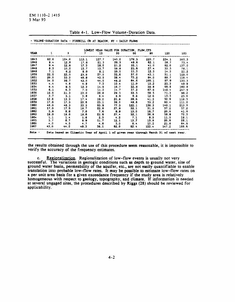
EM II1O-2 14155 Mar93

Table 4-1. Low-Flow Volume-Duration Data.

- VOLW-DURATION DATA - FISEKILL CR AT BSACON, NY - DAILY F~------ ----------.-------- -------- ------------- ----------- ------ --------------------------------

L~ST W VALUE FOS DURATION, F-, CFSYsAR 1 3 7 15 30 60 90 120 183------- -------- ------- -------- --------- ------- -.----- --------------- ------- ----.-.-------------1945 92.01946 9.41947 0.41948 8.31949 7.11950 22.01951 20.01952 34.01953 4.41954 8.41955 6.11956 19.01957 3.71956 12.01959 17.01060 48.01961 17.01962 5.91963 19.01964 1.11965 5.71966 4.01967 43.0-------------------

104.012.612.810.28.2

22.033.339.74.89.56.3

21.35.1

13.317.368.317,06.6

19.01.46.74.5

44.0--------- -,

115.117.617.315.79.0

23.940. sh3. o4.9

12.37.0

23.05.6

17.420.653.319.77.0

19.61.89.94.7

49.3.--------- .

127.721.319.015.79.1

27.045.544.07.3

14.611.226.8

6.419.225.163.922.9

2:::

1;:;

5::;.-----.---

143.028.521.210.910.032.658.446.210.418.714.729.5

2:::39.077.527.9

9.927.44.2

12.15.0

62.0----------,

179.540.832.121.611.337.073,264.611.022.937.253.59.8

29.649.8

122.132.115.032.17.1

13.76.4

S2.4----------

220.762.141.027.412.343.184.0

100.115.239.067.659.512.641.553.2

136.331.916.736.09.0

15.813.2

122.4-.--------

254.158.762.033.514.351.188.797.925.399.6

140.471.315.550.960.4

149.137.220.658.911.520.621.8

147.2----------

305.375.4

137.078.121.2

119.0116.4135.349.9

160.8247.9

98.225.6

118.5111.0213.957.241.970.519.126.164.8

108.6------

note - Data bud on Climtic Yeu of April 1 of given you through March 31 .af next year.

the results obtained through the use of this procedure seem reasonable, it is impossible toverify the accuracy of the frequency estimates.

c. Re~ionalization. Regionalization of low-flow events is usually not verysuccessful. The variations in geologic conditions such as depth to ground water, size ofground water basin, permeability of the aquifer, etc., are not easily quantifiable to enabletranslation into probable low-flow rates. It may be possible to estimate low-flow rates ona per unit area basis for a given exceedance frequency if the study area is relativelyhomogeneous with respect to geology, topography, and climate. If information is neededat several ungaged sites, the procedures described by Riggs (28) should be reviewed forapplicability.

4-2

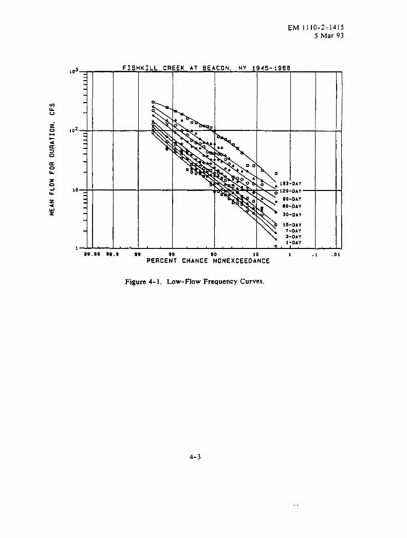
EM 1110-2-14155 Mar 93

~03

,~2_ _

lo—- -

l— —

FIS} EK AT BEACON, NY 1945-1960

k

IF \7-DAY3-OAY

—99.99 69.9 9s 90 so 10 1 .1 .01

PERCENT CHANCE NONEXCEEOANCE

Figure 4-1. Low-Flow Frequency Curves.

4-3

EM 1110-2-14155 Mar 93

CHAPTER5

PRECIPITATION FREQUENCY ANALYSIS

5-1. Ge neral Proced es The computation of frequency curves of stationprecipitation can be ~~ne”by procedures similar to those for streamflow analysis describedin the preceding sections. Both graphical and analytical methods may be used. Inprecipitation studies, however, instantaneous peak intensities are ordinarily not analyzedsince they are virtually impossible to measure and are of little practical value. Cumulativeprecipitation amounts for specified durations are commonly analyzed, mostly for durationsof less than 3 or 4 days. The National Weather Service has traditionally used theFisher-Tippett Type I frequency distribution with Gumbel’s fitting procedure. Thelogarithmic normal, pearson Type III and log-Pearson Type III (Figure 5-1) distributions,have also been used with success. Station precipitation alone is not adequate for mosthydrologic studies, and some method of evaluating the frequency of simultaneous ornear-simultaneous precipitation over an area is necessary. Procedures for obtainingdepth-area frequency curves are usually available from National Weather Servicepublications (references are given in subsequent paragraphs).

3s

ui= WSU. ;

90 se 10 1 .1 .01Pmrc=nt Cknce ExceeMnce

Figure 5-1. Frequency Curve, Annual Precipitation.

5-1

EM II1O-2-14155 Mar 93

5-2. Available~onal Inform ation. Where practical, use should be made of previousprecipitation- frequency-duration studies that have incorporated regional information. Fordurations of 5 to 60 minutes in an area generally east of 105th meridian, see Hydro-35 (9).For durations of 2 to 24 hours in the same area see Technical Paper 40 (10). Because ofthe orographic effect, individual reports have been prepared for each of the 11 westernstates (24). These reports have maps for 6- and 24-hour durations with extrapolationprocedures to obtain durations less than 6 hours. Longer duration events (2- to 10-days)are presented in references (21), (22) and (23).

5-3. Derivation of Flood-Freauenc v Relations from Prec iDitat ion.

ADD catIi ion. Precipitation-frequency relations are often used to deriveflood:frequency relations where inadequate flow data are available or where existing (orproposed) watershed changes have modified (or will modify) the rainfall-runoffrelationships. Guidelines for developing runoff frequencies from precipitationfrequencies are presented in references ( 10) and (44). Flood-frequency curves developedby rainfall-runoff procedures often have less variance (lower standard deviation) thanthose developed from annual flood peaks. This results because not all the possible lossrates for a given magnitude of precipitation are modeled. If extensive use will be made offrequency curves derived by rainfall-runoff modeling, an appropriate ratio adjustment forthe standard deviation should be developed for the region.

b. Calibration. Reference (44) describes the procedures involved in calibrating aHEC- 1 model to a flow-frequency curve based either on gaged data from a portion of thebasin or on regional flood-frequency relations. The coefficients from the calibratedmodel must be consistent with those from nearby basins that have also been modeled. Itmust be remembered that a frequency curve computed from observed flood peaks is basedon a relatively small sample. It is possible that the flow-frequency curve derived fromprecipitation-frequency data is more representative of the population flow-frequencycurve than the one computed from the statistics of the observed flood peaks. But, thereare also errors in calibrating the model and establishing loss rates approximate with thedifferent frequency events. Therefore, the derivation of frequency relations byrainfall-runoff modeling requires careful checking for consistency at every step.

c. ~ial Duration The precipitation-frequency relations presented in the NationalWeather Service publica~ions represent all the events above a given magnitude; therefore,these relations are from a partial-duration series. The resulting flood frequency relationsmust be adjusted if an annual peak flood frequency relationship is desired. Or, moretypically, the partial-duration series precipitation estimates are adjusted to representannual series estimates prior to use.

5-2

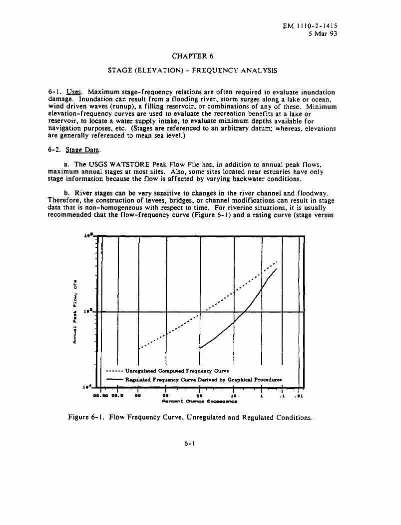
EM 1110-2-14155 Mar 93

CHAPTER6

STAGE (ELEVATION) - FREQUENCY ANALYSIS

6-1. ~. Maximum stage-frequency relations are often required to evaluate inundationdamage. Inundation can result from a flooding river, storm surges along a lake or ocean,wind driven waves (runUp), a filling reservoir, or combinations of any of these. Minimumelevation-frequency curves are used to evaluate the recreation benefits at a lake orreservoir, to locate a water supply intake, to evaluate minimum depths available fornavigation purposes, etc. (Stages are referenced to an arbitrary datum; whereas, elevationsare generally referenced to mean sea level.)

6-2. staee Data.

a. The USGS WATSTORE Peak Flow File has, in addition to annual peak flows,maximum annual stages at most sites. Also, some sites located near estuaries have onlystage information because the flow is affected by varying backwater conditions.

b. River stages can be very sensitive to changes in the river channel and floodway.Therefore, the construction of levees, bridges, or channel modifications can result in stagedata that is non-homogeneous with respect to time. For riverine situations, it is usuallyrecommended that the flow-frequency curve (Figure 6-1 ) and a rating curve (stage versus

:11

----.

. .

,“.“

.“.“

4

.“.“

7

------ Unre@sted Computed Frequency Curve

I — RegulatedFrequency Curve Derived by Graphlcel Procedures

99.99 Os. s Ss so se 10 1 .“1 .01P9mmt -cm I?xw-dem

Figure 6-1. Flow Frequency Curve, Unregulated and Regulated Conditions.

6-1

EM 1110-2-14155 Mar 93

flow, Figure 6-2) beusedto derive astage-frequency curve (Figure 6-3). Astage-frequency curve derived by indirect methods may not always represent the truerelation if the site is subject to occasional backwater situations. Backwater conditions canbe caused by an ice jam, a debris flow, a downstream reservoir, a high tide, a storm surge,or a downstream river. A coincident frequency analysis may be necessary to obtain anaccurate estimate of the stage-frequency relationship (see Chapter 11).

c. Usually the annual extreme value is used to develop an annual series, but aseasonal series or a partial-duration series could be developed if needed. Caution must beused in selecting independent events. Independent events are not easily determined if theevents are elevations of a large lake or reservoi~ in fact even the annual events may besignificantly correlated.

6-3. Freaue ncv Distribution. Stage (elevation) data are usually not normally distributed(not a straight line on probability paper). Therefore, an analytical analysis should ~ bemade without observing the fit to the plotted points (see Chapter 2). Usually, anarithmetic-probability plot is appropriate for stage or elevation data, but there may besituations where a logarithmic or some other appropriate transformation will make the plotmore nearly linear. When drawing the curve, known constraints must be kept in mind.As an example, the bottom elevation, bankfull stage, levee heights, etc., would beimportant for a riverine site. The minimum pool, top of conservation pool, top of floodcontrol pool, spillway elevation, operation criteria, etc., all influence theelevation-frequency relation for a reservoir, Figure 6-4. These constraints usually makethese frequency relations very non-linear. Extrapolation of stage (elevation) frequencyrelations must be done very cautiously. Again, any constraints acting on the relationsmust be used as a guide in drawing the curves. Historical information can be incorporatedinto a graphical analysis of stage (elevation) data by use of the procedures in Appendix 6of Bulletin 17B (ref 46). The statistical tests (Appendix 4, ref 46) to screen for outliersshould N be applied unless the stage (elevation) data can be shown to nearly fit a normaldistribution.

6-4. Exnected Proba bilitv. The expected probability adjustment should ~ be made tofrequency relations derived by graphical methods. The median plotting position formulacorrects for the bias caused by small sample sizes, The expected probability adjustmentshould be made when an analytical method is used directly to derive the stage (elevation)frequency relation. The expected probability adjustment should be made to theflow-frequency curve when the stage (elevation) frequency relation is derived indirectly,

6-2

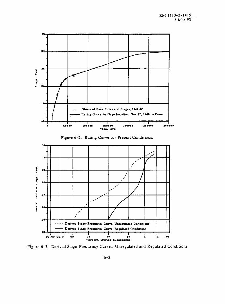
EM 1110-2-14155 Mar 93

Obaemad Peak F1OWSand Stages, 1949-8S

— Rating Curve for Gage Locstion, Nov 12, 1948 to Praaent

e seooe zeeooa 160800 aoeoso a6eo@e 3oeeeo

Figure 6-2. Rating Curve for Present Conditions.

3a

.“●.-

. .4

.

26, i

,,

,,

,,

..

.“,

,.-. .

..

..

.,

,,

----- Derived Stage-Frequency Curve, Unregulated Conditions

— Derived St~e-Frequency Curve, Regulated Conditionsla

I i 1 I 1 ISS: = S6-. S 6S so 60 l-a 1 .1 .s1

Pmmmnt ChMm E xrnmd~=

Figure 6-3. Derived Stage-Frequency Curves, Unregulated and Regulated Conditions

6-3

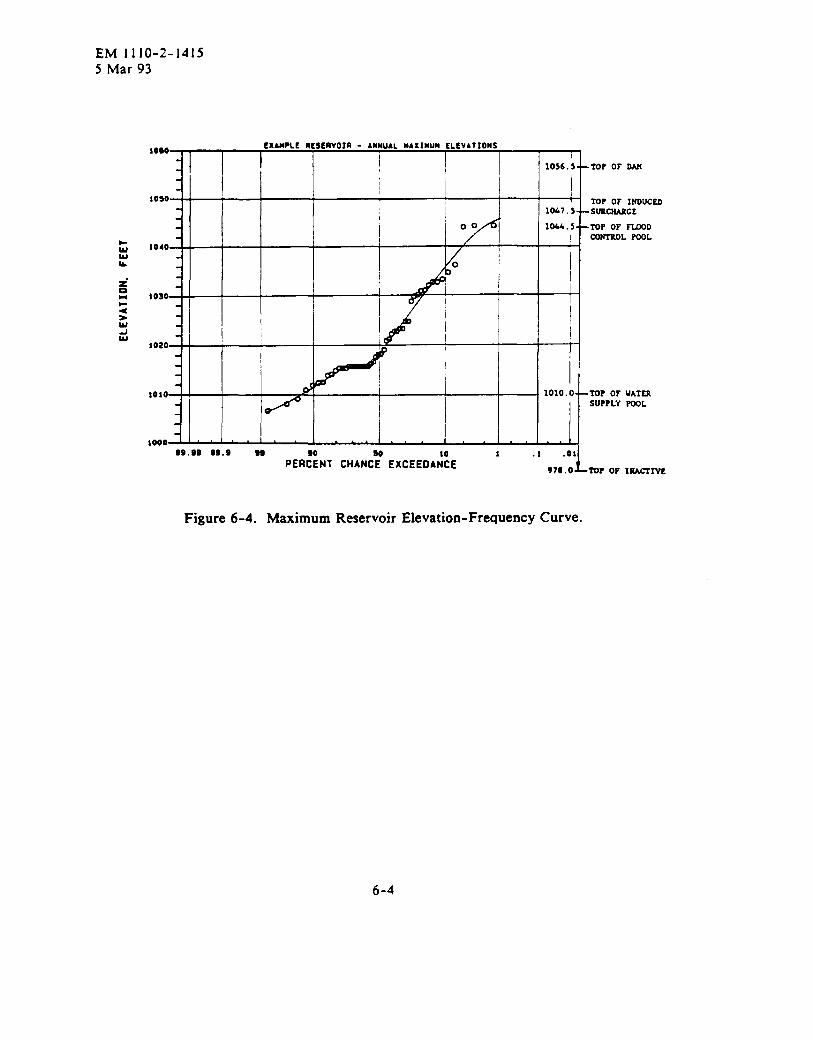
EM 1110-2-14155 Mar 93

i 060CXAMPLF mtSERVO19 - ANNUAL MAXIMUM ELEVATIONS

~I

10S6.S--TO? OF OAN

!toso

1 ! TOP OF INDUC~lu7.5- - SURCliARCE

loA6.5- -TOP OF WDI CONTROLPoOL

1040

to30I

1020J

I

tolo d 1010.0- -TOP OF UATSRSUPPLY POOL

1000 iS9. SS S9.9 2s 1 .1

PER:ENTCHANC; EXCEEDA;;E L

.01

978.0 TOP OF INA~Ivs

Figure 6-4. Maximum Reservoir Elevation-Frequency Curve.

6-4

EM 1110-2-14155 Mar 93

CHAPTER7

DAMAGE-FREQUENCY RELATIONSHIPS

7-1. Introduction.

a. There are three methods that may be used to compute average annual damage andare herein termed the historic method, the simulation method and the frequency method.If 50 years of damage information were available for an area that has remained inessentially the same land use with a reasonably constant level of economic activity,historic damage could be scaled to the present to account for price differences (inflation)and the average simply computed. This approach is termed the historic method and is themost direct but is seldom used because sufficient data usually do not exist and the land useand economic activity of an area are usually changing.

b. A hydrologic simulation model could be developed, or the historic record used,along with damage functions to generate a time trace of simulated damage. The averageof the time trace of damage would be the average annual damage. This would be termedthe “simulation” method. The simulation method has the advantage of permitting the useof complex damage functions that can consider more than a single parameter and thusenable a more accurate computation of damage. The disadvantage of this method is thatthe future floods are assumed to exactly duplicate the historic floods and no considerationgiven to the possibility of larger floods.

c. The most widely used approach within the Corps of Engineers is the frequencytechnique. This technique is described in detail in Section 7-2. This technique addressesthe disadvantages of the previous two methods, and yet is fairly easily applied.Experience in the development and application of damage functions is essential tocomputation of reasonable estimates. Care should be taken to assure the rating curve isnot looped so that discharge is a unique function of stage. Otherwise more complexfunctions that correctly relate stage and discharge should be developed and applied.Damage functions in agricultural areas are often a function of the season and the durationof flooding. Sensitivity analysis may be useful in determining the reliability of thecomputed expected annual damage considering the uncertainties involved.

7-2. Commutation of ExDected Annual Dama~e.

a. Figure 7-1 shows a schematic of the application of the three basic damageevaluation functions used to compute the expected value of the annual damage. The term“expected” is used rather than “average” because a frequency curve is used to represent thedistribution of future flood events and the expected value of damage is computed by thesummation of probability weighted estimates of damage.

b. The steps involved in determining the reduction in annual damage due to projectmeasures are:

(1) Develop the basic relationships (stage-damage, stage-discharge, anddischarge-exceedance frequency functions) for each index location for existingconditions.

7-1

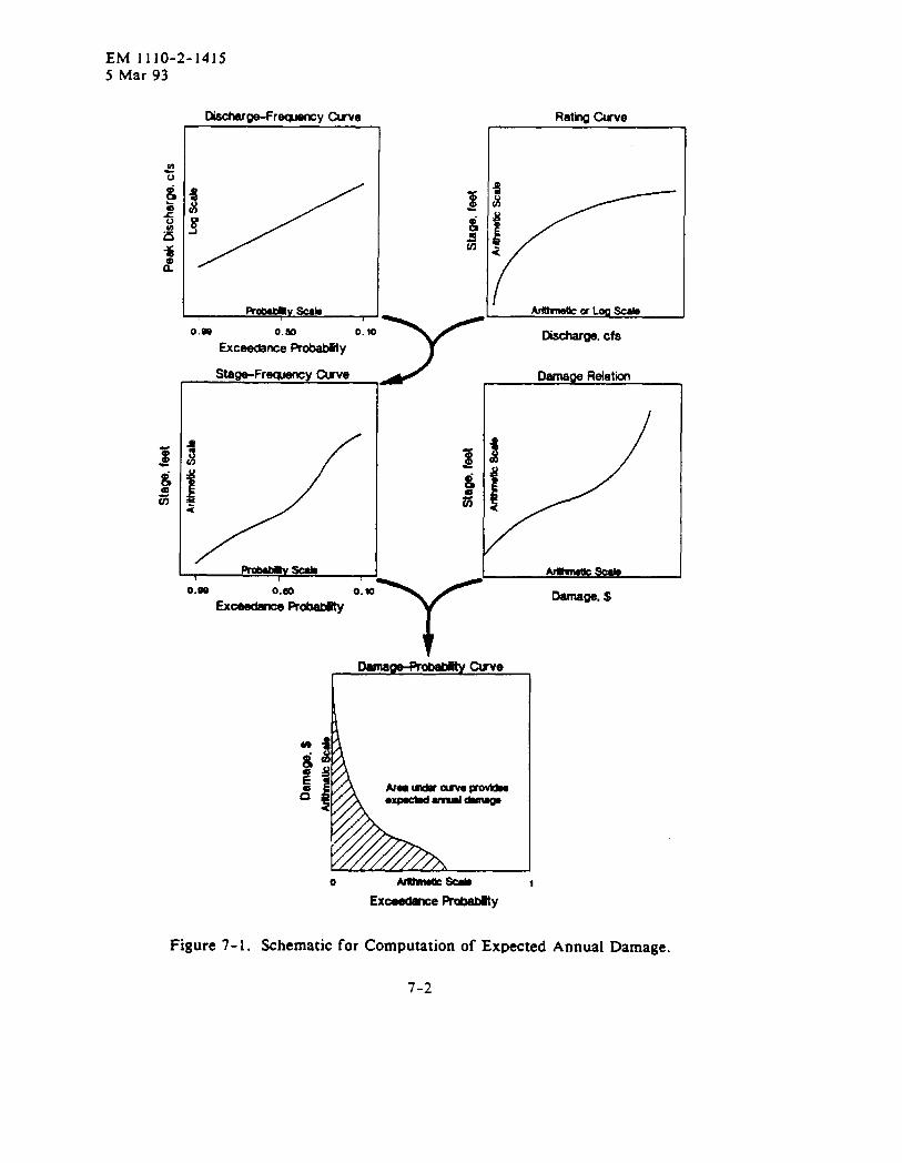
EM 1110-2-14155 Mar 93

Discharge-Fr~y Cuve Rati me

~~

Discharge,Cfs

Dmga Relatii

[

Figure 7-1. Schematic for Computation of Expected Annual Damage.

7-2

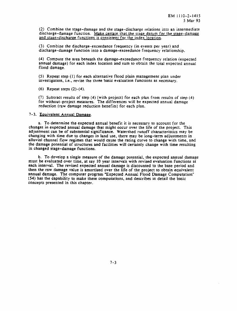
EM 1110-2-14155 Mar 93

(2) Combine the stage-damage and the stage-discharge relations into an intermediatedischarge-damage function. Make certain that the stage datum for the sta~e-dama~eand sta~e-dischar~e functions is consistent for the index location.

(3) Combine the discharge-exceedance frequency (in events per year) anddischarge-damage function into a damage-exceedance frequency relationship,

(4) compute the area beneath the damage-exceedance frequency relation (expectedannual damage) for each index location and sum to obtain the total expected annualflood damage.

(5) Repeat step (1) for each alternative flood plain management plan underinvestigation, i.e., revise the three basic evaluation functions as necessary.

(6) Repeat steps (2)-(4).

(7) Subtract results of step (4) (with project) for each plan from results of step (4)for without-project measures. The differences will be expected annual damagereduction (raw damage reduction benefits) for each plan.

7-3. Equivalent Annual Damaft~.

a. To determine the expected annual benefit it is necessary to account for thechanges in expected annual damage that might occur over the life of the project. Thisadjustment can be of substantial significance. Watershed runoff characteristics may bechanging with time due to changes in land use, there may be long-term adjustments inalluvial channel flow regimes that would cause the rating curve to change with time, andthe damage potential of structures and facilities will certainly change with time resultingin changed stage-damage functions.

b. To develop a single measure of the damage potential, the expected annual damagemust be evaluated over time, at say 10 year intervals with revised evaluation functions ateach interval. The revised expected annual damage is discounted to the base period andthen the raw damage value is amortized over the life of the project to obtain equivalentannual damage. The computer program “Expected Annual Flood Damage Computation”(54) has the capability to make these computations, and describes in detail the basicconcepts presented in this chapter.

7-3

EM 111O-2-I4155 Mar 93

CHAPTER8

STATISTICAL RELIABILITY CRITERIA

8-1. Obiectiv~. One principal advantage of analytical frequency analysis is that there aremeans for evaluating the reliability of the parameter estimates. This permits a morecomplete understanding of the frequency estimates and provides criteria fordecision-making. For instance, a common statistical index of reliability is the standarderror of estimate, which is defined as the root-mean-square error. In general, it isconsidered that the standard error is exceeded on the positive side one time out of sixestimates, and equally frequently on the negative side, for a total of one time in threeestimates. An error twice as large as the standard error of estimate is considered to beexceeded one time in 40 in either direction, for a total of one time in 20. Thesestatements are based on an assumed normal distribution of the errors; thus, they are onlyapproximate for other distributions of errors. Exact statements as to error probabilitymust be based on examination of the frequency curve of errors or the distribution of theerrors. Both the standard error of estimate and the confidence limits are discussed in thischapter.

8-2. Reliability of Freauencv Statistics. The standard errors of estimate of the mean,standard deviation, and skew coefficient, which are the principal statistics used infrequency analysis, are given by the following equations:

s~ = S/(N)fi (8-1)

Ss = S/(2N)% (8-2)

SG= (6N(N-1)/[(N-2)( N+l )(N+3)]}% (8-3)

where

s~ = the standard error of estimate for the mean

S5 = the standard error of estimate for the standard deviation

SG= the standard error for estimate for the skew coefficient, and S and N aredefined in Section 3-2.

These have been used to considerable advantage, as discussed in Chapter 9, in drawingmaps of mean, standard deviation and skew coefficient for regional frequency studies.

8-3. Reliability of Freaue cv Cu es The reliability of analytical frequencydeterminations can best be~llustr~t~d by establishing confidence limits. The error of theestimated value at a given frequency based on a sample from a normal distribution is afunction of the errors in estimating the mean and standard deviation. (Note that inpractical application there are errors introduced by not knowing the true theoreticaldistribution of the data, often termed model error.) Criteria for construction ofconfidence limits are based on the non-central tdistribution. Selected values are given inTable F-9. Using that appendix, the confidence limit curves shown on Figure 8- I

8-1

EM 1110-2-14155 Mar 93

were calculated. While the expected frequency is that shown by the middle curve, there isone chance in 20 that the true value for any given frequency is greater than that indicatedby the .05 curve and one chance in 20 that it is smaller than the value indicated by the .95curve. There are, therefore, nine chances in 10 that the true value lies between the .05and .95 curves. Appendix E and Example I in Appendix 12 of Bulletin 17B (40) provideadditional information and example computations.

o ObeeNed Annual Poeka— Computut Frequency Cuwe---- With Expectd Probability Adjustment

Confidence LimitCurvee

99:9a 99.9 !

+...........’

. . . . . . .

~,

&...,.,

..,’” ,P9’”

r

‘*-1968

,..’ ,

~

.U’”,, ..’/ . . ““

~+,..

,, //

/ +Qb

7- ,

Figure 8-1. Frequency Curve with Confidence Limit Curves.

8-2

EM 1110-2-14155 Mar 93

CHAPTER9

REGRESSION ANALYSIS AND APPLICATION TO REGIONAL STUDIES

9-1. Nature and At)Dlication.

a. General. Regression analysis is the term applied to the analytical procedure forderiving prediction equations for a variable (dependent) based on given values of one ormore other variables (independent). The dependent variable is the value sought and is tobe related to various explanatory variables which will be known in advance, and whichwill be physically related to the dependent variable. For example, the volume ofspring-season runoff from a river basin (dependent variable) might be correlated with thedepth of snow cover in the watershed (explanatory variable). Recorded values of suchvariables over a period of years might be graphed and the apparent relation sketched in byeye. However, regression analysis will generally permit a more reliable determination ofthe relation and has the additional advantage of providing a means for evaluating thereliability of the relation or of estimates based on the relation.

b. Def inition~. The function relating the variables is termed the “regressionequation,” and the proportion of the variance of the dependent variable that is explainedby the regression equation is termed the “coefficient of determination,” which is thesquare of the “correlation coefficient.” Correlation is a measure of the association betweentwo or more variables. Regression equations can be linear or curvilinear, but linearregression suffices for most applications, and curvilinear regression is therefore notdiscussed herein. Often a curvilinear relation can be linearized by using a logarithmic orother transform of one or more of the variables.

9-2. ~alculation of Regression EauationS.

a. ~imt)le Re~re ssion. In a simple regression (one in which there is only oneindependent, or explanatory, variable), the linear regression equation is written:

Y = a+bX (9-1)

in which Y is the dependent variable, X is the independent variable, “a” is the regressionconstant, and “b” is the regression coefficient. The coefficient “b” is evaluated from thetabulated data by use of the following equations

(9-2a)

or

b = RSY/SX (9-2b)

in which y is the deviation of a single value yi from the mean (~) of its series, x issimilarly defined, SYand SXare the respective standard deviations and R is computed by

9-1

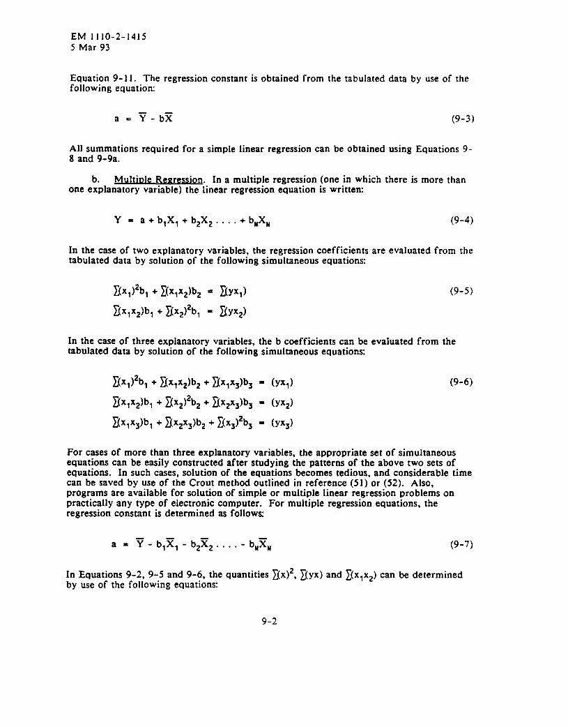
EM 1110-2-14155 Mar 93

Equation 9-11. The regression constant is obtained from the tabulated data by use of thefollowing equation:

All summations required for a simple linear regression can be obtained using Equations 9-8 and 9-9a.

b. Multinle Re~res sion. In a multiple regression (one in which there is more thanone explanatory variable) the linear regression equation is written

Y=a+blX1+ b2X2 . . ..+ bMXN (9-4)

In the case of two explanatory variables, the regression coefficients are evaluated from thetabulated data by solution of the following simultaneous equations

(9-5)fixl)zbl + ~(x1x2)b2 = ~(Yxl)

xx1x2)b1 + zx2)2b1 = XYX2)

In the case of three explanatory variables, the b coefficients can be evaluated from thetabulated data by solution of the following simultaneous equations

xx1)2b1+ x(x1x2)b2 + xx1x3)b3 = (Yxl) (9-6)

Ix1x2)b1 + Xx2)2b2 + Ex2x3)b3 = (YX2)

~(x1x~)bl + ~x2x3)b2 + ~x3)2b3 = (Yx~)

For cases of more than three explanatory variables, the appropriate set of simultaneousequations can be easily constructed after studying the patterns of the above two sets ofequations. In such cases, solution of the equations becomes tedious, and considerable timecan be saved by use of the Crout method outlined in reference (51) or (52). Also,programs are available for solution of simple or multiple linear regression problems onpractically any type of electronic computer. For multiple regression equations, theregression constant is determined as follows

a=~-bl%l-b2~2....-b~~~ (9-7)

In Equations 9-2, 9-5 and 9-6, the quantities 1(x)2, ~(yx) and ~(xlxz) can be determinedby use of the following equations:

9-2

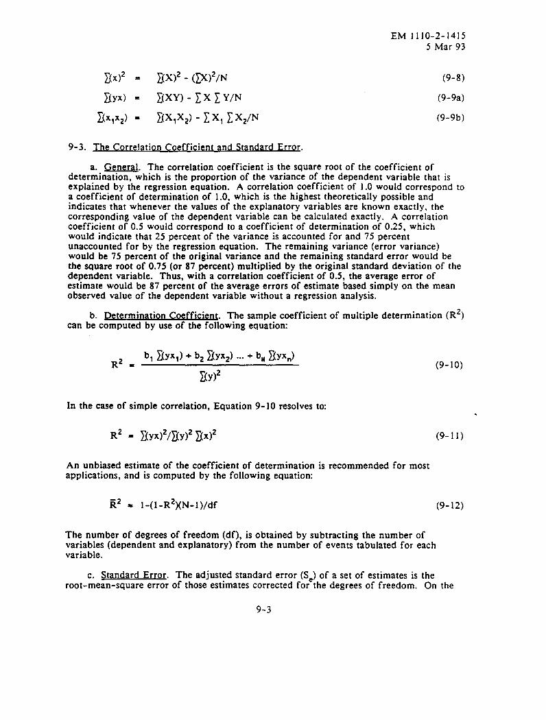
9-3.

EM 1110-2-14155 Mar93

(9-8)

(9-9a)

X(X1X2)= ~(x1x2)- zxl ~ X2/N (9-9b)

The Correlation Coefficient and Standard Error.

a. m. The correlation coefficient is the square root of the coefficient ofdetermination, which is the proportion of the variance of the dependent variable that isexplained by the regression equation. A correlation coefficient of 1.0 would corresponda coefficient of determination of 1.0, which is the highest theoretically possible andindicates that whenever the values of the explanatory variables are known exactly, thecorresponding value of the dependent variable can be calculated exactly. A correlationcoefficient of 0.5 would correspond to a coefficient of determination of 0.25, whichwould indicate that 25 percent of the variance is accounted for and 75 percentunaccounted for by the regression equation. The remaining variance (error variance)would be 75 percent of the original variance and the remaining standard error would be

to

the square root of 0.75 (or 87 &rcent) multiplied by the original standard deviation of thedependent variable. Thus, with a correlation coefficient of 0.5, the average error ofestimate would be 87 percent of the average errors of estimate based simply on the meanobserved value of the dependent variable without a regression analysis.

b. Dete rmination Coefficien~. The sample coefficient of multiple determination (Rz)can be computed by use of the following equation:

bl ~Yxl) + b2 ~YX2) ... + bMfiYxn)R2 = (9-lo)

XY)2

In the case of simple correlation, Equation 9-10 resolves to

(9-11)R2 = ~(yX)2/~(y)2 ~X)2

An unbiased estimate of the coefficient of determination is recommended for mostapplications, and is computed by the following equation:

(9-12)R2 = l-(1 -R2)(N-1)/df

The number of degrees of freedom (df), is obtained by subtracting the number ofvariables (dependent and explanatory) from the number of events tabulated for eachvariable.

c. Standard Error. The adjusted standard error (S=) of a set of estimates is theroot-mean-square error of those estimates corrected for the degrees of freedom. On the

9-3

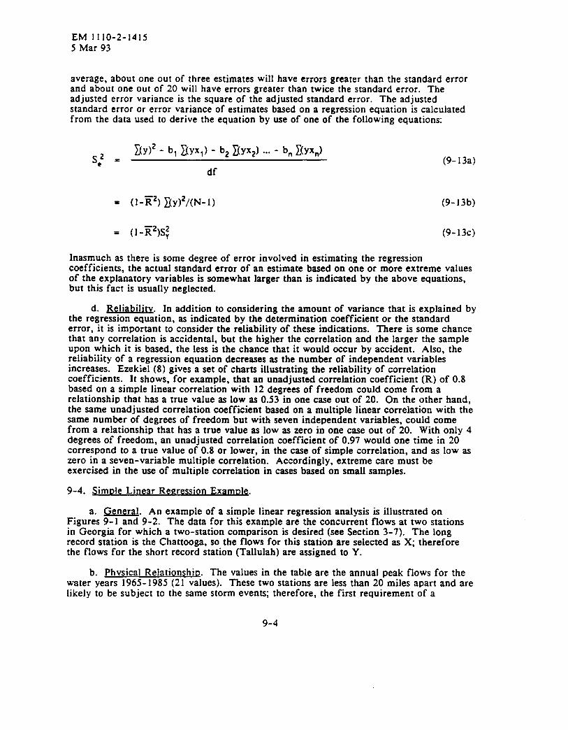
EM 1110-2-14155 Mar 93

average, about one out of three estimates will have errors greater than the standard errorand about one out of 20 will have errors greater than twice the standard error. Theadjusted error variance is the square of the adjusted standard error. The adjustedstandard error or error variance of estimates based on a regression equation is calculatedfrom the data used to derive the equation by use of one of the following equations:

s: .

a

Inasmuch ascoefficients.

~(Y)2- b, ~(Yxl) - b2 XYX2)...- bn ~(Yxn)(9-13a)

df

(1-~2) ~(y)2/(N- 1) (9-13b)

(1-F2)S; (9-13C)

there is some degree of error involved in estimating the regressionthe actual standard error of an estimate based on one or more extreme values

of the explanatory variables is somewhat larger than is indicated by the above equations,but this fact is usually neglected.

d. ~eliabilitv. In addition to considering the amount of variance that is explained bythe regression equation, as indicated by the determination coefficient or the standarderror, it is important to consider the reliability of these indications. There is some chancethat any correlation is accidental, but the higher the correlation and the larger the sampleupon which it is based, the less is the chance that it would occur by accident. Also, thereliability of a regression equation decreases as the number of independent variablesincreases. Ezekiel (8) gives a set of charts illustrating the reliability of correlationcoefficients. It shows, for example, that an unadjusted correlation coefficient (R) of 0.8based on a simple linear correlation with 12 degrees of freedom could come from arelationship that has a true value as low as 0.53 in one case out of 20. On the other hand,the same unadjusted correlation coefficient based on a multiple linear correlation with thesame number of degrees of freedom but with seven independent variables, could comefrom a relationship that has a true value as low as zero in one case out of 20. With only 4degrees of freedom, an unadjusted correlation coefficient of 0.97 would one time in 20correspond to a true value of 0.8 or lower, in the case of simple correlation, and as low aszero in a seven-variable multiple correlation. Accordingly, extreme care must beexercised in the use of multiple correlation in cases based on small samples.

9-4. simD1e Linear Regression ExamDl~.

a. -. An example of a simple linear regression analysis is illustrated onFigures 9-1 and 9-2. The data for this example are the concurrent flows at two stationsin Georgia for which a two-station comparison is desired (see Section 3-7). The longrecord station is the Chattooga, so the flows for this station are selected as X; thereforethe flows for the short record station (Tallulah) are assigned to Y.

b. Phvsical Relationship. The values in the table are the annuaJ peak flows for thewater years 1965-1985 (21 values). These two stations are less than 20 miles apart and arelikely to be subject to the same storm events; therefore, the first requirement of a

9-4

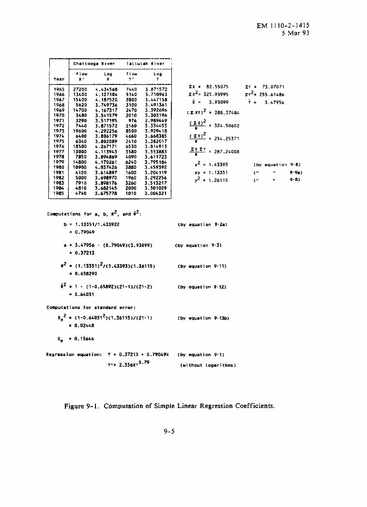
EM 1110-2-14155 Mar 93

.———Chattooga River Iallulch River

—------

F1OU Log F(OW Log

Year x’ x 71 Y

1965 27200 4.434568 7460 3.8715721966 13400 4.127104 5140 3.7109631967 15400 4.187520 2800 3.4471581968 5620 3.749736 3100 3.4913611969 14700 4.167317 2470 3.3926961970 3480 3.541579 2070 3.3031961971 3290 3.517195 976 2.9894491972 7440 3.871572 2160 3.3344531973 19600 4.292256 8500 3.9294181974 6400 3.806179 4660 3.6683851975 6340 3.802089 2410 3.3820171976 18500 4.267171 6530 3.8149131977 13000 4.113943 3580 3.5538831978 7850 3.894869 4090 3.6117231979 14800 4.170261 6240 3.7951841980 10900 4.037426 2880 3.4593921981 4120 3.614897 1600 3.2041191982 5000 3.698970 t960 3.2922561983 7910 3.898176 3260 3.5132171984 4810 3.682145 2000 3.3010291985 4740 3.675778 1010 3.006321

b z j.j3351/I.&33922

= 0.79049

a s 3.47956 - (0.79069)(3.93099)

= 0.37213

R2 ■ (1.13351 )2/(1.43393)(1.36115)

■ 0.658290

Ez=l - (1-0.65892)(21-1)/(21-2)

= 0.64031

Contputationa for standard ●rror:

S 2 = (1-0.640312 )(1.36115 )/(21-1)●

= 0.02648

se = 0.15&6

Regression ●quation: Y = 0.37213 + 0.79049x

y,= 2_356~,0.79

XX = 82.55075 ZY = 73.07071

XX2= 325.93995 ZY2= 255.61486

i= 3.93099 i= 3.47956

(X XY)2 = 288. Z748L

(Z X)2— = 324.50602n

( ZY)2—-— ,N 254.25371

xx ZY——. .N 287.26008

X2 = 1.43393 (by ●quation 9-8)

Xy = 1.13351 (,, ,, 9.9a)

Y2 = 1.26115 (4, ,8 9-8)

(by ●quation 9-2a)

(by ●quation 9-3)

(by ●quation 9.11)

(by ●quation 9-12)

(by equation 9-13b)

(by equation 9-1)

(without logarithms)

Figure 9-1. Computation of Simple Linear Regression Coefficients.

9-5

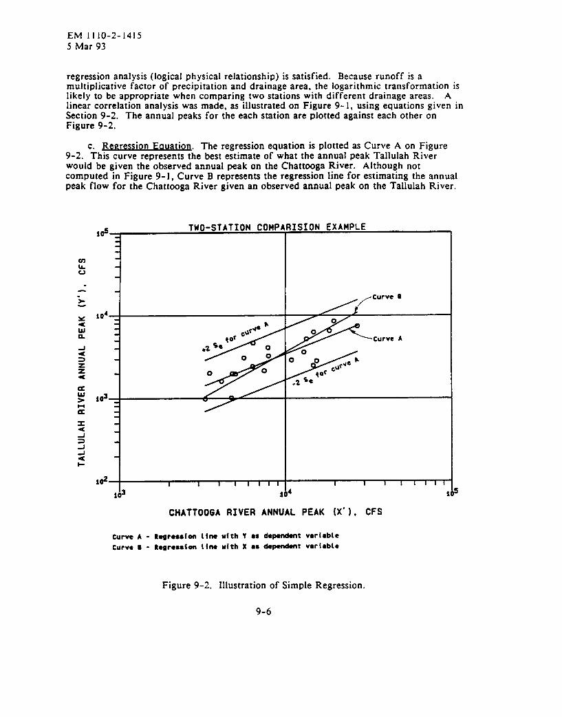
EM 1110-2-14155 Mar 93

regression analysis (logical physical relationship) is satisfied. Because runoff is amultiplicative factor of precipitation and drainage area, the logarithmic transformation islikely to be appropriate when comparing two stations with different drainage areas. Alinear correlation analysis was made, as illustrated on Figure 9-1, using equations given inSection 9-2. The annual peaks for the each station are plotted against each other onFigure 9-2.

c. Re~ress ion Eauation. The regression equation is plotted as Curve A on Figure9-2. This curve represents the best estimate of what the annual peak Tallulah Riverwould be given the observed annual peak on the Chattooga River. Although notcomputed in Figure 9-1, Curve B represents the regression line for estimating the annualpeak flow for the Chattooga River given an observed annual peak on the Tallulah River.

~&3 *~4

CHATTO06A RIVER ANNUALPEAK (X’

curve A - Regression 1tne with ~ ss dependent vsriabke

Curve B - Regression 1 ine uith X ss dependent verieble

Figure 9-2. Illustration of Simple Regression.

9-6

EM 1110-2-14155 Mar 93

d. Reliability. In addition to the curve of best fit, an approximate confidenceinterval can be established at a distance of plus and minus 2 standard errors from CurveA. Because logarithms are used in the regression analysis, the effect of adding (orsubtracting) twice the standard error to the estimate is equivalent to multiplying (ordividing) the annual peak values by the antilogarithm of twice the standard error. In thiscase, the standard error is 0.156, and the antilogarithm of twice this quantity is 2.05.Hence, values of annual peak flow represented by the confidence interval curves are thoseof Curve A multiplied and divided respectively by 2.05. There is a 95 percent chance thatthe true value of the dependent variable (Y) for a single observed independent value (X)will lie between these limits. The confidence interval is not correct for repeatedpredictions using the same sample (6).

9-5. Factors ResDonsible fo r Nondete rmination.

a. -. Factors responsible for correlations being less than 1.0 (perfectcorrelation) consist of pertinent factors not considered in the analysis and of errors in themeasurement of those factors considered. If the effect of measurement errors isappreciable, it is possible in some cases to evaluate the standard error of measurement ofeach variable (see Paragraph 9- 3c) and to adjust the correlation results from such effects.

b. Measurem ent Errors. If an appreciable portion of the variance of Y (dependentvariable) is attributable to measurement errors and these errors are random, then theregression equation would be more reliable than is indicated by the standard error ofestimate computed from Equation 9-13. This is because the departure of some of thepoints from the regression line on Figure 9-2 is artificially increased by measurementerrors and therefore exaggerates the unreliability of the regression function. In such acase, the curve is generally closer to the true values than to the erroneous observed values.Where there is large memurement error of the dependent variable, the standard error ofestimate should be obtained by taking the square root of the difference of the errorvariance obtained from Equation 9-13 and the measurement error variance. If well overhalf of the variance of the points from the best-fit line is attributable to measurementerror in the dependent variable, then the regression line would actually yield a betterestimate of a value than the original measurement. If appreciable errors exist in thevalues of an explanatory variable, the regression coefficient and constant will be affected,and erroneous estimates will result. Hence, it is important that values of the explanatoryvariables be accurately determined, if possible.

c. Other Factorq. In the example used in Section 9-4 there may well be factorsresponsible for brief periods of high intensities that do not contribute appreciably toannual precipitation. Consequently, some locations with extremely high mean annualprecipitation may have maximum short-time intensities that are not correspondingly high,and vice versa. Therefore, the station having the highest mean annual precipitation wouldnot automatically have the highest short-time intensity, but would in general havesomething less than this. On the other hand, if mean annual precipitation were made thedependent variable, the station having the highest short-time intensity would be expectedto have something less than the highest value of mean annual precipitation. Thus, byinterchanging the variables, a change in the regression line is effected. Curve B of Figure9-2 is the regression curve obtained by interchanging the variables Y and X. As there is aconsiderable difference in the two regression curves, it is important to use the variablewhose value is to be calculated from the regression equation as the dependent variable in

those cases where important factors have not been considered in the analysis.

9-7

EM 1110-2-14155 Mar 93

d. Avera~e SloD~. If it is obvious that all of the pertinent variables are included inthe analysis, then the variance of the points about the regression line is due entirely tomeasurement errors, and the resulting difference in slope of the regression lines is entirelyartificial. In cases where all pertinent variables are considered and most of themeasurement error is in one variable, that variable should be used as the dependentvariable. Its errors will then not affect the slope of the regression line. In other caseswhere all pertinent variables are considered, an average slope should be used. An averageslope can be obtained by use of the following equation

b = SY/SX (9-14)

9-6. ~.

a. H. An example of a multiple linear regression analysis is illustrated onFigure 9-3. In this case, the volume of spring runoff is correlated with the waterequivalent of the snow cover measured on April 1, the winter low-water flow (index ofground water) and the precipitation falling on the area during April. Here again, it wasdetermined that logarithms of the values would be used in the regression equation.Although loss of 4 degrees of freedom of 12 available, as in this case, is not ordinarilydesirable, the adjusted correlation coefficient attained (0.94) is particularly high, and theequation is consequently fairly reliable. The computations in Figure 9-3 were made withthe HEC computer program MLRP (reference 50).

b. Lo~arithmic Transformat ion. In determining whether logarithms should be usedfor the dependent variable as above, questions such as the following should be considered“Would an increase in snow cover contribute a greater increment to runoff underconditions of high ground water (wet ground conditions) than under conditions of lowground water?” If the answer is yes, then a logarithmic dependent variable (by which theeffects are multiplied together) would be superior to an arithmetic dependent variable (bywhich the effects are added together). Logarithms should be used for the explanatoryvariables when they would increase the linearity of the relationship. Usually logarithmsshould be taken of values that have a natural lower limit of zero and a natural upper limitthat is large compared to the values used in the study.

c. Fun ction of Multit)le Regress ion. It should be recognized that multiple regressionperforms a function that is difficult to perform graphically. Reliability of the results,however, is highly dependent on the availability of a large sampling of all importantfactors that influence the dependent variable. In this case, the standard error of anestimate as shown on Figure 9-3 is approximately 0.038, which, when added to alogarithm of a value, is equivalent to multiplying that value by 1.09. Thus, the standarderror is about 9 percent, and the 1-in-20 error is roughly 18 percent. As discussed inParagraph 9-3d, however, the calculated correlation coefficient may be accidentally high.

9-7. Partial Correlation. The value gained by using any single variable (such as Aprilprecipitation) in a regression equation can be measured by making a second correlationstudy using all of the variables of the regression equation except that one. The loss incorrelation by omitting that variable is expressed in terms of the partial correlationcoefficient. The square of the partial correlation coefficient is obtained as follows:

9-8

EM 1110-2-14155 Mar 93

INPUT DATA

00s No

123456789

101112

OBSID

19361937193879391940194119427943194419.4519461947

STATISTICS OF OATA

VARIABLE

LOG SNO

LOG W

LOG PRCP

LOG Q

LOG Q

.939

.9451.052

.744

.6661.0811.060.8921.021.920.755.960

AVERAGE

.2960

.4005

.9421

.9196

LOG SNO

.399

.343

.369

.266

.181

.297

.2W

.354

.295

.321

.168

.280

VARIANCE

.0050

.0028

.0572

.0181

UNBIASED CORRELATION COEFFI Cl ENTS (R2

VARIABLE LOG SNO LOG GW LOG PRCP

LOG SNO 1.0000 .0000

LOG W .0000 1.0000

LOG PRCP -.0459 .127s

LOG Q .6308 .4170

REGRESSION RESULTS

INOEPENOENT REGRESSION

VARIABLE COEFFICIENT

LOG SNO 1.621806LOG GU 1.012912

LOO PRCP .2~390

REGRESSION R

CONSTANT SWARE

-.223698 .9437

-.0459.127s

1.0000.2011

LOG GkJ LOG PRCP

.325 .710

.385 .634

.408 .886

.428 .581

.316 1.027

.460 1.315

.511 1.097

.379 .707

.395 1.240

.376 1.091

.413 1.038

.410 .979

STANDARDOEVIATIDN

.0704

.0531

.2392

.1346 DEPENOENT

LOG Q

.6308

.6170

.20111.0000

PARTIAL

DETERMINATION

COEFFICIENT

.9106

.6816

.7451

UNBIASEO STANDARD

R ERRU OF

SWARE ESTIMATE

.9226 .0375

VARIABLE

Figure 9-3. Example Multiple Linear Regression Analysis.

9-9

EM 1110-2-14155 Mar 93

rY:.12= 1 - (1-Ry:123)/( 1-R;12) (9-15)

in which the subscript to the left of the decimal indicates the variable whose partialcorrelation coefficient is being computed, and the subscripts on the right of the decimalindicate the independent variables. An approximation of the partial correlation cansometimes be made by use of beta coefficients. After the regression equation has beencalculated, beta coefficients are very easy to obtain by use of the following equation:

P. = bnSJSY (9-16)

The beta coefficients of the variables are proportional to the influence of each variable onthe result. While the partial correlation coefficient measures the increase in correlationthat is obtained by addition of one more explanatory variable to the correlation study, thebeta coefficient is a measure of the proportional influence of a given explanatory variableon the dependent variable. These two coefficients are related closely only when there isno interdependence among the various explanatory variables. However, some explanatoryvariables naturally correlate with each other, and when one is removed from the equation,the other will take over some of its weight in the equation. For this reason, it must bekept in mind that beta coefficien~ indicate partial correlation only approximately.

9-8. V rifi i~~. Acquisition of basic data after a regressionanalysis has been completed will provide an opportunity for making a check of the results.This is done simply by comparing the values of the dependent variable observed, withcorresponding values calculated from the regression equation. The differences are theerrors of estimate, and their root-mean-square is an estimate of the standard error of theregression-equation estimates (Paragraph 9-3). This standard error can be compared tothat already established in Equation 9-13. If the difference is not signi~lcant, there is noreason to suspect the regression equation of being invalid, but if the difference is large,the regression equation and standard error should be recalculated using the additional dataacquired.

9-9. ~ Techniques. Where the relationships among variables usedin a regression analysis are expected to be curvilinear and a simple transformation cannotbe employed to make these relationships linear, graphical regression methods may proveuseful. A satisfactory graphical analysis, however, requires a relatively large number ofobservations and tedious computations. The general theory employed is similar to thatdiscussed above for linear regression. Methods used wiil not be discussed herein, but canbe found in references 8 and 27.

9-10. Practical G uideline$. The most important thing to remember in makingcorrelation studies is that accidental correlations occur frequently, particularly when thenumber of observations is small. For this reason, variables should be correlated only whenthere is reason to believe that there is a physical relationship. It is helpful to makepreliminary examination of relationships between two or more variables by graphicalplotting. This is particularly helpful for determining whether a relationship is linear andin selecting a transformation for converting curvilinear relationships to linearrelationships. It should also be remembered that the chance of accidentally high

9-1o

EM 1110-2-14155 Mar 93

correlation increases with the number of correlations tried. If a variable being studied istested against a dozen other variables at random, there is a chance that one of these willproduce a good correlation, even though there may be no physical relation between thetwo. In general, the results of correlation analyses should be examined to assure that thederived relationship is reasonable. For example, if streamflow is correlated withprecipitation and drainage area size, and the regression equation relates streamflow tosome power of the drainage area greater than one, a maximum exponent value of oneshould be used, because the flow per square mile usually does not increase with drainagearea when other factors remain constant.

9-11. Re~ional Freauencv Analvsi$.

a. -. In order to improve flood frequency estimates and to obtain estimatesfor locations where runoff records are not available, regional frequency studies may beutilized. Procedures described herein consist of correlating the mean and standarddeviation of annual maximum flow values with pertinent drainage basin characteristics byuse of multiple linear regression procedures. The same principles can be followed usinggraphical frequency and correlation techniques where these are more appropriate.

b. Freauencv Statistic~. A regional frequency correlation study is based on the twoprincipal frequency statistics: the mean and standard deviation of annual maximum flowlogarithms. Prior to relating these frequency statistics to drainage basin characteristics, itis essential that the best possible estimate of each frequency statistic be made. This isdone by adjusting short-record values by the use of longer records at nearby locations.When many stations are involved, it is best to select long-record base stations for eachportion of the region. It might be desirable to adjust the base station statistics by use ofthe one or two longest-record stations in the region, and then adjust the short-recordstation values by use of the nearest or most appropriate base station. Methods of adjustingstatistics are discussed in Section 3-7.

c. ~raina~e-Basin Charact eristic~. A regional analysis involves the determination ofthe main factors responsible for differences in precipitation or runoff regimes betweendifferent locations. This would be done by correlating important factors with thelong-record mean and with the long-record standard deviation of the frequency curve foreach station (the long-record values are those based on extension of the records asdiscussed in Section 3-7). Statistics based on precipitation measurements in mountainousterrain might be correlated with the following factors:

- Elevation of station

- General slope of surrounding terrain

- Orientation of that slope

- Elevation of windward barrier

- Exposure of gage

- Distance of leeward controlling ridge

9-11

EM 1110-2-14155 Mar 93

Statistics based on runoff measurements might be correlated with the following factors:

d.

Drainage area (contributing)

Stream length

Slope of drainage area or of main channel

Surface storage (lakes and swamps)

Mean annual rainfall

Number of rainy days per year

Infiltration characteristics

Urbanized Area

Linear RelationshiD$. In order to obtain satisfactory results using multiple linearregression techniques, all variables must be expressed so that the relation between theindependent and any dependent variable can be expected to be linear, and so that theinteraction between two independent variables is reasonable. An illustration of the firstcondition is the relation between rainfall and runoff. If the runoff coefficient is sensiblyconstant, as in the case of urban or airport drainage, then runoff can be expected to bear alinear relation to rainfall. However, in many cases initial losses and infiltration lossescause a marked curvature in the relationship. Ordinarily, it will be found that thelogarithm of runoff is very nearly a linear function of rainfall, regardless of loss rates,and in such cases, linear correlation of logarithms would be most suitable, An illustrationof the second condition is the relation between rainfall, D, drainage area, A, and runoff,Q. If the relation used for correlation is as follows:

Q = aD+bA+c (9-17)

then it can be seen that one inch change in precipitation would add the same amount offlow, regardless of the size of drainage area. This is not reasonable, but again atransformation to logarithms would yield a reasonable relation

log Q=dlog D+elog A+logf (9-18)

or transformed

Q= fDdAe (9-19)

Thus, if logarithms of certain variables are used, doubling one independent quantity willmultiply the dependent variable by a fixed ratio, regardless of what fixed values the otherindependent variables have. This particular relationship is reasonable and can be easilyvisualized after a little study. There is no simple rule for deciding when to use

9-12

logarithmic transformation. It is usually appropriate,fixed lower limit of zero. The transformation shouldthroughout the range of data.

EM 1110-2-14155 Mar 93

however, when the variable has aprovide for near-uniform variance

e. FxamDle of Re~ional Correlation. An illustrative example of a regionalcorrelation analysis for the mean log of annual flood peaks (Y) with several basincharacteristics is shown on Figure 9-4. In this example, the dependent variable isprimarily related to the drainage area size, but precipitation and slope added a smallamount to the adjusted determination coefficient. The regression equation selected for theregional analysis included only drainage area as an independent variable.

f. Select ion of Use ful Variables. In the regression equations shown on Figure 9-4,the adjusted determination coefficient increases as variables are deleted according to theirlack of ability to contribute to the determination. This increase is because there is asignificant increase in the degrees of freedom as each variable is deleted for this smallsample of 20 observations. Both the adjusted determination coefficient and standard errorof estimate should be reviewed to determine how many variables are included in theadopted regression equation. Even in the case of a slight increase in correlation obtainedby adding a variable, consideration of the increased unreliability of R as discussed inSection 9-3 might indicate that the factor should be eliminated in cases of small samples.The simplest equation that provides an adequate predictive capability should be selected.In this example; there is some loss in determination in only using drainage area, but thissimple equation is adopted to illustrate regional analysis. The adopted equation is

log Y = 1.586 + 0.962 log (AREA) (9-20)

orY = 38.5 AREA”9Q (9-21)

The ~2 for this equation is 0.839.

Use of M~. Many hydrologic variables cannot be expressed numerically.Examgples are soil characteristics, vegetal cover, and geology. For this reason, numericalregional analysis will explain only a portion of the regional variation of runofffrequencies. The remaining unexplained variance is contained in the regression errors,which varies from station to station. These regression errors are computed by subtractingthe predicted values from the observed values for each station. These errors can then beplotted on a regional map at the centroid of each station’s area, and lines of equal valuesdrawn (perhaps using soils, vegetation, or topographic maps as a guide). Combining thisregional error with the regression equation should be much better than using the singleconstant for the entire region. In smoothing lines on such a map, consideration should begiven to the reliability of computed statistics. Equations 8-1 and 8-2 can be used tocompute the standard errors of estimating means and standard deviations. In Figure 9-5for example, Station 5340 (observation 11) had 66 years of record and the standard errorfor the mean was 0.028. There is about one chance in three that the mean is in error bymore than 0.029 or about one chance in twenty that the mean is in error by more than0.056 (twice the standard error). Figure 9-6 shows a map of the errors and Figure 9-5shows the regional map values for each station and evaluates the worth of the map. Themap has a mean square error of 0.0112 compared to that of 0.0356 for the regressionequation alone.

9-13

EM 1I1O-2-I4155 Mar 93

JIIWT OATA

FOREST

3s.0S2.O64.030.033.030.02s.041.027.057.054.081.085.0

2::S3.o67.065.0S9.oSO.O

PRECIP

40.0

3s.2

35.036.536.034.033.033.634.63s.542.040.043.063.0

43.0

37.0

37.8

39.0

44.0

47.0

SOILS3.53.23.33.s3.23.03.03.03.03.03.33.53.52.s4.93.23.23.0

3.26.3

as m as 101 50902 51bo3 51s04 S2005 52056 52607 S2708 52s09 S30S

10 S32011 S34012 53n13 53s014 539015 544516 54S517 549518 550019 552020 5s25

AREA SLWE292.0 6.3la5.o 14.32s2.0 44.0298.0 20.1Trl.o 24.4114.0 3s .852.2 29.966.8 12.6n.5 65.2

215.0 17.73s3.0 21.3

Is. r 291.043.8 S2.2

274.o 39.6136.0 37.4604.0 22.8

37.7 54.8173.0 4s.7443.0 24.4

23.8 115.7

LEtiCTN31.530.3

:::U.817.517.620.118.927.536.7S.6

22.132.322.7U.s15.224.256.010.0

LACES1.s1.01.01.01.01.01.01.01.01.13.s1.01.01.61.01.01.01.01.31.0

ELEV1.2301.0241.7401.6001.4471.3s31.4s91.3051.123

.966t .3701.3501.3001.2001.s001.m1.3501.7001.m1.s00

MEAN

3.7s3

3.7s34.030

4.0444.3333.7512.6373.1s63.3483.99s4.1222.722S.07S3.9303.5904.W23.2S43.8164.27s3.249

STATISTICS OF 0AT4

VARIASLE AVERAOE

AREA 2.IWSLWE 1.5105LENGTH 1.3s32STORAOE .0540ELEV 1.4339

FOREST 1.7293PRECIP 1.5s45

SOILS .5230PIEAN 3.6S24

STAASOARDDEVIATIW

.4743

.3542

.2345

.130s

.2659

. law

.W

vARIAscE

.2249

.12ss

.0350

.0171

.0707

.0353

.0020

.0034

.2655.05s1.49SS OEPE~NT VARIASLE

VMIMLEAREA

SLOPELEUGTPISTW

ELEVFORESTPRECIP

SOILSm

ARRA1.--.6327

-?-=71.0000-.n44

LEWTH LAKES.2749

-:% -.13181.ooOo .2345

.2345 l.m.Moo

:% .Oooo.2s12

-:Z.s263 :=

ELEV.Owo.1187

FORSST.Owo

.3635

PRECIP.-.1s67

SOILS H.- .9159.2053 -.4521

-.1096 .s263.Oooo .25%.5297 .Oooo.6304 .m.%12 .Oooo

1.0000 .Oooo.Oooo 1.0000

.9304 .Owo .Oooo .Oooo

.2749 .Oooo .Owo .2s12

.Oooo

.Woo.1187.3635. 1s67

1.Oooo.2m

.2WI1.0000

.an

.4304

.Owo

.6s77.Oooo .Oooo 1.Oow

.%12.000o .20s3- .4S21

.s297.91s9 .Oooo .000o

yRY OF REORESSl~ ASALYSES FOR HEAM LOO OF A-L PEAKSMJUSTEO sTmMo MEAs

REOSE3Sl~ . . . . . . . . . . REORESS1OS COEFFICIENT . . . . . . . . . . DETERMISATI~ ERRm OF SDUAREmsTAuT AREA EL= LESOTH US ELEV FOREST PRECIP S01LS =FFICIENT ESTIMATE ERROR

(LOO) CLOG) (LOO) (LOD> (ME) [LOO) tLm) (LW)

-1.s22 1.261 0.122 -0.32s -0.272 -0.164 0.03s l.m 0.140 0.s097 0.2162 0.02S7-1.633 1.269 0.169 -0.364 -0.m -0.169 0.054 1.s74 ----- 0.s254 0.2070 0.0257-1 .60s 1.267 0.179 -0.3s0 -0.301 -0.165 . . . . . 2.023 . . . . . 0.s366 0.1990 0.025s-1.W 1.130 0.243 . . . . . -0.251 -0.167 . . . . . I.m . . . . . 0.s469 0.1939 0.0263-1.130 1.104 0.250 . . . . . . . . . . -0.129 . . . . . 1.3W . . . . . 0.3337-1.034 1.W 0.19s

0.1S96 0.0269. . . . . . . . . . . . . . . . . . . . 1.319 . . . . . 0.s5s4 0.1s6s 0.027s

-1.134 0.97s . . . . . . . . . . . . . . . . . . . . . . . . . 1.m . . . . . 0.s553 0.1s9s 0.03021.ss6 O.w ----- . . . . . . . . . . . . . . . . . ..- . . . . . . . . . . 0.s390 0.19ss 0.0356

Figure 9-4. Regression Analysis for Regional Frequency Computations.

9-14

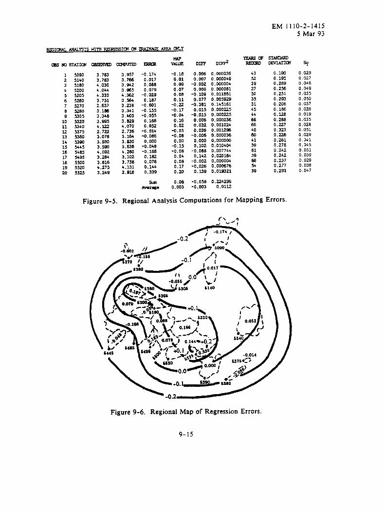
EM 1110-2-1415

123456709

1011K1314151617181920

509051405180

5260527052B05305532053405375536053905445548554955500

5525

3.7833.7834.0304. O&b4.3333.7512.6373.1863.3483.9954.W2.7223.0783.9303.5904.0923.2063.8164.2753.269

Figure 9-5.

3.9573.7663.9423.9654.3623.5643.2383.3413.4033.8294.0702.7363.1643.9303.6384.2603.1023.7384.1312.910

‘0.1740.0170.0880.079

-0.0290.187

-0.601-0.155-0.055

0.1660.052

-0.014-0.086

0.000-0.048-0.168

0.1820.0780. lb40.339

wVAUJ2

-0.180.010.090.070.080.11

-0.22-0.17-0.040.160.02

-0.05-0.080.00

-0.15-0.080.040.080.170.20

sun 0.06Avor~o 0.003

DIFF

0.0060.007

-0.0020.009

-0.1090.077

-0.3810.015

-0.0150.0060.0320.036

-0.0060.0000.102

-0.0680.142

-0.002-0.026

0.139

D+

0.0000360.0000490.0000040.0000810.0118810.0059290.1451610.0002250.0002250.0000360.0010240.0012960.0000360.0000000.0104040. oo77b40.0201640.0000040.0006760.019321

-0.058 0.224296-0.003 0.o112

43 0.190

52 0.195

39 0.28927 0.25650 0.25135 0.29331 0.20645 0.18644 0.12866 0.28866 0.22740 0.32360 0.22641 0.26139 0.27861 0.24239 0.24266 0.23754 0.27739 0.291

Regional Analysis Computations for Mapping Errors.

Figure 9-6. Regional Map of Regression Errors.

9-15

5 Mar 93

%0.0290.0270.0b60.0490.0350.0500.0370.0280.0190.0350.0280.0510.0290.0410.0450.0310.0390,0290.0380.047

EM 1110-2-14155 Mar 93

h. Summarv o fProcedur~. A regional analysis of precipitation or flood-flowfrequencies is generally accomplished by performing the following steps:

( 1) Select long-record base stations within the region as required for extension ofrecords at each of the short-record stations.

(2) Tabulate the maximum events of each station.

(3) Transform the data to logarithms and calculate ~, S and, if appropriate, G(Equations 3-1, 3-2 and 3-3) for each base station.

(4) Calculate z and S for each other station and for the corresponding values of thebase station, and calculate the correlation coefficient (Equation 3- 16).

(5) Adjust all values of% and S by use of the base station, (Equations 3-17 and 3-19). (If any base station is first adjusted by use of a longer-record base station, thelonger-record statistics should be used for all subsequent adjustments.)

(6) S~ect meteorological and drainage basin parameters that are expected to correlatewith X and S, and tabulate the values for each drainage basin or representative area.

(7) Calculate the regression equations relating ~ and S to the basin characteristics,using procedures explained in Section 9-2, and compute the correspondingdetermination coefficients.

(8) Eliminate variables in turn that contribute the least to the determinationcoefficient, recomputing the determination coefficient each time, and select theregression equation having the highest adjusted determination coefficient, or onewith fewer variables if the adjusted determination coef flcient is nearly the same.

(9) Compute the regression errors for each station, plot on a suit~ble map, and drawisopleths of the regression errors for the regression equations of X (see Figures 9-5and 9-6 fo~ an example) and S considering the standard error for each computed, oradjusted, X and S. Note that an alternate procedure is to add the regression constantto each error value and develop a map of this combined value. This procedureeliminates the need to keep the regression constant in the regression equation as themapped value now includes the regression constant.

(10) A frequency curve can be computed for any ungaged basin in the area coveredwithin the mapped re~on by using the adopted regression equations and appropriatemap values to obtain X and S, and then using the procedures discussed in Section 3-2to compute several points to define the frequency curve. (It may also be necessary todevelop regional (generalized) values of the skew coefficient if the Pearson type IIIdistribution is considered appropriate. The next section describes the necessary stepsto compute a generalized skew coefficient.)

i. e er Ii~~. Skew coefficients for use in hydrologic studiesshould be based on regional studies. Values based on individual records are highlyunreliable. Figure 9-7 is a plot of skew coefficients sequentially recomputed after addingthe annual peak for the given year. Note that, after 1950, the skew coefficient was at aat a minimum of about 0.5 in 1954 and maximum of about 1.9 in 1955, only one year

9-16

EM 1110-2-14155 Mar 93

apart. The procedures for developing generalized skew values are generally set forth inBulletin 17B (pages 10- 15).

ln summary, it is recommended that

( 1) the stations used in the study have 25 or more years of data,

(2) at least 40 stations be used in the analysis, or at least all stations surrounding thearea within 100 miles should be included,

(3) the skew values should be plotted at the centroid of the basins to determine ifany geographic or topographic trends are present,

(4) a prediction equation should be developed to relate the computed skewcoefficients to watershed and climate variables,

(5) the arithmetic mean of at least 20 stations, if possible, in an area of reasonablyhomogeneous hydrology should be computed, and

(6) then select the method that provides the most accurate estimation of the skewcoefficient (smallest mean-square error).

In addition to the above guidelines, care should be taken to select stations withoutsignificant man-made changes such as reservoirs, urbanization, etc.

9-17

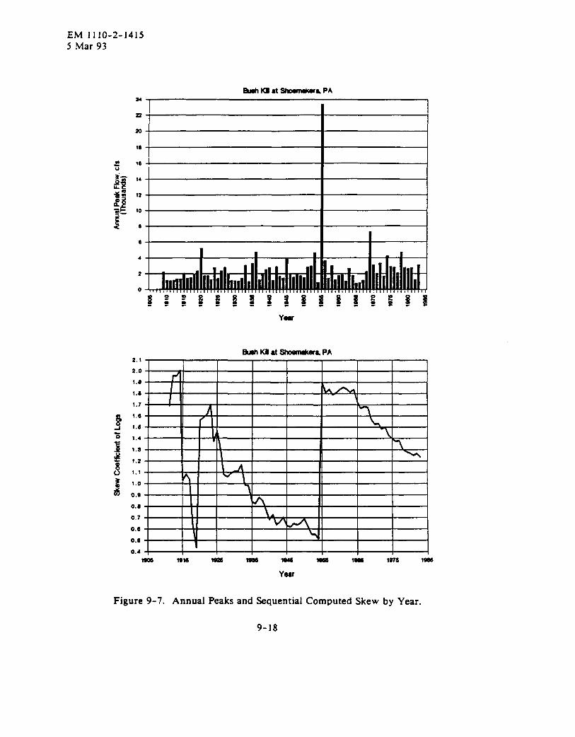
w I 00

— — d — — — —

— m 1 - - I .

— - m —

— - —

— - —

ul

EM 1110-2-14155 Mar 93

CHAPTER 10

ANALYSIS OF MIXED POPULATIONS

10-1. ~efinition. The term mixed population, in a hydrologic context, is applied to datathat results from two or more different, but independent, causative conditions. Forexample, floods originating in a mountainous area or the northern part of the UnitedStates at a given site could be caused by melting snow or by rain storms. Along the Gulfand Atlantic coasts, floods can be caused by general cyclonic storms or by intense tropicalstorms. A frequency curve representing the events caused by one of the climaticconditions may have a significantly different slope (standard deviation) than for the othercondition. A frequency plot of the annual events, irrespective of cause, may show arather sudden change in slope and the computed skew coefficient may be comparativelyhigh. In these situations, a frequency curve derived by combining the frequency curvesof each population can result in a computed frequency relation more representative of theobserved events.

10-2. Procedure.

a. The largest annual event is selected for each causative condition. As Bulletin 17B(46) cautions, “If the flood events that are believed to comprise two or more populationscannot be identified and separated by an objective and hydrologically meaningfulcriterion, the record shaIl be treated as coming from one population.” Also, Bulletin 17Bstates, “Separation by calendar periods in lieu of separation by events is not consideredhydrologically reasonable unless the events in the separated periods are clearly caused bydifferent hydrometeorologic conditions.”

b. The frequency relations for each separate population can be derived by thegraphical or analytical techniques described in Chapter 2-and then combined to yield themixed population frequency curve. The individual annual frequency curves are combinedby “probability of union.” For two curves, the equation is

Pc = P, + P2 - PIJ’2 (10-1)

where:

Pc = Annual exceedance probab ilit v of combined populations for a selectedmagnitude.

PI = Annual exceedance probability of same selected magnitude for populationseries 1.

P2 = Annua] exceedance proba bilit v of same magnitude selected above forpopulation series 2.

c. Figure 10-1 illustrates a combined annual-event frequency curve derived bycombining a hurricane event frequency curve with a nonhurricane event curve for theSusquehanna River at Harrisburg, PA. For more than two population series, n curves maybe more easily combined by the following form:

10-1

EM 111O-2-I4155 Mar 93

Pc = 1 -(i-Pi) (l-P2). .. (P”)”) (10-2)

NOTE: Theexceedance probability (percent chance exceedance divided by 100) must beused in the above equations.

d. If partial duration curves are to be added, the equation is simply PC = PI + Pz.This assumes that the events in both series are hydrologically independent. When thecombined curve is used in an economic analysis, the events in both series must also beeconomically independent.

10-3. ~aution$,

a. If annual flood peaks have been separated by causative factors, a generalized skewmust be derived for each separate series to apply the log-Pearson Type 111distribution asrecommended by Bulletin 17B. Plate 1 of Bulletin 17B or any other generalized skew mapbased on the maximum annual event, irrespective of cause, will not be applicable to any

of the separated series. Derivation of generalized skew relations for each series caninvolve much effort.

b. Some series may not have an event each year. For example, tropical storms do notoccur every year over most drainage areas in the United States, and quite often there areonly a few flood events for the series. Extensive regionalization may be necessary toreduce the probable error in the frequency relations which results from small sample sizes.

c. Sometimes frequency relations of particular seasons are of interest, i.e., quarterlyor monthly, and the curves are combined to verify the annual series curve. The combinedcurve will very likely flt the annual curve only in the middle parts of the curve. Thelower end of the curve will have a partial duration shape as many small events have beenincluded in the analysis. Also, it is possible that the slope of the frequency relation willbe higher at the upper end of the curve as the one season or month with the maximumevent included in its series will likely have a higher slope than that of the annual series.

d. A basic assumption of this procedure is that each series is independent of theother. Coincidental frequency analysis techniques must be used where dependence is afactor. For instance, the frequency curves of two or more tributary stations cannot becombined by the above equation to derive the frequency curve of a downstream site. Thisis because the downstream flow is a function of the summation of the coincident flows oneach of the tributaries.

10-2

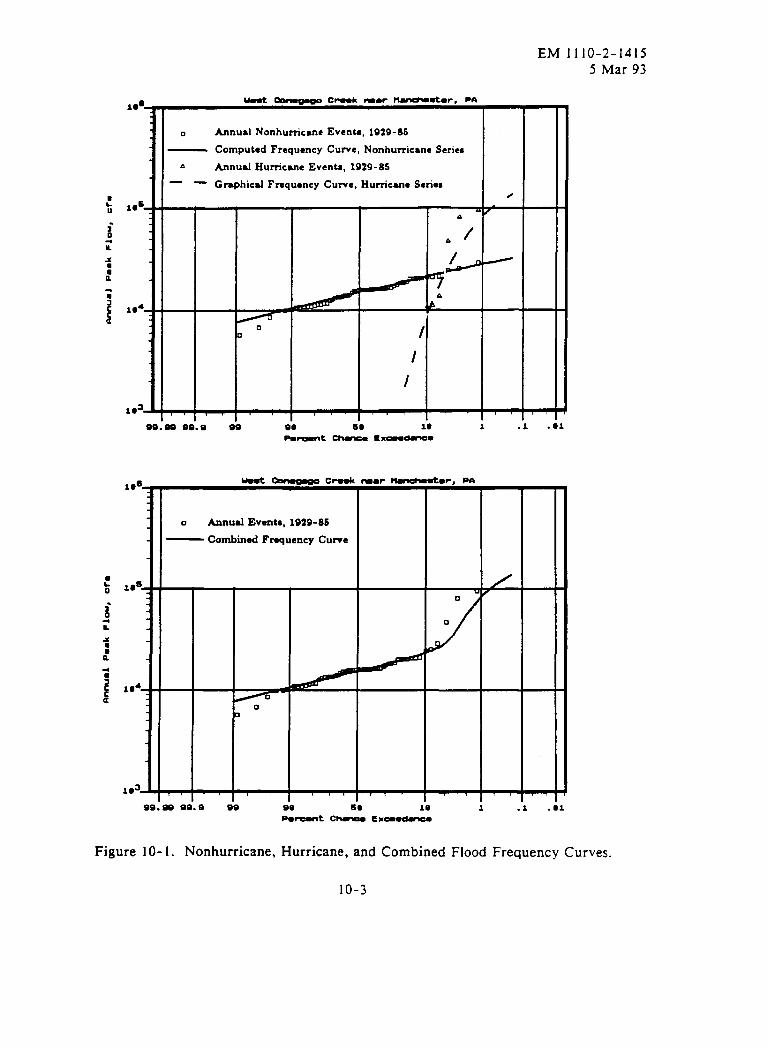
EM 1110-2-14155 Mar 93

o AnnuslNonhumcsneEvent#,1929-8S— ComputedFrequeneyCurve,Nonhu=iemeSeriem

A AnnualHurricuneEvents,19Z9-85—. Gr*phicdFrequencyCurve,Hurrie-e Seriee

/

~ “/

f

❑

0 /

/

I

99.9s 9s.9 99 se se 1s 1 .1 .Wx

9s. =

Figure 10-1.

❑

0

n❑

9s9 se se ie 1.

Pwmmt c~- E x~-=

—‘1. ● ❉

Nonhurricane, Hurricane, and Combined Flood Frequency Curves.

10-3

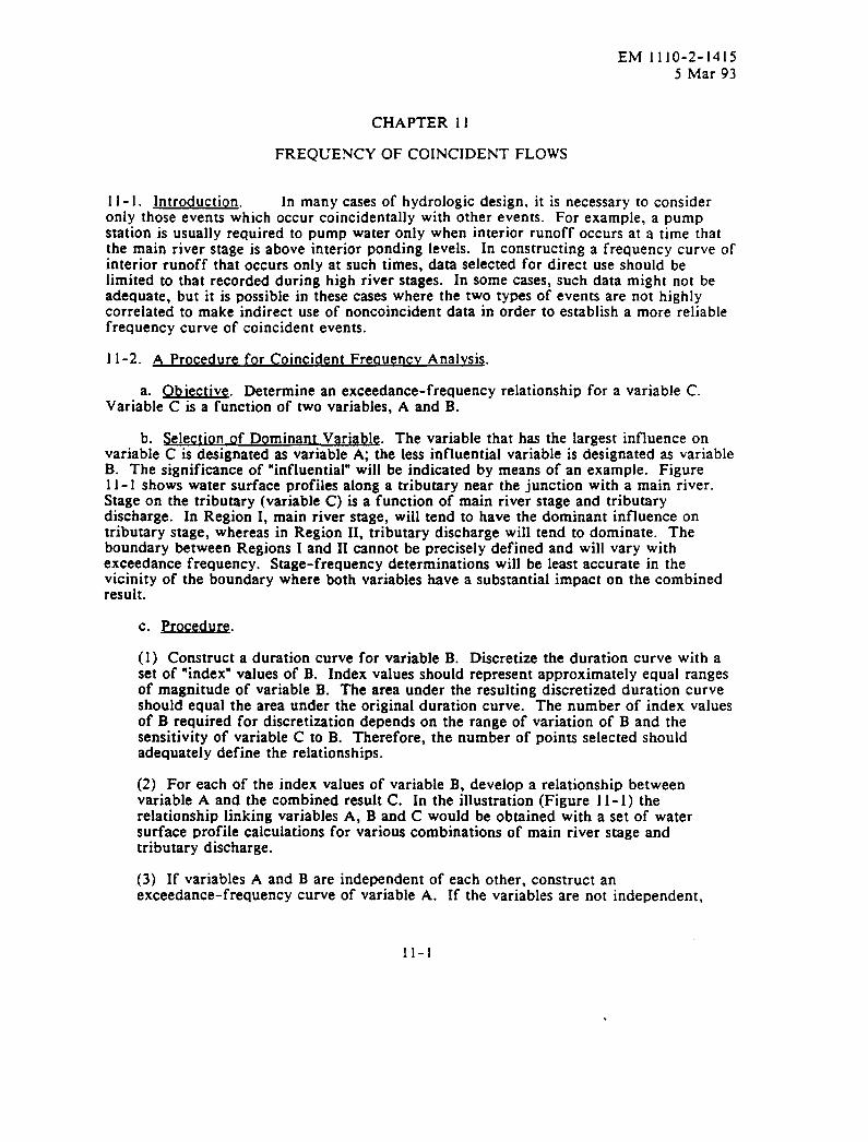
EM 1110-2-14155 Mar 93

CHAPTER II

FREQUENCY OF COINCIDENT FLOWS

11-1. Introduction. In many cases of hydrologic design, it is necessary to consideronly those events which occur coincidentally with other events. For example, a pumpstation is usually required to pump water only when interior runoff occurs at a time thatthe main river stage is above interior pending levels. In constructing a frequency curve ofinterior runoff that occurs only at such times, data selected for direct use should belimited to that recorded during high river stages. In some cases, such data might not beadequate, but it is possible in these cases where the two types of events are not highlycorrelated to make indirect use of noncoincident data in order to establish a more reliablefrequency curve of coincident events.

11-2. A Procedure for Co incident Freauencv Analvsi$.

a. ~. Determine an exceedance-frequency relationship for a variable C.Variable C is a function of two variables, A and B.

b. Selection of Dominant Variab le. The variable that has the largest influence onvariable C is designated m variable A; the less influential variable is designated as variableB. The significance of “influential” will be indicated by means of an example. Figure11-1 shows water surface profiles along a tributary near the junction with a main river.Stage on the tributary (variable C) is a function of main river stage and tributarydischarge. In Region I, main river stage, will tend to have the dominant influence ontributary stage, whereas in Region II, tributary discharge will tend to dominate. Theboundary between Regions I and 11cannot be precisely defined and will vary withexceedance frequency. Stage-frequency determinations will be least accurate in thevicinity of the boundary where both variables have a substantial impact on the combinedresult.

c. Procedu re.

(1) Construct a duration curve for variable B. Discretize the duration curve with aset of “index” values of B. Index values should represent approximately equal rangesof magnitude of variable B. The area under the resulting discretized duration curveshould equal the area under the original duration curve. The number of index valuesof B required for discretization depends on the range of variation of B and thesensitivity of variable C to B. Therefore, the number of points selected shouldadequately define the relationships.

(2) For each of the index values of variable B, develop a relationship betweenvariable A and the combined result C. In the illustration (Figure 11-1 ) therelationship linking variables A, B and C would be obtained with a set of watersurface profile calculations for various combinations of main river stage andtributary discharge.

(3) If variables A and B are independent of each other, construct anexceedance-frequency curve of variable A. If the variables are not independent,

11-1

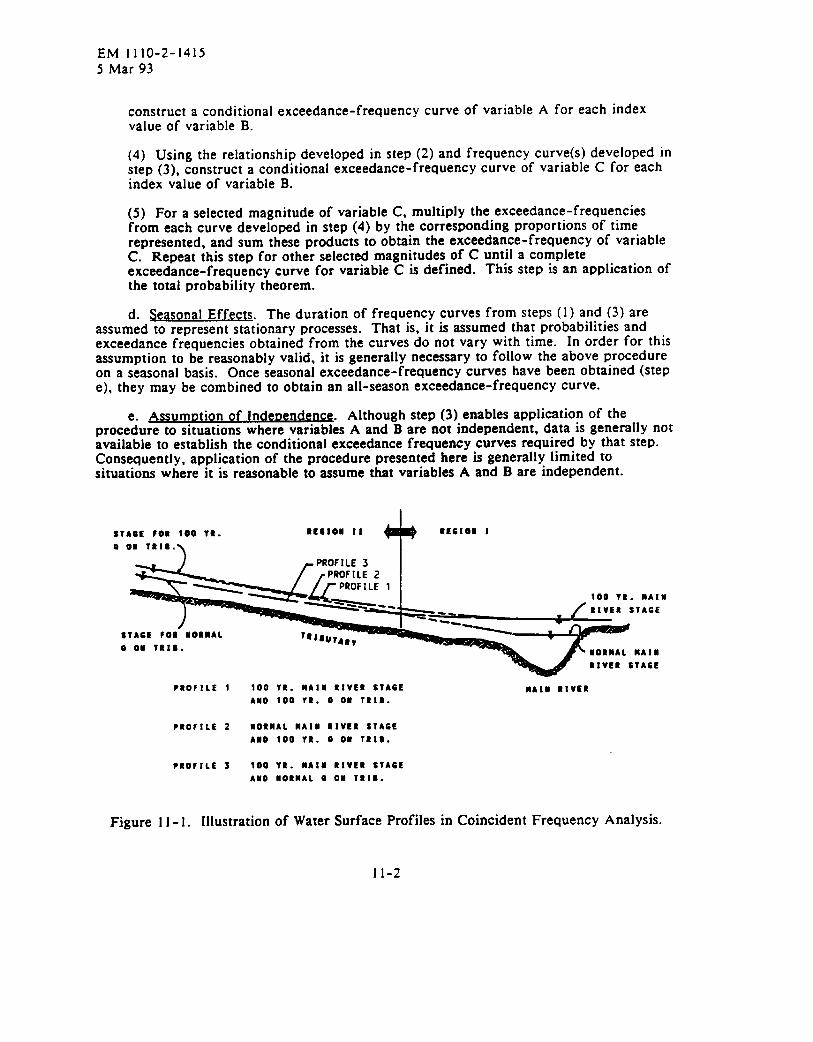
EM I11O-2-I4155 Mar 93

construct a conditional exceedance-frequencyvalue of variable B.

curve of variable A for each index

(4) Using the relationship developed in step (2) and frequency curve(s) developed instep (3), construct a conditional exceedance-frequency curve of variable C for eachindex value of variable B.

(5) For a selected magnitude of variable C, multiply the exceedance-frequenciesfrom each curve developed in step (4) by the corresponding proportions of timerepresented, and sum these products to obtain the exceedance-frequency of variableC. Repeat this step for other selected magnitudes of C until a completeexceedance-frequency curve for variable C is defined. This step is an application ofthe total probability theorem.

d. $easo nal Effects. The duration of frequency curves from steps (1) and (3) areassumed to represent stationary processes. That is, it is assumed that probabilities andexceedance frequencies obtained from the curves do not vary with time. In order for thisassumption to be reasonably valid, it is generally necessary to follow the above procedureon a seasonal basis. Once seasonal exceedance-frequency curves have been obtained (stepe), they may be combined to obtain an all-season exceedance-frequency curve.

e. Assu mntion of Indeoendenc~ Although step (3) enables application of theprocedure to situations where variables A and B are not independent, data is generally notavailable to establish the conditional exceedance frequency curves required by that step.Consequently, application of the procedure presented here is generally limited tosituations where it is reasonable to assume that variables A and B are independent.

STA8E FOa 100 VS. nfGIoll II

+

SEGIOU 1

0 on Tsls. \

100 Yt. MAIM

RIVER STAGE

STAGE FOR NORMAL r@ JBurA,,a on Tals. SORNAL NAI II

RIVER STAGE

●ROFILE 1 100 YR. NAIU RIVER STAGE MAIM RIVERASO 100 TR. O 011 TR IS.

PROFILE 2 NORMAL AIAIU RIVER STAGEAUO 100 TR. 9 On TSIS.

●ROFILE 3 100 YR. MAIII RIVER STAGEAUO NORMAL O ON TR IS.

Figure 11-1. Illustration of Water Surface Profiles in Coincident Frequency Analysis.

11-2

EM 1110-2-14155 Mar 93

CHAPTER 12

STOCHASTIC HYDROLOGY

12-1. Introduction.

a. A stochastic process is one in which there is a chance component in eachsuccessive event and ordinarily some degree of correlation between successive events.Modeling of a stochastic process involves the use of the “Monte Carlo” method of adding arandom (chance) component to a correlated component in order to construct each newevent. The correlated component can be related, not only to preceding events of the sameseries, but also to concurrent and preceding events of series of related phenomena.

b. Work in stochastic hydrology has related primarily to annual and monthlystreamflows, but the results often apply to other hydrologic quantities such asPrecipitation and temperatures. Some work on daily streamflow simulation has been done.

12-2. ADDlications.

a. Hydrologic records are usually shorter than 100 years in length, and most of themare shorter than 25 years. Even in the case of the longest records, the most extremedrought or flood event can be far different from the next most extreme event. There isoften serious question as to whether the extreme event is representative of the period ofrecord. The severity of a long drought can be changed drastically by adding orsubtracting 1 year of its duration. In order that some estimate of the likelihood of moresevere sequences can be made, the stoch~tic process can be simulated, and long sequencesof events can be generated. If the generation is done correctly, the hypothetical sequencewould have x equal likelihood of occurrence in the future as did the observed record.

b. The design of water resource projects is commonly based on assumed recurrenceof past hydrologic events. By generating a number of hydrologic sequences, each of aspecified desired length, it is possible to create a much broader base for hydrologic design.While it is not possible to create information that is not already in the record, it is possibleto use the information more systematically and more effectively. In selecting the numberand length of hydrologic sequences to be generated, it is usual] y considered that 10 to 20sequences would be adequate and that their length should correspond to the period ofproject amortization.

c. It must be recognized that the more hydrologic events that are generated, themore chance there is that an extreme event or combination of events will be exceeded.Consequently, it is not logical that a design be based on the most extreme generated event,but rather on some consideration of the total consequences that would prevail for a givendesign if all generated events should occur. The more events that are generated, the lessproportional weight each event is given. If a design is tested on 10 sequences ofhydrologic events, for example, the benefits and costs associated with each sequencewould be divided by 10 and added in order to obtain the “expected” net benefits.

12-3. Basic Procedure. Successful simulation of stochastic processes in hydrology hasbeen based generally on the concept of multiple linear regression, where the regression

12-1

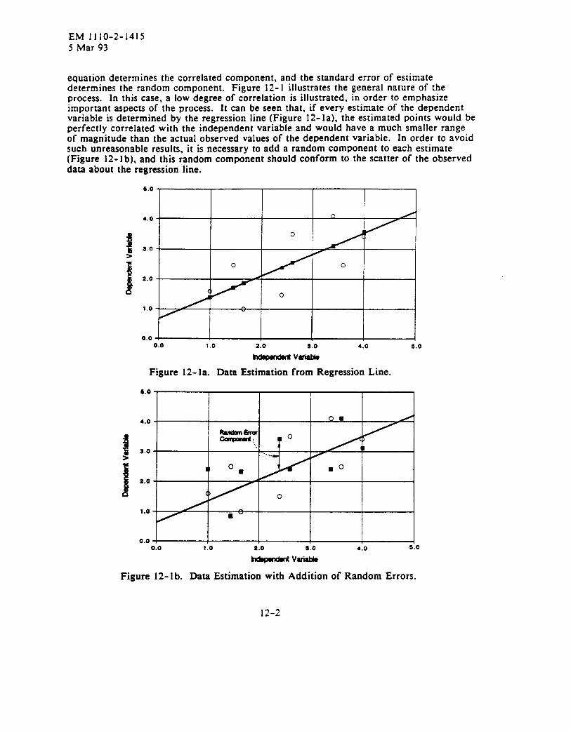
EM 1110-2-14155 Mar 93

equation determines the correlated component, and the standard error of estimatedetermines the random component. Figure 12-1 illustrates the general nature of theprocess. In this case, a low degree of correlation is illustrated, in order to emphasizeimportant aspects of the process. It can be seen that, if every estimate of the dependentvariable is determined by the regression line (Figure 12-1a), the estimated points would beperfectly correlated with the independent variable and would have a much smaller rangeof magnitude than the actual observed values of the dependent variable. In order to avoidsuch unreasonable results, it is necessary to add a random component to each estimate(Figure 12-1 b), and this random component should conform to the scatter of the observeddata about the regression line.

6.0

4,0 - 0

0

3.0

0

2.0

1.0-

0.00.0 1.0 2.0 3.0 4.0 S.o

~ V*

Figure 12- 1a. Data Estimation from Regression Line.

6.0

4.0- 0 9 /

~~’u

7

0

‘.3.0 ----

a 0m

2.0

( )

1.0

0.00.0 1.0 4.0 S.o

L v=

Figure 12-1 b. Data Estimation with Addition of Random Errors.

12-2

EM I11O-2-14I55 Mar 93

12-4. Monthlv Streamflow Model.

a. In accordance with the above basic procedure, a simulation model for generatingvalues of a variable which can be defined only partially by a deterministic relation is:

Y = a + blX1 + b2X2 + ZSY(l-R2)% (12-1)

where

Y= dependent variable

a = regression constant

b1,b2 = regression coefficients

X1,X2 = independent variables

Z = random number from normal standard population with zero mean andunit variance

Sy = standard deviation of dependent variable

R = multiple correlation coefficient

b. This type of simulation model can be used to generate related monthly streamflowvalues at one or more stations, Multiple linear regression theory is based on the assumeddistribution of all variables in accordance with the Gaussian normal distribution.Therefore, mathematical integrity requires that each variable be transformed to a normaldistribution, if it is not already normal. It has been found that the logarithms ofstreamflows are approximately normally distributed in most cases. For computationalefficiency it is convenient to work with deviations from the mean which have beennormalized by dividing by the standard deviation. This deviate is sometimes called thePearson Type 111deviate and can be computed as follows

ti = (xi j - xi)/si#where:

t = Pearson Type 111deviate

i = month number

j = year number

X = logarithm of flow

~ = mean of flow logarithms

s = standard deviation of flow logarithms

(12-2)

12-3

EM 1I1O-2-14155 Mar 93

c. If these deviates exhibit a skewness, they can be further transformed, ifnecessary. to a distribution very close to normal by use of the following approximatePearson ‘Type III transform equation:

Ki = (6/Gi) {[(Giti/2) + 1]1/3 + 1) + Gi/6

where:

K=

i=

G=

t=

normal standard deviate

month number

skew coefficient

Pearson Type 111deviate as defined in Equation

—

(12-3)

12-2

An equation for generating monthly streamflow is:

K ~,k = @lK~,l + B2Ki’,2 + ... + ~k.1K’i,k.1 + ~~K~.l,k

(12-4)

where:

K’ =

P=

i=

k=

n=

R=

z.

monthly flow logarithm, expressed as a normal standard deviate

beta coefficient, defined as bl#i#S,,~ where m is a station not equal tok and b is the regression coefficient.

month number for value being generated

station number for value being generated

number of interrelated stations

multiple correlation coefficient

random number from normal standard population

12-4

EM 1110-2-14155 Mar 93

For the case of a single station, this resolves to:

K; = Ri i.l K;.l+Zi(l-R/i.l~~, # (12-5)

d. Note that Equation 12-5 is very similar to Equation 12-1. The differences resultfrom using normal standard deviates. When this is done, the regression constant, a, equalszero, the regression coefficients, b, become beta coefficients, ~, and the standarddeviation, S, does not appear in the random component since it equals 1. Note also thatone of the independent variables is the flow for the preceding month in order to preservethe inherent serial correlation. The flow value in the original units is computed byreversing the transformation process, i.e., from normal standard deviate to Pearson Type111deviate, to logarithm of flow and finally flow value.

e. A step-by-step procedure for generating monthly streamflows for a number ofinterrelated locations having simultaneous records is as follows

(1) Compute the logarithm of each streamflow quantity. If a value of zerostreamflow is possible, it is necessary to add a small increment, such as 0.1percent of the mean annual flow, to each monthly quantity before taking thelogarithm.

(2) Compute the mean, standard deviation and skew coefficient of the valuesfor each location and each month, using equations given in Chapter 2.

(3) For each month and location, subtract the mean from each event and divideby the standard deviation (Equation 12-2).

(4) Transform these “standardized” quantities to a normal distribution by use ofEquation 12-3.

(5) Arrange the locations in any sequence, and compute a regression equationfor each location in turn for each month. In each case, the independentvariables will consist of concurrent monthly values at preceding stations andpreceding monthly values at the current and subsequent stations.

(6) Generate standardized variates for each location in turn for each month,starting with the earliest month of generated data. This is accomplished bycomputing a regression value and adding a random component. The randomcomponent, according to Equation 12-5, is a random selection from a normaldistribution with zero mean and unit standard deviation, multiplied by thealienation coefficient which is ( 1 - R2)%.

(7) Transform each generated value by reversing the transform of Equation 12-3 with the appropriate skew coefficient, multiplying by the standard deviationand adding to mean in order to obtain the logarithm of streamflow.

(8) Find the antilogarithm of the value determined in step (7) and subtract thesmall increment added in step (1). If a negative value results, set it to zero.

12-5

EM 1110-2-14155 Mar 93

f. It is obviously not feasible toaccomplish the above computations without the useof an electronic computer. A computer program, HEC-4 Monthly Streamflow Simulation(51) can be used for this purpose.

12-5. Data Fill In. Ordinarily, periods of recorded data at different locations do notcover the same time span, and therefore, it is necessary to estimate missing values in orderto obtain a complete set of data for analysis as described above. In estimating the missingvalues, it is important to preserve all statistical characteristics of the data, includingfrequency and correlation characteristics. To preserve these characteristics, it is necessaryto estimate each individual value on the basis of multiple correlation with the precedingvalue at that location and with the concurrent or preceding values in all other locations. Arandom component is also required, as indicated in Equation 12-1.

12-6. ADDliCat ion In Areas of Limited Data. The streamflow generation models discussedso far have assumed that sufficient records were available to derive the appropriatestatistics. For instance, the monthly streamflow model requires four frequency andcorrelation coefficients for each of the 12 months, or 48 values for one station simulation.A model has been developed (51) that combines the coefficients into a few generalizedcoefficients for the purpose of generating monthly streamflow at ungaged locations.(Procedures for determining generalized statistics for use in generating daily flows havenot yet been developed. ) The generalized model considers the following

- season of maximum runoff

- lag to season of minimum runoff

- average runoff

- variation between maximum and minimum runoff

standard deviation of flows

interstation and serial correlations of flows

12-7. Dailv Streamflow Model.

a. Generation of daily streamflows can be accomplished in a manner very similar tothe generation of monthly streamflow quantities. Although a computer program has beenprepared for this purpose, it is capable only of generating flows at a single location anddoes not provide a totally satisfactory hydrography. Since it is desired in many reservoiroperation studies to use a monthly interval most of the time, and to perform dailyoperation computations for only a few critical periods, the program has been designed togenerate daily flows after the monthly total runoff has been generated by anotherprogram. Flows for any particular day are correlated with flows for the preceding dayand for the second antecedent day.

b. A procedure that will give a reasonable shaped hydrography, as well as coordinatedhydrographs at many locations in a basin, would consist of (1) stochastic generation of

12-6

EM 1110-2-14155 Mar 93

precipitation over the basin, and (2) usinga precipitation-runoff model to derive theresulting stream flow.

12-8. Reliability. While the simulation of stochastic processes can add reliability inhydrologic design, the techniques have not yet developed to the stage that they arecompletely dependable. All mathematical models are simplified representations of thephysical phenomena. In most applications, simplifying assumptions do not cause seriousdiscrepancies. It is important at this “state of the art,” however, to examine carefully theresults of hydrologic simulation to assure that they are reasonable in each case.

12-7

EM 1110-2-14155 Mar 93

APPENDIXA

SELECTED BIBLIOGRAPHY

A.

1.

2.

3.

4.

5.

6.

7.

8.

9.

10.

11.

12.

13.

14.

REFERENCES AND TEXTBOOKS

Beard, L. R., “Statistical Methods in Hydrology,” U.S. Army Corps of Engineers,Sacramento, CA, January 1962.

Beard, L. R., “Flood Flow Frequency Techniques,” Technical Report CRWR-119,Center for Research in Water Resources, Austin, TX, October 1974.

Benjamin, J. R. and C. A. Cornell, Proba bilitv. Statistics. and Decision for CivilEn~ineerS, McGraw-Hill Book Co., New York, NY, 1970.

Crippen, J. R., “Composite Log-Type 111Frequency-Magnitude Curve of AnnualFloods,” U.S. Geological Survey Open-File Report 78-352, Reston, VA, 1978.

Dalrymple, T., “F1ood-Frequency Analysis,” U.S. Geological Survey Water-SupplyPaper 1543-A, GPO, Washington, D.C., 1960.

Dixon, W. J. and F. J. Massey, Jr., Intr i~, 3rd cd.,McGraw-Hill Book Co., 1969.

Draper, N. R. and H. Smith, ADDlied Re~ression Analvsi$, John Wiley & Sons, Inc.,1966.

Ezekiel, M. and Karl A. Fox, Methods of Correlation and Repression AnalvsiS, 3rdcd., John Wiley and Sons, 1959.

Frederick, R. H., et. al., “Five-To Sixty-Minute Precipitation Frequency for theEastern and Central U.S.,” NOAA Technical Memorandum NWS Hydro- 35, SilverSpring, MD, June 1977.

Frederick, R. H., “Interduration Precipitation Relations for Storms-Southeast States,”NOAA Technical Report NWS 21, Silver Springs, MD, March 1979.

Haan, C. T., statistical Methods in Hvdrolo~y, The Iowa State University Press,Ames, IA, 1977.1

Hardison, C. H., “Storage Analysis for Water Supply,w Chapter B2 of HydrologicAnalysis and Interpretation, Techniques of Water-Resources Investigations, U.S.Geological Survey, GPO, Washington, D.C., 1973.

Hazen, A., “Storage to be Provided in Impounding Reservoirs for Municipal WaterSupply”, Trans. ASCE 77, p 1539-1559, 1914.

Hershfield, D. M., “Rainfall Frequency Atlas of the U.S.,” Technical Paper No. 40,Weather Bureau, U.S. Department of Commerce, Washington, D.C., May 1961.

A-1

EM 111O-2-I4155 Mar 93

15.

16.

17.

18.

19.

20.

21.

22.

23.

24.

25.

26.

27.

inter-AgencyCommitteeon Water Resources,” Methods of Flow FrequencyAnalysis,” Bulletin 13, Subcommittee on Hydrology, Washington, D.C., April 1966.

James, G. and R. C. James, Mathematics Dictionar y, 3rd cd., D. Van Nostrand Co.,Inc., Princeton, NJ, 1968.

Kite, G. W., “Flood Frequency and Risk,” Inland Waters Directorate, Ottawa, Canada,1974.

Langbein, W. B., and K. T. Iseri,” General Introduction and Hydrologic Definitions,”U.S. Geological Survey Water-Supply Paper 1541-A, GPO, Washington, D.C., 1960.

Massey, B. C. and E. E. Schroeder,” Application of a Rainfall-Runoff Model inEstimating Flood Peaks for Selected Small Natural Drainage Basins in Texas,” U.S.Geological Survey Open-File Report 77-792, Reston, VA, December 1977.

McCuen, R. H., et al., “Flood Flow Frequency for Ungaged Watersheds - ALiterature Evaluation,” ARS, U.S. Department of Agriculture, Beltsville, MD,November 1977.

Miller, J. F., “Two- to Ten-Day Precipitation for Return Periods of 2 to 100 Years inthe Contiguous U.S.,” Technical Paper No. 49, Weather Bureau, U.S. Department ofCommerce, Washington, D.C., 1964.

Miller, J. F., “Two- to Ten-Day Rainfall for Return Periods of 2 to 100 Years in theHawaiian Islands,” Technical Paper No. 51, Weather Bureau, U.S. Department ofCommerce, Washington, D.C., 1965.

Miller, J. F., “Two- to Ten-Day Precipi@tion for Return Periods of 2 to 100 Years inAlaska,” Technical Paper No. 52, Weather Bureau, U.S. Department of Commerce,Washington, D.C., 1965.

Miller, J. F., et al., “Precipitation-Frequency Atlas of the Western U.S.,” NOAA Atlas2, Volume 1. - Montanz Volume 11. - Wyoming Volume III. - Colorado: Volume IV.- New Mexico; Volume V. - Idaho Volume VI. - Utah Volume VII, - NevadaVolume VIII. - ArizonX Volume IX. - Washington: Volume X. - Oregon Volume XI.- California Silver Spring, MD, 1973.

Owen, D. B., “Factors for One-Sided Tolerance Limits and for Variables SamplingPlans,” Monogram SCR-607, Sandia Corporation, available from NTIS, Springfield,VA 22151, March 1963.

Riggs, H. C., “Frequency Curves,” Chapture A2 of Hydrologic Analysis andInterpretation, Techniques of Water-Resources Investigations, U.S. GeologicalSurvey, GPO, Washington, D.C., 1968.

Riggs, H. C., .“Some Statistical Tools in Hydrology,” Chapter A 1 of HydrologicAnalysis and Interpretations, Techniques of Water-Resources Investigations, GPO,Washington, D.C., 1968.

A-2

EM 1110-2-14155 Mar 93

28.

29.

30.

31.

32.

33.

34.

35.

36.

37.

38.

39.

40.

41.

42.

Riggs, H. C., “Low-Flow Investigations,” Chapture B1 of Hydrologic Analysis andInterpretation, Techniques of Water-Resources Investigations, U.S. GeologicalSurvey, GPO, Washington, D.C., 1972.

Riggs, H. C., “Regional Analysis of Streamflow Characteristics,” Chapter B3 ofHydrologic Analysis and Interpretation, Techniques of Water ResourcesInvestigations, U.S. Geological Survey, GPO, Washington, D.C., 1973.

Sauer, V. B., W. O. Thomas, Jr., V. A. Stricker and K. V. Wilson, “FloodCharacteristics of Urban Watersheds in the United States,” U.S. Geological SurveyWater Supply Paper 2207, GPO, Washington, D.C., 1983.

Searcy, J. K., and C. H. Hardison, “Double-Mass Curves,” U.S. Geological SurveyWater-Supply Paper 1541-B, GPO, Washington, D.C., 1960.

Searcy J. K., “Flow-Duration Curves,” U.S. Geological Survey, Water-Supply Paper1541-A, GPO, Washington, D.C., 1960.

Sokolov, A. A., et al., Flood Flow ComDutation. Methods Comt)i]ed from WorldExDeriencQ, The UNESCO Press, Paris, France, 1976.

U.S. Army Corps of Engineers, “Stream Flow Volume-Duration-Frequency Studies,”CW- 152 Technical Report No. 1, Washington District, Washington, D.C., June 1955.

U.S. Army Corps of Engineers,” Frequency of New England Floods,” CW-151Research Note No. 1, Sacramento District, Sacramento, CA, July 1958.

U.S. Army Corps of Engineers, “Probability Estimates Based on SmallNormal-Distribution Samples,” CW-151 Research Note No. 2, Sacramento District,Sacramento, CA, March 1959.

U.S. Army Corps of Engineers, “Frequency Curves from Incomplete Samples,”CW-151 Research Note No. 3, Sacramento District, Sacramento, CA, September 1959.

U.S. Army Corps of Engineers, “Characteristics of Low FlowVolume-Duration-Frequency Statistics,” CW- 152 Technical Bulletin No. 1,Washington District, Washington, D.C., June 1960.

U. S. Army Corps of Engineers, “Hydrologic Data Management, “Volume 2 ofHydrologic Methods for Water Resources Development, the Hydrologic EngineeringCenter, Davis, CA, April 1972.

U.S. Army Corps of Engineers, “Regional Frequency Study, Upper Delaware andHudson River Basins, New York District,” Hydrologic Engineering Center, Davis,CA, November 1974.

U.S Army Corps of Engineers, “Hydrologic Frequency Analysis,” Volume 3 ofHydrologic Methods for Water Resources Development, the Hydrologic EngineeringCenter, Davis, CA, April 1975.

U.S. Army Corps of Engineers, “Reservoir Yield,” Volume 8 of HydrologicEngineering Methods for Water Resources Development, the Hydrologic EngineeringCenter, Davis, CA, June 1977.

A-3

EM 1110-2-14155 Mar 93

43.

44.

45.

46.

47.

48.

49.

B.

50.

51.

52.

53.

54.

55.

56.

U.S. Army Corps of Engineers, “Generalized Skew for State of New Jersey :SpecialProject Memo 480, Hydrologic Engineering Center, Davis, CA, December 1977.

U.S. Army Corps of Engineers, “Hydrologic Analysis of Ungaged Watersheds withHEC- 1,“ Hydrologic Engineering Center, Davis, CA, April 1982.

U.S. Army Corps of Engineers, Engineering Manual EM 1110-2-1413, “HydrologicAnalysis of Interior Areas,” January 1987.

Water Resources Council, “Guidelines for Determining Flood F1OWFrequency,”Bulletin 17B, Hydrology Committee, Washington, D.C., March 1982.

Water Resources Council, “A Uniform Technique for Determining Flood FlowFrequencies,” Bulletin 15, Hydrology Committee, Washington, D.C., December 1967.

World Meteorological Organization, “International Glossary of Hydrology,” FirstEdition, WMO No. 385, Geneva, Switzerland, 1974.

World Meteorological Organization, “Guide to Hydrometeorological Practices,” WMONo. 168, Third Edition, Geneva, Switzerland, 1974.

COMPUTER PROGRAMS

U.S. Army Corps of Engineers, “Multiple Linear Regression,” ComPuter program704-G 1-L2020, Hydrologic Engineering Center, Davis, CA, September 1970.

U.S. Army Corps of Engineers, “HEC-4, Monthly Streamflow Simulation,” ComputerProgram 723-X6 -L2340, Hydrologic Engineering Center, Davis, CA, February 1971.

U.S. Army Corps of Engineers, “Regional Frequency Computation,” ComputerProgram 723-X6 -L2350, Hydrologic Engineering Center, Davis, CA, July 1972.

U.S. Army Corps of Engineers, “Flood Flow Frequency Analysis, “Computer Program723-X6- L7550, Hydrologic Engineering Center, Davis, CA, February, 1982.

U.S. Army Corps of Engineers, “Expected Annual Flood Damage Computation,”Computer Program 761-X6-L7580, Hydrologic Engineering Center, Davis, CA, June1977.

U.S. Army Corps of Engineers, “ HEC-5, Simulation of Flood Control andConservation Systems.m Computer program 723-X6 -L2500, Hydrologic EngineeringCenter, Davis, CA, April 1982

U.S. Army Corps of Engineers, “HEC- 1, Flood Hydrography Package,” ComputerProgram 723-X6 -L201O, Hydrologic Engineering Center, Davis, CA, September198i .

A-4

EM 1110-2-14155 Mar 93

57. U,S. Army Corps of Engineers, “Storage, Treatment, Overflow, Runoff Model‘STORM’,” Computer Program 723-58 -L7520, Hydrologic Engineering Center,Davis, CA, August 1977.

58. U.S. Army Corps of Engineers, “Statistical Analysis of Time Series Data ‘STATS’,”under development, Hydrologic Engineering Center, Davis, CA, May 1987.

A-5

EM I11O-2-14155 Mar 93

APPENDIXB

GLOSSARY

These definitions have been collected from four major sources: (l) Guidelines forDetermining Flood Flow Frequency (17B), reference 46; (2) International Glossary ofHydrology (WMO), reference 48; (3) General Introduction and Hydrologic Definitions(USGS), reference 18; and (4) Mathematics Dictionary (MD), reference 16.

Analytical FrequencyAnalysis

Annual Event

Annual Series

Array

Autocorrelation

Base Discharge

Biased

Broken Record

Chi-SquareDistribution

Class Interval

DEFINITION

A predefine method of estimating the parameters that define aselected theoretical frequency distribution.

The most extreme event, either maximum or minimum, in theyear. (17B)

A general term for a set of any kind of data in which each item isthe maximum or minimum in a year. (17B)

A list of data in order of magnitude; in flood- frequency analysisit is customary to list the largest value first, in a low-frequencyanalysis, the smallest first. ( 17B)

See “Serial Correlation.”

Usually refers to the discharge above which independentinstantaneous peak flows are collected for a partial durationfrequency analysis.

The expected value of a statistic obtained from random samplingis not equal to the parameter or quantity being estimated. (MD)

A systematic record which is divided into seDarate continuoussegments because of deliberate discontinuation of recording forsignificant periods of time. (17B)

The distribution of sample variances drawn from a normaldistribution. Used to compute confidence intervals for thepopulation variance estimated from a sample.

A convenient sized interval into which data may be grouped. Theupper and lower bounds of the class interval are called “classlimits.” (MD)

B-1

EM 1110-2-14155 Mar 93

Climatic Year

Coefficient ofSkewness

Coefficient ofVariation

Confidence Limits

Correlation

Covariance

Cumulative FrequencyCurve

Deviation

Depth-Duration-Frequency

Distribution

Double Mass Curve

Drought

Duration Curve

Error Variance

Exceedance Frequency

Exceedance Interval

A continuous 12-month period during which a complete annualcycle occurs, arbitrarily selected for the presentation of datarelative to hydrologic or meteorologic phenomena. The climaticyear is usually designated by the calendar year during which mostof the 12 months occur. See “Water Year.” (USGS)

A numerical measure or index of the lack of symmetry in afrequency distribution. Function of the third moment ofmagnitudes about their mean, a measure of asymetry. Also called“coefficient of skew” or “skew coefficient.” (17B)

Statistical parameter describing the change of a stochastic variablein time or space, expressed as the ratio of the standard deviationto the mean. (WMO)

Computed values on both sides of an estimate of a parameter thatshow for a specified probability the range in which the true valueof the parameter lies. (17B)

The interdependence between two sets of numbers. (MD)

The first product moment of two variates normalized by theirrespective mean values. (WMO)

Relation of event magnitude to percentage of events exceeding (ornot exceeding) that magnitude.

The difference between the magnitude of an event and the meanof all the events in the sample.

Curve showing the frequency relationship of precipitation depthfor a given storm duration.

Function describing the relative frequency with which events ofvarious magnitudes occur. (17B)

Plot of successive accumulated values of one variable against thecontemporaneous accumulated values of another variable. (WMO)

A period of abnormally dry weather sufficiently prolonged forthe lack of precipitation to cause a serious hydrological imbalance.(WMO)

A cumulative frequency curve that shows the percent of time thatspecific values are equalled or exceeded. (USGS)

Square of the standard error.

See “Percent chance exceedance.”

See “Recurrence interval.”

EM 1110-2-14155 Mar 93

ExceedanceProbability

Expected Probability

F Distribution

Flow-Duration Curve

Frequency

Frequency Analysis

Frequency Curve

Generalized Skew

Geometric Mean

Graphical FrequencyAnalysis

Histogram

Historic Data

Homogeneity

Incomplete Record

Level of Significance

Probability that a random event will exceed a specified magnitudein a given time period, usually one year unless otherwiseindicated. ( 17B)

The average of the true probabilities of all magnitude estimatesfor any specified flood frequency that might be made fromsuccessive samples of a specified size. (17B)

The random sampling distribution of the ratio of two independentestimates of the variance of a normal distribution. (MD)

See “Duration Curve.”

The number of events in a sample (or the population) that meetspecified criteria.

Procedure involved in interpreting a record of events in terms offuture probabilities of occurrence. (WMO)

A graphical representation of a frequency distribution. Usually acumulative frequency curve with the abscissa a probability gridand the ordinate the event magnitude.

A skew coefficient derived by a procedure which integratesvalues obtained at many locations. (17B)

The Nth root of the product of N values or the antilogarithm ofthe mean logarithm of a set of values.

The development of a frequency curve by drawing a smoothcurve through plotted points while considering known constraints.Plotting positions are computed based on the order number andthe total number of values represented, and then plotted on theappropriate probability paper.

Univariate frequency diagram with rectangles proportional in areato the class frequency, erected on a horizontal axis with widthequal to the class interval. (WMO)

Information about significant events before or after the period of“systematic” data collection. (derived from 17B)

Records (samples) from the same population. (17B)

A streamflow record in which some peak flows are missingbecause they were too low or high to record or the gage was outof operation for a short period because of flooding. (17B)

The probability of rejecting a hypothesis when it is in fact true,At a “lO-percent” level of significance the probability is 1/10.(17B)

B-3

EM 1I1O-2-14I55 Mar 93

Log-Pearson Type 111Distribution

Mass Curve

Mean

Mean Daily

Median

Method of Moments

Mixed Populations

Mode

Non-Central tDistribution

Nonstationary

Normal Distribution

Outlier

Parameter

Parent Population

Application of the Pearson Type 111distribution to the logarithmsof the data.

Curve of an accumulative quantity versus time. (WMO)

The expected value of a random variable, the first moment. Thearithmic mean (or average) of a sample is an estimate of thepopulation mean.

The mean of daily values in a specified period, or the mean ofvalues within one day. (derived from WMO)

The value at which one-half of ordered observations lie on eitherside. If there is no middle value, the median is the average of thetwo middle values.

A standard statistical computation for estimating the moment of adistribution from the data of a sample. (17B)

A sample whose events have come from two or more differentpopulations, i.e., data not homogeneous.

The most frequent value of a set of numbers. (MD)

A distribution that combines the probable error in the mean andthe standard deviation for samples from a normal distribution.Used in the development of confidence limit curves about afrequency curve computed from sample statistics.

Not stationary with respect to time. See “Stationary Process.”

A probability distribution that is symmetrical about the mean,median, and mode (bell shaped). It is the most studieddistribution in statistics, even though most data are not exactlynormally distributed, because of its value in theoretical work andbecause many other distributions can be transformed into thenormal. It is also known as Gaussian, the Laplacean, theGauss-Laplace, or the Laplace-Gauss distribution, or the SecondLaw of Laplace. (17B)

Outliers (extreme events) are data points which depart from thetrend of the rest of the data. (17B)

A characteristic descriptor of the population, such as mean orstandard deviation. Parameter estimates are called statistics.

See “Population”.

Partial-Duration Series A list of flood peaks that exceed a chosen base stage or discharge,regardless of the number of peaks occurring in a year. (USGS)

B-4

EM 1110-2-14155 Mar 93

Pearson Type 111Distribution

Percent ChanceExceedance

Percent ChanceNon-Exceedance

Plotting Position

Population

Probability

Random

Recurrence Interval

Regional Analysis

Regression

Return Period

Risk

Sample

Family of asymmetrical, theoretical frequency distributions ofwhich the normal distribution is a special case.

The probability, expressed as a percentage, with which valuesexceed a specified magnitude.

The probability, expressed as a percentage, with which valueswill not exceed a specified magnitude.

Percent chance of exceedance (or non-exceedance) of an observedvalue estimated from its position in the array.

The entire (usually infinite in hydrologic application) number ofdata from which a sample is taken or collected. For example,total number of past, present, and future floods at a location on ariver is the population of floods for that location even if thefloods are not measured or recorded. (17B)

The ratio of the number of random events with some particularsize or other attribute to the total number of equally likely events.

Any event in the population has an equal chance of beingselected.

The average time interval between actual occurrences of ahydrological event of a given or greater magnitude. In an annualflood series, the average interval in which a flood of a given sizeis exceeded as an annual maximum. In a partial duration series,the average interval between floods of a given size, regardless oftheir relationship to the year or any other period of time. Thedistinction holds even though for large floods, recurrenceintervals are nearly the same for both series. (17B)

Extension of the results of the frequency analysis of point data toan area. (WMO)

An analytical procedure that derives estimation or predictionequations for a variable (dependent) based on given values of oneor more other variables (independent). Commonly, the principleof minimum squared error (least squares) is used in the derivation.

See “Recurrence Interval.”

The probability of a potential outcome (success) being realizedwithin a specified number of events (trials). In a hydrologiccontext, the probability that one or more events will exceed agiven annual event, that has an assumed “true” percent chanceexceedance, during a specified number of years. Risk iscomputed by the binomial distribution. (For contrast, seeuncertainty.)

An element, part, or fragment of a “population.” Everyhydrologic record is a sample of a much longer record. ( 17B)

B-5

EM 1110-2-14155 Mar 93

Sampling Error

Serial Correlation

Skew Coefficient

Stage

Standard Deviation

Standard Error

Stationary Process

Statistic

Stochastic Process

Student’s t-Distribution

Systematic Record

t-Distribution

Test of Significance

Transformation

The difference between a random sampling statistic and theparameter of the population from which the random sample wasdrawn. (MD)

A measure of the interdependence between an observation at agiven time period and that of a preceding time period. Alsocalled autocorrelation.

See ‘Coefficient of Skewness.”

The height of a water surface above an established datum plane.(USGS)

A measure of the dispersion or precision of a series of statisticalvalues such as precipitation or stream flow. It is the square rootof the sum of squares of the deviations from the arithmetic meandivided by the number of values or events in the series. It is nowstandard practice in statistics to divide by the number of valuesminus one in order to get an unbiased estimate of the variancefrom the sample data. ( 17B)

Standard deviation of the sampling distribution of a statisticalparameter. (WMO)

All of the generating moments of the frequency distributionremain fixed with respect to time.

An estimate of a population parameter obtained from a sample ofthe population.

Process in which both the probability and the sequence ofoccurrence of the variables are taken into account. (WMO)

A distribution used in evaluation of variables which involvesample standard deviation rather than population standarddeviation. (17B)

Information collected by a systematic data collection program.(derived from 17B)

See “Student’s t-Distribution.”

A test mode to learn the probability that a result is accidental orthat a result differs from another result. For all the many typesof tests, there are standard formulae and tables. ( 17B)

The change of numerical values of data to make latercomputations easier, to linearize a plot or to normalize a skeweddistribution by making it more nearly a normal distribution. Themost common transformations are those changing ordinarynumerical values into their logarithms, square roots or cube roots;many others are possible. ( 17B)

B-6

EM 1110-2-14155 Mar 93

Trend

Unbiased

Uncertainty

Variance

Watershed

Water Year

A statistical term referring to the direction or rate of increase ordecrease in magnitude of the individual members of a time seriesof data when random fluctuations of individual members aredisregarded. (USGS)

The expected value of a statistic obtained from random samplingis equal to the parameter or quantity being estimated. (MD)

The inherent error in an analysis caused by not knowing eitherthe true model or the model parameters. In frequency analysis,model uncertainty comes from assuming a theoretical frequencydistribution and parameter uncertainty comes from estimating theparameters for the selected distribution by sample statistics.

A measure of the amount of spread or dispersion of a set ofvalues around their mean, obtained by calculating the mean valueof the squares of the deviations from the mean, and hence equalto the square of the standard deviation. ( 17B)

The divide separating one drainage basin from another and in thepast has been generally used to convey this meaning. However,over the years, use of the term to signify drainage basin orcatchment area has come to predominate, although drainage basinis preferred. (USGS)

Continuous twelve-month period selected in such a way that allsolid and liquid precipitation runs off during this period. Thus,carryover is reduced to a minimum. (WMO) In U.S. GeologicalSurvey reports, it is the twelve-month period. October 1 throughSeptember 30. The water year is designated by the calendar yearwithin which most of the twelve-months occur. (USGS)

B-7

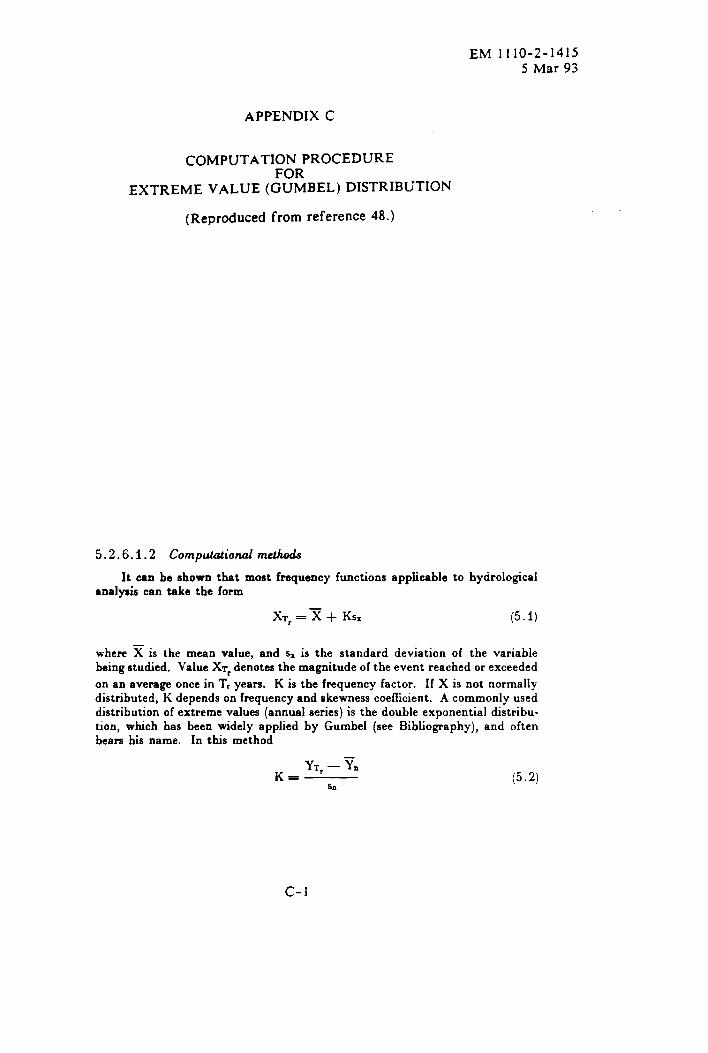
EM 1110-2-14155 Mar 93

APPENDIXC

COMPUTATION PROCEDUREFOR

EXTREME VALUE (GUMBEL) DISTRIBUTION

(Reproduced from reference 48.)

5.2.6.1.2 Compdational methods

It can be shown that most frequency functions applicable to hydrologicalanalysis can take the form

XT, = ~ + Ks. (5.1)

where % is the mean value, and s= is the standard deviation of the variablebeing studied. Value XT- denotes the magnitude of the event reached or exceeded

on an average once in T; years. K is the frequency factor. If X is not normallydistributed, K depends on frequency and skewness coe~cient. A commonly useddistribution of extreme values (annual series) is the double exponential distribu-tion, which has been widely applied by Gumbel (see Biblio~aphy), and oftenbears his name. In this method

(5.2)Sn

c-1

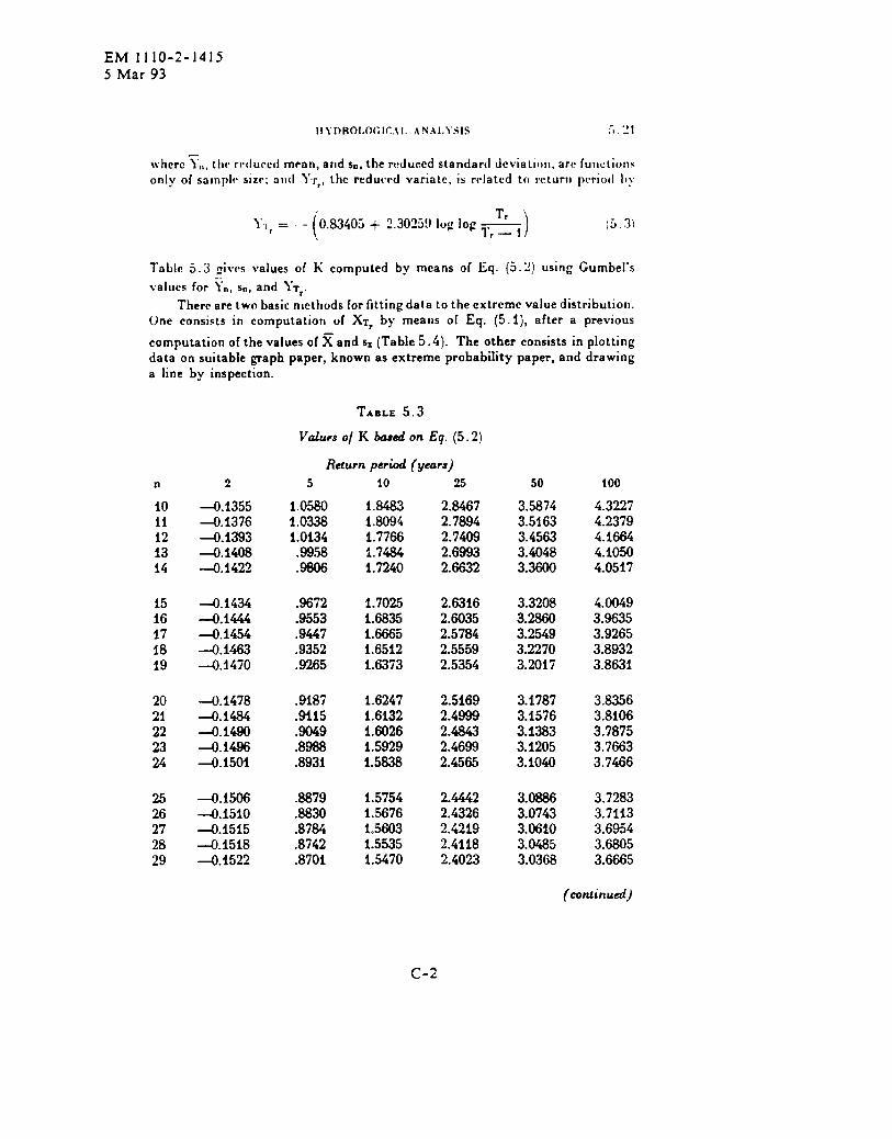
EM 1I1O-2-I4155 Mar 93

liYI)RO1.OGIC.\l. AN.*l. Y51S .-) ‘11

whcrc y,,, L}lI,r[,[luccd mean, a~ld sO,the r~”duccd standard dcviatit)ll, are furlctillnsonly of salnple size; at)~l YTr, lhc reduced variate, is related to return pf.riofl l)>

(

T,}“., = .- ‘0.83405 + 2.3025!)log log ~

r )(53)

Tablo 5.3 givf.s values of K computed by means of Eq. (5.2) using Gumbel’s

values for ~“, s“, and ~Tr.

There are two basic nlcthssds for fitting data to the extreme value distributio[l.(.)ne consists in computation of XT, by means of Eq. (5.1),aftera previous

computation of the values of ~ and s= (Table 5 .4). The other consists in plottingdata on suitable ~aph paper, known as extreme probability paper, and drawinga line by inspection.

TABLE 5.3

VSZLUPSo/ K bed on Eq. (5.2)

Return period (years)

n

101112i314

i516171819

2021222324

2526272829

2

4.1355-0.1376-0.1393-0.1408-0.1422

-0.1434-o.i4444.i454-o.i4634.1470

-0.1478-0.1484-0.1490-0.1496-0.1501

-0.1506-o.i510-o.i5i5-0.i518-0.:522

5

1.05801.03381.0134

.9958

.9806

.9672

.9553

.9447

.9352

.9265

.9i87

.9115

.9049

.8988

.8931

.8879

.8830

.8784

.8742

.8701

10

1.84831.80941.7766:.74841.7240

1.7025i.68351.66651.65121.6373

i.62471.61321.60261.59291.5838

1.57541.56761.56031.55351.5470

25

2.84672.78942.74092.69932.6632

2.63162.60352.57842.55592.5354

2.51692.49992.48432.46992.4565

2.44422.43262.42192.41182.4023

50

3.58743.51633.45633.40483.3600

3.32083.28603.25493.22703.2017

3.17873.15763.13833.12053.1040

3.08863.07433.06103.04853.0368

100

4.32274.23794.16644.io504.0517

4.00493.96353.92653.89323.8631

3.83563.81063.78753.76633.7466

3.72833.71i33.69543.68053.6665

(continued)

c-2

EM 1110-2-]4155 Mar 93

n

3031

:34

3536

:39

404142434.4

4546474849

5051525354

55

:5859

6061626364

0

—0.1526-0.1529-0.1532-0.1535-0.1538

-0.1540-0.1543-0.1545-0.1548-0.1550

-0.i552—0.1554-0.i556-0.1557-0.1559

4.1561-0.1562-0.1564-0.1566-0.1,567

4.i568-0.1570-0.15714.1572-o.i573

-0.1575-0.1576-o.i577-0.1578-0.1579

-0.1580-0.1581-0.1582-0.1583--0.1583

HYDROLOGICAL ANALYSIS

TABLE 5.3 (continued)

Return period (years)

5

.8MB4

.8628

.859Ii

.8562

.8532

.8504

.8476

.8450

.6425

.8402

.8379

.8357

.8337

.8317

.8298

.8279

.8262

.8245

.8228

.82i2

.8197

.8182

.8168

.8154

.8141

.8128

.8116

.8103

.8092

.8080

.8069

.8058

.8048

.8038

.8028

10

1.54101.53531.5299i.5248i.5i99

f.5i531.51101.50681.50281.4990

1.49541.49201.48861.48541.4824

1.47941.47661.47391.47121.4687

1.46631.46391.46161.45941.4573

1.45521.45321.45i2i.44941.4475

1.44581.44401.44241.44071.4391

c-3

25

2.39342.38502.37’702.36952.3623

2.35562.349f2.34302.337i2.3315

2.32622.32112.31622.3f152.3069

2.30262.29842.29442.29052.2868

2.28322.27972.27632.27312.2699

2.26692.26392.26102.25832.2556

2.25292.25042.24792.24552.2432

50

3.02573.01533.00542.99612.9873

2.97892.97092.96332.95612.9491

2.94252.93622.930~2.92432.9167

2.91332.908~2.90312.89832.8937

2.88922.88492.88072.87672.8728

2.86902.86532.86182.85832.8550

2.85t82.84862.84552.84262.8397

! 00

3,6534364103,ti2923.61813.6076

3.59763.58813.57903.57043.5622

3.5;433.54673.53953.53253.5259

3.51943.51333.50733.50~65.496i

3.49083.48563.48073.47593.4712

3.46673.46233.45813.45403.4500

3.446i3.44243.43873.43523.4317

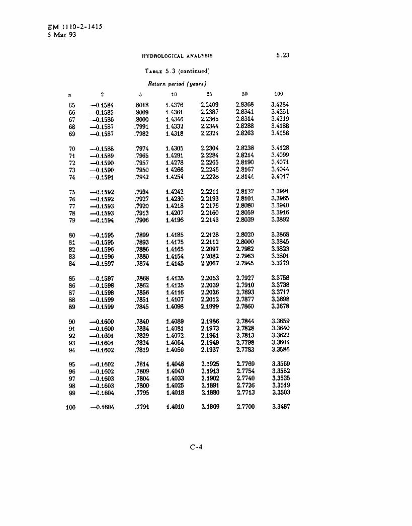
EM II1O-2-1415

5 Mar 93

n

6566676869

7071727374

-.

;:777879

808:828384

8586878889

9091929394

9596979899

100

0

--0.1584-0.1585-0.1586-0.15874.1587

-o.i588-0.i589-o.i590-0.1590-o.i59i

4.1592-0.i592-o.i593-0.15934.1594

-0.1595-0.15954.1596-0.15964.1597

-o.i597-o.i598-o.i5984.i599-0.1599

-o.i600-0.1600-0.1601-0.1601-0.1602

-0.1602-0.IW2-o.i603-0.16034.1604

-0.1604

llYDROLOGICAL ANALYSIS

TABLE 5.3 (continued)

Return period (years)

5

.8018

.8009

.8000

.7991

.7982

.7974

.7965

.7957

.7950

.7942

.7934

.7927

.7920

.7913

.7906

.7899

.7893

.7886

.7880

.7874

.7868

.7862

.7856

.7851

.7845

.7840

.7834

.7829

.7824

.7819

.7814

.7809

.7804

.7800

.7795

.779i

10

1.4376~.43611.43461.43321.4318

1.43051.42911.427814266i.cL54

1.42421.42301.42181.42071.4196

:.41851.41751.41651.41541.4145

1.41351.41251.41161.41071.4098

1.40891.40811.40721.40641.4056

1.40481.40401.40331.40251.4018

i.4oio

25

2.2409

2.2387

2.2365

2.2344

2.2324

2.23042.2~8.4

2.2265

2.2246

2.22%

2.22fi

2.2193

2.2i76

2.2160

2.2143

2.2128

2.2i12

2.20972.20822.2067

2.20532.20392.20262.20122.IM

2.19862.i9732.i96i2.19492.1937

2.19252.19:32.19022.189f2.1880

2.1869

50

2.8368

2.8341

2.8314

2.8288

2.8263

2.8238

2.8214

2.8190

2.8167

2.8i44

2.8122

2.8101

2.8080

2.8059

2.8039

2.8020

2.8000

2.7982

2.7963

2.7945

2.7927

2.7910

2.7893

2.7877

2.7860

2.7844

2.7828

2.7813

2.7798

2.7783

2.7769

2.7754

2.7740

2.7726

2.7713

2.7700

5.23

100

3.42843.425i3.42193.4i883.4158

3.41283.40993.40713.40443.4017

3.39913.39653.39403.39163.3892

3.38683.38453.38233.38013.3779

3.37583.37383.37173.36983.3678

3.36593.36403.36223.36043.3586

3.35693.35523.35353.35193.3503

3.3487

c-4

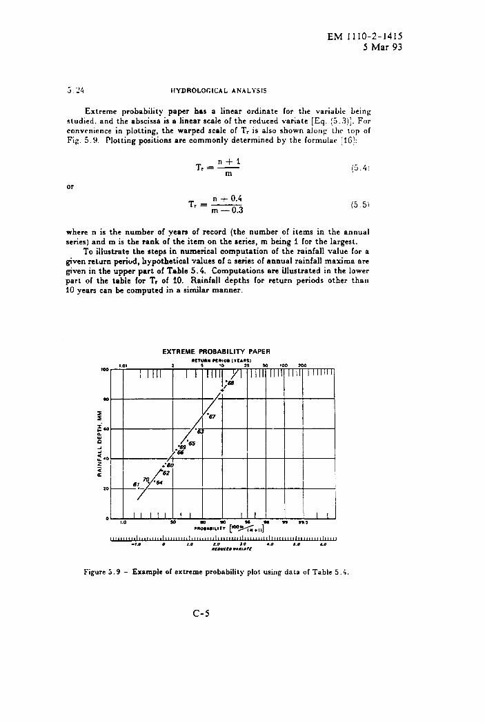
EM 1110-2-14155 Mar 93

5.24 lIYDROLOCICAL ANALYSIS

Extreme probability paper has a linear ordinatestudied, and the abscissa is a linear scale of the reduced

for the variable beingvariate (Eq.(5.3)].For. . .

convenience in plotting, the warped scale of T~ is also shown alorlg L}ICtopFig. 5.9. Plotting positions arecommonly determined bytheformulac[l6]:

n+lT,=—m (5

or

Tr=n +0.4

m— 0.3(5

of

4;

5)

where n is the number of yearn of record (the number of items in the annualseries) and m is the rank of the item on the series, m being 1 for the largest.

Toillustrate the stepsin numerical computation of the rainfall value fora@ven return period, hypothetical values of a series of annual rainfall maxima areffven in the upper part of Table 5.4. Computations are illustrated in the lowerpart of the table for T, of iO. Rainfall depths for return periods other tharlfO yearn can be computed in a similar manner.

EXTREME PROBABILITY PAPER

Figure 5.9 - Example of extreme probability plot using data of Table 5.4.

c-5

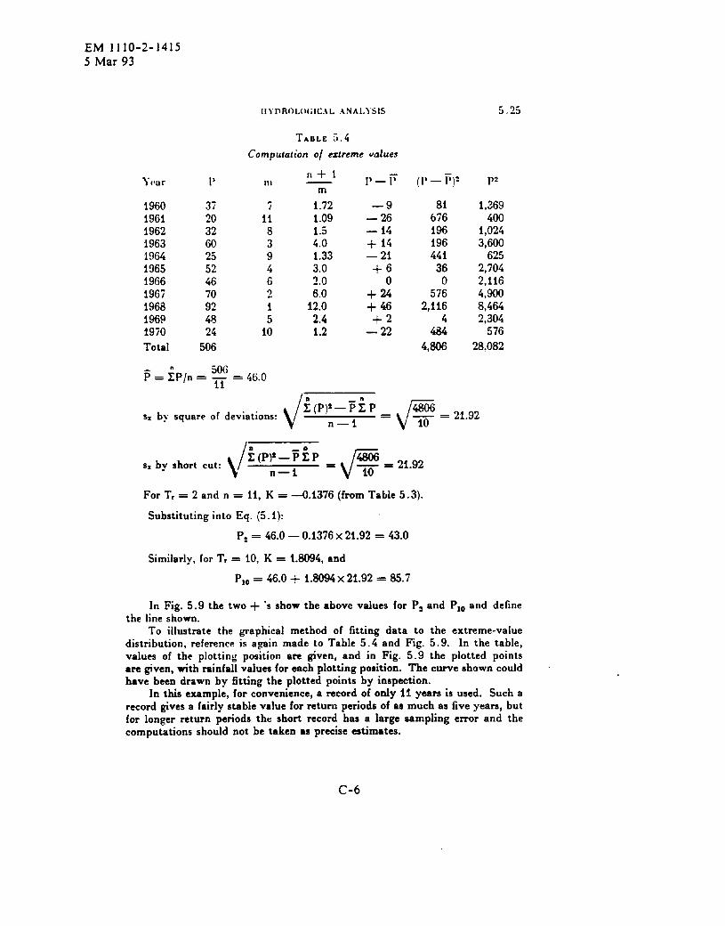
EM 1110-2-14155 Mar 93

1960 371961 ~()

1962 321963 601964 251965 521966 461967 70

1968 92

1969 48

1970 24

Total 506

II YDROL{I{; lC.\L .\ NALISIS

TABLE 5.4

Computation 0/ eztreme values

Ill

7ii

83946~

i5

io

506F=2P/n=~ = 46.0

11+1

m

1.72i.091.54.01.333.0~.()

6.012.0

2.41.2

1’ — F

—9— 26— 14+ 14— 2f

+6o

+ 24+ 46

+2— 22

8167619619644i

360

5762,116

44U

p2

1,269400

1,0243,600

6252,704

2,116

4,900

8,464

2,304

576

4,606 28,082

di(P)2 —Fi PSX by square of deviations: =

1 F~ = 21.92

n— 10

\/i (P)*—Fi P

r

4606SS by short cut: — = 21.92

n —i = 10

For T,=2andn=ll, K = —0.1376 (from Table 5. 3).

Substituting into Eq. (5. 1):

Pz = 46.0 — 0.1376 X 21.92 = 43.0

Similarly, for T, = 10, K = 1.6094, and

P10 = 46.0+ i.8094 X 21.92 = 65.7

In Fig. 5.9 the two + ‘s show the above values for P: and Plo al~d definethe line shown.

To illustrate the graphical method of fitting data to the extreme-valuedistribution, reference is a-in made to Table 5.4 and Fig. 5.9. In the table,values of the plotting position are @ven, and in Fig. 5.9 the plotted pointsare given, with rainfall values for each plotting position. The curve shown couldhave been drawn by fitting the plotted points by inspection.

In this example, for convenience, a record of only 11 years is used. Such arecord gives a fairly stable value for return periods of as much as five years, butfor longer return periods the short record has a large sampling error and thecomputations should not be taken as precise estimates.

C-6

EM 1110-2-1415

5 Mar 93

5,~G }{YDRO1.f)(;l(:.\LAN.AI.YSI+

For some types of data, instead of using the extreme-value distribution, abetter fit of the data, or a closer approach to linearity, may be obtained fromone of several other types of distribution, such as the normal or lognormalPearson Type III distribution. A commonly used distribution is one in whichthe magnitude scale is logarithmic and tile probability or return-period scaleis the normal distribution. This distribution and the plotting paper used withit are widely known as log-normal. For discussion of additional distributionsand of additional methods for fitting distributions, reference may be made totextbooks, and periodical statistical literature [i7, 18, 63-66].

An advantage of fitting data to a distribution is achievement of objectivity.This advantage has the corolla~ of standard treatment of data, so that a deci-sion is based on differences in data rather than differences in subjective inter-pretation of data. A third advantage of linearity in plotting points, and of closefit to a particular distribution, is the facility for extrapolating beyond the rangeof the data. However. it should be remembered that extrapolation involves con-.siderable sampling error.

For evaluation of the accuracy of the computed valuesdesirable to compute the confidence interval with limits:

XT, — t(a)*; XT, + t(a)Se

within which. with eiven confidence levels. one mav exnect

XT, it would be

to find the trueprecipitation ‘vah,se ~=r. values of t(a) for selected” co;fsdence levels are asfollows:

a = 95 0/0 t(a) = 1.960=goyo t(a) = 1.645

:=80yo t(a) = 1.282a=68~o t(a) = 1.000

In most cases, values of ~, the standard error of estimate, can be computedby means of the formufa

‘=~’”fi(5. 6)

In particular, for the Gumbel distribution the following relation [19] exists:

~,= \/f + 1.14K + l.10K~ (5.7)

whereK is the numericalvalue definedby Eq. (5.2) and readily obtainable fromTable 5.3. However,for conveniencein the use of Eq. (5.6) values of ~,~ (~can be obtained directly from Table 5.5. Thus, in determining the 80 per centconfidenceinterval for PIO= 85.7 in Table 5.4, for example,

t(a)% = 1.282 X 0.7783X 21.92 = 21.9

c-7

EM 1110-2-1415

5 Mar93

HYDROLOGICAL ANALYSIS 5.27

The lower and upper limits of the confidence interval are therefore 85.7–21.9and 85.7 + 21.9, respectively, which means that there is an 80 per cent probabilitythat the true value of PIO lies between 63.8 and 107.6. Similarly, the lower and

upper limits of the same confidence interval for P* = 43.0 arc 35. I and 50.9,

respectively, L}lCvalue of ~,/\/~ being 0.2803 (Table 5. 5).

TABLE 5.5

Vdw o/ f3r,/fi /or use in Eq. (5.6)

Return period (yeurs)

n

10111213f4

15161718i9

2021222324

2526272829

3031323334

3536373839

2

.2942

.2803

.2681

.2574

.2479

.2393

.2316

.2246

.2i82

.2123

.2068

.2018

.1971

.i927

.1886

.1847

.1811

.1777

.1745

.1714

.1685

.1657

.i631

.i606

.1582

.1559

.1537

.1516

.1496

.1476

5

.5863

.5522

.5232

.4982

.4763

.4569

.4397

.4242

.4102

.3974

.3857

.3750

.365i

.3559

.3473

.3394

.3319

.3249

.3183

.3121

.3062

.3007

.2954

.2904

.%56

.2811

.2767

.2726

.2686

.2648

10

.8285

.7783

.7358

.6992

.6673

.6392

.6142

.5918

.5716

.5532

.5365

.5211

.5069

.4937

.4815

.4702

.4595

.4496

.4402

.4314

.4230

.4152

.4077

.4006

.3938

.3874

.3813

.3754

.3698

.3645

25

1.1472

1.076i

i.0i61

.9645

.9196

.8801

.8450

.8i36

.7853

.7596

.7361

.7146

.6948

.6765

.6595

.6437

.6289

.6i50

.6020

.5898

.5782

.5673

.5569

.5471

.5377

.5289

.5204

.5123

.5045

.497i

50

1.3873

:.3007

1.2275

1.1646

1.1100

1.0620

1.0193

.981i

.9467

.9155

.887i

.8610

.8370

.8148

.7942

.7750

.7571

.7403

.7245

.7097

.6957

.6825

.6699

.6581

.6468

.6360

.6257

.6i59

.6066

.5976

100

1.62731.52521.43891.36481.3005

1.24391.1937i.i4881.10831.0716

i.0382

1.0075

.9793

.9532

.9290

.9064

.8854

.8657

.8472

.8298

.8134

.7978

.7831

.7692

.7559

.7433

.7313

.7198

.7088

.6983

(cotiind)

C-8

EM I11O-2-I4I55 Mar 93

5.28

II

4n

41~~4344

4546474849

5051525354

5556575859

6061626364

6566676869

7071~~

7374

?

.1457

.143!~

.1422

.1405

.138!)

.1373

.1358

.1344

.1330

.1316

.1303

.l~go

.1277

.1265

.1253

.1242

.1230

.1219

.1209

.1198

.ii88

.1179

.1169

.1160

.1150

.1142

.1133

.1124

.1116

.1108

.1100

.1092

.i084

.1077

.1070

HYDROLOGIC.+L AS ALYSIS

TABLE 5.5 (continued)

Ret urn period (years)

~

.3611

.~37(;

.~,7)4~

.2510

.2479

.2449

.~4i9

.2391

.2364

.2339

.2312

.2288

.2264

.224i

.2218

.2196

.2175

.2155

.2135

.2115

.2096

.2078

.2060

.2042

.2025

.2008

.1992

.1976

.1960

.1945

.1930

.191(;

.lgo~

.1S8S

.1874

10

,3,5!~3,3344,34!)~;

.3451

.3407

.3365

.3324

.3284

.324(;

.3209

.3174

.3139

.3106

.3073

.3042

.3012

.2982

.2953

.2925

.2898

.2872

.2~6

.2821

.2796

.2772

.2749

.2726

.2704

.2683

.26G1

.~~4f

.~G2~

.~~l

.~58~

.2363

c-9

25

.4900

.4832

.476(;

.4703

.4643

.4584

.4528

.4474

.4431

.4370

.4321

.4274

.4228

.4183

.4140

.4098

.4057

.4018

.3979

.3942

.3905

.3870

.3836

.3802

.3769

.3737

.3706

.3676

.3646

.3617

.3589

.3561

.3534

.3507

.3481

50

.5890

.5808

.572!)

.5653

.5580

.5509

.3441

.5373

.5312

.5231

.5i92,5134.5079.5025.4973

.4922

.4873

.4825

.4779

.4734

.4690

.4647

.4606

.4565

.4525

.4487

.4449

.4413

.4377

.4342

.4208

.4274,42G2.4210.4179

.6205

.6133

.6064

.5996

.5931

.5868

.5807

.5748

.5690

.5635

.5580

.5527

.5476

.5426

.5377

.5330

.5284

.5239

.5195

.5152

.5110

.5029

.4990

.4952

.4914

.4878

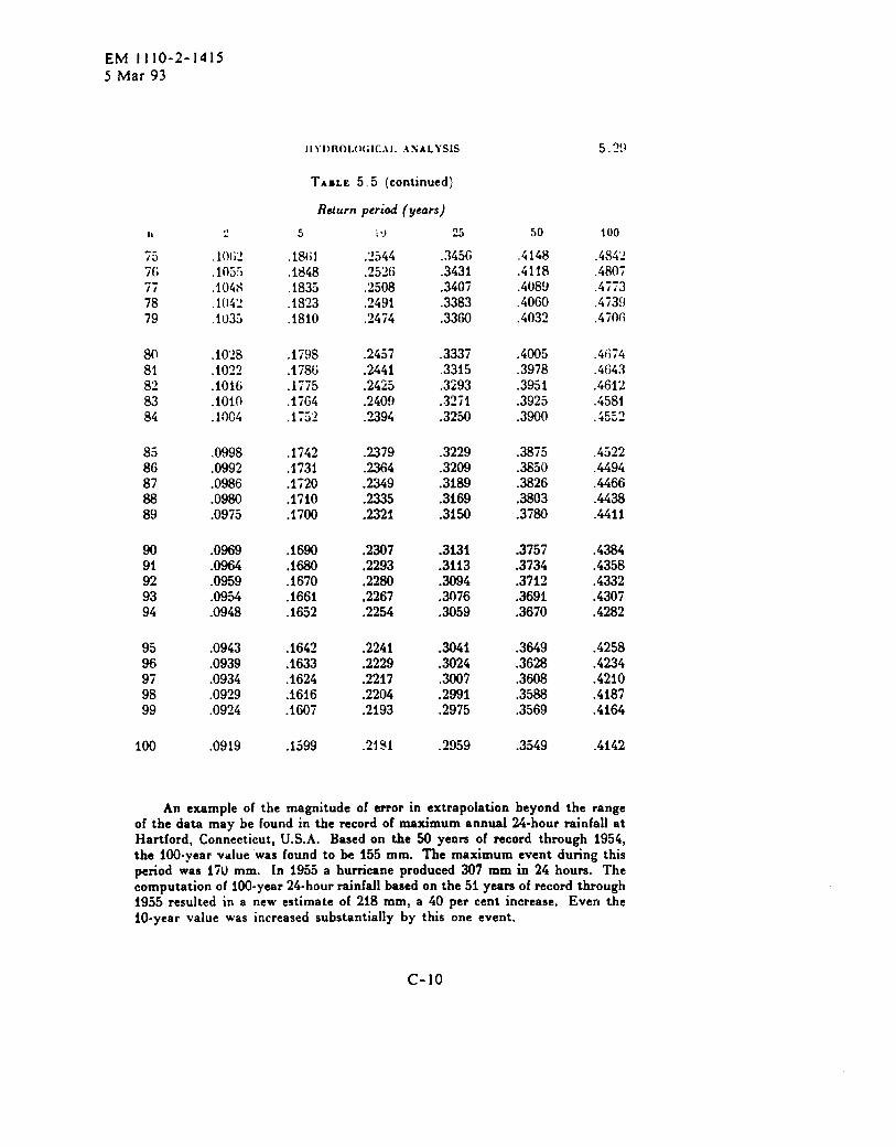
EM II1O-2-I4I55 Mar 93

11

737677

78

79

w

8182

83

84

85

86

87

88

89

90

91

92

93

94

95

96

97

98

99

100

.)

10[;2

. 105:)

.104s1(142

.io35

.1026

.io~~

.1016

.1010

. 10C4

.0998

.0992

.0986

.0980

.0973

.0969

.0964

.0959

.0954

.0948

.0943

.0939

.0934

.0919

11)’l)nOl.f)l;lC,\l..\SALYSIS

TADLE 5.5 (continued)

Return period (years)

5

.lalil

.1848

.1833

.1823

.1810

.1798

.1786

.1775

.1764

.1752

.1742

.1731

.1720

.1710

.1700

.1690

.lW

.1670

.i66i

.1652

.1642

.1633

.i624

.i616

.i60i

.1599

.~49~

.2474

.2457

.2441

.2425

.~409

.2379

.2364

.2349

.2335

.2321

.2307

.2293

.2280

.2267

.2254

.2241

.2229

.2217

.2204

.2193

.zf~l

~~

.3456

.3431

.3407

.3383

.3360

.3337

.3315

.3293

.3271

.3250

.3229

.3209

.3189

.3i69

.3150

.3131

.3i13

.3094

.3076

.3059

.3041

.3024

.3007

.2991

.2975

.2959

50

.4148

.4118

.4089

.4060

.4032

.4005

.3978

.3951

.3925

.3900

.3875

.3850

.3826

.3803

.3780

.3757

.3734

.3712

.3691

.3670

.3649

.3628

.3608

.3588

.3569

.3349

100

.4s42

.480:

.4773

.473!)

.4706

.4(;74

.4643

.4612

.4581

.~~:~

.4522

.4494

.4466

.4438

.4411

.4384

.4358

.4332

.4307

.4282

.4258

.4234

.4210

.4187

.4164

.4142

An examDle of the magnitude of error in extrapolation beyond the rangeof the data m~y be found ii the record of maximum” annual 24-hour rainfall itHartford, Connecticut, U.S.A. Based on the 50 years of record through 1954,the 100-year value was found to be 155 mm. The maximum event during thisperiod was 171) mm. In 1955 a hurricane produced 307 mm in 24 hours. Thecomputation of 100-year 24-hour rainfall based on the 51 years of record through1955 resulted in a new estimate of 218 mm, a 40 per cent increase. Even the10-year value was increased substantially by this one event.

c-lo

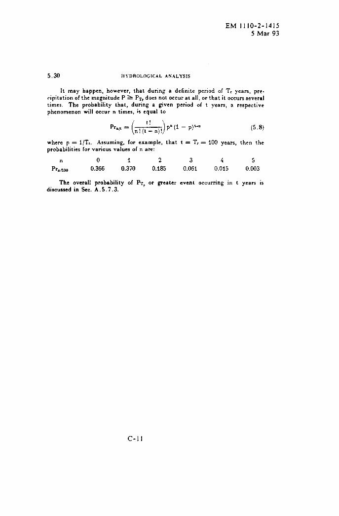
EM 1110-2-14155 Mar 93

5.30 liYDROLOGICAL ANALYSIS

It may happen, however, that during a definite period of T, years, pre-cipitation of the magnitude P > PTr does not occur at all, or that it occurs severaltimes. The probability that, during a given period of t years, a respectivephenomenon will occur n times, is equal to

‘rn’l=(n!(~:n)!)pn(i-p)Ln (5.8)

where p = I/T,. Assuming, for example, that t = T, = 100 years, then theprobabilities for various values of n are:

n o i 2 3 4 5

Prufl~ 0.366 0.370 0.185 0.061 0.015 0.003

The overall probability of P~, or greater event occurring in t years isdiscussed in kc. A. 5.7.3.

C-n

EM 1110-2-14155 Mar 93

APPENDIX D

HISTORIC DATA1Flood information outside that in the systematic record can often be

used to extend the record of the largest events to a historic period much

longer than that of the systematic record. In such a situation, the follow-

ing analytical techniques are used to compute a historically adjusted log-

Pearson Type 111 frequency curve.

1. Historic knowledge is used to define the historically longer period

of “H” years. The number “Z” of events that are known to be the largest in

the historically longer period “H” are given a weight of 1.0. The remaining

“N” events from the systematic record are given a weight of (H-Z)/(N+L) 01]the

assumption that their distribution is representative of the (H-Z) remaining

years of the historically longer period.

2. The computations can be done directly by applying the weights to

each individual year’s data using equations 6-1, 6-2a, 6-3a, and 6-4a.

Figure 6-1 is an example of this procedure in which there are 44 years of

systematic record and the 1897, 1919 and 1927 floods are known to be the

three largest floods in the 77year period 1897 to 1973. If statistics have

been previously computed for the current continuous record, they can be

adjusted to give the equivalent historically adjusted values using equations

6-1, 6-2b, 6-3b, and 6-4b, as illustrated in Figure 6-2.

3. The historically adjusted frequency curve is sketched on logarithmic-

probabiiity paper through points established by use of equation 6-5. The

individual flood events should also be plotted for comparison. The histor-

ically adjusted plotting positions for the individual flood events are

computed by use of equation 6-8, in which the historically adjusted order

number of each event “i” is computed from equations 6-6 and 6-7. The com-

putations are illustrated in Figures 6-1 and 6-2, and the completed plotting

is shown in Figure 6-3.

4. The following example illustrates the steps in application of the

historic peak a~”ustment only. It does not include the final step of

weighting with the generalized skew. The historically adjusted skew developed

by this procedure is appropriate to use in developing a generalized skew.

1 Reproduction of Appendix 6 of Bulletin 17B,

D-1

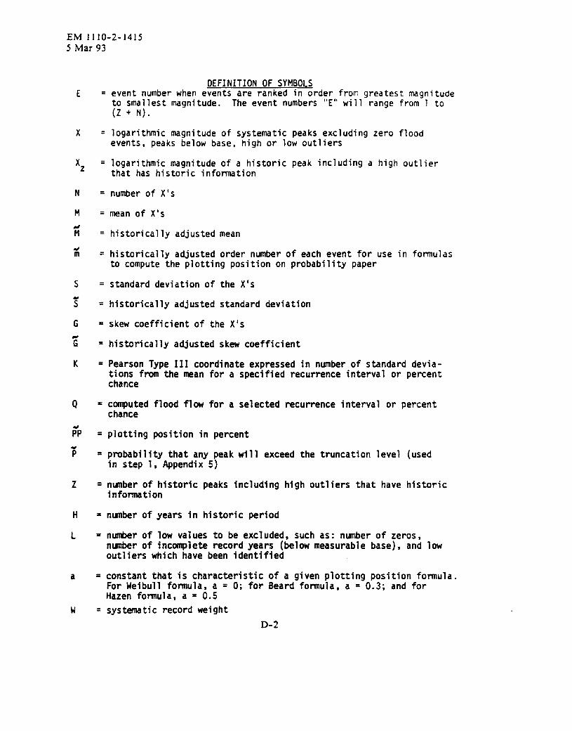
EM 1110-2-14155 Mar 93

E

x

Xz

N

M

fi

dm

s

3

G

E

K

Q

?P

?

z

H

L

a

w

DEFINITION OF SYMBOLSevent number when events are ranked in order fron qreatest maanitudeto smallest magnitude. The event numbers(Z+N)O

logarithmic magnitude of systematic peaksevents, peaks below base, high or low out’

logarithmic magnitude of a historic peak ‘that has historic information

number of X’s

mean of X’s

historically adjusted mean

“E” will-range from-l to

excluding zero floodiers

ncluding a high outlier

historicallyadjusted order number of each event for use in formulasto compute the plotting position on probabilitypaper

standard deviationof the X’s

historicallyadjusted standard deviation

skew coefficientof the X’s

historicallyadjusted skew coefficient

Pearson Type III coordinateexpressed in number of standard devia-tions from the mean for a specified recurrence interval or percentchance

computed flood flow for a selected recurrence interval or percentchance

plotting position in percent

probabilitythat any peak will exceed the truncation level (usedin step 1, Appendix 5)

nunber of historic peaks including high outliers that have historicinformation

number of years in historic period

number of low values to be excluded, such as: number of zeros,nunber of incomplete record years (belowmeasurable base), and lowoutlierswhich have been identified

constant that is characteristicof a given plotting position formula.For Weibull formula, a = O; for Beard formula, a = 0.3; and forHazen formula, a = 0.5

systematicrecord weightD-2

EM 1110-2-14155 Mar 93

M= LH-ML (6-2a)

-2s=

-2s=

Log

Wx(x - i)2+l(XZ - i)2(H-wL-1) (6-3a)

H-WL [WI(X - i)’+x(x - i)’]7

2)1&

~H-wL-1) (H-wL-;3

1WNM +~Xz

H-WL

(6-4a)

(6-2b)

W(N - l)s2+WN(M-~)2+z(Xz - i)2

(H-WL-1) (6-3b)

H-WL

3[

W(N - 1) (N - 2)S3G+3W (N- 1) (M-~)S2

(H-ML-1) (H-wL-2)~ N

+ UN (M - i)3 +X(XZ -i)3

1

(~-Ab)

Q=~+ti (6-5)

i= E;when:l~E~Z (6-6)

Iil=WE - (W-1) (Z+ 0.5); when: (Z+l):E:(Z+N+L) (6-7)

D-3

(6-8)

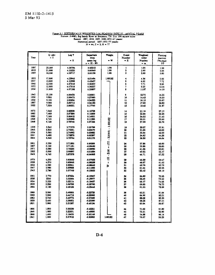
EM 1110-2-1415

5 Mar 93

F]~mStation:3.6055,Bigsu16yhst Bruaton,W. DA 205quareda

-Id: 1897,1919,1927,1930-1973(47p)mtipnod: la97-1973(77p)

14-44;z-3; ?i-77

Q (c6)~ mpuun w- Evau W*- PlOtt~Yur -Y k N- OAr mltlm

=x -* -w =E N&r (Welbull)x-(x-n) -m PP

1897 25,000 4.39794 0.s6212 1.00 11919

l.m21,000

1.2s4.32222 0.-0 1.00 2

19272.00 2.56

18,s00 4.2S717 0.5513s 1.00 3 9.00 3.85

1935 17,000 4.23045 0.51464 1.ss182 41937

4.3413,800

5.664.1399s 0.42407

]

61946

6.02 7.7212,000 4.07918 0.36327 6

19727.71

120009.6s

4.07918 0.36327 71956

9.39Il,aoo

12.M4.071s6 0.35607 8 11.07 14.19

1942 10,100 4.004S2 0.26661 91950 9.660

1275 16.353.96475 0.27s95 10

193014.43

9,10018.50

3.96904 0.2A323 1119s7 9,060

16.12 20.673.95713 o.241s2 12

1932 7,62017.60 22.82

3.69221 0.17740 13 19.48 24.97

1973 7,640 3.s6206 0.16726 1413s2 7,460

21.16 27.13S.67S60 0.15s09 15

19s5 7,1s022.04 29.23

s.s5612 0.14021 161936 6,740

24.53 31.453.s2366 o.11265 m

m 171948

26.216.130

33.603.76746 0.071s6 m 1s 27.89 35.76

m1939 5,s40 3.77379 0.0576s &

1945 5.63029.57 37.91

3.76051 0.03470 :1934 5,5s0

3la 40.063.74s63 o.oso82 G

v 21195; 6,460

32.94 42.233.73670 0.- ~ 2!

1944 6,S4034.52 443s

3.7!z154 0.01173 m 23 36.s0 46.64

1951 5,230e

3.71s50 0.002S6 & 241967 5,160

37.S8 4S.693.711s1 JI.004W II 26

1971 6,W39.ss 50.65

3.7066s 4.00685 M1963 5,000 z

41.35 63.013.66867 4.01684

G27

194943.03

4,74066.17

3.S7578 4.04003 28 U.71 57.32

1970 4.330 3.s3s49 4.07s32g

2919ss

46.394,270

69.473.6304s -o.m 30

195246.07

442W61.62

3.s2941 -0.0SS40 ; 311947

49.763.9s0

63.793.6666s -0.11663 32

194351.U

3,7s065.95

3.57749 4.1s

I__“

33 63.12 6s.10

1961 3,770 3.s7634 -0.IW7 241966

Mm 70.263.6* .o.lm 26

196456A9

3,32072.42

3.62114 4.19467 361933

66.173,220

74.603.50766 420796 27

196469.S5

3,10076.73

3.491s6 -0= 36 61.53 78.6S

1666 3.OSO 3.4s656 .om 391%9 2s00

63.21 61.M3.U716 as 40

1%3 2.74064.W 33.21

3.43775 .027- 411959 2,400

66.56 66.s63.s9021 -o- 42

162166s

Zoso87.51

3.21267 4.40194 43 69.94 89.67

1666 1,920 3- .0.42251 441640

71.621,5s0

91.S23-1 4.49060 45

16s073.31

1,4s093.s9

3.1s435 -0.56146 46.941

74.991,200

%.143.07918 .0.62662 1.661s2 47 76.67 98.29

D-4

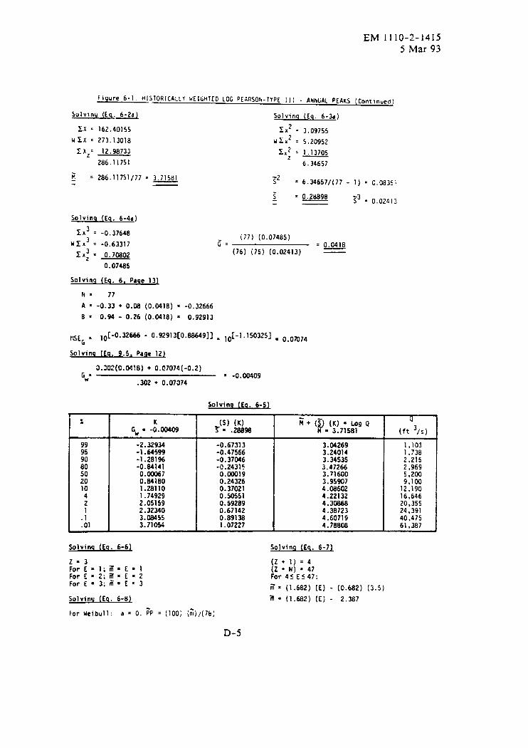
EM 1110-2-14155 Mar 93

Figure 6-1. HISTORICALLYii[lGtlTIO LOG PIA~SOh-TYPE 11: - ANhLjALPEAKs (Contlnuedj

Solvlny (E~.~

xx = 162.40155

U~X = 273.13018

ZXZ’ 12.98733

286.11751

B = 286.11751/77 = 3.71581

Sol ving (Eq. 6-4d)

1X3 = -0.37648

UXX3 = -0.63317 c=

Zx: = 0.70802

0.07485

Solving (Eq. 6-3d)

Xxz = 3.09755

U>,z = 5,20952

Zx: = 1.13705

6.34657

:2= 6.34657/(77 - 1) = 0.@351

~ = 0.28898 33 . 0,024,3

(77) (0.07485)=M

(76) (75) (0.02413) —

Solvinq (Eq. 6, Page 13~

N= 77

A = -0.33 + 0.08 (0.0418) = -0.32666

B=0.94- 0.26 (0.0418) = 0.92913

tUEL = 10[-0”326M - o“929’3[o-8864911 = lo[-l .1503251 = 0.07074

Solving [Eq. 9.5, Page 12~

0.302 (0.04!8) + 0.07074(-0.2)G= = -0.00409w .302 ● 0.07374

Solving (Eu. 6-S~

z

9995

:;50201042

.!

.01

GM = -:.00409-2.32934-1.64599-1 .281%-0.84141

0.000670.841801.281101 .?49292.051592.323403.084553.71054

Solving (Ea. 6-61

2=3For E=l; F=E=lFor E=2; fi=E=2For E=3; tii=E=3

Solving (Eg. 6-8}

-0.67313-0.47566-0.37046-C.24315

o.000190.243260.370210.505510.592890.671420.891381.07227

ii+(g (K)= Log QM = 3.71581

3.042693.240143.345353.472663.716003.959074.086024.221324.308684.387234.607194.78808

Solving (Eq. 6-71

(2+1)=4(z+ N) =47For45ES 47:

== (1.682) (E) - (0.682) (3.5)

iii= (1.682) (E) - 2.387

u

(ft 3/s)

1,1031,7382,2152,9695,2009,100

12,19016,64620.35524,39140,47561 .U1

For Ueibull: a = O. FP = (100) (~)/(7b)

D-5

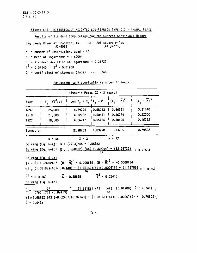
EM I11O-2-14155 Mar 93

Fiqure 6-2. HISTORICALLY WEIGHTED LOG-pEARSOi4TYPE 111 - ANNUAL PEAKS

Results of Standard Computation for the Current Continuous Record

Big Sandy River at Bruceton, TN. DA - 205 square miles#3-6065 (44 years )

N = number of observations used = 44

M = mean of logarithms = 3.69094

s = standard deviation of logarithms = 0.26721~2

= 0.07140 ~3= 0.01908

G = coefficient of skewness (logs) =-0.18746

Adjustment to Historically Weiqhted 77 Years

Historic Peaks (Z = 3 Years)

Year 1 Yz (ft3/s) I Log Yz = Xz ‘Xz - R ; (Xz- E)2 I (Xz- 1)3I

1897 1 25,000 I 4.39794 iO.68213 I 0.46531 1 0.31740

1919I

21,000 I 4.32222I0.60641 I 0.36774 , 0.22300

1927 I 18,50g I 4.26717 0.55136 I 0.30400 0.16762I I I I I

Summation 12.98733 1.83990 1.13705 0.7Q802

N = 44

Solving (Eq. 6-1~:

Solvinq (Eq. 6-2b):

Solvinq (Eq. 6-3b~:

(M - X) = -0.02487,

Z=3 H = 77

W = (77-3)/44 = 1.68182

I.J 1.68182) (44) (3.69094) + (12.98733)77

= 3.71581

(M - X)2 = 0.000619; (M-fi)3 = -0.0000154

52 = (1.68182)(43)(0.07140)+ (1.6(3182)(44)(0.000619)+ (1.13705)= o 0835,76

.

;2 = 0.08351 ~= 0.28898 :3= 0.02413

Solving (Eq. 6-4b):

c= 76

(1.68182) (43) (42) (0.01908) (-0.18746) +(717 (0.02413)[ 44

(3)(1.68182)(43)(-0.02487)(0.07140)+ (1.68182)(44)(-0.0000154)+ (0.70802)]

5= 0.0418

D-6

—

——

—.

——

—-.

—-.

—..-

—-

.—

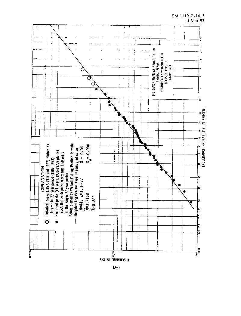
II

I1

II

II

11

l+.

l-:

.-—

—0 ● —

—. r

EXPL

ANAT

ION

Hist

oric

alpe

aks(18

97,1919an

d192

7)plo

ttedas

larg

est

in77

yearp

erio

d(189

7-19

73).

Reco

rdedpea

ks(4

4yea

rs,1930

-1973

)plot

ted

such

that

each

poin

tre

pres

ents

1,58

year

sin

the

long

er77

year

perio

d.Po

ints

plot

ted

byW

eibu

llPl

ottin

gPo

sitio

nfo

rmul

a.W

eigh

ted

Log

Pear

son

Type

Illco

mp~

edcu

rve.

N=44

,2=

3,H=

77G

=O

.O4

&3.7

1581

Gw

=.00

0f)4

?=0.

289

——

-

-‘-4

JBI.—

——

..-.

.———

..__

._

______

—.—.

z.—--— —.—

—-

..——

—-

<

●

��

�✎

/

.

——

r-–7

-r-

.—-

-—

—

-...

...

.

-.,

.._

/——

.

.,.

i

1.

/ 4’‘Ilo

0, .

.—

..i.

/. .

.i:

i.

“1:””

7--

I;---

-4——....—.._,

1“

(J.i

BIG

SAN

DY

RIV

IRA

lB

RU

CE

ION

.T

N:

AN

NU

AL

PEA

KS

t-H

IS1O

RIC

A11

YWII

GH

TIO

10G

PE

AR

$~N

TY

PE

III

FIG

UR

[6-

3

— —.

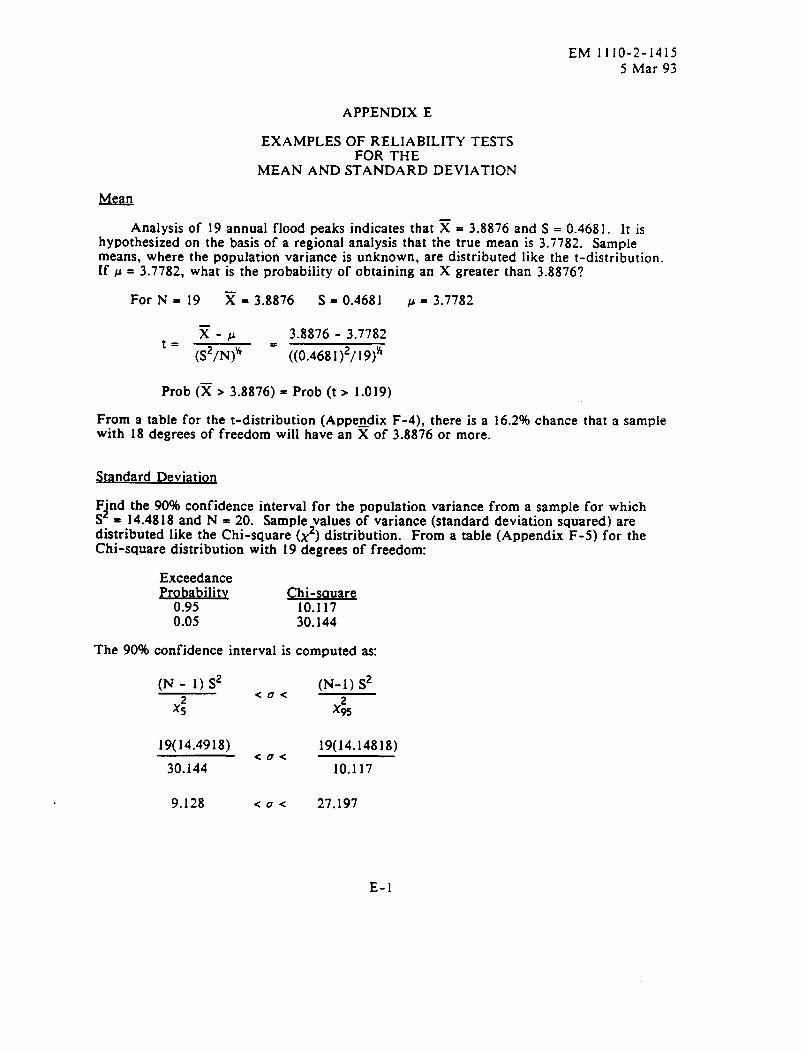
EM 1110-2-14155 Mar 93

APPENDIX E

EXAMPLES OF RELIABILITY TESTSFOR THE

MEAN AND STANDARD DEVIATION

Analysis of 19 annual flood peaks indicates that ~ = 3.8876 and S = 0.4681. It ishypothesized on the basis of a regional analysis that the true mean is 3.7782. Samplemeans, where the population variance is unknown, are distributed like the t-distribution.If ~ = 3.7782, what is the probability of obtaining an X greater than 3.8876?

For N = 19 ~ = 3.8876 S = 0.4681 ~ = 3.7782

K-p 3.8876-3.7782t

= (S2/N)K = ((0.4681 )2/19)%

Prob (~ > 3.8876) = Prob (t > 1.019)

From a table for the t-distribution (Appe~dix F-4), there is a 16.2% chance that a samplewith 18 degrees of freedom will have an X of 3.8876 or more.

~nd ard Deviation

Find the 90% confidence interval for the population variance from a sample for whichS2 = 14.4818 and N = 20. Sample values of variance (standard deviation squared) aredistributed like the Chi-square (X2)distribution. From a table (Appendix F-5) for theChi-square distribution with 19 degrees of freedom:

ExceedanceProbability Chi-sauar?

0.95 10.1170.05 30.144

The 90% confidence interval is computed u

(N- 1)S2 (N-1 ) S2<u<

x; x&

19(14.4918) 19(14.14818)<0<

30.144 10.117

9.128 <u< 27.197

E-1

EM 1110-2-14155 Mar 93

APPENDIX F

STATISTICAL TABLES

F-1

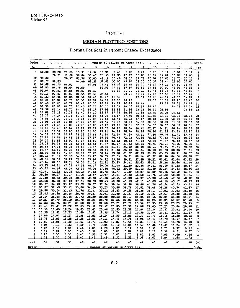
EM 1110-2-14155 Mar 93

Table F-l

MEDIAN PLOTTING POSITIONS

Plotting Positions in Percent Chance Exceedance

order ..,...,.,.. . . . . Number of Values in Array(N) . . . . . . . . . . . . . . .Order

m 1 2 3 4 6 7 e 10~ 1 13 (m

1 50.00 29.29 20.63 15.91 12.94 10.91 9.b3 8,30 7.41 6.70 6.11 5.61 5.19 170.71 50.00 38.64 31.47 26.55 22.95 20.21 18.06 16.32 14.89 13.68 12.66 z

52 98.68 79.37 61.36 50.00 42.18 36.48 32.13 2t3.71 25.94 23.66 21.75 20.13 351 96.77 9.6.65 84.09 68.53 57.82 50.00 44.04 39.35 35.57 32.44 29.82 27.60 450 94.86 96.70 98.62 87.06 73.45 63.52 55.96 50.00 45.19 41.22 37.89 35.06 549 92.95 94.76 96.64 98.60 89.09 77.05 67.87 60.65 54.81 50.00 45.96 42.53 648 91.04 92.81 94.65 96.57 98.57 90.57 79.79 71.29 64.43 58.78 54.04 50.00 747 89.13 90.07 92.67 94.55 96.50 98.54 91.70 81.94 74,06 67.56 62.11 57.47 846 87.22 68.92 90.68 92.52 94.43 96.43 98.50 92.59 63.68 76.34 70.18 64.94 945 85.31 66.97 88.70 90.50 92.37 94.32 96.35 98.47 93.30 85.11 78.25 72.40 1044 83.40 85.03 86.72 88.47 90.30 92.21 94.19 96.27 98.4b 93.89 86.32 79.87 1143 81.50 83.08 84.73 86.45 88.23 90.10 92.04 94.06 96.18 98.40 94.39 87.34 1242 79.59 81.14 82,75 84.42 86.17 87.98 89.88 91.86 93.93 96.10 98.36 94.81 1341 77.68 79.19 60.76 82.40 84.10 85.87 87.73 89.66 91.68 93.79 96.00 98.3240 75.77 77,24 78.78 80.37 82.03 83.76 85.57 87.46 89.43 91.49 93.64 95.91 98.28 4039 73.86 75.30 76.79 78.35 79.97 81.65 83.41 85.25 87.17 89.18 91.29 93.49 95.81 3938 71.95 73.35 74.01 76.32 77.90 79.54 81.28 83.05 84.92 86.88 88.93 91.08 93.33 3837 70.04 71.41 72.82 74.30 75.83 77.43 79.10 80.85 82.67 84.57 06.57 88.66 90.85 3738 68.13 69.46 70.84 72.27 73.77 75.32 76.95 78.64 80.41 82.27 84.21 86.24 88.38 3635 66.23 67.51 68.85 70.25 71.70 73.21 74.79 76.44 78.16 79.96 81.85 83.63 85.90 3534 64.32 65.57 66.87 68.22 69.63 71.1o 72.64 74.24 75.91 77.66 79.49 81.41 83.43 3433 62.41 63.62 64.88 66.20 67.57 68.99 70.46 72.03 73.66 75.35 77.13 78.99 80.95 3332 60.50 61.68 62.90 64.17 65.50 66.88 68.32 69.63 71.60 73.05 74.77 76.58 78.47 3231 58.59 59.73 60.92 62.15 63.43 84.77 66.17 67.63 69.15 70.74 72.41 74.16 76.00 3130 56.68 57.78 58.93 60.12 61.37 62.66 64.01 65.42 66.90 68.44 70.05 71.75 73.52 3029 54.77 55.84 56.95 58.10 59.30 60.55 61.86 63.22 64.64 66.13 67.69 69.33 71.05 2928 52.66 53.89 54.96 56.07 57.23 58.44 59.70 61.02 62.39 63.83 65.33 66.91 68.57 2827 50.95 51.95 52.96 54.05 55.17 56.33 57.55 58.81 60.14 61.52 62.98 64.50 66.09 2726 49.05 50.00 50.99 52,02 53.10 54.22 55.39 58.61 57.69 59.22 60.62 62.08 63.62 2625 47.14 48.05 49.01 50.00 51.03 52.11 53.23 54.41 55.63 56.91 58.26 59.66 61.14 2524 45.23 46.11 47.02 47.98 48.97 50.00 51.08 52.20 53.38 54.61 55.90 57.25 58.67 2423 43.32 44.16 45.04 45.95 46.90 47.69 48.92 50.00 51.13 52.30 53.54 54.83 56.19 2322 41.41 42.22 43.05 43.93 44.83 45.78 46.77 47.80 48.87 50.00 51.16 52.42 53.71 2221 39.50 40.27 41.07 41.90 42.77 43.67 44.61 45.59 46.62 47.70 48.82 50.00 51.24 2120 37.59 36.32 39.08 39.88 40.70 41.56 42.45 43.39 44.37 45.39 46.46 47.56 46.76 2019 35.66 36.38 37.10 37.85 36.63 39.45 40.30 41.19 42.11 43.09 44.10 45.17 46.29 1918 33.77 34.43 35.12 35.83 36.57 37.34 38.14 36.98 39.86 40.78 41.74 42.75 43.81 1817 31.87 32.49 33.13 33.80 34.50 35.23 35.99 36.78 37.61 38.48 39.38 40.34 41.33 1716 29.96 30.54 31.15 31.78 32.43 33.12 33.83 34.58 35.36 36.17 37.02 37.92 36.86 1615 28.05 28.59 29.16 29.75 30.37 31.01 31.68 32.37 33.10 33.07 34.67 35.50 36.38 1514 26.14 26.65 27.18 27.73 28.30 28.90 29.52 30.17 30.85 31.56 32.31 33.09 33.91 1413 24.23 24.70 25.19 25.70 28.23 26.79 27.36 27.97 26.60 2Q.26 29.95 30.67 31,43 1312 22.32 22.76 23.21 23.68 24.17 24.68 25.21 25.76 26.34 26.95 27.59 26.25 28.95 1211 20.41 20.81 21.22 21.65 22.10 22.57 23.05 23.56 24.09 24.65 25.23 25.64 26.48 1110 16.50 18.86 19.24 19.63 20.03 20.46 20.90 21.36 21.64 22.34 22.87 23.42 24.00 109 16.59 16.92 17.25 17.60 17.97 18.35 18.74 19.15 19.59 20.04 20.51 21.01 21.53 96 14.69 14.97 15.27 15.58 15.90 16.24 16.59 16.95 17.33 17.73 18.15 18.59 19.05 87 12.78 13.03 13.26 13.55 13.83 14.13 14.43 14.75 15.08 15.43 15.79 16.17 16.57 76 10.87 11.08 11.30 11.53 11.77 12.02 12.27 12.54 12.83 13.12 13.43 13.76 14.10 65 8.96 9.13 9.32 9.50 9.70 9.91 10.12 10.34 10.57 10.82 11.07 11.34 11.62 54 7.05 7.19 7.33 7.48 7.63 7.79 7.963

8.14 6.325.14

6.515.24

8.71 6.925.35 5.45

9.15 45.57 5.68 5.81 5.94 6.07 6.21

2 3.236.36

3.306.51

3.36 3.43 3.50 3.57 3.656.67 3

3.73 3.821

3.90 4.001.32 1.35 1.38

4.091.40 1.43

4.19 2.46 1.50 1.53 1.56 1.60 1.64 1.68

(m) 52 51 50

1.72 I

49 48 47 46 45 44 43 42 41 40 (m)

Order, . . . . . . . . . . Number of Value sin Arrsv (N) . . . . . . . . . . . . . .. Order

F-2

EM 1110-2-14155 Mar 93

Table F-l (Cent)

MEDIAN PLOTTING POSJTIONS

Plotting Positions in Percent Chance Exceedance

Order . . . . . . . . . . . .,, . Numbaraf Valuss in Array(N) . . . . . . . . . . . . . . . Order

(m) 14 15 16 17 18 19 20 21 22 23 241

254.83 4.52 4.24 4.00

26 (m)3.78 3.58 3.&l 3.25 3.10 2.97 2.85 2.73 2,63 1

2 11.78 11.01 10.34 9.75 9.22 8.74 8.31 7.92 7.57 7.24 6.95 6.67 6.42 23 18.73 17.51 16.44 15.50 14.65 13.90 13.22 12.60 12.03 11.52 11.05 10.61 10.21 34 25.68 2&.01 22.54 21.25 20.09 19.05 18.12 17.27 16.50 15.80 15.15 14.55 14.00 45 32.63 30.51 26.65 27.00 25.53 24.21 23.02 21.95 20.97 20.07 19.25 1S.49 17,79 56 39.58 37.oo 34.75 32.75 30.97 29.37 27.93 26.62 25.43 24.35 23.35 22.43 21.5B 67 46.53 43.50 40.85 38.50 36.41 34.53 32.83 31.30 29.90 28.62 27.45 26.37 25.37 78 53.47 50.00 46.95 44.25 41.84 39.66 37.74 35.97 34.37 32.90 31.55 30.31 29.16 89 60,42 56.50 53.05 50.00 47.28 44.64 42.64 40.65 38.63 37.17 35.65 34.24 32.95 910 67.37 63.00 59.15 55.75 52.72 50.00 47.55 45.32 43.30 41.45 39.75 38.18 36.74 1011 74.32 69.49 65.25 61.50 58.16 55.16 52.45 50.00 47.77 45.72 43.85 42.12 40,53 1112 81.27 75.99 71.35 67.25 63.59 60.32 57.36 54.68 52.23 50.00 47.95 46.06 44,32 1213 88.22 82.49 77.46 73.00 69.03 65.47 62.26 59.35 56.70 54.28 52.05 50.00 48.11 13lb 95.17 88.99 83.56 76.75 74.47 70.63 67.17 64.03 61,17 58.55 56.15 53.94 51.89 14

95.48 69.66 84.50 79.91 75.79 72.07 66.70 65.63 62.83 60.25 57.88 55.68 1539 96.24 95.76 90.25 85.35 80.95 76.96 73.36 70.10 67.10 64.35 61.82 59.47 1636 95.70 98.19 96.00 90.78 86.10 61.66 76.05 74.57 71.38 68.45 65.76 63.26 1737 93.16 95.59 98.16 06.22 91.26 86.78 82.73 79.03 75.85 72.55 69.69 67.05 1836 90.62 92.98 95.47 96.09 96.42 91.69 87.40 63.50 79.93 76.65 73.63 70.84 1935 88.08 90.38 92.79 95.34 96.04 96.59 92.08 87.97 64.20 80.75 77.57 74.63 2034 85.54 87.77 90.12 92.60 95.21 97.96 96.75 92.43 66.48 84.85 81.51 78.42 2133 83.01 85.17 87.45 89.85 92.39 95.07 S7.92 96.90 92.76 8S.95 85.45 82.21 2232 80.47 82.56 84.77 87.10 88.56 82.17 94.93 97.86 97.03 93.05 89.39 86.00 2331 77.93 79.86 82.10 84.35 86.74 89.26 81.83 94.77 97.79 97.15 93.33 89.79 2430 75.39 77.35 79.42 61.60 83.91 86.35 86.84 81.68 94.60 97.72 97.27 93.58 2529 72.85 74.75 76.75 76.86 81.08 83.44 85.84 88.59 91.42 94.43 97.64 97.37 2628 70.31 72.14 74.07 76.11 76.26 80.53 82.95 85.51 88.23 81.13 94.24 97.5527 67.77 69.54 71.40 73.36 75.43 77.63 79.95 82.42 85.05 87.84 90.83 94.03 97.47 2726 65.23 66.93 68.72 70.61 72.61 74.72 76.96 79.33 81.66 84.55 87.43 90.51 93.81 2625 62.69 64.33 66.05 67.86 69.78 71.81 73.96 76.24 78.67 81.26 84.03 86.99 90.16 2524 60.16 61.72 63.37 65.11 66.95 68.90 70.87 73.16 75.49 77.97 80.62 83.46 66.51 2423 57.62 59.12 60.70 62.37 64.13 65.98 67.97 70.07 72.30 74.68 77.22 79.94 82.86 2322 55.08 56.51 58.02 5S.62 61.30 63.09 64.S8 66.98 69.12 71.39 73,82 76.42 79.21 2221 52.54 53.81 55.35 56.87 56.48 60.18 61.88 63.88 65.83 68.10 70.42 72.90 75.56 2120 50.00 51.30 52.67 54.12 55.65 57.27 56.99 60.61 62.74 64.81 67.01 69.37 71.91 2018 47.46 46.70 50.00 51.37 52.83 54.36 55.99 57.72 58,56 61.52 63.61 65.85 68.26 1918 64.82 46.08 47.33 46.63 50.00 51.45 53.00 54.63 56.37 58.23 60.21 62.33 64.60 1817 42.38 43.49 44.65 45.88 47.17 46.55 50.00 51.54 53.19 54.94 56.81 56.81 60.95 1716 39.64 40.86 41.96 43.13 44.35 45.84 47.00 46.46 50.00 51.65 53.40 55.28 57.30 1615 37.31 38.28 38.30 40.36 41.52 42.73 44.01 45.37 46.81 48.35 50.00 51.76 53.65 1514 34.77 35.67 36.63 37.63 38.70 38.62 41.01 42.28 43.63 45.06 46.60 48.24 50.00 1413 32.23 33.07 33.95 34.89 35.67 36.91 36.02 38.19 40.44 41.77 43.19 44.72 46.35 1312 28.69 30.46 31.28 32.14 33.05 34.01 35.02 36.11 37.26 38.48 39.79 41.19 42.70 1211 27.15 27.86 28.60 29.39 30.22 31.10 32.03 33.02 34.07 35.18 36.39 37.67 39.05 1110 24.61 25.25 25.93 26.64 27.39 26.18 29.03 29.93 30.88 31.90 32.99 34.15 35.40 109 22.07 22.65 23.25 23.89 24.57 25.28 26.04 26.84 27.70 26.61 29.58 30.63 31.74 96 19.53 20.04 20.58 21.14 21.74 22.37 23.04 23.76 24.51 25.32 26.18 27.10 28.09 87 16.88 17.44 17.90 18.40 10.82 18.47 20.05 20.67 21.33 22.03 22.78 23.58 24.44 76 14,46 14.83 15.23 15.65 16.08 16.56 17.05 17.56 18.14 16.74 19.38 20.06 20.79 65 11.92 12.23 12.55 12.80 13.26 13.65 14.06 14.48 14.95 15.45 15.97 16.54 17.14 54 9.38 8.62 9.88 10.15 10.44 10.74 11.06 11.41 11.77 12.16 12.57 13.01 13.48 43 6.84 7.02 7.21 7.40 7.61 7.832

8.07 8.32 8.58 8.874.30

9.174.41

9.494.53 4.66 4.78 4.83 5.07

9.84 35.23 5.40 5.57 5.76 5.97 6.19 2

1 1.76 1.81 1.86 1.81 1.96 2.02 2.08 2.14 2.21 2.28 2.36 2.45 2.53 1

(m) 39 38 37 36 35 34 33 32 31 30 29 28 27 (m)

Order . . . . . . . . . . . . . .. Number of V.sluesin Arrsy (N) . . . . . . . . . . . . . ,. Order

F-3

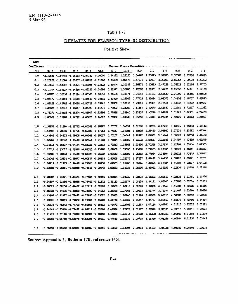
EM 1110-2-14155 Mar 93

Tabie F-2

DEVIATE SFOR PEARSON TYPE-111 DISTRIBUTION

Positive Skew

*W

tifzicimt . . . . . . . . . . . . . . . . . . . . .. *at-o b~m . . . . . . . . . . . . . . . . .

(G) 99.0 95.0 90.0 80,0 m.o 20.0 10.0 5.0 2.0 1.0 0.5 0.2 0,1

0.0 -2.32835 -1.64485 -1.28M5 4.64162 0.00000 0.64262 1.28~ 1.64485 2.05375 2.3=5 2.57583 2.87816 3.09323

0.1 -2.25256 -1.61594 -1.27037-0.84611 -0.01S62 0.83639 1.~178 1.67279 2.10697 2.38961 2.M5 2.99978 3.23322

0.2 -2.17640 -1. s7 -1.25824 -0.64M -0.0~ 0.63044 1.3010S 1.68971 2.15935 2.47Z 2.76321 3.lZ169 3.37703

0.3 -2.10394 -1.55527 -1.24516-0.65285 -0.04~ 0.62377 1.30936 1.72562 2.21081 2.54421 2.85636 3.24371 3.=139

0.4 ‘2.02933 -1.52257 -1.23114 -0.65508-0.06651 0.81638 1.31671 1.75048 2. XI.33 2.61539 2.94900 3.36566 3.-8

0.5 -1.95472 -1.49101 -1.21618 -0.- -0.06302 O.M~ 1.32308 1.77428 2.31084 2.68572 3.04102 3.48737 3.810~

0.6 -1.88029 -1.45762 -1.20020-0.65718 -O. -5 0.79950 1.= 1.79701 2.3=1 2.75514 3.13232 3.60872 3.95%7

0.7 -1.-1 -1.42345-1.18347 -0,85703-0.13578 0.79302 1.33204 1.8L864 2.40670 2.82359 3.=1 3.72957 4.10022

0.8 -1.73271 -1.36655-1.18574 -O. -7 -0.33~ 0.77~ 1.-O 1.82916 2.4= 2.89101 3.31243 3.84981 4.24439

0.9 -le66M1 -1.35289-1.14712-0.85426 -0.1~7 0.78802 1.33869 l.- 2.49811 2.95735 3.40109 3.-2 4.38807

1.0

1.1

1.2

1.3

1.4

1.5

1.6

1.7

1.6

1.9

2.0

2.1

2.2

2.3

2.4

2.5

2.6

2.7

2.6

2.9

-1.58838-1.33684-1.327624.85161-0.28387 0.75752 1.34039 1.67683 2.54206 3.- 3.46674 4.0~ 4.531U

-1.s1808 -1.mla -1.lon -0.64609-0.17968 0.74537 1.340s2 1.m95 2.58480 3.08E60 3.57530 4.20562 4.67344

-1.44942-1.24313-1.0860E-0.84389-0.29517 0.73257 1.34047 l.- 2.62631 3.14944 3.=73 4.32263 4..91492

-1.36267-1.20578-1.084234.63841-0.22040 0.72935 l.- 1.~72 2.66657 3.21.3033.74497 4.43839 4.95549

‘1.3MM -1.18627-1.04144-0.63223-0.~5 0.70522 1.32665 l.- 2.70~ 3.27324 3.82798 4.55304 5.09~5

‘1.M1l ‘1.23075‘1.O361O -0.82516-0.- 0,6803 1.33330 1.95063 2.74325 3.33035 3.90973 4.66651 5.23353

-l.= -1.- ‘0.W28 -0.61720-0.2542? 0.67532 1.32S00 1.96233 2.77964 3.38804 3.99016 4.77875 5.37087

‘1.14042-1.0~1 -o.- -0.80837-0.- 0.- 1.~76 1.87227 2.61472 3.44438 4.06926 4.68971 5.50701

-1.08711-1.02973-0.844S -0.79668-0.28350 0.64335 1.31760 1.98124 2.84848 3.4W5 4.14700 4.=7 5.64191

-1.a3895 -0.88381-0.92868-0.78838-O.*3 o.62a82 1.31054 1.86a08 2.ml 3.55295 4.22336 5.10768 5.77X9

4.88995-0.94871 4.M -0.77686-0.30685 0.60944 l.- 1.8$573 2.92202 3.60517 4.29832 5.21461 5.90776

-0.94607-0.91456-0.- -0.76482-0.31872 0.59383 1.29377 2.00326 2.94181 3.- 4.37186 5.32014 6.03ffi5

4.~522 +.68256 *.84422 -0.75221-0.- 0.57883 1.264U 2.W570 2.97026 3.70543 4.443W 5.42426 6.16616

-0.--0.64876 -0.8~ -0.73860-0.- 0.55549 1.27365 2.00803 2.99744 3.75347 4.51467 5.52694 6.29626

-0.63386-0.83E?7-0.79472-0.72495-0.35062 0.53663 1.26240 2.02328 3.02330 3.8W32 4.58393 5.=18 6.42292

43.7- 4.79025 4.7?082 ~.71067 4.3= 0.51768 1.25039 2.03247 3.04787 3.84540 4,65176 5.7Z7E 6.54814

-0.76676-0.76242+.74708 -0.--0.38652 0.48672 1.23768 2.0~ 3.07126 3.=0 4.71635 5.82629 6.67191

-0.74049-0.736104.72422-0.86231-0.37840 0.47S34 1.22422 2.01177 3.09320 3.93183 4.78323 5.92216 6.79421

-0.71435-0.72226-0.70208-0.66603-0.38353 0.4~ 1.23033 2.- 3.12398 3.87301 4.84669 6.018S 6.91505

-0.86959-0.667= -0.8K175-0.--0.36993 0.44035 1,3.95392.0071.O3.12356 4.0~ 4.80W 6.13254 7.03443

3.0 -O.- -0.68532-0.66023-0.-4.39554 0.42040 1.1- 2.00335 3.15193 4.05138 4.96959 6.~506 7.=5

Source: Appendix 3, Bulletin 17B, reference (46).

F-4

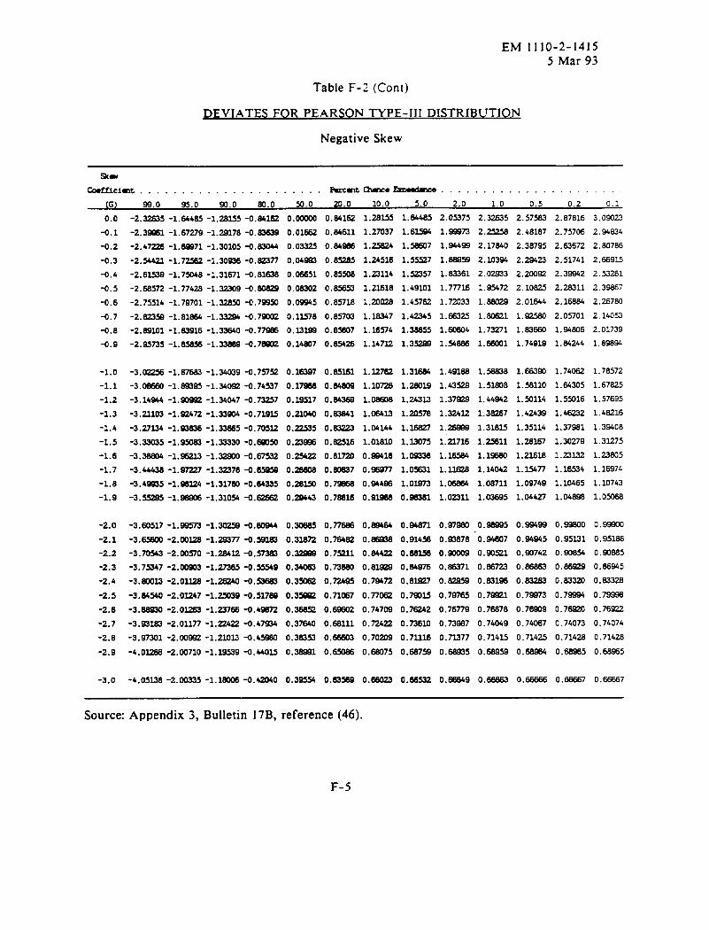
EM 1110-2-14155 Mar 93

Table F-2 (Cent)

DEVIATES FOR PEARSON TYPE-111 DISTRIB UTION

Negative Skew

9tal

Cimmciti . . . . . . . . . . . . . . . . . . . . .. Fucmt-o ~e . . . . . . . . . . . . . . . . .

(G) 98.0 95.0 93,0 M.o M.o 20.0 10.0 5.0 2.0 1.0 0.5 0.2 0.1

0.0 -2.=5 -1.84485-1.28155-0.84162 O.00000 0.84162 1.28155 1.64485 2.05375 2.32635 2.57W 2.87816 3.09323

-0.1 -2.39S61-1.67279-1.=178 -0.83639 0.0= 0.84611 1.27037 1.63594 1.99973 2.25253 2.48187 2.75706 2.94334

-0.2 -2.47226-1.6W71 -1.301O5-0.83044 0.03325 0.84066 1.25824 1.58807 1.94499 2.17840 2.38795 2.63672 2.80786

-0.3 -2.54421-1.7~-l.30W -0.82277 0.04993 0.- 1.24526 1.55527 1.88959 2.10394 2.29422 2.51741 2.=935

-0.4 -2.61539-1.7W8 -1.31671-0.81638 0.06651 0.85506 1.22114 1.52357 1.83361 2.02933 2.20092 2.39942 2.53U1

-0.5 -2.68572-1.77428-1.32309-0.60829 0.08302 0.- 1.21618 1.49101 1.77716 1.95472 2.10825 2.28311 2.39867

-0.6 ‘2.75514-1.79701‘1.32850-0.7S95410.09945 0.65718 1.~028 1.45762 1.7~33 1.W29 2.01844 2.16884 2.26780

-0.7 ‘2.823* ‘1.81864‘l.= ‘0.79002 0.13S78 0.85703 1.16347 1.42345 1.E63Z 1.-1 1.92580 2.05701 2.14053

-0.8 -2.8S101-1.83916-1.33640-0.77~ 0.131S9 O.-7 1.3.65741.38855 1.EJ36041.73271 1.83660 1.94306 2.01739

-0.9 -2.95735-1.85856‘1.- 4.78902 0.14807 0.W26 1.14732 1.3= 1.54886 l.~01 1.74913 1.84244 1.89894

-1.0

-1.1

-1.2

-1.3

-1.4

-1.5

-1.6

-1.7

-1.8

-1.9

-2.0

-2.1

-2.2

-2.3

-2.4

-2.5

-2.6

-2.7

-2.8

-2.9

-3.--1 .87683-1.34039-0.75752

-3.oEa360-1.=95 -1.34m -0.74537

-3.14%4 -1.90992-1.34047-0.73257

-3.22203-1.82472-1.33904-o.71835

-3.27134-1.93636-1.33865-0.70512

-3.33035-1.95083-1.33330-o.m3

-3.36804-1.98213-1.32800-0.67532

-3.44438-1.97227-1.32376-0.-

-3.4m5-l.98324 -1.31760-0.64335

-3.55295-1.--1.31054 -o.-

-3.60517-1.99573 -1.= -0.-

-3.65800-2.00128 -1.=77 -0.59263

-3.70543 -2.W570 -1.28412 -O.57383

-3.75347-2.00903 -1.27365-0.=9

-3.80013 -2.03228-1.- -0.53683

-3.84540 -2.0M7 -1.25039-0.51768

-3. - -2.0= -1.23766-0.49872

-3.63183 -2.01177 -1.~22 -0.47~

-3.97301 -2. oom-l.22013 -0.4-

-4.0~ -2.00710 -1.29539-0.44015

0.16397

0.17868

0.19317

0.22040

0.=5

0.23998

0.25422

0.26808

O.zam

0.29443

0.306850.32872

0.-

O.w

0.35062

0.3=

0.36852

0.37640

0.38333

0.38991

0.85161

o.e4m

0.84368

0.63841

0.83222

o.m3.6

0.81720

0.-7

0.7-

0.78828

0.77868

0.78482

0.75221

0.-

0.72495

0. 71W

o.-

0.68111

0.-3

0.-

1.12762

1.M728

1.08808

1.08413

1.04144

1.01810

0.=18

0.98977

0.94498

0.9-

0.894640.-0.844220.8=

0.79472

0.77082

0.74709

0.72422

0.70209

0.88075

1.316a4

1.28019

1.2431.3

1.20576

1.18827

1.23075

1.-8

1.05631

1.01.E73

0.98381

0.94671

0.91458

O.um

0.84976

0. Em7

0.79015

0.76242

0.73610

0.71.218

0. 3a759

1.49183

1.43529

1.37-

1.32412

1.=

1.23716

1.16584

1.12828

1.06864

1.02211

0.979800.=878

0.90W9

0.86371

0.63959

0.79765

0.76n9

0.73987

0.7n77

0.68935

1.58838

1.51808

1.44942

1.38267

1.31815

1.=11

1.1s680

1.14042

1.08711

1.03695

0.-5

“0.94W7

0.90521

0.=23

0.631%

o. 7=1

0.76878

0.74049

0.71435

0.68959

1.=90

1.58110

1.3114

1.4M39

1.35114

1.28167

1.21618

1.15477

1.09749

1.04427

0.994990.94945

0. =742

o.86e63

0.83283

0.79973

0. 76W9

0.74087

0.714=

0.66964

1.74062

1.64305

1.5316

1.46232

1.37981

1.30279

1.23132

1.16534

1.10465

1.04898

0.-O0.95131

0.90854

0.-

0.83320

0.79994

0.7-

0.74073

0.7142E

0.68965

1.78572

1.67~

1.57695

1.48216

1.39408

1.31275

1.23805

1.16974

1.10743

1.o-

0.-00.95186

0.W885

o.ffi945

0.6332E

0.79990

0.76922

0.74074

0.71428

0.68%5

-3.0 ‘4.051,38 -2.00335-1.18006-0.42040 0.39554 0.63~ 0.68023 0.66532 0.-9 0.66663 0.63668 0. E6667 0.=7

Source: Appendix 3, Bulletin 17B, reference (46).

F-5

EM 1110-2-14155 Mar 93

Table F-3

NORMAL DISTRIBUTION

Percent Chance Exceedance for Given Normal Standard Deviate (K)

. . . . . . . . . . . . . . . Incrmsnts to Kin Colunml . . . . . . . . . . . . . . .K .00 .01 .02 .03 .04 .05 ,06 .07 .08 ,09

.0

.1

.2

.3

::.6.7.8.9

1.01.11.21.31.41.51.61.71.61.9

2.02.12.22.32.42.52.62.72.82.9

3.03.13.23.33.43.53.6

:::3.9

4.0

5.0

6.0

50.0046.0242.0738.2134.4630.8527.4324.2021.1918.41

15.8713.5711.519.680.066.665.464.463.s92.67

2.281.791.391.072.820.621.466.347.256.167

.135

.0968

.0687

.0483

.0337

.0233

.0159

.01078 .01037

.00724 .00695

49.6045.6241.6837.8334.0930.5027.0923.6920.9018.14

15.6213.3511.319.517.936.555.374.363.512.81

2.221.741.361.044.798.604.453.336.248.181

.131

.0936

.0664

.0467

.0325

.0224

.0153

.00481 .00462

.00317 .00304

.042867

.07967

49.2045.2241.2937.4533.7230.1526.7623.5820.6117.88

15.3913.1411.129.347.786.435.264.273.442.74

2.171.701.321.017.776.587.440.326.240.175

.126

.0904

.0641

.0450

.0313

.0216

.0147

.0099

.00667

.00443

.00291

48.8044.8340.9037.0733.3629.8126.4323.2720.3317.62

15.1512.9210.939.187.646.305.164.163.362.68

2.121.661.29.9s0.755.570.427.317.233.169

.122

.0874

.0619

.0434

.0302

.0208

.0142

.00958

.00641

.00425

.00279

46.4044.6340.5236.6933.0029.4626.1122.9620.0517.36

14.9212.7110.759.017.496.185.054.093.292.62

2.071.621.25.964.734.554.415.307.226.164

.118

.0845

.0598

.0419

.0291

.0200

.0136

.00920

.00615

.00408

.00267

48.0144.0440.1336.3232.6429.1225.7822.6619.7717.11

14.6912.5110.566.857.356.064.954.013.222.56

2.021.581.22.939.714.539.402.298.219.159

.114

.0816

.0577

.0404

.0280

.0193

.0131

.00884

.00591

.00391

47.6143.6439.7435.9432.2828.7725.4622.3619.4916.85

14.4612.3010.388.697.215.944.853.923.142.50

1.971.541.19

,914.695.523.391.289.212.154

.111

.0789

.0557

.0390

.0270

.0185

.0126

.00850

.00567

.00375

.00256 .00245

47.2143.2539.3635.5731.9228.4325.1422.0619.2216.60

14.2312.1010.20

6.537.085.824.753.843.072.44

1.921.501.16

.889

.676

.508

.379

.280

.205

.149

.107

.0762

.0538

.0376

.0260

.0179

.0121

.00817

.00544

.00360

46.8142.8638.9735.2031.5628.1024.8321.7718.9416.35

14.0111.9010.038.386.945.714.653.753.012.39

1.861.461.13.866.657.494.368.272.199.144

.104

.0736

.0519

.0362

.0251

.0172

.0117

.00784

.00522

.00345

,00235 .00225

46.4142.4738.5934.8331.2127.7624.5121.4818.6716.11

13.7911.709.658.236.815.594.553.672.942.33

1.831.431.10.842.639.480.357.264.193.139

.100

.0711

.0501

.0350

.0242

.0165

.0112

.00753

.00501

.00331

.00216

Note - Values have been generated by use of computer routines for the normaldistribution.

F-6

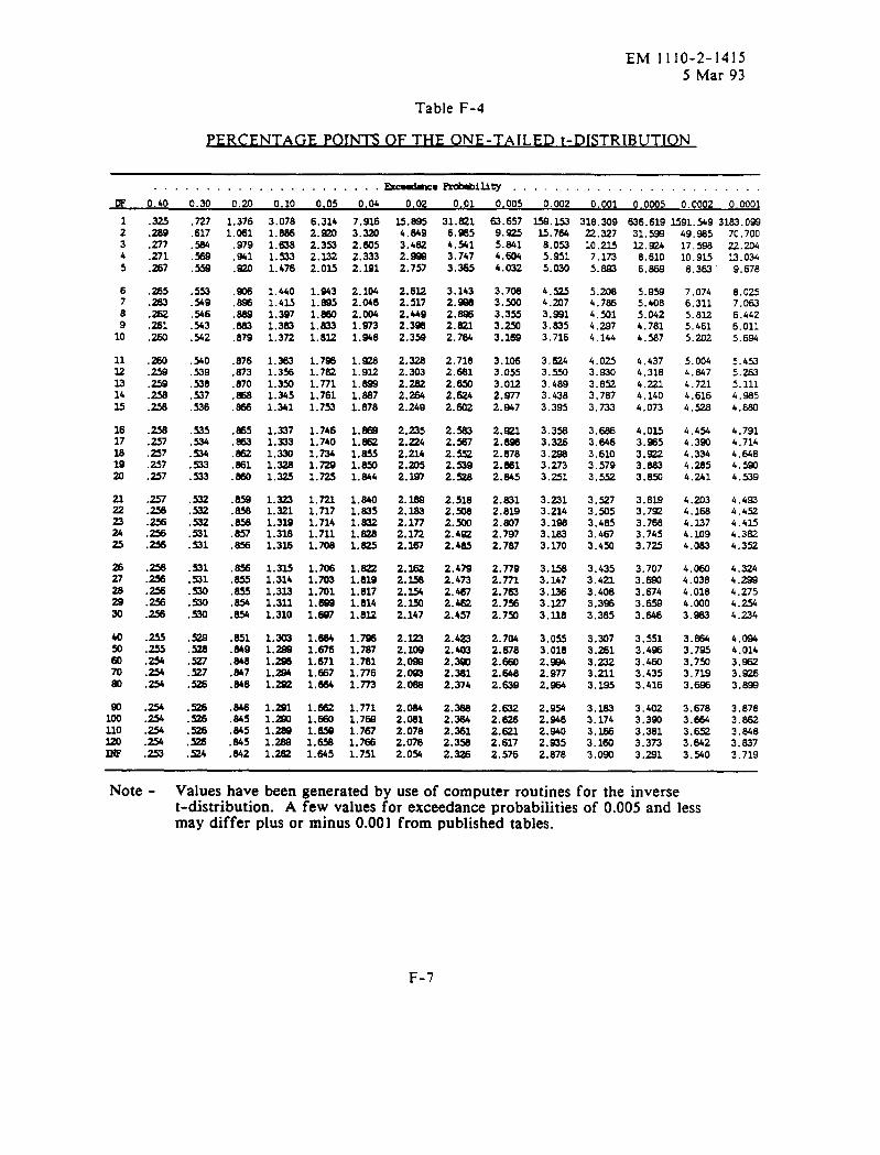
EM 1110-2-14155 Mar 93

Table F-4

P R NTA~ NE-TAILED t-DISTRIBUTION

. . . . . . . . . . . . . . . . . . . . . . Rcadmce-iu@ . . . . . . . . . . . . . . . . . . . . . . . .

E 0.60 0.30 0.20 0 0 005 004 00 00 0 005 0.002 0.001 0.0005~ 0.0001

12345

6789

10

1132lz1415

1617181920

22z232425

26

zB30

4050607060

solW110

z

.325

.2a9

.277

.271

.727

.6171.3761.061.979.941.=

3.0761.8861.6381.5331.676

6.3142.m2.353Z.m2.OH

7.9163.3202.6052.3332.191

IS.6954.6493.4632.9992.757

2.6E2.5172.4492.3962.359

2.3282.3032.2622.2642.24Q

2.2252.2242.2242.2052.m

2.1692.1632.1772.1722.267

2.2622.3582.3542.3502.147

2.3232.1092.m2.m2.066

2.0642.0612.0782.0762.054

31.6216.9654.5413.7473.365

3.1432.=2.6U62.6232.764

2.7182.6812.6502.6242.602

2.5632.s2.5522.5392.52a

2.5182.5082.5002.4s?2.465

2.4792.4732.4672.4622.457

2.4232.4032.=2.3612.374

2.3662.3642.3612.3582.326

63.6579.=5.8414.m4.032

3.7063.X3.3553.2503.169

3.1063.0553.0122.9772.%7

2.s?l2.6982.6702.6612.845

2.8212.81S2.W72.7972.787

2.7792.7712.7632.7562.750

2.7042.6762.W2.6482.639

2.6322.6262.6222.6172.576

L59.m15.7&8.0535.9515.030

4.%4.2n73.W13.6353.716

3.6243.5503.4893.4383.395

3.3563.3263.=3.2733.251

3.2213.2243.lW3.1833.170

3.ls83.1473.1363.3273.128

3.0553.0182.9342.9772.964

2.9542.W62.9402.9352.876

318.309 636,619M91.549 3183.0922.32710.21S7.1735.m

S.m4.7864.%14.2974,144

4.0253.9303.8523.7873.733

3.6663.6463.6103.5793.552

3.5273.5053.4853.4673.450

3.4353.4233.4083.3963.365

3.3073.2613.2323.2313.1.a5

3.I.633.174

::E3.090

31.599u.=8.6106.869

5.9595.4085.0424.7614.587

4.4374.31.34.2214.1404.073

4.0353.9653.=3.8833.850

3.8193.7=3.7683.7453.725

3.7073.6903.6743.6593.646

3.5513.4s63.4603.4353.416

3.4023.3933.3813.3733.291

*3.X2

17.59810.9158.363

7.0746.3115.8U5.4615.~2

5.Oofl4.3474.7214.6164.528

4.4544.3904.3344.2354.241

4.2034.16.s4.1374.M94.063

4.0604.0384.0184.0003.s83

3.s643.7953.7503.7193.*

3.6783.E643<6523.6423.540

/u. ruu

22.20413.0349.678

8.0257.0636.4426.0115.694

5.4535.2635.1114.9854.W

4.7914.7144.6484.m4.539

4.4934.4524.4154.3s24.352

4.3244.2994.2754.2544,234

4.0944.0143.9623.9263.699

3.8783.e623.8483.8373.719

.564

.267 .559

.265 .553.549.546.543.542

.540

.539

.906

.m

.869

.663

.879

1.4401.4U1.3971.3631.372

1.0431.6651.6601.633l.slz

2.1042.0462.0041.9731.S48

.263

.Za2

.261

.m

.m

.259.676.873.870.666.666

1.3631.3%1.3XI1.3451.341

1.7961.7621.7711.7611.753

l.Qa1.9321.-1.6671.878

.258

.258

.=

.257

.257

.257

.257

.257

.=

.2%

.s

.-

.2!?6

.256

.=

.=7

.536

.35

.534

.%

.533

.533

.%

.=

.%

.31

.531

.=1

.531

.665

.m1.3371.3331.3301.3261.325

1.7461.7401.7341.729I.m

1.6691.-1.655I.m1.644.mo

.659

.858

.8%

.657

.6%

1.3231.3211.3191.3181.326

1.3351.3141.3331.3111.310

1.3031.269l.zm1.2941.=

1.7211.7171.7141.7111.706

1.8401.6351.8321.8261.625

.m

.655

.655

.-

.654

1.7C61.7031.701l.m1.697

1.6841.6761.6711.6671.664

1.=1.82S1.6171.8141.622

1.7%1.7871.7811.n61.773

.530

.530

.530

.255

.255

.254

.651

.849

.84a

.847

.846.Q7

.254

.254 .846.845.645.845.642

1.=11.m1.=1.26sl.zaz

1.6621.6601.=1.6561.645

1.7711.76a1.7671.7s61.751

.254

.254

.254

.=

Note - Values have been generated by use of computer routines for the inverset-distribution. A few values for exceedance probabilities of 0.005 and lessmay differ plus or minus 0.001 from published tables.

F-7

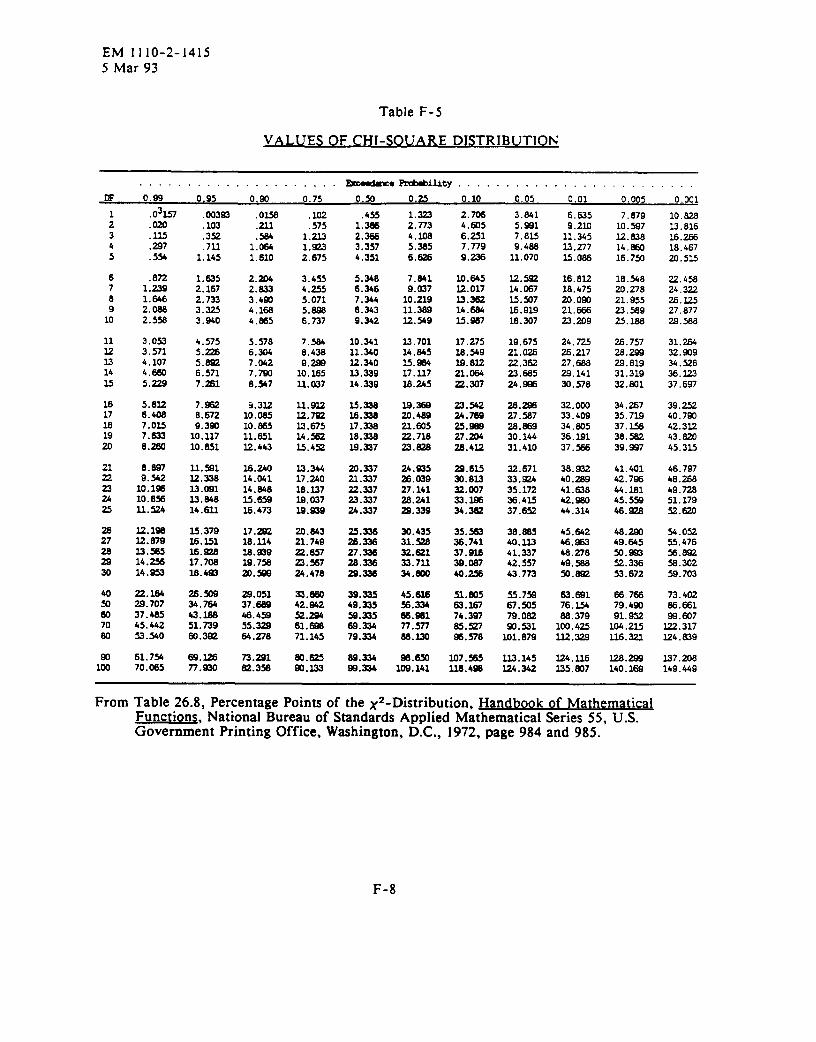
EM 1110-2-14155 Mar 93

Table F-5

VAL E F 1-U SO CH SOUARE DISTRIBUTION

. . . . . . . . . . . . . . . . . . . . Rualmco~ility . . . . . . . . . . . . . . . . . . . . . .

m 0.99 0.95 0,90 0.75 0.50 0,2s 0.10 0.05 0.01 0.005 0.001

12345

678910

11E1314M

1617181920

2122232425

E282930

40w607080

w100

0JIS7.020.115.Z7.554

.8721.2391.M62.0882.558

3.0533.5714.1074.W5.229

S.8126.4087.0357.6338.260

8.8979.54210.1%10.856U.524

12.19832.87s

z;=14.853

22.w29.70737.48545.44253.540

61.75470.065

.00393

.103

.352

.7111.145

1.6352.1672.7333.3253.940

4.5755.=5.=6.5717.281

7.=8.6729.38010.11710.851

11.S1U.338n.m33.84814.632

M. 37916.15116.Q817.70810.4=

26.50834.76443.1,8851.73960.3=

W.lzs77.=

.Om

.211

.W1.0641.610

2.2042.8333.4=4.16a4.M5

5.5786.3047.0427.7W8.547

9.33210.08510.86511.851u. 443

16.24014.04114.848M.-M. 473

17.=18.11418.93919.75820.5a8

29.05137.86a48.45955.32a64.278

73.20182.358

.102

.5751.2131.=2.675

3.4554.2555.0715.8986.737

::%9.29910.16512.037

11.912u. m13.67514.56235.452

13,34417.240U.337M. 03719.238

20.84323.74922.65723.=24.476

33.86042.W252.29461.89671.145

80.825m.133

,4551.X2.3663.3574.351

5.3486.3467.3448.3439.342

10.34111.34012.34013.33914.339

U.33816.33617.33818.33819.337

20.33721.33722.33723.33724.337

$:E27.3362a.33628.336

39.33549.33559.3356a.33479.334

89.33469.334

1.3232.7734.1085.3856.836

7.8419.037

10.23911.389n. 549

13.7o114.84535. -17.11716.245

::E21.605Z.71823.828

24.W52e.03927.14128.241=.339

30.43531.52832.82333.71134.m

45.63656.33466.88177.57788.320

88.8XIloa.141

2.7064.6056.2517.7799.236

10.645L2.01713.36214.68415.w7

17.27518.s91.9.81221.06422.307

23.54224.76825.96927.20428.432

29.6U30.81232.00733.38634.382

35.=36.74137.03639.08740.256

51.80583.26774.30785.52786.578

1o7.565Ua. 498

3.8415.Q317.8U9.48811.070

E.m14.08715.m716.91916.307

19.67521.02622.38223.68524.-

26.2m27.58728.=30.14631.410

32.67133.=35.17236.43537.652

38.88540.13.341.33742.55743.773

55.75967.50579.08293.531101.679

m. 145m.342

6.6359.210

11.34513.277M.086

16.SK18.47520.09121.6E623.209

24.72526.21727.68829.14130.578

22.00033.40934. m536,1.9137.566

38. =40.28941.63842. W44.314

45.64246.86348.27849.58850.882

63.6al76.15488.379

100.4251.12.329

E4 .136125.w?

7.87910.59712.83814.86016.750

18.54820.27821.95523.%925.188

26.7572a.29929.81931.31932.801

34.26735.71937.-38.58239.s7

41.40142.?=44.18145.=46.=

48.=49.645m.=52.33653.672

86.76679.4SU91.952104.215126.321

128.2S9140.169

10.82813.81616.2E618.4672n.515

22.45824.3=26.m27.87729.W

31.26432.93934.W36.12337.697

39.m40.79042.31Zf13.82n45.315

b6.79748.26849.72851.179=.620

54.05255.476%.892%. 30259.703

73.402e6.661W.W7322.317n4 .829

U?. 208149.449

From Table 26.8, Percentage Points of the X2-Distribution, ~ athematicalFunction$, National Bureau of Standards Applied Mathemat~al Series 55, U.S.Government Printing Office, Washington, D.C., 1972, page 984and 985.

F-8

EM II1O-2-I415

5 Mar 93

Table F-6

VALUES OF THE F DISTR1BUTION

F Distribution Values for Upper 5% (a= .05)

. . . . . . . . . . . . . ~of Fra&ntit&nuamr . . . . . . . . . . . . . . .

w 1 2 3 4 5 6 8 u 15 20 30 60 m

:345

6789

10

23u1.31415

2617181920

2222232425

m27aB30

4060

320

161.410.511o.137.716.61

5.895.595.325.124.96

4.W4.754.674.W4.34

4,494,454.414.3a4.35

4.324.304.284.264.24

4.234.214.204.284.17

4.084.m3.923.84

lm.529.009.556.945.79

5.144.744.464.264.10

3.993.883.813.743.66

3.633.593.553.%3.49

3.473.443.423.+03.39

3.373.353.343.333.32

3.233.ls3.073.00

225.719.169.266.595.41

4.764.354.073.M3.71

3.s3.493.413.343.2s

3.243.203.263.133.10

3.073.053.033.012.s

2.962.862.%2.932.92

2.842.762.882.60

224.619.259.326.395.29

4.534.3,23.W3.633.48

3.363.=3.183.213.06

3.012.962.Q32.802.07

2.842.822.802.782.78

2.742.732.712.702.88

2.812.532.452.37

230.219.309.016.265.05

4.393.073.693.483.33

3.203.113.032.%2.80

2.852.812.772.742.71

2.682.662.M2.622.60

2.592.572.s2.552.53

2.452.372.2.s2.21

234.019.338.W6.364.85

4.283.873.s3.373.22

3.083.m2. Q2.852.79

2.742.702.862.632.60

2.572.552.532.512.49

2.472.462.452.432.42

2.342.252.172.10

23s.919.376.656.044.62

4.253.733.443.233.07

2.852.85

::;2.64

2.592.552.512.482.45

2.422.402.372.362.3

2.322.312.2s2.282.27

2.282. M2.021.84

33.919.418.745.914.66

4.003.573.283.072.91

2.792.692.602.532.48

2.422.382.342.312.28

2.252.232.202.182.26

2.U2.332.222.102.09

z.m1.=1.631.75

245.918.438.705.=4.62

3.943.513.223.012.85

2.722.622.532.462.40

2.352.312.272.232.m

2.182.152.U2.U2.09

2.072.M2.042.032.01

1.=1.841.751.67

248.019.458.665.004.56

3.873.443.152.942.77

2.652.542.462.392.33

2.282.232.192.262.12

2.102.072.052.032.01

1.991.971.361.941.93

1.041.751.661.57

250.119.468.625.754.50

3.813.383.082.%2.70

2.572.472.382.312.25

2.192.152.112.072.04

2.011.961.961.941.=

1.901.881.671.851.64

1.741.651.551.46

=.219.488.575.694.43

3.743.303.012.792.62

2.492.382.302.222.16

2.112.062.021.9s1.95

1.921.8!31.861.841.s2

l.m1.791.771.751.74

I.&1.531.431.32

254.319.518.535.634.36

3.673.222.932.712.54

2.402.302.212.322.07

2.011.%1.Q1.s01.84

1.181.781.761.731.71

1.691.671.651.641.62

1.511.391.251.00

From Table 26.9, Percentage Points of the F-Distribution, Handb ook of MathematicalFunctions, National Bureau of Standards Applied Mathematical Series 55, U.S.Government Printing Office, Washington, D.C., 1972, page 987.

F-9

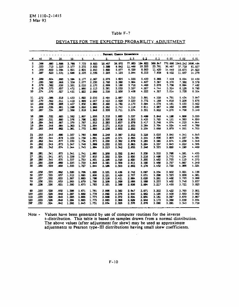
EM 1I1O-2-14155 Mar 93

Table F-7

DEVIATES FOR THE EXPECTED PROBABILITY ADJUSTMENT

. . . . . . . . . . . . . . . . . . . . . . ~ -o ~o . . . . . . . . . . . . . . . . . . .N &o 30. 20, 10. 5. 4, 2. 1, 0.5 0.2 0.1 0,05 0.02 0.01

2345

.396

.333

.309

.m

1.=1.2251.0941.031

3.7692.1771.6311.68U

7.7333.3722.6312.335

2.1772.0772.0101.9801.=

1.=1.6691.W1.6331.819

9.6953.8332.9232.5s

2.367Z.m2.1702.1132.069

19.4875.5a93.8233.285

2.9782.7=2.6892.5612.516

2.4642.4222.3802.3822.338

2.3282.3002.2a52.2712.259

2.2482.2292.2302.2222.235

2.=2.2022.1262.m2.286

2.3s12.2312.3282.2062.101

2.0962.=2.0862.0852.054

38.9728.0425.0774.1o5

3.8353.3603.1603.0532.W

2.8872.6292.7822.7432.713

2.8832.6562.8372.6192.602

2.5672.5742.5a22.5512.542

2.5322.5242.536Z.m2.503

2.6582.4292.4322.3=2.389

2.3822.3762.3722.3662.326

77.063 194.5?2 369.647 779.6% 1949.2423696.464.713.653.623

.6Q4

11.460 16.=3 25.76111. 42n7.856

6.3S65.5675.0764.7444.507

4.3264.1894.0783.9673.912

3.M3.7933.7463.7043.=

3.6253.m3.5803.5573.535

3.5263.4963.4823.4663.452

3.3543.2263.2613.2253.227

3.2023.m3.1813.1733.090

36.487 .-,..” “. --,..31. /L0

19.67511.957

9.0347.%26.6946.1265.7=

5.4345.2085.0304.e864.76a

4.6694.5634.5104.4464.391

4.3414.2974.2504.=4.1.ao

4.1614.2344.11o4.067&,066

3.2213.6383.7853.7483.721

3.7003.6833.6703.65s3.340

OA. W{

24.62514.278

10.438.5797.4926.7906.304

5.%75.6765.4625.2935.149

5.0304.%304.6444.7694.703

4.6454.5944.5484.51m4.469

4.4354.4034.3754.3494.324

4.*4.0613,9993.9573.m

3.9013.6623.0673.6543.719

6.5305.044

4.3553.9643.7U3.5373.406

3.3103.2233.1703.2263.074

3.0373.0052.0782.%32.a32

2.9322.W52.8792.-2.=

2.6412.=2.m2.8222.6a2

2.7422.7072.864

::Z

2.6472.8402.-2.=2.576

9.0036.519

5.4334.6374.4634.2n74.022

3.8813.7723.6643.6113.551

3.4993.4553.4173.3643.354

3.3283.3043.2833.2643.M

3.2303.2263.2023.1203.178

3.oa73.0513.m2.9992.a84

2.9712. m2.a542.W2.678

14.4499.432

7.4196.3705.7365.3145.014

4.7914.6184.4814.=4.276

4.m4.1314.0744.0243.979

3.9403.9053.8743.8453.62n

3.7s3.7753.7553,7373.720

3.M23.5353.4823.4623.439

3.4223.4083.3973.3883.291

67

.268

.263

.279

.276

.274

.m

.968

.950

.m7

.927

1.3941.5391.5011.4721.451

1.4331.6191.6071.3961.369

.5s28910

.575

.570

.=

.562

.559

1132lz14u

.272

.270

.269

.266

.287

.918

.911

.906

.901

.607

2.0352.W71.9651.a661.a49.554

2617la

E

2322232425

2627282930

.2M

.265

.m

.284

.263

.552

.551

.549

.548

. S46

.545

.544

.544

.543

.542

.541

. ml

.540

1.3621.3761.3701.3851.381

1.8071.7961.7871.7791.772

1.=l.m1.9131.W1.8s5

.263

.282

.=

.=

.ml

.261

.261

:=.260

.680

.676

.877

.875

.874

.873

.871

.870

.689

.866

1.3571.3531.3m1.3471.344

1.3411.3391.3371.3351.333

1.7651.7s1.7341.7491.745

1.7411.7371.7331.7301.727

1.6861.6811.6751.8621.*

1.6601.8551.6511.8481.644

40%w7080

.258

.257

.257

.256

.256

.53s

.533

.s32

.662

.657

.655

.853

.851

l.m1.3121.m71.3031.300

1.7M1.8W1.6851.6791.675

1.620l.ms1.7=1.7901.765

.531

90100mmm

.529

.529

.52a

.528

.850

.649

.649

.648

.842

1.=1.2971.2951.2961.282

1.6711.6891.-1.6651.645

1.7811.~81.7751.7731.751.524

Note - Values have been generated by use of computer routines for the inverset-distribution. This table is based on samples drawn from a normal distribution.The above values (after adjustment for skew) may be used as approximateadjustments to Pearson type-III distributions having small skew coefficients.

F-10

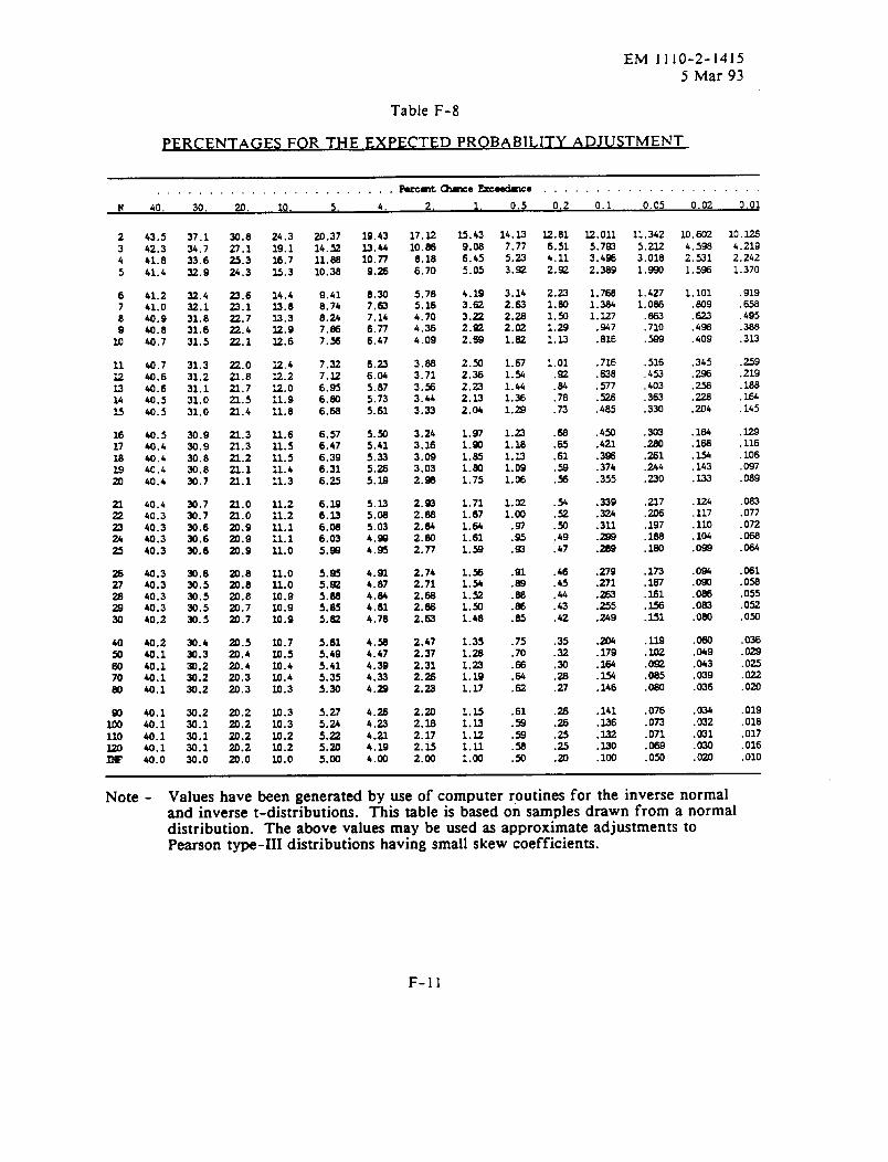
EM 1110-2-14155 Mar 93

Table F-8

PERCENTAGES FOR THE EXPECTED PROBABILITY ADJUSTMENT

. . . . . . . . . . . . . . . . . . . . kmt-eb~e . . .

N 40, 30. 20. 10. 5. 4. 2< 1. 0.5 0.2 0.1 0.05 0.02 0.01

2345

678910

11Ulz1415

1617ls1.9a

2122232425

2627282s30

4050m7060

G110mm

43.542.341.841.4

41.241.040.940.040.7

40.740.640.640.540.5

40.540.440,440.440.4

40.440.340.340.340.3

40.340.340.340.340.2

40.240.140.140.140.1

40.140.140.140.140.0

37.134.733.632.9

32.432.131.831.631.5

31.331.231.131.031.0

30.930.930.830.830.7

30.730.730.630.630.6

30.630.530.530.530.5

30.430.330.230.230.2

30.230.130.130.130.0

:::23.324.3

23.623.122.722.422.1

22.021.8

2:;22.4

22.321.322.222.122.1

23.022.0a.920.9m.9

m.a20.8~.6m.720.7

20.520.420.420.320.3

20.220.220.220.220.0

24.319.116.7M.3

14.41.3.613.3u.912.6

12.4U.212.o11.911.8

12.611.511.511.411.3

11.211.2lz.111.111.0

lz.olz.o10.910.9loos

10.71o.510.4M.410.3

10.310.310.210.210.0

20.3714.5211.6810.38

9.418.748.247.887.56

7.327.326.956.M6.68

6.576.476.396.316.25

6.396.336.086.035.ss

5.%5.=5.885.855.82

5.615.495.415.355.30

5.275.245.225.205.00

19.4333.4410.779.Z

8.307,637.146.n6,47

6.236.045.875.735.61

5.X5.415.33

::t

S.lz5.085.034.994.%

4.914.874.844.814.78

4.%4.474.394.334.20

4.264.234.224.194.00

17.1210.868.186.70

5.785.164.704.364.09

3.W3.713.s3.443.33

3.243.363.093.032.98

2.=2.662.842.802.n

2.742.712.682.*2.63

2.472.372.312.262.23

2.202.ls2.172.352.00

=.439.086.455.05

4.193.623.222.=2.69

2.X2.362.232.I.32.04

1.971.901.851.801.75

1.711.671.641.611.59

1.561.541.521.X1.48

1.351.281.221.ls1.17

1.151.131.121.111.00

14.137.775.233.92

3.142.632.282.021.U

1.671.541.441.361.29

1.221.18l.lz1.091.06

1.021.00.97.95.93

.91

.89

.88

.66

.65

.75

.70

.E6

.-

.62

.61

.59

.59

.58

.50

12.816.514.112.Q

2.221.60l.m1.291.13

1.01.92.64.78.73

.68

.65

.61

.s

.56

.54

.52

.50,49.47

.46

.45

.44

.43

.42

.35

.32

.M

.28

.27

.26

.26

.2s

.25

.20

lz.oll5.7$33.4962.389

1.7681.3841.127.947.816

.716

.638

.577

.526,485

.450

.421

.396

.374

.355

.339

.324

.311

.=

.289

.279

.271

.=

.255

.249

.204

.179

.164

.M

.146

.141

.336

.232

.130

.100

11.3425.2123.0181.993

1.4271.086.363.710.599

.516,453.403.363.330

.X3

.28a

.261

.244

.230

.217

.m

.197

.188

.160

.173

.167

.Ml

.m

.Ml

.U9

.102

.m

.085

.080

.076

.073

.071

.069

.050

10.6024.5982.5311.596

1.101.m9,623.498.409

.345

.296

.258

.228

.204

.184

.168

.W

.143

.133

lzb.117.110.104.099

.0%

.090

.066

.083

.080

.06J3

.049

.043

.039

.036

,034.032.031.030.020

10.IZ64.2192.2421.370

.919

.658

.495

.388

.313

.259

.219

.183

.164

.145

.U

.116,106.097.089

oe3.077.072.068.W

.061

.053

.055

.052

.050

.036

.029

.ox

.022

.020

.019

.018

.017

.016

.010

Note - Values have been generated by use of computer routines for the inverse normaland inverse t-distributions. This table is basedon samples drawn from a normaldistribution. The above values may be used as approximate adjustments toPearson type-III distributions having small skew coefficients.

F-11

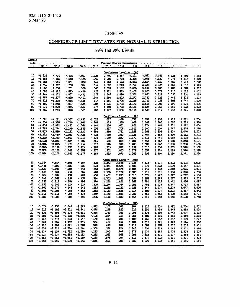
EM 1110-2-14155 Mar 93

Table F-9

coNFIDENCE LIMIT DEVIATES FOR NORMAL D1STRIBUTION

99% and 98% Limits

~hmtkek~ . . . . . . . . . . . . . . . . . . . . . .

N “ &:o” “ “95.0“ “b:o” “ “4,0“ i:o” 20.0 10.0 5,0 2.0 1,0 .5 .2 .1

:202530403060708090100

Calfidmce hl . ,0052.491 3.367 4.323 4.9al

4.0483.=43.3783.2243.0052.8752.7852.7192.6662.6242.588

5.5614.5304.093.7853.6033.3723.2293.3293.0582.9992.9522.914

1.2321.3851.4631.5541.W81.6681.7441.7871.6221.H1.8741.894

5.0744.2223.8323.8013.4473.2493.1253.0382.9742.W2.863Z.m

1.3141.4581.=1.6161.6671.7411.7=1.6331.6651.8911.9231.932

-1.232-1.365-1.483-1.554-1.606-1.688-1.744-1.787-1.622-1.650-1.674-1.604

-.731-.686-.951-1.032-1.056-1.125-1.172-1.m?-1.236-1.259-1.279-1.=

-.436-.s-.851-.708-.751-.s33-.857-.693-.916-.937-.955-.970

-.027-.175-.=-.317-.35a-.419-.460-.4%-.516-.535-.552-.565

1.028.789.640.559.m.428.379.344.317.2a5.277.=

-1.028-.769-.640-.55s-.503-.42a-.379-.344-.317-.285-.2n-.=

.=

.678

.%

.426

.450

.364

.340

.Zoa

:E.250.236

-.=-.678-.56a-.4a8-.450-.364-.340-.309-.285-.265-.250-.238

6.IZ64.9754.4604.1613.%23.7103.5553.4463.3=3.3043.2543.212

1.4051.%71.6711.7471.8041.6901.9501.9a62.0332.0632.0682.11.O

5.5724.6394.2123.@3.7=3.5773.4423.3473.2783.2233.1793.143

1.4=1.6451.7431.8231.8671.9462.0022.0452.0792.1072.1312.I.51

6.7805.5174.9484.6184.3884.=3.9513.8323.7443.6753.m3.574

1.6111.7651.8a71.9792.0402.3222.1=2.2482.2882.3202.3462.371

6.1785.1474.6754.3884.U3.9753,=3.7233.6473.5673.5383.4=

1.7041.8661.9742.0502.1092.2942.Z52.3012.3382.3682.3842.416

7.2585.8995.=4.8404.7074.4U4.2294.1034.0093.=63.6783.829

1.7541.9362.0%2.1602.2052.3022.3712.4242.4662.5002.5292.554

6.6055.5045.0014.7064.5084.2554.0973.9873.-3.6423.7913.748

1.8512.0242.2352.21s2.2n2.3672.4312.4802.5192.5512.5782.601

1.9961.7681.6321.s91.4211.3461.2s41.2541.=1.lWl.in

2.7182.4232.2b92.1321.=1.6911.8251.7761.7381.7081.382

3.3362.W22.n42.6362.4602.3502.2732.2262.1722.1362.lc6

10

:25304050607060m100

-5.581-4.530-4.059-3.785-3.3a3-3.372-3.229-3.12s-3.038-2.2a6-2.252-2.934

-4.321-3.336-2.362-2.774-2.636-2.460-2.350-2.273-2.216-2.172-2.236-2.106

-3.367‘2.718-2.423‘2.249-2.132-1.983-1.=-1.625-1.776-1.738-1.706-1.682

‘2.480-1.966-1.788-1.632-1.539-1.421-1.346-1.m-1.2s4-1.224-1.lm-1.177

1.0381.2821.2741.3401.Zal1.4641.5181.5561.5901.6M1.6371.656

.175

.259

.317

.359

.412

.460

.4a

.526

.%8

.651 .%1

.708 1.Olz1.0561.3251.1721.2071.=1.-l.m1.=

.751

.823

.657

.690

.916.535 .=7.552 .a35

.970

mdalc e xl . .0102.243 3.048 3.7381.641 Z.szl 3.1021.651 2.276 2.8061.536 2.m 2.6331.457 2.030 2.5S1.355 1.602 2.364l.aao 1.823 2.=1.W 1.764 2.2021.230 1.722 2.m1.263 1.688 2.2241.260 1.661 2.0621.142 1.=9 2.056

10

:253040508070w90100

-1.314-1.458-1.550-1.6M-1.667-1.741-1.m-1.823-1.865-1.m-1.833-1.=

-.m-.=-1.006-1.m-1.107-1.--1.212-1.245‘1.272-1.283-1.322-1.326

-.*-.62a-.705-.757-.797-.654-.6s4-.=4-.048-.266-.a64-.W

-.107-.236-.313-.364-.403-.49-.4%-.524-.545-.563-.578-.5al

4.5353.no3.4233.Z313.0712.=2.7812.7022.6442.=2.5612.531

tiide Lavel - .990.1o7 .= .604.236 .m .=.313 .705 lcm

lo

:253040xl6070609)lW

-5.074-4.222-3.632-3.601-3.447-3.fi9-3.225-3.038-2.a74-2.=-2.8a3-2.6Y3

-3.738-3.202-2.606-2.=-2.53s-2.364-2.269-2.202-Z.m-2.224-2.062-2.0s

-3.048-2.523-2.276-2.m-2.030-1.902-1.622-1.764-1.722-1.686-1.861-1.639

-2.243-1.641-1.651-1.=-1.457-1.355-1.=-1.244-1.220-1.183-1.160‘1.142

1.1351.2511.3361.3W1.4461.53s1.=1.8001.6301.6531.67b1.691

.364 .757 1.064.7a7 1.307.654 1.26a.= 1.232.m 1.245.ma 1.272.866 1.=.$84 1.311.= l.m

.403

.457

.4=

.524

.%5

.563

.578

.591

F-12

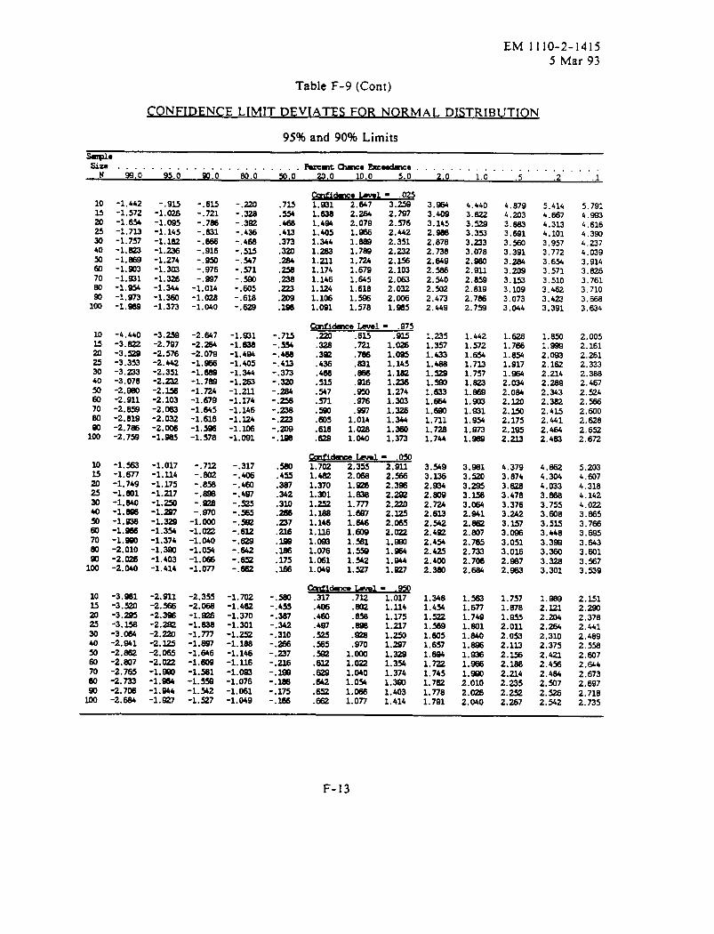
EM 1110-2-14155 Mar 93

Table F-9 (Cent)

coNFIDENC E LIMIT DE VIATF S FOR NORMAL DISTRIBUTION

95% and 90% Limits

~Fucmtaulcoh~e . . . . . . . . . . . . . . . . . . . . . .

U “ &:o” “ “9s.0“ “&:o”“ “Go “ “b:o” 10.0 5.0 2,0 1.0 .5 .2 .1

~q1.831 2.647 3.= 3.86410

1520253040m60708n90100

‘1.442-1.572-1.654-1.733-1.757-1.822-1.--1.s03-1.931-1.954-1.973-1.*

-.9U-1.026-1.095-1.145-1.le2-1.236‘1.274-1.303-1.%-1.344-1.360-1.373

-.615-.721-.786-.831-.866-.916-.950-.976-.997-1.014-1.028-1.040

-.220-.328-.3=-.436-.468-.515-.%7-.571-.590-,605-.618-.629

.715

.554

.468

.433

.373

.320

.284

.258

4.4403.e223.5293.3533.2333.0782.9802.9112.8592.8192.7862.759

1.4421.5721.6541.7231.7571.8231.8691.9331.s11.991.9731.=

3.W1

;:%3.1583.0642.W12.=2.W72.7652.7332.7M2.684

1.=1.6771.7491.8011.8401.8961.=1.=

;:R

::R

4.8794.2n33.8833.6913.5603.3913.2843.2093.2533.1093.0733.044

1.62a1.7661.8541.9171.9642.0342.0842.1202.m2.1752.1952.223

4.3793.8743.6283.4783.3763.2423.3s73.0963.0513.0262.9872.963

1.7571.8781.9552.0112.0532.1132.=2.1882.2142.2352.2522.267

5.4144.6674.3134.1013.9573.7723.6543.5713.5103.4Q3.4233.391

1.8501.9992.0932.1622.2142.28s2.3432.3822.4152.4412.4642.483

4.=4.3044.0333.a6a3.7353.8083.5153.4483.3993.3603.3283.301

1.9892.m2.W2.2642.3102.3752.4212.4%2.4842.%72.5262.542

5.7914.993b.6164.39)4.a74.0393.9143.m3.7613.7103.6683.634

2.0052.1612.2K12.3332.3882.4672.5242.=2.WO2.6282.6522.672

5.m34.6074.3184.1424.0223.8653.7E63.6953.6433.6013.s73.539

2.1512.m2.3782.4412.4892.5S2.W72.6442.6732.6972.7182.735

1.6361.4*1.4051.3441.2631.2111.1741.1461.3241.1061.081

2.2642.0791.=1.8891.7891.7241.6791.M51.6181.5961.578

2.7972.5762.4422.3512.2322.L%2.1032.0632.0322.W61.965

3.4093.1452.W2.8782.7382.8492.5662.5402.=2.4732.449

.228

.222

.198

-.735-.554-.468-.423-.373-.320-.284-.258-.238-.223-.209-.298

Wdmce Iavel - .975.220 .635 .915 1.23510

3320253040xl60708030100

-4.440-3.822-3.529-3.353-3.233‘3.078-2.=-2.911-2.85s‘2.819-2.786-2.759

-3.25s-2.797-2.576-2.442-2.351-2.232-2.M-2.103-2.063-2.032-2.006-1.885

-2.647-2.264-2.079-1.9E6-1.W-1.789-1.724-1.679-1.645-1.618-1.396-1.578

-1.al-1.638-1.404-1.405-1.344-1.2a3-1.232-1.174-1.146-1.124-1.108-1.091

.328 .722.786.831

1.0261.0351.1451.1821.2381.2741.3031.3261.3441.3601.373

1.3571.4331.4861.52s1.5901.a331.6641.6901.7111.7261.744

.3=

.436

.468 .886

.535

.547

.571

.=

.605

.916

.950

.976

.=71.0141.0281.040

.618

~- Lu’fOl - ,0s01.702 2.355 2.9111.482 2.068 2.s1.370 1.= 2.3961.301 1.838 2.=

3.5493.3362.8342.8092.732.6332.5422.4=2.4542.4252.4002.380

10M

E30405060708090

-1.563-1.677-1.749-1.801-1.840-1.696-1.936-1.866-1.m-2.010-2.026-2,040

-1.017-1.224-1.175-1.227-la-1.2s7-1.=-1.354-1.374-1.390-1.403-1.414

-.712-.m-.856-.898-.=-.!370-1.m-1.022-1.040-1.054-1.068-1.077

-.317-.*-.460-.4W-.525-.365-.5e2-.632-.629-.642-.652-.662

.580

.455

.387

.342

.320

.2661.2521.2861.1461.1261.0931.0761.0611.049

1.7771.6e7 ;:21.* 2.0651.606 2.0221.581 1.9801.= 1.9641.542 1.9441.= 1.327

.2s7

.226

.3s6

.286

.175,366

-.3W-.455-.387-.342-.310-.266-.227-.216-.M-.1=-.175-.M

m

-*O m - .9X.317 .712 1.017 1.34810

M2025

-3.ml-3.520-3.295-3.158-3.064-2.W1-2.862-2.807-2.765-2.733-2.7m-2.684

-2.921-2.568-2.386-2.=-2.220-2.325-2.065-2.022-1.=-1.=-1.944-1.m

-2.335-2.m8-1.=-1.838-1.777-1.m7-1.646-1.60s-1.561-1.559-1.542-1.527

-1.702-1.482-1.370-1.301-1.252-1.168-1.146-1.226-1.0s3-1.076-1.061-1.049

.4m .8n2 1.134.658 1.175

1.227:: 1.250.970 1.2971.000 1.=1.023 1.3541.040 1.3741.054 1.3901.066 1.4031.077 1.414

i;4541.5221.5691.6051.6571.6941.7221.7451.7621.7761.791

.480

.407

.525

.565

.=

.632

.829

.642

.652

.662100

F-13

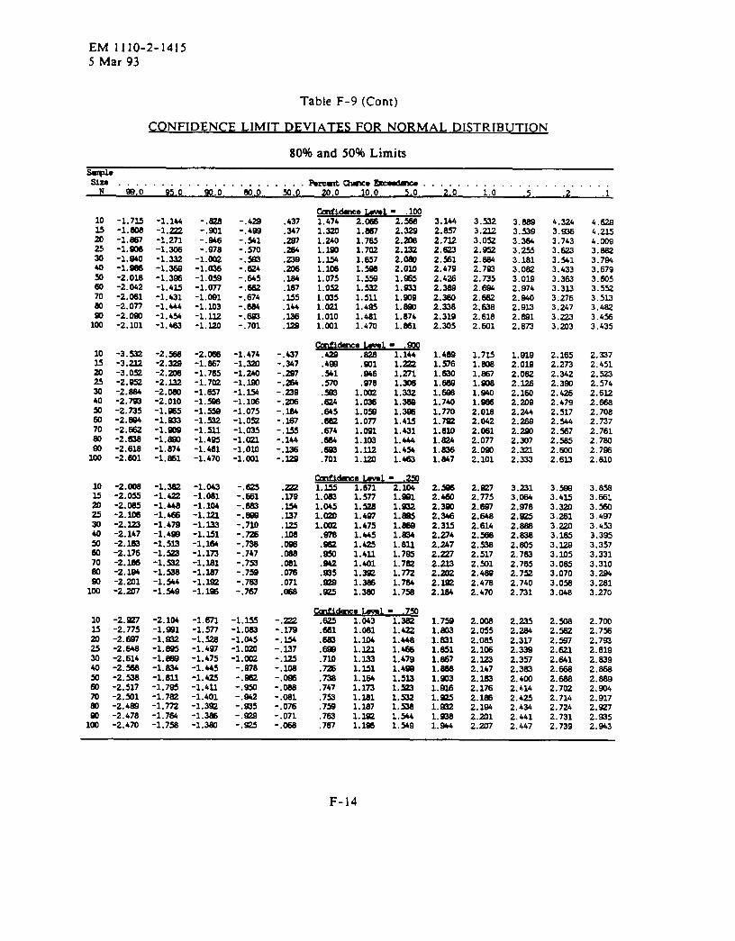
EM 1110-2-14155 Mar 93

Table F-9(Cont)

c~ NFIDENCE LIMIT DEVIAT FOR N AL DISTRIBUTION

80% and 50% Limits

fife . . . . . . . . . . . . . . . .......~~ek~ . . . . . . . . . . .u 99.0 95.0 mo M.o X1. o 20.0 10.0 5.0 2.0 1.0 “.s”””:2””’”,1

w~- ekl= .1001.474 2.m6 2.56810

25202530403607060m100

-1.715-1.606-1.m-1.m8-1.240-1.986-2.018-2.042-2.061-2.077-2.m-2.101

-1.146-1.222‘1.271-1.=-1.332-1.362-1.326-l+hu-1.431-1.444-1.454-1.463

-.626-.901-.946-.278-1.002-1.036-1.052-1.077-1.091-1.103-1.132-1.120

3.1442.657

3.5323.2323.0522.m22.6642.7932.7352.6s42.6622.6332.6182.601

1.715lam1.8671.9061.9401.X2.0182.0422.W12.0772.mo2.101

2.6272.7752.6272.6482.6142.m2.5332.5172.5012.4322.4782.470

2.0082.0552.0852.1062.2232.1472.2632.1762.2882.1942.2012.2117

.437

.347

:Z.239.206.164.167.us.144.336.lm

-.437-.347-.m-.264-.239-.206-.164-.267-.155-.144-.126-.m

.=

.179

:27.225

:Z.m.061.076.071.066

-.222-.179-.L54-.237-.325-.loa-.026-.068-.061-.076-.071-ma

3.8a93.5393.3643.2553.1813.0623.o192.9742.9402.9U2.s912.873

1.9192.0192.0622.1262.1602.2n92.%42.2692.2202.3072.3212.333

3.2313.0842.9782.m52.6a82.3362.M52.7332.7652.7522.7402.731

2.2352.2a42.3172.3392.3572.3632.4002.4142.4252.4342.4412.447

4.3243.9363.7433.6223.5413.4333.3633.3233.2763.2473.2233.203

2.1652.2732.3422.3902.4262.4792.5172.5442.S72.5652.6002.62.3

3.5m3.43s3.3203.2613.22113.1653.D3.1053.0853.0703.0583.048

2.m82.s2.W2.6222.6412.6682.6662.7022.7142.7242.7312.739

&.6294.2354.0093.ea23.7943.6793.6053.5523.5133.4823.4563.435

2.3372.4512.5232,5742.6122.6682.7082.7372.7612.7W2.7S2.810

3.8553.6613.=3.4973.4533.3953.3573.3313.31.O3.m43.2213.270

2.7W2.7562.7932.8192.6392.8682.6892.m42.9172.=72.=52.943

-.4W-.M1-.570-.5e3-.624-.645-.m2-.674-.W-.*-,701

1.3201.240l.m1.1541.2061.0751.0521.035l.ml1.0101.W1

1.6671.7651.7021.6571.5961.5591.5321.5111.4851.4811.470

2.3292.2062.2222.0602.0101.9651.s331.2Q9l.m1.6741.861

2.7322.6232.5612.4792.4262.3892.3m2.3382.3192.305

~-e lmve1= .200.429 .326 1.14410

M202530405060703020100

-3.532-3.222-3.052-2.952-2.684-2.m-2.735-2.624-2.662-2.638-2.618-2.601

-2.56a-2.329-2.m6-2.132-2.060-2.010-1.=-1.=-1.009-1.am‘1.874-1.861

-2.066-1.667-1.765-1.702-1.657-1.5e6-1.=-1.532-1.511-1.425-1.4al-1.470

-1.474-1.=-1.240-1.290-1.354-1.l(m-1.075-1.052-1.035-1.022-1.010-1.ml

1.4W1.S761.630lam1.6261.7401.770l.m1.820l.mh1.m61.647

.422 .201 1.=1.2711.3061.3321.3691.3261.4351.4311.4441.4541.463

.541

:Z.624.645.662

.946

.2761.0021.0361.059l.on1.0931.1031.2221.320

.674

.664

.66Q

.701

~dmce kl- 2501.355 1.671 2.I.041.063 1.577 l.ml

10M20253040w60706020lm

-2.008-2.055-2.065-2.206-2.m-2.147-2.m-2.176-2.266-2.124-2.2nl-2.207

-1.362-1.422-1.44a-1.466-1.479-1.4W-1.533-1.522-1.532-1.538-1.544-1.549

-1.043-1.ml-1.204-1.322-1.233-1.251-1.264-1.173-1.261-1.267-1.m-1.3.26

-.625-.661-.663-.629-.720-.?m-.736-.747-.753-.752-.763-.767

2.s2.46n2.3m2.3462.3=2.2742.2472.227

1.045l.m1.m2.978.262.250.942.m5

1.s22 1.2321.427 1.=1.475 I.=1.445 1.6341.425 1.6321.432 1.7251.401 1.7621.W 1.7721.3m 1.7641.3m 1.75%

2.2232.202

;:E

Culfidme Level- .75o.625 1.043 1.362.661 1.061 1.422

-2.=7-2.n5-2.627-2.646-2.614-2.m-2.538-2.517-2.=1-2.46s-2.476-2.470

-2.104-1.Oal-1.m2-1.m5-1.--1.634-1.812-1.795-1.7a2-1.772-1.764-1.7s

-1.671-1.577-1.526-1.4a7-1.475-1.445-1.425-1.422-1.401-1.3=-1.366-1.320

-1.155-1.063-1.045-1.om-1.002-.276-.262-.250-.942-.235-.m9-.m5

1.7s1.6031.6311.6511.6671.363lam1.9261.=1.m2l.ma1.944

.633 1.lo4 1.4

.mz 1.122 1.*

.720 1.123 1.479

.m 1.351 1.4a2

.736 1.164 1.523

.747 1.173 1.=

.753 l.lal 1.532

.75s 1.u7 1.536

.763 l.m 1.544

.767 l.m 1.549

F-14

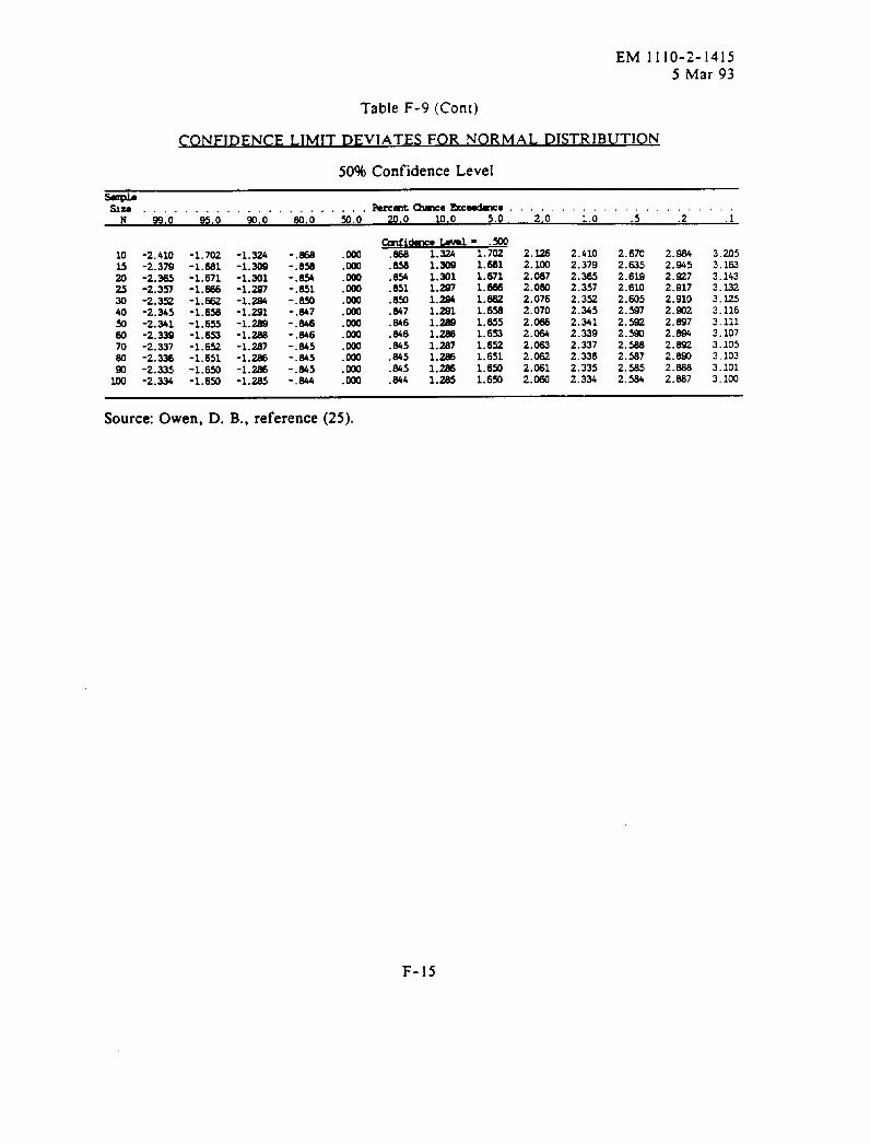
EM 1110-2-14155 Mar 93

Table F-9 (Cent)

coNFIDENCE LlMIT DEVIATE S FOR NORMAL DISTRIBUTION

50% Confidence Level

size .. be C3umce*~e . . . . . . . . . . . . .N ‘ &:o” “ “9s.0 “ b:o” ‘ “4.0 “ b.o W,o 10,0 5,0 2.0 1.0 .5 .2 .1

101520253040m60706090100

-2.410-2.379-2.365-2.357-2.352-2.345-2.31-2.339-2.337-2.336-2.335-2.334

-1.702-1.681-1.671-1.666-1.662-1.65E-1.655-1.653-1.652-1.651-1.650-1.6XI

-1.324-1.309-1.301-1.297-1.2s4-1.291-1.262-1.286-1.267-1.m-1.266-1.265

-.666-.m-.654-.651-.650-.647-.846-.846-.645-,645-.645-.644

.Ooo

.Ow

.Om

.m

.m

.Ooo

.Ooo

.Ow

.Ooo

.m

.m

.Ooo

Midence -1- .500.66a 1.= 1.702.656.854.851.650.647.646.M6.645.645.645.644

1.3021.301I.m1.294l.zm1.2891.2661.2671.=1.2661.2a5

1.6611.6711.-1.=1.6561.6551.6S1.6521.6511.6501.6W

2.1262.lW2.0672.0602.0762.0702.0662.064Z.m2.0622.0612.060

2.4102.3792.3652.3572.3S22.3452.3412.3392.3372.3362.3352.334

2.6702.6352.6192.6102.6052.S72.5%?2.5932.5632.5672.=2.%

2.9a42.9452.9272.9172.9102.9322.897Z.m2.6922.6932.=2.667

3.2053.1633.1433.1323.1253.1163.1113.1073.1053.1033.1013.100

Source: Owen, D. B., reference (25).

F-15

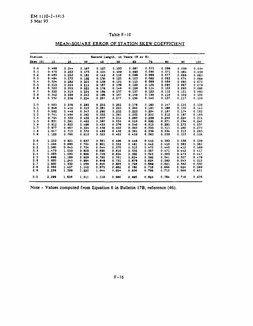
EM 1110-2-14155 Mar 93

Table F-10

MEAN-SOUARE ERROR OF STATION SKEW CO EFFICIENT

Station ..,...... . . . Record LenSth, in Years (Nor H) . . . . . . . . . . . . . .

Skew (G) 10 20 30 40 50 60 70 80 90 100

0.00.10.20.30.40.50.60.70.80.9

1.01.11.21.31.41.51.61.71.81.9

2.02.12.22.32.42.52.62.72.82.9

3.0

0.4680.&760.4850.4940.5040.5130.5220.5320.5420.552

0.6030.6460.6920.7410.7940.8510.9120.9771.0471.122

1.2021.2881.3801.4791.5851.6981.8201.9502.0892.239

2.399

0.2440.2530.2620.2720.2820.2930.3030.3150.3260.338

0.3760.4100.4480.4880.5330.5s10.6230.6670.7150.766

0.8210.8800.9431.0101.0831.1601.2431.3321.4271.529

1.638

0.1670.1750.1830.1920.2010.2110.2210.2310.2430.254

0.2850.3150,3470.3830.4220.4650.4980.5340.5720.613

0.6570.7040.7540.8080.8660.9280.9941.0661.1421.223

1.311

0.1270.1340.1420.1500.1580.1670.1760.1860.1960.207

0.2350.2610.2900.3220.3570.3970.4250.4560.4890.523

0.5610.6010.6440.6900.7390.7S20.84s0.9100.9751.044

1.119

0.1030.1090.1160.1230.1310.1390.1480.1570.1670.177

0.2020.2250.2520.2810.3140.3510.3760.4030.4320.463

0.4960.5320.5700.6100.6540.7010.7510.8050.8620.924

0.990

0.0870.0930.0990.1050.1130.1200.1280.1370.1460.156

0.1780.2000.2250.2520.2830.3180.3400.3650.3910.419

0,4490.4810.5150.5520.5020.6340.6790.7280.7800.836

0.895

0.0750.0800.0860.0920. 0s90.1060.1140.1220.1300.140

0.1600.1810.2040.2300.2590.2920.3130.3350.3590. 38S

0.4120.4420.4730.5070.5430.5820.6240.6890.7160.768

0.823

0.0660.0710.0770.0820.0890.0950.1020.1100.1180.127

O.lb?0.1660.1870.2120.2400.2710.2910.3110.3340.358

0.3830.4100.4400.4710.5050.5410.5800.6210.6660.713

0.764

0,0590.0640.0690.0740.0800.0670.0930.1010.1090.117

0.1350.1530.1740.1970.2240.2540.2720.2920.3130.335

0.3590.3s50.4120.4420.4730.5070.5430.5620.6240.669

0.716

0.0540.0580.0630.0680.0730.0790.0860.0930.1000.109

0.1260,1430.1630.1850.2110.2400.2570.2750.2950.316

0.3390.3630.3890.417o.4&70.4790.5130.5500.5890.631

0.676

Note - Values computed from Equation 6 in Bulletin 17B, reference (46).

F-16

EM 1110-2-14155 Mar 93

Table F-11

Q~.UFS (10 PERCE NT SIGNIFICANCE LEVEL)

Sample Outlier Sample Outlier Sample Outlier Sample OutlierSize K Value Size K Value Siz e K Value Size K Value

1011

::14

1516171819

20

;;2324

2526272829

3031

::34

3536

::39

4041424344

2.0362.0882.1342.1752.213

2.2472.2792.3092.3352.361

2.3852.4082.4292.4482.467

2.4862.5022.5192.5342.549

2.5632.5772.5912.6042.616

2.6282.6392.6502.6612.671

2.6822.6922.7002.7102.719

4546474849

5051525354

5556575859

:?626364

::676869

7071727374

7576777879

2.7272.7362.7442.7532.760

2.7682.7752.7832.7902.798

2.8042.8112.8182.8242.831

2.8372.8422.8492.8542.860

2.8662.8712.8772.8832.888

2.8932.8972.9032.9082.912

2.9172.9222.9272.9312.935

8081828384

85

:?8889

9091929394

;;979899

100101102103104

105106107108109

110111112113114

2.9402.9452.9492.9532.957

2.9612.9662.9702.9732.977

2.9812.9842.9892.9932.996

3.0003.0033.0063.0113.014

3.0173.0213.0243.0273.030

3.0333.0373.0403.0433.046

3.0493.0523.0553.0583.061

115116117118119

120121122123124

125126127128129

130131132133134

135136137138139

140141142143144

145146147148149

3.0643.0673.0703.0733.075

3.0783.0813.0833.0863.089

3.0923.0953.0973.1003.102

3.1043.1073.1093.1123.114

3.1163.1193.1223.1243.126

3.1293.1313.1333.1353.138

3.1403.1423.1443.1463.148

Note - Table contains one sided 10% significance level deviates for the normaldistribution. Source: Appendix 4, Bulletin 17B, reference (46).

F-17

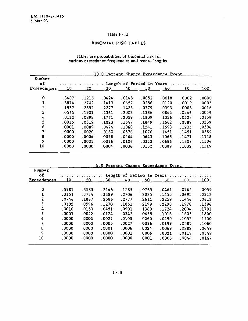
EM 1I1O-2-14I55 Mar 93

Table F-12

BINOMIAL RISK TABLES

Tables are probabilities of binomial risk forvarious exceedance frequencies and record lengths.

10.0 Percent Chance Exceedance EventNumber

of . . . . . . . . . . . . . . . . . . Length of Period in Years . . . . . . . . . . . . . . . . .

Ex ceedances 10 20 30 40 50 60 80 100

01

23456789

10

.3487

.3874

.1937

.0574

.0112

.0015

.0001

.0000

.0000

.0000

.0000

.1216

.2702

.2852

.1901

.0898

.0319

.0089

.0020

.0004

.0001

.0000

.0424

.1413

.2277

.2361

.1771

.1023

.0474

.0180

.0058

.0016

.0004

.0148

.0657

.1423

.2003

.2059

.1647

.1068

.0576

.0264

.0104

.0036

.0052

.0286

.0779

.1386

.1809

.1849

.1541

.1076

.0643

.0333

.0152

.0018

.0120

.0393

.0844

.1336

.1662

.1693

.1451

.1068

.0686

.0389

.0002

.0019

.0085

.0246

.0527

.0889

.1235

.1451

.1471

.1308

.1032

.0000

.0003

.0016

.0059

.0159

.0339

.0596

.0889

.1148

.1304

.1319

5.0 Percent Chance Exceedance EventNumber

of . . . . . . . . . . . . . . . . . . Length of Period in Years . . . . . . . . . . . . . . . . .Exceedances 10 20 30 40 50 60 80 100

01

23456789

10

.5987

.3151

.0746

.0105

.0010

.0001

.0000

.0000

.0000

.0000

.0000

.3585

.3774

.1887

.0596

.0133

.0022

.0003

.0000

.0000

.0000

.0000

.2146

.3389

.2586

.1270

.0451

.0124

.0027

.0005

.0001

.0000

.0000

.1285

.2706

.2777

.1851

.0901

.0342

.0105

.0027

.0006

.0001

.0000

.0769

.2025

.2611

.2199

.1360

.0658

.0260

.0086

.0024

.0006

.0001

.0461

.1455

.2259

.2298

.1724

.1016

.0490

.0199

.0069

.0021

.0006

.0165

.0695

.1446

.1978

.2004

.1603

.1055

.0587

.0282

.0119

.0044

.0059

.0312

.0812

.1396

.1781

.1800

.1500

.1060

.0649

.0349

.0167

F-18

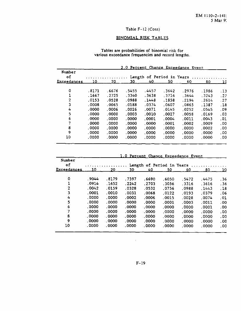
EM 1110-2-]41:5 Mar 91

Table F-12 (Cent)

~! TAB

Tables are probabilities of binomial risk forvarious exceedance frequencies and record lengths.

2. 0 Percent Chance Exceedance EventNumber

of . . . . . . . . . . . . . . . . . . Length of Period in Years . . . . . . . . . . . . . . .Exceedances 10 20 30 40 50 60 80 10

0123456789

10

.8171

.1667

.0153

.0008

.0000

.0000,0000.0000.0000.0000.0000

.6676

.2725

.0528

.0065

.0006

.0000

.0000

.0000

.0000

.0000

.0000

.5455

.3340

.0988

.0188

.0026

.0003

.0000

.0000

.0000

.0000

.0000

.4457

.3638

.1448

.0374

.0071

.0010

.0001

.0000

.0000

.0000

.0000

.3642

.3716

.1858

.0607

.0145

.0027

.0004

.0001

.0000

.0000

.0000

.2976

.3644

.2194

.0865

.0252

.0058

.0011

.0002

.0000

.0000

.0000

.19863243

:2614.1387.0545.0169.0043.0009.0002.0000.0000

.13

.27

.27

.18

.09

.03

.01

.00

.00

.00

.00

0~ ce E eedance EventN~ber

of .................. Length of Period in Years ...............

Ex ceedances 10 20 30 40 50 60 80 10

01

23456789

10

.9044

.0914

.0042

.0001

.0000

.0000

.0000

.0000

.0000

.0000

.0000

.8179

.1652

.0159

.0010

.0000

.0000

.0000

.0000

.0000

.0000

.0000

.7397

.2242

.0328

.0031

.0002

.0000

.0000

.0000

.0000

.0000

.0000

.6690

.2703

.0532

.0068

.0006

.0000

.0000

.0000

.0000

.0000

.0000

.6050

.3056

.0756

.0122

.0015

.0001

.0000

.0000

.0000

.0000

.0000

.5472

.3316

.0988

.0193

.0028

.0003

.0000

.0000

.0000

.0000

.0000

.4475

.3616

.1443

.0379

.0074

.0011

.0001

.0000

.0000

.0000

.0000

.36

.36

.18

.06

.01

.00

.00

.00

.00

.00

.00

F-19

EM 1110-2-14155 Mar 93

Table F-12 (Cent)

BINOMIAL RISK TABJ.Es

Tables are probabilities of binomial risk forvarious exceedance frequencies and record lengths.

~ ha ce ceedance Event

Numberof . . . . . . . . . . . . . . . . . . Length of Period in Years . . . . . . . . . . . . . . . . .

~xceedances 10 20 30 40 50 60 80 100

0123&56789

10

.9511

.0478

.0011

.0000

.0000

.0000

.0000

.0000

.0000

.0000

.0000

.9046

.0909

.0043

.0001

.0000

.0000

.0000,0000.0000.0000.0000

.8604

.1297

.0095

.0004

.0000

.0000

.0000

.0000

.0000

.0000

.0000

.8183

.1645

.0161

.0010

.0000

.0000

.0000

.0000

.0000

.0000

.0000

.7783

.1956

.0241

.0019

.0001

.0000

.0000

.0000

.0000

.0000

.0000

.7403

.2232

.0331

.0032

.0002

.0000

.0000

.0000

.0000

.0000

.0000

.6696

.2692

.0534

.0070

.0007

.0001

.0000

.0000

.0000

.0000

.0000

.6058

.3044

.0757

.0124

.0015

.0001

.0000

.0000

.0000

.0000

.0000

2P ercent Chance Exceedance EventNumber

of . . . . . . . . . . . . . . . . . . Length of Period in Years . . . . . . . . . . . . . . . . .Exceedances 10 20 30 40 50 60 80 100

0123456789

10

.9802

.0196

.0002

.0000

.0000

.0000

.0000

.0000

.0000

.0000

.0000

.9608

.0385

.0007

.0000

.0000

.0000

.0000

.0000

.0000

.0000

.0000

.9417

.0566

.0016

.0000

.0000

.0000

.0000

.0000

.0000

.0000

.0000

.9230

.0740

.0029

.0001

.0000

.0000

.0000

.0000

.0000

.0000

.0000

.9047

.0907

.0045

.0001

.0000

.0000

.0000

.0000

.0000

.0000

.0000

.8868

.1066,0063.0002.0000.0000.0000.0000.0000.0000.0000

.8520

.1366

.0108

.0006

.0000

.0000

.0000

.0000

.0000

.0000

.0000

.8186

.1640

.0163

.0011

.0001

.0000

.0000

.0000

.0000

.0000

.0000

F-20