IET Generation, Transmission & Distribution

Research Article

Distributed load shedding for microgrid withcompensation support via wireless network

ISSN 1751-8687Received on 4th July 2017Revised 22nd November 2017Accepted on 7th December 2017doi: 10.1049/iet-gtd.2017.1029www.ietdl.org

Qimin Xu1,2,3, Bo Yang1,2,3 , Cailian Chen1,2,3, Feilong Lin1,2,3, Xinping Guan1,2,3

1Department of Automation, Shanghai Jiao Tong University, Shanghai, People's Republic of China2Collaborative Innovation Center for Advanced Ship and Deep-Sea Exploration, Shanghai, People's Republic of China3Key Laboratory of System Control and Information Processing, Ministry of Education of China, Shanghai, People's Republic of China

E-mail: bo.yang@sjtu.edu.cn

Abstract: Due to the limited generation and finite inertia, microgrids suffer from a large frequency and voltage deviation whichcan lead to system collapse. Thus, a reliable load shedding method is required to maintain frequency stability. A wirelessnetwork, benefiting from the high flexibility and low deployment cost, is considered as a promising technology for fine-grainedmanagement. In this study, a distributed load shedding solution via a wireless network is proposed for balancing the supply–demand and reducing the load-shedding amount. Firstly, the real-power coordination of different priority loads is formulated asan optimisation problem. To solve this problem, a distributed load shedding algorithm based on sub-gradient method isdeveloped for gradually shedding loads. Using this method, power compensation can be utilised and has more time to decreasethe power deficit, consequently reducing the load-shedding amount. Secondly, a multicast metropolis schedule based on time-division multiple access is developed. In this protocol, time slots are dedicatedly allocated to increase the response rate. Achecking and retransmission mechanism is utilised to enhance the reliability of our method. Finally, the proposed solution isevaluated by using an NS3-Matlab co-simulator. The numerical results demonstrate the feasibility and effectiveness of oursolution.

1 IntroductionDue to the depleting fossil fuel resources, rising energy costs, anddeteriorating environmental conditions, more distributed energyresource (DER) units are incorporated into the current electricalpower system. Microgrids are developed to interconnect the DERunits in a relatively small area. However, there exist severaltechnical challenges in integrating DER units due to the nature ofmicrogrids, such as limited generation, finite inertia, anddistributed structure. Thus, determining how to monitor andmanage the numerous DER units and loads is a critical issue,especially when the load and generation drastically change or faultsoccur. In this context, restoration is the typical operation to keepthe supply–demand balance of the system by load shedding orgenerator power regulation.

Various kinds of restoration methods have been proposed toshed appropriate loads using different methodologies [1–3]. In [2,3], centralised methods were designed to coordinate multiplegenerators and loads in a microgrid. However, centralised methodsneed the collection of global information, and they easily sufferfrom single point failure. Besides, centralised methods are ill suitedto the structural nature of microgrids. Thus, distributed methodshave been developed to address the above problems. Multi-agentsystem-based methods were proposed for reliable load shedding ofmicrogrids [4] and restoration of the microgrid in an all-electricship [5]. These two algorithms were designed for the power systemwith specific structures. Additionally, the restoration decisionrequires sophisticated coordination and information exchangebetween different agents, while the convergence and stability of theproposed algorithms have not been rigorously analysed. Toovercome these shortcomings, consensus-based methods wereapplied to this problem [6–10]. In [6], an optimal load controlscheme was designed based on a power system model to reduce themismatch between load and generation which is caused by suddengeneration drop. In [7, 8], global information discovery (GID)algorithms for load shedding were proposed based on differentconsensus methods. In [9], a two-layer improved averageconsensus algorithm was designed for load shedding, which tookcost and marginal cost into consideration. In [10], a decentralised

under frequency load shedding was implemented based on theglobal information. These two works evaluated power deficiencyby the rate of change of frequency (ROCOF) only at first frequencythreshold which is a semi-adaptive scheme. However, they onlyshed the corresponding load amount, without consideration ofmitigating the impact of load shedding on customer's experience.The high pervasive smart meters and appliance with automaticsense and control function can be available in the future [11]. Thus,more fine-grain load management can be realised by thecollaboration of smart homes/buildings and worth furtherinvestigation.

The conventional method for load shedding based on theROCOF can estimate power deficit, but cannot obtain more loadinformation such as load priority and economy. Thus, for morefine-grain load management, utilising advanced information andcommunication technology is necessary. In the former works [6, 8–10], the ideal communication model was employed. However, asfor the load shedding operation performance, it is not onlydetermined by the control algorithm but also related to the protocoldesign of the communication system [12]. Compared with wirelinenetworks, wireless networks bring the benefits of high flexibility,low-cost deployment, and widespread access, which are suitablefor microgrids with numerous distributed DER units and loads.Thus, wireless networks, such as wireless local area network andlong-term evolution, are potential technologies to realise intelligentmanagement. The round-robin polling mechanism based time-division multiple access (TDMA) is a considerable protocol forwireless access in microgrids [13]. For distributed coordination andfast convergence, several protocols were designed based on aunicast mode to coordinate agents in microgrids [7]. Theseprotocols are only proposed for the GID. Additionally, the packetloss and hidden terminal problem are not taken into consideration.Therefore, since load shedding method is time-sensitive, theprotocol considering time efficiency and transmission reliability isurgently needed.

In this study, a fully distributed load shedding solution isproposed, which aims to improve customer's experience by fine-grain load management with a reliable communication protocol.The main contributions of this study are as follows:

IET Gener. Transm. Distrib.© The Institution of Engineering and Technology 2018

1

• Considering that the distributed management of the small-scalemicrogrid contains loads with different priorities, the real powerof loads are coordinated by the utilisation level. Thus, a loadpriority associated optimisation problem that aims atmaximising the weighted sum of the remained loads andbalancing the supply and demand is formulated, which has anon-smooth objective.

• For reducing the impact of load shedding on customer'sexperience, a distributed load shedding algorithm based on sub-gradient method (DLSS) method is proposed to shed loadsgradually by the frequency deviation rather than at a fixednumber of steps and fixed load-shedding amount. Hence, powercompensation can be utilised to reduce the load-sheddingamount. Moreover, the relevant analysis of convergence ispresented.

• A multicast metropolis schedule based on TDMA (MMST) isdeveloped to increase the response rate and guarantee thereliability of the DLSS method. In this protocol, a time slotallocation algorithm is designed to increase the number ofconcurrent transmission between agents, and a data framestructure piggybacks the checking information of packetsreceived from neighbour agents.

The paper is organised as follows. In Section 2, the systemstructure is introduced. Section 3 presents in detail the distributedload shedding solution. In Section 4, the proposed MMST protocolis elaborated. The performance of the proposed solution isevaluated and compared with the existing methods in Section 5.Finally, the conclusion is drawn in Section 6.

2 System structureIn this research, we consider a load shedding problem in amicrogrid. The microgrid network is denoted by a graph (N, ℰ). Ndenotes the bus set, which is defined asN = {1, …, N} = Ncg ∪ Nig. Ncg and Nig are the bus setsconnected to conventional distributed generators (DGs) andinverter-based DGs, respectively. ℰ ⊆ N × N denotes the set oftransmission lines interconnecting the buses. In the microgird,there is at least one bus connected to a synchronous generator (SG)or energy storage system (ESS), which can be used for powercompensation.

Assumption: we make the following assumptions:

• Each bus is managed by an agent who is regarded as a regionalcontroller. The agents communicate with each other via wirelessnetworks.

• Each agent has the information of global maximum generationcapacity. However, they do not have the real-time powergeneration and load demand of other buses.

• The communication range of each agent only covers itsneighbour agents, since the communication network ofmicrogrids has low density.

2.1 Generation model and multi-priority load model

The total power generation PG in the microgrid can be obtained by

PG = ∑i = 1

NPGi, (1)

where PGi denotes the power generation at bus i, N denotes thenumber of buses (agents) in the microgrid.

The total real power demand PD and load model [14] can beexpressed as

PD = ∑i = 1

NPLi + Ploss = ∑

i = 1

N

∑l = 1

NL, i

bi, lPLi, l + Ploss, (2)

PLi, l = PLi, l(0)(1 + κ f Δ f + κvΔV), (3)

where PLi, l(0) denote the real power of load l at base frequency andvoltage, and PLi, l at new voltage and frequency. Δ f and ΔV denotethe deviation of system frequency and voltage, respectively. κf andκv are the coefficients of real power load dependency on frequencyand voltage, respectively. bi, l represents the control variable of loadl at bus i. Thus, bi is an array of length NL, i (1/0 = active/non-active), where NL, i denotes the number of loads at bus i. Ploss is thereal power loss in the transmission line.

The real power of the total loads PLmax when faults happen can be

calculated as

PLmax = ∑

i = 1

NPLi

max = ∑i = 1

N

∑l = 1

NL, i

PLi, l(0), (4)

where PLimax denotes the total power of the loads at bus i when they

are all in active status.The loads are divided into G grades according to the economic

and social influence caused by load interruption. G denotes themaximum load grade, and G = 3 in most cases. The vital load isthe uninterruptible power-supplied load, which would cause greateconomic losses, and even casualty if interrupted. The secondgrade load would cause certain economic losses if interrupted. Thenon-vital load is the third grade load which can be adjusted. HencePL

max can also be represented by

PLmax = ∑

g = 1

GρgPL

max = ∑i = 1

N

∑g = 1

Gρg, iPLi

max, (5)

where ρg is the ratio of the gth grade loads in the real power of thetotal loads PL

max, and ρg, i denotes the ratio of the gth grade loads inthe total real power at bus i.

For different priority loads, wg denotes the weight factor of thegth loads, which is used to set a measurable indicator of loadshedding and ensure that the lower priority loads are shed first. Thesmaller g is, the higher priority the loads have. Thus, according to(5), the weighted sum of all the load power is written as

PWt = ∑g = 1

GwgρgPL

max, (6)

where wg decreases with the increase of load priority.For the load shedding problem, PLi is the adjustable variable,

which denotes the remained power of loads at bus i. The utilisationlevel ui is used to coordinate power of loads at each bus, which isdefined as

ui =PLi

PLimax =

∑l = 1NL, i bi, lPLi, l(0)

PLimax

+∑l = 1

NL, i bi, l(κ f Δ f + κvΔV)PLi

max , PLi ∈ [0, PLimax] .

(7)

2.2 Power deficit and load-shedding amount formulation

The power deficit ΔP~ can be estimated based on the ROCOF. If

initial power deficit ΔP~ caused by the fault is in the range as

follows:

∑g = m + 1

GρgPL

max < ΔP~ ⩽ ∑

g = m

GρgPL

max, (8)

the corresponding total weighted sum of load power that needs tobe shed PWΔ can be expressed as

2 IET Gener. Transm. Distrib.© The Institution of Engineering and Technology 2018

PWΔ = ∑g = m + 1

GwgρgPL

max + wm ΔP~ − ∑

g = m + 1

GρgPL

max . (9)

Similarly, the weighted sum of the remained load power PWi at busi based on (5) and (7) can be calculated as

PWi = ∑g = 1

mwgρg, iPLi

max + wm + 1 ui − ∑g = 1

mρg, i PLi

max,

if ui ∈ ∑g = 1

mρg, i, ∑

g = 1

m + 1ρg, i .

(10)

The left side of Fig. 1 shows the relationship between differentpriority loads, PWt and PWΔ in (6) and (9). Part ① and part ②represent the two terms of (9), respectively. The right sideillustrates the relationship between different priority loads andutilisation level ui at bus i in (10). Part ③ and part ④ represent thetwo terms of (10), respectively. Thus, the objective of loadshedding in this work is to satisfy

PWt − PWΔ = ∑i = 1

NPWi, (11)

where the right term is estimated based on system information andROCOF, and the left term is the adjustable variable.

3 Distributed load shedding solutionIn this section, the distributed load shedding solution is introduced,which is shown in Fig. 2. When fault causes overload, such asislanding and generation loss, the system starts the load-sheddingprocess. As the load shedding method depends on the operatinginformation of the microgrid, a GID is executed in the first stage.Under normal conditions, this operation runs periodically. The GIDalgorithm and its adopted communication protocol determine theminimum convergence time Tgi. Once the system frequency islower than the trigger frequency f tr, a GID process is executed.When the global information is obtained, the DLSS method iscarried out by each agent after a time delay tad, which disconnectsloads gradually with consideration of load priority. This process isended when the power balance is achieved, which consumes timeTls. Considering that the frequency may drop to the unsafe rangebefore the convergence of the DLSS process, a safety thresholdshedding is utilised. The proposed solution is detailed as follow.

3.1 Global information discovery

In this research, the global information of the microgrid that needsto be discovered includes three types: load information PL, ρg,system information f, V, and power deficit ΔP. Agents obtain theglobal information X by using the average consensus method whichonly needs that each agent exchanges data with directly connectedagents. This method can improve the estimation performance byreducing the measurement noise and oscillation of frequency [6].The average consensus of local information xi will converge to thecommon value X which is expressed as

X = 1N ∑

i ∈ Nxi

(0),

X = NX .(12)

where xi(0) is the initial value of local information xi.

Estimation of power deficit ΔP is the key point to determine themagnitude of shedding loads in the microgrid. Due to the two typesof generators, the estimations of ΔPi are different. ΔPi denotes thereal power deficit at bus i.

Conventional DGs: for conventional DGs without inverters, themagnitude of the power deficit can be estimated by

ΔPi = 2Hcg, if no

d f cg, idt , i ∈ Ncg, (13)

where the inertia constant Hcg, i of conventional DGs isdeterministic. The ROCOF d f cg, i/dt is measured when theimbalance of the real power occurs. f no is the base frequency.

Inverter-based DGs: the energy sources that are connected tothe microgrid system with inverters demonstrate little contributionto the system inertia, such as photovoltaics (PV). Hence, the powerdeficit of the inverter-based DG is estimated by droop controlcharacteristic. The relationship of real power and frequency issimilar to the conventional DGs. The magnitude of the powerdeficit of the inverter-based DG can be calculated by using thefollowing equation:

ΔPi = 2π( f ig, i − f no)ξi

= 2πΔ f ig, iξi

, i ∈ Nig, (14)

where Δ f ig, i denotes the measured frequency deviation of inverter-based DG i and ξi is the droop coefficient.

Tgi determines the response rate of the load shedding processaccording to Fig. 2. To minimise the Tgi, the MMST protocol isdesigned, which is introduced in Section 4.

Fig. 1  Multi-priority load diagram

Fig. 2  Diagram of the distributed load shedding solution(a) Distributed load shedding operation process, (b) Frequency regulation

IET Gener. Transm. Distrib.© The Institution of Engineering and Technology 2018

3

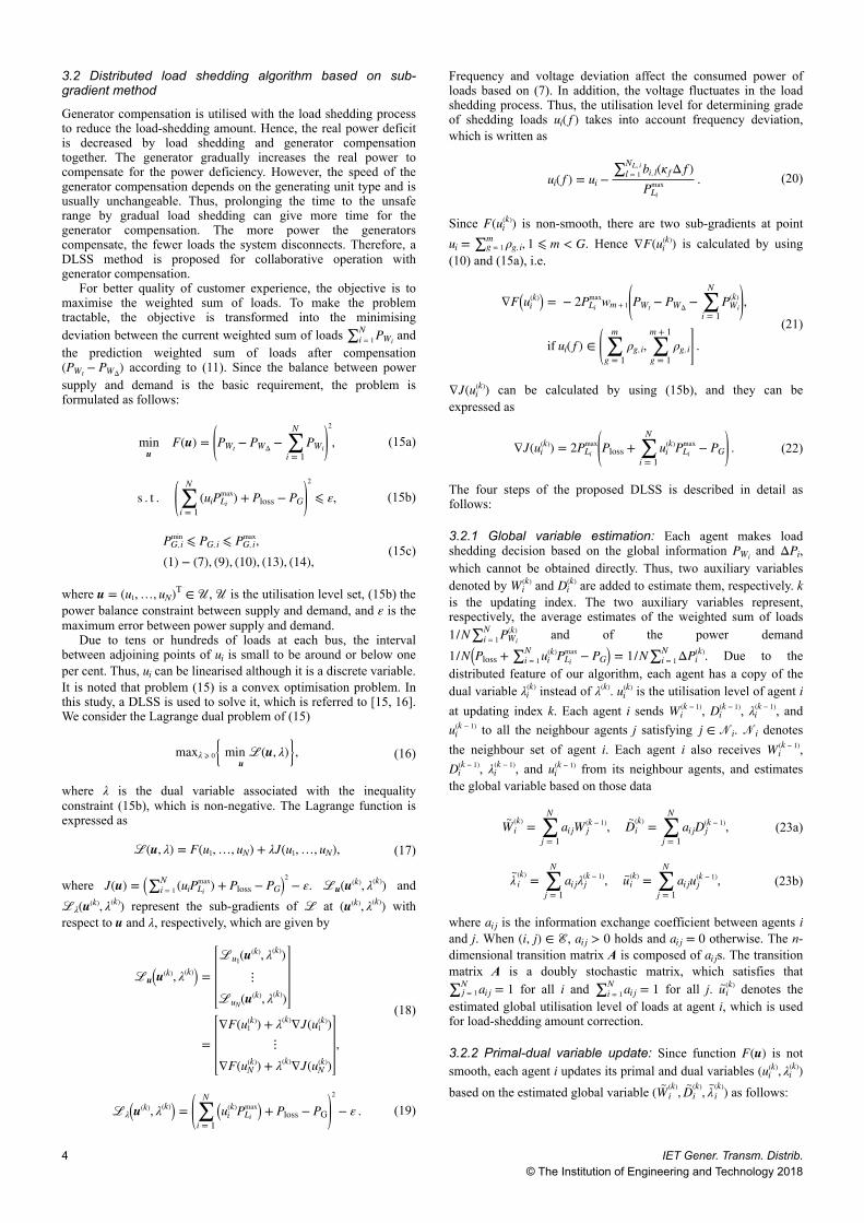
3.2 Distributed load shedding algorithm based on sub-gradient method

Generator compensation is utilised with the load shedding processto reduce the load-shedding amount. Hence, the real power deficitis decreased by load shedding and generator compensationtogether. The generator gradually increases the real power tocompensate for the power deficiency. However, the speed of thegenerator compensation depends on the generating unit type and isusually unchangeable. Thus, prolonging the time to the unsaferange by gradual load shedding can give more time for thegenerator compensation. The more power the generatorscompensate, the fewer loads the system disconnects. Therefore, aDLSS method is proposed for collaborative operation withgenerator compensation.

For better quality of customer experience, the objective is tomaximise the weighted sum of loads. To make the problemtractable, the objective is transformed into the minimisingdeviation between the current weighted sum of loads ∑i = 1

N PWi andthe prediction weighted sum of loads after compensation(PWt − PWΔ) according to (11). Since the balance between powersupply and demand is the basic requirement, the problem isformulated as follows:

minu

F(u) = PWt − PWΔ − ∑i = 1

NPWi

2

, (15a)

s . t . ∑i = 1

N(uiPLi

max) + Ploss − PG

2

⩽ ε, (15b)

PG, imin ⩽ PG, i ⩽ PG, i

max,(1) − (7), (9), (10), (13), (14),

(15c)

where u = (u1, …, uN)T ∈ U, U is the utilisation level set, (15b) thepower balance constraint between supply and demand, and ε is themaximum error between power supply and demand.

Due to tens or hundreds of loads at each bus, the intervalbetween adjoining points of ui is small to be around or below oneper cent. Thus, ui can be linearised although it is a discrete variable.It is noted that problem (15) is a convex optimisation problem. Inthis study, a DLSS is used to solve it, which is referred to [15, 16].We consider the Lagrange dual problem of (15)

maxλ ⩾ 0 min ℒu

(u, λ) , (16)

where λ is the dual variable associated with the inequalityconstraint (15b), which is non-negative. The Lagrange function isexpressed as

ℒ(u, λ) = F u1, …, uN + λJ u1, …, uN , (17)

where J(u) = ∑i = 1N (uiPLi

max) + Ploss − PG2− ε. ℒu(u(k), λ(k)) and

ℒλ(u(k), λ(k)) represent the sub-gradients of ℒ at (u(k), λ(k)) withrespect to u and λ, respectively, which are given by

ℒu u(k), λ(k) =ℒu1(u(k), λ(k))

⋮ℒuN(u(k), λ(k))

=∇F(u1

(k)) + λ(k)∇J(u1(k))

⋮∇F(uN

(k)) + λ(k)∇J(uN(k))

,

(18)

ℒλ u(k), λ(k) = ∑i = 1

Nui

(k)PLimax + Ploss − PG

2

− ε . (19)

Frequency and voltage deviation affect the consumed power ofloads based on (7). In addition, the voltage fluctuates in the loadshedding process. Thus, the utilisation level for determining gradeof shedding loads ui( f ) takes into account frequency deviation,which is written as

ui( f ) = ui −∑l = 1

NL, i bi, l(κ f Δ f )PLi

max . (20)

Since F(ui(k)) is non-smooth, there are two sub-gradients at point

ui = ∑g = 1m ρg, i, 1 ⩽ m < G. Hence ∇F(ui

(k)) is calculated by using(10) and (15a), i.e.

∇F ui(k) = − 2PLi

maxwm + 1 PWt − PWΔ − ∑i = 1

NPWi

(k) ,

if ui( f ) ∈ ∑g = 1

mρg, i, ∑

g = 1

m + 1ρg, i .

(21)

∇J(ui(k)) can be calculated by using (15b), and they can be

expressed as

∇J(ui(k)) = 2PLi

max Ploss + ∑i = 1

Nui

(k)PLimax − PG . (22)

The four steps of the proposed DLSS is described in detail asfollows:

3.2.1 Global variable estimation: Each agent makes loadshedding decision based on the global information PWi and ΔPi,which cannot be obtained directly. Thus, two auxiliary variablesdenoted by Wi

(k) and Di(k) are added to estimate them, respectively. k

is the updating index. The two auxiliary variables represent,respectively, the average estimates of the weighted sum of loads1/N∑i = 1

N PWi(k) and of the power demand

1/N Ploss + ∑i = 1N ui

(k)PLimax − PG = 1/N∑i = 1

N ΔPi(k). Due to the

distributed feature of our algorithm, each agent has a copy of thedual variable λi

(k) instead of λ(k). ui(k) is the utilisation level of agent i

at updating index k. Each agent i sends Wi(k − 1), Di

(k − 1), λi(k − 1), and

ui(k − 1) to all the neighbour agents j satisfying j ∈ Ni. Ni denotes

the neighbour set of agent i. Each agent i also receives Wi(k − 1),

Di(k − 1), λi

(k − 1), and ui(k − 1) from its neighbour agents, and estimates

the global variable based on those data

W~

i(k) = ∑

j = 1

Nai jW j

(k − 1), D~

i(k) = ∑

j = 1

Nai jDj

(k − 1), (23a)

λ~

i(k) = ∑

j = 1

Nai jλj

(k − 1), u~i(k) = ∑

j = 1

Nai juj

(k − 1), (23b)

where ai j is the information exchange coefficient between agents iand j. When (i, j) ∈ ℰ, ai j > 0 holds and ai j = 0 otherwise. The n-dimensional transition matrix A is composed of ai js. The transitionmatrix A is a doubly stochastic matrix, which satisfies that∑ j = 1

N ai j = 1 for all i and ∑i = 1N ai j = 1 for all j. u~i

(k) denotes theestimated global utilisation level of loads at agent i, which is usedfor load-shedding amount correction.

3.2.2 Primal-dual variable update: Since function F(u) is notsmooth, each agent i updates its primal and dual variables (ui

(k), λi(k))

based on the estimated global variable (W~i(k), D

~i(k), λ

~i(k)) as follows:

4 IET Gener. Transm. Distrib.© The Institution of Engineering and Technology 2018

ui(k) = ui

(k − 1) − τkℒui u(k − 1), λ~

i(k) +

= ui(k − 1) − 2τkPLi

max λi(k)ND

~i(k)

−wm + 1(PWt − PWΔ − NW~

i(k))

+,

ui( f ) ∈ ∑g = 1

mρg, i, ∑

g = 1

m + 1ρg, i ,

(24)

λi(k) = λ

~i(k) + τkℒλi u(k), λ

~i(k) +

= (λ~i(k) + τk((ND

~i(k))2 − ε)+,

(25)

where τk is the step size, (u)+ = max {u, 0}.The shedding sequence of loads is sorted in an ascending order

of weighted power wgPLi, l. Then, the shedding control variable bican be determined by approximating the obtained ui based on (7).

3.2.3 Local variable update: When the load shedding decision iscarried out, Wi

(k) and Di(k) need to be updated for the global

information estimation in the next iteration. Each agent i updatesvariables Wi

(k) and Di(k) with the changes of the local argument

functions PWi(k) and ΔPi

(k)

Wi(k) = W

~i(k) + PWi

(k) − PWi(k − 1), (26)

Di(k) = D

~i(k) + ΔPi

(k) − ΔPi(k − 1) . (27)

To reduce the jitter of utilisation level, the initial value of Wi(0) and

Di(0) can be set to PWt/N and ∑i = 1

N ΔPi/N based on the obtained datain the GID.

3.2.4 Load-shedding amount correction: The SG or ESS iscontrolled to generate real power to compensate for the deficiencyin the process of load shedding. The compensation rate isdetermined by the specification and power control algorithm of thegenerator or ESS, which is a relatively slower than load shedding.The total loads that are needed to shed ΔP

~ are updated as follows:

ΔP~(k) = ΔP(k) + (1 − u~i

(k))PLmax, (28)

where the first term of (28) is the current power deficit, and thesecond term is the sum of loads that have been shed. Thus theweighted sum of loads that need to be shed PWΔ can be updatedbased on (6) and (28). Due to this correction mechanism, adynamic load shedding method is realised.

The above steps of the DLSS method are summarised inAlgorithm 1 (see Fig. 3).

3.3 Safety threshold shedding

In the gradual load shedding, the safety threshold of systemfrequency must be guaranteed. If the system frequency drops downto the lower safety threshold f th and the gradual load shedding hasnot been finished, the safety threshold shedding is executedimmediately. The load-shedding amount Pshi follows the ruleaccording to [17] which is

Pshi =Δ f iPLi

∑i ∈ N Δ f iPLiΔP

~(k), (29)

where Δ f i denotes the frequency deviation at bus i compared withthe base frequency. Considering the small deviation of Δ f i betweendifferent buses in the microgrid, (29) can be written as

Pshi =uiPLi

max

u~iPLmax ΔP

~(k) . (30)

To describe the relationship between the safety threshold sheddingand other modules, a high-level logic overview is given in Fig. 4,which also provides a complete description of the proposedsolution. After the convergence of the GID, the DLSS method isused after a time delay tad. Thus, the total time delay equals totgi + tad. Regardless of the convergence of the DLSS process, thesafety threshold shedding is triggered if the frequency drops to f th.

3.4 Convergence analysis of DLSS method

The precondition of balancing the power supply–demand is theconvergence of the DLSS algorithm which is analysed here. It canbe known that the convexity of function J(u) implies that it hasuniformly bounded sub-gradient, which is equivalent to J(u) beingLipschitz continuous. Thus, based on (21), we have

∥ ∇J(u) ∥ = ∥∇J(u1

(k))⋮

∇J(uN(k))

∥

⩽ 2 NP⌣

LiΔP~, ∀u ∈ U,

(31)

∥ ∇J(u) − ∇J(u+) ∥ = ∥∇J(u1

(k)) − ∇J(u1+(k))

⋮∇J(uN

(k)) − ∇J(u2+(k))

∥

⩽ 2P⌣

Li

2 ∥ u − u+ ∥ , ∀u, u+ ∈ U,

(32)

where P⌣

Li = max1 ⩽ i ⩽ n {PLimax}.

Similarly, the convexity of function F(u) implies that it has auniformly bounded sub-gradient. Based on (22), we have

∥ ∇F(u) ∥ = ∥∇F(u1

(k))⋮

∇F(uN(k))

∥

⩽ 2 NP⌣

LiwGPWΔ, ∀u ∈ U,

(33)

Fig. 3  Algorithm 1: DLSS

Fig. 4  High level logic overview of the proposed solution

IET Gener. Transm. Distrib.© The Institution of Engineering and Technology 2018

5

∥ ∇F(u) − ∇F(u+) ∥ = ∥∇F(u1

+(k)) − ∇F(u1+(k))

⋮∇F(uN

+(k)) − ∇F(uN+(k))

∥

⩽ 2P⌣

Li

2 wG2 ∥ u − u+ ∥ , ∀u, u+ ∈ U .

(34)

 Proposition 1: Assume that the step size sequence τk is non-increasing such that τk > 0 for all k ⩾ 1. Then, u(k) andλi

(k), i = 1, …, n, generated by the algorithm of DLSS can convergeto an optimal primal solution with compensation u∗ ∈ U and anoptimal dual solution with compensation λ∗, respectively. Cλdenotes the upper bound of ∥ λ ∥.

The proof is given in [18].

3.5 Parameter setting

Frequency setting and time delay are two important parameters inROCOF relay. From the results in [19, 20], the frequency setting isan important trigger condition for the load shedding process, whichincludes over-frequency setting and under-frequency setting.

From (13) and (14), we can know that the ROCOF d f /dt has anegative correlation with the equivalent inertia Hsys at the samepower deficit ΔP

d fdt = f noΔP

2Hsys, (35)

where Hsys can be obtained based on (13) and (14) according to[21]. Hence, the time ttr that the frequency drops to the frequencysetting is represented by

ttr = ( f no − f tr)d f /dt = 2Hsys( f no − f tr)

f noΔP . (36)

Thus, due to the low inertia Hsys, the microgrid suffers from alarger ROCOF at the same power deficit compared with theconventional power system. When power imbalance occurs, thetime tfa that the frequency drops to the unsafe frequency f fa inmicrogrids is less than that in the conventional power system.Based on (35), tfa can also be calculated by

tfa = ( f no − f fa)Δ f /Δt = 2Hsys( f no − f fa)

f noΔP . (37)

The time trp for the ROCOF relay process equals to tfa − ttr. Thus,trp has a negative correlation with f tr. From Fig. 2b, we can knowthat the time for load shedding can be calculated astls = trp − tgi − tad. Hence, trp has a positive correlation with f tr.Considering that tgi is always larger than zero, tls may be belowzero with a large under-frequency setting. In other words, theROCOF relay may not carry out the load shedding process in timebefore the microgrid collapses. Therefore, the large frequencysetting is not suitable for the proposed solution in microgrids,especially in islanding mode. Consequently, the small frequencysetting Δ f = 0.5 Hz is selected in our solution.

The time delay is employed for improving the safety andminimising the possibility of false operation (nuisance tripping),which usually ranges from 50 to 500 ms [22]. Firstly, the GIDoperates based on the consensus method, which exhibited a goodperformance in reducing the measurement noise and oscillation offrequency [6]. Thus, this method can reduce the effect of nuisancetripping. Secondly, the smaller time delay has little impact on theavoidance of false operation. The larger time delay leads to alonger detection time of the faults, which may show that the loadshedding process does not respond promptly. In our proposedsolution, tgi can be considered as a part of the total time delaytd = tgi + tad. The smaller tgi gives a wide tuning range for the timedelay tad. tgi is determined by communication topology, transition

matrix A, and communication protocol. The former two can beadjusted according to the physical space and consensus theory [23].These topics are out of the scope of this paper. The MMSTprotocol is proposed to reduce the time delay caused by the thirdone, which is introduced in the following section. To sum up, thetotal response time tto must be less than tfa, which can be describedas

tto = ttr + tgi + tad < tfa . (38)

Additionally, the detailed simulation to analyse the performance ofthe proposed solution at different total time delays is described inSection 5.2.

4 MMST for load sheddingThe response time of the DLSS method is determined by theconvergence of the GID process, which is also related to acommunication protocol. Equation (12) can be expressed in thetime based update format as follows:

xi(k + 1)tone = ∑

j = 1

Nai jxj

(ktone), (39)

where tone denotes the time period of each iteration. Thus, theconvergence time can be represented by Tgi = Nuptone. Nup is theiterations of convergence. tone consists of a communication timedelay and a calculation time delay. The calculation time delay canbe neglected because the computing performance of each bus agentis powerful enough. Thus tone has a direct relationship with thecommunication protocol.

Since the TDMA scheme is a collision-free protocol, it isadopted to improve the convergence speed and guarantee thestability of the DLSS method. Thus, the MMST protocol for loadshedding is proposed here. The IEEE 802.11 protocol is employedfor analysis without loss of generality.

4.1 Time slot allocation for multicast metropolis schedule

The slot assignment to improve the channel utilisation is the mainproblem in this protocol design. In each update process of theproposed solution, each agent needs to exchange data with all theneighbour agents. If the unicast mode is adopted, each updatingprocess needs time slots S = 2|ℰ|, where |ℰ| is the number of thetransmission link. The multicast mode is adopted to reduce slots Sin each update, i.e. each agent sends information to all hisneighbour agents in the same slot. So the used time slots S arereduced from 2 |ℰ| to N. Due to the distributed nature and thesparsity characteristic of microgrids, S can be further reduced byrealising concurrent transmission. However, the concurrenttransmission may have the hidden terminal problem which causesthe packet collision. Thus, the objective is to obtain the optimaltransmission schedule to minimise the used time slot S subject totwo constraints. Firstly, each agent has one non-private slot totransmit information; secondly, the two-hop neighbours N2(i) ofagent i cannot transmit in the same slot.

The issue is a vertex colouring problem which has been provedto be an non-deterministic polynomial-time (NP)-hard problem.Thus we design a heuristic algorithm to obtain the sub-optimal slotassignment inspired by [24]. This algorithm has two loops to findthe suboptimal transmission schedule. The outer loop generates aslot and allocates it to a maximum degree agent firstly in this slotuntil all agents have a transmission slot. The inner loop is to findthe maximum number of concurrent transmission and thecorresponding agent group in this slot (see Fig. 5).

4.2 Frame design of multicast metropolis schedule

Due to the slot allocation algorithm in MMST, the packet losscaused by the hidden terminal problem is avoided. However,packet loss caused by link quality cannot be avoided. Thus the dataframe is defined in Fig. 6 for reliable packet delivery.

6 IET Gener. Transm. Distrib.© The Institution of Engineering and Technology 2018

The Index_DATA includes the consensus indices of thecurrently transmitted data, which is used for consensus operation inthe GID and utilisation level update. Index_NEIG and Bitmapindicate whether the data of neighbour agents have been receivedsuccessfully, which are inserted into the data frame. Index_NEIGcontains the neighbour indices of the agent who transmits the dataframe. The Status_NEIG-i in Bitmap is the status of the receiveddata from the ith neighbour agent. If the previous data frame fromthe ith neighbour agent has been received successfully,Status_NEIG-i is set to 1, otherwise set to 0. If the previous dataframe fails to receive, the neighbour agent will add it in historydata part of the data frame and retransmit with the new data. Thus,retransmission of the lost packet is realised to improve thetransmission reliability. The status data include two parts: currentstatus data and history status data. Current status data are theupdate data of each agent, and the history status data are theprevious data which have not been received correctly. The lengthof data can be adjusted according to the system requirement. In ourmethod, the data that need to be updated include load informationPLi, ρg, i, power deficit ΔPi, and utilisation level ui, u~i.

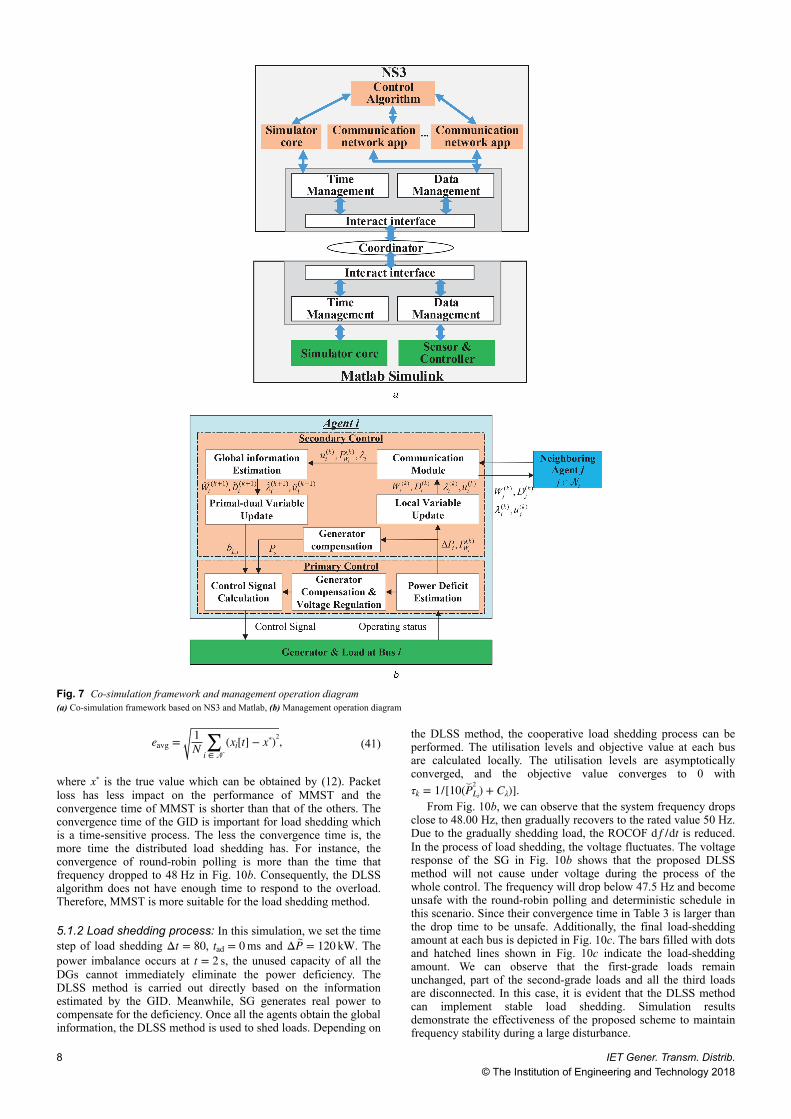
5 SimulationsIn this section, the proposed distributed load shedding solution istested using an NS3-Matlab co-simulator which is implementedbased on the co-simulation structure [25]. The microgrid ismodelled in Matlab/Simulink, and the network communication issimulated in NS3. The two simulators can exchange a message byusing the interactive interface part which is designed based on thesocket model. The co-simulation framework is shown in Fig. 7a.

The agents communicate via a wireless network which has thesame communication topology as the power transmission topology.The transition matrix A employs an improved Metropolis method[26], which is defined as

ai j =

1max {Ni, N j} + 1 j ∈ N(i)

1 − ∑ j ∈ Ni

1max {Ni, N j} + 1 i = j

0 otherwise,

(40)

where Ni denotes the number of neighbour agent i, and N(i)represents the set of agent i.

The management operation of each agent is shown in Fig. 7b.The hierarchical management strategy consists of two controllevels. The secondary level is responsible for exchanging andupdating the utilisation level and setting the reference power ofloads. The communication module exchanges local information

with its neighbour agents. The primary level is used for real powertracking while satisfying other constraints including reactive powerand voltage regulation. There are multi-priority loads at each bus.κf and κv are set to 1.0. The trigger frequency and the safetythreshold frequency are set to 49.5 and 48 Hz. The weight factor wgof the three priority loads is set to 1, 2 and 5. Under normalconditions, SG is just used for voltage regulation and generatespower at a low level. Once fault occurs, the SG generates power tocompensate for the deficit.

5.1 Case 1: islanding in a microgrid with radial topology

The 6-bus system with a radial topology is illustrated in Fig. 8a.This system contains different types of DGs, such as SG, PV, andwind turbine (WT). The information of the generators and loads isshown in Tables 1 and 2. The ramp-up and ramp-down rates of theSG are both set to 40 kW/s, which determine the maximumcompensation rate. In this case, the communication topology isdepicted in Fig. 8b.

When t = 2 s, the distributed microgrid is disconnected from themain grid. The power generation cannot restore system frequencyimmediately. As a result, the system frequency starts to droprapidly after this disturbance.

5.1.1 Global information discovery: The GID process is alwayscarried out periodically in normal operation mode. When powerimbalance occurs, this process is triggered by the drop in systemfrequency. The global information that contains the power deficitΔPi, the total real power of loads PL

max, and the ratio of the gth loadsρg. The iteration processes of the GID are shown in Fig. 9a. PV1 canbe obtained from Fig. 9a, so ρ1 is calculated by (PV1/PL

max). Thepower deficit of different DGs ΔPi is estimated by differentmethods in (13) and (14).

The process of power deficit discovery is used for theconvergence analysis of the proposed MMST protocol, round-robinpolling mechanism, and deterministic scheduling [7]. In this case,the time slot of the communication protocol is set to 5 ms, whichcan meet the per-hop latency in sub-6 GHz wireless technology.The three protocols need to allocate 4, 6, and 10 time-slots for oneiteration tone, respectively. Four conditions with different packetloss rates r are considered for analysis. The results are shown inFig. 9b and Table 3.

The results demonstrate that the convergence time Tgi increasesand the relative error e becomes larger with the increase of thepacket loss rate. The average coordination error eavg is defined as

Fig. 5  Algorithm 2: Time slot allocation algorithm of MMST

Fig. 6  DATA frame structure

IET Gener. Transm. Distrib.© The Institution of Engineering and Technology 2018

7

eavg = 1N ∑

i ∈ N(xi[t] − x∗)2, (41)

where x∗ is the true value which can be obtained by (12). Packetloss has less impact on the performance of MMST and theconvergence time of MMST is shorter than that of the others. Theconvergence time of the GID is important for load shedding whichis a time-sensitive process. The less the convergence time is, themore time the distributed load shedding has. For instance, theconvergence of round-robin polling is more than the time thatfrequency dropped to 48 Hz in Fig. 10b. Consequently, the DLSSalgorithm does not have enough time to respond to the overload.Therefore, MMST is more suitable for the load shedding method.

5.1.2 Load shedding process: In this simulation, we set the timestep of load shedding Δt = 80, tad = 0 ms and ΔP

~ = 120 kW. Thepower imbalance occurs at t = 2 s, the unused capacity of all theDGs cannot immediately eliminate the power deficiency. TheDLSS method is carried out directly based on the informationestimated by the GID. Meanwhile, SG generates real power tocompensate for the deficiency. Once all the agents obtain the globalinformation, the DLSS method is used to shed loads. Depending on

the DLSS method, the cooperative load shedding process can beperformed. The utilisation levels and objective value at each busare calculated locally. The utilisation levels are asymptoticallyconverged, and the objective value converges to 0 withτk = 1/[10(P⌣Li

2 ) + Cλ)].From Fig. 10b, we can observe that the system frequency drops

close to 48.00 Hz, then gradually recovers to the rated value 50 Hz.Due to the gradually shedding load, the ROCOF d f /dt is reduced.In the process of load shedding, the voltage fluctuates. The voltageresponse of the SG in Fig. 10b shows that the proposed DLSSmethod will not cause under voltage during the process of thewhole control. The frequency will drop below 47.5 Hz and becomeunsafe with the round-robin polling and deterministic schedule inthis scenario. Since their convergence time in Table 3 is larger thanthe drop time to be unsafe. Additionally, the final load-sheddingamount at each bus is depicted in Fig. 10c. The bars filled with dotsand hatched lines shown in Fig. 10c indicate the load-sheddingamount. We can observe that the first-grade loads remainunchanged, part of the second-grade loads and all the third loadsare disconnected. In this case, it is evident that the DLSS methodcan implement stable load shedding. Simulation resultsdemonstrate the effectiveness of the proposed scheme to maintainfrequency stability during a large disturbance.

Fig. 7  Co-simulation framework and management operation diagram(a) Co-simulation framework based on NS3 and Matlab, (b) Management operation diagram

8 IET Gener. Transm. Distrib.© The Institution of Engineering and Technology 2018

5.1.3 Load-shedding amount analysis: The compensationpower amount of distributed SG is related to the adjusted time ofthe DLSS method, which is impacted by step size τk. The moretime the SG has for compensation, the less loads should be shed.The simulation is carried out with different parameters τk andpower deficiency ΔP

~. The results are shown in Table 4. The five

parameters of τk are 1/[20P⌣

Li

2 (wG2 + Cλ)], 1/[15P

⌣Li

2 (wG2 + Cλ)],

1/[12P⌣

Li

2 (wG2 + Cλ)], 1/[10P

⌣Li

2 (wG2 + Cλ)], and 1/[4P

⌣Li

2 (wG2 + Cλ)]. We

can observe that the number of shedding steps is reduced and theload-shedding amount at each step is increased with the increase ofτk. Larger shedding amount can realise the supply–demand balancefaster, but there is no sufficient time for generator compensation.Thus, the load-shedding amount is not reduced significantly. Sincethe smaller parameters τk have little impact on the reduction offrequency derivative, it cannot avoid the frequency dropping to theunsafe range. From Table 4, it can be seen that the system

frequency drops to the unsafe range when the power deficits are160 and 200 kW with the smallest τk. In these cases, the safetythreshold shedding is executed. Thus, the final power deficit ΔP

~ by

load shedding is more than the case with larger τk. With the sameτk, the load-shedding amount at each step and the number ofshedding steps are affected by the power deficit ΔP

~. A rapid

frequency decline can be decreased after executing the steps with alarge load-shedding amount. Consequently, the frequency wouldnot drop too fast to reach the unsafe range. When the power deficitis relatively small, the initial steps have a small load-sheddingamount to avoid shedding loads too quickly. Hence, the generatorhas enough time to compensate for the power deficit.

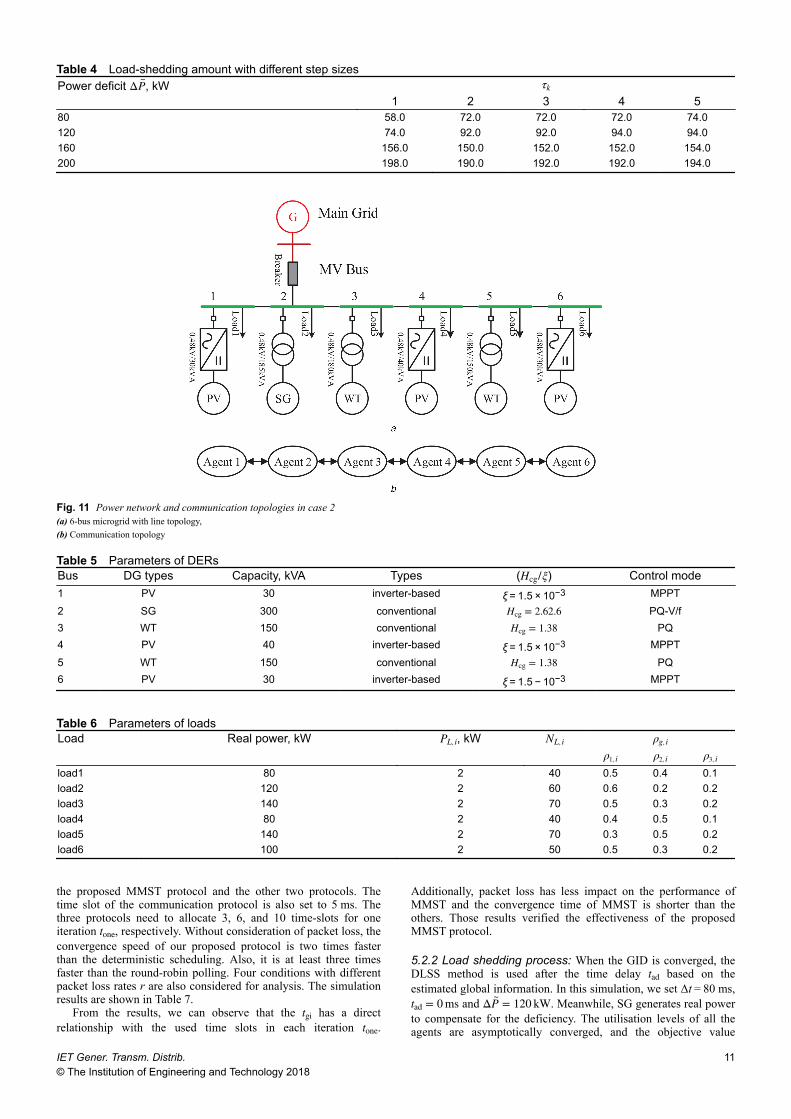
5.2 Case 2: disconnection in a microgrid with line topology

The 6-bus system with line topology is illustrated in Fig. 11a. Theinformation of the generators and loads are shown in Tables 5 and

Fig. 8  Power network and communication topologies in case 1(a) 6-bus microgrid with radial topology, (b) Communication topology

Table 1 Parameters of DERsBus DG types Capacity, kVA Types (Hcg/ξ) Control mode1 PV 30 inverter-based ξ = 1.5 × 10−3 MPPT

2 SG 185 conventional Hcg = 1.68 PQ-V/f3 PV 30 inverter-based ξ = 1.5 × 10−3 MPPT

4 WT 40 conventional Hcg = 0.68 PQ5 WT 150 conventional Hcg = 1.38 PQ6 WT 180 conventional Hcg = 1.46 PQ

Table 2 Parameters of loadsLoad Real power, kW PL, i, kW NL, i ρg, i

ρ1, i ρ2, i ρ3, i

load1 100 2 50 0.5 0.3 0.2load2 120 2 60 0.6 0.2 0.2load3 150 2 75 0.5 0.3 0.2load4 100 2 50 0.3 0.5 0.2load5 100 2 50 0.3 0.5 0.2load6 120 2 60 0.5 0.3 0.2

IET Gener. Transm. Distrib.© The Institution of Engineering and Technology 2018

9

6. The ramp-up and ramp-down rates of the SG are also both set to40 kW/s, which determine the maximum compensation rate. Thecommunication topology of this system is depicted in Fig. 11b. Adisconnection of the WT at bus 5 is simulated in the islandingmode.

5.2.1 Global information discovery: The frequency starts to droprapidly when the disconnection of the WT in bus 5 takes place att = 2 s. The unused capacity of SG cannot immediately eliminatethe power deficiency. If the frequency drops to the triggerfrequency f tr, the GID is carried out immediately. In this case, theprocess of total load power is used for the convergence analysis of

Fig. 9  Performance comparison between different protocols in case 1(a) GID, (b) Coordination error comparison

Table 3 Performance comparison in GIDPacket loss rate Round-robin polling Deterministic scheduling MMSTr Tgi, s e Tgi, s e Tgi, s e0% 1.25 0% 0.66 0% 0.32 0%1% 1.25 1.3% 0.75 1.29% 0.32 0%5% 1.35 1.6% 0.81 1.61% 0.32 0%10% 1.40 1.55% 0.84 1.54% 0.32 0.01%

Fig. 10  Performance of DLSS in case 1(a) Utilization levels of DLSS, (b) Frequency and voltage recovery, (c) Load shedding at each bus

10 IET Gener. Transm. Distrib.© The Institution of Engineering and Technology 2018

the proposed MMST protocol and the other two protocols. Thetime slot of the communication protocol is also set to 5 ms. Thethree protocols need to allocate 3, 6, and 10 time-slots for oneiteration tone, respectively. Without consideration of packet loss, theconvergence speed of our proposed protocol is two times fasterthan the deterministic scheduling. Also, it is at least three timesfaster than the round-robin polling. Four conditions with differentpacket loss rates r are also considered for analysis. The simulationresults are shown in Table 7.

From the results, we can observe that the tgi has a directrelationship with the used time slots in each iteration tone.

Additionally, packet loss has less impact on the performance ofMMST and the convergence time of MMST is shorter than theothers. Those results verified the effectiveness of the proposedMMST protocol.

5.2.2 Load shedding process: When the GID is converged, theDLSS method is used after the time delay tad based on theestimated global information. In this simulation, we set Δt = 80 ms,tad = 0 ms and ΔP

~ = 120 kW. Meanwhile, SG generates real powerto compensate for the deficiency. The utilisation levels of all theagents are asymptotically converged, and the objective value

Table 4 Load-shedding amount with different step sizesPower deficit ΔP

~, kW τk

1 2 3 4 580 58.0 72.0 72.0 72.0 74.0120 74.0 92.0 92.0 94.0 94.0160 156.0 150.0 152.0 152.0 154.0200 198.0 190.0 192.0 192.0 194.0

Fig. 11  Power network and communication topologies in case 2(a) 6-bus microgrid with line topology,(b) Communication topology

Table 5 Parameters of DERsBus DG types Capacity, kVA Types (Hcg/ξ) Control mode1 PV 30 inverter-based ξ = 1.5 × 10−3 MPPT

2 SG 300 conventional Hcg = 2.62.6 PQ-V/f3 WT 150 conventional Hcg = 1.38 PQ4 PV 40 inverter-based ξ = 1.5 × 10−3 MPPT

5 WT 150 conventional Hcg = 1.38 PQ6 PV 30 inverter-based ξ = 1.5 − 10−3 MPPT

Table 6 Parameters of loadsLoad Real power, kW PL, i, kW NL, i ρg, i

ρ1, i ρ2, i ρ3, i

load1 80 2 40 0.5 0.4 0.1load2 120 2 60 0.6 0.2 0.2load3 140 2 70 0.5 0.3 0.2load4 80 2 40 0.4 0.5 0.1load5 140 2 70 0.3 0.5 0.2load6 100 2 50 0.5 0.3 0.2

IET Gener. Transm. Distrib.© The Institution of Engineering and Technology 2018

11

converges to 0, which demonstrates that our solution retrieves thepower balance.

We can observe from Fig. 12b that the system frequency dropsclose to 48.00 Hz, and then gradually recovers to the rated value50 Hz. The initial estimated ROCOF is equal to 1.75 Hz/s. Withoutload shedding, the time that the frequency drops to 47 Hz is ∼1.8 s.The single step load shedding method executed the operation whenthe frequency dropped to 48 Hz. Due to the gradual load shedding,the ROCOF d f /dt is reduced. Thus, there is more time for powercompensation by our solution than other two solutions. In theprocess of load shedding by the proposed method, the voltagefluctuates. The voltage response of SG in Fig. 12b shows that theproposed DLSS method will not cause under voltage during theprocess of the whole control. Additionally, the bars filled with dotsand hatched lines shown in Fig. 12c indicate the final load-shedding amount. We can observe that the first-grade and second-grade loads remain unchanged, part of the third-grade loads aredisconnected. In this case, it is evident that the DLSS method can

implement stable load shedding. Simulation results demonstrate theeffectiveness of the proposed DLSS scheme to maintain frequencystability during a large disturbance.

5.2.3 Time delay analysis: Based on the analysis in Section 3.5,it is known that tgi can be considered as a part of the time delay inthe ROCOF relay. As tgi cannot be directly adjusted, we test thesolution performance at different time delays tad. The total timedelay is calculated by td = tgi + tad. The simulation results areshown in Table 8. Four different power deficits are considered,which are conducted with different power generations of the WT inbus 5. The step size τk is set to 1/[15P

⌣Li

2 (wG2 + Cλ)].

From the results, it can be known that our solution with thesmaller delay causes more power compensation. The larger timedelay causes a longer response time for the disconnectionoperation. Consequently, the frequency drops over a longer time. Inthe worst case, the load shedding process in (30) operates before

Table 7 Performance comparison in GIDPacket loss rate Round-robin polling Deterministic scheduling MMSTr Tgi, s e Tgi, s e Tgi, s e0% 0.95 0% 0.57 0% 0.29 0%1% 0.95 1.26% 0.65 1.25% 0.29 0%5% 1.05 1.56% 0.70 1.51% 0.29 0%10% 1.10 1.53% 0.75 1.49% 0.29 0.01%

Fig. 12  Performance of DLSS in case 2(a) Utilization levels of DLSS, (b) Frequency and voltage recovery, (c) Load shedding at each bus

Table 8 Load-shedding amount with different time delaysPower deficit ΔP

~, kW tad, ms

100 200 400 600 80090 40.0 42.0 52.0 60.0 70.0110 70.0 76.0 84.0 94.0 102.0130 102.0 106.0 116.0 124.0 130.0150 128.0 134.0 142.0 150.0 150.0

12 IET Gener. Transm. Distrib.© The Institution of Engineering and Technology 2018

the implementation of the DLSS method. Thus, the load-sheddingamount is similar to the initial estimated power deficit. Forexample, when ΔP

~ = 150 kW, the load-shedding amounts equal tothe power deficit at the time delay 600 and 800 ms. In thisscenario, the proposed solution has the same performancecompared with the conventional single step load shedding scheme.In other words, the power compensation cannot be realised.Consequently, the consumer’ experience cannot be improved byreducing the load-shedding amount. Therefore, if tgi is within areasonable range, we do not need to add another time delay tad.

6 ConclusionIn this study, a distributed load shedding solution is proposed toshed loads gradually considering the participation of smart homes/buildings. First, the DLSS method is proposed to alleviate the rateof frequency drop. Consequently, the time of frequency to beunsafe is prolonged. Thus, the generators have more time tocompensate power deficiency for reducing the load-sheddingamount. Second, an MMST protocol is developed to reduceresponse time and enhance the reliability of the DLSS method. Thesimulation results demonstrate that the proposed load sheddingsolution can maintain the stability of the system frequency andreduce the load-shedding amount. The future work will concernthis issue in the microgrid integrated into the ESS.

7 AcknowledgmentsThis work was supported by the National Key Research andDevelopment Program of China (2016YFB090190) and theNational Natural Science Foundation of China (61573245,61174127, 61521063, and 61633017). This work was also partiallysupported by the Shanghai Rising-Star Program under grant no.15QA1402300 and the Shanghai Municipal Commission ofEconomy and Informatization under SH-CXY-2016-003. Theauthors would like to thank the anonymous reviewers for theirprofessional and valuable comments, which have led to theimproved version.

8 References[1] Laghari, J., Mokhlis, H., Bakar, A., et al.: ‘Application of computational

intelligence techniques for load shedding in power systems: a review’, EnergyConvers. Manage., 2013, 75, pp. 130–140

[2] Gao, H., Chen, Y., Xu, Y., et al.: ‘Dynamic load shedding for an islandedmicrogrid with limited generation resources’, IET Gener. Transm. Distrib.,2016, 10, (12), pp. 2953–2961

[3] Hong, Y.-Y., Hsiao, C.M., Chang, Y.R., et al.: ‘Multiscenario underfrequencyload shedding in a microgrid consisting of intermittent renewables’, IEEETrans. Power Deliv., 2013, 28, (3), pp. 1610–1617

[4] Lim, Y., Kim, H.M., Kinoshita, T.: ‘Distributed load-shedding system foragent-based autonomous microgrid operations’, Energies, 2014, 7, (1), pp.385–401

[5] Huang, K., Cartes, D.A., Srivastava, S.K.: ‘A multiagent-based algorithm forring-structured shipboard power system reconfiguration’, IEEE Trans. Syst.Man Cybern. C, Appl. Rev., 2007, 37, pp. 1016–1021

[6] Zhao, C., Topcu, U., Low, S.H.: ‘Optimal load control via frequencymeasurement and neighborhood area communication’, IEEE Trans. PowerSyst., 2013, 28, (4), pp. 3576–3587

[7] Liang, H., Choi, B.J., Zhuang, W., et al.: ‘Multiagent coordination inmicrogrids via wireless networks’, IEEE Wirel. Commun., 2012, 19, (3), pp.14–22

[8] Xu, Y., Liu, W., Gong, J.: ‘Stable multi-agent-based load shedding algorithmfor power systems’, IEEE Trans. Power Syst., 2011, 26, (4), pp. 2006–2014

[9] Liu, W., Gu, W., Xu, Y., et al.: ‘Improved average consensus algorithm baseddistributed cost optimization for loading shedding of autonomous microgrids’,Int. J. Electr. Power Energy Syst., 2015, 73, pp. 89–96

[10] Gu, W., Liu, W., Zhu, J., et al.: ‘Adaptive decentralized under-frequency loadshedding for islanded smart distribution networks’, IEEE Trans. Sustain.Energy, 2014, 5, (3), pp. 886–895

[11] Taneja, J., Katz, R., Culler, D.: ‘Defining CPS challenges in a sustainableelectricity grid’. Proc. IEEE/ACM Int. Conf. on Cyber-Physical Systems,Beijing, CN, April 2012, pp. 119–128

[12] Parikh, P.P., Kanabar, M.G., Sidhu, T.S.: ‘Opportunities and challenges ofwireless communication technologies for smart grid applications’. Proc. IEEEPES General Meeting, Minneapolis, MN, USA, July 2010, pp. 1–7

[13] Yang, Q., Barria, J.A., Green, T.C.: ‘Communication infrastructures fordistributed control of power distribution networks’, IEEE Trans. Ind. Inf.,2011, 7, (2), pp. 316–327

[14] Laghari, J.A., Mokhlis, H., Karimi, M., et al.: ‘A new under-frequency loadshedding technique based on combination of fixed and random priority ofloads for smart grid applications’, IEEE Trans. Power Syst., 2015, 30, pp.2507–2515

[15] Xu, Y., Zhang, W., Liu, W., et al.: ‘Distributed subgradient-basedcoordination of multiple renewable generators in a microgrid’, IEEE Trans.Power Syst., 2014, 29, (1), pp. 23–33

[16] Chang, T.H., Nedić, A., Scaglione, A.: ‘Distributed constrained optimizationby consensus-based primal-dual perturbation method’, IEEE Trans. Autom.Control, 2014, 59, (6), pp. 1524–1538

[17] Zhong, Z.: ‘Power systems frequency dynamic monitoring system design andapplications’. PhD thesis, Virginia Polytechnic Institute and State Univ., 2005

[18] Xu, Q., Yang, B., Chen, C., et al.: ‘Distributed load shedding for microgridwith compensation support via wireless network’, 2017, http://arxiv.org/abs/1701.02195

[19] Vieira, J.C.M., Freitas, W., Xu, W., et al.: ‘Efficient coordination of ROCOFand frequency relays for distributed generation protection by using theapplication region’, IEEE Trans. Power Deliv., 2006, 21, pp. 1878–1884

[20] Motter, D., Vieira, J.C.M., Coury, D.V.: ‘Development of frequency-basedanti-islanding protection models for synchronous distributed generatorssuitable for real-time simulations’, IET Gener. Transm. Distrib., 2015, 9, (8),pp. 708–718

[21] Gu, W., Liu, S., Chen, S.: ‘Multi-stage underfrequency load shedding forislanded microgrid with equivalent inertia constant analysis’, Int. J. Electr.Power Energy Syst., 2013, 46, pp. 36–39

[22] Ten, C.F., Crossley, P.A.: ‘Evaluation of ROCOF relay performances onnetworks with distributed generation’. IET 9th Int. Conf. on Developments inPower System Protection, March 2008, pp. 523–528

[23] Olshevsky, A., Tsitsiklis, J.N.: ‘Convergence speed in distributed consensusand averaging’, SIAM J. Control Optim., 2009, 48, (1), pp. 33–55

[24] Brélaz, D.: ‘New methods to color the vertices of a graph’, Commun. ACM,1979, 22, (4), pp. 251–256

[25] Pan, Z., Xu, Q., Chen, C., et al.: ‘NS3-MATLAB co-simulator for cyber-physical systems in smart grid’. Proc. Chinese Control Conf. (CCC),Chengdu, CN, July 2016, pp. 577–581

[26] Xiao, L., Boyd, S., Kim, S.-J.: ‘Distributed average consensus with least-mean-square deviation’, J. Parallel Distrib. Comput., 2007, 67, (1), pp. 33–46

IET Gener. Transm. Distrib.© The Institution of Engineering and Technology 2018

13