RESEARCH Open Access

Distinguishing between hot-spots andmelting-pots of genetic diversity usinghaplotype connectivityBinh Nguyen1, Andreas Spillner2*, Brent C Emerson3, Vincent Moulton1

Abstract

We introduce a method to help identify how the genetic diversity of a species within a geographic region mighthave arisen. This problem appears, for example, in the context of identifying refugia in phylogeography, and in theconservation of biodiversity where it is a factor in nature reserve selection. Complementing current methods formeasuring genetic diversity, we analyze pairwise distances between the haplotypes of a species found in a geo-graphic region and derive a quantity, called haplotype connectivity, that aims to capture how divergent the haplo-types are relative to one another. We propose using haplotype connectivity to indicate whether, for geographicregions that harbor a highly diverse collection of haplotypes, diversity evolved inside a region over a long periodof time (a “hot-spot”) or is the result of a more recent mixture (a “melting-pot”). We describe how the haplotypeconnectivity for a collection of haplotypes can be computed efficiently and briefly discuss some related optimiza-tion problems that arise in this context. We illustrate the applicability of our method using two previously pub-lished data sets of a species of beetle from the genus Brachyderes and a species of tree from the genus Pinus.

BackgroundIt is now increasingly recognized that past climaticevents have played a significant role in shaping the dis-tribution of genetic diversity within species across thelandscape. The distribution of this genetic diversity canleave signatures indicating the locations of refugia or“hot-spots”, i.e. regions in which species have persistedfor long periods of time. These regions are important asthey have contributed to much of the observed structur-ing of genetic variation across the landscape [1].It has been observed (e.g. [2,3]) that hot-spots may be

distinguished by high levels of genetic diversity relativeto the geographic domain that has been colonized fromthese regions. In particular, this provides a simple andintuitive diagnostic for identifying probable species refu-gia. However, the merging together of gene pools pre-viously isolated in different refugia can also result inregions of high genetic diversity, so-called “melting-pots” [4]. Distinguishing between hot-spots and melting-pots is therefore an important problem in the area of

phylogeography, where one of the main objectives is toidentify the processes that are responsible for the con-temporary geographic distributions of species. It is alsoa key issue in selecting nature reserves, where the aim isto choose regions in order to best conserve biodiversity(see e.g. [5]). Here we describe a new approach to helpdistinguish between hot-spots and melting-pots for aspecies that is based on the mutational properties ofDNA sequences. Such sequences provide a robust fra-mework for the assessment of historical relationshipsamong genetic variants within a population. As a simpleillustration of our approach, suppose that we sample aset X of DNA haplotypes from a species inhabiting acertain region. Consider the two hypothetical phyloge-nies for X in Figure 1, in which the vertices correspond-ing to the sampled haplotypes are given by black dots.Although the genetic diversity of X is the same accord-ing to the total length of both phylogenies, we see thatin phylogeny (a) the haplotypes are dispersed across thephylogeny (a hot-spot scenario), whereas in phylogeny(b) the haplotypes form two groups (a melting-pot sce-nario) (cf. also category I vs category II patterns in [6]).To differentiate between such behaviors, we intro-

duce the concept of haplotype connectivity of a set X

* Correspondence: anspillner@googlemail.com2Department of Mathematics and Computer Science, University ofGreifswald, 17489 Greifswald, Germany

Nguyen et al. Algorithms for Molecular Biology 2010, 5:19http://www.almob.org/content/5/1/19

© 2010 Nguyen et al; licensee BioMed Central Ltd. This is an Open Access article distributed under the terms of the Creative CommonsAttribution License (http://creativecommons.org/licenses/by/2.0), which permits unrestricted use, distribution, and reproduction inany medium, provided the original work is properly cited.

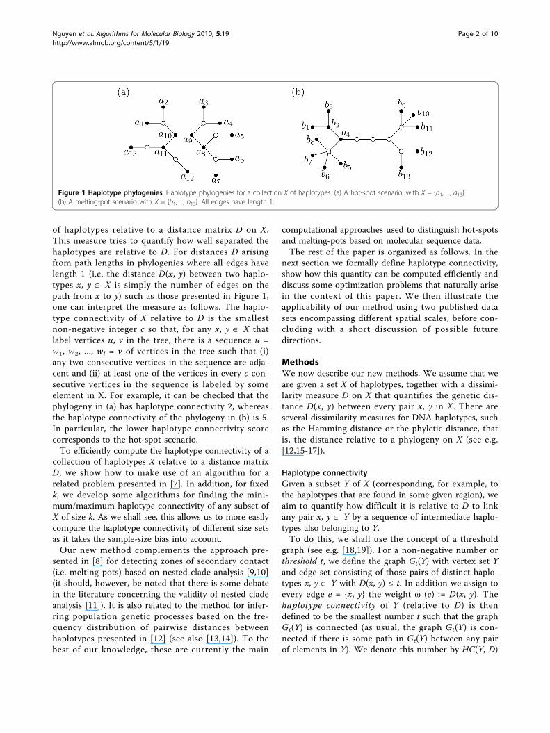
of haplotypes relative to a distance matrix D on X.This measure tries to quantify how well separated thehaplotypes are relative to D. For distances D arisingfrom path lengths in phylogenies where all edges havelength 1 (i.e. the distance D(x, y) between two haplo-types x, y Î X is simply the number of edges on thepath from x to y) such as those presented in Figure 1,one can interpret the measure as follows. The haplo-type connectivity of X relative to D is the smallestnon-negative integer c so that, for any x, y Î X thatlabel vertices u, v in the tree, there is a sequence u =w1, w2, ..., wl = v of vertices in the tree such that (i)any two consecutive vertices in the sequence are adja-cent and (ii) at least one of the vertices in every c con-secutive vertices in the sequence is labeled by someelement in X. For example, it can be checked that thephylogeny in (a) has haplotype connectivity 2, whereasthe haplotype connectivity of the phylogeny in (b) is 5.In particular, the lower haplotype connectivity scorecorresponds to the hot-spot scenario.To efficiently compute the haplotype connectivity of a

collection of haplotypes X relative to a distance matrixD, we show how to make use of an algorithm for arelated problem presented in [7]. In addition, for fixedk, we develop some algorithms for finding the mini-mum/maximum haplotype connectivity of any subset ofX of size k. As we shall see, this allows us to more easilycompare the haplotype connectivity of different size setsas it takes the sample-size bias into account.Our new method complements the approach pre-

sented in [8] for detecting zones of secondary contact(i.e. melting-pots) based on nested clade analysis [9,10](it should, however, be noted that there is some debatein the literature concerning the validity of nested cladeanalysis [11]). It is also related to the method for infer-ring population genetic processes based on the fre-quency distribution of pairwise distances betweenhaplotypes presented in [12] (see also [13,14]). To thebest of our knowledge, these are currently the main

computational approaches used to distinguish hot-spotsand melting-pots based on molecular sequence data.The rest of the paper is organized as follows. In the

next section we formally define haplotype connectivity,show how this quantity can be computed efficiently anddiscuss some optimization problems that naturally arisein the context of this paper. We then illustrate theapplicability of our method using two published datasets encompassing different spatial scales, before con-cluding with a short discussion of possible futuredirections.

MethodsWe now describe our new methods. We assume that weare given a set X of haplotypes, together with a dissimi-larity measure D on X that quantifies the genetic dis-tance D(x, y) between every pair x, y in X. There areseveral dissimilarity measures for DNA haplotypes, suchas the Hamming distance or the phyletic distance, thatis, the distance relative to a phylogeny on X (see e.g.[12,15-17]).

Haplotype connectivityGiven a subset Y of X (corresponding, for example, tothe haplotypes that are found in some given region), weaim to quantify how difficult it is relative to D to linkany pair x, y Î Y by a sequence of intermediate haplo-types also belonging to Y.To do this, we shall use the concept of a threshold

graph (see e.g. [18,19]). For a non-negative number orthreshold t, we define the graph Gt(Y) with vertex set Yand edge set consisting of those pairs of distinct haplo-types x, y Î Y with D(x, y) ≤ t. In addition we assign toevery edge e = {x, y} the weight ω (e) := D(x, y). Thehaplotype connectivity of Y (relative to D) is thendefined to be the smallest number t such that the graphGt(Y) is connected (as usual, the graph Gt(Y) is con-nected if there is some path in Gt(Y) between any pairof elements in Y). We denote this number by HC(Y, D)

Figure 1 Haplotype phylogenies. Haplotype phylogenies for a collection X of haplotypes. (a) A hot-spot scenario, with X = {a1, ..., a13}.(b) A melting-pot scenario with X = {b1, ..., b13}. All edges have length 1.

Nguyen et al. Algorithms for Molecular Biology 2010, 5:19http://www.almob.org/content/5/1/19

Page 2 of 10

or just HC(Y) in case it is clear what D is from thecontext.To illustrate these definitions, consider the subset Y =

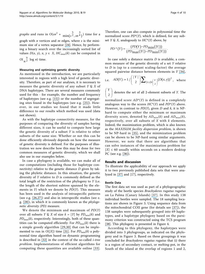
{b2, b4, ..., b12} of X = {b1, b2, ..., b13} and the phyleticdistance D on X induced by the phylogeny in Figure 1(b), i.e. the distance obtained by taking the path lengthbetween pairs of haplotypes. In Figure 2(a) we depictthe graph G2(Y). This is not connected, and soHC(Y) > 2. However, it is straight-forward to check thatHC(Y) = 5 (the graph G5(Y) is depicted in Figure 2(b)).Now, if t ≥ max{D(x, y): x, y Î Y } then the graph Gt

(Y) is the complete graph on Y, i.e. the graph in whichevery pair of vertices is linked by an edge, which wedenote by G*(Y). For every spanning tree T of G*(Y),that is, a subgraph of G*(Y) that is a tree and that con-tains all vertices of G*(Y), let ωmax(T) be the maximumof the edge weights over all edges of T. We claim that

HC Y T T G Ymax( ) min{ ( ) : ( )}.* is a spanning tree of

Indeed, since every spanning tree T of G*(Y) is a con-nected subgraph of G*(Y), we must have HC(Y) ≤ ωmax

(T). Conversely, putting t := HC(Y), by definition of HC(Y) the graph Gt(Y) is connected and every spanningtree T of Gt(Y) is also a spanning tree of G*(Y) withωmax(T) ≤ t = HC(Y). In particular, this implies thatthere always exist x, y Î Y with HC(Y) = D(x, y). Aspanning tree T of G*(Y) with score ωmax(T) equal toHC(Y) is also known as a bottleneck minimum spanningtree or bottleneck MST, for short. In [7] an algorithmfor computing such a tree is presented. This algorithmperforms a binary search [[20], p. 37] on the edgeweights in the graph. However, rather than explicitlysorting these weights first, an algorithm for finding themedian [21] is used. In this way, since in each step ofthe binary search at least half of the remaining edges inthe graph can be discarded, the overall run time is O(m)for a connected edge-weighted graph with m edges.Thus, as G*(Y) has O(|Y|2) edges, HC(Y) can be com-puted in O(|Y|2) time, which is clearly optimal. Alterna-tively, since every minimum spanning tree (MST), thatis, a spanning tree of G*(Y) with minimum total edge

weight, can easily be seen to be a bottleneck minimumspanning tree of G*(Y), one can also employ any algo-rithm for finding an MST of G*(Y) (see e.g. [[20],ch. 23]) to compute HC(Y).

Maximizing and minimizing haplotype connectivityIn our analyses it can be helpful to understand howlarge HC(Y) is relative to other subsets of the same sizeas Y. Therefore, for a subset Y ⊆ X of k haplotypes, wenow consider the problem of computing the minimumand maximum possible haplotype connectivity, denotedby HCmin(k) and HCmax(k), respectively, over all subsetsof X containing precisely k haplotypes. Based on this, wedefine, for any subset Y ⊆ X, the normalized haplotypeconnectivity of Y by

HC YHC Y HC Y

HC Y HC Y*( )

( ( ) min(| |))( max(| |) min(| |))

.

Note that this normalized score always lies between 0and 1. We will use this score to rank regions accordingto their haplotype connectivity.Computing HCmin(k) amounts to finding a k-element

subset Z of X such that the score ωmax(T) of a bottle-neck MST T of G*(Z) is minimized. This problem isknown as the bottleneck k-MST problem and can besolved in optimal O(|X|2) time by extending the algo-rithm for computing a bottleneck MST mentioned inthe previous section [22]. The key idea is to introduce,in addition to the given weights on the edges, a suitableweighting of the vertices of the graph.To compute HCmax(k), we first note that this quantity

equals the smallest threshold t such that for every subsetZ of X with k elements the graph Gt(Z) is connected. Inother words, every vertex separator of Gt(X) (i.e. everysubset S of X with Gt(X - S) disconnected) must havemore than |X| - k elements.Several algorithms for computing a vertex separator of

minimum size are known, e.g. based on a reformulationas a network flow problem [23]. The currently fastestalgorithm for this problem employs so-called expander

Figure 2 Threshold graphs. The graphs (a) G2(X) and (b) G5(X) induced by the haplotype phylogeny in Figure 1(b) on the subsetY = {b2, b4, ..., b12}. For example, there is no edge joining the haplotypes b2 and b10 in G2(X) because the number of edges on the path fromb2 to b10 in the phylogeny is greater than 2.

Nguyen et al. Algorithms for Molecular Biology 2010, 5:19http://www.almob.org/content/5/1/19

Page 3 of 10

graphs and runs in O(sn2 + min( , )s sn52

34 ) time for a

graph with n vertices and m edges, where s is the mini-mum size of a vertex separator [24]. Hence, by perform-ing a binary search over the increasingly sorted list ofvalues D(x, y), x, y Î X, HCmax(k) can be computed in

O(n

92 log n) time.

Measuring and optimizing genetic diversityAs mentioned in the introduction, we are particularlyinterested in regions with a high level of genetic diver-sity. Therefore, as part of our analyses, it is necessary tomeasure the genetic diversity of any subset Y ⊆ X ofDNA haplotypes. There are several measures commonlyused for this - for example, the number and frequencyof haplotypes (see e.g. [15]) or the number of segregat-ing sites found in the haplotypes (see e.g. [25]). How-ever, in our studies we found that it made littledifference to our results which method was used (datanot shown).As with the haplotype connectivity measure, for the

purposes of comparing the diversity of samples havingdifferent sizes, it can be useful to compute how largethe genetic diversity of a subset Y is relative to othersubsets of the same size. Whether or not this can bedone efficiently obviously depends on how the measureof genetic diversity is defined. For the purposes of illus-tration we now describe how this may be done for twocommon measures of genetic diversity, which we shallalso use in our examples below.In case a phylogeny is available, we can make all of

our computations (including those for haplotype con-nectivity) relative to the genetic distance D given by tak-ing the phyletic distance. In this situation, the geneticdiversity of Y relative to D is commonly defined as thetotal length of the restriction of the phylogeny to Y (i.e.the length of the shortest subtree spanned by the ele-ments in Y) which we denote by PD(Y). This measurehas been used in the analysis of intraspecific patterns(see e.g. [26,27]) and also in interspecific studies (see e.g. [28]), in which it is commonly known as the phyloge-netic diversity (PD) measure.We denote the minimum and maximum of PD(Y)

over all subsets Y ⊆ X of size k = |Y| by PDmin(k) andPDmax(k), respectively. Interestingly, both of these quan-tities can be computed efficiently: For PDmax(k) there isa simple greedy algorithm [29,30] that can be imple-mented to run in O(|X|) time [31]. For PDmin(k) a poly-nomial time algorithm based on dynamic programmingis described in [32] in the context of the so-called i-treeproblem. Implementations of efficient algorithms forcomputing these quantities are available online [33].

Therefore, one can also compute in polynomial time thenormalized score PD*(Y), which is defined, for any sub-set Y ⊆ X, analogously to HC*(Y) above, by

PD YPD Y PD Y

PD Y PD Y*( )

( ( ) min(| |))( max(| |) min(| |))

.

In case solely a distance matrix D is available, a com-mon measure of the genetic diversity of a set Y relativeto D is (up to a constant scaling-factor) the averagesquared pairwise distance between elements in Y [34],

i.e. AD YY

D x yx y

Y( ) : /| |

( ( , )){ , }

1

22

2, where

Y

2

denotes the set of all 2-element subsets of Y. The

normalized score AD*(Y) is defined in a completelyanalogous way to the scores HC*(Y) and PD*(Y) above.However, in contrast to PD(Y), given D and k, it is NP-hard to compute either the minimum or maximumdiversity score, denoted by ADmin(k) and ADmax(k),respectively, over all subsets of X with k elements.Indeed, the maximization problem, which is also knownas the MAXISUM facility dispersion problem, is shownto be NP-hard in [35], and the minimization problemcan be shown to be NP-hard using similar arguments.However, we note that there are algorithms thatcan solve instances of the maximization problem for|X| ≤ 60 usually within seconds on a modern desktopPC (see e.g. [36]).

Results and discussionTo illustrate the applicability of our approach we applyit to two previously published data sets that were ana-lyzed in [37] and [17], respectively.

Beetle DataThe first data set was used as part of a phylogeographicstudy of the beetle species Brachyderes rugatus rugatuson La Palma (Canary Islands) [37]. In this study 138individual beetles were sampled. The 18 sampling loca-tions are shown in Figure 3. Using sequence data fromthe mitochondrial COII gene (for details see [37]), the138 samples were subsequently grouped into 69 haplo-types, and a haplotype phylogeny based on the parsi-mony criterion was constructed using the TCS program[38]. This phylogeny is presented in Figure 4.According to this phylogeny, the haplotypes were

divided into 3 phylogroups, as indicated on the phylo-geny and in Figure 3. Based on these groupings it wasconcluded for Brachyderes rugatus rugatus that (i) thereis a region of secondary contact, or melting-pot, in theSouth of the island at the overlap of regions 1 and 2,

Nguyen et al. Algorithms for Molecular Biology 2010, 5:19http://www.almob.org/content/5/1/19

Page 4 of 10

and (ii) that there is an ancestral region or hot-spot inthe region containing the three sampling locations inthe top right of region 2. Note that in [37] support forconclusion (i) was provided by performing the test givenin [8] for detecting zones of secondary contact, whichessentially involves calculation of the average distancebetween the geographic centers of clades at increasingnesting levels in a phylogeny on the haplotypes ofinterest.To investigate whether our new method was suppor-

tive of conclusions (i) and (ii) or not, we first groupedthe sampling locations into 6 regions R1, ..., R6 asshown in Figure 3. We used these regions rather thanthe individual sampling locations, since the number ofsamples taken at each location was very small (between2 and 8). When forming the groups, geographicallyclose locations were grouped together. We also consid-ered other groupings based on geographic proximity(data not shown) and the outcome was similar, thoughless pronounced when the number of groupings wasreduced (smallest number of groupings used was 3).We then measured the diversity (using the measure

PD) and haplotype connectivity for the haplotypesfound in each region Ri relative to the phyletic dis-tances given by the phylogeny in Figure 4, as describedin the Methods section.The results for the 6 regions are summarized in Table

1. In this table, we present the size of the subset Y ofhaplotypes found in the region (column 2), the valuesPD(Y), PDmin(|Y|), PDmax(|Y|) (columns 3-5), and thenormalized diversity score PD*(Y) (column 6) as definedin the Methods section. Similarly, we present the valuesHC(Y), HCmin(|Y|), HCmax(|Y|) and HC*(Y) (columns7-10).As can be seen in Table 1, the two regions with the

highest PD*score are R6 and R3, which also have a muchhigher HC* score than any of the other four regions.This is supportive of conclusion (i), i.e. that R6 is prob-ably a melting-pot. Indeed, in Figure 4 the haplotypesfound in region R6 are highlighted in green, and it canbe seen that they clump together into two groups. Thisalso indicates why we obtained a high HC* score forthis region. Similarly, the high PD* and HC* scores forregion R3 suggests that this region is a melting-pot as

Figure 3 Sampling locations and regions for beetle data. A map of La Palma with sampling locations indicated by black dots [37]. Samplinglocations where haplotypes from a particular phylogroup (cf. Figure 4) were found are depicted by the dashed curves. Note that the samplinglocation Altos de Jedey is the only one where haplotypes from two distinct phylogroups (namely 1 and 2) were found. The six groups ofsampling locations corresponding to the six regions R1, R2, ..., R6 discussed in the text are also indicated.

Nguyen et al. Algorithms for Molecular Biology 2010, 5:19http://www.almob.org/content/5/1/19

Page 5 of 10

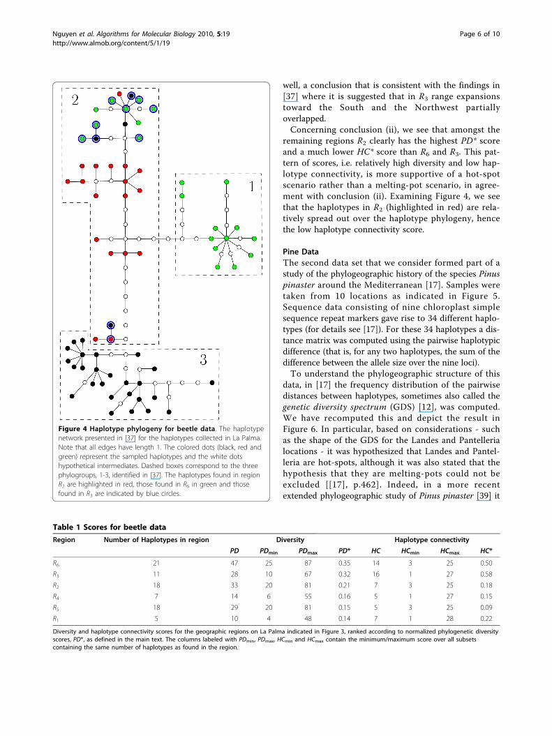
well, a conclusion that is consistent with the findings in[37] where it is suggested that in R3 range expansionstoward the South and the Northwest partiallyoverlapped.Concerning conclusion (ii), we see that amongst the

remaining regions R2 clearly has the highest PD* scoreand a much lower HC* score than R6 and R3. This pat-tern of scores, i.e. relatively high diversity and low hap-lotype connectivity, is more supportive of a hot-spotscenario rather than a melting-pot scenario, in agree-ment with conclusion (ii). Examining Figure 4, we seethat the haplotypes in R2 (highlighted in red) are rela-tively spread out over the haplotype phylogeny, hencethe low haplotype connectivity score.

Pine DataThe second data set that we consider formed part of astudy of the phylogeographic history of the species Pinuspinaster around the Mediterranean [17]. Samples weretaken from 10 locations as indicated in Figure 5.Sequence data consisting of nine chloroplast simplesequence repeat markers gave rise to 34 different haplo-types (for details see [17]). For these 34 haplotypes a dis-tance matrix was computed using the pairwise haplotypicdifference (that is, for any two haplotypes, the sum of thedifference between the allele size over the nine loci).To understand the phylogeographic structure of this

data, in [17] the frequency distribution of the pairwisedistances between haplotypes, sometimes also called thegenetic diversity spectrum (GDS) [12], was computed.We have recomputed this and depict the result inFigure 6. In particular, based on considerations - suchas the shape of the GDS for the Landes and Pantellerialocations - it was hypothesized that Landes and Pantel-leria are hot-spots, although it was also stated that thehypothesis that they are melting-pots could not beexcluded [[17], p.462]. Indeed, in a more recentextended phylogeographic study of Pinus pinaster [39] it

Figure 4 Haplotype phylogeny for beetle data. The haplotypenetwork presented in [37] for the haplotypes collected in La Palma.Note that all edges have length 1. The colored dots (black, red andgreen) represent the sampled haplotypes and the white dotshypothetical intermediates. Dashed boxes correspond to the threephylogroups, 1-3, identified in [37]. The haplotypes found in regionR2 are highlighted in red, those found in R6 in green and thosefound in R3 are indicated by blue circles.

Table 1 Scores for beetle data

Region Number of Haplotypes in region Diversity Haplotype connectivity

PD PDmin PDmax PD* HC HCmin HCmax HC*

R6 21 47 25 87 0.35 14 3 25 0.50

R3 11 28 10 67 0.32 16 1 27 0.58

R2 18 33 20 81 0.21 7 3 25 0.18

R4 7 14 6 55 0.16 5 1 27 0.15

R5 18 29 20 81 0.15 5 3 25 0.09

R1 5 10 4 48 0.14 7 1 28 0.22

Diversity and haplotype connectivity scores for the geographic regions on La Palma indicated in Figure 3, ranked according to normalized phylogenetic diversityscores, PD*, as defined in the main text. The columns labeled with PDmin, PDmax, HCmin and HCmax contain the minimum/maximum score over all subsetscontaining the same number of haplotypes as found in the region.

Nguyen et al. Algorithms for Molecular Biology 2010, 5:19http://www.almob.org/content/5/1/19

Page 6 of 10

was concluded that Landes was more likely to be amelting-pot.Using the same distance matrix, we computed diver-

sity and haplotype connectivity scores for each of the 10sampling locations as explained in the Methods section(using the measure AD for diversity). These are pre-sented in Table 2. Note that, in contrast to [17], ourscores do not take into account how often a haplotypewas found in a particular location but rather which hap-lotypes were found.As can be seen in Table 2, the two locations with

highest AD* diversity scores are Landes and Pantelleria.In view of the HC* scores for these locations, this sup-ports the melting-pot scenario, especially for the Landeslocation. Note that the bimodality of the GDS for theLandes location is also indicative of two clusters of hap-lotypes having low internal distances and high betweencluster distances, which could also be regarded as a sig-nature supporting a melting-pot scenario. However, theshape of the GDS for the Pantelleria location is some-what less distinctive and so, in this case at least, thehaplotype connectivity approach provides some usefuladditional information.

ConclusionsWe have presented a quantitative method to help shedlight on the phylogeographic history of a species, in par-ticular, for distinguishing between hot-spots and melt-ing-pots of haplotypic diversity. The application of ourmethod to the two data sets illustrates that our methodshould provide a useful addition to previously presentedtools based on nested clade analysis and the GDS.

The algorithm for computing the haplotype connectiv-ity of a collection of haplotypes can handle collectionsof several hundred haplotypes without difficulty. Thecomputation of minimum and maximum haplotype con-nectivity scores over all subsets of a certain size, thoughstill possible in polynomial time, is more demanding,especially computing the maximum as this involves thecomputation of minimum vertex separators in a graph.Although the (at least implicit) computation of suchseparators can probably not be avoided, for data setswhere the haplotype connectivity must be computed formany subsets of different size, it could be interesting todevelop a more efficient algorithm that preprocesses thedistance matrix for the haplotypes so that HCmax(k) canbe quickly reported for any given k.Our method depends on the haplotype distance and on

the measure of diversity used for regions. However, basedon experiments that we performed on the two data setsabove (data not shown), we suspect that the impact ofthese two choices on the results will usually be quitesmall, at least for standard measures of distance and diver-sity. Also, since very low diversity scores will tend to yieldlow haplotype connectivity scores, we mainly recommendthe use of our method only for regions yielding higherlevels of haplotypic diversity (which is the case for bothhot-spots and melting-pots). For example, for the Pinedata above, consider the three Portuguese sampling loca-tions Alcacier, Moncao and Leiria. In [39] it was suggestedthat there exists a glacial refugia of Pinus pinaster in Por-tugal. At least for Leiria our method supports this to someextent: In Table 2 we see that the normalized haplotypeconnectivity score is as small as possible while the

Figure 5 Sampling locations for pine data. Sampling locations for the data set in [17].

Nguyen et al. Algorithms for Molecular Biology 2010, 5:19http://www.almob.org/content/5/1/19

Page 7 of 10

Figure 6 Genetic diversity spectrum. The genetic diversity spectrum (GDS) for (a) the Landes location and (b) the Pantelleria location in Figure5. For every possible distance, the number of pairs of haplotypes that are that distance apart is depicted.

Nguyen et al. Algorithms for Molecular Biology 2010, 5:19http://www.almob.org/content/5/1/19

Page 8 of 10

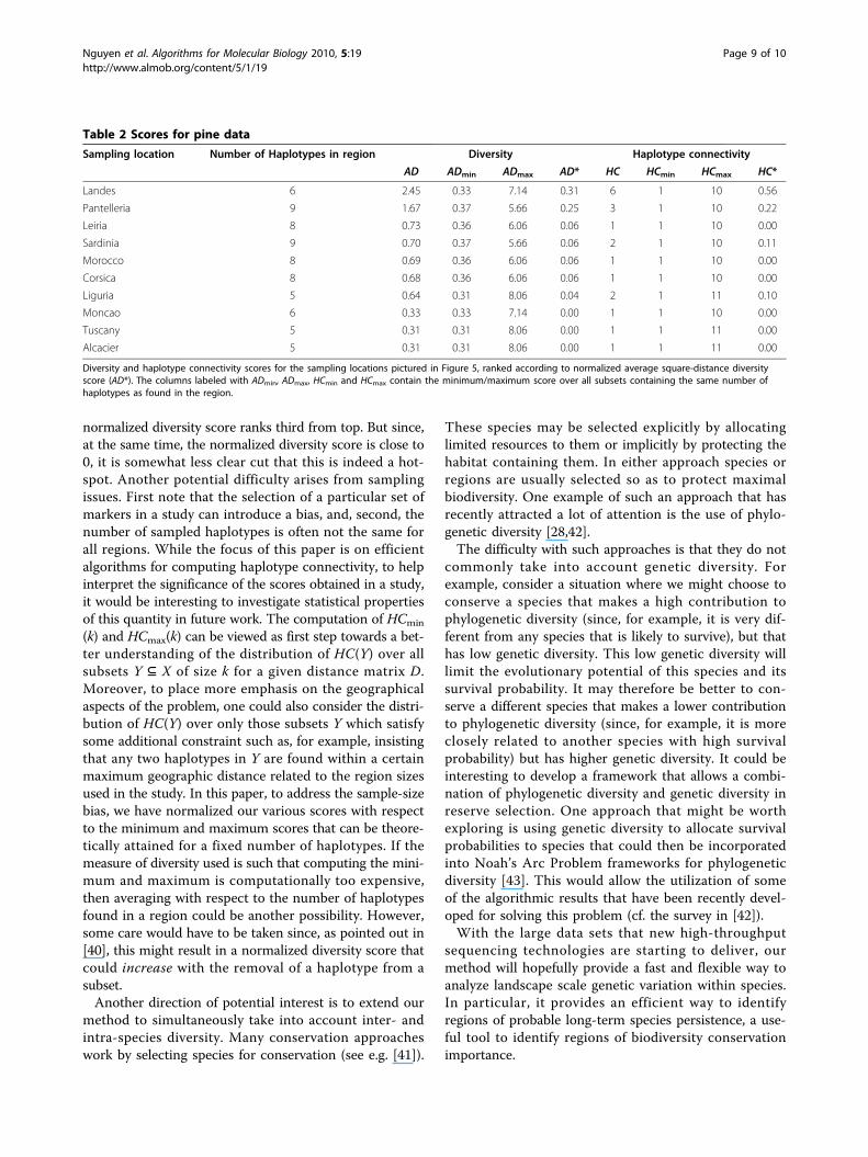
normalized diversity score ranks third from top. But since,at the same time, the normalized diversity score is close to0, it is somewhat less clear cut that this is indeed a hot-spot. Another potential difficulty arises from samplingissues. First note that the selection of a particular set ofmarkers in a study can introduce a bias, and, second, thenumber of sampled haplotypes is often not the same forall regions. While the focus of this paper is on efficientalgorithms for computing haplotype connectivity, to helpinterpret the significance of the scores obtained in a study,it would be interesting to investigate statistical propertiesof this quantity in future work. The computation of HCmin

(k) and HCmax(k) can be viewed as first step towards a bet-ter understanding of the distribution of HC(Y) over allsubsets Y ⊆ X of size k for a given distance matrix D.Moreover, to place more emphasis on the geographicalaspects of the problem, one could also consider the distri-bution of HC(Y) over only those subsets Y which satisfysome additional constraint such as, for example, insistingthat any two haplotypes in Y are found within a certainmaximum geographic distance related to the region sizesused in the study. In this paper, to address the sample-sizebias, we have normalized our various scores with respectto the minimum and maximum scores that can be theore-tically attained for a fixed number of haplotypes. If themeasure of diversity used is such that computing the mini-mum and maximum is computationally too expensive,then averaging with respect to the number of haplotypesfound in a region could be another possibility. However,some care would have to be taken since, as pointed out in[40], this might result in a normalized diversity score thatcould increase with the removal of a haplotype from asubset.Another direction of potential interest is to extend our

method to simultaneously take into account inter- andintra-species diversity. Many conservation approacheswork by selecting species for conservation (see e.g. [41]).

These species may be selected explicitly by allocatinglimited resources to them or implicitly by protecting thehabitat containing them. In either approach species orregions are usually selected so as to protect maximalbiodiversity. One example of such an approach that hasrecently attracted a lot of attention is the use of phylo-genetic diversity [28,42].The difficulty with such approaches is that they do not

commonly take into account genetic diversity. Forexample, consider a situation where we might choose toconserve a species that makes a high contribution tophylogenetic diversity (since, for example, it is very dif-ferent from any species that is likely to survive), but thathas low genetic diversity. This low genetic diversity willlimit the evolutionary potential of this species and itssurvival probability. It may therefore be better to con-serve a different species that makes a lower contributionto phylogenetic diversity (since, for example, it is moreclosely related to another species with high survivalprobability) but has higher genetic diversity. It could beinteresting to develop a framework that allows a combi-nation of phylogenetic diversity and genetic diversity inreserve selection. One approach that might be worthexploring is using genetic diversity to allocate survivalprobabilities to species that could then be incorporatedinto Noah’s Arc Problem frameworks for phylogeneticdiversity [43]. This would allow the utilization of someof the algorithmic results that have been recently devel-oped for solving this problem (cf. the survey in [42]).With the large data sets that new high-throughput

sequencing technologies are starting to deliver, ourmethod will hopefully provide a fast and flexible way toanalyze landscape scale genetic variation within species.In particular, it provides an efficient way to identifyregions of probable long-term species persistence, a use-ful tool to identify regions of biodiversity conservationimportance.

Table 2 Scores for pine data

Sampling location Number of Haplotypes in region Diversity Haplotype connectivity

AD ADmin ADmax AD* HC HCmin HCmax HC*

Landes 6 2.45 0.33 7.14 0.31 6 1 10 0.56

Pantelleria 9 1.67 0.37 5.66 0.25 3 1 10 0.22

Leiria 8 0.73 0.36 6.06 0.06 1 1 10 0.00

Sardinia 9 0.70 0.37 5.66 0.06 2 1 10 0.11

Morocco 8 0.69 0.36 6.06 0.06 1 1 10 0.00

Corsica 8 0.68 0.36 6.06 0.06 1 1 10 0.00

Liguria 5 0.64 0.31 8.06 0.04 2 1 11 0.10

Moncao 6 0.33 0.33 7.14 0.00 1 1 10 0.00

Tuscany 5 0.31 0.31 8.06 0.00 1 1 11 0.00

Alcacier 5 0.31 0.31 8.06 0.00 1 1 11 0.00

Diversity and haplotype connectivity scores for the sampling locations pictured in Figure 5, ranked according to normalized average square-distance diversityscore (AD*). The columns labeled with ADmin, ADmax, HCmin and HCmax contain the minimum/maximum score over all subsets containing the same number ofhaplotypes as found in the region.

Nguyen et al. Algorithms for Molecular Biology 2010, 5:19http://www.almob.org/content/5/1/19

Page 9 of 10

AcknowledgementsVM, BN and AS were supported in part by the Engineering and PhysicalSciences Research Council [Grant number EP/D068800/1]. We thank PeterLockhart for his helpful comments on an earlier version this paper and alsothe anonymous referees for their helpful comments.

Author details1School of Computing Sciences, University of East Anglia, Norwich, NR4 7TJ,UK. 2Department of Mathematics and Computer Science, University ofGreifswald, 17489 Greifswald, Germany. 3School of Biological Sciences,University of East Anglia, Norwich, NR4 7TJ, UK.

Authors’ contributionsBN implemented the algorithms for computing haplotype connectivityscores and carried out the analysis of the data sets. All authors participatedin the design of the study, contributed to the writing of the manuscript, andread and approved the final version of the manuscript.

Competing interestsThe authors declare that they have no competing interests.

Received: 23 December 2009 Accepted: 20 March 2010Published: 20 March 2010

References1. Emerson BC, Hewitt GM: Phylogeography. Curr Biol 2005, 15:R367-R371.2. Hewitt GM: Some genetic consequences of ice ages, and their role in

divergence and speciation. Biol J Linn Soc 1996, 58:247-276.3. Hewitt GM: The genetic legacy of the Quarternary ice ages. Nature 2000,

405:907-913.4. Petit R, Aguinagalde I, Beaulieu J, Bittkau C, Brewer S, Cheddadi R, Ennos R,

Fineschi S, Grivet D, Lascoux M, Mohanty A, Müller-Stark G, Demesure-Musch B, Palmée A, Martíin J, Rendell S, Vendramin G: Glacial refugia:hotspots but not melting pots of genetic diversity. Science 2003,300:1563-1565.

5. Desmet PG, Cowling RM, Ellis AG, Pressey RL: Integrating biosystematicdata into conservation planning: perspectives from Southern Africa’ssucculent Karoo. Syst Biol 2002, 51:317-330.

6. Avise JC, Arnold J, Ball RM, Bermingham E, Lamb T, Neigel JE, Reeb CA,Saunders NC: Intraspecific phylogeography: the mitochondrial DNAbridge between population genetics and systematics. Ann Rev Ecol Syst1987, 18:489-522.

7. Camerini P: The min-max spanning tree problem and some extensions.Inform Process Lett 1978, 7:10-14.

8. Templeton AR: Using phylogeographic analyses of gene trees to testspecies status and processes. Mol Ecol 2001, 10:779-791.

9. Posada D, Crandall KA, Templeton AR: Nested clade analysis statistics. MolEcol Notes 2006, 6:590-593.

10. Templeton AR: Nested clade analyses of phylogeographic data: testinghypothesis about gene flow and population history. Mol Ecol 1998,7:381-397.

11. Lacey Knowles L: Why does a method that fails continue to be used?Evolution 2008, 62:2713-2717.

12. Rozenfeld AF, Arnaud-Haond S, Hernández-García E, Eguíluz VM, Matías MA,Serrão E, Duarte CM: Spectrum of genetic diversity and networks ofclonal organisms. J R Soc Interface 2007, 4:1093-1102.

13. Excoffier L: Patterns of DNA sequence diversity and genetic structureafter a range expansion: lessons from the infinite-island model. Mol Ecol2004, 13:853-864.

14. Schneider S, Excoffier L: Estimation of past demographic parameters fromthe distribution of pairwise differences when the mutation rates varyamong sites: application to human mitochondrial DNA. Genetics 1999,152:1079-1089.

15. Nei M, Tajima F: DNA polymorphism detectable by restrictionendonucleases. Genetics 1981, 97:145-163.

16. Tamura K, Nei M: Estimation of the number of nucleotide substitutions inthe control region of the mitochondrial DNA in humans andchimpanzees. Mol Biol Evol 1993, 10:512-526.

17. Vendramin GG, Anzidei M, Madaghiele A, Bucci G: Distribution of geneticdiversity in Pinus pinaster Ait. as revealed by chloroplast microsatellites.Theor Appl Genet 1998, 97:456-463.

18. Huson D, Nettles S, Warnow T: Disk-Covering, a Fast-Converging Methodfor Phylogenetic Tree Reconstruction. J Comput Biol 1999, 6:369-386.

19. Berry A, Sigayret A, Sinoquet C: Maximal sub-triangulation in pre-processing phylogenetic data. Soft Computing - A Fusion of Foundations,Methodologies and Applications 2006, 10:461-468.

20. Cormen H, Leiserson CE, Rivest RL, Stein C: Introduction to Algorithms TheMIT Press 2001.

21. Schönhage A, Paterson M, Pippenger N: Finding the median. J ComputSyst Sci 1976, 13:184-199.

22. Punnen A, Chapovska O: The bottleneck k-MST. Inform Process Lett 2005,95:512-517.

23. Even S, Tarjan R: Network flow and testing graph connectivity. SIAM JComput 1975, 4:507-518.

24. Gabow H: Using expander graphs to find vertex connectivity. J ACM2006, 53:800-844.

25. Tajima F: The amount of DNA polymorphism maintained in a finitepopulation when neutral mutation rates varies among sites. Genetics1996, 143:1761-1770.

26. Rauch EM, Bar-Yam Y: Theory predicts the uneven distribution of geneticdiversity within species. Nature 2004, 431:449-452.

27. Rauch EM, Bar-Yam Y: Estimating the total genetic diversity of a spatialfield population from a sample and implications of its dependence onhabitat area. Proc Natl Acad Sci Unit States Am 2005, 102:9826-9829.

28. Faith D: Conservation evaluation and phylogenetic diversity. BiolConservat 1992, 61:1-10.

29. Pardi F, Goldman N: Species choice for comparative genomics: beinggreedy works. PLoS Genetics 2005, 1(6).

30. Steel MA: Phylogenetic diversity and the greedy algorithm. Syst Biol 2005,54(4):527-529.

31. Spillner A, Nguyen BT, Moulton V: Computing Phylogenetic Diversity forSplit Systems. IEEE ACM Trans Comput Biol Bioinformatics 2008, 5(2):235-244.

32. Blum A, Chalasani P, Coppersmith D, Pulleyblank WR, Raghavan P, Sudan M:The minimum latency problem. Proc. ACM Symposium on Theory ofComputing (STOC) 1994, 163-171.

33. Minh B, Klaere S, von Haeseler A: Taxon selection under split diversity.Syst Biol 2009, 58:586-594.

34. Echt CS, Verno LLD, Anzidei M, Vendramin GG: Chloroplast microsatellitesreveal population genetic diversity in red pine, Pinus resinosa Ait. MolEcol 1998, 7:307-317.

35. Hansen P, Moon I: Dispersing facilities on a network. TIMS/ORSA JointNational Meeting, Washington, D.C 1988.

36. Pisinger D: Upper bounds and exact algorithms for p-dispersionproblems. Comput Oper Res 2006, 33:1380-1398.

37. Emerson B, Forgie S, Goodacre S, Oromi P: Testing phylogeographicpredictions on an active volcanic island: Brachyderes rugatus (Coleoptera:Curculionidae) on La Palma (Canary Islands). Mol Ecol 2006, 15:449-458.

38. Clement M, Posada D, Crandall KA: TCS: A computer program to estimategene genealogies. Mol Ecol 2000, 9:1557-1659.

39. Bucci G, González-Martínez S, le Provost G, Plomion C, Ribeiro M,Sebastiani F, Alía R, Vendramin G: Range-wide phylogeography and genezones in Pinus pinaster Ait. revealed by chloroplast microsatellitemarkers. Mol Ecol 2007, 16:2137-2153.

40. Schweiger O, Klotz S, Durka W, Kühn I: A comparative test of phylogeneticdiversity indices. Oecologia 2008, 157:485-495.

41. Regan H, Hierl L, Franklin J, Deutschman D, Schmalbach H, Winchell C,Johnson B: Species prioritization for monitoring and management inregional multiple species conservation plans. Diversity and Distributions2007, 14:462-471.

42. Hartmann K, Steel M: Phylogenetic diversity: from combinatorics toecology. Reconstructing evolution: new mathematical and computationalapproaches Oxford University PressGascuel O, Steel M 2007.

43. Weitzman M: The Noah’s Ark Problem. Econometrica 1998, 66:1279-1298.

doi:10.1186/1748-7188-5-19Cite this article as: Nguyen et al.: Distinguishing between hot-spots andmelting-pots of genetic diversity using haplotype connectivity.Algorithms for Molecular Biology 2010 5:19.

Nguyen et al. Algorithms for Molecular Biology 2010, 5:19http://www.almob.org/content/5/1/19

Page 10 of 10