PhD-FSTC-2015-14The Faculty of Sciences, Technology and Communication

DISSERTATION

Presented on 19-03-2015 in Luxembourgto obtain the degree of

DOCTEUR DE L’UNIVERSITÉ DU LUXEMBOURGEN INFORMATIQUE

by

STEFANO DI ALESIOBorn on 20 January 1987 in Pescina (Abruzzo, Italy)

SUPPORTING STRESS TESTING IN REAL-TIME SYSTEMSWITH CONSTRAINT PROGRAMMING

DISSERTATION DEFENSE COMMITTEE

PROF. DR. ING. LIONEL BRIAND, Dissertation SupervisorUniversity of Luxembourg

PROF. DR. NICOLAS NAVET, ChairmanUniversity of Luxembourg

DR. SHIVA NEJATI, Deputy ChairmanUniversity of Luxembourg

DR. ING. SÉBASTIAN GÉRARD, MemberLISE laboratory, CEA LIST (France)

PROF DR. JEAN-CHARLES RÉGIN, MemberUniversity of Nice Sophia-Antipolis (France)

DR. ARNAUD GOTLIEB, External ExpertSimula Research Laboratory (Norway)

WARNING: Everything in this book may be all wrong. But if so, it’s all right!

The Music Lesson: A Spiritual Search for Growth Through MusicVICTOR L. WOOTEN

Yet another thing I never read, but which I slap here because people will complainif this claim is not supported by a citation that looks relevant.

How far does imagination shunt inwards?DANIEL SEAFOOTIS

Abstract

Failures in safety-critical Real-Time Embedded Systems (RTES) could result in catastrophic con-sequences for the system itself, its users, and the environment. Therefore, these systems are subject tostrict performance requirements specifying constraints on real-time properties such as task deadlines,response time and CPU usage. Lately, RTES have been shifting towards multi-threaded applicationdesign, highly configurable operating systems, and multi-core architectures for computing platforms.The concurrent nature of their operating environment also entails that the order of external events trig-gering RTES tasks is often unpredictable. Such complexity in the system architecture, concurrency,and environment renders performance testing increasingly challenging. Specifically, computing inputcombinations that are intended to violate performance requirements, i.e., stress testing, is one of thepreferred ways for verifying RTES performance. These input combinations are referred to as stresstest cases, and, upon execution, are predicted to result in worst-case scenarios with respect to a per-formance requirement. In RTES, stress test cases are usually characterized by sequences of arrivaltimes for aperiodic tasks in the subject system. Generating stress test cases is challenging because itis hard to predict how a particular sequence of arrival times will affect the system performance, andbecause the set of all arrival times for aperiodic tasks quickly grows as the system size increases. Forthis reason, search strategies based on Genetic Algorithms (GA) have been used to find stress testcases with high chances of violating performance requirements.

For practical use, software testing has to accommodate time and budget constraints. In the con-text of stress testing, it is essential to investigate the trade-off between the time needed to generatetest cases (efficiency), their capability to reveal scenarios that violate performance requirements (ef-fectiveness), and to cover different scenarios where these violations arise (diversity). Even though GAare efficient, and capable of finding diverse solutions, they explore only part of the search space, andtheir effectiveness depends on configuration parameters. This aspect justifies considering alternativestrategies, such as Constraint Programming (CP), that explore the search space completely. Further-more, to enable effective industrial application, stress testing has to be capable of seamless integrationin the development cycle of companies. Therefore, it is both important to capture specific system andcontextual properties in a conceptual model, and to map such conceptual model in a standard ModelDriven Engineering (MDE) language such as UML/MARTE.

In this thesis, we address the challenges above by presenting a practical approach, based on CP, tosupport performance stress testing in RTES. Specifically, we make the following contributions: (1) aconceptual model, mapped to UML/MARTE, which captures the abstractions required to generatestress test cases, (2) a constraint optimization model to generate such test cases, and (3) a combinedGA+CP stress testing strategy that achieves a practical trade-off between efficiency, effectiveness anddiversity. The validation of our work shows that (1) the conceptual model can be applied with a rea-sonable overhead in an industrial settings, (2) CP is able to effectively identify worst-case scenarioswith respect to task deadlines, response time, and CPU usage, and (3) the combined GA+CP strategyis more likely than GA and CP in isolation to scale to large and complex systems. The work in thisthesis opens up the exploration of further directions, involving the use of multi-objective optimizationto generate stress test cases that simultaneously exercise different performance properties of the sys-tem, and of MiniMax analysis to derive design and configuration guidelines that minimize the risk toviolate performance requirements at runtime.

Contents

Contents 7

List of Figures 10

List of Tables 12

List of Definitions 15

Acronyms 19

1 Introduction 231.1 Thesis Background . . . . . . . . . . . . . . . . . . . . . . . . . . . . . . . . . . . . . 241.2 Thesis Contributions . . . . . . . . . . . . . . . . . . . . . . . . . . . . . . . . . . . . 271.3 Thesis Outline . . . . . . . . . . . . . . . . . . . . . . . . . . . . . . . . . . . . . . . . 29

I Foundations and Context 31

2 Background 332.1 Real-Time Embedded Systems (RTES) . . . . . . . . . . . . . . . . . . . . . . . . . . . 35

2.1.1 Scheduling in RTES . . . . . . . . . . . . . . . . . . . . . . . . . . . . . . . . 392.1.2 Static Analysis in RTES . . . . . . . . . . . . . . . . . . . . . . . . . . . . . . 432.1.3 Simulation in RTES . . . . . . . . . . . . . . . . . . . . . . . . . . . . . . . . . 45

2.2 Model-driven Engineering (MDE) . . . . . . . . . . . . . . . . . . . . . . . . . . . . . 462.2.1 Models and Metamodels . . . . . . . . . . . . . . . . . . . . . . . . . . . . . . 472.2.2 Standards for Model-driven Engineering . . . . . . . . . . . . . . . . . . . . . . 50

2.2.2.1 Model-Driven Architecture (MDA) . . . . . . . . . . . . . . . . . . . 512.2.2.2 Unified Modeling Language (UML) . . . . . . . . . . . . . . . . . . . 512.2.2.3 UML Profile for Modeling and Analysis of Real-Time Embedded Sys-

tems (UML/MARTE) . . . . . . . . . . . . . . . . . . . . . . . . . . 562.3 Software Testing . . . . . . . . . . . . . . . . . . . . . . . . . . . . . . . . . . . . . . 62

2.3.1 Model-based Testing (MBT) . . . . . . . . . . . . . . . . . . . . . . . . . . . . 642.3.2 Performance and Stress Testing . . . . . . . . . . . . . . . . . . . . . . . . . . . 68

7

Contents Contents

2.3.3 Search-based Software Testing (SBST) . . . . . . . . . . . . . . . . . . . . . . 712.4 Mathematical Optimization . . . . . . . . . . . . . . . . . . . . . . . . . . . . . . . . . 72

2.4.1 Constrained Optimization (CO) and Constraint Programming (CP) . . . . . . . . 732.4.1.1 Constraint Satisfaction Problems (CSP) . . . . . . . . . . . . . . . . . 752.4.1.2 Constraint Optimization Problems (COP) . . . . . . . . . . . . . . . . 78

2.4.2 Metaheuristics . . . . . . . . . . . . . . . . . . . . . . . . . . . . . . . . . . . . 792.4.2.1 Random Search and Hill-Climbing . . . . . . . . . . . . . . . . . . . 802.4.2.2 Genetic Algorithms (GA) . . . . . . . . . . . . . . . . . . . . . . . . 82

3 Problem Description 853.1 Finding Worst-case Scenarios in Real-Time Embedded Systems . . . . . . . . . . . . . 853.2 Motivating Case Study . . . . . . . . . . . . . . . . . . . . . . . . . . . . . . . . . . . 87

3.2.1 Implementation 1: Data Transfer with Four Aperiodic Tasks . . . . . . . . . . . 903.2.2 Implementation 2: Data Transfer with One Singular Task and Four Activities . . 92

II Approach and Discussion 95

4 An Overview of Stress Testing in Real-Time Embedded Systems 97

5 UML/MARTE Modeling 1015.1 Conceptual Model . . . . . . . . . . . . . . . . . . . . . . . . . . . . . . . . . . . . . . 1015.2 Mapping of the Conceptual Model to UML/MARTE . . . . . . . . . . . . . . . . . . . 1045.3 Validation of the Conceptual Model . . . . . . . . . . . . . . . . . . . . . . . . . . . . 107

6 Generating Stress Test Cases with CP 1096.1 Description of the COP . . . . . . . . . . . . . . . . . . . . . . . . . . . . . . . . . . . 110

6.1.1 Constants . . . . . . . . . . . . . . . . . . . . . . . . . . . . . . . . . . . . . . 1126.1.2 Variables . . . . . . . . . . . . . . . . . . . . . . . . . . . . . . . . . . . . . . 1146.1.3 Constraints . . . . . . . . . . . . . . . . . . . . . . . . . . . . . . . . . . . . . 1176.1.4 Objective Functions . . . . . . . . . . . . . . . . . . . . . . . . . . . . . . . . . 1196.1.5 Search Heuristic . . . . . . . . . . . . . . . . . . . . . . . . . . . . . . . . . . . 120

6.2 Validation of the CP-based Strategy . . . . . . . . . . . . . . . . . . . . . . . . . . . . 1226.2.1 Validation of CP in the Fire and Gas Monitoring System . . . . . . . . . . . . . 1226.2.2 Validation of CP in Five Systems from Safety-critical Domains . . . . . . . . . . 123

6.2.2.1 Subject Systems . . . . . . . . . . . . . . . . . . . . . . . . . . . . . 1256.2.2.2 Research Questions . . . . . . . . . . . . . . . . . . . . . . . . . . . 1266.2.2.3 Comparison Metrics and Attributes . . . . . . . . . . . . . . . . . . . 127

6.2.2.3.1 Comparison Metrics . . . . . . . . . . . . . . . . . . . . . . 1276.2.2.3.2 Comparison Attributes . . . . . . . . . . . . . . . . . . . . . 129

6.2.2.4 Experiments Setup . . . . . . . . . . . . . . . . . . . . . . . . . . . . 1296.2.2.5 Results and Discussion . . . . . . . . . . . . . . . . . . . . . . . . . . 130

6.2.2.5.1 RQ1 — Efficiency . . . . . . . . . . . . . . . . . . . . . . . 131

8

6.2.2.5.2 RQ2 — Effectiveness . . . . . . . . . . . . . . . . . . . . . 1326.2.2.5.3 RQ3 — Scalability . . . . . . . . . . . . . . . . . . . . . . . 1326.2.2.5.4 Summary and Discussion . . . . . . . . . . . . . . . . . . . 132

6.2.2.6 Threats to Validity . . . . . . . . . . . . . . . . . . . . . . . . . . . . 134

7 Generating Stress Test Cases with GA+CP 1357.1 Description of the GA+CP strategy . . . . . . . . . . . . . . . . . . . . . . . . . . . . . 136

7.1.1 GA+CP in Practice: a Working Example . . . . . . . . . . . . . . . . . . . . . . 1397.2 Validation of the GA+CP strategy . . . . . . . . . . . . . . . . . . . . . . . . . . . . . 141

7.2.1 Research Questions . . . . . . . . . . . . . . . . . . . . . . . . . . . . . . . . . 1417.2.2 Comparison Metrics and Attributes . . . . . . . . . . . . . . . . . . . . . . . . . 142

7.2.2.1 Diversity Properties . . . . . . . . . . . . . . . . . . . . . . . . . . . 1457.2.2.2 Diversity Examples . . . . . . . . . . . . . . . . . . . . . . . . . . . . 146

7.2.3 Experiments Set-Up . . . . . . . . . . . . . . . . . . . . . . . . . . . . . . . . . 1477.2.4 Results and Discussion . . . . . . . . . . . . . . . . . . . . . . . . . . . . . . . 148

7.2.4.1 RQ1 — Efficiency . . . . . . . . . . . . . . . . . . . . . . . . . . . . 1497.2.4.2 RQ2 — Effectiveness . . . . . . . . . . . . . . . . . . . . . . . . . . 1497.2.4.3 RQ3 — Diversity . . . . . . . . . . . . . . . . . . . . . . . . . . . . . 1517.2.4.4 RQ4 — Scalability . . . . . . . . . . . . . . . . . . . . . . . . . . . . 1547.2.4.5 Summary and Discussion . . . . . . . . . . . . . . . . . . . . . . . . 154

7.2.5 Threats to Validity . . . . . . . . . . . . . . . . . . . . . . . . . . . . . . . . . 155

8 Discussion and Related Work 1578.1 Related Work in RTES . . . . . . . . . . . . . . . . . . . . . . . . . . . . . . . . . . . 1578.2 Related Work in Model-based Analysis . . . . . . . . . . . . . . . . . . . . . . . . . . . 1588.3 Related Work in Software Testing . . . . . . . . . . . . . . . . . . . . . . . . . . . . . 1608.4 Related Work in Mathematical Optimization . . . . . . . . . . . . . . . . . . . . . . . . 161

9 Conclusions and Future Work 1659.1 Summary of the Contributions . . . . . . . . . . . . . . . . . . . . . . . . . . . . . . . 166

9.1.1 A conceptual model to support stress testing in Real-Time Systems . . . . . . . . 1679.1.2 A CP-based strategy to identify worst-case scenarios in RTES . . . . . . . . . . 1679.1.3 A GA+CP search strategy to identify worst-case scenarios in RTES . . . . . . . 168

9.2 Perspectives and Future Work . . . . . . . . . . . . . . . . . . . . . . . . . . . . . . . . 1689.2.1 Identifying Worst-case Scenarios with respect to Several Requirements . . . . . 1699.2.2 Deriving Design Guidelines for Parameters Configuration . . . . . . . . . . . . . 169

9

List of Figures List of Figures

Bibliography 171

List of Figures

2.1 Typical operating scenario of Embedded Systems . . . . . . . . . . . . . . . . . . . . . . . 362.2 Typical RTES architectures [Noergaard, 2005] . . . . . . . . . . . . . . . . . . . . . . . . . 36

2.2.1 RTES without Operating System . . . . . . . . . . . . . . . . . . . . . . . . . . 362.2.2 RTES with Operating System and integrated middleware . . . . . . . . . . . . . 362.2.3 RTES with Operating System and higher-level middleware . . . . . . . . . . . . 36

2.3 Classification of RTES [Lin et al., 2006] . . . . . . . . . . . . . . . . . . . . . . . . . . . . 372.4 Example of Token Models [Kühne, 2006] . . . . . . . . . . . . . . . . . . . . . . . . . . . 472.5 Examples of a type model and its generalized type model [Kühne, 2006] . . . . . . . . . . . 48

2.5.1 Type model of a token model . . . . . . . . . . . . . . . . . . . . . . . . . . . . 482.5.2 Generalized type model of a type model . . . . . . . . . . . . . . . . . . . . . . 48

2.6 Metamodeling stack and classification of models [Kurtev et al., 2006] . . . . . . . . . . . . 492.6.1 Organization of the metamodeling stack . . . . . . . . . . . . . . . . . . . . . . 492.6.2 Classification of models as terminal models, metamodels, and metametamodels . 49

2.7 Two cornerstones of the MDA . . . . . . . . . . . . . . . . . . . . . . . . . . . . . . . . . 522.7.1 The MDA metamodeling stack, organized as a pyramid [Thirioux et al., 2007] . 522.7.2 Vision of software development in MDA [Miller et al., 2003] . . . . . . . . . . . 52

2.8 Taxonomy of UML 2.4.1 diagrams . . . . . . . . . . . . . . . . . . . . . . . . . . . . . . . 532.9 Graphical notation of Sequence Diagrams [OMG, 2011b] . . . . . . . . . . . . . . . . . . . 54

2.9.1 Lifelines and Messages in sequence diagrams . . . . . . . . . . . . . . . . . . . 542.9.2 Interaction Uses in sequence diagrams . . . . . . . . . . . . . . . . . . . . . . . 542.9.3 Combined Fragments in sequence diagrams . . . . . . . . . . . . . . . . . . . . 54

2.10 Example of UML Profiles [Fuentes-Fernández and Vallecillo-Moreno, 2004] . . . . . . . . . 562.10.1 Example of a UML profile concerning colors and weights . . . . . . . . . . . . 562.10.2 Example of a UML profile concerning nodes and edges . . . . . . . . . . . . . . 562.10.3 Example of application of the UML profiles . . . . . . . . . . . . . . . . . . . . 56

2.11 UML/MARTE Architecture [OMG, 2011a] . . . . . . . . . . . . . . . . . . . . . . . . . . 572.12 GRM and GQAM packages of UML/MARTE [OMG, 2011a] . . . . . . . . . . . . . . . . . 60

2.12.1 Dependencies of GRM . . . . . . . . . . . . . . . . . . . . . . . . . . . . . . . 602.12.2 Architecture of GRM . . . . . . . . . . . . . . . . . . . . . . . . . . . . . . . . 602.12.3 Architecture and dependencies of GQAM . . . . . . . . . . . . . . . . . . . . . 60

2.13 The V-Model for software development [Roger, 2005] . . . . . . . . . . . . . . . . . . . . . 622.14 Overview of Model-based Testing . . . . . . . . . . . . . . . . . . . . . . . . . . . . . . . 65

10

List of Figures List of Figures

2.14.1 Relationships between system, models, and test cases in MBT . . . . . . . . . . 652.14.2 Levels of abstraction in MBT [Utting et al., 2006] . . . . . . . . . . . . . . . . . 652.14.3 A typical MBT process [Utting and Legeard, 2010] . . . . . . . . . . . . . . . . 65

2.15 Off-line and on-line approaches for MBT [Hessel et al., 2008] . . . . . . . . . . . . . . . . 682.15.1 Off-line MBT . . . . . . . . . . . . . . . . . . . . . . . . . . . . . . . . . . . . 682.15.2 On-line MBT . . . . . . . . . . . . . . . . . . . . . . . . . . . . . . . . . . . . 68

2.16 A typical performance testing process [Gao et al., 2003] . . . . . . . . . . . . . . . . . . . . 692.17 Two examples of software testing activities commonly solved with search-based techniques . 71

2.17.1 Test case selection . . . . . . . . . . . . . . . . . . . . . . . . . . . . . . . . . 712.17.2 Test case prioritization . . . . . . . . . . . . . . . . . . . . . . . . . . . . . . . 71

2.18 Solution for the n-queens problem . . . . . . . . . . . . . . . . . . . . . . . . . . . . . . . 762.19 Functions where Random Search and Hill-Climbing perform differently [Luke, 2009] . . . . 81

2.19.1 Unimodal function . . . . . . . . . . . . . . . . . . . . . . . . . . . . . . . . . 812.19.2 Noisy function . . . . . . . . . . . . . . . . . . . . . . . . . . . . . . . . . . . 812.19.3 Needle-in-a-Haystack type of function . . . . . . . . . . . . . . . . . . . . . . . 812.19.4 Deceptive function . . . . . . . . . . . . . . . . . . . . . . . . . . . . . . . . . 81

3.1 Impact of changes in the arrival times of tasks with respect to deadline miss properties . . . 873.1.1 j0 and j2 arrive simultaneously, but no task misses its deadline . . . . . . . . . . 873.1.2 j2 arrives when j1 is executing, and makes it miss its deadline . . . . . . . . . . 87

3.2 The architecture of the Fire and Gas Monitoring System (FMS) . . . . . . . . . . . . . . . . 883.3 A class diagram representing the key entities in the Fire and Gas Monitoring System (FMS) . 893.4 Communication scenarios in the Fire and Gas Monitoring System (FMS) . . . . . . . . . . . 903.5 Typical operating scenario of drivers in the FMS . . . . . . . . . . . . . . . . . . . . . . . . 913.6 Alternative implementation of the scenario in Figure 3.5 . . . . . . . . . . . . . . . . . . . 93

4.1 An overview of our approach for generating stress test cases in Real-Time Embedded Systems. 98

5.1 Our conceptual model for supporting stress testing . . . . . . . . . . . . . . . . . . . . . . . 1025.2 State machine representing a task lifecycle . . . . . . . . . . . . . . . . . . . . . . . . . . . 1045.3 Sequence diagram modeling the data transfer scenario described in Figure 3.6 . . . . . . . . 105

6.1 A graphical overview of the Constrained Optimization Model to generate stress test cases. . 1116.2 Real-time scheduling example of four tasks on a dual-core platform . . . . . . . . . . . . . 1116.3 Branch and bound backtracking without and with our search heuristic. . . . . . . . . . . . . 121

6.3.1 Branch and bound without our heuristic . . . . . . . . . . . . . . . . . . . . . . 1216.3.2 Branch and bound with our heuristic . . . . . . . . . . . . . . . . . . . . . . . . 121

6.4 Objective values of FDM, FRT , and FCU over time . . . . . . . . . . . . . . . . . . . . . . . 1246.4.1 FDM value over time . . . . . . . . . . . . . . . . . . . . . . . . . . . . . . . . 1246.4.2 FRT value over time . . . . . . . . . . . . . . . . . . . . . . . . . . . . . . . . . 1246.4.3 FCU value over time . . . . . . . . . . . . . . . . . . . . . . . . . . . . . . . . 124

6.5 Experimental design of the CP-based approach validation . . . . . . . . . . . . . . . . . . . 130

7.1 Overview of GA+CP . . . . . . . . . . . . . . . . . . . . . . . . . . . . . . . . . . . . . . 137

11

7.2 GA+CP neighborhood search example . . . . . . . . . . . . . . . . . . . . . . . . . . . . . 1407.2.1 Solution x found by GA . . . . . . . . . . . . . . . . . . . . . . . . . . . . . . 1407.2.2 Solution x′ found by GA+CP . . . . . . . . . . . . . . . . . . . . . . . . . . . . 140

7.3 Six example solutions for the system in Table 7.2 . . . . . . . . . . . . . . . . . . . . . . . 1467.3.1 Solution x1 . . . . . . . . . . . . . . . . . . . . . . . . . . . . . . . . . . . . . 1467.3.2 Solution y1 . . . . . . . . . . . . . . . . . . . . . . . . . . . . . . . . . . . . . 1467.3.3 Solution x2 . . . . . . . . . . . . . . . . . . . . . . . . . . . . . . . . . . . . . 1467.3.4 Solution y2 . . . . . . . . . . . . . . . . . . . . . . . . . . . . . . . . . . . . . 1467.3.5 Solution x3 . . . . . . . . . . . . . . . . . . . . . . . . . . . . . . . . . . . . . 1467.3.6 Solution y3 . . . . . . . . . . . . . . . . . . . . . . . . . . . . . . . . . . . . . 146

7.4 Experimental design of the GA+CP approach validation . . . . . . . . . . . . . . . . . . . . 1487.5 Different scenarios of how GA+CP affects the number N of best solutions . . . . . . . . . . 151

7.5.1 Two or more solutions share the same local optimum in their neighborhoods . . . 1517.5.2 There is more than one local optimum in the neighborhood of a solution . . . . . 151

7.6 Experimental results for efficiency η versus system size . . . . . . . . . . . . . . . . . . . . 1547.6.1 ηs versus size . . . . . . . . . . . . . . . . . . . . . . . . . . . . . . . . . . . . 1547.6.2 ηn versus size . . . . . . . . . . . . . . . . . . . . . . . . . . . . . . . . . . . . 1547.6.3 ηm versus size . . . . . . . . . . . . . . . . . . . . . . . . . . . . . . . . . . . 154

List of Tables

3.1 Example system with three tasks, one of which is triggered . . . . . . . . . . . . . . . . . . 86

5.1 Mapping of the entities in our conceptual model to UML/MARTE . . . . . . . . . . . . . . 107

6.1 Subject systems data . . . . . . . . . . . . . . . . . . . . . . . . . . . . . . . . . . . . . . 1266.2 Experimental results for efficiency η . . . . . . . . . . . . . . . . . . . . . . . . . . . . . . 1316.3 Experimental results for effectiveness κ . . . . . . . . . . . . . . . . . . . . . . . . . . . . 133

7.1 Example system with four tasks and one dependency . . . . . . . . . . . . . . . . . . . . . 1407.2 Example system with one task . . . . . . . . . . . . . . . . . . . . . . . . . . . . . . . . . 1467.3 Experimental results for η , κ , and N . . . . . . . . . . . . . . . . . . . . . . . . . . . . . . 150

7.3.1 ηs in ICS . . . . . . . . . . . . . . . . . . . . . . . . . . . . . . . . . . . . . . 1507.3.2 ηn in ICS . . . . . . . . . . . . . . . . . . . . . . . . . . . . . . . . . . . . . . 1507.3.3 ηm in ICS . . . . . . . . . . . . . . . . . . . . . . . . . . . . . . . . . . . . . . 1507.3.4 κs in ICS . . . . . . . . . . . . . . . . . . . . . . . . . . . . . . . . . . . . . . 150

12

List of Tables List of Tables

7.3.5 κn in ICS . . . . . . . . . . . . . . . . . . . . . . . . . . . . . . . . . . . . . . 1507.3.6 κm in ICS . . . . . . . . . . . . . . . . . . . . . . . . . . . . . . . . . . . . . . 1507.3.7 Ns in ICS . . . . . . . . . . . . . . . . . . . . . . . . . . . . . . . . . . . . . . 1507.3.8 Nn in ICS . . . . . . . . . . . . . . . . . . . . . . . . . . . . . . . . . . . . . . 1507.3.9 Nm in ICS . . . . . . . . . . . . . . . . . . . . . . . . . . . . . . . . . . . . . . 1507.3.10 ηs in CCS . . . . . . . . . . . . . . . . . . . . . . . . . . . . . . . . . . . . . . 1507.3.11 ηn in CCS . . . . . . . . . . . . . . . . . . . . . . . . . . . . . . . . . . . . . . 1507.3.12 ηm in CCS . . . . . . . . . . . . . . . . . . . . . . . . . . . . . . . . . . . . . 1507.3.13 κs in CCS . . . . . . . . . . . . . . . . . . . . . . . . . . . . . . . . . . . . . . 1507.3.14 κn in CCS . . . . . . . . . . . . . . . . . . . . . . . . . . . . . . . . . . . . . . 1507.3.15 κm in CCS . . . . . . . . . . . . . . . . . . . . . . . . . . . . . . . . . . . . . 1507.3.16 Ns in CCS . . . . . . . . . . . . . . . . . . . . . . . . . . . . . . . . . . . . . . 1507.3.17 Nn in CCS . . . . . . . . . . . . . . . . . . . . . . . . . . . . . . . . . . . . . . 1507.3.18 Nm in CCS . . . . . . . . . . . . . . . . . . . . . . . . . . . . . . . . . . . . . 1507.3.19 ηs in UAV . . . . . . . . . . . . . . . . . . . . . . . . . . . . . . . . . . . . . . 1507.3.20 ηn in UAV . . . . . . . . . . . . . . . . . . . . . . . . . . . . . . . . . . . . . 1507.3.21 ηm in UAV . . . . . . . . . . . . . . . . . . . . . . . . . . . . . . . . . . . . . 1507.3.22 κs in UAV . . . . . . . . . . . . . . . . . . . . . . . . . . . . . . . . . . . . . . 1507.3.23 κn in UAV . . . . . . . . . . . . . . . . . . . . . . . . . . . . . . . . . . . . . . 1507.3.24 κs in UAV . . . . . . . . . . . . . . . . . . . . . . . . . . . . . . . . . . . . . . 1507.3.25 Ns in UAV . . . . . . . . . . . . . . . . . . . . . . . . . . . . . . . . . . . . . . 1507.3.26 Nn in UAV . . . . . . . . . . . . . . . . . . . . . . . . . . . . . . . . . . . . . 1507.3.27 Nm in UAV . . . . . . . . . . . . . . . . . . . . . . . . . . . . . . . . . . . . . 1507.3.28 ηs in GAP . . . . . . . . . . . . . . . . . . . . . . . . . . . . . . . . . . . . . . 1507.3.29 ηn in GAP . . . . . . . . . . . . . . . . . . . . . . . . . . . . . . . . . . . . . 1507.3.30 ηm in GAP . . . . . . . . . . . . . . . . . . . . . . . . . . . . . . . . . . . . . 1507.3.31 κs in GAP . . . . . . . . . . . . . . . . . . . . . . . . . . . . . . . . . . . . . . 1507.3.32 κn in GAP . . . . . . . . . . . . . . . . . . . . . . . . . . . . . . . . . . . . . . 1507.3.33 κm in GAP . . . . . . . . . . . . . . . . . . . . . . . . . . . . . . . . . . . . . 1507.3.34 Ns in GAP . . . . . . . . . . . . . . . . . . . . . . . . . . . . . . . . . . . . . 1507.3.35 Nn in GAP . . . . . . . . . . . . . . . . . . . . . . . . . . . . . . . . . . . . . 1507.3.36 Nm in GAP . . . . . . . . . . . . . . . . . . . . . . . . . . . . . . . . . . . . . 1507.3.37 ηs in HPSS . . . . . . . . . . . . . . . . . . . . . . . . . . . . . . . . . . . . . 1507.3.38 ηn in HPSS . . . . . . . . . . . . . . . . . . . . . . . . . . . . . . . . . . . . . 1507.3.39 ηm in HPSS . . . . . . . . . . . . . . . . . . . . . . . . . . . . . . . . . . . . . 1507.3.40 κs in HPSS . . . . . . . . . . . . . . . . . . . . . . . . . . . . . . . . . . . . . 1507.3.41 κn in HPSS . . . . . . . . . . . . . . . . . . . . . . . . . . . . . . . . . . . . . 1507.3.42 κm in HPSS . . . . . . . . . . . . . . . . . . . . . . . . . . . . . . . . . . . . . 1507.3.43 Ns in HPSS . . . . . . . . . . . . . . . . . . . . . . . . . . . . . . . . . . . . . 1507.3.44 Nn in HPSS . . . . . . . . . . . . . . . . . . . . . . . . . . . . . . . . . . . . . 1507.3.45 Nm in HPSS . . . . . . . . . . . . . . . . . . . . . . . . . . . . . . . . . . . . . 150

7.4 Experimental results for δh, δr, and δe . . . . . . . . . . . . . . . . . . . . . . . . . . . . . 153

13

List of Tables List of Tables

7.4.1 δh,s in ICS . . . . . . . . . . . . . . . . . . . . . . . . . . . . . . . . . . . . . . 1537.4.2 δh,n in ICS . . . . . . . . . . . . . . . . . . . . . . . . . . . . . . . . . . . . . 1537.4.3 δh,m in ICS . . . . . . . . . . . . . . . . . . . . . . . . . . . . . . . . . . . . . 1537.4.4 δr,s in ICS . . . . . . . . . . . . . . . . . . . . . . . . . . . . . . . . . . . . . . 1537.4.5 δr,n in ICS . . . . . . . . . . . . . . . . . . . . . . . . . . . . . . . . . . . . . . 1537.4.6 δr,m in ICS . . . . . . . . . . . . . . . . . . . . . . . . . . . . . . . . . . . . . 1537.4.7 δe,s in ICS . . . . . . . . . . . . . . . . . . . . . . . . . . . . . . . . . . . . . . 1537.4.8 δe,n in ICS . . . . . . . . . . . . . . . . . . . . . . . . . . . . . . . . . . . . . 1537.4.9 δe,m in ICS . . . . . . . . . . . . . . . . . . . . . . . . . . . . . . . . . . . . . 1537.4.10 δh,s in CCS . . . . . . . . . . . . . . . . . . . . . . . . . . . . . . . . . . . . . 1537.4.11 δh,n in CCS . . . . . . . . . . . . . . . . . . . . . . . . . . . . . . . . . . . . . 1537.4.12 δh,m in CCS . . . . . . . . . . . . . . . . . . . . . . . . . . . . . . . . . . . . . 1537.4.13 δr,s in CCS . . . . . . . . . . . . . . . . . . . . . . . . . . . . . . . . . . . . . 1537.4.14 δr,n in CCS . . . . . . . . . . . . . . . . . . . . . . . . . . . . . . . . . . . . . 1537.4.15 δr,m in CCS . . . . . . . . . . . . . . . . . . . . . . . . . . . . . . . . . . . . . 1537.4.16 δe,s in CCS . . . . . . . . . . . . . . . . . . . . . . . . . . . . . . . . . . . . . 1537.4.17 δe,n in CCS . . . . . . . . . . . . . . . . . . . . . . . . . . . . . . . . . . . . . 1537.4.18 δe,m in CCS . . . . . . . . . . . . . . . . . . . . . . . . . . . . . . . . . . . . . 1537.4.19 δh,s in UAV . . . . . . . . . . . . . . . . . . . . . . . . . . . . . . . . . . . . . 1537.4.20 δh,n in UAV . . . . . . . . . . . . . . . . . . . . . . . . . . . . . . . . . . . . . 1537.4.21 δh,m in UAV . . . . . . . . . . . . . . . . . . . . . . . . . . . . . . . . . . . . . 1537.4.22 δr,s in UAV . . . . . . . . . . . . . . . . . . . . . . . . . . . . . . . . . . . . . 1537.4.23 δr,n in UAV . . . . . . . . . . . . . . . . . . . . . . . . . . . . . . . . . . . . . 1537.4.24 δr,m in UAV . . . . . . . . . . . . . . . . . . . . . . . . . . . . . . . . . . . . . 1537.4.25 δe,s in UAV . . . . . . . . . . . . . . . . . . . . . . . . . . . . . . . . . . . . . 1537.4.26 δe,n in UAV . . . . . . . . . . . . . . . . . . . . . . . . . . . . . . . . . . . . . 1537.4.27 δe,m in UAV . . . . . . . . . . . . . . . . . . . . . . . . . . . . . . . . . . . . . 1537.4.28 δh,s in GAP . . . . . . . . . . . . . . . . . . . . . . . . . . . . . . . . . . . . . 1537.4.29 δh,n in GAP . . . . . . . . . . . . . . . . . . . . . . . . . . . . . . . . . . . . . 1537.4.30 δh,m in GAP . . . . . . . . . . . . . . . . . . . . . . . . . . . . . . . . . . . . . 1537.4.31 δr,s in GAP . . . . . . . . . . . . . . . . . . . . . . . . . . . . . . . . . . . . . 1537.4.32 δr,n in GAP . . . . . . . . . . . . . . . . . . . . . . . . . . . . . . . . . . . . . 1537.4.33 δr,m in GAP . . . . . . . . . . . . . . . . . . . . . . . . . . . . . . . . . . . . . 1537.4.34 δe,s in GAP . . . . . . . . . . . . . . . . . . . . . . . . . . . . . . . . . . . . . 1537.4.35 δe,n in GAP . . . . . . . . . . . . . . . . . . . . . . . . . . . . . . . . . . . . . 1537.4.36 δe,m in GAP . . . . . . . . . . . . . . . . . . . . . . . . . . . . . . . . . . . . . 1537.4.37 δh,s in HPSS . . . . . . . . . . . . . . . . . . . . . . . . . . . . . . . . . . . . 1537.4.38 δh,n in HPSS . . . . . . . . . . . . . . . . . . . . . . . . . . . . . . . . . . . . 1537.4.39 δh,m in HPSS . . . . . . . . . . . . . . . . . . . . . . . . . . . . . . . . . . . . 1537.4.40 δr,s in HPSS . . . . . . . . . . . . . . . . . . . . . . . . . . . . . . . . . . . . . 1537.4.41 δr,n in HPSS . . . . . . . . . . . . . . . . . . . . . . . . . . . . . . . . . . . . 1537.4.42 δr,m in HPSS . . . . . . . . . . . . . . . . . . . . . . . . . . . . . . . . . . . . 153

14

7.4.43 δe,s in HPSS . . . . . . . . . . . . . . . . . . . . . . . . . . . . . . . . . . . . 1537.4.44 δe,n in HPSS . . . . . . . . . . . . . . . . . . . . . . . . . . . . . . . . . . . . 1537.4.45 δe,m in HPSS . . . . . . . . . . . . . . . . . . . . . . . . . . . . . . . . . . . . 153

List of Definitions

2.1 Definition (Directed Multigraph) . . . . . . . . . . . . . . . . . . . . . . . . . . . . . . 482.2 Definition (Model) . . . . . . . . . . . . . . . . . . . . . . . . . . . . . . . . . . . . . 492.3 Definition (Metametamodel) . . . . . . . . . . . . . . . . . . . . . . . . . . . . . . . . 492.4 Definition (Metamodel) . . . . . . . . . . . . . . . . . . . . . . . . . . . . . . . . . . . 492.5 Definition (Terminal Model) . . . . . . . . . . . . . . . . . . . . . . . . . . . . . . . . 492.6 Definition (Minimum of a function) . . . . . . . . . . . . . . . . . . . . . . . . . . . . 722.7 Definition (Argument of the minimum of a function) . . . . . . . . . . . . . . . . . . . 722.8 Definition (Minimization problem) . . . . . . . . . . . . . . . . . . . . . . . . . . . . . 732.9 Definition (Maximum of a function) . . . . . . . . . . . . . . . . . . . . . . . . . . . . 732.10 Definition (Argument of the maximum of a function) . . . . . . . . . . . . . . . . . . . 732.11 Definition (Single-objective Maximization problem) . . . . . . . . . . . . . . . . . . . . 732.12 Definition (Constraint Satisfaction Problems) . . . . . . . . . . . . . . . . . . . . . . . 752.13 Definition (Variable assignment) . . . . . . . . . . . . . . . . . . . . . . . . . . . . . . 752.14 Definition (Satisfied constraint) . . . . . . . . . . . . . . . . . . . . . . . . . . . . . . . 752.15 Definition (Consistent assignment) . . . . . . . . . . . . . . . . . . . . . . . . . . . . . 752.16 Definition (Feasible Solution of a Constraint Satisfaction Problem) . . . . . . . . . . . . 752.17 Definition (Constraint Optimization Problem (COP)) . . . . . . . . . . . . . . . . . . . 782.18 Definition (Preferred solution) . . . . . . . . . . . . . . . . . . . . . . . . . . . . . . . 782.19 Definition (Optimal solution) . . . . . . . . . . . . . . . . . . . . . . . . . . . . . . . . 78

6.1 Definition (Observation Interval) . . . . . . . . . . . . . . . . . . . . . . . . . . . . . . 1126.2 Definition (Number of platform cores) . . . . . . . . . . . . . . . . . . . . . . . . . . . 1126.3 Definition (Set of tasks) . . . . . . . . . . . . . . . . . . . . . . . . . . . . . . . . . . . 1126.4 Definition (Priority of a task) . . . . . . . . . . . . . . . . . . . . . . . . . . . . . . . . 1126.5 Definition (Period of a task) . . . . . . . . . . . . . . . . . . . . . . . . . . . . . . . . 1126.6 Definition (Offset of a task) . . . . . . . . . . . . . . . . . . . . . . . . . . . . . . . . . 1126.7 Definition (Delay of a task) . . . . . . . . . . . . . . . . . . . . . . . . . . . . . . . . . 1126.8 Definition (Release of a task) . . . . . . . . . . . . . . . . . . . . . . . . . . . . . . . . 1136.9 Definition (Minimum and maximum inter-arrival times of a task) . . . . . . . . . . . . . 1136.10 Definition (Duration of a task) . . . . . . . . . . . . . . . . . . . . . . . . . . . . . . . 113

15

List of Definitions List of Definitions

6.11 Definition (Deadline of a task) . . . . . . . . . . . . . . . . . . . . . . . . . . . . . . . 1136.12 Definition (Triggering relation between tasks) . . . . . . . . . . . . . . . . . . . . . . . 1136.13 Definition (Dependency relation between tasks) . . . . . . . . . . . . . . . . . . . . . . 1136.14 Definition (Number of task executions) . . . . . . . . . . . . . . . . . . . . . . . . . . . 1146.15 Definition (Arrival time of a task execution) . . . . . . . . . . . . . . . . . . . . . . . . 1156.16 Definition (Active set of task executions) . . . . . . . . . . . . . . . . . . . . . . . . . . 1156.17 Definition (Preempted set of task executions) . . . . . . . . . . . . . . . . . . . . . . . 1156.18 Definition (Start and end times of task executions) . . . . . . . . . . . . . . . . . . . . . 1156.19 Definition (Waiting time of task executions) . . . . . . . . . . . . . . . . . . . . . . . . 1156.20 Definition (Deadline of task execution) . . . . . . . . . . . . . . . . . . . . . . . . . . . 1166.21 Definition (Deadline miss of task execution) . . . . . . . . . . . . . . . . . . . . . . . . 1166.22 Definition (Blocking task execution time quantum) . . . . . . . . . . . . . . . . . . . . 1166.23 Definition (Higher priority active tasks) . . . . . . . . . . . . . . . . . . . . . . . . . . 1166.24 Definition (Dependent active tasks) . . . . . . . . . . . . . . . . . . . . . . . . . . . . . 1166.25 Definition (Dependent preempted tasks) . . . . . . . . . . . . . . . . . . . . . . . . . . 1176.26 Definition (System load) . . . . . . . . . . . . . . . . . . . . . . . . . . . . . . . . . . 1176.27 Definition (Well-formedness Constraints) . . . . . . . . . . . . . . . . . . . . . . . . . 1176.28 Definition (Constraint WF1) . . . . . . . . . . . . . . . . . . . . . . . . . . . . . . . . 1176.29 Definition (Constraint WF2) . . . . . . . . . . . . . . . . . . . . . . . . . . . . . . . . 1176.30 Definition (Constraint WF3) . . . . . . . . . . . . . . . . . . . . . . . . . . . . . . . . 1176.31 Definition (Constraint WF4) . . . . . . . . . . . . . . . . . . . . . . . . . . . . . . . . 1186.32 Definition (Temporal Ordering Constraints) . . . . . . . . . . . . . . . . . . . . . . . . 1186.33 Definition (Constraint TO1) . . . . . . . . . . . . . . . . . . . . . . . . . . . . . . . . 1186.34 Definition (Constraint TO2) . . . . . . . . . . . . . . . . . . . . . . . . . . . . . . . . 1186.35 Definition (Constraint TO3) . . . . . . . . . . . . . . . . . . . . . . . . . . . . . . . . 1186.36 Definition (Constraint TO4) . . . . . . . . . . . . . . . . . . . . . . . . . . . . . . . . 1186.37 Definition (Multi-core Constraint) . . . . . . . . . . . . . . . . . . . . . . . . . . . . . 1186.38 Definition (Preemption Constraint) . . . . . . . . . . . . . . . . . . . . . . . . . . . . . 1186.39 Definition (Scheduling Efficiency Constraint) . . . . . . . . . . . . . . . . . . . . . . . 1196.40 Definition (Task Deadline Misses Function) . . . . . . . . . . . . . . . . . . . . . . . . 1196.41 Definition (Response Time Function) . . . . . . . . . . . . . . . . . . . . . . . . . . . . 1206.42 Definition (CPU Usage Function) . . . . . . . . . . . . . . . . . . . . . . . . . . . . . 1206.43 Definition (RQ1 — Efficiency) . . . . . . . . . . . . . . . . . . . . . . . . . . . . . . . 1266.44 Definition (RQ2 — Effectiveness) . . . . . . . . . . . . . . . . . . . . . . . . . . . . . 1266.45 Definition (RQ3 — Scalability) . . . . . . . . . . . . . . . . . . . . . . . . . . . . . . . 1266.46 Definition (Search Strategy) . . . . . . . . . . . . . . . . . . . . . . . . . . . . . . . . 1276.47 Definition (Target System) . . . . . . . . . . . . . . . . . . . . . . . . . . . . . . . . . 1276.48 Definition (Set of Solutions) . . . . . . . . . . . . . . . . . . . . . . . . . . . . . . . . 1276.49 Definition (Computation time) . . . . . . . . . . . . . . . . . . . . . . . . . . . . . . . 1276.50 Definition (Sum of time quanta in deadline misses) . . . . . . . . . . . . . . . . . . . . 1276.51 Definition (Number of tasks that miss a deadline) . . . . . . . . . . . . . . . . . . . . . 1286.52 Definition (Number of task executions that miss a deadline) . . . . . . . . . . . . . . . . 128

16

List of Definitions List of Definitions

6.53 Definition (Largest sum of time quanta in deadline misses) . . . . . . . . . . . . . . . . 1286.54 Definition (Largest number of tasks missing their deadline) . . . . . . . . . . . . . . . . 1286.55 Definition (Largest number of task executions missing their deadline) . . . . . . . . . . 1286.56 Definition (Set of best solutions with respect to the sum of time quanta in deadline misses) 1286.57 Definition (Set of best solutions with respect to the number of tasks missing their deadline)1286.58 Definition (Set of best solutions with respect to the number of task executions missing

their deadline) . . . . . . . . . . . . . . . . . . . . . . . . . . . . . . . . . . . . . . . . 1296.59 Definition (Efficiency) . . . . . . . . . . . . . . . . . . . . . . . . . . . . . . . . . . . 1296.60 Definition (Effectiveness) . . . . . . . . . . . . . . . . . . . . . . . . . . . . . . . . . . 129

7.1 Definition (Solution computed by GA) . . . . . . . . . . . . . . . . . . . . . . . . . . . 1367.2 Definition (Impacting Relation between two tasks) . . . . . . . . . . . . . . . . . . . . 1377.3 Definition (Impacting Set of a Task) . . . . . . . . . . . . . . . . . . . . . . . . . . . . 1387.4 Definition (Set of tasks that miss a deadline or are the closest to miss it among all tasks) . 1387.5 Definition (Union set of impacting sets of tasks missing or closest to miss their deadlines) 1387.6 Definition (Neighborhood of an arrival time and neighborhood size) . . . . . . . . . . . 1387.7 Definition (Constraint Model Implementing a Complete Search Strategy) . . . . . . . . 1387.8 Definition (Number of best solutions) . . . . . . . . . . . . . . . . . . . . . . . . . . . 1427.9 Definition (Shift Distance between Active Vectors) . . . . . . . . . . . . . . . . . . . . 1437.10 Definition (Average Shift Distance between Pairs of Executions) . . . . . . . . . . . . . 1437.11 Definition (Shift Diversity between Solutions) . . . . . . . . . . . . . . . . . . . . . . . 1437.12 Definition (Shift Diversity between Two Solutions) . . . . . . . . . . . . . . . . . . . . 1437.13 Definition (Pattern Distance between Active Vectors) . . . . . . . . . . . . . . . . . . . 1447.14 Definition (Average Pattern Distance between Pairs of Executions) . . . . . . . . . . . . 1447.15 Definition (Pattern Diversity between Two Solutions) . . . . . . . . . . . . . . . . . . . 1447.16 Definition (Pattern Diversity) . . . . . . . . . . . . . . . . . . . . . . . . . . . . . . . . 1447.17 Definition (Execution Diversity between Two Solutions) . . . . . . . . . . . . . . . . . 1457.18 Definition (Execution Diversity) . . . . . . . . . . . . . . . . . . . . . . . . . . . . . . 145

17

Acronyms

API Application Programming Interface.ASIC Application-Specific Integrated Circuit.

CCS Cruise Control System.CIM Computation Independent Model.CO Constrained Optimization.COP Constraint Optimization Problem.CP Constraint Programming.CPU Central Processing Unit.CSP Constraint Satisfaction Problem.

DM Deadline Monotonic.DSL Domain Specific Language.DSM Domain Specific Modeling.

EDF Earliest Deadline First.EVT Extreme Value Theory.

FMS Fire and Gas Monitoring system.FSM Finite State Machine.

GA Genetic Algorithms.GAP Generic Avionics Platform.GCM Generic Component Modeling.GPL General Purpose Language.GQAM Generic Quantitative Analysis Modeling.GRM Generic Resource Modeling.

HDD Hard Disk Drive.HiL Hardware-in-the-Loop.HLAM High-Level Application Modeling.HMBA Hybrid Measurement-based WCET Analysis.HPSS Herschel-Planck Satellite System.HRM Hardware Resource Modeling.

19

Acronyms Acronyms

HWMT High Water-Mark Time.

ICS Ignition Control System.IDE Integrated Development Environment.IP Integer Program.IUT Implementation Under Test.

KM Kongsberg Maritime.

LDS Limited Discrepancy Search.

MBA Measurement-based WCET Analysis.MBT Model-based Testing.MC Model Checking.MDA Model-driven Architecture.MDE Model-driven Engineering.MiL Model-in-the-Loop.MOF Meta-Object Facility.

NFP Non-Functional Properties.

OCL Object Constraint Language.OMG Object Management Group.OPL Optimization Programming Language.

PA Parametric WCET Analysis.PAM Performance Analysis Modeling.PDM Platform Description Model.PiL Processor-in-the-Loop.PIM Platform Independent Model.PLD Programmable Logic Device.PSM Platform Specific Model.

QoS Quality of Service.

RAM Rapid Access Memory.RM Rate Monotonic.RQ Research Question.RR Round Robin.RSM Repetitive Structure Modeling.RTA Response Time Analysis.RTES Real-Time Embedded Systems.RTOS Real-Time Operating System.

SA Static WCET Analysis.SAM Schedulability Analysis Modeling.

20

Acronyms Acronyms

SBSE Search-Based Software Engineering.SBST Search-Based Software Testing.SiL Software-in-the-Loop.SRM Software Resource Modeling.STA Statistical WCET Analysis.SUT System Under Test.

UAV Unmanned Air Vehicle.UBA Utilization-Based Analysis.UML Unified Modeling Language.UML/MARTE (MARTE) UML Profile for Modeling and Analysis of Real-Time Embedded systems.UML/SPT (SPT) UML Profile for Schedulability, Performance and Time.UTP UML Testing Profile.

VSL Value Specification Language.

WCET Worst-Case Execution Time.

xtUML (xUML) Executable UML.

21

Chapter 1

Introduction

Software in domains such as automotive, maritime, and aerospace is increasingly relying on safety-critical systems, whose failure could result in catastrophic consequences for the system itself, its users,and its environment. For this reason, the safety-related components of these systems are usually subjectto third-party certification to assess its operational safety. Among several different aspects, softwaresafety certification has to take into account performance requirements specifying how the system shouldreact to its environment, and how it should execute on its hardware platform. Such requirements oftenspecify constraints on real-time properties such as response time, jitter, task deadlines, and computationalresources utilization [Henzinger and Sifakis, 2006]. Specifically, widely used safety standards like IEC61508 and IEC 26262 clearly highlight the importance of performance analysis and testing, stating itis highly recommended for the highest Safety Integrity Levels [Brown, 2000]. However, safety-criticalapplications are progressively being built as Real-Time Embedded Systems (RTES), whose overall goalis monitoring, responding to, and controlling the external environment [Shaw, 2000].

As a consequence of advances in software technology, RTES have been shifting towards multi-threaded application design, highly configurable operating systems, and multi-core architectures for com-puting platforms [Kopetz, 2011]. The concurrent nature of the environment where these systems operatealso entails that the order of external events triggering the system tasks is often unpredictable [Gomaa,2006]. Such complexity in the system architecture, concurrency, and environment renders performanceanalysis and testing increasingly challenging. This aspect is reflected by the fact that most existingapproaches in Software Engineering prioritize the system functionality, though the degradation in per-formance can potentially have more severe consequences than incorrect system responses [Weyuker andVokolos, 2000]. In industrial contexts, this problem is mostly tackled by Performance Engineering prac-tices. This field extensively relies on profiling and benchmarking tools that dynamically analyze per-formance properties [Jain, 1991]. These tools, however, are limited to producing a small number ofsystem executions and require manual inspection of those executions. In general, such tools provideonly a rough assessment of the system performance, and can only be part of a more comprehensive andsystematic approach for performance evaluation.

23

Chapter 1. Introduction 1.1. Thesis Background

1.1 Thesis BackgroundWhen it comes to assessing whether a software system fulfills its intended purpose, Software Engineeringdistinguishes between the activities of validation and verification. Traditionally, the two are meant to an-swer the questions “are you building the right system?" and “are you building the system right?" [Boehm,1991], respectively. Indeed, validation ensures that the system meets the stakeholders’ requirements, andverification checks whether the system has been built according to its specification. While the formerusually requires interaction with the stakeholders, the latter is based only on comparing the system arti-facts with their specification. For this reason, research in software engineering has increasingly focusedover the years in devising automated or semi-automated methodologies for software verification.

There exist two fundamental, complementary approaches to software verification: namely formal ver-ification and testing. Formal verification techniques aim at mathematically proving the correctness of asystem with respect to a set of properties derived from the requirements. Among several others, commonapproaches for formal verification include Theorem Proving [Dijkstra et al., 1976], Static Analysis [Niel-son et al., 1999], and Model Checking [Clarke et al., 1999]. One of the main challenges faced by formalverification approaches is the so-called state (or combinatorial) explosion problem. Indeed, static ap-proaches revolve around proving reachability properties over a graph of the possible system states, butexhaustively exploring all the graph paths is generally infeasible for large systems. Despite the introduc-tion of Bounded Model Checking as a way to mitigate state explosion [Biere et al., 2003], there is nogeneral solution to the problem [Clarke et al., 2012].

In contrast to verification, testing consists in investigating whether given input combinations (testcases) produce their expected system outputs as described in a test oracle. If some test case produces anunexpected output, then a failure, caused by a fault (or defect, or bug) in the implementation, was trig-gered in the system execution. The main challenge of testing is the so-called coverage problem: in gen-eral, observing the system outputs for all the possible inputs is infeasible for large systems. Furthermore,some failures occur only in highly exceptional cases, and are hard to reproduce. Several techniques try toovercome this limitation by automating the generation of test cases that reach high coverage. Popular ap-proaches for testing are Mutation-Based Testing [King and Offutt, 1991] and Model-Based Testing [Dalalet al., 1999].

In safety-critical domains, carefully testing system performance as well as functional behavior isof paramount importance. It is common knowledge that, in general, test cases aimed at testing somefunctionality can also be used to evaluate system performance. However, such an approach might leadto overlooking crucial flaws in the system architecture or implementation, because it does not entail thegeneration of test cases specifically meant to stress the system performance. Therefore, computing inputcombinations that are intended to violate performance requirements has become one of the preferred waysfor testing RTES performance [Millett et al., 2007]. This technique is commonly known as stress testing,where “ [. . . ] a system is subjected to unrealistically harsh inputs or load with inadequate resources withthe intention of breaking it" [Beizer, 2002].

In the context of safety-critical RTES, there are three main performance-related aspects that need

24

1.1. Thesis Background Chapter 1. Introduction

to be thoroughly tested [Lee and Seshia, 2011], possibly by using stress testing approaches. These as-pects concern hard real-time, soft real-time, and resource usage constraints, respectively. Hard real-timeconstraints are often expressed as task deadlines, implying that system tasks must always terminate be-fore their given completion time. Such strict constraints entail that even a single deadline miss severelycompromises the system operational safety. Soft real-time constraints imply looser bounds on task com-pletion times, and are usually expressed as response time requirements, stating that the system shouldrespond to external inputs within a specified time. Failure to do so entails negative consequences over theQuality of Service (QoS), undermining the system responsiveness. Finally, resource constraints specifythat the usage of some resources, e.g., bandwidth, CPU, or memory, has always to be below a certainthreshold.

Design analysis techniques have traditionally been used in RTES for early verification of performancerequirements. For this purpose, specific methods for design-time performance analysis have been pro-posed [Gomaa, 2006]. Based on estimates for tasks execution times, these methods are mostly used toassess the tasks schedulability at design time through formulas and theorems from Real-Time SchedulingTheory [Tindell and Clark, 1994]. However, results from scheduling theory can be inaccurate, dependingon their assumptions regarding the target RTES. In general, extending these theories to multi-core pro-cessors has been shown to be a challenge [David et al., 2010]. Therefore, in large and complex RTES,scheduling analysis techniques are usually complemented by stress testing.

When stress testing a system, the goal is to find input combinations that are likely to pressure thesystem to violate performance requirements, i.e., to miss task deadlines, to exhibit high response time,or high CPU usage. These input combinations are referred to as stress test cases, which, upon execution,are predicted to result in worst-case scenarios with respect to a performance requirement. In RTES, thesetest cases are usually characterized by sequences of arrival times for aperiodic tasks in the system undertest.

Generating stress test cases is not trivial, because it is hard to predict how a particular sequence ofarrival times will affect the system performance. Furthermore, the set of all possible arrival times foraperiodic tasks quickly grows as the system size increases, rendering exhaustive testing infeasible. Forthis reason, search strategies are needed to effectively find stress test cases with high chances of violatingperformance requirements. The discipline studying how to formalize Software Engineering problems ina way that allows them to be solved with search strategies is commonly known as Search-Based SoftwareEngineering (SBSE), which specializes in Search-Based Software Testing (SBST) [Harman and Jones,2001]. In SBST, the requirements to verify are usually formalized with a mathematical function thatdrives the search towards optimal solutions, which in turn represent test cases.

The most recent [Afzal et al., 2009] contributions that have been proposed for automated stresstest cases generation are based on meta-heuristics and incomplete search, namely Genetic Algorithms(GA) [Briand et al., 2005, Briand et al., 2006, Garousi et al., 2008]. GA are search heuristics mimickingthe process of natural evolution, often used to solve optimization or search problems. Although thereis no universally accepted definition of GA, most of these algorithms have in common four elements: apopulation of chromosomes, selection according to fitness, crossover to produce new offspring and ran-

25

Chapter 1. Introduction 1.1. Thesis Background

dom mutation of individuals [Mitchell, 1998]. Chromosomes represent candidate solutions for a givenproblem, and consist of a set of genes, each representing a particular value in the solution. A typicalGA starts by randomly generating a population of chromosomes, and calculating their fitness. GA thenperforms a series of generations where pairs of chromosomes are selected according a given criterion.Genes in the pair are crossed over to form two offspring, which are then randomly mutated. Finally, twochromosomes in the population, chosen with decreasing probability according to fitness, are replaced bythe offspring. The main assumption behind GA is that good parents produce a good offspring, and, as inbiological evolution, only fit individuals survive and proliferate. Indeed, during a series of generations,the fittest chromosomes tend to survive in the population, while the unfit are discarded.

For practical use, software testing has to accommodate time and budget constraints. In the contextof stress testing, it is essential to investigate the trade-off between the time needed to generate test cases(efficiency), their capability to reveal scenarios that violate performance requirements (effectiveness), andto cover different scenarios where these violations arise (diversity). It is known that, in most applications,the incomplete and randomized nature of GA makes this class of algorithms efficient, and capable of find-ing solutions highly diverse from each other [Goldberg, 2006]. Nonetheless, when it comes to devising astress testing approach suitable for use in large industrial systems, there are two main reasons that justifythe investigation of alternatives to GA. First, GA is an incomplete and randomized search strategy thatexplores only part of the input space. This means that, depending on the choice for the initial population,GA could converge to plateaus yielding suboptimal solutions that characterize ineffective test cases, i.e.,test cases that are not likely to break task deadlines, response time, or CPU usage requirements. Second,GA relies on a set of parameters that have a significant impact on the search and therefore need to betuned. Examples of these parameters are the probabilities of crossover, mutation and replacement, thepopulation size, and its initial chromosomes. A suboptimal choice for the value of these parameters couldonce again lead the search to subspaces with ineffective solutions.

Addressing the above challenges leads us to consider strategies that both explore the search spacecompletely, and whose results do not depend on specific search parameters. Among all the techniquesfulfilling these two characteristics, Constraint Programming (CP) has been able to effectively solve searchproblems in a variety of domains [Rossi et al., 2006], and therefore represents a good candidate for astress testing search strategy. Specifically, CP has successfully been used to generate best- and worst-caseschedules, especially in the domain of job-shop scheduling problems [Baptiste et al., 2001]. Furthermore,CP is very well supported by both free and commercial tools that also provide APIs in several program-ming languages for building and developing domain-specific applications [Benhamou et al., 2010]. Thislast point is essential to develop any automated approach that aims at being used on industrial scale. CPis a programming paradigm where relations among variables are expressed in form of constraints [Apt,2003]. Specifically, CP can be used to solve Constraint Optimization Problems (COP), where the goal isto find a solution which maximizes a given objective function under constraints. This is usually done bybranch and bound algorithms that, when combined with a complete labeling strategy over the domainsof variables, compute the global optimum of a COP. Branch-and-bound algorithms usually iterate overthree steps: (1 – branch) divide a set of candidate solutions into two or more partitions, (2 – bound)compute bounds for the value of the objective function in one set of candidate solutions, and (3 – prune)possibly discard sets of candidate solutions that are shown to be sub-optimal or infeasible. The com-

26

1.2. Thesis Contributions Chapter 1. Introduction

mon representation of a branch and bound algorithm is a branching tree, since recursively applying thebranch step starting from the whole search space defines a tree structure whose nodes are the candidatesolutions, and whose edges are the node branches. Branch and bound algorithms are also supported bysearch heuristics, i.e., problem-specific techniques used to speed up the search process, for instance byspecifying the selection policy for the node to branch at each iteration. Due to its completeness, thesearch may take time to terminate and hence heuristics can be used to shorten the search time by provid-ing a quicker convergence towards the global optimum. COP are represented in constraint models thatinclude constant values, variables, constraints, and an objective function. Solutions for such models arefound by constraint solvers, which implement solving algorithms that use techniques such as constraintpropagation and domain filtering, and often allow to specify of user-defined search heuristics.

When devising a stress testing approach that aims at being suitable for industrial use, there are aspectsto consider other than choosing the appropriate search strategy. First, even though RTES share some com-monalities, they all require domain-specific configurations. This implies that, to enable effective stresstesting, a conceptual model capturing specific system and contextual properties is required. Abstractingthe main concepts needed for an analysis is indeed the first step in devising a generalizable approachthat is not tied to a specific system [Lindland et al., 1994]. Second, to enable effective industrial use,approaches have to be capable of seamless integration in the development cycle of companies. Nowa-days, Model Driven Engineering (MDE) has become popular in industry as a way to handle increasingsoftware complexity through the systematic use of models during development [Hutchinson et al., 2011].To simplify its application in standard MDE tools, a conceptual model has to be mapped to a standardmodeling language. In the context of RTES, reasoning about performance requirements such as dead-line misses, response time, and CPU usage requires the explicit modeling of time, which is one of thekey characteristics of the UML Profile for Modeling and Analysis of Real-Time and Embedded Systems(UML/MARTE, in short MARTE) [OMG, 2011a]. MARTE is meant to support the specification, design,and verification/validation of RTES, focusing on performance and scheduling analysis. Therefore, it rep-resents the reference modeling framework when mapping the abstractions needed for stress testing to astandard modeling language.

1.2 Thesis ContributionsIn this thesis, we addressed the challenges above by presenting a practical approach, based on ConstraintProgramming (CP), to support performance stress testing in Real-Time Embedded Systems (RTES).Specifically, we make the following contributions:

1. A conceptual model to support stress testing in Real-Time Systems. We provide a conceptualmodel that captures, independently from any modeling language, the abstractions required to sup-port stress testing of task deadlines, response time, and CPU usage in RTES. We also provide amapping between our conceptual model and UML/MARTE, in order to simplify its applicationin standard MDE tools. The subset of UML/MARTE that corresponds to out conceptual modelcontains tagged values and stereotypes that extend UML sequence diagrams, which are popular formodeling concurrent systems such as RTES. The conceptual model has been validated in a Fire

27

Chapter 1. Introduction 1.2. Thesis Contributions

and Gas monitoring System (FMS) for offshore platforms, concerning performance requirementsfor safety-critical I/O drivers. The validation shows that the conceptual model can be applied inindustrial settings a practically reasonable overhead, and enables the definition of a search strat-egy for worst-case scenarios with respect to performance requirements. This contribution has beenpublished in a conference paper [Nejati et al., 2012], and is discussed in Chapter 5.

2. A CP-based search strategy to identify worst-case scenarios in RTES. We cast the problemof generating stress test cases for task deadlines, response time, and CPU usage as a ConstraintOptimization Problem (COP) over our conceptual model. The COP implements a preemptive taskscheduler with fixed priorities, and, upon resolution, generates worst-case scenarios that can beused to characterize stress test cases. The COP is the result of a refinement process over four itera-tions in two years. (1) First, we devised a COP implemented in COMET [Hentenryck and Michel,2009], a constraint programming language that supports both modeling and search heuristics. Inthat work, we addressed the verification of CPU Usage and response time requirements. This firstiteration has been published in a conference paper [Nejati et al., 2012]. (2) Then, we implemented asecond version of that model in the Optimization Programming Language (OPL) [Van Hentenryck,1999], which, while retaining the same features as COMET, is also supported by a large commu-nity. In that work, we focused on generating worst-case scenarios for task deadline misses. Thissecond iteration has been published in a workshop paper [Di Alesio et al., 2012]. (3) Subsequently,we included a dedicated search procedure for a smarter labeling of variables, in order to provide afaster convergence of the search towards optimal solutions. However, these first three versions ofthe model included a variable boolean matrix showing tasks execution over time, which proved toseverely limit the efficiency of our model. This third iteration has been published in a conferencepaper [Di Alesio et al., 2013]. (4) To overcome this weakness, we finally improved the data struc-tures representing task executions by considering a discretized matrix, as opposed to a booleanone, to represent task executions over time. This fourth iteration has been published in a confer-ence paper [Di Alesio et al., 2014]. We validated the COP in the FMS, and in five other subjectsystems from several safety-critical domains. The validation on the industrial system shows thatCP is effectively able to find scenarios that break task deadlines and violate response time and CPUUsage requirements. On the other hand, the validation on the other five subject systems shows that,when compared to GA, CP is more effective, but less efficient and generates stress test cases thatare less diverse. This contribution is discussed in Chapter 6.

3. A combined GA+CP search strategy to identify worst-case scenarios in RTES. We devise asearch strategy to generate stress test cases, namely GA+CP, that combines GA and CP to providehigher scalability by retaining the efficiency and solution diversity of GA, and the effectiveness ofCP. The key idea behind GA+CP is to further improve the solutions computed by GA by performinga complete search with CP in their neighborhood. In this way, GA+CP takes advantage of theefficiency of GA, because solutions are initially computed with GA, and the subsequent CP searchis likely to terminate in a short time since it focuses on the neighborhood of a solution, rather thanon the entire search space. GA+CP also takes advantage of the diversity of the solutions foundby GA, because CP performs a local search in subspaces defined by GA solutions. Similarly,GA+CP takes advantage of the effectiveness of CP since, once GA has found a solution, CP furtherimproves it by either finding the best solution within the neighborhood, or proving upon termination

28

1.3. Thesis Outline Chapter 1. Introduction

that no better solution exists. We validated GA+CP using the same five subject systems as GA andCP in isolation. The validation shows that, in comparison with GA and CP in isolation, GA+CPachieves nearly the same effectiveness as CP and the same efficiency and solution diversity as GA,thus combining the advantages of the two techniques. This contribution has been accepted forpublication in a journal [Di Alesio et al., 2015], and is discussed in Chapter 7.

1.3 Thesis OutlineThis thesis is organized in two Parts. Part I describes the theoretical foundations behind our work, anddefines the problem of identifying worst-case scenarios with respect to performance requirements. ThisPart consists of two Chapters:

1. Chapter 2 – Background introduces the background of the thesis, ranging from Real-Time Em-bedded Systems (RTES) to Model-Driven Engineering (MDE), Software Testing, and Mathemati-cal Optimization.

2. Chapter 3 – Problem Description casts the problem of stress testing RTES performance to theidentification of worst-case scenarios. The problem is first illustrated through an example, and thenspecified in a safety-critical industrial system from the maritime and energy domain concerning aFire and Gas monitoring System (FMS) for offshore platforms.

Part II describes the contributions of the thesis, comparing our work with similar approaches. ThisPart consists of five Chapters:

1. Chapter 4 – An Overview of Stress Testing in Real-Time Embedded Systems introduces ourmethodology for generating stress test cases in Real-Time Systems. The approach consists ofmodeling the system in UML/MARTE, and searching for worst-case scenarios using a combinationof Genetic Algorithms (GA) and Constraint Programming (CP). These key components of ourapproach are described in the following three sections.

2. Chapter 5 – UML/MARTE Modeling describes a conceptual model defining the key abstractionsto identify worst-case scenarios in RTES. The conceptual model maps to a subset of UML/MARTE,and has been validated in the FMS.

3. Chapter 6 – Generating Stress Test Cases with CP describes how to cast the generation ofstress test cases as a Constrained Optimization Problem (COP). The Chapter details the constrainedoptimization model, which is validated in the FMS, and on a set of five subject systems from othersafety-critical domains.

4. Chapter 7 – Generating Stress Test Cases with GA+CP describes how to combine CP with GAfor the purpose of identifying worst-case scenarios with respect to performance requirements. TheChapter details the combined search strategy, which is validated on the same set of five subjectsystems used to validate the CP-based strategy.

5. Chapter 8 – Discussion and Related Work places our work in the four main relevant areas ofthe literature, namely methodologies for verifying RTES, Model-based and Software Testing ap-proaches, and search techniques used for Mathematical Optimization.

29

Chapter 1. Introduction 1.3. Thesis Outline

Finally, Chapter 9 – Conclusions and Future Work summarizes the thesis contributions and dis-cusses perspectives on future work.

30

Part I

Foundations and Context

Chapter 2

Background

Embedded Systems are cyber-physical systems built to perform a specific function, and whose softwarecomponents are tightly coupled to external hardware devices (Section 2.1). Several Embedded Systemshave to satisfy strict timing constraints on their computations, and are therefore referred to as Real-TimeEmbedded Systems (RTES). RTES are extremely common in safety-critical domains, where even a singlefailure can potentially result in catastrophic consequences. Therefore, RTES have to undergo a rigorousquality assessment process to ensure that their operation does not pose uncontrolled risks for the users, thesystem itself, and the environment. In particular, most RTES are developed as concurrent systems, wherefunctionalities are implemented in several interdependent tasks that interact with each other. Whetherthese tasks are going to satisfy timing constraints at runtime is determined by their schedule, which isin general unpredictable prior to the system execution. For this reason, the early development phases ofRTES are built upon scheduling (Section 2.1.1) and performance analysis techniques, in order to assessas early as possible whether the system is likely to meet its expected performance at runtime. Whilethe former are mostly based on theorems from scheduling theory, the latter are based on design-timeanalysis (Section 2.1.2) and simulation (Section 2.1.3).

RTES in industrial applications can be very large, and hence are developed using methodologiesaimed at managing software complexity. The most used of such methodologies is Model-Driven Engi-neering (MDE), which simplifies the understanding of a system through the use of modeling abstrac-tions (Section 2.2). Indeed, the key idea behind MDE is to use of models in order to abstract the systemdetails, and to specify such models using metamodels (Section 2.2.1). One of the most acknowledgedimplementations of MDE is the Model-Driven Architecture, defined in 2001 by the Object ManagementGroup (OMG) (Section 2.2.2.1). MDA defines the Unified Modeling Language (UML) as the referencelanguage to describe models (Section 2.2.2.2). UML is a general-purpose framework suitable to developa variety of systems, but it is not expressive enough to represent every domain-specific abstraction. In thecontext of RTES, UML is extended by the profile for Modeling and Analysis of Real-Time EmbeddedSystems (UML/MARTE, in short MARTE) which defines abstractions specific to the RTES domain (Sec-tion 2.2.2.3). In particular, MARTE provides modeling facilities to support the definition of schedulingand performance analysis methodologies of RTES.

33

Chapter 2. Background

However, design-time analysis is often not sufficient to guarantee that the system satisfies all of itsrequirements during operation. This is because such analysis either makes restrictive assumptions, orrequires a description of the system at a level of detail which is hard to manage for large industrialapplications. For this reason, design-time techniques are often complemented with testing, which aims attrying input combinations on a system implementation, and checking whether or not these inputs produceexpected outputs (Section 2.3). In particular, the principles of MDE have been applied to software testing,leading to the definition of Model-Based Testing (MBT) as an approach to derive test cases from thesystem specification (Section 2.3.1). In general, there exist several software testing techniques, most ofwhich focus on the system functional aspects. However, in the context of RTES, performance testingplays a major role, because it complements design-time scheduling analysis in order to ensure that thesystem satisfies its real-time constraints (Section 2.3.2). Performance testing in safety-critical RTES oftenrevolves around stress testing, intended as a way to test the system under the worst operating conditions.Specifically, stress testing in RTES aims at finding sequences of inputs and their timing that maximizethe chance to break task deadlines or to violate constraints on response time and CPU usage. Findingthese sequences of inputs is hard in general, because the set of possible task arrival times is too large to beexhaustively tested for large and complex systems. For this reason, stress testing is often cast as a searchproblem, similar to several other problems in Search-Based Software Testing (SBST) (Section 2.3.3).

Search problems consist in finding, among a large set of alternatives, a set of solutions which ful-fill given criteria. These criteria are often formulated as objective functions in some variables, so thatsearch problems consist in finding values for these variables which minimize or maximize the objectivefunctions. Mathematical Optimization is the discipline describing methods to solve these optimizationproblems (Section 2.4). There exist several techniques in Mathematical Optimization, which mostly de-pend on the shape of the objective function, and on the types of restrictions on the values for its variables.For instance, Constrained Optimization focuses on problems where the variables of the objective functionare subject to constraints, such as logical relations among boolean values, and equalities or inequalitiesamong integer and real values (Section 2.4.1). Problems in Constrained Optimization are usually solvedthrough the means of Constraint Programming (CP), which is a declarative paradigm where relationsamong variables are expressed in form of constraints. CP is largely used to solve both Constraint Opti-mization Problems (COP) and Constraint Satisfaction Problems (CSP), which are particular COP wherethe objective function is constant and the variables only appear in constraints. CSP are usually solvedusing a tree representation of the variables values. The tree is then visited, backtracking each time anassignment breaks a constraint (Section 2.4.1.1). Popular techniques to solve COP are also based on treesearch and backtracking, with the addition of keeping track of the best solution found (Section 2.4.1.2).These tree search approaches for CP exhaustively explore the search space, and are guaranteed to returnthe optimal solution upon termination. CP have been used in several applications, including schedulinganalysis, formal verification, and software testing. However, there exist practical problems which arehard to formulate as COP, and even when modeled through constraints they can not be solved to opti-mality in convenient time. For this reason, SBST often solves problems using randomized algorithms,which start by generating solutions at random, and then manipulate them to achieve better values of theobjective function. These algorithms are collectively known under the name of Metaheuristics, and, incontrast to methods in CP, do not exhaustively explore the search space (Section 2.4.2). Random Search

34

2.1. Real-Time Embedded Systems (RTES) Chapter 2. Background

and Hill-Climbing are the two most basic implementations of metaheuristics (Section 2.4.2.1). RandomSearch randomly generates solutions from scratch, thus exploring the search space. On the other hand,Hill-Climbing randomly generates a solution, and then improves it by making random modifications, thusexploiting the initial solution. Exploration and exploitation are the two dimensions determining the trade-off between gaining confidence that the search gets close to the global optimum, and finding a solutionwith a satisfactory objective value. In general, all metaheuristics achieve such trade-off by combiningRandom Search and Hill-Climbing. Genetic Algorithms (GA) have been successfully used in SBST dueto their flexibility in combining explorative and exploitative behavior (Section 2.4.2.2). GA start froman initial set of randomly generated solutions, and then combine them through crossover and mutationoperators, mimicking the natural evolution process of individuals. In the context of SBST, GA have beenextensively used for test case generation, and in particular to generate stress test cases for RTES.

2.1 Real-Time Embedded Systems (RTES)An Embedded System is a computing system where software and hardware are tightly coupled in orderto perform a specific function. In contrast to general-purpose systems such as personal computers, thesesystems are integrated (embedded) as part of a larger system and often use specific computational andexternal hardware. Embedded systems are the backbone of a variety of domains, ranging from microwaveovens and washing machines, to satellite and nuclear power plant control systems [Barr and Massa, 2006].Many embedded systems operate in safety-critical domains, where failures can result in severe damageof the system itself, harming its users and the environment [Knight, 2002]. For instance, a malfunctionin an air traffic monitoring system can lead to an airplane collision with catastrophic consequences. Mostof the time, in safety-critical domains the correct behavior of embedded systems does not only depend onthe result of the computation, but also on the time when the result has been computed. For instance, theAnti-lock Braking System (ABS) of a vehicle has to activate within milliseconds after the driver breaks,as failure to do so may result in a vehicle skid due to the wheels locking up. In general, embeddedsystems that have to satisfy these real-time constraints for computing the results are defined as Real-Time Embedded Systems (RTES) [Burns and Wellings, 2001].

RTES usually interact with the external environment through sensors and actuators, as in Figure 2.1.Sensors detect the status of the environment, and communicate it to the embedded software componentsexecuted by the hardware computing platform. Based on this input, the system decides to activate one ormore actuators, whose operation changes the status of the environment. A typical example is a fire moni-toring system: when smoke and temperature sensors detect a fire, the system activates the water sprinkles.In this way, the sprinkles extinguish the fire, so that the sensors do not detect anymore anomalies in smokeand temperature levels. Therefore, the system finally deactivates the sprinkles. This behavior fundamen-tally implements a feedback control loop, similar to Proportional-Integral-Derivative (PID) controllersfrom control theory [Lee and Markus, 1967]. Indeed, many devices that implement control loops, suchas digital controllers, signal processors, or sampled-data systems, are implemented as RTES [Liu et al.,2000].

Similar to most software systems, RTES are designed in a layered architecture consisting of three

35

Chapter 2. Background 2.1. Real-Time Embedded Systems (RTES)

Figure 2.1. Typical operating scenario of Embedded Systems, where external sensors examine the envi-ronment state. Based on this input, the system activates some specific actuator, changing the state of theenvironment

main tiers, as in figure Figure 2.2 [Noergaard, 2005].

(2.2.1) RTES without OperatingSystem

(2.2.2) RTES with Operating Sys-tem and integrated middleware

(2.2.3) RTES with Operating Sys-tem and higher-level middleware

Figure 2.2. Typical RTES architectures [Noergaard, 2005]

• Hardware Layer. This layer contains the physical components of the system, including externalhardware, such as sensors and actuators, and computing hardware, such as memory, processor, andnetwork. The system and application software layers contain instead the software components ofthe system.• System Software Layer. This layer contains device drivers, which provide interfaces to hardware

devices. Drivers implement basic functionality such as I/O and power management, allowing up-per software layers of RTES to access hardware functions independently from hardware details.Furthermore, the system software layer also contains the middleware, which is an abstraction layer

36

2.1. Real-Time Embedded Systems (RTES) Chapter 2. Background

that provides interoperability and connectivity mechanisms in systems with several applications.In simple systems (Figure 2.2.1), the middleware is a thin layer mediating between device drivers,and high-level applications. In larger systems, the functionalities of the middleware can be im-plemented within a Real-Time Operating System (RTOS), as in Figure 2.2.2. A RTOS is a set ofsoftware libraries managing hardware and software resources to provide common services for ap-plications. Other than providing middleware functionalities, RTOS also implement managementfunctions for concurrent processes. Large RTES often have a distributed architecture, and consist ofseveral sub-systems where different system software layers communicate. In those (Figure 2.2.3),the middleware is usually defined as the layer allowing interoperability between different RTOS.• Application Layer. This layer implements the system logic, defining the type and scope of the

RTES. Software in the application layer decides what actions a RTES takes upon receiving inputfrom the sensors.

RTES are usually classified depending on how strict their real-time constraints are. These constraintsoften specify requirements on two important activities in real-time process management, namely resourceallocation and dispatching. Resource allocation determines how much of the computational resources areallocated to the system processes, while dispatching determines how often such resources are allocatedto the processes. Specifically, the literature defines hard-, soft real-time and best effort systems [Brandtet al., 2003]. Figure 2.3 classifies real-time systems based on the relative tightness of resource allocationand dispatching requirements, ranging in the graph axes from loose to tight.

Figure 2.3. Classification of Real-Time Embedded Systems based on resource allocation and dispatchingrequirements [Lin et al., 2006]

• Hard Real-Time Systems have to respond to external inputs within strict time bounds. Failure to

37

Chapter 2. Background 2.1. Real-Time Embedded Systems (RTES)

do so can have potential catastrophic consequences: indeed, most safety-critical systems are hardreal-time systems. Systems in the transport, maritime, energy, and military domains often fall inthis class. The timing requirements in these systems are often expressed in terms of deadlines, i.e.,latest completion times for operations. Missing even a single deadline in a hard real-time systeminvalidates the computation results, compromising system safety. For this reason, hard real-timesystems often have no fault tolerance with respect to missed deadlines.• Soft Real-Time Systems do not have the same strict timing requirements as hard real-time systems,

as their output is valid to some extent even in cases where deadlines are missed. For this reason,real-time constraints in soft-real time systems are often expressed in terms of response time ratherthan deadlines. Media streaming systems are common examples of soft real-time systems: if theincoming stream can not be decoded in time and a single frame is lost, end-users are not likelyto notice the missing frame. However, if several frames in a row are lost, the system Quality ofService (QoS) suffers a negative impact. For this reason, soft real-time systems often present somedegree of fault tolerance with respect to unsatisfied real-time constraints. Soft real-time systems areusually divided into four sub-categories, depending upon the extent to which resource allocationand dispatching constraints are relaxed.

– Missed Deadline Soft Real-Time Systems can miss any number of deadline misses in caseno computational resource are available [Jones et al., 1997]. This is often the case for systemsthat are not capable of adapting their QoS to the available resources, and for which a timelycomputation of the results is not critical.

– Firm Real-Time Systems have more strict dispatching requirements than Missed Deadlinesystems, because in their operational context late results have little or no value [Bernat et al.,2001]. Usually, these systems can miss only some of their deadlines before their behavior isdeemed unsatisfactory. In particular, statistical firm real-time systems allow a given percent-age of processes to miss their deadlines, limiting the number of consecutive deadline misses.On the other hand, pattern-based firm real-time tasks allow deadline misses under user- orsystem-defined patterns, for instance requiring at least m out of every k jobs to meet theirdeadlines.

– Resource Adaptive Real-Time Systems are designed to adapt their resource usage, andhence their QoS, based on the available resources [Burns, 1991]. These systems can eitheradapt via discrete or continuous QoS levels. For example, in adaptive control systems controltask are allowed to use different sampling periods chosen from a discrete set. On the otherhand, a chess engine designed to play timed games continuously adapts its performance basedon the available time. The system always outputs a legal move before the time is over, eventhough the more time it spends, the better the chosen move is. Note that, when resources areinsufficient, missed deadline systems miss their deadlines, while resource adaptive systemsadapt their performance to the available resources.

– Rate-Based Real-Time Systems are the most flexible in terms of resource allocation anddispatching constraints, even though they require an average resource rate for correct oper-ation [Jeffay and Bennett, 1995]. Specifically, if a large amount resources is provided, thena long time may elapse before the next allocation. On the other hand, if less resources areallocated, then the subsequent allocation has to happen within short time. In general, the

38

2.1. Real-Time Embedded Systems (RTES) Chapter 2. Background

flexibility of rate-based systems is achieved by temporarily storing the output data in buffersuntil resources are available.

• Best-Effort Systems can run without a considerable amount of resources, and are subject to flex-ible dispatching requirements. Within this class, non-interactive CPU-bound systems generallyneed a significant amount of CPU, but they usually perform low-priority operations whose execu-tion is not urgent. On the other hand, I/O-bound processes are often interactive, and even thoughthey use relatively little CPU, they need a faster dispatching in order to provide a satisfactory re-sponsiveness. In general, best-effort systems are not subject to strict real-time constraints, andhence fall outside the scope of this thesis.

RTES can also be orthogonally characterized by the way system tasks are activated, i.e., by the tasksactivation type. This distinction is the basis for the following definitions of time-triggered and event-triggered real-time systems [Kopetz, 1991].

• Time-triggered Systems are controlled by the progress of time, as their tasks are activated atregular intervals of time called periods. For instance, wind shear detection systems are time-triggered: at regular interval of times, the system polls the external sensors to detect spikes inthe wind speed and direction.• Event-triggered Systems are instead controlled by the arrival of events. These systems are char-

acterized by aperiodic execution, since the triggering events are often unpredictable. For instance,the cruise control system of a vehicle is event-triggered: whenever the driver accelerates or breaks,the system adjusts the cruising speed.

RTES are often defined either as hard real-time, or as soft-real time, depending on how critical isa timely response for the system. However, large and complex systems can be both time-triggered andevent-triggered. This usually happens in systems where periodic behavior coexists with signals comingfrom the environment. For instance, a flight control system periodically monitors air pressure and temper-ature, but also activates wing flaps or air brakes when the pilot interacts with the flight controls [Pinedo,2012].

2.1.1 Scheduling in RTESRTES are often developed as concurrent systems, where several computations are executed in parallel bythe Real-Time Operating System. The basic abstraction for such computations is a process, i.e., a programin execution managed by the system [Tanenbaum, 2009]. A Real-Time Operating System assigns a setof resources to a process, such as CPU time to perform computations, and disk access to perform I/Ooperations, and address space in memory. Therefore, that there exist some overhead in managing aprocess, as each process is given its own resources. If multiple resources of the same kind are available,such as CPU cores in a multi-core hardware platform, the system can exploit hardware parallelism toefficiently run computations. However, if this is not the case, such as in single-core platforms, the RTOScan constantly alternate the processes giving each process access to the resource for a short time. Thisbehavior, called pseudo-parallelism, is mostly used by legacy systems to emulate concurrent behaviorin single-core environments. Besides processes, operating systems also allow the definition of threads,

39

Chapter 2. Background 2.1. Real-Time Embedded Systems (RTES)

i.e., light-weight processes whose creation and execution demands less overhead for the RTOS. Indeed,threads belong to a parent process, so that each thread shares their parent resources. When reasoningabout performance in the context of RTES, the differentiation between processes and threads is often notnecessary. This is because the time overhead in managing processes or threads is negligible compared toreal-time constraints on the tasks duration, and on the time when tasks are activated. For this reason, inthis thesis we use the generic term task to indicate both processes and threads.

Following from the classification of RTES based on the activation type, the literature defines fourmain types of tasks [Sprunt et al., 1989].

• Periodic tasks are activated at regular interval of times, since they have a specific occurrencefrequency. Tasks in time-triggered systems are periodic.• Aperiodic tasks can be activated at any time instant by a triggering event. In general, we say that an

aperiodic task arrives when its triggering event activates it1. Tasks in event-triggered systems areaperiodic. Specifically, Unbounded aperiodic tasks are triggered by a number of events for which itis not possible to establish an upper bound. On the other hand, Bursty aperiodic tasks are triggeredby a bounded number of events. In general, events triggering aperiodic tasks may arrive with anarbitrarily short distance between them. In some cases, it is possible to determine the minimumand maximum intervals of time that separates two consecutive executions of aperiodic tasks. Inthis case, the task is said to be sporadic. When analyzing the execution of tasks, the minimum andmaximum intervals of time separating two executions can be assumed equal to the smallest and thelargest intervals of time considered by the analysis, respectively. For this reason, in this thesis weuse the term aperiodic to also describe sporadic tasks.• Singular tasks are executed only once. In general, they are either periodic tasks whose period is

equal to the total execution time of the system, or aperiodic tasks whose triggering event is knownto be fired only once. Tasks implementing an infinite loop are usually also singular.

The temporal requirements and constraints that regulate tasks execution are usually represented astask attributes, which we describe hereby [Sprunt et al., 1989].

• Period. The period specifies how often a periodic task is activated. The task period is inverselyproportional to its frequency in time.• Minimum and Maximum Interarrival Time. The minimum and maximum interarrival times

specify the smallest and the largest intervals of time separating two consecutive executions ofaperiodic tasks.• Arrival Time. The arrival time is the moment when a task is activated. Note that this definition

implies that the arrival time of periodic tasks is known prior to the execution of the system, as itis function of its period. On the other hand, the arrival time of aperiodic tasks is only known atruntime when the corresponding triggering events occur.

1 In the literature, the most common nomenclature is that periodic tasks are activated (at regular intervals of time), whileaperiodic tasks arrive (when some event triggers them). To avoid confusion, in this thesis we do not distinguish between thetwo terms, since usually periodic tasks are activated by events sent by RTOS, and the arrival of aperiodic tasks corresponds totheir activation.

40

2.1. Real-Time Embedded Systems (RTES) Chapter 2. Background

• Offset. The offset specifies the time, counted from when the system starts, when the first occur-rence of a periodic task arrives. Usually, the period of the most important periodic tasks start assoon as the system is executed, and hence their offset is zero. However, there exist some periodictasks which are designed to wait some time before their period starts, usually to allow the RTOS toallocate resources necessary for their execution.• Release. The release specifies the time, counted from its arrival time, when a task can start being

executed. In general, critical tasks are executed as soon as they are activated. However, there existsome tasks which are designed to wait some time after their arrival before starting. Similar to thecase of tasks with non-zero offsets, this is to allow resource allocation from the RTOS. Furthermore,we also say that a task is ready for execution upon its arrival time, plus its release time. Note that,in the literature, arrival times are sometimes called release times. However, the definitions we gaveimply that the arrival time of a task is equal to its release time only if its release is zero.• Delay. The delay specifies the time that has to occur between the execution of two occurrences

of the same task. In general, when a task finishes its execution, its next occurrence is executed assoon as it is ready for execution, and there are available computing resources. However, in somecases, a task might be designed to wait some time after the completion of its preceding occurrence,usually to avoid monopolizing the RTOS resources.• Duration. For scheduling purposes, the duration represents the longest time a task takes to execute

its code when there is no interruption. This is often referred to as Worst-Case Execution Time(WCET). In general, the WCET for a task is unknown since it depends on a series of contextfactors including software libraries, programming languages, external and computational hardware.However, there exist several techniques to estimate the WCET (Section 2.1.2).• Deadline. The deadline specifies a constraint on the completion time of a task, and is expressed

relative to the time when a task has been activated. In general, every task has to complete beforeits deadline, as failure to do so poses a severe threat on the system safety.• Priority. The priority is a value that represents the relative importance between tasks in the sys-

tem. Higher priority tasks have execution precedence over lower-priority ones, which might getinterrupted (preempted) if there are not enough computational resources available for concurrentexecution.

In large RTES, tasks also interact with each other to implement complex functionalities, which re-quire advanced features such as synchronization and communication. For example, tasks can also sharecomputational resources with exclusive access. This is common in case of locks upon critical sections,whose access is usually synchronized by semaphores. Note that tasks sharing the computational resourcecan not run in parallel. In this case, we say that the tasks depend on each other. Another common type oftask interaction happens if a task, during its execution, can trigger other tasks. This is common in caseswhen, due to particular conditions, the triggering task has to perform additional operations which takeplace in the triggered tasks [Andrews, 1991]. In this case, we say that the triggering task triggers thetriggered task2.

2 Note that, when discussing tasks in generic contexts, we say that tasks are interdependent to mean that they interact witheach other through dependencies, triggering, or both.

41

Chapter 2. Background 2.1. Real-Time Embedded Systems (RTES)

In general, a task j consists of an ordered list [a1,a2, . . .an] of operations ai executed in sequentialorder. We refer to these operations as task activities. At the lowest level of abstraction, an activity isa single statement in the source code of a task. For this reason, arrival times, durations, releases, anddelays, can also be considered at activity-level. For example, the duration of an activity is its WCET.Similarly, the delay time of an activity ai is the time expected to elapse between the completion of ai,and the start of ai+1. Since activities are executed in sequential order, this means that the arrival timeof an activity ai is the time when the preceding activity ai−1 finishes executing, plus the delay of ai−1.Finally, the release of an activity a is the time, counted from its arrival time, that a has to wait beforebeing able to execute. Note that release and delay times between activities usually correspond to sleepcalls in the task source code. Task interactions can be considered at activity-level as well. In this case,an activity within a task can depend on an another activity in a different task, can trigger an activity ina different task, or can trigger another task. For example, an activity can trigger another activity of awaiting task by sending a specific message to that task, or can trigger a new task by launching it. Notethat, for scheduling purposes, a task j = [a1,a2, . . .an] with priority p consisting of n activities ai canbe considered as a sequence [ j1, j2, . . . jn] of n tasks with priority p, where the duration of ji is equal tothe duration of ai, and where ji triggers ji+1. In this case, each task ji inherits the dependencies andtriggering relationships of the corresponding activity ai. Also note that this property holds under theassumption that the RTOS overhead for managing tasks in negligible compared to their execution andinterarrival times. However, this assumption is realistic in most RTES, as discussed in the beginning ofthis section. Given the property above, when not specified otherwise, in this thesis we only consider tasksand task-level interactions.

The collection of tasks that constitute a system is called the system task set, and we refer to the setof all task arrival times in a task set as arrival pattern. When a task set is executed, the operating systemassigns tasks to the free CPU cores. If there are more tasks available for execution than CPU cores,the RTOS decides when and which task to schedule for execution. This operation is called scheduling,and produces a schedule, i.e., an order in which tasks are executed, and possibly preempted3. RTOSimplement different scheduling algorithms to schedule concurrent tasks according to different schedulingpolicies that specify the logic behind task scheduling. The main purposes of a scheduling algorithm is tominimize resource starvation, and to ensure fairness amongst the executing tasks.

There exists a variety of scheduling algorithms for RTOS, each serving different purposes depend-ing on the type and goals of the RTES. A common way to classify scheduling algorithms is based onwhen the decisions to schedule tasks for execution are taken. Off-line scheduling algorithms implementstatic policies according to a predefined schedule. This schedule is usually generated starting from thetask set hyper-period, i.e., the least common multiple among periods of tasks. At runtime, the RTOSdispatches tasks according to the schedule, periodically repeating the hyper-period schedule. Off-linealgorithms require the task properties to be known at design time, and for this reason are mostly suitablefor periodic task sets. These algorithms require very low runtime overhead, but have little flexibility withrespect to aperiodic tasks, whose schedule can not be predetermined prior to execution. An example of

3 Note that, for scheduling purposes, a task is an abstraction for a piece of code which is executed sequentially. For thisreason, in this thesis we do not consider concurrency within tasks, but rather only concurrency among tasks.

42

2.1. Real-Time Embedded Systems (RTES) Chapter 2. Background

off-line scheduling policy is the Round-Robin (RR), where tasks are cyclically executed according topredefined time slots. On-line scheduling algorithms instead dynamically perform scheduling decisionsat runtime [Buttazzo, 2011]. In particular, task attributes, such as deadlines, periods, and priorities, areused by the RTOS scheduler to decide what task to execute at each time. In on-line algorithms, tasks areusually preempted if there are higher priority tasks ready for execution, but not enough computationalresources to run them. For this reason, most on-line algorithms are defined as preemptive scheduling algo-rithms. One of the most common classifications of on-line algorithms is based on whether task prioritiesare fixed (Fixed Priority Scheduling) or they can be modified at runtime (Dynamic Priority Scheduling).For instance, in the Deadline Monotonic (DM) and Rate Monotonic (RM) algorithms, priorities are in-versely proportional to task deadlines and periods, respectively [Liu and Layland, 1973]. However, taskpriorities can also be assigned dynamically and change at runtime. The Earliest Deadline First (EDF)is an example of Dynamic Priority Scheduling algorithm, which periodically assigns the highest priorityto the task with the closest deadline [Dertouzos and Mok, 1989]. On-line schedulers can implement ad-vanced features, such as resource reclaiming in case that a task finishes before its estimated WCET. Thereclaimed resources can then be used for executing other tasks, or to lower the CPU speed in order tosave power [Bernat et al., 2004]. On-line scheduling algorithms are flexible enough to handle aperiodictasks, but a cost of a larger overhead for determining the tasks schedule.

Similar to the majority of commercial software systems, RTES have to undergo a rigorous qualityassessment process before being deployed. This is especially true for safety-critical systems, whereincorrect runtime behavior can not be tolerated. The quality assessment in RTES is mostly performedthrough the activities of static analysis (Section 2.1.2), simulation (Section 2.1.3), and testing4.

2.1.2 Static Analysis in RTESStatic analysis techniques reason over abstractions of the system, and do not require its implementation.For this reason, they can be applied even at design-time, provided that the system details are known.There exist five main types of static analyses in RTES, mostly based on Scheduling Theory [Coffmanand Bruno, 1976]. In scheduling theory, a schedule is defined as feasible iff every task in it meets itsdeadline. Furthermore, a task set is defined as schedulable iff there exists a feasible schedule for somearrival pattern. Based on these definitions, Scheduling Theory aims at determining whether or not a taskset is schedulable. This is mostly done through scheduling analysis techniques, which use proofs byconstruction or mathematical methods called schedulability tests. Indeed, for off-line scheduling, a taskset can be deemed schedulable upon a proof by construction, i.e., by constructing a feasible schedule.On the other hand, schedulability tests are sets of necessary or sufficient conditions for a task set to beschedulable. Whenever such conditions are both necessary and sufficient, the schedulability test is saidto be exact. There exist schedulability tests for most scheduling algorithms used in practice [Buttazzo,2011]: the most common are the Utilization-based Analysis (UBA) [Liu and Layland, 1973] and the Re-sponse Time Analysis (RTA) [Joseph and Pandya, 1986]. The UBA provides a sufficient, non-necessarycondition for the schedulability of a task set, based on the definition of a task critical instant as the task

4 Testing of RTES is discussed in Section 2.3, where we introduce software testing. Indeed, most of the principles andstrategies for testing software systems also hold in the domain of RTES.

43

Chapter 2. Background 2.1. Real-Time Embedded Systems (RTES)

arrival time that leads to its latest completion time. A critical instant for any task occurs whenever a taskarrives simultaneously with every other higher priority task. In this way, the case when all tasks arrivesimultaneously represent the worst-case scenario, as more critical instants occur at the same time. TheRTA provides an exact condition for the schedulability of a set of tasks based on a recursive formulacalculating the time when each task end. Once these times are known, they can be compared to taskdeadlines to determine the schedulability of the task set.

Scheduling analysis methods are based upon a static description of the system, including the tasksWorst-Case Execution Times. However, the problem of obtaining upper bounds for execution times ofprograms is undecidable, as it can be reduced to the halting problem. WCET closely depend on the worst-case input for tasks, which are often unknown and hard to predict. Therefore, tasks WCET have to beestimated, as providing their actual value is practically infeasible. Nonetheless, the validity of schedulinganalysis results depend on the how accurate the estimates of tasks Worst Case Execution Times are.Indeed, if these estimates are too pessimistic, a task can be predicted to miss a deadline in a scenario thatwill not happen at runtime because the task will not take as long as expected to execute. Similarly, ifWCET estimates are too optimistic, a task that is predicted not to miss a deadline will do so at runtimebecause it will take longer than expected to execute. For this reason, providing reliable estimates fortasks WCET is a fundamental step to enable effective RTES analysis. This activity is commonly knownunder the name of Worst-Case-Execution Time Analysis (WCET Analysis), whose main approaches aredescribed hereby [Wilhelm et al., 2008].

• Static WCET Analysis (SA). This approach estimates WCET by statically analyzing the tasksource code, together with hardware models specifying the functional and temporal behavior ofthe computing platform. SA is based on techniques such as flow analysis to compute loop bounds,and low-level analysis to predict cache hits or misses in memory. Since these techniques are oftenconservative, SA usually makes pessimistic assumptions overestimating WCET [Heckmann et al.,2003]. A particular type of SA is the Parametric (or symbolic) WCET Analysis (PA). This approachuses SA techniques to estimate WCET as functions of task parameters, rather than numerical timevalues. PA is usually used for on-line scheduling of tasks where the value of parameters are un-known prior to the system executions, or to find the source code blocks that have high impact onWCET. However, PA is often more complex than classical SA and thus is not effective on large andcomplex systems [Lisper, 2003].• Measurement-Based WCET Analysis (MBA). This approach is based on end-to-end measure-

ments performed by running the task on the hardware platform with given input combinations.Traditionally, execution times are measured by adding instrumentation to the task source code thatgenerates a trace of time stamps. However, this instrumentation code requires time to be run, andtherefore affects the time measurement. This is widely referred to as the probe effect. Recent MBAtechniques trace time at the hardware level, rather than injecting measurement function calls inthe source code, thus avoiding inaccuracies in time measurements [Bernat et al., 2002]. The mainassumption behind MBA is that the highest observed execution time, i.e., the High Water-MarkTime (HWMT), is a good estimate of the WCET provided that (1) the analysis is performed in arealistic operational setting, and (2) the analysis appropriately covers the input space of the RTES.This last point is crucial to ensure that the analysis runs the system on the worst-case inputs that

44

2.1. Real-Time Embedded Systems (RTES) Chapter 2. Background

in turn lead the task to execute in its worst-case path. Being based on measurement, the estimatesprovided by MBA can be too optimistic, underestimating the WCET. For this reason, a percentmargin is usually added to estimates obtained by MBA, but this comes at the cost of a possibleoverestimation [Kirner et al., 2004].• Hybrid Measurement-Based WCET Analysis (HMBA). This approach combines SA with MBA,

with the goal of balancing the trade-off between SA overestimation and MBA underestimation.HMBA divides the task source code into segments (instruction blocks), separated by instrumenta-tion points. The execution time of each block is then measured at each instrumentation point, andrecorded into a trace. The task WCET is then obtained through SA, where the execution times inthe trace are used in place of estimates derived from hardware models. Usually each instructionblock envelops a single loop, so that execution times in the trace can be combined without usingpure SA techniques that overestimate tasks WCET. However, the main assumption behind HMBAis that the execution time of each instruction block has been measured for its longest possible loop.This is hard to ensure in general, even though there have been successful attempts at using Ge-netic Algorithms (Section 2.4.2.2) to generate input data that provides reliable WCET estimates ofinstruction blocks [Wegener and Mueller, 2001].• Statistical WCET Analysis (STA). This approach uses statistical methods on a sample set of task

execution times to estimate the WCET under a given interval of confidence. STA is based on theExtreme Value Theory (EVT), an approach originally meant to analyze the risk of rare events bystudying the tail behavior of a distribution [Beirlant et al., 2006]. The main assumption behindSTA is that the WCET can be modeled as a random variable with Gumbel Max distribution, as itoften happens for worst-case measures in EVT [Edgar and Burns, 2001].

2.1.3 Simulation in RTESScheduling analysis techniques are useful for verifying RTES, especially at design-time when the im-plementation is not yet available. However, such techniques require restrictive assumptions on the taskset, for instance tasks being independent or periodic. For this reason, they face severe limitations whenapplied to large and complex RTES, where concurrent, inter-dependent tasks are run on multi-core plat-forms with preemptive scheduling policies. In such systems, these verification techniques are comple-mented with testing. However, testing in RTES has to account for the system complexity in software,hardware, and the environment. For this reason, it is common in RTES to perform a specific kind of test-ing at early stages of system development, when details about the hardware platform and the environmenthave been established, but physical components and implementation are not available yet. In the contextof RTES, this type of testing is often referred to as simulation [Broekman and Notenboom, 2003], as ittakes place at different stages of the system development, where implementation, computing platform,and external hardware are not fully available. Since the behavior of most RTES can be seen as a controlloop, these simulations are known as in-the-loop simulations, depending on the level of detail they runat. There exist four main types of in-the-loop simulation, hereby described.

• Model-in-the-Loop (MiL). This approach consists in simulating the RTES software, hardware andenvironment to ensure that the system complies with its specification. MiL simulation is based oncapturing the system behavior in behavioral model models, and therefore is mostly used in the con-

45

Chapter 2. Background 2.2. Model-driven Engineering (MDE)

text of Model-based Testing (Section 2.3.1). These models are run in environments simulating boththe computational and external hardware, in order to check the RTES compliance with requirementspecifications. MiL simulation mostly investigates functional aspects of the system, as a preciseperformance evaluation is left at further stages, when the physical hardware is available [Lindlaret al., 2010].• Software-in-the-Loop (SiL). MiL simulation can also be extended from models to executable

code in order to have a more thoughtful evaluation of the system behavior, as usually the modelsdo not capture implementation details. In SiL simulation, the system software, rather than a model,is run on a development platform that simulates the RTES hardware and environment [Kruse et al.,2009].• Processor-in-the-Loop (PiL). At development stages when the computational hardware of the

RTES is available, the system software can be run on a real computing platform in an environmentwhere the external hardware, such as sensors and actuators, and environment are simulated. Run-ning the system at the PiL level can reveal faults caused by code compilers or by the processorarchitecture that are overlooked at MiL and SiL level [Francis et al., 2007].• Hardware-in-the-Loop (HiL). Finally, when both the computing and the external hardware are

available, the RTES can be run on a real platform where only the external environment is simulated,possibly through the use of mathematical models describing continuous or discrete phenomena.HiL simulation is able to reveal faults in the low-level hardware services, such as I/O operations ofsensors and actuators [Short and Pont, 2008].

2.2 Model-driven Engineering (MDE)One of the basic principles behind Software Engineering is raising the level of abstraction when rea-soning about software. The idea is to eliminate complexity that is not inherent in software artifacts byabstracting away non-fundamental aspects. Reducing complexity of a certain task has indeed shown tohave a positive impact upon software productivity. This is reflected by the fact that, in productivity mod-els, the software cost metrics take into account complexity together with resources and personnel [Fentonand Pfleeger, 1998].

To address the need of reducing software development time and costs, Model-driven Engineering(MDE) rose in the last years as an approach to Software Engineering aimed at handling software com-plexity through abstractions. Specifically, the goal of MDE is to improve software productivity by usingmodels as the principal way to raise the level of abstraction of a system [Schmidt, 2006]. The cor-nerstones of MDE are usually summarized in four aspects: (1) models representing real-world elements,(2) metamodels describing the structure of models, (3) languages enabling the formal definition of modelsand metamodels, and (4) transformations between languages [Favre and Nguyen, 2005].

MDE factorizes software complexity into different levels of abstraction and concern, from high-level conceptual models down to individual aspects of deployment platforms. To do so, MDE combinesgeneral-purpose with domain-specific languages to define high- and low-level models respectively, anduses model transformation engines to automatically transform the former into the latter.

46

2.2. Model-driven Engineering (MDE) Chapter 2. Background

2.2.1 Models and MetamodelsThe word “model" derives from the Latin “modulus", that can be translated as pattern, rule, or exampleto be followed. Models are used in several scientific disciplines, ranging from biology, to chemistry andphysics. Even though the meaning of model can vary across disciplines, models all share a commoncharacteristic: a model is a simplification of a physical system, denoting a particular viewpoint of thesystem to control it for a given purpose [Apostel, 1961]. Specifically, a model is a sound abstractionof an original [Stachowiak, 1973]. Being an abstraction means that a model retains a relevant selectionof the original’s properties with respect to its context and the concerns of the model user. Being soundmeans that a model can be used in place of the original for analyzing, inferring, or predicting propertiesof the original.

Models are usually distinguished between descriptive and prescriptive [Ludewig, 2003]. Descriptivemodels are intended to mirror an existing original and its phenomena, while prescriptive models areused as a specification to create an original. While the former are mostly used in natural sciences orreverse engineering, Model-driven Engineering heavily relies on prescriptive models. Indeed, most of thesoftware models, such as design, process, and information flow models, are used to drive development asthey are the essential part of the system specification.

There is no universal agreement on a precise definition of a model. However, the experience frompractitioners and academics established over the years a common sense on the relationship betweena model and what it models, and the notions of metamodel and model instantiation. Since a modelis basically a representation operating an abstraction over its original, then the relationship between asubject and its model is a fundamental aspect in the theory of models. A model is either a token modelor a type model [Kühne, 2006]. We illustrate this distinction with the example of a road map depictingcities connected through roads.

Figure 2.4. Example of Token Models [Kühne, 2006]

Token models directly represent originals by capturing singular (as opposed to universal) aspects ofthe original elements. In Figure 2.4, the map on the left is an original, while the box at the center is atoken model of it. The token model associates one model element, e.g., Frankfurt, to exactly one originalelement, e.g., the city of Frankfurt in the map. In this sense, they provide a one-to-one mapping betweenthe model and the original properties. Note that the model abstracts away some properties of the original:

47

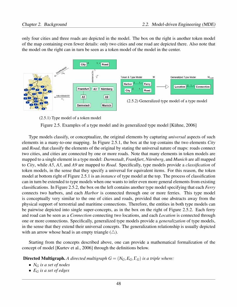
Chapter 2. Background 2.2. Model-driven Engineering (MDE)

only four cities and three roads are depicted in the model. The box on the right is another token modelof the map containing even fewer details: only two cities and one road are depicted there. Also note thatthe model on the right can in turn be seen as a token model of the model in the center.

(2.5.1) Type model of a token model

(2.5.2) Generalized type model of a type model

Figure 2.5. Examples of a type model and its generalized type model [Kühne, 2006]

Type models classify, or conceptualize, the original elements by capturing universal aspects of suchelements in a many-to-one mapping. In Figure 2.5.1, the box at the top contains the two elements Cityand Road, that classify the elements of the original by stating the universal nature of maps: roads connecttwo cities, and cities are connected by one or more roads. Note that many elements in token models aremapped to a single element in a type model: Darmstadt, Frankfurt, Nürnberg, and Munich are all mappedto City, while A5, A3, and A9 are mapped to Road. Specifically, type models provide a classification oftoken models, in the sense that they specify a universal for equivalent items. For this reason, the tokenmodel at bottom right of Figure 2.5.1 is an instance of type model at the top. The process of classificationcan in turn be extended to type models when one wants to infer even more general elements from existingclassifications. In Figure 2.5.2, the box on the left contains another type model specifying that each Ferryconnects two harbors, and each Harbor is connected through one or more ferries. This type modelis conceptually very similar to the one of cities and roads, provided that one abstracts away from thephysical support of terrestrial and maritime connections. Therefore, the entities in both type models canbe pairwise depicted into single super-concepts, as in the box on the right of Figure 2.5.2. Each ferryand road can be seen as a Connection connecting two locations, and each Location is connected throughone or more connections. Specifically, generalized type models provide a generalization of type models,in the sense that they extend their universal concepts. The generalization relationship is usually depictedwith an arrow whose head is an empty triangle (4).

Starting from the concepts described above, one can provide a mathematical formalization of theconcept of model [Kurtev et al., 2006] through the definitions below.

Directed Multigraph. A directed multigraph G = (NG,EG,ΓG) is a triple where:• NG is a set of nodes• EG is a set of edges

48

2.2. Model-driven Engineering (MDE) Chapter 2. Background

• ΓG : EG→ NG×NG is a function that maps edges to pair of nodes

Note that ΓG can possibly be non-injective, therefore allowing different edges to connect the same pairof nodes.

Model. A model M = (G,ω,µ) is a triple where:

• G = (NG,EG,ΓG) is a directed multigraph• ω is a reference model associated to its directed multigraph Gω = (NGω

,EGω,ΓGω

)• µ : NG∪EG→ NGω

is a function that maps nodes and edges of G to nodes of Gω

The relationship between a model and its reference model is called conformance, and specifies that eachelement in a model corresponds to an element in its reference model.

Metametamodel. A metametamodel M3 = (G3,ω3,µ3) is a model that is the reference model of itself,i.e., ω3 = M3.

Metamodel. A metamodel M2 = (G2,ω2,µ2) is a model such that its reference model is a metameta-model.

Terminal Model. A terminal model M1 = (G1,ω1,µ1) is a model such that its reference model is ametamodel.

(2.6.1) Organization of the metamodeling stack

(2.6.2) Classification of models as terminal models,metamodels, and metametamodels

Figure 2.6. Metamodeling stack and classification of models [Kurtev et al., 2006]

Figure 2.6.1 depicts the organization of models, metamodels, and metametamodels in terms of theconformance relationship. Such organization is usually referred to as metamodeling stack. In this figure,the conformance relationship is denoted by conformsTo or c2, and details how a model conforms to onemetamodel, which in turn is the archetype of one or more models that conform to it. A metamodelconforms to one self-conforming metametamodel. The definitions above also imply the classification ofmodels as in Figure 2.6.2, that shows that terminal models, metamodels, and metametamodels are allinstances of a generic Model type.

49

Chapter 2. Background 2.2. Model-driven Engineering (MDE)

Besides models and metamodels, Model-driven Engineering approaches also extensively rely onModel Transformations and Domain Specific Modeling (DSM) as ways to automate steps in the systemdevelopment, and to tackle software heterogeneity and complexity. These two concepts are not entirelyrelevant for the scope of the thesis, and are only briefly discussed for the sake of completeness.

MDE strongly revolves around the concept of models, that by nature are expensive and difficult tobuild. However, the formal definition of a metamodeling stack enable the (semi-)automated manipulationof models through model transformations. One of the most common definitions of model transformationimplies the automatic generation of a target model from a source model, according to a transformationdefinition [Kleppe et al., 2003]. A typical model transformation is based upon a transformation specifi-cation detailing the mapping of elements from a source metamodel into elements of a target metamodel.When executing the model transformation, an input model conforming to the source metamodel is trans-formed into an output model conforming to the target metamodel, following the rules of the specification.Model transformation allows to automate the generation and manipulation of models, which is error-prone if done by hand. One of the main use of model transformations is to generate source code frommodels upon the use of target metamodels which are intended to be manipulated through text. The au-tomatic generation of source code from system models allows developers to focus on design, rather thanimplementation, and to minimize the effort of maintaining consistency through artifacts at different levelsof abstractions.

However, model transformation by itself requires an input model, that has to be created by humans.Designing a model of a large and complex system can be challenging, because it is hard to capture allits different aspects. A basic principle behind the solution of several engineering problems is the divide-and-conquer approach: given a problem, first divide it into easier sub-problems, then solve them one ata time, and finally aggregate the solutions of the sub-problems to generate the solution of the originalproblem. In MDE, the same approach is applied to software development by dividing the design activityinto several areas of concerns, each focusing on a specific aspect of the system. In this way, it is possibleto reason over software specifications at a higher level of abstraction, and to provide partial specificationswhich are easier for experts to manage because they are closer to their domains. This approach is knownin MDE as DSM, a methodology that makes systematic use of Domain Specific (Modeling) Languages(DSL, or DSML) to represent artifacts of a system pertaining to a given domain. DSL are languagesmeant to support higher-level abstractions than General Purpose Languages (GPL), so they require lesseffort and fewer low-level details to specify a system. The separation of concerns behind DSM does notonly allow a better management of software complexity by humans. Indeed, DSM also fully exploits theidea of code generation through model transformations by providing modeling languages easier to useand understand. As a consequence, the joint use of DSM and model transformations increasingly shiftsthe focus of software development into the creation of models rather than code.

2.2.2 Standards for Model-driven EngineeringThe principles of Model-Driven Engineering provide conceptual foundations of the approach, but theycan applied in different ways. There exist several implementations of such principles that standardizethe manipulation of models, providing tool support for MDE approaches. These tools provide Inte-

50

2.2. Model-driven Engineering (MDE) Chapter 2. Background

grated Development Environments (IDE) with frameworks for repository management, model transfor-mation, and so on. In the rest of this chapter, we briefly discuss the Model-Driven Architecture (MDA)in Section 2.2.2.1 as the MDE reference implementation for the Unified Modeling Language (UML, Sec-tion 2.2.2.2). An extensive description of MDE standards, MDA and UML falls beyond the scope ofthis thesis. Nonetheless, introducing UML is necessary to describe the UML Profile for Modeling andAnalysis of Real-Time Embedded Systems (UML/MARTE, Section 2.2.2.3) that has been used in thisthesis to formalize the key abstractions of stress testing.

2.2.2.1 Model-Driven Architecture (MDA)

The most common implementation of the MDE principles is the Model-Driven Architecture (MDA)defined by the Object Management Group (OMG) in 2001 [Kleppe et al., 2003]. The Model DrivenArchitecture is based upon three cornerstones [Soley et al., 2000]. (1) First, MDA proposes a pyramidalconstruction of models, organized in four layers as in Figure 2.7.1. Artifacts in the bottom level M0represent actual systems in the real world. Those are modeled by token models in the level M1, whichare in turn compliant to metamodels in the level M2. The top level M3 consists of the Meta-ObjectFacility (MOF) as the reference self-conforming metametamodel used to specify all the metamodelsin MDA. (2) Second, MDA proposes a vision of software development structured in six main steps,each centered around a specific model as in Figure 2.7.2. System requirements are initially collectedinto a Computation Independent Model (CIM), independently from computational notions. Then, theCIM is transformed into a Platform Independent Model (PIM) that describes the CIM in computationalterms independently from specific implementation technologies. The PIM is merged with a PlatformDescription Model (PDM) containing information on the platform where the system will be deployed toform a Platform Specific Model (PSM). The PSM links the PIM specification with information about aspecific platform and can finally be transformed into executable source code. (3) Third, MDA proposesthe Unified Modeling Language (UML) as the reference language to describe models [Booch et al., 2000].

2.2.2.2 Unified Modeling Language (UML)

The Unified Modeling Language (UML) is a general-purpose modeling language, designed to provide astandard way for visualizing software systems. UML has been initially developed in 1998 as a graphicalnotation, and evolved to include a formal specification upon its adoption in the MDA in 2007. Since itscreation, UML has become an international standard for defining models of software systems. As of ver-sion 2.4.1, UML defines 14 types of diagrams, divided into two main classes: structural and behavioraldiagrams (Figure 2.8). A thorough description of UML and its diagram types falls outside the scope ofthis thesis. Nonetheless, we briefly introduce the UML diagram types, especially focusing on sequencediagrams. This is because sequence diagrams are the main way to visualize concurrency in software, andtherefore they are of primary importance to enable reasoning over performance properties in the contextof real-time systems.

• Structural Diagrams represent the static aspect of the system, i.e., the set of parts composing itsarchitecture. Structural diagrams describe the system in terms of components at different levels ofabstraction, focusing on their dependencies. There exist seven types of structural diagrams.

51

Chapter 2. Background 2.2. Model-driven Engineering (MDE)

(2.7.1) The MDA metamodeling stack, organized as apyramid [Thirioux et al., 2007]

(2.7.2) Vision of software development in MDA [Milleret al., 2003]

Figure 2.7. Two cornerstones of the MDA: the pyramidal metamodeling stack and the software develop-ment vision

– Class Diagrams are the most common diagrams in UML, and depict the key entities in thesystem as classes, i.e., object types, their properties as attributes, and their relationships asassociations.

– Component Diagrams display the structural relationship of components, i.e., sets of classesthat collaborate to realize certain features and communicate through interfaces.

– Object Diagrams, also referred to as Instance Diagrams, show relationships between actualobjects in the system, instanced from classes using real data. The most important abstractionin object diagrams defines active objects as an object that owns a process or thread, and thatcan initiate control activity. For this reason, active objects are the ones encapsulating thebehavior of the system, and are further described in behavioral diagrams. Objects that are notactive are said to be passive.

– Profile Diagrams describe UML profiles, i.e., extensions to the language that allow adapta-tion to different platforms and domains.

– Composite Structure Diagrams show the internal structure of classes in terms of functionsand variables.

– Package Diagrams represent groups (packages) of elements, such as classes and compo-nents, under a common namespace.

– Deployment Diagrams show how the software components of the system are allocated, i.e.,deployed, into hardware components.

• Behavioral Diagrams represent the dynamic aspect of the system, i.e., the interactions betweenparts of the system that define functionalities and runtime operation. Behavioral diagrams describethe system in terms of states of its components, focusing on changes in such states. There existseven types of structural diagrams.

– Use Case Diagrams are the most common behavioral diagrams in UML, and provide a highlevel description of the system functionalities (use cases) from the viewpoint of external en-

52

2.2. Model-driven Engineering (MDE) Chapter 2. Background

Figure 2.8. Taxonomy of UML 2.4.1 diagrams

tities that interface to it (actors).– Activity Diagrams model the system computational and organizational processes through

flowcharts of stepwise activities and actions.– State Machine Diagrams implement the concept of Finite States Automaton in UML, rep-

resenting the system behavior as a series of events that determine transitions through states.– Interaction Diagrams are a subset of behavioral diagrams that emphasize the data and con-

trol flow among elements of the system. There exist four types of interaction diagrams.∗ Communication Diagrams model the interactions between system objects in terms of

sequences of messages.∗ Interaction Overview Diagrams are particular activity diagrams where each activity is

pictured as a frame representing a nested interaction diagram.∗ Timing Diagrams model the change in state of system elements over time.∗ Sequence Diagrams are the most common interaction diagrams in UML, and show the

execution order of system processes, highlighting their interoperation. Sequence Dia-grams depict the entities operating concurrently as vertical lifelines, and messages ex-changed between them as horizontal arrows, entailing the order in which such messagesoccur.

Figure 2.9 illustrates the graphical notation of sequence diagrams through examples. Figure 2.9.1shows a sequence diagram describing an interaction scenario in an Access Control System (ACSystem)that regulates electronic door locks via access cards and PINs. In this interaction, labeled as UserAc-cepted, a User interacts with the system to unlock a door upon inserting the access card with its PIN.

53

Chapter 2. Background 2.2. Model-driven Engineering (MDE)

(2.9.1) Lifelines and Messages in sequence diagrams

(2.9.2) Interaction Uses in sequence diagrams (2.9.3) Combined Fragments in sequence diagrams

Figure 2.9. Graphical notation of Sequence Diagrams [OMG, 2011b]

The example shows three messages labeled as Code(PIN), CardOut, and OK, exchanged in this order bytwo lifelines of types User and ACSystem. The sequence diagram also includes a Local Attribute of typeInteger, representing the PIN being inserted by the user. Once the user inserts the card code, the systemasynchronously sends the messages CardOut and OK, and finally sends a fourth Unlock message to anundisplayed entity in the environment. Interaction diagrams, and in particular sequence diagrams, alsoallow the definition of Interaction Fragments, which are named elements representing an interaction unit.There exist several types of interaction fragments, among which Occurrence Specifications, ExecutionSpecifications, Interaction Uses and Combined Fragments are the most used in sequence diagrams.

• Execution Specifications (executions, or activations) represent a period of time in a lifelinewhere the participant entities either (1) execute a unit of behavior, (2) send a signal to another en-tity, or (3) wait for a reply message from an entity. Executions specifications are usually depictedin lifelines as rectangles. Occurrence Specifications (often simply called occurrences) represent amoment in time at the beginning or end of a message, or at the beginning or end of an execution.• Occurrence Specifications (or occurrences) appear on exactly one lifeline, and are ordered along

such lifeline. Note that occurrence specifications have no notation, as they are represented by apoint at the beginning or end of a message or execution.• Interaction Uses allow to reference interactions: Figure 2.9.2 shows the interaction UserAccess

54

2.2. Model-driven Engineering (MDE) Chapter 2. Background

that refers to the externally defined interactions EstablishAccess with argument Illegal PIN, andOpenDoor. Interaction uses are commonly used to simplify the notation of large and complexsequence diagrams by allowing the reuse of already defined interactions.• Combined Fragments define combinations or expressions of interaction fragments. The semantic

of combined fragments is defined by an interaction operator. Figure 2.9.3 shows an example of aPerson inserting his card into the system to unlock a door. After receiving the GivePIN messageby the AccessControl, the user inserts the four digits of his PIN one at a time. This is modeledby a combined fragment with the Loop operator, stating that the body of the loop is repeated fourtimes. Combined fragments can also have Interaction Constraints in the form of guards. If the userinserts the wrong code, the Wrong PIN guard evaluates to true, so that the user can insert the codetwo more times. Note that, as in this last case, combined fragments can be nested.

UML is a General Purpose Language designed to be used in software development at every stage,from high-level specification, e.g., with use case diagrams, to low-level implementation details, e.g.,with deployment and state machine diagrams. The universality of UML makes it suitable for a varietyof purposes, but comes at the cost of flexibility. Indeed, UML cannot always provide the abstractionlevel developers need to model software in every domain [Atkinson and Kühne, 2007]. In MDE, thisproblem is addressed with the use of Domain Specific Languages, but UML also includes the possibilityto define profiles, a built-in mechanism to tailor the language for specific needs. Specifically, profilesallow the extension of UML metaclasses by providing additional semantics through two main constructs:stereotypes and tagged values. Stereotypes define extensions of existing UML metaclasses, enabling theuse of domain-specific notation that provides additional semantic for the extended metaclass. Stereotypesare defined by a name and by the set of metamodel elements they extend. Tagged values are meta-attributes attached to a metaclass of the metamodel extended by a profile. Tagged values have a nameand a type, and are associated to a specific stereotype. We further illustrate these concepts through theexample in Figure 2.10.

Figure 2.10.1 shows the WeightsAndColours profile that extends UML proving modeling support forthe concepts of weights and colors, with the possibility to specify the color of colored elements, andthe weight of weighed elements. WeightsAndColours defines the two stereotypes Colored, extending theUML metaclasses Class and Association and Weighted, extending the metaclass Association. Stereo-types are graphically visualized in boxes labeled stereotype. This means that, when applying the profile,classes and associations can be colored, i.e., stereotyped Colored, and associations can also be weighted,i.e., stereotyped Weighted. The stereotype Colored has a tagged value named color specifying that eachcolored element has a specific color, chosen from an Enumeration of four. Similarly, the stereotypeWeighted has a integer tagged value named weight that represents the weight of the stereotyped associa-tion. Tagged values are formally specified as attributes of the class defining the stereotype. Figure 2.10.2shows TopologyProfile, another example of UML profile extending UML with concepts such as Nodeand Edge. Figure 2.10.3 finally shows a class diagram with classes and associations stereotyped withboth these profiles. Specifically, the diagram shows a Branch node in a weighted, LocalEdge associationwith a CentralOffice colored MainNode. In the example, the tagged values are represented within UMLnotes.

55

Chapter 2. Background 2.2. Model-driven Engineering (MDE)

(2.10.1) Example of a UML profile concerning colorsand weights

(2.10.2) Example of a UML profile concerning nodesand edges

(2.10.3) Example of application of the UML profiles

Figure 2.10. UML Profiles definition and usage showed through an example [Fuentes-Fernández andVallecillo-Moreno, 2004]

2.2.2.3 UML Profile for Modeling and Analysis of Real-Time Embedded Systems(UML/MARTE)

UML has been used for long time to model Real-Time Embedded Systems [Selic, 1998], but it is notflexible enough to be effectively applied in complex real-time systems. As discussed in Section 2.2.2.2,profiles are meant to tailor UML to specific domains, providing high level concepts to support softwaremodeling. When it comes to RTES, the UML profile for Modeling and Analysis of Real-time Embed-ded Systems (UML/MARTE, in short MARTE [OMG, 2011a]) is the most acknowledged and used bypractitioners. MARTE is an OMG standard defined in 2011 to replace its predecessor UML profile forSchedulability, Performance, and Time (SPT), aligned with UML v1.x [OMG, 2005].

56

2.2. Model-driven Engineering (MDE) Chapter 2. Background

The specification of MARTE defines the profile in two steps. The first step consists of defining theconcepts related to one specific concern in RTES. These concepts are referred to as domain elements,e.g., abstractions to model time, scheduling, or non-functional properties. The domain elements aregathered in the domain model, which is formalized through the definition of a meta-model and the detailedsemantics descriptions of each of its elements. The second step in the definition of MARTE consists of theactual formalization the UML profile, referred to as UML representation. In particular, the specificationof MARTE maps the concepts introduced in the domain model to UML stereotypes, tagged values,specific notations, and Object Constraint Language (OCL) rules. Note that abstractions in the domainmodel are grouped in packages, while the extensions in the UML representation are grouped in sub-profiles. Therefore, packages in the domain model map into sub-profiles in the UML representation.Also note that sub-profiles in the UML representation can also be grouped in packages, which should notbe confused with the packages of domain models.

Figure 2.11 shows the architecture of MARTE, which consists of four main packages, each groupingseveral sub-profiles. MARTE revolves around the main concept of providing support for both design andanalysis of RTES. These two development activities are supported with the abstractions defined in designmodel and analysis model packages [Gerard and Selic, 2008], respectively. Due to its completeness andlevel of detail, it is beyond the scope of this thesis to thoughtfully examine MARTE. Nonetheless, weprovide an overview of its architecture, especially focusing on the domain model packages containingabstractions for quantitative analysis and resource modeling. This is because the sub-profiles associatedto these packages provide frameworks for collecting information pertaining to schedulability and perfor-mance analysis, and to model resources in computational platforms. These two concepts are essentialwhen it comes to stress testing, that entails finding worst-case scenarios with respect to some perfor-mance requirement. Indeed, such worst-case scenarios are characterized by the way concurrent softwaretasks are scheduled by the Real-Time Operating System, and the schedules in turn depend on the runtimestatus and properties of the computational platform.

Figure 2.11. UML/MARTE Architecture [OMG, 2011a]

57

Chapter 2. Background 2.2. Model-driven Engineering (MDE)

• MARTE foundations contains the abstractions shared by the two main packages, MARTE designmodel, and MARTE analysis model. Therefore, this package defines concepts used in both analysisand design of RTES, such as abstractions for representing time, concurrent resources, and qualityof service. MARTE foundations is structured in five sub-profiles.

– CoreElements contains the basic elements used for structural and behavioral modeling ofRTES. The domain model of this profile consists of the two packages Foundations and Causal-ity, containing abstractions for model-based design and analysis of RTES, respectively.

– Non-Functional Properties (NFP) contains modeling constructs to declare non-functionalproperties as UML data types, so that they can be attached to standard UML elements. Thisprofile defines concepts to express relationships and constraints among non-functional prop-erties in order to model system non-functional requirements.

– Time supports modeling the notion of time and time-related concepts such as clocks and timeevents. This profile allows the definition of three time models: causal/temporal, for modelingrelative ordering of events, clocked/synchronous, for modeling time as a discrete successionof instants, and physical/real-time, for modeling continuous time.

– Generic Resource Modeling (GRM) contains abstractions to represent computing platformsas sets of resources, possibly organized as a hierarchy, where each resource offers services inresponse to service requests.

– Allocation Modeling (Alloc) provides support for allocating system functionalities into com-putational resources, providing a conceptual link between real-time software and the hardwareplatform that runs it.

• MARTE design model refines the concepts defined in MARTE foundations from the view-pointof RTES design. This package provides domain-specific concepts of real-time applications andcomponents, and software and hardware resources. MARTE design model is structured in foursub-profiles.

– Generic Component Modeling (GCM) refines concepts already defined in UML to supportmodeling component-based RTES.

– High-Level Application Modeling (HLAM) provides modeling concepts for modeling fea-tures in RTES at a high level of abstraction. The domain model of this profile defines Real-time Units (RtUnit) as the main concurrent entities of a system, and Protected Passive Units(PpUinit) as mechanisms to share information among real-time units.

– Software Resource Modeling (SRM) refines the concepts defined in GRM to model Appli-cation Programming Interfaces (API) for concurrent software, independently from the spe-cific Real-Time Operating System used. The domain model of this profile provides model-ing concepts for software resources (ResourceCore), concurrent execution contexts (Concur-rency), resources communication (Interaction), and management (Brokering). Being RTOS-independent, the concepts in SRM have to be complemented with specific modeling librariesimplementing OS standards. Such libraries are introduced in the package MARTE annexes.

– Hardware Resource Modeling (HRM) refines concepts in GRM to model components ofhardware platforms, such as processors, memory hierarchies, Application-Specific IntegratedCircuits (ASIC), and Programmable Logic Devices (PLD). Note that, while SRM providesgeneric abstractions that have to be complemented with modeling constructs specific to RTOS

58

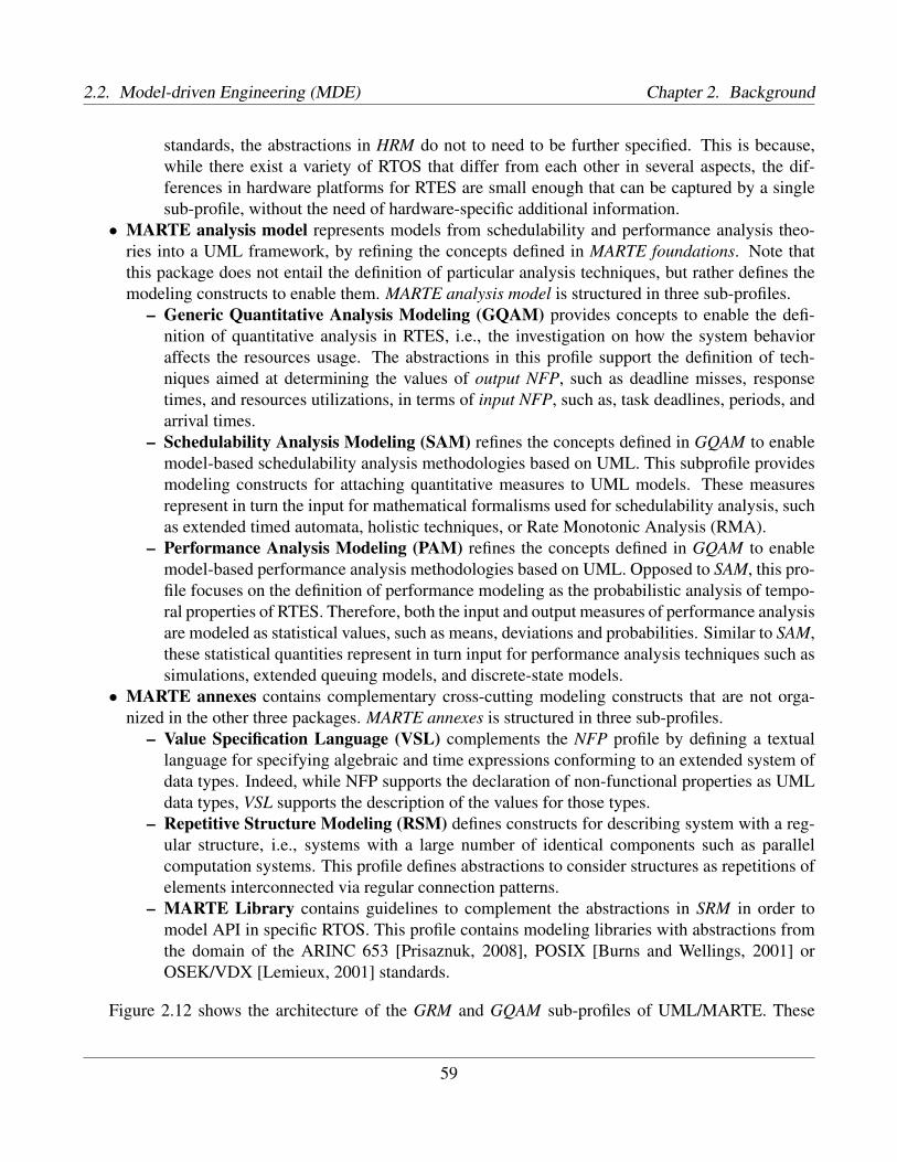
2.2. Model-driven Engineering (MDE) Chapter 2. Background

standards, the abstractions in HRM do not to need to be further specified. This is because,while there exist a variety of RTOS that differ from each other in several aspects, the dif-ferences in hardware platforms for RTES are small enough that can be captured by a singlesub-profile, without the need of hardware-specific additional information.

• MARTE analysis model represents models from schedulability and performance analysis theo-ries into a UML framework, by refining the concepts defined in MARTE foundations. Note thatthis package does not entail the definition of particular analysis techniques, but rather defines themodeling constructs to enable them. MARTE analysis model is structured in three sub-profiles.

– Generic Quantitative Analysis Modeling (GQAM) provides concepts to enable the defi-nition of quantitative analysis in RTES, i.e., the investigation on how the system behavioraffects the resources usage. The abstractions in this profile support the definition of tech-niques aimed at determining the values of output NFP, such as deadline misses, responsetimes, and resources utilizations, in terms of input NFP, such as, task deadlines, periods, andarrival times.

– Schedulability Analysis Modeling (SAM) refines the concepts defined in GQAM to enablemodel-based schedulability analysis methodologies based on UML. This subprofile providesmodeling constructs for attaching quantitative measures to UML models. These measuresrepresent in turn the input for mathematical formalisms used for schedulability analysis, suchas extended timed automata, holistic techniques, or Rate Monotonic Analysis (RMA).

– Performance Analysis Modeling (PAM) refines the concepts defined in GQAM to enablemodel-based performance analysis methodologies based on UML. Opposed to SAM, this pro-file focuses on the definition of performance modeling as the probabilistic analysis of tempo-ral properties of RTES. Therefore, both the input and output measures of performance analysisare modeled as statistical values, such as means, deviations and probabilities. Similar to SAM,these statistical quantities represent in turn input for performance analysis techniques such assimulations, extended queuing models, and discrete-state models.

• MARTE annexes contains complementary cross-cutting modeling constructs that are not orga-nized in the other three packages. MARTE annexes is structured in three sub-profiles.

– Value Specification Language (VSL) complements the NFP profile by defining a textuallanguage for specifying algebraic and time expressions conforming to an extended system ofdata types. Indeed, while NFP supports the declaration of non-functional properties as UMLdata types, VSL supports the description of the values for those types.

– Repetitive Structure Modeling (RSM) defines constructs for describing system with a reg-ular structure, i.e., systems with a large number of identical components such as parallelcomputation systems. This profile defines abstractions to consider structures as repetitions ofelements interconnected via regular connection patterns.

– MARTE Library contains guidelines to complement the abstractions in SRM in order tomodel API in specific RTOS. This profile contains modeling libraries with abstractions fromthe domain of the ARINC 653 [Prisaznuk, 2008], POSIX [Burns and Wellings, 2001] orOSEK/VDX [Lemieux, 2001] standards.

Figure 2.12 shows the architecture of the GRM and GQAM sub-profiles of UML/MARTE. These

59

Chapter 2. Background 2.2. Model-driven Engineering (MDE)

(2.12.1) Dependencies of GRM

(2.12.2) Architecture of GRM (2.12.3) Architecture and dependencies of GQAM

Figure 2.12. Architectures of the UML/MARTE packages for Generic Resource Modeling and GenericQuantitative Analysis Modeling [OMG, 2011a]

packages contain the stereotypes and attributes which map to the conceptual model of our stress testingapproach. Figures 2.12.1 and 2.12.2 show dependencies and architecture of the GRM domain model,which is structured in five packages.

• ResourceCore defines the basic abstractions for resource modeling, providing constructs to modelthe system in terms of resources, and services provided by such resources. A Resource representsa persistent entity of the system offering one or more ResourceServices. Resources have Instancesat runtime, and can be associated with non-functional properties.• ResourceTypes defines the fundamental types of resources and the services they provide. MARTE

defines seven main types of resources.– StorageResource models resources capable of storing information, such has Hard Disk Drives

(HDD) or Rapid Access Memory (RAM).– TimingResource models resources centered around the notion of time, such as clocks.– SynchResource models resources arbitrating concurrent execution flows, such as semaphores.– ComputingResource models physical or virtual processing devices capable of storing and

executing program code, such as Central Processing Units (CPU).– ConcurrencyResource models resources capable of executing concurrently with others, such

as threads or processes in a concurrent environment.– DeviceResource models external resources that require system services to operate, such as

peripheral devices.

60

2.2. Model-driven Engineering (MDE) Chapter 2. Background

– CommunicationResource models terminal entities (CommunicationEndPoint), and channels(CommunicationMedia) involved in a communication, such as system peripherals and buses.

• ResourceManagement defines resource management services in two main concepts. First, Re-sourceManager models a resource responsible for creating, maintaining, and deleting resourcesaccording to a ResourceControlPolicy. Second, ResourceBroker models resources responsible forallocation and de-allocation of resource instances to clients, according to an AccessControlPolicy.• ResourceUsages models the usage of resources providing concepts such as demand of resources

(UsageDemand) and amount of resources used (UsageTypeAmount).• Scheduling defines abstractions to model how the system behavior is arranged at run-time in terms

of the execution order of tasks. This package defines a ProcessingResource as a kind of resource ca-pable to process information, such as a ComputingResource, CommunicationMedia, or DeviceRe-source. Then, it defines a Scheduler as a ResourceBroker that brings access to ProcessingResourcesfollowing a certain SchedulingPolicy. Finally, it defines a SchedulableResource as a particular Con-currencyResource that can be granted computational power by a ProcessingResource according toSchedulableParameters.

Figure 2.12.3 shows the dependencies and the architecture of GQAM domain model. The main ab-straction of the package is the AnalysisContext, defined in terms of operations triggered over time byevents (WorkloadBehavior). and the container of resources that perform such operations (ResourcesPlat-form). GQAM is structured in three packages.

• Workload defines the concepts of system workload and behavior. A WorkloadBehavior is a set ofsystem behaviors (BehaviorScenario), triggered by a set of events (WorkloadEvent ), and consistingof sequences of operations (Step). Each Step is allocated into a SchedulableResource, and canbe acquiring (AcquireStep) or releasing (ReleaseStep) a resource to perform its operations. Forthis reason, the abstraction BehaviorScenario inherits from ResourceUsage, since each behavior ischaracterized by a demand of resources. Note that a BehaviorScenario is conceptually similar to atask in scheduling analysis (Section 2.1.1).• Resources refines the concept of resource defined in GRM by defining the ResourcesPlatform

abstraction, which represents a container for the resources used to perform a BehaviorScenariodefines two types of resource: ExecutionHost, a processor that executes operations specified in themodel, and CommunicationsHost, a hardware link between devices to transmit messages througha CommunicationChannel.• Observers defines the concept of TimedObserver as an entity collecting performance measures on

an interval of time between two specific events.

Effectively applying the UML/MARTE concepts in industrial contexts is a challenging task that iscomplicated by two main factors [Iqbal et al., 2012]. (1) MARTE is a very large profile that accountsfor a variety of performance-related aspects in RTES. Indeed, the profile is meant to provide modelingsupport in all the lifecycle phases of RTES, ranging from design to performance analysis and verification.Nonetheless, for practical use, one often needs only a subset of the abstractions defined in the profile.However, (2) MARTE is a relatively young standard, and there exists little published research providingguidelines on how to apply its concepts, i.e., on how to identify the relevant abstractions for a particular

61

Chapter 2. Background 2.3. Software Testing

kind of analysis. For these reasons, there is the need to define frameworks to guide practitioners inapplying MARTE. Typically, a methodology is needed which identifies the subset of MARTE that bestfits the performance analysis to be carried out. This is especially true when it comes to performance stresstesting. However, few sources are available that highlight relevant concepts in the profile for identifyingworst-case scenarios with respect to performance requirements.

2.3 Software TestingSoftware testing is an investigation conducted by system developers to systematically evaluate the Sys-tem Under Test (SUT) by observing its execution [Myers et al., 2011]. It is acknowledged as one of themost critical activities in the software development process, as studies have shown that testing typicallytakes more than 40% of the total development time [Boehm, 1981]. Even though there exist a large num-ber of strategies for software development, testing is an essential part in each of them. The archetype ofsuch strategies is the Waterfall Model, which is often represented as a V-Model (Figure 2.13) [Forsbergand Mooz, 1991]. The left side of the V shows the top-down steps where software requirements areprogressively refined into more detailed and technical representations of the system, down to its sourcecode. Then, once code has been generated, the development continues in a bottom-up fashion on the rightside of the V, where the software artifacts are tested in reversed order as they are created. The V-modelhighlights the relationship testing has with the different phases of software lifecycle, visualizing howlate-stage testing impacts early-stage development activities. For instance, if system testing highlightsarchitectural problems, the development might suffer a significant setback. This reason lead to the adop-tion of new software processes, which stress on the importance of test-driven development [Beck, 2003].Software testing is based on the concepts hereby defined [Ammann and Offutt, 2008].

Figure 2.13. The V-Model for software development [Roger, 2005]

62

2.3. Software Testing Chapter 2. Background

• Fault (or Defect). A fault is an anomaly in the system implementation, such as a wrong expres-sion in the system source code.Faults are often caused by human errors, such as misinterpreting arequirement, forgetting some conditions, or mistyping an instruction. A system can have a faultthat is not executed, and therefore has no effect on the system behavior. In this case, the fault isdormant. If the faulty instruction is executed, then the fault is activated.• Error (or Bug) An error is a wrong internal state of an executing system, such as a program

counter or an attribute with wrong values, caused by an activated fault. An error can have impactthe observable behavior of a system. In this case, the error propagates to the outside.• Failure. A failure is a deviation, caused by a propagated error, of the system behavior from the

expected behavior. The system evaluation performed during software testing is mostly aimed atidentifying failures in a system, so that the corresponding fault(s) can be corrected5.• Test Case. A test case is a set of data given as input to the SUT in order to observe the system

behavior in a particular scenario. In general, a test case is a possible input to a system, such as aset of particular values that a system interface takes as a parameter. Given that the ultimate goal oftesting is to identify defects, generating test cases that have high chance to reveal faulty behaviorin the system is a critical task. The process of creating test cases for a system is known as test casegeneration.• Test Suite. A test suite is a set of test cases. Since testing has to account time and budget con-

straints, it is not feasible to execute arbitrarily large test suites. In practice, one wants to find abalance between the size of the test suite, i.e., the time that it takes to execute all of its test cases,and the likelihood test cases have to reveal faults. This need is addressed by techniques known astest suite optimization or test suite reduction.• Test Case Specification. A test case specification is a document containing the scenarios that test

cases are meant to exercise. The test case specification is used to guide the test case generationprocess. Note that in Model-driven Engineering, both the system and the test case specification arerepresented by models (Section 2.3.1).• Test Oracle. A test oracle is a map that associates to each test case in a test suite its expected

behavior. Typical oracles consist of past versions of the same system, standards the system mustconform to, or user expectations.• Test Framework (or Test Harness). A test framework is a tool that supports (semi-)automation

of the testing process, including the generation of test cases, their execution, the comparison withtest oracles, and the generation of reports on the test executions.

It is well-known that testing, being based on the execution of a system, is a powerful techniqueto show the presence of defects, but can not show their absence [Dijkstra et al., 1970]. Indeed, thepotential size of input space and the presence of unbounded loops within the system control flow rendersexhaustive testing practically infeasible. This motivates the need to assess the quality of test suites,in order to reduce costs and gain confidence that the system has been properly tested. Evaluating thequality of test suites is mostly done by assessing the extent to which the system is thoroughly tested,and the capability of test cases to reveal faults. These two aspects are investigated trough test coverage

5 Note that testing is aimed at detecting system failures, not at diagnosing their causes. Indeed, the process of identifyingthe faults that cause failures is referred to as debugging. Nevertheless, testing and debugging are often mixed up.

63

Chapter 2. Background 2.3. Software Testing

criteria and mutation-based analysis, respectively. Test coverage is a measure of the proportion of asystem exercised, i.e., covered, by a test suite [Rapps and Weyuker, 1985]. This proportion can bemeasured with several criteria that reason over the system at different levels of abstractions, consideringuser requirements (requirement-based criteria), control flow graphs (control-flow-based criteria), statemachines (transition-based criteria), internal variables usage (data-flow-based criteria), and partitionsof input values (boundary-based criteria). For instance, transition-based criteria consider the system asa state machine, and measure the percentage of states or transitions visited when executing the test suite.Mutation analysis is a technique to measure the fault detection capability of a test suite [DeMillo et al.,1978]. The idea behind mutation analysis is to inject faults into a correct implementation of a system,thus creating faulty implementations called mutants. The test suite is then executed on each mutant, andthe number of mutants that reveal faults, referred to as killed mutants, determines the quality of the testsuite.

Testing not only affects the development costs of software, but also its quality [Deutsch and Willis,1988]. For this reason, software testing has been adopting formal and structured approaches. Indeed,many techniques for software testing have been devised over the years. One of the most important clas-sifications of testing strategies distinguishes black-box from white-box testing [Pressman and Jawadekar,1987]. Black-box testing techniques assume no details on the system implementation, interacting exclu-sively with user interfaces. The SUT is then seen as a black box, whose behavior is only determinedthrough the input-output relationships revealed during testing. Black-box testing is particularly usefulwhen system details are not available, allowing for an objective perspective that avoids bias when gen-erating test cases, due to knowing the fundamental aspects of the system. On the other hand, having nodetails on the parts of the system exercised by each test case renders achieving satisfactory testing cov-erage challenging. In white-box testing, the SUT is instead completely accessible. This allows a moreeffective generation of test cases, where coverage criteria can be taken into account. However, white boxtesting comes at the cost of requiring a careful investigation of the system artifacts to be more effectivethan black-box testing. Note that it is beyond the scope of this thesis to discuss a complete taxonomyof testing approaches. However, we briefly describe three most relevant areas for this thesis, namelyModel-based Testing (Section 2.3.1), Performance Testing (Section 2.3.2), and Search-Based SoftwareTesting (Section 2.3.3).

2.3.1 Model-based Testing (MBT)Model-driven Engineering (Section 2.2) is based on use of models as main artifacts during every phaseof software development, including testing. This lead to the definition of Model-based Testing (MBT)as an approach for deriving test cases from system models (Figure 2.14), implying that the test casespecification is also represented as a model. Even though there is no universal definition for MBT [Binder,2000], Figure 2.14.1 shows one of the most common understandings. The main idea behind MBT is thatthe specification of a system behavior can not only be used to guide development, but also to derive testcases that exercise particular behaviors. Specifically, models can be used to derive abstract test casesrepresenting test data and scenarios. These abstract test cases model executable test cases, which can berun on the system once implemented. One of the main advantages of MBT is that test cases are generatedfrom system models, which in turn are derived from requirements. Indeed, linking the test cases to system

64

2.3. Software Testing Chapter 2. Background

requirements simplifies their readability, understandability, and maintainability [Utting et al., 2006].

(2.14.1) Relationships between system,models, and test cases in MBT

(2.14.2) Levels of abstraction in MBT [Utting et al.,2006]

(2.14.3) A typical MBT process [Utting and Legeard,2010]

Figure 2.14. Overview of Model-based Testing: the system models are used to drive the generation oftest data (abstract test cases), that characterizes executable test cases

Similar to MDE, models in MBT can be defined at different levels of abstraction. Figure 2.14.2shows a graph where the x- and y-axes report the level of detail of the environment and system models,respectively. The models S, E, and SE represent the extreme cases, where the model formalizes all thedetails about the System, the Environment, or both. Such models are often too detailed to be managed,so in MBT these details are typically abstracted away as in M1, M2, and M3. This is also a commonpractice in MDE.

Figure 2.14.3 shows a typical MBT process, which consists of five main steps: (1) starting froma model of the system, (2) generate abstract test cases, (3) transform them into executable test caseswhich are (4) run in the system, and finally (5) analyze the results, possibly comparing them with testoracles [Utting and Legeard, 2010]. Another advantage of MBT is that the generation of abstract testcases and their transformation into executable test cases (test cases and test scripts in Figure 2.14.3,respectively) can be automated with relatively low effort [Utting and Legeard, 2010]. Usually, executabletest cases are generated via model transformation of the corresponding abstract test cases. There exist

65

Chapter 2. Background 2.3. Software Testing

several possible techniques for generating abstract test cases, mostly depending on test selection criteriaand generation technology [Utting et al., 2006].

In practice, it is not possible to exhaustively test the set of behaviors represented by models of largesystems. When generating test cases from a model, it is then necessary to define some criteria to chosethe behaviors to test. In this way, the test selection criteria define a test suite. There exist seven maintypes of test selection criteria for MBT [Utting et al., 2006].

• Requirement-based criteria aim at providing coverage of the system requirements. To implementthese criteria, requirements need to be traced to system models, so that each test case generatedexercises one or more system aspect expressed in a requirement.• Specification-based criteria are based on the test case specification. Even though it is in general

independent from the system models, the test case specification is often expressed with formalismssuch as Finite State Machines (FSM), constraints, and regular expressions [Utting et al., 2006].These formalisms are often used in conjunction with UML profiles such as the UML Testing Pro-file (UTP) [OMG, 2013], in order to provide the adequate abstraction level to generate test casesrepresenting the scenarios in the specification [Baker et al., 2008].• Structure-based criteria select test cases based on the structure of the model, typically with

control-flow-based, transition-based or state-based coverage criteria [El-Far and Whittaker, 2001].• Data-based criteria are based on the decomposition of the input space into equivalence classes,

as in boundary-based coverage criteria. In this way, that test cases can be selected to exercise onerepresentative value from each class.• Mutation-based criteria are based on the concept of mutation analysis. Even though mutation

analysis has been defined as a strategy to evaluate the quality of test suites, its principles canalso be applied to drive test case generation. This is mostly done by ensuring that the test casesgenerated kill a satisfactory number of mutants [Papadakis and Malevris, 2012].• Fault-based criteria rely on the knowledge of typically occurring faults, which are often captured

in the form of a fault model.• Probabilistic-based criteria are based on stochastic models of the environment, and are mostly

used when the usage patterns of the SUT are determined by such environment. Typical approachesprofile the system usage with Markov chains or statistical models [Beyer et al., 2003].

Abstract test cases generation can be classified under another dimension, orthogonal to selectioncriteria, concerning the technology that automates the generation of test cases. There exist four maintechnologies to automate test case generation in MBT [Utting et al., 2006].

• Search algorithms are generally used to generate test cases from behavioral models such as FiniteState Machines. Indeed, state machines are graphs where to each node corresponds a state, andto each edge corresponds a transition between states. Commonly used selection criteria for statemachines involve graph coverage, such as nodes, transitions, and cycles coverage. Test casessatisfying these criteria can be easily generated with search algorithms that explore the FSM graphs,and keep track of the paths yielding high coverage, which represent abstract test cases.• Model Checking (MC) is a software verification technique that aims at verifying properties ex-

66

2.3. Software Testing Chapter 2. Background

pressed in a model [Clarke et al., 1999]. Typically, a property is a condition that should never holdin the system at any given time. These properties are in turn formulated as reachability queries ofa faulty state in a FSM, in such a way that MC verifies whether this faulty state is reachable ornot from the initial state. If this is the case, MC returns a counterexample with the path leadingto the faulty state, otherwise it terminates proving that the property never holds because the faultystate can never be reached. MC is mostly used in software engineering to compare a model with itsspecification, e.g., to check the absence of deadlocks in a FSM modeling task executions. However,MC can also be used for test case generation by formulating test case specifications as reachabilityproperties in a state machine [Ammann et al., 1998]. For instance, a test case could be specifiedin a way that upon execution, the state S in the state machine M is reached at some point. In thiscase, MC can generate an abstract test case by computing a path in model M such that the state Sis visited.• Theorem Proving is another software verification technique that, similar to Model Checking, aims

at verifying properties expressed in a model [Hoare, 1969]. However, while Model Checking caststhese properties as reachability queries over a state machine, Theorem Proving verifies the sameproperties by casting them as logic formulas, and proving their satisfiability using deductive logic,such as Hoare Rules or Lambda Calculus [Halpern and Vardi, 1991]. However, Theorem Provingcan be used for to generate abstract test cases in MBT by modeling the system behavior as a setof logical expressions (predicates). The model is then partitioned into equivalence classes over thevalid semantic interpretations of the expressions. In this way, each equivalence class represents asystem behavior, and is therefore an abstract test case [Brucker and Wolff, 2013].• Symbolic Execution (or Symbolic Evaluation) is a technique aimed at determining what inputs

cause given statements of a program code to execute [King, 1976]. Typically, an interpreter followsthe program, assuming symbolic values for input variables. For each statement in the program, theinterpreter assigns to variables expressions in terms of the symbolic values, based on the previousstatements interpreted. Whenever the interpreter analyzes a conditional statement with n branches,it creates n logical constraints and associates each to the first statement the corresponding branch.When the program is fully analyzed, for each statement in the code the interpreter has created aconstraint model consisting of constraints on the program variables. Then, in order to find concretevalues for the input variables leading to the execution of a given statement, the corresponding con-straint model is solved with a constraint solver (Section 2.4.1). In MBT, Symbolic Execution canbe used as an alternative to Model Checking when proving reachability properties over executablemodels, e.g., models expressed with Executable UML (xtUML or xUML) [Mellor et al., 2002]. Inthis way, the concrete values found when solving a constraint model associated with a statement Lrepresent an abstract test case that executes L.

Finally, there exist two fundamental strategies for generating and executing test cases in MBT, namelyoff-line and on-line approaches (Figure 2.15) [Hessel et al., 2008]. In the former, (Figure 2.15.1), testcases are executed in an Implementation Under Test (IUT) after the test suite is fully generated. Inthis way, the test cases execution process is straightforward, because it is decoupled from generation.In addition, the test suite can be optimized prior to execution, for instance by eliminating redundant testcases and by ensuring the satisfaction of some coverage criteria. On the other hand, in on-line approaches

67

Chapter 2. Background 2.3. Software Testing

(2.15.1) Off-line MBT (2.15.2) On-line MBT

Figure 2.15. Off-line and on-line approaches for MBT [Hessel et al., 2008]

test generation and execution happen one after the other in a feedback loop (Figure 2.15.2). In this way,the outcome of past test cases can possibly influence the generation of new ones. On-line testing maycontinue until some coverage or fault-detection criteria have been satisfied. This approach is mostly usedfor systems where testers can not inject some of the inputs, such as non-deterministic systems whoseenvironment is hard to effectively simulate.

2.3.2 Performance and Stress TestingSoftware testing has historically focused on functional aspects, and has mostly been intended as a meanto ensure that each system input corresponds to the expected output. However, the degradation in perfor-mance can have potentially severe consequences, even worse that unexpected system responses [Weyukerand Vokolos, 2000]. This is especially true in the context of safety-critical systems, where respondingtimely to external inputs is as important as processing them in the correct way. Therefore, many stud-ies stated the importance of performance testing, especially during early development stages, when thesystem architecture is finalized [Denaro et al., 2004]. This aspect highlighted the need of methodologiesflexible enough to combine performance testing with early design-time analysis [Woodside et al., 2007].

For practitioners, performance testing investigates whether or not a software system handles the ex-pected user load by responding quickly enough [Barber, 2003]. Indeed, a common definition of per-formance testing involves the systematic evaluation of a System Under Test under realistic conditions,in order to check whether performance requirements are satisfied or not [Binder, 2000]. This definitionentails the investigation of abstract concepts such as the capacity and limits of the system, which aredefined in the performance requirements [Gao et al., 2003]. For this reason, performance test cases aredesigned starting from such requirements, which in turn can be expressed in different ways, dependingon the system scope, domain, and objectives. In this thesis, we focus on the description of performancetesting in the context of safety-critical Real-Time Embedded Systems, where the most important concernis ensuring a timely reaction to external triggers (Section 2.1).

Figure 2.16 depicts a typical performance testing process, which consists of five main steps [Gaoet al., 2003].

68

2.3. Software Testing Chapter 2. Background

1. Selection of Performance Requirements. The first step is to identify the concepts characterizingthe performance of the tested system [Nixon, 2000]. In RTES, common performance requirementsinvolve task deadlines, response time, and computational resources utilization, such as CPU, mem-ory and network bandwidth. Performance requirements are then formalized in formal metrics thatare measured during testing [Jain, 1991].

2. Definition of the Workload (or Performance Evaluation Model). The requirements selected arethen used to drive the definition of the workload, which consists of the scenarios that the systemhas to be tested in. The workload contains all the basic information characterizing performancetest cases. Indeed, at the lowest level of abstraction, each scenario corresponds to one test case.

3. Definition of the Performance Test Plan. Performance requirements, metrics and workload aredocumented in a performance test plan. The test plan also contains technical information related totest execution, such as hardware used, software versions, tools and test schedule.

4. Generation of the Performance Test Report. After test cases execution, the final step is toprepare a report that documents the results in order to analyze system performance. The resultingreport includes the measured values of performance metrics, possibly with graphs displaying theirevolution over time.

Figure 2.16. A typical performance testing process [Gao et al., 2003]

69

Chapter 2. Background 2.3. Software Testing

The performance testing process is thus centered on the definition of a workload that the system is ex-posed to. The workload is also called operational profile, as it can be seen as a mean to profile the systembehavior [Musa, 1996]. In the domain of distributed systems, the workload is often defined through theuse of traffic models, which stochastically predict the most likely user interactions with the system [Hongand Rappaport Stephen, 1986]. However, RTES interact with the external environment, which is in-trinsically hard to predict prior to system execution. This renders the definition of RTES workloadsa challenging task, as popular techniques such as workload characterization based on historical data orstochastic models can be rather ineffective. This is especially true in the context of safety-critical systems,where it is mandatory to test performance in worst-case scenarios, rather than only in the most commonones. Workloads are usually classified into real and synthetic workloads [Jain, 1991]. A real workloadcorresponds to a set of actual operating scenarios that occur in a given time frame. Real workloads areuseful to investigate the system under realistic conditions, but can not be controlled in practice. Indeed,they are not repeatable, and can not guarantee a significant variety of operating conditions. Nonetheless,systems can always be tested under real workloads. On the other hand, synthetic workloads are simula-tions of real conditions that can be repeatedly applied to the system, and controlled by testers. Wheneverworkload characterization is possible, synthetic workloads are created from real workload models, whichclassify particular system-user or system-environment interaction patterns. Note that, in the context ofRTES, using synthetic workloads requires the capability to interact with the system by simulating theexternal environment.

There exist several types of performance testing, each characterized by a specific workload that ex-ercises given aspects of the SUT performance [Shannon et al., 2005]. In the context of safety-criticalRTES, a major role in performance testing is played by stress testing, intended as testing a system under“unrealistically harsh inputs [. . . ] with the intention of breaking it" [Beizer, 2002]. For this reason, stresstest cases push the system “beyond its design limits" as they are “designed to cause a failure" [Binder,2000]. Indeed, stress testing is the simulation of border-line cases that represent worst-case scenarios.Testing these scenarios is particularly important for safety-critical systems, where failures can not betolerated as they may lead to catastrophic consequences for the system, its users and the environment.Therefore, stress testing workloads define worst-case scenarios, which in RTES are usually representedby particular sequences of external events triggering system tasks. These events are often signals comingfrom hardware sensors which carry must-answer data, such as alarms from fire, pressure or temperaturesensors. In RTES, stress testing workloads are mostly characterized by the timing patterns of such events.Consider for instance a fire monitoring system that has to activate water sprinklers in case smoke is de-tected. When testing such a system, it is crucial to investigate whether the sprinklers are timely activatedwhenever there is a fire, i.e., whatever the timing of the fire detectors signals is. There could be (worst)cases where the alarm comes when the system does not have enough resources or is blocked in otheroperations, resulting in a failure to activating the sprinklers on time. Stress testing is ultimately aimed atinvestigating whether worst-case scenarios like these pose significant safety risks. However, as explainedbefore, worst-case scenarios are hard to predict due to the environment unpredictability and the complexreal-time interactions between components in large systems.

70

2.3. Software Testing Chapter 2. Background

2.3.3 Search-based Software Testing (SBST)Many software engineering activities can be very expensive in terms of time, effort, and resources. As aconsequence, there have been many attempts in reducing the cost of these activities via automation [Mc-Clure, 1992]. Several methodologies have been proposed to automate software processes, for instanceusing data mining [Xie et al., 2009], code generation [Herrington, 2003], or automated reasoning [Be-navides et al., 2005] techniques. One of the most popular approaches to automate software engineeringactivities is re-expressing them as search problems, i.e., problems consisting of (1) defining a set of ob-jects of interest as problem variables, (2) defining a set of criteria to evaluate values (solutions) for thesevariables, and (3) finding, from the set of possible values (search space), solutions that fulfill the criteriaat best. This approach is commonly known as Search Based Software Engineering (SBSE) [Harman andJones, 2001], and has been successfully applied in several activities of software engineering, includingrequirements analysis [Greer and Ruhe, 2004], design [Clark and Jacob, 2001], maintenance [Antoniolet al., 2005] and project management [Alba and Francisco Chicano, 2007]. Out of all activities in softwareengineering, testing has been the first field where search-based techniques have been applied [Miller andSpooner, 1976]. Over the years, Search-Based Software Testing (SBST) has been successful in severalareas of software testing, especially test case generation [McMinn, 2004], selection [Yoo and Harman,2007], and prioritization [Li et al., 2007].

(2.17.1) Test case selection

(2.17.2) Test case prioritization

Figure 2.17. Two examples of software testing activities commonly solved with search-based techniques:test case selection and prioritization [Harman et al., 2012]

SBST is mostly centered around optimization problems, where the search aims at finding the bestsolutions with respect to some criteria. These solutions usually represent test data, rankings of test casesin a test suite, or sets of test cases fulfilling some requirement, such as optimal coverage. Figure 2.17shows two examples of software testing activities commonly addressed in SBST. Figure 2.17.1 shows amapping between test cases, and elements they cover, e.g., statements in code. The test case T1 coversthe statements S1 and Sm, T2 covers S2 and Tn covers S2 and Sm. The test case selection problem consistsin finding the minimal set of test cases that achieves some coverage criteria. Note that, in this case, the

71

Chapter 2. Background 2.4. Mathematical Optimization

search space grows exponentially in the size of the test suite. This is because, given a test suite T of n testcases, there exist 2n subsets of T . Figure 2.17.2 shows an example of the test case prioritization problem,consisting in finding the optimal execution order of test cases with respect to criteria such as coverage orfault detection rate. Even in this case the search space grows exponentially in the size of the test suite:given a set of n test cases, there exist n! permutations of test cases that define a sequence. These examplesshow that the search space is often too large to be exhaustively explored within a practically convenienttime. For this reason, SBST makes a extensive use of search algorithms, namely metaheuristics, whichaim at finding solutions by evaluating only a fraction of the search space [Harman, 2007]. We describemetaheuristics in Section 2.4.2.

2.4 Mathematical OptimizationMathematical Optimization (or Mathematical Programming) is the discipline describing methods forsolving optimization problems, i.e., problems that consist in finding the best (optimal) element(s), withrespect to given criteria, from a set of alternatives. This best element is referred to as global optimalsolution and it yields the global optimum value for the criteria. When such element is found, the corre-sponding problem is said to have been solved to optimality [Polak, 1997]. The optimization criteria areoften expressed as objective functions whose codomain is a partially ordered set. In this way, the goalof an optimization problem is to find either the minimum or the maximum value of the function, andthe values for the function variables that yield these minimum and maximum. Therefore, depending ontheir goal, optimization problems are referred to as either minimization or maximization problems. Ingeneral, an optimization problem can also specify that the optimum must present specific characteristicsother than minimizing or maximizing the objective function. Based on the concepts above, we providethe following formalization of minimization and maximization problems [Snyman, 2005]:

Minimum of a function. Let f : X →Y be a function whose codomain Y is a set with a partial order ≤,and let X ′ ⊆ X be a subset of X. The minimum of f restricted to X ′ is denoted by min

x∈X ′f (x), and defined

by the following property.

f (x∗) = minx∈X ′

f (x) ↔ ∀x′ ∈ X ′ · f (x∗)≤ f (x′)

Argument of the minimum of a function. Let f : X → Y be a function whose codomain Y is a set witha partial order ≤, and let X ′ ⊆ X be a subset of X. The argument of the minimum of f restricted to X ′ isdenoted by argmin

x∈X ′f (x), and defined by the following property.

x∗ = argminx∈X ′

f (x) ↔ ∀x′ ∈ X ′ · f (x∗)≤ f (x′)

Note that, in general, a function f can have more than one minimum, and more than one argument of theminimum. Also note that, by definition, f

(argmin

x∈X ′f (x)

)= min

x∈X ′f (x).

72

2.4. Mathematical Optimization Chapter 2. Background

Minimization problem. Let f : X → Y be a function whose codomain Y is a partially ordered set, andlet X ′⊆X be a subset of X. A (single-objective) minimization problem over f restricted to X ′ is a problemconsisting in finding the minimum, and the argument of the minimum of f restricted to X ′.

Note that, in this thesis, we do not consider multi-objective optimization problems.

Maximum of a function. Let f : X→Y be a function whose codomain Y is a set with a partial order≤,and let X ′ ⊆ X be a subset of X. The minimum of f restricted to X ′ is denoted by max

x∈X ′f (x), and defined

by the following property.

f (x∗) = maxx∈X ′

f (x) ↔ ∀x′ ∈ X ′ · f (x′)≤ f (x∗)

Argument of the maximum of a function. Let f : X →Y be a function whose codomain Y is a set witha partial order ≤, and let X ′ ⊆ X be a subset of X. The argument of the maximum of f restricted to X ′ isdenoted by argmax

x∈X ′f (x), and defined by the following property.

x∗ = argmaxx∈X ′

f (x) ↔ ∀x′ ∈ X ′ · f (x′)≤ f (x∗)

Note that, in general, a function f can have more than one maximum, and more than one argument of themaximum. Also note that, by definition, f

(argmax

x∈X ′f (x)

)= max

x∈X ′f (x).

Single-objective Maximization problem. Let f : X →Y be a function whose codomain Y is a partiallyordered set, and let X ′ ⊆ X be a subset of X. A (single-objective) maximization problem over f restrictedto X ′ is a problem consisting in finding the maximum, and the argument of the maximum of f restrictedto X ′.

Most practical optimization problems can be described with the formalizations above. Specifically, fis referred to as objective function, while max and argmax represent the global optimum and the globaloptimal solution, respectively. In practice, the key elements in these definitions, such as the function for the subset X ′, often have specific characteristics that can be exploited to solve the problem. Therefore,Mathematical Optimization has different subfields that focus on solving particular classes of optimizationproblems. For instance, Combinatorial Optimization is aimed at solving optimization problems wherethe domain X of f is a finite set [Nemhauser and Wolsey, 1988], while Stochastic Programming focuseson problems where f depends on random variables [Birge and Louveaux, 2011]. In this thesis, we de-scribe the two classes of optimization techniques that have mostly been applied to Software Engineeringproblems, namely Constrained Optimization (CO) (Section 2.4.1), and Metaheuristics (Section 2.4.2).

2.4.1 Constrained Optimization (CO) and Constraint Programming (CP)Constrained (or Constraint) Optimization (CO) is a field in Mathematical Optimization that focuseson problems where the variables of the objective function are subject to logical relations named con-straints [Gill et al., 1981]. Problems in CO are often referred to as Constraint Optimization Problems

73

Chapter 2. Background 2.4. Mathematical Optimization

(COP). Consistent to the definitions in Section 2.4, in COP the subset X ′ ⊆ X of the objective functiondomain can be expressed as a set of constraints, usually in form of equalities or inequalities. Constraintsenjoy a set of properties that simplify their adoption to model real-world problems [Lloyd, 1994]. Forinstance, constraints specify partial information on the variable values: usually, a single constraint doesnot uniquely specify the values for the problem variables, and has to be considered in conjunction withother constraints. However, constraints are commutative, as the order in which they are considered doesnot affect the set of values they describe. Constraints are declarative, as they only define relationshipsamong variables without specifying computational procedures. Finally, constraints can be combined toinfer other constraints. Consider for instance the variables x, y, and z, and the constraints c1 : x ≤ y, andc2 : y≤ z. In this case, c1 and c2 can be used to infer the constraint c3 : x≤ z.

In general, a solution of a COP has two key features, i.e., (1) satisfies all the constraints, and (2) op-timizes the objective function. However, several practical problems only consist in finding solutions thatsatisfy a set of constraints, because there is no relevant function to optimize. These problems are com-monly known as Constraint Satisfaction Problems (CSP). Even though CSP do not traditionally belong tothe field of Mathematical Optimization as they are not optimization problems, they can be seen as COPwhere the objective function is constant [Apt, 2003]. Indeed, these two classes of problems are oftentreated together, because the techniques used to solve them all reason over constraints6. Specifically,both CSP and COP are solved through the means of Constraint Programming (CP). CP is a programmingparadigm that expresses relationships among variables as a conjunction of logical constraints [Apt, 2003].Note that, as explained before, constraints do not specify machine instructions to execute, but rather prop-erties that characterize the values of variables7. For this reason, CP is a declarative paradigm, as are LogicProgramming and pure Functional Languages. Since constraints do specify a way to compute values thatsatisfy them, COP and CSP are solved in CP through constraint solvers, which implement resolutionalgorithms based on different strategies. In general, these resolution strategies are based upon problemproperties such as convexity or linearity. There exists a number of free and commercial constraint solvers,which are able to solve several types of COP and CSP: notable examples include ECLIPSE8, GECODE9,SICSTUS10, and the IBM ILOG CPLEX suite11. These solvers take as input a CSP or COP, whoseconstants, variables, constraints and objective functions are specified in a constraint model. Constraintmodels are usually implemented in mathematical languages, which offer primitives and constructs forthe definition of mathematical and programming objects, such as statements, variables, functions, lists,iterators and conditional expressions. Notable examples of such languages are A Mathematical Program-ming Language (AMPL) [Fourer et al., 1987], MiniZinc [Nethercote et al., 2007], and the OptimizationProgramming Language (OPL) [Van Hentenryck, 1999]. In the rest of this section, we formalize CSP

6 Note that, given a COP P and a candidate optimal solution x∗ which yields the objective value f ∗ = f (x∗), it is possibleto verify whether x∗ is the global optimum by solving a CSP P′. In particular, P′ has the same constraints of P, plus theadditional constraint f (x)> f ∗.

7 Note that, opposite to constraints, primitives in imperative programming languages also imply the computation of thevariables values.

8 http://eclipseclp.org/9 http://www.gecode.org/

10 http://sicstus.sics.se/11 http://www.ibm.com/software/commerce/optimization/cplex-optimizer/

74

2.4. Mathematical Optimization Chapter 2. Background

and COP, and we introduce the major techniques used to solve them. Note that, as it often happens in theCP literature, we first introduce CSP in Section 2.4.1.1, and then COP in Section 2.4.1.2 as an extensionof CSP.

2.4.1.1 Constraint Satisfaction Problems (CSP)

We formalize Constraint Satisfaction Problems (CSP) in the following way [Russell et al., 1995]:

Constraint Satisfaction Problems. A Constraint Satisfaction Problem P = (X ,D,C) is a triple where:• X = {x1,x2, . . .xn} is a finite set of n variables.• D = {D1,D2, . . . ,Dn} is a finite set of n domains, where for each i, Di ∈ D is the domain of xi ∈ X.

Let φ : X→D be the function that associates each variable to its domain, i.e., ∀xi ∈ X · φ(xi) = Di.• C = {c1,c2, . . . ,cm} is a finite set of m constraints. Each constraint c = (Xc,Rc) is a pair where:

– Xc ⊆ X is a subset of variables, called the scope of the constraint.– Rc ⊆

∏x∈Xc

φ(x) is a relation defined on the domains of variables in Xc.

Given a variable xi ∈ X , each element d ∈ Di is said to be a value for xi. The arity of a constraint is thenumber of variables in its scope. A CSP P is said to be binary if all its constraints have arity one or two.

Variable assignment. A variable assignment (or assignment) θ : X → φ(X) is a function that maps avariable x ∈ X to one value in its domain φ(x), i.e., ∀x ∈ X · θ(x) ∈ φ(x).

An assignment θ is said to be complete or total if it is a total function, i.e., if it assigns a value for eachvariable in X . An assignment which is not complete is said to be partial. A variable x ∈ X is said to beinstantiated in θ iff θ(x) is defined. Variables which are not instantiated in θ are said to be unassignedin θ . Note that, by definition, every variable in X is assigned in a complete assignment.

Satisfied constraint. A constraint c = (Xc,Rc) is said to be satisfied in an assignment θ , and is denotedby c |= θ , iff the tuple of values assigned by θ to variables in Xc belongs to the relation Rc, i.e., iff(θ(x) | x ∈ Xc

)∈ Rc.

A constraint which is not satisfied is said to be unsatisfied or violated.

Consistent assignment. An assignment θ is said to be consistent iff every constraint c = (Xc,Rc) whosevariables in Xc are assigned by θ is satisfied, i.e., iff ∀

(c ∈C | ∀x ∈ Xc · θ(x) ∈ φ(x)

)· c |= θ .

Feasible Solution of a Constraint Satisfaction Problem. A (feasible) solution of a CSP P is a completeconsistent assignment.

Note that a complete assignment is an element of the set S =∏

x∈X φ(x), which is the Cartesian product ofthe domains in D. Since S is the set of all the complete assignments of variables in X , it is a superset of allthe solutions of a CSP P. For this reason, S is said to be the solution space of P. In general, the solutionof a CSP can be seen as a search problem (Section 2.3.3) over S whose criteria is the completeness and

75

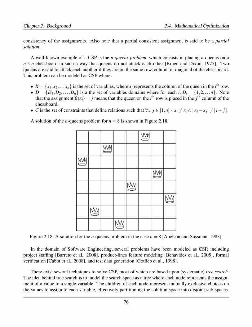
Chapter 2. Background 2.4. Mathematical Optimization

consistency of the assignments. Also note that a partial consistent assignment is said to be a partialsolution.

A well-known example of a CSP is the n-queens problem, which consists in placing n queens on an× n chessboard in such a way that queens do not attack each other [Bruen and Dixon, 1975]. Twoqueens are said to attack each another if they are on the same row, column or diagonal of the chessboard.This problem can be modeled as CSP where:

• X = {x1,x2, . . .xn} is the set of variables, where xi represents the column of the queen in the ith row.• D = {D1,D2, . . . ,Dn} is a the set of variables domains where for each i, Di = {1,2, . . .n}. Note

that the assignment θ(xi) = j means that the queen on the ith row is placed in the jth column of thechessboard.• C is the set of constraints that define relations such that ∀x, j ∈ [1,n] · xi 6= x j∧ | xi− x j |6=| i− j |.

A solution of the n-queens problem for n = 8 is shown in Figure 2.18.

Figure 2.18. A solution for the n-queens problem in the case n = 8 [Abelson and Sussman, 1983].

In the domain of Software Engineering, several problems have been modeled as CSP, includingproject staffing [Barreto et al., 2008], product-lines feature modeling [Benavides et al., 2005], formalverification [Cabot et al., 2008], and test data generation [Gotlieb et al., 1998].

There exist several techniques to solve CSP, most of which are based upon (systematic) tree search.The idea behind tree search is to model the search space as a tree where each node represents the assign-ment of a value to a single variable. The children of each node represent mutually exclusive choices onthe values to assign to each variable, effectively partitioning the solution space into disjoint sub-spaces.

76

2.4. Mathematical Optimization Chapter 2. Background

In this way, each root-leaf path in the tree corresponds to a complete variable assignment. However,the tree exponentially grows in the number of variables and the size of their domains. This means thatgenerating all the possible complete variable assignments and checking their consistency is infeasiblefor large problems. To address this problem, there exist tree search techniques that use (chronological)backtracking [Van Hentenryck, 1989]. In these techniques, the search tree is constructed and exploredin a depth-first process, which starts from a node with all the variables unassigned, i.e, with an emptypartial solution. At each iteration, the backtracking algorithm extends a partial solution by assigning avalue to an unassigned variable. This step is called labeling. If the new partial solution violates any ofthe constraints of the problem, a fail is said to be detected. In case of fail, the most recent assignmentis invalidated in a step backtrack. Then, the search continues iterating by assigning a value to the firstunassigned variable. The algorithm stops when a solution is found, i.e., when all variables are assignedin a way that no constraint is violated, or when no more labeling or backtracking is possible because nosolution exist. In general, the efficiency of the search process is influenced by the order in which thevariables and values are tried for assignments. The strategies to choose what variable and what valueto assign at each iteration are known under the name of variable and value ordering heuristics. In gen-eral, the values and variable order can be chosen either before the algorithm starts (static ordering), or atruntime depending on the current node of the tree (dynamic ordering) [Gent et al., 1996]. For instance,first-fail is one of the most common heuristics, which consists in ordering the variables in such a way thatthe tree levels have an increasing order of children [Haralick and Elliott, 1980]. This strategy is based onthe principle that, the earlier a fail is detected, the larger is the sub-tree that is proved to have no solutions,and that hence does not to be visited. For many problems of practical interest, proper ordering heuristicscan significantly speed up the search process. However, if heuristics choose a wrong assignment earlyin the tree, the search is likely to take too much time to backtrack and invalidate that early choice. Thisis because the efficiency of backtracking strongly depends on whether heuristics are able to choose theright branch early in the tree. A backtracking strategy called Limited Discrepancy Search (LDS) tries tomitigate this problem under the assumption that, most of the time, ordering heuristics chose the wrongassignments for variables only a small amount of time [Harvey and Ginsberg, 1995]. LDS rememberseach branch of a path p that ends with fail. Instead of the usual backtracking step, LDS tries the set ofpaths that differ from p by a single branch. If all of these fail, then LDS tries the paths that differ fromp by two branches, and so on. However, backtracking suffers in general from two major drawbacks:(1) late fail detection, due to fails not being detected before the corresponding branch in the tree is takenfor exploration. This can potentially lead the search to spend time on sub-trees that have no solution.(2) redundancy, due to conflicting values of variables not being remembered. This can potentially leadto repeated fails due to the same reason. For this reason, there exist several strategies aimed at mitigatingthese two drawbacks. Late fail detection is usually addressed through look-ahead strategies, which aimat predicting whether or not a tree branch leads only to fails (dead-end) [Apt, 1999]. This is usuallydone through Constraint Propagation algorithms, which eliminate from the solution space assignmentsinconsistent with some constraints [Haralick and Elliott, 1980]. Constraint Propagation considers theCSP constraints in increasing order of arity, and progressively eliminates (filters) from the variables do-main the values that violate such constraints. This domain reduction is referred to as domain filtering.Consider for instance a CSP where the variable x has domain [1,5], and is subject to the unary constraintc stating that x ≤ 3. Constraint Propagation starts the filtering process by reducing the domain of x to

77

Chapter 2. Background 2.4. Mathematical Optimization

the interval [1,3], because assigning 4 or 5 to x leads to a violation of c. Consider also the case wherethe same CSP has a variable y with domain [0,7], which is subject to the binary constraint y ≥ x+ 2.Since x is at least 1, y has to be at least 3, and therefore the Constraint Propagation algorithm filters thedomain of y reducing it to the interval [3,7]. Constraint Propagation repeatedly applies domain filteringuntil no more deduction is possible. There exist several strategies to perform Constraint Propagationand domain filtering. For instance, forward checking is a look-ahead strategy that performs ConstraintPropagation at each branch of the tree [Haralick and Elliott, 1980]. There exists also another class oftechniques, namely look-back strategies, which aim at addressing the backtracking redundancy by eitherdeciding how far to backtrack at each step, or by remembering the causes of past fails [Bayardo Jr andSchrag, 1997]. For instance, backjumping detects conflicting variables of a fail, and backtrack directlyto the assignment of those variables, instead of the most recently assigned variable [Dechter and Frost,2002]. On the other hand, techniques such as backchecking and backmarking record compatible andincompatible sets of assignments for variables. In this way, the search algorithm does not spend effortinto checking whether an assignment occurred in the past leads to a fail or not, and does not consider forfuture branches assignments which are already known to lead to fail.

2.4.1.2 Constraint Optimization Problems (COP)

A Constraint Optimization Problem (COP) can be considered as a Constraint Satisfaction Problem ex-tended by an objective (or cost) function that evaluates the quality of each solution. Therefore, weformalize COP in the following way [Russell et al., 1995]:Constraint Optimization Problem (COP). A Constraint Optimization Problem (COP) P is a couple(P′,F) where:

• P′ = (X ,D,C) is a CSP.• F :

(X → φ(X)

)→V is an objective (or cost) function that associates a variable assignment of P′

to a set V with a partial order ≤. F is defined only for complete consistent variable assignments(solutions).

Note that, when referring to variables, domains or constraints of a COP, we intend the ones of the associ-ated CSP. Also note that, for most practical problems, the partially ordered set V is a numerical set suchas N, Z, Q or R.

Preferred solution. A solution θ1 is said to be preferred to a solution θ2, iff the value of the objectivefunction applied to θ1 is less than the value of the objective function applied to θ2, i.e., iff F(θ1)≤ F(θ2).Optimal solution. A solution θ is said to be optimal iff no preferred solution θ ′ to θ exists, i.e., iff∀θ ′ ∈ {X → φ(X)} · F(θ)≤ F(θ ′).

Note that this formalization is consistent with the generic definitions given at the beginning of this Sec-tion. Specifically, the objective function F of a COP can be seen as a generic function f : A→ B thatmaps an assignment in A to a value in a partially ordered set B. Specifically, f is defined only for thecomplete consistent assignments (solutions) in A′ ⊆ A. In this way, the argument of the minimum of f

78

2.4. Mathematical Optimization Chapter 2. Background

restricted to A′ is exactly the solution s ∈ A′ such that f (s) is the minimum of f 12.

A well-known example of COP is the job-shop scheduling problem, which consists in assigning aset of jobs to processing machines [Coffman and Bruno, 1976]. Each job is a sequence of tasks, eachcompleted in a given processing time. Tasks must be performed in a specific order, and on a specificmachine. Therefore, a solution to the problem is a schedule of job sequences on machines, such thatno machine is processing two tasks at once. In general, machines consume resource while operating,and one wants to minimize the total time where the set of machines is active. Therefore, the optimalsolution to a job-shop scheduling problem is a schedule which minimizes the jobs makespan, i.e., thetotal elapsed time between the beginning of the first task, and the completion of the last task. Amongseveral application fields, COP have indeed been used for scheduling analysis, especially in the domainof manufacturing systems [Baptiste et al., 2001].

The techniques to solve COP are mostly extensions of the tree search algorithms to solve CSP. Specif-ically, Constructive algorithms gradually extend a partial solution to a complete one. The basic construc-tive algorithm is branch-and-bound, which iteratively searches for solutions by applying backtrackingand constraint propagation to the search tree [Lawler and Wood, 1966]. Opposite to algorithms for CSP,branch-and-bound does not stop as soon as a feasible solution is found, but keeps track of the best solu-tion found (incumbent), and its cost (objective function upper bound). At each iteration, the algorithmsearches for a solution with a lower cost than the upper bound. To do so, it evaluates the best value thatthe partial solutions can yield once all of its variables are assigned (objective function lower bound).Each time a value is assigned to a variable in the partial solution, the lower bound of that assignmentis computed. If the lower bound is greater than the upper bound, the subtree under the current partialassignment can not contain a solution with a better cost, and is pruned from the tree.

Most approaches for COP are complete, in the sense that they return the optimal solution upon ter-mination. However, for large problems, complete approaches can take long time to terminate. For thisreason, incomplete techniques have been devised to solve COP, and optimization problems in general.Such techniques are discussed in Section 2.4.2.

2.4.2 MetaheuristicsIn the field of Mathematical Optimization, there exist some problems whose global optimum is too hard tofind within reasonable time. This mostly happens when the objective function is hard to express throughequations, and no analytic or numerical approximation technique can be used to solve the problem. Insuch cases, the optimal solutions often have unknown characteristics, and the set of all possible solutionsis too large to be enumerated. However, most of the time, generating an arbitrary solution to the problemrequires significantly lower effort than finding the optimum. In such cases, the problem is often cast as asearch problem. Recall from Section 2.3.3 that a search problem is a problem that consists of three main

12 Traditionally, COP are defined as minimization problems. This is because a maximization problem of a function f withvalues in a partially ordered set B can be seen as a minimization problem of the same function where the partial order of B isinversed. For most practical problems, the partial order is a numerical set. In this case, maximizing f is indeed equivalent tominimizing − f . When not specified, in this thesis we assume that a COP models a minimization problem.

79

Chapter 2. Background 2.4. Mathematical Optimization

characteristics: (1) the definition of problem variables, (2) the definition of criteria to evaluate values(solutions) for these variables, and (3) the process of finding, from the set of possible values (searchspace), solutions that fulfill the criteria at best.

The field of Stochastic Optimization studies randomized algorithms and techniques which attemptat finding optimal solutions to these hard search problems. Specifically, metaheuristics is a term oftenused to describe the most general class of Stochastic Optimization algorithms13 [Luke, 2009]. Thesealgorithms can be used whenever it is possible to generate solutions and evaluate their quality. Opposedto analytical gradient-based methods [Snyman, 2005], metaheuristics do not require the search criteriato be expressed as functions, and therefore they are often referred to as black-box techniques. However,the search criteria are often referred to as objective function(s) to maximize or minimize, even thoughthey are not usually expressed as mathematical objects. Metaheuristics are used to solve problems inmany domains, including Software Engineering. Indeed, metaheuristics are extensively used in the areaSearch-Based Software Testing for test case generation, selection, and prioritization (Section 2.3.3).

2.4.2.1 Random Search and Hill-Climbing

In general, all metaheuristics can be described in terms of five steps [Luke, 2009]: (1 – initialize) providean initial set of solutions, (2 – assess) evaluate the quality of the solutions, (3 – tweak) create a newset of solutions by randomly modifying the existing ones, (4 – select) define a new set of solutions bychoosing a mix of old and new solutions to keep in memory, (5 – iterate) repeat steps 2-4 until giventermination criteria are reached. The solutions in steps 1-4, which the algorithm uses to drive the searchtowards the optimum, are typically referred to as candidate solutions of the problem at a given iteration.Given this description in five steps, metaheuristics differ from each other based on the logic behind steps3 and 4. The most naive search algorithm is Random Search, where solutions are randomly generated andevaluated against the search criteria [Hamlet, 1994]. The generation process can continue until the time orresource budget expires, and usually returns only the best solutions found. For instance, Random Testinghas been used in the context of Software Engineering for long time, proving to be effective in severalcase studies [Duran and Ntafos, 1984]. However, most search algorithms exploit specific properties ofthe solutions in an attempt to perform better than Random Search in terms of quality of solutions found,and time needed to find such solutions. The simplest algorithm that implements a basic reasoning overthe solutions found is Hill-Climbing [Blum and Roli, 2003]. This algorithm first randomly generatesa solution, and then creates a new version by making a small random modification. Then, it keeps thebest version with respect to the search criteria, and continues iterating by making new modifications tothe last kept solution. Hill-Climbing attempts at exploiting the supposition that similar solutions havesimilar quality with respect to the search criteria. In this way, small modifications generally result insmall changes in quality, and keeping the best version of two solutions allows to climb the hill of quality,up to reaching a plateau where these small modifications do not increase quality anymore.

13 Note that there is no universal agreement on a definition for metaheuristics. In general, Stochastic Optimization tech-niques such as Simulated Annealing, Evolutionary Algorithms, or Swarm Intelligence are traditionally seen as metaheuristics,while others such as Markov Chain Monte Carlo or Gibbs Sampling are not. To avoid confusion, in this thesis we do notdistinguish between the terms of metaheuristic and (randomized) search algorithm, even though in the literature this is notalways the case.

80

2.4. Mathematical Optimization Chapter 2. Background

Note that Random Search and Hill-Climbing are based upon two fundamentally different strategiesto find optimal solutions. On the one hand, Random Search continuously generates solutions unrelatedto each other, thus exploring the search space in an attempt to find the optimum. On the other hand, Hill-Climbing starts from one solution and exploits it by incrementally improving it with small modifications.Random Search fundamentally implements a Global Search strategy, by visiting different regions of thesearch space. Hill-Climbing instead implements a Local Search strategy, where small moves are madein the most promising directions of the search space. Global, explorative algorithms such as RandomSearch and local, exploitative algorithms such as Hill-Climbing perform very differently based on theshape of the function to optimize.

(2.19.1) Unimodal function (2.19.2) Noisy function

(2.19.3) Needle-in-a-Haystack type of func-tion (2.19.4) Deceptive function

Figure 2.19. Four examples of quality functions where Random Search and Hill-Climbing tend to per-form very differently [Luke, 2009]

Consider for instance Figure 2.19, where each graph depicts an objective function to maximize. Thex-axes report the solutions in the search space, while the y-axes report the value of the objective function.Hill-Climbing performs very well in cases such as in Figure 2.19.1, where there is a strong relationshipbetween the distance along the x-axis of two candidate solutions, and their quality. In this scenario,Random Search is very unlikely to reach the global optimum. However, when there is no relationship be-tween the distance of two solutions and their quality (Figure 2.19.2), Hill-Climbing is likely to convergeto a local optimum, possibly with a similar objective value as Random Search. In general, Hill-Climbing

81

Chapter 2. Background 2.4. Mathematical Optimization

is effective when the objective function has an informative gradient, which leads the search towards highquality solutions. In the unimodal and noisy functions, there is such gradient, and Hill-Climbing is guar-anteed to find the best solution within the neighborhood of the initial solution. Consider now the functionin Figure 2.19.3: in this case, there is no gradient to guide Hill-Climbing towards the optimum. There arealso cases, such as Figure 2.19.4, where the exploitation strategy of Hill-Climbing is counterproductive,since the gradient is likely to lead the search away from the optimum. In these last two cases, a globalsearch approach is more likely to perform better than local search. For vast majority of optimizationproblems where metaheuristics are applied, the shape of the objective function is not known, and there-fore it is not possible to predict whether an explorative or exploitative behavior is preferable. For thisreason, metaheuristics essentially combine the principles of Random Search (global explorative search),and Hill-Climbing (local exploitative search) [Glover and Kochenberger, 2003].

2.4.2.2 Genetic Algorithms (GA)

Many metaheuristics have been defined over the years, most of which have been successfully appliedto solve problems in Software Engineering [Harman, 2007]. However, it is beyond the scope of thisthesis to provide a thoughtful discussion on the different kinds of randomized search algorithms. Inthe context of Search-Based Software Testing, the literature [Ali et al., 2010] reports successful resultsespecially when using a class of metaheuristics known as Genetic Algorithms (GA) [Goldberg, 2006].Although there is no universally accepted definition, one can identify four elements that most methodsreferred to as GA have in common: (1) populations of individuals, (2) selection according to fitness,(3) crossover to produce new offspring, and (4) random mutation of new offspring [Mitchell, 1998].Each individual is referred to as chromosome or genotype, and represents a candidate solution for a givenproblem. Chromosomes consist of a set of genes, where each gene encodes a value in the solution. Thenumber of genes in a chromosome, is often referred to as the chromosome length. A typical GA startsby randomly generating a population of chromosomes, and evaluating their fitness by calculating thevalue of a fitness function. Then, the algorithm iterates through a series of generations consisting of threemain steps. (1) First, a pair of chromosomes is randomly selected with increasing probability accordingto fitness. (2) Then, the pair is crossed over to form two offspring, whose genes are then randomlymutated. (3) Finally, the offspring replaces two chromosomes the population, chosen with decreasingprobability according to fitness. Each of these three steps is performed by a specific operator, whichimplements the logic of selecting, crossing-over, and mutating chromosomes. Similar to what happensin nature, during a series of generations the fittest chromosomes tend to survive in the population, whilethe unfit are discarded. The main assumption behind GA is that high quality parents produce a highquality offspring, so that, similar to biological evolution, only the fit individuals survive and proliferate.Note that the selection, crossover, and mutation probabilities define the trade-off between explorativeand exploitative behavior. For instance, a strategy with higher mutation than crossover probability leadsto an explorative behavior that prefers to generate new solutions instead of optimizing the current ones.Similarly, a selection operator that tends to always discard unfit chromosomes leads to an exploitativebehavior that prefers inbreeding to outbreeding. There exists a number of free and commercial libraries,available in several programming languages, which implement GA: notable examples include OPEN

82

2.4. Mathematical Optimization Chapter 2. Background

BEAGLE14, the Genetic Algorithms Utility Library (GAUL)15, the Java Genetic Algorithms Package(JGAP)16, and the Genetic Algorithms Library (GALIB)17.

GA have been used for many activities in SBST, including the generation of workloads that representworst-case scenarios with respect to task deadlines [Briand et al., 2005]. Recall from Section 2.3.2 thatgenerating stress test cases that push a system into violating performance requirements is challengingbecause of the large set of possible scenarios where task can interact, and the complex nature of RTESwhich renders such task interactions unpredictable. Therefore, it is a natural choice to cast this problemas a search problem, and solve it through the use of metaheuristics. The key idea that enables the useof GA is to model the arrival times of aperiodic system tasks as chromosomes, and to evaluate theirfitness by computing the value of a function that properly rewards scenarios with deadline misses. Thisfitness function depends on the end times of tasks, which can be calculated starting from a fixed arrivalpattern. Indeed, the fitness of each chromosome is calculated by simulating the schedule that the Real-Time Operating System produces in case of the arrival pattern specified by the chromosome. We presentbelow a brief description of this GA-based approach for stress testing of task deadlines [Briand et al.,2006].

• Population, Chromosomes, and Genes. The initial population consists of 80 chromosomes,where each chromosome represents a set of arrival times for aperiodic tasks, i.e., an arrival pat-tern for the RTES. Each gene in the chromosome is encoded as the pair ( jk, t), where jk is the kth

execution of task j, and t is the arrival time of jk.• Crossover Operator. The algorithm uses with 0.7 probability a n-point crossover operator, where

n is the number of aperiodic tasks. Each crossover point is defined after the set of genes correspond-ing to an aperiodic task. In this way, chromosomes cross over exchanging genes associated to thesame task. Each crossover produces two offspring, where the genes of the parents are inheritedby the offspring with 0.5 probability, in a way that the children inherit each gene from a differentparent. Note that, due to real-time constraints, two consecutive arrival times of each aperiodic taskmust be separated by its minimum and maximum interarrival times. During the search, it mayhappen that a crossover operation breaks this constraint on a certain chromosome. In such case,the algorithm invalidates the operation, and proceeds by applying it to a different chromosome.• Mutation Operator. The genes in the chromosome are mutated by randomly replacing one arrival

time. This replacement is done by generating a time value in the interval defined by the minimumand maximum interarrival times of the preceding task execution. The mutation operator is appliedat each gene with a probability of 1.75 ·(λ

√l)−1, where λ is the population size, and l is the length

of the chromosomes.

The population size, and the crossover and mutation rates, have been derived from the literature ofGA and tuned for the specific domain of deadline miss analysis [Briand et al., 2005]. This GA-basedapproach uses the GALIB implementation, and has been successfully used to generate stress test cases in

14 http://code.google.com/p/beagle/15 http://gaul.sourceforge.net/16 http://jgap.sourceforge.net/17 http://ancet.mit.edu/ga/

83

Chapter 2. Background 2.4. Mathematical Optimization

a case study from the avionics domain featuring the weapon control system of a military aircraft [Lockeet al., 1990].

84

Chapter 3

Problem Description

Real-Time Embedded Systems (RTES) are becoming increasingly more complex and critical in manyindustry sectors. A main aspect of such complexity is their concurrent architecture that entails that sev-eral tasks are triggered and executed in parallel in ways which are difficult to establish a priori [Gomaa,2006]. Moreover, RTES are often safety critical [Kopetz, 2011], and thus bound to meet strict perfor-mance requirements. In addition, their tasks must satisfy execution constraints in terms of dependencyfrom shared computational resources, triggering of other tasks, maximum completion time, and execu-tion priority. Such complexity gives rise to a multitude of possible task execution scenarios at runtime,for which any manual reasoning is very inefficient, if not infeasible. In the domain of safety-criticalRTES one is especially interested in those particular scenarios that exercise a system in a way that tasksare pushed as close as possible to violate their performance requirements. Identifying such scenarios isthe basis for stress testing, a high-priority activity in the validation of RTES [Beizer, 2002]. In the rest ofthis chapter, we will first introduce the principles behind stress testing through an abstract example (Sec-tion 3.1), and then we will discuss the problem concretely in an industrial case study from the maritimeand energy domain (Section 3.2).

3.1 Finding Worst-case Scenarios in Real-Time EmbeddedSystems

Most of the approaches for analyzing time-related properties in RTES are based on a combination ofreal-time scheduling theory (Section 2.1.1) and static Worst-case Execution Time (WCET) analysis (Sec-tion 2.1.2). These methods estimate the schedulability of a tasks set under a given scheduling policy [Tin-dell and Clark, 1994], assuming worst case situations with respect to tasks arrival times, and using es-timates for task execution times [Baker, 2006]. For instance, the Completion Time Theorem (CTT)provides a sufficient condition for deadlines to be met in case of a task set of independent tasks scheduledwith the Rate Monotonic algorithm [Lehoczky et al., 1989]. The CTT specifies that, if each task meets itsdeadline when all tasks start executing at the same time, then the tasks will meet their deadlines for anycombination of start times. The CTT assumes that task do not depend on each other, which is hardly thecase in large and complex RTES. For this reason, the CTT has been extended into the Generalized Com-

85

Chapter 3. Problem Description 3.1. Finding Worst-case Scenarios in Real-Time Embedded Systems

pletion Time Theorem (GCTT) by considering interdependent tasks that share resources with exclusiveaccess [Gomaa, 2006]. Note that both the CTT and the GCTT only consider periodic tasks. For schedul-ing analysis, the GCTT has been extended to also consider aperiodic tasks [Sha and Goodenough, 1989].In this extension, aperiodic tasks are considered as periodic tasks with period equal to their maximuminterarrival time [Sprunt et al., 1989]. The CTT and the GCTT both consider that the worst-case scenariowith respect to task deadlines is the case where all tasks are simultaneously ready to execute when thesystem starts. However, this does not hold when both interdependent and aperiodic tasks are present.Consider for instance a fixed-priority preemptive scheduler that schedules the task set J = { j1, j2, j3} de-scribed in Table 3.1. The first row reports the observation interval T of the task set, and the number c ofcores of the target platform, i.e., the maximum number of tasks that can run in parallel. The first columnsof the table report the tasks priority, duration, period, minimum and maximum interarrival times, anddeadline. The last two columns report triggered tasks, and tasks that share computational resources withexclusive access. A centered dot (·) indicates that the property does not hold for a task. For example, j0is periodic, and therefore does not have minimum and maximum interarrival times. Similarly, j0 triggersj1 upon finishing execution, and does not share computational resources with other tasks. Note that, asit often happens in RTES analysis, time is discretized into time quanta. This means that time-relatedproperties of tasks are expressed as multiples of a time quantum. In the example, T is an integer intervalof 9 time quanta.

T = [0,8] c = 1

Task priority duration period min_ia max_ia deadline triggers depends

j0 0 2 9 · · 6 j1 ·j1 1 3 · · · 4 · ·j2 2 2 · 9 9 3 · ·

Table 3.1. Example system with three tasks, one of which is triggered

In this task set, j0 is a periodic task that triggers j1, and j2 is a higher priority aperiodic task. TheGCTT assumes that the worst-case scenario happens when j0 and j2 arrive simultaneously at the begin-ning of the observation interval. Note that this scenario does not lead to any deadline miss, as showedin Figure 3.1.1. However, there exists a scenario where j1 misses its deadline: this happens if j2 ar-rives after j0 has finished, as depicted in Figure 3.1.2. Note that similar examples can also be made forresponse time and CPU usage.

This example shows two important concerns when analyzing time-related properties of RTES. First,it shows how the GCTT result, i.e., that the worst-case scenarios happen when each task arrives simulta-neously at the beginning of the observation interval, is not valid when tasks have complex dependencies.Second, the example shows how the task arrival times have a great impact on hard real-time properties,and specifically, on deadline constraints. Note that arrival times of aperiodic tasks depend on the envi-ronment, and can never be predicted prior to the execution of the system. Indeed, the arrival times alsovary across different system executions due to the unpredictability of the environment.

For the reasons above, in order to evaluate deadline miss constraints, we need a strategy to search for

86

3.2. Motivating Case Study Chapter 3. Problem Description

(3.1.1) j0 and j2 arrive simultane-ously, but no task misses its deadline

(3.1.2) j2 arrives when j1 is execut-ing, and makes it miss its deadline

Figure 3.1. Impact of changes in the arrival times of tasks with respect to deadline miss properties

all the possible task arrival times. The search has to be performed in an effective way with the objectiveof finding scenarios that violate performance requirements or are close to violating them. In software for-mal verification, time-related properties expressed in a RTES models have been successfully verify withModel Checking (MC) approaches [Alur et al., 1990]. Such properties typically represent conditions,e.g., deadline misses, that should never hold in the system at any given time. Usually, MC approachescast the search of these properties as a reachability query over a Finite State Machine representing thesystem behavior. However, MC is mostly used for verification, i.e., to check if a given set of real-timetasks satisfy some property of interest. In general, one wants to complement formal design verificationby testing the system implementation, which is the focus of this thesis. Specifically, we focus on theproblem of identifying scenarios that exercise a system in a way that tasks are pushed as close as possibleto violate their performance requirements on deadlines, response time, and CPU usage. Consistent withthe widely accepted definition [Beizer, 2002], we refer to this activity as stress testing (Section 2.3.2).Specifically, given a performance requirement, we define a stress test case as a sequence of arrival timesfor aperiodic tasks that the search identifies as likely to violate that performance requirement.

The ultimate goal of this thesis is to define an efficient and effective strategy for the generation ofstress test cases. To do so, we have devised an approach based on UML/MARTE modeling (Chapter 5),where the search for arrival times of aperiodic tasks is carried out by a strategy where Constraint Pro-gramming (CP) (Chapter 6) is combined with Genetic Algorithms (GA) (Chapter 7).

3.2 Motivating Case StudyThe main motivation behind the work described in this thesis comes from the case study in the mar-itime and energy domain concerning a Fire and gas Monitoring System (FMS). The FMS is developedby Kongsberg Maritime (KM)1, a leading company in the production of systems for positioning, survey-

1www.km.kongsberg.com

87

Chapter 3. Problem Description 3.2. Motivating Case Study

ing, navigation, and automation to merchant vessels and offshore installations. The goal of the systemis to monitor potential gas leaks in oversea oil extraction platforms, and trigger an alarm in case a fireis detected. The system monitors and displays to human operators data coming from smoke detectors,heat detectors, and gas flow sensors. When the system receives some critical data from the hardwaresensors, it automatically triggers actuators, such as fire sprinklers and audio/visual alarms. Techniciansconstantly monitor the system, and can also directly interact with it, for instance to manually tune oper-ational parameters or control events raised by specific data. The FMS software architecture is shown inFigure 3.2.

Figure 3.2. The architecture of the Fire and Gas Monitoring System (FMS)

The software part of the system consists of a set of drivers, and a set of control modules. Drivers im-plement I/O communication between the system and the external environment, such as hardware sensors,actuators, and human operators. Control Modules implement the application logic of the FMS, i.e., theyprocess data coming from the environment and accordingly decide the operations to perform. Driversand Control Modules are the main software components of the FMS, and run on a Real-Time OperatingSystem that is executed over a multicore computing platform. The whole FMS is composed by approx-imately 5000 control modules and 500 sensors and actuators that communicate with the system throughca. 100 different drivers. Drivers and control Modules have an approximate size of 5 and 1 thousandslines of source code (kLoC) each. The system runs on a Real-Time Operating System (RTOS), namelyVxWorks2, that is configured with a fixed-priority preemptive scheduling policy. VxWorks is installed ona platform featuring a tri-core processor. This architectural design is common in many industry sectorsrelying on embedded systems [Buttazzo, 2011].

Figure 3.3 shows the key entities of the FMS which are relevant to our study. A communicationscenario consists in a driver communicating externally with some sensors and/or actuators, and commu-nicating internally with control modules. To cope with the large number of external hardware devices,

2 http://www.windriver.com/products/vxworks

88

3.2. Motivating Case Study Chapter 3. Problem Description

Figure 3.3. A class diagram representing the key entities in the Fire and Gas Monitoring System (FMS)

the system runs in parallel several instances of each driver. In the FMS, each driver implements a specificcommunication protocol, and it is meant to communicate only with sensors and actuators that implementthe same protocol. The reason for having different types of drivers relies in the variety of sensors andactuators built by different vendors. Indeed, devices work under specific communication protocols thathave to be implemented by the drivers in order to successfully connect the devices to the system.

Drivers constitute the most critical part of the FMS. Indeed, one of the main complexity factors indrivers is that they are meant to bridge the timing discrepancies between hardware devices and soft-ware controller modules. Hence, their design typically consists of parallel tasks that communicate asyn-chronously to smooth the data transfer between hardware and software. Therefore, drivers are subject tostrict requirements to ensure that their flexibility does not come at the cost of performance. Specifically,in each FMS driver (1) no task should miss its deadline, (2) the response time should be less than 1second, and (3) the CPU usage should be below 20%.

Three important context factors in the FMS case study influenced the definition of our approach togenerate stress test cases. (1) Different instances of a given driver are independent, in the sense thatthey do not communicate with one another and do not share memory. (2) The purpose of the constrainton CPU usage is to enable engineers to estimate the number of driver instances of a given monitoringapplication that can be deployed on a CPU. These constraints express bounds on the amount of CPU timerequired by one driver instance. Therefore, in this thesis we focus on individual driver instances. Theindependence of the drivers (first factor above) is the key to being able to localize CPU usage analysisto individual instances in a sound manner. (3) The drivers are not memory-bound, i.e., task deadlines,response time, and CPU usage, are not significantly affected by activities such as disk I/O and garbagecollection. To ensure this, KM over-approximates the maximum memory required for each driver in-stance by multiplying the number of hardware devices connected to the driver instance and the maximumsize of data sent by each device. Execution profiles at the partner company indicate that the drivers areextremely unlikely to exceed this limit during their lifetime.

Figure 3.4 shows the an a example of three communication scenarios in the FMS, represented by adashed rectangle. In the scenario at the top, the instance i1 of driver d1, which implements the protocol

89

Chapter 3. Problem Description 3.2. Motivating Case Study

Figure 3.4. An example showing three communication scenarios in the Fire and Gas Monitoring System(FMS)

p1, communicates with the sensors s1 and s2 and the control modules m1 and m2. In the scenario at thecenter, the instance i2 of d1 communicates with the sensor s3, the actuator a1, and the modules m1 and m2.In the scenario at the bottom, the instance i3 that runs the driver d2 communicates with the actuator a2and the module m3. Note that, in each scenario, the driver implements the same communication protocolof the sensors and actuators involved.

Drivers in the FMS share the same design pattern, where periodic and aperiodic tasks communicateasynchronously through buffers. There exist two major types of driver implementations, one with fouraperiodic tasks (Section 3.2.1), and another with a singular task consisting of four activities in an infiniteloop (Section 3.2.2)3. However, regardless of the implementation, all the drivers have to satisfy the sameperformance requirements. Nonetheless, the specific factors determining whether or not the performancerequirements will be satisfied at runtime closely depend on the specific implementation used.

3.2.1 Implementation 1: Data Transfer with Four Aperiodic TasksThe first implementation of the FMS drivers consists of six tasks communicating through three buffers.More precisely, in this implementation a generic driver consists of:

3 Recall from Section 2.1.1 that a singular task is executed only once during the system execution, and that an activityrepresents a sequence of operations that a task executes.

90

3.2. Motivating Case Study Chapter 3. Problem Description

• Three communication buffers, namely BoxIn, Queue, and BoxOut. These buffers serve as tem-porary storage locations for the data transiting from the hardware devices to the control modules.Moreover, the buffers have a fixed capacity, and exclusive access by software tasks, i.e., no twotask can simultaneously access a buffer. BoxIn and BoxOut contain formatted data that is comingfrom the external hardware, and going towards the control modules respectively. Queue contains apriority-ordered list of commands extracted from the data that have to be processed by the controlmodules.• Two periodic tasks, namely PullData and PushData. These tasks are periodically activated by a

scan signal, and transfer data from the hardware sensors, and to the control modules respectively.• Two aperiodic tasks, namely IOBoxRead (IOBR) and IOQueueRead (IOQR). These tasks are acti-

vated at irregular interval of times by a check signal that is fired by the RTOS to notify that BoxInand Queue are almost full and need to be emptied.• Two tasks triggered by aperiodic tasks, namely IOQueueWrite (IOQW), and IOBoxWrite (IOBW).

These tasks are activated by a trigger signal from IOBoxRead and IOQueueRead respectively,when they finish reading from the BoxIn and Queue buffers.

Figure 3.5. A typical operating scenario of drivers in the FMS consisting of a unidirectional data transferbetween external hardware sensors and control modules. The scenario is implemented by two periodictasks, four aperiodic tasks, and three buffers.

Figure 3.5 shows how tasks in the first driver implementation collaborate in the typical scenario, thatis a unidirectional data transfer between hardware sensors and control modules. (1) PullData periodicallyreceives data from sensors or human operators, formats the data in an appropriate command form, and(2) writes it in the buffer BoxIn. (3) When BoxIn is almost full, the check signal activates IOBoxRead that(4) reads the data from the buffer and (5) triggers IOQueueWrite. IOQueueWrite extracts the commandsfrom the data, and (6) stores them in the priority Queue. When Queue is reaches a critical capacity,

91

Chapter 3. Problem Description 3.2. Motivating Case Study

(7) the check signal activates IOQueueRead that (8) reads the highest priority command and (9) triggersIOBoxWrite which in turn (10) writes the command to BoxOut. When the periodic scan signal (11) acti-vates PushData, the task (12) reads the commands from BoxOut and finally (13) sends them to the controlmodules for processing.

As mentioned before, this asynchronous design is necessary for the drivers to smooth the data transferbetween external devices and control devices. However, the data transfer functionality is subject tostrict performance requirements in terms of task deadlines, response time, and CPU Usage. Specifically,(1) each of the six tasks that implement a driver has to finish before its deadline, typically in the rangeof milliseconds. Consider for instance a scenario where PushData is blocked on the BoxOut driver byIoBoxWrite, and thus is late in alerting the control modules that a fire has been detected. In this case,the system will fail to timely activate the alarm and the sprinklers, with potential severe consequences.Task deadlines are hard real-time constraints that have to be met to ensure that the system safely reactsin case of fire. However, the FMS is also subject to soft-real time constraints such as (2) response times.Indeed, the interval of time between an execution of PullData and the execution of PushData that sendsthe commands to the control modules has to be bounded. Consider for instance a scenario in whichsome data in BoxIn is not promptly emptied. If too much time passes after that data is collected by theexternal hardware, the new data arriving from the same sensor will arrive when the old data has still notbeen processed. Therefore, the FMS will perform the commands corresponding to the first chunk of datawhen the environment state has already changed. This behavior degrades the QoS, as the system will notreact promptly to external changes. Finally, driver instances are independent from each other, and thusconcurrently executed in the same hardware platform. For this reason, (3) each driver instance must notexceed a given threshold of CPU usage. Indeed, if a driver has a significant impact on the CPU time,other driver instances may have to wait too long for the operative system to grant them computationalresources and potentially fail to timely process critical data.

The main variables determining whether or not these requirements is satisfied at runtime are the arrivaltimes of the check signal. These arrival times depend on the environment, in the sense that they dependon the data sent by the hardware sensors via PullData. The arrival times also vary across different systemexecutions, as a consequence of the impossibility to predict the data coming from the sensors. Therefore,in order to evaluate task deadlines, response time, and CPU usage, we need a strategy to search for allthe possible task arrival times. The search has to be performed in an effective way with the objective offinding scenarios that are predicted to violate the requirements, or be close to violating them. Indeed, themore likely is a scenario predicted to violate a performance requirement, the higher the chances that thetest case characterized by such scenario stresses the system.

3.2.2 Implementation 2: Data Transfer with One Singular Task and FourActivities

There also exists a second implementation of the FMS drivers, where the functionalities of IoBoxRead,IoBoxWrite, IoQueueRead, and IoQueueWrite are implemented in four activities of a singular task,namely IoDispatch. IoDispatch encloses the four activities in an infinite loop, and sequentially executes

92

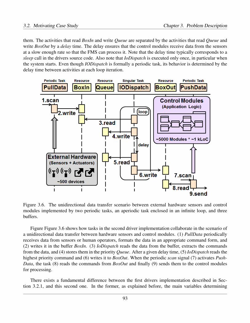
3.2. Motivating Case Study Chapter 3. Problem Description

them. The activities that read BoxIn and write Queue are separated by the activities that read Queue andwrite BoxOut by a delay time. The delay ensures that the control modules receive data from the sensorsat a slow enough rate so that the FMS can process it. Note that the delay time typically corresponds to asleep call in the drivers source code. Also note that IoDispatch is executed only once, in particular whenthe system starts. Even though IODispatch is formally a periodic task, its behavior is determined by thedelay time between activities at each loop iteration.

Figure 3.6. The unidirectional data transfer scenario between external hardware sensors and controlmodules implemented by two periodic tasks, an aperiodic task enclosed in an infinite loop, and threebuffers.

Figure Figure 3.6 shows how tasks in the second driver implementation collaborate in the scenario ofa unidirectional data transfer between hardware sensors and control modules. (1) PullData periodicallyreceives data from sensors or human operators, formats the data in an appropriate command form, and(2) writes it in the buffer BoxIn. (3) IoDispatch reads the data from the buffer, extracts the commandsfrom the data, and (4) stores them in the priority Queue. After a given delay time, (5) IoDispatch reads thehighest priority command and (6) writes it to BoxOut. When the periodic scan signal (7) activates Push-Data, the task (8) reads the commands from BoxOut and finally (9) sends them to the control modulesfor processing.

There exists a fundamental difference between the first drivers implementation described in Sec-tion 3.2.1, and this second one. In the former, as explained before, the main variables determining

93

Chapter 3. Problem Description 3.2. Motivating Case Study

whether or not the driver performance requirements are satisfied at runtime are the arrival times of thecheck signal. However, in the second implementation the arrival times of IoDispatch do not have signif-icant impact on the performance requirements. This is because the task arrives only once, and when thesystem is started. In this case, the delay times between the first and the last two activities of IoDispatchdetermine whether or not the driver satisfies its performance requirements at runtime. Indeed, if the delaytimes are too short, IoDispatch is continuously running and keeps the CPU busy, eventually exceeds thegiven threshold on CPU usage. On the other hand, if the delay times are too large, pullData may fill upBoxIn, and be blocked waiting for IODispatch to empty the buffer. As a result, pullData is not able toterminate before its next scan signal arrives, missing its deadline.

Opposite to the arrival times in the first implementation, the delay times do not depend on the en-vironment, but rather are tunable parameters that engineers can choose when configuring the system.Therefore, in order to evaluate task deadlines, response time, and CPU usage in this second implemen-tation, we need a strategy to search for all the possible task delay times. Note that the objective of thesearch remains finding scenarios that are predicted to violate the requirements, or be close to violatingthem. The difference with the search in the case of the first implementation lies within the choice of thevariables to search for.

The problem of ensuring that performance requirements are satisfied in the second drivers implemen-tation leads to a definition of stress test cases which is different from the one given at the end of Sec-tion 3.1. Indeed, in this second drivers implementation, a stress test case with respect to a performancerequirement is a sequence of delay times (rather than arrival times) likely to violate that performance re-quirement. These stress test cases retain the traditional goal of stress testing, i.e., ensuring that the systemsatisfies the performance requirements even under the worst operating conditions. However, these testcases identify values for tunable parameters (rather than replicable environmental conditions) that violatethe requirements. Therefore, the execution traces of these stress test cases can be used to ensure that uponconfiguration the parameter values remain within safe margins. Note that, on the other hand, executiontraces of stress test cases characterized by arrival times have to be carefully analyzed together with thesystem architecture, in order to find possible bottlenecks hindering the system performance. We finallypoint out that, for the rest of this thesis, we are consistent with the traditional meaning of stress testing inRTES with respect to environmental conditions, and hence with the definition of stress test cases given atthe end of Section 3.1. Recall from Section 2.1.1 that indeed, for scheduling analysis, each activity canbe considered as a task, provided that the RTOS overhead for managing tasks in negligible with respectto their execution and interarrival times. For this reason, when not specified otherwise, stress test casesare characterized by sequences of arrival times for aperiodic tasks.

94

Part II

Approach and Discussion

Chapter 4

Automating the Generation of Stress TestCases in Real-Time Embedded Systems: anOverview

In this thesis, we present an approach for generating stress test cases exercising performance require-ments of RTES. The framework blends UML/MARTE modeling to capture the timing and concurrencyaspects of the system design and platform, and automated search based on Genetic Algorithms (GA) (Sec-tion 2.4.2.2) and Constraint Programming (CP) (Section 2.4.1) to generate the stress test cases. Anoverview of the approach is shown in Figure 4.1.

The approach builds upon a conceptual model that captures details about the timing and concurrencyaspects in the software components and computing platform of the RTES. Specifically, the conceptualmodel captures abstractions in the software application, e.g., tasks with their priorities, periods, depen-dencies, and in the computing platform, e.g., processing cores and scheduling policies. Entities in thisconceptual model are mapped to MARTE stereotypes, thus defining a subset of the profile which is rele-vant for supporting the generation of stress test cases. In particular, the abstractions related to the softwareapplication are mapped to stereotypes that extend UML metaclasses represented in sequence diagrams.Note that sequence diagrams are popular for visualizing concurrent multi-threaded interactions, and areintuitive to most developers [Harel and Marelly, 2003]. On the other hand, abstractions in the conceptualmodel related to the computing platform are mapped to stereotypes that extend generic UML metaclasses,which can be represented in class or deployment diagrams. We validate the conceptual model in the Fireand Gas Monitoring System (FMS) introduced in Section 3.2, showing that it can be applied in an indus-trial setting with a practically reasonable overhead. The conceptual model and its mapping to MARTEhave been first introduced in a conference paper [Nejati et al., 2012], and is discussed in Chapter 5.

Design and platform models stereotyped with MARTE organize the input data for our approach,which generates stress test cases using automated search. Specifically, we cast the generation of stress testcases as an optimization problem over the abstractions represented in design and platform models. Thegoal of the optimization problem is finding arrival times for aperiodic tasks that maximize the likelihood

97

Chapter 4. An Overview of Stress Testing in Real-Time Embedded Systems

Figure 4.1. An overview of our approach for generating stress test cases in Real-Time Embedded Sys-tems.

of the RTES violating its performance requirements on task deadlines, response time and CPU usage.To solve this optimization problem, we discuss a search strategy based on CP. Specifically, we presenta Constraint Optimization Model (COP) that models the system design, real-time properties, executingplatform, and performance requirements. The COP is implemented as an Optimization ProgrammingLanguage (OPL) model, which is solved with IMB ILOG CPLEX CP OPTIMIZER. We validate ourCP-based search strategy in the FMS, showing that CP is able to effectively identify arrival times foraperiodic tasks that are predicted to maximize deadline misses, response time and CPU usage. We alsocompared CP with GA in five systems from safety-critical domains, analyzing both strategies in termsof the trade-off between the time needed to generate stress test cases, and their power for revealingworst-case scenarios with respect to task deadlines. The CP-based strategy has been first introduced ina workshop paper [Di Alesio et al., 2012], and in three conference papers [Nejati et al., 2012, Di Alesioet al., 2013, Di Alesio et al., 2014], and is discussed in Chapter 6.

The series of experiments to evaluate the performance of CP and GA shows an opposing trend. Specif-ically, GA is more efficient, i.e., faster in generating test cases, while CP is more effective, i.e., it generatestest cases that are more likely to reveal deadline misses. In practice, it is also important to evaluate towhat extent the test cases generated by an approach exercises different aspects of the system under test.This concept is commonly known as test coverage, and is an important metric to assess the quality ofa test suite (Section 2.3). In these experiments GA generated a large number of test cases that werealso highly diverse, i.e., they had a higher variety in terms of (1) time span, (2) preemptions betweentask executions, and (3) number of aperiodic task executions. On the other hand, CP generated fewersolutions which were mostly redundant. At a high level of abstraction, the experiments show that GA

98

Chapter 4. An Overview of Stress Testing in Real-Time Embedded Systems

provides more coverage than CP due to the higher diversity in the test cases generated. For this reason, inthis thesis we propose a strategy (GA+CP), based on the combined use of GA and CP, aimed at holdingboth the efficiency and solutions diversity of GA and the effectiveness of CP. The choice of combiningthe two search strategies has been motivated by the analysis of the results of our previous experiments.Specifically, we looked into the possibility of further improving the solutions computed by GA by per-forming a complete search with CP in their neighborhood. In this way, GA+CP takes advantage of theefficiency of GA, because solutions are initially computed with GA, and the subsequent CP search islikely to terminate in a short time since it focuses on the neighborhood of a solution, rather than on theentire search space. GA+CP also takes advantage of the diversity of the solutions found by GA, becauseCP performs a local search in subspaces defined by GA solutions. Similarly, GA+CP takes advantage ofthe effectiveness of CP since, once GA has found a solution, CP further improves it by either finding thebest solution within the neighborhood, or proving upon termination that no better solution exists. GA+CPhas first been introduced in a journal paper [Di Alesio et al., 2015], and is discussed in Chapter 7.

99

Chapter 5

Modeling Real-Time Embedded Systems withUML/MARTE to Support Stress Testing

Recall from Section 2.2.2.3 that UML/MARTE defines a large number of abstractions related to RTESperformance. Even though these abstractions support the definition of methodologies for performanceanalysis and verification, MARTE does not include guidelines on how to identify the relevant stereotypesand tagged values for a particular kind of analysis. In this section, we propose a conceptual model thatcaptures, independently from any modeling language, the abstractions required to support stress testing inRTES (Section 5.1). To simplify the application of our conceptual model in Model-Driven Engineering(MDE) approaches, we propose a mapping of our conceptual model to UML/MARTE (Section 5.2).Note that we define the abstractions needed to support stress test cases in two steps, i.e., first defininga conceptual model, and then its mapping to MARTE. This formalization approach is similar to theone in MARTE, where concepts related to RTES are first defined a domain model, and then formalizedas stereotypes and tagged values in a UML representation (Section 2.2.2.3). Finally, we validate theconceptual model in the Fire and Gas Monitoring System (FMS) described in Section 3.2. The validationshows that the conceptual model and its mapping to UML/MARTE can be applied with a practicallyreasonable overhead in an industrial context (Section 5.3).

5.1 A Conceptual Model to Support Stress Testing in Real-TimeEmbedded Systems

To enable a sound definition of our approach, we first define a conceptual model that identifies the keyabstractions of RTES that are relevant for stress testing. Note that, even though RTES share some com-monalities, they all require domain-specific configurations. This means that, we need to define a concep-tual model that captures the abstractions required for stress testing independently from specific contexts.Recall from Section 3.1 that the goal of our approach is finding worst-case scenarios for RTES tasks thatare likely to violate task deadlines, response time, and CPU usage constraints. Therefore, our conceptualmodel is based upon abstractions defined in the real-time scheduling theory (Section 2.1.1), such as tasks,activities, and scheduling policies. Figure 5.1 shows an overview of the conceptual model we propose,

101

Chapter 5. UML/MARTE Modeling 5.1. Conceptual Model

whose entities are explained below. Classes in the conceptual model are partitioned into the Applicationand Platform packages, which respectively correspond to the system design and platform of Figure 4.1.

Figure 5.1. Our conceptual model representing the key abstractions to support stress testing in Real-TimeEmbedded systems.

• Application. The software part of a RTES is an embedded application, which consists of severalparallel software tasks, and is allocated in a computing platform.

– Activity. Recall from Section 2.1.1 that an activity is a sequence of operations in a task, andthat task activities within a task are sequentially executed. Each activity a has an estimatedduration or Worst-Case Execution Time (WCET). Consecutive activities within a task areseparated by a delay time, and each activity starts executing after a given release. Activitiescan trigger other activities: for example, each activity in a task triggers the following one, thusdefining a temporal ordering. This is because after the last statement in an activity is executed,the program control flow executes the first statement in the following activity. Activities canalso trigger other tasks: for example, upon meeting certain conditions, an activity can spawna new task to perform additional operations. Moreover, activities in a task can also depend oneach other by sharing computational resources which are generally used for communication.

– DataDependency. Activities can depend on each other because they communicate in a syn-chronous or asynchronous way.

102

5.1. Conceptual Model Chapter 5. UML/MARTE Modeling

– Buffer. Asynchronous communication between two activities can use a buffer, whose accessis protected by semaphores, and hence is blocking. This means that at most one activity canaccess a buffer at any time. Note that, in this thesis, we only consider the case where tasksare communicating asynchronously through buffers.

– Task. The software part of a RTES consists of a set of parallel tasks that have to completebefore a given deadline. Each task also has a priority that determines the relative importanceof a task with respect to other tasks, so that the scheduler executes higher priority tasks beforelower priority tasks. Periodic tasks are triggered by timed events handled by the global clock,and are invoked at regular intervals. Therefore, their arrival times are fixed, and equal to mul-tiples of one interval, called period, which is counted starting from an offset. Periodic tasksare commonly used to send and receive data at regular interval of times, e.g., PushData andPullData in Figure 3.5. On the other hand, the arrival times for aperiodic tasks are bound byminimum and maximum inter-arrival times, which indicate the minimum and maximum timeintervals between two consecutive arrivals of the event triggering the task. Aperiodic tasks areinstead used to process asynchronous events/communications, e.g., IODispatch in Figure 3.5.Finally, the arrival time of triggered tasks is determined by particular activities, which spawnthe task upon finishing their execution. During its lifetime, a task can perform the followingoperations.∗ Trigger. Communicates to the scheduler that the task is ready to start a new execution in

response to a triggering event. The origin of the event depends on the type of the task.For periodic tasks, the event comes from an internal clock, for aperiodic tasks the eventcomes from the environment, and for triggered tasks the event comes from another task.∗ Start. Begins execution after having been assigned to a CPU core by the scheduler. This

operation precedes the execution of the first activity of each task.∗ Finish. Completes execution. This operation is performed after the last activity in a task

has completed.∗ Wait. Temporarily stops execution in order to synchronize with another task, or to acquire

a resource. Note that each buffer access within an activity implies an implicit wait by itstask.∗ Sleep. Temporarily stops execution for a given amount of time. Note that a sleep call for

a given time t at the beginning (end) of an activity corresponds to a release (delay) forthat activity equal to t.∗ Resume. Communicates to the scheduler that the task is ready to resume execution after

a previous wait or sleep operation.The state machine in Figure 5.2 shows the lifecycle of a task, where the operations determinetransitions between states. Tasks start in the idle state, and only consume CPU time in therunning state. Note that there is no final state. This is common in embedded systems, whichare intended to run continuously. Also note that, in our model, activities within tasks onlyrelease the CPU when preempted by the scheduler, so that the CPU can be used by anotheractivity belonging to a higher priority task. This means that tasks perform the operations onlybetween two consecutive activities.

• Platform. A computing platform is the hardware part of a RTES that executes embedded applica-

103

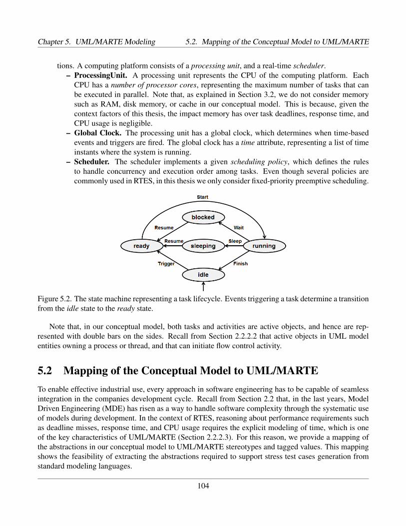
Chapter 5. UML/MARTE Modeling 5.2. Mapping of the Conceptual Model to UML/MARTE

tions. A computing platform consists of a processing unit, and a real-time scheduler.– ProcessingUnit. A processing unit represents the CPU of the computing platform. Each

CPU has a number of processor cores, representing the maximum number of tasks that canbe executed in parallel. Note that, as explained in Section 3.2, we do not consider memorysuch as RAM, disk memory, or cache in our conceptual model. This is because, given thecontext factors of this thesis, the impact memory has over task deadlines, response time, andCPU usage is negligible.

– Global Clock. The processing unit has a global clock, which determines when time-basedevents and triggers are fired. The global clock has a time attribute, representing a list of timeinstants where the system is running.

– Scheduler. The scheduler implements a given scheduling policy, which defines the rulesto handle concurrency and execution order among tasks. Even though several policies arecommonly used in RTES, in this thesis we only consider fixed-priority preemptive scheduling.

Figure 5.2. The state machine representing a task lifecycle. Events triggering a task determine a transitionfrom the idle state to the ready state.

Note that, in our conceptual model, both tasks and activities are active objects, and hence are rep-resented with double bars on the sides. Recall from Section 2.2.2.2 that active objects in UML modelentities owning a process or thread, and that can initiate flow control activity.

5.2 Mapping of the Conceptual Model to UML/MARTETo enable effective industrial use, every approach in software engineering has to be capable of seamlessintegration in the companies development cycle. Recall from Section 2.2 that, in the last years, ModelDriven Engineering (MDE) has risen as a way to handle software complexity through the systematic useof models during development. In the context of RTES, reasoning about performance requirements suchas deadline misses, response time, and CPU usage requires the explicit modeling of time, which is oneof the key characteristics of UML/MARTE (Section 2.2.2.3). For this reason, we provide a mapping ofthe abstractions in our conceptual model to UML/MARTE stereotypes and tagged values. This mappingshows the feasibility of extracting the abstractions required to support stress test cases generation fromstandard modeling languages.

104

5.2. Mapping of the Conceptual Model to UML/MARTE Chapter 5. UML/MARTE Modeling

Figure 5.3. A sequence diagram modeling the data transfer scenario described in Figure 3.6. The se-quence diagram is stereotyped with UML/MARTE stereotypes and tagged values mapped to concepts inthe conceptual model we defined.

Some of the abstractions in our conceptual model are already present in UML. Recall from Sec-tion 2.2.2.2 that each active object in a sequence diagram can be associated to a lifeline. In this way, exe-cution specifications represent the activities in our conceptual model. Similarly, occurrence specificationsrepresents sending and receiving of messages, and therefore can be used to describe the synchronous andasynchronous communication defined in our conceptual model. Figure 5.3 shows a sequence diagramcapturing the data transfer scenario of the Fire and Gas Monitoring System (FMS) described in Sec-tion 3.2.2. Tasks in the driver application are active objects, while buffers are passive objects. Eachactivity within a task is depicted using an execution specification, i.e., as a box on the task lifeline thatshows the interval of time that the task performs the activity. Therefore, pullData has two activities,ioDispatch has four, and pushData has three. Note that the order of activations on a task lifeline impliesthe temporal ordering between activities of that task. In sequence diagrams, a synchronous messagebetween two activities is shown using an arrow with a filled head, while an asynchronous message isshown by an arrow with an open head. Synchronous communication is blocking and does not necessarilyrequire a buffer, because the sending activity must wait until the receiving activity is ready to receive themessage. On the other hand, asynchronous communications can use buffers. Recall from Section 3.1 thatin the FMS, and hence in Figure 5.3, all communications are asynchronous and use buffers.

Even though UML sequence diagrams can already capture several concepts in a real-time applica-tion, other concepts defined in our conceptual model do not have appropriate counterparts in pure UML.Specifically, the schedulability concepts, and the timing and concurrency attributes of our conceptualmodel are captured by UML/MARTE. Recall from Section 2.2.2.3 that MARTE provides a Software Re-source Modeling (SRM) package, that defines abstractions to model software resources, and communica-

105

Chapter 5. UML/MARTE Modeling 5.2. Mapping of the Conceptual Model to UML/MARTE

tion between resources. Therefore, we map our notion of buffer to the MessageComResource stereotype,which is meant to represent artifacts for communicating messages among concurrent resources.

MARTE also provides a Generic Quantitative Analysis Modeling (GQAM) package, which is in-tended to provide a generic framework for collecting information required for performance and schedu-lability analysis. The domain model of this package includes two key abstractions that closely resembleour notions of task and activity, Scenario and Step respectively. A step is defined in the domain model ofGQAM as a unit of execution, while a scenario is defined a sequence of steps. These two concepts arerepresented by the stereotypes «GaStep» and «GaScenario», which we map in our conceptual model toactivities and tasks respectively. Note that these two stereotypes can be applied to a wide set of behavior-related elements in the UML metamodel, and in particular, to elements in sequence diagrams. In particu-lar, «GaScenario» and «GaStep» inherit from both «TimeModels::TimedProcessing», which extends theUML metaclasses Behavior, Message, Actions, and «GRM::Resource», which extends NamedElement.Steps and Scenarios in MARTE also include a list of measures that are widely used for analyzing ofreal-time properties of embedded systems. We map attributes of tasks and activities in our conceptualmodel to the tagged values representing those measures. Specifically, we map interOccTime, the timeinterval between two successive occurrences of scenarios, to period, offset, minimum, and maximuminter-arrival times of task. We also map execTime, i.e., the execution time of a step, to duration of activi-ties, and selfDelay, i.e., the time steps are delayed for execution, to activities delays and releases. Thesetagged values can be specified either as single values, or as bounds defining an interval. Note that «GaS-cenario» does not specify tagged values representing the concept of task deadline. Indeed, in MARTE,the concept of deadline is defined in the Schedulability Analysis Modeling (SAM) package, in particularthrough the domain class EndToEndFlow, and the associated stereotype «SaEndToEndFlow». For thisreason, we also map «SaEndToEndFlow» to our notion of task, so that the task deadline is mapped to thetagged value endToEndDeadline. We point out one discrepancy in our mapping of tasks and activities.In MARTE, the concept of execution priority is defined for individual steps, rather than for scenarios.Nonetheless, at the implementation level, it is common to define priorities at task-level, rather than atactivity-level. Indeed, our conceptual model reflects this fact by specifying priorities as task, rather thanactivity, attributes. To address this discrepancy, we assume in our mapping that steps within a scenarioall have the same priority p, and hence the scenario has priority p.

Finally, the abstractions related to the computing platform in our conceptual model are not capturedin sequence diagrams, but can be represented using MARTE stereotypes applied to class and deploy-ment diagrams. Specifically, the Generic Resource Modeling (GRM) package defines the stereotypes«Scheduler» and «SchedulingPolicy», which are mapped to the corresponding entities in our conceptualmodel. Furthermore, we map processing units to «ComputingResource», and global clocks to «Logical-Clock». In this way, we map the global clock time to the timeBase tagged value. Table 5.1 summarizes

106

5.3. Validation of the Conceptual Model Chapter 5. UML/MARTE Modeling

the mapping between entities in our conceptual model, and stereotypes in MARTE.

Conceptual Model UML/MARTE

Class/Attribute Stereotype/Tagged Value Sub-profile

App

licat

ion

Task «GaScenario» GQAM«SaEndToEndFlow» SAM

Task::deadline SaEndToEndFlow::endToEndDeadline SAMTask::priority GaStep::priority 1 GQAMPeriodicTask::offset GaScenario::interOccT GQAMPeriodicTask::period GaScenario::interOccT GQAMAperiodicTask::maxIa GaScenario::interOccT GQAMAperiodicTask::minIa GaScenario::interOccT GQAMActivity «GaStep» GQAMActivity::delay GaStep::selfDelay GQAMActivity::duration GaStep::execTime GQAMActivity::release GaStep::selfDelay GQAMBuffer «MessageComResource» SRM::SW_Interaction

Pla

tform

Scheduler «Scheduler» GRMScheduler::policy Scheduler::schedPolicy GRMSchedulingPolicy «SchedPolicyType» MARTE_Library::GRM_BasicTypesProcessingUnit «HwProcessor» HRM::HW_Logical::HW_ComputingProcessingUnit::nbCores HwProcessor::nbCores HRM::HW_Logical::HW_ComputingGlobalClock «LogicalClock» Time::TimeAccesses::ClocksGlobalClock::time Clock::timeBase Time::TimeAccesses::Clocks

Table 5.1. Mapping of the entities in our conceptual model to UML/MARTE. PeriodicTask, Aperiod-icTask and TriggeredTask do not appear in the mapping because they inherit the stereotypes from theirsuperclass Task.

5.3 Validation of the Conceptual Model in the Fire and GasMonitoring System

The practical usefulness of our approach depends two main factors. First, we need to investigate whetherthe input to our approach, i.e., the system specification stereotyped with the subset of UML/MARTE wedefined, can be provided with reasonable overhead. This first factor sums up to validating our conceptualmodel and its mapping to UML/MARTE in an industrial context, and is discussed in this section. Second,we also need to investigate whether the output of our approach can effectively be used to derive stresstest cases that are likely to violate performance requirements. This second factor closely depends on thesearch strategies used to generate test cases, and is discussed in Section 6.2 and Section 7.2.

As discussed in Section 5.1, the information required for generating stress test cases is captured by the1Note that, as explained above, MARTE defines the concept of priority at activity-level, rather than at task-level. For this

reason, we assume that all activities in a task have the same priority. Therefore, the priority of a task is equal to the priority ofits composing activities.

107

Chapter 5. UML/MARTE Modeling 5.3. Validation of the Conceptual Model

conceptual model we defined. To gather this information, we first built UML sequence diagrams for theFMS I/O drivers, starting by the existing design documents and implementation. Such sequence diagramswere iteratively validated and refined in collaboration with the lead engineer of the drivers in KongsbergMaritime. We extracted the quantitative elements of our conceptual models, i.e., the concrete values forthe tagged values, from design documents, source code, and performance profiling logs. Specifically, weextracted the values for priorities, deadlines, and periods of tasks from the certification design documents,and the drivers source code. Furthermore, we extracted the values for the activities duration from theperformance profiling logs of the drivers. We created the sequence diagrams augmented with the timinginformation from the MARTE stereotypes over 8 days, involving approximately 25 man-hours of effort.This was considered worthwhile, as safety-critical I/O drivers have a long lifetime and are regularlycertified. Finally, we obtained information on the computing platform from the RTOS configuration andhardware design documents. We finally remark that, the main rationale behind the mapping we providedin Table 5.1 is to allow engineers to develop and manipulate our input design notation with any modelingenvironment that supports UML/MARTE.

108

Chapter 6

Using Constraint Programming to Automatethe Generation of Stress Test Cases

The main objective of the conceptual model and its mapping to UML/MARTE is to organize the inputdata for our approach, which automates the stress test case generation. Recall from Section 3.1 that wedefine a stress test case with respect to a performance requirement as a sequence of arrival times foraperiodic tasks which maximizes the chance to violate that requirement. In this section, we cast thegeneration of stress test cases as a search problem over the space of task arrival times, and we solve thesearch problem with Constraint Programming (CP). Specifically, we cast the search for arrival times asa Constrained Optimization Problem (COP) over the abstractions of our conceptual model (Section 6.1).The goal of the COP is finding arrival times for aperiodic tasks that maximize the likelihood of the RTESviolating its performance requirements on task deadlines, response time and CPU usage. We refer to thisstrategy for generating stress test cases as CP-based strategy. When confusion with the programmingparadigm can not arise, we also refer to the CP-based strategy as CP.

We assess the practical usefulness of our CP-based strategy in two steps. First, we validate the COPin the Fire and Gas Monitoring System (FMS) described in Section 3.2 (Section 6.2.1). This validationshows that the COP effectively identifies in a few minutes stress test cases that are predicted to violatethe FMS requirements on deadline misses, response time, and CPU usage.

However, for practical use, test case generation has to accommodate time and budget constraints. Forthis reason, it is essential to investigate the trade-off between the time needed by a strategy to generatestress test cases, and their power for revealing deadline misses. Recall from Section 2.4.2.2 that a strategybased on Genetic Algorithms (GA) [Briand et al., 2006] has been proposed to support stress testing oftask deadlines by searching for worst-case scenarios, and is therefore a natural comparison baseline. Werefer to this strategy for generating stress test cases as GA-based strategy, or, when confusion with themetaheuristic can not arise, as GA. Therefore, the second step in validating CP consists in a systematiccomparison with GA for the purpose of generating stress test cases for deadline misses. We designed aseries of experiments in five subject systems from safety-critical domains, ranging in size and complex-ity (Section 6.2.2). The experiments show that, on average, GA is generally more efficient, i.e., faster

109

Chapter 6. Generating Stress Test Cases with CP 6.1. Description of the COP

in generating test cases, while CP is more effective, i.e., it generates test cases that are more likely toreveal deadline misses. Note that this result opens up the possibility to combine the two strategies inorder to retain the advantages of both. An hybrid approach combining GA and CP, which aims at strikinga profitable trade-off between efficiency and effectiveness, is discussed in Chapter 7.

6.1 A Constrained Optimization Problem to Automate theGeneration of Stress Test Cases in Real-Time EmbeddedSystems

We address the problem of determining worst-case schedules of tasks with an approach inspired by thework done in Constraint Programming to solve traditional scheduling problems [Baptiste et al., 2001].Specifically, we cast the search for real-time properties that characterize the worst-case schedules, namelyarrival times for aperiodic tasks, as a Constraint Optimization Problem (COP). The key idea behind ourformulation relies on five main points.

1. First, we model the system design, which is static and known prior to the analysis, as a set of con-stants (Section 6.1.1). The system design mainly consists of the tasks of the real-time application,their dependencies, period, duration, deadline, and priority.

2. Then, we model the system properties that depend on runtime behavior as a set of variables (Sec-tion 6.1.2). The main real-time properties are the number of task executions, the arrival times ofaperiodic tasks, and the specific runtime schedule of the tasks.

3. We model the Real-Time Operating System (RTOS) scheduler as a set of constraints among suchconstants and variables (Section 6.1.3). Indeed, the real-time scheduler periodically checks fortriggering signals of tasks and determines whether tasks are ready to be executed or need to bepreempted. Constraints of our model are described in.

4. We model the performance requirement to be tested, i.e., task deadlines, response time, or CPUusage, as an objective function to be maximized (Section 6.1.4).

5. Finally, we encapsulate the logic behind the RTOS scheduler in an effective labeling strategy overthe variables of the model (Section 6.1.5). By design, the scheduler tries to execute high prioritytasks as soon as possible, potentially preempting tasks with lower priority. We exploit this behaviorby proposing a labeling strategy for the variables related to tasks execution.

A graphical overview of our approach is shown in Figure 6.1. Our analysis is subject to two mainassumptions:

1. The RTOS scheduler checks the running tasks for potential preemptions at regular and fixed in-tervals of time, called time quanta. Therefore, each time value in our problem is expressed as amultiple of a time quantum. Accordingly to the specification of the RTOS executing the FMS, weconsider the length of ten milliseconds for time quanta.

2. The interval of time in which the scheduler switches context between tasks is negligible comparedto a time quantum.

110

6.1. Description of the COP Chapter 6. Generating Stress Test Cases with CP

Figure 6.1. A graphical overview of the Constrained Optimization Model to generate stress test cases.

These two assumptions are reasonable in the context of RTES, as the scheduling rate of operatingsystems varies in the ranges of few milliseconds, while the time needed for context switching is usuallyin the order of nanoseconds [Singh, 2009]. These assumptions allow us to consider time as discrete, andmodel the COP as an Integer Program (IP) over finite domains. We implemented the COP in OPL, andsolved it with IBM ILOG CPLEX CP OPTIMIZER. This choice was motivated by practical reasons,such as extensive documentation, strong supporting community, and its acknowledged efficiency to solveoptimization problems. Despite the scheduling nature of our problem, we implemented our model as atraditional IP as opposed to using the scheduling features of OPL and CP OPTIMIZER. This is becausewe could not express a preemptive priority-driven scheduling behavior in an effective way that exploitedthe capabilities of the solver.

Figure 6.2. Real-time scheduling example of four tasks on a dual-core platform

The rest of this section details our constraint model using the example shown in Figure 6.2. Thissystem features four tasks in increasing priority order, j0 to j3, running on a dual-core platform for 10time units. j0 and j1 are executed once, while j2 and j3 are executed twice. The figure reports the arrivaltimes and deadlines of the tasks, labeled by at and dl respectively, where the first index represents thetask, and the second the task execution. In this example, j0 is aperiodic, while j2 and j3 are periodic.

111

Chapter 6. Generating Stress Test Cases with CP 6.1. Description of the COP

Note that task j1 is triggered by j0 upon termination, and that j1 and j2 share the resource r12 withexclusive access.

6.1.1 ConstantsConstants are implemented as integers (int), integer ranges (range), tuples (tuple), sets of tuples (setOf )and integer expressions. Integers values are defined as external data.

Observation Interval. We define T as an integer interval of length tq, i.e., T def

= [0, tq−1].

T represents the time interval during which we observe the system behavior. Note that T is an integerinterval, as a consequence that time is discretized in our analysis. Therefore, each time value t ∈ T is atime quantum. In Figure 6.2, tq = 10 and T = [0,9].

Number of platform cores. We define c as the number of cores in the execution platform.

c represents the maximum number of tasks that can be executed in parallel. In Figure 6.2, c = 2, as atmost two tasks are allowed to run in parallel.

Set of tasks. We define J as the set of tasks of the system. We define Jp, Ja, and Jg as the set of periodic,aperiodic, and triggered system tasks, respectively.

Each task j ∈ J has a set of static properties, defined as constants, and a set of dynamic properties,defined as variables. Note that Jp, Ja, and Jg define a partition over J. We assume that OS tasks havelower priority than system tasks and can be preempted at any time, and hence, can be abstracted awayin our analysis. Each task j is implemented as an OPL tuple named Task, whose fields are the followingnon-relation constants. J is implemented as an OPL tuple set, while Jp, Ja, and Jg are OPL generic setsderived from J. In Figure 6.2, J = { j0, j1, j2, j3}, Ja = { j0}, Jp = { j2, j3}, and Jg = { j1}.

Priority of a task. We define pr( j) as the priority of task j. For simplicity, we define the set HP j of taskshaving higher or equal priority than j: HP j

def

= { j1 ∈ J | j 6= j1∧pr( j1)≥ pr( j)}.In Figure 6.2, pr( j0) = 0, pr( j1) = 1, pr( j2) = 2, and pr( j3) = 3.

Period of a task. We define pe( j) as the period of task j.

pe( j) is only defined if j is periodic. In Figure 6.2, pe( j2) = 5 and pe( j3) = 6.

Offset of a task. We define of ( j) as the offset of task j, i.e., the time, counted from the beginning of T ,after which the first period of task j begins.

of ( j) is only defined if j is periodic. In Figure 6.2, of ( j2) = 0 and of ( j3) = 1.

Delay of a task. We define dy( j) as the delay of task j, i.e., the time, that has to occur between twoexecutions of j.

In Figure 6.2, dy( j2) = 3.

112

6.1. Description of the COP Chapter 6. Generating Stress Test Cases with CP

Release of a task. We define re( j) as the release of task j, i.e., the time that j has to wait after its arrivalbefore starting to execute.

In Figure 6.2, all tasks have release 0.

Minimum and maximum inter-arrival times of a task. We define mn( j) and mx( j) as the minimumand maximum inter-arrival times of task j, respectively, i.e., the minimum and maximum time separatingtwo consecutive arrival times of j.

mn( j) and mx( j) are only defined if j is aperiodic since for all periodic tasks j, mn( j) = mx( j) = pe( j)trivially holds. In Figure 6.2, we assumed mn( j0) = 5 and mx( j0) = 10.

Duration of a task. We define dr( j) as the estimated Worst Case Execution Time (WCET) of task j. Forsimplicity, we define the integer interval Pj of execution slots as Pj

def

=[0, dr( j)−1

].

Since OPL does not support indexed ranges, Pj is implemented as a single range P def

= [0,maxj∈J

dr( j)−1].

This definition entails that ∀ j ∈ J · Pj ⊆ P. The iteration through values in Pj is emulated with a logicimplication. Indeed, the following properties hold for every logic predicate C and arithmetic expressionE.

∀p ∈ Pj · C(p) ⇐⇒ ∀p ∈ P · p < dr( j) =⇒ C(p) (6.1)∑p∈Pj

E(p) =∑p∈P

(p < dr( j)

)·E(p) (6.2)

Note that in Equation (6.2)(

p < dr( j))

is a boolean expression that is true if p < dr( j), and falseotherwise. For the rest of this paper, equalities and inequalities written within parentheses representboolean expressions that evaluate to the integer 1 if true, and to the integer 0 if false. This is also thedefault behavior in CP OPTIMIZER. In Figure 6.2, dr( j0) = 3 and Pj0 = [0,1,2].

Deadline of a task. We define dl( j) as the time, with respect to its arrival time, before which task jshould terminate.

In Figure 6.2, dl( j0) = 7, dl( j1) = 6, dl( j2) = 4, and dl( j3) = 3.

Triggering relation between tasks. We define tg( j1, j2) as a binary relation between tasks j1 and j2that holds if the event triggering j2 occurs when j1 finishes its execution. We define the sets TS j and STjof tasks triggered by and triggering j, respectively.

T S jdef

= { j1 ∈ J | tg( j, j1)} STjdef

= { j1 ∈ J | tg( j1, j)}

The relation tg is defined as irreflexive and antisymmetric. tg is implemented as an OPL tuple with twofields, the first being the task triggering, and the second being the task triggered. In Figure 6.2, tg( j0, j1)holds.

Dependency relation between tasks. We define de( j1, j2) as a binary relation between tasks j1 and j2that holds if there exists a computational resource r such that j1 and j2 access r during their execution

113

Chapter 6. Generating Stress Test Cases with CP 6.1. Description of the COP

in an exclusive way. We define the set DS j of tasks depending on j.

DS jdef

= { j1 ∈ J | j 6= j1∧de( j1, j)} (6.3)

The relation de is defined as reflexive and symmetric. This definition implies that j1 and j2 cannot beexecuted in parallel nor can preempt each other, but one can execute only after the other has releasedthe lock on the resource. de is implemented as an OPL tuple with two fields, each being one of the taskdepending on the other. In Figure 6.2, de( j1, j2) holds.

6.1.2 VariablesIndependent variables in our model are implemented as OPL finite domain variables (dvar int). Depen-dent variables are implemented as OPL variable expressions (dexpr int) defined through equality con-straints. The first three variables described hereafter, namely the number of task executions, their arrivaltimes, and active sets, are independent variables. The remaining variables described in this section are alldependent.

Number of task executions. We define te( j) as the number of times task j is executed within T . Forsimplicity, we define the integer interval K j of task executions for the task j as K j

def

= [0, te( j)−1].

Note that we refer to the kth execution of task j as the couple ( j,k). We assume the minimum andmaximum inter-arrival times bound the number of executions of an aperiodic task. This means that, foraperiodic tasks, te( j) is defined as a variable with domain

[⌊tq

mx( j)

⌋,⌊

tqmn( j)

⌋]. Similarly, we assume that

offset and period statically determine the number of executions of periodic tasks so that te( j)=⌊

tq−of ( j)pe( j)

⌋.

Therefore, the number of task executions of periodic tasks is constant, rather than variable. However, wedo not formally distinguish it from the number of task execution for aperiodic tasks. te is implemented asan integer array ranging over Jp if the task is periodic (or ranging over Jg if triggered by a periodic task),and as an integer variables array ranging over Ja if the task is aperiodic (or ranging over Jg if triggeredby an aperiodic task). Since OPL does not support ranges with variable bounds, K j is implemented as asingle constant range K.

K def

=

[0, max

(maxj∈Jp

⌊tq−of ( j)

pe( j)

⌋,max

j∈Ja

⌊tq

mn( j)

⌋)]

Note that K is defined as a range from 0 to the largest upper-bound for task executions of periodic andaperiodic tasks. This definition entails that ∀ j ∈ J · K j ⊆ K. The iteration through values in K j isperformed in a similar way as the case of Pj, thanks to the following properties for each logic predicateC and arithmetic expression E.

∀k ∈ K j · C(k) ⇐⇒ ∀k ∈ K · k < te( j) =⇒ C(k) (6.4)∑k∈K j

E(k) =∑k∈K

(k < te( j)

)·E(k) (6.5)

114

6.1. Description of the COP Chapter 6. Generating Stress Test Cases with CP

In Figure 6.2, te( j0) = 1, te( j3) = 2, K j1 = [0], and K j2 = [0,1].

Arrival time of a task execution. We define at( j,k) as the time when an event notifies the RTOS thattask j should be executed for the kth time.

We say that j arrives for the kth time at time t iff at( j,k) = t. When the specific execution k of j isunderstandable from the context, we simply say that j arrives at time t. In our analysis, we assume thatthe arrival time of periodic tasks is constant: ∀ j ∈ Jp, k ∈ K j · at( j,k) = o f ( j)+ k ·pe( j). Similarly tothe case of te, we do not formally distinguish the arrival times of periodic and aperiodic tasks. at hasdomain T for aperiodic tasks. In Figure 6.2, at( j0,0) = 0 and at( j2,1) = 5.

Active set of task executions. We define ac( j,k, p) as the pth time quantum in T in which task j isrunning for the kth execution. We also define A j,k as the integer vector of time quanta where j is executingfor the kth time, the vector A j of time quanta where j is executing, and the vector A of time quanta wheretasks are executing.

A j,kdef

= [ac( j,k, p) | p ∈ Pj] A jdef

= [A j,k | k ∈ K j] A def

= [A j | j ∈ J]

Note that A j and A are defined as vectors of vectors. Also note that we refer to both the set of all acvariables, and to A, as the schedule produced by the arrival times of the tasks in J. ac variables havedomain T . In Figure 6.2, ac( j0,0,0) = 0, ac( j0,0,1) = 2, A j0,0 = [1,2,4], A j0 =

[[1,2,3]

], and

A =[[[1,2,3]

],[[4,5]

],[[0,1], [6,7]

],[[1,2], [7,8]

]].

Preempted set of task executions. We define pm( j,k, p) as the number of time quanta for which the kth

execution of task j is preempted for the pth time.

pm( j,k, p) def

= ac( j,k, p)−ac( j,k, p−1)−1

pm is only defined for p > 0. In Figure 6.2, pm( j0,0,1) = 1, and pm( j0,0,2) = 0.

Start and end times of task executions. We define st( j,k) and en( j,k) as the first and the one after thelast time quantum in which task j is executing for the kth time.

st( j,k) def

= ac( j,k,0) en( j,k) def

= ac(

j,k,dr( j)−1)+1

We say that j starts or ends for the kth time at time t iff st( j,k) = t or en( j,k) = t − 1, respectively.In Figure 6.2, st( j0,0) = 0 and en( j1,0) = 6.

Waiting time of task executions. We define wt( j,k) as the time that j waits after its arrival time beforestarting its kth execution.

wt( j,k) def

= st( j,k)−at( j,k)

In Figure 6.2, wt( j0,0) = 0, and wt( j2,1) = 1.

115

Chapter 6. Generating Stress Test Cases with CP 6.1. Description of the COP

Deadline of task execution. We define ed( j,k) as the absolute deadline of the kth execution of j, i.e., thetime, with respect to the beginning of T , before which j should terminate to meet its deadline.

ed( j,k) def

= at( j,k)+dl( j)−1

ed is implemented as two-dimensional array of integer variable expressions ranging over the set J andthe range K. In Figure 6.2, ed( j0,0) = 6, and ed( j1,0) = 8.

Deadline miss of task execution. We define dm( j,k) be the amount of time by which j missed its deadlineduring its kth execution.

dm( j,k) def

= en( j,k)− ed( j,k)−1

dm is implemented as two-dimensional array of integer variable expressions ranging over the set J andthe range K. In Figure 6.2, dm( j0,0) =−3.

Blocking task execution time quantum. We define bl( j,k, j1,k1, p1) as a boolean variable that is trueif in the interval

[at( j,k),st( j,k)

)the task execution ( j1,k1) is active at the time slot p1:

bl( j,k, j1,k1, p1)def

= at( j,k)≤ ac( j1,k1, p1)< st( j,k)

In Figure 6.2, bl( j2,1, j1,0,1) = true, since ( j2,0) waits at t = 5 for the last time quantum of ( j1,0)before starting.

Higher priority active tasks. We define ha( j,k) as the number of time quanta in the interval[at( j,k),st( j,k)

)where exactly c tasks having higher priority of j and not depending on j are active.

Consider the summation indexes j1, k1, p1 defined over the sets HPj \DS j, K j1 , and Pj1 respectively, andthe summation indexes j2, k2, and p2 defined over the sets HP j \DS j, K j2 , and Pj2 , respectively.

ha( j,k) def

=∑

j1,k1,p1

bl( j,k, j1,k1, p1)∧

( ∑j2,k2,p2

bl( j,k, j2,k2, p2))= c

Note that for the definition of ha( j,k), it is important that HP j also includes tasks with equal prioritythan j. This is because, in the RTOS scheduling policy we consider, tasks can only preempt tasks withstrictly lower priority. In Figure 6.2, ha( j,k) = 0 for all task executions ( j,k), since in no case there aretwo tasks active when a task is waiting.

Dependent active tasks. We define da( j,k) as the number of time quanta in the interval[at( j,k),st( j,k)

)where task executions depending on j is active. Consider the summation indexes j1, k1,

p1 defined over the sets DS j, K j1 , and Pj1 , respectively.

da( j,k) def

=∑

j1,k1,p1

bl( j,k, j1,k1, p1)

116

6.1. Description of the COP Chapter 6. Generating Stress Test Cases with CP

In Figure 6.2, da( j2,1) = 1, because j1 is active for the time quantum t = 5 between the arrival and thestart of j2.

Dependent preempted tasks. We define dp( j,k) as the number of time quanta in the interval[at( j,k),st( j,k)

)where task executions depending on j have been preempted. Consider the summation

indexes j1, k1, p1 defined over the sets DS j, K j1 , and Pj1 , respectively.

dp( j,k) def

=∑

j1,k1,p1

pm( j1,k1, p1) ·bl( j,k, j1,k1, p1)

In Figure 6.2, dp( j,k) = 0 for all task executions ( j,k), since there are no dependent task preempted thatblock the execution of any task.

System load. We define ld(t) as the load of the system at time t, i.e., the number of tasks active at time t.Consider the summation indexes j, k, p defined over the sets J, K j, and Pj, respectively.

ld(t) def

=∑j,k,p

(ac( j,k, p) = t

)

In Figure 6.2, ld(0) = 2, and ld(3) = 1.

6.1.3 ConstraintsWe define five groups of constraints related to different aspects of the RTOS.

Well-formedness Constraints. Well-formedness constraints specify relations among variables that di-rectly follow from their definition in the schedulability theory.

Constraint WF1. Each task execution starts after its arrival and release time, and ends after the taskduration.

∀ j ∈ J, k ∈ K j · at( j,k)+ re( j)≤ st( j,k)≤ en( j,k)−dr( j) (WF1)

Constraint WF2. Consecutive executions of the same task are separated by task delays

∀ j ∈ J, k ∈ K j \{0} · en( j,k−1)+dy( j)≤ st( j,k) (WF2)

Constraint WF3. Arrival times of aperiodic tasks are separated by their minimum and maximum inter-arrival times.

∀ j ∈ Ja, k ∈ K j \{0} · at( j,k−1)+mn( j)≤ at( j,k)≤ at( j,k−1)+mx( j) (WF3)

117

Chapter 6. Generating Stress Test Cases with CP 6.1. Description of the COP

Constraint WF4. The time indexes p ∈ Pj define an order over the active time quanta of tasks.

∀ j ∈ J, k ∈ K j, p ∈ Pj \{0} · ac( j,k, p−1)< ac( j,k, p) (WF4)

Temporal Ordering Constraints. Temporal Ordering Constraints specify the relative ordering of tasksbasing on their dependency and triggering relations.

Constraint TO1. Each triggered task is executed the same number of times of its triggering task.

∀ j1 ∈ J, j2 ∈ TS j · te( j1) = te( j2) (TO1)

Constraint TO2. Each triggered task execution arrives when its triggering task execution ends.

∀ j1 ∈ J, k ∈ K j1 j2 ∈ TS j · en( j1,k) = at( j2,k) (TO2)

Constraint TO3. Executions of dependent tasks cannot overlap, i.e., each task can only start after theone it depends on has ended.

∀ j1 ∈ J, k1 ∈ K j1 j2 ∈ DS j, k2 ∈ K j2 · en( j1,k1)≤ st( j2,k2) ∨ (TO3)en( j2,k2)≤ st( j1,k1)

Constraint TO4. If two tasks that depend on each other arrive at the same time, the higher priority taskexecutes first.

∀ j1 ∈ J, k1 ∈ K j1, j2 ∈(DS j∩ (J \HP j)

), k2 ∈ K j2 · (TO4)

at( j1,k1) = at( j2,k2) =⇒ st( j1,k1)< st( j2,k2)

Multi-core Constraint. The Multi-core Constraint captures the specification of the number c of cores ofthe computing platform, and stating that no more than c tasks are allowed to be active in parallel at anytime. The constraint specifies that the system load should be less than the number of cores at any time.

∀t ∈ T · ld(t)≤ c (MC)

Note that, when c = 1, MC is equivalent to an alldifferent constraint over ac.

Preemption Constraint. The Preemption Constraint captures the priority-driven preemptive schedulingof the RTOS, and stating that each task should be preempted when a higher priority task is ready to beexecuted and no cores are available. The constraints specifies that the number of time quanta where atask execution is preempted times c is equal to the number of time quanta where higher priority tasks areactive. Consider the summation indexes j1, k1, and p1 defined over the sets HPj, K j1 , and Pj1 respectively.

∀ j ∈ J, k ∈ K j, p ∈ Pj · (P)

pm( j,k, p) · c =∑

j1,k1,p1

(ac( j,k, p−1)< ac( j1,k1, p1)< ac( j,k, p)

)

118

6.1. Description of the COP Chapter 6. Generating Stress Test Cases with CP

Scheduling Efficiency Constraint. The Scheduling Efficiency Constraint ensures that there is no un-necessary task preemption, and that tasks are executed as soon as possible. The constraint specifies that,for each time quanta in which a task execution ( j,k) is waiting, there should be either (1) exactly ctasks with higher priority that do not depend on j active, or (2) one task execution dependent on j that isactive, or (3) one task execution dependent on j that is preempted.

∀ j ∈ J, k ∈ K j · wt( j,k) = ha( j,k)+da( j,k)+dp( j,k) (SE)

6.1.4 Objective FunctionsWe formalized three objective functions, each modeling one performance requirement, and each meantto be maximized in a separate constraint model having the same constants, variables, and constraints.In this way, solutions to each of the three constraint models characterize worst-case scenarios for therequirement modeled by the function.Task Deadline Misses Function. We define FDM as the function that models the performance require-

ment involving task deadlines.FDM =

∑j∈J, k∈K j

2 dm( j,k)

As explained at the beginning of this chapter, the goal of our approach is to find values for the arrivaltimes of aperiodic tasks that maximize the likelihood of violating performance requirements, in particulardeadline misses. We formalized this concept through an objective function of whose value captures howarrival times compare in terms of their likelihood of triggering deadline misses. We first identify a set ofcharacteristics the function should meet:

• No deadline miss is overshadowed. In safety-critical real-time systems even a single deadline misscould lead the system to a fail state. Thus, a good function should not allow task executions whichmeet their deadline to overshadow deadline misses.• The more deadline misses, the higher the value. Intuitively, the function value should take into

account the number of deadline misses among task executions. Even if a system could recoverfrom a scenario where a task misses its deadline in a single execution, recovering from severaldeadline misses might be harder.• The larger the deadline misses, the higher the value. Our analysis is based on WCET estimates

(duration) for the system tasks. Such estimates could be over-pessimistic, and our approach couldcompute a test case identifying a deadline miss that does not happen when actually testing thesystem. However, the closest to its deadline a task is in our analysis, the more likely it is to miss adeadline in a real scenario. Such concept is captured by the quantity defined as deadline_miss: thelarger its value, the closer the task completion time to its deadline, with possibly the task missingits deadline. Hence, we expect a good function to prioritize scenarios where a larger deadline missis identified.

Having considered the criteria above, we adopted a modified version of the function defined by Briand etal. [Briand et al., 2006]:

119

Chapter 6. Generating Stress Test Cases with CP 6.1. Description of the COP

f ( j) =∑

k∈K j

2 dm( j,k)

Note that f is defined for a given task j. FDM is an alternative formulation of f which instead takes intoaccount all tasks is given by the sum of f for each task in the system:

FDM =∑j∈J

f ( j)

Also note that the purpose of f ( j) is to identify deadline miss scenarios for a single critical task j, sinceit has larger values when large deadline misses occur in j. On the other hand, FDM has larger valueswhen more deadline misses on several tasks occur, aiming at identifying scenarios stressing the wholesystem rather than a single task. Given that we use our subject systems for the purpose of experimentalevaluation and comparison, there is no clear guidance on how to choose a specific target task j for eachcase. For this reason, we model the performance requirement involving task deadlines with FDM. Recallfrom Section 6.1.2 that, dm( j,k) is positive if task j misses its deadline during its kth execution, andnegative otherwise. This means that large negative values stand for j ending long before its deadline.On the other hand, positive values stand for j failing to end before its deadline, thus missing it. Theexponential shape of the function favors executions with large deadline misses, thus avoiding them beingovershadowed by other executions.

Response Time Function. We define FRT as the function that models the system response time.

FRT =

(max

j∈J, k∈K jen( j,k)

)−(

minj∈J, k∈K j

at( j,k))

FRT measures the total length in time quanta of the schedule, starting from when the first task arrives, upto when the last ends. This function is also known in traditional scheduling as makespan.

CPU Usage Function. We define FCU as the function that models the system CPU usage.

FCU =

∑t∈T

(ld(t)> 0

)tq

FCU measures the average CPU usage of the system over T , by counting all the time quanta where at leastone task is active, i.e., where the system load is greater than 0.

6.1.5 Search HeuristicWe defined a search heuristic that refines the branching process of the CP OPTIMIZER solving algorithm.The heuristic specifies that the solver should mimic the behavior of a RTOS by first trying to schedule

120

6.1. Description of the COP Chapter 6. Generating Stress Test Cases with CP

tasks with higher priority. This is done by choosing the ac variables to branch on by decreasing priority,and then by assigning their time values in increasing order. For example, consider a system wherec = 1, j0, j1 ∈ J, pr( j1) > pr( j0). Suppose that, for given k0, p0, k1, j1 the filtering algorithm reducedthe domains of the ac variables to the set [0,1]. Figure 6.3.1 shows the branching tree in case the solverruns with default settings.

In the root node, the ac variables have domain [0,1]. The solver then tries the first variable assignmentin the branch b1, stating that j0 is executing at time 0. Then, the solver tries the second assignment inthe branch b2, stating that j1 is executing at time 0. This variable assignment violates the multi-coreconstraint MC since both j0 and j1 are executing at the same time. Therefore, the solver prunes thenode, backtracks to the father node, and tries the assignment in b3 where j1 is executing at time 1.This assignment violates the preemptive scheduling constraint P, since j1 has higher priority, but j0 isrunning instead. Only after backtracking up to the root node, the solver tries the assignments in b4 and b5which do not violate any constraint. Note that several other branching steps might have been necessaryif ac( j1,k1, p1) had a larger domain.

ac( j0,k0, p0) ∈ [0,1]ac( j1,k1, p1) ∈ [0,1]

ac( j0,k0, p0) = 0ac( j1,k1, p1) ∈ [0,1]

ac( j0,k0, p0) = 0ac( j1,k1, p1) = 0

b2

ac( j0,k0, p0) = 0ac( j1,k1, p1) = 1

b3

b1

ac( j0,k0, p0) = 1ac( j1,k1, p1) ∈ [0,1]

ac( j0,k0, p0) = 1ac( j1,k1, p1) = 0

b5

b4

(6.3.1) Branch and bound without our heuristic

ac( j0,k0, p0) ∈ [0,1]ac( j1,k0, p0) ∈ [0,1]

ac( j0,k0, p0) ∈ [0,1]ac( j1,k0, p0) = 0

ac( j0,k0, p0) = 0ac( j1,k0, p0) = 0

b2

ac( j0,k0, p0) = 1ac( j1,k1, p1) = 0

b3

b1

(6.3.2) Branch and bound with our heuristic

Figure 6.3. Branch and bound backtracking without and with our search heuristic. The nodes with a solidborder are the ones leading to a feasible solution.

Consider Figure 6.3.2, where the solver has been instructed to first branch by assigning the smallestvalue in its domain to the ac variable associated with the highest priority task. In this case, the solvertries the first assignment ac( j1,k1, p1) = 0 in the branch b1. Then, it tries the second assignment in thebranch b2, that violates MC. However, the third assignment in b3 does not violate any constraint, makingthe solver perform only one backtracking step.

The semantics of this heuristic, i.e., highest priority tasks should be scheduled first, is the same asthe semantics of the RTOS scheduler, which in turn is captured by preemptive scheduling constraint. Byusing this concept in the branching process, the solver is less likely to assign values for ac that violate thepreemptive scheduling constraint, and thus finds solutions faster. We implemented the search heuristicwithin a stand-alone application that solves the OPL model using the .NET CONCERT library to interfacewith the CP OPTIMIZER. Experimentation with our search heuristic showed a significant decrease in thetime needed by the solver to find solutions.

121

Chapter 6. Generating Stress Test Cases with CP 6.2. Validation of the CP-based Strategy

6.2 Validation of the CP-based Strategy for Stress Test CasesGeneration

We first assessed the practical usefulness of our CP-based strategy in the Fire and Gas Monitoring Sys-tem (FMS) described in Section 3.2. Recall from Section 6.2.1 that the FMS is a RTES whose maingoal is to monitor potential gas leaks and fires in offshore platforms, and activate countermeasures incase hazardous events are detected. Currently, KM engineers spend several days simulating the behaviorof the FMS and monitoring its performance requirements. We expect that, by following our systematicCP-based approach for stress testing, they can effectively derive stress test cases to produce satisfactoryevidence that no safety risks are posed by violating performance requirements at runtime. We note thatour methodology draws on context factors (Section 3.2) that need to be ascertained prior to application.While the generalizability of these factors needs to be further studied, we have found them to be com-monplace in many industry sectors relying on RTES. Furthermore, we note how casting the worst-casescenario analysis as a search problem relies on modeling the property to stress test as an objective func-tion to be maximized. This is a flexible design when it comes to adapting the constraint model to testdifferent performance requirements. Indeed, in such cases, it is only needed to consider a different ob-jective function modeling another performance requirement. Moreover, the final users of our approach,i.e., software testers and engineers, do not need to be aware of the mathematical details of the constraintmodel, as they can simply use our methodology as a black box test cases generator. Overall, the valida-tion of our CP-based strategy shows that the COP effectively identifies in a few minutes stress test casesthat are predicted to violate the FMS requirements on deadline misses, response time, and CPU usage.

However, for practical use, test case generation has to accommodate time and budget constraints. Forthis reason, it is essential to investigate the trade-off between the time needed by a strategy to generatestress test cases, and their power for revealing deadline misses. Recall from Section 2.4.2.2 that a strategybased on Genetic Algorithms (GA) [Briand et al., 2006] has been proposed to support stress testing oftask deadlines by searching for worst-case scenarios, and is therefore a natural comparison baseline. Werefer to this strategy for generating stress test cases as GA-based strategy. When confusion with themetaheuristic can not arise, we also refer to the GA-based strategy as GA. After validating CP in theFMS, we compared CP with GA for the purpose of generating stress test cases for deadline misses. Todo so, we designed a series of experiments in five subject systems from safety-critical domains, rangingin size and complexity (Section 6.2.2). The experiments show that, on average, GA is generally moreefficient, i.e., faster in generating test cases, while CP is more effective, i.e., it generates test cases that aremore likely to reveal deadline misses. Note that this result opens up the possibility to combine the twostrategies in order to retain the advantages of both. An hybrid approach combining GA and CP whichaims at striking a profitable trade-off between efficiency and effectiveness is discussed in Chapter 7.

6.2.1 Validation of CP in the Fire and Gas Monitoring SystemRecall from Section 3.2 that the work reported in this thesis originates from the interaction over the yearswith Kongsberg Maritime (KM), a leading company in the maritime and energy field. KM has pressingneeds to improve its practices related to safety certification, and this involves improving the validation of

122

6.2. Validation of the CP-based Strategy Chapter 6. Generating Stress Test Cases with CP

performance requirements. Therefore, we proposed, along with the approach in Chapter 5, the CP-basedstrategy described in this chapter to provide support for systematic performance testing.

The main goal of evaluating CP for stress testing is to investigate whether engineers can use the solu-tions of our Constrained Optimization Problem (COP), i.e., the values for the at variables (Section 6.1.2),to derive stress test cases for different performance requirements. Indeed, recall from Section 3.1 that wecharacterize stress test cases by arrival times of aperiodic tasks in the FMS drivers. We performed an ex-periment with the FMS drivers with an observation interval T of five seconds, assuming time quanta of 10ms. We run our OPL model for three times on a single AMAZON EC2 M2.XLARGE instance1. Each runmaximized one objective function defined in Section 6.1.4, and had a duration of five hours. Figure 6.4shows the feasible solutions with the best objective value that were found within five hours. Consistentwith the terminology used in Integer Programming, we refer to these solutions as incumbents [Atamtürkand Savelsbergh, 2005]. In each graph, the x-axis reports the incumbent computation times in the formathh:mm:ss, and the y-axis reports the corresponding objective value. The constraint problems had almost600 variables and more than one million constraints, using up to 10 GB RAM during resolution.

Since software testing has to accommodate time and budget constraints, we also investigated thetrade-off between the time needed to generate test cases, and their power for revealing violations ofperformance requirements. For this reason, we recorded the computation times of the first incumbentspredicted to violate the three performance requirements as expressed in Section 3.2. The run optimizingFDM is shown in Figure 6.4.1. The solver found 55 out of a total of 81 incumbents with at least onedeadline miss in their schedule; the first of such solutions was found after three minutes. The solutionyielding the best value for FDM produced a schedule where the PushData task missed its deadline by 10ms in three executions over T . Figure 6.4.2 shows the results for the run optimizing FRT . The solver found18 out of 19 incumbents with response time higher than one second; the first of such solutions was foundafter two minutes. The best solution with respect to FRT produced a schedule where the response time ofthe system was 1.2 seconds. Finally, the solutions found by optimizing FCU are shown in Figure 6.4.3.The solver found 16 out of 20 incumbents with CPU usage above 20%; the first of such solutions wasfound after four minutes. The solution with the highest value for FCU produced a schedule where theCPU usage of the system was 32%. In all of the three runs the solver terminated after the time budget offive hours, without completing the search with proof of optimality. However, for each objective function,the solver was able to find, within few minutes, solutions that are candidates to stress test the system asthey may lead to requirements violations. Note that these solutions can be used to start testing the systemwhile the search continues, because the highest the objective value, the more likely the solutions are topush the system to violating its performance requirements.

6.2.2 Validation of CP in Five Systems from Safety-critical DomainsAfter the initial validation of our CP-based strategy in the FMS, we investigated the overall performanceof CP for the purpose of generating stress test cases that break task deadlines. Recall from Section 2.4.2.2that a strategy based on Genetic Algorithms (GA) [Briand et al., 2006] has been recently proposed to

1 http://aws.amazon.com

123

Chapter 6. Generating Stress Test Cases with CP 6.2. Validation of the CP-based Strategy

(6.4.1) FDM value over time (6.4.2) FRT value over time

(6.4.3) FCU value over time

Figure 6.4. Objective values of FDM, FRT , and FCU over time, where we highlighted the time when thefirst incumbent predicted to violate a performance requirement was found

support stress testing of task deadlines, and is therefore a natural comparison baseline. To successfullyenable our empirical study, we slightly modified the original GA approach. Specifically, (1) we addedthe support for multi-core platforms, as the original work was meant for analyzing only software systemsrunning on single-core architectures, and (2) we replaced the original fitness function with the FDM de-fined in Section 6.1.4, in order to account for the deadline misses for all tasks, rather than for a singletarget task.

The comparison is performed on five subject systems from safety-critical domains reported in theliterature, briefly described in Section 6.2.2.1. The goal of our study is to answer the research questionspresented in Section 6.2.2.2 based on the metrics and attributes detailed in Section 6.2.2.3. The designof our experiment is described in Section 6.2.2.4, and its results are discussed in Section 6.2.2.5. Finally,Section 6.2.2.6 covers some potential threats that could affect the general validity of our conclusions.

124

6.2. Validation of the CP-based Strategy Chapter 6. Generating Stress Test Cases with CP

6.2.2.1 Subject Systems

To investigate the general performance of GA and CP in a variety of conditions, we selected five subjectsystems from safety-critical domains with varying size and complexity. Specifically, our comparison isbased on one system from the aerospace domain, two systems from the automotive domain, and two fromthe avionics domain. The systems presented in the following subject systems share the most commoncharacteristics of safety-critical RTES: they are integrated with the physical domain by interacting withexternal devices such as sensors and actuators, they have a concurrent design, and they are subject totiming requirements ranging in the order of milliseconds.

• Ignition Control System (ICS). Bosch GmbH2 developed an ignition control system of an auto-motive engine [Peraldi-Frati and Sorel, 2008]. The system features sensors and actuators to samplephysical phenomena such as knock, temperature variation and engine warm-up, and to performcorrections over them for a successful ignition of a spark plug in the engine.• Cruise Control System (CCS). Continental AG3 developed a Cruise Control System deployed on

AUTOSAR-compliant architectures [Anssi et al., 2011]. The system features a switch sensor thatacquires driver inputs (e.g., set/cancel cruise, increase/decrease speed), and a control system thatprocesses the inputs and maintains the specified vehicle speed.• Unmanned Air Vehicle (UAV). The ENSMA4, together with the University of Poitiers in France,

worked on a joint project for a mini Unmanned Air Vehicle named AMADO [Traore et al., 2006].The system embeds a camera to be able to follow dynamically defined way-points, and is connectedto a ground station via a wireless modem that allows it to receive instruction data during a mission.• Generic Avionics Platform (GAP). The Carnegie-Mellon University in Pennsylvania, together

with the US Naval Weapons Center5 and the IBM Federal Sector Division6, designed a specifi-cation for a hypothetical avionics software mission control computer of a military aircraft [Lockeet al., 1990]. Though the system can be configured to fit several possible missions, the specificationis targeted for the specific case of an air-to-surface attack.• Herschel-Planck Satellite System (HPSS). The European Space Agency7 carried out the Herschel-

Planck Mission consisting of the two satellites Herschel and Planck [Mikucionis et al., 2010].The satellites have different scientific purposes: Herschel carries a large infrared telescope, whilePlanck is a space observatory for studying the Cosmic Microwave Background. The satellites sharethe same computational architecture composed of a real-time operating system, a basic softwarelayer, and application software.

Table 6.1 summarizes relevant data from the systems specifications, reported in ascending order ofsize and complexity. Specifically, we take into account the number of software tasks, inter-dependencies,triggering relations, and platform cores. This data has been extracted from the sources cited above, which

2 http://www.bosch.com3 http://www.conti-online.com4 http://www.ensma.fr5 http://www.navair.navy.mil/nawcwd6 http://www.ibm.com/federal7 http://www.esa.int

125

Chapter 6. Generating Stress Test Cases with CP 6.2. Validation of the CP-based Strategy

include full descriptions of the systems. The complete version of the data extracted is available on-lineas a technical report8.

System

Software System Platform

LogsizeTasks RelationshipsCores

Periodic Aperiodic Dependencies Triggering

ICS 3 3 3 0 3 446.7CCS 8 3 3 6 2 551.6UAV 12 4 4 0 3 671.5GAP 15 8 6 5 2 709.4HPSS 23 9 5 0 1 836.6

Table 6.1. Subject systems data

To investigate the impact that the target system complexity has over the practical usefulness of thesearch strategies, we also quantified the system size. Specifically, we define the size of each system asthe size of its associated search space, that is the product of the domain size of the search variables (Sec-tion 6.1.2). Indeed, the search space contains by definition all the feasible assignments of values tovariables in the problem. The last column of the table reports the base 2 logarithm of the size of thesearch space. For example, in ICS there are ca. 2446.7 possible ways in which tasks could arrive and bescheduled for execution.

6.2.2.2 Research Questions

The goal of our empirical study is to answer the following research questions involving GA and CP forthe purpose of supporting stress testing of task deadlines.

RQ1 — Efficiency. Does one search strategy find the best solutions significantly faster than the other?RQ2 — Effectiveness. Does one search strategy find significantly better solutions (i.e., solutions with

worse deadline misses) than the other?RQ3 — Scalability. To what extent does the size of a system affect the efficiency of the two search

strategies?

RQ1 and RQ2 are investigated through a set of metrics and attributes detailed in Section 6.2.2.3. Thegoal of such metrics and attributes is to provide quantitative evidence to answer the research questions.On the other hand, RQ3 is discussed only qualitatively in Section 6.2.2.5. This is because we base ouranalysis of efficiency on a set of five subject system, and therefore no quantitative study, for examplebased on regression analysis, can be carried out to identify precise trends.

8 http://home.simula.no/∼stefanod/data.pdf

126

6.2. Validation of the CP-based Strategy Chapter 6. Generating Stress Test Cases with CP

6.2.2.3 Comparison Metrics and Attributes

Though the search for optimal solutions is driven by the function FDM defined in Section 6.1.4, we brokedown the function into several factors that are of practical interest while investigating worst case sce-narios for deadline misses. This is because, to properly answer the research questions, one must lookinto several complementary aspects of FDM. For this reason, we defined the efficiency and effectivenessproperties related to RQ1 and RQ2 as attributes, and we defined a set of metrics to enable their measure-ment. Therefore, we compare the performance of GA and CP by collecting data pertaining to the metricsand attributes defined below. To enable a formal definition of metrics and attributes, we introduce thefollowing notation:

Search Strategy. Let Γ denote the search strategies: Γ ∈ {GA,CP}.Target System. Let Σ denote the systems described in Section 6.2.2.1: Σ∈{ICS,CCS,UAV,GAP,HPSS}.Set of Solutions. Let X(Γ,Σ) denote the set of solutions found by the search strategy Γ during an exper-iment on the target system Σ.

6.2.2.3.1 Comparison Metrics The following metrics are defined for a given solution x ∈ X foundby the search strategy Γ during an experiment on the target system Σ. In the definitions, we omit thedependency from Γ and Σ for the sake of readability. Recall that a solution x is defined as a sequence ofarrival times x j,k for each aperiodic task, i.e., x =

[[x j,k | k ∈ K j] | j ∈ Ja

]. We use an alternative notation

for the variables when in need to make their context explicit. In such notation, the indexes j, k andp are reported as subscripts, and the parentheses contain the specific context that the variable refer to.Examples of contexts for variables are the system Σ under analysis, the search strategy Γ used, or thesolution x the properties belong to. For instance, we write dm j,k(x) to mean the value of dm( j,k) in thesolution x.

Computation time. We define t(x) as the time required to find solution x, from when the search starts.

The sum of time quanta in all deadline misses is strongly related to the value of the fitness/objectivefunction that guides the search. In practice, the sum of time quanta in deadline misses provides someinsight into the magnitude of the identified deadline misses. Since our approach is based on task executiontime estimates, the larger the sum of deadline misses, the more likely tasks are to miss their deadlines atruntime.Sum of time quanta in deadline misses. We define s(x) as the sum of time quanta in all deadline missesof solution x. Recall from Section 6.1.1 that, for a given solution x, we define dm( j,k) def

= en( j,k)−dl( j,k).

s(x) def

=∑

j∈J, k∈K j(x)max

(0, dm j,k(x)

)

The number of tasks that miss a deadline is relevant for generating stress test cases for task deadlinesas, in practice, every task that misses a deadline has to be looked into and possibly re-designed. Hence,not realizing that a task can miss its deadline may lead to overlooking an important flaw.

127

Chapter 6. Generating Stress Test Cases with CP 6.2. Validation of the CP-based Strategy

Number of tasks that miss a deadline. We define n(x) as the number of tasks that miss at least adeadline in solution x.

n(x) def

=∣∣∣{ j ∈ J | ∃k ∈ K j(x) · dm j,k(x)≥ 0

}∣∣∣The number of task executions that miss a deadline is also of interest as, in soft real-time systems, one

could tolerate less critical tasks missing some deadlines, provided that the frequency of deadline missesis acceptable. Therefore, overestimating this number might lead us to inspect a task when unnecessary,while underestimating it could lead to overlooking tasks that frequently miss their deadlines.Number of task executions that miss a deadline. We define m(x) as the number of task executions thatmiss a deadline in solution x.

m(x) def

=∣∣∣{k ∈ K j(x) | j ∈ J∧dm j,k(x)≥ 0

}∣∣∣Note that, by definition, ∀x ∈ X · m(x)≥ n(x).

We note how the metrics s, n, and m also capture the general quality of a solution. Intuitively, highervalues for s, n and m, all correspond in a different way to higher quality solutions. Specifically, solutionswith many large deadline misses or many tasks or task executions that miss a deadline characterize worstcase scenarios. Therefore, a best solution can be identified only with respect to a specific metric. Foreach search strategy Γ running during an experiment on the target system Σ, we define the followingquantities:Largest sum of time quanta in deadline misses. We define s∗ as the largest sum of time quanta in

deadline misses in X.s∗ def

= maxx∈X

s(x)

Largest number of tasks missing their deadline. We define n∗ as the largest number of tasks missingtheir deadline in X.

n∗ def

= maxx∈X

n(x)

Largest number of task executions missing their deadline. We define m∗ as the largest number of taskexecutions missing their deadline in X.

m∗ def

= maxx∈X

m(x)

Set of best solutions with respect to the sum of time quanta in deadline misses. We define X∗s as theset of best solutions with respect to the sum of time quanta in deadline misses.

X∗sdef

= {x ∈ X | s(x) = s∗}

Set of best solutions with respect to the number of tasks missing their deadline. We define X∗n as theset of best solutions with respect to the number of tasks missing their deadline.

X∗ndef

= {x ∈ X | n(x) = n∗}

128

6.2. Validation of the CP-based Strategy Chapter 6. Generating Stress Test Cases with CP

Set of best solutions with respect to the number of task executions missing their deadline. We defineX∗m as the set of best solutions with respect to the number of task executions missing their deadline.

X∗mdef

= {x ∈ X | m(x) = m∗}

6.2.2.3.2 Comparison Attributes We introduce two comparison attributes to capture two aspects ofpractical interest while testing. Indeed, a test suite has two desirable properties:

1. It is computed in the shortest possible time, and,2. It contains test cases that are as likely as possible to push tasks to miss their deadlines at runtime

Efficiency captures the first property, measuring how quickly a search strategy converges to the opti-mal solutions it finds. Effectiveness captures the second property, measuring how likely are the solutionsfound to characterize stress cases that reveal deadline misses at runtime. The comparison attributes arealso defined for each search strategy Γ running during an experiment on the target system Σ.

The more efficient a strategy, the faster it computes its best solutions. Therefore, the efficiencyattribute relates to RQ1 and RQ3.Efficiency. We define the efficiency η with respect to a given metric as the minimum time required to

compute one of the best solutions with respect to that metric. Specifically, we define the efficiency withrespect to s, m, and n.

ηsdef

= minx∈X∗s

t(x) ηndef

= minx∈X∗n

t(x) ηmdef

= minx∈X∗m

t(x)

The more effective a strategy, the better the solutions it computes. Therefore, the effectiveness at-tribute relates to RQ2.Effectiveness. We define the effectiveness κ with respect to a given metric as the value of that metric forthe best solutions found. Specifically, we define effectiveness with respect to s, m, and n.

κsdef

= s∗ κndef

= n∗ κmdef

= m∗

6.2.2.4 Experiments Setup

To answer RQ1 and RQ2, we performed a series of experiments over the systems described in Sec-tion 6.2.2.1. The experimental design is illustrated in Figure 6.5. Each experiment consisted of runningboth search strategies on a target system for a number of times, each run having the same duration. Toprovide an initial assessment of the practical usefulness of GA and CP, we chose to run each strategy ona desktop computer for one hour. To do so, we set up GA to continuously generate new solutions forone hour, while we set up CP to terminate the search after one hour. Running both strategy for the sameamount of time allows us to meaningfully compare their effectiveness. Furthermore, during the designof the experiment, we had to consider the inherent randomized behavior of GA in contrast to the fully

129

Chapter 6. Generating Stress Test Cases with CP 6.2. Validation of the CP-based Strategy

deterministic behavior of CP. Indeed, GA finds solutions starting from a randomly chosen initial popula-tion of individuals by applying crossover and mutation operators with a given probability, while CP findssolutions by solving a COP. For this reason, while we ran CP only once for one hour for each system,we ran GA 50 times for one hour on each system. In this way, we could compute distributions of thebest solutions recorded over 50 runs over the efficiency and effectiveness ranges. For each experiment,we recorded only the 100 solutions with the highest fitness/objective value found by GA and CP. This isbecause each solution characterizes a stress test case, and 100 has proven to be a satisfactory number ofobservations to meaningfully compare two distributions [Arcuri and Briand, 2011]. Since RQ1 and RQ2are related to attributes η and κ respectively, for each solution we computed the values of the metricst, s, n, and m used to define such attributes. Both GA and CP have been run one at a time on the samemachine, i.e., a desktop computer with a 3.3 Ghz dual-core Intel Core i3 processor, and 8GB RAM.

Figure 6.5. Experimental design: we run CP a single time recording the 100 solutions with highestobjective value, and calculating a single value for each metric. Then, we run GA 50 times recording the100 solutions with highest fitness value, and calculating distributions for the metrics.

6.2.2.5 Results and Discussion

Table 6.2 reports the efficiency η with respect to s, n and m for GA and CP and for each system. Thecomputation times for the best solutions are reported in the format mm:ss. In place of reporting the fulldistributions of GA, we report instead a set of statistics that meaningfully represent the efficiency of GAacross runs, specifically:

130

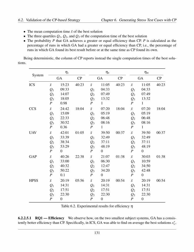
6.2. Validation of the CP-based Strategy Chapter 6. Generating Stress Test Cases with CP

• The mean computation time x of the best solution• The three quartiles Q1, Q2, and Q3 of the computation time of the best solution• The probability P that GA achieves a greater or equal efficiency than CP. P is calculated as the

percentage of runs in which GA had a greater or equal efficiency than CP, i.e., the percentage ofruns in which GA found its best result before or at the same time as CP found its own.

Being deterministic, the column of CP reports instead the single computation times of the best solu-tions.

Systemηs ηn ηm

GA CP GA CP GA CP

ICS x 15:23 40:23 x 11:05 40:23 x 11:05 40:23Q1 09:33 Q1 04:33 Q1 04:33Q2 14:07 Q2 07:49 Q2 07:49Q3 18:05 Q3 13:32 Q3 13:32P 0.98 P 1 P 1

CCS x 24:42 18:04 x 07:20 18:04 x 07:20 18:04Q1 15:09 Q1 05:19 Q1 05:19Q2 22:33 Q2 06:48 Q2 06:48Q3 30:52 Q3 08:16 Q3 08:16P 0.36 P 1 P 1

UAV x 42:01 01:05 x 39:50 00:37 x 39:50 00:37Q1 33:39 Q1 32:49 Q1 32:49Q2 38:34 Q2 37:11 Q2 37:11Q3 53:29 Q3 48:19 Q3 48:19P 0 P 0 P 0

GAP x 40:26 22:38 x 21:07 01:38 x 30:03 01:38Q1 33:00 Q1 06:30 Q1 10:59Q2 40:32 Q2 12:47 Q2 34:50Q3 50:22 Q3 34:20 Q3 42:48P 0.1 P 0 P 0

HPSS x 20:19 05:56 x 20:19 00:54 x 20:19 00:54Q1 14:31 Q1 14:31 Q1 14:31Q2 17:51 Q2 17:51 Q2 17:51Q3 22:30 Q3 22:30 Q3 22:30P 0 P 0 P 0

Table 6.2. Experimental results for efficiency η

6.2.2.5.1 RQ1 — Efficiency We observe how, on the two smallest subject systems, GA has a consis-tently better efficiency than CP. Specifically, in ICS, GA was able to find on average the best solutions x∗s ,

131

Chapter 6. Generating Stress Test Cases with CP 6.2. Validation of the CP-based Strategy

x∗n, and x∗m three or four times faster than CP. We can identify this trend also in CCS, where we recordedthe same efficiency gap with the exception of ηs, where the efficiency of CP is achieved by GA by thesecond quartile. However, for the three largest systems, CP is significantly faster than GA at finding thebest results with respect to s, n, and m. The efficiency of CP is indeed far above the one observed beforethe third quartile of GA. With the exception of ηs in GAP, no GA run was faster at finding its best resultthan CP.

Table 6.3 reports the effectiveness κ with respect to s, n, and m for GA and CP and for each system.As for Table 6.2, the columns of GA report statistics about the distribution of effectiveness:

• The mean value x of the best solution• The three quartiles Q1, Q2, and Q3 of the value of the best solution• The probability P that GA achieves a greater or equal effectiveness than CP. P is calculated as the

percentage of runs in which GA had a greater or equal effectiveness than CP, i.e., the percentage ofruns in which the best result found by GA was better than or equal to the best result found by CP.

The column of CP reports instead the single value of the best solutions.

6.2.2.5.2 RQ2 — Effectiveness We observe how, on the two smallest subject systems, the effective-ness of GA is on average similar to the effectiveness of CP. In ICS, GA reaches by the third quartile thesame result as CP for κs, κn, and κm. In CSS instead, GA reaches by the second quartile the same resultas CP for κs, and does so by the first quartile for both κn and κm. However in both cases, though thesolutions found by CP are better on average, the efficiency of GA is superior to the efficiency of CP. Thismeans that there is a high probability that in few runs GA finds the same best solutions with respect to s,n, and m as CP. For the three largest systems instead, with the exception of UAV for κn and κm, CP findssignificantly better values than GA for s, n, and m. Specifically, in UAV GA finds on average one dead-line miss of one time quantum, while CP finds one deadline miss of three time quanta. The differencein κs between GA and CP increases in GAP and HPSS. In GAP, GA has an average value of 19 for κs,while CP achieves 34 half of the time. In HPSS, GA hardly finds any deadline miss, while CP finds oneof five time quanta after a few minutes. These differences in the value of κs are of practical significancebecause, as discussed above, a larger sum of deadline misses indicates scenarios where tasks are morelikely to miss their deadlines at runtime. Furthermore, for all subject systems, no GA run found a bettersolution than CP.

6.2.2.5.3 RQ3 — Scalability In light of these results, we conclude that, for the smaller subject sys-tems, GA has proven to be more efficient than CP, and nearly as effective. On the other hand, for thelarger systems, CP has proven to be significantly more efficient and more effective than GA. The out-come of this experiments seems to suggest that, within the range covered by our systems and the proposedexperimental design, the larger the size of the system, the better CP when compared to GA.

6.2.2.5.4 Summary and Discussion We conjecture that the reason for this trend stems from the in-teraction between the size of the search space of the subject systems, and the heuristics used in our CP

132

6.2. Validation of the CP-based Strategy Chapter 6. Generating Stress Test Cases with CP

Systemκs κn κm

GA CP GA CP GA CP

ICS x 13.22 19 x 1.3 2 x 1.3 2Q1 14 Q1 1 Q1 1Q2 14 Q2 1 Q2 1Q3 19 Q3 2 Q3 2P 0.26 P 0.32 P 0.32

CCS x 12.14 13 x 2 2 x 2 2Q1 11 Q1 2 Q1 2Q2 13 Q2 2 Q2 2Q3 13 Q3 2 Q3 2P 0.52 P 1 P 1

UAV x 0.94 3 x 0.74 1 x 0.74 1Q1 0 Q1 0 Q1 0Q2 1 Q2 1 Q2 1Q3 1 Q3 1 Q3 1P 0.02 P 0.74 P 0.74

GAP x 19.18 34 x 2.4 3 x 3.06 5Q1 16 Q1 2 Q1 3Q2 19 Q2 2 Q2 3Q3 21 Q3 3 Q3 4P 0 P 0.4 P 0.02

HPSS x 0.04 5 x 0.04 1 x 0.04 1Q1 0 Q1 0 Q1 0Q2 0 Q2 0 Q2 0Q3 0 Q3 0 Q3 0P 0 P 0.04 P 0.04

Table 6.3. Experimental results for effectiveness κ

solution. The size of the search space is largely determined by the number of aperiodic task executionswithin the observation time interval. The systems where GA is more efficient than CP, i.e., ICS and CCS,have a smaller search space, and hence, GA is able to quickly converge towards the best solutions regard-less of its initial population. Therefore, in these systems GA performs reasonably well compared to CP.On the other hand, in systems with large search spaces, i.e., UAV, GAP, HPSS, GA needs more time toconverge towards its best solution. Thanks to its heuristic, CP is able to find solutions with a rather highobjective value in a few minutes.

Note that the efficiency and effectiveness results of the search strategies are obtained by running themfor one hour. Due to this time limit, in the larger systems, CP may fail at further improving the solutionsthat it finds at the very beginning of its search. Indeed, if the GA and CP had been run for longer

133

Chapter 6. Generating Stress Test Cases with CP 6.2. Validation of the CP-based Strategy

time on the larger systems, we might have obtained better solutions that take much longer to compute.Analyzing the experimental results, we found out that running GA and CP for one hour can provide onlya rough assessment on the efficiency and effectiveness of both strategies, and on the way the system sizeaffects efficiency and effectiveness. For this reason, we further investigated the performance of GA andCP in another series of experiments, where we run each strategy for 10 hours. This second series ofexperiments, discussed in Section 7.2, showed a clear trend, where GA is more efficient, while CP ismore effective. This second experiment motivated us in devising a combined strategy (Chapter 7) thataims at retaining the advantages of GA and CP.

6.2.2.6 Threats to Validity

We identified three main threats that could affect the general validity of our conclusions: First, the anal-ysis of efficiency, effectiveness and scalability is based on a set of five subject systems. Although com-paring GA and CP in a larger number of systems would have mitigated this threat, the systems have beenselected from different RTES domains and feature varying size and complexity.

Second, the size of the selected systems varies from 6 to 32 tasks, 3 to 9 of which aperiodic. Therecould be much larger systems featuring hundreds of tasks, and for those the efficiency and effectivenessof CP need to be investigated. This means that the conclusions drawn are valid only for systems in thesame size range of the subject systems used in the comparison.

Third, the experiment set-up relies on the choice of running both search strategies for one hour,and on specific parameters used for GA, such as the initial population size, the crossover and mutationprobabilities, and the population replacement rate. Different values for these parameters could have ledto higher efficiency and effectiveness. However, we used the same values as in the work of Briand etal. [Briand et al., 2006], that have been derived from the GA literature and specifically tuned for deadlinemisses analysis. However, by looking at the quartiles of the efficiency distributions, GA did not findalways find its best results significantly earlier than one hour. This means that, in most cases, GA did notreach a plateau before one hour, and there are chances for it to find a better solution if given more time.To mitigate this threat, we should investigate the efficiency and effectiveness in an experiment where GAand CP are run for longer time. As discussed at the end of Section 6.2.2.5, this longer experiment isdiscussed in Section 7.2.

134

Chapter 7

Combining Genetic Algorithms and ConstraintProgramming to Automate the Generation ofStress Test Cases

In Chapter 6 we discussed a strategy based on Constraint Programming (CP) to automate the genera-tion of stress test cases to break task deadlines. The strategy is based on the definition of a ConstraintOptimization Problem (COP) for the purpose of generating sequences of arrival times likely to lead todeadline misses. The COP models the properties of the system as integer constants and variables, andmodels the scheduler of the system as a set of constraints among such variables. The generation of stresstest cases is driven by an objective function that expresses the likelihood of the arrival times to violatea given performance requirement. In particular, we defined the objective function FDM expressing theextent to which a particular set of arrival times is predicted to break task deadlines. Also recall from Sec-tion 2.4.2.2 that Genetic Algorithms (GA) have been used in the past to support stress testing of taskdeadlines. Among others, Briand et al. proposed a GA-based search strategy [Briand et al., 2006] togenerate sequences of arrival times likely to lead to deadline misses. In that work, arrival times of aperi-odic tasks are modeled as chromosomes. The initial population of these chromosomes is initialized withrandom values, and their fitness is evaluated by computing the tasks schedule that is produced from thearrival times encoded in the chromosomes. Indeed, such a schedule contains information about the endtimes of tasks, which belong to the fitness function in a fashion similar to that of FDM. At each itera-tion of GA, a pair of chromosomes is crossed over and then mutated using specific operators that ensurecompliance with the inter-arrival times of aperiodic tasks.

Preliminary experimental results have shown in some cases an opposing trend: while GA was moreefficient, i.e., faster in generating test cases, CP was more effective, i.e., it generated test cases that weremore likely to identify deadline misses. Furthermore, GA was able to find a larger and more diverse setof test cases than CP, exercising the system in a more diverse way with respect to task executions. Specif-ically, the test cases generated by GA had a higher variety in terms of 1. time span and 2. preemptionsbetween task executions, and 3. number of aperiodic task executions. These three criteria are describedin Section 7.2.2 and define the concept of test case diversity. On the other hand, CP generated a smaller

135

Chapter 7. Generating Stress Test Cases with GA+CP 7.1. Description of the GA+CP strategy

number of test cases, most of which were redundant with respect to the three criteria, i.e., executed thesystem tasks during similar time intervals, with the same preemptions and number of executions.

Therefore, we looked into a way to achieve both the efficiency of GA and the effectiveness of CP. Thekey idea behind this new stress testing strategy is to improve the solutions computed by GA by perform-ing a complete search with CP in their neighborhood, hence defining a two-stage GA+CP strategy. In thisway, we expected the combined approach to take advantage of the efficiency of GA, because solutionsare initially computed with GA and the subsequent CP search is likely to terminate in a short time sinceit focuses on the neighborhood of a solution, rather than in the whole search space. Similarly, we ex-pected GA+CP to take advantage of the solutions diversity of GA, because these solutions define in turnsubspaces where CP searches for better solutions. Finally, we also expected GA+CP to take advantage ofthe effectiveness of CP since, after GA computes a solution, CP either finds the best solution within theneighborhood, or proves upon termination that no better solution exists in such neighborhood.

7.1 A hybrid GA+CP strategy to Automate the Generation ofStress Test Cases

We refine our strategy for determining worst-case schedules of tasks with an approach motivated by ourexperimental results on the comparison between the CP-based and GA-based strategies (Section 6.2.2).Specifically, we solve the search for arrival times of aperiodic tasks with a two-step strategy. The keyidea behind the strategy is to first generate a set of solutions with GA, and then perform a series of localsearches with CP in the neighborhood of those solutions. Figure 7.1 illustrates how GA+CP searches forsolutions through an abstract example.

1. GA Step. The initial population of GA consists of the three solutions x1, y1, and z1. In the firstgeneration, GA finds the solutions x2, y2, and z2 that are generated from x1, y1 and z1 respectively.After the five generations, GA converges on the solutions x6, y6 and z6.

2. CP Step. CP then searches for better solutions in the neighborhoods of x6, y6 and z6. This step isperformed by launching three separate instances of CP, each having x6, y6 and z6 as a starting point.The first two complete searches find the solutions x∗ and y∗. The last proves upon termination thatz6 is the best solution in its neighborhood, hence z6 = z∗. Therefore, x∗, y∗, and z∗ are the finalsolutions found by GA+CP, and are used to characterize stress test cases.

We begin the formal description of our approach by introducing the following notation.

Recall that a solution is a sequence of arrival times which the search identifies as likely to break taskdeadlines, and hence characterizes a stress test case.Solution computed by GA. Let x =

[[x j,k | k ∈ K j] | j ∈ Ja

]denote a solution computed by GA.

Note that, by definition, x is an assignment of arrival times for aperiodic tasks, where x j,k is the value forthe kth arrival time of task j: ∀ j ∈ Ja, k ∈ K j · at j,k(x) = x j,k.

136

7.1. Description of the GA+CP strategy Chapter 7. Generating Stress Test Cases with GA+CP

Figure 7.1. Overview of GA+CP: the solutions x1, y1 and z1 in the initial population of GA evolve intox6, y6, and z6, then CP searches in their neighborhood for the optimal solutions x∗, y∗ and z∗.

Consider two tasks j1 and j2 such that the arrival time of an execution of j1 can have a direct impactover an execution of j2. In practice, this can happen in two cases. The first case occurs if j1 has higherpriority than j2. In this case, j2 can be preempted at any time by j1 if there are not enough cores available.The second case occurs when j1 and j2 share the same computational resource. In this case, if j1 arrivesbefore j2 has acquired the lock on the resource, the latter will have to wait until such lock is released.Therefore, we define the impacting relation between two tasks in the following way:

Impacting Relation between two tasks. We define im as a binary relation defined over J× J holding ifthe arrival time of an execution of j1 can have a direct impact over an execution of j2:

im( j1, j2)def

= pr( j1)≥ pr( j2)∨de( j1, j2)

Note that im is defined reflexive, because trivially the arrival time of a task has an impact over theexecution of the task itself. However, j1 having higher priority or depending on j2 is not the only casein which j1 can have an in impact over an execution of j2. For instance, consider the case where j1 hashigher priority than another task j3, and j3 depends on j2. In this case, j1 could preempt j3 after j3 hasacquired the lock on the resource shared with j2, and then j2 would have to wait for both the completionof j1 and j3 before being able to execute. In this case, j1 can also have an impact over an execution of j2,albeit this impact is indirect since it involves j3. For this reason, we denote the transitive closure of im asim+, in order to cover all the cases where j1 can have a direct or indirect impact over the execution of j2.

137

Chapter 7. Generating Stress Test Cases with GA+CP 7.1. Description of the GA+CP strategy

Impacting Set of a Task. Let I : J→ P(J) be the function that represents the set of tasks that can havean impact over the execution of a target task: I j

def

={

j′ ∈ J | im+( j′, j)}. We define I j as the impacting set

of j.

Set of tasks that miss a deadline or are the closest to miss it among all tasks. We define J∗(x) as theset of tasks that miss at least a deadline in one execution, or are closer than others to doing so in theschedule generated by the arrival times in x.

J∗(x) def

={

j ∈ J∣∣∣ ∃k∗ ∈ K j∗(x) ·

(dm j∗,k∗(x)≥ 0 ∨

∀ j ∈ J, k ∈ K j · dm j∗,k∗(x)≥ dm j,k(x))}

Union set of impacting sets of tasks missing or closest to miss their deadlines. We define I∗(x) as theunion of the impacting sets of tasks in J∗(x).

I∗(x) def

=⋃

j∗∈J∗(x)I j∗(x)

By definition, I∗(x) contains all the tasks that can have an impact over a task that misses a deadline or isclosest to a deadline miss.

Neighborhood of an arrival time and neighborhood size. We define εD(x j,k) as the neighborhood ofx j,k of size D, i.e., as the interval centered in the arrival time x j,k whose radius is D.

εD(x j,k)def

= [x j,k−D, x j,k +D]

ε defines the part of the search space around x j,k where to find arrival times that are likely to break taskdeadlines. Note that D is a parameter of the search.

Constraint Model Implementing a Complete Search Strategy. Let M denote the constraint modeldefined in Section 6.1 that considers the function FDM (Section 6.1.4) for the purpose of identifying taskarrival times that are likely to break deadlines.

M models the static and dynamic properties of the software system as constants and variables respec-tively, and the scheduler of the operating system as a set of constraints among such variables. Note thatM is solved a using a complete search strategy over the space of arrival times. This means that Msearches for arrival times of all aperiodic tasks within the whole interval T .

Our combined GA+CP strategy consists of the following two steps:

1. GA Step. Run GA for a given amount of time to obtain a set X of solutions. For this purpose, weuse the implementation of GA introduced by Briand et al., with the same initial population size,replacement strategy, and probability values used for crossover and mutation [Briand et al., 2006].

138

7.1. Description of the GA+CP strategy Chapter 7. Generating Stress Test Cases with GA+CP

2. CP Step. For each solution x ∈ X , solve a constraint model M′(x) that searches for arrival timesonly within a fixed-size neighborhood of x.

M′(x) is derived from M by:

• Fixing the arrival time of tasks not in I∗. This is done by adding to M the following constraint:

∀ j ∈ J \ I∗(x), k ∈ K j(x) · at( j,k) = x j,k

In practice, this means that the arrival time of all task executions that do not have any impact ontasks being close to missing a deadline will be fixed in M′.• Bounding the arrival times of tasks in I∗. This is done by adding to M the following constraint:

∀ j ∈ I∗(x), k ∈ K j(x) · x j,k−D≤ at( j,k)≤ x j,k +D

In practice, this means that the arrival time of the task executions that can have an impact on tasksidentified by GA as close to missing a deadline will be declared in M′ as a variable with domainε(x j,k).

Note that, by definition, M′ implements a local search strategy over the search space of arrival times.This means that M′ searches only for arrival times of aperiodic tasks that can have an impact on tasksGA identifies as close to missing a deadline, and bounds the search within a neighborhood of size D fromthe solution computed by GA. Specifically, for given j and k, the inequality constraints on the variable atdefine in the solutions space a hypercube of side 2D centered in x j,k.

The search in GA+CP can be configured through two sets of parameters, one related to GA and theother to CP. GA relies on parameters specific to evolutionary algorithms, such as the initial populationsize, the crossover and mutation probabilities, and the population replacement rate. For those, we usedvalues that have been derived from the GA literature and specifically tuned for deadline miss analy-sis [Briand et al., 2006]. On the other hand, CP is a deterministic search strategy, and therefore does notrequire us to set such parameters. However, our combined search strategy depends on the neighborhoodsize D that CP searches for arrival times of aperiodic tasks. Our preliminary experimentation showed thata value of D around 1% of T yields a good compromise between efficiency and effectiveness. Specif-ically, lower values for D define a smaller neighborhood where GA+CP is less likely to improve thesolutions found by GA, while higher values for D define a larger neighborhood where GA+CP is likelyto spend a significant amount of time without finding better solutions.

7.1.1 GA+CP in Practice: a Working ExampleIn this section, we introduce an example to show how GA+CP works in practice. Consider the systemcomposed of five aperiodic tasks detailed in Table 7.1. Note that pe and of are not defined, since eachtask is aperiodic. There are also no tg relationships between tasks.

Suppose GA finds the solution x =[[0][2][3][6][3]

], where each task is executed once, and j0 arrives

at time 0, j1 at time 2, j3 at time 3, j4 at time 6 and j5 at time 3. The schedule corresponding to thissolution is shown in Figure 7.2.1.

139

Chapter 7. Generating Stress Test Cases with GA+CP 7.1. Description of the GA+CP strategy

T = [0,9] c = 1

Task pr dr mn mx dl de

j0 0 2 10 10 8j1 1 2 10 10 6 j4j2 2 2 10 10 5j3 3 2 10 10 4j4 4 2 10 10 3 j1

Table 7.1. Example system with four tasks and one dependency

(7.2.1) Solution x found by GA (7.2.2) Solution x′ found by GA+CP

Figure 7.2. GA+CP neighborhood search example

In x, j4 misses its deadline by 2 time quanta, being the task that has the biggest deadline miss.Therefore, J∗(x) = { j4}. By looking at the tasks priorities and dependencies, j1 depends on j4, and bothj2 and j3 have higher priority than j1, so all three can potentially have an impact over the execution ofj4 for the reasons detailed in above. This means that I j4(x) = { j1, j2, j3, j4}, and consequently I∗(x) ={ j1, j2, j3, j4}.

GA+CP searches the space around x up to a distance D from the tasks in I∗(x), i.e., the tasks that canpotentially have an impact over the execution of j4. This local search is performed by solving the CPmodel M′(x) derived from M by specifying that:

• The arrival time of j0 is fixed, since j0 6∈ I∗(x). This step is done by adding to M the followingconstraint: at( j0,0) = 0. In practice, at( j0,0) is declared in M′(x) as a constant with value 0.• The arrival times of tasks in I∗(x) are bounded within distance D from the arrival times computed

by GA in x. For this example, suppose D = 2. This step is done by adding to M the following

140

7.2. Validation of the GA+CP strategy Chapter 7. Generating Stress Test Cases with GA+CP

constraints:

2−2 = 0≤ at( j1,0)≤ 4 = 2+23−2 = 1≤ at( j2,0)≤ 5 = 3+26−2 = 4≤ at( j3,0)≤ 8 = 6+23−2 = 1≤ at( j4,0)≤ 5 = 3+2

In practice, at( j1) is declared in M′(x) as a variable with domain [0,4], at( j2) as a variable withdomain [1,5], at( j3) as a variable with domain [4,8], and at( j4) as a variable with domain [1,5].

GA+CP solves this model to optimality and finds the solution x′ =[[0][2][3][4][3]

], with the schedule

shown in Figure 7.2.2. In x′, j4 misses its deadline by 4 quanta, and therefore GA+CP has succeeded inimproving the solution found by GA by finding a larger deadline miss.

7.2 Validation of GA+CP in Five Subject Systems fromSafety-critical Domains

The goal of our empirical study is to compare the overall performance of GA, CP, and GA+CP for thepurpose of supporting stress testing of task deadlines. The design of this empirical study is similar to thatdescribed in Section 6.2.2, as the comparison is performed on the same five subject systems introducedin Section 6.2.2.1. The goal of our study is to answer the research questions presented in Section 7.2.1.Note that, in addition to the research questions related to efficiency, effectiveness, and scalability intro-duced in Section 6.2.2.2, we also investigate a fourth property of the search strategies that concerns thecapability to exercise the system in a more diverse way with respect to task executions. Therefore, wedefine metrics and attributes in Section 7.2.2 to capture the test cases variety in terms of (1) time spanand (2) preemptions between task executions, and (3) number aperiodic task executions. The designof our experiment is described in Section 7.2.3, and its results are discussed in Section 7.2.4. Finally,Section 7.2.5 covers some potential threats that could affect the general validity of our conclusions.

7.2.1 Research QuestionsThe goal of our empirical study is answering the following research questions involving GA, CP andGA+CP for the purpose of supporting stress testing of task deadlines. Note that RQ1, RQ2, and RQ4have been introduced in Section 6.2.2.2, and are reported here.

• RQ1 — Efficiency. Does one search strategy find the best solutions significantly faster than theother?• RQ2 — Effectiveness. Does one search strategy find significantly better solutions (i.e., solutions

with worse deadline misses) than the other?• RQ3 — Diversity. Does one search strategy find solutions that are significantly more diverse (i.e.,

solutions that exercise the system in a larger number of different ways) than the other?

141

Chapter 7. Generating Stress Test Cases with GA+CP 7.2. Validation of the GA+CP strategy

• RQ4 — Scalability. To what extent does the size of a system affect the efficiency of the searchstrategies?

RQ1, RQ2 and RQ3 are investigated through a set of metrics and attributes detailed in Section 7.2.2.The goal of such metrics and attributes is to provide quantitative evidence to answer the research ques-tions. Similar to Section 6.2.2.5, RQ4 will instead be only qualitatively discussed in Section 7.2.4. Notethat we base our analysis of efficiency on a set of five systems, and therefore no quantitative study, forexample based on regression analysis, can be carried out to identify precise trends.

7.2.2 Comparison Metrics and AttributesSimilar to Section 6.2.2.3, we broke down the objective function FDM (Section 6.1.4) into several fac-tors of practical interest while investigating worst case scenarios for deadline misses. For this reason,we defined the efficiency and effectiveness, and diversity properties related to RQ1, RQ2, and RQ3 asattributes, and we defined a set of metrics to enable their measurement. Therefore, we compare the per-formance of GA, CP and GA+CP by collecting data pertaining to the metrics t, s, n, m, and the attributesη and κ defined in Section 6.2.2.3. In addition, we define the attributes related to diversity for each searchstrategy Γ running during an experiment on the target system Σ. Indeed, an ideal test suite has three mainproperties:

1. It is computed in the shortest possible time.2. It contains test cases that are as likely as possible to push tasks to miss their deadlines at runtime.3. It contains test cases that are as little redundant as possible.

Recall from Section 6.2.2.3 that efficiency captures the first property, measuring how quickly a searchstrategy converges to the optimal solutions it finds, while effectiveness captures the second property,measuring how likely are the solutions found to characterize stress cases that will reveal deadline missesat runtime. The third property is instead captured by the concept of diversity. Conceptually, diversityamong stress test cases is similar to test coverage in functional testing. Indeed, a test suite that yieldshigh coverage with respect to a given criterion ensures that the system will be thoroughly tested withrespect to that criterion. Similarly, a test suite that yields high diversity ensures that test cases willthoroughly exercise interactions between task executions.

In general, the higher the number of best solutions of a search strategy, the higher the number ofeffective test cases it generates. Note that the effectiveness κ is a different concept from the number N ofsolutions which are effective. Since N does not take into account redundancy among solutions, it is nottrue in general that the higher N, the more effective a search strategy is. For example, a strategy couldgenerate a large number of effective test cases that yet exercise the system with respect to very similarscenarios. On the other hand, another strategy could generate fewer effective test cases that are insteadhighly diverse. For this reason, the number of best solutions is only meaningful when considered togetherwith the redundancy of the solutions, formalized by the concept of diversity. Therefore, the number ofbest solutions relates to RQ3.Number of best solutions. We define the number N of best solutions with respect to a given metric

142

7.2. Validation of the GA+CP strategy Chapter 7. Generating Stress Test Cases with GA+CP

as the cardinality of the set of best solutions found with respect to that metric. Specifically, we defineeffectiveness with respect to s, m, and n.

Nsdef

=∣∣∣X∗s ∣∣∣ Nn

def

=∣∣∣X∗n ∣∣∣ Nm

def

=∣∣∣X∗m∣∣∣

We define three types of diversity δ , each with respect to a given metric. Specifically, we define theshift diversity δh, the pattern diversity δr, and the executions diversity δe, each defined with respect to thethree metrics s, m, and n. Intuitively, the shift diversity δh measures the extent to which solutions exercisethe system during time intervals that are distant from each other. Therefore, the diversity attribute relatesto RQ3.

The shift diversity is defined based on the shift distance between active vectors, which measures thedistance in time between a given execution in two solutions.Shift Distance between Active Vectors. Let A j,k(x) and A j,k(y) be the active vectors of task execution( j,k) in the solutions x and y, respectively. We define the shift distance Dh, j,k(x,y) between A j,k(x) andA j,k(y) as the sum of absolute differences between their start and end times.

Dh, j,k(x,y)def

=∣∣∣st j,k(x)− st j,k(y)

∣∣∣+ ∣∣∣en j,k(x)− en j,k(y)∣∣∣

For example, in Figures 7.2.1 and 7.2.2, Dh, j1,0 = | 2−2 |+ | 6−8 |= 2.

Average Shift Distance between Pairs of Executions. We define Dh, j(x,y) as the average shift distanceover pairs of executions of task j in solutions x and y.

Dh, j(x,y)def

=

∑k∈(

K j(x)∩∈K j(y))Dh, j,k(x,y)

∣∣∣K j(x)∩K j(y)∣∣∣

In Figures 7.2.1 and 7.2.2, Dh, j1 = Dh, j1,0 = 2, since j1 is executed only once.

Shift Diversity between Solutions. We define δh

(A(x),A(y)

)as the shift diversity between the solutions

x and y as the sum of the shift distances between A j(x) and A j(y) for j ∈ J:

δh

(A(x),A(y)

)def

=∑j∈J

Dh, j(x,y)

Shift Diversity between Two Solutions. We define δh as the shift diversity with respect to a given metricas the average shift diversity over the set of best solutions for that metric.

δh,sdef

=

∑x,y∈X∗s

δh(x,y)

|X∗s |δh,n

def

=

∑x,y∈X∗n

δh(x,y)

|X∗n |δh,m

def

=

∑x,y∈X∗m

δh(x,y)

|X∗m|

143

Chapter 7. Generating Stress Test Cases with GA+CP 7.2. Validation of the GA+CP strategy

In Figures 7.2.1 and 7.2.2, δh = 0+2+2+8+4 = 16.

The pattern diversity δr measures the extent to which solutions exercise the system such that tasksare preempted at different times. The pattern diversity is defined based on the pattern distance betweenactive vectors, which measures the difference between the preemption times of a given task execution intwo solutions.Pattern Distance between Active Vectors. Let A j,k(x) and A j,k(y) be the active vectors of task execution( j,k) in the solutions x and y, respectively. We define the pattern distance Dr, j,k(x,y) between A j,k(x) andA j,k(y) as the sum of the absolute differences between the preemption values of task j.

Dr, j,k(x,y)def

=∑

p∈Pj\{0}

∣∣∣pm j,k,p(x)−pm j,k,p(y)∣∣∣

For example, in Figures 7.2.1 and 7.2.2, Dr, j2,0 = | 0−2 |= 2.

Average Pattern Distance between Pairs of Executions. We define Dr, j(x,y) as the average shift dis-tance over pairs of executions of task j in solutions x and y.

Dr, j(x,y)def

=

∑k∈(

K j(x)∩∈K j(y))Dr, j,k(x,y)

∣∣∣K j(x)∩K j(y)∣∣∣

In Figures 7.2.1 and 7.2.2, Dr, j2 = Dr, j2,0 = 2, since j2 is executed only once.

Pattern Diversity between Two Solutions. We define δr(A(x),A(y)

)as the diversity between the solu-

tions x and y, i.e., as the sum of the pattern distances between A j(x) and A j(y) for j ∈ J.

δr(A(x),A(y)

)def

=∑j∈J

Dr, j(x,y)

Pattern Diversity. We define the pattern diversity δr with respect to a given metric as the average patterndiversity over the set of best solutions for that metric.

δr,sdef

=

∑x,y∈X∗s

δr(x,y)

|X∗s |δr,n

def

=

∑x,y∈X∗n

δr(x,y)

|X∗n |δr,m

def

=

∑x,y∈X∗m

δr(x,y)

|X∗m|

In Figures 7.2.1 and 7.2.2, δr = 0+2+2+0+0 = 4.

The execution diversity δe measures the extent to which solutions exercise the system such that tasksare executed different numbers of times.

144

7.2. Validation of the GA+CP strategy Chapter 7. Generating Stress Test Cases with GA+CP

Execution Diversity between Two Solutions. We define δe(A(x),A(y)

)as the execution diversity be-

tween the solutions x and y, i.e., as the sum of the absolute differences between the number of taskexecutions in solutions x and y.

δe(A(x),A(y)

)def

=∑j∈J

∣∣∣|K j(x)|− |K j(y)|∣∣∣

Execution Diversity. We define δh as the execution diversity with respect to a given metric, i.e., as theaverage execution diversity over the set of best solutions for that metric.

δe,sdef

=

∑x,y∈X∗s

δe(x,y)

|X∗s |δe,n

def

=

∑x,y∈X∗n

δe(x,y)

|X∗n |δe,m

def

=

∑x,y∈X∗m

δe(x,y)

|X∗m|

For example, in Figures 7.2.1 and 7.2.2, δe = | 1− 1 | + | 1− 1 | + | 1− 1 | + | 1− 1 | + | 1− 1 | = 0because each task gets executed once in each solution.

7.2.2.1 Diversity Properties

We note that δh, δr, and δe are defined as non-negative, symmetric, and subadditive. Furthermore, whenconsidered in conjunction, the three diversities also satisfy the coincidence property. Specifically, δh, δr,and δe satisfy the following four properties.

1. Non-Negativity∀x,y · δh(x,y)≥ 0 ∧ δr(x,y)≥ 0 ∧ δe(x,y)≥ 0

2. Coincidence∀x,y · δh(x,y) = 0 ∧ δr(x,y) = 0 ∧ δe(x,y) = 0 ⇐⇒ x = y

3. Symmetry

∀x,y · δh(x,y) = δh(y,x) ∧ δr(x,y) = δr(y,x) ∧ δe(x,y) = δe(y,x)

4. Subadditivity (Triangle inequality)

∀x,y,z · δh(x,y)+δh(y,z)≥ δh(x,z) ∧δr(x,y)+δr(y,z)≥ δr(x,z) ∧δe(x,y)+δe(y,z)≥ δe(x,z)

The proofs of the above four properties are straightforward and follow from the definition of δh, δr,and δe as sums of absolute values. These properties enable the definition of the three types of diversityas distance functions on the set of solutions.

145

Chapter 7. Generating Stress Test Cases with GA+CP 7.2. Validation of the GA+CP strategy

7.2.2.2 Diversity Examples

In this section, we present an example with three pairs of solutions x and y. Each pair represent a casewhere only one type of diversity, δh, δr, and δe respectively, has a non-zero value. This highlights thenecessity of breaking down the concept of diversity into three orthogonal sub-attributes that have to beconsidered together when analyzing how differently stress test cases exercise the system.

Consider the single-task system detailed in Table 7.2. Note that pe and of are not defined, since j0 isaperiodic. Trivially, there are also no de and tg relationships.

T = [0,9] c = 1

Task pr dr mn mx dl

j0 0 3 4 10 6

Table 7.2. Example system with one task

(7.3.1) x1 (7.3.2) y1 (7.3.3) x2 (7.3.4) y2 (7.3.5) x3 (7.3.6) y3

Figure 7.3. Six example solutions for the system in Table 7.2

146

7.2. Validation of the GA+CP strategy Chapter 7. Generating Stress Test Cases with GA+CP

Figure 7.3 shows six different solutions for the system detailed in Table 7.2. In their schedules, weomitted the arrival times and deadlines of j0, since they are not relevant for the definition of diversity.Note that j0 is the only task of the system, and therefore it cannot be preempted. However, in theseexample solutions, we introduce unnecessary task preemptions to meaningfully describe the concept ofdiversity.

Consider the two solutions x1 and y1 in Figures 7.3.1 and 7.3.2. In this case, we note that δh(x1,y1) =| 2− 0 | + | 9− 7 | = 4. This reflects the fact that x1 is predicted to exercise the system in the interval[2,9], and y1 is predicted to do so in [0,7]. Furthermore, δr(x1,y1) = | 3−3 |+ | 4−4 |= 0. This reflectsthe fact that in both x1 and y2 task j0 is predicted to preempt at runtime in the same way, i.e., by twotime quanta the first time, and by three the second time. Finally, δe(x1,y1) = | 1− 1 | = 0 since in bothsolutions j0 gets executed once.

Furthermore, consider the two solutions x2 and y2 in Figures 7.3.3 and 7.3.4. In this case, we notethat δh(x2,y2) = | 0−0 |+ | 7−7 |= 0. This reflects the fact that x2 and y2 are both predicted to exercisethe system in the same interval [0,7]. However, δr(x2,y2) = | 1−5 |+ | 4−0 |= 8. This reflects the factthat in x2 and y2 task j0 is predicted to preempt at runtime in different ways. Indeed, j0 is preemptedtwice for one and four time quanta in x3, while in y2 it is preempted once for five time quanta. Finally,δe(x2,y2) = | 1−1 |= 0 since even in this case j0 gets executed once in both solutions.

Finally, consider the two solutions x3 and y3 in Figures 7.3.5 and 7.3.6. In this case, we note thatδh(x3,y3) = | 0−0 |+ | 3−3 |= 0. This reflects the fact that, considering only the first execution of j0that is present in both solutions, x3 and y3 are predicted to exercise the system in the same interval [0,4].Moreover, δr(x3,y3) = | 1− 1 | + | 0− 0 | = 0. This reflects the fact that, considering again the onlycommon execution of j0, x3 and y3 are both predicted to preempt j0 once by one time quanta. However,δe(x3,y3) = | 2−1 |= 1 since in this case j0 gets executed twice in x3 and only once in y3.

7.2.3 Experiments Set-UpTo answer the research questions, we performed a series of experiments over the systems describedin Section 6.2.2.1. The experimental design is illustrated in Figure 7.4. Each experiment consisted ofrunning GA, CP and GA+CP on a target system Σ for a number of times, each run generating a set Xof solutions. Since the purpose of our empirical study is to compare the practical usefulness of the threestrategies and give an insight over their scalability, we chose to run them in the way engineers wouldrealistically do so in a real testing environment. Based on our experience with industrial partners, weassumed that a reasonable choice would be running GA and CP for ten hours. Note that this interval issensibly longer than the one hour time budget we adopted while initially validating CP (Section 6.2.2.4).We set up GA to continuously generate new solutions for ten hours, while we set up CP to terminatethe search after ten hours. GA+CP was instead run by performing one local CP search for each solutionfound by GA. We set a timeout of 2 hours for these local searches, so that GA+CP was run for a totalof 12 hours. However, note that CP terminates the search upon proof of optimality. Since CP performedthe local searches in a significantly small subset of the search space (recall Figure 7.1), the local CPsearches always terminated with proof of optimality before the 2 hours timeout. Therefore, even if we

147

Chapter 7. Generating Stress Test Cases with GA+CP 7.2. Validation of the GA+CP strategy

instructed GA+CP to run longer than GA and CP, the time taken by CP to terminate the local searcheswas practically not significant with respect to the 10 hours taken by GA to generate its solutions. For eachrun of GA, CP, and GA+CP, we recorded in X only the 100 solutions with the highest fitness/objectivevalue found. As explained in Section 6.2.2.4, this is because each solution characterizes a stress testcase, and 100 has proven to be a satisfactory number of observations to meaningfully compare twodistributions [Arcuri and Briand, 2011]. Similar to GA and CP, we instructed GA+CP to run 100 CPsearches as described in Section 7.1 each in the neighborhood of a solution found by GA.

Figure 7.4. Experimental design: we run CP a single time recording the 100 solutions with highestobjective value, and calculating a single value for each metric. Then, we run GA and GA+CP 30 timesrecording the 100 solutions with highest fitness value, and calculating distributions for the metrics.

Running the three search strategies for approximately the same amount of time allows us to mean-ingfully compare effectiveness, number of solutions found, and diversity. Furthermore, during the designof the experiment, we had to consider the inherent randomized behavior of GA in contrast to the fulldeterminism of CP. Indeed, GA finds solutions starting from a randomly chosen initial population ofindividuals by applying crossover and mutation operators with a given probability, while CP finds solu-tions by solving a constraint optimization problem. For this reason, while we ran CP only once for eachsystem, we ran GA, and consequently GA+CP 30 times on each system. In this way, we could computethe comparison metrics distributions of the best solutions recorded over 30 runs. Since our research ques-tions are directly related to attributes η , κ , N, and δ , for each solution x ∈ X we computed the values ofthe metrics t, s, n, and m used to define such attributes. GA, CP and GA+CP runs have been separatelyexecuted on a single AMAZON EC2 M2.XLARGE1 instance.

7.2.4 Results and DiscussionIn this section, we discuss the experimental results for the attributes η , κ , N, and δ in each subjectsystem. Each attribute is discussed through 15 box-and-whisker plots, one for each pair of metric and

1 http://aws.amazon.com

148

7.2. Validation of the GA+CP strategy Chapter 7. Generating Stress Test Cases with GA+CP

system. In each plot, the x-axis reports the search strategies CP, GA, and GA+CP, denoted as C, G,and + respectively. The y-axis reports instead the value for the comparison attribute. Each plot is alsocomplemented by two p-values from the non-parametric Wilcoxon statistical significance test betweenGA+CP and CP (first row), and between GA+CP and GA (second row). Specifically, we report the p-values from the Wilcoxon rank-sum test for the difference between GA+CP and GA, and the Wilcoxonsigned-rank test for the difference between GA+CP and CP. The former is a two-sample test comparingtwo distributions, while the latter is a one-sample test, given the deterministic nature of CP. In particular,we investigated the statistical significance of differences between CP and GA/GA+CP by testing the nullhypothesis that the median of the GA/GA+CP distributions are the deterministic values obtained withCP. For all tests, we selected a level of significance α = 0.05. Note that a centered dot (·) in placeof a Wilcoxon test p-value indicates that the test has not been performed. This happens when the twodistributions considered for the test are identical, and hence the effective sample size, i.e., the number ofobservation pairs with different values, is zero.

7.2.4.1 RQ1 — Efficiency

The first three columns in Table 7.3 report the efficiency η with respect to s, n and m for GA+CP, GA,and CP, and for each subject system. The computation times for the best solutions are reported in theformat hh:mm. We observe how, on each system, GA+CP has a worse efficiency than GA with respectto each metric. With the exclusion of ηn for ICS and UAV, the difference in efficiency is also statisticallysignificant as shown by the p-values below 0.05. This result is expected because GA+CP performs acomplete search in the neighborhood of GA solutions, and therefore, the time GA+CP requires to find itsbest solution is in general higher than that of GA. However, the difference between the average efficiencyof GA+CP and GA is small from a practical standpoint, and does not keep GA+CP from being far moreefficient than CP. Specifically, the difference between the ηs, ηn and ηm medians of GA and GA+CP varyfrom around 20 minutes in ICS (Tables 7.3.1 to 7.3.3) up to 1.5 hour in HPSS (Tables 7.3.37 to 7.3.39).This difference has little practical significance when compared to the ten hours duration of each run, andto the efficiency of CP, that varies from 3.5 hours in ICS up to almost ten hours in HPSS. The statisticalsignificance of the difference between the efficiency of GA+CP and CP is also reflected in the p-value forthe signed-rank test, which is below 0.0001 for each metric and subject system. On average, the resultsshow that GA+CP is twice as fast than CP but only 20% slower than GA in finding the best solutions x∗s ,x∗n, and x∗m.

7.2.4.2 RQ2 — Effectiveness

The second three columns in Table 7.3 reports the effectiveness κ with respect to s, n and m for GA+CP,GA, and CP, and for each subject system. We observe how, on each system, GA+CP has equal or greatereffectiveness than that of GA with respect to each metric. This result is also expected, since GA+CPperforms a complete search in the neighborhood of GA solutions, and thus the solutions it finds arealways equal or better than those of GA. We note how GA+CP is significantly more effective than GAfor two out of three metrics in most of the subject systems, being so for all the three metrics in GAP andHPSS. Moreover, for n and m, GA+CP also achieves nearly the same effectiveness as CP in most of thesubject systems. In particular, in ICS, CCS and UAV, GA+CP achieves the same value as CP for κn in

149

Chapter 7. Generating Stress Test Cases with GA+CP 7.2. Validation of the GA+CP strategy

ηs ηn ηm κs κn κm Ns Nn Nm

ICS

(7.3.1) (7.3.2) (7.3.3) (7.3.4) (7.3.5) (7.3.6) (7.3.7) (7.3.8) (7.3.9)< .0001 < .0001 < .0001 < .0001 < .3256 < .0001 < .0001 < .0001 < .0001< .0001 .3403 .0026 .0730 .0062 < .0001 .2640 .1932 .1784

CC

S

(7.3.10) (7.3.11) (7.3.12) (7.3.13) (7.3.14) (7.3.15) (7.3.16) (7.3.17) (7.3.18)< .0001 < .0001 < .0001 < .0001 · · < .0001 < .0001 < .0001< .0016 .0001 .0001 .1996 .0001 · .1996 .0001 ·

UAV

(7.3.19) (7.3.20) (7.3.21) (7.3.22) (7.3.23) (7.3.24) (7.3.25) (7.3.26) (7.3.27)< .0001 < .0001 < .0001 < .0001 · .0005 < .0001 < .0001 < .0001

.0133 .6309 .0013 < .0001 .3337 < .0001 < .0001 < .0001 < .0001

GA

P

(7.3.28) (7.3.29) (7.3.30) (7.3.31) (7.3.32) (7.3.33) (7.3.34) (7.3.35) (7.3.36)< .0001 < .0001 < .0001 < .0001 < .0001 < .0001 .5171 .5171 .5171

.0009 .0009 .0009 .0062 .0062 .0062 .0246 .0246 .0246

HPS

S

(7.3.37) (7.3.38) (7.3.39) (7.3.40) (7.3.41) (7.3.42) (7.3.43) (7.3.44) (7.3.45)< .0001 < .0001 < .0001 < .0001 < .0001 < .0001 < .0001 .0004 < .0001

.0015 .0003 .0420 < .0001 < .0001 < .0001 .2215 .0605 .1324

Table 7.3. Experimental results of CP (C), GA (G), and GA+CP (+) for efficiency η , effectiveness κ , andnumber N of best solutions. Each box-and-whisker plot reports at the bottom the Wilcoxon test p-valuesbetween GA+CP and CP (first value), and between GA+CP and GA (second value).

150

7.2. Validation of the GA+CP strategy Chapter 7. Generating Stress Test Cases with GA+CP

the first quartile (Tables 7.3.5, 7.3.14 and 7.3.23), and for κm in the second quartile (Tables 7.3.6, 7.3.15and 7.3.24). On the other hand, in these three subject systems, GA achieves the same effectiveness asCP on the second or third quartile on average. Note that, in CCS and UAV, GA never achieves the sameeffectiveness as CP for the criteria n and m. In GAP, GA+CP achieves the same effectiveness as CP in thethird quartile for all the three criteria, identifying a deadline miss in one third of the runs (Tables 7.3.31to 7.3.33). In comparison, GA found a deadline miss only in a single run. Finally, in HPSS, GA+CP doesnot match the effectiveness of CP, but significantly improves the results of GA, having a first quartile thatis around 30% larger than that of GA for s and m (Tables 7.3.40 and 7.3.42). Finally, we note that, withthe exception of κs for ICS and CCS, whenever there is a statistically significant, positive difference inthe effectiveness between CP and GA+CP, there is also one between GA+CP and GA. On average, theresults show that GA+CP is significantly more effective than GA, and is approaching CP in finding thebest solutions x∗n and x∗m.

7.2.4.3 RQ3 — Diversity

The last three columns in Table 7.3 reports the number N of best solutions with respect to s, n and mfor GA+CP, GA, and CP, and for each subject system. We observe how, on most systems, the numberof best solutions found by GA+CP is similar to that of GA, even though it is not consistently larger orsmaller. We conjecture that the reason for this result stems from the way GA+CP is designed to improvethe solutions found by GA. Consider the scenarios shown in Figure 7.5.

(7.5.1) Two or more solutions share the same lo-cal optimum in their neighborhoods

(7.5.2) There is more than one local optimum inthe neighborhood of a solution

Figure 7.5. Different scenarios of how GA+CP affects the number N of best solutions

Suppose that GA finds two distinct best solutions with respect to a metric, namely x and y. It could bethe case that the best solution in the neighborhoods of x and y is the solution z∗ . In this case, the numberN of best solutions found by GA+CP is smaller than that of GA, because N(GA)= 2, and N(GA+CP)= 1(Figure 7.5.1). Suppose now that GA finds only a single best solution x with respect to a metric. It couldbe the case instead, that there is more than a single best solution in the neighborhood of x, namely x∗1,x∗2, and x∗3. In this scenario, the number N of best solutions found by GA+CP is larger than that of GA,because N(GA) = 1, and N(GA+CP) = 3 (Figure 7.5.2). In general, the two scenarios can happen inde-pendently from other factors since they depend only on the specific solutions found by GA in a subject

151

Chapter 7. Generating Stress Test Cases with GA+CP 7.2. Validation of the GA+CP strategy

system. For this reason, there is no clear trend on whether GA+CP finds a larger or smaller number of bestsolutions than GA with respect to a metric, as shown by the p-values. We note that, with the exceptionof GAP and UAV for Nn and Nm (Tables 7.3.26 and 7.3.27), GA and GA+CP find a significantly largernumber of best solutions than CP. Note that in ICS, CP finds only a single best solution with respect to s,n, and m (Tables 7.3.7 to 7.3.9), and does so for s and m in HPSS (Tables 7.3.43 and 7.3.45), and for s inCCS (Table 7.3.16). This result is expected because of the randomized nature of GA, and consequentlyof GA+CP. Indeed, GA finds its solutions by starting from a randomly selected initial population of 80individuals [Briand et al., 2006] and in our experiment we set up GA to continuously generate and evalu-ate solutions for ten hours. Even in cases where no deadline misses are revealed, GA is likely to generatea large set of solutions from the initial population. On the other hand, CP is designed to find solutionsfrom scratch with a branch-and-bound search process that progressively assigns values to variables inorder to satisfy constraints [Apt, 2003]. Furthermore, CP discards by design solutions that have worseobjective values than the current best known solution [Atamtürk and Savelsbergh, 2005], and is thus lesslikely to generate a large set of solutions. Recall that, in our analysis, each solution characterizes a stresstest case. Therefore, a large number of solutions is indicative of the size of test suite generated by thesearch strategies. However, we note that N itself is not sufficient by itself to give a practical measure forthe test suite dimension, because many of the solutions found could be redundant (Section 7.2.2). Forthis reason, the number N of best solutions needs to be considered together with their diversity.

Table 7.4 reports the diversity δh, δr, and δe with respect to s, n and m for GA+CP, GA, and CP, andfor each subject system. We observe that, on each system, the three diversities of GA+CP are similar tothose of GA, even though they are not consistently larger or smaller. We conjecture that the reason whyGA+CP retains a number N of best solutions similar to GA also explains this result. This means that thelocal search performed by CP in the neighborhood of solutions computed by GA had no significant effectover the three types of diversity in our experiment. Therefore, in our subject systems, the solutions foundby GA+CP retained a diversity similar to that of GA. Note that, as expected, in the cases where CP foundonly a single best solution with respect to a metric, the three diversities have a null value. In GAP, CPfound 82 best solutions with respect to s, n, and m, as opposed to 100 for GA and GA+CP. However, thesolutions found by GA and GA+CP are far less redundant than those of CP, having a significantly highershift, pattern, and execution diversity (Tables 7.4.28 to 7.4.36). The same also holds for the criterion s inUAV (Tables 7.4.19, 7.4.22 and 7.4.25), where the three search strategies found 100 best solutions. Wefinally remark that the diversity is not normalized, and the values are only meant to be compared withinthe same subject system and the same type of diversity. Recall from Section 7.2.2 that δh is defined interms of start and end times of task executions, and depends mostly on the observation interval T . δris defined in terms of preemptions between task executions, and depends mostly on the task durations.Finally, δe is defined in terms of number of task executions, and depends mostly on the ratio between Tand the minimum and maximum inter-arrival times of aperiodic tasks. Since T is usually much largerthan tasks durations, δh has higher values than δr and δe. For example, in ICS, the average value forδh,s(GA+CP) is 83.43. This means that on average, the task executions in the best solutions with respectto s found by GA+CP are shifted by 83.43 time quanta. Similarly, in ICS the average for δr,s(GA+CP) is41.08, meaning that the preemptions between task executions in the best solutions with respect to s foundby GA+CP differ on average by 41.08 time quanta. Finally, in ICS the average for δe,s(GA+CP) is 1.56,

152

7.2. Validation of the GA+CP strategy Chapter 7. Generating Stress Test Cases with GA+CP

δh,s δh,n δh,m δr,s δr,n δr,m δe,s δe,n δe,m

ICS

(7.4.1) (7.4.2) (7.4.3) (7.4.4) (7.4.5) (7.4.6) (7.4.7) (7.4.8) (7.4.9)< .0001 < .0001 < .0001 < .0001 < .0001 < .0001 < .0001 < .0001 < .0001

.4289 .0406 .5493 .7958 .1154 .9705 .9176 .4688 .8650

CC

S

(7.4.10) (7.4.11) (7.4.12) (7.4.13) (7.4.14) (7.4.15) (7.4.16) (7.4.17) (7.4.18)< .0001 < .0001 < .0001 < .0001 < .0001 < .0001 < .0001 < .0001 < .0001

.0070 .7394 .7283 .0536 .0948 .1297 .0003 .9352 1

UAV

(7.4.19) (7.4.20) (7.4.21) (7.4.22) (7.4.23) (7.4.24) (7.4.25) (7.4.26) (7.4.27)< .0001 .0761 .0761 < .0001 < .0001 < .0001 < .0001 < .0001 < .0001

.2061 .1087 .1087 < .0001 .0002 .0002 < .0001 < .0001 < .0001

GA

P

(7.4.28) (7.4.29) (7.4.30) (7.4.31) (7.4.32) (7.4.33) (7.4.34) (7.4.35) (7.4.36)< .0001 < .0001 < .0001 < .0001 < .0001 < .0001 < .0001 < .0001 < .0001

.0021 .0021 .0021 .0034 .0034 .0034 .0913 .0913 .0913

HPS

S

(7.4.37) (7.4.38) (7.4.39) (7.4.40) (7.4.41) (7.4.42) (7.4.43) (7.4.44) (7.4.45)< .0001 < .0001 < .0001 < .0001 < .0001 .0004 < .0001 < .0001 < .0001

.8071 .3147 .0004 .9410 .4597 .5692 .0075 .7061 .0314

Table 7.4. Experimental results of CP (C), GA (G), and GA+CP (+) for diversity δh, δr, and δe. Eachbox-and-whisker plot reports at the bottom the Wilcoxon test p-values between GA+CP and CP (firstvalue), and between GA+CP and GA (second value).

153

Chapter 7. Generating Stress Test Cases with GA+CP 7.2. Validation of the GA+CP strategy

meaning that on average the tasks in the best solutions with respect to s differ by 1.56 executions.

7.2.4.4 RQ4 — Scalability

Figure 7.6 reports the trend of the efficiency η with respect to the system size for GA+CP (downwardtriangle), GA (full dot), and CP (diamond). In each graph, the x-axis represents the system size, whilethe y-axis reports the efficiency of the search strategies. Since we have a set of five subject systems, wedid not perform any statistical analysis, and we only limit ourselves to a qualitative discussion. However,for the three criteria the efficiency of GA+CP seems to scale linearly with system size. Indeed, sincewe represent the size as a logarithm (Section 6.2.2.1), the x-axis in the three graphs has a logarithmicscale, while the y-axis has the usual linear scale. For this reason, the apparently exponential shape ofthe efficiency trend is in practice linear. Such results are encouraging as they suggest that GA+CP ismore to scale to large systems, and therefore be an advantageous solution given its practical trade-offbetween efficiency, effectiveness and diversity. In particular, note that, even if in HPSS the differencein efficiency between GA+CP and GA is larger than in the other subject systems, to this decrease inefficiency corresponds a significant increase in effectiveness, as discussed before. Finally, we remarkthat we did not investigate the trend for κ , N, and δ with respect to system size. This is because, unlikeη , these last three properties depend most on the specific problem being solved, rather than on its size.For example, there could be very large subject systems with few tasks missing their deadlines, and verysmall systems where more deadline misses are revealed.

(7.6.1) ηs versus size (7.6.2) ηn versus size (7.6.3) ηm versus size

Figure 7.6. Experimental results for efficiency η versus system size, comparing GA (N), CP (•), andGA+CP (�)

7.2.4.5 Summary and Discussion

In light of these results, we conclude that, for the subject systems in our experiment, GA+CP has beennearly as efficient as GA and practically as effective as CP, while also generating solutions with a diversitysimilar to that of GA. Therefore, our results show that, within the range covered by our subject systems,GA+CP retains the advantages of both the efficiency and diversity of GA and the effectiveness of CP.

We conjecture that the reason for this result stems from the three factors discussed above. First,GA+CP is designed to perform a complete local search in the neighborhood of the best solutions com-puted by GA. Since GA+CP performs an additional search step over GA, it is expected that GA+CPrequires more time than GA to find its best solutions. However, since the search performed during the

154

7.2. Validation of the GA+CP strategy Chapter 7. Generating Stress Test Cases with GA+CP

CP step is confined in a neighborhood of restricted size, such local search is likely to terminate withina short time. Therefore, the time that CP spends improving the solutions found by GA is likely to havea negligible impact when compared to the time required by GA to find them. This allows GA+CP toachieve an efficiency which is only slightly worse than that of GA. Second, the search CP performs inthe neighborhood of GA solutions is complete. Therefore, CP is certain to either find the best solutionwithin distance D from the one GA computed, or to terminate proving that the solution found by GA isthe best in its neighborhood. Furthermore, the search heuristics detailed in our previous work [Di Alesioet al., 2013] further improve the CP speed in optimizing the GA solutions. We performed a series ofexperiments on all subject systems varying the neighborhood size D, and empirically found out that avalue of D = 5 was sufficient for GA+CP to achieve the same effectiveness as CP. However, we note thaton different subject systems, CP might need to explore a larger neighborhood of GA solutions to reachthe effectiveness of CP, and exploring such larger space might lead to a lower efficiency. Third, GA+CPis designed to search in the neighborhood of solutions computed by GA. This means that the local searchperformed by CP can find the same local optimum for different GA solutions (Figure 7.5.1), or morethan one local optimum for a single GA solution (Figure 7.5.2). However, in our experiments these twoscenarios did not have a significant impact on the diversity of solutions identified by GA, and resulted inGA+CP retaining the same diversity as GA.

7.2.5 Threats to ValidityWe identified three main threats that could affect the general validity of our conclusions. First, theanalysis of efficiency, effectiveness, diversity, and scalability is based on a set of five subject systems.Although evaluating GA+CP with respect to GA and CP in a larger number of systems would havemitigated this threat, the systems have been selected from different RTES domains and vary in size andcomplexity.

Second, the size of the subject systems selected varies from 6 to 32 tasks, 3 to 9 of which are aperi-odic. There could be much larger systems featuring hundreds of tasks, and for those the efficiency andeffectiveness of GA+CP need to be investigated. This means that the conclusions drawn are valid onlyfor systems in the same size range of the subject systems used in the comparison. To mitigate these firsttwo threats, we could have manually constructed a set of systems with an increasing number of aperiodictasks. In this way, we would have evaluated GA+CP in an arbitrarily large set of artificial subject sys-tems, with the largest systems matching in size the most complex industrial RTES. However, this solutionwould have come at the cost of giving up the realistic nature of the five subject systems we presented.

Third, the experiment set-up relies on design choices that can potentially have a significant impactover the results. Specifically, we chose to run the search strategies for ten hours, and it is questionablewhether a longer time could have led to significantly different results. However, by looking at the quartilesof the efficiency distributions, GA found its best results significantly earlier than ten hours. This meansthat in most cases, GA reached a plateau before ten hours, and the chances for it to find a better solutionif given more time are likely to be low. Furthermore, GA, and consequently GA+CP, rely on parametersspecific of the domain of evolutionary algorithms, i.e., the initial population size, the crossover andmutation probabilities, and the population replacement rate. Values for these parameters different from

155

Chapter 7. Generating Stress Test Cases with GA+CP 7.2. Validation of the GA+CP strategy

the ones we used in the experiment could have led to significantly different results. However, we usedthe same values used by the strategy proposed by Briand et al. [Briand et al., 2006]. These values havebeen derived from the GA literature and specifically tuned for deadline miss analysis. Also note that,as opposed to GA, CP is fully deterministic, hence we expect the parameter sensitivity of GA+CP to besimilar to that of GA. Finally, GA+CP also depends on the neighborhood size D where CP improves thesolutions found by GA (Section 7.1). Our preliminary experimentation showed that a good compromisebetween efficiency and effectiveness is a value of D around 1% of T . To fully mitigate this threat, wewould need a systematic investigation on the impact D has on efficiency, effectiveness, diversity andscalability.

156

Chapter 8

Discussion and Related Work

This thesis discusses a practical approach, based on Constraint Programming (CP), to support perfor-mance stress testing in Real-Time Embedded Systems. The approach has been introduced in severalpeer-reviewed publications, namely in a workshop paper [Di Alesio et al., 2012], three conference pa-pers [Nejati et al., 2012,Di Alesio et al., 2013,Di Alesio et al., 2014], and a journal paper [Di Alesio et al.,2015]. Given the scope of the thesis described in Chapter 2, we identified four relevant areas to placeour work in the literature. First, we discuss related work in the field of Real-Time Embedded Systems(RTES), including scheduling theory and simulation approaches (Section 8.1). Second, we discuss re-lated work in the field of Model-based Analysis, including UML-based methodologies for performanceanalysis and formal verification (Section 8.2). Third, we discuss related work in the field of softwareperformance testing, especially in the field of Model-based Testing (MBT), and Search-Based SoftwareTesting (SBST) Section 8.3. Finally, we discuss related work in the field of Mathematical Optimiza-tion, focusing on Constraint Programming (CP) and hybrid search strategies (Section 8.4). Note that wediscuss related work in the area of Genetic Algorithms in Section 8.3, rather than Section 8.4. This isbecause, for topics relevant to this thesis, the work in the area of GA mostly concerns automated (stress)test case generation, which is traditionally considered along search-based methods in the field of softwaretesting. On the other hand, the work in the area of CP relevant to this thesis is focused on schedulinganalysis, which is traditionally considered along Constraint Programming applications.

8.1 Related Work in the field of Real-Time Embedded SystemsMost of the approaches for analyzing RTES are based on real-time scheduling theory (Section 2.1.1),static analysis (Section 2.1.2), and simulation (Section 2.1.3). Methods based on scheduling theory es-timate the schedulability of a tasks set under a given scheduling policy [Tindell and Clark, 1994], usingformulas and theorems that often assume worst case situations with respect to tasks arrival times andexecution times [Baker, 2006]. However, as discussed in Section 3.1, the assumption made by theoremssuch as the Completion Time Theorem (CTT) and the Generalized Completion Time Theorem (GCTT)often do not hold in large and complex RTES with interdependent aperiodic tasks.

157

Chapter 8. Discussion and Related Work 8.2. Related Work in Model-based Analysis

In general, results from the scheduling theory can be either too optimistic or too conservative de-pending on their assumptions on the task set. This might lead these theorems to overlook scenarios withdeadline misses, or to predict worst-case scenarios that may never be realized in practice [David et al.,2010]. Indeed, extending these theories to realistic RTES settings with multi-core processors and inter-dependent, aperiodic tasks has been shown to be a challenge [Buttazzo, 2011]. This is one of the mainreasons one cannot rely on scheduling theory alone when analyzing large and complex RTES. Indeed,opposite to scheduling theory, our approach does not aim at providing conditions that make a task setschedulable, but rather at generating scenarios for which performance requirements such as task dead-lines, response time, and CPU usage are violated.

Note that, in general, our approach requires values for the tasks Worst-Case Execution Times (WCET).However, being targeted at the generation of worst-case scenarios, our approach can be applied both fordesign-time analysis and for testing when the system is implemented. In the first case, techniques forstatic WCET estimation can be used. On the other hand, the WCET for tasks that have been imple-mented can be measured by executing such tasks1. Also note that, in this thesis, we consider our workas a test-case generation approach, and therefore we do not discuss its advantages and drawbacks withrespect to techniques specifically aimed at design-time analysis. However, we remark the commonalitiesour approach shares with the simulation approaches described in Section 2.1.3. Similar to Model-in-the-Loop strategies, our approach is based on a behavioral model of the system gathering the necessary datato generate stress test cases. Indeed, the generation of such test cases is the result of a search processthat depends on the computational hardware of the system, e.g., the number of processor cores, and thataims at finding worst-case scenarios that depend on the external environment. The stress test cases char-acterize environmental triggers to the system, and can therefore be used to simulate the environment atHardware-in-the-Loop (HiL) level.

8.2 Related Work in the field of Model-based AnalysisOther than approaches for RTES scheduling analysis based on real-time theory, there also exist model-based approaches that aim at capturing through models the real-time computation aspects of the sys-tem [Balsamo et al., 2004]. For this reason, these approaches traditionally belong to the field of Model-Driven Engineering (MDE) (Section 2.2). The idea behind these approaches is to analyze the schedula-bility of RTES in a system model that captures the properties of real-time tasks, such as periods, WCET,priorities, and dependencies. This provides the flexibility to incorporate specific domain assumptionsand to analyze a range of possible scenarios, not just the worst-cases [Mikucionis et al., 2010]. Indeed,opposite to theorems from the real-time scheduling theory, model-based approaches can better adapt tolarge and complex RTES where interdependent aperiodic tasks run on multi-core processors.

In general, model-based approaches for performance and scheduling analysis are based on explicitmodeling of the time and concurrency aspects of the target RTES [Di Marco and Inverardi, 2011]. Exam-ples of such approaches include queuing networks [Lazowska et al., 1984], stochastic Petri nets [Kartson

1 The techniques for estimating WCET have been discussed in Section 2.1.2. Since WCET are input of our approach, wedo not discuss methodologies for WCET estimation as related work.

158

8.2. Related Work in Model-based Analysis Chapter 8. Discussion and Related Work

et al., 1994], and stochastic automata networks [Plateau and Atif, 1991]. Recently, there has been agrowing interest in developing standardized languages to enhance the adoption of performance analysisconcepts and techniques in the industry [Petriu, 2010]. The most notable these languages is the UMLprofile for Modeling and Analysis of Real-Time Embedded Systems (UML/MARTE or MARTE), thatextends UML with modeling abstraction to support the definition of quantitative analysis methodologiesfor RTES (Section 2.2.2.2 and Section 2.2.2.3). Note that MARTE is a large profile that accounts for alarge variety of aspects in quantitative analysis of RTES, and does not include guidelines on what abstrac-tions to use for a particular analysis [Iqbal et al., 2012]. In this thesis, we do not provide an extension ofMARTE, but rather provide guidelines on what subset of MARTE is required for stress testing. Indeed,we provide a conceptual model capturing the timing and concurrency abstractions needed for the gener-ation of stress test cases. Then, we provide a mapping from this conceptual model to existing stereotypesin MARTE. The idea of devising a conceptual model to tailor UML profiles for a performance engineer-ing methodology has been successfully used in the past. Examples include methodologies for deadlocksdetection based on the predecessor of MARTE, the UML profile for Schedulability, Performance, andTime (UML/SPT, in short SPT) [Shousha et al., 2008], and for early scheduling analysis to design RTESin such a way that they comply to their timing constraints [Mraidha et al., 2011].

In the field of Model-Driven Software Verification, Model Checking (MC) has been successfully usedto verify performance-related properties expressed in a model [Alur et al., 1990]. In MC approaches,properties typically represent conditions that should never hold in the system at any given time. Theseproperties are formulated as reachability queries of a faulty state in a Finite-State Machine (FSM), andmodel checkers verify if there exists a path from the initial state of the FSM to this faulty state. MCis mostly used in software verification to compare a model with its specification, e.g., to check the ab-sence of deadline misses in a FSM modeling task executions. In particular, real-time model checkers,e.g., UPPAAL [Behrmann et al., 2004], are commonly used for the evaluation of time-related proper-ties. We identify three main differences between our work and MC approaches used in the context ofperformance analysis and testing. First, MC approaches are mostly used for verification, i.e., to checkif a given set of real-time tasks satisfy some property of interest. Even though our approach can also beused for design-time verification, the focus of this thesis is stress testing, intended as the generation ofscenarios that are likely to violate performance requirements. For this reason, our approach is comple-mentary, and not alternative, to MC approaches. Second, software testing approaches that use MC fortest case generation (Section 2.3.1) cast the performance property to be checked as a boolean reachabil-ity property over a FSM, in a way that a particular scenario either violates the property or does not. Onthe other hand, the search approaches used in this thesis for stress test cases generation are based uponthe optimization of a quantitative objective function that expresses the extent to which a given scenarioviolates the performance requirement. Third, to adapt model checkers for checking different propertiesof real-time applications, the target system FSM has to be modeled in such a way that the target propertycan be formulated as a reachability query. For example, consider the problem of verifying whether theCPU usage of a system exceeds a given threshold. This problem is solved by augmenting the systemFSM with an idle state that keeps track of the CPU time used by the tasks [Mikucionis et al., 2010]. Inthis way, the error states are the ones in the FSM that can be reached only when the CPU usage thresholdis violated. On the other hand, the approach in this thesis is based upon the optimization of an objective

159

Chapter 8. Discussion and Related Work 8.3. Related Work in Software Testing

function. This means that, to adapt our approach to generate test cases that stress real-time propertiesother than the ones we considered, one only needs to formulate a new objective function.

When it verifies that a given property does not hold in a model, MC also provides counter-examplessimilar to the scenarios that are the focus of our thesis. However, MC faces limitations when it comes togenerating worst-case scenarios with respect to time-related properties such as task deadlines.1. ModelChecking requires complex formal modeling of the system, which often leads to the well-known stateexplosion problem that has not been solved in the general case [Clarke et al., 2012]. 2. In practice,engineers are also interested in deadline near-misses, i.e., those scenarios where tasks are predicted to beclose to missing a deadline. Indeed, since Model Checking approaches are based on estimates for the taskexecution times, even such scenarios have to be tested because they can lead to deadline misses duringexecution. 3. Model Checkers usually do not provide a usable result prior to termination. However, forpractical use, testing has to be performed within a time budget. Therefore, to be effective, the generationof scenarios has to produce an usable output within the time budget, which is not the case if MC does notterminate soon enough. To the best of our knowledge, we are not aware of Model Checking approachestargeted at verifying task deadlines properties that overcome these three issues.

8.3 Related Work in the field of Software TestingTesting multi-threaded concurrent software has traditionally focused on functional properties rather thanon performance requirements [Weyuker and Vokolos, 2000]. However, the degradation in performancecan have more severe consequences than incorrect system responses, and therefore testing the perfor-mance of safety-critical RTES is of paramount importance [Parnas et al., 1990].

Over the last years, there has been a growing interest in using model-based approaches (Section 2.3.1)for performance testing, which base the test case generation process on the target system and workloadmodels [Dias Neto et al., 2007]. In particular, these approaches have been applied in the domain ofdistributed systems, for example concerning web applications [Shams et al., 2006], and transactionalsystems [Barna et al., 2011]. As it is common practice in Model-based Testing (MBT), these approachesgenerate abstract representation of test cases starting from the system models. These abstract test casesare then implemented in executable test cases which are run in the target system. Note that, the approachpresented in this thesis also fits in this scheme, and can therefore be defined as model-based. Specifically,in our approach each abstract test case represents a sequence of arrival times for aperiodic system tasks.The abstract test cases are derived through the means of a Constrained Optimization Problem (COP) fromsequence diagrams stereotyped with UML/MARTE. Note that, opposite to several MBT approaches, inthis thesis we do not focus on the generation of executable test cases, nor their execution on the targetsystem.

In industrial contexts, the problem of ensuring that system tasks satisfy their performance require-ments is mostly studied by Performance Engineering techniques (Section 2.3.2), which extensively relyon profiling and benchmarking tools to dynamically analyze performance properties [Jain, 1991]. Suchtools, however, are limited to producing a small number of system executions and require manual in-

160

8.4. Related Work in Mathematical Optimization Chapter 8. Discussion and Related Work

spection of those executions. In general, these tools provide only a rough assessment of the systemperformance, and cannot replace systematic stress and performance testing. Recently, there has beenresearch on automating load and stress testing through the use of PID controllers [Bayan and Cangussu,2008]. These controllers implement feedback control loops that dynamically adjust the system inputs inorder to maximize resources consumption. However, in such an approach, the controllers closely dependon the target system implementation to analyze inputs and outputs, and require a significant effort to bebuilt. Note that this is in contrast to the principles of MBT, where only the generation of executable testcases depends on the system implementation, while abstract test cases are only tied to system models.

Search-based approaches (Section 2.3.3) have extensively been used to test non-functional systemproperties [Afzal et al., 2009], often in conjunction with model-based approaches. Specifically, GeneticAlgorithms (GA) have successfully been used in the domain of distributed systems to support perfor-mance testing, for instance with respect to buffer overflows [Del Grosso et al., 2005], computationalresources consumption [Berndt and Watkins, 2005], Quality of Service (QoS) constraints [Shams et al.,2006], and network traffic [Garousi et al., 2008]. However, these approaches do not tackle hard real-timeconstraints such as deadline misses, as these properties are mostly important in RTES. In this domain,GA have also been used to generate test cases for testing timeliness properties, showing that it is able torun in large systems where the execution of MC approaches failed [Nilsson et al., 2006]. However, themain contribution of Nilsson et al. is a mutation-based testing criterion to assess test adequacy, whichis beyond the scope of this thesis. Therefore, as for testing hard real-time properties such as deadlinemisses, the state-of-the-art is represented by the work of Briand et al. [Briand et al., 2006]. In this thesis,we first use that work as a comparison baseline for Constraint Programming (CP), and then as the GApart of our combined GA+CP approach.

8.4 Related Work in the field of Mathematical OptimizationApproaches based on Constraint Programming (CP) have been applied for a long in the field of schedulinganalysis [Baptiste et al., 2001], especially concerning job-shop scheduling problems in the manufacturingdomain [Le Pape and Baptiste, 1997]. Among those, several approaches target task real-time constraintssuch as task deadlines [Hladik et al., 2008], or timeliness [Malapert et al., 2012]. Preemptive schedulingproblems have also been solved both with pure CP [Cambazard et al., 2004], and with hybrid approachesfeaturing combinations with GA [Yun and Gen, 2002]. Furthermore, recent implementations [Laborie,2009] have successfully used IBM ILOG CP OPTIMIZER and OPL for scheduling problems, albeitnot addressing task preemption. However, the goal of schedulability analysis approaches is to assesswhether or not the system tasks are schedulable, i.e., to find scenarios where tasks do not miss theirdeadlines. In this thesis, we have the opposite goal, as we are interested in generating scenarios thatviolate performance requirements, i.e., to find scenarios that break task deadlines and thresholds onresponse time and CPU usage. In the context of stress testing, CP has been used to generate stress testcases for multimedia systems [Zhang and Cheung, 2002]. The main focus of that work is to investigatememory saturation at runtime under heavy loads, as opposed to task deadlines, response time and CPUusage.

161

Chapter 8. Discussion and Related Work 8.4. Related Work in Mathematical Optimization

Despite the extensive literature for constraint based scheduling, we are unaware of CP approachestargeted to test case generation, such as the generation of worst case scenarios, and of approaches thatconsider all of the specific complexities of RETS such as multi-core architectures, task dependencies,aperiodic tasks, and preemptive scheduling policies. Nonetheless, these approaches have greatly inspiredus to consider CP in this thesis.

Note that, for the purpose of generating worst-case scenarios for stress testing, CP differs with GAapproach in three main respects. (1) The formulation of Constrained Optimization Problems (COP) inCP enables the use of complete search methods, such as branch and bound (Section 2.4.1). On the otherhand, metaheuristics such as GA are randomized and incomplete approaches that explore only part of thesearch space. This means that, upon termination, CP returns the global optimal solution, while GA cannot guarantee that the best solution found is a global optimum. (2) Unlike GA, CP is deterministic anddoes not rely on a set of parameters that have a significant impact on the search and therefore need to betuned, such as GA crossover and mutation probabilities, population size and replacement strategy. (3) InCP, the choice of the solver used to solve the COP depends on the shape of the objective function of theproblem. For instance, one cannot use non-integer objective functions with finite-domain solvers, whileGA this does not have this limitation.

There also have been various contributions in the area of hybrid search strategies to solve hardcombinatorial problems [Raidl, 2006], especially in the direction of combining CP with probabilisticmeta-heuristics [Focacci et al., 2003]. For instance, GA has been successfully used in the past to solveCOP [Homaifar et al., 1994]. There has also been interest in devising techniques to combine CP andlocal search [Hentenryck and Michel, 2009]. Most of these approaches compute a set of initial solutionsat random, and then optimize them by exploring their neighborhood [Mladenovic and Hansen, 1997].For instance, Large Neighborhood Search [Shaw, 1998] systematically explores subpart of the searchspace by relaxing current sub-optimal solutions and using constraint propagation to find better solutions.Despite this large number of hybrid search strategies, we are unaware of applications that are targeted attesting timing properties by generating stress test cases. However, the search strategy presented in ourwork shares several commonalities with existing work. Specifically, we use CP to completely explore aneighborhood of a solution computed externally, similar to Pesant et al. when they solved the TravelingSalesman Problem [Pesant and Gendreau, 1996]. As opposed to Guimarans et. al [Guimarans et al.,2011] that used the Clark and Wright Savings Heuristic to generate an initial set of solutions to furtheroptimize with CP, we use a state-of-the-art GA solution [Briand et al., 2006] instead.

We finally point out how, in contrast to strategies where GA is used as a mean to explore the CP searchtree [Iwamura and Liu, 1996], GA and CP are independent in our approach, as the latter is used only oncethe solutions have been computed by the former. The general idea of combining search-based approachesand constraint programming has already proven successful in the field of automated test data generation.For instance, Lakhotia et al. devised an approach aimed at test data generation in the presence of pointerinputs and dynamic data structure. The approach combines a CP-based lazy initialization techniqueadapted from symbolic execution with search-based testing [Lakhotia et al., 2010]. Other approachescombine global and local search, in such a way that solutions are initially computed by global search,and subsequently refined through local search. These approaches are commonly known under the name

162

8.4. Related Work in Mathematical Optimization Chapter 8. Discussion and Related Work

of Memetic Algorithms [Moscato et al., 2004], and are based upon the same behavior of GA+CP, i.e.,finding initial solutions, and then improving them. Memetic algorithms have successfully been appliedin the domain of Search-based Software Testing for the generation of test data [Harman and McMinn,2010] and test suites [Fraser et al., 2014].

163

Chapter 9

Conclusions and Future Work

Real-Time Embedded Systems (RTES) in safety critical domains have to react to external events withinstrict timing constraints. Failure to do so poses great risks for the system safety, as even a single taskmissing its deadline could result in a failure with severe consequences for the system itself, its users,and the environment. For this reason, systematic performance evaluation is of paramount importanceto assess the system capability to operate safely. In the context of safety-critical RTES, the three mainperformance-related aspects which have to be thoroughly investigated concern hard real-time, soft real-time, and resource usage constraints. However, the system environment plays a major role in determiningthe inputs, and as a result their timing can never be fully predicted prior to the system execution. Forassessing whether or not the expected performance is met at runtime, several techniques have been pro-posed, ranging from design verification to testing. In particular, stress testing approaches have beendeveloped with the goal of identifying scenarios that are likely to violate performance requirements. Dueto the large domain of system inputs, stress testing has often been cast as a search problem over the spaceof task arrival times. The best known search-based approach that has been used for generating stress testcases is based on metaheuristic search, namely Genetic Algorithms (GA).

For practical use, it is essential to investigate the trade-off between the time a stress testing approachneeds to generate stress test cases (efficiency), their capability to reveal scenarios that violate performancerequirements (effectiveness), and to cover different scenarios where such violations arise (diversity).This trade-off is mostly determined by the search strategy used for generating stress test cases. Eventhough GA has proven to be efficient and capable of finding solutions highly diverse from each other ina variety of problems, GA is an incomplete and randomized search strategy that explores only part ofthe input space. This means that a suboptimal choice for the initial population and the search parameterscould drive the search to subspaces with ineffective solutions. This reason justifies the investigationof alternatives to GA, such as complete search strategies based on Constraint Programming (CP), foridentifying worst-case scenarios with respect to performance requirements.

Furthermore, when devising a stress testing approach suitable for industrial use, choosing the ap-propriate search strategy is not the only concern. Indeed, since RTES require domain-specific config-urations, a conceptual model capturing specific system and contextual properties is required to enable

165

Chapter 9. Conclusions and Future Work 9.1. Summary of the Contributions

effective stress testing. However, the conceptual model itself is not sufficient because, to enable effec-tive industrial use, stress testing has to be capable of seamless integration in Model-Driven Engineering(MDE) development processes. Therefore, the conceptual model has to be mapped to a standard model-ing language, such as the Unified Modeling Language (UML). In the context of RTES, reasoning aboutperformance requirements such as deadline misses, response time, and CPU usage requires the explicitmodeling of time, which is one of the key characteristics of the UML Profile for Modeling and Analysisof Real-Time and Embedded Systems (UML/MARTE, in short MARTE). Therefore, MARTE representsthe reference modeling framework when mapping the abstractions needed for stress testing to a standardmodeling language.

In this thesis, we introduce three main contributions aimed at supporting the generation of stress testcases in RTES (Section 9.1). Specifically, the contributions include (1) a conceptual model, mapped toUML/MARTE, which captures the abstractions required to generate stress test cases (Section 9.1.1), (2) aconstraint optimization model to generate such test cases (Section 9.1.2), and (3) a combined GA+CPsearch strategy for stress testing that achieves a practical trade-off between efficiency, effectiveness anddiversity (Section 9.1.3). The validation of our work shows that the conceptual model can be applied witha reasonable overhead in an industrial settings, that CP is able to effectively identify worst-case scenarioswith respect to task deadlines, response time, and CPU usage, and that the combined GA+CP strategy ismore likely than GA and CP in isolation to scale to large and complex systems. Experimental results leaveroom for improvement, for example considering further combinations of meta-heuristic and completesearch, and test suite reduction techniques to find the minimal set of solutions yielding a given levelof effectiveness and diversity. In addition to improvements to the proposed approach, this thesis opensup the exploration of further directions in the area of software testing and analysis (Section 9.2). Suchdirections involve (1) the investigation of multi-objective optimization to generate stress test cases thatsimultaneously exercise different performance properties of the system, and (2) the derivation of designguidelines to configure software parameters in a way to minimize the risk performance requirements areviolated at runtime.

9.1 Summary of the ContributionsTo address the challenges described above, this thesis proposes a practical approach based on ConstraintProgramming (CP) to support performance stress testing in Real-Time Embedded Systems (RTES). Ourapproach expresses the generation of stress test cases as a search problem over the space of task arrivaltimes. In this way, each solution to the problem, i.e., each sequence of arrival times for aperiodic taskexecutions, characterizes one test case. The worst-case analysis performed by our approach is based on adescription of the system, and its executing platform. In particular, the input for the approach is derivedfrom UML models, e.g., sequence diagrams, stereotyped with MARTE. This allows our methodology tobe seamlessly integrated in MDE-compliant development processes.

166

9.1. Summary of the Contributions Chapter 9. Conclusions and Future Work

9.1.1 A conceptual model to support stress testing in Real-Time SystemsIn Chapter 5 we define a conceptual model that captures, independently from any modeling language, theabstractions required to support stress testing of task deadlines, response time, and CPU usage in RTES.We also provide a mapping between our conceptual model and UML/MARTE, in order to simplify itsapplication in standard MDE tools. The subset of UML/MARTE that corresponds to out conceptualmodel contains tagged values and stereotypes that extend UML sequence diagrams, which are popularfor modeling concurrent systems such as RTES.

The conceptual model has been validated in a Fire and Gas monitoring System (FMS) from themaritime and energy domain concerning performance requirements for safety-critical I/O drivers. Thevalidation showed that the conceptual model can be applied in industrial settings with a reasonable over-head, and enables the definition of a search strategy for worst-case scenarios with respect to performancerequirements. This contribution has been published in a conference paper [Nejati et al., 2012].

9.1.2 A CP-based strategy to identify worst-case scenarios in RTESIn Chapter 6 we cast the problem of generating stress test cases for task deadlines, response time, andCPU usage as a Constraint Optimization Problem (COP) over our conceptual model. The COP im-plements a preemptive task scheduler with fixed priorities and, upon resolution, generates worst-casescenarios that can be used to characterize stress test cases. This CP-based strategy is proposed as analternative to the state-of-the-art relying on metaheuristic search, such as Genetic Algorithms (GA). CPoffers a number of potential advantages over GA, which makes its investigation worthwhile in our con-text: it can potentially guarantee the completeness of the search provided it has sufficient time, and, beingdeterministic, it does not need its users to take into account parameters such as mutation and crossoverprobabilities, population size and replacement rate. The key idea behind the formulation of the iden-tification of worst-case scenarios with respect to performance requirements relies on five main points.(1) modeling the system design, which is static and known prior to the analysis, as a set of constants,while (2) modeling the system properties that depend on runtime behavior as a set of variables. (3) In thisway, the Real-Time Operating System (RTOS) scheduler is modeled as a set of constraints among suchconstants and variables, and (4) the performance requirement to be tested, i.e., task deadlines, responsetime, or CPU usage, is an objective function to be maximized. (5) Finally, the logic behind the RTOSscheduler can be encapsulated in an effective labeling strategy over the variables of the model, so that thesearch is more likely to quickly converge to optimal solutions.

The validation of the COP in the FMS showed that CP is effectively able to find scenarios that breaktask deadlines and violate response time and CPU Usage requirements. On the other hand, a secondvalidation on five subject systems from safety-critical domains showed that, when compared to GA, CPis more effective, but less efficient and generates stress test cases that are less diverse. This result raisesthe need for exploring further search strategies in order to achieve an optimal trade-off between efficiency,effectiveness, and diversity. This contribution is the result of a refinement process over four iterations intwo years, which have been published as a workshop paper [Di Alesio et al., 2012], and three conferencepapers [Nejati et al., 2012, Di Alesio et al., 2013, Di Alesio et al., 2014].

167

Chapter 9. Conclusions and Future Work 9.2. Perspectives and Future Work

9.1.3 A GA+CP search strategy to identify worst-case scenarios in RTESIn Chapter 7 we described a search strategy to generate stress test cases, namely GA+CP, that combinesGA and CP to provide higher scalability by retaining the efficiency and solution diversity of GA, andthe effectiveness of CP. The key idea behind GA+CP is to improve the solutions computed by GA byperforming a complete search with CP in their neighborhood. Specifically, our approach consists of twoseparate stages. First, the search problem is solved through GA, using a state-of-the-art implementationfor generating scenarios that are likely to reveal task deadline misses. This step produces an initial setof solutions, each characterizing a stress test case. Second, for each solution found by GA, CP searchesin its neighborhood for better solutions through the constraint optimization model we defined. This stepproduces the final set of solutions. In this way, GA+CP takes advantage of the efficiency of GA, becausesolutions are initially computed with GA, and the subsequent CP search is likely to terminate in a shorttime since it focuses on the neighborhood of a solution, rather than on the entire search space. GA+CPalso takes advantage of the diversity of the solutions found by GA, because CP performs a local searchin subspaces defined by GA solutions. Similarly, GA+CP takes advantage of the effectiveness of CPsince, once GA has found a solution, CP further improves it by either finding the best solution within theneighborhood, or proving upon termination that no better solution exists.

GA+CP has been validated with the same five subject systems used to evaluate the CP-based strategy.This validation showed that, in comparison with GA and CP in isolation, GA+CP achieves nearly thesame effectiveness as CP and the same efficiency and solution diversity as GA, thus combining theadvantages of the two techniques. Even though the scalability of GA+CP needs to be further ascertained,this result is encouraging, and is a significant step forward from GA and CP in isolation, towards a stresstesting approach suitable for industrial-size problems. This contribution has been accepted for publicationin a journal [Di Alesio et al., 2015].

9.2 Perspectives and Future WorkThe validation of GA+CP has been conducted on a set of five subject systems varying in size and com-plexity. However, there might be larger systems than those considered, and for which the efficiency,effectiveness, and diversity of GA+CP needs to be investigated. A systematic scalability analysis ofGA+CP entails the generation of a set of artificial systems with increasing number ot tasks and depen-dencies. Such systematic scalability analysis might pose new challenges for the improvement of ourstress testing search strategy, possibly leading to the definition of further ways to combine complete andmeta-heuristic search. Furthermore, a more detailed industrial application of our strategy might uncoverthe need of optimizing the set of solutions identified by our approach. For example, in cases where alarge set of solutions is identified, test suite reduction techniques can be used to find the minimal set ofsolutions yielding a desired level of effectiveness and diversity.

In addition to improvements to the proposed approach, this thesis opens up the exploration of twofurther directions in the area of software testing and analysis, concerning the identification of scenarioswhich are predicted to violate more than one performance requirements (Section 9.2.1), and the derivation

168

9.2. Perspectives and Future Work Chapter 9. Conclusions and Future Work

of guidelines to configure tunable parameters at design time, so that the system is as likely as possible tomeet its expected performance (Section 9.2.2).

9.2.1 Identifying Worst-case Scenarios with respect to Several RequirementsIn this thesis, we focus on the problem of identifying worst-case scenarios with respect to a single per-formance requirement, namely task deadlines, response time, and CPU usage. This is because, in safetycritical systems, a scenario that violates even a single performance requirement poses a severe threat tothe system safety. However, some real-time applications might tolerate some cases where performancerequirements are violated. This is common in soft real-time systems, which, provided that enough com-putational resources are available, are able to recover from short deadline misses. For these systems, wecould consider multi-objective optimization in order to generate test cases that push tasks to miss theirdeadlines while at the same time leading to high CPU usage. Such test cases would be able to uncoverscenarios where deadline misses are more severe, because they happen when the system has not enoughfree CPU time to recover in a timely manner. Indeed, a Pareto analysis considering more than one fit-ness/objective function at a time could identify as stressful scenarios where no performance requirementis explicitly violated. For instance, there might be systems where particular high values of CPU usageand response time pose safety risks, even if they both remain under their specified thresholds.

9.2.2 Deriving Design Guidelines for Parameters ConfigurationIn general, full exploitation of the benefits of systematic software engineering methodologies requires, inthe context of safety-critical RTES, a flexible approach that focuses on system performance both duringdesign and testing. Such strategy has to support developers in (1) designing the system in a way thatperformance requirements are as likely as possible to be satisfied during operation, and (2) exercisingthe system in a way that performance requirements are as likely as possible to be violated during testing.While (2), covered by this thesis, aims at providing satisfactory evidence that the system performance hasbeen thoroughly tested, (1) complementarily ensures that performance is engineered at early developmentstages, in order to mitigate the impact of late architectural changes. We envision that such flexibility canbe achieved with the current design of the approach we proposed, due to the fact that the worst-casescenario analysis is cast as an optimization problem.

In particular, the focus of this thesis is stress testing, which is an important activity to carry out inorder to mitigate the risks in safety-critical systems. In stress testing, the goal is to derive worst-casescenarios with respect to performance requirements, that characterize stress test cases representing theworst operational conditions in terms of arrival times for aperiodic tasks. However, in the way ourapproach is designed, it is possible to instead identify scenarios in terms of tunable parameters of thesystem, such as delay or offset times for periodic tasks. Particular scenarios minimizing the impact ofrequirements violations in the worst case could then be used to characterize design guidelines for optimalperformance, in order to build systems that are as likely as possible to meet their expected performance.

To perform this kind of analysis, we would need to consider a search strategy that differs from theone we defined in two aspects. First, the search would consider, in addition to variables modeling the

169

Chapter 9. Conclusions and Future Work 9.2. Perspectives and Future Work

environment, a set of parameters that can be tuned at design time. Examples of such parameters include,among others, task priorities and periods. Second, instead of maximizing an objective/fitness functionmodeling a performance requirement, the search would perform a MiniMax analysis with the goal ofidentifying values for the tunable parameters that lead to worst-case scenarios that are as close as possibleto satisfy, rather than to violate, performance requirements.

170

Bibliography

[Abelson and Sussman, 1983] Abelson, H. and Sussman, G. J. (1983). Structure and interpretation ofcomputer programs. MIT Press.

[Afzal et al., 2009] Afzal, W., Torkar, R., and Feldt, R. (2009). A systematic review of search-basedtesting for non-functional system properties. Information and Software Technology, 51(6):957–976.

[Alba and Francisco Chicano, 2007] Alba, E. and Francisco Chicano, J. (2007). Software project man-agement with gas. Information Sciences, 177(11):2380–2401.

[Ali et al., 2010] Ali, S., Briand, L. C., Hemmati, H., and Panesar-Walawege, R. K. (2010). A systematicreview of the application and empirical investigation of search-based test case generation. SoftwareEngineering, IEEE Transactions on, 36(6):742–762.

[Alur et al., 1990] Alur, R., Courcoubetis, C., and Dill, D. (1990). Model-checking for real-time sys-tems. In Logic in Computer Science, 1990. LICS’90, Proceedings., Fifth Annual IEEE Symposium on,pages 414–425. IEEE.

[Ammann and Offutt, 2008] Ammann, P. and Offutt, J. (2008). Introduction to software testing. Cam-bridge University Press.

[Ammann et al., 1998] Ammann, P. E., Black, P. E., and Majurski, W. (1998). Using model checkingto generate tests from specifications. In Formal Engineering Methods, 1998. Proceedings. SecondInternational Conference on, pages 46–54. IEEE.

[Andrews, 1991] Andrews, G. R. (1991). Concurrent programming: principles and practice. Benjam-in/Cummings Publishing Company.

[Anssi et al., 2011] Anssi, S., Tucci-Piergiovanni, S., Kuntz, S., Gérard, S., and Terrier, F. (2011). En-abling scheduling analysis for AUTOSAR systems. In Object/Component/Service-Oriented Real-TimeDistributed Computing, 2011 14th IEEE International Symposium on, pages 152–159. IEEE.

[Antoniol et al., 2005] Antoniol, G., Di Penta, M., and Harman, M. (2005). Search-based techniques ap-plied to optimization of project planning for a massive maintenance project. In Software Maintenance,2005. ICSM’05. Proceedings of the 21st IEEE International Conference on, pages 240–249. IEEE.

171

Bibliography Bibliography

[Apostel, 1961] Apostel, L. (1961). Towards the formal study of models in the non-formal sciences. InThe concept and the role of the model in mathematics and natural and social sciences, pages 1–37.Springer.

[Apt, 2003] Apt, K. (2003). Principles of constraint programming. Cambridge University Press.

[Apt, 1999] Apt, K. R. (1999). The essence of constraint propagation. Theoretical computer science,221(1):179–210.

[Arcuri and Briand, 2011] Arcuri, A. and Briand, L. (2011). A practical guide for using statistical teststo assess randomized algorithms in software engineering. In Software Engineering, 33rd InternationalConference on, pages 1–10. IEEE.

[Atamtürk and Savelsbergh, 2005] Atamtürk, A. and Savelsbergh, M. W. (2005). Integer-programmingsoftware systems. Annals of Operations Research, 140(1):67–124.

[Atkinson and Kühne, 2007] Atkinson, C. and Kühne, T. (2007). A tour of language customizationconcepts. Advances in Computers, 70:105–161.

[Baker et al., 2008] Baker, P., Dai, Z. R., Grabowski, J., Haugen, Ø., Schieferdecker, I., and Williams,C. (2008). Model-driven testing. Springer.

[Baker, 2006] Baker, T. P. (2006). An analysis of fixed-priority schedulability on a multiprocessor. Real-Time Systems, 32(1-2):49–71.

[Balsamo et al., 2004] Balsamo, S., Di Marco, A., Inverardi, P., and Simeoni, M. (2004). Model-basedperformance prediction in software development: A survey. Software Engineering, IEEE Transactionson, 30(5):295–310.

[Baptiste et al., 2001] Baptiste, P., Le Pape, C., and Nuijten, W. (2001). Constraint-based scheduling:applying constraint programming to scheduling problems, volume 39. Springer.

[Barber, 2003] Barber, S. (2003). Beyond performance testing. Rational Developer Network.

[Barna et al., 2011] Barna, C., Litoiu, M., and Ghanbari, H. (2011). Model-based performance testing:NIER track. In Software Engineering (ICSE), 2011 33rd International Conference on, pages 872–875.IEEE.

[Barr and Massa, 2006] Barr, M. and Massa, A. (2006). Programming embedded systems: with C andGNU development tools. " O’Reilly Media, Inc.".

[Barreto et al., 2008] Barreto, A., Barros, M. d. O., and Werner, C. M. (2008). Staffing a softwareproject: A constraint satisfaction and optimization-based approach. Computers & Operations Re-search, 35(10):3073–3089.

[Bayan and Cangussu, 2008] Bayan, M. and Cangussu, J. W. (2008). Automatic feedback, control-based, stress and load testing. In Proceedings of the 2008 ACM symposium on Applied computing,pages 661–666. ACM.

172

Bibliography Bibliography

[Bayardo Jr and Schrag, 1997] Bayardo Jr, R. J. and Schrag, R. (1997). Using csp look-back techniquesto solve real-world sat instances. In AAAI/IAAI, pages 203–208.

[Beck, 2003] Beck, K. (2003). Test-driven development: by example. Addison-Wesley Professional.

[Behrmann et al., 2004] Behrmann, G., David, A., and Larsen, K. G. (2004). A tutorial on UPPAAL. InFormal methods for the design of real-time systems, pages 200–236. Springer.

[Beirlant et al., 2006] Beirlant, J., Goegebeur, Y., Segers, J., and Teugels, J. (2006). Statistics of ex-tremes: theory and applications. John Wiley & Sons.

[Beizer, 2002] Beizer, B. (2002). Software testing techniques. Dreamtech Press.

[Benavides et al., 2005] Benavides, D., Trinidad, P., and Ruiz-Cortés, A. (2005). Automated reasoningon feature models. In Advanced Information Systems Engineering, pages 491–503. Springer.

[Benhamou et al., 2010] Benhamou, F., Jussien, N., and O’Sullivan, B. (2010). Trends in constraintprogramming. Wiley-ISTE.

[Bernat et al., 2004] Bernat, G., Broster, I., and Burns, A. (2004). Rewriting history to exploit gain time.In Real-Time Systems Symposium, 2004. Proceedings. 25th IEEE International, pages 328–335. IEEE.

[Bernat et al., 2001] Bernat, G., Burns, A., and Liamosi, A. (2001). Weakly hard real-time systems.Computers, IEEE Transactions on, 50(4):308–321.

[Bernat et al., 2002] Bernat, G., Colin, A., and Petters, S. M. (2002). WCET analysis of probabilistichard real-time systems. In Real-Time Systems Symposium, 2002. RTSS 2002. 23rd IEEE, pages 279–288. IEEE.

[Berndt and Watkins, 2005] Berndt, D. J. and Watkins, A. (2005). High volume software testing usinggenetic algorithms. In System Sciences, 2005. Proceedings of the 38th Annual Hawaii InternationalConference on, pages 318b–318b. IEEE.

[Beyer et al., 2003] Beyer, M., Dulz, W., and Zhen, F. (2003). Automated ttcn-3 test case generationby means of UML sequence diagrams and Markov chains. In Test Symposium, 2003. ATS 2003. 12thAsian, pages 102–105. IEEE.

[Biere et al., 2003] Biere, A., Cimatti, A., Clarke, E. M., Strichman, O., and Zhu, Y. (2003). Boundedmodel checking. Advances in computers, 58:117–148.

[Binder, 2000] Binder, R. V. (2000). Testing object-oriented systems: models, patterns, and tools.Addison-Wesley Professional.

[Birge and Louveaux, 2011] Birge, J. R. and Louveaux, F. (2011). Introduction to stochastic program-ming. Springer.

[Blum and Roli, 2003] Blum, C. and Roli, A. (2003). Metaheuristics in combinatorial optimization:Overview and conceptual comparison. ACM Computing Surveys (CSUR), 35(3):268–308.

173

Bibliography Bibliography

[Boehm, 1981] Boehm, B. W. (1981). Software engineering economics. Citeseer.

[Boehm, 1991] Boehm, B. W. (1991). Software risk management: principles and practices. Software,IEEE, 8(1):32–41.

[Booch et al., 2000] Booch, G., Jacobson, I., and Rumbaugh, J. (2000). OMG unified modeling languagespecification. Object Management Group ed: Object Management Group, 1034.

[Brandt et al., 2003] Brandt, S. A., Banachowski, S., Lin, C., and Bisson, T. (2003). Dynamic inte-grated scheduling of hard real-time, soft real-time, and non-real-time processes. In Real-Time SystemsSymposium, 2003. RTSS 2003. 24th IEEE, pages 396–407. IEEE.

[Briand et al., 2005] Briand, L. C., Labiche, Y., and Shousha, M. (2005). Stress testing real-time sys-tems with genetic algorithms. In Proceedings of the 2005 conference on Genetic and evolutionarycomputation, pages 1021–1028. ACM.

[Briand et al., 2006] Briand, L. C., Labiche, Y., and Shousha, M. (2006). Using genetic algorithmsfor early schedulability analysis and stress testing in real-time systems. Genetic Programming andEvolvable Machines, 7(2):145–170.

[Broekman and Notenboom, 2003] Broekman, B. and Notenboom, E. (2003). Testing embedded soft-ware. Pearson Education.

[Brown, 2000] Brown, S. (2000). Overview of iec 61508. design of electrical/electronic/programmableelectronic safety-related systems. Computing & Control Engineering Journal, 11(1):6–12.

[Brucker and Wolff, 2013] Brucker, A. D. and Wolff, B. (2013). On theorem prover-based testing. For-mal Aspects of Computing, 25(5):683–721.

[Bruen and Dixon, 1975] Bruen, A. and Dixon, R. (1975). The n-queens problem. Discrete Mathemat-ics, 12(4):393–395.

[Burns, 1991] Burns, A. (1991). Scheduling hard real-time systems: a review. Software EngineeringJournal, 6(3):116–128.

[Burns and Wellings, 2001] Burns, A. and Wellings, A. J. (2001). Real-time systems and programminglanguages: Ada 95, real-time Java, and real-time POSIX. Pearson Education.

[Buttazzo, 2011] Buttazzo, G. C. (2011). Hard real-time computing systems: predictable schedulingalgorithms and applications, volume 24. Springer.

[Cabot et al., 2008] Cabot, J., Clarisó, R., and Riera, D. (2008). Verification of UML/OCL class di-agrams using constraint programming. In Software Testing Verification and Validation Workshop,2008. ICSTW’08. IEEE International Conference on, pages 73–80. IEEE.

[Cambazard et al., 2004] Cambazard, H., Hladik, P.-E., Déplanche, A.-M., Jussien, N., and Trinquet, Y.(2004). Decomposition and learning for a hard real time task allocation problem. In Principles andPractice of Constraint Programming–CP 2004, pages 153–167. Springer.

174

Bibliography Bibliography

[Clark and Jacob, 2001] Clark, J. A. and Jacob, J. L. (2001). Protocols are programs too: the meta-heuristic search for security protocols. Information and Software Technology, 43(14):891–904.

[Clarke et al., 1999] Clarke, E. M., Grumberg, O., and Peled, D. (1999). Model checking. MIT press.

[Clarke et al., 2012] Clarke, E. M., Klieber, W., Novácek, M., and Zuliani, P. (2012). Model checkingand the state explosion problem. In Tools for Practical Software Verification, pages 1–30. Springer.

[Coffman and Bruno, 1976] Coffman, E. G. and Bruno, J. L. (1976). Computer and job-shop schedulingtheory. John Wiley & Sons.

[Dalal et al., 1999] Dalal, S. R., Jain, A., Karunanithi, N., Leaton, J., Lott, C. M., Patton, G. C., andHorowitz, B. M. (1999). Model-based testing in practice. In Proceedings of the 21st internationalconference on Software engineering, pages 285–294. ACM.

[David et al., 2010] David, A., Illum, J., Larsen, K., and Skou, A. (2010). Model-based framework forschedulability analysis using UPPAAL 4.1. Model-Based Design for Embedded Systems, page 93.

[Dechter and Frost, 2002] Dechter, R. and Frost, D. (2002). Backjump-based backtracking for constraintsatisfaction problems. Artificial Intelligence, 136(2):147–188.

[Del Grosso et al., 2005] Del Grosso, C., Antoniol, G., Di Penta, M., Galinier, P., and Merlo, E. (2005).Improving network applications security: a new heuristic to generate stress testing data. In Proceed-ings of the 2005 conference on Genetic and evolutionary computation, pages 1037–1043. ACM.

[DeMillo et al., 1978] DeMillo, R. A., Lipton, R. J., and Sayward, F. G. (1978). Hints on test dataselection: Help for the practicing programmer. Computer, 11(4):34–41.

[Denaro et al., 2004] Denaro, G., Polini, A., and Emmerich, W. (2004). Early performance testing ofdistributed software applications. ACM SIGSOFT Software Engineering Notes, 29(1):94–103.

[Dertouzos and Mok, 1989] Dertouzos, M. L. and Mok, A. K. (1989). Multiprocessor online schedulingof hard-real-time tasks. Software Engineering, IEEE Transactions on, 15(12):1497–1506.

[Deutsch and Willis, 1988] Deutsch, M. S. and Willis, R. R. (1988). Software quality engineering: atotal technical and management approach. Prentice-Hall, Inc.

[Di Alesio et al., 2012] Di Alesio, S., Gotlieb, A., Nejati, S., and Briand, L. (2012). Testing deadlinemisses for real-time systems using constraint optimization techniques. In Software Testing, Verificationand Validation (ICST), 2012 IEEE Fifth International Conference on, pages 764–769. IEEE.

[Di Alesio et al., 2013] Di Alesio, S., Nejati, S., Briand, L., and Gotlieb, A. (2013). Stress testing of taskdeadlines: A constraint programming approach. In Software Reliability Engineering (ISSRE), 2013IEEE 24th International Symposium on, pages 158–167. IEEE.

[Di Alesio et al., 2014] Di Alesio, S., Nejati, S., Briand, L., and Gotlieb, A. (2014). Worst-case schedul-ing of software tasks – a constraint optimization model to support performance testing. In Principlesand Practice of Constraint Programming (CP 2014).

175

Bibliography Bibliography

[Di Alesio et al., 2015] Di Alesio, S., Nejati, S., Briand, L., and Gotlieb, A. (2015). Combining ge-netic algorithms and constraint programming to support stress testing of task deadlines. Accepted forpublication in ACM Transactions on Software Engineering and Methodology (TOSEM).

[Di Marco and Inverardi, 2011] Di Marco, V. C. A. and Inverardi, P. (2011). Model-based softwareperformance analysis. Springer.

[Dias Neto et al., 2007] Dias Neto, A. C., Subramanyan, R., Vieira, M., and Travassos, G. H. (2007).A survey on model-based testing approaches: a systematic review. In Proceedings of the 1st ACMinternational workshop on Empirical assessment of software engineering languages and technolo-gies: held in conjunction with the 22nd IEEE/ACM International Conference on Automated SoftwareEngineering (ASE) 2007, pages 31–36. ACM.

[Dijkstra et al., 1970] Dijkstra, E. W., Dijkstra, E. W., and Dijkstra, E. W. (1970). Notes on structuredprogramming. Technological University Eindhoven Netherlands.

[Dijkstra et al., 1976] Dijkstra, E. W., Dijkstra, E. W., Dijkstra, E. W., and Dijkstra, E. W. (1976). Adiscipline of programming, volume 1. prentice-hall Englewood Cliffs.

[Duran and Ntafos, 1984] Duran, J. W. and Ntafos, S. C. (1984). An evaluation of random testing.Software Engineering, IEEE Transactions on, 10(4):438–444.

[Edgar and Burns, 2001] Edgar, S. and Burns, A. (2001). Statistical analysis of WCET for scheduling.In Real-Time Systems Symposium, 2001.(RTSS 2001). Proceedings. 22nd IEEE, pages 215–224. IEEE.

[El-Far and Whittaker, 2001] El-Far, I. K. and Whittaker, J. A. (2001). Model-based software testing.Encyclopedia of Software Engineering.

[Favre and Nguyen, 2005] Favre, J.-M. and Nguyen, T. (2005). Towards a megamodel to model softwareevolution through transformations. Electronic Notes in Theoretical Computer Science, 127(3):59–74.

[Fenton and Pfleeger, 1998] Fenton, N. E. and Pfleeger, S. L. (1998). Software metrics: a rigorous andpractical approach. PWS Publishing Co.

[Focacci et al., 2003] Focacci, F., Laburthe, F., and Lodi, A. (2003). Local search and constraint pro-gramming. In Handbook of metaheuristics, pages 369–403. Springer.

[Forsberg and Mooz, 1991] Forsberg, K. and Mooz, H. (1991). The relationship of system engineeringto the project cycle. In INCOSE International Symposium, volume 1, pages 57–65. Wiley OnlineLibrary.

[Fourer et al., 1987] Fourer, R., Gay, D. M., and Kernighan, B. W. (1987). AMPL: A mathematicalprogramming language. AT&T Bell Laboratories Murray Hill, NJ 07974.

[Francis et al., 2007] Francis, G., Burgos, R., Rodriguez, P., Wang, F., Boroyevich, D., Liu, R., andMonti, A. (2007). Virtual prototyping of universal control architecture systems by means of processorin the loop technology. In Applied Power Electronics Conference, APEC 2007-Twenty Second AnnualIEEE, pages 21–27. IEEE.

176

Bibliography Bibliography

[Fraser et al., 2014] Fraser, G., Arcuri, A., and McMinn, P. (2014). A memetic algorithm for whole testsuite generation. Journal of Systems and Software.

[Fuentes-Fernández and Vallecillo-Moreno, 2004] Fuentes-Fernández, L. and Vallecillo-Moreno, A.(2004). An introduction to UML profiles. UML and Model Engineering, 2.

[Gao et al., 2003] Gao, J., Tsao, H.-S., and Wu, Y. (2003). Testing and quality assurance for component-based software. Artech House.

[Garousi et al., 2008] Garousi, V., Briand, L. C., and Labiche, Y. (2008). Traffic-aware stress testing ofdistributed real-time systems based on UML models using genetic algorithms. Journal of Systems andSoftware, 81(2):161–185.

[Gent et al., 1996] Gent, I. P., MacIntyre, E., Presser, P., Smith, B. M., and Walsh, T. (1996). An empiri-cal study of dynamic variable ordering heuristics for the constraint satisfaction problem. In Principlesand Practice of Constraint ProgrammingâATCP96, pages 179–193. Springer.

[Gerard and Selic, 2008] Gerard, S. and Selic, B. (2008). The UML MARTE standardized profile. InProceedings of the 17th IFAC World Congress, volume 14.

[Gill et al., 1981] Gill, P. E., Murray, W., and Wright, M. H. (1981). Practical optimization. 1981. Aca-demic, London.

[Glover and Kochenberger, 2003] Glover, F. and Kochenberger, G. A. (2003). Handbook of metaheuris-tics. Springer.

[Goldberg, 2006] Goldberg, D. E. (2006). Genetic algorithms. Pearson Education India.

[Gomaa, 2006] Gomaa, H. (2006). Designing concurrent, distributed, and real-time applications withUML. In Proceedings of the 28th International Conference on Software Engineering, pages 1059–1060. ACM.

[Gotlieb et al., 1998] Gotlieb, A., Botella, B., and Rueher, M. (1998). Automatic test data generationusing constraint solving techniques. ACM SIGSOFT Software Engineering Notes, 23(2):53–62.

[Greer and Ruhe, 2004] Greer, D. and Ruhe, G. (2004). Software release planning: an evolutionary anditerative approach. Information and Software Technology, 46(4):243–253.

[Guimarans et al., 2011] Guimarans, D., Herrero, R., Riera, D., Juan, A. A., and Ramos, J. J. (2011).Combining probabilistic algorithms, constraint programming and lagrangian relaxation to solve thevehicle routing problem. Annals of Mathematics and Artificial Intelligence, 62(3-4):299–315.

[Halpern and Vardi, 1991] Halpern, J. Y. and Vardi, M. Y. (1991). Model checking vs. theorem proving:a manifesto. Artificial Intelligence and Mathematical Theory of Computation. Academic Press, Inc,212:151–176.

[Hamlet, 1994] Hamlet, R. (1994). Random testing. Encyclopedia of software Engineering.

177

Bibliography Bibliography

[Haralick and Elliott, 1980] Haralick, R. M. and Elliott, G. L. (1980). Increasing tree search efficiencyfor constraint satisfaction problems. Artificial intelligence, 14(3):263–313.

[Harel and Marelly, 2003] Harel, D. and Marelly, R. (2003). Specifying and executing behavioral re-quirements: The play-in/play-out approach. Software and Systems Modeling, 2(2):82–107.

[Harman, 2007] Harman, M. (2007). The current state and future of search based software engineering.In 2007 Future of Software Engineering, pages 342–357. IEEE Computer Society.

[Harman and Jones, 2001] Harman, M. and Jones, B. F. (2001). Search-based software engineering.Information and Software Technology, 43(14):833–839.

[Harman and McMinn, 2010] Harman, M. and McMinn, P. (2010). A theoretical and empirical study ofsearch-based testing: Local, global, and hybrid search. Software Engineering, IEEE Transactions on,36(2):226–247.

[Harman et al., 2012] Harman, M., McMinn, P., De Souza, J. T., and Yoo, S. (2012). Search based soft-ware engineering: Techniques, taxonomy, tutorial. In Empirical software engineering and verification,pages 1–59. Springer.

[Harvey and Ginsberg, 1995] Harvey, W. D. and Ginsberg, M. L. (1995). Limited discrepancy search.In IJCAI (1), pages 607–615.

[Heckmann et al., 2003] Heckmann, R., Langenbach, M., Thesing, S., and Wilhelm, R. (2003). Theinfluence of processor architecture on the design and the results of WCET tools. Proceedings of theIEEE, 91(7):1038–1054.

[Hentenryck and Michel, 2009] Hentenryck, P. V. and Michel, L. (2009). Constraint-based local search.The MIT Press.

[Henzinger and Sifakis, 2006] Henzinger, T. A. and Sifakis, J. (2006). The embedded systems designchallenge. In FM 2006: Formal Methods, pages 1–15. Springer.

[Herrington, 2003] Herrington, J. (2003). Code generation in action. Manning Publications Co.

[Hessel et al., 2008] Hessel, A., Larsen, K. G., Mikucionis, M., Nielsen, B., Pettersson, P., and Skou,A. (2008). Testing real-time systems using UPPAAL. In Formal methods and testing, pages 77–117.Springer.

[Hladik et al., 2008] Hladik, P.-E., Cambazard, H., Déplanche, A.-M., and Jussien, N. (2008). Solv-ing a real-time allocation problem with constraint programming. Journal of Systems and Software,81(1):132–149.

[Hoare, 1969] Hoare, C. A. R. (1969). An axiomatic basis for computer programming. Communicationsof the ACM, 12(10):576–580.

[Homaifar et al., 1994] Homaifar, A., Qi, C. X., and Lai, S. H. (1994). Constrained optimization viagenetic algorithms. Simulation, 62(4):242–253.

178

Bibliography Bibliography

[Hong and Rappaport Stephen, 1986] Hong, D. and Rappaport Stephen, S. (1986). Traffic model andperformance analysis for cellular mobile radio telephone systems with prioritized and nonprioritizedhandoff procedures. Vehicular Technology, IEEE Transactions on, 35(3):77–92.

[Hutchinson et al., 2011] Hutchinson, J., Rouncefield, M., and Whittle, J. (2011). Model-driven engi-neering practices in industry. In Software Engineering (ICSE), 2011 33rd International Conferenceon, pages 633–642. IEEE.

[Iqbal et al., 2012] Iqbal, M. Z., Ali, S., Yue, T., and Briand, L. (2012). Experiences of applying UML/-MARTE on three industrial projects. In ACM/IEEE 15th International Conference on Model DrivenEngineering Languages & Systems (MODELS 2012), pages 642–658. Springer-Verlag.

[Iwamura and Liu, 1996] Iwamura, K. and Liu, B. (1996). A genetic algorithm for chance constrainedprogramming. Journal of Information and Optimization sciences, 17(2):409–422.

[Jain, 1991] Jain, R. (1991). The art of computer system performance analysis: techniques for experi-mental design, measurement, simulation and modeling. New York: John Willey.

[Jeffay and Bennett, 1995] Jeffay, K. and Bennett, D. (1995). A rate-based execution abstraction formultimedia computing. In Network and Operating Systems Support for Digital Audio and Video,pages 64–75. Springer.

[Jones et al., 1997] Jones, M. B., Rosu, D., and Rosu, M.-C. (1997). CPU reservations and time con-straints: Efficient, predictable scheduling of independent activities. In SOSP’97: 16th ACM Sympo-sium on Operating Systems Principles, pages 198–211. ACM.

[Joseph and Pandya, 1986] Joseph, M. and Pandya, P. (1986). Finding response times in a real-timesystem. The Computer Journal, 29(5):390–395.

[Kartson et al., 1994] Kartson, D., Balbo, G., Donatelli, S., Franceschinis, G., and Conte, G. (1994).Modelling with generalized stochastic Petri nets. John Wiley & Sons, Inc.

[King, 1976] King, J. C. (1976). Symbolic execution and program testing. Communications of the ACM,19(7):385–394.

[King and Offutt, 1991] King, K. N. and Offutt, A. J. (1991). A Fortran language system for mutation-based software testing. Software: Practice and Experience, 21(7):685–718.

[Kirner et al., 2004] Kirner, R., Puschner, P., Wenzel, I., et al. (2004). Measurement-based worst-caseexecution time analysis using automatic test-data generation. na.

[Kleppe et al., 2003] Kleppe, A. G., Warmer, J. B., and Bast, W. (2003). MDA explained: the modeldriven architecture: practice and promise. Addison-Wesley Professional.

[Knight, 2002] Knight, J. C. (2002). Safety critical systems: challenges and directions. In SoftwareEngineering, 2002. ICSE 2002. Proceedings of the 24rd International Conference on, pages 547–550.IEEE.

179

Bibliography Bibliography

[Kopetz, 1991] Kopetz, H. (1991). Event-triggered versus time-triggered real-time systems. In Operat-ing Systems of the 90s and Beyond, pages 86–101. Springer.

[Kopetz, 2011] Kopetz, H. (2011). Real-time systems: design principles for distributed embedded ap-plications. Springer.

[Kruse et al., 2009] Kruse, P. M., Wegener, J., and Wappler, S. (2009). A highly configurable test systemfor evolutionary black-box testing of embedded systems. In Proceedings of the 11th Annual conferenceon Genetic and evolutionary computation, pages 1545–1552. ACM.

[Kühne, 2006] Kühne, T. (2006). Matters of (meta-) modeling. Software & Systems Modeling, 5(4):369–385.

[Kurtev et al., 2006] Kurtev, I., Bézivin, J., Jouault, F., and Valduriez, P. (2006). Model-based DSLframeworks. In Companion to the 21st ACM SIGPLAN symposium on Object-oriented programmingsystems, languages, and applications, pages 602–616. ACM.

[Laborie, 2009] Laborie, P. (2009). IBM ILOG CP Optimizer for detailed scheduling illustrated on threeproblems. In Integration of AI and OR Techniques in Constraint Programming for CombinatorialOptimization Problems, pages 148–162. Springer.

[Lakhotia et al., 2010] Lakhotia, K., McMinn, P., and Harman, M. (2010). An empirical investiga-tion into branch coverage for c programs using cute and austin. Journal of Systems and Software,83(12):2379–2391.

[Lawler and Wood, 1966] Lawler, E. L. and Wood, D. E. (1966). Branch-and-bound methods: A survey.Operations research, 14(4):699–719.

[Lazowska et al., 1984] Lazowska, E. D., Zahorjan, J., Graham, G. S., and Sevcik, K. C. (1984). Quanti-tative system performance: computer system analysis using queueing network models. Prentice-Hall,Inc.

[Le Pape and Baptiste, 1997] Le Pape, C. and Baptiste, P. (1997). An experimental comparison ofconstraint-based algorithms for the preemptive job shop scheduling problem. In CP97 Workshopon Industrial Constraint-Directed Scheduling. Citeseer.

[Lee and Seshia, 2011] Lee, E. A. and Seshia, S. A. (2011). Introduction to embedded systems: A cyber-physical systems approach. Lee & Seshia.

[Lee and Markus, 1967] Lee, E. B. and Markus, L. (1967). Foundations of optimal control theory. Tech-nical report, DTIC Document.

[Lehoczky et al., 1989] Lehoczky, J., Sha, L., and Ding, Y. (1989). The rate monotonic schedulingalgorithm: Exact characterization and average case behavior. In Real Time Systems Symposium, 1989.,Proceedings., pages 166–171. IEEE.

[Lemieux, 2001] Lemieux, J. (2001). Programming in the OSEK/VDX Environment. Elsevier.

180

Bibliography Bibliography

[Li et al., 2007] Li, Z., Harman, M., and Hierons, R. M. (2007). Search algorithms for regression testcase prioritization. Software Engineering, IEEE Transactions on, 33(4):225–237.

[Lin et al., 2006] Lin, C., Kaldewey, T., Povzner, A., and Brandt, S. A. (2006). Diverse soft real-timeprocessing in an integrated system. In Real-Time Systems Symposium, 2006. RTSS’06. 27th IEEEInternational, pages 369–378. IEEE.

[Lindland et al., 1994] Lindland, O. I., Sindre, G., and Solvberg, A. (1994). Understanding quality inconceptual modeling. Software, IEEE, 11(2):42–49.

[Lindlar et al., 2010] Lindlar, F., Windisch, A., and Wegener, J. (2010). Integrating model-based test-ing with evolutionary functional testing. In Software Testing, Verification, and Validation Workshops(ICSTW), 2010 Third International Conference on, pages 163–172. IEEE.

[Lisper, 2003] Lisper, B. (2003). Fully automatic, parametric worst-case execution time analysis. InWCET, pages 99–102.

[Liu and Layland, 1973] Liu, C. L. and Layland, J. W. (1973). Scheduling algorithms for multiprogram-ming in a hard-real-time environment. Journal of the ACM (JACM), 20(1):46–61.

[Liu et al., 2000] Liu, F., Narayanan, A., and Bai, Q. (2000). Real-time systems. Citeseer.

[Lloyd, 1994] Lloyd, J. W. (1994). Practical advantages of declarative programming. In Joint Conferenceon Declarative Programming, GULP-PRODE, volume 94, page 94.

[Locke et al., 1990] Locke, C. D., Vogel, D. R., Lucas, L., and Goodenough, J. B. (1990). Genericavionics software specification. Technical report, DTIC Document.

[Ludewig, 2003] Ludewig, J. (2003). Models in software engineering–an introduction. Software andSystems Modeling, 2(1):5–14.

[Luke, 2009] Luke, S. (2009). Essentials of metaheuristics, volume 3. Lulu Raleigh.

[Malapert et al., 2012] Malapert, A., Cambazard, H., Guéret, C., Jussien, N., Langevin, A., andRousseau, L.-M. (2012). An optimal constraint programming approach to the open-shop problem.INFORMS Journal on Computing, 24(2):228–244.

[McClure, 1992] McClure, C. (1992). The three Rs of software automation: re-engineering, repository,reusability. Prentice-Hall, Inc.

[McMinn, 2004] McMinn, P. (2004). Search-based software test data generation: a survey. Softwaretesting, Verification and reliability, 14(2):105–156.

[Mellor et al., 2002] Mellor, S. J., Balcer, M., and Foreword By-Jacoboson, I. (2002). Executable UML:A foundation for model-driven architectures. Addison-Wesley Longman Publishing Co., Inc.

181

Bibliography Bibliography

[Mikucionis et al., 2010] Mikucionis, M., Larsen, K. G., Rasmussen, J. I., Nielsen, B., Skou, A., Palm,S. U., Pedersen, J. S., and Hougaard, P. (2010). Schedulability analysis using UPPAAL: Herschel-Planck case study. In Leveraging Applications of Formal Methods, Verification, and Validation, pages175–190. Springer.

[Miller et al., 2003] Miller, J., Mukerji, J., et al. (2003). MDA guide version 1.0.1. Object ManagementGroup, 234:51.

[Miller and Spooner, 1976] Miller, W. and Spooner, D. L. (1976). Automatic generation of floating-pointtest data. IEEE Transactions on Software Engineering, 2(3):223–226.

[Millett et al., 2007] Millett, L. I., Thomas, M., Jackson, D., et al. (2007). Software for DependableSystems:: Sufficient Evidence? National Academies Press.

[Mitchell, 1998] Mitchell, M. (1998). An introduction to genetic algorithms. MIT press.

[Mladenovic and Hansen, 1997] Mladenovic, N. and Hansen, P. (1997). Variable neighborhood search.Computers & Operations Research, 24(11):1097–1100.

[Moscato et al., 2004] Moscato, P., Cotta, C., and Mendes, A. (2004). Memetic algorithms. In Newoptimization techniques in engineering, pages 53–85. Springer.

[Mraidha et al., 2011] Mraidha, C., Tucci-Piergiovanni, S., and Gerard, S. (2011). Optimum: a marte-based methodology for schedulability analysis at early design stages. ACM SIGSOFT Software Engi-neering Notes, 36(1):1–8.

[Musa, 1996] Musa, J. D. (1996). The operational profile. In Reliability and Maintenance of ComplexSystems, pages 333–344. Springer.

[Myers et al., 2011] Myers, G. J., Sandler, C., and Badgett, T. (2011). The art of software testing. JohnWiley & Sons.

[Nejati et al., 2012] Nejati, S., Di Alesio, S., Sabetzadeh, M., and Briand, L. (2012). Modeling andanalysis of CPU usage in safety-critical embedded systems to support stress testing. In Model DrivenEngineering Languages and Systems, pages 759–775. Springer.

[Nemhauser and Wolsey, 1988] Nemhauser, G. L. and Wolsey, L. A. (1988). Integer and combinatorialoptimization, volume 18. Wiley New York.

[Nethercote et al., 2007] Nethercote, N., Stuckey, P. J., Becket, R., Brand, S., Duck, G. J., and Tack, G.(2007). Minizinc: Towards a standard cp modelling language. In Principles and Practice of ConstraintProgramming–CP 2007, pages 529–543. Springer.

[Nielson et al., 1999] Nielson, F., Nielson, H. R., and Hankin, C. (1999). Principles of program analysis.Springer.

[Nilsson et al., 2006] Nilsson, R., Offutt, J., and Mellin, J. (2006). Test case generation for mutation-based testing of timeliness. Electronic Notes in Theoretical Computer Science, 164(4):97–114.

182

Bibliography Bibliography

[Nixon, 2000] Nixon, B. A. (2000). Management of performance requirements for information systems.Software Engineering, IEEE Transactions on, 26(12):1122–1146.

[Noergaard, 2005] Noergaard, T. (2005). Embedded systems architecture: a comprehensive guide forengineers and programmers. Newnes.

[OMG, 2005] OMG (2005). UML profile for schedulability, performance, and time v1.1. Technicalreport, OMG.

[OMG, 2011a] OMG (2011a). UML profile for MARTE: Modeling and analysis of real-time embeddedsystems v1.1. Technical report, OMG.

[OMG, 2011b] OMG (2011b). UML superstructure specification v2.4.1. Technical report, OMG.

[OMG, 2013] OMG (2013). UML testing profile v1.2. Technical report, OMG.

[Papadakis and Malevris, 2012] Papadakis, M. and Malevris, N. (2012). Mutation based test case gen-eration via a path selection strategy. Information and Software Technology, 54(9):915–932.

[Parnas et al., 1990] Parnas, D. L., van Schouwen, A. J., and Kwan, S. P. (1990). Evaluation of safety-critical software. Communications of the ACM, 33(6):636–648.

[Peraldi-Frati and Sorel, 2008] Peraldi-Frati, M.-A. and Sorel, Y. (2008). From high-level modelling oftime in MARTE to real-time scheduling analysis. ACESMB, page 129.

[Pesant and Gendreau, 1996] Pesant, G. and Gendreau, M. (1996). A view of local search in constraintprogramming. In Principles and Practice of Constraint ProgrammingâATCP96, pages 353–366.Springer.

[Petriu, 2010] Petriu, D. C. (2010). Software model-based performance analysis. Model Driven En-gineering for distributed Real-Time Systems: MARTE modelling, model transformations and theirusages (JP Babau, M. Blay-Fornarino, J. Champeau, S. Robert, A. Sabetta, Eds.), ISTE Ltd and JohnWiley & Sons Inc.

[Pinedo, 2012] Pinedo, M. L. (2012). Scheduling: theory, algorithms, and systems. Springer.

[Plateau and Atif, 1991] Plateau, B. and Atif, K. (1991). Stochastic automata network of modeling par-allel systems. Software Engineering, IEEE Transactions on, 17(10):1093–1108.

[Polak, 1997] Polak, E. (1997). Optimization: algorithms and consistent approximations. Springer-Verlag New York, Inc.

[Pressman and Jawadekar, 1987] Pressman, R. S. and Jawadekar, W. S. (1987). Software engineering.New York 1992.

[Prisaznuk, 2008] Prisaznuk, P. J. (2008). Arinc 653 role in integrated modular avionics (ima). In DigitalAvionics Systems Conference, 2008. DASC 2008. IEEE/AIAA 27th, pages 1–E. IEEE.

183

Bibliography Bibliography

[Raidl, 2006] Raidl, G. R. (2006). A unified view on hybrid metaheuristics. In Hybrid Metaheuristics,pages 1–12. Springer.

[Rapps and Weyuker, 1985] Rapps, S. and Weyuker, E. J. (1985). Selecting software test data using dataflow information. Software Engineering, IEEE Transactions on, 11(4):367–375.

[Roger, 2005] Roger, S. P. (2005). Software engineering: a practitionerâAZs approach. McGrow-HillInternational Edition.

[Rossi et al., 2006] Rossi, F., Van Beek, P., and Walsh, T. (2006). Handbook of constraint programming.Elsevier.

[Russell et al., 1995] Russell, S., Norvig, P., and Intelligence, A. (1995). A modern approach. ArtificialIntelligence. Prentice-Hall, Egnlewood Cliffs, 25.

[Schmidt, 2006] Schmidt, D. C. (2006). Model-driven engineering. COMPUTER-IEEE COMPUTERSOCIETY-, 39(2):25.

[Selic, 1998] Selic, B. (1998). Using UML for modeling complex real-time systems. In Languages,Compilers, and Tools for Embedded Systems, pages 250–260. Springer.

[Sha and Goodenough, 1989] Sha, L. and Goodenough, J. B. (1989). Real-time scheduling theory andada. Technical report, DTIC Document.

[Shams et al., 2006] Shams, M., Krishnamurthy, D., and Far, B. (2006). A model-based approach fortesting the performance of web applications. In Proceedings of the 3rd International Workshop onSoftware Quality Assurance, pages 54–61. ACM.

[Shannon et al., 2005] Shannon, M., Miller, G., and Prewitt, R. (2005). Software Testing Techniques:Finding the Defects that Matter. Charles River Media.

[Shaw, 2000] Shaw, A. C. (2000). Real-time systems and software. John Wiley & Sons, Inc.

[Shaw, 1998] Shaw, P. (1998). Using constraint programming and local search methods to solve vehiclerouting problems. In Principles and Practice of Constraint ProgrammingâATCP98, pages 417–431.Springer.

[Short and Pont, 2008] Short, M. and Pont, M. J. (2008). Assessment of high-integrity embedded au-tomotive control systems using hardware in the loop simulation. Journal of Systems and Software,81(7):1163–1183.

[Shousha et al., 2008] Shousha, M., Briand, L., and Labiche, Y. (2008). A UML/SPT model analysismethodology for concurrent systems based on genetic algorithms. In Model Driven Engineering Lan-guages and Systems, pages 475–489. Springer.

[Singh, 2009] Singh, A. (2009). Identifying Malicious Code Through Reverse Engineering, volume 44.Springer.

184

Bibliography Bibliography

[Snyman, 2005] Snyman, J. (2005). Practical mathematical optimization: an introduction to basic opti-mization theory and classical and new gradient-based algorithms, volume 97. Springer.

[Soley et al., 2000] Soley, R. et al. (2000). Model driven architecture. OMG white paper, 308:308.

[Sprunt et al., 1989] Sprunt, B., Sha, L., and Lehoczky, J. (1989). Aperiodic task scheduling for hard-real-time systems. Real-Time Systems, 1(1):27–60.

[Stachowiak, 1973] Stachowiak, H. (1973). Allgemeine Modelltheorie. Springer-Verlag, Wien.

[Tanenbaum, 2009] Tanenbaum, A. S. (2009). Modern operating systems. Pearson Education.

[Thirioux et al., 2007] Thirioux, X., Combemale, B., Crégut, X., Garoche, P.-L., et al. (2007). A frame-work to formalise the MDE foundations. Report for Towers’ 07, pages 14–30.

[Tindell and Clark, 1994] Tindell, K. and Clark, J. (1994). Holistic schedulability analysis for distributedhard real-time systems. Microprocessing and microprogramming, 40(2):117–134.

[Traore et al., 2006] Traore, K., Grolleau, E., and Cottet, F. (2006). Simpler analysis of serial transac-tions using reverse transactions. In Autonomic and Autonomous Systems, International Conferenceon, pages 11–11. IEEE.

[Utting and Legeard, 2010] Utting, M. and Legeard, B. (2010). Practical model-based testing: a toolsapproach. Morgan Kaufmann.

[Utting et al., 2006] Utting, M., Pretschner, A., and Legeard, B. (2006). A taxonomy of model-basedtesting. Technical report, University of Waikato.

[Van Hentenryck, 1989] Van Hentenryck, P. (1989). Constraint satisfaction in logic programming, vol-ume 5. MIT press Cambridge.

[Van Hentenryck, 1999] Van Hentenryck, P. (1999). The OPL optimization programming language. MITPress.

[Wegener and Mueller, 2001] Wegener, J. and Mueller, F. (2001). A comparison of static analysis andevolutionary testing for the verification of timing constraints. Real-Time Systems, 21(3):241–268.

[Weyuker and Vokolos, 2000] Weyuker, E. J. and Vokolos, F. I. (2000). Experience with performancetesting of software systems: issues, an approach, and case study. Software Engineering, IEEE Trans-actions on, 26(12):1147–1156.

[Wilhelm et al., 2008] Wilhelm, R., Engblom, J., Ermedahl, A., Holsti, N., Thesing, S., Whalley, D.,Bernat, G., Ferdinand, C., Heckmann, R., Mitra, T., et al. (2008). The worst-case execution-timeproblem - overview of methods and survey of tools. ACM Transactions on Embedded ComputingSystems (TECS), 7(3):36.

[Woodside et al., 2007] Woodside, M., Franks, G., and Petriu, D. C. (2007). The future of softwareperformance engineering. In Future of Software Engineering, 2007. FOSE’07, pages 171–187. IEEE.

185

Bibliography Bibliography

[Xie et al., 2009] Xie, T., Thummalapenta, S., Lo, D., and Liu, C. (2009). Data mining for softwareengineering. Computer, 42(8):55–62.

[Yoo and Harman, 2007] Yoo, S. and Harman, M. (2007). Pareto efficient multi-objective test case se-lection. In Proceedings of the 2007 international symposium on Software testing and analysis, pages140–150. ACM.

[Yun and Gen, 2002] Yun, Y.-S. and Gen, M. (2002). Advanced scheduling problem using constraintprogramming techniques in SCM environment. Computers & Industrial Engineering, 43(1):213–229.

[Zhang and Cheung, 2002] Zhang, J. and Cheung, S. (2002). Automated test case generation for thestress testing of multimedia systems. Software: Practice and Experience, 32(15):1411–1435.

186