Disruption of the bottom log layer in large-eddy simulations of full-depth Langmuir circulation

J. Fluid Mech. (2012), vol. 699, pp. 79–93. c© Cambridge University Press 2012 79doi:10.1017/jfm.2012.84

Disruption of the bottom log layer in large-eddysimulations of full-depth Langmuir circulation

A. E. Tejada-Martínez1†, C. E. Grosch2, N. Sinha1, C. Akan1

and G. Martinat2

1 Civil and Environmental Engineering, University of South Florida, Tampa, FL 33620, USA2 Center for Coastal Physical Oceanography and Ocean, Earth and Atmoshpheric Science,

Old Dominion University, Norfolk, VA 23509, USA

(Received 19 July 2011; revised 2 January 2012; accepted 9 February 2012;first published online 27 March 2012)

We report on disruption of the log layer in the resolved bottom boundary layer inlarge-eddy simulations (LES) of full-depth Langmuir circulation (LC) in a wind-drivenshear current in neutrally-stratified shallow water. LC consists of parallel counter-rotating vortices that are aligned roughly in the direction of the wind and are generatedby the interaction of the wind-driven shear with the Stokes drift velocity inducedby surface gravity waves. The disruption is analysed in terms of mean velocity,budgets of turbulent kinetic energy (TKE) and budgets of TKE components. Forexample, in terms of mean velocity, the mixing due to LC induces a large wake regioneroding the classical log-law profile within the range 90 < x+3 < 200. The dependenceof this disruption on wind and wave forcing conditions is investigated. Resultsindicate that the amount of disruption is primarily determined by the wavelengthof the surface waves generating LC. These results have important implications forturbulence parameterizations for Reynolds-averaged Navier–Stokes simulations of thecoastal ocean.

Key words: boundary layer structure, ocean processes, turbulent mixing

1. IntroductionLangmuir turbulence often occurring in the wind- and wave-forced ocean is

characterized by Langmuir circulation (LC) over a spectrum of scales of counter-rotating vortices roughly aligned in the direction of the wind. The typical crosswindlength scale of the smallest observed vortices is on the order of several centimetreswhen the wind begins to blow over a quiescent interface and short capillary wavesfirst appear. The crosswind length scale of the largest vortices reaches up to tensof metres when the wind waves become fully developed and the spectrum ofwaves includes longer gravity waves. Scott et al. (1969) notes that the smallest LC(i.e. centimetre-scale) appears briefly during gusts, is poorly defined and coexists withlarger LC (i.e. metre-scale). Larger LC has higher coherency, appears under windsgreater than 3 m s−1 and has longer life span.

Large-scale LC has historically been observed within the upper ocean mixed layerundergoing wind and wave forcing. These cells originate at the surface and extend

† Email address for correspondence: [email protected]

mailto:[email protected]

80 A. E. Tejada-Martínez, C. E. Grosch, N. Sinha, C. Akan and G. Martinat

to the base of the mixed layer, thereby contributing towards the maintenance of thislayer (Thorpe 2004). Large-scale LC has also been observed spanning the full watercolumn under neutrally stratified conditions in coastal shelf regions (Gargett et al.2004; Gargett & Wells 2007).

The rational theory developed by Craik & Leibovich (1976) by which LC developsfrom an instability associated with the interaction between the Stokes drift velocityinduced by surface waves and the wind-driven shear current has enabled large-eddy simulations (LES) of the turbulence characterized by large-scale LC. FollowingCraik–Leibovich theory, the Navier–Stokes equations are augmented with a vortexforce, referred to as the CL2 model, describing the interaction between surface wavesand the shear current. The CL2 formulation is attractive because it parameterizesthe LC-generating mechanism without the need to directly resolve surface waves.Thus, the top boundary of the domain can be taken as a free-slip, no-penetrationflat surface. LES based on the CL2 model has successfully described the structure oflarge-scale Langmuir turbulence in statistical equilibrium (e.g. Skyllingstad & Denbo1995; McWilliams, Sullivan & Moeng 1997; Tejada-Martınez & Grosch 2007; Tejada-Martınez et al. 2009).

The majority of LES of LC have been made for LC occupying the surface mixedlayer over deep water where the cells are depth-limited by stratification. One exceptionis the LES of Tejada-Martınez & Grosch (2007) who performed LES of full-depth LCin shallow water following the field observations of Gargett et al. (2004) and Gargett& Wells (2007). In this case the cells extend to the bottom of the water column andinteract with the bottom boundary layer. The LES of Tejada-Martınez & Grosch (2007)was performed under low-Reynolds-number conditions and forced with the same wind-to-wave forcing ratio as the field observations. Results of these simulations were ingeneral agreement with the field observations in terms of typical length scales of LCand the turbulence structure associated with the cells. Tejada-Martınez et al. (2009)showed that results of the LES can be scaled up favourably to the field observations,in spite of the low Reynolds number of the LES (Re = 395 based on wind frictionvelocity and water column half-depth) relative to that of the field measurements(Re = O(50 000)). Specifically, dimensionalization of LES velocity fluctuations witha friction velocity characteristic of the field measurements showed that the magnitudesof all three components of these fluctuations were in good agreement with thosemeasured in the field.

In this paper we extend the LES of Tejada-Martınez & Grosch (2007) in orderto investigate the effect of full-depth LC on bottom boundary layer dynamics,specifically on log-layer dynamics. For sufficiently long waves, full-depth LC isshown to potentially disrupt classical dynamics occurring within the typical bed stresslog layer in coastal shelf regions. For example, analysis of the budget terms in thetransport equation for turbulent kinetic energy (TKE) shows that the presence of full-depth LC profoundly affects the classical balance between production and dissipationwithin the log layer. Furthermore, the LES reveals that full-depth LC disrupts thelog-law behaviour of the mean velocity inducing what resembles a ‘law of the wakelike’ behaviour. Coles (1956) expressed the mean streamwise velocity in a turbulentboundary layer in terms of the law-of-the-wall function (which includes the log law)plus a law-of-the-wake function describing the deviation of the mean velocity from the

Disruption of the bottom log layer in full-depth Langmuir circulation 81

law-of-the-wall function. The law-of-the-wake function is active in the region abovethe log layer while vanishing at depths within the log layer and below.

2. LES equationsThe governing dimensionless, low-pass spatially filtered and time-filtered equations

augmented by the Craik–Leibovich vortex force accounting for LC (McWilliams et al.1997) are

∂ ui

∂xi= 0,

∂ ui

∂t+ uj

∂ ui

∂xj=−∂Π

∂xi+ 1

Re

∂2ui

∂x2j

+ ∂τij

∂xj+ 1

La2t

εijkUsj ωk,

(2.1)

where εijk is the totally antisymmetric third-rank tensor, an overbar denotes applicationof the low-pass spatial and temporal filters and ui and ωi are the ith components ofthe dimensionless space- and time-filtered velocity and vorticity, respectively, in theCartesian coordinate system (x1, x2, x3). Downwind (streamwise), crosswind (spanwise)and vertical directions are denoted by x1, x2 and x3 respectively. The space- andtime-filtered pressure is denoted as Π .

The fourth (last) term on the right-hand side of the second equation in (2.1) is thenon-dimensionalized Craik–Leibovich vortex force defined as the Stokes drift velocitycrossed with the filtered vorticity. Time filtering filters out surface gravity waves andthe Craik–Leibovich vortex force accounts for the effect of these waves on the flow,giving rise to LC. The dimensionless Stokes drift velocity is defined following Phillips(1967) as

Us1 =

cosh(2κ(x3 + 1))

2 sinh2(2κ)and Us

2 = Us3 = 0, (2.2)

where κ is the dimensionless dominant wavenumber of the filtered-out surfacegravity waves and −1 6 x3 6 1 with x3 = −1 the bottom and x3 = 1 the surface.The wavenumber is defined as κ = 2π/λ, where λ is the dominant dimensionlesswavelength of surface waves. For all values of λ used in our LES, values of Us

1 at thesurface are roughly comparable. However, the values of Us

1 at the bottom for the shortwaves are much smaller, by several orders of magnitude, than the values for the longerwaves.

The characteristic flow velocity is taken as bottom friction velocity, uτ , whereuτ = (τwall/ρo)

1/2, τwall is the mean viscous shear stress at the no-slip bottom boundaryof the flows considered and ρo is the constant density. Flows are driven by a constantwind stress τwind at the top of the domain, and the computed τwall averaged over timeand the no-slip bottom is equal to τwind .

Non-dimensionalizing the governing equations with characteristic flow velocity uτand characteristic length scale δ (half-depth) gives rise to the Reynolds numberRe = uτδ/ν (with ν the kinematic viscosity) and the turbulent Langmuir number,Lat = (uτ/us)

1/2, both appearing in (2.1). In the definition of Lat, the characteristicStokes drift velocity is us = ωka2, where ω is the dominant frequency, k is thedominant wavenumber and a is the amplitude of the surface gravity waves. Note thatLa2

t is inversely proportional to wave forcing relative to wind forcing. Although notshown here, also note that the Stokes drift velocity serves to modify the pressuregiving rise to Π as defined by McWilliams et al. (1997).


The subgrid-scale (SGS) stress τij in (2.1), generated by spatial filtering of thegoverning equations, is modelled using the dynamic Smagorinsky model:

τij = 2 (Cs∆)2 |S|︸︷︷︸

eddy viscosity

Sij, (2.3)

where ∆ is the width of the spatial filter (i.e. implicitly set by the smallestcharacteristic length scale resolved by the LES), Cs is the Smagorinsky coefficient,Sij = (ui,j + uj,i)/2 is the filtered strain-rate tensor, and |S| = (2SijSij)

1/2is its norm.

Model coefficient (Cs∆)2 is computed following the dynamic procedure described by

Lilly (1992) and implemented by Tejada-Martınez & Grosch (2007).We are interested in understanding the impact of full-depth LC on log-layer

dynamics in terms of TKE sinks and sources and energy transfers between TKEcomponents. Following the Reynolds decomposition, ui = 〈ui〉 + u′i, the transportequation for the resolved Reynolds stress tensor,

⟨u′iu′j

⟩, can be written as

∂

∂t

⟨u′iu′j

⟩+ 〈uk〉 ∂∂xk

⟨u′iu′j

⟩= Pij + Qij + Tij + T sgsij + Dij + Aij + Bij + εij + εsgs

ij , (2.4)

where

Pij = − ⟨u′iu′k⟩ ∂ ⟨uj

⟩∂xk− ⟨u′ju′k⟩ ∂ 〈ui〉

∂xk(mean shear production rate),

Qij = 1

La2t

[εjlkU

sl

⟨ω′ku

′i

⟩+ εilkUsl

⟨ω′ku

′j

⟩](C–L (Langmuir) forcing rate),

Tij = − ∂

∂xk

⟨u′iu′ju′k

⟩(turbulent transport rate),

T sgsij = ∂

∂xk

[⟨u′iτ

d′jk

⟩+ ⟨u′jτ d′ik

⟩](SGS transport rate),

Dij = 1Re

∂2

∂x2k

⟨u′iu′j

⟩(viscous diffusion rate),

Aij = − ∂

∂xk

[δjk

⟨Π ′u′i

⟩+ δik

⟨Π ′u′j

⟩](pressure transport rate),

Bij = 2⟨Π ′S′ij

⟩(pressure–strain redistribution rate),

εij = − 2Re

⟨∂ u′i∂xk

∂ u′j∂xk

⟩(viscous dissipation rate) ,

εsgsij = −

⟨τ d′

ik

∂ u′j∂xk

⟩−⟨τ d′

jk

∂ u′i∂xk

⟩(SGS dissipation rate).

(2.5)

In these equations angle brackets denote ensemble averaging and the prime denotes afluctuation. Note that in general⟨

a′ijb′kl

⟩= 〈aijbkl〉 − 〈aij〉〈bkl〉 . (2.6)

Similarly, the transport equation for resolved turbulent kinetic energy, q ≡ ⟨u′iu′i⟩/2,can be expressed as

∂ q

∂t+ 〈uk〉 ∂ q

∂xk= P+ Q+ T + T sgs + D+ A+ ε + εsgs, (2.7)


where

P = − ⟨u′iu′j⟩ ∂ 〈ui〉∂xj

(mean shear production rate),

Q = 1

La2t

εijkUsj

⟨ω′ku

′i

⟩(C–L (Langmuir) forcing rate),

T = − ∂

∂xj

⟨qu′j⟩

(turbulent transport rate),

T sgs = ∂

∂xj

⟨u′iτ

d′ij

⟩(SGS transport rate),

D = 1Re

∂2q

∂x2j

(viscous diffusion rate),

A = − ∂

∂xj

⟨Π ′u′j

⟩(pressure transport rate),

ε = − 1Re

⟨∂ u′i∂xj

∂ u′i∂xj

⟩(viscous dissipation rate) ,

εsgs = − ⟨τ d′ij S′ij

⟩(SGS dissipation rate).

(2.8)

Equations (2.1)–(2.4) and (2.7) have been presented in dimensionless form for easeof definition of parameters such as Re and Lat. Henceforth, all LES flow variables willbe considered dimensional unless specified otherwise.

2.1. Flow configurationThe flow configuration considered consists of a wind-driven shear flow with constantwind stress prescribed at the surface such that the Reynolds number is Re = 395.Furthermore, periodic boundary conditions are set in the horizontal (x1 and x2 ordownwind and crosswind) directions and no-slip is set at the bottom. The flow domainis L1 = 4πδ long in the downwind direction, L2 = (8π/3)δ wide in the crosswinddirection and L3 = 2δ in the vertical (x3) direction. The domain size in the crosswinddirection was chosen to adequately resolve one Langmuir cell as measured during thefield observations of Gargett et al. (2004) and Gargett & Wells (2007).

The governing equations (2.1) within the previously described domain configurationwere solved using the hybrid spectral/finite-difference solver of Tejada-Martınez &Grosch (2007) in which horizontal (x1 and x2) directions are discretized using fastFourier transforms and the vertical (x3) direction is discretized using fifth- and sixth-order compact finite-difference schemes.

All simulations were performed on a grid with 32 de-aliased modes in the x1

direction, 64 de-aliased modes in the x2 direction and 97 points in the x3 direction.This grid is uniform in x1 and x2 and highly stretched (variable) in x3 (i.e. in thevertical) in order to resolve the bottom viscous boundary layer. The vertical gridstretching is symmetric about the mid-depth of the water column, thus the surfaceviscous boundary layer is also well-resolved. Vertical grid spacing is coarsest at mid-depth and finest at the top and bottom of the water column. In all flows, the firstgrid point off the bottom wall is at distance x+3 = 1 from the wall, able to accuratelyresolve the viscous sublayer extending from x+3 = 0 at the bottom up to x+3 ≈ 7. Notethat x+3 measures distance to the boundary in wall or ‘plus’ units (e.g. distance to thebottom wall is x+3 = (x3 + δ)uτ/ν).


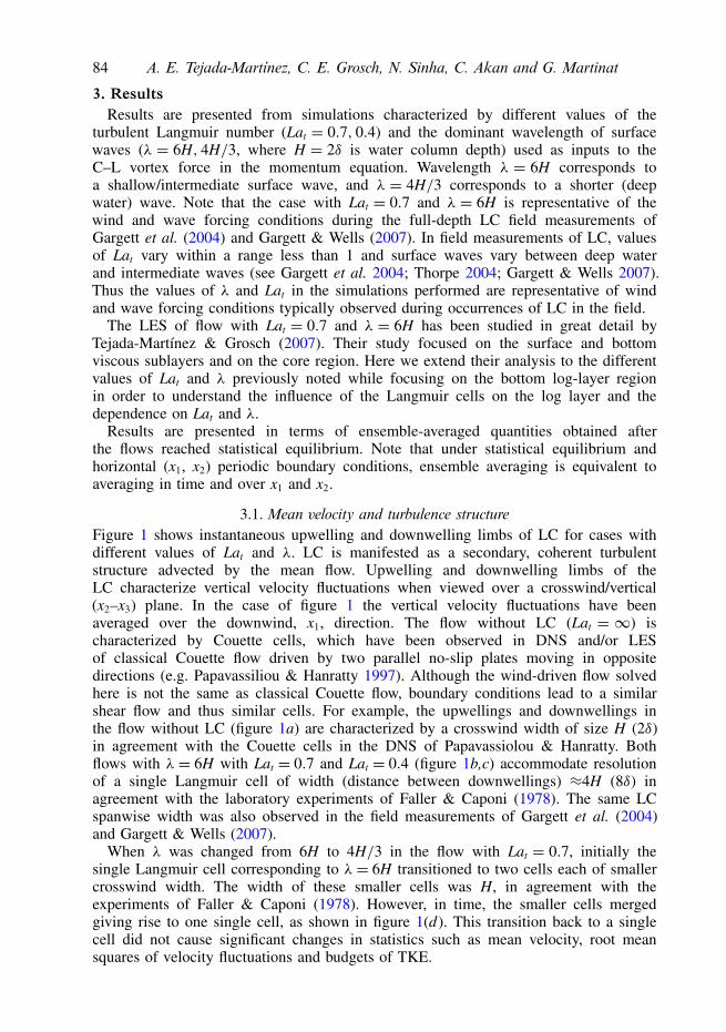
3. ResultsResults are presented from simulations characterized by different values of the

turbulent Langmuir number (Lat = 0.7, 0.4) and the dominant wavelength of surfacewaves (λ = 6H, 4H/3, where H = 2δ is water column depth) used as inputs to theC–L vortex force in the momentum equation. Wavelength λ = 6H corresponds toa shallow/intermediate surface wave, and λ = 4H/3 corresponds to a shorter (deepwater) wave. Note that the case with Lat = 0.7 and λ = 6H is representative of thewind and wave forcing conditions during the full-depth LC field measurements ofGargett et al. (2004) and Gargett & Wells (2007). In field measurements of LC, valuesof Lat vary within a range less than 1 and surface waves vary between deep waterand intermediate waves (see Gargett et al. 2004; Thorpe 2004; Gargett & Wells 2007).Thus the values of λ and Lat in the simulations performed are representative of windand wave forcing conditions typically observed during occurrences of LC in the field.

The LES of flow with Lat = 0.7 and λ = 6H has been studied in great detail byTejada-Martınez & Grosch (2007). Their study focused on the surface and bottomviscous sublayers and on the core region. Here we extend their analysis to the differentvalues of Lat and λ previously noted while focusing on the bottom log-layer regionin order to understand the influence of the Langmuir cells on the log layer and thedependence on Lat and λ.

Results are presented in terms of ensemble-averaged quantities obtained afterthe flows reached statistical equilibrium. Note that under statistical equilibrium andhorizontal (x1, x2) periodic boundary conditions, ensemble averaging is equivalent toaveraging in time and over x1 and x2.

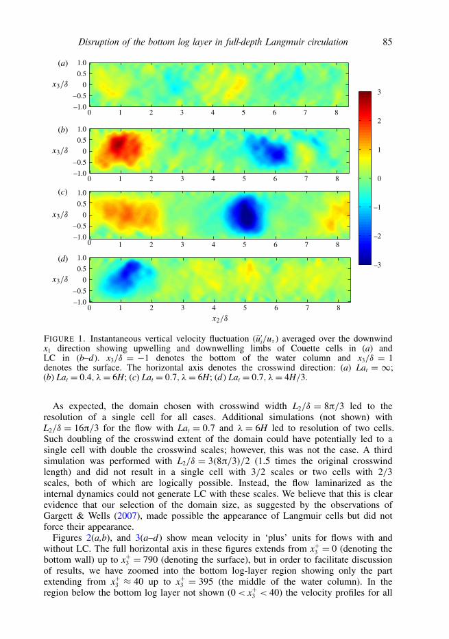
3.1. Mean velocity and turbulence structureFigure 1 shows instantaneous upwelling and downwelling limbs of LC for cases withdifferent values of Lat and λ. LC is manifested as a secondary, coherent turbulentstructure advected by the mean flow. Upwelling and downwelling limbs of theLC characterize vertical velocity fluctuations when viewed over a crosswind/vertical(x2–x3) plane. In the case of figure 1 the vertical velocity fluctuations have beenaveraged over the downwind, x1, direction. The flow without LC (Lat = ∞) ischaracterized by Couette cells, which have been observed in DNS and/or LESof classical Couette flow driven by two parallel no-slip plates moving in oppositedirections (e.g. Papavassiliou & Hanratty 1997). Although the wind-driven flow solvedhere is not the same as classical Couette flow, boundary conditions lead to a similarshear flow and thus similar cells. For example, the upwellings and downwellings inthe flow without LC (figure 1a) are characterized by a crosswind width of size H (2δ)in agreement with the Couette cells in the DNS of Papavassiolou & Hanratty. Bothflows with λ = 6H with Lat = 0.7 and Lat = 0.4 (figure 1b,c) accommodate resolutionof a single Langmuir cell of width (distance between downwellings) ≈4H (8δ) inagreement with the laboratory experiments of Faller & Caponi (1978). The same LCspanwise width was also observed in the field measurements of Gargett et al. (2004)and Gargett & Wells (2007).

When λ was changed from 6H to 4H/3 in the flow with Lat = 0.7, initially thesingle Langmuir cell corresponding to λ= 6H transitioned to two cells each of smallercrosswind width. The width of these smaller cells was H, in agreement with theexperiments of Faller & Caponi (1978). However, in time, the smaller cells mergedgiving rise to one single cell, as shown in figure 1(d). This transition back to a singlecell did not cause significant changes in statistics such as mean velocity, root meansquares of velocity fluctuations and budgets of TKE.


–0.5

0

0.5

–0.5

0

0.5

–0.5

0

0.5

–0.5

0

0.5

0 1 2 3 4 5 6 7 8

0

0 1 2 3 4 5 6 7 8

1 2 3 4 5 6 7 8

0 1 2 3 4 5 6 7 8

–3

–2

–1

0

1

2

3

–1.0

1.0

–1.0

1.0

–1.0

1.0

–1.0

1.0

(a)

(b)

(c)

(d)

FIGURE 1. Instantaneous vertical velocity fluctuation (u′i/uτ ) averaged over the downwindx1 direction showing upwelling and downwelling limbs of Couette cells in (a) andLC in (b–d). x3/δ = −1 denotes the bottom of the water column and x3/δ = 1denotes the surface. The horizontal axis denotes the crosswind direction: (a) Lat = ∞;(b) Lat = 0.4, λ= 6H; (c) Lat = 0.7, λ= 6H; (d) Lat = 0.7, λ= 4H/3.

As expected, the domain chosen with crosswind width L2/δ = 8π/3 led to theresolution of a single cell for all cases. Additional simulations (not shown) withL2/δ = 16π/3 for the flow with Lat = 0.7 and λ = 6H led to resolution of two cells.Such doubling of the crosswind extent of the domain could have potentially led to asingle cell with double the crosswind scales; however, this was not the case. A thirdsimulation was performed with L2/δ = 3(8π/3)/2 (1.5 times the original crosswindlength) and did not result in a single cell with 3/2 scales or two cells with 2/3scales, both of which are logically possible. Instead, the flow laminarized as theinternal dynamics could not generate LC with these scales. We believe that this is clearevidence that our selection of the domain size, as suggested by the observations ofGargett & Wells (2007), made possible the appearance of Langmuir cells but did notforce their appearance.

Figures 2(a,b), and 3(a–d) show mean velocity in ‘plus’ units for flows with andwithout LC. The full horizontal axis in these figures extends from x+3 = 0 (denoting thebottom wall) up to x+3 = 790 (denoting the surface), but in order to facilitate discussionof results, we have zoomed into the bottom log-layer region showing only the partextending from x+3 ≈ 40 up to x+3 = 395 (the middle of the water column). In theregion below the bottom log layer not shown (0< x+3 < 40) the velocity profiles for all


16

17

18

19

20

21

16

17

18

19

20

40 60 80 100 200 300 40 60 80 100 200 300

–1.0

–0.5

0

0.5

1.0

–1.0

–0.5

0

0.5

1.0

0 5 10 15 20 25 30 35 0 5 10 15 20 25 30 35

(a) (b)

(c) (d )

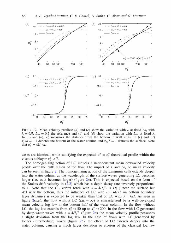
FIGURE 2. Mean velocity profiles: (a) and (c) show the variation with λ at fixed Lat withλ = 6H, Lat = 0.7 the reference and (b) and (d) show the variation with Lat at fixed λ.In (a) and (b), x+3 measures the distance from the bottom in wall units. In (c) and (d)x3/δ = −1 denotes the bottom of the water column and x3/δ = 1 denotes the surface. Notethat u+1 = 〈u1〉/uτ .

cases are identical, while satisfying the expected u+1 = x+3 theoretical profile within theviscous sublayer x+3 < 7.

The homogenizing action of LC induces a near-constant mean downwind velocityprofile over the bulk region of the flow. The impact of λ and Lat on mean velocitycan be seen in figure 2. The homogenizing action of the Langmuir cells extends deeperinto the water column as the wavelength of the surface waves generating LC becomeslarger (i.e. as λ becomes larger) (figure 2a). This is expected based on the form ofthe Stokes drift velocity in (2.2) which has a depth decay rate inversely proportionalto λ. Note that the CL vortex force with λ = 4H/3 is O(1) near the surface but�1 near the bottom, thus the influence of LC with λ = 4H/3 on bottom boundarylayer dynamics is expected to be weaker than that of LC with λ = 6H. As seen infigure 2(a,b), the flow without LC (Lat = ∞) is characterized by a well-developedmean velocity log law in the bottom half of the water column. In the flow withoutLC, the log-law extends from x+3 ≈ 50 up to x+3 ≈ 200. In the flow with LC generatedby deep-water waves with λ = 4H/3 (figure 2a) the mean velocity profile possessesa slight deviation from the log law. In the case of flows with LC generated bylonger (intermediate) waves (figure 2b), the effect of LC extends deeper into thewater column, causing a much larger deviation or erosion of the classical log law


UpwellingDownwelling

14

16

18

20

22

13

15

17

19

21

14

16

18

20

22

13

15

17

19

21

40 60 80 100 200 300

40 60 80 100 200 300 40 60 80 100 200 300

40 60 80 100 200 300

(a) (b)

(c) (d )

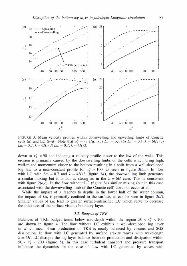
FIGURE 3. Mean velocity profiles within downwelling and upwelling limbs of Couettecells (a) and LC (b–d). Note that u+1 = 〈u1〉/uτ : (a) Lat = ∞; (b) Lat = 0.4, λ = 6H; (c)Lat = 0.7, λ= 6H; (d) Lat = 0.7, λ= 4H/3.

down to x+3 ≈ 90 and inducing a velocity profile closer to the law of the wake. Thiserosion is primarily caused by the downwelling limbs of the cells which bring high,well-mixed momentum closer to the bottom resulting in a shift from a well-developedlog law to a near-constant profile for x+3 > 100, as seen in figure 3(b,c). In flowwith LC with Lat = 0.7 and λ = 4H/3 (figure 3d), the downwelling limb generatesa similar mixing but it is not as strong as in the λ = 6H case. This is consistentwith figure 2(a,c). In the flow without LC (figure 3a) similar mixing (but in this caseassociated with the downwelling limb of the Couette cell) does not occur at all.

While the impact of λ reaches to depths in the lower half of the water column,the impact of Lat is primarily confined to the surface, as can be seen in figure 2(d).Smaller values of Lat lead to greater surface-intensified LC which serve to decreasethe thickness of the surface viscous boundary layer.

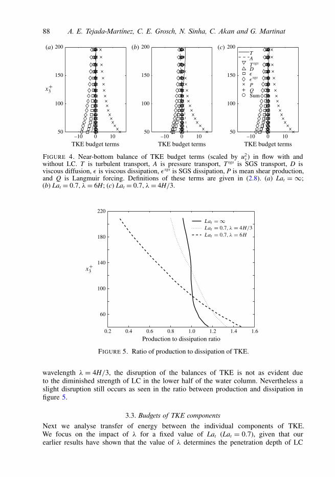
3.2. Budgets of TKEBalances of TKE budget terms below mid-depth within the region 50 < x+3 < 200are shown in figure 4. The flow without LC exhibits a well-developed log layerin which mean shear production of TKE is nearly balanced by viscous and SGSdissipation. In flow with LC generated by surface gravity waves with wavelengthλ = 6H, LC disrupts the log-layer balance between production and dissipation within50 < x+3 < 200 (figure 5). In this case turbulent transport and pressure transportinfluence the dynamics. In the case of flow with LC generated by waves with


100

150

0 100–10 100–10

TKE budget terms TKE budget terms TKE budget terms10–10

50

200

100

150

50

200

100

150

50

200(a) (b) (c)TATsgs

D

PQSum

sgs

FIGURE 4. Near-bottom balance of TKE budget terms (scaled by u2τ ) in flow with and

without LC. T is turbulent transport, A is pressure transport, T sgs is SGS transport, D isviscous diffusion, ε is viscous dissipation, εsgs is SGS dissipation, P is mean shear production,and Q is Langmuir forcing. Definitions of these terms are given in (2.8). (a) Lat = ∞;(b) Lat = 0.7, λ= 6H; (c) Lat = 0.7, λ= 4H/3.

0.4 0.6 0.8 1.0 1.2 1.4

60

100

140

180

220

Production to dissipation ratio0.2 1.6

FIGURE 5. Ratio of production to dissipation of TKE.

wavelength λ = 4H/3, the disruption of the balances of TKE is not as evident dueto the diminished strength of LC in the lower half of the water column. Nevertheless aslight disruption still occurs as seen in the ratio between production and dissipation infigure 5.

3.3. Budgets of TKE componentsNext we analyse transfer of energy between the individual components of TKE.We focus on the impact of λ for a fixed value of Lat (Lat = 0.7), given that ourearlier results have shown that the value of λ determines the penetration depth of LC


100

150

50

100

150

200

100

150

50

100

150

200

50

100

150

200

100

150

50

100

150

200

50

100

150

200

50

100

150

200

–20 0 20 –5 0 5 –2 –1 0 1 2

–20 0 20 –10 –5 0 5 10 –10 –5 0 5 10

0 0 0

50

200

50

200

50

200

–20 20 –5 5 –5 5

B

TA

D

PQSum

Tsgs

sgs

(a) (b) (c)

(d ) (e) ( f )

(g) (h) (i)

FIGURE 6. Near-bottom balance of TKE component budget terms (scaled by u2τ ) in flows

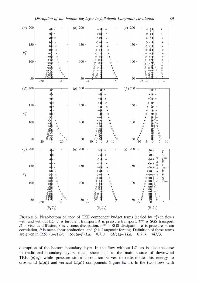
with and without LC. T is turbulent transport, A is pressure transport, T sgs is SGS transport,D is viscous diffusion, ε is viscous dissipation, εsgs is SGS dissipation, B is pressure–straincorrelation, P is mean shear production, and Q is Langmuir forcing. Definition of these termsare given in (2.5). (a–c) Lat =∞; (d–f ) Lat = 0.7, λ= 6H; (g–i) Lat = 0.7, λ= 4H/3.

disruption of the bottom boundary layer. In the flow without LC, as is also the casein traditional boundary layers, mean shear acts as the main source of downwindTKE 〈u′1u′1〉 while pressure–strain correlation serves to redistribute this energy tocrosswind 〈u′2u′2〉 and vertical 〈u′3u′3〉 components (figure 6a–c). In the two flows with


LC, one with λ = 6H and the other with λ = 4H/3, the Craik–Leibovich vortex forceacts as a source of vertical TKE, while pressure–strain correlation redistributes thisenergy to the crosswind component (figure 6d–i). Note that this behaviour is clearlyseen in the flow with λ= 4H/3 for which the log-layer disruption is not as evident interms of the previous diagnostics analysed (i.e. mean velocity and TKE budget terms).

4. Discussion and conclusionsWe have analysed mean velocity profiles and budgets of TKE resolved in LES of

full-depth LC in a wind-driven shear current in neutrally-stratified shallow water. Oneof the simulations performed was driven by wind and wave forcing representative ofconditions during field measurements of shallow-water, full-depth LC and is able tocapture the turbulent structure measured in the field. It was found that for sufficientlylong waves, LC disrupts classical boundary layer dynamics. For example, LC candisrupt the log law, inducing a ‘law of the wake like’ behaviour. LC can alsodisrupt the classical log-layer balance between production and dissipation of TKE.LC can also impact on the transfer of energy between TKE components inducingnew behaviour especially in terms of pressure–strain redistribution. In flows withfull-depth LC, pressure–strain redistribution transfers energy from vertical to crosswindTKE components, in contrast to classical boundary layers in which pressure–strainredistribution transfers energy from downwind to crosswind and vertical components.

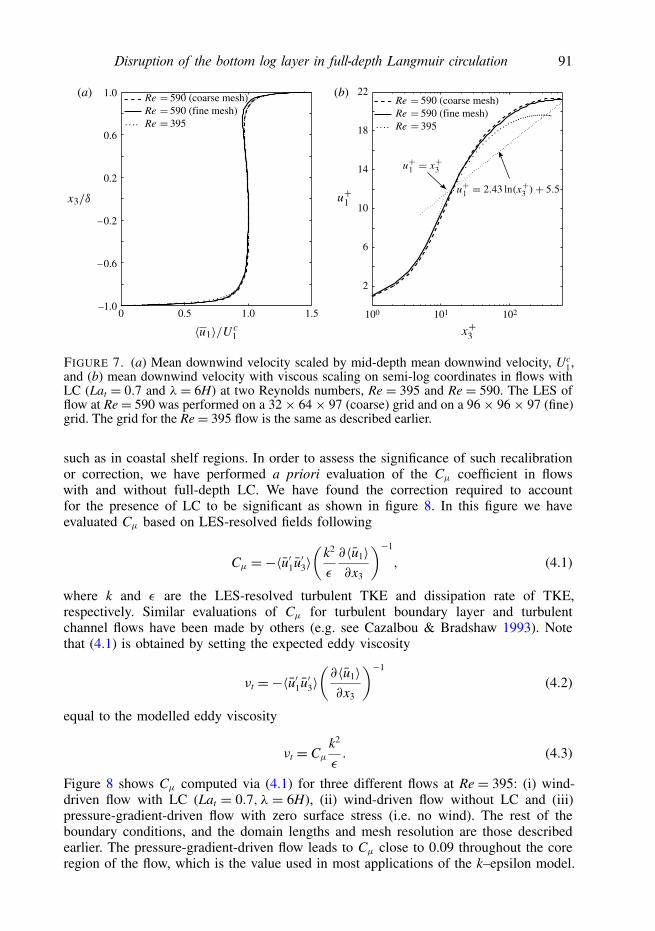
Results showing the disruption of the log layer in flows with LC have beenpresented for a fixed Reynolds number, Re = 395. We have performed simulationsat a higher Reynolds number and have found similar results. Figure 7 compares meanvelocity profiles for flows with LC (Lat = 0.7 and λ = 6H) at two different Reynoldsnumbers, Re = 395 and Re = 590. The flow at Re = 590 was simulated on a coarseand a fine grid. As seen in figure 7, the mean velocity profiles indicate that the resultswith Re = 590 are independent of the grid. When scaled by mean downwind velocityat mid-depth, there are minor changes in the mean downwind velocity profile as Re ischanged from 395 to 590 but no major changes are seen (figure 7a). When plotted in‘plus’ units on semi-log ordinates, the difference between the mean downwind velocityprofiles in the Re= 395 and Re= 590 flows is large (figure 7b). This difference servesas additional evidence that LC disrupts the log layer because if a log layer werepresent, then all of these curves would collapse onto a single linear curve in semi-logcoordinates.

The above results have important implications for turbulence parameterizationsfor RANS (Reynolds-averaged Navier–Stokes) simulation of the coastal ocean.Coefficients in popular RANS-based turbulence models are calibrated by constrainingthem such that model equations satisfy various flow conditions. For example, in thepopular k–epsilon model, the eddy viscosity is expressed as νt = Cµk2/ε. where k isTKE and ε is dissipation rate. Typically, in the log-layer region of a simple wall-bounded shear flow, k balances ε and the non-zero Reynolds shear stress component isnearly equal to the square of the wall friction velocity. These results are used togetherwith the log law and the corresponding mixing length to obtain a value for coefficientCµ (Cµ = 0.09, Pope 2000). As we have demonstrated in this paper, the presenceof full-depth LC can strongly disrupt the log layer, thereby eliminating one of theconstraints normally used to calibrate model coefficients. LES of full-depth LC hasrevealed that the classical balance between production and dissipation does not holdthroughout the disrupted log-layer region, thus coefficient Cµ should be recalibrated inapplications of the k–epsilon model to wind- and wave-driven flows in shallow water


–0.6

–0.2

0.2

0.6

2

6

10

14

18

0.5 1.0 100 101 102–1.0

1.0 22

Re 395Re 590 (fine mesh)Re 590 (coarse mesh)

Re 395Re 590 (fine mesh)Re 590 (coarse mesh)

0 1.5

(a) (b)

FIGURE 7. (a) Mean downwind velocity scaled by mid-depth mean downwind velocity, Uc1,

and (b) mean downwind velocity with viscous scaling on semi-log coordinates in flows withLC (Lat = 0.7 and λ = 6H) at two Reynolds numbers, Re = 395 and Re = 590. The LES offlow at Re= 590 was performed on a 32× 64× 97 (coarse) grid and on a 96× 96× 97 (fine)grid. The grid for the Re= 395 flow is the same as described earlier.

such as in coastal shelf regions. In order to assess the significance of such recalibrationor correction, we have performed a priori evaluation of the Cµ coefficient in flowswith and without full-depth LC. We have found the correction required to accountfor the presence of LC to be significant as shown in figure 8. In this figure we haveevaluated Cµ based on LES-resolved fields following

Cµ =−〈u′1u′3〉(

k2

ε

∂〈u1〉∂x3

)−1

, (4.1)

where k and ε are the LES-resolved turbulent TKE and dissipation rate of TKE,respectively. Similar evaluations of Cµ for turbulent boundary layer and turbulentchannel flows have been made by others (e.g. see Cazalbou & Bradshaw 1993). Notethat (4.1) is obtained by setting the expected eddy viscosity

νt =−〈u′1u′3〉(∂〈u1〉∂x3

)−1

(4.2)

equal to the modelled eddy viscosity

νt = Cµ

k2

ε. (4.3)

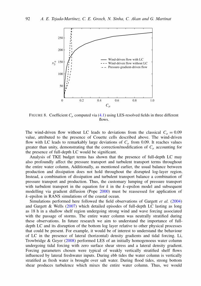
Figure 8 shows Cµ computed via (4.1) for three different flows at Re = 395: (i) wind-driven flow with LC (Lat = 0.7, λ = 6H), (ii) wind-driven flow without LC and (iii)pressure-gradient-driven flow with zero surface stress (i.e. no wind). The rest of theboundary conditions, and the domain lengths and mesh resolution are those describedearlier. The pressure-gradient-driven flow leads to Cµ close to 0.09 throughout the coreregion of the flow, which is the value used in most applications of the k–epsilon model.


0

50

100

150

200

250

0.2 0.4 0.6 0.8 1.0

Wind-driven flow with LCWind-driven flow without LCPressure-gradient-driven flow

FIGURE 8. Coefficient Cµ computed via (4.1) using LES-resolved fields in three differentflows.

The wind-driven flow without LC leads to deviations from the classical Cµ = 0.09value, attributed to the presence of Couette cells described above. The wind-drivenflow with LC leads to remarkably large deviations of Cµ from 0.09. It reaches valuesgreater than unity, demonstrating that the correction/modification of Cµ accounting forthe presence of full-depth LC would be significant.

Analysis of TKE budget terms has shown that the presence of full-depth LC mayalso profoundly affect the pressure transport and turbulent transport terms throughoutthe entire water column, Additionally, as mentioned earlier, the usual balance betweenproduction and dissipation does not hold throughout the disrupted log-layer region.Instead, a combination of dissipation and turbulent transport balance a combination ofpressure transport and production. Thus, the customary lumping of pressure transportwith turbulent transport in the equation for k in the k–epsilon model and subsequentmodelling via gradient diffusion (Pope 2000) must be reassessed for application ofk–epsilon in RANS simulations of the coastal ocean.

Simulations performed here followed the field observations of Gargett et al. (2004)and Gargett & Wells (2007) which detailed episodes of full-depth LC lasting as longas 18 h in a shallow shelf region undergoing strong wind and wave forcing associatedwith the passage of storms. The entire water column was neutrally stratified duringthese observations. In future research we aim to understand the importance of full-depth LC and its disruption of the bottom log layer relative to other physical processesthat could be present. For example, it would be of interest to understand the behaviourof LC in the presence of lateral (horizontal) density gradients and tidal forcing. Li,Trowbridge & Geyer (2008) performed LES of an initially homogenoeus water columnundergoing tidal forcing with zero surface shear stress and a lateral density gradient.Forcing parameters chosen were typical of weakly vertically stratified shelf flowsinfluenced by lateral freshwater inputs. During ebb tides the water column is verticallystratified as fresh water is brought over salt water. During flood tides, strong bottomshear produces turbulence which mixes the entire water column. Thus, we would


expect that conditions favourable for the generation of full-depth LC may occur duringperiods of flood tides when the water column becomes completely destratified, whileebb tides may lead to vertical stratification sufficiently strong to destroy the LC alongwith bottom-shear-generated turbulence.

AcknowledgementsThe support of the National Science Foundation through grants 0846510 and

0927724 is gratefully acknowledged. The authors would also like to acknowledge theuse of the services provided by Research Computing, University of South Florida.

R E F E R E N C E S

CAZALBOU, J. B. & BRADSHAW, P. 1993 Turbulent transport in wall-bounded flows. Evaluation ofmodel coefficients using direct numerical simulation. Phys. Fluids A 5, 3233–3239.

COLES, D. 1956 The law of the wake in the turbulent boundary layer. J. Fluid Mech. 1, 191–226.CRAIK, A. D. D. & LEIBOVICH, S. 1976 A rational model for Langmuir circulation. J. Fluid Mech.

73, 401–426.FALLER, A. & CAPONI, E. 1978 Laboratory studies of wind-driven Langmuir circulations.

J. Geophys. Res. 83, 3617–3633.GARGETT, A. & WELLS, R. 2007 Langmuir turbulence in shallow water. Part 1. Observations.

J. Fluid Mech. 576, 27–61.GARGETT, A., WELLS, R., TEJADA-MARTINEZ, A. E. & GROSCH, C. E. 2004 Langmuir

supercells: A dominant mechanism for sediment resuspension and transport. Science 306,1925–1928.

LANGMUIR, I. 1938 Surface motion induced by the wind. Science 87, 119–123.LI, M., TROWBRIDGE, J. & GEYER, R. 2008 Asymmetric tidal mixing due to the horizontal density

gradient. J. Phys. Oceanogr. 38, 418–434.LILLY, D. K. 1992 A proposed modification of the Germano subgrid-scale closure. Phys. Fluids 3,

2746–2757.MCWILLIAMS, J. C., SULLIVAN, P. P. & MOENG, C.-H. 1997 Langmuir turbulence in the ocean.

J. Fluid Mech. 334, 1–30.PAPAVASSILIOU, D. V. & HANRATTY, T. J. 1997 Interpretation of large-scale structures observed in

a turbulent plane Couette flow. Intl J. Heat Fluid Flow 18, 55–69.PHILLIPS, O. M. 1967 Dynamics of the Upper Ocean. Cambridge University Press.POPE, S. B. 2000 Turbulent Flows. Cambridge University Press.SCOTT, J., MYER, G., STEWART, R. & WALTHER, E. 1969 On the mechanism of Langmuir

circulations and their role in epilimnion mixing. Limnol. Oceanogr. 14, 493–503.SKYLLINGSTAD, E. D. & DENBO, D. W. 1995 An ocean large eddy simulation of Langmuir

circulations and convection in the surface mixed layer. J. Geophys. Res. 100, 8501–8522.TEJADA-MARTINEZ, A. E. & GROSCH, C. E. 2007 Langmuir turbulence in shallow water. Part 2.

Large-eddy simulation. J. Fluid Mech. 576, 63–108.TEJADA-MARTINEZ, A. E., GROSCH, C. E., GARGETT, A., POLTON, J., SMITH, J. &

MACKINNON, J. 2009 A hybrid spectral/finite-difference large-eddy simulator of turbulentprocesses in the upper ocean. Ocean Model. 30, 115–142.

THORPE, S. 2004 Langmuir circulation. Annu. Rev. Fluid Mech. 36, 55–79.

Disruption of the bottom log layer in large-eddy simulations of full-depth Langmuir circulation

Documents

Transcript of Disruption of the bottom log layer in large-eddy simulations of full-depth Langmuir circulation