Accepted Manuscript

Direct transcription methods based on fractional integralapproximation formulas for solving nonlinear fractional optimal controlproblems

Abubakar Bello Salati, Mostafa Shamsi, Delfim F. M. Torres

PII: S1007-5704(18)30155-2DOI: 10.1016/j.cnsns.2018.05.011Reference: CNSNS 4528

To appear in: Communications in Nonlinear Science and Numerical Simulation

Received date: 25 March 2018Accepted date: 16 May 2018

Please cite this article as: Abubakar Bello Salati, Mostafa Shamsi, Delfim F. M. Torres, Direct tran-scription methods based on fractional integral approximation formulas for solving nonlinear fractionaloptimal control problems, Communications in Nonlinear Science and Numerical Simulation (2018), doi:10.1016/j.cnsns.2018.05.011

This is a PDF file of an unedited manuscript that has been accepted for publication. As a serviceto our customers we are providing this early version of the manuscript. The manuscript will undergocopyediting, typesetting, and review of the resulting proof before it is published in its final form. Pleasenote that during the production process errors may be discovered which could affect the content, andall legal disclaimers that apply to the journal pertain.

brought to you by COREView metadata, citation and similar papers at core.ac.uk

provided by Repositório Institucional da Universidade de Aveiro

ACCEPTED MANUSCRIPT

ACCEPTED MANUSCRIP

T

Highlights

• A general class of fractional optimal control problems was considered, which contains the bang-bang, free

final time and path constraints problems.

• Fractional integration matrices of Grunwald-Letnikov, trapezoidal and Simpson’s formulas are derived.

• Using fractional integration matrix, the fractional optimal control problems are reduced to a finite-

dimensional optimization problem.

• In order to improve the speed and accuracy, the gradient of objective function and the Jacobian of

constraints are supplied for optimization solver.

• Numerical simulations are provided to illustrate the presented method on different types of fractional

optimal control problems.

1

ACCEPTED MANUSCRIPT

ACCEPTED MANUSCRIP

T

Direct transcription methods based on fractional integral approximationformulas for solving nonlinear fractional optimal control problems

Abubakar Bello Salatia, Mostafa Shamsia,∗, Delfim F. M. Torresb

aDepartment of Applied Mathematics, Faculty of Mathematics and Computer Science,Amirkabir University of Technology, No. 424 Hafez Avenue, Tehran, Iran

bDepartment of Mathematics, Center for Research and Development in Mathematics and Applications (CIDMA),University of Aveiro, 3810-193 Aveiro, Portugal

Abstract

This paper presents three direct methods based on Grunwald-Letnikov, trapezoidal and Simpson fractional

integral formulas to solve fractional optimal control problems (FOCPs). At first, the fractional integral form

of FOCP is considered, then the fractional integral is approximated by Grunwald-Letnikov, trapezoidal and

Simpson formulas in a matrix approach. Thereafter, the performance index is approximated either by trapezoidal

or Simpson quadrature. As a result, FOCP are reduced to nonlinear programming problems, which can be

solved by many well-developed algorithms. To improve the efficiency of the presented method, the gradient

of the objective function and the Jacobian of constraints are prepared in closed forms. It is pointed out that

the implementation of the methods is simple and, due to the fact that there is no need to derive necessary

conditions, the methods can be simply and quickly used to solve a wide class of FOCPs. The efficiency and

reliability of the presented methods are assessed by ample numerical tests involving a free final time with path

constraint FOCP, a bang-bang FOCP and an optimal control of a fractional-order HIV-immune system.

Keywords: Fractional optimal control, Direct numerical solution, Fractional integration matrix,

Grunwald-Letnikov, trapezoidal and Simpson fractional integral formulas.

2010 MSC: 26A33, 49M25.

1. Introduction

Fractional calculus may be considered an old and yet an interesting topic [1]. It deals with the investigation of

integrals and derivatives of an arbitrary order. At the initial stage, the fractional derivative was a mathematical

tool without a tangible application. But presently, fractional calculus has wide applications in various disciplines

like viscoelastic materials [2, 3], bioengineering applications [4, 5], signal processing [6, 7], mathematical finance

[8, 9], control theory [10, 11] and many other areas [12, 13]. The nonlocal nature of the fractional calculus has

given it a unique characteristic in modeling some complex systems with memory and hereditary properties that

arise from physical, engineering and even economic processes [14, 15]. More elaborate details on the theory and

∗Corresponding author.Email addresses: a.salati@aut.ac.ir, absalati@gmail.com (Abubakar Bello Salati), m_shamsi@aut.ac.ir (Mostafa

Shamsi), delfim@ua.pt (Delfim F. M. Torres)

Preprint submitted to Communications in Nonlinear Science and Numerical Simulation May 16, 2018

ACCEPTED MANUSCRIPT

ACCEPTED MANUSCRIP

T

applications of fractional calculus can be found in [2, 16, 17, 18].

Application of fractional calculus to optimal control problems has given birth to another new specialization,

known as fractional optimal control [18, 19, 20, 21]. According to [22], a Fractional Optimal Control Problem

(FOCP) is an optimal control problem in which the performance index and/or the dynamic equations contain at

least one fractional derivative operator. In simple terms, FOCPs are a generalization of the integer-order optimal

control problems, which are obtained by replacing integer-order derivatives with fractional ones. Recently, some

interesting and real-life models of FOCPs have been presented by the researchers in [23, 24, 25, 26, 27].

Like integer-order optimal control problems, the numerical methods for FOCPs can be categorized into

“direct” and “indirect” methods. With indirect methods, the solution is obtained by solving a fractional

Hamiltonian boundary-value problem, which is derived from the optimality conditions. Accordingly, the first

step in indirect methods is the derivation of first-order optimality conditions. On the other hand, direct

methods do not rely on optimality conditions. In these approaches, FOCPs are solved by transcribing them

into Nonlinear Programming problems (NLP). Thereafter, a NLP-solver is used to solve the resulting problem

[28]. The indirect methods, in comparison with the direct, have some disadvantages, including, (i) difficulties

in deriving the Hamiltonian boundary-value problem, especially for problems with path constraints, and (ii)

sensitivity to initial guess for state functions as well as costate or adjoint functions. Due to the aforementioned

reasons, direct methods are easier to employ than the indirect methods to solve both integer and fractional

order optimal control problems.

As earlier works on the formulation, derivation of optimality conditions and direct/indirect solution schemes

for FOCPs, we can refer to [29, 30, 31, 32, 33, 34, 35]. After these pioneer works, many other extensive

researches have been done on the development of numerical methods for FOCPs. For instance, we can refer

to Oustaloup recursive approximation [22], direct methods based on pseudo-state-space formulations of FOCP

[36], spectral methods based on orthogonal polynomials and fractional operational matrices [37, 38, 39, 40,

41, 42, 43], Legendre multiwavelet collocation methods [44], direct methods based on Bernstein polynomials

[45, 46, 47], nonstandard finite difference methods [48], linear programming approaches [49], integral fractional

pseudospectral methods [50], direct methods based on Ritz’s techniques [51, 52], the epsilon-Ritz method [53],

direct methods based on hybrid block-pulse with other basis functions [54, 55], pseudospectral methods based on

Legendre Muntz basis functions [56], dynamic Hamilton-Jacobi-Bellman methods [57], penalty and variational

methods [58], control parameterization methods [59], differential and integral fractional pseudospectral methods

[60], as well as other numerical techniques [61, 62, 63]. Efforts were also done to derive optimality conditions

for special types of FOCPs, such as bang-bang FOCPs [64] and free final and terminal time problems [65, 66].

Direct transcription methods based on local methods, such as trapezoidal and Simpson methods, are widely

used to solve integer-order optimal control problems and some softwares, such as SOCS [67] and ICLOCS [68],

are developed based on these methods. However, it is somewhat surprising that these methods have not been

yet fully explored to solve FOCPs. In this paper, we extend these methods to fractional order optimal control

problems. For this purpose, the matrix form of Grunwald-Letnikov, trapezoidal and Simpson approximation

3

ACCEPTED MANUSCRIPT

ACCEPTED MANUSCRIP

T

formulas for fractional integrals, which are called fractional integral matrices, are derived. These fractional

integration matrices are used to reduce the FOCP to a NLP. Thereafter, the resulted NLP is solved by using a

well-developed solver to obtain an approximate solution of the FOCP. Moreover, in order to increase the speed

of the proposed direct methods, the exact gradient of the objective function and the Jacobian of constraints are

derived and supplied to the NLP-solver. Finally, the reliability, efficiency and accuracy of the proposed direct

method are demonstrated with four test problems, including a nonlinear and complex FOCP, a FOCP with

path and terminal constraints, a bang-bang FOCP and an applied optimal control problem of a fractional order

HIV-immune system with memory.

The paper is organized as follows. In Section 2, the notions of fractional derivative and integral are reviewed

and three approximation methods for the fractional integral, in matrix form, are introduced. The considered

formulation of fractional optimal control problems is stated in Section 3. The detailed implementation of direct

methods is presented in Section 4. In Section 5, four numerical examples are provided to show the efficiency

and reliability of the proposed methods. Finally, a conclusion is given in Section 6.

2. Definition and approximation of fractional integral and derivative

In this section, some definitions, together with three approximation formulas for fractional integrals, are

reviewed. Moreover, for easy implementation, the matrix forms of these approximation formulas are derived.

Definition 2.1 (See, e.g., [16, 17]). The left sided fractional integral with order α > 0 of a given function

y(x), x ∈ (a, b), is defined as

0Iαx y (x) =1

Γ (α)

∫ x

0

(x− t)α−1 y (t) dt, (1)

where Γ(·) is Euler’s gamma function.

Definition 2.2 (See, e.g., [16, 17]). The left sided Caputo fractional derivative of order α ∈ (0, 1) of a func-

tion y (x) is defined as

C

0Dαxy (x) =1

Γ (1− α)

∫ x

0

(x− t)−αy (t) dt. (2)

The first step in developing our numerical methods is to approximate the fractional integral of a given

function. For this purpose, we briefly review Grunwald-Letnikov (GL), trapezoidal (TR) and Simpson (SI)

formulas for approximating the fractional integral.

2.1. The Grunwald-Letnikov formula for approximating a fractional integral

Let the fractional integral of function y be defined on the interval [0, 1]. To approximate the fractional

integral of function y, the interval [0, 1] is divided into n equal parts by the following mesh points:

xi := ih, i = 0, 1, . . . , n,

4

ACCEPTED MANUSCRIPT

ACCEPTED MANUSCRIP

T

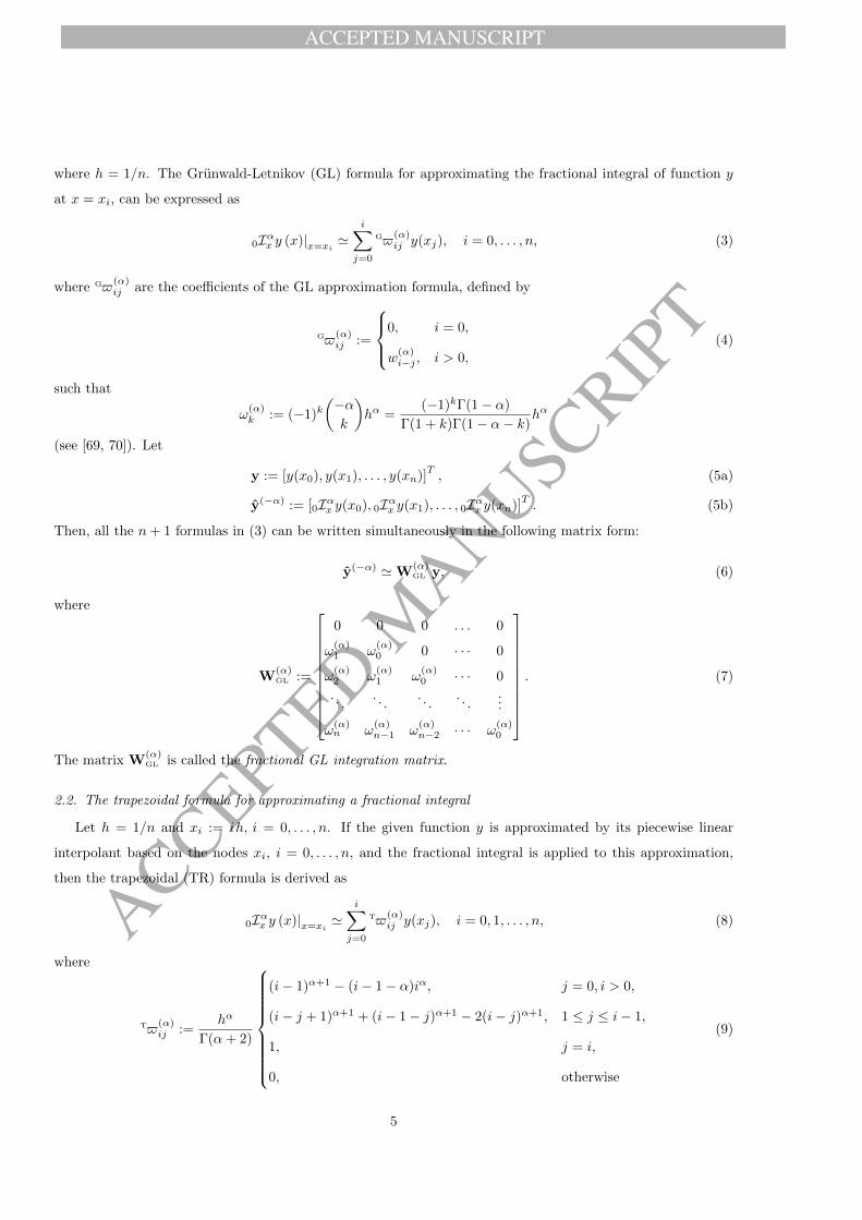
where h = 1/n. The Grunwald-Letnikov (GL) formula for approximating the fractional integral of function y

at x = xi, can be expressed as

0Iαx y (x)|x=xi'

i∑

j=0

G$(α)ij y(xj), i = 0, . . . , n, (3)

where G$(α)ij are the coefficients of the GL approximation formula, defined by

G$(α)ij :=

0, i = 0,

w(α)i−j , i > 0,

(4)

such that

ω(α)k := (−1)k

(−αk

)hα =

(−1)kΓ(1− α)

Γ(1 + k)Γ(1− α− k)hα

(see [69, 70]). Let

y := [y(x0), y(x1), . . . , y(xn)]T,

y(−α) := [0Iαx y(x0), 0Iαx y(x1), . . . , 0Iαx y(xn)]T.

(5a)

(5b)

Then, all the n+ 1 formulas in (3) can be written simultaneously in the following matrix form:

y(−α) 'W(α)GL y, (6)

where

W(α)GL :=

0 0 0 . . . 0

ω(α)1 ω

(α)0 0 · · · 0

ω(α)2 ω

(α)1 ω

(α)0 · · · 0

. . .. . .

. . .. . .

...

ω(α)n ω

(α)n−1 ω

(α)n−2 · · · ω

(α)0

. (7)

The matrix W(α)GL is called the fractional GL integration matrix.

2.2. The trapezoidal formula for approximating a fractional integral

Let h = 1/n and xi := ih, i = 0, . . . , n. If the given function y is approximated by its piecewise linear

interpolant based on the nodes xi, i = 0, . . . , n, and the fractional integral is applied to this approximation,

then the trapezoidal (TR) formula is derived as

0Iαx y (x)|x=xi'

i∑

j=0

T$(α)ij y(xj), i = 0, 1, . . . , n, (8)

where

T$(α)ij :=

hα

Γ(α+ 2)

(i− 1)α+1 − (i− 1− α)iα, j = 0, i > 0,

(i− j + 1)α+1 + (i− 1− j)α+1 − 2(i− j)α+1, 1 ≤ j ≤ i− 1,

1, j = i,

0, otherwise

(9)

5

ACCEPTED MANUSCRIPT

ACCEPTED MANUSCRIP

T

(see [69]). If we set

a(α)k := hα

Γ(α+2)

0, k = 0,

(k − 1)α+1 − (k − 1− α)kα, k > 0,

b(α)k := hα

Γ(α+2)

1, k = 0,

(k + 1)α+1 + (k − 1)α+1 − 2kα+1, k > 0,

then, we can express the coefficients of the trapezoidal formula (8) as

T$(α)ij :=

a(α)i , k = 0, j > 0,

b(α)i−j , 1 ≤ j ≤ i,

0, otherwise.

(10)

Considering (5), the trapezoidal formula (8) can be expressed in the following matrix form:

y(−α) 'W(α)TR y, (11)

where W(α)TR is the fractional TR integration matrix defined by

W(α)TR :=

0 0 0 0 0 . . . 0 0

a(α)1 b

(α)0 0 0 0 · · · 0 0

a(α)2 b

(α)1 b

(α)0 0 0 · · · 0 0

a(α)3 b

(α)2 b

(α)1 b

(α)0 0 · · · 0 0

a(α)3 b

(α)3 b

(α)2 b

(α)1 b

(α)0 · · · 0 0

......

.... . .

. . .. . .

......

a(α)n b

(α)n−2 b

(α)n−3 b

(α)n−4 · · · b

(α)1 b

(α)0 0

a(α)n b

(α)n−1 b

(α)n−2 b

(α)n−3 · · · b

(α)2 b

(α)1 b

(α)0

. (12)

2.3. The Simpson formula for approximating a fractional integral

Let n be even and the interval [0, 1] be divided into n parts by the mesh points xi := ih, i = 0, . . . , n. Then

the given function y on the intervals [x2i, x2i+2], i = 0, . . . , n2 − 2, can be approximated by its corresponding

quadratic interpolation polynomial, i.e., y is approximated by a piecewise quadratic polynomial on the whole

interval [0, 1]. By replacing y(t) with this piecewise quadratic polynomial approximation in (1), the Simpson

formula for approximating the fractional integral of function y on the nodes xi, i = 0, . . . , n, is derived as

0Iαx y (x)|x=xi'

i+1∑

j=0

S$(α)ij y(xj), i = 0, 1, . . . , n, (13)

where

S$(α)ij :=

γ(α)i , j = 0,

θ(α)i−j+1, j is odd,

µ(α)i−j+2, j is even,

(14)

6

ACCEPTED MANUSCRIPT

ACCEPTED MANUSCRIP

T

such that the parameters γ(α)k , θ

(α)k and µ

(α)k are defined as

γ(α)k :=

hα

Γ (α+ 3)

0, k ≤ 0,

12 (2α+ 3)α, k = 1,

λ(α)0,k , 2 ≤ k,

θ(α)k :=

hα

Γ (α+ 3)

0, k ≤ 0,

2α+ 2, k = 1,

λ(α)1,k , 2 ≤ k,

µ(α)k :=

hα

Γ (α+ 3)

0, k ≤ 0,

− 12α, k = 1,

λ(α)2,2 , k = 2,

λ(α)2,3 + 1

2 (2α+ 3)α, k = 3,

λ(α)2,k + λ

(α)0,k−2, 4 ≤ k,

where

λ(α)0,k :=

1

2

[2α2 − (3 k − 6)α+ 2 k2 − 6 k + 4

]kα − 1

2(2 k + α− 2) (k − 2)

α+1,

λ(α)1,k := 2 (k − 2)

α+1(k + α)− 2 kα+1 (k − α− 2) ,

λ(α)2,k :=

1

2kα+1 (2 k − α− 2)− 1

2(k − 2)

α (2 k2 + (3α− 2) k + 2α2

).

Considering (5), the Simpson formula (13) can be expressed in the following matrix form

y(−α) 'W(α)SI y, (15)

where W(α)SI is the fractional SI integration matrix

W(α)SI :=

0 0 0 0 0 . . . 0 0

γ(α)1 θ

(α)1 µ

(α)1 0 0 · · · 0 0

γ(α)2 θ

(α)2 µ

(α)2 0 0 · · · 0 0

γ(α)3 θ

(α)3 µ

(α)3 θ

(α)1 µ

(α)1 · · · 0 0

γ(α)4 θ

(α)4 µ

(α)4 θ

(α)2 µ

(α)2 · · · 0 0

......

.... . .

. . .. . .

......

γ(α)n−1 θ

(α)n−1 µ

(α)n−1 θ

(α)n−3 µ

(α)n−3 · · · θ

(α)1 µ

(α)1

γ(α)n θ

(α)n µ

(α)n θ

(α)n−2 µ

(α)n−2 · · · θ

(α)2 µ

(α)2

. (16)

The Simpson and trapezoidal approximation formulas have been presented in [69]. Due to the fact that these

matrix forms have some advantages in the implementation of our method, in this paper we derived the explicit

forms of these matrices.

7

ACCEPTED MANUSCRIPT

ACCEPTED MANUSCRIP

T

3. The fractional optimal control problem

In this work, we consider a general formulation for FOCPs, which is described as follows: find the optimal

control u(t) = [u1(t), . . . , uq(t)] ∈ Rq, the state x(t) = [x1(t), . . . , xp(t)] ∈ Rp and possibly the terminal time tf

that minimize the performance index

J [u] = h (tf ,x(tf )) +

∫ tf

0

g (x(t),u(t), t)dt (17a)

subject to the fractional dynamic system

C

0Dαt x(t) = f(x(t),u(t), t), 0 < α ≤ 1, (17b)

with the initial and boundary conditions

x(0) = x0, (17c)

ψ(x(tf ), tf ) = 0, (17d)

and with the path constraint

φ (x(t),u(t), t) ≤ 0. (17e)

Here, functions h, g, f , ψ and φ are sufficiently continuously differentiable and defined by the following mappings:

h : R× Rp → R,

g : Rp × Rq × R→ R,

f : Rp × Rq × R→ Rp,

ψ : Rp × R→ Rr1 , 0 ≤ r1 ≤ q,

φ : Rp × Rq × R→ Rr2 , 0 ≤ r2.

Most FOCPs found in the literature, in various disciplines like engineering, control, signal processing and others,

belong to the above general class of FOCPs [23, 24, 25].

For easy application of our numerical method, the time domain [0, tf ] is mapped to the canonical interval

[0, 1], by using the affine transformation t→ τtf . Applying this mapping and by noting that

C0 Dαt x(t) = (tf )

−α C0 Dατ x(τ),

the optimal control problem (17) is converted to the following form:

min J [u] =h (tf ,x(1)) + tf

∫ 1

0

g (x(τ),u(τ), tf τ)dτ

s.t. C

0Dαt x(τ) = (tf )αf(x(τ),u(τ), tf τ),

x(0) = x0,

ψ(x(1), tf ) = 0,

φ(x(τ),u(τ), tf τ) ≤ 0.

(18a)

(18b)

(18c)

(18d)

(18e)

8

ACCEPTED MANUSCRIPT

ACCEPTED MANUSCRIP

T

It should to be noted that, after applying the mentioned transformation, the symbols of variables in (18) should

be changed to new symbols. However, for the sake of simplicity, we shall retain the symbols already used.

4. The proposed method

We present a direct numerical approach to solve the FOCPs stated in (18). Let the interval [0, 1] be divided

into n equal parts by the following mesh points:

τk := kh, k = 0, . . . , n,

where h = 1/n. Moreover, for the sake of simplicity, we consider the notations

xi := x(τi), ui := u(τi), fi := f(x(τi),u(τi), tf τi). (19)

4.1. Discretization of the performance index

The performance index (18a) is discretized by a quadrature formula, such as the trapezoidal, Simpson or

other rules. In this way, we have

Jn = h(tf ,xn) + tf

n∑

i=0

wig(xi,ui, tf τi), (20)

where, in the case of using the trapezoidal rule,

w0 :=h

2, wi := h, i = 1, . . . , n− 1, wn :=

h

2

and, in the case of using Simpson rule,

w0 :=h

3, w2i−1 :=

4h

3, w2i :=

2h

3, i = 1, . . . ,

n

2− 1, wn :=

h

3.

4.2. Discretization of the fractional dynamic equation

By applying the fractional integral operator 0Iατ to both sides of the fractional dynamic equation (18b), and

by noting that 0Iατ (C0Dατ x (τ)) = x(τ)−x(0), the above fractional dynamic equations can be converted into the

following fractional integral form:

x(τ) = x(0) + (tf )α

0Iατ f(x(τ),u(τ), tf τ). (21)

By collocating the above equation at τ = τi, i = 1, . . . , n, we have

x(τi) = x(0) + (tf )α

[0Iαt (f(x(τ),u(τ), tf τ))]τ=τi. (22)

Considering the initial condition (18c) and notations (19), and by applying GL/TR/SI approximation formulas

(3)/(8)/(13), we can approximate the equation (22) as follows:

xi = x0 + (tf )α

i∑

j=0

$(α)ij f(xj ,uj , tf τj), i = 1, 2, . . . , n, (23)

9

ACCEPTED MANUSCRIPT

ACCEPTED MANUSCRIP

T

where $(α)ij are the coefficients of GL/TR/SI approximation formula defined in (4)/(9)/(14). Similarly, we can

discretize the path constraint (18e) as follows:

φ(xi,ui, tf τi) ≤ 0, i = 0, . . . , n. (24)

Moreover, the terminal condition (18d) can be discretized as

ψ(xn, tf ) = 0. (25)

In summary, the FOCP (18) is transcribed into the following nonlinear programming problem (NLP):

min Jn = h(tf ,xn) + tf

n∑

i=0

wig(xi,ui, tf τi)

s.t. xi = x0 + (tf )α

i∑

j=0

$(α)ij f (xj ,uj , tf τj) , i = 0, 1, . . . , n,

ψ(xn, tf ) = 0,

φ(xi,ui, tf τi) ≤ 0, i = 0, . . . , n.

(26a)

(26b)

(26c)

(26d)

It should be remembered that the decision variables of the above optimization problem are: xi, i = 0, . . . , n, ui,

i = 0, . . . , n, and maybe tf . By utilizing an optimization solver, we can solve the optimization problem (26) and

find the optimal value of the decision variables, which are the approximations of state and control functions at

the points τi, i = 0, . . . , n.

4.2.1. Reformat of the resulted optimization problem to the classical form

Traditionally, in an NLP, it is preferred that the decision variables are placed in a vector. This helps to

analyze and utilize a solver for solving the problem. Here, we reformulate the NLP (26) into the standard form,

where the decision variables are collected in a vector z. For fixed final time problems, the vector of all decision

variables is

z := [x0,u0,x1,u1, . . . ,xn,un]T

and for free final time problems

z := [x0,u0,x1,u1, . . . ,xn,un, tf ]T.

If we define new functions h and g as

h(z) := h(tf ,xn), g(z) :=

g(x0,u0, tf τ0)

g(x1,u1, tf τ1)...

g(xn,un, tf τn)

, (27)

then we can express the objective function (26a) as

Jn(z) := h(z) + tf wT g(z),

10

ACCEPTED MANUSCRIPT

ACCEPTED MANUSCRIP

T

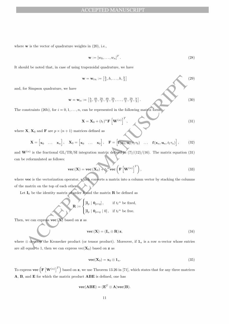
where w is the vector of quadrature weights in (20), i.e.,

w := [w0, . . . , wn]T. (28)

It should be noted that, in case of using trapezoidal quadrature, we have

w = wTR :=[h2 , h, . . . , h,

h2

](29)

and, for Simpson quadrature, we have

w = wSI :=[h3 ,

4h3 ,

2h3 ,

4h3 ,

2h3 , . . . ,

4h3 ,

2h3 ,

h3

]. (30)

The constraints (26b), for i = 0, 1, . . . , n, can be represented in the following matrix form:

X = X0 + (tf )αF

[W(α)

]T, (31)

where X, X0 and F are p× (n+ 1) matrices defined as

X =[x0 . . . xn

], X0 =

[x0 . . . x0

], F =

[f(x0,u0, tf τ0) . . . f(xn,un, tf τn)

], (32)

and W(α) is the fractional GL/TR/SI integration matrix defined in (7)/(12)/(16). The matrix equation (31)

can be reformulated as follows:

vec (X) = vec (X0) + tfαvec

(F[W(α)

]T), (33)

where vec is the vectorization operator, which converts a matrix into a column vector by stacking the columns

of the matrix on the top of each other.

Let Ik be the identity matrix of order k and the matrix R be defined as

R :=

[Ip | 0p×q] , if tfα be fixed,

[Ip | 0p×q | 0] , if tfα be free.

Then, we can express vec (X) based on z as

vec (X) = (In ⊗R) z, (34)

where ⊗ denotes the Kronecker product (or tensor product). Moreover, if 1n is a row n-vector whose entries

are all equal to 1, then we can express vec(X0) based on z as

vec(X0) = x0 ⊗ 1n. (35)

To express vec(F[W(α)

]T)based on z, we use Theorem 13.26 in [71], which states that for any three matrices

A, B, and E for which the matrix product ABE is defined, one has

vec(ABE) = (ET ⊗A)vec(B).

11

ACCEPTED MANUSCRIPT

ACCEPTED MANUSCRIP

T

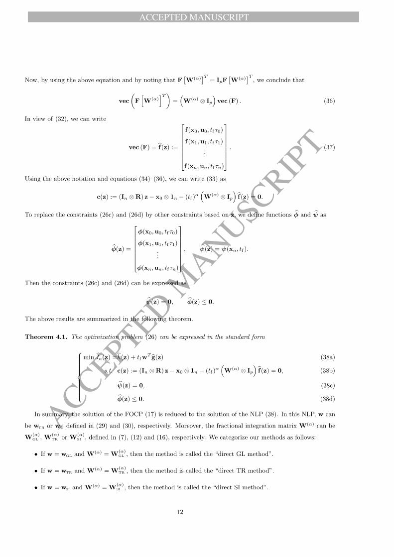
Now, by using the above equation and by noting that F[W(α)

]T= IpF

[W(α)

]T, we conclude that

vec

(F[W(α)

]T)=(W(α) ⊗ Ip

)vec (F) . (36)

In view of (32), we can write

vec (F) = f(z) :=

f(x0,u0, tf τ0)

f(x1,u1, tf τ1)...

f(xn,un, tf τn)

. (37)

Using the above notation and equations (34)–(36), we can write (33) as

c(z) := (In ⊗R) z− x0 ⊗ 1n − (tf )α(W(α) ⊗ Ip

)f(z) = 0.

To replace the constraints (26c) and (26d) by other constraints based on z, we define functions φ and ψ as

φ(z) =

φ(x0,u0, tf τ0)

φ(x1,u1, tf τ1)...

φ(xn,un, tf τn)

, ψ(z) = ψ(xn, tf ).

Then the constraints (26c) and (26d) can be expressed as

ψ(z) = 0, φ(z) ≤ 0.

The above results are summarized in the following theorem.

Theorem 4.1. The optimization problem (26) can be expressed in the standard form

min Jn(z) =h(z) + tf wT g(z)

s.t. c(z) := (In ⊗R) z− x0 ⊗ 1n − (tf )α(W(α) ⊗ Ip

)f(z) = 0,

ψ(z) = 0,

φ(z) ≤ 0.

(38a)

(38b)

(38c)

(38d)

In summary, the solution of the FOCP (17) is reduced to the solution of the NLP (38). In this NLP, w can

be wTR or wSI defined in (29) and (30), respectively. Moreover, the fractional integration matrix W(α) can be

W(α)GL , W

(α)TR or W

(α)SI , defined in (7), (12) and (16), respectively. We categorize our methods as follows:

• If w = wGL and W(α) = W(α)GL , then the method is called the “direct GL method”.

• If w = wTR and W(α) = W(α)TR , then the method is called the “direct TR method”.

• If w = wSI and W(α) = W(α)SI , then the method is called the “direct SI method”.

12

ACCEPTED MANUSCRIPT

ACCEPTED MANUSCRIP

T

4.2.2. Gradient of the objective function and Jacobian of the constraints

The speed of the proposed method depends on the speed one solves the NLP (38). On the other hand, a

crucial task in solving NLPs is computing the first derivatives of the objective and constraint functions (gradients

of the objective function and Jacobians of the constraints). Many NLP-solvers allow users to supply the exact

first derivatives. If the derivatives are not provided, then the solvers approximate them numerically, by finite

difference formulas. However, the use of first derivative approximations may seriously degrade the performance

and convergence of the NLP-solver. Thus, it is highly recommended that at least the exact gradient of the

objective function and the Jacobian of the constraints are provided by the user. These can make a great

improvement in the convergence, accuracy and computation time of the NLP-solver. In what follows, we detail

the closed forms for the gradient of the objective function and the Jacobian of constraints.

For free time problems, the gradient of the objective function can be obtained as

∇Jn(z) =

∂Jn(z)/∂x0

∂Jn(z)/∂u0

∂Jn(z)/∂x1

∂Jn(z)/∂u1

...

∂Jn(z)/∂xn

∂Jn(z)/∂un

∂Jn(z)/∂tf

=

tf w0 gx(x0,u0, tf τ0)

tf w0 gu(x0,u0, tf τ0)

tf w1 gx(x1,u1, tf τ1)

tf w1 gu(x1,u1, tf τ1)...

hx(tf ,xn) + tfwngx(xn,un, tf τn)

tfwngu(xn,un, tf τn)

ht(tf ,xn) +∑ni=0 wi

[g(xi,ui, tf τi) + tf τi gt(xi,ui, tf τi)

]

. (39)

For fixed final time problems, the gradient is the same as above, except that the last row is removed.

The Jacobian of constraints (38b), for free final time problems, can be derived as

∇c(z) =[

(In ⊗R)− (tf )α (

WT ⊗ Ip)∇f (z) (tf )

α−1(WT ⊗ Ip

) (−αf (z)− tf ftf (z)

) ], (40)

such that

∇f (z) :=

[fx]0 [fu]0

[fx]1 [fu]1. . .

[fx]n [fu]n

, ftf (z) :=

τ0ft(x0,u0, tf τ0)

τ1ft(x1,u1, tf τ1)...

τnft(xn,un, tf τn)

,

where [fx]i and [fu]i are the p-vectors defined as

[fx]i := fx(xi,ui, tf τi), [fu]i := fu(xi,ui, tf τi).

In the case of fixed final time problems, the Jacobian of constraints (38b) is obtained as

∇c(z) =[

(In ⊗R)− (tf )α(WT ⊗ Ip

)∇f (z)

]. (41)

13

ACCEPTED MANUSCRIPT

ACCEPTED MANUSCRIP

T

The Jacobian of constraint (38c), for fixed final time FOCPs, is derived as

∇ψ(z) =[

0r1×(n−1)(p+q) ψx(xn, tf ) 0r1×q

](42)

while for free final time FOCPs is given by

∇ψ(z) =[

0r1×(n−1)(p+q) ψx(xn, tf ) 0r1×q ψt(xn, tf )]. (43)

In case of free final time FOCPs, the Jacobian of the inequality constraints (38d) is obtained as

∇φ(z) =

[φx]0 [φu]0 τ0φt(x0,u0, tf τ0)

[φx]1 [φu]1 τ1φt(x1,u1, tf τ1)

. . .

[φx]n [φu]n τnφt(xn,un, tf τn)

, (44)

where [φx]i and [φu]i are the r2-vectors defined by

[φx]i := φx(xi,ui, tf τi), [φu]i := φu(xi,ui, tf τi), i = 0, . . . , n.

In case of fixed final time problems, the last column of the Jacobian matrix (44) is removed.

As we can see, the partial derivatives of g, f , ψ and φ with respect to x and u are needed to provide the

gradient of the objective function and the Jacobian of the constraints. We can use symbolic computation to

supply these partial derivatives.

5. Numerical examples

We now illustrate the direct methods presented in Section 4 through numerical experiments. We have

implemented the direct GL, TR and SI methods using Matlab on a 3.5 GHz Core i7 personal computer with

8 GB of RAM. Moreover, for solving the nonlinear programming problem (38), the solver Ipopt [72] was used,

which is based on an interior-point algorithm. In Ipopt, we can adjust the accuracy of solution by the input

parameter tolrfun. In our numerical experiments, we set tolrfun=10−12.

We consider four nontrivial examples. The first two examples are new while the last two examples have

been investigated before in the literature. At each example, the capability of the proposed direct methods is

highlighted. For the first example, which has an exact solution, the accuracy of our methods, and the required

CPU time, are assessed. In the second example, the ability of the method in solving a free final time FOCP with

path constraints is investigated. In the third example, we show that the proposed methods are also suitable to

deal with bang-bang optimal control problems. In the last example, we assess the ability of our direct methods

in solving a practical and challenging problem of HIV.

14

ACCEPTED MANUSCRIPT

ACCEPTED MANUSCRIP

T

0 5 10 15 20-3

-2

-1

0

1

2

3

0 5 10 15 200

1

2

3

4

5

0 5 10 15 20-0.1

-0.05

0

0.05

0.1

0 5 10 15 20-3

-2

-1

0

1

2

3

0 5 10 15 200

1

2

3

4

5

0 5 10 15 20-0.5

0

0.5

1

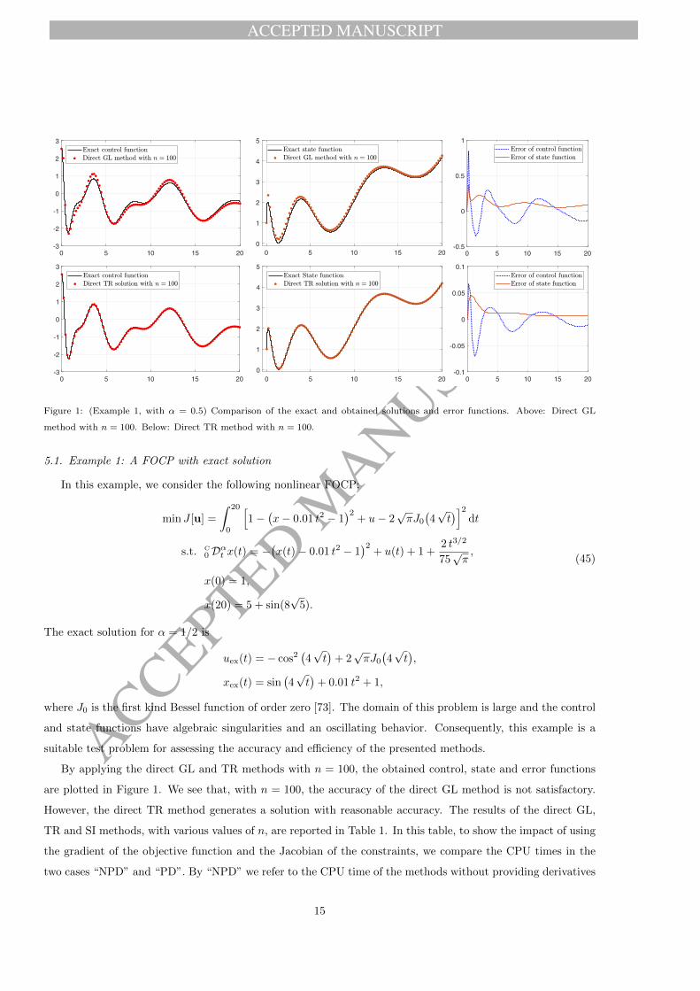
Figure 1: (Example 1, with α = 0.5) Comparison of the exact and obtained solutions and error functions. Above: Direct GL

method with n = 100. Below: Direct TR method with n = 100.

5.1. Example 1: A FOCP with exact solution

In this example, we consider the following nonlinear FOCP:

min J [u] =

∫ 20

0

[1−

(x− 0.01 t2 − 1

)2+ u− 2

√πJ0

(4√t)]2

dt

s.t. C

0Dαt x(t) = −(x(t)− 0.01 t2 − 1

)2+ u(t) + 1 +

2 t3/2

75√π,

x(0) = 1,

x(20) = 5 + sin(8√

5).

(45)

The exact solution for α = 1/2 is

uex(t) = − cos2(4√t)

+ 2√πJ0

(4√t),

xex(t) = sin(4√t)

+ 0.01 t2 + 1,

where J0 is the first kind Bessel function of order zero [73]. The domain of this problem is large and the control

and state functions have algebraic singularities and an oscillating behavior. Consequently, this example is a

suitable test problem for assessing the accuracy and efficiency of the presented methods.

By applying the direct GL and TR methods with n = 100, the obtained control, state and error functions

are plotted in Figure 1. We see that, with n = 100, the accuracy of the direct GL method is not satisfactory.

However, the direct TR method generates a solution with reasonable accuracy. The results of the direct GL,

TR and SI methods, with various values of n, are reported in Table 1. In this table, to show the impact of using

the gradient of the objective function and the Jacobian of the constraints, we compare the CPU times in the

two cases “NPD” and “PD”. By “NPD” we refer to the CPU time of the methods without providing derivatives

15

ACCEPTED MANUSCRIPT

ACCEPTED MANUSCRIP

T

Table 1: (Example 1, with α = 0.5) Obtained CPU times and the `2 norm of the errors by direct GL, TR and SI methods for

various values of n. All CPU times are in seconds.

Direct GL method Direct TR method Direct SI method

n CPU time (s) ERROR CPU time (s) ERROR CPU time (s) ERROR

NPD PD En(u) En(x) NPD PD En(u) En(x) NPD PD En(u) En(x)

100 8.9 0.5 1.68e-1 1.11e-1 6.3 0.6 2.07e-2 1.48e-2 6.4 0.5 8.99e-4 5.60e-4

200 22.6 0.7 9.19e-2 5.71e-2 17.9 0.8 5.21e-3 3.71e-3 12.7 0.8 7.66e-5 4.91e-5

300 23.2 1.3 6.37e-2 3.94e-2 22.7 1.5 2.32e-3 1.65e-3 25.2 1.1 1.80e-5 1.18e-5

400 33.6 2.1 4.88e-2 3.04e-2 34.4 2.2 1.31e-3 9.31e-4 35.6 2.1 6.48e-6 4.30e-6

500 53.1 3.0 3.95e-2 2.48e-2 47.6 3.6 8.39e-4 5.96e-4 50.8 3.2 2.94e-6 1.97e-6

600 76.5 4.4 3.32e-2 2.11e-2 63.6 5.0 5.84e-4 4.15e-4 76.5 5.1 1.54e-6 1.04e-6

700 84.9 6.5 2.87e-2 1.84e-2 94.3 6.9 4.29e-4 3.05e-4 100.6 7.7 8.98e-7 6.04e-7

800 130.1 8.7 2.52e-2 1.63e-2 110.4 8.7 3.29e-4 2.34e-4 107.5 9.2 5.62e-7 3.80e-7

900 163.2 12.3 2.25e-2 1.47e-2 150.9 11.9 2.60e-4 1.85e-4 188.2 13.4 3.70e-7 2.50e-7

1000 228.1 16.1 2.03e-2 1.34e-2 210.8 14.7 2.11e-4 1.50e-4 228.9 17.0 2.56e-7 1.73e-7

1100 287.9 23.9 1.85e-2 1.23e-2 304.3 20.0 1.74e-4 1.24e-4 364.6 19.7 1.83e-7 1.24e-7

1200 397.0 30.8 1.70e-2 1.14e-2 377.3 29.6 1.46e-4 1.04e-4 471.7 22.6 1.35e-7 9.15e-8

1300 485.5 39.4 1.57e-2 1.06e-2 454.4 32.6 1.25e-4 8.87e-5 516.7 34.6 1.02e-7 6.91e-8

1400 543.9 42.0 1.46e-2 9.89e-3 561.0 37.4 1.08e-4 7.65e-5 602.4 42.3 7.84e-8 5.34e-8

1500 654.4 46.7 1.36e-2 9.29e-3 676.9 46.2 9.38e-5 6.67e-5 652.8 49.1 6.15e-8 4.20e-8

1600 707.8 57.3 1.28e-2 8.77e-3 710.2 51.0 8.30e-5 5.90e-5 725.6 55.6 4.92e-8 3.36e-7

1700 >800 67.2 1.20e-2 8.31e-3 >800 54.5 7.30e-5 5.19e-5 >800 70.2 4.00e-8 2.73e-8

1800 >800 72.7 1.14e-2 7.89e-3 >800 69.7 6.52e-5 4.63e-5 >800 76.0 3.31e-8 2.26e-8

1900 >800 90.5 1.08e-2 7.52e-3 >800 74.5 5.84e-5 4.15e-5 >800 81.3 2.79e-8 1.90e-6

2000 >800 96.4 1.03e-2 7.18e-3 >800 97.6 5.26e-5 3.74e-5 >800 96.6 2.37e-8 1.61e-8

of the objective and constraint functions. In contrast, “PD” refers to the CPU time when the first derivatives

of the objective and constraint functions are supplied to the direct methods. In addition, in Table 1, En(u) and

En(x) are the `2 norm of the error in control and state, i.e.,

En(u) :=

(1

n

n∑

i=1

(ui − uex(τi))2

) 12

, En(x) :=

(1

n

n∑

i=1

(xi − xex(τi))2

) 12

,

where ui and xi are the obtained control and state functions in τ = τi by the presented methods with n nodes.

Figure 2 visualizes the results in Table 1. In Figure 2 (left), the loglog plot of En(u) and En(x) versus n are

plotted. Moreover, the regression lines and their slopes are reported too. In Figure 2 (right), the CPU times

of the direct GL, TR and SI methods are plotted for the two cases NPD and PD. From Table 1 and Figure 2,

we can see that by supplying the gradient of the objective function and the Jacobian of the constraints, the

CPU time is significantly reduced. Moreover, we find out that the computational times for direct GL, TR and

SI methods are almost the same. However, the direct SI method is more accurate than the direct TR and GL

methods. In view of Figure 2 (left), the accuracy order of the direct GL, TR and SI methods, in solving the

fractional optimal control problem (45), is O(h), O(h2) and O(h2.5), respectively.

16

ACCEPTED MANUSCRIPT

ACCEPTED MANUSCRIP

T

100 200 300 400500 700 1000 15002000n

1e-8

1e-7

1e-6

1e-5

1e-4

1e-3

1e-2

1e-1

1ERROR

En(u) GL methodEn(x) GL methodEn(u) TR methodEn(x) TR methodEn(u) SI methodEn(x) SI method

0 200 400 600 800 1000 1200 1400 1600 1800 2000n

0

60

120

180

240

300

360

420

480

540

600

660

720

780CPU Time

Direct GL (with providing derivatives)Direct TR (with providing derivatives)Direct SI (with providing derivatives)Direct GL (without providing derivatives)Direct TR (without providing derivatives)Direct SI (without providing derivatives)

SLOPE=−3.5060

SLOPE=−3.5326

SLOPE=−1.9946

SLOPE=−1.9936

SLOPE=−0.9070

SLOPE=−0.9445

more than 10 minutes

Figure 2: (Example 1, with α = 0.5) Left: The measured En(u) and En(x) in the direct GL/TR/SL methods against various n in

loglog scale. Right: CPU time of direct GL/TR/SI methods, with and without providing derivatives, versus n.

5.2. Example 2: A free final time FOCP with path and terminal constraints

In this example, a free final time FOCP with path constraint is considered. Moreover, the state function is

forced to lie on a circle at the final time:

min J [u] =1

2

∫ tf

0

[x2(t) + u2(t)

]dt

s.t. C

0Dαt x(t) = −x(t) + u(t),

x(0) = 1,

u(t) ≥ 0.2, 0 ≤ t ≤ tf ,

[x(t)− 0.2]2

+ [t− 0.5]2 ≥ 0.25,

[x(tf )− 0.2]2

+ [tf − 2]2

= 0.04.

(46)

Because of existence of path and terminal constraints, derivation of the optimality condition for this example is

difficult. Consequently, solving this problem by indirect methods is cumbersome. We remind that in this paper

we use a direct approach, which does not rely on the existence of optimality conditions.

By applying the direct GL, TR and SI methods on this example, the obtained final time tf , the optimal

objective value and CPU times for various values of α and n are reported in Table 2. It is worthwhile to note

that problem (46) is a free final time problem and has a nonsmooth solution. As a result, obtaining an accurate

solution for this problem is not easily accessible. However, from Table 2, the precision and accuracy of the

methods, especially the direct SI method, are concluded.

17

ACCEPTED MANUSCRIPT

ACCEPTED MANUSCRIP

T

Table 2: (Example 2, with α = 0.2, 0.4, . . . , 1.0) CPU time, final time and value of the performance index, obtained through the

direct GL, TR and SI methods with various values of n. All CPU times are in seconds.

Direct GL method Direct TR method Direct SI method

α n CPU tf Jn CPU tf Jn CPU tf Jn

0.2 31 0.2 1.859043 0.309055 0.1 1.859490 0.318655 0.1 1.859530 0.315002

0.2 61 0.3 1.859345 0.309217 0.2 1.859575 0.313881 0.3 1.859601 0.312309

0.2 91 0.6 1.859440 0.309338 0.6 1.859595 0.312419 0.9 1.859614 0.311426

0.2 501 73.1 1.859599 0.309759 54.2 1.859628 0.310313 83.8 1.859632 0.310177

0.4 31 0.3 1.820755 0.313741 0.2 1.820827 0.320906 0.2 1.821028 0.317973

0.4 61 0.4 1.820724 0.314198 0.4 1.820796 0.3178 0.4 1.820789 0.316745

0.4 91 0.7 1.820728 0.314534 0.9 1.820776 0.316984 0.8 1.820761 0.31639

0.4 501 75.5 1.820722 0.315516 85.3 1.820731 0.316007 67.8 1.820728 0.315953

0.6 31 0.2 1.806128 0.323821 0.1 1.806192 0.329454 0.1 1.806075 0.327235

0.6 61 0.3 1.806159 0.324495 0.3 1.805935 0.327472 0.4 1.805796 0.326846

0.6 91 0.6 1.806034 0.324961 1.1 1.805920 0.327014 0.7 1.805890 0.326683

0.6 501 91.1 1.805853 0.326182 60.5 1.805841 0.326606 77.4 1.805833 0.326589

0.8 31 0.1 1.801137 0.335882 0.1 1.801207 0.339415 0.1 1.801154 0.337831

0.8 61 0.3 1.801029 0.336271 0.4 1.801109 0.338177 0.4 1.801077 0.337766

0.8 91 0.5 1.801000 0.336595 0.5 1.801076 0.337928 0.9 1.801053 0.337733

0.8 501 63.2 1.800979 0.337453 55.5 1.801017 0.337723 93.1 1.801012 0.337716

1.0 31 0.1 1.800442 0.346938 0.1 2.088769 0.363078 0.2 1.800840 0.347474

1.0 61 0.3 1.800650 0.34678 0.3 1.800884 0.347631 0.3 1.800904 0.34732

1.0 91 0.5 1.800743 0.346865 0.6 1.800901 0.347456 0.8 1.800917 0.347311

1.0 501 44.8 1.800907 0.347191 71.8 1.800939 0.347304 112.4 1.800942 0.347298

18

ACCEPTED MANUSCRIPT

ACCEPTED MANUSCRIP

T

0 0.5 1 1.5 2 2.5 30.1

0.2

0.3

0.4

0.5

0.6

0.7

0.8

0.9α = 0.2α = 0.4α = 0.6α = 0.8α = 1.0

x(t)

0 0.2 0.4 0.6 0.8 1 1.2 1.4 1.6 1.8 2

-0.2

0

0.2

0.4

0.6

α = 0.2α = 0.4α = 0.6α = 0.8α = 1.0

u(t)

1.8009 1.801 1.805 1.821-0.3

-0.2

-0.1

0

0.11.8009

1.80101.8058

1.8207 1.8596

(x− 0.2)2 + (t− 2)2 = 0.04

(x− 0.2)2 + (t− 0.5)2 ≤ 0.25

Figure 3: (Example 2, with α = 0.2, 04, . . . , 1.0) The obtained control (above) and state (below) functions by the direct TR method.

5.3. Example 3: A Bang-bang problem

In this example, we apply our new numerical technique to the following bang-bang problem, which is treated

in [64]: determine the state x(t) and control u(t) on the interval t ∈ [0, 2] that minimize the performance index

J(x, u) =

∫ 2

0

[x1(t)− x2(t) + u(t)]dt

subject to the dynamic constraintsC

0Dαt x1(t) = x2(t)− u(t),

C

0Dαt x2(t) = −u(t),

and the initial conditions

x0 =

0

1

.

The exact solution to this problem is given by

u∗(t) =

1 t ∈ [0, 1],

0 t ∈ [1, 2],

x∗(t) =

x

1∗(t)

x2∗(t)

=

−t

1−√t

Γ(1.5)

, t ∈ [0, 1],

√t−1

Γ(1.5) − 1

1−√t−√t−1Γ(1.5)

, t ∈ [1, 2].

It is stressed that, in optimal control theory, the field of bang-bang optimal control problems is a classical topic.

For bang-bang problems, the control function switches abruptly between its bounds. Bang-bang optimal control

19

ACCEPTED MANUSCRIPT

ACCEPTED MANUSCRIP

T0 0.5 1 1.5 2t

-1

-0.5

0

0.5

1

Numerical x1(t)Numerical x2(t)Exact x1(t)Exact x2(t)

0 0.5 1 1.5 2t

-0.2

0

0.2

0.4

0.6

0.8

1

Numerical u(t)Exact u(t)

0 0.5 1 1.5 2t

-6

-4

-2

0

2

×10-3

Error of x1(t)Error of x2(t)

0 0.5 1 1.5 2t

9.9

9.95

10

10.05×10-9

Error of u(t)

Figure 4: (Example 3) Obtained solution via the direct TR method with n = 100. Above Left: The exact and obtained states.

Above Right: The exact and obtained control. Below Left: Error of the obtained states. Below Right: Error of the obtained

control.

problems have received considerable attention, due to the difficulties arising in their numerical solutions. See

[74] and references therein. Here, we assess our methods with this bang-bang problem.

The obtained control and state functions, by the direct TR method with n = 100, are plotted in Figure 4.

In addition, the errors of the obtained state and control are plotted in this figure too. It is seen that the control

and state functions are accurately approximated by the direct TR method. Moreover, we apply the direct TR

method with n = 100 on this example for α = 0.1, 0.2, . . . , 0.9, 1.0. The obtained state functions are plotted

in Figure 5. We can see that in the all cases the control functions are bang-bang. In addition, the measured

CPU times, optimal value of the objective function and switching times are reported in Table 3. To show the

precision of the method, the results with n = 400 are also reported in this table. We note that this problem

is bang-bang and the control function is discontinuous and the state functions are nonsmooth. Naturally, the

accuracy of a numerical method for such problems is lower in comparison with smooth problems. Nevertheless,

according to Table 3, the direct TR method provides solutions with reasonable accuracy for this bang-bang

problem.

20

ACCEPTED MANUSCRIPT

ACCEPTED MANUSCRIP

T

0 0.5 1 1.5 2t

-1.5

-1

-0.5

0

0.5

1

α = 0.1α = 0.2α = 0.3α = 0.4α = 0.5α = 0.6α = 0.7α = 0.8α = 0.9α = 1.0

0 0.5 1 1.5 2t

-0.2

0

0.2

0.4

0.6

0.8

1

x1(t) x2(t)

Figure 5: (Example 3, with α = 0.1, 0.2, . . . , 1.0) The obtained state and control functions, by the direct TR method with n = 100.

Table 3: (Example 3, with α = 0.1, 0.2, . . . , 1.0) The obtained CPU time, in seconds, value of the performance index and switching

time, by the direct TR method with n = 100 and n = 400.

n = 100 n = 400

α CPU Jn Switch CPU Jn Switch

0.10 1.1 -0.14900 1.34343 56.2 -0.14621 1.34586

0.20 0.5 -0.25034 1.26262 31.3 -0.25109 1.26065

0.30 1.5 -0.32036 1.17449 58.5 -0.32070 1.17042

0.40 0.5 -0.35859 1.08080 36.6 -0.35912 1.08521

0.50 0.4 -0.37187 1.00002 22.0 -0.37225 1.00000

0.60 0.5 -0.36618 0.91910 42.6 -0.36644 0.91478

0.70 0.5 -0.34794 0.83838 36.3 -0.34813 0.83458

0.80 1.4 -0.32337 0.74496 34.1 -0.32343 0.74937

0.90 0.9 -0.29773 0.67676 88.5 -0.29785 0.66917

1.00 1.4 -0.27611 0.58389 51.2 -0.27613 0.58395

21

ACCEPTED MANUSCRIPT

ACCEPTED MANUSCRIP

T

5.4. Example 4: Optimal control of a fractional-order HIV-immune system with memory

A HIV optimal control problem is now considered. The problem is stated in [23] as follows:

min J [u] = 500[x21(tf ) + x2

3(tf ) + x24(tf )] +

∫ tf

0

(500[x2

1(t) + x23(t) + x2

4(t)] + 0.005u21(t)

)dt,

C

0Dαt x1(t) = − a1 x1(t)− a2 x1(t)x2(t) + a3 a4 x4(t)(1− u1(t)),

C

0Dαt x2(t) =a5

1 + x1(t)− a2 x1(t)x2(t)− a6 x2(t) + a7

(1− x2(t) + x3(t) + x4(t)

a8

)x2(t),

C

0Dαt x3(t) = a2 x1(t)x2(t)− a9 x3(t)− a6 x3(t),

C

0Dαt x4(t) = a9 x3(t)− a4 x4(t)

x1 (0) = 0.049, x2 (0) = 904,

x3 (0) = 0.034, x4 (0) = 0.0042,

where the values of parameters ai, i = 1, . . . , 9, are as shown in Table 4. In [23], the authors used an indirect

Table 4: Parameter values used in the optimal control of the fractional HIV-immune system.

a1 a2 a3 a4 a5 a6 a7 a8 a9

2.4 2.4e-5 1200 0.24 10 0.02 0.03 1500 3e-3

method to solve this FOCP. There, necessary optimality conditions for the problem are firstly derived, then the

problem is solved using an iterative algorithm. Here, we solve the problem by the proposed direct methods.

In Figure 6, we plot the obtained control and state functions, by applying the direct TR method with

n = 1000 to the problem for α = 0.90, 0.95, 1.00. Our results are in good agreement with those of [23]. In

addition, to report the precision of the methods, the values of the performance index obtained by the direct TR

and SI methods are given in Table 5. Based on these results, we observe that, without deriving the optimality

conditions, the problem can be solved with a reasonable accuracy.

Table 5: (Example 4, with α = 0.90, 0.95, 1.00) Optimal value of the performance index obtained using the direct TR and SI

methods with n = 500 and 1000.

Direct TR method Direct SI method

n = 500 n = 1000 n = 500 n = 1000

α = 0.90 22.70 22.65 22.63 22.61

α = 0.90 18.07 18.03 18.01 17.99

α = 1.00 14.72 14.39 14.32 14.31

6. Conclusion

In this paper, three direct methods based on Grunwald-Letnikov, trapezoidal and Simpson approximation

formulas are presented for the numerical solution of a general class of fractional optimal control problems.

22

ACCEPTED MANUSCRIPT

ACCEPTED MANUSCRIP

T0 100 200 300 400 500t

0.000

0.020

0.040

0.049

α = 0.90α = 0.95α = 1.00

x1(t)

0 100 200 300 400 500t

904

920

940

960

980

1000

α = 0.90α = 0.95α = 1.00

x2(t)

0 100 200 300 400 500t

0.000

0.010

0.020

0.030

0.034

α = 0.90α = 0.95α = 1.00

x3(t)

0 100 200 300 400 500t

0.0000

0.0010

0.0020

0.0030

0.0042

α = 0.90α = 0.95α = 1.00

x4(t)

0 100 200 300 400 500

0.0000

0.0005

0.0010

0.0015

0 50 100 150 200 250 300 350 400 450 500t

0

0.2

0.4

0.6

0.8

1

1.2

α = 0.90α = 0.95α = 1.00

u(t)

Figure 6: (Example 4, with α = 0.90, 0.95, 1.00) Obtained states and control functions by the direct TR methods with n = 1000.

Optimality conditions are not needed in these methods. Thus, they can be applied to any type of fractional

optimal control problem.

The proposed direct methods are illustrated in four academic and practical test problems and the results

confirm that our methods are reliable. According to our numerical results, for problems with a smooth solution,

the accuracy of the direct Simpson method is superior and for problems with discontinuous or a nonsmooth

solution, the accuracy is satisfactory. Moreover, by providing the gradient of the objective function and the

Jacobian of the constraints, the CPU time is significantly reduced. We conclude that the direct methods here

proposed are simple, reliable, reasonably accurate and fast for solving fractional optimal control problems.

As further research works, we can refer to costate estimation and combining mesh generation techniques with

the presented method to improve the accuracy and speed of the methods in solving problems with nonsmooth

solutions.

Acknowledgements

Torres has been partially supported by FCT through the R&D Unit CIDMA (UID/MAT/04106/2013) and

TOCCATA project PTDC/EEI-AUT/2933/2014 funded by FEDER and COMPETE 2020.

References

[1] Machado, J.T., Kiryakova, V., Mainardi, F.. Recent history of fractional calculus. Communications in

Nonlinear Science and Numerical Simulation 2011;16(3):1140–1153. doi:10.1016/j.cnsns.2010.05.027.

23

ACCEPTED MANUSCRIPT

ACCEPTED MANUSCRIP

T

[2] Mainardi, F.. Fractional calculus and waves in linear viscoelasticity. Imperial College Press, London; 2010.

[3] Ahmadian, A., Ismail, F., Salahshour, S., Baleanu, D., Ghaemi, F.. Uncertain viscoelastic models with

fractional order: A new spectral tau method to study the numerical simulations of the solution. Commu-

nications in Nonlinear Science and Numerical Simulation 2017;53:44 – 64. doi:10.1016/j.cnsns.2017.03.012.

[4] Magin, R.L.. Fractional calculus in bioengineering. Begell House Redding; 2006.

[5] Ionescu, C., Lopes, A., Copot, D., Machado, J., Bates, J.. The role of fractional calculus in mod-

eling biological phenomena: A review. Communications in Nonlinear Science and Numerical Simulation

2017;51:141–159. doi:10.1016/j.cnsns.2017.04.001.

[6] Marks, R., Hall, M.. Differintegral interpolation from a bandlimited signal’s samples. IEEE Transactions

on Acoustics, Speech, and Signal Processing 1981;29(4):872–877.

[7] Ortigueira, M.D.. Fractional calculus for scientists and engineers; vol. 84 of Lecture Notes in Electrical

Engineering. Springer, Dordrecht; 2011. doi:10.1007/978-94-007-0747-4.

[8] Gorenflo, R., Mainardi, F., Scalas, E., Raberto, M.. Fractional calculus and continuous-time finance. III.

The diffusion limit. In: Mathematical finance (Konstanz, 2000). Trends Math.; Birkhauser, Basel; 2001, p.

171–180.

[9] Scalas, E., Gorenflo, R., Mainardi, F.. Fractional calculus and continuous-time finance. Physica A:

Statistical Mechanics and its Applications 2000;284(1):376–384.

[10] Mozyrska, D., Torres, D.F.M.. Minimal modified energy control for fractional linear control systems with

the Caputo derivative. Carpathian Journal of Mathematics 2010;26(2):210–221.

[11] Podlubny, I.. Fractional-order systems and fractional-order controllers. Institute of Experimental Physics,

Slovak Academy of Sciences, Kosice 1994;12(3):1–18.

[12] Agarwal, R.P., Baleanu, D., Nieto, J.J., Torres, D.F.M., Zhou, Y.. A survey on fuzzy fractional

differential and optimal control nonlocal evolution equations. Journal of Computational and Applied

Mathematics in press;doi:10.1016/j.cam.2017.09.039.

[13] Machado, J.T., Galhano, A.M.. A fractional calculus perspective of distributed propeller design. Commu-

nications in Nonlinear Science and Numerical Simulation 2018;55:174–182. doi:10.1016/j.cnsns.2017.07.009.

[14] Moreles, M.A., Lainez, R.. Mathematical modelling of fractional order circuit elements and

bioimpedance applications. Communications in Nonlinear Science and Numerical Simulation 2017;46:81 –

88. doi:10.1016/j.cnsns.2016.10.020.

[15] Tarasova, V.V., Tarasov, V.E.. Concept of dynamic memory in economics. Communications in Nonlinear

Science and Numerical Simulation 2018;55:127 – 145. doi:10.1016/j.cnsns.2017.06.032.

24

ACCEPTED MANUSCRIPT

ACCEPTED MANUSCRIP

T

[16] Podlubny, I.. Fractional differential equations; vol. 198 of Mathematics in Science and Engineering.

Academic Press, Inc., San Diego, CA; 1999.

[17] Diethelm, K.. The analysis of fractional differential equations; vol. 2004 of Lecture Notes in Mathematics.

Springer-Verlag, Berlin; 2010. doi:10.1007/978-3-642-14574-2.

[18] Malinowska, A.B., Torres, D.F.M.. Introduction to the fractional calculus of variations. Imperial College

Press, London; 2012.

[19] Almeida, R., Pooseh, S., Torres, D.F.M.. Computational methods in the fractional calculus of variations.

Imperial College Press, London; 2015. doi:10.1142/p991.

[20] Malinowska, A.B., Odzijewicz, T., Torres, D.F.M.. Advanced methods in the fractional calculus of

variations. SpringerBriefs in Applied Sciences and Technology; Springer, Cham; 2015.

[21] Fard, O.S., Soolaki, J., Torres, D.F.M.. A necessary condition of Pontryagin type for fuzzy frac-

tional optimal control problems. Discrete and Continuous Dynamical Systems Series S 2018;11(1):59–76.

doi:10.3934/dcdss.2018004.

[22] Tricaud, C., Chen, Y.. An approximate method for numerically solving fractional order optimal

control problems of general form. Computers & Mathematics with Applications 2010;59(5):1644–1655.

doi:10.1016/j.camwa.2009.08.006.

[23] Ding, Y., Wang, Z., Ye, H.. Optimal control of a fractional-order HIV-immune system with memory.

Control Systems Technology, IEEE Transactions on 2012;20(3):763–769.

[24] Sweilam, N., AL-Mekhlafi, S.. On the optimal control for fractional multistrain TB model. Optimal

Control Applications and Methods 2016;37(6):1355–1374. doi:10.1002/oca.2247.

[25] Sweilam, N.H., Al-Mekhlafi, S.M.. Legendre spectral-collocation method for solving fractional optimal

control of HIV infection of CD4+T cells mathematical model. The Journal of Defense Modeling and

Simulation 2017;14(3):273–284. doi:10.1177/1548512916677582.

[26] Zaky, M., Machado, J.T.. On the formulation and numerical simulation of distributed-order fractional

optimal control problems. Communications in Nonlinear Science and Numerical Simulation 2017;52:177 –

189. doi:10.1016/j.cnsns.2017.04.026.

[27] Wojtak, W., Silva, C.J., Torres, D.F.M.. Uniform asymptotic stability of a fractional tuberculosis model.

Math Model Nat Phenom 2018;13(1):in press. doi:10.1051/mmnp/2018015.

[28] Pooseh, S., Almeida, R., Torres, D.F.M.. Discrete direct methods in the fractional calculus of

variations. Computers & Mathematics with Applications An International Journal 2013;66(5):668–676.

doi:10.1016/j.camwa.2013.01.045.

25

ACCEPTED MANUSCRIPT

ACCEPTED MANUSCRIP

T

[29] Agrawal, O.P.. A general formulation and solution scheme for fractional optimal control problems. Non-

linear Dynamics 2004;38(1-4):323–337. doi:10.1023/B:NODY.0000045544.96418.bf.

[30] Agrawal, O.P., Baleanu, D.. A Hamiltonian formulation and a direct numerical scheme for

fractional optimal control problems. Journal of Vibration and Control 2007;13(9-10):1269–1281.

doi:10.1177/1077546307077467.

[31] Agrawal, O.P.. A formulation and numerical scheme for fractional optimal control problems. Journal of

Vibration and Control 2008;14(9-10):1291–1299. doi:10.1177/1077546307087451.

[32] Frederico, G.a.S.F., Torres, D.F.M.. Fractional conservation laws in optimal control theory. Nonlinear

Dynamics 2008;53(3):215–222. doi:10.1007/s11071-007-9309-z.

[33] Frederico, G.a.S.F., Torres, D.F.M.. Fractional optimal control in the sense of Caputo and the fractional

Noether’s theorem. International Mathematical Forum Journal for Theory and Applications 2008;3(9-

12):479–493.

[34] Baleanu, D., Defterli, O., Agrawal, O.P.. A central difference numerical scheme for fractional optimal

control problems. Journal of Vibration and Control 2009;15(4):583–597. doi:10.1177/1077546308088565.

[35] Agrawal, O.P., Defterli, O., Baleanu, D.. Fractional optimal control problems with several state and

control variables. Journal of Vibration and Control 2010;16(13):1967–1976. doi:10.1177/1077546309353361.

[36] Biswas, R.K., Sen, S.. Fractional optimal control problems: a pseudo-state-space approach. Journal of

Vibration and Control 2011;17(7):1034–1041. doi:10.1177/1077546310373618.

[37] Lotfi, A., Dehghan, M., Yousefi, S.A.. A numerical technique for solving fractional optimal control

problems. Comput Math Appl 2011;62(3):1055–1067. doi:10.1016/j.camwa.2011.03.044.

[38] Lotfi, A., Yousefi, S., Dehghan, M.. Numerical solution of a class of fractional optimal control problems

via the Legendre orthonormal basis combined with the operational matrix and the Gauss quadrature rule.

Journal of Computational and Applied Mathematics 2013;250:143–160. doi:10.1016/j.cam.2013.03.003.

[39] Bhrawy, A.H., Ezz-Eldien, S.S.. A new legendre operational technique for delay fractional optimal control

problems. Calcolo 2016;53(4):521–543. doi:10.1007/s10092-015-0160-1.

[40] Bhrawy, A., Doha, E., Tenreiro Machado, J., Ezz-Eldien, S.S.. An efficient numerical scheme for solving

multi-dimensional fractional optimal control problems with a quadratic performance index. Asian Journal

of Control 2015;17(6):2389–2402.

[41] Doha, E.H., Bhrawy, A.H., Baleanu, D., Ezz-Eldien, S.S., Hafez, R.M.. An efficient numerical

scheme based on the shifted orthonormal jacobi polynomials for solving fractional optimal control problems.

Advances in Difference Equations 2015;2015(1):15. doi:10.1186/s13662-014-0344-z.

26

ACCEPTED MANUSCRIPT

ACCEPTED MANUSCRIP

T

[42] Ezz-Eldien, S., Doha, E., Baleanu, D., Bhrawy, A.. A numerical approach based on Legendre orthonormal

polynomials for numerical solutions of fractional optimal control problems. Journal of Vibration and Control

2017;23(1):16–30.

[43] Ezz-Eldien, S.S., El-Kalaawy, A.A.. Numerical simulation and convergence analysis of fractional opti-

mization problems with right-sided caputo fractional derivative. Journal of Computational and Nonlinear

Dynamics 2017;13(1):011010–011010–8. doi:10.1115/1.4037597.

[44] Yousefi, S.A., Lotfi, A., Dehghan, M.. The use of a Legendre multiwavelet collocation method for

solving the fractional optimal control problems. Journal of Vibration and Control 2011;17(13):2059–2065.

doi:10.1177/1077546311399950.

[45] Alipour, M., Rostamy, D., Baleanu, D.. Solving multi-dimensional fractional optimal control problems

with inequality constraint by Bernstein polynomials operational matrices. Journal of Vibration and Control

2013;19(16):2523–2540. doi:10.1177/1077546312458308.

[46] Keshavarz, E., Ordokhani, Y., Razzaghi, M.. A numerical solution for fractional optimal con-

trol problems via bernoulli polynomials. Journal of Vibration and Control 2016;22(18):3889–3903.

doi:10.1177/1077546314567181.

[47] Rabiei, K., Ordokhani, Y., Babolian, E.. Numerical solution of 1D and 2D fractional optimal control

of system via Bernoulli polynomials. International Journal of Applied and Computational Mathematics

2018;4(1):7.

[48] Zahra, W., Hikal, M.. Non standard finite difference method for solving variable order fractional optimal

control problems. Journal of Vibration and Control 2017;23(6):948–958. doi:10.1177/1077546315586646.

[49] Rakhshan, S.A., Kamyad, A.V., Effati, S.. An efficient method to solve a fractional differential equation by

using linear programming and its application to an optimal control problem. J Vib Control 2016;22(8):2120–

2134. doi:10.1177/1077546315584471.

[50] Tang, X., Liu, Z., Wang, X.. Integral fractional pseudospectral methods for solving fractional optimal

control problems. Automatica 2015;62:304–311.

[51] Jahanshahi, S., Torres, D.F.M.. A simple accurate method for solving fractional variational and

optimal control problems. Journal of Optimization Theory and Applications 2017;174(1):156–175.

doi:10.1007/s10957-016-0884-3.

[52] Nemati, A., Yousefi, S., Soltanian, F., Ardabili, J.S.. An efficient numerical solution of fractional optimal

control problems by using the Ritz method and Bernstein operational matrix. Asian Journal of Control

2016;.

27

ACCEPTED MANUSCRIPT

ACCEPTED MANUSCRIP

T

[53] Lotfi, A., Yousefi, S.A.. Epsilon-ritz method for solving a class of fractional constrained optimization

problems. Journal of Optimization Theory and Applications 2014;163(3):884–899. doi:10.1007/s10957-013-

0511-5.

[54] Mashayekhi, S., Razzaghi, M.. An approximate method for solving fractional optimal control problems

by hybrid functions. Journal of Vibration and Control 2018;In press. doi:10.1177/1077546316665956.

[55] Yonthanthum, W., Rattana, A., Razzaghi, M.. An approximate method for solving fractional opti-

mal control problems by the hybrid of block-pulse functions and taylor polynomials. Optimal Control

Applications and Methods 2018;39(2):873–887. doi:10.1002/oca.2383.

[56] Ejlali, N., Hosseini, S.M.. A pseudospectral method for fractional optimal control problems. Journal of

Optimization Theory and Applications 2017;174(1):83–107.

[57] Rakhshan, S.A., Effati, S., Kamyad, A.V.. Solving a class of fractional optimal con-

trol problems by the Hamilton-Jacobi-Bellman equation. Journal of Vibration and Control in

press;doi:10.1177/1077546316668467.

[58] Lotfi, A.. A combination of variational and penalty methods for solving a class of fractional optimal control

problems. Journal of Optimization Theory and Applications 2017;174(1):65–82. doi:10.1007/s10957-017-

1106-3.

[59] Mu, P., Wang, L., Liu, C.. A control parameterization method to solve the fractional-order optimal

control problem. Journal of Optimization Theory and Applications 2018;In press:1–14. doi:10.1007/s10957-

017-1163-7.

[60] Tang, X., Shi, Y., Wang, L.L.. A new framework for solving fractional optimal control problems using

fractional pseudospectral methods. Automatica 2017;78:333–340.

[61] Singha, N., Nahak, C.. An efficient approximation technique for solving a class of fractional optimal

control problems. Journal of Optimization Theory and Applications 2017;174(3):785–802.

[62] Almeida, R., Torres, D.F.. A discrete method to solve fractional optimal control problems. Nonlinear

Dynamics 2015;80(4):1811–1816. doi:10.1007/s11071-014-1378-1.

[63] Baleanu, D., Jajarmi, A., Hajipour, M.. A new formulation of the fractional optimal control prob-

lems involving Mittag-Leffler nonsingular kernel. Journal of Optimization Theory and Applications

2017;175(3):718–737.

[64] Kamocki, R., Majewski, M.. Fractional linear control systems with Caputo derivative and their optimiza-

tion. Optimal Control Applications and Methods 2015;36(6):953–967.

[65] Biswas, R.K., Sen, S.. Free final time fractional optimal control problems. Journal of the Franklin Institute

2014;351(2):941–951. doi:10.1016/j.jfranklin.2013.09.024.

28

ACCEPTED MANUSCRIPT

ACCEPTED MANUSCRIP

T

[66] Pooseh, S., Almeida, R., Torres, D.F.M.. Fractional order optimal control problems

with free terminal time. Journal of Industrial and Management Optimization 2014;10(2):363–381.

doi:10.3934/jimo.2014.10.363.

[67] Betts, J.T., Huffman, W.P.. Sparse optimal control software SOCS. Mathematics and Engineering Analysis

Technical Document MEA-LR-085, Boeing Information and Support Services, The Boeing Company, PO

Box 1997;3707:98124–2207.

[68] Falugi, P., Kerrigan, E., Wyk, E.V.. Imperial College London Optimal Control Software User

Guide (ICLOCS). London, UK: Department of Electrical Engineering, Imperial College London.

http://www.ee.ic.ac.uk/ICLOCS.; 2010.

[69] Li, C., Zeng, F.. Numerical methods for fractional calculus; vol. 24. CRC Press; 2015.

[70] Brzeziski, D.W., Ostalczyk, P.. About accuracy increase of fractional order derivative and integral

computations by applying the Grunwald-Letnikov formula. Communications in Nonlinear Science and

Numerical Simulation 2016;40:151–162. doi:10.1016/j.cnsns.2016.03.020.

[71] Laub, A.. Matrix Analysis for Scientists and Engineers. Society for Industrial and Applied Mathematics;

2005.

[72] Wachter, A., Biegler, L.T.. On the implementation of an interior-point filter line-search algorithm for

large-scale nonlinear programming. Mathematical Programming 2006;106(1, Ser. A):25–57.

[73] Abramowitz, M., Stegun, I.A.. Handbook of mathematical functions: with formulas, graphs, and mathe-

matical tables; vol. 55. Courier Corporation; 1964.

[74] Shamsi, M.. A modified pseudospectral scheme for accurate solution of Bang-bang optimal control prob-

lems. Optimal Control Applications and Methods 2011;32(6):668–680.

29