
Direct Simulation Studies of Suspended Particles and Fibre-filled ...
254
Direct Simulation Studies of Suspended Particles and Fibre-filled Suspensions A thesis submitted in fulfillment of the requirements for the degree of Doctor of Philosophy School of Aerospace, Mechanical and Mechatronic Engineering The University of Sydney August, 2003 Clint G. Joung c
-
Upload
khangminh22 -
Category
Documents
-
view
1 -
download
0
Transcript of Direct Simulation Studies of Suspended Particles and Fibre-filled ...

Direct Simulation Studies of
Suspended Particles and
Fibre-filled Suspensions
A thesis submitted in fulfillment
of the requirements for the degree of
Doctor of Philosophy
School of
Aerospace, Mechanical and Mechatronic Engineering
The University of Sydney
August, 2003
Clint G. Joung c©

Dedication
Of the second-rate rulers, people speak respectfully, saying, ‘He
has done this, he has done that’. Of the first-rate rulers they do
not say this. They say: ‘We have done it all ourselves’.
Lao Tze 604− 531 BC, Tao Te Ching Ch. 17
This work is dedicated to a mentor of my earlier years, John Van Opstal.
i

Declaration
I declare that this thesis does not incorporate without acknowledgement any
material previously submitted for a degree or diploma in any university; and
that to the best of my knowledge and belief it does not contain any material
previously published or written by another person where due reference is not
made in the text.
ii

Acknowledgements
I wish to thank Professors Nhan Phan-Thien and Xijun Fan for their effective andwise supervision in the early years of my candidature. I also wish to thank Profes-sor Roger Tanner who supervised me for the remainder. Roger has always showngood humour and great understanding towards me. I appreciated his allowing methe indulgence to dictate my own pace and set my own course. This gave me thefreedom to breath and explore which I value enormously. For the people and placesI have met and seen, and the abilities and opportunities I have gained under theirguidance, I am greatly in debt to my three supervisors.
I acknowledge and thank the financial support of the Australian ResearchCouncil (ARC), and Moldflow Inc. who arranged for the provision of the APA(I)scholarship awarded to me during my candidature.
I thank current and former members of the Rheology group who also actedin times as unofficial co-supervisors. In particular I acknowledge and thank DrsYurun Fan, Hua Shu Dou and Shicheng Xue, who each helped substantially whenI needed further technical guidance. I thank Dr Xiaolin Luo from CMIS CSIROfor his help with aspects in programming with Fastflo. I am grateful to MarkWaring and Optimus Pty Ltd, who have continued to support me while I finishmy candidature, and have shown great interest in my career development.
The friendship of the Rheology group members were invaluable to me duringmy candidature. I appreciated the welcoming hand extended to me by SiminNasseri, Surjani Uthayakumaran, Ping Jiang, Jane Liu, Marcus Newberry, HowardSee, Damien Marik and Babatunde Fasheun. The many extracurricular activitesenjoyed with ‘the group’ are the most memorable of my stay. Outside of the group,I am grateful for the great and loyal friends I have in Morteza Nateghi - the eternalstudent and Linux installer extraordinaire, and ‘the captain’, Darren Lysenko, myfirst choice on any away team. My friends kept me together during my candidatureand so I thank them all once again for getting me over the line.
Finally my family took the burden of my years as a student with unendingpatience, understanding and good humour. To Wendy, Grace, Neal and my mum,I am eternally grateful.
iii

Abstract
A new Direct Simulation fibre model was developed which allowed flexibility
in the fibre during the simulation of fibre suspension flow. This new model
was called the ‘Chain-of-Spheres’ model. It was hypothesised that particle
shape and deformation could significantly affect particle dynamics, and also
suspension bulk properties such as viscosity. Data collected from the simula-
tion showed that flexible fibres in shear flow resulted in an order of 7− 10%
bulk relative viscosity increase over the ‘rigid’ fibre result. Results also es-
tablished the existence of a relationship between bulk viscosity and particle
stiffness. In comparison with experimental results, other more conventional
rigid fibre based methods appeared to underpredict relative viscosity. The
flexible fibre method thus markedly improved the ability to estimate relative
viscosity. The curved rigid fibre suspension also exhibited increased viscosity
of the order twice that of the equivalent straight rigid fibre suspension. With
such sensitivity to fibre shape, this result has some important implications
for the quality of fibre inclusions used. For consistent viscosity, the shape
quality of the fibres was shown to be important.
The ‘Chain of Spheres’ simulation was substantially extended to create a
new simulation method with the ability to model the dynamics of arbitrarily
shaped particles in the Newtonian flow field. This new ‘3D Particle’ simula-
tion method accounted for the inertial force on the particles, and also allowed
particles to be embedded in complex flow fields. This method was used to
reproduce known dynamics for common particle shapes, and then to predict
the unknown dynamics of various other particle shapes in shear flow. In later
sections, the simulation demonstrated inertia-induced particle migration in
iv

the non-linear shear gradient Couette cylinder flow, and was used to predict
the fibre orientation within a diverging channel flow. The performance of the
method was verified against known experimental measurements, observations
and theoretical and numerical results where available. The comparisons re-
vealed that the current method reproduced single particle dynamics with
great fidelity.
The broad aim of this research was to better understand the microstruc-
tural dynamics within the fibre-filled suspension and from it, derive useful
engineering information on the bulk flow of these fluids. This thesis rep-
resents a move forward to meet this broad aim. It is hoped that future
researchers may benefit from the new approaches and algorithms developed
here.
v

Contents
Declaration ii
Acknowledgements iii
Abstract iv
1 Introduction 1
1.1 Motivation . . . . . . . . . . . . . . . . . . . . . . . . . . . . . 1
1.2 Goals . . . . . . . . . . . . . . . . . . . . . . . . . . . . . . . . 3
1.3 Thesis Layout . . . . . . . . . . . . . . . . . . . . . . . . . . . 6
I Background and Review 8
2 Review 9
2.1 Suspensions . . . . . . . . . . . . . . . . . . . . . . . . . . . . 9
2.1.1 The Molecular Approach . . . . . . . . . . . . . . . . . 11
2.1.2 The Rod-like Particle . . . . . . . . . . . . . . . . . . . 12
2.1.3 Suspension Modelling . . . . . . . . . . . . . . . . . . . 15
2.1.4 Constitutive Model used in this work . . . . . . . . . . 18
2.1.5 Decoupled Flow and Particle Dynamics . . . . . . . . . 20
2.2 Numerical Method . . . . . . . . . . . . . . . . . . . . . . . . 21
2.2.1 Direct Simulation . . . . . . . . . . . . . . . . . . . . . 23
2.3 Summary . . . . . . . . . . . . . . . . . . . . . . . . . . . . . 31
vi

II Chain-of-Spheres Fibre Simulation 33
3 Direct Simulation of Flexible Fibres 34
3.1 Summary of Results . . . . . . . . . . . . . . . . . . . . . . . 34
3.2 Introduction and Background . . . . . . . . . . . . . . . . . . 35
3.3 Flexible Fibre Model . . . . . . . . . . . . . . . . . . . . . . . 38
3.3.1 Notation and Conventions . . . . . . . . . . . . . . . . 41
3.3.2 Centre of Mass . . . . . . . . . . . . . . . . . . . . . . 41
3.3.3 Forces and Moments . . . . . . . . . . . . . . . . . . . 43
3.3.4 Balancing Internal and External Moments . . . . . . . 50
3.3.5 Periodicity . . . . . . . . . . . . . . . . . . . . . . . . . 57
3.4 Simulation . . . . . . . . . . . . . . . . . . . . . . . . . . . . . 60
3.5 Results . . . . . . . . . . . . . . . . . . . . . . . . . . . . . . . 63
3.5.1 Verification: Rigid Fibre . . . . . . . . . . . . . . . . . 64
3.5.2 Flexible Fibre . . . . . . . . . . . . . . . . . . . . . . . 68
3.6 Conclusion . . . . . . . . . . . . . . . . . . . . . . . . . . . . . 82
4 Viscosity of Curved Fibres in Suspension 83
4.1 Introduction . . . . . . . . . . . . . . . . . . . . . . . . . . . . 83
4.2 Background . . . . . . . . . . . . . . . . . . . . . . . . . . . . 84
4.2.1 Shape Effects on Fibre Suspension Viscosity . . . . . . 84
4.3 Numerical Simulation Method . . . . . . . . . . . . . . . . . . 86
4.3.1 Direct Simulation of Fibre Suspensions . . . . . . . . . 86
4.3.2 Method . . . . . . . . . . . . . . . . . . . . . . . . . . 87
4.3.3 Modifications for the Rigid Curved Fibre Simulation . 91
4.3.4 Conditions . . . . . . . . . . . . . . . . . . . . . . . . . 93
4.3.5 Simulation initial conditions . . . . . . . . . . . . . . . 94
4.4 Results . . . . . . . . . . . . . . . . . . . . . . . . . . . . . . . 95
4.4.1 Curved Fibre Suspension - ηbulk sensitivity to curvature 97
4.4.2 Viscosity-Curvature Curve Fitting . . . . . . . . . . . 100
4.5 Discussion and Conclusion . . . . . . . . . . . . . . . . . . . . 103
vii

III Three Dimensional Fibre Simulation 106
5 Single Particle Dynamics in Shear Flow 107
5.1 Introduction . . . . . . . . . . . . . . . . . . . . . . . . . . . . 107
5.2 Numerical Method . . . . . . . . . . . . . . . . . . . . . . . . 108
5.2.1 The 3D Particle . . . . . . . . . . . . . . . . . . . . . . 109
5.2.2 Non-Dimensionality . . . . . . . . . . . . . . . . . . . . 112
5.2.3 ‘Rigid’ Particles and Bond Stiffness . . . . . . . . . . . 113
5.2.4 Inertia and Reynolds Number . . . . . . . . . . . . . . 113
5.2.5 Equations of Motion . . . . . . . . . . . . . . . . . . . 114
5.2.6 Flow Condition . . . . . . . . . . . . . . . . . . . . . . 126
5.2.7 Simulation Procedure . . . . . . . . . . . . . . . . . . 127
5.3 Results - Single Particle Dynamics . . . . . . . . . . . . . . . 128
5.3.1 The Rigid Rod-like Particle - Jeffrey Orbit . . . . . . 129
5.3.2 The Flexible Rod-Like Particle . . . . . . . . . . . . . 143
5.3.3 The Plate-Like Particle . . . . . . . . . . . . . . . . . . 148
5.3.4 Orbit Constancy of the Plate-Like Particle . . . . . . 153
5.3.5 Other shapes . . . . . . . . . . . . . . . . . . . . . . . 159
5.4 Summary and Conclusions . . . . . . . . . . . . . . . . . . . . 165
6 Particle Simulation in a Complex Flow Field 167
6.1 Introduction . . . . . . . . . . . . . . . . . . . . . . . . . . . . 167
6.2 Particle Migration . . . . . . . . . . . . . . . . . . . . . . . . 168
6.3 Numerical Method . . . . . . . . . . . . . . . . . . . . . . . . 169
6.3.1 The 3D Particle . . . . . . . . . . . . . . . . . . . . . . 169
6.3.2 Embedding particle within a FE flow field . . . . . . . 171
6.3.3 Simulation Procedure . . . . . . . . . . . . . . . . . . 173
6.4 Results Inner Rotating 2D Couette . . . . . . . . . . . . . . . 174
6.4.1 Couette flow field . . . . . . . . . . . . . . . . . . . . . 174
6.4.2 Rigid Fibre, Low Re . . . . . . . . . . . . . . . . . . . 179
6.4.3 Flexible Fibre, Low Re . . . . . . . . . . . . . . . . . . 179
6.4.4 Rigid Fibre, High Re . . . . . . . . . . . . . . . . . . . 179
viii

6.4.5 Flexible High Re Particles in a non-linear 2D shear
flow field . . . . . . . . . . . . . . . . . . . . . . . . . . 184
6.5 Summary and Conclusions . . . . . . . . . . . . . . . . . . . . 188
7 A Study of Short Fibre Orientation in Diverging Flow 190
7.1 Introduction . . . . . . . . . . . . . . . . . . . . . . . . . . . . 190
7.2 Background . . . . . . . . . . . . . . . . . . . . . . . . . . . . 192
7.3 Numerical Method . . . . . . . . . . . . . . . . . . . . . . . . 196
7.3.1 Simulation Procedure . . . . . . . . . . . . . . . . . . 196
7.3.2 Flow Geometry . . . . . . . . . . . . . . . . . . . . . . 196
7.4 Results: 2D Diverging Channel . . . . . . . . . . . . . . . . . 201
7.4.1 2D Director Based Theory versus Full 3D Methods . . 205
7.5 Summary and Conclusions . . . . . . . . . . . . . . . . . . . 208
IV Conclusion 210
8 Conclusion 211
8.1 Summary . . . . . . . . . . . . . . . . . . . . . . . . . . . . . 211
8.2 Conclusions and Final Remarks . . . . . . . . . . . . . . . . . 214
8.3 Future Directions . . . . . . . . . . . . . . . . . . . . . . . . . 215
References 216
A Additional Material 231
A.1 Simulation Source Code . . . . . . . . . . . . . . . . . . . . . 231
A.2 Electronic Version of Thesis . . . . . . . . . . . . . . . . . . . 231
B Pre-Rheology 232
B.1 Introduction . . . . . . . . . . . . . . . . . . . . . . . . . . . . 232
B.2 Pre-Rheology . . . . . . . . . . . . . . . . . . . . . . . . . . . 232
ix

List of Figures
1.1 Injection mould filling of a plastic chair . . . . . . . . . . . . . 1
1.2 Fibre reinforced automobile radiator top . . . . . . . . . . . . 2
1.3 The Injection Moulding machine . . . . . . . . . . . . . . . . . 2
1.4 Fibre suspension micrographs and simulation snapshots . . . . 4
2.1 The heirarchy of material classifications . . . . . . . . . . . . . 10
2.2 Unit orientation vector P in shear flow . . . . . . . . . . . . . 13
2.3 The Jeffrey orbit . . . . . . . . . . . . . . . . . . . . . . . . . 14
3.1 Blakeney’s viscosity for curved fibres . . . . . . . . . . . . . . 36
3.2 Chain-of-Spheres . . . . . . . . . . . . . . . . . . . . . . . . . 39
3.3 Chain-of-Spheres: bending and twisting joints . . . . . . . . . 40
3.4 Drag force on a sphere in viscous fluid . . . . . . . . . . . . . 44
3.5 Lubrication between spheres . . . . . . . . . . . . . . . . . . . 46
3.6 Chain-of-Spheres: Connector orientation and tension . . . . . 48
3.7 ‘Left’ and ‘Right’ moments . . . . . . . . . . . . . . . . . . . . 49
3.8 Basic moment cases at a deflecting joint . . . . . . . . . . . . 49
3.9 External forces produce ‘internal’ moments and deformation . 51
3.10 External forces produce ‘external’ wholebody motion . . . . . 52
3.11 Periodic reference cell . . . . . . . . . . . . . . . . . . . . . . . 59
3.12 Window of influence around sphere . . . . . . . . . . . . . . . 60
3.13 Rigid fibre relative viscosity in shear flow . . . . . . . . . . . . 65
3.14 Rigid fibre relative viscosity in extensional flow . . . . . . . . 67
3.15 The Jeffrey orbit drift into vorticity axis . . . . . . . . . . . . 69
x

3.16 Jeffrey orbit drift with fibre stiffness . . . . . . . . . . . . . . 70
3.17 Hinch flexible fibre test . . . . . . . . . . . . . . . . . . . . . . 72
3.18 Viscosity versus volume fraction: flexible versus rigid . . . . . 73
3.19 Nylon fibre viscosity . . . . . . . . . . . . . . . . . . . . . . . 75
3.20 Viscosity versus fibre stiffness over a range of concentrations . 76
3.21 Viscosity versus fibre stiffness curve fitting . . . . . . . . . . . 77
3.22 Viscosity versus fibre stiffness - fitted . . . . . . . . . . . . . . 79
3.23 Ci comparison . . . . . . . . . . . . . . . . . . . . . . . . . . . 81
4.1 Micrographs of Rayon fibres . . . . . . . . . . . . . . . . . . . 85
4.2 Periodic reference cell . . . . . . . . . . . . . . . . . . . . . . . 87
4.3 The Chain-of-Spheres . . . . . . . . . . . . . . . . . . . . . . . 88
4.4 Chain-of-Sphere joints . . . . . . . . . . . . . . . . . . . . . . 89
4.5 Curved fibres to varying degree . . . . . . . . . . . . . . . . . 92
4.6 Experimental versus numerical simulation comparison . . . . . 96
4.7 Viscosity curve: varying curvature . . . . . . . . . . . . . . . . 97
4.8 Viscosity versus curvature . . . . . . . . . . . . . . . . . . . . 98
4.9 The fitted curve shape . . . . . . . . . . . . . . . . . . . . . . 100
4.10 Viscosity versus curvature - fitted . . . . . . . . . . . . . . . . 102
5.1 3D Torus model . . . . . . . . . . . . . . . . . . . . . . . . . . 110
5.2 Drag force on sphere . . . . . . . . . . . . . . . . . . . . . . . 116
5.3 Extension, Bending and Torsion . . . . . . . . . . . . . . . . . 119
5.4 Skewing and Folding . . . . . . . . . . . . . . . . . . . . . . . 121
5.5 Bending modification . . . . . . . . . . . . . . . . . . . . . . . 122
5.6 Lubrication force . . . . . . . . . . . . . . . . . . . . . . . . . 124
5.7 The Rod-like particle . . . . . . . . . . . . . . . . . . . . . . . 129
5.8 Jeffrey orbit simulated with trajectory of fibre-end . . . . . . . 133
5.9 Orbit period versus aspect ratio . . . . . . . . . . . . . . . . . 134
5.10 Orbit period prediction error . . . . . . . . . . . . . . . . . . . 136
5.11 Particle spin . . . . . . . . . . . . . . . . . . . . . . . . . . . . 137
5.12 Particle spin per orbit . . . . . . . . . . . . . . . . . . . . . . 139
xi

5.13 CPU solution times, with and without hydrodynamic interaction142
5.14 Hinch flexible fibre test: Theory and three simulation results . 144
5.15 3D Hinch test . . . . . . . . . . . . . . . . . . . . . . . . . . . 146
5.16 3D Hinch test simulation results . . . . . . . . . . . . . . . . . 147
5.17 Plates and rectangles . . . . . . . . . . . . . . . . . . . . . . . 148
5.18 Plate unit normal . . . . . . . . . . . . . . . . . . . . . . . . . 149
5.19 Plate versus rod orbit shape . . . . . . . . . . . . . . . . . . . 150
5.20 Plate orbit simulated . . . . . . . . . . . . . . . . . . . . . . . 151
5.21 Plate orbit comparison . . . . . . . . . . . . . . . . . . . . . . 152
5.22 Viscosity related motion . . . . . . . . . . . . . . . . . . . . . 154
5.23 Inertia dependent square particle orbits . . . . . . . . . . . . . 155
5.24 Orbital constant versus shear . . . . . . . . . . . . . . . . . . 156
5.25 Orbital drift versus Reynolds number . . . . . . . . . . . . . . 157
5.26 Rectangular plate motion . . . . . . . . . . . . . . . . . . . . 160
5.27 Torus motion . . . . . . . . . . . . . . . . . . . . . . . . . . . 162
5.28 Small ball motion . . . . . . . . . . . . . . . . . . . . . . . . . 163
5.29 Big ball motion . . . . . . . . . . . . . . . . . . . . . . . . . . 163
5.30 Limp pom-pom . . . . . . . . . . . . . . . . . . . . . . . . . . 164
6.1 Rod-like particle . . . . . . . . . . . . . . . . . . . . . . . . . 170
6.2 Embedded particle in FE flow field . . . . . . . . . . . . . . . 172
6.3 Couette mesh . . . . . . . . . . . . . . . . . . . . . . . . . . . 175
6.4 ‘Rigid’ fibres in low Re Couette flow: Tracer path . . . . . . . 177
6.5 ‘Rigid’ fibres in low Re Couette flow: Radius vs shear . . . . . 178
6.6 ‘Flexible’ fibres in low Re Couette flow: Tracer path . . . . . . 180
6.7 ‘Flexible’ fibres in low Re Couette flow: Radius vs shear . . . 181
6.8 ‘Rigid’ fibres in high Re Couette flow: Tracer path . . . . . . 182
6.9 ‘Rigid’ fibres in high Re Couette flow: Radius vs shear . . . . 183
6.10 Channel flow FE mesh . . . . . . . . . . . . . . . . . . . . . . 185
6.11 Channel flow FE mesh - fibre simulation . . . . . . . . . . . . 187
6.12 Channel flow FE mesh - rectangle simulation . . . . . . . . . . 188
xii

7.1 The diverging channel and fibre orientations . . . . . . . . . . 193
7.2 Fibre representations . . . . . . . . . . . . . . . . . . . . . . . 195
7.3 Diverging channel FE mesh . . . . . . . . . . . . . . . . . . . 197
7.4 Fibre orientation in diverging channel . . . . . . . . . . . . . . 199
7.5 Simulated fibre through diverging channel β = 15 . . . . . . . 202
7.6 Simulated fibre through diverging channel β = 0(Centreline) . 203
7.7 Orientation angle versus shear . . . . . . . . . . . . . . . . . . 204
7.8 Rate of change of orientation . . . . . . . . . . . . . . . . . . . 206
B.1 The Clepsydra . . . . . . . . . . . . . . . . . . . . . . . . . . . 233
B.2 The Tower of the Winds water clock . . . . . . . . . . . . . . 234
B.3 The steam engine, or aeolipile by Heron of Alexandria . . . . . 235
B.4 The Chinese astronomical clock tower . . . . . . . . . . . . . . 236
B.5 The Gutenberg printing press . . . . . . . . . . . . . . . . . . 238
xiii

List of Tables
3.1 Notation and Conventions . . . . . . . . . . . . . . . . . . . . 42
3.2 Simulated material moduli . . . . . . . . . . . . . . . . . . . . 73
5.1 Parameters and default values . . . . . . . . . . . . . . . . . . 127
5.2 Fibre aspect ratios and Remax . . . . . . . . . . . . . . . . . . 131
6.1 Couette radial position and Remax . . . . . . . . . . . . . . . . 176
xiv

Chapter 1
Introduction
1.1 Motivation
Figure 1.1: Various stages during the injection moulding of a plastic chair. From InjectionMolding - An Introduction, G. Potsch and W. Michaeli, Hanser Pub. (1995).
Injection moulding is the dominant process in industry for forming plas-
tics. A wide and diverse range of products are manufactured using this
process. These may range from simple domestic items which may simply
benefit aesthetically from the use of molded plastic (e.g. Fig. 1.1), through
to completely mechanically functional plastic parts used for example in load
bearing, light-weight, high performance equipment (e.g. Fig 1.2). It is in
the latter situation where the fibre-filling method is of most interest to engi-

1.1 Motivation 2
neers. The inclusion of short fibres in the melt during the injection moulding
process can significantly improve the mechanical performance of the finished
moulded product [1]. This method has the added benefit that little or no
modification of equipment or procedure is required to convert to fibre-filled
Figure 1.2: Fibre reinforced automotive radiator top: Fibre filled plastics are increasinglyused in parts requiring mechanical strength, heat or chemical resistance. This was thedomain of the metals, but performance plastics are now increasingly being used instead.From Macroscopic Modelling of the Evolution of Fibre Orientation During Flow, N. Phan-Thien and R. Zheng, pp 77 − 111, Ch. 3 from Flow-Induced Alignment in CompositeMaterials, Woodhead Pub. (1997).
Figure 1.3: The Injection Moulding machine; Short fibre inclusions may be added withthe plastic. From Flow Analysis of Injection Molds, P. Kennedy, Hanser Pub. (1995).

1.2 Goals 3
plastic production. Therefore this type of injection moulding is a popular
method for the enhancement of moulded plastics (see Fig 1.3). Upon sub-
sequent cooling and solidification it is found that the moulded part usually
displays an increase in tensile strength and rigidity [1]. Specifically, the part
is stiffer in the direction to which most fibres are aligned, and more com-
pliant relatively in directions where fibres are not aligned [2]. It has also
been observed that the presence of fibres dominates the warpage behaviour
during cooling [3] and its inclusion will significantly affect the final shape
and residual stresses in the part. These phenomena are directly related to
the position and orientation of the embedded fibre population (Fig. 1.4). In
turn the fibre positions and orientations are directly related to the influence
of flow field on the suspension, in the mould during the filling stage [4][5].
To take best advantage of the benefits of fibre inclusions we must first
understand the dynamics of the fibres during the filling stage and their effect
on the bulk flow characteristics of the suspension. This understanding would
eventually allow engineers to refine mould design and control the moulding
process to enhance the desired mechanical properties. Controlling the orien-
tation of the fibres induced by the suspension flow is crucial in maintaining
quality control [6]. Similar concerns of suspension characterization (and ma-
nipulation) are shared amongst other diverse areas such as in plasma and
blood products for the biological sciences [4][7], and other various industrial
processes involving for example, paints, slurries and long distance piping [8].
The demand for predictive capabilities in suspensions warrants the current
efforts of researchers in this field and it is on this basis that the current work
is justified.
1.2 Goals
Theories which provide solutions for particle translation and rotation in a
flow field have existed for some time now (e.g., Jeffrey [4] and Advani and
Tucker [5]). A theoretical framework exists which allows the calculation of

1.2 Goals 4
Figure 1.4: (top) Micrographs of various fibre types embedded within fluids. From TheFlow Behavior of Fiber Suspensions in Newtonian Fluids and Polymer Solutions. 1. Me-chanical Properties, S. Goto, H. Nagazono and H. Kato, Vol.25, pp 119− 129, RheologicaActa, (1986). (bottom) Snapshots of a representative population of flexible fibres in nu-merical direct simulation.

1.2 Goals 5
stresses and viscosities of suspensions from the flow kinematics (e.g., Erick-
sen [9], Hand [10] and Batchelor [11]). Using these, commercial software1
is now able to predict to varying degrees of accuracy the fibre orientations
and other material properties of finished moulded parts. The predictive ca-
pabilities of these software simulations are impressive [12][13][3]. They are
however limited by the shortcomings of the theory. With the increasing use
of short fibre-filled plastics in industry, the accuracy of performance predic-
tions should be improved, and anomalous behaviour understood to meet the
improving quality control standards. Evaluation of current theories by Bay
[14] suggest that our capabilities are adequate but there is still much that
can be improved.
The level of understanding of a physical system is improved in direct pro-
portion to how fundamental an approach we take in modelling it. For the
fibre suspension, the important dynamics occur on the microscopic level, and
so it is argued that our attention should be directed there. By modelling on
a highly fundamental and microscopic level we may benefit in several ways.
The mathematical form of the models tend to be simpler. Theories, laws
and equations tend to be based on simpler, and more reliable mechanisms.
This leads to a reduced propensity to bias results, and unwittingly embed as-
sumptions and preconceptions into the design of experiments. Reflecting this
philosophy, the approach taken throughout this thesis is to focus attention
on the microstructural detail of the suspension, i.e. to focus the modelling
effort towards the constituent particles within the suspension. From a sound
basis for modelling the micro-structure, the second step relating microscopic
detail to bulk properties is merely an elaborate extrapolation.
Instead of using one of the common engineering numerical methods e.g.
Finite Difference, Finite Element, Boundary Element, or Finite Volume meth-
ods, a newer and less commonly known numerical method known as Direct
Simulation is used. This method, though highly computationally intensive,
1eg. mouldflow, C-Flow, Cadmould, Timon, Simuflow, CAE-mould, Caplas, McKam
etc [8]

1.3 Thesis Layout 6
is well suited to the microscopic approach. Using this method, the goal is
to achieve the capability of knowing at any instant the state of the suspen-
sion and determining the orientation of fibres in suspension. From this, an
accurate estimation of bulk viscosity, stress and normal stress differences is
possible.
It is a priority in this work to improve the quantitative predictive ca-
pabilities for these variables. One area which is shown to be beneficial is
in developing an improved account for fibre shape, and fibre flexbility. A
great deal of the work in part II focuses on the effect of fibre shape on the
bulk properties. It is shown that accounting for shape considerations has an
enormous effect on the related key bulk parameters, stress and viscosity.
It is a secondary goal to generate, via this work, new approaches, inno-
vations and refinements in the Direct Simulation method which may be of
benefit to future researchers who may choose to explore this approach. The
Direct Simulation method to date is not well developed but with demon-
strations of the results which can be achieved, it is hoped that researchers
may consider this a viable option in their own work. In this thesis, modifica-
tions and extensions are presented which allow the modelling of more than
merely spheres or cylindrical rod-like fibres. Complex particle shapes, with
adjustable stiffness and mass can be simulated within complex flow fields.
There is potential with this method which is not yet fully exploited.
1.3 Thesis Layout
This thesis is divided into four parts:
In Part I, previous works by other researchers in the field of suspensions
are introduced and discussed. The history of the direct simulation method
as applied in suspension rheology is discussed, as well as other notable ap-
proaches that have been taken. From Part I, it is hoped the reader will obtain
a basic understanding of the historical background, and motivation behind
the subsequent work of Parts II and III.

1.3 Thesis Layout 7
In Part II, a new direct simulation method is presented. The fibre sim-
ulation presented is based on a new ‘Chain-of-Spheres’ fibre model. This
model is directly useful in predictive work for fibre-filled suspensions, as seen
in injection moulding. From this model, a substantial new algorithm and
method is developed for the prediction of useful fibre suspension bulk prop-
erties, such as bulk viscosity, and first and second normal stress differences.
The bulk viscosity response to fibre shape, fibre stiffness and fibre flexibility
is a major focus of this section.
InPart III, a second direct simulation method is presented. This method
further develops the novel approach established in Part II. The use of hard
spheres or rod-like particle shapes, and simple linearly varying flow fields, are
basic requirements of a typical direct simulation method. With the approach
described in this section however, simulation of particles with complicated
shape embedded in complex flows are nevertheless made viable. Results in
this section demonstrate that the direct simulation method may be extended
substantially beyond expectations. The method and simulation described in
Part III is capable of reproducing the motion of arbitrarily shaped particles,
in a wide range of flow fields. The motion of several common particle shape
primitives are studied, and the particle response to various selected flows is
explored.
Finally in Part IV, the salient findings of the previous sections are re-
visited in summary form, and the thesis is concluded with a discussion on
future directions.

Part I
Background and Review

Chapter 2
Review
2.1 Suspensions
Some fluids are called ‘complex’ because they exhibit non-Newtonian re-
sponses to stress. That is, they do not deform in response to stress in the
simple linear way, as described by the equation attributed to Newton, Eq.
2.1, where η is a constant (η is generally not constant for non-Newtonian
fluids). Very few fluids in fact behave exactly according to Eq. 2.1, however
two important fluids water and air, are close. The ‘non-Newtonian’ classi-
fication is an exclusive one, given by default to fluids which do not fit into
the Newtonian description. While it is not particularly informative as to the
nature of the fluid (beyond the obvious), it has become convention to make
the distinction according to whether a fluid is ‘Newtonian’ or not. While the
term ‘complex’ can also imply complexity in structure as well as rheological
properties, in this context, the terms ‘complex’ and ‘non-Newtonian’ may be
taken to mean roughly the same thing.
η =σ
γ(2.1)
The particular materials on which we are concerned in this thesis are
fluids embedded with short elongated fibre inclusions. This type of fluid is
referred to as a fibre-filled suspension. The fibre-filled suspension belongs to

2.1 Suspensions 10
the family of particulate suspensions, which itself is one of several types of
complex fluids. (see Fig. 2.1).
Figure 2.1: The heirarchy of material classifications
Of these complex fluids one can take two approaches to their modelling.
The most common approach, supported by a large volume of published works,
assume these fluids are homogeneous continua and design constitutive models
to exhibit a fibre suspension-like response to stress. One approaches this
theory with a macroscopic perspective, accounting for and modelling only
for the bulk quantities one can see and measure. There are merits to this
approach, particularly since it is most practical and bypasses much irrelevant
detail for the working engineer. More is said on this topic in Section §2.2.From a fundamentalist point of view however, the fluid behaviour un-
doubtedly arises from the evolution of internal microstructures. These mech-
anisms are not being explored with that approach. The molecular approach
attempts to characterise the same fluid from the opposite perspective - to gain
a thorough understanding of the microstructure and micromechanics of these
fluids, and then attempt to extrapolate this knowledge to the macroscopic
scale. This approach was the slower of the two to evolve since it was far more
tedious and apparently unrewarding. It is only with the recent improvement
in computer speeds that the sheer volume of computations required is no
longer such a serious obstacle.

2.1 Suspensions 11
2.1.1 The Molecular Approach
Werner Kuhn [15] is credited with first representing macromolecules as ideal-
ized elastically linked dumbbells. The significance of this approach is twofold.
Firstly, the elastic dumbbell is simple, and represents the microstructure in a
highly literal way. Due to its simplicity, one may develop the required theory
and equations with relative ease. Theories required at the microscopic scale
are often simpler and visualized easier than those for the macroscale. The
elastic dumbbell is no exception. The core theories are far easier to imple-
ment as a molecular simulation, than an equivalent discretized continuum
algorithm. Secondly, its basic theories in e.g. linear elasticity, hydrodynam-
ics and Brownian motion are imposed at the microscale. The bulk properties
of the dumbbell filled fluid are a result of the evolution of the dumbbell
microstructure. One may go on to produce broad reaching macroscopic con-
stitutive equations but these are merely extrapolations from fundamentally
microscopic modelling. This approach provides an alternative to the tradi-
tional macroscale continuum approach. While the continuum modeller must
speculate on the micromechanics, the molecular modeller is a direct observer,
and thus has a clearer insight into the root causes of experimentally observed
phenomena.
Subsequent to Kuhn, Kramers [16] provided an expression for the polymer
contributed stress derived from kinetic theory, as did Giesekus [17][18] with
his alternative expression. Kirkwood and Riseman [19][20] contributed to
the modification for hydrodynamic interactions between monomer units of
a macromolecule - shown to be an important consideration particularly for
larger macromolecules where the subunits are more numerous. Zimm [21]
and Rouse [22] each produced their models of chain-like molecules where
spheres are linked with Hookean springs, with and without the hydrodynamic
interactions respectively. These early works are well described in Bird et al.
[23].

2.1 Suspensions 12
2.1.2 The Rod-like Particle
The modelling for suspensions began in the same era as Kuhn, but has since
borrowed heavily from the molecular work. Jeffrey’s work [4] on the ellipsoid
is the basis of many subsequent contributions to suspension rheology. In this
work the orientation of a lone, neutrally buoyant, non-Brownian, inertialess
ellipsoid in a sheared Newtonian fluid was shown to move in a cyclic and
unchanging orbit (see Fig. 2.3). Jeffrey provided formulae for the orientation
of the ellipsoid in time. It has since been observed experimentally that the
more industrially useful, cylindrical elongated fibre suspended in a sheared
Newtonian fluid exhibits a similar orientation motion [24][25], as do other
common axi-symmetrical particle shapes such as oblate disks [26]. If the
fibre’s main axis is represented by the unit orientation vector P (Fig. 2.2)
then the orientation in time is described by the evolution Eq. (2.2),
P = ω ·P+ λ (D ·P−D : PPP) (2.2)
where, ω = 12
(∇v −∇vT ) and D = 12
(∇v +∇vT) describe the flow gradi-
ents, v is the vectorial flow field, λ = a2r−1a2r+1
and ar is the fibre aspect ratio.
The period of a Jeffrey orbit may be predicted with Eq. (2.3),
Torbit =2π
γ
(ar +
1
ar
)(2.3)
Meanwhile the eccentricity of the orbit is defined by a single parameter C,
sometimes referred to as the ‘Orbital Constant’. Yamane et al. provide Eq.
(2.4) to calculate C from the orientation vector P.
1
a2r
Px2 +Py
2 = C2Pz2 (2.4)
In a Cartesian frame with flow towards the (x) axis and shear gradient in
the (xy) plane, C = 0 represents axial rotation of the vector P purely in the
vorticity axis (z), C = ∞ represents a ‘head-over-heel’ tumble in the (xy)
plane, and the range 0 < C <∞ represents the infinite closed orbital paths
in between. With this, we have a comprehensive, and experimentally verified
mathematical model for lone fibre motion.

2.1 Suspensions 13
! " #
!
! $
Figure 2.2: Unit orientation vector P in shear flow

2.1 Suspensions 14
0.2
0.4
0.6
0.8
z-1
-0.5
0
0.5
1
x
-0.4-0.2
00.2
0.4y
X Y
Z
Figure 2.3: The Jeffrey orbit

2.1 Suspensions 15
It was observed in the 1920s by Taylor [27] that a lone undisturbed fibre
in fact did not actually follow a closed orbit but drifted slowly through C
values until its main axis aligned with the vorticity axis. It was suggested
by Saffman [28], and was subsequently verified with further theoretical and
numerical studies by Iso et al. [29] that this behaviour was due to an extra
perturbation from elastic stresses in non-Newtonian, viscoelastic solvents.
The molten plastics used in injection moulding are often viscoelastic in na-
ture however the majority of fibre suspension studies and numerical simula-
tions to this date have been simplified for strictly Newtonian solvents only
[5][30][31][32][33][34][35][36][37]. To facilitate comparisons with previous re-
sults, the data produced here are also restricted to a Newtonian solvent. For
those particularly interested in suspension flows in non-Newtonian solvents,
they are referred to works such as, [30][38][39][40][41] and [42], where be-
haviour qualitatively different from Newtonian suspensions was found and
are discussed.
2.1.3 Suspension Modelling
The theoretical study of suspensions continued in earnest from the 1970s
with a series of papers by Hinch et al. on various aspects of suspensions.
In Hinch [43], it was found that including small Brownian motion in a fibre
suspension resulted in a stationary distribution of orbits, despite individual
fibres (presumably) not having any inherent preference for a particular orbital
constant, C. Further works by Hinch et al. included constitutive modelling
[44][45], characterization of fibre suspensions with Brownian motion [46][47],
and time dependent modelling with Brownian motion [48]. Brownian motion
is a crucial element in molecular dynamics modelling, however suspension
particles are often large enough so that their motion is not noticeably altered
by Brownian effects. Throughout this thesis it is assumed that the particles
are sufficiently large so that the influence of Brownian effects need not be
considered.
Batchelor [11] provided a method of determining bulk stress from the mi-

2.1 Suspensions 16
crostructure of a fibre suspension, with an early use of the Stokeslet to repre-
sent the local disturbance in the fluid medium due to the particle. Batchelor
also specified the conditions for the validity of ensemble or volume averag-
ing, and its equivalence to statistical pre-averaging - a process used often in
subsequent theoretical and numerical works.
At this time, we also saw the beginning of a more focused interest in the
individual motion of particles, rather than modelling solely for the purposes of
providing preaveraged bulk results. Batchelor used the Slender Body theory
[49] to model a long thin particle in a flow field. Hinch followed with work on
deformable threads [50][51], again applying the Slender Body theory with and
without Brownian motion respectively. In these, we see perhaps one of the
first more literal interpretations on the modelling of particles in suspension,
with a particular emphasis on flow induced particle shape and deformation.
In 1984, Folgar and Tucker [2] produced a mathematical model for fibre
suspension orientation distribution with an experimentally obtained term for
orientation diffusivity due to fibre interaction. Prior to this, Jeffrey’s equa-
tion (2.2) was only valid for undisturbed lone fibres and was inappropriate for
many interacting fibres. The modification of Jeffrey’s equation by Folgar and
Tucker (Eq. (2.5)) may be expressed as a combination of Eq. (2.2) with an
additional random force term, modelling the fibre-to-fibre interactions which
become significant (if not dominant) in non-dilute suspensions.
P = ·P− : PPP+ (δ −PP) · F(b) (t) (2.5)⟨F(b) (t)
⟩= 0⟨
F(b) (t+ s)F(b) (t)⟩= 2Drδ (s) δ
(2.6)
is the effective velocity gradient tensor = ∇vT − ζγ with γ = ∇v+∇vT ,ζ = 1
a2r+1, and δ is the unit tensor. The third term in Eq. (2.5) contains
the random force F(b) (t) always directed perpendicularly to P. The random
force has the property that the resultant over a sufficiently large timescale
is zero, and its magnitude is controlled by the parameter Dr, as expressed
in Eq. (2.6). Folgar and Tucker assumed the magnitude of orientation dif-
fusion, Dr is proportional to the flow gradient, hence the equivalence to

2.1 Suspensions 17
an experimentally determined particle interaction coefficient multiplied by
the shear gradient tensor, Dr = Ciγ. Values of the interaction coefficient
Ci have been estimated experimentally by Bay [14] (10−3 < Ci < 10−2) and
Folgar and Tucker [2] (3.2× 10⁻³ < Ci < 1.65× 10⁻², for varying fibre ma-
terials, ar and volume fraction φ), and numerically by Yamane et al. [35]
(10−5 < Ci < 10−4) and Fan et al. [31] (Ci ≈ 2.56× 10⁻³ for φ = 0.184 and
ar = 12.4, Ci ≈ 3.0×10⁻³ for φ = 0.168 and ar = 13.5) (In Chapter §3, a newestimate for Ci is made using the current method). A definitive description
of the nature of Ci is yet to be agreed on. The figures above provide a rough
estimate, but a quantitative value for Ci is also yet to be established. It has
recently been suggested that Ci may be better represented as a tensor instead
of a scalar to reflect the anisotropic nature of fibre suspensions [31][8].
Advani and Tucker [5] showed that solving for ensemble averaged ten-
sorial moments of P (derived from Eq. (2.6)) rather than solving for the
unsteady time dependent P itself, was more convenient in linking the pro-
cessing conditions to the bulk variables of interest such as stress tensor and
average orientation. The second and fourth moments of P are,
a2 = aij =∮PiPjΨ (P) dP ≈ 〈PP〉
a4 = aijkl =∮PiPjPkPlΨ (P) dP ≈ 〈PPPP〉 (2.7)
where the orientation distribution weighting function Ψ (P) is integrated with
P components over all P in the suspension domain to obtain the orientation
tensors a2 and a4. The integration is equivalent to the ensemble average
[11] (as denoted by the angled brackets <>) if taken over a sufficiently large
sample of fibres. Advani and Tucker’s tensorial orientation evolution may be
expressed as Eq. (2.8),
Da2
Dt= −1
2(ω · a2 − a2 · ω) + λ
2(γ · a2 + a2 · γ − 2γ : a4) + 2Ciγ (δ − 3a2)
(2.8)
derived from Eq. (2.5) and featuring the fourth order tensor a4. This equa-
tion conveniently links the flow conditions, vorticity ω and γ to the evolution
of the microstructure tensor, a2 in time. As the higher order a4 tensor is

2.1 Suspensions 18
required for the solution of a2, Eq. (2.8) is unfortunately unsolvable. If
however a4 was approximated by a suitable function in a2, an approximate
solution to Eq. (2.8) could be found. Tucker and collaborators searched for
approximate functions with a review of various closure approximations in [5]
and [37]. New closure approximations, suitable for various flow types were
also developed in [5, Hybrid Closure] and [52, Orthotropic Closure]. To date,
no one closure approximation has been shown to be capable of modelling
all flow situations well. Closure approximations are regarded as the single
most error prone stage in modelling suspensions in this way [14]. Despite
these deficiencies, this approach was computationally efficient and was ac-
cessible enough to allow its widespread uptake for industrial purposes such
as in injection moulding [12][8][3][13].
2.1.4 Constitutive Model used in this work
Given an orientation evolution equation (such as 2.8) and hence the configu-
ration state of the suspension (Eqs. (2.5) and (2.8)) a constitutive equation
is required to determine the bulk suspension stress tensor σ. The bulk stress
in the fibre suspension comes from two main sources,
σbulk = σsolvent + τfibre, (2.9)
where σsolvent is the stress contribution from the solvent fluid and τfibre is the
contribution from the fibre inclusion [11][8]. The solvent stress contribution
for a Newtonian fluid is expressible as,
σsolvent = −pδ + 2ηsD (2.10)
where p is the hydrodynamic pressure.
Transversely Isotropic Fluid
It remains then to find the particle contribution to stress. The most ap-
propriate constitutive equation for a dilute elongated fibre suspension is

2.1 Suspensions 19
based on that developed by Ericksen [9] and Hand [10], named the Trans-
versely Isotropic Fluid equation, or TIF. Originally created to describe non-
Newtonian properties in certain polymeric fluids, its use of an orientation
vector P is closely compatible with the orientation evolution models of Fol-
gar and Tucker, and Advani and Tucker (Eq. (2.2) and Eq. (2.8) respectively.
Improved for semi-concentrated to concentrated suspensions by Phan-Thien
and Graham [53], the TIF-PTG equation is,
τ = 2ηs D+ f(φ, ar)D : 〈PPPP〉 (2.11)
where
f(φ, ar) =a2rφ(2− φ
G
)4 (ln(2ar)− 1.5)
(1− φ
G
)2 , G = 0.53− 0.013ar, 5 < ar < 30
This equation has been used in a direct simulation by Fan et al. [31] for a
suspension of rigid fibres, and is also used in Part II of this current work to
determine bulk stress of the suspension.
Alternatively, given one can determine the forces and torques acting on
the fibres, one may sum the torque, T(p) and stresslet, S(p) exerted on each
fibre P for all fibres in a representative volume V . V should be large enough
so that the variation of the local statistical properties of the suspension are
negligible - the required criteria for ensemble averaging as discussed in detail
by Batchelor [11]). The particle-contributed stress is given by [11].
τ(p)ij =
1
V
∑p
(S
(p)ij +
1
2εijkT
(p)k
)(2.12)
and the stresslet on particle P is,
S(p)ij =
1
2
∫∫(xitj + xjti)ψ(r,P, t)dPdS, (2.13)
where the surface traction is defined as ti = σijnj, and n is the unit outward
normal vector. Here x is the location on the fibre surface on which the
traction t acts. This method is also widely used. For the work in this thesis
however, the TIF-PTG equation (2.11) was found to be the most convenient
and so was preferred over Eq. (2.12).

2.1 Suspensions 20
Suspension Viscosity
From the bulk stress tensor, the suspension viscosity, ηbulk may be deter-
mined, as well as first and second normal stress difference coefficients Ψ1,
Ψ2. ηbulk and Ψ1, Ψ2 are related to the stress tensor via the relations,
σyx = ηbulkγyx, σxx − σyy = Ψ1 (γyx)2 , σyy − σzz = Ψ2 (γyx)
2 (2.14)
Eq. (2.8) used in combination with the constitutive Eq. (2.11) and Eq.
(2.14) combine to quantify the influence of the forming conditions, flow field,
and solvent viscosity via temperature and pressure, on the fibre orientation
and ultimately determine the material properties of the suspension. The
goal is to determine suspension viscosity since it is viscosity that ultimately
determines the flow field within the injection mould cavity. It can be said that
the main preoccupation in this type of suspension modelling is to accurately
determine suspension viscosity since it is from this that all other predictions
of the suspension are based.
2.1.5 Decoupled Flow and Particle Dynamics
It should be noted that while the effect of the flow field on the fibre orientation
is clear given the modelling description above, the reciprocal influence of
fibres on the flow field is not considered in this approach. The effect from
coupling particle dynamics to flow field development is known to produce
some significant differences, particularly in cases with complex flows featuring
both strong elongational as well as sheared components. In such flows the
streamlines can be altered due to the presence of fibres [8].
In this thesis however, it is assumed always that dilute particle dynamics
apply, and so the de-coupling will not drastically affect the outcome of fibre
motion.

2.2 Numerical Method 21
2.2 Numerical Method
A fibre suspension may have many thousands or even millions of fibres. It
is practically impossible for all but a few uniquely simple scenarios to deter-
mine the influence of many individual fibres on bulk properties by analytical
means. For other kinds of problems, the complexity of the boundary condi-
tions or domain also discourages analytical solutions of the flow. The only
viable alternative is through numerical approximation. One can take two
different approaches: (1) Discretized continuum methods, and (2) Molecular
methods.
The continuum methods are the most well known and best developed.
By continuum method, it is meant the Finite Difference, Finite Volume,
Finite Element, Boundary Element methods. They are sometimes greatly
different in execution and details, but essentially the approaches are similar in
principle. By subdividing a complex flow domain into manageable divisions,
regions, or nodes and finding approximate solutions at each individually, a
single complex solution is reduced into many small simple problems. The
work changes from one of high theoretical complexity, to a large number
of repetitive simple problems divided over the domain. After solution, the
calculated values at nodes or elements are combined to obtain an approximate
flow solution over the entire domain of interest.
When applied to suspensions, these continuum based methods are ham-
pered by a further significant problem. The suspension is in reality made of
many discrete particles which are very difficult to represent with discretized
meshes. Representing the fibre-fluid interface greatly complicates the pro-
cess of correctly meshing the domain, as well as the extra physical modelling
required for the hydrodynamics on particle surfaces. Furthermore, as the
flowing microstructure must evolve with time, the solution typically requires
iterative remeshing and resolving with each timestep. To model a suspension
in detail in this way becomes exceedingly expensive computationally.
As mentioned earlier in Section §2.1 (pp. 10), the ‘simplest’ approach
to overcoming this problem is to treat the heterogenous fibre-fluid suspen-

2.2 Numerical Method 22
sion as an equivalent homogenous continuum1; one exhibiting equivalent fibre
suspension-like characteristics. This usually involves some form of stochastic
diffusing, averaging, or ‘smoothing’ process within the modelling to account
for the contribution of the fibres. That is, the individual discrete fibres per
unit volume of actual suspension are replaced with a ‘averaged’ or ‘smoothed’
homogenous continuum. The dynamics are governed by an average fibre evo-
lution model such as by Advani and Tucker, Eq. 2.8. (As discussed in earlier
sections, the stochastic component of the Advani-Tucker Eq. (2.8) means
that explicitly determining the orientation of individual fibres is impossible).
An approach similar to this was developed by Fan et al. [54] using a fibre
evolution equation related to Eq. 2.2, based on the CONNFFESSIT2 idea
of Ottinger [55], in conjunction with a Finite Element method (Sun et al.
[56][57]) for the viscoelastic flow. The combination of these methods were
used to successfully estimate suspension parameters in the non-Newtonian
fibre-filled flow past a 2D cylinder.
Others have used the Boundary Element Method (BEM) for the motion
of particles in Stokes flows. The main advantage for BEM is that the dimen-
sionality of the problem is reduced by a further order (compared to the other
named methods). The BEM problem only requires solutions to be calculated
at points on the domain (i.e. particle) surface or other interfaces instead of
at all points within the domain volume. Since the numerical solution over a
surface is smaller than solutions over a volume, the BEM problem is typically
smaller computationally, and more accurate. Some examples of suspension
research using BEM include those by Phan-Thien et al. [58], Fan et al. [59],
Qi et al. [60][61], and Nasseri et al. [62], who use various implementations of
BEM to solve for volume-averaged stress tensor, viscosity, velocity and stress
fields in the shear flow for periodic, suspended spheroids. Nasseri et al. [63]
has also used BEM to study the motion and hydrodynamic interactions be-
1This approach in fact, is usually not as simple as expected in practice. Conceptually
however it requires no modification to existing theory. In this way, it is ‘simple’.2Calculation Of Non-Newtonian Flow: Finite Element and Stochastic SImulation
Technique

2.2 Numerical Method 23
tween two close swimming micromachines, and Loewenberg et al. [64] has
studied the collision between two deformable drops in shearing flow.
These methods, and others, are all valid approaches to studying sus-
pensions. There are however other methods based on different approaches.
Molecular Dynamics and the direct simulation method is one of these. In the
following section, the method used in this thesis will be elaborated further.
2.2.1 Direct Simulation
The method of dynamically simulating suspended particles is known by sev-
eral names, coined by different researchers. For the purposes of consistency,
the name Dynamic Simulation will be used here. In Dynamic Simulation
the speed of the computer is used to rapidly calculate the trajectory and also
the orientation of individual particles embedded in a fluid medium at incre-
mental timesteps. The evolution of the entire microstructural state of the
suspension is thus calculated in explicit detail, and in reasonable time. The
strength of this method as it stands today, is the ability to link the underly-
ing fundamental mechanisms to the macroscopically observable properties of
the bulk suspension. It may be possible with increased computational power
to simulate entire bulk flows, at microscopic resolution.
Dynamic Simulation is an off-shoot of Kinetic Theory and is similar to
its numerical sub-branch, Molecular Dynamics modelling (MD). While the
two names, Dynamic Simulation and Molecular Dynamics modelling would
appear to represent the same ideas, the body of publications concerned with
these fields suggest that each title has developed separate de facto meanings.
Molecular Dynamics is typically associated with modelling of atomic (nano)
or molecular sized particles, for example, as constituents in a polymer. Dy-
namic Simulation is commonly associated with larger particles, e.g. spheres
or fibres as inclusions in a suspension. While there are certainly commonali-
ties between the two (for example, the aim to calculate bulk fluid stress and
viscosity), there are important differences. For example, there is the partic-
ular concern in Dynamic Simulation for the accuracy of particle orientation

2.2 Numerical Method 24
prediction in flow fields. Dynamic Simulation particles, like MD, are usually
influenced by viscous (Drag) force and Brownian motion. Dynamic Simu-
lation implementations however have usually been less concerned than MD
with effects from thermal, electrostatic, magnetic or other nano-scale influ-
ences. Dynamic Simulation has a more applied engineering focus, such as in
the prediction of microstructures and bulk properties in injection moulding
for composites, or slurry and mineral processing.
As the numerical simulation of suspensions is relatively new, there is no
specific reference to Dynamic Simulation in reviews (e.g. [23] [65]). For the
most part, its core theories are included in their coverage of Kinetic Theory.
While Dynamic Simulation and Molecular Dynamic modelling are closely
related, they may be separated by their different objectives and levels of
theoretical rigor required to meet their objectives. More specifically per-
haps, they may be separated by their different physical scales of reference -
nano-scale versus micro-scale, or larger. Batchelor [66, pp. 227] is quoted,
“. . . in some circumstances there exists a structure scale large compared with
molecular dimensions and at the same time small compared with the overall
dimensions of the given sample of material. . . the term ‘microscopic struc-
ture’ may then refer to the arrangement and properties on this intermediate
scale. In these circumstances . . . the problem moves from the domain of the
physicist to that of the engineer”. It is suggested that the discerning reader
make the distinction between Dynamic Simulation and Molecular Dynamic
modelling, and remind oneself of the connotations of each.
The concept of directly tracking the trajectory of multiple particles in sus-
pension is not a new one, but it has only recently become feasible with the
increase in computational power since the 1980s. As early as 1957, Alder and
Wainwright [67] numerically simulated the motion of discrete particles. The
trajectories of 32 hard spheres (a maximum of 500 was attempted) within a
periodic repeating rectangular box, were simultaneously calculated over CPU
times in the order of several hours. Having imposed initial particle positions
and velocities, and defined the mechanism for momentum transfer upon par-
2.2 Numerical Method 25
ticle collisions, the numerical simulation was run until a quasi-equilibrium
state was achieved, after which the pressure of the system was determined.
In its early stages however, it was perhaps viewed mostly as an expensive
and impractical, esoteric novelty. In part, this view was due to its extreme
demand for computer resources, at a time when computers were expensive
and slow. When the computing time was given however, brief but profound
glimpses were seen of the fundamental structures and mechanisms behind
many observed phenomena and material properties. The potential of this
method was clear, but was far from being realized. The research efforts of
rheologists gravitated towards other more fruitful endeavors, and rightly so.
Now with over 35 years of Moore’s law growth [68], the availability of com-
puter resources is much less of an issue and the direct simulation method is
increasingly being revisited.
The traditional suspension simulation attempted to model an infinite sus-
pension under a field of influence, usually an imposed shear flow. In a prac-
tical sense however simulating a truly infinite suspension is impossible and
instead requires the concept of a representative simulation domain of finite
volume, in combination with periodic boundary conditions. One then uses
only a finite number of particles within the simulation domain, and stacks
copies of the same cubic domain periodically around itself, as if embedded in
an infinite three dimensional lattice of bricks. The infinite suspension could
thus be approximated by a simulation domain with a few representative par-
ticles, combined with a method for the summation of an infinite lattice of
repeating domains (the Ewald summation technique [69], used by Brady et
al. [70] and Fan et al. [31] amongst others). The so called simulation do-
main is also referred to by different names by different people, e.g. the unit
cell, simulation cell and also calculation area by Yamamoto and Matsuoka
[71][72][73][74], the cubic region by Yamane et al. [35], the reference unit cell
by Fan et al. [31], and the implied periodic boundary condition by Brady et
al. [70], Bossis and Brady [75], and Yamane et al. [32]. The concept however
is the same. The particles being simulated are confined to motion within a

2.2 Numerical Method 26
small finite three dimensional volume in space but are taken to represent an
entire infinite suspension.
Brady and Bossis [75][76] and later Brady et al. [70] demonstrated the
feasibility of the Stokesian dynamics simulation method. In this method dis-
crete particles (hard spheres) interact through both hydrodynamic, and other
interparticle forces in a shearing flow (e.g. lubrication, Brownian, colloidal).
In this method the equation of motion for the fluid is the incompressible
Navier-Stokes equation, or alternatively the creeping Stokes flow, while the
particles are governed by Newton’s third law, M · dUdt
= Fh + Fp where M
is particle mass, U is particle velocity, Fh is hydrodynamic force and Fp are
other non-hydrodynamic forces. The hydrodynamic force, Fh is equal to the
force required to maintain the particle’s relative position within a moving
fluid, plus that required to cause relative velocity through the fluid. Hence,
Fh = R · U + Φ : E where R is the resistance matrix, U is the particle
velocity relative to the fluid, Φ is the resistance matrix for bulk flow and E
is bulk flow rate of strain. After substitution, and neglecting particle inertia,
the result is expressed by Eq. (2.15),
R ·U +Φ : E+ Fp = 0 (2.15)
where all current particle positions and bulk flow velocity are assumed to
be known. This leaves particle velocity U as the remaining unknown to
be found. In Stokesian dynamics simulation, a suspension is initialized with
particle positions, initial velocities, and a steady flow field. The simulation
then proceeds using the newly solved U to calculate new particle positions,
then recalculating the other suspension state variables (R,Φ,Fp) for the new
timestep tn+1 = tn +∆t whereafter the entire procedure is repeated. By al-
lowing details such as the precise form of Fp to be changed on a case by
case basis, the method is highly adaptable. The effects of particular forces
may be added or removed at will and with little alteration to the simulation
algorithm. A variant of the Stokesian Dynamics method is the Brownian
Dynamics method where a component of Fp is added to cause random Brow-
nian motion. Larson et al. [7] used this method in a numerical simulation

2.2 Numerical Method 27
to study the extensional behaviour of DNA molecules in an extensional flow
field. While the Stokesian dynamics method (as presented in Brady and
Bossis [75]) was strictly for hard spheres in creeping flows, the method was
substantially extended in further work by Claeys and Brady [77][78][79]. In
this three part work, they simulated ellipsoids instead of spheres and applied
their method to study the sedimentation behaviour of ellipsoids, infinite sus-
pensions of ellipsoids with viscosity versus volume fraction prediction, and
the role of microstructures in the properties of suspensions.
Yamane et al. [35] produced a numerical simulation of rod-like particle
suspensions in shear flow in 1994. While their method in principle is similar
to that of Brady and Bossis’ Stokesian Dynamics, they substituted the hard
sphere and associated theories for hydrodynamic drag and interactions with
those for a cylindrical rod. The cylindrical rod orientation moved according
to Jeffrey’s rules for ellipsoids (Eq. (2.2)). For interparticle interactions,
Yamane et al. considered only close range lubrication forces, assuming that
longer range hydrodynamic effects in a suspension are screened by intermedi-
ate bodies (Brownian motion was also neglected). Unlike the Folgar-Tucker
Eqs. (2.5) and (2.6), where interaction forces were modelled only on average,
Yamane et al. directly calculated interaction forces between fibre pairs as a
function of their relative orientations, velocities and proximity of touching
surfaces (see [35, Eqs. 15−21]). Yamane et al. found that the simulated mo-
tion of fibres in semi-dilute suspensions were not markedly different to those
in the dilute range. Semi-dilute suspension viscosity as found in simulation
was found to be closely predicted by existing dilute suspension theory. They
concluded that for elongated non-Brownian rods, the dilute theory was valid
even in the semi-dilute range. Also, the effect of long range hydrodynamic
interaction was very small and the short range lubrication forces alone ap-
peared to be sufficient for an accurate simulation (in apparent contradiction
to Claeys and Bradys work with ellipsoids [77][78][79] where the entire range
of hydrodynamic interaction was included). In 1995, Yamane et al. [32] also
added bounded wall considerations to this simulation.

2.2 Numerical Method 28
Fan et al. [31] extended the method of Yamane et al. [35] by including
the long range hydrodynamic interactions (using Slender Body approximation
[49]) which was missing from Yamane et al.’s work. In this case qualitative
behaviour was similar but divergence from dilute Jeffrey’s ellipsoid behaviour
occured in the semi-dilute suspension range. This was at a lower concentra-
tion than in Yamane et al.’s case and more in keeping with experimental
observations. Long range hydrodynamic interactions thus had the effect of
reducing the concentration range at which the dilute suspension theory failed.
Fan et al. continued numerical work in fibre suspensions with the Brown-
ian Configuration Field method (BCF) [54], combining the CONNFFESSIT
scheme of Ottinger [55] for Brownian fibre suspension orientation and stress,
with the DAVSS finite element scheme of Sun et al. [57] for the momentum
equation in viscoelastic flow. In adding the continuum FEA method, the
simulation was capable of providing stress component, velocity and pressure
contours for highly concentrated fibre suspension flows in actual flow do-
mains. They tested the simulation in the 2D axi-symmetric falling-ball in a
tube scenario with concentration as high as φ = 0.25 for ar = 20 fibres. Their
estimate for the benchmark cylinder drag force in steady flow compared well
with established values (maximum error was 1.65% over a range of concen-
tration up to φ = 0.25). Fan et al. [80] also considered shear induced fibre
migration, adding the migration theory of Phillips et al. [81] to their BCF
method.
During the 1990s there was a renewed focus on particle shape and motion.
While earlier works, (e.g. [49][50][51][77][78][79]) had also considered parti-
cle shape, the shapes used in earlier works were invariably near-spherical,
ellipsoidal, oblate discs, or cylindrical rods. Apart from Hinch’s work with
deformable threads, most particles modelled were also rigid. Boundary Ele-
ment Methods (BEM) did allow accurate modelling of complex shapes with
deformable interfaces (e.g. deformation of two interacting drops studied by
Loewenberg and Hinch [64]). This method however was prohibitively com-
putationally intensive and current implementations are restricted to only a

2.2 Numerical Method 29
few interfaces.
In the early 1990s a simple, more mechanistic method took shape, where
complex particle shapes were assembled from interlinked, hard, regular sub-
units. In this genre, Yamamoto and Matsuoka et al. and Klingenberg et
al. led two notable research efforts. Yamamoto and Matsuoka developed
the Particle Simulation Method (PSM), equivalent to Dynamic Simulation
described earlier. PSM is based on the Stokesian Dynamics framework with
a few important differences. The rigid spheres in the Stokesian Dynamics
method are no longer independent entities, but are linked by internal bonds
to construct fibre-like bead-chain structures. Linkages between spheres ex-
hibited linear extension, bending and torsional stiffness, allowing the bead-
chain structures to be elastically flexible. Eqs. (2.16) and (2.17) are the
general linear and rotational equations of motion for each sphere. In Dy-
namic Simulation and PSM, each sphere is treated as an independent entity
regardless of their membership within larger structures.
mdv
dt=(Fh)viscous
+(∑
Fi)intraparticle
+(∑
Fp)interparticle
(2.16)
(2
5ma2
)sphere
dω
dt=(Th)viscous
+(∑
Ti)intraparticle
+(∑
Tp)interparticle
(2.17)
In Eqs. (2.16) and (2.17), m and 25ma2 are mass and rotational moment of
inertia respectively for a sphere. The forces and torques belong to one of
three general categories, (1) those arising from hydrodynamic effects includ-
ing viscous drag, (2) those from intraparticle linkages, and (3) those from
interparticle interactions. The PSM was introduced in 1993 by Yamamoto
and Matsuoka [82] where they used a linear bead-chain of touching hard
spheres to model a cylindrical, flexible rod-like particle. In their paper, the
rigid fibre was shown to execute closed Jeffrey orbits, while flexible fibres
deviated from Jeffrey orbits. Flexible fibres were observed to assume com-
plex S -shaped configurations during phases of their deviant Jeffrey orbit.
Yamamoto and Matsuoka [71] extended the PSM by simulating for multiple
bead-chains in suspension, including hydrodynamic intraparticle interactions.

2.2 Numerical Method 30
Fibre suspensions were observed to align to shear flow over time as expected.
Elasticity in the fibres was found to contribute to an elasticity in the sus-
pension, indicated by the calculated stress tensor components and normal
stresses which were characteristic of viscoelastic flow. Yamamoto and Mat-
suoka [83] and also Nomura, Yamamoto and Matsuoka [74] added the ability
to account for fibre breakage in simulation. If a fibre was deflected beyond a
critical bending stress, the PSM was capable of simulating breakage by per-
manently removing the overloaded inter-bead bond within the Sphere-chain.
It was hence able to simulate for flow induced fibre fracture, the simulation
modelling the interaction of broken fibre fragments alongside the existing
unbroken suspension fibres. The PSM model was shown to represent the de-
flection behaviour well compared to loaded cantilever beam bending theory.
In 1996, Yamamoto and Matsuoka [73] added the ability to simulate the mo-
tion of bead-chain fibres embedded in a 2D diverging flow field, precalculated
using Finite Element Method (FEM). Fibre orientation in 2D divergent flow
using the PSM was in good agreement with theoretical predictions. Finally
with [34] and [72], Yamamoto and Matsuoka extended PSM once again by
allowing the simulation of bead-linked flexible rectangular plates in suspen-
sion.
Ross and Klingenberg [84], and Skjetne, Ross and Klingenberg [33] used
a similar method to produce their Particle-level Dynamic Simulation. Unlike
Yamamoto and Matsuoka who constructed structures from linked spheres in
direct contact with each other, Ross et al. and Skjetne et al. respectively
attempted linking prolate spheroids, and widely spaced ball-and-socket sub-
units in order to reduce the number of simulated bodies and improve CPU
time. They observed similarly complex single flexible fibre dynamics as did
Yamamoto and Matsuoka [82]. The results did not seem to change with
the nature of the fibre model used. So long as they were flexible multi-
bodied fibres and there were enough linkages, the common findings between
Yamamoto and Matsuoka et al. [82][71], Ross and Klingenberg [84], and
Skjetne et al. [33], such as vorticity drifting Jeffrey orbits and the various S -

2.3 Summary 31
shaped configurations of fibres closely agreed. In another variant by Schmid
and Klingenberg [85], small rod segments linked by hinges were used as fibre
subunits. Using this model the mechanism of fibre flocculation in flowing
suspension was explored in [85] (also by Schmid, Switzer and Klingenberg
[86]).
The work of the late 1990s reflects the current state of the Direct Sim-
ulation method. The development drive is perhaps motivated now by two
separate goals. One remains focused on the accurate modelling of bulk prop-
erties. This is the more traditional goal of the numerical rheologist. The
other pays a closer attention to the detailed motion of individual particles.
There is a particular interest with the microscopic details, for instance in the
field of liquid crystal technology, and with electro- or magneto-rheological
fluids where the local microstructure arrangements may play a particularly
important part in their respective technologies.
In Part II, we see works more in line with the first style of study, where
bulk viscosity response is scrutinised. In Part III, the work reflects the second
style, focusing on the fidelity of single particle dynamics modelling.
2.3 Summary
In Part I, we started with a brief early history of molecular modelling and
then followed the various steps which contributed to the current state of
suspension rheology, and Direct Simulation method. The issues discussed are
directly related to the issues influencing the original work to be presented in
Parts II and III.
In Part II, the first of two new direct simulation methods is presented.
The fibre simulation that will be presented is based on a new ‘Chain-of-
Spheres’ fibre model. This model features linked spheres with semi-rigid
joints in a chain configuration. The work in part II will focus on the accurate
prediction of bulk properties. In particular, bulk viscosity is predicted, and
the effects of influence by particle shape, stiffness, concentration, and flow

2.3 Summary 32
field will be explored.

Part II
Chain-of-Spheres Fibre
Simulation

Chapter 3
Direct Simulation of Flexible
Fibres
3.1 Summary of Results
In this part of the thesis, the first of two major simulation methods is pre-
sented. This chapter is based on the paper by Joung et al. [87], a copy of
which is provided as additional material in the sleeve of this thesis.
It is demonstrated that this simulation can be used to extract basic rhe-
ological information about the suspension including fibre orientations and
suspension viscosity. The method is based on recent simulation works by
Fan et al. [31] and Yamane et al. [35]. Their method has been modified to
allow a small amount of bending and torsion in the fibres. A restoring mo-
ment acts to straighten the fibres as they interact in the flow. The viscosity
of semi-concentrated to concentrated flexible fibre suspensions are shown to
increase by a magnitude of the order 7−10% greater than the equivalent rigid
straight fibre suspension tested. This is in qualitative agreement with exper-
imental work by Goto et al. [88] and Blakeney [89]. The implication is that
any constitutive relation for fibre suspension described by orientation vec-
tors may slightly underestimate suspension viscosity, particularly for fibres
of large aspect ratio, or low Young’s modulus where the possibility for fibre

3.2 Introduction and Background 35
flexure is greater [88]. If fibre deformation was accounted for (by whatever
means) in the existing constitutive relationship, predictions of bulk suspen-
sion parameters such as viscosity would be noticeably improved. A method
was developed to modify an existing rigid fibre viscosity to an equivalent
flexible fibre viscosity, hence improving viscosity prediction ability.
3.2 Introduction and Background
In most particulate suspension studies it is typical that the embedded parti-
cles are assumed to be rigid. This assumption allows one to develop theories
about that suspension without the complication of accounting for particle de-
formation. With this assumption many studies over the past three decades
have been performed but almost invariably1, for either rigid spherical or
cylindrical rod inclusions. It has however been generally acknowledged that
particle shape has an important effect on suspension viscosity. For instance,
the inclusion of the shape correction factor in Eq. (2.2) is generally accepted,
and contributions by researchers such as Anczurowski and Mason [90] and
Bretherton [25], clearly suggest qualitative differences in the suspension for
different particle shapes.
Early experimental results for ‘rigid’ (Rayon) rod suspensions by Nawab
and Mason [91] were reportedly over-predicting the theoretical relative vis-
cosity predictions of Burgers [92] by a factor of three. They speculated that
this may be because some of the fibres used were slightly curved. Forgacs and
Mason (1959) [93] showed that slight fibre curvature would drastically change
the period of fibre rotation, while Tchen [94] showed that large fibre curva-
ture significantly affects the drag on an ellipsoid translating through viscous
fluid. The evidence would suggest that a significant viscosity increase for
deformed fibre suspensions may be expected.
Blakeney [89] performing an experimental study, indeed found that slightly
curved fibre inclusions do significantly increase suspension viscosity over
1There have been exceptions such as studies of dilute deformable droplets in suspension.

3.2 Introduction and Background 36
straight fibres. Relative viscosity ηr can be expressed as a function of volume
fraction φ (for dilute suspensions) as in Eq. (3.1),
ηr = 1 + α0φ, (3.1)
Blakeney found that for a straight fibre suspension α0 = 1.98, while for
fibres with a mild bend of θ = 176 (Fig. 3.1), α0 = 3.57. That is, for
the case where volume fraction φ = 0.1 and θ = 176, the curved fibre
suspension was observed to be at least 13% more viscous than an equivalent
straight fibre suspension. Blakeney’s work was cited by Ganani and Powell
Figure 3.1: Viscosity for curved fibres versus straight fibres. Redrawn from Blakeney’sexperimental results. The ‘bump’ region occurs in the volume fraction region centred onφ = 0.005.
[38, pp. 210] in their review on works relating to rod-like suspensions, and
concluded that ‘relative viscosity depends upon volume fraction, aspect ratio,
shear rate and particle flexibility ’. It follows logically that if particle flexibility

3.2 Introduction and Background 37
is significant then particle shape is equally important. While the first three
items mentioned by Ganani and Powell have each been well studied, there
are very few works devoting anything more than a passing interest to the
fourth, fibre flexibility, and even less to its effects on suspension viscosity.
One of the first theoretical works devoted to flexibility in particles comes
from Hinch [50] where, utilizing the slender-body theory of Batchelor [49], he
developed the equations of motion for a lone inextensible thread in a New-
tonian shear flow. Another work by Doi and Kuzuu [95] studied the stresses
generated in flexible fibres. However none has characterized flexible fibre
suspensions in the same way that has been done for rigid fibre suspensions.
On the experimental side, Kitano et al. [96] presented an empirical re-
lationship between relative viscosity and volume fraction for various fillers
such as glass and carbon fibres. While Kitano et al. did not set out to
study flexibility directly, their results are worth noting since it was implied
that different materials (and different material stiffness) produced different
suspension viscosities. The last and most directly related experimental work
is produced by Goto et al. [88][97], where viscosity effects due to flexibility,
between different material fibres were directly compared against each other.
Goto et al. [88] observed firstly that a suspension of highly flexible fibres
will have a significantly greater relative viscosity than a stiffer fibre suspen-
sion of equivalent fibre shape over a comparable range of volume fractions2.
They concluded that ‘the viscous properties of the fibre suspensions depended
. . . particularly strongly on [the fibres] flexibility ’ [88, pp. 129].
2In suspension theories, there are three recognized concentration regimes: dilute, semi-
concentrated, and concentrated. The classification of a suspension is determined by the
ability of a fibre in suspension to freely rotate. A straight fibre has a length l, diameter d,
aspect ratio ar = l/d, and the suspension has a volume fraction φ. In the dilute region,
the distance between any two fibres is statistically greater than l and therefore fibres are
totally free to rotate unimpeded. In the dilute region, φa2r < 1. In the semi-concentrated
region, the fibre spacing is less than l but greater than d on the average. Inter-fibre
collisions occur regularly. In this region, 1 < φa2r < ar. In the concentrated region, fibre
spacing is within d and fibre-fibre interactions are most frequent. In this region, ar < φa2r.

3.3 Flexible Fibre Model 38
In this chapter, the method for a new flexible fibre simulation is described.
The motivation for creating this simulation was to,
• reproduce the flexibility dependent behaviour of suspensions observed
by Goto et al. [88];
• to illustrate some of the complex behaviour of flexible fibre systems
and
• to predict the viscosity of flexible fibre suspensions.
In a similar manner to previous works by Yamane et al. [32][35] and Fan et
al. [31], a direct numerical simulation was produced and from it relevant data
such as relative viscosity and fibre configuration state were determined. The
flexible fibre was modelled by a modified version of an inextensible ‘chain-
of-beads’ model as described by Bird et al. [23].
The fibres interact with the solvent and with each other through viscous
drag, long-range hydrodynamic effects and short-range lubrication forces act-
ing on the beads. The chain of beads featured bending and torsion restoring
moments in a manner similar to recent numerical work by Skjetne et al. [33],
Yamamoto and Matsuoka [34], and to a lesser extent Jabbarzadeh et al. [98].
The degree of flexibility of the fibre (straightening moment) was defined via
the widely used material constants, Young’s and shear moduli. This therefore
links these real world material properties to a numerical simulation method
which until now had always imposed the somewhat unrealistic rigid fibre
condition.
3.3 Flexible Fibre Model
The flexible fibre used in this simulation is modelled by a chain of spheres
(Figure 3.2). In this respect it is similar to models used by Skjetne et al.
[33], Yamamoto and Matsuoka [34] and Jabbarzadeh et al. [98], and is also
described in detail by Bird [23]. However the methods used to determine

3.3 Flexible Fibre Model 39
internal moments and subsequent fibre shapes in this simulation are different
to the methods used by those researchers. The spheres allow the use of
existing hydrodynamic theory to calculate interaction forces between fibres,
and also a provides a convenient means of subdividing the fibre into flexible
segments.
% & % '
% (
% ( &% ( '
) )
! % &
* + , - !
! !
, .
Figure 3.2: Chain-of-Spheres (Not drawn to scale)
External forces arise from viscous drag (including long range velocity
disturbances from other distant spheres), and short range lubrication forces
between close spheres. The spheres act as nodes along the length of the
fibre through which these external influences can interact. The spheres are
linked to each other by inextensible connectors. Both spheres and connectors
are rigid however only the spheres generate, and are affected by external
forces. The connectors only serve to transmit internal forces and maintain
the configuration of the fibre and therefore do not interact with the fluid.
Within each sphere is a joint linking two connectors (Fig. 3.3). To model
material flexure, the joint is assumed to be of circular cross section and of
a predefined elastic modulus. The diameter at the joint is equal to that of
a cylindrical rod of equal length and equivalent volume as the sphere-chain
fibre. Each joint allows limited bending and torsion and when (angularly)
deflected from equilibrium produces a restoring moment on the adjacent con-

3.3 Flexible Fibre Model 40
nectors.
The main conditions imposed in this simulation are:
• The solvent is a Newtonian fluid.
• Velocity gradients are assumed to be homogeneous.
• Spheres and fibres are large enough so that Brownian motion is negli-
gible.
• The suspension is assumed to meet the conditions set by Batchelor such
that an ensemble average of the population to produce the required bulk
properties is a valid procedure [11].
• De-coupling of flow and fibre orientation is valid.
• Spheres and fibres are force and torque free at all times. Flow rates are
such that inertial effects are negligible.
• All fibres are identical in configuration. (Due to flexibility, fibres are
not necessarily the same shape).
'
/ 0 /
0
Figure 3.3: Joints linking connectors may bend and twist.

3.3 Flexible Fibre Model 41
• At the stiffness and flow rates used in simulation, the fibres will remain
nearly straight at all times.
3.3.1 Notation and Conventions
Standard tensor notation as reiterated by Bird [99] and others, is used
throughout. As shown in Fig. 3.2, an end of the fibre is arbitrarily cho-
sen as the base and spheres and connectors are numbered from that base.
The indices and other naming conventions used in this chapter are listed in
Table 3.1.
Parameters used throughout this chapter are chosen such that all results
are non-dimensional, all lengths are relative to the bead radius a = 1.
3.3.2 Centre of Mass
The suspension moves relative to a fixed global origin. Global parameters
are those that are in relation to this reference frame. Local terms are those
which are relative to an individual fibre’s centre of mass (COM). The centre
of mass for a fibre, n, assuming all beads are the same dimension and mass
m, is simply,
rnc =
∑ν
mνrnν∑ν
mν(3.2)
where∑ν
is the summation over all ν spheres within the fibre.
Fig. 3.6 shows the unit connector orientation vector Qν . As described by
Bird [23], Qν can be related to global and local sphere location vectors rnν
and Rnν with the connectivity relations as per eq. (3.3),
Qµ =∑ν
Bµν · rν ,Rν = rν − rc =
∑µ
Bνµ ·Qµwhere
Bµν = δµ+1,ν − δµν ,
Bνµ =µNE
− (1− (µNE
)) forµ < ν
µ ≥ ν(3.3)

3.3 Flexible Fibre Model 42
Notation
Sphere number 1 < . . . µ, ν . . . < NE
Fibre number 1 < . . .m, n . . . < NF
Periodic reference cell coord. i, j, k
. . . regarding Centre of Mass (COM) c
Global position vector r
Local position vector from COM R
External Force vector F
External Moment vector M
Internal Tension vector X
Internal Moment vector Y
Connector Orientation unit vector Q
Unit normal to connector vector U
Orthogonal third unit vector to Q,U δ3
Fibre unit orientation vector P
Velocity vector V
Rotational velocity vector W,w
Bending angle θ
Torsion angle φ
Oseen Tensor Ω = 18πηs|r|
δ + rr
|r|2
Table 3.1: Notation and Conventions

3.3 Flexible Fibre Model 43
3.3.3 Forces and Moments
Since the connectors do not interact at all with the solvent fluid, all interac-
tions are between spheres only. One need not be concerned with distinguish-
ing spheres of different fibres while determining forces. As far as the external
force calculation is concerned, it can simply be regarded as a suspension of
NE × NF spheres. Interactions between spheres are governed by the same
laws regardless of whether they belong to the same fibre or different fibres.
It is only after external forces are determined and internal tension through
connectors are considered do the spheres become sub-units of fibres and move
accordingly.
External: Viscous Drag and Long Range Hydrodynamic Effects
The drag force on sphere ν, of fibre n, in motion through a viscous Newtonian
fluid is determined using Stokes law,
Fnν = −ζ [Vnν −V∞] (3.4)
Stokes drag coefficient is given in the following form,
ζ = 6πηsa (3.5)
where a is the sphere radius. At fibre n, sphere ν, the location is rnν and
the solvent velocity is V∞. Assuming a homogeneous velocity gradient K
tensor, V∞ is given by Eq. (3.6),
V∞ = K · rnν +V′nν (3.6)
The last term in Eq. (3.6) is the cumulative velocity disturbance at rnν
from the motion of (NE ×NF )− 1 other spheres in the suspension. Vector
rmµnν = rnν − rmµ is the position vector from another sphere µ (fibre m) to
the current sphere ν within fibre n. If sphere µ is producing a disturbance
in the solvent (moving relative to the solvent) then sphere µ must itself be

3.3 Flexible Fibre Model 44
1 &
#
Figure 3.4: Drag force on a sphere in viscous fluid

3.3 Flexible Fibre Model 45
experiencing a force, Fmµ. The velocity disturbance contribution at rnν due
to the wake of sphere µ is then determined using the Oseen tensor.
Ωmµnν =1
8πηs |rmµnν |
δ +
rmµnνrmµnν
|rmµnν |2
(3.7)
The cumulative velocity disturbance from the other (NE ×NF )−1 spheres
is then,
V′nν =
∑m
∑µ
Ωmµnν · Fmµ (3.8)
The effect from the long range velocity disturbance (or wake) is relatively
small in magnitude however it has been shown to qualitatively alter the be-
haviour of the suspension [31] and therefore should be included to accurately
model the suspension. Since this hydrodynamic effect takes contributions
even from distant spheres, it is termed long range interaction. Substituting
Eqs. (3.8) and (3.6) into (3.4), the force equation becomes,
Fnν = −ζ[Vnν −K · rnν −
∑m
∑µ
1
8πηs |rmµnν |
δ +
rmµnνrmµnν
|rmµnν |2
· Fmµ]
(3.9)
External: Short Range Interaction: Lubrication Force
An additional component comes from fibre-fibre ‘collisions’ and by necessity
occurs at very close range. The main practical concern when modelling close
range interaction is to ensure that spheres do not unrealistically overlap each
other and collapse into the same point in space. There are many approaches
to ensure the separation between two bodies however, the basic requirement
of symmetric reversibility in the Stokes fluid should be maintained. It is
a basic feature of Stokes flow that the position of interacting hard spheres
should return to their original positions if the flow was reversed - an apparent
time-symmetry. A failure to return to the original position on reversing flow
indicates an artificially created divergence from Stokes flow (i.e. simulation
inaccuracy).

3.3 Flexible Fibre Model 46
The use of lubrication forces (as opposed to repulsive or attractive po-
tential methods) was seen by Yamane et al. [35] as a suitable method to
maintain fibre and sphere separation, whilst maintaining the reversibility re-
quirement. Fan et al. [31] also used this method. The use of lubrication
forces is effective in these previous works and so is used here as well.
! '
!
#
#
Figure 3.5: Lubrication between spheres; Two beads approaching each other
Karilla and Kim [100, Ch 11.2.2] produced a solution for lubrication force
for two spheres in close proximity approaching each other. Lubrication forces
are significant only when in close proximity, therefore in this simulation lu-
brication force only applies when the gap between the surface of two spheres
h − 2a is within 0.2a of each other, i.e., h − 2a ≤ 0.2a (where the distance
between the sphere centres is h, and the distance 0.2a is assumed to be suf-
ficient). Let Vnν be the velocity of bead ν, fibre n, and Vmµ be the velocity

3.3 Flexible Fibre Model 47
of bead µ, fibre m. If rµν = rν − rµ is the position vector from bead µ to
bead ν, then the relative approaching or squeezing velocity component along
the centreline between these beads is given by,
Vsqz =
[rµν|rµν |
](rµν|rµν | · [Vnν −Vmµ]
)
Then the lubrication force is given to leading-term accuracy by,
Fµν = −3πηsa2
h− 2aVsqz (3.10)
A negative value of the lubrication force implies that overlapping of beads
has occurred. At extremely close range, Eq. (3.10) becomes inadequate and
will cause unnatural asymptotically large forces. To counter this, the use of
Eq. (3.10) is restricted to near contacts in the range, εGAP ≤ h− 2a ≤ 0.2a,
where εGAP is a very small positive number in the range which allows a
stable numerical simulation to proceed. For actual contacts the rotation rate
component of the fibre in the direction of the contact reduces to zero, hence
stopping further overlap between the fibres. While this technically violates
the Stokes reversibility condition, this situation was found not to occur often
and did not noticeably alter results. By careful adjustment of εGAP , one can
control the simulation so that this situation is rare or is eliminated entirely.
Internal: Connector Tension
Since the connectors are rigid and inextensible, the ‘tension’, X is simply the
reactive force that opposes exactly the external forces acting in the direction
of the connector. The connector orientation is described by the unit vector,
Q. Connectors are numbered in a similar convention as spheres. For every
fibre there is always one more sphere than there are connectors. If spheres
are numbered, 1 ≤ µ, ν ≤ NE, and connectors, 1 ≤ µ, ν ≤ NE − 1, the
tensions in connectors are,
Xv =Qν
|Qν |2NE∑1
−Qν · Fµ ν ≥ µ+Qν · Fµ ν < µ
for1 ≤ ν ≤ NE − 1
1 ≤ µ ≤ NE (3.11)

3.3 Flexible Fibre Model 48
Internal: Moments
When the forces are known the moments acting at each joint can then be
calculated. For fibre, n, at joint, ν (at the centre of bead ν) the moment is
simply equal to the moment balance generated by forces on spheres to either
side of joint ν.
Mν =∑µ
[rµ − rν ]× Fµ for ν = 1 . . . NE (3.12)
Eq. (3.12) however does not distinguish between the portion of the moment
causing flexure and that causing whole-body rotation. If one used Eq. (3.12)
to calculate the net moments ‘left ’ and ‘right ’ of the joint ν (Fig. 3.7), then
these two moment components can be separated at each joint. ‘Left ’ and
‘right ’ are arbitrarily chosen and simply serves to distinguish from what side
of a joint the moment was generated. In this case ‘left ’ is always the fibre end
comprising bead 1, while the ‘right ’ side is the fibre end with bead NE. Fig.
3.8 demonstrates how all cases can be broken down into combinations of four
basic cases. The four cases may be combined to produce all other scenarios
however they may only be combined in an additive fashion between flexure-
causing and whole-body rotation causing cases. Fig. 3.8 demonstrates two
& '
2
3 3
4
&
'2
3
4
&
&
'
'
2
2
3
3
Figure 3.6: Connector vectors Qν and tensions Xν

3.3 Flexible Fibre Model 49
examples for determining flexure and whole-body rotation causing moments.
&
'
2
4
5 6
&
'
2
4 5
6
2
&
6
4
Figure 3.7: ‘Left’ and ‘Right’ moments
1 7 1 7
1 7
1 7
1 7
& 4
& 4
7 4
7 4
% & 8
% ' 8
#
$ !
$ !
$ !
$ !
/ ( 9
$ !
$ !
$ !
Figure 3.8: Four basic moment cases at a joint (left). Two examples using these cases arealso shown (right).

3.3 Flexible Fibre Model 50
The examples are one dimensional, however it is directly applicable for
three dimensional moment vectors. Once flexure causing moments are deter-
mined for each joint, this moment can be decomposed into bending Ybν and
torsion Ytν vector components (see Fig. 3.3). The bend and twist angles(
θb, φt)are calculated for each joint using Eq. (3.13).
∣∣Ybν
∣∣ = −kb (θb − θeq)|Yt
ν | = −kt (φt − φeq) wherekb = EI
2a
kt = GJ2a
(3.13)
Eq. (3.13) includes the Young’s and shear moduli. Finally given bending
and twist angles, the adjacent connectors are then rotated to these calculated
angles and the fibre shape is renewed.
3.3.4 Balancing Internal and External Moments
It is important to make the point that a truly flexible beam or fibre (such as
those developed by Hinch [50] [51]) must develop an internal moment which is
dependent on the motion of the body itself as well as any external forces and
may not necessarily be balanced internally. Or put another way, a system of
equations describing a truly flexible fibre must be a dynamic one, described
by Eq. (3.14),
ρx−M ′′ = K (3.14)
where ρ is fibre density, x is position along the fibre centreline, M is moment
and K is distributed load on the fibre [101].
In this simulation the inertial component is neglected and therefore a truly
dynamic system has been made static. However this simulation is limited to
suspension flows taking place at a rate where inertial components are assumed
to be negligibly small. The errors from omitting inertial components would
likewise be small. Under these conditions this simulation may be viewed as
a valid approximation to true flexible fibre behaviour.
The methods used are approximate solutions only. They are not obvious
and so require some explanation. In the following sections it is explained

3.3 Flexible Fibre Model 51
how contrary to first impressions, internal and external fibre moments do in
fact balance.
Moment balances and fibre deformation
Central to this section is the premise that the fibre must be in equilibrium
both internally and externally at all times. The fibre deformation is separated
into ‘external’ and ‘internal’ aspects and each is found separately before
combining the two.
&
'
2
3 4
:
/
Figure 3.9: External forces produce ‘internal’ moments and deformation.
Consider a situation as shown in Fig. 3.9. Externally this fibre is in
equilibrium therefore the response of this fibre to the applied forces Fi1,2,3,4,5 is
purely internal. For a fibre in equilibrium bending due to external loads, the
internal moment either side of any point along its length must be balanced.
The moments are equal and opposite on both sides of the point. Now consider
Fig. 3.10 where there is a rigid body in a viscous fluid with several external
forces applied. The external forces are Fe1,2,3 and hence the resulting external
moment sum is described by Eq. (3.15) (the far right term is used in discrete

3.3 Flexible Fibre Model 52
case),
Me1 = R1 × Fe1Me2 = R2 × Fe2Me3 = R3 × Fe3
∑Me =
NE∑j
Rj × Fe j (3.15)
For constant fibre rotation rate ω, Eq. (3.15) must be balanced by viscous
drag (Eq. (3.16)), ∑Me =
NE∑j
Rj × Fe j = ζω (3.16)
where ζ is the rotational frictional drag coefficient about the Centre of Mass
(COM) for the body.
At this stage note the fact that Fi1,2,3,4,5 and Fe1,2,3 are both external
forces, causing exclusively internal moments, and exclusively external ‘whole-
body’ rotations respectively.
Now consider a sphere-chain (as used in this simulation). Each sphere
experiences external forces (hydrodynamic drag, lubrication and long range
effects). Therefore the forces found in simulation Fsim are equivalent to the
2
/
+
: 2: ': &
Figure 3.10: External forces produce ‘external’ wholebody motion.

3.3 Flexible Fibre Model 53
combination of Fi1,2,3,4,5... and Fe1,2,3... acting together. At any sphere v, the
force acting is Fv sim = Fv i +Fv e. One now faces the task of distinguishing
what proportion of each force found in simulation is Fi and what is Fe. In
other words, the aim is to determine the proportion of moments acting to-
wards the internal moments (for fibre deformation), and towards the external
moments (whole-body rotation). The approach used is to split the task into
two approximate methods, tackling each separately.
Internal Moments
Three basic rules declared here are,
1. At any joint (sphere) the internal moment component ‘left’ and ‘right’
of that point must be equal and opposite hence maintaining internal
moment balance.
2. There exists two species of forces. Finternal (Fi or Fflex) causes purely
internal bending and due to rule 1 must have an opposing partner(s)
on the other side of point v on the fibre such that internal moments
‘left’ and ‘right’ balance. Fexternal (Fe or Frot) acts purely in producing
whole-body rotation of the fibre.
3. Due to objectivity principles, internal forces/moments cannot be negated
or subtracted by external forces/moments and vice versa.
Consider the bead-chain fibre in suspension. All forces acting on the
beads are solved using Eqs. (3.9) and (3.10) with the methods described (see
Section §3.3.3). By simply summing moments ‘left’ and ‘right’ of a particular
bead v, the total ‘left’ and ‘right’ moments are known. For example, ‘left’ of
joint v,
ML = R1×F1+R2×F2+. . .+Rv−1×Fv−1+Rv×Fv ie, ML =v∑j=1
Rj×Fj(3.17)

3.3 Flexible Fibre Model 54
However recall that force is composed of an (as yet) unknown proportion of
flexure-causing and rotation causing components,
Fv sim = Fv i + Fv e (3.18)
Therefore there also exists ‘flexure causing’ moments and ‘rotation causing’
moments,
ML =v∑j=1
Rj × [Fflex j + Frot j] =v∑j=1
Rj × Fflex j +v∑j=1
Rj × Frot j =ML flex +ML rot
likewise for the ‘right’ side,
MR =NE∑j=v
Rj × [Fflex j + Frot j ] =NE∑j=v
Rj × Fflex j +NE∑j=v
Rj × Frot j =MR flex +MR rot
(3.19)
As a rule, the flexure-causing3 component of the ‘left’ moment must be
equal and opposite to the flexure-causing component of the ‘right’ moment,
ML flex = −MR flex. Meanwhile the rotation-causing components of either
side play no part at all in fibre bending. The remaining task is that of de-
termining the magnitude of ML flex and MR flex and then determining the
bending and twist angle at the joint. It is now clear that even in discrete cases
the internal moment balance is in fact preserved since ML flex = −MR flex.
The reason ML = −MR is due to the inclusion of the ‘whole-body’ compo-
nents. Although it appears that there is internal moment imbalance, this is
not true. Internally the balance is preserved since ML flex = −MR flex.
In summary,
ML =ML flex +ML rot MR =MR flex +MR rot ML flex = −MR flex
(3.20)
Next, the separation of the components is described.
Consider a joint (sphere) with two opposing moments acting, ML and
MR with unequal magnitudes. These moments may now be separated into
flexure-causing and whole-body rotation components. Due to the third rule,
3Note that the terms ‘flexure-causing’ and ‘internal’ are used interchangeably as they
refer to the same concept. Likewise, ‘external’, ‘rotation-causing’ and ‘whole-body rota-
tion’ also refer to the same concept.

3.3 Flexible Fibre Model 55
ML rot and MR rot may simply be combined into a single ‘rotation’ term.
Objectivity laws and the ‘no inertia’ condition allow it to be neglected from
any further consideration while determining internal deformations. The re-
mainder must be balanced on ‘left’ and ‘right’ sides of a point on a fibre
according to the first rule. The implication is that for a given ML and MR
of unequal magnitude and opposing direction, the lesser of the two moments
corresponds to the moment causing internal deformation. That is, at a joint
v,
if |ML v| < |MR v| then ML v =Mflexure vif |MR v| < |ML v| then MR v =Mflexure v
(3.21)
Note that fibre deformation only occurs when ML and MR are opposing.
When aligned they do not cause flexure. Rather they form a collaborative
effort to increase whole-body rotation velocity. With Eq. (3.21) the internal
moment may be calculated. Eqs. (3.13) may now be used to determine the
bending and torsion deformation at the joint.
The whole-body rotation causing moment at the joint could also be ex-
tracted (this method is not used however to determine whole-body rotation
in this simulation - see the following section). The difference between the
greater and the lesser moment is equal to the moment at the joint contribut-
ing to whole-body fibre rotation,
NE∑j=1
MR j −ML j if |ML j | < |MR j|ML j −MR j if |MR j | < |ML j|
=Mwholebody rotation (3.22)
Whole Body rotation
For this method, the following is assumed:
• The fibre is rigid during the whole-body rotation stage. The fibre is
only flexible during internal moment considerations.
For a truly flexible fibre this assumption is not true. However the assumption
that the fibre is always nearly straight allows some leniency. Also the use of

3.3 Flexible Fibre Model 56
sufficiently small iterations in simulation minimizes errors in the approxima-
tion.
Since internal forces and moments must balance out from a whole-body
viewpoint, Eq. (3.16) can also be written as,
Mrot =NE∑j=1
Rj × Ftotal j = ζω∆ (3.23)
(including Eq. (3.18)). Therefore from the total force Ftotal v on each bead, v
calculated in simulation, and with current bead position relative to the fibre
Centre of Mass (COM) Rv, the moment Mrot is now solved for.
Mrot is the moment causing deviational rotation velocity ω∆ due to fibre
interaction forces (Eq. (3.28)). Since Mrot is known through Eq. (3.23), ω∆
is now solved for. However rotational frictional drag coefficient is not known,
ζ nor is the vector direction for ω∆.
The assumption that the fibre is always nearly straight is resorted to once
again. For an arbitrary curved fibre, the rotational velocity ω∆ resulting
from an applied moment M will not necessarily be in-line with the moment
producing the rotation. That is, their unit vectors are not identical,
M
|M| =ω∆
|ω∆| (3.24)
However if the chain of beads are nearly straight, and the beads are equally
spaced, and of same shape and density, then the rotation vector will approx-
imately align to the moment causing the rotation.
M
|M| ≈ω∆
|ω∆| conditionally (3.25)
Since vector M can be found (using Eq. (3.23)), the approximate direction
of the deviational rotation of the fibre ω∆ is known. We are now left with
the task of finding |ω∆|.Consider a rigid sphere-chain fibre rotating at the deviational rotation
rate ω∆ about the COM. Bead v has a linear velocity of, Vv = ω∆ × Rv.Using Eq. (3.25), Vv =
(|ω∆| M
|M|
)× Rv. Hence that sphere experiences a

3.3 Flexible Fibre Model 57
translational drag force of Fdrag v = ζs
(|ω∆| M
|M|
)×Rv (using Stokes viscous
drag coefficient for a sphere, Eq. (3.5)). Converting the drag force into a mo-
ment about the COM,Mdrag v = Rv ×Fdrag v = Rv ×[ζs
(|ω∆| M
|M|
)×Rv
].
With Eq. (3.25), all beads of the fibre are summed taking only the moment
components in the direction of the total moment. This can now be done
with the knowledge that since total rotation is in-line with total moment,
the non-aligned moments will cancel out (approximately). Hence we finally
derive Eq. (3.31).
Final Moment Balance
Finally, internal and external moment equations are linked to complete the
moment balance. Recall the wholebody rotation moment Eq. (3.22), and
also Eq. (3.23) with Eq. (3.31). The equations are combined to form the
final whole-body moment balance.
NE∑j=1
MR j −ML j if |ML j| < |MR j|ML j −MR j if |MR j | < |ML j|
≈Mwholebody rotation ≈∑NE
j=1Rj × Ftotal j
≈NE∑ν
(Mtotal
|Mtotal| ·[Rv ×
[ζs
(|ω∆| Mtotal
|Mtotal|
)×Rν
]])Mtotal
|Mtotal|(3.26)
Together with Eq. (3.20), the internal and external moment balance is ob-
served for this system of equations.
3.3.5 Periodicity
Ideally the simulation would model a truly infinite suspension. In practise
however, the direct simulation is limited to a finite representative population
of fibres. From the finite representation, the results for an infinite suspension
must be extrapolated. Extrapolating infinite results from a finite simulation
is shown to be feasible and produce reasonable results, as seen in previous
simulations by Yamane et al. [35] and Fan et al. [31].
A common approach to approximating an infinite suspension is to sim-
ulate only a finite suspension, but surround the simulation domain with

3.3 Flexible Fibre Model 58
multiple ‘copies’ of itself on all sides (while maintaining the same suspension
concentration). The simulation proceeds to calculate for the motion of only
the finite number of fibres in the centre, but includes the long range hydro-
dynamic influence of all fibres, including the copies. Meanwhile, the added
‘copies’, which exactly mimic the simulated fibre motion, are assumed to
move ‘correctly’, as if their trajectory had actually been calculated in simu-
lation. This is not unreasonable as conditions are identical everywhere within
an infinite suspension experiencing a homogenous linear shear gradient. The
long range hydrodynamic influence felt by the few actual simulation fibres
in the centre is similar to what would be felt in a truly infinite suspension,
without the entire suspension actually having being simulated. This is a com-
putationally cheap way of artificially increasing the size of the suspension.
By increasing the amount of ‘copies’, the long range hydrodynamic effect on
the simulation fibres approaches that of a truly infinite suspension. Since the
long range hydrodynamic influence diminishes with distance (see the form of
the Oseen Eq. (3.7)), the hydrodynamic effect approaches a steady magni-
tude as the number of ‘copies’ increases to infinity (This argument is used in
the Ewald Summation method [69]).
Like earlier works from Yamane et al. [35] and Fan et al. [31], this
simulation takes place in a cubic volume named the reference cell. The
reference cell is of volume, V = l3, where l is the length of a fibre. The
volume fraction φ of the suspension is determined by the number of fibres
and the sphere density (number of spheres per fibre). These parameters will
be referred to as NF and NE respectively.
The method used in this work is similar to the Ewald summation method
[69], with the added assumption that long range hydrodynamic effects are
small in any case and decrease to insignificant magnitudes with distance. The
fibre configuration within the reference cell is repeated in a periodic lattice
as shown in Fig. 3.11. The number of repeating layers of cells surrounding
the reference cell (in the centre) can be varied. For most simulation results in
this work however, the layer depth is one cell deep, i.e. a (3× 3× 3) lattice

3.3 Flexible Fibre Model 59
of repeating cells surrounds the actual reference cell in the centre. While the
Ewald summation [69] calculates the hydrodynamic effect from an infinite
amount of reference cell ‘copying’, here it is assumed that one layer depth is
sufficient. In this respect, the method used here is more crude, however as
the hydrodynamic effect rapidly reduces with distance, the difference between
one cell layer depth and more should be very small, if not insignificant. There
is also an argument that hydrodynamic effects on a fibre from distant fibres
are completely masked by the mass of fibres in between. Due to this ‘masking
effect’, the inclusion of distant fibres would only increase the cost of the
simulation with little difference to results.
: $ ! - 2 2 2 .
Figure 3.11: The reference cell and periodic repetition of the cell
Long range forces are assumed to apply only within a finite window of
influence (see Fig. 3.12). On this basis, the cell depth one needs to simulate
is limited. Within the window of influence around a sphere, the described
interaction forces between spheres and fibres apply, however outside the win-
dow all forces are considered negligibly weak. The window depth may also be
varied, and when combined with a suitable reference cell depth, the amount
of interactions required to be simulated is controlled.

3.4 Simulation 60
3.4 Simulation
The simulation proceeds in a fashion similar to Fan et al. [31]. The end-to-
end unit vector of the sphere-chain is designated the ‘fibre orientation’ vector
P and Eq. 3.28 is used to find the rotation rate of P for all simulation fibres.
Once the suspension orientation is determined, a second step is employed to
determine fibre shape. Lastly the viscosity and other bulk data are extracted
through averaging over the fibre population.
The basic suspension information is established, such as number of fibres
NF , number of beads NE, unit bead radius a = 1, fibre length l, and
type and magnitude of flow, e.g., shear γ or extension ε. The initial fibre
suspension is then created in the reference cell. Fibres are initially straight
and beads are located at regular intervals along the fibre length. Fibres are
oriented randomly and initial fibre velocity and rotation rate is set to be
equal to that of the solvent local to the fibre. Care is taken to ensure that
no fibres are overlapping before commencing simulation. In shear flow, the
2
:
; $
2
Figure 3.12: Window of influence centred about the sphere

3.4 Simulation 61
simulation in run for the range, 0 ≤ γ ≤ 1000, and for elongational flow,
0 ≤ γ ≤ 100− 200. The increment is set at dγ = 0.01, for a unit shear rate
of γ = 1.
At each iteration the fibre centre of mass rnc, end-to-end vector P, global
bead positions rnν , bead velocity Vnν, external force Fnν and connector ten-
sion Xnν must be determined to fully understand the state of the suspension
and determine the fibre motion for the next time step. Given bead velocities
and fibre centre of mass, the velocity and new location for fibre Centre of
Mass can be found,
NE∑ν
VnνNE
= rnc rnc(new) = rnc(old) + rnc · dt (3.27)
The fibres net rotation rate wrotation may be considered to be made of two
components,
wrotation = w∞n +w∆∞ (3.28)
The fibre will have an undisturbed Jeffrey orbit rotation component w∞n,
w∞n Pn ×[a2r
a2r + 1
K ·Pn − 1
a2r + 1
KT ·Pn]
(3.29)
Strictly speaking, Eq. (3.29) is inappropriately used since it neglects the
rotation component parallel to vector Pn which would arise when the fibre is
not axisymmetric. However for the flow conditions and moduli used in this
simulation the flexible fibre will remain nearly straight and so the parallel
component will be relatively small. This component is neglected in deter-
mining w∞n and therefore Eq. (3.29) is approximate only. The parallel
component is not totally disregarded however. It will eventually be included
as a component of the deviational rotation w∆∞ to be determined next.
A fibre amongst its neighbours will also have a deviational component
w∆∞ due to inter-fibre interaction. We determine this component by consid-
ering the forces and moments on the fibre due to inter-fibre activity. From the
interaction forces Fnv and current local bead positions Rnv the net moment

3.4 Simulation 62
Mnc acting on fibre n about its centre of mass may be determined.
NE∑ν
Rnν × Fnν =Mnc (3.30)
It is assumed that the unit vector Mnc
|Mnc| is equal to the unit vector of the
deviational rotation rate w∆∞|w∆∞| . This is a reasonable assumption since it is
the moment on the fibre which causes the deviational rotation, and the fibre
is always nearly straight. Having assumed the direction of the deviational
rotation vector, one only needs to find the scalar magnitude |w∆∞| in Eq.
(3.31), and then multiply this with the unit direction vector to completely
determine the deviational component vector w∆∞.
Mnc =NE∑ν
(Mnc
|Mnc| ·[Rnν ×
[ζ
(|w∆∞| Mnc
|Mnc|)×Rnν
]])Mnc
|Mnc| (3.31)
where [Rnν ×
[ζ
(|w∆∞| Mnc
|Mnc|)×Rnν
]]is the moment vector arising from the force on a single bead in the fibre. The
unknown scalar |w∆∞| is determined numerically using Eq. (3.31). Therefore
with Eq. (3.31) and the subsidiary Eqs. (3.28) - (3.30) the wholebody
rotation rate is determined. The fibre may now be translated and rotated.
Finally the methods of Section §3.3 are used to improve the estimate of the
end-to-end vector P by then overlaying the sphere-chain and updating the
deformed fibre shape in response to its environment. It is emphasised that
this method is only valid when it is assumed the fibre will remain nearly
straight at all times. Particles that are highly deformed such as in tight arcs,
knots or loops cannot be properly modelled under these assumptions.
Once the new bead positions are established the new bead velocities can
be calculated,
Vnv−new =rnv−new − rnv−old
∆t(3.32)
The new forces between beads are calculated using Eq. (3.9) and (3.10)
for viscous drag, short and long range interactions. Finally the connector

3.5 Results 63
tensions, suspension orientation and stress can be found using Eqs. (3.11),
ensemble averaging and Eq. (2.11) respectively. The fibres are relatively stiff
and deviate little from dead-straight, unlike the completely flexible threads
used by Hinch [50] where higher order terms are required to adequately
describe thread dynamics and calculate stresses. In the context of nearly
straight fibres the use of the TIF equation is a valid approximation. When a
fibre translates beyond the reference cell it is repositioned such that it con-
tinues its journey from the other side of the cell - re-entering the cell. Thus
the volume fraction of the suspension is maintained. This procedure repeats
for each iteration and information regarding the fibre orientation evolution,
stress and viscosity can be extracted in each cycle.
Non-dimensionalised Young’s and shear modulus used in simulation is
related to real values with the following relations, Esim = Eγµ
and Gsim = Gγµ
where γ is the shear rate and µ is the solvent viscosity. In the case of the
‘imaginary soft fibre’, the Poisson ratio is assumed to be ν = 0.35 hence
allowing the determination of equivalent G given modulus E.
The simulation was written in Fortran77 and was compiled and executed
on a DEC Alpha workstation in the SyDCom4 computing facility. Execution
time for 100000 iterations ranges from several hours to several days or weeks
depending on the volume fraction and periodic depth.
3.5 Results
Before presenting flexible fibre results, we first verify the validity of this simu-
lation for the rigid fibre case. In the immediately following sections, the fibre
joints are artificially forced rigid. The bend and twist angles are permanently
set to zero deflection. As we will see when compared to previous known nu-
merical results and experimental observations, the simulation results are a
close qualitative and quantitative match. Following these rigid fibre verifi-
cation tests, results for a lone flexible fibre and flexible fibre suspensions are
4Sydney University Distributed Computing Facility

3.5 Results 64
presented and compared to previous results where available.
3.5.1 Verification: Rigid Fibre
Several different tests were performed to verify rigid fibre simulation results.
Basic characteristics that must be reproduced in a simulation were nominated
and then tested. For a lone rigid fibre in Newtonian shear flow,
• The fibre must execute a Jeffrey orbit as described by Eq. (2.2).
• The Jeffrey Orbital period must be predicted as described by Eq. (2.3).
Meanwhile for the suspension of rigid fibres, the following results were com-
pared against known results.
• Relative viscosity ηr for simple shear flow γ against volume fraction φ.
• Relative viscosity ηr for simple extensional flow ε against volume frac-
tion φ.
The simulation data was compared to previous numerical results for shear by
Fan et al. [31, Figs. 11 and 12] (which has been verified by other means [102])
and experimental results from Milliken et al. [103] and Bibbo [104]. Exten-
sional flow results are compared to a semi-empirical equation by Batchelor
[105] for rigid-rod suspensions.
Lone Rigid Fibre
Needless to say with the use of Eq. 3.29 within the simulation it is a fore-
gone conclusion that an undisturbed rigid fibre in shear flow will execute
the Jeffrey orbit at the correct orbital period for all aspect ratios and shear
rates. Indeed this behaviour was observed in this simulation (as expected)
for rigid undisturbed fibres over all aspect ratios and shear rates tested. One
may now proceed with the knowledge that correct lone rigid fibre motion is
successfully reproduced in this simulation.

3.5 Results 65
Rigid Fibre Suspensions
10-3 10-2 10-1
Volume Fraction
2
4
6
8
10
12
Rel
ativ
eV
isco
sity
Bibbo Expt.Milliken Expt.Fan Sim.Rigid Sim.
Figure 3.13: Rigid fibre relative viscosity in shear flow
Fig. 3.13 compares simulation viscosity () against Fan et al.’s numerical
result (×) for varying volume fraction. The fibre aspect ratio is ar = 16.9,
there are NE = 16 beads per fibre, bead radius is a = 1, solvent viscosity is
ηs = 1 and shear rate is γ = 1. Milliken () and Bibbo’s (©) experimental
results are also plotted. Simulation viscosity shows a good qualitative match
against those of Fan et al.. They also lie closer than Fan’s result to the
centre of the experimental data points produced by Bibbo, particularly in
the mid-concentration ranges. Milliken found a generally larger viscosity
over the volume fraction range, however his fibres were of a larger aspect
ratio ar = 18 and also it is believed the nature of his experiment produced
overestimations for viscosity. Milliken uses Falling-ball rheometry [103] and
it is suspected that an overestimate for viscosity may have been produced

3.5 Results 66
from the strong elongational flow component that is expected in the wake of
a sphere moving through viscous fluid. This concern has also been voiced by
Fan et al. [31]. Quantitatively the simulation viscosity is marginally larger
than Fan’s result over the semiconcentrated region (0.0035 < φ < 0.0592
for ar = 16.9). In the dilute and concentrated regions the two results are
very similar in magnitude. A feature not present in Fan’s result is a very
mild ‘bump’ (barely visible on the scale used in the graph) in the viscosity
curve in the semi-concentration region from 10−2 ≤ φ ≤ 10−1. This feature
may be the same one as noted by Blakeney [89, Figure 2, page 327] in his
experimental work on rigid rod suspensions which he attributed to an increase
in ‘mechanical interactions’ between fibres (see Fig. 3.1). That is to say
in this particular range of volume fraction the suspension is sparse enough
to allow fibre rotations at a relatively unrestricted and high velocity, but
dense enough that the likelihood of inter-fibre collision is high. This ‘bump’
region is apparently where these two opposing factors combine to cause the
orientation dispersion to be at its greatest and hence for viscosity to reach
a local maxima. Of course at higher volume fractions viscosity continues
to increase in absolute magnitude however this could be attributed more to
increasing concentration. This ‘bump’ can be looked upon as the volume
fraction region where the contribution to suspension viscosity per fibre is at
its greatest and is most efficiently made.
Fig. 3.14 compares simulation viscosity against Batchelor’s semi-empirical
viscosity equation in extensional flow [105]. This equation yields an estimate
for Trouton ratio and is of the form,
λtroutonηs
= 3 +4
3
φa2r
ln(πφ
) (3.33)
where λtrouton is the Trouton viscosity, ηs is solvent viscosity, ar is fibre aspect
ratio and φ is volume fraction. In a review by Acrivos [39, chapter 15] this
equation was judged to be ‘very satisfactory’ and so is deemed suitable to
compare current results with. As we can see from Fig. 3.14, while the rel-
ative viscosity is somewhat overestimated over the whole breadth of volume

3.5 Results 67
10-4 10-3 10-2 10-1 100
Volume Fraction
20
40
60
80
100
Tro
uton
Rel
ativ
eV
isco
sity Batchelor theoretical
Simulation
Figure 3.14: Rigid fibre relative viscosity in extensional flow

3.5 Results 68
fraction, the qualitative match is clear. Fibres are rigid, with aspect ratio
ar = 16.9, sphere radius a = 1, spheres per fibre NE = 16, and extensional
rate ε = 1.
For the most part then, the rigid fibre simulation accurately predicts
known rigid fibre behaviour, both as individuals and interacting as groups
in suspension. In the next section the rigid-joint restriction is removed and
fibres are allowed to deform.
3.5.2 Flexible Fibre
There is little previous work on flexible fibres to compare findings with.
Before looking at multiple fibres in suspension it is worthwhile looking at
lone flexible fibre motion. In the following sections the results of two previous
works by Hinch [50], and Skjetne et al. [33] in flexible fibres are reproduced.
Following these verification tests we may then proceed with more confidence
to the flexible fibre suspension results.
Lone Flexible Fibre Jeffrey’s Orbital Drift
Skjetne et al. [33] reported on the simulated dynamics of a single flexible fibre
in Newtonian shear flow. Amongst the many scenarios studied they report
that flexible fibres will execute what initially is a Jeffrey orbit. However
this orbit is not a stable one and will drift through orbital constants C.
Also observed experimentally by Arlov et al. [106], C will tend to drift (for
the most part) either to 0 or ∞, depending on the initial C value, with
intermediate values also observed.
In Fig. 3.15 we can see clearly that orbital drift occurs in the simulation
results (top) and is qualitatively similar to that produced by Skjetne et al.
(bottom). The simulation fibre is ar = 16.9, NE = 16, a = 1, γ = 1 and is
of a modulus equal to that for Vinylon (Young’s modulus Esim = 5.2× 10⁹,
shear modulus Gsim = 1.9× 10⁹).
Fig. 3.16 shows the different rates of Jeffrey orbit drift between the
rigid case and successively more flexible materials from glass fibre through

3.5 Results 69
!
Figure 3.15: The Jeffrey orbit constant C is initially low. Over successive orbits the fibredrifts into the vorticity (z) axis. The result by Skjetne et al. (below) is reproduced insimulation (top).

3.5 Results 70
-0.8
-0.6
-0.4
-0.2
z
-1
-0.5
0
0.5
1
x
-0.4-0.2
00.2
0.4
y
Imaginary Soft Fibre(0.525 GPa)
-0.8
-0.6
-0.4
-0.2
z
-1
-0.5
0
0.5
1
x
-0.4-0.2
00.2
0.4
y
Nylon Fibre(1.5 GPa)
-0.8
-0.6
-0.4
-0.2
z
-1
-0.5
0
0.5
1
x
-0.4-0.2
00.2
0.4
y
Vinylon Fibre(5.2 GPa)
-0.8
-0.6
-0.4
-0.2
z
-1
-0.5
0
0.5
1
x
-0.4-0.2
00.2
0.4
y
Glass Fibre(75 GPa)
-0.8
-0.6
-0.4
-0.2
z
-1
-0.5
0
0.5
1
x
-0.4-0.2
00.2
0.4
y
Rigid Fibre
100 101 102 103
shear
100
101
102
103
104
Jeff
rey
Orb
itC
on
stan
tC
x x x x x x xxxxxxxxxxxxx
xxxxxxxxx
xxxxxxxxxxx
xxxxxxxxxxxxx
xxxxxxxxxxx
xxxxxxxxxxxxxxxxxxxxxxxxxxxxxxxxxxxxxxxxxxxxxxxxxxxxxxxxxxxxxxxxxxxxxxxxxxxxxxxxxxxxxxxxxxxxxxxxxxxxxxxxxxxxxxxxxxxxxxxxxxxxxxxxxxxxxxxxxxxxxxxxxxxxxxxxxxxxxxx
rigidglassvinylonnylonimaginary
x
Figure 3.16: Comparison of orbit drift with decreasing stiffness Jeffrey orbit constantsplotted against shear. Note the varying rate of increase in Jeffrey Orbit constant dependingon fibre stiffness. Alignment to the vorticity (z) axis is not steady and the fibre orientationoscillates about that axis, particularly for the more flexible materials. The orbit constantranges from O(50) < C < ∞ (O(104) in numerical simulation) as indicated by the scatterof data points.

3.5 Results 71
to nylon and an ‘imaginary’ soft fibre. The glass fibre () is an order of
magnitude stiffer than the other materials and behaves most like the rigid
fibre (−−). There is some divergence from the Jeffrey orbit but it is small
and not visible at the scale shown. Vinylon (×) executes several orbits with
increasing orbit constant C until it is aligned with the vorticity (z) axis. The
softer materials nylon () and ‘imaginary’ () also show a spiralling into the
vorticity axis but at proportionally faster rates. The softest ‘imaginary’ fibre
does not complete a half orbit before it is aligned with the (z) axis. It is
apparent that the rate of orbital drift towards the vorticity axis is inversely
proportional to the elastic modulus of the material.
dC
dt∝ 1
E(3.34)
This behaviour of aligning to the vorticity axis is reminiscent of that
observed in viscoelastic solvents. The Newtonian solvent with elastic fibre
mimics the behaviour of a viscoelastic solvent with rigid fibre. This could
possibly form the basis for a new model of viscoelastic fluids, but this is left
for future exploration.
Single Flexible Fibre Straightening
One of the few theoretical works on flexible fibres was by Hinch [50, Fig. 3]
where he looks at a flexible inextensible ‘thread’ in shear flow. The thread
is of infinitesimal thickness (ar = ∞) and there is no straightening tendency
(Moduli E = G = 0). Given an initial shape and orientation in shear flow
Hinch predicted the shape of the thread at successive values of shear. This
result is reproduced with the current simulation.
Fig. 3.17 compares results by Hinch (left) against those produced in
simulation (right). The thread is initially given a sinusoidal shape directed
either with (Reversed ‘S’, or ‘left facing’) or against (‘S’ or ‘right facing’)
the flow gradient and the evolving shape is calculated for shear values over
the range, γ = 1, 2, 3, 4, 5, 6. The simulation fibre has ar = 16.9, NE = 16,
a = 1, γ = 1. To correctly model a thread with no straightening tendency

3.5 Results 72
the material moduli are set to zero (E = G = 0) and the beads are allowed to
‘drift’ with the flow. The qualitative match between theory and simulation
is excellent. Because Hinch’s thread has no thickness (ar = ∞) the thread
will straighten but will not continue its rotation beyond aligning to the shear
direction. This result is expected for a fibre of infinite aspect ratio in shear
and is predicted by Jeffrey’s Eq. (2.2). The simulation however requires that
ar be finite and hence it is observed that the fibre straightens and aligns to
the shear direction (as does Hinch’s result) but then continues to rotate.
Flexible Fibre Suspension
The significant point made by Goto et al. [88] is that a more flexible fibre
inclusion will result in a more viscous suspension. Using fibres of ar = 16.9,
NE = 16, a = 1, and a shear rate of γ = 1 a series of simulation runs
were performed for fibres of varying material stiffness. All materials used
in simulation, and also those used by Goto et al., Milliken et al., and other
" # $ % & % '% ( ( ) %
* )
" # $ % & % % ) ( ) %
+ , -
Figure 3.17: Distortion of a flexible thread in a shearing flow. Hinch (left) and Simulation(right)

3.5 Results 73
researchers referred to here, are listed in order of their stiffness in Table 3.2.
Fibre Materials Modulus(Esim = E
γµ
)‘Rigid’ NA
Carbon [[88],[97]] 235− 245
Glass [[88],[97]] 75
Vinylon [[88],[97]] 5.2− 8.0
Polymethyl Methacrylate-Perspex [[103]] 2.4− 3.4
Nylon [[88],[2],[97],[104]] 1.5− 2.5
‘Imaginary’ 0.525
Table 3.2: Simulated material moduli
10-3 10-2 10-1
Volume Fraction
1
2
3
4
5
6
7
Rel
ativ
eV
isco
sity Rigid Sim.
Glass Sim.Vinylon Sim.Nylon Sim.Imaginary Sim.
Figure 3.18: Viscosity versus volume fraction: flexible materials compared to rigid

3.5 Results 74
Fig. 3.18 shows how the different materials used in simulation, Glass (8),
Vinylon (), Nylon (), Imaginary () compare to rigid fibres (♦). The
differences appear to be quantitative only. Immediately we can see that the
more flexible the material the greater the viscosity of the suspension. Glass
being the stiffest of the simulated materials produces results only slightly
greater than the rigid fibres over the whole volume fraction range (not no-
ticeably different at the scale shown in Fig. 3.18). The most compliant
materials Nylon and‘Imaginary’ both show significantly greater suspension
viscosity than the rigid fibres (of the order 7− 10% greater than the rigid in
the semiconcentrated to concentrated regions). These results are consistent
with the experimental observations of Goto et al. [88]. Note that for lower
volume fractions the difference in viscosity between materials becomes neg-
ligible. All materials match the rigid curve at lower volume fractions until
a certain point when the curve diverges from the rigid fibre curve. This di-
vergence point is dependent on the modulus of the material and determines
the viscosity calculated at higher volume fractions. As modulus increases the
divergence point moves towards the higher volume fraction.
Fig. 3.19 compares the experimental result of Bibbo for Nylon fibre (©)
against the simulated Nylon () result. The simulated rigid curve (♦) is
also plotted. The experimental data is scattered particularly in the semi-
concentrated region. This may be an indication of the increased inter-fibre
activity at this concentration. We can see that the trajectory of the simulated
Nylon curve () follows experimental data well, and is a definite improvement
over the equivalent rigid fibre result (♦) especially at higher concentrations
(see Fig. 3.19). It would seem that the differences between theoretical and
experimental ‘rigid fibre’ results of past researchers may be accounted for
when fibre flexibility is considered.
Stiffness Dependence of Suspension Viscosity
In Fig. 3.20 we plot the relative viscosity against the stiffness. For this
example the fibres are always ar = 16.9, NE = 16, a = 1 and shear rate

3.5 Results 75
10-3 10-2 10-1
Volume Fraction
1
2
3
4
5
6
7
Rel
ativ
eV
isco
sity
Bibbo Expt.Rigid Sim.Nylon Sim.
Figure 3.19: Nylon fibre compared to rigid and Bibbo experimental

3.5 Results 76
is γ = 1. The seven different curves represent constant concentration lines
(NF = fibre number per reference cell) for NF = 1, 5, 16, 31, 46, 64 and
90. We can see that there is a distinct modulus ‘band’ in the range 109 <
Esim < 1010 within which the viscosity drops rapidly as stiffness increases
for all concentrations tested. For the stiffness region Esim < 109 suspension
viscosity does not change significantly. For the region Esim > 1010 suspension
viscosity again does not change significantly and in fact approaches the rigid
fibre result.
108 109 1010 1011
Stiffness
1
2
3
4
5
6
7
8
Rel
ativ
eV
isco
sity
= 0.002 (NF=1)= 0.009 (NF=5)= 0.028 (NF=16)= 0.054 (NF=31)= 0.080 (NF=46)= 0.111 (NF=64)= 0.156 (NF=90)
φφφφφφφ
(Ε/γµ).
Figure 3.20: Relative viscosity versus stiffness - constant concentration lines
Fig. 3.20 also displays clearly the findings of Goto et al.’s experimental
work - the suspension viscosity is indeed inversely related to the fibre stiff-
ness. Further to Goto et al.’s conclusion we can also now state that this
inverse relationship is valid only in a certain range of stiffness. When stiff-
ness is high the suspension viscosity approaches a lower limit predicted by

3.5 Results 77
the existing rigid fibre constitutive relations such as TIF. When stiffness is
very low the suspension viscosity approaches an upper limit beyond which
any further reduction in stiffness yields negligible further viscosity increase.
The difference between the upper and lower viscosity limits is quite large.
For example at NF = 46 (♦), φ = 0.0798 the upper viscosity limit is 41%
greater than the lower limit viscosity. For NF = 90 (), φ = 0.156 the
upper limit viscosity is 65% greater in magnitude than the lower viscosity
limit. We can see that the upper to lower viscosity difference increases as
suspension concentration increases. With differences as great as this the use
of ‘rigid’ fibres must be used with caution when accurate viscosity prediction
is required.
x
y a dc
b
Figure 3.21: Curve fitting of viscosity versus fibre stiffness
This variation in viscosity with modulus may be fitted with the empirical

3.5 Results 78
Eq. (3.35),
y = − a
1 + eb−x
c
+ d (3.35)
where a is the difference between the upper and lower ηrelative value, b is the
displacement of the curve in the horizontal axis, c controls gradient and d is
the maximum ηrelative value (Fig. 3.21). When terms are renamed to apply
to the problem at hand, the equation becomes,
ηflex = ηrigid +∆η
(1− 1
1 + eEmean−E
c
)(3.36)
There are three parameters in this equation ∆η, Emean and c which must
be determined from data. From the simulation series shown in Fig. 3.20
these parameters are estimated to be,
∆η (φ) = 92.3853φ2 + 0.5677φ+ 0.0206
Emean = 2.43× 10⁹
c = 6.3× 10⁸
(3.37)
where φ is volume fraction. Eq. (3.36) is then used to fit the simulation data
as shown in Fig. 3.22.
Eq. (3.36) may be used as the basis of a method for predicting flexible
fibre suspension viscosity. Given that the equivalent rigid fibre suspension
viscosity (ηrigid) can be found through existing methods (e.g., TIF equation,
or direct simulation) one only needs to know the fibre modulus, and the
suspension volume fraction φ to the find the three new parameters (Eq.
(3.37)) and hence estimate the flexible suspension viscosity using Eq. (3.36).
Interaction Coefficient
In their work, Fan et al. [31, Figs. 7 and 8] calculated with their direct sim-
ulation a numerical estimate for the interaction coefficient, Ci and compared
this with experimental results from Folgar and Tucker [2, ar = 16 Nylon fi-
bres in Silicone Oil]. This comparison is repeated using this simulation where
rigid fibres are now modelled by the chain of beads.

3.5 Results 79
108 109 1010 1011
Stiffness
1
2
3
4
5
6
7
8
Rel
ativ
eV
isco
sity
(Ε/γµ).
Figure 3.22: Viscosity estimate using curve-fitting
3.5 Results 80
As discussed earlier (page 17), the Interaction Coefficient, Ci is a scalar
term and operates in Eq. (2.8). However, recently there has been speculation
that Ci may serve better as a tensorial term. If Ci is tensorial then the
Advani-Tucker equation must be modified. When this is done the modified
equation is,
C·PP+PP·C−2C : PPPP−2
3C+
2
3PPtr (C) =
1
3γ
( ·PP+PP · T − 2 : PPPP
)(3.38)
where in shear flow,
C =
C11 C12 C13
C21 C22 C23
C31 C32 C33
= γ
0 1− ζ 0
−ζ 0 0
0 0 0
ζ = 1
a2r+1
The tensor C can be solved given the fibre orientation vectors P and their
moments PP and PPPP. In simulation we have a finite number of fibres and
so ensemble averaging is used to approximate these tensors. Then 13trace(C)
is used as the scalar equivalent Ci. In Fig. 3.23 the results from the simulation
() for a fibre ar = 16.9, NE = 16, a = 1 and shear rate γ = 1 are
compared with Fan et al.’s latest numerical results (,,,,) and also
experimental results by Folgar and Tucker (©) for fibres with ar = 16.
The simulation Ci values span approximately the same magnitude as
the Folgar and Tucker experimental result. Furthermore it is noted that
the simulation result also lies within Bay’s experimentally determined range,
10−3 < Ci < 10−2 which is very encouraging. Fan et al.’s latest numerical
results approximate the experimental result very well, particularly at higher
volume fractions. The Ci range predicted by Yamane et al. is two orders of
magnitude smaller than experimental results. It is noted that for all three
groups of data, Ci tends to increase as concentration increases however the
rate of change varies between the simulation and experimental results. The
two results begin with a similar gradient for lower concentrations but the
experimental curve maintains a higher gradient at higher volume fractions
that the simulation.

3.5 Results 81
10-2 10-1 100 101
ar*volume fraction
10-3
10-2
10-1
Ci
Folgar Tucker Expt.Fan et al. (ar=10)Fan et al. (ar=16.9)Fan et al. (ar=20)Fan et al. (ar=30)Fan et al. (ar=31.9)Rigid Sim. (ar=16.9)
Figure 3.23: Ci comparison between rigid fibre simulation, Fan et al.’s simulation andFolgar and Tucker’s experimental results

3.6 Conclusion 82
3.6 Conclusion
This chapter describes the creation of a numerical direct simulation of flexible
fibres in Newtonian suspension, the associated theories and the results ob-
tained from it. This simulation accounts for the interaction of fibres through
both short and long range hydrodynamic interactions. For internal defor-
mation the fibres are modelled as a chain of spheres joined with connectors.
The connectors are allowed to rotate in relation to each other and therefore
allow the deformation of the fibre as it interacts with the environment. As
whole-body fibres, the simulation proceeds in a manner similar to that de-
veloped by Yamane et al. [35] and also used by Fan et al. [31]. The data
produced may be used to calculate useful properties of the suspension such
as bulk viscosity.
The simulation was created with the goal of achieving results on two
levels. Firstly to reproduce the existing results of previous researchers in
rigid fibre suspensions, and then to extend the findings to those of flexible
fibres. The second goal was to improve the accuracy of viscosity prediction.
This simulation has been observed to reproduce the Jeffrey orbit, and
the orbital period (as a function of aspect ratio) for lone undisturbed rigid
fibres. The suspension viscosity is well predicted for the rigid fibre suspen-
sion as compared to experimental results [103][104][105], both in shear and
extensional flow. For lone flexible fibres this simulation can reproduce re-
sults seen by Skjetne et al. [33] and Hinch [50] for orbital drifting and fibre
straightening. Goto et al.’s conclusions on the relation of viscosity and flexi-
bility are concurred with and elaborated on, and a method was developed to
modify the existing rigid fibre viscosity result to an equivalent flexible fibre
viscosity as a function of the fibres Young’s modulus. It was shown that
when fibre flexibility is accounted for, the suspension viscosity prediction is
markedly improved. Finally the so called Interaction Coefficient Ci of Folgar
and Tucker has been reproduced to a magnitude which is comparable to the
experimental results and is in agreement with the latest numerical results of
Fan et al.

Chapter 4
Viscosity of Curved Fibres in
Suspension
4.1 Introduction
In this chapter we continue the development of the original simulation method
first presented in Chapter 3. The work in this chapter is based on the paper
by Joung et al. [107], a copy of which is also provided as additional material
in the sleeve of this thesis.
The relationship between fibre shape and relative viscosity of a fibre sus-
pension is explored further here. The numerical simulation was used to model
non-Brownian curved rigid fibres in suspension under the influence of New-
tonian shear flow. Curvature in the simulated fibres was taken to represent
general deformities of real fibres in suspension. The simulation method was
previously used by Joung et al. [87] to determine suspension viscosity for
flexible fibres in suspension.
The results showed that when compared to the equivalent straight rigid
fibre suspension, fibre curvature was found to contribute to a large increase
in suspension viscosity. For typical semi-concentrated to concentrated sus-
pensions, curved fibres were observed to produce viscosity increases of the
order twice that of straight fibre suspensions. Results indicate that even a

4.2 Background 84
small bend in the fibres may cause a large bulk viscosity increase. Suspension
viscosity is therefore highly dependent on the quality control measures taken
during sample preparation.
4.2 Background
In this work, as in Chapter 3, the main focus is on the viscosity of fibre sus-
pensions since viscosity is important to the flow field development of molten
plastics. As in [87], the same direct simulation method is used to observe
the microstructural development of the fibre suspension in a shear flow and
calculate suspension viscosity. In Chapter 3 however the simulation fibres
were flexible and deformed in time and with flow conditions. In this chapter,
the fibres are forced to be rigid but curved. Rigidity is enforced in order to
eliminate fibre flexibility effects as a factor from results. This was the partic-
ular focus of 3. Curvature in the fibre is now introduced as a metaphor for
general shape variations and deformities observed in real fibres. As shown in
Fig. 4.1, deformity in fibre suspension is a real and commonly occuring event
and the effects of it are studied here. Deformities of this kind are presumably
produced in the laboratory by the method used to cut fibre samples. Defor-
mations may also arise from fibre degradation over time, thermal variations
(warpage), abrasions and other factors not usually addressed in theoretical
and numerical works.
4.2.1 Shape Effects on Fibre Suspension Viscosity
The common approach in fibre suspension theory is to assume that fibres are
rigid straight cylindrical rods. This assumption greatly simplifies the theory
since a rigid straight cylinder is an easily defined geometry. In this way,
complications arising from shape changes during flow may be avoided. It has
been shown however that fibre shape is an important factor in the resultant
suspension viscosity [90][25]. Nawab and Mason [91] observed experimen-
tally that Nylon fibre suspensions could produce a measured viscosity three

4.2 Background 85
times the order of theoretical predictions. They speculated that this differ-
ence might be a result of fibre curvature. Forgacs and Mason [93] showed
that a slight curvature in the fibre would greatly alter fibre rotations. Ki-
tano et al. [96] presented an empirical relationship between relative viscosity
and volume fraction for various fillers such as glass and carbon fibres. Their
results suggested that different materials would produce different suspension
viscosities. It is reasonable to suppose that the varying filler stiffness (and
hence shape deformation) was the cause for the viscosity variation. Like-
wise Goto et al. [88][97] looked experimentally at the relationship between
fibre flexibility and suspension viscosity. They found that more flexible fibres
produced relatively higher suspension viscosity than the equivalent stiffer fi-
bre suspensions. Blakeney [89] found that slightly curved fibres (of the order
O(5) end-to-end fibre axis tangent angle) could increase suspension viscosity
by the order 10− 15% above that of a comparable straight fibre suspension.
While we do not have the confidence to say yet that all straight rigid rod
theories will generally under-estimate viscosity, the evidence does seem to
imply that fibre deformity does contribute to a significant suspension vis-
cosity increase over the equivalent straight fibre suspension. With this work
we use a numerical basis to reproduce and describe this viscosity-curvature
relationship.
Figure 4.1: Photographs of Rayon fibres used by Milliken et al. [103, Fig. 2]

4.3 Numerical Simulation Method 86
4.3 Numerical Simulation Method
4.3.1 Direct Simulation of Fibre Suspensions
The methods of Folgar and Tucker (Eq. (2.5)) and Advani and Tucker (Eq.
2.8) use stochastic components and so the fibre orientation should be seen
as an orientation probability. Information of the motion of individual fibres
in the suspension is not available with those methods. Direct simulation on
the other hand is a very different method where the state of every fibre in
suspension is known, and is determined through purely mechanistic theory.
The trajectories of all suspension fibres are explicitly calculated numerically.
Basic rules governing how fibres will translate, and interact with the sus-
pending fluid and other fibres are defined. The fibres are then placed in
a flow field and the position and orientation of every fibre is tracked with
time. As fibres come in contact with obstacles or interact with another fibre,
the rules governing the interaction behaviour determine how the fibre will
react in that situation. As the simulation is run, many thousands or mil-
lions of interactions may take place and eventually structural evolution on a
macroscopic level may be observed.
The direct numerical simulation used in this chapter was based on the
simulation reported in Chapter 3. The numerical simulation reported in
Chapter 3 was based on the work of Fan et al. [31] however the method
was substantially modified to allow for flexible fibres instead of the standard
cylindrical rigid fibre. The numerical method for the simulation discussed
here is briefly reiterated in the following section, with additional detail con-
cerning modifications relevant for the work in this chapter. It is advised
that interested readers consult Chapter 3 for a complete description of the
method.

4.3 Numerical Simulation Method 87
4.3.2 Method
This simulation method is similar to that of Fan et al. [31]. Multiple fibres
are placed in a simulation ‘cell’ containing a shear flow field. Each fibre is
described by a unit vector P. Fibre centre of mass translation occurs in an
affine manner. The rotation of P is described by Eq. 4.1, (this is another
form of Jeffrey’s equation).
ω∞ ≈ P×[a2r
a2r + 1
D ·P− 1
a2r + 1
DT ·P]
(4.1)
Fibre interaction forces are calculated given their current relative position
and velocity, and local flow conditions. These interactions include short
range lubrication forces, and viscous drag with long range hydrodynamic
effects. From these interaction forces, Fan et al. calculated an additional
deviational rotation component which is added to that found using Eq. 4.1.
All fibres are then translated and rotated for that timestep and the process is
repeated for subsequent timesteps, thus the suspension evolves in simulation
over time. Fan et al. use Ewald summation in their algorithm as a means of
modelling for an infinite suspension.
: $ ! - 2 2 2 .
Figure 4.2: The reference cell and periodic repetition of the cell

4.3 Numerical Simulation Method 88
The simulation reported in Chapter 3 is similar to Fan et al.’s [31], how-
ever the fibre model is changed and thus associated theories involving in-
teraction forces are changed accordingly. Also an additional calculation is
performed for fibre shape changes. Instead of Ewald summation to simu-
late an infinite suspension, duplicate cells are ‘copied’ on all sides of the
simulation cell to create a lattice structure - see Fig. 4.2.
The rigid cylindrical rod of Fan et al. [31] is replaced with an inextensible
chain of spheres linked with joints centered within each sphere, see Fig. 4.3.
The joints have an elastic rotational stiffness which attempts to straighten
% & % '
% (
% ( &% ( '
) )
! % &
* + , - !
! !
, .
Figure 4.3: The Chain-of-Spheres fibre model used by Joung et al. (The deformation hasbeen exaggerated for visualisation)
the joint if deflected. Internal bending moment Ybν , torsion moment Yt
ν ,
(see Fig. 4.4) and the bend and twist angles(θb, φt
)may be calculated for
each joint using Eq. (4.2), given the Young’s and shear moduli. θeq and φeq
are the equilibrium bend and twist angle at the joint. For straight fibres
θeq = φeq = 0. ∣∣Ybν
∣∣ = −kb (θb − θeq) when kb = EI2a
|Ytν | = −kt (φt − φeq) when kt = GJ
2a
(4.2)
Joint deflections are caused by fibre interaction forces. Fan et al. solved
a slender body approximation for long range forces and a lubrication approx-

4.3 Numerical Simulation Method 89
imation for close range interaction. In this simulation we do not use slender
body approximation and instead apply long range interaction forces appro-
priate to spheres in viscous flow, as described in depth by Karilla and Kim
[100]. For a moving sphere m, viscous drag force is described by Stokes Eq.
(4.3),
Fvisc m = −6πηsa [Vm −V∞] (4.3)
where a is the sphere radius, Vm is sphere velocity and V∞ is local fluid
freestream velocity. Undisturbed freestream velocity V∞ = D · rm +V′m is
perturbed by the long range hydrodynamic effects of other suspension spheres
via the V′m term (rm is the sphere position vector). This perturbation on a
sphere m is the cumulative perturbation velocity from all other spheres n in
the suspension, as described by Eq. (4.4),
V′m =
∑n
Ωmn · Fn (4.4)
where Fn is the drag force acting on all other suspension spheres n, and Ωmn
is the Oseen tensor. The Oseen tensor is,
Ωmn =1
8πηs |rmn|δ +
rmnrmn
|rmn|2
(4.5)
'
/ 0 /
0
Figure 4.4: The joint linking connector segments

4.3 Numerical Simulation Method 90
where rmn is the relative position vector between spheres m and n in suspen-
sion.
Short range lubrication forces are calculated using Eq. (4.6)
Flub mn = −3πηsa2
h− 2aVsqz (4.6)
where Vsqz is the relative ‘squeezing’ velocity between spheres m and n given
by,
Vsqz =
[rmn|rmn|
](rmn|rmn| · [Vn −Vm]
)and h = |rmn|
The simulation proceeds as follows. The end-to-end vector of the bead-
chain is taken to be the vector P. Once the fibre rotation and translation
rates are known, their new position and orientation are calculated for the
current iteration as per the description above. Following this stage, the
vector P is overlaid by the chain of beads. Since the interaction forces are
known through Eqs. (4.3) and (4.6), an additional calculation based on Eq.
(4.2) is performed to determine the deflection of the bead-chain along the
fibre length. Hence at each timestep, fibres may also deform in response
to flow conditions and interactions. Fibre deformation effectively results in
another small rotation in the end-to-end orientation vector P. Any bulk
properties observed to change with stiffness moduli may thus be attributed
to flexibility effects.
Finally a stress rule is required to calculate the bulk properties given the
suspension microstructure. The total stress tensor is,
σbulk = σsolvent + τfibre (4.7)
The solvent stress component is,
σsolvent = −pδ + ηs · γ (4.8)
where p is hydrodynamic pressure. The remaining particle contributed stress
τfibre, is appropriately expressed for fibre suspensions by the Transversely
Isotropic Fluid equation (TIF) developed by Ericksen [9] and Hand [10]. An

4.3 Numerical Simulation Method 91
improved version by Phan-Thien and Graham [53] (TIF-PTG) is,
τ = 2ηs D + f(φ, ar)D: 〈PPPP〉 (4.9)
where,
f(φ, ar) =a2rφ(2− φ
G
)4 (ln(2ar)− 1.5)
(1− φ
G
)2 G = 0.53− 0.013ar 5 < ar < 30
From the stress tensor we find suspension relative viscosity ηbulk and the first
and second normal stress difference coefficients, Ψ1, Ψ2 from the relations,
τyx = ηbulkγyx τxx − τyy = Ψ1 (γyx)2 τyy − τzz = Ψ2 (γyx)
2 (4.10)
4.3.3 Modifications for the Rigid Curved Fibre Simu-
lation
The simulation as described above allows the joints along the sphere-chain
to bend and twist. For the simulation reported here, the fibre is rigid
and so the algorithms involved with joint bending are disabled and bend
angle is fixed. Bend angle at each joint along the fibre was set equally
such that the accumulated angle from one end to the other ranged from
2 <
[θfibre =
NoBeads−1∑joint=2
θjoint
]< 40. Fibres of varying curvature are shown
in Fig. 4.5.
Each simulation ‘run’ contained fibres curved to the same degree. No
mixed suspensions with varying curvature fibres were run. These fibres were
simulated in shear flow and suspension viscosity was calculated using the
TIF-PTG Eq. (4.9) over varying volume fractions and varying curvature
angles.
Appropriate use of the TIF stress equation on curved fibres
In justifying the appropriateness of using the TIF stress Eq. (4.9) on these
curved fibres, we appeal to the work of Hinch [50] for flexible, inextensible

4.3 Numerical Simulation Method 92
threads. Hinch presented Eq. (4.11) for thread tension.
T = p · E · p12
(L2 − s2)− 2εp · E·
(∫ s
−Ly − s+ L
2L
∫ L
−Ly
)(4.11)
where using the notation of Hinch, T is thread tension, L is half the fibre
length, s is the length variable along the fibre centreline, ε is the magnitude
of the deflection and y(s) is the shape function of the thread as a function
of s.
Let us describe the arc of the curved fibre in this simulation with the
fundamental mode shape y(s) = ε cos(π2Ls). If the fundamental mode shape
is substituted into Eq. (4.11) and integrated, we get for the second term,2Lπsin
(π2Ls)− 2s
L. Since the stress contribution from the fibre is proportional
to the integral of tension along the entire fibre length, we may substitute
s = L into the resulting integral. The integral goes to zero, and hence the
entire second term of Eq. (4.11) goes to zero. The first order O (ε) effects on
tension (and hence stress) for the curved fibre is zero. Therefore the errors
associated with using the TIF equation on these curved fibres are sufficiently
small as to be considered negligible (second order in deflection magnitude,
O (ε2) or smaller).
While errors associated with the use of TIF may be acceptably small it
is however acknowledged that many other theories used for this work were
also intended only for straight rods. Therefore as in [87] our confidence in
0o 2o 4o 10o 20o 30o 40o
Figure 4.5: Curved Chain-of-Sphere fibres. Curve angle from 2 < θfibre < 40

4.3 Numerical Simulation Method 93
the results decreases as fibres increasingly deviate from dead-straight. In
the Results section §4.4, one should note that as curvature increases, our
estimate for viscosity will become inaccurate. This should be kept in mind
particularly while reviewing Figs. 4.8 and 4.10. However by the same token
the inaccuracies reduce to zero with curvature and so the pronounced effects
shown in Figs. 4.8 and 4.10 for low curvature are not invalidated by the
‘nearly straight’ fibre assumption.
4.3.4 Conditions
The main conditions imposed on this simulation are,
• The solvent is a Newtonian fluid.
• Velocity gradients are homogeneous.
• Beads and fibres are of dimensions such that Brownian effects are neg-
ligible.
• The suspension is assumed to meet conditions set by Batchelor [11] such
that an ensemble average of the fibre population is a valid procedure
to produce the required bulk properties.
• Flow field and fibre orientation are de-coupled.
• Beads and fibres are force and torque free at all times. Flow rates are
sufficiently slow that inertial effects are negligible.
• All fibres are identical in connectivity configuration and shape.
To elaborate on the fourth condition, Batchelor [11, Section §3] assumes the
state of some quantity can be adequately estimated from a single sufficiently
extensive realization. Hence an ensemble average over some region in space
may be taken to be equivalent to the integral average of the same quantity
over any spatial coordinate with respect to which the quantity is statistically
stationary. It is assumed in this work that the dimensions of the reference

4.3 Numerical Simulation Method 94
simulation cell are sufficiently large, and the number of fibres used in simula-
tion are sufficiently great, so as to allow valid averages for stress, viscosity or
any other quantity derived from averaging. Furthermore it is assumed that
any quantity derived by averaging within the reference cell is representative
over the entire infinite suspension since the quantity is assumed statistically
stationary in space.
On the second and fifth conditions, it has been shown that the presence
of particles in a flowing fluid will alter the development of the flow field
(Lipscomb et al. [108]). In this simulation it is assumed that fluid veloc-
ity field is unaffected by the motion and orientation of fibres. The errors
associated with this assumption would presumably decrease as fibre concen-
tration is reduced. In light of Lipscomb et al ’s work this assumption however
is not entirely correct. These effects have not been considered at this time
and thus it must also be assumed that the main focus of this chapter, the
viscosity-curvature phenomenon discussed in Section §4.4 is independent of
the flow-fibre de-coupling assumption.
4.3.5 Simulation initial conditions
As shown in Fig. 4.3, one end of the fibre is arbitrarily chosen as the ‘base’
and beads and connectors are numbered from that base. Parameters used
throughout this work are chosen such that all results are non-dimensional,
all lengths are relative to the bead radius a = 1.
The basic suspension information is established before commencing. These
include terms such as the number of fibres, number of beads, unit bead radius
a = 1, fibre length, and type and magnitude of flow, e.g., shear flow, with
shear rate γ, or extension with extensional rate ε.
The initial fibre suspension is then placed in the reference cell. Fibres are
oriented randomly and initial fibre velocity and rotation rate is set to be equal
to that of the freestream fluid in the locality of the fibre. Care is taken to
ensure that no fibres are overlapping before commencing the simulation. For
shear flow the simulation is typically run for, 0 ≤ γ ≤ 1000. The increment

4.4 Results 95
is dγ = 0.01, with a unit shear rate of γ = 1. For each iteration, information
such as the fibre centre of mass, end-to-end vector P, global bead positions
rm, bead velocity Vm, and external force Fm are determined. From this
information the suspension orientation state is known and hence the bulk
properties can be calculated.
When a fibre translates beyond the reference cell it is repositioned so
that it continues its motion from the other side of the cell. That is, the
fibre re-enters the cell immediately after it has exited, hence maintaining the
suspension volume fraction.
The simulation was written in Fortran77 and was compiled and executed
on a Digital Alphastation 500 in the SyDCom1 computing facility. Execution
time for 100000 iterations ranged from several hours to several days or weeks
depending on the volume fraction and periodic depth.
4.4 Results
In this section the results for curved rigid fibre suspensions are presented.
Viscosity data is presented as a function of curvature for varying concentra-
tions. The fibres used are always of aspect ratio ar = 16.9 to allow compar-
ison with equivalent experimental data by Bibbo [104], and numerical data
by Fan et al. [31]. The number of spheres in a fibre is always NE = 16, and
bead radius a = 1. The suspension concentration is controlled by varying the
number of fibres within the reference cell. The suspension is sheared at the
rate γ = 1 with solvent viscosity normalized to ηs = 1. End-to-end curvature
of the fibres range from 2 ≤ θfibre ≤ 40. Although the use of Eq. (4.1) is
increasingly inaccurate at curvatures as large as 40, results at this curvature
magnitude are included in the results for completeness. While the viscosity
trends as curvature increases to 40 may be interesting for speculative pur-
poses, the reader should be cautious about making definite conclusions at
these larger angles.
1Sydney University Distributed Computing Facility

4.4 Results 96
10-3 10-2 10-1
Volume Fraction
2
4
6
8
10
12
Rel
ativ
eV
isco
sity
Bibbo Expt.Milliken Expt.Fan Sim.Rigid Sim.
Rigid fibre suspension in shear flowExperimental versus numerical simulationFibre Aspect Ratio AR=16.9
Figure 4.6: Experimental versus numerical simulation comparison for straight rigid ar = 16fibres. Bibbo (©) and Milliken et al. () results are experimental while Fan et al. ()and the current results () are numerical simulation results.

4.4 Results 97
4.4.1 Curved Fibre Suspension - ηbulk sensitivity to cur-
vature
Fig. 4.7 compares the same ‘straight’ fibre simulation result against pro-
gressively more curved fibre simulation results. This result is in agreement
10-3 10-2 10-1
Volume Fraction
2
4
6
8
10
12
Rel
ativ
eV
isco
sity
Curvature Angle = 0o (Straight fibres)Curvature Angle = 2o
Curvature Angle = 4o
Curvature Angle = 9.9o
Curvature Angle = 19.8o
Curvature Angle = 29.7o
Curvature Angle = 39.6o
Curved fibre suspension in shear flowSimulation results - varying curvatureFibre Aspect Ratio AR=16.9
Figure 4.7: Simulation results for varying fibre curvature. Curved fibre suspensions (hollowsymbols) consistently result in higher viscosity than straight fibres ().
with the earlier premise that curvature in the fibre is a significant contrib-
utor to the elevation in viscosity over straight fibre suspensions. Over the
entire volume fraction range and for all curvatures tested, there is a large in-
crease in the viscosity. Furthermore, the curved fibre viscosity magnitude is
in fact quantitatively improved when compared with the experimental results
of Bibbo (©) (compare with Fig. 4.6).
Fig. 4.7 does not reveal the relationship between suspension viscosity
and fibre curvature. In Fig. 4.8, relative viscosity is plotted against fibre
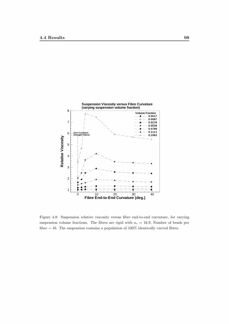
4.4 Results 98
0 10 20 30 40Fibre End-to-End Curvature (deg.)
1
2
3
4
5
6
7
8
Rel
ativ
eV
isco
sity
0.00170.00870.02780.05380.07980.11110.1562
Suspension Viscosity versus Fibre Curvature(varying suspension volume fraction)
Zero Curvature(Straight Fibres)
Volume Fraction
Figure 4.8: Suspension relative viscosity versus fibre end-to-end curvature, for varyingsuspension volume fractions. The fibres are rigid with ar = 16.9, Number of beads perfibre = 16. The suspension contains a population of 100% identically curved fibres.

4.4 Results 99
curvature for varying suspension concentrations. The viscosity data features
a peak for rather small curvature angles in the range 5 < θfibre < 10.
Beyond this, viscosity reduces in magnitude and appears to converge to a
value much larger than for straight fibres (although we can expect results to
become inaccurate at large curvatures).
Fig. 4.8 reveals a peculiar phenomenon where viscosity rises rapidly for
very small curvature angles. The gradient of curves in Fig. 4.8 at zero fibre
curvature is non-zero and is in fact quite steep. It is also noted that the
proportional increase in viscosity, as curvature deviates from ‘dead-straight’,
is more pronounced for higher volume fractions. For example the highly
concentrated fibre suspension of volume fraction φ = 0.1562 (symbol ()
in Fig. (4.8)) has a relative viscosity of ηr ≈ 3.5 when fibre curvature is
θfibre = 0 (dead straight), but for a small curvature of θfibre = 4, relative
viscosity jumps to ηr ≈ 7.7. The relative viscosity is approximately twice the
magnitude of the ‘dead-straight’ result and for the same curvatures, this or-
der increase is approximately consistent over all the tested volume fractions.
This magnitude of viscosity increase is reminiscent of Nawab and Mason’s
[91] observed experimental viscosity of order three times the theoretical pre-
dictions (as discussed in Section §4.2). Fibre deformations may very well
have played an important part in their result.
This result demonstrates the extreme sensitivity of the suspension vis-
cosity to fibre shape imperfections. For a seemingly small shape distortion,
the effect on viscosity is dramatic. Suspension viscosity appears to reach a
maximum at a very small curvature. Beyond this critical curvature angle
the viscosity reduces markedly again. This behaviour would pose the fol-
lowing problem to experimental researchers attempting to produce accurate
reproducible viscosity results. First, great care must be taken so that fibre
samples are well prepared. Tolerance to bent fibres and other deformation is
low and consequences of using imperfect fibres are severe. Yet as we can see
from a snapshot of a typical suspension by Milliken et al. [103] (Fig. 4.1),
small curvatures are not uncommon despite the care taken by Milliken in

4.4 Results 100
preparing fibre samples. Second, results cannot be improved much by simply
removing the most extremely bent fibres from the sample. As we have seen,
the greatest effects occur for curvatures of only 5 < θfibre < 10. One would
have to undertake the much more arduous task of removing all fibres with
curvature beyond say, 1. Last, one can expect more flexible fibre materials
to deform more than stiffer ones. Therefore, for consistency, stiffer fibres are
preferable to more flexible fibres. Likewise for fibres of greater aspect ratio
(whereby the tendency to flex is greater than for shorter stout fibres), stiffer
fibres are preferable when consistently reproducible viscosity is desirable.
4.4.2 Viscosity-Curvature Curve Fitting
0 2 4 6 8 10x
0
0.2
0.4
0.6
0.8
1
1.2
1.4
y
F(x)exp
hyperboliccombined
Figure 4.9: The F (x)exp and hyperbolic components, and the combined result
The data as presented in Fig. 4.8 cannot be fitted easily by a low order
least square polynomial fit. Instead it is better described with a combination

4.4 Results 101
of hyperbolic and F (x)exp functions (where F (x)exp is of the form F (x)exp =
xe−x). Fig. 4.9 shows the two individual components and the resultant sum
of these two parts. The resulting empirical equation fitted to the simulation
data is,
ηbulk (θfibre, φ) = εθfibree(−αθfibre−ζ) + δ
eβθfibre − e−βθfibre
eβθfibre + e−βθfibre+ γ (4.12)
where the coefficients, α, β, γ, δ, ε and ζ are functions of volume fraction φ
in the range, 0 ≤ φ ≤ 0.16,
α (φ) = 0.0007φ
+ 1.2φ+ 0.005,
β (φ) = 4.2828φ2 − 0.1138φ+ 0.0022,
γ (φ) = 8904.6471φ4 − 1716.2639φ3 + 118.8461φ2 + 5.2429φ+ 0.9922,
δ (φ) = −747.8328φ3 + 237.5086φ2 − 8.4300φ+ 0.3531,
ε (φ) = 0.01φ
− 1.5φ+ 2,
ζ (φ) = 153.3682φ2 − 61.5718φ+ 5.8786.
(4.13)
Eq. (4.12) fits most of the simulation data well as can be seen in Fig.
4.10. One should note that fibre aspect ratio and bulk properties are related.
Therefore the constants presented in Eq. (4.13) are applicable only for fibres
with aspect ratio ar = 16.9. The actual form of the viscosity-curvature
relationship for all fibre aspect ratios and curvatures is yet to be found.
This curve fit is presented simply as a glimpse into the true nature of this
relationship.
We may expect that at any time in shear flow a certain proportion of
fibres are permanently bent. A certain percentage may also acquire bends
due to mechanical interaction or thermal gradients (warpage). The steep
gradient of the viscosity-curvature curve at low curvature angle reveals the
sensitivity of suspension viscosity to even the slightest curvature in fibres.
The wide scatter in existing experimental viscosity data may well be caused
by minor fibre shape imperfections.

4.4 Results 102
0 10 20 30 40Fibre End-to-End Curvature (deg.)
1
2
3
4
5
6
7
8
Rel
ativ
eV
isco
sity
0.00170.00870.02770.05380.07980.11110.1562
Suspension Viscosity versus Fibre Curvature(Curve Fitting to data)
Volume Fraction
Figure 4.10: Curve fitted equation plotted with simulation results (ar = 16.9). The compu-tations were not continued beyond 15% volume fraction because of excessive computationaltime required

4.5 Discussion and Conclusion 103
4.5 Discussion and Conclusion
This work studied the importance of fibre shape in sheared fibre suspensions.
The initial hypothesis was that small deformities in the fibres of a suspension
can produce a noticeable effect on suspension viscosity. In this work, fibres
were directly simulated in Newtonian shear flow for varying volume fraction
and varying fibre curvature θfibre, and the bulk viscosity was observed.
It was found that there was a rapid and large increase in bulk viscosity
as fibre curvature was increased. The viscosity - curvature relationship can
be fitted to a single Eq. (4.12) given volume fraction and fibre curvature (for
fibre aspect ratio ar = 16.9 only).
The curious form of the curvature-viscosity relationship (Fig. 4.10) leads
one to ask the obvious question of why this happens. The answer is unknown,
but a speculative discussion is offered. It is acknowledged that fibre align-
ment is central to the resulting viscosity of a fibre suspension. Briefly, fibre
misalignment increases interaction activity and encourages further misalign-
ment. The resulting suspension is more resistant to flow and so a viscosity
increase is measured. When a single infinite aspect ratio fibre has aligned to
shear direction it presents no profile in the shear direction. Theoretically it
will remain aligned indefinitely. A curved fibre however does present a profile
in the shear direction. The more curved a fibre, the larger the profile seen in
the shear direction. Therefore regardless of aspect ratio it does not remain
aligned indefinitely. Curved fibres in suspension will not exhibit as strong
a tendency to remain aligned to shear flow as does a straight fibre suspen-
sion. Curved fibres are less able to pack neatly into dense aligned structures
than straight fibres. Therefore a curved fibre suspension has a propensity to
misalignment and hence we see a viscosity increase with curvature. This can-
not however explain the subsequent viscosity decrease beyond approximately
θfibre = 10 curvature angle. It is yet to be seen whether the behaviour in
that region also reflects a truly physical phenomenon or is merely the result
of theoretical or numerical inadequacy.
The implications are of particular importance to experimenters in fibre

4.5 Discussion and Conclusion 104
suspensions. It would appear that the viscosity (and possibly other bulk
properties) are highly sensitive to the quality control maintained in preparing
the fibre samples. The rapid increase in bulk viscosity as seen in Fig. 4.10
shows that even a small deviation from ‘dead straight’ fibres, or the use
of highly flexible fibres, or highly elongated fibres (large aspect ratio fibres
are more prone to bending) will result in large deviations in bulk property.
Further, one simply cannot remove the most deformed from the fibre samples
in the hope of reducing this viscosity increase. From the results shown in
Fig. 4.10, it appears that the fibres which contribute most to the increase
are those with a relatively mild curve of the order O(5 to 10).

Summary: Part II
In Part II the first of two new direct simulation methods was presented. The
fibre simulation was based on the new ‘Chain-of-Spheres’ fibre model. Part
II clearly shows the ability of this method to accurately estimate suspension
bulk viscosity. We have seen estimations for viscosity over a range of volume
fractions and also over a range of fibre stiffness.
The ability to account for fibre deformation proved to be particularly
useful as it allowed for the simulation of particular details of fibre motion,
for example, orbital drift to vorticity axis, ’S’ shape configurations and shape
evolution with shear, which have so far only been implied by theory, and seen
before only in other flexible fibre direct simulations. The viscosity predictions
were seen to more accurately match equivalent experimental data when fibre
flexibility was accounted for.
The relationship between fibre stiffness, and bulk viscosity was character-
ized for the first time using this method. Lastly we have seen an indication
as to the level of sensitivity of suspensions to fibre shape imperfections. The
suspension viscosity was noted to approximately double as only mild curva-
tures of 4 were introduced.
In Part III, we move away from the prediction of bulk properties and
focus closer on the motion of individual particles. A new, more capable
simulation method is presented featuring the ability to model the motion of
particles of arbitrary shapes, within arbitrarily complex flow fields.

Part III
Three Dimensional Fibre
Simulation

Chapter 5
Single Particle Dynamics in
Shear Flow
5.1 Introduction
Part III (Chapter 5 to 7) describes a new direct simulation created for the
modelling of arbitrarily shaped particles in Newtonian fluid. To date, particle
shapes used in simulation have been restricted to simple axially symmetric
cylinders, ellipses, spheres or discs. Like the simulation used in Part II,
the new simulation method is based on the Stokes law for viscous drag on a
sphere, and uses spherical ‘subunits’ as the building blocks of greater complex
structures. Within this framework, arbitrarily shaped particle structures may
be designed and created with little effort.
In this chapter, the simulation is used to study the single particle dy-
namics of various shapes in Newtonian shear flow. Known and unknown
shape-dependent particle behaviour is demonstrated, and when available, is
tested against existing theories or observations.
In Section §5.2, a modification and extension of the sphere-chain style
of simulation is described. This new simulation is similar to the PSM of
Yamamoto and Matsuoka (referred to in Section §2.2.1). The main differ-
ence is the extended linkages allowed for each subunit sphere. Each sphere

5.2 Numerical Method 108
may be linked to a maximum of 30 other spheres. Previous simulations al-
lowed subunits only two bonds each (i.e. end-to-end) effectively allowing
only thread-like structures to be made (with the exception of Yamamoto
et al.’s four bonded spheres in [34] and [72]). With the increased number
of bonds allowed, truly three dimensional particle structures may be con-
structed. For example, many filler particles are planar in form. Planes and
various other shaped particles were chosen for investigation. Irregular, non-
symmetrical particles may be simulated as easily as conventional spheres,
ellipsoids, cylindrical fibres and oblate discs. The motion of these familiar
shapes in shear flow will be revisited, as well as a brief look at the motion for
some new complex particle shapes. This 3D sphere-chain simulation is also
capable of modelling fibre dynamics embedded within realistic complex flow
fields. The focus of the work in Chapters 6 and 7 is on fibre flow through
two complex flow fields.
5.2 Numerical Method
While multi-body style simulations are generally very powerful, the speci-
ficity of some model designs described in Section §2.2.1 restricts them to a
very limited range of applicability. For example, the ball-and-socket model
of Skjetne et al. [33] was designed in part to reduce the numbers of sub-
units required to assemble a given length of particle. This design however
limited possible particle shapes to end-to-end linked chains only. It is also
computationally expensive to keep track of all the necessary parameters in
a ball-and-socket based simulation, see for instance, the discussion in §5.2.5on calculating intraparticle torque.
From a programmer’s perspective, the scope for applying the simulation
to a wide variety of problems diminishes rapidly as the model specificity in-
creases. Sphere-based models have an inherent isotropy, and sphere-based
hydrodynamics have a simplicity which allows scope for expansion. This is
evident from the numerous PSM variants Yamamoto et al. have published.

5.2 Numerical Method 109
It was a secondary aim in this work to produce a simulation whose range of
application was as wide as this genre allows. To this end, this current simu-
lation is also sphere-based and wherever possible, complexity and specificity
in theory or algorithm are minimized or substituted with simpler, or at least
more widely applicable alternatives.
It will be shown subsequently how complex and realistic particle motion
can arise from quite simple theories and algorithms, based on the application
of as little as three simple rules for viscous drag, internal force and internal
torque between linked spheres.
5.2.1 The 3D Particle
For the purposes of this discussion, the suspension particles will be referred
to as particles, and the spherical building blocks used to construct particles
as subunits. Particles of different shapes, bond arrangements or mechanical
characteristics are said to belong to different species. Within the particle,
subunits may be positioned in space arbitrarily. Unlike Yamamoto et al.’s
PSM, subunits are not bonded by direct contact, but instead by ‘elastic’1
bonds over short distances (any distance is in fact possible however physical
limitations apply, see Section §5.2.5). Subunits are allowed a maximum of
30 bonds, to any other subunits within the particle. Only subunits interact
with each other or with the suspension medium. One is not concerned with
subunit-bond or bond-bond intersections during particle design. By the care-
ful arrangement of subunits and bonds, arbitrarily shaped 3D particles may
be conceived in a manner akin to the design of spaceframe structures.
An example of a basic particle shape is the torus shown in Fig. 5.1. In this
case, the torus is constructed from a hexagonal cross section. Six subunits
occupy each perimeter node of the hexagon, with a seventh at the centre.
The cross section is rotated at 30 intervals through a circular revolution to
1Although bonds have a finite stiffness and are based on elastic theory, the bond stiffness
of particles used in this thesis are always set to ‘high’ values. It is assumed in this thesis
that particles are always approximately ‘rigid’. See Section §5.2.3

5.2 Numerical Method 110
X Y
Z
Perspective
X
Y
Z
XY Plane
X Y
Z
YZ Plane
Y X
Z
XZ Plane
Figure 5.1: 3D Torus model, 84 spheres (spheres are not drawn to scale)

5.2 Numerical Method 111
produce the torus shape. In the primitive shown in Fig. 5.1, the radius of
revolution is twice the section radius. Coordinates of each subunit correspond
to the nodal positions of the 3D framework. Each subunit’s relationship
to the larger structure is completely described by 94 parameters. These
are, its individual identification number, its coordinates (relative to a local
origin), identification numbers of other subunits with which it shares a bond
(maximum 30), and each bond’s non-dimensional Stiffness2 (Esim) and Shear
Moduli (Gsim). For example, for a subunit i, 94 parameters as shown in Eq.
(5.1) are required.
for bead i :
IDi,
(x, y, z)i ,
[ID1, ID2, . . . , ID29, ID30]i ,
[E1, E2, . . . , E29, E30]i ,
[G1, G2, . . . , G29, G30]i
(5.1)
Hence to fully describe the structure and mechanical characteristics of the
torus consisting of 84 subunits, an (84× 94) primitive matrix is sufficient.
Each particle used is represented by a primitive matrix of this type. There
is no limitation to the size of the primitive matrix (apart from those relat-
ing to computational resources and solution time), nor to the combination
of different particle species in the same simulation run (e.g. heterogenous
suspensions are possible). Particle mechanical strength may be modified by
altering the Stiffness or Shear moduli (E1−30 and G1−30) on a bond-by-bond
basis within the primitive matrix3. As there is no concern over overlapping
of bonds, it is conceivable that one may for example repeat bonds between
2Although bonds have a finite stiffness and are based on elastic theory, the bond stiffness
of particles used in this thesis are always set to ‘high’ values. It is assumed in this thesis
that particles are always approximately ‘rigid’. See Section §5.2.33Although bonds have a finite stiffness and are based on elastic theory, the bond stiffness
of particles used in this thesis are always set to ‘high’ values. It is assumed in this thesis
that particles are always approximately ‘rigid’. See Section §5.2.3

5.2 Numerical Method 112
the same pair of subunits (ID1−30) to locally double the material rigidity, or
perform a combination of the two methods. The particles are then scaled,
rotated and translated to an arbitrary initial position prior to simulation.
In the case of suspensions (multiple particles in the one simulation), the
individual primitive matrices of each particle are compiled into a single global
subunits matrix with globally re-numbered subunit IDi. The simulation then
treats the global subunits matrix in the same way it would a single primitives
subunit matrix. In a heterogenous suspension for example, if there are 50
particles of species M , each with 25 subunits, and 100 particles of species
N , each with 84 subunits, then the global subunits matrix will be of di-
mension, ([50× 25species M + 100× 84species N ]× 94). During simulation, the
global subunits matrix is updated at each timestep to reflect the positions of
each subunit. The global subunits matrix is an important internal dataset
since it reflects the microstructure of the suspension. Contents of this matrix
are extracted and stored in datafiles for postprocessing. In order to approx-
imate a reasonably uniform material density and structural isotropy within
particles, it is recommended that subunits are positioned, and their bonds
made in regular patterns such as BCC or FCC configurations.
5.2.2 Non-Dimensionality
The radius and mass of the constituent subunits are by default a = 1 and
m = 1, unless stated otherwise. All scales are made dimensionless. Subunit
radius is taken as the unit length scale for all lengths in this simulation. Sim-
ulation moduli Esim and Gsim are non-dimensionalised in a similar manner to
the simulation in Part II, i.e. Esim = Eγµ
and Gsim = Gγµ. Bulk viscosity is nor-
malised against the solvent viscosity. All forces and torque are taken in their
non-dimensional form, using non-dimensional components. The ‘timescale’
is correlated with non-dimensional shear.

5.2 Numerical Method 113
5.2.3 ‘Rigid’ Particles and Bond Stiffness
In most cases presented in this simulation, the bonds were made very stiff so
that the simulation particles could be considered approximately, ‘rigid’. The
elastic theory is therefore only used in order to maintain internal rigidity and
particle shape. While the simulation is technically capable of modelling flex-
ible particles, particle flexibility is a complication which will not be studied
in detail at this time. There are a few ‘flexible’ particle cases included in
later results, however these results should been viewed separately from the
rest of the results presented. They are included only for illustrative purposes
for the interested reader.
Although the effect of particle flexibility is not studied at this time, the
structure of the particles are based on elastic theory. Future studies involv-
ing flexibility (e.g. the effects of flexibility on orientation, dynamics and
viscosity) is desirable, however these aspects are too complex to be studied
here. Therefore, in lieu of substantial alteration to algorithms, it was de-
cided that the simulation would remained unchanged, with the potential to
model flexible particles in the future. For the purposes of this thesis, the
particle ‘rigidity’ is maintained via the use of high stiffness moduli. In the
following sections on force and torque (Section §5.2.5), the reader should be
mindful that the internal forces and torques play very little part in the salient
simulation results apart from maintaining the particle shape.
5.2.4 Inertia and Reynolds Number
The fluid is always assumed to be creeping flow. Therefore the fluid inertia
is assumed to be negligible. Particle inertial effects however may apply, since
the mass of subunits are non-zero. Proudman and Pearson [109] expanded
the Navier-Stokes equations with inertial effects to obtain a highly accurate
prediction for drag force around the sphere with a low Reynolds number. At
a Reynolds number of 0.05 the drag predicted by the creeping flow Stokes
law is only 2 percent less than the Proudman and Pearson expansion [110].

5.2 Numerical Method 114
Many readers conform to the often referred to magnitude of Re 10−4. By
Happel and Brenners observation however, higher Re situations need not be
immediately disqualified as inaccurate. ‘The exact Reynolds number above
which the neglect of fluid inertia constitutes a poor approximation depends,
in the final analysis, on the accuracy required.’ [110, pp. 42]. A variation of
the order 2% or even slightly larger, is perfectly acceptable in many cases,
including those seen in this chapter. When more than a single character-
istic dimension is used, Happel and Brenner note that Reynolds numbers
significantly greater than unity are possible without inertial effects being ap-
preciable. Also, they note that phenomena arising from inertia are lost in
the creeping motion assumption. It is argued that the continued use of the
Stokes drag force law in the low Reynolds number range is perfectly accept-
able for this simulation. In any case, in later results (e.g. see Section §5.3.4),the effect of various Re values for simulation particles will be studied. In
this study, appropriate Re ranges will be determined for minimised inertial
effects. It will be shown that particles used throughout Part III of this thesis
are mostly unaffected by inertial effects.
While inertial effects are not the main focus of this work, Eqs. 5.2 and
5.3 include the inertial terms and so the equations of motion are capable
of accounting for inertial effects. Some subunits in the results reported in
this chapter may experience conditions where Reynolds numbers are higher
than Re = 10−4. Reynolds numbers however generally remain in the low
Reynolds number range (e.g. Relow < 1). In fact, some preliminary results to
come show that higher Reynolds numbers are sometimes experienced without
results noticeably deviating from equivalent creeping flow based theory.
5.2.5 Equations of Motion
The simulation discussed in this chapter is posed at the level of the spherical
subunit and not the particle itself. Particle motion, orientation and deforma-
tion arise only as a consequence of the cooperative movement of the group
of subunits. The movement of subunits are influenced by the flow field of

5.2 Numerical Method 115
the suspending medium, interparticle interactions, and intraparticle bonds
to other subunits. These influences are manifested as forces and torques
on subunits from which the simulation calculates a trajectory over succes-
sive timesteps. Forces and torques between subunits are calculated on a
cumulative pairwise basis. As is customary in Stokesian Dynamics [75], the
additivity of pairwise interactions is assumed in order to improve computa-
tional time. The equations of motion are based on Eqs. 2.16 and 2.17, and
include inertial components. They are restated here as Eqs. (5.2) and (5.3)
for convenience.
mdv
dt=(Fh)viscous
+(∑
Fi)intraparticle
+(∑
Fp)interparticle
(5.2)
(2
5ma2
)sphere
dw
dt=(Th)viscous
+(∑
Ti)intraparticle
+(∑
Tp)interparticle
(5.3)
It is worthy to note that of most existing multi-body simulation variants, a
great deal of complexity is associated with accounting for the relative orien-
tation between subunits - to solve for the torque components of Eq. (5.3).
Past simulations usually required subunit-fixed local orientation vectors to
be updated with each timestep in order to determine relative angular deflec-
tions and subsequent intraparticle torque (see Eqs. 5.10b, 5.10c and Figs.
5.3b, 5.3c). The trigonometric manipulation required is computationally ex-
pensive and prone to inaccuracy relative to other intrinsic operations. If it
were possible to avoid solving Eq. (5.3) in favor of an alternative method,
then the complexity of coded algorithms would be significantly streamlined
and simulation time would be improved.
In the following sections, the method used for viscous, intraparticle and
interparticle force and torque will be detailed. It will be shown how all
components of Eq. (5.3) are eliminated or replaced with alternate methods.
The resulting simulation method solves instead a streamlined version of the
force Eq. (5.2) only. The reader is reminded to recall from Section §5.2.3that except for the Stokes viscous drag force, these calculations are only used
in this chapter to maintain particle shape, and hence internal flexibility is

5.2 Numerical Method 116
mostly eliminated as a significant factor in any results.
Viscous Force and Torque
A spherical body moving through a Newtonian fluid experiences a drag force
and torque resisting that motion (Fig. 5.2a). In this simulation, subunits are
spherical and so, the drag force and torque on subunit i may be expressed
by Stokes law for drag on a sphere, Eq. (5.4) and (5.5) respectively.
+
- .
- .
- < .
<
Figure 5.2: (a) Drag force on a sphere, (b) The rotation of the ij bond due to the driftof sphere j is equivalent to the rotation of the same ij bond due to an imposed torque onsphere i (excluding the extension of the ij bond).
Fhi = −6πηa
(dridt
− v∞ (ri)
)(5.4)
Thi = −8πηa
(dθidt
−w∞ (ri)
)(5.5)
v∞ (ri) and w∞ (ri) are linear and angular fluid velocity at subunit i′s global
position, ri. θi is subunit i’s current orientation. a is the spherical subunit
radius and η is the fluid viscosity.
The force Eq. (5.4) is used as shown in the simulation, however the
torque Eq. (5.5) is not. For all intents and purposes, a sphere that is rotated

5.2 Numerical Method 117
is identical to the original unrotated sphere. The only discernible change
while rotating this system of linked spheres is the orientation of the bonds
to neighboring subunits. Assumingdrj
dt− v∞ (rj) = 0, Eq. (5.4) is used
to calculate the drift of the neighboring subunit j. Ignoring for the time
being the radial ij bond length change, the resulting orientation of the ij
bond due to the drift of subunit j is equivalent to that found by directly
rotating the rigid ij dumbbell about i with torque Thi from Eq. (5.5) (see
Fig. 5.2b). Eq. (5.5) may be done away with all together as its effect is
implied by the relative drift of neighboring subunits as calculated from Eq.
(5.4). This reasoning depends on three conditions, (1) the Newtonian flow
velocity field v∞ varies linearly and mildly over the length scale of ij bonds,
(2) the subunits are ideal non-slipping spheres where the centre of resistance
is equivalent to the centre of mass, and (3) At some other stage, the radial
ij bond length change is compensated for. This compensation comes in the
form of an intraparticle extensional bond stiffness rule (Section §5.2.5). With
reasonable particle designs (Section §5.2.1), these conditions will be met for
most cases. The(Th)viscous
component of Eq. (5.3) may thus be entirely
eliminated from the simulation.
Long Range Hydrodynamic Interaction
In Eq. 5.4, the freestream velocity term, v∞ is composed of the undisturbed
macroscopic freestream velocity, V∞ = K·r (whereK is the velocity gradient
tensor and r is the position in the flow), and a long range wake disturbance
accumulated from the motion of other spheres in the suspension, V′. That
is Eq (5.6),
v∞ = V∞ +V′ (5.6)
As in Eqs. (3.7) and (3.8) in Part II, the Oseen tensor is used in this instance
to determine the velocity disturbance at a sphere n due to the wake from
another sphere m. Eqs. (5.7) and (5.8) are restated here for convenience.
Ωmn =1
8πη |rmn|δ +
rmnrmn
|rmn|2
(5.7)

5.2 Numerical Method 118
V′n =
∑m
Ωmn · Fm (5.8)
Eqs. (5.7) and (5.8) are substituted into Eq. 5.6 to obtain v∞, including the
small influence of long range hydrodynamic interactions. In simulation the
forces from the previous iteration are used in Eq. (5.8).
In the results section, data will be presented for simulation runs with and
without hydrodynamic long range interaction. While long range hydrody-
namic interaction is by default implemented here (unless stated otherwise),
the computational load added by including this feature is highly prohibitive.
At very high concentrations, other researchers [21][23] have shown hydrody-
namic interaction to be significant. The results in this chapter however show
very little difference with or without hydrodynamic interaction, apart from
a massive increase in CPU time with the interaction included.
Similar numerical works by Fan et al. [31] and the work in Part II include
hydrodynamic interaction. It should be noted that the various peculiar par-
ticle motions observed in those works are almost identically reproduced in
this simulation - with long range interaction disabled. There is strong circum-
stantial evidence against including the long range hydrodynamic interaction.
From the result comparisons with and without long range interaction in the
sections to come, it could be concluded that very little new knowledge is
gained by its inclusion, and the computational cost is too severe. While it
remains included in this simulation, its automatic inclusion in simulations of
this type should be further reviewed.
Intraparticle Force and Torque
Intraparticle force and torque may be categorized further into those arising
from extensional, bending and torsional stiffness (Fig. 5.3). Bond Stiffness is
controlled by the non-dimensional Extensional and Shear Moduli, Esim and
Gsim respectively. Each bond within a particle is assigned an independent
extensional and shear stiffness modulus via the particles primitive matrix,
as discussed in Section §5.2.1. For the purposes of calculating forces and

5.2 Numerical Method 119
<
<
! "
Figure 5.3: (a) Extension, (b) Bending and (c) Torsion in a bond between subunit i andj

5.2 Numerical Method 120
torques, bonds are assumed to deform like an elastic cylindrical beam of cross
sectional radius a (the non-dimensional spherical subunit radius). Stiffness
coefficients for the cylindrical beam are thus able to be defined as shown in
Eq. (5.9).
keij =πa2Esim (a) stretching stiffness
kbij =πa3
8Esim (b) bending stiffness
ktij =πa3
4Gsim (c) twisting stiffness
(5.9)
Intraparticle force and torque are linearly related to extensional and angular
deflection by Eqs. (5.10a, 5.10b and 5.10c).
F ei = keij(|rij| − dij) (a) extension force
T bi = kbij (θb − θeq) (b) bending torque
T ti = ktij (φt − φeq) (c) twisting torque
(5.10)
In simulation, extensional force on a subunit is calculated using Eq.
(5.10a). dij is the equilibrium ij bond length. |rij | = |rj − ri| is the in-
stantaneous ij bond length calculated from the known positions of subunits
ri and rj at each timestep. A component of subunit i’s response to the ex-
tensional force F ei is the correction for the drifting ij bond length change,
found to be necessary in Section §5.2.5.As already discussed, it is the intention that all torque based calcula-
tions be eliminated or replaced by alternative methods. Eqs. (5.10b) and
(5.10c) are not used in this simulation. The computational overhead re-
quired to maintain and update θb, θeq, φt, and φeq in simulation is high and
best avoided. In Yamamoto et al.’s PSM, Klingenberg et al.’s particle level
simulation, and the flexible fibre simulations of Part II, fibre cross sections
were one dimensional and hence bond bending and torsion were a necessary
consideration for realistic particle modelling. Without it, subsections of a
fibre-like particle could rotate freely about their bonds, acting unrealistically
to relieve internal stresses and alter particle dynamics. In the spaceframe-
like particle constructions used in this simulation, the particles’ torsional and
bending stiffness are inherent in the highly crossbraced 3D structure. The
bending and torsion equations are no longer strictly necessary to provide

5.2 Numerical Method 121
bending and torsional stiffness in the structure. There are however occasions
where rotational bond stiffness is still desirable (e.g. Fig. 5.4). In Fig. 5.4a,
< <
<
<
==
==
Figure 5.4: Rotational bond stiffness stops (a) skewing and (b) folding.
the structure is susceptible to skewing as there is no rotational bond stiff-
ness at the node points (i,j,k, and l). If a cross brace il bond is now added
(Fig. 5.4b), the structure is still susceptible to folding in the third dimension.
While this simulation is intended primarily for the modelling of 3D particles,
the inclusion of some rotational stiffness allows compatibility with the 2D
and 1D models of earlier implementations.
Torsion is comparatively insignificant and is omitted in this simulation,
but bending is included. Bending Eq. (5.10b) is not used directly however.
Instead it is turned into an equivalent force. In Fig. 5.5a, the linear velocity
of subunit j due to a rigid-body rotation of dumbbell ij about i (rotational
velocity wirel = w∞ −wi) is equal to the cross product, vjrigid = wirel × rij.However, since dumbbell ij is not rigid, the actual linear velocity of subunit j
is vij = vj−vi. vij may be broken down into components parallel (vijpar) and
perpendicular (vijper) to rij. The difference, vijdeform = vjrigid−vijper may be
taken to be the velocity component of j due purely to bending deformation

5.2 Numerical Method 122
<" 1 " "
<
<
<
<
Figure 5.5: (a) Rigid-body bending versus actual bending (b) Bending deflection

5.2 Numerical Method 123
(extensional deformation is dealt with separately by Eq. (5.10a)). Over a
non-dimensional simulation iteration dγ, this velocity difference is equivalent
to a linear deflection dxij = dt ·vijdeform. All bonds themselves are assumed
to efficiently transfer forces and torques to the linked subunits at their bond
roots. The linear deflection dxij over a moment arm dij will result in a
bending moment at the root of the ij bond, at i. If the angular deflection
α is always assumed to be small, approximately satisfying the relationship
tan (α) =|dxij |dij
, then substituting into Eq. (5.10b), the bending moment at i
is T bi = kbij (α). Acting over the moment arm dij, this is equivalent to a force
on subunit j of Fbj = − T bi
dij
dxij
|dxij | . The bending moment experienced at subunit
i produces the same outcome as an equivalent position-correcting force on
subunit j of the form described by Eq. (5.11),
Fbj = −kbij
dijtan−1
( |dxij |dij
)dxij|dxij| (5.11)
where dxij is expressed by Eq. (5.12).
dxij = dt · [[wirel × rij]− [δ − rijrij] · vij] (5.12)
For each subunit i, the bending moment is calculated using Eq. (5.10b). The
bending moment is converted into an equivalent force using Eq. (5.11) which
is applied not to i but subunit j.
Interparticle Force and Torque
Interparticle forces and torques are those which act between different parti-
cles. While interparticle forces may arise for many varying reasons, in this
simulation only the short range repulsive forces required to prevent particle
overlap are considered. Kim and Karilla [100, Ch. 11.2.2] described lubrica-
tion forces between two spheres in close proximity (Fig. 5.6).
The lubrication force Eq. (5.13) describes the force acting on a subunit
i and is used to maintain particle separation in suspension in a reversible
manner.
Fpim = 3πηa2
h− 2aVsqzjn−im (5.13)

5.2 Numerical Method 124
(
<
!
! '
Figure 5.6: Interparticle lubrication force between subunit i of particle m and subunit j
of particle n

5.2 Numerical Method 125
In Eq. (5.13), a is the subunit radius and h is the centre distance between
subunit i of particle m and subunit j of particle n. Vsqzjn−im is the squeez-
ing velocity or the component of the relative velocity at which subunit j of
particle n approaches subunit i of particle m as expressed in Eq. (5.14).
Vsqzjn−im =
[rjn − rim|rjn − rim|
]·([rjn − rim|rjn − rim|
]· (vjn − vim)
)(5.14)
This force is only required at close range when overlap is imminent. For
this work, Eq. (5.13) is included in the force summation when the distance
between subunits is in the range h− 2a < Llub where Llub = 2a. One should
choose the upper range limit (in this case, 2a) such that for a given Vsqzjn−im
upon the activation of Fpim, there is sufficient time for the particle contact
surface velocities to equalize before actual contact. While Yamane et al. [35]
and Fan et al. [31] use a cutoff of 0.2a, their cutoff was appropriate only
in the context of their single body fibre models. A larger Llub is required
here to allow for the transmission of internal forces to affect particle level
velocity change. As the force magnitude in Eq. (5.13) is inversely related to
subunit separation, the simulation outcomes should be reasonably insensitive
to Llub as it is increased. It is assumed that interparticle forces Fp always act
through the subunit’s centre of mass, thus producing no associated torque.
It is also assumed that any interparticle torques are negligible. Therefore
(∑Tp)interparticle of Eq. (5.3) is eliminated.
Eq. (5.13) and variants of it, have been successfully used in previous
simulations by Yamamoto et al. [82], Ross and Klingenberg [84], Yamane et
al. [35] [32] and Fan et al. [31].
Final Equations of Motion
The general equations of motion (5.2) and (5.3) were in Sections §5.2.5through to §5.2.5. The torque Eq. (5.3) is eliminated in this process. The
final equation of motion is expressed by Eq. (5.15) which is integrated in
simulation to determine each subunit’s instantaneous velocity and position

5.2 Numerical Method 126
with shear.
midvi
dt= −6πηa
(dri
dt− v∞ (ri)
)viscous
+
bonds
only∑j
keij [|rij | − dij]
extension
−
bonds
only∑j
kbji
djitan−1
(dxji
dji
)dxji
|dxji|
bending
intraparticle
+
only when
h− 2a < 0.2a∑j
3πη a2
h−2aVsqzj−i
interparticle
(5.15)
5.2.6 Flow Condition
The suspending medium is a Newtonian fluid. Temperature effects, phase
changes, or free surfaces are not considered. The flow field is assumed to
develop independently of the particle motion. Although Lipscomb et al. [108]
showed that the decoupling of particle motion and flow field development is
increasingly inaccurate at higher concentration, most other direct simulation
works also neglect this. In any case, all cases presented in this thesis are
dilute. It is therefore assumed that a decoupled flow field is acceptable here.
If the entire flow domain is subject to the same flow condition (e.g. simple
shear flow) then a tensorially defined flow is convenient and computationally
efficient. The velocity gradient tensor components, ∂vi
∂xjare specified prior
to commencing simulation. From this, all other commonly used flow terms
are generated, e.g. deformation rate tensor, γ = ∇v + ∇vT , D = 12γ,
K = ∇vT , vorticity tensor, ω = ∇v − ∇vT , local velocity, vi(ri) = K · riand rotation rate,Wi =
12[∇× vi (ri)]. Given the known position of subunits
in simulation ri, the fluid velocity and other flow terms can be determined
for use in the equations of motion (Section §5.2.5).

5.2 Numerical Method 127
For the shear flow simulations presented here, the flow direction is always
in the positive (x) direction. The shear gradient is along the (y) axis. The
shear magnitude is always γ = 1. Along the (z) axis, the (xy) flow field
planar sections are identical. The flow conditions described apply over an
infinite domain and so wall effects are not considered here.
5.2.7 Simulation Procedure
The parameters in Table 5.1 are the default values used unless stated other-
wise.
Parameters
Subunit Radius a = 1
Subunit Mass 0.1 < m < 1.0
Non-dimensional Solvent Viscosity 1.0 < η < 10
Lubrication Cut-off distance Llub = 2a
Table 5.1: Parameters and default values
As mentioned earlier, the time variable is directly correlated with non-
dimensional shear deformation. Due to the non-dimensionalizing process, the
simulation may be measured against shear γ. Shear deformation is an impor-
tant global variable which must be set prior to commencing. Deformation
variables included the initial shear γi, ending shear γe, and increment dγ.
Usually γi = 0, while dγ was in the range 0.0001 < dγ < 0.001 depending on
the accuracy required. Ending shear γe is case dependent but must be large
enough to allow certain particle dynamic phenomenon to evolve and become
evident (100 < γe was usually sufficient but will be stated individually for
each case when necessary).
In the following study of individual particle motion, a single particle of
a nominated species was used. The particle (and its member subunits) may
be subject to scaling and rotation. Once the initial orientation was set, it
was translated to its initial position (usually the origin). Each subunit was

5.3 Results - Single Particle Dynamics 128
imparted with an initial velocity (by default, velocity was equal to that of
the local fluid which it displaced).
Once the simulation commenced, the equations of motion of Section §5.2.5were solved. After solving Eq. 5.15 for all subunits, the subunit accelerations
were integrated using the simple trapezoidal method to determine subunit
velocity, and new position in space (Eq. 5.16).
Vγ+dγ = Vγ +12dγ(aγ−dγ + aγ)
xγ+dγ = xγ +12dγ(Vγ−dγ + Vγ)
(5.16)
where a is linear acceleration, V is linear velocity, and x is position of the
subunit in space. Knowing this, the global subunits matrix was updated
for each iteration. Relevant data were collected and output to a datafile for
postprocessing prior to the next iteration. The simulation continued in dγ
increments until the ending point γe or other termination condition was met.
The simulation results presented in Section §5.3 were computed on Intel
x86 processor based computers (Intel Pentium II and III generation) running
Microsoft Windows and RedHat Linux operating systems. The simulation
source code was written in ANSI standard Fortran77 and compiled using Intel
Fortran 95 Compiler for Linux v6 and Digital Visual Fortran v6 Compiler.
CPU times for single particle simulation runs ranged from minutes, through
to several days for suspensions, depending on the size of the global subunits
matrix produced and the shear range set, dγ and γe.
5.3 Results - Single Particle Dynamics
In the immediately following section, the simulation performance is compared
in reproducing some known particle dynamic behaviour in a series of verifi-
cation tests. Afterwards, more single fibre dynamics are detailed. Finally,
results for particles of non-standard shapes and structural characteristics are
presented.
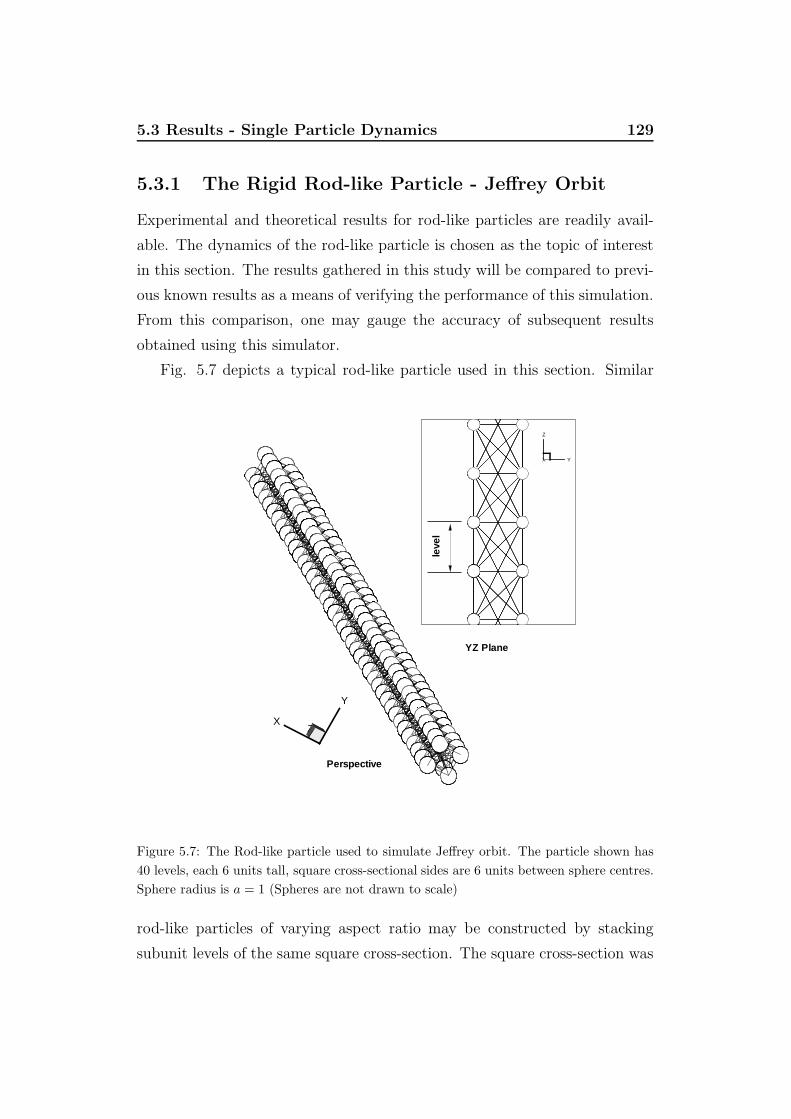
5.3 Results - Single Particle Dynamics 129
5.3.1 The Rigid Rod-like Particle - Jeffrey Orbit
Experimental and theoretical results for rod-like particles are readily avail-
able. The dynamics of the rod-like particle is chosen as the topic of interest
in this section. The results gathered in this study will be compared to previ-
ous known results as a means of verifying the performance of this simulation.
From this comparison, one may gauge the accuracy of subsequent results
obtained using this simulator.
Fig. 5.7 depicts a typical rod-like particle used in this section. Similar
ZX
Y
YZ Plane
Perspective
X Y
Zle
vel
Figure 5.7: The Rod-like particle used to simulate Jeffrey orbit. The particle shown has40 levels, each 6 units tall, square cross-sectional sides are 6 units between sphere centres.Sphere radius is a = 1 (Spheres are not drawn to scale)
rod-like particles of varying aspect ratio may be constructed by stacking
subunit levels of the same square cross-section. The square cross-section was

5.3 Results - Single Particle Dynamics 130
chosen because it is ‘mass-balanced’ about the axis of revolution. It maintains
this property while using only the 4 nodes for the cross section. While a more
‘circular’ section could have been used (e.g. hexagon, octagon) this requires
more spheres and ultimately increases the simulation size. Mass balance is
important in this study since it ensures the sectional centre of resistance is
always coincident with the axis of revolution, and thus particle dynamics are
close to that of a truly axi-symmetric body. In Fig. 5.7 the species shown has
40 levels of subunits, each level is 6 units tall. Spheres in the cross-section
are 3√2 units from the centroid (i.e. the corners of the square cross-section
are at local coordinates (3, 3), (−3, 3), (−3,−3), and (3,−3)). The sphere
radius is a = 1.
To calculate an aspect ratio, a fibre diameter must first be known. Since
this fibre has a square cross-section, a diameter must be approximated. A
possible ‘diameter’ taken could be 2×3√
(2) (i.e. the square cross-section di-
agonal), giving the fibre an aspect ratio of ar ≈ 28.3. However, a more appro-
priate approximation is to use the diameter for a circle section equivalent in
area to the square section, i.e. l2sqr.side ≡ πr2eqv.circle. Hence reqv.circle = lsqr.side√π
.
This approach gives the slightly higher approximation for aspect ratio of
ar ≈ 35.4. The ‘equivalent circle’ area approach is the method used to esti-
mate aspect ratio.
Each subunit in a ‘level’ is bonded to all four subunits of the neighbouring
levels, above and below it, as well as the subunits within its own level. The
result is a regular, highly interconnected pattern of linkages forming the
particle structure. Bond non-dimensional Extensional and Shear Moduli are
set in simulation, to a relatively high value of Esim = 8000 and Gsim = 8000,
so the particle will exhibit a high degree of rigidity. For the following results,
22 different aspect ratio fibres were tested in shear flow. The number of
‘levels’ and the corresponding aspect ratio are listed in Table 5.2.
Single particles of varying aspect ratio are placed (alone) in a simulation
reference cell of Newtonian sheared fluid. The centre of mass of the particle
coincides with the global origin. The initial orientation of the particle is

5.3 Results - Single Particle Dynamics 131
Levels Aspect Ratio Remax
2 1.8 0.0095
3 2.6 0.0143
4 3.5 0.0191
5 4.4 0.0239
6 5.3 0.0286
7 6.2 0.0334
8 7.1 0.0382
9 8.0 0.0430
10 8.9 0.0477
12 10.6 0.0573
14 12.4 0.0668
16 14.2 0.0764
18 16.0 0.0859
20 17.7 0.0955
25 22.1 0.1194
30 26.6 0.1432
35 31.0 0.1671
40 35.4 0.1910
70 62.0 0.3342
100 88.6 0.4775
140 124.1 0.6685
180 159.5 0.8594
Table 5.2: The square cross-section fibre. ‘Levels’, corresponding Aspect Ratio, and themaximum Reynolds number estimated for the spheres at fibre-end during shear flow rota-tion

5.3 Results - Single Particle Dynamics 132
always in the (xz) plane, with an inclination of 60 from the (z) axis towards
the (x) axis. With this configuration, the initial Jeffrey orbital constant
is always Cinitial = 0.08. The flow velocity is in the (x) direction varying
linearly with (y). Shear rate is of magnitude γ = 1.
Sphere mass is m = 0.1 and solvent viscosity is ηsim = 5. Assuming the
region of the fibre near the centre of mass is nearly stationary (much lower
Reynolds numbers here), and the ends of the fibre experience the greatest
velocities, the Reynolds number will be greatest for the spheres at the ends
of the fibre. Reynolds number is Re = ρV lη. ρ is the density of the sphere
itself, i.e. ρ = m43πa3
. Assume a fibre tumbling purely in the shear plane.
Maximum velocity for the rotating fibre is assumed to occur at the fibre end
when oriented perpendicular to the shear direction. Maximum velocity is
thus approximately, Vmax ≈ γ · Lfibre
2, where Lfibre is the fibre length. The
characteristic length is equivalent to the sphere radius, l ≡ a.As seen in Table 5.2, the estimated maximum Reynolds number that any
subunit within the fibre could experience, is always in the ‘low Reynolds
number’ range, certainly less than 1 for all fibres tested. Recall Happel and
Brenner’s conclusion that Stokes law drag on a sphere is not much differ-
ent in magnitude to low Reynolds number drag [110]. Furthermore fibres
closer into the centre of mass will always experience lower Reynolds number
conditions. The high rigidity of the internal bonds means that any subunit
trajectory inaccuracy (due to inertial effects) will be mostly negated by the
bonding influence of the majority of other lesser inertia-affected subunits.
The trajectory of subunits at the ends of the fibre cannot deviate far from
an equivalent inertialess result - in spite of the higher Reynolds number that
a few ‘end subunits’ are experiencing. All fibres tested are therefore not
greatly affected by inertia, and results should be directly comparable with
inertia-less Jeffrey theory predictions.
The Jeffrey orbit is characteristic of the motion of a rigid fibre in shear
and hence its appearance is the first indicator of a correct simulation. In Fig.
5.8 the simulated Jeffrey orbit is plotted for the ar = 35.4 particle. In Fig.
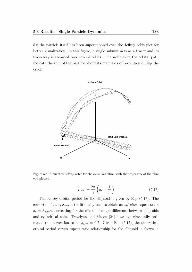
5.3 Results - Single Particle Dynamics 133
5.8 the particle itself has been superimposed over the Jeffrey orbit plot for
better visualization. In this figure, a single subunit acts as a tracer and its
trajectory is recorded over several orbits. The wobbles in the orbital path
indicate the spin of the particle about its main axis of revolution during the
orbit.
X Y
Z
Jeffrey Orbit
Tracer Subunit
Rod-Like Particle
Figure 5.8: Simulated Jeffrey orbit for the ar = 35.4 fibre, with the trajectory of the fibreend plotted
Torbit =2π
γ
(ar +
1
ar
)(5.17)
The Jeffrey orbital period for the ellipsoid is given by Eq. (5.17). The
correction factor, λcorr is traditionally used to obtain an effective aspect ratio,
ae = λcorrar correcting for the effects of shape difference between ellipsoids
and cylindrical rods. Trevelyan and Mason [24] have experimentally esti-
mated this correction to be λcorr = 0.7. Given Eq. (5.17), the theoretical
orbital period versus aspect ratio relationship for the ellipsoid is shown in

5.3 Results - Single Particle Dynamics 134
100 101 102
Aspect Ratio
100
200
300
400
500
600700800
Orb
italP
erio
d
TheoryCorrected Theory (ae=0.7ar)
Simulation LRHydro.Simulation No LRHydro.
Figure 5.9: Jeffrey orbital period vs particle aspect ratio. theory (-), and corrected theory(- ·) compared with Simulation results with long-range hydrodynamic interaction (•), andalso without () hydrodynamic interaction

5.3 Results - Single Particle Dynamics 135
Fig. 5.9. In this figure the theoretical relationship (Eq. (5.17)) is plotted
(Theory (-)), as well as Trevelyan and Mason’s corrected theory (- ·) whereeffective aspect ratio with λcorr = 0.7 is used. Finally the simulation data
points are plotted as black circles (•). Also included are data points from
an equivalent series of simulation runs, where long-range hydrodynamic in-
teraction was disabled (). That is, the V′ in Eq. (5.6) was removed, and
hence the summation in Eq. (5.8) was not done for that case. Since most
simulation data points are in the range 2 < ar < 20 the graph is plotted
in log axes to reveal more detail in the lower regions. It is clear the sim-
ulated data matches the corrected theory very well over almost the entire
tested aspect ratio range. It is also interesting to note that there is a small
quantitative difference between the two series of simulation runs, but no
qualitative difference. The simulation orbital period with long-range hydro-
dynamic interaction enabled (•) is on average 15.1% greater in magnitude
than the simulation without. Long-range hydrodynamic interaction appears
to have the effect of marginally increasing orbital period over the entire as-
pect ratio range. However there appears to be no other qualitative difference,
e.g. the shape of the Jeffrey orbit and the different fibre orientations were
all unchanged. Finally, the largest deviation from theory occured at the
highest aspect ratios (Fibres with 140 and 180 ‘levels’, i.e. ar = 124.1 and
ar = 159.5). Reasons for this divergence will be discussed shortly.
One may now refine Trevelyan and Mason’s correction factor λcorr using
this simulation data. The exercise was undertaken whereby over the likely
range 0.65 < λcorr < 0.75, the area difference under the ‘period versus aspect
ratio’ curve was compared and minimized, relative to the simulation data
(the (•) case). In Fig. 5.10, the root square of the area difference is plotted
against the λcorr range. Since the data points for ar = 124.1 and 159.5 in Fig.
5.9 diverge excessively, these two points are omitted from the calculation.
The minimum as indicated in Fig. 5.10 represents a refined value for λcorr
based on the simulation results. The refined shape correction factor between
ellipsoid and the rod-like particle is estimated to be λcorr = 0.7124. This

5.3 Results - Single Particle Dynamics 136
value is used in the following section involving particle spin.
0.65 0.675 0.7 0.725 0.75
Correction Factor
0
20
40
60
80
100
120
140
160
Roo
tSqr
.Err
or[a
r2 ]0.5
Minimum0.7124
Figure 5.10: The minimum error between theoretical and (•) simulated data occurs whenthe shape correction factor is λcorr = 0.7124.
Fibre Spin
As seen in Fig. 5.8, the wobble of the tracer subunit over the Jeffrey orbital
path is an indication of the particle’s spin about its main axis of revolution.
In Fig. 5.11, the (y) axis trajectory of the tracer subunit, when plotted
against shear, (γ) reveals both high and low frequency regular oscillations
indicating spin and orbital rotation cycles respectively. Particle spin is a
behaviour that has not been revealed by numerical simulation until now. It
is the use of full 3D particles with finite width which permits this result.
Particle motion was theoretically analyzed at length by Anczurowski and
Mason [90]. Indeed, included in their work is a derived expression for the

5.3 Results - Single Particle Dynamics 137
Z
X
Y
Jeffrey OrbitPerspective
0 100 200 300Shear
-20
-15
-10
-5
0
5
10
15
20
Yp
osi
tion
Tracer Subunit Y Position vs Shear
γ
Figure 5.11: Jeffrey orbit with wobbles indicating particle spin - the (y) axis trajectoryof the tracer subunit reveals a high frequency oscillation representing complete spins (n),and low frequency oscillations representing orbital cycles.

5.3 Results - Single Particle Dynamics 138
axial spin of a cylinder within the orbital period. It is this expression which
for convenience will be paraphrased here and also used for comparison with
simulation data.
The theoretical number of complete spins for an elongated cylinder (ar >
1) is expressed by Eq. (5.18),
n = gK (k) (5.18)
g =a2r + 1
πar (C2a2r + 1)
12
(5.19)
k =
√C2 (a2
r − 1)
C2a2r + 1
(5.20)
where g is given by Eq. (5.19), and K (k) is the complete elliptic integral
of the first kind of modulus k, given by Eq. (5.20). The complete elliptic
integral of k may be approximated by the series expansion as shown in Eq.
(5.21).
K(k) =π
2
1 +
(1
2
)2
k2 +
(1 · 32 · 4
)2
k4 +
(1 · 3 · 52 · 4 · 6
)2
k6 + . . .
(5.21)
Using this method, the theoretical relationship between particle spin per or-
bital period (n) and effective aspect ratio (assuming λcorr = 0.7124) is shown
in Fig. 5.12 by the solid line. The equivalent simulation data was obtained
from output data, simply by dividing the number of higher frequency oscilla-
tions (spin), by the number of low frequency spatial oscillations (orbits) over
the same shear interval (see Fig. 5.11 bottom). The spin results are plotted
in Fig. 5.12. The Corrected theoretical result is the solid line (-), the sim-
ulation with long-range hydrodynamic interaction is (•), and the simulation
without the long-range interaction is (). Again as most of the aspect ratios
are in the range from 2− 20, log axes are used to reveal detail in this range.
We can see that over the range 12 < ar < 100 the simulated particle spin
(with long-range hydrodynamic interaction (•)) is reasonably well predicted
compared to the theory despite a general under-estimation to a small degree.
It should be noted that the differences at low ar are accentuated by the log

5.3 Results - Single Particle Dynamics 139
100 101 102
Aspect Ratio
5
10
15
20
2530
Spi
npe
rO
rbita
lPer
iod
Simulation LRHydro.Simulation No LRHydro.
Corrected Theory
Figure 5.12: particle spins per orbital period (n) versus effective aspect ratio. CorrectedTheory versus Simulation, both with long-range hydrodynamic interaction (•) and without()

5.3 Results - Single Particle Dynamics 140
scaling. The error generally increases with aspect ratio. The simulation
series without long-range interaction () generally performs slightly worse
than those with interaction enabled. Long-range hydrodynamic interaction
appears to improve the spin prediction performance for lower aspect ratio
fibres, but becomes less effective with increased aspect ratio where fibres
contain more interacting subunits. As with Fig. 5.9, the divergence with
theory occurs most with the largest aspect ratio particles (ar = 124.1 and
159.5), and there is also anomalous behaviour over the low aspect ratio range
from 3 < ar < 12.
It is believed that the less accurate low ar prediction is due to the fact that
in this range, the simulated particle shape is actually more like a cube than
a rod. The assumption that these shapes are like cylinders becomes increas-
ingly significant in the accuracy of calculated aspect ratio. reqv.circle =lsqr.side√
π
is still used as the effective particle ‘radius’ when in fact the cross section is
square (one would construct a more detailed cylindrical particle species in
this case - Section §5.2.1). It is probable that the error in predictions up to
ar = 12 in Fig. 5.12 is due to this error in ‘aspect ratio’ calculation, and also
reflects the different dynamics of cuboids to cylinders and ellipsoids. In the
limiting case of ar → 1, there is no Jeffrey orbit as such, and as aspect ratio
approaches 1, spins also approach 1. That is, spin and orbit rates converge
until the particle simply ‘spins’ with the rotational rate of the local fluid.
This reveals a limitation in the simulation in that it does not represent par-
ticle dynamics well when there are too few subunits used in the construction
of the particle. Like any other form of numerical discretization, the accuracy
improves with finer divisions.
At the other end of the ar range, it was observed that the particles ex-
hibited noticeable deformation, despite the large stiffness constants used. It
was shown in Part II, that even small deformations and flexibility in rod-
like particles causes an erratic, irregular orbital motion and presumably also
divergent spin rate. For realistic rod-like particles subject to flexibility and
deformation, one should expect the eventual divergence from a theory which
5.3 Results - Single Particle Dynamics 141
relies on the rigidity of particles. As the aspect ratio increases, the particle
becomes more slender and for the same stiffness moduli, will become increas-
ingly susceptible to bending deflection and/or buckling. In this light, the
result for high ar is not altogether unexpected.
CPU solve time and long-range interaction
The simulation with long-range hydrodynamic interaction included (•), clearlyproduced results closer to theoretical prediction. The main difference be-
tween the simulations with (•), and without () however are mostly quanti-
tative.
In Fig. 5.9 the only real difference is an approximately consistent elevation
in orbital period magnitude of 15% across the ar range. In Fig. 5.12 the
inclusion of long-range hydrodynamic interaction did appear to improve the
quality of the spin prediction somewhat (in the range 3 < ar < 12), however
at these low ar, the difference is accentuated by the log scaling. The difference
in spin rate over the whole ar range is roughly an even increase in spins per
orbit.
The difference in computational solution time, with and without long-
range interaction is however highly significant. In Fig. 5.13, the CPU solution
times for both simulation series are compared. The simulations were run on
four different computers. They were Intel PII 233Mhz and 366Mhz, and Intel
PIII 800Mhz and 850Mhz. All had sufficient memory so that the simulation
could run mostly in RAM (minimal memory swapping to harddisk). To allow
better comparison, the CPU times were normalised to represent the solution
to a simulation shear of γ = 300 at increment dγ = 0.0003 (a quite small
increment, hence the rather large timescale in Fig. 5.13). As shown in Fig.
5.13, the simulations with long-range interaction (•) take far longer to finish,
compared to those without interaction (). As ar increases, the CPU times
(in minutes4) for the two different simulation series, quickly separate to an
4CPU time is independent of other solution parameters and does not need to be non-
dimensionalised

5.3 Results - Single Particle Dynamics 142
100 101 102
Aspect Ratio
102
103
104
105
CP
Utim
eto
sim
ula
tesh
ear=
300
(min
.)
Simulation LRHydro.Simulation No LRHydro.
PIII850M
hz
PIII800M
hz
PIII800Mhz
PIII850Mhz
PII 233Mhz
PII 366Mhz
Figure 5.13: CPU solution times, with (•) and without () hydrodynamic interactionenabled. Hydrodynamic interaction calculations severely increase solution time. Thedifference in solution time is very large and grows quickly towards an order of magnitudeseparation.

5.3 Results - Single Particle Dynamics 143
order of magnitude difference.
When qualitative information only is sought, such as studies on orienta-
tion and flow conditions etc, or only a rough idea on particle velocity and
spin, there is little to be gained by insisting on using the full long-range hy-
drodynamic simulation method. The increase in CPU solution time is very
high and the added information is of only limited value. The difference only
seems to be a small improvement in the prediction of particle rotation and
spin rate.
In summary, the simulation has been shown to faithfully simulate the
important case of the rigid rod-like particle in shear flow. The Jeffrey or-
bital motion was reproduced well with accurate orbital period prediction as
compared to theory. The simulation’s ability to predict particle spin was
demonstrated, and the spin-rate compared reasonably well with the theo-
retical prediction. It was argued that including long-range hydrodynamic
interaction (through the Oseen tensor) was highly costly computationally,
and was of only limited benefit. Finally the data from this section was
used to refine Trevelyan and Mason’s ellipsoid-to-rod shape correction fac-
tor, λcorr = 0.7124. In the following section, the rigidity of the particle is
relaxed and the effects of flexibility are compared to known flexible particle
behaviour.
5.3.2 The Flexible Rod-Like Particle
As mentioned earlier, this simulation was presented as a rigid particle sim-
ulation. The contribution of the particle deformation theory was minimised
since the stiffness moduli were usually set very high and the near-rigidity as-
sumption was assumed. The simulation particles presented in this thesis are
considered ‘rigid’ and therefore particle flexibility was effectively eliminated
as an important factor in the results. It is not impossible however to soften
this condition and approximate flexible particles. While confidence for re-
sults of ‘flexible’ particles is not as high as for rigid particles, it is interesting
nevertheless to observe some flexible particle results as a preview of possible

5.3 Results - Single Particle Dynamics 144
future directions this method could take. In this section, the flexible rod-like
particle is studied. This section should be viewed in isolation from the rest
of the results section.
Hinch described the deformation of a flexible thread in flow in his two
papers, [50] and [51]. In these works, the thread is an inextensible two dimen-
sional entity with no bending stiffness. The inextensible thread is initially
positioned in an S -shaped configuration across a shear flow gradient. Hinch
determined from a theoretical basis, the drifting thread’s shape in 1γ shear
deformation intervals from 0 < γ < 6 when the thread ends face into, and
also away from the direction of flow. In Fig. 5.14(far left) the thread, repro-
duced from Hinch [50] is shown. Since Hinch’s result was analytically derived,
. / / &
" # $ % & %
" # $ % & % " $ % & % " $ % & %
& 0 / ( )
1 & " $
" $ % & %
1 & " ) 2 $
" $ % & %
& 0 ( )
+ , -
Figure 5.14: (far left) The thread of Hinch is initially positioned in an S shape acrossa shear gradient and allowed to drift with the flow. The configuration of the threadover successive shear-steps from γ = 0 to γ = 6 are superimposed; (centre left) In PartII, simulated Hinch’s thread with a flexible fibre simulation; (centre right) The currentsimulation reproduces the the same scenario well for the low Reynolds number case (m =0.1, ηsim = 10.0, Esim = 5000, Gsim = 0, Remax = 0.0119); (far right) The currentsimulation shows inertia related shape differences for higher Reynolds number case (m =1.0, ηsim = 1.0, Esim = 2000, Gsim = 0, Remax = 1.1937).
comparison against it is a useful test of the fidelity of a simulations particle
deformation model. In Part II, Hinch’s scenario was used as a verification
result for the first flexible fibre simulator. In that work, the thread was

5.3 Results - Single Particle Dynamics 145
modelled using 16 subunit beads linked together with ‘inextensible’ bonds
(high Estretch) exhibiting no resistance to angular deflection (Ebending = 0).
Given an initial S -shape (sinusoid) both facing into and against the shear
flow, the result of Hinch was successfully reproduced with great accuracy.
In Fig. 5.14(centre left) the simulation results from Part II are redrawn for
convenience.
The Hinch scenario was repeated once again as verification of the defor-
mation model used in this current simulation (Fig. 5.14(centre right) and
(far right)). In a manner similar to Part II, the inextensible thread was now
modelled by a 21 subunit chain. Bond stiffness modulus was set to a high
value, Esim = 5000 (and also Esim = 2000) to approximate inextensibility in
the thread. The bending force (Eq. 5.11) is also disabled for this particle.
The 21 subunits are initially positioned in a sinusoidal arrangement, facing
into and against a shear flow gradient of magnitude γ = 1. Two different
simulations were run, one for a low Reynolds number case (Re = 0.0119), and
one for a larger Reynolds number (Re = 1.1937) where inertial effects may
take effect. The different Reynolds number cases were achieved by vary-
ing the values for non-dimensional simulation viscosity and subunit mass
(m = 0.1 and η = 10.0, or m = 1.0 and η = 1.0). In Fig. 5.14(centre right
and (( far right))) the new simulation results are shown superimposed in 1
shear deformation intervals from 0 < γ < 6, consistent with results by Hinch
and from Part II.
On comparing results, one finds that for the low Reynolds number case
(centre right), the current simulation reproduces previous results well. At
each 1γ interval the corresponding thread shape between the Hinch result,
‘Part II’ result, and current low Re simulation (centre right) result can be
clearly identified, and the evolution of the shape is very similar. The cur-
rent simulation at higher Reynolds number (far right) does not match the
theoretical result as well as the ‘Part II’ result or the current low Reynolds
number result, particularly for the thread shapes at shear γ = 1 and γ = 2.
For the higher Reynolds number case, the inertial influences on subunits

5.3 Results - Single Particle Dynamics 146
are not great, but noticeable. Massive subunits with initial velocity tend
to ‘overshoot’ their position relative to inertialess, or low Reynolds number
counterparts. Hence the shape inflections along the thread contour (compare
the γ = 2 shapes) are reasonably explained and reflect the presence of inertial
components in the equations of motion.
As a final exercise on this topic, a fully three dimensional rod-like particle
was tested in the same Hinch scenario. In Fig. 5.15 the fully 3D rod-like
X
Y
Z
XY plane
Y X
Z
XZ plane
level
X
Y
Z
Perspective
Figure 5.15: Rod-like particle used in the Hinch inextensible thread scenario
particle species used for this exercise is shown. This particle species is similar
to the one shown in Fig. 5.7 since the cross section of this species is also
square. This time however every second cross section level is axially rotated
by 45. This configuration maintains the axial symmetry but allows a slightly
denser subunit packing, more diagonal cross bracing links within structure
and subsequently a more accurate model of a cylindrical rod in deflection than

5.3 Results - Single Particle Dynamics 147
the elongated cuboid. The particle should be highly flexible so a relatively
low stiffness modulus was used, Esim = Gsim = 400. The particle was initially
positioned lying across the shear gradient along the (y) axis. Unlike the 2D
species, this particle’s original shape is straight. The S -shape however is
seen to develop from the flow conditions during its motion. In Fig. 5.16,
γ=0 γ=1 γ=13
γ=25 γ=30 γ=33
γ=35 γ=37 γ=41
Figure 5.16: Simulated rotation and deformation of a highly flexible 3D rodlike particle inshear flow. The characteristic S -shape seen in Hinch’s inextensible thread is induced bythe flow. (Subunit diameter not drawn to scale).
we see simulation snapshots of the particle rotation in the (xy) plane for
select times. For the 2D subunit-chained particle, orientation rotation stops
once it aligns with the shear (x) direction. This is characteristic motion for
a particle of infinite aspect ratio (zero width) predicted by Jeffrey’s theory.
For the 3D particle with finite width however, the particle is able to rotate

5.3 Results - Single Particle Dynamics 148
past the shear direction, continuing to tumble in the shear (xy) plane. In
Fig. 5.16 we see selected snapshots over three quarters of a revolution (i.e.
270). The 3D particle is highly flexible and due to flow vorticity quickly
adapts the characteristic S -shape. During periods when particle orientation
is aligned to shear, particle stiffness and extensibility in shear restores the
original straight particle shape. Unlike the 2D particle, the 3D particle will
continue rotating in this manner indefinitely.
5.3.3 The Plate-Like Particle
The simulation of plate-like particles is rare and to date only Yamamoto
and Matsuoka [72] are believed to have accomplished this numerically with
their PSM simulations. Experimentally, there are notable studies on the
orbital rotation of oblate discs by Trevelyan and Mason [24], Goldsmith and
Mason [26] and Anczurowski and Mason [90]. While oblate discs have aspect
ratios ar < 1 it is observed in these experimentally derived works that the
orientation of the main axis of revolution still obeys the Jeffrey Eq. (2.2).
For this section, plate-like particle species were created and compared with
the theoretical prediction for oblate ellipsoid orientation in shear flow. Fig.
X Y
Z
(10x5x2) Rectangle
X Y
Z
(10x10x2) Square
Figure 5.17: The (10 × 10 × 2) square plate (left) and the (10× 5 × 2) rectangular plate(right). (xy) plane view. (Subunit diameter not drawn to scale)
5.17 shows two example 3D plate-like particle species used in the simulation.

5.3 Results - Single Particle Dynamics 149
The square plate (Fig. 5.17 (left)) is a 200 subunit particle made of two
(10 × 10) interlinked layers, while the rectangle (Fig. 5.17(right)) uses 100
subunits in a double (10 × 5) layer. For the results following, the subunit
bond stiffness was set to a high stiffness value of Esim = 5000. The particle is
placed at the global origin and subjected to Newtonian shear flow. The main
‘axis of revolution’ n of the square plate is located at the centre and points
perpendicularly from the plate surface (Fig. 5.18). For the simulated data,
X
Y
Z
n unit normal
Figure 5.18: The orientation axis for the square plate is defined by vector n located at thecentre of the plate and directed perpendicularly from the surface.
the initial orientation of the particle is always such that the plate edges are
parallel to the constant (x) and constant (y) planes, and unit vector n is 60
from the (z) axis pointing towards the (x) axis, lying in the (xz) plane, i.e.
the initial orientation (Jeffrey orbital constant value) is C = 0.1732. Since

5.3 Results - Single Particle Dynamics 150
the square plate width is 9 times the thickness, the aspect ratio is ar = 19.
When particle aspect ratio is lower than 1 the Jeffrey theory predicted that
the Jeffrey orbit changes orientation from one with a tendency to linger in
the shear direction, to one tending to cross the shear direction (see Fig.
5.19). While an elongated particle has a preference for alignment in shear
direction, a platelike particle has a tendency to align such that its largest
face is parallel to the shear planes of the flow. One may interpret both these
cases as attempts by the particle to minimize the sectional profile presented
to the flow freestream. In Fig. 5.19, we see the theoretical plot based on
X
Y
Z
Oblate Particlear=0.1
Elongated Particlear=10.0
Initial Orientation(C=0.1732)
Figure 5.19: For the same orbital constant C, the Jeffrey orbit will differ depending onwhether ar > 1 or ar < 1.
Eq. (2.2) for example oblate (ar = 0.1) and elongated (ar = 10) particles.
Although the initial orientation of n is the same, there is a large change in

5.3 Results - Single Particle Dynamics 151
orbital shape as ar makes the transition from being greater than, to being
less than 1. This is a phenomenon that any simulation of this kind should be
capable of reproducing. In Fig. 5.20, snapshots are provided of the output
from the current simulation.
X Y
Z
γ=2 γ=5 γ=10 γ=15
γ=20 γ=25 γ=30 γ=35
Figure 5.20: Snapshots of simulated plate motion. Subunit ‘1’ is coloured black for bettervisualisation. (m = 0.1, ηsim = 10.0, Esim = Gsim = 5000, Re = 0.0107)
The square particle is seen to rotate about the (z) vorticity axis much
like a truly axi-symmetric disc. A majority of time is spent with the plate
face parallel to the (xz) shear plane as expected. This motion has also
been derived theoretically by Anczurowski and Mason [90], been observed
experimentally by Goldsmith and Mason [26, Fig. 2, plate 1], and previously
numerically simulated by Yamamoto and Matsuoka [72]. In Fig. 5.21, the
simulated motion of the unit normal vector n is plotted against the equivalent
theoretical result. The relevant parameters are, C = 0.1732, ar sim = 19,
ar theory = 110, γ = 1, ηtheory = 1, ηsim = 10, m = 0.1, and Remax = 0.0107.
The simulation compares very well against the theoretical result. There
is a very slight drift in C compared to the theoretical closed orbit. This
is most visible at the y axis extremities, as pointed out in Fig. 5.21. This
difference is most likely due to a small amount of deformation and/or residual

5.3 Results - Single Particle Dynamics 152
X Y
Z
Starting PointC=0.1732
Simulated orbit
Simulation versus TheoryUnit normal vector
ar =1/9m =0.1
=10.0Remax=0.0107η
Theoreticalorbit
γ =1
Figure 5.21: Jeffrey orbits are compared for the theoretical oblate disc (Theory (−)),against the simulated square plate (©).
5.3 Results - Single Particle Dynamics 153
inertial effect. The overall difference however is insignificant. The maximum
Resim experienced by subunits in this simulation was approximately 0.01.
Simulation particles like this square, with Remax in this order of magnitude
or smaller, are clearly quite adequate in approximating inertial-less particles.
This is also consistent with the ‘low Reynolds number’ arguments of Happel
and Brenner [110] as discussed in Section §5.2.4.
5.3.4 Orbit Constancy of the Plate-Like Particle
Under different combinations of subunit mass and solvent viscosity, the plate-
like particles were seen to drift from the Jeffrey predicted orbits by varying
degrees. The most likely causes for drift in the orbit are due to particle
flexibility, and from inertial effects. Since internal stiffness was set very high
in all cases, the flexibility issues are effectively eliminated.
The remaining cause for drift is due to particle inertia. In the non-
dimensional simulation, one can obtain a measure of the strength of the
inertial effects by correlating against Reynolds number on subunits within the
particle. In this section, the Reynolds number on subunits are correlated with
observed orbital constant C drift. From this, a range of suitable Reynolds
numbers on subunits can be estimated such that inertial effects in simulation
may be minimised.
In Fig. 5.22, the tracer path with shear for the #1 numbered subunit
(corner subunit) of the plate-like particle is compared side-by-side for a high
Reynolds number (Remax = 1.0743), and a low Reynolds number (Remax =
0.0107) particle. Observing Remax for only the corner subunit is sufficient
since the corner subunits experience the greatest relative velocity and hence
the highest Re and inertial effects. The subunits closer to the centre of mass
and rotation move with less velocity and experience less inertia effects. We
only need be concerned with the maximum Re since deviation from Stokes
law in a low Reynolds number flow is directly proportional to Re [110]. All
other flow parameters and initial particle position (orbital constant C =
0.1732) are identical between simulation runs. It can be seen that for a high

5.3 Results - Single Particle Dynamics 154
Reynolds number (high inertia) particle, the larger planar face of the square
particle quickly aligns parallel to the (xy) shear gradient plane, minimizing its
sectional exposure to the freestream flow. The particle motion quickly settles
to one of pure spin with the orientation axis n aligning to the vorticity (z)
axis without further rotation. On the other hand, when Reynolds number is
low (low inertial effects) the same particle shape reverts to the theoretically
predicted Jeffrey orbit for an oblate disc. In Fig. 5.23, the orbital motion of
the perpendicular unit vector n is shown over a range of inertial conditions
0.0011 < Remax < 53.7148, (initial C = 0.1732 always). It is clear that as
Remax increases, the orbital motion degenerates from the Jeffrey theoretical
prediction to one where the orientation vector n becomes completely aligned
with the vorticity axis.
For the various simulation cases 0.0011 < Remax < 53.7148, in Fig 5.24,
we can observe the drift C of the particle with shear γ. For the range
6.4458 < Remax < 53.7148, C rapidly drops to zero, i.e. the particle rapidly
begins spinning in the vorticity axis. This is clearly inertia affected rotation.
For Remax ≤ 1.0743, C is relatively constant (oscillatory but not drifting),
i.e. the particle demonstrates the Jeffrey predicted orbit. Inertia does not
drastically affect the motion in this range. For the case Remax = 0.0011,
X Y
Z
Remax=1.0743
bead 1 tracer pathX Y
Z
Remax=0.0179
bead 1 tracer path
Figure 5.22: Starting from identical flow conditions and initial positions, the plate-likeparticle orientation varied greatly depending on the Remax on the tracer sphere.

5.3 Results - Single Particle Dynamics 155
Re=53.7148X Y
Z
Initial positionRe=10.7430 Re=6.4458
Re=1.0743 Re=0.1074 Re=0.0107
Re=0.0054 Re=0.0018 Re=0.0011
Figure 5.23: As Remax increases, the orbital motion degenerates from one which closelyfollows the theoretical prediction to one where orientation vector n, completely aligns withthe vorticity axis.

5.3 Results - Single Particle Dynamics 156
0 20 40 60 80 100γ
0
5
10
15
20
25
30
Orb
italC
ons
tant
C
Re 53.7148Re 10.7430Re 6.4458Re 1.0743Re 0.1074Re 0.0107Re 0.0054Re 0.0018Re 0.0011
Orbital Constant C drift vs Shear
Figure 5.24: Orbital constant C versus shear γ for various Remax square plate particles

5.3 Results - Single Particle Dynamics 157
the subunit mass was so small in magnitude that numerical errors became
significant in the equation of motion Eq. (5.15).
If the linear gradient of each curve, dCdγ
in Fig. 5.24 is plotted against
Remax, we obtain Fig. 5.25. It is clear in Fig. 5.25 that C drift is nearly
10-3 10-2 10-1 100 101 102
Remax
-0.5
-0.4
-0.3
-0.2
-0.1
0
0.1
Cdr
iftra
tew
ithsh
ear
Simulation C driftrate versus Remax
Figure 5.25: The Orbital drift rate dCdγ versus Remax shows a range of Remax where dC/dγ
is minimised, and hence inertial effects are at a minimum.
zero in the range 0.002 Remax 1.0, and hence inertial effects on orbital
motion are minimised. The behaviour in the range Remax 0.002 is affected
by numerical effects (simulation results are not obtained from this Re range).
So long as the subunits in similar simulation particles are approximately in
the range, 0.002 Remax 1.0, inertial effects should be negligible.

5.3 Results - Single Particle Dynamics 158
Preferred Orientation
Whether a non-interacting ellipsoid would achieve any preferred orbit has
been a topic of discussion since Jeffrey first published his work [4]. Jeffrey
himself speculated that orbital constants would tend towards those corre-
sponding to a minimum energy dissipation, C → 0 for ar > 1, and C → ∞for ar < 1 (i.e. n for an oblate ellipsoid tends to rotate without spin purely
in the shear plane, while for the elongated rod n aligns to the vorticity axis
and spins without rotation). Eisenschitz [111] disagreed, believing that all
particles would maintain their initial orbit. Various experimental observa-
tions agree with neither (but more with Eisenschitz than Jeffrey). Trevelyan
et al. [24] reported inconclusive results, where C was seen to increase in some
instances, decrease in others, or vary erratically. Goldsmith et al. [26] found
no tendency to drift at all, and Anczurowski et al. [90] also reported discs
remaining in their initial orbital constant.
The results of this simulation agree more with Eisenschitz and the ex-
perimental observations of Goldsmith et al. and Anczurowski et al.. The
observed inertia dependent drift in C shown in this section however suggests
that the agreement must be qualified for real life particles which possess
a certain mass. Under shear conditions, viscous resistance over the broad
plate surface induces a substantial axial spin on the particle, on top of the
predicted n rotation. As particle inertia increases, the orbit is shown to be in-
creasingly affected by inertia, causing the orbital constant C to tend towards
zero at faster rates. When inertial effects are reduced, the particle is shown
to increasingly agree with Eisenschitz and comply with Jeffrey’s theoretical
Eq. (2.2). None of the experimental results, nor the numerical results from
Yamamoto et al.’s PSM or the current work agree with the Jeffrey ‘minimum
energy dissipation’ idea.
The inertial effect is shown to be a deciding factor in the preferred particle
orientation for plates. To ensure agreement with the Jeffrey theory, inertia
must be controlled. Jeffrey’s theory is an inertialess one, and so these results
highlight the difference with and without inertia. The results from Fig. 5.25

5.3 Results - Single Particle Dynamics 159
show that so long as subunits experience low Remax 1.0, and preferably
Remax 0.1, inertial effects should be rendered insignificant.
It should be noted that depending on the inertia of the particle, the ob-
served drift may take many orbits to become apparent. All particles with
mass in a Newtonian fluid will eventually drift, however with careful consid-
eration, parameters can be selected such that inertia is effectively negligible
for the time period to be studied in simulation.
5.3.5 Other shapes
In this section, the shear flow dynamics of other particle shapes are presented.
No previous results are believed to exist for comparison so this section will
merely report qualitatively on the observed dynamics found. The species
tested were the rectangular plate (Fig. 5.17right), the torus (Fig. 5.1), small
and large ‘balls’, and the limp Pom-Pom. The limp Pom-Pom is another
case where flexibility is permitted and so should be reviewed in isolation to
the others. The Newtonian fluid is always in shear flow (γ = 1).
A discussion on rod-like particle orientation usually involves measure-
ments of C and the motion of the orientation vector n. The information
to be conveyed here however is intended merely to be illustrative of the
rotational behaviour observed. Also, some particle shapes here are not ad-
equately described with single vectors or orientation parameters. Therefore
for the following particles, instead we plot the paths of ‘tracer’ subunits in
three dimensional space. The particle itself in its final configuration (at
γend = 300) is finally superimposed on the tracer plot for better visualisation
of the shape and motion.
Rectangle
The rectangular plate is constructed in the same way as the square plate
described earlier (Esim = Gsim = 5000). The rectangle (Fig. 5.26) in shear
flow was seen to align parallel to the (xy) shear plane increasingly rapidly as
Remax increased. This is consistent with the behaviour of the square plate

5.3 Results - Single Particle Dynamics 160
Tracer Paths forvarious Remaxrectangularparticles
X Y
Z
Re=10.7430
X Y
Z
Re=5.3715
X Y
Z
Re=2.1486
X Y
Z
Re=0.5371
X Y
Z
Re=0.2149
X Y
Z
Re=0.1074
X Y
Z
Re=0.0358
X Y
Z
Re=0.0179
X Y
Z
Re=0.0107
X Y
Z
Re=0.0054
X Y
Z
Re=1.0743
Figure 5.26: The rectangular particle prefers an (xy) shear plane (C = 0) orbit for highRemax. For low Remax orbits, the motion becomes irregular and does not follow a closedorbital path like the square plate.

5.3 Results - Single Particle Dynamics 161
under similar circumstances. At the lower Remax however, the rectangular
plate shows a tendency for extended periods of ‘rolling’ about its longer axis
(see Fig. 5.26 Remax = 0.0179), interspersed with erratic Jeffrey-like orbits
and intermittent reversals in orientation. Unlike the rod or disc, the rectangle
is not axi-symmetric and so with each orbit is unable to maintain any stable
C orbit. These observations for the rectangular plate are entirely consistent
with observations described by Yamamoto and Matsuoka [72].
Yamamoto and Matsuoka also simulated ‘logrolling’ of rod-like parti-
cles with their PSM. They discussed the theoretical possibility of a stable
vorticity-aligned ‘logrolling’ suspension state under certain low shear condi-
tions. Yamamoto and Matsuoka speculated that ‘logrolling’ had not been
seen in simulations only because low aspect ratio particles were never tested
(ar < 20). According to Yamamoto and Matsuoka, a low particle aspect
ratio was an important factor for ‘logrolling’ to occur.
Yamamoto and Matsuoka’s view on ‘logrolling’ may well be correct. This
opinion is backed by the current result, and also those seen for low ar shapes
like balls (Section §5.3.5), and the pom-pom (Section §5.3.5). The ball shapedparticle (ar ≈ 1) spins purely about the vorticity axis. In this case ‘spin’
could be seen as a type of ‘logrolling’. The limp pom-pom result shows that
particles with little or no propensity to maintain any particular shape would
be moulded by the flow into a vorticity logrolling ovoid (i.e. a spheroid
extended along the axis of spin). The default preference of any particle is
to ‘logroll’ about vorticity until that preference is superseded by stronger
influences, e.g. the preference for rigid rods to align to the streamline. The
topic of course requires more study than can be offered here and so we shall
depart from this subject and leave it open for other researchers.
Torus
The torus (Fig. 5.1, Esim = Gsim = 2000) was expected to behave in a
similar manner to the square plate and oblate disc. In Fig. 5.27, the torus in
fact showed a rather different response. Over the range of inertial conditions

5.3 Results - Single Particle Dynamics 162
tested (0.0233 < Remax < 1.8608) the torus invariably preferred alignment
with the (xy) shear plane. For Remax = 1.8608 the alignment was rapid
and was indicative of strong inertial forces. For Remax = 0.3722 and 0.1861,
the torus attempted several square plate-like orbits, however again it quickly
returned to the xy plane. Since in some respect the torus is similar in shape to
a plate or disc, this is not surprising. At Remax = 0.0233 the torus deformed
into a roughly ellipsoidal shape and aligned along the shear direction. This is
like the behaviour of flexible red blood cells observed under similar conditions
by Goldsmith [112].
Small and Large Balls
In Figs. 5.28 and 5.29 are the tracer paths of small and large ‘balls’ in
shear flow (Esim = Gsim = 5000). The balls were roughly isometric, the
smaller ‘ball’ actually being a diamond shape and the larger, a rounded
cube. As neither shape presented any significant cross sectional variation
to the flow during rotation, both particles settled on rotating entirely about
X Y
Z
Initial (xz plane)
X Y
Z
Re=1.8608
X Y
Z
Re=0.3722
X Y
Z
Re=0.1861
X Y
Z
Re=0.0233
Figure 5.27: The torus was seen to show a strong preference to align parallel to the (xy)shear plane regardless of the inertial conditions.

5.3 Results - Single Particle Dynamics 163
X Y
Z
Re=0.2387
X Y
Z
initial
Figure 5.28: The small ball (7 subunit body centred diamond) rotated entirely about the(z) vorticity axis.
X Y
Z
Initial
X Y
Z
Re=1.1937
Figure 5.29: The big ball (514 subunit rounded cuboid) also reverted to pure spin aboutthe (z) vorticity axis. The subunit size (right) is reduced for better view of the tracerpath.

5.3 Results - Single Particle Dynamics 164
the (z) vorticity axis. It is also noted that like the torus, there was a slight
tendency to elongate into an ellipsoid aligned in the shear direction. Since
Esim was higher here, and the ball structures are more highly cross linked,
the deformation was not as great as for the torus.
Pom-Pom
The Pom-pom is a partially 2D structure since the pom-pom branches are
not full 3D structures but merely linear chains (Fig. 5.30). The particle
internal stiffness in the central cubic area was Esim = Gsim = 2000, while
along the branches there is no cross bracing and hence the branches are
completely flexible, similar to the Hinch thread (Section §5.3.2). The results
here therefore should be considered separately from the other particles, as
with all other particles where flexibility was allowed (recall Section §5.2.3).The central core is a cuboid but while the 8 branches are nearly inextensible,
X Y
Z
Initial
X Y
Z
Re=1.0743
Figure 5.30: The limp Pom-pom is seen to roll into a central mass rotating with the (z)vorticity axis.
they are flexible in bending. The Pom-pom is ‘limp’ except for its cuboid
core, and branches are free to drift and entangle in the flow. In shear flow we
see that the pom-pom branches wind around the core forming an ovoid, but
generally irregularly structured mass twisted about the (z) vorticity axis.
Once this final elongated shape coalesced, the shape did not change any

5.4 Summary and Conclusions 165
further and simply spun about the (z) vorticity axis for the remainder of the
simulation time.
5.4 Summary and Conclusions
This chapter reported on a new method for the direct simulation of parti-
cles suspended in Newtonian fluid. The method allowed for the modelling of
arbitrarily shaped three dimensional particles. The new particle simulation
was then subjected to verification tests in order to gauge its ability to repro-
duce known particle dynamic behaviour. Finally the simulation was run for
several important and common particle shapes and the particle dynamics of
these species were reported.
Rod-like particles exhibited the theoretically predicted Jeffrey orbit with
a preference to linger in the (x) shear aligned orientation. The orbital period
and spin rate was in good agreement with previous theoretical, numerical
and experimental studies. Flexible rod-like particles were shown to exhibit
deviant spiralling Jeffrey orbits in agreement with previous numerical works.
For the case of semi-rigid multibody particle simulations, it was argued that
including long-range hydrodynamic interaction was sometimes unnecessary
for qualitative results. Plate-like particles were shown to rotate in either a
Jeffrey theory predicted orbit, or to revert to an orientation state parallel to
the (xy) shear plane. The latter state was due to the effects of particle spin
and inertia. The effects of inertia in simulation were however shown to be
easily controllable. By modifying simulation parameters such that the largest
Re experienced by a constituent subunit was less than about Remax < 1.0, or
preferably Remax < 0.1, inertial effects were made negligible. This range of
Remax of course varies from particle to particle however particles of similar
mass or shape should respond in a similar way to Remax.
Following the verification tests for rod and plate motion, the simulation
was then tested in shear for a range of other representative shapes from the
elongated rectangular plate to the centrally concentrated balls and pom-pom.

5.4 Summary and Conclusions 166
The rectangular plate moved in an irregular manner sometimes spinning with
vorticity about its longer axis reminiscent of the log-rolling of liquid crystal
particles, other times exhibiting Jeffrey-like orbits like an elongated rod, and
sometimes reverting to the (xy) shear plane spin like a square plate. As a par-
ticle’s mass distribution became more centrally concentrated (torus & balls)
the particle motion was shown to revert to pure spin about the (z) vortic-
ity axis regardless of the simulation viscosity. These centrally concentrated
particles do not present any significant variation in profile to the freestream
flow as it rotates. In lieu of a strong orientation, the orientation of the torus
and ball is dominated by the flow vorticity hence the observed vorticity spin
preference. Finally the limp pom-pom showed a tendency to coalesce into an
irregular elongated mass and spin purely in the vorticity axis. The results
presented here are but a few particle shapes of interest. We have now estab-
lished that the method described here can credibly reproduce a wide range
of particle dynamics.
In the following chapters, the simulation is extended beyond the simple
shear flow regime by embedding the particles within realistic complex flow
fields. In Chapter 6, we study the effects of varying flow gradients and inertia
on the trajectory of particles. The cylindrical Couette flow field is used to
demonstrate the ability of the simulation method to numerically recreate
inertially driven particle migration. In Chapter 6, we study the rod-like fibre
as it travels through a diverging channel. The evolution of fibre orientation
during the shear to extension transition will be studied in detail. Through
comparison and analysis of previous theoretical treatments of this situation,
the deficiencies of existing 2D fibre theories will be demonstrated and new
fibre dynamics based on the full 3D particle model will be described.

Chapter 6
Particle Simulation in a
Complex Flow Field
6.1 Introduction
This chapter is the second of three on the direct simulation of arbitrarily
shaped particles in Newtonian flow. The method described in the Chapter
5, is now expanded with the ability to embed particles within a complex flow
field.
The new simulation is used to study the effects of non-linear shear gra-
dient and inertia on particle migration in a cylindrical Couette flow field.
While analytic solutions for the Couette flow field are available, it is done
this way here (as a presolved FE field) as a demonstration of the simulation
in a familiar flow situation. More complicated flow fields can be also be used,
as is done in Chapter 7.
This chapter reports on the development of a variation on the work in
Chapter 5. The simulation particles are now allowed free movement, em-
bedded in a realistic flow field. Because the simulation method is capable of
modelling particle dynamics in a non-linear shear gradient, we chose to test
this ability for the case of a rod-like particle in a common non-linear flow
field - the cylindrical Couette flow field.

6.2 Particle Migration 168
In the following sections, fibre motion in a cylindrical Couette flow will
be described. The simulation method will be briefly re-iterated with new
information on the method of embedding within a pre-solved finite element
mesh. Finally the results will be presented and discussed.
6.2 Particle Migration
Phillips et al. [81] is often referred to as the basis of many subsequent suspen-
sion migration theories. The key mechanism for particle migration in shear
flow, according to their theory, arises from the imbalance in the frequency of
irreversible interparticle collisions on the side of the particle experiencing the
higher shear rate, as compared to the side with lower shear rate. The reaction
of the particle to this imbalance is to translate normal to the shearing plane
in the direction of lower collision. Since the interaction is irreversible the
displacement does not return to zero once the colliding particle has moved
on. According to Phillips et al., this is the basic mechanism of migration.
Furthermore, as more particles move to regions of less collision frequency,
a concentration gradient develops, causing a viscosity gradient which also
contributes to the migration.
This theory however does not account for the migration of lone particles
which have also been observed in experiments. There must be other con-
ditions where particle migration may take place, which do not depend on
interparticle interaction. For example under certain conditions, inertia may
contribute to individual particle migration [113]. The lateral force arising
from the ‘Slip-Spin’ behaviour of a spinning sphere in a viscous medium was
studied by Rubinow and Keller [114]. The observed ‘tubular pinch effect’
for suspension tube (Poiseuille) flows suggests an inertially induced migra-
tion away from the tube axis balanced by a repelling wall-effect near the
tube wall. The result is a particle concentration peak located approximately
0.6×radius from the tube walls [115]. Observations of deformable blood cells
in tube flows suggest that particle shape and deformation also play a part in

6.3 Numerical Method 169
migration [112][116].
With the new capability for embedding complex flow fields, the simulation
method is suited to particle dynamics in non-linear flow conditions, and is
also capable of accounting for particle shape and inertia. The cause for the
migration in the results of this chapter are already well known. It is clearly
inertia-induced migration (results will show particle drift in reponse to an
increase in Re on subunits). We present these results only to demonstrate
this simulation’s ability to reproduce this behaviour.
6.3 Numerical Method
The numerical method was described in detail in Chapter 5. The method
used is mostly unchanged apart from the extensions described in the following
sections (§6.3.2). The reader is referred to Section §5.2.5 in Chapter 5 for a
full description of the numerical method used.
6.3.1 The 3D Particle
An example of a simulation rod-like particle is shown in Fig. 6.1. This rod-
like particle was used to obtain the simulation results for this chapter. In this
case, the rod-like particle is constructed from a square cross section. With
each level (see Fig. 6.1(xz)plane view), the square section is rotated by
45 about the main (z) axis. This arrangement allows for slightly tighter
packing of subunits and more diagonal bonds than if the rotations were
not made. The bending characteristics are closer to a true cylindrical rod
than the equivalent cuboid rod-like particle. The width of the fibre square
cross-sections are 3 (i.e. the corners of the square cross-section are at local
coordinates (1.5, 1.5), (−1.5, 1.5), (−1.5,−1.5), and (1.5,−1.5)), and there
are 20 levels, each of height 3. Sphere subunit radius is 1. The fibre ‘diameter’
is based on an equivalent circular cross section i.e. l2sqr.side ≡ πr2eqv.circle, hence,reqv.circle =
lsqr.side√π
as in Chapter 5. Aspect ratio is then calculated based on
this equivalent radius, i.e. ar = 17.72.

6.3 Numerical Method 170
X
Y
Z
XY plane
Y X
Z
XZ plane
level
X
Y
Z
Perspective
Figure 6.1: 3D rod-like particle, 84 spheres (spheres are not drawn to scale)

6.3 Numerical Method 171
Each subunit is linked to every other subunit in the same level, and also
the level above and below. The resulting structure is a highly regular cross-
linked, rod-like shape. Coordinates of each subunit correspond to the nodal
positions of the 3D framework. Each subunit’s relationship to the larger
structure is completely described by 94 parameters. These are, its individual
identification number, its coordinates (relative to a local origin), identifica-
tion numbers of other subunits with which it shares a bond (maximum 30),
and each bond’s non-dimensional Stiffness moduli (Esim) and Shear (Gsim).
For the subunit i, 94 parameters are required, as shown in Eq. (6.1).
for bead i :
IDi,
(x, y, z)i ,
[ID1, ID2, . . . , ID29, ID30]i ,
[E1, E2, . . . , E29, E30]i ,
[G1, G2, . . . , G29, G30]i
(6.1)
To fully describe the structure and mechanical characteristics of the rod-like
particle consisting of 84 subunits, a (84× 94) primitive matrix is sufficient.
Each particle used in simulation is represented by a primitive matrix.
There is no limitation to the size of the primitive matrix apart from those
relating to computational resources and solution time. Particle mechanical
strength may be modified by altering the Stiffness or Shear modulus (E1−30
and G1−30) on a bond-by-bond basis within the primitive matrix. The parti-
cles are then scaled, rotated and translated to an appropriate initial position
prior to simulation.
6.3.2 Embedding particle within a FE flow field
In this extension to the method, the simulation is now allowed to take place
embedded within a pre-solved finite element flow field. The Finite Element
PDE solver FastFlo ver3.0 was used to pre-solve the non-dimensionalized

6.3 Numerical Method 172
momentum Eq. (6.2) (2D incompressible Navier-Stokes).
∂v
∂t+ (v · ∇)v +∇p− 1
Re∇ · [∇v] = 0 (6.2)
Fluid Reynolds numbers were in the range 0.001 < Re < 0.005 approximat-
ing creeping flow. An Operator Splitting algorithm was used to solve the
convection and diffusion terms in two separate stages per convergence itera-
tion. This method is an established one and as it is not crucial to the particle
simulation, it will not be elaborated further here. A full description is in [117,
Ch. 20]. Fastflo is used to generate the velocity vi, and velocity gradient ∂vi
∂xj
fields which are imported into the particle simulation. FE meshes in FastFlo
are composed of 2D 6-node 7-point quadrature triangle elements, as shown in
the example in Fig. 6.2. The meshes are unstructured and auto-generated by
Region of Interest
Cylinder WallNo SlipBoundaryCondition
6 Node,7 Pt Quadrature2D Triangularelement
3D Rod-LikeParticleEmbedded
Region ofInterest
2D Flow Past Cylinder - Navier-Stokes
Vy contourlines
Figure 6.2: The FE solution data for Navier-Stokes flow imported and used in the particlesimulation. (Fibres are not drawn to scale)
FastFlo given the flow domain and boundary conditions. The characteristic
dimensions of the FE solution are independent of the simulation’s charac-
teristic dimensions, e.g. the characteristic length in the couette solution is
the inner cylinder radius, while in the particle simulation, it is the subunit
radius a. The velocity field must be appropriately scaled to suit the particle

6.3 Numerical Method 173
simulation and the various dimensions after scaling are correctly reconciled
for an appropriate particle simulation to proceed.
The simulation extracts the local flow velocity and velocity gradients
of each subunit by referring to the imported FE data. After the correct
element is identified, the flow data is interpolated from the basis functions
for the triangular element. Unlike previous single-body particle works, this
particle simulation maintains its validity when the flow field is non-linearly
varying over the length scale of the particle. This is because the local flow
conditions around a particle are sampled multiple times at the coordinates
of each individual constituent subunit. The flow linearity requirement is not
entirely eliminated, but is now limiting only over the length scale of subunits,
not entire particles.
Since the particle simulation is fully three dimensional, the 2D FE flow
field is extruded into the (z) axis once imported into the particle simulation.
Along the (z) axis, the (xy) flow field planar sections are identical. There-
fore, while ∂vx
∂x, ∂vx
∂yand ∂vy
∂x, ∂vy
∂ygradients are possible, velocity and velocity
gradients in the (z) axis direction are reduced to zero. The simulation may
easily be modified to import truly 3D meshes, but this will be left for future
extensions. Wall effects are not considered at this time. Temperature effects,
phase changes, or free surfaces are also not considered.
6.3.3 Simulation Procedure
Infinite flow domains are not permitted and so limits are imposed on the space
within which particles may exist in this simulation. The global maximum
and minimum range is specified prior to simulation, Xmin, Ymin, Zmin and
Xmax, Ymax, Zmax, producing a large cuboid as the allowable simulation
domain. In relation to the imported FE flow field, the FE mesh must exist
entirely within this allowable domain. If particles stay within the FE domain,
then they should never travel beyond the particle simulation limits.
Once the simulation commences, the equations of motion of Section §5.2.5are solved and the positions of subunits are updated for each iteration. Rel-
6.4 Results Inner Rotating 2D Couette 174
evant data is output to a datafile for post-processing. The simulation con-
tinues in dγ increments until the ending deformation γe or other termination
condition is met.
The simulation results and also the FE flow field data used in Section
§6.4 were computed on Intel x86 processor based PCs running MS-Windows
Operating Systems, and RedHat Linux v7.3 operating systems. The simu-
lation source code was written in ANSI standard Fortran77 and compiled
using Intel Fortran 95 Compiler for Linux v6, and Digital Visual Fortran v6
Compiler.
6.4 Results Inner Rotating 2D Couette
6.4.1 Couette flow field
The 2D Navier-Stokes flow field (Eq. 6.2) was solved by Finite Element
method in Fastflo. The characteristic length, and inner cylinder radius was
Ri = 1, while the outer stationary cylinder was of radius Ro = 3.717, as
shown in Fig. 6.3. These proportions were chosen to be consistent with other
well cited earlier works that used these same proportions [81][118][119]. For
the non-dimensional FE solution the rotation rate of the inner cylinder is
Ωanticlockwise = 1. The generally unstructured mesh was concentrated as a
function of radius with the smallest triangular elements at the inner cylinder
surface. In all 4000 corner nodes, and 7744 triangular elements were used.
A non-slip, no flux surface boundary condition was applied and the solution
was iterated until a convergent result was obtained. The resulting flow field
was one of concentric circular velocity paths with the highest velocity and
shear rate at the inner cylinder surface. The velocity and shear rate reduces
non-linearly to zero at the outer cylinder boundary.
After the FE velocity field is obtained, it is scaled by a factor 269. This is
the ratio between the Couette flow’s characteristic length ri, and the particle
simulation’s characteristic length a. This made the scaled inner Couette
radius 269 times larger than the particle simulation characteristic length, i.e.

6.4 Results Inner Rotating 2D Couette 175
ri = 269a. The scaled inner radius was approximately 4.3 and 76.8 times the
fibre length and diameter respectively (see Fig. 6.3). In the process, the FE
field is scaled to dimensions roughly of the scales seen in the lab, and finally
suitable for the particle simulation.
Couette Mesh
4000 Cnr Nodes7744 Elements
Inner Radius Ri=1RotationAnticlockwise
Outer Radius Ro=3.717No RotationRodlike Particles
in Initial Positions
Figure 6.3: The cylindrical Couette FE mesh with six fibre particles in their initial positions
This velocity field was used in the simulation with embedded rod-like
particles (as seen in Fig. 6.1). Three different series of simulations were
run with varying particle parameters. (1) In the first, particles are ‘rigid’
(Esim = Gsim = 8000), with parameters such that subunits are experienc-
ing low Reynolds number flow conditions. (2) In the second, particles are
‘flexible’ (Esim = Gsim = 400), with parameters such that subunits are expe-
riencing low Reynolds number flow conditions. (Note, the reader is reminded
that all results for flexible particles should only be viewed as qualitative in-

6.4 Results Inner Rotating 2D Couette 176
formation, and in isolation from other simulation results. See Section §5.2.3)(3) In the third, particles are ‘rigid’ (Esim = Gsim = 8000), with parameters
such that subunits are experiencing High Reynolds number flow conditions.
Three rod-like particles were arranged initially radially outward at dis-
tances radii = 0.368, 0.568, 0.868 from the centre. (For the high Reynolds
number case, six particles were used, initially located at radii = 0.368, 0.468,
0.568, 0.668, 0.768, 0.868) The particles were placed at these radial intervals
to experience flow conditions at the various radial distances from the moving
inner cylinder surface. Since this is an inertial particle simulation, and fluid
velocities range according to radius from the centre, the initial Remax varies
depending on the initial radial position of each fibre. The estimated initial
Remax for each fibre’s subunit #1 is listed in Table 6.1. By ‘Radial Position’
Radial Position 1 < r < 3.717 Low Re Sim. High Re Sim.
1.3680 1.5381 76.9071
1.7398 − 48.0669
2.1115 0.6088 30.4424
2.4833 − 20.8290
2.8550 − 12.8179
3.2639 0.1282 6.4089
Table 6.1: Approximate subunit Re numbers in Couette flow
(in Table 6.1) it is meant the radius from the centre of the Couette device,
and is given relative to the inner cylinder radius ri = 1.
The tracer subunit positions on each fibre are recorded against shear
deformation. Shear deformation is taken to be the shear of the fluid at the
non-slip inner cylinder surface. The simulation shear ranges from γi = 0 to
γe = 1000, with dγ = 0.0002. The inner cylinder therefore executes 159.1
anticlockwise revolutions during the simulation.

6.4 Results Inner Rotating 2D Couette 177
Couette Velocity Vector Diagram
Tracer final positionSubunit 1Particle 2
Tracer initialposition
Tracer final positionSubunit 1Particle 1
Tracer final positionSubunit 1Particle 3
Rigid FibreESim=8000
Figure 6.4: ‘Rigid’ fibres in low Reynolds number Couette flow. Tracer paths are plotted.

6.4 Results Inner Rotating 2D Couette 178
0 250 500 750 1000γ
1
1.5
2
2.5
3
3.5
Rad
ius
(inne
rra
diu
s=
1)
Particle 2
Particle 1
Particle 3
Particle Radius vs Shear: Low Re Particle (ESim=8000)
(inner radius)
Figure 6.5: ‘Rigid’ fibres in low Reynolds number Couette flow. The radius of tracers fromthe Couette centre are plotted against γ.

6.4 Results Inner Rotating 2D Couette 179
6.4.2 Rigid Fibre, Low Re
In Fig. 6.4, the tracer paths for subunits #1 of each fibre are plotted over
the range 0 < γ < 1000. The result is as expected. Fibres are seen to tumble
occasionally as in shear flow, and tracers move in concentric circles of roughly
the same radius about the Couette.
In Fig. 6.5, the radial position of tracers are plotted against γ. Radius
generally does not change indicating that fibre motion is in concentric circles,
as expected. The ‘pulses’ in this figure indicate fibre tumbling as it travels
around the Couette. In the locality of the fibre, the flow is roughly shear
flow and so Jeffrey-like orbits are expected. The ‘pulses’ drop in frequency
with radius since shear rates decrease with radius.
6.4.3 Flexible Fibre, Low Re
In Fig. 6.6, the tracer paths for subunits #1 of each fibre are again plotted
over the range 0 < γ < 1000. The result is again as expected. Fibres are
seen to tumble occasionally as in shear flow, and tracers move in concentric
circles of roughly the same radius about the Couette.
In Fig. 6.7, the radial position of tracers are plotted against γ. Radius
again does not change much indicating that fibres move in concentric circles.
The ‘pulses’ with γ indicate tumbling in the fibre as it travels around the
Couette. The ‘pulses’ also decrease in intensity with γ. On closer inspection
of the data, it was revealed that fibres slowly transformed from head-over-
heel tumbling, to axis rolling in the vorticity axis. This is a known behaviour
of flexible fibres in shear.
It must be concluded that flexibility alone does not appear to contribute
to any particle migration. This is a point that is revisited in Section §6.4.5.
6.4.4 Rigid Fibre, High Re
In Fig. 6.8, we see the tracer path for subunit 1 of particle 1 (the inner most
particle at initial r = 1.3680). The position of the six fibres at the simulation

6.4 Results Inner Rotating 2D Couette 180
Couette Velocity Vector Diagram
Tracer final positionSubunit 1Particle 2
Tracer initialposition
Tracer final positionSubunit 1Particle 1
Tracer final positionSubunit 1Particle 3
Flexible FibreESim=400
Figure 6.6: ‘Flexible’ fibres in low Reynolds number Couette flow

6.4 Results Inner Rotating 2D Couette 181
0 250 500 750 1000γ
1
1.5
2
2.5
3
3.5
Rad
ius
(inne
rra
diu
s=
1)
Particle 2
Particle 1
Particle 3
Particle Radius vs Shear: Low Re Particle (ESim=400)
(inner radius)
Figure 6.7: ‘Flexible’ fibres in low Reynolds number Couette flow. The radius of tracersfrom the Couette centre are plotted against γ.

6.4 Results Inner Rotating 2D Couette 182
end γe = 1000 is also drawn for better visualisation. The tracer path and
the particles are superimposed over a velocity vector field. The tracer path
Couette Velocity Vector Diagram
TracerSubunit 1Particle 1
TracerInitialPosition
Figure 6.8: ‘Rigid’ fibres in high Reynolds number Couette flow. A clear drift has takenplace for all six fibres.
shows a clear spiralling outward. The inner most fibre subunit was initially
experiencing a very high Remax ≈ 76.9071. Since, all other flow and particle
conditions are unchanged, the drift is clearly inertia induced. The rate of
drift diminishes with radius.
In Fig. 6.9, the tracer radial distance is plotted for all six fibres. While
the drift rate diminishes with radius, and hence shear rate, it is likely that
the driving force behind the drift is mostly inertial, and not shear-induced
migration. In the following section however, we will explore the shear flow
aspect of migration further.

6.4 Results Inner Rotating 2D Couette 183
0 250 500 750 1000γ
1
1.5
2
2.5
3
3.5
Rad
ius
(inne
rra
diu
s=
1)
Particle 4
Particle 2
Particle 1
Particle 5
Particle 3
Particle Radius vs Shear: high Re Particles
(inner radius)
Figure 6.9: ‘Rigid’ fibres in high Reynolds number Couette flow. The radius of tracersfrom the Couette centre are plotted against γ. The drift rate is linked to radial distance,and hence the shear rate in the region. The particles prefer an orientation aligned with thelocal flow direction, however an end-over-end tumble can also be seen at approximatelyregular time intervals.

6.4 Results Inner Rotating 2D Couette 184
6.4.5 Flexible High Re Particles in a non-linear 2D
shear flow field
In this section, particle migration is studied, in relation to the combined
influences of high inertia and non-linear shear rates. High Re is a requisite
for drift as is evident in the previous sections, or it at least accelerates drift
rate. The non-linear shear gradient is of particular interest however and is
the main focus of this section.
In the previous sections, the flow streamlines were circular so while cross
streamline migration (‘drift’) was clearly apparent, it was not clear whether
the drift was entirely and exclusively due to inertial forces, or whether the
non-linear shear gradient also made a contribution.
Here, two different particles are simulated in a highly non-linear shear
gradient flow. (Note, it is not important exactly what type of flow is used.
So long as the shear gradient is highly non-linear, if particle migration is
observed, a relationship between non-linear shear gradient and particle mi-
gration will be evident.)
To eliminate some factors such as inertia (around a curved path), this
time the flow domain is not curved, but straight. The flow takes place in a
2D infinite channel. The FE mesh is a 1× 1 square, see Fig. 6.10. The flow
velocity is from left to right. The shear gradient used is highly non-linear.
The velocity profile is according to Eq. 6.3. Prior to importing into the
particle simulation, the velocity field is scaled by a factor 150. That is, the
characteristic length of the mesh was 1, but was scaled by 150 relative to the
particle simulation characteristic length a = 1.
vx = y4 (6.3)
Eq. 6.3 is used as the velocity profile. It is emphasised again that for this test
it is not important what type of profile is used, or even whether it represents
a realistic flow. The salient feature is that it is non-linear, and (it will be
seen in the Results section that) the particle migrates. Since it is a straight
streamline, the particle’s momentum is in the (x) direction. Any resulting
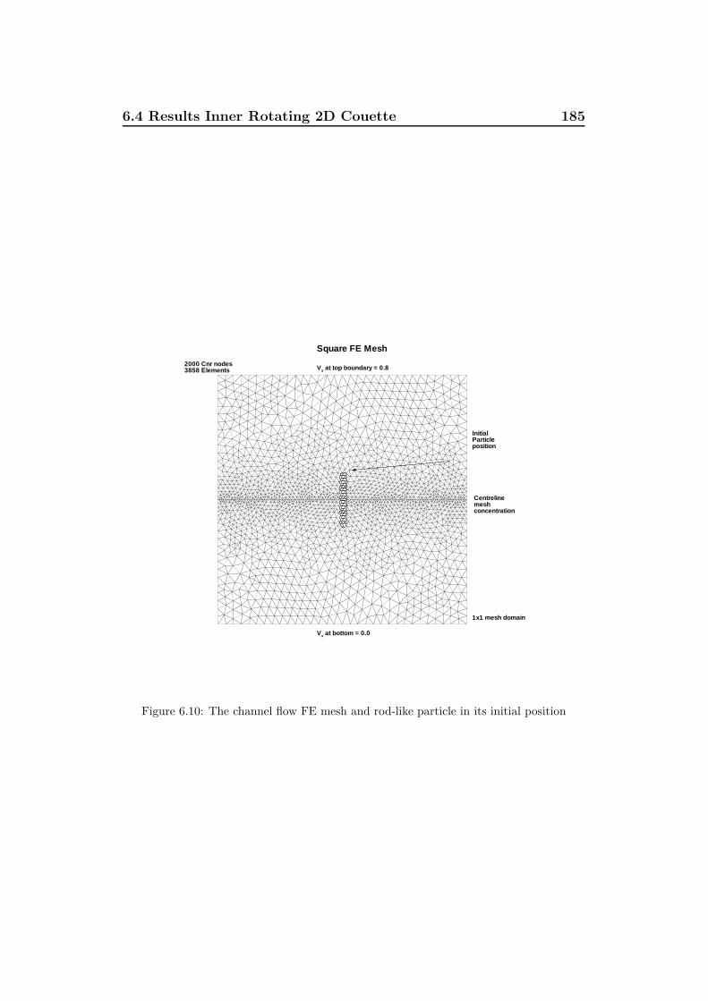
6.4 Results Inner Rotating 2D Couette 185
Square FE Mesh
InitialParticleposition
2000 Cnr nodes3858 Elements
Centrelinemeshconcentration
1x1 mesh domain
Vx at top boundary = 0.8
Vx at bottom = 0.0
Figure 6.10: The channel flow FE mesh and rod-like particle in its initial position

6.4 Results Inner Rotating 2D Couette 186
particle migration (not in the (x) direction) must then be due mostly to
the non-linear shear gradient. Inertial effects due to flow around a curved
streamline are avoided using this channel flow situation.
The fibre is initially positioned vertically oriented (along y axis). The
tracer subunit at the ‘top’ of the fibre experiences the greatest initial velocity.
It also experiences the largest Re of approximately Remax = 4.641 (Since
scaled velocity at that point is approximately vx = 19.44, subunit mass
m = 1, viscosity ηsim = 1, and characteristic length is a = 1, also Esim =
Gsim = 150).
The FE mesh and the fibre initial position is as shown in Fig. 6.10. The
unstructured FE mesh features 3848 triangular elements (2000 corner nodes
in total). The particle is placed in the centre of the mesh and since for the
majority of the simulation it will travel from left to right along the centreline,
a mesh concentration is placed along that line. When the particle exits the
right of the domain, the simulation automatically repositions it on the left
side of the mesh to re-enter. The flow field thus approximates an infinitely
long 2D channel. The simulation runs over the shear range from γinitial = 0
to γend = 500 with increment dγ = 0.005.
In Fig. 6.11, the initial and final positions of the rod-like particle are
shown, with the tracer paths for subunits at either end of the particle. The
tracer path ‘folds’ over the flow domain since it exited to the right, and re-
entered from the left twice during the simulation run. The result shows a
clear drift towards the low shear region in agreement with the previously
know observations of shear induced particle migration. This is also true for
the rectangle in the same situation (see Fig. 6.12 Remax = 2.6183, a = 1,
m = 1, ηsim = 1, Esim = Gsim = 1000). The particle momentum is directed
predominantly along the (x right) direction, and the particle translation path
is not constantly curved (as was the case with the Couette flow field). There is
no interaction between any other particles (except intra-particle interactions
amongst the subunits). By elimination, this drift must be attributed to the
non-linear shear gradient, and inertial effects. Recall that as shown in Section

6.4 Results Inner Rotating 2D Couette 187
Non-Linear Velocity Gradient in Square FE region
InitialParticleposition
Particle at finalshear with tracerpath behind
High shear at top
Low shear at bottom
Figure 6.11: The initial and final particle positions with tracer paths. The tracer path foldsover twice as the particle exits to the right, and re-enters from the left at two occasionswithin the duration of the simulation run. The figure is superimposed over a velocityvector diagram of the flow field.

6.5 Summary and Conclusions 188
§6.4.3, flexibility alone does not appear to contribute to particle migration.
Therefore we may eliminate particle flexibility here.
Non-Linear Velocity Gradient in Square FE region
InitialParticleposition
Particle at finalshear with tracerpath behind
High shear at top
Low shear at bottom
Figure 6.12: The 10× 5× 2 rectangular particle in the channel flow. Tracers indicate thepath of subunits during flow. Initial Reynolds number experienced was Remax = 2.6183.
6.5 Summary and Conclusions
In this chapter, the simulation method was extended with the ability to em-
bed the particle simulation within a pre-solved finite element flow field. The
simulation was capable of accurately reproducing particle dynamics including
particle inertia and arbitrary particle shape in a realistic non-linear complex
flow field.

6.5 Summary and Conclusions 189
The capabilities were tested with a demonstration in simulation of fi-
bres embedded in a 2D cylindrical Couette flow. A high Re rod-like particle
was shown to migrate across streamlines in the highly non-linear shear en-
vironment of Couette flow. The migration seen here did not depend on the
traditional migration theory of Phillips et al. [81], but was due to the effect
of particle inertia, and non-linear shear flow gradient. Results for a high
Re, 10× 5× 2 rectangular particle in a non-linear shear flow also indicate a
relationship between particle inertia and migration. Flexibility in particles
however was shown not to play a significant part in migration.

Chapter 7
A Study of Short Fibre
Orientation in Diverging Flow
7.1 Introduction
This chapter is the last of three on the direct simulation of arbitrarily shaped
particles in Newtonian flow.
In this chapter the earlier theoretical work by Vincent and Agassant [120],
and numerical work by Yamamoto and Matsuoka [73] are revisited. Results
are presented here on the prediction of fibre orientation in a 2D diverging
flow. Comparison is made with aspects of the results in [120] and [73], and
the different methods by which the results were obtained are evaluated.
The orientation dynamics of the elongated fibre is known for both pure
shear and pure elongation flow. The diverging channel flow is interesting
because it features both a shear dominated Poiseuille flow and a gradual
transition to an elongation dominated flow. The diverging channel flow is
used to demonstrate the ability of this simulation to reproduce fibre orien-
tation within realistic flow fields which contain elements of both shear and
elongation.
The results for the 3D particle simulation are noticeably different to the
theoretically derived work of Vincent and Agassant, where the fibre is as-

7.1 Introduction 191
sumed to be sufficiently described as a 2D orientation vector. It is argued
here that the current result is superior to Vincent and Agassant’s because
of its use of a truly 3D particle geometry. It is argued that the differences
between the results implies a deficiency in the 2D orientation vector based
theory.
While there are many variations of the theory based on Jeffrey’s work,
they are all bound by the same assumptions and limitations inherited from
the original concept. The suspended Jeffrey ellipsoid was reduced to two
defining characteristics; (1) Unit vector P, the vectorial representation of
main axis orientation, and (2) the location of the centre of mass. While this
may be a perfectly adequate representation for the often used rigid cylindrical
rod in linear shear flow field, there are some aspects of this approach that
may not accurately portray a real fibre.
One such example is the fact that the vectorial director representation
does not truly account for the fibre’s width (shape). The Jeffrey theory in-
cludes a shape correction factor λ, which scales rotational velocity to compen-
sate for the effect of shape difference between the ellipsoid and a cylinder-like
fibre. λ however is only a scaling factor and does not qualitatively alter par-
ticle dynamics, according to the particle shape. The vector P is merely a two
dimensional mathematical representation and has length but no actual width
(Fig. 7.2a). A finite width, or otherwise varied shape, may cause a noticeable
difference in the particle dynamics in certain conditions. Researchers such as
Brenner [121][110] have provided analytic formulae of hydrodynamic resis-
tance coefficient for various candidate particle shapes, e.g. spheroids, prolate
spheroids, long slender axisymmetric bodies etc. These formulae however are
limited to those particular shapes only. To simulate for non-axisymmetric,
irregular, or other various shapes, new resistance coefficients would have to
be created.
Another example of possible inaccuracy is the fact that the flow conditions
D, ω and v are only ‘sampled’ at a single point (the fibre centre of mass)
while the fibre in reality occupies a finite volume in space over which flow

7.2 Background 192
conditions may vary. This reduces accuracy in particle dynamics modelling
when flow conditions are not linear (i.e. not symmetrical) over the length
scale of the particle.
The current simulation method is not based on the theory of Jeffrey [4],
and so provides an independent method with which one may compare results.
Instead of being represented by a vectorial director, fibres in this simulation
are multi-body constructions of linked spheres (see Fig. 7.2c). The fibre
structure is fully three dimensional and hence has finite dimensions (width)
unlike its vectorial counterpart. In the following sections it will be shown how
results obtained from the 3D fibre model have some qualitatively different
features compared to the 2D vectorial model. It will be argued that these
results may be more realistic and the difference in results are due to the
ability of this simulation to account for finite particle dimension, and non-
linear flow gradients within the length scale of the fibre.
7.2 Background
Vincent and Agassant [120] provided a theoretical analysis of the fibre orien-
tation in the diverging channel flow. With theory based on the fibre dynamics
of Jeffrey [4], Vincent and Agassant predicted the orientation as a fibre trav-
elled through a diverging channel (Fig. 7.1).
In the diverging channel, the flow field exits the narrow channel with a
Poiseuille profile. As fibres prefer alignment with the shear direction, it is
justified to assumed the fibres enter the divergence closely aligned with the
streamline. The magnitude of shear reduces and elongational components
increase in the divergent region, causing the fibre to tend towards a transverse
orientation. Depending on the local region within the divergence, the relative
magnitude of shear and elongation flow components vary in intensity and
hence so does the preference for transverse orientation. The result is a pattern
of fibre orientations as shown in Fig. 7.1.
Vincent and Agassant obtained a similar result using their theoretical

7.2 Background 193
!
;
$
Figure 7.1: For a diverging channel flow the elongated fibre orients itself transversely tothe streamline. The degree of its orientation ranges from almost complete perpendicularalignment along the centreline where elongational flow is strongest, to near streamlinealignment near the channel walls where shear flow is strong.

7.2 Background 194
analysis. They also found however that the final orientation varied pro-
portionally with the degree of the initial orientation when it entered the
divergence. This conclusion will be examined with results from the current
simulation. It will be asserted that in creeping, or near-creeping flows, the
final orientation of the fibre is dependent mostly on the flow geometry, and
not initial fibre orientation. This is an indication of the different outcomes
achieved when a 3D particle model is used, as compared to the 2D vectorial
director model.
Yamamoto and Matsuoka [73] attempted a numerical solution of the same
problem. Their ‘Particle Simulation Method’ (PSM) was closely related to
the current simulation and was also capable of including particle inertia,
particle flexibility, and ‘sampling’ of flow conditions at multiple points (in-
stead of at the centre of particle mass only). Like the current method, the
simulation particle was constructed from subunit spheres. Yamamoto and
Matsuoka’s PSM linked spheres in an end-to-end configuration with exten-
sible and rotateable bonds (Fig. 7.2b). The bond stiffness was controllable
allowing variable bond stiffness. The end-to-end bonding configuration al-
lowed elongated chains of spheres or ‘fibre-like’ particles to be simulated.
In [73], they embedded their simulation fibre in a presolved FE flow field.
The two dimensional diverging channel was used and compared to Vincent
and Agassant’s work. In [73, Fig. 13], the comparison between Vincent and
Agassant’s theory and the PSM simulation was shown to be close.
While Yamamoto and Matsuoka’s PSM is related to the current simu-
lation, there is one important difference. The PSM fibre geometry remains
essentially only two dimensional. While each subunit sphere has a finite ra-
dius, the radius is only relevant in the force-torque calculations. In terms
of particle geometry, the subunits are essentially infinitely small points lined
up in a straight line, and when viewed along the axis the ‘cross-section’ is
reducible to a single dimensionless point. It retains the vectorial P-like char-
acteristic of having a finite length but no width. In the particular geometry
and relative length scales used here, finite width is an important factor which
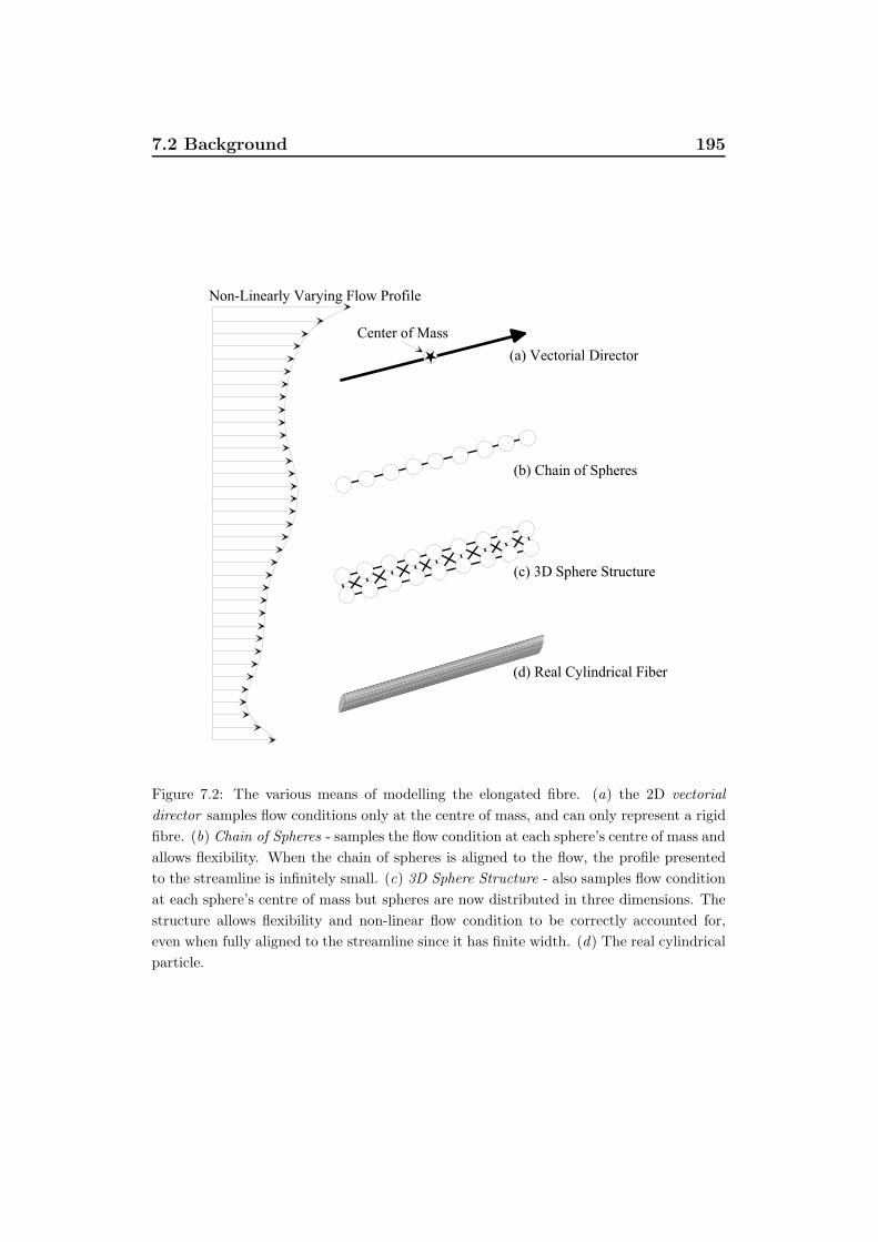
7.2 Background 195
- . , 9
- . ! !
- . 2 9 !
- . :
( , $
Figure 7.2: The various means of modelling the elongated fibre. (a) the 2D vectorialdirector samples flow conditions only at the centre of mass, and can only represent a rigidfibre. (b) Chain of Spheres - samples the flow condition at each sphere’s centre of mass andallows flexibility. When the chain of spheres is aligned to the flow, the profile presentedto the streamline is infinitely small. (c) 3D Sphere Structure - also samples flow conditionat each sphere’s centre of mass but spheres are now distributed in three dimensions. Thestructure allows flexibility and non-linear flow condition to be correctly accounted for,even when fully aligned to the streamline since it has finite width. (d) The real cylindricalparticle.

7.3 Numerical Method 196
greatly affects the final outcome. In these particular circumstances, the stiff-
ened ‘chain-of-sphere’ fibre of Yamamoto and Matsuoka is only marginally
better than the single vectorial director of Vincent and Agassant, and not
accurate enough to display the same particle dynamics shown using the full
3D model.
7.3 Numerical Method
The numerical method was described in detail in Chapter 5. In Chapter 6, a
description was added for the modifications allowing embedded simulations
in FE meshes. The method is essentially unchanged since Chapter 6.
7.3.1 Simulation Procedure
The equations of motion (5.15) (Chapter 6, Section §5.2.5) were solved and
the positions of subunits were updated for each iteration in shear dγ. Rel-
evant data was processed and output to a datafile for post-processing prior
to the next iteration.
7.3.2 Flow Geometry
The flow geometry used here was identical to that used by Vincent and
Agassant [120] and also the numerical work of Yamamoto and Matsuoka [73].
The diverging channel scenario is such a case that the particular combination
of shear and extensional flows illustrate the differences between 2D and 3D
models very well.
In Fig. 7.3 the Finite Element mesh is shown with embedded rod-like
particles positioned at the exit of the narrow channel before the diverging
flow begins (flow was from left to right). The unstructured mesh consisted
of 4000 corner nodes and 7572 triangular elements. The average element size
reduced with proximity to the channel walls (the regions of highest shear).
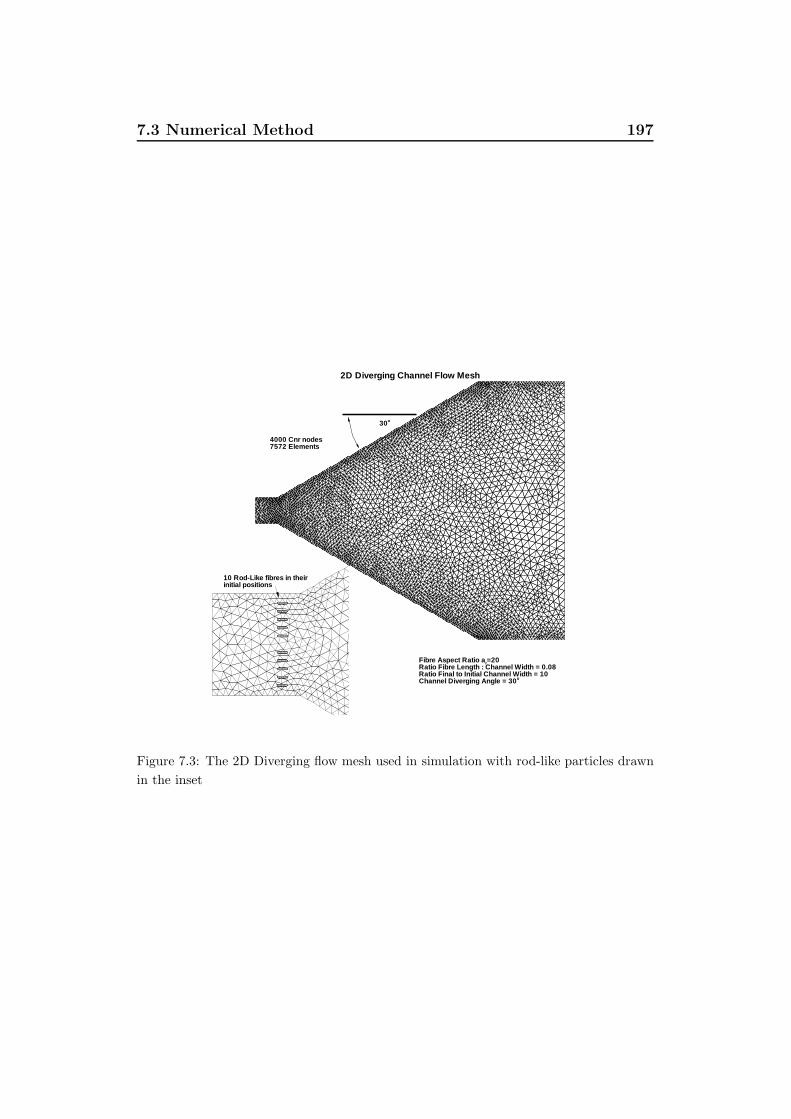
7.3 Numerical Method 197
2D Diverging Channel Flow Mesh
4000 Cnr nodes7572 Elements
30o
Fibre Aspect Ratio ar=20Ratio Fibre Length : Channel Width = 0.08Ratio Final to Initial Channel Width = 10Channel Diverging Angle = 30o
10 Rod-Like fibres in theirinitial positions
Figure 7.3: The 2D Diverging flow mesh used in simulation with rod-like particles drawnin the inset

7.3 Numerical Method 198
The fluid was a Newtonian fluid based on the 2D incompressible Navier-
Stokes Eq. (6.2). To approximate near-creeping flow, Eq. (6.2) was solved
using Refluid = 0.001. The flow field was pre-solved to steady state by the
Finite Element method using the commercial PDE solver, Fastflo v3.0. The
incoming flow profile was defined by the FE boundary condition and was in
the form of 2D Poiseuille channel flow as specified by Eq. 7.1,
vx = V(1− y2
w2
)vy = 0
(7.1)
where w = 1 was the half-width of the narrow channel. The origin was
located at the entering flow boundary at the channel centreline. Entering
non-dimensional maximum centreline velocity was Venter = 1. The channel
diverged at 30 from the centreline, and the ratio of final to initial channel
width was 10 : 1. Prior to use in the particle simulation, the FE flow field
(characteristic length w) was scaled by 375, i.e. w = 375a, to make the flow
field an appropriate scale relative to the particle simulation’s characteristic
length a. This scaling factor was arbitrarily set, but was selected such that
the relative dimensions of flow to particle were of the order seen in [120] and
[73].
The embedded rod-like particle used here had an aspect ratio, ar = 17.72.
This was the same rod fibre used in Chapter 6 (Vincent and Agassant used
ar = 20 fibres). The scaling was such that the fibre length was 0.08 the
length of the narrow channel width (this ratio was 0.025 in [73]). Particle
stiffness was high (Esim = Gsim = 3000) to approximate a rigid fibre.
A single fibre was placed at the exit of the narrow channel along an
initial ‘trajectory’ line β (see Fig. 7.4a). It should be noted that the term
‘trajectory’ is a misnomer as angle β is not necessarily the direction of the
streamline at that point. The angle β merely refers to the angle subtended
by the centreline and the line extending from the origin to the initial position
of the fibre at the narrow channel exit. For want of a better term however,
this line will continue to be referred to as ‘trajectory’.
In this series of simulations, trajectories of β = 0 and β = 15 were used.

7.3 Numerical Method 199
1 & 4
$
& 6 2 ' $
7 3 5 3 $
> 0
<
>
- .
? 7
7
@ ( /
) :
2 9 : =
$ !
$ !
1
#
- . ! >
Figure 7.4: (a) The initial position and orientation for fibres along the β = 15 trajectoryline. (b) For fully 3D particles the finite particle width causes a region of ‘stable alignment’which can alter the resulting orientation through the divergence.

7.3 Numerical Method 200
The fibre was positioned at the mouth of the narrow channel, at coordinates
(x = 1.732w, y = 0.464w), so that the initial trajectory was β = 15. Another
series was also run where (x = 1732w, y = 0), for β = 0. Initial particle
velocity was equal to the local freestream velocity. The scaled velocity profiles
in the narrow channel varied depending on the initial y position. In this
case, simulation fibres at initial position β = 15 started with an initial
and maximum Remax ≈ 0.1874. Fibres at β = 0 started with an initial
and maximum Remax ≈ 0.2387. Velocities downstream of this point reduce
rapidly as do Re on the particles. Previous chapters show that inertial effects
have a negligible effect on particle dynamics at these Remax magnitudes.
Finally, the fibre was oriented relative to the trajectory β by an orienta-
tion angle θ. This angle is the ‘initial orientation’ which will be studied and
compared with other results later. θ < 0 when the leading end of the fibre
is above the trajectory line, and θ > 0 when the leading end of the fibre
points below the trajectory line. When θ = 0 the fibre is in line with the
trajectory line β. A range of θ from −10 θ +30 was used in the same
way as Vincent and Agassant [120].
The orientation angle of the fibre relative to the global framework α
(α = 0 on the channel centreline) is the subtraction of θ from β, that is,
α = β − θ. In the results section, the variation of α as the fibre travels
through the divergence is plotted.
While the flow field is a two dimensional field (extruded in the third
dimension), the particle simulation itself is three dimensional. Therefore if
the particle orientation moves out of the (xy) plane, α refers to the apparent
orientation as seen from an observer looking perpendicularly upon the (xy)
plane. In Chapter 5, we saw that particles usually require a large number of
rotations before any out-of-plane (z) orientation developed. We shall see in
this scenario that fibres do not have the opportunity to complete even half
a revolution before the simulation has ended. In all results, the apparent
orientation was virtually identical to the actual orientation.
The simulation results and also the FE flow field data to be discussed in

7.4 Results: 2D Diverging Channel 201
Section §7.4 were computed on Intel x86 processor based PCs running MS-
Windows Operating Systems, and RedHat Linux v7.3 operating systems.
The simulation source code was written in ANSI standard Fortran77 and
compiled using Intel Fortran 95 Compiler for Linux v6, and Digital Visual
Fortran v6 Compiler for Intel/Windows.
7.4 Results: 2D Diverging Channel
In Fig. 7.5 the simulated fibre is shown at various γ (between 0 < γ < 1000+,
increment dγ = 0.0002) as it travels along the β = 15 trajectory. The
different versions show the fibre motion for varying initial fibre orientations,
θ = −10, −5, −1, +1, +5, +7, +10, +15, +18, +20, +30. Fig.
7.6 is the equivalent plot for the trajectory β = 0 (fibre initially on the
centreline), and varying initial orientation, θ = +1, +5, +10. In Fig.
7.7, the fibre orientation angle α is plotted against γ.
For Fig. 7.7(left) three groups of data were observed. The first group
of fibres (−10 < θ < +7) rotated slowly anticlockwise and ended pointing
approximately αfinal ≈ 145 away from the centreline direction (direction
of flow along centreline). The fibre started initially aligned at αinitial =
β − θinitial to the centreline. There was then a relatively short period where
fibre orientation moved from αinitial towards conformation with the master
curve. This is represented by the mismatching individual curves for γ < 1000.
For the remainder of the flow 1000 < γ < 4000 the fibre executed a slow
anticlockwise rotation at nearly the same rate for all individual cases. This
is presumably the preferred local shear direction in that particular region of
the flow.
The second group (+15o < θ < +30o) underwent a similar anti-clockwise
rotation, however the whole curve was shifted ∆α = −180 indicating the
fibre initially executed a rapid reversal (end-over-end tumble in the clockwise
direction first) before the same slow anticlockwise rotation as was seen in
the first group. This initial reversal is due to the relatively steep θinitial of

7.4 Results: 2D Diverging Channel 202
−10o −5o −1o
+1o +5o +7o
+10o +15o +18o
+20o +30o
Figure 7.5: Simulation results showing fibre orientation at selected γ for the trajectoryβ = 15 and varying orientation, θ. With the exception of θ = +10 all others appearnearly identical (The fibre is represented here with a line with length 5 times the truescale length for better visualisation).

7.4 Results: 2D Diverging Channel 203
1o 5o
10o
Figure 7.6: Fibres in channel flow at selected γ. Fibres are on the centreline trajectoryβ = 0, for varying initial orientation θ = +1, +5, +10.

7.4 Results: 2D Diverging Channel 204
0 1000 2000 3000 4000 5000
−150
−100
−50
0
50
100
150
Orientation versus Shear
Shear
Ang
le (
deg)
Group 1
Group 2
+10o
−10o
−5o −1o +1o +5o +7o +10o
+15o
+18o
+20o
+30o
0 1000 2000 3000 4000 5000
−40
−20
0
20
40
60
80
100
120
140
160
Orientation versus Shear (Adjusted)
Shear
Ang
le (
deg)
−10o
−5o −1o +1o +5o +7o +10o
+15o
+18o
+20o
+30o
Figure 7.7: (left) Fibre orientation angle α versus shear for various initial θinitial. (right)The same plot, α versus shear, with the +180 correction for fibres that executed an initialreversal. It is clear that the initial fibre orientation is irrelevant to the progress of α withγ with the exception of θ = +10, indicated by the (∗) symbol. (α is the orientation ofthe fibre relative to the centreline, α = β − θ).

7.4 Results: 2D Diverging Channel 205
the fibre combined with the relatively strong extensional flow regime in the
region immediately entering the divergence. In Fig. 7.7(right) the initial
reversal was adjusted by shifting these plots up by ∆α = +180. Once the
adjustment was made, it was seen that all data curves (except θ = +10,
symbol (∗)) collapsed approximately into one master α (t) curve. Finally, in
regards to the first and second groups of data, one may notice that the mean
gradients, dα(t)dt mean
for the first group (Fig. 7.7(left)) are slightly steeper
than dα(t)dt mean
for the second ‘reversed’ group (This is also indicated by the
different levels for the two plateau regions in Fig. 7.8). This is due simply to
the fact that the fibres that executed an initial reversal, ended their clockwise
rotation with a new orientation α (t) + 180 which happened to be closer to
the final αfinal ≈ 145 than the non-reversed fibres for the same γ period.
The reversed fibres subsequently required less anticlockwise rotation over the
remaining γ to achieve the same αfinal. Hence dα(t)dt mean
is marginally lower
than the non-reversed fibre group.
The third group consists of the single θ = 10o data (Fig. 7.7, symbol (∗)).This third group will be discussed in Section §7.4.1.
7.4.1 2D Director Based Theory versus Full 3D Meth-
ods
Figs. 7.5 and 7.7 in particular are of interest since the equivalent theoretical
results of Vincent and Agassant [120, Fig. 11] predicted that fibres along
the same β trajectory would result in a smoothly varying αfinal of magni-
tude proportional to the initial θinitial. Furthermore the rotation of the fibre
with time could be either clockwise or anti-clockwise, depending on whether
θinitial < 0 or θinitial > 0, and the rate of rotation was dependent on the
magnitude of θinitial. Fig. 7.5 and 7.7 appear to contradict this prediction, in-
dicating instead that apart from a narrow range around θ = +10 (∗) (for theβ = 15 case only), the fibre orientation over the whole γ range follows nearly
the same α(γ) curve and dαdγ
regardless of initial θinitial. Furthermore this
rotation was always anti-clockwise, regardless of whether θinitial was greater

7.4 Results: 2D Diverging Channel 206
than or less than 0o.
−10 −5 0 5 10 15 20 25 30−0.01
−0.005
0
0.005
0.01
0.015
0.02
0.025
0.03Rate of Orientation Change for different initial Orientation
Initial Angle (Deg)
Mea
n R
ate
of C
hang
e ov
er s
imul
ated
she
ar (
Deg
/She
ar)
Aligned
Beta 15o Particle Centreline Particle Beta 15o (No Hydro.)
Figure 7.8: The rate of change of orientation, dαdγ plotted against θinitial (recall α = β−θ).
There are three distinct bands of angular rate, (1) a plateau region α < 8, (2) a secondplateau region α > 18, and (3) a narrow transition band of altered fibre dynamics,8o < α < 18 (Data for simulation series without long-range hydrodynamic interaction isalso plotted (∗)).
At first glance, this result might suggest a problem in the current simu-
lation since Vincent and Agassant’s result [120] was correctly derived. Ya-
mamoto and Matsuoka’s PSM [73] also reproduced Vincent and Agassant’s
result. Both [120] and [73] however did not specifically allow for the fact that
a real fibre has finite width and in some cases, e.g. a non-linear flow, the
fibre width has a non-negligible effect on fibre orientation. It is argued that
the differences between 2D and full 3D fibre models are highlighted in the
low flow-rate diverging channel scenario. It is argued that in this situation,
sampling the flow field at a single point (the fibre’s centre of mass) is not
adequate in accurately determining the orientation of the fibre if one uses
orientation rules based on vectorial directors and linear flow gradient. Issues

7.4 Results: 2D Diverging Channel 207
such as flow and configuration reversibility are not necessarily true in this
situation. One must take into consideration the non-linearity of the flow field
over the characteristic subunit length either by refining the flow dependent
rules of orientation accordingly, or alternatively taking multiple flow condi-
tion samples and solving for coordinated multibody motion as is done in the
current simulation.
The fibre width plays a key role in the fibre’s rotation direction. A 2D
fibre-director may execute both clockwise and anti-clockwise rotation de-
pending on θinitial. This is because the 2D theory does not include an anti-
clockwise (for β > 0 trajectories only) viscous drag moment arising from
drag across the fibre width. For any 3D finite width particle on any trajec-
tory where β > 0, the prevailing rotation will be anti-clockwise regardless
of θinitial because that is the rotation of the fluid (and vice versa for β < 0
trajectories). When θinitial was severe enough, the fibres were observed un-
dergoing a short period of clockwise rotation until the fibre reached the flows
shear direction in the locality of the fibre. It then however quickly reverted
back to anti-clockwise rotation for the remainder of the motion.
Consider a finite dimension 3D fibre represented in Fig. 7.4b as an elon-
gated rectangle. It has a small range of ±∆θ rotation where overall fibre
length (corner-to-corner) could be seen to increase slightly with small ∆θ.
This range of orientation could be viewed as a special range where altered,
or non-Jeffrey-like fibre dynamics could occur. The 2D fibre-director theory
is not applicable here. While this range is very small, it is quite significant
since a cylindrical fibre in shear spends a great majority of its time in pre-
cisely this near-aligned orientation range. Depending on the aspect ratio,
a rod-like particle in shear may easily spend over 90% of the time nearly-
aligned to the streamline [31][87]. This is arguably an unacceptable amount
of time for which a 2D director based theory may not be applicable. For
the rod-like fibre species used in this simulation, the length is 14.3 times
longer than its maximum width. This makes this small θ range approxi-
mately ∆θ ≈ ±4. Since β = 15 and α = β ∓ ∆θ, the range of αaltered is

7.5 Summary and Conclusions 208
approximately 11 < α < 19. This mostly coincides with the range captured
in simulation (8 < αsim < 18) where the dαdγ
curve underwent its ‘change
between plateaus’ in Fig. 7.8.
Fig. 7.8 is certainly peculiar, however it should be noted that it was not
generated under particularly obscure circumstances or conditions. This plot
is reproducible under varying conditions. A simulation series without the
long-range hydrodynamic interaction was also run and similar results were
obtained (see the (∗) datapoints in Fig. 7.8). That simulation series was
run with greatly different increment dγ = 0.01 (as opposed to 0.0002 for
the current results), and with Reβ=15max = 0.9370, and Reβ=0
max = 1.1937 (as
opposed to 0.1874 and 0.2387 respectively). Despite these differences, the
distinctive shape of the plot in Fig. 7.8 is present regardless. It is put that
these results reflect a real phenomenon, and it is observed here only because
of the use of a 3D fibre model.
On these results it is argued that while Vincent and Agassant’s theoretical
work [120] was correct (within its own limitations), the assumption that a
fibre is like a 2D vectorP is not entirely accurate. It is argued that the current
simulation results are in fact correct, or rather more correct, and that the
differences between a 2D and 3D model can cause a noticeable divergence in
the outcome under certain non-trivial circumstances.
7.5 Summary and Conclusions
In this chapter, the new particle simulation method is applied to a study
of fibre orientation in a 2D diverging channel. For comparison, an earlier
theoretical result is referred to of the same scenario studied by Vincent and
Agassant [120], and a numerical result studied by Yamamoto and Matsuoka
[73].
At first glance the current simulation appeared to have reproduced the
expected result well. The range of orientation seen in Figs. 7.5 and 7.6
qualitatively matched the expected results (Fig. 7.1). On closer inspection

7.5 Summary and Conclusions 209
behavioural peculiarities were noticed which indicated a divergence from
Vincent and Agassant’s prediction. The current results showed that after
an initial period of adjustment, the 3D fibre rotated at an orientation rate
α = f (γ), mostly independent of its initial orientation. For a given initial
trajectory β, the fibre finished in approximately the same final orientation
regardless of αinitial. αfinal appeared only to be dependent on the domain
geometry, fibre geometry and flow conditions (velocity, viscosity etc.). When
the rate of rotation was plotted for a range of initial orientations, a distinc-
tive relationship was apparent. Two ‘plateau’ regions in the α−θ plot clearlyindicated fibres moving at a rotation rate mostly independent of initial ori-
entation (Fig. 7.8).
Based on simple reasoning in Section §7.4.1 the 3D method was predicted
to show altered non-Jeffrey-like particle dynamics in a narrow orientation
range, which would not be seen in a 2D method. The altered region is
seen in Fig. 7.8 in the range between 8 < θinitial < 18 (only for the case
β = 15). This region, predicted by simple reasoning, appeared to be verified
by numerical simulation. The range of altered dynamics depends on the
fibre aspect ratio and is only revealed with 3D particle models which directly
account for details of the fibre’s geometry. It was a basic assumption of the
vectorial method that a 3D fibre can be represented by the two dimensional
vector. Given these results, it is argued that this assumption may not always
be true.

Part IV
Conclusion

Chapter 8
Conclusion
8.1 Summary
The main goal of this thesis was to gain a better understanding of the mi-
crostructural dynamics within a flowing fibre-filled suspension, and from it
derive useful information of bulk property. These aims were achieved through
the use of the Direct Simulation numerical method. The direct simulation
method itself is open to many different approaches. In this thesis, fibres
were represented by multi-bodied constructions of spheres. Spheres were
the building blocks used to form greater structures. These structures were
initially elongated chains-of-spheres (Part II) and were taken to represent
rod-like fibres. These particle constructions were then extended into truly
three dimensional structures (Part III), allowing for an arbitrary range of
particle shapes to be observed in flow fields. In the development of these
algorithms and models, the method itself was refined and improved.
In Chapter 3, the Chain-of-Spheres simulation was used to extract de-
tailed information about the suspension including fibre orientation and bulk
viscosity. The simulation was shown to quantitatively predict non-dimensional
bulk viscosity with good precision over a range of volume fractions. When
the fibres were allowed to deform in the flow, it was observed that semi-
concentrated to concentrated suspensions exhibited a viscosity increase of

8.1 Summary 212
the order 7 − 10% greater than the equivalent rigid fibre suspension tested.
This result is in agreement with experimental work by Goto et al. [88] and
Blakeney [89]. The existence of a relationship between bulk viscosity and par-
ticle stiffness was established. This result shows that fibre material stiffness
can play an important part in the final viscosity value found. Furthermore it
implied that real fibre suspension viscosities may be underestimated by rigid
fibre theories.
It was apparent from the results of Chapter 3, that matters relating to
fibre shape and deformation could play an important part in the rheology
of the suspension. This needed to be explored further, and was done so in
Chapter 4. In Chapter 4, particular attention was paid to the influence of
fibre shape on relative viscosity. The original chain-of-spheres simulation was
modified to model for rigid, but deliberately curved fibres. Curvature in the
fibre was taken to represent the general deformities that a real fibre may
endure. When compared to the equivalent straight rigid fibre suspension,
fibre curvature was found to contribute to an even greater increase in bulk
viscosity. Greater than those seen for Chapter 3. Curved fibre suspensions
were observed to be experiencing viscosity increases of the order twice that
of straight fibre suspensions. It was apparent that even small fibre defor-
mities could affect microstructural development such that the bulk viscosity
markedly increased. With such a sensitivity to fibre shape, this result has
some important implications. One must consider the quality of fibre in-
clusions when repeatability of suspension measurements is required. When
consistent material performance is necessary in fibre composites, the exper-
imenter is highly dependent on the quality control measures taken during
sample preparation.
In Chapter 5, the older method of Part II (Ch. 3 and 4) was signif-
icantly extended. Any complexity in particle shape severely complicates
theory development. Theories for some time were mostly restricted to axi-
ally symmetric cylinders, ellipses, spheres and discs. Up to Chapter 4, the
Chain-of-Sphere simulation was used where the particle shape was limited

8.1 Summary 213
to simple linear chains. The new simulation reported in Chapter 5, was ca-
pable of modelling greater complex particle structures, within complex flows
generated separately using Finite Element methods. In Chapter 5, the simu-
lation was used to study the dynamics of various particle shapes in shearing
Newtonian fluid. In this chapter, it was demonstrated that the method could
reproduce basic known fibre behaviour, such as the Jeffrey orbit. The three
dimensional simulation was capable of revealing greater details of the mo-
tion such as the correct orbital periods, and a good approximation of spin
during orbit. From this, the ellipsoid-to-cylinder shape correction factor,
(λcorr = 0.7124) of Trevelyan and Mason [24] was verified to great accu-
racy by this completely different approach. Other particle shapes were also
observed in motion. Complex behaviour and configurations were observed,
such as the apparent log-rolling of the rectangular plate, and the ovoid shape
of the collapsed limp Pom-Pom. The results showed that this simulation is
capable of a highly accurate reproduction of the micro-dynamics of different
shaped particles.
In Chapter 6, the three dimensional simulation was developed further.
The particles were now embedded in a complex FE flow field. It was possible
to model particle motion through flow regions with complicated and varying
non-linear flow gradients. The case of a rod-like particle in a cylindrical
Couette flow field was used to demonstrate this capability and explore an
interesting real-life scenario. Inertia induced particle migration in non-linear
shear gradients was explored. Rod-like particles with high inertial forces were
observed migrating to the outer rim of the Couette device. Particles with
high Re were also shown to migrate across streamlines in highly non-linear
straight channel flow.
Finally in Chapter 7, the case of fibre orientation in a 2D diverging flow
was explored. Like the Couette cylinder, the diverging flow was also cho-
sen for the unique and varying flow types shown in different regions of the
flow. The orientation dynamics of the rod-like fibre is already well known for
simple flows, from the work of Jeffrey. The diverging channel flow however

8.2 Conclusions and Final Remarks 214
featured both a shear dominated Poiseuille flow at the entrance, and a grad-
ual transition to an elongation dominated flow. This variation was used to
demonstrate the ability to determine orientation as a fibre travelled through
this rapidly evolving flow environment.
The simulation results show detailed differences to results by Vincent and
Agassant [120], and by Yamamoto and Matsuoka [73]. The final orientation
of fibres travelling through the divergence are not particularly influenced by
the initial orientation when it entered the divergence. This is different to the
above researchers, who argued that initial orientation determined the final
orientation. Vincent and Agassant [120], and Yamamoto and Matsuoka [73]
both use a two dimensional fibre model. It is argued that in the diverging
channel scenario, the two dimensional model cannot include the secondary
contributions of particle width and non-linear shear gradients over the length
scales of the subunits.
8.2 Conclusions and Final Remarks
Fibre suspensions are interesting materials which may yield interesting op-
portunities for study at all levels, from the microscopic field of view, through
to the macroscopic. The study of the broader, measureable parameters such
as bulk viscosity and stress is the traditional realm of the rheologist. With
the current advances in computer power however, new numerical approaches
are possible, and the detailed, comprehensive understanding of the dynamics
of microstructure and its relation to observed phenomena is feasible. The
methods developed in this thesis show that fibre suspensions can be accu-
rately modelled at the microscopic level, and successfully extrapolated into
the macroscopic level. Particularly important bulk parameters such as viscos-
ity, extensional viscosity, interaction coefficient CI , shape correction factor λ,
and orbital constant C were calculated and were shown to agree with other
works where available.
A priority while undertaking this research was to improve the capabilites

8.3 Future Directions 215
of the method. This task was difficult because this method is currently un-
derdeveloped. There were relatively few previous examples of innovation in
this field to compare with. Compared to the large research efforts directed
towards other more established numerical methods, the worker in this field
is destined to take far greater leaps into the dark with every addition. The
simulation of Part II was refined through streamlining of existing methods,
and new innovations in model design. By the end of Part III, we saw de-
velopments including the ability to model for particles of arbitrary shape,
embedded within complex flows of the users design.
It is hoped that future researchers may gain from these additions and be
encouraged to extend the potential of this method further.
8.3 Future Directions
As mentioned, this method is still relatively underdeveloped. There is much
that can be improved, and one need only look at the caveats and assumptions
used throughout this thesis to see where the main deficiencies lie. Recom-
mended future developments should be in the following areas;
• The simulation of particles in viscoelastic fluids.
• Coupling of the dynamics of particles, with the flow field development.
• Three dimensional complex flow fields (by Finite Element method or
any other method).
• Parallelisation of algorithms: The algorithms of this work are excel-
lent candidates for parallelisation. The improvement in solution time
through parallel algorithms may allow whole bulk flows, with truly
microscopic resolution to be achieveable now, without any need for
improvements in computer speed.
• Improved constitutive equations are required to cater for multibody
constructed particles.

8.3 Future Directions 216
• Improved particle flexibility models are desirable.

Bibliography
[1] G. Potsch and W. Michaeli, Injection Molding - An Introduction,
Hanser Pub, 1995.
[2] F. Folgar and C. L. Tucker, Orientation Behavior of Fibers in Con-
centrated Suspensions, Journal of Reinforced Plastics and Composites
3, 98 (1984).
[3] R. Zheng, N. McCaffrey, K. Winch, H. Yu, and P. Kennedy, Predict-
ing Warpage of Injection Molded Fibre-Reinforced Plastics, Journal of
Thermoplastic Composite Materials 9, 90 (1996).
[4] G. Jeffrey, The Motion of Ellipsoid Particles Immersed in a Viscous
Fluid, Proceedings of the Royal Society of London A102, 161 (1923).
[5] S. G. Advani and C. L. Tucker, The Use of Tensors to Describe and
Predict Fibre Orientation in Short Fibre Composites, The Journal of
Rheology 8, 751 (1987).
[6] X. J. Fan, Rheology of Semiconcentrated Fibre Suspension in the
Oldroyd-B Fluid, Acta Mechanica Sinica 8, 295 (1992).
[7] R. Larson, H. Hu, D. Smith, and S. Chu, Brownian Dynamics Sim-
ulations of a DNA Molecule in an Extensional Flow Field, Journal of
Rheology 43, 267 (1999).
[8] N. Phan-Thien and R. Zheng, Macroscopic modelling of the evolution
of fibre orientation during flow, in Flow-Induced Alignment in Com-

BIBLIOGRAPHY 218
posite Materials, edited by D. Guell and T. Papathanasiou, chapter 3,
pages 77–111, Woodhead Publishing Ltd, Cambridge UK, 1997.
[9] J. L. Ericksen, Anisotropic Fluids, Archive for Rational Mechanics and
Analysis 4, 231 (1960).
[10] G. L. Hand, A Theory of Anisotropic Fluids, Journal of Fluid Mechan-
ics 13, 33 (1961).
[11] G. K. Batchelor, The Stress System in a Suspension of Force-Free
Particles, Journal of Fluid Mechanics 41, 545 (1970).
[12] R. Zheng, P. Kennedy, N. Phan-Thien, and X.-J. Fan, Thermovis-
coelastic Simulation of Thermally and Pressure Induced Stresses in
Injection Moulding for the Prediction of Shrinkage and Warpage for
Fibre-Reinforced Thermoplastics, Journal of Non-Newtonian Fluid Me-
chanics 84, 159 (1999).
[13] P. Kennedy, Flow Analysis of Injection Molds, Hanser Publisher, 1995.
[14] R. S. Bay, Fibre Orientation in Injection Molded Composites: A Com-
parison of Theory and Experiment, PhD thesis, Department of Me-
chanical Engineering. University of Illinois USA, 1991.
[15] W. Kuhn, Uber Die Gestalt Fadenformiger Molekule in Losungen, Kol-
loid Zeitschrift 68, 2 (1934).
[16] H. A. Kramers, Het Gedrag Van Macromoleculen in Een Stroomende
Vloeistof, Physica 11, 1 (1944).
[17] H. Giesekus, Elasto-Viskose Flussigkeiten, Fur Die in Station-
aren Schichtstromungen Samtliche Normalspannungskomponenten Ver-
schieden Gross Sind, Rheologica Acta 2, 50 (1962).
[18] H. Giesekus, Die Elastizitat Von Flussigkeiten, Rheologica Acta 5, 29
(1966).

BIBLIOGRAPHY 219
[19] J. G. Kirkwood and J. Riseman, The Instrinsic Viscosities and Dif-
fusion Constants of Flexible Macromolecules in Solution, Journal of
Chemical Physics 16, 565 (1948).
[20] J. G. Kirkwood and J. Riseman, Errata: The Intrinsic Viscosities and
Diffusion Constants of Flexible Macromolecules in Solution, Journal of
Chemical Physics 22, 1626 (1954).
[21] B. H. Zimm, Dynamics of Polymer Molecules in Dilute Solution: Vis-
cosity, Flow Birefringemence and Dielectric Loss, Journal of Chemical
Physics 24, 269 (1956).
[22] P. E. Rouse, A Theory of the Linear Viscoelastic Properties of Dilute
Solutions of Coiling Polymers, Journal of Chemical Physics 21, 1272
(1953).
[23] R. B. Bird, O. Hassager, R. C. Armstrong, and C. F. Curtiss, Dynamics
of Polymeric Liquids - Volume 2 Kinetic Theory, volume 2, John Wiley
and Sons, 1977.
[24] B. J. Trevelyan and S. G. Mason, Particle Motions in Sheared Suspen-
sions. I. Rotations, Journal of Colloid Science 16, 354 (1951).
[25] F. P. Bretherton, The Motion of Rigid Particles in a Shear Flow at
Low Reynolds Number, Journal of Fluid Mechanics 14, 284 (1962).
[26] H. L. Goldsmith and S. G. Mason, Particle Motions in Sheared Suspen-
sions XIII The Spin and Rotation of Disks, Journal of Fluid Mechanics
12, 88 (1962).
[27] G. I. Taylor, The Motion of Ellipsoidal Particles in a Viscous Fluid,
Proceedings of the Royal Society of London 103, 58 (1923).
[28] P. G. Saffman, On the Motion of Small Spheroidal Particles in a Vis-
cous Liquid, Journal of Fluid Mechanics 1, 540 (1956).

BIBLIOGRAPHY 220
[29] Y. Iso, D. L. Koch, and C. Cohen, Orientation in Simple Shear Flow
of Semi-Dilute Fiber Suspensions 1. Weakly Elastic Fluids, Journal of
Non-Newtonian Fluid Mechanics 62, 115 (1996).
[30] J. Azaiez, Constitutive Equations for Fiber Suspensions in Viscoelastic
Media, Journal of Non-Newtonian Fluid Mechanics 66, 35 (1996).
[31] X. Fan, N. Phan-Thien, and R. Zheng, A Direct Simulation of Fi-
bre Suspensions, Journal of Non-Newtonian Fluid Mechanics 74, 113
(1998).
[32] Y. Yamane, Y. Kaneda, and M. Doi, The Effect of Interaction of Rod-
like Particles in Semi-Dilute Suspensions under Shear Flow, Journal of
the Physical Society of Japan 64, 3265 (1995).
[33] P. Skjetne, R. F. Ross, and D. J. Klingenberg, Simulation of Single
Fiber Dynamics, Journal of Chemical Physics 107, 2108 (1997).
[34] S. Yamamoto and T. Matsuoka, Dynamic simulation method for par-
ticle dispersed systems, in Proceedings of the 14th Annual Meeting of
the Polymer Processing Society. International Conference on Polymer
Processing, pages G2–07 305–306, Polymer Processing Society, 1998.
[35] Y. Yamane, Y. Kaneda, and M. Doi, Numerical Simulation of Semi-
Dilute Suspensions of Rodlike Particles in Shear Flow, Journal of Non-
Newtonian Fluid Mechanics 54, 405 (1994).
[36] S. G. Advani and C. L. Tucker, A Numerical Simulation of Short
Fibre Orientation in Compression Molding, Polymer Composites 11,
164 (1990).
[37] S. G. Advani and C. L. Tucker, Closure Approximations for Three-
Dimensional Structure Tensors, Journal of Rheology 34, 367 (1990).

BIBLIOGRAPHY 221
[38] E. Ganani and R. L. Powell, Suspensions of Rodlike Particles: Liter-
ature Review and Data Correlations, Journal of Composite Materials
19, 194 (1985).
[39] D. J. Jeffrey and A. Acrivos, The Rheological Properties of Suspensions
of Rigid Particles, AIChE Journal 22, 417 (1976).
[40] N. Y. Kuzuu and M. Doi, Nonlinear Viscoelasticity of Concentrated
Solution of Rod-Like Polymers, Polymer Journal 12, 883 (1980).
[41] L. G. Leal, The Slow Motion of Slender Rod-Like Particles in a Second-
Order Fluid, Journal of Fluid Mechanics 69, 305 (1975).
[42] A. Ait-Kadi and M. Grmela, Modelling the Rheological Behaviour of
Fibre Suspensions in Viscoelastic Mdeia, Journal of Non-Newtonian
Fluid Mechanics 53, 65 (1994).
[43] L. Leal and E. Hinch, The Effect of Weak Brownian Rotations on
Particles in Shear Flow, Journal of Fluid Mechanics 46, 685 (1971).
[44] L. G. Leal and E. J. Hinch, The Rheology of a Suspension of Nearly
Spherical Particles Subject to Brownian Rotations, Journal of Fluid
Mechanics 55, 745 (1972).
[45] E. J. Hinch and L. G. Leal, Constitutive Equations in Suspension Me-
chanics, Part 2. Approximate Forms for a Suspension of Rigid Particles
Affected by Brownian Rotations, Journal of Fluid Mechanics 76, 187
(1976).
[46] E. J. Hinch and L. G. Leal, The Effect of Brownian Motion on the Rhe-
ological Properties of a Suspension on Non-Spherical Particles, Journal
of Fluid Mechanics 52, 683 (1972).
[47] L. G. Leal and E. J. Hinch, Theoretical Studies of a Suspension of
Rigid Particles Affected by Brownian Couples, Rheologica Acta 12,
127 (1973).

BIBLIOGRAPHY 222
[48] E. J. Hinch and L. G. Leal, Time-Dependent Shear Flows of a Sus-
pensions of Particles with Weak Brownian Rotations, Journal of Fluid
Mechanics 57, 753 (1973).
[49] G. Batchelor, Slender-Body Theory for Particles of Arbitrary Cross-
Section in Stokes Flow, Journal of Fluid Mechanics 44, 419 (1970).
[50] E. J. Hinch, The Distortion of a Flexible Inextensible Thread in a
Shearing Flow, Journal of Fluid Mechanics 74, 317 (1976).
[51] E. J. Hinch, The Deformation of a Nearly Straight Thread in a Shearing
Flow with Weak Brownian Motions, Journal of Fluid Mechanics 75, 765
(1976).
[52] J. S. Cintra and C. L. Tucker, Orthotropic Closure Approximations for
Flow-Induced Fiber Orientation, Journal of Rheology 39, 1095 (1995).
[53] N. Phan-Thien and A. L. Graham, A New Constitutive Equation for
Fibre Suspensions: Flow Past a Sphere, Rheologica Acta 30, 44 (1991).
[54] X. Fan, N. Phan-Thien, and R. Zheng, Simulation of Fibre Suspension
Flows by the Brownian Configuration Field Method, Journal of Non-
Newtonian Fluid Mechanics 84, 257 (1999).
[55] H. C. Ottinger, Stochastic Processes in Polymeric Fluids - Tools
and Examples for Developing Simulation Algorithms, Springer-Verlag
Berlin Heidelberg, 1996.
[56] J. Sun, N. Phan-Thien, and R. I. Tanner, An Adaptive Vis-
coelastic Stress Splitting Scheme and its Applications: AVSS/SI and
AVSS/SUPG, Journal of Non-Newtonian Fluid Mechanics 65, 75
(1996).
[57] J. Sun, M. D. Smith, R. C. Armstrong, and R. A. Brown, Finite
Element Method for Viscoelastic Flows Based on the Discrete Adaptive
Viscoelastic Stress Splitting and the Discontinuous Galerkin Method:

BIBLIOGRAPHY 223
DAVSS-G/DG, Journal of Non-Newtonian Fluid Mechanics 86, 281
(1999).
[58] N. Phan-Thien, T. Tran-Cong, and A. L. Graham, Shear Flow of
Periodic Arrays of Particle Clusters: A Boundary-Element Method,
Journal of Fluid Mechanics 228, 275 (1991).
[59] X.-J. Fan, N. Phan-Thien, and R. Zheng, Complete Double Layer
Boundary Element Method for Periodic Suspensions, Zeitschrift fur
angewandte mathematik und Physik ZAMP 49, 167 (1998).
[60] F. Qi, N. Phan-Thien, and X. Fan, Effective Moduli of Particulate
Solids: Completed Double Layer Boundary Element Method with Lu-
brication Approximation, Zeitschrift fur angewandte Mathematik und
Physik ZAMP 51, 92 (2000).
[61] F. Qi, N. Phan-Thien, and X. J. Fan, Effective Moduli of Particulate
Solids: Lubrication Approximation Method, Zeitschrift fur angewandte
Mathematik und Physik ZAMP 52, 1 (2001).
[62] S. Nasseri, N. Phan-Thien, and X. Fan, Lubrication Approximation in
Completed Double Layer Boundary Element Method, Computational
Mechanics 26, 388 (2000).
[63] S. Nasseri and N. Phan-Thien, Hydrodynamic Interaction Between Two
Nearby Swimming Micromachines, Computational Mechanics 20, 551
(1997).
[64] M. Loewenberg and E. J. Hinch, Collision of Two Deformable Drops
in Shear Flow, Journal of Fluid Mechanics 338, 299 (1997).
[65] D. Doraiswamy, The Origins of Rheology: A Short Historical Excur-
sion, Journal of Rheology - Rheology Bulletin 71 (2002).
[66] G. K. Batchelor, Transport Properties of Two-Phase Materials with
Random Structure, Annual Review of Fluid Mechanics 6, 227 (1974).

BIBLIOGRAPHY 224
[67] B. J. Alder and T. E. Wainwright, Phase Transistion for a Hard Sphere
System, Journal of Chemical Physics 27, 1208 (1957).
[68] G. E. Moore, Cramming More Components Onto Integrated Circuits,
Electronics 38, 114 (1965).
[69] P. P. Ewald, Die Berechnung Optischa und Elektrostatischer Gitterpo-
tentiale, Annalen Der Physik 64, 253 (1921).
[70] J. F. Brady, R. J. Phillips, J. C. Lester, and G. Bossis, Dynamic Sim-
ulation of Hydrodynamically Interacting Suspensions, Journal of Fluid
Mechanics 195, 257 (1988).
[71] S. Yamamoto and T. Matsuoka, Dynamic Simulation of Fiber Suspen-
sions in Shear Flow, Journal of Chemical Physics 102, 2254 (1995).
[72] S. Yamamoto and T. Matsuoka, Dynamic Simulation of a Platelike
Particle Dispersed System, Journal of Chemical Physics 107, 3300
(1997).
[73] S. Yamamoto and T. Matsuoka, Dynamic Simulation of Microstructure
and Rheology of Fiber Suspensions, Polymer Engineering and Science
36, 2396 (1996).
[74] T. Nomura, S. Yamamoto, and T. Matsuoka, Numerical simulation
method for fracture of fibers in injection molded composites, in Pro-
ceedings of the 7th International Conference on Numerical Methods in
Industrial Forming Processes, page poly3, 2001.
[75] G. Bossis and J. F. Brady, Dynamic Simulation of Sheared Suspensions.
1. General Method, Journal of Chemical Physics 80, 5141 (1984).
[76] J. F. Brady and G. Bossis, The Rheology of Concentrated Suspensions
of Spheres in Simple Shear Flow by Numerical Simulation, Journal of
Fluid Mechanics 155, 105 (1985).

BIBLIOGRAPHY 225
[77] I. L. Claeys and J. F. Brady, Suspensions of Prolate Spheroids in
Stokes Flow. Part 1. Dynamics of a Finite Number of Particles in an
Unbounded Fluid, Journal of Fluid Mechanics 251, 411 (1993).
[78] I. L. Claeys and J. F. Brady, Suspensions of Prolate Spheroids in Stokes
Flow. Part 2. Statistically Homogeneous Dispersions, Journal of Fluid
Mechanics 251, 443 (1993).
[79] I. L. Claeys and J. F. Brady, Suspensions of Prolate Spheroids in
Stokes Flow. Part 3. Hydrodynamic Transport Properties of Crystalline
Dispersions, Journal of Fluid Mechanics 251, 479 (1993).
[80] X. Fan, N. Phan-Thien, and R. Zheng, Simulation of Fibre Suspension
Flow with Shear-Induced Migration, Journal of Non-Newtonian Fluid
Mechanics 90, 47 (2000).
[81] R. J. Phillips, R. C. Armstrong, R. A. Brown, A. L. Graham, and J. R.
Abbott, A Constitutive Equation for Concentrated Suspensions That
Accounts for Shear-Induced Particle Migration, Physics of Fluids A -
Fluid Dynamics 4, 30 (1992).
[82] S. Yamamoto and T. Matsuoka, A Method for Dynamic Simulation of
Rigid and Flexible Fibers in a Flow Field, Journal of Chemical Physics
98, 644 (1993).
[83] S. Yamamoto and T. Matsuoka, Dynamic Simulation of Flow-Induced
Fiber Fracture, Polymer Engineering and Science 35, 1022 (1995).
[84] R. F. Ross and D. J. Klingenberg, Dynamic Simulation of Flexible
Fibers Composed of Linked Rigid Bodies, Journal of Chemical Physics
106, 2949 (1997).
[85] C. F. Schmid and D. J. Klingenberg, Mechanical Flocculation on Flow-
ing Fiber Suspensions, Physical Review Letters 84, 290 (2000).

BIBLIOGRAPHY 226
[86] C. F. Schmid, L. H. Switzer, and D. J. Klingenberg, Simulations of
Fiber Flocculation: Effects of Fiber Properties and Interfiber Friction,
Journal of Rheology 44, 781 (2000).
[87] C. G. Joung, N. Phan-Thien, and X. J. Fan, Direct Simulation of Flex-
ible Fibers, Journal of Non-Newtonian Fluid Mechanics 99, 1 (2001).
[88] S. Goto, H. Nagazono, and H. Kato, The Flow Behavior of Fiber
Suspensions in Newtonian Fluids and Polymer Solutions. 1. Mechanical
Properties, Rheologica Acta 25, 119 (1986).
[89] W. R. Blakeney, The Viscosity of Suspensions of Straight, Rigid Rods,
Journal of Colloid and Interface Science 22, 324 (1966).
[90] E. Anczurowski and S. G. Mason, The Kinetics of Flowing Dispersions.
II. Equilibrium Orientations for Rods and Discs (Theoretical), Journal
of Colloid and Interface Science 23, 522 (1967).
[91] M. A. Nawab and S. G. Mason, Viscosity of Dilute Suspensions of
Threadlike Particles, Journal of Physical Chemistry 62, 1248 (1958).
[92] J. M. Burgers, Second Report on Viscosity and Plasticity, Nordemann,
New York , 113 (1938).
[93] O. L. Forgacs and S. G. Mason, Particle Motions in Sheared Suspen-
sions. X. Orbits of Flexible Threadlike Particles, Journal of Colloid
Science 14, 473 (1959).
[94] C.-M. Tchen, Motion of Small Particles in Skew Shape Suspended in
a Viscous Fluid, Journal of Applied Physics 25, 463 (1954).
[95] M. Doi and N. Y. Kuzuu, Nonlinear elasticity of rodlike macromolecules
in condensed state, in Reports on Progress in Polymer Physics in
Japan, volume 22, 1979.

BIBLIOGRAPHY 227
[96] T. Kitano, T. Kataoka, and T. Shirota, An Empirical Equation of
the Relative Viscosity of Polymer Melts Filled with Various Inorganic
Fillers, Rheologica Acta 20, 207 (1981).
[97] S. Goto, H. Nagazono, and H. Kato, The Flow Behaviour of Fibre
Suspensions in Newtonian Fluids and Polymer Solutions II. Capilliary
Flow, Rheological Acta 25, 246 (1986).
[98] A. Jabbarzadeh, J. Atkinson, and R. Tanner, Nanorheology of Molecu-
larly Thin Films in N-Hexadecane in Couette Shear Flow by Molecular
Dynamics Simulation, Journal of Non-Newtonian Fluid Mechanics 77,
53 (1998).
[99] R. B. Bird, R. C. Armstrong, and O. Hassager, Dynamics of Polymer
Liquids - Volume 1 Fluid Mechanics, volume 1, John Wiley and Sons,
1977.
[100] S. Kim and S. Karilla, Microhydrodynamics Principles and Selected Ap-
plications, Butterworth Series of Chemical Engineering, Butterworth
Heinemann, 1991.
[101] L. D. Landau and E. M. Lifshitz, Theory of Elasticity, volume 7 of
Course of Theoretical Physics, Pergamon Press, second edition, 1970.
[102] X. J. Fan, N. Phan-Thien, and R. Zheng, Simulation of Fibres Sus-
pension Flows by the Brownian Configuration Field Method, Journal of
Non-Newtonian Fluid Mechanics 84, 257 (1999).
[103] W. J. Milliken, M. Gottlieb, A. L. Graham, L. A. Mondy, and R. L.
Powell, The Viscosity-Volume Fraction Relation for Suspensions of
Rod-Like Particles by Falling Ball Rheometry, Journal of Fluid Me-
chanics 202, 217 (1989).
[104] M. A. Bibbo, Rheology of Semi-Concentrated Fiber Suspensions, PhD
thesis, Chemical Engineering, Massachusetts Institute of Technology,
1987.

BIBLIOGRAPHY 228
[105] G. K. Batchelor, The Stress Generated in a Non-Dilute Suspensions
of Elongated Particles by Pure Straining Motion, Journal of Fluid Me-
chanics 46, 813 (1971).
[106] A. P. Arlov, O. Forgacs, and S. Mason, Particle Motions in Sheared
Suspensions 4: General Behaviour of Wood Pulp Fibres, Svensk Pap-
perstidning 61, 61 (1958).
[107] C. G. Joung, N. Phan-Thien, and X. J. Fan, Viscosity of Curved
Fibers in Suspension, Journal of Non-Newtonian Fluid Mechanics 102,
1 (2002).
[108] G. G. Lipscomb, M. M. Denn, D. Hur, and D. Boger, The Flow of
Fibre Suspensions in Complex Geometries, Journal of Non-Newtonian
Fluid Mechanics 26, 297 (1988).
[109] I. Proudman and J. R. A. Pearson, Expansions at Small Reynolds
Numbers for the Flow Past a Sphere and a Circular Cylinder, Journal
of Fluid Mechanics 2, 237 (1957).
[110] J. Happel and H. Brenner, Low Reynolds Number Hydrodynamics with
Special Applications to Particulate Media, Martinus Nijhoff Publishers,
1986.
[111] R. Eisenschitz, Die Viscositat Von Suspensionen Langgestreck-
ter Teilchen und Ihre Interpretation Durch Raumbeanspruchung,
Zeitschrift fur Physikalische Chemie. Abteilung A, Chemische Thermo-
dynamik, Kinetik, Elektrochemie, Eigenschaftslehre A158, 78 (1932).
[112] H. L. Goldsmith, Red Cell Motions and Wall Interactions in Tube
Flow, Federation Proceedings 30, 1578 (1971).
[113] A. Karnis, H. L. Goldsmith, and S. G. Mason, The Flow of Suspen-
sions Through Tubes. V. Inertial Effects, Canadian Journal of Chemical
Engineering 44, 181 (1966).

BIBLIOGRAPHY 229
[114] S. I. Rubinow and J. B. Keller, The Transverse Force on a Spinning
Sphere Moving in a Viscous Fluid, Journal of Fluid Mechanics 11, 447
(1961).
[115] B. P. Ho and L. G. Leal, Inertial Migration of Rigid Spheres In a Two-
Dimensional Unidirectional Flows, Journal of Fluid Mechanics 65, 365
(1974).
[116] W. S. J. Uijttewaal, E.-J. Nijhof, and R. M. Heethaar, Lateral Migra-
tion of Blood Cells and Microspheres in Two-Dimensional Poiseuille
Flow: A Laser Doppler Study, Journal of Biomechanics 27, 35 (1994).
[117] Commonwealth Scientific and Industrial Research Organisation
(CSIRO), Compumod Pty Ltd Distributors, Level 13, 309 Pitt St, Syd-
ney, 2000, Fastflo Tutorial Guide, 3 edition, 1999.
[118] C. A. Stover, D. L. Koch, and C. Cohen, Observations of Fibre Ori-
entation in Simple Shear Flow of Semi-Dilute Suspensions, Journal of
Fluid Mechanics 238, 277 (1992).
[119] L. A. Mondy, H. Brenner, S. A. Altobelli, J. R. Abbott, and A. L.
Graham, Shear-Induced Particle Migration in Suspensions of Rods,
Journal of Rheology 38, 444 (1994).
[120] M. Vincent and J. F. Agassant, Experiental and Theoretical Study of
Short Fiber Orientation in Diverging Flows, Rheologica Acta 24, 603
(1985).
[121] H. Brenner, Rheology of a Dilute Suspensions of Axisymmetric Brown-
ian Particles, International Journal of Multiphase Flow 1, 195 (1974).
[122] R. S. Brumbaugh, Ancient Greek Gadgets and Machines, Thomas Y.
Crowell Company, 1966.

BIBLIOGRAPHY 230
[123] A. Neuburger, The Technical Arts and Sciences of the Ancients,
Methuen and Company, 1969, Translated by Henry L. Brose from
original text Die Technik des Altertums.
[124] I. of the History of the Natural Sciences, Ancient China’s Technology
and Science, Foreign Languages Press, Beijing, 1983.
[125] F. Gies and J. Gies, Cathedral, Forge, and Waterwheel: Technology
and Invention in the Middle Ages, Harper Perrenial Publishers, 1994.

Appendix A
Additional Material
A.1 Simulation Source Code
The latest source code for the ‘Chain-of-Spheres’ simulation (Part II) and the ‘3DParticle’ Simulation (Part III), along with assorted datafiles and other code can befound in the CD-ROM included at the back of this thesis. The ‘Chain-of-Spheres’simulation and associated files are found at:
CDROM:/01-Chain_of_Spheres/01-Source_Code_Stable/f409
The ‘3D Particle’ simulation and associated files are found at:
CDROM:/02-3D_Particle/01-Source_Code_Stable/F55116
The two simulations were written in ANSI standard Fortran77 and compiled usingthe Digital Fortran Compiler. Simulations were executed on various machines.These include DEC/Compaq Alpha processor based workstations running UNIXand Linux operating systems, and Intel x86-based PCs running both Linux andWindows.
A.2 Electronic Version of Thesis
Electronic versions of this thesis (Postscript, Adobe PDF, and LATEX2ε) are avail-able in various formats on the attached CD-ROM at:
CDROM:/04-Thesis

Appendix B
Pre-Rheology
B.1 Introduction
This is a brief history of some lesser known ancient technologies which might
be considered to have a rheological flavour. Rheology as a distinct and recog-
nised science did not exist prior to the early 1900’s. It took more than one
and a half millennia of ‘promising starts’ and gadgeteering in pre-16th cen-
tury Europe before mostly theological pre-occupations finally gave way to
the new empirical sciences and technologies. This history takes place mostly
prior to the Rennaissance. The following passage is by no means complete,
and is intended only for the historically inclined reader.
B.2 Pre-Rheology
Evidence for mankind’s interest in Rheology and technology of flow can be
found as far back as the ancients (e.g. [122][123][124][125]). The clepsydra is
perhaps the most cited device from antiquity. Essentially nothing more than
a vessel with a small hole in the bottom, time could be measured by the rate
at which water leaked from it. The accuracy was mediocre, as the rate of flow
diminished with the water level. However it was the first time-measuring in-
novation since the ancient sundial, and an example of the utilization of fluid
property in a measuring instrument of practical use by mankind. The me-

B.2 Pre-Rheology 233
chanician, Ctesibius (270 B.C.) refined the clepsydra further by eliminating
the variation in water pressure as water level reduced. An overflow design
was invented by which the water level in the vessel was maintained with a
continuous water input supply and an overflow design to remove any excess
(Fig. B.1). The clepsydra could then be used continuously and indefinitely
as a time measurer, corrected only intermittently with astronomical time-
keeping. Ctesibius also contributed to the knowledge of Alexandria with
inventions based on the compressibility of air and water [122][123]. The
*
;
+ # $
$
: #
- .
0 ! $
Figure B.1: The constant water pressure clepsydra of Ctesibius 270 B.C.
clepsydra was the first of a series of improvements on the concept of the
‘water clock’, culminating in the octogonal Tower of the Winds, (see Fig.
B.2) created by Andronicus of Rhodes in the first century A.D. for the agora
of Athens1. The Tower of the Winds was a public timekeeper and weather
station with a water mechanism at its core. It featured a large ornamental
dial, marking the hours with hands attached to rotating drums connected
to floats. Heron of Alexandria (1st century A.D.), taught by the designs of
Ctesibius, added his own knowledge of the power of fire and steam to develop
the first steam engine (Fig. B.3). Heron created numerous ingenious gadgets
and devices demonstrating a deep understanding of fluid mechanics, such as
1The Agora was the business centre of ancient Athens
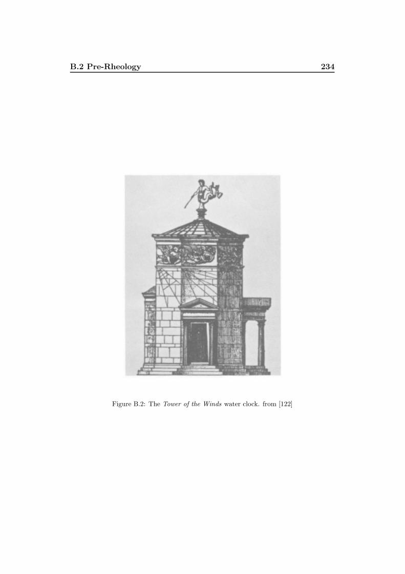
B.2 Pre-Rheology 234
Figure B.2: The Tower of the Winds water clock. from [122]

B.2 Pre-Rheology 235
the ability to siphon, and many other fluid responses to pressure, heat and
flow [122]. Also related to water time keeping, the Han Dynasty astronomer
Zhang Heng (2nd century A.D.) invented a water driven celestial globe based
on an independently invented clepsydra. The celestical globe revolved with
the diurnal motion of the skies above him [124] (Fig. B.4).
Figure B.3: The steam engine, or Aeolipile invented by Heron of Alexandria. From [123]
On the topic of water transport, Archimedes of Syracuse (3rd century
B.C.) invented the screw for pumping water to a higher level. Three King-
doms Dynasty inventor Ma Chun (260 A.D.) invented the Chinese equivalent
square-pallet chain pump. This was a conveyor-belt like device with buckets
linked in a belt. Power was provided by a man on a treadmill, an animal,
and then eventually water power. Siphoning was also used in ancient China’s
Eastern Han Dynasty (25-220 A.D.) as a means of irrigation. In 1044 A.D.
Zeng Gongliang is recorded using a large siphon to draw water over a hill
using a long bamboo pipe. It is unclear what method of suction he used to
initiate the siphoning over such a distance [124].
In the Eastern Han Dynasty (25-220 A.D.), oil (or Shiyou, literally rock
oil) was found in a spring flowing out of a mountain south of Yanshou County
of Jiuquan. When collected in a pot it changed from a brownish yellow to
black and so was also called shiqi (rock laquer). Not only was it found to burn
with an extremely bright flame but was also an excellent lubricant for axles
and bearings [124]. In the Eastern Mediterranean early in the Byzantine

B.2 Pre-Rheology 236
Roman period, military engineers of Constantinople devised a petroleum
based naval weapon known as the Greek Fire. Discharged from tubes off the
ships prows during close combat, ignited fluid was propelled under pressure
onto the walls of enemy ships like a modern flame thrower. The problem with
the Naphtha (petroleum distillate) available was that it would not adhere to
the enemy ship walls easily, and would disperse rapidly once it fell into the
water. An unknown inventor thickened the Naphtha with resin and sulfur.
Like modern Napalm, the resulting formula did not disperse in water, nor
could it be easily put out with water, continuing to burn enemy ships hulls
on the waterline. Enemy Arab fleets were attacked in this manner outside
Constantinople in 673 A.D. and also 717 A.D.
The innovations perhaps most resembling modern rheological knowledge
are related to paper technology. In 1957 remnants of Western Han dynasty
hemp paper (49 B.C.) were discovered in Baqiao in an eastern suburb of
Figure B.4: Su Sung’s water driven astronomical clock-tower, built in 1090. From [125]

B.2 Pre-Rheology 237
Xi’an in Shaanxi Province (Northern Central China bordering Inner Mongo-
lia). Microscopic study of these specimens indicated that a small amount of
ramie (plant fibre) was combined with the base hemp pulp. These specimens
represent the oldest known vegetable-fiber paper [124]. The ancient Chinese
could in fact manufacture paper of specified tensile strength by altering the
fibre content, much like modern fibre-filled composites. A similar technology
using gums, pastes and starches was added in Baghdad during the migration
of paper technology to Europe. By the 6th century A.D., there was avail-
able thicker paper for packaging and light structural use, through to various
writing paper grades, and even soft, sometimes powdered and fragrant toilet
paper for royalty (toilet paper is another invention of the Chinese). Starch-
paste was widely used in the Tang Dynasty (618-907 A.D.) as filler and to
keep fibers suspended in the vat during paper production. This was later
replaced in the Song dynasty (960-1279 A.D.) with a sticky vegetable juice
called zhiyao (paper drug), used to make a more even fibre distribution in
the pulp (i.e. resistant to sedimentation). Similar approaches are used in
modern food technology. The benefits of paper as a writing medium were
exploited most in Europe. Part of the innovation of Gutenberg’s printing
press was the technology developed for ink. Johann Gutenberg invented the
moveable text printing press in 1450 A.D., in the cathedral city of Mainz,
on the Rhine River (see Fig. B.5). Paper technology in Europe was well
developed by that stage, mostly by painters and artists in early rennaissance
Italy. The other three printing technologies, the press, movable type and
ink was made workable by Gutenberg. In relation to ink, printing required
an ink with different characteristics from those of water-based writing ink
which smudged, did not spread unformly, and leached through to the back-
side of the paper. Italian painters in the previous century had invented the
technique of mixing pigments (insoluble natural substances) in linseed oil.
Gutenberg experimented successfully with a mixture of lampblack (chimney
soot), turpentine, and linseed or walnut oil, reduced by heating. The new ink
had the right consistency and wetting ability to adhere to slightly dampened

B.2 Pre-Rheology 238
Figure B.5: The Gutenberg printing press. From [125]

B.2 Pre-Rheology 239
paper without blurring, and was an attractive jet black. By the end of the
Rennaissance, Europe and Asia clearly had the ability not just to harvest and
use raw materials, but to modify and design man-made fluids and materials
to suit a wide range of specific industrial requirements. These ranged from
lubricants, to paints and inks, even to the idea of reinforcing structures using
fibre composites.