Direct Detection of Low Mass WIMPs - MPG.PuRe
137
Fakultät für Physik und Astronomie Ruprecht-Karls-Universität Heidelberg Diplomarbeit im Studiengang Physik vorgelegt von Felix Kahlhöfer geboren in Bergisch Gladbach 2010
-
Upload
khangminh22 -
Category
Documents
-
view
0 -
download
0
Transcript of Direct Detection of Low Mass WIMPs - MPG.PuRe

Fakultät für Physik und Astronomie
Ruprecht-Karls-Universität Heidelberg
Diplomarbeit
im Studiengang Physik
vorgelegt von
Felix Kahlhöfer
geboren in Bergisch Gladbach
2010


Sensitivität von
Flüssig-Xenon-Detektoren
für Leichte Dunkle Materie
Die Diplomarbeit wurde von Felix Kahlhöfer
ausgeführt am
Max-Planck-Institut für Kernphysik
unter der Betreuung von
Herrn Prof. Manfred Lindner


Department of Physics and Astronomy
University of Heidelberg
Diploma thesis
in Physics
submitted by
Felix Kahlhoefer
born in Bergisch Gladbach
2010


Sensitivity of Liquid Xenon Detectors
for Low Mass Dark Matter
This diploma thesis has been carried out by Felix Kahlhoefer
at the
Max-Planck-Institut fuer Kernphysik
under the supervision of
Prof. Manfred Lindner


Sensitivität von Flüssig-Xenon-Detektoren für Leichte DunkleMaterieExperimente zum direkten Nachweis von dunkler Materie auf der Basis vonFlüssig-Xenon-Detektoren zählen zu den vielversprechendsten Strategien umdie Eigenschaften der dunklen Materie zu ergründen. In dieser Arbeit erörternwir die Sensitivität solcher Detektoren für Kernrückstöße mit einer Energieunter 10 keV, wie man sie für Dunkle-Materie-Teilchen mit einer Masse vonweniger als 10 GeV erwartet. Das Interesse an leichter dunkler Materie rührther von der angeblichen Beobachtung eines entsprechenden Signals in denbeiden Experimenten DAMA und CoGeNT. In dieser Diplomarbeit zeigen wir,dass auch Flüssig-Xenon-Detektoren wie XENON100 in der Lage sein sollten,solche leichte dunkle Materie zu beobachten, und somit die laufende Diskussionbeilegen können. Zuerst betrachten wir die Detektorauflösung und bestimmendie Akzeptanz von Flüssig-Xenon-Detektoren im Bereich niedriger Energien.Anschließend beschäftigen wir uns mit der Produktion und dem Nachweisvon Szintillationslicht in flüssigem Xenon und berechnen dazu die relativeSzintillationseffizienz. Außerdem führen wir Monte Carlo Simulationen durch,um die Lichtsammeleffizienz eines vorgegebenen Detektors vorherzusagen. ZumAbschluss diskutieren wir die Phänomenologie für den direkten Nachweis vonfermionischer dunkler Materie. Dazu berechnen wir die Wirkungsquerschnittefür die Streuung von dunkler Materie an Atomkernen in verschiedenen Modellenund bestimmen die resultierenden Ausschlussbereiche aktueller Experimente.
Sensitivity of Liquid Xenon Detectors for Low Mass Dark MatterDark matter direct detection experiments based on liquid xenon detectors areone of the most promising strategies to determine the nature of dark matter.In this thesis, we discuss the sensitivity of such detectors for nuclear recoilswith energy below 10 keV corresponding to dark matter particles with a massof less than 10 GeV. The interest in low mass dark matter has been roused bythe claimed observation of a corresponding signal in the experiments DAMAand CoGeNT. We demonstrate that liquid xenon detectors like XENON100should also be able to observe such low mass dark matter particles and canconsequently settle the present discussion. First, we discuss the detectorresolution and determine the acceptance of liquid xenon detectors in the lowenergy region. Next, we analyze the production and detection of scintillationlight in liquid xenon, calculating the relative scintillation efficiency. Moreover,we perform Monte Carlo simulations to predict the light collection efficiencyfor a given detector. Finally, we discuss the phenomenology of direct detectionfor fermionic dark matter. We calculate the cross sections for the interactionbetween dark matter and nuclei in different models and give the correspondingexclusion limits of recent experiments.


Contents
Acknowledgments ix
1 Introduction 11.1 The standard model of cosmology . . . . . . . . . . . . . . . . . . . . 21.2 Observational evidence for dark matter . . . . . . . . . . . . . . . . . 31.3 Theory of dark matter . . . . . . . . . . . . . . . . . . . . . . . . . . 5
1.3.1 Relic densities . . . . . . . . . . . . . . . . . . . . . . . . . . . 51.3.2 Dark matter properties . . . . . . . . . . . . . . . . . . . . . . 61.3.3 Candidates for dark matter . . . . . . . . . . . . . . . . . . . 7
1.4 Motivation and outline . . . . . . . . . . . . . . . . . . . . . . . . . . 8
2 Detection of dark matter 102.1 Direct detection of dark matter . . . . . . . . . . . . . . . . . . . . . 11
2.1.1 Differential event rates . . . . . . . . . . . . . . . . . . . . . . 112.1.2 The dark matter velocity distribution . . . . . . . . . . . . . . 122.1.3 Cross sections . . . . . . . . . . . . . . . . . . . . . . . . . . . 132.1.4 Dark matter spectra . . . . . . . . . . . . . . . . . . . . . . . 142.1.5 Astrophysical uncertainties . . . . . . . . . . . . . . . . . . . . 15
2.2 Direct detection experiments . . . . . . . . . . . . . . . . . . . . . . . 162.3 Evidence for dark matter? . . . . . . . . . . . . . . . . . . . . . . . . 172.4 The XENON100 experiment . . . . . . . . . . . . . . . . . . . . . . . 18
3 Detector performance at low energies 233.1 Detector resolution . . . . . . . . . . . . . . . . . . . . . . . . . . . . 24
3.1.1 S1 fluctuations . . . . . . . . . . . . . . . . . . . . . . . . . . 243.1.2 S2 fluctuations . . . . . . . . . . . . . . . . . . . . . . . . . . 25
3.2 Simulation of the nuclear recoil band . . . . . . . . . . . . . . . . . . 263.3 Cut acceptances . . . . . . . . . . . . . . . . . . . . . . . . . . . . . . 29
3.3.1 Single scatter cut . . . . . . . . . . . . . . . . . . . . . . . . . 323.3.2 Nuclear recoil cut . . . . . . . . . . . . . . . . . . . . . . . . . 33
3.4 The total acceptance function . . . . . . . . . . . . . . . . . . . . . . 363.5 Summary of results . . . . . . . . . . . . . . . . . . . . . . . . . . . . 39

4 The effective scintillation yield of liquid xenon 404.1 Production of scintillation light in liquid xenon . . . . . . . . . . . . . 414.2 Stopping powers of liquid xenon . . . . . . . . . . . . . . . . . . . . . 42
4.2.1 Electronic stopping power . . . . . . . . . . . . . . . . . . . . 434.2.2 Nuclear stopping power . . . . . . . . . . . . . . . . . . . . . . 444.2.3 Total electronic excitation . . . . . . . . . . . . . . . . . . . . 46
4.3 Recombination . . . . . . . . . . . . . . . . . . . . . . . . . . . . . . 484.4 Calculation of the relative scintillation efficiency . . . . . . . . . . . . 504.5 Summary of results . . . . . . . . . . . . . . . . . . . . . . . . . . . . 54
5 Predicted sensitivity of future liquid xenon experiments 555.1 Large liquid xenon detectors . . . . . . . . . . . . . . . . . . . . . . . 565.2 Estimated energy thresholds . . . . . . . . . . . . . . . . . . . . . . . 57
5.2.1 Light collection maps . . . . . . . . . . . . . . . . . . . . . . . 575.2.2 Light collection efficiency . . . . . . . . . . . . . . . . . . . . . 595.2.3 Predicted exclusion limits . . . . . . . . . . . . . . . . . . . . 62
5.3 Proposed design changes . . . . . . . . . . . . . . . . . . . . . . . . . 635.3.1 Oblate detectors . . . . . . . . . . . . . . . . . . . . . . . . . 635.3.2 4pi QUPID coverage . . . . . . . . . . . . . . . . . . . . . . . 65
5.4 Estimated background rates . . . . . . . . . . . . . . . . . . . . . . . 665.4.1 Internal electron recoil background . . . . . . . . . . . . . . . 675.4.2 Cut efficiencies and position resolution . . . . . . . . . . . . . 685.4.3 Background rates for alternative detector designs . . . . . . . 705.4.4 Intrinsic background . . . . . . . . . . . . . . . . . . . . . . . 71
5.5 Summary of results . . . . . . . . . . . . . . . . . . . . . . . . . . . . 73
6 Analysis of matrix elements for fermionic dark matter 746.1 Spin-independent interactions . . . . . . . . . . . . . . . . . . . . . . 756.2 Spin-dependent interactions . . . . . . . . . . . . . . . . . . . . . . . 776.3 Momentum and velocity dependence in matrix elements . . . . . . . . 816.4 General analysis of four-fermion interactions . . . . . . . . . . . . . . 83
6.4.1 Scalar interactions . . . . . . . . . . . . . . . . . . . . . . . . 846.4.2 Vector interactions . . . . . . . . . . . . . . . . . . . . . . . . 866.4.3 Tensor interactions . . . . . . . . . . . . . . . . . . . . . . . . 88
6.5 Matching and form factors . . . . . . . . . . . . . . . . . . . . . . . . 886.6 Summary of results . . . . . . . . . . . . . . . . . . . . . . . . . . . . 91
7 Summary and conclusions 92
A The Dirac equation 97
B Calculation of exclusion limits 99

C Coulomb correction to electronic stopping 100
D Details on the Monte Carlo simulations with Geant4 103D.1 Detector design . . . . . . . . . . . . . . . . . . . . . . . . . . . . . . 103D.2 Material properties . . . . . . . . . . . . . . . . . . . . . . . . . . . . 104
D.2.1 QUPIDs . . . . . . . . . . . . . . . . . . . . . . . . . . . . . . 104D.2.2 Optical properties . . . . . . . . . . . . . . . . . . . . . . . . . 104D.2.3 Radioactivity . . . . . . . . . . . . . . . . . . . . . . . . . . . 106
D.3 Simulation details . . . . . . . . . . . . . . . . . . . . . . . . . . . . . 106D.3.1 Simulation of scintillation light . . . . . . . . . . . . . . . . . 106D.3.2 Simulation of radioactivity . . . . . . . . . . . . . . . . . . . . 106
Bibliography 109
Index 117


Poets say science takes away from the beauty of the stars — mereglobs of gas atoms. I too can see the stars on a desert night, andfeel them. But do I see less or more? The vastness of the heavensstretches my imagination — stuck on this carousel my little eye cancatch one-million-year-old light. A vast pattern — of which I am apart... What is the pattern, or the meaning, or the why? It doesnot do harm to the mystery to know a little about it. For far moremarvelous is the truth than any artists of the past imagined it.
(Richard Feynman)


Acknowledgments
First of all, I thank Manfred Lindner for giving me the opportunity to write thisdiploma thesis. It was him who first directed my attention to the topic of dark matterand who introduced me to the XENON Collaboration. I am very grateful for hisguidance and his encouragement. Moreover, I would like to thank Manfred Lindnerfor offering me the possibility to visit the Gran Sasso Underground Laboratory and toattend the Workshop on the Interconnection between Particle Physics and Cosmology(PPC 2010) in Turin, which have been great experiences from both personal andscientific point of view.Next, it is a pleasure to thank those people who have collaborated with me on
different parts of my thesis and supervised my work. I thank Fedor Bezrukov forthe very productive collaboration on the relative scintillation efficiency of liquidxenon and some very inspiring discussions. I have benefited a lot from his wideknowledge. I also thank Thomas Schwetz for all the insight he has shared with me onthe phenomenology of dark matter and the analysis of direct detection experiments.Moreover, I would like to express my gratitude that he shared with me his programcodes to calculate exclusion limits, and for his idea to attempt a general operatoranalysis of four-fermion interactions. Also, I am indebted to Hardy Simgen forinitiating me into the world of experimental physics, more precisely the XENONtechnology, and for his help with Geant4. In this context, I would also like to thankMarc Weber and Sebastian Lindemann, who have made available their support onmany occasions. Most notably, I am grateful for the inspiring collaboration withMarc on the Monte Carlo simulations of the nuclear recoil band.
Furthermore, this thesis would not have been possible without the help and supportof the entire XENON Collaboration, most notably Rafael Lang, Teresa Marrodan-Undagoitia, Alexander Kish, Emilija Pantic, Marc Schumann, and Laura Baudis,who have repeatedly given me advice and answered my questions. I am grateful thatthe collaboration allowed me to participate in the weekly teleconferences and theXENON1T meeting in Heidelberg. I especially thank Rafael Lang for various helpfuldiscussions and his great patience.
I am deeply thankful for having had so many nice people around during my time atthe Max-Planck-Institut für Kernphysik. First of all, I would like to show my gratitudeto my office mates Nico Kronberg and Julian Heeck, not only for answering an

uncountable number of questions (related to physics, computer problems, typographyand almost anything else), but also for lots of fun and the extremely enjoyableatmosphere of mutual support. Of course, I equally thank the people from room B,namely Michael Dürr, Angnis Schmidt-May, Daniel Schmidt and Alexander Dück.I thank the whole division Particle & Astroparticle Physics for the good time thatI have had, especially Martin Holthausen, Viviana Niro and James Berry. Also, Ithank Anja Berneiser for being a great help in all questions of administration andbureaucracy.For proofreading this work, I am indebted to Michael Dürr, Marc Weber and
Sebastian Lindemann.Furthermore, I am grateful to the Studienstiftung des deutschen Volkes for sup-
porting my studies at the University of Heidelberg.My acknowledgments would certainly not be complete without thanking those
people who have accompanied me for a long time and supported me during my entireuniversity education. First of all, I owe my deepest gratitude to my girlfriend InésUsandizaga for her never-ending patience in stressful times and her infallible talentto cheer me up and calm me down. I also thank Stephan Steinfurt for our weeklylunch breaks and many interesting discussions. My final thanks go to my family:my parents Hermann and Christine and my sister Eva, to whom I owe more than Ican express here. Thank you for all your help and encouragement, which made thisdiploma thesis possible.

CHAPTER 1Introduction
To observe the motion of astrophysical objects and understand the laws that describetheir trajectories has traditionally been one of the central interests of physicists. Ithas led to the discovery of the laws of gravitation, the confirmation of the theory ofgeneral relativity, and to our present understanding of the universe. At the sametime, such observations still raise questions that we cannot yet answer. In 1933,Zwicky observed that the velocity distribution of galaxies in the Coma cluster cannotbe explained by the gravitational potential inferred from the luminous matter alone.The observation that large amounts of non-luminous matter, so-called dark matter ,must be present in the universe has been confirmed many times since then — butour understanding of the nature of this dark matter has made only little progress.Today, the central strategy of astrophysics is the spectral analysis of radiation
from different kinds of sources. This strategy has led to the discovery of Hubble’s lawof the expansion of the universe and to the understanding of the Cosmic MicrowaveBackground (CMB). Together, these observations build the foundations of our modernunderstanding of cosmology, the so-called Big Bang scenario. We now have a highlysophisticated model, called ΛCDM, that can explain a large variety of astrophysicalobservations with only six parameters.
The parameters of ΛCDM can be determined from a global analysis of experimentaldata. The results imply that baryons, the constituents of ordinary matter, contributeonly 4–5% to the energy density of the universe. Dark matter, in fact, is far moreabundant, accounting for approximately 23% of the energy density. The remaining72% are not matter at all but vacuum energy, also known as dark energy. On theone hand, these results strongly confirm the observation that dark matter must bepresent in the universe. On the other hand, we must admit that the great success ofΛCDM implies that we only understand a tiny fraction of the content of the universe.The remainder is dark, meaning that it eludes conventional detection techniques.
Over the past few decades, the puzzle of dark matter has gained more and moreinterest. The reason is that dark matter turns out to be closely related to centralproblems of particle physics. In fact, the most promising models that extend theStandard Model of particle physics in order to solve the hierarchy problem, namely

2 Introduction
supersymmetry and extra dimensions, naturally predict a good candidate for the darkmatter particle. This connection between modern cosmology and modern particlephysics makes the nature of dark matter such a fascinating and important problem.In this chapter, we will give a general introduction to the topic of this thesis. In
section 1.1 we introduce the relevant preliminaries from cosmology and discuss theΛCDM model. An account of the experimental evidence for dark matter will begiven in section 1.2. We will summarize our present knowledge about dark matterand discuss possible models in section 1.3. Finally, in section 1.4, we will connectthese general considerations with the topic of this thesis, giving a motivation for andan outline of the following chapters. For a more detailed introduction to the topic ofdark matter, we refer to [1–3].
1.1 The standard model of cosmology
Today, most cosmologists agree that the universe has evolved from a singular state,called the Big Bang. Therefore, the universe was extremely dense initially, buthas expanded since, and is expected to continue this expansion. In the process,it has undergone various transitions, which we can still trace today, for examplenucleosynthesis and recombination. All these observations are well described by theΛCDM model. The name of the model indicates the necessary ingredients: Vacuumenergy (described by a cosmological constant Λ) and Cold Dark Matter.1 Only ifboth of these contribute significantly to the total energy density, we are able toexplain the observed history of the universe.To describe the expansion of the universe since the Big Bang, one introduces a
scale factor a(t) with the present value a0 = 1. The rate of expansion is given by theHubble parameter
H(t) ≡ a(t)a(t) , (1.1)
whose present value (also called the Hubble constant) is H0 = 73± 3 km s−1 Mpc−1.This value can be obtained from Hubble’s law by measuring the cosmological redshift z,defined by 1 + z = a0/a, for nearby galaxies. Note that H0 is often quoted indimensionless form: h = H0/100 km s−1 Mpc−1 = 0.73± 0.03.
The time evolution of H is given by the Friedmann equations, which describe theexpansion of an isotropic and homogeneous universe as a function of its total energydensity ρtot:
H2 + k
a2 = 8πG3 ρtot . (1.2)
1We shall explain what cold means in this context in section 1.3.

1.2 Observational evidence for dark matter 3
Here, G is the gravitational constant and k is the spatial curvature, which can bek = −1, 0, or 1, corresponding to an open, flat, or closed universe, respectively. Ifthe energy density is equal to the critical value
ρtot = ρc ≡3H2
08πG , (1.3)
the Friedmann equations describe a flat universe with k = 0.In general, we distinguish different contributions to the total energy density which
may have different equations of state. An equation of state relates the density ρiand the pressure pi of a substance i. Usually, it has the form pi = wρi, leading toa time evolution of the density given by ρi ∝ a−3(1+w) [4]. For matter, w = 0, sothat ρm ∝ a−3. Radiation has w = 1/3, so that ρr ∝ a−4 and its density is negligibletoday. Finally, we include a vacuum energy induced by a cosmological constant Λ,which has w = −1 and consequently a density ρΛ independent of time. It will beconvenient to express each density relative to the critical energy density given inequation (1.3), so we define
Ωi = ρiρc. (1.4)
Equation (1.2) can then be written as(H
H0
)2= Ωm
(a
a0
)3+Ωk
(a
a0
)2+ΩΛ , (1.5)
where Ωk = −k/a20H
20 and ΩΛ = Λ/3H2
0 . The matter energy density Ωm can besplit into two parts, Ωm = Ωb +ΩCDM, where Ωb is the baryon density and ΩCDMis the cold dark matter density. In the following section, we shall see that ΩCDMcontributes significantly (in fact dominantly) to the total amount of matter.
1.2 Observational evidence for dark matter
In general, there are two ways to explain a discrepancy between the expected andthe observed trajectories of gravitationally interacting objects: We can either changethe amount of gravitating matter by introducing dark matter, or we can modify thelaws of gravity. The second approach, known as Modified Newtonian Dynamics, hasrepeatedly been suggested as an alternative to dark matter. The idea is to introducea new large scale, above which the gravitational force deviates from its known form.However, evidence for dark matter can be observed at very different scales, so it isdifficult to explain all observations with a single new scale. Without striving forcompleteness, we will review the most important of these observations, starting atthe smallest scale, the scale of galaxies.

4 Introduction
Figure 1.1: Rotation curve ofNGC 6503. The dotted, dashed,and dash-dotted lines are thecontributions of gas, disk, anddark matter, respectively. Fig-ure taken from [5].
Figure 1.2: The Bullet Cluster 1E0657-558 — acollision of two clusters. The colored picture isan x-ray image of the visible matter, the greencontours show the distribution of the total massinferred from gravitational lensing. One observesa clear discrepancy between visible and gravitat-ing matter. Figure taken from [6].
The most convincing evidence for dark matter on galactic scales comes from theobservation that the outer regions of galaxies are rotating faster than expected fromthe laws of gravitation. According to Newtonian dynamics, one would expect that
vrot(r) =√GM(r)
r, (1.6)
where M(r) is the integral of the galaxy’s mass density from 0 to r. Withoutdark matter, M(r) should be constant beyond the optical disc, and consequentlyv(r) ∝ r−1/2 for large r. However, systematic measurements of rotation curves,meaning the velocities of stars and gas as a function of their radial distance from thegalactic center, give a quite different picture. One observes a constant v(r) at largedistances [5], indicating that the mass density M(r) must increase proportional to reven in regions where no luminous matter is observed (see figure 1.1).
The conclusion of this observation is that galaxies must have a non-luminous masscomponent having ρ(r) ∝ r−2 at large distances. This component is often referred toas the dark matter halo of a galaxy. While evidence for dark matter halos has beencollected for a large number of galaxies, including elliptical galaxies, dwarf spheroidalgalaxies, and spiral galaxy satellites (see [1] for further references), their precise formand density distribution is still unknown and subject to intense discussion.Similar observations can be made on the scale of galaxy clusters, for example
by comparing the temperature of a cluster with the observed amount of luminousmass. Another very impressive piece of evidence comes from gravitational lensing
1.3 Theory of dark matter 5
data, which determine the mass of a cluster from the distortion of the images ofbackground objects. Such measurements allow to demonstrate clearly the mismatchbetween the distribution of visible and gravitating matter (see figure 1.2).
Nevertheless, the observations discussed so far do not allow for a determination ofthe total amount of dark matter in the universe, namely ΩCDM. This quantity, as wellas the other contributions to the total energy density can, however, be measured oncosmological scales. The most precise results come from the analysis of the CosmicMicrowave Background. The most recent measurements of the Wilkinson MicrowaveAnisotropy Probe (WMAP7) give [7]
ΩΛ = 0.734± 0.029 (1.7)ΩCDM = 0.222± 0.026 (1.8)
Ωb = 0.0448± 0.0028 . (1.9)
Note that these results imply that Ωm + ΩΛ ≈ 1 and Ωk ≈ 0, meaning that weappear to live in a spatially flat universe. We conclude that only about a quarterof the total energy density of the universe is due to matter. And again less than aquarter of the total matter content of the universe is baryonic. A similar value forΩb is independently obtained from Big Bang nucleosynthesis. We have to concludethat most of the matter in the universe is made out of particles that we have not yetbeen able to observe.
1.3 Theory of dark matter
In spite of the strong evidence for dark matter at very different scales, the natureof the dark matter particle remains unknown. In this section, we summarize ourpresent knowledge about the properties that any candidate for the dark matterparticle must possess. The most important requirement is that a sufficiently largeabundance of the particle is produced in the early universe so that it can accountfor the observed dark matter density. From this consideration, it turns out thatnone of the known particles of the Standard Model can form the main constituent ofdark matter. Consequently, we have to look at possible new particles which arise inextensions of the Standard Model.
1.3.1 Relic densities
In the early universe, all particle species are expected to be in thermal equilibrium,meaning that the number density neq of a particle with mass mχ and g degrees offreedom is given by
neq = g(mχT
2π
)3/2e−mχ/T , (1.10)

6 Introduction
where T is the temperature. As the universe expands and cools down, T dropsbelow mχ. At this point, the number of particles becomes Boltzmann suppressed,so that annihilations of particles of this species become less likely. As soon as theinteraction rate of the particle species becomes smaller than the expansion rate ofthe universe, it will fall out of local thermodynamic equilibrium. It will decouple andform a thermal relic. The temperature at which this decoupling happens is calledthe freeze-out temperature TF.
We can calculate the density of such a thermal relic starting from the Boltzmannequation, which reads in this case
dndt + 3Hn = −〈σv〉
(n2 − (neq)2
), (1.11)
where 〈σv〉 is the thermal average of the total annihilation cross section of the particlemultiplied by its velocity. For heavy particles, 〈σv〉 can be expanded in powers of v2
to give
〈σv〉 = a+ b〈v2〉+O(〈v4〉) . (1.12)
Without going through the details of the calculation, we give the final result forthe relic density:
Ωχh2 ≈ 1.07 · 109 GeV−1
MPl
xF√g∗(a+ 3b/xF) . (1.13)
Here, xF = mχ/TF, MPl is the Planck mass and g∗ counts the number of relativisticdegrees of freedom at T = TF. xF is not easy to determine exactly, but in mostcases roughly given by xF ≈ 20. In [1], the authors give a simplified version ofequation (1.13):
Ωχh2 ≈ 3 · 10−27 cm3 s−1
〈σv〉. (1.14)
For any proposed dark matter candidate, we can use this formula to see whether Ωχ
matches with the expected value for ΩCDM. However, there are more requirementsbesides the correct abundance that a dark matter candidate must fulfill.
1.3.2 Dark matter properties
First of all, we know from the CMB that most of dark matter must be non-baryonic.Baryonic dark objects, usually called Massive Compact Halo Objects (MACHOs), forexample brown dwarf stars or large gas giants like Jupiter, are known to exist, butcontribute only a small fraction to the total amount of dark matter. From primordialnucleosynthesis and the Lyman alpha forest, we can also exclude diffuse baryons as

1.3 Theory of dark matter 7
the main constituent of dark matter.Moreover, we know that dark matter should be collisionless (for example to
explain the observation of the Bullet Cluster in figure 1.2). Finally, to account forthe observed abundance, it must either be stable or have a lifetime that is largecompared to the age of the universe.
From these considerations, neutrinos may seem like the perfect candidate for darkmatter, since we know that they are massive and interact only weakly. Clearly,neutrinos do contribute to the total amount of dark matter. However, there aretwo problems with neutrinos. First, it turns out that they are simply not abundantenough to be the dominant component of dark matter, unless there is a differentmechanism to produce them. The greater problem is that, because of their lowmass, neutrinos were still relativistic when they decoupled from thermal equilibrium.Such relativistic dark matter particles are referred to as hot dark matter . Largeamounts of hot dark matter tend to erase local density fluctuations in the universeand therefore prevent the formation of small-scale structures. Therefore, we knowthat light neutrinos cannot account for all of the dark matter.
1.3.3 Candidates for dark matter
Whatever is the dominant component of dark matter, it must be cold (meaningnon-relativistic), collisionless, stable and non-baryonic [8]. Excellent candidatesfor dark matter are so-called Weakly Interacting Massive Particles (WIMPs). Likeneutrinos, these particles have only weak interactions with ordinary matter buttheir mass is much larger. In fact, it would be natural for such a particle to have amass around the electroweak scale, meaning mχ ≈ 100− 1000 GeV. On dimensionalgrounds, the cross section of such a particle should then be
〈σv〉 ≈ g4weak
16π2m2χ
. (1.15)
Substituting this expression into equation (1.14), we indeed get the correct order ofmagnitude for Ωχ. Weak-scale particles automatically have the correct relic densityand consequently make excellent candidates for dark matter. This observation isknown as the WIMP miracle.The second reason for the great popularity of WIMP candidates for dark matter
is that they arise naturally in extensions of the Standard Model. Almost all theoriesthat attempt to solve the gauge hierarchy problem introduce new particles at theelectroweak scale. If one of these particles can be made stable, it is automatically agood candidate for dark matter. In supersymmetric extensions of the Standard Model,this particle would be the lightest supersymmetric particle, which is usually expectedto be the neutralino. In models with universal extra dimensions one similarly obtainsa stable heavy particle, the lightest Kaluza-Klein particle.

8 Introduction
However, it is certainly not necessary that the dark matter particle is a WIMP.Viable candidates, which are well motivated by extensions of the Standard Model,include gravitinos, axions and sterile neutrinos. These candidates have in commonthat they all have much smaller masses and much weaker interactions than WIMPsand are consequently extremely difficult to detect experimentally. Of course, manymore candidates for dark matter have been proposed and it is beyond the scope ofthis thesis to mention all of them. Nevertheless, the point we wish to make is thatalthough WIMPs are the most attractive candidates for dark matter, one should beopen-minded towards alternatives.
1.4 Motivation and outline
The identity of dark matter is one of the central problems of modern physics. Manyexperiments have been performed, are currently running or will be built to solveit. So far, most experiments have only given null results, allowing to exclude somedark matter candidates and set strong bounds on others. Those experiments, whichactually have observed a signal that may be due to dark matter, give a contradictoryand even more puzzling picture (see chapter 2.3). Recent observations indicate thatthe dark matter mass may be much smaller than the weak scale — in conflict withthe WIMP idea. It will be the task of present and future dark matter experimentsto confirm or refute this observation, and the task of theoretical physicists to refineexisting models or propose new ones to consistently interpret experimental data.
In this thesis, we want to discuss and examine possible ways to shed light on themysteries of dark matter. If the dark matter particle is a WIMP, direct detectionexperiments based on liquid xenon have a good chance to detect it. We want todemonstrate that — in contrast to recent claims [9] — they are also highly competitivefor the detection of dark matter with lower mass. Consequently, it is reasonable toexpect that within the near future, liquid xenon detectors will either observe a darkmatter signal or exclude current experimental claims with high significance.
In chapter 2, we discuss experimental strategies to detect dark matter. The focus ofthis thesis is on direct detection experiments, which attempt to observe dark matterinteractions in low background underground detectors. We discuss the expectedexperimental signatures and how they depend on the dark matter properties andastrophysical input. Moreover, we give an overview over present direct detectionexperiments and recent notable results, with a special emphasis on the XENONexperiment.Then, in chapter 3, we go into more detail on the expected performance of
XENON100. This performance depends crucially on the sensitivity of the detectorat low energies. Consequently, we discuss the low energy threshold and the energyresolution of the detector. We also estimate the fluctuations of the expected signals,and determine the detector acceptance at low recoil energies.
1.4 Motivation and outline 9
Another important open question related to the performance of the XENON100experiment concerns the relative scintillation efficiency of nuclear recoils in liquidxenon. Experiments currently disagree on the behavior of this quantity at lowenergies. In chapter 4, we first review existing theoretical models for the processesthat lead to the production of scintillation light, and then present our own calculationof the relative scintillation efficiency.
In chapter 5, we turn to future experiments based on the liquid xenon technology.Our goal is to estimate the sensitivity of such experiments, again with a special focuson the low energy region. Using Monte Carlo simulations, we can determine the lightyield for different potential detector designs and calculate the low energy thresholds.To investigate whether the expected sensitivity is limited by radioactive background,we also perform Monte Carlo simulations of internal background from γ-rays.
We return to more theoretical questions in chapter 6, investigating different modelsfor dark matter to see how the signatures in direct detection experiments may change.Our goal is to present a systematic analysis of all possible interactions betweenfermionic dark matter and quarks and calculate the resulting cross sections fornon-relativistic scattering of dark matter on nuclei. Such an analysis will allow todevelop a general understanding of whether the results from different direct detectionexperiments are in conflict or not.
Finally, a summary and our conclusions, as well as suggestions for further work, willbe given in chapter 7. In the appendices, we summarize the notation and conventionsused in this thesis and provide additional details on the calculations and the MonteCarlo simulations.
A comment on units
Given that this thesis comprises both theoretical and experimental approaches todark matter detection, we have to deal with the different systems of units in thetwo fields. For the microscopic descriptions of particle interactions, we use naturalunits, setting c = ~ = kB = 1. For example, we use eV for both masses andenergies. Nevertheless, we prefer to give distances in m, using the conversion factor~c = 197 MeV fm = 1. Note that, for simplicity, we refrain from using atomic unitsin chapter 4. Consequently, the Bohr radius is a0 = 53 pm, the Bohr velocity isv0 = α = 1/137 and the electron charge is given by e2 = α~c = 1.44 MeV fm.
For macroscopic quantities, as they appear in the context of liquid xenon detectors(for example the fiducial mass, the detector dimensions or the runtime of an experi-ment), we use SI units. Also, it is conventional to use the unit km/s for astrophysicalvelocities, for instance the galactic escape velocity. We stick to this convention, butassume implicitly that these velocities are divided by cSI = 3 · 105 km/s when usingthem in the context of particle interactions.

CHAPTER 2Detection of dark matter
In the previous chapter, we have presented substantial evidence that dark mattercontributes significantly to the energy density of the universe. From such observationswe can also infer some basic properties of dark matter, for example that it must bemostly non-baryonic. Nevertheless, many central questions concerning the particlesthat constitute dark matter, especially regarding their mass, their spin or theirinteractions with visible matter, cannot be answered this way.To learn more about the nature of dark matter particles, we must find a way to
actually detect them experimentally. For this purpose, many collaborations aroundthe world have developed experimental strategies and built various kinds of detectors.There are three different experimental strategies for solving the dark matter puzzle:Direct detection experiments, indirect detection experiments and collider experiments.Most likely, only a combination of these strategies will allow to solve all problemsrelated to dark matter.Direct detection experiments attempt to observe dark matter particles as they
pass through the Earth. Even though dark matter is expected to have only veryscarce interactions, its density in the galactic halo of the Milky Way should besufficiently large that scattering processes with nuclei do occur occasionally. Theresulting nuclear recoils can be measured with dedicated low background detectors.Indirect detection experiments aim to observe the products of dark matter annihi-
lations, which occur in regions of high dark matter density — such as the center ofthe galaxy or the core of the sun. The annihilation products could include neutri-nos, positrons, anti-protons and γ-rays, which would have a characteristic energyspectrum. These particles could then be observed with many ground-based andspace-based telescopes.Collider experiments, finally, attempt to actually produce dark matter by colliding
Standard Model particles at high energies. The goal is to invert the annihilationprocess that occurs in the early universe, or to produce other new heavy particlesthat subsequently decay into the dark matter particle. However, since dark matterparticles are long-lived and neutral, they will appear in the detectors only as missingmomentum and energy, making an actual identification very difficult.

2.1 Direct detection of dark matter 11
In this thesis, we will focus on direct detection experiments. We present thecalculation of the direct detection event rate in section 2.1 and also discuss theastrophysical input and related uncertainties. In section 2.2, we will describe how toextract possible signals and give an overview of the existing direct detection experi-ments. Section 2.3 discusses some recent experimental results and the implicationsof these findings for future experiments. To conclude this chapter, we will discuss insection 2.4 in detail the XENON experiment, which will be the central topic for therest of this thesis.
2.1 Direct detection of dark matter
As dark matter particles pass through the Earth, they will occasionally undergoelastic collisions with nuclei. Direct detection experiments attempt to measure theenergy (called Enr) that is transferred to the recoiling nucleus in such a scatteringprocess. In this section, we want to calculate and discuss the probability distributionof nuclear recoil energies, or said differently, the energy spectrum that we expect tosee in a detector for such scattering events.
2.1.1 Differential event rates
The central quantity relevant for the direct detection of dark matter is the differentialevent rate dR/ dEnr. The unit of the differential event rate is the number of eventsper kg detector mass per day runtime per keV energy, which is often called differentialrate unit (dru). One obtains the total event rate R (in events per kg per day) byintegrating the differential event rate from the lower to the upper energy thresholdof the detector. To obtain the total number of expected events, we must multiplythe total event rate with the exposure of the experiment, which is the product ofdetector mass and runtime of the experiment. For more details on the calculation ofevent rates, we refer to appendix B.We shall denote the mass of the dark matter particle with mχ and the mass
of the nuclei in the target with mN. We furthermore introduce the reduced massµN = mχmN/(mχ +mN). Analogously, the quantities mp and µp refer to the massand the reduced mass of a single proton. The number density of dark matterparticles is equal to ρ0/mχ, where the local energy density of dark matter is given byρ0 = (0.30± 0.05) GeV cm−3 [10]. To obtain the dark matter flux, we must multiplythe number density with the dark matter velocity v. This velocity, however, is notthe same for all dark matter particles. Instead, we have a distribution of velocitiesdescribed by a function f(v), which we will discuss in section 2.1.2.The differential event rate is given by the product of the dark matter flux, the
density of target nuclei and the differential interaction cross section, integrated over

12 Detection of dark matter
all contributing dark matter velocities:
dRdEnr
= ρ0
mNmχ
∞∫vmin
vf(v) dσdEnr
(v, Enr) dv . (2.1)
To determine, which velocities can contribute to a given nuclear recoil energy, wemust look at the kinematics of the collision between dark matter particle and nucleus.Since all velocities are non-relativistic, we can easily express the nuclear recoil energyin terms of the dark matter velocity and the scattering angle θ in the center-of-massframe
Enr = µ2Nv
2(1− cos θ)/mN . (2.2)
Consequently, to obtain a recoil energy of Enr, the dark matter velocity must at leastbe
vmin =√mNEnr
2µ2N
. (2.3)
2.1.2 The dark matter velocity distribution
In the standard halo model, the distribution of dark matter velocities is described byan isotropic Gaussian distribution
f(v) d3v = 1(πv2
c )3/2 exp(−v
2
v2c
)d3v , (2.4)
where vc = (220 ± 20) km s−1 is the local circular velocity. Strictly speaking, thevelocity that appears in equation (2.4) is the velocity in the Galactic rest frame.Since we are interested in the distribution of velocities relative to the Earth, we mustreplace v by v + vE, where the motion of the Earth is given by [11]
vE = |vE| = vc
[1.05 + 0.07 cos
(2π(t− tp)
1 yr
)], (2.5)
with tp = June2nd± 1.3 days (for more details, see [12]). Consequently, we get
∫f(v) d3v =
∫ 1(πv2
c )3/2 exp(−|v + vE|2
v2c
)d3v
=∫ v√
πvcvE
[exp
(−(v − vE)
v2c
)− exp
(−(v + vE)
v2c
)]dv (2.6)
≡∫f(v) dv .

2.1 Direct detection of dark matter 13
Another correction to the velocity distribution comes from the fact that no dark mat-ter particles with a velocity above the galactic escape velocity vesc = (544±50) km s−1
can be bound in the galactic halo. Consequently we must modify equation (2.6) insuch a way that f(v) = 0 for v > vesc [13]:
f(v) dv = 1k
[exp
(−(v − vE)
v2c
)− exp
(−(v + vE)
v2c
)]Θ (vesc − |v + vE|) dv , (2.7)
where
k = (πvc)3/2[Erf
(vesc
vc
)− 2√
πvescvc exp
(−v
2escv2
c
)](2.8)
ensures that∫∞0 f(v) dv = 1.
2.1.3 Cross sections
The differential cross section dσ/ dEnr in equation (2.1) contains the input fromparticle physics to the differential event rate. It depends fundamentally on theinteraction between dark matter and quarks, which result from the underlyingparticle physics model. We will discuss in chapter 6 how to calculate the cross sectionfor a large number of models. In this section, we will only state the results that arenecessary for us to calculate the differential event rate. It turns out that we candistinguish between interactions that are independent of the nuclear spin (so-calledSI interactions) and interactions that depend on it (so-called SD interactions). Inthis chapter, as well as for chapters 3 to 5, we will only consider SI interactions.In this case, we can separate the energy and velocity dependence of the cross
section by writing(dσ
dEnr
)SI
= mNσ0F2(Enr)
2µ2Nv
2 . (2.9)
Here, F 2(Enr) is the nuclear form factor, which reflects the loss of coherence withincreasing momentum transfer. It corresponds essentially to the Fourier transform ofthe nucleon density. One usually assumes the parameterization
F 2(q) =(
3j1(qR1)qR1
)2
exp(−q2s2
), (2.10)
where q =√
2mNEnr is the momentum transfer and j1 is a spherical Bessel function.The parameters s and R1 describe the size and the form of the nucleus. They areusually taken to be s ≈ 1 fm and R1 =
√R2 − 5s2 with R ≈ 1.2 fm
√A, where A is
the mass number of the target nucleus.

14 Detection of dark matter
In the most simple cases, the fundamental cross section σ0 does not depend onthe momentum transfer and the velocity. It depends only on the couplings of darkmatter to protons and neutrons, called fp and fN, respectively. We can write [14]
σ0 = [Zfp + (A− Z)fN]2
f 2p
µ2Nµ2
pσSI
p , (2.11)
where Z is the atomic number of the target nucleus and σSIp is the dark matter proton
cross section. fp and fN can in principle be calculated from quark couplings to darkmatter and the quark content of the nucleons. However, for most cases, one obtainsfp ≈ fN, so that equation (2.11) simplifies to
σ0 = A2µ2Nµ2
pσSI
p . (2.12)
2.1.4 Dark matter spectra
Substituting equation (2.12) and equation (2.9) into equation (2.1), we get
dRdEnr
= ρ0A2
2µ2pmχ
σSIp F
2(Enr)∞∫
vmin
f(v)v
dv . (2.13)
With f(v) from equation (2.7), the integral can be performed analytically (see forinstance [15]) to give a function g(vmin). Figure 2.1 shows some typical differentialevent rates. We make the following observations:
• The differential event rate decreases exponentially with increasing recoil energy.This decrease is partly due to a decreasing nuclear form factor F (Enr), reflectingthe loss of coherence, and partly due to a decreasing velocity integral g(vmin)reflecting the smaller number of dark matter particles that have a sufficientlylarge velocity to contribute.
• The differential event rate is proportional to A2, so that scattering at low recoilenergies is strongly enhanced for targets with high mass number. At the sametime, the differential event rate falls more steeply for heavier targets, becausethe nuclear form factor F (Enr) decreases more quickly.
• Similarly, for lower dark matter mass, the differential event rates will be largerat low recoil energy because of the overall factor m−1
χ and smaller at high recoilenergy, because vmin grows more quickly if mχ is small.
In fact, for mχ mN we have µN ≈ mχ and thus vmin =√mNEnr/2m2
χ. Since wehave g(vmin) = 0 for vmin > vesc + vE, the velocity cutoff at vesc implies an energy

2.1 Direct detection of dark matter 15
0 20 40 60 80 10010-4
0.001
0.01
0.1
1
Nuclear recoil energy keV
Dif
fere
ntia
leve
ntra
te
dru
mΧ = 250 GeV
mΧ = 50 GeV
mΧ = 30 GeV
mΧ = 20 GeV
(a) A xenon target with mN = 131.3 u.
0 20 40 60 80 10010-4
0.001
0.01
0.1
1
Nuclear recoil energy keV
Dif
fere
ntia
leve
ntra
te
dru
mΧ = 250 GeV
mΧ = 50 GeV
mΧ = 30 GeV
mΧ = 20 GeV
(b) A germanium target with mN = 72.6 u.
Figure 2.1: Differential event rate for various dark matter masses and different targetmaterials. In each case, we have set σSI
p = 10−41 cm2, which is rather large for darkmatter.
cutoff for the differential event rate. For mχ mN, we obtain
dRdEnr
= 0 for Enr >2m2
χ(vesc + vE)2
mN. (2.14)
This bound becomes stronger as the dark matter mass decreases, so that all eventsoccur at very low recoil energy. This fact makes the experimental observation of lowmass dark matter very difficult (see chapter 3).
2.1.5 Astrophysical uncertainties
To conclude this section, we would like to point out that large uncertainties arepresent in the differential event rates shown in figure 2.1. All astrophysical input,meaning the dark matter density ρ0, the circular velocity vc and the escape velocityvesc are known with 10% accuracy at best. Moreover, the velocity distributionmight not be purely Gaussian. These uncertainties persist in all conclusions drawnfrom direct detection experiments. To be able to compare results from differentexperiments, it is generally agreed to use the above values for the astrophysicalquantities. Nevertheless, the conclusions drawn from such a comparison (for examplewhether different experiments are compatible or not) may still depend on thesechoices. For a discussion of related problems, see [15, 16].

16 Detection of dark matter
2.2 Direct detection experiments
We now turn to the discussion of experimental strategies for the direct detection ofdark matter. First of all, note that the differential event rates are extremely small.For a dark matter particle with σSI
p < 10−42 cm2 we expect less than one event perday per kg for common target materials. Consequently, one needs experiments withan extremely low background in order to be able to observe a dark matter signal atall. Nevertheless, the differential event rate in equation (2.13) has three characteristicfeatures that offer the possibility to identify dark matter experimentally: energydependence, material dependence and the time dependence of vE.
The most obvious feature of the differential event rate is the exponential suppressionwith higher recoil energy. To observe this characteristic spectrum, we must have adetector that can accurately measure the nuclear recoil energy down to a threshold ofonly a few keV. Doing so with detectors of different target materials would also allowto identify the second important signature, namely that the event rate is proportionalto A2 (the so-called material dependence).
Many different collaborations worldwide follow this approach. The most challengingtask for each experiment is to reject background from particles that scatter elasticallywith electrons. The presently strongest constraints for the proton cross section σSI
pcome from CDMS-II [17] and XENON10 [18]. CDMS-II uses germanium and silicondetectors cooled to less than 50 mK, while XENON10 employs a liquid xenon dual-phase time projection chamber. While both experiments have not seen a conclusivedark matter signal, the CoGeNT collaboration, also using a germanium detector, hasrecently presented some noteworthy results, which may indicate the observation ofdark matter [19]. We will discuss these results in more detail in section 2.3.Furthermore, KIMS [20], using a CsI(Tl) target, COUPP [21], using CF3I, and
PICASSO [22], using a C4F10 target, give the best bounds on spin-dependent in-teractions. The experiments ZEPLIN-III [23], using a liquid xenon target, andCRESST-II [24], employing CaWO4, strongly constrain inelastic dark matter [25].Since we will not go into more detail on these models for the moment, we shall notdiscuss these experiments further and refer to [14] for a detailed analysis.1
A very different approach to direct detection of dark matter comes from noting thatthe differential event rate is time-dependent, because f(v) depends on vE(t) — seeequation (2.5). Consequently, both the energy spectrum and the total event rate areexpected to vary over the course of the year. One can try to search experimentally forsuch a modulation of the signal. The advantage of this method is that backgroundrejection is less important, because a constant background should not spoil themodulation.
This approach has been pursued by the DAMA collaboration with the experiments1Note that we have not mentioned experiments that are currently running or close to com-
pletion and are expected to give competitive results in the near future. Also, we have neglectedexperiments that have been competitive in the past but are no more.

2.3 Evidence for dark matter? 17
DAMA/NaI and DAMA/LIBRA [26], both using NaI(Tl) scintillators. In fact, thecollaboration observes clear evidence for an annual modulation of the signal. Theorigin of this modulation, however, is unclear. The interpretation of these resultswill be the topic of the following section.
2.3 Evidence for dark matter?
As we have mentioned in the previous section, two collaborations claim to haveobserved a dark matter signal: CoGeNT and DAMA. The CoGeNT collaborationobserves a large number of events close to the low energy threshold of their detector,which is the lowest threshold achieved by any dark matter experiment. Although theobserved spectrum is compatible with an exponentially falling background, it hasnot been possible to identify a source for such a background. Consequently, one maytreat the signal as originating from dark matter. Because of the steep decrease ofthe observed signal, the corresponding dark matter particle would have to be light,meaning mχ ≈ 10 GeV.
The DAMA collaboration observes an annual modulation of their signal with 8.2σsignificance. Moreover, the measured phase agrees with the phase expected from themotion of the Earth around the sun. Although many suggestions have been madeconcerning the possible origins of such modulations and the presented evidence hasnot been able to convince all critics, it is tempting to interpret this modulation signalas an observation of dark matter. Since the modulation is observed only at low recoilenergies, the data again points towards a dark matter particle with low mass.Nevertheless, with standard assumptions, the results from CoGeNT and DAMA
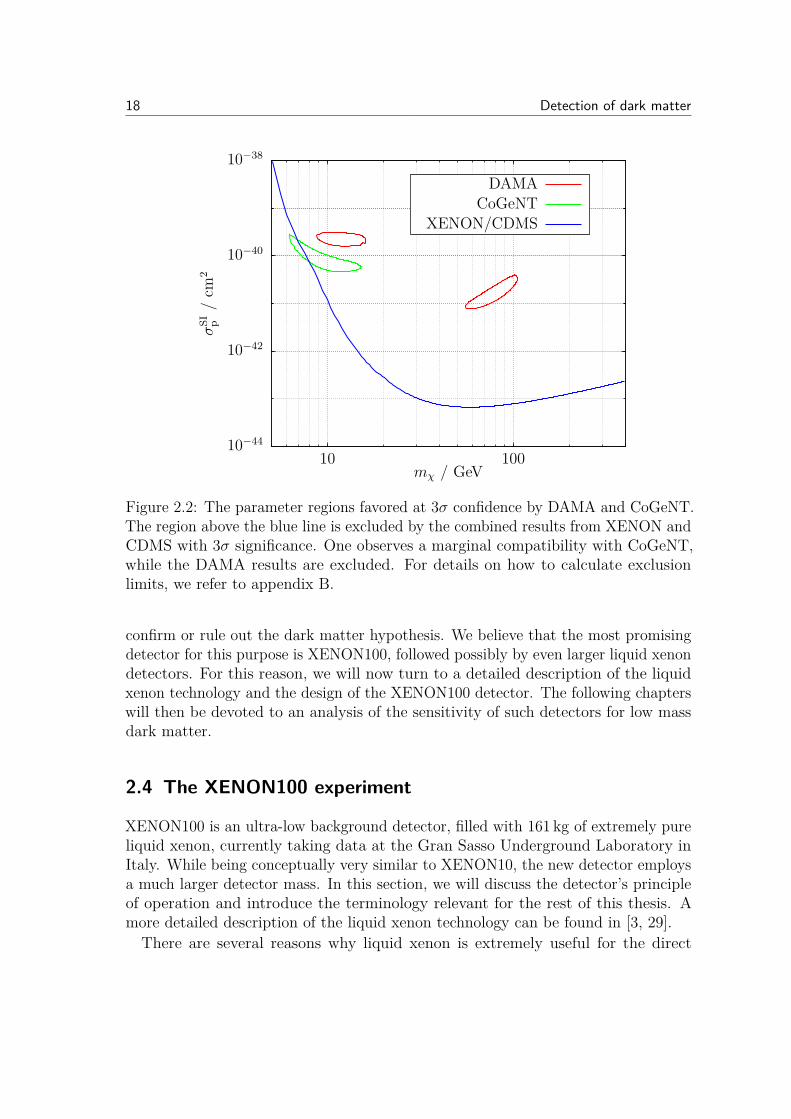
are not compatible with each other, because they favor different parameter regions.What is worse, the results are also in conflict with the data presented by CDMSand XENON. If either of the signals observed by CoGeNT or DAMA were due tostandard SI interaction of dark matter, both CDMS and XENON should most likelyhave observed a signal. The parameter regions favored by CoGeNT and DAMA andthe regions excluded by CDMS and XENON are shown in figure 2.2.It turns out that, there is a marginal compatibility between CoGeNT and the
combined data from CDMS and XENON, while a naive interpretation of the DAMAsignal in terms of SI interactions of dark matter is ruled out. Of course, one couldthink of more complicated models or try to vary the astrophysical input in order toreduce this tension. Also, a different interpretation of the experimental data mightimprove the compatibility (see for example the ongoing discussion on channeling inDAMA [27]). For an exhaustive discussion of these questions, we refer to [28].In this thesis, we do not want to take a position on the question whether the
signals observed by CoGeNT and DAMA are due to dark matter or not. The pointwe wish to make is that it is desirable to be able to check the parameter regionpreferred by CoGeNT and DAMA with a higher statistical significance in order to
18 Detection of dark matter
10−44
10−42
10−40
10−38
10 100
σSI p
/cm
2
mχ / GeV
DAMACoGeNT
XENON/CDMS
Figure 2.2: The parameter regions favored at 3σ confidence by DAMA and CoGeNT.The region above the blue line is excluded by the combined results from XENON andCDMS with 3σ significance. One observes a marginal compatibility with CoGeNT,while the DAMA results are excluded. For details on how to calculate exclusionlimits, we refer to appendix B.
confirm or rule out the dark matter hypothesis. We believe that the most promisingdetector for this purpose is XENON100, followed possibly by even larger liquid xenondetectors. For this reason, we will now turn to a detailed description of the liquidxenon technology and the design of the XENON100 detector. The following chapterswill then be devoted to an analysis of the sensitivity of such detectors for low massdark matter.
2.4 The XENON100 experiment
XENON100 is an ultra-low background detector, filled with 161 kg of extremely pureliquid xenon, currently taking data at the Gran Sasso Underground Laboratory inItaly. While being conceptually very similar to XENON10, the new detector employsa much larger detector mass. In this section, we will discuss the detector’s principleof operation and introduce the terminology relevant for the rest of this thesis. Amore detailed description of the liquid xenon technology can be found in [3, 29].There are several reasons why liquid xenon is extremely useful for the direct

2.4 The XENON100 experiment 19
]2 [cm2Radius0 50 100 150 200 250
z [c
m]
-30
-25
-20
-15
-10
-5
0
Figure 2.3: A typical distribution of backgroundevents in the liquid xenon sensitive volume.Events that are identified as nuclear recoils aremarked with a red circle. The dashed line in-dicates the 40 kg fiducial volume. Figure takenfrom [30].
Figure 2.4: A typical scatteringevent in a liquid xenon detector.Ed and Eg denote the electricfields used to drift the electronsand extract them into the gasphase, respectively. Figure cour-tesy of the XENON Collaboration.
detection of dark matter. First of all, it is an excellent scintillator and offers a highionization yield as response to energy deposition. In fact, liquid xenon has the highestscintillation and ionization yield of all liquid noble gases and moreover does not requirewave-length shifters. One can detect both light and charge simultaneously to givevery good background rejection (see below). Moreover, liquid xenon is comparablyinexpensive, so the detector can easily be scaled to larger masses. Finally, becauseof its large atomic mass (Z = 54, A = 131.3), liquid xenon benefits from the factorA2 that appears in the differential event rate for dark matter and also has a strongself-shielding, meaning a high stopping power for γ-rays.The most important property of dark matter detectors is an efficient rejection of
background. Because of the strong self-shielding of liquid xenon, most backgroundevents occur close to the surface of the sensitive volume (see figure 2.3). If we are ableto reconstruct the position of each primary event in three dimensions, we can reducethe background by employing a fiducial volume cut. For this reason, the XENON100detector is a dual-phase time projection chamber (TPC) that is monitored by twoarrays of photomultiplier tubes (PMTs).An interaction in the sensitive liquid xenon (LXe) volume leads to two distinct
signals. The first signal, called S1, results from the primary scintillation of liquidxenon at the position of the interaction. To measure the ionization signal as well,

20 Detection of dark matter
one applies a high voltage electric field that extracts the electrons into the gas phase.In the gaseous xenon (GXe) the charge cloud then produces a secondary scintillationsignal, called S2, via the proportional scintillation mechanism (see figure 2.4). Thez-position1 of the primary event can be inferred from the delay of the S2 signal dueto the drift velocity of the electrons, while the x- and y-position can be reconstructedfrom the PMT hit pattern of the S2 signal.
The S1 signal, on the other hand, is used for the reconstruction of the primary recoilenergy. For scattering events that produce a recoiling electron (such as Comptonscattering of γ-rays), the electron recoil energy is given by
Eer = S1Ly · See
. (2.15)
Here S1 is given in photoelectrons (phe) and Ly is the light yield of the detector,obtained from calibration with γ-rays. See is a quenching factor that reflects thesuppression of scintillation light in the presence of an electric field. For XENON100, itis See = 0.58 [30]. Note that Ly itself depends on Eer, so equation (2.15) can only besolved numerically. For example, Ly = 2.2 phe/keV for Eer = 122 keV (correspondingto the energy of γ-rays from the decay of 57Co).
For nuclear recoils (from neutron scattering or, in fact, dark matter interactions),the reconstruction of the energy scale is more involved. The reason is that in thiscase scintillation light is strongly suppressed due to nuclear quenching (see chapter 4).One usually defines the so-called relative scintillation efficiency, Leff , as the ratio ofthe scintillation yield for nuclear recoils and the scintillation yield for electron recoilswith an energy of 122 keV at zero electric field. We can then write
Enr = S1Leff · Ly
See
Snr, (2.16)
where Snr = 0.95 is the quenching factor for nuclear recoils in an electric field [29].The relative scintillation efficiency Leff is energy dependent, but unfortunately notvery well known. We show different measurements of Leff as well as a global fitin figure 2.5. Unless stated otherwise, we shall from now on use the lower 90%confidence contour (referred to as the conservative choice) for Leff . In chapter 4,however, we will also develop a theoretical model to predict Leff .
One must keep in mind that both Eer and Enr are reconstructed energies. Not onlydo they depend on our assumptions for the light yield and the quenching factors,but they are also affected by the energy resolution of the detector. Moreover, thereconstruction will be completely wrong if we misidentify an electron recoil as anuclear recoil or vice versa. Consequently, reconstructed energies are no more thanthe best guess for the actual recoil energy. To emphasize this fact, we will denote
1The z-axis is by convention the symmetry axis of the TPC.

2.4 The XENON100 experiment 21
]nr
Nuclear Recoil Equivalent Energy [keV1 10 100
eff
L
0
0.05
0.1
0.15
0.2
0.25
0.3
0.35 Arneodo (2000)
Bernabei (2001)
Akimov (2002)
Aprile (2005)
Chepel (2006)
Aprile (2009)
Manzur (2010)
Figure 2.5: Experimental data for the relative scintillation efficiency Leff . The thickblue line indicates the global fit, while the thin blue lines indicate the upper andlower 90% confidence contour. Dashed lines indicate possible extrapolations forEnr < 4 keV, where no measurements are available. Figure taken from [30].
reconstructed energies with keVee for electron recoils and keVnr for nuclear recoils,while reserving the unit keV for true physical recoil energies.
We have already mentioned the fiducial volume cut that is used to drasticallyreduce the background level. However, to achieve yet a stronger background rejection,the XENON100 detector employs several additional techniques. First of all, there isan active veto, composed of an additional layer of liquid xenon, which is opticallyseparated from the sensitive volume and monitored by additional PMTs. This vetoallows to effectively reduce background from external sources such as cosmic raymuons.
What remains as the dominant contribution to the background are radioactive con-taminations of the detector materials as well as intrinsic background (see chapter 5.4).Since γ-rays scatter mostly off electrons, while dark matter almost exclusively inter-acts with nuclei, we must find a way to distinguish electron recoils and nuclear recoils.For liquid xenon detectors this distinction is made by comparing the magnitude ofthe S1 and the S2 signal. Calibration data from γ-ray and neutron sources showsthat the ratio S2/S1 is much larger for electron recoils than it is for nuclear recoils(see figure 2.6).1 Consequently, we can effectively reject background from electronscattering by requiring that log10 (S2/S1) < f(S1), where the function f(S1) isreferred to as the nuclear recoil cut. This cut will be the topic of chapter 3.3.2.
Background from neutron scattering, finally, can be reduced by applying a singlescatter cut. Neutrons are likely to scatter more than once inside the sensitive volume,
1This surprising observation is believed to be due to the different track structure for nuclearrecoils, leading to different recombination rates.

22 Detection of dark matter
]nr
Nuclear Recoil Equivalent Energy [keV0 5 10 15 20 25 30 35 40
(S2/
S1)
10lo
g
1.2
1.4
1.6
1.82
2.2
2.4
2.6
2.8
30 5 10 15 20 25 30 35 40
(S2/
S1)
10lo
g
1.2
1.4
1.6
1.82
2.2
2.4
2.6
2.8
3
Figure 2.6: Electronic (top) and nuclear (bottom) recoil bands. The data pointsare from 60Co and AmBe calibration, respectively. For the x-axis, the S1 signal hasbeen converted to nuclear recoil energy, using equation (2.16). The blue and redlines correspond to the median of the electronic and nuclear recoil band, respectively.The vertical dashed lines indicate the S1 search window 4 phe ≤ S1 ≤ 20 phe, whilethe long dashed line shows the S2 threshold S2 > 300 phe. Figure taken from [30].
while dark matter particles will never have more than one interaction. Thus, we caneffectively reject neutrons by requiring that we observe only one S2 signal above agiven threshold. We will discuss this cut again in chapters 3.3.1 and 5.4.
Unless the XENON100 detector actually observes a significant number of nuclearrecoil events in the search region 4 ≤ S1 ≤ 20, it will strongly improve the exclusionlimits for SI interactions. In fact, at mχ ≈ 50 GeV, XENON100 will be sensitive tocross sections as low as σSI
p ≈ 2 · 10−45 cm2. The sensitivity of the experiment formχ ≤ 10 GeV, however, is highly controversial (see for example [31]). It depends onmany factors such as the detector resolution, the cut acceptance and the effectivescintillation yield. In the following chapters, we will examine each of these problemsand demonstrate that liquid xenon detectors are indeed capable of checking theparameter region preferred by CoGeNT and DAMA.
CHAPTER 3Detector performance at low energies
In the following two chapters we will discuss the performance of liquid xenon detectorsfor low energy nuclear recoils, meaning Enr ≈ 1− 10 keV. For any dark matter directdetection experiment a high sensitivity at these energies is very important. Thereason is that the dark matter spectrum decreases exponentially with increasingrecoil energy, so the expected total event rate in a detector will increase significantlyif the low energy sensitivity can be improved. If the dark matter particle is heavy,the recoil spectrum decreases only slowly with energy (see figure 2.1), so a loweracceptance can still be compensated by a larger exposure. For light dark matter,however, all events occur at very low recoil energies, so an insufficient sensitivity inthis region will render the detector essentially blind for such particles.As we have mentioned in chapter 2, there have recently been some experimental
indications that dark matter might be lighter than generally expected, possibly oforder 10 GeV. Clearly, one would like to probe this parameter region with liquid xenondetectors in order to confirm or exclude these observations. However, to illustratethe difficulty related to this task, we can make a simple estimate of the maximumrecoil energy that such a light dark matter particle would deposit in the detector.Using equation (2.14) and substituting mχ = 10 GeV, we get Emax
nr ≈ 11 keV.The XENON100 experiment employs a threshold of S1 ≥ 4 phe, corresponding
to an energy threshold of roughly 10 keVnr (see figure 2.6). From the calculationabove, we would naively draw the conclusion that the XENON100 experiment —and all upcoming liquid xenon experiments with a similar threshold — are almostcompletely insensitive to dark matter particles with mχ < 10 GeV. Fortunately, wehave neglected a very important property of liquid xenon detectors: the detectorresolution. At recoil energies where only few photoelectrons are observed, we mustexpect large relative fluctuations in the S1 signal. Because of such fluctuations, anuclear recoil that would on average produce only two or three photoelectrons has asignificant probability to pass the S1 ≥ 4 phe threshold. The detector resolution isconsequently very important for the low energy sensitivity of liquid xenon detectors.Clearly, to calculate exclusion bounds from the XENON experiment, we need to
quantify the probability distribution of S1 signals for a given recoil energy. We will

24 Detector performance at low energies
discuss the relevant statistics and propose a model to describe these fluctuations insection 3.1, also discussing the fluctuations of the S2 signal. In section 3.2 we willpropose a method to test this model using Monte Carlo simulations of the nuclearrecoil band. From such simulations, we can also learn a lot about the acceptance ofthe detector at low energies. Consequently, we will discuss the different cuts usedin the XENON100 experiment and try to estimate their acceptance in section 3.3.Finally, we will put all the pieces together and present an novel framework tocalculate exclusion limits in section 3.4. In this context we will also discuss, howinhomogeneities inside the detector can further increase fluctuations.
To avoid confusion, note that we are not concerned with possible improvements ofthe detector sensitivity in this chapter — our purpose is to determine the sensitivityfor a given detector. Although our discussion can be applied to a large variety ofdetectors, we will use the properties of the XENON100 detector for concreteness.A discussion of ways to improve the low energy sensitivity in future liquid xenondetectors will be left for chapter 5.
3.1 Detector resolution
3.1.1 S1 fluctuations
Writing down equation (2.16), we have pretended that there is a one-to-one relationbetween nuclear recoil energies and the produced number of S1 photoelectrons. Thefinite detector resolution, however, leads to fluctuations in the number of photoelec-trons even for a fixed recoil energy. Consequently, S1 cannot be expressed simply asa function of the nuclear recoil energy, but rather as a probability distribution withan expectation value µS1 that depends on Enr:
p(S1 = n1) = p1(n1, µS1(Enr)) . (3.1)
It should be clear from the discussion above, that in order to determine thesensitivity of a liquid xenon detector for low energy nuclear recoils, we need toknow the probability distribution p1(n1, µS1(Enr)). To determine p1, we need to lookcarefully at the detection process of scintillation light.
The idea is that the number of photons produced initially is much larger than thenumber of photoelectrons actually detected. For a nuclear recoil energy of 10 keV weexpect roughly 60 photons to be produced at the position of the scattering event(see chapter 4), but only about 4 photoelectrons will be detected.
This strong reduction comes mostly from the light collection efficiency of thedetector and the quantum efficiency of the PMTs. For XENON100, the lightcollection efficiency is LCE ≈ 0.25 meaning that only one out of four photons

3.1 Detector resolution 25
produced initially will actually hit a PMT.1 The PMTs used in XENON100, on theother hand, have a quantum efficiency of QE ≈ 0.25, meaning that only one outof four photons that hit a PMT actually produce a photoelectron. Consequently,the probability that a photon produces a photoelectron is only about 6%. Thisprobability applies independently to each photon, so the production of photoelectronsessentially corresponds to a Bernoulli trial.From these considerations, we expect the number of photoelectrons to follow
Binomial statistics, meaning that
p1(n1, µS1(Enr)) =Nph
n1
pn1(1− p)Nph−n1 , (3.2)
where Nph is the number of photons produced initially and p = QE · LCE is theprobability to produce a photoelectron. Note that Nph depends on µS1, because werequire that p ·Nph = µS1(Enr).2 For small p and large Nph the Binomial distributioncan be well approximated by the Poisson distribution, which is much more convenientfor actual calculations:
p1(n1, µS1(Enr)) = µS1(Enr)n1 e−µS1(Enr)
n1!. (3.3)
In the derivation of p1, we have not considered the production process of scintillationphotons. Nevertheless, for very small numbers of photoelectrons, the detectionprocess gives the dominant contribution to fluctuations, details of the productionprocess turn out to be subdominant. Thus, we will assume in the following, thatS1 fluctuations can be well described by a Poisson distribution. We will consider indetail subdominant contributions to S1 fluctuations in section 3.4 and show thateven the tails of the S1 distribution are well described by Poisson statistics. Inaddition, we show in section 3.2 that our assumption reproduces the shape of thenuclear recoil band with good agreement.
3.1.2 S2 fluctuations
Having discussed the statistics that describe fluctuations of the S1 signal, we nowturn to the analogous discussion for the S2 signal. In general, the S2 signal ismuch larger than the S1 signal, because every electron extracted into the gas phaseproduces about 20 photoelectrons. Consequently, the S2 signal does not limit thesensitivity of liquid xenon detectors in the low energy region. Nevertheless, we willneed a proper description of S2 fluctuations for a simulation of the nuclear recoil
1We will discuss the light collection efficiency in more detail in section 3.4 and chapter 5.2The value obtained for Nph will not necessarily be an integer. However, as Nph 1, round-
ing should not give a large error.

26 Detector performance at low energies
band, as we shall see in section 3.2.We will assume that S1 and S2 fluctuations are uncorrelated. This assumption
does not hold strictly, because one observes experimentally an anticorrelation of thetwo signals. The explanation is that the number of electron-ion pairs that recombineto produce a scintillation photon changes from event to event. However, while theanticorrelation of the two signals is large for electron recoils, it is observed to bemuch smaller for nuclear recoils, because a large fraction of the scintillation lightdoes not originate from recombination but from direct excitations (see chapter 4.3).
In contrast to the S1 signal, the S2 signal is amplified, meaning that the numberof produced photoelectrons n is much larger than the number of initially producedelectrons Nq. Consequently, the fluctuations in the production process, whichwe could neglect for the S1 signal, will dominate the distribution of S2 signals.Unfortunately, while we understand the detection process quite well, the distributiondescribing the production of electrons is not very well known.The most reasonable assumption is that the fluctuations of Nq can again be
described by Poisson statistics:
pq(Nq, µq(Enr)) = µq(Enr)Nq e−µq(Enr)
Nq! , (3.4)
where µq(Enr) is determined from measurements of the ionization yield of liquidxenon (see figure 3.2). If each electron produces r photoelectrons in the amplificationprocess, the distribution of photoelectrons is then roughly a normal distribution withmean µS2 = rµq and standard deviation σS2 = r
√µq = √rµS2:
p2(n2, Enr) = 1√2πrµS2(Enr)
exp(−(n2 − µS2(Enr))2
2rµS2(Enr)
). (3.5)
For the XENON100 experiment, the amplification factor r has been determined fromcalibration data to equal r = 17.6 phe/e− [32].
3.2 Simulation of the nuclear recoil band
Equation (3.3) and equation (3.5) as well as the assumption that the two signalsare uncorrelated summarize our model for the distribution functions that describethe fluctuations of S1 and S2 signals. To test our model and check the underlyingassumptions, we would like to make predictions that can be compared to experimentaldata. What we want to predict is the shape of the nuclear recoil band, which can bedetermined experimentally from calibration with AmBe (see figure 2.6).Monte Carlo simulations of the nuclear recoil band are a difficult task, because
we must be careful to precisely reproduce the experimental conditions. First of all,we need to know the energy spectrum of neutron recoils expected for calibration

3.2 Simulation of the nuclear recoil band 27
/ keVnrE0 5 10 15 20 25 30 35 40 45 50
Eve
nts
210
310
410
Figure 3.1: The neutron recoil energy spectrum for single scatters obtained fromGeant4 simulations of the XENON100 detector.
with AmBe. Such an energy spectrum can be extracted from the Geant4 simulationsperformed by the XENON100 collaboration (see figure 3.1).1 From these simulations,we can also obtain additional information for each event, for example the number ofenergy deposition steps and the position of each scattering process.2
To reproduce actual signals in the detector, we must convert the energy spectruminto S1 and S2 signals. First, we calculate the expectation values µS1 and µS2 usingthe best-fit choice for Leff from figure 2.5 and the ionization yield measured byManzur et al. [33] (see figure 3.2). Then, we randomly generate S1 and S2 signalsaccording to the respective distribution functions. An additional Gaussian smearingwith σ = 1 is applied to both signals to account for the finite PMT resolution.
Next, we need to make sure that we correctly treat the time and position resolutionof the detector. In an event with more than one scattering process, the detectorcannot distinguish the different S1 signals, because it cannot resolve the time betweentwo scattering processes. Consequently, to compare simulated signals to experimentalones, we must add up all S1 signals occurring in one event, carefully taking intoaccount the position dependence of the light collection efficiency. On the other hand,the S2 signals can be distinguished if the z-position is separated by at least 3 mm,so we add up S2 signals only for neutron recoils that occur very close to each other.As it is done in the analysis of the experimental data, if there remains more thanone S2 signal, we keep only the largest one.3
1The relevant data files were kindly provided by Alexander Kish.2Note that the term “event” refers to the propagation of one neutron through the detector.
Consequently one event may comprise more than one scattering process.3In the experimental analysis, events with more than one S2 signal are usually removed by the
single scatter cut (see section 3.3.2). However, we do not impose such a cut because we do not

28 Detector performance at low energies
2 5 10 20 50 100
2
5
10
20
Energy / keVnr
Ionizationyield/e-keVnr-1
Figure 3.2: The adapted fit for the ionization yield Qy in electrons produced pernuclear recoil energy (violet line). The data points are taken from [33]. Note thatmost measurements have been performed at stronger electric field than the oneemployed by XENON100 (E = 0.5 kV/cm).
In the next step, we need to make sure that we include only events in our simulationthat would also be recorded during a calibration run. We require that the largestS2 signal must be greater than 300 phe and lie inside the 40 kg fiducial volume (seefigure 2.3). Note that we do not impose any restrictions on the magnitude of theS1-signal, so we include events with S1 < 4 phe. In this region, the acceptance of thedetector is expected to be pretty low (because the signal can hardly be distinguishedfrom noise), but this problem should not affect the shape of the nuclear recoil band.We will come back to the discussion of the acceptance in section 3.3.
For all simulated events we plot log10 (S2/S1) versus S1. We take the logarithmbecause for normally distributed S1 and S2, the quotient S2/S1 is similar to a log-normal distribution, so log10 (S2/S1) should be approximately normally distributed.Therefore, we can use the median and the upper and lower 15.87% and 2.27%quantiles to approximate the mean and the 1σ and 2σ region of the nuclear recoilband for each S1 bin. The resulting plot is shown in figure 3.3. We indeed obtaingood agreement with experimental data in the absolute position of the nuclear recoilband, which is essentially determined by our choice of the scintillation yield and theionization yield, and the width of the band, which is essentially determined by ourassumptions on the distribution of S1 and S2 signals.
Only at large values of S1, we observe a deviation between the experimental andthe simulated nuclear recoil band. The most likely explanation is that we havechosen slightly too small values for Qy. Also note that the 2σ region of the nuclear
want to reduce the number of events without necessity.

3.3 Cut acceptances 29
Figure 3.3: A Monte Carlo simulation of the nuclear recoil band. The yellow solidline corresponds to the median value, the green and blue solid lines indicate the 1σand 2σ region respectively (more precisely, the upper and lower 15.87% and 2.27%quantiles). The dashed lines show the corresponding values for experimental data.
recoil band is somewhat broader in the experimental data than in the simulation.The reason is that one observes experimentally a small number of anomalous eventsleading to non-Gaussian tails in the nuclear recoil band that broaden the 2σ region.The most likely explanation for these events is that they happen close to the surfaceof the detector and suffer from incomplete collection of photons and electrons.The simulated nuclear recoil band would look quite different had we taken the
conservative choice of Leff instead of the best-fit one. This observation is a first hintthat the relative scintillation efficiency does not decrease at very low recoil energiesbut rather remains constant. We will come back to this question in the next chapter,but we will stick to the conservative choice for Leff in this chapter nevertheless togive a conservative estimate of the detector sensitivity. The central information thatwe wanted to obtain from the simulation of the nuclear recoil band is that indeedour model for the distribution functions of S1 and S2 signals is very accurate.
3.3 Cut acceptances
As we have pointed out in section 3.2, not every scattering process with sufficientlylarge S1 and S2 signals will indeed be accepted as a valid event. The reason isthat we must require every signal to fulfill certain conditions in order to ensure dataquality and reject noise. For example, to prevent signals from PMT dark counts, werequire a two-fold coincidence for every S1 signal, meaning that we accept an eventonly if two PMTs observe an S1 signal simultaneously. While such a cut is necessary

30 Detector performance at low energies
S1 / phe0 5 10 15 20 25
Cou
nts
0
5000
10000
15000
20000
25000 Simulated S1 spectrum
Experimental S1 spectrum
Figure 3.4: Comparison of the S1 spectra obtained from the projection of the nuclearrecoil band on the x-axis. The red histogram shows the results from Monte Carlosimulations, while the blue histogram shows the corresponding S1 spectrum fromcalibration data. We have chosen the normalization in such a way that the twospectra agree approximately for large values of S1.
to obtain meaningful data, there is a certain risk that it also removes valid events.We define the acceptance of a cut as the probability that the cut accepts a valid
event and the efficiency of a cut as the probability that it rejects an invalid event.Clearly, we can increase the efficiency of a cut by making the cut more stringent,but doing so will reduce its acceptance and vice versa. In general, the acceptancewill be a function of S1, which we denote by acut(S1). If acut(S1) is very small atsmall S1, the sensitivity of the detector in the low energy region will be reduced.
Problems with noise and data quality are not present in Monte Carlo simulations.We can therefore use the simulations discussed in section 3.2 to determine thecut acceptance of the detector. For this purpose, we want to make a quantitativecomparison of experimental and simulated data rather than a qualitative one as infigure 3.3. To do so, we project the nuclear recoil band on the x-axis and calculatethe number of events in each S1 bin (called the S1 spectrum).Figure 3.4 shows the S1 spectra for calibration data and the data obtained from
Monte Carlo simulations. The relative scale of the two spectra is arbitrary andhas been chosen in such a way that the two spectra match approximately for largeS1. We can see that both spectra show a similar behavior, with a maximum atabout S1 = 3 phe. The decrease for larger values of S1 results from the exponentialdecrease of the neutron recoil spectrum (see figure 3.1). The decrease for smallervalues of S1, on the other hand, does not have a physical reason, but is due to thecuts that we apply to the data.
The key observation is that the two spectra agree quite well at large energies, but

3.3 Cut acceptances 31
Figure 3.5: Determination of the cut acceptance acut(S1) from Monte Carlo sim-ulations. The histogram is calculated by dividing the experimental S1 spectrumshown in figure 3.4 by the simulated one. The blue line indicates the publishedresults for the acceptance function from reference [30]. Note that the normalizationof the histogram is arbitrary, so we have chosen it in such a way that acut = 0.9 forS1 = 20 phe.
begin to deviate as S1 decreases below 10 phe. This deviation is the result of the cutacceptance of the detector. For the Monte Carlo simulation, the only relevant cutis the requirement S2 > 300. For the experimental data, the number of S1 signalsis reduced further by the acceptance of the data quality cuts. We can quantifythe acceptance function acut by dividing the S1 spectrum from calibration data bythe simulated spectrum. Again, since we do not know the relative scale of the twospectra, we cannot determine the normalization of the acceptance function.
We present our result for the acceptance function in figure 3.5. The normalizationhas been chosen arbitrarily so that acut = 0.9 at S1 = 20 phe. For comparison,we also plot the acceptance function that has been published together with thefirst results of the XENON100 experiment [30]. The two functions indeed agreeremarkably well. Only in the region above S1 = 20 phe, we observe that the ratio ofexperimental S1 signals and simulated S1 signals continues to increase, althoughwe would expect the acceptance function to be more or less constant. This increasecould either point to shortcomings of the neutron energy spectrum that we takefrom Geant4 simulations, or to the presence of anomalous events in the calibrationdata. In fact, the non-Gaussian tails that we have observed already in figure 3.3,may also account for the slower decrease of the experimental S1 spectrum towardslarger recoil energies. Because we are only interested in the region 4 ≤ S1 ≤ 20, wewill use the published values for acut for all calculations in the following.
So far, we have only considered the cuts that are needed to reject noise and ensure

32 Detector performance at low energies
data quality. However, for the dark matter search we must apply two additional cutsin order to reject background from neutrons and γ-rays (see chapter 2.4). These cutsare the single scatter cut, which is used to identify and remove neutrons, and thenuclear recoil cut, which distinguishes between electron recoils and nuclear recoils inorder to reject background from γ-rays. However, the acceptance for these two cutsis difficult to determine and presently unknown. In the remainder of this section, wewill discuss the related difficulties.
3.3.1 Single scatter cut
Neutrons typically scatter more than once inside the active volume. We can thereforeeffectively remove background from neutrons by requiring that there should be onlyone S2 peak in a valid event. Unfortunately, it turns out that even valid single scatterevents sometimes have more than one S2 peak due to noise or delayed electrons.Removing all events with more than one S2 peak would therefore dramatically reducethe cut acceptance for valid single scatter events.To maintain a high acceptance for single scatters, one usually relaxes the single
scatter cut and removes only those events that have a second S2 peak above 300 phe.Of course, doing so will also reduce the rejection efficiency for multiple scatters. Inconsequence, we must expect a larger number of background events. Moreover, whatis even worse, if we cannot efficiently reject multiple scatters, the nuclear recoil bandfrom AmBe calibration will be distorted. The reason is that we cannot distinguish thedifferent S1 signals of multiple scatters but measure only their sum (see section 3.2).Thus, if we cannot reject all multiple scatters, we will get a number of events thathave a large S1 signal compared to their S2 signal. For these events log10(S2/S1)will be comparably small, so the nuclear recoil band for multiple scatters lies belowthe nuclear recoil band for single scatters (see figure 3.6).This effect would not be a problem if the number of single scatters were much
larger than the number of multiple scatters that are not rejected. Unfortunately,because of the exponentially falling neutron spectrum (see figure 3.1), we must expectlarge numbers of multiple scatters with only one S2 peak above 300 phe. In fact, weobtain from Monte Carlo simulations, that the number of multiple scatter events,which pass the relaxed single scatter cut, is almost as big as the number of true singlescatters (in figure 3.6, there are 8.0 · 104 multiple scatters compared to 9.1 · 104 singlescatters). Consequently, the contribution of multiple scatters will effect a significantdistortion of the nuclear recoil band.This distortion is a serious problem because it means that we cannot easily infer
the nuclear recoil band for true single scatter from calibration with neutrons. Tomitigate this problem, one could consider to apply a stronger single scatter cut, forexample by requiring that any additional S2 peak must be smaller than 100 phe. Forthis modified cut, multiple scatters contribute only about 20% to the total number ofevents. Moreover, scattering processes with an S2 signal below 100 phe will in most

3.3 Cut acceptances 33
Figure 3.6: A Monte Carlo simulation of the nuclear recoil band. The black dotsare true single scatters, while the red dots are multiple scatters that pass the singlescatter cut (only one S2 signal above 300 phe). Solid lines indicate the median(yellow), as well as the 1σ (green) and 2σ (blue) region for true single scatters. Thedashed lines show the corresponding values for multiple scatter events.
cases give only a negligible contribution to the sum of S1 signals. Consequently, wecan hope for a much smaller distortion of the nuclear recoil band. At the same time,however, the modification reduces the acceptance of the single scatter cut, whichwill affect the sensitivity of the detector.
To understand the acceptance and the rejection efficiency of the single scattercut and determine the nuclear recoil band for true single scatters is certainly oneof the most important open problems for the data analysis of XENON100. As it isnot yet clear, which single scatter cut the XENON collaboration will decide to use,we cannot at this point determine the corresponding acceptance function. We willassume in the following, however, that the acceptance of the single scatter cut doesnot limit the sensitivity of XENON100 in the low energy region.
3.3.2 Nuclear recoil cut
We can discriminate electron recoils and nuclear recoils, because for comparable S1signals the former have much larger S2 signals. Consequently, to reject electronrecoils, we discard all events that have a large ratio of S2/S1. To achieve a sufficientlyhigh rejection efficiency,1 one in fact removes all events that lie above the medianof the nuclear recoil band (the yellow line in figure 3.3). By construction, this cutwill also remove 50% of all nuclear recoils and consequently reduce dramatically the
1As we shall see in chapter 5, the rejection efficiency must be 99% or better.

34 Detector performance at low energies
(a) µS1 = 10 and µS2 = 1400 (b) µS1 = 3 and µS2 = 500
Figure 3.7: Distribution of events in the log10 (S2/S1) versus S1 plane for fixedexpectation values of S1 and S2. The red line indicates the nuclear recoil cut.The green shaded area corresponds to the acceptance region after the requirement4 ≤ S1 ≤ 20 and the nuclear recoil cut have been applied.
acceptance of the detector.Naively, we could try to include this cut by simply multiplying the cut acceptance
from figure 3.5 with 0.5. However, at this point we encounter a very fundamentalproblem related to the determination of cut acceptances. As Sorensen first pointedout in [34], if we apply several cuts to our data set, the acceptance probabilitiesof the different cuts may not be independent, so we cannot simply multiply them.To make this statement more precise, we shall rephrase it in mathematical terms.If p(c1) is the probability that an event passes cut 1 and p(c2) is the probabilitythat this event passes cut 2, then we can express the probability that is passes bothcuts as p(c1 ∧ c2) = p(c2|c1) · p(c1), where p(c2|c1) is the conditional probabilitythat the event passes cut 2 if it has already passed cut 1. Consequently, the naivemultiplication of cut acceptances, such as p(c1∧ c2) = p(c2) · p(c1), will only be validif p(c2|c1) = p(c2). In the following, we will give a simple example for two cuts, whichare not independent, so that p(c2|c1) 6= p(c2). Therefore, a simple multiplication ofcut acceptances will not do in this case.1The cuts that we want to consider are the nuclear recoil cut (nr cut) and the
requirement 4 ≤ S1 ≤ 20. In the following, we want to demonstrate that
anr ≡ p(nr cut|4 ≤ S1 ≤ 20) 6= p(nr cut) = 0.5 . (3.6)
To understand why these two cuts are not independent, remember that, because ofthe poor energy resolution of the detector, nuclear recoils with a fixed energy will
1In fact, this problem occurs whenever a cut depends not only on S1, but also on S2.

3.3 Cut acceptances 35
scatter widely in the log10 (S2/S1) versus S1 plane. As an example, we show infigure 3.7a a large number of events that have been generated using the distributionsfrom section 3.1 with µS1 = 10 and µS2 = 1400. If we only consider events inside theS1 search window, we observe that some of them fall above and others below thenuclear recoil cut. In this case, the nuclear recoil cut effectively reduces the numberof accepted events, so anr < 1.
However, if we now make the same plot for the choices µS1 = 3 and µS2 = 500, weget a somewhat different picture (see figure 3.7b). Almost all events that pass theS1 ≥ 4 requirement, automatically pass the nuclear recoil cut as well. The reasonis obvious: The events that we have simulated here produce on average less than 4photoelectrons. If 4 or more photoelectrons are produced due to fluctuations, the S1signal will be large compared to the S2 signal (remember that we assume S1 and S2fluctuations to be independent). Consequently, such an event will have a low value oflog10 (S2/S1). In this case, the nuclear recoil cut is almost without effect - all recoilswith large value of log10 (S2/S1) are already removed by the S1 cut. Consequently,in this case anr ≈ 1.
For this reason, the nuclear recoil cut acceptance depends on the recoil energy andcan in fact be much larger than 50% towards lower energies. In order to properlycalculate the cut acceptance, we must take into account the probability distributionsfor S1 and S2 signals. If we define a function f(S1) to parameterize the nuclearrecoil cut, meaning that we require log10 (S2/S1) < f(S1), we can translate thisinequality into
S2 < S1 · 10f(S1) ≡ g(S1) . (3.7)
Using p(c2|c1) = p(c1 ∧ c2)/p(c1), the nuclear recoil cut acceptance anr(Enr) isgiven by:
anr(Enr) =
20∑n1=4
p1(n1, µS1(Enr)) ·g(n1)∑n2=300
p2(n2, µS2(Enr))20∑
n1=4p1(n1, µS1(Enr))
. (3.8)
Again, we cannot presently calculate anr(Enr), because the nuclear recoil bandfor single scatters and therefore g(S1) has not yet been extracted from calibrationdata (see the discussion in the previous section). Until the cuts have been finalizedand we have a proper description of the nuclear recoil band, we must use the simpleapproximation that the nuclear recoil cut acceptance is 50% for all recoil energies.Since we expect that anr(Enr) > 0.5 at low recoil energies, taking anr = 0.5 everywhereshould give a conservative estimate of the acceptance in this region. On the otherhand, a constant nuclear recoil cut acceptance will overestimate the acceptance forhigh recoil energies, but here only few events are expected anyways.

36 Detector performance at low energies
3.4 The total acceptance function
In this section, we will put all the pieces together and introduce a convenientframework to discuss the sensitivity of liquid xenon detectors. The idea is to splitthe calculation of exclusion limits into two parts: The first part contains everythingrelated to the performance of the detector and the second part contains the actualphysics of dark matter. In fact, all relevant detector properties can be summarizedin one simple function which we will call the total acceptance function A(Enr). For agiven nuclear recoil energy Enr, A(Enr) gives the probability that a nuclear recoilwith this energy leads to a signal within the search window (meaning within agiven range of photoelectrons). Multiplying the total acceptance function with thedifferential WIMP spectrum dR/ dEnr then gives the actual differential event ratein the detector (see also appendix B).The question is how to obtain A(Enr). Neglecting fluctuations, we could simply
convert Enr into photoelectrons by inverting equation (2.16). The function A(Enr)would then equal 1 if S1(Enr) lies within the search window, S1min ≤ S1 ≤ S1max,and 0 otherwise. However, in section 3.3, we have seen that the acceptance ofthe detector is smaller than 1 even inside the search window because of the cutsthat we apply to ensure data quality and reject background (acut from figure 3.5).Consequently, A(Enr) = acut(S1(Enr)) if S1(Enr) lies within the search window and0 otherwise (see the green line in figure 3.8).Because of fluctuations, as discussed in section 3.1, we cannot express S1 as a
function of the nuclear recoil energy. Consequently, we must use the probabilitydistribution from equation (3.3) to calculate A(Enr):
A(Enr) =S1max∑
n1=S1min
p1(n1, µS1(Enr)) · acut(n1) . (3.9)
As a result, there will be a smearing of the total acceptance function: Recoil energiesthat would be rejected in the absence of fluctuations have a non-zero chance toproduce a sufficient number of photoelectrons. At the same time, events inside theacceptance window will — with a certain chance — produce too few or too manyphotoelectrons to give a detectable signal. The result of this smearing is indicatedby the blue line in figure 3.8. As expected, the inclusion of fluctuations leads to adramatic increase of the acceptance for events with a low recoil energy. For recoilenergies just slightly below the threshold, acceptance is indeed larger than 30% andeven at a recoil energy of 5 keV, the acceptance is still about 1%.Considering that we will multiply the total acceptance function A(Enr) with an
exponentially decreasing dark matter spectrum, the precise form of the acceptancefunction at very low energies will be extremely important. One could be worried, thathere our approximation of Poisson statistics will break down. It is therefore advisableto calculate A(Enr) for both, a Poisson distribution and a Binomial distribution of

3.4 The total acceptance function 37
Figure 3.8: The total acceptance function A(Enr). The green (dashed) line corre-sponds to the total acceptance function neglecting fluctuations. The red (solid) lineand the blue (dotted) line correspond to fluctuations described by Binomial andPoisson statistics respectively.
S1 signals, to see whether the two agree and our approximation is actually valid.In order to calculate A(Enr), we will use Monte Carlo simulations.1 For a given
recoil energy, we calculate µ(Enr) using the conservative choice of Leff shown infigure 2.5, and calculate Nph = µ(Enr)/(QE · LCE) with LCE = QE = 0.25. Nowwe use Binomial statistics (with probability LCE) to randomly determine the numberof photons that hit a PMT and again Binomial statistics (with probability QE) todetermine the number of photoelectrons produced. Repeating this process for avery large number of events will give the probability distribution for the number ofphotoelectrons produced by a nuclear recoil with energy Enr. We can then substitutethis distribution for p1 into equation (3.9) to calculate A(Enr).The result of this calculation is shown as the red line in figure 3.8. A compari-
son between the results obtained from assuming Poisson statistics and the MonteCarlo simulation based on Binomial statistics reveal that indeed Poisson statisticsapproximate the Binomial distribution very well.
To conclude this chapter, we will turn to a discussion of additional contributionsto S1 fluctuations that may further reduce the resolution of the detector and thusimprove the detector sensitivity. However, it will turn out that we have alreadycaptured the main contribution to fluctuations and all additional effects will giveonly minor, in fact negligible, corrections. In this context, the framework of anacceptance function will be very convenient, because A(Enr) can be understoodmuch more intuitively than an exclusion plot. Moreover, the large disadvantage ofexclusion plots is, that they depend on various parameters from particle physics and
1The calculations presented here could be done analytically as well. However, when we wantto include the light collection efficiency, Monte Carlo simulations will be necessary.

38 Detector performance at low energies
astrophysics and consequently are much harder to reproduce and compare.A possible contribution to S1 fluctuations could come from the production mecha-
nism of scintillation photons. So far, we have assumed that Nph is fixed for a givenrecoil energy, but of course the emission of scintillation light is also a statisticalprocess, so we should expect a varying number of photons even for fixed recoil energy.Again, Poisson statistics are appropriate to describe the production process.1 Fromthe discussion above, we know that Nph ≈ 16n, so
∆Nph
Nph= 1√
Nph≈ 1
4√n
= 14∆n
n. (3.10)
The fluctuations that occur in the production process are a factor of 4 smaller thanthe fluctuations in the detection process. We therefore expect that only the detectionprocess is relevant for the detector resolution. We can easily confirm this expectationby extending the Monte Carlo simulations from above to include fluctuations of theinitial number of photons in an additional step (see figure 3.9a).Another possible contribution to fluctuations is more difficult to treat. So far we
have considered the detector to be homogeneous so that we could neglect the positionof the primary event. However, in a more realistic description, the light collectionefficiency (LCE) will depend on the position of the primary event: Events close tothe PMT arrays will have a larger LCE than those in the center of the detector (seechapter 5.2 and figure 5.3). This inhomogeneity effects a variation of the number ofproduced photoelectrons even in the absence of other statistical processes.Again, Monte Carlo simulations allow to quickly estimate the magnitude of this
effect. This time the position of each event is set randomly within the 40 kg fiducialvolume from figure 2.3. The actual light collection efficiency for each position isthen taken from calibration data of the detector [32]. We can see in figure 3.9b thatat low energies, the total acceptance function is still completely dominated by thePoisson fluctuations of the detection process and including LCE variations givesalmost no improvement. Nevertheless, the sensitivity above the upper thresholdimproves significantly by including LCE variations.This result is intuitively clear, because ∆LCE/LCE is a detector property and
independent of the recoil energy, so the variation of the light collection efficiencywill only be important if ∆n/n is sufficiently small. However, since only few eventsare expected at high recoil energies, exclusion limits will not change significantlyby including the variation of light collection efficiency. At best, including LCEvariations may slightly improve the sensitivity for heavy dark matter.
1In principle the width of the distribution could be modified by a Fano factor. If this factoris much smaller than one, we can certainly neglect fluctuations of Nph. Consequently, we assumehere that the Fano factor is approximately equal to one.

3.5 Summary of results 39
(a) Varying photon number (b) Varying light collection efficiency
Figure 3.9: The total acceptance function A(Enr). Again, the green (dashed) linecorresponds to the total acceptance function neglecting fluctuations and the blue(dotted) line corresponds to fluctuations described by Poisson statistics. The red(solid) line includes different subdominant contributions to the fluctuations of the S1signal. As expected, no significant improvement of the total acceptance function isobtained in the low energy region.
3.5 Summary of results
In this chapter, we have provided good arguments that Poisson statistics are appro-priate to describe S1 fluctuations, while an additional amplification factor r must beincluded to describe the fluctuations of the S2 signal. A more detailed description ofthe various processes involved in the production and detection of scintillation lightdo not change this conclusion significantly. We have checked our model using MonteCarlo simulations, which do not only confirm our assumptions, but also allow todetermine the acceptance of the detector for low energy recoils. We obtain that theacceptance of the data quality cuts is greater than 60% for S1 ≥ 4 phe, in agreementwith previously published results.
In conclusion, liquid xenon detectors possess a significant sensitivity even in theenergy region that is naively below the lower threshold of the detector. Of course,all our calculations in this chapter rely on the assumption that indeed a sufficientamount of scintillation light is produced even at very low recoil energies. The criticalreview of this assumption will be the topic of the following chapter. Once we haveobtained a prediction for the effective scintillation yield at low recoil energies, wecan use the results from this chapter to calculate the expected sensitivity for theXENON100 experiment (see chapter 4.5).

CHAPTER 4The effective scintillation yield of liquid xenon
In this chapter we will discuss the effective scintillation yield for liquid xenon, aquantity that is both essential for calculating exclusion limits and highly controversial.At least, we know that scintillation light is strongly suppressed for nuclear recoilscompared to electron recoils. The reason is that a recoiling nucleus can effectivelyloose its energy through elastic collisions with other nuclei in the detector. Most ofthe initial recoil energy is thus transferred, eventually, to heat. Recoiling electrons,in contrast, cannot transfer any significant amount of their energy to nuclei becauseof the huge difference in mass. They will transfer all their energy into electronicexcitations, and thus produce a larger amount of scintillation light.Conventionally, the effective scintillation yield of nuclear recoils is described by
the dimensionless quantity Leff , called relative scintillation efficiency. It relates theS1 scintillation signal to the physical recoil energy of the nucleus Enr as
Enr = S1Ly · Leff
· See
Snr. (4.1)
Ly is the light yield for 122 keV electron recoils in the presence of an electric fieldand See,nr are the electric field quenching factors for electronic and nuclear recoils(see chapter 2.4). Thus, Leff quantifies the suppression of scintillation for nuclearrecoils compared to 122 keV electron recoils at zero electric field.It is generally agreed that the relative scintillation efficiency will depend on the
nuclear recoil energy. How this dependence should look like is presently unclearfrom both experimental and theoretical point of view. Many measurements ofthe relative scintillation efficiency have been carried out, giving a wide range of(partly contradictory) results (see [33, 35–41] as well as figure 2.5). However, mostmeasurements imply at least a slight decrease of the relative scintillation efficiencywith decreasing energy.
On the theoretical side the problem is to understand the production of scintillationlight for a slow moving xenon atom. This problem can be roughly divided intothree parts. First we need to know the ionization and excitation probabilities forindividual collisions of xenon atoms. Then we must simulate the propagation of

4.1 Production of scintillation light in liquid xenon 41
recoiling atoms to determine the total amount of electronic excitations, and finallywe must understand the recombination rate for the produced free electrons and ions.At the end, a theoretical treatment of the problem should produce predictions forboth the scintillation and the ionization signals produced in the detector.
In section 4.1 we review the process of generation of scintillation light and ionizationin liquid xenon. We introduce the notion of the nuclear and electronic stoppingpowers in section 4.2 in order to perform an analysis of individual xenon scatteringevents. From the results we calculate the total energy in the electronic excitations.In section 4.3, we then analyze the recombination process. In section 4.4 all theresults are collected and translated into the ionization and scintillation yields andcompared with the experimental data.
4.1 Production of scintillation light in liquid xenon
A large variety of effects must be taken into account to describe all physical processesthat lead from the initial recoil to the production of scintillation light in liquid xenon.Specifically, we expect the following steps [42]:
• In an interaction with a dark matter particle, an energy of 1–100 keV istransferred to the nucleus. As the corresponding recoil velocity is well belowthe Fermi velocity of the most loosely bound electrons, we expect the atom toremain neutral in the scattering process.
• The recoiling atom will scatter off neighboring nuclei. While most scatteringevents are expected to be elastic, there will occasionally be inelastic collisionsleading to excitation or ionization of either (or both) of the atoms.
• After each scattering process, both atoms will continue their propagation witha fraction of the initial recoil energy. Consequently, both can again scatterelastically or inelastically off other atoms.
• During the process of thermalization, the recoiling xenon atoms will leavebehind a large number of ionized or excited xenon atoms — distributed alongmany branches of the initial track.
• The free electrons will now either recombine with surrounding ions to formexcited xenon atoms or escape from recombination. The fraction of escapingelectrons will depend on the strength of the applied electric drift field, butsome electrons will escape even in the absence of a field.
• Excited xenon atoms are free initially, but will soon be self-trapped and formexcimers. These excimers emit vuv scintillation light on the transition to the

42 The effective scintillation yield of liquid xenon
ground state. In a simplified picture, the process is
Xe∗ + Xe→ Xe∗2 (4.2)Xe∗2 → 2Xe + hν (4.3)
• In some cases, especially at high excitation density, two exited xenon atomswill combine to produce only one scintillation photon. This process, known asbiexcitonic quenching, will effectively reduce the scintillation yield.
At first sight, the large number of steps makes it very hard to disentangle possibleambiguities. A decrease of scintillation efficiency at low recoil energies could beequally attributed to a decreasing cross section for inelastic scattering (for exampledue to threshold effects), a different track structure, an increasing fraction of escapingelectrons or a stronger quenching mechanism. This ambiguity can be lifted at leastpartially by considering not only the relative scintillation efficiency of nuclear recoils,but also the ionization yield. This quantity is much better determined experimentally(because free electrons can be extracted with high efficiency and the signal can bestrongly amplified in the gas phase), but has been — to the best of our knowledge —ignored in all previous attempts to give a theoretical model for the scattering processesin liquid xenon.The sum of ionization and scintillation, which we will refer to as the total elec-
tronic excitation, should correspond to the total energy lost in inelastic collisions.Consequently, it should only depend on the scattering cross sections and not onthe processes occurring later, such as recombination, which will only lead to aredistribution between ionization and scintillation. Thus, if both signals showeda similar energy dependence, this would suggest a general suppression of inelasticscattering at low energies — which is what one might naively expect. However, whatis actually observed experimentally, is a strong increase of the ionization yield at lowenergies. This observation indicates that the suppression of the scintillation signal atlow energies does not result from the actual inelastic scattering processes, but fromthe large number of escaping electrons.
4.2 Stopping powers of liquid xenon
In this section we will describe the interactions of neutral xenon atoms and discusspossible scattering processes at energies of a few keV. The quantities we are interestedin are the rate at which energy is transferred to recoiling nuclei by elastic collisionsand the rate at which electrons are excited by inelastic collisions. These quantitiesare often called nuclear stopping power and electronic stopping power.

4.2 Stopping powers of liquid xenon 43
4.2.1 Electronic stopping power
The electronic stopping power is defined as the average energy which an atom losesto electronic excitations per distance traveled through the detector:
Se = dEdx . (4.4)
In a “semiclassical” approach, an electron is excited when it collides with a nucleus.1The stopping power should therefore be proportional to the electron mass densityn0, their velocity vF, the momentum transfer cross section σtr(vF), and the velocityof the incoming particle v. In fact, electronic stopping is often described by [43–47]
Se = n0vvFσtr(vF) . (4.5)
We should take a moment to discuss the validity of such a semiclassical approach.Equation (4.5) is in fact based on several assumptions:
• Instead of describing the atomic system by a many-particle wavefunction, weclaim that only the electron density is relevant to the problem, and we ignorethe modification of the electron density during the atomic collision.
• Collisions between electrons and nuclei are treated like classical point likeinteractions.
• Electrons are assumed to be free. Consequently, no minimal energy transfer isrequired for an excitation.
For a uniform electron gas the electronic stopping power is proportional to thevelocity of the incoming particle, a result that has been derived by Lindhard etal. [48]. The authors obtain
Se =√
8πe2a0ζ0ZN ·v
v0, (4.6)
where a0 and v0 are Bohr radius and Bohr velocity respectively and ζ0 is an empiricalparameter, often2 set to ζ0 = Z1/6. Finally, N = 13.76 nm−3 is the number densityof xenon atoms.This formula is in principle even applicable for the case of small nuclear recoil
velocities, meaning vnr < v0 (or Enr < 1 MeV). However, it is not clear that wecan assume a velocity proportional stopping power all the way down to vnr = 0.In fact, at very low velocities, departures from velocity-proportionality have been
1Note that, for the energies we are concerned with, electrons are much faster than the recoilingnucleus.
2In an independent derivation, Firsov obtained the same formula with ζ0 ≈ 1.63 [49].

44 The effective scintillation yield of liquid xenon
observed [44]. Also, there are several arguments in favor of a more rapid drop of Sefor v < v0. The two most important ones are threshold effects and Coulomb effects.
The argument for threshold effects essentially goes as follows: In an elastic collisionbetween a nucleus and a free electron, only a fraction me/mN of the nucleus energycan be transferred to the electron. For nuclei with energies in the keV range, theresulting electron energy is at most a few eV – so we can no longer ignore gap energiesor the work function of xenon. There has been a long and intense discussion onwhether such threshold effects are present or not (see for example [50]). However,many experiments and theoretical considerations report electronic excitations farbelow the naive threshold [51, 52].An effect from Coulomb repulsion is expected, because at low relative velocities
colliding nuclei will not penetrate the electron clouds of each other strongly. Con-sequently, with decreasing energy the recoiling nucleus will probe only regions oflower electron density [53]. We discuss a possible way to include this correction inappendix C, but come to the conclusion that it contradicts experimental data.Both of these arguments fail, because they continue to exploit the point-like
interaction of the nucleus with the electron. However, for low nuclear velocity theelectron cloud itself rearranges during the collision (or, in a more semiclassicallanguage, the electron makes several rotations in the combined electric field of thetwo colliding atoms). This effect leads to a much more complicated non-perturbativemechanism of the energy transfer to the electron. An analysis of such collisions wasperformed fully for the case of simple atoms [52]. The authors observe that ionizationoccurs even at energies far below the naive threshold. Lacking a similar calculationfor xenon atoms, we will continue to use equation (4.6) even for low energies.
To conclude this section, we provide dimensionless quantities instead of Se, whichare usually preferred in the literature. Therefore, we define
ε = a
2e2Z2E , (4.7)
ρ = Nπa2x , (4.8)
se = dεdρ = Se
2πe2aZ2N= a0ζ0
a
√8ε
e2amN
, (4.9)
where a = 0.626a0Z−1/3 is the Thomas-Fermi screening length. For liquid xenon,
the reduced energy ε, which we will use throughout the rest of the chapter, can beexpressed as ε = 1.05 · 10−3Enr/ keV.
4.2.2 Nuclear stopping power
The second quantity needed to calculate the amount of energy lost to electronicexcitations is the nuclear stopping power, corresponding to the probability for elasticscattering of two xenon atoms. To calculate the cross section, we approximate the

4.2 Stopping powers of liquid xenon 45
0.001 0.01 0.1 1 10
0.1
0.5
0.2
0.3
0.15
Η = Ε sin Θ2
fHΗ
L
Ziegler et al.MolièreLenz-JensenThomas-Fermi
(a) Screening function
0.001 0.01 0.1 1 100.02
0.05
0.1
0.2
0.5
Ε
sHΕL
Ziegler et al.MolièreLenz-JensenThomas-Fermi
(b) Nuclear stopping power
Figure 4.1: Comparison of different choices for the screening function and thecorresponding nuclear stopping powers.
electron wave functions by the electron density, and ignore modifications of theelectron clouds during the collision. The energy transfer in such a collision dependsin general on the energy Enr of the projectile and the scattering angle θ. However, itturns out that due to scaling properties all relevant functions depend only on thecombined variable [54]
η = ε sin θ2 , (4.10)
where ε again denotes the reduced energy.The differential cross section for elastic scattering can then be written as
dσdη = πa2f(η)
η2 , (4.11)
where a is again the screening radius. The function f(η) depends on the screeningfunction that we adopt to describe the charge density. For a large number of screeningfunctions, f(η) can approximately be written as [55]
f(η) ≈ λη1−2m(1 + [2λη2(1−m)]q
)1/q . (4.12)
From f(η) we can obtain the dimensionless nuclear stopping power sn(ε):
sn(ε) = 1ε
ε∫0
dηf(η) . (4.13)

46 The effective scintillation yield of liquid xenon
Both quantities, f(η) and sn(ε) have been calculated by various authors withdiffering results. The large uncertainties, especially for the low energy region, aredue to different approximations for the screening function. Lindhard et al. favorthe Thomas-Fermi screening function corresponding to (m = 0.333, q = 0.667,λ = 1.309). However, today it is generally agreed that the Thomas-Fermi screeningfunction overestimates the potential at large distances and therefore gives too largestopping powers at low energies [54]. One therefore often prefers the Molière or theLenz-Jensen screening functions that show better agreement with experimental data.They correspond to the parameter choices (m = 0.216, q = 0.570, λ = 2.37) and(m = 0.191, q = 0.512, λ = 2.92), respectively. For a comparison of the differentscreening functions, see figure 4.1.
Ziegler et al. [56] have confronted the different screening functions with experimen-tal data and numerical results from Hartree-Fock methods. They find yet another(so-called universal) screening function given by the following expression:1
sn(εZ) = ln(1 + 1.1383εZ)2 [εZ + 0.01321ε0.21226
Z + 0.19593ε0.5Z ] . (4.14)
From this, f(η) can be calculated using f(x) = ddx [xsn(x)].
While the universal screening function from Ziegler et al. appears to be themost reliable, the advantage of the simpler screening functions is that f(η) can beapproximated by a power law for very small values of η (i.e. η < 10−4):
f(η) ' λη1−2m . (4.15)
In the following we will use the universal screening function unless stated otherwise.
4.2.3 Total electronic excitation
In this section we will combine the nuclear stopping power sn(ε) from equation (4.14)and the electronic stopping power se(ε) from equation (4.5) in order to predict whatamount of the initial recoil energy is transferred to electronic excitations. We willdenote the total energy in electronic excitations by κ(ε) and also define the quotient
ξ(ε) = se(ε)sn(ε) . (4.16)
First of all, we should discuss the general tendencies which we expect for κ(ε) andξ(ε). At energies above 1 MeV, inelastic collisions will dominate because the electronicstopping power grows proportional to
√E, while the nuclear stopping power decreases
1It is important to notice that Ziegler et al. use a slightly different definition for the reducedenergy, because they assume a different screening length. For xenon, the conversion factor isεZ = 1.068ε.

4.2 Stopping powers of liquid xenon 47
0.0001 0.001 0.01 0.10.00
0.05
0.10
0.15
0.20
Ε
ΞHΕ
L
Ziegler et al.Thomas-Fermi
Figure 4.2: The function ξ(ε) for different choices of the nuclear stopping power.
after reaching its maximum around 100 keV (see figure 4.1). Consequently, κ(ε) ≈ εin this energy region. At energies of 10 keV and below, on the other hand, the nuclearstopping power is much larger than the electronic stopping power. Consequently, weexpect κ(ε) ε and ξ(ε) 1.In the low energy region, a first estimate for κ(ε) is given by
κ(ε) = ε · se(ε)sn(ε) + se(ε)
≈ ε · ξ(ε) . (4.17)
Making this estimate, we have included only electronic excitations produced by theprimary recoiling nucleus. We expect, however, that at least some recoiling nucleifrom secondary elastic collisions still have enough energy to inelastically excite otheratoms. Thus, part of the energy lost in elastic collisions can still be transferred toelectronic excitations.To take this effect into account, one could try to perform numerical simulations.
In [57], however, Lindhard et al. have derived an integral equation to determineκ(ε). Under the approximation that most electronic excitations occur at large impactparameter and have only small energy transfer, the authors show that for ξ(ε) 1,κ(ε) ∝ ε · ξ(ε). The constant of proportionality can be calculated analytically, if ξ(ε)can be described by a power law. Here, we do not want to restrict ourselves to thiscase, so we will keep the constant of proportionality as a free parameter, writing
κ(ε) = αεξ(ε) . (4.18)
For α = 1 we recover the simple estimate in equation (4.17) which is supposed tounderestimate κ, so we expect α > 1, but still of order 1, for consistency.
48 The effective scintillation yield of liquid xenon
For Thomas-Fermi screening, we obtain from equation (4.15) that ξ(ε) ∝ ε0.17
and therefore κ(ε) ∝ ε1.17. In other words, Lindhard’s theory predicts an increasingfraction of electronic excitations as the nuclear recoil energy increases from 1 keVto 100 keV. This result has often been quoted as a possible explanation for theenergy dependence of the scintillation yield in liquid xenon. However, we understandnow that this result strongly depends on the choice for the screening function. Asargued in section 4.2.2, choosing a Thomas-Fermi screening function will tend tooverestimate the nuclear stopping power at low energies. Consequently, we mustexpect to underestimate ξ(ε). It appears much more reasonable to choose a nuclearstopping power that agrees better with experimental data. In fact, choosing theuniversal stopping power from Ziegler et al. which is still closest to Thomas-Fermi,already changes the behavior of ξ(ε) considerably (see figure 4.2). Now, ξ(ε) isno longer increasing monotonically, but develops a minimum around a few keV,remaining almost constant in most of the region we are interested in.As we have seen, the uncertainties concerning the fraction of energy deposited
in electronic excitations remains quite large. Although Lindhard’s theory has beenquoted frequently in the context of the effective scintillation yield, it appears difficultto obtain even a general tendency from this theory. We believe that some conclusionsdrawn from it, especially concerning the energy dependence, depend on quite weakassumptions. Moreover, we will show below, that a much more reasonable agreementwith experimental data is achieved for an almost constant ξ(ε).
4.3 Recombination
Now that we have an estimate of the total energy in electronic excitations, we needto determine how this energy is distributed between ionization and scintillation.This distribution depends not only on the number of excited and ionized atomsproduced initially, but especially on the recombination rate. Recombination willoccur, whenever an electron and an ion produced in a nuclear recoil process approachsufficiently close. The recombination rate should be proportional to the ionizationdensity, which in turn is roughly proportional to the electronic stopping power se(ε).Thus, we expect a higher ionization density and a higher recombination rate, athigher recoil energies. In this section, we follow closely the Ph.D. thesis of Dahl [58].As discussed in section 4.1, after all recoiling atoms have thermalized, we are
left with a certain number of excitons, called Nex, and a certain number of ionizedatoms, Ni. We expect that a fraction r of the ionized atoms will recombine withfree electrons, forming excitons that will eventually emit scintillation photons. Thenumber of photons produced should consequently be given by
Nph = Nex + r ·Ni = Ni
(r + Nex
Ni
). (4.19)

4.3 Recombination 49
We assume that the fraction Nex/Ni is energy independent (see [59] for a discussion),although it may depend on the nature of the recoiling particle.1 The simulations from[58] are in agreement with this assumption. For a discussion on ways to determineNex/Ni experimentally, we refer to [63]. Consequently, an energy dependence canonly be introduced by the recombination fraction r. For later uses, we also definethe number of electrons produced,
Nq = (1− r) ·Ni . (4.20)
Nex and Ni are presently unknown. However, they should both be proportionalto κ(ε), which in turn was determined to be proportional to εξ(ε). As we kept theconstant of proportionality undetermined, we can do the same thing for Nex +Ni,writing simply
Ni +Nex = Ni
(1 + Nex
Ni
)= βεξ(ε) . (4.21)
Thus, we can calculate Nex and Ni from κ(ε) once we have determined Nex/Ni andβ. If we also know the recombination fraction r(ε), we can then infer Nph.The present task is therefore to determine Nex/Ni and r(ε). Of course, it would
be desirable to derive these quantities from an analytical model. In fact, varioustheories describing recombination exist (for a review, see [64]). The basic idea is tointroduce a critical radius, called Onsager radius, which is defined by
e2
rc= kT . (4.22)
If the distance between electron and ion is larger than rc, thermal fluctuations willprevent recombination, while for smaller distances, recombination will occur. Inorder to calculate the recombination rate, one needs to describe diffusion processesfor electrons and ions. A calculation by Thomas and Imel [65] gives
Nq
Ni= 1− r = 4
χNiln(
1 + χNi
4
), (4.23)
where χ is a free parameter of the theory.2In order to determine χ, Dahl has performed Monte Carlo simulations [58] of
nuclear recoils at different recoil energies. For each recoil energy, the simulation
1For example, we expect Nex/Ni to be larger for the collision of two xenon atoms than forelectron recoils, because the xenon atoms can temporarily form molecular orbitals that enhancethe probability for excitations [60–62].
2In fact, χ can be expressed in terms of the mobility of the charge carries, µ, the drift velocity,v, and the typical size of the track, a: χ = 4πµ/a2v. However, as these parameters are unknown,we may just as well take χ as the parameter of the theory.

50 The effective scintillation yield of liquid xenon
0 100 200 300 400 5000.0
0.1
0.2
0.3
0.4
0.5
0.6
0.7
Ni
r
Figure 4.3: Recombination fraction r as a function of the number of ionized atoms.
provides Nq, the number of free electrons remaining after recombination. Now χcan be determined by fitting the theory to the data. Note that Nq depends not onlyon r but also on the total number of ionized atoms produced, so the fit will alsodetermine the previously unknown parameter Nex/Ni.Monte Carlo simulations have been performed for different values of the electric
field and show, as expected, a decrease of recombination with increasing field strength.As Nex/Ni should not depend on the electric field, only χ is allowed to vary. Sincewe are interested in the limit of zero electric field, we take the value of χ for thelowest drift field available, which is 60 V/cm, being much smaller than electric fieldsusually applied in experiments. The results are
Nex
Ni≈ 0.9 , (4.24)
χ ≈ 0.039 . (4.25)
The recombination fraction r is shown in figure 4.3. As expected, it increases withthe total number of produced ions corresponding to higher recoil energies.
4.4 Calculation of the relative scintillation efficiency
Having calculated the total energy in electronic excitations and the recombinationfraction, we are now able to predict both the ionization and the scintillation yield.However, one free parameter still remains in our theory: the proportionality factor β,which we introduced in equation (4.21). Combining this equation with equation (4.23),

4.4 Calculation of the relative scintillation efficiency 51
we can write
Nq(ε) = Ni(ε)4
χNi(ε)ln(
1 + χNi(ε)4
), (4.26)
Ni(ε) = βξ(ε)1 +Nex/Ni
. (4.27)
Nq(ε) has been measured experimentally (most recently in [33]), so we can de-termine β from fitting equation (4.26) to the available data. Instead of Nq(ε), oneconventionally plots the ionization yield, which is defined as Qy(Enr) = Nq(Enr)/Enrand measured in e−/keVnr. Of course, it is not possible experimentally to measure theionization yield at zero electric field, so we must change the value for χ accordingly.We will use the experimental data taken at E = 1 kV/cm and take the value χ = 0.03determined by Dahl [58] for E = 0.88± 0.04 kV/cm. Although there is only one freeparameter, a reasonable fit can be obtained setting β = (1.2± 0.1) · 105 (see the redline in figure 4.4a), which indicate that our description is sufficient.1
We are now in the position to predict the relative scintillation efficiency. The valueof Nph can be obtained directly from Nq because Nq + Nph = Nex + Ni = βεξ(ε)and this sum is known once we have determined β. In order to obtain Leff , we needto divide Nph by the number of photons produced by the reference electron recoilat 122 keV. This value can be determined from the Wph value for xenon, whichis the energy that an electron recoil must on average deposit in the detector toproduce a scintillation photon. From [29], we take Wph = 21.6 eV and infer thatN ref
ph = 46 phe/keVee.Before giving our result for Leff we need to include one more process, that has
been neglected so far. As mentioned in section 4.1, the number of excitons can bereduced by biexcitonic quenching (see [42, 66, 67]). The idea is that in collisions oftwo excited atoms, only one scintillation photon is produced. Several authors havesuggested a parameterization of this process in terms of Birk’s saturation law [67–69].They introduce an energy dependent quenching factor qel given by
qel = 11 + k · se(ε)
, (4.28)
where k is called Birk’s constant and has been determined by [68] to be k =2.015 · 10−3 g/MeV cm2 = 21.4 in reduced units. The value suggested in [69] issmaller by about 15 %. One can see from equation (4.28) that at very low recoilenergies, when only few excited atoms are produced, biexcitonic collisions are rareand cease to reduce the photon yield.
1The reason why β is so large is that κ(ε) is a reduced energy.

52 The effective scintillation yield of liquid xenon
2 5 10 20 50 100
2
5
10
20
Energy / keVnr
Ionizationyield/e-keVnr-1
(a) The ionization yield
2 5 10 20 50 1000
0.1
0.2
0.3
Energy / keVnr
Relativescintillationefficiency
(b) The relative scintillation efficiency
Figure 4.4: Predictions for the ionization yield Qy and the relative scintillationefficiency Leff compared to the experimental data presented in [33] (and furtherreferences therein). The lines with different colors correspond to different choices ofthe function ξ(ε): The blue line corresponds to the original function ξ(ε) obtainedfrom Lindhard’s theory (nuclear stopping power based on Thomas-Fermi screening).The red line, which we consider as the best description, corresponds to our proposalto modify Lindhard’s theory by using the universal nuclear stopping power fromZiegler et al. (see also figure 4.2). The purple line has been obtained by assuminga threshold effect at 5 keV that reduces the electronic excitations and consequentlyacts like a smooth cut-off for ξ(ε). The ionization yield becomes clearly inconsistentwith data, thus limiting the scintillation efficiency from below. For the orangeline, finally, we have included an enhancement of the electronic stopping power atlow energies to obtain better agreement with the ionization yield. For all plots wehave used β = 1.2 · 105. For our prediction of Qy we assume an electric field ofE = 0.88± 0.04 kV/cm.

4.4 Calculation of the relative scintillation efficiency 53
Now we can write down our final result for Leff :
Leff = Nph(Enr)Enr ·N ref
ph· qel(Enr) . (4.29)
All parameters appearing in this equation have either been measured or were fixedpreviously. Consequently, we can now plot Leff and compare it to available data (seethe red curve in figure 4.4b). Our model predicts a flat Leff at low recoil energies,giving roughly Leff = 0.11 at Enr = 2 keV. This prediction agrees well with the valuesmeasured by Aprile et al. Also, good agreement in both Qy and Leff is found betweenour results and the results that Sorensen obtained from Monte Carlo simulations ofthe nuclear recoil band [34].We would like to emphasize that the Lindhard factor, meaning ξ(ε), is still
the dominating uncertainty of our model. In fact, we are under the impression,that this uncertainty has been often underestimated previously, as not even thegeneral tendency (suppression or enhancement) of electronic excitations at low recoilenergies is quite clear. However, the point we wish to make is that making differentassumptions for the nuclear and electronic stopping powers will necessarily affect thepredictions for both, ionization yield and relative scintillation efficiency.
We show different curves corresponding to different assumptions on ξ(ε) in figure4.4. All choices of ξ(ε) give predictions for Leff that are compatible with experimentaldata. However, if ξ(ε) decreases with decreasing recoil energy (as one would expectin the presence of threshold effects or Coulomb effects), one cannot account for theincreasing ionization yield that we observe experimentally.Our central observation is therefore that any model attempting to explain the
scintillation yield of liquid xenon, must at the same time explain the ionizationyield. Consequently, a general suppression of electronic excitations at low recoilenergies is clearly incompatible with experiments. In contrast, an energy dependentrecombination fraction can clearly accommodate (and even predict) the opposingtrends seen in scintillation and ionization yield. The red line in figure 4.4b is not onlywell motivated theoretically but also provides a good description of both ionizationyield and relative scintillation efficiency.
Our results rely on the assumption that the ratio Nex/Ni does not vary stronglywith energy. If we allow for an arbitrary energy dependence of this quantity andsimultaneously vary ξ(ε), we could obviously fit any measurement for the ionizationyield and the relative scintillation efficiency. However, from all available data, suchan energy dependence is not expected. Moreover, to suppress scintillation andenhance ionization at low energies, Nex/Ni would have to decrease, implying thatexcitation becomes less likely compared to ionization. Such a behavior would mostlikely contradict the fact that less energy is required to excite a xenon atom than toionize it.

54 The effective scintillation yield of liquid xenon
0 10 20 30 40 50 600.0
0.2
0.4
0.6
0.8
Recoil Energy keV
Acc
epta
nce
AHE
L
(a) The total acceptance function for theXENON100 detector (not including thenuclear recoil cut).
10−44
10−42
10−40
10−38
10 100
σSI p
/cm
2
mχ / GeV
DAMACoGeNT
XENON100
(b) Expected exclusion limit for XENON100 andthe preferred regions from DAMA and CoGeNTat 95% confidence level.
Figure 4.5: Expected performance of the XENON100 experiment. For the exclusionlimits, we have assumed a runtime of 100 days. See text for further assumptions.
4.5 Summary of results
Combining our prediction for the relative scintillation efficiency (the red line infigure 4.4b) with our results from chapter 3, we can calculate the total acceptancefunction for XENON100. We assume S1 fluctuations to be described by Poissonstatistics, as in equation (3.3), and include in addition the effect from variationsof the light collection efficiency as discussed in chapter 3.4. We take the publishedvalues for the cut acceptance acut (see figure 3.5) and calculate the total acceptancefunction using equation (3.9). We assume that the acceptance of the single scattercut is close to 100% and the nuclear recoil cut is defined in such a way that itsacceptance is nearly constant in S1. Consequently, we include this cut by simplymultiplying the total acceptance function with 0.5.From the total acceptance function shown in figure 4.5a, we can calculate the
expected exclusion limit for XENON100 for a runtime of 100 days. Our result isshown in figure 4.5b. Clearly, the upcoming data from XENON100 should be ableto settle the discussion about the dark matter observations by CoGeNT and DAMAby either observing a similar signal or ruling out the preferred parameter regions.

CHAPTER 5Predicted sensitivity of future liquid xenon experiments
Having discussed in detail the sensitivity of the XENON100 detector, we will nowturn to future experiments based on liquid xenon. It is clear that larger detectorswill be needed in the future, either to increase the sensitivity if nothing is found atXENON100, or to confirm a possible signal with larger statistics so that one canreconstruct the spectrum and determine the dark matter mass. The possibility ofupscaling is one of the greatest virtues of the dual-phase liquid xenon technology.In fact, the XENON Collaboration has already made the first step from XENON10to XENON100 with great success and the next generation detector XENON1Tis currently being planned [70]. Even larger liquid xenon detectors have beensuggested [71], with a fiducial mass of up to 10 tons.
Certainly, no liquid xenon detector with 10 tons fiducial mass or more will be builtwithin the next ten years. Nevertheless, it is worthwhile to discuss in general theadvantages and difficulties connected to such an increase of the fiducial volume fortwo reasons. First, understanding the most challenging problems of future darkmatter detectors is a valuable guideline for present research and development. Andsecond, we can look for alternative detector designs that offer better sensitivity orsuffer from less problems.In this chapter we will denote the detector diameter and height by d and h,
respectively. Unless explicitly stated otherwise, we will assume that d = h tooptimize the ratio of volume to surface. The position of an event is specified by thecoordinates (x, y, z), where
√x2 + y2 = r ≤ d/2 and −h ≤ z ≤ 0, so that z = 0
corresponds to the liquid surface. Unless explicitly stated otherwise, we shall assumea fiducial volume cut of 10 cm as proposed for XENON1T, meaning that the fiducialvolume is given by r < d/2− 10 cm and −h+ 10 cm ≤ z ≤ −10 cm.
In section 5.1 we will discuss why liquid xenon detectors are especially well suited forupscaling and what difficulties we must expect. The low energy threshold, which turnsout to be the greatest challenge, will be the topic of section 5.2. Alternative detectordesigns with an especially low threshold are the topic of section 5.3. Section 5.4is dedicated to a discussion of the background from radioactivity. Most of theresults presented in this chapter are based on Monte Carlo simulations with Geant4.

56 Predicted sensitivity of future liquid xenon experiments
Appendix D provides more information on the detector design and the materialsused in the simulation and the general structure of the code.
5.1 Large liquid xenon detectors
In principle, it is not obvious that an increase of fiducial mass will improve thesensitivity of a detector. In fact, almost all current direct detection experimentsobserve a number of background events, and this number will rise if the size of thedetector is increased. At the end of the day, the background still limits the sensitivityof the detector — so little is gained from increasing the fiducial mass. It is the greatvirtue of liquid xenon detectors that they observe only very little background, so thesensitivity can indeed be improved substantially by increasing the detector volume.Increasing the size of a liquid xenon detector will bring even further advantages.
First, the strong self-shielding of liquid xenon will lead to a region with extremelylow background in the center of the detector. Second, the ratio of volume to surfacewill improve, so the fiducial volume cut will remove a much smaller fraction of theliquid xenon. Also, major sources of radioactivity (such as the photo-sensors) scaleproportional to the surface, so they will contribute less to the background rate.And finally, as the size of the detector increases, neutron background will also besuppressed, because the chance decreases that a neutron scatters only once insidethe active volume, so the background rejection is more efficient.Nevertheless, there are difficulties related to increasing the detector dimensions.
These difficulties are mostly connected to the magnitude and quality of the S1 andS2 signals. As we pointed out in chapter 3.1.1, the S1 signal limits the detectorsensitivity in the low energy region. If the light yield of the detector decreases,meaning fewer photoelectrons are produced per keV energy deposition, the lowenergy threshold increases and the detector sensitivity is reduced. For this reason,it is unclear from the beginning whether an increase of fiducial volume will at allimprove the sensitivity in the low energy region. We will address this question insection 5.2.The S2 signal comes with additional problems. First of all, the electron drift
length increases with the detector height. Thus, in order to keep the loss of chargeunder control, we must increase the electron lifetime in liquid xenon, while keepingthe drift velocity constant. The first demand requires electronegative impurities tobe strongly reduced, while the second demand implies that the electric field has toremain constant. Thus, the high voltage (HV) applied to the grids in the TPC mustincrease with the detector size.1 This problem is a great challenges for upscalingand may in fact require a significant change of the detector design (see section 5.3).However, we assume for now that another factor of five in the HV is achievable and
1The term grids is used frequently in the context of liquid xenon detectors to refer to thestainless steel meshes that provide the electric field.

5.2 Estimated energy thresholds 57
the known technology remains viable for larger detectors.Still, even for constant drift velocity of the electrons there will be a longer drift
time, leading to larger diffusion of the charge cloud. Consequently, we expect theposition resolution of the detector to deteriorate, reducing the efficiency of the singlescatter cut because two events that occur close to each other can no longer bediscriminated. This problem may significantly increase the background rate, so wediscuss it in detail in section 5.4. Finally, note that a longer drift time also increasesthe risk that two events interfere with each other, because a second event may happenbefore the electrons of the first event have reached the cathode.
5.2 Estimated energy thresholds
As we emphasized in chapter 3, it is extremely important for every dark matterdetector to achieve a high sensitivity in the low energy region. If we assume thatfuture liquid xenon detectors will also require S1 ≥ 4 phe, the energy threshold isdetermined by the light yield Ly of the detector according to
Eminnr = 4
Ly · Leff· See
Snr. (5.1)
The light yield is the product of the number of photons produced per keV in anelectron recoil, the light collection efficiency (LCE) and the quantum efficiency (QE)of the photo-sensors. For constant drift field, the only quantity that depends on thedetector geometry is LCE. Consequently, we can write
Eminnr ∝ LCE−1 , (5.2)
where the constant of proportionality can be estimated from the XENON100 detectorto be roughly 2.5 keV.Clearly, with increasing detector dimensions, photons will have to travel larger
distances, so they are more likely to be absorbed before they hit a photo-sensor.Consequently, the light collection efficiency decreases, leading to a rise of the detectorthreshold and a loss of sensitivity in the low energy region. In this section we willcarefully analyze the process of light collection in order to understand whether wecan still gain sensitivity from increasing the fiducial volume.
5.2.1 Light collection maps
To determine the light collection efficiency for a given detector layout, Monte Carlosimulations are almost unavoidable. Simple geometrical considerations fail, becausethe large number of scattering and reflection processes lead to complicated photontracks. We have performed such Monte Carlo simulations for different detector

58 Predicted sensitivity of future liquid xenon experiments
Number of detected photons20 40 60 80
Cou
nts
0
50
100
150
200Top QUPID array
Number of detected photons60 80 100 120
Cou
nts
0
50
100
150
Bottom QUPID array
Number of detected photons100 120 140 160 180
Cou
nts
0
20
40
60
80
Sum of top and bottom QUPID arrays
Figure 5.1: A typical result from the Monte Carlo simulation of scintillation photons.For this plot, we used a detector with d = h = 2.0 m. In each event, 500 scintillationphotons were generated at the center of the detector.
sizes and designs (see appendix D). Ultimately we are interested in the change oflight collection efficiency with increasing detector size, but first of all we need tounderstand the light collection properties for a given detector. Clearly, it is nottrivial to quantify the light collection efficiency by a single number only, because itvaries with the position of the primary event. A nuclear recoil close to the bottomQUPID1 array will appear brighter than a recoil near the detector wall or in thecenter of the active volume.For primary events2 with a fixed position, the number of scintillation photons
that reach the QUPIDs follows a Gaussian distribution (see Figure 5.1). Thisobservation is also true for the top and the bottom QUPID array separately. Notethat fluctuations of the total number of detected photons is smaller than expectedfrom simply adding the top and bottom signal. The reason is that the two signalsare anticorrelated, because the more photons reach the top QUPID array, the lessphotons are observed at the bottom. We define the light collection efficiency ofa given position as the average number of detected photons divided by the totalnumber of scintillation photons produced initially. With this definition, we can nowstudy how the light collection efficiency varies over the volume of the detector.
1In all our simulations, we employ QUPIDs (see appendix D.2.1) as photo-sensors.2A primary event means in this case a keV γ-ray that instantly produces a large number of

5.2 Estimated energy thresholds 59
0
50
100
150
200
250
300
−200 −150 −100 −50 0
Detectedph
oton
s
z-position / cm
Top arrayBottom arrayBoth arrays
Figure 5.2: Dependence of the number of detected photons on the position of theprimary event. For this plot a detector with d = h = 2.0 m was used. Only thez-position was varied, keeping x = y = 0 cm. In each event, 500 primary scintillationphotons were generated.
Let us first look at the top and bottom QUPID array separately (see figure 5.2).As expected, moving the position of the primary event towards the top of the detectorwill increase the light collection efficiency for the top QUPID array and reduce itfor the bottom QUPID array. On average less photons reach the top QUPID arraythan the bottom one, because of total internal reflection on the liquid surface. Asa consequence, the position with lowest total light collection efficiency lies slightlyabove the center of the detector. The results of extensive Monte Carlo simulationsof scintillation light for varying position of the primary event in a detector withd = h = 2.0 m are summarized in figure 5.3. As expected, the light collectionefficiency of the detector is best near the symmetry axis r = 0 and close to thebottom, and worst at the outer radius slightly above the center.
5.2.2 Light collection efficiency
Certainly, a plot like the one in figure 5.3 would be the best way to describe thelight collection efficiency of a given detector. However, in order to compare detectorsof different sizes, we must find a simpler description. In fact, we do not need toknow where the region of highest LCE lies, but only how large it is. What wetherefore need is a function m(LCE) giving the size (or the mass) of the detectorregion with a given LCE. From the light collection map in 5.3 we can guess howsuch a function would look: There is a large region with more or less constant andrather low light collection efficiency and small regions at the bottom and top where
scintillation photons.

60 Predicted sensitivity of future liquid xenon experiments
-100 -40 40 100
0
-40
-80
-120
-160
-200
y-position cm
z-po
sitio
n
cm20 %
60 %
Figure 5.3: The light collection map of a detector with d = h = 2.0 m. We have setx = 0 cm everywhere, but of course, the plot would look the same for y = 0 cm andvarying x.
the light collection efficiency reaches large values. Thus, m(LCE) should have apeak at small values and a long tail towards higher values.
Indeed Monte Carlo simulations confirm our expectation (see figure 5.4). The lightcollection efficiency can roughly be described by the function
m(LCE) = N · exp(−a(LCE − b) + e−a(LCE−b)
2
), (5.3)
where a and b are parameters that we determine by a fit to the simulated data and Nis an appropriate normalization factor. In the end, we are interested in the averagelight collection efficiency LCE and its standard deviation ∆LCE, which we cancalculate from a and b.We have determined the parameters a and b for different detector sizes and
calculated the corresponding light collection efficiencies. For each detector, weinclude only events inside the fiducial volume. Our results are summarized infigure 5.5. We observe an exponential decrease of the mean light collection efficiencyand its variation with growing detector size.1 We obtain
LCE = (0.53± 0.01) · exp[−(0.29± 0.01) m−1 · x
],
∆LCE = (0.28± 0.01) · exp[−(0.55± 0.02) m−1 · x
]. (5.4)
1From the data points shown in figure 5.5 one could also assume a linear decrease. However,simulating the mean light collection efficiency for much larger values of d and h we could confirmthat an exponential gives the correct extrapolation.

5.2 Estimated energy thresholds 61
Light Collection Efficiency0.2 0.3 0.4 0.5 0.6
m(L
CE
) / k
g
0
500
1000
Figure 5.4: The function m(LCE) for a detector with d = h = 2.0 m. One canclearly see that the largest contribution comes from the region with LCE ≈ 25%.The corresponding fit parameters are a = 38.8± 0.4 and b = 0.2628± 0.0004, givingLCE = 0.295± 0.001 and ∆LCE = 0.091± 0.001.
Note that ∆LCE/LCE decreases with increasing detector size. Thus, the variationof light collection efficiency, which we already deemed irrelevant at low energies forXENON100 (see chapter 3.4), will be even less important for larger detectors.
Before we can turn to discussing the implications of our results, we should addressone more issue: the absorption length of liquid xenon. Liquid xenon itself does notabsorb its own scintillation light, but many impurities such as H2O do. For thesimulations above, we have used an absorption length of α = 10 m (which is also thevalue assumed in [70]). Naively, we would expect LCE ∝ exp(−d/α), so our resultsshould not depend on α as long as α d. However, the actual distance traveled
0.25
0.3
0.35
0.4
1 1.5 2 2.5
LCE
TPC diameter / m
0.05
0.1
0.15
0.2
1 1.5 2 2.5
∆LCE
TPC diameter / m
Figure 5.5: Dependence of the average light collection efficiency, LCE, and itsstandard deviation, ∆LCE, on the size of the detector. Only statistical errors areshown.

62 Predicted sensitivity of future liquid xenon experiments
0
0.1
0.2
0.3
0.4
0.5
5 10 15 20
LCE
Absorption length / m
d = 1.0md = 1.4md = 1.8md = 2.2m
Figure 5.6: Dependence of the mean light collection efficiency LCE on the absorptionlength for various values of the detector diameter.
by a photon can be many times larger than the detector diameter due to multiplereflection and Rayleigh scattering. As a consequence, a strong dependence of theLCE on the absorption length is observed even for α d (see figure 5.6).Clearly, a large absorption length is highly desirable in order to maximize the
light collection efficiency. Consequently, increasing the liquid xenon purity will beanother central challenges for the upscaling of the liquid xenon technology. Currently,absorption lengths of 5 m have been achieved, so assuming α > 10 m may seem overlyoptimistic. In the following we will always assume α = 10 m.1
5.2.3 Predicted exclusion limits
We can now calculate the low energy threshold using equation (5.4) and equation (5.1)to obtain the expected exclusion limits for future detectors of various sizes. Of course,we do not know the total acceptance function for future experiments, but we expectit to be similar to the one from XENON100. We therefore assume Poisson statisticsfor the S1 signal and take the function shown in figure 3.5 for the cut acceptanceacut(S1). Moreover, we assume a flat 50% nuclear recoil cut acceptance and theconservative choice of Leff . The resulting curves are shown in figure 5.7.
One can see that the sensitivity for heavy dark matter particles increases stronglywith increasing detector size. In contrast, the sensitivity in the low mass regionshows only very slight improvements. This result is not surprising, because as thefiducial mass is increased only the regions with low light collection efficiency grow —and these regions are essentially blind for low mass dark matter. One way to increase
1This choice is also the reason why the light collection efficiency we obtain from our simula-tions is much better than the light collection efficiency observed in XENON100.

5.3 Proposed design changes 63
10 20 50 100 200 50010-48
10-47
10-46
10-45
10-44
10-43
10-42
Dark matter mass GeV
WIM
P-nu
cleo
ncr
oss
sect
ion
cm
²
Figure 5.7: 90% exclusion limits for multi-ton liquid xenon experiments. The fourcurves correspond to d =1.0, 1.3, 1.7 and 2.2 m from red to blue. The duration of theexperiment is 100 days in each case. We have used standard assumptions, meaningthe conservative choice of Leff and flat 50% acceptance for the nuclear recoil cut.
the sensitivity for low mass dark matter would be to strive for a larger absorptionlength of liquid xenon. Alternatively, we can think about possible design changes.
5.3 Proposed design changes
As we have seen in the previous section, an increase of the detector size does notsignificantly improve the sensitivity in the low energy region. Consequently, very largeliquid xenon detectors are of little help in searching for low mass dark matter. For thispurpose, different detector designs should be considered. Such novel designs usuallyrely on a larger number of photo-sensors in order to increase the light collectionefficiency. In this section, we will propose and discuss two possible concepts for futureliquid xenon detectors: Oblate detectors and detectors with 4π QUPID coverage.
5.3.1 Oblate detectors
Oblate detectors are detectors with d > h (see figure D.1 in appendix D). Traditionally,they are disfavored because their volume to surface ratio is worse than for detectorswith d = h and consequently they offer a smaller fiducial mass for the same total

64 Predicted sensitivity of future liquid xenon experiments
0.3
0.4
0.5
0.6
100 120 140
LCE
TPC diameter / cm(a) Average light collection efficiency.
10 1005020 3015 701 ´ 10-46
2 ´ 10-46
5 ´ 10-46
1 ´ 10-45
2 ´ 10-45
5 ´ 10-45
1 ´ 10-44
Dark matter mass GeV
WIM
P-nu
cleo
ncr
oss
sect
ion
cm
²
d = 1.40 m
d = 1.15 m
d = 1.00 m
(b) Exclusion limits.
Figure 5.8: Sensitivity of multi-ton liquid xenon experiments with oblate detectors.Note that the detector height varies with the detector diameter, so that the totalliquid xenon mass remains constant at 2.35 t. The 90% exclusion limits have beencalculated with the same assumptions as in figure 5.7.
liquid xenon mass. However, in this section our aim is not to maximize the fiducialvolume but instead to improve the light yield, so we dare to deviate from thistradition. We shall take a detector with d = h = 1.0 m (corresponding to 2.35 t totaland 1.2 t fiducial mass) as the starting point and then determine how the sensitivityof the detector changes as we increase d and reduce h in such a way that the totalliquid xenon mass remains constant.
First, we notice that the resulting loss in fiducial mass is not as bad as one mightexpect. In fact, even for h = 0.5 m and d = 1.41 m we get a fiducial mass of 1.04 t,a reduction of only about 15% compared to the case where d = h. At the sametime, the number of QUPIDs grows from 242 to 508 — an increase of 110%. We cantherefore reasonably hope that sensitivity is gained rather than lost as we increase d.
Using Monte Carlo simulations, we have determined the light collection efficiencyof different detectors with a total liquid xenon mass of 2.35 t but a diameter varyingbetween 1.0 m and 1.41 m (corresponding to h varying between 1.0 m and 0.5 m).Our results are presented in figure 5.8a. The light collection efficiency indeed risessignificantly as the detector diameter increases and its height decreases. Figure 5.8bshows the corresponding exclusion limits. Although we have reduced the fiducialvolume, the sensitivity increases in the low mass region while remaining almostconstant for larger dark matter mass.
In summary, oblate detectors are an attractive option for future experiments basedon liquid xenon with an emphasis on observing light dark matter. In fact a detector

5.3 Proposed design changes 65
Figure 5.9: An example for aliquid xenon detector with 4πQUPID coverage.
10 20 50 100 200
1 ´ 10-46
5 ´ 10-461 ´ 10-45
5 ´ 10-451 ´ 10-44
5 ´ 10-441 ´ 10-43
Dark matter mass GeVW
IMP-
nucl
eon
cros
sse
ctio
n
cm²
Figure 5.10: The expected 90% exclusion limitfor a 4π detector and d = h = 1.0 m (blueline) compared to a conventional detector ofthe same size (red line). We use the sameassumptions as in figure 5.7, except that wetake 4 ≤ S1 ≤ 50 for the 4π detector.1
with d > h has even further advantages. The comparably small height alleviatesmany of the problems associated with the electron drift length (see section 5.1). Mostnotably, the position resolution improves and the high voltage can be reduced. Onthe other hand, QUPIDs are among the most expensive components of the detector,so increasing their number will significantly raise the total cost of the experiment.
5.3.2 4π QUPID coverage
A more radical (and certainly more expensive) approach would be to place QUPIDson all detector walls. A typical design of such a detector is shown in figure 5.9. Ofcourse, besides the enormous cost of such a detector, such a severe design change islikely to cause major technical difficulties. For example, it is presently unclear howa strong homogeneous drift field in the active volume can be maintained withoutaffecting the performance of the QUPIDs. Another problem is data acquisition,which will be much more complicated for such a large number of channels.
Nevertheless, the light collection efficiency will indeed increase strongly. MonteCarlo simulations of detectors with 4π QUPID coverage demonstrate that a light
1If we kept the requirement S1 ≤ 20 for the detector with 4π QUPID coverage, we would onlybe sensitive to recoil energies up to about 9 keV, because of the very high light collection efficiency.Consequently, a large number of events would fall above the search region, which would artificiallyreduce the sensitivity of the detector for heavy dark matter particles.

66 Predicted sensitivity of future liquid xenon experiments
collection efficiency of LCE = 80% can be achieved for a detector with d = h = 1.0 m,leading to an energy threshold as low as 3 keV. Moreover, the light collection efficiencydecreases only slowly with increasing detector diameter, remaining above 70% evenfor d = h = 2.4 m. Consequently, exclusion limits in the low mass region will improvesignificantly, as we show in figure 5.10.
However, there is another major problem related an increasing number of QUPIDs,that we have not discussed yet. QUPIDs contribute significantly to the backgroundlevel, which may limit the sensitivity of both oblate detectors and detectors with 4πQUPID coverage. To find out whether the design changes proposed in this sectionare feasible at all, we thus need to perform Monte Carlo simulations of the estimatedbackground from radioactivity.
5.4 Estimated background rates
In the previous two sections, we have discussed the expected sensitivities for differentfuture liquid xenon detectors, giving exclusion limits for various detector designs(see figures 5.7, 5.8b and 5.10). However, our results rely on the assumption that theradioactive contamination of the detector materials is low enough that we will notobserve any background events. The presence of background events will inevitablyreduce the sensitivity of a detector [72]. Consequently, we will explore in this sectionwhether it is possible to maintain the great virtue of liquid xenon detectors, theextremely low background level, even for future detectors.A distinction is made between electron recoil background, which results mostly
from beta- and gamma-decays, and nuclear recoil background, which originates fromneutrons produced by spontaneous fission, (α, n) reactions and muon spallation. Onefurther distinguishes internal background, which comes from the detector components,intrinsic background, which originates from the liquid xenon and its impurities, andexternal background, which comes from environmental radioactivity and cosmic rays.Here we will limit ourselves to the electron recoil background, because the sim-
ulation of neutrons in the low energy region is very involved and computationallyextensive. This limitation implies another simplification: We do not have to worryabout external background, because γ-rays from rock and concrete radioactivitycan be absorbed effectively with a water shield and contribute negligibly to thebackground level.In this section we will address the following questions: How does the internal
electron recoil background change with the size of the detector if the radiopurityof the materials remains constant? How do the fiducial volume cut and the singlescatter cut affect the background rates? What internal background rates must weexpect from the alternative detector designs proposed in section 5.3? And finally,what intrinsic contributions are there to the electron recoil background and how willthey ultimately limit our sensitivity?

5.4 Estimated background rates 67
0.1
1
10
100
1 1.5 2
Backgrou
ndevents
TPC diameter / m
Copper HolderTitanium Cryostat
QUPID ArraysTeflon Panels
Total Background
Figure 5.11: Contribution to the total background from the various detector compo-nents as a function of the detector diameter. The number of events correspond to aruntime of one year. We have applied a fiducial volume cut of 10 cm, a single scattercut with a position resolution 3 mm and considered only events in the relevant energywindow 4 ≤ S1 ≤ 20. The solid lines correspond to parabolas f(d) = a · d2.
5.4.1 Internal electron recoil background
We can use a similar Geant4 code as in sections 5.2 and 5.3 to simulate backgroundfrom radioactivity. In the following, we consider only the four most relevant radioac-tive contaminants, namely 238U, 232Th, 40K and 60Co as well as the daughter isotopesfrom the decay chains of 238U and 232Th. For details on the assumed radioactivityof the materials and the simulation procedure, we refer to appendix D. We shallrefer to the total number of events in a given period of time as the background level(or the total background), while using the term background rate for the normalizedquantity in events per ton per year.The simulation allows us to determine the number of background events that
we expect inside the fiducial volume over a runtime of one year for each detectorcomponent and each contaminant separately. We present the results of our simulationsin figure 5.11 for the case of a conventional detector with d = h. The greatestcontribution to the total background comes from the QUPID arrays. The PTFEpanels and the titanium cryostat contribute much less, while the contribution fromthe copper holders is nearly negligible. We can describe the total background level

68 Predicted sensitivity of future liquid xenon experiments
Diameter Fiducial mass Background events Background ratein meters in tons in events (ton year)−1
1.0 1.2 92± 12 0.381± 0.0121.2 2.4 123± 14 0.261± 0.0141.4 4.1 173± 16 0.212± 0.0131.6 6.5 243± 20 0.188± 0.0141.8 9.7 307 ± 22 0.159± 0.018
Table 5.1: The total number of background events (see figure 5.11) and the result-ing background level from Monte Carlo simulations of the internal electron recoilbackground in detectors of various sizes.
by a function B(d) = (91.7± 1.9 m−2) · d2, in agreement with our expectation thatthe number of background events should be proportional to the surface area of thedetector.To obtain the background rate in events (ton year)−1 we must divide the total
number of events by the exposure. Moreover, we must consider, that only a verysmall fraction of electron recoils will pass the nuclear recoil cut (see chapter 2.4).We assume a rejection efficiency of 99.5%, meaning that only 0.5% of the electronrecoils will have a sufficiently small S2 signal to imitate dark matter signals. Ourresults are summarized in table 5.1. For comparison, note that a dark matter particlewith mχ = 100 GeV and σSI
p = 10−47 cm2 would lead to an event rate of about0.44 events (ton year)−1.First of all, we note that the background rate decreases with increasing detector
dimensions. The reason is that the number of background events grows proportionalto d2, while the fiducial volume grows even more quickly than d3, because we loose asmaller fraction of the total liquid xenon mass to the fiducial volume cut as the volumeincreases. Nevertheless, we would hope to gain a factor of about 8 in sensitivity as weincrease the detector diameter from 1.0 m to 1.8 m, while the background rate dropsonly by a factor of 2.4. Thus, we must worry about the influence of the backgroundon the detector performance. We shall return to this question in section 5.5.
5.4.2 Cut efficiencies and position resolution
The nuclear recoil cut allows to suppress background from γ-rays with high efficiency.However, we want to demonstrate in this section that we also need the single scattercut and the fiducial volume cut to achieve an acceptable background level. In fact, wehave already applied these cuts in the simulations above to obtain realistic predictions.Moreover, we have assumed that the position resolution of the detector remainsconstant at 3 mm for all detector sizes. In reality, it will inevitably deteriorate,

5.4 Estimated background rates 69
150
200
250
0 5 10 15Totalb
ackg
roun
devents
Position resolution / mm
Figure 5.12: Dependence of the back-ground level on the position resolutionfor a detector with d = h = 1.4 m. Allother cuts are the same as in figure 5.11.The solid line corresponds to a linear fit.
0
200
400
600
5 10 15 20Totalb
ackg
roun
devents
Fiducial volume cut / cm
Figure 5.13: Dependence of the back-ground level on the fiducial volume cutfor a detector with d = h = 1.4 m. Allother cuts are the same as in figure 5.11.The solid line shows an exponential fit.
because a longer electron drift length leads to a larger diffusion of the charge cloud.A worse position resolution reduces the efficiency of the single scatter cut, becausewe cannot resolve all scattering events. In this section we will estimate, how thebackground level changes if the position resolution deteriorates and how a strongerfiducial volume cut may compensate for this change.We observe in figure 5.12, that the background level indeed rises significantly as
the position resolution deteriorates. First of all, this observation confirms that thesingle scatter cut is indeed very useful to suppress background from γ-rays. On theother hand, we conclude that we should not ignore the change in position resolutionwhen simulating the background rate. For example, if we assume that the positionresolution changes from 3 mm for d = 1.0 m to 5 mm for d = 1.8 m, we must expectthe background level to rise by about 8% compared to the value in table 5.1 ford = 1.8 m.
The dependence of the background level on the fiducial volume cut is very strong(see figure 5.13). The reason is the strong self-shielding of liquid xenon, which ensuresthat all background events from γ-rays occur close to the surface of the fiducialvolume (see figure 5.14). We observe that the background decreases by a factor oftwo for every 4 cm of liquid xenon self-shielding. This observation is good news,because it implies that we can drastically reduce the background from γ-rays byapplying a slightly stronger fiducial volume cut.
To compensate the increase of background with worse position resolution, we canslightly increase the fiducial volume cut. In the example from above, it would sufficeto go from 10 cm to 10.5 cm as d increases from 1.0 m to 1.8 m. Thus, we do notexpect that a worse position resolution is a significant threat for future liquid xenon

70 Predicted sensitivity of future liquid xenon experiments
r-position / mm0 100 200 300 400
z-po
sitio
n / m
m
-900
-800
-700
-600
-500
-400
-300
-200
-100
-110
1
10
Figure 5.14: Position distribution of γ-ray background events for a detectors withd = h = 1.0 m. We have applied the same cuts as in figure 5.11. Because of thestrong self-shielding of liquid xenon, all events occur close to the surface of thefiducial volume.
detectors. Of course, this conclusion is true only as far as electron recoil backgroundis concerned. The single scatter cut is much more important for neutron background,which cannot be removed effectively by the fiducial volume cut. Consequently, ahigh position resolution is still very desirable for future liquid xenon detectors.
5.4.3 Background rates for alternative detector designs
We can make further use of Monte Carlo simulations to estimate the backgroundlevel for the alternative detector designs presented in section 5.3. As we have seen infigure 5.11, QUPIDs give the dominant contribution to the background rate, so weexpect that the background level should be roughly proportional to their number.Consequently, any attempts to improve the light collection efficiency of a detector byincreasing the number of QUPIDs will also raise the background rate, potentiallylimiting the sensitivity.A dedicated Monte Carlo simulation of an oblate detector with d = 1.41 m and
h = 0.5 m yields a background rate of 0.88± 0.08 events (ton year)−1, which is morethan two times larger than the background rate for a detector with d = h = 1.0 m.Similarly, we obtain for a detector with d = h = 1.0 m and 4π QUPID coveragea background rate of 1.04 ± 0.10 events (ton year)−1. Clearly, we have to expectbackground events from electron recoils in both of these detectors, which will reducethe sensitivity. We conclude that increasing the QUPID number demands additionalconcessions, such as a modified fiducial volume cut.

5.4 Estimated background rates 71
5.4.4 Intrinsic background
Having discussed the internal background that results from the radioactive con-taminants of the detector components, we now turn to the intrinsic background.Intrinsic background events are almost uniformly distributed inside the liquid xenon.Consequently, their number grows proportional to the volume rather than the surface,so the intrinsic background rate is independent of the detector dimensions. Evena stronger fiducial volume cut cannot reduce this rate. We therefore expect thatthe intrinsic background will become more and more important as the detectordimensions grow, and that it will ultimately limit the sensitivity of future liquidxenon detectors. In this section we will consider three possible sources of intrinsicbackground:1 Beta-decay of 85Kr, electron scattering of solar pp-neutrinos, anddouble-beta-decay of 136Xe.Krypton contamination is always present in liquid xenon and hard to remove
completely. The XMASS Collaboration has achieved a purity of 1 ppt Kr/Xe [73],which is also what we assume. Krypton in turn contains the beta-decaying isotope85Kr at the level of 1.5·10−11 [74]. In spite of these tiny quantities, the continuous beta-spectrum with end point 687 keV poses a serious intrinsic background, because 85Krhas a relatively short half-life of only 10.76 years. Consequently, even a contaminationof 1 ppt Kr/Xe will give an activity of 0.14 mBq per ton liquid xenon.Solar pp-neutrinos are produced in the reaction p + p → d + νe + e+ with a
continuous energy spectrum that ends at Emaxν = 423 keV [75]. The cross section for
electron scattering of neutrinos is given by [76]
dσdy = G2
FmeEν2π
[(2 sin2 θw + 1)2 + 4 sin4 θw(1− y)2
], (5.5)
where GF = 1.166 · 10−5 GeV−2 is Fermi’s constant, sin2(θw) = 0.231 is the Weinbergangle [10], Eν is the neutrino energy and y = Eν−E′ν
Eνis the relative energy transfer.
If we denote the differential neutrino flux by F (Eν), the differential event rate inthe detector is given by
dRdE = ρe
Emaxν∫
Eminν
dσdEF (Eν) dEν . (5.6)
where ρe = 3.67 · 1025 kg−1 is the density of quasi-free electrons in xenon and
Eminν = 1
2
[E +
√E(E + 2me)
]. (5.7)
1In principle, there will also be intrinsic background from 39Ar and 222Rn. However, argon canbe removed effectively from liquid xenon and 222Rn has a rather short half-life, so we assume thatfuture liquid xenon experiments will not be limited by these backgrounds [70].

72 Predicted sensitivity of future liquid xenon experiments
0 100 200 300 400 5001 ´ 10-7
5 ´ 10-71 ´ 10-6
5 ´ 10-61 ´ 10-5
5 ´ 10-51 ´ 10-4
Electron recoil energy keV
Dif
fere
ntia
leve
ntra
te
dru
136Xe
pp-Ν
85Kr
Figure 5.15: Contributions to the intrinsic background in liquid xenon detectors. Wehave assumed a krypton contamination of 1 ppt and a 136Xe half-life of 1022yr.
Finally, natural xenon contains 8.9% of 136Xe which can undergo double-beta-decay. Although the half-life has not yet been measured, it is expected to be closeto its current experimental limit of τ1/2 = 1022yr. We show the spectra of all threecontributions in figure 5.15.In the dark matter search region 4 ≤ S1 ≤ 20, corresponding to roughly
2 keVee ≤ E ≤ 11 keVee, the energy spectra of 85Kr and solar pp-neutrinos are almostconstant, while the contribution from 136Xe can be neglected. At these energies, weexpect a differential event rate of 10−5 events (kg day)−1 from solar pp-neutrinos and3 · 10−5 events (kg day)−1 from 85Kr. These values translate to a background rateof 0.018 events (ton year)−1 for solar pp-neutrinos and 0.055 events (ton year)−1 for85Kr, where we have again assumed a discrimination power of 99.5%.
From these observations we conclude that the intrinsic background is not negligible.In fact, it becomes more and more important as we increase the detector dimensionsand is of the same magnitude as the internal background from γ-rays for d ≥ 1.8 m.What is worse, it is essentially irreducible. Even if we imagine that krypton can beremoved to the level of 0.2 ppt, the solar neutrino background will remain. Unlessa better discrimination power between electron recoils and nuclear recoils can beachieved, this background will ultimately limit the sensitivity that liquid xenondetectors can achieve.1
1Note that nuclear recoils of solar neutrinos as discussed in [77] do not limit the sensitivity offuture liquid xenon detectors, because the maximum recoil energy is well below the threshold.

5.5 Summary of results 73
5.5 Summary of results
To conclude this chapter, we can use the background rates that we obtained insection 5.4 (see table 5.1) to re-examine the exclusion limits from section 5.2 (seefigure 5.7). We obtained that a detector with d = 1 m (approximately 1 t fiducialmass) can achieve a sensitivity of σSI
p ≈ 3 · 10−47 cm2 for mχ = 50 GeV in a runtimeof one year. From the Monte Carlo simulations of radioactive contaminations weconclude that we expect less than 0.5 events from internal electron recoil backgroundin such an experiment, if a rejection efficiency of the nuclear recoil cut of 99.5% canbe achieved.1 The background from intrinsic sources is even smaller, namely below0.1 events, if 85Kr can be removed to the 1 ppt level. Consequently, electron recoilbackground should not limit the sensitivity of a ton-sized experiment like XENON1T.For a detector with d = 1.8 m (fiducial mass of about 10 t), we would expect a
maximum sensitivity of σSIp ≈ 3 · 10−48 cm2. However, such an experiment would
observe more than 1.5 events from internal electron recoil background, unless thefiducial volume cut is increased. In addition, more than 0.5 events are expected fromintrinsic background, which cannot be removed by the fiducial volume cut.2 Therefore,the detector will most likely observe a number of background events.3 Clearly,unless the radiopurity of the detector components can be improved significantly, thebackground will eventually limit the sensitivity of future liquid xenon detectors.
In summary, we believe that oblate detectors offer an attractive option to increasethe detector sensitivity in the low energy region while avoiding many of the problemsthat come with upscaling. A detector with d = 1.41 m and h = 0.5 m (1.04 t fiducialmass) offers a similar sensitivity for dark matter particles with mχ < 10 GeV as aconventional detector with 10 t fiducial mass, while having an acceptable backgroundlevel of less than 0.9 events per year from electron recoils. Detectors with 4π QUPIDcoverage, on the other hand, pose great technical challenges and increase the costof the experiment significantly but certainly offer the best sensitivity for the entireparameter region — if the background rate is under control. Another option wouldbe to aim for a significant increase of the liquid xenon absorption length, which couldhave similar benefits for the light collection efficiency while avoiding many of theproblems that come with a large number of QUPIDs.
1Note that presently achieved rejection efficiencies are about 99%, so this assumption is in factrather optimistic.
2Moreover, in contrast to γ-rays, electrons from beta-decay always give only one S2 signal, sothe single scatter cut does not reduce the intrinsic background either.
3We still have neglected the background from neutron scattering which is expected to becomedominant for large liquid xenon detectors [70].

CHAPTER 6Analysis of matrix elements for fermionic dark matter
So far, we have calculated all exclusion limits using the standard cross section forspin-independent interaction between dark matter and nucleons from equation (2.9).In this chapter, we will discuss more complicated interactions. In general, the crosssections can depend on the spin of the dark matter particle, sχ, the spin of thenucleus, sN , and the initial and final momentum of the nucleus, p and p′.1 Insteadof p and p′, it is convenient to use the momentum transfer q = p′ − p and themomentum sum P = p+ p′ = 2p+ q.In principle, the cross section can be an arbitrary scalar function of P and q.
However, the central point of this chapter is that for dimensional reasons only |q|/mand |P |/m can appear in the cross section, wherem is a mass scale. The only availablemass scales are mχ and mN , which are both much larger than 1 GeV. The momenta|q| and |P |, on the other hand, are at most about 100 MeV. Consequently, scatteringwith momentum dependent cross sections will be suppressed. To understand thismomentum dependence, we can expand the cross sections in powers of |q|/m and|P |/m and consider only zeroth and first order.2In this chapter, we would like to look systematically at possible interactions
between dark matter and nuclei. For the present discussion, we limit ourselves tothe case of fermionic dark matter with spin 1/2, but many of our results can begeneralized to other models. Also, we assume for simplicity that the nucleus is alsoa spin-1/2 fermion. Other cases can be obtained in complete analogy by replacingthe Pauli matrices with the correct representation of the spin algebra.To illustrate the central concepts of this chapter, we begin with the derivation
of familiar cross sections, namely for standard spin-independent (SI) interaction insection 6.1, and for standard spin-dependent (SD) interaction in section 6.2. Weshow that the calculation of cross sections can essentially be split into two parts:The matching of quark operators to nucleus operators and the calculation of the
1In the laboratory frame, we would have p = 0, but we prefer to work in the center-of-massframe, where the initial momentum of the nucleus, p, and the initial momentum of the darkmatter particle, p, are related by p = −p = −µv with the reduced mass µ.
2There are a few examples where inverse powers of |q|/m can appear, but we will only discussthem marginally.

6.1 Spin-independent interactions 75
non-relativistic limit for the nucleus operators. We will discuss the latter problemin sections 6.3 and 6.4, giving a generalization of the previous calculations. Insection 6.5, we turn to the problem of matching and form factors. In the end, wewill have all the ingredients needed to calculate cross sections for a large number ofpossible models.
6.1 Spin-independent interactions
The simplest model that leads to spin-independent interaction is the exchange of aheavy scalar boson φ, for example the Higgs boson, between quarks and dark matter.The couplings of quarks and dark matter to this heavy scalar are given by Yukawaterms:
L ⊃ αφχχ+ βqφqq + h.c. , (6.1)
where the sum over all quarks is implied. In general, the second term should beβijqiqj, but we assume that β is flavor diagonal. If the mass of the scalar is largecompared to the momentum transfer, meaning mφ 100 MeV, we can integrate outthe exchange particle.1 We then obtain the effective four-fermion interaction
L ⊃ gqχχqq , (6.2)
where gq is proportional to αβq/m2φ.
The interaction between dark matter particles and quarks induces an interactionbetween dark matter particles and nuclei that we expect to be of a similar form,namely
M∝ χχNN , (6.3)
where N is the nucleus field. However, the matching of quark operators to nucleusoperators turns out to be rather complicated, so we must be careful to take onlyone step at a time. In the end, we will in fact obtain a somewhat more difficultexpression for the dark matter-nucleus interaction.The first step is to go from quarks to nucleons and calculate the interaction
between dark matter and individual protons and neutrons. For this purpose, weneed to know the contribution of the different quarks to the nucleon. Consequently,we must evaluate 〈p|qq|p〉 and 〈n|qq|n〉, where p and n denote proton and neutron,respectively. We define the coupling constants
f(p)Tq = 〈p|mqqq|p〉
mp
, f(n)Tq = 〈n|mqqq|n〉
mn
. (6.4)
1We refer to [78] for a discussion of potential difficulties that can arise during this step.

76 Analysis of matrix elements for fermionic dark matter
Note that f (p) and f (n) are related by isospin symmetry, for example f (p)Tu = f
(n)Td
. Theoperator qq is directly connected to the nucleon mass and the so-called pion-nucleonsigma term. Therefore, one can determine the parameters f (p) and f (n) with goodaccuracy from both measurement and calculation. The coupling constant for darkmatter to protons is then given by [12]
fp =∑
q=u,d,s
mp
mq
gqf(p)Tq + 2
27
1−∑
q=u,d,sf
(p)Tq
∑q=c,b,t
gqmp
mq
, (6.5)
and similarly for fn. Using these coefficients, we can write the matrix element as
M = fpχχpp+ fnχχnn . (6.6)
In principle, there should moreover be form factors for proton and neutron that dependon the momentum transfer q. However, for a momentum transfer |q| < 100 MeV, itis a good approximation to set the nucleon form factors equal to unity.The next step is to obtain a nucleus operator from the nucleon operators. In our
case, this step is very simple, because the operators pp and nn simply count protonsand neutrons, respectively. We therefore get for the nucleus field N
M = (Zfp + (A− Z)fn)χχNNF (q2) . (6.7)
The form factor for the entire nucleus cannot be neglected. In the present case, itessentially corresponds to the Fourier transformation of its mass density. An explicitparameterization of F (q2) is given in equation (2.10).Moreover, one might be worried that equation (6.7) is not complete and that
additional operators like NγµNqµ appear in the matching process. However, we willshow in section 6.5 that the operator in equation (6.7) is indeed the only one thatcan occur.We have now reached the final step of the calculation, which is to take the non-
relativistic limit of the expression in equation (6.7). To do so, we write the fermionfields N and χ in terms of two-component spinors Nh and χh (see appendix A):1
N(p) = 1√2mN
√p · σNh√p · σNh
; χ(p) = 1√2mχ
√p · σχh√p · σχh
. (6.8)
In the non-relativistic limit, we can approximate E ≈ mN and E ≈ mχ and use theexpansion [79]
√p · σ ≈
√mN − p · σ ≈
√mN
(1− p · σ2mN
). (6.9)
1The label h stands for heavy field.

6.2 Spin-dependent interactions 77
We then get
N(p′)N(p) = N †(p′)γ0N(p)
= 12mN
(N †h√p′ · σ, N †h
√p′ · σ
)0 1
1 0
√p · σNh√p · σNh
= 1
2mN
N †h(√
p′ · σ√p · σ +
√p′ · σ√p · σ
)Nh . (6.10)
Using the expansion from equation (6.9), we get(√
p′ · σ√p · σ +
√p′ · σ√p · σ
)=
2mN + O(p2/m2N) and consequently NN = N †hNh, as expected. Using N †hNh = 1,
we get the non-relativistic limit,
dσdq2 ∝ (Zfp + (A− Z)fn)2 F 2(q2) . (6.11)
The implications of this result for dark matter direct detection have already beendiscussed in chapter 2.1. Note that the cross section has a very simple form becausethe momentum transfer q appears only in the form factor.To illustrate some of the problems that we want to discuss in this chapter, let
us consider a slight modification of the model above. Assume a mediator bosonwith mass mφ ≈ |q| or even lighter. In this case, we can no longer integrate outthe mediator, so we would have to multiply our result in equation (6.11) with anoverall factor of m4
φ/(m2φ + q2)2. This modification would introduce an additional
non-trivial momentum dependence and consequently change the differential eventrates. Experimentally, we would observe an enhancement of nuclear recoils withsmall momentum transfer and a suppression of nuclear recoils with larger momentumtransfer. Consequently, much larger dark matter masses would suddenly be compati-ble with DAMA and CoGeNT, but at the same time, the entire allowed parameterregion is excluded by XENON and CDMS (see figure 6.1a).
6.2 Spin-dependent interactions
For the model above, the cross section does not depend on the spin of the particles.The reason is that the spin-operator σ only appears dotted into p/m, which issuppressed in the non-relativistic limit compared to the spin-independent contribution.However, other models exist where such a suppression is not present. For example,consider an interaction mediated by a vector boson that couples only to the axialcurrents
L ⊃ αV µχγµγ5χ+ βqV
µqγµγ5q + h.c. (6.12)
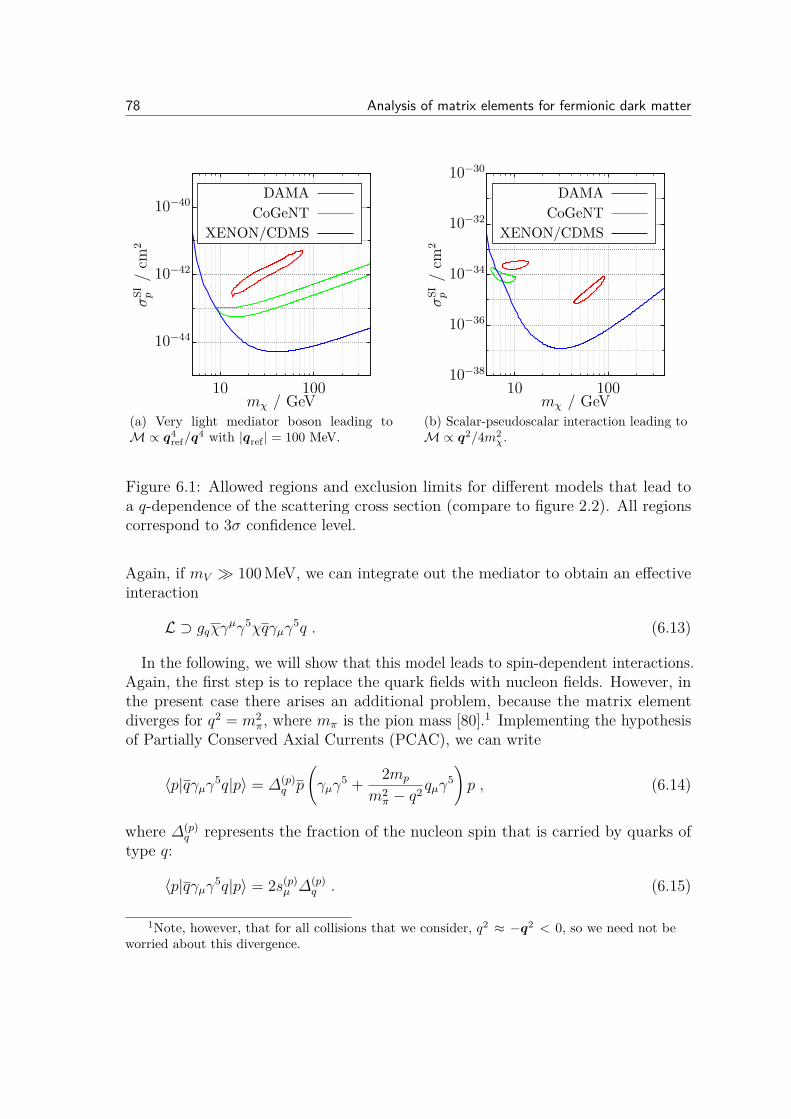
78 Analysis of matrix elements for fermionic dark matter
10−44
10−42
10−40
10 100
σSI p
/cm
2
mχ / GeV
DAMACoGeNT
XENON/CDMS
(a) Very light mediator boson leading toM∝ q4
ref/q4 with |qref | = 100 MeV.
10−38
10−36
10−34
10−32
10−30
10 100
σSI p
/cm
2
mχ / GeV
DAMACoGeNT
XENON/CDMS
(b) Scalar-pseudoscalar interaction leading toM∝ q2/4m2
χ.
Figure 6.1: Allowed regions and exclusion limits for different models that lead toa q-dependence of the scattering cross section (compare to figure 2.2). All regionscorrespond to 3σ confidence level.
Again, if mV 100 MeV, we can integrate out the mediator to obtain an effectiveinteraction
L ⊃ gqχγµγ5χqγµγ
5q . (6.13)
In the following, we will show that this model leads to spin-dependent interactions.Again, the first step is to replace the quark fields with nucleon fields. However, inthe present case there arises an additional problem, because the matrix elementdiverges for q2 = m2
π, where mπ is the pion mass [80].1 Implementing the hypothesisof Partially Conserved Axial Currents (PCAC), we can write
〈p|qγµγ5q|p〉 = ∆(p)q p
(γµγ
5 + 2mp
m2π − q2 qµγ
5)p , (6.14)
where ∆(p)q represents the fraction of the nucleon spin that is carried by quarks of
type q:
〈p|qγµγ5q|p〉 = 2s(p)µ ∆(p)
q . (6.15)
1Note, however, that for all collisions that we consider, q2 ≈ −q2 < 0, so we need not beworried about this divergence.

6.2 Spin-dependent interactions 79
Again, the expression for neutrons is analogous. Here we see for the first time, thatmatching fundamental fields to those of composite particles can introduce additionaloperators with more complicated q-dependence.
The step from nucleons to nuclei can be performed without additional contributionsat leading order [81].1 Of course, form factors, which describe the distribution ofnucleon spins inside the nucleus, will be introduced, but we will neglect them forthe moment and only include them later on. To match nucleon operators to nucleusoperators, we define
ap =∑
q=u,d,s
gq√2GF
∆(p)q , an =
∑q=u,d,s
gq√2GF
∆(n)q , (6.16)
and introduce Λ = (ap〈sp〉+ an〈sn〉) /J , where J is the total angular momentum ofthe nucleus and 〈sp,n〉 denote the expectation value of the spin content of proton andneutron in the nucleus, respectively. We can then write
M∝ Λχγµγ5χN
(γµγ
5 + 2mp
m2π − q2 qµγ
5)N . (6.17)
Now, we need to take the non-relativistic limit of the expressions Nγ5N andNγµγ
5N . For the first one, we get
N(p′)γ5N(p) = N †(p′)γ0γ5N(p)
= 12mN
(N †h√p′ · σ, N †h
√p′ · σ
)0 1
1 0
−1 00 1
√p · σNh√p · σNh
= 1
2mN
N †h(√
p′ · σ√p · σ −
√p′ · σ√p · σ
)Nh . (6.18)
Here, the leading-order term cancels and we get(√
p′ · σ√p · σ −
√p′ · σ√p · σ
)=
(p− p′) · σ = −q · σ, so that
N(p′)γ5N(p) = − q
2mN
·N †hσNh . (6.19)
For the expression Nγµγ5N we get after a similar calculation
N(p′)γµγ5N(p) = P
2mN·N †hσNh for µ = 0
N †hσiNh for µ = i, (6.20)
where P = p+ p′. The operator N †hσNh, which we obtain in both cases, measures1However, there will be a suppressed operator that corresponds to the electric dipole moment
of the nucleus (see section 6.5).

80 Analysis of matrix elements for fermionic dark matter
the spin of the nucleus: N †hσNh ∝ sN .Finally, we need to contract the non-relativistic expression for the nucleus fields
with the corresponding one for the dark matter particle, which of course has the sameform as equation (6.20), but with p instead of p.1 Note that the time componentsof all operators are suppressed by powers of p/m.2 Consequently, we only need tomultiply the spatial components and obtain
χγµγ5χN
(γµγ
5 + 2mp
m2π − q2 qµγ
5)N ∝ −sχ ·sN−
mp
m2π − q2
(sχ · q)(sN · q)mN
. (6.21)
To get the differential cross section, we must take the spin average of |M|2. Doingso gives us a factor of q2 from both (sχ · q) and (sN · q). For example, using12∑
spins χhχ†h = 1 we get
12∑spins|χ†hσiχhqi|2 = 1
2∑spins
(χ†hσiχhqi)(χ†hσjχhq
j) (6.22)
= 12∑spins
tr(χhχ†hσiχhχ†hσj)qiqj (6.23)
= 12tr(σiσj)q
iqj = δijqiqj = q2 . (6.24)
We obtain
14∑spins|M|2 ∝ Λ2
3 + 2 mp
m2π − q2
q2
mN
+(
mp
m2π − q2
q2
mN
)2 ≡ Λ2S(|q|) . (6.25)
In the impulse approximation, we then get [82]
dσdq2 = G2
Fπ(2J + 1)v2
∑spins|M|2 = 8G2
Fπv2 Λ
2J(J + 1)S(|q|)S(0) , (6.26)
The function S(|q|) encodes the momentum dependence of the cross section and isconventionally parameterized by
S(|q|) = a20S00(|q|) + a0a1S01(|q|) + a2
1S11(|q|) , (6.27)
where a0 = ap + an and a1 = ap − an are isoscalar and isovector coupling, respec-tively. S(|q|) can be extended to include not only the explicit q-dependence fromequation (6.25) but also the nuclear form factor, which is less important in this case.
1Of course, in the center-of-mass frame, we simply have p = −p.2Note that while the time-component of Pµ is of order mN , the time-component of qµ is
strongly suppressed, because q0 = E′ − E ≈ 1/2mN (v′2 − v2) = O(p2/m).

6.3 Momentum and velocity dependence in matrix elements 81
101 102 10310-39
10-38
10-37
10-36
10-35
10-34
10-33
10-32
mΧ @GeVD
Σp
@cm
2 D
æ
ø
ò SD elastic, ap=1, an=0
90% C.L.
101 102 10310-39
10-38
10-37
10-36
10-35
10-34
10-33
10-32
mΧ @GeVD
Σn
@cm
2 D
æ
ø
ò
SD elastic, ap=0, an=1
90% C.L.
CDMS 08+09
XENON 09
DAMA H90%3ΣL
DAMA H90%3ΣLHno channelingL
CoGeNT
CoGeNT H90%3ΣLHno exponential BGL
CDMS Si
COUPP
PICASSO
Figure 6.2: Exclusion limits from various dark matter direct detection experimentscompared with the favored regions from DAMA and CoGeNT for spin-dependentinteraction. For dark matter that couples only to the neutron spin, meaning an = 1,ap = 0, the results from DAMA and CoGeNT are clearly excluded by XENON10.For ap = 1, an = 0, XENON10 is not very sensitive, but the experiments COUPPand PICASSO give strong constraints. Figure taken from [14].
The parameters Sij can either be measured experimentally or calculated from nuclearshell models (see for example [83]).Clearly, exclusion limits for spin-dependent interactions are very different from
the spin-independent ones. First of all, there is no factor of A2, so the cross sectionwill no longer be enhanced for heavy nuclei. What really matters, is the spin ofthe nucleus, contained in the parameter Λ. As a consequence, experiments basedon germanium are rather insensitive to spin-dependent interactions, while strongexclusion limits are obtained from experiments that use fluorine as the target, forexample COUPP [21] and PICASSO [22]. We present typical exclusion limits infigure 6.2.
6.3 Momentum and velocity dependence in matrix elements
We have shown above how spin-independent and spin-dependent interactions mayarise. The two interaction terms that we considered, equation (6.2) and equa-tion (6.13), are in fact the dominant ones if the dark matter particle is a neutralino.However, in general models it is possible that these terms are absent and other terms,that would normally give only sub-leading contributions, become important.To give a simple example, let us consider the modification of equation (6.1). We
replace the scalar mediator boson by a pseudoscalar, which has slightly different

82 Analysis of matrix elements for fermionic dark matter
couplings [78]
L ⊃ iαφχγ5χ+ βqφqq + h.c. (6.28)
Since nothing changes in the quark sector, the matching to nucleus fields can beperformed as above, giving
M = (Zfp + (A− Z)fn)χγ5χNNF (q2) . (6.29)
However, as we take the non-relativistic limit, new structures appear. Using theresult from equation (6.19), we get
M = (Zfp + (A− Z)fn) q
2mχ
· χ†hσχhN†hNhF (q2) ∝ q · sχ
mχ
. (6.30)
Consequently, after taking the spin average of |M|2, the resulting cross section willbe proportional to q2/m2
χ. Consequently, scattering with small momentum transferwill be suppressed, while scattering of light dark matter particles will be enhanced.As a result, the differential event rate will no longer be exponentially falling, butwill rise at low recoil energies and then reach a maximum around 10 keV (see [78]).Figure 6.1b shows how this change affects exclusion limits.
This simple example demonstrates that we can expect new experimental signaturesin the absence of unsuppressed interaction terms. Our aim for this chapter is tocalculate systematically all possible terms that can arise at next-to-leading order andunderstand the resulting cross sections. Although there are quite many operatorsthat we can write down in the fundamental theory, the matrix elements in thenon-relativistic limit are rather simple, because they can only depend on scalarproducts of the four available vectors q, P , sN and sχ, where each power of |q| or|P | must be divided by either mN or mχ.
We will perform the calculation in three separate steps. In this section, we completethe list of fermion bilinears and calculate the non-relativistic limit for each. In thefollowing section, we will discuss Lorentz invariant products of two fermion bilinearsand give the non-relativistic limit of all possible four-fermion interactions. In thiscontext, we will also consider the contraction of a fermion bilinear with Pµ or qµ.Finally, in the last section of this chapter, we will return to the matching of quarkoperators to nucleus operators and state all terms that can appear in the process.
We have already determined the non-relativistic limits of the scalar operator NNin equation (6.11), the pseudoscalar operator Nγ5N in equation (6.19), and the axialvector operator Nγµγ5N in equation (6.20). To complete the list of fermion bilinears,we now calculate the non-relativistic limits of the vector operator NγµN , the tensoroperator NσµνN , and the pseudotensor operator Nσµνγ5N , where σµν = i
2 [γµ, γν ].
N(p′)γµN(p) = N †(p′)γ0γµN(p)

6.4 General analysis of four-fermion interactions 83
= 12mN
(N †h√p′ · σ, N †h
√p′ · σ
)0 1
1 0
0 σµ
σµ 0
√p · σNh√p · σNh
= 1
2mN
N †h(√
p′ · σσµ√p · σ +
√p′ · σσµ√p · σ
)Nh
= N †hNh for µ = 0
P i
2mNN †hNh − iqj
2mNεijkN †hσkNh for µ = i
, (6.31)
where we have used equation (A.6). In contrast to the axial vector bilinear, here thetime component is unsuppressed, while the spatial components are of higher order.Similar, but more cumbersome, calculations give for the tensor operators
N(p′)σµνN(p) =
iqi
2mNN †hNh + Pj
2mNεijkN †hσkNh for µ = i, ν = 0
εijkN †hσkNh for µ = i, ν = j, (6.32)
N(p′)σµνγ5N(p) = −iN
†hσ
iNh µ = i, ν = 0i
2mNN †hP
[iσj]Nh − qk2mN
εijkN †hNh µ = i, ν = j, (6.33)
where P [iσj] = P iσj −P jσi. Note that both operators are anti-symmetric in µ and νbecause σµν = −σνµ. The corresponding expressions for the dark matter bilinears canbe obtained in complete analogy by replacing mN with mχ and q,P with −q,−P .
6.4 General analysis of four-fermion interactions
With the results from the previous sections, we can now calculate the non-relativisticlimit of any four-fermion interaction. In general, a four-fermion interaction is obtainedby combining two fermion bilinears with matching Lorentz structure. If the Lorentzstructure does not match, we can still combine the two bilinears by contracting allremaining Lorentz indices with powers of qµ or P µ. Doing so essentially correspondsto allowing higher dimensional operators with additional derivatives that result froma more complete high energy theory. For dimensional reasons, the additional powersof |q| and |P | must be divided by a mass scale Λ, which can be understood as thescale of new physics. However, Λ can be at or even below the TeV-scale, so thereis no large hierarchy between Λ and mχ,N .1 Therefore, we assume that |q|/Λ and|P |/Λ are of the same order as |q|/m and |P |/m rather than of order q2/m2 andP 2/m2 and include them in our calculations.First of all we observe that certain combinations lead to unsuppressed matrix
elements and cross sections that remain non-zero as |q|, |P | → 0. We have al-ready seen in section 6.1 that the product (scalar)×(scalar) leads to unsuppressedspin-independent interactions and in section 6.2 that (axial)×(axial) leads to un-
1In fact, in section 6.5, we will even encounter cases where Λ = mN .

84 Analysis of matrix elements for fermionic dark matter
suppressed spin-dependent interactions.1 Similarly, (vector)×(vector) leads tounsuppressed spin-independent interactions, while both, (tensor)×(tensor) and(pseudotensor)×(pseudotensor), give unsuppressed spin-dependent interactions.2
Note, however, that the cross sections obtained in each case are not necessarilyequal. The reason is, that operators with different Lorentz structure couple todifferent charges. For example, the operator qq is sensitive to all quarks in thenucleon (including sea quarks), so the resulting coupling to the nucleus will beproportional to the nucleus mass. The operator qγµq, on the other hand, is aconserved current and consequently is only sensitive to valence quarks. The resultingcross section will therefore depend on the nuclear charge.3 Also form factors will ingeneral be different (although in this case they are coincidentally the same, becausewe observe experimentally that the distribution of mass inside a nucleus matches thedistribution of charge). We will come back to this discussion in section 6.5.
The unsuppressed operators have been discussed extensively in the literature (seefor example [14]). Only recently, various authors have begun to study suppressedoperators as well [78, 84, 85]. Physical motivation for such operators comes forexample from the idea that the dark matter particle may be composite and interactwith nuclei only through its electromagnetic dipole moment [86–89]. So far, however,only some special models have been considered. Here, we want to discuss suppressedoperators in full generality and will therefore derive a complete list of matrix elementsthat can arise at next-to-leading order from four-fermion interactions.
6.4.1 Scalar interactions
We begin with the simplest case, where the dark matter and nucleus bilinear are botheither Lorentz scalars or pseudoscalars, so that there are no free Lorentz indices. Wehave already discussed the case (scalar)×(scalar), which leads to unsuppressed spin-independent interaction, and the case (pseudoscalar)×(scalar), which depends on thespin of the dark matter particle and the momentum transfer but not on the nuclearspin, consequently giving suppressed spin-independent interactions. Similarly, thecase (scalar)×(pseudoscalar) has a factor of |q|/mN instead of |q|/mχ and dependson the nuclear spin instead of the dark matter spin, therefore giving suppressed spin-dependent interactions. The product (pseudoscalar)×(pseudoscalar) is suppressedby two powers of |q|/m, so we neglect it completely.Next, we can form additional Lorentz scalars and pseudoscalars by contracting
1The notation (axial)×(axial) stands for the contraction of axial dark matter bilinear andaxial nucleus bilinear.
2In fact, since σµνγ5 = i2εµνκλσκλ, the product (tensor)×(tensor) is equivalent to the product
(pseudotensor)×(pseudotensor).3Charge in this context means charge under the relevant gauge group. If the charge assign-
ments for up- and down-quark coincide with their electromagnetic charge, then nuclear chargeindeed means Z.

6.4 General analysis of four-fermion interactions 85
Operator Interaction Non-relativistic matrix elementχχNN Unsuppressed SI 1χγ5χNN Suppressed SI sχ · q/2mχ
χχNγ5N Suppressed SD −sN · q/2mN
χγ5χNγ5N Strongly suppressed 0χχNγµNPµ/Λ Suppressed SI 2mN/Λ
χχNγµγ5Nqµ/Λ Suppressed SD −sN · q/ΛχχNγµNqµ/Λ Vanishes 0χχNγµγ5NPµ/Λ Vanishes 0χγ5χNγµNPµ/Λ Suppressed SI 2mNsχ · q/mχΛ
χγ5χNγµγ5Nqµ/Λ Strongly suppressed 0χγ5χNγµNqµ/Λ Vanishes 0χγ5χNγµγ5NPµ/Λ Vanishes 0
Table 6.1: Scalar products of fermion bilinears to first order in |p|/m. The caseswhere the dark matter bilinear is a (pseudo)vector are analogous to the cases wherethe nucleus bilinear is a (pseudo)vector.
vectorial bilinears with qµ/Λ or P µ/Λ, meaning that we include derivative interactions.We get up to first order:
N(p′)γµN(p)qµΛ
= 0 , (6.34)
N(p′)γµN(p)PµΛ
= 2mN
ΛN †hNh = 2mN
Λ× (scalar) , (6.35)
N(p′)γµγ5N(p)qµΛ
= −qiΛN †hσ
iNh = 2mN
Λ× (pseudoscalar) , (6.36)
N(p′)γµγ5N(p)PµΛ
= 0 , (6.37)
so that nothing new is obtained from these operators. Equations (6.34)–(6.37)are indeed correct not only to first order in |p|/m, but to all orders. The reasonis that γµpµN(p) = mNN(p) and N(p′)γµp′µ = mNN(p′) as in equation (A.15).Consequently, we get for example
N(p′)γµN(p)qµ = N(p′)γµ(p′µ − pµ)N(p) = N(p′)(mN −mN)N(p) = 0 . (6.38)
The complete list of possible products is given in table 6.1.

86 Analysis of matrix elements for fermionic dark matter
6.4.2 Vector interactions
For the vectorial operators, something interesting happens. While the products(vector)×(vector) and (axial)×(axial) both give unsuppressed interactions, the prod-uct (vector)×(axial) is suppressed. The reason is that the vector current has anunsuppressed time component and suppressed spatial components, while it is theother way around for the axial current. In detail, we get
χγµγ5χNγµN = − P
2mχ
· χ†hσχhN†hNh
− χ†hσiχh(P i
2mN
N †hNh −iqj
2mN
εijkN †hσkNh
)
= −(
12mN
+ 12mχ
)P · χ†hσχhN
†hNh + iqj
2mN
εijkχ†hσiχhN†hσkNh
∝ −P · sχ2µ + iq · (sN × sχ)2mN
. (6.39)
Taking the spin average, gives
14∑spins|M|2 = P 2
4µ2 + 2q2
4m2N
, (6.40)
where the additional factor of 2 arises because of εijkεilk = 2δjl .For the first time, we obtain a cross section, that actually depends on P . To
understand the implications of this result, remember that P 2 = (p+ p′)2 = (2p+q)2 = 4p2 + 4pq + q2. At the same time, we have in the center-of-mass framep2 = p′2 = (p+q)2 = p2 + 2pq+q2, and consequently, P 2 = 4p2−q2 = 4µ2v2−q2.Therefore,
14∑spins|M|2 = v2 − q2
4µ2 + q2
2m2N
. (6.41)
The resulting cross section depends not only on the momentum transfer, but alsoon the velocity of the dark matter particle. At equal momentum transfer, fast darkmatter particles contribute more to the differential event rate than slow ones.As above, we can also consider the products of vectorial bilinears with other
bilinears, where free Lorentz indices are contracted with either P µ or qµ. The combi-nations of vectorial and scalar bilinears have already been discussed in section 6.4.1,so we limit ourselves to the combination of vectorial and tensor operators here:
N(p′)σµνN(p)qµΛ
= 0 for ν = 0
qjΛεijkN †hσkNh for ν = i
, (6.42)

6.4 General analysis of four-fermion interactions 87
Operator Interaction Non-relativistic matrix elementχγµχNγµN Unsuppressed SI 1
χγµγ5χNγµγ5N Unsuppressed SD sN · sχ
χγµγ5χNγµN Suppressed SI and SD −P ·sχ2µ + iq·(sN×sχ)2mN
χγµχNγµγ5N Suppressed SD P ·sN2µ −
iq·(sχ×sN )2mχ
χγνχNσµνγ5NP µ/Λ Suppressed SD imN
Λ
[P ·sNµ− iq·(sχ×sN )
mχ
]χγνχNσµνγ
5Nqµ/Λ Suppressed SD iq · sN/ΛχγνχNσµνNP
µ/Λ Strongly suppressed 0χγνχNσµνNq
µ/Λ Strongly suppressed 0χγνγ5χNσµνNP
µ/Λ Suppressed SI isχ · q/Λχγνγ5χNσµνNq
µ/Λ Suppressed SD q · (sχ × sN)/Λχγνγ5χNσµνγ
5NP µ/Λ Suppressed SD 2imNsχ · sN/Λχγνγ5χNσµνγ
5Nqµ/Λ Strongly suppressed 0
Table 6.2: Vector products of fermion bilinears to first order in |p|/m. The caseswhere the dark matter operator is a (pseudo)tensor are analogous to the cases wherethe nucleus operator is a (pseudo)tensor.
N(p′)σµνN(p)PµΛ
= 0 for ν = 0− iqi
ΛN †hNh for ν = i
= −iqν
Λ× (scalar) , (6.43)
N(p′)σµνγ5N(p)qµΛ
= iqi
ΛN †hσiNh for ν = 0
0 for ν = j, (6.44)
N(p′)σµνγ5N(p)PµΛ
= iP
Λ·N †hσNh ν = 0
2imNΛN †hσ
iNh ν = i
≈ 2imN
Λ× (axial) . (6.45)
Equation (6.43) and equation (6.45) also follow directly from equation (A.15) andthe observation that
Pµσµν = i
2 (γµγν − γνγµ) (p′µ + pµ)
= i
2(γµ(2p′µ − qµ)γν − γνγµ(2pµ + qµ)
)= i
(γµp′µγ
ν − γνγµpµ)− i
2 (γµγν + γνγµ) qµ
= i(γµp′µγ
ν − γνγµpµ − qν)
= i(/p′γν − γν/p− qν) . (6.46)
We present all possible products in table 6.2.

88 Analysis of matrix elements for fermionic dark matter
Operator Interaction Non-relativistic matrix elementχσµνχNσµνN Unsuppressed SD 2sN · sχ
χσµνγ5χNσµνγ5N Unsuppressed SD 2sN · sχ
χσµνγ5χNσµνN Suppressed SD and SI iP ·(sχ×sN )(mN−mχ)mχmN
− q·sχmN− q·sN
mχ
χσµνχNσµνγ5N Suppressed SD and SI iP ·(sχ×sN )(mN−mχ)
mχmN− q·sχ
mN− q·sN
mχ
Table 6.3: Tensor products of fermion bilinears to first order in |p|/m.
6.4.3 Tensor interactions
By now there is only one combination that we have not discussed yet: the productof tensor and pseudotensor. We get
χσµνγ5χNσµνN = − qi
mN
N †hNhχ†hσiχh −
qi
mχ
N †hσiNhχ†hχh (6.47)
+ iPi
(1mχ
− 1mN
)εijkχ†hσjχhN
†hσkNh (6.48)
∝ iP · (sχ × sN)(
1mχ
− 1mN
)− q · sχ
mN
− q · sNmχ
, (6.49)
which, as expected from the symmetry between tensor and pseudotensor, is invariantunder the exchange χ↔ N . We summarize the tensor operators in table 6.3.
6.5 Matching and form factors
With the results from the previous section, we can calculate cross sections once weknow the effective interaction between dark matter and nucleus. What remains isthe question how to determine the effective nucleus operator from the fundamentalLagrangian. In the limit of zero momentum transfer, the answer is easy. If thequark operator has the form βqqOq, where O is an arbitrary product of γ-matrices,the corresponding nucleus operator must also be of the form gNON , because bothoperators must have the same Lorentz structure and parity. The only problem thatremains in this case is how to obtain the coupling constant g from the fundamentalcoupling constants βq. This problem, however, is well understood for almost alloperators — see [90] for a good review. The only exception is the operator qγ5q,because it is not present in the Standard Model, so there is no way to determineexperimentally the coupling constants and form factors that would arise in theprocess of matching this operator to the corresponding one for nuclei. Of course, itshould be possible to calculate these quantities from QCD, but to the best of ourknowledge such a calculation has not been done.
6.5 Matching and form factors 89
For non-zero momentum transfer, matching becomes more difficult, because nowthe resulting nucleus operator can depend on the Lorentz vectors qµ and P µ as wellas the Lorentz scalar q2 (or equivalently q2 = −q2). The first consequence is theoccurrence of form factors, so βqqOq will match to gNONF (q2) with F (0) = 1.These form factors will, in general, be different for different operators.1 The secondconsequence is that additional operators may appear in the matching process. Wehave seen one example already in section 6.2 for the matching of the axial vectorbilinear. Fortunately, any new operator must have the same Lorentz structure andparity as the original one. Let us consider all possible quark operators in turn anddetermine in each case the most general nucleus operator that can be induced in thematching process.For the scalar operator qq, we get
qq → NNF(s)1 (q2) +NγµNqµF
(s)2 (q2)
+NγµNPµF(s)3 (q2) +NσµνNPµqνF
(s)4 (q2) . (6.50)
However, we have seen already in section 6.4.1 that the second term vanishes andthe third term is again proportional to NN . A similar calculation shows that thefourth term is proportional to q2NN , so that in fact, the only remaining operator is
qq → NNF(s)1 (q2) . (6.51)
This result justifies the assumption made in section 6.1 that no additional operatorsappear in the matching process for the scalar operator.Analogously, we can write
qγ5q → Nγ5NF(p)1 (q2) +Nγµγ5NqµF
(p)2 (q2)
+Nγµγ5NPµF(p)3 (q2) +Nσµνγ5NPµqνF
(p)4 (q2) . (6.52)
In this case, the third term vanishes, the second one is proportional to Nγ5N andthe last one can be decomposed into a term proportional to Nγ5N and a termproportional to q2Nγ5N . Consequently, we can write
qγ5q → Nγ5NF(p)1 (q2) . (6.53)
For the vector operator, things are more complicated. In general, five operators1It is often argued that we only need two different form factors, one for spin-dependent and
one for spin-independent scattering. The argument is that we can take the non-relativistic limitalready for the nucleon fields. The non-relativistic matrix elements will then be independent ofthe detailed Lorentz structure of the operators. Consequently, the form factors describing thestructure of the nucleus must be the same for all matrix elements that have the same dependenceon the nucleon spins. However, it is not quite clear whether we can indeed treat nucleons asnon-relativistic, so this solution is at best an approximation (see [78] for a discussion).

90 Analysis of matrix elements for fermionic dark matter
could appear in the matching process:
qγµq → NγµNF(v)1 (q2) +NNqµF
(v)2 (q2) +NNP µF
(v)3 (q2)
+NσµνNqνF(v)4 (q2) +NσµνNPνF
(v)5 (q2) . (6.54)
However, we know from equation (6.46), that the last term is proportional to NNqµ.Moreover, we can use the Gordon identity, which states that
NNP µ = 2mNγµN − iNσµνqνN . (6.55)
Consequently, only three of the four remaining terms are independent, and we canwrite
qγµq → NγµNF(v)1 (q2) +NNqµF
(v)2 (q2) +NσµνNqνF
(v)4 (q2) . (6.56)
Finally, we use the fact that qγµq is a conserved current, so any induced nucleusoperator Γ µ must satisfy the Ward identity qµΓ µ = 0. While the first and last termin equation (6.56) automatically vanish when contracted with qµ, the second onedoes not, so we must require F (v)
2 (q2) = 0. Consequently, the most general form forthe nucleus operator induced from qγµq is (adapting the notation from [79])
qγµq → N
(F1(q2)γµ + iF2(q2)
2mN
σµνqν
)N . (6.57)
The second term can be interpreted as the contribution of the magnetic dipolemoment of the nucleus.
Normally, the first term gives the leading order contribution to the scattering crosssections for dark matter, so the second term can be safely neglected. However, fromequation (6.31) and equation (6.42) we know that the spatial components of bothoperators, NγµN and NσµνNqν/mN , are of the order |q|/mN . Consequently, if wecombine these operators with a dark matter bilinear with suppressed time component(for example χγµγ5χ), the contribution of the vector operator will be suppressed andboth terms in equation (6.57) contribute at the same (namely next-to-leading) order.For the axial operator, we can proceed in analogy. In general, we would have
qγµγ5q → Nγµγ5NF(a)1 (q2) +Nγ5NqµF
(a)2 (q2) +Nγ5NP µF
(a)3 (q2)
+Nσµνγ5NqνF(a)4 (q2) +Nσµνγ5NPνF
(a)5 (q2) . (6.58)
Again, only three terms are independent, so we can write
qγµq → Nγµγ5NF(a)1 (q2) +Nγ5NqµF
(a)2 (q2) +Nσµνγ5NqνF
(a)4 (q2) . (6.59)
This time, however, there is no conserved current which allows us to eliminate the

6.6 Summary of results 91
second term. In fact, we have seen already in section 6.2, that this term must bepresent to account for the divergence at q2 = m2
π. The third term, on the other hand,corresponds to the electric dipole moment of the nucleus.For the tensor operator (and the pseudotensor operator), we can again use the
Gordon identity to replace N(P µqν − P νqµ)N by 2mN(γµqν − γνqµ)N , neglectingterms that are quadratic in q. Consequently, the tensor operator will match to
qσµνq → NσµνNF(t)1 (q2) +N(γµqν − γνqµ)NF (t)
2 (q2)+N(γµP ν − γνP µ)NF (t)
3 (q2) . (6.60)
6.6 Summary of results
We have now presented all the pieces needed to calculate cross sections for thescattering of dark matter particles on nuclei from any fundamental interactioninvolving fermionic dark matter. What one has to do is
1. Obtain the effective four-fermion interaction on the quark level.
2. Match the quark bilinear to the corresponding nucleus bilinear using theformulas in this section.
3. Calculate (or measure) the effective coupling constants and the resulting formfactors.
4. Take the non-relativistic limit of the resulting matrix element using the formulasgiven in section 6.4.
5. Calculate the spin average of |M|2.
Clearly, step 3 is the most difficult part and the results are known only for few simplecases.
To conclude, we observe that while the scattering of dark matter is rather simpleat leading order, it gets more involved once leading order terms are absent. At next-to-leading order we must worry about the interplay between various form factorsand coupling constants. The resulting cross sections can depend on the momentumtransfer, the spin of the nucleus and even the velocity of the dark matter particle.As we have seen in chapters 3 and 4, the final results of XENON100 may excludethe possibility that the signals from DAMA and CoGeNT are due to unsuppressedSI interactions. In this case, it will be the next step to analyze the matrix elementsthat arise at next-to-leading order to see if any of these allow for a reconciliation ofthe different experiments. We leave such an analysis to future work.

CHAPTER 7Summary and conclusions
The fact that we have compelling evidence for the existence of dark matter fromastrophysical and cosmological observations, but know only little about the particlesthat constitute most of it, is one of the greatest puzzles of modern physics. Not onlydo we want to understand the large abundance of dark matter in the universe, butwe also hope to obtain first clues about physics beyond the Standard Model fromthe properties of the dark matter particle. Direct detection experiments, especiallyliquid xenon detectors, appear to be a very promising way to observe dark matterand finally solve this puzzle. Nevertheless, present experimental results are still farfrom providing a clear picture.
The claimed observations of a dark matter signal in the direct detection experimentsDAMA and CoGeNT have led to a strong interest in dark matter particles withlow mass (mχ < 10 GeV). Liquid xenon detectors have difficulties to probe thisparameter region because of their relatively high energy threshold. In this thesis, wehave looked thoroughly at the sensitivity of liquid xenon detectors for low energynuclear recoils. It depends essentially on four factors: the detector resolution, the cutacceptance, the relative scintillation efficiency of liquid xenon and the light collectionefficiency of the detector. As the central result of our work, we obtain that none ofthese factors precludes the observation of low mass dark matter.In chapter 1, we have reviewed the standard model of cosmology and the exper-
imental evidence which leads to the conclusion that there must be 4 to 5 timesmore dark than visible matter in the universe. From the little we know about darkmatter, it should be cold, collisionless, stable and non-baryonic. We have arguedthat Weakly Interacting Massive Particles are a good candidate for the dark matterparticle because they possess all these properties and moreover are produced withthe correct abundance in the early universe due to the WIMP-miracle.In chapter 2, we have given an overview of experimental strategies to detect
dark matter. We have derived and discussed the differential event rate in directdetection experiments and the characteristic signatures of a dark matter signal. Theenhancement of the event rate for heavy nuclei is the first reason for using liquidxenon detectors. Additional advantages are the strong self-shielding and the high

93
scintillation and ionization yields. We have presented the principle of operation ofthe XENON100 detector and introduced the terminology relevant for the analysis ofthe primary and secondary scintillation signals, S1 and S2. Also, we have pointedout the tension between the signals observed by DAMA and CoGeNT and the nullresults from XENON and CDMS.In chapter 3, we have discussed the reason for the large fluctuations of the S1
and the S2 signal in liquid xenon detectors at low energies. For the S1 signal,the detection process limits the detector resolution, leading in good approximationto a Poisson smearing of the low energy threshold. The statistical nature of theproduction process for photons is not important to describe S1 fluctuations, butwe must take into account the production process for electrons to give a correctstatistical description of the S2 signal. Consequently, the variance of the S2 signalis larger than expected from Poisson statistics. We have confirmed our model offluctuations by performing Monte Carlo simulations of the nuclear recoil band, whichagree well with experimental data. In conclusion, the resolution of liquid xenondetectors is rather poor at low energies. Nevertheless, the resulting smearing of thethreshold improves the sensitivity of liquid xenon detectors significantly.The cut acceptance can also be determined from Monte Carlo simulations of the
nuclear recoil band. We find good agreement between the results of our simulationsand the published values. However, this acceptance function includes neither thesingle scatter cut nor the nuclear recoil cut. We expect the single scatter cut to havea high acceptance, but emphasize the importance of a large rejection efficiency formultiple scatters. Otherwise, there will be the risk that a large number of multiplescatters in calibration data distorts the nuclear recoil band. The acceptance of thenuclear recoil cut, on the other hand, is difficult to determine, because the acceptanceprobability is not independent of the other cuts which we apply. Therefore, the flat50% acceptance, which has been assumed previously, can be only an approximation.In fact, from a more careful treatment one obtains a higher acceptance at low recoilenergies, so assuming a flat acceptance gives a conservative estimate.In chapter 4 we have calculated the relative scintillation efficiency for low energy
nuclear recoils in liquid xenon. Our idea was to develop a theory that predicts both,ionization and scintillation yield. This aim was achieved by combining Lindhard’stheory for the initial production of electronic excitations and the well motivatedassumption of energy independent partition between ionization and excitation inthe underlying collisions. Our conclusion is that scintillation and ionization arecorrelated, so that a rapidly dropping Leff would imply a drop in the scintillation yieldwhich is incompatible with existing data. Consequently, we exclude the possibility ofthreshold effects that reduce electronic excitations in the keV range.
All these considerations lead to the conclusion that liquid xenon detectors possessan impressive sensitivity for low energy nuclear recoils corresponding to low massdark matter. We have calculated the acceptance function for the XENON100 detector(see figure 4.5a) and predicted the sensitivity of the experiment after a runtime of

94 Summary and conclusions
100 days (see figure 4.5b). In summary, XENON100 should definitely be able toconfirm or rule out the results from CoGeNT and DAMA under the assumption ofstandard spin-independent scattering.Whether XENON100 observes a dark matter signal or not, larger liquid xenon
detectors will be built in the near future to increase the sensitivity and confirm theresults from XENON100. We have dedicated chapter 5 to a study of such futuredetectors. In fact, liquid xenon detectors are very well suited for upscaling. Thethree factors that we considered above, namely detector resolution, cut acceptanceand relative scintillation efficiency, remain essentially unchanged for larger detectors.What changes significantly, however, is the fourth factor, namely the light collectionefficiency. With increasing detector dimensions, the light collection efficiency will bereduced. Thus, the low energy threshold of future liquid xenon detectors is expectedto rise, leading to a loss of sensitivity for low mass dark matter.To quantify this effect, we have performed Monte Carlo simulations of the light
collection efficiency in dependence of the detector size and the absorption lengthof liquid xenon. We conclude that, unless the absorption length can be increasedsignificantly, an increase in fiducial mass will not necessarily improve the sensitivity inthe low energy region. A better sensitivity for low mass dark matter could, however,be achieved by changing the detector design in order to increase the number ofphoto-sensors. Specifically, we considered oblate detectors and detectors with 4πQUPID coverage.
While both of these options are promising in terms of the light collection efficiency,a serious problem is the rising background level induced by radioactive contaminantsin the photo-sensors. Indeed, Monte Carlo simulations of the internal electron recoilbackground show, that the QUPIDs are the dominant source of background events.Consequently, the background level will limit the sensitivity of detectors with a largenumber of QUPIDs, unless the radiopurity can be improved. A similar observationcan be made for detectors with fiducial mass of 10 t or more. Although the internalbackground from the detector components can be reduced by applying a strongerfiducial volume cut, we cannot reduce the intrinsic background from 85Kr and solarpp-neutrinos. Consequently, it is impossible for liquid xenon detectors to observedark matter with σSI
p < 10−48 cm2.If the upcoming results from XENON100 do not confirm the observations from
DAMA and CoGeNT, there will be a strong tension between the different experiments.For experimentalists, the challenge will be to understand the backgrounds in thedetector very well and provide a convincing analysis of the detector acceptance. Fortheoretical physicists, the most interesting question will be, whether the results fromthe different experiments are necessarily in contradiction with each other, or whetherthe data point towards a novel interpretation of dark matter that allows to reconcileall experiments.
As a first step in this direction, we have performed in chapter 6 a general operatoranalysis of all possible interactions between fermionic dark matter particles and

95
quarks. The challenge is to infer the dark matter-nucleus interaction from thefundamental couplings and then calculate the resulting cross sections in the non-relativistic limit. For a few cases, these calculations are well known, giving thestandard results for spin-independent and spin-dependent interactions. In manycases, however, new operators may appear in the matching process, and for each ofthese new operators we have to determine the effective coupling constants and formfactors from models of the nucleus.We have decided to consider also subleading contributions, which are usually
neglected but lead to interesting experimental signatures if the leading order termsare absent. For all possible four-fermion interactions of dimension four and five,we have calculated the matrix elements in the non-relativistic limit. It turns out,that for certain combinations of fermion bilinears, the resulting cross sections maydepend on the momentum transfer in the scattering process as well as on the velocityof the incoming dark matter particle. Such dependences allow for example tosuppress scattering with low momentum transfer, similar to the case of inelastic darkmatter [25].
Clearly, much work remains to be done. Concerning the data analysis of XENON100,we believe that detailed Monte Carlo simulations of the nuclear recoil band inXENON100 will play an essential part in determining the acceptance of the sin-gle scatter cut and the nuclear recoil cut, which will be necessary for a consistentinterpretation of the final results. In addition, such simulations may improve ourunderstanding of the data obtained from AmBe calibration and could even provide away to determine the scintillation and ionization yields (see [34]).
To check our results for Leff , it would be very helpful to perform an ab-initioanalysis of atomic collisions, including the calculation of exclusive cross sections, aswell as a Monte Carlo simulation of the recombination processes. Such an analysisshould take into account the electronic structure of the outer electron shells ofxenon (for example, using Density Functional Theory). Alternatively, the crosssections could be determined experimentally from the collisions of individual xenonatoms. The final confirmation of our model can of course only come from precisemeasurements of the ionization yield and the relative scintillation efficiency.Concerning the studies of future detectors, we suggest to consider thoroughly
possible design changes in order to improve the light collection efficiency or reducethe background level. Important questions related to XENON1T will concern thecryostat material and the choice between QUPIDs and ordinary PMTs. The codethat we developed may help to make these decisions. Moreover, to complement oursimulations of the electron recoil background, a similar study for neutron backgroundneeds to be performed. Also, we would like to emphasize the importance of liquidxenon purification for the sensitivity of future detectors — to increase the absorptionlength and reduce the intrinsic background from 85Kr.
The next steps towards a theoretical understanding of dark matter should includea careful evaluation of the coupling constants and form factors that appear in the

96 Summary and conclusions
process of matching quark operators to nucleus operators. For the step from quarks tonucleons, these calculations will rely strongly on QCD, while the step from nucleonsto nuclei requires a precise model of the nucleus. The subsequent step will then be tosee whether any of the new operators that appear at subleading order may reconcileall experimental observations.In conclusion, there are exciting times ahead for the physics of dark matter. We
expect the publication of the results from XENON100 in the near future, and inthe following years the competition for the first detector of the next generation(with a fiducial mass of more than 1 t). At the same time, the interpretation of theexperimental results will require the ingenuity of theoretical physicists to solve thedark matter puzzle.The increase in sensitivity that is expected for the dark matter searches within
the next decade, combined with the results from the LHC, may very well lead to anunambiguous identification of dark matter. On the other hand, experiments mayobserve nothing at all — or reveal something completely unexpected. Clearly, wemust remain open-minded for unconventional interpretations and new insights (seefigure 7.1).
(a) Typical total acceptance function for a liquid xenon detector.
(b) “It was a picture of a boa constrictor digesting an elephant.”
Figure 7.1: What will future direct detection experiments reveal about the nature ofdark matter? An interpretation of the total acceptance function of a liquid xenondetector in the spirit of Antoine de Saint-Exupéry’s Little Prince [91].
APPENDIX AThe Dirac equation
The Dirac equation is the equation of motion for spin-1/2 particles, which are describedby four-component Dirac spinors ψ:
(iγµ∂µ −m)ψ = 0 . (A.1)
The 4× 4 matrices γµ satisfy the Clifford algebra
γµ, γν = 2gµν , (A.2)
where gµν is the metric tensor. We adopt the sign convention (+,−,−,−).For the γ-matrices, we take the chiral representation,
γµ = 0 σµ
σµ 0
, γ5 = iγ0γ1γ2γ3 =−1 0
0 1
, (A.3)
with σ = (1,σ) and σ = (1,−σ). 1 is the 2× 2 identity matrix and the σi arethe Pauli matrices
σ1 =0 1
1 0
, σ2 =0 −ii 0
, σ3 =1 0
0 −1
. (A.4)
The Pauli matrices are hermitian and traceless and have the property thatσi, σj
= 2δij ,
[σi, σj
]= 2iεijkσk , (A.5)
with the Kronecker symbol δij and the Levi-Civita symbol εijk. Consequently,
σiσj = δij + iεijkσk , (A.6)tr(σiσj
)= δij , (A.7)
(p · σ)2 = 1p2 . (A.8)

98 The Dirac equation
To solve the Dirac equation for a particle with four-momentum p = (E,p) andmass m =
√p2, we introduce a normalized two-component spinor ξ and write
ψ(p) = 1√2m
e−ip·x√p · σξ√
p · σξ
. (A.9)
With this ansatz, we get
γµ∂µψ = − i√2m
eip·x γµpµ
√p · σξ√p · σξ
(A.10)
= − i√2m
eip·x 0 p · σp · σ 0
√p · σξ√p · σξ
(A.11)
= − i√2m
eip·xp · σ√p · σξp · σ√p · σξ
. (A.12)
Now we use√p · σ√p · σ =
√(1− pσ)(1 + pσ) (A.13)
=√12 − (pσ)2 = 1
√1− p2 = 1
√p2 = 1m , (A.14)
to get γµ∂µψ(p) = −imψ(p). Consequently, ψ(p) as defined in equation (A.9) satisfiesthe Dirac equation. To simplify notation, we define /p ≡ γµpµ. The Dirac equationthen implies that
/pψ(p) = mψ(p) . (A.15)
To conclude this appendix, we note that the Dirac equation can be derived from aLorentz-invariant Lagrangian density
L = ψ (iγµ∂µ +m)ψ , (A.16)
where ψ = ψ†γ0. Note that, in contrast to [79], we have chosen the non-relativisticnormalization for ψ. Thus, in our normalization,
ψ(p)ψ(p) = 12m
(ξ†√p · σ, ξ†
√p · σ
)0 11 0
√p · σξ√p · σξ
(A.17)
= 12m
(ξ†√p · σ√p · σξ + ξ†
√p · σ√p · σξ
)= ξ†ξ = 1 . (A.18)

APPENDIX BCalculation of exclusion limits
In this appendix, we discuss how to calculate exclusion limits for dark matter directdetection experiments. Such exclusion limits are conventionally calculated underthe assumption that no background events are observed. If the experiment doesin the end observe background events, the exclusion limits will be weaker. In thiscase, one needs to use more sophisticated methods — such as the Maximum GapMethod [72] — for the calculation.In principle, to determine whether an experiment can exclude a choice of the
parameters σSIp = σ0 and mχ = m0, we must calculate the total number of events
that the experiment is expected to observe for this combination. To do so, we mustcalculate the differential event rate for these parameters as described in chapter 2.1.
Of course, not all dark matter scattering events will result in a detectable signal, sowe must multiply the differential event rate with the total acceptance function of thedetector, A(Enr), which we introduce in chapter 3.4. The acceptance function givesthe probability that a nuclear recoil of energy Enr leads to a signal in the detector.It takes into account the detector resolution, the light yield and the cut acceptancesof the detector (see chapter 3 for a discussion).Once we have determined the total acceptance function, we can obtain the total
event rate by integrating
Rtot =∞∫0
dRdEnr
A(Enr) . (B.1)
Multiplying Rtot with the exposure of the experiment now gives the total number ofexpected events N .Assuming that instead of the expected number of events N , the detector will
observe no event at all, we can reject the hypothesis σSIp = σ0 and mχ = m0, if N
is sufficiently large. If N > 2.30, we can reject the hypothesis with 90% confidenceand if N > 3.00 the hypothesis is ruled out with 95% confidence [10]. Consequently,90% confidence exclusion limits, as shown for example in chapter 5 are obtained bycalculating all combinations of mχ and σSI
p that give N = 2.30.

APPENDIX CCoulomb correction to electronic stopping
For a uniform electron gas the electronic stopping power is proportional to thevelocity of the ionizing particle, as stated in equation (4.5). The same result is alsovalid for liquid scintillators, if the velocity of the passing atom is comparable to theBohr velocity. However, at very low velocities, colliding atoms do not penetrate eachother strongly because of the Coulomb repulsion. In this case, the nucleus passesonly through regions of low electron density and consequently experiences a smallerstopping force. As a result, we expect a stronger decrease of the electronic stoppingpower. This effect has been referred to as the Coulomb correction to Lindhard’stheory [53].It is not clear how to include this correction into the calculation of electronic
stopping powers. In reference [43], Tilinin suggested to calculate Se by integratingdE/ dx over the volume accessible for a recoiling nucleus and multiplying the resultwith the number density of xenon atoms. Following this approach, we obtain fromequation (4.5)
Se =∫Vacc
Nn0vvFσtr(vF) dV = Nmev∫Vacc
n(r)vF(r)σtr (vF(r)) dV , (C.1)
where n = n0/me is the number density of electrons. Before we can evaluate thisintegral, we must determine Vacc, n(r), vF(r) and σtr(v).To obtain the accessible volume, we need to know the interaction potential V (r)
for two xenon atoms. This potential has been calculated by Schneider [92] basedon a Density Functional Theory calculation done by Gordon and Kim [93]. In acollision process with energy Enr, the distance of closest approach, r0(Enr), is givenby the root of the equation V (r0) = Enr. The accessible volume Vacc is then given byall points with r ≥ r0. As expected, r0 is a function of Enr, which decreases withincreasing recoil energy, so the accessible volume will grow.
To simplify the integral in equation (C.1), we assume that the electron density isradially symmetric. Of course, this assumption will not hold strictly, as two atomsapproach each other, but it is a good approximation at low energies, when the atoms

101
stay rather far apart and most of the nuclear charge is screened by inner electrons.1We will therefore replace n(r) by the electron density n(r) of a single xenon atomthat Ziegler et al. calculated with Hartree-Fock methods [56].
For a uniform electron gas, we can calculate the Fermi velocity from the electrondensity:
vF = 1me
3√
3nπ2 . (C.2)
In our case, we have a non-uniform electron density, so the Fermi velocity will beslightly larger [47]:
v2F = v2
F + 14 (a0n
′(r)/n(r))2. (C.3)
We will, however, neglect this effect in the following, assuming that n′(r) n(r)/a0and use the approximation of a uniform electron gas.Finally, the transport cross section σtr has been calculated by Tilinin in [94].
Consequently, we know all quantities that appear in equation (C.1) and can calculatethe electronic stopping power numerically. Under the assumption of a radiallysymmetric electron distribution, we can write
Se = 4πNmev
∞∫r0
n(r)vF(r)σtr(vF(r))r2 dr . (C.4)
For convenience, we define the dimensionless quantities x = r/a and T = σtr/πa2
and get
Se = 4πNmev
∞∫r0
n(r)vF(r)σtr(vF)r2 dr (C.5)
= 4π2Nmeva5∞∫x0
n(x)vF(x)T (vF(x))x2 dx (C.6)
= 4π2Nmev
v0e2a4 1
4√
23
√9π2
2Z a0
∞∫x0
n(x)vF(x)T (vF(x))x2 dx (C.7)
=√
8πNe2a0v
v0a4π
2
23
√27π16Z
∞∫x0
n(x)4/3T (vF(x))x2 dx (C.8)
≡√
8πNe2a0v
v0τ(Enr) , (C.9)
1More precisely, radial symmetry should be a valid approximation, if r0 is greater than theThomas-Fermi screening length a.

102 Coulomb correction to electronic stopping
0.001 0.01 0.1 1
0.001
0.01
0.1
Ε
sHΕL
Coulomb correction
Lindhard' s theory
Figure C.1: The final result for the dimensionless electronic stopping power dε/dρ.
where we made use of a = 14√
23√
9π2
2Z a0.The final result has been written in a way that for constant τ(Enr) we recover a
velocity proportional stopping power. In fact, for τ(Enr) ≈ 100, our result coincideswith the result from Lindhard’s theory. Such a constant value for τ(Enr) indeedoccurs for v ≥ v0, because at very small distances, the Fermi velocity is large andthe transport cross section becomes negligibly small. We present the result of ourcalculation in figure C.1, again using the reduced units defined in equation (4.9).
We observe that Tilinin’s approach for the Coulomb correction predicts an electronicstopping power that drops rapidly below 100 keV. At 10 keV the corrected stoppingpower is already a factor of two smaller than the original result from Lindhard. Itshould be clear from the discussion in chapter 4 that there is no way to explain arising ionization yield at low energies with this model.We must conclude that the results for the electronic stopping power derived
from equation (C.1) are in contradiction with experimental data. To resolve thiscontradiction, one could try a more accurate treatment and calculate the trajectoriesof xenon atoms during a scattering process in order to integrate the electronic stoppingpower along the path. Tilinin argues, however, that for small angle scattering, whichis the most likely to occur at low energies, the volume integral in equation (C.1)should give the same result.
As argued in chapter 4, there appears to be no naive way to include the Coulombcorrection to the electronic stopping power. Probably, the assumption of a point-likeinteraction between nucleus and electron is no longer valid at very low velocities,because the electron cloud can rearrange during the collision. A possible way toaccount for this effect may be time-dependent Density Functional Theory as describedin [95].

APPENDIX DDetails on the Monte Carlo simulations with Geant4
All simulations have been performed with MaGe [96], a Monte Carlo frameworkfor experiments with low background based on Geant4 [97]. The general structureof the code, the physics list and the event generator have been adapted from thecorresponding simulations for XENON100 [32], while the detector design was changedcompletely and new features were added to improve the user interface.
D.1 Detector design
The detector design employed in our simulations is based on early proposals forXENON1T [70]. In detail it contains:
• A liquid xenon time projection chamber (TPC) that is surrounded by a teflon(PTFE) layer for the reflection of scintillation light,
• A titanium cryostat consisting of an inner and outer vessel with vacuumbetween them,
• A layer of acrylic (PMMA) that separates the cryostat vessel from the PTFElayer,
• QUPIDs (see section D.2) on the bottom and top of the TPC, placed on asupport base made of copper,
• Stainless steel grids for the drift field and the extraction field.
Note that several simplifications have been made and some recent changes in thedesign are not included.1 Since this thesis is only concerned with internal electronrecoil background, there is no need to include the water shield into the simulation.
1Most notably, the field shaping rings are not included in the simulation. Also, the XENONcollaboration has recently proposed to separate the flange for inner and outer vessel to reduce heattransfer.

104 Details on the Monte Carlo simulations with Geant4
Component Unit TPC diameter and height in meter1.0 1.2 1.4 1.6 1.8
Liquid Xenon kg 2291 3958 6286 9383 13360Titanium kg 337 447 573 714 870PTFE kg 148 241 368 535 742Copper kg 155 215 284 363 451PMMA kg 198 273 360 459 570QUPIDs piece 242 374 508 628 842
Table D.1: Masses of the various detector components (in kg) for different TPC sizes
The main virtue of our code is that the detector dimensions are not fixed. Theheight and diameter of the TPC can be varied independently, allowing to studylarger detectors as well as detectors with a novel design (see chapter 5.3). As theTPC dimensions are changed, the program rescales the relevant parts of the detector,such as the size of the cryostat. Other parts remain fixed, for example the drift gapin the gas phase. The QUPIDs also have a fixed size, but their number increaseswith larger diameter. The appropriate number of QUPIDs and their placement on ahexagonal grid is automatically determined by the code. For concreteness, we showtwo examples of different detector dimensions in figure D.1 and give a list of thecomponent masses for some typical choices in table D.1.
D.2 Material properties
D.2.1 QUPIDs
For future experiments, the XENON Collaboration plans to use a newly developedphoto-sensor, called QUPID (Quartz Photon Intensifying Detector). The photoelec-trons produced in a QUPID are accelerated to 6 keV and focused onto an AvalanchePhotoDiode. QUPIDs are expected to have extremely low radioactivity, a goodtransparency and a quantum efficiency of QE > 30% [98]. A schematical drawing ofthe QUPID design is shown in figure D.2.
D.2.2 Optical properties
In order to determine the light collection efficiency, we need to include the opticalproperties in the vacuum-ultraviolet (vuv) region for all materials. While therefractive indices are well known, the greatest uncertainty comes from the PTFEreflectivity, which we assumed to equal 0.95. The reflectivity for copper was assumedto equal 0.2. Another important property is the optical transparency of the grid,

D.2 Material properties 105
Figure D.1: Examples of the detector design. In both cases, the detector has afiducial volume of 1 t. While the left one corresponds to the conventional designwith equal height and diameter, the right one has a larger diameter to increase thenumber of QUPIDs and improve the light collection efficiency (see chapter 5.3).
Figure D.2: A scematical drawing of the design of a QUPID. Figure taken from [98].

106 Details on the Monte Carlo simulations with Geant4
Component Unit Radioactivity in mBq/unit238U 232Th 40K 60Co
Titanium kg 0.25 0.2 1.3 −PTFE kg 0.31 0.16 2.2 0.11Copper kg 0.07 0.03 0.5 0.0045QUPIDs piece 0.49 0.4 2.4 0.21
Table D.2: Assumed radioactivity for the various components of the detector. Theradioactivity of the PMMA is negligible.
which we took to be 0.94, the value from XENON100.1 For liquid xenon, theoptical properties depend on the achieved purity and therefore we keep them as freeparameters that can be changed during the simulation.
D.2.3 Radioactivity
For the simulation of internal electron recoil background, we need to make assumptionson the radioactivity of all materials in the detector. These materials have beenscreened by the XENON Collaboration. In most cases only upper limits are known,but we adapt these values for our simulation. Should the radioactivity turn out tobe much lower, the background level can simply be rescaled accordingly. For anoverview of the assumed radioactivities, see table D.2.
D.3 Simulation details
D.3.1 Simulation of scintillation light
To simulate scintillation light, we generate a large number of primary scintillationphotons at a given position inside the liquid xenon. The photons are traced untilthey are either absorbed (by the PTFE, the copper, the grids or the liquid xenonitself) or hit a QUPID. This process is repeated many times to determine the averagenumber of photons that reach the QUPID arrays. If we allow the position of theprimary scintillation photons to vary randomly, we can also determine the averagelight collection efficiency of the detector.
D.3.2 Simulation of radioactivity
To simulate radioactivity, one must select a detector component, a radioactive isotopeand set a period of time. Based on the assumed radioactivity shown in table D.2,
1The XENON Collaboration aims to improve the transparency and reach 0.97 in XENON1T.

D.3 Simulation details 107
the program calculates the expected number of decays. Each decay is simulatedby placing a radioactive atom at a random position within the selected detectorcomponent. The decay products are simulated until their energy falls below thesimulation threshold.1 Whenever energy is deposited inside the active volume, theevent is written into a ROOT-file [99].
In a second step, we scan the ROOT-file to look for single-scatter events. This stepis very important, because events that deposit their energy in the liquid xenon in morethan one step can be easily distinguished from potential dark matter signals and donot contribute to the background. At this point we must take the position resolution(typically 3 mm) of the detector into account. Two events that are separated by adistance less than the position resolution will be indistinguishable experimentallyand consequently should be treated as one event.
Finally, we apply the fiducial volume cut and select the events in the relevant energyregion. Note that due to the suppression of scintillation light for nuclear recoils, anuclear recoil energy of 10 keV corresponds to the same amount of scintillation light asa 2 keV electron recoil. Consequently, the dark matter search window (4 ≤ S1 ≤ 20)translates to roughly 2 keVee ≤ Eer ≤ 11 keVee for electron recoils.
In the end, we are left with a very small number of events: Only about one out ofa million decays will give an event that passes all selection criteria. Consequently,we need to simulate very large numbers of decays. To obtain a reasonable estimateof the background expected in a runtime of one year, we must generate up to 109
primary events.
1To simulate the decay chains of 238U and 232Th, the procedure is slightly more complicated:For each event, the program chooses randomly an isotope from the decay chain and simulates itsdecay products, instantly removing the daughter isotope without further decays. Consequently, tosimulate 100 decays of 238U we have to simulate (on average) 1400 decays, in order to include thedecays of the 13 daughter isotopes as well.


Bibliography
[1] G. Bertone, D. Hooper, and J. Silk, “Particle dark matter: Evidence, candidatesand constraints”, Phys. Rept. 405 (2005) 279–390, arXiv:hep-ph/0404175.
[2] K. A. Olive, “Dark matter”, arXiv:astro-ph/0301505.
[3] P. F. Sorensen, A Position-Sensitive Liquid Xenon Time-Projection Chamberfor Direct Detection of Dark Matter: The XENON10 Experiment. PhD thesis,Brown University, 2008.
[4] S. M. Carroll, “Lecture notes on general relativity”, arXiv:gr-qc/9712019.
[5] K. G. Begeman, A. H. Broeils, and R. H. Sanders, “Extended rotation curves ofspiral galaxies: Dark haloes and modified dynamics”, Mon. Not. Roy. Astron.Soc. 249 (1991) 523.
[6] D. Clowe et al., “A direct empirical proof of the existence of dark matter”,Astrophys. J. 648 (2006) L109–L113, arXiv:astro-ph/0608407.
[7] E. Komatsu et al., “Seven-Year Wilkinson Microwave Anisotropy Probe(WMAP) Observations: Cosmological Interpretation”, arXiv:1001.4538[astro-ph.CO].
[8] J. L. Feng, “Dark Matter Candidates from Particle Physics and Methods ofDetection”, arXiv:1003.0904 [astro-ph.CO].
[9] J. I. Collar, “Light WIMP Searches: The Effect of the Uncertainty in RecoilEnergy Scale and Quenching Factor”, arXiv:1010.5187 [astro-ph.IM].
[10] Particle Data Group Collaboration, K. Nakamura, “Review of particlephysics”, J. Phys. G37 (2010) 075021.
[11] G. Jungman, M. Kamionkowski, and K. Griest, “Supersymmetric dark matter”,Phys. Rept. 267 (1996) 195–373, arXiv:hep-ph/9506380.
[12] D. G. Cerdeno and A. M. Green, “Direct detection of WIMPs”,arXiv:1002.1912 [astro-ph.CO].

110 Bibliography
[13] J. D. Lewin and P. F. Smith, “Review of mathematics, numerical factors, andcorrections for dark matter experiments based on elastic nuclear recoil”,Astropart. Phys. 6 (1996) 87–112.
[14] J. Kopp, T. Schwetz, and J. Zupan, “Global interpretation of direct DarkMatter searches after CDMS-II results”, JCAP 1002 (2010) 014,arXiv:0912.4264 [hep-ph].
[15] C. McCabe, “The Astrophysical Uncertainties Of Dark Matter Direct DetectionExperiments”, Phys. Rev. D82 (2010) 023530, arXiv:1005.0579 [hep-ph].
[16] A. M. Green, “Dependence of direct detection signals on the WIMP velocitydistribution”, arXiv:1009.0916 [astro-ph.CO].
[17] The CDMS-II Collaboration, Z. Ahmed et al., “Dark Matter Search Resultsfrom the CDMS II Experiment”, Science 327 (2010) 1619–1621,arXiv:0912.3592 [astro-ph.CO].
[18] XENON Collaboration, J. Angle et al., “First Results from the XENON10Dark Matter Experiment at the Gran Sasso National Laboratory”, Phys. Rev.Lett. 100 (2008) 021303, arXiv:0706.0039 [astro-ph].
[19] CoGeNT Collaboration, C. E. Aalseth et al., “Results from a Search forLight-Mass Dark Matter with a P-type Point Contact Germanium Detector”,arXiv:1002.4703.
[20] KIMS Collaboration, H. S. Lee et al., “Limits on WIMP-nucleon cross sectionwith CsI(Tl) crystal detectors”, Phys. Rev. Lett. 99 (2007) 091301,arXiv:0704.0423 [astro-ph].
[21] COUPP Collaboration, E. Behnke et al., “Improved Spin-Dependent WIMPLimits from a Bubble Chamber”, Science 319 (2008) 933–936,arXiv:0804.2886 [astro-ph].
[22] S. Archambault et al., “Dark Matter Spin-Dependent Limits for WIMPInteractions on 19-F by PICASSO”, Phys. Lett. B682 (2009) 185–192,arXiv:0907.0307 [hep-ex].
[23] V. N. Lebedenko et al., “Result from the First Science Run of the ZEPLIN-IIIDark Matter Search Experiment”, Phys. Rev. D80 (2009) 052010,arXiv:0812.1150 [astro-ph].
[24] G. Angloher et al., “Commissioning Run of the CRESST-II Dark MatterSearch”, arXiv:0809.1829 [astro-ph].

Bibliography 111
[25] D. Tucker-Smith and N. Weiner, “Inelastic dark matter”, Phys. Rev. D64(2001) 043502, arXiv:hep-ph/0101138.
[26] DAMA Collaboration, R. Bernabei et al., “First results from DAMA/LIBRAand the combined results with DAMA/NaI”, Eur. Phys. J. C56 (2008) 333–355,arXiv:0804.2741 [astro-ph].
[27] R. Bernabei et al., “Possible implications of the channeling effect in NaI(Tl)crystals”, Eur. Phys. J. C53 (2008) 205–213, arXiv:0710.0288 [astro-ph].
[28] D. Hooper, J. I. Collar, J. Hall, and D. McKinsey, “A Consistent Dark MatterInterpretation For CoGeNT and DAMA/LIBRA”, arXiv:1007.1005[hep-ph].
[29] E. Aprile and T. Doke, “Liquid xenon detectors for particle physics andastrophysics”, Reviews of Modern Physics 82 (2010) 2053–2097,arXiv:0910.4956 [physics.ins-det].
[30] XENON100 Collaboration, E. Aprile et al., “First Dark Matter Results fromthe XENON100 Experiment”, Phys. Rev. Lett. 105 (2010) 131302,arXiv:1005.0380 [astro-ph.CO].
[31] C. Savage, G. Gelmini, P. Gondolo, and K. Freese, “XENON10/100 darkmatter constraints in comparison with CoGeNT and DAMA: examining the Leffdependence”, arXiv:1006.0972 [astro-ph.CO].
[32] XENON Collaboration, E. Aprile et al. Private communication.
[33] A. Manzur et al., “Scintillation efficiency and ionization yield of liquid xenonfor mono-energetic nuclear recoils down to 4 keV”, Phys. Rev. C81 (2010)025808, arXiv:0909.1063 [physics.ins-det].
[34] P. Sorensen, “A coherent understanding of low-energy nuclear recoils in liquidxenon”, arXiv:1007.3549.
[35] F. Arneodo et al., “Scintillation efficiency of nuclear recoil in liquid xenon”,Nucl. Instrum. Meth. A449 (2000) 147–157.
[36] D. Akimov et al., “Measurements of scintillation efficiency and pulse-shape forlow energy recoils in liquid xenon”, Phys. Lett. B524 (2002) 245–251,arXiv:hep-ex/0106042.
[37] E. Aprile et al., “Scintillation response of liquid xenon to low energy nuclearrecoils”, Phys. Rev. D72 (2005) 072006, arXiv:astro-ph/0503621.

112 Bibliography
[38] V. Chepel et al., “Scintillation efficiency of liquid xenon for nuclear recoils withthe energy down to 5 keV”, Astropart. Phys. 26 (2006) 58–63.
[39] E. Aprile et al., “Simultaneous Measurement of Ionization and Scintillationfrom Nuclear Recoils in Liquid Xenon as Target for a Dark MatterExperiment”, Phys. Rev. Lett. 97 (2006) 081302, arXiv:astro-ph/0601552.
[40] P. Sorensen et al., “The scintillation and ionization yield of liquid xenon fornuclear recoils”, Nucl. Instrum. Meth. A601 (2009) 339–346,arXiv:0807.0459 [astro-ph].
[41] E. Aprile et al., “New Measurement of the Relative Scintillation Efficiency ofXenon Nuclear Recoils Below 10 keV”, Phys. Rev. C79 (2009) 045807,arXiv:0810.0274 [astro-ph].
[42] A. Hitachi, T. Doke, and A. Mozumder, “Luminescence quenching in liquidargon under charged-particle impact – relative scintillation yield at differentlinear energy transfers”, Physical Review B 46 (1992) no. 18, 11463–11470.
[43] I. Tilinin, “Quasi-classical expression for inelastic energy-losses in atomicparticle collisions below the Bohr velocity”, Physical Review A 51 (1995) no. 4,3058–3065.
[44] J. Valdes, J. Eckardt, G. Lantschner, and N. Arista, “Energy-loss of slowprotons in solids - deviation from the proportionality with projectile velocity”,Physical Review A 49 (1994) no. 2, 1083–1088.
[45] P. Echenique, R. Nieminen, J. Ashley, and R. Ritchie, “Nonlinear stoppingpower of an electron-gas for slow ions”, Physical Review A 33 (1986) no. 2,897–904.
[46] T. Ferrell and R. Ritchie, “Energy-losses by slow ions and atoms to electronicexcitation in solids”, Physical Review B 16 (1977) no. 1, 115–123.
[47] H. Winter, J. Juaristi, I. Nagy, A. Arnau, and P. Echenique, “Energy loss ofslow ions in a nonuniform electron gas”, Physical Review B 67 (2003) no. 24,245401.
[48] J. Lindhard and M. Scharff, “Energy dissipation by ions in keV region”,Physical Review 124 (1961) no. 1, 128.
[49] O. Firsov, “A qualitative interpretation of the mean electron excitation energyin atomic collisions”, Soviet Physics Jetp-Ussr 9 (1959) no. 5, 1076–1080.

Bibliography 113
[50] D. J. Ficenec, S. P. Ahlen, A. A. Marin, J. A. Musser, and G. Tarle,“Observation of electronic excitation by extremely slow protons with applicationsto the detection of supermassive charged particles”, Phys. Rev. D36 (1987)311–314.
[51] J. Brenot, D. Dhuicq, J. Gauyacq, J. Pommier, V. Sidis, M. Barat, andE. Pollack, “Collisions between rare-gas atoms at low keV energies – SymmetricSystems”, Physical Review A 11 (1975) no. 4, 1245–1266.
[52] S. Ovchinnikov, G. Ogurtsov, J. Macek, and Y. Gordeev, “Dynamics ofionization in atomic collisions”, Physics Reports-Review Section Of PhysicsLetters 389 (2004) no. 3, 119–159.
[53] D. Semrad, “Coulomb effect and threshold effect in electronic stopping powerfor slow protons”, Physical Review A 33 (1986) no. 3, 1646–1652.
[54] P. Sigmund, “Stopping Of Heavy Ions - A Theoretical Approach”, vol. 204 ofSpringer Tracts In Modern Physics, pp. 1–5. Springer-Verlag Berlin, 2004.
[55] K. Winterbon, P. Sigmund, and J. Sanders, “Spatial distribution of energydeposited by atomic particles in elastic collisions”, Kongelige DanskeVidenskabernes Selskab, Matematisk-Fysiske Meddelelser 37 (1970) no. 14,5–61.
[56] J. Ziegler, J. Biersack, and U. Littmark, Stopping and range of ions in solids.Pergamon Press, New York, 1985.
[57] J. Lindhard, V. Nielsen, M. Scharff, and P. Thomsen, “Integral equationsgoverning radiation effects”, Mat. Fys. Medd. Dan. Vid. Selsk. 33 (1963) no. 10,1.
[58] C. Dahl, The physics of background discrimination in liquid xenon, and firstresults from Xenon10 in the hunt for WIMP dark matter. PhD thesis,Princeton University, 2009.
[59] R. Platzman, “Total ionization in gases by high-energy particles - an appraisalof our understanding”, International Journal Of Applied Radiation AndIsotopes 10 (1961) 116.
[60] U. Fano and W. Lichten, “Interpretation of Ar+–Ar Collisions at 50 KeV”,Phys. Rev. Lett. 14 (1965) 627–629.
[61] R. Spicuzza and Q. Kessel, “Ionization due to multiple n-shell and m-shellexcitation in penetrating collisions of 0.15-1.20 MeV Xe+ with Xe”, PhysicalReview A 14 (1976) no. 2, 630–637.

114 Bibliography
[62] M. Kimura and N. Lane, “The low-energy, heavy-particle collisions – a closecoupling treatment”, Advances In Atomic Molecular And Optical Physics 26(1989) 79–160.
[63] A. Manalaysay, Response of liquid xenon to low-energy ionizing radiation andits use in the XENON10 Dark Matter search. PhD thesis, University of Zurich,2010.
[64] ICARUS Collaboration, S. Amoruso et al., “Study of electron recombinationin liquid argon with the ICARUS TPC”, Nucl. Instrum. Meth. A523 (2004)275–286.
[65] J. Thomas and D. A. Imel, “Recombination of electron-ion pairs in liquid argonand liquid xenon”, Physical Review A 36 (1987) 614–616.
[66] A. Hitachi, “Quenching factor and electronic LET in a gas at low energy”, J.Phys. Conf. Ser. 65 (2007) 012013.
[67] A. Hitachi, “Properties of liquid xenon scintillation for dark matter searches”,Astropart. Phys. 24 (2005) 247–256.
[68] D.-M. Mei, Z.-B. Yin, L. Stonehill, and A. Hime, “A Model of Nuclear RecoilScintillation Efficiency in Noble Liquids”, Astropart. Phys. 30 (2008) 12–17,arXiv:0712.2470 [nucl-ex].
[69] V. Tretyak, “Semi-empirical calculation of quenching factors for ions inscintillators”, Astropart. Phys. 33 (2010) 40–53, arXiv:0911.3041[nucl-ex].
[70] XENON Collaboration, E. Aprile et al., “XENON1T at LNGS”. ProposalApril 2010.
[71] K. Arisaka et al., “XAX: a multi-ton, multi-target detection system for darkmatter, double beta decay and pp solar neutrinos”, Astropart. Phys. 31 (2009)63–74, arXiv:0808.3968 [astro-ph].
[72] S. Yellin, “Finding an upper limit in the presence of unknown background”,Phys. Rev. D66 (2002) 032005, arXiv:physics/0203002.
[73] XMASS Collaboration, K. Abe et al., “Distillation of Liquid Xenon toRemove Krypton”, arXiv:0809.4413 [physics.ins-det].
[74] S. Lindemann, “Reinigung und Nachweis von Edelgasen mit miniaturisiertenProportionalzählrohren”. Diploma thesis, University of Heidelberg, 2009.

Bibliography 115
[75] J. N. Bahcall, “Gallium solar neutrino experiments: Absorption cross sections,neutrino spectra, and predicted event rates”, Phys. Rev. C56 (1997) 3391–3409,arXiv:hep-ph/9710491.
[76] R. N. Mohapatra and P. B. Pal, “Massive neutrinos in physics and astrophysics.Second edition”, World Sci. Lect. Notes Phys. 60 (1998) 1–397.
[77] A. Gutlein et al., “Solar and Atmospheric Neutrinos: Background Sources forthe Direct Dark Matter Searches”, Astropart. Phys. 34 (2010) 90–96,arXiv:1003.5530 [hep-ph].
[78] J. Fan, M. Reece, and L.-T. Wang, “Non-relativistic effective theory of darkmatter direct detection”, arXiv:1008.1591 [hep-ph].
[79] M. E. Peskin and D. V. Schroeder, An Introduction to quantum field theory.Addison-Wesley, Reading, 1995.
[80] A. Kurylov and M. Kamionkowski, “Generalized analysis of weakly-interactingmassive particle searches”, Phys. Rev. D69 (2004) 063503,arXiv:hep-ph/0307185.
[81] J. R. Ellis and R. A. Flores, “Realistic prediction for the detection ofsupersymmetric dark matter”, Nucl. Phys. B307 (1988) 883.
[82] J. Engel, “Nuclear form-factors for the scattering of weakly interacting massiveparticles”, Phys. Lett. B264 (1991) 114–119.
[83] M. T. Ressell and D. J. Dean, “Spin-dependent neutralino nucleus scattering forA approx. 127 nuclei”, Phys. Rev. C56 (1997) 535–546,arXiv:hep-ph/9702290.
[84] H. An, S.-L. Chen, R. N. Mohapatra, S. Nussinov, and Y. Zhang, “EnergyDependence of Direct Detection Cross Section for Asymmetric Mirror DarkMatter”, Phys. Rev. D82 (2010) 023533, arXiv:1004.3296 [hep-ph].
[85] A. L. Fitzpatrick and K. M. Zurek, “Dark Moments and the DAMA-CoGeNTPuzzle”, Phys. Rev. D82 (2010) 075004, arXiv:1007.5325 [hep-ph].
[86] E. Masso, S. Mohanty, and S. Rao, “Dipolar Dark Matter”, Phys. Rev. D80(2009) 036009, arXiv:0906.1979 [hep-ph].
[87] T. Banks, J.-F. Fortin, and S. Thomas, “Direct Detection of Dark MatterElectromagnetic Dipole Moments”, arXiv:1007.5515 [hep-ph].
[88] V. Barger, W.-Y. Keung, and D. Marfatia, “Electromagnetic properties of darkmatter: dipole moments and charge form factor”, arXiv:1007.4345 [hep-ph].

116 Bibliography
[89] S. Chang, N. Weiner, and I. Yavin, “Magnetic Inelastic Dark Matter”,arXiv:1007.4200 [hep-ph].
[90] G. Belanger, F. Boudjema, A. Pukhov, and A. Semenov, “Dark matter directdetection rate in a generic model with micrOMEGAs2.1”, Comput. Phys.Commun. 180 (2009) 747–767, arXiv:0803.2360 [hep-ph].
[91] A. d. Saint-Exupéry, The Little Prince. Reynal & Hitchcock, 1943.
[92] B. Schneider, “Study of potential curves of xenon with other rare-gas atoms”,Journal Of Chemical Physics 58 (1973) no. 10, 4447–4451.
[93] R. Gordon and Y. Kim, “Theory for forces between closed-shell atoms andmolecules”, Journal Of Chemical Physics 56 (1972) no. 6, 3122.
[94] I. Tilinin, “Elastic-scattering of medium energy electrons and positrons bycomplex atoms”, Zhurnal Eksperimentalnoi I Teoreticheskoi Fiziki 94 (1988)no. 8, 96–103.
[95] H. Ludde, “Time-dependent density functional theory in atomic collisions”, inMany-Particle Quantum Dynamics in Atomic and Molecular Fragmentation,vol. 35 of Springer Series on Atomic, Optical, and Plasma Physics, pp. 205–220.Springer-Verlag Berlin, 2003.
[96] Y.-D. Chan et al., “MaGe - a Geant4-based Monte Carlo framework for low-background experiments”, arXiv:0802.0860 [nucl-ex].
[97] GEANT4 Collaboration, S. Agostinelli et al., “GEANT4: A simulationtoolkit”, Nucl. Instrum. Meth. A506 (2003) 250–303.
[98] A. Fukasawa, K. Arisaka, H. Wang, and M. Suyama, “QUPID, a single photonsensor for extremely low radioactivity”, Nucl. Instrum. Meth. A623 (2010)270–272.
[99] R. Brun and F. Rademakers, “ROOT: An object oriented data analysisframework”, Nucl. Instrum. Meth. A389 (1997) 81–86.

Index
ΛCDM, 2
abundance, see relic densityacceptance
cut, 30, 31total, 36–38, 54, 101
background, 67internal, 67–71intrinsic, 72–73rate, 68–69
biexcitonic quenching, 42, 51
CDMS, 16CoGeNT, 16–18Cosmic Microwave Background, 5Coulomb effect, 44, 102–104cut
data quality, 29fiducial volume, 19, 21, 70nuclear recoil, 21, 33, 69single scatter, 21, 32, 70
DAMA, 16–18dark matter, 1
baryonic, 6cold, 7density, 11evidence, 3–5hot, 7low mass, 17
detectiondirect, 10–18indirect, 10
dipole momentdark matter, 85electric, 92magnetic, 91
distributionBinomial, 25Poisson, 25
electronic excitation, 42, 46–48energy
reconstructed, 20reduced, see units, reduced
event ratedifferential, 11–15total, 11, 101
excimer, 41exclusion limit, 17, 101exposure, 11
fiducial volume, see cut, fiducial volumeform factor
nuclear, 13, 77, 90nucleon, 77spin-dependent, 81
gamma matrices, 99Geant4, 105
interactionderivative, 84effective, 76, 79four-fermion, 76, 84–85spin-dependent, 13, 78–82spin-independent, 13, 76–78

118 Index
krypton, 72
light collection efficiency, 24, 58–62map, 59variations, 38, 62
Lindhard’s theory, 43
matching, 76, 89–92mediator
light, 78pseudoscalar, 82–83scalar, 76vectorial, 78
non-relativistic limit, 77, 80nuclear recoil band, 22
simulations, 26
oblate detectors, 64
Pauli matrices, 99
quantum efficiency, 24, 58QUPID, 106
4π coverage, 66–67
recombination, 41, 48–51relic density, 5–6resolution
energy, 23–26position, 69–71
scintillationfluctuations, 24–26primary, 19relative efficiency, 20, 40–54secondary, 20
screening function, 45Thomas-Fermi, 46
solar pp-neutrinos, 72spectrum
S1, 30neutron energy, 26
spinor, 99
stopping powerelectronic, 43–44nuclear, 44–46universal, 46
thresholdS1, 23S2, 22effect, 44energy, 58–64
units, 9reduced, 44
upscaling, 57
velocityBohr, 9, 43, 102dark matter distribution, 12–13Fermi, 103galactic escape, 13local circular, 12
W-value, 51WIMP, 7
XENONXENON10, 16XENON100, 18–22XENON1T, 56
yieldionization, 26–27, 51–52light, 20scintillation, see scintillation, rela-
tive efficiency

Erklärung:
Ich versichere, dass ich diese Arbeit selbstständig verfasst habe und keine anderenals die angegebenen Quellen und Hilfsmittel benutzt habe.
Heidelberg, den 26. 11. 2010 .............................................(Felix Kahlhöfer)