1

Direct Analysis and Design Using Amplified First-Order Analysis Part 2 – Moment Frames and General Rectangular Framing Systems

Donald W. White, Andrea Surovek and Ching-Jen Chang

Donald W. White is Professor, Structural Engineering, Mechanics and Materials, Georgia Institute of Technology, Atlanta, GA 30332-0355

Andrea Surovek is Assistant Professor, Civil and Environmental Engineering, South Dakota School of Mines and Technology, Rapid City, SD 57701

Ching-Jen Chang is Graduate Research Assistant, Structural Engineering, Mechanics and Materials, Georgia Institute of Technology, Atlanta, GA

INTRODUCTION

In Part 1 of this paper (White et al. 2005a), a method is presented for practical Direct Analysis and design of combined braced and gravity framing systems. Part 1 shows that the AISC (2005a) Direct Analysis approach is in essence a rigorous implementation of a “second order [elastic] analysis that includes an initial out-of-plumbness of the structure,” which is specified as a fundamental alternative to the base required strength equations for braced framing systems in AISC (1999). For braced frames, the Direct Analysis approach involves two modifications to a conventional elastic analysis of the structure:

1. A uniform nominal out-of-plumbness of L/500 is included in the analysis model. This nominal geometric imperfection is typically represented by adding a notional lateral load of

Ni = 0.002Yi (1)†

at each level in the structure, where Yi is the total factored gravity load acting on the ith level.

2. The nominal stiffnesses of all the components in the structural system are factored by a uniform value of 0.8.

The rationale for these modifications is explained in Part 1. These adjustments to the elastic analysis model, combined with an accurate calculation of second-order effects, provide an improved representation of the actual second-order inelastic forces and moments in the structure at the strength limit of the most critical member or members. Due to this improvement in the calculation of the internal forces and moments, the AISC (2005a) Direct Analysis method bases the member axial resistance Pn on the actual unsupported length for all types of framing systems.

Also, Part 1 proposes a specific second-order elastic analysis procedure that is particularly straightforward to apply, thus making it simple to assess when second-order effects are or are not important and to account for these effects. Instead of amplifying the calculated first-order internal forces (and moments in the case of moment frame systems), the method focuses on calculating the amplified first-order sidesway inter-story displacements ( )1olttot B ∆+∆=∆ ‡. It then applies the story P∆ shears associated with these displacements as equal and opposite forces

† Equations (1) through (20) and (A1) through (A13), and Figs. 1 through 4, are from Part 1 (White et al. 2005).

2

at the top and bottom of each story to determine the second-order component of the internal forces throughout the structure. This proposed second-order elastic analysis approach is based on a form of the equations originally proposed by LeMessurier (1976), and within the limits of a number of practical approximations explained by White et al. (2005a), is an exact non-iterative P∆ analysis. Engineers should recognize that the equation for ltB in Part 1 is the same form as the sidesway amplifier for braced frames in AISC (2005a).

This paper addresses an extension of the Direct Analysis approach, with the use of LeMessurier’s (1976 & 1977) amplified first-order elastic procedure for the underlying second-order analysis, to general rectangular framing systems including moment frames. The next section of the paper explains one additional modification required by the AISC (2005a) Direct Analysis method for moment frames. This is followed by a generalization of the amplified first-order elastic analysis equations from Part 1 to account for Pδ (P-small delta) effects in moment frame systems. The development focuses on a simplification of the equations originally presented by LeMessurier (1977). The paper closes by demonstrating various attributes of the proposed analysis and design calculations using one of LeMessurier’s (1977) example frames.

DIRECT ANALYSIS APPROACH FOR MOMENT FRAMES

Part 1 (White et al. 2005a) details the concepts and application of the AISC (2005a) Direct Analysis approach for combined gravity and braced framing systems. For moment frames, this approach requires one additional modification to a conventional elastic analysis: for members in which the axial load Pr exceeds 0.5Py, an additional inelastic stiffness reduction of

y

r

y

r

PP

PP14 ⎟⎟⎠

⎞⎜⎜⎝

⎛−=τ (21)

is applied to the member flexural rigidity, or in other words,

EIe = 0.8τEI (22)

where EIe is the member effective flexural rigidity. This modification is required to account for the more severe impact of distributed yielding on the flexural (versus axial) deformations in certain situations. Distributed yielding has a greater effect on the flexural than on the axial rigidity particularly in cases such as weak-axis bending of I-shapes. The rationale for the above modifications is discussed in detail by White et al. (2003a & b) and Surovek-Maleck and White (2004). The reader is referred to Maleck (2001), Martinez-Garcia (2002), Deierlein (2003 & 2004), Surovek-Maleck et al. (2003), Surovek-Maleck and White (2003), White et al. (2003a & b), Surovek-Maleck and White (2004) and Nair (2005) for other detailed discussions, validation and demonstration of the Direct Analysis concepts.

AMPLIFIED FIRST-ORDER ELASTIC ANALYSIS EQUATIONS

With two minor modifications, the amplified first-order elastic analysis procedure presented in Part 1 applies also to general rectangular framing composed of any combination of moment, braced and gravity systems. These modifications are:

3

1. An additional term must be included in the sidesway displacement amplification factor ltB to account for the influence of Pδ (P-small delta) moments in moment frame columns on the sidesway response.

2. The traditional “no-translation” (or NT) moment amplifier, B1 in AISC (2005a) but based on the use of a reduced elastic stiffness, should be applied to the total column moments.

The next section explains how Pδ moments influence the sidesway response in framing systems where part of the lateral load resistance is provided by moment frames. A simplified form of LeMessurier’s (1977) equations is developed that accounts for these effects. This is followed by an explanation of the concepts behind the above application of the NT moment amplifier to the total column moments.

Modification of the Sidesway Amplification Factor to Account for Pδ Effects in Moment Frame Columns on the Sidesway Response

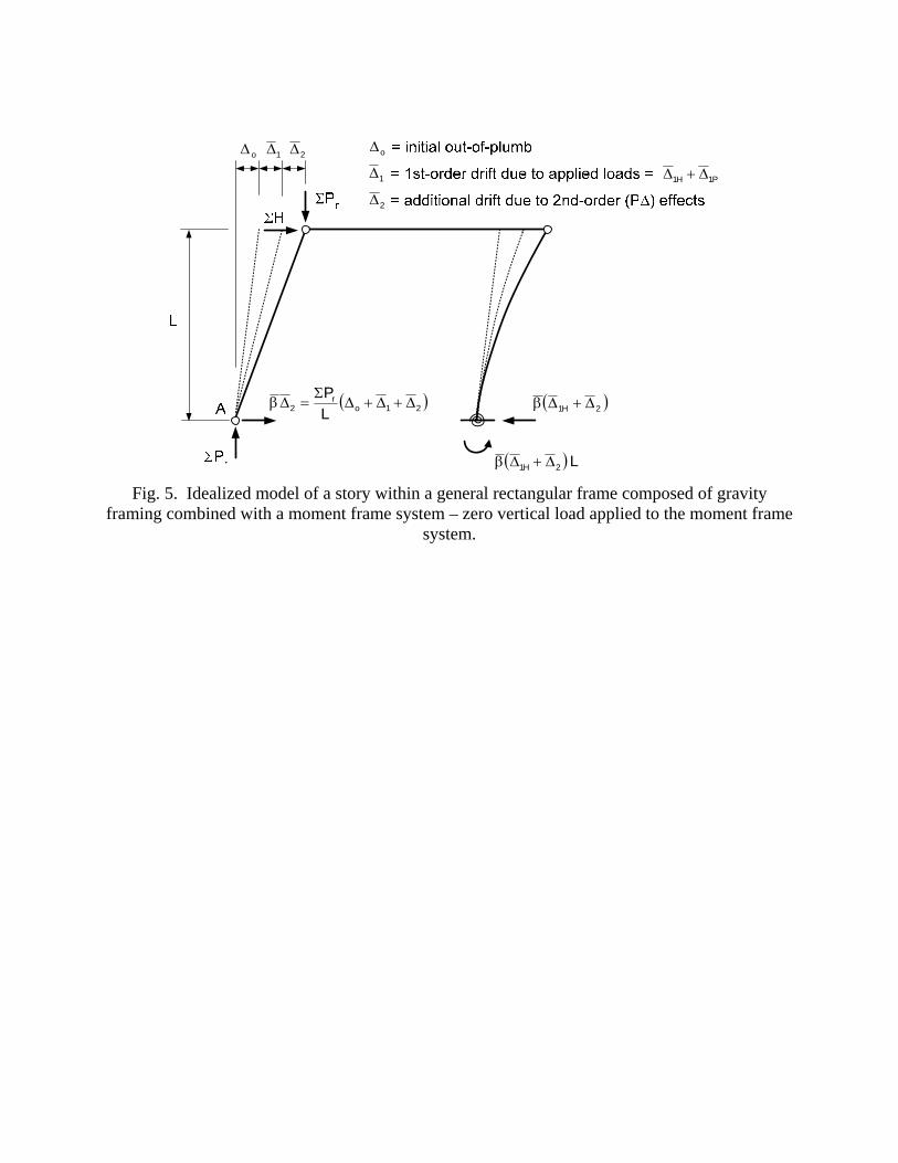
Figure 5 shows a conceptual model similar to the one for combined gravity and braced frames in Fig. 4. This figure represents a hypothetical case in which the moment frame system, represented by the cantilever column on the right-hand side with an elastic spring at its base, supports zero gravity (vertical) load. The only change from the model of Fig. 4 is that the linear spring of stiffness β is replaced by a flexural system of the same lateral stiffness. The single lateral load resisting column in Fig. 5 represents the contributions from all the columns of the physical moment frame system to the structure’s sidesway stiffness (or flexibility). The rotational spring at the base of this column represents the contributions from the beams and connections of the moment frame system. The amplified first-order analysis equations presented in Part 1 apply to this conceptual model without any modification. In other words, in the hypothetical case that the lateral-load resisting system supports zero gravity load, it does not matter whether this system is composed of a truss, a shear panel, or a combination of flexural members. Sidesway stiffness is sidesway stiffness regardless of the source.

The reader familiar with (LeMessurier 1977) should note that the symbol β in this paper represents the total sidesway stiffness of the lateral load resisting system, consistent with the AISC (1999 & 2005a) term for the lateral stiffness of a bracing system. This is different from LeMessurier’s (1977) notation for β. LeMessurier’s β parameter is denoted in this paper by the term βL. In the context of the model shown in Fig. 5,

3cL

LEIβ

=β (23)

where βL = 3 for the cantilever column shown, if the elastic spring at its base is effectively rigid, and βL = 12 for a column with rigid rotational restraint at both ends. Also, the relationship between the story stiffness β and LeMessurier’s PL parameter, i.e., the contribution from a column to the story stiffness in terms of the rotational displacement ∆1/L, is

2cL

L LEIPL β

==β (24)

4

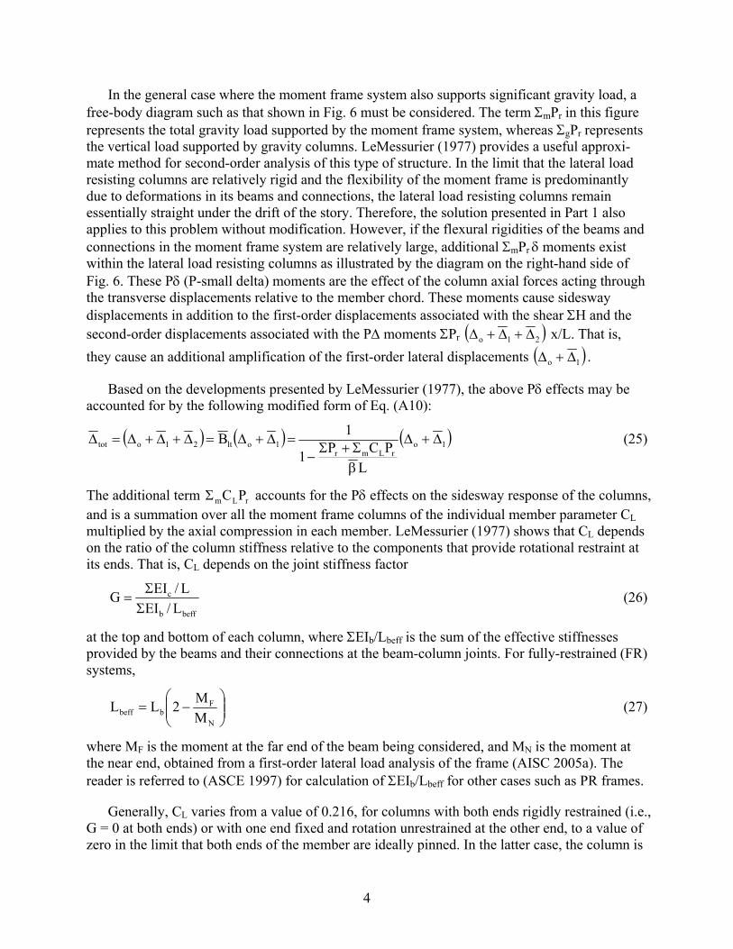
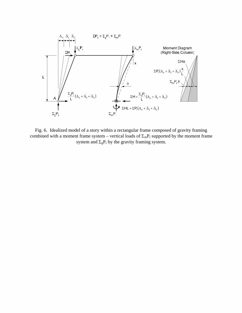
In the general case where the moment frame system also supports significant gravity load, a free-body diagram such as that shown in Fig. 6 must be considered. The term ΣmPr in this figure represents the total gravity load supported by the moment frame system, whereas ΣgPr represents the vertical load supported by gravity columns. LeMessurier (1977) provides a useful approxi-mate method for second-order analysis of this type of structure. In the limit that the lateral load resisting columns are relatively rigid and the flexibility of the moment frame is predominantly due to deformations in its beams and connections, the lateral load resisting columns remain essentially straight under the drift of the story. Therefore, the solution presented in Part 1 also applies to this problem without modification. However, if the flexural rigidities of the beams and connections in the moment frame system are relatively large, additional ΣmPr δ moments exist within the lateral load resisting columns as illustrated by the diagram on the right-hand side of Fig. 6. These Pδ (P-small delta) moments are the effect of the column axial forces acting through the transverse displacements relative to the member chord. These moments cause sidesway displacements in addition to the first-order displacements associated with the shear ΣH and the second-order displacements associated with the P∆ moments ΣPr ( )21o ∆+∆+∆ x/L. That is, they cause an additional amplification of the first-order lateral displacements ( )1o ∆+∆ .

Based on the developments presented by LeMessurier (1977), the above Pδ effects may be accounted for by the following modified form of Eq. (A10):

( ) ( ) ( )1orLmr

1olt21otot

LPCP1

1B ∆+∆

βΣ+Σ

−=∆+∆=∆+∆+∆=∆ (25)

The additional term rLm PCΣ accounts for the Pδ effects on the sidesway response of the columns, and is a summation over all the moment frame columns of the individual member parameter CL multiplied by the axial compression in each member. LeMessurier (1977) shows that CL depends on the ratio of the column stiffness relative to the components that provide rotational restraint at its ends. That is, CL depends on the joint stiffness factor

beffb

c

L/EIL/EIG

ΣΣ

= (26)

at the top and bottom of each column, where ΣEIb/Lbeff is the sum of the effective stiffnesses provided by the beams and their connections at the beam-column joints. For fully-restrained (FR) systems,

⎟⎟⎠

⎞⎜⎜⎝

⎛−=

N

Fbbeff M

M2LL (27)

where MF is the moment at the far end of the beam being considered, and MN is the moment at the near end, obtained from a first-order lateral load analysis of the frame (AISC 2005a). The reader is referred to (ASCE 1997) for calculation of ΣEIb/Lbeff for other cases such as PR frames.

Generally, CL varies from a value of 0.216, for columns with both ends rigidly restrained (i.e., G = 0 at both ends) or with one end fixed and rotation unrestrained at the other end, to a value of zero in the limit that both ends of the member are ideally pinned. In the latter case, the column is

5

of course no longer part of the lateral load resisting system. It is a pin-ended gravity column (or a bracing system member) in which δ (the deflection relative to the rotated chord) is zero along the entire member length. Therefore, the Pδ moment is zero and CL = 0 in this type of column.

LeMessurier’s (1977) procedure requires some effort to calculate CL for each of the moment frame columns. Although simpler methods of determining CL have been developed (LeMessurier 1993), these methods also involve a calculation for each of these members. A more efficient approach can be devised by using a conservative “average” CL. This is accomplished by rewriting the sidesway amplification factor in Eq. (25) as

M

i

M

rLavgrrLmrlt

R1

1

RL/P1

1

L)C1(P

1

1

LPCP1

1B

ββ

−=

βΣ

−=

β+Σ

−=

βΣ+Σ

−= (28)

where

( )LavgM

C1R1

+= (29)

By using LeMessurier’s (1977) equations, one can show that if GA < GB and GA > 0.2, where GA and GB are the joint stiffness factors at the two ends of a column, CL is always less than or equal to 0.18 and can in fact be as small as 0.11. Therefore, if G = 0.2 is assumed as a representative lower bound for the joint stiffness factor in practical moment frame systems, CLavg can be taken conservatively as 0.18 and thus RM in Eq. (29) can be taken as 0.85. AISC (2005a) specifies this RM value for all systems that include moment frames for part of the lateral load resistance. In cases where one or both ends of all the members are ideally fixed, the maximum unconservative error in the effective sidesway buckling resistance MRβ associated with the use of CLavg = 0.18 and RM = 0.85 is three percent.

The above approximation ignores the fact that CL = 0 in any columns belonging to gravity or braced framing systems. A better approximation for general systems involving combined gravity, moment and braced frames is

r

rmM P

P15.01RΣΣ

−= (30)

where ΣmPr is the sum of the vertical loads supported by all the columns in the moment frame(s). Equation (30) varies RM from 0.85 for a structure that does not have any gravity or braced frame columns in the story under consideration to a value of 1.0 for a story that does not contain any moment frames. This equation is related to Eq. (C-C2-7) for the parameter RL in the Commentary of AISC (2005a), used in the calculation of sidesway buckling loads.

One exception can be made to the calculation of RM by Eq. (30). Based on LeMessurier’s (1977) equations, if GA < GB and GA > 4, CL is always less than 0.03, and in fact can be smaller than 0.01. Therefore, assuming that three percent maximum underestimation of the sidesway buckling load (implicit within the AISC (2005a) use of RM = 0.85) is acceptable, then in stories where all the moment frame G values are greater than or equal to four, CLavg may be taken as zero. This rule can be stated as

6

RM = 1.0 for Gmin > 4 (31)

where Gmin is the smallest joint stiffness factor in the moment frame system(s) of the story.

In summary, based on the above developments, the total story sidesway displacements may be calculated using the simplified equation

( ) ( ) ( )1o

M

i1olt21otot

R1

1B ∆+∆

ββ

−=∆+∆=∆+∆+∆=∆ (32)

where RM is calculated from Eqs. (30) and (31).

Given the total sidesway displacement calculated from Eq. (32), the total internal lateral bending moment in the story may be expressed as

M

ior

M

i

M

i

H1totrH1

R1

1P

R11

R111

MPMM

ββ

−∆Σ+

⎥⎥⎥⎥⎥

⎦

⎤

⎢⎢⎢⎢⎢

⎣

⎡

ββ

−

⎟⎟⎠

⎞⎜⎜⎝

⎛−

ββ

+Σ=∆Σ+Σ=Σ (33)

after substituting Eq. (32) for tot∆ and some algebraic simplification, where ΣM1H = ΣHL. If the initial out-of-plumbness is taken equal to zero, or if the “first-order” P∆ shears due to the nominal out-of-plumbness (ΣPr∆o/L) are applied to the structure, producing the notional lateral loads specified by Eq. (1) in addition to the applied lateral loads ΣH, Eq. (33) may be written simply as

⎥⎥⎥⎥⎥

⎦

⎤

⎢⎢⎢⎢⎢

⎣

⎡

ββ

−

⎟⎟⎠

⎞⎜⎜⎝

⎛−

ββ

+Σ=∆Σ+Σ=Σ

M

i

M

i

H1totrH1

R11

R111

MPMM (34)

where in this case, ΣM1H includes the effect of any non-zero notional lateral loads.

Equation (34) shows that in general the total story internal sidesway moment is amplified differently than the story sidesway displacement (see Eq. (32)). LeMessurier (1977) also shows this result, but in the context of his parameters βL and PL. Since RM is generally less than or equal to one, the internal moment amplification is always smaller than the sidesway displacement amplification. However, in the limit that RM = 1, the amplification of the internal moments (Eq. (34)) and the amplification of the sidesway inter-story displacements (Eq. (32)) are identical. In this limit, the sidesway amplifier reduces to Eqs. (2) or (A9) derived for braced framing systems in Part 1 (White et al. 2005a).

The proposed amplified first-order elastic analysis method does not amplify the first-order internal sidesway moments directly, as in Eqs. (33) and (34). Rather, the total sidesway displacements are calculated from Eq. (32), and then the corresponding P∆ shears

7

⎟⎠

⎞⎜⎝

⎛ ∆+∆Σ=∆ L

BPH 1oltrP (5)

are applied to the structure as equal and opposite forces at the top and bottom of each story to determine the second-order components of all the internal forces and moments throughout the structure. This avoids the need for separate artificial NT and LT analyses, and leads to a more general, straightforward and intuitive calculation of the second-order internal forces and moments than the application of story-based amplification factors such as in Eqs. (33) and (34).

Application of the NT Amplification Factor to the Total Column Moments

In practically all cases where moment frames are used to provide a portion of the lateral load resistance, and where the moment frame columns are idealized as not having any transverse loads along their length, the traditional AISC (2005a) “no-translation” moment amplifier is equal to 1.0. In the context of the Direct Analysis method, this amplifier can be expressed as

0.1

PP1

CB

nt.e

r

mnt ≥

−= (35)

in the context of the Direct Analysis method, where Cm is the equivalent uniform moment factor defined in AISC (2005a) and nt.eP is the member elastic buckling load calculated assuming that sidesway is prevented (and using the reduced elastic flexural rigidity given by Eq. (22)). In structures where ntB = 1.0 in all of the moment frame columns, no further modification of the step-by-step procedures outlined in Part 1 is necessary. Furthermore, in cases where ntB > 1.0 in some of the moment frame columns, the additional P-small delta effects on the column moments can be approximated conservatively by using Eq. (35) with the total member moments, including the sidesway P∆ moments caused by the loads ∆PH (Eq. (5)). The authors consider this approximation to be acceptable since ntB is often relatively close to 1.0 even in extreme cases where the NT moment amplifier is greater than one. Also, in cases where ntB (calculated using the nominal elastic stiffness) is greater than 1.2, the Commentary of AISC (2005a) recommends the use of a rigorous second-order elastic analysis. In such cases, the Pδ moments in the columns significantly increase the column NT deformations, and therefore reduce the effective column flexural stiffnesses. This reduction in the column stiffnesses influences the end restraint provided to the beams by the column members, as well as the distribution of the internal moments throughout the moment frames. A typical result is that the column NT moments are actually reduced, while the positive bending moments in the beams are increased. Simplified moment amplification procedures, such as the AISC (2005a) NT-LT method, do not have any chance of providing generally accurate estimates of the internal moments in these extreme cases. In unusual cases where ntB or ntB is significantly greater than 1.0, the authors suggest that it is prudent for the Engineer to use a carefully tested and validated general-purpose second-order analysis program that accurately captures both P∆ and Pδ effects. The AISC (2005a) Appendix 7 Commentary suggests a few simplified benchmark problems for testing of second-order analysis software. Other more general second-order elastic analysis benchmark problems are available from references such as Clarke et al. (1993). White et al. (2003b) provide additional discussions

8

regarding the handling of Pδ effects in frames containing members with ntB or ntB significantly greater than 1.0

LEMESSURIER’S DESIGN EXAMPLE 4

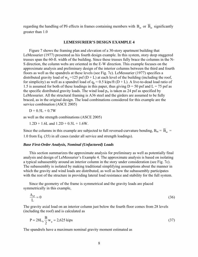
Figure 7 shows the framing plan and elevation of a 30-story apartment building that LeMessurier (1977) presented as his fourth design example. In this system, story deep staggered trusses span the 60-ft. width of the building. Since these trusses fully brace the columns in the N-S direction, the column webs are oriented in the E-W direction. This example focuses on the approximate analysis and preliminary design of the interior columns between the third and fourth floors as well as the spandrels at these levels (see Fig. 7c). LeMessurier (1977) specifies a distributed gravity load of wg =125 psf (D + L) at each level of the building (including the roof, for simplicity) as well as a spandrel load of qg = 0.5 kips/ft (D + L). A live-to-dead load ratio of 1.5 is assumed for both of these loadings in this paper, thus giving D = 50 psf and L = 75 psf as the specific distributed gravity loads. The wind load pw is taken as 24 psf as specified by LeMessurier. All the structural framing is A36 steel and the girders are assumed to be fully braced, as in the original design. The load combinations considered for this example are the service combination (ASCE 2005)

D + 0.5L + 0.7W

as well as the strength combinations (ASCE 2005)

1.2D + 1.6L and 1.2D + 0.5L + 1.6W.

Since the columns in this example are subjected to full reversed-curvature bending, Bnt = ntB = 1.0 from Eq. (35) in all cases (under all service and strength loadings).

Base First-Order Analysis, Nominal (Unfactored) Loads

This section summarizes the approximate analysis for preliminary as well as potentially final analysis and design of LeMessurier’s Example 4. The approximate analysis is based on isolating a typical subassembly around an interior column in the story under consideration (see Fig. 7c). The subassembly is isolated by making traditional simplifying assumptions about the manner in which the gravity and wind loads are distributed, as well as how the subassembly participates with the rest of the structure in providing lateral load resistance and stability for the full system.

Since the geometry of the frame is symmetrical and the gravity loads are placed symmetrically in this example,

0L

P1 =∆ (36)

The gravity axial load on an interior column just below the fourth floor comes from 28 levels (including the roof) and is calculated as

kips625,2w2BL28P gb == (37)

The spandrels have a maximum nominal gravity moment estimated as

9

0.2612/LqM 2bgg == ft-kips (38)

The nominal (D + L) moment in the interior columns is taken equal zero, as in (LeMessurier 1977).

The nominal wind shear in each interior column between the third and fourth floors is

kips8.17101p

2BL5.27H w == (39)

by the portal method, where 27.5 levels contribute to the wind shear, and the column shear forces are assumed to be distributed two parts to the interior columns and one part to the exterior members. The resulting nominal wind moment in the interior columns is

80.22/HLMw == ft-kips (40)

which is also the average wind moment in the third and fourth floor spandrels. The interior column axial force due to wind is zero based on the portal method idealization. The changes in the column axial forces due to lateral loading or general sidesway can be included in the proposed analysis approach (by performing an analysis of the full structure), but are expected to be small for this frame. Similarly, the sidesway deflections due to cantilever action are expected to be small for this 30-story frame, since its overall height-to-width ratio is close to 1.0.

Design Requirements for Acceptable Drift at Service Load Levels

LeMessurier (1977) makes a compelling argument that in general, second-order P∆ effects should be considered when checking service drift limit states. The authors suggest that at the least, when the drift limit is established using specific rational criteria such as preventing damage to nonstructural elements, it is imperative to compare the calculated second-order drifts to the rationally determined drift limit. In cases where potential drift limits are more arbitrary, the Engineer should carefully consider what actual service drifts can be tolerated. LeMessurier develops an equation for a required first-order drift limit ψ1 given:

1. A specified limit on the actual second-order drift, ψ2,

2. The distributed wind load used for the analysis, pw,

3. An average gravity load distributed over the interior volume of the structure, γg, and

4. The width over which γg acts within the plane of the framing system(s) being considered, ΣLb.

The following equation is the same as LeMessurier’s, except the factor RM from Eqs. (30) and (31) is included in the development:

M

bg

2

w

w1

RLp

pΣγ

+ψ

=ψ (41)

This equation accounts for P∆ effects at the specified service load level in converting from the specified second-order drift limit ψ2 to the corresponding first-order limit ψ1

§. The term RM is § Also, Eq. (41) is based on the assumption that the tributary widths perpendicular to the plane of the frame are the same for both the gravity and the wind loads.

10

included in Eq. (41) since its effect on the sidesway displacement amplification can be signifi-cant at service load levels in some cases**. However, the final calculations for the example frame show that the use of RM = 1.0 is sufficient based on Eq. (31). Therefore, if a second-order drift limit of ψ2 = 0.002 = 1/500 is selected for the load case (D + 0.5L + 0.7W), one obtains:

645100155.0

0.1ft250

ft9)psf125(7.0

002.0)psf24(7.0

)psf24(7.0

RL

Lw7.0

002.0p7.0

p7.0

M

bgw

w1 ==

+=

Σ+

=ψ (42)

where the 0.7 factor on wg is based on the service dead load factor of 1.0, the live load factor of 0.5, and the assumed live-to-dead load ratio of 1.5, i.e., [1(1)+0.5(1.5)] / [1 + 1.5] = 0.7. This limit corresponds to a first-order drift under the nominal loading of

4511

7.0L1H1 =

ψ=

∆ (43)

This is approximately the same as the first-order drift limit selected by LeMessurier (1977) to restrict the second-order drift under (D + L + W) to 1/300.

Given the above limit on ψ1, the minimum nominal sidesway stiffness required from each interior column subassembly of the moment frame (assuming each interior column contributes two parts to the total story stiffness and each exterior column contributes one part) is

inkips5.74

LH7.0

1

=ψ

=β (44)

In the following, a trial size is selected for the columns of the example frame first based on required strength under (1.2D + 1.6L), assuming β = 74.5 kips/in and a column inelastic stiffness reduction factor τ (Eq. (21)) equal to 1.0. Once this preliminary column size is determined, a trial size is then determined for the spandrels to achieve the required nominal sidesway stiffness of Eq. (44). Subsequently, final strength checks are provided for the columns and the spandrels.

Trial Column Size for (1.2D + 1.6L)

Based on the Direct Analysis method, the column strength term φcPn for the example frame is always governed by weak-axis flexural buckling with KLy = L = 9 ft, since K is taken equal to one in both the strong and weak-axis directions. Furthermore, in the Direct Analysis approach, the framing system is analyzed for strength with a nominal initial out-of-plumbness of ∆o = 0.002L and a reduced elastic stiffness. As a result, a more rational estimate is obtained for the required internal forces and moments than in traditional analysis and design methods.

The ideal story stiffness per interior column under the maximum live load combination is

inkips0.35

LP44.1

i ==β (45)

** LeMessurier (1977) suggests that the effect of CL, and thus the effect of RM, can be neglected when Blt with RM = 1.0 is less than 1.50. This is based on the fact that the resulting maximum unconservative error in the amplification of the sidesway moments is three percent at this value of Blt. However, the maximum error in the amplification of the sidesway displacements is 10 percent at this value of Blt.

11

Therefore, based on RM = 1.0, assuming that the Engineer recognizes up front that this is an accurate value for the example frame, and using β = 74.5 kips/in from Eq. (44) as a target,

42.2

R8.01

1B

M

ilt =

ββ

−= (46)

This gives a total story drift at the maximum strength limit of

206100485.0

LB

Lo

lttot ==

∆=

∆ (47)

and a story P∆ shear per column of

kips3.18L

P44.1H totP =

∆=∆ (48)

where 1.44 = [1.2(1) + 1.6(1.5)] / [1 + 1.5]. The resulting required column flexural strength is

5.8221LHM Pr == ∆ ft-kips (49)

Given this required moment and the required axial load capacity of Pr = 1.44P = 3,780 kips, a W14x455 can be selected using a beam-column design aid such as in AISC (2005b), but with Fy = 36 ksi. The applicable beam-column interaction check is

928.0033.098899.0

MM

98

PP

nb

r

nc

r =+=φ

+φ

(50)

where φcPn = 4,205 kips for KLy = 9 ft and φc = 0.9, and φbMn = φbMp = 2,527 ft-kips for Lb = 9 ft. The column P∆ moment due to the initial nominal out-of-plumbness does not influence the column size selection, but increases the interaction equation value from 0.899 to 0.928.

At this point, the Engineer should recognize that the ratio of the required axial strength to the yield load of the selected column cross-section is

784.0kips824,4kips780,3

FAP

PP

yg

r

y

r === (51)

The columns in the example frame experience substantial distributed yielding due to the applied load plus residual stress effects under the loading (1.2D + 1.6L). Therefore, the inelastic stiffness reduction factor τ (Eq. (21)) needs to be considered. This is accomplished after preliminary sizes are selected for the spandrels. The column inelastic stiffness reduction is also neglected in the preliminary design of the spandrels.

Selection of the Spandrels Based on Drift Control

Based on the trial column size W14x455 (Ic = 7190 in4) and the required β from Eq. (44), LeMessurier’s stiffness factor βL evaluates as

12

451.0EIL

c

3

L =β

=β (52)

LeMessurier (1977) provides the following equation for the required joint stiffness factor at the top and bottom of a column when the end restraints are equal and points of inflection exist at the middle of the column and the beam lengths:

⎟⎟⎠

⎞⎜⎜⎝

⎛−

β=⎥

⎦

⎤⎢⎣

⎡ΣΣ

= 112L/IL/IG

Lbb

c (53)

At this stage, if one assumes equal Ic/L for the columns above and below the story as in (LeMessurier 1977), all of the quantities in Eq. (53) are established except Ib. By solving Eq. (53) for Ib, one obtains the minimum girder moment of inertia necessary to provide the required β from Eq. (44), or to satisfy the drift constraint of Eq. (42), as Ib = 780 in4. Based on the assumption that it is desirable to restrict the girder nominal depths to 18 in. within the 9 ft. story height, the most economical section that satisfies the drift-based requirement is a W18x50, Ix = 800 in4. LeMessurier (1977) also selects this member in his final design.

It is informative to check the drift of the frame under the service (D + 0.5L + 0.7W) using the above W14x455 column and W18x50 spandrels. The ideal stiffness for this load case is

kips0.17L

P7.0i ==β (54)

where the 0.7 factor in this equation is based on (D + 0.5L) and D/L = 1.5. Furthermore,

0.25L/IL/IG

bb

c =ΣΣ

= (55)

for the above preliminary design sections, assuming the same Ic/L in the adjacent stories, giving

462.0)G1(

12L =

+=β (56)

(LeMessurier 1977), and

inkips5.76

LEI3

cL =β

=β (57) ††

Given the above values, and using RM = 1.0 based on Eq. (31),

29.11

1Bi

lt =

ββ

−= (58)

and

515100194.0

L1H7.0B

L lttot ==

β=

∆ (59)

†† In lieu of Eqs. (55) through (57), β can be calculated directly from the wind analysis as β = ΣH / ∆1H.

13

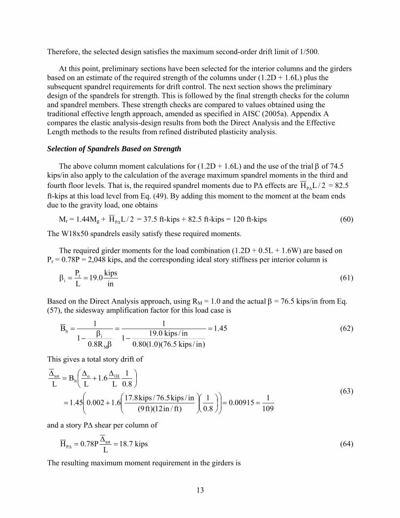
Therefore, the selected design satisfies the maximum second-order drift limit of 1/500.

At this point, preliminary sections have been selected for the interior columns and the girders based on an estimate of the required strength of the columns under (1.2D + 1.6L) plus the subsequent spandrel requirements for drift control. The next section shows the preliminary design of the spandrels for strength. This is followed by the final strength checks for the column and spandrel members. These strength checks are compared to values obtained using the traditional effective length approach, amended as specified in AISC (2005a). Appendix A compares the elastic analysis-design results from both the Direct Analysis and the Effective Length methods to the results from refined distributed plasticity analysis.

Selection of Spandrels Based on Strength

The above column moment calculations for (1.2D + 1.6L) and the use of the trial β of 74.5 kips/in also apply to the calculation of the average maximum spandrel moments in the third and fourth floor levels. That is, the required spandrel moments due to P∆ effects are 2/LHP∆ = 82.5 ft-kips at this load level from Eq. (49). By adding this moment to the moment at the beam ends due to the gravity load, one obtains

Mr = 1.44Mg + 2/LHP∆ = 37.5 ft-kips + 82.5 ft-kips = 120 ft-kips (60)

The W18x50 spandrels easily satisfy these required moments.

The required girder moments for the load combination (1.2D + 0.5L + 1.6W) are based on Pr = 0.78P = 2,048 kips, and the corresponding ideal story stiffness per interior column is

inkips0.19

LPr

i ==β (61)

Based on the Direct Analysis approach, using RM = 1.0 and the actual β = 76.5 kips/in from Eq. (57), the sidesway amplification factor for this load case is

45.1

)in/kips5.76)(0.1(80.0in/kips0.191

1

R8.01

1B

M

ilt =

−=

ββ

−= (62)

This gives a total story drift of

109100915.0

8.01

)ft/in12)(ft9(in/kips5.76/kips8.176.1002.045.1

8.01

L6.1

LB

LH1o

lttot

==⎟⎟⎠

⎞⎜⎜⎝

⎛⎟⎠⎞

⎜⎝⎛⎟⎟⎠

⎞⎜⎜⎝

⎛+=

⎟⎠⎞

⎜⎝⎛ ∆

+∆

=∆

(63)

and a story P∆ shear per column of

kips7.18L

P78.0H totP =

∆=∆ (64)

The resulting maximum moment requirement in the girders is

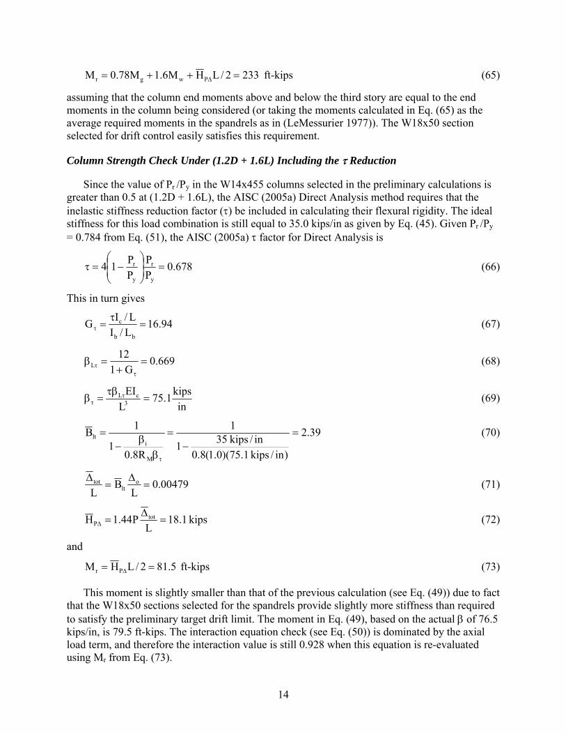
14

2332/LHM6.1M78.0M Pwgr =++= ∆ ft-kips (65)

assuming that the column end moments above and below the third story are equal to the end moments in the column being considered (or taking the moments calculated in Eq. (65) as the average required moments in the spandrels as in (LeMessurier 1977)). The W18x50 section selected for drift control easily satisfies this requirement.

Column Strength Check Under (1.2D + 1.6L) Including the τ Reduction

Since the value of Pr /Py in the W14x455 columns selected in the preliminary calculations is greater than 0.5 at (1.2D + 1.6L), the AISC (2005a) Direct Analysis method requires that the inelastic stiffness reduction factor (τ) be included in calculating their flexural rigidity. The ideal stiffness for this load combination is still equal to 35.0 kips/in as given by Eq. (45). Given Pr /Py = 0.784 from Eq. (51), the AISC (2005a) τ factor for Direct Analysis is

678.0PP

PP14

y

r

y

r =⎟⎟⎠

⎞⎜⎜⎝

⎛−=τ (66)

This in turn gives

94.16L/IL/IGbb

c =τ

=τ (67)

669.0G1

12L =

+=β

ττ (68)

inkips1.75

LEI3

cL =τβ

=β ττ (69)

39.2

)in/kips1.75)(0.1(8.0in/kips351

1

R8.01

1B

M

ilt =

−=

ββ

−=

τ

(70)

00479.0L

BL

olt

tot =∆

=∆ (71)

kips1.18L

P44.1H totP =

∆=∆ (72)

and

5.812/LHM Pr == ∆ ft-kips (73)

This moment is slightly smaller than that of the previous calculation (see Eq. (49)) due to fact that the W18x50 sections selected for the spandrels provide slightly more stiffness than required to satisfy the preliminary target drift limit. The moment in Eq. (49), based on the actual β of 76.5 kips/in, is 79.5 ft-kips. The interaction equation check (see Eq. (50)) is dominated by the axial load term, and therefore the interaction value is still 0.928 when this equation is re-evaluated using Mr from Eq. (73).

15

If the AISC (2005a) Chapter C Effective Length procedure is used with a calculated in-plane inelastic effective length factor of K = 2.75 for this frame, the governing beam-column check is

972.0025.098949.0

MM

98

PP

nb

r

nc

r =+=φ

+φ

(74)

The Engineer should note that the axial capacity ratio Pr/φcPn = 0.949, based on in-plane sidesway buckling of the frame, is larger than the corresponding value of 0.899 in Eq. (50), which is based on out-of-plane column buckling. AISC (2005a) requires the use of a minimum lateral load of Ni = 0.002Yi (the same as in Eq. (1)) for gravity load only load combinations when the Effective Length method is employed. This minimum lateral load effect gives a rather inconsequential increase in the above beam-column strength check. In general, this minimum lateral load is necessary to ensure that some accounting is made for geometric imperfection effects in determining the internal forces and moments required for strength. The corresponding additional internal moments are strictly not necessary for the design of the beam-columns for in-plane stability. However, these additional moments can be an important consideration in the design of the beam-column members for out-of-plane stability, and in the design of the beams, the beam-to-column connections, and the column bases.

One can observe that the governing beam-column interaction value of 0.928 from Eq. (50), using the Direct Analysis method, is slightly less conservative than the above value of Pr/φcPn = 0.949, using the traditional AISC (1999) Effective Length method. Also, the calculation of the inelastic effective length factor of K = 2.75 involves significantly more effort than the above Direct Analysis calculations. If the Engineer chooses to use the simpler elastic effective length equation (C-C2-5) of AISC (2005a), K = 4.62 for the example frame, leading to a substantially larger Pr/φcPn of 1.11. The reader is referred to White et al. (2003b) for the details of these calculations.

The amplification of the sidesway displacements is Blt = 1.84 under the load combination (1.2D + 1.6L) for the example frame, determined using the Effective Length method without any stiffness reduction. AISC (2005a) requires the use of the Direct Analysis method in all cases where Blt is greater than 1.5, since the approximations associated with the Effective Length approach can be rather significant in certain cases having large sidesway amplification. In LeMessurier’s Example 4, these approximations lead to a conservative strength assessment for the column members. However, in some cases, e.g., see Deierlein (2004), Kuchenbecker et al. (2004) and White et al. (2005b), these approximations can lead to somewhat unconservative results for the beam and connection moments, the column base moments, and/or the moments for checking the out-of-plane strength of beam-column members.

All the calculations illustrated thus far utilize the base beam-column strength interaction curve of AISC (2005a) Section H1.1. This curve is a single bilinear form for checking the combined in-plane and out-of-plane resistances. However, AISC (2005a) Section H1.3 also allows the Engineer to conduct a separate in-plane and out-of-plane resistance check for doubly-symmetric members loaded by axial compression and strong-axis bending. This gives a less conservative estimate of the beam-column capacities in cases where axial capacity is governed by out-of-plane failure. Within the context of the Direct Analysis approach, Section H1.3

16

requires a check of the in-plane strength using the interaction equation shown previously but with φcPn based on the in-plane L/rx (= 14.7 for this example)

909.0kipsft527,2

kipsft5.8198

kips292,4kips780,3

MM

98

PP

nb

r

nxc

r =+=φ

+φ

(75)

and it provides a separate interaction equation that gives an enhanced representation of the out-of-plane strength using φcPn based on L/ry:

900.0kipsft527,2

kipsft5.81kips205,4kips780,3

MM

PP

22

nb

r

nyc

r =⎟⎟⎠

⎞⎜⎜⎝

⎛+=⎟⎟

⎠

⎞⎜⎜⎝

⎛φ

+φ

(76)

Based on the more refined separate in-plane and out-of-plane beam-column strength checks from AISC (2005a), both the Direct Analysis and the Effective Length methods predict that the in-plane strengths govern for the critical (1.2D + 1.6L) load combination. The Direct Analysis method gives the above beam-column interaction value of 0.909 whereas the Effective Length Method gives a value of 0.972 based on Eq. (74). Also, the Direct Analysis method streamlines the design of the beam-column members, since it uses K = 1 throughout in calculating the column axial strengths φcPn.

Spandrel Strength Check Under (1.2D + 1.6L) Including the τ Reduction

The spandrel moments are also influenced by the inelastic stiffness reduction in the columns. Based on the approximate analysis used in this study, the P∆ contribution to these moments is also 81.5 ft-kips, from Eq. (73), which is smaller than the 82.5 ft-kips used in the preliminary calculations (see Eq. (49)). The spandrels have sufficient strength under the load combination (1.2D + 1.6L):

[Mr = 1.44Mg + ∆PH L/2 = 37.5 ft-kips + 81.5 ft-kips = 119 ft-kips]

< [ φbMp = 273 ft-kips ] (77)

The spandrel required moment under (1.2D + 1.6L) is Mr = 37.5 + 62.7 ft-kips = 100 ft-kips using the AISC (2005a) Effective Length method. The Direct Analysis approach gives a more rational calculation of the internal moments and forces at the strength limit for this type of frame, which has significant second-order sidesway amplification.

It should be noted that although the column axial loads and inelastic stiffness reduction are relatively large at the maximum strength level in the example frame, the influence of the stiffness reduction on the internal forces and the strength checks is relatively minor.

Column Strength Check under (1.2D + 0.5L + 1.6W)

The final check necessary for LeMessurier’s Example 4 is the column strength under the maximum wind load combination. As stated previously, Pr = 2,048 kips for this load case, and the ideal stiffness is βi = 19.0 kips/in from Eq. (61). Also, Pr /Py = 0.424 for this load combination. Therefore, τ = 1 and β = 76.5 kips/in from Eq. (57). The key calculations are thus

17

45.1

)in/kips5.76)(0.1(8.0in/kips191

1

R8.01

1B

M

ilt =

−=

ββ

−=

τ

(78)

109100915.0

8.01

46416.1002.045.1

8.01

L6.1

LB

LH1o

lttot ==⎟⎟

⎠

⎞⎜⎜⎝

⎛⎟⎠⎞

⎜⎝⎛⎟⎠⎞

⎜⎝⎛+=⎟

⎠⎞

⎜⎝⎛ ∆

+∆

=∆ (79)

where ∆1H/L = 1/464 is taken from Eq. (63),

kips7.18L

P78.0H totP =

∆=∆ (80)

and

2132/LHM6.1M Pwr =+= ∆ ft-kips (81)

This results in an interaction equation value of

562.0kipsft2,527

kipsft21398

kips205,4kips048,2

MM

98

PP

nb

r

nc

r =+=φ

+φ

(82)

The interaction value for this check using the AISC (2005a) effective length method is 0.662 (White et al. 2003b).

Comparison to Other First-Order Elastic Analysis Methods

It should be readily apparent that the proposed second-order analysis procedure has significant advantages relative to the AISC (2005a) B1-B2 or NT-LT analysis method in that it does not require separate NT and LT analyses. One determines the amplified sidesway displacements directly, then calculates and applies the associated P∆ shears to the structure in a separate first-order analysis to determine the second-order internal forces and moments. This avoids questions such as which story B2 factor should be applied to the beam moments at a given floor level, and it generally does a better job of estimating the distribution of second-order internal forces between the different framing systems in combined gravity, braced and moment frames. Also, the application of the above story P∆ shears to determine the second-order forces and moments is more intuitive, i.e., it is more representative of the true second-order behavior, than the application of amplification factors to the member axial forces and moments as specified in AISC (2005a).

AISC (2005a) also states within a user note that “it is conservative to apply the sum of the non-sway and sway moments … by the B2 amplifier, in other words Mr = B2(Mnt + Mlt).” This approach of amplifying the total member moments by B2 leads to significant conservatism in the calculation of the spandrel moments for the (1.2D + 1.6L) load combination of the example frame. The required moments using this approximation with the Direct Analysis method are 171 and 242 ft-kips for the loadings (1.2D + 1.6L) and (1.2D + 0.5L + 1.6W) respectively (versus

18

119 ft-kips from Eq. (73) plus 1.44Mg and 233 ft-kips from Eq. (65)). They are 132 and 198 ft-kips for these loadings using this approximation with the Effective Length method (versus 100 and 191 ft-kips using the recommended procedure). Nevertheless, the girder size still is governed by the drift requirements for this example. Also, since the column strength checks are dominated by the axial capacity ratio (see Eqs. (50), (74) and (82)), the use of the above conservative approach has a negligible effect on these checks for the example frame.

SUMMARY

This paper presents an application of the AISC (2005a) Direct Analysis approach for moment and general combined framing systems. The Direct Analysis approach accounts explicitly for nominal initial out-of-plumbness of the framing as well as reduction in the stiffness of the structure at the maximum strength limit of the most critical member or members in the structural system. In as such, this approach provides a more rational estimate of the internal forces and moments at the maximum strength limit. Also, the column and beam-column strength checks in moment frames may be based on K = 1 by using this method. One additional modification to a conventional elastic analysis is required in general for beam-columns in moment frames, i.e., the flexural rigidity must be reduced by an additional column inelastic stiffness reduction factor τ for columns loaded by axial forces in excess of 0.5Py.

This paper proposes two modifications to the amplified first-order elastic analysis procedure presented in Part 1 to extend this method to general rectangular framing involving any combination of moment, braced and gravity systems. These modifications are:

1. An additional term must be included in the sidesway displacement amplification factor ltB to account for the influence of Pδ (P-small delta) moments in moment frame columns on the sidesway response.

2. The traditional “no-translation” (or NT) moment amplifier, B1 in AISC (2005a) but based on the use of a reduced elastic stiffness, should be applied to the total column moments.

The paper presents analysis and design calculations using the above combined methods for an example from LeMessurier (1977) that illustrates a number of important stability design issues. The preliminary design starts with the calculation of a target story sidesway stiffness necessary to control the second-order drift under service load conditions to a specified limit. The Direct Analysis approach, combined with the proposed amplified first-order elastic analysis procedure for calculation of the second-order internal forces and moments, provides a more intuitive, straightforward and accurate set of analysis and design calculations than the traditional AISC Effective Length and NT-LT analysis procedures. The combination of the AISC (2005a) Direct Analysis method with the underlying second-order elastic analysis procedure is generally applicable to all types of rectangular framing systems.

ACKNOWLEDGEMENTS

The concepts in this paper have benefited from many discussions with the members of AISC Technical Committee 10 and the former AISC-SSRC Ad hoc Committee on Frame Stability in the development of the Direct Analysis method. The authors express their appreciation to the

19

members of these committees for their many contributions. The opinions, findings and conclusions expressed in this paper are those of the authors and do not necessarily reflect the views of the individuals in the above groups.

REFERENCES

AISC (2005a). Specification for Structural Steel Buildings, American Institute of Steel Construction, Chicago, IL.

AISC (2005b). AISC Manual of Steel Construction, American Institute of Steel Construction, Inc., Chicago, IL.

AISC (1999). Load and Resistance Factor Design Specification for Steel Buildings, American Institute of Steel Construction, Inc., Chicago, IL.

Alemdar, B.N., (2001). “Distributed Plasticity Analysis of Steel Building Structural Systems”, Doctoral dissertation, School of Civil and Environmental Engineering, Georgia Institute of Technology, Atlanta, GA.

ASCE (1997). Effective Length and Notional Load Approaches for Assessing Frame Stability: Implications for American Steel Design, American Society of Civil Engineers Structural Engineering Institute Task Committee on Effective Length under the Technical Committee on Load and Resistance Factor Design, 442 pp.

ASCE (2005). Minimum Design Loads for Buildings and Other Structures, ASCE/SEI 7-05 American Society of Civil Engineers, Reston, VA.

Clarke, M.J., Bridge, R.Q., Hancock, G.J. and Trahair, N.S. (1993). “Benchmarking and Verification of Second-Order Elastic and Inelastic Frame Analysis Programs,” Plastic Hinge Based Methods for Advanced Analysis and Design of Steel Frames, D.W. White and W.F. Chen (ed.), Structural Stability Research Council, March, pp. 245-274.

Deierlein, G. (2003). “Background and Illustrative Examples on Proposed Direct Analysis Method for Stability Design of Moment Frames,” Background Materials, AISC Committee on Specifications, Ballot 2003-4-360-2, August 20, 17 pp.

Deierlein, G. (2004). “Stable Improvements: Direct Analysis Method for Stability Design of Steel-Framed Buildings,” Structural Engineer, November, 24-28.

Galambos, T.V. (1998). Guide to Stability Design Criteria for Metal Structures, 5th Edition, T.V. Galambos (ed.), Structural Stability Research Council, Wiley.

Galambos, T.V. and Ketter, R.L. (1959). "Columns Under Combined Bending and Thrust," Journal of the Engineering Mechanics Division, ASCE, 85(EM2), 135-152.

Kuchenbecker, G.H., White, D.W. and Surovek-Maleck, A.E. (2004). “Simplified Design of Building Frames using First-Order Analysis and K = 1.0,” Proceedings, SSRC Annual Technical Sessions, April, 20 pp.

LeMessurier, W. J. (1993). “Discussion of the Proposed LRFD Commentary to Chapter C of the Second Edition of the AISC Specification,” Presentation to the ASCE Technical Committee on Load and Resistance Factor Design, Irvine, California, April 18, 1993.

20

LeMessurier, W.J. (1976). “A Practical Method for Second Order Analysis. Part 1 – Pin Jointed Systems,” Engineering Journal, AISC, 12(4), 89-96.

LeMessurier, W.J. (1977). “A Practical Method for Second Order Analysis. Part 2 – Rigid Frames,” Engineering Journal, AISC, 14(2), 49-67.

Maleck, A. (2001). “Second-Order Inelastic and Modified Elastic Analysis and Design Evaluation of Planar Steel Frames,” Doctoral dissertation, School of Civil and Environmental Engineering, Georgia Institute of Technology, Atlanta, GA, 579 pp.

Martinez-Garcia, J.M. (2002). “Benchmark Studies to Evaluate New Provisions for Frame Stability Using Second-Order Analysis,” M.S. Thesis, School of Civil Engineering, Bucknell University, Lewisburg, PA, 757 pp.

Nair, R.S. (2005). “Stability and Analysis Provisions of the 2005 AISC Specification for Steel Buildings,” Proceedings, Structures Congress 2005, ASCE, 3 pp.

Surovek-Maleck, A. and White, D.W. (2004). “Alternative Approaches for Elastic Analysis and Design of Steel Frames. I: Overview,” Journal of Structural Engineering, ASCE, 130(8), 1186-1196.

Surovek-Maleck, A., White, D.W. and Ziemian, R.D. (2003). “Validation of the Direct Analysis Method,” Structural Engineering, Mechanics and Materials Report No. 35, School of Civil and Environmental Engineering, Georgia Institute of Technology, Atlanta, GA.

White, D.W., Surovek-Maleck, A. and Kim, S.C. (2005a). “Direct Analysis and Design Using Amplified First-Order Analysis. Part 1 – Combined Braced and Gravity Framing Systems,” Engineering Journal, AISC, to appear.

White, D.W., Surovek, A. and Kuchenbecker, G. (2005b). “Comparison of the AISC (2005) Direct Analysis and Effective Length Methods Using Three Representative Single-Story Frames,” Structural Engineering, Mechanics and Materials Report No. 15, School of Civil and Environmental Engineering, Georgia Institute of Technology, Atlanta, GA.

White, D.W., Surovek-Maleck, A.E. and Kim, S.-C. (2003a). “Direct Analysis and Design Using Amplified First-Order Analysis, Part 1 – Combined Braced and Gravity Framing Systems,” Structural Engineering, Mechanics and Materials Report No. 42, School of Civil and Environmental Engineering, Georgia Institute of Technology, Atlanta, GA, 34 pp.

White, D.W., Surovek-Maleck, A.E. and Chang, C.-J. (2003b). “Direct Analysis and Design Using Amplified First-Order Analysis, Part 2 – Moment Frames and General Framing Systems,” Structural Engineering, Mechanics and Materials Report No. 43, School of Civil and Environmental Engineering, Georgia Institute of Technology, Atlanta, GA, 39 pp.

APPENDIX A

Comparison of Maximum Strengths by the AISC (2005a) Direct Analysis and Effective Length Methods to the Maximum Strength Obtained by Distributed Plasticity Analysis

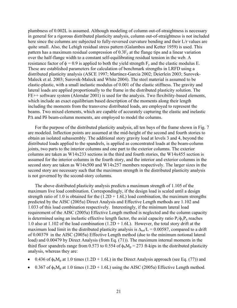
It is informative to compare the elastic analysis and design solutions presented in the body of the paper to the results from a refined distributed plasticity analysis for the governing strength load combination (1.2D + 1.6L). For the distributed plasticity design analysis, a nominal out-of-

21

plumbness of 0.002L is assumed. Although modeling of column out-of-straightness is necessary in general for a rigorous distributed plasticity analysis, column out-of-straightness is not included here since the columns are subjected to fully-reversed curvature bending and their L/r values are quite small. Also, the Lehigh residual stress pattern (Galambos and Ketter 1959) is used. This pattern has a maximum residual compression of 0.3Fy at the flange tips and a linear variation over the half-flange width to a constant self-equilibrating residual tension in the web. A resistance factor of φ = 0.9 is applied to both the yield strength Fy and the elastic modulus E. These are established parameters for calculation of benchmark strengths in LRFD using a distributed plasticity analysis (ASCE 1997; Martinez-Garcia 2002; Deierlein 2003; Surovek-Maleck et al. 2003; Surovek-Maleck and White 2004). The steel material is assumed to be elastic-plastic, with a small inelastic modulus of 0.001 of the elastic stiffness. The gravity and lateral loads are applied proportionally to the frame in the distributed plasticity solution. The FE++ software system (Alemdar 2001) is used for the analysis. Two flexibility-based elements, which include an exact equilibrium based description of the moments along their length including the moments from the transverse distributed loads, are employed to represent the beams. Two mixed elements, which are capable of accurately capturing the elastic and inelastic P∆ and Pδ beam-column moments, are employed to model the columns.

For the purpose of the distributed plasticity analysis, all ten bays of the frame shown in Fig. 7 are modeled. Inflection points are assumed at the mid-height of the second and fourth stories to obtain an isolated subassembly. The additional story gravity load at levels 3 and 4, beyond the distributed loads applied to the spandrels, is applied as concentrated loads at the beam-column joints, two parts to the interior columns and one part to the exterior columns. The exterior columns are taken as W14x233 sections in the third and fourth stories, the W14x455 section is assumed for the interior columns in the fourth story, and the interior and exterior columns in the second story are taken as W14x500 and W14x257 members respectively. The larger sizes in the second story are necessary such that the maximum strength in the distributed plasticity analysis is not governed by the second-story columns.

The above distributed plasticity analysis predicts a maximum strength of 1.105 of the maximum live load combination. Correspondingly, if the design load is scaled until a design strength ratio of 1.0 is obtained for the (1.2D + 1.6L) load combination, the maximum strengths predicted by the AISC (2005a) Direct Analysis and Effective Length methods are 1.102 and 1.033 of this load combination respectively. Interestingly, if the minimum lateral load requirement of the AISC (2005a) Effective Length method is neglected and the column capacity is determined using an inelastic effective length factor, the axial capacity ratio Pr/φcPn reaches 1.0 also at 1.102 of the load combination (1.2D + 1.6L). However, the total story drift at the maximum load limit in the distributed plasticity analysis is ∆tot/L = 0.00587, compared to a drift of 0.00379 in the AISC (2005a) Effective Length method (due to the minimum notional lateral load) and 0.00479 by Direct Analysis (from Eq. (71)). The maximum internal moments in the third floor spandrels range from 0.573 to 0.554 of φbMp = 273 ft-kips in the distributed plasticity analysis, whereas they are:

• 0.436 of φbMp at 1.0 times (1.2D + 1.6L) in the Direct Analysis approach (see Eq. (77)) and

• 0.367 of φbMp at 1.0 times (1.2D + 1.6L) using the AISC (2005a) Effective Length method.

22

If the minimum lateral load requirement is neglected in the AISC (2005a) Effective Length method, the maximum girder moment under 1.0 times (1.2D + 1.6L) is only 0.137 of φbMp. The drift of the frame is ∆tot/L = 0.00470 at 95 percent of the maximum load capacity in the distributed plasticity analysis. The moments in the spandrels calculated by the distributed plasticity analysis and by Direct Analysis match closely at this load level.

The failure mode in this structure is inelastic sidesway “buckling” of the third story columns, since the girders are still completely elastic at the maximum load limit. The effective elastic moment of inertia in the W14x455 interior columns varies along the length and ranges from 0.28 to 0.52 of their elastic moment of inertia at the limit load from the distributed plasticity analysis. The reductions in the flexural rigidities are similar but slightly smaller in the exterior columns. One can see that both the Effective Length and the Direct Analysis methods give a reasonable estimate of the distributed plasticity solution, with the Direct Analysis calculations being somewhat simpler to perform and giving comparable or slightly better estimates of the behavior observed in the distributed plasticity analysis. The conventional Effective Length approach in AISC (1999) determines the internal forces and moments in the fictitious geometrically-perfect nominally-elastic structure, but then compensates in the design of the beam-columns by basing φcPn on the buckling strength of the perfect structure, typically via a story sidesway buckling K factor (Surovek-Maleck and White 2004; Deierlein 2004). This approach generally underestimates the Mr values in the beam, connection, and out-of-plane beam-column strength checks (hence, the requirement of a minimum notional lateral load with gravity only load combinations in AISC (2005a)). For lightly-loaded laterally-stiff structures, these errors are small. However, for more heavily-loaded laterally-flexible structures, these effects can be significant. The Direct Analysis approach provides a more rational estimate of the internal forces and moments in the structural system at the strength limit of the most critical member(s).

APPENDIX B

NOMENCLATURE

Ag = Gross area of cross section ltB = Sidesway displacement amplification factor given by Eq. (28)

B1, ntB = Non-sway moment amplification factor CL = Factor from LeMessurier (1977) that accounts for the influence of individual

member Pδ effects on the amplification of the sidesway displacements

CLavg = Weighted average CL over all the columns in a story = r

rLm

P)PC(

ΣΣ

Cm = Beam-column equivalent uniform moment factor E = Modulus of elasticity Fy = Yield stress G = Joint stiffness factor given by Eq. (26) GA, GB = Joint stiffness factor at column ends A and B H, ΣH = Story shear due to the applied loads on the structure

∆PH , ∆PH = Story shear due to P∆ effects I = Moment of inertia

23

Ib, Ic = Moment of inertia of beam and column Ie = Effective elastic moment of inertia K = Column effective length factor L = Story height Lb = Length of a beam Lbeff = Length of an equivalent prismatic elastic beam subjected to fully-reversed

curvature bending MF, MN = Sidesway moment at the far and near end of a beam, respectively Mg = Nominal (unfactored) moment due to gravity load ML, MS = Larger and smaller end moment, respectively Mn = Nominal moment resistance Mp = Plastic moment resistance Mr = Required moment resistance Mw = Nominal (unfactored) moment due to wind load Ni = Notional load at ith level in the structure P = Column axial load Pcr = Column buckling load

nt.eP = Column non-sway elastic buckling resistance PL = Contribution from a column to the story stiffness in terms of the rotational

displacement ∆1/L, i.e., column shear force required to obtain a first-order drift of ∆1/L = 1.

Pn = Nominal axial load resistance Pr = Required axial load resistance ΣPr = Total required story vertical load Py = Yield load = AgFy P∆ = P-large delta effect, equal to the moment caused by the member axial force

acting through the relative transverse displacement between its ends, or equal to the total story vertical load acting through the total inter-story sidesway displacement

Pδ = P-small delta effect, equal to the moment caused by the member axial force acting through the transverse displacement relative to a chord between its ends

RM = Story factor that accounts for the influence of Pδ effects in moment frame columns on the amplification of the sidesway displacements

Yi = Total factored gravity load acting on the ith level pw = Wind load in pounds per square foot qg = Uniformly distributed gravity loading on spandrels rx, ry = Radius of gyration about x- and y- axis, respectively wg = Uniform floor distributed gravity load β, β = Total story sidesway stiffness of the lateral load resisting system βi = Story sidesway destabilizing effect, or ideal story stiffness = ΣPr / L βL = LeMessurier’s column sidesway stiffness coefficient, shown in Eq. (23) δ = Transverse deflection of a member relative to a chord between its ends γg = Average gravity load per unit interior volume of the structure φ = Resistance factor φb, φc = Resistance factor for flexure and for compression

24

τ = Column inelastic stiffness reduction factor τ (subscript) = Indicates quantities calculated including the influence of column inelastic

stiffness reduction ψ1 = First-order service drift limit, given by Eq. (41) ψ2 = Specified second-order service drift limit ∆ = Inter-story sidesway displacement ∆o = Initial story out-of-plumbness

1∆ , 1∆ = First-order inter-story sidesway displacement due to applied loads = ∆1H + ∆1P or H1∆ + P1∆

2∆ , 2∆ = Additional inter-story sidesway displacement due to second-order (P∆) effects

H1∆ , H1∆ = First-order inter-story sidesway displacement due to ΣH

P1∆ , P1∆ = First-order inter-story sidesway displacement due to vertical loads

tot∆ , tot∆ = Total inter-story sidesway displacement Σ = Summation Σc, Σg, Σm = Summation over the connected columns, gravity columns and moment frame columns, respectively

(over bar) = Indicates quantities that are influenced by the stiffness reduction employed in the Direct Analysis approach

( )21or

2 LP

∆+∆+∆Σ

=∆β

1∆ 2∆o∆ o∆

1∆ P1H1 ∆+∆

2∆

( )2H1 ∆+∆β

( )L2H1 ∆+∆β Fig. 5. Idealized model of a story within a general rectangular frame composed of gravity

framing combined with a moment frame system – zero vertical load applied to the moment frame system.

( )21org

LP

H ∆+∆+∆Σ

+Σ

( )21orPHL ∆+∆+∆Σ+Σ

( )LxP 21or ∆+∆+∆Σ

HxΣ

1∆ 2∆o∆

( )21org

LP

∆+∆+∆Σ

Fig. 6. Idealized model of a story within a rectangular frame composed of gravity framing

combined with a moment frame system – vertical loads of ΣmPr supported by the moment frame system and ΣgPr by the gravity framing system.

Fig. 7. LeMessurier’s (1977) Example 4 frame.